: Phase space and density matrix formulations

Nonlinear longitudinal relaxation of a quantum superparamagnet with arbitrary spin value S:Phase space and density matrix formulations

Yuri P. Kalmykov,1 Serguey V. Titov,2 and William T. Coffey3

1Laboratoire de Mathématiques, Physique et Systèmes, Université de Perpignan Via Domitia, 52, Avenue de Paul Alduy,66860 Perpignan Cedex, France

2Institute of Radio Engineering and Electronics, Russian Academy of Sciences, Vvedenskii Square 1, Fryazino 141190, Russia3Department of Electronic and Electrical Engineering, Trinity College, Dublin 2, Ireland

�Received 14 October 2009; revised manuscript received 4 December 2009; published 26 March 2010�

The nonlinear relaxation of quantum spins interacting with a thermal bath is treated via the respectiveevolution equations for the reduced density matrix and phase space distribution function in the high tempera-ture and weak spin-bath coupling limits using the methods already available for classical spins. The solution ofeach evolution equation is written as a finite series of the polarization operators and spherical harmonics,respectively, where the coefficients of the series �statistical averages of the polarization operators and sphericalharmonics� are found from entirely equivalent differential-recurrence relations. Each system matrix has anidentical set of eigenvalues and eigenfunctions. For illustration, the time behavior of the longitudinal compo-nent of the magnetization and its characteristic relaxation times are evaluated for a uniaxial paramagnet ofarbitrary spin S in an external constant magnetic field applied along the axis of symmetry. In the large spinlimit, the quantum solutions reduce to those of the Fokker-Planck equation for a classical uniaxial superpara-magnet. For linear response, the results entirely agree with existing solutions.

DOI: 10.1103/PhysRevB.81.094432 PACS number�s�: 75.50.Xx, 75.50.Tt, 03.65.Yz, 05.40.�a

I. INTRODUCTION

Phase-space representations of quantum mechanical evo-lution equations �via the coherent state representation of thedensity matrix ��t� introduced by Glauber and Sudarshanlong familiar in quantum optics1–3� when applied to spin sys-

tems characterized by a Hamiltonian HS allow one to analyzespin relaxation using a master equation for a quasiprobabilitydistribution function WS

�s�� ,� , t� of spin orientations in aphase �here configuration� space �� ,��. Here � and � are thepolar and azimuthal angles constituting the canonicalvariables4–9 and the master equation is

�WS�s�

�t= LSWS

�s�, �1�

where S is the spin size and LS is a differential operatordepending on the particular spin system. Equation �1� is de-rived by mapping onto phase space the evolution equationfor the reduced density matrix �, namely,

� �

�t+

i

��HS, �� = Q�� , �2�

where Q�� is the collision kernel operator. The transforma-tion may be accomplished because WS

�s�� ,� , t� and � arerelated via the bijective map2

WS�s��,�,t� = Tr��t�ws��,�� ,

��t� =2S + 1

4��

�,�ws��,��WS

�−s��,�,t�sin �d�d� .

The Wigner-Stratonovich operator �or kernel of the transfor-mation� ws�� ,�� is defined as

ws��,�� =� 4�

2S + 1 L=0

2S

M=−L

L

�CS,S,L,0S,S �−sYL,M

� ��,��TL,M�S� .

Here Tr�ws�=1 and ��2S+1� /4��,�ws sin �d�d�= I�S� �I�S�

is the identity matrix�, the asterisk denotes the complex con-

jugate, YL,M�� ,�� are the spherical harmonics,10 TL,M�S� are the

polarization operators,10 and CS,S,L,0S,S are the Clebsch-Gordan

coefficients.10 Either WS�s�� ,� , t� or � allow one to calculate

the average value of an arbitrary spin operator A as

�A� = Tr��A�

or

�A� =2S + 1

4��

�,�A�s��,��WS

�−s��,�,t�sin �d�d� ,

respectively, where A�s�� ,��=Tr�Aws�� ,�� is the Weyl

symbol of A. The symbol s characterizes quasiprobabilityfunctions of spins belonging to the SU�2� dynamical symme-try group. The parameter values s=0 and s= �1 correspondto the Stratonovich11 and Berezin12 contravariant and cova-riant functions, respectively �the latter are directly related tothe P and Q symbols appearing naturally in the coherentstate representation2�. We consider below only WS

�−1�� ,��omitting everywhere the superscript −1 in WS

�−1�� ,�� be-cause it alone satisfies the non-negativity condition requiredof a true probability density function, viz., W�−1�� ,��0.13

The phase space distribution �Wigner� function for spinshaving been originally introduced by Stratonovich11 forclosed systems was further developed for both closed andopen spin systems.7–9,14–18 In the present context phase spacemethods are highly relevant because they allow one to mapquantum mechanical evolution equations for the �reduced�

PHYSICAL REVIEW B 81, 094432 �2010�

1098-0121/2010/81�9�/094432�14� ©2010 The American Physical Society094432-1

http://dx.doi.org/10.1103/PhysRevB.81.094432

density matrix for spins onto a classically meaningfulc-number space, which has an obvious advantage over theoperator equations in the consideration of the classicallimit.17 In particular, the mapping of the quantum spin dy-namics onto c-number quasiprobability density evolutionequations transparently shows how evolution equation �1�reduces in that limit to the Fokker-Planck equation describ-ing the stochastic dynamics of a classical spin.5,6,9,17,18 More-over, the formalism is relatively easy to implement in prac-tice because the existence of phase space master equationsfor spins enables existing powerful computational techniquesfor Fokker-Planck equations �e.g., statistical moments, con-tinued fractions, mean first passage times, etc.19,20� to beseamlessly carried over into the quantum domain.7–9

Now, although the phase space and spin density matrixrepresentations have outwardly very different forms, theymust yield exactly the same results. However, use of one orthe other representation may provide a more transparentmethod of obtaining the desired result depending on theproblem at hand. In particular the phase space representation,because it is closely allied to the classical representation, isvery convenient for the study of the passage to the classicallimit. This feature has been amply demonstrated in Ref. 9 forthe simple model of a spin in a dc magnetic field. Here, asanother explicit example, which now involves the magneto-crystalline anisotropy, we consider a uniaxial paramagnet ofarbitrary spin value S in an external constant magnetic fieldH0 applied along the Z axis, i.e., the axis of symmetry. Thus,the Hamiltonian has the form

H = HS + HSB + HB,

where

HS = −

S2 SZ2 −

�

SSZ, �3�

SZ is the Z component of the spin operator S, is the aniso-tropy constant, �=S��H0 is the field parameter, � is thegyromagnetic ratio, and =1 / �kT� is the inverse thermal en-

ergy, the term HSB describes interaction of the spin with the

thermostat, and HB characterizes the thermostat. This Hamil-tonian includes a uniaxial anisotropy term plus the Zeemancoupling to the external field, comprising a generic model forthe study of quantum relaxation phenomena in uniaxial spinsystems such as molecular magnets, nanoclusters, etc. �see,e.g., Refs. 26 and 27 and references cited therein�. RecentlyGaranin26 and García-Palacios et al.27 using the spin densitymatrix in the second order of perturbation theory in the spin-bath coupling considered the longitudinal relaxation of quan-tum superparamagnets with Hamiltonian �3� for arbitrary S.They gave a concise treatment of the spin dynamics by pro-ceeding from the quantum Hubbard operator representationof the evolution equation for the spin density matrix. How-ever, they limited themselves to the linear response so thattheir solution pertains to a small perturbation in the dc fieldand is not valid for arbitrary changes. Here we shall presentsolutions for the nonlinear relaxation of the averaged longi-

tudinal component of the spin �SZ��t� as a function of the

spin value S using both the density matrix and phase spaceformulation. As far as the phase space approach is con-cerned, the master equation corresponding to Hamiltonian�3� has been derived already in Ref. 18 but has not yet beensolved. Here we shall demonstrate how the solution of thecorresponding classical problem21–25 carries over into thequantum domain illustrating how the magnetization, its re-versal, and integral relaxation times for an arbitrarily strongchange in the uniform field may be evaluated. Furthermore,

we shall show that the long time behavior of �SZ��t� compris-ing 2S exponentials may be accurately approximated by asingle exponential with a definite relaxation time T1 for ar-

bitrary S. In other words, even for a giant spin �S 1�, �SZ��t�still obeys the Bloch equation

d

dt�SZ��t� + ��SZ��t� − �SZ�eq�/T1 = 0, �4�

where �SZ�eq is the equilibrium average of the operator SZ. Inthe linear-response approximation, the solution reduces tothat previously given by Garanin26 and García-Palacios andZueco.27

The paper is arranged as follows. In Sec. II, the method ofstatistical moments in the context of the density matrix andphase space formalism is presented. In Sec. III, thedifferential-recurrence equations for relaxation functions�statistical moments� of a uniaxial quantum paramagnet arederived. In Sec. IV, by solving these equations, the nonlineartransient response of a uniaxial quantum paramagnet istreated. The characteristic relaxation times of nonlinear tran-sients are calculated in Sec. V. The results are presented inSec. VI. Section VII contains their discussion and conclu-sions. Various useful formulas for a classical superparamag-net are summarized in Appendix A. The detailed calculationof the integral relaxation time is given in Appendix B.

II. METHOD OF STATISTICAL MOMENTS

A very efficient method of solution of the Fokker-Planckequation governing the stochastic dynamics of classical spinsystems comprises the determination of the statisticalmoments19,20,28 which in general satisfy differential-recurrence relations. This method can also be applied to thequantum problem. The reason is that the phase-space distri-bution WS�� ,� , t� may be presented for arbitrary S in termsof a finite linear combination of the spherical harmonics,namely,2

2S + 1

4�WS��,�,t� =

L=0

2S

M=−L

L

�YL,M� ��t�YL,M��,�� , �5�

where

�YL,M� ��t� =

2S + 1

4��

�,�YL,M

� ��,��WS��,�,t�sin �d�d�

and YL,M� = �−1�MYL,−M. Equation �5� obviously emphasizes

the relationship with the conventional infinite series repre-sentation of the relevant classical Boltzmann distribution.

KALMYKOV, TITOV, AND COFFEY PHYSICAL REVIEW B 81, 094432 �2010�

094432-2

The formal solution of the reduced density evolution equa-tion �2� can also be written in analogous fashion using the

polarization operators TL,M�S� as the linear combination2,10,28

��t� = L=0

2S

M=−L

L

�− 1�MaL,−M�t�TL,M�S� , �6�

where the coefficients aL,M �representing the expectation val-

ues of the TL,M�S� in a state described by �� are10

aL,M�t� = �TL,M�S� ��t� = Tr��t�TL,M

�S� � . �7�

In general, the scalar coefficients �TL,M�S� � are related to the

expectation values of the spherical harmonics �YL,M� �statis-tical moments� by the equation18

�YL,M� =�2S + 1

4�CS,S,L,0

S,S �TL,M�S� �

=�2S�!�2S + 1�

�4��2S − L�!�2S + L + 1�!�TL,M

�S� � . �8�

Thus, knowing �YL,M��t� from phase space equations �1� and�5�, we can also determine � from Eqs. �6� and �8� withoutformally solving its evolution equation �2�. Vice versa, hav-

ing calculated �TL,M�S� ��t� from the density matrix Eqs. �2� and

�6�, we can also find WS�� ,� , t� from Eqs. �5� and �8� with-out formally solving the phase space evolution equation �1�.

The finite series Eq. �5� is valid for an arbitrary spinsystem with states described by � given by Eq. �6�. In gen-eral, either expansion of the phase-space distribution as alinear combination of the spherical harmonics or expansionof the density matrix in polarization operators permits direct

calculation of the observables �SX�, �SZ�, etc. For example,

noting the correspondence rules of the operator SZ and itsWeyl symbol �c number� SZ�� ,�� in the phase space, wehave in the phase space representation18

�SZ��t� = �4�/3�S + 1��Y1,0��t� .

While in terms of the polarization operators, we have

�SZ��t� = �S�S + 1��2S + 1�/3�T1,0�S��t� .

The differential-recurrence relations for �YL,M��t� can beobtained by substituting the distribution function WS�� ,� , t�from Eq. �5� into master equation �1� so that the latter be-comes

d

dt�YL,M��t� =

L�,M�

bL,ML�,M��YL�,M��t� , �9�

where bL,ML�,M� are the Fourier coefficients which depend on

the precise form of the Hamiltonian. The corresponding

equation for �TL,M�S� ��t�, viz.,

d

dt�TL,M

�S� ��t� = L�,M�

� �2S − L�!�2S + L + 1�!�2S − L��!�2S + L� + 1�!

�bL,ML�,M��TL�,M�

�S� ��t� , �10�

can be obtained either by substituting the polarization opera-tor series representation of the reduced density matrix � fromEq. �6� into Eq. �2� or directly from the Fourier series Eq. �9�by noting Eq. �8�. Equations �9� and �10� are entirely equiva-lent and can be solved either by direct matrix diagonaliza-tion, involving the calculation of the eigenvalues and eigen-vectors of the system matrix, or by the computationallyefficient �matrix� continued fraction method19,20 so yieldingthe magnetization as a function of S, etc.

III. DIFFERENTIAL-RECURRENCE RELATION FORSTATISTICAL MOMENTS FOR A UNIAXIAL

PARAMAGNET

The density matrix evolution equation for the reduceddensity matrix � describing the longitudinal relaxation of auniaxial spin system with Hamiltonian �3� is in the weakcoupling and high temperature limit18

� �

�t= St�� , �11�

where

St�� = 2D��S−�, S+� + �S+e�/S2��2SZ+I�S��+��/S�I�S��t�, S−�� ,

�12�

S�= SX� iSY; SX and SY are the X and Y components of the

spin operator S, respectively. The collision kernel operatorSt�� in Eq. �12� is explicitly determined via the ansatz that

the equilibrium spin density matrix �eq=e−HS /Tr�e−HS� ren-ders it zero, i.e., St��eq�=0. Conditions for the validity of Eq.�11� are discussed in detail elsewhere.18 Essentially, thatequation follows from the equation of motion of the reduceddensity matrix in the rotating-wave approximation �familiarin quantum optics, where counter-rotating, rapidly oscillatingterms are averaged out27�. Moreover the spin-bath interac-tions are taken in the weak coupling limit and for Ohmicdamping. Thus, the correlation time characterizing the bath isshort enough to allow one to approximate the stochastic pro-cess originating in it by a Markov process. These approxi-mations may be used in the high temperature limit, ��m−�m�1��1, where �m ,�m�1 are the energy eigenvalues. Inthe parameter range, where the approximation fails �e.g.,throughout the very low temperature region�, more generalforms of the phase space and density matrix equations mustbe used �such as treated, e.g., in Refs. 26 and 27�. Neverthe-less, we still use the model based on the above approxima-tion because despite many drawbacks26,27 it can qualitativelydescribe the relaxation in spin systems. Moreover, the modelcan be regarded as the direct quantum generalization of theLangevin formalism used by Brown in his theory of relax-ation of classical superparamagnetic particles.21

The phase space evolution equation for WS�� , t� corre-sponding to Eq. �11� is �because in longitudinal relaxation

NONLINEAR LONGITUDINAL RELAXATION OF A… PHYSICAL REVIEW B 81, 094432 �2010�

094432-3

the azimuthal angle dependence of WS may be ignored�18

�WS

�t=

D�

2

�

�z �1 − z2� � �

�z�P�S� + 1 + z�P�S� − 1��WS

− �2S + 1��P�S� − 1�WS�� , �13�

where D� is the “diffusion” coefficient, z=cos �, and the

operator P�S� has a complicated differential form, given ex-plicitly in Ref. 18. For =0, i.e., for a spin in a dc magnetic

field, we have simply P�S�=e�/S and Eq. �13� reduces to theFokker-Planck equation treated in Ref. 9. In the classicallimit, Eq. �13� further reduces to the Fokker-Planck equationfor a classical uniaxial paramagnet in a dc magnetic field,viz.,20–25

�

�tW = D�

�

�z��1 − z2��

�zW + W

�

�zV�� , �14�

where V�z�=−z2−�z is the normalized classical free energy.The formal solutions of the axially symmetric Eqs. �13�

and �11� can now be written as

��t� = L=0

2S

aL�t�TL,0�S� , �15�

2S + 1

4�WS��,�,t� =

L=0

2S

bL�t�YL,0��,�� . �16�

The coefficients aL�t� and bL�t� are of course �cf. Eqs. �5� and

�7�� the averages of the polarization operators TL,0�S� and

spherical harmonics YL,0, viz.,

aL�t� = �TL,0�S� ��t�, bL�t� = �YL,0��t� . �17�

By substituting Eqs. �15� and �16� into Eqs. �11� and �13�,respectively, we have the finite hierarchy of differential-recurrence equations for the statistical moments �in contrastto the classical case, where the corresponding hierarchy isinfinite�.

Since either approach presented above yields similar hier-archies, we give the derivation using the density matrix. Thisis accomplished as follows. First, the matrix exponent

e�/S2��2SZ+I�S��+��/S�I�S�in Eq. �12� can be expanded in terms of

the polarization operators TL,0�S� as

e�/S2��2SZ+I�S��+��/S�I�S�= e�/S2�+��/S�

l=0

2S

dlTl,0�S�, �18�

where

dl�� = Tr�e�2/S2�S0Tl,0�S�� =� 2l + 1

2S + 1 m=−S

S

CS,m,l,0S,m e�2/S2�m.

�19�

Here the expansion coefficients dl have been found by usingthe orthogonality property

Tr�TL1,M1

�S� TL2,M2

�S� � = �− 1�M1�L1,L2�M1,−M2

�20�

and the explicit form of the matrix elements, viz.,

�TL,M�S� �m�,m= ��2L+1� / �2S+1��1/2CS,m,L,M

S,m� . By substituting Eq.�15� into the explicit evolution Eq. �11�, noting Eq. �18�, andthe product formula10

Tl,0�S�TL,0

�S� = L�=�L−l�

L+l

�− 1�2S+L��2l + 1��2L + 1�

� l,L,L�

S,S,S�Cl,0,L,0

L�,0 TL�,0�S� , �21�

�� l,L,L�S,S,S � is Wigner’s 6j-symbol10� we have the hierarchy of

multiterm differential-recurrence equations for the averagesaL�t�, namely,

�N�aL�t�

�t=

L�=0

2S

gL,L�S aL��t� , �22�

where �N= �2D��−1 is the characteristic �free diffusion� timeand

gL,L�S =

L�L + 1�

4��2S − L��2S + L + 2�

�2L + 1��2L + 3��L,L�+1

−L�L + 1�

4�L,L� −

L�L + 1�

4

��2S − L + 1��2S + L + 1�

�2L + 1��2L − 1��L,L�−1 − e�/S2�+��/S�

��− 1�2S+LL�L + 1�

4�2L� + 1

�� l=�L�−L�

L�+L

dl��2l + 1 l,L�,L

S,S,S�Cl,0,L�,0

L,0

+��2S − L + 1��2S + L + 1�

��2L − 1��2L + 1�

l=�L�−L+1�

L�+L−1

dl��2l + 1

� l,L�,L − 1

S,S,S�Cl,0,L�,0

L−1,0

−��2S − L��2S + L + 2�

��2L + 3��2L + 1�

l=�L�−L−1�

L�+L+1

dl��2l + 1

� l,L�,L + 1

S,S,S�Cl,0,L�,0

L+1,0 � �23�

with a0= �T0,0�S��= �2S+1�−1/2. We remark that the built-in

functions ClebschGordan��a ,�� , �b ,� , �c ,�� andSixJSymbol��j1 , j2 , j3� , �j4 , j5 , j6�� of the MATHEMATICA pro-gram facilitate calculation of the Clebsch-Gordan coeffi-cients and the Wigner 6j symbols in Eq. �23�. On the otherhand, in the phase space representation, we have formally therelevant system of differential-recurrence equations for the


094432-4

averaged spherical harmonics �Yl,0��t� from Eqs. �9�, �10�,and �22�. Alternatively the differential-recurrence equationscan be directly derived by substituting Eq. �16� into Eq. �13�and using the recurrence relations10

� cos �Yl,m

sin ��Yl,m� = �1

l�� l + 1�2 − m2

�2l + 1��2l + 3�Yl+1,m

− � − 1

l + 1�� l2 − m2

4l2 − 1Yl−1,m,

��2 Yl,m = �m2 csc2 � − l�l + 1��Yl,m − cot ��Yl,m.

The details have been given in Ref. 9 for =0.In the classical limit, S→�, Eq. �22� reduces to the

differential-recurrence equation for a classical uniaxial para-magnet treated in Refs. 20, 29, and 30 �see Appendix A�. Inthe limiting case =0, Eqs. �19� and �23� simplify yieldingdl�0�=�2S+1�l,0 and gL,L�

S =0 with the exceptions gL,LS

=e�/SqL and gL,L�1S =−e�/SqL

�, where

qL = −L�L + 1�

4, qL

� = �1

4L�L + 1�

2S � L + 3/2 � 1/22L + 1

,

so that with the replacement

cL�t� →��2S − L�!�2S + L + 1�!�2L + 1�

4��2S�!aL�t� ,

we have from Eq. �22�

�N�cL�t�

�t= �1 + e�/S�qLcL�t�

+ �1 − e�/S�qL−cL−1�t� + �1 − e�/S�qL

+cL+1�t� .

�24�

This result exactly corresponds to the spin relaxation in auniform field treated comprehensively in Ref. 9.

IV. CALCULATION OF THE OBSERVABLES

We suppose that the magnitude of an external uniform dcmagnetic field is suddenly altered at time t=0 from HI to HII�the magnetic fields HI and HII are applied parallel to the Zaxis of the laboratory coordinate system in order to preserveaxial symmetry�. Thus, we study as in the classical case,20

the nonlinear transient longitudinal relaxation of a system ofspins starting from an equilibrium state I with density matrix�eq

I �t�0� to a new equilibrium state II with density matrix�eq

II �t→��. Here the longitudinal component of the spin

�SZ��t� relaxes from the equilibrium value �SZ�I to the value

�SZ�II, the transient being described by an appropriate relax-ation function. The transient response so formulated is trulynonlinear because the change in amplitude HI−HII of theexternal dc magnetic field is arbitrary �the linear response isthe particular case �HI−HII�→0�. We remark in passing thatthe equilibrium phase space distributions Weq

I and WeqII corre-

sponding to the equilibrium spin density matrices �eqI and �eq

II

comprise the appropriate stationary �time independent� solu-

tions of Eq. �13�. These distributions have been extensivelystudied in Ref. 31 and are given by

WSi �� =

L=0

2S2L + 1

2S + 1�PL�iPL�cos �� , �25�

where �PL�i= �S+1 /2�−11 PL�z�WS

i �z�dz are the equilibriumvalues of the Legendre polynomials PL given explicitly by31

�PL�i = ZS−1CS,S,L,0

S,S m=−S

S

CS,m,L,0S,m e�m/S�2+�i�m/S�

and ZS=Tr�e−HS�=m=−SS e�m / S�2+�i�m/S� is the partition func-

tion.According to Eq. �22�, the behavior of any selected aver-

age is coupled to that of all the others so forming a finitehierarchy �because the index L ranges only between 0 and2S� of averages. The solution of such a multiterm recurrencerelation may always be obtained by rewriting it as a first-order linear matrix differential equation with constant coef-ficients. In order to accomplish this, we first construct a col-umn vector C�t� such that

C�t� =�c1�t�c2�t�]

c2S�t�� , �26�

with elements cL�t�= �TL,0�S� ��t�− �TL,0

�S� �II. Now the after-effectfunctions cL�t� satisfy the same recurrence relations Eq. �22�as the aL�t� with the initial conditions

cL�0� = �TL,0�S� �I − �TL,0

�S� �II. �27�

However, vector �26� now contains just 2S elements �theindex L ranges between 1 and 2S� as the evolution equationfor the function c0�t� is simply �tc0�t�=0 with the trivialsolution c0�t�=const. Hence, the matrix representation of therecurrence equations for the cL�t� has the form of the linearmatrix differential equation

C�t� + X · C�t� = 0, �28�

where X is the 2S�2S system matrix with matrix elementsgiven by

�X�n,m = − �N−1gn,m

S . �29�

For example, for S=1, the matrix X is given by

X =1

2�N� 1 + e�− 3−1/2�2e�+ − 1 − e�−�

31/2�1 − e�−� 2e�+ + 3 + e�− � . �30�

The solution of the homogeneous matrix Eq. �28� is32

C�t� = e−XtC�0� . �31�

The one-sided Fourier transform of Eq. �31� yields the spec-

trum C��=0�C�t�e−i�tdt, viz.,

C�� = �X + i�I�−1C�0� . �32�


094432-5

Matrix solutions �31� and �32� may now be used to cal-culate the longitudinal component of the magnetization spinoperator

�SZ��t� − �SZ�II = �S�S + 1��2S + 1�/3c1�t� �33�

and its spectrum as well as the integral relaxation time de-fined as the area under the relaxation curve of the relevantobservable so that

�int =1

�SZ�I − �SZ�II

�0

t

��SZ��t� − �SZ�II�dt . �34�

Equation �34� can now be written20 using the final valuetheorem of Fourier-Laplace transforms as

�int = c1�0�/c1�0� , �35�

where c1��=0�c1�t�e−i�tdt. The function c1�0� is the first

element of the vector C�0� which in accordance with Eq.�32� is

C�0� = �X�−1C�0� . �36�

The general solution �31� can be written as32

C�t� = Ue−�tU−1C�0� , �37�

where � is a diagonal matrix containing the eigenvalues�1 ,�2 , . . . ,�2S of the system matrix X and U is a right eigen-vector matrix composed of all the eigenvectors of the systemmatrix X, namely, U−1XU=�. All the �k are real and posi-tive. In accordance with Eqs. �35� and �36�, the relaxationfunction c1�t� and the integral relaxation time are given by

c1�t� = k=1

2S

u1,kgke−�kt, �38�

�int = k=1

2S

u1,kgk�k−1/

k=1

2S

u1,kgk, �39�

where ul,k are the matrix elements of U and gk are the ele-ments of the vector U−1C�0�. Thus, the integral relaxationtime contains contributions from all the eigenvalues �k andso characterizes the overall relaxation behavior. The otherimportant characteristic of the relaxation process is thesmallest nonvanishing eigenvalue �1. This is the reciprocaltime constant associated with the long time behavior of therelaxation function c1�t� comprising the slowest �lowest fre-quency� relaxation mode. A knowledge of �1 is essential be-cause it characterizes the reversal time of the magnetization.Furthermore, because the influence of the high-frequency re-laxation modes on the low-frequency relaxation may oftenbe ignored, �1 provides sufficient information concerning thelow-frequency dynamics of the system �see Sec. VI�.

Our matrix method also allows us to evaluate the linearresponse of a spin system due to infinitesimally smallchanges in the magnitude of the dc field, which we stress hasalready been evaluated26,27 using the spin density matrix.Thus, we again suppose that the uniform dc field HII is di-rected along the Z axis of the laboratory coordinate systemand that a small probing field H1 �H1 �HII� having been ap-

plied to the assembly of spins in the distant past �t=−�� sothat equilibrium conditions obtain at time t=0 is switched offat t=0. The only difference here is in the initial conditions.Instead of the general Eq. �27�, in linear response, �I−�II=��1, they become

cL�0� = �TL,0�S� ��0� − �TL,0

�S� �II ��

STr��eq

II SZ�TL,0�S� − �TL,0

�S� �III�S�� .

�40�

Furthermore, c1�t� /c1�0� reduces to the normalized longitu-dinal dipole equilibrium correlation function C��t�,33 that is,

C��t� = lim�→0

c1�t�c1�0�

=1

��−1��

0

SZ�0�SZ�t + i��d��II

− �SZ�II2� �

1

��1

2�SZ�0�SZ�t� + SZ�t�SZ�0��II − �SZ�II

2� ,

�41�

where

�� = −1��0

SZ�0�SZ�i��d��II

− �SZ�II2 � �SZ

2�II − �SZ�II2

�42�

is the normalized static susceptibility. According to linear-response theory,33 having determined the one-sided Fourier

transform C��=0�C��t�e−i�tdt, we have the dynamic sus-

ceptibility ��=��− i�� via33

��/�� = 1 − i�C�� . �43�

We have also the integral relaxation time, which is now thecorrelation time of C��t�, viz.,20

�cor = C��0� . �44�

Yet another time constant characterizing the time behavior ofC��t� is the effective relaxation time �ef defined by20,34

�ef = − 1/C��0� �45�

�yielding precise information on the initial decay of C��t� inthe time domain�. Just as the correlation time �cor, �ef mayequivalently be defined in terms of the eigenvalues �k as

�ef = k=1

2S

u1,kgk/k=1

2S

u1,kgk�k. �46�

According to Eqs. �38� and �43�, the dynamic susceptibilityis a finite sum of Lorentzians, viz.,

��

= p=1

2Scp

1 + i�/�p, �47�

where cp=u1,pgp. In the low- ��→0� and high- ��→�� fre-quency limits, its behavior can be easily evaluated. NotingEqs. �39� and �46�, we have from Eq. �47�, respectively, for�→0 and for �→�,

�� 1 − i��cor + ¯�, � → 0, �48�


094432-6

�� i��ef�−1 + ¯ , � → � . �49�

We remark that the equilibrium averages �SZ�I, �SZ�II, and

�SZ2�II appearing in the above expressions can be expressed in

terms of both the density matrix and phase space distributionas

�SZ�i = m=−S

S

m�mi , �SZ

2�i = m=−S

S

m2�mi , �50�

�SZ�i = �S +1

2��S + 1��

−1

1

zWSi �z�dz , �51�

�SZ2�II = �S +

1

2��S + 1��

−1

1 ��S +3

2�z2 −

1

2�WS

II�z�dz .

�52�

Here we have noted that the corresponding Weyl symbols of

the operators SZ and SZ2 are SZ= �S+1�cos � and SZ

2

= �S+1��S+ 32 �cos2 �− 1

2 �, respectively.

V. ANALYTIC SOLUTIONS FOR THERELAXATION TIMES

The matrix solution outlined above can be radically sim-plified for axially symmetric Hamiltonian �3� because thediagonal terms of the density matrix decouple from the non-diagonal ones. Hence, only the former partake in the timeevolution. In order to see this we first transform the densitymatrix evolution equation into an evolution equation for itsindividual matrix elements. We have from Eq. �11� the fol-lowing three-term differential-recurrence equation for the di-agonal elements �m=�m,m �m=−S ,−S+1, . . . ,S�

�N��m�t�

�t= pm

− �m−1�t� + pm�m�t� + pm+ �m+1�t� , �53�

where

pm = Sm,m−1+ Sm−1,m

− + Sm,m+1− Sm+1,m

+ e�2m+1��/S2�+��II/S�,

pm+ = − Sm,m+1

− Sm+1,m+ ,

pm− = − Sm,m−1

+ Sm−1,m− e�2m−1��/S2�+��II/S�,

and

Sm�1,m� = � ��S � m��S � m + 1�/2.

Substitution of the equilibrium matrix element �mII

=e�/S2�m2+��II/S�m /ZSII with ZS

II=m=−SS e�/S2�m2+��II/S�m into the

right-hand side of Eq. �53� renders it zero, namely,

pm− �m−1

II + pm�mII + pm

+ �m+1II = 0,

because of our ansatz that the equilibrium spin density ma-trix �eq must render the collision kernel zero. Consequently,�m

II is the stationary solution of Eq. �53�.In order to calculate the integral relaxation time defined

by Eq. �34�, we now introduce the functions fm�t� defined as

fm�t� = �m�t� − �mII . �54�

The fm�t� also satisfy Eq. �53�. The initial conditions forfm�t�, i.e., at t=0, are

fm�0� = �mI − �m

II . �55�

Noting that

�SZ��t� − �SZ�II = m=−S

S

mfm�t�

and

�SZ��0� − �SZ�II = �SZ�I − �SZ�II,

the normalized spectra of the relaxation function c1�� /c1�0�and the integral relaxation time are now given by �cf. Eq.�34��

c1��c1�0�

=1


m=−S

S

mfm�� , �56�

�int =1


m=−S

S

mfm�0� , �57�

where �SZ�i=m=−SS m�m

i . As shown in Appendix B,c1�� /c1�0� and �int can be calculated analytically using con-tinued fractions. In particular, we have

�int =2�N


k=1−S

S m=k

S

��mI − �m

II� m�=k

S

�m� − �SZ�II��m�II

�S�S + 1� − k�k − 1��kII .

�58�

Both the eigensolution Eq. �39� and the explicit Eq. �58�yield exactly the same numerical result. Thus, �int for variousnonlinear transient responses �such as the rise, decay, andrapidly reversing field transients� may be easily evaluatedfrom Eq. �58�. In linear response, i.e., transient relaxationbetween the states I and II with

0 5 10 15 2010−1

101

103

105 2 3 4

S = 8ξ

I= 0 → ξ

II

σ

τ int/τ

N

1: ξII

= κ (κ → 0)

2: ξII

= 2

3: ξII

= 4

4: ξII

= 6

1

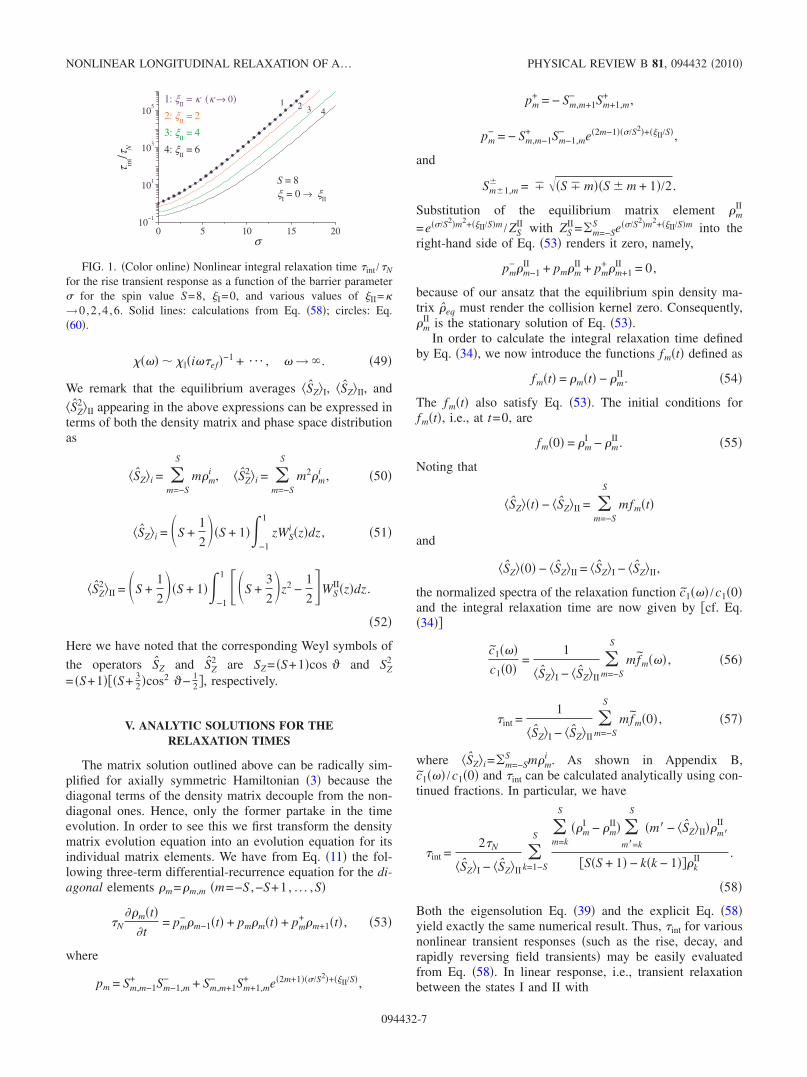
FIG. 1. �Color online� Nonlinear integral relaxation time �int /�N

for the rise transient response as a function of the barrier parameter for the spin value S=8, �I=0, and various values of �II=�→0,2 ,4 ,6. Solid lines: calculations from Eq. �58�; circles: Eq.�60�.


094432-7

HSI =

S2 SZ2 +

�II + �

SSZ and HS

II =

S2 SZ2 +

�II

SSZ

�� is a small external field parameter�, the initial conditionfor fm�t� becomes

fm�0� = e�/S2�m2+��II+��/S�m/ZSI − e�/S2�m2+��II/S�m/ZS

II

��

S�m − �SZ�II��m

II . �59�

Thus, Eq. �58� yields the correlation time �cor as

�cor =2�N

��

k=1−S

S �m=k

S

�m − �SZ�II��mII�2

�S�S + 1� − k�k − 1��kII . �60�

Equations �58� and �60� are valid for an arbitrary axially

symmetrical potential HS�SZ�. The particular form of the po-tential is contained only in the equilibrium matrix elements

of the density operator �mII and in the constants �� and �SZ�II.

We remarked above that the linear response has been pre-viously studied by Garanin26 and García-Palacios andZueco27 using the spin density matrix in the second order of

perturbation theory. In that context they also gave analyticexpressions for the linear-response integral relaxation time�cor, effective relaxation time �ef, and the longest relaxationtime ��1

−1 for more general models of a quantum super-paramagnet interacting with phonons, e.g., superimposed lin-ear and bilinear spin-bath interactions with super-Ohmicdamping. However, for the collision kernel given by Eq. �12�pertaining to the high temperature and weak coupling limittheir results for �cor reduce to ours. Hence, we can also applythe general results for �ef and �1

−1 given in Ref. 27. Thus, theeffective relaxation time �ef defined as

�ef = − �S��SZ�I��=0/ m=−S

S

mfm�0� �61�

is

�ef =2��N

k=1−S

S

�S�S + 1� − k�k − 1��kII

. �62�

Furthermore, the approximate equation for the longest relax-ation time ��1

−1 is

�� =2�N

��

k=1−S

S �m=k

S

�m − �SZ�II��mII�

m=−S

k−1

�� − sgn�m − mb��mII�

�S�S + 1� − k�k − 1��kII , �63�

where mb is the quantum number corresponding to the top ofthe barrier, �=m=−S

S sgn�m−mb��mII, and

�� = m=−S

S

m sgn�m − mb��mII − �

m=−S

S

m�mII�

�� m=−S

S

sgn�m − mb��mII� .

For values of the field ��, the relative deviation of �� from�1

−1 does not exceed 1%.27

The foregoing equations have been derived using the den-sity matrix method. They can also be obtained using thephase space formalism.9 For example, the effective relax-ation time �ef from Eq. �62� can be written as

�ef = 2�N

�SZ2�II − �SZ�II

2

�S2 − SZ2 + SZ�II

, �64�

where �SZ�II and �SZ2�II are given by Eqs. �51� and �52� and

�S2 − SZ2 + SZ�II = �S + 1��S +

1

2��

−1

1

��S�1 − z2� +1

2+ z −

3

2z2�WS

II�z�dz .

�65�

Equation �64� is simply a quantum analog of the knownequation for the effective relaxation time �ef of a classicalsuperparamagnet20

�ef = 2�N

�cos2 ��II − �cos ��II2

1 − �cos2 ��II. �66�

VI. RESULTS

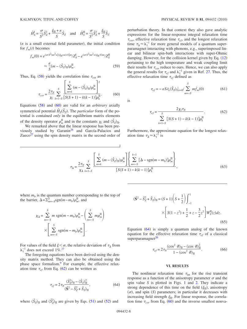
The nonlinear relaxation time �int for the rise transientresponse as a function of the anisotropy parameter and thespin value S is plotted in Figs. 1 and 2. They indicate astrong dependence of this time on the field ��II�, anisotropy��, and spin �S� parameters; in particular it decreases withincreasing field strength �II. For linear response, the correla-tion time �cor from Eq. �60� and the inverse smallest nonva-


094432-8

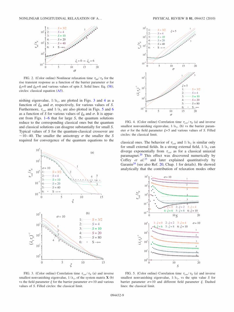
nishing eigenvalue, 1 /�1, are plotted in Figs. 3 and 4 as afunction of �II and , respectively, for various values of S.Furthermore, �cor and 1 /�1 are also plotted in Figs. 5 and 6as a function of S for various values of �II and . It is appar-ent from Figs. 1–6 that for large S, the quantum solutionsreduce to the corresponding classical ones but the quantumand classical solutions can disagree substantially for small S.Typical values of S for the quantum-classical crossover are�10–40. The smaller the anisotropy the smaller the Srequired for convergence of the quantum equations to the classical ones. The behavior of �cor and 1 /�1 is similar only

for small external fields. In a strong external field, 1 /�1 candiverge exponentially from �cor as for a classical uniaxialparamagnet.20 This effect was discovered numerically byCoffey et al.23 and later explained quantitatively byGaranin24 �see also Ref. 20, Chap. 1 for details�. He showedanalytically that the contribution of relaxation modes other

0 5 10 15 2010−2

100

102

104

ξI= 0 → ξ

II= 6

σ

τ int/τ

N

1: S = 3/22: S = 43: S = 104: S = 205: S = 406: S →∞

1

5

FIG. 2. �Color online� Nonlinear relaxation time �int /�N for therise transient response as a function of the barrier parameter for�I=0 and �II=6 and various values of spin S. Solid lines: Eq. �58�;circles: classical equation �A5�.

0 5 10 1510−4

10−2

100

102

104

54

3

2

ξ

τ cor/τ

N σ = 101: S = 3/22: S = 43: S = 104: S = 205: S = 406: S → ∞

1

(a)

0 5 10 15

100

101

102

103

104

4

32

(λ1τ N

)−1

5

1: S = 3/22: S = 43: S = 104: S = 205: S = 806: S →∞

ξ

1

σ = 10(b)

FIG. 3. �Color online� Correlation time �cor /�N �a� and inversesmallest nonvanishing eigenvalue, 1 /�1, of the system matrix X �b�vs the field parameter � for the barrier parameter =10 and variousvalues of S. Filled circles: the classical limit.

0 5 10 15 2010−2

100

102

104

106

τ cor/τ

N

σ

1: S = 3/22: S = 43: S = 104: S = 205: S = 406: S → ∞

ξ = 51

5

0 5 10 15 2010−2

100

102

104

(λ1τ N

)−1 ξ = 51: S = 3/22: S = 43: S = 104: S = 205: S = 806: S →∞

σ

1 5

FIG. 4. �Color online� Correlation time �cor /�N �a� and inversesmallest nonvanishing eigenvalue, 1 /�1, �b� vs the barrier param-eter for the field parameter �=5 and various values of S. Filledcircles: the classical limit.

0 10 2010−4

10−2

100

102

104σ = 10

S

τ cor/τ

N

1: ξ = 0 2: ξ = 2 3: ξ = 44: ξ = 6 5: ξ = 8 6: ξ = 10

1

2

3

4

5

6

0 10 20100

101

102

103

104

(λ1τ N

)−1

σ = 10

S

1: ξ = 0 2: ξ = 2 3: ξ = 44: ξ = 6 5: ξ = 8 6: ξ = 10

1

2

3

4

5

6

FIG. 5. �Color online� Correlation time �cor /�N �a� and inversesmallest nonvanishing eigenvalue, 1 /�1, vs the spin value S forbarrier parameter =10 and different field parameter �. Dashedlines: the classical limit.


094432-9

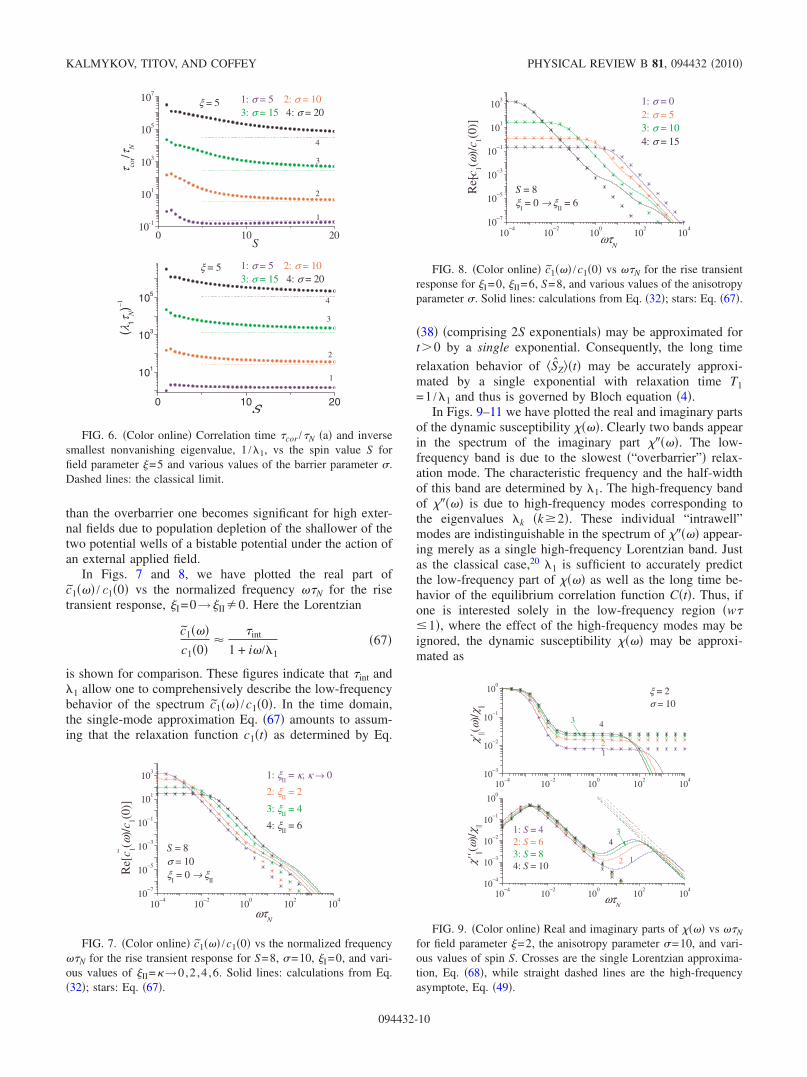
than the overbarrier one becomes significant for high exter-nal fields due to population depletion of the shallower of thetwo potential wells of a bistable potential under the action ofan external applied field.

In Figs. 7 and 8, we have plotted the real part ofc1�� /s1�0� vs the normalized frequency ��N for the risetransient response, �I=0→�II�0. Here the Lorentzian

c1��c1�0�

��int

1 + i�/�1�67�

is shown for comparison. These figures indicate that �int and�1 allow one to comprehensively describe the low-frequencybehavior of the spectrum c1�� /c1�0�. In the time domain,the single-mode approximation Eq. �67� amounts to assum-ing that the relaxation function c1�t� as determined by Eq.

�38� �comprising 2S exponentials� may be approximated fort�0 by a single exponential. Consequently, the long time

relaxation behavior of �SZ��t� may be accurately approxi-mated by a single exponential with relaxation time T1=1 /�1 and thus is governed by Bloch equation �4�.

In Figs. 9–11 we have plotted the real and imaginary partsof the dynamic susceptibility ��. Clearly two bands appearin the spectrum of the imaginary part ��. The low-frequency band is due to the slowest �“overbarrier”� relax-ation mode. The characteristic frequency and the half-widthof this band are determined by �1. The high-frequency bandof �� is due to high-frequency modes corresponding tothe eigenvalues �k �k�2�. These individual “intrawell”modes are indistinguishable in the spectrum of �� appear-ing merely as a single high-frequency Lorentzian band. Justas the classical case,20 �1 is sufficient to accurately predictthe low-frequency part of �� as well as the long time be-havior of the equilibrium correlation function C�t�. Thus, ifone is interested solely in the low-frequency region �w��1�, where the effect of the high-frequency modes may beignored, the dynamic susceptibility �� may be approxi-mated as

0 10 2010-1

101

103

105

107

ξ = 5

S

τ cor/τ

N

1: σ = 5 2: σ = 103: σ = 15 4: σ = 20

1

2

3

4

0 10 20

101

103

105

ξ = 5

S

(λ1τ N

)−1

1: σ = 5 2: σ = 103: σ = 15 4: σ = 20

1

2

3

4

FIG. 6. �Color online� Correlation time �cor /�N �a� and inversesmallest nonvanishing eigenvalue, 1 /�1, vs the spin value S forfield parameter �=5 and various values of the barrier parameter .Dashed lines: the classical limit.

10−4 10−2 100 102 10410−7

10−5

10−3

10−1

101

103

S = 8σ = 10ξ

I= 0 → ξ

II

ωτN

Re[

c 1(ω)/

c 1(0)]

1: ξII

= κ, κ → 0

2: ξII

= 2

3: ξII

= 4

4: ξII

= 6

~

FIG. 7. �Color online� c1�� /c1�0� vs the normalized frequency��N for the rise transient response for S=8, =10, �I=0, and vari-ous values of �II=�→0,2 ,4 ,6. Solid lines: calculations from Eq.�32�; stars: Eq. �67�.

10−4 10−2 100 102 10410−7

10−5

10−3

10−1

101

103

Re[

c 1(ω)/

c 1(0)]

S = 8ξ

I= 0 → ξ

II= 6

ωτN

1: σ = 02: σ = 53: σ = 104: σ = 15

~

FIG. 8. �Color online� c1�� /c1�0� vs ��N for the rise transientresponse for �I=0, �II=6, S=8, and various values of the anisotropyparameter . Solid lines: calculations from Eq. �32�; stars: Eq. �67�.

10−4 10−2 100 102 10410−3

10−2

10−1

100

3

2

4

ξ = 2σ = 10

χ'||(ω

)/χ ||

1: S = 42: S = 63: S = 84: S = 10

1

10−4 10−2 100 102 10410−4

10−3

10−2

10−1

100

3

2 1

4

ωτN

χ'' ||(ω

)/χ ||

FIG. 9. �Color online� Real and imaginary parts of �� vs ��N

for field parameter �=2, the anisotropy parameter =10, and vari-ous values of spin S. Crosses are the single Lorentzian approxima-tion, Eq. �68�, while straight dashed lines are the high-frequencyasymptote, Eq. �49�.


094432-10

��

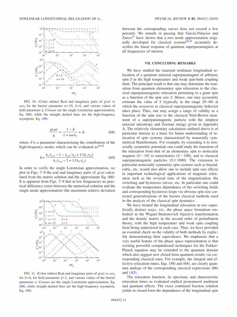
�1 − �

1 + i�/�1+ � , �68�

where � is a parameter characterizing the contribution of thehigh-frequency modes which can be evaluated as20,25

� =�1�cor − 1 − �cor/�ef + 1/��1�ef�

�1�cor − 2 + 1/��1�ef�. �69�

In order to verify the single Lorentzian approximation, weplot in Figs. 7–9 the real and imaginary parts of �� calcu-lated from the matrix solution and the approximate Eq. �68�.It is apparent from Figs. 7–9 that at low frequencies no prac-tical difference exists between the numerical solution and thesingle-mode approximation �the maximum relative deviation

between the corresponding curves does not exceed a fewpercent�. We remark in passing that García-Palacios andZueco27 have shown that a two mode approximation origi-nally developed for classical systems20,25 accurately de-scribes the linear response of quantum superparamagnets atall frequencies of interest.

VII. CONCLUDING REMARKS

We have studied the transient nonlinear longitudinal re-laxation of a quantum uniaxial superparamagnet of arbitraryspin S in the high temperature and weak spin-bath couplinglimit. The principal result is that one may determine the tran-sition from quantum elementary spin relaxation to the clas-sical superparamagnetic relaxation pertaining to a giant spinas a function of the spin size S. Hence, one may accuratelyestimate the value of S �typically in the range 20–40� atwhich the crossover to classical superparamagnetic behaviortakes place. Thus, one may assign a range of validity as afunction of the spin size to the classical Néel-Brown treat-ment of a superparamagnetic particle with the simplestuniaxial anisotropy and Zeeman energy given in AppendixA. The relatively elementary calculation outlined above is ofparticular interest as a basis for future understanding of re-laxation of spin systems characterized by nonaxially sym-metrical Hamiltonians. For example, by extending it to non-axially symmetric potentials one could study the transition ofthe relaxation from that of an elementary spin to molecularmagnets �S�10� to nanoclusters �S�100�, and to classicalsuperparamagnetic particles �S�1000�. The extension toparticular nonaxially symmetric spin systems such as biaxial,cubic, etc. would also allow one to include spin size effectsin important technological applications of magnetic relax-ation such as the reversal time of the magnetization, theswitching and hysteresis curves, etc. In particular one couldevaluate the temperature dependence of the switching fieldsand corresponding hysteresis loops via obvious spin size cor-rected generalizations of the known classical methods usedin the analysis of the classical spin dynamics.

We have treated the longitudinal relaxation in two super-ficially distinct ways, viz., the phase space formalism em-bodied in the Wigner-Stratonovich bijective transformationand the density matrix in the second order of perturbationtheory, with the high temperature and weak spin couplinglimit being understood in each case. Thus, we have providedan essential check on the validity of both methods by explic-itly demonstrating their equivalence. We emphasize that avery useful feature of the phase space representation is thatexisting powerful computational techniques for the Fokker-Planck equation may be extended to the quantum domainwhich also suggest new closed form quantum results via cor-responding classical ones. For example, the integral and ef-fective relaxation times, Eqs. �58� and �64�, are clearly quan-tum analogs of the corresponding classical expressions �66�and �A5�.

The relaxation function, its spectrum, and characteristicrelaxation times as evaluated explicit pronounced nonlinearand quantum effects. The exact continued fraction solutionyields in closed form the dependence of the longitudinal spin

10−4 10−2 100 102 10410−4

10−3

10−2

10−1

100

3

1

2

4

1: ξ = 02: ξ = 23: ξ = 44: ξ = 6

S = 6σ = 10

χ'||(ω

)/χ ||

10−4 10−2 100 102 10410−4

10−3

10−2

10−1

100

4

3

1

2

ωτN

χ'' ||(ω

)/χ ||

FIG. 10. �Color online� Real and imaginary parts of �� vs��N for the barrier parameter =10, S=6, and various values offield parameter �. Crosses are the single Lorentzian approximation,Eq. �68�, while the straight dashed lines are the high-frequencyasymptote, Eq. �49�.

10−6 10−4 10−2 100 102 10410-4

10-3

10-2

10-1

100

2

2

34

1

S = 6ξ = 2

1: σ = 02: σ = 53: σ = 104: σ = 15

10−6 10−4 10−2 100 102 10410−5

10−4

10−3

10−2

10−1

100

χ'||(ω

)/χ ||

34

ωτN

χ'' ||(ω

)/χ ||

1

FIG. 11. �Color online� Real and imaginary parts of �� vs ��N

for S=6, for field parameter �=2, and various values of the barrierparameter . Crosses are the single Lorentzian approximation, Eq.�68�, while straight dashed lines are the high-frequency asymptote,Eq. �49�.


094432-11

relaxation function on the spin size S, which is dominated bya single exponential having as time constant the longest re-laxation time 1 /�1. Thus, a simple description of the longtime behavior of the longitudinal relaxation function asBloch equation �4� holds for the nonlinear response of aquantum superparamagnet for arbitrary spin S. In linear re-sponse, the approach so developed reproduces the resultspreviously obtained by Garanin26 and García-Palacios andZueco.27 We remark in passing that our approach can also beapplied to the calculation of nonlinear ac stationary re-sponses of quantum superparamagnets by generalizing thematrix continued fraction method of solution of the Fokker-Planck equation for classical spins driven by a strong acfield.35 This will allow to treat quantum effects in the acnonlinear response of quantum superparamagnets.36 It hasbeen shown experimentally36 for the molecular magnet Mn12characterized by S=10 that the behavior of the nonlinearsusceptibility of quantum superparamagnets is qualitativelydifferent from that of classical spin systems with S 1.

ACKNOWLEDGMENTS

This paper emanated from research conducted with thefinancial support of FP7-PEOPLE-Marie Curie Actions�Project No. 230785 NANOMAGNETS� and IRCSET/EGIDE exchange program Ulysses. We thank D. A. Garaninfor useful discussions.

APPENDIX A: CLASSICAL LIMIT

In the classical limit, S→�, Hamiltonian �3� correspondsto a free energy V of the form

V�� = − cos2 � − � cos � . �A1�

The distribution functions in the equilibrium states I and IIare given by

Wi�z� = ez2+�iz/Zi �i = I,II� ,

where z=cos �,

Zi =1

2��

e−hi

2�erf i��1 + hi�� + erf i��1 − hi��

is the partition function, hi=�i / �2�, and erf i�x�= 2��

0xet2dt

is the error function of imaginary argument. For arbitrary ,Eq. �22� becomes in the classical limit, S→�,

�N�cL�t�

�t= qLcL�t� + qL

−cL−1�t� + qL+cL+1�t� + qL

−−cL−2�t�

+ qL++cL+2�t� , �A2�

where cL�t�= �PL�cos ��t�− �PL�cos ��II, PL are the Leg-endre polynomials,

qL = −L�L + 1�

2�1 −

2

�2L − 1��2L + 3�� ,

qL� = � �

L�L + 1�2�2L + 1�

,

qL−− = − qL−1

++ =L�L + 1��L − 1��2L − 1��2L + 1�

.

The detailed solution of Eq. �A2� is given in Ref. 20, Ch. 8.For =0, we have from Eq. �A2�

2�N

L�L + 1��

�tcL�t� + cL�t� =

�

2L + 1�cL−1�t� − cL+1�t�� ,

�A3�

which is the known result for relaxation of a classical spin ina uniform field.20,37 Recurrence equations �A2� can also bepresented in the homogeneous matrix form

C�t� + Xc · C�t� = 0, �A4�

where the system matrix Xc is now infinite and five diagonal.In the classical limit, the nonlinear integral relaxation

time �int of the dipole relaxation function c1�t�= �cos ��t�− �cos ��II is given by20,29,30

�int =2�N

�cos ��I − �cos ��II�

−1

1 ��z��z�e−z2−�IIz

1 − z2 dz ,

�A5�

where

��z� = �−1

z

�WI�z�� − WII�z��dz�

=�1/2e−hII

2

21/2ZII�erf i��z + hII�� + erf i��1 − hII��

−�1/2e−hI

2

21/2ZI�erf i��z + hI�� + erf i��1 − hI�� ,

��z� = �−1

z

�z� − �z�II�e�z�2+2hIIz��dz�

=1

2�e�z2+2hIIz� − e�1−2hII��

− e�1−hII2 ��

1/2 sinh�2hII�23/2ZII

�erf i��z + hII��

+ erf i��1 − hII�� ,

�cos ��i =e sinh�2hi�

Zi− hi.

In linear response, the correlation time �cor can be expressedin the closed form as20,25


094432-12

�cor =2�N

ZII��cos2 ��II − �cos ��II2 ��−1

1

��−1

z

�z� − �cos ��II�ez�2+�IIz�dz��2

�e−z2−�IIz

1 − z2 dz , �A6�

which is in complete agreement with Eq. �60� in the limitS→�.

APPENDIX B: CALCULATION OF THE INTEGRALRELAXATION TIME

In algebraic transformations, it is more convenient towork with indexes ranging from 0 to 2S. Hence, we intro-duce a new index n defined as n=m+S. Equation �53� cannow be rearranged as

�N� fn

�t= pn

−fn−1 + pnfn + pn+fn+1, �B1�

where

pn = −1

2�2S − n + 1�n −

1

2�2S − n��n + 1�e�2n−2S+1��/S2�+��II/S�,

pn+ =

1

2�2S − n��n + 1� ,

pn− =

1

2�2S − n + 1�ne�2n−2S−1��/S2�+��II/S�.

Now recurrence equations �B1� can also be presented in thehomogeneous matrix form

�NF�t� = � · F�t� , �B2�

where the vector F�t� and the system matrix � are

F�t� =�f0�t�f1�t�f2�t�f3�t�]

f2S�t�� ,

� =�p0 p0

+ 0 0 ¯ 0

p1− p1 p1

+ 0 ¯ 0

0 p2− p2 p2

+¯ 0

0 0 p3− p3 ¯ 0

] ] ] ] � ]

0 0 0 0 ¯ p2S

� . �B3�

We remark that the system matrix � has exactly the sameeigenvalues as the system matrix X given by Eq. �29� plus an

additional zero eigenvalue �0=0 corresponding to the ther-mal equilibrium state.

Clearly Eq. �B2� can be solved by the matrix methodsdescribed in Sec. III. However, we shall present an exactanalytic solution in terms of continued fractions. Applyingthe general method of solution of inhomogeneous three termrecurrence relations to the Fourier-Laplace transform of Eq.�B1�,20 we have

f n�� = �n��pn− f n−1�� + �N�pn−1

+ �−1l=n

2S

�k=n

l

�pk−1+ �k��f l�0� .

�B4�

Here �n�� are the continued fractions defined by the recur-rence equation

�n�� = �i��N − pn − pn+pn+1

− �n+1��−1

for 0�n�2S and �2S+1��=0. For �=0, Eq. �B4� can beconsiderably simplified

f n�0� = e�2�n−S�−1��/S2�+��/S� f n−1�0� −2�N

n�2S − n + 1� m=n−S

S

fm�0� ,

�B5�

where we have noticed that �n�0�= �pn−1+ �−1. Because recur-

rence equations �B1� are not linearly independent, the deter-minant of the matrix � from Eq. �B1� is zero �det �=0�.Thus, the functions f n�0� can be determined only in terms of

f0�0�. In order to find f0�0�, we can utilize the normalizationproperties of the density matrix, namely,

m=−S

S

fm�t� = m=−S

S

��m�t� − �mII� = 0,

so that

m=−S

S

fm�0� = 0. �B6�

Consequently, Eqs. �B4� and �B6� yield the closed-form ex-pression

f0�0� =2�Ne−�II

Z

k=1−S

S m=k

S

��mI − �m

II� m�=k

S

�m�II

�S − k + 1��k + S��keq . �B7�

By substituting Eqs. �B5� and �B7� into Eq. �56�, we have theintegral relaxation time as

�int =1


n=1

2S

nfn�0� . �B8�

Equation �B8� can be written in the analytic form of Eq. �58�.The spectrum c1�� is

c1��c1�0�

=1


n=1

2S

nfn�� . �B9�


094432-13

1 W. P. Schleich, Quantum Optics in Phase Space �Wiley-VCH,Berlin, 2001�.

2 R. R. Puri, Mathematical Methods of Quantum Optics �Springer,Berlin, 2001�.

3 D. F. Walls and G. J. Milburn, Quantum Optics �Springer, Berlin,2007�.

4 L. M. Narducci, C. M. Bowden, V. Bluemel, and G. P. Carra-zana, Phys. Rev. A 11, 280 �1975�.

5 Y. Takahashi and F. Shibata, J. Phys. Soc. Jpn. 38, 656 �1975�.6 A. M. Perelomov, Generalized Coherent States and Their Appli-

cations �Springer, Berlin, 1986�.7 N. Hashitsumae, F. Shibata, and M. Shingu, J. Stat. Phys. 17,

155 �1977�.8 F. Shibata, J. Phys. Soc. Jpn. 49, 15 �1980�.9 Yu. P. Kalmykov, W. T. Coffey, and S. V. Titov, Phys. Rev. E 76,

051104 �2007�; EPL 88, 17002 �2009�.10 D. A. Varshalovich, A. N. Moskalev, and V. K. Khersonskii,

Quantum Theory of Angular Momentum �World Scientific, Sin-gapore, 1998�.

11 R. L. Stratonovich, Zh. Eksp. Teor. Fiz. 31, 1012 �1956� �Sov.Phys. JETP 4, 891 �1957��.

12 F. A. Berezin, Commun. Math. Phys. 40, 153 �1975�.13 Yu. P. Kalmykov, W. T. Coffey, and S. V. Titov, Phys. Rev. B

77, 104418 �2008�.14 M. Radcliffe, J. Phys. A 4, 313 �1971�; F. T. Arecchi, E.

Courtens, R. Gilmore, and H. Thomas, Phys. Rev. A 6, 2211�1972�; M. O. Scully and K. Wodkiewicz, Found. Phys. 24, 85�1994�; G. S. Agarwal, Phys. Rev. A 57, 671 �1998�; C. Brif andA. Mann, ibid. 59, 971 �1999�; A. B. Klimov, J. Math. Phys.43, 2202 �2002�.

15 Y. Takahashi and F. Shibata, J. Stat. Phys. 14, 49 �1976�; F.Shibata, Y. Takahashi, and N. Hashitsumae, ibid. 17, 171�1977�.

16 F. Shibata and M. Asou, J. Phys. Soc. Jpn. 49, 1234 �1980�; F.Shibata and C. Uchiyama, ibid. 62, 381 �1993�.

17 D. Zueco and I. Calvo, J. Phys. A: Math. Theor. 40, 4635�2007�.

18 Yu. P. Kalmykov, W. T. Coffey, and S. V. Titov, J. Stat. Phys.131, 969 �2008�.

19 H. Risken, The Fokker-Planck Equation, 2nd ed. �Springer, Ber-lin, 1989�.

20 W. T. Coffey, Yu. P. Kalmykov, and J. T. Waldron, The LangevinEquation, 2nd ed. �World Scientific, Singapore, 2004�.

21 W. F. Brown, Jr., Phys. Rev. 130, 1677 �1963�.22 A. Aharoni, Phys. Rev. 177, 793 �1969�.23 W. T. Coffey, D. S. F. Crothers, Yu. P. Kalmykov, and J. T.

Waldron, Phys. Rev. B 51, 15947 �1995�.24 D. A. Garanin, Phys. Rev. E 54, 3250 �1996�.25 Yu. P. Kalmykov, W. T. Coffey, and S. V. Titov, J. Magn. Magn.

Mater. 265, 44 �2003�; Yu. P. Kalmykov and S. V. Titov, Fiz.Tverd. Tela �St. Petersburg� 45, 2037 �2003� �Phys. Solid State45, 2140 �2003��.

26 D. A. Garanin, Phys. Rev. E 55, 2569 �1997�.27 J. L. García-Palacios and D. Zueco, J. Phys. A 39, 13243 �2006�;

D. Zueco and J. L. García-Palacios, Phys. Rev. B 73, 104448�2006�.

28 K. Blum, Density Matrix: Theory and Applications, 2nd ed. �Ple-num, New York, 1996�.

29 Yu. P. Kalmykov, J. L. Déjardin, and W. T. Coffey, Phys. Rev. E55, 2509 �1997�.

30 Yu. P. Kalmykov and S. V. Titov, Fiz. Tverd. Tela �St. Peters-burg� 42, 893 �2000� �Phys. Solid State 42, 918 �2000��.

31 Yu. P. Kalmykov, W. T. Coffey, and S. V. Titov, J. Phys. A:Math. Theor. 41, 105302 �2008�.

32 R. Bellman, Introduction to Matrix Analysis �McGraw-Hill, NewYork, 1960�.

33 R. Kubo, M. Toda, and N. Hashitsumae, Statistical Physics II,Nonequilibrium Statistical Mechanics �Springer-Verlag, Berlin,1985�.

34 W. T. Coffey, Yu. P. Kalmykov, and E. S. Massawe, Adv. Chem.Phys. 85, 667 �1993�.

35 P. M. Déjardin and Yu. P. Kalmykov, J. Appl. Phys. 106, 123908�2009�.

36 R. López-Ruiz, F. Luis, A. Millán, C. Rillo, D. Zueco, and J. L.García-Palacios, Phys. Rev. B 75, 012402 �2007�.

37 J. T. Waldron, Yu. P. Kalmykov, and W. T. Coffey, Phys. Rev. E49, 3976 �1994�.


094432-14

Documents

: Phase space and density matrix formulations