Embed Size (px)
Citation preview
Habilitation à diriger des recherchesUniversité Lille 1 - Sciences et Technologiespréparée au sein du centre de recherche INRIA Lille - Nord Europe
Specialité : Mathématiques
Daniil RYABKO
APPRENABILITÉ DANS LES PROBLÈMESDE L’INFÉRENCE SÉQUENTIELLE
LEARNABILITY IN PROBLEMS OFSEQUENTIAL INFERENCE
Habilitation soutenue à Villneuve d’Ascq le 19 décembre 2011 devant le jurycomposé de
Pr. Peter AUER University of Leoben RapporteurPr. Jan BEIRLANT K.U.Leuven ExaminateurPr. Léon BOTTOU Microsoft RapporteurPr. Max DAUCHET Université Lille 1 ExaminateurPr. László GYÖRFI Budapest University RapporteurPr. Rémi MUNOS INRIA Lille - Nord Europe ExaminateurPr. Philippe PREUX Université Lille 3 Examinateur
Résumé
Les travaux présentés sont dédiés à la possibilité de faire de l’inférence statis-tique à partir de données séquentielles. Le problème est le suivant. Étant don-née une suite d’observations x1,...,xn,... , on cherche à faire de l’inférence sur leprocessus aléatoire ayant produit la suite. Plusieurs problèmes, qui d’ailleursont des applications multiples dans différents domaines des mathématiques etde l’informatique, peuvent être formulés ainsi. Par exemple, on peut vouloirprédire la probabilité d’apparition de l’observation suivante, xn+1 (le problèmede prédiction séquentielle); ou répondre à la question de savoir si le processusaléatoire qui produit la suite appartient à un certain ensemble H0 versus appar-tient à un ensemble différent H1 (test d’hypothèse) ; ou encore, effectuer uneaction avec le but de maximiser une certain fonction d’utilité. Dans chacunde ces problèmes, pour rendre l’inférence possible il faut d’abord faire certaineshypothèses sur le processus aléatoire qui produit les données. La question cen-trale adressée dans les travaux présentés est la suivante : sous quelles hypothèsesl’inférence est-elle possible ? Cette question est posée et analysée pour des prob-lèmes d’inférence différents, parmi lesquels se trouvent la prédiction séquentielle,les tests d’hypothèse, la classification et l’apprentissage par renforcement.
2
Abstract
Given a growing sequence of observations x1,...,xn,... , one is required, at eachtime step n, to make some inference about the stochastic mechanism generatingthe sequence. Several problems that have numerous applications in differentbranches of mathematics and computer science can be formulated in this way.For example, one may want to forecast probabilities of the next outcome xn+1
(sequence prediction); to make a decision on whether the mechanism generatingthe sequence belongs to a certain family H0 versus it belongs to a differentfamily H1 (hypothesis testing); to take an action in order to maximize someutility function.
In each of these problems, as well as in many others, in order to be able tomake inference, one has to make some assumptions on the probabilistic mecha-nism generating the data. Typical assumptions are that xi are independent andidentically distributed, or that the distribution generating the sequence belongsto a certain parametric family. The central question addressed in this work is:under which assumptions is inference possible? This question is considered forseveral problems of inference, including sequence prediction, hypothesis testing,classification and reinforcement learning.
3
Contents
Publications on which this manuscript is based . . . . . . . . . . . . . 7Acknowledgements . . . . . . . . . . . . . . . . . . . . . . . . . . . . . 10
1 Introduction 11Organization of this manuscript . . . . . . . . . . . . . . . . . . . . . . 13
2 Sequence prediction [R1, R3, R8] 142.1 Notation and definitions . . . . . . . . . . . . . . . . . . . . . . . 172.2 If there exists a consistent predictor then there exists a consistent
Bayesian predictor with a discrete prior [R3] . . . . . . . . . . . . 202.2.1 Introduction and related work . . . . . . . . . . . . . . . . 202.2.2 Results . . . . . . . . . . . . . . . . . . . . . . . . . . . . . 23
2.3 Characterizing predictable classes [R3] . . . . . . . . . . . . . . . 302.3.1 Separability . . . . . . . . . . . . . . . . . . . . . . . . . . 312.3.2 Conditions based on local behaviour of measures . . . . . . 34
2.4 Conditions under which one measure is a predictor for another [R8] 402.4.1 Measuring performance of prediction . . . . . . . . . . . . 432.4.2 Dominance with decreasing coefficients . . . . . . . . . . . 442.4.3 Preservation of the predictive ability under summation
with an arbitrary measure . . . . . . . . . . . . . . . . . . 482.5 Nonrealizable version of the sequence prediction problem [R1] . . 50
2.5.1 Sequence prediction problems . . . . . . . . . . . . . . . . 54
4
2.5.2 Characterizations of learnable classes for prediction in to-tal variation . . . . . . . . . . . . . . . . . . . . . . . . . . 56
2.5.3 Characterizations of learnable classes for prediction in ex-pected average KL divergence . . . . . . . . . . . . . . . . 59
2.6 Longer proofs . . . . . . . . . . . . . . . . . . . . . . . . . . . . . 672.6.1 Proof of Theorem 2.7 . . . . . . . . . . . . . . . . . . . . . 672.6.2 Proof of Theorem 2.22 . . . . . . . . . . . . . . . . . . . . 722.6.3 Proof of Theorem 2.35 . . . . . . . . . . . . . . . . . . . . 74
3 Statistical analysis of stationary ergodic time series [R2, R4, R5,
R11] 803.1 Preliminaries . . . . . . . . . . . . . . . . . . . . . . . . . . . . . 823.2 Statistical analysis based on estimates of distributional distance
[R4] . . . . . . . . . . . . . . . . . . . . . . . . . . . . . . . . . . 853.2.1 Goodness-of-fit . . . . . . . . . . . . . . . . . . . . . . . . 893.2.2 Process classification . . . . . . . . . . . . . . . . . . . . . 903.2.3 Change point problem . . . . . . . . . . . . . . . . . . . . 91
3.3 Characterizing families of stationary processes for which consis-tent tests exist [R2] . . . . . . . . . . . . . . . . . . . . . . . . . . 923.3.1 Definitions: consistency of tests . . . . . . . . . . . . . . . 973.3.2 Topological characterizations . . . . . . . . . . . . . . . . . 973.3.3 Examples . . . . . . . . . . . . . . . . . . . . . . . . . . . 99
3.4 Clustering time series [R11] . . . . . . . . . . . . . . . . . . . . . 1023.4.1 Problem formulation . . . . . . . . . . . . . . . . . . . . . 1043.4.2 Clustering algorithm . . . . . . . . . . . . . . . . . . . . . 106
3.5 Discrimination between B-processes is impossible [R5] . . . . . . . 1083.6 Longer proofs . . . . . . . . . . . . . . . . . . . . . . . . . . . . . 111
3.6.1 Proof of Theorem 3.9 . . . . . . . . . . . . . . . . . . . . . 1113.6.2 Proofs for Section 3.3 . . . . . . . . . . . . . . . . . . . . . 1123.6.3 Proof of Theorem 3.19 . . . . . . . . . . . . . . . . . . . . 120
5
4 Finding an optimal strategy in a reactive environment [R7] 1314.1 Problem formulation . . . . . . . . . . . . . . . . . . . . . . . . . 1344.2 Self-optimizing policies for a set of value-stable environments . . . 1374.3 Non-recoverable environments . . . . . . . . . . . . . . . . . . . . 1394.4 Examples . . . . . . . . . . . . . . . . . . . . . . . . . . . . . . . 1414.5 Necessity of value-stability . . . . . . . . . . . . . . . . . . . . . . 1464.6 Longer proofs . . . . . . . . . . . . . . . . . . . . . . . . . . . . . 148
5 Classification [R9, R10] 1545.1 Relaxing the i.i.d. assumption in classification [R10] . . . . . . . . 155
5.1.1 Definitions and general results . . . . . . . . . . . . . . . . 1575.1.2 Application to classical nonparametric predictors . . . . . 1625.1.3 Application to empirical risk minimisation. . . . . . . . . . 164
5.2 Computational limitations on the statistical characterizations oflearnability in classification [R9] . . . . . . . . . . . . . . . . . . . 1675.2.1 Notation and definitions . . . . . . . . . . . . . . . . . . . 1685.2.2 Sample complexity explosion for computable
learning rules . . . . . . . . . . . . . . . . . . . . . . . . . 1715.2.3 Different settings and tightness of the negative results . . . 174
5.3 Longer proofs . . . . . . . . . . . . . . . . . . . . . . . . . . . . . 1755.3.1 Proofs for Section 5.1.1 . . . . . . . . . . . . . . . . . . . . 1755.3.2 Proofs for Section 5.1.2 . . . . . . . . . . . . . . . . . . . . 1795.3.3 Proofs for Section 5.1.3 . . . . . . . . . . . . . . . . . . . . 1845.3.4 Proof of Theorem 5.10 . . . . . . . . . . . . . . . . . . . . 185
6
Publications on which this manuscript is based
Journal papers
[R1] D. Ryabko. On the relation between realizable and non-realizable cases ofthe sequence prediction problem. Journal of Machine Learning Research,12:2161–2180, 2011.
[R2] D. Ryabko. Testing composite hypotheses about discrete ergodic processes.Test, (in press), 2011.
[R3] D. Ryabko. On finding predictors for arbitrary families of processes. Jour-nal of Machine Learning Research, 11:581–602, 2010.
[R4] D. Ryabko and B. Ryabko. Nonparametric statistical inference for ergodicprocesses. IEEE Transactions on Information Theory, 56(3):1430–1435,2010.
[R5] D. Ryabko. Discrimination between B-processes is impossible. Journal ofTheoretical Probability, 23(2):565–575, 2010.
[R6] D. Ryabko and J. Schmidhuber. Using data compressors to construct ordertests for homogeneity and component independence. Applied MathematicsLetters, 22(7):1029–1032, 2009.
[R7] D. Ryabko and M. Hutter. On the possibility of learning in reactiveenvironments with arbitrary dependence. Theoretical Computer Science,405(3):274–284, 2008.
[R8] D. Ryabko and M. Hutter. Predicting non-stationary processes. AppliedMathematics Letters, 21(5):477–482, 2008.
[R9] D. Ryabko. On sample complexity for computational classification prob-lems. Algorithmica, 49(1):69–77, 2007.
7
[R10] D. Ryabko. Pattern recognition for conditionally independent data. Jour-nal of Machine Learning Research, 7:645–664, 2006.
Selected conference papers
[R11] D. Ryabko. Clustering processes. In Proc. the 27th International Con-ference on Machine Learning (ICML 2010), pages 919–926, Haifa, Israel,2010.
[R12] D. Ryabko. Sequence prediction in realizable and non-realizable cases.In Proc. the 23rd Conference on Learning Theory (COLT 2010), pages119–131, Haifa, Israel, 2010.
[R13] D. Ryabko. Testing composite hypotheses about discrete-valued stationaryprocesses. In Proc. IEEE Information Theory Workshop (ITW’10), pages291–295, Cairo, Egypt, 2010. IEEE.
[R14] D. Ryabko. An impossibility result for process discrimination. In Proc.2009 IEEE International Symposium on Information Theory (ISIT), pages1734–1738, Seoul, South Korea, 2009. IEEE.
[R15] D. Ryabko. Characterizing predictable classes of processes. Proceedingsof the 25th Conference on Uncertainty in Artificial Intelligence (UAI’09),Montreal, Canada, 2009.
[R16] D. Ryabko. Some sufficient conditions on an arbitrary class of stochasticprocesses for the existence of a predictor. In Proc. 19th InternationalConf. on Algorithmic Learning Theory (ALT’08), LNAI 5254, pages 169–182, Budapest, Hungary, 2008. Springer.
[R17] D. Ryabko and B. Ryabko. On hypotheses testing for ergodic processes.In Proc. 2008 IEEE Information Theory Workshop (ITW), pages 281–283,Porto, Portugal, 2008. IEEE.
8
[R18] D. Ryabko and M. Hutter. On sequence prediction for arbitrary mea-sures. In Proc. 2007 IEEE International Symposium on InformationTheory (ISIT), pages 2346–2350, Nice, France, 2007. IEEE.
[R19] D. Ryabko and M. Hutter. Asymptotic learnability of reinforcement prob-lems with arbitrary dependence. In Proc. 17th International Conf. on Al-gorithmic Learning Theory (ALT), LNAI 4264, pages 334–347, Barcelona,Spain, 2006. Springer.
[R20] D. Ryabko. On computability of pattern recognition problems. In Proc.16th International Conf. on Algorithmic Learning Theory (ALT), LNAI3734, pages 148–156, Singapore, 2005. Springer.
[R21] D. Ryabko. Application of classical nonparametric predictors to learningconditionally i.i.d. data. In Proc. 15th International Conf. on AlgorithmicLearning Theory (ALT), LNAI 3244, pages 171–180, Padova, Italy, 2004.Springer.
[R22] D. Ryabko. Online learning of conditionally i.i.d. data. In 21st Inter-national Conference on Machine Learning (ICML), pages 727–734, Banff,Canada, 2004.
9

Acknowledgements
Thanks for reading.
10
Chapter 1
Introduction
This manuscript summarizes my work on the problem of learnability in mak-ing sequential inference. The problem is as follows. Given a growing sequenceof observations x1,...,xn,... , one is required, at each time step n, to make someinference about the stochastic mechanism generating the sequence. Several prob-lems that have numerous applications in different branches of mathematics andcomputer science can be formulated in this way. For example, one may want toforecast probabilities of the next outcome xn+1 (sequence prediction); to make adecision on whether the mechanism generating the sequence belongs to a certainfamily H0 versus it belongs to a different family H1 (hypothesis testing); to takean action in order to maximize some utility function. In each of these problems,as well as in many others, in order to be able to make inference, one has to makesome assumptions on the probabilistic mechanism generating the data. Typicalassumptions are that xi are independent and identically distributed, or that thedistribution generating the sequence belongs to a certain parametric family. Thecentral question addressed in this work is: under which assumptions is inferencepossible? This question is considered for several problems of inference, includingsequence prediction, hypothesis testing, classification and reinforcement learn-ing.
The motivation for studying such questions is as follows. There are numer-ous applications of the problems of sequential inference considered, including the
11
analysis of data coming from a stock market, biological databases, network traf-fic, surveillance, etc. Moreover, new applications spring up regularly. Clearly,each application requires its own set of assumptions or its own model: indeed, amodel that describes well DNA sequences probably should not be expected to de-scribe a network traffic stream as well. At the same time, the methods developedfor sequential data analysis, for example, for sequence prediction, are typicallylimited to a restricted set of models, the construction of which is driven notso much by applications as by the availability of mathematical and algorithmictools. For example, much of the non-parametric analysis in sequence predictionand the problems of finding an optimal behaviour in an unknown environmentis limited to finite-state models, such as Markov or hidden Markov models. Oneapproach to start addressing this problem is to develop a theory that would al-low one to check whether a given model is feasible, in the sense that it allowsfor the existence of a solution to the target problem of inference. Another ques-tion is how to find a solution given a model in a general form. This manuscriptsummarizes some first steps I have made in solving these general problems.
The most important results presented here are as follows. For the problemof hypothesis testing, I have obtained a topological characterization (necessaryand sufficient conditions) of those (composite) hypotheses H0⊂ E that can beconsistently tested against E\H0, where E is the set of all stationary ergodicdiscrete-valued process measures. The developed approach, which is based onempirical estimates of the distributional distance, has allowed me to obtain con-sistent procedures for change point estimation, process classification and clus-tering, under the only assumption that the data (real-valued, in this case) isgenerated by stationary ergodic distributions: a setting that is much more gen-eral than those in which consistent procedures were known before. I have alsodemonstrated that a consistent test for homogeneity does not exist for the gen-eral case of stationary ergodic (discrete-valued) sequences. For the problem ofsequence prediction, I have shown that if there is a consistent predictor for aset of process distributions C, then there is a Bayesian predictor consistent forthis set. This is a no-assumption result: the distributions in C can be arbi-
12

trary (non-i.i.d., non-stationary, etc.) and the set itself does not even have tobe measurable. I have also obtained several descriptions (sufficient conditions)of those sets C of process distributions for which consistent predictors exist. Forthe problem of selecting an optimal strategy in a reactive environment (perhaps,the most general inference problem considered) I have identified some sufficientconditions on the environments under which it is possible to find a universalasymptotically optimal strategy.
Organization of this manuscript
Each of the subsequent chapters is devoted to a specific group of inference prob-lems. These chapters are essentially constructed from the papers listed below,which are streamlined and endowed with unified introductions and notation.References to the corresponding papers follow the title of of each chapter orsection. While trying to keep the contents concise, I have decided to include allproofs (in appendices to the chapters) to make the manuscript self-contained.The contents of the Section 5.1 is extracted from my Ph.D. thesis; the rest ofthe work is posterior.
13
Chapter 2
Sequence prediction [R1, R3, R8]
The problem is sequence prediction in the following setting. A sequence x1,...,xn,...
of discrete-valued observations is generated according to some unknown proba-bilistic law (measure) µ. After observing each outcome, it is required to give theconditional probabilities of the next observation. The measure µ is unknown.We are interested in constructing predictors ρ whose conditional probabilitiesρ(·|x1,...,xn) converge (in some sense) to the “true” µ-conditional probabilitiesµ(·|x1,...,xn), as the sequence of observations increases (n→∞). In general, thisgoal is impossible to achieve if nothing is known about the measure µ generatingthe sequence. In other words, one cannot have a predictor whose error goes tozero for any measure µ. The problem becomes tractable if we assume that themeasure µ generating the data belongs to some known class C. The main generalproblems considered in this chapter are as follows.
(i) Given a set C of process measures, what are the conditions on C underwhich there exists a measure ρ that predicts every µ∈C? (Section 2.3)
(ii) Is there a general way to construct such a measure ρ? What form shouldρ have? (Section 2.2)
(iii) Given two process measures µ and ρ, what are the conditions on themunder which ρ is a predictor for µ? (Section 2.4)
14
(iv) Given a set C of process measures, what are the conditions on C underwhich there exists a measure ρ which predicts every measure ν that ispredicted by at least one measure µ∈C? (Section 2.5)
The last question is explained by the following consideration. Since a predictorρ that we wish to construct is required, on each time step, to give conditionalprobabilities ρ(·|x1,...,xn) of the next outcome given the past, for each possiblesequence of past observations x1,...,xn, the predictor ρ itself defines a measure onthe space of one-way infinite sequences. This enables us to pose similar questionsabout the measures µ generating the data and predictors.The motivation for studying predictors for arbitrary classes C of processesis two-fold. First of all, the problem of prediction has numerous applicationsin such diverse fields as data compression, market analysis, bioinformatics, andmany others. It seems clear that prediction methods constructed for one appli-cation cannot be expected to be optimal when applied to another. Therefore, animportant question is how to develop specific prediction algorithms for each ofthe domains. Apart from this, sequence prediction is one of the basic ingredientsfor constructing intelligent systems. Indeed, in order to be able to find optimalbehaviour in an unknown environment, an intelligent agent must be able, at thevery least, to predict how the environment is going to behave (or, to be moreprecise, how relevant parts of the environment are going to behave). Since theresponse of the environment may in general depend on the actions of the agent,this response is necessarily non-stationary for explorative agents. Therefore, onecannot readily use prediction methods developed for stationary environments,but rather has to find predictors for the classes of processes that can appear asa possible response of the environment.
To evaluate the quality of prediction we will mostly use expected (with re-spect to data) average (over time) Kullback-Leibler divergence, as well as totalvariation distance (see Section 2.1 for definitions). Prediction in total variationis a very strong notion of performance; in particular, it is not even possible topredict an arbitrary i.i.d. Bernoulli distribution in this sense. Prediction in ex-pected average KL divergence is much weaker and therefore more practical, but
15
it is also more difficult to study, as is explained below.Next we briefly describe some of the answers to the questions (i)-(iv)
posed above that we have obtained. It is well-known [11, 46] (see also Theo-rem 2.2 below) that a measure ρ predicts a measure µ in total variation if andonly if µ is absolutely continuous with respect to ρ. This answers question (ii)
for prediction in total variation. Moreover, since in probability theory we knowvirtually everything about absolute continuity, this fact makes it relatively easyto answer the rest of the questions for this measure of performance. We ob-tain (Theorem 2.31) two characterizations of those sets C for which consistentpredictors exist (question (i)): one of them is separability (with respect to totalvariation distance) and the other is an algebraic condition based on the notion ofsingularity of measures. We also show that question (iv) is equivalent two ques-tions (i) and (ii) for prediction in total variation. Perhaps more importantly, itturns out that whenever there is a predictor that predicts every measure µ∈C,there exists a Bayesian predictor with a countably discrete prior (concentrated onC) that predicts every measure µ∈C as well. This provides an answer to question(ii). We show (Theorems 2.7, 2.35) that this property also holds to prediction inexpected average KL divergence. In both cases (prediction in total variation andin KL divergence) this is a no-assumption result: the set C can be completelyarbitrary (it does not even have to be measurable). We also obtain sufficientconditions, expressed in terms of separability, that provide answers to questions(i) and (iv) for prediction in expected average KL divergence. To provide ananswer to question (ii) we find a suitable generalization of the notion of absolutecontinuity (a requirement which is stronger than local absolute continuity, butmuch weaker than absolute continuity proper) under which a measure ρ predictsa measure µ in expected average KL divergence (Section 2.4), and also use thiscondition to obtain another characterization that addresses the question (i).
The content of this chapter is organized as follows. Section 2.1 providesnotation, definition and auxiliary results. In Section 2.2 we show that if there is apredictor that is consistent (in either KL divergence or total variation) for everyµ in C, then there exists a Bayesian predictor with a discrete prior which also
16
has this consistency property. Several sufficient conditions on the set C for theexistence of a consistent predictor are provided in Section 2.3. These conditionsinclude separability of C (with respect to appropriate topologies). In Section 2.4we address the question of what are the conditions on a measure ρ under which itis a consistent predictor for a single measure µ in KL divergence. Some sufficientconditions are found, that generalize absolute continuity in a natural way.
Finally, in Section 2.5 we turn to the non-realizable version of the sequenceprediction problem (question (iv) above); we show that is different from therealizable version if we consider prediction in KL divergence, and obtain someanalogues and generalizations of the results on the realizable problem for thenon-realizable version.
2.1 Notation and definitions
Let X be a finite set. The notation x1..n is used for x1,...,xn. We considerstochastic processes (probability measures) on Ω:=(X∞,F) where F is the sigma-field generated by the cylinder sets [x1..n], xi ∈X,n∈N and [x1..n] is the set ofall infinite sequences that start with x1..n. For a finite set A denote |A| itscardinality. We use Eµ for expectation with respect to a measure µ.
Next we introduce the criteria of the quality of prediction used in this chap-ter. For two measures µ and ρ we are interested in how different the µ- andρ-conditional probabilities are, given a data sample x1..n. Introduce the (condi-tional) total variation distance
v(µ,ρ,x1..n) :=supA∈F|µ(A|x1..n)−ρ(A|x1..n)|.
Definition 2.1. Say that ρ predicts µ in total variation if
v(µ,ρ,x1..n)→0 µ a.s.
This convergence is rather strong. In particular, it means that ρ-conditional
17
probabilities of arbitrary far-off events converge to µ-conditional probabilities.Recall that µ is absolutely continuous with respect to ρ if (by definition) µ(A)>0
implies ρ(A)> 0 for all A∈F. Moreover, ρ predicts µ in total variation if andonly if µ is absolutely continuous with respect to ρ:
Theorem 2.2 ([11, 46]). If ρ, µ are arbitrary probability measures on (X∞,F),then ρ predicts µ in total variation if and only if µ is absolutely continuous withrespect to ρ.
Thus, for a class C of measures there is a predictor ρ that predicts everyµ∈C in total variation if and only if every µ∈C has a density with respect toρ. Although such sets of processes are rather large, they do not include evensuch basic examples as the set of all Bernoulli i.i.d. processes. That is, there isno ρ that would predict in total variation every Bernoulli i.i.d. process measureδp, p∈ [0,1], where p is the probability of 0 (see the Bernoulli i.i.d. example inSection 2.2.2 for a more detailed discussion). Therefore, perhaps for many (ifnot most) practical applications this measure of the quality of prediction is toostrong, and one is interested in weaker measures of performance.
For two measures µ and ρ introduce the expected cumulative Kullback-Leiblerdivergence (KL divergence) as
δn(µ,ρ) :=Eµn∑t=1
∑a∈X
µ(xt=a|x1..t−1)logµ(xt=a|x1..t−1)
ρ(xt=a|x1..t−1), (2.1)
In words, we take the expected (over data) average (over time) KL divergencebetween µ- and ρ-conditional (on the past data) probability distributions of thenext outcome.
Definition 2.3. Say that ρ predicts µ in expected average KL divergence if
1
ndn(µ,ρ)→0.
This measure of performance is much weaker, in the sense that it requiresgood predictions only one step ahead, and not on every step but only on average;
18
also, the convergence is not with probability 1, but in expectation. With predic-tion quality so measured, predictors exist for relatively large classes of measures;most notably, [78] provides a predictor which predicts every stationary process inexpected average KL divergence. A simple but useful identity that we will need(in the context of sequence prediction introduced also by [78]) is the following
dn(µ,ρ)=−∑
x1..n∈Xn
µ(x1..n)logρ(x1..n)
µ(x1..n), (2.2)
where on the right-hand side we have simply the KL divergence between measuresµ and ρ restricted to the first n observations.
Thus, the results of the following sections will be established with respectto two very different measures of prediction quality, one of which is very strongand the other rather weak. This suggests that the facts established reflect somefundamental properties of the problem of prediction, rather than those pertinentto particular measures of performance. On the other hand, it remains open toextend the results of this section to different measures of performance (e.g., tothose introduced in Section 2.4).
The following sets of process measures will be used repeatedly in the exam-ples.
Definition 2.4. Consider the following classes of process measures: P is the setof all process measures, D is the set of all degenerate discrete process measures, Sis the set of all stationary processes and Mk is the set of all stationary measureswith memory not greater than k (k-order Markov processes, with B :=M0 beingthe set of all i.i.d. processes):
D :=µ∈P :∃x∈X∞ µ(x)=1, (2.3)
S :=µ∈P :∀n,k≥1∀a1..n∈Xn µ(x1..n=a1..n)=µ(x1+k..n+k=a1..n), (2.4)
19
Mk :=µ∈S :∀n≥k ∀a∈X∀a1..n∈Xn
µ(xn+1 =a|x1..n=a1..n)=µ(xk+1 =a|x1..k=an−k+1..n), (2.5)
B :=M0. (2.6)
Abusing the notation, we will sometimes use elements of D and X∞ in-terchangeably. The following (simple and well-known) statement will be usedrepeatedly in the examples.
Lemma 2.5. For every ρ∈P there exists µ∈D such that dn(µ,ρ)≥nlog|X| forall n∈N.
Proof. Indeed, for each n we can select µ(xn = a) = 1 for a∈X that minimizesρ(xn=a|x1..n−1), so that ρ(x1..n)≤|X|−n.
2.2 If there exists a consistent predictor then there
exists a consistent Bayesian predictor with a
discrete prior [R3]
In this section we show that if there is a predictor that predicts every µ insome class C, then there is a Bayesian mixture of countably many elementsfrom C that predicts every µ∈C too. This is established for the two notions ofprediction quality that were introduced: total variation and expected averageKL divergence.
2.2.1 Introduction and related work
If the class C of measures is countable (that is, if C can be represented as C :=
µk : k ∈ N), then there exists a predictor which performs well for any µ ∈C. Such a predictor can be obtained as a Bayesian mixture ρS :=
∑k∈Nwkµk,
where wk are summable positive real weights, and it has very strong predictiveproperties; in particular, ρS predicts every µ∈C in total variation distance, as
20
follows from the result of [11]. Total variation distance measures the differencein (predicted and true) conditional probabilities of all future events, that is, notonly the probabilities of the next observations, but also of observations thatare arbitrary far off in the future (see formal definitions in Section 2.1). Inthe context of sequence prediction the measure ρS (introduced in [92]) was firststudied by [85]. Since then, the idea of taking a convex combination of a finite orcountable class of measures (or predictors) to obtain a predictor permeates mostof the research on sequential prediction (see, for example, [18]) and more generallearning problems (see [41] as well as Chapter 4 of this manuscript). In practice,it is clear that, on the one hand, countable models are not sufficient, since alreadythe class µp : p∈ [0,1] of Bernoulli i.i.d. processes, where p is the probabilityof 0, is not countable. On the other hand, prediction in total variation canbe too strong to require: predicting probabilities of the next observation maybe sufficient, maybe even not on every step but in the Cesaro sense. A keyobservation here is that a predictor ρS =
∑wkµk may be a good predictor not
only when the data is generated by one of the processes µk, k∈N, but when itcomes from a much larger class. Let us consider this point in more detail. Fixfor simplicity X=0,1. The Laplace predictor
λ(xn+1 =0|x1,...,xn)=#i≤n :xi=0+1
n+|X|(2.7)
predicts any Bernoulli i.i.d. process: although convergence in total variation dis-tance of conditional probabilities does not hold, predicted probabilities of thenext outcome converge to the correct ones. Moreover, generalizing the Laplacepredictor, a predictor λk can be constructed for the classMk of all k-order Markovmeasures, for any given k. As was found by [78], the combination ρR :=
∑wkλk
is a good predictor not only for the set ∪k∈NMk of all finite-memory processes,but also for any measure µ coming from a much larger class: that of all sta-tionary measures on X∞. Here prediction is possible only in the Cesaro sense(more precisely, ρR predicts every stationary process in expected time-averageKullback-Leibler divergence, see definitions below). The Laplace predictor itself
21
can be obtained as a Bayes mixture over all Bernoulli i.i.d. measures with uni-form prior on the parameter p (the probability of 0). However the same (asymp-totic) predictive properties are possessed by a Bayes mixture with a countablysupported prior which is dense in [0,1] (e.g., taking ρ :=
∑wkδk where δk,k∈N
ranges over all Bernoulli i.i.d. measures with rational probability of 0). For agiven k, the set of k-order Markov processes is parametrized by finitely many[0,1]-valued parameters. Taking a dense subset of the values of these parameters,and a mixture of the corresponding measures, results in a predictor for the classof k-order Markov processes. Mixing over these (for all k∈N) yields, as in [78],a predictor for the class of all stationary processes. Thus, for the mentionedclasses of processes, a predictor can be obtained as a Bayes mixture of countablymany measures in the class. An additional reason why this kind of analysis isinteresting is because of the difficulties arising in trying to construct Bayesianpredictors for classes of processes that can not be easily parametrized. Indeed, anatural way to obtain a predictor for a class C of stochastic processes is to takea Bayesian mixture of the class. To do this, one needs to define the structureof a probability space on C. If the class C is well parametrized, as is the casewith the set of all Bernoulli i.i.d. process, then one can integrate with respect tothe parametrization. In general, when the problem lacks a natural parametriza-tion, although one can define the structure of the probability space on the setof (all) stochastic process measures in many different ways, the results one canobtain will then be with probability 1 with respect to the prior distribution (see,for example, [43]). Pointwise consistency cannot be assured (see, for example,[29]) in this case, meaning that some (well-defined) Bayesian predictors are notconsistent on some (large) subset of C. Results with prior probability 1 can behard to interpret if one is not sure that the structure of the probability spacedefined on the set C is indeed a natural one for the problem at hand (whereasif one does have a natural parametrization, then usually results for every valueof the parameter can be obtained, as in the case with Bernoulli i.i.d. processesmentioned above). The results of the present section show that when a predictorexists it can indeed be given as a Bayesian predictor, which predicts every (and
22
not almost every) measure in the class, while its support is only a countable set.It is worth noting that for the problem of sequence prediction the case of sta-
tionary ergodic data is relatively well-studied, and several methods of consistentprediction are available, both for discrete- and real-valued data; limitations ofthese methods are also relatively well-understood (besides the works cited above,see also [5, 79, 63, 64, 1]). This is why in this chapter we mostly concentrate onthe general case of (non-stationary) sources of data.
After the theorems we present some examples of families of measures forwhich predictors exist.
2.2.2 Results
Theorem 2.6. Let C be a set of probability measures on (X∞,F). If there isa measure ρ such that ρ predicts every µ∈C in total variation, then there is asequence µk∈C, k∈N such that the measure ν :=
∑k∈Nwkµk predicts every µ∈C
in total variation, where wk are any positive weights that sum to 1.
This relatively simple fact can be proven in different ways, relying on thementioned equivalence (Theorem 2.2) of the statements “ρ predicts µ in totalvariation distance” and “µ is absolutely continuous with respect to ρ.” The proofpresented below is not the shortest possible, but it uses ideas and techniques thatare then generalized to the case of prediction in expected average KL-divergence,which is more involved, since in all interesting cases all measures µ ∈ C aresingular with respect to any predictor that predicts all of them. Another proofof Theorem 2.6 can be obtained from Theorem 2.9 in the next section. Yetanother way would be to derive it from algebraic properties of the relation ofabsolute continuity, given in [70].
Proof. We break the (relatively easy) proof of this theorem into three steps,which will make the proof of the next theorem more understandable.Step 1: densities. For any µ∈C, since ρ predicts µ in total variation, by Theo-rem 2.2, µ has a density (Radon-Nikodym derivative) fµ with respect to ρ. Thus,
23
for the (measurable) set Tµ of all sequences x1,x2,...∈X∞ on which fµ(x1,2,...)>0
(the limit limn→∞ρ(x1..n)µ(x1..n)
exists and is finite and positive) we have µ(Tµ)=1 andρ(Tµ)> 0. Next we will construct a sequence of measures µk ∈ C, k ∈N suchthat the union of the sets Tµk has probability 1 with respect to every µ∈C, andwill show that this is a sequence of measures whose existence is asserted in thetheorem statement.
Step 2: a countable cover and the resulting predictor. Let εk := 2−k and letm1 :=supµ∈Cρ(Tµ). Clearly, m1>0. Find any µ1∈C such that ρ(Tµ1)≥m1−ε1,and let T1 = Tµ1 . For k > 1 define mk := supµ∈Cρ(Tµ\Tk−1). If mk = 0 thendefine Tk :=Tk−1, otherwise find any µk such that ρ(Tµk\Tk−1)≥mk−εk, and letTk :=Tk−1∪Tµk . Define the predictor ν as ν :=
∑k∈Nwkµk.
Step 3: ν predicts every µ ∈ C. Since the sets T1, T2\T1,...,Tk\Tk−1,... aredisjoint, we must have ρ(Tk\Tk−1)→0, so that mk→0 (since mk≤ρ(Tk\Tk−1)+
εk→0). LetT :=∪k∈NTk.
Fix any µ∈C. Suppose that µ(Tµ\T )>0. Since µ is absolutely continuous withrespect to ρ, we must have ρ(Tµ\T )>0. Then for every k>1 we have
mk=supµ′∈C
ρ(Tµ′\Tk−1)≥ρ(Tµ\Tk−1)≥ρ(Tµ\T )>0,
which contradicts mk→0. Thus, we have shown that
µ(T∩Tµ)=1. (2.8)
Let us show that every µ ∈ C is absolutely continuous with respect to ν.Indeed, fix any µ∈ C and suppose µ(A)> 0 for some A∈F. Then from (2.8)we have µ(A∩T )> 0, and, by absolute continuity of µ with respect to ρ, alsoρ(A∩T )>0. Since T =∪k∈NTk, we must have ρ(A∩Tk)>0 for some k∈N. Sinceon the set Tk the measure µk has non-zero density fµk with respect to ρ, we must
24
have µk(A∩Tk)>0. (Indeed, µk(A∩Tk)=∫A∩Tk
fµkdρ>0.) Hence,
ν(A∩Tk)≥wkµk(A∩Tk)>0,
so that ν(A)>0. Thus, µ is absolutely continuous with respect to ν, and so, byTheorem 2.2, ν predicts µ in total variation distance.
Thus, examples of families C for which there is a ρ that predicts every µ∈Cin total variation, are limited to families of measures which have a density withrespect to some measure ρ. On the one hand, from statistical point of view, suchfamilies are rather large: the assumption that the probabilistic law in questionhas a density with respect to some (nice) measure is a standard one in statistics.It should also be mentioned that such families can easily be uncountable. On theother hand, even such basic examples as the set of all Bernoulli i.i.d. measuresdoes not allow for a predictor that predicts every measure in total variation.Indeed, all these processes are singular with respect to one another; in particular,each of the non-overlapping sets Tp of all sequences which have limiting fractionp of 0s has probability 1 with respect to one of the measures and 0 with respectto all others; since there are uncountably many of these measures, there is nomeasure ρ with respect to which they all would have a density (since such ameasure should have ρ(Tp)> 0 for all p) . As it was mentioned, predicting intotal variation distance means predicting with arbitrarily growing horizon [46],while prediction in expected average KL divergence is only concerned with theprobabilities of the next observation, and only on time and data average. Forthe latter measure of prediction quality, consistent predictors exist not onlyfor the class of all Bernoulli processes, but also for the class of all stationaryprocesses [78]. The next theorem establishes the result similar to Theorem 2.29for expected average KL divergence.
Theorem 2.7. Let C be a set of probability measures on (X∞,F). If there is ameasure ρ such that ρ predicts every µ∈C in expected average KL divergence,then there exist a sequence µk∈C, k∈N and a sequence wk>0,k∈N, such that
25
∑k,∈Nwk = 1, and the measure ν :=
∑k∈Nwkµk predicts every µ∈C in expected
average KL divergence.
A difference worth noting with respect to the formulation of Theorem 2.6(apart from a different measure of divergence) is in that in the latter the weightswk can be chosen arbitrarily, while in Theorem 2.7 this is not the case. In general,the statement “
∑k∈Nwkνk predicts µ in expected average KL divergence for some
choice of wk, k∈N” does not imply “∑
k∈Nw′kνk predicts µ in expected average
KL divergence for every summable sequence of positive w′k,k ∈ N,” while theimplication trivially holds true if the expected average KL divergence is replacedby the total variation. This is illustrated in the last example of this section.
The idea of the proof of Theorem 2.7 is as follows. For every µ and every n weconsider the sets T nµ of those x1..n on which µ is greater than ρ. These sets have tohave (from some n on) a high probability with respect to µ. Then since ρ predictsµ in expected average KL divergence, the ρ-probability of these sets cannotdecrease exponentially fast (that is, it has to be quite large). (The sequencesµ(x1..n)/ρ(x1..n), n∈N will play the role of densities of the proof of Theorem 2.6,and the sets T nµ the role of sets Tµ on which the density is non-zero.) We thenuse, for each given n, the same scheme to cover the set Xn with countablymany T nµ , as was used in the proof of Theorem 2.6 to construct a countablecovering of the set X∞ , obtaining for each n a predictor νn. Then the predictorν is obtained as
∑n∈Nwnνn, where the weights decrease subexponentially. The
latter fact ensures that, although the weights depend on n, they still play norole asymptotically. The technically most involved part of the proof is to showthat the sets T nµ in asymptotic have sufficiently large weights in those countablecovers that we construct for each n. This is used to demonstrate the implication“if a set has a high µ probability, then its ρ-probability does not decrease toofast, provided some regularity conditions.”
The proof is deferred to Section 2.6.1.Example: countable classes of measures. A very simple but rich exampleof a class C that satisfies the conditions of both the theorems above, is anycountable family C=µk :k∈N of measures. In this case, any mixture predictor
26
ρ :=∑
k∈Nwkµk predicts all µ∈C both in total variation and in expected averageKL divergence. A particular instance, that has gained much attention in theliterature, is the family of all computable measures. Although countable, thisfamily of processes is rather rich. The problem of predicting all computablemeasures was introduced in [85], where a mixture predictor was proposed.Example: Bernoulli i.i.d. processes. Consider the class B=µp :p∈ [0,1] ofall Bernoulli i.i.d. processes: µp(xk =0)=p independently for all k∈N. Clearly,this family is uncountable. Moreover, each set
Tp :=x∈X∞ : the limiting fraction of 0s in x equals p,
has probability 1 with respect to µp and probability 0 with respect to any µp′ :p′ 6=p. Since the sets Tp, p∈ [0,1] are non-overlapping, there is no measure ρ forwhich ρ(Tp)> 0 for all p∈ [0,1]. That is, there is no measure ρ with respect towhich all µp are absolutely continuous. Therefore, by Theorem 2.2, a predictorthat predicts any µ ∈B in total variation does not exist, demonstrating thatthis notion of prediction is rather strong. However, we know (e.g., [54]) thatthe Laplace predictor (2.7) predicts every Bernoulli i.i.d. process in expectedaverage KL divergence (and not only). Hence, Theorem 2.29 implies that thereis a countable mixture predictor for this family too. Let us find such a predictor.Let µq :q∈Q be the family of all Bernoulli i.i.d. measures with rational probabilityof 0, and let ρ :=
∑q∈Qwqµq, where wq are arbitrary positive weights that sum
to 1. Let µp be any Bernoulli i.i.d. process. Let h(p,q) denote the divergenceplog(p/q)+(1−p)log(1−p/1−q). For each ε we can find a q ∈ Q such thath(p,q)<ε. Then
1
ndn(µp,ρ)=
1
nEµp log
logµp(x1..n)
logρ(x1..n)≤ 1
nEµp log
logµp(x1..n)
wqlogµq(x1..n)
=− logwqn
+h(p,q)≤ε+o(1). (2.9)
Since this holds for each ε, we conclude that 1ndn(µp,ρ)→0 and ρ predicts every
27
µ∈B in expected average KL divergence.Example: stationary processes. In [78] a predictor ρR was constructed whichpredicts every stationary process ρ∈S in expected average KL divergence. (Thispredictor is obtained as a mixture of predictors for k-order Markov sources, forall k∈N.) Therefore, Theorem 2.7 implies that there is also a countable mixturepredictor for this family of processes. Such a predictor can be constructed asfollows (the proof in this example is based on the proof in [80], Appendix 1).Observe that the familyMk of k-order stationary binary-valued Markov processesis parametrized by 2k [0,1]-valued parameters: probability of observing 0 afterobserving x1..k, for each x1..k∈Xk. For each k∈N let µkq , q∈Q2k be the (countable)family of all stationary k-order Markov processes with rational values of all theparameters. We will show that any predictor ν :=
∑k∈N∑
q∈Q2kwkwqµkq , where
wk, k∈N and wq,q∈Q2k , k∈N are any sequences of positive real weights thatsum to 1, predicts every stationary µ ∈ S in expected average KL divergence.For µ ∈ S and k ∈N define the k-order conditional Shannon entropy hk(µ) :=
Eµlogµ(xk+1|x1..k). We have hk+1(µ)≥hk(µ) for every k∈N and µ∈S, and thelimit
h∞(µ) := limk→∞
hk(µ) (2.10)
is called the limit Shannon entropy; see, for example, [32]. Fix some µ∈S. It iseasy to see that for every ε>0 and every k∈N we can find a k-order stationaryMarkov measure µkqε , qε∈Q
2k with rational values of the parameters, such that
Eµlogµ(xk+1|x1..k)
µkqε(xk+1|x1..k)<ε. (2.11)
28
We have
1
ndn(µ,ν)≤− logwkwqε
n+
1
ndn(µ,µkqε)
=O(k/n)+1
nEµlogµ(x1..n)− 1
nEµlogµkqε(x1..n)
=o(1)+h∞(µ)− 1
nEµ
n∑k=1
logµkqε(xt|x1..t−1)
=o(1)+h∞(µ)− 1
nEµ
k∑t=1
logµkqε(xt|x1..t−1)−n−kn
Eµlogµkqε(xk+1|x1..k)
≤o(1)+h∞(µ)−n−kn
(hk(µ)−ε), (2.12)
where the first inequality is derived analogously to (2.9), the first equality followsfrom (2.2), the second equality follows from the Shannon-McMillan-Breimantheorem (e.g., [32]), that states that 1
nlogµ(x1..n)→h∞(µ) in expectation (and
a.s.) for every µ∈S, and (2.2); in the third equality we have used the fact thatµkqε is k-order Markov and µ is stationary, whereas the last inequality followsfrom (2.11). Finally, since the choice of k and ε was arbitrary, from (2.12)and (2.10) we obtain limn→∞
1ndn(µ,ν)=0.
Example: weights may matter. Finally, we provide an example that il-lustrates the difference between the formulations of Theorems 2.6 and 2.7: inthe latter the weights are not arbitrary. We will construct a sequence of mea-sures νk,k ∈N, a measure µ, and two sequences of positive weights wk and w′kwith
∑k∈Nwk =
∑k∈Nw
′k = 1, for which ν :=
∑k∈Nwkνk predicts µ in expected
average KL divergence, but ν ′ :=∑
k∈Nw′kνk does not. Let νk be a determin-
istic measure that first outputs k 0s and then only 1s, k ∈N. Let wk =w/k2
with w = 6/π2 and w′k = 2−k. Finally, let µ be a deterministic measure thatoutputs only 0s. We have dn(µ,ν) =−log(
∑k≥nwk)≤−log(wn−2) = o(n), but
dn(µ,ν ′)=−log(∑
k≥nw′k)=−log(2−n+1)=n−1 6=o(n), proving the claim.
29
2.3 Characterizing predictable classes [R3]
In this section we exhibit some sufficient conditions on the class C, under which apredictor for all measures in C exists. It is important to note that none of theseconditions relies on a parametrization of any kind. The conditions presentedare of two types: conditions on asymptotic behaviour of measures in C, and ontheir local (restricted to first n observations) behaviour. Conditions of the firsttype concern separability of C with respect to the total variation distance andthe expected average KL divergence. We show that in the case of total variationseparability is a necessary and sufficient condition for the existence of a predictor,whereas in the case of expected average KL divergence it is sufficient but is notnecessary.
The conditions of the second kind concern the “capacity” of the sets Cn :=
µn :µ∈C, n∈N, where µn is the measure µ restricted to the first n observa-tions. Intuitively, if Cn is small (in some sense), then prediction is possible. Wemeasure the capacity of Cn in two ways. The first way is to find the maximumprobability given to each sequence x1,...,xn by some measure in the class, andthen take a sum over x1,...,xn. Denoting the obtained quantity cn, one can showthat it grows polynomially in n for some important classes of processes, such asi.i.d. or Markov processes. We show that, in general, if cn grows subexponen-tially then a predictor exists that predicts any measure in C in expected averageKL divergence. On the other hand, exponentially growing cn are not sufficientfor prediction. A more refined way to measure the capacity of Cn is using aconcept of channel capacity from information theory, which was developed for aclosely related problem of finding optimal codes for a class of sources. We extendcorresponding results from information theory to show that sublinear growth ofchannel capacity is sufficient for the existence of a predictor, in the sense ofexpected average divergence. Moreover, the obtained bounds on the divergenceare optimal up to an additive logarithmic term.
30
2.3.1 Separability
Knowing that a mixture of a countable subset gives a predictor if there is one,a notion that naturally comes to mind, when trying to characterize families ofprocesses for which a predictor exists, is separability. Can we say that there isa predictor for a class C of measures if and only if C is separable? Of course, totalk about separability we need a suitable topology on the space of all measures,or at least on C. If the formulated questions were to have a positive answer,we would need a different topology for each of the notions of predictive qualitythat we consider. Sometimes these measures of predictive quality indeed definea nice enough structure of a probability space, but sometimes they do not. Thequestion whether there exists a topology on C, separability with respect to whichis equivalent to the existence of a predictor, is already more vague and less ap-pealing. Nonetheless, in the case of total variation distance we obviously havea candidate topology: that of total variation distance, and indeed separabilitywith respect to this topology is equivalent to the existence of a predictor, as thenext theorem shows. This theorem also implies Theorem 2.6, thereby providingan alternative proof for the latter. In the case of expected average KL diver-gence the situation is different. While one can introduce a topology based on it,separability with respect to this topology turns out to be a sufficient but not anecessary condition for the existence of a predictor, as is shown in Theorem 2.11.
Definition 2.8 (unconditional total variation distance). Introduce the (uncon-ditional) total variation distance
v(µ,ρ) :=supA∈F|µ(A)−ρ(A)|.
Theorem 2.9. Let C be a set of probability measures on (X∞,F). There is ameasure ρ such that ρ predicts every µ∈C in total variation if and only if C isseparable with respect to the topology of total variation distance. In this case, anymeasure ν of the form ν=
∑∞k=1wkµk, where µk :k∈N is any dense countable
subset of C and wk are any positive weights that sum to 1, predicts every µ∈C
31
in total variation.
Proof. Sufficiency and the mixture predictor. Let C be separable in total varia-tion distance, and let D=νk :k∈N be its dense countable subset. We have toshow that ν :=
∑k∈Nwkνk, where wk are any positive real weights that sum to
1, predicts every µ∈C in total variation. To do this, it is enough to show thatµ(A)>0 implies ν(A)>0 for every A∈F and every µ∈C. Indeed, let A be suchthat µ(A)=ε>0. Since D is dense in C, there is a k∈N such that v(µ,νk)<ε/2.Hence νk(A)≥µ(A)−v(µ,νk)≥ε/2 and ν(A)≥wkνk(A)≥wkε/2>0.
Necessity. For any µ∈C, since ρ predicts µ in total variation, µ has a density(Radon-Nikodym derivative) fµ with respect to ρ. We can define L1 distancewith respect to ρ as Lρ1(µ,ν)=
∫X∞|fµ−fν |dρ. The set of all measures that have a
density with respect to ρ, is separable with respect to this distance (for example,a dense countable subset can be constructed based on measures whose densitiesare step-functions, that take only rational values, see, e.g., [53]); therefore, itssubset C is also separable. Let D be any dense countable subset of C. Thus,for every µ∈C and every ε there is a µ′ ∈D such that Lρ1(µ,µ′)<ε. For everymeasurable set A we have
|µ(A)−µ′(A)|=∣∣∣∣∫A
fµdρ−∫A
fµ′dρ
∣∣∣∣≤∫A
|fµ−fµ′|dρ≤∫X∞|fµ−fµ′ |dρ<ε.
Therefore, v(µ,µ′)=supA∈F|µ(A)−µ′(A)|<ε, and the set C is separable in totalvariation distance.
Definition 2.10 (asymptotic KL “distance” D). Define asymptotic expected av-erage KL divergence between measures µ and ρ as
D(µ,ρ)=lim supn→∞
1
ndn(µ,ρ). (2.13)
Theorem 2.11. For any set C of probability measures on (X∞,F), separabilitywith respect to the asymptotic expected average KL divergence D is a sufficientbut not a necessary condition for the existence of a predictor:
32
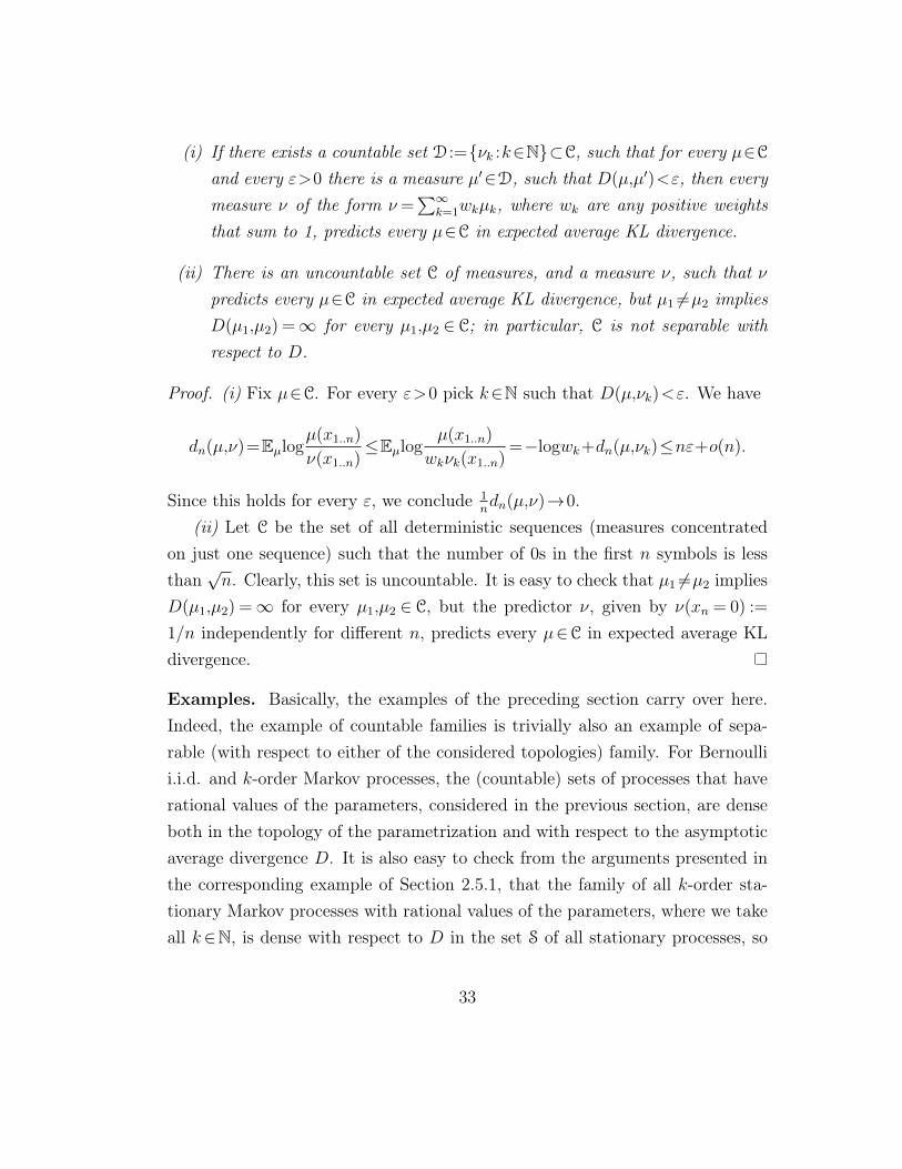
(i) If there exists a countable set D :=νk :k∈N⊂C, such that for every µ∈Cand every ε>0 there is a measure µ′∈D, such that D(µ,µ′)<ε, then everymeasure ν of the form ν =
∑∞k=1wkµk, where wk are any positive weights
that sum to 1, predicts every µ∈C in expected average KL divergence.
(ii) There is an uncountable set C of measures, and a measure ν, such that νpredicts every µ∈C in expected average KL divergence, but µ1 6=µ2 impliesD(µ1,µ2) =∞ for every µ1,µ2 ∈ C; in particular, C is not separable withrespect to D.
Proof. (i) Fix µ∈C. For every ε>0 pick k∈N such that D(µ,νk)<ε. We have
dn(µ,ν)=Eµlogµ(x1..n)
ν(x1..n)≤Eµlog
µ(x1..n)
wkνk(x1..n)=−logwk+dn(µ,νk)≤nε+o(n).
Since this holds for every ε, we conclude 1ndn(µ,ν)→0.
(ii) Let C be the set of all deterministic sequences (measures concentratedon just one sequence) such that the number of 0s in the first n symbols is lessthan
√n. Clearly, this set is uncountable. It is easy to check that µ1 6=µ2 implies
D(µ1,µ2) =∞ for every µ1,µ2 ∈ C, but the predictor ν, given by ν(xn = 0) :=
1/n independently for different n, predicts every µ∈C in expected average KLdivergence.
Examples. Basically, the examples of the preceding section carry over here.Indeed, the example of countable families is trivially also an example of sepa-rable (with respect to either of the considered topologies) family. For Bernoullii.i.d. and k-order Markov processes, the (countable) sets of processes that haverational values of the parameters, considered in the previous section, are denseboth in the topology of the parametrization and with respect to the asymptoticaverage divergence D. It is also easy to check from the arguments presented inthe corresponding example of Section 2.5.1, that the family of all k-order sta-tionary Markov processes with rational values of the parameters, where we takeall k∈N, is dense with respect to D in the set S of all stationary processes, so
33
that S is separable with respect to D. Thus, the sufficient but not necessarycondition of separability is satisfied in this case. On the other hand, neither ofthese latter families is separable with respect to the topology of total variationdistance.
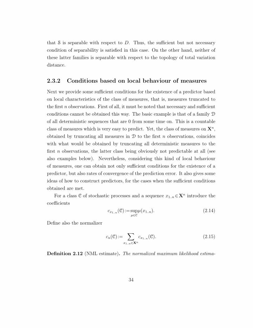
2.3.2 Conditions based on local behaviour of measures
Next we provide some sufficient conditions for the existence of a predictor basedon local characteristics of the class of measures, that is, measures truncated tothe first n observations. First of all, it must be noted that necessary and sufficientconditions cannot be obtained this way. The basic example is that of a family D
of all deterministic sequences that are 0 from some time on. This is a countableclass of measures which is very easy to predict. Yet, the class of measures on Xn,obtained by truncating all measures in D to the first n observations, coincideswith what would be obtained by truncating all deterministic measures to thefirst n observations, the latter class being obviously not predictable at all (seealso examples below). Nevertheless, considering this kind of local behaviourof measures, one can obtain not only sufficient conditions for the existence of apredictor, but also rates of convergence of the prediction error. It also gives someideas of how to construct predictors, for the cases when the sufficient conditionsobtained are met.
For a class C of stochastic processes and a sequence x1..n∈Xn introduce thecoefficients
cx1..n(C) :=supµ∈C
µ(x1..n). (2.14)
Define also the normalizer
cn(C) :=∑
x1..n∈Xn
cx1..n(C). (2.15)
Definition 2.12 (NML estimate). The normalized maximum likelihood estima-
34
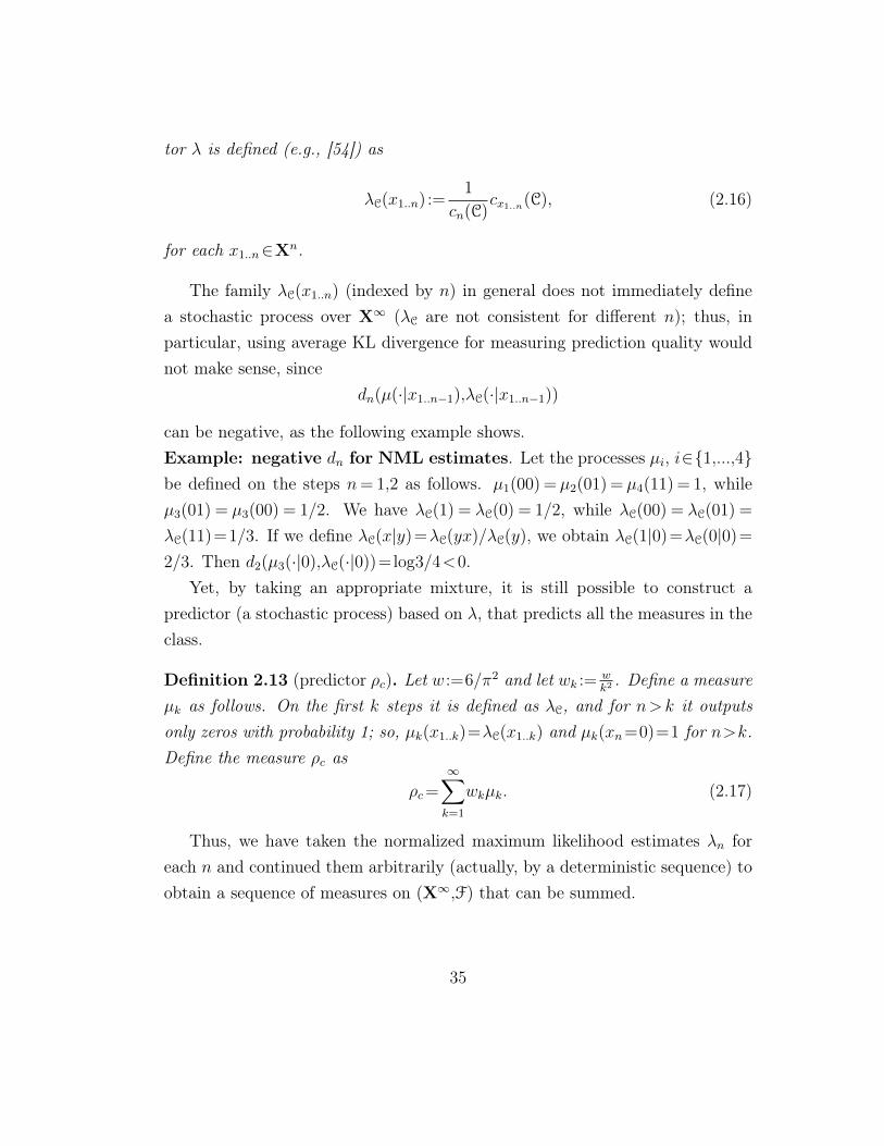
tor λ is defined (e.g., [54]) as
λC(x1..n) :=1
cn(C)cx1..n(C), (2.16)
for each x1..n∈Xn.
The family λC(x1..n) (indexed by n) in general does not immediately definea stochastic process over X∞ (λC are not consistent for different n); thus, inparticular, using average KL divergence for measuring prediction quality wouldnot make sense, since
dn(µ(·|x1..n−1),λC(·|x1..n−1))
can be negative, as the following example shows.Example: negative dn for NML estimates. Let the processes µi, i∈1,...,4be defined on the steps n= 1,2 as follows. µ1(00) = µ2(01) = µ4(11) = 1, whileµ3(01) = µ3(00) = 1/2. We have λC(1) = λC(0) = 1/2, while λC(00) = λC(01) =
λC(11)=1/3. If we define λC(x|y)=λC(yx)/λC(y), we obtain λC(1|0)=λC(0|0)=
2/3. Then d2(µ3(·|0),λC(·|0))=log3/4<0.Yet, by taking an appropriate mixture, it is still possible to construct a
predictor (a stochastic process) based on λ, that predicts all the measures in theclass.
Definition 2.13 (predictor ρc). Let w :=6/π2 and let wk := wk2. Define a measure
µk as follows. On the first k steps it is defined as λC, and for n>k it outputsonly zeros with probability 1; so, µk(x1..k)=λC(x1..k) and µk(xn=0)=1 for n>k.Define the measure ρc as
ρc=∞∑k=1
wkµk. (2.17)
Thus, we have taken the normalized maximum likelihood estimates λn foreach n and continued them arbitrarily (actually, by a deterministic sequence) toobtain a sequence of measures on (X∞,F) that can be summed.
35
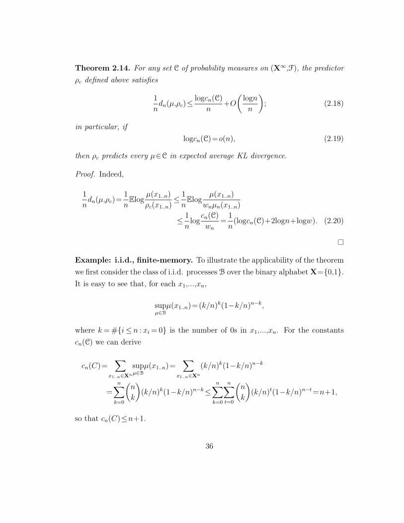
Theorem 2.14. For any set C of probability measures on (X∞,F), the predictorρc defined above satisfies
1
ndn(µ,ρc)≤
logcn(C)
n+O
(logn
n
); (2.18)
in particular, iflogcn(C)=o(n), (2.19)
then ρc predicts every µ∈C in expected average KL divergence.
Proof. Indeed,
1
ndn(µ,ρc)=
1
nElog
µ(x1..n)
ρc(x1..n)≤ 1
nElog
µ(x1..n)
wnµn(x1..n)
≤ 1
nlog
cn(C)
wn=
1
n(logcn(C)+2logn+logw). (2.20)
Example: i.i.d., finite-memory. To illustrate the applicability of the theoremwe first consider the class of i.i.d. processes B over the binary alphabetX=0,1.It is easy to see that, for each x1,...,xn,
supµ∈B
µ(x1..n)=(k/n)k(1−k/n)n−k,
where k= #i≤ n : xi = 0 is the number of 0s in x1,...,xn. For the constantscn(C) we can derive
cn(C)=∑
x1..n∈Xn
supµ∈B
µ(x1..n)=∑
x1..n∈Xn
(k/n)k(1−k/n)n−k
=n∑k=0
(n
k
)(k/n)k(1−k/n)n−k≤
n∑k=0
n∑t=0
(n
k
)(k/n)t(1−k/n)n−t=n+1,
so that cn(C)≤n+1.
36
In general, for the class Mk of processes with memory k over a finitespace X we can get polynomial coefficients cn(Mk) (see, for example, [54] andalso Section 2.4). Thus, with respect to finite-memory processes, the conditionsof Theorem 2.14 leave ample space for the growth of cn(C), since (2.19) allowssubexponential growth of cn(C). Moreover, these conditions are tight, as thefollowing example shows.Example: exponential coefficients are not sufficient. Observe that thecondition (2.19) cannot be relaxed further, in the sense that exponential coeffi-cients cn are not sufficient for prediction. Indeed, for the class of all deterministicprocesses (that is, each process from the class produces some fixed sequence ofobservations with probability 1) we have cn=2n, while obviously for this class apredictor does not exist.Example: stationary processes. For the set of all stationary processes wecan obtain cn(C)≥2n/n (as is easy to see by considering periodic n-order Markovprocesses, for each n∈N), so that the conditions of Theorem 2.14 are not satisfied.This cannot be fixed, since uniform rates of convergence cannot be obtained forthis family of processes, as was shown in [78].
Optimal rates of convergence. A natural question that arises with respectto the bound (2.18) is whether it can be matched by a lower bound. This ques-tion is closely related to the optimality of the normalized maximum likelihoodestimates used in the construction of the predictor. In general, since NML esti-mates are not optimal, neither are the rates of convergence in (2.18). To obtain(close to) optimal rates one has to consider a different measure of capacity.
To do so, we make the following connection to a problem in informationtheory. Let P(X∞) be the set of all stochastic processes (probability measures)on the space (X∞,F), and let P(X) be the set of probability distributions overa (finite) set X. For a class C of measures we are interested in a predictor thathas a small (or minimal) worst-case (with respect to the class C) probability oferror. Thus, we are interested in the quantity
infρ∈P(X∞)
supµ∈C
D(µ,ρ), (2.21)
37
where the infimum is taken over all stochastic processes ρ, and D is the asymp-totic expected average KL divergence (2.13). (In particular, we are interested inthe conditions under which the quantity (2.21) equals zero.) This problem hasbeen studied for the case when the probability measures are over a finite set X,and D is replaced simply by the KL divergence d between the measures. Thus,the problem was to find the probability measure ρ (if it exists) on which thefollowing minimax is attained
R(A) := infρ∈P(X)
supµ∈A
d(µ,ρ), (2.22)
where A⊂P(X). This problem is closely related to the problem of finding thebest code for the class of sources A, which was its original motivation. Thenormalized maximum likelihood distribution considered above does not in gen-eral lead to the optimum solution for this problem. The optimum solution isobtained through the result that relates the minimax (2.22) to the so-calledchannel capacity.
Definition 2.15 (Channel capacity). For a set A of measures on a finite set Xthe channel capacity of A is defined as
C(A) := supP∈P0(A)
∑µ∈S(P )
P (µ)d(µ,ρP ), (2.23)
where P0(A) is the set of all probability distributions on A that have a finitesupport, S(P ) is the (finite) support of a distribution P ∈ P0(A), and ρP =∑
µ∈S(P )P (µ)µ.
It is shown in [75, 33] that C(A)=R(A), thus reducing the problem of findinga minimax to an optimization problem. For probability measures over infinitespaces this result (R(A)=C(A)) was generalized by [39], but the divergence be-tween probability distributions is measured by KL divergence (and not asymp-totic average KL divergence), which gives infinite R(A) e.g. already for the classof i.i.d. processes.
38
However, truncating measures in a class C to the first n observations, we canuse the results about channel capacity to analyse the predictive properties of theclass. Moreover, the rates of convergence that can be obtained along these linesare close to optimal. In order to pass from measures minimizing the divergencefor each individual n to a process that minimizes the divergence for all n we usethe same idea as when constructing the process ρc.
Theorem 2.16. Let C be a set of measures on (X∞,F), and let Cn be the classof measures from C restricted to Xn. There exists a measure ρC such that
1
ndn(µ,ρC)≤ C(Cn)
n+O
(logn
n
); (2.24)
in particular, if C(Cn)/n→ 0, then ρC predicts every µ∈C in expected averageKL divergence. Moreover, for any measure ρC and every ε>0 there exists µ∈Csuch that
1
ndn(µ,ρC)≥ C(Cn)
n−ε.
Proof. As shown in [33], for each n there exists a sequence νnk , k∈N of measureson Xn such that
limk→∞
supµ∈Cn
dn(µ,νnk )→C(Cn).
For each n∈N find an index kn such that
| supµ∈Cn
dn(µ,νnkn)−C(Cn)|≤1.
Define the measure ρn as follows. On the first n symbols it coincides with νnkn andρn(xm = 0) = 1 for m>n. Finally, set ρC =
∑∞n=1wnρn, where wk = w
n2 ,w= 6/π2.We have to show that limn→∞
1ndn(µ,ρC) = 0 for every µ∈C. Indeed, similarly
39
to (2.20), we have
1
ndn(µ,ρC)=
1
nEµlog
µ(x1..n)
ρC(x1..n)
≤ logw−1k
n+
1
nEµlog
µ(x1..n)
ρn(x1..n)≤ logw+2logn
n+
1
ndn(µ,ρn)
≤o(1)+C(Cn)
n. (2.25)
The second statement follows from the fact [75, 33] that C(Cn) = R(Cn)
(cf. (2.22)).
Thus, if the channel capacity C(Cn) grows sublinearly, a predictor can beconstructed for the class of processes C. In this case the problem of constructingthe predictor is reduced to finding the channel capacities for different n andfinding the corresponding measures on which they are attained or approached.Examples. For the class of all Bernoulli i.i.d. processes, the channel capacityC(Bn) is known to be O(logn) [54]. For the family of all stationary processes itis O(n), so that the conditions of Theorem 2.16 are satisfied for the former butnot for the latter.
We also remark that the requirement of a sublinear channel capacity cannotbe relaxed, in the sense that a linear channel capacity is not sufficient for pre-diction, since it is the maximal possible capacity for a set of measures on Xn,achieved, for example, on the set of all measures, or on the set of all deterministicsequences.
2.4 Conditions under which one measure is a pre-
dictor for another [R8]
In this section we address the following question: what are the conditions underwhich a measure ρ is a good predictor for a measure µ? As it was mentioned, forprediction in total variation distance, this relationship is described by the relation
40
of absolute continuity (see Theorem 2.2). Here we will attempt to establishsimilar conditions for other measures of predictive quality, including, but notlimited to, expected average KL divergence.
We start with the following observation. For a Bayesian mixture ξ of acountable class of measures νi, i∈N, we have ξ(A)≥wiνi(A) for any i and anymeasurable set A, where wi is a constant. This condition is stronger than theassumption of absolute continuity and is sufficient for prediction in a very strongsense. Since we are willing to be satisfied with prediction in a weaker sense (e.g.convergence of conditional probabilities), let us make a weaker assumption: Saythat a measure ρ dominates a measure µ with coefficients cn>0 if
ρ(x1,...,xn) ≥ cnµ(x1,...,xn) (2.26)
for all x1,...,xn.The first question we consider in this section is, under what conditions on
cn does (2.26) imply that ρ predicts µ? Observe that if ρ(x1,...,xn)> 0 for anyx1,...,xn then any measure µ is locally absolutely continuous with respect to ρ(that is, the measure µ restricted to the first n trials µ|Xn is absolutely contin-uous w.r.t. ρ|Xn for each n), and moreover, for any measure µ some constantscn can be found that satisfy (2.26). For example, if ρ is Bernoulli i.i.d. measurewith parameter 1
2and µ is any other measure, then (2.26) is (trivially) satis-
fied with cn = 2−n. Thus we know that if cn ≡ c then ρ predicts µ in a verystrong sense, whereas exponentially decreasing cn are not enough for prediction.Perhaps somewhat surprisingly, we will show that dominance with any subex-ponentially decreasing coefficients is sufficient for prediction in expected averageKL divergence. Dominance with any polynomially decreasing coefficients, andalso with coefficients decreasing (for example) as cn = exp(−
√n/logn), is suffi-
cient for (almost sure) prediction on average (i.e. in Cesaro sense). However, forprediction on every step we have a negative result: for any dominance coefficientsthat go to zero there exists a pair of measures ρ and µ which satisfy (2.26) but ρdoes not predict µ in the sense of almost sure convergence of probabilities. Thus
41
the situation is similar to that for predicting any stationary measure: predictionis possible in the average but not on every step.
Note also that for Laplace’s measure ρL it can be shown that ρL dominatesany i.i.d. measure µ with linearly decreasing coefficients cn = 1
n+1; a generaliza-
tion of ρL for predicting all measures with memory k (for a given k) dominatesthem with polynomially decreasing coefficients. Thus dominance with decreas-ing coefficients generalizes (in a sense) predicting countable classes of measures(where we have dominance with a constant), absolute continuity (via local ab-solute continuity), and predicting i.i.d. and finite-memory measures.
Another way to look for generalizations is as follows. The Bayes mixture ξ,being a sum of countably many measures (predictors), possesses some of theirpredicting properties. In general, which predictive properties are preserved undersummation? In particular, if we have two predictors ρ1 and ρ2 for two classesof measures, we are interested in the question whether 1
2(ρ1+ρ2) is a predictor
for the union of the two classes. An answer to this question would improve ourunderstanding of how far a class of measures for which a predicting measureexists can be extended without losing this property.
Thus, the second question we consider in this section is the following: supposethat a measure ρ predicts µ (in some weak sense), and let χ be some otherprobability measure (e.g. a predictor for a different class of measures). Does themeasure ρ′= 1
2(ρ+χ) still predict µ? That is, we ask to which prediction quality
criteria does the idea of taking a Bayesian sum generalize. Absolute continuityis preserved under summation along with its (strong) prediction ability. It wasmentioned in [80] that prediction in the (weak) sense of convergence of expectedaverages of conditional probabilities is preserved under summation. Here we findthat several stronger notions of prediction are not preserved under summation.
Thus we address the following two questions. Is dominance with decreasingcoefficients sufficient for prediction in some sense, under some conditions on thecoefficients (Section 2.4.2)? And, if a measure ρ predicts a measure µ in somesense, does the measure 1
2(ρ+χ) also predict µ in the same sense, where χ is an
arbitrary measure (Section 2.4.3)? Considering different criteria of prediction
42
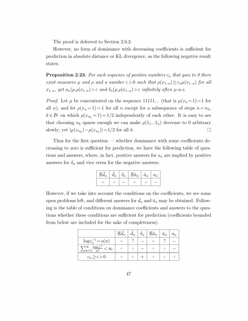
(a.s. convergence of conditional probabilities, a.s. convergence of averages, etc.)in the above two questions we obtain not two but many different questions, forsome of which we find positive answers and for some negative, yet some are leftopen.
The rest of this section is organized as follows. Section 2.4.1 introducesthe measures of divergence of probability measures that we will consider. Sec-tion 2.4.2 addresses the question of whether dominance with decreasing coeffi-cients is sufficient for prediction, while in Section 2.4.3 we consider the problemof summing a predictor with an arbitrary measure.
2.4.1 Measuring performance of prediction
In addition to the measures of performance of prediction used in the previoussections (expected average KL divergence and total variation), here we introduceseveral more.
For two measures µ and ρ define the following measures of divergence.
(δ) Kullback-Leibler (KL) divergence
δn(µ,ρ|x<n)=∑x∈X
µ(xn=x|x<n)logµ(xn=x|x<n)
ρ(xn=x|x<n),
(d) average KL divergence dn(µ,ρ|x1..n)=1
ndn(µ,ρ)=
1
n
n∑t=1
δt(µ,ρ|x<t),
(a) absolute distance an(µ,ρ|x<n)=∑x∈X
|µ(xn=x|x<n)−ρ(xn=x|x<n)|,
(a) average absolute distance an(µ,ρ|x1..n)=1
n
n∑t=1
at(µ,ρ|x<t).
Definition 2.17. We say that ρ predicts µ
(d) in (non-averaged) KL divergence if δn(µ,ρ|x<n)→0 µ-a.s. as t→∞,
(d) in (time-average) average KL divergence if dn(µ,ρ|x1..n)→0 µ-a.s.,
43
(Ed) in expected average KL divergence if Eµdn(µ,ρ|x1..n)→0,
(a) in absolute distance if an(µ,ρ|x<n)→0 µ-a.s.,
(a) in average absolute distance if an(µ,ρ|x1..n)→0 µ-a.s.,
(Ea) in expected average absolute distance if Eµan(µ,ρ|x1..n)→0.
The argument x1..n will be often left implicit in our notation. Recall (defini-tion 2.1) measure ρ converges to a measure µ in total variation (tv) if supA⊂σ(
⋃∞t=nX
t)|µ(A|x<n)−ρ(A|x<n)|→0 µ-almost surely. The following implications hold (and are completeand strict):
δ ⇒ d Ed⇓ ⇓ ⇓
tv ⇒ a ⇒ a ⇒ Ea(2.27)
to be understood as e.g.: if dn→0 a.s. then an→0 a.s, or, if Edn→0 then Ean→0.The horizontal implications ⇒ follow immediately from the definitions, and the⇓ follow from the following Lemma:
Lemma 2.18. For all measures ρ and µ and sequences x1..∞ we have: a2t ≤2δt
and a2n≤2dn and (Ean)2≤2Edn.
Proof. Pinsker’s inequality [41, Lem.3.11a] implies a2t ≤ 2δt. Using this and
Jensen’s inequality for the average 1n
∑nt=1[...] we get
2dn =1
n
n∑t=1
2δt ≥1
n
n∑t=1
a2t ≥
(1
n
n∑t=1
at
)2
= a2n (2.28)
Using this and Jensen’s inequality for the expectation E we get 2Edn≥Ea2n≥
(Ean)2.
2.4.2 Dominance with decreasing coefficients
First we consider the question whether property (2.26) is sufficient for prediction.
44
Definition 2.19. We say that a measure ρ dominates a measure µ with coeffi-cients cn>0 iff
ρ(x1..n) ≥ cnµ(x1..n). (2.29)
for all x1..n.
Suppose that ρ dominates µ with decreasing coefficients cn. Does ρ predictµ in (expected, expected average) KL divergence (absolute distance)? First letus give an example.
Proposition 2.20. Let ρL be the Laplace measure, given by ρL(xn+1 =a|x1..n)=k+1n+|X| for any a∈X and any x1..n∈Xn, where k is the number of occurrences ofa in x1..n (this is also well defined for n=0). Then
ρL(x1..n) ≥ n!
(n+|X|−1)!µ(x1..n) (2.30)
for any measure µ which generates independently and identically distributed sym-bols. The equality is attained for some choices of µ.
Proof. We will only give the proof for X=0,1, the general case is analogous.To calculate ρL(x1..n) observe that it only depends on the number of 0s and 1sin x1..n and not on their order. Thus we compute ρL(x1..n) = k!(n−k)!
(n+1)!where k is
the number of 1s. For any measure µ such that µ(xn = 1) =p for some p∈ [0,1]
independently for all n, and for Laplace measure ρL we have
µ(x1..n)
ρL(x1..n)=
(n+ 1)!
k!(n− k)!pk(1− p)n−k = (n+ 1)
(n
k
)pk(1− p)n−k
≤ (n+ 1)n∑k=0
(n
k
)pk(1− p)n−k = n+ 1,
for any n-letter word x1,...,xn where k is the number of 1s in it. The equalityin the bound is attained when p= 1, so that k=n, µ(x1..n) = 1, and ρL(x1..n) =
1n+1
.
Thus for Laplace’s measure ρL and binaryX we have cn=O( 1n). As mentioned
45
in the introduction, in general, exponentially decreasing coefficients cn are notsufficient for prediction, since (2.26) is satisfied with ρ being a Bernoulli i.i.d.measure and µ any other measure. On the other hand, the following propositionshows that in a weak sense of convergence in expected average KL divergence(or absolute distance) the property (2.26) with subexponentially decreasing cnis sufficient. We also remind that if cn are bounded from below then predictionin the strong sense of total variation is possible.
Theorem 2.21. Let µ and ρ be two measures on X∞ and suppose that ρ(x1..n)≥cnµ(x1..n) for any x1..n, where cn are positive constants satisfying 1
nlogc−1
n →0. Then ρ predicts µ in expected average KL divergence Eµdn(µ,ρ)→ 0 and inexpected average absolute distance Eµan(µ,ρ)→0.
Proof. For convergence in average expected KL divergence, using (2.2) we derive
Eµdn(µ,ρ)=1
nElog
µ(x1..n)
ρ(x1..n)≤ 1
nlogc−1
n →0.
The statement for expected average distance follows from this andLemma 2.18.
With a stronger condition on cn prediction in average KL divergence can beestablished.
Theorem 2.22. Let µ and ρ be two measures on X∞ and suppose that ρ(x1..n)≥cnµ(x1..n) for every x1..n, where cn are positive constants satisfying
∞∑n=1
(log c−1n )2
n2< ∞. (2.31)
Then ρ predicts µ in average KL divergence dn(µ,ρ)→ 0 µ-a.s. and in averageabsolute distance an(µ,ρ)→0 µ-a.s.
In particular, the condition (2.31) on the coefficients is satisfied for polyno-mially decreasing coefficients, or for cn=exp(−
√n/logn).
46
The proof is deferred to Section 2.6.2.However, no form of dominance with decreasing coefficients is sufficient for
prediction in absolute distance or KL divergence, as the following negative resultstates.
Proposition 2.23. For each sequence of positive numbers cn that goes to 0 thereexist measures µ and ρ and a number ε>0 such that ρ(x1..n)≥cnµ(x1..n) for allx1..n, yet an(µ,ρ|x1..n)>ε and δn(µ,ρ|x1..n)>ε infinitely often µ-a.s.
Proof. Let µ be concentrated on the sequence 11111... (that is µ(xn=1)=1 forall n), and let ρ(xn = 1) = 1 for all n except for a subsequence of steps n=nk,k∈ IN on which ρ(xnk = 1) = 1/2 independently of each other. It is easy to seethat choosing nk sparse enough we can make ρ(11...1n) decrease to 0 arbitraryslowly; yet |µ(xnk)−ρ(xnk)|=1/2 for all k.
Thus for the first question — whether dominance with some coefficients de-creasing to zero is sufficient for prediction, we have the following table of ques-tions and answers, where, in fact, positive answers for an are implied by positiveanswers for δn and vice versa for the negative answers:
Edn dn δn Ean an an
+ + − + + −
However, if we take into account the conditions on the coefficients, we see someopen problems left, and different answers for dn and an may be obtained. Follow-ing is the table of conditions on dominance coefficients and answers to the ques-tions whether these conditions are sufficient for prediction (coefficients boundedfrom below are included for the sake of completeness).
Edn dn δn Ean an an
logc−1n =o(n) + ? − + ? −∑∞
n=1logc−1
n
n2 <∞ + + − + + −cn≥c>0 + + + + + +
47
We know from Proposition 2.23 that the condition cn≥c>0 for convergence in δncan not be improved; thus the open problem left is to find whether log c−1
n =o(n)
is sufficient for prediction in dn or at least in an.Another open problem is to find out whether any conditions on dominance
coefficients are necessary for prediction; so far we only have some sufficient con-ditions. On the one hand, the obtained results suggest that some form of dom-inance with decreasing coefficients may be necessary for prediction, at least inthe sense of convergence of averages. On the other hand, the condition (2.26)is uniform over all sequences which probably is not necessary for prediction. Asfor prediction in the sense of almost sure convergence, perhaps more subtle be-havior of the ratio µ(x1..n)
ρ(x1..n)should be analyzed, since dominance with decreasing
coefficients is not sufficient for prediction in this sense.
2.4.3 Preservation of the predictive ability under summa-
tion with an arbitrary measure
Now we turn to the question whether, given a measure ρ that predicts a measureµ in some sense, the “contaminated” measure (1−ε)ρ+εχ for some 0<ε<1 alsopredicts µ in the same sense, where χ is an arbitrary probability measure. Sincemost considerations are independent of the choice of ε, in particular the resultsin this section, we set ε= 1
2for simplicity. We define
Definition 2.24. By “ρ contaminated with χ” we mean ρ′ := 12(ρ+χ), where ρ
and χ are probability measures.
Positive results can be obtained for convergence in expected average KLdivergence. The statement of the next proposition in a different form was men-tioned in [80, 42]. Since the proof is simple we present it here for the sake ofcompleteness; it is based on the same ideas as the proof of Theorem 2.21.
Proposition 2.25. Let µ and ρ be two measures on X∞ and suppose that ρpredicts µ in expected average KL divergence. Then so does the measure ρ′ =12(ρ+χ) where χ is any other measure on X∞.
48
Proof.
0 ≤ Edn(µ, ρ′) =1
nE
n∑t=1
∑xt∈X
µ(xt|x<t) logµ(xt|x<t)ρ′(xt|x<t)
=1
nE log
µ(x1..n)
ρ′(x1..n)
=1
nE log
µ(x1..n)
ρ(x1..n)
ρ(x1..n)
ρ′(x1..n)= Edn(µ, ρ) +
1
nE log
ρ(x1..n)
ρ′(x1..n),
where the first term tends to 0 by assumption and the second term is boundedfrom above by 1
nlog2→0. Since the sum is bounded from below by 0 we obtain
the statement of the proposition.
Next we consider some negative results. An example of measures µ, ρ and χsuch that ρ predicts µ in absolute distance (or KL divergence) but 1
2(ρ+χ) does
not, can be constructed similarly to the example from [45] (of a measure ρ whichis a sum of distributions arbitrarily close to µ yet does not predict it). The ideais to take a measure χ that predicts µ much better than ρ on almost all steps,but on some steps gives grossly wrong probabilities.
Proposition 2.26. There exist measures µ, ρ and χ such that ρ predicts µ inabsolute distance (KL divergence) but 1
2(ρ+χ) does not predict µ in absolute
distance (KL divergence).
Proof. Let µ be concentrated on the sequence 11111... (that is µ(xn = 1) = 1
for any n), and let ρ(xn = 1) = nn+1
with probabilities independent on differenttrials. Clearly, ρ predicts µ in both absolute distance and KL divergence. Letχ(xn = 1) = 1 for all n except on the sequence n= nk = 22k = n2
k−1, k ∈ IN onwhich χ(xnk = 1) = nk−1/nk = 2−2k−1 . This implies that χ(11..nk) = 2/nk andχ(11..nk−1) = χ(11..nk−1
) = 2/nk−1 = 2/√nk. It is now easy to see that 1
2(ρ+χ)
does not predict µ, neither in absolute distance nor in KL divergence. Indeedfor n=nk for some k we have
12(ρ+χ)(xn = 1|1<n) =
ρ(11..n) + χ(11..n)
ρ(1<n) + χ(1<n)≤ 1/(n+1) + 2/n
1/n + 2/√n→ 0.
49
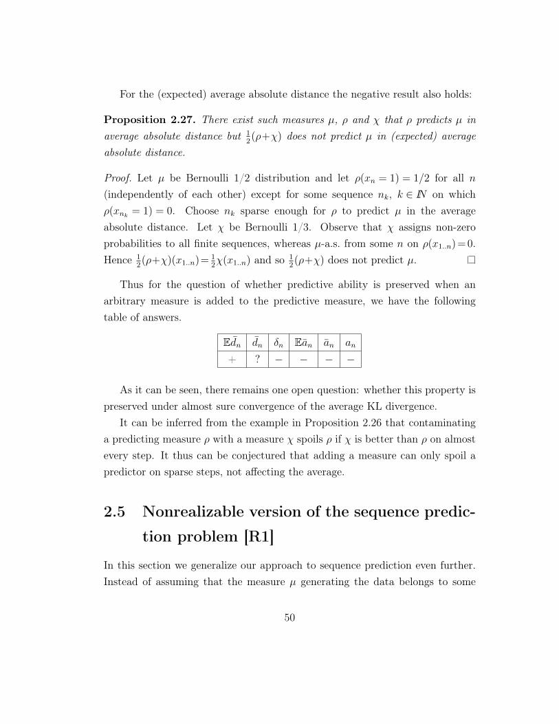
For the (expected) average absolute distance the negative result also holds:
Proposition 2.27. There exist such measures µ, ρ and χ that ρ predicts µ inaverage absolute distance but 1
2(ρ+χ) does not predict µ in (expected) average
absolute distance.
Proof. Let µ be Bernoulli 1/2 distribution and let ρ(xn = 1) = 1/2 for all n(independently of each other) except for some sequence nk, k ∈ IN on whichρ(xnk = 1) = 0. Choose nk sparse enough for ρ to predict µ in the averageabsolute distance. Let χ be Bernoulli 1/3. Observe that χ assigns non-zeroprobabilities to all finite sequences, whereas µ-a.s. from some n on ρ(x1..n) = 0.Hence 1
2(ρ+χ)(x1..n)= 1
2χ(x1..n) and so 1
2(ρ+χ) does not predict µ.
Thus for the question of whether predictive ability is preserved when anarbitrary measure is added to the predictive measure, we have the followingtable of answers.
Edn dn δn Ean an an
+ ? − − − −
As it can be seen, there remains one open question: whether this property ispreserved under almost sure convergence of the average KL divergence.
It can be inferred from the example in Proposition 2.26 that contaminatinga predicting measure ρ with a measure χ spoils ρ if χ is better than ρ on almostevery step. It thus can be conjectured that adding a measure can only spoil apredictor on sparse steps, not affecting the average.
2.5 Nonrealizable version of the sequence predic-
tion problem [R1]
In this section we generalize our approach to sequence prediction even further.Instead of assuming that the measure µ generating the data belongs to some
50
set C of measures, we would like to assume that the measure µ is completelyarbitrary. As we know, in this case we cannot hope to get the error convergeto zero. However, we can try to make the error as small as the error of anypredictor from a given set C.
Recall that a predictor ρ is required to give conditional probabilities ρ(xn+1 =
a|x1,...,xn) for all possible histories x1,...,xn. Therefore, it defines itself a prob-ability measure on the space Ω of one-way infinite sequences. In other words, aprobability measure on Ω can be considered both as a data-generating mecha-nism and as a predictor.
Thus, given a set C of probability measures on Ω, one can ask two kinds ofquestions about C. First, does there exist a predictor ρ, whose forecast prob-abilities converge (in a certain sense) to the µ-conditional probabilities, if anarbitrary µ∈C is chosen to generate the data? Here we assume that the “true”measure that generates the data belongs to the set C of interest, and would liketo construct a predictor that predicts all measures in C. The second type of ques-tions is as follows: does there exist a predictor that predicts at least as well asany predictor ρ∈C, if the measure that generates the data comes possibly fromoutside of C? Thus, here we consider elements of C as predictors, and we wouldlike to combine their predictive properties, if this is possible. Note that in thissetting the two questions above concern the same object: a set C of probabilitymeasures on Ω.
Each of these two questions, the realizable and the non-realizable one, haveenjoyed much attention in the literature; the setting for the non-realizable caseis usually slightly different, which is probably why it has not (to the best of theauthor’s knowledge) been studied as another facet of the realizable case. Therealizable case has been considered in detail in the previous sections (Section 2.2–2.4).
The non-realizable case is usually studied in a slightly different, non-probabilistic,setting. We refer to [18] for a comprehensive overview. It is usually assumedthat the observed sequence of outcomes is an arbitrary (deterministic) sequence;it is required not to give conditional probabilities, but just deterministic guesses
51
(although these guesses can be selected using randomisation). Predictions resultin a certain loss, which is required to be small as compared to the loss of agiven set of reference predictors (experts) C. The losses of the experts and thepredictor are observed after each round. In this approach, it is mostly assumedthat the set C is finite or countable. The main difference with the formulationconsidered in this section is that we require a predictor to give probabilities,and thus the loss is with respect to something never observed (probabilities, notoutcomes). The loss itself is not completely observable in our setting. In thissense our non-realizable version of the problem is more difficult. Assuming thatthe data generating mechanism is probabilistic, even if it is completely unknown,makes sense in such problems as, for example, game playing, or market analysis.In these cases one may wish to assign smaller loss to those models or expertswho give probabilities closer to the correct ones (which are never observed), eventhough different probability forecasts can often result in the same action. Aim-ing at predicting probabilities of outcomes also allows us to abstract from theactual use of the predictions (for example, making bets) and thus from consid-ering losses in a general form; instead, we can concentrate on those forms of lossthat are more convenient for the analysis. In this latter respect, the problems weconsider are easier than those considered in prediction with expert advice. (How-ever, in principle, nothing restricts us to considering the simple losses that wechose; they are just a convenient choice.) Noteworthy, the probabilistic approachalso makes the machinery of probability theory applicable, hopefully making theproblem easier. Another way to look at the difference between the non-realizableproblems of this manuscript and prediction with expert advice is as follows: thelatter is prequential (in the sense of [23]), whereas the former is not.
Let us further break the non-realizable case into two problems. The firstone is as follows. Given a set C of predictors, we want to find a predictor whoseprediction error converges to zero if there is at least one predictor in C whose pre-diction error converges to zero; we call this problem simply the “non-realizable”case, or Problem 2 (leaving the name “Problem 1” to the realizable case). Thesecond non-realizable problem is the “fully agnostic” problem: it is to make the
52

prediction error asymptotically as small as that of the best (for the given processmeasure generating the data) predictor in C (we call this Problem 3). Thus, wenow have three problems about a set of process measures C to address.
In this section we show that if the quality of prediction is measured in totalvariation, then all the three problems coincide: any solution to any one of themis a solution to the other two. For the case of expected average KL divergence,all the three problems are different: the realizable case is strictly easier than non-realizable (Problem 2), which is, in turn, strictly easier than the fully agnosticcase (Problem 3). We then analyse which results concerning prediction in totalvariation can be transferred to which of the problems concerning prediction inaverage KL divergence. We will extend the result of Section 2.2 about theexistence of Bayesian predictor from Problem 1 to the (non-realizable) case ofProblem 2, for prediction in expected average KL divergence. We do not havean analogous result for Problem 3 (and, in fact, conjecture that the oppositestatement holds true). However, for the fully agnostic case of Problem 3, weshow that separability with respect to a certain topology given by KL divergenceis a sufficient (though not a necessary) condition for the existence of a predictor.This is used to demonstrate that there is a solution to this problem for the setof all finite-memory process measures, complementing similar results obtainedearlier in different settings. On the other hand, we show that there is no solutionto this problem for the set of all stationary process measures, in contrast to aresult of B. [78] that gives a solution to the realizable case of this problem (thatis, a predictor whose expected average KL error goes to zero if any stationaryprocess is chosen to generate the data). Finally, we also consider a modifiedversion of Problem 3, in which the performance of predictors is only comparedon individual sequences. For this problem, we obtain, using a result from [77],a characterisation of those sets C for which a solution exists in terms of theHausdorff dimension.
53
2.5.1 Sequence prediction problems
For the two notions of predictive quality introduced, we can now state formallythe sequence prediction problems.Problem 1(realizable case). Given a set of probability measures C, find a mea-sure ρ such that ρ predicts in total variation (expected average KL divergence)every µ∈C, if such a ρ exists.
This is the problem considered in Sections 2.2 (restated here to ease thecomparison). Problem 1 is about finding a predictor for the case when theprocess generating the data is known to belong to a given class C. That is, theset C here is a set of measures that generate the data. Next let us formulate thequestions about C as a set of predictors.Problem 2 (non-realizable case). Given a set of process measures (predictors)C, find a process measure ρ such that ρ predicts in total variation (in expectedaverage KL divergence) every measure ν ∈ P such that there is µ ∈ C whichpredicts (in the same sense) ν.
While Problem 2 is already quite general, it does not yet address what canbe called the fully agnostic case: if nothing at all is known about the process νgenerating the data, it means that there may be no µ∈C such that µ predictsν, and then, even if we have a solution ρ to the Problem 2, we still do not knowwhat the performance of ρ is going to be on the data generated by ν, comparedto the performance of the predictors from C. To address this fully agnostic casewe have to introduce the notion of loss.
Definition 2.28. Introduce the almost sure total variation loss of ρ with respectto µ
ltv(µ,ρ) :=infα∈ [0,1] : lim supn→∞
v(µ,ρ,x1..n)≤α µ–a.s.,
and the asymptotic KL loss
lKL(ν,ρ) :=lim supn→∞
1
ndn(ν,ρ).
We can now formulate the fully agnostic version of the sequence prediction
54
problem.Problem 3. Given a set of process measures (predictors) C, find a processmeasure ρ such that ρ predicts at least as well as any µ in C, if any processmeasure ν∈P is chosen to generate the data:
l(ν,ρ)−l(ν,µ)≤0 (2.32)
for every ν∈P and every µ∈C, where l(·,·) is either ltv(·,·) or lKL(·,·).The three problems just formulated represent different conceptual approaches
to the sequence prediction problem. Let us illustrate the difference by the fol-lowing informal example. Suppose that the set C is that of all (ergodic, finite-state) Markov chains. Markov chains being a familiar object in probability andstatistics, we can easily construct a predictor ρ that predicts every µ∈ C (forexample, in expected average KL divergence, see [54]). That is, if we know thatthe process µ generating the data is Markovian, we know that our predictor isgoing to perform well. This is the realizable case of Problem 1. In reality, rarelycan we be sure that the Markov assumption holds true for the data at hand.We may believe, however, that it is still a reasonable assumption, in the sensethat there is a Markovian model which, for our purposes (for the purposes ofprediction), is a good model of the data. Thus we may assume that there is aMarkov model (a predictor) that predicts well the process that we observe, andwe would like to combine the predictive qualities of all these Markov models.This is the “non-realizable” case of Problem 2. Note that this problem is moredifficult than the first one; in particular, a process ν generating the data may besingular with respect to any Markov process, and still be predicted well (in thesense of expected average KL divergence, for example) by some of them. Still,here we are making some assumptions about the process generating the data,and, if these assumptions are wrong, then we do not know anything about theperformance of our predictor. Thus, we may ultimately wish to acknowledgethat we do not know anything at all about the data; we still know a lot aboutMarkov processes, and we would like to use this knowledge on our data. If there
55
is anything at all Markovian in it (that is, anything that can be captured by aMarkov model), then we would like our predictor to use it. In other words, wewant to have a predictor that predicts any process measure whatsoever (at least)as well as any Markov predictor. This is the “fully agnostic” case of Problem 3.
Of course, Markov processes were just mentioned as an example, while inthis section we are only concerned with the most general case of arbitrary (un-countable) sets C of process measures.
The following statement is rather obvious.
Proposition 2.29. Any solution to Problem 3 is a solution to Problem 2, andany solution to Problem 2 is a solution to Problem 1.
Despite the conceptual differences in formulations, it may be somewhat un-clear whether the three problems are indeed different. It appears that this de-pends on the measure of predictive quality chosen: for the case of predictionin total variation distance all the three problems coincide, while for the case ofprediction in expected average KL divergence they are different.
2.5.2 Characterizations of learnable classes for prediction
in total variation
As it was mentioned, a measure µ is absolutely continuous with respect to ameasure ρ if and only if ρ predicts µ in total variation distance. This reducesstudying at least Problem 1 for total variation distance to studying the relationof absolute continuity. Introduce the notation ρ≥tvµ for this relation.
Let us briefly recall some facts we know about ≥tv; details can be found,for example, in [70]. Let [P]tv denote the set of equivalence classes of P withrespect to ≥tv, and for µ∈Ptv denote [µ] the equivalence class that contains µ.Two elements σ1,σ2∈ [P]tv (or σ1,σ2∈P) are called disjoint (or singular) if thereis no ν ∈ [P]tv such that σ1 ≥tv ν and σ2 ≥tv ν; in this case we write σ1 ⊥tv σ2.We write [µ1]+[µ2] for [1
2(µ1 +µ2)]. Every pair σ1,σ2 ∈ [P]tv has a supremum
sup(σ1,σ2)=σ1+σ2. Introducing into [P]tv an extra element 0 such that σ≥tv 0
56
for all σ ∈ [P]tv, we can state that for every ρ,µ ∈ [P]tv there exists a uniquepair of elements µs and µa such that µ=µa+µs, ρ≥µa and ρ⊥tv µs. (This isa form of Lebesgue decomposition.) Moreover, µa = inf(ρ,µ). Thus, every pairof elements has a supremum and an infimum. Moreover, every bounded set ofdisjoint elements of [P]tv is at most countable.
Furthermore, we introduce the (unconditional) total variation distance be-tween process measures.
Definition 2.30 (unconditional total variation distance). The (unconditional)total variation distance is defined as
v(µ,ρ) :=supA∈B|µ(A)−ρ(A)|.
Known characterizations of those sets C that are bounded with respect to≥tv can now be related to our prediction problems 1-3 as follows.
Theorem 2.31. Let C⊂P. The following statements about C are equivalent.
(i) There exists a solution to Problem 1 in total variation.
(ii) There exists a solution to Problem 2 in total variation.
(iii) There exists a solution to Problem 3 in total variation.
(iv) C is upper-bounded with respect to ≥tv.
(v) There exists a sequence µk∈C, k∈N such that for some (equivalently, forevery) sequence of weights wk ∈ (0,1], k ∈ N such that
∑k∈Nwk = 1, the
measure ν=∑
k∈Nwkµk satisfies ν≥tvµ for every µ∈C.
(vi) C is separable with respect to the total variation distance.
(vii) Let C+ :=µ∈P :∃ρ∈C ρ≥tvµ. Every disjoint (with respect to ≥tv) subsetof C+ is at most countable.
57
Moreover, every solution to any of the Problems 1-3 is a solution to the othertwo, as is any upper bound for C. The sequence µk in the statement (v) can betaken to be any dense (in the total variation distance) countable subset of C (cf.(vi)), or any maximal disjoint (with respect to ≥tv) subset of C+ of statement(vii), in which every measure that is not in C is replaced by any measure from C
that dominates it.
Proof. The implications (i)⇐(ii)⇐(iii) are obvious (cf. Proposition 2.29). Theequivalence (iv)⇔ (i) is a reformulation of the result of Theorem 2.2. (i)⇒ (ii)
follows from the equivalence (i)⇔ (iv) and the transitivity of ≥tv; (i)⇒ (iii)
follows from the transitivity of ≥tv and from Lemma 2.32 below: indeed, fromLemma 2.32 we have ltv(ν,µ) = 0 if µ≥tv ν and ltv(ν,µ) = 1 otherwise. Fromthis and the transitivity of ≥tv it follows that if ρ ≥tv µ then also ltv(ν,ρ) ≤ltv(ν,µ) for all ν ∈ P. The equivalence of (v), (vi), and (i) was established inTheorems 2.6 and 2.9. The equivalence of (iv) and (vii) was proven in [70]. Theconcluding statements of the theorem are easy to demonstrate from the resultscited above.
The following lemma is an easy consequence of [11].
Lemma 2.32. Let µ,ρ be two process measures. Then v(µ,ρ,x1..n) converges toeither 0 or 1 with µ-probability 1.
Proof. Assume that µ is not absolutely continuous with respect to ρ (the othercase is covered by [11]). By Lebesgue decomposition theorem, the measure µadmits a representation µ = αµa+(1−α)µs where α ∈ [0,1] and the measuresµa and µs are such that µa is absolutely continuous with respect to ρ and µs
is singular with respect to ρ. Let W be such a set that µa(W ) = ρ(W ) = 1
and µs(W ) = 0. Note that we can take µa = µ|W and µs = µ|X∞\W . From[11] we have v(µa,ρ,x1..n)→ 0 µa-a.s., as well as v(µa,µ,x1..n)→ 0 µa-a.s. andv(µs,µ,x1..n)→0 µs-a.s. Moreover, v(µs,ρ,x1..n)≥|µs(W |x1..n)−ρ(W |x1..n)|=1 sothat v(µs,ρ,x1..n)→1 µs-a.s. Furthermore,
v(µ,ρ,x1..n)≤v(µ,µa,x1..n)+v(µa,ρ,x1..n)=I
58
andv(µ,ρ,x1..n)≥−v(µ,µs,x1..n)+v(µs,ρ,x1..n)=II.
We have I→ 0 µa-a.s. and hence µ|W -a.s., as well as II→ 1 µs-a.s. and henceµ|X∞\W -a.s. Thus,
µ(v(µ,ρ,x1..n)→0 or 1)
≤µ(W )µ|W (I→0)+µ(X∞\W )µ|X∞\W (II→1)=µ(W )+µ(X∞\W )=1,
which concludes the proof.
Remark. Using Lemma 2.32 we can also define expected (rather than almostsure) total variation loss of ρ with respect to µ, as the µ-probability that v(µ,ρ)
converges to 1:
l′tv(µ,ρ) :=µx1,x2,···∈X∞ :v(µ,ρ,x1..n)→1.
Then Problem 3 can be reformulated for this notion of loss. However, it is easyto see that for this reformulation Theorem 2.31 holds true as well.
Thus, we can see that, for the case of prediction in total variation, all thesequence prediction problems formulated reduce to studying the relation of ab-solute continuity for process measures and those families of measures that areabsolutely continuous (have a density) with respect to some measure (a predic-tor).
2.5.3 Characterizations of learnable classes for prediction
in expected average KL divergence
First of all, we have to observe that for prediction in KL divergence Problems 1, 2,and 3 are different, as the following theorem shows. While the examples providedin the proof are artificial, there is a very important example illustrating thedifference between Problem 1 and Problem 3 for expected average KL divergence:
59
the set S of all stationary processes, given in Theorem 2.39 in the end of thissection.
Theorem 2.33. For the case of prediction in expected average KL divergence,Problems 1, 2 and 3 are different: there exists a set C1⊂P for which there isa solution to Problem 1 but there is no solution to Problem 2, and there is aset C2⊂P for which there is a solution to Problem 2 but there is no solution toProblem 3.
Proof. We have to provide two examples. Fix the binary alphabetX=0,1. Foreach deterministic sequence t=t1,t2,···∈X∞ construct the process measure γt asfollows: γt(xn=tn|t1..n−1):=1− 1
n+1and for x1..n−1 6=t1..n−1 let γt(xn=0|x1..n−1)=
1/2, for all n∈N. That is, γt is Bernoulli i.i.d. 1/2 process measure stronglybiased towards a specific deterministic sequence, t. Let also γ(x1..n)=2−n for allx1..n∈Xn, n∈N (the Bernoulli i.i.d. 1/2). For the set C1 :=γt :t∈X∞ we have asolution to Problem 1: indeed, dn(γt,γ)≤1=o(n). However, there is no solutionto Problem 2. Indeed, for each t∈D we have dn(t,γt)= logn=o(n) (that is, forevery deterministic measure there is an element of C1 which predicts it), whileby Lemma 2.5 for every ρ∈P there exists t∈D such that dn(t,ρ)≥n for all n∈N(that is, there is no predictor which predicts every measure that is predicted byat least one element of C1).
The second example is similar. For each deterministic sequence t=t1,t2,···∈Dconstruct the process measure γt as follows: γ′t(xn = tn|t1..n−1) := 2/3 and forx1..n−1 6=t1..n−1 let γ′t(xn=0|x1..n−1)=1/2, for all n∈N. It is easy to see that γ isa solution to Problem 2 for the set C2 :=γ′t :t∈X∞. Indeed, if ν∈P is such thatdn(ν,γ′)=o(n) then we must have ν(t1..n)=o(1). From this and the fact that γand γ′ coincide (up to O(1)) on all other sequences we conclude dn(ν,γ)=o(n).However, there is no solution to Problem 3 for C2. Indeed, for every t∈D wehave dn(t,γ′t) = nlog3/2+o(n). Therefore, if ρ is a solution to Problem 3 thenlim sup 1
ndn(t,ρ)≤ log3/2<1 which contradicts Lemma 2.5.
Thus, prediction in expected average KL divergence turns out to be a morecomplicated matter than prediction in total variation. The next idea is to try and
60
see which of the facts about prediction in total variation can be generalized tosome of the problems concerning prediction in expected average KL divergence.
First, observe that, for the case of prediction in total variation, the equiva-lence of Problems 1 and 2 was derived from the transitivity of the relation ≥tv ofabsolute continuity. For the case of expected average KL divergence, the relation“ρ predicts µ in expected average KL divergence” is not transitive (and Prob-lems 1 and 2 are not equivalent). However, for Problem 2 we are interested inthe following relation: ρ “dominates” µ if ρ predicts every ν such that µ predictsν. Denote this relation by ≥KL:
Definition 2.34 (≥KL). We write ρ≥KLµ if for every ν∈P the equality lim sup 1ndn(ν,µ)=
0 implies lim sup 1ndn(ν,ρ)=0.
The relation ≥KL has some similarities with ≥tv. First of all, ≥KL is alsotransitive (as can be easily seen from the definition). Moreover, similarly to ≥tv,one can show that for any µ,ρ any strictly convex combination αµ+(1−α)ρ is asupremum of ρ,µ with respect to ≥KL. Next we will obtain a characterizationof predictability with respect to ≥KL similar to one of those obtained for ≥tv.
The key observation is the following. If there is a solution to Problem 2 fora set C then a solution can be obtained as a Bayesian mixture over a countablesubset of C. For total variation this is the statement (v) of Theorem 2.31.
Theorem 2.35. Let C be a set of probability measures on Ω. If there is a measureρ such that ρ≥KLµ for every µ∈C (ρ is a solution to Problem 2) then there is asequence µk∈C, k∈N, such that
∑k∈Nwkµk≥KLµ for every µ∈C, where wk are
some positive weights.
The proof is deferred to Section 2.6.3.For the case of Problem 3, we do not have results similar to Theorem 2.35 (or
statement (v) of Theorem 2.31); in fact, we conjecture that the opposite is true:there exists a (measurable) set C of measures such that there is a solution toProblem 3 for C, but there is no Bayesian solution to Problem 3, meaning thatthere is no probability distribution on C (discrete or not) such that the mixtureover C with respect to this distribution is a solution to Problem 3 for C.
61
However, we can take a different route and extend another part of Theo-rem 2.31 to obtain a characterization of sets C for which a solution to Problem 3exists.
We have seen that, in the case of prediction in total variation, separabilitywith respect to the topology of this distance is a necessary and sufficient con-dition for the existence of a solution to Problems 1-3. In the case of expectedaverage KL divergence the situation is somewhat different, since, first of all,(asymptotic average) KL divergence is not a metric. While one can introduce atopology based on it, separability with respect to this topology turns out to bea sufficient but not a necessary condition for the existence of a predictor, as isshown in the next theorem.
Definition 2.36. Define the distance d∞(µ1,µ2) on process measures as follows
d∞(µ1,µ2)=lim supn→∞
supx1..n∈Xn
1
n
∣∣∣∣logµ1(x1..n)
µ2(x1..n)
∣∣∣∣, (2.33)
where we assume log0/0:=0.
Clearly, d∞ is symmetric and satisfies the triangle inequality, but it is notexact. Moreover, for every µ1,µ2 we have
lim supn→∞
1
ndn(µ1,µ2)≤d∞(µ1,µ2). (2.34)
The distance d∞(µ1,µ2) measures the difference in behaviour of µ1 and µ2 onall individual sequences. Thus, using this distance to analyse Problem 3 is mostclose to the traditional approach to the non-realizable case, which is formulatedin terms of predicting individual deterministic sequences.
Theorem 2.37. (i) Let C be a set of process measures. If C is separable withrespect to d∞ then there is a solution to Problem 3 for C, for the case ofprediction in expected average KL divergence.
(ii) There exists a set of process measures C such that C is not separable with
62
respect to d∞, but there is a solution to Problem 3 for this set, for the caseof prediction in expected average KL divergence.
Proof. For the first statement, let C be separable and let (µk)k∈N be a densecountable subset of C. Define ν :=
∑k∈Nwkµk, where wk are any positive summable
weights. Fix any measure τ and any µ∈C. We will show that lim supn→∞1ndn(τ,ν)≤
lim supn→∞1ndn(τ,µ). For every ε, find such a k∈N that d∞(µ,µk)≤ε. We have
dn(τ,ν)≤dn(τ,wkµk)=Eτ logτ(x1..n)
µk(x1..n)−logwk
=Eτ logτ(x1..n)
µ(x1..n)+Eτ log
µ(x1..n)
µk(x1..n)−logwk
≤dn(τ,µ)+ supx1..n∈Xn
log
∣∣∣∣ µ(x1..n)
µk(x1..n)
∣∣∣∣−logwk.
From this, dividing by n taking lim supn→∞ on both sides, we conclude
lim supn→∞
1
ndn(τ,ν)≤ lim sup
n→∞
1
ndn(τ,µ)+ε.
Since this holds for every ε>0 the first statement is proven.The second statement is proven by the following example. Let C be the set
of all deterministic sequences (measures concentrated on just one sequence) suchthat the number of 0s in the first n symbols is less than
√n, for all n∈N. Clearly,
this set is uncountable. It is easy to check that µ1 6=µ2 implies d∞(µ1,µ2) =∞for every µ1,µ2∈C, but the predictor ν, given by ν(xn=0)=1/n independentlyfor different n, predicts every µ∈C in expected average KL divergence. Since allelements of C are deterministic, ν is also a solution to Problem 3 for C.
Although simple, Theorem 2.37 can be used to establish the existence of asolution to Problem 3 for an important class of process measures: that of allprocesses with finite memory, as the next theorem shows. Results similar toTheorem 2.38 are known in different settings, e.g., [91, 76, 17] and others.
63
Theorem 2.38. There exists a solution to Problem 3 for prediction in expectedaverage KL divergence for the set of all finite-memory process measures M :=
∪k∈NMk.
Proof. We will show that the set M is separable with respect to d∞. Then thestatement will follow from Theorem 2.37. It is enough to show that each set Mk
is separable with respect to d∞.For simplicity, assume that the alphabet is binary (|X|=2; the general case
is analogous). Observe that the family Mk of k-order stationary binary-valuedMarkov processes is parametrized by |X|k [0,1]-valued parameters: probability ofobserving 0 after observing x1..k, for each x1..k∈Xk. Note that this parametriza-tion is continuous (as a mapping from the parameter space with the Euclideantopology to Mk with the topology of d∞). Indeed, for any µ1,µ2∈Mk and everyx1..n∈Xn such that µi(x1..n) 6=0, i=1,2, it is easy to see that
1
n
∣∣∣∣logµ1(x1..n)
µ2(x1..n)
∣∣∣∣≤ supx1..k+1
1
k+1
∣∣∣∣logµ1(x1..k+1)
µ2(x1..k+1)
∣∣∣∣, (2.35)
so that the right-hand side of (2.35) also upper-bounds d∞(µ1,µ2), implyingcontinuity of the parametrization.
It follows that the set µkq , q∈Q|X|k of all stationary k-order Markov processes
with rational values of all the parameters (Q :=Q∩[0,1]) is dense in Mk, provingthe separability of the latter set.
Another important example is the set of all stationary process measures S.This example also illustrates the difference between the prediction problems thatwe consider. For this set a solution to Problem 1 was given in [78]. In contrast,here we show that there is no solution to Problem 3 for S.
Theorem 2.39. There is no solution to Problem 3 for the set of all stationaryprocesses S.
Proof. This proof is based on the construction similar to the one used in [78] todemonstrate impossibility of consistent prediction of stationary processes with-out Cesaro averaging.
64
Let m be a Markov chain with states 0,1,2,... and state transitions definedas follows. From each sate k ∈N∪0 the chain passes to the state k+1 withprobability 2/3 and to the state 0 with probability 1/3. It is easy to see thatthis chain possesses a unique stationary distribution on the set of states (see,e.g., [83]); taken as the initial distribution it defines a stationary ergodic processwith values in N∪0. Fix the ternary alphabet X=a,0,1. For each sequencet=t1,t2,···∈0,1∞ define the process µt as follows. It is a deterministic functionof the chain m. If the chain is in the state 0 then the process µt outputs a; ifthe chain m is in the state k>0 then the process outputs tk. That is, we havedefined a hidden Markov process which in the state 0 of the underlying Markovchain always outputs a, while in other states it outputs either 0 or 1 accordingto the sequence t.
To show that there is no solution to Problem 3 for S, we will show that thereis no solution to Problem 3 for the smaller set C := µt : t∈ 0,1∞. Indeed,for any t∈0,1∞ we have dn(t,µt) =nlog3/2+o(n). Then if ρ is a solution toProblem 3 for C we should have lim supn→∞
1ndn(t,ρ)≤ log3/2<1 for every t∈D,
which contradicts Lemma 2.5.
From the proof of Theorem 2.39 one can see that, in fact, the statementthat is proven is stronger: there is no solution to Problem 3 for the set of allfunctions of stationary ergodic countable-state Markov chains. We conjecturethat a solution to Problem 2 exists for the latter set, but not for the set of allstationary processes.
As we have seen in the statements above, the set of all deterministic mea-sures D plays an important role in the analysis of the predictors in the sense ofProblem 3. Therefore, an interesting question is to characterize those sets C ofmeasures for which there is a predictor ρ that predicts every individual sequenceat least as well as any measure from C. Such a characterization can be obtainedin terms of Hausdorff dimension, using a result of [77], that shows that Haus-dorff dimension of a set characterizes the optimal prediction error that can beattained by any predictor.
65
For a set A⊂X∞ denote H(A) its Hausdorff dimension (see, for example,[10] for its definition).
Theorem 2.40. Let C⊂P. The following statements are equivalent.
(i) There is a measure ρ∈P that predicts every individual sequence at leastas well as the best measure from C: for every µ ∈ C and every sequencex1,x2,···∈X∞ we have
lim infn→∞
− 1
nlogρ(x1..n)≤ lim inf
n→∞− 1
nlogµ(x1..n). (2.36)
(ii) For every α∈[0,1] the Hausdorff dimension of the set of sequences on whichthe average prediction error of the best measure in C is not greater than αis bounded by α/log|X|:
H(x1,x2,···∈X∞ : infµ∈C
lim infn→∞
− 1
nlogµ(x1..n)≤α)≤α/log|X|. (2.37)
Proof. The implication (i)⇒(ii) follows directly from [77] where it is shown thatfor every measure ρ one must have
H(x1,x2,···∈X∞ : lim infn→∞
− 1
nlogρ(x1..n)≤α)≤α/log|X|.
To show the opposite implication, we again refer to [77]: for every set A⊂X∞
there is a measure ρA such that
lim infn→∞
− 1
nlogρA(x1..n)≤H(A)log|X|. (2.38)
For each α∈ [0,1] define Aα := x1,x2,··· ∈X∞ : infµ∈Clim infn→∞− 1nlogµ(x1..n)≤
α). By assumption, H(Aα)≤α/log|X|, so that from (2.38) for all x1,x2,···∈Aαwe obtain
lim infn→∞
− 1
nlogρA(x1..n)≤α. (2.39)
Furthermore, define ρ :=∑
q∈QwqρAq , where Q= [0,1]∩Q is the set of rationals
66
in [0,1] and (wq)q∈Q is any sequence of positive reals satisfying∑
q∈Qwq=1. Forevery α∈ [0,1] let qk∈Q, k∈N be such a sequence that 0≤ qk−α≤1/k. Then,for every n∈N and every x1,x2,···∈Aqk we have
− 1
nlogρ(x1..n)≤− 1
nlogρq(x1..n)− logwqk
n.
From this and (2.39) we get
lim infn→∞
− 1
nlogρ(x1..n)≤ lim inf
n→∞ρqk(x1..n)+1/k≤qk+1/k.
Since this holds for every k∈N, it follows that for all x1,x2,···∈∩k∈NAqk =Aα wehave
lim infn→∞
− 1
nlogρ(x1..n)≤ inf
k∈N(qk+1/k)=α,
which completes the proof of the implication (ii)⇒(i).
2.6 Longer proofs
2.6.1 Proof of Theorem 2.7
The proof is broken into the same steps as the (simpler) proof of Theorem 2.6,to make the analogy explicit and the proof more understandable.
Proof. Define the weights wk :=wk−2, where w is the normalizer 6/π2.Step 1: densities. Define the sets
T nµ :=
x1..n∈Xn :µ(x1..n)≥ 1
nρ(x1..n)
. (2.40)
Using Markov’s inequality, we derive
µ(Xn\T nµ )=µ
(ρ(x1..n)
µ(x1..n)>n
)≤ 1
nEµ
ρ(x1..n)
µ(x1..n)=
1
n, (2.41)
so that µ(T nµ )→1. (Note that if µ is singular with respect to ρ, as is typically
67
the case, then ρ(x1..n)µ(x1..n)
converges to 0 µ-a.e. and one can replace 1nin (2.40) by 1,
while still having µ(T nµ )→1.)Step 2n: a countable cover, time n. Fix an n∈N. Define mn
1 :=maxµ∈Cρ(T nµ )
(sinceXn are finite all suprema are reached). Find any µn1 such that ρn1 (T nµn1 )=mn1
and let T n1 :=T nµn1 . For k>1, let mnk := maxµ∈Cρ(T nµ \T nk−1). If mn
k >0, let µnk beany µ ∈ C such that ρ(T nµnk\T
nk−1) =mn
k , and let T nk := T nk−1∪T nµnk ; otherwise letT nk :=T nk−1. Observe that (for each n) there is only a finite number of positivemnk , since the set Xn is finite; let Kn be the largest index k such that mn
k > 0.Let
νn :=Kn∑k=1
wkµnk . (2.42)
As a result of this construction, for every n∈N every k≤Kn and every x1..n∈T nkusing (2.40) we obtain
νn(x1..n)≥wk1
nρ(x1..n). (2.43)
Step 2: the resulting predictor. Finally, define
ν :=1
2γ+
1
2
∑n∈N
wnνn, (2.44)
where γ is the i.i.d. measure with equal probabilities of all x ∈ X (that is,γ(x1..n) = |X|−n for every n ∈ N and every x1..n ∈Xn). We will show that νpredicts every µ∈C, and then in the end of the proof (Step r) we will show howto replace γ by a combination of a countable set of elements of C (in fact, γ isjust a regularizer which ensures that ν-probability of any word is never too closeto 0).
Step 3: ν predicts every µ ∈ C. Fix any µ ∈ C. Introduce the parame-ters εnµ ∈ (0,1), n ∈ N, to be defined later, and let jnµ := 1/εnµ. Observe thatρ(T nk \T nk−1)≥ρ(T nk+1\T nk ), for any k>1 and any n∈N, by definition of these sets.Since the sets T nk \T nk−1, k∈N are disjoint, we obtain ρ(T nk \T nk−1)≤1/k. Hence,ρ(T nµ \T nj )≤ εnµ for some j ≤ jnµ , since otherwise mn
j = maxµ∈Cρ(T nµ \T njnµ )>εnµ so
68
that ρ(T njnµ+1\T njnµ )>εnµ=1/jnµ , which is a contradiction. Thus,
ρ(T nµ \T njnµ )≤εnµ. (2.45)
We can upper-bound µ(T nµ \T njnµ ) as follows. First, observe that
dn(µ,ρ)=−∑
x1..n∈Tnµ ∩Tnjnµ
µ(x1..n)logρ(x1..n)
µ(x1..n)
−∑
x1..n∈Tnµ \Tnjnµ
µ(x1..n)logρ(x1..n)
µ(x1..n)
−∑
x1..n∈Xn\Tnµ
µ(x1..n)logρ(x1..n)
µ(x1..n)
=I+II+III. (2.46)
Then, from (2.40) we getI≥−logn. (2.47)
Observe that for every n∈N and every set A⊂Xn, using Jensen’s inequality wecan obtain
−∑
x1..n∈A
µ(x1..n)logρ(x1..n)
µ(x1..n)=−µ(A)
∑x1..n∈A
1
µ(A)µ(x1..n)log
ρ(x1..n)
µ(x1..n)
≥−µ(A)logρ(A)
µ(A)≥−µ(A)logρ(A)− 1
2. (2.48)
Thus, from (2.48) and (2.45) we get
II≥−µ(T nµ \T njnµ )logρ(T nµ \T njnµ )−1/2≥−µ(T nµ \T njnµ )logεnµ−1/2. (2.49)
69
Furthermore,
III≥∑
x1..n∈Xn\Tnµ
µ(x1..n)logµ(x1..n)≥µ(Xn\T nµ )logµ(Xn\T nµ )
|Xn\T nµ |
≥−1
2−µ(Xn\T nµ )nlog|X|≥−1
2−log|X|, (2.50)
where in the second inequality we have used the fact that entropy is maximizedwhen all events are equiprobable, in the third one we used |Xn\T nµ |≤|X|n, whilethe last inequality follows from (2.41). Combining (2.46) with the bounds (2.47),(2.49) and (2.50) we obtain
dn(µ,ρ)≥−logn−µ(T nµ \T njnµ )logεnµ−1−log|X|,
so thatµ(T nµ \T njnµ )≤ 1
−logεnµ
(dn(µ,ρ)+logn+1+log|X|
). (2.51)
Since dn(µ,ρ)=o(n), we can define the parameters εnµ in such a way that −logεnµ=
o(n) while at the same time the bound (2.51) gives µ(T nµ \T njnµ )=o(1). Fix sucha choice of εnµ. Then, using µ(T nµ )→1, we can conclude
µ(Xn\T njnµ )≤µ(Xn\T nµ )+µ(T nµ \T njnµ )=o(1). (2.52)
We proceed with the proof of dn(µ,ν)=o(n). For any x1..n∈T njnµ we have
ν(x1..n)≥ 1
2wnνn(x1..n)≥ 1
2wnwjnµ
1
nρ(x1..n)=
wnw
2n(εnµ)2ρ(x1..n), (2.53)
where the first inequality follows from (2.44), the second from (2.43), and in theequality we have used wjnµ =w/(jnµ)2 and jnµ =1/εµn. Next we use the decomposi-
70
tion
dn(µ,ν)=−∑
x1..n∈Tnjnµ
µ(x1..n)logν(x1..n)
µ(x1..n)−
∑x1..n∈Xn\Tn
jnµ
µ(x1..n)logν(x1..n)
µ(x1..n)=I+II.
(2.54)From (2.53) we find
I≤−log(wnw
2n(εnµ)2
)−
∑x1..n∈Tnjnµ
µ(x1..n)logρ(x1..n)
µ(x1..n)
=(1+3logn−2logεnµ−2logw)+
dn(µ,ρ)+∑
x1..n∈Xn\Tnjnµ
µ(x1..n)logρ(x1..n)
µ(x1..n)
≤o(n)−
∑x1..n∈Xn\Tn
jnµ
µ(x1..n)logµ(x1..n)
≤o(n)+µ(Xn\T njnµ )nlog|X|=o(n), (2.55)
where in the second inequality we have used −logεnµ = o(n) and dn(µ,ρ) = o(n),in the last inequality we have again used the fact that the entropy is maximizedwhen all events are equiprobable, while the last equality follows from (2.52).Moreover, from (2.44) we find
II≤ log2−∑
x1..n∈Xn\Tnjnµ
µ(x1..n)logγ(x1..n)
µ(x1..n)≤1+nµ(Xn\T njnµ )log|X|=o(n), (2.56)
where in the last inequality we have used γ(x1..n) = |X|−n and µ(x1..n)≤1, andthe last equality follows from (2.52).
From (2.54), (2.55) and (2.56) we conclude 1ndn(ν,µ)→0.
Step r: the regularizer γ. It remains to show that the i.i.d. regularizer γ inthe definition of ν (2.44), can be replaced by a convex combination of a countably
71
many elements from C. Indeed, for each n∈N, denote
An :=x1..n∈Xn :∃µ∈C µ(x1..n) 6=0,
and let for each x1..n∈Xn the measure µx1..n be any measure from C such thatµx1..n(x1..n)≥ 1
2supµ∈Cµ(x1..n). Define
γ′n(x′1..n) :=1
|An|∑
x1..n∈An
µx1..n(x′1..n),
for each x′1..n∈An, n∈N, and let γ′ :=∑
k∈Nwkγ′k. For every µ∈C we have
γ′(x1..n)≥wn|An|−1µx1..n(x1..n)≥ 1
2wn|X|−nµ(x1..n)
for every n∈N and every x1..n∈An, which clearly suffices to establish the boundII=o(n) as in (2.56).
2.6.2 Proof of Theorem 2.22
Proof. Again the second statement (about absolute distance) follows from thefirst one and Lemma 2.18, so that we only have to prove the statement aboutKL divergence.
Introduce the symbol En for µ-expectation over xn conditional on x<n. Con-sider random variables ln=logµ(xn|x<n)
ρ(xn|x<n)and ln= 1
n
∑nt=1lt. Observe that δn=Enln,
so that the random variables mn= ln−δn form a martingale difference sequence(that is, Enmn=0) with respect to the standard filtration defined by x1,...,xn,... .Let also mn= 1
n
∑nt=1mt. We will show that mn→0 µ-a.s. and ln→0 µ-a.s. which
implies dn→0 µ-a.s.Note that
ln =1
nlog
µ(x1..n)
ρ(x1..n)≤ log c−1
n
n→ 0.
Thus to show that ln goes to 0 we need to bound it from below. It is easy to seethat nln is (µ-a.s.) bounded from below by a constant, since ρ(x1..n)
µ(x1..n)is a positive
72
µ-martingale whose expectation is 1, and so it converges to a finite limit µ-a.s.by Doob’s submartingale convergence theorem, see e.g. [83, p.508].
Next we will show that mn→0 µ-a.s. We have
mn = logµ(x1..n)
ρ(x1..n)− log
µ(x<n)
ρ(x<n)− En log
µ(x1..n)
ρ(x1..n)+ En log
µ(x<n)
ρ(x<n)
= logµ(x1..n)
ρ(x1..n)− En log
µ(x1..n)
ρ(x1..n).
Let f(n) be some function monotonically increasing to infinity such that
∞∑n=1
(log c−1n + f(n))2
n2< ∞ (2.57)
(e.g. choose f(n) = logn and exploit (logc−1n +f(n))2 ≤ 2(logc−1
n )2 +2f(n)2 and(2.31).) For a sequence of random variables λn define
(λn)+(f) =
λn if λn ≥ −f(n)
0 otherwise
and λ−(f)n =λn−λ+(f)
n . Introduce also
m+n =
(log
µ(x1..n)
ρ(x1..n)
)+(f)
− En(
logµ(x1..n)
ρ(x1..n)
)+(f)
,
m−n =mn−m+n and the averages m+
n and m−n . Observe that m+n is a martingale
difference sequence. Hence to establish the convergence m+n → 0 we can use
the martingale strong law of large numbers [83, p.501], which states that, for amartingale difference sequence γn, if E(nγn)2 <∞ and
∑∞n=1Eγ2
n/n2 <∞ then
γn→ 0 a.s. Indeed, for m+n the first condition is trivially satisfied (since the
expectation in question is a finite sum of finite numbers), and the second followsfrom the fact that |m+
n |≤ logc−1n +f(n) and (2.57).
73
Furthermore, we have
m−n =
(log
µ(x1..n)
ρ(x1..n)
)−(f)
− En(
logµ(x1..n)
ρ(x1..n)
)−(f)
.
As it was mentioned before, logµ(x1..n)ρ(x1..n)
converges µ-a.s. either to (positive) infinity
or to a finite number. Hence(
logµ(x1..n)ρ(x1..n)
)−(f)
is non-zero only a finite number oftimes, and so its average goes to zero. To see that
En(
logµ(x1..n)
ρ(x1..n)
)−(f)
→0
we write
En(
logµ(x1..n)
ρ(x1..n)
)−(f)
=∑xn∈X
µ(xn|x<n)
(log
µ(x<n)
ρ(x<n)+ log
µ(xn|x<n)
ρ(xn|x<n)
)−(f)
≥∑xn∈X
µ(xn|x<n)
(log
µ(x<n)
ρ(x<n)+ log µ(xn|x<n)
)−(f)
and note that the first term in brackets is bounded from below, and so for thesum in brackets to be less than −f(n) (which is unbounded) the second termlog µ(xn|x<n) has to go to −∞, but then the expectation goes to zero sincelimu→0ulogu=0.
Thus we conclude that m−n → 0 µ-a.s., which together with m+n → 0 µ-a.s.
implies mn→ 0 µ-a.s., which, finally, together with ln→ 0 µ-a.s. implies dn→ 0
µ-a.s.
2.6.3 Proof of Theorem 2.35
Proof. This proof follows the same step as the proof of Theorem 2.7 (presentedin Section 2.6.1) but is a bit more involved.
Define the sets Cµ as the set of all measures τ ∈P such that µ predicts τ inexpected average KL divergence. Let C+ :=∪µ∈CCµ. For each τ ∈C+ let p(τ) be
74
any (fixed) µ∈C such that τ ∈Cµ. In other words, C+ is the set of all measuresthat are predicted by some of the measures in C, and for each measure τ in C+
we designate one “parent” measure p(τ) from C such that p(τ) predicts τ .Define the weights wk :=1/k(k+1), for all k∈N.
Step 1. For each µ∈ C+ let δn be any monotonically increasing function suchthat δn(µ)=o(n) and dn(µ,p(µ))=o(δn(µ)). Define the sets
Unµ :=
x1..n∈Xn :µ(x1..n)≥ 1
nρ(x1..n)
, (2.58)
V nµ :=
x1..n∈Xn :p(µ)(x1..n)≥2−δn(µ)µ(x1..n)
, (2.59)
andT nµ :=Un
µ ∩V nµ . (2.60)
We will upper-bound µ(T nµ ). First, using Markov’s inequality, we derive
µ(Xn\Unµ )=µ
(ρ(x1..n)
µ(x1..n)>n
)≤ 1
nEµ
ρ(x1..n)
µ(x1..n)=
1
n. (2.61)
Next, observe that for every n∈N and every set A⊂Xn, using Jensen’s inequalitywe can obtain
−∑
x1..n∈A
µ(x1..n)logρ(x1..n)
µ(x1..n)=−µ(A)
∑x1..n∈A
1
µ(A)µ(x1..n)log
ρ(x1..n)
µ(x1..n)
≥−µ(A)logρ(A)
µ(A)≥−µ(A)logρ(A)− 1
2. (2.62)
Moreover,
dn(µ,p(µ))=−∑
x1..n∈Xn\V nµ
µ(x1..n)logp(µ)(x1..n)
µ(x1..n)
−∑
x1..n∈V nµ
µ(x1..n)logp(µ)(x1..n)
µ(x1..n)≥δn(µn)µ(Xn\V n
µ )−1/2,
75
where in the inequality we have used (2.59) for the first summand and (2.62) forthe second. Thus,
µ(Xn\V nµ )≤ dn(µ,p(µ))+1/2
δn(µ)=o(1). (2.63)
From (2.60), (2.61) and (2.63) we conclude
µ(Xn\T nµ )≤µ(Xn\V nµ )+µ(Xn\Un
µ )=o(1). (2.64)
Step 2n: a countable cover, time n. Fix an n∈N. Define mn1 :=maxµ∈Cρ(T nµ )
(sinceXn are finite all suprema are reached). Find any µn1 such that ρn1 (T nµn1 )=mn1
and let T n1 :=T nµn1 . For k>1, let mnk := maxµ∈Cρ(T nµ \T nk−1). If mn
k >0, let µnk beany µ ∈ C such that ρ(T nµnk\T
nk−1) =mn
k , and let T nk := T nk−1∪T nµnk ; otherwise letT nk :=T nk−1. Observe that (for each n) there is only a finite number of positivemnk , since the set Xn is finite; let Kn be the largest index k such that mn
k > 0.Let
νn :=Kn∑k=1
wkp(µnk). (2.65)
As a result of this construction, for every n∈N every k≤Kn and every x1..n∈T nkusing the definitions (2.60), (2.58) and (2.59) we obtain
νn(x1..n)≥wk1
n2−δn(µ)ρ(x1..n). (2.66)
Step 2: the resulting predictor. Finally, define
ν :=1
2γ+
1
2
∑n∈N
wnνn, (2.67)
where γ is the i.i.d. measure with equal probabilities of all x∈X (that is, γ(x1..n)=
|X|−n for every n∈N and every x1..n∈Xn). We will show that ν predicts everyµ∈C+, and then in the end of the proof (Step r) we will show how to replace γ bya combination of a countable set of elements of C (in fact, γ is just a regularizer
76
which ensures that ν-probability of any word is never too close to 0).Step 3: ν predicts every µ ∈ C+. Fix any µ ∈ C+. Introduce the param-
eters εnµ ∈ (0,1), n ∈ N, to be defined later, and let jnµ := 1/εnµ. Observe thatρ(T nk \T nk−1)≥ρ(T nk+1\T nk ), for any k>1 and any n∈N, by definition of these sets.Since the sets T nk \T nk−1, k∈N are disjoint, we obtain ρ(T nk \T nk−1)≤1/k. Hence,ρ(T nµ \T nj )≤ εnµ for some j ≤ jnµ , since otherwise mn
j = maxµ∈Cρ(T nµ \T njnµ )>εnµ sothat ρ(T njnµ+1\T njnµ )>εnµ=1/jnµ , which is a contradiction. Thus,
ρ(T nµ \T njnµ )≤εnµ. (2.68)
We can upper-bound µ(T nµ \T njnµ ) as follows. First, observe that
dn(µ,ρ)=−∑
x1..n∈Tnµ ∩Tnjnµ
µ(x1..n)logρ(x1..n)
µ(x1..n)
−∑
x1..n∈Tnµ \Tnjnµ
µ(x1..n)logρ(x1..n)
µ(x1..n)
−∑
x1..n∈Xn\Tnµ
µ(x1..n)logρ(x1..n)
µ(x1..n)
=I+II+III. (2.69)
Then, from (2.60) and (2.58) we get
I≥−logn. (2.70)
From (2.62) and (2.68) we get
II≥−µ(T nµ \T njnµ )logρ(T nµ \T njnµ )−1/2≥−µ(T nµ \T njnµ )logεnµ−1/2. (2.71)
77
Furthermore,
III≥∑
x1..n∈Xn\Tnµ
µ(x1..n)logµ(x1..n)
≥µ(Xn\T nµ )logµ(Xn\T nµ )
|Xn\T nµ |≥−1
2−µ(Xn\T nµ )nlog|X|, (2.72)
where the first inequality is obvious, in the second inequality we have used thefact that entropy is maximized when all events are equiprobable and in the thirdone we used |Xn\T nµ | ≤ |X|n. Combining (2.69) with the bounds (2.70), (2.71)and (2.72) we obtain
dn(µ,ρ)≥−logn−µ(T nµ \T njnµ )logεnµ−1−µ(Xn\T nµ )nlog|X|,
so that
µ(T nµ \T njnµ )≤ 1
−logεnµ
(dn(µ,ρ)+logn+1+µ(Xn\T nµ )nlog|X|
). (2.73)
From the fact that dn(µ,ρ)=o(n) and (2.64) it follows that the term in bracketsis o(n), so that we can define the parameters εnµ in such a way that −logεnµ=o(n)
while at the same time the bound (2.73) gives µ(T nµ \T njnµ ) = o(1). Fix such achoice of εnµ. Then, using (2.64), we conclude
µ(Xn\T njnµ )≤µ(Xn\T nµ )+µ(T nµ \T njnµ )=o(1). (2.74)
We proceed with the proof of dn(µ,ν)=o(n). For any x1..n∈T njnµ we have
ν(x1..n)≥ 1
2wnνn(x1..n)≥ 1
2wnwjnµ
1
n2−δn(µ)ρ(x1..n)≥ wn
4n(εnµ)22−δn(µ)ρ(x1..n),
(2.75)where the first inequality follows from (2.67), the second from (2.66), and inthe third we have used wjnµ = 1/(jnµ)(jnµ +1) and jnµ = 1/εµn. Next we use the
78
decomposition
dn(µ,ν)=−∑
x1..n∈Tnjnµ
µ(x1..n)logν(x1..n)
µ(x1..n)−
∑x1..n∈Xn\Tn
jnµ
µ(x1..n)logν(x1..n)
µ(x1..n)=I+II.
(2.76)From (2.75) we find
I≤−log(wn
4n(εnµ)22−δn(µ)
)−
∑x1..n∈Tnjnµ
µ(x1..n)logρ(x1..n)
µ(x1..n)
=(o(n)−2logεnµ+δn(µ))+
dn(µ,ρ)+∑
x1..n∈Xn\Tnjnµ
µ(x1..n)logρ(x1..n)
µ(x1..n)
≤o(n)−
∑x1..n∈Xn\Tn
jnµ
µ(x1..n)logµ(x1..n)
≤o(n)+µ(Xn\T njnµ )nlog|X|=o(n), (2.77)
where in the second inequality we have used −logεnµ = o(n), dn(µ,ρ) = o(n) andδn(µ)=o(n), in the last inequality we have again used the fact that the entropyis maximized when all events are equiprobable, while the last equality followsfrom (2.74). Moreover, from (2.67) we find
II≤ log2−∑
x1..n∈Xn\Tnjnµ
µ(x1..n)logγ(x1..n)
µ(x1..n)≤1+nµ(Xn\T njnµ )log|X|=o(n), (2.78)
where in the last inequality we have used γ(x1..n) = |X|−n and µ(x1..n)≤1, andthe last equality follows from (2.74).
From (2.76), (2.77) and (2.78) we conclude 1ndn(ν,µ)→0.
Step r: the regularizer γ. It remains to show that the i.i.d. regularizer γ in thedefinition of ν (2.67), can be replaced by a convex combination of a countablymany elements from C. This can be done exactly as in the corresponding step(Step r) of the proof of Theorem 2.7 (Section 2.6.1).
79
Chapter 3
Statistical analysis of stationaryergodic time series [R2, R4, R5, R11]
Numerous statistical inference problems can be formulated in the following way:given a sample x1,...,xn (where the variables xi are possibly multi-dimensional)we need to decide whether the (unknown) distribution that generated this samplebelongs to a family of distributions H0 versus it belongs to a family H1. Thisformulation encompasses a broad range of problems, that can roughly be groupedinto two categories: model verification and property testing. Model verificationproblems include goodness-of-fit testing (the case when H0 consists of just oneelement H0 =ρ0), and testing membership to various parametric families, e.g.,to the set of all Markov processes. Property testing problems include testing forhomogeneity, component independence, and many others.
Most of the research on these and related problems, even in non-parametricsettings, is traditionally concentrated on studying independent and identicallydistributed variables xi. Unlike on sequence prediction, the research on hypoth-esis testing for general stationary ergodic processes is very scarce, and for manyproblems it has still remained unclear whether they can be solved in this setting.This is why in this chapter we concentrate on stationary ergodic time series, anddo not venture beyond this model. Restricting our considerations to the set of
80
stationary ergodic processes allows us to benefit from the structure imposed onit by the distributional distance: the space of all stationary process is separablewith respect to it, and possesses numerous other useful properties.
The presented contribution is as follows. A new methodology for construct-ing statistical inference procedures is proposed, which is based on estimating thedistributional distance. The developed method is used to construct consistentalgorithms for such problems as time series classification, change point estima-tion and time series clustering, for real-valued data, under the only assumptionthat the sequences under study are generated by stationary ergodic distribution.Using this method, for discrete-valued data, a complete characterization (neces-sary and sufficient conditions) of those hypotheses H0⊂E for which there exista consistent test against E\H0 is proposed. Some generalizations of this results(e.g., to arbitrary families H0,H1⊂E) are also considered.
In addition, it is shown that there is no consistent test for homogeneity ifthe only assumption on the data is that it is stationary ergodic, and even ifone makes a slightly stronger assumption that the distributions are B-processes.This result (for stationary ergodic data) has been claimed in [69]; however, whatis really proven in that work is only that there is no consistent estimate of acertain process distance (d-distance) for stationary ergodic processes; thus, thestatement about homogeneity testing was only a conjecture. A proof of a strongerversion (for B-processes) of this conjecture is presented in this chapter.
The rest of this chapter is organized as follows. Section 3.1 introduces ad-ditional definitions and results that we need, including the definition of dis-tributional distance. Section 3.2 presents the proposed approach to statisticalinference, which is based on empirical estimates of the distributional distance.This approach is used to obtain consistent goodness-of-fit tests, as well as changepoint estimates and a method for time series classification. All these algorithmsare very simple and serve as an illustration of the proposed approach; at thesame time, these results are considerably more general than those available be-fore. Section 3.3 presents the criterion for the existence of a consistent test forH0⊂E against E\H0, and some generalizations. Section 3.4 further extends the
81
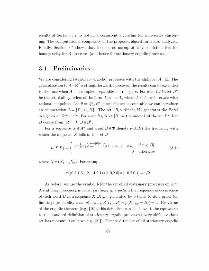
results of Section 3.2 to obtain a consistent algorithm for time-series cluster-ing. The computational complexity of the proposed algorithm is also analyzed.Finally, Section 3.5 shows that there is no asymptotically consistent test forhomogeneity for B-processes (and hence for stationary ergodic processes).
3.1 Preliminaries
We are considering (stationary ergodic) processes with the alphabet A=R. Thegeneralization to A=Rd is straightforward; moreover, the results can be extendedto the case when A is a complete separable metric space. For each k∈N, let Bk
be the set of all cylinders of the form A1×···×Ak where Ai⊂A are intervals withrational endpoints. Let B=∪∞k=1B
k; since this set is countable we can introducean enumeration B= Bi : i∈N. The set Bi×A∞ : i∈N generates the Borelσ-algebra on R∞=A∞. For a set B∈B let |B| be the index k of the set Bk thatB comes from: |B|=k :B∈Bk.
For a sequence X ∈An and a set B ∈B denote ν(X,B) the frequency withwhich the sequence X falls in the set B
ν(X,B) :=
1
n−|B|+1
∑n−|B|+1i=1 I(Xi,...,Xi+|B|−1)∈B if n≥|B|,
0 otherwise(3.1)
where X=(X1,...,Xn). For example,
ν((0.5,1.5,1.2,1.4,2.1),([1.0,2.0]×[1.0,2.0])
)=1/2.
As before, we use the symbol S for the set of all stationary processes on A∞.A stationary process ρ is called (stationary) ergodic if the frequency of occurrenceof each word B in a sequence X1,X2,... generated by ρ tends to its a priori (orlimiting) probability a.s.: ρ(limn→∞ν(X1..n,B) = ρ(X1..|B| =B)) = 1. By virtueof the ergodic theorem (e.g. [10]), this definition can be shown to be equivalentto the standard definition of stationary ergodic processes (every shift-invariantset has measure 0 or 1; see e.g. [21]). Denote E the set of all stationary ergodic
82
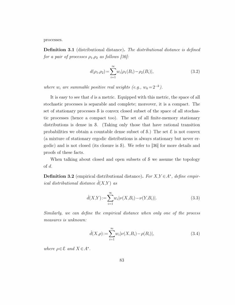
processes.
Definition 3.1 (distributional distance). The distributional distance is definedfor a pair of processes ρ1,ρ2 as follows [36]:
d(ρ1,ρ2)=∞∑i=1
wi|ρ1(Bi)−ρ2(Bi)|, (3.2)
where wi are summable positive real weights (e.g., wk=2−k).
It is easy to see that d is a metric. Equipped with this metric, the space of allstochastic processes is separable and complete; moreover, it is a compact. Theset of stationary processes S is convex closed subset of the space of all stochas-tic processes (hence a compact too). The set of all finite-memory stationarydistributions is dense in S. (Taking only those that have rational transitionprobabilities we obtain a countable dense subset of S.) The set E is not convex(a mixture of stationary ergodic distributions is always stationary but never er-godic) and is not closed (its closure is S). We refer to [36] for more details andproofs of these facts.
When talking about closed and open subsets of S we assume the topologyof d.
Definition 3.2 (empirical distributional distance). For X,Y ∈A∗, define empir-ical distributional distance d(X,Y ) as
d(X,Y ) :=∞∑i=1
wi|ν(X,Bi)−ν(Y,Bi)|. (3.3)
Similarly, we can define the empirical distance when only one of the processmeasures is unknown:
d(X,ρ) :=∞∑i=1
wi|ν(X,Bi)−ρ(Bi)|, (3.4)
where ρ∈E and X∈A∗.
83
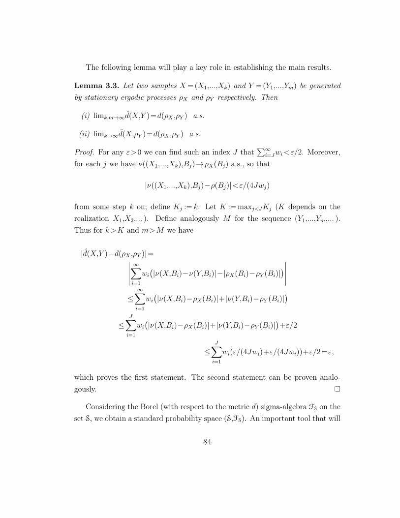
The following lemma will play a key role in establishing the main results.
Lemma 3.3. Let two samples X= (X1,...,Xk) and Y = (Y1,...,Ym) be generatedby stationary ergodic processes ρX and ρY respectively. Then
(i) limk,m→∞d(X,Y )=d(ρX ,ρY ) a.s.
(ii) limk→∞d(X,ρY )=d(ρX ,ρY ) a.s.
Proof. For any ε>0 we can find such an index J that∑∞
i=Jwi<ε/2. Moreover,for each j we have ν((X1,...,Xk),Bj)→ρX(Bj) a.s., so that
|ν((X1,...,Xk),Bj)−ρ(Bj)|<ε/(4Jwj)
from some step k on; define Kj := k. Let K := maxj<JKj (K depends on therealization X1,X2,... ). Define analogously M for the sequence (Y1,...,Ym,... ).Thus for k>K and m>M we have
|d(X,Y )−d(ρX ,ρY )|=∣∣∣∣∣∞∑i=1
wi(|ν(X,Bi)−ν(Y,Bi)|−|ρX(Bi)−ρY (Bi)|
)∣∣∣∣∣≤∞∑i=1
wi(|ν(X,Bi)−ρX(Bi)|+|ν(Y,Bi)−ρY (Bi)|
)≤
J∑i=1
wi(|ν(X,Bi)−ρX(Bi)|+|ν(Y,Bi)−ρY (Bi)|
)+ε/2
≤J∑i=1
wi(ε/(4Jwi)+ε/(4Jwi))+ε/2=ε,
which proves the first statement. The second statement can be proven analo-gously.
Considering the Borel (with respect to the metric d) sigma-algebra FS on theset S, we obtain a standard probability space (S,FS). An important tool that will
84
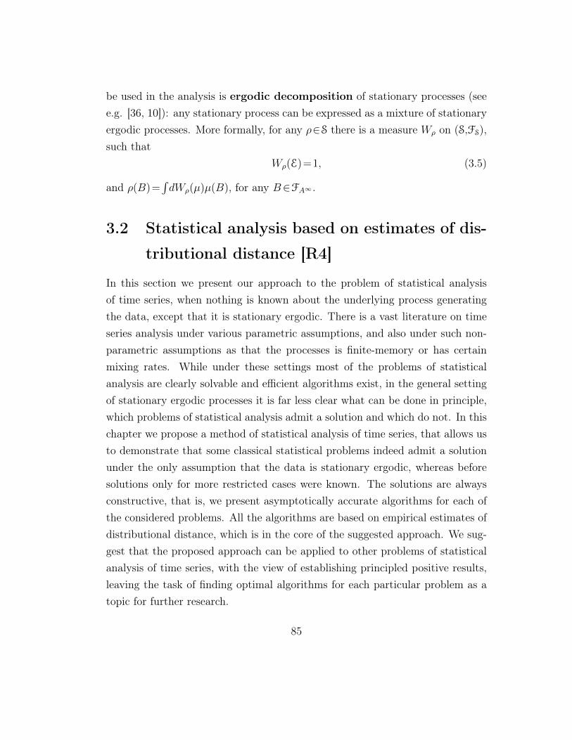
be used in the analysis is ergodic decomposition of stationary processes (seee.g. [36, 10]): any stationary process can be expressed as a mixture of stationaryergodic processes. More formally, for any ρ∈S there is a measure Wρ on (S,FS),such that
Wρ(E)=1, (3.5)
and ρ(B)=∫dWρ(µ)µ(B), for any B∈FA∞ .
3.2 Statistical analysis based on estimates of dis-
tributional distance [R4]
In this section we present our approach to the problem of statistical analysisof time series, when nothing is known about the underlying process generatingthe data, except that it is stationary ergodic. There is a vast literature on timeseries analysis under various parametric assumptions, and also under such non-parametric assumptions as that the processes is finite-memory or has certainmixing rates. While under these settings most of the problems of statisticalanalysis are clearly solvable and efficient algorithms exist, in the general settingof stationary ergodic processes it is far less clear what can be done in principle,which problems of statistical analysis admit a solution and which do not. In thischapter we propose a method of statistical analysis of time series, that allows usto demonstrate that some classical statistical problems indeed admit a solutionunder the only assumption that the data is stationary ergodic, whereas beforesolutions only for more restricted cases were known. The solutions are alwaysconstructive, that is, we present asymptotically accurate algorithms for each ofthe considered problems. All the algorithms are based on empirical estimates ofdistributional distance, which is in the core of the suggested approach. We sug-gest that the proposed approach can be applied to other problems of statisticalanalysis of time series, with the view of establishing principled positive results,leaving the task of finding optimal algorithms for each particular problem as atopic for further research.
85
Here we concentrate on the following three conceptually simple problems:goodness-of-fit (or identity) testing, process classification, and the change pointproblem. A somewhat more technical problem of time-series clustering will beconsidered in Section 3.4.Identity testing. The first problem is the following problem of hypothesis test-ing. A stationary ergodic process distribution ρ is known theoretically. Given adata sample, it is required to test whether it was generated by ρ, versus it wasgenerated by any other stationary ergodic distribution that is different from ρ
(goodness-of-fit, or identity testing). The case of i.i.d. or finite-memory processeswas widely studied (see e.g. [21]); in particular, when ρ has a finite memory [81]proposes a test against any stationary ergodic alternative: a test that can bebased on an arbitrary universal code. It was noted in [82] that an asymptoti-cally accurate test for the case of stationary ergodic processes over finite alpha-bet exists (but no test was proposed). Here we propose a concrete and simpleasymptotically accurate goodness-of-fit test, which demonstrates the proposedapproach: to use empirical distributional distance for hypotheses testing. Byasymptotically accurate test we mean the following. First, the Type I error ofthe test (or its size) is fixed and is given as a parameter to the test. That is,given any α> 0 as an input, under H0 (that is, if the data sample was indeedgenerated by ρ) the probability that the test says “H1” is not greater than α.Second, under any hypothesis in H1 (that is, if the distribution generating thedata is different from ρ), the test will say “H0” not more than a finite numberof times, with probability 1. In other words, the Type I error of the test is fixedand the Type II error can be made not more than a finite number of times,as the data sample increases, with probability 1 under any stationary ergodicalternative.Process classification. In the next problem that we consider, we again have todecide whether a data sample was generated by a process satisfying a hypothesisH0 or a hypothesis H1. However, here H0 and H1 are not known theoretically,but are represented by two additional data samples. More precisely, the probelmis that of process classification, which can be formulated as follows. We are given
86
three samples X = (X1,...,Xk), Y = (Y1,...,Ym) and Z = (Z1,...,Zn) generated bystationary ergodic processes with distributions ρX , ρY and ρZ . It is known thatρX 6= ρY but either ρZ = ρX or ρZ = ρY . It is required to test which one is thecase. That is, we have to decide whether the sample Z was generated by thesame process as the sample X or by the same process as the sample Y . Thisproblem for the case of dependent time series was considered for example in[37], where a solution is presented under the finite-memory assumption. It isclosely related to many important problems in statistics and application areas,such as pattern recognition. Apparently, no asymptotically accurate procedurefor process classification has been known so far for the general case of stationaryergodic processes. Here we propose a test that converges almost surely to thecorrect answer. In other words, the test makes only a finite number of errorswith probability 1, with respect to any stationary ergodic processes generatingthe data. Unlike in the previous problem, here we do not explicitly distinguishbetween Type I and Type II error, since the hypotheses are by nature symmetric:H0 is “ρZ =ρX” and H1 is “ρZ =ρY ”.Change point estimation. Finally, we consider the change point problem. Itis another classical problem, with vast literature on both parametric (see e.g.[7]) and non-parametric (see e.g. [15]) methods for solving it. In this sectionwe address the case where the data is dependent, its form and the structureof dependence is unknown, and, importantly, marginal distributions before andafter the change may be the same. We consider the following (off-line) settingof the problem: a (real-valued) sample Z1,...,Zn is given, where Z1,...,Zk aregenerated according to some distribution ρX and Zk+1,...,Zn are generated ac-cording to some distribution ρY which is different from ρX . It is known that thedistributions ρX and ρY are stationary ergodic, but nothing else is known aboutthem.
Most literature on change point problem for dependent time series assumesthat the marginal distributions before and after the change point are different,and often also make explicit restrictions on the dependence, such as requirementson mixing rates. Nonparametric methods used in these cases are typically based
87
on Kolmogorov-Smirnov statistic, Cramer-von Mises statistic, or generalizationsthereof [15, 16, 35]. The main difference with our results is that we do notassume that the single-dimensional marginals (or finite-dimensional marginalsof any given fixed size) are different, and do not make any assumptions on thestructure of dependence. The only assumption is that the (unknown) processdistributions before and after the change point are stationary ergodic.Methodology. All the tests that we construct are based on empirical estimatesof the so-called distributional distance. For two processes ρ1,ρ2 a distributionaldistance is defined as
∑∞k=1wk|ρ1(Bk)−ρ2(Bk)|, where wk are positive summable
real weights, e.g. wk=2−k and Bk range over a countable field that generates thesigma-algebra of the underlying probability space. For example, if we are talkingabout finite-alphabet processes with the binary alphabet A= 0,1, Bk wouldrange over the set A∗ = ∪k∈NAk; that is, over all tuples 0,00,01,10,000,001,... ;therefore, the distributional distance in this case is the weighted sum of differ-ences of probabilities of all possible tuples. In this section we consider real-valuedprocesses, A=R, so Bk can be taken to range over all intervals with rationalendpoints, all pairs of such intervals, triples, etc.
Although distributional distance is a natural concept that, for stochasticprocesses, has been studied for a while [36], its empirical estimates have not,to our knowledge, been used for statistical analysis of time series. We arguethat this distance is rather natural for this kind of problems, first of all, sinceit can be consistently estimated (unlike, for example, d distance, which cannot[69] be consistently estimated for the general case of stationary ergodic pro-cesses). Secondly, it is always bounded, unlike (empirical) KL divergence, whichis often used for statistical inference for time series (e.g. [21, 81, 2, 20] andothers). Other approaches to statistical analysis of stationary dependent timeseries include the use of (universal) codes [50, 81, 80]. Here we first show thatdistributional distance between stationary ergodic processes can be consistentlyestimated based on sampling, and then apply it to construct a consistent testfor the three problems of statistical analysis described above.
Although empirical estimates of the distributional distance involve taking an
88
infinite sum, in practice it is obvious that only a finite number of summandshas to be calculated. This is due to the fact that empirical estimates have tobe compared to each other or to theoretically known probabilities, and sincethe (bounded) summands have (exponentially) decreasing weights, the resultof the comparison is known after only finitely many evaluations (see a moreformal discussion on this in Section 3.4 on time-series clustering). Therefore,the algorithms presented can be applied in practice. On the other hand, themain value of the results is in the demonstration of what is possible in principle;finding practically efficient procedures for each of the considered problems is aninterestring problem for further research.
3.2.1 Goodness-of-fit
For a given stationary ergodic process measure ρ and a sample X=(X1,...,Xn)
we wish to test the hypothesis H0 that the sample was generated by ρ versus H1
that it was generated by a stationary ergodic distribution that is different fromρ. Thus, H0 =ρ and H1 =E\H0.
Define the set Dnδ as the set of all samples of length n that are at least δ-far
from ρ in empirical distributional distance:
Dnδ :=X∈An : d(X,ρ)≥δ.
For each n and each given confidence level α define the critical region Cnα of the
test as Cnα :=Dn
γ whereγ :=infδ :ρ(Dn
δ )≤α.
The test rejects H0 at confidence level α if (X1,...,Xn)∈Cnα and accepts it oth-
erwise. In words, for each sequence we measure the distance between the em-pirical probabilities (frequencies) and the measure ρ (that is, the theoretical ρ-probabilities); we then take a largest ball (with respect to this distance) aroundρ that has ρ-probability not greater than 1−α. The test rejects all sequencesoutside this ball.
89
Definition 3.4 (Goodness-of-fit test). For each n∈N and α∈(0,1) the goodness-of-fit test Gα
n :An→0,1 is defined as
Gαn(X1,...,Xn) :=
1 if (X1,...,Xn)∈Cn
α ,
0 otherwise.
Theorem 3.5. The test Gαn has the following properties.
(i) For every α∈(0,1) and every n∈N the Type I error of the test is not greaterthan α: ρ(Gα
n=1)≤α.
(ii) For every α ∈ (0,1) the Type II error goes to 0 almost surely: for everyρ′ 6=ρ we have limn→∞G
αn=1 with ρ′ probability 1.
Note that using an appropriate randomization in the definition of Cnα we can
make the Type I error exactly α.
Proof. The first statement holds by construction. To prove the second statement,let the sample X be generated by ρ′ ∈ E, ρ′ 6= ρ, and define δ = d(ρ,ρ′)/2. ByLemma 3.3 we have ρ(Dn
δ )→0, so that ρ(Dnδ )<α from some n on; denote it n1.
Thus, for n>n1 we have Dnδ ⊂Cn
α . At the same time, by Lemma 3.3 we haved(X,ρ)>δ from some n on, which we denote n2(X), with ρ′-probability 1. So, forn>maxn1,n2(X) we have X∈Dn
δ ⊂Cnα , which proves the statement (ii).
3.2.2 Process classification
Let there be given three samples X = (X1,...,Xk), Y = (Y1,...,Ym) and Z =
(Z1,...,Zn). Each sample is generated by a stationary ergodic process ρX , ρYand ρZ respectively. Moreover, it is known that either ρZ =ρX or ρZ =ρY , butρX 6=ρY . We wish to construct a test that, based on the finite samples X,Y andZ will tell whether ρZ =ρX or ρZ =ρY .
The test chooses the sample X or Y according to whichever is closer to Zin d. That is, we define the test G(X,Y,Z) as follows. If d(X,Z)≤ d(Y,Z) thenthe test says that the sample Z is generated by the same process as the sample
90
X, otherwise it says that the sample Z is generated by the same process as thesample Y.
Definition 3.6 (Process classifier). Define the classifier L :A∗×A∗×A∗→1,2as follows
L(X,Y,Z) :=
1 if d(X,Z)≤ d(Y,Z)
2 otherwise,
for X,Y,Z∈A∗.
Theorem 3.7. The test L(X,Y,Z) makes only a finite number of errors when|X|,|Y | and |Z| go to infinity, with probability 1: if ρX =ρZ then
L(X,Y,Z)=1
from some |X|,|Y |,|Z| on with probability 1; otherwise
L(X,Y,Z)=2
from some |X|,|Y |,|Z| on with probability 1.
Proof. From the fact that d is a metric and from Lemma 3.3 we conclude thatd(X,Z)→ 0 (with probability 1) if and only if ρX = ρZ . So, if ρX = ρZ then byassumption ρY 6=ρZ and d(X,Z)→0 a.s. while
d(Y,Z)→d(ρY ,ρZ) 6=0.
Thus in this case d(Y,Z)>d(X,Z) from some |X|,|Y |,|Z| on with probability 1,from which moment we have L(X,Y,Z)=1. The opposite case is analogous.
3.2.3 Change point problem
The sample Z = (Z1,...,Zn) consists of two concatenated parts X = (X1,...,Xk)
and Y =(Y1,...,Ym), where m=n−k, so that Zi=Xi for 1≤i≤k and Zk+j=Yj for1≤ j≤m. The samples X and Y are generated independently by two different
91
stationary ergodic processes with alphabet A = R. The distributions of theprocesses are unknown. The value k is called the change point. It is assumedthat k is linear in n; more precisely, αn<k<βn for some 0<α≤β<1 from somen on.
It is required to estimate the change point k based on the sample Z.For each t, 1≤ t≤n, denote U t the sample (Z1,...,Zt) consisting of the first t
elements of the sample Z, and denote V t the remainder (Zt+1,...,Zn).
Definition 3.8 (Change point estimator). Define the change point estimatek :A∗→N as follows:
k(X1,...,Xn) :=argmaxt∈[αn,n−βn]d(U t,V t).
The following theorem establishes asymptotic consistency of this estimator.
Theorem 3.9. For the estimate k of the change point k we have
|k−k|=o(n) a.s.
where n is the size of the sample, and when k,n−k→∞ in such a way thatα< k
n<β for some α,β∈(0,1) from some n on.
The proof is deferred to Section 3.6.1.
3.3 Characterizing families of stationary processes
for which consistent tests exist [R2]
Given a sample X1,...,Xn, where, for the sake of this section, Xi are from afinite alphabet A, we wish to decide whether it was generated by a distributionbelonging to a family H0, versus it was generated by a distribution belongingto a family H1. The only assumption we are willing to make about the thedistribution generating the sample is that it is stationary ergodic.
92
A test is a function that takes a sample and gives a binary (possibly incorrect)answer: the sample was generated by a distribution from H0 or from H1. Ananswer i∈0,1 is correct if the sample is generated by a distribution that belongsto Hi. Here we are concerned with characterizing those pairs of H0 and H1 forwhich consistent tests exist. There are several ways of formalizing what is aconsistent test, from which we consider two. For these two notions of consistencywe find some necessary and some sufficient conditions for the existence of aconsistent test, expressed in topological terms. For one notion of consistency(asymmetric testing) considered, the necessary and sufficient conditions coincidewhen H1 is the complement of H0, thereby providing a complete characterizationof the hypotheses for which consistent tests exist.
Examples. Before introducing the definitions of consistency, let us give someexamples motivating the general problem in question. Most of these examples areclassical problems studied in mathematical statistics and related fields, mostly fori.i.d. data, with much literature devoted to each of them. (An incomplete surveyof related work for non-i.i.d. data is given further in this section.) The most basiccase of the hypothesis testing problem is testing a simple hypothesis H0 =ρ0versus a simple hypothesis H1 =ρ1, where ρ0 and ρ1 are two stationary ergodicprocess distributions (which are assumed completely known theoretically). Amore complex but more realistic problem is when only one of the hypothesis issimple, H0 =ρ0 but the alternative is general, for example H1 is the set of allstationary ergodic processes that are different from ρ0. This is the goodness-of-fitproblem that we have considered in Section 3.2. One may also consider variantsin which the alternative is the set of all stationary ergodic processes that differfrom ρ0 by at least ε in some distance. The described hypotheses are variantsof the so-called goodness-of-fit, or identity testing problem. Another class ofhypothesis testing problems is presented by the problem of model verification.Suppose we have some relatively simple (possibly parametric) set of assumptions,and we wish to test whether the process generating the given sample satisfies thisassumptions. As an example, H0 can be the set of all k-order Markov processes(fixed k ∈N) and H1 is the set of all stationary ergodic processes that do not
93
belong to H0; one may also wish to consider more restrictive alternatives, forexample H1 is the set of all k′-order Markov processes where k′>k. Of course,instead of Markov processes one can consider other models, e.g. Hidden Markovprocesses. A similar problem is that of testing that the process has entropy lessthan some given ε versus its entropy exceeds ε, or versus its entropy is greaterthan ε+δ for some positive δ.
Yet another type of hypothesis testing problems concerns property testing.Suppose we are given two samples, generated independently of each other bystationary ergodic distributions, and we wish to test the hypothesis that theyare independent versus they are not independent. Or, that they are generatedby the same process versus they are generated by different processes.
In all the considered cases, when the hypothesis testing problem turns outto be too difficult (i.e. there is no consistent test for the chosen notion of con-sistency) for the case of stationary ergodic processes, one may wish to restricteither H0, H1 or both H0 and H1 to some smaller class of processes. Thus,one may wish to test the hypothesis of independence when, for example, bothprocesses are known to have finite memory, or to have certain mixing rates.
All the problems described above are special cases of the following generalformulation: given two sets H0 and H1 which are contained in the set of all sta-tionary ergodic process distributions, and given a sample generated by a processthat comes from either H0 or H1, we would like have a test that tells us whichone is the case: H0 or H1. The goal of this section is to characterize those pairsof H0,H1 for which a consistent test exists. Ideally, the characterization shouldbe complete, that is, in the form of necessary and sufficient conditions, that canbe verified for at least most of the problems outlined above. This goal is partiallyachieved: for two (rather natural) notions of consistency, we find some neces-sary and some sufficient conditions, that, for one of these notions of consistency,coincide in the case when H1 is the complement of H0. We show that these con-ditions are indeed relatively easy to verify for some of the considered hypotheses,such as identity testing, model verification and testing independence.
In this section we will use the following notions of consistency of tests (see
94
Section 3.3.1 for formal definitions). The first one is the same that was introducedin Section 3.2: the Type I error (level) is fixed and the probability of Type II erroris required to go to 0 as the sample size increases. To distinguish it from othernotions of consistency that we will consider, we call it asymmetric consistency.
The second notion of consistency that we will consider is uniform consistency.For two hypothesis H0 and H1, a test is called uniformly consistent, if for anyε> 0 there is a sample size n such that the probability of error on a sample ofsize larger than n is not greater than ε if any distribution from H0∪H1 is chosento generate the sample. Thus, a uniformly consistent test provides performanceguarantees for finite sample sizes.Prior work. There is a vast body of literature on hypothesis testing for i.i.d.(real- or discrete-valued) data (see e.g. [58, 49]). In the context of discrete-valued i.i.d. data, the necessary and sufficient conditions for the two types ofconsistency introduced are rather simple. There is an asymmetrically consistenttest if and only if the closure of H0 does not intersect H1, and there is a uniformlyconsistent test if and only if the closures of H0 and H1 are disjoint, where thetopology is that of the parameter space (probabilities of each symbol), see e.g.[19]. Some extensions to Markov chains are also possible [9, 6].
There is, however, much less literature on hypothesis testing beyond i.i.d.or parametric models, while the question of determining whether a consistenttest exists, for different notions of consistency and different hypotheses, is muchless trivial. For a weaker notion of consistency, namely, requiring that the testshould stabilize on the correct answer for a.e. realization of the process (undereither H0 or H1), [50] constructs a consistent test for so-called constrained finite-state model classes (including finite-state Markov and hidden Markov processes),against the general alternative of stationary ergodic processes. For the same no-tion of consistency, [65] gives sufficient conditions on two hypotheses H0 and H1
that consist of stationary ergodic real-valued processes, under which a consistenttest exists, extending the results of [25] for i.i.d. data. The latter condition isthat H0 and H1 are contained in disjoint Fσ sets (countable unions of closedsets), with respect to the topology of weak convergence. In [62] some results
95
are presented on testing the hypothesis that the process has a finite memory,and some related problems. Asymmetrically consistent tests for some specifichypotheses, but under the general alternative of stationary ergodic processes,have been proposed in Section 3.2 above (see also references therein).The results. Here we obtain some topological characterizations of the hy-potheses for which consistent tests exist, for the case of stationary ergodic dis-tributions. The obtained characterizations are rather similar to those mentionedabove for the case of i.i.d. data, but are with respect to the topology of distribu-tional distance. The fact that necessary and sufficient conditions are obtainedfor one of the notions of consistency, indicates that this topology is the right oneto consider.
The tests that we construct are based on empirical estimates of distribu-tional distance. In particular, the uniform test ϕH0,H1 outputs 0 if the givensample is closer to the (closure of) H0 than to the (closure of) H1, and outputs1 otherwise. The asymmetric test ψαH0,H1
, for a given level α, takes the smallestε-neighbourhood of the closure of H0 that has probability not less than 1−αwith respect to any distribution in it, and outputs 0 if the sample falls into thisneighbourhood, and 1 otherwise.
This is a generalization of the goodness-of-fit procedure introduced in Sec-tion 3.2.
For the case of testing H0 against its complement to the set E of all stationaryergodic processes, we obtain the following necessary and sufficient condition(formalized in the next section).Theorem. There exists an asymmetrically consistent test for H0 against H1 :=
E\H0 if and only if H1 has probability 0 with respect to ergodic decompositionof every distribution from the closure of H0. In this case, the test ψαH0,H1
isasymmetrically consistent too.
For the general case, as well as for the case of uniform consistency, we obtainsome necessary and some sufficient conditions, in the same terms. The mainresults are illustrated with derivations of several known and some new resultsfor specific hypotheses. In particular, we show that any set of processes which
96
is continuously parametrized by a compact set of parameters, and is closed un-der taking ergodic decompositions, can be tested with asymmetric consistencyagainst its complement to the set of all stationary ergodic processes. Such para-metric families include k-order Markov processes and k-state Hidden Markovprocesses.
3.3.1 Definitions: consistency of tests
A test is a function ϕ :A∗→0,1 that takes a sample and outputs a binaryanswer, where the answer i is interpreted as “the sample was generated by adistribution that belongs to Hi”. The answer i is correct if the sample wasindeed generated by a distribution from Hi, otherwise we say that the test madean error. A test ϕ makes the Type I error if it says 1 while H0 is true, and itmakes Type II error if it says 0 while H1 is true.
Call a family of tests ψα,α∈ (0,1) asymmetrically consistent if: (i) Theprobability of Type I error is always bounded by α: ρX∈An :ψα(X)=1≤α forevery ρ∈H0, every n∈N and every α∈(0,1), and (ii) Type II error is made notmore than a finite number of times with probability 1: ρ(limn→∞ψ
α(X1..n)=1)=1
for every ρ∈H1 and every α∈ (0,1). (Abusing the notation, we will sometimescall families of tests ψα,α∈(0,1) simply tests.)
A test ϕ is called uniformly consistent if for every α there is an nα ∈Nsuch that for every n≥nα the probability of error on a sample of size n is lessthan α: ρ(X∈An :ϕ(X)= i)<α for every ρ∈H1−i and every i∈0,1.
3.3.2 Topological characterizations
The tests presented below are based on empirical estimates of the distributionaldistance d:
d(X1..n,ρ)=∞∑i=1
wi|ν(X1..n,Bi)−ρ(Bi)|,
where n ∈ N, ρ ∈ S, X1..n ∈ An. That is, d(X1..n,ρ) measures the discrepancybetween empirically estimated and theoretical probabilities. For a sample X1..n∈
97
An and a hypothesis H⊂E define
d(X1..n,H)= infρ∈H
d(X1..n,ρ).
For H⊂S, denote clH the closure of H (with respect to the topology of d).For H0,H1⊂S, the uniform test ϕH0,H1 is constructed as follows. For each
n∈N let
ϕH0,H1(X1..n) :=
0 if d(X1..n,clH0∩E)<d(X1..n,clH1∩E),
1 otherwise.(3.6)
Since the set S is a complete separable metric space, it is easy to see that thefunction ϕH0,H1(X1..n) is measurable provided clH0 is measurable.
Theorem 3.10 (uniform testing). Let H0,H1 be measurable subsets of E. IfWρ(Hi) = 1 for every ρ ∈ clHi then the test ϕH0,H1 is uniformly consistent.Conversely, if there exists a uniformly consistent test for H0 against H1 thenWρ(H1−i)=0 for any ρ∈clHi.
The proofs are deferred to section 3.6.Construct the asymmetric test ψαH0,H1
,α∈(0,1) as follows. For each n∈N,δ>0 and H⊂E define the neighbourhood bnδ (H) of n-tuples around H as
bnδ (H) :=X∈An : d(X,H)≤δ.
Moreover, letγn(H,θ) :=infδ : inf
ρ∈Hρ(bnδ (H))≥θ
be the smallest radius of a neighbourhood around H that has probability notless than θ with respect to any process in H, and let Cn(H,θ) := bnγn(H,θ)(H) bea neighbourhood of this radius. Define
ψαH0,H1(X1..n) :=
0 if X1..n∈Cn(clH0∩E,1−α),
1 otherwise.
98
Again, it is easy to see that the function ϕH0,H1(X1..n) is measurable, since theset S is separable. We will often omit the subscript H0,H1 from ψαH0,H1
when itcan cause no confusion.
Theorem 3.11. Let H0,H1 be measurable subsets of E. If Wρ(H0)=1 for everyρ∈ clH0 then the test ψαH0,H1
is asymmetrically consistent. Conversely, if thereis an asymmetrically consistent test for H0 against H1 then Wρ(H1)=0 for anyρ∈clH0.
For the case when H1 is the complement of H0 the necessary and sufficientconditions of Theorem 3.11 coincide and give the following criterion.
Corollary 3.12. Let H0⊂E be measurable and let H1 =E\H0. The followingstatements are equivalent:
(i) There exists an asymmetrically consistent test for H0 against H1.
(ii) The test ψαH0,H1is asymmetrically consistent.
(iii) The set H1 has probability 0 with respect to ergodic decomposition of everyρ in the closure of H0: Wρ(H1)=0 for each ρ∈clH0.
3.3.3 Examples
Theorems 3.11 and 3.10 can be used to check whether a consistent test existsfor such problems as identity, independence, estimating the order of a (Hidden)Markov model, bounding entropy, bounding distance, uniformity, monotonicity,etc. Some of these examples are considered in this section.Example 1: Simple hypotheses, Identity. First of all, it is obvious that setsthat consisit of just one or finitely many stationary ergodic processes are closedand closed under ergodic decompositions; therefore, for any pair of disjoint setsof this type, there exists a uniformly consistent test. (In particular, there is auniformly consistent test for H0 = ρ0 against H1 = ρ1.) A more interestingcase is identity testing, or goodness-of-fit, introduced in Section 3.2: the problem
99
here consists in testing whether a distribution generating the sample obeys acertain given law, versus it does not. Let ρ∈E, H0 =ρ and H1 =E\H0. Thenthere is an asymmetrically consistent test for H0 against H1. The conditions ofTheorem 3.12 are easily verified for this case, so that we recover Theorem 3.5.
As far as uniform testing is concerned, it is, first of all, clear that for any ρ0
there is no uniformly consistent test for identity. More generally, for any non-empty H0 there is no uniformly consistent test for H0 against E\H0 provided thelatter complement is also non-empty. Indeed, this follows from Theorem 3.10since in these cases the closures of H0 and H1 are not disjoint. One might suggestat this point that a uniformly consistent test exists if we restrict H1 to thoseprocesses that are sufficiently far from ρ0. However, this is not true. We canprove an even stronger negative result.
Proposition 3.13. Let ρ,ν ∈ E, ρ 6= ν and let ε > 0. There is no uniformlyconsistent test for H0 =ρ against H1 =ν ′∈E :d(ν ′,ν)≤ε.
The proof of the proposition is deferred to the Section 3.6.2. What it meansis that, while distributional distance is well suited for characterizing those hy-potheses for which consistent test exist, it is not suited for formulating the actualhypotheses. Apparently a stronger distance is needed for the latter.
Example 2: Markov and Hidden Markov processes: bounding the or-der. For any k, there is an asymmetrically consistent test of the hypothesisMk= “the process is Markov of order not greater than k” against E\Mk. For anyk, there is an asymmetrically consistent test of HMk=“the process is given bya Hidden Markov process with not more than k states” against H1 =E\HMk.Indeed, in both cases (k-order Markov, Hidden Markov with not more than k
states), the hypothesis H0 is a parametric family, with a compact set of parame-ters, and a continuous function mapping parameters to processes (that is, to thespace S). Weierstrass theorem then implies that the image of such a compactparameter set is closed (and compact). Moreover, in both cases H0 is closedunder taking ergodic decompositions. Thus, by Theorem 3.11, there exists anasymmetrically consistent test.
100
The problem of estimating the order of a (hidden) Markov process, basedon a sample from it, was addressed in a number of works. In the contest ofhypothesis testing, asymmetrically consistent tests for Mk against Mt with t>kwere given in [6], see also [9]. The existence of non-uniformly consistent tests (anotion weaker than that of asymmetric consistency) forMk against E\Mk, and ofHMk against E\HMk, was established in [50]. Asymmetrically consistent testsfor Mk against E\Mk were obtained in [80], while for the case of asymmetrictesting for HMk against E\HMk the positive result above is apparently new.
Example 3: Smooth parametric families. From the discussion in the pre-vious example we can see that the following generalization is valid. Let H0⊂S
be a set of processes that is continuously parametrized by a compact set of pa-rameters. If H0 is closed under taking ergodic decompositions, then there is anasymmetrically consistent test for H0 against E\H0. In particular, this strength-ens the mentioned result of [50], since a stronger notion of consistency is used,as well as a more general class of parametric families is considered.
Clearly, a similar statement can be derived for uniform testing: given twodisjoint sets H0 and H1 each of which is continuously parametrized by a compactset of parameters and is closed under taking ergodic decompositions, there existsa uniformly consistent test of H0 against H1.
Example 4: Independence. Suppose that A = A1×A2, so that a sampleX1..n consists of two processes X1
1..n and X21..n, which we call features. The
hypothesis of independence is that the first feature is independent from thesecond: ρ(X1
1..t ∈ T1,X21..t ∈ T2) = ρ(X1
1..t ∈ T1)ρ(X21..t ∈ T2) for any (T1,T2) ∈An
and any n ∈N. Let I be the set of all stationary ergodic processes satisfyingthis property. It is easy to see that Theorem 3.11 implies, that there existsan asymmetrically consistent test for I∩Mk against E\I, for any given k ∈N.Analogously, if we confine H0 to Hidden Markov processes of a given order,then asymmetric testing is possible. That is, there exists an an asymmetricallyconsistent test for I∩HMk against E\I, for any given k∈N. As far as uniformtesting is concerned, positive results can be obtained if we restrict both H0
and H1 to the corresponding subset of some set continuously parametrized by
101
a compact set of parameters, such as the sets of (Hidden) Markov processes ofgiven order.
The question of whether I can be tested against E\I is more difficult. It isclear that the closure of I only contains processes with independent features.It is not clear whether any of the limiting points of I has ergodic componentswhose features are not independent. If there are none, this would prove thatthere exists an asymmetrically consistent test for independence, for the class ofstationary ergodic process.
3.4 Clustering time series [R11]
In this section we use the approach developed in the previous sections to con-struct an algorithm for clustering time-series data and show its consistency underthe general assumption that the time series are stationary ergodic.
Given a finite set of objects the problem to “cluster” similar objects together,in the absence of any examples of “good” clusterings, is notoriously hard toformalize. Most of the work on clustering is concerned with particular parametricdata generating models, or particular algorithms, a given similarity measure, and(very often) a given number of clusters. It is clear that, as in almost learningproblems, in clustering finding the right similarity measure is an integral partof the problem. However, even if one assumes the similarity measure known,it is hard to define what a good clustering is [52, 89]. What is more, even ifone assumes the similarity measure to be simply the Euclidean distance (on theplane), and the number of clusters k known, then clustering may still appearintractable for computational reasons. Indeed, in this case finding k centres(points which minimize the cumulative distance from each point in the sampleto one of the centres) seems to be a natural goal, but this problem is NP-hard[61].
In this section we consider the problem of clustering time-series data. That is,each data point is itself a sample generated by a certain discrete-time stochasticprocess. This version of the problem has numerous applications, such as cluster-
102
ing biological data, financial observations, or behavioural patterns, and as suchit has gained a tremendous attention in the literature.
The main observation that we make here is that, in the case of clusteringprocesses, one can benefit from the notion of ergodicity to define what appearsto be a very natural notion of consistency. This notion of consistency is shownto be satisfied by simple algorithms that we present, which are polynomial in allarguments.
With these considerations in mind, define the clustering problem as follows.N samples are given: x1 =(x1
1,...,x1n1
),...,xN =(xN1 ,...,xNnN
). Each sample is drawnby one out of k different stationary ergodic distributions. The samples are notassumed to be drawn independently; rather, it is assumed that the joint distri-bution of the samples is stationary ergodic. The target clustering is as follows:those and only those samples are put into the same cluster that were generatedby the same distribution. As is usual in the clustering literature, the numberk of target clusters is assumed to be known. A clustering algorithm is calledasymptotically consistent if the probability that it outputs the target clusteringconverges to 1, as the lengths (n1,...,nN) of the samples tend to infinity (a variantof this definition is to require the algorithm to stabilize on the correct answerwith probability 1). Note the particular regime of asymptotic: not with respectto the number of samples N , but with respect to the length of the samplesn1,...,nN .
Similar formulations have appeared in the literature before. Perhaps themost close approach is mixture models [84, 90]: it is assumed that there arek different distributions that have a particular known form (such as Gaussian,Hidden Markov models, or graphical models) and each one out of N samplesis generated independently according to one of these k distributions (with somefixed probability). Since the model of the data is specified quite well, one canuse likelihood-based distances (and then, for example, the k-means algorithm),or Bayesian inference, to cluster the data. Clearly, the main difference from oursetting is in that we do not assume any known model of the data; not evenbetween-sample independence is assumed.
103
The problem of clustering in our formulation is close to the following two clas-sical problems of mathematical statistics. The first one is homogeneity testing,or the two-sample problem. Two samples x1 = (x1
1,...,x1n1
) and x2 = (x21,...,x
2n2
)
are given, and it is required to test whether they were generated by the samedistribution, or by different distributions. This corresponds to clustering justtwo data points (N=2) with the number k of clusters unknown: either k=1 ork=2. As we show in Section 3.5, this problem is impossible to solve for station-ary ergodic (binary-valued) processes, which is why we assume known k in thissection. The second problem is process classification, or the three-sample prob-lem, that we have considered in detail in Section 3.2.2: Three samples x1,x2,x3
are given, it is known that two of them were generated by the same distribution,while the third one was generated by a different distribution. It is required tofind out which two were generated by the same distribution. This correspondsto clustering three data points, with the number of clusters k=2. The clusteringalgorithm that we will present in this section is therefore a generalization of thesimple procedure of Section 3.2.2.
In this section we will also consider in some detail the question of calculatingempirical estimates of the distributional distance (on which all the algorithms inthis chapter are based). Although its definition involves infinite summation, weshow that it can be easily calculated.
3.4.1 Problem formulation
The clustering problem can be defined as follows. We are given N samplesx1,...,xN , where each sample xi is a string of length ni of symbols from A:xi=X
i1..ni
. Each sample is generated by one out of k different unknown stationaryergodic distributions ρ1,...,ρk∈E. Thus, there is a partitioning I=I1,...,Ik ofthe set 1..N into k disjoint subsets Ij,j=1..k
1..N=∪kj=1Ij,
104
such that xj, 1≤j≤N is generated by ρj if and only if j∈Ij. The partitioningI is called the target clustering and the sets Ii,1≤ i≤ k, are called the targetclusters. Given samples x1,...,xN and a target clustering I, let I(x) denote thecluster that contains x.
A clustering function F takes a finite number of samples x1,...,xN and anoptional parameter k (the target number of clusters) and outputs a partitionF (x1,...,xN ,(k))=T1,...,Tk of the set 1..N.
Definition 3.14 (asymptotic consistency). Let a finite number N of samples begiven, and let the target clustering partition be I. Define n=minn1,...,nN. Aclustering function F is strongly asymptotically consistent if
F (x1,...,xN ,(k))=I
from some n on with probability 1. A clustering function is weakly asymptoticallyconsistent if
P (F (x1,...,xN ,(k))=I)→1.
Note that the consistency is asymptotic with respect to the minimal lengthof the sample, and not with respect to the number of samples.
Since in this section we will be also interested in analysing computation com-plexity of the proposed methods, we will use a slightly more detailed definitionof the distributional distance.
Definition 3.15. The distributional distance is defined for a pair of processesρ1,ρ2 as follows
d(ρ1,ρ2)=∞∑
m,l=1
wmwl∑
B∈Bm,l|ρ1(B)−ρ2(B)|,
where wj =2−j.
105
The clustering algorithm below is based on empirical estimates of d:
d(X11..n1
,X21..n2
)=∞∑
m,l=1
wmwl∑
B∈Bm,l|ν(X1
1..n1,B)−ν(X2
1..n2,B)|, (3.7)
where n1,n2∈N, ρ∈S, X i1..ni∈Ani .
It is easy to check that Lemma 3.3 holds for this modified definition of d aswell.
3.4.2 Clustering algorithm
Algorithm 1 is a simple clustering algorithm, which, given the number k ofclusters, will be shown to be consistent under most general assumptions. Itworks as follows. The point x1 is assigned to the first cluster. Next, find thepoint that is farthest away from x1 in the empirical distributional distance d,and assign this point to the second cluster. For each j= 3..k, find a point thatmaximizes the minimal distance to those points already assigned to clusters, andassign it to the cluster j. Thus we have one point in each of the k clusters. Nextsimply assign each of the remaining points to the cluster that contains the closestpoints from those k already assigned. One can notice that Algorithm 1 is justone iteration of the k-means algorithm, with so-called farthest-point initialization[47], and a specially designed distance.
Proposition 3.16 (calculating d(x1,x2)). For two samples x1 =X11..n1
and x2 =
X21..n2
the computational complexity (time and space) of calculating the empiricaldistributional distance d(x1,x2) (3.7) is O(n2logs−1
min), where n=max(n1,n2) and
smin = mini=1..n1,j=1..n2,X1
i 6=X2j
|X1i −X2
j |.
Proof. First, observe that for fixed m and l, the sum
Tm,l :=∑
B∈Bm,l|ν(X1
1..n1,B)−ν(X2
1..n2,B)| (3.8)
106
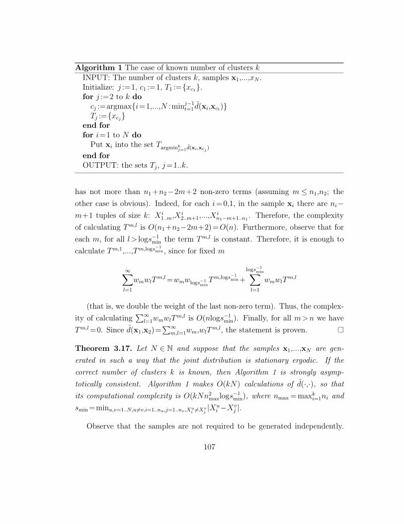
Algorithm 1 The case of known number of clusters kINPUT: The number of clusters k, samples x1,...,xN .Initialize: j :=1, c1 :=1, T1 :=xc1.for j :=2 to k docj :=argmaxi=1,...,N :minj−1
t=1 d(xi,xct)Tj :=xcj
end forfor i=1 to N doPut xi into the set Targminkj=1d(xi,xcj )
end forOUTPUT: the sets Tj, j=1..k.
has not more than n1 +n2−2m+2 non-zero terms (assuming m ≤ n1,n2; theother case is obvious). Indeed, for each i= 0,1, in the sample xi there are ni−m+1 tuples of size k: X i
1..m,Xi2..m+1,...,X
in1−m+1..n1
. Therefore, the complexityof calculating Tm,l is O(n1+n2−2m+2) =O(n). Furthermore, observe that foreach m, for all l > logs−1
min the term Tm,l is constant. Therefore, it is enough tocalculate Tm,1,...,Tm,logs−1
min , since for fixed m
∞∑l=1
wmwlTm,l=wmwlogs−1
minTm,logs−1
min +
logs−1min∑
l=1
wmwlTm,l
(that is, we double the weight of the last non-zero term). Thus, the complex-ity of calculating
∑∞l=1wmwlT
m,l is O(nlogs−1min). Finally, for all m>n we have
Tm,l=0. Since d(x1,x2)=∑∞
m,l=1wm,wlTm,l, the statement is proven.
Theorem 3.17. Let N ∈ N and suppose that the samples x1,...,xN are gen-erated in such a way that the joint distribution is stationary ergodic. If thecorrect number of clusters k is known, then Algorithm 1 is strongly asymp-totically consistent. Algorithm 1 makes O(kN) calculations of d(·,·), so thatits computational complexity is O(kNn2
maxlogs−1min), where nmax = maxki=1ni and
smin =minu,v=1..N,u6=v,i=1..nu,j=1..nv ,Xui 6=Xv
j|Xu
i −Xvj |.
Observe that the samples are not required to be generated independently.
107
The only requirement on the distribution of samples is that the joint distributionis stationary ergodic. This is perhaps one of the mildest possible probabilisticassumptions.
Proof. By Lemma 3.3, d(xi,xj), i,j∈1..N converges to 0 if and only if xi andxj are in the same cluster. Since there are only finitely many samples xi, thereexists some δ > 0 such that, from some n on, we will have d(xi,xj)<δ if xi,xjbelong to the same target cluster (I(xi) = I(xj)), and d(xi,xj) > δ otherwise(I(xi) 6=I(xj)). Therefore, from some n on, for every j≤k we will have maxi=1,...,N : minj−1
t=1 d(xi,xct)>δ and the sample xcj , where cj = argmaxi= 1,...,N :
minj−1t=1 d(xi,xct), will be selected from a target cluster that does not contain any
xci , i<j. The consistency statement follows.Next, let us find how many pairwise distance estimates d(xi,xj) the algorithm
has to make. On the first iteration of the loop, it has to calculate d(xi,xc1)
for all i = 1..N . On the second iteration, it needs again d(xi,xc1) for all i =
1..N , which are already calculated, and also d(xi,xc2) for all i= 1..N , and soon: on jth iteration of the loop we need to calculate d(xi,xcj), i= 1..N , whichgives at most kN pairwise distance calculations in total. The statement aboutcomputational complexity follows from this and Proposition 3.16: indeed, apartfrom the calculation of d, the rest of the computations is of order O(kN).
3.5 Discrimination between B-processes is impos-
sible [R5]
Two series of binary observations x1,x1,... and y1,y2,... are presented sequentially.A discrimination procedure (or homogeneity test) D is a family of mappingsDn :Xn×Xn→0,1, n∈N, X=0,1, that maps a pair of samples (x1,...,xn),(y1,...,yn) into a binary (“yes” or “no”) answer: the samples are generated bydifferent distributions, or they are generated by the same distribution.
A discrimination procedure D is asymptotically correct for a set C of processdistributions if for any two distributions ρx,ρy∈C independently generating the
108
sequences x1,x2,... and y1,y2,... correspondingly the expected output convergesto the correct answer: the following limit exists and the equality holds
limn→∞
EDn((x1,...,xn),(y1,...,yn))=
0 if ρx=ρy,1 otherwise.
This is perhaps the weakest notion of correctness one can consider. Clearly,asymptotically correct discriminating procedures exist for many classes of pro-cesses, for example for the class of all i.i.d. processes (e.g. [58]) and variousparametric families.
We show that there is no asymptotically correct discrimination procedurefor the class of all B-processes (see the definition below), meaning that for anydiscrimination the expected answer does not converge to the correct one for someprocesses. The class of B-processes is sufficiently wide to include, for example,k-order Markov processes and functions of them, but, on the other hand, itis a strict subset of the set of stationary ergodic processes. B-processes playimportant role in such fields as information theory and ergodic theory [?, 67].
Previously, in [69] and [68] it was shown that consistent estimates of d-distance (defined below) for B-processes exist, while it is impossible to estimatethis distance outside this class. In [69] it is also claimed that consistent discrim-ination procedure does not exist for the set of all stationary ergodic processes;however, what is shown in that work is that consistent estimate of d-distance donot exist for this set. The result of this section is stronger than this claim: aconsistent discrimination procedure does not exist for a smaller set of processes,that of all B-processes.
Next we define the d distance and B-processes (mainly following [69] in ourformulations) and give more precise formulations of some of the existing resultsmentioned above.
For two finite-valued stationary processes ρx and ρy the d-distance d(ρx,ρy)
is said to be less than ε if there exists a single stationary process νxy on pairs(xn,yn), n∈N, such that xn, n∈N are distributed according to ρx and yn are
109
distributed according to ρy while
νxy(x1 6=y1)≤ε. (3.9)
The infimum of the ε’s for which a coupling can be found such that (3.9) issatisfied is taken to be the d-distance between ρx and ρy.
Definition 3.18. A process is called a B-process (or a Bernoulli process) if itis in the d-closure of the set of all aperiodic stationary ergodic k-step Markovprocesses, where k∈N.
For more information on d-distance and B-processes see [67]. As it wasmentioned, [69] constructs an estimator sn such that
limn→∞
sn((x1,...,xn),(y1,...,yn))= d(ρ1,ρ2) ρ1×ρ2–a.s. (3.10)
if both processes ρ1 and ρ2 generating the samples xi and yi respectively areB-processes. In the same work it is shown that there is no estimator sn forwhich (3.10) holds for every pair ρ1,ρ2 of stationary ergodic processes. Someextensions of these results are given in [68].
It is interesting to compare these results to those that are obtained for thedistributional distance. As we have shown (Lemma 3.3), this distance can beconsistently estimated. Moreover, based on its estimate, we can also constructa consistent change point estimate, as was demonstrated in Section 3.2 above.On the other hand, the results of the present section implies that one cannotconsistently tell whether there is a change in the sample or not.
Summarizing, we can say that the stronger the distance the harder it is toestimate: the distributional distance can be consistently estimated for stationaryergodic processes, the d distance can be consistently estimated for B-processesbut not for stationary ergodic processes, while the strongest possible distance—the one that gives discrete topology, cannot be consistently estimated for B-processes, as is shown in this section.
The main result of this section is the following theorem.
110
Theorem 3.19. There is no asymptotically correct discrimination procedure forthe set of all B-processes.
The proof, which we defer to Section3.6.3, is by contradiction. It is assumedthat a consistent discrimination procedure exists, and a process is exhibitedthat will trick such a procedure to give divergent results. The construction onwhich the proof is based uses the ideas of the construction of B. Ryabko used in[78] to demonstrate that consistent prediction for stationary ergodic processes isimpossible (see also the modification of this construction in [38]).
3.6 Longer proofs
3.6.1 Proof of Theorem 3.9
Proof. To prove the statement, we will show that for every γ, 0< γ < 1 withprobability 1 the inequality d(U t,V t)<d(X,Y ) holds for each t such that αk≤t<γk possibly except for a finite number of times. Thus we will show that linearγ-underestimates occur only a finite number of times, and for overestimate it isanalogous. Fix some γ, 0<γ<1 and ε>0. Let J be big enough to have
∑∞i=Jwi<
ε/2 and also big enough to have an index j<J for which ρX(Bj) 6=ρY (Bj). TakeMε∈N large enough to have |ν(Y,Bi)−ρY (Bi)|≤ε/2J for all m>Mε and for eachi, 1≤ i≤J , and also to have |Bi|/m<ε/J for each i, 1≤ i≤J . This is possiblesince empirical frequencies converge to the limiting probabilities a.s. (that is,Mε depends on the realizations Y1,Y2,... ) (cf. the proof of Lemma 3.3). Find aKε (that depends on X) such that for all k>Kε and for all i, 1≤ i≤J we have
|ν(U t,Bi)−ρX(Bi)|≤ε/2J for each t∈ [αn,...,k] (3.11)
(this is possible simply because αn→∞). Furthermore, we can select Kε largeenough to have |ν((Xs,Xs+1,...,Xk),Bi)−ρX(Bi)| ≤ ε/2J for each s≤ γk: thisfollows from (3.11) and the indentity ν((Xs,Xs+1,...,Xk) = k
k−sν((X1,...,Xk)−s−1k−sν(X1,...,Xs−1)+o(1).
111
So, for each s∈ [αn,γk] we have∣∣∣∣ν(V s,Bj)−(1−γ)kρX(Bj)+mρY (Bj)
(1−γ)k+m
∣∣∣∣≤
∣∣∣∣∣(1−γ)kν((Xs,...,Xk),Bj)+mν(Y,Bj)
(1−γ)k+m−
(1−γ)kρX(Bj)+mρY (Bj)
(1−γ)k+m
∣∣∣∣∣+ |Bj|m+γk
≤3ε/J,
for k>Kε and m>Mε (from the definitions of Kε and Mε). Hence
|ν(X,Bj)−ν(Y,Bj)|−|ν(U s,Bj)−ν(V s,Bj)|
≥|ν(X,Bj)−ν(Y,Bj)|
−∣∣∣∣ν(U s,Bj)−
(1−γ)kρX(Bj)+mρY (Bj)
(1−γ)k+m
∣∣∣∣−3ε/J
≥|ρX(Bj)−ρY (Bj)|
−∣∣∣∣ρX(Bj)−
(1−γ)kρX(Bj)+mρY (Bj)
(1−γ)k+m
∣∣∣∣−4ε/J
=δj−4ε/J,
for some δj that depends only on k/m and γ. Summing over all Bi, i∈N, we get
d(X,Y )−d(U s,V s)≥wjδj−5ε,
for all n such that k>Kε and m>Mε, which is positive for small enough ε.
3.6.2 Proofs for Section 3.3
The proofs will use the following lemmas.
Lemma 3.20 (smooth probabilities of deviation). Let m>2k>1, ρ∈S, H⊂S,
112
and ε>0. Then
ρ(d(X1..m,H)≥ε)≤2ε′−1ρ(d(X1..k,H)≥ε′), (3.12)
where ε′ :=ε− 2km−k+1
−tk with tk being the sum of all the weights of tuples longerthan k in the definition of d: tk :=
∑i:|Bi|>kwi. Further,
ρ(d(X1..m,H)≤ε)≤2ρ
(d(X1..k,H)≤ m
m−k+12ε+
4k
m−k+1
). (3.13)
The meaning of this lemma is as follows. For any word X1..m, if it is faraway from (or close to) a given distribution µ (in the empirical distributionaldistance), then some of its shorter subwords Xi..i+k are far from (close to) µ too.In other words, for a stationary distribution µ, it cannot happen that a smallsample is likely to be close to µ, but a larger sample is likely to be far.
Proof. Let B be a tuple such that |B|<k and X1..m∈Am be any sample of sizem>1. The number of occurrences of B in X can be bounded by the number ofoccurrences of B in subwords of X of length k as follows:
#(X1..m,B)≤ 1
k−|B|+1
m−k+1∑i=1
#(Xi..i+k−1,B)+2k
=m−k+1∑i=1
ν(Xi..i+k−1,B)+2k.
Indeed, summing over i=1..m−k the number of occurrences of B in all Xi..i+k−1
we count each occurrence of B exactly k−|B|+1 times, except for those thatoccur in the first and last k symbols. Dividing by m−|B|+1, and using thedefinition (3.1), we obtain
ν(X1..m,B)≤ 1
m−|B|+1
(m−k+1∑i=1
ν(Xi..i+k−1,B)|+2k
). (3.14)
113
Summing over all B, for any µ, we get
d(X1..m,µ)≤ 1
m−k+1
m−k+1∑i=1
d(Xi..i+n−1,µ)+2k
m−k+1+tk, (3.15)
where in the right-hand side tk corresponds to all the summands in the left-handside for which |B|>k, where for the rest of the summands we used |B|≤k. Sincethis holds for any µ, we conclude that
d(X1..m,H) ≤ 1
m−k+1
(m−k+1∑i=1
d(Xi..i+k−1,H)
)+
2k
m−k+1+ tk. (3.16)
Note that the d(Xi..i+k−1,H) ∈ [0,1]. Therefore, for the average in the r.h.s.of (3.16) to be larger than ε′, at least ε′/2(m−k+1) summands have to be largerthan ε′/2.
Using stationarity, we can conclude
ρ(d(X1..k,H)≥ε′
)≥ε′/2ρ
(d(X1..m,H)≥ε
),
proving (3.12). The second statement can be proven similarly; indeed, analo-gously to (3.14) we have
ν(X1..m,B)≥ 1
m−|B|+1
m−k+1∑i=1
ν(Xi..i+k−1,B)− 2k
m−|B|+1
≥ 1
m−k+1
(m−k+1
m
m−k+1∑i=1
ν(Xi..i+k−1,B)
)− 2k
m,
where we have used |B| ≥ 1. Summing over different B, we obtain (similarto (3.15)),
d(X1..m,µ)≥ 1
m−k+1
m−k+1∑i=1
m−k+1
mdk(Xi..i+n−1,µ)− 2k
m(3.17)
114
(since the frequencies are non-negative, there is no tn term here). For the averagein (3.17) to be smaller than ε, at least half of the summands must be smallerthan 2ε. Using stationarity of ρ, this implies (3.13).
Lemma 3.21. Let ρk ∈S, k∈N be a sequence of processes that converges to aprocess ρ∗. Then, for any T ∈A∗ and ε>0 if ρk(T )>ε for infinitely many indicesk, then ρ∗(T )≥ε
Proof. The statement follows from the fact that ρ(T ) is continuous as a functionof ρ.
Proof of Theorem 3.11. To establish the first statement of Theorem 3.11, wehave to show that the family of tests ψα is consistent. By construction, for anyρ∈clH0∩E we have ρ(ψα(X1..n)=1)≤α.
To prove the consistency of ψ, it remains to show that
ξ( limn→∞
ψα(X1..n)=1)
for any ξ∈H1 and α>0. To do this, fix any ξ∈H1 and let
∆:=d(ξ,clH0) := infρ∈clH0∩E
d(ξ,ρ).
Since ξ /∈ clH0, we have ∆> 0. Suppose that there exists an α> 0, such that,for infinitely many n, some samples from the ∆/2-neighbourhood of n-samplesaround ξ are sorted as H0 by ψ, that is, Cn(clH0∩E,1−α)∩bn∆/2(ξ) 6=∅. Thenfor these n we have γn(clH0∩E,1−α)≥∆/2.
This means that there exists an increasing sequence nm,m∈N, and a sequenceρm∈clH0, m∈N, such that
ρm(d(X1..nm ,clH0∩E)>∆/2)>α.
Using Lemma 3.20, (3.12) (with ρ= ρm, m= nm, k = nk, and H = clH0), andtaking k large enough to have tnk < ∆/4, for every m large enough to have
115
2nknm−nk+1
<∆/4, we obtain
8∆−1ρm
(d(X1..nk ,clH0)≥∆/4
)≥ρm
(d(X1..nm ,clH0)≥∆/2
)>α. (3.18)
Thus,ρm(bnk∆/4(clH0∩E))<1−α∆/8. (3.19)
Since the set clH0 is compact (as a closed subset of a compact set S), we mayassume (passing to a subsequence, if necessary) that ρm converges to a certainρ∗∈clH0. Since (3.19) this holds for infinitely many m, using Lemma 3.21 (withT =bnk∆/4(clH0∩E)) we conclude that
ρ∗(bnk∆/4(clH0∩E))≤1−∆α/8.
Since the latter inequality holds for infinitely many indices k we also have
ρ∗(lim supn→∞
d(X1..n,clH0∩E)>∆/4)>0.
However, we must have ρ∗(limn→∞d(X1..n,clH0∩E) = 0) = 1 for every ρ∗∈ clH0:indeed, for ρ∗ ∈ clH0∩E it follows from Lemma 3.3, and for ρ∗ ∈ clH0\E fromLemma 3.3, ergodic decomposition and the conditions of the theorem (Wρ(H0)=
1 for ρ∈clH0).This contradiction shows that for every α there are not more than finitely
many n for which Cn(clH0∩E,1−α)∩bn∆/2(ξ) 6=∅. To finish the proof of the firststatement, it remains to note that, as follows from Lemma 3.3,
ξX1,X2,.... :X1..n∈bn∆/2(ξ) from some n on≥ξ(
limn→∞
d(X1..n,ξ)=0)
=1.
To establish the second statement of Theorem 3.11 we assume that thereexists a consistent test ϕ for H0 against H1, and we will show that Wρ(H1)=0
116
for every ρ∈clH0. Take ρ∈clH0 and suppose that Wρ(H1)=δ>0. We have
lim supn→∞
∫H1
dWρ(µ)µ(ψδ/2n =0)≤∫H1
dWρ(µ)lim supn→∞
µ(ψδ/2n =0)=0,
where the inequality follows from Fatou’s lemma (the functions under integralare all bounded by 1), and the equality from the consistency of ψ. Thus, fromsome n on we will have
∫H1dWρµ(ψ
δ/2n =0)<1/4 so that ρ(ψ
δ/2n =0)<1−3δ/4. For
any set T ∈An the function µ(T ) is continuous as a function of T . In particular,it holds for the set T := X1..n :ψ
δ/2n (X1..n) = 0. Therefore, since ρ∈ clH0, for
any n large enough we can find a ρ′ ∈ H0 such that ρ′(ψδ/2n = 0) < 1−3δ/4,which contradicts the consistency of ψ. Thus, Wρ(H1)=0, and Theorem 3.11 isproven.
Proof of Theorem 3.10. To prove the first statement of the theorem, we will showthat the test ϕH0,H1 is a uniformly consistent test for clH0∩E against clH1∩E(and hence for H0 against H1), under the conditions of the theorem. Supposethat, on the contrary, for some α>0 for every n′∈N there is a process ρ∈clH0
such that ρ(ϕ(X1..n)=1)>α for some n>n′. Define
∆:=d(clH0,clH1) := infρ0∈clH0∩E,ρ1∈clH1∩E
d(ρ0,ρ1),
which is positive since clH0 and clH1 are closed and disjoint. We have
α<ρ(ϕ(X1..n)=1)
≤ρ(d(X1..n,H0)≥∆/2 or d(X1..n,H1)<∆/2)
≤ρ(d(X1..n,H0)≥∆/2)+ρ(d(X1..n,H1)<∆/2). (3.20)
This implies that either ρ(d(X1..n,clH0)≥∆/2)>α/2 or ρ(d(X1..n,clH1)<∆/2)>
α/2, so that, by assumption, at least one of these inequalities holds for infinitelymany n∈N for some sequence ρn∈H0. Suppose that it is the first one, that is,
117
there is an increasing sequence ni, i∈N and a sequence ρi∈clH0, i∈N such that
ρi(d(X1..ni ,clH0)≥∆/2)>α/2 for all i∈N. (3.21)
The set S is compact, hence so is its closed subset clH0. Therefore, the sequenceρi, i∈N must contain a subsequence that converges to a certain process ρ∗ ∈clH0. Passing to a subsequence if necessary, we may assume that this convergentsubsequence is the sequence ρi, i∈N itself.
Using Lemma 3.20, (3.12) (with ρ= ρnm , m= nm, k = nk, and H = clH0),and taking k large enough to have tnk<∆/4, for every m large enough to have
2nknm−nk+1
<∆/4, we obtain
8∆−1ρnm
(d(X1..nk ,clH0)≥∆/4
)≥ρnm
(d(X1..nm ,clH0)≥∆/2
)>α/2. (3.22)
That is, we have shown that for any large enough index nk the inequalityρnm(d(X1..nk ,clH0)≥∆/4)>∆α/16 holds for infinitely many indices nm. Fromthis and Lemma 3.21 with T =Tk :=X : d(X1..nk ,clH0)≥∆/4 we conclude thatρ∗(Tk)>∆α/16. The latter holds for infinitely many k; that is, ρ∗(d(X1..nk ,clH0)≥∆/4)>∆α/16 infinitely often. Therefore,
ρ∗(lim supn→∞
d(X1..n,clH0)≥∆/4)>0.
However, we must have
ρ∗( limn→∞
d(X1..n,clH0)=0)=1
for every ρ∗∈clH0: indeed, for ρ∗∈clH0∩E it follows from Lemma 3.3, and forρ∗ ∈ clH0\E from Lemma 3.3, ergodic decomposition and the conditions of thetheorem.
Thus, we have arrived at a contradiction that shows that ρn(d(X1..n,clH0)>
∆/2)>α/2 cannot hold for infinitely many n∈N for any sequence of ρn∈clH0.Analogously, we can show that ρn(d(X1..n,clH1)<∆/2)>α/2 cannot hold for
118
infinitely many n∈N for any sequence of ρn∈clH0. Indeed, using Lemma 3.20,equation (3.13), we can show that ρnm(d(X1..nm ,clH1)≤∆/2)>α/2 for a largeenough nm implies ρnm(d(X1..nk ,clH1)≤3∆/4)>α/4 for a smaller nk. Therefore,if we assume that ρn(d(X1..n,clH1)<∆/2)>α/4 for infinitely many n∈N for somesequence of ρn ∈ clH0, then we will also find a ρ∗ for which ρ∗(d(X1..n,clH1)≤3∆/4)>α/4 for infinitely many n, which, using Lemma 3.3 and ergodic decompo-sition, can be shown to contradict the fact that ρ∗(limn→∞d(X1..n,clH1)≥∆)=1.
Thus, returning to (3.20), we have shown that from some n on there is noρ∈ clH0 for which ρ(ϕ= 1)>α holds true. The statement for ρ∈ clH1 can beproven analogously, thereby finishing the proof of the first statement.
To prove the second statement of the theorem, we assume that there exists auniformly consistent test ϕ forH0 againstH1, and we will show thatWρ(H1−i)=0
for every ρ∈clHi. Indeed, let ρ∈clH0, that is, suppose that there is a sequenceξi∈H0,i∈N such that ξi→ρ. Assume Wρ(H1) = δ>0 and take α := δ/2. Sincethe test ϕ is uniformly consistent, there is an N ∈N such that for every n>Nwe have
ρ(ϕ(X1..n=0))≤∫H1
ϕ(X1..n=0)dWρ+
∫E\H1
ϕ(X1..n=0)dWρ
≤δα+1−δ≤1−δ/2.
Recall that, for T ∈A∗, µ(T ) is a continuous function in µ. In particular, thisholds for the set T = X ∈An :ϕ(X) = 0, for any given n∈N. Therefore, forevery n>N and for every i large enough, ρi(ϕ(X1..n) =0)<1−δ/2 implies alsoξi(ϕ(X1..n) = 0)< 1−δ/2 which contradicts ξi ∈H0. This contradiction showsWρ(H1)=0 for every ρ∈clH0. The case ρ∈clH1 is analogous.
Proof of Proposition 3.13. Consider the process (x1,y1),(x2,y2),... on pairs (xi,yi)∈A2, such that the distribution of x1,x2,... is ν, the distribution of y1,y2,... is ρand the two components xi and yi are independent; in other words, the distribu-tion of (xi,yi) is ν×ρ. Consider also a two-state stationary ergodic Markov chain
119
µ, with two states 1 and 2, whose transition probabilities are
(1−p p
q 1−q
),
where 0<p<q<1. The limiting (and initial) probability of the state 1 is p/(p+q)
and that of the state 2 is q/(p+q). Finally, the process z1,z2,... is constructed asfollows: zi=xi if µ is in the state a and zi=yi otherwise (here it is assumed thatthe chain µ generates a sequence of outcomes independently of (xi,yi). Clearly,for every p,q satisfying 0<p< q < 1 the process z1,z2,... is stationary ergodic;denote ζ its distribution. Let pn :=1/(n+1), n∈N. Since d(ρ,ν)>ε, we can finda δ > 0 such that d(ρ,ζn)>ε where ζn is the distribution ζ with parameters pnand qn, where qn satisfies qn/(pn+qn)=δ. Thus, ζn∈H1 for all n∈N. However,limn→∞ζn = ζ∞ where ζ∞ is the stationary distribution with Wζ∞(ρ) = δ andWζ∞(ν)=1−δ. Therefore, ζ∞∈clH1 and Wζ∞(H0)>0, so that by Theorem 3.10there is no uniformly consistent test for H0 against H1.
3.6.3 Proof of Theorem 3.19
We will assume that asymptotically correct discrimination procedure D for theclass of all B-processes exists, and will construct a B-process ρ such that ifboth sequences xi and yi, i ∈ N are generated by ρ then EDn diverges; thiscontradiction will prove the theorem.
The scheme of the proof is as follows. On Step 1 we construct a sequenceof processes ρ2k, ρd2k+1, and ρu2k+1, where k=0,1,... . On Step 2 we construct aprocess ρ, which is shown to be the limit of the sequence ρ2k, k∈N, in d-distance.On Step 3 we show that two independent runs of the process ρ have a propertythat (with high probability) they first behave like two runs of a single processρ0, then like two runs of two different processes ρu1 and ρd1, then like two runsof a single process ρ2, and so on, thereby showing that the test D diverges andobtaining the desired contradiction.
Assume that there exists an asymptotically correct discriminating proce-dure D. Fix some ε∈(0,1/2) and δ∈ [1/2,1), to be defined on Step 3.
Step 1. We will construct the sequence of process ρ2k, ρu2k+1, and ρd2k+1,
120
where k=0,1,... .Step 1.0. Construct the process ρ0 as follows. A Markov chain m0 is defined
on the set N of states. From each state i∈N the chain passes to the state 0
with probability δ and to the state i+1 with probability 1−δ. With transitionprobabilities so defined, the chain possesses a unique stationary distribution M0
on the set N, which can be calculated explicitly using e.g. [83, Theorem VIII.4.1],and is as follows: M0(0)=δ,M0(k)=δ(1−δ)k, for all k∈N. Take this distributionas the initial distribution over the states.
The function f0 maps the states to the output alphabet 0,1 as follows:f0(i)=1 for every i∈N. Let st be the state of the chain at time t. The processρ0 is defined as ρ0 = f0(st) for t∈N. As a result of this definition, the processρ0 simply outputs 1 with probability 1 on every time step (however, by usingdifferent functions f we will have less trivial processes in the sequel). Clearly, theconstructed process is stationary ergodic and a B-process. So, we have definedthe chain m0 (and the process ρ0) up to a parameter δ.
Step 1.1. We begin with the process ρ0 and the chain m0 of the previousstep. Since the test D is asymptotically correct we will have
Eρ0×ρ0Dt0((x1,...,xt0),(y1,...,yt0))<ε,
from some t0 on, where both samples xi and yi are generated by ρ0 (that is, bothsamples consist of 1s only). Let k0 be such an index that the chain m0 startingfrom the state 0 with probability 1 does not reach the state k0−1 by time t0 (wecan take k0 = t0+2).
Construct two processes ρu1 and ρd1 as follows. They are also based on theMarkov chain m0, but the functions f are different. The function fu1 :N→0,1is defined as follows: fu1(i) = f0(i) = 1 for i≤ k0 and fu1(i) = 0 for i > k0. Thefunction fd1 is identically 1 (fd1(i) = 1, i∈N). The processes ρu1 and ρd1 aredefined as ρu1 =fu1(st) and ρd1 =fd1(st) for t∈N. Thus the process ρd1 will againproduce only 1s, but the process ρu1 will occasionally produce 0s.
Step 1.2. Being run on two samples generated by the processes ρu1 and ρd1
121
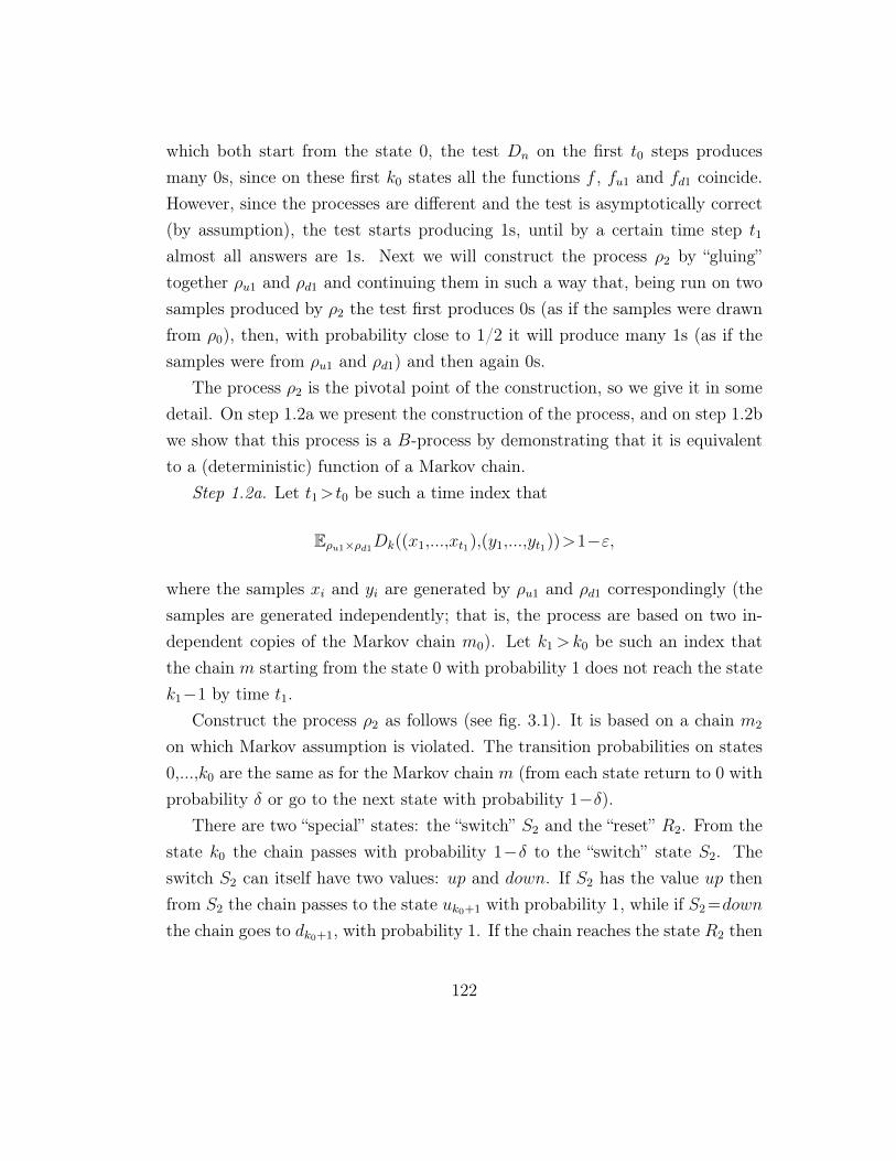
which both start from the state 0, the test Dn on the first t0 steps producesmany 0s, since on these first k0 states all the functions f , fu1 and fd1 coincide.However, since the processes are different and the test is asymptotically correct(by assumption), the test starts producing 1s, until by a certain time step t1
almost all answers are 1s. Next we will construct the process ρ2 by “gluing”together ρu1 and ρd1 and continuing them in such a way that, being run on twosamples produced by ρ2 the test first produces 0s (as if the samples were drawnfrom ρ0), then, with probability close to 1/2 it will produce many 1s (as if thesamples were from ρu1 and ρd1) and then again 0s.
The process ρ2 is the pivotal point of the construction, so we give it in somedetail. On step 1.2a we present the construction of the process, and on step 1.2bwe show that this process is a B-process by demonstrating that it is equivalentto a (deterministic) function of a Markov chain.
Step 1.2a. Let t1>t0 be such a time index that
Eρu1×ρd1Dk((x1,...,xt1),(y1,...,yt1))>1−ε,
where the samples xi and yi are generated by ρu1 and ρd1 correspondingly (thesamples are generated independently; that is, the process are based on two in-dependent copies of the Markov chain m0). Let k1>k0 be such an index thatthe chain m starting from the state 0 with probability 1 does not reach the statek1−1 by time t1.
Construct the process ρ2 as follows (see fig. 3.1). It is based on a chain m2
on which Markov assumption is violated. The transition probabilities on states0,...,k0 are the same as for the Markov chain m (from each state return to 0 withprobability δ or go to the next state with probability 1−δ).
There are two “special” states: the “switch” S2 and the “reset” R2. From thestate k0 the chain passes with probability 1−δ to the “switch” state S2. Theswitch S2 can itself have two values: up and down. If S2 has the value up thenfrom S2 the chain passes to the state uk0+1 with probability 1, while if S2 =down
the chain goes to dk0+1, with probability 1. If the chain reaches the state R2 then
122
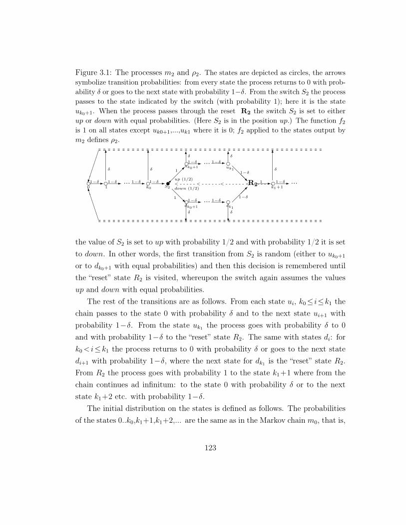
Figure 3.1: The processes m2 and ρ2. The states are depicted as circles, the arrowssymbolize transition probabilities: from every state the process returns to 0 with prob-ability δ or goes to the next state with probability 1−δ. From the switch S2 the processpasses to the state indicated by the switch (with probability 1); here it is the stateuk0+1. When the process passes through the reset R2 the switch S2 is set to eitherup or down with equal probabilities. (Here S2 is in the position up.) The function f2
is 1 on all states except uk0+1,...,uk1 where it is 0; f2 applied to the states output bym2 defines ρ2.
d0-1−δ d
1-1−δ ... -1−δ d
k0
-1−δS2
t up (1/2)
down (1/2)
1
duk0+1
-1−δ ... -1−δ duk1
@@R1 ddk0+1
-1−δ ... -1−δ ddk1
@@@R1−δ
1−δ
R2< - - - - - < - - - - - -< - - - - - - < - - - - - - --1 dk1+1-1−δ ...
- - - - - - - - - - - - - - - - - - - - - - - - - - - - - - - - - - - - - - - - - - - - - - -- - - - - - - - - - - - - - - - - - - - - - - - - - - - - - - - - - - - - - - - - - - - - - -6
δ
6
δ
6δ 6δ
?δ
?δ
6
δ
BBBBBM
- - - - - - - - - - - - - - - - - - - - - - - - - - - - - - - - - - - - - - - - - - - - - - -- - - - - - - - - - - - - - - - - - - - - - - - - - - - - - - - - - - - - - - - - - - - - - -
the value of S2 is set to up with probability 1/2 and with probability 1/2 it is setto down. In other words, the first transition from S2 is random (either to uk0+1
or to dk0+1 with equal probabilities) and then this decision is remembered untilthe “reset” state R2 is visited, whereupon the switch again assumes the valuesup and down with equal probabilities.
The rest of the transitions are as follows. From each state ui, k0≤ i≤k1 thechain passes to the state 0 with probability δ and to the next state ui+1 withprobability 1−δ. From the state uk1 the process goes with probability δ to 0and with probability 1−δ to the “reset” state R2. The same with states di: fork0<i≤k1 the process returns to 0 with probability δ or goes to the next statedi+1 with probability 1−δ, where the next state for dk1 is the “reset” state R2.From R2 the process goes with probability 1 to the state k1+1 where from thechain continues ad infinitum: to the state 0 with probability δ or to the nextstate k1+2 etc. with probability 1−δ.
The initial distribution on the states is defined as follows. The probabilitiesof the states 0..k0,k1+1,k1+2,... are the same as in the Markov chain m0, that is,
123
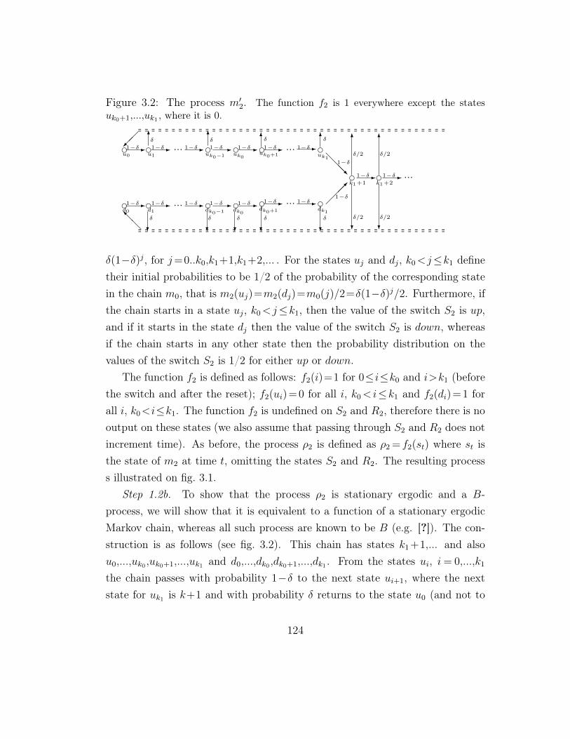
Figure 3.2: The process m′2. The function f2 is 1 everywhere except the statesuk0+1,...,uk1 , where it is 0.
du0
-1−δ du1
-1−δ ... -1−δ duk0−1
-1−δ duk0
-1−δ
dd0-1−δ d
d1-1−δ ... -1−δ d
dk0−1
-1−δ ddk0
-1−δ
duk0+1
-1−δ ... -1−δ duk1
ddk0+1
-1−δ ... -1−δ ddk1
@@@R1−δ
1−δ
dk1+1-1−δ d
k1+2-1−δ ...
- - - - - - - - - - - - - - - - - - - - - - - - - - - - - - - - - - - - - - - - - - - - - -- - - - - - - - - - - - - - - - - - - - - - - - - - - - - - - - - - - - - - - - - - - - - -6δ 6δ 6δ 6δ
?δ
?δ
?δ
?δ
?δ
- - - - - - - - - - - - - - - - - - - - - - - - - - - - - - - - - - - - - - - - - - - - - -- - - - - - - - - - - - - - - - - - - - - - - - - - - - - - - - - - - - - - - - - - - - - -
6
δ/2
6
δ/2
?δ/2
?δ/2
@@I
δ(1−δ)j, for j=0..k0,k1+1,k1+2,... . For the states uj and dj, k0<j≤k1 definetheir initial probabilities to be 1/2 of the probability of the corresponding statein the chain m0, that is m2(uj)=m2(dj)=m0(j)/2=δ(1−δ)j/2. Furthermore, ifthe chain starts in a state uj, k0<j≤k1, then the value of the switch S2 is up,and if it starts in the state dj then the value of the switch S2 is down, whereasif the chain starts in any other state then the probability distribution on thevalues of the switch S2 is 1/2 for either up or down.
The function f2 is defined as follows: f2(i)=1 for 0≤i≤k0 and i>k1 (beforethe switch and after the reset); f2(ui) = 0 for all i, k0<i≤k1 and f2(di) = 1 forall i, k0<i≤k1. The function f2 is undefined on S2 and R2, therefore there is nooutput on these states (we also assume that passing through S2 and R2 does notincrement time). As before, the process ρ2 is defined as ρ2 = f2(st) where st isthe state of m2 at time t, omitting the states S2 and R2. The resulting processs illustrated on fig. 3.1.
Step 1.2b. To show that the process ρ2 is stationary ergodic and a B-process, we will show that it is equivalent to a function of a stationary ergodicMarkov chain, whereas all such process are known to be B (e.g. [?]). The con-struction is as follows (see fig. 3.2). This chain has states k1 +1,... and alsou0,...,uk0 ,uk0+1,...,uk1 and d0,...,dk0 ,dk0+1,...,dk1 . From the states ui, i= 0,...,k1
the chain passes with probability 1−δ to the next state ui+1, where the nextstate for uk1 is k+1 and with probability δ returns to the state u0 (and not to
124
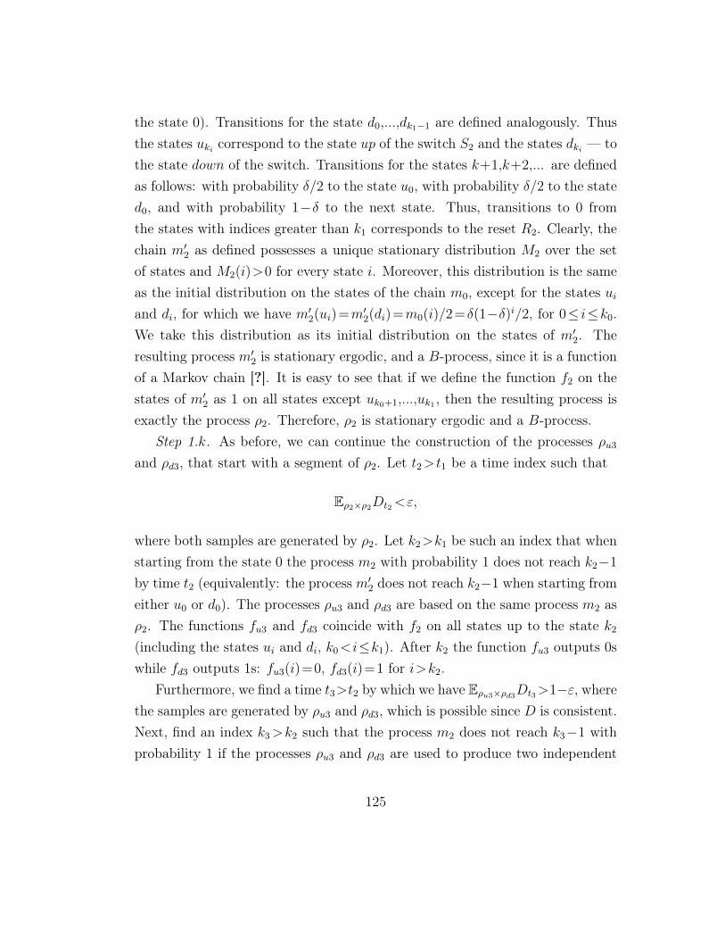
the state 0). Transitions for the state d0,...,dk1−1 are defined analogously. Thusthe states uki correspond to the state up of the switch S2 and the states dki — tothe state down of the switch. Transitions for the states k+1,k+2,... are definedas follows: with probability δ/2 to the state u0, with probability δ/2 to the stated0, and with probability 1−δ to the next state. Thus, transitions to 0 fromthe states with indices greater than k1 corresponds to the reset R2. Clearly, thechain m′2 as defined possesses a unique stationary distribution M2 over the setof states and M2(i)>0 for every state i. Moreover, this distribution is the sameas the initial distribution on the states of the chain m0, except for the states uiand di, for which we have m′2(ui)=m′2(di)=m0(i)/2= δ(1−δ)i/2, for 0≤ i≤k0.We take this distribution as its initial distribution on the states of m′2. Theresulting process m′2 is stationary ergodic, and a B-process, since it is a functionof a Markov chain [?]. It is easy to see that if we define the function f2 on thestates of m′2 as 1 on all states except uk0+1,...,uk1 , then the resulting process isexactly the process ρ2. Therefore, ρ2 is stationary ergodic and a B-process.
Step 1.k. As before, we can continue the construction of the processes ρu3
and ρd3, that start with a segment of ρ2. Let t2>t1 be a time index such that
Eρ2×ρ2Dt2<ε,
where both samples are generated by ρ2. Let k2>k1 be such an index that whenstarting from the state 0 the process m2 with probability 1 does not reach k2−1
by time t2 (equivalently: the process m′2 does not reach k2−1 when starting fromeither u0 or d0). The processes ρu3 and ρd3 are based on the same process m2 asρ2. The functions fu3 and fd3 coincide with f2 on all states up to the state k2
(including the states ui and di, k0<i≤k1). After k2 the function fu3 outputs 0swhile fd3 outputs 1s: fu3(i)=0, fd3(i)=1 for i>k2.
Furthermore, we find a time t3>t2 by which we have Eρu3×ρd3Dt3>1−ε, wherethe samples are generated by ρu3 and ρd3, which is possible since D is consistent.Next, find an index k3>k2 such that the process m2 does not reach k3−1 withprobability 1 if the processes ρu3 and ρd3 are used to produce two independent
125
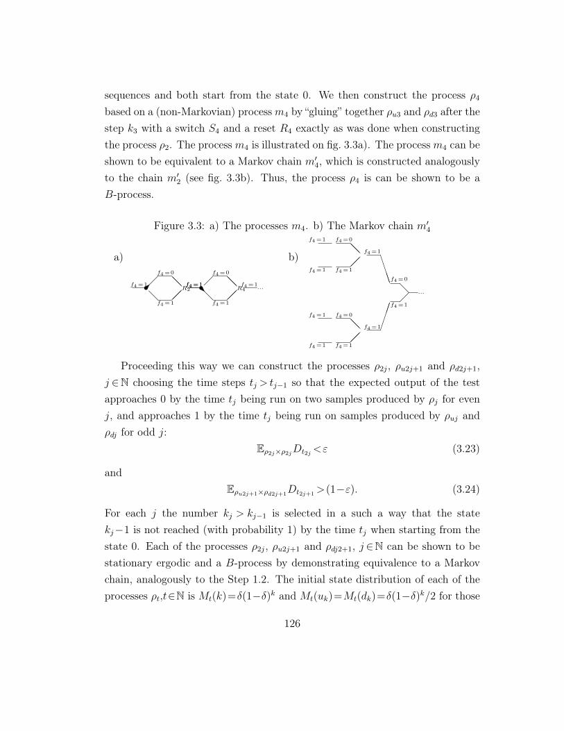
sequences and both start from the state 0. We then construct the process ρ4
based on a (non-Markovian) processm4 by “gluing” together ρu3 and ρd3 after thestep k3 with a switch S4 and a reset R4 exactly as was done when constructingthe process ρ2. The processm4 is illustrated on fig. 3.3a). The processm4 can beshown to be equivalent to a Markov chain m′4, which is constructed analogouslyto the chain m′2 (see fig. 3.3b). Thus, the process ρ4 is can be shown to be aB-process.
Figure 3.3: a) The processes m4. b) The Markov chain m′4
s
@
@@
R2
f4=0
f4=1
f4=1
f4=1sR@
@@
R4
f4=0
f4=1
f4=1
f4=1...
@@
f4=0f4=1
f4=1 f4=1
f4=1
@@
f4=0f4=1
f4=1 f4=1
f4=1
@ ...
BBBB
f4=0
f4=1
a) b)
Proceeding this way we can construct the processes ρ2j, ρu2j+1 and ρd2j+1,j ∈N choosing the time steps tj > tj−1 so that the expected output of the testapproaches 0 by the time tj being run on two samples produced by ρj for evenj, and approaches 1 by the time tj being run on samples produced by ρuj andρdj for odd j:
Eρ2j×ρ2jDt2j<ε (3.23)
andEρu2j+1×ρd2j+1
Dt2j+1>(1−ε). (3.24)
For each j the number kj > kj−1 is selected in a such a way that the statekj−1 is not reached (with probability 1) by the time tj when starting from thestate 0. Each of the processes ρ2j, ρu2j+1 and ρdj2+1, j ∈N can be shown to bestationary ergodic and a B-process by demonstrating equivalence to a Markovchain, analogously to the Step 1.2. The initial state distribution of each of theprocesses ρt,t∈N is Mt(k)=δ(1−δ)k and Mt(uk)=Mt(dk)=δ(1−δ)k/2 for those
126
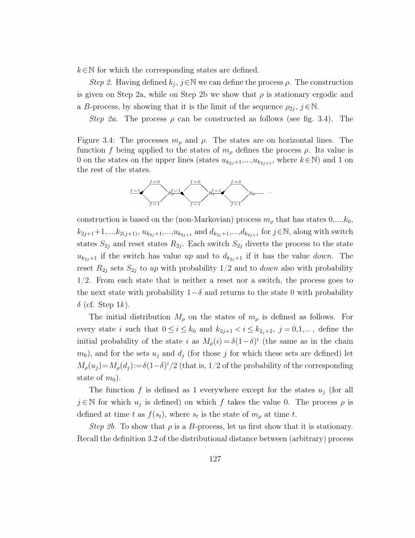
k∈N for which the corresponding states are defined.Step 2. Having defined kj, j∈N we can define the process ρ. The construction
is given on Step 2a, while on Step 2b we show that ρ is stationary ergodic anda B-process, by showing that it is the limit of the sequence ρ2j, j∈N.
Step 2a. The process ρ can be constructed as follows (see fig. 3.4). The
Figure 3.4: The processes mρ and ρ. The states are on horizontal lines. Thefunction f being applied to the states of mρ defines the process ρ. Its value is0 on the states on the upper lines (states uk2j+1,...,uk2j+1
, where k∈N) and 1 onthe rest of the states.
s
@
@@
R2
f=0
f=1
f=1
sR@
@@
R4
f=0
f=1
f=1
s
@
@@
R6
f=0
f=1
f=1
...
construction is based on the (non-Markovian) process mρ that has states 0,...,k0,k2j+1+1,...,k2(j+1), uk2j+1,...,uk2j+1
and dk2j+1,...,dk2j+1for j∈N, along with switch
states S2j and reset states R2j. Each switch S2j diverts the process to the stateuk2j+1 if the switch has value up and to dk2j+1 if it has the value down. Thereset R2j sets S2j to up with probability 1/2 and to down also with probability1/2. From each state that is neither a reset nor a switch, the process goes tothe next state with probability 1−δ and returns to the state 0 with probabilityδ (cf. Step 1k).
The initial distribution Mρ on the states of mρ is defined as follows. Forevery state i such that 0≤ i≤ k0 and k2j+1 < i≤ k2j+2, j = 0,1,... , define theinitial probability of the state i as Mρ(i) = δ(1−δ)i (the same as in the chainm0), and for the sets uj and dj (for those j for which these sets are defined) letMρ(uj)=Mρ(dj):=δ(1−δ)i/2 (that is, 1/2 of the probability of the correspondingstate of m0).
The function f is defined as 1 everywhere except for the states uj (for allj ∈N for which uj is defined) on which f takes the value 0. The process ρ isdefined at time t as f(st), where st is the state of mρ at time t.
Step 2b. To show that ρ is a B-process, let us first show that it is stationary.Recall the definition 3.2 of the distributional distance between (arbitrary) process
127
distributions. The set of all stochastic processes, equipped with this distance, iscomplete, and the set of all stationary processes is its closed subset [36]. Thus,to show that the process ρ is stationary it suffices to show that limj→∞d(ρ2j,ρ)=
0, since the processes ρ2j, j ∈ N, are stationary. To do this, it is enough todemonstrate that
limj→∞|ρ((x1,...,x|B|)=B)−ρ2j((x1,...,x|B|)=B)|=0 (3.25)
for each B ∈X∗. Since the processes mρ and m2j coincide on all states up tok2j+1, we have
|ρ(xn=a)−ρ2j(xn=a)|= |ρ(x1 =a)−ρ2j(x1 =a)|
≤∑
k>k2j+1
Mρ(k)+∑
k>k2j+1
M2j(k)
for every n∈N and a∈X. Moreover, for any tuple B∈X∗ we obtain
|ρ((x1,...,x|B|)=B)−ρ2j((x1,...,x|B|)=B)|
≤|B|
∑k>k2j+1
Mρ(k)+∑
k>k2j+1
M2j(k)
→0
where the convergence follows from k2j→∞. We conclude that (3.25) holds true,so that d(ρ,ρ2j)→0 and ρ is stationary.
To show that ρ is a B-process, we will demonstrate that it is the limit ofthe sequence ρ2k, k∈N in the d distance (which was only defined for stationaryprocesses). Since the set of all B-process is a closed subset of all stationaryprocesses, it will follow that ρ itself is a B-process. (Observe that this way weget ergodicity of ρ “for free”, since the set of all ergodic processes is closed in ddistance, and all the processes ρ2j are ergodic.) In order to show that d(ρ,ρ2k)→0
we have to find for each j a processes ν2j on pairs (x1,y1),(x2,y2),... , such that xiare distributed according to ρ and yi are distributed according to ρ2j, and such
128
that limj→∞ν2j(x1 6=y1)=0. Construct such a coupling as follows. Consider thechains mρ and m2j, which start in the same state (with initial distribution beingMρ) and always take state transitions together, where if the process mρ is in thestate ut or dt, t≥k2j+1 (that is, one of the states which the chain m2j does nothave) then the chain m2j is in the state t. The first coordinate of the processν2j is obtained by applying the function f to the process mρ and the second byapplying f2j to the chain m2j. Clearly, the distribution of the first coordinate isρ and the distribution of the second is ρ2j. Since the chains start in the samestate and always take state transitions together, and since the chains mρ andm2j coincide up to the state k2j+1 we have ν2j(x1 6= y1)≤
∑k>k2j+1
Mρ(k)→ 0.Thus, d(ρ,ρ2j)→0, so that ρ is a B-process.
Step 3. Finally, it remains to show that the expected output of the test Ddiverges if the test is run on two independent samples produced by ρ.
Recall that for all the chains m2j, mu2j+1 and md2j+1 as well as for the chainmρ, the initial probability of the state 0 is δ. By construction, if the process mρ
starts at the state 0 then up to the time step k2j it behaves exactly as ρ2j thathas started at the state 0. In symbols, we have
Eρ×ρ(Dt2j |sx0 =0,sy0 =0)=Eρ2j×ρ2j(Dt2j |sx0 =0,sy0 =0) (3.26)
for j ∈N, where sx0 and sy0 denote the initial states of the processes generatingthe samples x and y correspondingly.
We will use the following simple decomposition
E(Dtj)=δ2E(Dtj |sx0 =0,sy0 =0)+(1−δ2)E(Dtj |sx0 6=0 or sy0 6=0), (3.27)
From this, (3.26) and (3.23) we have
Eρ×ρ(Dt2j)≤δ2Eρ×ρ(Dt2j |sx0 =0,sy0 =0)+(1−δ2)
=δ2Eρ2j×ρ2j(Dt2j |sx0 =0,sy0 =0)+(1−δ2)
≤Eρ2j×ρ2j+(1−δ2)<ε+(1−δ2). (3.28)
129
For odd indices, if the process ρ starts at the state 0 then (from the definitionof t2j+1) by the time t2j+1 it does not reach the reset R2j; therefore, in this casethe value of the switch S2j does not change up to the time t2j+1. Since thedefinition of mρ is symmetric with respect to the values up and down of eachswitch, the probability that two samples x1,...,xt2j+1
and y1,...,yt2j+1generated
independently by (two runs of) the process ρ produced different values of theswitch S2j when passing through it for the first time is 1/2. In other words, withprobability 1/2 two samples generated by ρ starting at the state 0 will look bythe time t2j+1 as two samples generated by ρu2j+1 and ρd2j+1 that has started atstate 0. Thus
Eρ×ρ(Dt2j+1|sx0 =0,sy0 =0)≥ 1
2Eρu2j+1×ρd2j+1
(Dt2j+1|sx0 =0,sy0 =0) (3.29)
for j∈N. Using this, (3.27), and (3.24) we obtain
Eρ×ρ(Dt2j+1)≥δ2Eρ×ρ(Dt2j+1
|sx0 =0,sy0 =0)
≥ 1
2δ2Eρ2j+1×ρ2j+1
(Dt2j+1|sx0 =0,sy0 =0)
≥ 1
2
(Eρ2j+1×ρ2j+1
(Dt2j+1)−(1−δ2)
)>
1
2(δ2−ε). (3.30)
Taking δ large and ε small (e.g. δ = 0.9 and ε = 0.1), we can make thebound (3.28) close to 0 and the bound (3.30) close to 1/2, and the expectedoutput of the test will cross these values infinitely often. Therefore, we haveshown that the expected output of the test D diverges on two independent runsof the process ρ, contradicting the consistency ofD. This contradiction concludesthe proof.
130
Chapter 4
Finding an optimal strategy in areactive environment [R7]
Many real-world “learning” problems (like learning to drive a car or playing agame) can be modelled as an agent π that interacts with an environment µ andis (occasionally) rewarded for its behaviour. We are interested in agents whichperform well in the sense of having high long-term reward, also called the valueV (µ,π) of agent π in environment µ. If µ is known, it is a pure (non-learning)computational problem to determine the optimal agent πµ :=argmaxπV (µ,π). Itis far less clear what an “optimal” agent means, if µ is unknown. A reasonableobjective is to have a single policy π with high value simultaneously in manyenvironments. We will formalize and call this criterion self-optimizing later.
This problem generalizes dramatically the problem of sequence prediction,as well as those of classification and (to a large extent) hypothesis testing. Forexample, the problem of sequence prediction is a special case in which actionshave no impact on the environment. While being very general, the problem offinding an optimal strategy in a reactive environment is also very difficult; theresults of this chapter present some first steps in attacking this problem in fullgenerality.
Some related work. Reinforcement learning, sequential decision theory, adap-
131
tive control theory, and active expert advice, are theories dealing with this prob-lem. They overlap but have different core focus: Reinforcement learning algo-rithms [86] are developed to learn µ or directly its value. Temporal differencelearning is computationally very efficient, but has slow asymptotic guarantees(only) in (effectively) small observable MDPs. Others have faster guarantee infinite state MDPs [14]. There are algorithms [31] which are optimal for anyfinite connected POMDP, and this is apparently the largest class of environ-ments considered. In sequential decision theory, a Bayes-optimal agent π∗ thatmaximizes V (ξ,π) is considered, where ξ is a mixture of environments ν ∈ C
and C is a class of environments that contains the true environment µ∈C [41].Policy π∗ is self-optimizing in an arbitrary class C, provided C allows for self-optimizingness [40]. Adaptive control theory [57] considers very simple (froman AI perspective) or special systems (e.g. linear with quadratic loss function),which sometimes allow computationally and data efficient solutions. Action withexpert advice [24, 71, 72, 18] constructs an agent (called master) that performsnearly as well as the best agent (best expert in hindsight) from some class ofexperts, in any environment ν.
The difficulty in active learning problems can be identified (at least, for count-able classes) with traps in the environments. Initially the agent does not knowµ, so has asymptotically to be forgiven in taking initial “wrong” actions. Awell-studied such class are ergodic MDPs which guarantee that, from any actionhistory, every state can be (re)visited [40].
The results. The aim of this chapter is to characterize as general as possi-ble classes C in which self-optimizing behaviour is possible (more general thanPOMDPs). To do this, we need to characterize classes of environments thatforgive. For instance, exact state recovery is unnecessarily strong; it is sufficientbeing able to recover high rewards, from whatever states. Further, in manyreal world problems there is no information available about the “states” of theenvironment (e.g. in POMDPs) or the environment may exhibit long historydependencies.
We propose to consider only environments in which, after any arbitrary finite
132

sequence of actions, the best value is still achievable. The performance criterionhere is asymptotic average reward. Thus we consider such environments forwhich there exists a policy whose asymptotic average reward exists and upper-bounds asymptotic average reward of any other policy. Moreover, the sameproperty should hold after any finite sequence of actions has been taken (notraps). We call such environments recoverable. If we only want to get ε-close tothe optimal value infinitely often with decreasing ε (that is, to have the sameupper limit for the average value), then this property is already sufficient.
Yet recoverability in itself is not sufficient for identifying behaviour whichresults in optimal limiting average value. We require further that, from anysequence of k actions, it is possible to return to the optimal level of rewardin o(k) steps; that is, it is not just possible to recover after any sequence of(wrong) actions, but it is possible to recover fast. Environments which possessthis property are called value-stable. (These conditions will be formulated in aprobabilistic form.)
We show that for any countable class of value-stable environments there existsa policy which achieves best possible value in any of the environments from theclass (i.e. is self-optimizing for this class).
Furthermore, we present some examples of environments which possess value-stability and/or recoverability. In particular, any ergodic MDP can be easilyshown to be value-stable. A mixing-type condition which implies value-stabilityis also demonstrated. In addition, we provide a construction allowing to buildexamples of value-stable and/or recoverable environments which are not iso-morphic to a finite POMDP, thus demonstrating that the class of value-stableenvironments is quite general.
Finally, we consider environments which are not recoverable but still arevalue-stable. In other words, we consider the question of what does it mean tobe optimal in an environment which does not “forgive” wrong actions. Even insuch cases some policies are better than others, and we identify some conditionswhich are sufficient for learning a policy that is optimal from some point on.
It is important in our argument that the class of environments for which
133
we seek a self-optimizing policy is countable, although the class of all value-stable environments is uncountable. To find a set of conditions necessary andsufficient for learning which do not rely on countability of the class is yet anopen problem. However, from a computational perspective countable classesare sufficiently large (e.g. the class of all computable probability measures iscountable). In view of the results of the previous chapters, in particular, of theresults on sequence prediction, countable classes of environments are a naturalfirst step to solve the general problem of characterizing learnability.
4.1 Problem formulation
The agent framework is general enough to allow modelling nearly any kind of(intelligent) system. In cycle k, an agent performs action yk∈Y (output) whichresults in observation ok∈O and reward rk∈R, followed by cycle k+1 and so on.We assume that the action space Y, the observation space O, and the rewardspace R⊂IR are finite, w.l.g. R=0,...,rmax. We abbreviate zk :=ykrkok∈Z :=
Y×R×O and xk=rkok∈X :=R×O. An agent is identified with a (probabilistic)policy π. Given history z<k, the probability that agent π acts yk in cycle k is (bydefinition) π(yk|z<k). Thereafter, environment µ provides (probabilistic) rewardrk and observation ok, i.e. the probability that the agent perceives xk is (bydefinition) µ(xk|z<kyk). Note that policy and environment are allowed to dependon the complete history. We do not make any MDP or POMDP assumption here,and we do not talk about states of the environment, only about observations.Each (policy,environment) pair (π,µ) generates an I/O sequence zπµ1 zπµ2 ... . Moreformally, history zπµ1..k is a random variable with probability
P(zπµ1..k = z1..k
)= π(y1) · µ(x1|y1) · ... · π(yk|z<k) · µ(xk|z<kyk).
Since value maximizing policies can always be chosen deterministic, there is noreal need to consider probabilistic policies, and henceforth we consider determin-istic policies p. We assume that µ∈C is the true, but unknown, environment,
134
and ν∈C a generic environment.For an environment ν and a policy p define random variables (upper and
lower average value)
V (ν, p) := lim supm
1mrpν1..m
and V (ν, p) := lim inf
m
1mrpν1..m
where r1..m :=r1+...+rm. If there exists a constant V or a constant V such that
V (ν, p) = V a.s., or V (ν, p) = V a.s.
then we say that the upper limiting average or (respectively) lower average valueexists, and denote it by V (ν,p) :=V (or V (ν,p) :=V ). If both upper and loweraverage limiting values exist and are equal then we simply say that averagelimiting value exist and denote it by V (ν,p) :=V (ν,p)=V (ν,p)
An environment ν is explorable if there exists a policy pν such that V (ν,pν)
exists and V (ν,p)≤ V (ν,pν) with probability 1 for every policy p. In this casedefine V ∗ν := V (ν,pν). An environment ν is upper explorable if there exists apolicy pν such that V (ν,pν) exists and V (ν,p)≤ V (ν,pν) with probability 1 forevery policy p. In this case define V ∗ν :=V (ν,pν).
A policy p is self-optimizing for a set of explorable environments C if V (ν,p)=
V ∗ν for every ν ∈ C. A policy p is upper self-optimizing for a set of explorableenvironments C if V (ν,p)=V
∗ν for every ν∈C.
In the case when we we wish to obtain the optimal average value for anyenvironment in the class we will speak about self-optimizing policies, whereasif we are only interested in obtaining the upper limit of the average value thenwe will speak about upper self-optimizing policies. It turns out that the lattercase is much more simple. The next two definitions present conditions on theenvironments which will be shown to be sufficient to achieve the two respectivegoals.
Definition 4.1 (recoverable). We call an upper explorable environment ν recov-erable if for any history z<k such that ν(x<k|y<k)>0 there exists a policy p such
135
thatP (V (ν,p)=V
∗ν |z<k)=1.
Conditioning on the history z<k means that we take ν-conditional probabil-ities (conditional on x<k) and first k−1 actions of the policy p are replaced byy<k.
Recoverability means that after taking any finite sequence of (possibly sub-optimal) actions it is still possible to obtain the same upper limiting averagevalue as an optimal policy would obtain. The next definition is somewhat morecomplex.
Definition 4.2 (value-stable environments). An explorable environment ν isvalue-stable if there exist a sequence of numbers rνi ∈ [0,rmax] and two functionsdν(k,ε) and ϕν(n,ε) such that 1
nrν1..n→V ∗ν , dν(k,ε)=o(k),
∑∞n=1ϕν(n,ε)<∞ for
every fixed ε, and for every k and every history z<k there exists a policy p=pz<kν
such thatP(rνk..k+n − r
pνk..k+n > dν(k, ε) + nε | z<k
)≤ ϕν(n, ε). (4.1)
First of all, this condition means that the strong law of large numbers forrewards holds uniformly over histories z<k; the numbers rνi here can be thoughtof as expected rewards of an optimal policy. Furthermore, the environment is“forgiving” in the following sense: from any (bad) sequence of k actions it ispossible (knowing the environment) to recover up to o(k) reward loss; to recovermeans to reach the level of reward obtained by the optimal policy which fromthe beginning was taking only optimal actions. That is, suppose that a personA has made k possibly suboptimal actions and after that “realized” what thetrue environment was and how to act optimally in it. Suppose that a person Bwas from the beginning taking only optimal actions. We want to compare theperformance of A and B on first n steps after the step k. An environment isvalue stable if A can catch up with B except for o(k) gain. The numbers rνi canbe thought of as expected rewards of B; A can catch up with B up to the rewardloss dν(k,ε) with probability ϕν(n,ε), where the latter does not depend on pastactions and observations (the law of large numbers holds uniformly).
136
Examples of value-stable environments will be considered in Section 4.4.
4.2 Self-optimizing policies for a set of value-stable
environments
In this section we present the main self-optimizingness result along with aninformal explanation of its proof, and a result on upper self-optimizingness,which turns out to have much more simple conditions.
Theorem 4.3 (value-stable⇒self-optimizing). For any countable set C of value-stable environments, there exists a policy which is self-optimizing for C.
A formal proof is given in Section 4.6; here we give some intuitive justifica-tion. Suppose that all environments in C are deterministic. We will constructa self-optimizing policy p as follows: Let νt be the first environment in C. Thealgorithm assumes that the true environment is νt and tries to get ε-close toits optimal value for some (small) ε. This is called an exploitation part. If itsucceeds, it does some exploration as follows. It picks the first environment νe
which has higher average asymptotic value than νt (V ∗νe >V ∗νt) and tries to getε-close to this value acting optimally under νe. If it can not get close to theνe-optimal value then νe is not the true environment, and the next environmentcan be picked for exploration (here we call “exploration” successive attempts toexploit an environment which differs from the current hypothesis about the trueenvironment and has a higher average reward). If it can, then it switches toexploitation of νt, exploits it until it is ε′-close to V ∗νt , ε
′<ε and switches to νe
again this time trying to get ε′-close to Vνe ; and so on. This can happen only afinite number of times if the true environment is νt, since V ∗νt<V
∗νe . Thus after
exploration either νt or νe is found to be inconsistent with the current history. Ifit is νe then just the next environment νe such that V ∗νe>V ∗νt is picked for explo-ration. If it is νt then the first consistent environment is picked for exploitation(and denoted νt). This in turn can happen only a finite number of times before
137
the true environment ν is picked as νt. After this, the algorithm still continuesits exploration attempts, but can always keep within εk→0 of the optimal value.This is ensured by d(k)=o(k).
The probabilistic case is somewhat more complicated since we can not saywhether an environment is “consistent” with the current history. Instead we testeach environment for consistency as follows. Let ξ be a mixture of all environ-ments in C. Observe that together with some fixed policy each environment µcan be considered as a measure on Z∞. Moreover, it can be shown that (for anyfixed policy) the ratio ν(z<n)
ξ(z<n)is bounded away from zero if ν is the true environ-
ment µ and tends to zero if ν is singular with µ (in fact, here singularity is aprobabilistic analogue of inconsistency). The exploration part of the algorithmensures that at least one of the environments νt and νe is singular with ν onthe current history, and a succession of tests ν(z<n)
ξ(z<n)≥αs with αs→ 0 is used to
exclude such environments from consideration.
Upper self-optimizingness. Next we consider the task in which our goal ismore moderate. Rather than trying to find a policy which will obtain the sameaverage limiting value as an optimal one for any environment in a certain class,we will try to obtain only the optimum upper limiting average. That is, wewill try to find a policy which infinitely often gets as close as desirable to themaximum possible average value. It turns out that in this case a much simplercondition is sufficient: recoverability instead of value-stability.
Theorem 4.4 (recoverable⇒upper self-optimizing). For any countable class C
of recoverable environments, there exists a policy which is upper self-optimizingfor C.
A formal proof can be found in Section 4.6; its idea is as follows. The upperself-optimizing policy p to be constructed will loop through all environments inC in such a way that each environment is tried infinitely often, and for eachenvironment the agent will try to get ε-close (with decreasing ε) to the upper-limiting average value, until it either manages to do so, or a special stopping
138
condition holds: ν(z<n)ξ(z<n)
<αs, where αs is decreasing accordingly. This conditionnecessarily breaks if the upper limiting average value cannot be achieved.
4.3 Non-recoverable environments
Before proceeding with examples of value-stable environments, we briefly discusswhat can be achieved if an environment does not forgive initial wrong actions,that is, is not recoverable. It turns out that value-stability can be defined fornon-recoverable environments as well, and optimal — in a worst-case sense —policies can be identified.
For an environment ν, a policy p and a history z<k such that ν(x<k|y<k)>0,if there exists a constant V or a constant V such that
P (V (ν,p) = V |z<k)=1, or P (V (ν,p) = V |z<k)=1,
then we say that the upper conditional (on z<k) limiting average or (respectively)lower conditional average value exists, and denote it by V (ν,p,z<k) := V (orV (ν,p,z<k) := V ). If both upper and lower conditional average limiting valuesexist and are equal then we say that that average conditional value exist anddenote it by V (ν,p,(z<k)) :=V (ν,p,z<k)=V (ν,p,z<k)
Call an environment ν strongly (upper) explorable if for any history z<k suchthat ν(x<k|y<k)> 0 there exists a policy pz<kν such that V (ν,pz<kν ) (V (ν,pz<kν ))exists and V (ν,p,z<k)≤ V (ν,pz<kν ,z<k) (respectively V (ν,p,z<k)≤ V (ν,pz<kν ,z<k))with probability 1 for every policy p. In this case define V ∗ν (z<k) := V (ν,pz<kν )
(respectively V ∗ν(z<k) :=V (ν,pz<kν )).For a strongly explorable environment ν define the worst-case optimal value
W ∗ν := inf
k,z<k:ν(x<k>0)V ∗ν (z<k),
139
and for a strongly upper explorable ν define the worst-case upper optimal value
W∗ν := inf
k,z<k:ν(x<k>0)V∗ν(z<k).
In words, the worst-case optimal value is the asymptotic average reward whichis attainable with certainty after any finite sequence of actions has been taken.
Note that a recoverable explorable environment is also strongly explorable.A policy p will be called worst-case self-optimizing or worst-case upper self-
optimizing for a class of environments C if lim inf 1mrpν1m≥W ∗
ν , or (respectively)lim sup 1
mrpν1m≥W
∗ν with probability 1 for every ν∈C, where r1..m :=r1+...+rm.
Definition 4.5 (worst-case value-stable environments). A strongly explorableenvironment ν is worst-case value-stable if there exists a sequence of num-bers rνi ∈ [0,rmax] and two functions dν(k,ε) and ϕν(n,ε) such that 1
nrν1..n→W ∗
ν ,dν(k,ε) = o(k),
∑∞n=1ϕν(n,ε)<∞ for every fixed ε, and for every k and every
history z<k there exists a policy p=pz<kν such that
P(rνk..k+n − r
pνk..k+n > dν(k, ε) + nε | z<k
)≤ ϕν(n, ε). (4.2)
Note that a recoverable environment is value-stable if and only if it is worst-case value-stable.
Worst-case value stability helps to distinguish between irreversible actions(or “traps”) and actions which result only in a temporary loss in performance;moreover, worst-case value-stability means that a temporary loss in performancecan only be short (sublinear).
Finally, we can establish the following result (cf. Theorems 4.3 and 4.4).
Theorem 4.6 (worst-case self-optimizing). (i) For any countable set of worst-case value-stable environments C there exist a policy p which is worst-caseself-optimizing for C.
(ii) For any countable set of strongly upper explorable environments C thereexist a policy p which is worst-case upper self-optimizing for C.
140
The proof of this theorem is analogous to the proofs of Theorems 4.3 and 4.4;the differences are explained in Section 4.6.
4.4 Examples
In this section we illustrate the applicability of the results of the previous sectionby classes of value-stable environments. These are also examples of recoverableenvironments, since recoverability is strictly weaker than value-stability. In theend of the section we also give some simple examples of recoverable but notvalue-stable environments.
We first note that passive environments are value-stable. An environmentis called passive if the observations and rewards do not depend on the actionsof the agent. Sequence prediction task provides a well-studied (and perhapsthe only reasonable) class of passive environments: in this task the agent isrequired to give the probability distribution of the next observation given theprevious observations. The true distribution of observations depends only on theprevious observations (and does not depend on actions and rewards). Since wehave confined ourselves to considering finite action spaces, the agent is requiredto give ranges of probabilities for the next observation, where the ranges arefixed beforehand. The reward 1 is given if all the ranges are correct and thereward 0 is given otherwise. It is easy to check that any such environment isvalue-stable with rνi ≡1, d(k,ε)≡1, ϕ(n,ε)≡0, since, knowing the distribution,one can always start giving the correct probability ranges (this defines the policypν).
Obviously, there are active value stable environments too. The next propo-sition provides some conditions on mixing rates which are sufficient for value-stability; we do not intend to provide sharp conditions on mixing rates but ratherto illustrate the relation of value-stability with mixing conditions.
We say that a stochastic process hk, k∈IN satisfies strong α-mixing conditions
141
with coefficients α(k) if (see e.g. [12])
supn∈IN
supB∈σ(h1,...,hn),C∈σ(hn+k,... )
|P (B ∩ C)− P (B)P (C)| ≤ α(k),
where σ() stands for the sigma-algebra generated by the random variables inbrackets. Loosely speaking, mixing coefficients α reflect the speed with whichthe process “forgets” about its past.
Proposition 4.7 (mixing and value-stability). Suppose that an explorable en-vironment ν is such that there exist a sequence of numbers rνi and a functiond(k) such that 1
nrν1..n→V ∗ν , d(k)=o(k), and for each z<k there exists a policy p
such that the sequence rpνi satisfies strong α-mixing conditions with coefficientsα(k)= 1
k1+εfor some ε>0 and
rνk..k+n − E(rpνk..k+n | z<k
)≤ d(k)
for any n. Then ν is value-stable.
Proof. Using the union bound we obtain
P(rνk..k+n − r
pνk..k+n > d(k) + nε
)≤ I
(rνk..k+n − Erpνk..k+n > d(k)
)+ P
(∣∣rpνk..k+n − Erpνk..k+n
∣∣ > nε).
The first term equals 0 by assumption and the second term for each ε can beshown to be summable using [12, Thm.1.3]: for a sequence of uniformly boundedzero-mean random variables ri satisfying strong α-mixing conditions the follow-ing bound holds true for any integer q∈ [1,n/2]
P (|r1..n| > nε) ≤ ce−ε2q/c + cqα
(n
2q
)for some constant c; in our case we just set q=n
ε2+ε .
(PO)MDPs. Applicability of Theorem 4.3 and Proposition 4.7 can be illus-
142
trated on (PO)MDPs. We note that self-optimizing policies for (uncountable)classes of finite ergodic MDPs and POMDPs are known [14, 31]; the aim of thepresent section is to show that value-stability is a weaker requirement than therequirements of these models, and also to illustrate applicability of our results.We call µ a (stationary) Markov decision process (MDP) if the probability ofperceiving xk∈X, given history z<kyk only depends on yk∈Y and xk−1. In thiscase xk ∈X is called a state, X the state space. An MDP µ is called ergodicif there exists a policy under which every state is visited infinitely often withprobability 1. An MDP with a stationary policy forms a Markov chain.
An environment is called a (finite) partially observable MDP (POMDP) ifthere is a sequence of random variables sk taking values in a finite space S calledthe state space, such that xk depends only on sk and yk, and sk+1 is independentof s<k given sk. Abusing notation the sequence s1..k is called the underlyingMarkov chain. A POMDP is called ergodic if there exists a policy such that theunderlying Markov chain visits each state infinitely often with probability 1.
In particular, any ergodic POMDP ν satisfies strong α-mixing conditionswith coefficients decaying exponentially fast in case there is a set H ⊂R suchthat ν(ri∈H) = 1 and ν(ri= r|si=s,yi=y) 6= 0 for each y∈Y,s∈S,r∈H,i∈ IN .Thus for any such POMDP ν we can use Proposition 4.7 with d(k,ε) a constantfunction to show that ν is value-stable:
Corollary 4.8 (POMDP⇒value-stable). Suppose that a POMDP ν is ergodicand there exists a set H⊂R such that ν(ri∈H)=1 and ν(ri=r|si=s,yi=y) 6=0
for each y ∈Y,h ∈ S,r ∈H, where S is the finite state space of the underlyingMarkov chain. Then ν is value-stable.
However, it is illustrative to obtain this result for MDPs directly, and in aslightly stronger form.
Proposition 4.9 (MDP⇒value-stable). Any finite-state ergodic MDP ν is avalue-stable environment.
Proof. Let d(k,ε)=0. Denote by µ the true environment, let z<k be the currenthistory and let the current state (the observation xk) of the environment be
143
a∈X, where X is the set of all possible states. Observe that for an MDP thereis an optimal policy which depends only on the current state. Moreover, such apolicy is optimal for any history. Let pµ be such a policy. Let rµi be the expectedreward of pµ on step i. Let l(a,b) =minn :xk+n= b|xk =a. By ergodicity of µthere exists a policy p for which El(b,a) is finite (and does not depend on k). Apolicy p needs to get from the state b to one of the states visited by an optimalpolicy, and then acts according to pµ. Let f(n) := nrmax
logn. We have
P(∣∣rµk..k+n − r
pµk..k+n
∣∣ > nε)≤ sup
a∈XP(∣∣E (rpµµk..k+n|xk = a
)− rpµk..k+n
∣∣ > nε))
≤ supa,b∈X
P (l(a, b) > f(n)/rmax)
+ supa∈X
P(∣∣E (rpµµk..k+n|xk = a
)− rpµµk..k+n
∣∣ > nε− 2f(n)∣∣∣xk = a
).
In the last term we have the deviation of the reward attained by the optimalpolicy from its expectation. Clearly, both terms are bounded exponentially inn.
In the examples above the function d(k,ε) is a constant and ϕ(n,ε) decaysexponentially fast. This suggests that the class of value-stable environmentsstretches beyond finite (PO)MDPs. We illustrate this guess by the constructionthat follows.
A general scheme for constructing value-stable environment or recover-able environments: infinitely armed bandit. Next we present a construction ofenvironments which cannot be modelled as finite POMDPs but are value-stableand/or recoverable. Consider the following environment ν. There is a countablefamily C′=ζi : i∈ IN of arms, that is, sources generating i.i.d. rewards 0 and1 (and, say, empty observations) with some probability δi of the reward being1. The action space Y consists of three actions Y = g,u,d. To get the nextreward from the current arm ζi an agent can use the action g. Let i denote theindex of the current arm. At the beginning i=0, the current arm is ζ0 and thenthe agent can move between arms as follows: it can move U(i) arms “up” usingthe action u (i.e. i := i+U(i)) or it can move D(i) arms “down” using the action
144
d (i.e. i := i−D(i) or 0 if the result is negative). The reward for actions u andd is 0. In all the examples below U(i)≡1, that is, the action u takes the agentone arm up.
Clearly, ν is a POMDP with countably infinite number of states in the un-derlying Markov chain, which (in general) is not isomorphic to a finite POMDP.
Proposition 4.10. If D(i) = i for all i∈ IN then the environment ν just con-structed is value-stable. If D(i) ≡ 1 then ν is recoverable but not necessarilyvalue-stable; that is, there are choices of the probabilities δi such that ν is notvalue-stable.
Proof. First we show that in either case (D(i)=i or D(i)=1) ν is explorable. Letδ=supi∈INδi. Clearly, V (ν,p′)≤δ with probability 1 for any policy p′ . A policy pwhich, knowing all the probabilities δi, achieves V (ν,p)=V (ν,p)=δ=:V ∗ν a.s., canbe easily constructed. Indeed, find a sequence ζ ′j, j∈IN , where for each j thereis i=: ij such that ζ ′j =ζi, satisfying limj→∞δij =δ. The policy p should carefullyexploit one by one the arms ζj, staying with each arm long enough to ensure thatthe average reward is close to the expected reward with εj probability, where εjquickly tends to 0, and so that switching between arms has a negligible impacton the average reward. Thus ν can be shown to be explorable. Moreover, apolicy p just sketched can be made independent on (observation and) rewards.
Next we show if D(i) = i, that is, the action d always takes the agent downto the first arm, then the environment in value-stable. Indeed, one can modifythe policy p (possibly allowing it to exploit each arm longer) so that on eachtime step t (from some t on) we have j(t)≤
√t, where j(t) is the number of the
current arm on step t. Thus, after any actions-perceptions history z<k one needsabout
√k actions (one action u and enough actions d) to catch up with p. So,
(4.1) can be shown to hold with d(k,ε)=√k, ri the expected reward of p on step
i (since p is independent of rewards, rpνi are independent), and the rates ϕ(n,ε)
exponential in n.To construct a non-value-stable environment with D(i)≡1, simply set δ0 =1
and δj=0 for j>0; then after taking n actions u one can only return to optimal
145
rewards with n actions (d), that is d(k) = o(n) cannot be obtained. Still it iseasy to check that recoverability is preserved, whatever the choice of δi.
In the above construction we can also allow the action d to bring the agentd(i)<i steps down, where i is the number of the current environment ζ, accordingto some (possibly randomized) function d(i), thus changing the function dν(k,ε)and possibly making it non-constant in ε and as close as desirable to linear.
4.5 Necessity of value-stability
Now we turn to the question of how tight the conditions of value-stability are.The following proposition shows that the requirement d(k,ε)=o(k) in (4.1) cannot be relaxed.
Proposition 4.11 (necessity of d(k,ε)=o(k)). There exists a countable familyof deterministic explorable environments C such that
• for any ν ∈C for any sequence of actions y<k there exists a policy p suchthat
rνn..k+n = rpνk..k+n for all n ≥ k,
where rνi are the rewards attained by an optimal policy pν (which from thebeginning was acting optimally), but
• for any policy p there exists an environment ν∈C such that V (ν,p)<V ∗ν .
Clearly, each environment from such a class C satisfies the value stabilityconditions with ϕ(n,ε)≡0 except d(k,ε)=k 6=o(k).
Proof. There are two possible actions yi ∈ a,b, three possible rewards ri ∈0,1,2 and no observations.
Construct the environment ν0 as follows: if yi=a then ri=1 and if yi=b thenri=0 for any i∈IN .
For each i let ni denote the number of actions a taken up to step i: ni :=
#j≤i :yj=a. For each s>0 construct the environment νs as follows: ri(a)=1
146
for any i, ri(b)=2 if the longest consecutive sequence of action b taken has lengthgreater than ni and ni≥s; otherwise ri(b)=0.
Suppose that there exists a policy p such that V (νi,p)=V ∗νi for each i>0 andlet the true environment be ν0. By assumption, for each s there exists such n
that#i ≤ n : yi = b, ri = 0 ≥ s > #i ≤ n : yi = a, ri = 1
which implies V (ν0,p)≤1/2<1=V ∗ν0 .
It is also easy to show that the uniformity of convergence in (4.1) can notbe dropped. That is, if in the definition of value-stability we allow the functionϕ(n,ε) to depend additionally on the past history z<k then Theorem 4.3 doesnot hold. This can be shown with the same example as constructed in the proofof Proposition 4.11, letting d(k,ε)≡ 0 but instead allowing ϕ(n,ε,z<k) to takevalues 0 and 1 according to the number of actions a taken, achieving the samebehaviour as in the example provided in the last proof.
Moreover, we show that the requirement that the class C to be learnt iscountable can not be easily withdrawn. Indeed, consider the class of all deter-ministic passive environments in the sequence prediction setting. In this taskan agent gets the reward 1 if yi = oi+1 and the reward 0 otherwise, where thesequence of observation oi is deterministic. Different sequences correspond todifferent environments. As it was mentioned before, any such environment νis value-stable with dν(k,ε)≡ 1, ϕν(n,ε)≡ 0 and rνi ≡ 1. Obviously, the class ofall deterministic passive environments is not countable. Since for every policyp there is an environment on which p errs exactly on each step, the class of alldeterministic passive environments can not be learned. Therefore, the followingstatement is valid:
Proposition 4.12. There exist (uncountable) classes of value-stable environ-ments for which there are no self-optimizing policies.
However, strictly speaking, even for countable classes value-stability is notnecessary for self-optimizingness. This can be demonstrated on the class νi :i>0
147
from the proof of Proposition 4.11. (Whereas if we add ν0 to the class a self-optimizing policy no longer exists.) So we have the following:
Proposition 4.13. There are countable classes of not value-stable environmentsfor which self-optimizing policies exist.
4.6 Longer proofs
In each of the proofs, a self-optimizing (or upper self-optimizing) policy p will beconstructed. When the policy p has been defined up to a step k, an environmentµ, endowed with this policy, can be considered as a measure on Zk. We assumethis meaning when we use environments as measures on Zk (e.g. µ(z<i)).
Proof of Theorem 4.3. A self-optimizing policy p will be constructed asfollows. On each step we will have two polices: pt which exploits and pe whichexplores; for each i the policy p either takes an action according to pt (p(z<i)=
pt(z<i)) or according to pe (p(z<i)=pe(z<i)), as will be specified below.In the algorithm below, i denotes the number of the current step in the
sequence of actions-observations. Let n = 1, s = 1, and jt = je = 0. Let alsoαs=2−s for s∈IN . For each environment ν, find such a sequence of real numbersενn that ενn→0 and
∑∞n=1ϕν(n,ε
νn)≤∞.
Let ß:IN→C be such a numbering that each ν∈C has infinitely many indices.For all i>1 define a measure ξ as follows
ξ(z<i) =∑ν∈C
wνν(z<i), (4.3)
where wν∈R are (any) such numbers that∑
νwν =1 and wν>0 for all ν∈C.Define T . On each step i let
T ≡ Ti :=
ν ∈ C :
ν(z<i)
ξ(z<i)≥ αs
Define νt. Set νt to be the first environment in T with index greater than ß(jt).
148
In case this is impossible (that is, if T is empty), increment s, (re)define T andtry again. Increment jt.Define νe. Set νe to be the first environment with index greater than ß(je) suchthat V ∗νe>V ∗νt and ν
e(z<k)>0, if such an environment exists. Otherwise proceedone step (according to pt) and try again. Increment je.Consistency. On each step i (re)define T . If νt /∈T , define νt, increment s anditerate the infinite loop. (Thus s is incremented only if νt is not in T or if T isempty.)
Start the infinite loop. Increment n.Let δ :=(V ∗νe−V ∗νt)/2. Let ε :=εν
t
n . If ε<δ set δ=ε. Let h=je.Prepare for exploration.
Increment h. The index h is incremented with each next attempt of exploringνe. Each attempt will be at least h steps in length.
Let pt=py<iνt and set p=pt.Let ih be the current step. Find k1 such that
ihk1
V ∗νt ≤ ε/8 (4.4)
Find k2>2ih such that for all m>k2∣∣∣∣ 1
m− ihrν
t
ih+1..m − V ∗νt∣∣∣∣ ≤ ε/8. (4.5)
Find k3 such thathrmax/k3<ε/8. (4.6)
Find k4 such that for all m>k4
1
mdνe(m, ε/4) ≤ ε/8,
1
mdνt(m, ε/8) ≤ ε/8 and
1
mdνt(ih, ε/8) ≤ ε/8. (4.7)
Moreover, it is always possible to find such k>maxk1,k2,k3,k4 that
1
2krν
e
k..3k ≥1
2krν
t
k..3k + δ. (4.8)
149
Iterate up to the step k.Exploration. Set pe=py<nνe . Iterate h steps according to p=pe. Iterate furtheruntil either of the following conditions breaks
(i)∣∣rνek..i−rpνk..i∣∣<(i−k)ε/4+dνe(k,ε/4),
(ii) i<3k.
(iii) νe∈T .
Observe that either (i) or (ii) is necessarily broken.If on some step νt is excluded from T then the infinite loop is iterated. If after
exploration νe is not in T then redefine νe and iterate the infinite loop. Ifboth νt and νe are still in T then return to “Prepare for exploration” (otherwisethe loop is iterated with either νt or νe changed).End of the infinite loop and the algorithm.
Let us show that with probability 1 the “Exploration” part is iterated only afinite number of times in a row with the same νt and νe.
Suppose the contrary, that is, suppose that (with some non-zero probability)the “Exploration” part is iterated infinitely often while νt,νe∈T . Observe that(4.1) implies that the νe-probability that (i) breaks is not greater than ϕνe(i−k,ε/4); hence by Borel-Cantelli lemma the event that (i) breaks infinitely oftenhas probability 0 under νe.
Suppose that (i) holds almost every time. Then (ii) should be broken exceptfor a finite number of times. We can use (4.4), (4.5), (4.7) and (4.8) to show thatwith probability at least 1−ϕνt(k−ih,ε/4) under νt we have 1
3krpν
t
1..3k≥V ∗νt+ε/2.Again using Borel-Cantelli lemma and k>2ih we obtain that the event that (ii)
breaks infinitely often has probability 0 under νt.Thus (at least) one of the environments νt and νe is singular with respect to
the true environment ν given the described policy and current history. Denotethis environment by ν ′. It is known (see e.g. [21, Thm.26]) that if measures µ
150
and ν are mutually singular then µ(x1,...,xn)ν(x1,...,xn)
→∞ µ-a.s. Thus
ν ′(z<i)
ν(z<i)→ 0 ν-a.s. (4.9)
Observe that (by definition of ξ) ν(z<i)ξ(z<i)
is bounded. Hence using (4.9) we can seethat
ν ′(z<i)
ξ(z<i)→ 0 ν-a.s.
Since s and αs are not changed during the exploration phase this implies that onsome step ν ′ will be excluded from T according to the “consistency” condition,which contradicts the assumption. Thus the “Exploration” part is iterated onlya finite number of times in a row with the same νt and νe.
Observe that s is incremented only a finite number of times since ν′(z<i)ξ(z<i)
isbounded away from 0 where ν ′ is either the true environment ν or any envi-ronment from C which is equivalent to ν on the current history. The latterfollows from the fact that ξ(z<i)
ν(z<i)is a submartingale with bounded expectation,
and hence, by the submartingale convergence theorem (see e.g. [30]) convergeswith ν-probability 1.
Let us show that from some step on ν (or an environment equivalent to it)is always in T and selected as νt. Consider the environment νt on some step i.If V ∗νt>V
∗ν then νt will be excluded from T since on any optimal for νt sequence
of actions (policy) measures ν and νt are singular. If V ∗νt <V∗ν than νe will be
equal to ν at some point, and, after this happens sufficient number of times, νt
will be excluded from T by the “exploration” part of the algorithm, s will bedecremented and ν will be included into T . Finally, if V ∗νt =V ∗ν then either theoptimal value V ∗ν is (asymptotically) attained by the policy pt of the algorithm,or (if pνt is suboptimal for ν) 1
irpν
t
1..i<V∗νt−ε infinitely often for some ε, which has
probability 0 under νt and consequently νt is excluded from T .Thus, the exploration part ensures that all environments not equivalent to ν
with indices smaller than ß(ν) are removed from T and so from some step on νt
is equal to (an environment equivalent to) the true environment ν.
151
We have shown in the “Exploration” part that n→∞, and so ενtn →0. Finally,using the same argument as before (Borel-Cantelli lemma, (i) and the definitionof k) we can show that in the “exploration” and “prepare for exploration” parts ofthe algorithm the average value is within ενtn of V ∗νt provided the true environmentis (equivalent to) νt.
Proof of Theorem 4.4. Let ß : IN→C be such a numbering that each ν ∈Chas infinitely many indices. Define the measure ξ as in (4.3). The policy p actsaccording to the following algorithm.
Set εs=αs=2−s for s∈IN , set j=1, s=n=1. The integer i will denote thecurrent step in time.
Do the following ad infinitum. Set ν to be the first environment in C withindex greater than ß(j). Find the policy pν which achieves the upper limitingaverage value with probability one (such policy exists by definition of recover-ability). Act according to pν until either∣∣∣∣1i rpν1..i − V
∗(p, pν)
∣∣∣∣ < εn (4.10)
orν(z<i)
ξ(z<i)< αs. (4.11)
Increment n, s, i.It can be easily seen that one of the conditions necessarily breaks. Indeed,
either in the true environment the optimal upper limiting average value for thecurrent environment ν can be achieved by the optimal policy pν , in which case(4.10) breaks; or it cannot be achieved, which means that ν and ξ are singular,which implies that (4.11) will be broken (see e.g. [21, Thm.26]; cf. the sameargument in the proof of Theorem 4.3). Since ν equals the true environmentinfinitely often and εn→0 we get the statement of the theorem.
Proof of Theorem 4.6 is analogous to the proofs of Theorems 4.3 and 4.4,except for the following. Instead of the optimal average value V ∗ν and upperoptimal average value V ∗ν the values V ∗ν (z<k) and V ∗ν(z<k) should be used, and
152

they should be updated after each step k.
153
Chapter 5
Classification [R9, R10]
The problem of classification (or pattern recognition) consists in assigning a(discrete-valued) label Y for an object X, on the basis of a sample of object-label pairs (X1,Y1),...,(Xn,Yn).
Classification is perhaps the one learning problem for which the question oflearnability is well-understood; at least, this is the case under the assumptionthat the examples (Xi,Yi) are independent and identically distributed. Whilethis assumption is very strong, it may be considered reasonable for a variety ofapplications (with some notable exceptions which we will consider below). Inthis setting, the question of statistical learnability is effectively solved by theVapnik-Chervonenkis theory; those classes of functions f can be learned (fromfinite samples) that have finite VC dimension [88]. In this case, one can useempirical risk minimization as a learning rule.
The contribution to this area presented here is two-fold. First, it is shownthat the i.i.d. requirement on the distribution of samples is redundant, in thesense that most of the learning algorithms developed to work under this settingcan be provably used in a more general (and, as it is argued below, more naturalfor many applications) setting. These results (extracted from my Ph.D. thesis)are presented in Section 5.1.
Second, it is demonstrated that the characterization of learnability presentedby the VC theory is not quite complete, in the sense the number of samples
154
required to learn a classification function increases from linear in the VC di-mension to arbitrary fast-growing functions, if one limits the consideration tocomputable methods only. This result is presented in Section 5.2.
5.1 Relaxing the i.i.d. assumption in classification
[R10]
As it was mentioned, the majority of methods developed for solving the problemof classification rely on the assumptions that the examples are independent andidentically distributed. This section is devoted to relaxing this assumption.
Consider the following example, that helps to motivate this problem. Sup-pose we are trying to recognise a hand-written text. Obviously, letters in thetext are dependent (for example, we strongly expect to meet “u” after “q”). Thisseemingly implies that classification methods can not be applied to this task,which is, however, one of their classical applications.
We show that the following two assumptions on the distribution of examplesare sufficient for classification. First, that the dependence between objects isonly that between their labels and the type of object-label dependence does notchange in time. Second, the rate of occurrence of each label should keep abovesome positive threshold.
These intuitive ideas lead us to the following model (to which we refer as “theconditional model”). The labels y ∈Y are drawn according to some unknown(but fixed) distribution over the set of all infinite sequences of labels. There canbe any type of dependence between labels; moreover, we can assume that weare dealing with any (fixed) combinatorial sequence of labels. However, in thissequence the rate of occurrence of each label should keep above some positivethreshold. For each label y the corresponding object x∈X is generated accordingto some (unknown but fixed) probability distribution P (x|y). All the rest is asin the i.i.d. model.
The main difference from the i.i.d. model is in that in the conditional model
155
the distribution of labels is arbitrary (apart from the frequency threshold re-quirement).
In this section we provide a tool for obtaining estimations of probability oferror of a predictor in the conditional model from an estimation of the proba-bility of error in the i.i.d. model. The general theorems about extending resultsconcerning performance of a predictor to the conditional model are illustratedon two classes of predictors. First, we extend weak consistency results concern-ing partitioning and nearest neighbour estimates from the i.i.d. model to theconditional model. Second, we use some results of Vapnik-Chervonenkis theoryto estimate performance in the conditional model (on finite amount of data) ofpredictors minimising empirical risk, and also obtain some strong consistencyresults.
These results on specific predictions methods are obtained as applicationsof the following observation. The only assumption on a predictor under whicha predictor works in the new model as well as in the i.i.d. model is what wecall tolerance to data (a stability-kind condition): in any large dataset there isno small subset which strongly changes the probability of error. This propertyshould also hold with respect to permutations. This assumption on a predictorshould be valid in the i.i.d. model. Thus, the results achieved in the i.i.d. modelcan be extended to the conditional model; this concerns distribution–free resultsas well as distribution–specific, results on the performance on finite samples aswell as asymptotic results.Related work. Various approaches to relaxing the i.i.d. assumption in learn-ing tasks have been proposed in the literature. Thus, in [56, 55] the the nearestneighbour and kernel estimators are studied in the setting of regression esti-mation with continuous regression function, under the assumption that labelsare conditionally independent given their objects, while objects form any indi-vidual sequence (which is the opposite to what we do). There are also severalapproaches in which different types of assumptions on the joint distribution ofobjects and labels are made; then the authors construct a predictor or a class ofpredictors, to work well under the assumptions made. Thus, in [34, 3] a general-
156
isation of PAC approach to Markov chains with finite or countable state space ispresented. There is also a track of research on prediction under the assumptionthat the distribution generating examples is stationary and ergodic. The basicdifference from our learning task, apart from different probabilistic assumption,is in that we are only concerned with object-label dependence, while in predict-ing ergodic sequences it is label-label (time series) dependence that is of primaryinterest. On this task see [78, 4, 64, 66] and references therein.
5.1.1 Definitions and general results
Consider a sequence of examples (x1,y1),(x2,y2),...; where each example zi :=
(xi,yi) consists of an object xi ∈X and a label yi := η(xi) ∈Y. Here X is ameasurable space, Y :=0,1, and η :X→Y is some deterministic function. Forsimplicity, we made the assumption that the space Y is binary, but all resultseasily extend to the case of any finite space Y. The notation Z := X×Y isused for the measurable space of examples. Objects are drawn according tosome probability distribution P on X∞ (and labels are defined by η). Thus weconsider only the case of deterministically defined labels (that is, the noise-freemodel).
The notation P is used for distributions onX∞ while the symbol P is reservedfor distributions on X. In the latter case P∞ denotes the i.i.d. distribution onX∞ generated by P . Correspondingly we will use symbols E, E and E∞ forexpectations over spaces X∞ and X.
The traditional assumption about the distribution P generating objects isthat examples are independently and identically distributed (i.i.d.) according tosome distribution P on X (i.e. P=P∞).
Here we replace this assumption with the following two conditions.First, for any n∈N and for any measurable set A⊂X
P(Xn∈A |Yn,X1,Y1,...,Xn−1,Yn−1)=P(Xn∈A |Yn) (5.1)
(i.e. some versions of conditional probabilities coincide). This condition looks
157
very much like Markov condition which requires that each object depends on thepast only through its immediate predecessor. The condition (5.1) says that eachobject depends on the past only through its label.
Second, for any y∈Y, for any n1,n2∈N and for any measurable set A⊂X
P(Xn1∈A |Yn1 =y)=P(Xn2∈A |Yn2 =y) (5.2)
(i.e. the process is uniform in time; (5.1) allows dependence in n).Note that the first condition means that objects are conditionally indepen-
dent given labels (on conditional independence see [22]).
Definition 5.1. Under the conditions (5.1) and (5.2) we say that objects areconditionally independent and identically distributed (conditionally i.i.d).
For each y∈Y denote the distributionP(Xn |Yn=y) by Py (it does not dependon n by (5.2) ). Clearly, the distributions P0 and P1 define some distributions Pon X up to a parameter p∈ [0,1]. That is, Pp(A)=pP1(A)+(1−p)P0(A) for anymeasurable set A⊂X and for each p∈ [0,1]. Thus with each distribution P satis-fying the assumptions (5.1) and (5.2) we will associate a family of distributionsPp, p∈ [0,1].
The assumptions of the conditional model can be also interpreted as follows.Assume that we have some individual sequence (yn)n∈N of labels and two proba-bility distributions P0 and P1 on X, such that there exists sets X0 and X1 in X
such that P1(X1) =P0(X0) = 1 and P0(X1) =P1(X0) = 0 (i.e. X0 and X1 definesome function η). Each example xn∈X is drawn according to the distributionPyn ; examples are drawn independently of each other.
A predictor is a measurable function Γn :=Γ(x1,y1,...,xn,yn,xn+1) taking val-ues in Y (more formally, a family of functions indexed by n).
The probability of error of a predictor Γ on each step n is defined as
errn(Γ,P,z1,...,zn) :=P
(x,y)∈Z :y 6=Γn(z1,...,zn,x)
(zi, 1≤i≤n are fixed and the probability is taken over zn+1). We will sometimes
158
omit some of the arguments of errn when it can cause no confusion; in particular,we will often use a short notation P(errn(Γ,Z1,...,Zn)>ε) and an even shorterone P(errn(Γ)>ε) in place of
Pz1,...,zn : errn(Γ,P,z1,...,zn)>ε
.
For a pair of distributions P0 and P1 and any δ∈(0,1/2) define
5δ(P0,P1,n,ε) := supp∈[δ,1−δ]
P∞p (errn(Γ)>ε) (5.3)
For a predictor Γ and a distribution P on X define
∆(P,n,z1,...,zn) := maxj≤κn; π:1,...,n→1,...,n
|errn(Γ,P∞,z1,...,zn)−
errn−j(Γ,P∞,zπ(1),...,zπ(n−j))|.
Define the tolerance to data of Γ as
∆(P,n,ε) :=P n(∆(P,n,Z1,...,Zn)>ε
)(5.4)
for any n∈N, any ε>0 and κn :=√nlogn. Furthermore, for a pair of distributions
P0 and P1 and any δ∈(0,1/2) define
∆δ(P0,P1,n,ε) := supp∈[δ,1−δ]
∆(Pp,n,ε).
Tolerance to data means, in effect, that in any typical large portion of datathere is no small portion that changes strongly the probability of error. Thisproperty should also hold with respect to permutations.
We will also use another version of tolerance to data, in which instead ofremoving some examples we replace them with an arbitrary sample z′j,...,z′n con-
159
sistent with η:
∆(P,z1,...,zn) := supj<κn;π:1,...,n→1,...,n;z′n−j ,...,z′n
|errn(Γ,P∞,z1,...,zn)−errn(Γ,P∞,ζ1,...,ζn)|,
where ζπ(i) :=zπ(i) if i<n−j and ζπ(i) :=z′i otherwise; the maximum is taken overall z′i, n−j<i≤n consistent with η. Define
∆(P,n,ε) :=P n(∆(P,n,Z1,...,Zn)>ε
)and
∆δ(P0,P1,n,ε) := supp∈[δ,1−δ]
∆(Pp,n,ε).
The same notational convention will be applied to ∆ and ∆ as to errn.Various notions similar to tolerance to data have been studied in literature.
Perhaps first they appeared in connection with deleted or condensed estimates(see e.g. [74]), and were later called stability (see [13, 48] for present studies ofdifferent kinds of stability, and for extensive overviews). Naturally, such notionsarise when there is a need to study the behaviour of a predictor when some of thetraining examples are removed. These notions are much similar to what we calltolerance to data, only we are interested in the maximal deviation of probabilityof error while usually it is the average or minimal deviations that are estimated.
A predictor developed to work in the off-line setting should be, loosely speak-ing, tolerant to small changes in a training sample. The next theorem showsunder which conditions this property of a predictor can be utilised.
Theorem 5.2. Suppose that a distribution P generating examples is such thatthe objects are conditionally i.i.d, i.e. P satisfies (5.1) and (5.2). Fix someδ ∈ (0,1/2], let p(n) := 1
n#i≤n : Yi = 1 and Cn :=P(δ≤ p(n)≤ 1−δ) for each
160
n∈N. Let also αn := 11−1/
√n. For any predictor Γ and any ε>0 we have
P(errn(Γ)>ε)≤C−1n αn
(5δ(P0,P1,n+κn,δε/2)
+∆δ(P0,P1,n+κn,δε/2))+(1−Cn), (5.5)
and
P(errn(Γ)>ε)≤C−1n αn
(5δ(P0,P1,n,δε/2)
+∆δ(P0,P1,n,δε/2))+(1−Cn). (5.6)
The proofs for this section can be found in Section 5.3.1.The theorem says that if we know with some confidence Cn that the rate of
occurrence of each label is not less than some (small) δ, and have some boundson the error rate and tolerance to data of a predictor in the i.i.d. model, thenwe can obtain bounds on its error rate in the conditional model.
Thus we have a tool for estimating the performance of a predictor on eachfinite step n. In Section 5.1.3 we will show how this result can be appliedto predictors minimising empirical risk. However, if we are only interested inasymptotic results the formulations can be somewhat simplified.
Consider the following asymptotic condition on the frequencies of labels.Define p(n) := 1
n#i≤n :Yi = 1. We say that the rates of occurrence of labels
are bounded from below if there exist such δ, 0<δ<1/2 that
limn→∞
P(p(n)∈ [δ,1−δ])=1. (5.7)
As the condition (5.7) means Cn→ 1 we can derive from Theorem 5.2 thefollowing corollary.
Corollary 5.3. Suppose that a distribution P satisfies (5.1), (5.2), and (5.7)for some δ∈(0,1/2]. Let Γ be such a predictor that
limn→∞5δ(P0,P1,n,ε)=0 (5.8)
161
and eitherlimn→∞
∆δ(P0,P1,n,ε)=0 (5.9)
orlimn→∞
∆δ(P0,P1,n,ε)=0 (5.10)
for any ε>0. ThenE(errn(Γ,P,Z1,...,Zn))→0.
In Section 5.1.2 we show how this statement can be applied to prove weakconsistence of some classical nonparametric predictors in the conditional model.
5.1.2 Application to classical nonparametric predictors
In this section we will consider two types of classical nonparametric predictors:partitioning and nearest neighbour classifiers.
The nearest neighbour predictor assigns to a new object xn+1 the label of itsnearest neighbour among x1,...,xn:
Γn(x1,y1,...,xn,yn,xn+1) :=yj,
where j :=argmini=1,...,n‖x−xi‖.For i.i.d. distributions this predictor is also consistent, i.e.
E∞(errn(Γ,P∞))→0,
for any distribution P on X (see [27]).We generalise this result as follows.
Theorem 5.4. Let Γ be the nearest neighbour classifier. Let P be some distri-bution on X∞ satisfying (5.1), (5.2) and (5.7). Then
E(errn(Γ,P))→0.
The proofs for this section can be found in Section 5.3.2.
162
A partitioning predictor on each step n partitions the object space X=Rd,d ∈ N into disjoint cells An1 ,An2 ,... and classifies in each cell according to themajority vote:
Γ(z1,...,zn,x) :=
0 if
∑ni=1Iyi=1Ixi∈A(x)≤
∑ni=1Iyi=0Ixi∈A(x)
1 otherwise,
where A(x) denotes the cell containing x. Define
diam(A) := supx,y∈A‖x−y‖
and
N(x) :=n∑i=1
Ixi∈A(x).
It is a well known result (see, e.g. [26]) that a partitioning predictor isweakly consistent, provided certain regulatory conditions on the size of cells.More precisely, let Γ be a partitioning predictor such that diam(A(X))→ 0 inprobability and N(X)→∞ in probability. Then for any distribution P on X
E∞(errn(Γ,P∞))→0.
We generalise this result to the case of conditionally i.i.d. examples as follows.
Theorem 5.5. Let Γ be a partitioning predictor such that diam(A(X))→ 0 inprobability and N(X)→∞ in probability, for any distribution generating i.i.d.examples. Then
E(errn(Γ,P))→0
for any distribution P on X∞ satisfying (5.1), (5.2) and (5.7).
Observe that we only generalise results concerning weak consistency of (one)nearest neighbour and non-data-dependent partitioning rules. More general re-sults exist (see e.g. [28]), in particular for data-dependent rules. However, wedo not aim to generalise state-of-the-art results in nonparametric classification,
163
but rather to illustrate that weak consistency results can be extended to theconditional model.
5.1.3 Application to empirical risk minimisation.
In this section we show how to estimate the performance of a predictor minimis-ing empirical risk (over certain class of functions) using Theorem 5.2. To do thiswe estimate the tolerance to data of such predictors, using some results fromVapnik-Chervonenkis theory. For the overviews of Vapnik-Chervonenkis theorysee [88, 26].
Let X=Rd for some d∈N and let C be a class of measurable functions of theform ϕ :X→Y=0,1, called decision functions. For a probability distributionP on X define err(ϕ,P ) :=P (ϕ(Xi) 6= Yi). If the examples are generated i.i.d.according to some distribution P , the aim is to find a function ϕ from C forwhich err(ϕ,P ) is minimal:
ϕP =argminϕ∈Cerr(ϕ,P ).
In the theory of empirical risk minimisation this function is approximated bythe function
ϕ∗n :=argminϕ∈C
errn(ϕ)
where errn(ϕ):=∑n
i=1Iϕ(Xi)6=Yi is the empirical error functional, based on a sam-ple (Xi,Yi), i= 1,...,n. Thus, Γn(z1,...,zn,xn+1) :=ϕ∗n(xn+1) is a predictor min-imising empirical risk over the class of functions C.
One of the basic results of Vapnik-Chervonenkis theory is the estimation ofthe difference of probabilities of error between the best possible function in theclass (ϕP ) and the function which minimises empirical error:
P(errn(Γ,P∞)−err(ϕP ,P )>ε
)≤8S(C,n)e−nε
2/128,
164
where the symbol S(C,n) is used for the n-th shatter coefficient of the class C:
S(C,n) := maxA:=x1,...,xn⊂X
#C∩A :C∈C.
Thus,P (errn(Γ)>ε)≤Ierr(ϕP ,P )>ε/2+8S(C,n)e−nε
2/512.
A particularly interesting case is when the optimal rule belongs to C, i.e. whenη∈C. This situation was investigated in e.g. [87]. Obviously, in this case ϕP ∈Cand err(ϕP ,P )=0 for any P . Moreover, a better bound exists (see [88, 26])
P (errn(Γ,P )>ε)≤2S(C,n)e−nε/2.
Theorem 5.6. Let C be a class of decision functions and let Γ be a predictorwhich for each n∈N minimises errn over C on the observed examples (z1,...,zn).Fix some δ∈ (0,1/2], let p(n) := 1
n#i≤n :Yi = 0 and Cn :=P(δ≤ p(n)≤ 1−δ)
for each n∈N. Assume n>4/ε2 and let αn := 11−1/
√n. We have
∆(P0,P1,n,ε)≤16S(C,n)e−nε2/512. (5.11)
(which does not depend on the distributions P0 and P1) and
P(errn(Γ,P)>ε)≤I2err(ϕP1/2 ,P1/2)>ε/2 (5.12)
+16αnC−1n S(C,n)e−nδ
2ε2/2048+(1−Cn).
If in addition η∈C then
∆(n,ε)≤4S(C,2n)2−nε)/8 (5.13)
and
P(errn(Γ,P)>ε)≤4αnC−1n S(C,n)e−nδε/16+(1−Cn). (5.14)
165
Thus, if we have bounds on the VC dimension of some class of classifiers, wecan obtain bounds on the performance of predictors minimising empirical errorfor the conditional model.
Next we show how strong consistency results can be achieved in the condi-tional model. For general strong universal consistency results (with examples)see [60, 88].
Denote the VC dimension of C by V (C):
V (C) :=maxn∈N :S(C,n)=2n.
Using Theorem 5.6 and Borel-Cantelli lemma, we obtain the following corollary.
Corollary 5.7. Let Ck, k∈N be a sequence of classes of decision functions withfinite VC dimension such that limk→0infϕ∈Ckerr(ϕ,P )=0 for any distribution Pon X. If kn→∞ and V (Ckn )logn
n→0 as n→∞ then
err(Γ,P)→0P−a.s.
where Γ is a predictor which in each trial n minimises empirical risk over Ckn
and P is any distribution satisfying (5.1), (5.2) and∑∞
n=1(1−Cn)<∞.
In particular, if we use bound on the VC dimension on classes of neuralnetworks provided in [8] then we obtain the following corollary.
Corollary 5.8. Let Γ be a classifier that minimises the empirical error overthe class C(k), where C(k) is the class of neural net classifiers with k nodes inthe hidden layer and the threshold sigmoid, and k→∞ so that klogn/n→ 0 asn→∞. Let P be any distribution on X∞ satisfying (5.1) and (5.2) such that∑∞
n=1(1−Cn)<∞. Then
limn→∞
errn(Γ)=0 P−a.s.
166
5.2 Computational limitations on the statistical
characterizations of learnability in classifica-
tion [R9]
In this section we investigate the question of whether finite-step performanceguarantees can be obtained if we consider the class of computable (on someTuring machine) classification methods. To make the problem more realistic, weassume that the target classification function η (that maps objects to labels) isalso computable. Two definitions of target functions are considered: they areeither of the form 0,1∞→0,1 or 0,1t→Y for some t (which can be differentfor different target functions).
We show that there are classes Ck of functions for which the number ofexamples needed to approximate the classification problem to a certain accuracygrows faster in the VC dimension of the class than any computable function(rather than being linear as in the statistical setting, [88]). In particular thisholds if Ck is the class of all computable functions of length not greater than k,in which case k is a (trivial) upper bound of the VC dimension.
Importantly, the same negative result holds even if we allow the data to begenerated “actively,” e.g., by some algorithm, rather than just by some fixedprobability distribution.
To obtain this negative result we consider the task of data compression: animpossibility result for the task of data compression allows us to estimate thesample complexity for classification. We also analyse how tight the negativeresult is, and show that for some simple computable rule (based on the nearestneighbour estimate) the sample complexity is finite in k, under different defini-tions of computational classification task.
Related work. In comparison to the vast literature on classification, rel-atively little attention had been paid to the “computable” version of the task.There is a track of research in which different concepts of computable learnabil-ity of functions on countable domains are studied, see [44]. Another approach is
167
to consider classification methods as functions computable in polynomial time,or under other resource constraints. This approach leads to many interesting re-sults, but it usually considers more specific settings of a learning problem, suchas learning DNFs, finite automata, etc.
It may be interesting to observe the connection of the results for classifica-tion with another learning problem, sequence prediction. In one of its simplestforms this task is as follows: it is required to predict the next outcome of adeterministic sequence of symbols, where the sequence is assumed to be com-putable (is generated by some program). There is a predictor which can solveany such problem and the number of errors it makes is at most linear in thelength of the program generating the sequence (see, e.g. [41], Section 3.2.3).Such a predictor is not computable. Trivially, there is no computable predictorfor all computable sequences, since for any computable predictor a computablesequence can be constructed on which it errs at every trial, simply by revers-ing the predictions. Thus we have linear number of errors for non-computablepredictor versus infinitely many errors for any computable one; whereas in clas-sification, as we show, it is linear for a non-computable predictor versus growingfaster than any computable function for any computable predictor.
5.2.1 Notation and definitions
By computable functions we mean functions computable on a Turing machinewith an input tape, output tape, and some working tapes, the number of whichis supposed to be fixed throughout the section.
All computable functions can be encoded (in a canonical way) and thus theset of computable functions can be effectively enumerated. Fix some canonicalenumeration and define the length of a computable function η as l(η):=|n| wheren is the minimal number of η in such enumeration. For an introduction to thecomputability theory see, for example, [73].
From the set of all computable functions we are interested in labelling func-tions, that is, in functions which represent classification problems. In classifi-
168
cation a labelling function is usually a function from the interval [0,1] or [0,1]d
(sometimes more general spaces are considered) to a finite space Y := 0,1.As we are interested in computable functions, we should consider instead totalcomputable functions of the form 0,1∞→Y. However, since we require thatlabelling functions are total (defined on all inputs) and computable, it can beeasily shown (e.g. with König’s lemma [51]) that any such function never scansits input tape further than a certain position independent of the input. Thusapparently the smallest meaningful class of computable labelling functions thatwe can consider is the class of functions of the form 0,1t→Y for some t. So,we call a partial recursive function (or program) η a labelling function if thereexists such t=:t(η)∈N that η accepts all strings from Xt :=0,1t and only suchstrings. (It is not essential for this definition that η is not a total function. Anequivalent for our purposes definition would be as follows: a labelling function isany total function which outputs the string 00 on all inputs except on the stringsof some length t=: t(η), on each of which it outputs either 0 or 1.)
It can be argued that this definition of a labelling function is too restrictiveto approximate well the notion of a real function. However, as we are afternegative results (for the class of all labelling functions), it is not a disadvantage.Other possible definitions are discussed in Section 5.2.3, where we are concernedwith tightness of our negative results. In particular, all the results hold true if atarget function is any total computable function of the form 0,1∞→Y.
Define the task of computational classification as follows. An (unknown)labelling function η is fixed. The objects x1,...,xn ∈X are drawn according tosome distribution P on Xt(η). The labels yi are defined according to η, that isyi :=η(xi).
A predictor is a family of functions ϕn(x1,y1,...,xn,yn,x) (indexed by n) takingvalues in Y , such that for any n and any t∈N, if xi ∈Xt for each i, 1≤ i≤n,then the marginal ϕ(x) is a total function on Xt. We will often identify ϕn withits marginal ϕn(x) when the values of other variables are clear. Thus, given asample x1,y1,...,xn,yn of labelled objects of the same size t a predictor producesa labelling function on Xt which is supposed to approximate η.
169
A computable predictor is a total computable function from Xt×Y ×···×Xt×Y ×Xt to 0,1, where the arguments are assumed to be encoded into a singleinput in a certain fixed (simple canonical) way.
We are interested in what sample size is required to approximate a labellingfunction η.
For a (computable) predictor ϕ, a labelling function η and 0<ε∈R define
δn(ϕ,η,ε) :=supPt
Pt
x1,...,xn∈Xt :
Ptx∈Xt :ϕn(x1,y1,...,xn,yn,x) 6=η(x)
>ε,
where t=t(η) and Pt ranges over all distributions on Xt (i.i.d. on Xnt ). As usual
in PAC theory we have two probabilities here: the Pt-probability over a trainingsample of size n that the Pt-probability of error of a predictor ϕ exceeds ε; thenthe supremum is taken over all possible distributions Pt.
For any δ>0 define the sample complexity of η with respect to ϕ as
N(ϕ,η,δ,ε) :=minn∈N :δn(ϕ,η,ε)≤δ.
The number N(ϕ,η,δ,ε) is the minimal sample size required for a predictor ϕ toachieve ε-accuracy with probability 1−δ when the (unknown) labelling functionis η, under all probability distributions.
With the use of statistical learning theory [88] we can easily derive the fol-lowing statement
Proposition 5.9. There exists a predictor ϕ such that
N(ϕ,η,δ,ε)≤ constε
l(η)log1
δ
for any labelling function η and any ε,δ>0.
Observe that the bound is linear in the length of η.In the next section we investigate the question of whether any such bounds
170
exist if we restrict our attention to computable predictors.
Proof. The predictor ϕ is defined as follows. For each sample x1,y1,...,xn,yn itfinds a shortest program η such that η(xi) = yi for all i ≤ n. Clearly, l(η) ≤l(η). Observe that the VC-dimension of the class of all computable functionsof length not greater than l(η) is bounded from above by l(η), as there are notmore than 2l(η) such functions. Moreover, ϕ minimizes empirical risk over thisclass of functions. It remains to use the bound (see e.g. [26], Corollary 12.4)supη∈CN(ϕ,η,δ,ε)≤max
(V (C)8
εlog 13
δ,4εlog 2
δ
), where V (C) is the VC-dimension
of the class C.
5.2.2 Sample complexity explosion for computable
learning rules
The main result of this section is that for any computable predictor ϕ there isno computable upper bound in terms of l(η) on the sample complexity of thefunction η with respect to ϕ:
Theorem 5.10. For every computable predictor ϕ and every partial computablefunction β :N→N that has infinite domain and goes to infinity, there are infinitelymany functions η, such that for some n>β(l(η))
Px∈Xt(η) :ϕ(x1,y1,...,xn,yn,x) 6=η(x)>0.05,
for any x1,...,xn ∈Xt(η), where yi = η(xi) and P is the uniform distribution onXt(η).
For example, we can take β(n)=2n, or 22n .
Corollary 5.11. For any computable predictor ϕ, any total computable functionβ :N→N and any δ<1
supη:l(η)≤k
N(ϕ,η,δ,0.05)>β(k)
171
from some k on.
Observe that there is no δ in the formulation of Theorem 5.10. Moreover,it is not important how the objects (x1,...,xn) are generated — it can be anyindividual sample. In fact, we can assume that the sample is chosen in anymanner, for example by some algorithm. This means that no computable upperbound on sample complexity exists even for active learning algorithms.
It appears that the task of classification is closely related to another learningtask — data compression. Moreover, to prove Theorem 4.3 we need a similarnegative result for this task. Thus before proceeding with the proof of thetheorem, we introduce the task of data compression and derive a negative resultfor it. We call a total computable function ψ :X→X a data compressor if it isan injection (i.e. x1 6=x2 implies ψ(x1) 6=ψ(x2)). We say that a data compressorcompresses the string x if |ψ(x)| < |x|. Clearly, for any natural n any datacompressor compresses not more than half of the strings of size up to n.
Next we introduce Kolmogorov complexity; for fine details see [59]. Thecomplexity of a string x∈X with respect to a Turing machine ζ is defined as
Cζ(x)=minpl(p) :ζ(p)=x,
where p ranges over all binary strings (interpreted as partial computable com-putable functions; minimum over empty set is defined as ∞). There exists sucha machine ζ that Cζ(x)≤Cζ′(x)+cζ′ for any x and any machine ζ ′ (the constantcζ′ depends on ζ ′ but not on x). Fix any such ζ and define the Kolmogorovcomplexity of a string x∈X as
C(x) :=Cζ(x).
Clearly, C(x)≤|x|+b for any x and for some b depending only on ζ. A stringis called c-incompressible if C(x)≥|x|−c. Obviously, any data compressor cannot compresses many c-incompressible strings, for any c. However, highly com-pressible strings (that is, strings with Kolmogorov complexity low relatively to
172
their length) might be expected to be compressed well by some sensible datacompressor. The following lemma shows that this cannot be always the case, nomatter what we mean by “relatively low”.
The lemma is proven using the fact that there are no non-trivial computablelower bounds on Kolmogorov complexity; the lemma itself can be considered asa different formulation of this statement. The proof of the lemma is followed bythe proof of Theorem 5.10.
Lemma 5.12. For every data compressor ψ and every partial computable func-tion γ : N→ N which has an infinite domain and goes to infinity there existinfinitely many strings x such that C(x)≤γ(|x|) and |ψ(x)|≥|x|.
For example, we can take γ(n)=loglogn.
Proof. Suppose the contrary, i.e. that there exist a data compressor ψ and somefunction γ :N→N monotonically increasing to infinity such that if C(x)≤γ(|x|)then ψ(x)< |x| except for finitely many x. Let T be the set of all strings whichare not compressed by ψ
T :=x : |ψ(x)|≥|x|.
Define the function τ on the set T as follows: τ(x) is the number of theelement x in T
τ(x) :=#x′∈T :x′≤x
for each x∈T . Obviously, the set T is infinite. Moreover, τ(x)≤x for any x∈T(recall that we identify X and N via length-lexicographical ordering). Observethat τ is a total computable function on T and onto N. Thus τ−1 :N→X is atotal computable function on N. Hence, for any x∈T for which γ(|x|) is definedwe have, except for finitely many x:
C(τ(x))≥C(τ−1(τ(x))−c=C(x)−c>γ(|x|)−c, (5.15)
for a constant c depending only on τ , where the first inequality follows fromcomputability of τ−1 and the last from the definition of T . Since τ is computable
173
we also have C(τ(x))≤C(x)+c′ for some constant c′.It is a well-known result (see e.g. [59]) that for any unbounded partial com-
putable function δ with infinite domain there are infinitely many x∈X such thatC(x)≤ δ(|x|). In particular, allowing δ(|x|) = γ(|x|)−c′−2c, we conclude thatthere are infinitely many x∈T such that
C(τ(x))≤C(x)+c′≤γ(|τ(x)|)−2c≤γ(|x|)−2c,
which contradicts (5.15).
5.2.3 Different settings and tightness of the negative re-
sults
In this section we discuss how tight the conditions of the statements are and towhat extend they depend on the definitions.
Let us consider the question of whether there exists some (not necessarilycomputable) total sample-complexity function
Nϕ(k,δ,ε) := supη:l(η)≤k
N(ϕ,η,δ,ε),
at least for some predictor ϕ.
Proposition 5.13. There exists a predictor ϕ such that Nϕ(k,δ,ε)<∞ for anyε,δ>0 and any k∈N.
Indeed it is easy to see that the “pointwise” predictor
ϕ(x1,y1,...,xn,yn,x)=
yi if x=xi,1≤ i≤n0 x /∈x1,...,xn
(5.16)
satisfies the conditions of the proposition.It can be argued that probably this statement is due to our definition of a
labelling function. Next we will discuss some other variants of this definition.
174
First, observe that if we define a labelling function as any total computablefunction on 0,1∗ then some labelling functions will not approximate any func-tion on [0,1]; for example the function η+ which counts bitwise sum of its input:η+(x):=
∑|x|i=1xi mod 2. That is why we require a labelling function to be defined
only on Xt for some t.Another way to define a labelling function (which perhaps makes labelling
functions most close to real functions) is as a function which accepts any infinitebinary string. Let us call an i-labelling function any total recursive functionη :Y∞→Y. That is, η is computable on a Turing machine with an input tapeon which one way infinite input is written, an output tape and possibly someworking tapes. The program η is required to halt on any input. As it wasmentioned earlier, in this case the situation essentially does not change, since(as it is easy to show) for any i-labelling function η there exist nη∈N such thatη does not scan its input tape beyond position nη. In particular, η(x)=η(x′) assoon as xi =x′i for any i≤nη. Moreover, it is easy to check that Theorem 5.10holds for i-labelling functions as well. Finally, it can be easily verified thatProposition 5.13 holds true if we consider i-labelling functions instead of labellingfunctions, constructing the required predictor based on the nearest neighbourpredictor. Indeed, it suffices to replace the “pointwise” predictor in the proof ofProposition 5.13 by the predictor ϕ, which assigns to the object x the label ofthat object among x1,...,xn with whom x has longest mutual prefix (where theprefixes are compared up to some growing horizon).
5.3 Longer proofs
5.3.1 Proofs for Section 5.1.1
Before proceeding with the proof of Theorem 5.2 we give some definitions andsupplementary facts.
175
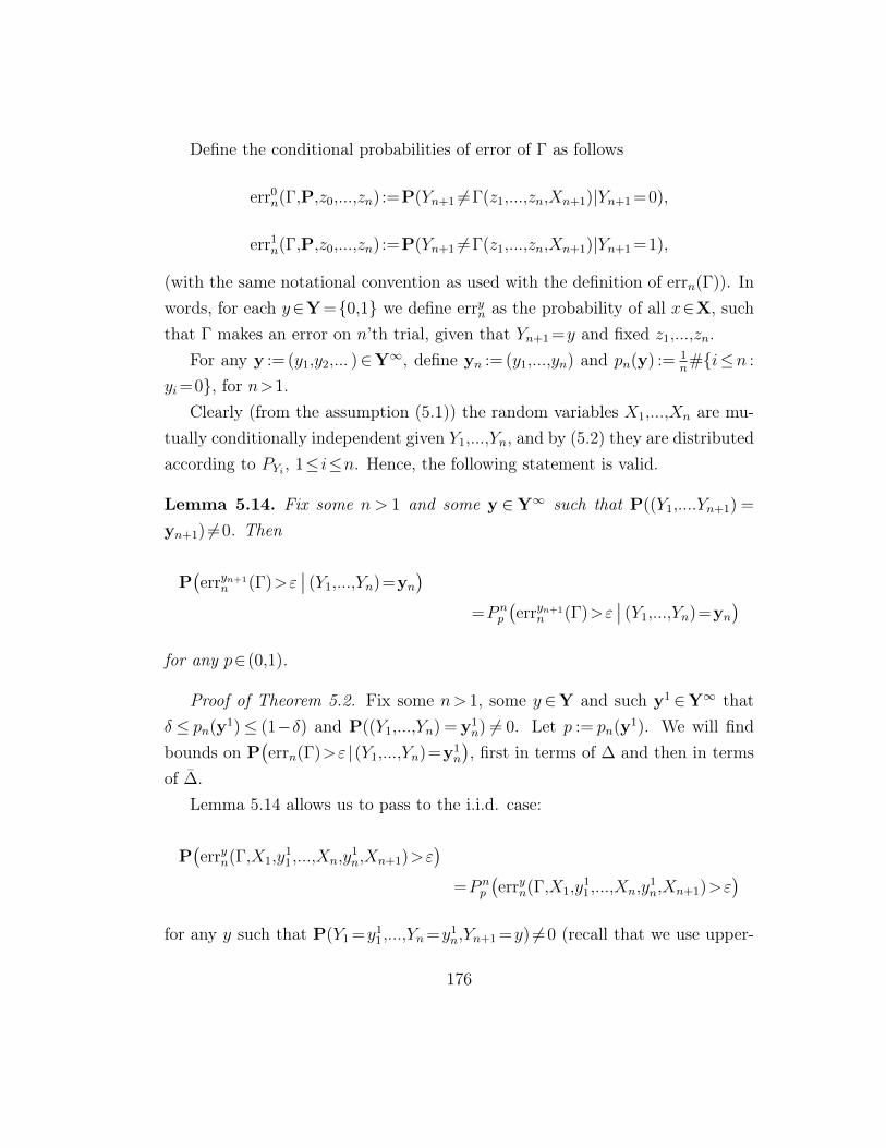
Define the conditional probabilities of error of Γ as follows
err0n(Γ,P,z0,...,zn) :=P(Yn+1 6=Γ(z1,...,zn,Xn+1)|Yn+1 =0),
err1n(Γ,P,z0,...,zn) :=P(Yn+1 6=Γ(z1,...,zn,Xn+1)|Yn+1 =1),
(with the same notational convention as used with the definition of errn(Γ)). Inwords, for each y∈Y=0,1 we define erryn as the probability of all x∈X, suchthat Γ makes an error on n’th trial, given that Yn+1 =y and fixed z1,...,zn.
For any y := (y1,y2,... )∈Y∞, define yn := (y1,...,yn) and pn(y) := 1n#i≤n :
yi=0, for n>1.Clearly (from the assumption (5.1)) the random variables X1,...,Xn are mu-
tually conditionally independent given Y1,...,Yn, and by (5.2) they are distributedaccording to PYi , 1≤ i≤n. Hence, the following statement is valid.
Lemma 5.14. Fix some n > 1 and some y ∈Y∞ such that P((Y1,....Yn+1) =
yn+1) 6=0. Then
P(erryn+1
n (Γ)>ε∣∣ (Y1,...,Yn)=yn
)=P n
p
(erryn+1
n (Γ)>ε∣∣ (Y1,...,Yn)=yn
)for any p∈(0,1).
Proof of Theorem 5.2. Fix some n> 1, some y∈Y and such y1 ∈Y∞ thatδ ≤ pn(y1)≤ (1−δ) and P((Y1,...,Yn) = y1
n) 6= 0. Let p := pn(y1). We will findbounds on P
(errn(Γ)>ε |(Y1,...,Yn)=y1
n
), first in terms of ∆ and then in terms
of ∆.Lemma 5.14 allows us to pass to the i.i.d. case:
P(erryn(Γ,X1,y
11,...,Xn,y
1n,Xn+1)>ε
)=P n
p
(erryn(Γ,X1,y
11,...,Xn,y
1n,Xn+1)>ε
)for any y such that P(Y1 =y1
1,...,Yn=y1n,Yn+1 =y) 6=0 (recall that we use upper-
176
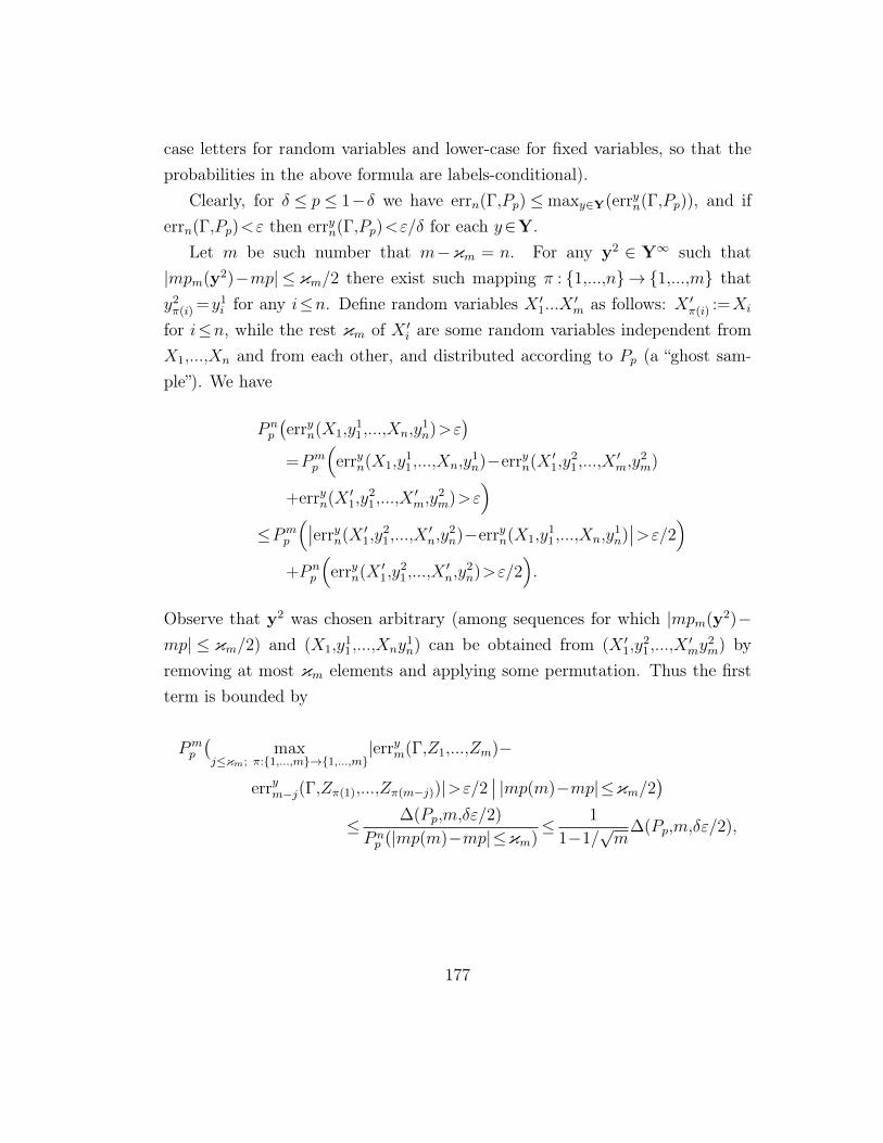
case letters for random variables and lower-case for fixed variables, so that theprobabilities in the above formula are labels-conditional).
Clearly, for δ ≤ p ≤ 1−δ we have errn(Γ,Pp) ≤maxy∈Y(erryn(Γ,Pp)), and iferrn(Γ,Pp)<ε then erryn(Γ,Pp)<ε/δ for each y∈Y.
Let m be such number that m−κm = n. For any y2 ∈ Y∞ such that|mpm(y2)−mp| ≤ κm/2 there exist such mapping π : 1,...,n→ 1,...,m thaty2π(i) =y1
i for any i≤n. Define random variables X ′1...X ′m as follows: X ′π(i) :=Xi
for i≤n, while the rest κm of X ′i are some random variables independent fromX1,...,Xn and from each other, and distributed according to Pp (a “ghost sam-ple”). We have
P np
(erryn(X1,y
11,...,Xn,y
1n)>ε
)=Pm
p
(erryn(X1,y
11,...,Xn,y
1n)−erryn(X ′1,y
21,...,X
′m,y
2m)
+erryn(X ′1,y21,...,X
′m,y
2m)>ε
)≤Pm
p
(∣∣erryn(X ′1,y21,...,X
′n,y
2n)−erryn(X1,y
11,...,Xn,y
1n)∣∣>ε/2)
+P np
(erryn(X ′1,y
21,...,X
′n,y
2n)>ε/2
).
Observe that y2 was chosen arbitrary (among sequences for which |mpm(y2)−mp| ≤ κm/2) and (X1,y
11,...,Xny
1n) can be obtained from (X ′1,y
21,...,X
′my
2m) by
removing at most κm elements and applying some permutation. Thus the firstterm is bounded by
Pmp
(max
j≤κm; π:1,...,m→1,...,m|errym(Γ,Z1,...,Zm)−
errym−j(Γ,Zπ(1),...,Zπ(m−j))|>ε/2∣∣ |mp(m)−mp|≤κm/2
)≤ ∆(Pp,m,δε/2)
P np (|mp(m)−mp|≤κm)
≤ 1
1−1/√m
∆(Pp,m,δε/2),
177
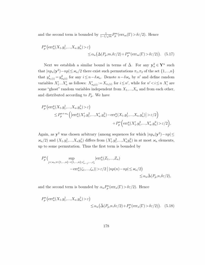
and the second term is bounded by 11−1/
√mPmp (errm(Γ)>δε/2). Hence
P np
(erryn(X1,y
11,...,Xn,y
1n)>ε
)≤αn
(∆(Pp,m,δε/2)+Pm
p (errm(Γ)>δε/2)). (5.17)
Next we establish a similar bound in terms of ∆. For any y2n ∈Yn such
that |npn(y2)−np|≤κn/2 there exist such permutations π1,π2 of the set 1,...,nthat y1
π1(i) = y2π2(i) for any i≤n−δκn. Denote n−δκn by n′ and define random
variables X ′1...X ′n as follows: X ′π2(i) :=Xπ1(i) for i≤n′, while for n′<i≤n X ′i aresome “ghost” random variables independent from X1,...,Xn and from each other,and distributed according to Pp. We have
P np
(erryn(X1,y
11,...,Xn,y
1n)>ε
)≤P n+κn
p
(∣∣erryn(X ′1,y21,...,X
′n,y
2n)−erryn(X1,y
11,...,Xn,y
1n)∣∣>ε/2)
+P np
(erryn(X ′1,y
21,...,X
′n,y
2n)>ε/2
),
Again, as y2 was chosen arbitrary (among sequences for which |npn(y2)−np|≤κn/2) and (X1,y
11,...,Xny
1n) differs from (X ′1,y
21,...,X
′ny
2n) in at most κn elements,
up to some permutation. Thus the first term is bounded by
P np
(sup
j<κn;π:1,...,n→1,...,n;z′n−j ,...,z′n|erryn(Z1,...,Zn)
−erryn(ζ1,...,ζn)|>ε/2∣∣ |np(n)−np|≤κn/2
)≤αn∆(Pp,n,δε/2),
and the second term is bounded by αnP np (errn(Γ)>δε/2). Hence
P np
(erryn(X1,y
11,...,Xn,y
1n)>ε
)≤αn
(∆(Pp,n,δε/2)+P n
p (errn(Γ)>δε/2)). (5.18)
178
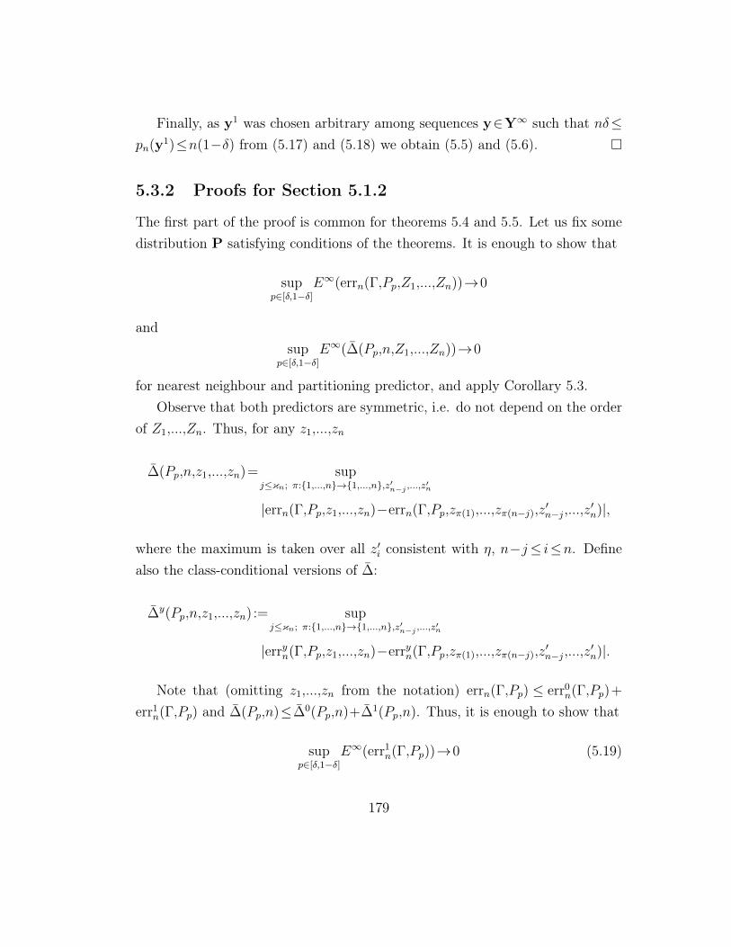
Finally, as y1 was chosen arbitrary among sequences y∈Y∞ such that nδ≤pn(y1)≤n(1−δ) from (5.17) and (5.18) we obtain (5.5) and (5.6).
5.3.2 Proofs for Section 5.1.2
The first part of the proof is common for theorems 5.4 and 5.5. Let us fix somedistribution P satisfying conditions of the theorems. It is enough to show that
supp∈[δ,1−δ]
E∞(errn(Γ,Pp,Z1,...,Zn))→0
andsup
p∈[δ,1−δ]E∞(∆(Pp,n,Z1,...,Zn))→0
for nearest neighbour and partitioning predictor, and apply Corollary 5.3.Observe that both predictors are symmetric, i.e. do not depend on the order
of Z1,...,Zn. Thus, for any z1,...,zn
∆(Pp,n,z1,...,zn)= supj≤κn; π:1,...,n→1,...,n,z′n−j ,...,z′n
|errn(Γ,Pp,z1,...,zn)−errn(Γ,Pp,zπ(1),...,zπ(n−j),z′n−j,...,z
′n)|,
where the maximum is taken over all z′i consistent with η, n−j≤ i≤n. Definealso the class-conditional versions of ∆:
∆y(Pp,n,z1,...,zn) := supj≤κn; π:1,...,n→1,...,n,z′n−j ,...,z′n
|erryn(Γ,Pp,z1,...,zn)−erryn(Γ,Pp,zπ(1),...,zπ(n−j),z′n−j,...,z
′n)|.
Note that (omitting z1,...,zn from the notation) errn(Γ,Pp) ≤ err0n(Γ,Pp)+
err1n(Γ,Pp) and ∆(Pp,n)≤∆0(Pp,n)+∆1(Pp,n). Thus, it is enough to show that
supp∈[δ,1−δ]
E∞(err1n(Γ,Pp))→0 (5.19)
179
andsup
p∈[δ,1−δ]E∞(∆1(Pp,n))→0. (5.20)
Observe that for each of the predictors in question the probability of errorgiven that the true label is 1 will not decrease if an arbitrary (possibly large)portion of training examples labelled with ones is replaced with an arbitrary(but consistent with η) portion of the same size of examples labelled with zeros.Thus, for any n and any p∈ [δ,1−δ] we can decrease the number of ones in oursample (by replacing the corresponding examples with examples from the otherclass) down to (say) δ/2, not decreasing the probability of error on exampleslabelled with 1. So,
E∞(err1n(Γ,Pp))≤E∞(err1
n(Γ,Pδ/2|pn=δ/2))+Pp(pn≤δ/2), (5.21)
where as usual pn := 1n#i≤n :yi=1. Obviously, the last term (quickly) tends
to zero. Moreover, it is easy to see that
E∞(err1n(Γ,Pδ/2)|pn=n(δ/2))
≤E∞(err1
n(Γ,Pδ/2)∣∣|n(δ/2)−pn|≤κn/2
)+E∞(∆1(Pδ/2,n))
≤ 1
1−1/√nE∞(err1
n(Γ,Pδ/2))+E∞(∆1(Pδ/2,n)). (5.22)
The first term tends to zero, as it is known from the results for i.i.d. processes;thus, to establish (5.19) we have to show that
E(∆1(Pp,n,Z1,...,Zn))→0 (5.23)
for any p∈(0,1).
180
We will also show that (5.23) is sufficient to prove (5.20). Indeed,
∆1(Pp,n,z1,...,zn)≤err1n(Γ,Pp,z1,...,zn)+
supj≤κn; π:1,...,n→1,...,n,z′n−j ,...,z′n
err1n(Γ,Pp,zπ(1),...,zπ(n−j),z
′n−j,...,z
′n)
Denote the last summand by D. Again, we observe that D will not decrease ifan arbitrary (possibly large) portion of training examples labelled with ones isreplaced with an arbitrary (but consistent with η) portion of the same size ofexamples labelled with zeros. Introduce ∆1(Pp,n,z1,...,zn) as ∆1(Pp,n,z1,...,zn)
with κn in the definition replaced by 2δκn. Using the same argument as in (5.21)
and (5.22) we have
E∞(D) ≤ 1
1−1/√n
(E∞(∆1(Pδ/2,n)) +E∞(errn(Γ,Pδ/2)
)+ Pp(pn ≤ δ/2).
Thus, (5.20) holds true if (5.23) and
E∞(∆1(Pp,n,Z1,...,Zn))→0. (5.24)
Finally, we will prove (5.23); it will be seen that the proof of (5.24) is analo-gous (i.e. replacing κn by 2
δκn does not affect the proof). Note that
E∞(∆(Pp,n,Z1,...,Zn))≤Pp(
supj≤κn; π:1,...,n→1,...,n,z′n−j ,...,z′n∣∣errn(Γ,Pp,Z1,...,Zn) 6=errn(Γ,Pp,Zπ(1),...,Zπ(n−j),z
′n−j,...,z
′)∣∣),
where the maximum is taken over all z′i consistent with η, n−j≤ i≤n. The lastexpression should be shown to tend to zero. This we will prove for each of thepredictors separately.
Nearest Neighbour predictor. Fix some distribution Pp, 0<p< 1 and some
181
ε>0. Fix also some n∈N and define (leaving x1,...,xn implicit)
Bn(x) :=P n+1p t∈X : t and x have the same nearest neighbour among x1,...,xn
and Bn :=E(Bn(X)) Note that E∞(Bn) = 1/n, where the expectation is takenover X1,...,Xn. Define B :=(x1,...,xn)∈Xn :Bn≤1/nε and A(x1,...,xn) :=x :
Bn(x)≤1/nε2. Applying Markov’s inequality twice, we obtain
E∞(∆(Pp,n))≤E∞(∆(Pp,n)|(X1,...,Xn)∈B)+ε
≤E∞(
supj≤κn; π:1,...,n→1,...,n,z′n−j ,...,z′n
Ppx : errn(Γ,Pp,Z1,...,Zn) 6=errn(Γ,Pp,Zπ(1),...,Zπ(n−j),z
′n−j,...,z
′n)∣∣x∈A(X1,...,Xn)
∣∣(X1,...,Xn)∈B)
+2ε.
(5.25)
Removing one point xi from a sample x1,...,xn we can only change the valueof Γ in the area
x∈X :xi is the nearest neighbour of x=Bn(xi),
while adding one point x0 to the sample we can change the value of Γ in the area
Dn(x0) :=x∈X :x0 is the nearest neighbour of x.
It can be shown that the number of examples (among x1,...,xn) for which a pointx0 is the nearest neighbour is not greater than a constant γ which depends onlythe space X (see [26], Corollary 11.1). Thus,
Dn(x0)⊂∪i=j1,...,jγBn(xi)
182
for some j1,...,jγ, and so
E∞(∆(Pp,n))≤2ε+2(γ+1)κnE∞( maxx∈A(X1,...,Xn)
Bn(x)|(X1,...,Xn)∈B)
≤2κnγ+1
nε2+2ε,
which, increasing n, can be made less than 3ε.
Partitioning predictor. For any measurable sets B⊂Xn and A⊂X define
D(B,A) :=E∞(
supj≤κn; π:1,...,n→1,...,n,z′n−j ,...,z′n
Ppx : errn(Γ,Pp,Z1,...,Zn) 6=errn(Γ,Pp,Zπ(1),...,Zπ(n−j),z
′n−j,...,z
′n)∣∣x∈A∣∣(X1,...,Xn)∈B
)+2ε.
and D :=D(Xn,X).Fix some distribution Pp, 0<p<1 and some ε>0. Introduce
η(x,X1,...,Xn) :=1
N(x)
n∑i=1
IYi=1IXi∈A(x)
(X1,...Xn will usually be omitted). From the consistency results for i.i.d. model(see, e.g. [26], Theorem 6.1) we know that En+1|ηn(X)−η(X)|→ 0 (the upperindex in En+1 indicating the number of examples it is taken over).
Thus, E|ηn(X)−η(X)| ≤ ε4 from some n on. Fix any such n and let B :=
(x1,...,xn) :E|ηn(X)−η(X)| ≤ ε2. By Markov inequality we obtain Pp(B)≥1−ε2. For any (x1,...,xn)∈B let A(x1,...,xn) be the union of all cells Ani for whichE(|ηn(X)−η(X)||X∈Ani )≤ε. Clearly, with x1,...,xn fixed, Pp(X∈A(x1,...,xn))≥1−ε. Moreover, D≤D(B,A)+ε+ε2.
Fix A := (x1,...,xn) for some (x1,...,xn)∈B. Since η(x) is always either 0 or1, to change a decision in any cell A⊂A we need to add or remove at least(1−ε)N(A) examples, where N(A):=N(x) for any x∈A. Let N(n):=E(N(X))
and A(n) :=E(Pp(A(X)). Clearly, N(n)nA(n)
=1 for any n, as EN(X)n
=A(n).
183
As before, using Markov inequality and shrinking A if necessary we can havePp(
ε2nA(X)N(n)
≤ ε|X ∈A) = 1, Pp( ε2nA(n)N(X)
≤ ε|X ∈A) = 1, and D≤D(B,A)+3ε+ε2.Thus, for all cells A⊂A we have N(A)≥εnA(n), so that the probability of errorcan be changed in at most 2 κn
(1−ε)εnA(n)cells; but the probability of each cell is
not greater than N(n)εn
. Hence E∞(∆(Pp,n))≤2 κnn(1−ε)ε2 +3ε+ε2.
5.3.3 Proofs for Section 5.1.3
Proof of Theorem 5.6. Fix some probability distribution Pp and some n ∈N.Let ϕ× be any decision rule ϕ ∈ C picked by Γn−κn on which (along with thecorresponding permutation) the maximum
maxj≤κn; π:1,...,n→1,...,n
|errn(Γ,z1,...,zn)−errn−j(Γ,zπ(1),...,zπ(n−j))|
is reached. We need to estimate P n(|err(ϕ∗)−err(ϕ×)|>ε).Clearly, |errn(ϕ×)−errn(ϕ∗)| ≤ κn, as κn is the maximal number of errors
which can be made on the difference of the two samples.Moreover,
P n(|err(ϕ∗n)−err(ϕ×)|>ε
)≤P n
(|err(ϕ∗n)− 1
nerrn(ϕ∗)|>ε/2
)+P n
(| 1n
errn(ϕ×)−err(ϕ×)|>ε/2−κn/n)
Observe that
P n(supϕ∈C| 1n
errn(ϕ)−err(ϕ)|>ε)≤8S(C,n)e−nε2/32, (5.26)
see [26], Theorem 12.6. Thus,
∆(Pp,n,ε)≤16S(C,n)e−n(ε/2−κn/n)2/32≤16S(C,n)e−nε2/512
184
for n>4/ε2. So,
P(errn(Γ,P)>ε)≤Isupp∈[δ,1−δ]err(ϕPp ,Pp)>ε/2
+16αC−1n S(C,n)e−nδ
2ε2/2048+(1−Cn).
It remains to notice that
err(ϕPp ,Pp)= infϕ∈C
(perr1(ϕ,Pp)+(1−p)err0(ϕ,Pp))
≤ infϕ∈C
(err1(ϕ,P1/2)+err0(ϕ,P1/2))=2err(ϕP1/2,P1/2)
for any p∈ [0,1].So far we have proven (5.11) and (5.12); (5.13) and (5.14) can be proven
analogously, only for the case η∈C we have
P n(supϕ∈C| 1n
errn(ϕ)−err(ϕ)|>ε)≤S(C,n)e−nε
instead of (5.26), and err(ϕPp ,Pp)=0.
5.3.4 Proof of Theorem 5.10
Suppose the contrary, that is that there exists such a computable predictor ϕand a partial computable function β : N→N such that for any except finitelymany labelling functions η for which β(l(η)) is defined and all n> β(l(η)) wehave
Px :ϕ(x1,y1,...,xn,yn,x) 6=η(x)≤0.05,
for some xi∈Xt(η), yi=η(xi), i∈N, where P is the uniform distribution on Xt(η).Define ε := 0.05. We will construct a data compressor ψ which contradicts
Lemma 5.12. For each y∈X define m := |y|, t :=plogmq. Generate (lexicograph-ically) first m strings of length t and denote them by xi, 1≤ i≤m. Define thelabelling function ηy as follows: ηy(x) = yi, if x starts with xi, where 1≤ i≤m.Clearly, C(ηy)≥C(y)−c, where c is some universal constant capturing the above
185
description. Let the distribution P be uniform on Xt.Set n :=
√m. Next we run the predictor ϕ on all possible tuples x =
(x1,...,xn)∈X nt and each time count the errors that ϕ makes on all elements
of Xt:E(x) :=x∈Xt :ϕ(x1,y
1,...,xn,yn,x) 6=ηy(x).
Thus E(x) is the set of all objects on which ϕ errs after being trained on x. If|E(x)|>εm for all x∈Xt then ψ(y) :=0y.
Otherwise proceed as follows. Fix some tuple x=(x′1,...,x′n) such that |E(x)|≤
εm, and let H :=x′1,...,x′n be the unordered tuple x. Define
κi :=
e if xi∈E(x)\Hc0 if xi∈H,yi=0
c1 if xi∈H,yi=1
∗ otherwise
for 1≤i≤m. Thus, each κi is a member of a five-letter alphabet (a four-elementset) e,c0,c1,∗. Denote the string κ1...κm by K.
So K contains the information about the (unordered) training set and theelements on which ϕ errs after being trained on this training set. Hence thestring K, the predictor ϕ and the order of (x′1,...,x
′n) (which is not contained in
K) are sufficient to restore the string y. Furthermore, the n-tuple (x′1,...,x′n) can
be obtained from H (the un-ordered tuple) by the appropriate permutation; letr be the number of this permutation in some fixed ordering of all n! such per-mutations. Using Stirling’s formula, we have |r|≤2nlogn=
√mlogm; moreover,
to encode r with some self-delimiting code we need not more than 2√mlogm
symbols (for m>3). Denote such an encoding of r by ρ.Next, as there are at least (1−ε− 1√
m)m symbols ∗ in the m-element string
K (at most εm symbols e0 and e1, and n=√m symbols c0 and c1), it can be
encoded by some simple binary code σ in such a way that
|σ(K)|≤ 1
2m+8(εm+n). (5.27)
186
Indeed, construct σ as follows. First replace all occurrences of the string ∗∗with 0. Encode the rest of the symbols with any fixed 3-bit encoding suchthat the code of each letter starts with 1. Clearly, σ(K) is uniquely decodable.Moreover, it is easy to check that (5.27) is satisfied, as there are not less than12(m−2(εm+n)) occurrences of the string ∗∗. We also need to write m in a
self-delimiting way (denote it by s); clearly, |s|≤2logm.We can define a monotone increasing function β′ with an infinite domain on
which it coincides with β. Indeed, this can be done by executing in a quasi-parallel fashion β on all inputs and defining β′(k)=β(k) if β(k) was found andβ′(l)<β′(k) for all l on which β′ is already defined. Next we can define a functionβ−1(n) with infinite domain such that β−1 goes monotonically to infinity and suchthat β−1(β′(n)) =n. This can be done by running in a quasi-parallel fashion βon all inputs m and stopping when β(m)=n with m as an output.
Finally, ψ(y)=1sρσ(K) and |ψ(y)|≤|y|, for m>210. Thus, ψ compresses any(except finitely many) y such that n>β′(C(ηy)); i.e. such that
√m>β′(C(ηy))≥
β′(C(y)−c). This contradicts Lemma 5.12 with γ(k) :=β−1(√k)+c.
187
Bibliography
[1] Terrence M. Adams and Andrew B. Nobel. On density estimation fromergodic processes. The Annals of Probability, 26(2):794–804, 1998.
[2] R Ahlswede and I Csiszar. Hypothesis testing with communication con-straints. IEEE Transactions on Information Theory, 32(4):533–542, 1986.
[3] David Aldous and Umesh Vazirani. A Markovian extension of Valiant’slearning model. Inf. Comput., 117:181–186, March 1995.
[4] P. Algoet. Universal schemes for learning the best nonlinear predictor giventhe infinite past and side information. Information Theory, IEEE Transac-tions on, 45(4):1165 –1185, may 1999.
[5] P.H. Algoet. Universal schemes for prediction, gambling and portfolio se-lection. The Annals of Probability, 20(2):901–941, 1992.
[6] T. Anderson and L. Goodman. Statistical inference about Markov chains.Ann. Math. Stat., 28(1):89–110, 1957.
[7] M. Basseville and I.V. Nikiforov. Detection of abrupt changes: theory andapplication. Prentice Hall information and system sciences series. PrenticeHall, 1993.
[8] Eric B. Baum and David Haussler. What size net gives valid generalization?Neural Comput., 1:151–160, March 1989.
188
[9] P. Billingsley. Statistical inference about Markov chains. Ann. Math. Stat.,32(1):12–40, 1961.
[10] P. Billingsley. Ergodic theory and information. Wiley, New York, 1965.
[11] D. Blackwell and L. Dubins. Merging of opinions with increasing informa-tion. Annals of Mathematical Statistics, 33:882–887, 1962.
[12] D. Bosq. Nonparametric Statistics for Stochastic Processes. Estimation andPrediction. Springer, 1996.
[13] Olivier Bousquet and André Elisseeff. Stability and generalization. J. Mach.Learn. Res., 2:499–526, March 2002.
[14] R. I. Brafman and M. Tennenholtz. A general polynomial time algorithmfor near-optimal reinforcement learning. In Proc. 17th International JointConference on Artificial Intelligence (IJCAI-01), pages 734–739, 1999.
[15] B.E. Brodsky and B.S. Darkhovsky. Nonparametric methods in change-pointproblems. Mathematics and its applications. Kluwer Academic Publishers,1993.
[16] E. Carlstein and S. Lele. Nonparametric change-point estimation for datafrom an ergodic sequence. Teor. Veroyatnost. i Primenen., 38:910–917,1993.
[17] N. Cesa-Bianchi and G. Lugosi. On prediction of individual sequences.Annals of Statistics, 27:1865–1895, 1999.
[18] N. Cesa-Bianchi and G. Lugosi. Prediction, Learning, and Games. Cam-bridge University Press, 2006.
[19] I. Csiszar. Information-type measures of difference of probability distribu-tions and indirect observations. Studia Sci. Math. Hungar, 2:299–318, 1967.
189
[20] I. Csiszar. Information theoretic methods in probability and statistics. InInformation Theory. 1997. Proceedings., 1997 IEEE International Sympo-sium on, page 2, jun-4 jul 1997.
[21] I. Csiszar and P.C. Shields. Notes on information theory and statistics. InFoundations and Trends in Communications and Information Theory, 2004.
[22] A. P. Dawid. Conditional independence in statistical theory. Journal of theRoyal Statistical Society. Series B (Methodological), 41(1):pp. 1–31, 1979.
[23] A. P. Dawid. Prequential data analysis. Lecture Notes-Monograph Series,17:113–126, 1992.
[24] D. Pucci de Farias and N. Megiddo. How to combine expert (and novice) ad-vice when actions impact the environment? In Sebastian Thrun, LawrenceSaul, and Bernhard Schölkopf, editors, Advances in Neural Information Pro-cessing Systems 16. MIT Press, Cambridge, MA, 2004.
[25] A. Dembo and Y. Peres. A topological criterion for hypothesis testing. Ann.Math. Stat., 22:106–117, 1994.
[26] L. Devroye, L. Györfi, and G. Lugosi. A probabilistic theory of patternrecognition. Applications of mathematics. Springer, 1996.
[27] Luc Devroye. On the asymptotic probability of error in nonparametricdiscrimination. The Annals of Statistics, 9(6):pp. 1320–1327, 1981.
[28] Luc Devroye, Laszlo Gyorfi, Adam Krzyzak, and Gabor Lugosi. On thestrong universal consistency of nearest neighbor regression function esti-mates. The Annals of Statistics, 22(3):pp. 1371–1385, 1994.
[29] P. Diaconis and D. Freedman. On the consistency of bayes estimates. Annalsof Statistics, 14(1):1–26, 1986.
[30] J. L. Doob. Stochastic Processes. John Wiley & Sons, New York, 1953.
190
[31] E. Even-Dar, S. M. Kakade, and Y. Mansour. Reinforcement learning inPOMDPs without resets. In IJCAI, pages 690–695, 2005.
[32] R. G. Gallager. Information Theory and Reliable Communication. JohnWiley & Sons, New York, NY, USA, 1968.
[33] R. G. Gallager. Source coding with side information and universal coding.Technical Report LIDS-P-937, M.I.T., 1976 (revised 1979).
[34] David Gamarnik. Extension of the pac framework to finite and countableMarkov chains. In Proceedings of the twelfth annual conference on Compu-tational learning theory, COLT ’99, pages 308–317, New York, NY, USA,1999. ACM.
[35] L Giraitis, R Leipus, and D Surgailis. The change-point problem for depen-dent observations. JStat Plan and Infer, pages 1–15, 1995.
[36] R. Gray. Probability, Random Processes, and Ergodic Properties. SpringerVerlag, 1988.
[37] M. Gutman. Asymptotically optimal classification for multiple tests withempirically observed statistics. IEEE Transactions on Information Theory,35(2):402–408, 1989.
[38] L. Gyorfi, G. Morvai, and S. Yakowitz. Limits to consistent on-line fore-casting for ergodic time series. IEEE Transactions on Information Theory,44(2):886–892, 1998.
[39] D. Haussler. A general minimax result for relative entropy. IEEE Trans.on Information Theory, 43(4):1276–1280, 1997.
[40] M. Hutter. Self-optimizing and Pareto-optimal policies in general envi-ronments based on Bayes-mixtures. In Proc. 15th Annual Conference onComputational Learning Theory (COLT 2002), Lecture Notes in ArtificialIntelligence, pages 364–379, Sydney, Australia, July 2002. Springer.
191
[41] M. Hutter. Universal Artificial Intelligence: Sequential Decisions based onAlgorithmic Probability. Springer, Berlin, 2005.
[42] M. Hutter. On the foundations of universal sequence prediction. In Proc. 3rdAnnual Conference on Theory and Applications of Models of Computation(TAMC’06), volume 3959 of LNCS, pages 408–420. Springer, 2006.
[43] M. Jackson, E. Kalai, and R. Smorodinsky. Bayesian representation ofstochastic processes under learning: de finetti revisited. Econometrica,67(4):875–794, 1999.
[44] S. Jain. Systems that learn: an introduction to learning theory. Learning,development, and conceptual change. MIT Press, 1999.
[45] E. Kalai and E. Lehrer. Bayesian forecasting. Discussion paper 998, 1992.
[46] E. Kalai and E. Lehrer. Weak and strong merging of opinions. Journal ofMathematical Economics, 23:73–86, 1994.
[47] I. Katsavounidis, C.-C. Jay Kuo, and Zhen Zhang. A new initializationtechnique for generalized lloyd iteration. IEEE Signal Processing Letters,1:144–146, 1994.
[48] Michael Kearns and Dana Ron. Algorithmic stability and sanity-checkbounds for leave-one-out cross-validation. Neural Comput., 11:1427–1453,August 1999.
[49] M.G. Kendall and A. Stuart. The advanced theory of statistics; Vol.2: In-ference and relationship. London, 1961.
[50] J.C. Kieffer. Strongly consistent code-based identification and order esti-mation for constrained finite-state model classes. IEEE Transactions onInformation Theory, 39(3):893–902, 1993.
[51] S.C. Kleene. Mathematical logic. Wiley, 1967.
192
[52] J. Kleinberg. An impossibility theorem for clustering. In 15th Conf.Neiral Information Processing Systems (NIPS’02), pages 446–453, Mon-treal, Canada, 2002. MIT Press.
[53] A. N. Kolmogorov and S. V. Fomin. Elements of the Theory of Functionsand Functional Analysis. Dover, 1975.
[54] R. Krichevsky. Universal Compression and Retrival. Kluwer AcademicPublishers, 1993.
[55] S.R. Kulkarni and S.E. Posner. Rates of convergence of nearest neighborestimation under arbitrary sampling. Information Theory, IEEE Transac-tions on, 41(4):1028 –1039, jul 1995.
[56] S.R. Kulkarni, S.E. Posner, and S. Sandilya. Data-dependent kn-nn andkernel estimators consistent for arbitrary processes. Information Theory,IEEE Transactions on, 48(10):2785 – 2788, oct 2002.
[57] P. R. Kumar and P. P. Varaiya. Stochastic Systems: Estimation, Identifi-cation, and Adaptive Control. Prentice Hall, Englewood Cliffs, NJ, 1986.
[58] E. Lehmann. Testing Statistical Hypotheses, 2nd edition. Wiley, New York,1986.
[59] M. Li and P.M.B. Vitányi. An introduction to Kolmogorov complexity andits applications. Springer-Verlag, 2008.
[60] G. Lugosi and K. Zeger. Nonparametric estimation via empirical risk mini-mization. Information Theory, IEEE Transactions on, 41(3):677 –687, may1995.
[61] M. Mahajan, P. Nimbhorkar, and K. Varadarajan. The planar k-meansproblem is np-hard. In WALCOM ’09: Proceedings of the 3rd InternationalWorkshop on Algorithms and Computation, pages 274–285, Berlin, Heidel-berg, 2009. Springer-Verlag.
193
[62] G. Morvai and B. Weiss. On classifying processes. Bernoulli, 11(3):523–532,2005.
[63] G. Morvai, S. Yakowitz, and L. Gyorfi. Nonparametric inference for ergodic,stationary time series. Ann. Statist, 24(1):370–379, 1996.
[64] G. Morvai, S.J. Yakowitz, and P. Algoet. Weakly convergent nonparametricforecasting of stationary time series. Information Theory, IEEE Transac-tions on, 43(2):483 –498, March 1997.
[65] A. Nobel. Hypothesis testing for families of ergodic processes. Bernoulli,12(2):251–269, 2006.
[66] Andrew B. Nobel. Limits to classification and regression estimation fromergodic processes. The Annals of Statistics, 27(1):pp. 262–273, 1999.
[67] D. Ornstein. Ergodic Theory, Randomness, and Dynamical Systems. YaleMathematical Monographs. Yale University Press, 1974.
[68] D. S. Ornstein and P. C. Shields. The d-recognition of processes. Advancesin Mathematics, 104(2):182 – 224, 1994.
[69] D.S. Ornstein and B. Weiss. How sampling reveals a process. Annals ofProbability, 18(3):905–930, 1990.
[70] A.I. Plesner and V.A. Rokhlin. Spectral theory of linear operators, II.Uspekhi Matematicheskikh Nauk, 1:71–191, 1946.
[71] J. Poland and M. Hutter. Defensive universal learning with experts. InProc. 16th International Conf. on Algorithmic Learning Theory (ALT’05),volume 3734 of LNAI, pages 356–370, Singapore, 2005. Springer, Berlin.
[72] J. Poland and M. Hutter. Universal learning of repeated matrix games.In Annual Machine Learning Conference of Belgium and The Netherlands(Benelearn’06), Ghent, 2006.
194
[73] H. Rogers. Theory of recursive functions and effective computability.McGraw-Hill series in higher mathematics. McGraw-Hill, 1967.
[74] W. H. Rogers and T. J. Wagner. A finite sample distribution-free per-formance bound for local discrimination rules. The Annals of Statistics,6(3):pp. 506–514, 1978.
[75] B. Ryabko. Coding of a source with unknown but ordered probabilities.Problems of Information Transmission, 15(2):134–138, 1979.
[76] B. Ryabko. Twice-universal coding. Problems of Information Transmission,3:173–177, 1984.
[77] B. Ryabko. Noiseless coding of combinatorial sources, Hausdorff dimension,and Kolmogorov complexity. Problems of Information Transmission, 22:16–26, 1986.
[78] B. Ryabko. Prediction of random sequences and universal coding. Problemsof Information Transmission, 24:87–96, 1988.
[79] B. Ryabko. Compression-based methods for nonparametric prediction andestimation of some characteristics of time series. IEEE Transactions onInformation Theory, 55:4309–4315, 2009.
[80] B. Ryabko and J. Astola. Universal codes as a basis for time series testing.Statistical Methodology, 3:375–397, 2006.
[81] B. Ryabko, J. Astola, and A. Gammerman. Application of Kolmogorovcomplexity and universal codes to identity testing and nonparametric test-ing of serial independence for time series. Theoretical Computer Science,359:440–448, 2006.
[82] P. Shields. The interactions between ergodic theory and information theory.IEEE Trans. on Information Theory, 44(6):2079–2093, 1998.
[83] A. N. Shiryaev. Probability. Springer, 1996.
195
[84] P. Smyth. Clustering sequences with hidden Markov models. In Advances inNeural Information Processing Systems, pages 648–654. MIT Press, 1997.
[85] R. J. Solomonoff. Complexity-based induction systems: comparisons andconvergence theorems. IEEE Trans. Information Theory, IT-24:422–432,1978.
[86] R. Sutton and A. Barto. Reinforcement learning: An introduction. Cam-bridge, MA, MIT Press, 1998.
[87] L. G. Valiant. A theory of the learnable. Commun. ACM, 27:1134–1142,November 1984.
[88] V.N. Vapnik. Statistical learning theory. Adaptive and learning systems forsignal processing, communications, and control. Wiley, 1998.
[89] R. Zadeh and S. Ben-David. A uniqueness theorem for clustering. In A. NgJ. Bilmes, editor, Proceedings of the 25th Conference on Uncertainty inArtificial Intelligence (UAI’09), Montreal, Canada, 2009.
[90] Shi Zhong and Joydeep Ghosh. A unified framework for model-based clus-tering. Journal of Machine Learning Research, 4:1001–1037, 2003.
[91] J. Ziv and A. Lempel. Compression of individual sequences via variable-ratecoding. IEEE Transactions on Information Theory, 24:530–536, 1978.
[92] A. K. Zvonkin and L. A. Levin. The complexity of finite objects and thedevelopment of the concepts of information and randomness by means of thetheory of algorithms. Russian Mathematical Surveys, 25(6):83–124, 1970.
196