A complex in Morse theory computing intersection homologyA complex in Morse theory computing intersection homology Tome 67, no 1 (2017), p. 197-236. ... A COMPLEX IN MORSE THEORY COMPUTING

AN

NALESDE

L’INSTIT

UTFOUR

IER

ANNALESDE

L’INSTITUT FOURIER

Ursula LUDWIG

A complex in Morse theory computing intersection homologyTome 67, no 1 (2017), p. 197-236.

<http://aif.cedram.org/item?id=AIF_2017__67_1_197_0>

© Association des Annales de l’institut Fourier, 2017,Certains droits réservés.

Cet article est mis à disposition selon les termes de la licenceCREATIVE COMMONS ATTRIBUTION – PAS DE MODIFICATION 3.0 FRANCE.http://creativecommons.org/licenses/by-nd/3.0/fr/

L’accès aux articles de la revue « Annales de l’institut Fourier »(http://aif.cedram.org/), implique l’accord avec les conditions généralesd’utilisation (http://aif.cedram.org/legal/).

cedramArticle mis en ligne dans le cadre du

Centre de diffusion des revues académiques de mathématiqueshttp://www.cedram.org/

http://aif.cedram.org/item?id=AIF_2017__67_1_197_0

http://creativecommons.org/licenses/by-nd/3.0/fr/

http://aif.cedram.org/

http://aif.cedram.org/legal/

http://www.cedram.org/

http://www.cedram.org/

Ann. Inst. Fourier, Grenoble67, 1 (2017) 197-236

A COMPLEX IN MORSE THEORY COMPUTINGINTERSECTION HOMOLOGY

by Ursula LUDWIG

Abstract. — Let X be a space with isolated conical singularities. The aim ofthis article is to establish, using anti-radial Morse functions on X, a combinatorialcomplex which computes the intersection homology of X. The complex constructedhere, is generated by the smooth critical points of the Morse function and repre-sentatives of the de Rham cohomology (in low degree) of the link manifolds ofthe singularities of X. It can be seen as an analogue of the famous Thom-Smalecomplex for smooth Morse functions and singular homology on a compact mani-fold. The article also discusses the homotopy principle familiar in smooth Morsehomology in this singular context.Résumé. — Dans cet article on associe à une fonction de Morse f anti-radiale

sur un espace singulier X à singularités coniques un complexe généré par les pointscritiques de f et par certaines formes sur le link de la singularité. Ce complexe cal-cule de façon canonique l’homologie d’intersection. Également on discute le com-portement de ce complexe par rapport aux homotopies. Le complexe construit danscet article est un analogue du complexe de Thom-Smale sur une variété lisse pourune fonction de Morse lisse et l’homologie singulière.

1. Introduction

Let M be a smooth compact manifold and f : M → R a smooth Morsefunction. The famous Morse inequalities state that there is a relation be-tween the number of critical points of index i of the Morse function f ,denoted by ci(f) and the i-th Betti number (for singular homology) of M ,denoted by bi(M). More precisely in their strong form the Morse inequali-ties state, that for all k, 0 6 k 6 dimM :

(1.1)k∑i=0

(−1)k−ici(f) >k∑i=0

(−1)k−ibi(M).

Keywords: intersection homology, Morse theory, radial vector fields, Thom-Smalecomplex.Math. classification: 55N33, 58A35, 58K05, 57R70.

198 Ursula LUDWIG

A way to prove this Morse inequalities is to show the existence of acombinatorial complex (C∗, ∂∗), which is generated by the critical pointsof f and whose homology is isomorphic to the singular homology H∗(M)(see e.g. [7], pg. 106). Let g be a Riemannian metric on M , such thatthe pair (f, g) satisfies the Morse-Smale transversality condition, i.e. allintersections of stable and unstable manifolds of critical points of f (andthe flow associated to the vector field −∇gf) are transverse. Then, such acomplex has first been established by Thom [44] and Smale [43], using theunstable cell decomposition of M for the negative gradient flow, i.e. theflow associated to the vector field −∇gf .The Thom-Smale complex has seen a revival in the 1990s, where the idea

of counting trajectories between critical points, has been exploited in aninfinite dimensional context by Floer [13]. Generalisations to Morse-Bottfunctions (see [3]), invariant Morse functions (see [5], [3]), to manifolds withboundaries (see [1, 26, 28]) and to stratified spaces (see [31]), have beenstudied since.

In the 1980s, inspired by ideas in quantum field theory, Witten [51] de-fined another complex, generated by the critical points of a Morse function,which this time computes the singular cohomology ofM . The Witten com-plex is produced in an analytic way, using a deformation of the de Rhamcomplex by means of the Morse function. It was conjectured by Witten,that for big deformation parameter the Witten complex converges to thedual Thom-Smale complex. A rigorous proof of Witten’s approach has beengiven by Helffer and Sjöstrand using semi-classical analysis in [23]. An-other proof of the comparison theorem between the Witten complex andthe Thom-Smale complex has been given by Bismut and Zhang in [5]. Theapproach in [5] is based on a result of Laudenbach [27], who gave a reinter-pretation of the Thom-Smale complex in terms of currents. The comparisonresult of these two complexes in Morse theory, was used in [4] and [5] togeneralise the Cheeger-Müller theorem on the comparison of Reidemeisterand analytic torsion.For singular spaces, an important topological invariant is the intersection

homology introduced by Goresky and MacPherson in the 1980s (see [16,17], see also the book [25] for an introduction to intersection homology;the definition of intersection homology will be recalled in Section 5.1).Intersection homology on singular spaces does satisfy essentially all niceproperties (Poincaré duality, Lefschetz hyperplane theorem etc.), singularhomology satisfies on smooth manifolds.

ANNALES DE L’INSTITUT FOURIER

A COMPLEX IN MORSE THEORY 199

The aim of this article is to define an analogue of the Thom-Smale com-plex on singular spaces with isolated singularities, which computes theintersection homology of the space. Let us point out, that the complexconstructed here is a complex of R-vector spaces. This is in contrast tothe smooth situation, where the Thom-Smale complex can also be definedover Z.Let us explain the setting and the main result of this paper: In the whole

article, the space X will be a space with isolated conical singularities ofdimension dimX = n. Let us recall the main properties of such a space(see Definition 2.1 for full details): Outside a finite set of points Sing(X),called the singular set, X is a smooth manifold. Moreover, for each pointp ∈ Sing(X) there exists an open neighbourhood U(p) ⊂ X, which ishomeomorphic to a cone

(1.2) U(p) ' cLp :=([0,∞)× Lp

)/ ∼,

where Lp is a smooth compact connected manifold, called the link of X atp. The top stratum X \ Sing(X) is equipped with a conical Riemannianmetric g.

Let f : X → R be an anti-radial Morse function (see Definition 2.6).We denote by Crit(f) := Crit(f|X\Sing(X)) ∪ Sing(X) the set of criticalpoints of f . Singular points of X are local maxima of the anti-radial Morsefunction. After possibly perturbing the conical metric g outside a neigh-bourhood of Crit(f), we can assume that the negative gradient flow satisfiesthe Morse-Smale transversality condition (see Definition 3.1 and the dis-cussion thereafter). We will moreover assume that the gradient vector fieldis standard near critical points (see Definition 2.7).For p ∈ Sing(X), let us denote by H∗(Lp) the de Rham cohomology of

the link manifold Lp. Let

(1.3) Ξn−kp := ξn−kp,l | l = 1, . . . ,dimHn−k(Lp) ⊂ Ωn−k(Lp)

be a set of closed forms, such that [ξn−kp,l ] | l = 1, . . . ,dimHn−k(Lp) ⊂Hn−k(Lp) is a basis of Hn−k(Lp). Let us denote by

(1.4) Ξp :=⋃

k>n2 +1

Ξn−kp and by Ξ :=⋃

p∈Sing(X)

Ξp.

We equip each unstable cell Wu(p), p ∈ Crit(f), with an orientation.Using the negative gradient flow, this gives a way of “counting with signs”the trajectories of the negative gradient flow between two smooth criticalpoints p, q ∈ Crit(f|X\Sing(X)), with ind(p) − ind(q) = 1. We denote thisnumber by n(p, q) (see Definition 3.3). We moreover assume in the whole

TOME 67 (2017), FASCICULE 1

200 Ursula LUDWIG

paper that the top stratum X \Sing(X) is oriented. Hence, as explained inSection 3.2, all stable cells W s(p) as well as all intersections W s(p) ∩ Lq,q ∈ Sing(X), p ∈ Crit(f|X\Sing(X)), inherit orientations.We denote by fsm := f|X\Sing(X) and by Critk(fsm) the set of smooth

critical points of index k.The main idea of the article consists in the construction of the following

complex:

Definition. — To the anti-radial, standard Morse-Smale pair (f, g)and the set Ξ we associate a complex (Cu∗ (f, g,Ξ), ∂∗) as follows:Cuk = Cuk (f, g,Ξ)

:=

⊕p∈Critk(fsm)

R · [Wu(p)]⊕⊕

p∈Sing(X),ξn−kp,l∈Ξn−kp

R · [ξn−kp,l ] if k > n2 + 1,

⊕p∈Critk(fsm)

R · [Wu(p)] if k < n2 + 1.

The boundary operator ∂∗ is defined as follows:

(1.5) ∂[Wu(p)] =∑

q∈Critk−1(fsm)

n(p, q) · [Wu(q)] for p ∈ Critk(fsm);

and

(1.6) ∂[ξn−kp,l ] =∑

q∈Critk−1(fsm)

(∫W s(q)∩Lp

ξn−kp,l

)· [Wu(q)]

for p ∈ Sing(X), ξn−kp,l ∈ Ξn−kp .

We denote by IH∗(X) the intersection homology with lower middle per-versity of X and real coefficients. The main result of this article is thefollowing theorem:

Main Theorem. — Let X be a singular space with isolated conicalsingularities. Let (f, g) be an anti-radial, standard Morse-Smale pair andlet Ξ be a set of representatives of the de Rham cohomology of the linkmanifolds of Sing(X) as in (1.3) and (1.4).

Then the complex (Cu∗ (f, g,Ξ), ∂∗) is well-defined, i.e. ∂2∗ = 0, and com-

putes the intersection homology with lower middle perversity of X,

(1.7) H∗((Cu∗ (f, g,Ξ), ∂∗)

)' IH∗(X).

Moreover, let (fα, gα) and (fβ , gβ) be two anti-radial Morse-Smale pairs.Then there is a canonical isomorphism of homologies:

(1.8) H∗((Cu∗ (fα, gα,Ξ), ∂∗)

)−→ H∗

((Cu∗ (fβ , gβ ,Ξ), ∂∗)

).



For p ∈ Sing(X), let us denote by IH∗(cLp, Lp) the relative intersectionhomology with lower middle perversity of the cone cLp. Set

(1.9) ci(f) := ci(fsm) +∑

p∈Sing(X)

IHi(cLp, Lp).

As a corollary of the Main Theorem, one gets the following Morse inequal-ities for the intersection Betti numbers Ibi(X) := dim IHi(X):

(1.10)k∑i=0

(−1)k−ici(f) >k∑i=0

(−1)k−iIbi(X), 0 6 k 6 n.

In the definition of the complex (Cu∗ (f, g,Ξ), ∂∗) we have used a set ofrepresentatives Ξ of the de Rham cohomology of the link manifolds. Theset Ξ contains only forms of “low degree”, the degree at which we truncateis related to the lower middle perversity. For any other perversity p inthe sense of the theory of Goresky and MacPherson [16], one can definein a completely analogous way a combinatorial complex computing theintersection homology of X with perversity p. For this, one has to choose,in the definition of Ξ a truncation at a different degree which only dependson the perversity p (see Example 8.2.2).

The Main Theorem gives a way of computing the intersection homol-ogy of a singular space using Morse theory. While this is interesting initself, the initial motivation of the present article originated from a dif-ferent mathematical problem: In [30] the author has studied the Wittendeformation of the complex of L2-forms on a singular space with isolatedconical singularities using anti-radial Morse functions. The combinatorialcomplex has been defined in a special situation (for so-called special anti-radial Morse functions) and it has been shown (Theorem II in [30]), thatfor special anti-radial Morse functions the Witten complex converges tothe dual combinatorial complex. Using the results of the present articleand combining them with the analytic result of [30], one can show thatfor an arbitrary anti-radial Morse function, the Witten complex in [30]converges to the dual of (Cu∗ (f, g,Ξ), ∂∗).The motivation for [30] as well as for the present article, comes from a

topic in global analysis of singular spaces, which has achieved some interestin recent years, namely the study of analytic torsion for spaces with conicalsingularities [12, 47, 21, 22]. Comparison theorems between analytic andtopological torsion on smooth manifolds, aka Cheeger-Müller type theo-rems, have been an object of intensive study during the last 40 years inglobal analysis (see [39, 9, 34, 35]). As mentioned before, the most general


202 Ursula LUDWIG

comparison result of torsions on smooth compact manifolds is due to Bis-mut and Zhang [4], who approached the question using Morse theory andthe Witten deformation, as well as local index techniques. It is thereforenatural to try to generalise the approach in [4] to the singular context. Thepresent article is a step in this direction.Let us give some indications on the ideas used in the proof of the Main

Theorem and how they are related to existing literature: For the proof ofthe first part of the theorem, the main idea is to study the compactificationof the unstable manifolds of critical points and to refine the unstable celldecomposition. This is done by adapting to the singular setting the resultof Laudenbach [27] (see also the book [29] for more detailed proofs). Letus underline, that throughout the article, we will use the compactificationof stable and unstable manifolds à la Laudenbach (see Remark 3.5 for itsrelation to the compactification in the topology of “broken trajectories”).

For discussing how the geometric complex changes, when passing fromthe anti-radial Morse-Smale pair (fα, gα) to another anti-radial Morse-Smale pair (fβ , gβ), we use Morse theory on the product space X = X×S1.This approach is close to the approach used in smooth Morse homologyinspired from Floer homology (see Section 4.1.3 in [42], also Section 4.2in [49]). Thus, at this stage, we do not proceed as in Section (f) and (g)in [27], where this passage is explained using ideas from bifurcation theory(in particular in [27] the phenomenon of birth-death points is discussed indetail). However, still our compactification of stable and unstable cells isthe compactification à la Laudenbach.Let us mention, that the complex constructed here, using the smooth

critical points of the anti-radial Morse function and forms on the links ofsingular points, is related to the definition of the complex associated toa Morse-Bott function on a smooth manifold (see Section 3 in [3]). Withthe right interpretations, the complex (Cu∗ (f, g,Ξ), ∂∗) can be seen as asubcomplex of the Morse-Bott complex associated to the “blow-up” of Xwith the “blow-up” function of f on it.The present article uses anti-radial Morse functions. They are inspired

from radial vector fields as introduced by Marie-Hélène Schwartz in [40, 41]in her study of characteristic classes on singular spaces via obstruction the-ory. Another powerful tool on singular spaces are stratified Morse functionsas introduced by Goresky and MacPherson in [19]. While one can get theMorse inequalities (1.10) as well using methods in [19], the dynamical sys-tem point of view in Morse theory is much easier adapted to anti-radial



Morse functions. Note that, as has been seen in [20], even to define sta-ble/unstable manifolds in the context of stratified Morse theory is not aneasy task.The article is organised as follows: In Section 2 we recall some basic

notions, in particular we recall the notion of a singular space with conicalsingularities and we define anti-radial Morse functions on a singular space.Moreover we recall the notion of an smcs in the sense of Laudenbach [27]. InSection 3 we study the decomposition of X into stable resp. unstable cellsof an anti-radial Morse function. This is a straightforward generalisation ofsmooth Morse theory. In Section 4 we give a refinement of the unstable celldecomposition. In Section 5 we use the construction of Section 4 to definea subcomplex (D∗(f, g,Ξ, T ), ∂∗) of the intersection chain complex of X.In Section 6 we prove the first part of the Main Theorem, i.e. we provethat the abstract complex (Cu∗ (f, g,Ξ), ∂∗) is well-defined. Moreover, usingthe constructions of Section 5, we prove that the complex (Cu∗ (f, g,Ξ), ∂∗)computes the intersection homology of X. Moreover we define a pairingof (Cu∗ (f, g,Ξ), ∂∗) with the complex of L2-forms on X, which induces thecanonical pairing between intersection homology and L2-cohomology of X.

In Section 7 we consider two anti-radial Morse-Smale pairs (fα, gα) and(fβ , gβ) and construct the quasi-isomorphism of complexes leading to (1.8).To this purpose we generalise some of the concepts from Section 3 andSection 4 to the singular space X = X ×S1, which is a singular space withan one-dimensional singular stratum. Finally, in Section 8 we illustrate ourconstruction by several examples.

Acknowledgements. — First and foremost I would like to thank Jean-Michel Bismut for many discussions and for his support throughout mylong-term research project. I have profited a lot from long discussions withFrançois Laudenbach and Markus Banagl, and I would like to thank themfor their generosity. I would also like to thank Jean-Paul Brasselet andDavid Trotman for discussions during the final redaction of this paper.The author has been supported by the Marie Curie Intra European Fel-

lowship (within the 7th European Community Framework Programme)COMPTORSING and wishes to thank the Département de Mathéma-tiques, Université Paris-Orsay, for hospitality.


204 Ursula LUDWIG

2. Some basic definitions

2.1. Singular spaces with isolated conical singularities.

In this subsection we recall the definition of a space with isolated conicalsingularities.

In the whole article the following notations will be used: For Z a topo-logical space, we will denote by

(2.1) cZ :=([0,∞)× Z

)/(0,x)∼(0,y),

the infinite cone over Z. We will denote by r ∈ [0,∞) the radial coordinatein cZ and by 0 the cone point. For δ > 0 we denote by

(2.2) cδZ :=([0, δ)× Z

)/(0,x)∼(0,y),

the open cone truncated at r = δ.

Definition 2.1. — Let X be a topological space, Sing(X) ⊂ X a finiteset of points, such that Xsm := X \Sing(X) is a smooth oriented manifoldof dimension n. Let g be a Riemannian metric on Xsm. The pair (X, g)is called a space with isolated conical singularities if it admits a disjointdecomposition

(2.3) X = M ∪

⋃p∈Sing(X)

Uδ(p)

,

with the following properties:(1) M is a smooth compact manifold with boundary of dimension

dimM = n.(2) For p ∈ Sing(X), Uδ(p) denotes an open neighbourhood of p. There

exists a diffeomorphism

(2.4) ϕ : Uδ(p) \ p ' cδLp \ 0,

where Lp is a smooth compact connected manifold of dimensiondimLp = n− 1 =: m, called the link of X at p. Moreover

(2.5) g|Uδ(p)\p = ϕ∗(dr2 + r2gLp

),

where gLp is a fixed metric on the manifold Lp (not dependingon r); and the diffeomorphism ϕ extends to a homeomorphism, stilldenoted by ϕ,

(2.6) ϕ : Uδ(p) ' cδLp.



(3) The boundary of M is the disjoint union of the link manifolds Lp:

(2.7) ∂M =⋃

p∈Sing(X)

Lp.

The set Sing(X) is called the singular set of X.

For p ∈ Sing(X) the open neighbourhood Uδ(p) appearing in part (2) ofDefinition 2.1 is the δ-neighbourhood of p, with respect to the inner metricinduced from g. Note that, for 0 < ε < δ, the ε-neighbourhood of p, Uε(p)can be identified via the chart ϕ with cεLp. Moreover we identify ∂Uε(p)with Lp,ε := ε × Lp ⊂ cLp.

2.2. Submanifolds with conical singularities (smcs) in the senseof Laudenbach

In this subsection, for convenience of the reader, we will recall the notionof a submanifold with conical singularities of dimension k of a smoothmanifold N as defined by Laudenbach in [27], Section (a). In the rest ofthe article we will refer to it as smcs in the sense of Laudenbach or moreshortly as smcs. In Definition 2.4 we extend the notion of an smcs to closedsubsets of the singular space X. The reader is warned that the meaning of“conical” is slightly different in Definition 2.1 and Definition 2.2.Let N be a smooth manifold of dimension n. Let Σ ⊂ N be a closed

subset. A stratification of Σ is a filtration by closed subsets

(2.8) Σ = Σk ⊇ Σk−1 ⊇ . . . ⊇ Σ0.

The following definition is inductive.

Definition 2.2 (Section (a) in [27]). — Let N be a smooth manifoldof dimension n. An smcs of N of dimension 0 is a discrete finite set ofpoints in N . A stratified subset Σ = (Σk,Σk−1, . . . ,Σ0) of N is an smcs ofdimension k if the following conditions are satisfied:

(1) For any i 6 k the set Σ(i) := Σi \Σi−1 is either empty or a smoothsubmanifold of N of dimension i. The sets Σ(i) are called the strataof Σ.

(2) For any point x ∈ Σ(i), there exist a neighbourhood V in N , adiffeomorphism ϕ : V ' Di ×Dn−i from V into a product of discs,and an smcs T = (Tk−i, . . . , T0, ∅, . . . , ∅) of dimension k− i in Dn−i

such that:

(2.9) ϕ(V ∩ (Σk, . . . ,Σ0)) = Di × (Tk−i, . . . , T0, ∅, . . . , ∅).


206 Ursula LUDWIG

(3) If x ∈ Σ0 = Σ(0), there is an n-dimensional C1-ball B in N centredat x such that

Σ′ := Σ ∩ ∂Bis an smcs of dimension (k − 1) in the (n− 1)-sphere ∂B, and

(2.10) (B,B ∩ Σk, . . . B ∩ Σ1) = (B, cΣ′k−1, . . . , cΣ′0),

where cΣ′i denotes the cone over Σ′i with respect to the linear struc-ture of the C1-parametrised ball B.

Let N be a smooth manifold. A submanifold S of N is said to be trans-verse to an smcs Σ of N , if S is transverse to each stratum Σ(i) of Σ.

Proposition 2.3 (Lemma 1 in [27]). — If a submanifold S ⊂ N ofcodimension q is transverse to an smcs Σ = (Σk,Σk−1, . . . ,Σ0) of N ofdimension k, then the intersection Σ ∩ S = (Σk ∩ S,Σk−1 ∩ S, . . . ,Σ0 ∩ S)is an smcs of dimension k − q of S.

We extend the notion of an smcs to closed subsets Σ of a singular spacewith conical singularities (X, g) as follows:

Definition 2.4. — Let (X, g) be a space with isolated conical singu-larities and let Σ ⊂ X be a closed subset of X with a stratification

(2.11) Σ = Σk ⊇ Σk−1 ⊇ . . . ⊇ Σ0.

We call Σ = (Σk, . . . ,Σ0) an smcs of X of dimension k if the followingconditions hold:

(1) Singular points of X are contained in Σ0,

(2.12) Sing(X) ∩ Σ ⊂ Σ0.

(2) The closed subset Σ ∩Xsm of Xsm with the stratification

(2.13) Σk ∩Xsm ⊇ Σk−1 ∩Xsm ⊇ . . . ⊇ Σ0 ∩Xsm

is an smcs of dimension k of the smooth manifold Xsm.(3) For any p ∈ Σ ∩ Sing(X) there exists an ε > 0 such that the in-

tersection of Σ with ∂Uε(p) is transverse and in the chart (2.6) wehave

(2.14) ϕ|Uε(p)∩Σ : Uε(p) ∩ Σ ' cε(Lp,ε ∩ ϕ(Σ)

)⊂ cε

(Lp,ε

).

In the following, we will often denote an smcs of dimension k simply byΣ or by (Σ,Σk−1).In Section 4, Section 5 and Section 6 we will use the following result,

which follows from existing literature on stratified spaces:



Proposition 2.5. — Let X be a singular space with conical singular-ities, dimX = n. Let Σ = (Σn, . . . ,Σ0) be an smcs of X of dimension n,with Σn = X. Then X admits a triangulation compatible with the strat-ification Σ, i.e. each closed subset Σi of the filtration is a union of closedsimplices of the triangulation.

Sketch of proof. — Let us first explain the result for the case whereX is smooth. One of the most prominent notions for stratified spaces isthe so-called Whitney-(b) condition introduced by Whitney in [50] (seealso e.g. Section 1.4.3 in the book [38] for the definition). The Whitney-(b)condition is a C1-invariant (see Corollary 3.3 in [45]). The charts appearingin Definition 2.2 are C1-charts in which the Whitney-(b) condition holds.Therefore Σ is a Whitney-(b) stratification of X and Whitney stratifiedsets admit triangulations compatible with the stratification (see [14], [24],[46] and the references therein). By inspecting the proof of [14] and [15] onecan check that in the case of an smcs the triangulation constructed in [14]is a smooth triangulation of the smooth manifold X.Let now X be a space with isolated conical singularities. One gets the

claim, using condition (3) in Definition 2.4, the above arguments in thesmooth case and the construction in [14].

2.3. Anti-radial Morse functions. Standard Morse functions

Definition 2.6. — Let (X, g) be a space with isolated conical singu-larities. A continuous function f : X → R is called an anti-radial Morsefunction, if the following two conditions hold:

(1) The restriction fsm := f|Xsm is a smooth Morse function.(2) Near a singular point p ∈ Sing(X) the function f has the following

normal form in the local coordinates (r, y) ∈ Uδ(p) ' cδLp in (2.6):

(2.15) f(r, y) = f(p)− 12r

2.

Condition (2) in Definition 2.6 implies in particular that every singularpoint p ∈ Sing(X) is a local maximum for the anti-radial Morse function.We will use the following convention for p ∈ Sing(X),

(2.16) ind(p) := dimX = n.

We denote by Crit(fsm) the set of critical points of fsm, by Criti(fsm)the set of critical points of fsm of index i. We denote by

(2.17) Crit(f) := Crit(fsm) ∪ Sing(X).


208 Ursula LUDWIG

Let p ∈ Criti(fsm). By Morse Lemma (see e.g. Lemma 2.2 in [32]) thereexists an open neighbourhood U(p) of p and local coordinates x1, . . . , xnnear p such that for x = (x1, . . . , xn) ∈ U(p):

(2.18) f(x) = f(p) + 12(−x2

1 . . .− x2i + x2

i+1 + . . .+ x2n

).

Definition 2.7. — Let (X, g) be a space with isolated conical singu-larities and let f : X → R be an anti-radial Morse function. We say thatthe pair (f, g) is Standard Morse, shortly (SM), if for all p ∈ Criti(fsm) wehave

(2.19) −∇gf = x1∂

∂x1+ . . .+ xi

∂

∂xi− xi+1

∂

∂xi+1− . . .− xn

∂

∂xn

in a Morse chart (2.18) near p.

3. The negative gradient flow. Stable and unstable celldecomposition

This section discusses stable and unstable manifolds, trajectory spaces,as well as the Morse-Smale transversality condition in our singular setting.The results are straightforward generalisations of smooth Morse theory.

3.1. The negative gradient flow and the Morse-Smale condition

In this subsection (X, g) is a singular space with conical isolated singu-larities and f : X → R an anti-radial Morse function. For a set A ⊂ X, wewill denote by A the closure of A in X.

The negative gradient vector field −∇gf on Xsm induces a smooth flowon Xsm, which extends continuously to a flow on X

(3.1) Φ : R×X −→ X.

For p ∈ Crit(f) the stable resp. unstable set of p is defined as follows

(3.2) W s/u(p) = W s/u(p, (f, g)) :=x ∈ X | lim

t→±∞Φ(t, x) = p

.

For p ∈ Crit(fsm), by smooth Morse theory (see e.g. Theorem 2.7 in [49]),both the stable and unstable set W s/u(p) are submanifolds of Xsm.For p ∈ Sing(X), using the anti-radiality of the Morse function, it is easy

to see that W s(p) = p. Moreover Wu(p) ∩Xsm is a submanifold of Xsm

with Wu(p) ∩ Sing(X) = p.



Note that one has a (disjoint) decomposition of X into unstable resp.stable cells

(3.3) X =⋃

p∈Crit(f)

Wu/s(p).

Note that by the anti-radiality condition, for p ∈ Sing(X), q ∈ Crit(fsm)the intersection Wu(p)∩W s(q) lies in Xsm and W s(p)∩Wu(q) = ∅. More-over for p, p′ ∈ Sing(X), p 6= p′,

(3.4) Wu(p) ∩W s(p′) = ∅.

Hence, one can generalise the Morse-Smale transversality condition to thissingular setting:

Definition 3.1. — Let (X, g) be a space with isolated conical singu-larities and let f : X → R be an anti-radial Morse function. The pair (f, g)satisfies the Morse-Smale transversality condition, if

for all p, q ∈ Crit(f), the intersection Wu(p) ∩W s(q) is transverse. (T )

The Morse-Smale condition (T) implies that the intersection Wu(p) ∩W s(q) is a smooth manifold of dimension ind(p) − ind(q). Note that, itis easily seen by adapting the arguments in [43] (in particular Lemma 1.2in [43]) that the Morse-Smale transversality condition (T ) can always beachieved by a small perturbation of the metric g outside a small neigh-bourhood of Crit(f) (in Proposition 6.4 of [31] a proof of this fact has beengiven in a more general situation).

Remark 3.2. — For a smooth manifold equipped with a smooth Morsefunction the stable and unstable cell decomposition (3.3) has been noticedalready by Thom in [44]. The Morse-Smale condition for smooth Morsefunctions on smooth manifolds is not yet present in Thom’s note [44]. Ithas been introduced by Smale [43].

3.2. Orientation

For the rest of the article we will assume that (X, g) is a space withisolated conical singularities, f : X → R is an anti-radial Morse functionsuch that the pair (f, g) satisfies the conditions (T ) and (SM).In this subsection we will shorty explain our conventions on orientation.Stable and unstable cells of critical points are contractible and there-

fore orientable. By choosing an orientation on all unstable cells one getsinduced orientations on all intersections Wu(p) ∩ W s(q), p, q ∈ Crit(f)


210 Ursula LUDWIG

(for more details we refer the reader to e.g. [49], Section 3.4). The orienta-tion of Wu(p) ∩W s(q) together with the negative gradient flow induce anorientation of the unparametrised trajectory space

(3.5) M(p, q) := Wu(p) ∩W s(q) ∩ f−1(a),

where a ∈ ]f(q), f(p)[ is a regular level. In particular, if ind(p) = ind(q) + 1,the unparametrised trajectory space M(p, q) is a finite set of pointsequipped with signs. Hence, we can define, precisely as in smooth Morsetheory:

Definition 3.3. — Let p, q ∈ Crit(f), ind(p)− ind(q) = 1. We define

(3.6) n(p, q) := number of points in M(p, q) counted with signs.

Recall that in this article Xsm was assumed to be oriented (see Defi-nition 2.1). For p ∈ Sing(X) the orientation of the unstable cell Wu(p)will be chosen to be compatible with that of Xsm. Moreover we will ori-ent the stable cells compatibly, i.e. we have for each p ∈ Crit(fsm) thatTpW

u(p) ⊕ TpW s(p) = TpXsm and the orientations are such that the ori-entation of Wu(p) followed by that of W s(p) gives the orientation of Xsm.Let L be the link manifold of a singularity of X. Using the gradient flow,

we have induced orientations on the intersection L∩W s(p), p ∈ Crit(fsm).The orientation of L∩W s(p) is used in the definition (1.6) of the boundaryoperator of the complex (C∗(f, g,Ξ), ∂∗): the closed forms in Ξ will beintegrated over the oriented smcs L ∩W s(p).

The orientability of X (more precisely the orientability of the link man-ifold L) is crucial in this article: Poincaré duality on the oriented linkmanifold is used in the proof of Theorem 6.2 (more precisely in (6.10)).For a non-orientable space X the constructions of this article can be

adapted by using a set Ξ of closed forms with values in the orientationbundle of L instead (see Example 8.3).

3.3. The stable/unstable cell decomposition

For p ∈ Crit(f), we denote byW s/u(p) the closure of the stable/unstableset W s/u(p) in X. Recall from Section 2.1 that for p ∈ Sing(X) and ε > 0small enough, we can identify a small neighbourhood Uε(p) with cεLp andthe boundary ∂Uε(p) with Lp. We omit the subscript p in the following forsimplicity.The next proposition generalises Proposition 2 in [27] to our setting:



Proposition 3.4.(a) Let r ∈ Crit(f). Then Wu(r) is an smcs of X. The strata of

Wu(r) \Wu(r) are unstable manifolds Wu(q), where q ∈ Crit(fsm)with ind(q) < ind(r). Let q ∈ Critind(r)−1(fsm) with Wu(q) ⊂Wu(r). Then, nearWu(q),Wu(r) consists of n+(r, q)+n−(r, q) con-nected components, Wu(q) being the oriented boundary of n+(r, q)of these. Moreover n(r, q) = n+(r, q)− n−(r, q).

(b) For r ∈ Crit(fsm), the set W s(r) is an smcs of X. The strata ofW s(r) \W s(r) are stable manifolds W s(q), where q ∈ Crit(f) withind(q) > ind(r). Moreover, if ind(r) = ind(q)−1, nearW s(q),W s(r)consists of n+(q, r) + n−(q, r) connected components, W s(q) beingthe oriented boundary of n+(q, r) (resp. n−(q, r)) of these.

Proof. — By anti-radiality, the negative gradient flow does only leavesingular points of X in positive time. Hence the smcs-property in (a) and(b) follow, as in smooth Morse theory, by a repeated application of Lemma4 in [27] (see also Section A.7 in [29]). Note that, if p ∈ W s(r) ∩ Sing(X)by the anti-radiality condition the intersection W s(r)∩L is transverse andtherefore by Proposition 2.3 also an smcs. Since the negative gradient vectorfield has the form r ∂∂r near a singular point, we have

(3.7) W s(r) ∩ Uε(p) = cε(W s(r) ∩ L).

This shows that W s(r) satisfies the condition (3) in the Definition 2.4 ofan smcs in X.

Remark 3.5. — Let us mention, that the literature inspired from Floertheory usually considers the closure of stable and unstable cells with respectto the topology of broken trajectories Wu(p)

broken. This compactification

takes place outside the manifold. The space Wu(p)broken

is homeomor-phic to a manifold with corners, and there is a natural surjective mapWu(p)

broken→ Wu(p). The interested reader is referred to Section 4.4 of

the book [37] where the two ways of compactifying trajectory spaces insmooth Morse theory, as well as the relation between them, is discussed indetail.

Corollary 3.6. — Let p ∈ Sing(X) be a singular point of X withlink manifold L. Then the decomposition of L induced from the stable celldecomposition (3.3) of X induces a stratification ΣsL,

(3.8) L =⋃

q∈Crit0(fsm)

W s(q) ∩ L ⊇ . . . ⊇⋃

q∈Critn−1(fsm)

W s(q) ∩ L,


212 Ursula LUDWIG

which makes L into an smcs. Moreover, if ind(r) = ind(q)−1, nearW s(q)∩L,W s(r)∩L consists of n+(q, r)+n−(q, r) connected components,W s(q)∩Lbeing the oriented boundary of n+(q, r) (resp. n−(q, r)) of these.

Proof. — From Proposition 3.4 (b) we deduce, that the stratificationof Xsm

Xsm =⋃

q∈Crit0(fsm)

W s(q) \ Sing(X) ⊇ . . . ⊇⋃

q∈Critn(fsm)

W s(q) \ Sing(X)

makes Xsm into an smcs. Note that⋃q∈Critn(fsm)

W s(q) \ Sing(X) = Critn(fsm).

The claim follows by applying Proposition 2.3.

Remark 3.7. — In Section 8 of [31] it has been proved that, as in smoothMorse theory, the stable manifolds of the anti-radial Morse function f gen-erate a Thom-Smale complex for the singular space X. For p ∈ Crit(f)we denote by [W s(p)] the corresponding generator. As a consequence ofProposition 3.4 (b) one gets, that the boundary operator in this complexis defined by

(3.9) ∂[W s(r)] = ±∑

ind(q)=ind(r)+1

n(q, r) · [W s(q)].

The main result in [31] (Theorem 8.2) states, that the complex generatedby the stable manifolds of an anti-radial Morse function does compute thesingular homology of X. Actually, the theory in [31] is developed in a moregeneral setting, namely on general Thom-Mather stratified spaces.

4. A refinement of the unstable cell decomposition of X

In this section we will define a refinement of the unstable cell decomposi-tion X =

⋃q∈Crit(f)W

u(q), by decomposing Wu(p) for each singular pointp ∈ Sing(X). Since f is anti-radial, there are no flow lines between twopoints p, p′ ∈ Sing(X). It is therefore enough to explain the constructionfor the case where Sing(X) = p. We denote by L the link of X at p.

4.1. Compatible triangulation T of the link manifold L

Let ΣsL be the stratification of L induced from the stable cell decomposi-tion (see Corollary 3.6). By Corollary 3.6 and Proposition 2.5, there exists



a smooth triangulation T of L, compatible with the stratification ΣsL. Bya result in [36], we can moreover assume that the dual cell decompositionis a smooth cell decomposition of L. Let Ds

n−k be an open (n − k)-cell ofT . Since the triangulation T is compatible with the stratification ΣsL of L,there exists exactly one q ∈ Crit(fsm) with

(4.1) Dsn−k ⊂W s(q) ∩ L

and we write

(4.2) Dsn−k ∼W s(q).

Note that, since n− k = dimDsn−k 6 dimW s(q)− 1 = n− 1− ind(q),

(4.3) ind(q) 6 k − 1.

Recall that X is oriented (see Definition 2.1), all unstable and all stablecells are oriented according to the conventions in Section 3.2. We chooseorientations on all cells of T as follows: All (n− k)- cells Ds

n−k of T with

(4.4) Dsn−k ∼W s(q) for some q ∈ Critk−1(fsm)

inherit an orientation from the orientation of W s(q)∩L. All other cells areoriented arbitrarily.Let us denote by (T s∗ , ∂s∗) the complex generated by the closed cells of

the triangulation T . We denote the generator corresponding to the closedcell Ds

i by [Dsi ] ∈ T si . The boundary map ∂si : T si → T si−1 is the unique R-

linear map such that ∂s[Dsi ] =

∑[Di−1]∈T s

i−1±[Ds

i−1]; the sign in the abovedefinition is + if the orientations of [Ds

i ] and [Dsi−1] are compatible and −

else. Up to signs the complex (T s∗ , ∂s∗) can be identified with the complexof simplicial chains of L with respect to the triangulation T .Let T ′ be the barycentric subdivision of T . We denote byDu

k−1 the (open)dual cell of Ds

n−k in the barycentric subdivision T ′. We orient Duk−1 such

that the orientation of Duk−1 followed by the negative gradient flow and the

orientation of Dsn−k yields the orientation of X. We denote by (Tu∗ , ∂u∗ ) the

complex dual to (T s∗ , ∂s∗). It is generated by the (closed) dual cells [Du] ofcells [Ds] ∈ T s∗ . Note that with the orientations chosen above, we havethat

(4.5) 〈∂u[Du], [Ds]〉 = ±〈[Du], ∂s[Ds]〉 for all [Du] ∈ Tu, [Ds] ∈ T s;

the sign in (4.5) depends only on the dimension of the cells.


214 Ursula LUDWIG

4.2. The cone cDu

We denote by R := R ∪ ±∞.

Definition 4.1. — For a dual cell [Duk−1] ∈ Tuk−1, we define the “cone

over Duk−1 with respect to the flow Φ” by

(4.6) cDuk−1 := Φt(x) | x ∈ Du

k−1, t ∈ R.

Note that, from (4.6) and the fact that the flow Φ is continuous andMorse-Smale, we have cDu

k−1 = cDuk−1. Moreover, p ∈ cDu

k−1. The conecDu

k−1 intersects the open cell Dsn−k in a single point and the intersection

is transverse. The flow Φ and the orientation of Duk−1 induce an orientation

of the interior of cDuk−1.

The next proposition gives a description of the boundary of cDuk−1.

Proposition 4.2. — Let Dsn−k be an (n− k)-dimensional open cell in

T , with Dsn−k ∼ W s(q) for some q ∈ Crit(fsm). Denote by Du

k−1 the dualcell of Ds

n−k. Then cDuk−1 is an smcs of X. More precisely

(a) Let ind(q) = k − 1. Then,

(4.7) Wu(q) ⊂ cDuk−1.

Near Wu(q) the cone cDuk−1 is diffeomorphic to a (single) half-

space Rk−1 × R>0 with boundary Wu(q) ' Rk−1 and the orienta-tions of Wu(q) and of cDu

k−1 are compatible.Moreover

(4.8) Wu(q′) ∩ cDuk−1 6= ∅ for all q

′ ∈( ⋃l>k−1

Critl(fsm))\ q.

(b) Let ind(q) < k − 1. Then,

(4.9) Wu(q) ⊂ cDuk−1.

Moreover

(4.10) Wu(q′) ∩ cDuk−1 6= ∅ for all q

′ ∈⋃

l>k−1Critl(fsm).

Proof. — By Morse-Smale transversality we can assume that f is self-indexing. Note first, that since the triangulation T is compatible with thestratification ΣsL of L, and since Du

k−1 is a dual cell in the barycentricsubdivision of T , Du

k−1 is an smcs of L transverse to every stable man-ifold W s(q′), q′ ∈ Crit(fsm). Let Uε(p) be a small neighbourhood of thesingularity p of X. Then, by anti-radiality, obviously

(4.11) cDuk−1 ∩ Uε(p) = cεDu

k−1.



Therefore cDuk−1 ∩ f−1(]n− 1 + ε, n]) is an smcs of f−1(]n− 1 + ε, n]). By

downward induction on k ∈ 0, . . . n−1 and applying Lemma 4 in [27] (seealso Section A.7 in [29]), cDu

k−1∩f−1(]k−ε, n]) is an smcs of f−1(]k−ε, n]).In particular, cDu

k−1 = cDuk−1 is an smcs of X.

The claims (4.7)-(4.10) follow from the following observation:Duk−1 inter-

sects only cells Ds of the triangulation T , which are adjacent to Dsn−k, i.e.

Dsn−k ⊂ Ds. Since the triangulation T is compatible with the stratification

ΣsL of L, we have that

(4.12) Ds ∼W s(r) for some r ∈ Crit(f) with ind(r) 6 ind(q).

4.3. The map τT from forms on L to currents on L

We denote by (CT ′∗ (L), ∂∗) the complex of simplicial chains of L withrespect to the triangulation T ′. Note that (CT ′∗ (L), ∂∗) can be seen as asub-complex of the complex of de Rham currents on L, by associating toeach closed simplex the current of integration over it.The constructions in this section are adapted from [27], [29].

Definition 4.3. — For ξ ∈ Ωn−k(L) we define

(4.13) τT (ξ) :=∑

[Dsn−k]∈T s

n−k

(∫Dsn−k

ξ

)· [Du

k−1] ∈ CT′

k−1(L).

We denote by (Ω∗(L), d) the de Rham complex of smooth forms on L.

Proposition 4.4. — Let ξ ∈ Ω∗(L).(a) We have τT (dξ) = ±∂τT (ξ). In particular ∂τT (ξ) = 0, when ξ is

closed.(b) For a closed form ξ ∈ Ω∗(L) the regular current ξ and the integra-

tion current ±τT (ξ) are homologous.

Proof. — (a) For a cell [Dsn−k] ∈ T sn−k, we denote by [Du

k−1] ∈ Tuk−1 thedual cell. For cells [Ds

n−k+1] ∈ T sn−k+1 and [Dsn−k] ∈ T sn−k let us denote by

α(Dsn−k+1, D

sn−k) ∈ ±1 the coefficients defining the boundary operator

in the complex (T s∗ , ∂s∗):

(4.14) ∂[Dsn−k+1] =

∑[Dsn−k]∈T s

n−k

α(Dsn−k+1, D

sn−k) · [Ds

n−k].

The boundary operator in the dual complex (Tu∗ , ∂u∗ ) is then given by

∂[Duk−1] = ±

∑[Duk−2]∈Tu

k−2

α(Dsn−k+1, D

sn−k) · [Du

k−2].(4.15)


216 Ursula LUDWIG

Therefore:

∂τT (ξ) =∑

[Dsn−k]∈T s

n−k

(∫Dsn−k

ξ

)· ∂[Du

k−1]

= ±∑

[Dsn−k+1]∈T s

n−k+1

(∫∂[Ds

n−k+1]ξ

)· [Du

k−2]

= ±∑

[Dsn−k+1]∈T s

n−k+1

(∫Dsn−k+1

dξ

)· [Du

k−2] = ±τT (dξ)

(4.16)

(b) To proof the claim one can proceed exactly as in [29], Proposi-tion 6.6.4.

5. A subcomplex of the intersection chain complex

The aim of this section is to construct a subcomplex (Du∗ (f, g,Ξ, T ), ∂∗)

of the intersection chain complex, associated to the anti-radial standardMorse-Smale pair (f, g), the set of representatives Ξ of the cohomologies ofthe link manifolds (see (1.3) and (1.4)) and the compatible triangulations Tof the link manifolds. The construction uses the refinement of the unstablecell decomposition done in Section 4.The subcomplex (Du

∗ (f, g,Ξ, T ), ∂∗) will be used in Section 6 to provethe first part of the Main Theorem.

5.1. Definition of the subcomplex (Du∗ (f, g,Ξ, T ), ∂∗) of the

intersection chain complex

The intersection homology of a singular space has been defined byGoresky and MacPherson in [16] and [17]; we recall the definition (of sim-plicial intersection homology) for convenience of the reader (see [16], seealso [25] Section 4.2): Let S be a triangulation of X which is compatiblewith the stratification (X,Sing(X)). We denote by CSi (X) the space of sim-plicial i-chains in S (with coefficients in R). A simplicial chain σ ∈ CSi (X)is allowed for the lower middle perversity m if

(5.1) dim (Sing(X) ∩ σ) 6 dim σ − n+(⌊n

2

⌋− 1).

By convention, we set dim ∅ = −∞. We denote by ICSi (X) the subspaceof the space of simplicial i-chains in S, consisting of allowable i-chains σ,



such that ∂σ is an allowable (i− 1)-chain. We denote by ICi(X) the limitof ICSi (X) over all triangulations S of X compatible with the stratification(X,Sing(X)). The complex (IC∗(X), ∂∗) is the intersection chain complexof X with lower middle perversitym. Its homology is called the intersectionhomology with lower middle perversity m:

(5.2) IH∗(X) := IHm∗ (X) := H∗

((IC∗(X), ∂∗)

).

Since X has isolated singularities only, every triangulation S compatiblewith the stratification (X,Sing(X)) is flag-like. Hence, by a result in [18],the natural map (ICS∗ (X), ∂∗) −→ (IC∗(X), ∂∗) is a quasi-isomorphism

(5.3) H∗((ICS∗ (X), ∂∗)

)' IH∗(X).

We have a decomposition of X given by all unstable cells of Crit(f). Asexplained in Section 4, for each p ∈ Sing(X) we choose a triangulationTp of the link Lp, compatible with the stable cell decomposition. As inSection 4 we can then decompose Wu(p) into cones cDu

p . Recall that byProposition 3.4 and Proposition 4.2 the closures of all unstable cells andeach cone cDu

p is an smcs. Thus we get a decomposition of X into allunstable cells of Crit(fsm), all singular points in Sing(X) and all interiorsof the cones cDu

p . This decomposition induces a stratification Σ of X, whichgives X a structure of an smcs. Thus, by Proposition 2.5, X admits atriangulation S compatible with the stratification Σ of X. Note that S istherefore also compatible with the stratification (X,Sing(X)) of X. Wedenote by (ICS∗ (X), ∂∗) the complex of intersection chains of X in S.

Definition 5.1. — Let p ∈ Sing(X). For ξ ∈ Ωn−k(Lp) we define

(5.4) cτTp(ξ) :=∑

[Dsp,n−k]∈T s

p,n−k

(∫Dsp,n−k

ξ

)· [cDu

p,k−1] ∈ CSk (X).

Lemma 5.2. — Let p ∈ Sing(X). Let k > n2 + 1 and ξ ∈ Ωn−k(Lp) a

closed form. Then

(5.5) cτTp(ξ) ∈ ICSk (X)

with boundary

(5.6) ∂cτTp(ξ) =∑

q∈Critk−1(fsm)

(∫W s(q)∩Lp

ξ

)· [Wu(q)] ∈ ICSk−1(X).

Proof. — For simplicity we omit the subscript p in the following. Fork > n

2 + 1 the chain cτT (ξ), which contains the singular point of X, sat-isfies the allowability condition (5.1) for lower middle perversity. Using


218 Ursula LUDWIG

Proposition 4.2 and Proposition 4.4 (a) we get

∂cτT (ξ) =∑

q∈Critk−1(fsm)

∑Dsn−k∼W s(q)

(∫Dsn−k

ξ

)· [Wu(q)]

=∑

q∈Critk−1(fsm)

(∫W s(q)∩L

ξ

)· [Wu(q)] ∈ CS(X).

(5.7)

Therefore ∂cτT (ξ) is allowed, since it does not contain the singular point.We conclude that cτT (ξ), ∂cτT (ξ) ∈ ICS∗ (X).

Let Ξ be the set of representatives of⊕

p∈Sing(X),k>n

2 +1

Hn−k(Lp) as defined

in (1.3) and (1.4).

Definition/Lemma 5.3. — We denote by (Du∗ (f, g,Ξ, T ), ∂∗) the fol-

lowing subcomplex of (ICS∗ (X), ∂∗):Duk = Du

k (f, g,Ξ, T )

:=

⊕p∈Critk(fsm)

R · [Wu(p)]⊕⊕

p∈Sing(X),ξn−kp,l∈Ξn−kp

R · [cτT (ξn−kp,l )] if k > n2 + 1,

⊕p∈Critk(fsm)

R · [Wu(p)] if k < n2 + 1.

Proof. — From (5.6) we have that ∂cτT (ξn−kp,l ) ∈ Duk−1(f, g,Ξ, T ). More-

over, by Lemma 5.2, all chains in Duk (f, g,Ξ, T ) are intersection chains in

ICSk (X).

5.2. Dependence of the subcomplex (Du∗ (f, g,Ξ, T ), ∂∗) on the

choice of representatives Ξ and on the choice of thecompatible triangulation T

Proposition 5.4. — Let k > n2 + 1. Let ξ, ξ′ ∈ Ωn−k(L) be two closed

forms representing the same cohomology class [ξ] = [ξ′] ∈ Hn−k(L), i.e. forsome form α ∈ Ωn−k−1(L):

(5.8) ξ′ = ξ + dα.

Then we have

(5.9) cτT (ξ′) = cτT (ξ)±∂cτT (α)±

∑r∈Critk(fsm)

(∫W s(r)∩L

α

)· [Wu(r)]



and

(5.10) ∂cτT (ξ′) = ∂cτT (ξ)± ∂

∑r∈Critk(fsm)

(∫W s(r)∩L

α

)· [Wu(r)]

.

Proof. — The claim in (5.9) follows using Proposition 4.2 and Propo-sition 4.4 and arguing as in Lemma 5.2. The claim in (5.10) is a directconsequence of (5.9).

Proposition 5.5. — Let T and T be two triangulations of L compatiblewith the stratification ΣsL. Let k > n

2 + 1 and let ξ ∈ Ωn−k(L) be a closedform. Then

(5.11) cτT (ξ)− cτ T (ξ) ∈ ∂(IC∗(X)).

Proof. — Note that, by Proposition 4.4 the regular current ξ (in L) ishomologous to both integration currents τT (ξ) and τ T (ξ). We deduce that[τT (ξ)] = [τ T (ξ)] ∈ H∗(L), i.e. for some k-chain σ in L,

(5.12) τT (ξ)− τ T (ξ) = ∂σ.

The chain σ can be moved to be transverse to all cellsW s(q), q ∈ Crit(fsm).Set

(5.13) cσ := Φt(x) | x ∈ σ, t ∈ R.

Since by (5.6) we have ∂(cτT (ξ)) = ∂(cτ T (ξ)), we get

(5.14) ∂cσ = cτT (ξ)− cτ T (ξ) ∈ ICk(X).

Note that

(5.15) dim(cσ) = k + 1 > n

2 + 2,

and therefore cσ ∈ ICk+1(X). This proves the claim.

6. The geometric complex. Main Theorem (first part)

Section 6.1 and Section 6.2 give a proof of the first part of the MainTheorem.


220 Ursula LUDWIG

6.1. Well-definedness of the abstract geometric complex(Cu∗ (f, g,Ξ), ∂∗)

We denote by (Cu∗ (f, g,Ξ), ∂∗) the complex defined in the introduction.

Lemma 6.1. — The boundary operator ∂∗ is well-defined and ∂2∗ = 0.

Proof. — Let us denote by iε : Lp,ε = Lp × ε → X the inclusion andby π : cLp \ 0 ' (0,∞)× Lp → Lp the projection. By abuse of notationwe will denote the pull-back π∗ξ ∈ Ω∗(cLp \ p) of a form ξ ∈ Ω∗(Lp) stillby ξ.Recall first that for q ∈ Critk−1(fsm) by Proposition 3.4 and Proposi-

tion 2.3, W s(q) ∩ L is an smcs of L of dimension m− (k − 1) = n− k. ByA.2 and A.3 of [29] integration of smooth forms on an smcs is well-defined.Therefore the integral

(6.1)∫W s(q)∩Lp

ξ :=∫W s(q)∩Lp,ε

i∗επ∗ξ

is well-defined. Using Stokes’ theorem, one sees that the right hand sideof (6.1) does not depend on ε > 0 chosen small enough.We now prove that ∂2

∗ = 0. By the anti-radiality of f , the fact that∂2[Wu(p)] = 0 for p ∈ Crit(fsm) can be proved using smooth Morse theory.

In the following, we write simply ξ for ξn−kp,l ∈ Ξ. Using Corollary 3.6 (forthe last equality in (6.2)) we have:

∂2[ξ] = ∂

∑q∈Critk−1(fsm)

(∫W s(q)∩L

ξ

)· [Wu(q)]

=

∑q∈Critk−1(fsm)

(∫W s(q)∩L

ξ

)· ∂[Wu(q)]

=∑

q∈Critk−1(fsm)

(∫W s(q)∩L

ξ

) ∑r∈Critk−2(fsm)

n(q, r) · [Wu(r)]

=∑

r∈Critk−2(fsm)

∫∑q∈Critk−1(fsm)

n(q,r)·[W s(q)∩L]ξ

[Wu(r)]

= ±∑

r∈Critk−2(fsm)

(∫∂[W s(r)∩L]

ξ

)[Wu(r)].

(6.2)

Using Stokes’ formula we get from (6.2) that ∂2[ξ] = 0.



6.2. Embedding of the geometric complex into the intersectionchain complex. Proof of the isomorphism (1.7) of the Main

Theorem

By (1.6) and (5.6) the map

(6.3) (Cu∗ (f, g,Ξ), ∂∗) −→ (Du∗ (f, g,Ξ, T ), ∂∗)

defined by

(6.4) Wu(p) 7→ Wu(p), p ∈ Crit(fsm)ξ 7→ cτ(ξ), ξ ∈ Ξ,

is a well-defined isomorphism of chain complexes between the complex(Cu∗ (f, g,Ξ), ∂∗) and the complex (Du

∗ (f, g,Ξ, T ), ∂∗). By composition withthe natural map

(6.5) (Du∗ (f, g,Ξ, T ), ∂∗) ⊂ (ICS∗ (X), ∂∗) −→ (IC∗(X), ∂∗),

we get a chain map

(6.6) h(Ξ,T ) : (Cu∗ (f, g,Ξ), ∂∗) −→ (IC∗(X), ∂∗).

The next theorem proves the isomorphism (1.7) of the Main Theorem:

Theorem 6.2. — The chain map (6.6) induces an isomorphism of ho-mologies:

(6.7) H∗((Cu∗ (f, g,Ξ), ∂∗)

)' IH∗(X).

Proof. — Let us denote by (Cu∗ (fsm), ∂∗) ⊂ (Cu∗ (f, g,Ξ), ∂∗) the subcom-plex generated by all unstable cells of points in Crit(fsm). From smoothMorse theory (see Theorem 7.4 in [33]) we know that the homology of thiscomplex computes canonically the absolute homology of the manifold withboundary M (see Definition 2.1),

(6.8) H∗((Cu∗ (fsm), ∂∗)

)' H∗(M).

Let p ∈ Sing(X). Let us denote by IH∗(cLp, Lp) the relative intersectionhomology with lower middle perversity of the cone cLp. Recall that thelocal calculation of intersection homology gives (see Section 2.4 in [17],also Proposition 4.7.2 in [25])

(6.9) IHi(cLp, Lp) =Hi−1(Lp) for i > n

2 + 1,0 otherwise.


222 Ursula LUDWIG

The quotient complex ((Cu(f, g,Ξ)/Cu(fsm))∗, ∂∗) has boundary oper-ator ∂∗ = 0 and we have using de Rham’s Theorem and Poincaré Dualityon the link:

Hi

(((Cu(f, g,Ξ)/Cu(fsm))∗, ∂∗)

)=⊕p∈Sing(X)H

n−idR (Lp) for i > n

2 +1,0 otherwise,

=⊕p∈Sing(X)Hi−1(Lp) for i > n

2 +1,0 otherwise.

(6.10)

Therefore, by (6.9) and (6.10) we get

(6.11) H∗((Cu(f, g,Ξ)/Cu(fsm)∗, ∂∗)

)'

⊕p∈Sing(X)

IH∗(cLp, Lp).

We have a commutative diagram of chain complexes, with exact rows(6.12)0 → (Cu

∗ (fsm), ∂∗) //

ιM

(Cu∗ (f, g, Ξ), ∂∗) //

hΞ,T

(Cu∗ (f, g, Ξ)/Cu

∗ (fsm), ∂∗) → 0

hcL,L,Ξ,T

0 → (C∗(M), ∂∗) // (IC∗(X), ∂∗) // (IC∗(X, M), ∂∗) → 0.

From (6.8) and (6.11) we deduce that the maps ιM resp. hcL,L,Ξ,T arequasi-isomorphisms. Using the long exact homology sequences associatedto the short exact sequences in (6.12) and the 5-Lemma we deduce theisomorphism (6.7).

6.3. The pairing with L2-cohomology

The conical Riemannian metric g on X induces an L2-metric on formson Xsm. We denote by (C∞, d) the complex of smooth L2-forms on Xsm,i.e.

(6.13) C∞,i = ω ∈ Ωi(Xsm) | ω ∈ L2, dω ∈ L2.

The cohomology of the complex of L2-forms is the so-called L2-cohomologyof X, first introduced by Cheeger [10]:

(6.14) H∗(2)(X) := H∗((C∞, d)).

By the result of Cheeger-Goresky-MacPherson [11], for spaces with iso-lated conical singularities, the integration map

(6.15)∫

: (IC∗(X), ∂∗)× (C∞, d) −→ R



induces an isomorphism between intersection cohomology with lower mid-dle perversity and L2-cohomology.The integration map (6.15) induces a pairing

(6.16) P(Ξ,T ) =∫ (hΞ,T , id) : (Cu∗ (f, g,Ξ), ∂∗)× (C∞, d) −→ R.

Theorem 6.3. — The restriction of the integration map

(6.17) P(Ξ,T ) : (Cu(f, g,Ξ), ∂)× (C∞, d) −→ R

to closed L2-forms does not depend on the choice of the triangulation T

of the links of points in Sing(X) used in the construction of hΞ,T . Theisomorphism induced from integration

(6.18) H∗(2)(X) ' H∗(Hom

(Cu∗ (f, g,Ξ), ∂∗

)),

is the canonical isomorphism between intersection cohomology and L2-cohomology.

Proof. — Let T and T be two triangulations of L compatible with thestratification ΣsL. Let k > n

2 + 1 and ξ ∈ Ωn−k(L) ∩ Ξ a closed form.Then from Proposition 5.5 and Stokes’ theorem we get that P(Ξ,T )(ξ, ω) =P(Ξ,T )(ξ, ω).

7. Homotopy. Main Theorem (second part)

7.1. Radial Morse function on X × S1

The space X := X × S1 is a stratified space of dimension n + 1, withtwo strata: the singular 1-dimensional stratum X(1) = Sing(X) × S1 andthe top stratum X(n+1) = (X \ Sing(X))× S1 = X \ X(1).

Let (fα, gα) and (fβ , gβ) be two anti-radial Morse-Smale pairs on X.Let us fix a homotopy gss∈[0,1] of conical Riemannian metrics on X:For p ∈ Sing(X) there exists an open neighbourhood U(p) as well as ahomotopy gLp,s of Riemannian metrics on the link manifold Lp, suchthat

(7.1) gs|U(p) = dr2 + r2gLp,s.

We also fix a homotopy fss∈[0,1] of anti-radial Morse functions: For p ∈Sing(X), U(p) as above and s ∈ [0, 1], we have

(7.2) fs|U(p)(r) = fs(p)−12r

2.


224 Ursula LUDWIG

We will moreover assume that the homotopies gs and fs are constant nearthe end points, i.e. that for some fixed δ ∈ [0, 1/4] we have

(fs, gs) = (fα, gα) for s ∈ [0, δ],

(fs, gs) = (fβ , gβ) for s ∈ [1− δ, 1].(7.3)

We parametrise the circle S1 by [−1, 1], with the endpoints being identified.

Proposition 7.1. — The function F = Fκ : X × S1 → R defined by

(7.4) F (x, s) = κ

2 (1 + cosπs) + f|s|(x)

has the following properties:(a) The function F is continuous and strata-wise smooth.(b) For κ 0 the set of critical points of the restriction F|X(n+1)

isgiven by

(7.5) Crit(F|X(n+1)) =

(Critfαsm × 0

)∪(Critfβsm × 1

).

All critical points of F|X(n+1)are non-degenerate and have Morse

index

(7.6) indF (p, 0) = indfα(p) + 1 and indF (p, 1) = indfβ (p).

(c) The set of critical points of the restriction F|X(1): Sing(X)×S1 → R

is precisely given by(Sing(X)×0

)∪(Sing(X)×1

); the points in

Sing(X)×0 are maxima, the points in Sing(X)×1 are minima.

Let gS1 denote the standard metric on the circle. Set G := gx,|s| + gS1 ,which is a Riemannian metric on X(n+1). The negative gradient vector field−∇GF satisfies the following conditions:

(i) Let p ∈ Sing(X). In U(p) × S1 the negative gradient vector field−∇GF is of the form

(7.7) r∂

∂r− πκ

2 sin πs ∂∂s.

(ii) The flow induced from −∇GF is well defined for all times andyields a continuous, strata-preserving, strata-wise smooth map Φ :R× X → X.

(iii) The sets X ×0 and X ×1 are invariant under the flow Φ. Theflow Φ restricted to X × 0 coincides with the flow on X inducedby (fα, gα) and similarly for X × 1 and (fβ , gβ).

(iv) For κ chosen big enough, there are no flow lines from X × 1 toX × 0.



(v) For p ∈ Sing(X) the point (p, 0) is a local maximum of F . The onlytrajectories ending in positive infinite time in (p, 1) are trajectoriescoming from (p, 0).

Note that from (7.7), one sees that the gradient −∇GF is “tangential”to the singular stratum X(1) and is “radial”. For a point y ∈ Crit(F ) wedenote by W s/u(y) the stable resp. unstable set with respect to the flow Φ.For q ∈ Crit(fαsm), we write W s/u((q, 0)) := W s/u(q, (fα, gα), X × 0) forthe stable/unstable manifold of q ∈ X × 0 with respect to the negativegradient flow associated to the pair (fα, gα) on X × 0. Similarly, forq ∈ Crit(fβsm) and W s/u((q, 1)) := W s/u(q, (fβ , gβ), X × 1) .

Proposition 7.2.(a) For y ∈ Crit(F|X(n+1)

), the stable set W s(y) is a smooth submani-

fold of X(n+1). The unstable set Wu(y) is a smooth submanifold ofX(n+1) and Wu(y) ∩ X(1) = ∅.

(b) For q ∈ Crit(fαsm) we have W s((q, 0)) = W s((q, 0)) ⊂ X × 0. Forq ∈ Crit(fβsm) we have Wu((q, 1)) = Wu((q, 1)) ⊂ X × 1.

(c) Let p ∈ Sing(X). The stable sets of (p, 0) resp. (p, 1) are submani-folds of dimension 0 resp. 1 of X(1). The unstable sets are stratifiedspaces with two strata.

Proof. — As noted before −∇GF is tangential and radial. One thereforegets the claim by adapting Proposition 5.1 and Proposition 5.2 in [31] tothe present situation.

Note that from Proposition 7.2 one has that, for x, y ∈ Crit(F ), eitherWu(x)∩ W s(y) ⊂ X(1) or Wu(x)∩ W s(y) ⊂ X(n+1). We say that the pair(F,G) satisfies the Morse-Smale condition if the intersection Wu(x)∩W s(y)is transverse (in X(1) resp. in X(n+1)). Applying the Morse theory for strati-fied spaces with tangential conditions developed in [31] (more precisely, seethe proof of Proposition 6.4 therein) one can prove that, after possiblyperturbing, one can in addition to (i)-(v) assume:

(vi) The pair (F,G) satisfies the Morse-Smale condition.Analogously to Proposition 3.4 one can study the closure of the stable

and unstable sets of critical points of F . In Proposition 7.3 we will onlygive the result related to the closure of W s((q, 1)), q ∈ Crit(fβsm), whichwill be needed in Lemma 7.4.We orient the unstable cells of (F,G) as follows: For p ∈ Crit(fβ), the

unstable cells Wu((p, 1)) = Wu((p, 1)) ⊂ X×1 inherit orientations from


226 Ursula LUDWIG

the orientations of the unstable cells of (fβ , gβ). For p ∈ Crit(fα), we orientthe unstable cells Wu((p, 0)) by the orientation induced by ∂

∂s followedby the orientation of the cell Wu(p, 0). We orient X by ∂

∂s followed bythe orientation of X. All stable cells W s are oriented according to ourconvention explained in Section 3.2.Let p ∈ Sing(X). We will identify a tubular neighbourhood of p×S1 ⊂

X with cεLp×S1 and its boundary with Lp×S1. By abuse of notation, for aform ξ ∈ Ω∗(Lp), we still denote by ξ the pull-back form π∗ξ ∈ Ω∗(Lp×S1),where π : Lp×S1 → Lp. For r, q ∈ Crit(fβ) with indfβ (r)−indfβ (q) = 1, wedenote by nβ(r, q) the number of trajectories, counted with signs, betweenr and q for the flow associated to (fβ , gβ) on X ' X × 1. Note thatwith our convention for the orientation of unstable cells, this is as wellthe number of trajectories, counted with signs, for the flow Φ between thepoints (r, 1) and (q, 1). For r ∈ Critk−1(fαsm) and q ∈ Critk−1(fβsm) wedenote by(7.8)

n(r, q) =number of trajectories of the flow Φ between (r, 0) and (q, 1)which pass through X × 1/2 (counted with signs).

Proposition 7.3. — Let the pair (F,G) be as constructed above, suchthat (i)-(vi) hold. Let q ∈ Critk−1(fβsm).

(a) The closure of W s((q, 1)) is an smcs in X(n+1).(b) For p ∈ Sing(X), the transverse intersection W s((q, 1))∩ (Lp×S1)

is an smcs of Lp×S1. Moreover the boundary of W s((q, 1))∩ (Lp×[0, 1]) is given by:

∂[W s(q, 1) ∩ (Lp × [0, 1])

]=

±( ∑r∈Critk(fβsm)

nβ(r, q)[W s(r, 1) ∩ (Lp × [0, 1])

]− [W s(q, 1) ∩ (Lp × 1)]

+∑

r∈Critk−1(fαsm)

n(r, q)[W s(r, 0) ∩ (Lp × 0)

] ).

Proof. — The notation in the part (b) has to be understood in the senseof Remark 3.7. The proof is a direct generalisation of Proposition 3.4 andCorollary 3.6.



7.2. The geometric complex associated to (F,G)

For p ∈ Sing(X) let Ξn−kp be the set of representatives ofHn−k(Lp) as de-fined in (1.3). As in (1.4), set Ξp :=

⊕k>n

2 +1 Ξn−kp and Ξ =⊕

p∈Sing(X) Ξp.Let us denote by (Cu∗ (fα, gα,Ξ), ∂α∗ ) resp. (Cu∗ (fβ , gβ ,Ξ), ∂β∗ ) the

abstract geometric complex (as defined in the introduction) associatedto the pair (fα, gα) resp. (fβ , gβ) and the set Ξ. In the next definition,for q ∈ Crit(fβsm), we will simply write [q] for the generator [Wu(q)]of (Cu∗ (fβ , gβ ,Ξ), ∂β∗ ); similarly for q ∈ Crit(fαsm) seen as generator of(Cu∗ (fα, gα,Ξ), ∂α∗ ).

Definition/Lemma 7.4. — The map

(7.9) Ψ : (Cu∗ (fα, gα,Ξ), ∂α∗ ) −→ (Cu∗ (fβ , gβ ,Ξ), ∂β∗ )

defined by

ξp 7→ ξp −∑

q∈Critk(fβsm)

(∫W s(q,1)∩(L×[0,1])

ξ

)· [q],

for p ∈ Sing(X), ξp ∈ Ξn−kp , and

[r] 7→∑

q∈Critk(fβsm)

n(r, q) · [q], for r ∈ Crit(fαsm).

is a map of chain complexes.

Proof. — To show that the map Ψ is a map of chain complexes, we followan idea from smooth Morse theory (see e.g. Section 4.2.1 in [49]) and study ageometric complex associated to the Morse-Smale pair (F,G) and the set Ξ.In the following we will use two copies of Ξ, one for the Morse pair (fα, gα)and one for the Morse pair (fβ , gβ). We denote these two copies by Ξαand Ξβ respectively. For ξn−kp ∈ Ξn−kp , we denote by ξn−k,αp ∈ Ξn−k,αp resp.ξn−k,βp ∈ Ξn−k,βp the two copies. In the next definition, we identify the pointp ∈ Crit(fβ) with (p, 1) ∈ Crit(F ). We identify the point p ∈ Crit(fα) with(p, 0) ∈ Crit(F ). We denote by (C∗(F,G,Ξ),∆∗) the following abstractcomplex:

(7.10) Ck(F,G,Ξ) := Ck−1(fα, gα)⊕ Ck(fβ , gβ).

The boundary operator ∆∗ is defined as:

(7.11) ∆k =(−∂αk−1 0Ψk−1 ∂βk

).


228 Ursula LUDWIG

Note that only “half” of the trajectories between (r, 0) and (q, 1), r ∈Crit(fα), q ∈ Crit(fβ), are counted in the definition of the boundary oper-ator ∆∗.

By definition of the boundary operator ∆∗ and the fact that (∂α∗ )2 =(∂β∗ )2 = 0, one has the following equivalence

(7.12) ∆2 = 0⇐⇒ −Ψ∂α + ∂βΨ = 0.

Again one can use smooth Morse theory (see e.g. [49], Section 4.2.1) toprove that for y ∈ Crit(F|X(n+1)

): ∆2y = 0. To show that for p ∈ Sing(X)and ξn−k,αp ∈ Ξn−k,αp :

(7.13) ∆2ξα =(−Ψ∂α + ∂βΨ

)ξα = 0,

one uses the definition of Ψ, ∂α, ∂β and part (b) of Proposition 7.3.

7.3. The canonical isomorphism for two anti-radial Morse-Smalepairs (fα, gα) and (fβ , gβ)

Theorem 7.5. — Let (fα, gα) and (fβ , gβ) be anti-radial Morse-Smalepairs. Then there is a canonical isomorphism between the associated ho-mologies

(7.14) Ψβα : H∗((Cu∗ (fα, gα,Ξ), ∂α∗ )

)→ H∗

((Cu∗ (fβ , gβ ,Ξ), ∂β∗ )

).

Moreover the following functorial relations are fulfilled for the familyΨαβ | (fα, gα), (fβ , gβ) anti-radial Morse-Smale pairs :

• Ψγβ∗ Ψβα

∗ = Ψγα∗

• Ψαα∗ = id.

Sketch of proof. — In addition to the considerations done in Section 7.2,one has to treat homotopies of homotopies similarly to Section 4.2.2 in [49](see also Section 4.3.1 in [42]). This can be done considering Morse theory(and an associated complex) for an appropriate function X×S1×S1 → R.In Section 7.2, we have shown how to generalise the construction of Sec-tion 4.2.1 in [49] to anti-radial Morse-Smale pairs on the singular space X.Along the same lines, also the construction of homotopies of homotopiesin Section 4.2.2. in [49] can be generalised to anti-radial Morse-Smale pairson X.



8. Examples

8.1. The case of a smooth manifold

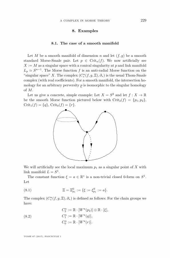
Let M be a smooth manifold of dimension n and let (f, g) be a smoothstandard Morse-Smale pair. Let p ∈ Critn(f). We now artificially seeX := M as a singular space with a conical singularity at p and link manifoldLp ' Sn−1. The Morse function f is an anti-radial Morse function on the“singular space” X. The complex (Cu∗ (f, g,Ξ), ∂∗) is the usual Thom-Smalecomplex (with real coefficients). For a smooth manifold, the intersection ho-mology for an arbitrary perversity p is isomorphic to the singular homologyof M .Let us give a concrete, simple example: Let X = S2 and let f : X → R

be the smooth Morse function pictured below with Crit2(f) = p1, p2,Crit1(f) = q, Crit0(f) = r.

We will artificially see the local maximum p1 as a singular point of X withlink manifold L = S1.The constant function ξ = a ∈ R∗ is a non-trivial closed 0-form on S1.

Let

(8.1) Ξ = Ξ0p1

:= ξ := ξ0p1

:= a.

The complex (Cu∗ (f, g,Ξ), ∂∗) is defined as follows: For the chain groups wehave:

Cu2 := R · [Wu(p2)]⊕ R · [ξ],Cu1 := R · [Wu(q)],Cu0 := R · [Wu(r)].

(8.2)


230 Ursula LUDWIG

For the boundary operator we have:

∂ξ = ±(∫

W s(q)∩La

)· [Wu(q)] = ±a · [Wu(q)],

∂[Wu(p2)] = ±[Wu(q)],∂[Wu(q)] = 0 = ∂[Wu(r)];

(8.3)

the signs above depend on the chosen orientations of the Wu’s. Note that,for ξ = 1, we recover the usual Thom-Smale complex for the smooth Morsefunction f and the manifold S2.

8.2. The suspension of the torus

Let X = ΣT 2 be the unreduced suspension of the torus. The space X hastwo isolated singularities, which we denote by P and Q. The link manifoldsare LP = LQ = T 2. It is not difficult to see, that there exists an anti-radial Morse function f on X, with exactly 4 smooth critical points, whichare all lying in 1/2 × T 2. We denote them as follows: Crit2(f) = p,Crit1(f) = q1, q2, Crit0(f) = r.

8.2.1. Lower middle perversity

Set ΞP = Ξ0P := ξP := ξ0

P := a, and ΞQ = Ξ0Q := ξQ := ξ0

Q := b,where a, b ∈ R∗. The complex (Cu∗ (f, g,Ξ), ∂∗) is defined as follows:For the chain groups we have:

Cu3 := R · [ξP ]⊕ R · [ξQ],Cu2 := R · [Wu(p)],Cu1 := R · [Wu(q1)]⊕ R · [Wu(q2)],Cu0 := R · [Wu(r)].

(8.4)


(8.5)∂[ξP ] = ±a · [Wu(p)], ∂[ξQ] = ±b · [Wu(p)],∂[Wu(p)] = ∂[Wu(q1,2)] = ∂[Wu(r)] = 0.

One verifies easily that the complex (Cu∗ (f, g,Ξ), ∂∗) computes the inter-section homology with lower middle perversity of X:

(8.6) H∗((Cu∗ (f, g,Ξ), ∂∗)) ' IH∗(X) =

R i = 0, 3,0 i = 2,R2 i = 1.



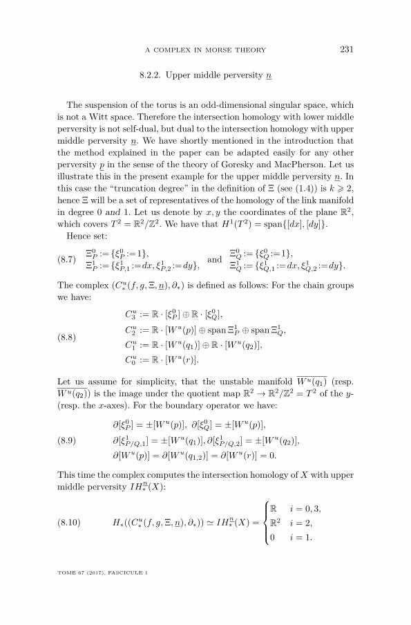
8.2.2. Upper middle perversity n

The suspension of the torus is an odd-dimensional singular space, whichis not a Witt space. Therefore the intersection homology with lower middleperversity is not self-dual, but dual to the intersection homology with uppermiddle perversity n. We have shortly mentioned in the introduction thatthe method explained in the paper can be adapted easily for any otherperversity p in the sense of the theory of Goresky and MacPherson. Let usillustrate this in the present example for the upper middle perversity n. Inthis case the “truncation degree” in the definition of Ξ (see (1.4)) is k > 2,hence Ξ will be a set of representatives of the homology of the link manifoldin degree 0 and 1. Let us denote by x, y the coordinates of the plane R2,which covers T 2 = R2/Z2. We have that H1(T 2) = span[dx], [dy].Hence set:

(8.7) Ξ0P := ξ0

P :=1,Ξ1P := ξ1

P,1 :=dx, ξ1P,2 :=dy, and Ξ0

Q := ξ0Q :=1,

Ξ1Q := ξ1

Q,1 :=dx, ξ1Q,2 :=dy.

The complex (Cu∗ (f, g,Ξ, n), ∂∗) is defined as follows: For the chain groupswe have:

Cu3 := R · [ξ0P ]⊕ R · [ξ0

Q],

Cu2 := R · [Wu(p)]⊕ span Ξ1P ⊕ span Ξ1

Q,

Cu1 := R · [Wu(q1)]⊕ R · [Wu(q2)],Cu0 := R · [Wu(r)].

(8.8)

Let us assume for simplicity, that the unstable manifold Wu(q1) (resp.Wu(q2)) is the image under the quotient map R2 → R2/Z2 = T 2 of the y-(resp. the x-axes). For the boundary operator we have:

(8.9)∂[ξ0

P ] = ±[Wu(p)], ∂[ξ0Q] = ±[Wu(p)],

∂[ξ1P/Q,1] = ±[Wu(q1)], ∂[ξ1

P/Q,2] = ±[Wu(q2)],∂[Wu(p)] = ∂[Wu(q1,2)] = ∂[Wu(r)] = 0.

This time the complex computes the intersection homology ofX with uppermiddle perversity IHn

∗ (X):

(8.10) H∗((Cu∗ (f, g,Ξ, n), ∂∗)) ' IHn∗ (X) =

R i = 0, 3,R2 i = 2,0 i = 1.


232 Ursula LUDWIG

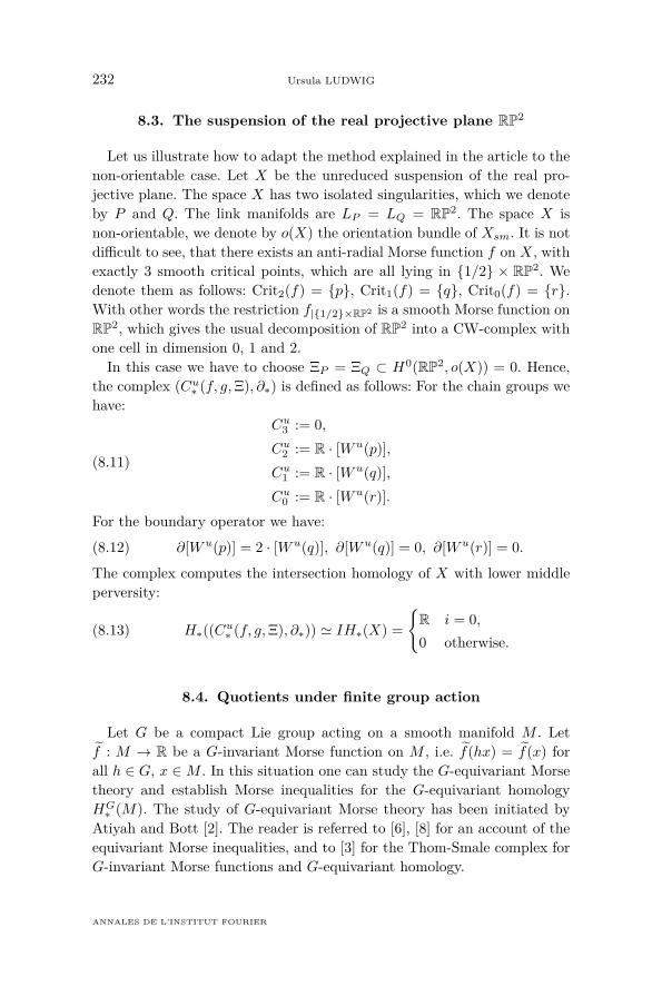
8.3. The suspension of the real projective plane RP2

Let us illustrate how to adapt the method explained in the article to thenon-orientable case. Let X be the unreduced suspension of the real pro-jective plane. The space X has two isolated singularities, which we denoteby P and Q. The link manifolds are LP = LQ = RP2. The space X isnon-orientable, we denote by o(X) the orientation bundle of Xsm. It is notdifficult to see, that there exists an anti-radial Morse function f on X, withexactly 3 smooth critical points, which are all lying in 1/2 × RP2. Wedenote them as follows: Crit2(f) = p, Crit1(f) = q, Crit0(f) = r.With other words the restriction f|1/2×RP2 is a smooth Morse function onRP2, which gives the usual decomposition of RP2 into a CW-complex withone cell in dimension 0, 1 and 2.In this case we have to choose ΞP = ΞQ ⊂ H0(RP2, o(X)) = 0. Hence,

the complex (Cu∗ (f, g,Ξ), ∂∗) is defined as follows: For the chain groups wehave:

Cu3 := 0,Cu2 := R · [Wu(p)],Cu1 := R · [Wu(q)],Cu0 := R · [Wu(r)].

(8.11)


(8.12) ∂[Wu(p)] = 2 · [Wu(q)], ∂[Wu(q)] = 0, ∂[Wu(r)] = 0.

The complex computes the intersection homology of X with lower middleperversity:

(8.13) H∗((Cu∗ (f, g,Ξ), ∂∗)) ' IH∗(X) =R i = 0,0 otherwise.

8.4. Quotients under finite group action

Let G be a compact Lie group acting on a smooth manifold M . Letf : M → R be a G-invariant Morse function on M , i.e. f(hx) = f(x) forall h ∈ G, x ∈M . In this situation one can study the G-equivariant Morsetheory and establish Morse inequalities for the G-equivariant homologyHG∗ (M). The study of G-equivariant Morse theory has been initiated by

Atiyah and Bott [2]. The reader is referred to [6], [8] for an account of theequivariant Morse inequalities, and to [3] for the Thom-Smale complex forG-invariant Morse functions and G-equivariant homology.



In the particular case of (certain) finite group actions, the present papersuggest yet another way of studying Morse theory: namely by studyingMorse theory on the (singular) quotient space. We will shortly explain thispoint of view in this subsection.

Let M be an oriented manifold with an orientation preserving action ofa finite group G. Let g be a G-invariant Riemannian metric on M . Letf : M → R be a smooth G-invariant Morse function on M . For finitegroups G-invariant Morse functions exist (see [48], Lemma 4.8).The quotient spaceX := M/G has a natural stratification by orbit types,

which gives X the structure of a Whitney stratified space (see e.g. [38],Theorem 4.4.6).Let us assume that X has only isolated singularities. The metric g in-

duced from g is conical in the sense of Definition 2.1. Let us assume, thatevery fixed point of the action of G is a critical point of f of index dimM .Then f descends to an anti-radial Morse function f : X → R.

For p ∈ Crit(f) let us denote by Wu(p) the unstable manifold of p withrespect to the flow induced from the negative gradient flow ∇

gf on M .

One has:

(8.14) h(Wu(p)) = ±Wu(h(p)) for all h ∈ G, p ∈ Crit(f).

The sign in (8.14) depends on the orientation of the unstable cells, andthe orientation can be chosen such that the sign is +. The unstable/stablecell decomposition of M for the Morse function f , descends into the unsta-ble/stable cell decomposition of X for the Morse function f . If the gradientvector field ∇

gf on M is Morse-Smale, so is the gradient vector field ∇gf

on X.The space X is a homology manifold, therefore the intersection homology

IH∗(X) is isomorphic to the singular homology of X (see [16], Section 6.4).For p ∈ Sing(X) the link manifold Lp is a homology sphere. Hence Ξp ⊂H0(Lp) ' R does contain a single element. The complex (Cu∗ (f, g,Ξ), ∂∗)does compute the singular homology of X.

BIBLIOGRAPHY

[1] M. Akaho, “Morse homology and manifolds with boundary”, Commun. Contemp.Math. 9 (2007), no. 3, p. 301-334.

[2] M. F. Atiyah & R. Bott, “The Yang-Mills equations over Riemann surfaces”,Philos. Trans. Roy. Soc. London Ser. A 308 (1983), no. 1505, p. 523-615.

[3] D. M. Austin & P. J. Braam, “Morse-Bott theory and equivariant cohomology”,in The Floer memorial volume, Progr. Math., vol. 133, Birkhäuser, Basel, 1995,p. 123-183.


234 Ursula LUDWIG

[4] J.-M. Bismut & W. Zhang, “An extension of a theorem by Cheeger and Müller”,Astérisque (1992), no. 205, p. 235, With an appendix by François Laudenbach.

[5] ———, “Milnor and Ray-Singer metrics on the equivariant determinant of a flatvector bundle”, Geom. Funct. Anal. 4 (1994), no. 2, p. 136-212.

[6] R. Bott, “Lectures on Morse theory, old and new”, Bull. Amer. Math. Soc. (N.S.)7 (1982), no. 2, p. 331-358.

[7] ———, “Morse theory indomitable”, Inst. Hautes Études Sci. Publ. Math. (1988),no. 68, p. 99-114 (1989).

[8] K.-C. Chang, Infinite dimensional Morse theory and multiple solution problems.,Boston: Birkhäuser, 1993.

[9] J. Cheeger, “Analytic torsion and the heat equation”, Ann. of Math. (2) 109(1979), no. 2, p. 259-322.

[10] ———, “On the Hodge theory of Riemannian pseudomanifolds”, in Geometry ofthe Laplace operator (Proc. Sympos. Pure Math., Univ. Hawaii, Honolulu, Hawaii,1979), Proc. Sympos. Pure Math., XXXVI, Amer. Math. Soc., Providence, R.I.,1980, p. 91-146.

[11] J. Cheeger, M. Goresky & R. MacPherson, “L2-cohomology and intersectionhomology of singular algebraic varieties”, in Seminar on Differential Geometry, Ann.of Math. Stud., vol. 102, Princeton Univ. Press, Princeton, N.J., 1982, p. 303-340.

[12] A. Dar, “Intersection R-torsion and analytic torsion for pseudomanifolds”, Math.Z. 194 (1987), no. 2, p. 193-216.

[13] A. Floer, “Witten’s complex and infinite-dimensional Morse theory”, J. Differen-tial Geom. 30 (1989), no. 1, p. 207-221.

[14] M. Goresky, “Triangulation of stratified objects”, Proc. Amer. Math. Soc. 72(1978), no. 1, p. 193-200.

[15] ———, “Whitney stratified chains and cochains”, Trans. Amer. Math. Soc. 267(1981), no. 1, p. 175-196.

[16] M. Goresky & R. MacPherson, “Intersection homology theory”, Topology 19(1980), no. 2, p. 135-162.

[17] ———, “Intersection homology. II”, Invent. Math. 72 (1983), no. 1, p. 77-129.[18] ———, “Simplicial Intersection Homology”, Invent. Math. 84 (1986), no. 2, p. 432-

433, Appendix to MacPherson, Robert and Vilonen, Kari "Elementary constructionof perverse sheaves".

[19] ———, Stratified Morse theory, Ergebnisse der Mathematik und ihrer Grenzgebiete(3) [Results in Mathematics and Related Areas (3)], vol. 14, Springer-Verlag, Berlin,1988.

[20] M. Grinberg, “Gradient-like flows and self-indexing in stratified Morse theory”,Topology 44 (2005), no. 1, p. 175-202.

[21] L. Hartmann & M. Spreafico, “The analytic torsion of a cone over a sphere”, J.Math. Pures Appl. (9) 93 (2010), no. 4, p. 408-435.

[22] ———, “The analytic torsion of a cone over an odd dimensional manifold”, J.Geom. Phys. 61 (2011), no. 3, p. 624-657.

[23] B. Helffer & J. Sjöstrand, “Puits multiples en mécanique semi-classique. IV.Étude du complexe de Witten”, Comm. Partial Differential Equations 10 (1985),no. 3, p. 245-340.

[24] F. E. A. Johnson, “On the triangulation of stratified sets and singular varieties”,Trans. Amer. Math. Soc. 275 (1983), no. 1, p. 333-343.

[25] F. Kirwan & J. Woolf, An introduction to intersection homology theory, seconded., Chapman & Hall/CRC, Boca Raton, FL, 2006, xiv+229 pages.



[26] P. Kronheimer & T. Mrowka, Monopoles and three-manifolds, New Math-ematical Monographs, vol. 10, Cambridge University Press, Cambridge, 2007,xii+796 pages.

[27] F. Laudenbach, “Appendix: On the Thom-Smale complex”, Astérisque (1992),no. 205, p. 235.

[28] ———, “A Morse complex on manifolds with boundary”, Geom. Dedicata 153(2011), p. 47-57.

[29] ———, Transversalité, courants et théorie de Morse, Éditions de l’École Polytech-nique, Palaiseau, 2012, Un cours de topologie différentielle. [A course of differentialtopology], Exercises proposed by François Labourie, x+182 pages.

[30] U. Ludwig, “Comparison between two complexes on a singular space”, to appearin Journal für die reine und angewandte Mathematik (Crelle).

[31] ———, “Morse-Smale-Witten complex for gradient-like vector fields on stratifiedspaces”, in Singularity theory, World Sci. Publ., Hackensack, NJ, 2007, p. 683-713.

[32] J. Milnor,Morse theory, Based on lecture notes by M. Spivak and R. Wells. Annalsof Mathematics Studies, No. 51, Princeton University Press, Princeton, N.J., 1963,vi+153 pages.

[33] J. Milnor, Lectures on the h-cobordism theorem, Notes by L. Siebenmann and J.Sondow, Princeton University Press, Princeton, N.J., 1965.

[34] W. Müller, “Analytic torsion and R-torsion of Riemannian manifolds”, Adv. inMath. 28 (1978), no. 3, p. 233-305.

[35] ———, “Analytic torsion and R-torsion for unimodular representations”, J. Amer.Math. Soc. 6 (1993), no. 3, p. 721-753.

[36] J. R. Munkres, “Concordance is equivalent to smoothability”, Topology 5 (1966),p. 371-389.

[37] L. Nicolaescu, An invitation to Morse theory, second ed., Universitext, Springer,New York, 2011, xvi+353 pages.

[38] M. J. Pflaum, Analytic and geometric study of stratified spaces, Lecture Notes inMathematics, vol. 1768, Springer-Verlag, Berlin, 2001, viii+230 pages.

[39] D. B. Ray & I. M. Singer, “R-torsion and the Laplacian on Riemannian mani-folds”, Advances in Math. 7 (1971), p. 145-210.

[40] M.-H. Schwartz, “Classes caractéristiques définies par une stratification d’une var-iété analytique complexe. I”, C. R. Acad. Sci. Paris 260 (1965), p. 3262-3264.

[41] ———, Champs radiaux sur une stratification analytique, Travaux en Cours [Worksin Progress], vol. 39, Hermann, Paris, 1991, x+185 pages.

[42] M. Schwarz, Morse homology, Progress in Mathematics, vol. 111, Birkhäuser Ver-lag, Basel, 1993, x+235 pages.

[43] S. Smale, “On gradient dynamical systems”, Ann. of Math. (2) 74 (1961), p. 199-206.

[44] R. Thom, “Sur une partition en cellules associée à une fonction sur une variété”,C. R. Acad. Sci. Paris 228 (1949), p. 973-975.

[45] D. J. A. Trotman, “Geometric versions of Whitney regularity for smooth stratifi-cations”, Ann. Sci. École Norm. Sup. (4) 12 (1979), no. 4, p. 453-463.

[46] A. Verona, Stratified mappings—structure and triangulability, Lecture Notes inMathematics, vol. 1102, Springer-Verlag, Berlin, 1984, ix+160 pages.

[47] B. Vertman, “Analytic torsion of a bounded generalized cone”, Comm. Math. Phys.290 (2009), no. 3, p. 813-860.

[48] A. G. Wasserman, “Equivariant differential topology”, Topology 8 (1969), p. 127-150.

[49] J. Weber, “The Morse-Witten complex via dynamical systems”, Expo. Math. 24(2006), no. 2, p. 127-159.


236 Ursula LUDWIG

[50] H. Whitney, “Local properties of analytic varieties”, in Differential and Combina-torial Topology (A Symposium in Honor of Marston Morse), Princeton Univ. Press,Princeton, N. J., 1965, p. 205-244.

[51] E. Witten, “Supersymmetry and Morse theory”, J. Differential Geom. 17 (1982),no. 4, p. 661-692 (1983).

Manuscrit reçu le 25 juillet 2014,révisé le 23 juin 2015,accepté le 10 septembre 2015.

Ursula LUDWIGUniversität Duisburg-EssenFakultät für MathematikThea-Leymann-Str. 9D-45127 Essen (Germany)[email protected]


mailto:[email protected]

Documents

A complex in Morse theory computing intersection homologyA complex in Morse theory computing intersection homology Tome 67, no 1 (2017), p. 197-236. ... A COMPLEX IN MORSE THEORY COMPUTING