A New Mathematical Formulation and a Faster Algorithm for ... · there are (mn)! di erent permutations for the TP and the search space becomes very large for this approach to be e

CIRRELT-2020-15

A New Mathematical Formulation and a Faster Algorithm for Sparse Transportation Problems Tania C.L. Silva Arinei C.L. Silva Gustavo V. Loch Leandro C. Coelho May 2020

Document de travail également publié par la Faculté des sciences de l’administration de l’Université Laval, sous le numéro FSA-2020-005.

A New Mathematical Formulation and a Faster Algorithm for Sparse Transportation Problems

Tania C.L. Silva1, Arinei C. L. Silva2, Gustavo V. Loch2, Leandro C. Coelho3, *

1. Research Group of Technology Applied to Optimization (GTAO), Instituto Federal do Paraná (IFPR), Brazil

2. Research Group of Technology Applied to Optimization (GTAO), Federal University of Paraná (UFPR), Brazil

3. Interuniversity Research Centre on Enterprise Networks, Logistics and Transportation (CIRRELT), Department of Operations and Decision Systems, and Canada research chair in integrated logistics, Université Laval, 2325 de la Terrasse, Québec, Canada G1V 0A6

Abstract. The Sparse Transportation Problem (STP) is a generalization of the classic Transportation Problem (TP) with at least one forbidden arc. Unlike the Balanced TP (BTP) which always admits a feasible solution, the same is not valid for an STP. In this paper we propose a new mathematical formulation and a new exact method for solving STPs that always yields an optimal solution if the problem is feasible. Moreover, our method correctly proves infeasibility when the problem does not admit a feasible solution. We provide several theoretical insights and proofs for different parts of our mathematical formulation and method, advancing the theory of algorithms used for TPs and specifically for solving STPs. Moreover, through numerical examples and detailed results we demonstrate how our method works compared to the state-of-the-art approaches existing in the literature. We also significantly accelerate the performance of our method by using partial pricing, notably outperforming a minimum cost network flow algorithm applied to the TP. Detailed computational experiments on feasible instances empirically demonstrate average reductions of more than 82.7% in runtime when our sparse method with partial pricing is compared to the state-of-the-art approach from the literature for STPs. In case of infeasible instances, the overall average runtime reductions were higher than 84.8%. We also conduct computational experiments of our new mathematical formulation in the state-of-the-art network flow algorithm and the state-of-the-art linear programming solver Gurobi, and observed runtime reductions of over 80% and 73%, respectively. We also show that the first feasible solution obtained with our method is significantly better than the one found by using the traditional TP formulation. Keywords. Sparse transportation problem, forbidden arcs, MODI method, exact algorithm, partial pricing. Acknowledgements. We are grateful to Programa de Pós graduação em Métodos Numéricos em Engenharia (PPGMNE-UFPR), Departamento de Administração Geral e Aplicada (DAGA-UFPR), Departamento de Engenharia de Produção and Grupo de Tecnologias Aplicadas à Otimização (GTAO) for their support at Universidade Federal do Paraná. This project was partly funded by the Natural Sciences and Engineering Research Council of Canada (NSERC) under grant 2019-00094. This support is greatly acknowledged.

Results and views expressed in this publication are the sole responsibility of the authors and do not necessarily reflect those of CIRRELT. Les résultats et opinions contenus dans cette publication ne reflètent pas nécessairement la position du CIRRELT et n'engagent pas sa responsabilité.

_____________________________ * Corresponding author: [email protected]

Dépôt légal – Bibliothèque et Archives nationales du Québec Bibliothèque et Archives Canada, 2020

© Silva, Silva, Loch, Coelho and CIRRELT, 2020

1 Introduction

The Transportation Problem (TP) is one of the most classical problems in Linear Programming

(LP). This problem is defined so as to minimize the total cost to ship a commodity from m

sources to n destinations, subject to the capacity of the m sources and the requirements of the

n demands nodes.

The first studies on TPs are due to the French mathematician Gaspard Monge in 1781 [21]. He

formulated the optimal TP to move a pile of soil or rubble to an excavation or fill. In the 1940s,

Soviet mathematician and economist Leonid Kantorovich introduced a dual formulation, along

with necessary and sufficient optimality conditions. Today, this problem is named as Monge-

Kantorovich mass-transportation problem [27].

The LP formulation and the discrete case of TPs are credited to Hitchcock [15] and Koopmans

[19], that developed the basic TP independently. However, optimal solutions to more complex

problems were only made possible in 1951, when Dantizg [8] applied the concept of LP to

solve the TP. In the following decades some TP studies were carried out by Arsham and Kahn

[3], Kleinschmidt and Schannath [17], and Papamanthou et al. [23].

LetM and N be the sets of m sources and n demand nodes, and let Si represent the quantity

available at source i ∈ M, Dj be the demand at destination j ∈ N , and A be the set of

admissible arcs. Let also cij, (i, j) ∈ A, be the unit shipping cost from source i to destination j,

and xij be the decision variable representing the quantity to be shipped from i to j. A classic

formulation to the TP is given by (1)–(4).

(TP ) : min∑

(i,j)∈A

cijxij (1)

subject to

∑j:(i,j)∈A

xij ≤ Si ∀i ∈M (2)


CIRRELT-2020-15 1

∑i:(i,j)∈A

xij ≥ Dj ∀j ∈ N (3)

xij ≥ 0 (i, j) ∈ A. (4)

In case A = |1, 2, . . . ,m| × |1, 2, . . . , n| we have a Dense TP (DTP), otherwise the problem

is called a Sparse TP (STP). Moreover, if∑

i∈M Si =∑

j∈N Dj = L, then the TP is called

Balanced (BTP). Finally, if the DTP is a BTP it always admits a feasible solution. As a TP

that is not balanced can be easily converted into a BTP [22], we will only consider BTPs in

the remainder of this paper.

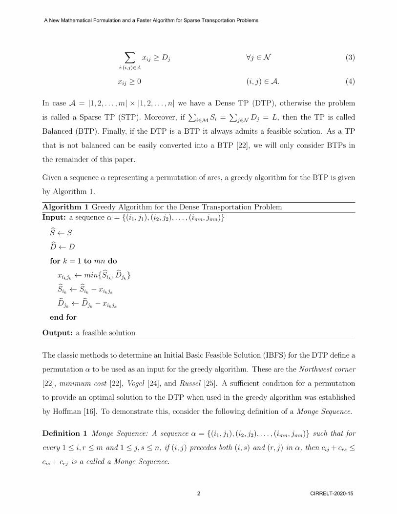
Given a sequence α representing a permutation of arcs, a greedy algorithm for the BTP is given

by Algorithm 1.

Algorithm 1 Greedy Algorithm for the Dense Transportation Problem

Input: a sequence α = {(i1, j1), (i2, j2), . . . , (imn, jmn)}

S ← S

D ← D

for k = 1 to mn do

xikjk ← min{Sik , Djk}

Sik ← Sik − xikjkDjk ← Djk − xikjk

end for

Output: a feasible solution

The classic methods to determine an Initial Basic Feasible Solution (IBFS) for the DTP define a

permutation α to be used as an input for the greedy algorithm. These are the Northwest corner

[22], minimum cost [22], Vogel [24], and Russel [25]. A sufficient condition for a permutation

to provide an optimal solution to the DTP when used in the greedy algorithm was established

by Hoffman [16]. To demonstrate this, consider the following definition of a Monge Sequence.

Definition 1 Monge Sequence: A sequence α = {(i1, j1), (i2, j2), . . . , (imn, jmn)} such that for

every 1 ≤ i, r ≤ m and 1 ≤ j, s ≤ n, if (i, j) precedes both (i, s) and (r, j) in α, then cij + crs ≤

cis + crj is a called a Monge Sequence.


2 CIRRELT-2020-15

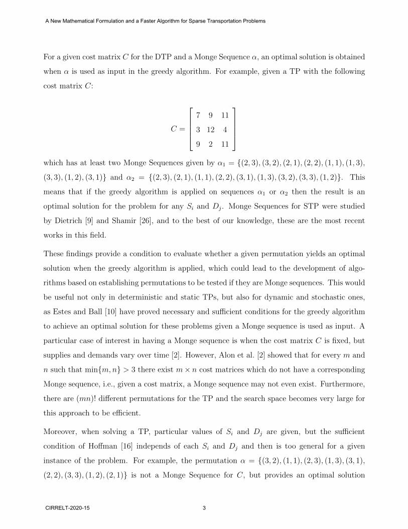
For a given cost matrix C for the DTP and a Monge Sequence α, an optimal solution is obtained

when α is used as input in the greedy algorithm. For example, given a TP with the following

cost matrix C:

C =

7 9 11

3 12 4

9 2 11

which has at least two Monge Sequences given by α1 = {(2, 3), (3, 2), (2, 1), (2, 2), (1, 1), (1, 3),

(3, 3), (1, 2), (3, 1)} and α2 = {(2, 3), (2, 1), (1, 1), (2, 2), (3, 1), (1, 3), (3, 2), (3, 3), (1, 2)}. This

means that if the greedy algorithm is applied on sequences α1 or α2 then the result is an

optimal solution for the problem for any Si and Dj. Monge Sequences for STP were studied

by Dietrich [9] and Shamir [26], and to the best of our knowledge, these are the most recent

works in this field.

These findings provide a condition to evaluate whether a given permutation yields an optimal

solution when the greedy algorithm is applied, which could lead to the development of algo-

rithms based on establishing permutations to be tested if they are Monge sequences. This would

be useful not only in deterministic and static TPs, but also for dynamic and stochastic ones,

as Estes and Ball [10] have proved necessary and sufficient conditions for the greedy algorithm

to achieve an optimal solution for these problems given a Monge sequence is used as input. A

particular case of interest in having a Monge sequence is when the cost matrix C is fixed, but

supplies and demands vary over time [2]. However, Alon et al. [2] showed that for every m and

n such that min{m,n} > 3 there exist m× n cost matrices which do not have a corresponding

Monge sequence, i.e., given a cost matrix, a Monge sequence may not even exist. Furthermore,

there are (mn)! different permutations for the TP and the search space becomes very large for

this approach to be efficient.

Moreover, when solving a TP, particular values of Si and Dj are given, but the sufficient

condition of Hoffman [16] independs of each Si and Dj and then is too general for a given

instance of the problem. For example, the permutation α = {(3, 2), (1, 1), (2, 3), (1, 3), (3, 1),

(2, 2), (3, 3), (1, 2), (2, 1)} is not a Monge Sequence for C, but provides an optimal solution


CIRRELT-2020-15 3

when Algorithm 1 is applied if S = (15, 1220, 55) and D = (920, 10, 360). However, if S =

(515, 720, 55) and D = (320, 610, 360), the solution provided by α is not optimal.

The literature also presents an alternative necessary and sufficient condition for optimality,

and an improvement process for the cases for which optimality conditions are not satisfied.

Charnes and Cooper [6] introduced the stepping stone method, which consists of finding a θ-

loop to each non-basic variable. Another method is based on dual variables, called the Modified

Distribution (MODI) method, also known as the u-v method [4, 22]. Loch and Silva [20] study

on the average number of iterations required to find an optimal solution for different methods

of IBFS when the MODI method is applied.

The TP being a special case of the min-cost network, it can be solved using algorithms for those

problems. One of the most efficient and well-known algorithms to solve min-cost network flow

problems is the scaling push-relabel [13]. We compare the performance of our method with this

algorithm, testing instances of different densities, feasible and infeasible.

Although the TP is one of the most well-known problems in LP and many variations have been

proposed since its introduction, only few papers in the literature present methods that exploit

their inherent structures. In particular, when dealing with a sparse problem, the traditional

way to solve the problem is to convert it into a DTP and then apply the aforementioned

methods. In this paper, we take advantage of the sparse structure of the matrices and derive

a new mathematical formulation and a new method to solve STPs more efficiently. Our exact

algorithm presents many computational advantages when solving an STP and reduces to the

traditional method when solving a DTP.

The remainder of this paper is organized as follows. In Section 2 the classical approach to

solve STPs is presented along with two examples. In Section 3 we present our methodological

contribution and two detailed examples. In Section 4 theoretical analysis of our method are

provided. Section 5 describes how a partial pricing scheme can speed up the calculations of

our algorithm. Section 6 describes extensive computational experiments that were carried out

to assess the performance of our new method. Finally, in Section 7 we present the conclusions

of this paper.


4 CIRRELT-2020-15

2 Sparse Transportation Problems

An STP is a generalization of the TP in which the set of arcs is divided into forbidden and

admissible ones. The aim is to find an optimal solution using only admissible arcs. The STP is

also a particular case of the Constrained TP (CTP), in which the capacity of at least one arc

is zero [7, 11, 18].

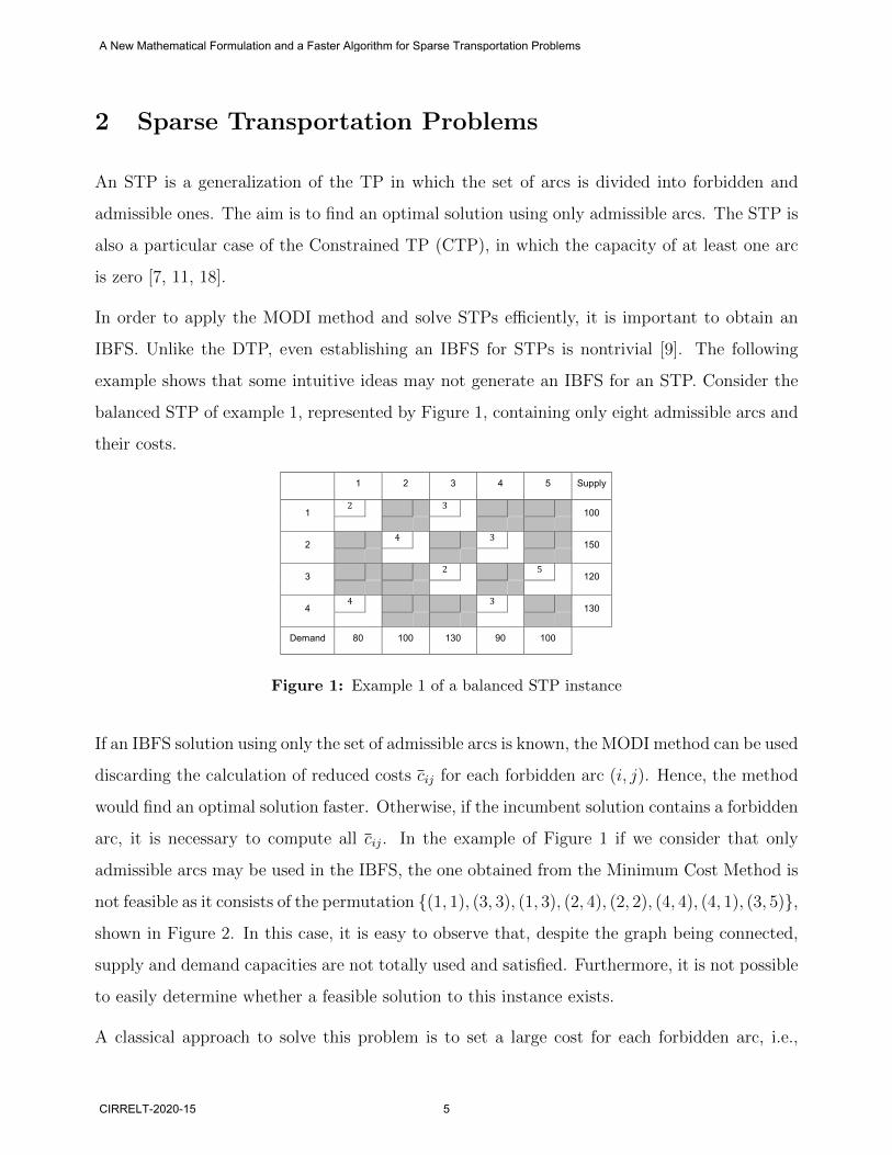
In order to apply the MODI method and solve STPs efficiently, it is important to obtain an

IBFS. Unlike the DTP, even establishing an IBFS for STPs is nontrivial [9]. The following

example shows that some intuitive ideas may not generate an IBFS for an STP. Consider the

balanced STP of example 1, represented by Figure 1, containing only eight admissible arcs and

their costs.

1 2 3 4 5 Supply

1 2

3

100

2 4

3

150

3 2

5

120

4 4

3

130

Demand 80 100 130 90 100

1 2 3 4 5 Supply

1 2 3

10 80 10

2 4 3

0 60 90

3 2 5

0 120

4 4 3

130

Demand 0 40 0 0 100

Figure 1: Example 1 of a balanced STP instance

If an IBFS solution using only the set of admissible arcs is known, the MODI method can be used

discarding the calculation of reduced costs cij for each forbidden arc (i, j). Hence, the method

would find an optimal solution faster. Otherwise, if the incumbent solution contains a forbidden

arc, it is necessary to compute all cij. In the example of Figure 1 if we consider that only

admissible arcs may be used in the IBFS, the one obtained from the Minimum Cost Method is

not feasible as it consists of the permutation {(1, 1), (3, 3), (1, 3), (2, 4), (2, 2), (4, 4), (4, 1), (3, 5)},

shown in Figure 2. In this case, it is easy to observe that, despite the graph being connected,

supply and demand capacities are not totally used and satisfied. Furthermore, it is not possible

to easily determine whether a feasible solution to this instance exists.

A classical approach to solve this problem is to set a large cost for each forbidden arc, i.e.,


CIRRELT-2020-15 5

1 2 3 4 5 Supply

1 2

3

100

2 4

3

150

3 2

5

120

4 4

3

130

Demand 80 100 130 90 100

1 2 3 4 5 Supply

1 2 3

10 80 10

2 4 3

0 60 90

3 2 5

0 120

4 4 3

130

Demand 0 40 0 0 100

Figure 2: Example of unsuccessful use of the Minimum Cost Method to an STP instance

use forbidden arcs as artificial variables. Setting the value of the unit cost for forbidden arcs

to at least∑

i∈M ai × max{|cij| : i = 1, . . . ,m, j = 1, . . . , n} is enough [22]. However, this

method does not take advantage of the sparse structure of the problem. This new problem

always admits a feasible solution; if its optimal solution contains any artificial variable with

value grater than zero, the original STP is infeasible.

For instance, we set a cost equal to 10000 to each forbidden arc (Figure 3a). Once the problem

is balanced and each forbidden arc is transformed into an artificial variable, it is possible to

apply the Minimum Cost Method, obtain an IBFS (see Figure 3b), and then use the MODI

method.

When the reduced costs for the IBFS are computed, arcs (3, 5) and (4, 4) are associated with

negative reduced costs (Figure 3c). As (4, 4) is associated with the most negative one (−9996),

it will be the entering arc. Thus, the θ-loop is {(4, 4), (4, 2), (2, 2), (2, 4)}, θ = min{x42, x24} =

x42 = 30 and (4, 2) is the arc to leave the basis.

After the first iteration (Figure 3d), arc (3, 5) is associated with the most negative reduced cost

(−19990) and is the entering arc (Figure 3e), θ-loop= {(3, 5), (4, 5), (4, 4), (2, 4), (2, 2), (1, 2),

(1, 3), (3, 3)} and θ = min{x45, x24, x12, x33} = x12 = 10. In this case the exiting arc is (1, 2) and

Figure 3f shows the next solution. After the second iteration (Figure 3f), arc (4, 1) is the only one

associated with a negative reduced cost (Figure 3g), θ-loop= {(4, 1), (1, 1), (1, 3), (3, 3), (3, 5),

(4, 5)} and θ = min{x11, x33, x45} = x45 = 80. In this case the exiting arc is (4, 5) and Figure

3h presents the new solution.


6 CIRRELT-2020-15

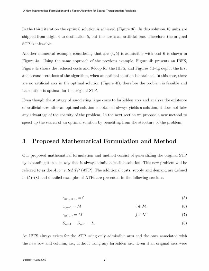
In the third iteration the optimal solution is achieved (Figure 3i). In this solution 10 units are

shipped from origin 4 to destination 5, but this arc is an artificial one. Therefore, the original

STP is infeasible.

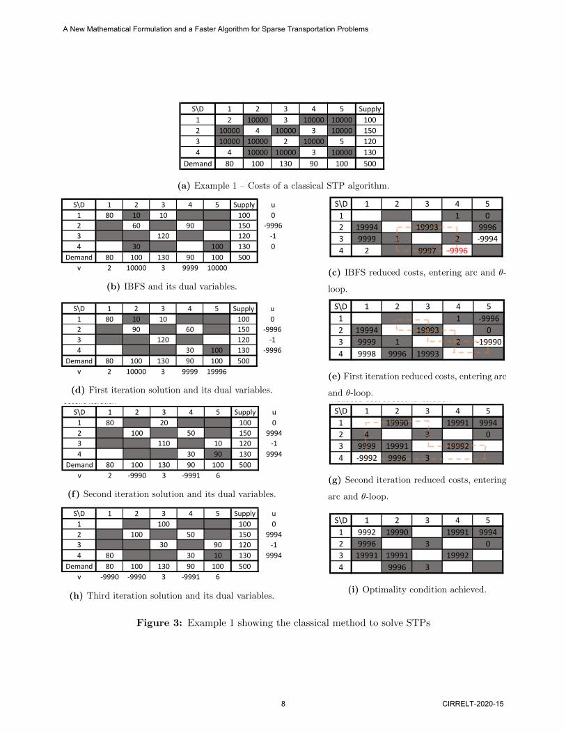
Another numerical example considering that arc (4, 5) is admissible with cost 6 is shown in

Figure 4a. Using the same approach of the previous example, Figure 4b presents an IBFS,

Figure 4c shows the reduced costs and θ-loop for the IBFS, and Figures 4d–4g depict the first

and second iterations of the algorithm, when an optimal solution is obtained. In this case, there

are no artificial arcs in the optimal solution (Figure 4f), therefore the problem is feasible and

its solution is optimal for the original STP.

Even though the strategy of associating large costs to forbidden arcs and analyze the existence

of artificial arcs after an optimal solution is obtained always yields a solution, it does not take

any advantage of the sparsity of the problem. In the next section we propose a new method to

speed up the search of an optimal solution by benefiting from the structure of the problem.

3 Proposed Mathematical Formulation and Method

Our proposed mathematical formulation and method consist of generalizing the original STP

by expanding it in such way that it always admits a feasible solution. This new problem will be

referred to as the Augmented TP (ATP). The additional costs, supply and demand are defined

in (5)–(8) and detailed examples of ATPs are presented in the following sections.

cm+1,n+1 = 0 (5)

ci,n+1 = M i ∈M (6)

cm+1,j = M j ∈ N (7)

Sm+1 = Dn+1 = L. (8)

An IBFS always exists for the ATP using only admissible arcs and the ones associated with

the new row and column, i.e., without using any forbidden arc. Even if all original arcs were


CIRRELT-2020-15 7

O\D 1 2 3 4 5 Supply

1 0 0 100 0 0 100 100

2 0 100 0 50 0 150 150

3 0 0 30 0 90 120 120

4 80 0 0 40 10 130 130

Demand 80 100 130 90 100 500

80 100 130 90 100 101800

Costs

S\D 1 2 3 4 5 Supply

1 2 10000 3 10000 10000 100

2 10000 4 10000 3 10000 150

3 10000 10000 2 10000 5 120

4 4 10000 10000 3 10000 130

Demand 80 100 130 90 100 500

IBFS

S\D 1 2 3 4 5 Supply u S\D 1 2 3 4 5

1 80 10 10 100 0 1 1 0

2 60 90 150 -9996 2 19994 19993 9996

3 120 120 -1 3 9999 1 2 -9994

4 30 100 130 0 4 2 9997 -9996

Demand 80 100 130 90 100 500

v 2 10000 3 9999 10000

S\D 1 2 3 4 5 Supply u S\D 1 2 3 4 5

1 80 10 10 100 0 1 1 -9996

2 90 60 150 -9996 2 19994 19993 0

3 120 120 -1 3 9999 1 2 -19990

4 30 100 130 -9996 4 9998 9996 19993

Demand 80 100 130 90 100 500

v 2 10000 3 9999 19996

S\D 1 2 3 4 5 Supply u S\D 1 2 3 4 5

1 80 20 100 0 1 19990 19991 9994

2 100 50 150 9994 2 4 3 0

3 110 10 120 -1 3 9999 19991 19992

4 30 90 130 9994 4 -9992 9996 3

Demand 80 100 130 90 100 500

v 2 -9990 3 -9991 6

S\D 1 2 3 4 5 Supply u S\D 1 2 3 4 5

1 100 100 0 1 9992 19990 19991 9994

2 100 50 150 9994 2 9996 3 0

3 30 90 120 -1 3 19991 19991 19992

4 80 30 10 130 9994 4 9996 3

Demand 80 100 130 90 100 500

v -9990 -9990 3 -9991 6

First Iteration

Second Iteration

Third Iteration

30=min(30,90)

80=min(90,110,80)

10=min(100,60,10,120)

Reduced Cost at IBFS

Reduced Cost at First Iteration

Reduced Cost at Second Iteration

Reduced Cost at Third Iteration

optimal

(a) Example 1 – Costs of a classical STP algorithm.


1 0 0 100 0 0 100 100

2 0 100 0 50 0 150 150

3 0 0 30 0 90 120 120

4 80 0 0 40 10 130 130

Demand 80 100 130 90 100 500

80 100 130 90 100 101800

Costs


1 2 10000 3 10000 10000 100

2 10000 4 10000 3 10000 150

3 10000 10000 2 10000 5 120

4 4 10000 10000 3 10000 130

Demand 80 100 130 90 100 500

IBFS

S\D 1 2 3 4 5 Supply u S\D 1 2 3 4 5

1 80 10 10 100 0 1 1 0

2 60 90 150 -9996 2 19994 19993 9996

3 120 120 -1 3 9999 1 2 -9994

4 30 100 130 0 4 2 9997 -9996

Demand 80 100 130 90 100 500

v 2 10000 3 9999 10000

S\D 1 2 3 4 5 Supply u S\D 1 2 3 4 5

1 80 10 10 100 0 1 1 -9996

2 90 60 150 -9996 2 19994 19993 0

3 120 120 -1 3 9999 1 2 -19990

4 30 100 130 -9996 4 9998 9996 19993

Demand 80 100 130 90 100 500

v 2 10000 3 9999 19996

S\D 1 2 3 4 5 Supply u S\D 1 2 3 4 5

1 80 20 100 0 1 19990 19991 9994

2 100 50 150 9994 2 4 3 0

3 110 10 120 -1 3 9999 19991 19992

4 30 90 130 9994 4 -9992 9996 3

Demand 80 100 130 90 100 500

v 2 -9990 3 -9991 6

S\D 1 2 3 4 5 Supply u S\D 1 2 3 4 5

1 100 100 0 1 9992 19990 19991 9994

2 100 50 150 9994 2 9996 3 0

3 30 90 120 -1 3 19991 19991 19992

4 80 30 10 130 9994 4 9996 3

Demand 80 100 130 90 100 500

v -9990 -9990 3 -9991 6

First Iteration

Second Iteration

Third Iteration

30=min(30,90)

80=min(90,110,80)

10=min(100,60,10,120)





optimal

(b) IBFS and its dual variables.


1 0 0 100 0 0 100 100

2 0 100 0 50 0 150 150

3 0 0 30 0 90 120 120

4 80 0 0 40 10 130 130

Demand 80 100 130 90 100 500

80 100 130 90 100 101800

Costs


1 2 10000 3 10000 10000 100

2 10000 4 10000 3 10000 150

3 10000 10000 2 10000 5 120

4 4 10000 10000 3 10000 130

Demand 80 100 130 90 100 500

IBFS

S\D 1 2 3 4 5 Supply u S\D 1 2 3 4 5

1 80 10 10 100 0 1 1 0

2 60 90 150 -9996 2 19994 19993 9996

3 120 120 -1 3 9999 1 2 -9994

4 30 100 130 0 4 2 9997 -9996

Demand 80 100 130 90 100 500

v 2 10000 3 9999 10000

S\D 1 2 3 4 5 Supply u S\D 1 2 3 4 5

1 80 10 10 100 0 1 1 -9996

2 90 60 150 -9996 2 19994 19993 0

3 120 120 -1 3 9999 1 2 -19990

4 30 100 130 -9996 4 9998 9996 19993

Demand 80 100 130 90 100 500

v 2 10000 3 9999 19996

S\D 1 2 3 4 5 Supply u S\D 1 2 3 4 5

1 80 20 100 0 1 19990 19991 9994

2 100 50 150 9994 2 4 3 0

3 110 10 120 -1 3 9999 19991 19992

4 30 90 130 9994 4 -9992 9996 3

Demand 80 100 130 90 100 500

v 2 -9990 3 -9991 6

S\D 1 2 3 4 5 Supply u S\D 1 2 3 4 5

1 100 100 0 1 9992 19990 19991 9994

2 100 50 150 9994 2 9996 3 0

3 30 90 120 -1 3 19991 19991 19992

4 80 30 10 130 9994 4 9996 3

Demand 80 100 130 90 100 500

v -9990 -9990 3 -9991 6

First Iteration

Second Iteration

Third Iteration

30=min(30,90)

80=min(90,110,80)

10=min(100,60,10,120)





optimal

(c) IBFS reduced costs, entering arc and θ-

loop.


1 0 0 100 0 0 100 100

2 0 100 0 50 0 150 150

3 0 0 30 0 90 120 120

4 80 0 0 40 10 130 130

Demand 80 100 130 90 100 500

80 100 130 90 100 101800

Costs


1 2 10000 3 10000 10000 100

2 10000 4 10000 3 10000 150

3 10000 10000 2 10000 5 120

4 4 10000 10000 3 10000 130

Demand 80 100 130 90 100 500

IBFS

S\D 1 2 3 4 5 Supply u S\D 1 2 3 4 5

1 80 10 10 100 0 1 1 0

2 60 90 150 -9996 2 19994 19993 9996

3 120 120 -1 3 9999 1 2 -9994

4 30 100 130 0 4 2 9997 -9996

Demand 80 100 130 90 100 500

v 2 10000 3 9999 10000

S\D 1 2 3 4 5 Supply u S\D 1 2 3 4 5

1 80 10 10 100 0 1 1 -9996

2 90 60 150 -9996 2 19994 19993 0

3 120 120 -1 3 9999 1 2 -19990

4 30 100 130 -9996 4 9998 9996 19993

Demand 80 100 130 90 100 500

v 2 10000 3 9999 19996

S\D 1 2 3 4 5 Supply u S\D 1 2 3 4 5

1 80 20 100 0 1 19990 19991 9994

2 100 50 150 9994 2 4 3 0

3 110 10 120 -1 3 9999 19991 19992

4 30 90 130 9994 4 -9992 9996 3

Demand 80 100 130 90 100 500

v 2 -9990 3 -9991 6

S\D 1 2 3 4 5 Supply u S\D 1 2 3 4 5

1 100 100 0 1 9992 19990 19991 9994

2 100 50 150 9994 2 9996 3 0

3 30 90 120 -1 3 19991 19991 19992

4 80 30 10 130 9994 4 9996 3

Demand 80 100 130 90 100 500

v -9990 -9990 3 -9991 6

First Iteration

Second Iteration

Third Iteration

30=min(30,90)

80=min(90,110,80)

10=min(100,60,10,120)





optimal

(d) First iteration solution and its dual variables.


1 0 0 100 0 0 100 100

2 0 100 0 50 0 150 150

3 0 0 30 0 90 120 120

4 80 0 0 40 10 130 130

Demand 80 100 130 90 100 500

80 100 130 90 100 101800

Costs


1 2 10000 3 10000 10000 100

2 10000 4 10000 3 10000 150

3 10000 10000 2 10000 5 120

4 4 10000 10000 3 10000 130

Demand 80 100 130 90 100 500

IBFS

S\D 1 2 3 4 5 Supply u S\D 1 2 3 4 5

1 80 10 10 100 0 1 1 0

2 60 90 150 -9996 2 19994 19993 9996

3 120 120 -1 3 9999 1 2 -9994

4 30 100 130 0 4 2 9997 -9996

Demand 80 100 130 90 100 500

v 2 10000 3 9999 10000

S\D 1 2 3 4 5 Supply u S\D 1 2 3 4 5

1 80 10 10 100 0 1 1 -9996

2 90 60 150 -9996 2 19994 19993 0

3 120 120 -1 3 9999 1 2 -19990

4 30 100 130 -9996 4 9998 9996 19993

Demand 80 100 130 90 100 500

v 2 10000 3 9999 19996

S\D 1 2 3 4 5 Supply u S\D 1 2 3 4 5

1 80 20 100 0 1 19990 19991 9994

2 100 50 150 9994 2 4 3 0

3 110 10 120 -1 3 9999 19991 19992

4 30 90 130 9994 4 -9992 9996 3

Demand 80 100 130 90 100 500

v 2 -9990 3 -9991 6

S\D 1 2 3 4 5 Supply u S\D 1 2 3 4 5

1 100 100 0 1 9992 19990 19991 9994

2 100 50 150 9994 2 9996 3 0

3 30 90 120 -1 3 19991 19991 19992

4 80 30 10 130 9994 4 9996 3

Demand 80 100 130 90 100 500

v -9990 -9990 3 -9991 6

First Iteration

Second Iteration

Third Iteration

30=min(30,90)

80=min(90,110,80)

10=min(100,60,10,120)





optimal

(e) First iteration reduced costs, entering arc

and θ-loop.


1 0 0 100 0 0 100 100

2 0 100 0 50 0 150 150

3 0 0 30 0 90 120 120

4 80 0 0 40 10 130 130

Demand 80 100 130 90 100 500

80 100 130 90 100 101800

Costs


1 2 10000 3 10000 10000 100

2 10000 4 10000 3 10000 150

3 10000 10000 2 10000 5 120

4 4 10000 10000 3 10000 130

Demand 80 100 130 90 100 500

IBFS

S\D 1 2 3 4 5 Supply u S\D 1 2 3 4 5

1 80 10 10 100 0 1 1 0

2 60 90 150 -9996 2 19994 19993 9996

3 120 120 -1 3 9999 1 2 -9994

4 30 100 130 0 4 2 9997 -9996

Demand 80 100 130 90 100 500

v 2 10000 3 9999 10000

S\D 1 2 3 4 5 Supply u S\D 1 2 3 4 5

1 80 10 10 100 0 1 1 -9996

2 90 60 150 -9996 2 19994 19993 0

3 120 120 -1 3 9999 1 2 -19990

4 30 100 130 -9996 4 9998 9996 19993

Demand 80 100 130 90 100 500

v 2 10000 3 9999 19996

S\D 1 2 3 4 5 Supply u S\D 1 2 3 4 5

1 80 20 100 0 1 19990 19991 9994

2 100 50 150 9994 2 4 3 0

3 110 10 120 -1 3 9999 19991 19992

4 30 90 130 9994 4 -9992 9996 3

Demand 80 100 130 90 100 500

v 2 -9990 3 -9991 6

S\D 1 2 3 4 5 Supply u S\D 1 2 3 4 5

1 100 100 0 1 9992 19990 19991 9994

2 100 50 150 9994 2 9996 3 0

3 30 90 120 -1 3 19991 19991 19992

4 80 30 10 130 9994 4 9996 3

Demand 80 100 130 90 100 500

v -9990 -9990 3 -9991 6

First Iteration

Second Iteration

Third Iteration

30=min(30,90)

80=min(90,110,80)

10=min(100,60,10,120)





optimal

(f) Second iteration solution and its dual variables.


1 0 0 100 0 0 100 100

2 0 100 0 50 0 150 150

3 0 0 30 0 90 120 120

4 80 0 0 40 10 130 130

Demand 80 100 130 90 100 500

80 100 130 90 100 101800

Costs


1 2 10000 3 10000 10000 100

2 10000 4 10000 3 10000 150

3 10000 10000 2 10000 5 120

4 4 10000 10000 3 10000 130

Demand 80 100 130 90 100 500

IBFS

S\D 1 2 3 4 5 Supply u S\D 1 2 3 4 5

1 80 10 10 100 0 1 1 0

2 60 90 150 -9996 2 19994 19993 9996

3 120 120 -1 3 9999 1 2 -9994

4 30 100 130 0 4 2 9997 -9996

Demand 80 100 130 90 100 500

v 2 10000 3 9999 10000

S\D 1 2 3 4 5 Supply u S\D 1 2 3 4 5

1 80 10 10 100 0 1 1 -9996

2 90 60 150 -9996 2 19994 19993 0

3 120 120 -1 3 9999 1 2 -19990

4 30 100 130 -9996 4 9998 9996 19993

Demand 80 100 130 90 100 500

v 2 10000 3 9999 19996

S\D 1 2 3 4 5 Supply u S\D 1 2 3 4 5

1 80 20 100 0 1 19990 19991 9994

2 100 50 150 9994 2 4 3 0

3 110 10 120 -1 3 9999 19991 19992

4 30 90 130 9994 4 -9992 9996 3

Demand 80 100 130 90 100 500

v 2 -9990 3 -9991 6

S\D 1 2 3 4 5 Supply u S\D 1 2 3 4 5

1 100 100 0 1 9992 19990 19991 9994

2 100 50 150 9994 2 9996 3 0

3 30 90 120 -1 3 19991 19991 19992

4 80 30 10 130 9994 4 9996 3

Demand 80 100 130 90 100 500

v -9990 -9990 3 -9991 6

First Iteration

Second Iteration

Third Iteration

30=min(30,90)

80=min(90,110,80)

10=min(100,60,10,120)





optimal

(g) Second iteration reduced costs, entering

arc and θ-loop.


1 0 0 100 0 0 100 100

2 0 100 0 50 0 150 150

3 0 0 30 0 90 120 120

4 80 0 0 40 10 130 130

Demand 80 100 130 90 100 500

80 100 130 90 100 101800

Costs


1 2 10000 3 10000 10000 100

2 10000 4 10000 3 10000 150

3 10000 10000 2 10000 5 120

4 4 10000 10000 3 10000 130

Demand 80 100 130 90 100 500

IBFS

S\D 1 2 3 4 5 Supply u S\D 1 2 3 4 5

1 80 10 10 100 0 1 1 0

2 60 90 150 -9996 2 19994 19993 9996

3 120 120 -1 3 9999 1 2 -9994

4 30 100 130 0 4 2 9997 -9996

Demand 80 100 130 90 100 500

v 2 10000 3 9999 10000

S\D 1 2 3 4 5 Supply u S\D 1 2 3 4 5

1 80 10 10 100 0 1 1 -9996

2 90 60 150 -9996 2 19994 19993 0

3 120 120 -1 3 9999 1 2 -19990

4 30 100 130 -9996 4 9998 9996 19993

Demand 80 100 130 90 100 500

v 2 10000 3 9999 19996

S\D 1 2 3 4 5 Supply u S\D 1 2 3 4 5

1 80 20 100 0 1 19990 19991 9994

2 100 50 150 9994 2 4 3 0

3 110 10 120 -1 3 9999 19991 19992

4 30 90 130 9994 4 -9992 9996 3

Demand 80 100 130 90 100 500

v 2 -9990 3 -9991 6

S\D 1 2 3 4 5 Supply u S\D 1 2 3 4 5

1 100 100 0 1 9992 19990 19991 9994

2 100 50 150 9994 2 9996 3 0

3 30 90 120 -1 3 19991 19991 19992

4 80 30 10 130 9994 4 9996 3

Demand 80 100 130 90 100 500

v -9990 -9990 3 -9991 6

First Iteration

Second Iteration

Third Iteration

30=min(30,90)

80=min(90,110,80)

10=min(100,60,10,120)





optimal

(h) Third iteration solution and its dual variables.


1 0 0 100 0 0 100 100

2 0 100 0 50 0 150 150

3 0 0 30 0 90 120 120

4 80 0 0 40 10 130 130

Demand 80 100 130 90 100 500

80 100 130 90 100 101800

Costs


1 2 10000 3 10000 10000 100

2 10000 4 10000 3 10000 150

3 10000 10000 2 10000 5 120

4 4 10000 10000 3 10000 130

Demand 80 100 130 90 100 500

IBFS

S\D 1 2 3 4 5 Supply u S\D 1 2 3 4 5

1 80 10 10 100 0 1 1 0

2 60 90 150 -9996 2 19994 19993 9996

3 120 120 -1 3 9999 1 2 -9994

4 30 100 130 0 4 2 9997 -9996

Demand 80 100 130 90 100 500

v 2 10000 3 9999 10000

S\D 1 2 3 4 5 Supply u S\D 1 2 3 4 5

1 80 10 10 100 0 1 1 -9996

2 90 60 150 -9996 2 19994 19993 0

3 120 120 -1 3 9999 1 2 -19990

4 30 100 130 -9996 4 9998 9996 19993

Demand 80 100 130 90 100 500

v 2 10000 3 9999 19996

S\D 1 2 3 4 5 Supply u S\D 1 2 3 4 5

1 80 20 100 0 1 19990 19991 9994

2 100 50 150 9994 2 4 3 0

3 110 10 120 -1 3 9999 19991 19992

4 30 90 130 9994 4 -9992 9996 3

Demand 80 100 130 90 100 500

v 2 -9990 3 -9991 6

S\D 1 2 3 4 5 Supply u S\D 1 2 3 4 5

1 100 100 0 1 9992 19990 19991 9994

2 100 50 150 9994 2 9996 3 0

3 30 90 120 -1 3 19991 19991 19992

4 80 30 10 130 9994 4 9996 3

Demand 80 100 130 90 100 500

v -9990 -9990 3 -9991 6

First Iteration

Second Iteration

Third Iteration

30=min(30,90)

80=min(90,110,80)

10=min(100,60,10,120)





optimal(i) Optimality condition achieved.

Figure 3: Example 1 showing the classical method to solve STPs


8 CIRRELT-2020-15


1 80 0 20 0 0 100 1002 0 100 0 50 0 150 1503 0 0 110 0 10 120 120

4 0 0 0 40 90 130 130

Demand 80 100 130 90 100 500

80 100 130 90 100 1700

Costs


1 2 10000 3 10000 10000 1002 10000 4 10000 3 10000 1503 10000 10000 2 10000 5 120

4 4 10000 10000 3 6 130

Demand 80 100 130 90 100 500

IBFS

S\D 1 2 3 4 5 Supply u S\D 1 2 3 4 5

1 80 10 10 100 0 1 1 99942 60 90 150 -9996 2 19994 19993 199903 120 120 -1 3 9999 1 2 0

4 30 100 130 0 4 2 9997 -9996

Demand 80 100 130 90 100 500

v 2 10000 3 9999 6

S\D 1 2 3 4 5 Supply u S\D 1 2 3 4 5

1 80 10 10 100 0 1 1 -22 90 60 150 -9996 2 19994 19993 99943 120 120 -1 3 9999 1 2 -9996

4 30 100 130 -9996 4 9998 9996 19993

Demand 80 100 130 90 100 500

v 2 10000 3 9999 10002

S\D 1 2 3 4 5 Supply u S\D 1 2 3 4 5

1 80 20 100 0 1 9996 9997 99942 100 50 150 0 2 9998 9997 99943 110 10 120 -1 3 9999 9997 9998

4 30 90 130 0 4 2 9996 9997

Demand 80 100 130 90 100 500

v 2 4 3 3 6

optimal




First Iteration

Second Iteration

30=min(30,90)

10=min(100,60,10,120)

(a) Example 2 – Costs of a classical STP algorithm.


1 80 0 20 0 0 100 1002 0 100 0 50 0 150 1503 0 0 110 0 10 120 120

4 0 0 0 40 90 130 130

Demand 80 100 130 90 100 500

80 100 130 90 100 1700

Costs


1 2 10000 3 10000 10000 1002 10000 4 10000 3 10000 1503 10000 10000 2 10000 5 120

4 4 10000 10000 3 6 130

Demand 80 100 130 90 100 500

IBFS

S\D 1 2 3 4 5 Supply u S\D 1 2 3 4 5

1 80 10 10 100 0 1 1 99942 60 90 150 -9996 2 19994 19993 199903 120 120 -1 3 9999 1 2 0

4 30 100 130 0 4 2 9997 -9996

Demand 80 100 130 90 100 500

v 2 10000 3 9999 6

S\D 1 2 3 4 5 Supply u S\D 1 2 3 4 5

1 80 10 10 100 0 1 1 -22 90 60 150 -9996 2 19994 19993 99943 120 120 -1 3 9999 1 2 -9996

4 30 100 130 -9996 4 9998 9996 19993

Demand 80 100 130 90 100 500

v 2 10000 3 9999 10002

S\D 1 2 3 4 5 Supply u S\D 1 2 3 4 5

1 80 20 100 0 1 9996 9997 99942 100 50 150 0 2 9998 9997 99943 110 10 120 -1 3 9999 9997 9998

4 30 90 130 0 4 2 9996 9997

Demand 80 100 130 90 100 500

v 2 4 3 3 6

optimal




First Iteration

Second Iteration

30=min(30,90)

10=min(100,60,10,120)

(b) IBFS and its dual variables.


1 80 0 20 0 0 100 1002 0 100 0 50 0 150 1503 0 0 110 0 10 120 120

4 0 0 0 40 90 130 130

Demand 80 100 130 90 100 500

80 100 130 90 100 1700

Costs


1 2 10000 3 10000 10000 1002 10000 4 10000 3 10000 1503 10000 10000 2 10000 5 120

4 4 10000 10000 3 6 130

Demand 80 100 130 90 100 500

IBFS

S\D 1 2 3 4 5 Supply u S\D 1 2 3 4 5

1 80 10 10 100 0 1 1 99942 60 90 150 -9996 2 19994 19993 199903 120 120 -1 3 9999 1 2 0

4 30 100 130 0 4 2 9997 -9996

Demand 80 100 130 90 100 500

v 2 10000 3 9999 6

S\D 1 2 3 4 5 Supply u S\D 1 2 3 4 5

1 80 10 10 100 0 1 1 -22 90 60 150 -9996 2 19994 19993 99943 120 120 -1 3 9999 1 2 -9996

4 30 100 130 -9996 4 9998 9996 19993

Demand 80 100 130 90 100 500

v 2 10000 3 9999 10002

S\D 1 2 3 4 5 Supply u S\D 1 2 3 4 5

1 80 20 100 0 1 9996 9997 99942 100 50 150 0 2 9998 9997 99943 110 10 120 -1 3 9999 9997 9998

4 30 90 130 0 4 2 9996 9997

Demand 80 100 130 90 100 500

v 2 4 3 3 6

optimal




First Iteration

Second Iteration

30=min(30,90)

10=min(100,60,10,120)

(c) IBFS reduced costs, entering arc and θ-

loop.


1 80 0 20 0 0 100 1002 0 100 0 50 0 150 1503 0 0 110 0 10 120 120

4 0 0 0 40 90 130 130

Demand 80 100 130 90 100 500

80 100 130 90 100 1700

Costs


1 2 10000 3 10000 10000 1002 10000 4 10000 3 10000 1503 10000 10000 2 10000 5 120

4 4 10000 10000 3 6 130

Demand 80 100 130 90 100 500

IBFS

S\D 1 2 3 4 5 Supply u S\D 1 2 3 4 5

1 80 10 10 100 0 1 1 99942 60 90 150 -9996 2 19994 19993 199903 120 120 -1 3 9999 1 2 0

4 30 100 130 0 4 2 9997 -9996

Demand 80 100 130 90 100 500

v 2 10000 3 9999 6

S\D 1 2 3 4 5 Supply u S\D 1 2 3 4 5

1 80 10 10 100 0 1 1 -22 90 60 150 -9996 2 19994 19993 99943 120 120 -1 3 9999 1 2 -9996

4 30 100 130 -9996 4 9998 9996 19993

Demand 80 100 130 90 100 500

v 2 10000 3 9999 10002

S\D 1 2 3 4 5 Supply u S\D 1 2 3 4 5

1 80 20 100 0 1 9996 9997 99942 100 50 150 0 2 9998 9997 99943 110 10 120 -1 3 9999 9997 9998

4 30 90 130 0 4 2 9996 9997

Demand 80 100 130 90 100 500

v 2 4 3 3 6

optimal




First Iteration

Second Iteration

30=min(30,90)

10=min(100,60,10,120)

(d) First iteration solution and its dual variables.


1 80 0 20 0 0 100 1002 0 100 0 50 0 150 1503 0 0 110 0 10 120 120

4 0 0 0 40 90 130 130

Demand 80 100 130 90 100 500

80 100 130 90 100 1700

Costs


1 2 10000 3 10000 10000 1002 10000 4 10000 3 10000 1503 10000 10000 2 10000 5 120

4 4 10000 10000 3 6 130

Demand 80 100 130 90 100 500

IBFS

S\D 1 2 3 4 5 Supply u S\D 1 2 3 4 5

1 80 10 10 100 0 1 1 99942 60 90 150 -9996 2 19994 19993 199903 120 120 -1 3 9999 1 2 0

4 30 100 130 0 4 2 9997 -9996

Demand 80 100 130 90 100 500

v 2 10000 3 9999 6

S\D 1 2 3 4 5 Supply u S\D 1 2 3 4 5

1 80 10 10 100 0 1 1 -22 90 60 150 -9996 2 19994 19993 99943 120 120 -1 3 9999 1 2 -9996

4 30 100 130 -9996 4 9998 9996 19993

Demand 80 100 130 90 100 500

v 2 10000 3 9999 10002

S\D 1 2 3 4 5 Supply u S\D 1 2 3 4 5

1 80 20 100 0 1 9996 9997 99942 100 50 150 0 2 9998 9997 99943 110 10 120 -1 3 9999 9997 9998

4 30 90 130 0 4 2 9996 9997

Demand 80 100 130 90 100 500

v 2 4 3 3 6

optimal




First Iteration

Second Iteration

30=min(30,90)

10=min(100,60,10,120)(e) First iteration reduced costs, entering arc

and θ-loop.


1 80 0 20 0 0 100 1002 0 100 0 50 0 150 1503 0 0 110 0 10 120 120

4 0 0 0 40 90 130 130

Demand 80 100 130 90 100 500

80 100 130 90 100 1700

Costs


1 2 10000 3 10000 10000 1002 10000 4 10000 3 10000 1503 10000 10000 2 10000 5 120

4 4 10000 10000 3 6 130

Demand 80 100 130 90 100 500

IBFS

S\D 1 2 3 4 5 Supply u S\D 1 2 3 4 5

1 80 10 10 100 0 1 1 99942 60 90 150 -9996 2 19994 19993 199903 120 120 -1 3 9999 1 2 0

4 30 100 130 0 4 2 9997 -9996

Demand 80 100 130 90 100 500

v 2 10000 3 9999 6

S\D 1 2 3 4 5 Supply u S\D 1 2 3 4 5

1 80 10 10 100 0 1 1 -22 90 60 150 -9996 2 19994 19993 99943 120 120 -1 3 9999 1 2 -9996

4 30 100 130 -9996 4 9998 9996 19993

Demand 80 100 130 90 100 500

v 2 10000 3 9999 10002

S\D 1 2 3 4 5 Supply u S\D 1 2 3 4 5

1 80 20 100 0 1 9996 9997 99942 100 50 150 0 2 9998 9997 99943 110 10 120 -1 3 9999 9997 9998

4 30 90 130 0 4 2 9996 9997

Demand 80 100 130 90 100 500

v 2 4 3 3 6

optimal




First Iteration

Second Iteration

30=min(30,90)

10=min(100,60,10,120)

(f) Second iteration solution and its dual variables.


1 80 0 20 0 0 100 1002 0 100 0 50 0 150 1503 0 0 110 0 10 120 120

4 0 0 0 40 90 130 130

Demand 80 100 130 90 100 500

80 100 130 90 100 1700

Costs


1 2 10000 3 10000 10000 1002 10000 4 10000 3 10000 1503 10000 10000 2 10000 5 120

4 4 10000 10000 3 6 130

Demand 80 100 130 90 100 500

IBFS

S\D 1 2 3 4 5 Supply u S\D 1 2 3 4 5

1 80 10 10 100 0 1 1 99942 60 90 150 -9996 2 19994 19993 199903 120 120 -1 3 9999 1 2 0

4 30 100 130 0 4 2 9997 -9996

Demand 80 100 130 90 100 500

v 2 10000 3 9999 6

S\D 1 2 3 4 5 Supply u S\D 1 2 3 4 5

1 80 10 10 100 0 1 1 -22 90 60 150 -9996 2 19994 19993 99943 120 120 -1 3 9999 1 2 -9996

4 30 100 130 -9996 4 9998 9996 19993

Demand 80 100 130 90 100 500

v 2 10000 3 9999 10002

S\D 1 2 3 4 5 Supply u S\D 1 2 3 4 5

1 80 20 100 0 1 9996 9997 99942 100 50 150 0 2 9998 9997 99943 110 10 120 -1 3 9999 9997 9998

4 30 90 130 0 4 2 9996 9997

Demand 80 100 130 90 100 500

v 2 4 3 3 6

optimal




First Iteration

Second Iteration

30=min(30,90)

10=min(100,60,10,120)

(g) Optimality condition achieved.

Figure 4: Example 2 showing the classical method to solve STPs


CIRRELT-2020-15 9

forbidden, the original supplies and demands could be transported by the newly added variables.

The LP model of the ATP is given by (9)–(14):

(ATP ) : min∑

(i,j)∈A

cijyij +∑i∈M

Myi,n+1 +∑j∈N

Mym+1,j + 0ym+1,n+1 (9)

subject to:

∑j:(i,j)∈A

yij + yi,n+1 = Si ∀i ∈M (10)

∑i:(i,j)∈A

yij + ym+1,j = Dj ∀j ∈ N (11)

m+1∑i=1

yi,n+1 = L (12)

n+1∑j=1

ym+1,j = L (13)

yij ≥ 0 ∀i ∈M∪ {m+ 1}, j ∈ N ∪ {n+ 1}. (14)

The proposed method adds m+n+1 variables and two constraints to the problem. Specifically,

it adds one variable to the left hand side of each supply and demand constraint of the original

STP.

In the next two sections we describe how our proposed method works in case the original STP

is infeasible (Section 3.1) or feasible (Section 3.2).

3.1 Proposed Method for an Infeasible STP instance

The first example of the usage of our method is the STP of Figure 1. Considering (5)–(8) to

expand the STP represented in Figure 1 yields the problem depicted in Figure 5 illustrating an

ATP. As it will be later proved, if ym+1,n+1 < L after the MODI method is applied to the ATP,

then the solution is not optimal to the original STP.


10 CIRRELT-2020-15

S\D 1 2 3 4 5 Supply1 0 0 100 0 0 100 1002 0 100 0 50 0 150 1503 0 0 30 0 90 120 1204 80 0 0 40 10 130 130

Demand 80 100 130 90 100 50080 100 130 90 100 1800

S\D 1 2 3 4 5 Supply1 2 3 1002 4 3 1503 2 5 1204 4 3 130

Demand 80 100 130 90 100 500

S\D 1 2 3 4 5 6 Supply1 2 3 10000 1002 4 3 10000 1503 2 5 10000 1204 4 3 10000 1305 10000 10000 10000 10000 10000 0 500

Demand 80 100 130 90 100 500 1000

IBFSS\D 1 2 3 4 5 6 Supply u S\D 1 2 3 4 5 6

1 80 10 10 100 0 12 60 90 150 -19996 2 199963 120 120 -1 3 -19994 14 130 130 0 4 2 -199965 40 100 360 500 -10000 5 19998 19997 1

Demand 80 100 130 90 100 500 1000v 2 20000 3 19999 20000 10000

S\D 1 2 3 4 5 6 Supply u S\D 1 2 3 4 5 61 80 10 10 100 0 12 100 50 150 0 2 03 120 120 -1 3 -19994 14 40 90 130 0 4 25 100 400 500 -10000 5 19998 19996 19997 19997

Demand 80 100 130 90 100 500 1000v 2 4 3 3 20000 10000

S\D 1 2 3 4 5 6 Supply u S\D 1 2 3 4 5 61 80 20 100 0 1 199942 100 50 150 19994 2 03 110 10 120 -1 3 199954 40 90 130 19994 4 -199925 90 410 500 9994 5 4 19996 3 19997

Demand 80 100 130 90 100 500 1000v 2 -19990 3 -19991 6 -9994

S\D 1 2 3 4 5 6 Supply u S\D 1 2 3 4 5 61 100 100 0 1 19992 199942 100 50 150 19994 2 03 30 90 120 -1 3 199954 80 40 10 130 19994 45 10 490 500 9994 5 19996 19996 3 19997

Demand 80 100 130 90 100 500 1000 optimalv -19990 -19990 3 -19991 6 -9994

80=min(80,110,90,90)

Third Iteration Reduced Cost at Third Iteration

Reduced Costs for the IBFS

40=min(130,40,90)

First Iteration Reduced Cost at First Iteration

10=min(120,10,100)

Second Iteration Reduced Cost at Second Iteration

Figure 5: Example 1 of cost matrix for our method to solve an STP

The traditional methods to find an IBFS can be applied without restrictions for the ATP. Using

the Minimum Cost Method, considering α = {(1, 1), (3, 3), (1, 3), (2, 4), (2, 2), (1, 6), (4, 6), (5, 2),

(5, 5), (5, 6)} the greedy algorithm yields the solution shown in Figure 6a. It is then possible to

continue using the MODI method considering only the set A of admissible arcs and the newly

added ones.

Arcs (3, 5) and (4, 4) are the ones associated with negative reduced costs for this IBFS (Figure

6b). Taking the most negative one, (4, 4), to enter the basis, we have θ-loop= {(4, 4), (2, 4),

(2, 2), (5, 2), (5, 6), (4, 6)}, θ = min{y24, y52, y46} = y52 = 40 and arc (5, 2) to leave the basis.

After the first iteration (Figure 6c), arc (3, 5) is the one to enter the basis, θ-loop= {(3, 5),

(3, 3), (1, 3), (1, 6), (5, 6), (5, 5)}, θ = min{y33, y16, y55} = y16 = 10 and arc (1, 6) leaves the basis

(Figure 6d). After the second iteration (Figure 6e), arc (4, 1) is the entering one, θ-loop= {(4, 1),

(1, 1), (1, 3), (3, 3), (3, 5), (5, 5), (5, 6), (4, 6)}, θ = min{y11, y33, y55, y46} = y11 = 80 and arc (1, 1)

leaves the basis (Figure 6f).

When the reduced costs at the third iteration are computed (Figure 6g), we have achieved the

optimality condition for the ATP (Figure 6h). In this case, ym+1,n+1 < L and the solution is

then not optimal for the original STP. In fact, it will be shown that the original STP instance

is not feasible.

3.2 Proposed Method for a Feasible STP instance

The second example of the proposed method is the STP instance of Figure 4a and the ATP is

the one of Figure 7. It will be shown later that if ym+1,n+1 = L when the optimality condition

is satisfied for the ATP, then the solution is optimal for the original STP.


CIRRELT-2020-15 11

S\D 1 2 3 4 5 Supply1 0 0 100 0 0 100 1002 0 100 0 50 0 150 1503 0 0 30 0 90 120 1204 80 0 0 40 10 130 130

Demand 80 100 130 90 100 50080 100 130 90 100 1800

S\D 1 2 3 4 5 Supply1 2 3 1002 4 3 1503 2 5 1204 4 3 130

Demand 80 100 130 90 100 500

S\D 1 2 3 4 5 6 Supply1 2 3 10000 1002 4 3 10000 1503 2 5 10000 1204 4 3 10000 1305 10000 10000 10000 10000 10000 0 500

Demand 80 100 130 90 100 500 1000


1 80 10 10 100 0 12 60 90 150 -19996 2 199963 120 120 -1 3 -19994 14 130 130 0 4 2 -199965 40 100 360 500 -10000 5 19998 19997 1

Demand 80 100 130 90 100 500 1000v 2 20000 3 19999 20000 10000

S\D 1 2 3 4 5 6 Supply u S\D 1 2 3 4 5 61 80 10 10 100 0 12 100 50 150 0 2 03 120 120 -1 3 -19994 14 40 90 130 0 4 25 100 400 500 -10000 5 19998 19996 19997 19997

Demand 80 100 130 90 100 500 1000v 2 4 3 3 20000 10000

S\D 1 2 3 4 5 6 Supply u S\D 1 2 3 4 5 61 80 20 100 0 1 199942 100 50 150 19994 2 03 110 10 120 -1 3 199954 40 90 130 19994 4 -199925 90 410 500 9994 5 4 19996 3 19997

Demand 80 100 130 90 100 500 1000v 2 -19990 3 -19991 6 -9994

S\D 1 2 3 4 5 6 Supply u S\D 1 2 3 4 5 61 100 100 0 1 19992 199942 100 50 150 19994 2 03 30 90 120 -1 3 199954 80 40 10 130 19994 45 10 490 500 9994 5 19996 19996 3 19997

Demand 80 100 130 90 100 500 1000 optimalv -19990 -19990 3 -19991 6 -9994

80=min(80,110,90,90)



40=min(130,40,90)


10=min(120,10,100)


(a) IBFS and its dual variables.

S\D 1 2 3 4 5 Supply1 0 0 100 0 0 100 1002 0 100 0 50 0 150 1503 0 0 30 0 90 120 1204 80 0 0 40 10 130 130

Demand 80 100 130 90 100 50080 100 130 90 100 1800

S\D 1 2 3 4 5 Supply1 2 3 1002 4 3 1503 2 5 1204 4 3 130

Demand 80 100 130 90 100 500

S\D 1 2 3 4 5 6 Supply1 2 3 10000 1002 4 3 10000 1503 2 5 10000 1204 4 3 10000 1305 10000 10000 10000 10000 10000 0 500

Demand 80 100 130 90 100 500 1000


1 80 10 10 100 0 12 60 90 150 -19996 2 199963 120 120 -1 3 -19994 14 130 130 0 4 2 -199965 40 100 360 500 -10000 5 19998 19997 1

Demand 80 100 130 90 100 500 1000v 2 20000 3 19999 20000 10000

S\D 1 2 3 4 5 6 Supply u S\D 1 2 3 4 5 61 80 10 10 100 0 12 100 50 150 0 2 03 120 120 -1 3 -19994 14 40 90 130 0 4 25 100 400 500 -10000 5 19998 19996 19997 19997

Demand 80 100 130 90 100 500 1000v 2 4 3 3 20000 10000

S\D 1 2 3 4 5 6 Supply u S\D 1 2 3 4 5 61 80 20 100 0 1 199942 100 50 150 19994 2 03 110 10 120 -1 3 199954 40 90 130 19994 4 -199925 90 410 500 9994 5 4 19996 3 19997

Demand 80 100 130 90 100 500 1000v 2 -19990 3 -19991 6 -9994

S\D 1 2 3 4 5 6 Supply u S\D 1 2 3 4 5 61 100 100 0 1 19992 199942 100 50 150 19994 2 03 30 90 120 -1 3 199954 80 40 10 130 19994 45 10 490 500 9994 5 19996 19996 3 19997

Demand 80 100 130 90 100 500 1000 optimalv -19990 -19990 3 -19991 6 -9994

80=min(80,110,90,90)



40=min(130,40,90)


10=min(120,10,100)


(b) IBFS reduced costs, entering arc and θ-

loop.

S\D 1 2 3 4 5 Supply1 0 0 100 0 0 100 1002 0 100 0 50 0 150 1503 0 0 30 0 90 120 1204 80 0 0 40 10 130 130

Demand 80 100 130 90 100 50080 100 130 90 100 1800

S\D 1 2 3 4 5 Supply1 2 3 1002 4 3 1503 2 5 1204 4 3 130

Demand 80 100 130 90 100 500

S\D 1 2 3 4 5 6 Supply1 2 3 10000 1002 4 3 10000 1503 2 5 10000 1204 4 3 10000 1305 10000 10000 10000 10000 10000 0 500

Demand 80 100 130 90 100 500 1000


1 80 10 10 100 0 12 60 90 150 -19996 2 199963 120 120 -1 3 -19994 14 130 130 0 4 2 -199965 40 100 360 500 -10000 5 19998 19997 1

Demand 80 100 130 90 100 500 1000v 2 20000 3 19999 20000 10000

S\D 1 2 3 4 5 6 Supply u S\D 1 2 3 4 5 61 80 10 10 100 0 12 100 50 150 0 2 03 120 120 -1 3 -19994 14 40 90 130 0 4 25 100 400 500 -10000 5 19998 19996 19997 19997

Demand 80 100 130 90 100 500 1000v 2 4 3 3 20000 10000

S\D 1 2 3 4 5 6 Supply u S\D 1 2 3 4 5 61 80 20 100 0 1 199942 100 50 150 19994 2 03 110 10 120 -1 3 199954 40 90 130 19994 4 -199925 90 410 500 9994 5 4 19996 3 19997

Demand 80 100 130 90 100 500 1000v 2 -19990 3 -19991 6 -9994

S\D 1 2 3 4 5 6 Supply u S\D 1 2 3 4 5 61 100 100 0 1 19992 199942 100 50 150 19994 2 03 30 90 120 -1 3 199954 80 40 10 130 19994 45 10 490 500 9994 5 19996 19996 3 19997

Demand 80 100 130 90 100 500 1000 optimalv -19990 -19990 3 -19991 6 -9994

80=min(80,110,90,90)



40=min(130,40,90)


10=min(120,10,100)


(c) First iteration solution and its dual variables.

S\D 1 2 3 4 5 Supply1 0 0 100 0 0 100 1002 0 100 0 50 0 150 1503 0 0 30 0 90 120 1204 80 0 0 40 10 130 130

Demand 80 100 130 90 100 50080 100 130 90 100 1800

S\D 1 2 3 4 5 Supply1 2 3 1002 4 3 1503 2 5 1204 4 3 130

Demand 80 100 130 90 100 500

S\D 1 2 3 4 5 6 Supply1 2 3 10000 1002 4 3 10000 1503 2 5 10000 1204 4 3 10000 1305 10000 10000 10000 10000 10000 0 500

Demand 80 100 130 90 100 500 1000


1 80 10 10 100 0 12 60 90 150 -19996 2 199963 120 120 -1 3 -19994 14 130 130 0 4 2 -199965 40 100 360 500 -10000 5 19998 19997 1

Demand 80 100 130 90 100 500 1000v 2 20000 3 19999 20000 10000

S\D 1 2 3 4 5 6 Supply u S\D 1 2 3 4 5 61 80 10 10 100 0 12 100 50 150 0 2 03 120 120 -1 3 -19994 14 40 90 130 0 4 25 100 400 500 -10000 5 19998 19996 19997 19997

Demand 80 100 130 90 100 500 1000v 2 4 3 3 20000 10000

S\D 1 2 3 4 5 6 Supply u S\D 1 2 3 4 5 61 80 20 100 0 1 199942 100 50 150 19994 2 03 110 10 120 -1 3 199954 40 90 130 19994 4 -199925 90 410 500 9994 5 4 19996 3 19997

Demand 80 100 130 90 100 500 1000v 2 -19990 3 -19991 6 -9994

S\D 1 2 3 4 5 6 Supply u S\D 1 2 3 4 5 61 100 100 0 1 19992 199942 100 50 150 19994 2 03 30 90 120 -1 3 199954 80 40 10 130 19994 45 10 490 500 9994 5 19996 19996 3 19997

Demand 80 100 130 90 100 500 1000 optimalv -19990 -19990 3 -19991 6 -9994

80=min(80,110,90,90)



40=min(130,40,90)


10=min(120,10,100)


(d) First iteration reduced costs, entering

arc and θ-loop.

S\D 1 2 3 4 5 Supply1 0 0 100 0 0 100 1002 0 100 0 50 0 150 1503 0 0 30 0 90 120 1204 80 0 0 40 10 130 130

Demand 80 100 130 90 100 50080 100 130 90 100 1800

S\D 1 2 3 4 5 Supply1 2 3 1002 4 3 1503 2 5 1204 4 3 130

Demand 80 100 130 90 100 500

S\D 1 2 3 4 5 6 Supply1 2 3 10000 1002 4 3 10000 1503 2 5 10000 1204 4 3 10000 1305 10000 10000 10000 10000 10000 0 500

Demand 80 100 130 90 100 500 1000


1 80 10 10 100 0 12 60 90 150 -19996 2 199963 120 120 -1 3 -19994 14 130 130 0 4 2 -199965 40 100 360 500 -10000 5 19998 19997 1

Demand 80 100 130 90 100 500 1000v 2 20000 3 19999 20000 10000

S\D 1 2 3 4 5 6 Supply u S\D 1 2 3 4 5 61 80 10 10 100 0 12 100 50 150 0 2 03 120 120 -1 3 -19994 14 40 90 130 0 4 25 100 400 500 -10000 5 19998 19996 19997 19997

Demand 80 100 130 90 100 500 1000v 2 4 3 3 20000 10000

S\D 1 2 3 4 5 6 Supply u S\D 1 2 3 4 5 61 80 20 100 0 1 199942 100 50 150 19994 2 03 110 10 120 -1 3 199954 40 90 130 19994 4 -199925 90 410 500 9994 5 4 19996 3 19997

Demand 80 100 130 90 100 500 1000v 2 -19990 3 -19991 6 -9994

S\D 1 2 3 4 5 6 Supply u S\D 1 2 3 4 5 61 100 100 0 1 19992 199942 100 50 150 19994 2 03 30 90 120 -1 3 199954 80 40 10 130 19994 45 10 490 500 9994 5 19996 19996 3 19997

Demand 80 100 130 90 100 500 1000 optimalv -19990 -19990 3 -19991 6 -9994

80=min(80,110,90,90)



40=min(130,40,90)


10=min(120,10,100)


(e) Second iteration solution and its dual variables.

S\D 1 2 3 4 5 Supply1 0 0 100 0 0 100 1002 0 100 0 50 0 150 1503 0 0 30 0 90 120 1204 80 0 0 40 10 130 130

Demand 80 100 130 90 100 50080 100 130 90 100 1800

S\D 1 2 3 4 5 Supply1 2 3 1002 4 3 1503 2 5 1204 4 3 130

Demand 80 100 130 90 100 500

S\D 1 2 3 4 5 6 Supply1 2 3 10000 1002 4 3 10000 1503 2 5 10000 1204 4 3 10000 1305 10000 10000 10000 10000 10000 0 500

Demand 80 100 130 90 100 500 1000


1 80 10 10 100 0 12 60 90 150 -19996 2 199963 120 120 -1 3 -19994 14 130 130 0 4 2 -199965 40 100 360 500 -10000 5 19998 19997 1

Demand 80 100 130 90 100 500 1000v 2 20000 3 19999 20000 10000

S\D 1 2 3 4 5 6 Supply u S\D 1 2 3 4 5 61 80 10 10 100 0 12 100 50 150 0 2 03 120 120 -1 3 -19994 14 40 90 130 0 4 25 100 400 500 -10000 5 19998 19996 19997 19997

Demand 80 100 130 90 100 500 1000v 2 4 3 3 20000 10000

S\D 1 2 3 4 5 6 Supply u S\D 1 2 3 4 5 61 80 20 100 0 1 199942 100 50 150 19994 2 03 110 10 120 -1 3 199954 40 90 130 19994 4 -199925 90 410 500 9994 5 4 19996 3 19997

Demand 80 100 130 90 100 500 1000v 2 -19990 3 -19991 6 -9994

S\D 1 2 3 4 5 6 Supply u S\D 1 2 3 4 5 61 100 100 0 1 19992 199942 100 50 150 19994 2 03 30 90 120 -1 3 199954 80 40 10 130 19994 45 10 490 500 9994 5 19996 19996 3 19997

Demand 80 100 130 90 100 500 1000 optimalv -19990 -19990 3 -19991 6 -9994

80=min(80,110,90,90)



40=min(130,40,90)


10=min(120,10,100)


(f) Second iteration reduced costs, entering

arc and θ-loop.

S\D 1 2 3 4 5 Supply1 0 0 100 0 0 100 1002 0 100 0 50 0 150 1503 0 0 30 0 90 120 1204 80 0 0 40 10 130 130

Demand 80 100 130 90 100 50080 100 130 90 100 1800

S\D 1 2 3 4 5 Supply1 2 3 1002 4 3 1503 2 5 1204 4 3 130

Demand 80 100 130 90 100 500

S\D 1 2 3 4 5 6 Supply1 2 3 10000 1002 4 3 10000 1503 2 5 10000 1204 4 3 10000 1305 10000 10000 10000 10000 10000 0 500

Demand 80 100 130 90 100 500 1000


1 80 10 10 100 0 12 60 90 150 -19996 2 199963 120 120 -1 3 -19994 14 130 130 0 4 2 -199965 40 100 360 500 -10000 5 19998 19997 1

Demand 80 100 130 90 100 500 1000v 2 20000 3 19999 20000 10000

S\D 1 2 3 4 5 6 Supply u S\D 1 2 3 4 5 61 80 10 10 100 0 12 100 50 150 0 2 03 120 120 -1 3 -19994 14 40 90 130 0 4 25 100 400 500 -10000 5 19998 19996 19997 19997

Demand 80 100 130 90 100 500 1000v 2 4 3 3 20000 10000

S\D 1 2 3 4 5 6 Supply u S\D 1 2 3 4 5 61 80 20 100 0 1 199942 100 50 150 19994 2 03 110 10 120 -1 3 199954 40 90 130 19994 4 -199925 90 410 500 9994 5 4 19996 3 19997

Demand 80 100 130 90 100 500 1000v 2 -19990 3 -19991 6 -9994

S\D 1 2 3 4 5 6 Supply u S\D 1 2 3 4 5 61 100 100 0 1 19992 199942 100 50 150 19994 2 03 30 90 120 -1 3 199954 80 40 10 130 19994 45 10 490 500 9994 5 19996 19996 3 19997

Demand 80 100 130 90 100 500 1000 optimalv -19990 -19990 3 -19991 6 -9994

80=min(80,110,90,90)



40=min(130,40,90)


10=min(120,10,100)


(g) Third iteration solution and its dual variables.

S\D 1 2 3 4 5 Supply1 0 0 100 0 0 100 1002 0 100 0 50 0 150 1503 0 0 30 0 90 120 1204 80 0 0 40 10 130 130

Demand 80 100 130 90 100 50080 100 130 90 100 1800

S\D 1 2 3 4 5 Supply1 2 3 1002 4 3 1503 2 5 1204 4 3 130

Demand 80 100 130 90 100 500

S\D 1 2 3 4 5 6 Supply1 2 3 10000 1002 4 3 10000 1503 2 5 10000 1204 4 3 10000 1305 10000 10000 10000 10000 10000 0 500

Demand 80 100 130 90 100 500 1000


1 80 10 10 100 0 12 60 90 150 -19996 2 199963 120 120 -1 3 -19994 14 130 130 0 4 2 -199965 40 100 360 500 -10000 5 19998 19997 1

Demand 80 100 130 90 100 500 1000v 2 20000 3 19999 20000 10000

S\D 1 2 3 4 5 6 Supply u S\D 1 2 3 4 5 61 80 10 10 100 0 12 100 50 150 0 2 03 120 120 -1 3 -19994 14 40 90 130 0 4 25 100 400 500 -10000 5 19998 19996 19997 19997

Demand 80 100 130 90 100 500 1000v 2 4 3 3 20000 10000

S\D 1 2 3 4 5 6 Supply u S\D 1 2 3 4 5 61 80 20 100 0 1 199942 100 50 150 19994 2 03 110 10 120 -1 3 199954 40 90 130 19994 4 -199925 90 410 500 9994 5 4 19996 3 19997

Demand 80 100 130 90 100 500 1000v 2 -19990 3 -19991 6 -9994

S\D 1 2 3 4 5 6 Supply u S\D 1 2 3 4 5 61 100 100 0 1 19992 199942 100 50 150 19994 2 03 30 90 120 -1 3 199954 80 40 10 130 19994 45 10 490 500 9994 5 19996 19996 3 19997

Demand 80 100 130 90 100 500 1000 optimalv -19990 -19990 3 -19991 6 -9994

80=min(80,110,90,90)



40=min(130,40,90)


10=min(120,10,100)


(h) optimality condition achieved.

Figure 6: Example of our method for an infeasible STP.

S\D 1 2 3 4 5 Supply1 0 0 100 0 0 100 1002 0 100 0 50 0 150 1503 0 0 30 0 90 120 1204 80 0 0 40 10 130 130

Demand 80 100 130 90 100 50080 100 130 90 100 1860

S\D 1 2 3 4 5 Supply1 2 3 1002 4 3 1503 2 5 1204 4 3 6 130

Demand 80 100 130 90 100 500

S\D 1 2 3 4 5 6 Supply1 2 3 10000 1002 4 3 10000 1503 2 5 10000 1204 4 3 6 10000 1305 10000 10000 10000 10000 10000 0 500

Demand 80 100 130 90 100 500 1000

IBFSS/D 1 2 3 4 5 6 Supply u S/D 1 2 3 4 5 6

1 80 10 10 100 0 12 60 90 150 -19996 2 199963 120 120 -1 3 0 14 100 30 130 0 4 2 -199965 40 460 500 -10000 5 19998 19997 1 19994

Demand 80 100 130 90 100 500 1000v 2 20000 3 19999 6 10000

S/D 1 2 3 4 5 6 Supply u S/D 1 2 3 4 5 61 80 10 10 100 0 12 90 60 150 -19996 2 199963 120 120 -1 3 -19996 14 30 100 130 -19996 4 19998 199965 10 490 500 -10000 5 19998 19997 1 -2

Demand 80 100 130 90 100 500 1000v 2 20000 3 19999 20002 10000

S/D 1 2 3 4 5 6 Supply u S/D 1 2 3 4 5 61 80 20 100 0 1 199962 100 50 150 0 2 199963 110 10 120 -1 3 199974 40 90 130 0 4 25 0 500 500 9996 5 2 1 1 -2

Demand 80 100 130 90 100 500 1000 0=min(0,50,90)v 2 4 3 3 6 -9996

S/D 1 2 3 4 5 6 Supply u S/D 1 2 3 4 5 61 80 20 100 0 1 199962 100 50 150 0 2 199963 110 10 120 -1 3 199974 40 90 130 0 4 2 199965 0 500 500 9994 5 4 2 3 3

Demand 80 100 130 90 100 500 1000 optimalv 2 4 3 3 6 -9994




30=min(90,40,30)


10=min(120,10,10,90,30)

Figure 7: Example 2 of cost matrix for our method to solve an STP


12 CIRRELT-2020-15

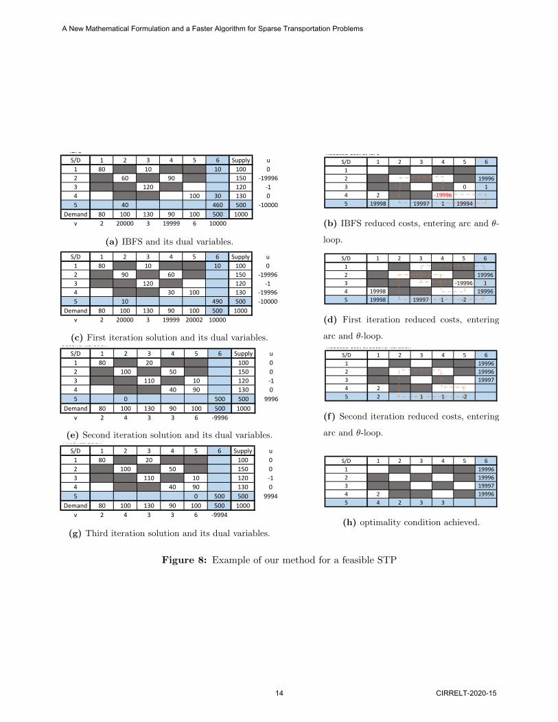
The traditional methods to obtain an IBFS may once again be used. For example, us-

ing the Minimum Cost Method, considering α = {(1, 1), (3, 3), (1, 3), (2, 4), (2, 2), (4, 5), (5, 2),

(1, 6), (4, 6), (5, 6)} it is possible to use the MODI method considering only admissible arcs.

In the IBFS (Figure 8a), the only arc with a negative reduced cost is (4, 4) (Figure 8b).

Thus, θ-loop= {(4, 4), (2, 4), (2, 2), (5, 2), (5, 6), (4, 6)}, θ = min{y24, y52, y46} = y46 = 30 and

arc (4, 6) leaves the basis (Figure 8b). After the first iteration (Figure 8c), arc (3, 5) en-

ters the basis, θ-loop= {(3, 5), (3, 3), (1, 3), (1, 6), (5, 6), (5, 2), (2, 2), (2, 4), (4, 4), (4, 5)}, θ =

min{y33, y16, y52, y24, y45} = y16 = 10 and arc (1, 6) leaves the basis (Figure 8d). After the

second iteration (Figure 8e), arc (5, 5) is the only one with a negative reduced cost and θ-

loop= {(5, 5), (5, 2), (2, 2), (2, 4), (4, 4), (4, 5)}, θ = min{y52, y24, y45} = y52 = 0 and arc (5, 2)

leaves the basis (Figure 8f).

When the reduced costs at the third iteration are computed (Figure 8h), we have that the

optimally condition for the ATP was achieved. In this case, ym+1,n+1 = L and the solution of

Figure 8g discarding the extra blue cells is optimal for the original STP.

4 Theoretical Analysis of the Proposed Mathematical

Formulation and Method

The sparsity σ of an STP may be defined as σ = (mn−|A|)mn

. Therefore, the number of arcs to be

considered in the proposed method is (1−σ)(mn)+m+n+1, while in the classical approach it

is always necessary to consider mn arcs. For this reason, the higher the sparsity is, the better

our method will perform compared to the classical approach.

In the previous sections we have shown through numerical examples how the proposed method

works. We now focus on detailed theoretical explanations. First, it is possible to argue that in

the classical approach, once a BFS using only admissible arcs is found, it is no longer necessary

to compute the reduced cost for any forbidden arc; the same holds for our new method, meaning

that the third iteration presented in Section 3.2 was not required. To this end, we refer to the

Phase I of the methods when all reduced costs need to be computed (namely when the solution


CIRRELT-2020-15 13

S\D 1 2 3 4 5 Supply1 0 0 100 0 0 100 1002 0 100 0 50 0 150 1503 0 0 30 0 90 120 1204 80 0 0 40 10 130 130

Demand 80 100 130 90 100 50080 100 130 90 100 1860

S\D 1 2 3 4 5 Supply1 2 3 1002 4 3 1503 2 5 1204 4 3 6 130

Demand 80 100 130 90 100 500

S\D 1 2 3 4 5 6 Supply1 2 3 10000 1002 4 3 10000 1503 2 5 10000 1204 4 3 6 10000 1305 10000 10000 10000 10000 10000 0 500

Demand 80 100 130 90 100 500 1000


1 80 10 10 100 0 12 60 90 150 -19996 2 199963 120 120 -1 3 0 14 100 30 130 0 4 2 -199965 40 460 500 -10000 5 19998 19997 1 19994

Demand 80 100 130 90 100 500 1000v 2 20000 3 19999 6 10000

S/D 1 2 3 4 5 6 Supply u S/D 1 2 3 4 5 61 80 10 10 100 0 12 90 60 150 -19996 2 199963 120 120 -1 3 -19996 14 30 100 130 -19996 4 19998 199965 10 490 500 -10000 5 19998 19997 1 -2

Demand 80 100 130 90 100 500 1000v 2 20000 3 19999 20002 10000

S/D 1 2 3 4 5 6 Supply u S/D 1 2 3 4 5 61 80 20 100 0 1 199962 100 50 150 0 2 199963 110 10 120 -1 3 199974 40 90 130 0 4 25 0 500 500 9996 5 2 1 1 -2

Demand 80 100 130 90 100 500 1000 0=min(0,50,90)v 2 4 3 3 6 -9996

S/D 1 2 3 4 5 6 Supply u S/D 1 2 3 4 5 61 80 20 100 0 1 199962 100 50 150 0 2 199963 110 10 120 -1 3 199974 40 90 130 0 4 2 199965 0 500 500 9994 5 4 2 3 3

Demand 80 100 130 90 100 500 1000 optimalv 2 4 3 3 6 -9994




30=min(90,40,30)


10=min(120,10,10,90,30)

(a) IBFS and its dual variables.

S\D 1 2 3 4 5 Supply1 0 0 100 0 0 100 1002 0 100 0 50 0 150 1503 0 0 30 0 90 120 1204 80 0 0 40 10 130 130

Demand 80 100 130 90 100 50080 100 130 90 100 1860

S\D 1 2 3 4 5 Supply1 2 3 1002 4 3 1503 2 5 1204 4 3 6 130

Demand 80 100 130 90 100 500

S\D 1 2 3 4 5 6 Supply1 2 3 10000 1002 4 3 10000 1503 2 5 10000 1204 4 3 6 10000 1305 10000 10000 10000 10000 10000 0 500

Demand 80 100 130 90 100 500 1000


1 80 10 10 100 0 12 60 90 150 -19996 2 199963 120 120 -1 3 0 14 100 30 130 0 4 2 -199965 40 460 500 -10000 5 19998 19997 1 19994

Demand 80 100 130 90 100 500 1000v 2 20000 3 19999 6 10000

S/D 1 2 3 4 5 6 Supply u S/D 1 2 3 4 5 61 80 10 10 100 0 12 90 60 150 -19996 2 199963 120 120 -1 3 -19996 14 30 100 130 -19996 4 19998 199965 10 490 500 -10000 5 19998 19997 1 -2

Demand 80 100 130 90 100 500 1000v 2 20000 3 19999 20002 10000

S/D 1 2 3 4 5 6 Supply u S/D 1 2 3 4 5 61 80 20 100 0 1 199962 100 50 150 0 2 199963 110 10 120 -1 3 199974 40 90 130 0 4 25 0 500 500 9996 5 2 1 1 -2

Demand 80 100 130 90 100 500 1000 0=min(0,50,90)v 2 4 3 3 6 -9996

S/D 1 2 3 4 5 6 Supply u S/D 1 2 3 4 5 61 80 20 100 0 1 199962 100 50 150 0 2 199963 110 10 120 -1 3 199974 40 90 130 0 4 2 199965 0 500 500 9994 5 4 2 3 3

Demand 80 100 130 90 100 500 1000 optimalv 2 4 3 3 6 -9994




30=min(90,40,30)


10=min(120,10,10,90,30)

(b) IBFS reduced costs, entering arc and θ-

loop.

S\D 1 2 3 4 5 Supply1 0 0 100 0 0 100 1002 0 100 0 50 0 150 1503 0 0 30 0 90 120 1204 80 0 0 40 10 130 130

Demand 80 100 130 90 100 50080 100 130 90 100 1860

S\D 1 2 3 4 5 Supply1 2 3 1002 4 3 1503 2 5 1204 4 3 6 130

Demand 80 100 130 90 100 500

S\D 1 2 3 4 5 6 Supply1 2 3 10000 1002 4 3 10000 1503 2 5 10000 1204 4 3 6 10000 1305 10000 10000 10000 10000 10000 0 500

Demand 80 100 130 90 100 500 1000


1 80 10 10 100 0 12 60 90 150 -19996 2 199963 120 120 -1 3 0 14 100 30 130 0 4 2 -199965 40 460 500 -10000 5 19998 19997 1 19994

Demand 80 100 130 90 100 500 1000v 2 20000 3 19999 6 10000

S/D 1 2 3 4 5 6 Supply u S/D 1 2 3 4 5 61 80 10 10 100 0 12 90 60 150 -19996 2 199963 120 120 -1 3 -19996 14 30 100 130 -19996 4 19998 199965 10 490 500 -10000 5 19998 19997 1 -2

Demand 80 100 130 90 100 500 1000v 2 20000 3 19999 20002 10000

S/D 1 2 3 4 5 6 Supply u S/D 1 2 3 4 5 61 80 20 100 0 1 199962 100 50 150 0 2 199963 110 10 120 -1 3 199974 40 90 130 0 4 25 0 500 500 9996 5 2 1 1 -2

Demand 80 100 130 90 100 500 1000 0=min(0,50,90)v 2 4 3 3 6 -9996

S/D 1 2 3 4 5 6 Supply u S/D 1 2 3 4 5 61 80 20 100 0 1 199962 100 50 150 0 2 199963 110 10 120 -1 3 199974 40 90 130 0 4 2 199965 0 500 500 9994 5 4 2 3 3

Demand 80 100 130 90 100 500 1000 optimalv 2 4 3 3 6 -9994




30=min(90,40,30)


10=min(120,10,10,90,30)

(c) First iteration solution and its dual variables.

S\D 1 2 3 4 5 Supply1 0 0 100 0 0 100 1002 0 100 0 50 0 150 1503 0 0 30 0 90 120 1204 80 0 0 40 10 130 130

Demand 80 100 130 90 100 50080 100 130 90 100 1860

S\D 1 2 3 4 5 Supply1 2 3 1002 4 3 1503 2 5 1204 4 3 6 130

Demand 80 100 130 90 100 500

S\D 1 2 3 4 5 6 Supply1 2 3 10000 1002 4 3 10000 1503 2 5 10000 1204 4 3 6 10000 1305 10000 10000 10000 10000 10000 0 500

Demand 80 100 130 90 100 500 1000


1 80 10 10 100 0 12 60 90 150 -19996 2 199963 120 120 -1 3 0 14 100 30 130 0 4 2 -199965 40 460 500 -10000 5 19998 19997 1 19994

Demand 80 100 130 90 100 500 1000v 2 20000 3 19999 6 10000

S/D 1 2 3 4 5 6 Supply u S/D 1 2 3 4 5 61 80 10 10 100 0 12 90 60 150 -19996 2 199963 120 120 -1 3 -19996 14 30 100 130 -19996 4 19998 199965 10 490 500 -10000 5 19998 19997 1 -2

Demand 80 100 130 90 100 500 1000v 2 20000 3 19999 20002 10000

S/D 1 2 3 4 5 6 Supply u S/D 1 2 3 4 5 61 80 20 100 0 1 199962 100 50 150 0 2 199963 110 10 120 -1 3 199974 40 90 130 0 4 25 0 500 500 9996 5 2 1 1 -2

Demand 80 100 130 90 100 500 1000 0=min(0,50,90)v 2 4 3 3 6 -9996

S/D 1 2 3 4 5 6 Supply u S/D 1 2 3 4 5 61 80 20 100 0 1 199962 100 50 150 0 2 199963 110 10 120 -1 3 199974 40 90 130 0 4 2 199965 0 500 500 9994 5 4 2 3 3

Demand 80 100 130 90 100 500 1000 optimalv 2 4 3 3 6 -9994




30=min(90,40,30)


10=min(120,10,10,90,30)

(d) First iteration reduced costs, entering

arc and θ-loop.

S\D 1 2 3 4 5 Supply1 0 0 100 0 0 100 1002 0 100 0 50 0 150 1503 0 0 30 0 90 120 1204 80 0 0 40 10 130 130

Demand 80 100 130 90 100 50080 100 130 90 100 1860

S\D 1 2 3 4 5 Supply1 2 3 1002 4 3 1503 2 5 1204 4 3 6 130

Demand 80 100 130 90 100 500

S\D 1 2 3 4 5 6 Supply1 2 3 10000 1002 4 3 10000 1503 2 5 10000 1204 4 3 6 10000 1305 10000 10000 10000 10000 10000 0 500

Demand 80 100 130 90 100 500 1000


1 80 10 10 100 0 12 60 90 150 -19996 2 199963 120 120 -1 3 0 14 100 30 130 0 4 2 -199965 40 460 500 -10000 5 19998 19997 1 19994

Demand 80 100 130 90 100 500 1000v 2 20000 3 19999 6 10000

S/D 1 2 3 4 5 6 Supply u S/D 1 2 3 4 5 61 80 10 10 100 0 12 90 60 150 -19996 2 199963 120 120 -1 3 -19996 14 30 100 130 -19996 4 19998 199965 10 490 500 -10000 5 19998 19997 1 -2

Demand 80 100 130 90 100 500 1000v 2 20000 3 19999 20002 10000

S/D 1 2 3 4 5 6 Supply u S/D 1 2 3 4 5 61 80 20 100 0 1 199962 100 50 150 0 2 199963 110 10 120 -1 3 199974 40 90 130 0 4 25 0 500 500 9996 5 2 1 1 -2

Demand 80 100 130 90 100 500 1000 0=min(0,50,90)v 2 4 3 3 6 -9996

S/D 1 2 3 4 5 6 Supply u S/D 1 2 3 4 5 61 80 20 100 0 1 199962 100 50 150 0 2 199963 110 10 120 -1 3 199974 40 90 130 0 4 2 199965 0 500 500 9994 5 4 2 3 3

Demand 80 100 130 90 100 500 1000 optimalv 2 4 3 3 6 -9994




30=min(90,40,30)


10=min(120,10,10,90,30)

(e) Second iteration solution and its dual variables.

S\D 1 2 3 4 5 Supply1 0 0 100 0 0 100 1002 0 100 0 50 0 150 1503 0 0 30 0 90 120 1204 80 0 0 40 10 130 130

Demand 80 100 130 90 100 50080 100 130 90 100 1860

S\D 1 2 3 4 5 Supply1 2 3 1002 4 3 1503 2 5 1204 4 3 6 130

Demand 80 100 130 90 100 500

S\D 1 2 3 4 5 6 Supply1 2 3 10000 1002 4 3 10000 1503 2 5 10000 1204 4 3 6 10000 1305 10000 10000 10000 10000 10000 0 500

Demand 80 100 130 90 100 500 1000


1 80 10 10 100 0 12 60 90 150 -19996 2 199963 120 120 -1 3 0 14 100 30 130 0 4 2 -199965 40 460 500 -10000 5 19998 19997 1 19994

Demand 80 100 130 90 100 500 1000v 2 20000 3 19999 6 10000

S/D 1 2 3 4 5 6 Supply u S/D 1 2 3 4 5 61 80 10 10 100 0 12 90 60 150 -19996 2 199963 120 120 -1 3 -19996 14 30 100 130 -19996 4 19998 199965 10 490 500 -10000 5 19998 19997 1 -2

Demand 80 100 130 90 100 500 1000v 2 20000 3 19999 20002 10000

S/D 1 2 3 4 5 6 Supply u S/D 1 2 3 4 5 61 80 20 100 0 1 199962 100 50 150 0 2 199963 110 10 120 -1 3 199974 40 90 130 0 4 25 0 500 500 9996 5 2 1 1 -2

Demand 80 100 130 90 100 500 1000 0=min(0,50,90)v 2 4 3 3 6 -9996

S/D 1 2 3 4 5 6 Supply u S/D 1 2 3 4 5 61 80 20 100 0 1 199962 100 50 150 0 2 199963 110 10 120 -1 3 199974 40 90 130 0 4 2 199965 0 500 500 9994 5 4 2 3 3

Demand 80 100 130 90 100 500 1000 optimalv 2 4 3 3 6 -9994




30=min(90,40,30)


10=min(120,10,10,90,30)

(f) Second iteration reduced costs, entering

arc and θ-loop.

S\D 1 2 3 4 5 Supply1 0 0 100 0 0 100 1002 0 100 0 50 0 150 1503 0 0 30 0 90 120 1204 80 0 0 40 10 130 130

Demand 80 100 130 90 100 50080 100 130 90 100 1860

S\D 1 2 3 4 5 Supply1 2 3 1002 4 3 1503 2 5 1204 4 3 6 130

Demand 80 100 130 90 100 500

S\D 1 2 3 4 5 6 Supply1 2 3 10000 1002 4 3 10000 1503 2 5 10000 1204 4 3 6 10000 1305 10000 10000 10000 10000 10000 0 500

Demand 80 100 130 90 100 500 1000


1 80 10 10 100 0 12 60 90 150 -19996 2 199963 120 120 -1 3 0 14 100 30 130 0 4 2 -199965 40 460 500 -10000 5 19998 19997 1 19994

Demand 80 100 130 90 100 500 1000v 2 20000 3 19999 6 10000

S/D 1 2 3 4 5 6 Supply u S/D 1 2 3 4 5 61 80 10 10 100 0 12 90 60 150 -19996 2 199963 120 120 -1 3 -19996 14 30 100 130 -19996 4 19998 199965 10 490 500 -10000 5 19998 19997 1 -2

Demand 80 100 130 90 100 500 1000v 2 20000 3 19999 20002 10000

S/D 1 2 3 4 5 6 Supply u S/D 1 2 3 4 5 61 80 20 100 0 1 199962 100 50 150 0 2 199963 110 10 120 -1 3 199974 40 90 130 0 4 25 0 500 500 9996 5 2 1 1 -2

Demand 80 100 130 90 100 500 1000 0=min(0,50,90)v 2 4 3 3 6 -9996

S/D 1 2 3 4 5 6 Supply u S/D 1 2 3 4 5 61 80 20 100 0 1 199962 100 50 150 0 2 199963 110 10 120 -1 3 199974 40 90 130 0 4 2 199965 0 500 500 9994 5 4 2 3 3

Demand 80 100 130 90 100 500 1000 optimalv 2 4 3 3 6 -9994




30=min(90,40,30)


10=min(120,10,10,90,30)

(g) Third iteration solution and its dual variables.

S\D 1 2 3 4 5 Supply1 0 0 100 0 0 100 1002 0 100 0 50 0 150 1503 0 0 30 0 90 120 1204 80 0 0 40 10 130 130

Demand 80 100 130 90 100 50080 100 130 90 100 1860

S\D 1 2 3 4 5 Supply1 2 3 1002 4 3 1503 2 5 1204 4 3 6 130

Demand 80 100 130 90 100 500

S\D 1 2 3 4 5 6 Supply1 2 3 10000 1002 4 3 10000 1503 2 5 10000 1204 4 3 6 10000 1305 10000 10000 10000 10000 10000 0 500

Demand 80 100 130 90 100 500 1000


1 80 10 10 100 0 12 60 90 150 -19996 2 199963 120 120 -1 3 0 14 100 30 130 0 4 2 -199965 40 460 500 -10000 5 19998 19997 1 19994

Demand 80 100 130 90 100 500 1000v 2 20000 3 19999 6 10000

S/D 1 2 3 4 5 6 Supply u S/D 1 2 3 4 5 61 80 10 10 100 0 12 90 60 150 -19996 2 199963 120 120 -1 3 -19996 14 30 100 130 -19996 4 19998 199965 10 490 500 -10000 5 19998 19997 1 -2

Demand 80 100 130 90 100 500 1000v 2 20000 3 19999 20002 10000

S/D 1 2 3 4 5 6 Supply u S/D 1 2 3 4 5 61 80 20 100 0 1 199962 100 50 150 0 2 199963 110 10 120 -1 3 199974 40 90 130 0 4 25 0 500 500 9996 5 2 1 1 -2

Demand 80 100 130 90 100 500 1000 0=min(0,50,90)v 2 4 3 3 6 -9996

S/D 1 2 3 4 5 6 Supply u S/D 1 2 3 4 5 61 80 20 100 0 1 199962 100 50 150 0 2 199963 110 10 120 -1 3 199974 40 90 130 0 4 2 199965 0 500 500 9994 5 4 2 3 3

Demand 80 100 130 90 100 500 1000 optimalv 2 4 3 3 6 -9994




30=min(90,40,30)


10=min(120,10,10,90,30)

(h) optimality condition achieved.

Figure 8: Example of our method for a feasible STP


14 CIRRELT-2020-15

still uses a forbidden arc), and to Phase II when only admissible arcs are used and not all

reduced costs need to be calculated. In the computational experiments section we will detail

the runtime for each of these two phases. This will allow us to compare the running time for

each iteration, notably for Phase I and precisely measure the gains of our method.

Besides being capable to correctly identify whether the original STP in infeasible, our method

can be easily implemented from any MODI implementation. The only important modification

lies in the second step, because instead of calculating cij = cij − ui − vj, ∀i and j, the only

computation required is cij = cij − ui − vj, (i, j) ∈ A.

In what follows, let A′ be the set composed by the union of set A and the arcs associated with

the newly added variables to the STP.

Theorem 1: The ATP is always feasible.

Proof of Theorem 1

In order to show that ATP is always feasible, it suffices to determine one feasible solution. A

feasible solution to ATP can be obtained by setting:

yi,n+1 = Si i ∈M (15)

ym+1,j = Dj j ∈ N (16)

ym+1,n+1 = 0 (17)

yij = 0 ∀(i, j) ∈ A. (18)

Replacing the variable values (15)–(18) in the LHS of equations (10)–(13) yields expressions

(19)–(22), respectively:

∑j:(i,j)∈A

yij + yi,n+1 = 0 + Si = Si i ∈M (19)

∑i:(ij)∈A

yij + ym+1,j = 0 +Dj = Dj j ∈ N (20)


CIRRELT-2020-15 15

n+1∑j=1

ym+1,j =n∑

j=1

ym+1,j + xm+1,n+1 =n∑

j=1

Dj = L = Sm+1 (21)

m+1∑i=1

yi,n+1 =m∑i=1

yi,n+1 + ym+1,n+1 =m∑i=1

Si = L = Dn+1. (22)

This implies that all constraints are satisfied, which completes the proof. �

It is shown that the solution defined by (15)–(18) satisfies each constraint of ATP. Therefore,

this problem is feasible and admits an optimal solution, denoted by y∗ij, (i, j) ∈ A′. Particularly

for variable ym+1,n+1 two situations can occur: either y∗m+1,n+1 = L or y∗m+1,n+1 < L.

Note that any of the variables set to zero in expressions (17) and (18) can be used as a degener-

ated basic variable to the ATP, which can be exploited in the MODI method. In what follows

we consider variable ym+1,n+1.

Theorem 2: If yij ∈ A′ is a feasible solution to the ATP and ym+1,n+1 = L, the original STP is

feasible.

Proof of Theorem 2

Replacing ym+1,j = 0, j ∈ N , yi,n+1 = 0, i ∈M and ym+1,n+1 = L in (10)–(13) yields (23)–(26):

L =n+1∑j=1

ym+1,j + ym+1,n+1 ⇒ L =∑j∈N

ym+1,j +L⇒∑j∈N

ym+1,j = 0⇒ ym+1,j = 0 j ∈ N (23)

∑i∈M

yi,n+1 = 0⇒ yi,n+1 = 0 i ∈M (24)

∑j∈N

yij + yi,n+1 = Si i ∈M⇒∑j∈N

yij = Si i ∈M (25)

∑i∈M

yij + ym+1,j = Dj j ∈ N ⇒∑i∈M

yij = Dj j ∈ N . (26)

Setting xij = yij, (i, j) ∈ A, makes (25) and (26) assure that (2) and (3) are satisfied. Thus, x

is a feasible solution to the STP. �

Corollary 1: If x = xij, (i, j) ∈ A, is a feasible solution to the STP, so yij =

xij, (i, j) ∈ A

ym+1,n+1 = L

is feasible to ATP.


16 CIRRELT-2020-15

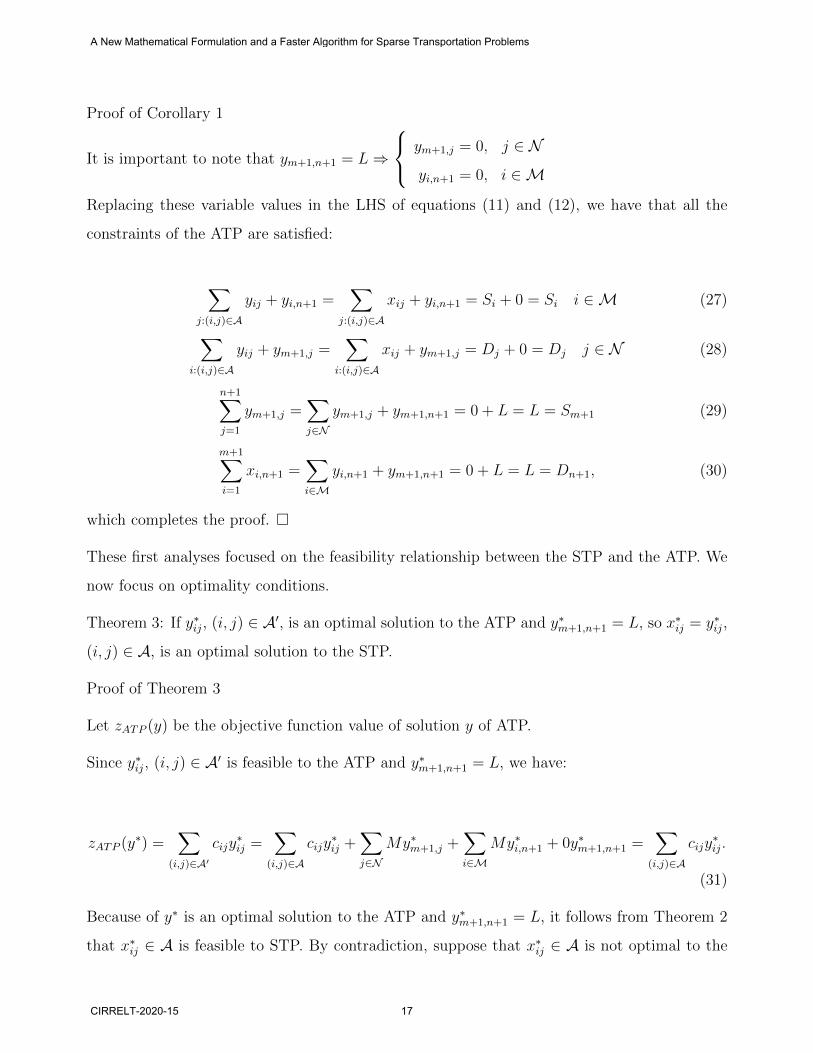
Proof of Corollary 1

It is important to note that ym+1,n+1 = L⇒

ym+1,j = 0, j ∈ N

yi,n+1 = 0, i ∈M

Replacing these variable values in the LHS of equations (11) and (12), we have that all the

constraints of the ATP are satisfied:

∑j:(i,j)∈A

yij + yi,n+1 =∑

j:(i,j)∈A

xij + yi,n+1 = Si + 0 = Si i ∈M (27)

∑i:(i,j)∈A

yij + ym+1,j =∑

i:(i,j)∈A

xij + ym+1,j = Dj + 0 = Dj j ∈ N (28)

n+1∑j=1

ym+1,j =∑j∈N

ym+1,j + ym+1,n+1 = 0 + L = L = Sm+1 (29)

m+1∑i=1

xi,n+1 =∑i∈M

yi,n+1 + ym+1,n+1 = 0 + L = L = Dn+1, (30)

which completes the proof. �

These first analyses focused on the feasibility relationship between the STP and the ATP. We

now focus on optimality conditions.

Theorem 3: If y∗ij, (i, j) ∈ A′, is an optimal solution to the ATP and y∗m+1,n+1 = L, so x∗ij = y∗ij,

(i, j) ∈ A, is an optimal solution to the STP.

Proof of Theorem 3

Let zATP (y) be the objective function value of solution y of ATP.

Since y∗ij, (i, j) ∈ A′ is feasible to the ATP and y∗m+1,n+1 = L, we have:

zATP (y∗) =∑

(i,j)∈A′

cijy∗ij =

∑(i,j)∈A

cijy∗ij +

∑j∈N

My∗m+1,j +∑i∈M

My∗i,n+1 + 0y∗m+1,n+1 =∑

(i,j)∈A

cijy∗ij.

(31)

Because of y∗ is an optimal solution to the ATP and y∗m+1,n+1 = L, it follows from Theorem 2

that x∗ij ∈ A is feasible to STP. By contradiction, suppose that x∗ij ∈ A is not optimal to the


CIRRELT-2020-15 17

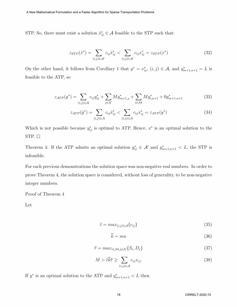
STP. So, there must exist a solution x∗ij ∈ A feasible to the STP such that:

zSTP (x∗) =∑

(i,j)∈A′

cijx∗ij <

∑(i,j)∈A′

cijx∗ij = zSTP (x∗) (32)

On the other hand, it follows from Corollary 1 that y∗ = x∗ij, (i, j) ∈ A, and y∗m+1,n+1 = L is

feasible to the ATP, so

zATP (y∗) =∑

(i,j)∈A

cijy∗ij +

∑j∈N

My∗m+1,j +∑i∈M

My∗i,n+1 + 0y∗m+1,n+1 (33)

zATP (y∗) =∑

(i,j)∈A

cijx∗ij <

∑(i,j)∈A

cijx∗ij = zATP (y∗) (34)

Which is not possible because y∗ij is optimal to ATP. Hence, x∗ is an optimal solution to the

STP. �

Theorem 4: If the ATP admits an optimal solution y∗ij ∈ A′ and y∗m+1,n+1 < L, the STP is

infeasible.

For each previous demonstrations the solution space was non-negative real numbers. In order to

prove Theorem 4, the solution space is considered, without loss of generality, to be non-negative

integer numbers.

Proof of Theorem 4

Let

c = max(i,j)∈A{cij} (35)

k = mn (36)

r = maxi∈M,j∈N{Si, Dj} (37)

M > ckr ≥∑

(i,j)∈A

cijxij. (38)

If y∗ is an optimal solution to the ATP and y∗m+1,n+1 < L then


18 CIRRELT-2020-15

∑i∈M

y∗i,n+1 =∑j∈N

y∗m+1,j ≥ 1. (39)

And because

zATP (y) =∑

(i,j)∈A

cijyij +∑j∈N

Mym+1,j +∑i∈M

Myi,n+1 + 0ym+1,n+1 (40)

it follows that

zATP (y) ≥∑

(i,j)∈A

cijyij + 2M (41)

Assuming that the STP admits a feasible solution x, we know that this solution augmented by

ym+1,n+1 = L is feasible to the ATP (from Corollary 1), and the objective function value for

this solution to the ATP is:

zATP (x) =∑

(i,j)∈A

cijxij < M <∑

(i,j)∈A

cijy∗ij + 2M ≤ zATP (y∗) (42)

Expression (42) contradicts the fact that y∗ minimizes zATP . Therefore, the STP is infeasible.

�

In Corollary 1 and Theorem 3 we have proved that if the ATP is feasible and y∗m+1,n+1 = L, by

solving the ATP we have the solution to the STP. Moreover, Theorem 4 demonstrates that an

optimal solution to the ATP in which y∗m+1,n+1 < L suffices to show that the STP is infeasible.

Hence, solving an ATP leads to the solution of an STP.

Finally, the next theorem shows that is not necessary to compute reduced costs for forbidden

arcs. The gains of the proposed method lie in computing them only for admissible arcs, which

is sufficient as demonstrated next. The following theorem provides a practical result for the

improvement procedure in our algorithm, and explains the advantage of the proposed method

in the number of reduced costs that must be updated.


CIRRELT-2020-15 19

Theorem 5: In an STP with arc set A, finite costs cij for (i, j) ∈ A, forbidden arcs with costs

equal to at least M =∑

i∈M ai ×max{|cij| : i = 1, . . . ,m, j = 1, . . . , n}, and a BFS using only

arcs belonging to A, the entrance of an arc (i, j) /∈ A never improves the solution.

Proof of Theorem 5

When the costs associated with the basic variables are finite, so are u′ and v′. Therefore, for

any (i, j) /∈ A we have that cij = cij − ui − vj = M − ui − vj > 0. Hence, it is not necessary to

compute cij for (i, j) /∈ A. �

As a result of the Theorem 5, we have that the biggest challenge to solve STPs is to determine a

BFS using only admissible arcs; once one is known, the classical approach may also be applied.

Combining the developments presented in this section, we have that the ATP always admits a

feasible solution and when the MODI method is applied computing the reduced costs only for

(i, j) ∈ A′, an optimal solution to ATP is obtained. Thus, two possibilities arise:

1. y∗ is an optimal solution to the ATP and y∗m+1,n+1 = L ⇒ the STP is feasible and its

optimal solution is obtained by discarding y∗m+1,n+1 and setting x∗ij = y∗ij : (i, j) ∈ A;

2. y∗ is an optimal solution to the ATP and y∗m+1,n+1 < L ⇒ the STP is infeasible.

5 Acceleration technique using partial pricing

Partial Pricing (PP) is a well-known strategy in solving LP problems [14, 12]. It consists in

evaluating the reduced costs of only a subset SPP of non-basic variables [5]. The challenges in

using PP are to determine the sequence of non-basic variables to be evaluated as well as how

many reduced costs will be computed.

In our algorithm the costs cij associated with each variable were already sorted when ap-

plying the minimum cost method. We use this sorted list A at each iteration, avoiding

any computational burden. The rationale for this choice is to first evaluate variables with

low values of cij, such that when we compute cij = cij − ui − vj we have higher chances


20 CIRRELT-2020-15

of obtaining negative values of cij in the early attempts. For example, in Figure 1 A =

{(1, 1), (3, 3), (1, 3), (2, 4), (4, 4), (2, 2, ), (4, 1), (3, 5)}.

Regarding the size of our PP list, we determine a value LPP such that we stop the search once

we have identified the first LPP variables with negative reduced costs (or fewer if all variables

have been tested). These variables with negative reduced costs constitute the set SPP . This

procedure is repeated at each iteration. We note, however, that the sequence of variables to be

evaluated according to their costs cij does not need to be reordered.

The pseudocode of our implementation of PP is described in Algorithm 2. Note that because

it guarantees to compute a negative reduced cost variable if one exists, optimality conditions

are respected.

6 Computational Experiments

In order to evaluate the performance of our new exact method, we have conducted extensive

computational experiments. We have implemented the MODI method in C++ using the same

data structure for both the traditional method and our sparse approach, meaning that the gains

obtained are direct results of our new method to solve STPs. For each parameter combination

we have solved 100 different instances randomly generated and the results showed in this section

represent the averages of performance measures. Since runtimes are in the order of milliseconds

and to avoid any bias, for each instance and each algorithm, we run it 20 times, discarding the

best five and the worst five times, averaging the time of the remaining 10 runs. Moreover, the

order of each execution were further randomized to avoid any bias or trends in CPU usage.

Thus, for a total of 8,200 instances, we have run them 20 times in our TP algorithm with

full and partial pricing, and with and without forbidden arcs; 20 times using the algorithm

of Ababei [1] with and without forbidden arcs; and 20 times using Gurobi with and without

forbidden arcs. This totals 1,312,000 executions.

All computations were performed on a desktop PC equipped with an Intel i7 8565 running

at 1.8GHz with 16GB of RAM installed (even though the memory footprint of our codes is


CIRRELT-2020-15 21

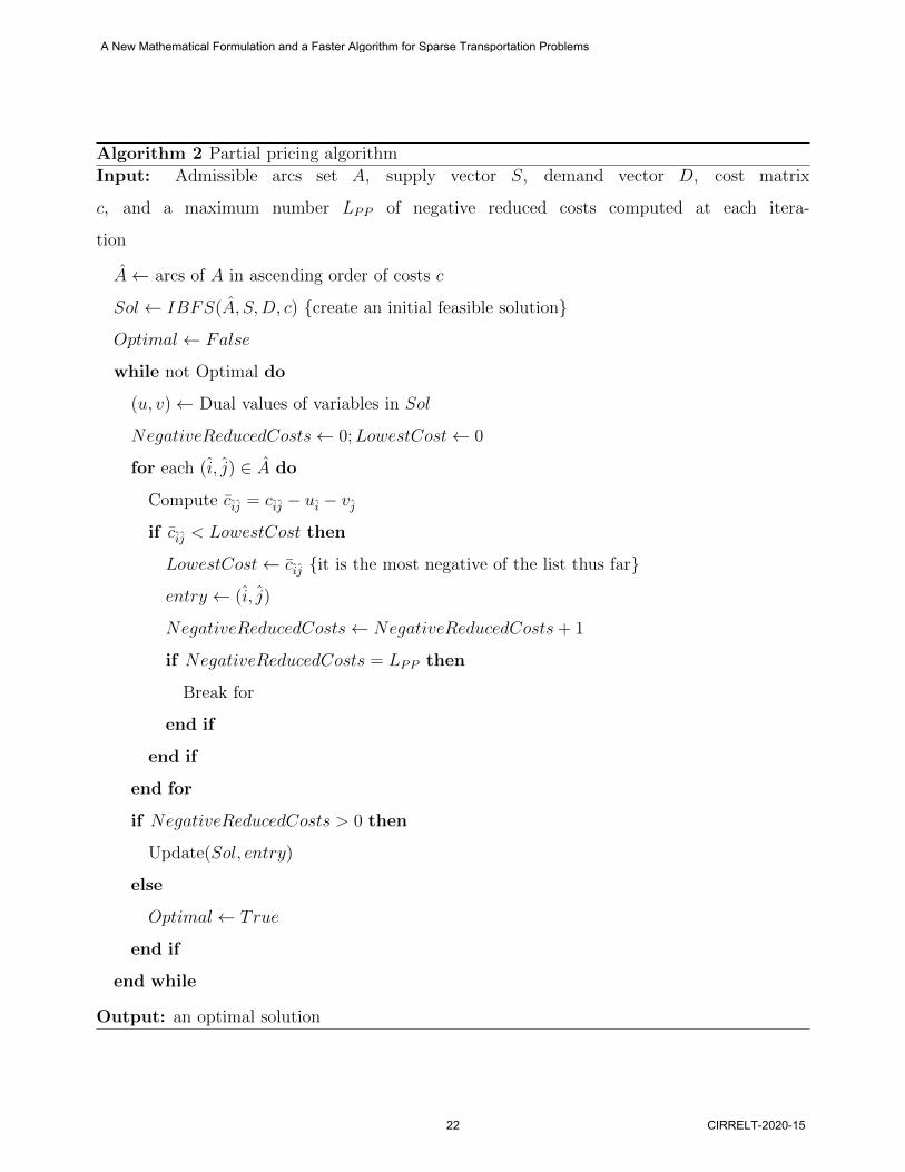
Algorithm 2 Partial pricing algorithm

Input: Admissible arcs set A, supply vector S, demand vector D, cost matrix

c, and a maximum number LPP of negative reduced costs computed at each itera-

tion

A← arcs of A in ascending order of costs c

Sol← IBFS(A, S,D, c) {create an initial feasible solution}

Optimal ← False

while not Optimal do

(u, v)← Dual values of variables in Sol

NegativeReducedCosts← 0;LowestCost← 0

for each (i, j) ∈ A do

Compute cij = cij − ui − vjif cij < LowestCost then

LowestCost← cij {it is the most negative of the list thus far}

entry ← (i, j)

NegativeReducedCosts← NegativeReducedCosts+ 1

if NegativeReducedCosts = LPP then

Break for

end if

end if

end for

if NegativeReducedCosts > 0 then

Update(Sol, entry)

else

Optimal ← True

end if

end while

Output: an optimal solution


22 CIRRELT-2020-15

extremely small), with the Windows 10 operating system. The algorithms were all coded in

C++ and we used Gurobi 9.0 as the LP solver. In order to compare with the min-cost network

flow scaling push-relabel algorithm, we use the open-source C++ implementation of Ababei [1]

of the original algorithm of Goldberg [13]. All instances and detailed results are available from

https://www.leandro-coelho.com/sparse-transportation-problem/.

In Section 6.1 we show the results for feasible problems, considering problems sizes ranging from

100× 100 to 500× 500 and densities ranging from 2% to 75%. Section 6.2 shows the results for

infeasible problems with same ranges of size and density. Moreover, for all the computational

experiments with partial pricing we used LPP = 120.

An overall comparison of the different implementations that we analysed is based on the total

execution time. More detailed comparison of the four versions of the MODI method (with

partial and full pricing, with and without forbidden arcs) are evaluated by running time, number

of iterations, average time per iteration, number of reduced costs computed, and gap of the

IBFS to an optimal solution. Additionally, for infeasible instances, we also evaluate the time

required to prove that the instances were infeasible.

6.1 Results for Feasible Instances

In what follows we present the details of extensive computational results on 100 feasible in-

stances of each configuration of sizes and densities for L = 100m, cmin = 10, cmax = 1000.

Specifically, we compare the performance of our method against the traditional one of using

artificial variables for all forbidden arcs, with and without partial pricing. Moreover, we also

present the results of Gurobi and of a network flow algorithm on both the traditional method

(all variables, including forbidden arcs), and in our sparse representation. The general results

of execution times are presented in Tables 1 and 2 and the later in this section we detail the

performances of our new approach and the partial pricing. The LP formulation in Gurobi and

the network flow algorithm implementation of Ababei [1] allow solving the STP using only

admissible arcs, referred to columns Sparse in Tables 1 and 2. In order to present a detailed

comparison we conducted computational experiments considering high costs for non-admissible


CIRRELT-2020-15 23

arcs and the results are presented under columns Traditional. Recall that each value presented

in our tables are average over 100 instances executed 20 times each where the best five and

worst five results are discarded.

When comparing the results of Gurobi and of the network flow algorithm implementation

presented in Tables 1 and 2, we have that in cases of using high costs to forbidden arcs, the

second one had the better execution times, but the gains of considering only admissible arcs

are much higher in Gurobi. Moreover, when using only admissible arcs the general purpose

solver Gurobi outperforms the specialized implementation in a lower level language (C++) of

Ababei [1], with the only few exceptions observed in higher density cases. In the same tables

both MODI method with Full Pricing (MODI FP) and with Partial Pricing (MODI PP) refer

to results of our implementation in C++. For problems os size 100×100 the MODI FP is faster

than the best results of Gurobi and our Sparse approach with FP outperforms Gurobi by a large

margin in most of the cases, but loses performance for larger problems with high densities. As

our focus lies on solving STPs, the gains obtained for lower density cases are already relevant.

However, in order to provide a new state-of-the-art solver for STPs we also implemented a

Partial Pricing strategy to speed up the MODI methods. The usage of PP made it possible

to outperform the state-of-the-art solver Gurobi in all cases by a factor of around 4×. The

relative gains of each approach in the MODI method are presented in Figure 9, highlighting

the percentage of runtime reductions and the behavior of each density level when increasing

the size of the problem. Moreover, the relative gains of our Sparse MODI method with Partial

Pricing (SMODIPP) when compared to the network flow algorithm are presented in Figure 10.

A more detailed analysis of the results from Table 1 show some unexpected results. For example,

in the traditional cases with high costs for forbidden arcs, we have that Gurobi’s runtimes

increase as the density becomes higher. In the sparse case with only admissible arcs we have

that for instances of sizes 100× 100 and 200× 200 the runtime increases more significantly as

the density increases. However, it is not possible to find a pattern for problems of size 300×300

and larger. It is not possible to identify the reasons as the solver was used as a block box. It

is important to note that for lower density instances of Table 2 this behavior does not exist for

problems solved with Gurobi, i.e., it does not occur in problems of size 500×500 with densities


24 CIRRELT-2020-15

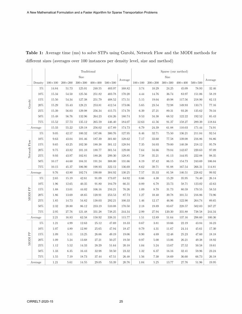
Table 1: Average time (ms) to solve STPs using Gurobi, Network Flow and the MODI methods for

different sizes (averages over 100 instances per density level, size and method)

Traditional Sparse (our method)

SizeAverage

SizeAverage

Density 100×100 200×200 300×300 400×400 500×500 100×100 200×200 300×300 400×400 500×500

Gu

rob

i

5% 14.84 51.73 125.01 248.55 403.97 168.82 3.74 10.29 24.25 45.09 78.93 32.46

10% 15.34 54.50 125.56 251.82 403.78 170.20 4.44 14.76 36.74 83.97 151.06 58.19

15% 15.50 54.34 127.38 251.79 408.52 171.51 5.15 19.04 49.98 117.56 218.90 82.13

20% 15.29 55.43 128.21 253.81 412.54 173.06 5.65 23.54 72.98 149.93 133.71 77.16

25% 15.39 56.03 129.98 256.34 415.75 174.70 6.39 27.21 89.31 93.20 135.62 70.34

50% 15.48 56.76 132.96 264.23 434.26 180.74 9.53 34.38 68.52 122.22 192.52 85.43

75% 15.52 57.73 135.12 265.59 446.40 184.07 12.63 41.56 91.37 158.27 289.39 118.64

Average 15.33 55.22 129.18 256.02 417.89 174.73 6.79 24.39 61.88 110.03 171.44 74.91

Net

wor

kF

low

5% 9.05 42.57 100.32 187.06 300.76 127.95 6.46 32.71 75.50 136.21 211.84 92.54

10% 9.63 43.04 101.46 187.39 301.60 128.62 7.17 33.60 77.58 139.08 216.86 94.86

15% 9.65 43.25 102.30 188.38 301.12 128.94 7.35 34.03 79.00 140.38 218.12 95.78

20% 9.75 43.82 101.10 188.77 301.54 129.00 7.64 34.66 79.84 142.67 220.63 97.09

25% 9.93 43.97 102.81 188.26 299.30 128.85 7.58 35.21 81.13 144.95 222.88 98.35

50% 10.17 44.60 104.31 191.24 308.00 131.66 8.19 37.42 86.15 154.73 243.69 106.04

75% 10.15 45.37 106.90 198.93 322.12 136.69 8.62 39.71 91.88 167.54 266.31 114.81

Average 9.76 43.80 102.74 190.00 304.92 130.25 7.57 35.33 81.58 146.51 228.62 99.92

MO

DI

FP

5% 2.65 15.19 42.61 91.09 173.07 64.92 0.66 4.38 15.29 35.95 74.40 26.14

10% 1.96 12.65 40.35 91.80 184.79 66.31 0.89 6.78 23.73 58.71 123.02 42.63

15% 1.88 13.01 44.02 106.16 216.21 76.26 1.09 8.70 31.73 80.59 170.55 58.53

20% 1.86 13.69 48.65 120.91 253.53 87.73 1.27 10.40 39.78 101.51 216.86 73.96

25% 1.85 14.73 54.82 138.03 292.21 100.33 1.46 12.17 46.96 122.90 264.74 89.65

50% 2.32 20.80 86.12 233.19 510.08 170.50 2.18 19.89 83.67 228.57 502.03 167.27

75% 2.95 27.76 121.48 331.28 738.25 244.34 2.99 27.94 120.30 331.88 738.58 244.34

Average 2.21 16.83 62.58 158.92 338.31 115.77 1.51 12.89 51.64 137.16 298.60 100.36

MO

DI

PP

5% 1.21 4.99 12.63 25.12 47.69 18.33 0.67 3.81 10.66 22.19 43.84 16.23

10% 1.07 4.89 12.80 25.65 47.94 18.47 0.79 4.31 11.67 24.14 45.61 17.30

15% 1.09 5.11 13.25 26.66 49.19 19.06 0.90 4.69 12.48 25.23 47.60 18.18

20% 1.09 5.24 13.68 27.21 50.27 19.50 0.97 5.00 13.06 26.21 49.38 18.92

25% 1.12 5.52 14.33 28.29 51.64 20.18 1.04 5.24 13.67 27.52 50.58 19.61

50% 1.33 6.35 16.43 32.98 59.50 23.32 1.32 6.37 16.16 32.41 59.96 23.24

75% 1.55 7.19 18.73 37.44 67.51 26.48 1.56 7.30 18.69 36.60 66.73 26.18

Average 1.21 5.61 14.55 29.05 53.39 20.76 1.04 5.25 13.77 27.76 51.96 19.95


CIRRELT-2020-15 25

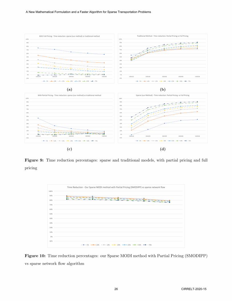
-10%

0%

10%

20%

30%

40%

50%

60%

70%

80%

90%

100%

100X100 200X200 300X300 400X400 500X500

With Full Pricing - Time reduction: sparse (our method) vs traditional method

5% 10% 15% 20% 25% 50% 75%

(a)

-10%

0%

10%

20%

30%

40%

50%

60%

70%

80%

90%

100%

100X100 200X200 300X300 400X400 500X500

Traditional Method - Time reduction: Partial Pricing vs Full Pricing

5% 10% 15% 20% 25% 50% 75%

(b)

-10%

0%

10%

20%

30%

40%

50%

60%

70%

80%

90%

100%

100X100 200X200 300X300 400X400 500X500

With Partial Pricing - Time reduction: sparse (our method) vs traditional method

5% 10% 15% 20% 25% 50% 75%

(c)

-10%

0%

10%

20%

30%

40%

50%

60%

70%

80%

90%

100%

100X100 200X200 300X300 400X400 500X500

Sparse (our Method) - Time reduction: Partial Pricing vs Full Pricing

5% 10% 15% 20% 25% 50% 75%

(d)

Figure 9: Time reduction percentages: sparse and traditional models, with partial pricing and full

pricing

-10%

0%

10%

20%

30%

40%

50%

60%

70%

80%

90%

100%

Time Reduction - Our Sparse MODI method with Partial Pricing (SMODIPP) vs sparse network flow

5% 10% 15% 20% 25% 50% 75%

Figure 10: Time reduction percentages: our Sparse MODI method with Partial Pricing (SMODIPP)

vs sparse network flow algorithm


26 CIRRELT-2020-15

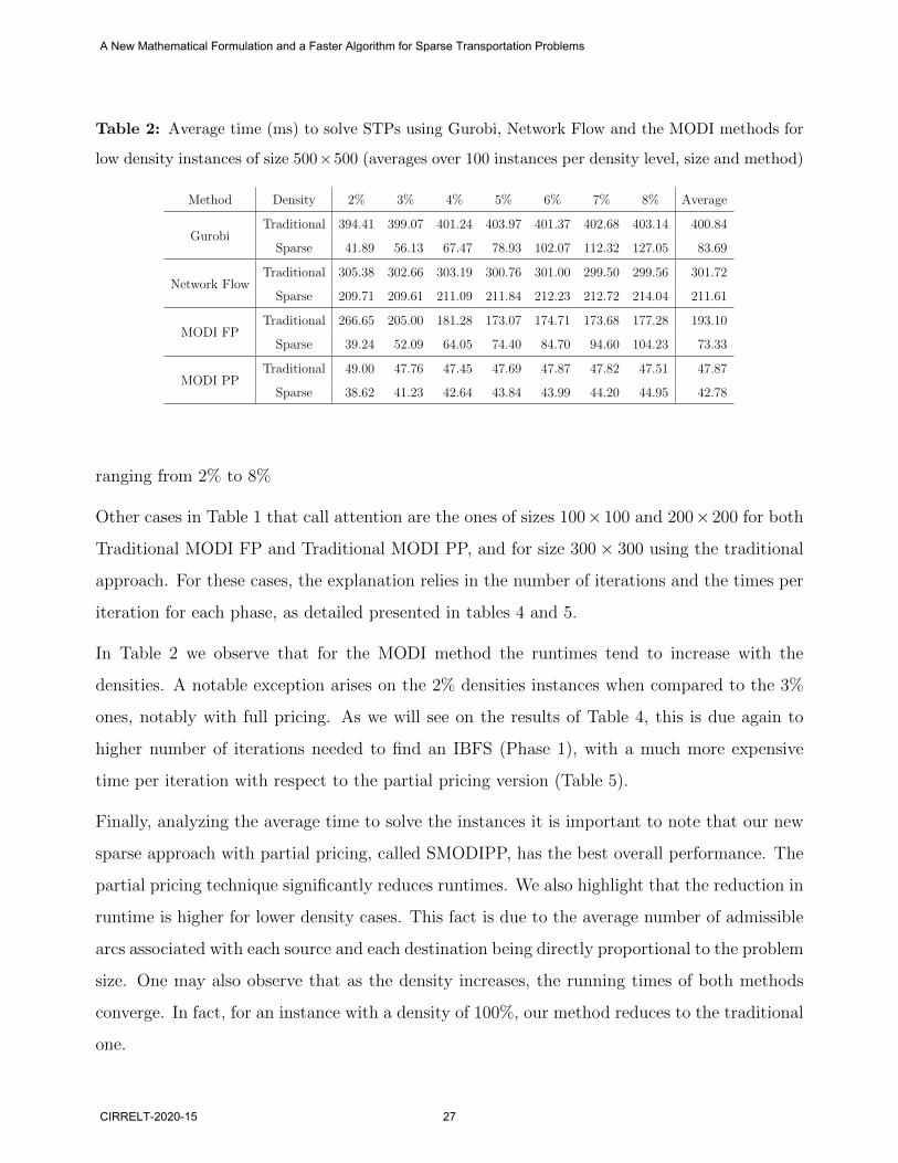
Table 2: Average time (ms) to solve STPs using Gurobi, Network Flow and the MODI methods for

low density instances of size 500×500 (averages over 100 instances per density level, size and method)

Method Density 2% 3% 4% 5% 6% 7% 8% Average

GurobiTraditional 394.41 399.07 401.24 403.97 401.37 402.68 403.14 400.84

Sparse 41.89 56.13 67.47 78.93 102.07 112.32 127.05 83.69

Network FlowTraditional 305.38 302.66 303.19 300.76 301.00 299.50 299.56 301.72

Sparse 209.71 209.61 211.09 211.84 212.23 212.72 214.04 211.61

MODI FPTraditional 266.65 205.00 181.28 173.07 174.71 173.68 177.28 193.10

Sparse 39.24 52.09 64.05 74.40 84.70 94.60 104.23 73.33

MODI PPTraditional 49.00 47.76 47.45 47.69 47.87 47.82 47.51 47.87

Sparse 38.62 41.23 42.64 43.84 43.99 44.20 44.95 42.78

ranging from 2% to 8%

Other cases in Table 1 that call attention are the ones of sizes 100×100 and 200×200 for both

Traditional MODI FP and Traditional MODI PP, and for size 300× 300 using the traditional

approach. For these cases, the explanation relies in the number of iterations and the times per

iteration for each phase, as detailed presented in tables 4 and 5.

In Table 2 we observe that for the MODI method the runtimes tend to increase with the

densities. A notable exception arises on the 2% densities instances when compared to the 3%

ones, notably with full pricing. As we will see on the results of Table 4, this is due again to

higher number of iterations needed to find an IBFS (Phase 1), with a much more expensive

time per iteration with respect to the partial pricing version (Table 5).

Finally, analyzing the average time to solve the instances it is important to note that our new

sparse approach with partial pricing, called SMODIPP, has the best overall performance. The

partial pricing technique significantly reduces runtimes. We also highlight that the reduction in

runtime is higher for lower density cases. This fact is due to the average number of admissible

arcs associated with each source and each destination being directly proportional to the problem

size. One may also observe that as the density increases, the running times of both methods

converge. In fact, for an instance with a density of 100%, our method reduces to the traditional

one.


CIRRELT-2020-15 27

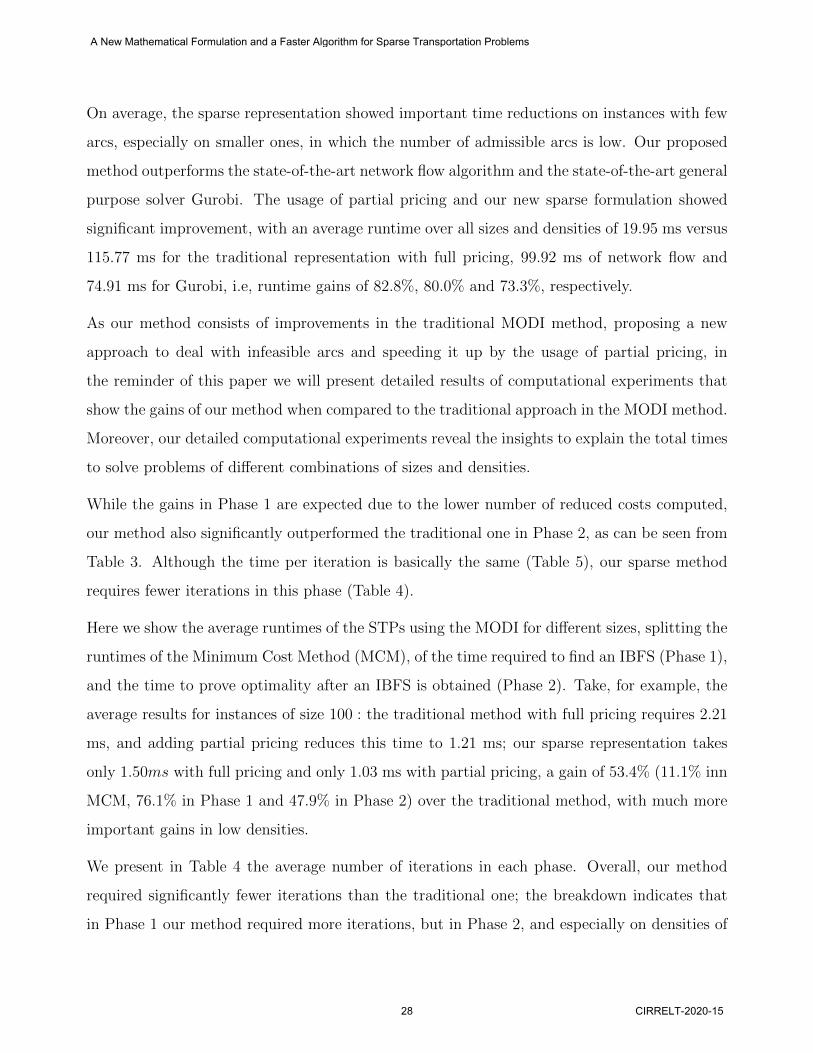
On average, the sparse representation showed important time reductions on instances with few

arcs, especially on smaller ones, in which the number of admissible arcs is low. Our proposed

method outperforms the state-of-the-art network flow algorithm and the state-of-the-art general

purpose solver Gurobi. The usage of partial pricing and our new sparse formulation showed

significant improvement, with an average runtime over all sizes and densities of 19.95 ms versus

115.77 ms for the traditional representation with full pricing, 99.92 ms of network flow and

74.91 ms for Gurobi, i.e, runtime gains of 82.8%, 80.0% and 73.3%, respectively.

As our method consists of improvements in the traditional MODI method, proposing a new

approach to deal with infeasible arcs and speeding it up by the usage of partial pricing, in

the reminder of this paper we will present detailed results of computational experiments that

show the gains of our method when compared to the traditional approach in the MODI method.

Moreover, our detailed computational experiments reveal the insights to explain the total times

to solve problems of different combinations of sizes and densities.

While the gains in Phase 1 are expected due to the lower number of reduced costs computed,

our method also significantly outperformed the traditional one in Phase 2, as can be seen from

Table 3. Although the time per iteration is basically the same (Table 5), our sparse method

requires fewer iterations in this phase (Table 4).

Here we show the average runtimes of the STPs using the MODI for different sizes, splitting the

runtimes of the Minimum Cost Method (MCM), of the time required to find an IBFS (Phase 1),

and the time to prove optimality after an IBFS is obtained (Phase 2). Take, for example, the

average results for instances of size 100 : the traditional method with full pricing requires 2.21

ms, and adding partial pricing reduces this time to 1.21 ms; our sparse representation takes

only 1.50ms with full pricing and only 1.03 ms with partial pricing, a gain of 53.4% (11.1% inn

MCM, 76.1% in Phase 1 and 47.9% in Phase 2) over the traditional method, with much more

important gains in low densities.

We present in Table 4 the average number of iterations in each phase. Overall, our method

required significantly fewer iterations than the traditional one; the breakdown indicates that

in Phase 1 our method required more iterations, but in Phase 2, and especially on densities of


28 CIRRELT-2020-15

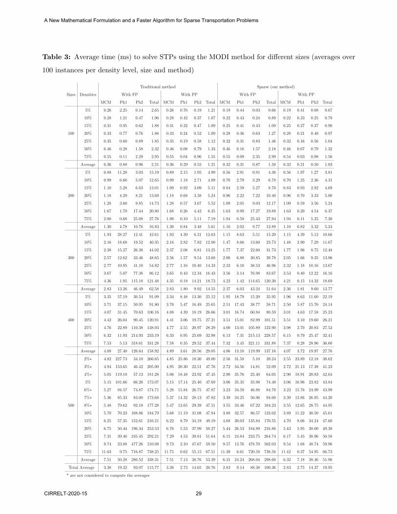
Table 3: Average time (ms) to solve STPs using the MODI method for different sizes (averages over

100 instances per density level, size and method)

Sizes Densities

Traditional method Sparse (our method)

With FP With PP With FP With PP

MCM Ph1 Ph2 Total MCM Ph1 Ph2 Total MCM Ph1 Ph2 Total MCM Ph1 Ph2 Total

100

5% 0.26 2.25 0.14 2.65 0.26 0.76 0.19 1.21 0.19 0.44 0.03 0.66 0.19 0.41 0.08 0.67

10% 0.28 1.21 0.47 1.96 0.28 0.42 0.37 1.07 0.22 0.43 0.24 0.89 0.22 0.33 0.25 0.79

15% 0.31 0.95 0.62 1.88 0.31 0.32 0.47 1.09 0.25 0.41 0.43 1.09 0.25 0.27 0.37 0.90

20% 0.33 0.77 0.76 1.86 0.33 0.24 0.52 1.09 0.28 0.36 0.63 1.27 0.28 0.21 0.48 0.97

25% 0.35 0.60 0.89 1.85 0.35 0.19 0.58 1.12 0.32 0.31 0.83 1.46 0.32 0.16 0.56 1.04

50% 0.46 0.28 1.58 2.32 0.46 0.08 0.79 1.33 0.46 0.16 1.57 2.18 0.46 0.07 0.79 1.32

75% 0.55 0.11 2.29 2.95 0.55 0.04 0.96 1.55 0.55 0.09 2.35 2.99 0.54 0.03 0.98 1.56

Average 0.36 0.88 0.96 2.21 0.36 0.29 0.55 1.21 0.32 0.31 0.87 1.50 0.32 0.21 0.50 1.03

200

5% 0.88 11.28 3.03 15.19 0.89 2.15 1.95 4.99 0.56 2.91 0.91 4.38 0.56 1.97 1.27 3.81

10% 0.99 6.60 5.07 12.65 0.99 1.18 2.71 4.89 0.70 2.79 3.29 6.78 0.70 1.25 2.36 4.31

15% 1.10 5.28 6.63 13.01 1.09 0.92 3.09 5.11 0.84 2.59 5.27 8.70 0.83 0.93 2.92 4.69

20% 1.18 4.29 8.21 13.69 1.18 0.68 3.38 5.24 0.96 2.22 7.22 10.40 0.96 0.70 3.33 5.00

25% 1.28 3.60 9.85 14.73 1.28 0.57 3.67 5.52 1.09 2.05 9.03 12.17 1.09 0.59 3.56 5.24

50% 1.67 1.70 17.44 20.80 1.68 0.26 4.42 6.35 1.63 0.99 17.27 19.89 1.63 0.20 4.54 6.37

75% 2.00 0.68 25.08 27.76 1.98 0.10 5.11 7.19 1.94 0.58 25.43 27.94 1.94 0.11 5.25 7.30

Average 1.30 4.78 10.76 16.83 1.30 0.84 3.48 5.61 1.10 2.02 9.77 12.89 1.10 0.82 3.32 5.24

300

5% 1.93 28.27 12.41 42.61 1.93 4.39 6.31 12.63 1.15 8.63 5.51 15.29 1.15 4.39 5.12 10.66

10% 2.16 18.68 19.52 40.35 2.16 2.82 7.82 12.80 1.47 8.66 13.60 23.73 1.48 2.90 7.29 11.67

15% 2.38 15.27 26.38 44.02 2.37 2.08 8.81 13.25 1.77 7.37 22.60 31.73 1.77 1.96 8.75 12.48

20% 2.57 12.62 33.46 48.65 2.56 1.57 9.54 13.68 2.06 6.88 30.85 39.78 2.05 1.66 9.35 13.06

25% 2.77 10.95 41.10 54.82 2.77 1.16 10.40 14.33 2.33 6.10 38.53 46.96 2.32 1.18 10.16 13.67

50% 3.67 5.07 77.38 86.12 3.65 0.43 12.34 16.43 3.56 3.14 76.98 83.67 3.53 0.40 12.22 16.16

75% 4.36 1.95 115.18 121.48 4.35 0.18 14.21 18.73 4.23 1.42 114.65 120.30 4.21 0.15 14.32 18.69

Average 2.83 13.26 46.49 62.58 2.83 1.80 9.92 14.55 2.37 6.03 43.24 51.64 2.36 1.81 9.60 13.77

400

5% 3.35 57.19 30.54 91.09 3.34 8.48 13.30 25.12 1.95 18.79 15.20 35.95 1.96 8.63 11.60 22.19

10% 3.71 37.15 50.95 91.80 3.70 5.47 16.49 25.65 2.51 17.43 38.77 58.71 2.50 5.87 15.76 24.14

15% 4.07 31.45 70.63 106.16 4.08 4.39 18.19 26.66 3.01 16.74 60.84 80.59 3.01 4.63 17.58 25.23

20% 4.42 26.04 90.45 120.91 4.41 3.06 19.75 27.21 3.51 15.01 82.99 101.51 3.51 3.10 19.60 26.21

25% 4.76 22.89 110.38 138.03 4.77 2.55 20.97 28.29 4.00 13.01 105.89 122.90 3.98 2.70 20.83 27.52

50% 6.32 11.93 214.93 233.19 6.33 0.95 25.69 32.98 6.13 7.31 215.13 228.57 6.15 0.79 25.47 32.41

75% 7.53 5.13 318.61 331.28 7.58 0.35 29.52 37.44 7.32 3.45 321.11 331.88 7.37 0.28 28.96 36.60

Average 4.88 27.40 126.64 158.92 4.89 3.61 20.56 29.05 4.06 13.10 119.99 137.16 4.07 3.72 19.97 27.76

500

2%∗ 4.82 227.73 34.10 266.65 4.85 25.86 18.30 49.00 2.56 31.58 5.10 39.24 2.55 23.89 12.18 38.62

3%∗ 4.94 153.65 46.42 205.00 4.95 20.30 22.51 47.76 2.72 34.56 14.81 52.09 2.72 21.13 17.38 41.23

4%∗ 5.05 119.10 57.13 181.28 5.06 18.48 23.92 47.45 2.90 35.76 25.40 64.05 2.90 18.91 20.83 42.64

5% 5.15 101.66 66.26 173.07 5.15 17.14 25.40 47.69 3.06 35.35 35.98 74.40 3.06 16.96 23.82 43.84

6%∗ 5.27 94.57 74.87 174.71 5.28 15.84 26.75 47.87 3.23 34.59 46.88 84.70 3.23 15.76 24.99 43.99

7%∗ 5.36 85.33 83.00 173.68 5.37 14.32 28.13 47.82 3.39 34.25 56.96 94.60 3.39 13.86 26.95 44.20

8%∗ 5.48 79.62 92.18 177.28 5.47 12.65 29.39 47.51 3.55 33.46 67.22 104.23 3.55 12.65 28.75 44.95

10% 5.70 70.23 108.86 184.79 5.68 11.19 31.08 47.94 3.88 32.57 86.57 123.02 3.89 11.22 30.50 45.61

15% 6.25 57.35 152.61 216.21 6.22 8.79 34.19 49.19 4.68 30.03 135.84 170.55 4.70 8.66 34.24 47.60

20% 6.75 50.44 196.34 253.53 6.76 5.53 37.99 50.27 5.44 26.53 184.89 216.86 5.43 5.95 38.00 49.38

25% 7.31 39.46 245.45 292.21 7.29 4.53 39.81 51.64 6.15 24.84 233.75 264.74 6.17 5.45 38.96 50.58

50% 9.74 23.08 477.26 510.08 9.73 2.10 47.67 59.50 9.57 13.76 478.70 502.03 9.54 1.68 48.74 59.96

75% 11.63 9.75 716.87 738.25 11.75 0.62 55.15 67.51 11.39 6.61 720.58 738.58 11.42 0.37 54.95 66.73

Average 7.51 50.28 280.52 338.31 7.51 7.13 38.76 53.39 6.31 24.24 268.04 298.60 6.32 7.18 38.46 51.96

Total Average 3.38 19.32 93.07 115.77 3.38 2.73 14.65 20.76 2.83 9.14 88.38 100.36 2.83 2.75 14.37 19.95

* are not considered to compute the averages


CIRRELT-2020-15 29

25% and less, our method required significantly fewer iterations. Moreover, Table 5 shows the

average time per iteration, where it becomes finally clear why overall our method performed

so much better. Finally, Table 6 explains where this gain originates: our method requires

significantly fewer computations of reduced costs.

In order to understand the gains of Phase 2 in running time and number of reduced costs

computed, since the algorithm for Phase 2 is identical for both methods, we also evaluate the

gap between the optimal solution value and the cost of the first feasible solution found, i.e.,

that when Phase 1 ends. The results are shown in Table 7. For less dense instances, our

method finishes Phase 1 with a solution significantly better than that of the traditional method

and very close to the optimal one, explaining why the Phase 2 of our method requires fewer

iterations and is so much faster.

This section showed that our method outperformed the traditional approach for solving STPs,

in case of feasible problems. Moreover, the gains are seen not only comparison with the MODI

Method, but also in relation to the state-of-the-art solver Gurobi and the network flow algo-

rithm.

We have also performed experiments with L = 100×m, cmin = 10, cmax = 10000 and L = 10000,

cmin = 10, cmax = 1000. Since the results do not show anything new, they are not reported

and can be obtained on the website alongside all results and instances.

6.2 Results for infeasible instances

Our method also correctly identifies infeasibility and to measure the performance for this case

we analyzed the running time, number of iterations, the average time per iteration when proving

that no feasible solution to the original STP exists, and the number of reduced costs computed.

The results are shown on in Tables 8–10. Our approach also outperformed the traditional one

when proving infeasibility and it is possible to observe that for low density instances we have

gains in both the number of iterations and time per iteration. For higher densities the gains

are due to lower running time per iteration.


30 CIRRELT-2020-15

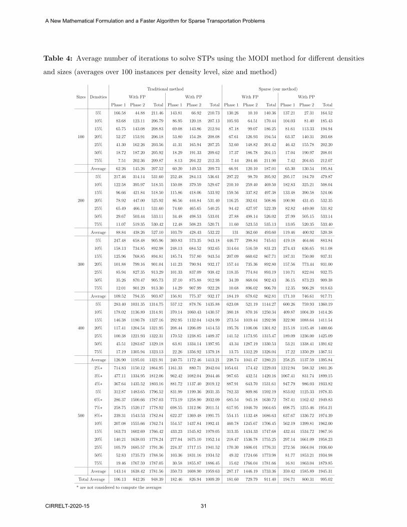
Table 4: Average number of iterations to solve STPs using the MODI method for different densities

and sizes (averages over 100 instances per density level, size and method)

Sizes Densities



Phase 1 Phase 2 Total Phase 1 Phase 2 Total Phase 1 Phase 2 Total Phase 1 Phase 2 Total

100

5% 166.58 44.88 211.46 143.81 66.92 210.73 130.26 10.10 140.36 137.21 27.31 164.52

10% 83.68 123.11 206.79 86.95 120.18 207.13 105.93 64.51 170.44 104.03 81.40 185.43

15% 65.75 143.08 208.83 69.08 143.86 212.94 87.18 99.07 186.25 81.61 113.33 194.94

20% 52.27 153.91 206.18 53.80 154.28 208.08 67.61 126.93 194.54 63.37 140.31 203.68

25% 41.30 162.26 203.56 41.31 165.94 207.25 52.60 148.82 201.42 46.42 155.78 202.20

50% 18.72 187.20 205.92 18.29 191.33 209.62 17.37 186.78 204.15 17.04 190.97 208.01

75% 7.51 202.36 209.87 8.13 204.22 212.35 7.44 204.46 211.90 7.42 204.65 212.07

Average 62.26 145.26 207.52 60.20 149.53 209.73 66.91 120.10 187.01 65.30 130.54 195.84

200

5% 217.46 314.14 531.60 252.48 284.13 536.61 297.22 98.70 395.92 295.17 184.70 479.87

10% 122.58 395.97 518.55 150.08 379.59 529.67 210.10 259.40 469.50 182.83 325.21 508.04

15% 96.66 421.84 518.50 115.86 418.06 533.92 159.56 337.82 497.38 133.48 390.58 524.06

20% 78.92 447.00 525.92 86.56 444.84 531.40 116.25 392.61 508.86 100.90 431.45 532.35

25% 65.49 466.11 531.60 74.60 465.65 540.25 94.42 427.97 522.39 82.82 449.00 531.82

50% 29.67 503.44 533.11 34.48 498.53 533.01 27.88 498.14 526.02 27.99 505.15 533.14

75% 11.07 519.35 530.42 12.48 508.23 520.71 11.60 523.53 535.13 13.05 520.35 533.40

Average 88.84 438.26 527.10 103.79 428.43 532.22 131 362.60 493.60 119.46 400.92 520.38

300

5% 247.48 658.48 905.96 369.83 573.35 943.18 446.77 298.84 745.61 419.18 464.66 883.84

10% 158.13 734.85 892.98 248.13 684.52 932.65 314.64 516.59 831.23 274.43 636.65 911.08

15% 125.96 768.85 894.81 185.74 757.80 943.54 207.09 660.62 867.71 187.31 750.00 937.31

20% 101.88 799.16 901.04 141.23 790.94 932.17 157.44 735.36 892.80 157.56 773.44 931.00

25% 85.94 827.35 913.29 101.33 837.09 938.42 118.35 774.84 893.19 110.71 822.04 932.75

50% 35.26 870.47 905.73 37.10 875.88 912.98 34.39 868.04 902.43 36.15 873.23 909.38

75% 12.01 901.29 913.30 14.29 907.99 922.28 10.68 896.02 906.70 12.35 906.28 918.63

Average 109.52 794.35 903.87 156.81 775.37 932.17 184.19 678.62 862.81 171.10 746.61 917.71

400

5% 283.40 1031.35 1314.75 557.12 878.76 1435.88 623.08 521.19 1144.27 600.26 759.93 1360.19

10% 178.02 1136.89 1314.91 370.14 1060.43 1430.57 380.18 870.16 1250.34 409.87 1004.39 1414.26

15% 146.38 1180.78 1327.16 292.95 1132.04 1424.99 273.54 1019.44 1292.98 322.90 1088.64 1411.54

20% 117.41 1204.54 1321.95 208.44 1206.09 1414.53 195.76 1106.06 1301.82 215.18 1185.48 1400.66

25% 100.38 1221.93 1322.31 170.52 1238.85 1409.37 141.52 1173.95 1315.47 189.09 1236.00 1425.09

50% 45.51 1283.67 1329.18 63.81 1334.14 1397.95 43.34 1287.19 1330.53 53.21 1338.41 1391.62

75% 17.19 1305.94 1323.13 22.26 1356.92 1379.18 13.75 1312.29 1326.04 17.22 1350.29 1367.51

Average 126.90 1195.01 1321.91 240.75 1172.46 1413.21 238.74 1041.47 1280.21 258.25 1137.59 1395.84

500

2%∗ 714.83 1150.12 1864.95 1161.33 880.71 2042.04 1054.61 174.42 1229.03 1212.94 588.32 1801.26

3%∗ 477.11 1334.95 1812.06 962.42 1082.04 2044.46 987.65 432.51 1420.16 1067.41 831.74 1899.15

4%∗ 367.64 1435.52 1803.16 881.72 1137.40 2019.12 887.91 643.70 1531.61 947.79 986.03 1933.82

5% 312.87 1483.65 1796.52 831.99 1199.36 2031.35 782.33 809.86 1592.19 853.02 1125.33 1978.35

6%∗ 286.37 1500.66 1787.03 773.19 1258.90 2032.09 685.54 945.18 1630.72 787.41 1162.42 1949.83

7%∗ 258.75 1520.17 1778.92 698.55 1312.96 2011.51 617.95 1046.70 1664.65 698.75 1255.46 1954.21

8%∗ 239.31 1543.53 1782.84 622.27 1369.48 1991.75 554.15 1132.48 1686.63 637.67 1336.72 1974.39

10% 207.08 1555.66 1762.74 554.57 1437.84 1992.41 460.78 1245.67 1706.45 562.19 1399.81 1962.00

15% 163.73 1602.69 1766.42 433.23 1545.82 1979.05 313.35 1434.33 1747.68 432.44 1534.72 1967.16

20% 140.21 1638.03 1778.24 277.04 1675.10 1952.14 218.47 1536.78 1755.25 297.14 1661.09 1958.23

25% 105.79 1685.57 1791.36 224.37 1717.15 1941.52 170.30 1606.01 1776.31 272.56 1664.04 1936.60

50% 52.83 1735.73 1788.56 103.36 1831.16 1934.52 49.32 1724.66 1773.98 81.77 1853.21 1934.98

75% 19.46 1767.59 1787.05 30.58 1855.87 1886.45 15.62 1766.04 1781.66 16.81 1863.04 1879.85

Average 143.14 1638.42 1781.56 350.73 1608.90 1959.63 287.17 1446.19 1733.36 359.42 1585.89 1945.31

Total Average 106.13 842.26 948.39 182.46 826.94 1009.39 181.60 729.79 911.40 194.71 800.31 995.02



CIRRELT-2020-15 31

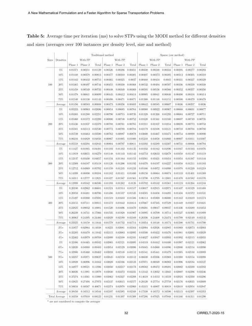
Table 5: Average time per iteration (ms) to solve STPs using the MODI method for different densities

and sizes (averages over 100 instances per density level, size and method)

Sizes Densities




100

5% 0.01371 0.00251 0.01129 0.00526 0.00286 0.00451 0.00338 0.00248 0.00334 0.00295 0.00277 0.00293

10% 0.01448 0.00378 0.00813 0.00477 0.00310 0.00381 0.00407 0.00373 0.00395 0.00313 0.00305 0.00310

15% 0.01442 0.00432 0.00753 0.00465 0.00325 0.0037 0.00468 0.00434 0.0045 0.00331 0.00327 0.00329

20% 0.01465 0.00497 0.00744 0.00455 0.00338 0.00368 0.00532 0.00494 0.00507 0.00336 0.00339 0.00338

25% 0.01458 0.00549 0.00733 0.00448 0.00349 0.00369 0.00595 0.00556 0.00566 0.00352 0.00357 0.00356

50% 0.01478 0.00841 0.00899 0.00445 0.00412 0.00414 0.00905 0.00841 0.00846 0.00400 0.00416 0.00414

75% 0.01540 0.01130 0.01143 0.00498 0.00471 0.00471 0.01308 0.01148 0.01151 0.00508 0.00479 0.00478

Average 0.01456 0.00583 0.00888 0.00473 0.00356 0.00403 0.00642 0.00585 0.00607 0.0036 0.00357 0.0036

200

5% 0.05223 0.00963 0.02696 0.00854 0.00685 0.00764 0.00980 0.00922 0.00967 0.00668 0.00691 0.00677

10% 0.05385 0.01280 0.02251 0.00790 0.00715 0.00735 0.01328 0.01268 0.01295 0.00684 0.00727 0.00711

15% 0.05460 0.01572 0.02299 0.00800 0.00740 0.00752 0.01620 0.01561 0.01580 0.00697 0.00749 0.00735

20% 0.05436 0.01837 0.02379 0.00788 0.00761 0.00765 0.01911 0.01837 0.01854 0.00698 0.00773 0.00758

25% 0.05501 0.02113 0.02530 0.00772 0.00788 0.00784 0.02179 0.02108 0.02121 0.00710 0.00794 0.00780

50% 0.05739 0.03463 0.03590 0.00762 0.00887 0.00878 0.03600 0.03467 0.03471 0.00754 0.00899 0.00890

75% 0.06216 0.04829 0.04856 0.00867 0.01005 0.01000 0.05210 0.04858 0.04860 0.00907 0.01011 0.01007

Average 0.05558 0.02294 0.02943 0.00804 0.00797 0.00811 0.02392 0.02289 0.02307 0.00731 0.00806 0.00794

300

5% 0.11427 0.01885 0.04491 0.01193 0.01102 0.01135 0.01932 0.01842 0.01896 0.01047 0.01103 0.01076

10% 0.11819 0.02655 0.04279 0.01148 0.01143 0.01142 0.02753 0.02633 0.02678 0.01058 0.01147 0.01119

15% 0.12137 0.03430 0.04657 0.01134 0.01164 0.01155 0.03561 0.03421 0.03454 0.01054 0.01167 0.01144

20% 0.12389 0.04187 0.05118 0.01126 0.01206 0.01192 0.04370 0.04197 0.04227 0.01058 0.01211 0.01183

25% 0.12712 0.04969 0.05702 0.01159 0.01245 0.01233 0.05166 0.04972 0.04998 0.01078 0.01239 0.01218

50% 0.14399 0.08890 0.09104 0.01182 0.01411 0.01400 0.09150 0.08864 0.08874 0.01133 0.01401 0.01389

75% 0.16311 0.12777 0.12821 0.01427 0.01567 0.01561 0.13790 0.12795 0.12801 0.01470 0.01582 0.01576

Average 0.12999 0.05542 0.06596 0.01193 0.01262 0.0126 0.05702 0.05532 0.05561 0.01123 0.01264 0.01244

400

5% 0.20180 0.02962 0.06681 0.01524 0.01514 0.01517 0.03017 0.02915 0.02971 0.01437 0.01529 0.01488

10% 0.20858 0.04481 0.06706 0.01486 0.01557 0.01535 0.04585 0.04456 0.04495 0.01434 0.01572 0.01531

15% 0.21497 0.05980 0.07695 0.01519 0.01610 0.01586 0.06114 0.05969 0.06000 0.01442 0.01619 0.01574

20% 0.22155 0.07511 0.08815 0.01472 0.01642 0.01614 0.07667 0.07505 0.07529 0.01449 0.01657 0.01621

25% 0.22825 0.09032 0.10081 0.01520 0.01696 0.01670 0.09201 0.09017 0.09037 0.01436 0.01689 0.01653

50% 0.26239 0.16741 0.17066 0.01535 0.01928 0.01907 0.16995 0.16709 0.16714 0.01527 0.01905 0.01889

75% 0.30063 0.24395 0.24466 0.02029 0.02180 0.02169 0.26336 0.24468 0.24474 0.01799 0.02149 0.02142

Average 0.23325 0.10158 0.11644 0.01578 0.01732 0.01714 0.10354 0.10148 0.10174 0.01500 0.01731 0.01700

500

2%∗ 0.31857 0.02964 0.14038 0.0223 0.02081 0.02164 0.02994 0.02926 0.02985 0.01969 0.02073 0.02003

3%∗ 0.32205 0.03478 0.11042 0.02115 0.02083 0.02095 0.03500 0.03422 0.03476 0.01981 0.02091 0.02029

4%∗ 0.32402 0.03979 0.09768 0.02099 0.02108 0.02101 0.04027 0.03947 0.03993 0.01992 0.02115 0.02055

5% 0.32486 0.04465 0.09342 0.02065 0.02121 0.02095 0.04519 0.04442 0.04480 0.01987 0.02121 0.02062

6%∗ 0.33020 0.04988 0.09483 0.02054 0.02129 0.02096 0.05045 0.04960 0.04996 0.02000 0.02154 0.02090

7%∗ 0.32980 0.05460 0.09462 0.02059 0.02148 0.02112 0.05541 0.05441 0.05479 0.01985 0.02150 0.02089

8%∗ 0.33257 0.05971 0.09637 0.02045 0.02150 0.02112 0.06038 0.05936 0.05969 0.01988 0.02154 0.02098

10% 0.33929 0.06996 0.10162 0.02028 0.02166 0.02123 0.07071 0.06949 0.06982 0.01996 0.02184 0.02127

15% 0.34977 0.09521 0.11886 0.02050 0.02217 0.02173 0.09582 0.09472 0.09491 0.02002 0.02239 0.02182

20% 0.36026 0.11981 0.13878 0.02030 0.02272 0.02231 0.12142 0.12032 0.12045 0.02007 0.02296 0.02246

25% 0.37274 0.14561 0.15900 0.02062 0.02327 0.02288 0.14619 0.14553 0.14559 0.02024 0.02350 0.02296

50% 0.43825 0.27494 0.27973 0.02137 0.02615 0.02577 0.28120 0.27754 0.27758 0.02176 0.02635 0.02609

75% 0.50634 0.40567 0.40671 0.02374 0.02978 0.02960 0.45315 0.40807 0.40818 0.02618 0.02954 0.02947

Average 0.38450 0.16512 0.18544 0.02107 0.02385 0.02349 0.17338 0.16572 0.16590 0.02115 0.02397 0.02353

Total Average 0.16358 0.07018 0.08123 0.01231 0.01307 0.01308 0.07286 0.07025 0.07048 0.01166 0.01311 0.01290



32 CIRRELT-2020-15

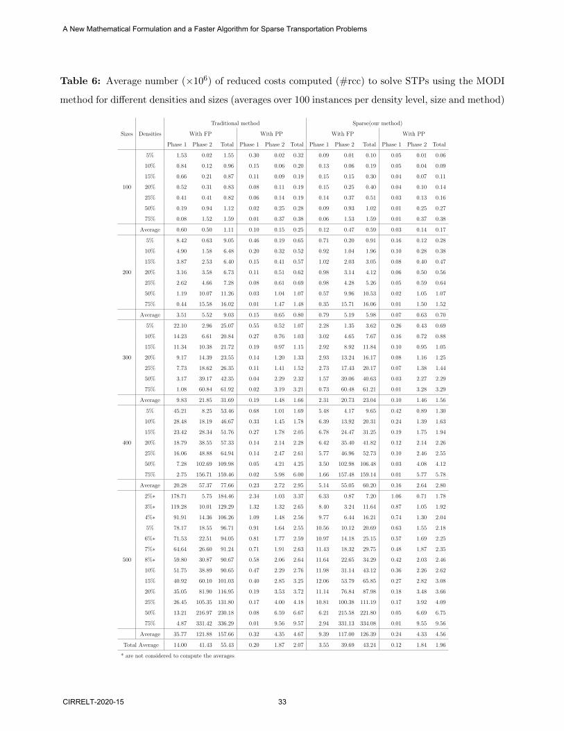
Table 6: Average number (×106) of reduced costs computed (#rcc) to solve STPs using the MODI

method for different densities and sizes (averages over 100 instances per density level, size and method)

Sizes Densities

Traditional method Sparse(our method)



100

5% 1.53 0.02 1.55 0.30 0.02 0.32 0.09 0.01 0.10 0.05 0.01 0.06

10% 0.84 0.12 0.96 0.15 0.06 0.20 0.13 0.06 0.19 0.05 0.04 0.09

15% 0.66 0.21 0.87 0.11 0.09 0.19 0.15 0.15 0.30 0.04 0.07 0.11

20% 0.52 0.31 0.83 0.08 0.11 0.19 0.15 0.25 0.40 0.04 0.10 0.14

25% 0.41 0.41 0.82 0.06 0.14 0.19 0.14 0.37 0.51 0.03 0.13 0.16

50% 0.19 0.94 1.12 0.02 0.25 0.28 0.09 0.93 1.02 0.01 0.25 0.27

75% 0.08 1.52 1.59 0.01 0.37 0.38 0.06 1.53 1.59 0.01 0.37 0.38

Average 0.60 0.50 1.11 0.10 0.15 0.25 0.12 0.47 0.59 0.03 0.14 0.17

200

5% 8.42 0.63 9.05 0.46 0.19 0.65 0.71 0.20 0.91 0.16 0.12 0.28

10% 4.90 1.58 6.48 0.20 0.32 0.52 0.92 1.04 1.96 0.10 0.28 0.38

15% 3.87 2.53 6.40 0.15 0.41 0.57 1.02 2.03 3.05 0.08 0.40 0.47

20% 3.16 3.58 6.73 0.11 0.51 0.62 0.98 3.14 4.12 0.06 0.50 0.56

25% 2.62 4.66 7.28 0.08 0.61 0.69 0.98 4.28 5.26 0.05 0.59 0.64

50% 1.19 10.07 11.26 0.03 1.04 1.07 0.57 9.96 10.53 0.02 1.05 1.07

75% 0.44 15.58 16.02 0.01 1.47 1.48 0.35 15.71 16.06 0.01 1.50 1.52

Average 3.51 5.52 9.03 0.15 0.65 0.80 0.79 5.19 5.98 0.07 0.63 0.70

300

5% 22.10 2.96 25.07 0.55 0.52 1.07 2.28 1.35 3.62 0.26 0.43 0.69

10% 14.23 6.61 20.84 0.27 0.76 1.03 3.02 4.65 7.67 0.16 0.72 0.88

15% 11.34 10.38 21.72 0.19 0.97 1.15 2.92 8.92 11.84 0.10 0.95 1.05

20% 9.17 14.39 23.55 0.14 1.20 1.33 2.93 13.24 16.17 0.08 1.16 1.25

25% 7.73 18.62 26.35 0.11 1.41 1.52 2.73 17.43 20.17 0.07 1.38 1.44

50% 3.17 39.17 42.35 0.04 2.29 2.32 1.57 39.06 40.63 0.03 2.27 2.29

75% 1.08 60.84 61.92 0.02 3.19 3.21 0.73 60.48 61.21 0.01 3.28 3.29

Average 9.83 21.85 31.69 0.19 1.48 1.66 2.31 20.73 23.04 0.10 1.46 1.56

400

5% 45.21 8.25 53.46 0.68 1.01 1.69 5.48 4.17 9.65 0.42 0.89 1.30

10% 28.48 18.19 46.67 0.33 1.45 1.78 6.39 13.92 20.31 0.24 1.39 1.63

15% 23.42 28.34 51.76 0.27 1.78 2.05 6.78 24.47 31.25 0.19 1.75 1.94

20% 18.79 38.55 57.33 0.14 2.14 2.28 6.42 35.40 41.82 0.12 2.14 2.26

25% 16.06 48.88 64.94 0.14 2.47 2.61 5.77 46.96 52.73 0.10 2.46 2.55

50% 7.28 102.69 109.98 0.05 4.21 4.25 3.50 102.98 106.48 0.03 4.08 4.12

75% 2.75 156.71 159.46 0.02 5.98 6.00 1.66 157.48 159.14 0.01 5.77 5.78

Average 20.28 57.37 77.66 0.23 2.72 2.95 5.14 55.05 60.20 0.16 2.64 2.80

500

2%∗ 178.71 5.75 184.46 2.34 1.03 3.37 6.33 0.87 7.20 1.06 0.71 1.78

3%∗ 119.28 10.01 129.29 1.32 1.32 2.65 8.40 3.24 11.64 0.87 1.05 1.92

4%∗ 91.91 14.36 106.26 1.09 1.48 2.56 9.77 6.44 16.21 0.74 1.30 2.04

5% 78.17 18.55 96.71 0.91 1.64 2.55 10.56 10.12 20.69 0.63 1.55 2.18

6%∗ 71.53 22.51 94.05 0.81 1.77 2.59 10.97 14.18 25.15 0.57 1.69 2.25

7%∗ 64.64 26.60 91.24 0.71 1.91 2.63 11.43 18.32 29.75 0.48 1.87 2.35

8%∗ 59.80 30.87 90.67 0.58 2.06 2.64 11.64 22.65 34.29 0.42 2.03 2.46

10% 51.75 38.89 90.65 0.47 2.29 2.76 11.98 31.14 43.12 0.36 2.26 2.62

15% 40.92 60.10 101.03 0.40 2.85 3.25 12.06 53.79 65.85 0.27 2.82 3.08

20% 35.05 81.90 116.95 0.19 3.53 3.72 11.14 76.84 87.98 0.18 3.48 3.66

25% 26.45 105.35 131.80 0.17 4.00 4.18 10.81 100.38 111.19 0.17 3.92 4.09

50% 13.21 216.97 230.18 0.08 6.59 6.67 6.21 215.58 221.80 0.05 6.69 6.75

75% 4.87 331.42 336.29 0.01 9.56 9.57 2.94 331.13 334.08 0.01 9.55 9.56

Average 35.77 121.88 157.66 0.32 4.35 4.67 9.39 117.00 126.39 0.24 4.33 4.56

Total Average 14.00 41.43 55.43 0.20 1.87 2.07 3.55 39.69 43.24 0.12 1.84 1.96



CIRRELT-2020-15 33

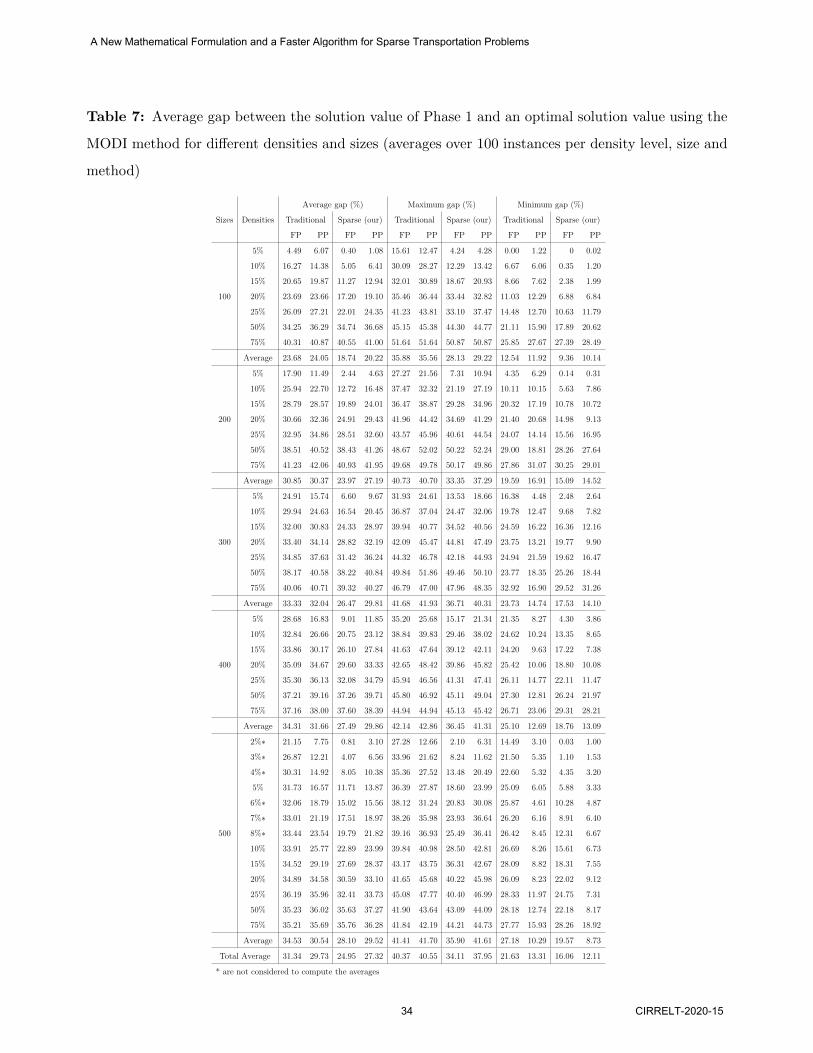
Table 7: Average gap between the solution value of Phase 1 and an optimal solution value using the

MODI method for different densities and sizes (averages over 100 instances per density level, size and

method)

Sizes Densities

Average gap (%) Maximum gap (%) Minimum gap (%)

Traditional Sparse (our) Traditional Sparse (our) Traditional Sparse (our)

FP PP FP PP FP PP FP PP FP PP FP PP

100

5% 4.49 6.07 0.40 1.08 15.61 12.47 4.24 4.28 0.00 1.22 0 0.02

10% 16.27 14.38 5.05 6.41 30.09 28.27 12.29 13.42 6.67 6.06 0.35 1.20

15% 20.65 19.87 11.27 12.94 32.01 30.89 18.67 20.93 8.66 7.62 2.38 1.99

20% 23.69 23.66 17.20 19.10 35.46 36.44 33.44 32.82 11.03 12.29 6.88 6.84

25% 26.09 27.21 22.01 24.35 41.23 43.81 33.10 37.47 14.48 12.70 10.63 11.79

50% 34.25 36.29 34.74 36.68 45.15 45.38 44.30 44.77 21.11 15.90 17.89 20.62

75% 40.31 40.87 40.55 41.00 51.64 51.64 50.87 50.87 25.85 27.67 27.39 28.49

Average 23.68 24.05 18.74 20.22 35.88 35.56 28.13 29.22 12.54 11.92 9.36 10.14

200

5% 17.90 11.49 2.44 4.63 27.27 21.56 7.31 10.94 4.35 6.29 0.14 0.31

10% 25.94 22.70 12.72 16.48 37.47 32.32 21.19 27.19 10.11 10.15 5.63 7.86

15% 28.79 28.57 19.89 24.01 36.47 38.87 29.28 34.96 20.32 17.19 10.78 10.72

20% 30.66 32.36 24.91 29.43 41.96 44.42 34.69 41.29 21.40 20.68 14.98 9.13

25% 32.95 34.86 28.51 32.60 43.57 45.96 40.61 44.54 24.07 14.14 15.56 16.95

50% 38.51 40.52 38.43 41.26 48.67 52.02 50.22 52.24 29.00 18.81 28.26 27.64

75% 41.23 42.06 40.93 41.95 49.68 49.78 50.17 49.86 27.86 31.07 30.25 29.01

Average 30.85 30.37 23.97 27.19 40.73 40.70 33.35 37.29 19.59 16.91 15.09 14.52

300

5% 24.91 15.74 6.60 9.67 31.93 24.61 13.53 18.66 16.38 4.48 2.48 2.64

10% 29.94 24.63 16.54 20.45 36.87 37.04 24.47 32.06 19.78 12.47 9.68 7.82

15% 32.00 30.83 24.33 28.97 39.94 40.77 34.52 40.56 24.59 16.22 16.36 12.16

20% 33.40 34.14 28.82 32.19 42.09 45.47 44.81 47.49 23.75 13.21 19.77 9.90

25% 34.85 37.63 31.42 36.24 44.32 46.78 42.18 44.93 24.94 21.59 19.62 16.47

50% 38.17 40.58 38.22 40.84 49.84 51.86 49.46 50.10 23.77 18.35 25.26 18.44

75% 40.06 40.71 39.32 40.27 46.79 47.00 47.96 48.35 32.92 16.90 29.52 31.26

Average 33.33 32.04 26.47 29.81 41.68 41.93 36.71 40.31 23.73 14.74 17.53 14.10

400

5% 28.68 16.83 9.01 11.85 35.20 25.68 15.17 21.34 21.35 8.27 4.30 3.86

10% 32.84 26.66 20.75 23.12 38.84 39.83 29.46 38.02 24.62 10.24 13.35 8.65

15% 33.86 30.17 26.10 27.84 41.63 47.64 39.12 42.11 24.20 9.63 17.22 7.38

20% 35.09 34.67 29.60 33.33 42.65 48.42 39.86 45.82 25.42 10.06 18.80 10.08

25% 35.30 36.13 32.08 34.79 45.94 46.56 41.31 47.41 26.11 14.77 22.11 11.47

50% 37.21 39.16 37.26 39.71 45.80 46.92 45.11 49.04 27.30 12.81 26.24 21.97

75% 37.16 38.00 37.60 38.39 44.94 44.94 45.13 45.42 26.71 23.06 29.31 28.21

Average 34.31 31.66 27.49 29.86 42.14 42.86 36.45 41.31 25.10 12.69 18.76 13.09

500

2%∗ 21.15 7.75 0.81 3.10 27.28 12.66 2.10 6.31 14.49 3.10 0.03 1.00

3%∗ 26.87 12.21 4.07 6.56 33.96 21.62 8.24 11.62 21.50 5.35 1.10 1.53

4%∗ 30.31 14.92 8.05 10.38 35.36 27.52 13.48 20.49 22.60 5.32 4.35 3.20

5% 31.73 16.57 11.71 13.87 36.39 27.87 18.60 23.99 25.09 6.05 5.88 3.33

6%∗ 32.06 18.79 15.02 15.56 38.12 31.24 20.83 30.08 25.87 4.61 10.28 4.87

7%∗ 33.01 21.19 17.51 18.97 38.26 35.98 23.93 36.64 26.20 6.16 8.91 6.40

8%∗ 33.44 23.54 19.79 21.82 39.16 36.93 25.49 36.41 26.42 8.45 12.31 6.67

10% 33.91 25.77 22.89 23.99 39.84 40.98 28.50 42.81 26.69 8.26 15.61 6.73

15% 34.52 29.19 27.69 28.37 43.17 43.75 36.31 42.67 28.09 8.82 18.31 7.55

20% 34.89 34.58 30.59 33.10 41.65 45.68 40.22 45.98 26.09 8.23 22.02 9.12

25% 36.19 35.96 32.41 33.73 45.08 47.77 40.40 46.99 28.33 11.97 24.75 7.31

50% 35.23 36.02 35.63 37.27 41.90 43.64 43.09 44.09 28.18 12.74 22.18 8.17

75% 35.21 35.69 35.76 36.28 41.84 42.19 44.21 44.73 27.77 15.93 28.26 18.92

Average 34.53 30.54 28.10 29.52 41.41 41.70 35.90 41.61 27.18 10.29 19.57 8.73

Total Average 31.34 29.73 24.95 27.32 40.37 40.55 34.11 37.95 21.63 13.31 16.06 12.11



34 CIRRELT-2020-15

The results of Table 8 show that Gurobi is the fastest one to prove the infeasibility for most

of the cases. The exceptions are for problems of size 100 × 100 and densities lower than 20%,

in which cases our SMODIPP method had the best runtimes. Moreover, we observe that our

SMODIPP method outperforms the network flow algorithm in all cases by a large margin,

specially for those ones with fewer number of admissible arcs.

Table 8: Average time (ms) to prove infeasibility for infeasible STPs using the Gurobi, Network

Flow and the MODI methods for different sizes (averages over 100 instances per density level, size and

method)

Traditional Sparse (our method)

SizeAverage

SizeAverage

Density 100×100 200×200 300×300 400×400 500×500 100×100 200×200 300×300 400×400 500×500

Guro

bi

5% 14.69 57.21 230.61 447.25 723.64 294.68 1.02 1.01 1.67 2.00 3.25 1.79

10% 15.18 98.24 273.15 518.48 990.31 379.07 1.01 1.31 2.40 6.06 9.14 3.98

15% 15.44 116.88 310.10 617.51 1060.46 424.08 1.03 1.99 3.38 8.60 13.06 5.61

20% 15.37 131.50 339.37 704.33 1178.05 473.72 1.06 2.04 6.57 11.13 17.05 7.57

25% 15.44 136.30 360.15 741.32 1289.43 508.53 1.06 2.49 7.96 13.49 21.14 9.23

50% 15.87 157.25 222.79 417.95 682.49 299.27 1.58 7.11 14.01 27.69 42.64 18.61

75% 17.33 96.43 230.11 445.85 736.94 305.33 2.02 10.19 22.68 40.89 77.55 30.67

Average 15.62 113.40 280.90 556.10 951.62 383.53 1.25 3.73 8.38 15.69 26.26 11.06

Net

wor

kF

low

5% 9.56 42.77 101.78 189.38 308.47 130.39 6.38 30.85 73.21 131.30 206.25 89.60

10% 8.91 42.59 101.73 188.83 303.86 129.18 6.19 30.88 73.56 132.69 207.39 90.14

15% 9.23 42.97 101.12 188.09 302.39 128.76 6.35 31.39 74.00 134.10 208.59 90.88

20% 9.33 42.77 100.74 186.87 300.83 128.11 6.55 31.34 73.50 134.65 211.06 91.42

25% 9.16 42.66 101.15 186.04 294.31 126.66 6.33 31.35 75.81 134.95 212.16 92.12

50% 9.02 42.18 99.87 185.21 300.27 127.31 6.61 33.05 77.54 140.49 223.39 96.22

75% 8.40 40.55 97.42 181.12 292.74 124.05 6.86 33.79 80.80 146.75 234.78 100.60

Average 9.09 42.36 100.54 186.51 300.41 127.78 6.47 31.81 75.49 136.42 214.80 93.00

MO

DI

FP

5% 3.35 29.30 104.77 270.07 574.60 196.42 0.67 4.53 15.81 37.51 77.12 27.13

10% 3.28 28.20 103.29 265.17 573.36 194.66 0.95 7.05 24.39 58.81 122.75 42.79

15% 3.23 28.07 104.46 273.89 594.83 200.90 1.16 8.66 31.26 78.06 163.99 56.63

20% 3.21 27.96 105.68 284.02 623.67 208.91 1.32 10.12 37.77 98.43 209.81 71.49

25% 3.15 27.97 111.25 294.22 655.54 218.43 1.44 11.60 45.37 118.84 259.50 87.35

50% 3.40 30.07 118.37 322.81 706.73 236.27 2.22 18.61 76.89 206.57 451.14 151.09

75% 3.58 30.56 125.09 331.83 706.60 239.53 2.92 24.67 102.15 272.69 586.97 197.88

Average 3.32 28.88 110.42 291.72 633.62 213.59 1.53 12.18 47.66 124.42 267.32 90.62

MO

DI

PP

5% 1.48 6.42 16.33 31.85 59.93 23.20 0.69 4.03 11.35 23.55 46.72 17.27

10% 1.42 6.52 17.24 34.87 66.49 25.31 0.85 4.66 12.93 27.60 54.62 20.14

15% 1.43 6.81 18.68 39.29 77.81 28.80 0.97 5.22 15.04 32.95 64.47 23.73

20% 1.45 7.26 20.78 45.37 88.14 32.60 1.06 5.80 17.01 37.71 76.59 27.63

25% 1.47 7.74 23.26 50.62 98.56 36.33 1.13 6.38 18.99 43.61 84.43 30.91

50% 1.77 10.10 30.90 67.81 129.66 48.05 1.58 9.38 28.19 63.12 119.88 44.43

75% 2.13 13.16 41.28 91.19 173.83 64.32 2.08 12.68 39.88 88.55 166.13 61.86

Average 1.59 8.29 24.07 51.57 99.20 36.94 1.19 6.88 20.48 45.30 87.55 32.28

In the more detailed results of Table 10 we observe that the main gains are in the number of


CIRRELT-2020-15 35

Table 9: Average time (ms) to solve prove infeasibility for infeasible STPs using the Network Flow

and the MODI methods for low density instances of size 500 × 500 (averages over 100 instances per

density level and method)

Method Density 2% 3% 4% 5% 6% 7% 8% Average

GurobiTraditional 426.41 620.56 732.01 723.64 749.40 874.32 856.42 711.82

Sparse 1.72 2.00 2.80 3.25 6.01 6.79 7.42 4.28

Network FlowTraditional 310.31 309.79 308.84 308.47 307.40 307.61 306.65 308.44

Sparse 205.33 205.52 206.36 206.25 206.89 206.74 207.03 206.30

MODI FPTraditional 595.21 586.89 584.02 574.60 579.84 572.16 578.73 581.64

Sparse 40.06 54.00 66.63 77.12 87.27 96.29 105.49 75.26

MODI PPTraditional 59.46 59.79 59.75 59.93 60.92 62.25 62.78 60.70

Sparse 39.95 43.01 44.62 46.72 47.51 48.81 49.89 45.79

reduced costs computed, which have reductions greater than 90% for the densities of 20% or

lower. Particularly for instances of problems of size 500 × 500 and densities of 10% or lower

this reduction is over 99%. We also highlight that, unlike what we observed in the feasible

instances, here the partial pricing significantly increased the number of iterations. However,

the average time saving in the in the iterations is high enough to allow the usage of partial

pricing leading to substantial gains in the overall runtime.

7 Conclusion

We have proposed a new mathematical formulation and a faster algorithm to solve STPs. Our

method is very general and can also be applied for dense BTPs, and any unbalanced problem

instance can be easily converted to a balanced one. In addition we have provided theorems

that prove the mathematical and theoretical aspects of our approach. When the MODI method

was used and the results compared to the ones obtained by the classical approach, we observed

gains in the number of reduced costs computed, number of iterations, runtime, and gap between

the value of the first feasible solution and an optimal solution. A partial pricing scheme has

significantly improved the performance of our method, outperforming both a minimum cost

network flow algorithm and the state-of-the-art solver Gurobi. Moreover, the gain in runtime


36 CIRRELT-2020-15

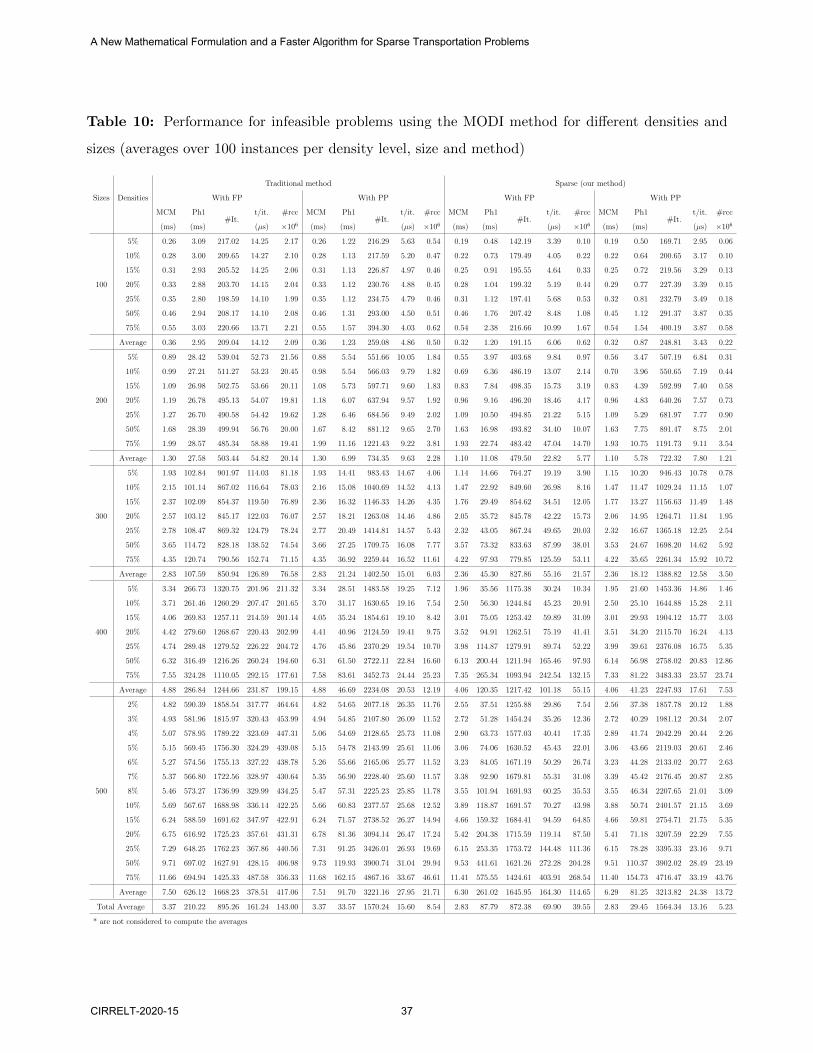
Table 10: Performance for infeasible problems using the MODI method for different densities and

sizes (averages over 100 instances per density level, size and method)

Sizes Densities



MCM Ph1#It.

t/it. #rcc MCM Ph1#It.



t/it. #rcc

(ms) (ms) (µs) ×106 (ms) (ms) (µs) ×106 (ms) (ms) (µs) ×106 (ms) (ms) (µs) ×106

100

5% 0.26 3.09 217.02 14.25 2.17 0.26 1.22 216.29 5.63 0.54 0.19 0.48 142.19 3.39 0.10 0.19 0.50 169.71 2.95 0.06

10% 0.28 3.00 209.65 14.27 2.10 0.28 1.13 217.59 5.20 0.47 0.22 0.73 179.49 4.05 0.22 0.22 0.64 200.65 3.17 0.10

15% 0.31 2.93 205.52 14.25 2.06 0.31 1.13 226.87 4.97 0.46 0.25 0.91 195.55 4.64 0.33 0.25 0.72 219.56 3.29 0.13

20% 0.33 2.88 203.70 14.15 2.04 0.33 1.12 230.76 4.88 0.45 0.28 1.04 199.32 5.19 0.44 0.29 0.77 227.39 3.39 0.15

25% 0.35 2.80 198.59 14.10 1.99 0.35 1.12 234.75 4.79 0.46 0.31 1.12 197.41 5.68 0.53 0.32 0.81 232.79 3.49 0.18

50% 0.46 2.94 208.17 14.10 2.08 0.46 1.31 293.00 4.50 0.51 0.46 1.76 207.42 8.48 1.08 0.45 1.12 291.37 3.87 0.35

75% 0.55 3.03 220.66 13.71 2.21 0.55 1.57 394.30 4.03 0.62 0.54 2.38 216.66 10.99 1.67 0.54 1.54 400.19 3.87 0.58

Average 0.36 2.95 209.04 14.12 2.09 0.36 1.23 259.08 4.86 0.50 0.32 1.20 191.15 6.06 0.62 0.32 0.87 248.81 3.43 0.22

200

5% 0.89 28.42 539.04 52.73 21.56 0.88 5.54 551.66 10.05 1.84 0.55 3.97 403.68 9.84 0.97 0.56 3.47 507.19 6.84 0.31

10% 0.99 27.21 511.27 53.23 20.45 0.98 5.54 566.03 9.79 1.82 0.69 6.36 486.19 13.07 2.14 0.70 3.96 550.65 7.19 0.44

15% 1.09 26.98 502.75 53.66 20.11 1.08 5.73 597.71 9.60 1.83 0.83 7.84 498.35 15.73 3.19 0.83 4.39 592.99 7.40 0.58

20% 1.19 26.78 495.13 54.07 19.81 1.18 6.07 637.94 9.57 1.92 0.96 9.16 496.20 18.46 4.17 0.96 4.83 640.26 7.57 0.73

25% 1.27 26.70 490.58 54.42 19.62 1.28 6.46 684.56 9.49 2.02 1.09 10.50 494.85 21.22 5.15 1.09 5.29 681.97 7.77 0.90

50% 1.68 28.39 499.94 56.76 20.00 1.67 8.42 881.12 9.65 2.70 1.63 16.98 493.82 34.40 10.07 1.63 7.75 891.47 8.75 2.01

75% 1.99 28.57 485.34 58.88 19.41 1.99 11.16 1221.43 9.22 3.81 1.93 22.74 483.42 47.04 14.70 1.93 10.75 1191.73 9.11 3.54

Average 1.30 27.58 503.44 54.82 20.14 1.30 6.99 734.35 9.63 2.28 1.10 11.08 479.50 22.82 5.77 1.10 5.78 722.32 7.80 1.21

300

5% 1.93 102.84 901.97 114.03 81.18 1.93 14.41 983.43 14.67 4.06 1.14 14.66 764.27 19.19 3.90 1.15 10.20 946.43 10.78 0.78

10% 2.15 101.14 867.02 116.64 78.03 2.16 15.08 1040.69 14.52 4.13 1.47 22.92 849.60 26.98 8.16 1.47 11.47 1029.24 11.15 1.07

15% 2.37 102.09 854.37 119.50 76.89 2.36 16.32 1146.33 14.26 4.35 1.76 29.49 854.62 34.51 12.05 1.77 13.27 1156.63 11.49 1.48

20% 2.57 103.12 845.17 122.03 76.07 2.57 18.21 1263.08 14.46 4.86 2.05 35.72 845.78 42.22 15.73 2.06 14.95 1264.71 11.84 1.95

25% 2.78 108.47 869.32 124.79 78.24 2.77 20.49 1414.81 14.57 5.43 2.32 43.05 867.24 49.65 20.03 2.32 16.67 1365.18 12.25 2.54

50% 3.65 114.72 828.18 138.52 74.54 3.66 27.25 1709.75 16.08 7.77 3.57 73.32 833.63 87.99 38.01 3.53 24.67 1698.20 14.62 5.92

75% 4.35 120.74 790.56 152.74 71.15 4.35 36.92 2259.44 16.52 11.61 4.22 97.93 779.85 125.59 53.11 4.22 35.65 2261.34 15.92 10.72

Average 2.83 107.59 850.94 126.89 76.58 2.83 21.24 1402.50 15.01 6.03 2.36 45.30 827.86 55.16 21.57 2.36 18.12 1388.82 12.58 3.50

400

5% 3.34 266.73 1320.75 201.96 211.32 3.34 28.51 1483.58 19.25 7.12 1.96 35.56 1175.38 30.24 10.34 1.95 21.60 1453.36 14.86 1.46

10% 3.71 261.46 1260.29 207.47 201.65 3.70 31.17 1630.65 19.16 7.54 2.50 56.30 1244.84 45.23 20.91 2.50 25.10 1644.88 15.28 2.11

15% 4.06 269.83 1257.11 214.59 201.14 4.05 35.24 1854.61 19.10 8.42 3.01 75.05 1253.42 59.89 31.09 3.01 29.93 1904.12 15.77 3.03

20% 4.42 279.60 1268.67 220.43 202.99 4.41 40.96 2124.59 19.41 9.75 3.52 94.91 1262.51 75.19 41.41 3.51 34.20 2115.70 16.24 4.13

25% 4.74 289.48 1279.52 226.22 204.72 4.76 45.86 2370.29 19.54 10.70 3.98 114.87 1279.91 89.74 52.22 3.99 39.61 2376.08 16.75 5.35

50% 6.32 316.49 1216.26 260.24 194.60 6.31 61.50 2722.11 22.84 16.60 6.13 200.44 1211.94 165.46 97.93 6.14 56.98 2758.02 20.83 12.86

75% 7.55 324.28 1110.05 292.15 177.61 7.58 83.61 3452.73 24.44 25.23 7.35 265.34 1093.94 242.54 132.15 7.33 81.22 3483.33 23.57 23.74

Average 4.88 286.84 1244.66 231.87 199.15 4.88 46.69 2234.08 20.53 12.19 4.06 120.35 1217.42 101.18 55.15 4.06 41.23 2247.93 17.61 7.53

500

2% 4.82 590.39 1858.54 317.77 464.64 4.82 54.65 2077.18 26.35 11.76 2.55 37.51 1255.88 29.86 7.54 2.56 37.38 1857.78 20.12 1.88

3% 4.93 581.96 1815.97 320.43 453.99 4.94 54.85 2107.80 26.09 11.52 2.72 51.28 1454.24 35.26 12.36 2.72 40.29 1981.12 20.34 2.07

4% 5.07 578.95 1789.22 323.69 447.31 5.06 54.69 2128.65 25.73 11.08 2.90 63.73 1577.03 40.41 17.35 2.89 41.74 2042.29 20.44 2.26

5% 5.15 569.45 1756.30 324.29 439.08 5.15 54.78 2143.99 25.61 11.06 3.06 74.06 1630.52 45.43 22.01 3.06 43.66 2119.03 20.61 2.46

6% 5.27 574.56 1755.13 327.22 438.78 5.26 55.66 2165.06 25.77 11.52 3.23 84.05 1671.19 50.29 26.74 3.23 44.28 2133.02 20.77 2.63

7% 5.37 566.80 1722.56 328.97 430.64 5.35 56.90 2228.40 25.60 11.57 3.38 92.90 1679.81 55.31 31.08 3.39 45.42 2176.45 20.87 2.85

8% 5.46 573.27 1736.99 329.99 434.25 5.47 57.31 2225.23 25.85 11.78 3.55 101.94 1691.93 60.25 35.53 3.55 46.34 2207.65 21.01 3.09

10% 5.69 567.67 1688.98 336.14 422.25 5.66 60.83 2377.57 25.68 12.52 3.89 118.87 1691.57 70.27 43.98 3.88 50.74 2401.57 21.15 3.69

15% 6.24 588.59 1691.62 347.97 422.91 6.24 71.57 2738.52 26.27 14.94 4.66 159.32 1684.41 94.59 64.85 4.66 59.81 2754.71 21.75 5.35

20% 6.75 616.92 1725.23 357.61 431.31 6.78 81.36 3094.14 26.47 17.24 5.42 204.38 1715.59 119.14 87.50 5.41 71.18 3207.59 22.29 7.55

25% 7.29 648.25 1762.23 367.86 440.56 7.31 91.25 3426.01 26.93 19.69 6.15 253.35 1753.72 144.48 111.36 6.15 78.28 3395.33 23.16 9.71

50% 9.71 697.02 1627.91 428.15 406.98 9.73 119.93 3900.74 31.04 29.94 9.53 441.61 1621.26 272.28 204.28 9.51 110.37 3902.02 28.49 23.49

75% 11.66 694.94 1425.33 487.58 356.33 11.68 162.15 4867.16 33.67 46.61 11.41 575.55 1424.61 403.91 268.54 11.40 154.73 4716.47 33.19 43.76

Average 7.50 626.12 1668.23 378.51 417.06 7.51 91.70 3221.16 27.95 21.71 6.30 261.02 1645.95 164.30 114.65 6.29 81.25 3213.82 24.38 13.72

Total Average 3.37 210.22 895.26 161.24 143.00 3.37 33.57 1570.24 15.60 8.54 2.83 87.79 872.38 69.90 39.55 2.83 29.45 1564.34 13.16 5.23



CIRRELT-2020-15 37

required to prove infeasibility was more than 80% for instances with densities lower than 10%.

References

[1] C. Ababei. C++ implementation of Goldberg’s CS2 scaling minimum-cost flow algorithm,

2009. URL http://www.ece.ndsu.nodak.edu/~cris/software.html.

[2] N. Alon, S. Cosares, D. S. Hochbaum, and R. Shamir. An algorithm for the detection and

construction of Monge sequences. Linear Algebra and its Applications, 114-115:669–680,

1989.

[3] H. Arsham and A. B. Kahn. A simplex-type algorithm for general transportation problems:

an alternative to stepping-stone. The Journal of the Operational Research Society, 40(6):

581–590, 1989.

[4] M. S. Bazaraa, J. J. Jarvis, and H. D. Sherali. Linear Programming and Network Flows.

Wiley, N.Y., 4 edition, 2009.

[5] M. Benichou, J.-M. Gauthier, G. Hentges, and G. Ribiere. The efficient solution of large-

scale linear programming problems – some algorithmic techniques and computational re-

sults. Mathematical Programming, 13(1):280–322, 1977.

[6] A. Charnes and W. W. Cooper. The stepping stone method of explaining linear program-

ming calculations in transportation problems. Management Science, 1(1):49–69, 1954.

[7] K. Dahiya and V. Verma. Capacitated transportation problem with bounds on RIM

conditions. European Journal of Operational Research, 178(3):718–737, 2007.

[8] G. B. Dantizg. Application of the simplex method to a transportation problem. In T. C.

Koopmans, editor, Activity Analysis of Production and Allocation, chapter XII. John Wiley

and Sons, N.Y., 1951.

[9] B. L. Dietrich. Monge sequences, antimatroids, and the transportation problem with

forbidden arcs. Linear Algebra and its Applications, 139:133–145, 1990.


38 CIRRELT-2020-15

[10] A. Estes and M. O. Ball. Monge properties, optimal greedy policies, and policy improve-

ment for the dynamic stochastic transportation problem. SSRN Electronic Journal, pages

1–43, 2017.

[11] J. R. Evans. A combinatorial equivalence between a class of multicommodity flow problems

and the capacitated transportation problem. Mathematical Programming, 10:401–404,

1976.

[12] R. Fourer. Solving staircase linear programs by the simplex method, 2: Pricing. Mathe-

matical Programming, 25(3):251–292, 1983.

[13] A. V. Goldberg. An efficient implementation of a scaling minimum-cost flow algorithm.

Journal of Algorithms, 22(1):1–29, 1997.

[14] R. J. Herman. Dynamically restricted pricing in the simplex method for linear program-

ming. Mathematical Programming, 23(1):314–325, 1982.

[15] F. L. Hitchcock. The distribution of a product from several sources to numerous localities.

Journal of Mathematics and Physics, 20(1–4):224–230, 1941.

[16] A. J. Hoffman. On simple transportation problems. In Convexity: Proceedings of Symposia

in Pure Mathematics, volume 7, pages 317–327. American Mathematical Society, 1963.

[17] P. Kleinschmidt and H. Schannath. A strongly polynomial algorithm for the transportation

problem. Mathematical Programming, 68(1):1–13, 1995.

[18] D. Klingman and R. Russell. Solving constrained transportation problems. Operations

Research, 23(1):91–106, 1975.

[19] T. C. Koopmans. Optimum utilization of the transportation system. Econometrica, 17:

136–146, 1949.

[20] G. V. Loch and A. C. L. Silva. A computational study on the number of iterations to solve

the transportation problem. Applied Mathematical Sciences, 8(92):4579–4583, 2014.


CIRRELT-2020-15 39

[21] G. Monge. Memoire sur la theorie des deblais et des remblais. In Histoire de l’Academie

Royale des Sciences, Annee M. DCCLXXXI, avec les Memoires de Mathematique et de

Physique, pour la meme Annee, Tires des Registres de cette Academie, pages 666–704.

Paris, 1781.

[22] K. G. Murty. Operations Research: Deterministic Optimization Models. Pearson, New

York, 1 edition, 1994.

[23] C. Papamanthou, K. Paparrizos, and N. Samaras. Computational experience with exterior

point algorithms for the transportation problem. Applied Mathematics and Computation,

158(2):459–475, 2004.

[24] N. V. Reinfeld and W.R. Vogel. Mathematical Programming, pages 59–70. Prentice-Hall,

Englewood Cliffs, New Jersey, 1958.

[25] E. J. Russell. Extension of Dantzig’s algorithm to finding an initial near-optimal basis for

the transportation problem. Operations Research, 17(1):187–191, 1969.

[26] R. Shamir. A fast algorithm for constructing Monge sequences in transportation problems

with forbidden arcs. Discrete Mathematics, 114(1):435–444, 1993.

[27] A.M Vershik. Long history of the Monge-Kantorovich transportation problem. Math

Intelligencer, 35(1):1–2, 2013.


40 CIRRELT-2020-15

Documents

A New Mathematical Formulation and a Faster Algorithm for ... · there are (mn)! di erent permutations for the TP and the search space becomes very large for this approach to be e