Embed Size (px)
Citation preview
Cahiers du département d’économétrie
Faculté des sciences économiques et sociales Université de Genève
Août 2002
Département d’économétrie Université de Genève, 40 Boulevard du Pont-d’Arve, CH -1211 Genève 4
http://www.unige.ch/ses/metri/
A Panel Data Analysis of Residential Water Demand in Presence of Nonlinear Progressive Tariffs
Mohamed AYADI, Jaya KRISHNAKUMAR and
Mohamed Salah MATOUSSI
No 2002.06
A Panel Data Analysis of Residential Water Demand in Presence of Nonlinear Progressive Tariffs 1
by
Mohamed AYADI University of Tunis
Jaya KRISHNAKUMAR2 University of Geneva
and
Mohamed Salah MATOUSSI University of Tunis
August 2002
Abstract
Any optimal policy to change consumer behaviour with respect to water demand in an environment characterised by scarce resources, requires an appropriate specification and estimation of a suitable model. Incorporating several innovations in a classical consumer demand model has allowed us to obtain satisfactory results for Tunisia. Our findings show that is important to distinguish between different blocks of consumption levels in order to design a tariff policy which discourages high levels of consumption through price increases in higher blocks, at the same time without affecting the well being of the relatively poor by keeping constant lower block prices. Keywords : Water demand, block tariff structure, econometric modelling, panel data. JEL Classification: D12, Q25.
1 We would like to thank Fabrizio Carlevaro for useful suggestions during the course of this research. Helpful comments from Ariel Dinar and the participants of the International Seminar on Scarcity of Water and Sustainable Management, Tunis, March 2000, and the International Conference of t he European Society of Ecological Economics on Ecological Economics and Development, Geneva, March 1998, are also acknowledged. The current version incorporates many new theoretical and empirical elements compared to the earlier ones.
2 Corresponding author; address: Department of Econometrics, University of Geneva, UNI-MAIL, 40, Bd. du Pont d’Arve, CH -1211, GENEVA 4, Switzerland. Email: [email protected]
2
A Panel Data Analysis of Residential Water Demand in Presence of
Nonlinear Progressive Tariffs
Abstract
Any optimal policy to change consumer behaviour with respect to water demand in an
environment characterised by scarce resources, requires an appropriate specification and
estimation of a suitable model. Incorporating several innovations in a classical consumer demand
model has allowed us to obtain satisfactory results for Tunisia. Our findings show that is
important to distinguish between different blocks of consumption levels in order to design a tariff
policy which discourages high levels of consumption through price increases in higher blocks, at
the same time without affecting the well being of the relatively poor by keeping constant lower
block prices.
1. Introduction
In Tunisia it is widely agreed that there will be a major deficit between readily usable water
resources and real demand around the year 2010 and the country must resort to non conventional
resources such as desalination of briny water and so on. These resources are highly costly
compared to the traditional ones like the use of surface or ground water. In addition to the
continuous rise in costs of conventional resources, the big jump in cost that these alternative
solutions will lead to cannot be abruptly imposed on the society at the time of shortage as it will
have negative spillovers on the economic, social and even the political sides. Hence the entire
policy regarding the supply and allocation of water has to be gradually modified over time in such
a way that an eventual disequilibrium is reasonably managed and its extent reduced. One of the
immediate measures to be adopted is the conservation of this scarce resource in order to lower the
rate of increase of its consumption. The extra time gained as a result of this could also see
technological innovations reducing the cost of other methods like desalination for instance.
Hence, the authorities need to control water demand as effectively and equitably as possible. One
of the key inputs that the authorities need for implementing such a measure is an analysis of the
effect of price variations on demand.
Let us now turn to the various components of water consumption. Though water used for
agricultural purposes is by far the biggest component of water consumption, residential use of
water is equally important for the following reasons. Residential use is considered to be one of the
3
most essential uses of water as it concerns the satisfaction of basic human needs of survival and
hygiene. Secondly, water allocated for human consumption is the best kind from the point of view
of its quality in terms of hardness (or softness), purity etc. and from the point of view of reliability
and regularity of supply, easy accessibility and so on. Thus in the event of a shortage, there is
bound to be a transfer from other uses to the residential one. It is to be noted that in Tunisia which
is generally poor in water resources, the shortage of high quality water, is even more acute.
Therefore it is highly imperative to conserve this resource through adequate planning.
Household consumption can be influenced in many ways: direct restriction or rationing,
education and strong encouragement of consumers toward water conservation and effective price
strategy. This last option requires a preliminary estimation of the demand for water and a study of
its responsiveness to prices. It should be noted that the water distribution authority of Tunisia,
SONEDE, applies a nonlinear tariff structure in which prices are differentiated for different
brackets of consumption and increase in steps as the volume of consumption increases in order to
encourage water saving in the higher brackets. As this pricing structure has now been effective for
the past twenty years, we presume that the consumers have had enough time to react and perhaps
adapt their consumption behaviour to it. This paper gives a quantitative picture of the structure
and evolution of residential water demand by region in Tunisia using an econometric model. The
estimated model not only identifies the significant factors determining water demand but also
quantifies the impact of price changes on its consumption. There have been other studies in this
connection (Rodriguez (1991) and Lahouel et al. (1994)) but their results were not always
satisfactory. We believe that many innovations have enabled us to obtain statistically sound
results and draw interesting conclusions on the behaviour of households with respect to water use
in response to nonlinear tariffs. The new inputs concern the following points: (a) the use of
regional data which have enabled us to use panel data techniques in the estimation stage; and
which has allowed us to incorporate region-specific factors in the demand function (b) an
appropriate division of the country into six regions; (c) the addition of an appropriate new variable
to account for the specific characteristics of a developing country in which the distribution
network is rapidly expanding; (d) the construction of suitable consumption brackets that identify
different types of consumer behaviour in response to a multistep progressive tariff structure and
(e) the consideration of cross-correlations induced by the shifting of consumers from one bracket
to another, an important factor for capturing the effect of price changes. We note that the
classification of ranges of consumption into different categories has made it possible to find out
the target range for directing the price policy as our results confirm that people in a higher range
of consumption are susceptible to a bigger reaction than those in the lower range where a greater

4
proportion is used for essential purposes. Finally, we are also able to perceive the “sliding effect”
of people moving from one range of consumption to the next and the effect of new entrants to the
network as a result of economic development.
Our paper will be organized as follows: In Section 2 we present our data base and carry out a
preliminary descriptive analysis in order to bring out the main features in the evolution of the key
variables. These features lead us to formulate a theoretical model of water demand in Section 3 in
which we discuss various possible ways of specifying the model and appropriate methods of
estimation of the coefficients and variance-covariance parameters. Section 4 analyses the
estimation results including statistical and economic interpretations and compares the different
models. Section 5 presents results of some simulations carried out on the basis of our estimation
results in order to get an idea of the actual amount of water saving that will be induced by price
increases. The policy implications of our results are given as conclusions in Section 6.
2. Descriptive analysis of the data
2.1. Source and nature of data
We use data collected by SONEDE, the National Water Distribution Company and
classified by brackets (of consumption level), by quarters and by regions. The period covered is
from the first quarter of 1980 (when the data source begins) to the 4th quarter 1996. Data on
income are derived from budget surveys compiled by the National Statistical Institute, INS.
Observations relating to the year 1984 and quarters 3 and 4 of the year 1985 are missing and were
therefore “estimated” using the available information.
The sample consists of 68 quarterly observations per region. INS divides Tunisia into six
regions for the purpose of the survey and we adopt the same classification. Statistics on
consumption provided by SONEDE are regrouped into 12 brackets. We aggregated these into 5
brackets corresponding to those used for the 5 different tariff rates applied. They are given below:
Bracket 1 : 0-20 m3 per connected household, per quarter.
Bracket 2 : 21-40 m3 per connected household, per quarter.
Bracket 3 : 41-70 m3 per connected household, per quarter.
Bracket 4 : 71-150 m3 per connected household, per quarter.
Bracket 5 : more than 150 m3 per connected household, per quarter.
5
2.2 Evolution of key variables
Demand and price
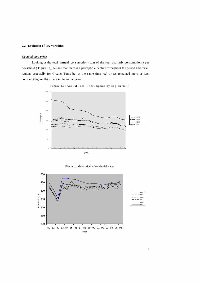
Looking at the total annual consumption (sum of the four quarterly consumptions) per
household ( Figure 1a), we see that there is a perceptible decline throughout the period and for all
regions especially for Greater Tunis but at the same time real prices remained more or less
constant (Figure 1b) except in the initial years.
F i g u r e 1 a : A n n u a l T o t a l C o n s u m p t i o n b y R e g i o n ( m 3 )
0
5 0
1 0 0
1 5 0
2 0 0
2 5 0
3 0 0
8 0 8 1 8 2 8 3 84 85 86 8 7 8 8 8 9 9 0 9 1 9 2 9 3 94 95 96
y e a r
cons
umpt
ion
G.Tunis N . E a s t N.West C . E a s t C.West South
Figure 1b: Mean prices of residential water
200
250
300
350
400
450
500
80 81 82 83 84 85 86 87 88 89 90 91 92 93 94 95 96year
mea
n re
al p
rice
PXRGT
PXRCE
PXRCO
PXRNE
PXRNO
PXRSD
6
Demand by brackets
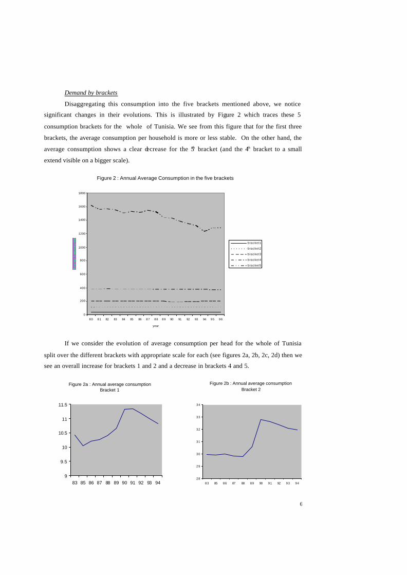
Disaggregating this consumption into the five brackets mentioned above, we notice
significant changes in their evolutions. This is illustrated by Figure 2 which traces these 5
consumption brackets for the whole of Tunisia. We see from this figure that for the first three
brackets, the average consumption per household is more or less stable. On the other hand, the
average consumption shows a clear decrease for the 5th bracket (and the 4th bracket to a small
extend visible on a bigger scale).
Figure 2 : Annual Average Consumption in the five brackets
0
200
400
600
800
1000
1200
1400
1600
1800
80 81 82 83 84 85 86 87 88 89 90 91 92 93 94 95 96
year
bracket1
bracket2
bracket3
bracket4
bracket5
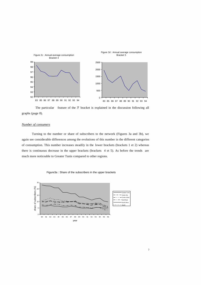
If we consider the evolution of average consumption per head for the whole of Tunisia
split over the different brackets with appropriate scale for each (see figures 2a, 2b, 2c, 2d) then we
see an overall increase for brackets 1 and 2 and a decrease in brackets 4 and 5.
Figure 2a : Annual average consumption Bracket 1
9
9.5
10
10.5
11
11.5
83 85 86 87 88 89 90 91 92 93 94
Figure 2b : Annual average consumption Bracket 2
28
29
30
31
32
33
34
83 85 86 87 88 89 90 91 92 93 94
7
The particular feature of the 3rd bracket is explained in the discussion following all
graphs (page 8).
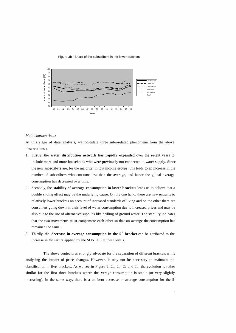
Number of consumers
Turning to the number or share of subscribers to the network (Figures 3a and 3b), we
again see considerable differences among the evolutions of this number in the different categories
of consumption. This number increases steadily in the lower brackets (brackets 1 et 2) whereas
there is continuous decrease in the upper brackets (brackets 4 et 5). As before the trends are
much more noticeable to Greater Tunis compared to other regions.
Figure 2c : Annual average consumption Bracket 4
92
93
94
95
96
97
98
99
83 85 86 87 88 89 90 91 92 93 94
Figure 2d : Annual average consumption Bracket 5
0
500
1000
1500
2000
2500
83 85 86 87 88 89 90 91 92 93 94
Figure3a : Share of the subscribers in the upper brackets
0
5
10
15
20
25
80 81 82 83 84 85 86 87 88 89 90 91 92 93 94 95 96
year
shar
e of
sub
scrib
ers
(%)
Greater Tunis
Centre Est
Centre West
North East
North West
South
8
Main characteristics
At this stage of data analysis, we postulate three inter-related phenomena from the above
observations :
1. Firstly, the water distribution network has rapidly expanded over the recent years to
include more and more households who were previously not connected to water supply. Since
the new subscribers are, for the majority, in low income groups, this leads to an increase in the
number of subscribers who consume less than the average, and hence the global average
consumption has decreased over time.
2. Secondly, the stability of average consumption in lower brackets leads us to believe that a
double sliding effect may be the underlying cause. On the one hand, there are new entrants to
relatively lower brackets on account of increased standards of living and on the other there are
consumers going down in their level of water consumption due to increased prices and may be
also due to the use of alternative supplies like drilling of ground water. The stability indicates
that the two movements must compensate each other so that on average the consumption has
remained the same.
3. Thirdly, the decrease in average consumption in the 5t h bracket can be attributed to the
increase in the tariffs applied by the SONEDE at these levels.
The above conjectures strongly advocate for the separation of different brackets while
analysing the impact of price changes. However, it may not be necessary to maintain the
classification in five brackets. As we see in Figure 2, 2a, 2b, 2c and 2d, the evolution is rather
similar for the first three brackets where the average consumption is stable (or very slightly
increasing). In the same way, there is a uniform decrease in average consumption for the 5th
Figure 3b : Share of the subscribers in the lower brackets
50
55
60
65
70
75
80
85
90
95
100
80 81 82 83 84 85 86 87 88 89 90 91 92 93 94 95 96
Year
shar
e of
sub
crib
ers
(%)
Greater Tunis
Centre Est
Centre West
North East
North West
South
9
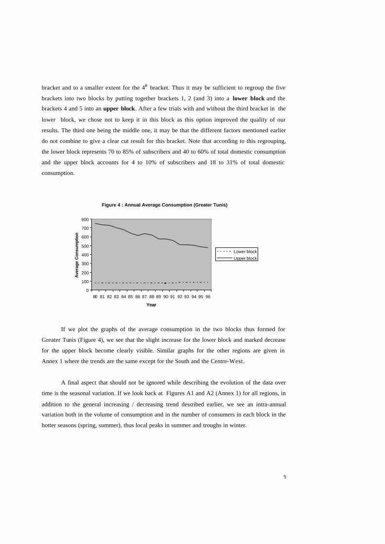
bracket and to a smaller extent for the 4th bracket. Thus it may be sufficient to regroup the five
brackets into two blocks by putting together brackets 1, 2 (and 3) into a lower block and the
brackets 4 and 5 into an upper block. After a few trials with and without the third bracket in the
lower block, we chose not to keep it in this block as this option improved the quality of our
results. The third one being the middle one, it may be that the different factors mentioned earlier
do not combine to give a clear cut result for this bracket. Note that according to this regrouping,
the lower block represents 70 to 85% of subscribers and 40 to 60% of total domestic consumption
and the upper block accounts for 4 to 10% of subscribers and 18 to 31% of total domestic
consumption.
If we plot the graphs of the average consumption in the two blocks thus formed for
Greater Tunis (Figure 4), we see that the slight increase for the lower block and marked decrease
for the upper block become clearly visible. Similar graphs for the other regions are given in
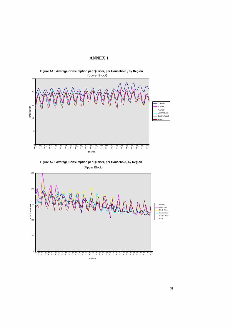
Annex 1 where the trends are the same except for the South and the Centre-West.
A final aspect that should not be ignored while describing the evolution of the data over
time is the seasonal variation. If we look back at Figures A1 and A2 (Annex 1) for all regions, in
addition to the general increasing / decreasing trend described earlier, we see an intra-annual
variation both in the volume of consumption and in the number of consumers in each block in the
hotter seasons (spring, summer), thus local peaks in summer and troughs in winter.
Figure 4 : Annual Average Consumption (Greater Tunis)
0
100
200
300
400
500
600
700
800
80 81 82 83 84 85 86 87 88 89 90 91 92 93 94 95 96
Year
Ave
rage
Con
sum
ptio
n
Lower block
Upper block
10
3. The Model
3.1 Theoretical Issues
Classical economic theory suggests that income and prices are important explanatory
factors in a model of demand and water is no exception to this. However, household/individual
behaviour with respect to water use may follow different patterns depending on the habits and
lifestyles that tend to vary with the level of income. One part of the demand is used by all to
satisfy basic needs like thirst, cooking and cleaning and this part, being essential, is highly
inelastic to price and income changes. This p art of water consumption can be considered to be an
“essential good” with very low price elasticities. As one goes higher in income levels, one may
find other uses of water such as watering the garden or refilling private swimming pools. This part
of the demand will no doubt be elastic with respect to price and income changes thus “behaving”
like a luxury good. Further, it will also differ significantly among households depending on their
lifestyle and the type of sanitary/technological installations in the house. This is seen for instance
in the great variation in the willingness to pay (WTP) of households in higher income categories
(cf. Ayadi et al.(2000)). As the proportion of the consumption of the “luxury good” relative to the
“essential good” increases with higher and higher standard of living, the WTP also increases.
Thus higher income groups have a higher proportion of the “luxury good” component of water
consumption and are, at least initially, willing to pay higher prices in order to satisfy their higher
need for water consumption. However this behaviour may not last long and if the same price
structure persists, households may in the long run adapt their behaviour and installations to water
saving options so that they are not any more in high consumption brackets with high prices. This
long term reduction in total water consumption will have two consequences: (i) an obvious
decrease in average consumption and (ii) a ‘sliding down’ from a higher consumption bracket to a
lower one reducing the number of consumers in the high brackets. Hence the number (or
proportion) of subscribers in each bracket needs to be explicitly modelled as it is also an
endogenous variable in the phenomenon under study.
Now, let us ask the question as to what price variable is relevant in this context. There are
two basic choices found in the literature. The first is the marginal price i.e. the price paid for the
last m3 of water consumed (see e.g. Howe and Linaweaver (1967)). In our case it is the tariff rate
of the bracket considered. A main drawback of this variable is that it completely ignores the tariff
rates of the remaining brackets to which the consumers may not be indifferent. Another indicator
associated with marginal price is the difference between the average and the marginal prices
11
multiplied by the quantity consumed (e.g. Billings and Agthe (1980), Nieswiadomy and Molina
(1989)). This variable represents (in absolute value) the surplus of the household in terms of how
much it saves by not paying all its consumption at the marginal price of the bracket in question.
The influence of this variable is similar to an income effect and its coefficient is expected to be in
the same order of magnitude as income but of the opposite sign (cf. Nordin (1976), Scheffer and
David (1985)).
The second choice is the average price, which is simply the total water bill of the
household divided by the volume consumed (see for instance Wong (1972), Foster and Beattie
(1980)). At the regional level, this will be given by the sum of water bills of all households in that
block divided by the total volume of water consumed by the households. We believe that the
household is certainly sensitive to the total amount that it pays for its water consumption and thus
this variable is one of the key variables affecting its behaviour. The average price defined above is
in fact the unit value of water at the regional level. Economic theory discurages the use of such a
variable due to the presence of quality effects ( cf. Deaton (1988) and Ayadi et al.(2002)); water
being homogeneous product in terms of quality this inconvenience is avoided here. However, we
hasten to add that it has also its own defects. Omitting fixed costs, the average price is a weighted
sum of the marginal prices of the different brackets of the tariff structure, the weights being given
by the shares of the consumption in each bracket in the total consumption. Therefore the average
price depends on the quantities consumed in each bracket the sum of which is in fact our
dependent variable. This backward link between the average price and the quantity consumed may
lead to what is called a simultaneity bias, resulting in incorrect estimations3. Further, at the
regional level, the shifting of consumers from one bracket to another (say due to price changes)
modifies the consumption shares of both brackets and hence the weights. This may lead to
distorted price effects depending on whether the “sliding” consumers consume more or less than
the earlier average in each bracket. In order to overcome these problems two alternative
procedures were attempted in our study: (a) apply the instrumental variable (IV) method (see
Greene (1997) for instance), using all the marginal prices in the tariff structure as instruments for
the average price, (b) use exogenous weights, for instance, the median values of shares of all
consumers, in the calculation of the average price (we call this price the ‘modified price’ in our
table of results) and thus break the link to the dependent variable.
3 Reference to the simultaneity problem in this context is already found in the literature for example in Chicoine et al (1986) and Nieswiadomy and Molina (1989).
12
3.2 Econometric specification
Our model consists of two equations: a demand equation explaining the quantity of water
consumed per household in each bracket and a second equation explaining the proportion of
households in the bracket allowing us to capture the sliding effect in terms of certain relevant
factors. The demand equation takes a classical form i.e a function of income and prices and
modifies it to incorporate new elements that take into account the special features of Tunisian
water consumption like the division into different consumption blocks, the rapid expansion of
distribution network and the climatic conditions pertaining to a dry area on earth. The model is
specified at the regional level so that variations across regions can be explicitly accounted for.
Thus for period t and region g, the demand equation for a particular block ? is specified as:
GgTt
QDLogRLLogNLogPLogRLogC tgs
stgsgtggtggtggtgggtg
,...1;,...1)1(
14,2,1
543210
??
??????? ??
???????? ???????
where C, R and P are respectively the average consumption of water per household, the average
income of households and the price paid by the consumers in the block considered, N represents
the network size present to capture the effect of network expansion, RL is an indicator of rainfall,
QD s is a quarterly dummy for the sth quarter and ? a random disturbance term.
In the second equation of the model, the proportion of households in each bracket ? (for
region g and period t) is expressed as a function of the same explanatory variables as those of
average consumption except for income.
GgTt
QDLogRLLogNLogPNNB
Log tgs
stgsgtggtggtgggtg
,...1;,...1)2(
24,2,1
43210
??
?????????
??? ?
?
???????
??????
where NB denotes the number of consumers in the corresponding block.
Price effect in the above equation (whatever be the price used) will actually capture the
sliding of consumers from one bracket to another subsequent to a change. Hence it should have a
negative coefficient for the upper block as consumers slide down from a higher block to a lower
one in case of a price increase whereas since demand is expected to be relatively inelastic to price
in the lower brackets the coefficient will be positive in the lower block (as the earlier consumers
13
do not move and new ones come from the upper block) . Increase in rainfall should also transfer
the consumers from a higher bracket to a lower one with the reduction being more perceivable in
the upper block. As far as seasonality goes, within the upper block, cold and wet seasons have
less consumers than the dry one (summer) whereas in the lower block the consumers may increase
again due to the joining from above.
Note that in equations (1) and (2) the coefficients are specified to be different for different
regions and different blocks. Coefficient variation over blocks is maintained throughout our study
as it is one of the interesting features of our analysis. However the two equations were also
estimated assuming same coefficients for all regions except for the intercept, the resulting model
being the fixed effects model of panel data literature. On the other hand if we keep the coefficients
different for different regions we have the variable coefficient model. In our applicat ion, we
propose to vary the price coefficients only in the variable coefficient alternative as these are the
main coefficients of interest, and so that the number of parameters is not unnecessarily increased.
For a given ? (block), equations (1) and (2) form a SUR model and combining the two
blocks we get a two level SUR system for which we assume non zero correlations across all
equations. Denoting the vectors of TG errors of equations (1) and (2) for block 1 as u1 and u2
respectively and the same vectors for block 2 as u3 and u4 respectively, we postulate
4,3,2,1,)()3( ??? kjIuuE TGjkkj ?
Thus the SUR system has to be estimated by feasible GLS or by 3SLS in case average prices are
instrumented by marginal prices as discussed earlier. In our practical application we have
considered two variants: the above structure of covariances (3) and also zero correlation between
different blocks (maintaining nonzero correlation between equations (1) and (2) within each
block). The latter gives rise to a block diagonal structure for the system variance-covariance
matrix leading to separate estimations by GLS or 3SLS for each block.
4. Empirical Results
4.1 General remark
Our econometric model was implemented in two stages. In the first stage we pool data for
all regions and the two blocks (a total of 408 observations for each block) , and estimate the same
14
model for each block except that we take account of possible differences in behaviour across
regions by adding fixed regional dummies in the regression equation. This is the so-called fixed
effects model.
In the second stage of our empirical work we once again combine all data exactly in the
same way as for the first stage except that in each block’s regression equation the price response
coefficients are also allowed to vary across regions to account for heterogeneity of regional
behaviour. This is the variable coefficient version of the model. The model was estimated
successively with the marginal and the average price as an explanatory variable in the demand
equation. Since the quality of results obtained using marginal prices directly in the equation
was not good, we choose to present and analyse only those using average prices so that the
reader is not overwhelmed with too many results. However, we will also discuss the results
obtained taking the marginal prices as instruments for the average prices. The average income
R is calculated using the INS budget survey data as it is not available in the data collected by
SONEDE. It was noted that the proportions of households in the upper and lower blocks are about
10% and 75% respectively. Hence the average income of the lower block households was
approximated by the average income of the lower 75% fractile of the income distribution obtained
in the budget survey. The same procedure was adopted for the upper block. The network size
variable N is approximated either by the number or the percentage of households connected to the
network in each region; QDs is a dummy variable for quarter s (as there is a constant in the model,
the third quarter is omitted to avoid multicollinearity).
4.2 Fixed effects models
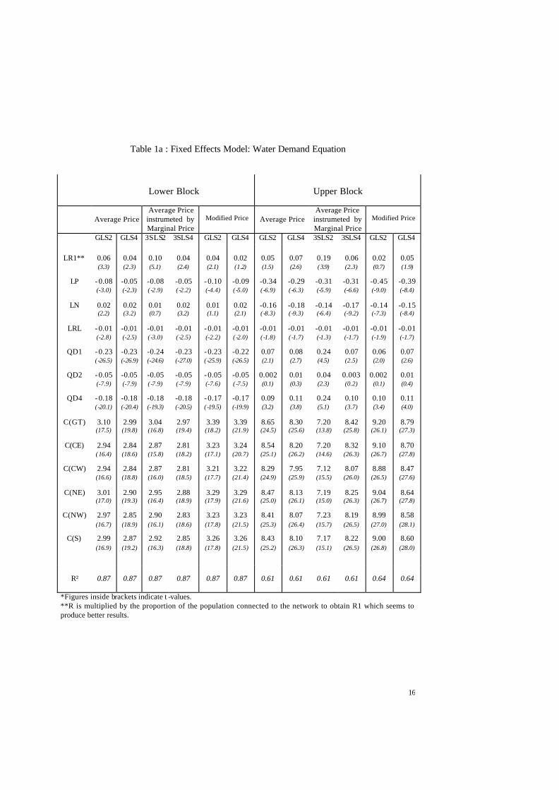
The results concerning the fixed effects models combining all regions and blocks are
given in Tables 1a and 1b. Let us recall that the fundamental difference among the three
variants (Average price, Average price instrumented by marginal price, Modified price)
concerns the treatment of the price variable (see Section 3.1). Within each variant, GLS2
(3SLS2) denotes the case where no correlation is assumed between blocks and GLS4 (3SLS4)
the case there are nonzero correlations across all equations. In general, GLS2 (3SLS2) and
GLS4 (3SLS4) estimates of price effects are of the same order of magnitude in all the three
variants, whereas for the income effect there seems to be a bigger difference between GLS2
(3SLS2) and GLS4 (3SLS4) rather than between the variants. We will come back to this
comparison later.
15
Turning to the estimates of price elasticity (Table 1a), we perceive the following
tendencies:
? The price elasticities of the lower block are small in absolute value and around –0.1
? The price elasticities of the upper block are bigger in absolute value and around -0.4
? There is some variations in the intercepts across regions and all are positive (implying
positive minimal consumptions).
? The order of magnitude is the same for GLS and 3SLS methods but slightly increases in
absolute value for the modified price method.
The network expansion effect is highly significant for both blocks but of opposite sign
for all methods. The average consumption of the new entrants seems to be slightly higher then
that of the existing lower consumers, thus giving a positive coefficients for the network effect
on the lower block. However the new comers do not consume as much as the average
consumer of the upper block resulting in a negative impact on the mean consumption of this
block.
Rainfall has a significant impact on consumption for both blocks. Its coefficient is
negative as expected. The following observations can be made regarding the seasonal
dummies. As we have taken the dry season (QDi3) as the reference, the coefficients of the wet
and cold ones (QDi 1 , QDi2 and QDi 4) are negative for the lower block (with both the GLS and
3SLS procedures of all the three variants) implying an expected lower consumption in these
seasons. The winter and autumn (QDi1 and QDi4) decreases seem to be more than the spring
one. However for the upper block, the results seem to be opposite with all the three dummies
having a positive coefficient with all procedures, and the effect of the dummies is less
pronounced (in absolute terms) than the corresponding value for the lower block. This
apparent increase in average consumption in the wet/cold seasons for the upper block may be
because of the sliding down of some consumers from the upper block (those with a lower
average consumption) to the lower block thus leaving the block with a greater proportion of
customers with a relatively higher average consumption. The regional effects are not very
different with slightly higher consumption in Greater Tunis and North East.
Turning to the estimations of the second equation (Table 1b), it is interesting to note
the significance of the sliding effect as brought out by these results. Looking at the effect of
16
Table 1a : Fixed Effects Model: Water Demand Equation
Lower Block
Upper Block
Average Price
Average Price instrumeted by Marginal Price
Modified Price
Average Price
Average Price instrumeted by Marginal Price
Modified Price
GLS2 GLS4 3SLS2 3SLS4 GLS2 GLS4 GLS2 GLS4 3SLS2 3SLS4 GLS2 GLS4
LR1**
LP
LN
LRL
QD1
QD2
QD4
C(GT)
C(CE)
C(CW)
C(NE)
C(NW)
C(S)
0.06 (3.3)
- 0.08 (-3.0)
0.02 (2.2)
- 0.01 (-2.8)
- 0.23 ( -26.5)
- 0.05 (-7.9)
- 0.18 ( -20.1)
3.10 (17.5)
2.94 (16.4)
2.94 (16.6)
3.01 (17.0)
2.97 (16.7)
2.99 (16.9)
0.04 (2.3)
-0.05 (-2.3)
0.02 (3.2)
-0.01 (-2.5)
-0.23 (-26.9)
-0.05 (-7.9)
-0.18 (-20.4)
2.99 (19.8)
2.84 (18.6)
2.84 (18.8)
2.90 (19.3)
2.85 (18.9)
2.87 (19.2)
0.10 (5.1)
-0.08 ( -2.9)
0.01 (0.7)
-0.01 ( -3.0)
-0.24 (-24.6)
-0.05 ( -7.9)
-0.18 (-19.3)
3.04 (16.8)
2.87 (15.8)
2.87 (16.0)
2.95 (16.4)
2.90 (16.1)
2.92 (16.3)
0.04 (2.4)
-0.05 ( -2.2)
0.02 (3.2)
-0.01 ( -2.5)
-0.23 (-27.0)
-0.05 ( -7.9)
-0.18 (-20.5)
2.97 (19.4)
2.81 (18.2)
2.81 (18.5)
2.88 (18.9)
2.83 (18.6)
2.85 (18.8)
0.04 (2.1)
- 0.10 (-4.4)
0.01 (1.1)
- 0.01 (-2.2)
- 0.23 ( -25.9)
- 0.05 (-7.6)
- 0.17 ( -19.5)
3.39 (18.2)
3.23 (17.1)
3.21 (17.7)
3.29 (17.9)
3.23 (17.8)
3.26 (17.8)
0.02 (1.2)
-0.09 ( -5.0)
0.02 (2.1)
-0.01 ( -2.0)
-0.22 (-26.5)
-0.05 ( -7.5)
-0.17 (-19.9)
3.39 (21.9)
3.24 (20.7)
3.22 (21.4)
3.29 (21.6)
3.23 (21.5)
3.26 (21.5)
0.05 (1.5)
-0.34 ( -6.9)
-0.16 ( -8.3)
-0.01 ( -1.8)
0.07 (2.1)
0.002 (0.1)
0.09 (3.2)
8.65 (24.5)
8.54 (25.1)
8.29 (24.9)
8.47 (25.0)
8.41 (25.3)
8.43 (25.2)
0.07 (2.6)
-0.29 ( -6.3)
-0.18 ( -9.3)
-0.01 ( -1.7)
0.08 (2.7)
0.01 (0.3)
0.11 (3.8)
8.30 (25.6)
8.20 (26.2)
7.95 (25.9)
8.13 (26.1)
8.07 (26.4)
8.10 (26.3)
0.19 (3.9)
-0.31 (-5.9)
-0.14 (-6.4)
-0.01 (-1.3)
0.24 (4.5)
0.04 (2.3)
0.24 (5.1)
7.20 (13.8)
7.20 (14.6)
7.12 (15.5)
7.19 (15.0)
7.23 (15.7)
7.17 (15.1)
0.06 (2.3)
-0.31 (-6.6)
-0.17 (-9.2)
-0.01 (-1.7)
0.07 (2.5)
0.003 (0.2)
0.10 (3.7)
8.42 (25.8)
8.32 (26.3)
8.07 (26.0)
8.25 (26.3)
8.19 (26.5)
8.22 (26.5)
0.02 (0.7)
-0.45 (-9.0)
-0.14 (-7.3)
-0.01 (-1.9)
0.06 (2.0)
0.002
(0.1)
0.10 (3.4)
9.20 (26.1)
9.10 (26.7)
8.88 (26.5)
9.04 (26.7)
8.99 (27.0)
9.00 (26.8)
0.05 (1.9)
-0.39 (-8.4)
-0.15 (-8.4)
-0.01 (-1.7)
0.07 (2.6)
0.01 (0.4)
0.11 (4.0)
8.79 (27.3)
8.70 (27.8)
8.47 (27.6)
8.64 (27.8)
8.58 (28.1)
8.60 (28.0)
R²
0.87
0.87
0.87
0.87
0.87
0.87
0.61
0.61
0.61
0.61
0.64
0.64
*Figures inside brackets indicate t -values. **R is multiplied by the proportion of the population connected to the network to obtain R1 which seems to produce better results.

17
Table 1 b : Fixed Effects Model: Consumers Proportion Equation
Lower Block
Upper Bloc k
Average Price
Average Price instrumeted by Marginal Price
Modified Price
Average Price
Average Price instrumeted by Marginal Price
Modified Price
GLS2 GLS4 3SLS2 3SLS4 GLS2 GLS4 GLS2 GLS4 3SLS2 3SLS4 GLS2 GLS4
LP
LN
LRL
QD1
QD2
QD4
C(GT)
C(CE)
C(CW)
C(NE)
C(NW)
C(S)
0.05 (1.8)
0.03 (5.4)
0.02 (5.4)
0.26 (31.6)
0.09 (12.9)
0.23 (26.8)
3.27 (18.3)
3.45 (19.3)
3.58 (20.2)
3.46 (19.5)
3.56 (20.1)
3.45 (19.5)
0.05 (2.5)
0.03 (5.1)
0.02 (4.7)
0.26 (32.0)
0.09 (13.0)
0.23 (27.2)
3.26 (22.6)
3.44 (2.8)
3.56 (25.1)
3.45 (24.2)
3.55 (24.9)
3.44 (24.1)
0.05 (1.8)
0.03 (5.4)
0.02 (4.6)
0.26 (31.6)
0.09 (12.9)
0.23 (26.8)
3.27 (18.3)
3.45 (19.3)
3.58 (20.2)
3.46 (19.5)
3.56 (20.1)
3.45 (19.5)
0.06 (2.6)
0.03 (5.2)
0.02 (4.7)
0.26 (32.0)
0.08 (13.0)
0.23 (27.1)
3.24 (22.2)
3.42 (23.4)
3.55 (24.8)
3.43 (23.8)
3.53 (24.5)
3.42 (23.7)
0.07 (3.2)
0.04 (6.2)
0.02 (4.4)
0.26 (33.0)
0.09 (13.2)
0.23 (27.8)
3.01 (16.4)
3.19 (17.4)
3.34 (18.9)
3.21 (17.8)
3.32 (18.7)
3.20 (17.8)
0.06 (3.7)
0.04 (6.3)
0.02 (4.4)
0.26 (33.1)
0.09 (13.2)
0.23 (28.0)
3.09 (20.8)
3.27 (22.1)
3.41 (24.1)
3.29 (22.7)
3.39 (23.8)
3.28 (22.6)
-0.62 ( -6.6)
-0.21 ( -6.9)
-0.04 ( -2.5)
-0.95 (-32.2)
-0.23 ( -9.5)
-0.82 (-26.7)
9.84 (25.0)
9.21 (23.5)
8.47 (20.9)
9.04 (22.7)
8.60 (21.2)
9.10 (22.9)
-0.47 ( -7.0)
-0.25 ( -9.6)
-0.03 ( -2.3)
-0.95 (-32.6)
-0.23 ( -9.6)
-0.83 (-27.1)
9.37 (28.3)
8.74 (26.5)
7.95 (24.1)
8.54 (25.9)
8.08 (24.5)
8.61 (26.2)
-0.59 (-6.3)
-0.22 (-7.2)
-0.03 (-2.5)
-0.95 (-32.4)
-0.23 (-9.5)
-0.82 (-26.8)
9.80 (24.9)
9.17 (23.4)
8.42 (20.8)
8.99 (22.5)
8.54 (21.1)
9.04 (22.8)
-0.48 (-7.0)
-0.25 (-9.6)
-0.03 (-2.3)
-0.95 (-32.6)
-0.23 (-9.6 )
-0.83 (-27.1)
9.40 (28.3)
8.77 (26.5)
7.98 (24.1)
8.57 (25.9)
8.11 (24.4)
8.63 (26.2)
-0.63 (-6.3)
-0.22 (-7.1)
-0.03 (-2.3)
-0.96 ( -33.0)
-0.23 (-9.5)
-0.83 ( -27.0)
9.95 (23.8)
9.33 (22.3)
8.58 (19.9)
9.15 (21.6)
8.69 (20.3)
9.21 (21.8)
-0.34 (-4.8)
-0.28 ( -11.0)
-0.03 (-2.0)
-0.97 ( -33.2)
-0.23 (-9.6)
-0.84 ( -27.5)
8.96 (26.0)
8.34 (24.2)
7.49 (21.7)
8.12 (23.5)
7.62 (22.1)
8.18 (23.8)
R²
0.92
0.92
0.92
0.92
0.92
0.92
0.92
0.92
0.92
0.92
0.92
0.92
*Figures inside brackets indicate t -values. **R is multiplied by the proportion of the population connected to the network to obtain R1 which seems to produce better results.
18
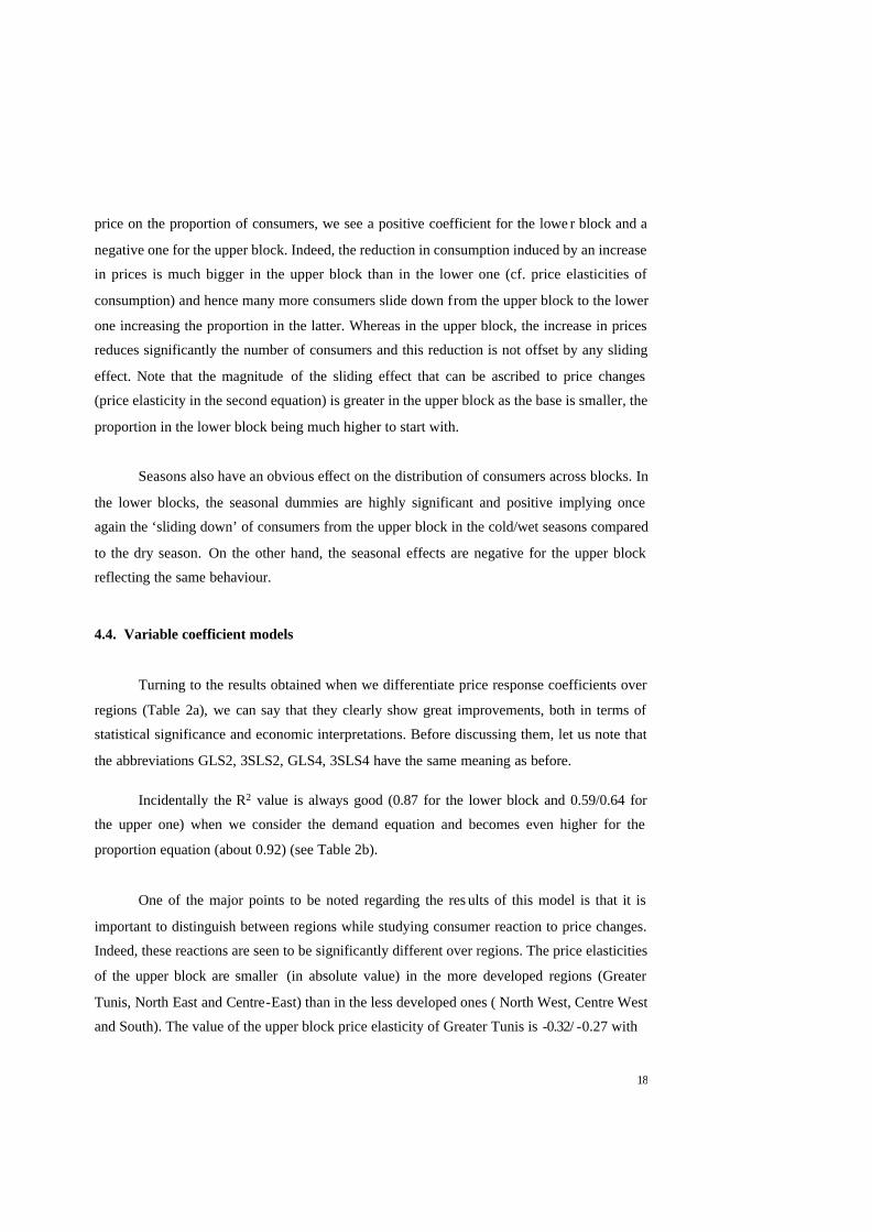
price on the proportion of consumers, we see a positive coefficient for the lowe r block and a
negative one for the upper block. Indeed, the reduction in consumption induced by an increase
in prices is much bigger in the upper block than in the lower one (cf. price elasticities of
consumption) and hence many more consumers slide down from the upper block to the lower
one increasing the proportion in the latter. Whereas in the upper block, the increase in prices
reduces significantly the number of consumers and this reduction is not offset by any sliding
effect. Note that the magnitude of the sliding effect that can be ascribed to price changes
(price elasticity in the second equation) is greater in the upper block as the base is smaller, the
proportion in the lower block being much higher to start with.
Seasons also have an obvious effect on the distribution of consumers across blocks. In
the lower blocks, the seasonal dummies are highly significant and positive implying once
again the ‘sliding down’ of consumers from the upper block in the cold/wet seasons compared
to the dry season. On the other hand, the seasonal effects are negative for the upper block
reflecting the same behaviour.
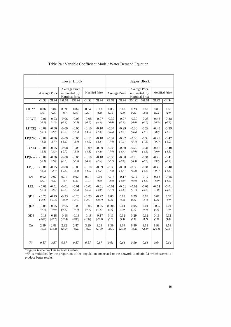
4.4. Variable coefficient models
Turning to the results obtained when we differentiate price response coefficients over
regions (Table 2a), we can say that they clearly show great improvements, both in terms of
statistical significance and economic interpretations. Before discussing them, let us note that
the abbreviations GLS2, 3SLS2, GLS4, 3SLS4 have the same meaning as before.
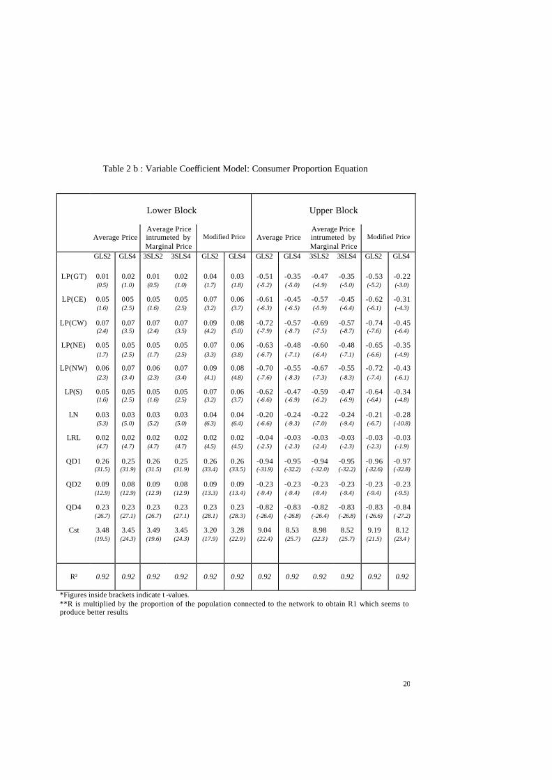
Incidentally the R2 value is always good (0.87 for the lower block and 0.59/0.64 for
the upper one) when we consider the demand equation and becomes even higher for the
proportion equation (about 0.92) (see Table 2b).
One of the major points to be noted regarding the res ults of this model is that it is
important to distinguish between regions while studying consumer reaction to price changes.
Indeed, these reactions are seen to be significantly different over regions. The price elasticities
of the upper block are smaller (in absolute value) in the more developed regions (Greater
Tunis, North East and Centre-East) than in the less developed ones ( North West, Centre West
and South). The value of the upper block price elasticity of Greater Tunis is -0.32/ -0.27 with
19
Table 2a : Variable Coefficient Model: Water Demand Equation
Lower Block
Upper Block
Average Price
Average Price intrumeted by Marginal Price
Modified Price
Average Price
Average Price intrumeted by Marginal Price
Modified Price
GLS2 GLS4 3SLS2 3SLS4 GLS2 GLS4 GLS2 GLS4 3SLS2 3SLS4 GLS2 GLS4
LR1**
LP(GT)
LP(CE)
LP(CW)
LP(NE)
LP(NW)
LP(S)
LN
LRL
QD1
QD2
QD4
Cst
0.06 (3.3)
- 0.06 (-2.2)
- 0.09 (-3.2)
- 0.09 (-3.2)
- 0.08 (-2.8)
- 0.09 (-3.1)
- 0.08 (-3.0)
0.02 (2.2)
- 0.01 (-2.8)
- 0.23 ( -26.6)
- 0.05 (-7.9)
- 0.18 ( -20.2)
2.99 (16.9)
0.04 (2.4)
-0.03 (-1.5)
-0.06 (-2.7)
-0.06 -2.7()
-0.05 (-2.2)
-0.06 (-2.6)
-0.05 (-2.4)
0.02 (3.1)
-0.01 (-2.5)
-0.23 (-27.9)
-0.05 (-8.0)
-0.18 (-20.5)
2.88 (19.2)
0.09 (4.5)
-0.06 ( -2.1)
-0.09 ( -3.2)
-0.09 ( -3.1)
-0.08 ( -2.7)
-0.08 ( -3.0)
-0.08 ( -2.8)
0.01 (1.5)
-0.01 ( -3.0)
-0.23 (-26.8)
-0.05 ( -8.1)
-0.18 (-20.4)
2.92 (16.3)
0.04 (2.4)
-0.03 ( -1.5)
-0.06 ( -2.6)
-0.06 ( -2.7)
-0.05 ( -2.1)
-0.06 ( -2.5)
-0.05 ( -2.4)
0.02 (3.1)
-0.01 ( -2.5)
-0.23 (-27.1)
-0.05 ( -7.9)
-0.18 (-20.5)
2.87 (19.1)
0.04 (2.1)
- 0.08 (-3.6)
- 0.10 (-4.9)
- 0.11 (-4.9)
- 0.09 (-4.3)
- 0.10 (-4.7)
- 0.10 (-4.5)
0.01 (1.1)
- 0.01 (-2.2)
- 0.23 ( -26.1)
- 0.05 (-7.7)
- 0.18 ( -19.6)
3.29 (18.0)
0.02 (1.2)
-0.07 ( -4.0)
-0.10 ( -5.6)
-0.10 ( -5.6)
-0.09 ( -4.9)
-0.10 ( -5.4)
-0.09 ( -5.2)
0.02 (1.9)
-0.01 ( -2.0)
-0.22 (-26.7)
-0.05 ( -7.6)
-0.17 (-20.0)
3.29 (21.8)
0.05 (1.7)
-0.32 ( -6.4)
-0.34 ( -6.6)
-0.37 ( -7.6)
-0.35 ( -7.0)
-0.35 ( -7.2)
-0.35 ( -7.0)
-0.16 ( -8.0)
-0.01 ( -1.7)
0.08 (2.5)
0.005 (0.3)
0.11 (3.6)
8.39 (24.7)
0.08 (2.8)
-0.27 ( -5.8)
-0.29 ( -6.1)
-0.32 ( -7.1)
-0.30 ( -6.4)
-0.30 ( -6.6)
-0.30 ( -6.4)
-0.17 ( -9.0)
-0.01 ( -1.6)
0.09 (3.2)
0.01 (0.5)
0.12 (4.3)
8.04 (25.8)
0.23 (4.8)
-0.30 (-5.8)
-0.30 (-5.6)
-0.30 (-5.7)
-0.29 (-5.6)
-0.28 (-5.3)
-0.30 (-5.8)
-0.12 (-6.0)
-0.01 (-1.1)
0.29 (5.5)
0.05 (2.9)
0.29 (6.1)
6.80 (14.1)
0.08 (2.6)
-0.28 (-6.0)
-0.29 (-6.3)
-0.33 (-7.3)
-0.31 (-6.6)
-0.31 (-6.8)
-0.31 (-6.6)
-0.17 (-8.8)
-0.01 (-1.6)
0.09 (3.1)
0.01 (0.5)
0.12 (4.2)
8.11 (26.0)
0.03 (0.9)
-0.43 (-8.5)
-0.45 (-8.7)
-0.48 (-9.7)
-0.46 (-9.0)
-0.46 (-9.2)
-0.46 (-9.1)
-0.13 (-6.9)
-0.01 (-1.8)
0.07 (2.3)
0.005
(0.3)
0.11 (3.7)
8.98 (26.4)
0.06 (2.0)
-0.38 (-7.9)
-0.39 (-8.2)
-0.42 (-9.2)
-0.40 (-8.5)
-0.41 (-8.7)
-0.40 (-8.6)
-0.15 (-8.0)
-0.01 (-1.6)
0.09 (3.0)
0.01 (0.6)
0.12 (4.4)
8.58 (27.5)
R²
0.87
0.87
0.87
0.87
0.87
0.87
0.61
0.61
0.59
0.61
0.64
0.64
*Figures inside brackets indicate t -values. **R is multiplied by the proportion of the population connected to the network to obtain R1 which seems to produce better results.
20
Table 2 b : Variable Coefficient Model: Consumer Proportion Equation
Lower Block
Upper Block
Average Price
Average Price intrumeted by Marginal Price
Modified Price
Average Price
Average Price intrumeted by Marginal Price
Modified Price
GLS2 GLS4 3SLS2 3SLS4 GLS2 GLS4 GLS2 GLS4 3SLS2 3SLS4 GLS2 GLS4
LP(GT)
LP(CE)
LP(CW)
LP(NE)
LP(NW)
LP(S)
LN
LRL
QD1
QD2
QD4
Cst
0.01 (0.5)
0.05 (1.6)
0.07 (2.4)
0.05 (1.7)
0.06 (2.3)
0.05 (1.6)
0.03 (5.3)
0.02 (4.7)
0.26 (31.5)
0.09 (12.9)
0.23 (26.7)
3.48 (19.5)
0.02 (1.0)
005 (2.5)
0.07 (3.5)
0.05 (2.5)
0.07 (3.4)
0.05 (2.5)
0.03 (5.0)
0.02 (4.7)
0.25 (31.9)
0.08 (12.9)
0.23 (27.1)
3.45 (24.3)
0.01 (0.5)
0.05 (1.6)
0.07 (2.4)
0.05 (1.7)
0.06 (2.3)
0.05 (1.6)
0.03 (5.2)
0.02 (4.7)
0.26 (31.5)
0.09 (12.9)
0.23 (26.7)
3.49 (19.6)
0.02 (1.0)
0.05 (2.5)
0.07 (3.5)
0.05 (2.5)
0.07 (3.4)
0.05 (2.5)
0.03 (5.0)
0.02 (4.7)
0.25 (31.9)
0.08 (12.9)
0.23 (27.1)
3.45 (24.3)
0.04 (1.7)
0.07 (3.2)
0.09 (4.2)
0.07 (3.3)
0.09 (4.1)
0.07 (3.2)
0.04 (6.3)
0.02 (4.5)
0.26 (33.4)
0.09 (13.3)
0.23 (28.1)
3.20 (17.9)
0.03 (1.8)
0.06 (3.7)
0.08 (5.0)
0.06 (3.8)
0.08 (4.8)
0.06 (3.7)
0.04 (6.4)
0.02 (4.5)
0.26 (33.5)
0.09 (13.4)
0.23 (28.3)
3.28 (22.9)
-0.51 ( -5.2)
-0.61 ( -6.3)
-0.72 ( -7.9)
-0.63 ( -6.7)
-0.70 ( -7.6)
-0.62 ( -6.6)
-0.20 ( -6.6)
-0.04 ( -2.5)
-0.94 (-31.9)
-0.23 ( -9.4)
-0.82 (-26.4)
9.04 (22.4)
-0.35 ( -5.0)
-0.45 ( -6.5)
-0.57 ( -8.7)
-0.48 ( -7.1)
-0.55 ( -8.3)
-0.47 ( -6.9)
-0.24 ( -9.3)
-0.03 ( -2.3)
-0.95 (-32.2)
-0.23 ( -9.4)
-0.83 (-26.8)
8.53 (25.7)
-0.47 (-4.9)
-0.57 (-5.9)
-0.69 (-7.5)
-0.60 (-6.4)
-0.67 (-7.3)
-0.59 (-6.2)
-0.22 (-7.0)
-0.03 (-2.4)
-0.94 (-32.0)
-0.23 (-9.4)
-0.82 (-26.4)
8.98 (22.3)
-0.35 (-5.0)
-0.45 (-6.4)
-0.57 (-8.7)
-0.48 (-7.1)
-0.55 (-8.3)
-0.47 (-6.9)
-0.24 (-9.4)
-0.03 (-2.3)
-0.95 (-32.2)
-0.23 (-9.4)
-0.83 (-26.8)
8.52 (25.7)
-0.53 (-5.2)
-0.62 (-6.1)
-0.74 (-7.6)
-0.65 (-6.6)
-0.72 (-7.4)
-0.64 (-6.4 )
-0.21 (-6.7)
-0.03 (-2.3)
-0.96 ( -32.6)
-0.23 (-9.4)
-0.83 ( -26.6)
9.19 (21.5)
-0.22 (-3.0)
-0.31 (-4.3)
-0.45 (-6.4)
-0.35 (-4.9)
-0.43 (-6.1)
-0.34 (-4.8)
-0.28 ( -10.8)
-0.03 (-1.9)
-0.97 ( -32.8)
-0.23 (-9.5)
-0.84 ( -27.2)
8.12 (23.4 )
R²
0.92
0.92
0.92
0.92
0.92
0.92
0.92
0.92
0.92
0.92
0.92
0.92
*Figures inside brackets indicate t -values. **R is multiplied by the proportion of the population connected to the network to obtain R1 which seems to produce better results.

21
the average price variant and -0.43/-0.38 with the modified price, whereas that of Centre West
-0.37/-0.32 for the first variant and -0.48/-0.42 for the second one. We may infer that
economic development and the accompanying increase in standard of living leads to less
reticence towards water conservation and saving, making the price effect smaller.
As before, the upper block price elasticities are in general significantly greater (in
absolute value) than the corresponding lower block ones. Incidentally, the variation of price
elasticities across brackets is also observed in other studies such as the one by Saleth and
Dinar (1997) in which the range of variation of the (marginal) price elasticity is even bigger
(from –0.47 to –5.34). There is also some variation in price coefficients across regions for the
lower block but to a lesser extent.
Regarding the consumer proportion equation (Table 2b), again we have positive price
effects in the lower block and negative in the upper block. The negative effects of the upper
block are highly significant and much greater in absolute value than the corresponding ones in
the lower block. The results confirm that regional differences in price effects are important.
In each block, the magnitude of price effects on consumer shares is seen to be linked
to the economic development of the region concerned. The lowest values are found for
Greater Tunis, North East and Centre East.
Finally, comparing the results of the two covariance structures GLS2/3SLS2 and
GLS4/3SLS4, we can say the following:
- The income elasticities of the demand for water are lower with GLS2/3SLS2 for the
upper block and higher with the same for the lower block.
- The order of magnitude of the price elasticities (when significant) is not very different
between GLS2/ 3SLS2 and GLS4/3SLS4 with a slightly higher value for GLS2/ 3SLS2
in particular for the consumer share equation.
We also carried out a likelihood ratio test comparing the four equation model with
non-zero correlation between all pairs of equations to the model in which no correlation is
assumed between any two equations of two different blocks. The former is largely
accepted according to our results. We therefore go on to interpret the estimated values of
these various covariances (or correlation coefficients) presented in Table 3.
22
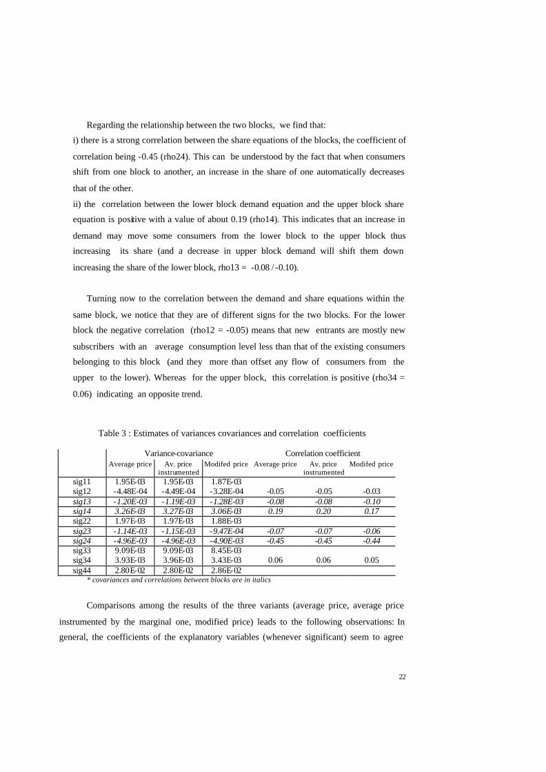
Regarding the relationship between the two blocks, we find that:
i) there is a strong correlation between the share equations of the blocks, the coefficient of
correlation being -0.45 (rho24). This can be understood by the fact that when consumers
shift from one block to another, an increase in the share of one automatically decreases
that of the other.
ii) the correlation between the lower block demand equation and the upper block share
equation is positive with a value of about 0.19 (rho14). This indicates that an increase in
demand may move some consumers from the lower block to the upper block thus
increasing its share (and a decrease in upper block demand will shift them down
increasing the share of the lower block, rho13 = -0.08 / -0.10).
Turning now to the correlation between the demand and share equations within the
same block, we notice that they are of different signs for the two blocks. For the lower
block the negative correlation (rho12 = -0.05) means that new entrants are mostly new
subscribers with an average consumption level less than that of the existing consumers
belonging to this block (and they more than offset any flow of consumers from the
upper to the lower). Whereas for the upper block, this correlation is positive (rho34 =
0.06) indicating an opposite trend.
Table 3 : Estimates of variances covariances and correlation coefficients
Variance-covariance Correlation coefficient Average price Av. price
instrumented Modifed price Average price Av. price
instrumented Modifed price
sig11 1.95E-03 1.95E-03 1.87E-03 sig12 -4.48E-04 -4.49E-04 -3.28E-04 -0.05 -0.05 -0.03 sig13 -1.20E-03 -1.19E-03 -1.28E-03 -0.08 -0.08 -0.10 sig14 3.26E-03 3.27E-03 3.06E-03 0.19 0.20 0.17 sig22 1.97E-03 1.97E-03 1.88E-03 sig23 -1.14E-03 -1.15E-03 -9.47E-04 -0.07 -0.07 -0.06 sig24 -4.96E-03 -4.96E-03 -4.90E-03 -0.45 -0.45 -0.44 sig33 9.09E-03 9.09E-03 8.45E-03 sig34 3.93E-03 3.96E-03 3.43E-03 0.06 0.06 0.05 sig44 2.80E-02 2.80E-02 2.86E-02
* covariances and correlations between blocks are in italics
Comparisons among the results of the three variants (average price, average price
instrumented by the marginal one, modified price) leads to the following observations: In
general, the coefficients of the explanatory variables (whenever significant) seem to agree
23
well between the average price and the IV variants, but using the modified price produces
different parameter estimates.
5. Simulation Results
The satisfactory results obtained in the estimation process motivated us to carry out
simulation experiments to evaluate the actual quantity of water that will be saved in each
region if the authorities were to increase prices. We also analysed how rainfall (or lack of it)
and the different seasons influence these quantities. In these experiments we keep the total
number of subscribers (all brackets put together) constant at the most recent value. The
calculations are based on the parameter estimates of the variable coefficient model which are
more interesting in terms of economic content. Note that the variantions obtained in our
simulations have to be interpreted in a comparative static framework.
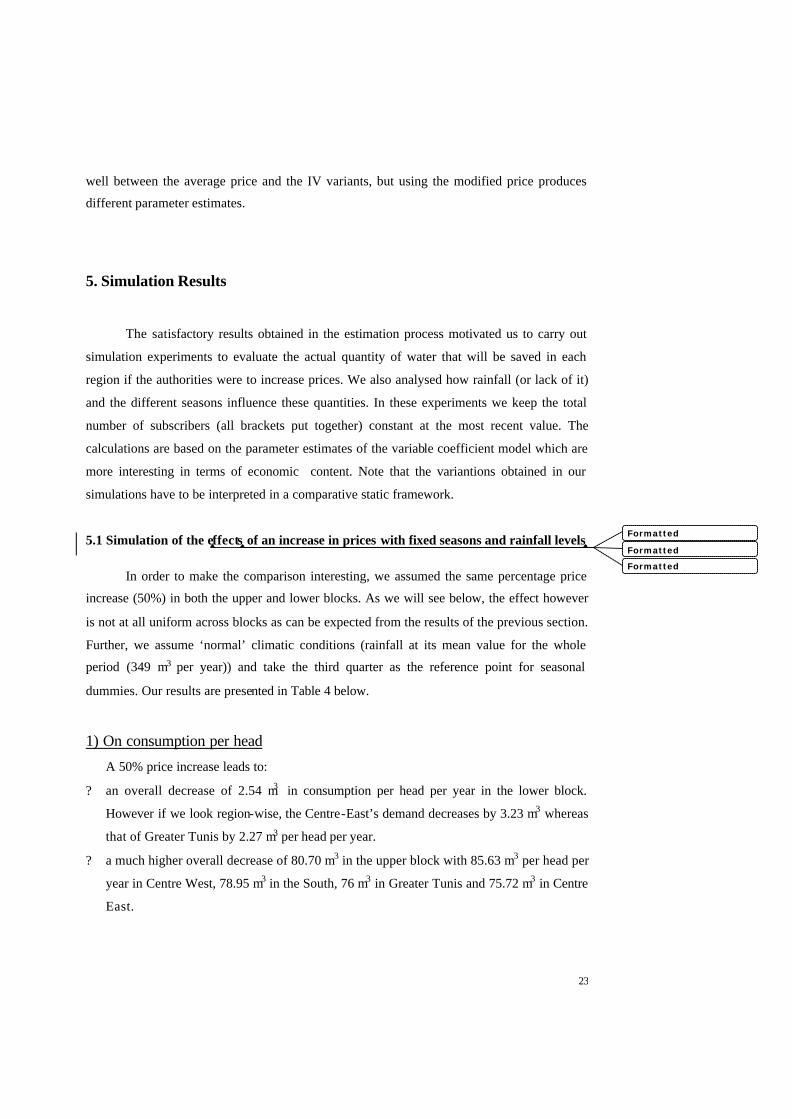
5.1 Simulation of the effects of an increase in prices with fixed seasons and rainfall levels In order to make the comparison interesting, we assumed the same percentage price
increase (50%) in both the upper and lower blocks. As we will see below, the effect however
is not at all uniform across blocks as can be expected from the results of the previous section.
Further, we assume ‘normal’ climatic conditions (rainfall at its mean value for the whole
period (349 m3 per year)) and take the third quarter as the reference point for seasonal
dummies. Our results are presented in Table 4 below.
1) On consumption per head
A 50% price increase leads to:
? an overall decrease of 2.54 m3 in consumption per head per year in the lower block.
However if we look region-wise, the Centre-East’s demand decreases by 3.23 m3 whereas
that of Greater Tunis by 2.27 m3 per head per year.
? a much higher overall decrease of 80.70 m3 in the upper block with 85.63 m3 per head per
year in Centre West, 78.95 m3 in the South, 76 m3 in Greater Tunis and 75.72 m3 in Centre
East.
Formatted
Formatted
Formatted
24
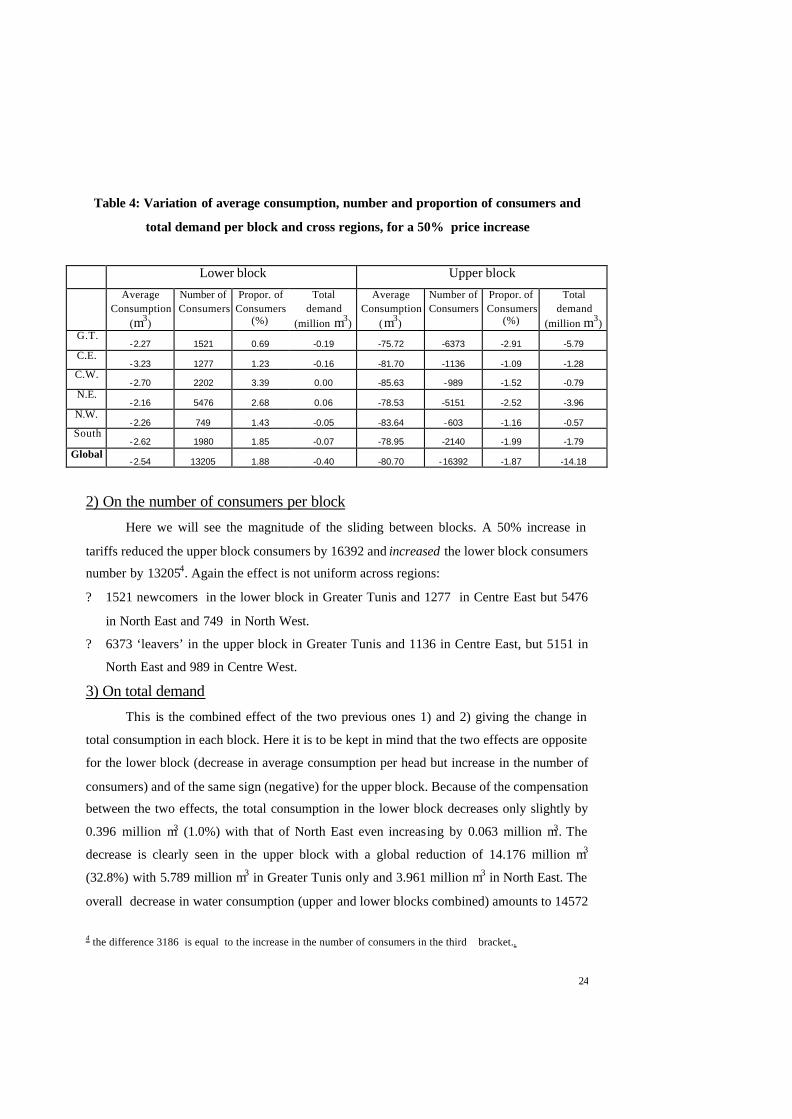
Table 4: Variation of average consumption, number and proportion of consumers and
total demand per block and cross regions, for a 50% price increase
Lower block Upper block
Average Consumption
(m3)
Number of Consumers
Propor. of Consumers
(%)
Total demand
(million m3)
Average Consumption
(m3)
Number of Consumers
Propor. of Consumers
(%)
Total demand
(million m3) G.T.
-2.27 1521 0.69 -0.19 -75.72 -6373 -2.91 -5.79 C.E.
-3.23 1277 1.23 -0.16 -81.70 -1136 -1.09 -1.28 C.W.
-2.70 2202 3.39 0.00 -85.63 -989 -1.52 -0.79 N.E.
-2.16 5476 2.68 0.06 -78.53 -5151 -2.52 -3.96 N.W.
-2.26 749 1.43 -0.05 -83.64 -603 -1.16 -0.57 South
-2.62 1980 1.85 -0.07 -78.95 -2140 -1.99 -1.79 Global
-2.54 13205 1.88 -0.40 -80.70 -16392 -1.87 -14.18 2) On the number of consumers per block
Here we will see the magnitude of the sliding between blocks. A 50% increase in
tariffs reduced the upper block consumers by 16392 and increased the lower block consumers
number by 132054. Again the effect is not uniform across regions:
? 1521 newcomers in the lower block in Greater Tunis and 1277 in Centre East but 5476
in North East and 749 in North West.
? 6373 ‘leavers’ in the upper block in Greater Tunis and 1136 in Centre East, but 5151 in
North East and 989 in Centre West.
3) On total demand
This is the combined effect of the two previous ones 1) and 2) giving the change in
total consumption in each block. Here it is to be kept in mind that the two effects are opposite
for the lower block (decrease in average consumption per head but increase in the number of
consumers) and of the same sign (negative) for the upper block. Because of the compensation
between the two effects, the total consumption in the lower block decreases only slightly by
0.396 million m3 (1.0%) with that of North East even increasing by 0.063 million m3. The
decrease is clearly seen in the upper block with a global reduction of 14.176 million m3
(32.8%) with 5.789 million m3 in Greater Tunis only and 3.961 million m3 in North East. The
overall decrease in water consumption (upper and lower blocks combined) amounts to 14572
4 the difference 3186 is equal to the increase in the number of consumers in the third bracket..
25
m3 which is about 17% of initial total demand. However, as seen above the bulk of this
saving comes from the upper block (97%) and only a small change is due to the lower one
(3%). This implies that in order to achieve any given target of demand reduction the policy
makers should not apply the same price change for both blocks; on the contrary a relatively
high increase has to be directed toward the upper block while keeping the price stable for the
lower one.
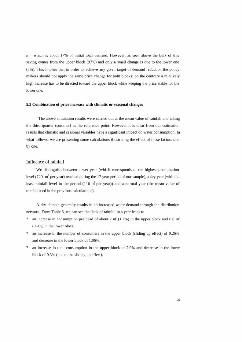
5.2 Combination of price increase with climatic or seasonal changes
The above simulation results were carried out at the mean value of rainfall and taking
the third quarter (summer) as the reference point. However it is clear from our estimation
results that climatic and seasonal variables have a significant impact on water consumption. In
what follows, we are presenting some calculations illustrating the effect of these factors one
by one.
Influence of rainfall
We distinguish between a wet year (which corresponds to the highest precipitation
level (729 m3 per year) reached during the 17 year period of our sample), a dry year (with the
least rainfall level in the period (116 m3 per year)) and a normal year (the mean value of
rainfall used in the previous calculations).
A dry climate generally results in an increased water demand through the distribution
network. From Table 5, we can see that lack of rainfall in a year leads to
? an increase in consumption per head of about 7 m3 (1.2%) in the upper block and 0.8 m3
(0.9%) in the lower block.
? an increase in the number of consumers in the upper block (sliding up effect) of 0.26%
and decrease in the lower block of 1.06%.
? an increase in total consumption in the upper block of 2.9% and decrease in the lower
block of 0.3% (due to the sliding up effect).
26
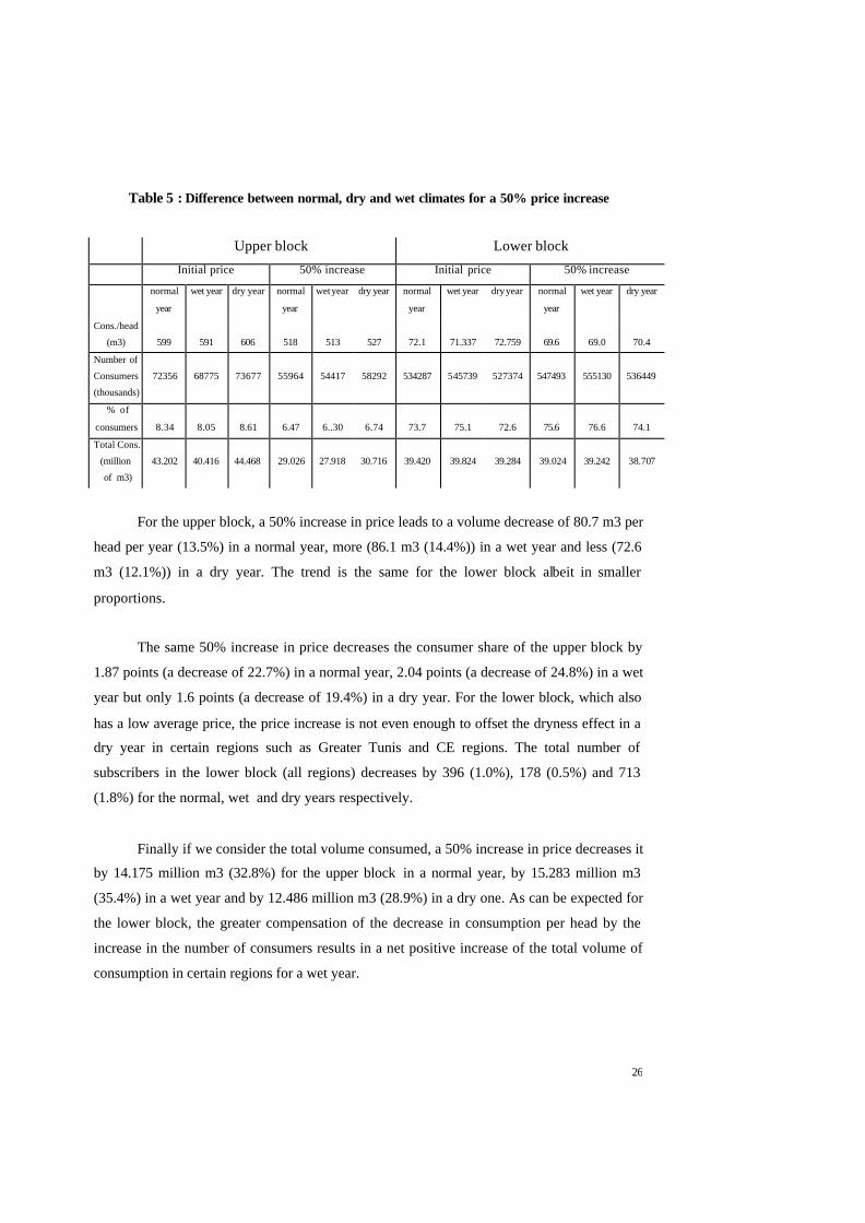
Table 5 : Difference between normal, dry and wet climates for a 50% price increase
Upper block Lower block
Initial price 50% increase Initial price 50% increase
normal
year
wet year dry year normal
year
wet year dry year normal
year
wet year dry year normal
year
wet year dry year
Cons./head
(m3)
599
591
606
518
513
527
72.1
71.337
72.759
69.6
69.0
70.4
Number of
Consumers
(thousands)
72356
68775
73677
55964
54417
58292
534287
545739
527374
547493
555130
536449
% of
consumers
8.34
8.05
8.61
6.47
6..30
6.74
73.7
75.1
72.6
75.6
76.6
74.1
Total Cons.
(million
of m3)
43.202
40.416
44.468
29.026
27.918
30.716
39.420
39.824
39.284
39.024
39.242
38.707
For the upper block, a 50% increase in price leads to a volume decrease of 80.7 m3 per
head per year (13.5%) in a normal year, more (86.1 m3 (14.4%)) in a wet year and less (72.6
m3 (12.1%)) in a dry year. The trend is the same for the lower block albeit in smaller
proportions.
The same 50% increase in price decreases the consumer share of the upper block by
1.87 points (a decrease of 22.7%) in a normal year, 2.04 points (a decrease of 24.8%) in a wet
year but only 1.6 points (a decrease of 19.4%) in a dry year. For the lower block, which also
has a low average price, the price increase is not even enough to offset the dryness effect in a
dry year in certain regions such as Greater Tunis and CE regions. The total number of
subscribers in the lower block (all regions) decreases by 396 (1.0%), 178 (0.5%) and 713
(1.8%) for the normal, wet and dry years respectively.
Finally if we consider the total volume consumed, a 50% increase in price decreases it
by 14.175 million m3 (32.8%) for the upper block in a normal year, by 15.283 million m3
(35.4%) in a wet year and by 12.486 million m3 (28.9%) in a dry one. As can be expected for
the lower block, the greater compensation of the decrease in consumption per head by the
increase in the number of consumers results in a net positive increase of the total volume of
consumption in certain regions for a wet year.
27
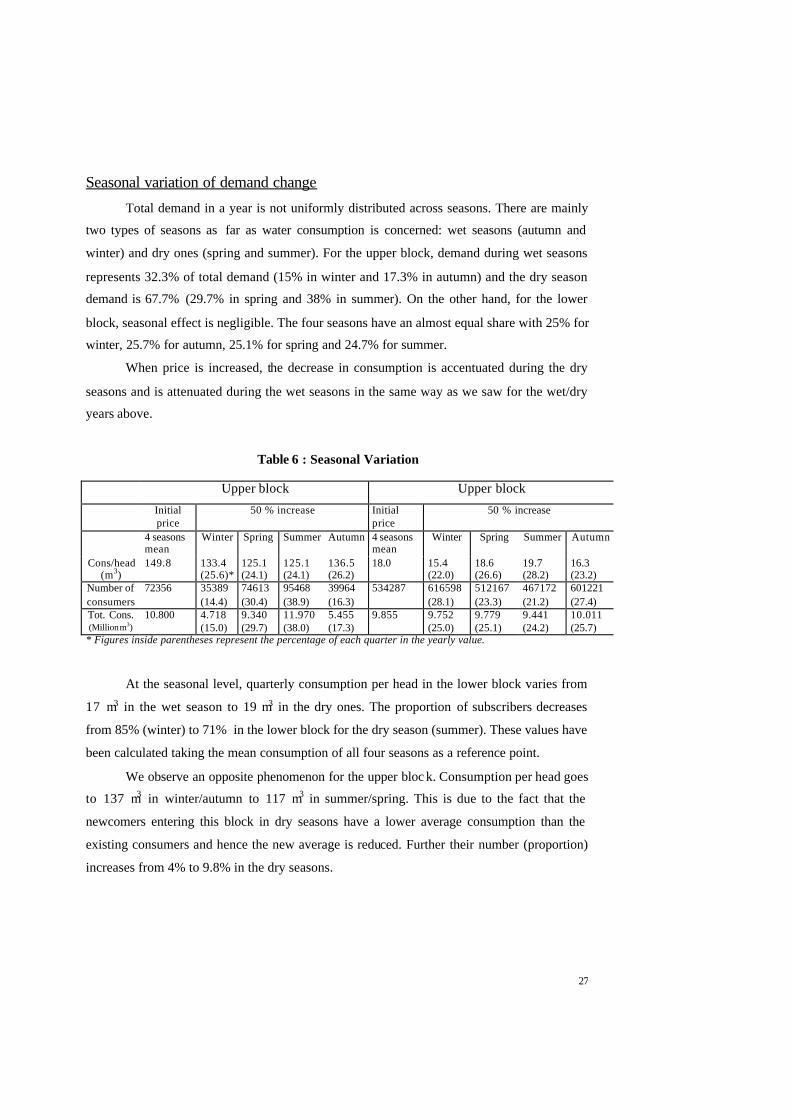
Seasonal variation of demand change
Total demand in a year is not uniformly distributed across seasons. There are mainly
two types of seasons as far as water consumption is concerned: wet seasons (autumn and
winter) and dry ones (spring and summer). For the upper block, demand during wet seasons
represents 32.3% of total demand (15% in winter and 17.3% in autumn) and the dry season
demand is 67.7% (29.7% in spring and 38% in summer). On the other hand, for the lower
block, seasonal effect is negligible. The four seasons have an almost equal share with 25% for
winter, 25.7% for autumn, 25.1% for spring and 24.7% for summer.
When price is increased, the decrease in consumption is accentuated during the dry
seasons and is attenuated during the wet seasons in the same way as we saw for the wet/dry
years above.
Table 6 : Seasonal Variation Upper block Upper block
Initial price
50 % increase Initial price
50 % increase
4 seasons mean
Winter Spring Summer Autumn 4 seasons mean
Winter Spring Summer Autumn
Cons/head (m3)
149.8 133.4 (25.6)*
125.1 (24.1)
125.1 (24.1)
136.5 (26.2)
18.0 15.4 (22.0)
18.6 (26.6)
19.7 (28.2)
16.3 (23.2)
Number of consumers
72356 35389 (14.4)
74613 (30.4)
95468 (38.9)
39964 (16.3)
534287 616598 (28.1)
512167 (23.3)
467172 (21.2)
601221 (27.4)
Tot. Cons. (Million m3)
10.800 4.718 (15.0)
9.340 (29.7)
11.970 (38.0)
5.455 (17.3)
9.855 9.752 (25.0)
9.779 (25.1)
9.441 (24.2)
10.011 (25.7)
* Figures inside parentheses represent the percentage of each quarter in the yearly value.
At the seasonal level, quarterly consumption per head in the lower block varies from
17 m3 in the wet season to 19 m3 in the dry ones. The proportion of subscribers decreases
from 85% (winter) to 71% in the lower block for the dry season (summer). These values have
been calculated taking the mean consumption of all four seasons as a reference point.
We observe an opposite phenomenon for the upper bloc k. Consumption per head goes
to 137 m3 in winter/autumn to 117 m3 in summer/spring. This is due to the fact that the
newcomers entering this block in dry seasons have a lower average consumption than the
existing consumers and hence the new average is reduced. Further their number (proportion)
increases from 4% to 9.8% in the dry seasons.
28
6. Conclusions
To sum up, the empirical results of our water demand model have been satisfactory
both from the economic and statistical points of view. We have attributed it to many new
additions to a classical model, such as the regional dimension, appropriate separation and
aggregation of different consumption brackets, incorporation of the network and sliding
effects and suitable estimation procedures. Our key findings are as follows.
Water demand in Tunisia is relatively sensitive to prices in the upper bracket and in
regions of dynamic economic activity and characterised by alternative sources of supply. This
is seen in the high price elasticity of more than 0.40 in absolute value for upper block in
Greater Tunis and North East. This leads us to believe that decentralised and effective pricing
strategy can result in a decrease in the water consumption of well-to-do people by raising
prices in the higher brackets. This strategy needs to be complemented by an appropriate
policy on preservation of ground water as this is the popular alternative source of supply
among this group.
On the other hand, prices should not be increased for the lower blocks as the
consumers in this block are essentially in low income groups and their elasticity is very small.
Hence increasing the price will only lead to a decrease in their purchasing power and thereby
a lowering of their quality of life.
Our simulation results confirm that this type of progressive non linear tariff structure
is an optimal solution to attain any desired reduction in water consumption without penalising
the consumers at the lower end of the spectrum. In addition, the tariffs policy should also be
adjusted taking into account the variability of the effect of price change over different seasons
and rainfall conditions.
Finally, we observe that the National Water Distributor SONEDE is in fact currently
acting in the right direction by subsiding the lower block consumers and increasing the tariff
rates in the higher brackets . The results of our study strongly advocate for a continuation of
this policy in the medium term.
29
References
Agthe, D.E. and R.B. Billings (1980) “Dynamic models of residential water demand”, Water
Resources Research, Vol.16, No.3, pp. 476 -480.
Ayadi, M., M. S. Matoussi and A. Telili (2000) “Retructuration tarifaire et conservation de l eau
residentielle", Paper presented at the 18th Journees de Micro-Economie Appliquee, Nancy.
Ayadi, M., J. Krishnakumar and M. S. Matoussi (2002) “Pooling surveys in the estimation of
income and price elsticities: Application to Tunisian households", Empirical
Economics,Forthcaming.
Billings, B.R. and D.E. Agthe (1980) “Price Elasticities for Water: A Case Study of Increasing
Block Rates”, Land Economics , Vol. 56, No.1, pp. 73-84.
Blundell, R. , P. Pashardes and G. Weber (1993) “ What Do We Learn About Consumer
Demand Patterns from Micro Data ? ” American Economic Review, Vol. 83, No.3.
Chicoine, D.L., S.C. Deller and G. Ramamurthy (1986) “Water Demand Estimation Under
Block Rate Pricing: A Simultaneous Equation Approach”, Water Resources Research, Vol.22,
No.6, pp. 859-863.
Deaton, Angus (1988) “Quality, Quantity and Spatial Variation of Price”, American Economic
Review, Vol. 78, pp. 418-43.
Foster, H.S. and B.R. Beattie (1981) “On the Specification of Price in Studies of Consumer
Demand Under Block Price Rescheduling”, Land Economics , Vol. 57, No.4, pp. 624-629.
Greene, W.H. (1994) Econometric Analysis, Maxwell Macmillan International Editions: New
York.
Hanemann, W.M. (1996) “Designing New Water Rates for Los Angeles”, in Advances in the
Economics of Environmental Resources , Vol.1, pp. 11-21, JAI Press Inc.
30
Howe, C.W. and F.P. Linaweaver (1967) “The Impact of Price on Residential Water Demand
and its Relation to System Design and Price Structure”, Water Resources Bulletin, Vol. 3, No.1,
pp. 13-32.
Lahouel M.H., M.S. Rejeb, C. Mamoghli and M. Daoues (1994) “Etude économique sur l’eau
potable en Tunisie ”, SONEDE, Tunisia.
Moncur, J.E.T. (1987) “Urban Water Pricing and Drought Management”, Water Resources
Research, Vol.23, No.3, pp. 393-398.
Nieswiadomy, M.L. and D.J. Molina (1989) “Comparing Residential Water Demand Estimates
under Decreasing and Increasing Block Rates”, Land Economics , Vol.65, No.3, pp. 280-289.
Nieswiadomy, M.L. and D.J. Molina (1991) “A Note on Price Perception in Water Demand
Models”, Land Economics , Vol.67, No.3, pp. 352-359.
Nordin, J.A. (1976) “A Proposed Modification of Taylor’s Demand Analysis: Comment”, Bell
Journal of Economics, Vol.6, No.1, pp. 719-721.
Rodriguez F. and E. Betteta (1991) “ Economics of Urban Water Supply : Theory and Case
Study ”, E.D.I. Washington D.C.
Saleth R.M. and A. Dinar (1997) “Satisfying Urban Thirst: Water Supply Augmentation and
Pricing Policy in Hyderabad City, India”, World Bank Technical Working Paper No. 395.
Schefter, J.E. and E.L. David (1985) “Estimating Residential Water Demand Under Multi-Part
Tariffs Using Aggregate Data”, Land Economics , Vol.61, No.3, pp. 352-359.
Wong, S.T. (1972) , “A Model of Municipal Water Demand: A Case Study Northeastern Illinois”,
Land Economics , Vol. 48, No.1, pp. 34-44.
31
ANNEX 1
Figure A1 : Average Consumption per Quarter, per Household , by Region(Lower Block)
0
5
10
15
20
25
80,1
80,4
81,3
82,2
83,1
83,4
84,3
85,2
86,1
86,4
87,3
88,2
89,1
89,4
90,3
91,2
92,1
92,4
93,3
94,2
95,1
95,4
96,3
quarter
con
sum
pti
on
G.Tunis
N.East
N.WestCentre East
Centre West
South
Figure A2 : Average Consumption per Quarter, per Household, by Region
(Upper Block)
0
50
100
150
200
250
80,1
80,3
80,4
81,2
81,4
82,2
82,4
83,2
83,4
84,2
84,4
85,2
85,4
86,2
86,4
87,2
87,4
88,2
88,4
89,2
89,4
90,2
90,4
91,2
91,4
92,2
92,4
93,2
93,4
94,2
94,4
95,2
95,4
96,2
96,4
quarter
con
sum
pti
on
G Tunis
North East
North West
Centre East
Centre West
South