1

Université de Montréal

A theoretical and experimental

dissociation of two models of

decision-making

Matthew A. Carland

Département des neurosciences, Faculté de médecine

Mémoire présentée à la Faculté de médecine

en vue de l’obtention du grade de maîtrise en sciences neurobiologique

August, 2014

© Matthew A. Carland, 2014

2

Abstract (French)

La prise de décision est un processus computationnel fondamental dans de nombreux aspects du

comportement animal. Le modèle le plus souvent rencontré dans les études portant sur la prise de

décision est appelé modèle de diffusion. Depuis longtemps, il explique une grande variété de données

comportementales et neurophysiologiques dans ce domaine. Cependant, un autre modèle, le modèle

d’urgence, explique tout aussi bien ces mêmes données et ce de façon parcimonieuse et davantage

encrée sur la théorie. Dans ce travail, nous aborderons tout d’abord les origines et le développement

du modèle de diffusion et nous verrons comment il a été établi en tant que cadre de travail pour

l’interprétation de la plupart des données expérimentales liées à la prise de décision. Ce faisant, nous

relèveront ses points forts afin de le comparer ensuite de manière objective et rigoureuse à des

modèles alternatifs. Nous réexaminerons un nombre d’assomptions implicites et explicites faites par

ce modèle et nous mettrons alors l’accent sur certains de ses défauts. Cette analyse servira de cadre

à notre introduction et notre discussion du modèle d’urgence. Enfin, nous présenterons une

expérience dont la méthodologie permet de dissocier les deux modèles, et dont les résultats

illustrent les limites empiriques et théoriques du modèle de diffusion et démontrent en revanche

clairement la validité du modèle d'urgence. Nous terminerons en discutant l'apport potentiel du

modèle d'urgence pour l'étude de certaines pathologies cérébrales, en mettant l'accent sur de

nouvelles perspectives de recherche.

Mots-clés: Prise de décision; modèle de diffusion; Modèle d’intégration; Modèle d’urgence;

Discrimination perceptuelle; Compromis vitesse/précision; Mouvement aléatoire de points;

Echantillonnage séquentiel; Test d’hypothèses; Temps de réponse; Comparaison de modèles; Neuro-

économie; Taux de récompense

3

Abstract (English)

Decision-making is a computational process of fundamental importance to many aspects of animal

behavior. The prevailing model in the experimental study of decision-making is the drift-diffusion

model, which has a long history and accounts for a broad range of behavioral and neurophysiological

data. However, an alternative model – called the urgency-gating model – has been offered which can

account equally well for much of the same data in a more parsimonious and theoretically-sound

manner. In what follows, we will first trace the origins and development of the DDM, as well as give a

brief overview of the manner in which it has supplied an explanatory framework for a large number

of behavioral and physiological studies in the domain of decision-making. In so doing, we will attempt

to build a strong and clear case for its strengths so that it can be fairly and rigorously compared to

potential alternative models. We will then re-examine a number of the implicit and explicit

theoretical assumptions made by the drift-diffusion model, as well as highlight some of its empirical

shortcomings. This analysis will serve as the contextual backdrop for our introduction and discussion

of the urgency-gating model. Finally, we present a novel experiment, the methodological design of

which uniquely affords a decisive empirical dissociation of the models, the results of which illustrate

the empirical and theoretical shortcomings of the drift-diffusion model and instead offer clear

support for the urgency-gating model. We finish by discussing the potential for the urgency gating

model to shed light on a number of clinical disorders, highlighting a number of future directions for

research.

Key words: Decision-making, Drift-diffusion model, Integration model, Urgency-gating model, Perceptual discriminations, Speed-accuracy trade-off, Random-dot motion, Sequential sampling, Hypothesis-testing, Response time, Model comparison, Neuroeconomics, Reward rate

4

TABLE OF CONTENTS 1. Introduction (p8)

1.1. The origins of decision models: the sequential sampling test (p8) 1.2. The “basic” drift-diffusion model (p11) 1.3. The “basic” DDM: a brief experimental history (p13) 1.4. The random-dot motion task (p13) 1.5. Model convergences (p15)

1.5.1. Noise (p16) 1.5.2. Biases (p16) 1.5.3. Non-decision delays (p17)

1.6. The ”pure” DDM (p17) 1.7. The ”pure” DDM: a brief experimental overview (p20) 1.8. Model divergences (p21)

2. Physiology (p22) 2.1. Neural evidence mechanisms (p23) 2.2. Neural evidence accumulation mechanisms (p24) 2.3. Neural threshold mechanisms (p27) 2.4. Summary: physiology (p29) 2.5. The current state of the sequential sampling framework (p30)

3. Revisiting the foundational assumptions of the DDM (p31) 3.1. Assumption #1: sequential sampling is required for simple perceptual judgements (p31) 3.2. Assumption #2: threshold settings are constant (p35) 3.3. Assumption #3: integration is required for noise compensation (p39) 3.4. Assumption #4: environments are generally stable (p40) 3.5. Assumption #5: sample commutativity (p41) 3.6. Summary (p43)

4. Introducing the urgency-gating model (p44) 4.1. Defining the model (p44) 4.2. Dynamical features of the UGM (p46) 4.3. Re-visiting physiology (p48)

4.3.1. Evidence signals (p48) 4.3.2. Accumulating and thresholding (p50) 4.3.3. Output variability in the UGM: intra- vs. inter-trial noise (p52)

4.4. Experimental differentiation of the models (p52) 5. Main experiment (p56)

5.1. Methods (p58) 5.2. Results (p63)

6. Discussion (p70) 6.1. Current evidence vs. total weight of evidence (p73) 6.2. The importance of filtering noisy input signals (p75) 6.3. Urgency, time pressure and reward rate (p77) 6.4. The wider significance of the UGM (p80)

6.4.1. Urgency signals and reward rate maximization: beyond RT (p80) 6.4.2. Potential physiological origins of the urgency signal (p84) 6.4.3. Urgency and delay discounting (p85) 6.4.4. Urgency in the aetiology of Parkinson’s disorder (p88)

6.5. Conclusion (p90)

5

LIST OF TABLES:

(N/A)

6

LIST OF FIGURES:

1: The “basic” drift-diffusion model (p11)

2: The “pure” drift-diffusion model (p18)

3: Evidence-accumulation and thresholding processes in area LIP (p28)

4: Constant vs. dropping thresholds (p38)

5: Sample commutativity in the DDM (p42)

6: The dynamic components of the urgency-gating model (p45)

7: Model turn-around times (p48)

8: The “tokens” task (p54)

9: The logic of the current experiment (p57)

10: VMD “bias” trial types (p61)

11: Reaction times for “no-pulse” trials in the blocked and interleaved conditions (p65)

12: Cumulative response time distributions for pulse- and no-pulse trials (p66)

13: Cumulative response time distributions for paired bias trials (p70)

7

LIST OF ABBREVIATED TERMS:

BA – Bias-against

BF – Bias-for

BG – Basal ganglia

CMD – Constant-motion discrimination

DDM – Drift-diffusion model

DT – Decision time

DU – Bias “down-up”

FEF – Frontal eye fields

LIP – Lateral intraparietal area

PD – Parkinson’s disorder

RDM – Random-dot motion

RT – Response time

SC – Superior colliculus

TAFC – Two-alternative forced-choice task

UGM – Urgency-gating model

UD – Bias “up-down”

VMD – Variable-motion discrimination

8

Introduction

Writ large, “decision-making” can be abstractly described as an effortful, resource-intensive

deliberation between competing options. By this formulation, decision-making is an essential feature

of animal behavior and cognition, as animals must by necessity be able to acquire information about

the environment and apply the information obtained therefrom to produce adaptive behaviors

through which they can acquire the various resources they require for survival and propogation. To

this end, animals are equipped with a brain that must accomplish this general task through sole

reference to the information supplied to it by its sensory systems. As such, “adaptive behavior”

necessarily entails the generation of- and deliberation amongst competing hypotheses both within

and across multiple levels of the nervous system’s processes effectively mediating between sensory

input, cognition, and motor output. Moreover, the brain must do so in real-time, and on the basis of a

finite set of inherently probabilistic cues extracted from its diverse suite of sensory mechanisms. In

this sense, then, “decision-making” is not only relevant to the complex cognitive processes connoted

by its everyday meaning, but in fact comprises a fundamental computational process that is essential

to the brain’s general operations (Gold & Shadlen, 2001; 2002; Bogacz et al., 2006; Yang & Shadlen,

2007).

The origins of decision models: the sequential sampling test

Importantly, the general process of employing probabilistic information to deliberate between

multiple hypotheses is a problem that is not specific to animal cognition. In fact, the basic framework

of hypothesis-testing can be formulated on purely mathematical grounds as a formal statistical

problem (Gold & Shadlen, 2001; Bogacz, 2007). While the initial impetus for its mathematical

formalization was provided by cryptographic efforts on the part of the Allies during World War II (for

review see Gold & Shadlen, 2002), its core premises were subsequently adapted into a domain-

general statistical process shortly following the end of the war efforts. The resulting general

formulation of hypothesis-testing involves three essential components (c.f. Good, 1979).

Firstly, the bearing of each “sample” on each of the hypotheses under consideration must be

discretely quantified. In statistical terms, this amounts to defining a set of hypotheses, each of which

implies a set of expectations about what kind of samples would be likely given that each hypothesis

9

were true. This allows for any given sample to be assigned a discrete probabilistic value according to

how strongly it supports each of the hypotheses under consideration. Secondly, for any decision in

which the informational content of a single sample is not sufficient to conclusively distinguish

between the hypotheses (i.e. most decisions), a method is required by which individual samples can

be combined to yield a quantitative measure of the total information presently available. This aspect

of the hypothesis-testing procedure exploits a proven mathematical principle which states that

multiple, statistically independent pieces of probabilistic information can be summated to produce a

joint estimate of probability that is greater than any of its individual constituent parts (Pierce, 1878).

This allows for multiple independent samples to yield a corresponding decrease in the uncertainty

associated with two hypotheses for as long as more samples are acquired. Thirdly, a criterion must be

set according to which either more samples are collected, or the decision is terminated in favor of

one of the given hypotheses.

Together, these three features comprise the process of sequential analysis, in which the overall

weight of evidence bearing on the hypotheses under consideration is updated given each new piece

of evidence until sufficient information has been acquired to choose between one of two hypotheses

at a desired level of confidence. Adapting this process from the domain of cryptography to a general

statistical test resulted in the sequential sampling procedure (see Wald, 1945; Barnard, 1946; Wald,

1947; Wald & Wolfowitz, 1948; Lehmann, 1959) encompassing both a recursive sampling process as

well as a “stopping rule,” or desired evidence criterion, which determines the point at which sampling

is terminated and a corresponding hypothesis is chosen.

The addition of the “stopping rule” is crucial for two reasons. Firstly, it places a bound on the

sampling procedure, which could otherwise be carried out indefinitely; this allows for a decision

between hypotheses to be formally ended so that other, subsequent decisions can be made on the

basis of the first decision’s outcome (Gold & Shadlen, 2000; 2002). Secondly, this stopping rule not

only determines how many sampling iterations will be required, but also specifies the level of

accuracy of the ensuing decision (Busemeyer & Townsend, 1993).

This abstract, domain-general process provides an appropriate conceptual framework for studying

animal behavior, as animals must base their actions on a finite set of inferences about their

environment, and accordingly must choose the actions that are the most likely to lead to the

acquisition of their motivational needs (c.f. DeGroot, 1970). Thus, applying this conceptual framework

10

to animal behavior entails the following set of assumptions: (1) information is acquired in sequential

fashion through the body’s extended range of sensory systems; (2) this information is interpreted

with respect to a subset of potential reward-pursuit behaviors that are currently afforded by the

environment, thereby providing “evidence” for- or against certain “hypotheses” representing specific

courses of action; (3) this evidence is “accumulated” over the course of the deliberation process,

resulting in a gradual decrease in the uncertainty associated with the potential actions under

consideration which is proportionate to the total amount of accumulated evidence; (4) the

deliberation ends when uncertainty has been reduced to a certain level corresponding to the desired

accuracy of the decision, at which point the action entailed by the winning “hypothesis” is initiated.

This conceptual framework enabled the formulation of empirical tests following the insight that the

“length” of the sequential sampling procedure – as represented by the number of sampling iterations

entailed by any particular instantiation of the test – is analogous to the amount of time used by an

animal to make a decision on the basis of a given set of observations (Stone, 1960). Re-casting this

abstract framework for hypothesis-testing into an explicitly temporal domain has two major

consequences. Firstly, the quality of the evidence obtained will have a direct impact on how quickly

the decision is made, such that more informative samples will cause the uncertainty to decrease at a

faster rate (Ratcliff, 1978). Secondly, the stringency of the decision criterion will also determine how

long a decision takes, with more accurate decisions requiring more sampling time (Busemeyer &

Townsend, 1993; Gold & Shadlen, 2002; Bogacz et al., 2006).

Consequently, a trade-off necessarily arises between the speed of a decision and its accuracy

(Swensson, 1972; Pachella, 1974; Wickelgren, 1977; Bogacz et al., 2006; Balci et al., 2011), and in this

respect the sequential sampling framework conforms to a long-known principle governing action-

based decisions (Woodworth, 1899; Garret, 1922; Hick, 1952). How this trade-off is managed is of no

small consequence to real-world decision-makers, who must balance between maximizing both their

total opportunities for reward (i.e. the total number of decisions they can make within a given period

of time, as determined by the speed of their decisions) and their likelihood of successfully obtaining a

reward from a given decision (i.e. the success or accuracy of their decisions; see Cisek et al., 2009;

Balci et al., 2011; Thura et al., 2012). Thus, for any given environment, decision criteria that are less

stringent will lead to faster but less accurate decisions, and criteria that are more stringent will lead

11

to slower but more accurate decisions (Ratcliff, 1978; Gold & Shadlen, 2002; Bogacz, 2007; Balci et al.,

2012).

The basic drift-diffusion model

The sequential sampling framework served as the foundation for a number of early decision models

which treat decisions as an iterative process during which a single variable tracks the cumulative

evidence for favoring one hypothesis relative to another as increasing numbers of samples are

obtained; sampling is continued until the total amount of accumulated information meets the

decision criterion, at which point the decision process is terminated and a corresponding action is

undertaken (Ratcliff, 1978; Mazurek et al., 2003). Any such model can be said to constitute a discrete

analogue of a sequential sampling procedure, and therefore posits a set of broad mutual

dependencies between evidence quality, decision criteria, and the amount of time required for a

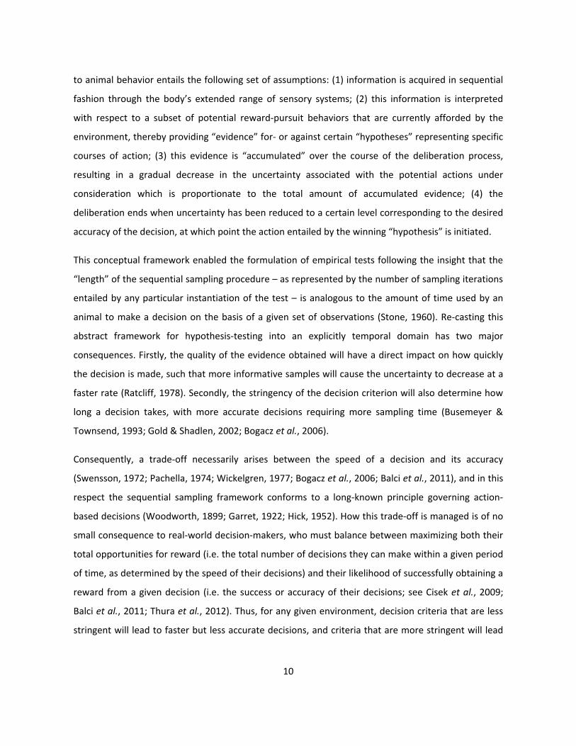
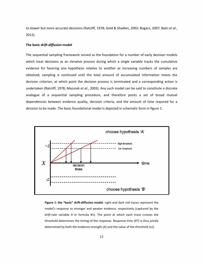
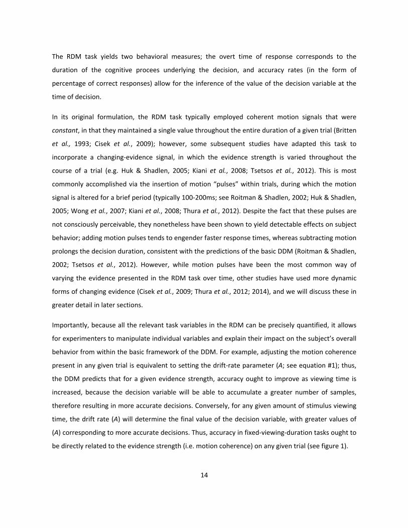
decision to be made. The basic foundational model is depicted in schematic form in figure 1.

Figure 1: the “basic” drift-diffusion model. Light and dark red traces represent the

model’s response to stronger and weaker evidence, respectively (captured by the

drift-rate variable A in formula #1). The point at which each trace crosses the

threshold determines the timing of the response. Response time (RT) is thus jointly

determined by both the evidence strength (A) and the value of the threshold (±z).

12

We will refer to the basic, schematic model illustrated in figure 1 as the basic drift-diffusion model

(DDM), which can be defined by the following equation:

dx = Adt, x(0) = 0 (1)

As illustrated in figure 1, the process encompassed by equation #1 above can be schematically

conceptualized as unfolding within a two-dimensional decision space. One of its dimensions is

symmetrically delineated by the decision bounds (±z). These are analogous to the “stopping rule” in

the sequential sampling test, and therefore represent the quantity of evidence required to terminate

the decision process in favor of each of the two hypotheses under consideration (NB: while these

“decision bounds” are given different names among various models, for the sake of terminological

consistency we will hereafter refer to these as the decision thresholds). A decision formally begins

with the initialization of a decision variable (dx) at a starting value of zero; this value – together with

the symmetry of the decision bounds (±z) – reflects the assumption that both hypotheses are

considered to be equally likely prior to the acquisition of any samples. The variable (x) denotes the

difference between the evidence supporting the two opposing hypotheses at any given time (t). The

decision variable dx is continuously updated as the decision process unfolds, and thus at any given

time reflects the sum of all previously-accumulated evidence. Adt represents the increase in x during

dt: A therefore determines the drift rate of the decision variable over the course of the decision

process, and is analogous to the “quality” of the evidence used as input to the model (i.e. higher

values of A amount to a faster rate of change in the decision variable dx, and therefore lead to faster

decisions).

As the evidence grows in favor of one hypothesis, support for the opposing choice necessarily

dimishes; the evolution of dx over time as more samples are acquired subsequently resembles a

diffusion process between the two bounds (the feature after which the model was eventually named;

see Ratcliff, 1978). A decision is made when the decision variable dx crosses either of the two

thresholds ±z, and the time of crossing is the response time (RT). Speed–accuracy trade-offs arise in

the model as a direct result of the threshold setting (±z), such that lower thresholds lead to faster-

but less accurate decisions, whereas higher thresholds lead to slower- but more accurate decisions

(Domenech & Dreher, 2010; Forstmann et al., 2010; Balci et al., 2011).

13

The “basic” DDM: a brief experimental history

The mutual dependencies among decision factors entailed by the sequential sampling framework

provided a set of tractable experimental hypotheses regarding the effects of evidence quality on the

timing of decisions, and thereby laid the groundwork for experimental investigations of decision-

making behavior. Empirical testing of the basic DDM model typically involved presenting subjects with

a binary decision between two mutually-exclusive options, resulting in a class of task paradigms which

came to be known as two-alternative forced-choice (TAFC) tasks (Schall, 2001; Gold & Shadlen, 2002).

While many TAFC tasks were developed across a wide range of psychological domains (see Green &

Luce, 1973; Ratcliff, 1978; Gronlund & Ratcliff, 1989; Ratcliff & McKoon, 1989; 1995; Wagenmakers et

al., 2004; 2008), the nascent field of decision-making research ultimately converged on a number of

psychophysical tasks, a handful of which today constitute the dominant experimental paradigms for

most decision-making research. Early psychophysical tasks included judgments of dot separation,

luminance discriminations, numerosity judgement, and binary color discriminations (Ratcliff &

Rouder, 1998; Ratcliff et al., 1999; Rouder, 2000); however, the random-dot motion (RDM) task has

come to be one of the prevailing and most ubiquitous experimental tasks for investigating the

foundations of the decision-making process. In large part this is because it allows for the precise

experimental definition of each relevant task factor, thereby facilitating the empirical quantification

of changes in choice behavior engendered by manipulations to any of the discrete decision variables

(Parker & Newsome, 1998).

The random-dot motion task

The RDM task is named after its stimulus, which consists of an image sequence showing a group of

moving dots. Upon each frame, a fraction of these dots are selected to be re-drawn along a vector

corresponding to the location of one of several peripheral targets, and the rest of the dots are moved

randomly (Britten et al., 1993). The nature of this stimulus allows for the precise quantification and

manipulation of “evidence strength,” expressable as the percentage of dots comprising its coherent

motion signal. The relevance of this motion signal to the choice targets is easily learned, as the

direction of the coherent motion signal corresponds to the location of the peripheral targets which

are used by the subject to report the decision outcome. The strength of this signal then corresponds

to “evidence strength” in a straightforward way, as a greater degree of motion coherence is more

easily detectable, and is thereby analogous to higher-quality “samples” (Drugowitsch et al., 2012).

14

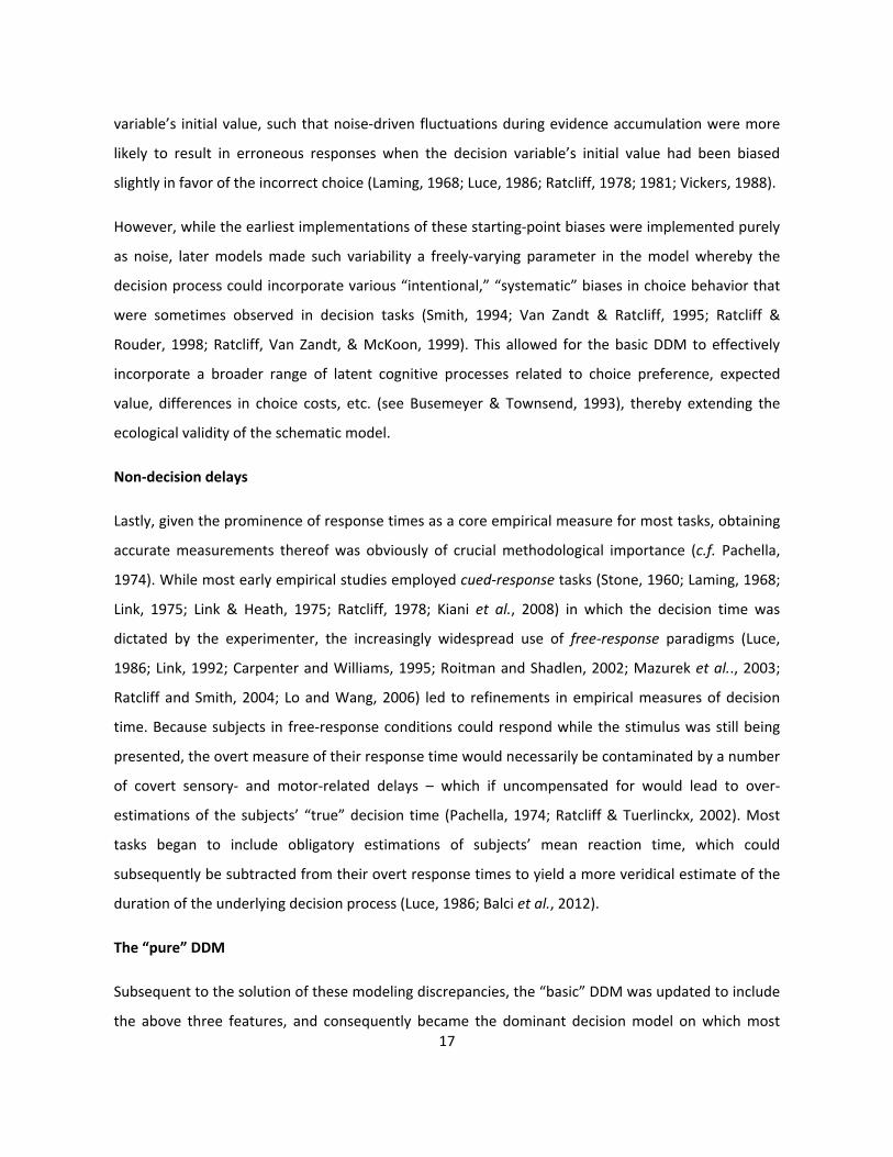
The RDM task yields two behavioral measures; the overt time of response corresponds to the

duration of the cognitive procees underlying the decision, and accuracy rates (in the form of

percentage of correct responses) allow for the inference of the value of the decision variable at the

time of decision.

In its original formulation, the RDM task typically employed coherent motion signals that were

constant, in that they maintained a single value throughout the entire duration of a given trial (Britten

et al., 1993; Cisek et al., 2009); however, some subsequent studies have adapted this task to

incorporate a changing-evidence signal, in which the evidence strength is varied throughout the

course of a trial (e.g. Huk & Shadlen, 2005; Kiani et al., 2008; Tsetsos et al., 2012). This is most

commonly accomplished via the insertion of motion “pulses” within trials, during which the motion

signal is altered for a brief period (typically 100-200ms; see Roitman & Shadlen, 2002; Huk & Shadlen,

2005; Wong et al., 2007; Kiani et al., 2008; Thura et al., 2012). Despite the fact that these pulses are

not consciously perceivable, they nonetheless have been shown to yield detectable effects on subject

behavior; adding motion pulses tends to engender faster response times, whereas subtracting motion

prolongs the decision duration, consistent with the predictions of the basic DDM (Roitman & Shadlen,

2002; Tsetsos et al., 2012). However, while motion pulses have been the most common way of

varying the evidence presented in the RDM task over time, other studies have used more dynamic

forms of changing evidence (Cisek et al., 2009; Thura et al., 2012; 2014), and we will discuss these in

greater detail in later sections.

Importantly, because all the relevant task variables in the RDM can be precisely quantified, it allows

for experimenters to manipulate individual variables and explain their impact on the subject’s overall

behavior from within the basic framework of the DDM. For example, adjusting the motion coherence

present in any given trial is equivalent to setting the drift-rate parameter (A; see equation #1); thus,

the DDM predicts that for a given evidence strength, accuracy ought to improve as viewing time is

increased, because the decision variable will be able to accumulate a greater number of samples,

therefore resulting in more accurate decisions. Conversely, for any given amount of stimulus viewing

time, the drift rate (A) will determine the final value of the decision variable, with greater values of

(A) corresponding to more accurate decisions. Thus, accuracy in fixed-viewing-duration tasks ought to

be directly related to the evidence strength (i.e. motion coherence) on any given trial (see figure 1).

15

Indeed, decision-making research is replete with behavioral studies that have extensively

corroborated these predictions not only through the use of the RDM task (e.g. Britten et al., 1992;

1993; Gold & Shadlen, 2000; Roitman & Shadlen, 2002; Mazurek et al., 2003; Ditterich et al., 2003;

2006b; Ratcliff & Smith, 2004; Huk & Shadlen, 2005; Palmer, Huk & Shadlen, 2005; Bogacz et al.,

2006; Kiani et al., 2008; Drugowitsch et al., 2012) but also through a variety of other psychophysical

and cognitive tasks (Stone, 1960; Laming, 1968; Green & Luce, 1973; Pachella, 1974; Link, 1975; Link

& Heath, 1975; Wickelgren, 1977; Ratcliff, 1978; Luce, 1986; Gronlund & Ratcliff, 1989; Ratcliff &

McKoon, 1989; Link, 1992; Carpenter & Williams, 1995; Hanes & Schall, 1996; Schall & Thompson,

1999; Reddi et al., 2003; Wagenmakers et al., 2004; 2008; Smith & McKenzie, 2011). Thus, the early

success of the DDM arose from its ability to attribute particular changes in overt measures of

behavioral performance to manipulations of specific model parameters, and this ability has come to

represent the benchmark test for all decision models in general. This overarching framework for

evaluating decision models been referred to as the principle of “selective influence” (see Rae,

Heathcote et al., 2014), by which a model is considered successful to the extent that it can capture an

overt difference in behavior induced by a given experimental manipulation with a simple parametric

change.

Ultimately, the employment of the basic DDM framework enabled the earliest decision-making

researchers to amass a large body of behavioral data that subsequently guided the development of

increasingly sophisticated sequential-sampling based models. Consequently, the first several decades

of decision-making research led to a number of mechanistic additions to the basic DDM, several of

which became universally adopted. We will discuss three of these in particular in what follows.

Model convergences

Originally, the mechanistic simplicity of the “basic” model outlined above consistenty led to major

inaccuracies in its predictions. Chief among these was its fundamental inability to reproduce the

variable distributions of response times commonly obtained in real animal subjects, who do not

respond in exactly the same way to otherwise identical trials (Busemeyer & Townsend, 1993).

Furthermore, the model was also unable to account for how erroneous decisions could arise – a

major shortcoming, especially in light of the fact that subjects rarely attain perfect accuracy even for

very easy discriminations (McElree & Dosher, 1989; Ratcliff, 1978; Reed, 1973; Usher & McClelland,

2001). Such problems were not unique to the basic DDM family of models, but also plagued a number

16

of other early models, such as signal-detection-theory models (Green & Swets, 1966) and stage theory

models (Sternberg, 1969; for historical overviews see Townsend & Ashby, 1983 and Busemeyer &

Townsend, 1993); however, the DDM ultimately superceded these other model classes when it fixed

these shortcomings with the addition of a small number of features, to which we now turn.

Noise

The first – and most important – revision to the basic DDM was the addition of random variability in

the model’s mechanisms. This addition was motivated not only by ubiquitous findings of variable RT

distributions in behavioral data (Pachella, 1974; Link & Heath, 1975; Wickelgren, 1977; Ratcliff, 1978;

Ratcliff & Smith, 2004), but was further grounded in the assumption that subjects cannot perfectly

calibrate their decision-making parameters to exactly the same state across otherwise identical trials

(see Ratcliff & Smith, 2004). This assumption was also plausible on biological grounds, as inherent

variability arising at multiple levels of the nervous system would manifest as minor variations in

decision behavior to otherwise identical stimulus input (Gold & Shadlen, 2001; 2002; Mazurek et al.,

2003).

While noise could be implemented in any number of ways, the most common solution took the form

of adding random variability to each “sample” fed to the model (Bogacz et al., 2006; Balci et al.,

2011), thereby producing minor variations in the decision variable’s threshold-crossing time

(Busemeyer & Townsend, 1993; Ratcliff, 2001). Adding noise to the models in this way allowed them

to generate orderly, regular distributions of response times (Ratcliff & Smith, 2004; Bogacz et al.,

2006). In fact, adding this single mechanism to previous, more rudimentary models was often enough

to fix them considerably (Ratcliff & Smith, 2004; Bogacz et al., 2006; Bogacz, 2007). Ultimately, the

role of noise in modeling the decision process is so crucial that its inclusion or omission is by itself

often enough to make the difference between a model successfully accounting for data and its

complete failure to do so (c.f. Van Zandt & Ratcliff, 1995).

Biases

However, there remained a few consistent discrepancies that were not fully redressed by the addition

of sampling noise alone. For example, it was consistently observed that response-time distributions

for correct trials differed significantly from those for error trials (Laming, 1968; Ratcliff, 1985; Ratcliff

et al., 1999). This was eventually fixed by adding an additional source of variability to the decision

17

variable’s initial value, such that noise-driven fluctuations during evidence accumulation were more

likely to result in erroneous responses when the decision variable’s initial value had been biased

slightly in favor of the incorrect choice (Laming, 1968; Luce, 1986; Ratcliff, 1978; 1981; Vickers, 1988).

However, while the earliest implementations of these starting-point biases were implemented purely

as noise, later models made such variability a freely-varying parameter in the model whereby the

decision process could incorporate various “intentional,” “systematic” biases in choice behavior that

were sometimes observed in decision tasks (Smith, 1994; Van Zandt & Ratcliff, 1995; Ratcliff &

Rouder, 1998; Ratcliff, Van Zandt, & McKoon, 1999). This allowed for the basic DDM to effectively

incorporate a broader range of latent cognitive processes related to choice preference, expected

value, differences in choice costs, etc. (see Busemeyer & Townsend, 1993), thereby extending the

ecological validity of the schematic model.

Non-decision delays

Lastly, given the prominence of response times as a core empirical measure for most tasks, obtaining

accurate measurements thereof was obviously of crucial methodological importance (c.f. Pachella,

1974). While most early empirical studies employed cued-response tasks (Stone, 1960; Laming, 1968;

Link, 1975; Link & Heath, 1975; Ratcliff, 1978; Kiani et al., 2008) in which the decision time was

dictated by the experimenter, the increasingly widespread use of free-response paradigms (Luce,

1986; Link, 1992; Carpenter and Williams, 1995; Roitman and Shadlen, 2002; Mazurek et al.., 2003;

Ratcliff and Smith, 2004; Lo and Wang, 2006) led to refinements in empirical measures of decision

time. Because subjects in free-response conditions could respond while the stimulus was still being

presented, the overt measure of their response time would necessarily be contaminated by a number

of covert sensory- and motor-related delays – which if uncompensated for would lead to over-

estimations of the subjects’ “true” decision time (Pachella, 1974; Ratcliff & Tuerlinckx, 2002). Most

tasks began to include obligatory estimations of subjects’ mean reaction time, which could

subsequently be subtracted from their overt response times to yield a more veridical estimate of the

duration of the underlying decision process (Luce, 1986; Balci et al., 2012).

The “pure” DDM

Subsequent to the solution of these modeling discrepancies, the “basic” DDM was updated to include

the above three features, and consequently became the dominant decision model on which most

18

models are based. Having thus reviewed the motivations behind these fairly ubiquitous model

additions, we now re-introduce the relatively simple version of the DDM defined previously with a

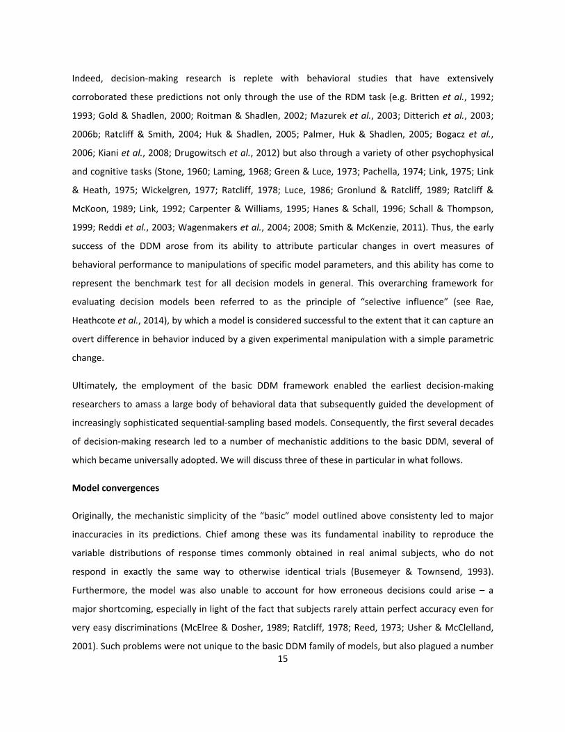
richer, more elaborate version which has served as the de facto standard model to the present day.

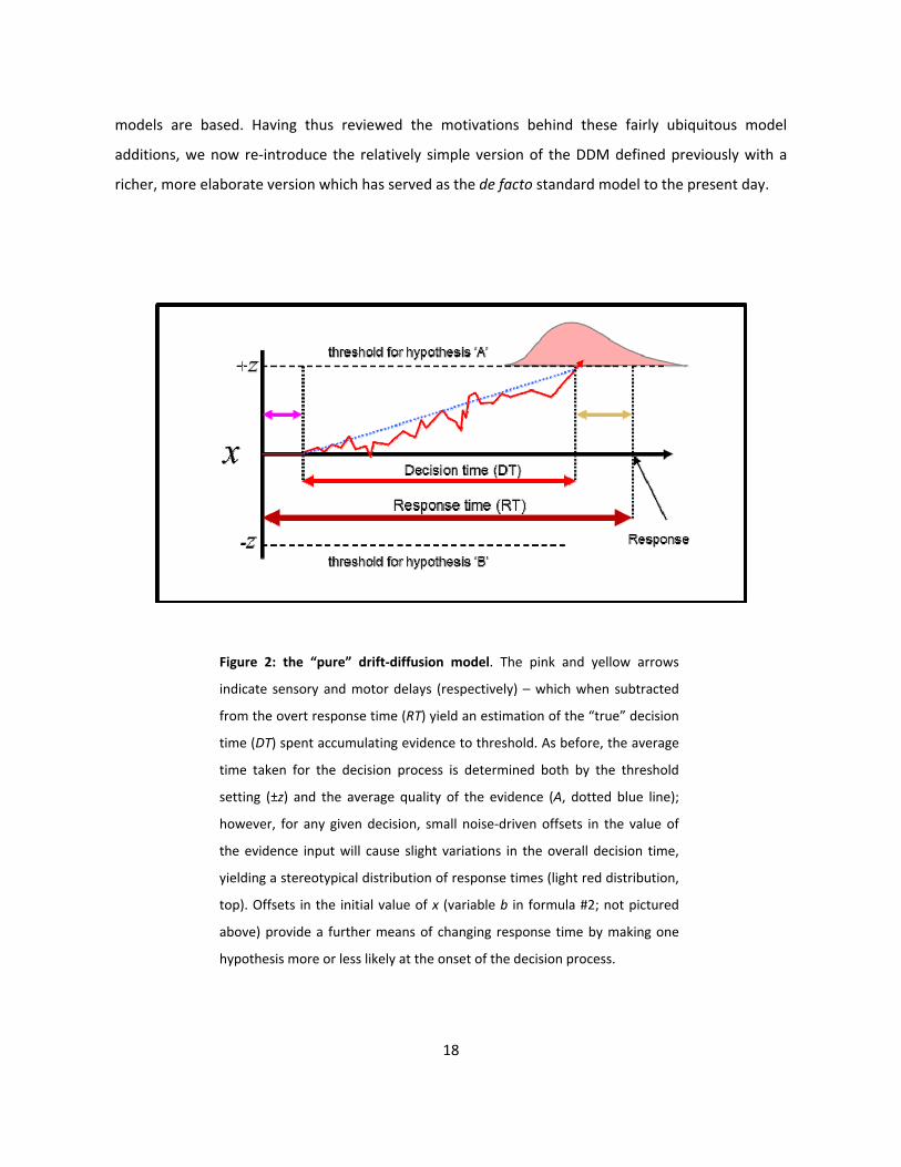
Figure 2: the “pure” drift-diffusion model. The pink and yellow arrows

indicate sensory and motor delays (respectively) – which when subtracted

from the overt response time (RT) yield an estimation of the “true” decision

time (DT) spent accumulating evidence to threshold. As before, the average

time taken for the decision process is determined both by the threshold

setting (±z) and the average quality of the evidence (A, dotted blue line);

however, for any given decision, small noise-driven offsets in the value of

the evidence input will cause slight variations in the overall decision time,

yielding a stereotypical distribution of response times (light red distribution,

top). Offsets in the initial value of x (variable b in formula #2; not pictured

above) provide a further means of changing response time by making one

hypothesis more or less likely at the onset of the decision process.

19

Adding the features discussed above to the “basic” DDM defined by formula #1 yields the following

first-order stochastic differential equation, which we will subsequently refer to as the “pure” DDM:

dx = Adt + σdW, x(t0) = b (2)

As in the previous formula, the decision variable dx effectively implements a random walk between

two symmetric decision thresholds, and the rate at which this decision variable “drifts” between

them is determined by the magnitude of the evidence values drawn from the distribution A.

However, in this model, each sample drawn from A is assumed to contain an unknown amount of

noise, supplied in the above formula by the term dW, which represents white noise drawn from a

Gaussian distribution with a mean of 0 and a variance of σ2dt (c.f. Balci et al., 2012). Furthermore, the

decision variable is assigned an intial value of b; this value can be freely adjusted to implement an

initial bias in the decision process such that a positive value of b makes the positive threshold a priori

more likely to be chosen by decreasing the distance between the starting point of evidence

accumulation and the positive threshold (and vice versa for negative values). Lastly, while the decision

time (DT) in this formulation is identified with the time of first crossing of the decision variable across

one of the decision bounds (±z), the model yields an additional time measure – the response time (RT)

– which is the sum of the decision time and the sum of non-decision-related latencies t0 reflecting the

contribution of various sensory encoding- and motor execution delays to the observed time of a

subject’s response. Subtracting an estimate of these non-decision delays from the overt response

times observed during experimention thus yields a more precise estimate of the underlying cognitive

decision process (Balci et al., 2012).

The specific implementation of noise in this “pure” DDM results in each sample having a small,

random offset (either positive or negative) from its “true” value. However, while this adds a degree of

uncertainty to the value of each sample, the assumption of a normal distribution of noise with a

mean of 0 means that adding multiple noisy samples together over time will tend to cause the noise

component to cancel out, leaving a veridical estimate of the underlying signal. Because the DDM

effectively adds multiple independent samples together over time, this very process of successive

sample integration provides the model with an intrinsic means for counteracting the distorting

influence of noise (Ratcliff & Rouder, 1998; Bogacz et al., 2006; Bogacz, 2007; Balci et al., 2011).

Consequently, in this version of the DDM “…the relative contribution of noise to the decision variable

20

diminishes as the number of samples accumulated increases, thereby decreasing the likelihood for

noise-driven errors to arise as decision thresholds are increased, and thereby reinforcing the

relationship between decision threshold and accuracy already latent in the basic DDM” (Bogacz et al.,

2006). This cancellation of noise via the addition – or integration – of multiple samples over time has

explicitly served as a further theoretical argument in favor of the pure DDM, because the coupling of

this implementation of noise with the integrative process of sequential sample summation endows

the model with all the benefits of intra-trial variability in the stochastic decision process while

simultaneously providing a concrete mechanism by which much of its potential distorting effects can

be canceled out (Bogacz, 2007). The mechanisms of this model therefore not only effectively provide

some protection against noise, but further allow the model to account for speed-accuracy trade-offs

better than the noiseless, “basic” version of the DDM (Laming, 1968; Ratcliff et al., 1999; Mazurek et

al., 2003; Bogacz et al., 2006; Bogacz, 2007).

The “pure” DDM: a brief experimental overview

The “pure” DDM has been successfully applied to all manner of tasks across a number of distinct

psychological domains, wherein it successfully predicts and explains the influence of various task

manipulations involving evidence strength and viewing time on overall decision behavior (Stone,

1960; Laming, 1968; Vickers, 1970; Link, 1975; Link & Health, 1975; Ratcliff, 1978; Luce, 1986; Hanes

& Schall, 1996; Schall & Thompson, 1999; Ratcliff & Rouder, 2000; Schall, 2001; Shadlen & Newsome,

2001; Gold & Shadlen, 2002; Ratcliff, Thapar, & McKoon, 2003; Ratcliff, Gomez, & McKoon, 2004;

Smith & Ratcliff, 2004). In other words, it accurately describes and replicates discrete changes in

decision behavior by uniting the various latent cognitive factors into a singular mechanistic

framework that explains and predicts their interactions on overall decision behavior. Moreover, its

ability to do so conforms to the previously-stated principle of “selective influence,” by which a model

is evaluated according to the extent that it can successfully describe empirically meaningful changes

in behavior in terms of manipulations of a small number of the model’s relevant parameters.

Due to its foundations in the sequential sampling framework it also describes speed-accuracy trade-

offs, which are intrinsic to the model and arise as a straightforward consequence of the mechanisms

it encompasses. Furthermore, the DDM’s mathematical tractability supplies it with a further

advantage, in that a mathematically optimal set of parameters for the DDM can be objectively

derived for any given task setting, which will produce the greatest average reward rate for any task,

21

provided that the distribution of trial difficulties are specified (Ratcliff & Smith, 2004; Bogacz et al.,

2006; Bogacz, 2007; Simen et al., 2009). This aspect of the DDM has allowed for the empirical

demonstration and quantification of optimality in natural animal behavior. Such demonstrations are

typically founded on the assumption that in most experimental settings as well as in real-world

environments, animals are motivated to achieve the highest possible reward rate over time (as

opposed to optimizing their decision process on an individual-trial basis; see Cisek et al., 2009; Balci et

al., 2011; Thura et al., 2012). Thus, sequential sampling models – and, by extension, the “pure” DDM

derived therefrom – can therefore provide discrete mathematical solutions to speed-accuracy trade-

off-related phenomena that are a typical feature of cognitive tasks in general (Swensson, 1972;

Wickelgren, 1977; Luce, 1986; for overview see Balci et al., 2011).

Model divergences

In presenting the “pure” DDM above, it bears mentioning that the sequential sampling framework

from which this model was developed has ultimately given rise to a large number of derivative

models, among which there are almost as many specific mechanistic differences as there are

individual models. This diverse plurality of models can in part be attributed to the fact that the

sequential sampling framework was originally developed from outside the context of any particular

domain of application, therefore leaving many of its finer implementational details unspecified; in

other words, its basic mathematical formulation does not greatly constrain the particular ways in

which its essential dynamics may be implemented. While the “pure” DDM – or integration model –

shown above is currently the prevailing, dominant model in the field, it is nonetheless only the most

prominent member within a diverse family of models which all have their theoretical roots in the

sequential sampling framework.

Nonetheless, even where individual sequential-sampling-based models differ in subtle ways, in

general they tend to agree on substantive questions of interpretation (Donkin, Brown, Heathcote &

Wagenmakers, 2011). In fact, most models can be mathematically incorporated into the DDM, even

when they differ significantly in the dynamics they afford. This has been demonstrated

mathematically in a number of large-scale model-comparison studies (see Ratcliff & Smith, 2004;

Bogacz et al., 2006; Bogacz, 2007). Accordingly, the “pure” DDM can be considered a fair

representative for the many closely-related models that have their common roots in the sequential

sampling framework (c.f. Cisek et al., 2009).

22

The ultimate test for any model is how well it can constrain and explain the actual physiological

implementation of the decision process as it occurs in the brain (Platt & Glimcher, 1999; Gold &

Shadlen, 2002; Purcell et al., 2010; Turner et al., 2013). Where models make identical or similar

predictions, but differ in their mechanistic implementations, the most sensible recourse for deciding

between them is to assess their individual mechanisms in terms of their biological plausibility.

In this light, the convergence of many models on a limited range of essential features provides a set

of concrete and empirically well-established proscriptive hypotheses regarding what sorts of decision-

making mechanisms may exist in the brain (Ratcliff & McKoon, 1995; Gold & Shadlen, 2002;

Churchland et al., 2008). Specifically, these ought to include functionally-analogous neural

implementations of several major decision factors including 1) sensory evidence signals; 2) the

encoding of accumulated integrated evidence, and 3) decision thresholds. Finding evidence for similar

mechanistic processes in the brain would therefore constitute further proof that sequential-sampling

models are the appropriate framework for studying natural decision-making behavior. In what

follows, we briefly outline the body of physiological evidence that has emerged as a result of the

DDM’s considerable history of empirical success.

Physiology

The convergence of multiple models on the limited range of essential features encapsulated in the

extended DDM model presented above can be considered to provide a set of relatively concrete and

empirically-corroborated tentative hypotheses regarding what sorts of decision-making mechanisms

may exist in the brain (Gold & Shadlen, 2002; Bogacz, 2007). However, given the mathematical

complexity of many of the operations involved in the models, it is unlikely that real-world decision-

makers are actually computing precise probability estimates, integrating samples perfectly, etc. (Cisek

et al., 2009; Rae, Heathcote et al., 2014). Instead, the models are taken as representing the “essential

dynamic properties” (c.f. Tuckwell, 1988) of the decision process, and the specific mathematical

computations implied by such models are otherwise assumed to be realized in approximated form by

the underlying neural system (Busemeyer & Townsend, 1993). Therefore, the mathematical

descriptions and procedures suggested by the DDM and related sequential-sampling-based models

are taken only as a general framework whose dynamic properties and individual mechanisms neural

23

computations can plausibly be fitted to approximate, and any neurobiological theory of decision-

making will have to be constrained by the types of computational mechanisms that are actually

achievable by biological neural networks. Accordingly, the search for neural implementations ought

to entail looking for plausible, neurally-realizable approximations of the essential dynamic properties

exhibited in abstract form by the models themselves (c.f. Tuckwell, 1988; Busemeyer & Townsend,

1993).

Neural evidence mechanisms

The extensive use of psychophysically-oriented experimental paradigms in decision-making research

meant that the well-characterized anatomical localization of much of the brain’s sensory-processing

hierarchies could be exploited to constrain potential areas of interest, given the provisional

assumption that the evidence signals relevant to a given decision ought to be at least in part supplied

by sensory areas whose functional profiles correspond to the discriminations entailed by a given task.

In fact, the RDM task was itself originally developed from a simple noisy motion-detection task meant

to elucidate the functional properties of extrastriate visual cortical area V5/MT (Morgan & Ward,

1980; Seigel & Anderson, 1986), and was subsequently taken up by Newsome & Paré (1988) who

adapted it to its current form for the purposes of providing direct proof for its role in supplying the

evidence during perceptual decisions in the RDM task. To date, a wide array of subsequent single-cell

recording studies have now yielded substantial evidence that the firing rates of direction-selective

cells in area MT during a random-dot motion task are linearly correlated with the relative strength of

the coherent motion in the stimulus, and that this activity can be “read-out” to predict the accuracy

of a subject’s decision (Newsome et al., 1989; Britten et al., 1992; Britten et al., 1993; Britten et al.,

1996; Shadlen et al., 1996). Moreover, its role in the decision process has been further demonstrated

by both focal chemical inactivation (Newsome & Paré, 1988) and electrical microstimulation (Salzman

et al., 1990; 1992; Salzman & Newsome, 1994; Ditterich et al., 2003) of MT cells, such that

manipulations of neuronal activity in this region can effectively delay or hasten the ensuing

behavioral response. The ability for manipulations of MT activity to influence the decision process

suggests a directly causal role for area MT in supplying evidence for decisions relying on motion-

based stimulus cues such as the RDM, in a manner that is mechanistically analogous to the evidence

signal posited by the DDM (specifically, its activity essentially appears to encode the drift-rate

variable (A) from formula #2 above; see Ratcliff & Smith, 2004; Bogacz et al., 2006; Balci et al., 2011).

24

Furthermore, the general role of supplying evidence for a perceptual discrimination appears to

generalize beyond the specific functional contributions of area MT to a RDM task. A number of other

studies have located similar evidence-coding activity during other tasks, supplied by different sensory

processing areas whose respective functional profiles correspond to the nature of the perceptual

discrimination being tested; these have included cortical areas related to somatosensory (Salinas et

al., 2000; Romo & Salinas, 2003; Houweling & Brecht, 2008; Hernández et al., 2010), auditory (Sally &

Kelly, 1988; Kaiser et al., 2007; Yang et al., 2008; Jaramillo & Zador, 2011; Bizley et al., 2013;

Znamenskiy & Zador, 2013), olfactory (Uchida & Mainen, 2003; Uchida et al., 2006) and non-motion-

related visual processing (Heekeren et al., 2004; 2008; Yang & Maunsell, 2004; Kosai et al., 2014).

Thus, taken together, this extensive body of studies has demonstrated a neural implementation of

evidence signals derived from sensory input that provide a quantitatively-graded signal compatible

with the putative role of evidence signals in the decision process as posited by the DDM.

Neural evidence accumulation mechanisms

The evidence-coding signals provided by the cortical regions identified above appear to represent the

current evidence, but do not perform the accumulative functions otherwise crucial to the DDM’s

essential dynamics; thus, such signals had to be found elsewhere. As before, the search for evidence-

accumulating functions was guided by a number of provisional hypotheses afforded by the

experimental history of the DDM. In the case of most of the experimental tasks employed in decision-

making studies, subjects are already aware of the mapping between the relevant stimulus dimensions

and the specific motor responses used to report the decision outcome (Gold & Shadlen, 2000; Yang &

Shadlen, 2007). For example, the “motion evidence” for a RDM task is not evidence about “motion

direction” in an abstract sense, but rather is evidence for the specific behavioral response used to

report the decision and thereby obtain a reward (Platt & Glimcher, 1999; Gold & Shadlen, 2000; 2002;

Yang & Shadlen, 2007). Consequently, this insight motivated the adoption of the provisional

physiological hypothesis that evidence accumulation may take place in high-level motor command

structures responsible for issuing the behavioral response required by a given task (Platt & Glimcher,

1999; Gold & Shadlen, 2000).

This prediction has been borne out by a wide range of studies which have yielded extensive evidence

for such mechanisms among a diverse range of cortical and extracortical sites. In the superior

colliculus (SC), for example, a number of experimental studies featuring tasks in which a subject’s

25

decision is reported with a saccade have revealed that the relative activity of collicular neurons

strongly covaries with both the probability and magnitude of a reward associated with the cell’s

spatial target over the course of the decision period (Basso & Wurtz, 1998; see Ratcliff, Cherian &

Seagreaves, 2003 for overview). Other studies have revealed a number of suggestive correlations

between the build-up of activity in individual collicular neurons and both the likelihood (Dorris &

Munoz, 1998; Dorris et al., 2000) as well as the latency (Basso & Wurtz, 1998; Everling et al., 1999;

Dorris et al., 2000) of an ensuing saccade into the response field of the recorded cells. Finally, the

baseline activity levels of these collicular cell populations at the time of a decision’s onset appear to

reflect a predisposition to choose a target in the corresponding space of the visual field (Horwitz &

Newsome, 1999; 2001), consistent with the biasing mechanisms featured in the “pure” DDM defined

in equation #2. Collectively, these studies provide compelling support for the hypothesis that the

superior colliculus serves as a physiological site for bridging the accumulation of decision evidence

with the principal behavioral output of that decision (i.e. a saccade), which is itself consistent with the

well-established functional role of the SC in coordinating and executing oculomotor behaviors (Basso

& Wurtz, 1998; Dorris & Munoz, 1998; Everling et al., 1999).

Physiological assays of other cortical regions have furnished further support for this overarching

neural hypothesis. For example, the well-characterized functional role of the frontal eye fields (FEF) in

coordinating and initiating eye movements motivated a series of studies using the RDM task to

establish a direct correspondence between neural activity in FEF cells and the development of an

ongoing decision. These studies ultimately showed that direction-selective cells in this region appear

to implement the accumulation of information during a RDM task, with neural activity building up as

a function of both motion strength and viewing time (Gold & Shadlen, 2000; Ding & Gold, 2012),

consistent with the dynamics of the decision variable in a DDM model (for an analogous example of

such neural activity recordings from Roitman & Shadlen’s (2002) study of area LIP see figure 3,

below).

Finally, similar findings have also been obtained in the lateral intraparietal area (LIP), another cortical

area with an empirically well-substantiated role in the spatial coordination of oculomotor behavior

(see Platt & Glimcher, 1999; Roitman & Shadlen, 2002). Here, once again, a number of physiological

assays have revealed the effective neural implementation of a developing decision via single-cell

recordings in this area (Gnadt & Anderson, 1988; Hanes & Schall, 1996; Platt & Glimcher, 1997; Colby

26

& Goldberg, 1999; Platt & Glimcher, 1999; Shadlen & Newsome, 2001; Roitman & Shadlen, 2002;

Leon & Shadlen, 2003; Dorris & Glimcher, 2004; Sugrue, Corrado & Newsome, 2004; Hanks, Ditterich

& Shadlen, 2006; Ipata et al., 2006; Yang & Shadlen, 2007). Further consistent with corresponding

studies of other brain areas mentioned previously, area LIP also exhibits quantitatively-graded

decision-related buildup of activity whose rate of growth is commensurate with the strength of the

evidence both for tasks in which the evidence input is continuous (as in an RDM task; see see Roitman

& Shadlen, 2002; Ratcliff, Cherian & Segraves, 2003; Smith & Ratcliff, 2004; Gold & Shadlen, 2007;

Kiani, Hanks & Shadlen, 2008) as well as when the evidence arrives in discrete units over time (Yang &

Shadlen, 2007). Additionally, further single-unit recording studies of cellular activity in LIP have led to

the suggestion that the encoding of accumulated evidence appears to take place in probabilistic units

of log-likelihood, which is further consonant with the general framework of sequential sampling at

large (see Wald, 1947; Gold & Shadlen, 2002; Yang & Shadlen, 2007). In other words, the

qualitatively-graded activity of LIP cells appears to reflect the brain’s ability to extract and accumulate

probabilistic evidence from sensory information over time (Yang & Shadlen, 2007).

Finally, physiological recording in area LIP has established that the temporal profile of decision-

related activity in this region is consistent with the hypothesis that LIP is in direct receipt of input

from a number of extrastriatal visual areas known to play a role in the types of psychophysical

discriminations commonly featured in decision tasks (see Roitman & Shadlen, 2002; Shadlen &

Newsome, 2001; Hanks, Ditterich & Shadlen, 2006; Huk & Shadlen, 2005; Yang & Shadlen, 2007; and

references therein). For example, Kiani, Hanks & Shadlen (2008) used an RDM task to show that the

total latency between the time of stimulus onset and LIP responses falls within a window of ~210-

260ms, which suggests a delay between LIP and its putative motion-related evidence input from MT

that is only approximately ~100ms (Britten et al.., 1996; Bair et al.., 2002; Roitman and Shadlen, 2002;

Osborne et al.., 2004; Huk and Shadlen, 2005). Conversely, this suite of temporal relationships

between LIP and the cortical sensory areas which presumably provide it with its fundamental input is

further consonant with anatomical studies that suggest that sensory areas including MT/V5 and V4

are anatomically well-poised to supply feedforward input to areas encoding the total accumulated

evidence, such as FEF and LIP. This has been demonstrated in explicit anatomical terms by a number

of physiological studies documenting reciprocal cortico-cortical connections across a range of visual

sensory and parietally-situated motor control centers, including those between LIP and MT & V4

(Blatt, Anderson & Stoner, 1990) as well as between MT and both LIP and FEF (Ungerleider &

27

Desimone, 1986). Thus, LIP in particular appears to be a central hub in decision-making activity, which

together with a diverse set of cortical sensory-processing areas appear to constitute a widely-

distributed network for decision-making.

However, it must be noted that LIP’s role in decision-making is not wholly accounted for; for instance,

it has been shown that LIP activity can exhibit responses to a number of extended factors which can

not themselves be definitively attributed to evidence-related processing, such as target value (Platt &

Glimcher, 1999; Sugrue et al., 2004), reward expectation (Sugrue, Corrado & Newsome, 2004; Dorris

& Glimcher, 2004), or even the mere passage of time (Ditterich, 2006a; Beck et al., 2008; Churchland

et al., 2008; Hanks et al., 2011; Standage et al.., 2011). Ultimately, however, such findings are not

themselves inconsistent with the general role of area LIP in evidence accumulation presented here; in

fact, these influences may all be indicative of a more general role for LIP in coordinating behavior in

response to a wide variety of task-relevant variables (Rao, 2010). However, we will return to the topic

of non-evidence-dependent activity in LIP in later sections, and will for now merely note that its wider

functional profile has not been entirely determined.

Neural threshold mechanisms

Lastly, while empirical evidence has been presented for the neurobiological implementation of

evidence estimation and accumulation in a number of brain regions, the implementation of a decision

threshold remains to be established. The DDM posits that the threshold is set at a constant level, and

that the crossing of this threshold by the decision variable determines the timing of the ensuing

response. This therefore suggests that demonstrating the existence of analogous neural decision

thresholds would require measuring neuronal activity while a decision was completed, and analysing

this activity to see whether decision times could be predicted on the basis of the decision variable

having reached a common activity level across multiple trials. Importantly, however, most behavioral

tasks studied in laboratory experiments have been fixed-duration studies (Rieke et al., 1997; Parker &

Newsome, 1998); thus, when the stimulus viewing duration is controlled by the experimenter, the

true decision time is covert, thereby prohibiting a precise estimation of the subjects’ actual decision

time (Britten et al. 1993; Shadlen & Newsome 2001; Parker et al. 2002; DeAngelis & Newsome 2004;

Krug 2004; Krug et al. 2004; Uka & DeAngelis 2004). Therefore, the use of free-response tasks was

empirically necessary to identify neural mechanisms analogous to the threshold mechanisms

suggested by the DDM (see Kiani, Hanks & Shadlen, 2008).

28

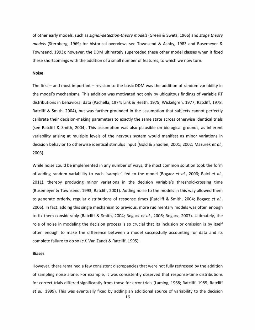
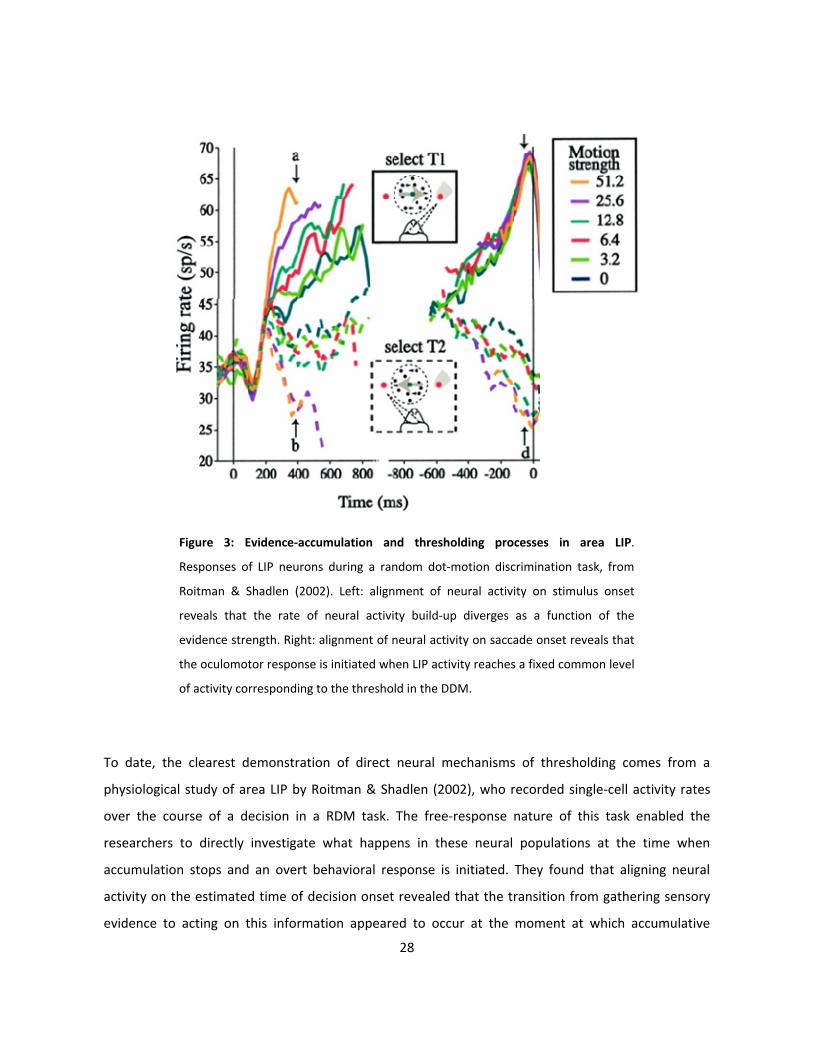
Figure 3: Evidence-accumulation and thresholding processes in area LIP.

Responses of LIP neurons during a random dot-motion discrimination task, from

Roitman & Shadlen (2002). Left: alignment of neural activity on stimulus onset

reveals that the rate of neural activity build-up diverges as a function of the

evidence strength. Right: alignment of neural activity on saccade onset reveals that

the oculomotor response is initiated when LIP activity reaches a fixed common level

of activity corresponding to the threshold in the DDM.

To date, the clearest demonstration of direct neural mechanisms of thresholding comes from a

physiological study of area LIP by Roitman & Shadlen (2002), who recorded single-cell activity rates

over the course of a decision in a RDM task. The free-response nature of this task enabled the

researchers to directly investigate what happens in these neural populations at the time when

accumulation stops and an overt behavioral response is initiated. They found that aligning neural

activity on the estimated time of decision onset revealed that the transition from gathering sensory

evidence to acting on this information appeared to occur at the moment at which accumulative

29

neural activity in area LIP reached a fixed, absolute level that was consistent across trials (see figure

3). Additionally, the threshold at which the build-up of neuronal activity terminated and triggered an

outcome-reporting movement was identical for both correct and incorrect trials, therefore indicating

that these LIP neurons do not reflect the objective direction of the stimulus motion, but rather

indicate the subjects’ belief about the decision evidence (Roitman & Shadlen, 2002; Yang & Shadlen,

2007).

A series of subsequent studies have also corroborated the finding of absolute neural activity

thresholds during decision-making, the crossing of which predicts both the ultimate choice and the

timing of the subject’s behavioral report (Ratcliff, Cherian & Segraves, 2003; Mazurek et al., 2003;

Kiani et al., 2008; Ding & Gold, 2012). Taken together, these studies have collectively shown that LIP

activity can be consistently seen to rise toward a common firing-rate threshold that is independent of

a specific trial’s motion coherence as well as the ensuing decision time. The fact that the final firing

rate value was common across all conditions suggests that the threshold is constant, with variations

in decision timing being due to corresponding differences in the underlying factors governing the rate

at which this activity builds up, at least part of which would be evidence-related (Roitman & Shadlen,

2002; Mazurek et al., 2003; Kiani et al., 2008).

Summary: physiology

In general, the studies reviewed in the foregoing would appear to confirm the neural implementation

of evidence signals, evidence accumulation, and thresholding mechanisms as posited by the DDM.

More recently, the anatomical and functional details of the emerging neurobiological scheme has led

to the suggestion that decision processes take place on a level of neural organization that effectively

links sensory, cognitive and motor processes within a common domain, thereby facilitating the rapid

conversion of sensory information into behavior in real-time, consistent with the ecological demands

of real-world behavior (Gold & Shadlen, 2000; Cisek, 2007).

Ultimately, the emergent functionality of these many individual neural mechanisms strongly conform

to the mechanistic predictions made by the DDM, and therefore have typically been interpreted as

evidence for a more-or-less direct (if approximate) neurobiological implementation of the decision

process as outlined in mathematical abstraction by the sequential sampling framework at large (Gold

& Shadlen, 2002). More broadly, these findings appear to substantiate the notion that animal

30

behavior is broadly analogous to hypothesis-testing, for which evidence is accumulated over time and

summated to provide an informed (but still inherently probabilistic) estimate of the state of the

world, and therefore by extension the best course of action that the environment currently affords

(Gold & Shadlen, 2002; Bogacz et al., 2006).

The current state of the sequential sampling framework

As we noted earlier, a number of crucial mechanistic additions were made to the “basic” DDM

(equation #1) in order for it to successfully capture a number of common features in behavioral data.

While these mechanisms were universally adopted (and led to the highly successful “pure” DDM;

equation #2), many divergent and increasingly-complex models continued to be developed over time.

Problematically, however, the progressive diversification and mechanistic embellishment of the ever-

growing family of sequential-sampling-based models has been accompanied by a corresponding

tendency for the ensuing models to become capable of mutual “mimicry,” by which any sufficiently

complex model can match the output of any other by mere virtue of the fact that its mechanistic

complexity ensures that a set of parameters can almost always be found which will reproduce the

output of a competing model (see Bogacz, 2007; Tsetsos et al., 2011; 2012; Rae, Heathcote et al.,

2014). Thus, as models become more complex they necessarily become more flexible in their ability

to fit data – but it cannot therefore be concluded that such a model necessarily represents the best or

most parsimonious explanatory framework for the observed phenomena. Instead, an alternative

evaluative framework is required to resolve disputes between models without recourse to the

models’ abilities to reproduce the predictions of another.

On this point, several recent studies have presented data that resists explanation by the DDM (Usher

& McClelland, 2001; Cisek et al., 2009; Thura et al., 2012; Tsetsos et al., 2012). While adherents of the

DDM have sucessfully addressed a few of these challenges with parametric modifications (see Ratcliff

& Smith, 2004; Bogacz et al., 2006; Bogacz, 2007; Kiani et al., 2008), many of these empirical

challenges remain outstanding. Despite these suggestive demonstrations of the DDM’s potential

shortcomings, however, these studies have generally not considerably undermined the DDM’s status

as the prevailing model. In fact, the DDM has been continued to be acknowledged as the de facto

model even by modelers with personal allegiances to alternative models (see Usher & McClelleand,

2001; Wang, 2002; Wong & Wang, 2008; Cisek et al., 2009; Balci et al., 2011; Thura et al., 2012;

Tsetsos et al., 2012).

31

Thus, the persistence of the DDM in the face of such empirical challenges serves to highlight a

broader potential problem with the reigning methodology of decision research; that is, it could be

argued (and has been: see Rae, Heathcote et al., 2014) that the ability of the DDM to replicate the

output of models that otherwise differ substantially in their dynamics may have unintentionally

precluded the search for alternative (and potentially more parsimonious) models by obscuring the

theoretical utility of such alternatives behind a strategy of continued parametric revisions. Instead, to

prevent over-commitment to a singular, increasingly-mechanistically-embellished model, the core

assumptions on which models are built must be continually questioned to clear the ground for

potential alternatives. Accordingly, we proceed along these lines by revisiting and reconsidering some

of the core assumptions underlying the DDM in its current form to see if there may be just cause to

resume the search for models that deviate substantially from the essential framework of the DDM

which, because of the DDM’s status as the default paradigm, would not otherwise be searched for.

Revisiting the foundational assumptions of the DDM

Assumption #1: sequential sampling is required for simple perceptual judgments

The core functionality of the DDM rests on the assumption that a single sample is rarely sufficient to

make an informed decision; thus, it relies on the integration of multiple samples over time to exploit

the intrinsic relationship by which decision accuracy can be increased by accumulating additional

samples, and this mechanism is directly responsible for the model’s output of a decision variable that

grows over time. Taking the logic of the DDM to its natural conclusion, then, would lead to the

straightforward prediction that decision accuracy ought to increase monotonically for as long as

sampling is continued. That is, even a particularly difficult perceptual discrimination, if given enough

time, ought to eventually reach near-perfect levels of accuracy. Problematically, however, this

prediction is not borne out in the extensive body of data on perceptual discrimination tasks. Instead,

it has been consistently observed that success rates tend to asymptote after a certain amount of

viewing time, even when additional sampling time is provided (Wickelgren, 1977; Shadlen &

Newsome, 2001; Usher & McClelland, 2001; Roitman & Shadlen, 2002; Huk & Shadlen, 2005; Kiani et

al., 2008). For example, when Roitman & Shadlen (2002) controlled their subjects’ viewing time

during an RDM task, they found that accuracy rates tended to asymptote fairly rapidly, even for

32

difficult trials in which additional viewing time should have been of significant benefit to the subject.

While this appears to occur in all trials regardless of difficulty, the amount of time it takes for

accuracy to stabilize at a consistent final level appears to be dependent on the strength of the

evidence in a given trial; very strong evidence leads to near-instant saturation of accuracy rates,

whereas relatively difficult discriminations appear to lead to asymptoting accuracty rates after

between 800ms (Roitman & Shadlen, 2002; Kiani, Hanks & Shadlen, 2008) and 1000ms (Usher &

McClelland, 2001; Tsetsos et al., 2012).

However, the above studies all employed RDM tasks, which therefore leave open the possibility that

this phenomenon could be task-specific. However, a number of studies using different behavioral

tasks have also yielded data suggesting that decisions tend to be made on the basis of information

arriving in a window of time which is often substantially shorter than the full length of the decision

process itself (Cook & Maunsell, 2002; Ludwig et al., 2005; Luna et al., 2005; Ghose, 2006; Uchida et

al., 2006; Yang et al., 2008; Kuruppath et al., 2014; but see also Burr & Santoro, 2001). Together,

these studies would appear to argue against a traditional conceptualization of integration as a

decision-making mechanism, and instead seem to suggest that there is some limit to the utility of

extended sampling that instead motivates subjects to base decisions on only a subset of the total

information presented to them. In other words, the apparent mechanisms purportedly implementing

evidence integration may actually be serving a different purpose.

Two resolutions to these observations have been previously proposed. On one hand, adherents to the

DDM family of models have proposed that the decision process is cognitively taxing, and that subjects

therefore simply allot a limited amount of time to the formulation of a decision. Consequently, they

argue that the saturation of accuracy rates can be explained by an early truncation of the decision

process such that subjects are satisfied with a given level of performance for a given difficulty;

accordingly, they claim that subjects integrate samples until they reach the desired threshold, and

simply ignore all further information (Kiani et al., 2008).

If this were true, then it would follow that manipulations of evidence within a trial should only be

effective in changing subjects’ behavior if these changes occur early in the trial, i.e. while the animal is

still integrating evidence. In other words, decision-makers ought to exhibit primacy biases, such that

early decision information should matter more than later information. Indeed, such primacy biases

have been shown by several studies (Huk & Shadlen, 2005; Kiani et al., 2008). However, other studies

33

have shown that it is possible to obtain both primacy- and recency biases, in which subjects appear to

base their decisions on a limited range of stimulus information that is either early or late

(respectively) within a given trial (Usher & McClelland, 2001; Huk & Shadlen, 2005; Tsetsos et al.,

2012). Thus the DDM’s “early decision truncation” account cannot explain how these different

patterns emerge, thereby motivating the search for an alternative explanation. Instead, the authors

of the aforementioned studies have proposed a variety of alternative models that feature novel

mechanisms such as “leak” (see Usher & McClelland, 2001), which they believe to account for the

variety of temporal biases observed in their experimental tasks. However, while these models can be

parameterized to account for the emergence of these different temporal bias patterns (Usher &

McClelland, 2001; Tsetsos et al., 2012), these models do not motivate these mechanistic additions

ecologically, nor do they explain how such parameters relate to subjects’ performance under varying

conditions. In other words, these models represent mechanistic embellishments to the DDM that,

while sufficient to replicate behavioral data, are not for this reason necessary.

However, a third explanation for the saturation of accuracy rates may be found by examining the

latent assumptions of the sequential sampling framework itself. Recall that the primary feature

linking the DDM with the sequential sampling framework – and which constitutes its central

explanatory mechanism – is its the ability to reduce uncertainty by exploitating the addititive

properties of probabilistic cues (Pierce, 1878; Wald & Wolfowitz, 1948). However, the utility of a

sequential sampling test – and therefore, the DDM – is predicated entirely on the assumption that

such samples are statistically independent, i.e. that they do not contain any overlap in the information

that they provide.

While this assumption has occasionally been explicitly acknowledged during empirical evaluation of

the DDM (for examples see Bogacz et al., 2006 and Kiani, Hanks & Shadlen, 2008), it remains at least

an implicit assumption in all sequential-sampling-based models, and is not a demonstrated fact.

Meanwhile, this assumption of sample independence has strong consequences for the dynamics of

sequential-sampling models and therefore merits close investigation, because it is only under this

assumption that a decision can increase in accuracy indefinitely as more samples are acquired.

This assumption only recently began to attract attention and re-examination after several decades of

having been taken for granted. Recently, a series of studies (Cisek et al., 2009; Thura et al., 2012)

have proposed that any task in which the evidence is held constant will eventually result in

34

diminishing returns on the information provided by successive samples. Their logic was predicated on

a Bayesian analysis of mutual information, which states that as samples are repeatedly drawn from an

underlying distribution, the information content of each sample will be increasingly predicted by the

prior samples. In other words: later samples contribute less novel information to the growing body of

information. In this case, collecting samples over time will progressively leave less novel information

to be uniquely provided by subsequent samples, and the net informational yield from combining

them together will therefore eventually be less than their sum. The precise time course of the

diminishing returns on information will be inversely related to the degree of mutual information

contained in the samples: the more they overlap in information content, the fewer samples will need

to be collected before they cease being informative – in all cases, however, the earliest samples will

tend to convey substantially more information than later ones. This overall principle can also be

phrased in an alternative way: only novel information can cause an integrated sum to increase in size.

The consequences of this on the output of a model founded on the sequential sampling framework

are non-trivial. For example, the accuracy of a perceptual discrimination about a a static, unchanging

visual stimulus without noise would not be expected to benefit from an extended sampling period

because all of the information pertinent to the required decision is fully present at the moment it is

presented; and indeed, such discriminations are often extremely rapid and do not improve

substantially over time (see Uchida et al., 2006; Stanford et al., 2010; Zariwala et al., 2013; Kuruppath

et al., 2014). By contrast, a task like the RDM presents a less extreme case; because the coherent

motion signal is embedded in noisy, random dot fluctuations, multiple visual samples will still be

required to correctly discern the noise from the veridical signal, and one would expect extended

viewing times to yield corresponding increases in accuracy for this reason. Importantly, however, if

the motion coherence value is constant throughout a given trial, there will remain some degree of

mutual information across samples, and the benefit of acquiring further samples will therefore

decrease over time to the point where additional samples incur no attendant benefit to accuracy.

Mechanistically, the consequence of this for an integration-based model is that the growth rate of the

decision variable will necessarily decrease over time as successive samples become increasingly

informationally redundant (c.f. Thura et al., 2012), and will eventually stabilize at an asymptote value

once most of the novel information has been collected. In other words, integration cannot improve

decision accuracy indefinitely because the integrated sum only increases in response to novel

information.

35

Consequently, re-considering the types of tasks typically used in decision-making research along

information-theoretic grounds can provide a straightforward explanation for the consistent trend for

accuracy in constant-evidence tasks to saturate over time: because most of the extant work in

perceptual decision-making has employed tasks in which evidence strength remains constant over the

duration of an individual trial (e.g. Ratcliff, 1978; Shadlen & Newsome, 2001; Roitman & Shadlen,

2002; Ratcliff & Smith, 2004; Bogacz et al., 2006), these tasks will necessarily lead to diminishing

returns on the ability of prolonged stimulus viewing durations to improve accuracy. Indeed, precisely

this phenomenon has been observed in a wide range of experimental tasks (see above); moreover,

such a scenario is also likely to obtain in many – if not most – real-world environments, in which

animals sample a finite set of stimuli before making a decision (see Uchida & Mainen, 2003; Uchida et

al., 2006; Thura et al., 2012; Zawala et al., 2013; Kuruppath et al., 2014).

In itself, this discrepancy between real-world behavior and the theoretical rationale of integration-

based models presents a problem for the DDM’s theoretical account of decision-making behavior –

but only because of the DDM’s reliance on integration to bring the decision variable to threshold.

Otherwise, the existence of mutual information between samples need not itself present a damning

problem for any neural implementation of the decision process; we will propose one such solution in

the following section. Nonetheless, the issue of mutual information and its mechanistic consequences

for the DDM remains a salient theoretical weakness in its general explanatory framework.

Furthermore, it has additional consequences for the dynamics of the DDM, to which we now turn.

Assumption #2: threshold settings are constant

In the above, we argued that mutual informational content shared amongst successive samples

would appear to preclude the possibility that integrating evidence can improve decision accuracy

indefinitely. Rather, information-theoretic considerations of the signal properties of the stimuli used

in many of the more common experimental decision-making tasks would suggest that the usefulness

of linear integration should have a clear (and mathematically specifiable) limit. However, in addition

to manifesting in the saturation of accuracy rates over short time scales, the tendency for repeated

sampling to yield diminishing informational returns causes problems for any model in which the

threshold is constant, because for any evidence accumulation function that asymptotes over time

there will necessarily exist a set of static threshold parameters that this integrated amount will never

be able to reach. Conversely, setting the threshold at a value that the evidence will be able to reach

36

would appear to require knowing ahead of time the strength of the evidence one is likely to obtain in

a given environmental setting – an assumption which is difficult to motivate, especially in real-world

settings where similar “trials” are typically not encounted serially in sets of several hundred at a time

as they often are in experimental tasks.

To be fair, a static parameterization of the “stopping rule” is the most straightforward interpretation

of the sequential sampling procedure’s framework, and the constancy of the threshold parameter

may therefore have quite naturally been implicitly assumed during the translation of the sequential

sampling framework into discrete decision models like the DDM. Thus, the traditionally widespread

assumption of static thresholds may again simply be a reflection of the implementational openness of

the sequential-sampling framework. However, alternative implementations of the decision threshold

have been proposed in the past; in fact, the possibility of a dropping decision criterion was suggested

as early as 1988, when Busemeyer & Rappoport demonstrated the superiority of a DDM with a

dropping threshold criterion through the use of memory-search and other cognitive (i.e. non-

perceptual decision) tasks. However, their tasks differed substantially in format from those typically

used in contemporary decision-making studies, therefore leaving open the question of whether or

not such a mechanism may be of benefit to the DDM’s ability to explain the types of perceptual

discrimination tasks typically employed in decision-making studies.

Nonetheless, despite its early historical appearance, this mechanistic revision has generally not been

seriously considered by many of the strongest proponents of the DDM. Curiously, however, it should

be noted that the assumption of static decision thresholds has occasionally been explicitly made

solely for the purposes of parametric convenience. Parameterizing the DDM (or similar models) to

implement a time-dependent decision threshold would have necessitated multiple additional

parameters – and these parametric embellishments were occasionally viewed by some modelers as

detracting from the mechanistic elegance (as well as the mathematical tractability) of the models (c.f.

Ratcliff & Smith, 2004). A further – and more recent – example of this can be found in the broad

model-comparison study of Bogacz et al. (2006), who, despite having acknowledged the possibility of

a dropping criterion, nonetheless chose not to include this feature in their model comparisons for

considerations of mathematical tractibility.

Accordingly, several contemporary studies have since demonstrated that loosening the (often merely

implicit) theoretical and mechanistic commitments to fixed decision criteria yields models that in

37

many cases provide more accurate fits to behavioral data. For example, Drugowitsch et al. (2012)

point out that a decision threshold that drops over time is a relatively simple – and ecologically

plausible – way that a real animal could effectively manage the fact that the evidence quality of a

given environment is unknown. Thus, when the distribution of decision difficulties includes very

difficult discriminations, it can be advantageous to terminate difficult discriminations earlier so that

the decision-maker can move on to potentially easier decisions. Thus, dropping the decision threshold

over time effectively counteracts the rising time cost of accumulating evidence under conditions of

high ambiguity, and therefore would enable a decision-maker to achieve a higher average reward rate

by truncating difficult decisions early. Moreover, Drugowitsch et al. (2012) further substantiated this

argument by incorporating a dropping threshold into previous models in which the thresholds were

held constant, and demonstrated that doing so could improve their ability to fit behavioral data,

which it did specifically by eliminating large numbers of very long response times which had formally

caused the tails of model-predicted RT distributions to be “too heavy” (c.f. Laming, 1968; see

Drugowitsch, 2012). In other words, older models consistently overestimated the length of difficult

decisions, and adding a dropping threshold effectively fixed these inaccuracies (Laming, 1968;

Drugowitsch, 2012; Liu & Watanabe, 2012). Thus, because adding a dropping decision criterion to a

model improves its ability to replicate real behavioral data, this constitutes evidence that real animals

implement some sort of dropping-threshold mechanism. Findings such as these are further supported

by mathematical considerations of reward-rate optimization, in which it has been shown that in all

cases so far studied, models with dropping thresholds regularly outperform those with static

thresholds (Ditterich, 2006a; Cisek et al., 2009; Balci et al., 2011; Liu & Watanabe, 2012; Thura et al.,

2012; Standage et al., 2014).

Superficially, the notion of a dropping threshold might appear to contradict the physiological findings

we reviewed earlier in which stable, absolute thresholds of neural activity were observed to directly

predict the effective end of a deliberation process and the subsequent issuing of the corresponding

behavioral report. There is, however, a straightforward and neurally-plausible mechanistic alternative

to the otherwise strict definition of a constant neural threshold that itself is otherwise

implementationally and dynamically equivalent to a dropping threshold; namely, the addition of a

time-dependent signal that grows over time, which would then be continuously added to the

representation of the accumulated evidence. Such a signal would effectively implement a dropping

threshold by decreasing the absolute difference between the neural activity threshold and the

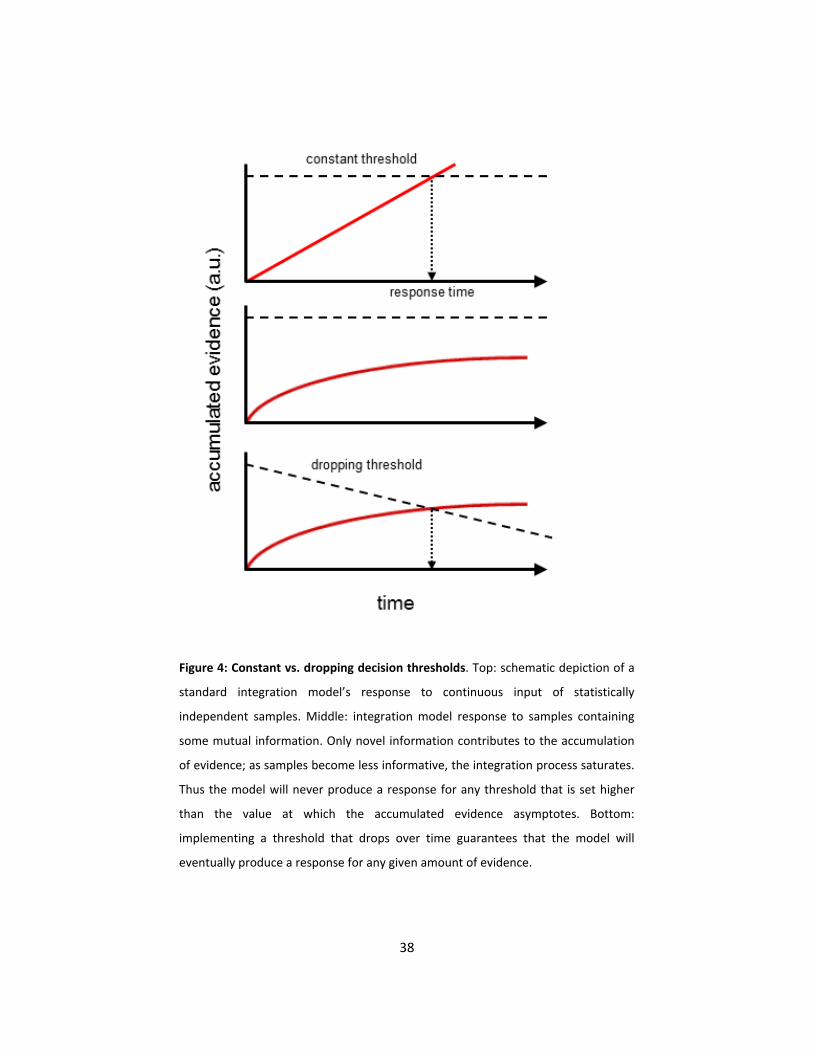
38

Figure 4: Constant vs. dropping decision thresholds. Top: schematic depiction of a

standard integration model’s response to continuous input of statistically

independent samples. Middle: integration model response to samples containing

some mutual information. Only novel information contributes to the accumulation

of evidence; as samples become less informative, the integration process saturates.

Thus the model will never produce a response for any threshold that is set higher

than the value at which the accumulated evidence asymptotes. Bottom:

implementing a threshold that drops over time guarantees that the model will

eventually produce a response for any given amount of evidence.

39

current sum of the accumulated evidence. Furthermore, because it provides an alternative means to

bring an evidence signal to threshold, implementing such a mechanism would free a model from

relying on the assumption of statistically independent samples, instead allowing for the replacement

of an integration mechanism with a more theoretically-plausible alternative. Therefore, this

mechanistic revision to the extant decision-making frameworks represents a plausible avenue along

which an alternative model could supercede the DDM’s explanatory framework.

Assumption #3: integration is required for noise compensation

The previous two arguments have been offered with the aims of questioning and potentially

loosening some of the now deeply-entrenched core assumptions made by the reigning decision

models in the field of decision-making. These arguments have specifically targeted the assumptions

typically used to explain the purportedly well-established utility of sample integration as the primary

mechanism by which animals make decisions on the basis of uncertain information. However, there

remains yet another major functional aspect of the sequential sampling framework for which any

alternative model must propose a functionally-equivalent replacement; namely, the role of an

integration mechanism in compensating for noise. Without this function, the decision-making

system’s functionality would be significantly impaired, and any purported alternative to a sequential-

sampling-based model must there offer an alternative means for achieving this essential function.

Fortunately, while the mechanism of integration is indeed a viable means of noise-control within the

assumptions of the DDM’s essential framework, it is not the sole mechanism by which this could be

achieved. For example, the influence of network-level noise could be counteracted equally well by

subjecting incoming evidence signals to a low-pass filter. Given an appropriate implementation (i.e.

with an appropriate filter cutoff frequency), such a mechanism could minimize the impact of high-

frequency variations in the evidence signal derived from sensory estimates while retaining much of

the original, veridical input signal driven by the external stimulus. Moreover, such a filtering function

is well within the computational repertoire of biological neurons (Abeles, 1991; Fourcaud-Trocmé et

al., 2003; Rivlin-Etzion et al., 2008) and is therefore at least superficially plausible in the context of a

putative biological implementation of the decision process.

In the formulation of the DDM provided in formula #2, noise in the decision process is presumed to

arise from inherent variabilities in the firing rates of the neurons implementing the decision model at

40

multiple levels of processing. For example, the evidence signal putatively supplied by area MT (as

discussed above) is presumably itself the result of the computational process by which MT extracts

individual motion components from a wider set of visual sensory data. Furthermore, some versions of

the DDM family of models also assume that noise arises due to the inability of neurons to maintain a

stable, consistent representation of decision factors, and these may manifest as noise in the decision

variable’s starting point, the threshold value, or the developing decision variable.

However, it is relatively well-known that the brain typically does not represent discrete elements of

its processing on a single-neuron level; instead, representational functions appear to be distributed

across large and highly-correlated populations of neuronal activity. Consequently, if we assume that

the discrete decision factors (represented by the individual terms in the models’ mathematical

formulations as per formulas #1 and #2) are distributed among large populations of neurons, variance

on the neuronal level, when aggregated, will generally tend to be self-canceling. Thus, “noise” would

not arise in the system as a consequence of representation or transmission across networks, but

would instead emerge principally as a result of the moment-to-moment computations underlying the

extraction of the relevant stimulus dimension from the sensory signal. If noise arises principally as a

consequence of the derivation of evidence state estimates – for example in the form of high-

frequency fluctuations in MT’s estimate of the current state of the evidence – this type of noise can

be effectively canceled out simply by applying a low-pass filter in any “downstream” network to

which it feeds its signal as input.

Thus the mathematically-grounded noise-cancellation properties of the integration process, while

itself a sufficient solution to certain types of normally-distributed noise, is not itself the sole means by

which this essential function may be implemented. This, in principle, opens the possibility for

alternative models which are not themselves based on the linear integration of individual noisy

samples over time. This therefore further loosens decision models from their traditional a priori

commitment to integration as an intrinsically necessary mechanism for decision-making.

Assumption #4: environments are generally stable

Having covered a few potential mechanistic issues with the DDM, we now turn to its broader

dynamical properties. The DDM’s dynamics rely on a unitary decision variable which retains the

influence of all prior samples, and therefore the state of the decision network can only be changed by

41

adding additional samples to this running estimate of the total prior evidence. Consequently, in the

event of a sudden change in the sensory evidence, an integration-based mechanism cannot reflect

the new state of the stimulus until it has “un-integrated” the previously accumulated evidence. This is

a non-trivial drawback in the context of real-world behavior, where the environment may change

suddenly and unpredictably.

Admittedly, such a circumstance is not often encountered in most of the extant empirical work, as the

majority of experiments involve tasks in which the evidence within a given trial is always held

constant. Moreover, even for the comparatively few experimental studies in which the evidence can

change within a trial (see Huk & Shadlen, 2005; Brown et al., 2005; Wong et al., 2007; Kiani, Hanks &

Shadlen, 2008; Tsetsos, Usher & McClelland, 2011; Tsetsos, Gao, McClelland & Usher, 2012), the

stimuli generally change only in magnitude, and do not feature qualitative, wholesale reversals in the

evidence. Nonetheless, such a circumstance is likely to be relevant to many real-world decisions

(Trimmer et al., 2008; Chittka et al., 2009), and therefore ought to be considered when evaluating the

strengths and weaknesses of proposed models.

Assumption #5: sample commutativity

As it is featured in the DDM, integration consists a continuous arithmetic addition of the

informational content of each sample to the running sum of evidence; and because integration is an

additive process, it is subject to the mathematical law of commutativity whereby the outcome of the

integration process should not be sensitive to the order of operations. Consequently, the DDM

predicts that the precise order – or timing – of samples should not matter, so long as they occur at

some point prior to the effective time of decision (Busemeyer & Townsend, 1993).

While this prediction should hold for any decision, it is especially pertinent in experiments featuring

tasks in which the evidence is allowed to change within the course of a given trial. The most common

experimental case of this can be found in the numerous RDM task studies in which transient motion

“pulses” are added during the course of a trial (Huk & Shadlen, 2005; Wong et al., 2007; Kiani et al.,

2008; Thura et al., 2012; Tsetsos et al., 2012). In keeping with the logic of the sequential sampling

framework, this transient increase in evidence strength – even if only brief – increases the total sum

of information presented to the subject and therefore ought to cause the integrated sum to reach the

threshold faster, thereby resulting in faster response times.

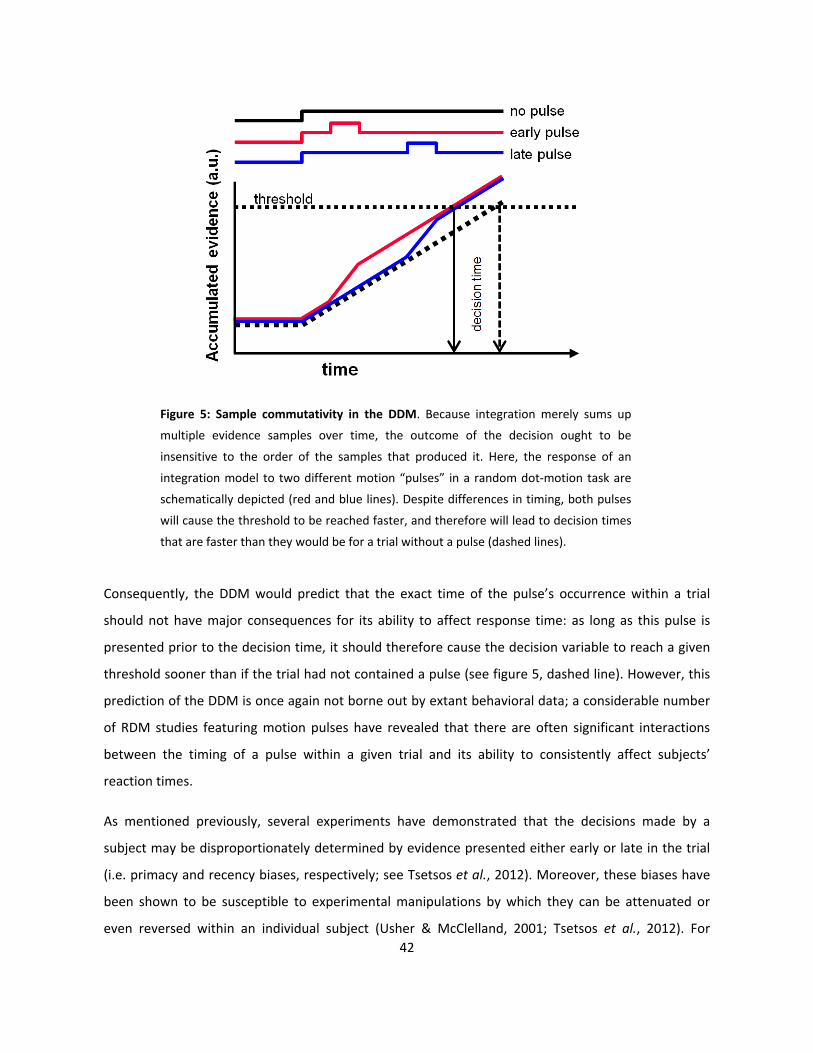
42

Figure 5: Sample commutativity in the DDM. Because integration merely sums up

multiple evidence samples over time, the outcome of the decision ought to be

insensitive to the order of the samples that produced it. Here, the response of an

integration model to two different motion “pulses” in a random dot-motion task are

schematically depicted (red and blue lines). Despite differences in timing, both pulses

will cause the threshold to be reached faster, and therefore will lead to decision times

that are faster than they would be for a trial without a pulse (dashed lines).

Consequently, the DDM would predict that the exact time of the pulse’s occurrence within a trial

should not have major consequences for its ability to affect response time: as long as this pulse is

presented prior to the decision time, it should therefore cause the decision variable to reach a given

threshold sooner than if the trial had not contained a pulse (see figure 5, dashed line). However, this

prediction of the DDM is once again not borne out by extant behavioral data; a considerable number

of RDM studies featuring motion pulses have revealed that there are often significant interactions

between the timing of a pulse within a given trial and its ability to consistently affect subjects’

reaction times.

As mentioned previously, several experiments have demonstrated that the decisions made by a

subject may be disproportionately determined by evidence presented either early or late in the trial

(i.e. primacy and recency biases, respectively; see Tsetsos et al., 2012). Moreover, these biases have

been shown to be susceptible to experimental manipulations by which they can be attenuated or

even reversed within an individual subject (Usher & McClelland, 2001; Tsetsos et al., 2012). For

43

example, Tsetsos et al. (2012) presented subjects with an identical cued-response RDM task with

pulses in two separate conditions which varied in “time pressure.” In the “high time pressure”

condition, subjects also had only a small window of time in which to report their decision, and

stimulus viewing times were drawn from an inverse exponential distribution such that very short

trials were substantially more common than long trials. In the “low time pressure” condition, trial

lengths were drawn from a uniform distribution, and the response window was lengthened. In both

conditions, brief “pulses” of added motion coherence were randomly added during the trial.

However, in both conditions the stimulus would vanish unexpectedly after a randomly determined

viewing time, therefore motivating the hypothesis that subjects ought to privilege early information

in both conditions. Instead, Tsetsos et al. (2012) found that the degree to which the task context

exerted time pressure on the subjects was often sufficient to cause reversals from primacy- to

recency biases, such that the effect of the pulses on their subjects’ behavior was dependent on both

their relative timing within a trial as well as the degree of time pressure placed on the decision.

This finding cannot be explained by the DDM, and the authors instead accounted for these findings

with a leaky competing accumulator (LCA) model which can be parameterized to account for the suite

of time dependency biases obtained in their task. However, the LCA model also does not itself specify

why these parameters should change in response to the manipulations in the task. Thus while the LCA

model can accurately capture these trends in the subjects’ behavior, the lack of a clearly-delineated

relationship between these particular model parameters and the manipulation of “time pressure” in

their task represents a conspicuous blind spot in the theoretical motivation of this model. In short, a

model which could replicate this data while also providing an explanation for this overall

phenomenon would be theoretically superior.

Summary

At this point, we have outlined a number of problematic issues with the DDM’s overall account of the

extant empirical data that, in spite of its widespread acceptance, still await definitive empirical

resolutions. In what follows we present an alternative model, and show that not only can it offer an

equally plausible theoretical account of much of the data that has been already successfully

addressed by the DDM, but also that it can overcome many of the potentially problematic issues we

have outlined in the foregoing discussion.

44

Introducing the urgency-gating model

In all of the models discussed so far, the reigning theoretical assumption has been that the brain

arrives at a decision specifically by integrating evidence in favor of competing choices until reaching a

fixed threshold. However, models based on this framework suffer from a number of subtle but non-

trivial issues regarding a number of their theoretical assumptions and mechanistic implications. Thus

we will now sketch out the alternative model we are proposing, which we call the urgency-gating

model (UGM), before giving a formal mathematical definition. Along the way we will show that the

UGM can account for most of the extant behavioral data equally as well as the DDM, but without

suffering from the theoretical shortcomings identified in the previous section. We will then briefly re-

visit the physiological data to offer an alternative, UGM-based interpretation of the extant

neurobiological findings before going on to discuss issues pertaining to the theoretical differentiation

of the UGM from the DDM.

Defining the model

The most salient mechanistic departure the UGM makes from the previous models is that it dispenses

with the assumption that the primary essential mechanism governing the formation of a decision is

the temporal integration of multiple discrete evidence samples over time. Instead, it posits that

evidence is represented in the form of a quantitatively-graded signal representing only the current

state of the decision-relevant evidence. It further posits that this real-time evidence signal is

effectively protected against the influence of noise by being subjected to a low-pass filter which

eliminates high-frequency fluctuations in the derivation of the estimate of the evidence signal while

preserving any persistent underlying signal in the sensory input. This low-pass-filtered evidence-

tracking signal is then combined with a separate, independent time-varying urgency signal that grows

over time at a rate commensurate with the urgency to respond. This “urgency” signal also effectively

implements a decision threshold that drops over time by decreasing the difference in activity

between the developing decision variable and the effective neural threshold. Variability in response

times arises by introducing inter-trial variations in the rate at which the urgency signal rises over the

course of a given decision. Importantly, the urgency signal links the dynamics of the model with task

factors relevant to “time pressure,” and thereby supplies the model with a clear and empirically-

tractable means of interpreting a variety of time-dependent influences on decisions.

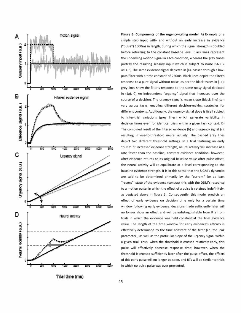
45

Figure 6: Components of the urgency-gating model. A) Example of a

simple step input with- and without an early increase in evidence

(“pulse”) 1000ms in length, during which the signal strength is doubled

before returning to the constant baseline level. Black lines represent

the underlying motion signal in each condition, whereas the grey traces

portray the resulting sensory input which is subject to noise (SNR =

4:1). B) The same evidence signal depicted in (a), passed through a low-

pass filter with a time constant of 250ms. Black lines depict the filter’s

response to a pure signal without noise, as per the black traces in (1a);

grey lines show the filter’s response to the same noisy signal depicted

in (1a). C) An independent “urgency” signal that increases over the

course of a decision. The urgency signal’s mean slope (black line) can

vary across tasks, enabling different decision-making strategies for

different contexts. Additionally, the urgency signal slope is itself subject

to inter-trial variations (grey lines) which generate variability in

decision times even for identical trials within a given task context. D)

The combined result of the filtered evidence (b) and urgency signal (c),

resulting in rise-to-threshold neural activity. The dashed grey lines

depict two different threshold settings. In a trial featuring an early

“pulse” of increased evidence strength, neural activity will increase at a

rate faster than the baseline, constant-evidence condition; however,

after evidence returns to its original baseline value after pulse offset,

the neural activity will re-equilibrate at a level corresponding to the

baseline evidence strength. It is in this sense that the UGM’s dynamics

are said to be determined primarily by the “current” (or at least

“recent”) state of the evidence (contrast this with the DDM’s response

to a motion pulse, in which the effect of a pulse is retained indefinitely,

as depicted above in figure 5). Consequently, this model predicts an

effect of early evidence on decision time only for a certain time

window following early evidence: decisions made sufficiently later will

no longer show an effect and will be indistinguishable from RTs from

trials in which the evidence was held constant at the final evidence

value. The length of the time window for early evidence’s efficacy is

effectively determined by the time constant of the filter (i.e. the leak

parameter), as well as the particular slope of the urgency signal within

a given trial. Thus, when the threshold is crossed relatively early, this

pulse will effectively decrease response time; however, when the

threshold is crossed sufficiently later after the pulse offset, the effects

of this early pulse will no longer be seen, and RTs will be similar to trials

in which no pulse pulse was ever presented.

46

A schematic depiction of the model’s dynamics is illustrated in figure 6 above, and can be specified in

mathematical form by the following equation:

xi(t) = g • Ei(t) • u(t) (3)

In this formulation, the decision variable (x) at time (t) assumes a value determined by the evidence

signal consisting of the current evidence (E) at time (t), multiplied by a gain factor (g); this evidence is

then combined with a separate, independent urgency signal (u), whose value at time (t) is determined

by the subjects’ growing urgency to end the decision and execute a response. Beyond the discrete

specifications afforded by the mathematical formula itself are number of assumptions about the

derivation of several of the model’s parameters, which therefore play a critical role in the resulting

dynamics. The value assumed by the urgency signal – and the rate at which it increases over time – is

proposed to reflect the temporal features of the task. Under conditions of high time pressure – or

high urgency – the decision variable xi(t) will, for any given evidence value, increase at a faster rate

than under conditions of lower urgency. This has important consequences for the dynamics of the

model in several ways. Firstly – and most straightforwardly – for any given value of the evidence

signal, the the average response time will change in a manner directly proportional to the rate of the

urgency signal’s growth (i.e. higher urgency signal slopes will yield faster decisions). Conversely, for

any given rate of urgency signal growth, stronger evidence will yield faster response times than

weaker evidence. Secondly, because the urgency signal shapes the effective decision threshold, the

function of controlling the speed-accuracy trade-off – provided by the static threshold setting in the

DDM – is now effectively assigned to the urgency signal. Thus, in broad outline, the UGM predicts a

set of mutual dependencies among decision factors that correspond to those posited by the

sequential sampling framework (see figures 1 & 2).

Dynamical features of the UGM

While the principal departure of the UGM is its abandonment of evidence integration, a similarly

crucial feature is its de-coupling of the evidence signal (g x E(t)) from the urgency signal (u(t)) – which,

as we will now discuss, is the core structural characteristic that endows it with its particular dynamics

which are crucial to its explanatory flexibility. Firstly, the addition of an urgency signal to the evidence

signal effectively frees the model from the consequences of sample redundancy discussed previously.

47

In the UGM, even very weak evidence will eventually cross the threshold because the urgency signal

will continue to grow even in the absence of additional novel evidence. Furthermore, the rising

urgency signal effectively implements a decision threshold that drops over time, thereby prohibiting

the indefinite stalling of the decision process due to diminishing returns on evidence.

Secondly, the UGM implements an alternative means of noise control, by employing a low-pass filter.

This neurally-plausible signal-filtration scheme (Abeles, 1991; Fourcaud-Trocmé et al., 2003; Rivlin-

Etzion et al., 2008) allows for persistent correlations in sensory input to serve as evidence input to the

model while nonetheless minimizing the impact of high-frequency fluctuations in the ongoing

derivation of the evidence from uncorrelated noisy sensory input. Admittedly, this functionality is

predicated on the assumption that an appropriate filter frequency cutoff value can be found that will

reliably discern between noise-driven errors in the derivation of the evidence signal and genuine

changes in the underlying decision evidence. However, this parameterization issue can be considered

relatively trivial, given that the time course of the evidence presented in most experimental tasks

differs from the typical mean firing rate of a cortical sensory neuron by at least an order of magnitude

(e.g. see experimental methodology and neural data from Kiani et al., 2008), thereby permitting a

large range of filter frequency cutoff values that will effectively differentiate between endogenous

processing noise and the underlying signal embedded in the stimulus.

However, the particular properties of this filter can still have an effect on the UGM’s overall

dynamics, because the settings of this filter determine how quickly the evidence signal can achieve a

stable, equilibrated response to changes in sensory input. Specifically, this is related to the time

constant of the filter, which is mathematically defined as the amount of time required for the filter to

respond to a step input by reaching (1–(1/e)) – approximately 63% – of its final (i.e. asymptotic) value.

In simpler terms, the time constant is a quantification of the delay between a change in the sensory

input and a corresponding change in the evidence signal. In figure 6, the raw sensory input to the low-

pass filter is illustrated in figure 6a, and the corresponding response of a filter with a 250ms time

constant is depicted in figure 6b. The UGM’s output can, under some conditions, be qualitatively

sensitive to this parameter, as the time constant of the filter determines how long changes in the

evidence signal persist, and therefore determines the effective time window for evidence

manipulations to affect response time.

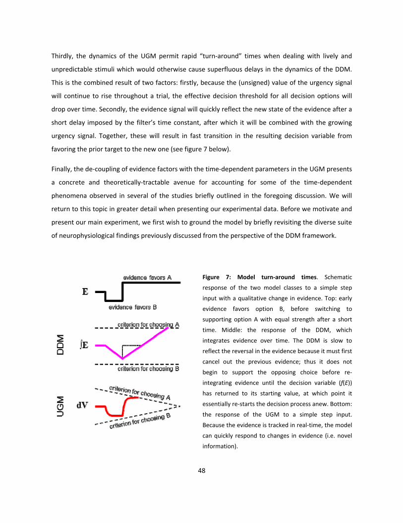
48

Thirdly, the dynamics of the UGM permit rapid “turn-around” times when dealing with lively and

unpredictable stimuli which would otherwise cause superfluous delays in the dynamics of the DDM.

This is the combined result of two factors: firstly, because the (unsigned) value of the urgency signal

will continue to rise throughout a trial, the effective decision threshold for all decision options will

drop over time. Secondly, the evidence signal will quickly reflect the new state of the evidence after a

short delay imposed by the filter’s time constant, after which it will be combined with the growing

urgency signal. Together, these will result in fast transition in the resulting decision variable from

favoring the prior target to the new one (see figure 7 below).

Finally, the de-coupling of evidence factors with the time-dependent parameters in the UGM presents

a concrete and theoretically-tractable avenue for accounting for some of the time-dependent

phenomena observed in several of the studies briefly outlined in the foregoing discussion. We will

return to this topic in greater detail when presenting our experimental data. Before we motivate and

present our main experiment, we first wish to ground the model by briefly revisiting the diverse suite

of neurophysiological findings previously discussed from the perspective of the DDM framework.

Figure 7: Model turn-around times. Schematic

response of the two model classes to a simple step

input with a qualitative change in evidence. Top: early

evidence favors option B, before switching to

supporting option A with equal strength after a short

time. Middle: the response of the DDM, which

integrates evidence over time. The DDM is slow to

reflect the reversal in the evidence because it must first

cancel out the previous evidence; thus it does not

begin to support the opposing choice before re-

integrating evidence until the decision variable (f(E))

has returned to its starting value, at which point it

essentially re-starts the decision process anew. Bottom:

the response of the UGM to a simple step input.

Because the evidence is tracked in real-time, the model

can quickly respond to changes in evidence (i.e. novel

information).

49

Re-visiting physiology

While much of the physiological work we discussed previously was both guided by and intepreted in

light of the framework supplied by DDM, its results are not for this reason restricted from being

explained by alternative models. In fact, the UGM is itself equally consonant with much of what is

currently known about the physiology of decision-making.

Evidence signals

As previously discussed, a large number of neurophysiological assays uncovered apparent neural

correlates of an “evidence signal” that conforms to the functional expectations as outlined by the

DDM. In general, these signals: (1) can be observed to originate in specific sensory areas in a manner

that corresponds straightforwardly to the informational demands of a given decision task; (2) appear

to encode an approximately real-time estimate of the current evidence bearing on a decision, as

indicated by momentary sensory input; (3) represent evidence in the form of population-wide neural

activity levels in a manner proportionately and quantitatively commensurate with the strength of the

evidence; and (4) transmit the resulting evidence signal to a number of cortical and subcortical sites

that accumulate this evidence for the purposes of preparing and executing the ensuing behaviors.

While many of the studies that supplied this physiological account of evidence signals were explicitly

motivated by the framework of the DDM, the functional role assigned to them in the UGM is

essentially identical and therefore calls for no major revisions to their neurophysiological

interpretation. In the UGM these first-order evidence signals do not themselves perform any

accumulative function, but merely reflect the current evidence by converging on a level of activity

that is quantitatively commensurate with the strength of the evidence indicated by sensory input.

Thus, all the evidence-signal-related physiological findings reviewed above can apply in largely the

same way to the framework of the UGM, with the sole exception of noise control. However, while

the precise biological substrate of the filter mechanism is not currently known, the UGM’s dynamics

do not strongly depend on its architectural localization in the overall decision network architecture.

For example, in the case of motion evidence in the context of an RDM task, the UGM’s essential

dynamics do not strongly depend on whether this low-pass filter is implemented within area MT

itself, or if filtration is instead performed elsewhere. Thus it does not place any strong a priori

constraints on the neural realization of the filter itself.

50

Accumulating and thresholding

While the DDM and the UGM do not assign substantially divergent functional roles to the evidence

signal or its biological implementation, they differ significantly in how the evidence signal estimates

supplied by sensory processing areas are subsequently processed to compute the decision variable.

Instead of accounting for the growth of the decision variable by the sequential addition of evidence

samples over time, the UGM posits that a sensory estimate of the current state of evidence is

combined with an independent urgency signal. Because this urgency signal increases in strength over

time, the result will resemble an accumulation of neural activity even for cases in which the evidence

remains constant throughout the decision. While the mechanistic differences between the DDM and

the UGM are by no means trivial, this dynamical overlap means that the framework of the UGM is

compatible with much of the physiological findings pertaining to evidence accumulation in areas

including FEF, LIP and SC discussed above, regardless of whether such information arrives

continuously (Platt & Glimcher, 1997; Colby & Goldberg, 1999; Gold & Shadlen, 2000; Roitman &

Shadlen, 2002) or in discrete steps (Yang & Shadlen, 2007).

While the DDM and UGM can both account for the general build-up of decision-related neural

activity, the two models could in principle be differentiated by further examining the composition of

the resulting output signal encoding the decision variable. Specifically, if the changes in this signal

over time are due to the integration of multiple samples over time then its activity should be driven

almost exclusively by evidence-related factors. In contrast, if it could be demonstrated that at least

part of this neural build-up is due to time-dependent factors in a manner that is otherwise

functionally independent of evidence, then this would constitute distinct proof in favor of the UGM.

In fact, a number of prior studies – themselves predating and therefore not specifically motivated by

the UGM framework – have provided some evidence that a significant portion of the rising neural

activity typically associated with the integration of evidence over time is not driven by evidence, but

instead encodes the mere passage of time itself (Janssen & Shadlen, 2005; Ditterich, 2006b; Beck et

al., 2008; Churchland et al.., 2008; Cisek et al.., 2009; Hanks et al., 2011; Standage et al.., 2011;

Drugowitsch et al.., 2012; Standage et al.., 2013; Standage et al., 2014). For example,

neurophysiological assays of LIP activity have revealed that firing rates for neurons encoding the

spatial locations of potential targets can be seen to exhibit a time-dependent increase in activity over

the course of a trial, and that the rate at which it increases remains consistent even across multiple

51

values of motion coherence strength in an RDM task, suggesting that it is functionally independent of

evidence (Leon & Shadlen, 2003; Rao 2010: see also figure #9 in Drugowitsch et al., 2012).

Furthermore, this time-varying signal has been shown to affect all LIP neurons in a similar manner,

regardless of the response field of the individual cells (ibid), which further suggests its functional

independence from task factors related to evidence. Exactly such a time-dependent signal is central

to the framework proposed by the UGM, and the demonstration of such signals in a functionally well-

characterized decision-related area like LIP thus constitutes suggestive proof in favor of the UGM. In

fact, this signal has been labeled an “urgency signal” by a number of researchers (Reddi & Carpenter,

2000; Reddi et al., 2003; Churchland et al., 2008; Drugowitsch et al., 2012).

Moreover, the addition of a growing, time-varying signal to the evidence-accumulation process

decreases the difference between the decision variable and the effective neural threshold over time,

and therefore effectively implements a dropping threshold. This makes the UGM consistent with

previous studies demonstrating that the addition of a dropping threshold improves the predictions of

prior integration-based models featuring static threshold parameters (Drugowitsch et al., 2012; Liu &

Watanabe, 2012). Furthermore, it makes the UGM physiologically consistent with the numerous

observations of “hard-coded” neural activity thresholds observed in studies of decision-related neural

activity in the LIP (Roitman & Shadlen, 2002; Mazurek et al., 2003; Ratcliff, Cherian & Segraves, 2003;

Kiani et al., 2008).

While the provenance of such an urgency signal is not yet known, the observation that it appears to

act as a time-dependent gain that is applied across the full range of outcomes in a given task has been

taken as suggestive evidence that it may be a domain-general signal that itself originates in

subcortical networks and which is commonly projected to many diverse cortical areas. Some

theoretical speculations have been offered, and suggested candidates for such a subcortical

implementation have included the locus coeruleus (see Bogacz et al., 2006 and references therein)

and the globus pallidus (see Desmurget & Turner, 2010). Again, however, the lack of a precise

anatomical localization of the urgency signal does not itself pose any specific problems regarding the

re-interpretation of the physiological findings reviewed so far from the perspective of the UGM.

52

Output variability in the UGM: intra- vs. inter-trial noise

In most real-world environments – and indeed in many experimental tasks as well – the quality of the

evidence available for a decision are typically beyond the control of decision-makers themselves.

Instead, they must adapt their decision-making behavior in response to the amount of information

available in a given environment – and one of the main purposes for any decision model is to provide

a set of tractable mechanisms and parameters by which adaptive decision control can be described.

In the DDM, controlling the speed-accuracy trade-off is done by specifying a threshold value, and

variability in response times arises due to intra-trial fluctuations in the noise afflicting the evidence

input. In the UGM this is accomplished by setting both the mean and standard deviation of the

urgency signal’s rise (see figure 6 above). The former provides the primary means of control over the

speed-accuracy trade-off, while the latter enables the model to generate orderly distributions of

response times by varying the slope of the urgency signal across trials. This change from an intra-trial

to an inter-trial source of variability is motivated by a series of mathematical analyses performed by

Carpenter & Williams (1995), who demonstrated that variability in human response times in a given

task are most parsimoniously explained by inter-trial variabilies, themselves perhaps caused by larger-

scale temporal fluctuations in arousal or attention across large numbers of trials. Conversely, they

also showed that neurally-plausible forms of intra-trial noise, such as that posited by the DDM, is

unlikely to contribute substantially to the timing of decisions on a behaviorally-appreciable level (c.f.

Cisek et al., 2009). Consequently, the UGM employs inter-trial variability in the slope of the urgency

signal to inject the model with a source of variability that is both neurally-plausible and whose effects

on the model’s output is consistent with extant behavioral data. In summary, the UGM’s functional

architecture allows for essentially all of the physiological findings discussed in the foregoing to be

interpreted equally as well from within the UGM’s mechanistic framework.

Experimental differentiation of the models

Importantly, the DDM and the UGM make identical predictions under any condition in which the

evidence presented on a given trial is held constant. This overlap in the model’s respective dynamics

renders much of the extant empirical work agnostic on the matter of which model is superior, as the

majority of experimental investigations undertaken in the past few decades have predominantly

featured tasks in which the evidence is held constant on a within-trial basis. Consequently, there have

53

been only a small number of studies so far whose methodologies afforded strong conclusions

regarding the differentiation of the DDM and the UGM.

Cisek et al. (2009) explicitly sought to differentiate the DDM from the UGM by using a novel

experimental task in which the evidence changes continuously over the duration of each trial. In their

“tokens” task, subjects were presented with a central target which contained 15 tokens, each of

which was randomly distributed to one of two peripheral targets every 200ms; the subjects’ task was

to predict which of the two targets would contain more tokens by the end of the trial. The

formulation of this task allowed for the “success probability” associated with each of the two targets

to be explicitly mathematically defined at any given point in the trial (i.e. as a function of the number

of targets presently contained within a given target vs. the number of tokens remaining to be

distributed), yielding a value between 0 and 1 indicating the current probability of success for that

target. Subjects were free to respond at any time, and were able to save time by choosing one of the

targets as soon as they felt sufficiently confident in their response. Once the choice was reported (by

moving a cursor to the corresponding target), the remaining tokens were distributed more quickly to

their final targets, and feedback was given. Importantly, however, completing this task required

achieving a certain number of correct responses, and thereby entailed a trade-off between

maximizing accuracy and minimizing the time spent across trials.

While the distribution of tokens in most trials was randomly determined, a subset of “bias” trials

(10%) were given to explicitly test the dynamics of the decision process. In such trials, the first six

token movements favored one target, causing the success probability for that target to be high

relatively early in the trial. If no immediate choice was made, this initial “bias” would then be

canceled out with the next few tokens moving to the opposite target, thereby making the success

probability associated with each target equal. Importantly, the DDM and the UGM make different

predictions for the timing of decisions made after the early bias. Because the DDM relies on

integration of evidence over time, it retains a “memory” of previous evidence that should cause

faster decisions on trials in which the early evidence favored the chosen target compared to trials in

which the bias favored the opposite target. The UGM, however, only uses the current state of the

evidence, and therefore the dynamics of an urgency-gating model should not be sensitive to early

biases for decisions made later; thus the UGM predicts no difference in decision timing between the

two bias types for trials in which the decision was made later than 1200ms in the trial.

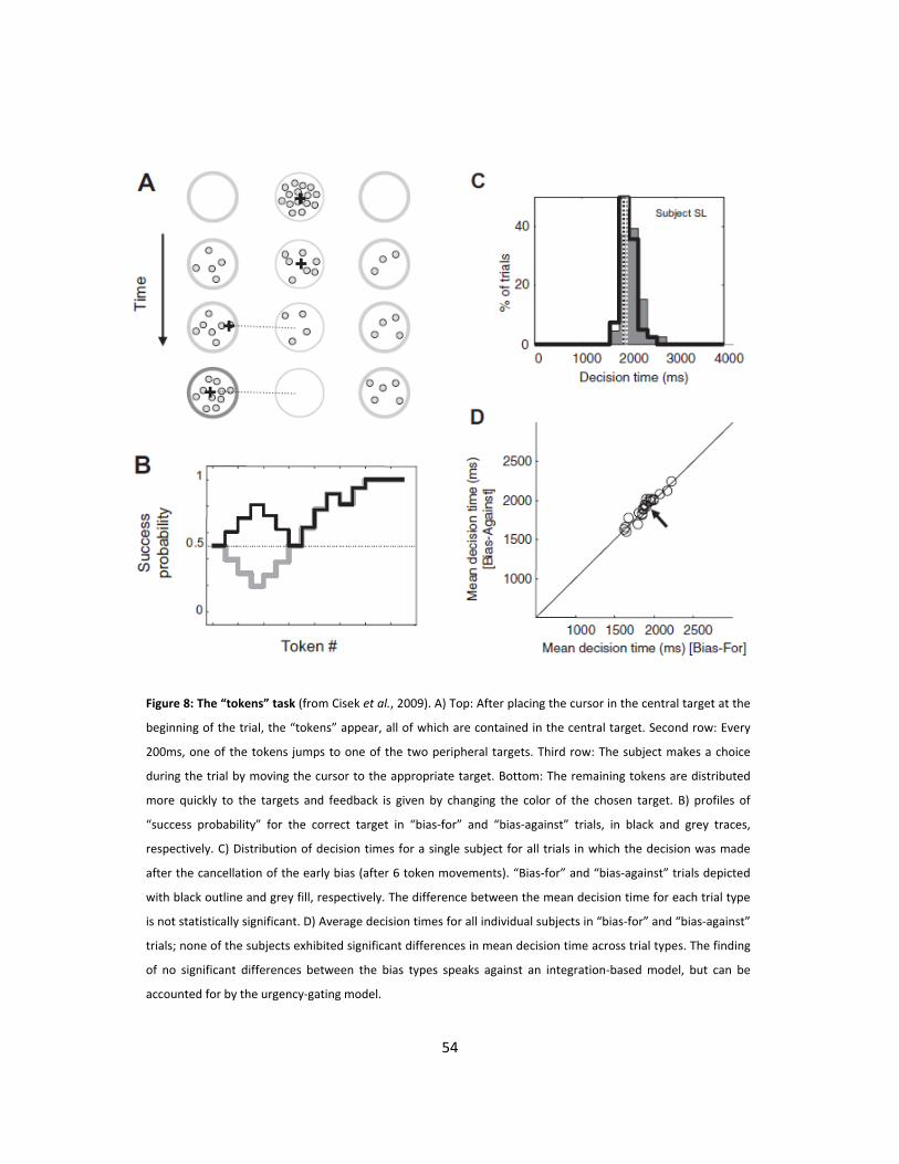
54

Figure 8: The “tokens” task (from Cisek et al., 2009). A) Top: After placing the cursor in the central target at the

beginning of the trial, the “tokens” appear, all of which are contained in the central target. Second row: Every

200ms, one of the tokens jumps to one of the two peripheral targets. Third row: The subject makes a choice

during the trial by moving the cursor to the appropriate target. Bottom: The remaining tokens are distributed

more quickly to the targets and feedback is given by changing the color of the chosen target. B) profiles of

“success probability” for the correct target in “bias-for” and “bias-against” trials, in black and grey traces,

respectively. C) Distribution of decision times for a single subject for all trials in which the decision was made

after the cancellation of the early bias (after 6 token movements). “Bias-for” and “bias-against” trials depicted

with black outline and grey fill, respectively. The difference between the mean decision time for each trial type

is not statistically significant. D) Average decision times for all individual subjects in “bias-for” and “bias-against”

trials; none of the subjects exhibited significant differences in mean decision time across trial types. The finding

of no significant differences between the bias types speaks against an integration-based model, but can be

accounted for by the urgency-gating model.

55

Indeed, as can be seen in figures 8c & 8d, the data obtained by Cisek et al. (2009) bears out the

predictions of the UGM, in that no significant differences in decision timing were found. However,

some concerns remained regarding how generalizable these findings were to decision-making in

general. Firstly, the tokens task does not involve a noisy stimulus, making performance on this task

less reliant on integration than most of the perceptual discrimination tasks commonly used in

decision-making research. Secondly, because tokens remained in their targets over the entire

duration of the trial, the state of the evidence was continuously indicated by the task display,

therefore further reducing the task’s reliance on integration mechanisms to store and accumulate

evidence information over time. Thirdly, the task involved making an inference about the future state

of the stimulus, which may therefore have involved cognitive processes beyond those typically

involved in most common forms of decision-making tasks. For these reasons, it could be argued that

the findings of Cisek et al. (2009) were purely task-dependent and therefore do not directly speak to

the pertinent issues address by integration-based models.

A follow-up study by Thura et al. (2012) sought to redress these potential shortcomings by adapting

the logic of the tokens task to a RDM format. In their study, the motion coherence of the random dot

display changed over time in discrete “coherence steps,” analogous to the token movements in the

Cisek et al.’s task. Here, the RDM stimulus was initialized with a coherence value of 0; after 225ms,

3% of the dots would begin moving towards the left or the right. Every 225ms thereafter, another 3%

of the dots would begin moving in either the same or the opposite direction. Subjects were tested

under two conditions. In one, they had to anticipate which of the two targets would correspond to

the stronger of the two motion signals by the trial’s end; in the second condition, they merely had to

report the current state of the stimulus at the time of their decision. Again, subjects were allowed to

respond at any time, at which point the allocation of motion strength corresponding to the “token

movements” would accelerate, thereby implicitly providing a trade-off between accuracy and speed.

Thura et al. also included identical “bias” trials in their RDM adaptation of the tokens task (see figure

8b), therefore allowing a similar differentiation between the DDM and the UGM to that undertaken

by Cisek et al. (2009). Once again, they found that early biases in the motion signal did not affect the

timing of decisions made after the bias period, contrary to the predictions of integration-based

models like the DDM.

56

Together, these studies provide exclusive empirical support for the UGM, as they were the first

studies to directly test a case in which the DDM and the UGM make explicitly divergent predictions.

However, despite Thura et al.’s (2012) use of the RDM paradigm, some concerns have still remained

about the potential for the findings to have been due to some novel aspect of the task design.

Therefore, we sought to design an experiment which would more strongly dissociate between the

models, using an experimental paradigm that was maximally similar to those used in previous work

(RDM pulse study citations). To this end, we presented subjects with a common form of the RDM task

in which within-trial changes in the evidence strength are provided by inserting brief motion “pulses”

during which the strength of the motion coherence briefly doubles in strength. While both the DDM

and the UGM predict that enhancing the evidence in this way should affect response times, the

UGM’s dynamics diverge from those of the DDM in that the UGM predicts that the efficacy of such a

pulse should be strongly dependent on the timing of the pulse relative to the ensuing decision –

thereby presenting a clear empirical avenue for decisively dissociating the models.

Main experiment

The logic of our experimental design is illustrated in Figure 9 below. As in a typical random-dot

motion discrimination (RDM) task, subjects are presented with a coherent motion stimulus that is

constant across time and are asked to respond as soon as they detect the direction of motion.

Unknown to the subjects, in some trials there is a brief (100ms) increase of motion coherence that

occurs at different times after motion onset. If decisions are made using a perfect integrator (figures

9a & 9b), then early motion pulses should briefly increase the rate of integration and result in

decisions that are faster (red) than those made in no-pulse trials (black). In contrast, pulses that

appear late in the trial (blue) will have no effect if the decision bound is low (figure 9a), because they

occur after the decision has already been made. If the decision bound is high, then both early and late

pulses will have similar effects (figure 9b). In other words, as subjects slow down their decision policy,

the time window in which pulses have an effect on reaction times is predicted to expand, but early

pulses will always be at least as effective as late pulses because there is no leak.

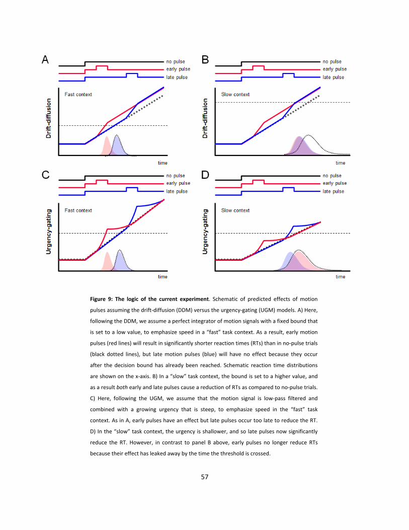
57

Figure 9: The logic of the current experiment. Schematic of predicted effects of motion

pulses assuming the drift-diffusion (DDM) versus the urgency-gating (UGM) models. A) Here,

following the DDM, we assume a perfect integrator of motion signals with a fixed bound that

is set to a low value, to emphasize speed in a “fast” task context. As a result, early motion

pulses (red lines) will result in significantly shorter reaction times (RTs) than in no-pulse trials

(black dotted lines), but late motion pulses (blue) will have no effect because they occur

after the decision bound has already been reached. Schematic reaction time distributions

are shown on the x-axis. B) In a “slow” task context, the bound is set to a higher value, and

as a result both early and late pulses cause a reduction of RTs as compared to no-pulse trials.

C) Here, following the UGM, we assume that the motion signal is low-pass filtered and

combined with a growing urgency that is steep, to emphasize speed in the “fast” task

context. As in A, early pulses have an effect but late pulses occur too late to reduce the RT.

D) In the “slow” task context, the urgency is shallower, and so late pulses now significantly

reduce the RT. However, in contrast to panel B above, early pulses no longer reduce RTs

because their effect has leaked away by the time the threshold is crossed.

58

In contrast, if the integration mechanism is replaced with a low-pass filter and combined with an

urgency signal, then early pulses will have a stronger effect than late pulses in conditions where

urgency is steep (figure 9c), but the reverse will be true when urgency is shallow (figure 9d). This is

because the information provided by early pulses will have leaked away by the time the decision

bound is crossed. Consequently, as subjects slow down, the time window in which pulses are

effective is predicted to shift, and late pulses will become more effective than early pulses.

Our approach for testing these predictions is to present subjects with an identical set of no-pulse and

pulse trials in two different contexts, one in which they are motivated to respond quickly and one in

which they are motivated to slow down; the resulting differences in response times between the no-

pulse trials and each of the pulse conditions should, in principle, reveal the underlying dynamics of

the decision process and thereby strongly distinguish between the two models.

Methods

Subjects and apparatus

Thirty-two right-handed participants (17 female) with normal- or corrected-to-normal vision provided

written consent and were naïve to the purpose of our experimental task. Participants were seated in

front of a large digitizing tablet placed at arm-level for recording subject movements (125Hz sample

rate @ .013 cm accuracy). Stimuli, targets and feedback were projected by an LCD monitor onto a

half-silvered mirror positioned 16cm above and parallel to the digitizer surface, and thus appeared to

float on the plane of the digitizing tablet. The subjects’ task was to report the direction of motion of

the RDM stimulus by completing planar reaching movements using a handheld cordless stylus

embedded within a vertical plastic handle toward one of two targets whose locations corresponded

to the potential motion directions. The task and data collection was programmed in LabView, stored

in a database (Microsoft SQL Server 2005), and analyzed using custom Matlab scripts.

Behavioral task

Each trial began when subjects moved the cursor into a small circular target (1cm in diameter) near

the center of a white display. After 500ms, two circular targets (3cm in diameter) appeared 6cm to

each side of the stimulus display area, separated by 180°. After another 300ms, 200 black dots

appeared in a borderless circular area (3cm diameter) in the center of the display, between the two

59

targets. Each of the dots was re-drawn in a new location 2 pixels away from its previous location on

each frame (60Hz). Most of the dot displacements were random, but a small subset of the dots was

re-drawn along a vector corresponding to the location of one of the two targets. While the individual

dots assigned to the coherently-moving subset changed from frame to frame, the resulting percept

was a consistent motion signal whose direction subjects could reliably and accurately report, with a

degree of difficulty inversely related to the percentage of coherently-moving dots (Newsome, Britten

& Movshon, 1989; Kim & Shadlen, 1999).

Subjects were given up to 3000ms to report the direction of the coherent motion by moving from the

initial start target to one of the two choice targets, and were free to respond at any time. Movements

had to be completed in less than 1000ms, and had to land within the chosen target circle. The motion

stimulus continued up until the point at which the cursor crossed a target circle’s border. The cursor

had to remain within the chosen target for 500ms, at which point the outline of the target turned

green or red to indicate a correct or incorrect choice, respectively. After a brief inter-trial interval of

500ms, all on-screen objects disappeared except for the starting target, and a new trial began.

In the analyses reported here, response times for each trial were obtained post hoc by determining

the precise moment at which the cursor’s velocity began to increase from a point of rest within the

start target. However, an ad hoc estimate of RT based on the time at which the cursor exited the

boundary of the start target was used to obtain session-specific estimates of subjects’ mean reaction

times; these were then used to provide on-line feedback during the experimental sessions.

Before each session began, we presented the subject with 40 very easy motion-discrimination trials in

which the motion coherence was 50%, and instructed them to respond as rapidly as possible. The

average RT estimated from these trials was then stored as a session-specific estimate of a “non-

decision delay” comprising both sensory and motor delays (mean=475ms, std=103ms). For versions of

our task in which the motion signal changed directions within a trial (see below), we subtracted this

estimated mean reaction-time from the ad-hoc estimated RT to determine the state of the motion

signal at the estimated time that subjects made their decision (see “VMD” trial section below).

Importantly, these initial 40 trials were the only ones for which subjects were ever provided with

explicit instructions about how quickly to respond. For the main experimental task, subjects were

informed of the 3-second time limit but were told that they could make their decision whenever they

liked, though in fact most of our subjects very rarely took more than 1800ms to make their decision.

60

Subjects completed two different kinds of session: “blocked” or “interleaved”. “Blocked” sessions

consisted entirely of trials with a single, common baseline motion coherence value of 3%, starting

from the onset of the RDM stimulus. We refer to these as “constant-motion discrimination” (CMD)

trials. In 40% of such trials there were no additional changes to the stimulus, and we refer to these as

“no-pulse” trials. The remaining 60% of the CMD trials contained brief motion “pulses” during which

the coherence of the motion stimulus was doubled (to 6%) for 100ms. These pulses could occur 100,

200, 400 or 1600ms following stimulus onset. We refer collectively to such trials as “pulse” trials. Such

brief coherence manipulations have been repeatedly shown to affect response timing in RDM tasks

(Huk & Shadlen, 2005; Wong et al., 2007), even though they were not consciously detectable by our

subjects, as confirmed by post-experiment interview, consistent with similar studies (Kiani, Hanks &

Shadlen, 2008). Thus, as far as the subjects were aware, the motion coherence for all CMD trials was

constant throughout each trial, regardless of whether a pulse was or was not actually shown.

“Interleaved” sessions consisted of a mix of trial types. Twenty percent of the trials in these sessions

were CMD trials, including both pulse- and no-pulse trials, identical in every respect to those in the

blocked sessions. These CMD trials were randomly interleaved among “variable-motion

discrimination” (VMD) trials, which comprised the remaining 80% of the interleaved session.

Analogous to the “token movements in Cisek et al. (2009), these trials began with a net motion

coherence of 0, and was adjusted either up or down in 3% steps every 200ms (sometimes reversing

the direction of motion). Of the VMD trials, 60% were random, such that each motion coherence

change was given an independent and equal probability of favoring each of the two possible targets.

The remaining VMD trials were divided amongst a number of pre-generated trial types meant to

further test the predictions of the two models, specifically with regards to how long the dynamics of

each model are affected by biases in prior evidence.

The pre-generated VMD trials came in six types: “easy,” “ambiguous,” and four “bias” trial types:

“bias-for,” “bias-against,” “bias up-down” and “bias down-up.” “Easy” trials were defined as trials in

which at least four of the first five motion changes favored the same target, and in which no

subsequent changes in the motion signal brought the net motion favoring that target below 9%.

“Ambiguous” trials were those in which the motion signal did not strongly favor either target

(coherence<=6%) until at least 1200ms into the trial. “Bias” trials were trials in which the motion

signal initialy grew strongly in favor of one target (9%) before returning to 0%, after which the motion

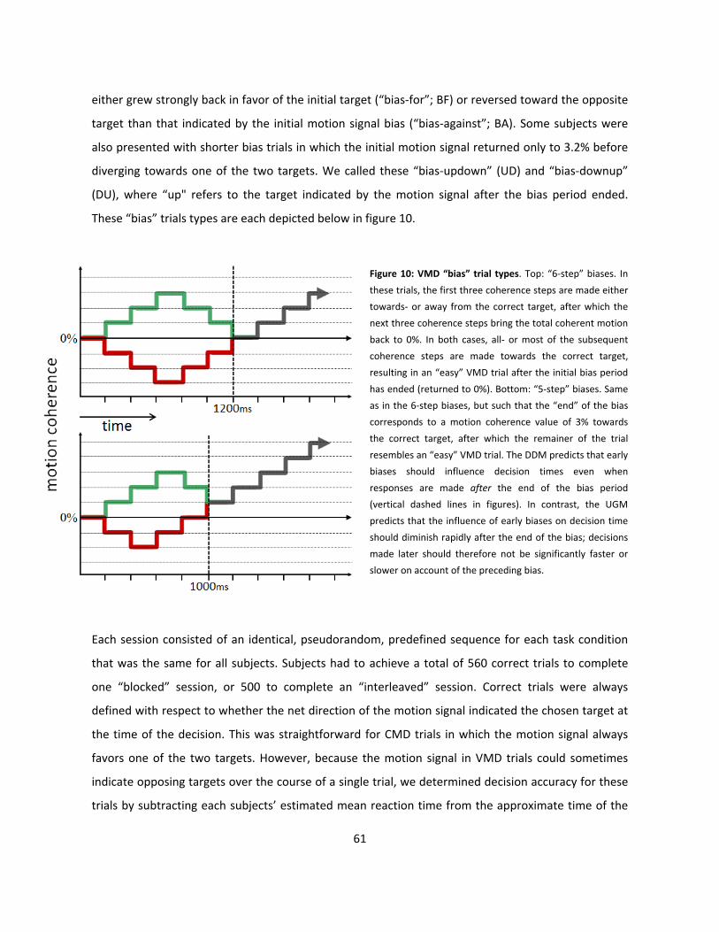
61

either grew strongly back in favor of the initial target (“bias-for”; BF) or reversed toward the opposite

target than that indicated by the initial motion signal bias (“bias-against”; BA). Some subjects were

also presented with shorter bias trials in which the initial motion signal returned only to 3.2% before

diverging towards one of the two targets. We called these “bias-updown” (UD) and “bias-downup”

(DU), where “up" refers to the target indicated by the motion signal after the bias period ended.

These “bias” trials types are each depicted below in figure 10.

Figure 10: VMD “bias” trial types. Top: “6-step” biases. In these trials, the first three coherence steps are made either towards- or away from the correct target, after which the next three coherence steps bring the total coherent motion back to 0%. In both cases, all- or most of the subsequent coherence steps are made towards the correct target, resulting in an “easy” VMD trial after the initial bias period has ended (returned to 0%). Bottom: “5-step” biases. Same as in the 6-step biases, but such that the “end” of the bias corresponds to a motion coherence value of 3% towards the correct target, after which the remainer of the trial resembles an “easy” VMD trial. The DDM predicts that early biases should influence decision times even when responses are made after the end of the bias period (vertical dashed lines in figures). In contrast, the UGM predicts that the influence of early biases on decision time should diminish rapidly after the end of the bias; decisions made later should therefore not be significantly faster or slower on account of the preceding bias.

Each session consisted of an identical, pseudorandom, predefined sequence for each task condition

that was the same for all subjects. Subjects had to achieve a total of 560 correct trials to complete

one “blocked” session, or 500 to complete an “interleaved” session. Correct trials were always

defined with respect to whether the net direction of the motion signal indicated the chosen target at

the time of the decision. This was straightforward for CMD trials in which the motion signal always

favors one of the two targets. However, because the motion signal in VMD trials could sometimes

indicate opposing targets over the course of a single trial, we determined decision accuracy for these

trials by subtracting each subjects’ estimated mean reaction time from the approximate time of the

62

start of the movement with which they reported their decision. The trial was counted as correct if the

motion signal at this time indicated the chosen target, even if the signal had changed directions later.

In general, however, trials in which the computed decision time occurred within 200ms of a

qualitative reversal in the stimulus only comprised a small minority of total trials (<3%), and so are

not likely to have qualitatively distorted the overall results even if some of these calculations were

inaccurate with respect to the subject’s intended choice.

Both session types required approximately 50 minutes on average to complete, depending on an

individual subjects’ speed and accuracy on that day. Importantly, however, subjects were paid the

same amount per session ($20 CAD) regardless of how long it took for them to reach the quota of

correct trials. Thus, while we otherwise provided no explicit penalty for wrong answers, the structure

of the task nonetheless implicitly motivated subjects to find a policy that maximizes reward rate for

each experimental session.

Crucially, our two session types differed with respect to the value of stimulus observation time. In

blocked sessions, the average success rate was not appreciably improved with long observation times

because the motion in CMD trials is nearly constant. In contrast, because the interleaved sessions are

dominated by VMD trials, in which the motion can be much stronger later in time, there is an

advantage in slowing down one’s decision policy so that decisions can be made on the basis of

stronger evidence. Thus, we expected our subjects to make slower decisions in CMD trials during the

interleaved sessions than in the same trials during the blocked sessions, because they should adopt a

slower policy in the interleaved sessions (increase their decision bound, or decrease their urgency

signal). We initially ran 27 subjects on 3 sessions each (1 blocked, 2 interleaved, together yielding

1,560 correct individual trials per subject), allowing across-subject analyses. Next, to obtain enough

data to perform analyses on a within-subject basis, we ran an additional 5 subjects for 10+ sessions

each (range=10-20, mean = 13.8, yielding ~5,200-10,300 correct individual trials per subject).

If our manipulation of decision policy between the two session types was effective, then we should be

able to discriminate between the DDM and UGM by comparing trials in which evidence is identical

and only the effective decision policy differs (see figure 9). If early pulses have an effect on reaction

times that is always at least as strong as late pulses, then this would support a pure integration model

such as the DDM. If, instead, early pulses lose their efficacy in the interleaved session while late

63

pulses become more effective, then this would support an urgency-gating model in which evidence is

not integrated over time, but instead low-pass filtered with a highly leaky integrator.

Modeling

We simulated the low-pass filtering of sensory information using a first-order linear differential

equation

gExdtdx +−=τ

(4)

where τ = 166ms is the time constant and g = .04 is the gain. The evidence E is set to 1 to simulate 3%

coherent motion and increased to 1.8 for 100ms to simulate the motion pulse. The resulting variable

x(t) is then combined with an urgency signal as

)()()( tUtxty ⋅= (5)

where U(t) is the urgency signal that rises from zero with a slope that varies from trial to trial

according to a normal distribution with mean u and standard deviation s. When the variable y(t)

reached a threshold of T = 2000, the decision was made, and a non-decision delay t0 (300ms in our

simulations) was added to yield a reaction time. The remaining parameters were estimated from the

data. To simulate each of the conditions (blocked and interleaved), we picked values of u and s that

produced the best fit to the mean and standard deviation of the RT distribution from 3% coherence

no-pulse CMD trials in each condition. We then used the same parameter settings when simulating

pulse trials.

Results Effects of sessions

First, we determined whether our manipulation of decision policy succeeded. We did this by

comparing RTs for identical no-pulse CMD trials across the two conditions. Mean RTs (± s.e.m.) of

individual subjects are shown in figure 11a for constant-evidence, 3% motion coherence trials in both

the “blocked” (x-axis) and “interleaved” (y-axis) conditions. All individual data points lie above the

unity line, indicating that the mean RTs for CMD trials were slower when interleaved among VMD

trials than when blocked together (p<10-40). Cumulative RT distributions for the same no-pulse CMD

trials for the 5 subjects who completed the greatest number of experimental sessions (figures 11b &

64

11c) show both a clear rightward displacement along the x-axis – indicating later RTs in general – as

well as a decreased slope in the interleaved condition – indicating an increased range of reaction

times. Importantly, this main effect holds across all of our subjects in spite of the otherwise large

inter-subject variability in overall speed. In other words, while some subjects tended to be

significantly faster than others, all of them individually slowed down considerably during the

interleaved sessions, in which delaying decision times tends to yield a benefit to accuracy. This

behavior emerged despite the fact that no explicit instructions were ever provided to the subjects

regarding the timing of their decisions.

The strength and consistency of this result across all of our subjects thus strongly supports the

effectiveness of our contextual manipulation on subjects’ decision-making behavior. Moreover,

because these differences obtain in no-pulse CMD trials which were otherwise identical, the most

parsimonious interpretation of this effect is that it is the result of a slowed decision policy for the

interleaved sessions relative to the blocked sessions. In the framework of the DDM, this corresponds

to increasing the decision bound in interleaved sessions, and in the framework of the UGM, to

decreasing the slope of the urgency signal (as per figure 9 above).

Effects of pulses

Our next step was to analyze the effects of pulses in each task context to distinguish between the

specific predictions of each model under conditions of changing evidence (figure 9). Similar to the

above, this analysis also focused exclusively on CMD trials (no-pulse and pulse) which were identical

in each session type. Note that because nearly all decisions were made before 1800ms in either

session type, the 1600ms pulse timing did not yield enough data to warrant a meaningful analysis and

these trials were therefore excluded from subsequent analyses.

Figure 12a shows the cumulative RT distributions from blocked (top) and interleaved (bottom)

sessions for the subject who performed the largest number of sessions (“JM”; nsessions=20,

ntrials=12,900). Like all subjects, JM’s mean RT for no-pulse, constant-evidence trials (black trace) is

significantly faster when these appeared in the blocked condition than the interleaved condition

(median no-pulse RT, blocked = 726ms; median no-pulse RT, interleaved = 1,165ms; see figure insets).

In the blocked condition, the earliest two pulse timings (100ms and 200ms; red and magenta traces,

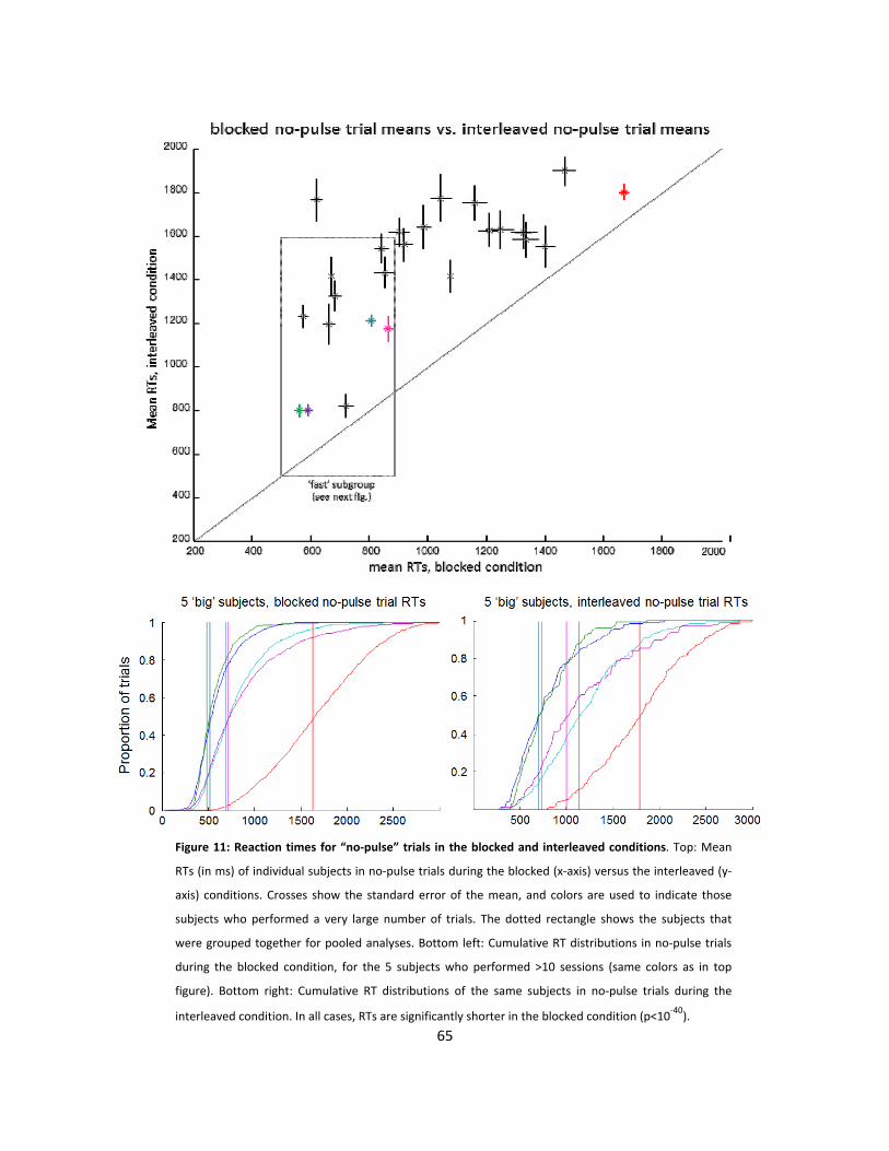
65

Figure 11: Reaction times for “no-pulse” trials in the blocked and interleaved conditions. Top: Mean

RTs (in ms) of individual subjects in no-pulse trials during the blocked (x-axis) versus the interleaved (y-

axis) conditions. Crosses show the standard error of the mean, and colors are used to indicate those

subjects who performed a very large number of trials. The dotted rectangle shows the subjects that

were grouped together for pooled analyses. Bottom left: Cumulative RT distributions in no-pulse trials

during the blocked condition, for the 5 subjects who performed >10 sessions (same colors as in top

figure). Bottom right: Cumulative RT distributions of the same subjects in no-pulse trials during the

interleaved condition. In all cases, RTs are significantly shorter in the blocked condition (p<10-40).

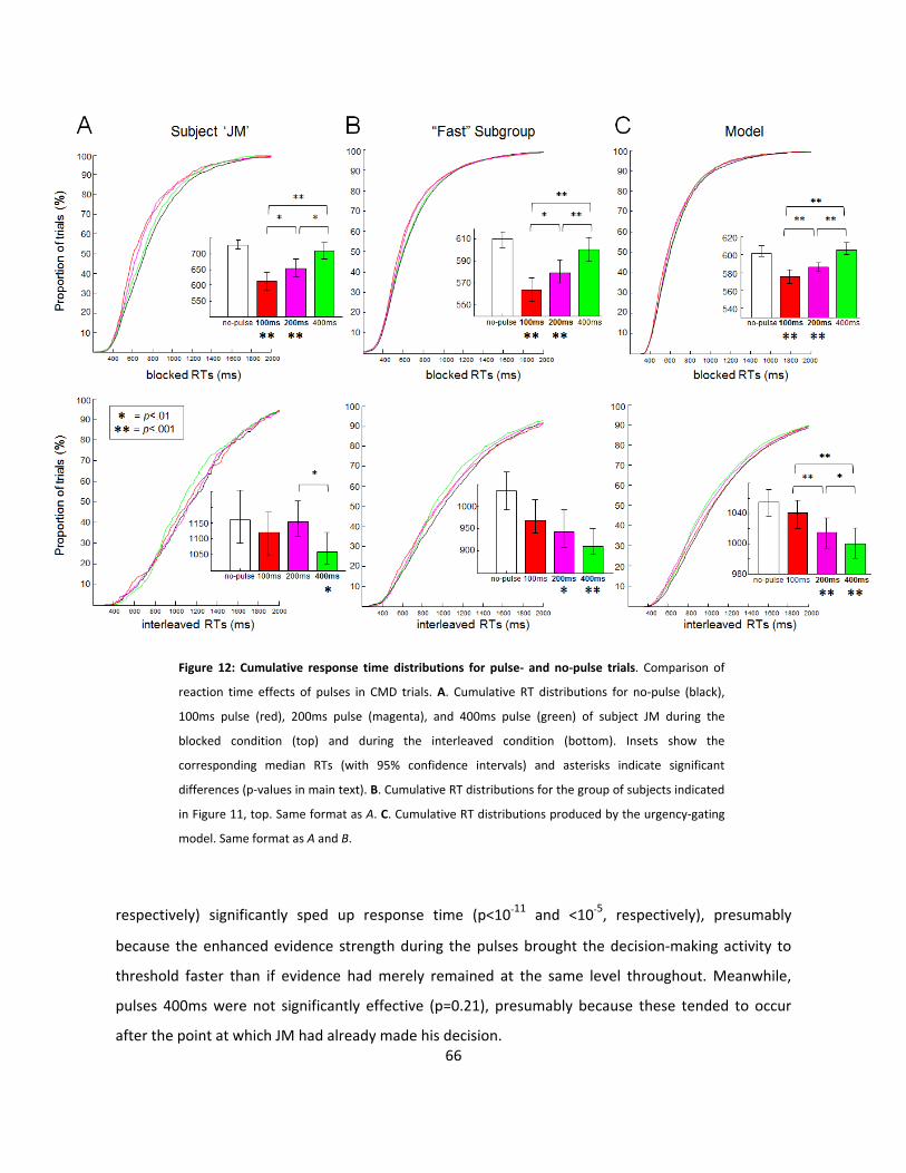
66

Figure 12: Cumulative response time distributions for pulse- and no-pulse trials. Comparison of

reaction time effects of pulses in CMD trials. A. Cumulative RT distributions for no-pulse (black),

100ms pulse (red), 200ms pulse (magenta), and 400ms pulse (green) of subject JM during the

blocked condition (top) and during the interleaved condition (bottom). Insets show the

corresponding median RTs (with 95% confidence intervals) and asterisks indicate significant

differences (p-values in main text). B. Cumulative RT distributions for the group of subjects indicated

in Figure 11, top. Same format as A. C. Cumulative RT distributions produced by the urgency-gating

model. Same format as A and B.

respectively) significantly sped up response time (p<10-11 and <10-5, respectively), presumably

because the enhanced evidence strength during the pulses brought the decision-making activity to

threshold faster than if evidence had merely remained at the same level throughout. Meanwhile,

pulses 400ms were not significantly effective (p=0.21), presumably because these tended to occur

after the point at which JM had already made his decision.

67

In contrast, when JM was completing an interleaved session, his reaction times were slower for all

pulse trials than when these same trials were presented in the blocked condition (see median RTs in

figure insets). Moreover, the specific pulse timings that were effective in enhancing his response time

were different than those which were effective in the blocked condition. Pulses at 400ms now

significantly speeded up RTs (p=0.03), in contrast to the blocked condition in which these pulses had

no effect (p=0.21). Most importantly, the RT distributions for trials with early pulses (100ms &

200ms), were no longer statistically distinguishable from no-pulse trials (p=0.75 and 0.98,

respectively).

A similar – though not identical – pattern obtained for other subjects as well. For example, for our

subject with the second-largest number of sessions (“VC”, nsessions=16, ntrials=9,957), only the 200ms

pulse was significant in affecting mean RT in the blocked condition (p=0.016 in the blocked condition,

p=0.27 in the interleaved condition), whereas only the 400ms pulse was effective in the interleaved

condition (p=0.38 in the blocked condition, p=0.001 in the interleaved condition). Similar trends were

also observed across most of our subjects, though we did not have enough trials for these trends to

reach significance on the level of individual subjects. However, four out of five of our 10+ session

subjects showed statistically significant patterns in their data that are qualitatively consistent with the

results shown in figure 12a and 12b, insofar as the efficacy of individual pulse timings was observed

to change across our two task conditions according to the predictions of the UGM as depicted in

figure 9. The fifth subjects’ RTs were extremely slow in both session types, and did not appear to be

influenced by any pulses in either condition, which in itself is consistent with a high leak parameter. In

other words, if his mean response time in the blocked condition was already slow enough that the

effects of early pulses had fully leaked away by the time his decision was made, then these same

pulses would remain ineffective as his decisions were further slowed down during the interleaved

condition. In general, then, while some individual subjects exhibited different patterns of pulse

efficacy, their unique results are nonetheless qualitatively consistent with the UGM’s predictions.

As can be seen in figure 11a, our subjects varied greatly in terms of their average RTs within both of

our two task conditions. This considerable range of inter-subject variability meant that pooling RT

data across subjects could obscure otherwise meaningful effects of our experimental manipulations

in two possible ways.

68

Firstly, consider the total variability in the overall RT distribution of an individual subject relative to

the magnitude of the significant pulse effects (as per figure 12a). Such relatively subtle – though

nonetheless significant – effects would become increasingly difficult to detect as the total range of

RTs under consideration increases. Given the large degree of inter-subject variability in mean RT

under otherwise identical conditions (see figure 11a), pooling the data from all of our subjects

together would therefore greatly expand the total range of RTs, thereby making any meaningful

effects of the pulses more difficult to detect – even for a “best-case” scenario in which a given pulse

timing was significant to the same degree within each of our individual subjects.

Importantly, however, the UGM predicts that the efficacy of a given pulse timing ought to depend

directly on an individual subject’s mean RT (see figure 9). Meanwhile, the considerable variability in

mean RT across our subjects (figure 11a) entails that the effects of a given pulse in a given task

condition may vary across subjects; thus the “best-case scenario” mentioned above is unlikely to

obtain, especially if the data conforms to the UGM’s predictions. Consequently, pooling together data

from all subjects could therefore not only obscure any consistent, identical effects across subjects (as

per above), but could also in fact actively cancel out any significant effects that might be unique to

specific individual subjects. Because such within-subject effects are directly pertinent to our

experimental hypotheses, pooling together all RT data indiscriminately would therefore be

inappropriate for the purposes of arbitrating between the predictions of the DDM and the UGM.

For these reasons, we instead pooled subjects into distinct subgroups on the basis of the similarity of

their mean RTs in the blocked condition. The rationale behind this approach to sub-grouping is that

according to the logic of both models, similarities among subjects’ mean RTs are likely to be a

reflection of a more fundamental similarity regarding their effective threshold settings. Thus, given

similar threshold settings, we would expect the impact of our motion pulses to be similar across such

subjects. This parametric similarity thus allows us to analyze larger subsets of data in a manner that

remains sensitive to our fundamental experimental hypotheses (see figure 9). Such a subset is

indicated in Figure 11a, and the pooled RT distributions appear in Figure 12b. Accordingly, the

cumulative RT distributions from this subject group strongly resemble those of the individual subject

shown in figure 12a, whose data were included in this subgroup. For this subject group, only the

200ms pulse is effective across both task conditions (p<10-8 in the blocked condition, p=0.002 in the

interleaved condition); the 100ms pulses were effective only in the blocked sessions (p<10-15 in the

69

blocked condition, p=0.052 in the interleaved condition), in which RTs are much faster on average,

and the 400ms pulses were only effective in the interleaved sessions, in which RTs are slower (p=0.21

in the blocked condition, p<10-4 in the interleaved condition). Thus, the data from this subgroup of

subjects with relatively fast response times agrees with the UGM-based interpretation described

above, and therefore further contradicts the predictions of the DDM.

Modeling results

Figure 12c shows the RT distributions produced by the urgency-gating model with a 166ms time

constant (see methods). For the group of subjects shown in Figure 11a, the non-decision delay t0 was

estimated as 300ms. The urgency signal settings were context-dependent: for modeling the fast

decision policy in the “blocked” condition, U=eN(μ, σ) where N is a normal distribution with μ=.7 and

σ=.15; for the slower decision policy in the “interleaved” condition, μ=-0.425 and σ=.25. These

parameters were chosen so that the RT distributions produced by the model for the no-pulse trials

resembled those from no-pulse trials of the fast subjects (figure 12b, black). Pulses were then added

to the input signal and their effects analysed in the same manner as the behavioral data. As predicted

by the UGM, the earliest two pulses were more effective for the fast policy (figure 12c, top) while the

latter two were effective in the slow policy (figure 12c, bottom).

Effects of bias trials

Finally, we analyzed our subjects’ RTs for “bias” VMD trials to see what influence large, early 5- and 6-

step biases in evidence have on relatively late decisions. In figure 13 below we show cumulative

response time distributions only for trials in which our subjects made a (correct) decision after the

initial bias period ended (see figure 10).

In the case of the 6-step bias trials (“bias-for” and “bias-against”), RT distributions were practically

identical (K-S test, p<.00023) – a finding that is in close agreement with previous data from both Cisek

et al. (2009) and Thura et al. (2012) showing a lack of effect of similar early biases in evidence on later

response times. Like these prior findings, the present results argue strongly against integration-based

models, which predict that the effects of such early biases in evidence ought to have a lasting effect

on RTs even when decisions are made substantially later after the bias has ended. In contrast, the

UGM’s emphasis on current evidence entails the prediction that the effects of these biases should

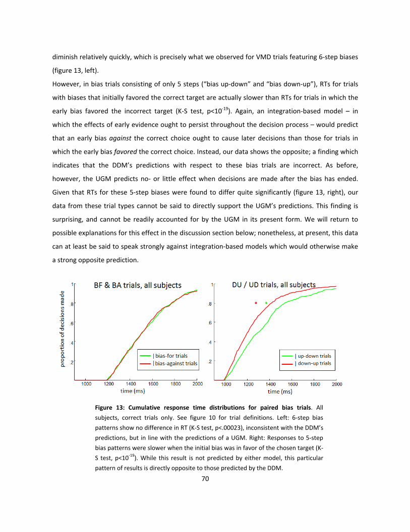
70

diminish relatively quickly, which is precisely what we observed for VMD trials featuring 6-step biases

(figure 13, left).

However, in bias trials consisting of only 5 steps (“bias up-down” and “bias down-up”), RTs for trials

with biases that initially favored the correct target are actually slower than RTs for trials in which the

early bias favored the incorrect target (K-S test, p<10-19). Again, an integration-based model – in

which the effects of early evidence ought to persist throughout the decision process – would predict

that an early bias against the correct choice ought to cause later decisions than those for trials in

which the early bias favored the correct choice. Instead, our data shows the opposite; a finding which

indicates that the DDM’s predictions with respect to these bias trials are incorrect. As before,

however, the UGM predicts no- or little effect when decisions are made after the bias has ended.

Given that RTs for these 5-step biases were found to differ quite significantly (figure 13, right), our

data from these trial types cannot be said to directly support the UGM’s predictions. This finding is

surprising, and cannot be readily accounted for by the UGM in its present form. We will return to

possible explanations for this effect in the discussion section below; nonetheless, at present, this data

can at least be said to speak strongly against integration-based models which would otherwise make

a strong opposite prediction.

Figure 13: Cumulative response time distributions for paired bias trials. All subjects, correct trials only. See figure 10 for trial definitions. Left: 6-step bias patterns show no difference in RT (K-S test, p<.00023), inconsistent with the DDM’s predictions, but in line with the predictions of a UGM. Right: Responses to 5-step bias patterns were slower when the initial bias was in favor of the chosen target (K-S test, p<10-19). While this result is not predicted by either model, this particular pattern of results is directly opposite to those predicted by the DDM.

71

Discussion

The main result of our study is that when subjects slow down their decision policy, the effect of early

pulses becomes weaker than the effect of later pulses (figure 12). While the specific pattern of pulse

efficacy in our two task conditions varied across subjects, the earliest pulse timings consistently lost

their efficacy as subjects slowed down. This result is important because it cannot be reproduced by

the DDM, or indeed any model whose central mechanisms involve the integration of the motion

signal over time; such models will always predict that early pulses will be at least as effective as late

pulses in reducing reaction times, because an integrator retains all input until decision time.

In contrast, the UGM explains this finding by positing that the motion signal is low-pass filtered and

brought to threshold through combination with an independent urgency signal that controls the

decision timing policy; thus, after a pulse, neural activity related to evidence increases briefly but

returns to the baseline “no-pulse” level only a short time later. A motion pulse therefore hastens the

response time on a given trial only if the decision is made after the pulse has caused a corresponding

increase in the evidence signal, but before the effect of the pulse has leaked away – otherwise, the RT

will not differ from a no-pulse trial (see figure 9). In other words, the UGM makes the qualitative

prediction that the efficacy of a given motion pulse will depend on its timing with respect to the time

of decision. By extension, any systematic change in the average timing of decisions will change which

pulse timings enhance RT. This is precisely what we observed: as subjects adjusted their average

speed of decision from one session type to the next, the effects of pulses became strongly dependent

on average response time, such that the effects of early pulses had time to leak away when decisions

were made relatively late. Such early-pulse trials – presented in a context of slower average decision

time – yielded RT distributions that were indistinguishable from no-pulse trials, despite the fact that

these same pulse timings were effective in sessions in which decisions tended to be made faster. Our

results would therefore appear to argue unambiguously against integration-based models, and

instead support the UGM.

There is, however, one possible objection to our interpretation of the findings presented here.

Because the motion signal during VMD trials in the interleaved sessions began at zero – and therefore

did not grow much in strength until several steps into the trial – it could be argued that our subjects

had merely learned to delay the onset of evidence integration for the first few hundred milliseconds

72

during the VMD sessions. Employing such a strategy would have spared our subjects the effort of

integrating what would otherwise tend to be a relatively uninformative stimulus, when they could

instead simply wait to integrate any signals at all until a point in the trial when the motion signal is

likely to be stronger (and therefore easier to discriminate). If true, this would cause them to show no

effects of the earliest pulse timings (e.g. the 100- and 200ms pulses) in the interleaved CMD trials,

because these pulses would have already ended before the subjects actually began integrating

evidence. Correspondingly, if the onset of integration was delayed by 200-300ms, the 400ms pulse

would effectively become a 100ms pulse, which would explain why such pulses suddenly became

effective in the VMD sessions. Moreover, this would not only explain the shifts in pulse efficacies

obtained in the VMD condition, but also the slower RT distributions for all VMD trials in general.

If our subjects really were simply ignoring the earliest portion of the evidence in VMD trials, however,

then any VMD trials in which our subjects made very early decisions would not be based on evidence,

and therefore ought to have yielded success rates at close to chance levels. To examine this

possibility, therefore, we analyzed the success probability for all VMD trials in which our five subjects

with the most sessions made their decision within the first two simulated “token” steps (DT <400ms).

This analysis revealed that such decisions were correct 79.67% of the time, thereby indicating that

this early information was not, in fact, ignored. This makes further sense considering our baseline

coherence value for CMD sessions was 3%, which is equivalent to a single coherence step in the VMD

trials. Thus while it was generally true that the evidence tended to improve over the course of VMD

trials – thus motivating the changes in decision policy shown in figure 11 – it does not necessarily

follow that the early portions of these trials are completely uninformative; in fact they are just as

informative as a regular CMD trial after only 200ms. Thus it makes sense that our subjects would not

have simply ignored this information altogether.

In sum, the differences we obtained in the efficacy of our various pulse timings as our subjects’

decision policies were manipulated across sessions strongly support the UGM (see figure 9).

Furthermore, the mechanisms of the UGM, and the manner in which its dynamics respond to various

forms of time-related factors can reveal several important features of the brain’s implementation of

the decision process, to which we now turn.

73

Current evidence vs. total weight of evidence

First and foremost, this finding directly contradicts the main predictions of integration-based models

like the DDM and instead strongly suggests that decisions are driven by the current (or at least recent)

state of the evidence, and not the total weight of all prior evidence. In this respect, the current

findings are in agreement with a number of prior studies demonstrating that decisions tend to be

made on the basis of information arriving from a rather narrow window of time (Cook & Maunsell,

2002; Gold & Shadlen, 2003; Ludwig et al., 2005; Luna et al., 2005; Ghose, 2006; Uchida et al., 2006;

Yang et al., 2008; Stanford et al., 2010; Zariwala et al., 2013; Kuruppath et al., 2014).

This conclusion is further corroborated by our findings regarding the “bias” VMD trials. As previously

observed (Cisek et al., 2009; Thura et al., 2012), early biases in evidence do not appear to have a

lasting effect on decisions (or at least, not in the manner predicted by integration-based models). In

the case of 6-step biases, for example, there appears to be no effect on response times for decisions

made after the end of the bias period (see figure 13, left). This closely mirrors our pulse data from the

CMD trials (see figure 12) in that the effects of early pulses were seen to leak away quite rapidly after

the offset of a pulse: in other words, such biases can be thought of simply as substantially larger

“pulses,” whose effects on the developing decision thus leak away over time in a manner similar to

the smaller pulses we inserted into CMD trials. Such a lack of an effect makes sense in light of the

UGM, because the evidence signal will quickly adapt to the offset of the bias after a short delay

imposed by the settings of the low-pass filter. This is precisely what appears to have occurred in our

6-step bias trials.

Our results from the 5-step biases (figure 13, right), however, are more difficult to interpret. An

integration-based model would predict faster responses for early biases in favor of the chosen target,

and slower responses for biases opposing it: instead, our data shows the direct opposite. While this

nonetheless directly contradicts the DDM’s explicit predictions, the UGM itself cannot offer a

straightforward explanation of why decisions would be slower following early evidence that favors

the chosen target. One potentially relevant factor may concern the fact that the 5-step biases, unlike

the 6-step biases, do not return to a state of 0% coherence. However, neither the DDM nor the UGM

offer any concrete mechanistic explanation for the apparently rather strong ramifications of such a

difference on the ensuing RT distributions. However, another possible explanation could be offered

on the basis of the pattern of evidence change in each trial type: in the “down-up” bias trials, all

74

motion changes after the first two coherence steps are continuously towards the same target;

whereas in the “up-down” trials, the initial bias is interrupted by two contrary motion changes. Again,

the mechanistic framework of the DDM does not appear to offer any straightforward account of why

such a difference would have the dramatic effect on RTs that we observed in the present experiment.

However, given that the UGM’s dynamics effectively emphasize novel information, the introduction

of the brief qualitative change in the development of the motion signal unique to the “up-down” bias

trials could play a role in slowing down the ensuing reaction times, as this brief reversal could be

interpreted as important novel information, which the UGM would necessarily be sensitive to. While

at present we cannot offer any conclusive explanation, the data we obtained in this regard could

serve as a potential avenue for further experimentation. In any case, however, the lack of an effect of

early biases in the 6-step bias trials remains a salient finding against integration-based models, as

these models make the strong prediction that the effect of such early- and dramatic biases should be

retained over the course of the decision process.

In general, the UGM’s reliance on only the current evidence makes sense not only with respect to the

experimental data reviewed here, but also makes ecological sense when considering the assumptions

made by integration-based models. Such models, like the DDM, operate as stated solely on the

assumption that each sensory sample is fully statistically independent from those that preceded it

(Bogacz 2006; Rao 2010; Thura, 2012). However, in any constant-evidence task, repeatedly sampling

the stimulus means that each additional sample is increasingly redundant, providing progressively less

novel information over time (c.f. Thura et al., 2012). Thus, it instead makes more sense to accumulate

information only to the extent that it is genuinely novel. This provides the main rationale for the fast

evidence-tracking mechanism employed by the UGM – namely, a low-pass filtered signal which

quickly adjusts to represent the current state of the sensory evidence while ignoring fluctuations at

frequencies above the range at which the signal of interest is likely to change. This mechanism not

only ensures that only novel information is accumulated, but also enables faster transitions between

decision options under conditions in which evidence can change. A perfect integrator would be slow

to reflect such changes, as it would have to first “undo” the previously-integrated sum for the initial

choice before it could begin to accumulate evidence in favor of the new choice. An urgency-gating

model, in contrast, could respond to the new choice after only a brief delay determined by the time-

constant of its low-pass filter (see figures 6a, 6b, and figure 7). This dynamical feature of the UGM is

directly exemplified by the lack of lingering effects of early biases discussed above, and is further

75

revealed by the dynamics of the evidence manipulations we performed in our main experiment.

Moreover, beyond its direct ramifications for the present experiment, this feature is likely to be

germane to natural, ecologically-situated behaviors taking place in unpredictable environments, in

which the relevant decision factors are not known ahead of time to the same degree as they are

under experimental conditions.

One potential alternative to the UGM’s account of these results could involve the addition of a “leak”

parameter to the DDM, such that early manipulations of evidence eventually leak away over time.

Indeed, just such a proposal has been suggested by a number of previous studies, and has led to a

sub-class of integration-based model called the leaky competing accumulator model (Usher &

McClelland, 2001). This model has been successfully employed in the past to account for a number of

previous findings in which the effects of changing evidence were observed to be time-dependent in a

manner similar to our present experiment (see Usher & McClelland, 2001; Tsetsos et al., 2012; Ossmy

et al., 2013).

However, it is unlikely that such models could by themselves account for our present data. In our

subjects the effects of pulses appear to “leak” away within only a few hundred milliseconds (see

figure 12); this would entail a leak parameter so large as to severely inhibit the ability for any

integration-based model to successfully accumulate weak evidence to a decision threshold. In fact,

adding such a leak would effectively turn such a model into a low-pass filter with a rather short time

constant (~200ms). Consequently, this leak parameter would have to be compensated for with the

addition of a dropping threshold so that decisions made on the basis of relatively weak evidence (as

they are in our task) would not continue indefinitely. Importantly, this is essentially what the UGM is

proposing; moreover, whereas introducing this feature to an integration-based model would require

the addition of several new parameters to the DDM, the same dynamics emerge from the UGM in a

more parsimonious manner.

The importance of filtering noisy input signals

Since its original formulation, the UGM has been explicitly challenged in a number of recent studies,

often involving its treatment of noise (Churchland et al., 2011; Winkel et al., 2014). Dealing with noise

is particularly important in the RDM task, in which the stimulus is inherently very noisy. Integrator

models deal with noise by adding together successive samples on the assumption that the noise

76

components of the input will cancel each other out over time, leaving an estimate of the underlying

signal (Ratcliff, 2001). On the surface, the UGM may appear susceptible to random, noise-driven

fluctuations because it privileges recent information (as claimed by Winkel et al., 2014). However,

because the UGM includes a low-pass filter, it is just as effective as an integrator at dealing with

noise: the time constant of the filter jointly determines both the frequency of input fluctuations

which will be screened out as noise, as well as the amount of time required for the evidence signal to

respond to a genuine change in the underlying stimulus. Indeed, for input signal components above

the filter cutoff frequency, a low-pass filter and an integrator are mathematically equivalent (for

mathematical proof see Thura et al, 2012, pages 7 & 16, and equations therein).

Two recent studies have attempted to criticize the UGM on noise-related grounds. Churchland et al.

(2011) suggested that the UGM cannot explain correlations in neural activity during motion

discrimination tasks, but these authors neglected to include the low-pass filter that is an essential

component of the urgency-gating model. More recently, Winkel et al. (2014) showed that in a

particular RDM task with pulses, early changes in evidence appeared to have an influence on decision

time in human subjects, even for decisions made substantially later (>1000ms). They then attempted

to replicate this behavioral data with both the DDM and the UGM, and claimed that the UGM was

unable to account for these effects, whereas the DDM was able to reproduce the qualitative trends in

the data. However, their implementation of the UGM, like that of Churchland et al. (2012), also

lacked a low-pass filter, which is critically necessary to the UGM’s dynamics and without which it

cannot work. A fair comparison of the UGM and the DDM, however, must allow both models to retain

their capacity to deal with such noise. Consequently, we successfully replicated their data with a UGM

that included a low-pass filter, thereby demonstrating that the UGM can, in fact, provide a qualitative

fit to their data (Carland, Thura, Cisek, in review). Crucially, even when the UGM matched their data,

it did not do so by causing early evidence to persist for as long as Winkel et al. claimed; rather, the

means of the RT distributions shifted slightly due to the early evidence causing slightly more early

decisions – similar to the effects of pulses in our present experiment – and therefore this early

evidence affected only a subset of the response times. This finding thus demonstrated a crucial

methodological point that is of critical importance when comparing models: dynamical differences

among models cannot be fully appreciated without a fine-grained analysis of response time

distributions. Simply comparing mean response times can lead to erroneous conclusions, such as

77

Winkel et al.’s conclusion that early evidence impacts the timing of decisions over an extended period

of time.

Ultimately, the challenges made to the UGM so far have involved implementations thereof which

have been mechanistically incomplete, and therefore have not served as fair comparisons. However,

when implemented correctly, the UGM can account for most of the extant data equally as well as the

DDM. Thus, while the DDM has a long history, most of the data used to support it can be used equally

as well to support the UGM, as they make identical predictions under conditions of constant evidence

(Cisek et al., 2009; Thura et al., 2012; see also figure 9). The converse, however, is not the case: much

of the extant experimental work in which evidence has been allowed to change within a given trial

has yielded data that has been consistently problematic for the DDM in non-trivial ways.

Furthermore, even when the DDM has successfully addressed these studies, it typically has done so

by adding further parameters, rather than making substantial mechanistic revisions to its basic

framework. This approach is problematic because it can be continued indefinitely – with apparent

empirical success – but merely for the trivial reason that additional model parameters necessarily

enrich the dynamics of a model (Rae, Heathcote et al., 2014).

Urgency, time pressure and reward rate

The manipulation of time pressure in our task relied on our subjects’ ability to implicity adjust their

decision policy to adapt to the evidence available in each task context. In the “blocked” condition,

there was no benefit to prolonging decisions, and our subjects consistently appeared to adopt a

strategy of hastening their decisions by responding as soon as they could detect the motion signal. In

contrast, in the “interleaved” condition the quality of the sensory evidence tended to increase over

time, and our subjects implicitly adapted to this context by making significantly slower decisions,

thereby capitalizing on the benefit to decision accuracy that they could obtain by delaying their

decisions until the evidence was less ambiguous.

This ability of our subjects to tailor their decision policy to each task context speaks to the broader

notion of behavioral optimization. Many studies have demonstrated that decision-makers are acutely

sensitive to the reward contingencies of experimental tasks, and that they frequently converge on

decision policies that are near-optimal after only a relatively short learning period (see Bogacz et al.,

2006; Balci et al., 2012). While the precise mathematical derivation of optimal decision policies is a

78

computationally demanding problem that is likely beyond the capacities of most human subjects

under normal conditions (and almost certainly beyond those of non-human subjects), the ability for

decision models to capture behaviorally-meaningful changes in decision policy with only a few

parametric changes suggests that the ability of decision-makers to converge on near-optimal policies

may be the result of the fact that the speed-accuracy trade-offs intrinsic to ecological behaviors can

be effectively managed with only a small number of relevant parameters, thereby constraining the

problem space to a limited number of dimensions.

The use of a singular “urgency” signal to control the timing of decisions thus provides a unitary means

for a decision-maker to adapt their decision policy to maximize reward rate. That is, the two

parameters governing the urgency signal’s dynamics (i.e. the mean and standard deviation of the

urgency signal’s slope) control the average timing of the decision both by weighting the evidence

more strongly over time as well as controlling the rate at which the effective decision threshold

drops, thereby preventing the unneccessary loss of time during difficult decisions. This singular

control mechanism is thus an effective means by which an animal may regulate many diverse aspects

of its decision strategy. Relatedly, while advocates of integration-based models have previously made

a number of claims regarding the optimality of the DDM, many such demonstrations have – either

implicitly or explicitly – evaluated these models only under the assumption that thresholds remain

constant throughout a decision period (Ratcliff & Smith, 2004; Bogacz et al., 2006; Simen et al., 2009).

While the DDM can indeed achieve greater reward rates than any other integration-based model, its

optimality has only been demonstrated under the assumption of static thresholds. A number of

subsequent studies that have directly compared a number of constant- and dropping-threshold

models have revealed that in all cases, models in which the thresholds drop over time always

outperform static-threshold models (Balci et al., 2012; Thura et al., 2012). Accordingly, the role of

urgency in controlling the timing of behavior directly implements a dropping threshold in the decision

process, thereby enabling a decision-maker to adapt their decision policy to maximize reward rate in

a manner consistent with mathematical analyses of optimal behavior.

Our use of two distinct decision contexts to manipulate the “time pressure” in our task is also

consonant with previous work by Balci et al. (2012), who demonstrated that subjects typically adjust

their decision policy on a “sessional” basis by converging on a single set of parameters that optimize

behavior with respect to the overall distribution of trial difficulties encountered in a given setting.

79

However, while Balci et al. demonstrated this in the context of a constant-evidence task, our current

results demonstrate that this principle applies to the more ecologically-relevant case of changing-

evidence tasks. Moreover, we induced these adaptive changes in our subjects’ decision policies not

by simply changing the strength of the evidence, but also by changing the value of stimulus

observation time, such that extra observation time in the “blocked” condition represented only a

time cost, whereas additional observation time in the “interleaved” sessions was valuable as it could

lead to improved decision accuracy. Consequently, these two experimental contexts presented our

subjects with unique speed-accuracy trade-offs that mandated the use of different decision policies

to maximize the rate of reward acquisition throughout the experimental session.

The explicit link between the UGM’s urgency signal and the timing parameters of a task also afford a

clear means for interpreting a variety of prior findings. For example, the systematic transitions in

efficacy between early and late pulses across our two experimental conditions are analogous to the

primacy and recency biases observed during a similar RDM task by a number of previous studies

(Usher & McClelland, 2001; Huk & Shadlen, 2005; Kiani et al., 2008; Tsetsos et al., 2012). In these

studies, each of these biases could be obtained within individual subjects, and the transition between

these biases appeared to be caused by manipulating the “time pressure” involved in the performance

of the task (Tsetsos et al., 2012). The authors of these studies explained these effects by

parameterizing a DDM-influenced model to incorporate a “leak” of accumulated evidence over time,

with the value of this leak parameter being allowed to vary freely when modeling the behavioral data

from each task condition: however, the precise relationship between “time pressure” and “leak” in

these authors’ accounts was neither ecologically- nor physiologically motivated. In contrast, the

UGM’s explicit link between time-pressure and the rate at which the urgency signal rises over time

provides a more complete theoretical framework for accounting for the emergence of such biases:

when time pressure is high, the urgency signal will rise more quickly, causing early pulses to be more

likely to reach the decision threshold, with later pulses tending to occur too late to cause an effect.

Conversely, when time pressure is low, the effect of early pulses will leak away by the time most

decisions are made, whereas late pulses will now tend to become effective as they fall closer in time

to the time of decision. Given that Tsetsos et al. (2012) explicitly used “time pressure” to elicit these

various biases (albeit in a different manner than in our task), the framework offered by the UGM

provides a straightforward explanation for the emergence of these biases in a manner that does not

simply rely on adding yet more parameters to an increasingly-complex integration model. Moreover,

80

the model can itself specify and predict the effects of time-related task factors on behavioral

performance, rather than merely accounting for them in a post hoc manner.

The wider significance of the UGM

So far we have reviewed a number of discrete, empirically-demonstrated shortcomings of the DDM as

well as identified some broader, potentially problematic theoretical issues with the DDM, with the

aims of loosening the otherwise implicit commitment to the DDM as the essential decision model. In

its place we offer the UGM, a mechanistically simple model which nonetheless can account for much

of the behavioral and physiological data equally as well as the DDM, but which is not itself beholden

to several of the problematic foundational assumptions inherited from the sequential sampling

framework. However, while we have focused on discrete comparisons between the DDM and UGM

with regards to their theoretical rationale, parameterization, and their ability to account for

behavioral data, the UGM also offers additional potential benefits to the field beyond merely serving

as an alternative model of decision behavior during TAFC perceptual discrimination tasks.

Accordingly, we now turn to a discussion of the broader significance of the UGM, and its potential

implications beyond the simple, traditional forms of decision-making research described thus far.

Urgency signals and reward rate maximization: beyond RT

As mentioned previously, one of the important strengths of the UGM lies in its potential to account

for how real-world decision-makers can rapidly achieve optimal (or near-optimal) decision strategies

for maximizing the rate of reward acquisition across a diverse range of environments and contexts.

The mechanistic centrality of the urgency signal in governing the ensuing temporal dynamics of

decisions, together with its parametric simplicity, means that the search space for optimal decision

parameters can be essentially pre-constrained to two variables: one specifying the mean slope of the

urgency signal, and a second governing its variability with respect to this mean across multiple

decisions or trials. This parametric elegance provides the UGM with the flexibility required to find

decision policies which can maximize the rate of reward across a number of different decision

contexts and settings.

Traditionally, measures of behavioral optimization have focused exclusively on the timing of the

decision process, such that a decision policy is considered optimal if it can be shown to produce

decision times whose durations are appropriate for achieving the best possible average rate of

81

reward over large sets of trials (Ratcliff & Smith, 2004; Bogacz et al., 2006; Simen et al., 2009; Balci et

al., 2012). However, decisions in both experimental and real-world settings typically entail the

selection of a behavior by which such rewards are acquired – and non-decision factors such as the

speed, accuracy, and energetic costs of movements may therefore have a direct impact on reward

rate independently of the length of the deliberation process itself. For this reason, it could be argued

that the optimization of reward rate involves not only the fine-tuning of those decision parameters

explicitly featured in the DDM and UGM themselves (see above equations), but also may involve the

parameterization of non-decision processes, such as those related to motor execution.

A relatively simple example in support of such an argument comes from an early study by Ljungberg

et al. (1992), who showed that a monkey’s reaching movements to collect food rewards were

executed more quickly when such rewards were made continuously available. When these same

rewards were available only according to a schedule of fixed intervals, the monkey’s movements

tended to be made significantly more slowly, i.e. at a default speed more typical of the monkey’s

general behavior when not performing a task under time pressure. This relationship between reward

availability and movement speed was originally interpreted as arising due to the fact that when

rewards are plentiful, slower movements would reduce the overall rate of reward, whereas the cost

of making faster – but more effortful – movements is justified by the potential gains. Therefore,

movements should be made more quickly under such conditions so as to acquire more rewards in a

shorter period of time. In other words, when the potential reward rate was high, the relative cost of

moving quickly was sufficiently counterbalanced by the availability of reward, and movement speed

was increased accordingly. In contrast, when rewards were available at a limited and fixed rate, the

ultimate rate of reward was not significantly affected by motor speed (being essentially

predetermined by the reward schedule alone), and the monkey could therefore collect the maximum

possible reward while still conserving effort by making unhurried movements. Consequently, the

selection of movement speed appears to represent the outcome of a process by which reward rate is

optimized by maximizing reward intake while simultaneously minimizing the cost (in effort and/or

energy) of the required actions.

While Ljungberg et al.’s (1992) study did not involve a perceptual decision component per se, this

early finding linking movement speed to reward rate has been expanded upon by a number of

additional studies operating under the general rationale that the most fundamental purpose of motor

82

behavior is to place an animal in a more rewarding state (c.f. Choi et al., 2014). These subsequent

studies have extensively catalogued the ways in which various motor factors can contribute

substantially to the optimization of decision-making behavior (see Segraves et al., 1987; Snyder et al,

2002; van Donkelaar et al, 2004; Churchland et al, 2006; Xu-Wilson et al., 2009; Opris et al, 2011;

Salinas et al, 2014), and together provide substantial empirical justification for considering motor-

behavioral factors when assessing the overall optimality of real-world decision behavior.

Pursuant to this broadened perspective on behavioral optimization, some recent evidence suggests

that “urgency” may play a direct causal role in governing the speed with which movements are made,

thereby providing a discrete mechanism by which the relationship between reward rate and motor

control may be understood from within a single unified framework. For example, Thura, Cos, Trung &

Cisek (2014) have recently shown that the speed of the arm-reaching movement with which a

monkey reports the outcome of a decision appears to increase as a direct function of elapsed time,

such that movements following trials in which the decision was made late tend to be faster than

those same movements used to report the outcome of a relatively faster (earlier) decision. These

observations were interpreted as evidence that the additional deliberation time spent producing later

decisions can be (at least partially) offset by increasing the speed of the movement used to report

that decision’s outcome. Such a means of counteracting the cost of time therefore serves as an

additional means of enhancing reward rate in a manner which is nonetheless separate from the

parameterization of the decision process in itself.

Additionally, Thura et al.’s (2014) experimental procedure also featured two distinct task blocks: a

“fast” block, in which inter-trial intervals were relatively short, and a “slow” block in which they

tended to be longer. Accordingly, the available reward rate in the fast block was higher than that in

the slow block. Thus, similar to our present experiment, these two task contexts entailed parametric

adjustments to the urgency signal across conditions in order to achieve the optimal reward rate

within each task block. Importantly, when comparing movement speeds across these two conditions,

Thura et al. observed that the absolute range of the variability in movement speed corresponded to

the inferred urgency parameters appropriate to each condition, such that arm movements were

faster overall in the fast block than they were during the slow block (ibid). Furthermore, comparisons

of movement speeds across similar trials within task blocks indicated that the motor parameters

governing movement speed grow steadily over the course of a given decision, similar to the manner

83

in which the urgency signal itself is posited to rise over time to control the weighting of evidence.

Additionally, the velocity of saccadic movements were also significantly faster during the fast blocks

relative to the slow blocks, despite the fact that oculomotor movements are controlled by separate

motor networks that are independent from those governing arm movements (Bahill et al., 1975;

Raybourn & Keller, 1977; Scudder et al., 2002). Thus, movement speed across multiple behavioral

domains appears to track the state of the urgency signal not only within a given trial, but also across

different decision contexts.

Importantly, these consistent, inverse relationships between decision timing and movement duration

emerged in the absence of any explicit instructions regarding movement speed, but instead were

elicited solely by the changes in reward rate caused by the manipulation of inter-trial intervals across

task blocks. Consequently, the observed changes in both decision timing and movement speed can be

safely interpreted as having arisen in response to the implicit manipulations of reward rate. In

general, then, these results suggest that monkeys are compensating for the effect of longer decision

times on reward rate by producing faster and more effortful movements. In this respect, Thura et al.’s

findings are in agreement with additional findings from a study by Salinas et al. (2014), who observed

similar modulation of oculomotor behaviors during a speed-accuracy trade-off task in which faster

movements were employed to effectively counteract the time cost of lengthier decisions. Although

Salinas et al. did not use a UGM to explain their results, their model included a time-dependent signal

analogous to the urgency signal of the UGM, and their results are therefore highly compatible with

the notion of an urgency-like mechanism for relating reward rate maximization to motor control.

Ultimately, the observation that these decision-related and non-decision motor parameters appear to

vary together raises the possibilty that these effects may both be reflections of a common control

parameter. For this reason, Thura et al. concluded that reward rate optimization appears to involve

“…a global, context-dependent arousal that influences the oculomotor as well as the arm motor

system” (Thura et al. 2014, p11) – a function that they ascribe to the urgency mechanism in the UGM.

Importantly, the evidence for global control signals modulating both decision-making and motor

behavior supplied by the findings discussed above are further complemented by a host of other

studies on the topic of “motor motivation” (c.f. Mazzoni et al., 2007) which have extensively

documented similar links between reward rate and various underlying parameters of motor control

(see Takikawa et al., 2002; Watanabe & Hikosaka, 2005; Bendiksby & Platt, 2006; Harris & Wolpert,

84

2006; Milstein & Dorris, 2007; Niv et al., 2007; Pasquereau et al, 2007; Shadmehr, 2010; Shadmehr et

al., 2010; Turner & Desmurget, 2010; Guitart-Masip et al, 2011; Dayan, 2012; Haith et al., 2012;

Salamone et al, 2012; Tachibana & Hikosaka, 2012; Choi et al, 2014). These studies suggest that the

selection of motor speed bears a systematic relationship to reward rate, and, taken together, provide

substantial support for the possibility that animals may employ a single underlying mechanism to

simultaneously adjust both the speed of their decisions as well as the motor behaviors by which their

outcomes are reported. The practical outcome of such a control scheme would be a single, unitary

mechanism for negotiating the trade-offs between speed and accuracy (or speed and behavioral

effort) arising within both the decision process as well as within the specific motor domains through

which these decisions’ outcomes are effectively expressed.

Together, then, this extended body of research would in turn point toward the possibility that

“urgency” – or something mechanistically very similar – may serve a broad and crucial role in the

wider functional economy of the brain. Notably, however, the extended family of integration-based

models do not feature any mechanism(s) by which the mutual dependencies among decision time,

reward rate and movement speed could be easily accounted for. Ultimately, then, this growing body

of empirical support for the functional coupling between motor parameters and reward rate

maximization not only represents a novel avenue for decision research, but is also one which the

UGM is uniquely suited to explain.

Potential physiological origins of the urgency signal

Given the provisional evidence for this broadened functional role of the urgency signal, a salient

outstanding question remains regarding the potential origin of this signal. Relatedly, a considerable

number of physiological studies have demonstrated time-dependent build-up of neural activity in a

wide array of cortical areas across a number of diverse tasks (see Leon and Shadlen 2003; Janssen and

Shadlen 2005; Maimon & Assad 2006; Renoult et al., 2006; Churchland et al. 2008; Lebedev et al.,

2008; Mita et al., 2009; Casini & Vidal, 2011; Hanks et al. 2011; Heitz & Schall, 2012). One possible

explanation for these physiological observations is that “urgency” may simply be a local feature

common within many otherwise independent cortical networks subserving decision-related

processing. The observation of “urgency-like” build-up in these regions could therefore be interpreted

as a straightforward consequence of a cortical region’s engagement in the functional demands of a

particular task, without therefore necessarily indicating a common source or function.

85

However, another possibility is that these consistent observations of “urgency-like” activity could be

indicative of a singular control signal that is broadcast widely throughout the brain, whose functional

purpose would be to coordinate multiple aspects of behavior simultaneously. With regards to this

possibility, several key features of the basal ganglia’s (BG’s) broader connective and functional profile

would recommend it as a candidate source for such a signal. Firstly, the observation of common

patterns of activity across a variety of cortical sites would fit well with the BG’s widespread and

reciprocal anatomical connectivity with a broad range of cortical networks (Graybiel et al., 1994; Niv

et al., 2007; Gurney et al., 2001a; 2001b; Forstmann et al., 2010). The well-known functional

contibutions of the basal ganglia to motor control – especially in regards to its regulation of the

speed- and size of movements (Kori et al., 1995; Hikosaka et al., 2000; Sato & Hikosaka, 2002; Niv et

al, 2007; Turner & Desmurget, 2010; Opris et al., 2011; Tachibana & Hikosaka, 2012) would further

argue for its candidacy in this regard. Additionally, a number of BG structures have been directly

implicated in behavioral adjustments involving the management of speed-accuracy trade-offs

observed during a number of tasks (Lo & Wang, 2006; Bogacz & Gurney, 2007; Forstmann et al., 2008;

van Veen et al., 2008; Domenech & Dreher, 2010; Forstmann et al., 2010; Humphries et al., 2012;

Nagano-Saito et al., 2012; Ding & Gold, 2013) – a functional link which is further consistent with the

BG’s empirically-established role in modulating behavior in accordance with the reinforcement

contingencies of a given task (Graybiel et al., 1994; Barto, 1995; Schultz et al., 1997; Kawagoe et al.,

1998; Doya, 2000; Sato & Hikosaka, 2002; Tobler et al., 2005; Daw & Doya, 2006; Kable & Glimcher,

2007; Kobayashi & Schultz, 2008; Turner & Desmurget, 2010; Hayden et al., 2011; Opris et al., 2011;

Jimura et al., 2013). Finally, a long history of findings regarding the centrality of dopaminergic activity

in the regulation of reward-driven behavior (Kori et al., 1995; Niv et al., 2007; Pine et al., 2010; Turner

& Desmurget, 2010; Burke & Tobler, 2011; Opris et al., 2011; Humphries et al., 2012; Hsiao & Lo,

2013) is strongly suggestive of BG involvement in linking various aspects of reward processing with

overt expressions of behavior. Taken together, then, these various anatomical and functional aspects

of the BG make them highly plausible as a likely neurobiological origin of a unitary signal that is

broadcast widely across the brain.

Urgency and delay-discounting

The putative functional generality of urgency signals – along with their possible origin in the basal

ganglia – entail a number of suggestive implications for understanding a variety of clinical disorders.

86

One such avenue of potential research has been identified in a series of recent studies by Shadmehr

and colleagues, who have investigated the links between reward-rate maximization and motor

control from the perspective of temporal discounting (see Xu-Wilson et al., 2009; Shadmehr, 2010;

Shadmehr et al., 2010; Haith et al., 2012; Choi et al., 2014). Temporal discounting is a well-studied

and seemingly ubiquitous feature of animal behavior across both human and non-human species

(Myerson & Green, 1995; Kacelnik, 1997; Navarick, 2004; Schweighofer et al., 2006; Kobayashi &

Schultz, 2008; Shapiro et al., 2008; Hwang et al., 2009; Jimura et al., 2009; Green et al., 2010),

according to which animals assign progressively less subjective value to a reward as its receipt is

delayed further into the future (Millar & Navarick, 1984; Navarick, 2004; Schweighofer et al., 2006;

Haith et al., 2012). Importantly, human individuals are known to vary considerably in the rate at

which they devalue a given reward over time (Green et al., 1981; Frederick et al., 2002; Green &

Myerson, 2004; Navarick, 2004; McClure et al., 2007); furthermore, these individual differences in

delay-discounting policy are remarkably stable over extended periods of time (Ebert & Prelec, 2007;

Kirby, 2009), suggesting that individual variations in temporal discounting functions are reflective of a

discrete underlying personality trait dimension (Metcalfe & Mischel, 1999; Frederick et al., 2002;

Rachlin, 2006; Van den Burgh et al., 2008; Zauberman et al., 2009; Peters & Büchel, 2011). Relatedly,

a substantial body of psychometric research places individual differences in temporal discounting

(alternatively “time preference” or “temporal orientation”: see Frederick et al., 2002, and Steinberg

et al., 2009) within a broader constellation of personality traits related to general impulsivity

(Kacelnik, 1997; Metcalfe & Mischel, 1999; Reynolds, 2006; Madden & Bickel, 2010; Pine et al., 2010;

Sharp et al., 2012), which has in turn been implicated as a latent risk factor for a variety of clinical

outcomes related to ADHD and addiction as well as to a wider array of problematic risk-seeking and

externalizing (i.e. antisocial) behaviors (Kirby et al., 1999; Dallery & Raiff, 2007; MacKillop & Kahler,

2009; Moore & Cusens, 2010; Bickel et al., 2011; Peters & Büchel, 2011; Sharp et al., 2012; Koffarnus

et al., 2013; McClure & Bickel, 2014). The interrelationships among these traits – and their relevance

to clinical outcomes – are theorized to arise as a consequence of a suite of subtler latent deficits in

accurately assessing future outcomes in general (Kacelnik, 1997; Reynolds, 2006; Steinberg et al.,

2009; Madden & Bickel, 2010; Bickel et al., 2011; Koffarnus et al., 2013; Story et al., 2014).

In pursuit of these potential connections to clinical issues, Shadmehr and colleagues exploited the

fundamental logic of temporal discounting with the objective of developing decision-making

paradigms that could yield discrete behavioral measurements of a subject’s underlying temporal

87

discounting function (Shadmehr, 2010; Haith et al., 2012; Choi et al., 2014). Specifically building upon

the substantial body of previous decision-making studies establishing the causal relationship between

reward rate and movement speed, they reasoned that differences in temporal discounting policy

ought to affect subjective estimates of reward rate, which in turn may manifest as overt changes in

movement speed in response to experimental manipulations of reward rate (Shadmehr, 2010;

Shadmehr et al., 2010; Shadmehr & Mussa-Ivaldi, 2012). For example, consider a hypothetical two-

block task design in which subjects acquire rewards of uniform size in response to correct choices

between two targets, which they report with saccadic eye movements. Further suppose that in the

first task block, rewards are acquired immediately, with no delay; in the second block, subjects then

perform the same task in which these same rewards are now acquired after a uniform delay that is

consistent across all trials. The general framework of delay-discounting leads to the straightforward

prediction that the delayed rewards will be assigned less subjective value than when these same

rewards are obtained immediately; thus the reward rate for any given subject will necessarily be

lower in the second block relative to the first. However, if subjects differ in the rate at which they

discount rewards over time, the relative magnitude of this change in reward rate across the two task

blocks will be perceived as being larger by a subject who discounts rewards more rapidly than it will

by a subject who discounts them more slowly – even if the actual change in reward rate is objectively

the same in both cases. Consequently, if movement speed is a direct function of reward rate, it

follows that a subject who discounts rewards steeply should exhibit a more pronounced change in

movement velocity across the two task blocks in comparison to a subject who discounts less steeply

(Shadmehr & Mussa-Ivaldi, 2012). Based on this reasoning, Shadmehr et al. hypothesized that it

should be possible, in principle, to compare and quantify the discounting functions of individual

subjects by measuring the changes in the speed of their movements in response to experimental

manipulations of reward rate over the course of a simple decision task.

This was essentially the hypothesis tested by Choi et al. (2014), who found that the resulting

behavioral measures of movement speed could indeed serve as a valid and reliable behavioral metric

for an individual’s rate of temporal discounting, such that greater changes in movement speed in

response to a given manipulation of reward rate are indicative of steeper underlying discounting

functions. Intriguingly, the authors also obtained significant correlations between these behavioral

measures and a number of traditional psychometric assessments of trait impulsivity that they

administered to their subjects (Choi et al., 2014). Thus, in light of the aforementioned relationships

88

between temporal discounting and impulsivity on one hand, and between impulsivity and clinical risk

status on the other, the correlations Choi et al. (2014) obtained between their behavioral measures of

temporal discounting and traditional personality measures of impulsivity are highly suggestive of the

latent clinical utility of such decision tasks as proximal measures of temporal discounting function.

Such tasks might be of genuine clinical significance not only because of their potential to discretely

quantify temporal discounting policies Shadmehr & Mussa-Ivaldi, 2012; Choi et al., 2014), but also

because such indirect behavioral indices of temporal discounting may also avoid many of the

methodological pitfalls otherwise inherent in the self-reported nature of the questionnaire-based

batteries typically used to assess underlying trait impulsivity (see Navarick, 2004).

Urgency in the aetiology of Parkinson’s disorder

The potential clinical ramifications of contemporary decision-making research are not limited only to

impulsivity, but may in fact have the potential to be extended towards our understanding of

neuropathologies such as Parkinson’s disease (PD). Once again, this potential is grounded in the

explicit mechanistic links made between reward rate and movement speed in the urgency-gating

framework. For example, Mazzoni et al. (2007) administered a simple arm-reaching task to both

healthy subjects and PD patients, who were asked to complete a required number of accurate

reaching movements to variously-sized targets without visual feedback while maintaining the speed

of their movements within a certain prespecified range. While the PD patient group as a whole

required more attempts on average to complete the required number of correct movements, analysis

of their movement kinematics revealed that they were in fact capable of making movements with

speed and accuracy comparable to that of healthy controls. Instead, their true deficits appeared to

reflect an inability to reliably select appropriate parameters from among their extended repertoire of

motor commands, with the ultimate result that they require more attempts to succesfully complete a

given reaching movement according to a given set of parametric specification. Furthermore, these

impairments were observed to become more pronounced as the biomechanical costs of the required

movements increased (ibid), suggesting that the underlying motor-parameter-selection mechanisms

themselves were related to the subjects’ assessment of the relative rewards and/or costs of the

movements to be made.

Mazzoni et al. (2007) thus ultimately concluded that the pathophysiological slowing of movement

typically observed in advanced stages of Parkinson’s disease may not involve straightforward deficits

89

in motor control, as previously thought (Pendt et al., 2011). Instead, the underlying deficit in

Parkinsonian bradykinesia may consist of impairments in the ability to accurately estimate the

relative cost of a given movement, with PD patients tending to implicitly over-estimate the cost of a

given movement – a tendency that becomes more pronounced as the objective costs of a movement

increase. This, in turn, would decrease the subjective value assigned to any given action, which by

extension will result in a distorted estimate of the overall reward rate within any given task. The

effects of these underlying deficits in reward valuation may therefore manifest as disturbances in

overt motor behavior indirectly via their distal effects on an underlying, implicit “motor motivation”

system.

Notably, given that Mazzoni et al.’s (2007) mechanistic explanation of these deficits is predicated on

an explicit functional relationship between reward- and motor control networks, their account is

strongly reminiscent of the role of urgency signals described above. The possibility that movement

disorders may actually be distal reflections of “urgency-like” mechanisms originating in the basal

ganglia enjoys further plausiblity given that the BG are widely considered to be the primary locus of of

PD pathophysiology. This conclusion is further supported by a number of closely-related studies

noting similar relationships between motor control and various aspects dopaminergic transmission

among the BG (Niv et al., 2007; Pine et al., 2010; Maia & Frank, 2011; Pendt et al., 2011; Haith et al.,

2012), as well as being consonant with the wider role of the BG in relating reward contingenies to

motor behavior (Graybiel et al., 1994; Schultz et al., 1997; Daw & Doya, 2006; Kobayashi & Schultz,

2008; van Veen et al., 2008; Turner & Desmurget, 2010; Hayden et al., 2011; Opris et al., 2011;

Humphries et al., 2012; Hsiao & Lo, 2013). Consequently, such studies are steadily building up

empirical support for the idea that the underlying aetiologies of both Parkinson’s disorder as well as

of individual clinical risk factors such as impulsivity may find a common origin in “urgency”-related

dysfunction – albeit with differing symptomatic manifestations.

Conclusion

The present experiment was meant to explicitly test the predictions of the DDM and the UGM for a

unique experimental task within which the two models’ predictions diverge – and its results in this

regard argue decisively in favor of the UGM. This result is important because while most prior

90

decision-making research has been guided by a broadly consensual commitment to integration-based

models, the results of most such empirical work could be accounted for more-or-less equally by both

integration-based and urgency-gating models. The majority of the extant behavioral and physiologal

data accumulated over the preceding decades of decision-making research, therefore, cannot be said

to have permitted strong conclusions regarding the superiority of either model.

Nonetheless, popular support for integration models has remained unjustifiably strong in spite of

both the lack of exclusive empirical support for such models, as well as the considerable number of

substantive theoretical and empirical criticisms that can be made of them. For these reasons,

contemporary work employing novel variants of traditional decision-making paradigms that are

capable of differentiating between integration-based and alternative models will be of continuing

importance to the development of the field, as they may stimulate the development of newer and

more complete models by loosening the entrenched (and increasingly untenable) comittment to

integration-based models as the default explanatory framework in contemporaty decision-making

research.

Strictly speaking, our experiment was not the first such study to argue against the DDM: a number of

recent studies have also presented data that strongly resist easy explanation by integration-based

models (Usher & McClelland, 2001; Cisek et al., 2009; Thura et al., 2012; Tsetsos et al., 2012).

However, while such studies are of note for this reason alone, the alternative models they have been

used to support can nonetheless be argued to fall short on the basis that their mechanistic revisions

to the DDM are neither ecologically well-motivated, nor sufficient to overcome many of the

theoretical shortcomings inherent in the sequential sampling framework identified in the foregoing

discussion. Neither is the present experiment the first to offer decisive empirical support explicitly for

the UGM: a number of prior studies have previously shown data that are exclusively consistent with

an urgency-gating framework (Cisek et al., 2009; Thura et al., 2012; Thura et al., 2014). However,

these studies have been questioned on the basis of their methodological departure from more

traditional forms of perceptual decision tasks, and their results can therefore be potentially dismissed

as being task-specific (see Thura et al., 2012, p1-2). The present experiment is, however, the first

study to date to yield relatively unambiguous and exclusive support for the UGM using a decision task

which was designed to be as similar as possible to those used extensively in the past to support

integration models. Its results therefore cannot be easily dismissed as task-dependent, and in this

91

respect futher reinforce the conclusions of prior studies whose results similarly appear to support the

UGM (Cisek et al., 2009; Thura et al., 2012; Thura et al., 2014). The present work also further

reinforces the broader array of studies which have provided direct evidence against the DDM and its

closely-related models (Usher & McClelland, 2001; Cisek et al., 2009; Thura et al., 2012; Tsetsos et al.,

2012), but also further extend such studies by offering a single, ecologically-motivated framework by

which the mutual influences among reward rate, movement speed, and the various parameters

governing decision timing can be systematically accounted for by their effects on a common control

mechanism of broad functional scope.

This unified framework can in turn generate novel predictions not only for decision-making research,

but also offers a number of relatively concrete and empirically-tractable inroads for addressing a

number of broader phenomena of significant clinical interest, as outlined in the preceding discussion.

Thus the urgency-gating model may ultimately provide a theoretical impetus to integrate empirical

efforts from within the domain of perceptual discrimination tasks to larger issues of potentially broad

clinical relevance. The most immediate way in which the UGM might do so is by guiding the

adaptation of simple, traditional decision-making tasks into relatively straightforward and valid

alternative diagnostic measures, thereby enhancing the methodological repertoire available to

clinicians in regards to the psychometric measurement and/or risk-assessment of various populations.

This makes the UGM a promising foundation for future research: moreover, this unique theoretical

potential is specific to the UGM, and therefore further distinguishes it from integration models like

the DDM. Thus, at its most general, the development and empirical refinement of novel decision-

making models like the UGM may ultimately serve to situate the field of decision-making within a

wider psychological and neurobiological purview.

92

Works Cited

(By order of first author and year of publication)

------------------------------------------------------------------------------------------

Abeles, M. (1991). Corticonics: neural circuits of the cerebral cortex. Cambridge University Press.

Bahill, T.A., Clark, M.R. & Stark, L. (1975). The main sequence: A tool for studying human eye movements. Mathem. Biosci. 24(3-4): 191-204.

Balci, F., Simen, P., Niyogi, R., Saxe, A., Hughes, J. A., Holmes, P., & Cohen, J. D. (2011). Acquisition of decision making criteria: reward rate ultimately beats accuracy. Atten Percept Psychophys 73(2): 640-657.

Bair, W., Cavanaugh, J.R., Smith, M.A., Movshon, J.A. (2002). The timing of response onset and offset in macaque visual neurons. J Neurosci 22: 3189-3205.

Barnard, G.A. (1946). Sequential tests in industrial statistics. J Royal Stat Soc 8: 1-26.

Barto, A.G. (1995). Adaptive critics and the basal ganglia. In Models of Information Processing in the Basal Ganglia (pp215-232), Cambridge, MA.

Basso, M.A. & Wurtz, R.H. (1998). Modulation of neuronal activity in superior colliculus by changes in target probability. J Neurosci 18(18): 7519-34.

Beck, J.M., Ma, W.J., Kiani, R., Hanks, T., Churchland, A.K., Roitman, J., Shadlen, M.N., Latham, P.E., Pouget, A. (2008). Probabilistic population codes for Bayesian decision making. Neuron 60: 1142–1152.

Bendiksby, M.S. & Platt, M.L. (2006). Neural correlates of reward and attention in macaque area LIP. Neuropsychologia, 44(12): 2411-20.

Bickel, W.K., Yi, R., Landes, R.D., Hill, P.F. & Baxter, C. (2011). Remember the future: working memory training decreases delay discounting among stimulant addicts. Biol Psychiatry 69(3): 260-65.

Bizley, J.K., Walker, K.M., Nodal, F.R., King, A.J. & Schnupp, J.W. (2013). Auditory cortex represents both pitch judgments and the corresponding acoustic cues. Curr Biol 23(7): 620-5.

Blatt, G.J., Andersen, R.A. & Stoner, G.R. (1990). Visual receptive field organization and cortico-cortical connections of the lateral intraparietal area (area LIP) in the macaque. J Comp Neurol 299(4): 421-45.

Bogacz, R., Brown, E., Moehlis, J., Holmes, P., & Cohen, J. D. (2006). The physics of optimal decision making: a formal analysis of models of performance in two-alternative forced-choice tasks. Psychol Rev 113(4): 700-765.

93

Bogacz, R. (2007). Optimal decision-making theories: linking neurobiology with behaviour. Trends Cogn Sci 11: 118–125.

Britten K. H., Shadlen, M.N., Newsome, W.T. & Movshon, J.A. (1992). The analysis of visual motion: a comparison of neuronal and psychophysical performance. J Neurosci 12: 4745–4765.

Britten, K. H., Shadlen, M.N., Newsome, W.T. & Movshon, J.A. (1993). Responses of neurons in macaque MT to stochastic motion signals. Vis Neurosci 10: 1157-1169.

Britten, K. H., Newsome, W.T., Shadlen, M.N., Celebrini, S. & Movshon, J.A. (1996). A relationship between behavioral choice and the visual responses of neurons in macaque MT. Vis Neurosci 13: 87–100.

Brown, E., Gao, J., Holmes, P., Bogacz, R., Gilzenrat, M., & Cohen, J. D. (2005). Simple networks that optimize decisions. Intl J of Bifurcations & Chaos 15: 803-826.

Burke, C.J. & Tobler, P.N. (2011). Coding of reward probability and risk by single neurons in animals. Front Neurosci 5:121, doi: 10.3389.

Burr, D.C. & Santoro, L. (2001). Temporal integration of optic flow, measured by contrast and coherence thresholds. Vision Res 41(15): 1891-9.

Busemeyer, J. R., & Rapoport, A. (1988). Psychological models of deferred decision making. J Math Psych 32: 1-44.

Busemeyer, J. R. & Townsend, J. T. (1993). Decision field theory: a dynamic-cognitive approach to decision making in an uncertain environment. Psychol Rev 100(3): 432-459.

Carland, M., Marcos, E., Thura, D., Verschure, P., & Cisek, P. (2013). Decision-making is influenced by a context-dependent urgency signal. Program No.286.11.2013 Neuroscience Meeting Planner, San Diego, CA: Society for Neuroscience. Online.

Carland, M., Marcos, E., Thura, D. & Cisek, P. (2014). Perceptual decisions are better explained by urgency-gating than by sensory accumulation. (submitted)

Carpenter, R. H. & Williams, M. L. (1995). Neural computation of log likelihood in control of saccadic eye movements. Nature 377(6544): 59-62.

Chittka, L., Skorupski, P. & Raine, N.E. (2009). Speed-accuracy tradeoffs in animal decision making. Trends Ecol Evol 24: 400–407.

Choi, J.E., Vaswani, P. A. & Shadmehr, R. (2014). Vigor of movements and the cost of time in decision making. J Neurosci, 34(4): 1212-23.

Churchland, M.M., Santhanam, G. & Shenoy, K.V. (2006). Preparatory activity in premotor and motor cortex reflects the speed of the upcoming reach. J Neurophysiol 96(6): 3130-46.

94

Churchland, A.K., Kiani, R., & Shadlen, M. N. (2008). Decision-making with multiple alternatives. Nature Neuroscience 11: 693–702.

Churchland, A.K., Kiani, R., Chaudhuri, R., Wang, X.J., Pouget, A. & Shadlen, M.N. (2011). Variance as a signature of neural computations during decision making. Neuron 69: 818–831.

Cisek, P., Puskas, G.A., & El-Murr, S. (2009). Decisions in changing conditions: The urgency-gating model. Journal of Neuroscience 29(37): 11560-11571.

Cisek, P. (2007). Cortical mechanisms of action selection: the affordance competition hypothesis. Philos Trans R Soc Lond B Biol Sci 1485: 1585-99.

Colby, C.L. & Goldberg, M.E. (1999). Space and attention in parietal cortex. Annu Rev Neurosci 22:319–349.

Cook, E.P. & Maunsell, J.H. (2002). Dynamics of neuronal responses in macaque MT and VIP during motion detection. Nat Neurosci 5: 985–994.

Dallery, J. & Raiff, B.R. (2007). Delay discounting predicts cigarette smoking in a laboratory model of abstinence reinforcement. Psychopharm 190(4): 485-96.

Daw, N.D. & Doya, K. (2006). The computational neurobiology of learning and reward. Curr Opin Neurobiol 16(2): 199-204.

DeAngelis, G.C. & Newsome, W.T. (2004). Perceptual “read-out” of conjoined direction and disparity maps in extrastriate area MT. PloS biol 2(3): E77.

DeGroot, M. H. (1970). Optimal statistical decisions. New York: McGraw-Hill.

Desmurget, M. & Turner, R.S. (2010). Motor sequences and the basal ganglia: kinematics, not habits. J Neurosci 30: 7685–7690, 2010.

Ding, L. & Gold, J.I. (2012). Neural correlates of perceptual decision making before, during, and after decision commitment in monkey frontal eye field. Cereb Cortex 22(5): 1052-67.

Ditterich, J., Mazurek, M. E., & Shadlen, M. N. (2003). Microstimulation of visual cortex affects the speed of perceptual decisions. Nat Neurosci, 6, 891–898.

Ditterich, J. (2006a). Evidence for time-variant decision making. Eur J Neurosci 24(12): 3628-3641.

Ditterich, J. (2006b). Stochastic models of decisions about motion direction: behavior and physiology. Neural Netw 19: 981–1012.

Donkin, C., Brown, S., Heathcote, A., & Wagenmakers, E.-J. (2011). Diffusion versus linear ballistic accumulation: Different models but the same conclusions about psychological processes? Psychonomic Bulletin & Review 18: 61–69.

95

Domenech, P. & Dreher, J. C. (2010). Decision threshold modulation in the human brain. J Neurosci 30(43): 14305-14317.

Dorris, M.C. & Munoz, D.P. (1998). Saccadic probability influences motor preparation signals and time to saccadic initiation. J Neurosci 18(17): 7015-26.

Dorris, M.C. & Glimcher, P.W. (2004). Activity in posterior parietal cortex is correlated with the relative subjective desirability of action. Neuron 44(2): 365-78.

Doya, K. (2000). Complementary roles of basal ganglia and cerebellum in learning and motor control. Curr Opin Neurobiol 10(6): 732-9.

Drugowitsch, J., Moreno-Bote, R., Churchland, A.K., Shadlen, M.N. & Pouget, A. (2012). The cost of accumulating evidence in perceptual decision making. J Neurosci 32: 3612–3628.

Ebert, J.E. & Prelec, D. (2007). The fragility of time: Time-insensitivity and valuation of the near and far future. Mgmt Sci 53(9): 1423-38.

Everling, S., Dorris, M.C., Klein, R.M. & Munoz, D.P. (1999). Role of primate superior colliculus in preparation and execution of anti-saccades and pro-saccades. J Neurosci 19(7): 2740-54.

Forstmann, B.U., Dutilh, G., Brown, S., Neumann, J., von Cramon, D.Y., Ridderinkhof, K.R. & Wagenmakers, E.J. (2008). Striatum and pre-SMA facilitate decision-making under time pressure. Proc Nat’l Acad Sci USA 105(45): 17538-42.

Forstmann, B.U., Anwander, A., Schafer, A., Neumann, J., Brown, S., Wagenmakers, E.J., Bogacz, R. & Turner, R. (2010). Cortico-striatal connections predict control over speed and accuracy in perceptual decision-making. Proc Nat’l Acad Sci USA 107(36): 15916-20.

Fourcaud-Trocmé, N., Hansel, D., van Vreeswijk, C. & Brunel, N. (2003). How spike generation mechanisms determine the neuronal response to fluctuating inputs. J Neurosci, 23(37): 11628-40.

Frederick, S., Loewenstein, G. & O'donoghue, T. (2002). Time discounting and time preference: A critical review. J Econ Lit 40(2): 351-401.

Garrett, H.E. (1922). A study on the relation of accuracy to speed. Arch Psych 56.

Ghose, G.M. (2006). Strategies optimize the detection of motion transients. Journal of Vision 6(4): 429-440.

Gluth, S., Rieskamp, J., & Büchel, C. (2012). Deciding when to decide: time-variant sequential sampling models explain the emergence of value-based decisions in the human brain. J Neurosci 32(31): 10686-10698.

Gnadt J.W. & Andersen R.A. (1988). Memory related motor planning activity in posterior parietal cortex of macaque. Exp Brain Res 70:216–220.

96

Gold J.I. & Shadlen M.N. (2000). Representation of a perceptual decision in developing oculomotor commands. Nature 404: 390–394.

Gold J.I. & Shadlen, M.N. (2001). Neural computations that underlie decisions about sensory stimuli. Trends Cognit Sci 5: 10-16.

Gold, J.I. & Shadlen, M.N. (2002). Banburismus and the brain: Decoding the relationship between sensory stimuli, decisions and reward. Neuron 36: 299–308.

Gold, J.I. & Shadlen, M.N. (2003). The influence of behavioral context on the representation of a perceptual decision in developing oculomotor commands. J Neurosci 23: 632–651.

Gold, J.I. & Shadlen, M.N. (2007). The neural basis of decision making. Ann Rev Neurosci 30: 535–574.

Good, I.J. (1979). Studies in the history of probability and statistics: XXXVI. A. M. Turing’s statistical work in World War II. Biometrika 66: 393–396.

Graybiel, A.M., Aosaki, T., Flaherty, A.W. & Kimura, M. (1994). The basal ganglia and adaptive motor control. Science 265(5180): 1826-31.

Green, D.M., & Swets, J.A. (1966). Signal detection theory and psychophysics. New York, NY: Wiley.

Green, D.M. & Luce, R.D. (1973). Speed-accuracy trade off in auditory detection. In: Attention and performance IV. New York: Academic.

Green, L., Fisher, E., Perlow, S. & Sherman, L. (1981). Preference reversal and self control: Choice as a function of reward amount and delay. Behaviour Analysis Letters.

Green, L. & Myerson, J. (2004). A discounting framework for choice with delayed and probabilistic rewards. Psych Bull 130(5): 769.

Green, L., Myerson, J. & Calvert, A.L. (2010). Pigeons’ discounting of probabilistic and delayed reinforcers. J Exp Analysis Behav 94(2): 113-23.

Gronlund, S.D. & Ratcliff, R. (1989). Time course of item and associative information: Implications for global memory models. J Exper Psych: Learning, Memory, and Cognition 15: 846–858.

Gurney, K., Prescott, T.J. & Redgrave, P. (2001a). A computational model of action selection in the basal ganglia: A new functional anatomy (I). Biol Cybern 84(6): 401-10.

Gurney, K., Prescott, T.J. & Redgrave, P. (2001b). A computational model of action selection in the basal ganglia: Analysis and simulation of behavior (II). Biol Cybern 84(6): 411-23.

Haith, A.M., Reppert, T.R. & Shadmehr, R. (2012). Evidence for hyperbolic temporal discounting of reward in control of movements. J Neurosci 32(34): 11727-36.

97

Hanes, D.P. & Schall, J.D. (1996). Neural control of voluntary movement initiation. Science 274: 427–430.

Hanks, T.D., Ditterich, J. & Shadlen, M.N. (2006). Microstimulation of macaque area LIP affects decision-making in a motion discrimination task. Nat Neurosci 9(5): 682-9.

Hanks, T.D., Mazurek, M.E., Kiani, R., Hopp, E. & Shadlen, M.N. (2011). Elapsed decision time affects the weighting of prior probability in a perceptual decision task. J Neurosci 31: 6339–6352

Harris, C.M. & Wolpert, D.M. (2006). The main sequence of saccades optimizes speed-accuracy trade-off. Biol Cybern 95(1): 21-9.

Hayden, B.Y., Pearson, J.M. & Platt, M.L. (2011). Neuronal basis of sequential foraging decisions in a patchy environment. Nat Neurosci 14(7): 933-9.

Heekeren, H.R., Marrett, S., Bandettini, P.A. & Ungerleider, L.G. (2004). A general mechanism for perceptual decision-making in the human brain. Nature 431: 859–862.

Heekeren, H.R., Marrett, S. & Ungerleider, L.G. (2008). The neural systems that mediate human perceptual decision making. Nat Rev Neurosci 9(6): 467-479.

Heitz, R.P. & Schall, J.D. (2012). Neural mechanisms of speed-accuracy trade-off. Neuron 76(3): 616-28.

Hernández, A., Nácher, V., Luna, R., Zainos, A., Lemus, L., Alvarez, M., Vázquez, Y., Camarillo, L. & Romo, R. Decoding a perceptual decision process across cortex. Neuron 66(2): 300-14.

Hick, W. E. (1952). On the rate of gain of information. Quart J Exper Psych 4(1): 11–26.

Hikosaka, O., Takikawa, Y. & Kawagoe, R. (2000). Role of the basal ganglia in the control of purposive saccadic eye movements. Physiol Rev 80(3): 953-78.

Horwitz, G.D. & Newsome, W.T. (1999). Separate signals for target selection and movement specification in the superior colliculus. Science 284: 1158–1161.

Horwitz, G.D. & Newsome, W.T. (2001). Target selection for saccadic eye movements: prelude activity in the superior colliculus during a direction-discrimination task. J Neurophysiol 86: 2543–2558.

Houweling, A.R. & Brecht, M. (2008). Behavioural report of single neuron stimulation in somatosensory cortex. Nature 451: 65–68.

Hsiao, P.Y. & Lo, C.C. (2013). A plastic cortico-striatal circuit model of adaptation in perceptual decision-making. Front Comput Neurosci 7:178, doi: 10.3389.

Huk, A.C. & Shadlen, M.N. (2005). Neural activity in macaque parietal cortex reflects temporal integration of visual motion signals during perceptual decision making. Journal of Neuroscience 25(45): 10420-10436.

98

Humphries, M.D., Khamassi, M. & Gurney, K. (2012). Dopaminergic control of the exploration-exploitation trade-off via the basal ganglia. Front Neurosci 6:9, doi: 10.3389.

Hwang, J., Kim, S. & Lee, D. (2009). Temporal discounting and inter-temporal choice in rhesus monkeys. Front Behav Neurosci 3:9 doi: 10.3389.

Ipata, A.E., Gee, A.L., Goldberg, M.E. & Bisley, J.W. (2006). Activity in the lateral intrapartietal area predicts the goal and latency of saccades in a free-viewing visual search task. J Neurosci 26(14): 3656-61.

Janssen, P. & Shadlen, M.N. (2005). A representation of the hazard rate of elapsed time in macaque area LIP. Nat Neurosci 8: 234–241.

Jaramillo, S. & Zador, A.M. (2011). The auditory cortex mediates the perceptual effects of acoustic temporal expectation. Nat Neurosci 14(2): 246-51.

Jimura, K., Myerson, J., Hilgard, J. Braver, T.S. & Green, L. (2009). Are people really more patient than other animals? Evidence from human discounting of real liquid rewards. Psychon Bull Rev 16(6): 1071-5.

Jimura, K., Chushak, M.S. & Braver, T.S. (2013). Impulsivity and self-control during intertemporal decision-making linked to the neural dynamics of reward value representation. J Neurosci 33(1): 344-57.

Kable, J.W. & Glimcher, P.W. (2007). The neural correlates of subjective value during intertemporal choice. Nat Neurosci 10(12): 1625:33.

Kacelnik, A. (1997). Normative and descriptive models of decision making: Time discounting and risk sensitivity. Ciba Found Symp 208: 51-67.

Kaiser, J., Lennert, T. & Lutzenberger, W. (2007). Dynamics of oscillatory activity during auditory decision making. Cereb Cortex 17(10): 2258-67.

Kawagoe, R., Takikawak, Y. & Hikosaka, O. (1998). Expectation of reward modulates cognitive signals in the basal ganglia. Nat Neurosci 1(5): 411-6.

Kiani, R., Hanks, T. D., & Shadlen, M. N. (2008). Bounded integration in parietal cortex underlies decisions even when viewing duration is dictated by the environment. Journal of Neuroscience 28(12): 3017-3029.

Kim, J.N. & Shadlen, M.N. (1999). Neural correlates of a decision in the dorsolateral prefrontal cortex of the macaque. Nat Neurosci 2: 176–185.

Kirby, K.N., Petry, N.M. & Bickel, W.K. (1999). Heroin addicts have higher discount rates for delayed rewards than non-drug-using controls. J Exp Psych: Gen 128(1): 78.

99

Kirby, K.N. (2009). One-year temporal stability of delay-discount rates. Psychon Bull Rev 16(3): 457-62.

Kobayashi, S. & Schultz, W. (2008). Influence of reward delays on responses of dopamine neurons. J Neurosci 28(31): 7837-46.

Koffarnus, M.N., Jarmolowicz, D.P., Mueller, E.T. & Bickel, W.K. (2013). Changing delay discounting in the light of the competing neurobehavioral decision systems theory: a review. J Exp Analysis Behav 99(1): 32-57.

Kori, A., Miyashita, N., Kato, M., Hikosaka, O., Usui, S. & Matsumura, M. (1995). Eye movements in monkeys with local dopamine depletion in the caudate nucleus: Deficits in voluntary saccades (II). J Neurosci 15(1): 928-41.

Kosai, Y., El-Shamayleh, Y., Fyall, A.M. & Pasupathy, A. (2014). The role of visual area V4 in the discrimination of partially occluded shapes. J Neurosci 34(25): 8570-84.

Krug, K. (2004). A common neuronal code for perceptual processes in visual cortex? Comparing choice and attentional correlates in V5/MT. Philos Trans R Soc Lond B Biol Sci 359: 929–941.

Krug, K., Cumming, B.G. & Parker, A.J. (2004). Comparing perceptual signals of single V5/MT neurons in two binocular depth tasks. J Neurophysiol 92: 1586 –1596.

Kuruppath, P., Gugig, E. & Azouz, R. (2014). Microvibrissae-based texture discrimination. J Neurosci 34(15) : 5115-20.

Laming, D.R.J. (1968). Information theory of choice-reaction times. New York: Wiley.

Lehmann, E.L. (1959). Testing statistical hypotheses. New York: Wiley.

Leon, M.I. & Shadlen, M.N. (2003). Representation of time by neurons in the posterior parietal cortex of the macaque. Neuron 38: 317–327.

Link, S.W. (1975). The relative judgment theory of two choice response time. J Math Psych, 12, 114–135.

Link, S.W, & Heath, R.A. (1975). A sequential theory of psychological discrimination. Psychometrika, 40, 77-111.

Liu, C.C. & Watanabe, T. (2012). Accounting for speed-accuracy trade-off in perceptual learning. Vision Res 61: 107-14.

Ljungberg, T., Apicella, P. & Schultz, W. (1992). Responses of monkey dopamine neurons during learning of behavioral reactions. J Neurophysiol 67(1): 145-63.

Lo, C.C., & Wang, X.J. (2006). Cortico-basal ganglia circuit mechanism for a decision threshold in reaction time tasks. Nat Neurosci 9: 956–963.

100

Luce, R.D. (1986). Response times: their role in inferring elementary mental organization. New York: Oxford University Press.

Ludwig, C.J., Gilchrist, I.D., McSorley, E. & Baddeley, R.J. (2005). The temporal impulse response underlying saccadic decisions. J Neurosci 25: 9907–9912.

Luna, R., Hernandez, A., Brody, C.D. & Romo, R. (2005). Neural codes for perceptual discrimination in primary somatosensory cortex. Nat Neurosci 8: 1210–1219.

MacKillop, J. & Kahler, C.W. (2009). Delayed reward discounting predicts treatment response for heavy drinkers receiving smoking cessation treatment. Drug & Alc Dependence 104(3): 197-203.

Madden, G. J. & Bickel, W.K. (2010). Impulsivity: The behavioral and neurological science of discounting. American Psychological Association.

Mazurek, M.E., Roitman, J.D., Ditterich, J. & Shadlen, M.N. (2003). A role for neural integrators in perceptual decision making. Cereb Cortex 13: 1257–1269.

Mazzoni, P., Hristova, A., Krakauer, J.W. (2007). Why don’t we move faster? Parkinson’s disease, movement vigor, and implicit motivation. J Neurosci 27: 7105–7116.

McClure, S.M., Ericson, K.M., Laibson, D.I., Loewenstein, G. & Cohen, J.D. (2007). Time discounting for primary rewards. J Neurosci 27(21): 5796-804.

McClure, S.M. & Bickel, W.K. (2014). A dual-systems perspective on addiction: contributions from neuroimaging and cognitive training. Annals New York Acad Sci 1327(1): 62-78.

McElree, B., & Dosher, B.A. (1989). Serial position and set size in short-term memory: The time course of recognition. J Exp Psych: General 118: 346–373.

Metcalfe, J. & Mischel, W. (1999). A hot/cool-system analysis of delay of gratification: dynamics of willpower. Psych Rev 106(1): 3.

Millar, A. & Navarick, D.J. (1984). Self-control and choice in humans: Effects of video game playing as a positive reinforcer. Learning & Motiv 15(2): 203-18.

Milstein, D.M. & Dorris, M.C. (2007). The influence of expected value on saccadic preparation. J Neurosci 27(18): 4810-18.

Moore, S.C. & Cusens, B. (2010). Delay discounting predicts increase in blood alcohol level in social drinkers. Psychiatry Res 179(3): 324-27.

Morgan, M.J. & Ward, R. (1980). Conditions for motion flow in dynamic visual noise. Vision Res 20: 431-435.

101

Myerson, J. & Green, L. (1995). Discounting of delayed rewards: Models of individual choice. J Exp Analysis Behav 64(3): 263-76.

Navarick, D.J. (2004). Discounting of delayed reinforcers: measurement by questionnaires versus operant choice procedures. Psychol Record 54: 85-94.

Newsome, W.T. & Paré, E.B. (1988). A selective impairment of motion perception following lesions of the middle temporal visual area (MT). J Neurosci 8: 2201-2211.

Newsome, W.T., Britten, K.H. & Movshon, J.A. (1989). Neuronal correlates of a perceptual decision. Nature 341: 52-54.

Niv, Y., Daw, N.D., Joel, D. & Dayan, P. (2007). Tonic dopamine: Opportunity costs and the control of response vigor. Psychopharmacology 191(3): 507-20.

Opris, I., Lebedev, M. & Nelson, R.J. (2011). Motor planning under unpredictable reward: Modulations of response vigor and primate striatum activity. Front Neurosci 5:61, doi: 10.3389.

Osborne, L.C., Bialek, W. & Lisberger, S.G. (2004). Time course of information about motion direction in visual area MT of macaque monkeys. J Neurosci 24: 3210 –3222.

Ossmy, O., Moran, R., Pfeffer, T., Tsetsos, K., Usher, M., & Donner, T. H. (2013). The timescale of perceptual evidence integration can be adapted to the environment. Curr.Biol 23(11): 981-986.

Pachella, R.G. (1974). The interpretation of reaction time in informationprocessing research. In Human information processing: Tutorial in performance and recognition: 41–82. Hillsdale: Erlbaum.

Palmer, J., Huk, A.C. & Shadlen, M.N. (2005). The effect of stimulus strength on the speed and accuracy of a perceptual decision. J Vis 5(5): 376-404.

Parker, A.J. & Newsome, W.T. (1998). Sense and the single neuron: probing the physiology of perception. Annu Rev Neurosci 21: 227-77.

Parker, A.J., Krug, K. & Cumming, B.G. (2002). Neuronal activity and its links with the perception of multi-stable figures. Philos Trans R Soc Lond B Biol Sci 357: 1053–1062.

Pendt, L.K., Reuter, I. & Müller, H. (2011). Motor skills learning, retention, and control deficits in Parkinson’s disease. PloS One 6(7): e21669.

Peters, J. & Büchel, C. (2011). The neural mechanisms of inter-temporal decision-making: understanding variability. Trends Cogn Sci 15(5): 227-39.

Pierce, C.S. (1878). The probability of induction. Popular Science Monthly 12: 705-718.

Pine, A., Shiner, T., Seymour, B. & Dolan, R.J. (2010). Dopamine, time, and impulsivity in humans. J Neurosci 30(26): 8888-8896.

102

Platt, M.L. & Glimcher, P.W. (1997). Responses of intraparietal neurons to saccadic targets and visual distractors. J Neurophysiol 78: 1574–1589.

Platt, M.L. & Glimcher, P.W. (1999). Neural correlates of decision variables in parietal cortex. Nature 400 (6741): 233-8.

Purcell, B.A., Heitz, R.P., Cohen, J.Y., Schall, J.D., Logan, G.D. & Palmeri, T.J. (2010). Neurally-constrained modeling of perceptual decision making. Psychol Rev 117(4): 1113-43.

Rachlin, H. (2006). Notes on discounting. J Exper Analysis Behav 85(3): 425-35.

Rae, B., Heathcote, A., Donkin, C., Averell, L., & Brown, S. (2014). The Hare and the Tortoise: Emphasizing Speed Can Change the Evidence Used to Make Decisions. J Exp Psychol Learn Mem Cogn 40(5): 1226-43.

Rao, R.P.N. (2010). Decision making under uncertainty: a neural model based on partially observable Markov decision processes. Front Comp Neurosci 4: 146.

Ratcliff, R. (1978). A theory of memory retrieval. Psych Rev 83: 59-108.

Ratcliff, R. (1981). A theory of order relations in perceptual matching. Psych Rev 88: 552–572.

Ratcliff, R. & McKoon, G. (1989). Similarity information versus relational information: Differences in the time course of retrieval. Cognitive Psychology, 21, 139–155.

Ratcliff, R. & McKoon, G. (1995). Sequential effects in lexical decision: Tests of compound cue retrieval theory. J Exp Psych: Learning, Memory, and Cognition 21: 1380-1388.

Ratcliff, R. & Rouder, J.N. (1998). Modeling response times for two-choice decisions. Psych Sci 9: 347–356.

Ratcliff, R., Van Zandt, T. & McKoon, G. (1999). Connectionist and diffusion models of reaction time. Psych Rev 106: 261–300.

Ratcliff, R. (2001). Putting noise into neurophysiological models of simple decision making. Nat Neurosci 4:336.

Ratcliff, R. (2002). A diffusion model account of response time and accuracy in a brightness discrimination task: fitting real data and failing to fit fake but plausible data. Psychon Bull Rev 9: 278–291.

Ratcliff, R. & Tuerlinckx, F. (2002). Estimating parameters of the diffusion model: Approaches to dealing with contaminant reaction times and parameter variability. Psychon Bull Rev 9: 438–481.

Ratcliff, R., Cherian, A. & Segraves, M. (2003). A comparison of macaque behavior and superior colliculus neuronal activity to predictions from models of two-choice decisions. J Neurophysiol 90: 1392-1407.

103

Ratcliff, R., Thapar, A., & McKoon, G. (2003). A diffusion model analysis of the effects of aging on brightness discrimination. Percep Psychophys 65: 523–535.

Ratcliff, R. & Smith, P.L. (2004). A comparison of sequential sampling models for two-choice reaction time. Psychol Rev 111: 333–367.

Ratcliff, R., Gomez, P. & McKoon, G. (2004). A diffusion model account of the lexical decision task. Psychol Rev 111: 159–182.

Ratcliff, R., Hasegawa, Y. T., Hasegawa, Y. P., Smith, P. L., & Segraves, M. A. (2007). Dual diffusion model for single-cell recording data from the superior colliculus in a brightness-discrimination task. J Neurophysiol 97(2): 1756-74.

Raybourn, M.S. & Keller, E.L. (1977). Colliculoreticular organization in the primate oculomotor system. J Neurophysiol 40(4): 861-78.

Reddi, B.A. & Carpenter, R.H. (2000). The influence of urgency on decision time. Nat Neurosci 3: 827–830.

Reddi, B.A., Asrress, K.N. & Carpenter, R.H. (2003). Accuracy, information, and response time in a saccadic decision task. J Neurophysiol 90(5): 3538-46.

Reed, A.V. (1973). Speed–accuracy trade-off in recognition memory. Science 181: 574–576.

Reynolds, B. (2006). A review of delay-discounting research with humans: relations to drug use and gambling. Behav Pharmacol 17(8): 651-67.

Rieke, F.M., Warland, D., de Ruyter van Steveninck, R. & Bialek, W. (1997). Spikes: exploring the neural code. Cambridge, MA: MIT.

Rivlin-Etzion, M., Marmor, O., Saban, G., Rosin, B., Haber, S.N., Vaadia, E., Prut, Y. & Bergman, H. (2008). Low-pass filter properties of basal ganglia-cortical-muscle loops in the normal and MPTP primate model of parkinsonism. J Neurosci 28(3): 633-649.

Roitman, J.D. & Shadlen, M.N. (2002). Response of neurons in the lateral intraparietal area during a combined visual discrimination reaction time task. J Neurosci 22(21): 9475-9489.

Romo, R. & Salinas, E. (2003). Flutter discrimination: neural codes, perception, memory and decision making. Nat Rev Neurosci 4: 203–218.

Rouder, J.N. (2000). Assessing the roles of change discrimination and accumulation: Evidence for a hybrid model of perceptual decision-making in luminance discrimination. J Exper Psychol: Human Perception and Performance 26: 359–378.

Salinas, E., Hernandez, A., Zainos, A. & Romo, R. (2000). Periodicity and firing rate as candidate neural codes for the frequency of vibrotactile stimuli. J Neurosci 20(14): 5503-15.

104

Salinas, E., Scerra, V.E., Hauser, C.K., Costello, M.G. & Stanford, T.R. (2014). Decoupling speed and accuracy in an urgent decision-making task reveals multiple contributions to their trade-off. Front Neurosci 8:85, doi: 10.3389.

Sally, S.L. & Kelly, J.B. (1988). Organization of auditory cortex in the albino rat: sound frequency. J Neurophysiol 59: 1627–1638.

Salzman, C.D., Britten, K.H. & Newsome, W.T. (1990). Cortical microstimulation influences perceptual judgments of motion direction. Nature 346: 174-177.

Salzman, C.D., Murasugi, C.M., Britten, K.H. & Newsome, W.T. (1992). Microstimulation in visual area MT: effects on direction discrimination performance. J Neurosci 12: 2331–2355.

Salzman, C.D. & Newsome, W.T. (1994). Neural mechanisms for forming a perceptual decision. Science 264(5156): 231-7.

Sato, M. & Hikosaka, O. (2002). Role of primate substantia nigra pars reticulata in reward-oriented saccadic eye movement. J Neurosci 22(6): 2363-73.

Schall, J.D. (2001). Neural basis of deciding, choosing and acting. Nat Rev Neurosci 2: 33–42.

Schultz, W., Dayan, P. & Montague, P.R. (1997). A neural substrate of prediction and reward. Science 265(5306): 1593-9.

Schweighofer, N., Shishida, K., Han, C.E., Okamoto, Y., Tanaka, S.C., Yamakawi, S. & Doya, K. (2006). Humans can adopt optimal discounting strategy under real-time constraints. PloS Comput Biol 2(11): e152.

Scudder, C.A., Kaneko, C.S. & Fuchs, A.F. (2002). The brainstem burst generator for saccadic eye movements: A modern synthesis. Exp Brain Res 142(4): 439-62.

Segraves, M.A., Goldberg, M.E., Deng, S.Y., Bruce, C.J., Ungerleider, L.G. & Mishkin, M. (1987). The role of striate cortex in the guidance of eye movements in the monkey. J Neurosci 7(10): 3040-58.

Shadlen, M.N., Britten, K.H., Newsome, W.T. & Movshon, J.A. (1996). A computational analysis of the relationship between neuronal and behavioral responses to visual motion. J Neurosci 16: 1486–1510.

Shadlen, M.N. & Newsome, W.T. (2001). Neural basis of a perceptual decision in the parietal cortex (Area LIP) of the rhesus monkey. J Neurophys 86: 1916–1936.

Shadmehr, R. (2010). Control of movements and temporal discounting of reward. Curr Opin Neurobio 20(6): 726-30.

Shadmehr, R., Orban de Xivry, J.J., Xu-Wilson, M. & Shih, T.Y. (2010). Temporal discounting of reward and the cost of time in motor control. J Neurosci 30(31): 10507-16.

105

Shadmehr, R. & Mussa-Ivaldi, S. (2012). Biological learning and control: How the brain builds representations, predicts events, and makes decisions. MIT Press.

Shapiro, M.S., Siller, S. & Kacelnik, A. (2008). Simultaneous and sequential choice as a function of reward delay and magnitude: Normative, descriptive, and process-based models tested in the European starling (Sturnus vulgaris). J Exp Psychol Anim Behav Process 34(1): 75-93.

Sharp, C., Barr, G., Ross, D., Bhimani, R., Ha, C. & Vuchinich, R. (2012). Social discounting and externalizing behavior problems in boys. J Behavioral Decision-Making 25(3): 239-47.

Siegel, R.M. & Andersen, R.A. (1986). Motion perceptual deficits following ibotenic acid lesions of the middle temporal area (MT) in the behaving rhesus monkey. Sot Neurosci Abstr 12: 1183.

Simen, P., Contreras, D., Buck, C., Hu, P., Holmes, P. & Cohen, J.D. (2009). Reward rate optimization in two-alternative decision-making: Empirical tests of theoretical predictions. J Exp Psychol Hum Percept Perfom 35(6) : 1865-97.

Smith, P.L. (1994). Fechner’s legacy and challenge: Review of The wave theory of difference and similarity. J Mathem Psychol 38: 407–420.

Smith, P.L. & Ratcliff, R. (2004). Psychology and neurobiology of simple decisions. Trends Neurosci 27: 161–168.

Smith, P.L. & McKenzie, C.R. (2011). Diffusive information accumulation by minimal recurrent neural models of decision-making. Neural Comput 23(8): 2000-31.

Snyder, L.H., Calton, J.L., Dickinson, A.R. & Lawrence, B.M. (2002). Eye-hand coordination: Saccades are faster when accompanied by a coordinated arm movement. J Neurophysiol 87(5): 2279-86.

Standage, D., You, H., Wang, D.H. & Dorris, M.C. (2011). Gain modulation by an urgency signal controls the speed-accuracy trade-off in a network model of a cortical decision circuit. Front Comput Neurosci 5: 7

Standage, D., You, H., Wang, D.H. & Dorris, M.C. (2013). Trading speed and accuracy by coding time: a coupled-circuit cortical model. PloS Comput Biol 9(4).

Standage, D., Blohm, G. & Dorris, M.C. (2014). On the neural implementation of the speed-accuracy trade-off. Front Neurosci 8: 236.

Stanford, T.R., Shankar, S., Massoglia, D.P., Costello, M.G. & Salinas, E. (2010). Perceptual decision making in less than 30 milliseconds. Nat Neurosci 13: 379–385.

Steinberg, L., Graham, S., O’Brien, L., Woolard, J., Cauffman, E. & Banich, M. (2009). Age differences in future orientation and delay discounting. Child Dev Clin Psych 80(1): 28-44.

106

Sternberg, S. (1969). The discovery of processing stages: Extensions of Donder’s method. In Attention and performance II: 276–315. Amsterdam: North Holland.

Stone, M. (1960). Models for reaction time. Psychometrika 25: 251-260.

Story, G.W., Vlaev, I., Seymour, B., Darzi, A. & Dolan, R.J. (2014). Does temporal discounting explain unhealthy behavior? a systematic review and reinforcement learning perspective. Front Behav Neurosci 8: 76.

Sugrue, L.P., Corrado, G.S. & Newsome, W.T. (2004). Matching behavior and the representation of value in the parietal cortex. Science 304: 1782–1787.

Swensson, R.G. (1972). The elusive trade-off: Speed vs. accuracy in visual discrimination tasks. Percept & Psychophys 12(1): 16-32.

Tachibana, Y. & Hikosaka, O. (2012). The primate ventral pallidum encodes expected reward value and regulates motor action. Neuron 76(4): 826-37.

Takikawa, Y., Kawagoe, R., Itoh, H., Nakahara, H. & Hikosaka, O. (2002). Modulation of saccadic eye movements by predicted reward outcome. Exp Brain Res 142(2): 284-91.

Thura, D., Beauregard-Racine, J., Fradet, C. W. & Cisek, P. (2012). Decision making by urgency gating: theory and experimental support. J Neurophysiol 108(11): 2912-2930.

Thura, D. & Cisek, P. (2014). Deliberation and commitment in the premotor and primary motor cortex during dynamic decision-making. Neuron 81(6): 1401-1416.

Thura, D., Cos, I., Trung, J., and Cisek, P. (2014). Context-dependent urgency influences speed-accuracy trade-offs in decision-making and movement execution. J. Neurosci 34(49): 16442-54.

Tobler, P.N., Fiorillo, C.D. & Schultz, W. (2005). Adaptive coding of reward value by dopamine neurons. Science 307(5715): 1642-5.

Townsend, J.T. & Ashby, G.A. (1983). Stochastic modeling of elementary psychological processes. Cambridge University Press.

Trimmer, P.C., Houston, A.I., Marshall, J.A., Bogacz, R., Paul, E.S., Mendl, M.T. & McNamara, J.M. (2008). Mammalian choices: combining fast-but-inaccurate and slow-but-accurate decision-making systems. Proc Biol Sci 275: 2353–2361.

Tsetsos, K., Usher, M. & McClelland, J.L. (2011). Testing multi-alternative decision models with non-stationary evidence. Front Neurosci 5: 63.

Tsetsos, K., Gao, J., McClelland, J.L. & Usher, M. (2012). Using time-varying evidence to test models of decision dynamics: bounded diffusion vs. the leaky competing accumulator model. Front Neurosci 6:79.

107

Tuckwell, H.C. (1988). Introduction to theoretical neurobiology: Vol. 2. Nonlinear and stochastic theories. Cambridge University Press.

Turner, R.S. & Desmurget, M. (2010). Basal ganglia contributions to motor control: A vigorous tutor. Curr Opin Neurobiol 20(6): 704-16.

Turner, B.M., Forstmann, B.U., Wagenmakers, E.J., Brown, S.D., Sederberg, P.B. & Steyvers, M. (2013). A Bayesian framework for simultaneously modeling neural and behavioral data. Neuroimage 72: 193-206.

Uchida, N. & Mainen, Z.F. (2003). Speed and accuracy of olfactory discrimination in the rat. Nat Neurosci 6: 1224–1229.

Uchida, N., Kepecs, A. & Mainen, Z.F. (2006). Seeing at a glance, smelling in a whiff: rapid forms of perceptual decision making. Nat Rev Neurosci 7: 485–491.

Uka, T. & DeAngelis, G.C. (2004). Contribution of area MT to stereoscopic depth perception: choice-related response modulations reflect task strategy. Neuron 42: 297-310.

Ungerleider, L.G. & Desimone, R. (1986). Cortical connections of visual area MT in the macaque. J Comp Neurol 248(2): 190-222.

Usher, M. & McClelland, J.L. (2001). The time course of perceptual choice: the leaky, competing accumulator model. Psychol Rev 108(3): 550-592.

Van den Bergh, B., Dewitte, S. & Warlop, L. (2008). Bikinis instigate generalized impatience in intertemporal choice. J Consumer Research 35(1): 85-97.

van Donkelaar, P., Siu, K.C. & Walterschied, J. (2004). Saccadic output is influenced by limb kinetics during eye-hand coordination. J Mot Behav 36(3): 245-52.

van Veen, V., Krug, M.K. & Carter, C.S. (2008). The neural and computational basis of controlled speed-accuracy trade-off during task performance. J Cogn Neurosci 20(11): 1952-65.

Van Zandt, T. & Ratcliff, R. (1995). Statistical mimicking of reaction time data: single-process models, parameter variability, and mixtures. Psychon Bull Rev 2(1): 20-54.

Vickers, D. (1970). Evidence for an accumulator model of psychophysical discrimination. Ergonomics 13: 37–58.

Vickers, D. (1979). Decision processes in perception. San Diego, CA: Academic Press.

Wagenmakers, E.J., Steyvers, M., Raaijmakers, J.G.W., Shiffrin, R.M., van Rijn, H. & Zeelenberg, R. (2004). A model for evidence accumulation in the lexical decision task. Cog Psychol 48: 332–367.

108

Wagenmakers, E. J., Ratcliff, R., Gomez, P., & McKoon, G. (2008). A diffusion model account of criterion shifts in the lexical decision task. Journal of Memory and Language, 58, 140-159.

Wald A. (1945). Sequential tests of statistical hypotheses. Ann Math Stat 16: 117–186.

Wald, A. (1947). Sequential analysis. New York: Wiley.

Wald, A. & Wolfowitz, J. (1948). Optimum character of the sequential probability ratio test. Annals Math Stat 19: 326–339.

Wang, X.J. (2008). Decision making in recurrent neuronal circuits. Neuron 60(2): 215-34.

Watanabe, K. & Hikosaka, O. (2005). Immediate changes in anticipatory activity of caudate neurons associated with reversal of position-reward contingency. J Neurophysiol 94(3): 1879-87.

Wickelgren, W.A. (1977). Speed-accuracy trade-off and information processing dynamics. Acta Psychologica 41: 67-85.

Winkel, J., Keuken, M.C., van, M.L., Wagenmakers, E.J. & Forstmann, B.U. (2014). Early evidence affects later decisions: Why evidence accumulation is required to explain response time data. Psychon Bull Rev 21(3): 777-84.

Woodworth, R.S. (1899). The Accuracy of Voluntary Movement. Psychol Rev 3: 1-119.

Wong, K.F., Huk, A.C., Shadlen, M.N. & Wang, X.J. (2007). Neural circuit dynamics underlying accumulation of time-varying evidence during perceptual decision making. Front Comput Neurosci 1:6.

Xu-Wilson, M., Zee, D.S. & Shadmehr, R. (2009). The intrinsic value of visual information affects saccade velocities. Exp Brain Res 196(4): 475-81.

Yang, T., Shadlen, M.N. (2007). Probabilistic reasoning by neurons. Nature 447: 1075-1080.

Yang, Y., DeWeese, M.R., Otazu, G.H., Zador, A.M. (2008). Millisecond-scale differences in neural activity in auditory cortex can drive decisions. Nat Neurosci 11: 1262–1263.

Zauberman, G., Kim, B.K., Malkoc, S.A. & Bettman, J.R. (2009). Discounting time and time discounting: Subjective time perception and intertemporal preferences. J Market Research 46(4): 543-56.

Zawala, H.A., Kepecs, A., Uchida, N., Hirokawa, J. & Mainen, Z.F. (2013). The limits of deliberation in a perceptual decision task. Neuron 78(2): 339-51.

Znamenskiy, P. & Zador, A.M. (2013). Corticostriatal neurons in auditory cortex drive decisions during auditory discrimination. Nature 497(7450): 482-5.