Embed Size (px)
Citation preview

Actes des Huitièmes journées nationales du
Groupement De Recherche CNRS duGénie de la Programmation et du Logiciel
FEMTO-ST - Université de Bourgogne Franche-Comté
8 au 10 juin 2016

Editeurs : Frédéric DadeauPierre-Etienne Moreau
Impression : service de reprographie, FEMTO-ST - Université de Bourgogne Franche-Comté
Table des matières
Préface 5
Comités 7
Conférenciers invités 9
Pascal Cuoq (Trust in Soft) : SQLite au peigne fin . . . . . . . . . . . . . . . . . . . . . . . 11
Jean-Marc Jézéquel (IRISA - Université de Rennes 1) : Families of DSLs . . . . . . . . . . . 13
Sessions des groupes de travail 17
Groupes de travail Compilation et LTP 17
Timothy Bourke (ENS, PSL Research University, Inria), Pierre-Évariste Dagand (SorbonneUniversity, CNRS, Inria), Marc Pouzet (Sorbonne University, ENS, PSL Research University,Inria), Lionel Rieg (Collège de France)Verifying clock-directed modular code generation for Lustre . . . . . . . . . . . . . . . . . . . 19
Catherine Dubois (Samovar UMR CNRS 5157, ENSIIE), Alain Giorgetti (FEMTO-ST UMRCNRS 6174, Université de Bourgogne Franche-Comté), and Richard Genestier (FEMTO-STUMR CNRS 6174, Université de Bourgogne Franche-Comté)Test et preuve pour des structures combinatoires : Coq et Prolog . . . . . . . . . . . . . . . . 21
Thomas Ehrhard (IRIF, UMR 8243)Call-By-Push-Value du point de vue de la logique linéaire . . . . . . . . . . . . . . . . . . . . 23
Selma Azaiez (CEA Saclay), Damien Doligez (Inria Paris), Matthieu Lemerre (Inria Paris),Tomer Libal (Inria Saclay), and Stephan Merz (Inria Nancy, CNRS, Université de Lorraine,LORIA, UMR 7503)PharOS is Deterministic, Provably . . . . . . . . . . . . . . . . . . . . . . . . . . . . . . . . 25
Nasrine Damouche (Laboratoire de Mathématiques et de Physiques, LAMPS, Université dePerpignan Via Domitia), Matthieu Martel (Laboratoire de Mathématiques et de Physiques,LAMPS, Université de Perpignan Via Domitia), Alexandre Chapoutot (U2IS, ENSTA Pa-risTech, Université de Paris-Saclay)Amélioration à la Compilation de la Précision de Programmes Numériques . . . . . . . . . . 27
1
Huitièmes journées nationales du GDR GPL – 8 au 10 juin 2016
Maroua Maalej (University of Lyon, LIP)Symbolic Range Analysis of Pointers . . . . . . . . . . . . . . . . . . . . . . . . . . . . . . . 35
Groupe de travail GLACE 39
Cyril Cecchinel, Sébastien Mosser, and Philippe Collet (Université Nice Sophia Antipolis,CNRS, I3S, UMR 7271)Software Development Support for Shared Sensing Infrastructures : a Generative and Dyna-mic Approach . . . . . . . . . . . . . . . . . . . . . . . . . . . . . . . . . . . . . . . . . . . . 41
M. Ahmad (Université de Pau et des Pays de l’Adour, Université de Toulouse, CNRS-IRIT),N. Belloir (Université de Pau et des Pays de l’Adour), J. M. Bruel (Université de Toulouse,CNRS-IRIT)Modeling and Verification of Functional and Non Functional Requirements of Ambient SelfAdaptive Systems . . . . . . . . . . . . . . . . . . . . . . . . . . . . . . . . . . . . . . . . . . 57
Groupes de travail GLE et RIMEL 91
Luciana L. Silva (Federal University of Minas Gerais, Federal Institute of Triangulo Mineiro,Brazil), Marco Tulio Valente (Federal University of Minas Gerais, Brazil), Marcelo Maia(Federal University of Uberlandia, Brazil) and Nicolas Anquetil (Inria Lille Nord Europe)Developers’ Perception of Co-Change Patterns : An Empirical Study . . . . . . . . . . . . . 93
André Hora (Federal University of Minas Gerais, Brazil, Inria Lille Nord Europe, Univer-sity of Lille, CRIStAL, UMR 9189), Romain Robbes (University of Chile, Santiago, Chile),Nicolas Anquetil (Inria Lille Nord Europe University of Lille, CRIStAL, UMR 9189), AnneEtien (Inria Lille Nord Europe University of Lille, CRIStAL, UMR 9189), Stéphane Ducasse(Inria Lille Nord Europe University of Lille, CRIStAL, UMR 9189), Marco Tulio Valente(Federal University of Minas Gerais, Brazil)How Do Developers React to API Evolution ? The Pharo Ecosystem Case . . . . . . . . . . 103
Matthieu Foucault (Université de Bordeaux, LaBRI), Marc Palyart (UBC, Canada), XavierBlanc (Université de Bordeaux, LaBRI), Gail C. Murphy (UBC, Canada), Jean-Rémy Falleri(Université de Bordeaux, LaBRI)Impact of Developer Turnover on Quality in Open-Source Software . . . . . . . . . . . . . . 113
Jabier Martinez, Tewfik Ziadi, Tegawendé Bissyandé, Jacques Klein and Yves Le Traon(Université Luxembourg)Automating the Extraction of Model-based Software Product Lines from Model Variants . . . 127
Geoffrey Hecht (University of Lille, Inria, Université du Québec à Montréal, Canada), OmarBenomar (Université du Québec à Montréal, Canada), Romain Rouvoy (University of Lille,Inria), Naouel Moha (Université du Québec à Montréal, Canada), Laurence Duchien (Uni-versity of Lille, Inria)Tracking the Software Quality of Android Applications along their Evolution . . . . . . . . . 129
2
Table des matières
Frederico Alvares de Oliveira Jr. (Inria Grenoble), Eric Rutten (Inria Grenoble), LionelSeinturier (University of Lille, Inria)High-level Language Support for Reconfiguration Control in Component-based Architectures . 141
Groupe de travail IDM 159
Benoit Combemale (Université de Rennes, Inria)Omniscient Debugging and Concurrent Execution of Heterogeneous Domain-Specific Models 161
Reda Bendraou (Sorbonne Universités, UPMC Univ. Paris 06, UMR 7606)Model-Driven Process Engineering for flexible yet sound process modeling, execution andverification . . . . . . . . . . . . . . . . . . . . . . . . . . . . . . . . . . . . . . . . . . . . . 169
Arnaud Cuccuru, Jérémie Tatibouet, Sahar Guermazi, Sébastien Revol and Sébastien Gérard(CEA, LIST)An Overview of OMG Specifications for Executable UML Modeling . . . . . . . . . . . . . . 171
Groupe de travail IE 173
Driss Sadoun (INALCO)Utilisation des ontologies pour l’ingénierie des exigences . . . . . . . . . . . . . . . . . . . . 175
Ciprian Teodorov, Philippe Dhaussy (Lab-STICC, UMR CNRS 6285, ENSTA Bretagne)Vérification Formelle d’Observateurs Orientée Contexte . . . . . . . . . . . . . . . . . . . . 179
Raúl Mazo (CRI, Université Panthéon - Sorbonne)Vers des systèmes logiciels auto-adaptatifs qui permettent la re-configuration lors de l’exécution183
Groupe de travail LaMHA 187
V. Allombert · F. Gava · J. Tesson (LACL, University of Paris-East)Multi-ML : Programming Multi-BSP Algorithms in ML . . . . . . . . . . . . . . . . . . . . . 189
Sylvain Jubertie, Joël Falcou, Ian Masliah (LRI, Université Paris-Sud)Organisation des structures de données : abstractions et impact sur les performances . . . . 209
Thibaut Tachon (DPSL-DAL, Central Software Institute, Huawei Technologies, LIFO, Uni-versité d’Orléans), Gaetan Hains (DPSL-DAL, Central Software Institute, Huawei Technolo-gies), Frederic Loulergue (LIFO, Université d’Orléans), and Chong Li (DPSL-DAL, CentralSoftware Institute, Huawei Technologies)From BSP regular expressions to BSP automata . . . . . . . . . . . . . . . . . . . . . . . . . 215
Groupe de travail MFDL 217
Badr Siala, Mohamed Tahar Bhiri, Jean-Paul Bodeveix and Mamoun Filali (Université deSfax, IRIT CNRS UPS Université de Toulouse)Un processus de développement Event-B pour des applications distribuées . . . . . . . . . . . 219
3
Huitièmes journées nationales du GDR GPL – 8 au 10 juin 2016
Sebastien Bardin (Airbus Group, CEA LIST, IRISA, LORIA, Université Grenoble Alpes)Projet ANR BINSEC : analyse formelle de code binaire pour la sécurité . . . . . . . . . . . 227
Thomas Fayolle (LACL, Université Paris Est, GRIL, Université de Sherbrooke, Ikos Consul-ting, Levallois Perret)Combiner des diagrammes d’état étendus et la méthode B pour la validation de systèmesindustriels . . . . . . . . . . . . . . . . . . . . . . . . . . . . . . . . . . . . . . . . . . . . . . 229
Thi-Kim-Zung Pham (CNAM, University of Engineering and Technology, Vietnam NationalUniversity, Catherine Dubois (ENSIIE, lab. Samovar), Nicole Levy (CNAM, lab. Cedric)Vers un développement formel non incrémental . . . . . . . . . . . . . . . . . . . . . . . . . 233
Groupe de travail MTV2 241
Lydie Du Bousquet (UGA, LIG, CNRS) and Masahide Nakamura (Kobe University)Quelle confiance peut-on établir dans un système intelligent ? . . . . . . . . . . . . . . . . . 243
Maxime Puys, Marie-Laure Potet and Jean-Louis Roch (VERIMAG, UGA, Grenoble INP)Génération systématique de scénarios d’attaques contre des systèmes industriels . . . . . . . 245
Julien Lorrain (FEMTO-ST), Elizabeta Fourneret (Smartesting Solutions & Services), Fré-déric Dadeau (FEMTO-ST) and Bruno Legeard (FEMTO-ST, Smartesting Solutions &Services)MBeeTle - un outil pour la génération de tests à-la-volée à l’aide de modèles . . . . . . . . . 253
Adel Djoudi (CEA, LIST), Robin David (CEA, LIST, LORIA), Josselin Feist (VERIMAG),Sebastien Bardin (CEA, LIST) and Thanh Dinh Ta (VERIMAG)BINSEC : plate-forme d’analyse de code binaire . . . . . . . . . . . . . . . . . . . . . . . . . 257
Table ronde : Enseignement de l’informatique dans le primaire et le secondaire 259
Martin Quinson (IRISA, ENS Rennes) :Enseignement de l’informatique dans le primaire et le secondaire . . . . . . . . . . . . . . . 261
Prix de thèse du GDR Génie de la Programmation et du Logiciel 263
Mounir Assaf (LSL - CEA LIST, CIDRE - Irisa/Inria/CentraleSupélec & Stevens Instituteof Technology) : From qualitative to quantitative program analysis : permissive enforcementof secure information flow . . . . . . . . . . . . . . . . . . . . . . . . . . . . . . . . . . . . . 265
Thibaud Antignac (Privatics, laboratoire CITI, Inria Grenoble – Rhône-Alpes, INSA Lyon) :Méthodes formelles pour le respect de la vie privée par construction . . . . . . . . . . . . . . 267
4
Préface
C’est avec grand plaisir que je vous accueille pour les Huitièmes Journées Nationales du GDR Géniede la Programmation et du Logiciel (GPL) à l’Université de Bourgogne Franche-Comté. Succéder àLaurence Duchien pour continuer à rassembler et animer la communauté du GDR GPL est un réelhoneur, mais aussi un grand défi. Je remercie très chaleureusement Yves Ledru et Laurence Duchienpour avoir animé, dynamisé et créé les conditions si particulières de cette belle communauté.
Les missions principales du GDR GPL sont l’animation scientifique de la communauté et la promo-tion de nos disciplines, notamment en direction des jeunes chercheurs, mais également en direction desmondes académique et socio-économique. Cette animation scientifique est d’abord le fruit des effortsde nos groupes de travail, actions transverses et de l’Ecole des Jeunes Chercheurs en Programmation.
Le GDR GPL est maintenant dans sa huitième année d’activité. Les journées nationales sont untemps fort de l’activité de notre GDR, l’occasion pour toute la communauté d’échanger et de s’enrichirdes derniers travaux présentés. Plusieurs événements scientifiques sont co-localisés avec ces journéesnationales : la 5ème édition de la Conférence en IngénieriE du Logiciel (CIEL 2016), la 10ème éditionde la Conférence francophone sur les Architectures Logicielles (CAL 2016), ainsi que la 15ème éditiond l’atelier francophone sur les Approches Formelles dans l’Assistance au Développement de Logiciels(AFADL 2016).
Ces journées sont une vitrine où chaque groupe de travail donne un aperçu de ses recherches.Une trentaine de présentations ont ainsi été sélectionnées par les responsables des groupes de travail.Comme les années précédentes, nous avons demandé aux groupes de travail de nous proposer, en règlegénérale, des présentations qui avaient déjà fait l’objet d’une sélection dans une conférence nationaleou internationale ; ceci nous garantit la qualité du programme.
Deux conférenciers invités nous ont fait l’honneur d’accepter notre invitation. Il s’agit de PascalCuoq (Trust in Soft) et de Jean-Marc Jézéquel (IRISA - Université de Rennes 1), lauréat de lamédaille d’argent du CNRS en 2016. Une table ronde, animée par Martin Quinson, abordera le thèmede l’enseignement de l’informatique dans le primaire et le secondaire.
Le GDR GPL a à cœur de mettre à l’honneur les jeunes chercheurs. C’est pourquoi nous décerne-rons un prix de thèse du GDR pour la quatrième année consécutive. Nous aurons le plaisir de remettrele premier prix de thèse GPL à Mounir Assaf pour sa thèse intitulée From qualitative to quantitativeprogram analysis : permissive enforcement of secure information flow, ainsi qu’un accessit à ThibaudAntignac pour sa thèse intitulée Méthodes formelles pour le respect de la vie privée par construction.Le jury chargé de sélectionner le lauréat a été présidé par Catherine Dubois, que je remercie toutparticulièrement, ainsi que l’ensemble des membres du jury.
Avant de clôturer cette préface, je tiens à remercier tous ceux qui ont contribué à l’organisationde ces journées nationales : les responsables de groupes de travail, les membres du comité de direction
5

Huitièmes journées nationales du GDR GPL – 8 au 10 juin 2016
du GDR GPL et tout particulièrement le comité d’organisation de ces journées nationales présidépar Frédéric Dadeau. Je remercie chaleureusement l’ensemble des collègues bisontins qui n’ont pasménagé leurs efforts pour nous accueillir dans les meilleures conditions.
Pierre-Etienne MoreauDirecteur du GDR Génie de la Programmation et du Logiciel
6

Comités
Comité de programme des journées nationales
Le comité de programme des journées nationales 2016 est composé par les membres du comité dedirection du GDR GPL et les responsables de groupes de travail.
Pierre-Etienne Moreau (président), LORIA, Université de Lorraine
Yamine Ait Ameur, IRIT, ENSEEIHTNicolas Anquetil, CRIStAL, Université de LilleXavier Blanc, LaBRI, Université de Bordeaux, IUFMireille Blay-Fornarino, I3S, Université Nice-Sophia-AntipolisSandrine Blazy, IRISA, Université de RennesFlorian Brandner, ENSTAEric Cariou, LIUPPA, Université de Pau et des pays de l’AdourKhalil Drira, LAAS, CNRSCatherine Dubois, Samovar, ENSIIEJean-Rémy Falleri, LABRI, ENSEIRB-MATMECAJean-Christophe Filliatre, LRI, CNRSAurélie Hurault, IRIT, ENSEEIHTLaure Gonnord, LIP (ENS Lyon), Université Lyon 1Akram Idani, LIG, Université Joseph FourierClaude Jard, AtlanSTIC, LINA, Université de NantesNikolai Kosmatov, CEA-LISTRégine Laleau, LACL, Université de Paris-Est CréteilYves Ledru, LIG, Université Joseph FourierAxel Legay, IRISA, InriaPascale Le Gall, MAS, Centrale ParisMartin Monperrus, CRIStAL, Université de LilleSébastien Mosser, I3S, Université de NiceClémentine Nébut, LIRMM, Université de MontpellierFlavio Oquendo, IRISA, Université de RennesMarc Pouzet, LIENS, IUF, ENS, Université Pierre et Marie CurieFabrice Rastello, INRIA, ENS LyonOlivier H. Roux, IRCCyN, Université de NantesRomain Rouvoy, CRIStAL, Université Lille 1Camille Salinesi, CRI, Université Paris 1 Panthéon-SorboneChristelle Urtado, Mines d’AlèsVirginie Wiels, ONERA
7

Huitièmes journées nationales du GDR GPL – 8 au 10 juin 2016
Comité scientifique du GDR GPL
Franck Barbier (LIUPPA, Pau)Pierre Casteran (LABRI, Bordeaux)Pierre Cointe (LINA, Nantes)Roberto Di Cosmo (PPS, Paris VII)Christophe Dony (LIRMM, Montpellier)Laurence Duchien (CRIStAL, Lille)Stéphane Ducasse (INRIA, Lille)Marie-Claude Gaudel (LRI, Orsay)Jean-Louis Giavitto (IRCAMS, Paris)Yann-Gaël Guéhéneuc (Polytech, Montréal)Gaétan Hains (LACL, Créteil)Nicolas Halbwachs (Verimag, Grenoble)Olivier Hermant (Mines Paris)Valérie Issarny (INRIA, Rocquencourt)Jean-Marc Jézéquel (IRISA, Rennes)Dominique Méry (LORIA, Nancy)Christel Seguin (ONERA, Toulouse)
Comité d’organisation
Frédéric Dadeau, (Président), FEMTO-ST - Université de Bourgogne Franche-Comté
8

Conférenciers invités
9

Huitièmes journées nationales du GDR GPL – 8 au 10 juin 2016
10
Conférenciers invités
SQLite au peigne fin
Auteur : Pascal Cuoq (Trust in Soft)
Résumé :SQLite est une bibliothèque extrêmement utilisée, inclue pour prendre deux exemples sur chaque télé-phone Android et sur chaque téléphone iOS. Au cours du développement d’un nouvel outil de détectiondynamique, tis-interpreter, nous nous sommes fixé pour objectif de faire passer dans tis-interpreterl’imposante suite de tests avec couverture MC/DC existant pour SQLite. Cette présentation résumele travail qui a été nécessaire pour passer du SQLite d’origine, déjà soumis à et amélioré sur la basedes diagnostiques de tous les outils disponible, en un SQLite dans lequel tis-interpreter ne détecte pasde comportement non défini. Il sera aussi question du travail nécessaire pour passer du tis-interpreterd’origine, basé sur la technologie Frama-C utilisée opérationnellement dans les domaines aéronau-tique, nucléaire et spatial, et soumis à l’évaluation du NIST sur la suite de tests Juliet, en un outilcapable d’analyser le code source de SQLite.
Biographie :Après une thèse avec Marc Pouzet et un post-doctorat avec Kwangkeun Yi, Pascal Cuoq est entré auCEA, où il a travaillé dans les domaines de l’analyse statique et de la vérification formelle de logicielpendant dix ans. Au CEA, il a travaillé sur le logiciel de vérification Caveat, et a, avec BenjaminMonate, créé la plate-forme de vérification de programmes Frama-C. Pascal Cuoq est co-fondateur etdirecteur scientifique de la société TrustInSoft, qui fournit produits et services basés sur Frama-C.
11

Huitièmes journées nationales du GDR GPL – 8 au 10 juin 2016
12
Conférenciers invités
Families of DSLs
Auteur : Jean-Marc Jézéquel (IRISA - Université de Rennes 1)
Résumé :The engineering of complex systems involves many different stakeholders, each with their own domainof expertise. Hence more and more organizations are adopting Domain Specific Languages (DSLs) toallow domain experts to express solutions directly in terms of relevant domain concepts. This newtrend raises new challenges about designing DSLs, handling variation points among DSLs, evolving aset of DSLs and coordinating the use of multiple DSLs. In this talk we explore various dimensions ofthese challenges, and outline a possible research roadmap for addressing them. We detail one of thesechallenges, which is the safe reuse of model transformations across variants of DSLs.
Biographie :Jean-Marc Jézéquel is a Professor at the University of Rennes and Director of IRISA, one of thelargest public research lab in Informatics in France. His interests include model driven software engi-neering for software product lines, and specifically component based, dynamically adaptable systemswith quality of service constraints, including reliability, performance, timeliness etc. He is the authorof several books published by Addison-Wesley and of more than 200 publications in internationaljournals and conferences. He was a member of the steering committees of the AOSD and MODELSconference series. He also served on the editorial boards of IEEE Computer, IEEE Transactions onSoftware Engineering, the Journal on Software and Systems, on the Journal on Software and SystemModeling and the Journal of Object Technology. He received an engineering degree from TelecomBretagne in 1986, and a Ph.D. degree in Computer Science from the University of Rennes, France, in1989.
13

Huitièmes journées nationales du GDR GPL – 8 au 10 juin 2016
14

Sessions des groupes de travail
15


Session commune aux groupes de travailCompilation et LTPCompilation — Langages, Types et Preuves
17

Huitièmes journées nationales du GDR GPL – 8 au 10 juin 2016
18
Verifying clock-directed modular code generationfor Lustre
Timothy Bourke1,2, Pierre-Évariste Dagand4,3,1, Marc Pouzet4,2,1, and Lionel Rieg5
1 Inria Paris2 École normale supérieure, PSL Research University
3 CNRS, LIP6 UMR 76064 Sorbonne Universités, UPMC Univ Paris 06
5 Collège de France
Lustre was presented in 1987 as a programming language for control and signal processingsystems [Caspi et al., 1987]. Several properties made it suitable for safety-critical applications:constructs for programming reactive controllers, execution in statically-bounded time and memory,and traceable compilation schemes [Biernacki et al., 2008]. In particular, compilation consists intransforming a set of equations, which define streams of values, into a sequence of imperativeinstructions, which manipulate the memory of a machine. Repeatedly executing the instructionsis supposed to generate successive values of the original streams: but how can this be ensured?
Our response consists in formally specifying the source and target languages, implementingthe compiler in an Interactive Theorem Prover (ITP) and proving a correctness relation betweensource and target programs. Building on prior work [Auger, 2013] that treats scheduling andnormalization of dataflow programs in the Coq theorem prover, this paper focuses on bridging thegap between the dataflow world and the imperative one.
1 Source and Target Languages: CoreDF & Minimp
Compared to Lustre, CoreDF eschew separate initialization (->) and delay operators (pre) infavor of initialized registers (fby). This choice obviates the need for an analysis pass to determinewhether delays are initialized before use. Additionally, the inputs of a node application must allbe on the same clock, unlike in Lustre where they may be on subclocks of the clock of the firstinput. Prior formalizations [Auger, 2013] make the same two assumptions, but, unlike us, theytreat generalized merges and modular resets. While generalized merges introduce only technicalissues, modular resets pose important semantic issues even if their compilation is uncomplicated;we leave them for future work. The semantics G node f(
⇀xs , ys) of a node f in a program G relatesa list of input streams xs to an output stream ys, where we model streams as functions from thenatural numbers to a domain of values.
Minimp is a fairly conventional imperative language whose expressions and commands readand manipulate a pair of memory environments. A local memory (env) models a stack frame,mapping variable names to boolean or integer values. A global memory (mem) models a staticmemory containing two mappings, variable names to values and variable names to instances (sub-memories). The memory instances of programs compiled from CoreDF reflect the tree of nodesin the original sources: there is an entry in values for each fby and one in instances for each nodeapplication. A class groups together a class name, a step method, and a reset method. A programis a list of classes. A step invocation looks up the given class name and executes the associatedstep method in a global (sub-)memory retrieved from instances. Reset invocations initialize aninstance memory.
2 Code Generation
The translation maps a list of dataflow nodes into a list of imperative classes. Basic equationsbecome assignments to local memory, node applications become step invocations that update localmemory with a result and global memory with an updated instance, and fbys become assignmentsto global memory. Our definitions encode the standard technique [Biernacki et al., 2008].
Groupes de travail Compilation et LTP
19
3 Relating dataflow and imperative programs
In the context of a dataflow program, the semantics of a node relates input streams to an outputstream. The imperative code produced by translating the program must satisfy an essential prop-erty: repeated execution against successive values of the input streams generates the successivevalues of the output stream. The correctness of the translation is thus captured by
Proposition 1. Let G be a well-formed CoreDF program containing a node called f with seman-tics G node f(
⇀xs , ys). Translating G into an imperative program and iterating f’s step statementn times against successive values of ⇀xs gives an environment containing the nth value of ys iff thelatter is present:
∃env mem, step(n+ 1, r, f,⇀xs , env ,mem)∧ ∀o, ys(n) = present o ⇐⇒ env(r) = o.
where the step predicate executes f ’s step method n times from an environment created byits reset method to give the environments env ′ and mem ′; passing the appropriate input valuefrom ⇀xs at each instant.
Intermediate dataflow semantics with exposed memory: The proposition above is too weak toprove directly because it says nothing about the global memory. Indeed, the generated programmanipulates a tree of mem elements that mirrors the structure of node instantiations in theoriginal program. For the correctness proof to go through, we must state an invariant that re-lates the sequences of values taken by the fby-streams to the values successively read from andwritten to the corresponding registers. To do so, we have introduced a new semantic judgmentG mnode f(
⇀xs ,M, ys), which exposes a memory tree M isomorphic to that of the translated codebut in which instance variables are streams of constant values. The behavior of this model is in-tentionally very close to that of the translated code. From the fact that a node has a semantics,we can prove that it also has a semantics with exposed memories.
Proving translation correctness: Correctness is shown via three nested inductions: over instants,node instantiations, and the equations within a node; and two nested case distinctions: on thethree classes of equations, and whether or not each is executed at a given instant. It relies ona few dozen auxiliary lemmas that include the correctness of expression translation and nestedconditional generation.
4 Future Work
We have yet to verify the typing and clocking systems; in other words, that well-typed and well-clocked programs have a semantics, which should allow us to derive rather than decree the timingproperties required for the correctness proof. Developing the link with CompCert is another objec-tive, which will involve adapting our treatment of types and operators, and compiling our memorytrees into nested records.
Bibliography
C. Auger. Compilation certifiée de SCADE/LUSTRE. PhD thesis, Univ. Paris Sud 11, Orsay,France, Apr. 2013.
D. Biernacki, J.-L. Colaço, G. Hamon, and M. Pouzet. Clock-directed modular code generationfor synchronous data-flow languages. In Proc. SIGPLAN Conf. on Languages, Compilers, andTools for Embedded Systems (LCTES), pages 121–130, Tucson, AZ, USA, June 2008. ACM.
P. Caspi, D. Pilaud, N. Halbwachs, and J. Plaice. LUSTRE: A declarative language for program-ming synchronous systems. In Proc. 14th Symp. Principles Of Programming Languages (POPL),pages 178–188, Munich, Germany, Jan. 1987. ACM.
Huitièmes journées nationales du GDR GPL – 8 au 10 juin 2016
20
Test et preuve pour des structurescombinatoires : Coq et Prolog
Catherine Dubois1, Alain Giorgetti2, and Richard Genestier2
1 Samovar (UMR CNRS 5157), ENSIIE, Évry, [email protected]
2 FEMTO-ST institute (UMR CNRS 6174 - UBFC/UFC/ENSMM/UTBM)Université de Franche-Comté, Besançon, France
[email protected], [email protected]
Faire une preuve interactivement à l’aide d’un assistant à la preuve - quicon-que s’y est essayé le dira - n’est pas chose facile. Mais le plus frustrant est sansdoute d’essayer de faire une preuve d’un lemme incorrect. Il est donc intéressantde pouvoir tester ces conjectures avant de les prouver. Des outils plus ou moinsaboutis traitent cette question pour la plupart des assistants à la preuve (Isabelle[1], Agda [4], PVS [5], FoCaLiZe [2] et plus récemment Coq [6]). Ces outils sonttrès souvent inspirés de QuickCheck [3]. Ils permettent d’acquérir une certaineconfiance dans le lemme testé et dans les définitions utilisées dans son énoncéou, en cas d’échec, d’obtenir un ou plusieurs contre-exemples. Dans le cadre del’étude de structures combinatoires comme les cartes combinatoires [9] ou lesλ-termes [7], les objectifs principaux concernent le comptage de ces structureset la mise en place de bijections entre différentes familles de structures. Dans cecadre, il est souvent utile d’énumérer les structures jusqu’à une certaine taille etd’utiliser ces éléments pour tester une certaine propriété.
Nous proposons une méthodologie alliant test aléatoire et test exhaustif bornépour tester des propriétés écrites en Coq et portant sur des structures combi-natoires. Plus précisément, nous utilisons conjointement le plugin QuickChickde Coq et Prolog (ainsi que la bibliothèque Prolog de validation développée parV. Senni) pour réaliser cette combinaison. La méthodologie est exposée sur deuxexemples : les permutations et les cartes combinatoires enracinées.
Méthodologie et outils utilisés
Test aléatoire. QuickChick 3 est un plugin de test développé pour Coq [6].Il permet de tester la validité de propriétés exécutables avec des données géné-rées aléatoirement. QuickChick fournit différents combinateurs pour écrire desgénérateurs aléatoires et le code dédié au test. La propriété sous test doit êtreexécutable, ce qui demande en général de transformer un prédicat en une fonctionbooléenne équivalente. Dans certains cas, il est possible, pour ce faire, d’utiliserle plugin Relation Extraction [8].
Test exhaustif borné. Nous proposons d’utiliser Prolog pour énumérer lesstructures combinatoires jusqu’à une certaine taille, ce qui est en général très
3. https://github.com/QuickChick
Groupes de travail Compilation et LTP
21
facile à obtenir grâce au mécanisme de backtracking de Prolog. Chaque solutionproposée par Prolog est traduite en un objet Coq avec lequel des lemmes Coq ouleur version exécutable sont instanciés. Dans le cas non exécutable, des tactiquesappropriées peuvent être appliquées pour démontrer chaque instance des lemmes.
Cas d’étude
Nous illustrons ces différents modes de validation avec la mise au point de spé-cifications Coq pour les structures combinatoires des permutations et des cartesenracinées. Une permutation est définie comme une fonction injective sur un in-tervalle d’entiers naturels. Une telle permutation est isomorphe à une liste sansdoublons contenant les éléments de l’intervalle de définition. Nous définissonsensuite la somme directe de deux permutations ainsi qu’une opération d’inser-tion. Dans un premier temps, l’objectif est de tester (puis démontrer) que cesdeux opérations construisent bien des permutations lorsqu’elles sont appliquéesà des permutations. Nous nous intéressons ensuite au cas des cartes combina-toires enracinées définies comme des paires transitives de permutations. Deuxopérations spécifiques d’ajout d’une arête sont ensuite définies. Elles permettentde construire des cartes à partir de cartes plus petites. Ici la propriété que nouscherchons à valider concerne la préservation de la transitivité.
Références
1. Berghofer, S., Nipkow, T. : Random testing in Isabelle/HOL. In : Cuellar, J., Liu, Z.(eds.) Software Engineering and Formal Methods (SEFM 2004). pp. 230–239. IEEEComputer Society (2004)
2. Carlier, M., Dubois, C., Gotlieb, A. : Constraint Reasoning in FOCALTEST. In :Int. Conf. on Soft. and Data Tech. (ICSOFT’10). Athens (Jul 2010)
3. Claessen, K., Hughes, J. : QuickCheck : a lightweight tool for random testing ofHaskell programs. In : Proceedings of Int. Conf. on Functional Programming (ICFP2000). SIGPLAN Not., vol. 35, pp. 268–279. ACM, New York, NY, USA (2000)
4. Dybjer, P., Haiyan, Q., Takeyama, M. : Combining testing and proving in dependenttype theory. In : Basin, D., Wolff, B. (eds.) Proceedings of Theorem Proving inHigher Order Logics. LNCS, vol. 2758, pp. 188–203. Springer (2003)
5. Owre, S. : Random testing in PVS. In : Workshop on Automated Formal Methods(AFM) (2006)
6. Paraskevopoulou, Z., Hritcu, C., Dénès, M., Lampropoulos, L., Pierce, B.C. : Foun-dational property-based testing. In : Interactive Theorem Proving - ITP 2015, Nan-jing, China. LNCS, vol. 9236, pp. 325–343. Springer (2015)
7. Tarau, P. : Ranking/unranking of lambda terms with compressed de bruijn indices.In : Intelligent Computer Mathematics - International Conference, CICM 2015,Washington, DC, USA. LNCS, vol. 9150, pp. 118–133. Springer (2015)
8. Tollitte, P., Delahaye, D., Dubois, C. : Producing certified functional code from in-ductive specifications. In : Certified Programs and Proofs, CPP 2012, Kyoto, Japan,2012. LNCS, vol. 7679, pp. 76–91. Springer (2012)
9. Tutte, W.T. : On the enumeration of planar maps. Bull. Amer. Math. Soc. 74, 64–74(1968)
Huitièmes journées nationales du GDR GPL – 8 au 10 juin 2016
22
Call-By-Push-Value du point de vue de lalogique linéaire
Thomas EhrhardIRIF — UMR 8243
Avril 2016
A l’origine, la correspondance de Curry-Howard établit un isomorphismeentre preuves de la logique intuitionniste (exprimées en déduction naturelle) etlambda-calcul typé, c’est-à-dire programmes purement fonctionnels typés. Ellepropose une façon de concevoir le lien entre un programme (terme du lambda-calcul) et sa spécification (formule logique prouvée, ou, plus généralement, réa-lisée) qui est à la base de du système d’extraction de Coq ou de la réalisabilitéclassique de Jean-Louis Krivine.
Cette correspondance présente également un versant catégorique de séman-tique dénotationnelle dans lequel les formules (ou types) sont interprétées commedes objets d’une catégorie et les preuves (ou programmes) sont interprétéscomme des morphismes de cette catégorie. Étendre la correspondance de Curry-Howard à des langages qui ne sont plus purement fonctionnels passe par la com-préhension catégorique de ces extensions de la pure fonctionnalité. Au milieudes années 1980, Eugnenio Moggi propose d’utiliser les monades pour “encap-suler” ces effets dans un cadre de sémantique dénotationnelle : il parvient ainsià capturer l’usage de variables affectables (comme celles des langages non fonc-tionnels usuels, variables dont la valeur peut être modifiée par le programme),la manipulation des continuations (comme permet de le faire le call/cc descheme), le choix non déterministe etc. Le choix probabiliste est plus difficile àprendre en compte dans ce cadre monadique.
À la même époque, Jean-Yves Girard découvre la logique linéaire qui seprésente comme un raffinement de la logique intuitionniste, complètement com-patible avec la correspondance de Curry-Howard, et dans lequel les règles struc-turelles (affaiblissement, contraction) prennent un statut logique grâce à l’in-troduction des connecteurs exponentiels. L’effet majeur de ce raffinement est laréintroduction d’une négation involutive, comme celle de la logique classique quiétait réputée non susceptible d’une interprétation opérationnelle comme celle dela logique intuitionniste. Ce “miracle” est rendu possible par l’introduction duconcept fondamental de linéarité : d’un point de vue catégorique, les preuvesde la logique linéaire sont interprétées typiquement comme des morphismes li-néaire (en un sens similaire à celui de l’algèbre linéaire) et la négation linéairereprésente tout simplement la notion familière de dualité. Opérationnellement,
1
Groupes de travail Compilation et LTP
23
cette dualité correspond à une symétrie parfaite entre le programme et son en-vironnement.
Un peu plus tard, Timothy Griffin fait une observation fondamentale : laconstruction call/cc peut être typée au moyen de la loi de Peirce
((A → B) → A) → A
qui est une tautologie classique non prouvable en logique intuitionniste. Au-trement dit : la construction call/cc permet d’étendre la correspondance deCurry-Howard à la logique classique. En introduisant la polarisation, la logiquelinéaire a immédiatement fourni une explication de ce phénomène. On peut isolerdeux classes duales de formules de logique linéaire, les positives et les négatives,qui préservent en un certain sens les règles structurelles. Les formules de la lo-gique classique s’interpètent par des formules négatives, et les règles structurellesqui leur sont associées (plus les propriétés de la négation linéaire) permettentde rendre compte en logique linéaire des règles de la logique classique.
À la fin des années 1990, Paul Blain Levy introduit Call-By-Push-Value(CBPV) pour étendre l’approche monadique de Moggi à un langage qui n’estplus strictement en appel par valeur. Je proposerai dans mon exposé une inter-pétation a priori purement fonctionnelle de CBPV du point de vue de la logiquelinéaire, et plus précisément, de la polarisation. Alors que l’interpétation de la lo-gique classique repose sur la stricte dualité entre formules positives et négatives,CBPV repose sur l’identification de formules positives au sein de d’un universplus vaste de formules non nécessairement polarisées. Dans cette approche, lesvaleurs sont des termes particuliers de type positif qui sont interprétés en séman-tique dénotationnelle par des morphismes respectant la “structure structurelle”des objets interprétant ces types. Syntaxiquement, cela signifie que ces termessont librement duplicables et effaçables par les programmes qui les prennent enargument.
J’illustrerai ces propriétés structurelles des valeurs dans le cadre d’une ex-tension probabiliste de CBPV qui admet une interprétation dénotationnelle na-turelle dans le modèle des espaces cohérents probabilistes de la logique linéaire.Ainsi, le terme dice de type int qui réduit en 0 ou 1 avec probabilité 1/2 n’estpas une valeur de type int et n’est donc pas duplicable en CBPV. Par contre,le résultat de son évaluation (soit 0, soit 1) est une valeur de type int, et estdonc duplicable. Il reste possible de dupliquer dice à condition de le mettredans une boîte (au sens figuré, ou au sens de la logique linéaire, il se trouvepar chance que les deux coïncident), mais cette mise en boîte apparaît dansles types. Ces caractéristiques permettent, sans s’imposer une stricte stratégied’appel par valeur, d’écrire des programmes fonctionnels probabilistes qui nesont pas représentables en pur appel par nom. Et en effet CBPV “contient” à lafois l’appel par nom et l’appel par valeur.
2
Huitièmes journées nationales du GDR GPL – 8 au 10 juin 2016
24
PharOS is Deterministic, Provably
Selma Azaiez1, Damien Doligez2, Matthieu Lemerre1,Tomer Libal3, and Stephan Merz4,5
1 CEA, Saclay, France2 Inria, Paris, France3 Inria, Saclay, France
4 Inria, Villers-les-Nancy, France5 CNRS, Universite de Lorraine, LORIA, UMR 7503, Vandoeuvre-les-Nancy, France
The observable behavior of a multi-process system depends not only on theinputs received from the system’s environment, but is also influenced by the rel-ative order in which processes are scheduled for execution. Because programmersusually have very little influence on the way processes are scheduled, the overallbehavior can be non-deterministic even when every process operates determin-istically. This leads to so-called “Heisenbugs” that make testing and debuggingconcurrent systems very challenging.
Designers of (embedded) real-time systems, such as controllers of safety-critical components in cars or airplanes, have devised principles for avoidingnon-deterministic behavior. In particular, they can rely on the access of systemcomponents to a common time base for enforcing stricter scheduling disciplines.For example, the original idea of time-triggered architecture [3] was to assignfixed slots of execution to each process and to use a deterministic communicationlayer. In the PharOS real-time system [5, 6], commercialized6 under the nameAsterios R©, every instruction that a process wishes to execute is associated witha temporal window of execution. Moreover, a message can only be received bya process if the execution window of the receiving instruction is strictly laterthan the execution window of the sending instruction. In this way, a messagethat can be received in some execution must be received in all executions thatrespect the timing constraints, independently of the order in which processes arescheduled. This argument is at the core of the pencil-and-paper proof establishingdeterminacy for PharOS [5].
In the work reported here [1], we represented the execution model of PharOSin the specification language TLA+ [4] and used TLAPS, the TLA+ Proof Sys-tem [2] to formally prove determinacy for that model. Our proof is based onthe paper-and-pencil proof of [5] but is written in assertional style, i.e., based onexplicit inductive invariants. In order to express the property of determinacy in alinear-time temporal logic, we statically define “witness” executions where eachprocess executes infinitely often and then show that at any point of an actualexecution, the sequence of local states of each process is a prefix of the sequenceof the states of the same process in an (arbitrary) fixed witness execution. Wealso prove the existence of witness executions by exhibiting a specific schedulingstrategy. The proof represents a non-trivial case study for TLAPS, with approx-
6 http://www.krono-safe.com
Groupes de travail Compilation et LTP
25
imately 2,000 lines of proof, not counting some general-purpose lemmas that arenow included in the TLAPS standard library.
The work reinforces our confidence in the result that PharOS executions areindeed deterministic. The formal proof did not find any actual error in the origi-nal proof, but we found it useful to introduce some suitable intermediate abstrac-tions, and we also sharpened some of the assumptions. The main assumption isthat deadlines are never missed, a hypothesis that is validated by schedulabilityanalysis for actual systems, but we did not formalize the extensions discussedin [5] to cases where some deadlines are missed or abrupt termination occurs. Aninteresting direction of future work would be to formally prove that an actualimplementation, such as the Asterios R© system, is a refinement of our high-levelmodel of execution.
References
1. Selma Azaiez, Damien Doligez, Matthieu Lemerre, Tomer Libal, and Stephan Merz.Proving determinacy of the PharOS real-time operating system. In Michael Butlerand Klaus-Dieter Schewe, editors, 5th Intl. Conf. Abstract State Machines, Alloy, B,TLA, VDM, and Z (ABZ 2016), LNCS, Linz, Austria, 2016. Springer. To appear.
2. Denis Cousineau, Damien Doligez, Leslie Lamport, Stephan Merz, Daniel Ricketts,and Hernan Vanzetto. TLA+ proofs. In Dimitra Giannakopoulou and DominiqueMery, editors, 18th Intl. Symp. Formal Methods (FM 2012), volume 7436 of LNCS,pages 147–154, Paris, France, 2012. Springer.
3. Hermann Kopetz and Gunther Bauer. The time-triggered architecture. Proc. of theIEEE, 91(1):112–126, 2003.
4. Leslie Lamport. Specifying Systems. Addison-Wesley, Boston, Mass., 2002.5. Matthieu Lemerre and Emmanuel Ohayon. A model of parallel deterministic real-
time computation. In Proc. 33rd IEEE Real-Time Systems Symp. (RTSS 2012),pages 273–282, San Juan, PR, U.S.A., 2012. IEEE Comp. Soc.
6. Matthieu Lemerre, Emmanuel Ohayon, Damien Chabrol, Mathieu Jan, and Marie-Benedicte Jacques. Method and tools for mixed-criticality real-time applicationswithin PharOS. In 14th IEEE Intl. Symp. Object/Component/Service-OrientedReal-Time Distributed Computing Workshops, pages 41–48, Newport Beach, CA,U.S.A., 2011. IEEE Comp. Soc.
Huitièmes journées nationales du GDR GPL – 8 au 10 juin 2016
26
Amélioration à la Compilationde la Précision de ProgrammesNumériques
Nasrine Damouche1, Matthieu Martel1, AlexandreChapoutot2
1 Laboratoire de Mathématiques et de Physiques, LAMPS,Université de Perpignan Via Domitia, France.e-mail: [email protected]: [email protected]
2 U2IS, ENSTA ParisTech, Université de Paris-Saclay,828 bd des Maréchaux, 91762 Palaiseau cedex France.e-mail: [email protected]
Résumé Les calculs en nombres flottants sont intensivementutilisés dans divers domaines, notamment les systèmes em-barqués critiques. En général, les résultats de ces calculs sontperturbés par les erreurs d’arrondi. Dans un scenario critique,ces erreurs peuvent être accumulées et propagées, générantainsi des dommages plus ou moins graves sur le plan hu-main, matériel, financier, etc. Il est donc souhaitable d’obte-nir les résultats les plus précis possible lorsque nous utilisonsl’arithmétique flottante. Pour ce faire, nous avons développéun outil qui corrige partiellement ces erreurs d’arrondi, parune transformation automatique et source à source des pro-grammes. Notre transformation repose sur une analyse sta-tique par interprétation abstraite qui fournit des intervallespour les variables présentées dans les codes sources. Noustransformons non seulement des expressions arithmétiquesmais aussi des morceaux de code avec des affectations, desboucles, des conditionnelles, des fonctions, etc. Les résultatsobtenus par notre outils sont très prometteurs. Nous avonsmontré que nous améliorions de manière significative la pré-cision numérique des calculs en minimisant l’erreur par rap-port à l’arithmétique exacte des réels. Un autre critère trèsintéressant est que notre technique permet d’accélérer la vi-tesse de convergence de méthodes numériques itératives paramélioration de leur précision comme les méthodes de New-ton, Jacobi, Gram-Schmidt, etc. Nous avons réussi à réduirele nombre d’itérations nécessaire pour converger de plusieursdizaines de pourcents. Nous avons aussi étudié l’impact del’optimisation de la précision sur le format des variables (ensimple ou double précision). Pour ce faire, nous avons com-paré deux programmes sources écrits en simple et en doubleprécision avec celui transformé en simple précision. Les ré-sultats obtenus montrent que le programme transformé (32Bits) est très proche du résultat exact de celui de départ (64
Correspondence to: [email protected]
Bits). Cela permet à l’utilisateur de dégrader la précision sansperdre beaucoup d’informations. D’un point de vue théorique,nous avons prouvé que les programmes générés n’ont pas for-cément la même sémantique que les programmes d’origine,mais que mathématiquement, ils sont équivalents.
Mots Clés : Précision numérique, Arithmétique des nombresflottants, Transformation de programmes, Analyse statique,Preuve de correction.
1 Introduction
Suite à des progrès rapides et incessants, l’informatique apris une ampleur prépondérante dans divers domaines d’ap-plication comme l’industrie spatiale, l’aéronautique, les équi-pements médicaux, le nucléaire, etc. Nous avons tendance àcroire aveuglément aux différents calculs effectués par les or-dinateurs mais un problème majeur se pose, lié à la fiabilitédes traitements numériques, car les ordinateurs utilisent desnombres à virgule flottante qui n’ont qu’un nombre fini dechiffres. Autrement dit, l’arithmétique des ordinateurs baséesur les nombres flottants fait qu’une valeur ne peut être re-présentée exactement en mémoire, ce qui oblige à l’arrondir.En général, cette approximation est acceptable car la perte esttellement faible que les résultats obtenus sont très proches desrésultats réels. Cependant dans un scénario critique, ces ap-proximations engendrent des dégâts considérables sur le planindustriel, financier, humain et bien d’autres. La complexitédes calculs en virgule flottante dans les systèmes embarquésne cesse d’augmenter, rendant ainsi le sujet de la précisionnumérique de plus en plus sensible. Vu le rôle qu’elle joue surla fiabilité des systèmes embarqués, l’industrie encourage leschercheurs pour valider [4,9,10,13,14,23] et améliorer [15,22] leurs logiciels afin d’éviter des failles et éventuellementdes catastrophes comme l’échec du missile Patriote en 1991et l’explosion de la fusée Ariane 5 en 1996.
Cet article traite de la transformation automatique de pro-grammes dans le but d’améliorer leur précision numérique [6,7,8]. De nombreuses techniques ont été proposées pour trans-former automatiquemnt des expressions arithmétiques. Dansses travaux de thèse [15], A. Ioualalen a introduit une nou-velle représentation intermédiaire (IR) permettant de repré-senter dans une structure polynomiale, un nombre exponen-tiel d’expressions arithmétiques équivalentes. Cette représen-tation, nommée APEG [15,16] pour Abstract Program Ex-pression Graph, a réussi à réduire la complexité de la trans-formation en un temps et une taille polynomiaux. Le but denotre travail est d’aller au delà des expressions arithmétiques,en s’intéressant à transformer automatiquement des bouts decode de taille plus ou moins grande. Notre transformationopère sur des séquences de commandes comprenant des af-fectations, des conditionnelles, des boucles, des fonctions,
2 Nasrine Damouche et al.: Amélioration à la Compilation de la Précision de Programmes Numériques
etc., pour améliorer leur précision numérique. Nous avonsdéfini un ensemble de règles de transformation pour les com-mandes [7]. Appliquées dans un ordre déterministe, ces règlespermettent d’obtenir un programme plus précis parmi toutceux considérés. Les résultats obtenus montrent que la pré-cision numérique des programmes est significativement amé-liorée (en moyenne de 20%). Actuellement, nous nous inté-ressons à optimiser une seule variable de référence à partirdes intervalles donnés aux valeurs d’entrées de programmeet des bornes d’erreurs calculées en utilisant les techniquesd’interprétation abstraite [5] pour l’arithmétique des nombresflottants [7,17].
Théoriquement, nous avons défini un ensemble de règlesde transformation qui ont été implémentées dans un logi-ciel, Salsa. Cet outil se comporte comme un compilateur àla seule différence qu’il utilise les résultats d’une analysestatique fournissant des intervalles pour chaque variable àchaque point de contrôle. Notons que le programme généréne possède pas forcément la même sémantique que celui dedépart mais que les programmes sources et transformés sontmathématiquement équivalents pour les entrées (intervalles)considérées. De plus, le programme transformé est plus pré-cis. La correction de notre approche repose sur une preuvemathématique par induction comparant le programme trans-formé avec celui d’origine.
Cet article est organisé comme suit. Nous détaillons à lasection 2 les bases de l’arithmétique flottante et nous don-nons par la suite un bref aperçu de la transformation des ex-pressions arithmétiques. La section 3 concerne les différentesrègles de transformation qui nous permettent d’obtenir lesprogrammes optimisés automatiquement. Nous donnerons ensection 4 le théorème de correction de notre transformation.En dernier lieu, dans la section 5, nous décrivons les diffé-rents résultats expérimentaux obtenus avec notre outil. Nousconcluons à la section 6 qui résume nos travaux et ouvre surde nombreuses perspectives.
2 Analyse et transformation des expressions
Dans cette section, nous présentons les méthodes utiliséespour borner et réduire les erreurs d’arrondi sur les expressionsarithmétiques [15,16]. Dans un premier temps, nous présen-tons brièvement la norme IEEE754 et les méthodes d’analysestatique permettant de calculer les erreurs de calculs. Par lasuite, nous évoquons la transformation automatique des ex-pressions arithmétiques.
2.1 Analyse statique pour la précision numérique
La norme IEEE754 est le standard scientifique permet-tant de spécifier l’arithmétique à virgule flottante [1,21]. Lesnombres réels ne peuvent être représentés exactement en mé-moire sur machine. A cause des erreurs d’arrondi apparais-sant lors des calculs, la précision des résultats numériques est
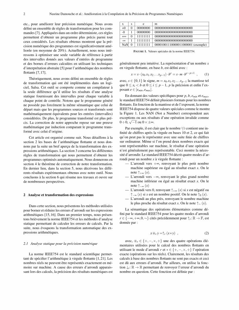
x s e m+0 0 00000000 00000000000000000000000-0 1 00000000 00000000000000000000000+∞ 0 11111111 00000000000000000000000-∞ 1 11111111 00000000000000000000000NaN 0 11111111 00001001110000011000001 (exemple)
FIGURE 1. Valeurs spéciales de la norme IEEE754.
généralement peu intuitive. La représentation d’un nombre xen virgule flottante, en base b, est défini avec :
x = s · (x0.x1.x2 . . .xp−1) ·be = s ·m ·be−p+1 , (1)
avec, s ∈ {0,1} le signe, m = x0.x1.x2 . . .xp−1 la mantisse telque 0 ≤ xi < b et 0 ≤ i ≤ p− 1, p la précision et enfin l’ex-posant e ∈ [emin,emax].
En donnant des valeurs spécifiques pour p, b, emin et emax,le standard IEEE754 définit plusieurs formats pour les nombresflottants. En fonction de la mantisse et de l’exposent, la normeIEEE754 dispose de quatre valeurs spéciales comme le montrela Figure 1. Les NAN (Not a Number) correspondent auxexceptions ou aux résultats d’une opération invalide comme0÷0,
√−1 ou 0×±∞.
Par exemple, il est clair que le nombre 1/3 contient une in-finité de chiffres après la virgule en bases 10 et 2, ce qui faitqu’on peut pas le représenter avec une suite finie de chiffressur ordinateur. Même si l’on prend deux nombres exacts quisont représentables sur machine, le résultat d’une opérationn’est généralement pas représentable. Ceci montre la néces-sité d’arrondir. Le standard IEEE754 décrit quatre modes d’ar-rondi pour un nombre x à virgule flottante :
— L’arrondi vers +∞, renvoyant le plus petit nombremachine supérieur ou égal au résultat exact x. On lenote ↑+∞ (x).
— L’arrondi vers −∞, renvoyant le plus grand nombremachine inférieur ou égal au résultat exact x. On lenote ↑−∞ (x)
— L’arrondi vers 0, renvoyant ↑+∞ (x) si x est négatif ou↑−∞ (x) si x est un nombre positif. On le note ↑0 (x).
— L’arrondi au plus près, renvoyant le nombre machinele plus proche du résultat exact x. On le note ↑∼ (x).
La sémantique des opérations élémentaires comme dé-fini par le standard IEEE754 pour les quatre modes d’arrondir ∈ {−∞,+∞,0,∼} cités précédemment pour ↑r: R→ F, estdonnée par :
x~r y =↑r (x∗ y) , (2)
avec, ~r ∈ {+,−,×,÷} une des quatre opérations élé-mentaires utilisées pour le calcul des nombres flottants enutilisant le mode d’arrondi r et ∗ ∈ {+,−,×,÷} l’opérationexacte (opérations sur les réels). Clairement, les résultats descalculs à base des nombres flottants ne sont pas exacts et ceciest dû aux erreurs d’arrondi. Par ailleurs, on utilise la fonc-tion ↓r: R→ R permettant de renvoyer l’erreur d’arrondi dunombre en question. Cette fonction est définie par :
Nasrine Damouche et al.: Amélioration à la Compilation de la Précision de Programmes Numériques 3
↓r (x) = x− ↑r (x) . (3)
Il est à noter que nos techniques de transformation présen-tées dans la Section 3 ne dépendent pas d’un mode d’arrondiprécis. Pour simplifier notre analyse, on suppose qu’on utilisele mode d’arrondi au plus près dans le reste de cet article, cequi revient à écrire ↑ et ↓ au lieu de ↑r et ↓r.
Pour calculer les erreurs se glissant durant l’évaluationdes expressions arithmétiques, nous définissons des valeursnon standard faites d’une paire (x,µ) ∈ F×R= E, où la va-leur x représente un nombre flottant et µ l’erreur exacte liée àx. Plus précisément, µ est la différence exacte entre la valeurréelle et flottante de x comme définit par l’équation (3). A titred’exemple, prenons le nombre réel 1/3 qui sera représenté parla valeur suivante :
v = (↑∼ (1/3),↓∼ (1/3)) = (0.33333333,(1/3−0.33333333)).
La sémantique concrète des opérations élémentaires dans Eest détaillée dans [18].
La sémantique abstraite associée à E utilise une paired’intervalles (x],µ]) ∈ E], tel que le premier intervalle x]
contient les nombres flottants du programme, et le deuxièmeintervalle µ] contient les erreurs sur x] obtenues en sous-trayant le nombre flottant de la valeur exacte. Cette valeurabstrait un ensemble de valeurs concrètes {(x,µ) : x ∈ x] etµ ∈ µ]}. Revenons maintenant à la sémantique des expres-sions arithmétiques dont l’ensemble des valeurs abstraites estnoté par E]. Un intervalle x] est approché avec un intervalledéfini par l’équation (4) qu’on note ↑] (x]).
↑] ([x,x]) = [↑ (x),↑ (x)] . (4)
La fonction d’abstraction ↓], quant à elle, abstrait la fonc-tion concrète ↓, autrement dit, elle permet de sur-approcherl’ensemble des valeurs exactes d’erreur, ↓ (x) = x− ↑ (x) desorte que chaque erreur associée à l’intervalle x ∈ [x,x] est in-cluse dans ↓] ([x,x]). Pour un mode d’arrondi au plus proche,la fonction d’abstraction est donnée par l’équation (5).
↓] ([x,x]) = [−y,y] avec y =12
ulp(max(|x|, |x|)
). (5)
En pratique, l’ulp(x) qui est une abréviation de unit in thelast place représente la valeur du dernier chiffre significatifd’un nombre à virgule flottante x. Formellement, la sommede deux nombres à virgule flottante revient à additionner leserreurs générées par l’opérateur avec l’erreur causée par l’ar-rondi du résultat. Similairement pour la soustraction de deuxnombres flottants, on soustrait les erreurs sur les opérateurset on les ajoute aux erreurs apparues au moment de l’arrondi.Quant à la multiplication de deux nombres à virgule flottante,la nouvelle erreur est obtenue par développement de la for-mule (x]1 + µ]
1)× (x]2 + µ]2). Les équations (6) à (8) donnent
la sémantique des opérations élémentaires.
(x]1,µ]1)+(x]2,µ
]2) = (↑] (x]1 + x]2),µ
]1 +µ]
2+ ↓] (x]1 + x]2)) , (6)
(x]1,µ]1)− (x]2,µ
]2) = (↑] (x]1− x]2),µ
]1−µ]
2+ ↓] (x]1− x]2)) , (7)
(x]1,µ]1)× (x]2,µ
]2) = (↑] (x]1× x]2),
x]2×µ]1 + x]1×µ]
2 +µ]1×µ]
2+ ↓] (x]1× x]2)) . (8)
Notons qu’il existe d’autres domaines abstraits plus ef-ficaces, à titre d’exemple [4,13,14], et aussi des techniquescomplémentaires comme [2,3,9,23]. De plus, on peut faireréférence à des méthodes qui transforment, synthétisent ouréparent les expressions arithmétiques basées sur des entiersou sur la virgule fixe [12]. On citera également [4,11,19,20,23] qui s’intéressent à améliorer les rangs des variables à vir-gule flottante.
2.2 Les expressions arithmétiques
Nous présentons ici rapidement les travaux de thèse deA. Ioualalen qui portent sur la transformation [6] des expres-sions arithmétiques en utilisant les APEGs [15,16,24]. LesAPEGs, abréviation de Abstract Program Equivalent Graph,permettent de représenter en taille polynomiale un nombreexponentiel d’expressions mathématiques équivalentes. UnAPEG se compose de classes d’équivalence représentées pardes ellipses qui contiennent des opérations, et des boites. Pourformer une expression valide, nous construisons l’APEG cor-respondant à l’expression arithmétique en question d’abord,ensuite, il faut choisir une opération dans chaque classe d’équi-valence. Pour éviter le problème lié à l’explosion combina-toire, les APEGs regroupent plusieurs expressions arithmé-tiques équivalentes à base de commutativité, d’associativitéet de distributivité dans des boites. Une boite avec n opé-rateurs peut représenter un très grand nombre de formuleséquivalentes allant jusqu’à 1×3×5...×(2n−3) expressions.La construction d’un APEG nécessite l’usage de deux algo-rithmes. Le premier algorithme dit de propagation effectueune recherche récursive dans l’APEG afin d’y trouver les opé-rateurs binaires symétriques qui à leur tour, seront mis dansles boites abstraites. Le deuxième algorithme, d’expansion,cherche dans l’APEG une expression plus précise parmi toutesles expressions équivalentes. Enfin, nous recherchons l’ex-pression arithmétique la plus précise selon la sémantique abs-traite de la Section 2.1.
La syntaxe des expressions arithmétiques et booléennesest donnée par l’équation (9).
Expr 3 e ::= id | cst | e+ e | e− e | e× e | e÷ eBExpr 3 b ::= true | false | b∧b | b∨b | ¬b |
e = e | e < e | e > e(9)
4 Nasrine Damouche et al.: Amélioration à la Compilation de la Précision de Programmes Numériques
2 a
×
+
b
□
+(a,a,b)
×
c ×
+
c b c
×
a a
+×
× +
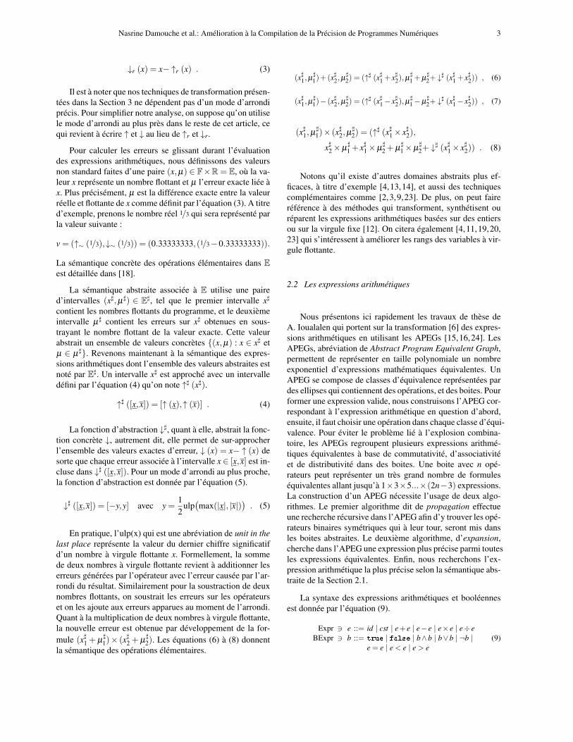
FIGURE 2. APEG for the expression e =((a+a)+ c
)× c.
Exemple Afin de bien éclairer cette notion, nous donnons ci-dessous quelques expressions arithmétiques correspondant àl’APEG de l’expression e = ((a+a)+b)×c) de la Figure 2.Sur cette dernière, les ellipses en pointillé correspondent auxclasses d’équivalences qui contiennent des APEGs et les rec-tangles sont les boites constituées d’une opération et n opé-randes, autrement dit, c’est les différentes façons de combinerces opérateurs avec les opérandes en question.
A (p) =
((a+a)+b
)× c,
((a+b)+a
)× c,(
(b+a)+a)× c,
((2×a)+b
)× c,
c×((a+a)+b
), c×
((a+b)+a
),
c×((b+a)+a
), c×
((2×a)+b
),
(a+a)× c+b× c, (2×a)× c+b× c,b× c+(a+a)× c, b× c+(2×a)× c
. (10)
�
3 Transformation des commandes
Afin d’améliorer au mieux la précision numérique descalculs, nous transformons automatiquement des programmesutilisant l’arithmétique des nombres à virgule flottante en nousappuyant sur des techniques d’interprétation abstraite. Cettetransformation concerne les expressions arithmétique commel’addition, la multiplication, les fonctions trigonométriques,etc., mais aussi les morceaux de code tel que les affectations,conditionnelles, boucles et fonctions. La syntaxe correspon-dant à nos commandes est la suivante :
Com 3 c ::= id = e | c1;c2 | ifΦ e then c1 else c2
| whileΦ e do c | nop . (11)
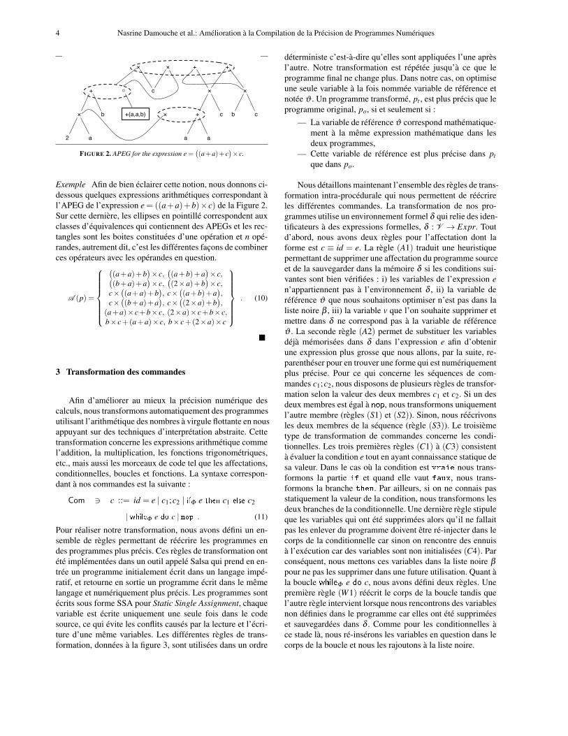
Pour réaliser notre transformation, nous avons défini un en-semble de règles permettant de réécrire les programmes endes programmes plus précis. Ces règles de transformation ontété implémentées dans un outil appelé Salsa qui prend en en-trée un programme initialement écrit dans un langage impé-ratif, et retourne en sortie un programme écrit dans le mêmelangage et numériquement plus précis. Les programmes sontécrits sous forme SSA pour Static Single Assignment, chaquevariable est écrite uniquement une seule fois dans le codesource, ce qui évite les conflits causés par la lecture et l’écri-ture d’une même variables. Les différentes règles de trans-formation, données à la figure 3, sont utilisées dans un ordre
déterministe c’est-à-dire qu’elles sont appliquées l’une aprèsl’autre. Notre transformation est répétée jusqu’à ce que leprogramme final ne change plus. Dans notre cas, on optimiseune seule variable à la fois nommée variable de référence etnotée ϑ . Un programme transformé, pt , est plus précis que leprogramme original, po, si et seulement si :
— La variable de référence ϑ correspond mathématique-ment à la même expression mathématique dans lesdeux programmes,
— Cette variable de référence est plus précise dans ptque dans po.
Nous détaillons maintenant l’ensemble des règles de trans-formation intra-procédurale qui nous permettent de réécrireles différentes commandes. La transformation de nos pro-grammes utilise un environnement formel δ qui relie des iden-tificateurs à des expressions formelles, δ : V → Expr. Toutd’abord, nous avons deux règles pour l’affectation dont laforme est c ≡ id = e. La règle (A1) traduit une heuristiquepermettant de supprimer une affectation du programme sourceet de la sauvegarder dans la mémoire δ si les conditions sui-vantes sont bien vérifiées : i) les variables de l’expression en’appartiennent pas à l’environnement δ , ii) la variable deréférence ϑ que nous souhaitons optimiser n’est pas dans laliste noire β , iii) la variable v que l’on souhaite supprimer etmettre dans δ ne correspond pas à la variable de référenceϑ . La seconde règle (A2) permet de substituer les variablesdéjà mémorisées dans δ dans l’expression e afin d’obtenirune expression plus grosse que nous allons, par la suite, re-parenthéser pour en trouver une forme qui est numériquementplus précise. Pour ce qui concerne les séquences de com-mandes c1;c2, nous disposons de plusieurs règles de transfor-mation selon la valeur des deux membres c1 et c2. Si un desdeux membres est égal à nop, nous transformons uniquementl’autre membre (règles (S1) et (S2)). Sinon, nous réécrivonsles deux membres de la séquence (règle (S3)). Le troisièmetype de transformation de commandes concerne les condi-tionnelles. Les trois premières règles (C1) à (C3) consistentà évaluer la condition e tout en ayant connaissance statique desa valeur. Dans le cas où la condition est vraie nous trans-formons la partie if et quand elle vaut faux, nous trans-formons la branche then. Par ailleurs, si on ne connais passtatiquement la valeur de la condition, nous transformons lesdeux branches de la conditionnelle. Une dernière règle stipuleque les variables qui ont été supprimées alors qu’il ne fallaitpas les enlever du programme doivent être ré-injecter dans lecorps de la conditionnelle car sinon on rencontre des ennuisà l’exécution car des variables sont non initialisées (C4). Parconséquent, nous mettons ces variables dans la liste noire βpour ne pas les supprimer dans une future utilisation. Quant àla boucle whileΦ e do c, nous avons défini deux règles. Unepremière règle (W1) réécrit le corps de la boucle tandis quel’autre règle intervient lorsque nous rencontrons des variablesnon définies dans le programme car elles ont été suppriméeset sauvegardées dans δ . Comme pour les conditionnelles àce stade là, nous ré-insérons les variables en question dans lecorps de la boucle et nous les rajoutons à la liste noire.
Nasrine Damouche et al.: Amélioration à la Compilation de la Précision de Programmes Numériques 5
δ ′ = δ [id 7→ e] id 6∈ β〈id = e,δ ,C,β 〉 ⇒ϑ 〈nop,δ ′,C,β 〉 (A1)
e′ = δ (e) σ ] = [[C[c]]]]ι] 〈e′,σ ]〉;∗ e′′
〈id = e,δ ,C,β 〉 ⇒ϑ 〈id = e′′,δ ,C,β 〉 (A2)
〈nop ; c ,δ ,C,β 〉 ⇒ϑ 〈c,δ ,C,β 〉 (S1) 〈c ; nop ,δ ,C,β 〉 ⇒ϑ 〈c,δ ,C,β 〉 (S2)
C′ =C[[];c2
]〈c1,δ ,C′,β 〉 ⇒∗ϑ 〈c′1,δ ′,C′,β ′〉 C′′ =C[c′1; []]
〈c2,δ ′,C′′,β ′〉 ⇒ϑ 〈c′2,δ ′′,C′′,β ′′〉〈c1 ; c2 ,δ ,C,β 〉 ⇒ϑ 〈c′1 ; c′2,δ ′′,C,β ′′〉 (S3)
σ ] = [[C[ifΦ e then c1 else c2]]]]ι] [[e]]]σ ] = true 〈c1,δ ,C,β 〉 ⇒ϑ 〈c′1,δ ′,C,β 〉
〈ifΦ e then c1 else c2,δ ,C,β 〉 ⇒ϑ 〈Ψ(Φ ,c′1),Ψ(Φ ,δ ′),C,β 〉 (C1)
σ ] = [[C[ifΦ e then c1 else c2]]]]ι] [[e]]]σ ] = false 〈c2,δ ,C,β 〉 ⇒ϑ 〈c′2,δ ′,C,β 〉
〈ifΦ e then c1 else c2,δ ,C,β 〉 ⇒ϑ 〈Ψ(Φ ,c′2),Ψ(Φ ,δ ′),C,β 〉 (C2)
Var(e)∩Dom(δ ) = /0 β ′ = β ∪Assigned(c1)∪Assigned(c2)〈c1,δ ,C,β ′〉 ⇒ϑ 〈c′1,δ1,C,β1〉 〈c2,δ ,C,β ′〉 ⇒ϑ 〈c′2,δ2,C,β2〉 δ ′ = δ1∪δ2
〈ifΦ e then c1 else c2,δ ,C,β 〉 ⇒ϑ 〈ifΦ e then c′1 else c′2,δ ′,C,β ′〉 (C3)
V =Var(e) c′ = AddDe f s(V,δ ) δ ′ = δ|Dom(δ )\V〈c′; ifΦ e then c1 else c2,δ ′,C,β ∪V 〉 ⇒ϑ 〈c′′,δ ′,C,β ′〉〈ifΦ e then c1 else c2,δ ,C,β 〉 ⇒ϑ 〈c′′,δ ′,C,β ′〉 (C4)
Var(e)∩Dom(δ ) = /0 C′ =C[whileΦ e do []] 〈c,δ ,C′,β 〉 ⇒ϑ 〈c′,δ ′,C′,β ′〉〈whileΦ e do c,δ ,C,β 〉 ⇒ϑ 〈whileΦ e do c′,δ ′,C,β ′〉 (W1)
V =Var(e)∪Var(Φ) c′ = AddDe f s(V,δ ) δ ′ = δ|Dom(δ )\V〈c′;whileΦ e do c,δ ′,C,β ∪V 〉 ⇒ϑ 〈c′′,δ ′,C,β ′〉
〈whileΦ e do c,δ ,C,β 〉 ⇒ϑ 〈c′′,δ ′,C,β ′〉 (W2)
FIGURE 3. Règles de transformation pour améliorer la précision de programmes.
4 Preuve de correction
Pour vérifier la correction de notre transformation, nousintroduisons un théorème qui compare deux programmes etmontre que le programme le plus précis peut être utilisé à laplace de celui moins précis. Notre preuve est basée sur une sé-mantique opérationnelle classique pour les expressions arith-métiques et les commandes. La comparaison entre les deuxprogrammes nécessite de spécifier une variable de référenceϑ définie par l’utilisateur. Plus précisément, un programmetransformé pt est plus précis qu’un programme d’origine posi et seulement si les deux conditions suivantes sont vérifiées :
— La variable de référence ϑ correspond à même ex-pression mathématique dans les deux programmes,
— La variable de référence ϑ est plus précise dans leprogramme transformé pt que dans celui d’origine po.
Nous utilisons la relation d’ordrev⊆E×E disant qu’unevaleur (x,µ) est plus précise qu’une valeur (x′,µ ′) si ellescorrespondent à la même valeur réelle et si l’erreur µ est pluspetite que µ ′.
Définition 1 (Comparaison des expressions). Nous consi-dérons v1 = (x1,µ1) ∈ E et v2 = (x2,µ2) ∈ E. Nous disonsque v1 est plus précise que v2, noté v1 v v2, si et seulement six1 +µ1 = x2 +µ2 et |µ1| ≤ |µ2|. �
Définition 2 (Comparaison des commandes). Soit co et ctdeux commandes, δo et δt deux environnements formels et ϑla variable de référence. Nous disons que
〈ct ,δt ,C,β 〉 ≺ϑ 〈co,δo,C,β 〉 (12)
si et seulement si pour chaque σ ∈Mem,
∃σo ∈Mem,〈co,σ〉 →∗ 〈nop,σo〉 ,
∃σt ∈Mem,〈ct ,σ〉 →∗ 〈nop,σt〉 ,
— soit σt(ϑ)v σo(ϑ),— soit pour chaque id ∈ Dom(σo)\Dom(σt), δt(id) = e
et 〈e,σ〉 →∗e σo(id).
�
La deuxième définition spécifie que :— Les deux commandes co et ct calculent la même va-
leur de référence ϑ dans les deux environnements δoet δt dans une arithmétique exacte,
— La commande transformée est plus précise,— Si après exécution du programme, une variable est
indéfinie dans l’environnement concret δt , alors l’ex-pression formelle correspondante est déjà enregistréedans δt .
6 Nasrine Damouche et al.: Amélioration à la Compilation de la Précision de Programmes Numériques
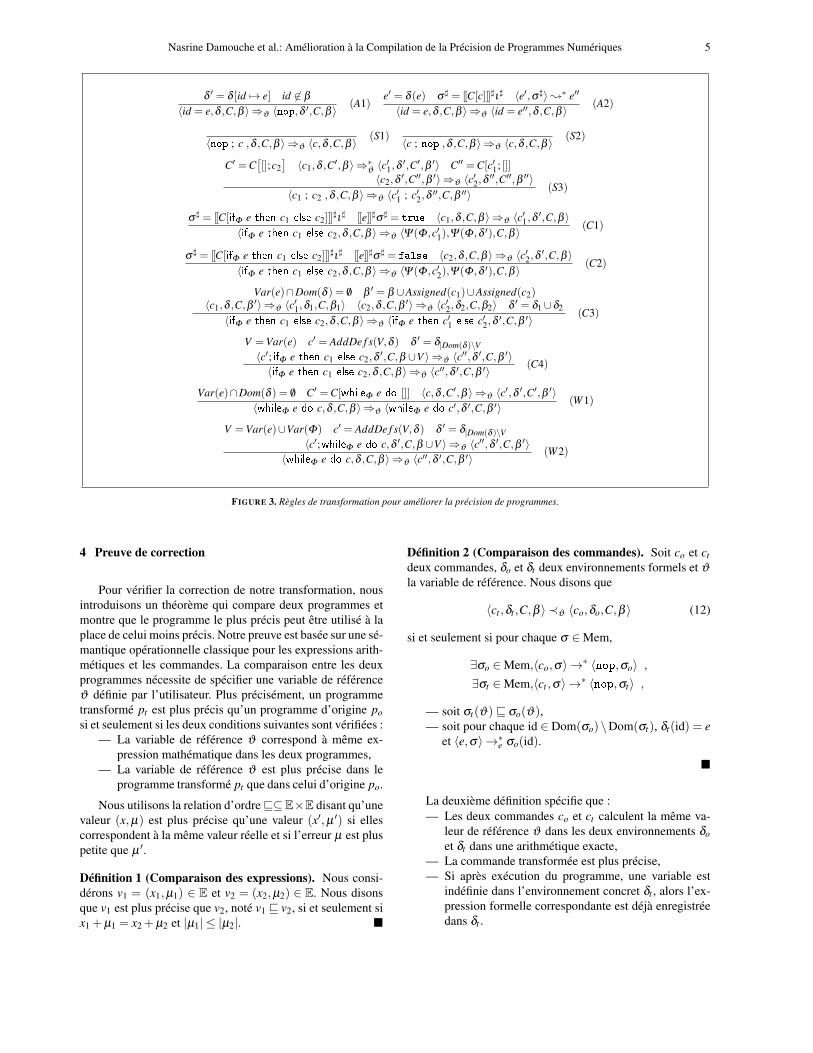
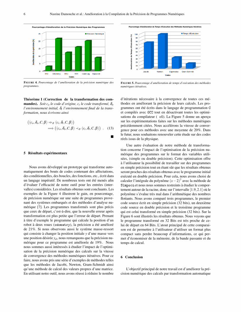
Pourcentage d'Amélioration de la Précision Numérique des Programmes
FIGURE 4. Pourcentage de l’amélioration de la précision numérique desprogrammes.
Théorème 1 (Correction de la transformation des com-mandes). Soit co le code d’origine, ct le code transformé, δol’environnement initial, δt l’environnement final de la trans-formation, nous écrivons ainsi
(〈co,δo,C,β 〉 ⇒ϑ 〈ct ,δt ,C,β 〉
)
=⇒(〈co,δo,C,β 〉 ≺ϑ 〈ct ,δt ,C,β 〉
). (13)
�
5 Résultats expérimentaux
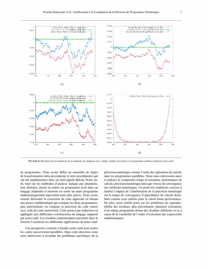
Nous avons développé un prototype qui transforme auto-matiquement des bouts de codes contenant des affectations,des conditionnelles, des boucles, des fonctions, etc., écrit dansun langage impératif. De nombreux tests ont été menés afind’évaluer l’efficacité de notre outil pour les entrées (inter-valles) considérées. Les résultats obtenus sont concluants. Lesexemples de la Figure 4 illustrent le gain, en pourcentage,de précision numérique sur une suite de programmes prove-nant des systèmes embarqués et des méthodes d’analyse nu-mérique [7]. Les programmes transformés sont plus précisque ceux de départ, c’est-à-dire, que la nouvelle erreur aprèstransformation est plus petite que l’erreur de départ. Prenantà titre d’exemple le programme qui calcule la position d’unrobot à deux roues (odometry), la précision a été amélioréde 21%. Si nous observons aussi le système masse-ressortqui consiste à changer la position initiale y d’une masse versune position désirée yd , nous remarquons que la précision nu-mérique pour ce programme est améliorée de 19%. Nousnous sommes aussi intéressés à étudier l’impact de l’optimi-sation de la précision numérique des calculs sur la vitessede convergence des méthodes numériques itératives. Pour cefaire, nous avons pris une série d’exemples de méthodes tellesque les méthodes de Jacobi, Newton, Gram-Schmidt ainsiqu’une méthode de calcul des valeurs propres d’une matrice.En utilisant notre outil, nous avons réussi à réduire le nombre
Am
éliora
tion
de T
em
ps d
'Exécu
tion
(%
)
Pourcentage d'Amélioration de Temps d'Exécution des Méthodes Numériques Itératives
FIGURE 5. Pourcentage d’amélioration de temps d’exécution des méthodesnumériques itératives.
d’itérations nécessaire à la convergence de toutes ces mé-thodes en améliorant la précision de leurs calculs. Les pro-grammes ont été écrits dans le langage de programmation C
et compilés avec GCC tout en désactivant toutes les optimi-sations du compilateur (-o0). La Figure 5 donne un aperçusur les expérimentations faites sur les méthodes numériquesprécédemment citées. Nous accélérons la vitesse de conver-gence pour ces méthodes avec une moyenne de 20%. Dansle futur, nous souhaitons renouveler cette étude sur des codesréels issus de la physique.
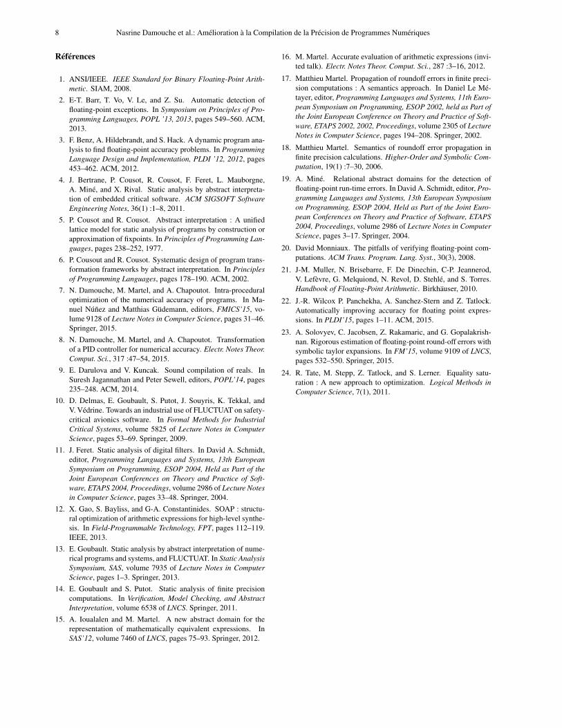
Une autre évaluation de notre méthode de transforma-tion concerne l’impact de l’optimisation de la précision nu-mérique des programmes sur le format des variables utili-sées, (simple ou double précision). Cette optimisation offreà l’utilisateur la possibilité de travailler sur des programmesen simple précision tout en étant sûr que les résultats obtenusseront proches des résultats obtenus avec le programme initialexécuté en double précision. Pour cela, nous avons choisi decalculer l’intégrale du polynôme (x−2)7 avec la méthode deSimpson et nous nous sommes restreints à étudier le compor-tement autour de la racine, donc sur l’intervalle [1.9,2.1] où lepolynôme s’évalue très mal dans l’arithmétique des nombresflottants. Nous avons comparé trois programmes, le premiercode source écrit en simple précision (32 bits), un deuxièmecode source en double précision et le troisième programmequi est celui transformé en simple précision (32 bits). Sur laFigure 6 sont illustrés les résultats obtenus. Nous voyons quele programme transformé en 32 Bits est très proche de ce-lui de départ en 64 Bits. L’atout principal de cette comparai-son est de permettre à l’utilisateur d’utiliser un format pluscompact sans perdre beaucoup d’informations, ce qui per-met d’économiser de la mémoire, de la bande passante et dutemps de calcul.
6 Conclusion
L’objectif principal de notre travail est d’améliorer la pré-cision numérique des calculs par transformation automatique
Nasrine Damouche et al.: Amélioration à la Compilation de la Précision de Programmes Numériques 7
(a) (b)
(c) (d)
FIGURE 6. Résultats de la simulation de la méthode des Simpson avec simple, double précision et le programme optimisé utilisant notre outil.
de programmes. Nous avons défini un ensemble de règlesde transformation intra-procédurale et inter-procédurales quiont été implémentées dans un outil appelé Salsa. Notre ou-til, basé sur les méthodes d’analyse statique par interpréta-tion abstraite, prend en entrée un programme écrit dans unlangage impératif et retourne en sortie un autre programmemathématiquement équivalent mais plus précis. Nous avonsensuite démontré la correction de cette approche en faisantune preuve mathématique qui compare les deux programmes,plus précisément, on compare la précision du code sourceavec celle du code transformé. Cette preuve par induction estappliquée aux différentes constructions du langage supportépar notre outil. Les résultats expérimentaux présentés dans laSection 5 montrent les différentes applications de notre outil.
Une perspective consiste à étendre notre outil pour traiterles codes massivement parallèles. Dans cette direction, nousnous intéressons à résoudre des problèmes spécifiques de la
précision numérique comme l’ordre des opérations de calculsdans les programmes parallèles. Nous nous intéressons aussià explorer le compromis temps d’exécution, performance decalculs, précision numérique ainsi que vitesse de convergencedes méthodes numériques. Un point très ambitieux consiste àétudier l’impact de l’amélioration de la précision numériquesur le temps de convergence d’algorithmes de calculs distri-bués comme ceux utilisés pour le calcul haute performance.De plus, notre intérêt porte sur les problèmes de reproduc-tibilité des résultats, plus précisément, plusieurs exécutionsd’un même programme donne des résultats différents et ce àcause de la variabilité de l’ordre d’exécution des expressionsmathématiques.
8 Nasrine Damouche et al.: Amélioration à la Compilation de la Précision de Programmes Numériques
Références
1. ANSI/IEEE. IEEE Standard for Binary Floating-Point Arith-metic. SIAM, 2008.
2. E-T. Barr, T. Vo, V. Le, and Z. Su. Automatic detection offloating-point exceptions. In Symposium on Principles of Pro-gramming Languages, POPL ’13, 2013, pages 549–560. ACM,2013.
3. F. Benz, A. Hildebrandt, and S. Hack. A dynamic program ana-lysis to find floating-point accuracy problems. In ProgrammingLanguage Design and Implementation, PLDI ’12, 2012, pages453–462. ACM, 2012.
4. J. Bertrane, P. Cousot, R. Cousot, F. Feret, L. Mauborgne,A. Miné, and X. Rival. Static analysis by abstract interpreta-tion of embedded critical software. ACM SIGSOFT SoftwareEngineering Notes, 36(1) :1–8, 2011.
5. P. Cousot and R. Cousot. Abstract interpretation : A unifiedlattice model for static analysis of programs by construction orapproximation of fixpoints. In Principles of Programming Lan-guages, pages 238–252, 1977.
6. P. Cousout and R. Cousot. Systematic design of program trans-formation frameworks by abstract interpretation. In Principlesof Programming Languages, pages 178–190. ACM, 2002.
7. N. Damouche, M. Martel, and A. Chapoutot. Intra-proceduraloptimization of the numerical accuracy of programs. In Ma-nuel Núñez and Matthias Güdemann, editors, FMICS’15, vo-lume 9128 of Lecture Notes in Computer Science, pages 31–46.Springer, 2015.
8. N. Damouche, M. Martel, and A. Chapoutot. Transformationof a PID controller for numerical accuracy. Electr. Notes Theor.Comput. Sci., 317 :47–54, 2015.
9. E. Darulova and V. Kuncak. Sound compilation of reals. InSuresh Jagannathan and Peter Sewell, editors, POPL’14, pages235–248. ACM, 2014.
10. D. Delmas, E. Goubault, S. Putot, J. Souyris, K. Tekkal, andV. Védrine. Towards an industrial use of FLUCTUAT on safety-critical avionics software. In Formal Methods for IndustrialCritical Systems, volume 5825 of Lecture Notes in ComputerScience, pages 53–69. Springer, 2009.
11. J. Feret. Static analysis of digital filters. In David A. Schmidt,editor, Programming Languages and Systems, 13th EuropeanSymposium on Programming, ESOP 2004, Held as Part of theJoint European Conferences on Theory and Practice of Soft-ware, ETAPS 2004, Proceedings, volume 2986 of Lecture Notesin Computer Science, pages 33–48. Springer, 2004.
12. X. Gao, S. Bayliss, and G-A. Constantinides. SOAP : structu-ral optimization of arithmetic expressions for high-level synthe-sis. In Field-Programmable Technology, FPT, pages 112–119.IEEE, 2013.
13. E. Goubault. Static analysis by abstract interpretation of nume-rical programs and systems, and FLUCTUAT. In Static AnalysisSymposium, SAS, volume 7935 of Lecture Notes in ComputerScience, pages 1–3. Springer, 2013.
14. E. Goubault and S. Putot. Static analysis of finite precisioncomputations. In Verification, Model Checking, and AbstractInterpretation, volume 6538 of LNCS. Springer, 2011.
15. A. Ioualalen and M. Martel. A new abstract domain for therepresentation of mathematically equivalent expressions. InSAS’12, volume 7460 of LNCS, pages 75–93. Springer, 2012.
16. M. Martel. Accurate evaluation of arithmetic expressions (invi-ted talk). Electr. Notes Theor. Comput. Sci., 287 :3–16, 2012.
17. Matthieu Martel. Propagation of roundoff errors in finite preci-sion computations : A semantics approach. In Daniel Le Mé-tayer, editor, Programming Languages and Systems, 11th Euro-pean Symposium on Programming, ESOP 2002, held as Part ofthe Joint European Conference on Theory and Practice of Soft-ware, ETAPS 2002, 2002, Proceedings, volume 2305 of LectureNotes in Computer Science, pages 194–208. Springer, 2002.
18. Matthieu Martel. Semantics of roundoff error propagation infinite precision calculations. Higher-Order and Symbolic Com-putation, 19(1) :7–30, 2006.
19. A. Miné. Relational abstract domains for the detection offloating-point run-time errors. In David A. Schmidt, editor, Pro-gramming Languages and Systems, 13th European Symposiumon Programming, ESOP 2004, Held as Part of the Joint Euro-pean Conferences on Theory and Practice of Software, ETAPS2004, Proceedings, volume 2986 of Lecture Notes in ComputerScience, pages 3–17. Springer, 2004.
20. David Monniaux. The pitfalls of verifying floating-point com-putations. ACM Trans. Program. Lang. Syst., 30(3), 2008.
21. J-M. Muller, N. Brisebarre, F. De Dinechin, C-P. Jeannerod,V. Lefèvre, G. Melquiond, N. Revol, D. Stehlé, and S. Torres.Handbook of Floating-Point Arithmetic. Birkhäuser, 2010.
22. J.-R. Wilcox P. Panchekha, A. Sanchez-Stern and Z. Tatlock.Automatically improving accuracy for floating point expres-sions. In PLDI’15, pages 1–11. ACM, 2015.
23. A. Solovyev, C. Jacobsen, Z. Rakamaric, and G. Gopalakrish-nan. Rigorous estimation of floating-point round-off errors withsymbolic taylor expansions. In FM’15, volume 9109 of LNCS,pages 532–550. Springer, 2015.
24. R. Tate, M. Stepp, Z. Tatlock, and S. Lerner. Equality satu-ration : A new approach to optimization. Logical Methods inComputer Science, 7(1), 2011.
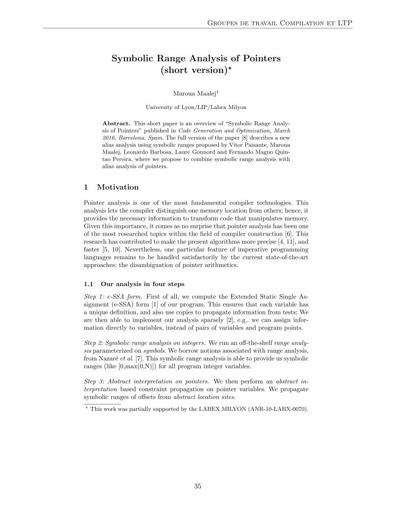
Symbolic Range Analysis of Pointers(short version)?
Maroua Maalej1
University of Lyon/LIP/Labex Milyon
Abstract. This short paper is an overview of “Symbolic Range Analy-sis of Pointers” published in Code Generation and Optimization, March2016, Barcelona, Spain. The full version of the paper [8] describes a newalias analysis using symbolic ranges proposed by Vitor Paisante, MarouaMaalej, Leonardo Barbosa, Laure Gonnord and Fernando Magno Quin-tao Pereira, where we propose to combine symbolic range analysis withalias analysis of pointers.
1 Motivation
Pointer analysis is one of the most fundamental compiler technologies. Thisanalysis lets the compiler distinguish one memory location from others; hence, itprovides the necessary information to transform code that manipulates memory.Given this importance, it comes as no surprise that pointer analysis has been oneof the most researched topics within the field of compiler construction [6]. Thisresearch has contributed to make the present algorithms more precise [4, 11], andfaster [5, 10]. Nevertheless, one particular feature of imperative programminglanguages remains to be handled satisfactorily by the current state-of-the-artapproaches: the disambiguation of pointer arithmetics.
1.1 Our analysis in four steps
Step 1: e-SSA form. First of all, we compute the Extended Static Single As-signment (e-SSA) form [1] of our program. This ensures that each variable hasa unique definition, and also use copies to propagate information from tests; Weare then able to implement our analysis sparsely [2], e.g,. we can assign infor-mation directly to variables, instead of pairs of variables and program points.
Step 2: Symbolic range analysis on integers. We run an off-the-shelf range analy-sis parameterized on symbols. We borrow notions associated with range analysis,from Nazare et al. [7]. This symbolic range analysis is able to provide us symbolicranges (like [0,max(0,N)]) for all program integer variables.
Step 3: Abstract interpretation on pointers. We then perform an abstract in-terpretation based constraint propagation on pointer variables. We propagatesymbolic ranges of offsets from abstract location sites.
? This work was partially supported by the LABEX MILYON (ANR-10-LABX-0070).
Groupes de travail Compilation et LTP
35
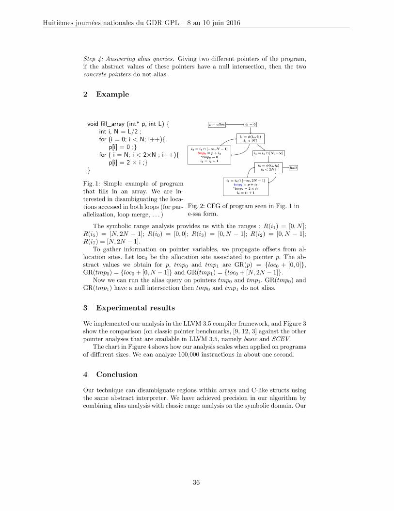
Step 4: Answering alias queries. Giving two different pointers of the program,if the abstract values of these pointers have a null intersection, then the twoconcrete pointers do not alias.
2 Example
void fill_array (int* p, int L) {int i, N = L/2 ;for (i = 0; i < N; i++){
p[i] = 0 ;}for ( i = N; i < 2×N ; i++){
p[i] = 2 × i ;}}
Fig. 1: Simple example of programthat fills in an array. We are in-terested in disambiguating the loca-tions accessed in both loops (for par-allelization, loop merge, . . . )
p = alloc i0 = 0
i1 = φ(i0, i3)i1 < N?
i2 = i1 ∩ [−∞, N − 1]tmp0 = p+ i2
∗tmp0 = 0i3 = i2 + 1
i5 = φ(i4, i6)i5 < 2N?
i7 = i6 ∩ [−∞, 2N − 1]tmp1 = p+ i7
∗tmp1 = 2× i7i6 = i7 + 1
halt
i4 = i1 ∩ [N,+∞]
Fig. 2: CFG of program seen in Fig. 1 ine-ssa form.
The symbolic range analysis provides us with the ranges : R(i1) = [0, N ];R(i5) = [N, 2N − 1]; R(i0) = [0, 0]; R(i3) = [0, N − 1]; R(i2) = [0, N − 1];R(i7) = [N, 2N − 1].
To gather information on pointer variables, we propagate offsets from al-location sites. Let loc0 be the allocation site associated to pointer p. The ab-stract values we obtain for p, tmp0 and tmp1 are GR(p) = {loc0 + [0, 0]},GR(tmp0) = {loc0 + [0, N − 1]} and GR(tmp1) = {loc0 + [N, 2N − 1]}.
Now we can run the alias query on pointers tmp0 and tmp1. GR(tmp0) andGR(tmp1) have a null intersection then tmp0 and tmp1 do not alias.
3 Experimental results
We implemented our analysis in the LLVM 3.5 compiler framework, and Figure 3show the comparison (on classic pointer benchmarks, [9, 12, 3] against the otherpointer analyses that are available in LLVM 3.5, namely basic and SCEV.
The chart in Figure 4 shows how our analysis scales when applied on programsof different sizes. We can analyze 100,000 instructions in about one second.
4 Conclusion
Our technique can disambiguate regions within arrays and C-like structs usingthe same abstract interpreter. We have achieved precision in our algorithm bycombining alias analysis with classic range analysis on the symbolic domain. Our
Huitièmes journées nationales du GDR GPL – 8 au 10 juin 2016
36
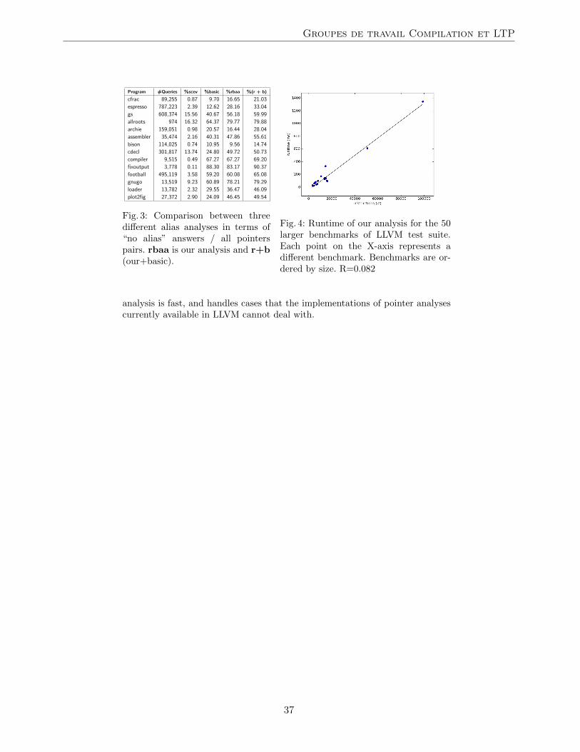
Program #Queries %scev %basic %rbaa %(r + b)cfrac 89,255 0.87 9.70 16.65 21.03espresso 787,223 2.39 12.62 28.16 33.04gs 608,374 15.56 40.67 56.18 59.99allroots 974 16.32 64.37 79.77 79.88archie 159,051 0.98 20.57 16.44 28.04assembler 35,474 2.16 40.31 47.86 55.61bison 114,025 0.74 10.95 9.56 14.74cdecl 301,817 13.74 24.80 49.72 50.73compiler 9,515 0.49 67.27 67.27 69.20fixoutput 3,778 0.11 88.30 83.17 90.37football 495,119 3.58 59.20 60.08 65.08gnugo 13,519 9.23 60.89 78.21 79.29loader 13,782 2.32 29.55 36.47 46.09plot2fig 27,372 2.90 24.09 46.45 49.54
Fig. 3: Comparison between threedifferent alias analyses in terms of“no alias” answers / all pointerspairs. rbaa is our analysis and r+b(our+basic).
Fig. 4: Runtime of our analysis for the 50larger benchmarks of LLVM test suite.Each point on the X-axis represents adifferent benchmark. Benchmarks are or-dered by size. R=0.082
analysis is fast, and handles cases that the implementations of pointer analysescurrently available in LLVM cannot deal with.
Groupes de travail Compilation et LTP
37

Bibliography
[1] Rastislav Bodik, Rajiv Gupta, and Vivek Sarkar. ABCD: eliminating arraybounds checks on demand. In PLDI, pages 321–333. ACM, 2000.
[2] Jong-Deok Choi, Ron Cytron, and Jeanne Ferrante. Automatic constructionof sparse data flow evaluation graphs. In POPL, pages 55–66. ACM, 1991.
[3] Dirk Grunwald, Benjamin Zorn, and Robert Henderson. Improving thecache locality of memory allocation. In PLDI, pages 177–186. ACM, 1993.
[4] Ben Hardekopf and Calvin Lin. The ant and the grasshopper: fast andaccurate pointer analysis for millions of lines of code. In PLDI, pages 290–299. ACM, 2007.
[5] Ben Hardekopf and Calvin Lin. Flow-sensitive pointer analysis for millionsof lines of code. In CGO, pages 265–280, 2011.
[6] Michael Hind. Pointer analysis: Haven’t we solved this problem yet? InPASTE, pages 54–61. ACM, 2001.
[7] Henrique Nazare, Izabela Maffra, Willer Santos, Leonardo Barbosa, LaureGonnord, and Fernando Magno Quintao Pereira. Validation of memoryaccesses through symbolic analyses. In OOPSLA, pages 791–809. ACM,2014.
[8] Vitor Paisante, Maroua Maalej, Leonardo Barbosa, Laure Gonnord, andFernando Magno Quintao Pereira. Symbolic Range Analysis of Pointers.In International Symposium of Code Generation and Optmization, pages791–809, Barcelon, Spain, March 2016.
[9] Barbara G. Ryder, William A. Landi, Philip A. Stocks, Sean Zhang, andRita Altucher. A schema for interprocedural modification side-effect analy-sis with pointer aliasing. ACM Trans. Program. Lang. Syst., 23(2):105–186,2001.
[10] L. Shang, X. Xie, and J. Xue. On-demand dynamic symmary-based points-to analysis. In CGO, pages 264–274. ACM, 2012.
[11] Qirun Zhang, Xiao Xiao, Charles Zhang, Hao Yuan, and Zhendong Su.Efficient subcubic alias analysis for C. In OOPSLA, pages 829–845. ACM,2014.
[12] Qin Zhao, Rodric Rabbah, and Weng-Fai Wong. Dynamic memory opti-mization using pool allocation and prefetching. SIGARCH Comput. Archit.News, 33(5):27–32, 2005.
Huitièmes journées nationales du GDR GPL – 8 au 10 juin 2016
38

Session du groupe de travail GLACEGénie Logiciel pour les systèmes Cyber-physiquEs
39

Huitièmes journées nationales du GDR GPL – 8 au 10 juin 2016
40
Software Development Supportfor Shared Sensing Infrastructures:
a Generative and Dynamic Approach
Cyril Cecchinel1,2, Sebastien Mosser1,2, and Philippe Collet1,2
1Universite Nice Sophia Antipolis, I3S, UMR 7271, 06900 Sophia Antipolis, France2CNRS, I3S, UMR 7271, 06900 Sophia Antipolis, France
{cecchine,mosser,collet}@i3s.unice.fr
Abstract. Sensors networks are the backbone of large sensing infras-tructures such as Smart Cities or Smart Buildings. Classical approachessuffer from several limitations hampering developers’ work (e.g., lack ofsensor sharing, lack of dynamicity in data collection policies, need todig inside big data sets, absence of reuse between implementation plat-forms). This paper presents a tooled approach that tackles these issues.It couples (i) an abstract model of developers’ requirements in a giveninfrastructure to (ii) timed automata and code generation techniques,to support the efficient deployment of reusable data collection policieson different infrastructures. The approach has been validated on sev-eral real-world scenarios and is currently experimented on an academiccampus.
Keywords: Sensor Network · Software Composition · Modeling.
1 Introduction
The Internet of Things [13] relies on physical objects interconnected betweeneach others, creating a mesh of devices producing information flow. The Gartnergroup predicts up to 26 billions of things connected to the Internet by 2020.These things are organized into sensor networks deployed in Large-scale SensingInfrastructures (LSIs), e.g., Smart Cities or Smart Buildings, which continu-ously collect data about our environment. These LSIs implement Cyber PhysicalSystems (CPSs) that monitor ambiant environments.
Facing the problem of managing tremendous amounts of data, a commonlyused approach is to rely on sensor pooling [9], [19] and to push data collectedby sensors in a central cloud-based platform [15]. Consequently, sensors cannotbe exploited at the same time and one needs to rely on data mining solutionsto extract and exploit relevant data according to usage scenarios [1], [17]. Thisapproach is adapted for many scenarios where data mining techniques are re-quired, and has the advantage of separating concerns of data collection fromdata exploitation. Nevertheless, there are many real-life case studies and sce-narios where developers need to exploit shared LSIs and implement a diversityof applications that do not need data mining expertise [4]. In this context, the
Groupe de travail GLACE
41
cloud servers create de facto silos that isolate datasets from each others andact as a centralized bottleneck. In addition, the computation capabilities of theother layers of the LSI (e.g., the micro-controllers used to pilot the sensors atthe hardware level, or the nano-computers acting as network bridges to connecta local sensor infrastructure to the Internet) are under-exploited [10].
To develop software that fully exploits a LSI, the infrastructure must beconsidered as a white box. But the developer tasks is then more complex as theyhave to deal with tedious low-level details of implementation out of their mainbusiness concerns. This assumes a deep knowledge of micro-controller (sensorplatforms) and nano-computer (bridges) programming [4], while a diversity oftechnological platforms must be handled. In such a situation, programming atthe higher level of abstraction and reusing as much code as possible betweenscenarios and LSIs is of crucial importance. Moreover developers also have todeal with the sharing aspects. It is hard for them as new requirements must beenacted on the LSI and may easily interfere with the other ones.
In this paper, we propose a tooled approach that tackles all these problemsand aims at improving reuse, supporting sharing and dynamic data collectionpolicies. A software framework enables developers to specify and program at anappropriate level their sensor exploitation code. It relies on an abstract model ofdevelopers’ requirements in a given infrastructure so that timed automata andcode generation techniques can be combined to support the efficient deploymentof data collection policies into a LSI. As a result, several applications can relyon the same sensors, and thus share them. A given code can be reused, trans-lated and deployed on different infrastructures. The framework also ensures thatmultiple policies can be dynamically composed, so that the generated code auto-matically handle all requirements and get only relevant data to each consumer.
The remainder of this paper is organized as follows. In Sec. 2, we describethe motivations of our work by introducing a real-life case study and organizingrequirements. We present in Sec. 3 the foundations of our framework. In Sec. 4we assess our approach, providing an illustration, discussing current applicationsand validating the identified requirements. Sec. 5 discusses related work whileSec. 6 concludes this paper and describes future work.
2 Motivations
In this section, we motivate our work by first introducing the SmartCampusproject, then by defining requirements for a development support for shared LSIs.SmartCampus has been deployed on the SophiaTech campus1 of the Universityof Nice, located in the Sophia Antipolis technology park. We also introduce arunning example extracted from SmartCampus.
2.1 The SmartCampus Project
The SmartCampus project is a prototypical example of an LSI [4]. It acts asan open platform to enable final users (i.e., students, teaching and administra-tive staff) to build their own innovative services on top of the collected (open)
1 http://campus.sophiatech.fr/en/index.php
Huitièmes journées nationales du GDR GPL – 8 au 10 juin 2016
42
data. This project is exactly the class of LSI this work is addressing as it facesthe following issues : (i) it is not possible to store all the collected data in abig data approach and (ii) even if one can afford to store all these data, thetargeted developers do not master data mining techniques to properly exploitit. Typically, pieces of software deployed in SmartCampus are driven by func-tional requirements (e.g., “where to park my car?”) and leverage a subset ofthe available sensors (here the parking lot occupation sensors) to address theserequirements. Contrarily to classical systems that use sensor pooling [9, 19], dif-ferent applications, such as the parking place locator and an emergency systemassessing the availability of fire brigade access in the parking lots, rely on thesame set of sensors at the very same time. Moreover, developers do not knowthe kind of hardware deployed physically in the buildings. To support softwarereuse across different architectures, there is a need to abstract the complexity ofusing such heterogeneous sensor networks at the proper level of abstraction.
2.2 Supporting Shared Sensing Infrastructure
From the functional analysis of the SmartCampus project (ended in December2013), we highlighted four requirements with respect to software reuse [4]. Theserequirements are not only project specific, but also do apply to any IoT-basedplatform needing to share its sensors on a large scale, e.g., LSIs. This class ofsystem include upcoming smart-building or smart cities wishing to aggregatecommunities of users to leverage sensors-based system and produce innovativeservices based on citizen needs.
Pooling and Sharing (R1). Classical systems rely on sensor polling, with corre-sponding booking policies. Typical examples of such systems are, for example,the IoT lab platform in France, containing 2,700 sensors deployed in 5 researchcenters across the country for experiments [9], or the Santander smart city witha closed set of IoT based scenarios [19]. Users book a subset of sensors, workwith it and release it afterwards. This setup does not match what is expectedin the SmartCampus context. Moreover sensors available in an LSI are clas-sically available through pooling mechanisms [12], [21]. On the one hand, thismechanism is useful when sensors are installed to match a particular setup anddeliver a single service. But on the other hand, it is completely irrelevant tothe set of scenarios defined by our class of application. Providing a system thatonly support sharing is also irrelevant, as one needs to deploy critical pieces ofsoftware to sensors and be assured that such a critical process will be isolatedfrom other processes (this is similar to the virtual machine isolation requirementin cloud computing).
Yield only relevant data (R2). To support sharing, classical architectures actuallycollect data at the minimal available frequency, and store the complete dataset ina cloud-based system, like in Xively [15]. Then, data mining techniques are usedto recompute the relevant data from this complete dataset [1], [17]. This fakedsharing leads to two type of issues: (i) application developers must be aware ofthe data mining paradigm instead of focusing on their system and (ii) as their is
Groupe de travail GLACE
43
no model of what data was expected by the application, it is impossible to reusethe code written for a given LSI into another one. It is worth to note that byyielding only relevant data, developers who want to express mining scenarios willsimply define as relevant a wider set of data than classical developers, makingthe two approaches non-exclusive.
Dynamically support data collection policies (R3). There is a need to model whatkind of data are expected by a given application, in a data collection policy.From a developer perspective, this requirement is critical as it is not reasonableto program specifically for each LSI addressed by the same application, utterlypreventing software reuse. In addition applications exploiting the sensors requireto change their policies, for example by temporarily increasing some collectionfrequency during a short period of time. These policies must be enacted dynam-ically on the LSI to support such changes. Working with a formal definition ofwhat data are expected by the different consumers is the entry point to applyverification and validation techniques on LSIs.
Handling the infrastructure diversity (R4). As the state of the art relies onartifacts defined at the code level, it is difficult if not impossible to support soft-ware reuse across different LSIs. Several approaches leverage operating systemstechniques to provide a standard way to program sensors (e.g., TinyOS [14],Contiki [8]). However, these operating systems must be supported by the avail-able sensors. If not, it is up to the developer to manually translate the code fromone system to another. In addition, even in the same LSI, hardware obsolescencerequires to replace old sensors by new one, often with new hardware due to sen-sor production life cycle [3]. Thus, it is critical to operate at a code-independentlevel to express data collection policies.
Summary. Classical approaches are deporting all the sensing intelligence to acloud-based solution, under-exploiting the computation capabilities of the otherlayers of the LSI [10]. This also floods the cloud storage with irrelevant data.Even with the help of data mining solutions, the resulting architectures areeither centralized with important overhead, or distributed, but still based on aninflexible mining pipeline with identified bottlenecks [17]. Thus, based on theanalysis made in the SmartCampus, there is no solution covering all the fourrequirements expressed by the project. To some extent, this is not surprising.These approaches rely on a strong hypothesis of single consumer and very limitedaccess to the sensors. Thus, only half of R1 (i.e., pooling) and half of R2 (i.e.,mining) are covered. The two last requirements R3 & R4 are covered at thecode level, preventing reuse and making maintenance and evolution complex.Considering the emerging class of system that targets communities of developerssuch as the Fireball project2, the previous assumptions does not hold anymore.
2.3 Running Example
We introduce here a running example to illustrate the approach. It is a simplifi-cation of the use cases identified in the SmartCampus’s experimental LSI [4].
2 http://www.fireball4smartcities.eu/
Huitièmes journées nationales du GDR GPL – 8 au 10 juin 2016
44
The SmartCampus implementation defines a CPS based on two layers:micro-controllers (sensors and sensor boards) and nano-computer (bridging thesensor network and the Internet). Sensor measurements are sent to a sensorboard, which aggregates sensors physically connected to it. The board is usuallyimplemented by a micro-controller that collects data and send them to its as-sociated bridge. A bridge aggregates data coming from multiple sensor boards(thanks to radio or wire-based protocols) and broadcasts on the Internet thereceived streams to a data collection API, using classical Ethernet connection.
In our example we consider two users, Alice and Bob, who need to use thesame sensors to build their own application. Alice develops an application ex-ploiting the associated LSI by collecting data from a temperature sensor everycouple of second. Without any specific support, she has to write (i) code to beenacted on the different micro-controllers linked to temperature sensors (an in-finite loop measuring the temperature every 2 seconds), (ii) code to aggregatesthese data at the bridge level (reading the data sent by the micro-controllersin proprietary representations, and sending it to the cloud-based collector, afterhaving performed data translation from micro-controller format to the collectorone), and finally (iii) the code that exploits the collected data to implement herapplication. We claim here that only the latter should be Alice’s concern. On hisside, Bob develops an application exploiting a temperature sensor each secondand a humidity sensor every three seconds. He needs to perform the same kindsof actions as Alice : (i) writing the code that reads temperature sensors eachsecond and humidity sensors every 3 seconds, (ii) aggregating these data at thebridge level and (iii) implementing his application exploiting the collected data.
As simple as this example is, it illustrates the identified requirements. Bothusers will need to use the same temperature sensor (R1), and as they havedifferent usages of this sensor, we do not want them to be flooded with non-desirable data (R2). As the sensor network evolves and has to support newusers (i.e., the arrival of Bob), it needs to dynamically adapt the data collectionpolicies (R3). Finally, as the sensor networks is going to be heterogeneous andcomposed of different layers (i.e., collection and network), the produced codemust automatically fit the infrastructure (R4).
3 Contribution: The COSmIC Framework
To address the four identified requirements, we propose the COSmIC frame-work, a set of Composition Operators for Sensing InfrastruCtures. This sectiondescribes the foundations underlying the framework.
3.1 Data Collection Policies as Timed Automata
In sensor networks, automata are commonly used for protocol modeling, andcomponent model approaches [23] are used to develop embedded applications,focusing on the definition of Interface Automaton between each components.These automaton-based interfaces enable the different components. We proposeto leverage this representation to (i) model the data collection policy expressed
Groupe de travail GLACE
45
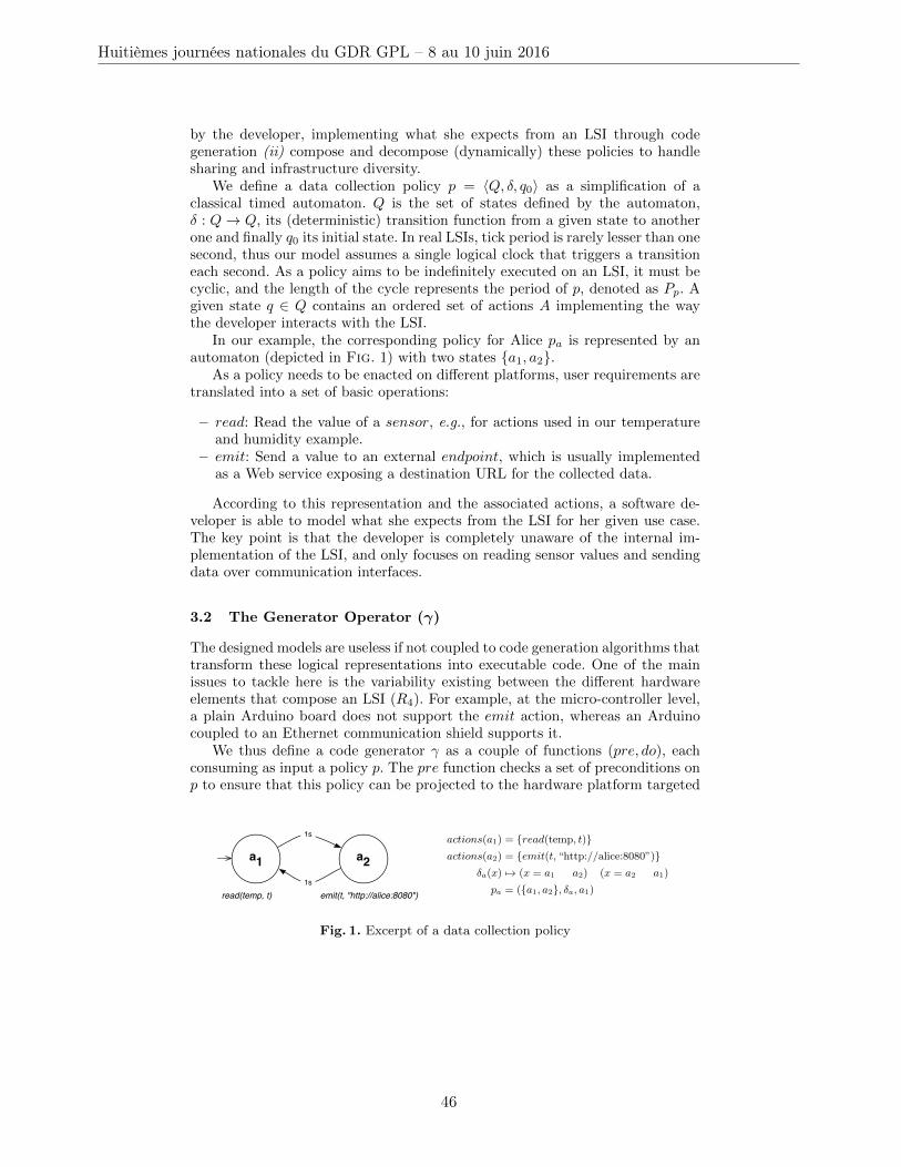
by the developer, implementing what she expects from an LSI through codegeneration (ii) compose and decompose (dynamically) these policies to handlesharing and infrastructure diversity.
We define a data collection policy p = 〈Q, δ, q0〉 as a simplification of aclassical timed automaton. Q is the set of states defined by the automaton,δ : Q→ Q, its (deterministic) transition function from a given state to anotherone and finally q0 its initial state. In real LSIs, tick period is rarely lesser than onesecond, thus our model assumes a single logical clock that triggers a transitioneach second. As a policy aims to be indefinitely executed on an LSI, it must becyclic, and the length of the cycle represents the period of p, denoted as Pp. Agiven state q ∈ Q contains an ordered set of actions A implementing the waythe developer interacts with the LSI.
In our example, the corresponding policy for Alice pa is represented by anautomaton (depicted in Fig. 1) with two states {a1, a2}.
As a policy needs to be enacted on different platforms, user requirements aretranslated into a set of basic operations:
– read: Read the value of a sensor, e.g., for actions used in our temperatureand humidity example.
– emit: Send a value to an external endpoint, which is usually implementedas a Web service exposing a destination URL for the collected data.
According to this representation and the associated actions, a software de-veloper is able to model what she expects from the LSI for her given use case.The key point is that the developer is completely unaware of the internal im-plementation of the LSI, and only focuses on reading sensor values and sendingdata over communication interfaces.
3.2 The Generator Operator (γ)
The designed models are useless if not coupled to code generation algorithms thattransform these logical representations into executable code. One of the mainissues to tackle here is the variability existing between the different hardwareelements that compose an LSI (R4). For example, at the micro-controller level,a plain Arduino board does not support the emit action, whereas an Arduinocoupled to an Ethernet communication shield supports it.
We thus define a code generator γ as a couple of functions (pre, do), eachconsuming as input a policy p. The pre function checks a set of preconditions onp to ensure that this policy can be projected to the hardware platform targeted
a1 a2
1s
1s
read(temp, t) emit(t, "http://alice:8080")
In our example, the corresponding policy for Alice pa is represented by anautomaton (depicted in Fig. 1) with two states {a1, a2}:
actions(a1) = {read(temp, t)}actions(a2) = {emit(t, “http://alice:8080”)}
�a(x) 7! (x = a1 ) a2) _ (x = a2 ) a1)
pa = ({a1, a2}, �a, a1)
As a policy needs to be enacted on di↵erent platforms, user requirements aretranslated into a set of basic operations:
– read: Read the value of a sensor, e.g., for actions used in our temperatureand humidity example.
– emit: Send a value to an external endpoint, which is usually implementedas a Web service exposing an destination URL for the collected data.
According to this representation and the associated actions, a software de-veloper is able to model what she expects from the LSI for her given use case.The key point is that the developer is completely unaware of the internal im-plementation of the LSI, and only focuses on reading sensor values and sendingdata over communication interfaces.
3.2 The Generator Operator (�)
The designed models are useless if not coupled to code generation algorithms thattransform these logical representations into executable code. One of the mainissues to tackle here is the variability existing between the di↵erent hardwareelements that compose an LSI (R4). For example, at the micro-controller level,a plain Arduino board does not support the emit action, whereas an Arduinocoupled to an Ethernet communication shield supports it.
We thus define a code generator � as a couple of functions (pre, do), eachconsuming as input a single policy p. The pre function checks a set of precondi-tions on p to ensure that this policy can be projected to the hardware platformtargeted by p. The do function takes as input the automaton to transform, aswell as additional parameters given by the environment. These parameters maplogical names to physical elements when relevant (e.g., sensors on an Arduinoplatform are only identified by the pin number they are plugged in). In a produc-tion environment, the generators will not be executed by the developer herself.She will only express her needs, and will enact them on the LSI which actu-ally knows its internal infrastructure. A deployment engine will select the rightgenerator and use it for each targeted hardware element.
on a ce deployment engine dans Cosmic ? sinon c’est di�cile a faire ? on re-utilise une techno connue (donc citation...) ?
For example, we consider here the policy pa defined in the previous section,and an Arduino platform as generation target. The corresponding precondition
Fig. 1. Excerpt of a data collection policy
Huitièmes journées nationales du GDR GPL – 8 au 10 juin 2016
46
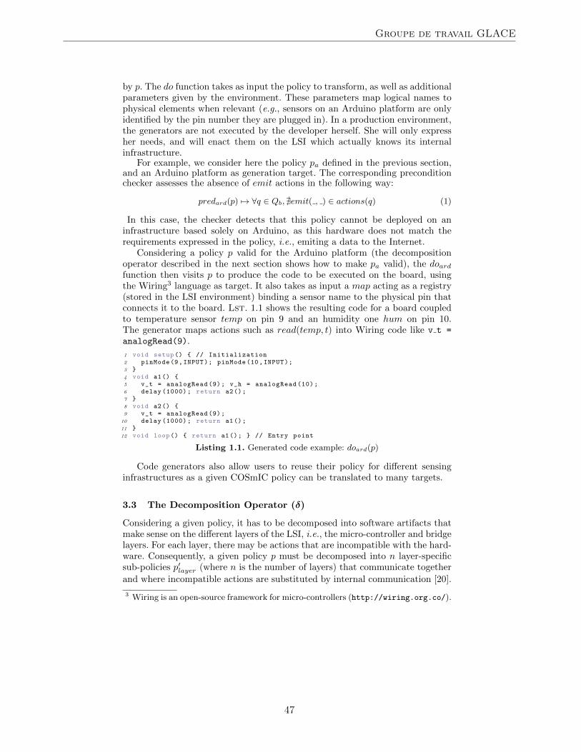
by p. The do function takes as input the policy to transform, as well as additionalparameters given by the environment. These parameters map logical names tophysical elements when relevant (e.g., sensors on an Arduino platform are onlyidentified by the pin number they are plugged in). In a production environment,the generators are not executed by the developer herself. She will only expressher needs, and will enact them on the LSI which actually knows its internalinfrastructure.
For example, we consider here the policy pa defined in the previous section,and an Arduino platform as generation target. The corresponding preconditionchecker assesses the absence of emit actions in the following way:
predard(p) 7→ ∀q ∈ Qb, @emit( , ) ∈ actions(q) (1)
In this case, the checker detects that this policy cannot be deployed on aninfrastructure based solely on Arduino, as this hardware does not match therequirements expressed in the policy, i.e., emiting a data to the Internet.
Considering a policy p valid for the Arduino platform (the decompositionoperator described in the next section shows how to make pa valid), the doardfunction then visits p to produce the code to be executed on the board, usingthe Wiring3 language as target. It also takes as input a map acting as a registry(stored in the LSI environment) binding a sensor name to the physical pin thatconnects it to the board. Lst. 1.1 shows the resulting code for a board coupledto temperature sensor temp on pin 9 and an humidity one hum on pin 10.The generator maps actions such as read(temp, t) into Wiring code like v t =
analogRead(9).
1 void setup() { // Initialization2 pinMode(9,INPUT); pinMode (10,INPUT);3 }4 void a1() {5 v_t = analogRead (9); v_h = analogRead (10);6 delay (1000); return a2();7 }8 void a2() {9 v_t = analogRead (9);
10 delay (1000); return a1();11 }12 void loop() { return a1(); } // Entry point
Listing 1.1. Generated code example: doard(p)
Code generators also allow users to reuse their policy for different sensinginfrastructures as a given COSmIC policy can be translated to many targets.
3.3 The Decomposition Operator (δ)
Considering a given policy, it has to be decomposed into software artifacts thatmake sense on the different layers of the LSI, i.e., the micro-controller and bridgelayers. For each layer, there may be actions that are incompatible with the hard-ware. Consequently, a given policy p must be decomposed into n layer-specificsub-policies p′layer (where n is the number of layers) that communicate together
and where incompatible actions are substituted by internal communication [20].
3 Wiring is an open-source framework for micro-controllers (http://wiring.org.co/).
Groupe de travail GLACE
47
This decomposition is performed thanks to a compatibility table T . A functionfT (a, P ) applied on this table returns a boolean value reflecting the compatibil-ity of an action a on the platform P 4. This decomposition process is defined asfollows:
δ(p) ≡ ∀a ∈ p, ∀P ∈ layers, fT (a, P )⇒ a ∈ p′a (2)
If we consider micro-controllers implemented by Arduino boards and bridgesimplemented by Raspberry nano-computers, the micro-controller level will notsupport the emission of data to external endpoints, due to a lack of propercommunication interface. In our example, Alice’s policy will be decomposed bythe operator into two sub-policies: δ(pa) = {p′mic, p
′bri}. Consequently, the pmic
will read the sensor value and send it to an internal endpoint (substitution of theemit action) thanks to the serial communication that links the sensor board toits bridge. This policy is accepted by the predard function defined in the Arduinocode generator, meaning that pmic can be deployed on such hardware. The pbripolicy is executed on the bridge to read the internal communication port andemit the received data to the external endpoint.
3.4 The Composition Operator (⊕)
On a shared LSI, policies designed by different developers will be executed onthe very same piece of hardware COSmIC provides a composition operator de-noted as ⊕ at the automaton level. It composes two given policies and producesa single policy containing an automaton corresponding strictly to the parallelcomposition of the two inputs.
The ⊕-operator assimilates a timed automaton implementing a policy p witha period Pp as a periodic function. The composition of two periodic functions f1and f2 is a periodic function f = f1 ◦f2 where its period Pf is the least commonmultiple of Pf1 and Pf2 . Applied to policies, this means that the compositionof two policies p1 and p2, denoted as p = p1 ⊕ p2 is a policy with a periodPp = lcm(Pp1 , Pp2), where each actions of p1 (respectively p2) are executedaccording to Pp1
(respectively Pp2). As this ⊕-operator is endogenous, it allows
a software developer to dynamically reuse a policy by composing it with newincoming policies.
In our example, the policies defined by Alice in pa and Bob in pb will exploitthe same temperature sensor on the same micro-controller and use the samebridge to emit their values. More details on the composition and decompositionprocesses are given in Sec. 4.2.
4 Assessment
In this section, we describe the current implementation and its application toour prototypical LSI. Then, we show how COSmIC can be used to model anddeploy the running example. We validate our identified requirements throughsome acceptance criteria and finally discuss threats to validity.
4 An example of such a table is given in Sec. 4.2.
Huitièmes journées nationales du GDR GPL – 8 au 10 juin 2016
48
4.1 Implementation and Application
The initial prototype of the COSmIC framework is available on GitHub5. Itis implemented with the Scala language (∼ 3500 lines of code) and covers allthe concepts presented in Sec. 3. We are currently experimenting COSmIC onArduino, Raspberry Pi and Cubieboard platforms as part of the SmartCam-pus project. We also used the FIT IoT-lab platform6, featuring a pool of over2700 sensors nodes spread across France, to experiment on the ARM Cortex M3platform.
To experiment and demonstrate the abstraction of platforms, code generationcapabilities, sharing and reuse, we have modeled four identified SmartCampusscenarios and then generated code for each platform type we experiment with:
– S1 - Late worker detection: at night, occupied offices are detected by checkingif the light is on (light sensor) and if there is someone in the office (presencesensor);
– S2 - Fire prevention: a warning signal on a temperature threshold (temper-ature sensor);
– S3 - Heat monitoring : air-conditioning and heating are controlled by check-ing the ambient air in buildings (temperature sensor);
– S4 - Energy wasting : To comply with environmental standards, the qualitymanager wants to monitor light kept on when the building is empty (lightsensor and presence sensor).
Table 1 presents the number of lines of code (LoC) generated for each plat-form. Every code generator includes a static overhead (template code), specificto the targeted platform. This template provides the implementation of meth-ods called by the COSmIC code generation. The corresponding LoC (italic rowon TAB. 1) vary between platforms as some of them are providing more fea-tures. The Raspberry Pi template contains only 85 LoC, corresponding to serialreading and value emission on the Internet (a Raspberry Pi cannot read valuesdirectly from sensors in the SmartCampus infrastructure). On the other hand,the ARM Cortex M3 template comprises 169 LoC to handle its sensor and net-work interface. Using a template is efficient as we target low-level platforms, andthose functions encapsulate a part of their complexity. For example, a methodprovided in the ARM Cortex M3 template handles the IPv6 retrieval of sensormeasures from a border-router.
We can first observe that without considering the boilerplate code definedin the templates, there is no real difference in terms of LoC between COSmICand the underlying programming languages. This is not surprising as the designchoice of using templates hides low-level details to raise the level of abstractionof each platform. But the key point is that the code written with the COS-mIC framework is not a single-target code but actually a model, which can beverified, composed automatically and projected to multiple platforms. Anotherinteresting property is that users do not need to know the underlying platform.For example, if a policy relies only on digital sensors, one can use the Contiki
5 http://ace-design.github.io/cosmic/6 https://www.iot-lab.info/
Groupe de travail GLACE
49
Table 1. LoC resulting from scenario generation
Arduino Arduino Raspberry ARM Cortex COSmICnative contiki / Python M3 / Python source
Template 13 22 85 169 0S1 6 14 13 11 7S2 5 13 11 10 5S3 5 13 11 10 7S4 6 14 13 11 7
S = S1 ⊕ S2 ⊕ S3 ⊕ S4 63 51 45 39 27Deployed: S + Template 76 73 160 208 N/A
Bob's composed policy
A Ø
B
A1 Ø
A2 Ø
C
Ø
ØBC B B
σ
B2C2 B2 B2
B1C1 B1 B1
A2B2C2
B2 A2B2
B2C2
A2B2 B2
σ
Alice's policy
Sensor platform
Bridge
⊕
⊕
A1B1C1
B2 A1B1
B2C2
A2B2 B2
⊕ Source code
Source code
Operation1s TransitionCode generation
Ø IDLE State
x
Express a policy
❶
❶
❶
❷ ❷
❸
❸
❹
❹
Fig. 2. COSmIC processes on the running example
operating system [8] to use a thread-based implementation of this policy. If a newrequirement including values coming from analog sensors needs to be enactedon the same board, Contiki cannot be used anymore and the implementationmust be completely rebuilt using only native operations. This is not the casewith COSmIC: the two policies will be automatically composed, and it simplyimplies to change the call to the code generator as the Contiki one will rejectthe composed policy.
4.2 Illustration
We illustrate the application of the COSmIC operators from policy definitionto code generation on the Alice and Bob example (see Sec. 2.3), on the topof the SmartCampus infrastructure7. Fig. 2 gives an overview of the differentactivities.
7 More details can be found on a companion web page:https://github.com/ace-design/cosmic/blob/master/publications/ICSR15.md
Huitièmes journées nationales du GDR GPL – 8 au 10 juin 2016
50
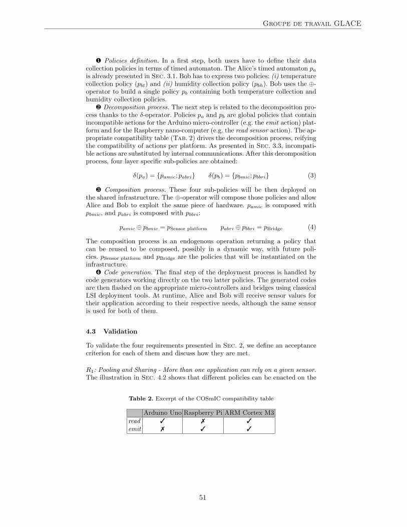
¶ Policies definition. In a first step, both users have to define their datacollection policies in terms of timed automaton. The Alice’s timed automaton pais already presented in Sec. 3.1. Bob has to express two policies: (i) temperaturecollection policy (pbt) and (ii) humidity collection policy (pbh). Bob uses the ⊕-operator to build a single policy pb containing both temperature collection andhumidity collection policies.
· Decomposition process. The next step is related to the decomposition pro-cess thanks to the δ-operator. Policies pa and pb are global policies that containincompatible actions for the Arduino micro-controller (e.g. the emit action) plat-form and for the Raspberry nano-computer (e.g. the read sensor action). The ap-propriate compatibility table (Tab. 2) drives the decomposition process, reifyingthe compatibility of actions per platform. As presented in Sec. 3.3, incompati-ble actions are substituted by internal communications. After this decompositionprocess, four layer specific sub-policies are obtained:
δ(pa) = {pamic; pabri} δ(pb) = {pbmic; pbbri} (3)
¸ Composition process. These four sub-policies will be then deployed onthe shared infrastructure. The ⊕-operator will compose those policies and allowAlice and Bob to exploit the same piece of hardware. pamic is composed withpbmic, and pabri is composed with pbbri:
pamic ⊕ pbmic = pSensor platform pabri ⊕ pbbri = pBridge (4)
The composition process is an endogenous operation returning a policy thatcan be reused to be composed, possibly in a dynamic way, with future poli-cies. pSensor platform and pBridge are the policies that will be instantiated on theinfrastructure.
¹ Code generation. The final step of the deployment process is handled bycode generators working directly on the two latter policies. The generated codesare then flashed on the appropriate micro-controllers and bridges using classicalLSI deployment tools. At runtime, Alice and Bob will receive sensor values fortheir application according to their respective needs, although the same sensoris used for both of them.
4.3 Validation
To validate the four requirements presented in Sec. 2, we define an acceptancecriterion for each of them and discuss how they are met.
R1: Pooling and Sharing - More than one application can rely on a given sensor.The illustration in Sec. 4.2 shows that different policies can be enacted on the
Table 2. Excerpt of the COSmIC compatibility table
Arduino Uno Raspberry Pi ARM Cortex M3read 3 7 3emit 7 3 3
Groupe de travail GLACE
51
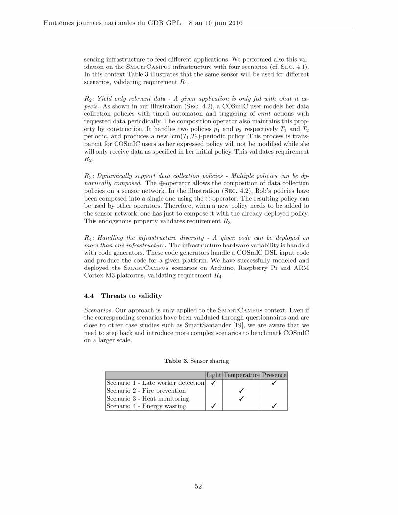
sensing infrastructure to feed different applications. We performed also this val-idation on the SmartCampus infrastructure with four scenarios (cf. Sec. 4.1).In this context Table 3 illustrates that the same sensor will be used for differentscenarios, validating requirement R1.
R2: Yield only relevant data - A given application is only fed with what it ex-pects. As shown in our illustration (Sec. 4.2), a COSmIC user models her datacollection policies with timed automaton and triggering of emit actions withrequested data periodically. The composition operator also maintains this prop-erty by construction. It handles two policies p1 and p2 respectively T1 and T2periodic, and produces a new lcm(T1,T2)-periodic policy. This process is trans-parent for COSmIC users as her expressed policy will not be modified while shewill only receive data as specified in her initial policy. This validates requirementR2.
R3: Dynamically support data collection policies - Multiple policies can be dy-namically composed. The ⊕-operator allows the composition of data collectionpolicies on a sensor network. In the illustration (Sec. 4.2), Bob’s policies havebeen composed into a single one using the ⊕-operator. The resulting policy canbe used by other operators. Therefore, when a new policy needs to be added tothe sensor network, one has just to compose it with the already deployed policy.This endogenous property validates requirement R3.
R4: Handling the infrastructure diversity - A given code can be deployed onmore than one infrastructure. The infrastructure hardware variability is handledwith code generators. These code generators handle a COSmIC DSL input codeand produce the code for a given platform. We have successfully modeled anddeployed the SmartCampus scenarios on Arduino, Raspberry Pi and ARMCortex M3 platforms, validating requirement R4.
4.4 Threats to validity
Scenarios. Our approach is only applied to the SmartCampus context. Even ifthe corresponding scenarios have been validated through questionnaires and areclose to other case studies such as SmartSantander [19], we are aware that weneed to step back and introduce more complex scenarios to benchmark COSmICon a larger scale.
Table 3. Sensor sharing
Light Temperature PresenceScenario 1 - Late worker detection 3 3Scenario 2 - Fire prevention 3Scenario 3 - Heat monitoring 3Scenario 4 - Energy wasting 3 3
Huitièmes journées nationales du GDR GPL – 8 au 10 juin 2016
52
Timed automata. Our data collection policies are represented by timed au-tomata. If this approach fits the SmartCampus use case, the combination ofdifferent scenarios can lead to a combinatorial explosion, (e.g., collections on ashared sensor at frequencies of one second and one hour would lead to a 3600states automaton with only two relevant states). The code generation processis impacted by such automata. We currently reduce the size of such automatathanks to a factorization process, but this optimization does not scale with alarge number of concurrent scenarios. The use of such automata also impactsthe resources. Platforms have to be always powered on, to the detriment of thebattery autonomy, to maintain a running clock delivering periodic clock tick.Devising better techniques to handle such cases and providing resource manage-ment is part of our future work.
Action execution duration. Our automata represent clocks with a 1 Hz fre-quency. If the execution of an action is longer than one second, it might beoverlapped and aborted by the state transition leading the policy into an in-consistent state. In the future, we plan to use languages based on the formalClock Constraint Specification Language (CCSL) [6] to determine the durationof action execution and to ensure the temporal correctness of policies.
Deployment of new policies. Our approach handles the dynamic compositionof data collection policies and code generation for a given platform. However,we do not support dynamic deployment as some sensor platforms need to be re-flashed with a new firmware. When the platform support it, we rely on operatingsystems (e.g., Contiki) to support this feature.
5 Related Work
Programming sensor networks with specific OS. Several operating systems havebeen specifically designed for sensing infrastructures, e.g., TinyOS [14] or Con-tiki [8]. TinyOS is based on a component architecture and comes with its pro-gramming language NesC. A developer can create new components or reusecomponents from the TinyOS’s component library to build her own application.Contiki is adapted for networked and resource-constrained devices. Contiki ap-plications can be written and compiled using a specific C compiler. Those OS ab-stract some complexities of application development, such as memory or energyoptimization, but the developer has to be aware of what kind of sensor platformsshe is using, directly dealing with their implementation details at a lower level.This leads to a lack of reusability, whereas our approach introduces a genericway to program sensor network. The COSmIC code is written independentlyfrom a sensing infrastructure and code generators handle the transformation toa targeted platform.
Sensor network as a database. On top of operating systems deployed on sens-ing infrastructure, several approaches consider the sensor network itself as adatabase [7]. Storing the data as close as possible to the sensor producing it in-stead of pushing everything to the Cloud was demonstrated as cost-efficient andenergy saving [22]. The TinyDB system [16] (not maintained since 2005) pro-vides processing mechanisms for sensor querying and data retrieval. It considers
Groupe de travail GLACE
53
a sensor as a micro-database storing their collected data, and allows develop-ers to query sensors according to different criteria (e.g., location). The Cougarsystem [24] also considers data collected by sensors, and supports users by onlyexpressing queries that are automatically propagated to the sensors. This systemdoes not support sharing (as queries cannot be composed easily), and relies ona centralized engine that computes a collection planning and collects data. Onthe contrary, COSmIC fully distributes the policies to the different sensors andthe infrastructure layers, and supports multiple endpoints for each application.
Model-driven and generative approaches. The model-driven development para-digm has been notably used to design dynamically adaptive systems and toevolve them at runtime [18]. In this approach, the current context model is ana-lyzed at runtime and, if an adaptation needs to be performed, a suitable configu-ration is built thanks to reference models. The approach can fit lightweight nodesin a sensor network [11]. Our work differs as we do not perform adaptivenessaccording to the context but design sensor network applications with policiesbased on a composition equation that can be reused for other compositions orfor verification purposes. Exploiting runtime composition is a perspective of ourwork. The way we generate code is close to the Scalaness approach [5]. It is atype-safe language used to wirelessly program embedded networks running un-der TinyOS. Two stages are required to program these networks: (i) one writesa Scalaness program, which is then (ii) translated into Java bytecode. We differfrom this approach as we use behavior models to generate code and we do notalways have the same destination platforms as we target heterogeneous sensornetworks.
6 Conclusions & Perspectives
In this paper we have presented the COSmIC Framework used for supportingdifferent developers’ collect policies on a shared LSI, generating code deployedat the approriate layer of the LSI. It addresses several limitations of classicalapproaches, focusing on the sharing of the infrastructure and the production ofrelevant-only datasets, and allowing software developers to focus on their con-cerns instead of LSI implementation details. The framework is implemented us-ing the Scala language and preliminary experiments have been conducted on topof the SmartCampus platform [4]. The COSmIC framework is a first step forcomposing policies on an LSI, with a focus on policy definition and compositionoperators.
Future work aims at extending the approach and making it scale to very largeLSIs. First, we will extend this set of operators to build a complete compositionalgebra, with a formal definition of operator properties (e.g., commutativity, as-sociativity, idempotency), conflict detection mechanisms to prevent inconsistentstates (i.e., sending a value before reading it) and a formal support to attachconstraints to actions. We also plan to extend these constraints to timed ones,using the TimeSquare toolkit [6] to specify and analyze constraints based onits logical time model and to check them also at runtime. We also plan to en-large the set of interactions with the LSI by introducing new actions allowing
Huitièmes journées nationales du GDR GPL – 8 au 10 juin 2016
54
a developer to perform some data computation within the sensor network (e.g.,Compute the average value of data coming from different sensors.
For those developers, we will improve the available abstractions by providinga higher level DSL. It will notably hide the creation and management of statesand transitions, providing a real focus on what data are collected, processed andused in applications.
The decomposition operator also triggers interesting challenges with respectto the variability of hardware (i.e., Arduino, Phidgets platforms) and facili-ties (i.e., Supported programming language, resources available) available inthe context of LSIs. We plan to use a feature modeling [2] approach to cap-ture this variability, and to bind these models to the generation mechanisms,providing a variable code generation according to the available hardware in agiven LSI. Finally, we also plan to support policy composition and variabilityreasoning at runtime to handle dynamic adaptiveness. We expect the resultingtooled approach to provide an end-to-end support for developers of the massivelyunder-deployment sensing infrastructures.
References
1. Aggarwal, C.C. (ed.): Managing and Mining Sensor Data. Springer (2013)2. Apel, S., Batory, D.S., Kastner, C., Saake, G.: Feature-Oriented Software Product
Lines - Concepts and Implementation. Springer (2013)3. Buratti, C., Conti, A., Dardari, D., Verdone, R.: An overview on wireless sensor
networks technology and evolution. Sensors 9(9), 6869–6896 (2009), http://www.mdpi.com/1424-8220/9/9/6869
4. Cecchinel, C., Jimenez, M., Mosser, S., Riveill, M.: An Architecture to Supportthe Collection of Big Data in the Internet of Things. In: International Workshopon Ubiquitous Mobile Cloud (UMC’14, co-located with SERVICES’14). pp. 1–8.IEEE, Anchorage, Alaska, USA (Jun 2014)
5. Chapin, P.C., Skalka, C., Smith, S.F., Watson, M.: Scalaness/nesT: Type Spe-cialized Staged Programming for Sensor Networks. In: Jrvi, J., Kstner, C. (eds.)GPCE. pp. 135–144. ACM (2013)
6. Deantoni, J., Mallet, F.: TimeSquare: Treat your Models with Logical Time. In:Carlo A. Furia, S.N. (ed.) TOOLS - 50th International Conference on Objects,Models, Components, Patterns - 2012. Lecture Notes in Computer Science - LNCS,vol. 7304, pp. 34–41. Czech Technical University in Prague, in co-operation withETH Zurich, Springer, Prague, Tcheque, Republique (May 2012)
7. Diao, Y., Ganesan, D., Mathur, G., Shenoy, P.J.: Rethinking data managementfor storage-centric sensor networks. In: CIDR 2007, Third Biennial Conferenceon Innovative Data Systems Research, Asilomar, CA, USA, January 7-10, 2007,Online Proceedings. pp. 22–31 (2007)
8. Dunkels, A., Gronvall, B., Voigt, T.: Contiki - a lightweight and flexible operat-ing system for tiny networked sensors. In: Local Computer Networks, 2004. 29thAnnual IEEE International Conference on. pp. 455–462 (Nov 2004)
9. Fambon, O., Fleury, E., Harter, G., Pissard-Gibollet, R., Saint-Marcel, F.: Fit iot-lab tutorial: hands-on practice with a very large scale testbed tool for the internetof things. In: 10emes journees francophones Mobilite et Ubiquite (UbiMob). pp.1–5 (June 2014)
10. Fleurey, F., Morin, B., Solberg, A.: A Model-Driven Approach to Develop AdaptiveFirmwares. In: Giese, H., Cheng, B.H.C. (eds.) SEAMS. pp. 168–177. ACM (2011)
Groupe de travail GLACE
55

11. Fouquet, F., Morin, B., Fleurey, F., Barais, O., Plouzeau, N., Jezequel, J.M.: ADynamic Component Model for Cyber Physical Systems. In: Proceedings of the15th ACM SIGSOFT Symposium on Component Based Software Engineering. pp.135–144. CBSE ’12, ACM, New York, NY, USA (2012)
12. Gluhak, A., Krco, S., Nati, M., Pfisterer, D., Mitton, N., Razafindralambo, T.:A Survey on Facilities for Experimental Internet of Things Research. IEEECommunications Magazine 49(11), 58–67 (Dec 2011), http://hal.inria.fr/
inria-00630092
13. Gubbi, J., Buyya, R., Marusic, S., Palaniswami, M.: Internet of Things (IoT): AVision, Architectural Elements, and Future Directions. Future Generation Comp.Syst. 29(7), 1645–1660 (2013)
14. Levis, P., Madden, S., Polastre, J., Szewczyk, R., Woo, A., Gay, D., Hill, J., Welsh,M., Brewer, E., Culler, D.: Tinyos: An operating system for sensor networks. In:in Ambient Intelligence. Springer Verlag (2004)
15. LogMeIn: Xively (May 2014), http://xively.com/16. Madden, S.R., Franklin, M.J., Hellerstein, J.M., Hong, W.: Tinydb: An acquisi-
tional query processing system for sensor networks. ACM Trans. Database Syst.30(1), 122–173 (Mar 2005), http://doi.acm.org/10.1145/1061318.1061322
17. Mahmood, A., Ke, S., Khatoon, S., Xiao, M.: Data mining techniques for wirelesssensor networks: A survey. IJDSN 2013 (2013)
18. Morin, B., Barais, O., Jezequel, J., Fleurey, F., Solberg, A.: [email protected] toSupport Dynamic Adaptation. Computer 42(10), 44–51 (2009)
19. Sanchez, L., Galache, J., Gutierrez, V., Hernandez, J., Bernat, J., Gluhak, A.,Garcia, T.: Smartsantander: The meeting point between future internet researchand experimentation and the smart cities. In: Future Network Mobile Summit(FutureNetw), 2011. pp. 1–8 (June 2011)
20. Stickel, M.E.: A Unification Algorithm for Associative-Commutative Functions. J.ACM 28(3), 423–434 (Jul 1981)
21. Tonneau, A.S., Mitton, N., Vandaele, J.: A Survey on (mobile) wireless sensornetwork experimentation testbeds. In: DCOSS - IEEE International Conferenceon Distributed Computing in Sensor Systems. Marina Del Rey, California, Etats-Unis (May 2014), http://hal.inria.fr/hal-00988776
22. Tsiftes, N., Dunkels, A.: A database in every sensor. In: Proceedings of the 9thACM Conference on Embedded Networked Sensor Systems. pp. 316–332. SenSys’11, ACM, New York, NY, USA (2011), http://doi.acm.org/10.1145/2070942.2070974
23. Volgyesi, P., Maroti, M., Dora, S., Osses, E., Ledeczi, A.: Software Compositionand Verification for Sensor Networks. Sci. Comput. Program. 56(1-2), 191–210(2005)
24. Yao, Y., Gehrke, J.: The cougar approach to in-network query processing in sensornetworks. SIGMOD Rec. 31(3), 9–18 (Sep 2002), http://doi.acm.org/10.1145/601858.601861
Huitièmes journées nationales du GDR GPL – 8 au 10 juin 2016
56
Modeling and Verification ofFunctional and Non Functional Requirements of
Ambient Self Adaptive Systems
M. Ahmada,b, N. Belloira, J. M. Bruelb
aUniversity of Pau and the Pays of the Adour, LIUPPA64000 Cedex, France
bUniversity of Toulouse, CNRS/IRITF-31062 Toulouse Universite Cedex, France
Abstract
Self Adaptive Systems modify their behavior at run-time in response to chang-ing environmental conditions. For these systems, Non Functional Requirementsplay an important role, and one has to identify as early as possible the require-ments that are adaptable. We propose an integrated approach for modelingand verifying the requirements of Self Adaptive Systems using Model DrivenEngineering techniques. For this, we use Relax, which is a Requirements En-gineering language which introduces flexibility in Non Functional Requirements.We then use the concepts of Goal Oriented Requirements Engineering for elic-iting and modeling the requirements of Self Adaptive Systems. For propertiesverification, we use OMEGA2/IFx profile and toolset. We illustrate our pro-posed approach by applying it on an academic case study.
Keywords: Requirements Engineering, Model Driven Engineering, Relax,Dynamic Adaptive Systems, Domain Specific Language, Non FunctionalRequirements, Properties Verification, Goal Oriented RequirementsEngineering
1. Introduction
As applications continue to grow in size, complexity, and heterogeneity, itbecomes increasingly necessary for computing based systems to dynamically selfadapt to changing environmental conditions. These systems are called Dynam-ically Adaptive Systems (DASs) [41]. Example applications that require DASscapabilities include automotive systems, telecommunication systems, environ-mental monitoring, and power grid management systems. In this context, anadaptive system is a set of interacting or interdependent entities, real or abstract,forming an integrated whole that together are able to respond to environmentalchanges or changes in the interacting parts. A Self Adaptive Systems (SAS),like other systems, has goals that must be satisfied and, whether these goalsare explicitly identified or not, system requirements should be formulated to
Email addresses: [email protected] (M. Ahmad),[email protected] (N. Belloir), [email protected] (J. M. Bruel)
Preprint submitted to Elsevier November 26, 2014
Groupe de travail GLACE
57
guarantee goal satisfaction. This fundamental principle has served systems de-velopment well for several decades but is founded on an assumption that goalsare fixed. In general, goals can remain fixed if the environment in which thesystem operates is stable [40]. The distributed nature of SAS and changing envi-ronmental factors (including human interaction) makes it difficult to anticipateall the explicit states in which the system will be during its lifetime.
It is generally accepted that errors in requirements are very costly to fix[29]. The avoidance of erroneous requirements is particularly important forthe emerging class of systems that need to adapt dynamically to changes intheir environment. Many such DASs are being conceived for applications thatrequire a high degree of assurance [36], in which an erroneous requirement mayresult in a failure at run-time that has serious consequences. The requirementfor high assurance is not unique to DASs, but the requirement for dynamicadaptation introduces complexity of a kind not seen in conventional systemswhere adaptation, if it is needed at all, can be done off-line. The consequentdynamic adaptation complexity is manifested at all levels, from the servicesoffered by the run-time platform, to the analytical tools needed to understandthe environment in which the DASs must operate.
Requirements Engineering (RE) is concerned with what a system ought to doand within which constraints it must do it. RE for SAS, therefore, must addresswhat adaptations are possible and what constrains how those adaptations arecarried out. In particular, questions to be addressed include: what aspects ofthe environment are relevant for adaptation? Which requirements are allowed tovary or evolve at run-time and which must always be maintained? In short, REfor SAS must deal with uncertainty because the expectations on the environmentfrequently vary over time. We identify the uncertainty in requirements of thesesystems and show how to verify it.
We are of the view that, on one hand, requirements for SAS should considerthe notion of uncertainty while defining it; on the other hand, there shouldbe a way to verify these requirements as early as possible, even before thedevelopment of these systems starts. In order to handle the notion of uncertaintyin SAS, RE languages for these systems should include explicit constructs foridentifying the point of flexibility in its requirements [41]. In this context,we provide an integrated approach to achieve this objective. We have usedtwo approaches for defining and modeling requirements, i.e. Goal OrientedRequirements Engineering (GORE) techniques are used to define and modelthe requirements of SAS [23, 44, 28, 43] and SysML is used to specify thesystem and to provide a link with the requirements.
We propose a model based requirements modeling and verification process forSAS that takes into account the uncertainty in requirements of these systems.We provide some tools to implement our apporach and then apply it on anacademic case study. The notion of goals is added to take into account theadvantages offered by GORE. Requirements verification is done using modelchecking technique.
This paper is organized as follows: In section 2, we describe the backgroundand the concepts which form the basis of this work, section 3 shows the stateof the art regarding RE for SAS and properties verification of these systems,section 4 shows and illustrate our proposed approach through an example andthe tools that we have developed, section 5 shows the case study that we usedfor the validation of our approach, and section 6 concludes the paper and shows
2
Huitièmes journées nationales du GDR GPL – 8 au 10 juin 2016
58
the future work.
2. Background
2.1. RELAX
Relax is an RE language for DASs in which explicit constructs are includedto handle uncertainty. For example, the system might wish to temporarily Re-lax a non-critical requirement in order to ensure that critical requirements canstill be met. The need for DASs is typically due to two key sources of uncer-tainty. First is the uncertainty due to changing environmental conditions, suchas sensor failures, noisy networks, malicious threats, and unexpected (human)input; the term environmental uncertainty is used to capture this class of un-certainty. A second form of uncertainty is behavioral uncertainty, which refersto situations where the requirements themselves need to change. It is difficultto know all requirements changes at design time and, in particular, it may notbe possible to enumerate all possible alternatives [41].
2.1.1. RELAX Vocabulary
The vocabulary of Relax is designed to enable the analysts to identify therequirements that may be Relax-ed when the environment changes. Relaxaddresses both types of uncertainties. Relax also outlines a process for trans-lating traditional requirements into Relax requirements. The only focal pointis for the requirement engineers to identify the point of flexibility in their require-ments. Relax identifies two types of requirements: one that can be Relax-edin favor of other ones called variant or Relax-ed and other that should neverchange called invariant. It is important to note that the decision of whether arequirement is invariant or not is an issue for the system stakeholders, aided bythe requirements engineer.
Relax takes the form of a structured natural language, including operatorsdesigned specifically to capture uncertainty [40]; their semantics is also defined.Figure 1 shows the set of Relax operators, organized into modal, temporal, or-dinal operators and uncertainty factors. The conventional modal verb SHALLis retained for expressing a requirement with Relax operators providing moreflexibility in how and when that functionality may be delivered. More specifi-cally, for a requirement that contributes to the satisfaction of goals that may betemporarily left unsatisfied, the inclusion of an alternative, temporal or ordinalRelax-ation modifier will define the requirement as Relax-able.
2.1.2. RELAX Grammar
The syntax of Relax expressions is defined by the grammar shown in Fig-ure 2. Parameters of Relax operators are typed as follows: p is an atomicproposition, e is an event, t is a time interval, f is a frequency and q is a quan-tity. An event is a notable occurrence that takes place at a particular instantin time. A time interval is any length of time bounded by two time instants.A frequency defines the number of occurrences of an event within a given timeinterval. If the number of occurrences is unspecified, then it is assumed to beone. A quantity is something measurable, meaning it can be enumerated. Inparticular, a Relax expression ϕ is said to be quantifiable if and only if thereexists a function ∆ such that ∆(ϕ) is a quantity. A valid Relax expression
3
Groupe de travail GLACE
59
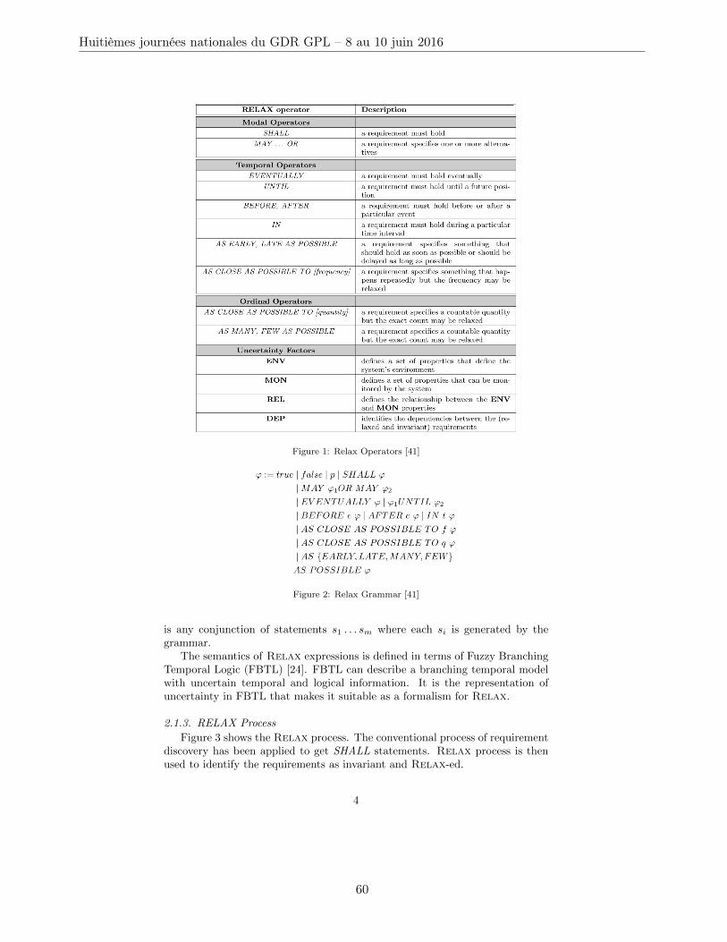
Figure 1: Relax Operators [41]
Figure 2: Relax Grammar [41]
is any conjunction of statements s1 . . . sm where each si is generated by thegrammar.
The semantics of Relax expressions is defined in terms of Fuzzy BranchingTemporal Logic (FBTL) [24]. FBTL can describe a branching temporal modelwith uncertain temporal and logical information. It is the representation ofuncertainty in FBTL that makes it suitable as a formalism for Relax.
2.1.3. RELAX Process
Figure 3 shows the Relax process. The conventional process of requirementdiscovery has been applied to get SHALL statements. Relax process is thenused to identify the requirements as invariant and Relax-ed.
4
Huitièmes journées nationales du GDR GPL – 8 au 10 juin 2016
60
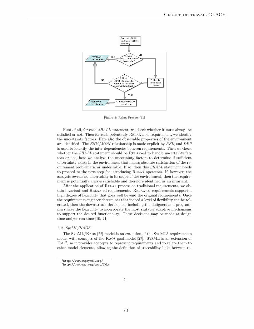
Figure 3: Relax Process [41]
First of all, for each SHALL statement, we check whether it must always besatisfied or not. Then for each potentially Relax-able requirement, we identifythe uncertainty factors. Here also the observable properties of the environmentare identified. The ENV /MON relationship is made explicit by REL, and DEPis used to identify the inter-dependencies between requirements. Then we checkwhether the SHALL statement should be Relax-ed to handle uncertainty fac-tors or not, here we analyze the uncertainty factors to determine if sufficientuncertainty exists in the environment that makes absolute satisfaction of the re-quirement problematic or undesirable. If so, then this SHALL statement needsto proceed to the next step for introducing Relax operators. If, however, theanalysis reveals no uncertainty in its scope of the environment, then the require-ment is potentially always satisfiable and therefore identified as an invariant.
After the application of Relax process on traditional requirements, we ob-tain invariant and Relax-ed requirements. Relax-ed requirements support ahigh degree of flexibility that goes well beyond the original requirements. Oncethe requirements engineer determines that indeed a level of flexibility can be tol-erated, then the downstream developers, including the designers and program-mers have the flexibility to incorporate the most suitable adaptive mechanismsto support the desired functionality. These decisions may be made at designtime and/or run time [10, 21].
2.2. SysML/KAOS
The SysML/Kaos [22] model is an extension of the SysML1 requirementsmodel with concepts of the Kaos goal model [27]. SysML is an extension ofUml2, so it provides concepts to represent requirements and to relate them toother model elements, allowing the definition of traceability links between re-
1http://www.omgsysml.org/2http://www.omg.org/spec/UML/
5
Groupe de travail GLACE
61
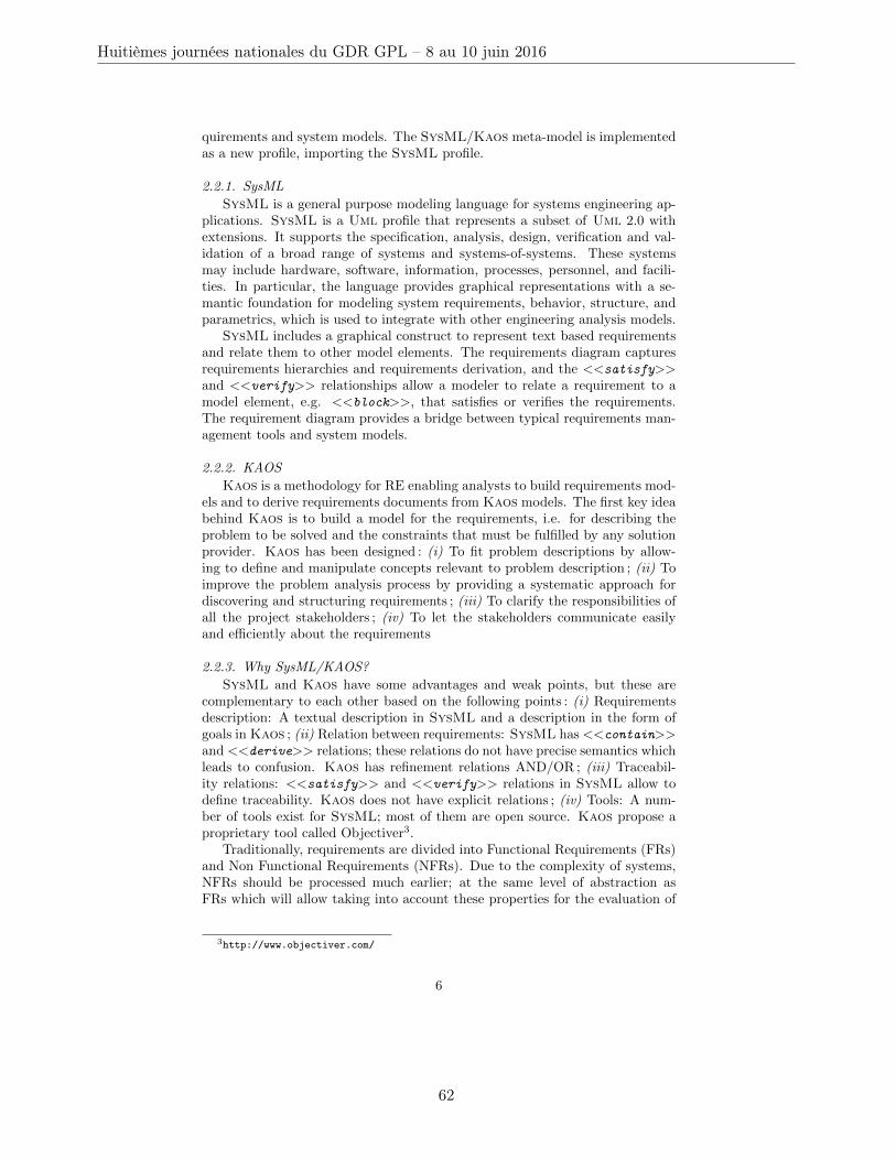
quirements and system models. The SysML/Kaos meta-model is implementedas a new profile, importing the SysML profile.
2.2.1. SysML
SysML is a general purpose modeling language for systems engineering ap-plications. SysML is a Uml profile that represents a subset of Uml 2.0 withextensions. It supports the specification, analysis, design, verification and val-idation of a broad range of systems and systems-of-systems. These systemsmay include hardware, software, information, processes, personnel, and facili-ties. In particular, the language provides graphical representations with a se-mantic foundation for modeling system requirements, behavior, structure, andparametrics, which is used to integrate with other engineering analysis models.
SysML includes a graphical construct to represent text based requirementsand relate them to other model elements. The requirements diagram capturesrequirements hierarchies and requirements derivation, and the <<satisfy>>and <<verify>> relationships allow a modeler to relate a requirement to amodel element, e.g. <<block>>, that satisfies or verifies the requirements.The requirement diagram provides a bridge between typical requirements man-agement tools and system models.
2.2.2. KAOS
Kaos is a methodology for RE enabling analysts to build requirements mod-els and to derive requirements documents from Kaos models. The first key ideabehind Kaos is to build a model for the requirements, i.e. for describing theproblem to be solved and the constraints that must be fulfilled by any solutionprovider. Kaos has been designed : (i) To fit problem descriptions by allow-ing to define and manipulate concepts relevant to problem description ; (ii) Toimprove the problem analysis process by providing a systematic approach fordiscovering and structuring requirements ; (iii) To clarify the responsibilities ofall the project stakeholders ; (iv) To let the stakeholders communicate easilyand efficiently about the requirements
2.2.3. Why SysML/KAOS?
SysML and Kaos have some advantages and weak points, but these arecomplementary to each other based on the following points : (i) Requirementsdescription: A textual description in SysML and a description in the form ofgoals in Kaos ; (ii) Relation between requirements: SysML has <<contain>>and <<derive>> relations; these relations do not have precise semantics whichleads to confusion. Kaos has refinement relations AND/OR ; (iii) Traceabil-ity relations: <<satisfy>> and <<verify>> relations in SysML allow todefine traceability. Kaos does not have explicit relations ; (iv) Tools: A num-ber of tools exist for SysML; most of them are open source. Kaos propose aproprietary tool called Objectiver3.
Traditionally, requirements are divided into Functional Requirements (FRs)and Non Functional Requirements (NFRs). Due to the complexity of systems,NFRs should be processed much earlier; at the same level of abstraction asFRs which will allow taking into account these properties for the evaluation of
3http://www.objectiver.com/
6
Huitièmes journées nationales du GDR GPL – 8 au 10 juin 2016
62
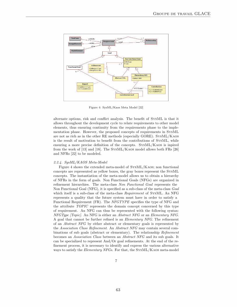
Figure 4: SysML/Kaos Meta Model [22]
alternate options, risk and conflict analysis. The benefit of SysML is that itallows throughout the development cycle to relate requirements to other modelelements, thus ensuring continuity from the requirements phase to the imple-mentation phase. However, the proposed concepts of requirements in SysMLare not as rich as in the other RE methods (especially GORE). SysML/Kaosis the result of motivation to benefit from the contributions of SysML, whileensuring a more precise definition of the concepts. SysML/Kaos is inpiredfrom the work of [13] and [18]. The SysML/Kaos model allows both FRs [26]and NFRs [22] to be modeled.
2.2.4. SysML/KAOS Meta-Model
Figure 4 shows the extended meta-model of SysML/Kaos; non functionalconcepts are represented as yellow boxes, the gray boxes represent the SysMLconcepts. The instantiation of the meta-model allows us to obtain a hierarchyof NFRs in the form of goals. Non Functional Goals (NFGs) are organized inrefinement hierarchies. The meta-class Non Functional Goal represents theNon Functional Goal (NFG), it is specified as a sub-class of the meta-class Goalwhich itself is a sub-class of the meta-class Requirement of SysML. An NFGrepresents a quality that the future system must have in order to satisfy aFunctional Requirement (FR). The NFGTYPE specifies the type of NFG andthe attribute TOPIC represents the domain concept concerned by this typeof requirement. An NFG can thus be represented with the following syntax:NFGType [Topic]. An NFG is either an Abstract NFG or an Elementary NFG.A goal that cannot be further refined is an Elementary NFG. The refinementof an Abstract NFG by either abstract or elementary goals is represented bythe Association Class Refinement. An Abstract NFG may contain several com-binations of sub goals (abstract or elementary). The relationship Refinementbecomes an Association Class between an Abstract NFG and its sub goals. Itcan be specialized to represent And/Or goal refinements. At the end of the re-finement process, it is necessary to identify and express the various alternativeways to satisfy the Elementary NFGs. For that, the SysML/Kaos meta-model
7
Groupe de travail GLACE
63
considers the concept of the meta-class Contribution Goal. A Contribution Goalcaptures a possible way to satisfy an Elementary NFG. The Association ClassContribution describes the characteristics of the contribution. It provides twoproperties: ContributionNature and ContributionType. The first one specifieswhether the contribution is positive or negative, whereas the second one specifieswhether the contribution is direct or indirect. A positive (or negative) contribu-tion helps positively (or negatively) to the satisfaction of an Elementary NFG.A direct contribution describes an explicit contribution to the Elementary NFG.An indirect contribution describes a kind of contribution that is a direct con-tribution to a given goal but induces an unexpected contribution to anothergoal. Finally, the concept of Impact is used to connect NFGs to FunctionalGoals (FGs). It captures the fact that a Contribution Goal has an effect onFGs.
2.3. The OMEGA2 UML/SysML Profile and IFx Toolset
Formal methods provide tools to verify the consistency and correctness ofa specification with respect to the desired properties of the system. For thisreason, we use these methods to prove some of the properties of the systembefore the system development even starts. We use OMEGA2/IFx profile andtoolset for the properties verification and model simulation of our case study.
2.3.1. The OMEGA2 Profile
OMEGA2 profile [32] is an executable Uml/SysML profile used for theformal specification and validation of critical real-time systems. It is based on asubset of Uml 2.2/SysML 1.1 containing the main constructs for defining thesystem structure and behavior.
The OMEGA2 Uml/SysML profile defines the semantics of Uml/SysMLelements providing the means to model coherent and unambiguous system mod-els. In order to make the models verifiable, it presents as extension the ob-servers mechanism for specifying dynamic properties of models. The OMEGA2Uml/SysML Profile is implemented by the IFx toolbox which provides staticanalysis, simulation and timed automaton based model checking [14] techniquesfor validation.
The architecture of an OMEGA2 model is described in Class/Block Def-inition Diagrams by classes/blocks with their relationships. Each class/blockdefines properties and operations, as well as a state machine. The hierar-chical structure of a model is defined in composite structures/Internal BlockDiagram (IBD): parts that communicate through ports and connectors. Forthe SysML block diagram (Block Definition Diagram (BDD)), the followingconcepts are taken into account: blocks and their relationships (association,aggregation, generalization), the interfaces, the basic types, signals.
For the system behavior, the OMEGA2 profile takes into account the follow-ing concepts: State machines (excluding: history states, entry point, exit point,junction) and Actions; for this, the profile defines a concrete syntax. This syn-tax is used for example to define operation bodies and transition effects in statemachines. The textual action language is compatible with the Uml 2.2 actionmeta-model and implements its main elements: object creation and destruc-tion, operation calls, expression evaluation, variable assignment, signal output,return action as well as control flow structuring statements.
8
Huitièmes journées nationales du GDR GPL – 8 au 10 juin 2016
64
For specifying and verifying dynamic properties of models, OMEGA2 usesthe notion of observers. Observers are special classes/blocks monitoring run-time state and events. They are defined by classes/blocks stereotyped with<<observer>>. They may have local memory (attributes) and a state ma-chine describes their behavior. States are classified as <<success>> and<<error>> states to express the (non)satisfaction of safety properties. Themain issue in modeling observers is the choice of events which trigger theirtransitions.
The trigger of an observer transition is a match clause specifying the typeof event (e.g., receive), some related information (e.g., the operation name) andobserver variables that may receive related information (e.g., variables receivingthe values of operation call parameters). Besides events, an observer may accessany part of the state of the Uml model: object attributes and state, signalqueues.
2.3.2. IFx Toolset
OMEGA2 models can be simulated and properties can be verified usingthe IFx toolset [11]. The IFx toolset provides verification which ensures theautomatic process of verifying whether an OMEGA2 Uml/SysML model sat-isfies (some of) the properties (i.e. observers) defined on it. The verificationmethod employed in IFx is based on systematic exploration of the system statespace (i.e., enumerative model checking). The IFx toolset also provides simula-tion which designates the interactive execution of an OMEGA2 Uml/SysMLmodel. The execution can be performed step-by-step, random, or guided by asimulation scenario (for example an error scenario generated during a verifica-tion activity).
The IFx toolset relies on a translation of Uml/SysML models towards asimple specification language based on an asynchronous composition of extendedtimed automata, the IF language4, and on the use of simulation and verificationtools available for IF. The translation takes an input model in XML MetadataInterchange (XMI) 2.0 format. The compiler verifies the set of well-formednessrules imposed by the profile and generates an IF model that can be furtherreduced by static analysis techniques. This model is subject to verification thateither validates the model with respect to its properties or produces a list of errorscenarios that can be further debugged using the simulator. The OMEGA2/IFxapproach has been applied for the verification and validation of industry grademodels [20] providing interesting results.
3. State of the Art
Different road map papers on Software Engineering (SE) for SAS [21, 19]discuss the state of the art, its limitations, and identify critical challenges. [21]presents a research road map for SE of SAS focusing on four views, which areidentified as essential: requirements, modeling, engineering, and assurances.The focus is on development methods, techniques, and tools that seem to berequired to support the systematic development of complex software systemswith dynamic self adaptive behavior. The most recent road map paper [19]
4http://www-if.imag.fr/
9
Groupe de travail GLACE
65
discusses four essential topics of self-adaptation: design space for self-adaptivesolutions, software engineering processes for self-adaptive systems, from central-ized to decentralized control, and practical run-time verification and validationfor SAS.
3.1. Requirements Engineering for Self Adaptive Systems
An SAS is able to modify its behavior according to changes in its environ-ment. As such, an SAS must continuously monitor changes in its context andreact accordingly. But here the question arises as to what aspects of the environ-ment the SAS should monitor. Clearly, the system cannot monitor everythingand exactly what should the system do if it detects a less than optimal pat-tern in the environment? Presumably, the system still needs to maintain a setof high level goals that should be maintained regardless of the environmentalconditions. But non critical goals could well be Relax-ed, thus allowing thesystem a degree of flexibility during or after adaptation. It is important toidentify these properties as early as possible.
Levels of Requirement Engineering for Modeling (LoREM) [23] is an ap-proach for modeling the requirements of Dynamic Adaptive Systems (DAS)using i* goal models [42]. The i* goal models are used to represent the stake-holder objectives, non-adaptive system behavior (business logic), adaptive be-havior, and adaptation mechanism needs of DAS. Each of these i* goal modelsaddresses the three RE concerns (conditions to monitor, decision-making pro-cedure, and possible adaptations) from a specific developers perspective.
Awareness Requirements (AwReqs) [35] are requirements that talk aboutthe success or failure of other requirements. More generally, AwReqs talk aboutthe states requirements can assume during their execution at run-time. AwReqsare represented in a formal language and can be directly monitored by a require-ments monitoring framework.
Claims [39, 38] were applied as markers of uncertainty to record the ra-tionale for a decision made with incomplete information in DASs. The workin [33] integrates Relax and Claims to assess the validity of Claims at run-time while tolerating minor and unanticipated environmental conditions thatcan otherwise trigger adaptations.
Relax can be used in goal oriented modeling approaches for specifying andmitigating sources of uncertainty in DASs [12]. AutoRELAX [34], is an approachthat generates Relax-ed goal models that address environmental uncertaintyby identifying which goals to Relax, which Relax operators to apply, andthe shape of the fuzzy logic function that defines the goal satisfaction criteria.AutoRELAX also requires an executable specification of the DAS, such as asimulation or a prototype, which applies the set of utility functions to measurehow well the DAS satisfies its requirements in response to adverse conditions.For the experimental setup of AutoRELAX, a null hypothesis is defined whichstates that there is no difference between a Relax-ed and an unRelax-ed goalmodel.
Fuzzy Live Adaptive Goals for Self-Adaptive Systems (FLAGS) [7] is an in-novative goal model which deals with the challenges posed by SAS. Goal modelshave been used for representing systems requirements, and also for tracing themonto their underlying operationalization.
The state of the art regarding RE for SAS shows different approaches fromthe point of view of its complementarity with Relax. The different steps in
10
Huitièmes journées nationales du GDR GPL – 8 au 10 juin 2016
66
LoREM are interesting but our focus is on Relax-ed requirements as we wantto identify the uncertainty in the requirements of DASs. Regarding AwReqs,in future work, we want to integrate this concept into our approach usingMonitor-Analyze-Plan-Execute (MAPE) [25] feedback loop that operationalizesthe system’s adaptability mechanisms. Claims are also subject to uncertainty,in the form of unanticipated environmental conditions and unreliable monitoringinformation, that can adversely affect the behavior of the DAS if it spuriouslyfalsifies a claim. A Claim can also be monitored at run time to prove or disproveits validity [39], thereby triggering adaptation to reach more desirable systemconfigurations if necessary. Claims therefore complement Relax.
3.2. Properties Verification of SAS
For the properties verification of SAS, we use the OMEGA2/IFx profile andtoolset which was developed in our team. The advantage of the OMEGA2 profileis that it provides the notion of observers for specifying and verifying dynamicproperties of models. In terms of properties verification, there exists a numberof techniques. In the following, we give a description of some of it.
[9] presents a verification approach based on MEDISTAM-RT, which is amethodological framework for the design and analysis of real-time systems andtimed traces semantics, to check the fulfillment of NFRs. It only focuses onsafety and timeliness properties, to assure the correct functioning of AmbientAssisted Living (AAL) systems and to show the applicability of this methodol-ogy in the context of this kind of system.
[5] introduces a profile named Timed UML and RT-LOTOS Environment(TURTLE) which extends the Uml class and activity diagrams with composi-tion and temporal operators. TURTLE is a real-time Uml profile with a formalsemantics expressed in Real Time Language Of Temporal Ordering Specifica-tions (RTLOTOS) [17]. With its formal semantics and toolkit, TURTLE en-ables a priori detection of design errors through a combination of simulationand verification/validation techniques.
In [26], the authors propose an extension to SysML with concepts from thegoal model of the Kaos method (SysML/Kaos) with rules to derive a formalB [1] specification from this goal model. The B formal method is a completemethod that supports a large segment of the software development life cycle:specification, refinement and implementation.
In MEDISTAM-RT, the focus is on safety and timeliness properties, we donot treat any specific type of properties. We verify those requirements that areof interest for adaptation in SAS. In TURTLE, design errors can be detectedthrough simulation and verification, that’s the reason why we plan to explore thecomplementarity of this approach with our approach. The use of formal methodslike B can help avoid the state space explosion problem which is inherent inmodel checking techniques. We have worked on studying the complementarityof these two approaches and we plan to integrate it in our approach in the futurework.
4. Proposed Approach
In this section, we introduce the overall view of our proposed approach [2].We show our contribution then we describe the overall process of our approach.
11
Groupe de travail GLACE
67
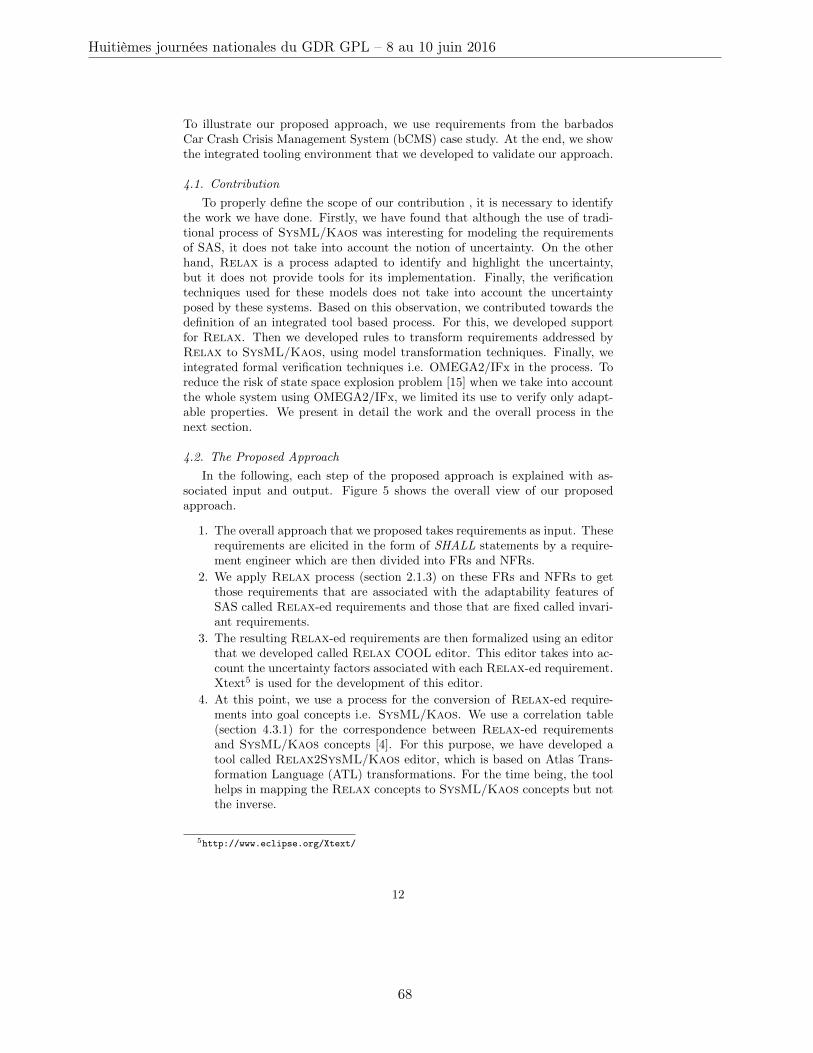
To illustrate our proposed approach, we use requirements from the barbadosCar Crash Crisis Management System (bCMS) case study. At the end, we showthe integrated tooling environment that we developed to validate our approach.
4.1. Contribution
To properly define the scope of our contribution , it is necessary to identifythe work we have done. Firstly, we have found that although the use of tradi-tional process of SysML/Kaos was interesting for modeling the requirementsof SAS, it does not take into account the notion of uncertainty. On the otherhand, Relax is a process adapted to identify and highlight the uncertainty,but it does not provide tools for its implementation. Finally, the verificationtechniques used for these models does not take into account the uncertaintyposed by these systems. Based on this observation, we contributed towards thedefinition of an integrated tool based process. For this, we developed supportfor Relax. Then we developed rules to transform requirements addressed byRelax to SysML/Kaos, using model transformation techniques. Finally, weintegrated formal verification techniques i.e. OMEGA2/IFx in the process. Toreduce the risk of state space explosion problem [15] when we take into accountthe whole system using OMEGA2/IFx, we limited its use to verify only adapt-able properties. We present in detail the work and the overall process in thenext section.
4.2. The Proposed Approach
In the following, each step of the proposed approach is explained with as-sociated input and output. Figure 5 shows the overall view of our proposedapproach.
1. The overall approach that we proposed takes requirements as input. Theserequirements are elicited in the form of SHALL statements by a require-ment engineer which are then divided into FRs and NFRs.
2. We apply Relax process (section 2.1.3) on these FRs and NFRs to getthose requirements that are associated with the adaptability features ofSAS called Relax-ed requirements and those that are fixed called invari-ant requirements.
3. The resulting Relax-ed requirements are then formalized using an editorthat we developed called Relax COOL editor. This editor takes into ac-count the uncertainty factors associated with each Relax-ed requirement.Xtext5 is used for the development of this editor.
4. At this point, we use a process for the conversion of Relax-ed require-ments into goal concepts i.e. SysML/Kaos. We use a correlation table(section 4.3.1) for the correspondence between Relax-ed requirementsand SysML/Kaos concepts [4]. For this purpose, we have developed atool called Relax2SysML/Kaos editor, which is based on Atlas Trans-formation Language (ATL) transformations. For the time being, the toolhelps in mapping the Relax concepts to SysML/Kaos concepts but notthe inverse.
5http://www.eclipse.org/Xtext/
12
Huitièmes journées nationales du GDR GPL – 8 au 10 juin 2016
68
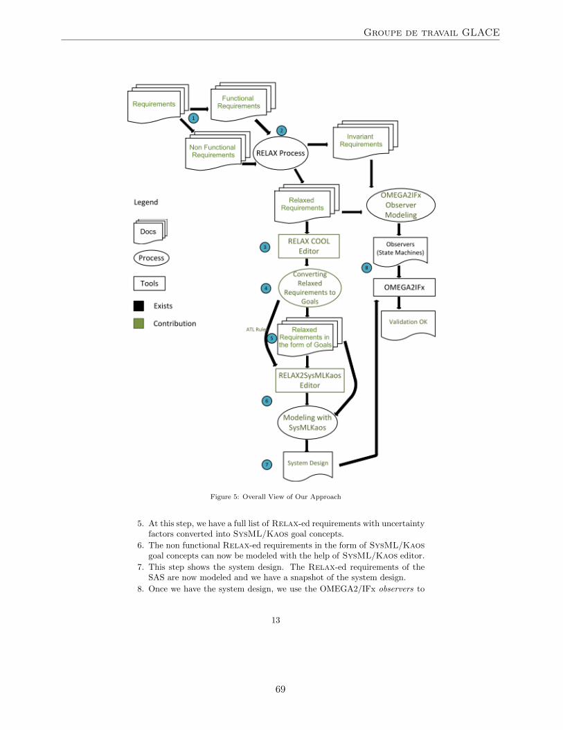
Figure 5: Overall View of Our Approach
5. At this step, we have a full list of Relax-ed requirements with uncertaintyfactors converted into SysML/Kaos goal concepts.
6. The non functional Relax-ed requirements in the form of SysML/Kaosgoal concepts can now be modeled with the help of SysML/Kaos editor.
7. This step shows the system design. The Relax-ed requirements of theSAS are now modeled and we have a snapshot of the system design.
8. Once we have the system design, we use the OMEGA2/IFx observers to
13
Groupe de travail GLACE
69
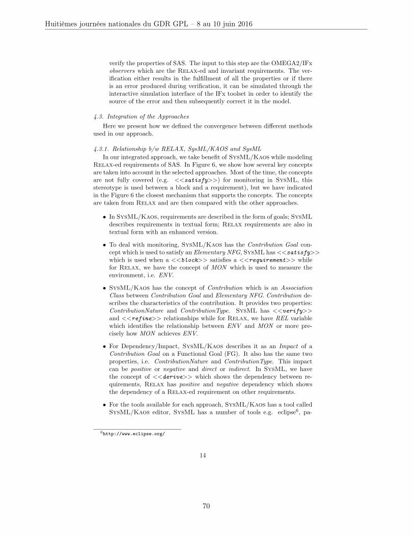
verify the properties of SAS. The input to this step are the OMEGA2/IFxobservers which are the Relax-ed and invariant requirements. The ver-ification either results in the fulfillment of all the properties or if thereis an error produced during verification, it can be simulated through theinteractive simulation interface of the IFx toolset in order to identify thesource of the error and then subsequently correct it in the model.
4.3. Integration of the Approaches
Here we present how we defined the convergence between different methodsused in our approach.
4.3.1. Relationship b/w RELAX, SysML/KAOS and SysML
In our integrated approach, we take benefit of SysML/Kaos while modelingRelax-ed requirements of SAS. In Figure 6, we show how several key conceptsare taken into account in the selected approaches. Most of the time, the conceptsare not fully covered (e.g. <<satisfy>>) for monitoring in SysML, thisstereotype is used between a block and a requirement), but we have indicatedin the Figure 6 the closest mechanism that supports the concepts. The conceptsare taken from Relax and are then compared with the other approaches.
• In SysML/Kaos, requirements are described in the form of goals; SysMLdescribes requirements in textual form; Relax requirements are also intextual form with an enhanced version.
• To deal with monitoring, SysML/Kaos has the Contribution Goal con-cept which is used to satisfy an Elementary NFG, SysML has <<satisfy>>which is used when a <<block>> satisfies a <<requirement>> whilefor Relax, we have the concept of MON which is used to measure theenvironment, i.e. ENV.
• SysML/Kaos has the concept of Contribution which is an AssociationClass between Contribution Goal and Elementary NFG. Contribution de-scribes the characteristics of the contribution. It provides two properties:ContributionNature and ContributionType. SysML has <<verify>>and <<refine>> relationships while for Relax, we have REL variablewhich identifies the relationship between ENV and MON or more pre-cisely how MON achieves ENV.
• For Dependency/Impact, SysML/Kaos describes it as an Impact of aContribution Goal on a Functional Goal (FG). It also has the same twoproperties, i.e. ContributionNature and ContributionType. This impactcan be positive or negative and direct or indirect. In SysML, we havethe concept of <<derive>> which shows the dependency between re-quirements, Relax has positive and negative dependency which showsthe dependency of a Relax-ed requirement on other requirements.
• For the tools available for each approach, SysML/Kaos has a tool calledSysML/Kaos editor, SysML has a number of tools e.g. eclipse6, pa-
6http://www.eclipse.org/
14
Huitièmes journées nationales du GDR GPL – 8 au 10 juin 2016
70
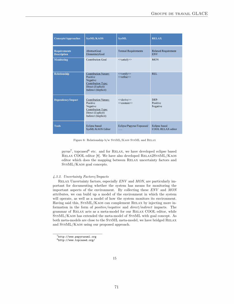
Figure 6: Relationship b/w SysML/Kaos SysML and Relax
pyrus7, topcased8 etc. and for Relax, we have developed eclipse basedRelax COOL editor [8]. We have also developed Relax2SysML/Kaoseditor which does the mapping between Relax uncertainty factors andSysML/Kaos goal concepts.
4.3.2. Uncertainty Factors/Impacts
Relax Uncertainty factors, especially ENV and MON, are particularly im-portant for documenting whether the system has means for monitoring theimportant aspects of the environment. By collecting these ENV and MONattributes, we can build up a model of the environment in which the systemwill operate, as well as a model of how the system monitors its environment.Having said this, SysML/Kaos can complement Relax by injecting more in-formation in the form of positive/negative and direct/indirect impacts. Thegrammar of Relax acts as a meta-model for our Relax COOL editor, whileSysML/Kaos has extended the meta-model of SysML with goal concept. Asboth meta-models are close to the SysML meta-model, we have bridged Relaxand SysML/Kaos using our proposed approach.
7http://www.papyrusuml.org8http://www.topcased.org/
15
Groupe de travail GLACE
71
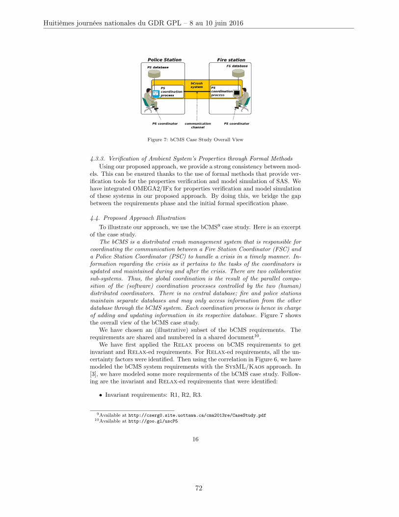
Figure 7: bCMS Case Study Overall View
4.3.3. Verification of Ambient System’s Properties through Formal Methods
Using our proposed approach, we provide a strong consistency between mod-els. This can be ensured thanks to the use of formal methods that provide ver-ification tools for the properties verification and model simulation of SAS. Wehave integrated OMEGA2/IFx for properties verification and model simulationof these systems in our proposed approach. By doing this, we bridge the gapbetween the requirements phase and the initial formal specification phase.
4.4. Proposed Approach Illustration
To illustrate our approach, we use the bCMS9 case study. Here is an excerptof the case study.
The bCMS is a distributed crash management system that is responsible forcoordinating the communication between a Fire Station Coordinator (FSC) anda Police Station Coordinator (PSC) to handle a crisis in a timely manner. In-formation regarding the crisis as it pertains to the tasks of the coordinators isupdated and maintained during and after the crisis. There are two collaborativesub-systems. Thus, the global coordination is the result of the parallel compo-sition of the (software) coordination processes controlled by the two (human)distributed coordinators. There is no central database; fire and police stationsmaintain separate databases and may only access information from the otherdatabase through the bCMS system. Each coordination process is hence in chargeof adding and updating information in its respective database. Figure 7 showsthe overall view of the bCMS case study.
We have chosen an (illustrative) subset of the bCMS requirements. Therequirements are shared and numbered in a shared document10.
We have first applied the Relax process on bCMS requirements to getinvariant and Relax-ed requirements. For Relax-ed requirements, all the un-certainty factors were identified. Then using the correlation in Figure 6, we havemodeled the bCMS system requirements with the SysML/Kaos approach. In[3], we have modeled some more requirements of the bCMS case study. Follow-ing are the invariant and Relax-ed requirements that were identified:
• Invariant requirements: R1, R2, R3.
9Available at http://cserg0.site.uottawa.ca/cma2013re/CaseStudy.pdf10Available at http://goo.gl/uscP5
16
Huitièmes journées nationales du GDR GPL – 8 au 10 juin 2016
72
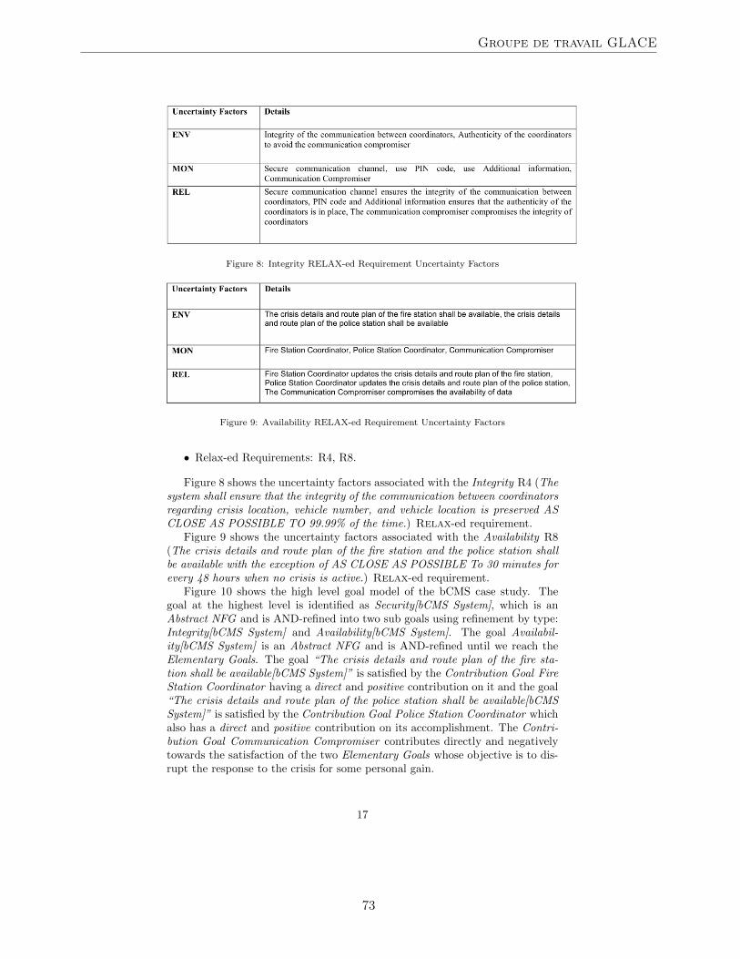
Figure 8: Integrity RELAX-ed Requirement Uncertainty Factors
Figure 9: Availability RELAX-ed Requirement Uncertainty Factors
• Relax-ed Requirements: R4, R8.
Figure 8 shows the uncertainty factors associated with the Integrity R4 (Thesystem shall ensure that the integrity of the communication between coordinatorsregarding crisis location, vehicle number, and vehicle location is preserved ASCLOSE AS POSSIBLE TO 99.99% of the time.) Relax-ed requirement.
Figure 9 shows the uncertainty factors associated with the Availability R8(The crisis details and route plan of the fire station and the police station shallbe available with the exception of AS CLOSE AS POSSIBLE To 30 minutes forevery 48 hours when no crisis is active.) Relax-ed requirement.
Figure 10 shows the high level goal model of the bCMS case study. Thegoal at the highest level is identified as Security[bCMS System], which is anAbstract NFG and is AND-refined into two sub goals using refinement by type:Integrity[bCMS System] and Availability[bCMS System]. The goal Availabil-ity[bCMS System] is an Abstract NFG and is AND-refined until we reach theElementary Goals. The goal “The crisis details and route plan of the fire sta-tion shall be available[bCMS System]” is satisfied by the Contribution Goal FireStation Coordinator having a direct and positive contribution on it and the goal“The crisis details and route plan of the police station shall be available[bCMSSystem]” is satisfied by the Contribution Goal Police Station Coordinator whichalso has a direct and positive contribution on its accomplishment. The Contri-bution Goal Communication Compromiser contributes directly and negativelytowards the satisfaction of the two Elementary Goals whose objective is to dis-rupt the response to the crisis for some personal gain.
17
Groupe de travail GLACE
73
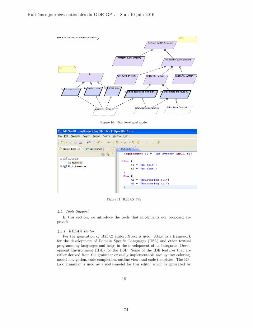
Figure 10: High level goal model
Figure 11: RELAX File
4.5. Tools Support
In this section, we introduce the tools that implements our proposed ap-proach.
4.5.1. RELAX Editor
For the generation of Relax editor, Xtext is used. Xtext is a frameworkfor the development of Domain Specific Languages (DSL) and other textualprogramming languages and helps in the development of an Integrated Devel-opment Environment (IDE) for the DSL. Some of the IDE features that areeither derived from the grammar or easily implementable are: syntax coloring,model navigation, code completion, outline view, and code templates. The Re-lax grammar is used as a meta-model for this editor which is generated by
18
Huitièmes journées nationales du GDR GPL – 8 au 10 juin 2016
74
Figure 12: Relaxed Requirement to Abstract Goal Mapping
Xtext that we call Relax.ecore. Figure 11 shows an example of the Relax filewith uncertainty factors. The Relax file is represented with an extension .rlx.Once we have the .rlx file, we can transform it into an XMI model. The XMImodel can then be manipulated and will serve us for the model transformationfrom Relax to SysML/Kaos as explained in the next section.
4.5.2. RELAX to SysML/Kaos Transformation
In our approach, we want to transform Relax-ed requirements uncertaintyfactors into SysML/Kaos goal concepts. This transformation will help in tak-ing into account the adaptability features associated with SAS in the form ofuncertainty factors of Relax-ed requirements and then modeling these require-ments in SysML/Kaos. In this way, we can benefit from the advantages offeredby GORE. For this purpose, the Relax and SysML/Kaos meta-models areused.
ATL Rules
ATL is a model transformation language and toolkit. It provides a wayto produce a number of target models from a set of source models. An ATLtransformation program is composed of rules that define how source model el-ements are matched and navigated to create and initialize the elements of thetarget models. The generation of target model elements is achieved through thespecification of transformation rules.
Mapping between RELAX and SysML/Kaos Elements
Here, we present the relationship between Relax and SysML/Kaos ele-ments. The Relax abstract syntax is defined in the Relax meta-model. Inturn, the SysML/Kaos abstract syntax is defined in the SysML/Kaos meta-model.
Figure 6 shows the mapping between the two concepts. For the ATL trans-formation rules, a Relax-ed requirement is mapped to an Abstract Goal asshown in Figure 12, an ENV is mapped to an Elementary Goal and MON ismapped to Contribution Goal. Figure 13 shows the generated SysML/Kaosmodel after the application of ATL rules. Figure 14 shows the SysML/Kaosmodel opened in the editor.
5. Proof of Concepts
In this section, we apply our approach on an academic Ambient AssistedLiving (AAL) case study. The goal of AAL solutions is to apply ambient in-telligence technology to enable people with specific demands, e.g. handicappedor elderly, to live in their preferred environment [9]. In order to achieve thisgoal, different kinds of AAL systems can be proposed and most of them pose
19
Groupe de travail GLACE
75
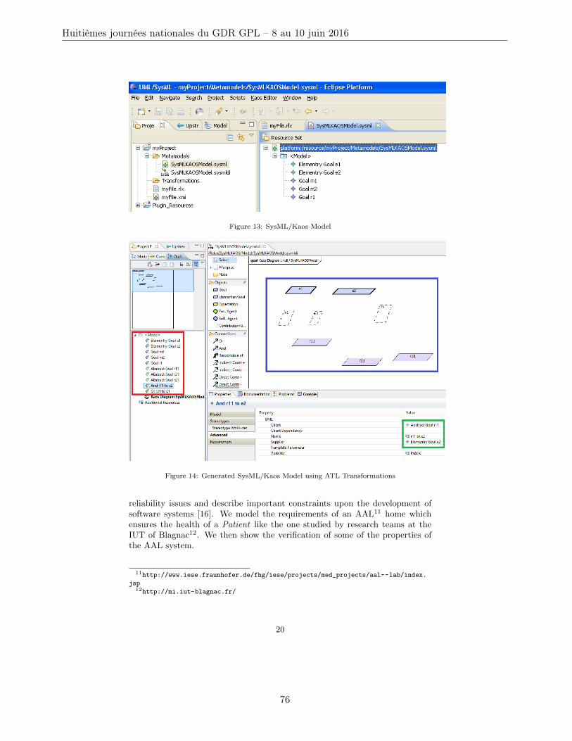
Figure 13: SysML/Kaos Model
Figure 14: Generated SysML/Kaos Model using ATL Transformations
reliability issues and describe important constraints upon the development ofsoftware systems [16]. We model the requirements of an AAL11 home whichensures the health of a Patient like the one studied by research teams at theIUT of Blagnac12. We then show the verification of some of the properties ofthe AAL system.
11http://www.iese.fraunhofer.de/fhg/iese/projects/med_projects/aal--lab/index.
jsp12http://mi.iut-blagnac.fr/
20
Huitièmes journées nationales du GDR GPL – 8 au 10 juin 2016
76
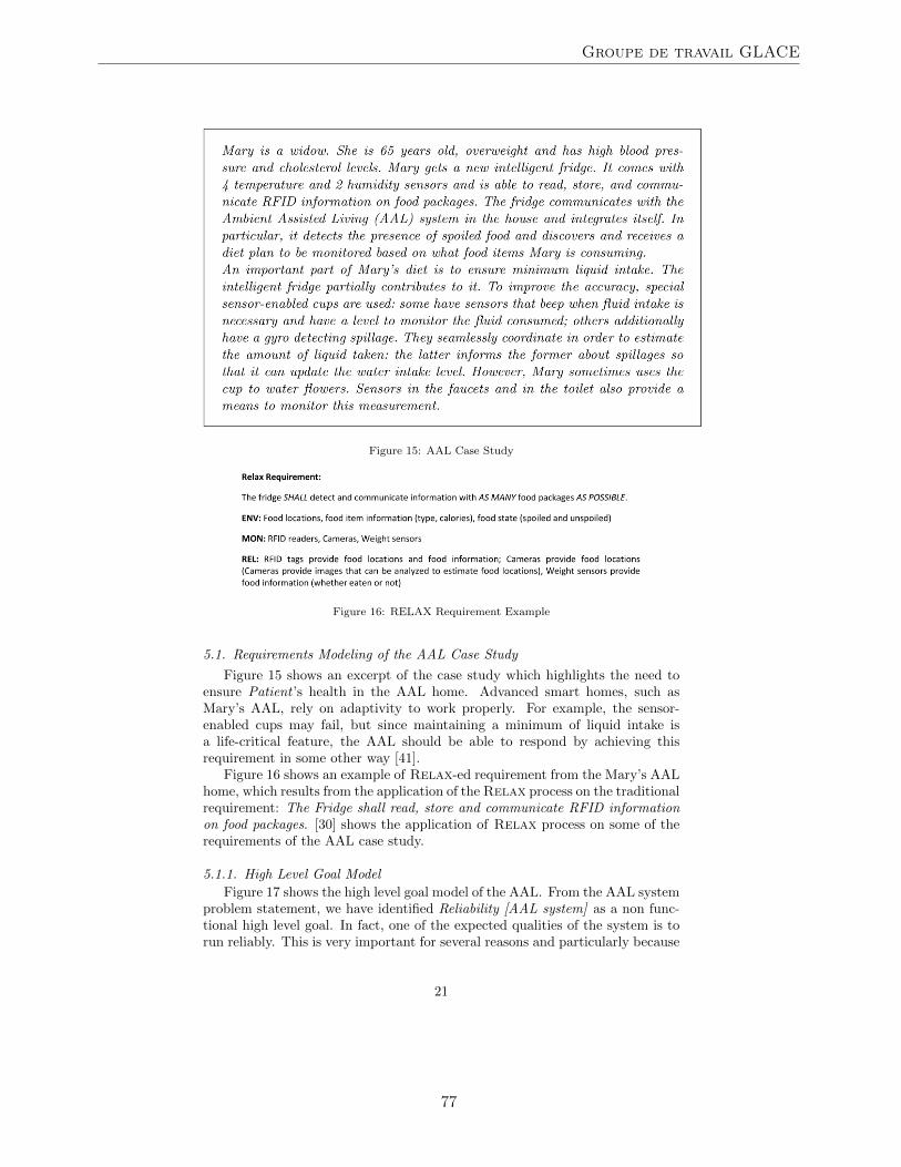
Figure 15: AAL Case Study
Figure 16: RELAX Requirement Example
5.1. Requirements Modeling of the AAL Case Study
Figure 15 shows an excerpt of the case study which highlights the need toensure Patient ’s health in the AAL home. Advanced smart homes, such asMary’s AAL, rely on adaptivity to work properly. For example, the sensor-enabled cups may fail, but since maintaining a minimum of liquid intake isa life-critical feature, the AAL should be able to respond by achieving thisrequirement in some other way [41].
Figure 16 shows an example of Relax-ed requirement from the Mary’s AALhome, which results from the application of the Relax process on the traditionalrequirement: The Fridge shall read, store and communicate RFID informationon food packages. [30] shows the application of Relax process on some of therequirements of the AAL case study.
5.1.1. High Level Goal Model
Figure 17 shows the high level goal model of the AAL. From the AAL systemproblem statement, we have identified Reliability [AAL system] as a non func-tional high level goal. In fact, one of the expected qualities of the system is torun reliably. This is very important for several reasons and particularly because
21
Groupe de travail GLACE
77
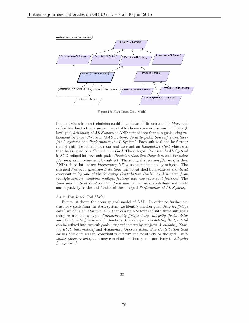
Figure 17: High Level Goal Model
frequent visits from a technician could be a factor of disturbance for Mary andunfeasible due to the large number of AAL houses across the world. The highlevel goal Reliability [AAL System] is AND-refined into four sub goals using re-finement by type: Precision [AAL System], Security [AAL System], Robustness[AAL System] and Performance [AAL System]. Each sub goal can be furtherrefined until the refinement stops and we reach an Elementary Goal which canthen be assigned to a Contribution Goal. The sub goal Precision [AAL System]is AND-refined into two sub goals: Precision [Location Detection] and Precision[Sensors] using refinement by subject. The sub goal Precision [Sensors] is thenAND-refined into three Elementary NFGs using refinement by subject. Thesub goal Precision [Location Detection] can be satisfied by a positive and directcontribution by one of the following Contribution Goals: combine data frommultiple sensors, combine multiple features and use redundant features. TheContribution Goal combine data from multiple sensors, contribute indirectlyand negatively to the satisfaction of the sub goal Performance [AAL System].
5.1.2. Low Level Goal Model
Figure 18 shows the security goal model of AAL. In order to further ex-tract new goals from the AAL system, we identify another goal, Security [fridgedata], which is an Abstract NFG that can be AND-refined into three sub goalsusing refinement by type: Confidentiality [fridge data], Integrity [fridge data]and Availability [fridge data]. Similarly, the sub goal Availability [fridge data]can be refined into two sub goals using refinement by subject: Availability [Stor-ing RFID information] and Availability [Sensors data]. The Contribution Goalhaving high-end sensors contributes directly and positively to the goal Avail-ability [Sensors data], and may contribute indirectly and positively to Integrity[fridge data].
22
Huitièmes journées nationales du GDR GPL – 8 au 10 juin 2016
78
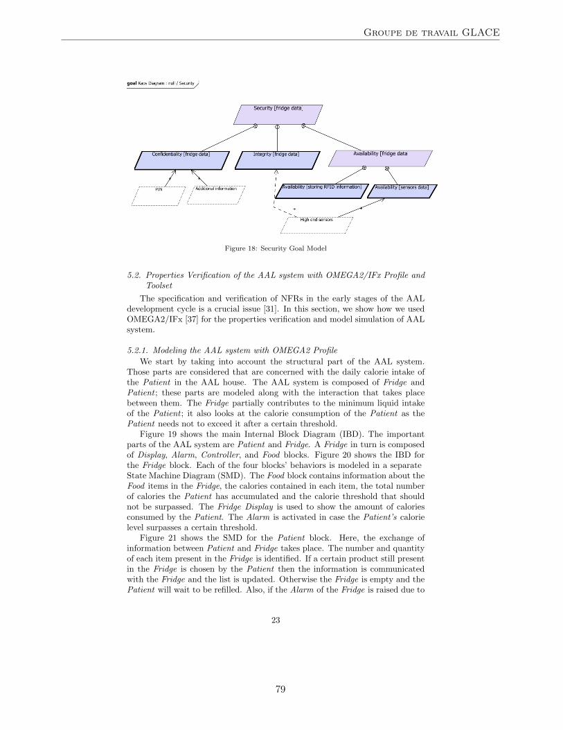
Figure 18: Security Goal Model
5.2. Properties Verification of the AAL system with OMEGA2/IFx Profile andToolset
The specification and verification of NFRs in the early stages of the AALdevelopment cycle is a crucial issue [31]. In this section, we show how we usedOMEGA2/IFx [37] for the properties verification and model simulation of AALsystem.
5.2.1. Modeling the AAL system with OMEGA2 Profile
We start by taking into account the structural part of the AAL system.Those parts are considered that are concerned with the daily calorie intake ofthe Patient in the AAL house. The AAL system is composed of Fridge andPatient ; these parts are modeled along with the interaction that takes placebetween them. The Fridge partially contributes to the minimum liquid intakeof the Patient ; it also looks at the calorie consumption of the Patient as thePatient needs not to exceed it after a certain threshold.
Figure 19 shows the main Internal Block Diagram (IBD). The importantparts of the AAL system are Patient and Fridge. A Fridge in turn is composedof Display, Alarm, Controller, and Food blocks. Figure 20 shows the IBD forthe Fridge block. Each of the four blocks’ behaviors is modeled in a separateState Machine Diagram (SMD). The Food block contains information about theFood items in the Fridge, the calories contained in each item, the total numberof calories the Patient has accumulated and the calorie threshold that shouldnot be surpassed. The Fridge Display is used to show the amount of caloriesconsumed by the Patient. The Alarm is activated in case the Patient’s calorielevel surpasses a certain threshold.
Figure 21 shows the SMD for the Patient block. Here, the exchange ofinformation between Patient and Fridge takes place. The number and quantityof each item present in the Fridge is identified. If a certain product still presentin the Fridge is chosen by the Patient then the information is communicatedwith the Fridge and the list is updated. Otherwise the Fridge is empty and thePatient will wait to be refilled. Also, if the Alarm of the Fridge is raised due to
23
Groupe de travail GLACE
79
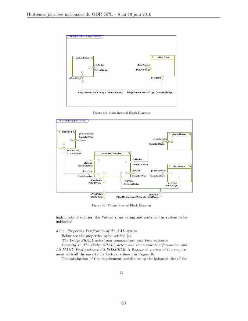
Figure 19: Main Internal Block Diagram
Figure 20: Fridge Internal Block Diagram
high intake of calories, the Patient stops eating and waits for the system to beunblocked.
5.2.2. Properties Verification of the AAL system
Below are the properties to be verified [4].The Fridge SHALL detect and communicate with Food packagesProperty 1: The Fridge SHALL detect and communicate information with
AS MANY Food packages AS POSSIBLE. A Relax-ed version of this require-ment with all the uncertainty factors is shown in Figure 16.
The satisfaction of this requirement contributes to the balanced diet of the
24
Huitièmes journées nationales du GDR GPL – 8 au 10 juin 2016
80
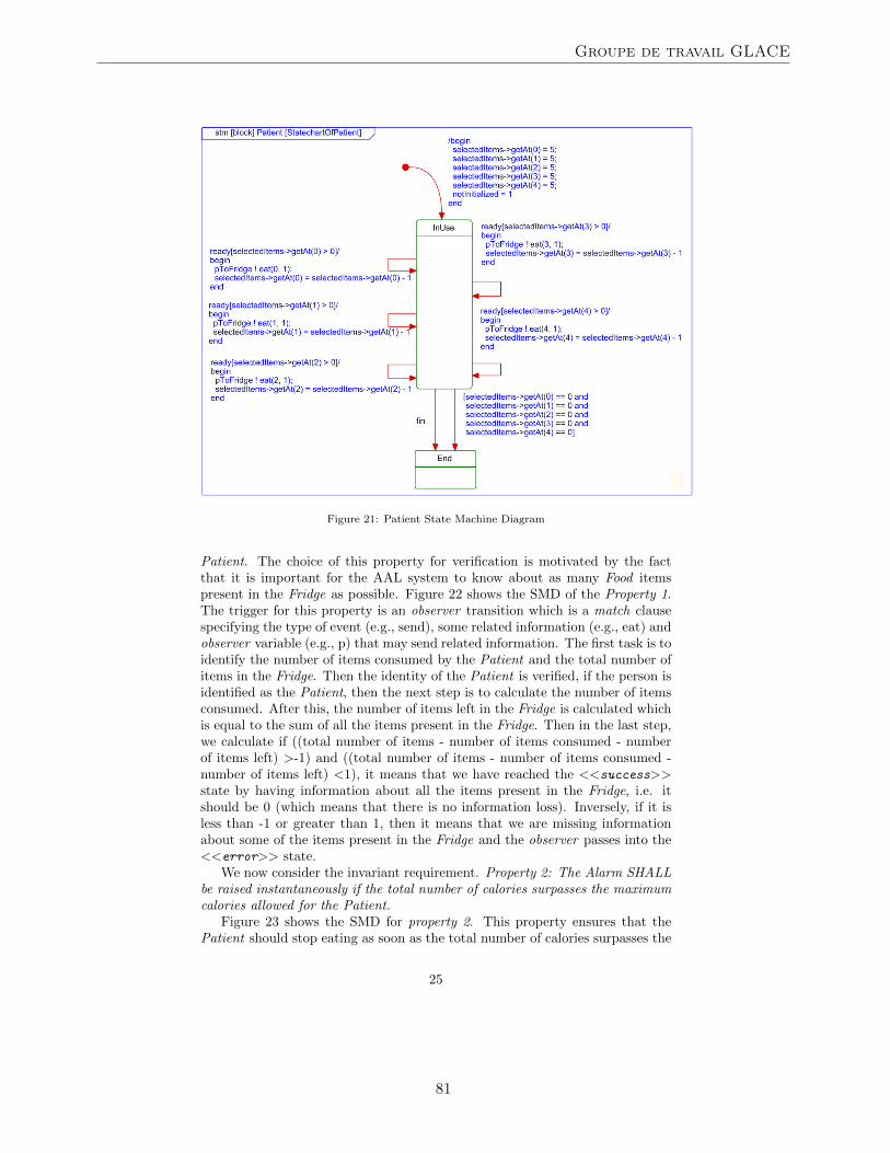
Figure 21: Patient State Machine Diagram
Patient. The choice of this property for verification is motivated by the factthat it is important for the AAL system to know about as many Food itemspresent in the Fridge as possible. Figure 22 shows the SMD of the Property 1.The trigger for this property is an observer transition which is a match clausespecifying the type of event (e.g., send), some related information (e.g., eat) andobserver variable (e.g., p) that may send related information. The first task is toidentify the number of items consumed by the Patient and the total number ofitems in the Fridge. Then the identity of the Patient is verified, if the person isidentified as the Patient, then the next step is to calculate the number of itemsconsumed. After this, the number of items left in the Fridge is calculated whichis equal to the sum of all the items present in the Fridge. Then in the last step,we calculate if ((total number of items - number of items consumed - numberof items left) >-1) and ((total number of items - number of items consumed -number of items left) <1), it means that we have reached the <<success>>state by having information about all the items present in the Fridge, i.e. itshould be 0 (which means that there is no information loss). Inversely, if it isless than -1 or greater than 1, then it means that we are missing informationabout some of the items present in the Fridge and the observer passes into the<<error>> state.
We now consider the invariant requirement. Property 2: The Alarm SHALLbe raised instantaneously if the total number of calories surpasses the maximumcalories allowed for the Patient.
Figure 23 shows the SMD for property 2. This property ensures that thePatient should stop eating as soon as the total number of calories surpasses the
25
Groupe de travail GLACE
81
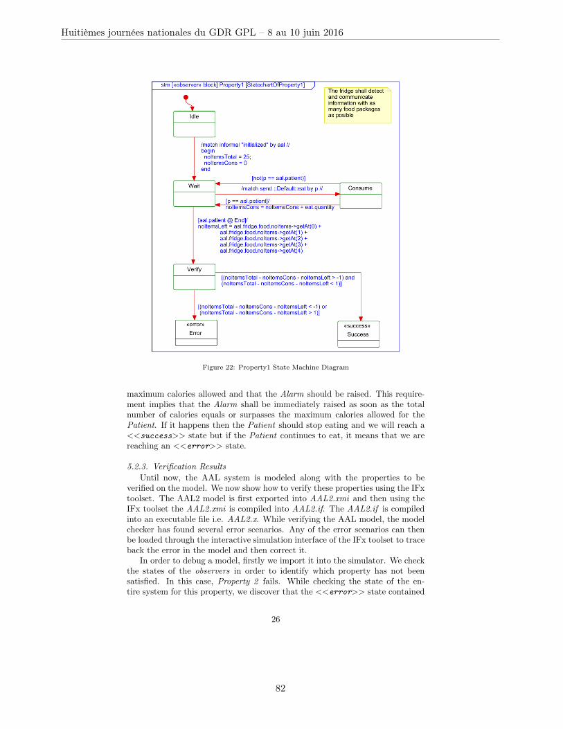
Figure 22: Property1 State Machine Diagram
maximum calories allowed and that the Alarm should be raised. This require-ment implies that the Alarm shall be immediately raised as soon as the totalnumber of calories equals or surpasses the maximum calories allowed for thePatient. If it happens then the Patient should stop eating and we will reach a<<success>> state but if the Patient continues to eat, it means that we arereaching an <<error>> state.
5.2.3. Verification Results
Until now, the AAL system is modeled along with the properties to beverified on the model. We now show how to verify these properties using the IFxtoolset. The AAL2 model is first exported into AAL2.xmi and then using theIFx toolset the AAL2.xmi is compiled into AAL2.if. The AAL2.if is compiledinto an executable file i.e. AAL2.x. While verifying the AAL model, the modelchecker has found several error scenarios. Any of the error scenarios can thenbe loaded through the interactive simulation interface of the IFx toolset to traceback the error in the model and then correct it.
In order to debug a model, firstly we import it into the simulator. We checkthe states of the observers in order to identify which property has not beensatisfied. In this case, Property 2 fails. While checking the state of the en-tire system for this property, we discover that the <<error>> state contained
26
Huitièmes journées nationales du GDR GPL – 8 au 10 juin 2016
82
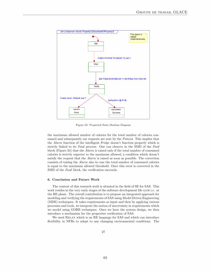
Figure 23: Property2 State Machine Diagram
the maximum allowed number of calories for the total number of calories con-sumed and subsequently eat requests are sent by the Patient. This implies thatthe Alarm function of the intelligent Fridge doesn’t function properly which isstrictly linked to its Food process. One can observe in the SMD of the Foodblock (Figure 24) that the Alarm is raised only if the total number of consumedcalories is strictly superior to the maximum allowed; a condition which doesn’tsatisfy the request that the Alarm is raised as soon as possible. The correctionconsists of raising the Alarm also in case the total number of consumed caloriesis equal to the maximum allowed threshold. Once this error is corrected in theSMD of the Food block, the verification succeeds.
6. Conclusion and Future Work
The context of this research work is situated in the field of SE for SAS. Thiswork resides in the very early stages of the software development life cycle i.e. atthe RE phase. The overall contribution is to propose an integrated approach formodeling and verifying the requirements of SAS using Model Driven Engineering(MDE) techniques. It takes requirements as input and then by applying variousprocesses and tools, we integrate the notion of uncertainty in requirements whichwe model using GORE techniques. Once we have the system design, we thenintroduce a mechanism for the properties verification of SAS.
We used Relax which is an RE language for SAS and which can introduceflexibility in NFRs to adapt to any changing environmental conditions. The
27
Groupe de travail GLACE
83
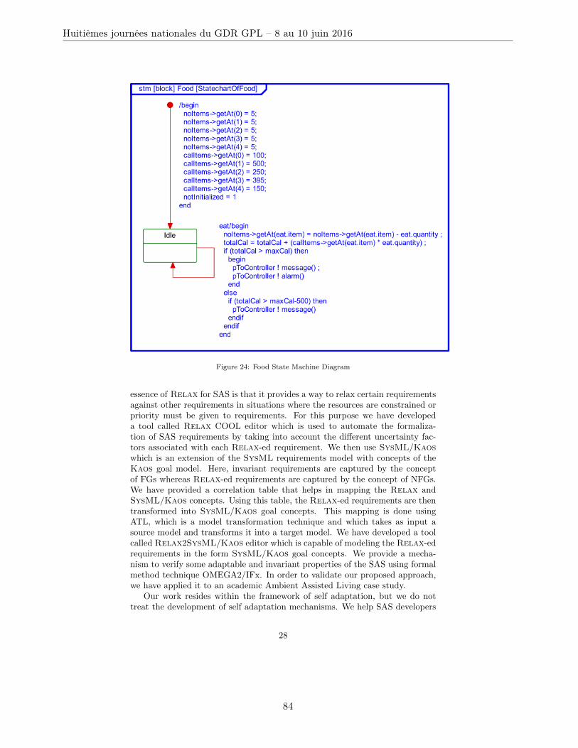
Figure 24: Food State Machine Diagram
essence of Relax for SAS is that it provides a way to relax certain requirementsagainst other requirements in situations where the resources are constrained orpriority must be given to requirements. For this purpose we have developeda tool called Relax COOL editor which is used to automate the formaliza-tion of SAS requirements by taking into account the different uncertainty fac-tors associated with each Relax-ed requirement. We then use SysML/Kaoswhich is an extension of the SysML requirements model with concepts of theKaos goal model. Here, invariant requirements are captured by the conceptof FGs whereas Relax-ed requirements are captured by the concept of NFGs.We have provided a correlation table that helps in mapping the Relax andSysML/Kaos concepts. Using this table, the Relax-ed requirements are thentransformed into SysML/Kaos goal concepts. This mapping is done usingATL, which is a model transformation technique and which takes as input asource model and transforms it into a target model. We have developed a toolcalled Relax2SysML/Kaos editor which is capable of modeling the Relax-edrequirements in the form SysML/Kaos goal concepts. We provide a mecha-nism to verify some adaptable and invariant properties of the SAS using formalmethod technique OMEGA2/IFx. In order to validate our proposed approach,we have applied it to an academic Ambient Assisted Living case study.
Our work resides within the framework of self adaptation, but we do nottreat the development of self adaptation mechanisms. We help SAS developers
28
Huitièmes journées nationales du GDR GPL – 8 au 10 juin 2016
84
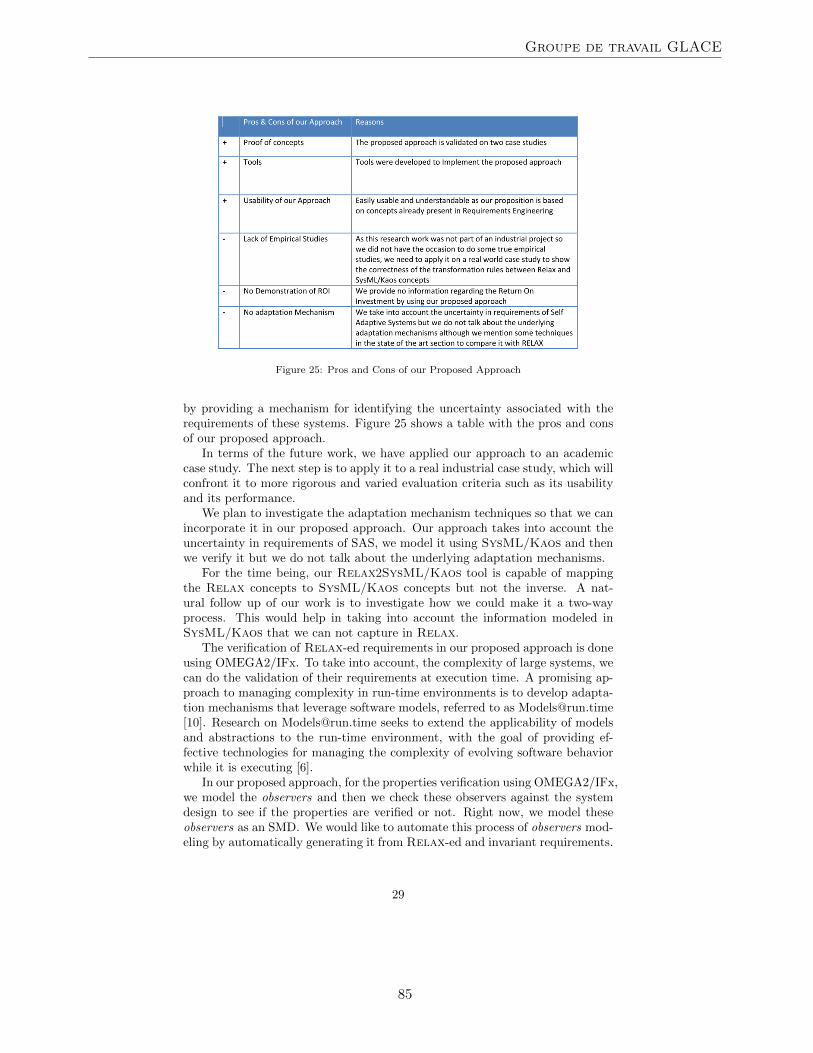
Figure 25: Pros and Cons of our Proposed Approach
by providing a mechanism for identifying the uncertainty associated with therequirements of these systems. Figure 25 shows a table with the pros and consof our proposed approach.
In terms of the future work, we have applied our approach to an academiccase study. The next step is to apply it to a real industrial case study, which willconfront it to more rigorous and varied evaluation criteria such as its usabilityand its performance.
We plan to investigate the adaptation mechanism techniques so that we canincorporate it in our proposed approach. Our approach takes into account theuncertainty in requirements of SAS, we model it using SysML/Kaos and thenwe verify it but we do not talk about the underlying adaptation mechanisms.
For the time being, our Relax2SysML/Kaos tool is capable of mappingthe Relax concepts to SysML/Kaos concepts but not the inverse. A nat-ural follow up of our work is to investigate how we could make it a two-wayprocess. This would help in taking into account the information modeled inSysML/Kaos that we can not capture in Relax.
The verification of Relax-ed requirements in our proposed approach is doneusing OMEGA2/IFx. To take into account, the complexity of large systems, wecan do the validation of their requirements at execution time. A promising ap-proach to managing complexity in run-time environments is to develop adapta-tion mechanisms that leverage software models, referred to as [email protected][10]. Research on [email protected] seeks to extend the applicability of modelsand abstractions to the run-time environment, with the goal of providing ef-fective technologies for managing the complexity of evolving software behaviorwhile it is executing [6].
In our proposed approach, for the properties verification using OMEGA2/IFx,we model the observers and then we check these observers against the systemdesign to see if the properties are verified or not. Right now, we model theseobservers as an SMD. We would like to automate this process of observers mod-eling by automatically generating it from Relax-ed and invariant requirements.
29
Groupe de travail GLACE
85

The use of model checking techniques used by OMEGA2/IFx exposes us tothe problem of state space explosion which is inherent in these techniques. Wehandle this problem in our proposed approach by only injecting Relax-ed orinvariant requirements, i.e. those requirements that are of interest for SAS. Butwe can counter this problem using formal methods like B. There are already someworks done for the mapping between SysML/Kaos and B in this regard. In[26], a method is defined for bridging the gap between the requirements analysislevel (Extended SysML) and the formal specification level (B). This methodderives the architecture of B specifications from SysML goal hierarchies. Webelieve that using proof based formal methods like B can help in overcomingthe state space explosion problem associated with model checking techniques.
7. References
[1] Jean R. Abrial. The B-Book: Assigning Programs to Meanings. CambridgeUniversity Press, New York, NY, USA, 1996.
[2] Manzoor Ahmad. Modeling and Verification of Functional and Non FunctionalRequirements of Ambient, Self Adaptive Systems. PhD thesis, MathematiqueInformatique Telecommunications, University of Toulouse Mirail, France, 2013.
[3] Manzoor Ahmad, Joao Araujo, Nicolas Belloir, Rgine Laleau Jean M. Bruel,Christophe Gnaho, and Farrida Semmak. Self-Adaptive Systems RequirementsModelling: four Related Approaches Comparison. In Comparing *Requirements*Modeling Approaches Workshop (CMA@RE), RE 2013, Rio de Janeiro Brazil,2013. IEEE Computer Society Press.
[4] Manzoor Ahmad, Iulia Dragomir, Jean M. Bruel, Iulian Ober, and Nicolas Belloir.Early analysis of ambient systems sysml properties using omega2-ifx. In 3rd In-ternational Conference on Simulation and Modeling Methodologies, Technologiesand Applications (SIMULTECH’13), 2013.
[5] Ludovic Apvrille, Jean P. Courtiat, Christophe Lohr, and Pierre de Saqui-Sannes.TURTLE: A Real-Time UML Profile Supported by a Formal Validation Toolkit.IEEE Trans. Softw. Eng., 30(7), 2004.
[6] Uwe Aßmann, Nelly Bencomo, Betty H. C. Cheng, and Robert B. France. [email protected] (Dagstuhl Seminar 11481). Dagstuhl Reports, 1(11), 2011.
[7] Luciano Baresi, Liliana Pasquale, and Paola Spoletini. Fuzzy Goals forRequirements-Driven Adaptation. In Proceedings of the 2010 18th IEEE Interna-tional Requirements Engineering Conference, RE ’10, pages 125–134, Washington,DC, USA, 2010. IEEE Computer Society.
[8] Jeremy Bascans, Jeremy Walczak, Jerome Zeghoudi, Manzoor Ahmad, JacobGeisel, and Jean M. Bruel. COOL RELAX Editor, M2ICE Project, Universit deToulouse le Mirail, 2013.
[9] Kawtar Benghazi, Marıa Visitacion Hurtado, Marıa Luisa Rodrıguez, and ManuelNoguera. Applying formal verification techniques to ambient assisted living sys-tems. In OnTheMove Workshop (OTM ’09). Springer-Verlag Berlin Heidelberg2009, 2009.
[10] Gordon S. Blair, Nelly Bencomo, and Robert B. France. Models@ Run.Time.Computer, 42(10):22–27, 2009.
30
Huitièmes journées nationales du GDR GPL – 8 au 10 juin 2016
86

[11] Marius Bozga, Susanne Graf, Ileana Ober, Iulian Ober, and Joseph Sifakis. TheIF Toolset. In Formal Methods for the Design of Real-Time Systems (FMDRTS’04). Springer Berlin/Heidelberg, 2004.
[12] Betty H. C. Cheng, Pete Sawyer, Nelly Bencomo, and Jon Whittle. A Goal-BasedModeling Approach to Develop Requirements of an Adaptive System with Envi-ronmental Uncertainty. In Proceedings of the 12th International Conference onModel Driven Engineering Languages and Systems (MODELS’09), Berlin, Hei-delberg, 2009. Springer-Verlag.
[13] Lawrence Chung, Brian A. Nixon, Eric Yu, and John Mylopoulos. Non-FunctionalRequirements in Software Engineering. Springer, 1st edition, 1999.
[14] Edmund M. Clarke, Orna Grumberg, and Doron Peled. Model Checking. MITPress, London, 1999.
[15] Edmund M. Clarke, William Klieber, Milo Novek, and Paolo Zuliani. ModelChecking and the State Explosion Problem. In Bertrand Meyer and Martin Nor-dio, editors, Tools for Practical Software Verification, volume 7682 of LectureNotes in Computer Science, pages 1–30. Springer Berlin Heidelberg, 2012.
[16] Jane Cleland-Huang, Raffaella Settimi, Xuchang Zou, and Peter Solc. AutomatedClassification of Non-Functional Requirements. Requir. Eng., 12(2):103–120, May2007.
[17] Jean P. Courtiat, Celso A. S. Santos, Christophe Lohr, and B. Outtaj. Experi-ence with RT-LOTOS, a Temporal Extension of the LOTOS Formal DescriptionTechnique. Comput. Commun., 23(12), 2000.
[18] Luiz Marcio Cysneiros and Julio Cesar Sampaio do Prado Leite. Nonfunctionalrequirements: From elicitation to conceptual models. In IEEE Transactions OnSoftware Engineering, volume 30, pages 328–350, 2004.
[19] Rogerio de Lemos et al. Software engineering for self-adaptive systems: A secondresearch roadmap.
[20] Iulia Dragomir, Iulian Ober, and David Lesens. A Case Study in Formal SystemEngineering with SysML. In 17th International Conference on Engineering ofComplex Computer Systems (ICECCS ’12). IEEE, 2012.
[21] Betty H.C. Cheng et al. Software Engineering for Self-Adaptive Systems. chapterSoftware Engineering for Self-Adaptive Systems: A Research Roadmap, pages1–26. Springer-Verlag, Berlin, Heidelberg, 2009.
[22] Christophe Gnaho and Farida Semmak. Une Extension SysML pour l’ingenieriedes Exigences Non-Fonctionnelles Orientee But. In Ingenierie des Systemesd’Information. Lavoisier Paris FRANCE, 2010.
[23] HeatherJ. Goldsby, Pete Sawyer, Nelly Bencomo, Betty H.C. Cheng, and DannyHughes. Goal-Based Modeling of Dynamically Adaptive System Requirements. InProceedings of the 15th Annual IEEE International Conference and Workshop onthe Engineering of Computer Based Systems, ECBS ’08, Washington, DC, USA,2008. IEEE Computer Society.
[24] Seong ick Moon, K.H. Lee, and Doheon Lee. Fuzzy branching temporal logic.In IEEE Transactions on Systems, Man, and Cybernetics, Part B: Cybernetics,2004.
31
Groupe de travail GLACE
87

[25] Jeffrey O. Kephart and David M. Chess. The Vision of Autonomic Computing.Computer, 36(1), 2003.
[26] Rgine Laleau, Farida Semmak, Abderrahman Matoussi, Dorian Petit, AhmedHammad, and Bruno Tatibouet. A First Attempt to Combine SysML Require-ments Diagrams and B. Innovations in Systems and Software Engineering, 6,2010.
[27] Axel V. Lamsweerde. Requirements Engineering: From System Goals to UMLModels to Software Specifications. Wiley, 1st edition edition, 2009.
[28] Alexei Lapouchnian, Sotirios Liaskos, John Mylopoulos, and Yijun Yu. TowardsRequirements-Driven Autonomic Systems Design. In Proceedings of the 2005workshop on Design and evolution of autonomic application software, DEAS ’05,pages 1–7, New York, NY, USA, 2005. ACM.
[29] Robyn R. Lutz. Targeting Safety-Related Errors during Software RequirementsAnalysis. J. Syst. Softw., 34(3), 1996.
[30] Jean-Michel Bruel Manzoor Ahmad. A comparative study of relax and sysm-l/kaos. Technical report, Instituit de Recherche en Informatique de Toulouse,University Toulouse II Le Mirail, France, 2014.
[31] Jurgen Nehmer, Martin Becker, Arthur Karshmer, and Rosemarie Lamm. LivingAssistance Systems: an Ambient Intelligence Approach. In Proceedings of the28th international conference on Software engineering (ICSE ’06 ). ACM, 2006.
[32] Iulian Ober and Iulia Dragomir. OMEGA2: A New Version of the Profile and theTools. In 15th International Conference on Engineering of Complex ComputerSystems (ICECCS ’10). IEEE, 2010.
[33] Andres J. Ramirez, Betty H. C. Cheng, Nelly Bencomo, and Pete Sawyer. Re-laxing Claims: Coping with Uncertainty While Evaluating Assumptions at RunTime. In RobertB. France, Jrgen Kazmeier, Ruth Breu, and Colin Atkinson, ed-itors, Model Driven Engineering Languages and Systems, volume 7590 of LectureNotes in Computer Science. Springer Berlin Heidelberg, 2012.
[34] Andres J. Ramirez, Erik M. Fredericks, Adam C. Jensen, and Betty H. C. Cheng.Automatically RELAXing a Goal Model to Cope with Uncertainty. In Proceed-ings of the 4th international conference on Search Based Software Engineering,SSBSE’12, pages 198–212, Berlin, Heidelberg, 2012. Springer-Verlag.
[35] Vıtor E. S. Souza, Alexei Lapouchnian, William N. Robinson, and John Mylopou-los. Awareness Requirements for Adaptive Systems. In Proceedings of the 6th In-ternational Symposium on Software Engineering for Adaptive and Self- ManagingSystems, SEAMS ’11, pages 60–69, New York, NY, USA, 2011. ACM.
[36] Eric P. Kasten Seyed M. Sadjadi, Philip K. McKinley. Architecture and Operationof an Adaptable Communication Substrate. In Proceedings. The Ninth IEEEWorkshop on Future Trends of Distributed Computing Systems FTDCS’03, 2003.
[37] Verimag and Irit. OMEGA2-IFx for UML/SysML v2.0, Profile and Toolset, UserManual Document v1.1, 2011.
[38] Kristopher Welsh and Pete Sawyer. Understanding the Scope of Uncertainty inDynamically Adaptive Systems. In Requirements Engineering: Foundation forSoftware Quality. Springer Berlin Heidelberg, 2010.
32
Huitièmes journées nationales du GDR GPL – 8 au 10 juin 2016
88
[39] Kristopher Welsh, Pete Sawyer, and Nelly Bencomo. Towards RequirementsAware Systems: Run-Time Resolution of Design-Time Assumptions. In Pro-ceedings of the 2011 26th IEEE/ACM International Conference on AutomatedSoftware Engineering. IEEE Computer Society, 2011.
[40] Jon Whittle, Pete Sawyer, Nelly Bencomo, and Betty H. C. Cheng. A Lan-guage for Self-Adaptive System Requirements. In International Workshop onService-Oriented Computing: Consequences for Engineering Requirements, 2008.SOCCER ’08., 2008.
[41] Jon Whittle, Pete Sawyer, Nelly Bencomo, Betty H. C. Cheng, and Jean M.Bruel. RELAX: Incorporating Uncertainty into the Specification of Self-AdaptiveSystems. In Proceedings of the 2009 17th IEEE International Requirements En-gineering Conference, RE, RE ’09, pages 79–88, Washington, DC, USA, 2009.IEEE Computer Society.
[42] Eric S. K. Yu. Towards Modeling and Reasoning Support for Early-Phase Re-quirements Engineering. In Proceedings of the 3rd IEEE International Symposiumon Requirements Engineering. IEEE Computer Society, 1997.
[43] Yijun Yu, Alexei Lapouchnian, Sotirios Liaskos, John Mylopoulos, and Julio C.S. P. Leite. From Goals to High-Variability Software Design. In Proceedings ofthe 17th international conference on Foundations of intelligent systems, ISMIS’08,pages 1–16, Berlin, Heidelberg, 2008. Springer-Verlag.
[44] Yijun Yu, Julio C.S.P. Leite, and John Mylopoulos. From Goals to Aspects: Dis-covering Aspects from Requirements Goal Models. In Proceedings of the Require-ments Engineering Conference, 12th IEEE International, RE ’04, pages 38–47,Washington, DC, USA, 2004. IEEE Computer Society.
33
Groupe de travail GLACE
89

Huitièmes journées nationales du GDR GPL – 8 au 10 juin 2016
90
Session commune aux groupes de travailGLE et RIMELGénie Logiciel Empirique — Rétro-Ingénierie, Maintenance et Evo-lution des Logiciels
91

Huitièmes journées nationales du GDR GPL – 8 au 10 juin 2016
92
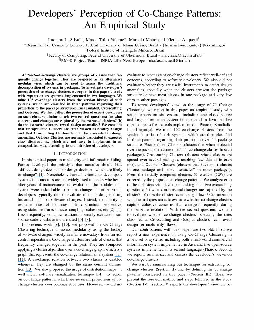
Developers’ Perception of Co-Change Patterns:An Empirical Study
Luciana L. Silva∗†, Marco Tulio Valente∗, Marcelo Maia‡ and Nicolas Anquetil§∗Department of Computer Science, Federal University of Minas Gerais, Brazil - {luciana.lourdes,mtov}@dcc.ufmg.br
†Federal Institute of Triangulo Mineiro, Brazil‡Faculty of Computing, Federal University of Uberlandia, Brazil - [email protected]
§RMoD Project-Team - INRIA Lille Nord Europe - [email protected]
Abstract—Co-change clusters are groups of classes that fre-quently change together. They are proposed as an alternativemodular view, which can be used to assess the traditionaldecomposition of systems in packages. To investigate developer’sperception of co-change clusters, we report in this paper a studywith experts on six systems, implemented in two languages. Wemine 102 co-change clusters from the version history of suchsystems, which are classified in three patterns regarding theirprojection to the package structure: Encapsulated, Crosscutting,and Octopus. We then collect the perception of expert developerson such clusters, aiming to ask two central questions: (a) whatconcerns and changes are captured by the extracted clusters? (b)do the extracted clusters reveal design anomalies? We concludethat Encapsulated Clusters are often viewed as healthy designsand that Crosscutting Clusters tend to be associated to designanomalies. Octopus Clusters are normally associated to expectedclass distributions, which are not easy to implement in anencapsulated way, according to the interviewed developers.
I. INTRODUCTION
In his seminal paper on modularity and information hiding,Parnas developed the principle that modules should hide“difficult design decisions or design decisions which are likelyto change” [1]. Nonetheless, Parnas’ criteria to decomposesystems into modules are not widely used to assess whether—after years of maintenance and evolution—the modules of asystem were indeed able to confine changes. In other words,developers typically do not evaluate modular designs usinghistorical data on software changes. Instead, modularity isevaluated most of the times under a structural perspective,using static measures of size, coupling, cohesion, etc [2]–[4].Less frequently, semantic relations, normally extracted fromsource code vocabularies, are used [5]–[8].
In previous work [9], [10], we proposed the Co-ChangeClustering technique to assess modularity using the historyof software changes, widely available nowadays from versioncontrol repositories. Co-change clusters are sets of classes thatfrequently changed together in the past. They are computedapplying a cluster algorithm over a co-change graph, which is agraph that represents the co-change relations in a system [11],[12]. A co-change relation between two classes is enabledwhenever they are changed by the same commit transac-tion [13]. We also proposed the usage of distribution maps—awell-known software visualization technique [14]—to reasonon co-change patterns, which are recurrent projections of co-change clusters over package structures. However, we did not
evaluate to what extent co-change clusters reflect well-definedconcerns, according to software developers. We also did notevaluate whether they are useful instruments to detect designanomalies, specially when the clusters crosscut the packagestructure or have most classes in one package and very fewones in other packages.
To reveal developers’ view on the usage of Co-ChangeClustering, we report in this paper an empirical study withseven experts on six systems, including one closed-sourceand large information system implemented in Java and fiveopen-source software tools implemented in Pharo (a Smalltalk-like language). We mine 102 co-change clusters from theversion histories of such systems, which are then classifiedin three patterns regarding their projection over the packagestructure: Encapsulated Clusters (clusters that when projectedover the package structure match all co-change classes in suchpackages), Crosscutting Clusters (clusters whose classes arespread over several packages, touching few classes in eachone), and Octopus Clusters (clusters that have most classesin one package and some “tentacles” in other packages).From the initially computed clusters, 53 clusters (52%) arecovered by the proposed co-change patterns. We analyze eachof these clusters with developers, asking them two overarchingquestions: (a) what concerns and changes are captured by thecluster? (b) does the cluster reveal design flaws? Our intentionwith the first question is to evaluate whether co-change clusterscapture cohesive concerns that changed frequently duringthe software evolution. With the second question, we aimto evaluate whether co-change clusters—specially the onesclassified as Crosscutting and Octopus clusters—can revealdesign (or modularity) flaws.
Our contributions with this paper are twofold. First, wereport a new experience on using Co-Change Clustering ina new set of systems, including both a real-world commercialinformation system implemented in Java and five open-sourcesystems implemented in a second language (Pharo). Second,we report, summarize, and discuss the developer’s views onco-change clusters.
We start by summarizing our technique for extracting co-change clusters (Section II) and by defining the co-changepatterns considered in this paper (Section III). Then, wepresent the research method and steps followed in the study(Section IV). Section V reports the developers’ view on co-
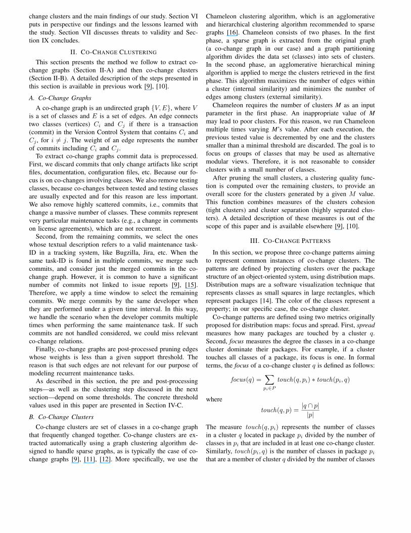
change clusters and the main findings of our study. Section VIputs in perspective our findings and the lessons learned withthe study. Section VII discusses threats to validity and Sec-tion IX concludes.
II. CO-CHANGE CLUSTERING
This section presents the method we follow to extract co-change graphs (Section II-A) and then co-change clusters(Section II-B). A detailed description of the steps presented inthis section is available in previous work [9], [10].
A. Co-Change GraphsA co-change graph is an undirected graph {V,E}, where V
is a set of classes and E is a set of edges. An edge connectstwo classes (vertices) Ci and Cj if there is a transaction(commit) in the Version Control System that contains Ci andCj , for i 6= j. The weight of an edge represents the numberof commits including Ci and Cj .
To extract co-change graphs commit data is preprocessed.First, we discard commits that only change artifacts like scriptfiles, documentation, configuration files, etc. Because our fo-cus is on co-changes involving classes. We also remove testingclasses, because co-changes between tested and testing classesare usually expected and for this reason are less important.We also remove highly scattered commits, i.e., commits thatchange a massive number of classes. These commits representvery particular maintenance tasks (e.g., a change in commentson license agreements), which are not recurrent.
Second, from the remaining commits, we select the oneswhose textual description refers to a valid maintenance task-ID in a tracking system, like Bugzilla, Jira, etc. When thesame task-ID is found in multiple commits, we merge suchcommits, and consider just the merged commits in the co-change graph. However, it is common to have a significantnumber of commits not linked to issue reports [9], [15].Therefore, we apply a time window to select the remainingcommits. We merge commits by the same developer whenthey are performed under a given time interval. In this way,we handle the scenario when the developer commits multipletimes when performing the same maintenance task. If suchcommits are not handled considered, we could miss relevantco-change relations.
Finally, co-change graphs are post-processed pruning edgeswhose weights is less than a given support threshold. Thereason is that such edges are not relevant for our purpose ofmodeling recurrent maintenance tasks.
As described in this section, the pre and post-processingsteps—as well as the clustering step discussed in the nextsection—depend on some thresholds. The concrete thresholdvalues used in this paper are presented in Section IV-C.
B. Co-Change ClustersCo-change clusters are set of classes in a co-change graph
that frequently changed together. Co-change clusters are ex-tracted automatically using a graph clustering algorithm de-signed to handle sparse graphs, as is typically the case of co-change graphs [9], [11], [12]. More specifically, we use the
Chameleon clustering algorithm, which is an agglomerativeand hierarchical clustering algorithm recommended to sparsegraphs [16]. Chameleon consists of two phases. In the firstphase, a sparse graph is extracted from the original graph(a co-change graph in our case) and a graph partitioningalgorithm divides the data set (classes) into sets of clusters.In the second phase, an agglomerative hierarchical miningalgorithm is applied to merge the clusters retrieved in the firstphase. This algorithm maximizes the number of edges withina cluster (internal similarity) and minimizes the number ofedges among clusters (external similarity).
Chameleon requires the number of clusters M as an inputparameter in the first phase. An inappropriate value of Mmay lead to poor clusters. For this reason, we run Chameleonmultiple times varying M’s value. After each execution, theprevious tested value is decremented by one and the clusterssmaller than a minimal threshold are discarded. The goal is tofocus on groups of classes that may be used as alternativemodular views. Therefore, it is not reasonable to considerclusters with a small number of classes.
After pruning the small clusters, a clustering quality func-tion is computed over the remaining clusters, to provide anoverall score for the clusters generated by a given M value.This function combines measures of the clusters cohesion(tight clusters) and cluster separation (highly separated clus-ters). A detailed description of these measures is out of thescope of this paper and is available elsewhere [9], [10].
III. CO-CHANGE PATTERNS
In this section, we propose three co-change patterns aimingto represent common instances of co-change clusters. Thepatterns are defined by projecting clusters over the packagestructure of an object-oriented system, using distribution maps.Distribution maps are a software visualization technique thatrepresents classes as small squares in large rectangles, whichrepresent packages [14]. The color of the classes represent aproperty; in our specific case, the co-change cluster.
Co-change patterns are defined using two metrics originallyproposed for distribution maps: focus and spread. First, spreadmeasures how many packages are touched by a cluster q.Second, focus measures the degree the classes in a co-changecluster dominate their packages. For example, if a clustertouches all classes of a package, its focus is one. In formalterms, the focus of a co-change cluster q is defined as follows:
focus(q) =∑
pi∈Ptouch(q, pi) ∗ touch(pi, q)
where
touch(q, p) =|q ∩ p||p|
The measure touch(q, pi) represents the number of classesin a cluster q located in package pi divided by the number ofclasses in pi that are included in at least one co-change cluster.Similarly, touch(pi, q) is the number of classes in package pithat are a member of cluster q divided by the number of classes
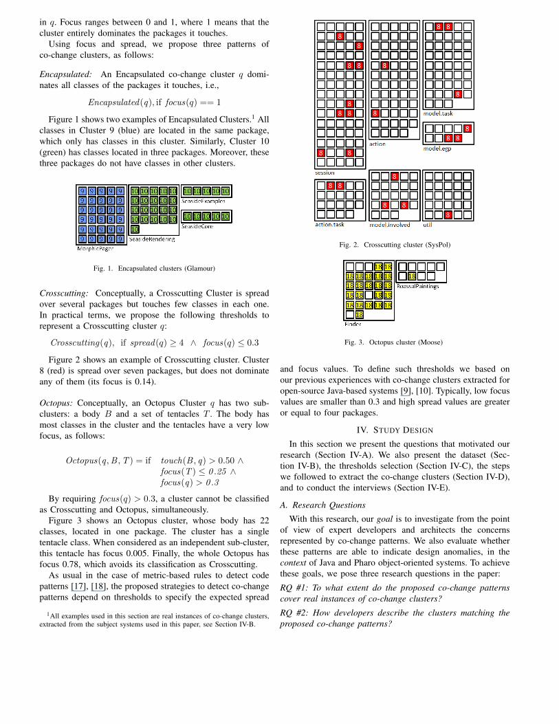
in q. Focus ranges between 0 and 1, where 1 means that thecluster entirely dominates the packages it touches.
Using focus and spread, we propose three patterns ofco-change clusters, as follows:
Encapsulated: An Encapsulated co-change cluster q domi-nates all classes of the packages it touches, i.e.,
Encapsulated(q), if focus(q) == 1
Figure 1 shows two examples of Encapsulated Clusters.1 Allclasses in Cluster 9 (blue) are located in the same package,which only has classes in this cluster. Similarly, Cluster 10(green) has classes located in three packages. Moreover, thesethree packages do not have classes in other clusters.
Fig. 1. Encapsulated clusters (Glamour)
Crosscutting: Conceptually, a Crosscutting Cluster is spreadover several packages but touches few classes in each one.In practical terms, we propose the following thresholds torepresent a Crosscutting cluster q:
Crosscutting(q), if spread(q) ≥ 4 ∧ focus(q) ≤ 0.3
Figure 2 shows an example of Crosscutting cluster. Cluster8 (red) is spread over seven packages, but does not dominateany of them (its focus is 0.14).
Octopus: Conceptually, an Octopus Cluster q has two sub-clusters: a body B and a set of tentacles T . The body hasmost classes in the cluster and the tentacles have a very lowfocus, as follows:
Octopus(q ,B ,T ) = if touch(B , q) > 0.50 ∧focus(T ) ≤ 0 .25 ∧focus(q) > 0 .3
By requiring focus(q) > 0.3, a cluster cannot be classifiedas Crosscutting and Octopus, simultaneously.
Figure 3 shows an Octopus cluster, whose body has 22classes, located in one package. The cluster has a singletentacle class. When considered as an independent sub-cluster,this tentacle has focus 0.005. Finally, the whole Octopus hasfocus 0.78, which avoids its classification as Crosscutting.
As usual in the case of metric-based rules to detect codepatterns [17], [18], the proposed strategies to detect co-changepatterns depend on thresholds to specify the expected spread
1All examples used in this section are real instances of co-change clusters,extracted from the subject systems used in this paper, see Section IV-B.
Fig. 2. Crosscutting cluster (SysPol)
Fig. 3. Octopus cluster (Moose)
and focus values. To define such thresholds we based onour previous experiences with co-change clusters extracted foropen-source Java-based systems [9], [10]. Typically, low focusvalues are smaller than 0.3 and high spread values are greateror equal to four packages.
IV. STUDY DESIGN
In this section we present the questions that motivated ourresearch (Section IV-A). We also present the dataset (Sec-tion IV-B), the thresholds selection (Section IV-C), the stepswe followed to extract the co-change clusters (Section IV-D),and to conduct the interviews (Section IV-E).
A. Research Questions
With this research, our goal is to investigate from the pointof view of expert developers and architects the concernsrepresented by co-change patterns. We also evaluate whetherthese patterns are able to indicate design anomalies, in thecontext of Java and Pharo object-oriented systems. To achievethese goals, we pose three research questions in the paper:
RQ #1: To what extent do the proposed co-change patternscover real instances of co-change clusters?
RQ #2: How developers describe the clusters matching theproposed co-change patterns?
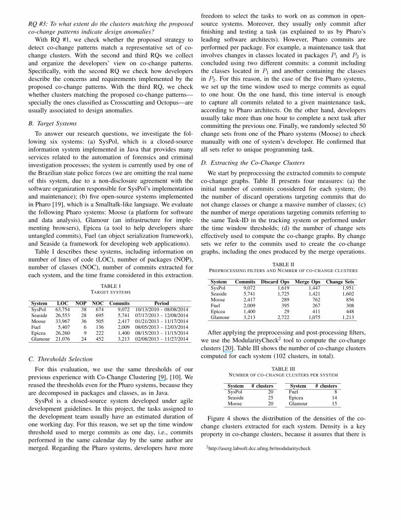
RQ #3: To what extent do the clusters matching the proposedco-change patterns indicate design anomalies?
With RQ #1, we check whether the proposed strategy todetect co-change patterns match a representative set of co-change clusters. With the second and third RQs we collectand organize the developers’ view on co-change patterns.Specifically, with the second RQ we check how developersdescribe the concerns and requirements implemented by theproposed co-change patterns. With the third RQ, we checkwhether clusters matching the proposed co-change patterns—specially the ones classified as Crosscutting and Octopus—areusually associated to design anomalies.
B. Target Systems
To answer our research questions, we investigate the fol-lowing six systems: (a) SysPol, which is a closed-sourceinformation system implemented in Java that provides manyservices related to the automation of forensics and criminalinvestigation processes; the system is currently used by one ofthe Brazilian state police forces (we are omitting the real nameof this system, due to a non-disclosure agreement with thesoftware organization responsible for SysPol’s implementationand maintenance); (b) five open-source systems implementedin Pharo [19], which is a Smalltalk-like language. We evaluatethe following Pharo systems: Moose (a platform for softwareand data analysis), Glamour (an infrastructure for imple-menting browsers), Epicea (a tool to help developers shareuntangled commits), Fuel (an object serialization framework),and Seaside (a framework for developing web applications).
Table I describes these systems, including information onnumber of lines of code (LOC), number of packages (NOP),number of classes (NOC), number of commits extracted foreach system, and the time frame considered in this extraction.
TABLE ITARGET SYSTEMS
System LOC NOP NOC Commits PeriodSysPol 63,754 38 674 9,072 10/13/2010 - 08/08/2014Seaside 26,553 28 695 5,741 07/17/2013 - 12/08/2014Moose 33,967 36 505 2,417 01/21/2013 - 11/17/2014Fuel 5,407 6 136 2,009 08/05/2013 - 12/03/2014Epicea 26,260 9 222 1,400 08/15/2013 - 11/15/2014Glamour 21,076 24 452 3,213 02/08/2013 - 11/27/2014
C. Thresholds Selection
For this evaluation, we use the same thresholds of ourprevious experience with Co-Change Clustering [9], [10]. Wereused the thresholds even for the Pharo systems, because theyare decomposed in packages and classes, as in Java.
SysPol is a closed-source system developed under agiledevelopment guidelines. In this project, the tasks assigned tothe development team usually have an estimated duration ofone working day. For this reason, we set up the time windowthreshold used to merge commits as one day, i.e., commitsperformed in the same calendar day by the same author aremerged. Regarding the Pharo systems, developers have more
freedom to select the tasks to work on as common in open-source systems. Moreover, they usually only commit afterfinishing and testing a task (as explained to us by Pharo’sleading software architects). However, Pharo commits areperformed per package. For example, a maintenance task thatinvolves changes in classes located in packages P1 and P2 isconcluded using two different commits: a commit includingthe classes located in P1 and another containing the classesin P2. For this reason, in the case of the five Pharo systems,we set up the time window used to merge commits as equalto one hour. On the one hand, this time interval is enoughto capture all commits related to a given maintenance task,according to Pharo architects. On the other hand, developersusually take more than one hour to complete a next task aftercommitting the previous one. Finally, we randomly selected 50change sets from one of the Pharo systems (Moose) to checkmanually with one of system’s developer. He confirmed thatall sets refer to unique programming task.
D. Extracting the Co-Change Clusters
We start by preprocessing the extracted commits to computeco-change graphs. Table II presents four measures: (a) theinitial number of commits considered for each system; (b)the number of discard operations targeting commits that donot change classes or change a massive number of classes; (c)the number of merge operations targeting commits referring tothe same Task-ID in the tracking system or performed underthe time window thresholds; (d) the number of change setseffectively used to compute the co-change graphs. By changesets we refer to the commits used to create the co-changegraphs, including the ones produced by the merge operations.
TABLE IIPREPROCESSING FILTERS AND NUMBER OF CO-CHANGE CLUSTERS
System Commits Discard Ops Merge Ops Change SetsSysPol 9,072 1,619 1,447 1,951Seaside 5,741 1,725 1,421 1,602Moose 2,417 289 762 856Fuel 2,009 395 267 308Epicea 1,400 29 411 448Glamour 3,213 2,722 1,075 1,213
After applying the preprocessing and post-processing filters,we use the ModularityCheck2 tool to compute the co-changeclusters [20]. Table III shows the number of co-change clusterscomputed for each system (102 clusters, in total).
TABLE IIINUMBER OF CO-CHANGE CLUSTERS PER SYSTEM
System # clusters System # clustersSysPol 20 Fuel 8Seaside 25 Epicea 14Moose 20 Glamour 15
Figure 4 shows the distribution of the densities of the co-change clusters extracted for each system. Density is a keyproperty in co-change clusters, because it assures that there is
2http://aserg.labsoft.dcc.ufmg.br/modularitycheck
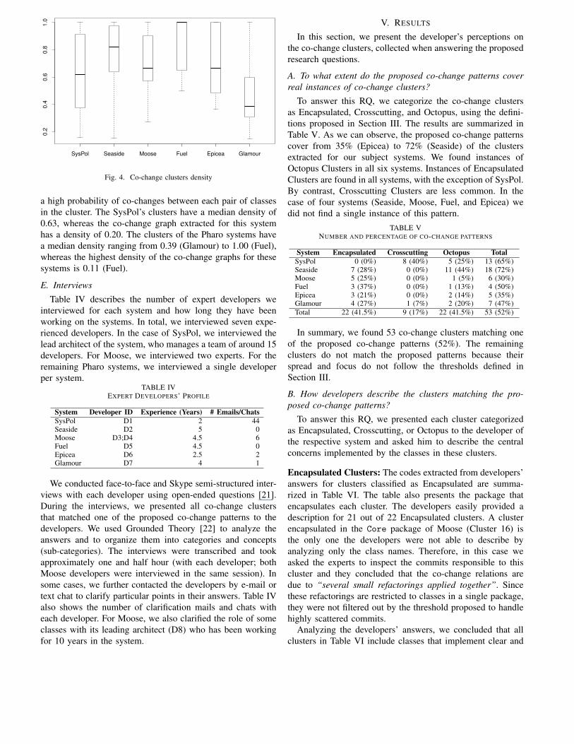
SysPol Seaside Moose Fuel Epicea Glamour
0.2
0.4
0.6
0.8
1.0
Fig. 4. Co-change clusters density
a high probability of co-changes between each pair of classesin the cluster. The SysPol’s clusters have a median density of0.63, whereas the co-change graph extracted for this systemhas a density of 0.20. The clusters of the Pharo systems havea median density ranging from 0.39 (Glamour) to 1.00 (Fuel),whereas the highest density of the co-change graphs for thesesystems is 0.11 (Fuel).
E. Interviews
Table IV describes the number of expert developers weinterviewed for each system and how long they have beenworking on the systems. In total, we interviewed seven expe-rienced developers. In the case of SysPol, we interviewed thelead architect of the system, who manages a team of around 15developers. For Moose, we interviewed two experts. For theremaining Pharo systems, we interviewed a single developerper system.
TABLE IVEXPERT DEVELOPERS’ PROFILE
System Developer ID Experience (Years) # Emails/ChatsSysPol D1 2 44Seaside D2 5 0Moose D3;D4 4.5 6Fuel D5 4.5 0Epicea D6 2.5 2Glamour D7 4 1
We conducted face-to-face and Skype semi-structured inter-views with each developer using open-ended questions [21].During the interviews, we presented all co-change clustersthat matched one of the proposed co-change patterns to thedevelopers. We used Grounded Theory [22] to analyze theanswers and to organize them into categories and concepts(sub-categories). The interviews were transcribed and tookapproximately one and half hour (with each developer; bothMoose developers were interviewed in the same session). Insome cases, we further contacted the developers by e-mail ortext chat to clarify particular points in their answers. Table IValso shows the number of clarification mails and chats witheach developer. For Moose, we also clarified the role of someclasses with its leading architect (D8) who has been workingfor 10 years in the system.
V. RESULTS
In this section, we present the developer’s perceptions onthe co-change clusters, collected when answering the proposedresearch questions.
A. To what extent do the proposed co-change patterns coverreal instances of co-change clusters?
To answer this RQ, we categorize the co-change clustersas Encapsulated, Crosscutting, and Octopus, using the defini-tions proposed in Section III. The results are summarized inTable V. As we can observe, the proposed co-change patternscover from 35% (Epicea) to 72% (Seaside) of the clustersextracted for our subject systems. We found instances ofOctopus Clusters in all six systems. Instances of EncapsulatedClusters are found in all systems, with the exception of SysPol.By contrast, Crosscutting Clusters are less common. In thecase of four systems (Seaside, Moose, Fuel, and Epicea) wedid not find a single instance of this pattern.
TABLE VNUMBER AND PERCENTAGE OF CO-CHANGE PATTERNS
System Encapsulated Crosscutting Octopus TotalSysPol 0 (0%) 8 (40%) 5 (25%) 13 (65%)Seaside 7 (28%) 0 (0%) 11 (44%) 18 (72%)Moose 5 (25%) 0 (0%) 1 (5%) 6 (30%)Fuel 3 (37%) 0 (0%) 1 (13%) 4 (50%)Epicea 3 (21%) 0 (0%) 2 (14%) 5 (35%)Glamour 4 (27%) 1 (7%) 2 (20%) 7 (47%)Total 22 (41.5%) 9 (17%) 22 (41.5%) 53 (52%)
In summary, we found 53 co-change clusters matching oneof the proposed co-change patterns (52%). The remainingclusters do not match the proposed patterns because theirspread and focus do not follow the thresholds defined inSection III.
B. How developers describe the clusters matching the pro-posed co-change patterns?
To answer this RQ, we presented each cluster categorizedas Encapsulated, Crosscutting, or Octopus to the developer ofthe respective system and asked him to describe the centralconcerns implemented by the classes in these clusters.
Encapsulated Clusters: The codes extracted from developers’answers for clusters classified as Encapsulated are summa-rized in Table VI. The table also presents the package thatencapsulates each cluster. The developers easily provided adescription for 21 out of 22 Encapsulated clusters. A clusterencapsulated in the Core package of Moose (Cluster 16) isthe only one the developers were not able to describe byanalyzing only the class names. Therefore, in this case weasked the experts to inspect the commits responsible to thiscluster and they concluded that the co-change relations aredue to “several small refactorings applied together”. Sincethese refactorings are restricted to classes in a single package,they were not filtered out by the threshold proposed to handlehighly scattered commits.
Analyzing the developers’ answers, we concluded that allclusters in Table VI include classes that implement clear and
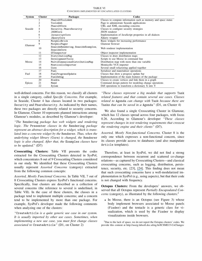
TABLE VICONCERNS IMPLEMENTED BY ENCAPSULATED CLUSTERS
System Cluster Packages Codes
Seaside
1 Pharo20ToolsWeb Classes to compute information such as memory and space status2 ToolsWeb Page to administrate Seaside applications3 Pharo20Core URL and XML enconding concerns4 Security, PharoSecurity Classes to configure security strategies5 JSONCore JSON renderer6 JavascriptCore Implementation of JavaScript properties in all dialects7 JQueryCore JQuery wrapper
Glamour
8 MorphicBrick Basic widgets for increasing performance9 MorphicPager Glamour browser
10 SeasideRendering, SeasideExamples, Web renderer implementationSeasideCore
11 GTInspector Object inspector implementation
Moose
12 DistributionMap Classes to draw distribution maps13 DevelopmentTools Scripts to use Moose in command line14 MultiDimensionsDistributionMap Distribution map with more than one variable15 MonticelloImporter Monticello VCS importer16 Core Several small refactoring applied together
Fuel17 Fuel Serializer and materializer operations18 FuelProgressUpdate Classes that show a progress update bar19 FuelDebug Implementation of the main features of the package
Epicea20 Hiedra Classes to create vertices and link them in a graph21 Mend Command design pattern for modeling change operations22 Xylem Diff operations to transform a dictionary X into Y
well-defined concerns. For this reason, we classify all clustersin a single category, called Specific Concerns. For example,in Seaside, Cluster 4 has classes located in two packages:Security and PharoSecurity. As indicated by their names,these two packages are directly related to security concerns.In Glamour, Cluster 10 represents planned interactions amongGlamour’s modules, as described by Glamour’s developer:
“The Rendering package has web widgets and renderinglogic. The Presenter classes in the Rendering packagerepresent an abstract description for a widget, which is trans-lated into a concrete widget by the Renderer. Thus, when theunderlying widget library (Core) is changed, the Renderer
logic is also changed. After that, the Examples classes haveto be updated.” (D7)
Crosscutting Clusters: Table VII presents the codesextracted for the Crosscutting Clusters detected in SysPol,which concentrates 8 out of 9 Crosscutting Clusters consideredin our study. We identified that these Crosscutting Clustersusually represent Assorted Concerns (category) extractedfrom the following common concepts:
Assorted, Mostly Functional Concerns. In Table VII, 7 out of8 Crosscutting Clusters express SysPol’s functional concerns.Specifically, four clusters are described as a collection ofseveral concerns (the reference to several is underlined, inTable VII). In the case of these clusters, the classes in apackage tend to implement multiple concerns; and a concerntend to be implemented by more than one package. Forexample, SysPol’s developer made the following commentswhen analyzing one of the clusters:
“CreateArticle is a quite generic use case in our system.It is usually imported by other use cases. Sometimes, whenimplementing a new use case, you must first change classesassociated to CreateArticle” (D1, on Cluster 2)
“These classes represent a big module that supports Task
related features and that contain several use cases. Classesrelated to Agenda can change with Task because there areTasks that can be saved in a Agenda” (D1, on Cluster 4)
We also found a single Crosscutting Cluster in Glamour,which has 12 classes spread across four packages, with focus0.26. According to Glamour’s developer “These classesrepresent changes in text rendering requirements that crosscutthe rendering engine and their clients” (D7).
Assorted, Mostly Non-functional Concerns. Cluster 8 is theonly one which expresses a non-functional concern, sinceits classes provide access to databases (and also manipulateArticle templates).
Therefore, at least in SysPol, we did not find a strongcorrespondence between recurrent and scattered co-changerelations—as captured by Crosscutting Clusters—and classicalcrosscutting concerns, such as logging, distribution, persis-tence, security, etc. [23], [24]. This finding does not meanthat such crosscutting concerns have a well-modularized im-plementation in SysPol (e.g., using aspects), but that their codeis not changed with frequency.
Octopus Clusters: From the developers’ answers, we ob-served that all Octopus represent Partially Encapsulated Con-cerns (category), as illustrated by the following clusters:3
• In Moose, there is an Octopus (see Figure 3) whosebody implement browsers associated to Moose panels(Finder) and the tentacle is a generic class for vi-sualization, which is used by the Finder to displayvisualizations inside browsers.
3Due to the lack of space, we do not report the Octopus clusters’ codes. Weprovide this content at http://aserg.labsoft.dcc.ufmg.br/ICSME15-CoChanges
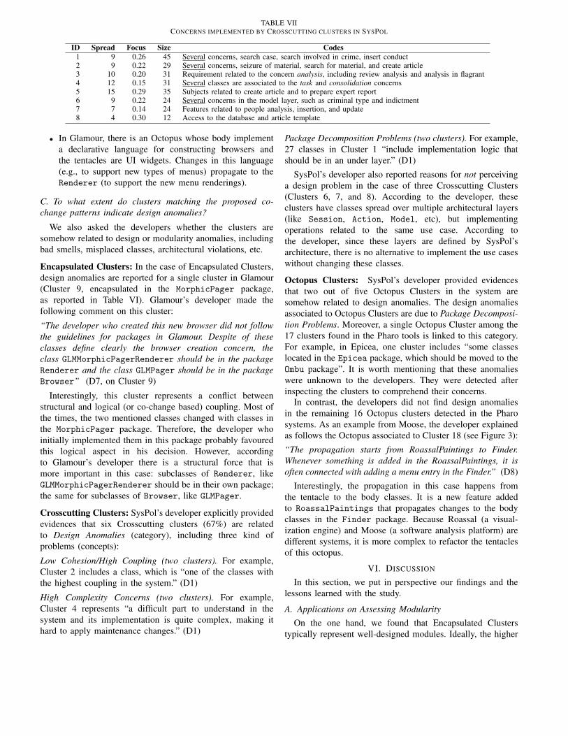
TABLE VIICONCERNS IMPLEMENTED BY CROSSCUTTING CLUSTERS IN SYSPOL
ID Spread Focus Size Codes1 9 0.26 45 Several concerns, search case, search involved in crime, insert conduct2 9 0.22 29 Several concerns, seizure of material, search for material, and create article3 10 0.20 31 Requirement related to the concern analysis, including review analysis and analysis in flagrant4 12 0.15 31 Several classes are associated to the task and consolidation concerns5 15 0.29 35 Subjects related to create article and to prepare expert report6 9 0.22 24 Several concerns in the model layer, such as criminal type and indictment7 7 0.14 24 Features related to people analysis, insertion, and update8 4 0.30 12 Access to the database and article template
• In Glamour, there is an Octopus whose body implementa declarative language for constructing browsers andthe tentacles are UI widgets. Changes in this language(e.g., to support new types of menus) propagate to theRenderer (to support the new menu renderings).
C. To what extent do clusters matching the proposed co-change patterns indicate design anomalies?
We also asked the developers whether the clusters aresomehow related to design or modularity anomalies, includingbad smells, misplaced classes, architectural violations, etc.
Encapsulated Clusters: In the case of Encapsulated Clusters,design anomalies are reported for a single cluster in Glamour(Cluster 9, encapsulated in the MorphicPager package,as reported in Table VI). Glamour’s developer made thefollowing comment on this cluster:
“The developer who created this new browser did not followthe guidelines for packages in Glamour. Despite of theseclasses define clearly the browser creation concern, theclass GLMMorphicPagerRenderer should be in the packageRenderer and the class GLMPager should be in the packageBrowser” (D7, on Cluster 9)
Interestingly, this cluster represents a conflict betweenstructural and logical (or co-change based) coupling. Most ofthe times, the two mentioned classes changed with classes inthe MorphicPager package. Therefore, the developer whoinitially implemented them in this package probably favouredthis logical aspect in his decision. However, accordingto Glamour’s developer there is a structural force that ismore important in this case: subclasses of Renderer, likeGLMMorphicPagerRenderer should be in their own package;the same for subclasses of Browser, like GLMPager.
Crosscutting Clusters: SysPol’s developer explicitly providedevidences that six Crosscutting clusters (67%) are relatedto Design Anomalies (category), including three kind ofproblems (concepts):
Low Cohesion/High Coupling (two clusters). For example,Cluster 2 includes a class, which is “one of the classes withthe highest coupling in the system.” (D1)
High Complexity Concerns (two clusters). For example,Cluster 4 represents “a difficult part to understand in thesystem and its implementation is quite complex, making ithard to apply maintenance changes.” (D1)
Package Decomposition Problems (two clusters). For example,27 classes in Cluster 1 “include implementation logic thatshould be in an under layer.” (D1)
SysPol’s developer also reported reasons for not perceivinga design problem in the case of three Crosscutting Clusters(Clusters 6, 7, and 8). According to the developer, theseclusters have classes spread over multiple architectural layers(like Session, Action, Model, etc), but implementingoperations related to the same use case. According tothe developer, since these layers are defined by SysPol’sarchitecture, there is no alternative to implement the use caseswithout changing these classes.
Octopus Clusters: SysPol’s developer provided evidencesthat two out of five Octopus Clusters in the system aresomehow related to design anomalies. The design anomaliesassociated to Octopus Clusters are due to Package Decomposi-tion Problems. Moreover, a single Octopus Cluster among the17 clusters found in the Pharo tools is linked to this category.For example, in Epicea, one cluster includes “some classeslocated in the Epicea package, which should be moved to theOmbu package”. It is worth mentioning that these anomalieswere unknown to the developers. They were detected afterinspecting the clusters to comprehend their concerns.
In contrast, the developers did not find design anomaliesin the remaining 16 Octopus clusters detected in the Pharosystems. As an example from Moose, the developer explainedas follows the Octopus associated to Cluster 18 (see Figure 3):
“The propagation starts from RoassalPaintings to Finder.Whenever something is added in the RoassalPaintings, it isoften connected with adding a menu entry in the Finder.” (D8)
Interestingly, the propagation in this case happens fromthe tentacle to the body classes. It is a new feature addedto RoassalPaintings that propagates changes to the bodyclasses in the Finder package. Because Roassal (a visual-ization engine) and Moose (a software analysis platform) aredifferent systems, it is more complex to refactor the tentaclesof this octopus.
VI. DISCUSSION
In this section, we put in perspective our findings and thelessons learned with the study.
A. Applications on Assessing ModularityOn the one hand, we found that Encapsulated Clusters
typically represent well-designed modules. Ideally, the higher
the number of Encapsulated Clusters, the higher the quality ofa module decomposition. Interestingly, Encapsulated Clustersare the most common co-change patterns in the Pharo softwaretools we studied, which are generally developed by high-skilled developers. On the other hand, Crosscutting Clustersin SysPol tend to reveal design anomalies with a precision of67% (at least in our sample of eight Crosscutting Clusters).Typically, these anomalies are due to concerns implementedusing complex class structures, which suffer from designproblems like high coupling/low cohesion. They are not relatedto classical non-functional concerns, like logging, persistence,distribution, etc. We emphasize that the differences betweenJava (SysPol) and Pharo systems should not be associatedexclusively to the programming language. For example, inprevious studies we evaluated at least two Java-based systemswithout Crosscutting Clusters [10]. In fact, SysPol’s expertassociates the modularity problems found in the system toa high turnover in the development team, which is mostlycomposed by junior developers and undergraduate students.
Finally, developers are usually skeptical about removingthe octopus’ tentacles, by for example moving their classesto the body by inserting a stable interface between the bodyand the tentacles. For example, Glamour’s developer madethe following comments when asked about these possibilities:
“Unfortunately, sometimes it is difficult to localize changesin just one package. Even a well-modularized system is asystem after all. Shielding changes in only one package isnot absolutely possible.” (D7)
B. The Tyranny of the Static Decomposition
Specifically for Crosscutting Clusters, the false positives wefound are due to maintenance tasks whose implementationrequires changes in multiple layers of the software architecture(like user interface, model, persistence, etc). Interestingly, theexpert developers usually view their static software architec-tures as dominant structures. Changes that crosscut the layersin this architecture are not perceived as problems, but asthe only possible implementation solution in face of theircurrent architectural decisions. During the study, we referredto this recurrent observation as the tyranny of the staticdecomposition. We borrowed the term from the “tyranny ofthe dominant decomposition” [25], normally used in aspect-oriented software development to denote the limitations oftraditional languages and modularization mechanisms whenhandling crosscutting concerns.
In future work, we plan to investigate this tyranny indetails, by arguing developers if other architectural styles arenot possible, for example centered on domain-driven designprinciples [26]. We plan to investigate whether informationsystems architected using such principles are less subjected tocrosscutting changes, as the ones we found in SysPol.
C. (Semi-)Automatic Remodularizations
Modular decisions deeply depend on software architects ex-pertise and also on particular domain restrictions. For example,even for SysPol’s developer it was difficult to explain and
reason about the changes captured by some of the CrosscuttingClusters detected in his system. For this reason, the studydid not reveal any insights on techniques or heuristics thatcould be used to (semi-)automatically remove potential designanomalies associated to Crosscutting Clusters. However, co-change clusters readily meet the concept of virtual separationof concerns [27], [28], which advocates module views thatdo not require syntactic support in the source code. In thissense, co-change clusters can be an alternative to the Pack-age Explorer, helping developers to comprehend the spatialdistribution of changes in software systems.
D. Limitations
We found three co-change clusters that are due to flossrefactoring, i.e., programming sessions when the developer in-tersperses refactoring with other kinds of source code changes,like fixing a bug or implementing a new feature [29]. To tacklethis limitation, we can use tools that automatically detectrefactorings from version histories, like Ref-Finder [30] andRef-Detector [31]. Once the refactorings are identified, we canremove co-change relations including classes only modified asprescribed by the identified refactorings.
Furthermore, 49 co-change clusters have no matched theproposed patterns (48%). We inspected them to comprehendwhy they were not categorized as Encapsulated, Crosscutting,or Octopus. We observed that 32 clusters are well-confined inpackages, i.e., they touch a single package but their focus islower than 1.0. This behavior does not match Encapsulatedpattern because these clusters share the packages they touchwith other clusters. Moreover, we also identified 14 clusterssimilar to Octopus, i.e., they have bodies in a package andarms in others. However, some clusters have bodies smallerand others have arms tinier than the threshold settings. Theremaining three clusters touch very few classes per packagebut their spread is lower than the threshold settings.
Finally, we did not look for false negatives, i.e., sets ofclasses that changed together, but that are not classified asco-change clusters by the Chameleon graph clustering algo-rithm. Usually, computing false negatives in the context ofarchitectural analysis is more difficult, because we dependon architects to generate golden sets. Specifically in the caseof co-change clusters, we have the impression that expertdevelopers are not completely aware of the whole set ofchanges implemented in their systems and on the co-changerelations established due to such changes, making it morechallenging to build a golden set of co-change clusters.
VII. THREATS TO VALIDITY
First, we evaluated six systems, implemented in two lan-guages (Java and Pharo) and related to two major domains(information systems and software tools). Therefore, our re-sults may not generalize to other systems, languages, andapplication domains (external validity). Second, our resultsmay reflect personal opinions of the interviewed developers onsoftware architecture and development (conclusion validity).
Anyway, we interviewed expert developers, with large expe-rience, and who are responsible for the central architecturaldecisions in their systems. Third, our results are directlyimpacted by the thresholds settings used in the study (internalvalidity). We handled this threat by reusing thresholds fromour previous work on Co-Change Clustering, which weredefined after extensive experimental testings. Furthermore,thresholds selection is usually a concern in any technique fordetecting patterns in source code. Finally, there are threatsconcerning the way we measured the co-change relations(construct validity). Specifically, we depend on pre and pos-processing filters to handle commits that could pollute theco-change graphs with meaningless relations. For example,during the analysis with developers, we detected three co-change clusters (6%) that are motivated by small refactorings.Ideally, it would be interesting to discard such commitsautomatically. Finally, we only measured co-change relationsfor classes. However, SysPol has other artifacts, such as XMLand XHTML files, which are not considered in the study.
VIII. RELATED WORK
Semantic Clustering is a technique based on Latent Seman-tic Indexing (LSI) and clustering to group source code artifactsthat use similar vocabulary [6], [7]. Therefore, Co-Changeand Semantic Clustering are conceptually similar techniques,sharing the same goals. However, they use different datasources (commits vs vocabularies) and processing algorithms(Chamaleon graph clustering algorithm vs LSI). Moreover,Semantic Clustering was not evaluated in the field, usingdevelopers’ views on the extracted clusters.
Ball et al. introduced the concept of co-change graphs [11]and Beyer and Noack improved this concept proposing a graphvisualization technique to reveal clusters of frequently co-changed artifacts [12]. Their approach clusters all softwareartifacts which are represented as vertices in the co-changegraphs. In contrast, we prune several classes during the co-change graph and co-change cluster extraction phases. We alsocompute co-change clusters using a clustering algorithm de-signed for sparse graphs, as is typically the case of co-changegraphs. Finally, our focus is not on software visualization buton using co-change clusters to support modularity analysis.
Co-Change mining is used to predict changes [13], [32],to support program visualization [12], [33], to reveal logicaldependencies [34], [35], to improve defect prediction tech-niques [36], and to detect bad smells [37]. Zimmermann etal. propose an approach that uses association rules mining onversion histories to suggest possible future changes (e.g., ifclass A usually co-changes with B, and a commit only changesA, a warning is raised recommending to check whether B
should not be changed too) [13]. However, co-change clustersare coarse-grained structures, when compared to the set ofclasses in association rules. They usually have more classes (atleast, four classes according to our thresholds) and are detectedless frequently. Therefore, they are better instruments to helpdevelopers on program comprehension.
Bavota et al. investigate how the various types of cou-pling aligns with developer’s perceptions [38]. They considercoupling measures based on structural, dynamic, semantic,and logical information and evaluate how developers rate theidentified coupling links. Their results suggest that semanticcoupling seems to better reflect the developers’ mental modelthat represents interactions between entities. However, thedevelopers interviewed in the study evaluated only pairs ofclasses. In contrast, we retrieve co-change clusters having fouror more classes.
Vanya et al. use co-change clusters to support systemspartitioning, aiming to reduce coupling between parts of asystem [39]. Their approach differs from ours because co-change clusters containing files from the same part of thesystem are discarded. Beck and Diehl compare and combinelogical and structural dependencies to retrieve modular de-signs [40], [41]. They report clustering experiments to recoverthe architecture of ten Java programs. Their results indicatethat logical dependencies are interesting when substantialevolutionary data is available. In this paper, we consideredall commits available for the evaluated systems (almost 24Kcommits).
IX. CONCLUSION
One of the benefits of modularity is managerial, by allowingseparate groups to work on each module with little need forcommunication [1]. However, this is only possible if modulesconfine changes; crosscutting changes hamper modularity bymaking it more difficult to assign work units to specific teams.In this paper, we evaluate in the field a technique calledCo-Change Clustering, proposed to assess modularity usinglogical (or evolutionary) coupling, as captured by co-changerelations. We concluded that Encapsulated Clusters are veryoften linked to healthy designs and that 67% of CrosscuttingClusters are associated to design anomalies. Octopus Clustersare normally associated to expected class distributions, whichare not easy to implement in an encapsulated way, accordingto the interviewed developers.
As future work, we plan to conduct a large scale studyto analyze whether the occurrence of co-change patterns isassociated to programming languages. Particularly, we intendto consider well-known projects implemented in other lan-guages, such as C/C++. Also, we plan to investigate the effectthat alternative software architecture styles, e.g., architecturesbased on domain-driven principles, have on co-change pat-terns. Specifically, we plan to check whether such architecturescan avoid the generation of clusters matching Crosscutting orOctopus patterns. We also plan to compare and contrast theresults of Co-Change Clustering with the ones generated bySemantic Clustering [5], [6].
ACKNOWLEDGMENTS
This research is supported by grants from FAPEMIG, CAPES,and CNPq. We would like to thank the developers of SysPoland the developers of the evaluated Pharo systems for accept-ing to participate in our study.
REFERENCES
[1] D. L. Parnas, “On the criteria to be used in decomposing systems intomodules.” Communications of the ACM, vol. 15, no. 12, pp. 1053–1058,1972.
[2] B. S. Mitchell and S. Mancoridis, “On the automatic modularization ofsoftware systems using the Bunch tool,” IEEE Transactions on SoftwareEngineering, vol. 32, no. 3, pp. 193–208, 2006.
[3] S. R. Chidamber and C. F. Kemerer, “A metrics suite for object orienteddesign,” IEEE Transactions on Software Engineering, vol. 20, no. 6, pp.476–493, 1994.
[4] N. Anquetil, C. Fourrier, and T. C. Lethbridge, “Experiments withclustering as a software remodularization method,” in 6th WorkingConference on Reverse Engineering (WCRE), 1999, pp. 235–255.
[5] G. Santos, M. T. Valente, and N. Anquetil, “Remodularization analysisusing semantic clustering,” in 1st CSMR-WCRE Software EvolutionWeek, 2014, pp. 224–233.
[6] A. Kuhn, S. Ducasse, and T. Girba, “Enriching reverse engineeringwith semantic clustering,” in 12th Working Conference on ReverseEngineering (WCRE), 2005, pp. 133–142.
[7] A. Kuhn, S. Ducasse, and T. Gırba, “Semantic clustering: Identifyingtopics in source code,” Information and Software Technology, vol. 49,no. 3, pp. 230–243, 2007.
[8] G. Bavota, M. Gethers, R. Oliveto, D. Poshyvanyk, and A. de Lucia,“Improving software modularization via automated analysis of latenttopics and dependencies,” ACM Transactions on Software Engineeringand Methodology (TOSEM), vol. 23, no. 1, pp. 1–33, 2014.
[9] L. L. Silva, M. T. Valente, and M. Maia, “Assessing modularity usingco-change clusters,” in 13th International Conference on Modularity,2014, pp. 49–60.
[10] ——, “Co-change clusters: Extraction and application on assessingsoftware modularity,” Transactions on Aspect-Oriented Software Devel-opment (TAOSD), pp. 1–37, 2015.
[11] T. Ball, J. K. A. A. Porter, and H. P. Siy, “If your version control systemcould talk ...” in ICSE Workshop on Process Modeling and EmpiricalStudies of Software Engineering, 1997.
[12] D. Beyer and A. Noack, “Clustering software artifacts based on fre-quent common changes,” in 13th International Workshop on ProgramComprehension (IWPC), 2005, pp. 259–268.
[13] T. Zimmermann, P. Weissgerber, S. Diehl, and A. Zeller, “Miningversion histories to guide software changes,” IEEE Transactions onSoftware Engineering, vol. 31, no. 6, pp. 429–445, 2005.
[14] S. Ducasse, T. Gırba, and A. Kuhn, “Distribution map,” in 22nd IEEEInternational Conference on Software Maintenance (ICSM), 2006, pp.203–212.
[15] C. Couto, P. Pires, M. T. Valente, R. Bigonha, and N. Anquetil,“Predicting software defects with causality tests,” Journal of Systemsand Software, pp. 1–38, 2014.
[16] G. Karypis, E.-H. S. Han, and V. Kumar, “Chameleon: hierarchicalclustering using dynamic modeling,” Computer, vol. 32, no. 8, pp. 68–75, 1999.
[17] R. Marinescu, “Detection strategies: metrics-based rules for detectingdesign flaws,” in 20th IEEE International Conference on SoftwareMaintenance (ICSM), 2004, pp. 350–359.
[18] M. Lanza and R. Marinescu, Object-Oriented Metrics in Practice: UsingSoftware Metrics to Characterize, Evaluate, and Improve the Design ofObject-Oriented Systems. Springer, 2006.
[19] O. Nierstrasz, S. Ducasse, and D. Pollet, Pharo by Example. SquareBracket Associates, 2010.
[20] L. L. Silva, D. Felix, M. T. Valente, and M. Maia, “ModularityCheck: Atool for assessing modularity using co-change clusters,” in 5th BrazilianConference on Software: Theory and Practice, 2014, pp. 1–8.
[21] U. Flick, An Introduction to Qualitative Research. SAGE, 2009.[22] J. Corbin and A. Strauss, “Grounded theory research: Procedures,
canons, and evaluative criteria,” Qualitative Sociology, vol. 13, no. 1,pp. 3–21, 1990.
[23] G. Kiczales, J. Lamping, A. Mendhekar, C. Maeda, C. Lopes, J.-M. Loingtier, and J. Irwin, “Aspect-oriented programming,” in 11thEuropean Conference on Object-Oriented Programming (ECOOP), ser.LNCS, vol. 1241. Springer Verlag, 1997, pp. 220–242.
[24] G. Kiczales, E. Hilsdale, J. Hugunin, M. Kersten, J. Palm, and W. G.Griswold, “An overview of AspectJ,” in 15th European Conferenceon Object-Oriented Programming (ECOOP), ser. LNCS, vol. 2072.Springer Verlag, 2001, pp. 327–355.
[25] P. Tarr, H. Ossher, W. Harrison, and S. M. Sutton, Jr., “N degrees of sep-aration: Multi-dimensional separation of concerns,” in 21st InternationalConference on Software Engineering (ICSE), 1999, pp. 107–119.
[26] E. Evans, Domain-Driven Design: Tackling Complexity in the Heart ofSoftware. Prentice Hall, 2003.
[27] S. Apel and C. Kastner, “Virtual separation of concerns - A secondchance for preprocessors,” Journal of Object Technology, vol. 8, no. 6,pp. 59–78, 2009.
[28] C. Kastner, S. Apel, and M. Kuhlemann, “Granularity in software prod-uct lines,” in 30th International Conference on Software Engineering(ICSE), 2008, pp. 311–320.
[29] E. Murphy-Hill, C. Parnin, and A. P. Black, “How we refactor, and howwe know it,” in 31st International Conference on Software Engineering(ICSE), 2009, pp. 287–297.
[30] K. Prete, N. Rachatasumrit, N. Sudan, and M. Kim, “Template-based re-construction of complex refactorings,” in IEEE International Conferenceon Software Maintenance (ICSM), 2010, pp. 1–10.
[31] N. Tsantalis, V. Guana, E. Stroulia, and A. Hindle, “A multidimensionalempirical study on refactoring activity,” in Conference of the Centerfor Advanced Studies on Collaborative Research (CASCON), 2013, pp.132–146.
[32] M. P. Robillard and B. Dagenais, “Recommending change clusters tosupport software investigation: An empirical study,” Journal of SoftwareMaintenance and Evolution: Research and Practice, vol. 22, no. 3, pp.143–164, 2010.
[33] M. D’Ambros, M. Lanza, and M. Lungu, “Visualizing co-change in-formation with the evolution radar,” IEEE Transactions on SoftwareEngineering, vol. 35, no. 5, pp. 720–735, 2009.
[34] A. Alali, B. Bartman, C. D. Newman, and J. I. Maletic, “A preliminaryinvestigation of using age and distance measures in the detectionof evolutionary couplings,” in 10th Working Conference on MiningSoftware Repositories (MSR), 2013, pp. 169–172.
[35] G. A. Oliva, F. W. Santana, M. A. Gerosa, and C. R. B. de Souza,“Towards a classification of logical dependencies origins: a case study,”in 12th International Workshop on Principles of Software Evolution andthe 7th annual ERCIM Workshop on Software Evolution (EVOL/IWPSE),2011, pp. 31–40.
[36] M. D’Ambros, M. Lanza, and R. Robbes, “On the relationship betweenchange coupling and software defects,” in 16th Working Conference onReverse Engineering (WCRE), 2009, pp. 135–144.
[37] F. Palomba, G. Bavota, M. D. Penta, R. Oliveto, A. de Lucia, andD. Poshyvanyk, “Detecting bad smells in source code using changehistory information,” in 28th IEEE/ACM International Conference onAutomated Software Engineering (ASE), 2013, pp. 11–15.
[38] G. Bavota, B. Dit, R. Oliveto, M. Di Penta, D. Poshyvanyk, andA. De Lucia, “An empirical study on the developers’ perception ofsoftware coupling,” in 35th International Conference on Software Engi-neering (ICSE), 2013, pp. 692–701.
[39] A. Vanya, L. Hofland, S. Klusener, P. van de Laar, and H. van Vliet,“Assessing software archives with evolutionary clusters,” in 16th IEEEInternational Conference on Program Comprehension (ICPC), 2008, pp.192–201.
[40] F. Beck and S. Diehl, “Evaluating the impact of software evolution onsoftware clustering,” in 17th Working Conference on Reverse Engineer-ing (WCRE), 2010, pp. 99–108.
[41] ——, “On the impact of software evolution on software clustering,”Empirical Software Engineering, vol. 18, no. 5, pp. 970–1004, 2013.
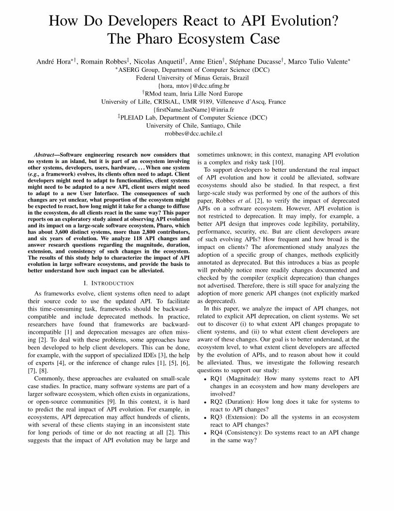
How Do Developers React to API Evolution?The Pharo Ecosystem Case
André Hora∗†, Romain Robbes‡, Nicolas Anquetil†, Anne Etien†, Stéphane Ducasse†, Marco Tulio Valente∗∗ASERG Group, Department of Computer Science (DCC)
Federal University of Minas Gerais, Brazil{hora, mtov}@dcc.ufmg.br
†RMod team, Inria Lille Nord EuropeUniversity of Lille, CRIStAL, UMR 9189, Villeneuve d’Ascq, France
{firstName.lastName}@inria.fr‡PLEIAD Lab, Department of Computer Science (DCC)
University of Chile, Santiago, [email protected]
Abstract—Software engineering research now considers thatno system is an island, but it is part of an ecosystem involvingother systems, developers, users, hardware, . . . When one system(e.g., a framework) evolves, its clients often need to adapt. Clientdevelopers might need to adapt to functionalities, client systemsmight need to be adapted to a new API, client users might needto adapt to a new User Interface. The consequences of suchchanges are yet unclear, what proportion of the ecosystem mightbe expected to react, how long might it take for a change to diffusein the ecosystem, do all clients react in the same way? This paperreports on an exploratory study aimed at observing API evolutionand its impact on a large-scale software ecosystem, Pharo, whichhas about 3,600 distinct systems, more than 2,800 contributors,and six years of evolution. We analyze 118 API changes andanswer research questions regarding the magnitude, duration,extension, and consistency of such changes in the ecosystem.The results of this study help to characterize the impact of APIevolution in large software ecosystems, and provide the basis tobetter understand how such impact can be alleviated.
I. INTRODUCTION
As frameworks evolve, client systems often need to adapttheir source code to use the updated API. To facilitatethis time-consuming task, frameworks should be backward-compatible and include deprecated methods. In practice,researchers have found that frameworks are backward-incompatible [1] and deprecation messages are often miss-ing [2]. To deal with these problems, some approaches havebeen developed to help client developers. This can be done,for example, with the support of specialized IDEs [3], the helpof experts [4], or the inference of change rules [1], [5], [6],[7], [8].
Commonly, these approaches are evaluated on small-scalecase studies. In practice, many software systems are part of alarger software ecosystem, which often exists in organizations,or open-source communities [9]. In this context, it is hardto predict the real impact of API evolution. For example, inecosystems, API deprecation may affect hundreds of clients,with several of these clients staying in an inconsistent statefor long periods of time or do not reacting at all [2]. Thissuggests that the impact of API evolution may be large and
sometimes unknown; in this context, managing API evolutionis a complex and risky task [10].
To support developers to better understand the real impactof API evolution and how it could be alleviated, softwareecosystems should also be studied. In that respect, a firstlarge-scale study was performed by one of the authors of thispaper, Robbes et al. [2], to verify the impact of deprecatedAPIs on a software ecosystem. However, API evolution isnot restricted to deprecation. It may imply, for example, abetter API design that improves code legibility, portability,performance, security, etc. But are client developers awareof such evolving APIs? How frequent and how broad is theimpact on clients? The aforementioned study analyzes theadoption of a specific group of changes, methods explicitlyannotated as deprecated. But this introduces a bias as peoplewill probably notice more readily changes documented andchecked by the compiler (explicit deprecation) than changesnot advertised. Therefore, there is still space for analyzing theadoption of more generic API changes (not explicitly markedas deprecated).
In this paper, we analyze the impact of API changes, notrelated to explicit API deprecation, on client systems. We setout to discover (i) to what extent API changes propagate toclient systems, and (ii) to what extent client developers areaware of these changes. Our goal is to better understand, at theecosystem level, to what extent client developers are affectedby the evolution of APIs, and to reason about how it couldbe alleviated. Thus, we investigate the following researchquestions to support our study:
• RQ1 (Magnitude): How many systems react to APIchanges in an ecosystem and how many developers areinvolved?
• RQ2 (Duration): How long does it take for systems toreact to API changes?
• RQ3 (Extension): Do all the systems in an ecosystemreact to API changes?
• RQ4 (Consistency): Do systems react to an API changein the same way?
In this study we cover the Pharo1 software ecosystem, whichhas about 3,600 distinct systems, more than 2,800 contributorsand six years of evolution, and we analyze 118 API changes.We also compare our results with the Robbes et al. study onAPI deprecation on Pharo [2] to better understand how thesetwo types of API evolution affect client systems.
The contributions of this paper are summarized as follows:1) We provide a large-scale study, at the ecosystem level,
to better understand to what extent client developersare impacted by API changes that are not marked asdeprecated.
2) We provide a comparison between our results and theones of the previous API deprecation study [2].
Structure of the paper: In Section II, we present the APIchanges considered in this study. We describe our experimentdesign in Section III. We present and discuss the experimentresults in Section IV. We present the implications of our studyin Section V, and the threats to the validity in Section VI.Finally, we present related work in Section VII, and weconclude the paper in Section VIII.
II. API CHANGES
A. Definition
In this work, we focus on API changes related to methodreplacements and improvements, following the line studied byseveral researches in the context of framework migration [1],[5], [6], [7], [11], [12], [13], [8]. Next, we define and provideexamples on the two types of API changes considered in thispaper.Method replacements: In this type of API change, oneor more methods in the old release are replaced by oneor more methods in the new release. For example, in aone-to-one mapping, the method LineConnection.end() wasreplaced by LineConnection.getEndConnector() from JHotDraw5.2 to 5.3 [1]. In another case, in a one-to-many map-ping, the method CutCommand(DrawingView) was replacedby CutCommand(Alignment, DrawingEditor) and UndoableCom-mand(Command) [1]. In both examples, the removed methodshave not been deprecated; they were simply dropped, causingclients to fail.Method improvements: In this type of API change, one(or more) method in the old release is improved, producingone (or more) new method in the new release. For example,in Apache Ant, the method to close files was improved tocentralize the knowledge on closing files [13], producing aone-to-one mapping where calls to InputStream.close() shouldbe replaced by FileUtils.close(InputStream). In this case, bothsolutions to close files are available in the new release, i.e.,both methods can be used. However, the latter is the suggestedone in order to improve maintenance. In the Moose plat-form2, a convention states that calls to MooseModel.root() andMooseModel.add(MooseModel) should be replaced by Moose-Model.install() when adding models. Again, all the methods are
1http://www.pharo.org, verified on 25/03/20152http://www.moosetechnology.org, verified on 25/03/2015
available to be used, but MooseModel.install() is the suggestedone to improve code legibility.3
These types of API changes are likely to occur duringframework evolution, thus their detection is helpful for clientdevelopers. Recently, researchers proposed techniques to au-tomatically infer rules that describe such API changes [1],[6], [7], [11], [12], [13]. In this study, we adopt our previousapproach [7] in order to detect API changes, which coversboth aforementioned cases.
B. Detecting API Changes
In our approach, API changes are automatically producedby applying the association rules data mining technique [14]on the set of method call changes between two versions ofone method. We produce rules in the format old-call → new-call, indicating that the old call should be replaced by the newone. Each rule has a support and confidence, indicating thefrequency that the rule occurs in the set of analyzed changesand a level of confidence. We also use some heuristics to filterrules that are more likely to represent relevant API changes;for example, rules can be ranked by confidence, support oroccurrences in different revisions. Please, refer to our previousstudy [7] for an in-depth description about how the rules aregenerated.
III. EXPERIMENT DESIGN
A. Selecting the Clients: Pharo Ecosystem
For this study, we select the ecosystem built around thePharo open-source development community. Our analysis in-cluded six years of evolution (from 2008 to 2013) with3,588 systems and 2,874 contributors. There are two factorsinfluencing this choice. First, the ecosystem is concentratedon two repositories, SqueakSource and SmalltalkHub, whichgives us a clear inclusion criterion. Second, we are interestedin comparing our results with the previous work of Robbes etal. [2]; using the same ecosystem facilitates this comparison.The Pharo ecosystem: Pharo is an open-source, Smalltalk-inspired, dynamically typed language and environment. It iscurrently used in many industrial and research projects.4 ThePharo ecosystem has several important projects. For example,Seaside5 is a web-development framework, a competitor forRuby on Rails as the framework of choice for rapid webprototyping. Moose is an open-source platform for softwareand data analysis. Phratch, a visual and educational program-ming language, is a port of Scratch to the Pharo platform.Many other projects are developed in Pharo and hosted in theSqueakSource or SmalltalkHub repositories.The SqueakSource and SmalltalkHub repositories: Squeak-Source and SmalltalkHub repositories are the basis for the soft-ware ecosystem that the Pharo community have built over theyears. They are the de facto platform for sharing open-sourcecode for this community offering a nearly complete view of
3See the mailing discussion in: http://goo.gl/Ul3Sha, verified on 25/03/20154http://consortium.pharo.org, verified on 25/03/20155http://www.seaside.st, verified on 25/03/2015
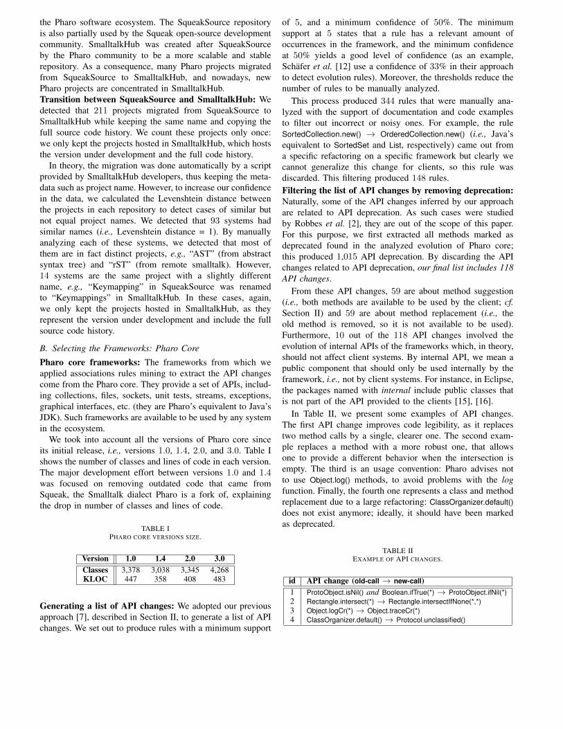
the Pharo software ecosystem. The SqueakSource repositoryis also partially used by the Squeak open-source developmentcommunity. SmalltalkHub was created after SqueakSourceby the Pharo community to be a more scalable and stablerepository. As a consequence, many Pharo projects migratedfrom SqueakSource to SmalltalkHub, and nowadays, newPharo projects are concentrated in SmalltalkHub.Transition between SqueakSource and SmalltalkHub: Wedetected that 211 projects migrated from SqueakSource toSmalltalkHub while keeping the same name and copying thefull source code history. We count these projects only once:we only kept the projects hosted in SmalltalkHub, which hoststhe version under development and the full code history.
In theory, the migration was done automatically by a scriptprovided by SmalltalkHub developers, thus keeping the meta-data such as project name. However, to increase our confidencein the data, we calculated the Levenshtein distance betweenthe projects in each repository to detect cases of similar butnot equal project names. We detected that 93 systems hadsimilar names (i.e., Levenshtein distance = 1). By manuallyanalyzing each of these systems, we detected that most ofthem are in fact distinct projects, e.g., “AST” (from abstractsyntax tree) and “rST” (from remote smalltalk). However,14 systems are the same project with a slightly differentname, e.g., “Keymapping” in SqueakSource was renamedto “Keymappings” in SmalltalkHub. In these cases, again,we only kept the projects hosted in SmalltalkHub, as theyrepresent the version under development and include the fullsource code history.
B. Selecting the Frameworks: Pharo Core
Pharo core frameworks: The frameworks from which weapplied associations rules mining to extract the API changescome from the Pharo core. They provide a set of APIs, includ-ing collections, files, sockets, unit tests, streams, exceptions,graphical interfaces, etc. (they are Pharo’s equivalent to Java’sJDK). Such frameworks are available to be used by any systemin the ecosystem.
We took into account all the versions of Pharo core sinceits initial release, i.e., versions 1.0, 1.4, 2.0, and 3.0. Table Ishows the number of classes and lines of code in each version.The major development effort between versions 1.0 and 1.4was focused on removing outdated code that came fromSqueak, the Smalltalk dialect Pharo is a fork of, explainingthe drop in number of classes and lines of code.
TABLE IPHARO CORE VERSIONS SIZE.
Version 1.0 1.4 2.0 3.0Classes 3,378 3,038 3,345 4,268KLOC 447 358 408 483
Generating a list of API changes: We adopted our previousapproach [7], described in Section II, to generate a list of APIchanges. We set out to produce rules with a minimum support
of 5, and a minimum confidence of 50%. The minimumsupport at 5 states that a rule has a relevant amount ofoccurrences in the framework, and the minimum confidenceat 50% yields a good level of confidence (as an example,Schäfer et al. [12] use a confidence of 33% in their approachto detect evolution rules). Moreover, the thresholds reduce thenumber of rules to be manually analyzed.
This process produced 344 rules that were manually ana-lyzed with the support of documentation and code examplesto filter out incorrect or noisy ones. For example, the ruleSortedCollection.new() → OrderedCollection.new() (i.e., Java’sequivalent to SortedSet and List, respectively) came out froma specific refactoring on a specific framework but clearly wecannot generalize this change for clients, so this rule wasdiscarded. This filtering produced 148 rules.Filtering the list of API changes by removing deprecation:Naturally, some of the API changes inferred by our approachare related to API deprecation. As such cases were studiedby Robbes et al. [2], they are out of the scope of this paper.For this purpose, we first extracted all methods marked asdeprecated found in the analyzed evolution of Pharo core;this produced 1,015 API deprecation. By discarding the APIchanges related to API deprecation, our final list includes 118API changes.
From these API changes, 59 are about method suggestion(i.e., both methods are available to be used by the client; cf.Section II) and 59 are about method replacement (i.e., theold method is removed, so it is not available to be used).Furthermore, 10 out of the 118 API changes involved theevolution of internal APIs of the frameworks which, in theory,should not affect client systems. By internal API, we mean apublic component that should only be used internally by theframework, i.e., not by client systems. For instance, in Eclipse,the packages named with internal include public classes thatis not part of the API provided to the clients [15], [16].
In Table II, we present some examples of API changes.The first API change improves code legibility, as it replacestwo method calls by a single, clearer one. The second exam-ple replaces a method with a more robust one, that allowsone to provide a different behavior when the intersection isempty. The third is an usage convention: Pharo advises notto use Object.log() methods, to avoid problems with the logfunction. Finally, the fourth one represents a class and methodreplacement due to a large refactoring: ClassOrganizer.default()does not exist anymore; ideally, it should have been markedas deprecated.
TABLE IIEXAMPLE OF API CHANGES.
id API change (old-call → new-call)1 ProtoObject.isNil() and Boolean.ifTrue(*) → ProtoObject.ifNil(*)2 Rectangle.intersect(*) → Rectangle.intersectIfNone(*,*)3 Object.logCr(*) → Object.traceCr(*)4 ClassOrganizer.default() → Protocol.unclassified()
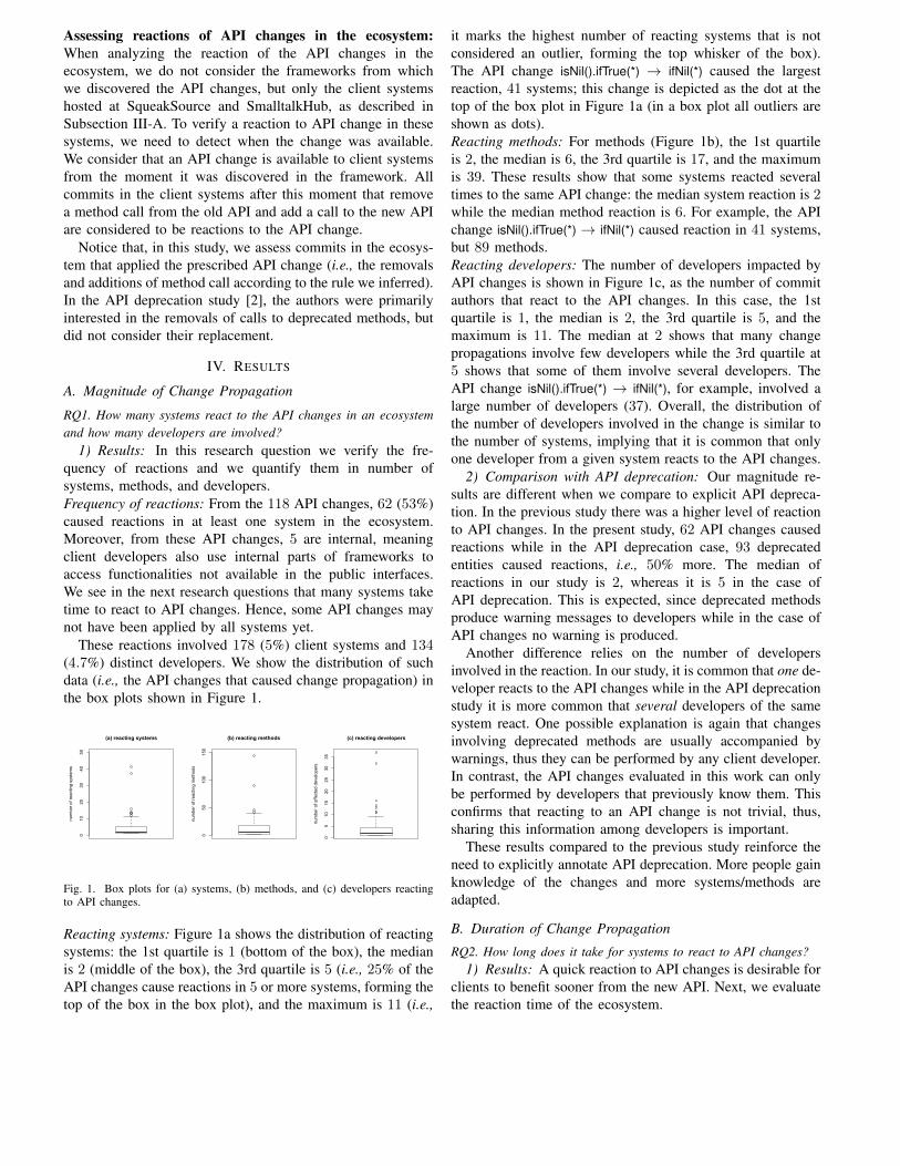
Assessing reactions of API changes in the ecosystem:When analyzing the reaction of the API changes in theecosystem, we do not consider the frameworks from whichwe discovered the API changes, but only the client systemshosted at SqueakSource and SmalltalkHub, as described inSubsection III-A. To verify a reaction to API change in thesesystems, we need to detect when the change was available.We consider that an API change is available to client systemsfrom the moment it was discovered in the framework. Allcommits in the client systems after this moment that removea method call from the old API and add a call to the new APIare considered to be reactions to the API change.
Notice that, in this study, we assess commits in the ecosys-tem that applied the prescribed API change (i.e., the removalsand additions of method call according to the rule we inferred).In the API deprecation study [2], the authors were primarilyinterested in the removals of calls to deprecated methods, butdid not consider their replacement.
IV. RESULTS
A. Magnitude of Change Propagation
RQ1. How many systems react to the API changes in an ecosystemand how many developers are involved?
1) Results: In this research question we verify the fre-quency of reactions and we quantify them in number ofsystems, methods, and developers.Frequency of reactions: From the 118 API changes, 62 (53%)caused reactions in at least one system in the ecosystem.Moreover, from these API changes, 5 are internal, meaningclient developers also use internal parts of frameworks toaccess functionalities not available in the public interfaces.We see in the next research questions that many systems taketime to react to API changes. Hence, some API changes maynot have been applied by all systems yet.
These reactions involved 178 (5%) client systems and 134(4.7%) distinct developers. We show the distribution of suchdata (i.e., the API changes that caused change propagation) inthe box plots shown in Figure 1.
010
2030
4050
(a) reacting systems
num
ber o
f rea
ctin
g sy
stem
s
050
100
150
(b) reacting methods
num
ber o
f rea
ctin
g m
etho
ds
05
1015
2025
3035
(c) reacting developers
num
ber o
f affe
cted
dev
elop
ers
Fig. 1. Box plots for (a) systems, (b) methods, and (c) developers reactingto API changes.
Reacting systems: Figure 1a shows the distribution of reactingsystems: the 1st quartile is 1 (bottom of the box), the medianis 2 (middle of the box), the 3rd quartile is 5 (i.e., 25% of theAPI changes cause reactions in 5 or more systems, forming thetop of the box in the box plot), and the maximum is 11 (i.e.,
it marks the highest number of reacting systems that is notconsidered an outlier, forming the top whisker of the box).The API change isNil().ifTrue(*) → ifNil(*) caused the largestreaction, 41 systems; this change is depicted as the dot at thetop of the box plot in Figure 1a (in a box plot all outliers areshown as dots).Reacting methods: For methods (Figure 1b), the 1st quartileis 2, the median is 6, the 3rd quartile is 17, and the maximumis 39. These results show that some systems reacted severaltimes to the same API change: the median system reaction is 2while the median method reaction is 6. For example, the APIchange isNil().ifTrue(*) → ifNil(*) caused reaction in 41 systems,but 89 methods.Reacting developers: The number of developers impacted byAPI changes is shown in Figure 1c, as the number of commitauthors that react to the API changes. In this case, the 1stquartile is 1, the median is 2, the 3rd quartile is 5, and themaximum is 11. The median at 2 shows that many changepropagations involve few developers while the 3rd quartile at5 shows that some of them involve several developers. TheAPI change isNil().ifTrue(*) → ifNil(*), for example, involved alarge number of developers (37). Overall, the distribution ofthe number of developers involved in the change is similar tothe number of systems, implying that it is common that onlyone developer from a given system reacts to the API changes.
2) Comparison with API deprecation: Our magnitude re-sults are different when we compare to explicit API depreca-tion. In the previous study there was a higher level of reactionto API changes. In the present study, 62 API changes causedreactions while in the API deprecation case, 93 deprecatedentities caused reactions, i.e., 50% more. The median ofreactions in our study is 2, whereas it is 5 in the case ofAPI deprecation. This is expected, since deprecated methodsproduce warning messages to developers while in the case ofAPI changes no warning is produced.
Another difference relies on the number of developersinvolved in the reaction. In our study, it is common that one de-veloper reacts to the API changes while in the API deprecationstudy it is more common that several developers of the samesystem react. One possible explanation is again that changesinvolving deprecated methods are usually accompanied bywarnings, thus they can be performed by any client developer.In contrast, the API changes evaluated in this work can onlybe performed by developers that previously know them. Thisconfirms that reacting to an API change is not trivial, thus,sharing this information among developers is important.
These results compared to the previous study reinforce theneed to explicitly annotate API deprecation. More people gainknowledge of the changes and more systems/methods areadapted.
B. Duration of Change Propagation
RQ2. How long does it take for systems to react to API changes?1) Results: A quick reaction to API changes is desirable for
clients to benefit sooner from the new API. Next, we evaluatethe reaction time of the ecosystem.
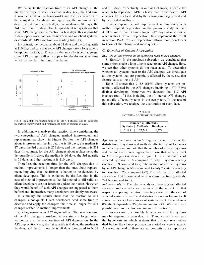
We calculate the reaction time to an API change as thenumber of days between its creation date (i.e., the first timeit was detected in the framework) and the first reaction inthe ecosystem. As shown in Figure 2a, the minimum is 0days, the 1st quartile is 5 days, the median is 34 days, the3rd quartile is 110 days. The 1st quartile at 5 days shows thatsome API changes see a reaction in few days: this is possibleif developers work both on frameworks and on client systems,or coordinate API evolution via mailing lists [17].
In contrast, the median at about 34 days and the 3rd quartileat 110 days indicate that some API changes take a long time tobe applied. In fact, as Pharo is a dynamically typed language,some API changes will only appear for developers at runtimewhich can explain the long time frame.
0200
400
600
800
(a) reacting time
num
ber o
f day
s
method improvement
methodreplacement
0200
400
600
800
(b) reacting time(method improvement and replacement)
num
ber o
f day
s
Fig. 2. Box plots for reaction time of (a) all API changes and (b) separatedby method improvement and replacement, both in number of days.
In addition, we analyze the reaction time considering thetwo categories of API changes, method improvement andreplacement, as shown in Figure 2b. For the API changesabout improvement, the 1st quartile is 10 days, the median is47 days, the 3rd quartile is 255 days, and the maximum is 351days. In contrast, for the API changes about replacement, the1st quartile is 1 days, the median is 20 days, the 3rd quartileis 59 days, and the maximum is 110 days.
Therefore, the reaction time for the API changes due tomethod improvements is longer than the ones about replace-ment, implying that the former is harder to be detected byclient developers. This is explained by the fact that in thecase of method improvements, the old method is still valid, soclient developers are not forced to update their code. However,they would benefit if such API changes are suggested to thembeforehand. In practice, many developers are simply not aware.
In summary, the results show that the reaction to APIchanges is not quick. Client developers need some time todiscover and apply the changes; this time is longer for APIchanges related to method improvements.
2) Comparison with API deprecation: The reaction timeof the API changes considered in our study is longer whenwe compare to the reaction time of API deprecation. In theAPI deprecation case, the 1st quartile is 0 days, the median is14 days, and the 3rd quartile is 90 days (compared to 5, 34
and 110 days, respectively, in our API changes). Clearly, thereaction to deprecated APIs is faster than in the case of APIchanges. This is facilitated by the warning messages producedby deprecated methods.
If we compare method improvement in this study withmethod explicit deprecation in the previous study, we seeit takes more than 3 times longer (47 days against 14) toreact without explicit deprecation. To complement the resultin section IV-A, explicit deprecation allows more developersto know of the change and more quickly.
C. Extension of Change Propagation
RQ3. Do all the systems in an ecosystem react to API changes?1) Results: In the previous subsection we concluded that
some systems take a long time to react to an API change. Here,we see that other systems do not react at all. To determinewhether all systems react to the API changes, we investigateall the systems that are potentially affected by them, i.e., thatfeature calls to the old API.
Table III shows that 2,188 (61%) client systems are po-tentially affected by the API changes, involving 1,579 (55%)distinct developers. Moreover, we detected that 112 APIchanges (out of 118), including the 10 internal API changes,potentially affected systems in the ecosystem. In the rest ofthis subsection, we analyze the distribution of such data.
TABLE IIIEXTENSION OF CHANGE PROPAGATION.
Number of affected...Systems Methods Developers
2,188 107,549 1,579
Affected systems and methods: Figures 3a and 3b show thedistribution of systems and methods affected by API changesin the ecosystem. We note that the number of affected systemsand methods are much higher than those that actually reactto API changes (as shown in Figure 1). The 1st quartile ofaffected systems is 15 compared to only 1 system reacting(methods: 59 compared to 2). The median of affected systemsby an API change is 56.5 compared to only 2 systems reactingto it (methods: 253 compared to 2). The 3rd quartile of affectedsystems is 154.5 compared to 5 systems reacting (methods:744.5 compared to 17).Relative analysis: The relative analysis of reacting and affectedsystems produces a better overview of the impact. In thatrespect, comparing the ratio of reacting systems to the ratio ofaffected systems gives the distribution shown in Figure 4a. Itshows that a very low number of systems react: the median is0%, the 3rd quartile is 3%, the maximum is 7%. We investigatepossible reasons for this low amount of reactions.
In an ecosystem, a possibly large amount of the systemsmay be stagnant, or even dead [2]. Thus, we first investigatethe hypothesis in which systems that did not react eitherdied before the change propagation started or were stagnant.A system is dead if there are no commits to its repository
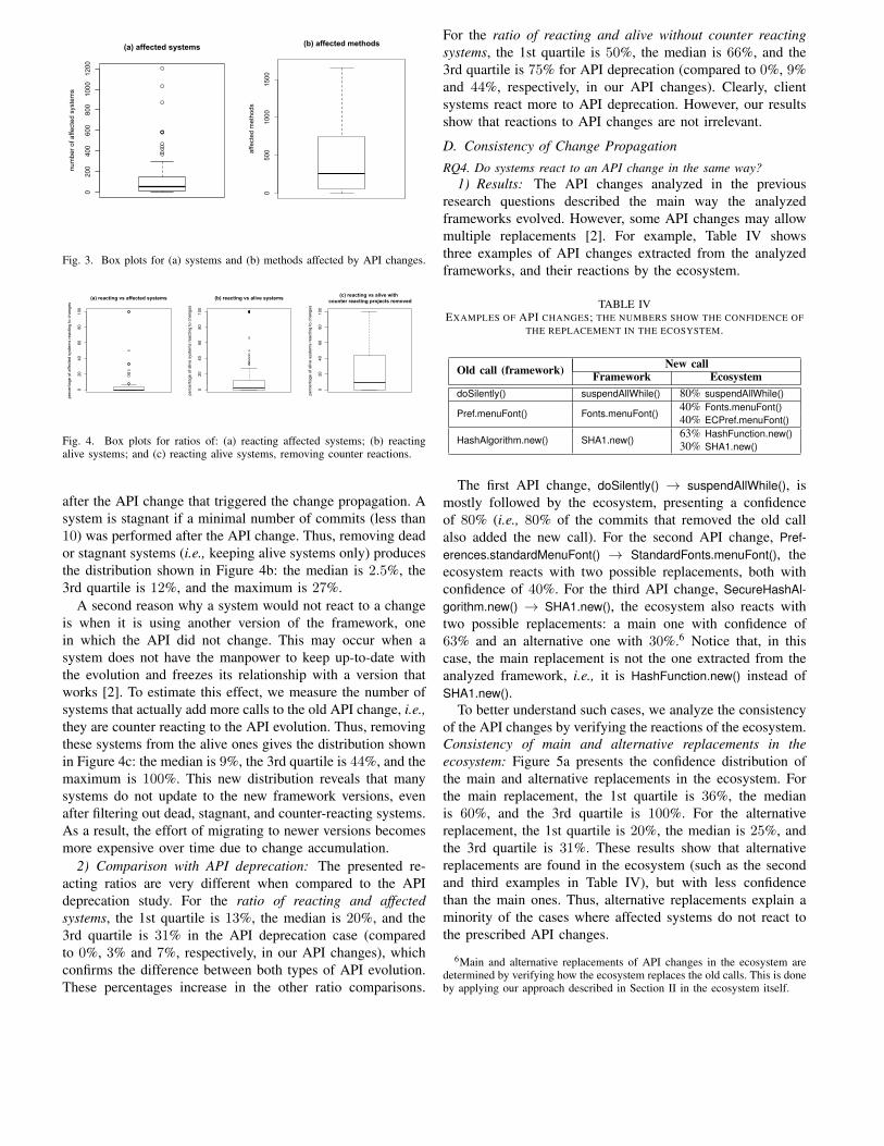
0200
400
600
800
1000
1200
(a) affected systems
num
ber o
f affe
cted
sys
tem
s
0500
1000
1500
(b) affected methods
affe
cted
met
hods
Fig. 3. Box plots for (a) systems and (b) methods affected by API changes.
020
4060
80100
(a) reacting vs affected systems
perc
enta
ge o
f affe
cted
sys
tem
s re
actin
g to
cha
nges
020
4060
80100
(b) reacting vs alive systems
perc
enta
ge o
f aliv
e sy
stem
s re
actin
g to
cha
nges
020
4060
80100
(c) reacting vs alive with counter reacting projects removed
perc
enta
ge o
f aliv
e sy
stem
s re
actin
g to
cha
nges
Fig. 4. Box plots for ratios of: (a) reacting affected systems; (b) reactingalive systems; and (c) reacting alive systems, removing counter reactions.
after the API change that triggered the change propagation. Asystem is stagnant if a minimal number of commits (less than10) was performed after the API change. Thus, removing deador stagnant systems (i.e., keeping alive systems only) producesthe distribution shown in Figure 4b: the median is 2.5%, the3rd quartile is 12%, and the maximum is 27%.
A second reason why a system would not react to a changeis when it is using another version of the framework, onein which the API did not change. This may occur when asystem does not have the manpower to keep up-to-date withthe evolution and freezes its relationship with a version thatworks [2]. To estimate this effect, we measure the number ofsystems that actually add more calls to the old API change, i.e.,they are counter reacting to the API evolution. Thus, removingthese systems from the alive ones gives the distribution shownin Figure 4c: the median is 9%, the 3rd quartile is 44%, and themaximum is 100%. This new distribution reveals that manysystems do not update to the new framework versions, evenafter filtering out dead, stagnant, and counter-reacting systems.As a result, the effort of migrating to newer versions becomesmore expensive over time due to change accumulation.
2) Comparison with API deprecation: The presented re-acting ratios are very different when compared to the APIdeprecation study. For the ratio of reacting and affectedsystems, the 1st quartile is 13%, the median is 20%, and the3rd quartile is 31% in the API deprecation case (comparedto 0%, 3% and 7%, respectively, in our API changes), whichconfirms the difference between both types of API evolution.These percentages increase in the other ratio comparisons.
For the ratio of reacting and alive without counter reactingsystems, the 1st quartile is 50%, the median is 66%, and the3rd quartile is 75% for API deprecation (compared to 0%, 9%and 44%, respectively, in our API changes). Clearly, clientsystems react more to API deprecation. However, our resultsshow that reactions to API changes are not irrelevant.
D. Consistency of Change PropagationRQ4. Do systems react to an API change in the same way?
1) Results: The API changes analyzed in the previousresearch questions described the main way the analyzedframeworks evolved. However, some API changes may allowmultiple replacements [2]. For example, Table IV showsthree examples of API changes extracted from the analyzedframeworks, and their reactions by the ecosystem.
TABLE IVEXAMPLES OF API CHANGES; THE NUMBERS SHOW THE CONFIDENCE OF
THE REPLACEMENT IN THE ECOSYSTEM.
Old call (framework) New callFramework Ecosystem
doSilently() suspendAllWhile() 80% suspendAllWhile()
Pref.menuFont() Fonts.menuFont()40% Fonts.menuFont()40% ECPref.menuFont()
HashAlgorithm.new() SHA1.new()63% HashFunction.new()30% SHA1.new()
The first API change, doSilently() → suspendAllWhile(), ismostly followed by the ecosystem, presenting a confidenceof 80% (i.e., 80% of the commits that removed the old callalso added the new call). For the second API change, Pref-erences.standardMenuFont() → StandardFonts.menuFont(), theecosystem reacts with two possible replacements, both withconfidence of 40%. For the third API change, SecureHashAl-gorithm.new() → SHA1.new(), the ecosystem also reacts withtwo possible replacements: a main one with confidence of63% and an alternative one with 30%.6 Notice that, in thiscase, the main replacement is not the one extracted from theanalyzed framework, i.e., it is HashFunction.new() instead ofSHA1.new().
To better understand such cases, we analyze the consistencyof the API changes by verifying the reactions of the ecosystem.Consistency of main and alternative replacements in theecosystem: Figure 5a presents the confidence distribution ofthe main and alternative replacements in the ecosystem. Forthe main replacement, the 1st quartile is 36%, the medianis 60%, and the 3rd quartile is 100%. For the alternativereplacement, the 1st quartile is 20%, the median is 25%, andthe 3rd quartile is 31%. These results show that alternativereplacements are found in the ecosystem (such as the secondand third examples in Table IV), but with less confidencethan the main ones. Thus, alternative replacements explain aminority of the cases where affected systems do not react tothe prescribed API changes.
6Main and alternative replacements of API changes in the ecosystem aredetermined by verifying how the ecosystem replaces the old calls. This is doneby applying our approach described in Section II in the ecosystem itself.
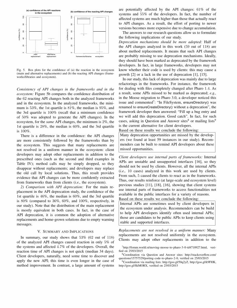
mainreplacement
alternativereplacement
020
4060
80100
(a) confidence of the API reactionsin the ecosystem
conf
iden
ce (%
)
frameworks/libraries ecosystem
020
4060
80100
(b) confidence of the reacting API changes
conf
iden
ce (%
)Fig. 5. Box plots for the confidence of (a) the reaction in the ecosystem(main and alternative replacements) and (b) the reacting API changes (frame-works/libraries and ecosystem).
Consistency of API changes in the frameworks and in theecosystem: Figure 5b compares the confidence distribution ofthe 62 reacting API changes both in the analyzed frameworksand in the ecosystem. In the analyzed frameworks, the mini-mum is 53%, the 1st quartile is 81%, the median is 95%, andthe 3rd quartile is 100% (recall that a minimum confidenceof 50% was adopted to generate the API changes). In theecosystem, for the same API changes, the minimum is 2%, the1st quartile is 28%, the median is 60%, and the 3rd quartileis 100%.
There is a difference in the confidence: the API changesare more consistently followed by the frameworks than bythe ecosystem. This suggests that many replacements arenot resolved in a uniform manner in the ecosystem: clientdevelopers may adopt other replacements in addition to theprescribed ones (such as the second and third examples inTable IV); method calls may be simply dropped, so theydisappear without replacements; and developers may replacethe old call by local solutions. Thus, this result providesevidence that API changes can be more confidently extractedfrom frameworks than from clients (i.e., the ecosystem).
2) Comparison with API deprecation: For the main re-placement in the API deprecation study, the confidence of the1st quartile is 46%, the median is 60%, and the 3rd quartileis 80% (compared to 36%, 60%, and 100%, respectively, inour study). Note that the distribution of the main replacementis mostly equivalent in both cases. In fact, in the case ofAPI deprecation, it is common the adoption of alternativereplacements and home-grown solutions due to empty warningmessages.
V. SUMMARY AND IMPLICATIONS
In summary, our study shows that 53% (62 out of 118)of the analyzed API changes caused reaction in only 5% ofthe systems and affected 4.7% of the developers. Overall, thereaction time of API changes is not quick (median 34 days).Client developers, naturally, need some time to discover andapply the new API; this time is even longer in the case ofmethod improvement. In contrast, a large amount of systems
are potentially affected by the API changes: 61% of thesystems and 55% of the developers. In fact, the number ofaffected systems are much higher than those that actually reactto API changes. As a result, the effort of porting to newerversions becomes more expensive due to change accumulation.
The answers to our research questions allow us to formulatethe following implications of our study.Deprecation mechanisms should be more adopted: Half ofthe API changes analyzed in this work (59 out of 118) areabout method replacements. It means that such API changesare probably missing to use deprecation mechanisms. Ideally,they should have been marked as deprecated by the frameworkdevelopers. In fact, in large frameworks, developers may notknow whether their code is used by clients: this may cause agrowth [2] or a lack in the use of deprecation [1], [15].
In our study, this lack of deprecation was mainly due to largerefactorings in the frameworks. For instance, the frameworkfor dealing with files completely changed after Pharo 1.4. Asa result, some APIs missed to be marked as deprecated; e.g.,in the Moose migration to Pharo 3.0, a developer noticed thisissue and commented7: “In FileSystem, ensureDirectory() wasrenamed to ensureCreateDirectory() without a deprecation”, theframework developer then answered: “Fill up a bug entry andwe will add this deprecation. Good catch”. In fact, for suchcases, asking in Question and Answer sites8 or mailing lists9
is the current alternative for client developers.Based on these results we conclude the following:Many deprecation opportunities are missed by the develop-ers (we found at least 59 instances in our study). Recom-menders can be built to remind API developers about thesemissed opportunities.
Client developers use internal parts of frameworks: InternalAPIs are unstable and unsupported interfaces [16], so theyshould not be used by clients. However, all the internal APIs(i.e., 10 cases) analyzed in this work are used by clients.From such, 5 caused the clients to react as in the frameworks.Thus, our results reinforce (at large-scale and ecosystem level)previous studies [11], [18], [16], showing that client systemsuse internal parts of frameworks to access functionalities notavailable in the public interfaces for a variety of reasons.Based on these results we conclude the following:Internal APIs are sometimes used by client developers inthe ecosystem under analysis. Recommenders can be buildto help API developers identify often used internal APIs;those are candidates to be public APIs to keep clients usingstable and supported interfaces.
Replacements are not resolved in a uniform manner: Manyreplacements are not resolved uniformly in the ecosystem.Clients may adopt other replacements in addition to the
7http://forum.world.st/moving-moose-to-pharo-3-0-td4718927.html, veri-fied on 25/03/2015
8Coordination via Question and Answer sites: http://stackoverflow.com/questions/15757529/porting-code-to-pharo-2-0, verified on 25/03/2015
9Coordination via mailing lists: http://goo.gl/50q2yZ, http://goo.gl/k9Fl0K,http://goo.gl/SkMORX, verified on 25/03/2015
prescribed ones; method calls may be simply dropped; anddevelopers may replace the old call by local solutions. In thiscontext, some studies propose the extraction of API changesfrom frameworks (e.g., [11]) other propose the extraction fromclients (e.g., [12]).Based on these results we conclude the following:There is no clear agreement on the best extraction sourceto detect API changes: frameworks or client systems. Thisstudy reinforces frameworks as a more reliable source.
Reactions to API changes can be partially automated: Aswe observed, many systems do not react to the API changesbecause they are not aware. Moreover, in the case of largeclient systems, the adaptation may take a long time and iscostly if done manually.Based on these results we conclude the following:Most of the API changes that we found in this work canbe implemented as rules in static analysis tools such asFindBugs [19], PMD [20], and SmallLint [21]. These rulescould help client developers to keep their source code up-to-date with the new APIs.
VI. THREATS TO VALIDITY
Construct Validity: The construct validity is related towhether the measurement in the study reflects real-worldsituations. In our study, the main threat is the quality of thedata we analyze and the degree of involved manual analysis.
Software ecosystems present some instances of duplication(around 15% of the code [22]), where packages are copiedfrom a repository to another (e.g., a developer keeping a copyof a specific framework version). This may overestimate thenumber of systems reacting to an API change.
Smalltalk (and Pharo) is a dynamically typed language, sothe detection of API change reaction may introduce noise assystems may use unrelated methods with the same name. Thismeans that an API change that uses a common method namemakes change propagation hard to be detected. This threat isalleviated by our manual filtering of noisy API changes.
Another factor that alleviates this threat is our focus onspecific evolution rules (i.e., a specific replacement of one ormore calls by one or more calls). For the first three researchquestions, we include only commits that are removing anold API and adding a new API to detect an API reaction.Requiring these two conditions to be achieved, decreases—or in some cases eliminates—the possibility of noise. Forthe fourth research question, we require the presence of themethods that contain a call to the old API. In this case, thenoise could have been an issue, however, this threat is reducedsince we discarded the API changes involved with commonmethods, i.e., the noisy ones.
We also identify two threats regarding the comparison withthe API deprecation study [2]. First, the time interval studiedis not the same one: we analyzed the ecosystem evolutionin the period from 2008 to 2013 while the API deprecationstudy analyzed from 2004 to 2011. Second, the way APIchanges are selected is different: while we deprecation study
simply collected the list of API deprecation, we inferred theAPI changes from commits in source code repository; theseAPI changes were manually validated by the authors of thepaper with the support of documentation and code examplesto eliminate incorrect and noisy ones. For these reasons, wecan not claim that this is an exact comparison. Parts of thedifferences observed may be due to other factors.Internal Validity: The internal validity is related to un-controlled aspects that may affect the experimental results.In our study, the main threat is the possible errors in theimplementation of our approach.
Our tool to detect API changes has been (i) used by severalmembers of our laboratory to support their own research onframeworks evolution, and (ii) divulged in the Moose reengi-neering mailing list, so that developers of this community canuse it; thus, we believe that these tasks reduce the risks of thisthreat.External Validity: The external validity is related to thepossibility to generalize our results. In our study, the mainthreat is the representativeness of our case studies.
We performed the study on a single ecosystem. It needsto be replicated on other ecosystems in other languages tocharacterize the phenomenon of change propagation morebroadly. Our results are limited to a single community inthe context of open-source; closed-source ecosystems, due todifferences in the internal processes, may present differentcharacteristics. However, our study detected API change reac-tions in thousands of client systems, which makes our resultsmore robust.
The Pharo ecosystem is a Smalltalk ecosystem, a dynami-cally typed programming language. Ecosystems in a staticallytyped programming language may present differences. In par-ticular, we expect static type checking to reduce the problemof noisy API changes for such ecosystems.
As an alternative to our choice of ecosystem, we could haveselected a development community based on a more popularlanguage such as Java or C++. However, this would havepresented several disadvantages. First, deciding which systemsto include or exclude would have been much more challenging.Second, the potentially very large size of the ecosystem couldprove impractical. We consider the size of the Pharo ecosystemas a “sweet spot”: with about 3,600 distinct systems and morethan 2,800 contributors, it is large enough to be relevant.
VII. RELATED WORK
A. Software Ecosystems Analysis
Software ecosystem is an overloaded term, which has sev-eral meanings. There are two principal facets: the first onefocuses on the business aspect [23], [24], and the second onthe artefact analysis aspect, i.e., on the analysis of multiple,evolving software systems [25], [9], [2]. In this work we usethe latter one; we consider an ecosystem to be “a collectionof software projects which are developed and co-evolve in thesame environment” [9]. These software systems have commonunderlying components, technology, and social norms [25].
Software ecosystems have been studied under a varietyof aspects. Jergensen et al. [25] study the social aspect ofecosystems by focusing on how developers move betweenprojects in the software ecosystems. The studies of Lungu etal. [26] and Bavota et al. [10] aim to recover dependencies be-tween the software projects of an ecosystem to support impactanalysis. Lungu et al. [27] focus on the software ecosystemsanalysis through interactive visualization and exploration ofthe systems and their dependencies. Gonzalez-Barahona etal. [28] study the Debian Linux distribution to measure its size,dependencies, and commonly used programming languages.
Recently, Mens et al. [29] proposed the investigation ofsimilarities between software ecosystems and natural ecosys-tems found in ecology. In this context, they are studyingthe GNOME and the CRAN ecosystems to better understandhow software ecosystems can benefit from biological ones.German et al. [30] also analyze the evolution of the CRANecosystem, investigating the growth of the ecosystem, and thedifferences between core and contributed packages.
In the context of API evolution and ecosystem impactanalysis, McDonnell et al. [31] investigate API stability andadoption on a small-scale Android ecosystem. In such study,API changes are derived from Android documentation. Theyhave found that Android APIs are evolving fast while clientadoption is not catching up with the pace of API evolution.Our study does not rely on documentation but on sourcecode changes to generate the list of APIs to answer differentquestions. Moreover, our study investigates the impact of APIevolution on thousands of distinct systems.
In a large-scale study, Robbes et al. [2] investigate theimpact of a specific type of API evolution, API deprecation,in an ecosystem that includes more than 2,600 projects; suchecosystem is the same that is used in our work. Our studyconsiders API changes that were not marked as deprecated.Thus, there is no overlap between the changes investigatedin our work and the ones investigated by that work. In fact,these studies complement each other to better characterize thephenomenon of change propagation at the ecosystem level.
B. API Evolution Analysis
Many approaches have been developed to support APIevolution and reduce the efforts of client developers. Chowand Notkin [4] present an approach where the API developersannotate changed methods with replacement rules that will beused to update client systems. Henkel and Diwan [3] proposeCatchUp!, a tool that uses an IDE to capture and replayrefactorings related to the API evolution. Hora et al. [7], [8]present tools to keep track of API evolution and popularity.
Kim et al. [32] automatically infer rules from structuralchanges. The rules are computed from changes at or above thelevel of method signatures, i.e., the body of the method is notanalyzed. Kim et al. [33] propose a tool (LSDiff) to supportcomputing differences between two system versions. In suchstudy, the authors take into account the body of the methodto infer rules, improving their previous work [32] where onlymethod signatures were analyzed. Nguyen et al. [34] propose
LibSync that uses graph-based techniques to help developersmigrate from one framework version to another. Using thelearned adaptation patterns, the tool recommends locations andupdate operations for adapting due to API evolution.
Dig and Johnson [15] help developers to better understandthe requirements for migration tools. They found that 80%of the changes that break client systems are refactorings.Cossette et al. [35] found that, in some cases, API evolutionis hard to handle and needs the assistance of an expert.
Some studies address the problem of discovering the map-ping of APIs between different platforms that separatelyevolved. For example, Zhong et al. [36] target the mappingbetween Java and C# APIs while Gokhale et al. [37] presentthe mapping between JavaME and Android APIs.
VIII. CONCLUSION
This paper presented an empirical study about the impact ofAPI evolution, in the specific case of methods unrelated to APIdeprecation. The study was done in the context of a large-scalesoftware ecosystem, Pharo, with about 3,600 distinct systems.We analyzed 118 important API changes from frameworks,and we found that 53% impacted other systems. We reiteratethe most interesting conclusions from our experiment results:
• API changes can have a large impact on the ecosystem interms of client systems, methods, and developers. Clientdevelopers need some time to discover and apply the newAPI, and the majority of the systems do not react at all.
• API changes can not be marked as deprecated becauseframework developers are not aware of their use byclients. Moreover, client developers can use internal APIsto access functionalities not available in the public inter-faces.
• Replacements can not be resolved in a uniform mannerin the ecosystem. Thus, API changes can be more confi-dently extracted from frameworks than from clients.
• Most of the analyzed API changes can be implementedas rules in static analysis tools to reduce the adaptationtime or the amount of projects that are not aware abouta new/better API.
• API changes knowledge can be concentrated in a smallamount of developers. API changes and deprecation canpresent different characteristics, for example, reaction toAPI changes is slower and less clients react.
As future work, we plan to extend this research to analyzeecosystems based on statically typed languages. Thus, theresults presented in our study will enable us to comparereactions of statically and dynamically typed ecosystems tobetter characterize the phenomenon of change propagation.
ACKNOWLEDGMENT
This research was supported by CNPq (Conselho Nacionalde Desenvolvimento Científico e Tecnológico - Brasil), ANR(Agence Nationale de la Recherche - ANR-2010-BLAN-0219-01) and FAPEMIG.
REFERENCES
[1] W. Wu, Y.-G. Gueheneuc, G. Antoniol, and M. Kim, “Aura: a hybridapproach to identify framework evolution,” in International Conferenceon Software Engineering, 2010.
[2] R. Robbes, M. Lungu, and D. Röthlisberger, “How do developers reactto API deprecation? The case of a smalltalk ecosystem,” in InternationalSymposium on the Foundations of Software Engineering, 2012.
[3] J. Henkel and A. Diwan, “Catchup!: Capturing and replaying refactor-ings to support API evolution,” in International Conference on SoftwareEngineering, 2005.
[4] K. Chow and D. Notkin, “Semi-automatic update of applications inresponse to library changes,” in International Conference on SoftwareMaintenance, 1996.
[5] A. Hora, N. Anquetil, S. Ducasse, and S. Allier, “Domain SpecificWarnings: Are They Any Better?” in International Conference onSoftware Maintenance, 2012.
[6] S. Meng, X. Wang, L. Zhang, and H. Mei, “A history-based matchingapproach to identification of framework evolution,” in InternationalConference on Software Engineering, 2012.
[7] A. Hora, A. Etien, N. Anquetil, S. Ducasse, and M. T. Valente,“APIEvolutionMiner: Keeping API Evolution under Control,” in Soft-ware Evolution Week (European Conference on Software Maintenanceand Working Conference on Reverse Engineering), 2014.
[8] apiwave, “Discover and track APIs,” http://apiwave.com, 2015.[9] M. Lungu, “Reverse Engineering Software Ecosystems,” PhD thesis,
University of Lugano, Switzerland (October 2009), 2009.[10] G. Bavota, G. Canfora, M. D. Penta, R. Oliveto, and S. Panichella, “The
evolution of project inter-dependencies in a software ecosystem: thecase of Apache,” in International Conference on Software Maintenance,2013.
[11] B. Dagenais and M. P. Robillard, “Recommending adaptive changesfor framework evolution,” in International Conference on Softwareengineering, 2008.
[12] T. Schäfer, J. Jonas, and M. Mezini, “Mining framework usage changesfrom instantiation code,” in International Conference on Software engi-neering, 2008.
[13] A. Hora, N. Anquetil, S. Ducasse, and M. T. Valente, “Mining Sys-tem Specific Rules from Change Patterns,” in Working Conference onReverse Engineering, 2013.
[14] M. Zaki and W. Meira Jr, “Fundamentals of data mining algorithms,”2012.
[15] D. Dig and R. Johnson, “The role of refactorings in API evolution,” inInternational Conference on Software Maintenance, 2005.
[16] J. Businge, A. Serebrenik, and M. G. van den Brand, “Eclipse APIusage: the good and the bad,” Software Quality Journal, 2013.
[17] N. Haenni, M. Lungu, N. Schwarz, and O. Nierstrasz, “A QuantitativeAnalysis of Developer Information Needs in Software Ecosystems,” inEuropean Conference on Software Architecture Workshops, 2014.
[18] J. Boulanger and M. Robillard, “Managing concern interfaces,” inInternational Conference on Software Maintenance, 2006.
[19] D. Hovemeyer and W. Pugh, “Finding Bugs is Easy,” in Object OrientedProgramming Systems Languages and Applications, 2004.
[20] T. Copeland, PMD Applied. Centennial Books, 2005.[21] D. Roberts, J. Brant, and R. Johnson, “A Refactoring Tool for Smalltalk,”
Theory and Practice of Object Systems, vol. 3, 1997.[22] N. Schwarz, M. Lungu, and R. Robbes, “On how often code is
cloned across repositories,” in International Conference on SoftwareEngineering, 2012.
[23] D. G. Messerschmitt and C. Szyperski, “Software ecosystem: under-standing an indispensable technology and industry,” MIT Press Books,vol. 1, 2005.
[24] S. Jansen, S. Brinkkemper, and M. Cusumano, Software Ecosystems:Analyzing and Managing Business Networks in the Software Industry.Edward Elgar Pub, 2013.
[25] C. Jergensen, A. Sarma, and P. Wagstrom, “The onion patch: migrationin open source ecosystems,” in European Conference on Foundations ofSoftware Engineering, 2011.
[26] M. Lungu, R. Robbes, and M. Lanza, “Recovering inter-project de-pendencies in software ecosystems,” in International Conference onAutomated Software Engineering, 2010.
[27] M. Lungu, M. Lanza, T. Gîrba, and R. Robbes, “The small projectobservatory: Visualizing software ecosystems,” Science of ComputerProgramming, vol. 75, no. 4, 2010.
[28] J. M. Gonzalez-Barahona, G. Robles, M. Michlmayr, J. J. Amor, andD. M. German, “Macro-level software evolution: a case study of a largesoftware compilation,” Empirical Software Engineering, vol. 14, no. 3,2009.
[29] T. Mens, M. Claes, P. Grosjean, and A. Serebrenik, “Studying evolvingsoftware ecosystems based on ecological models,” in Evolving SoftwareSystems, T. Mens, A. Serebrenik, and A. Cleve, Eds. Springer BerlinHeidelberg, 2014.
[30] D. M. German, B. Adams, and A. E. Hassan, “The evolution of the Rsoftware ecosystem,” in European Conference on Software Maintenanceand Reengineering, 2013.
[31] T. McDonnell, B. Ray, and M. Kim, “An empirical study of API stabilityand adoption in the android ecosystem,” in International Conference onSoftware Maintenance, 2013.
[32] M. Kim, D. Notkin, and D. Grossman, “Automatic inference of struc-tural changes for matching across program versions,” in InternationalConference on Software Engineering, 2007.
[33] M. Kim and D. Notkin, “Discovering and Representing Systematic CodeChanges,” in International Conference on Software Engineering, 2009.
[34] H. A. Nguyen, T. T. Nguyen, G. Wilson, Jr., A. T. Nguyen, M. Kim,and T. N. Nguyen, “A graph-based approach to API usage adaptation,”in International Conference on Object Oriented Programming SystemsLanguages and Applications, 2010.
[35] B. E. Cossette and R. J. Walker, “Seeking the ground truth: a retroactivestudy on the evolution and migration of software libraries,” in Interna-tional Symposium on the Foundations of Software Engineering, 2012.
[36] H. Zhong, S. Thummalapenta, T. Xie, L. Zhang, and Q. Wang, “MiningAPI mapping for language migration,” in International Conference onSoftware Engineering, 2010.
[37] A. Gokhale, V. Ganapathy, and Y. Padmanaban, “Inferring likely map-pings between APIs,” in International Conference on Software Engi-neering, 2013.
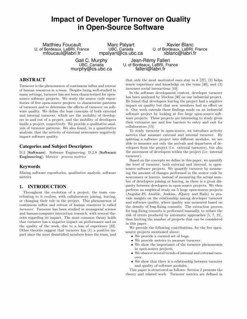
Impact of Developer Turnover on Qualityin Open-Source Software
Matthieu FoucaultU. of Bordeaux, LaBRI, France
Marc PalyartUBC, Canada
Xavier BlancU. of Bordeaux, LaBRI, France
[email protected] C. Murphy
UBC, [email protected]
Jean-Rémy FalleriU. of Bordeaux, LaBRI, France
ABSTRACTTurnover is the phenomenon of continuous influx and retreatof human resources in a team. Despite being well-studied inmany settings, turnover has not been characterized for open-source software projects. We study the source code repos-itories of five open-source projects to characterize patternsof turnover and to determine the effects of turnover on soft-ware quality. We define the base concepts of both externaland internal turnover, which are the mobility of develop-ers in and out of a project, and the mobility of developersinside a project, respectively. We provide a qualitative anal-ysis of turnover patterns. We also found, in a quantitativeanalysis, that the activity of external newcomers negativelyimpact software quality.
Categories and Subject DescriptorsD.2 [Software]: Software Engineering; D.2.8 [SoftwareEngineering]: Metrics—process metrics
KeywordsMining software repositories, qualitative analysis, softwaremetrics
1. INTRODUCTIONThroughout the evolution of a project, the team con-
tributing to it evolves, with collaborators joining, leaving,or changing their role in the project. This phenomenon ofcontinuous influx and retreat of human resources is calledturnover. Turnover has been studied in managerial scienceand human-computer interaction research, with several the-ories regarding its impact. The most common theory holdsthat turnover has a negative impact on performance and onthe quality of the work, due to a loss of experience [22].Other theories suggest that turnover has (1) a positive im-pact since the most dissatisfied members leave the team, and
that only the most motivated ones stay in it [27], (2) helpsrenew experience and knowledge on the team [40], and (3)increases social interactions [10].
In the software development context, developer turnoverhas been analyzed by Mockus [30] on one industrial project.He found that developers leaving the project had a negativeimpact on quality but that new members had no effect onit. Our work extends these findings made on an industrialsoftware project by looking at five large open-source soft-ware projects. These projects are interesting to study giventheir extensive use and low barriers to entry and exit forcollaborators [15].
To study turnover in open-source, we introduce activitymetrics that measure external and internal turnover. Bysplitting a software project into different modules, we areable to measure not only the arrivals and departures of de-velopers from the project (i.e. external turnover), but alsothe movement of developers within the project (i.e. internalturnover).
Based on the concepts we define in this paper, we quantifythe level of turnover, both external and internal, in open-source software projects. We quantify turnover by measur-ing the amount of changes performed in the source code bynewcomers or leavers, instead of measuring the actual num-ber of developers joining or leaving, as there is a great dis-parity between developers in open-source projects. We thenperform an empirical study on 5 large open-source projects(Angular.JS, Ansible, Jenkins, JQuery and Rails) to pro-vide insights on the relationship among developer turnoverand software quality, where quality was measured based onthe density of bug-fixing commits. The extraction processfor bug-fixing commits is performed manually, to reduce therisk of errors produced by automatic approaches [5, 7, 21],thus limiting the number of projects that can be consideredin this paper.
We provide the following contributions, for the five open-source projects mentioned above:• We provide a curated set of bugs.• We provide metrics to measure turnover.• We show the importance of the turnover phenomenon
in open-source projects.• We observe several trends of internal and external turn-
over.• We show that there is a relationship between turnover
and quality of software modules.This paper is structured as follows: Section 2 presents the
theory and related work. Turnover metrics are defined in
Section 3. Our research questions are detailed in Section 4and the methodology we used to build our dataset in Sec-tion 5. Our results are then presented in Section 6. Section 7presents an overview of the main threats to the validity ofthese results, and finally, Section 8 concludes and presentstrails for future work. We produced a replication packagewhich allows to reproduce and extend the results presentedin this study. This package, which has been successfullyevaluated by the Replication Packages Evaluation Commit-tee and found to meet expectations, is presented Section 10.
2. THEORY & RELATED WORKAs the literature contains different and sometimes contra-
dictory opinions on turnover, we first describe all its possibleinterpretations. We then present existing work on turnoverin collaborative communities and finally research specific tosoftware development.
2.1 Turnover PerceptionMember turnover, initially defined as the rate at which in-
dividuals leave a project, can be extended to all the changesmade to the development team of a project. These modifi-cations of the team can be either external, (i.e., a memberleaves or joins the team) or internal (i.e., a member changesher role in the team). Distinct theories regarding the impactof turnover, whether it is external or internal, suggest thatit has both positive and negative aspects on a team.
2.1.1 External TurnoverThe most common vision holds that external turnover neg-
atively impacts employee performance [22, 43]. Departureslead to a loss of experience and knowledge, but also disruptthe social network and environment of those who remain [4,11]. Moreover, it induces devoting resources and time torecruit and train new employees.
A second vision considers turnover as a good opportunityfor organizations, as leavers are those most dissatisfied withthe current organization, and those who remain enjoy betterconditions and performance [27].
A last perspective sees moderate levels of turnover asthe best organizational performance [3]. When there is noturnover, experience and knowledge are not renewed, andbecome obsolete and parochial [40]. Introduction of newpeople is a solution to overcome this situation, as their vi-sion is less established and less redundant with respect tothe knowledge possessed by the current team.
2.1.2 Internal TurnoverInternal turnover was defined in traditional organizations
as the number of employees who changed function withinan organization [20]. Motivations behind such actions areopportunities for career moves to increase income and au-tonomy as well as getting new responsibilities and express-ing new skills [41]. Kanter et al. pointed out that membershad lower aspirations and involvements in their work whenmobility was blocked [26]. Thus, internal mobility is com-monly supported to maintain members commitment to theorganization.
2.2 Turnover in Collaborative PlatformsTurnover has been studied in online communities and col-
laborative platforms where participants are free to enteror leave at any moment without any cost. In the English
Wikipedia, high turnover is even the norm with sixty per-cent of editors contributing only for a single day [32]. Rans-botham et al. suggested that collaboration success can bereached thanks to moderate levels of turnover [36], providedthat the level of novel knowledge exceeds the loss of existingknowledge held by departing people. Similarly, Dabbish etal. discovered that membership turnover might bring freshlevels of activity and liveliness in a community which leadsto increased participation [10]. Inversely, Qin et al. observedthat departures of WikiProjects contributors has a negativeeffect on the community and causes social capital losses [35].
2.3 Turnover in Software DevelopmentDeveloper turnover in open-source software projects was
studied mainly to understand developers motivations to con-tribute. Yu et al. suggested that personal expectation playsa role in project retention, and that turnover is partially ex-plained by dissatisfaction [45]. Hynninen et al. conducteda survey with developers and suggested that their depar-tures from a project can be a manifestation of low orga-nizational commitment [23]. A study from Schilling et al.unveiled that the level of development experience and knowl-edge is strongly associated with retention [38]. Accordingto Sharma et al., past activity, age and size of a projectas well as developer tenures are important predictors ofturnover [39]. These observations are consistent with otherclassical theoretical models related to job satisfaction [44].
Measures of knowledge loss were suggested by Izquierdo-Cortazar et al [24]. These measures include the evolution oforphan lines of code lastly edited by a developer who left theteam. They showed that while in some projects, developersdevote efforts to maintain code introduced by former devel-opers, in others, they seek to eliminate such code. Robleset al. designed a methodology to compute generations ofjoining and leaving developers [37]. Finally, Fronza et al.propose a wordle to visualize the level of cooperation of ateam and mitigate the knowledge loss due to turnover [17].
Hall et al. conducted a survey with practitioners to unveilthat turnover may be related to project success, but howeverdid not define turnover metrics computable by analyzingthe history of the project [19]. Mockus found that whiledepartures of members impact the software quality becauseof the loss of knowledge and experience, newcomers are notresponsible for an increase of defects, possibly because theyare not assigned to important changes [30]. Mockus alsofound a relationship between turnover and productivity incommercial projects [29].
Mens et al. explored developer turnover in the Gnomeecosystem with concepts and metrics similar as the ones weuse in this paper [28]. They looked at developer turnoverat a coarser grain: in their study, internal turnover refers tothe mobility of developers between projects of the Gnomeecosystem, while external turnover in their case was associ-ated to developers entering or leaving the Gnome ecosystem.Our study differs from theirs as it we look at a finer gran-ularity: we measure mobility of developer between modulesof a project, and in and out of a project. In their study theysought for possible patterns of developer turnover, with theconclusion that this is a highly project-specific phenomenon.They did not, seek for a relationship between turnover andcode quality.
Alice Bob Jane Alan
m1 m1
m2 m2
P2P1 S0S-2 S-1
Figure 1: Example of fictive software project con-taining two modules.
3. TURNOVER METRICSA software project can have many kinds of turnover. To be
able to study different aspects of turnover, we introduce fivemetrics that can be computed from the source code historyof a software project.
3.1 Setup and RequirementsIn order to compute turnover metrics, we need to define
the periods over which turnover will be computed, as wellas how contributors are identified.
3.1.1 Period SelectionWe compute developer turnover by comparing the contrib-
utors of software modules in two consecutive time periods:P1 and P2. These two periods are therefore delimited bythree snapshots of the project history: S0, S−1 and S−2
such that P1 is delimited by S−2 and S−1 and that P2 isdelimited by S−1 and S0 (see Figure 1).
In practice, S0 is the snapshot for which we want to com-pute turnover metrics. The selection of the two other snap-shots can be based on different approaches. One could con-sider either the prior releases of the software, snapshots suchthat periods P1 and P2 have the same duration, or snapshotssuch that periods P1 and P2 have the same overall activityin the repository. We study in Section 5 the impact of thesechoices on turnover computation.
3.1.2 Software Modules and ContributorsDeveloper turnover is relative to the software project’s
structure. A developer who has only worked on a few mod-ules in the system that suddenly contributes to more, shouldbe considered as new, or inexperienced, as she moves to newparts of the code base.
We therefore consider that a software project is composedof a finite set M of software modules developed by a finiteset of developers who submit their code modifications bysending commits to a shared code repository. Each module isdefined by a finite set of source code files. When a developermodifies one of the files of a software module by committingher work, she is contributing to that module. A developercontributes to the software project as soon as she contributesonce to any module of the software.
To illustrate all our definitions, we rely on the fictitioussoftware depicted in Figure 1, which is composed of twomodules developed over two periods P1 and P2. A totalof four developers participated to this software between theS−2 and S0 snapshots.
Given a module m, Dm,P is the set of developers whomade at least one contribution to m during the period P .
We obtain with our example Dm2,P1 = {Bob, Jane} andDm2,P2 = {Bob, Alan}.Dt is the set of developers who made at least one contribu-
tion to the software during the period t, i.e. DP =M⋃m
Dm,P .
From our example, we have DP1 = {Alice, Bob, Jane} andDP2 = {Bob, Jane, Alan}.
3.2 Turnover Actors and MetricsWe now provide formal definitions for the sets of develop-
ers involved in turnover, and the metrics associated to them.We consider two kinds of developer turnover: external andinternal turnover. The developers involved in each kind ofturnover are considered to be either newcomers or leavers.Finally, we define stayers, i.e. the developers contributingto both studied periods.
We consider as newcomers the developers who joined theteam of a module in the period P2, whereas leavers are thedevelopers who left the team of a module within the periodP1. This difference between the periods is due to the factthat the intent of our metrics is to evaluate the impact ofturnover on the quality of the software at the S0 snapshot.Thus, newcomers of the P2 period may influence its qualityas their first contributions on a module were between S−1
and S0, and leavers of the P1 period may influence its qual-ity as the loss of knowledge their departure induce will beperceptible after they left, i.e., after the S−1 snapshot.
3.2.1 External TurnoverExternal turnover refers to the movement of developer in
and out of a project.External newcomers of a module m are the developers
who contributed to the module between S−1 and S0, butdid not contribute to any module of the project betweenS−2 and S−1 (i.e., during the P1 period). The set of externalnewcomers is noted ENm,P1,P2 and is computed as follows:
ENm,P1,P2 = Dm,P2 −DP1
In Figure 1, we observe that Alan is a newcomer in m2,and that he did not work on any module during P1. Heis therefore an external newcomer, and thus ENm2,P1,P2 ={Alan}.External leavers of a module m refer to developers who
worked on the module during P1 but did not contribute tothe project at all in P2. The set of external leavers is notedELm,P1,P2 and is computed as follows:
ELm,P1,P2 = Dm,P1 −DP2
We observe that only Alice contributed to m1 during P1
but was inactive on the project in P2. Consequently,ELm1,P1,P2 = {Alice}.
3.2.2 Internal TurnoverInternal turnover refers to movements of developers inside
a project. Even though some developers contribute to aproject in both periods P1 and P2, they may not work onthe same modules in the two periods.Internal newcomers are the developers who contributed
to m in P2, but not in P1. However, they contributed toat least one other module than m in this period. They arenoted INm,P1,P2 and are computed as follows:
INm,P1,P2 = (Dm,P2 −Dm,P1) ∩DP1
Following the previous illustrations, we obtain hereINm1,P1,P2 = {Jane} and INm2,P1,P2 = ∅.
Internal leavers refer to developers who ceased to con-tribute to a module m but are still active in the project.This set is noted ILm,P1,P2 and is computed as follows:
ILm,P1,P2 = (Dm,P1 −Dm,P2) ∩DP2
We observe that only Jane modified m1 during P2 butnot in P1, while working on m2 during P1. Consequently,ILm2,P1,P2 = {Jane}.
3.2.3 StayersFinally, stayers are the developers who contributed to a
module m in both P1 and P2. We define the set of stayersfor a given module as:
Stm,P1,P2 = Dm,P1 ∩Dm,P2
3.2.4 Metric DefinitionsThe intention of our metrics is to quantify the impact
that the different turnover actors may have on a module’squality at the snapshot S0 of the project. Due to the largeinequalities in the involvement of developers in open-sourceprojects, we cannot quantify turnover by counting the num-ber (or ratio) of developer in each of the categories definedabove. Filtering the developers by considering only core orpaid contributors is not a viable alternative either. Indeed,peripheral developers as a group still produce a significantamount of contributions, and ignoring these contributionsmay significantly impact our measurements. Therefore, tomeasure the impact that each category of turnover actorshave on the source code, we use the activity of developers,i.e., the amount of source code they produce.
For a given module m, developer d and period t, we defineAm,d,t as the activity of the developer, which we measure us-ing the code churn, i.e. the number of lines of code added ordeleted by can be measured with the number of file modifi-cations she performed on the module, or the code churn (i.e.,the total number of lines added or deleted) of such modifica-tions. In this paper we only present results obtained usingthe code churn as an activity measure. However, results ob-tained with the number of modifications are similar, and areavailable online (see Section 9).
The five metrics we define are the internal and externalleavers activity (ILA and ELA, resp.), the internal and exter-nal newcomers ratio (INA and ENA, resp.), and the stayersactivity (SA):
ILAm,P1,P2 =∑
d∈ILm,P1,P2
Am,d,P1
ELAm,P1,P2 =∑
d∈ELm,P1,P2
Am,d,P1
INAm,P1,P2 =∑
d∈INm,P1,P2
Am,d,P2
ENAm,P1,P2 =∑
d∈ENm,P1,P2
Am,d,P2 ,
StAm,P1,P2 =∑
d∈Stm,P1,P2
avg(Am,d,P1 , Am,d,P2)
4. RESEARCH QUESTIONSTo the best of our knowledge we found no previous study
that looked at trends of developer turnover in open-source
software projects. Hence the first objective of our study is toseek for such trends, starting with a global view of turnoverat the project level, and then focusing on developer turnoveron module thanks to the metrics previously defined.
More formally, we seek to answer the following two re-search questions:
RQ1 Using the concepts of external newcomers and leaversat the project level, is turnover an important phe-nomenon (in terms of number of developers involved)in open-source software projects?
RQ2 Looking deeply into the project at the module level,is there any patterns regarding the contributions ofpersistent, internal and external developers?
By answering the aforementioned research questions, weprovide an overview of developer turnover both at the projectand at the module levels. We then go further by exploringthe relationship between developer turnover at the modulelevel and software quality, which we measure based on bug-fix information.
We then answer the following research question:
RQ3 Using the turnover metrics at the module level, isthere any relationship with the quality of the softwaremodules?
5. DATASET CONSTRUCTIONAlthough many automatic techniques are often used to
build large datasets, they are all imprecise to a certain ex-tent. Instead of having a dataset with dozens of projectcontaining approximate measures, we chose to focus on thereliability of the information extracted from the dataset. Inparticular, to answer our research questions, our datasetmust meet several requirements:• The author of each contribution must be clearly iden-
tified.• The source code of the project must be organized into
modules.• A measure of quality must be available for each mod-
ule.Each of these criteria is addressed in current research, and
software engineering researchers are still developing tech-niques to extract reliable information from software reposi-tories, as we detail below.
5.1 Authors Identification
Centralized VCS.The first issue regarding the identification of authors is
related to the version control system (VCS) used by theproject. In centralized VCSs such as Subversion, a developermust enter her credentials to commit her code to the centralrepository. Given the large number of contributors to open-source projects, assigning credentials to each of them wouldbe unwieldy, and contributions are therefore submitted viapatches, and applied by core developers who have credentialsfor the repository.
This issue is fixed by the use of decentralized VCSs suchas Git, which are able to distinguish the original authorof a commit and the developer who added it to the mainrepository (i.e., the committer) [6]. However, automaticallyselecting a large number of Git repositories (from hosting
platforms such as GitHub) would not be a suitable processin our case as a non negligible amount of large Git repos-itories are simply mirrors of Subversion repositories. Wellknown examples of such repositories include the gcc com-piler project, or most of the projects hosted by the ApacheSoftware Foundation (eg. the httpd server). Moreover, evenif a project currently uses Git as a VCS, it may not have beenso for all its development history. It is not uncommon fora project, especially older projects, to migrate its code basefrom one VCS to another throughout its history. This is thecase of two projects selected in our dataset, Rails and Jenk-ins, which originally used Subversion and then migrated toGit. We manually searched commit messages for contentssuch as “Patch sent by Alice” to determine if at one pointthese projects were still using Subversion or if they did mi-grate to Git, and only include the history subsequent to thismigration in our analyses.
Identity Merging.Even when the identity of each contribution’s author is
reliable, it is possible that a single developer has severalidentities in the VCS, because of typos, changes in the con-figuration of the Git client, or a change of email addressfor instance. This issue is addressed by identity merging,for which Goeminne and Mens address a comprehensive re-view [18]. Following their recommendations, we use a semi-automatic process which is based on their simple algorithmwhich has a very high recall. To counter the low precision ofthe algorithm, we manually review the results of the identitymerge algorithm and remove false positive merges.
5.2 Quality MeasurementOur study aims to evaluate the quality of project’ modules
for a given snapshot. In most software engineering studiesthe quality of software projects is assessed by looking at thenumber of bugs fixed by the developers.
Bug Fix Identification.In order to measure the amount of these bugs, the state-
of-the-art technique used in studies mining software reposi-tories consists in parsing the commit messages, looking forthe identifier of a bug stored in the project’s bugtracker(e.g., ”Bug #42”) [46]. However, recent work raised concernsregarding the precision and recall of this automatic process,due to the misclassification of issues in the bugtrackers, orimprecision of algorithms linking bugs to source code [21, 5,7].
Some approaches remove these concerns by only consid-ering information stored in the VCS, and assume that thenumber of bug-fixing commits is a fair representation of theactual number of bugs within a software module. Unfortu-nately, to the best of our knowledge, no automatic approachhas a satisfactory precision to produce reliable statistics. Forinstance, among the best automatic approaches, the onesdeveloped by Tian et al. [42] and Mockus et al. [31] have aprecision of only 53% and 61%, respectively, in the evaluatedbenchmarks, which in our case would have unpredictable ef-fect on the number of bug-fixing commits identified, andwould be a non-negligible bias to our study.
As we did not find a suitable automatic approach we choseto manually analyze commits to constitute our dataset tothe detriment of the number of projects that we were able
to include in it. Our manual approach therefore aims toidentify commits that are true bugfixes.
Maintenance Branches.To have measures which are representative of the quality
of the code at a given snapshot or release, we need to iso-late post-release bugfixes from development bugfixes. Post-release bugfixes for a snapshot S0 are commits that fix a bugwhich was in the project’s code at the snapshot S0, whiledevelopment bugfixes performed after the snapshot S0 mayhave been introduced between the snapshot S0 and the timeof the bugfix. If the development history of a project is linear(i.e. if all the commits are performed on a single branch),isolating one category of commits from the other may becumbersome and imprecise. Therefore, another constraint isadded to the projects to include in our dataset: the releaseS0 must have a dedicated maintenance branch, sometimescalled long time support (or LTS) branch, where the onlycommits performed in it aim to improve the code qualityof the release S0. These maintenance branches differ fromdevelopment branches. They usually do not contain newfeatures. The operations performed in such branches aremainly bug-fixing, documentation, optimizations, or com-patibility updates related to third party dependencies (e.g.,the 2.3.x maintenance branch of Rails contains updates re-lated to new versions of the Ruby programming language).Moreover, we restrict our search to maintenance brancheswhere no commit was performed for the past six months,in order to have branches where most of the bugs were hadtime to get fixed.
Bug Fix Classification.Our definition of a bug-fixing commit includes any se-
mantic changes to the source code which fixes an unwantedbehavior. The type of bugs considered includes any arith-metic or logic bug (e.g., division by zero, infinite loops, etc.),resource bugs (e.g., null pointer exceptions, buffer overflows,etc.), multi-threading issues such as deadlocks or race con-ditions, interfacing bugs (e.g., wrong usage of a particularAPI, incorrect protocol implementation or assumptions of aparticular platform, etc), security vulnerabilities, as well asmisunderstood requirements and design flaws.
We identified bug-fixing commits manually, discarding com-mits where new features are implemented. We choose toignore commits where performance optimizations are per-formed, as we consider performance issues as a different as-pect of code quality. Moreover, we also ignore commits thatresolve compatibility issues due to the evolution of a third-party dependency, as these bugfixes are not due to the lackof quality of the changed code, but to the modification ofan external requirement. Finally, it occurs that bug-fixingcommits are lated discarded by the developers due to a re-gression introduced by the bugfix. In such cases, the devel-opers perform a “revert” operation of such commits, and weignore both the “revert” and the “reverted” commits.
We consider that bug-fixing commits are atomic, in theway that we do not consider the possibility that a bug-fixingcommit may in fact include two bug-fixes. Moreover, if abug-fixing commits affects two modules, the number of bug-fixing commits will be incremented in both modules.
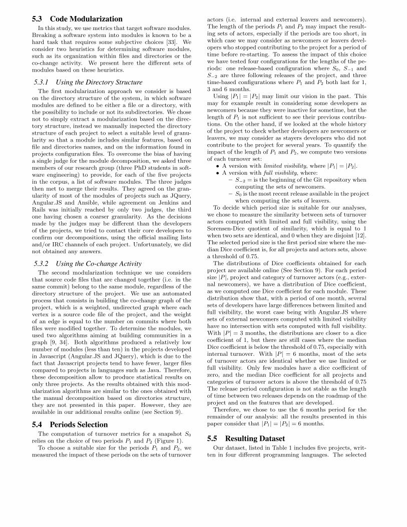
5.3 Code ModularizationIn this study, we use metrics that target software modules.
Breaking a software system into modules is known to be ahard task that requires some subjective choices [33]. Weconsider two heuristics for determining software modules,such as its organization within files and directories or theco-change activity. We present here the different sets ofmodules based on these heuristics.
5.3.1 Using the Directory StructureThe first modularization approach we consider is based
on the directory structure of the system, in which softwaremodules are defined to be either a file or a directory, withthe possibility to include or not its subdirectories. We chosenot to simply extract a modularization based on the direc-tory structure, instead we manually inspected the directorystructure of each project to select a suitable level of granu-larity so that a module includes similar features, based onfile and directories names, and on the information found inprojects configuration files. To overcome the bias of havinga single judge for the module decomposition, we asked threemembers of our research group (three PhD students in soft-ware engineering) to provide, for each of the five projectsin the corpus, a list of software modules. The three judgesthen met to merge their results. They agreed on the gran-ularity of most of the modules of projects such as JQuery,Angular.JS and Ansible, while agreement on Jenkins andRails was initially reached by only two judges, the thirdone having chosen a coarser granularity. As the decisionsmade by the judges may be different than the developersof the projects, we tried to contact their core developers toconfirm our decompositions, using the official mailing listsand/or IRC channels of each project. Unfortunately, we didnot obtained any answers.
5.3.2 Using the Co-change ActivityThe second modularization technique we use considers
that source code files that are changed together (i.e. in thesame commit) belong to the same module, regardless of thedirectory structure of the project. We use an automatedprocess that consists in building the co-change graph of theproject, which is a weighted, undirected graph where eachvertex is a source code file of the project, and the weightof an edge is equal to the number on commits where bothfiles were modified together. To determine the modules, weused two algorithms aiming at building communities in agraph [9, 34]. Both algorithms produced a relatively lownumber of modules (less than ten) in the projects developedin Javascript (Angular.JS and JQuery), which is due to thefact that Javascript projects tend to have fewer, larger filescompared to projects in languages such as Java. Therefore,these decomposition allow to produce statistical results ononly three projects. As the results obtained with this mod-ularization algorithms are similar to the ones obtained withthe manual decomposition based on directories structure,they are not presented in this paper. However, they areavailable in our additional results online (see Section 9).
5.4 Periods SelectionThe computation of turnover metrics for a snapshot S0
relies on the choice of two periods P1 and P2 (Figure 1).To choose a suitable size for the periods P1 and P2, we
measured the impact of these periods on the sets of turnover
actors (i.e. internal and external leavers and newcomers).The length of the periods P1 and P2 may impact the result-ing sets of actors, especially if the periods are too short, inwhich case we may consider as newcomers or leavers devel-opers who stopped contributing to the project for a period oftime before re-starting. To assess the impact of this choicewe have tested four configurations for the lengths of the pe-riods: one release-based configuration where S0, S−1 andS−2 are three following releases of the project, and threetime-based configurations where P1 and P2 both last for 1,3 and 6 months.
Using |P1| = |P2| may limit our vision in the past. Thismay for example result in considering some developers asnewcomers because they were inactive for sometime, but thelength of P1 is not sufficient to see their previous contribu-tions. On the other hand, if we looked at the whole historyof the project to check whether developers are newcomers orleavers, we may consider as stayers developers who did notcontribute to the project for several years. To quantify theimpact of the length of P1 and P2, we compute two versionsof each turnover set:• A version with limited visibility, where |P1| = |P2|.• A version with full visibility, where:
– S−2 = is the beginning of the Git repository whencomputing the sets of newcomers.
– S0 is the most recent release available in the projectwhen computing the sets of leavers.
To decide which period size is suitable for our analyses,we chose to measure the similarity between sets of turnoveractors computed with limited and full visibility, using theSorensen-Dice quotient of similarity, which is equal to 1when two sets are identical, and 0 when they are disjoint [12].The selected period size is the first period size where the me-dian Dice coefficient is, for all projects and actors sets, abovea threshold of 0.75.
The distributions of Dice coefficients obtained for eachproject are available online (See Section 9). For each periodsize |P |, project and category of turnover actors (e.g., exter-nal newcomers), we have a distribution of Dice coefficient,as we computed one Dice coefficient for each module. Thesedistribution show that, with a period of one month, severalsets of developers have large differences between limited andfull visibility, the worst case being with Angular.JS wheresets of external newcomers computed with limited visibilityhave no intersection with sets computed with full visibility.With |P | = 3 months, the distributions are closer to a dicecoefficient of 1, but there are still cases where the medianDice coefficient is below the threshold of 0.75, especially withinternal turnover. With |P | = 6 months, most of the setsof turnover actors are identical whether we use limited orfull visibility. Only few modules have a dice coefficient ofzero, and the median Dice coefficient for all projects andcategories of turnover actors is above the threshold of 0.75The release period configuration is not stable as the lengthof time between two releases depends on the roadmap of theproject and on the features that are developed.
Therefore, we chose to use the 6 months period for theremainder of our analysis: all the results presented in thispaper consider that |P1| = |P2| = 6 months.
5.5 Resulting DatasetOur dataset, listed in Table 1 includes five projects, writ-
ten in four different programming languages. The selected
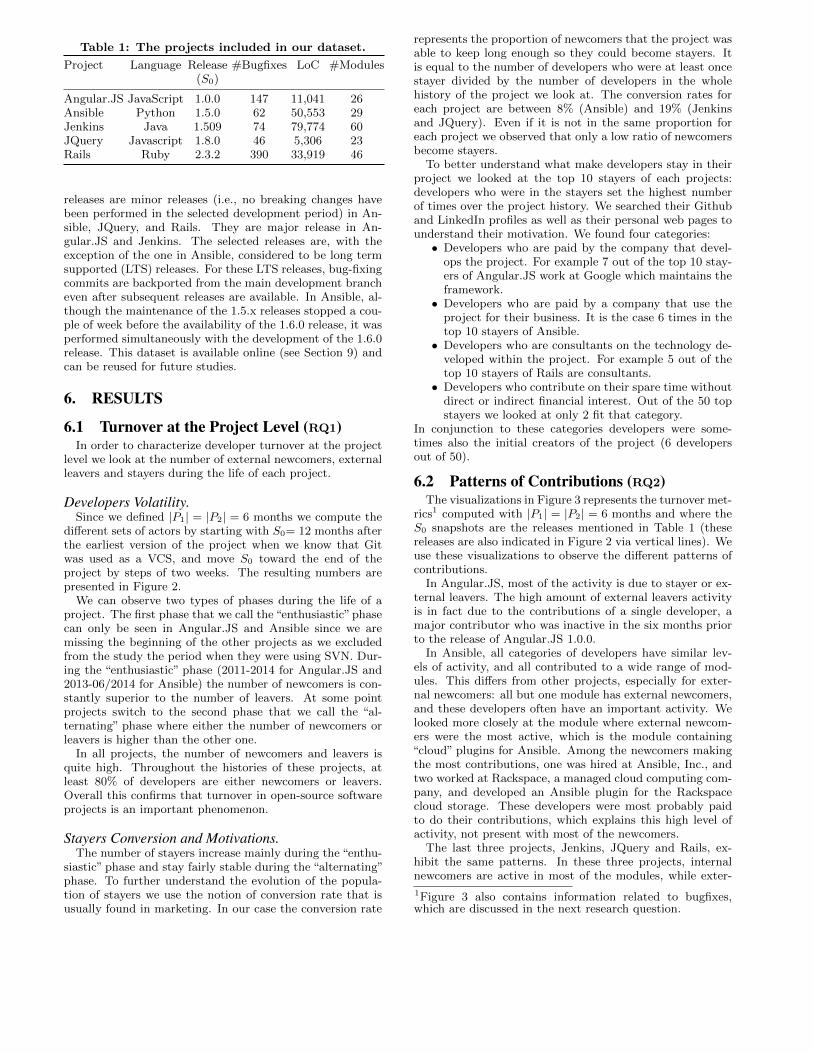
Table 1: The projects included in our dataset.
Project Language Release #Bugfixes LoC #Modules(S0)
Angular.JS JavaScript 1.0.0 147 11,041 26Ansible Python 1.5.0 62 50,553 29Jenkins Java 1.509 74 79,774 60JQuery Javascript 1.8.0 46 5,306 23Rails Ruby 2.3.2 390 33,919 46
releases are minor releases (i.e., no breaking changes havebeen performed in the selected development period) in An-sible, JQuery, and Rails. They are major release in An-gular.JS and Jenkins. The selected releases are, with theexception of the one in Ansible, considered to be long termsupported (LTS) releases. For these LTS releases, bug-fixingcommits are backported from the main development brancheven after subsequent releases are available. In Ansible, al-though the maintenance of the 1.5.x releases stopped a cou-ple of week before the availability of the 1.6.0 release, it wasperformed simultaneously with the development of the 1.6.0release. This dataset is available online (see Section 9) andcan be reused for future studies.
6. RESULTS
6.1 Turnover at the Project Level (RQ1)In order to characterize developer turnover at the project
level we look at the number of external newcomers, externalleavers and stayers during the life of each project.
Developers Volatility.Since we defined |P1| = |P2| = 6 months we compute the
different sets of actors by starting with S0= 12 months afterthe earliest version of the project when we know that Gitwas used as a VCS, and move S0 toward the end of theproject by steps of two weeks. The resulting numbers arepresented in Figure 2.
We can observe two types of phases during the life of aproject. The first phase that we call the “enthusiastic” phasecan only be seen in Angular.JS and Ansible since we aremissing the beginning of the other projects as we excludedfrom the study the period when they were using SVN. Dur-ing the “enthusiastic” phase (2011-2014 for Angular.JS and2013-06/2014 for Ansible) the number of newcomers is con-stantly superior to the number of leavers. At some pointprojects switch to the second phase that we call the “al-ternating” phase where either the number of newcomers orleavers is higher than the other one.
In all projects, the number of newcomers and leavers isquite high. Throughout the histories of these projects, atleast 80% of developers are either newcomers or leavers.Overall this confirms that turnover in open-source softwareprojects is an important phenomenon.
Stayers Conversion and Motivations.The number of stayers increase mainly during the “enthu-
siastic” phase and stay fairly stable during the “alternating”phase. To further understand the evolution of the popula-tion of stayers we use the notion of conversion rate that isusually found in marketing. In our case the conversion rate
represents the proportion of newcomers that the project wasable to keep long enough so they could become stayers. Itis equal to the number of developers who were at least oncestayer divided by the number of developers in the wholehistory of the project we look at. The conversion rates foreach project are between 8% (Ansible) and 19% (Jenkinsand JQuery). Even if it is not in the same proportion foreach project we observed that only a low ratio of newcomersbecome stayers.
To better understand what make developers stay in theirproject we looked at the top 10 stayers of each projects:developers who were in the stayers set the highest numberof times over the project history. We searched their Githuband LinkedIn profiles as well as their personal web pages tounderstand their motivation. We found four categories:• Developers who are paid by the company that devel-
ops the project. For example 7 out of the top 10 stay-ers of Angular.JS work at Google which maintains theframework.• Developers who are paid by a company that use the
project for their business. It is the case 6 times in thetop 10 stayers of Ansible.• Developers who are consultants on the technology de-
veloped within the project. For example 5 out of thetop 10 stayers of Rails are consultants.• Developers who contribute on their spare time without
direct or indirect financial interest. Out of the 50 topstayers we looked at only 2 fit that category.
In conjunction to these categories developers were some-times also the initial creators of the project (6 developersout of 50).
6.2 Patterns of Contributions (RQ2)The visualizations in Figure 3 represents the turnover met-
rics1 computed with |P1| = |P2| = 6 months and where theS0 snapshots are the releases mentioned in Table 1 (thesereleases are also indicated in Figure 2 via vertical lines). Weuse these visualizations to observe the different patterns ofcontributions.
In Angular.JS, most of the activity is due to stayer or ex-ternal leavers. The high amount of external leavers activityis in fact due to the contributions of a single developer, amajor contributor who was inactive in the six months priorto the release of Angular.JS 1.0.0.
In Ansible, all categories of developers have similar lev-els of activity, and all contributed to a wide range of mod-ules. This differs from other projects, especially for exter-nal newcomers: all but one module has external newcomers,and these developers often have an important activity. Welooked more closely at the module where external newcom-ers were the most active, which is the module containing“cloud” plugins for Ansible. Among the newcomers makingthe most contributions, one was hired at Ansible, Inc., andtwo worked at Rackspace, a managed cloud computing com-pany, and developed an Ansible plugin for the Rackspacecloud storage. These developers were most probably paidto do their contributions, which explains this high level ofactivity, not present with most of the newcomers.
The last three projects, Jenkins, JQuery and Rails, ex-hibit the same patterns. In these three projects, internalnewcomers are active in most of the modules, while exter-
1Figure 3 also contains information related to bugfixes,which are discussed in the next research question.
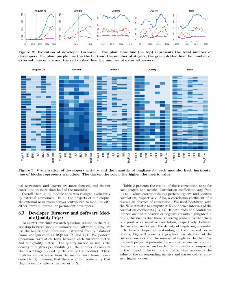
2011 2012 2013 2014 2015
0100
300
500
700
Angular.JS
2014 2015
0100
300
500
700
Ansible
2012 2013 2014 2015
020
4060
80120
Jenkins
2011 2012 2013 2014
020
4060
80
JQuery
2009 2011 2013 2015
0200
400
600
800
Rails
Figure 2: Evolution of developer turnover. The plain blue line (on top) represents the total number ofdevelopers, the plain purple line (on the bottom) the number of stayers, the green dotted line the number ofexternal newcomers and the red dashed line the number of external leavers.
Tot
al A
INA
EN
A
ILA
ELA StA
Bug
Fix
es
Angular.JS
Tot
al A
INA
EN
A
ILA
ELA StA
Bug
Fix
es
Ansible
Tot
al A
INA
EN
A
ILA
ELA StA
Bug
Fix
es
Jenkins
Tot
al A
INA
EN
A
ILA
ELA StA
Bug
Fix
es
JQuery
Tot
al A
INA
EN
A
ILA
ELA StA
Bug
Fix
es
Rails
Figure 3: Visualization of developers activity and the quantity of bugfixes for each module. Each horizontalline of blocks represents a module. The darker the color, the higher the metric value.
nal newcomers and leavers are more focused, and do notcontribute to more than half of the modules.
Overall there is no module that was changed exclusivelyby external newcomers. In all the projects of our corpus,the external newcomers always contributed to modules witheither internal internal or permanent developers.
6.3 Developer Turnover and Software Mod-ule Quality (RQ3)
To answer our third research question, related to the rela-tionship between module turnover and software quality, weuse the bug-related information extracted from our dataset(same configuration as RQ2 for P1 and P2). We performSpearman correlation tests between each turnover metricand our quality metric. The quality metric we use is thedensity of bugfixes per module (i.e., the number of commitsthat fixed bugs divided by the size of the module). Thesebugfixes are extracted from the maintenance branch asso-ciated to S0, meaning that there is a high probability thatthey indeed fix defects that occur in S0.
Table 2 presents the results of these correlation tests foreach project and metric. Correlation coefficients vary from−1 to 1, which corresponds to a perfect negative and positivecorrelation, respectively. Also, a correlation coefficient of 0reveals an absence of correlation. We used bootstrap withthe BCa statistic to compute 95% confidence intervals of thecorrelation coefficients [13, 14]. If both ends of a confidenceinterval are either positive or negative (results highlighted inbold), this means that there is a strong probability that thereis a positive or negative correlation, respectively, betweenthe turnover metric and the density of bug-fixing commits.
To have a deeper understanding of the observed corre-lations, Figure 3 presents a graphical visualization of theturnover metrics and the number of bugfixes. In that Fig-ure, each project is presented by a matrix where each columnrepresents a metric, and each line represents a componentof the project. The cell of the matrix then represents thevalue of the corresponding metrics and darker colors repre-sent higher values.
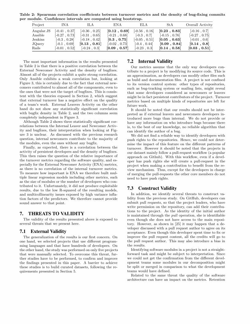
Table 2: Spearman correlation coefficients between turnover metrics and the density of bug-fixing commitsper module. Confidence intervals are computed using bootstrap.
Project INA ILA ENA ELA StA Overall Activity
Angular.JS [-0.41 , 0.37] [-0.36 , 0.25] [0.12 , 0.69] [-0.56 , 0.16] [0.23 , 0.83] [-0.16 , 0.7]Ansible [-0.27 , 0.73] [-0.31 , 0.65] [-0.21 , 0.68] [-0.3 , 0.7] [-0.15 , 0.76] [-0.27 , 0.75]Jenkins [-0.3 , 0.28] [-0.18 , 0.42] [0.3 , 0.75] [-0.05 , 0.51] [0.05 , 0.63] [-0.01 , 0.6]JQuery [-0.1 , 0.69] [0.13 , 0.81] [-0.02 , 0.73] [-0.4 , 0.44] [0.09 , 0.84] [0.14 , 0.8]Rails [-0.01 , 0.52] [-0.24 , 0.3] [0.09 , 0.57] [-0.23 , 0.3] [0.14 , 0.58] [0.03 , 0.51]
The most important information in the results presentedin Table 2 is that there is a positive correlation between theExternal Newcomer Activity and the density of bugfixes.Almost all of the projects exhibit a quite strong correlation.Only Ansible exhibits a weak correlation but, looking atFigure 3, this is certainly due to the fact that external new-comers contributed to almost all of the components, even tothe ones that were not the target of bugfixes. This is consis-tent with the theories exposed in Section 2, which suggestthat external turnover has a negative effect on the qualityof a team’s work. External Leavers Activity on the otherhand do not show any statistically significant correlationwith bugfix density in Table 2, and the two columns seemcompletely independent in Figure 3.
Although Table 2 shows three statistically significant cor-relations between the Internal Leaver and Newcomer Activ-ity and bugfixes, their interpretation when looking at Fig-ure 3 is unclear. As discussed with the previous researchquestion, internal newcomers contribute to the majority ofthe modules, even the ones without any bugfix.
Finally, as expected, there is a correlation between theactivity of persistent developers and the density of bugfixes.This then raises the question of the relative importance ofthe turnover metrics regarding the software quality, and es-pecially for the External Newcomer Activity (ENA) metrics,as there is no correlation of the internal turnover metrics.To measure how important is ENA we therefore built mul-tiple linear regression models including other metrics, suchas the size of modules or the number of developers who con-tributed to it. Unfortunately, it did not produce exploitableresults, due to the low R-squared of the resulting models,and multicollinearity issues exposed by high variance infla-tion factors of the predictors. We therefore cannot providesound answer to that point.
7. THREATS TO VALIDITYThe validity of the results presented above is exposed to
several threats that we present here.
7.1 External ValidityThe generalization of the results is our first concern. On
one hand, we selected projects that use different program-ming languages and that have hundreds of developers. Onthe other hand, the study was performed on only five projectsthat were manually selected. To overcome this threat, fur-ther studies have to be performed, to confirm and improvethe findings presented in this paper. A barrier to achievethese studies is to build curated datasets, following the re-quirements presented in Section 5.
7.2 Internal ValidityOur metrics assume that the only way developers con-
tribute to a project is by modifying its source code. This isan approximation, as developers can modify other files suchas build and documentation files. A project is not confinedto its version control system: other types of repositories,such as bug-tracking system or mailing lists, might revealthat some developers considered as newcomers or leaversmight be in fact persistent contributors of the project. Turnovermetrics based on multiple kinds of repositories are left forfuture work.
It should be noted that our results should not be inter-preted as if external leavers and newcomers developers in-troduced more bugs than internal. We do not provide orhave any information on who introduce bugs because thereis, to the best of our knowledge, no reliable algorithm thatcan identify the author of a bug.
We did not find a reliable way to identify developers withpush rights to the repositories. Hence, we could not deter-mine the impact of this feature on the different patterns ofturnover. However it should be noted that the projects inour dataset mainly follow a pull-request workflow (a popularapproach on Github). With this workflow, even if a devel-oper has push rights she will create a pull-request in theproject when making a contribution to benefit from the re-view mechanism. Thus, except for the developers in chargeof merging the pull-requests the other core members do notneed to have push rights.
7.3 Construct ValidityIn addition, we identify several threats to construct va-
lidity from the previous study. On GitHub, developers cansubmit pull requests, so that the project leaders, who havewrite permission on the repository, can add their contribu-tions to the project. As the identity of the initial authoris maintained through the pull operation, she is identifiableeven though she does not have access to the main reposi-tory. However, as shown in [25] it may happen that a de-veloper discussed with a pull request author to agree on itsacceptance. Even though this developer spent time to fix orimprove the pull request content, all the credits will go tothe pull request author. This may also introduce a bias inthe results.
Identifying software modules in a project is not a straight-forward task and might be subject to interpretation. Sincewe could not get the confirmation from the different devel-opment teams some modules in our decomposition mightbe split or merged in comparison to what the developmentteams would have defined.
Related to the same threat the quality of the softwarearchitecture can have an impact on the metrics. Retention
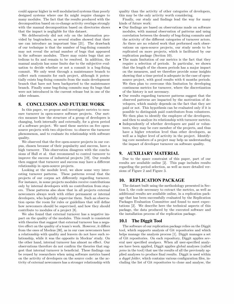
could appear higher in well modularized systems than poorlydesigned systems where one fix might require changes tomany modules. The fact that the results produced with thedecomposition based on co-change activity overlaps stronglywith the manual decomposition based on directories showsthat the impact is negligible for this dataset.
We deliberatively did not rely on the information pro-vided by bugtrackers, as several studies showed that theiruse can introduce an important bias [21]. The drawbackof our technique is that the number of bug-fixing commitsmay not reveal the actual number of bugs that appearedin the software modules. There may exists bugs that aretedious to fix and remain to be resolved. In addition, themanual analysis has some limits due to the subjective eval-uation to decide whether or not a commit is a bug-fixingcommit. We only went through a maintenance branch tocollect such commits for each project, although it poten-tially exists bug-fixing commits from the main developmentbranch that have not been backported to the maintenancebranch. Finally some bug-fixing commits may fix bugs thatwere not introduced in the current release but in one of theolder releases.
8. CONCLUSION AND FUTURE WORKIn this paper, we propose and investigate metrics to mea-
sure turnover in open-source software projects. Our met-rics measure how the structure of a group of developers ischanging, both internally and externally, for a given periodof a software project. We used these metrics on five open-source projects with two objectives: to observe the turnoverphenomenon, and to evaluate its relationship with softwarequality.
We observed that the five open-source projects in our cor-pus, chosen because of their popularity and success, have ahigh turnover. This observation disagrees with the conclu-sions of Hall et al. that recommend to control turnover toimprove the success of industrial projects [19]. Our resultsthen suggest that turnover and success may have a differentrelationship in open-source projects.
Looking at the module level, we show some very inter-esting turnover patterns. These patterns reveal that theprojects of our corpus act differently regarding turnover.For instance, in some projects modules receive contributionsonly by internal developers with no contribution from stay-ers. These patterns also show that in all projects externalnewcomers always work with either permanent or internaldevelopers, who hopefully supervise them. Such an observa-tion opens the room for rules or guidelines that will definehow newcomers should be supervised, and how they shouldcontribute to modules of a project [8].
We also found that external turnover has a negative im-pact on the quality of the modules. This result is consistentwith theories that suggest that external turnover has a nega-tive effect on the quality of a team’s work. However, it differsfrom the ones of Mockus [30], as in our case newcomers havea relationship with quality and leavers do not have such re-lationship, while it was the opposite in Mockus’ study. Onthe other hand, internal turnover has almost no effect. Ourobservations therefore do not confirm the theories that sug-gest that internal turnover is beneficial. These findings canbe reused by researchers when using software metrics basedon the activity of developers on the source code: as the ac-tivity of external newcomers has a stronger relationship with
quality than the activity of other categories of developers,this may be the only activity worth considering.
Finally, our study and findings lead the way for manykinds of future work:• Our findings are based on observations made on software
modules, with manual observation of patterns and usingcorrelation between the density of bug-fixing commits andthe activity of the different categories of turnover actors.As there are no related work that performed such obser-vations on open-source projects, our study needs to bereplicated on more projects, which is facilitated by ourreplication package (Section 10).• The main limitation of our metrics is the fact that they
require a selection of periods. In particular, we shownthat the length of the chosen periods has a major impacton the measures, and we therefore provide some insightsshowing that a time period is adequate in the case of open-source project, with good results with 6 months periods.We then plan to overcome this limitation by developingcontinuous metrics for turnover, where the discretizationof the history is not necessary.• Our results regarding turnover patterns suggest that the
observed patterns are impacted by the motivation of de-velopers, which mainly depends on the fact that they arepaid or not. This hypothesis can be evaluated only if it ispossible to distinguish paid contributors from volunteers.We then plan to identify the employee of the developers,and then to analyze its relationship with turnover metrics.• Independently of whether developers are paid or volun-
teers, they may be core member of the projects, and thushave a higher retention level than other developers, aswell as a higher level of activity in the project. Identify-ing core members of a project may help us understandingthe impact of developer turnover on software quality.
9. AUXILIARY MATERIALDue to the space constraint of this paper, part of our
results are available online [2]. This page includes resultsregarding the period selection, as well as more detailed ver-sions of Figure 2 and Figure 3.
10. REPLICATION PACKAGEThe dataset built using the methodology presented in Sec-
tion 5, the code necessary to extract the metrics, as well asadditional results are available online, in a replication pack-age that has been successfully evaluated by the ReplicationPackages Evaluation Committee and found to meet expec-tations [2]. We describe here the technical aspects of thispackage, the data produced by the executed software andthe installation process of the replication package.
10.1 The Diggit ToolThe software of our replication package relies on the Diggit
tool, which supports analysis of Git repositories and whichhelps manage the analysis process [1]. Diggit manages a setof Git repositories. On each repository, Diggit applies sev-eral user specified analyses. When all user-specified analy-ses have been applied, Diggit applies global analyses (calledjoins in the tool) that use the results of all the previously ap-plied analyses to produce final results. Diggit is used withina diggit folder, which contains various configuration files, in-cluding the list of Git repositories to clone and analyse, the
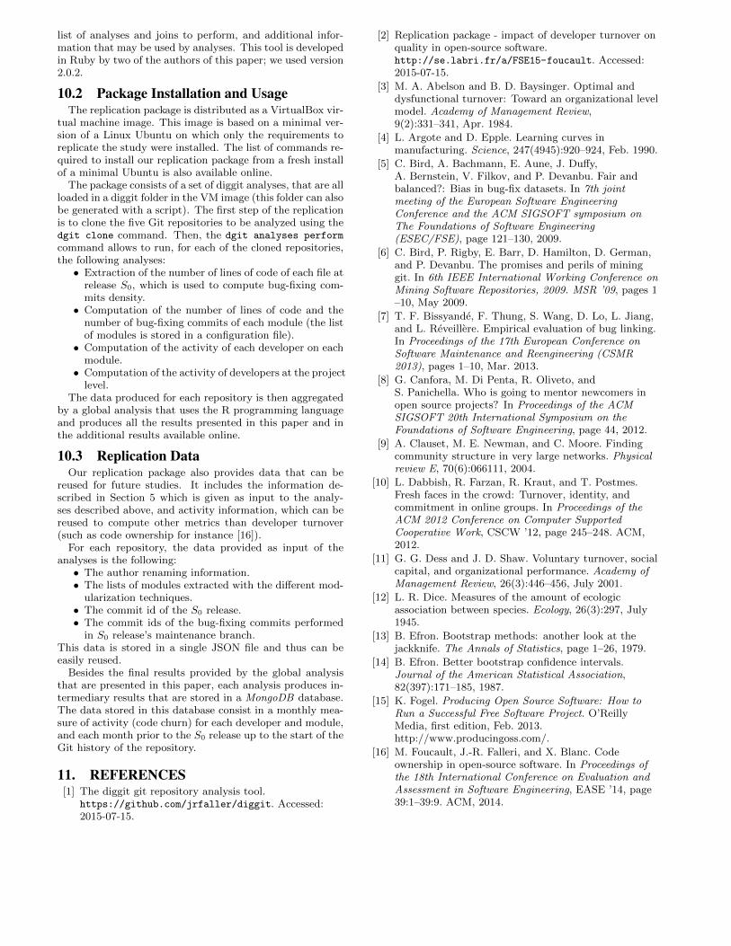
list of analyses and joins to perform, and additional infor-mation that may be used by analyses. This tool is developedin Ruby by two of the authors of this paper; we used version2.0.2.
10.2 Package Installation and UsageThe replication package is distributed as a VirtualBox vir-
tual machine image. This image is based on a minimal ver-sion of a Linux Ubuntu on which only the requirements toreplicate the study were installed. The list of commands re-quired to install our replication package from a fresh installof a minimal Ubuntu is also available online.
The package consists of a set of diggit analyses, that are allloaded in a diggit folder in the VM image (this folder can alsobe generated with a script). The first step of the replicationis to clone the five Git repositories to be analyzed using thedgit clone command. Then, the dgit analyses perform
command allows to run, for each of the cloned repositories,the following analyses:• Extraction of the number of lines of code of each file at
release S0, which is used to compute bug-fixing com-mits density.• Computation of the number of lines of code and the
number of bug-fixing commits of each module (the listof modules is stored in a configuration file).• Computation of the activity of each developer on each
module.• Computation of the activity of developers at the project
level.The data produced for each repository is then aggregated
by a global analysis that uses the R programming languageand produces all the results presented in this paper and inthe additional results available online.
10.3 Replication DataOur replication package also provides data that can be
reused for future studies. It includes the information de-scribed in Section 5 which is given as input to the analy-ses described above, and activity information, which can bereused to compute other metrics than developer turnover(such as code ownership for instance [16]).
For each repository, the data provided as input of theanalyses is the following:• The author renaming information.• The lists of modules extracted with the different mod-
ularization techniques.• The commit id of the S0 release.• The commit ids of the bug-fixing commits performed
in S0 release’s maintenance branch.This data is stored in a single JSON file and thus can beeasily reused.
Besides the final results provided by the global analysisthat are presented in this paper, each analysis produces in-termediary results that are stored in a MongoDB database.The data stored in this database consist in a monthly mea-sure of activity (code churn) for each developer and module,and each month prior to the S0 release up to the start of theGit history of the repository.
11. REFERENCES[1] The diggit git repository analysis tool.
https://github.com/jrfaller/diggit. Accessed:2015-07-15.
[2] Replication package - impact of developer turnover onquality in open-source software.http://se.labri.fr/a/FSE15-foucault. Accessed:2015-07-15.
[3] M. A. Abelson and B. D. Baysinger. Optimal anddysfunctional turnover: Toward an organizational levelmodel. Academy of Management Review,9(2):331–341, Apr. 1984.
[4] L. Argote and D. Epple. Learning curves inmanufacturing. Science, 247(4945):920–924, Feb. 1990.
[5] C. Bird, A. Bachmann, E. Aune, J. Duffy,A. Bernstein, V. Filkov, and P. Devanbu. Fair andbalanced?: Bias in bug-fix datasets. In 7th jointmeeting of the European Software EngineeringConference and the ACM SIGSOFT symposium onThe Foundations of Software Engineering(ESEC/FSE), page 121–130, 2009.
[6] C. Bird, P. Rigby, E. Barr, D. Hamilton, D. German,and P. Devanbu. The promises and perils of mininggit. In 6th IEEE International Working Conference onMining Software Repositories, 2009. MSR ’09, pages 1–10, May 2009.
[7] T. F. Bissyande, F. Thung, S. Wang, D. Lo, L. Jiang,and L. Reveillere. Empirical evaluation of bug linking.In Proceedings of the 17th European Conference onSoftware Maintenance and Reengineering (CSMR2013), pages 1–10, Mar. 2013.
[8] G. Canfora, M. Di Penta, R. Oliveto, andS. Panichella. Who is going to mentor newcomers inopen source projects? In Proceedings of the ACMSIGSOFT 20th International Symposium on theFoundations of Software Engineering, page 44, 2012.
[9] A. Clauset, M. E. Newman, and C. Moore. Findingcommunity structure in very large networks. Physicalreview E, 70(6):066111, 2004.
[10] L. Dabbish, R. Farzan, R. Kraut, and T. Postmes.Fresh faces in the crowd: Turnover, identity, andcommitment in online groups. In Proceedings of theACM 2012 Conference on Computer SupportedCooperative Work, CSCW ’12, page 245–248. ACM,2012.
[11] G. G. Dess and J. D. Shaw. Voluntary turnover, socialcapital, and organizational performance. Academy ofManagement Review, 26(3):446–456, July 2001.
[12] L. R. Dice. Measures of the amount of ecologicassociation between species. Ecology, 26(3):297, July1945.
[13] B. Efron. Bootstrap methods: another look at thejackknife. The Annals of Statistics, page 1–26, 1979.
[14] B. Efron. Better bootstrap confidence intervals.Journal of the American Statistical Association,82(397):171–185, 1987.
[15] K. Fogel. Producing Open Source Software: How toRun a Successful Free Software Project. O’ReillyMedia, first edition, Feb. 2013.http://www.producingoss.com/.
[16] M. Foucault, J.-R. Falleri, and X. Blanc. Codeownership in open-source software. In Proceedings ofthe 18th International Conference on Evaluation andAssessment in Software Engineering, EASE ’14, page39:1–39:9. ACM, 2014.
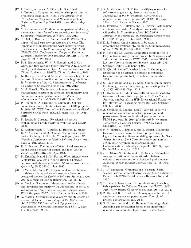
[17] I. Fronza, A. Janes, A. Sillitti, G. Succi, andS. Trebeschi. Cooperation wordle using pre-attentiveprocessing techniques. In 2013 6th InternationalWorkshop on Cooperative and Human Aspects ofSoftware Engineering (CHASE), pages 57–64, May2013.
[18] M. Goeminne and T. Mens. A comparison of identitymerge algorithms for software repositories. Science ofComputer Programming, 78(8):971–986, 2013.
[19] T. Hall, S. Beecham, J. Verner, and D. Wilson. Theimpact of staff turnover on software projects: Theimportance of understanding what makes softwarepractitioners tick. In Proceedings of the 2008 ACMSIGMIS CPR Conference on Computer PersonnelDoctoral Consortium and Research, SIGMIS CPR ’08,page 30–39. ACM, 2008.
[20] D. S. Hamermesh, W. H. J. Hassink, and J. C. v.Ours. Job turnover and labor turnover: A taxonomy ofemployment dynamics. Open Access publications fromTilburg University 12-86873, Tilburg University, 1996.
[21] K. Herzig, S. Just, and A. Zeller. It’s not a bug, it’s afeature: How misclassification impacts bug prediction.In Proceedings of the 2013 International Conferenceon Software Engineering, page 392–401, 2013.
[22] M. A. Huselid. The impact of human resourcemanagement practices on turnover, productivity, andcorporate financial performance. Academy ofManagement Journal, 38(3):635–672, June 1995.
[23] P. Hynninen, A. Piri, and T. Niinimaki. Off-sitecommitment and voluntary turnover in GSD projects.In 2010 5th IEEE International Conference on GlobalSoftware Engineering (ICGSE), pages 145–154, Aug.2010.
[24] D. Izquierdo-Cortazar. Relationship betweenorphaning and productivity in evolution and GIMP.2008.
[25] E. Kalliamvakou, G. Gousios, K. Blincoe, L. Singer,D. M. German, and D. Damian. The promises andperils of mining GitHub. In Proceedings of the 11thWorking Conference on Mining Software Repositories,page 92–101. ACM, 2014.
[26] R. M. Kanter. The impact of hierarchical structureson the work behavior of women and men. SocialProblems, 23(4):415–430, Apr. 1976.
[27] D. Krackhardt and L. W. Porter. When friends leave:A structural analysis of the relationship betweenturnover and stayers’ attitudes. Administrative ScienceQuarterly, 30(2):242–61, Jan. 1985.
[28] T. Mens, M. Claes, P. Grosjean, and A. Serebrenik.Studying evolving software ecosystems based onecological models. In Evolving Software Systems, pages297–326. Springer Berlin Heidelberg, Jan. 2014.
[29] A. Mockus. Succession: Measuring transfer of codeand developer productivity. In Proceedings of the 31stInternational Conference on Software Engineering,ICSE ’09, page 67–77. IEEE Computer Society, 2009.
[30] A. Mockus. Organizational volatility and its effects onsoftware defects. In Proceedings of the EighteenthACM SIGSOFT International Symposium onFoundations of Software Engineering, FSE ’10, page117–126. ACM, 2010.
[31] A. Mockus and L. G. Votta. Identifying reasons forsoftware changes using historic databases. InProceedings of the International Conference onSoftware Maintenance (ICSM’00), ICSM ’00, page120–. IEEE Computer Society, 2000.
[32] K. Panciera, A. Halfaker, and L. Terveen. Wikipediansare born, not made: A study of power editors onwikipedia. In Proceedings of the ACM 2009International Conference on Supporting Group Work,GROUP ’09, page 51–60. ACM, 2009.
[33] D. L. Parnas. On the criteria to be used indecomposing systems into modules. Communicationsof the ACM, 15(12):1053–1058, 1972.
[34] P. Pons and M. Latapy. Computing communities inlarge networks using random walks. In Computer andInformation Sciences - ISCIS 2005, number 3733 inLecture Notes in Computer Science, pages 284–293.Springer Berlin Heidelberg, 2005.
[35] X. Qin, M. Salter-Townshend, and P. Cunningham.Exploring the relationship between membershipturnover and productivity in online communities.2014.
[36] S. Ransbotham and G. C. Kane. Online communities:Explaining rises and falls from grace in wikipedia. MISQ., 35(3):613–628, Sept. 2011.
[37] G. Robles and J. M. Gonzalez-Barahona. Contributorturnover in libre software projects. In Open SourceSystems, number 203 in IFIP International Federationfor Information Processing, pages 273–286. SpringerUS, Jan. 2006.
[38] A. Schilling, S. Laumer, and T. Weitzel. Who willremain? an evaluation of actual person-job andperson-team fit to predict developer retention inFLOSS projects. In 2012 45th Hawaii InternationalConference on System Science (HICSS), pages3446–3455, Jan. 2012.
[39] P. N. Sharma, J. Hulland, and S. Daniel. Examiningturnover in open source software projects usinglogistic hierarchical linear modeling approach. In OpenSource Systems: Long-Term Sustainability, number378 in IFIP Advances in Information andCommunication Technology, pages 331–337. SpringerBerlin Heidelberg, Jan. 2012.
[40] J. D. Shaw, N. Gupta, and J. E. Delery. Alternativeconceptualizations of the relationship betweenvoluntary turnover and organizational performance.Academy of Management Journal, 48(1):50–68, Feb.2005.
[41] J. D. Thompson. Organizations in action: Socialscience bases of administrative theory. SSRN ScholarlyPaper ID 1496215, Social Science Research Network,1967.
[42] Y. Tian, J. Lawall, and D. Lo. Identifying linux bugfixing patches. In Software Engineering (ICSE), 201234th International Conference on, page 386–396, 2012.
[43] Z. Ton and R. S. Huckman. Managing the impact ofemployee turnover on performance: The role ofprocess conformance. Jan. 2008.
[44] S. G. Westlund and J. C. Hannon. Retaining talent:Assessing job satisfaction facets most significantlyrelated to software developer turnover intentions.

Journal of Information Technology Management,19(4):1–15, 2008.
[45] Y. Yu, A. Benlian, and T. Hess. An empirical study ofvolunteer members’ perceived turnover in open sourcesoftware projects. In 2012 45th Hawaii InternationalConference on System Science (HICSS), pages3396–3405, Jan. 2012.
[46] T. Zimmermann, R. Premraj, and A. Zeller.Predicting defects for eclipse. In InternationalWorkshop on Predictor Models in SoftwareEngineering, 2007. PROMISE’07: ICSE Workshops
2007, page 9, May 2007.

Huitièmes journées nationales du GDR GPL – 8 au 10 juin 2016
126
Titre de la contribution : Automating the Extraction of Model-based
Software Product Lines from Model Variants
Auteurs : Jabier Martinez, Tewfik Ziadi, Tegawendé Bissyandé, Jacques Klein and Yves Le Traon We address the problem of automating 1) the analysis of existing similar model variants and 2) migrating them into a software product line. Our approach, named MoVaPL, considers the identification of variability and commonality in model variants, as well as the extraction of a CVL-compliant Model-based Software Product Line (MSPL) from the features identified on these variants. MoVaPL builds on a generic representation of models making it suitable to any MOF-based models. We apply our approach on variants of the open source ArgoUML UML modeling tool as well as on variants of an In-flight Entertainment System. Evaluation with these large and complex case studies contributed to show how our feature identification with structural constraints discovery and the MSPL generation process are implemented to make the approach valid (i.e., the extracted software product line can be used to regenerate all variants considered) and sound (i.e., derived variants We address the problem of automating 1) the analysis of existing similar model variants and 2) migrating them into a software product line. Our approach, named MoVaPL, considers the identification of variability and commonality in model variants, as well as the extraction of a CVL-compliant Model-based Software Product Line (MSPL) from the features identified on these variants. MoVaPL builds on a generic representation of models making it suitable to any MOF-based models. We apply our approach on variants of the open source ArgoUML UML modeling tool as well as on variants of an In-flight Entertainment System. Evaluation with these large and complex case studies contributed to show how our feature identification with structural constraints discovery and the MSPL generation process are implemented to make the approach valid (i.e., the extracted software product line can be used to regenerate all variants considered) and sound (i.e., derived variants which did not exist are at least structurally valid).which did not exist ar- at least structurally valid).
Groupes de travail GLE et RIMEL
127

Huitièmes journées nationales du GDR GPL – 8 au 10 juin 2016
128
Tracking the Software Quality of AndroidApplications along their Evolution
Geoffrey Hecht1,2, Omar Benomar2, Romain Rouvoy1, Naouel Moha2, Laurence Duchien11 University of Lille / Inria, France
2 Universite du Quebec a Montreal, [email protected], [email protected], [email protected],
[email protected], [email protected]
Abstract—Mobile apps are becoming complex software sys-tems that must be developed quickly and evolve continuouslyto fit new user requirements and execution contexts. However,addressing these requirements may result in poor design choices,also known as antipatterns, which may incidentally degradesoftware quality and performance. Thus, the automatic detectionand tracking of antipatterns in this apps are important activitiesin order to ease both maintenance and evolution. Moreover,they guide developers to refactor their applications and thus,to improve their quality. While antipatterns are well-known inobject-oriented applications, their study in mobile applicationsis still in its infancy. In this paper, we analyze the evolution ofmobile apps quality on 3, 568 versions of 106 popular Androidapplications downloaded from the Google Play Store. For thispurpose, we use a tooled approach, called PAPRIKA, to identify 3object-oriented and 4 Android-specific antipatterns from binariesof mobile apps, and to analyze their quality along evolutions.
Keywords—Android, antipattern, mobile app, software quality.
I. INTRODUCTION
Software evolve over time, inevitably, to cope with the in-troduction of new requirements, to adapt to new environments,to fix bugs, or to improve software design. However, regardlessof the type of changes performed, the software quality maydeteriorate as a result of software aging [38].
Software quality declines along evolutions because of theinjection of poor design and implementation choices intosoftware. Code smells and antipatterns are symptoms of suchbad choices [17]. Additionally, the introduction of antipatternsmay affect software maintainability [53], [54], increase thechange-proneness [26], the fault-proneness [27], and the com-plexity [50] of software modules. Therefore, the existence ofantipatterns in software is a relevant indicator of its quality.
The research community recognized this issue and pro-posed several techniques to detect code smells and antipat-terns [34], [37]. Most of them are concerned with identifyingpossible deviations from Object-Oriented (OO) principles,such as functional decomposition and encapsulation. Despitethe availability of software development kits for mobile apps,specific code smells and antipatterns may still emerge, due tothe limitations and constraints on resource like memory, CPUor screen sizes. Mobile apps may also exhibit OO code smellsand antipatterns, such as Blob class, which may decrease theirquality as they evolve. To the best of our knowledge, mostof the proposed techniques and methods for code smells andantipatterns detection in mobile applications do not involve
large empirical data to give a genuine picture of the issue,rather they detect antipatterns on a single version of fewspecific open source systems [49]. This is all the more true inthe case of techniques for Android applications as the researchfield is in its infancy. Also, OO antipatterns and mobile-specificones are rarely studied together in order to assess the softwarequality of Android applications.
Regarding software quality along software evolutions, mosttechniques are based on the analysis of variation of softwaremetrics over time. For instance, studies have been performedon the distribution of bug introduction to software along itsevolutions [36] or on an aggregation of metrics as a qualityindicator [20]. However, these techniques were not applied tomobile applications.
In this paper, we present a fully automated approach thatmonitors the evolution of mobile apps and assesses theirquality by considering antipatterns. To this end, we propose asoftware quality estimation technique based on the consistencybetween software artifacts size and OO and Android antipat-terns. To identify these antipatterns from Android applications,we use a metrics-based detection technique. Rather than eval-uating each application independently, our approach leveragesthe whole dataset to detect and evaluate the evolution ofantipatterns in each application. The antipatterns detection andquality tracking are automatic processes included in PAPRIKA,our tooled approach. Typically, we intend to answer the twofollowing research questions:
• RQ1: Can we infer software quality evolution trendsacross different versions of Android applications?
• RQ2: How does software quality evolve in Androidapplications?
The rationale behind our approach is the close relationshipbetween antipatterns and software artifacts size. A recentlarge empirical study [45] showed that most antipatterns areintroduced at the creation of software artifacts. The samestudy indicates that some antipatterns are introduced as aresult of several changes performed on software artifacts alongevolutions. Based on these findings, we propose to study thevariations between software artifacts sizes and the number ofantipatterns contained in them. Typically, we intend to trackthe lack of correlation between the number of antipatternsand the software size along evolutions. Our study is basedon a dataset made of 106 Android applications and 3, 568versions. We choose popular applications from the Google PlayStore in order to be representative of complex and up-to-date
applications. However, most of these applications are not open-source. Thus, it was necessary to detect the antipatterns at thebytecode granularity. In this way, our approach could be usedby both developers and app store providers to track the appsquality evolution at both global and local scales.
The main contributions of this paper are: (1) an approachto track and evaluate the quality of android apps along theirevolutions via the detection of antipatterns, (2) the observationof particular relationships between these antipatterns in thecase of mobile applications, (3) the identification of 5 qualityevolution trends and their possible causes inferred by theanalysis of our dataset and, finally (4) an empirical studyinvolving over 3500 version on which we apply our tooledapproach.
This paper is organized as follows: Section II gives a briefbackground on Android apps and bytecode-based techniques.Section III discusses different contributions related to ourwork. Our automatic tooled approach, PAPRIKA, is detailedin Section IV. The results of the application of our approachare presented in Section V. Section VI concludes the paper.
II. BACKGROUND ON ANDROID PACKAGE ANDBYTECODE
This section provides a short overview of the specificitiesof Android Application Package (APK) and Dalvik bytecode.
Android apps are distributed using the APK file format.APK files are archive files in a ZIP format, which are organizedas follows: 1) the file AndroidManifest.xml describesapplication metadata including name, version, permissions andreferenced library files of the application, 2) the directoryMETA-INF that contains meta-data and certificate informa-tion, 3) an asset and a res directory containing non-compiled resources, 4) a lib directory for eventual nativecode used as library, 5) a resources.arsc file for pre-compiled resources, and 6) a .dex file containing the com-piled application classes and code in dex file format [5]. WhileAndroid apps are developed using the Java language, they usethe Dalvik Virtual Machine as a runtime environment. Themain difference between the Java Virtual Machine (JVM) andthe Dalvik Virtual Machine is that Dalvik is register-based,in order to be memory efficient compared to the stack-basedJVM [5]. The resulting bytecode compiled from Java sourcesand interpreted by the Dalvik Virtual Machine is thereforedifferent.
Disassembler exists for the Dex format [8] and tools totransform the bytecode into intermediate languages or evenJava are numerous [11], [14], [21], [42]. However, there isan important loss of information during this transformationfor all the existing approaches. For instance, additional algo-rithms have to be used to infer the type of local variablesor to determine the type of branches as for, while andif constructions are replaced by goto instructions in thebytecode [5], [14]. Some dependencies are also absent fromthe Dex files, resulting in phantom classes, which cannot beanalyzed without the source code. And, of course, the nativecode included in the lib directory cannot be decompiled withthese tools. It is also important to note that around 30% ofall the mobile apps distributed on the Google Play Store areobfuscated [52] in order to prevent reverse-engineering. The
ProGuard tool used to obfuscate code is even pre-installed onthe beta of Android Studio provided by Google to replaceEclipse ADT [3]. It is likely that code obfuscation will be evenmore common in the future. With obfuscation, most classes andmethods are renamed, often with just one or two alphabeticalcharacters, leading to the loss of most of lexical properties.Fortunately, the application structure is preserved and classesfrom the Android Framework are not renamed, thus allowingto retrieve some information from the classes that inherit them.
III. RELATED WORK
In this section, we discuss the relevant literature aboutanalysis and antipatterns detection in mobile apps and relatedwork on software evolution.
Mobile apps are mostly developed using OO languages,such as Java or Objective-C. Since their definition by Chi-damber and Kemerer [19], OO metrics have gained popularityto assess software quality. Numerous works validated OOmetrics to be efficient quality indicators [12], [15], [28], [43].This has lead to the creation of tooled approaches, such asDECOR [35] or IPLASMA [31], which use OO metrics todetect code smells and antipatterns in OO applications. Mostof the code smells and antipatterns, like long method or blobclass, detected by these approaches are inspired by the workof Fowler [23] and Brown et al. [17]. These approaches arecompatible with Java, but since they were mostly developedbefore the emergence of mobile apps they are not takinginto account the specificities of Android apps and are notcompatible with Dex bytecode.
With regard to mobile apps, Linares-Vasquez et al. [29]used DECOR to perform the detection of 18 different OOantipatterns in mobile apps built using Java Mobile Edition(J2ME) [6]. This large-scale study was performed on 1, 343apps and shows that the presence of antipatterns negativelyimpacts the software quality metrics, in particular metrics re-lated to fault-proneness. They also found that some antipatternsare more common with certain categories of Java mobile apps.Specifically in Android apps, Verloop [49] used popular Javarefactoring tools, such as PMD [7] or JDEODORANT [44] todetect code smells, like large class or long method in open-source software. They found that antipatterns tend to appear atdifferent frequencies in classes that inherit from the AndroidFramework (called core classes) compare to classes whichare not (called non-core classes). For example, long methodwas detected twice as much in core classes in term of ratio.However, they did not considered Android-specific antipatternsin both of these studies.
The detection and the specification of mobile-specificantipatterns are still considered as open issues. Reimann etal. [39] propose a catalog of 30 quality smells dedicatedto Android. These code smells are mainly originated fromthe good and bad practices documented online in Androiddocumentations or by developers reporting their experience onblogs. They are concerning various aspect like implementa-tions, user interfaces or database usages. They are reportedto have a negative impact on properties, such as efficiency,user experience or security. We chose to detect some ofthese code smells with our approach, which are presented inSection IV-D. We selected antipatterns that can be detected by
static analysis and despite code obfuscation. Reimann et al.are also offering the detection and correction of code smellsvia the REFACTORY tool [40]. This tool can detect the codesmells from an EMF model. The source code can be convertedto EMF if necessary. However, we have not been yet able toexecute this tool on an Android app. Moreover, there is noevidence that all the antipatterns of the catalog are detectableusing this approach.
Concerning the analysis of Android apps and the study oftheir specificities, the SAMOA [33] tool allows developersto analyze their mobile apps from the source code. The toolcollects metrics, such as the number of packages, lines ofcode, or the cyclomatic complexity. It also provides a wayto visualize external API calls as well as the evolution ofmetrics along versions and a comparison with other analyzedapps. They performed this analysis on 20 applications anddiscovered that they are significantly different from classicalsoftware systems. They are smaller, and make an intensiveusage of external libraries, which leads to a more complex codeto understand during maintenance activities. Ruiz et al. [41]analyzed Android packages to understand the reuse of classesin Android apps. They extract bytecode and then analyze classsignatures for this purpose. They discovered that softwarereuse via inheritance, libraries, and frameworks is prevalentin mobile apps compared to regular software. Xu [52] alsoexamined APKs of 122, 570 applications and determines thatdeveloper errors are common in manifest and permissions. Healso analyzed the apps’ code and observed that Java reflectionand code obfuscation are widely used in mobile apps, makingreverse-engineering harder. He also noticed the heavy usage ofexternal libraries in its corpus of analyzed apps. Nonetheless,antipatterns were not considered as part of these studies.
Much work has been done concerning the assessmentof software quality throughout the evolution of OO non-mobile applications. Zhu et al. [56] monitor software qualitythroughout the evolution by considering three different mod-ularity views: Package, Structural and Semantic. They assesssoftware quality by computing the deviation trends betweenthe considered modular views to indicate on quality evolution.The idea behind their approach is that if the considereddifferent views are well aligned, then software quality isgood. They studied the quality evolution of three open sourceJava systems. Zhang and Kim [55] propose to study softwareevolution quality by monitoring the number of defects usingStatistical Process Control (SPC) and control charts (c-charts).They examined over 60 c-charts representing different Eclipseand Gnome components and identified 6 common qualityevolution patterns. The quality evolution patterns serve asindicators of symptomatic situations that development teamsshould address. For instance, the Roller Coaster pattern, whichrepresents large variations of defect numbers, suggests thatsoftware quality is unstable and that better management andplanning is required to ensure high and consistent quality.Tufano et al. [45] conducted a large scale empirical studyto investigate the code smells introduction by developersby analyzing the change history of software projects. Theauthors aim at identifying how code smells are introduced insoftware along its evolutions. Their major findings are thatmost code smells are introduced when files are created andnew features are developed or existing ones are enhanced. VanEmden and Moonen [48] propose an approach to detect code
smells in Java programs. They distinguish between two typeof smells: primitive smells which are detected directly fromcode and derived smells which are deduced from the context.The detected antipatterns are then presented to the developersfor inspection and quality assurance using visualization. Inthis approach, the developers are left with the responsibilityof assessing the quality by analyzing the visualization. Ourapproach provides the developers an estimation of softwarequality based on antipatterns.
Unlike the above mentioned contributions, and regardlessof software quality along evolutions, some studies analyzesoftware evolution to abstract higher level information with thepurpose of comprehension. Barry et al. [13] propose a methodto identify software evolution patterns. The pattern identifi-cation is based on software volatility information. Volatilityis approximated by computing the amplitude, dispersion, andperiodicity of software changes at regular intervals in thesoftware history. Each period is defined by a volatility class,and sequence analysis is applied to reveal similar patternsin time. Xing and Stroulia [51] present an approach forunderstanding evolution phases and styles of object-orientedsystems. The authors use a structural differencing algorithmto compare changing system class models over time, andgather the system’s evolution profile. The resulting sequenceof structural changes is then analyzed to gain insight aboutthe system’s evolution. Finally, Benomar et al. [16] investigatethe automatic detection of software development phases bystudying software evolutions. They use a search-based tech-nique to identify software evolution periods having similardevelopment activities. Search heuristics, such as developmentrate, importance and type of changes are used to define andunderstand software evolution.
Our proposed approach aims at identifying hotspots interms of software quality along evolutions. We consider theanalysis of mobile apps evolution and apply a novel approachto detect antipatterns, which we use to estimate the softwarequality. The proposed approach is automatic and takes asinput versions of mobile apps and monitors their quality alongevolutions.
IV. PAPRIKA: A TOOLED APPROACH TO DETECTSOFTWARE ANTI-PATTERNS
In this section, we introduce the key components of PA-PRIKA, our tooled approach for analyzing the design of mobileapps in order to detect software antipatterns.
A. Overview of the Approach
PAPRIKA builds on a four-step approach, which is sum-marized in Figure 1. As a first step, PAPRIKA parses theAPK file of the mobile app under analysis to extract somemetadata (e.g., app name, package) and a representation of thecode. Additional metadata (e.g., rating, number of downloads)are also extracted from the Google Play Store and passed asarguments. This representation is then automatically visitedto compute a model of the code (including classes, methods,attributes) as a graph annotated with a set of raw qualitymetrics (cf. Section V). As a second step, this model storedinto a graph database (cf. Section IV-C). The third step consistsin querying the graph to detect the presence of common
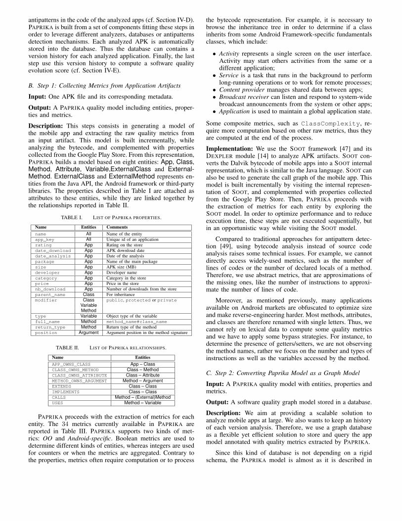
antipatterns in the code of the analyzed apps (cf. Section IV-D).PAPRIKA is built from a set of components fitting these steps inorder to leverage different analyzers, databases or antipatternsdetection mechanisms. Each analyzed APK is automaticallystored into the database. Thus the database can contains aversion history for each analyzed application. Finally, the laststep use this version history to compute a software qualityevolution score (cf. Section IV-E).
B. Step 1: Collecting Metrics from Application Artifacts
Input: One APK file and its corresponding metadata.
Output: A PAPRIKA quality model including entities, proper-ties and metrics.
Description: This steps consists in generating a model ofthe mobile app and extracting the raw quality metrics froman input artifact. This model is built incrementally, whileanalyzing the bytecode, and complemented with propertiescollected from the Google Play Store. From this representation,PAPRIKA builds a model based on eight entities: App, Class,Method, Attribute, Variable,ExternalClass and External-Method. ExternalClass and ExternalMethod represents en-tities from the Java API, the Android framework or third-partylibraries. The properties described in Table I are attached asattributes to these entities, while they are linked together bythe relationships reported in Table II.
TABLE I. LIST OF PAPRIKA PROPERTIES.
Name Entities Commentsname All Name of the entityapp_key All Unique id of an applicationrating App Rating on the storedate_download App APK download datedate_analysis App Date of the analysispackage App Name of the main packagesize App APK size (MB)developer App Developer namecategory App Category in the storeprice App Price in the storenb_download App Number of downloads from the storeparent_name Class For inheritancemodifier Class public, protected or private
VariableMethod
type Variable Object type of the variablefull_name Method method_name#class_namereturn_type Method Return type of the methodposition Argument Argument position in the method signature
TABLE II. LIST OF PAPRIKA RELATIONSHIPS.
Name EntitiesAPP_OWNS_CLASS App – ClassCLASS_OWNS_METHOD Class – MethodCLASS_OWNS_ATTRIBUTE Class – AttributeMETHOD_OWNS_ARGUMENT Method – ArgumentEXTENDS Class – ClassIMPLEMENTS Class – ClassCALLS Method – (External)MethodUSES Method – Variable
PAPRIKA proceeds with the extraction of metrics for eachentity. The 34 metrics currently available in PAPRIKA arereported in Table III. PAPRIKA supports two kinds of met-rics: OO and Android-specific. Boolean metrics are used todetermine different kinds of entities, whereas integers are usedfor counters or when the metrics are aggregated. Contrary tothe properties, metrics often require computation or to process
the bytecode representation. For example, it is necessary tobrowse the inheritance tree in order to determine if a classinherits from some Android Framework-specific fundamentalsclasses, which include:
• Activity represents a single screen on the user interface.Activity may start others activities from the same or adifferent application;
• Service is a task that runs in the background to performlong-running operations or to work for remote processes;
• Content provider manages shared data between apps;• Broadcast receiver can listen and respond to system-wide
broadcast announcements from the system or other apps;• Application is used to maintain a global application state.
Some composite metrics, such as ClassComplexity, re-quire more computation based on other raw metrics, thus theyare computed at the end of the process.
Implementation: We use the SOOT framework [47] and itsDEXPLER module [14] to analyze APK artifacts. SOOT con-verts the Dalvik bytecode of mobile apps into a SOOT internalrepresentation, which is similar to the Java language. SOOT canalso be used to generate the call graph of the mobile app. Thismodel is built incrementally by visiting the internal represen-tation of SOOT, and complemented with properties collectedfrom the Google Play Store. Then, PAPRIKA proceeds withthe extraction of metrics for each entity by exploring theSOOT model. In order to optimize performance and to reduceexecution time, these steps are not executed sequentially, butin an opportunistic way while visiting the SOOT model.
Compared to traditional approaches for antipattern detec-tion [49], using bytecode analysis instead of source codeanalysis raises some technical issues. For example, we cannotdirectly access widely-used metrics, such as the number oflines of codes or the number of declared locals of a method.Therefore, we use abstract metrics, that are approximations ofthe missing ones, like the number of instructions to approxi-mate the number of lines of code.
Moreover, as mentioned previously, many applicationsavailable on Android markets are obfuscated to optimize sizeand make reverse-engineering harder. Most methods, attributes,and classes are therefore renamed with single letters. Thus, wecannot rely on lexical data to compute some quality metricsand we have to apply some bypass strategies. For instance, todetermine the presence of getters/setters, we are not observingthe method names, rather we focus on the number and types ofinstructions as well as the variables accessed by the method.
C. Step 2: Converting Paprika Model as a Graph Model
Input: A PAPRIKA quality model with entities, properties andmetrics.
Output: A software quality graph model stored in a database.
Description: We aim at providing a scalable solution toanalyze mobile apps at large. We also wants to keep an historyof each version analysis. Therefore, we use a graph databaseas a flexible yet efficient solution to store and query the appmodel annotated with quality metrics extracted by PAPRIKA.
Since this kind of database is not depending on a rigidschema, the PAPRIKA model is almost as it is described in
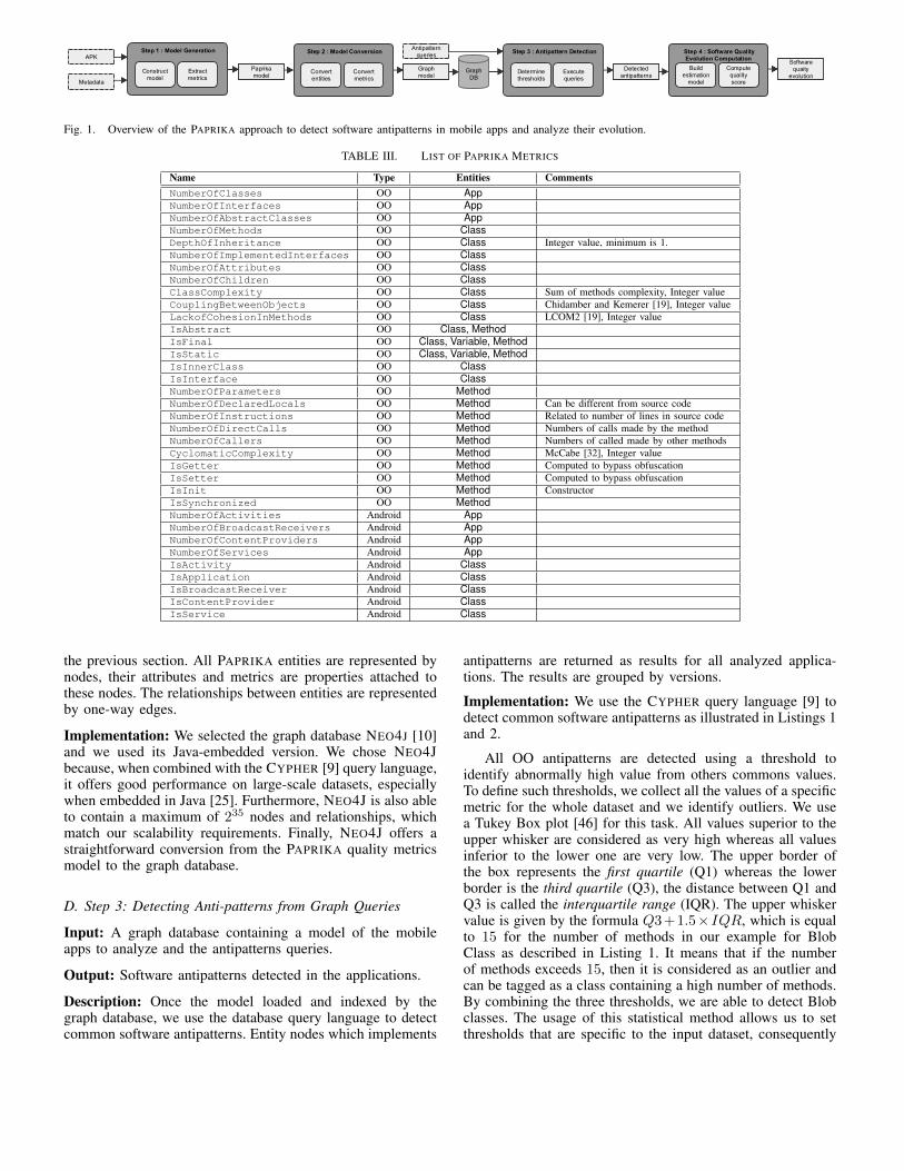
GraphDB
APK
Paprikamodel
Metadata
Step 1 : Model Generation
Constructmodel
Extractmetrics
Step 3 : Antipattern Detection
Determinethresholds
Executequeries
Graphmodel
Antipatternqueries
Detectedantipatterns
Step 2 : Model Conversion
Convertentities
Convertmetrics
Step 4 : Software QualityEvolution Computation
Buildestimationmodel
Computequalityscore
Softwarequaityevolution
Fig. 1. Overview of the PAPRIKA approach to detect software antipatterns in mobile apps and analyze their evolution.
TABLE III. LIST OF PAPRIKA METRICS
Name Type Entities CommentsNumberOfClasses OO AppNumberOfInterfaces OO AppNumberOfAbstractClasses OO AppNumberOfMethods OO ClassDepthOfInheritance OO Class Integer value, minimum is 1.NumberOfImplementedInterfaces OO ClassNumberOfAttributes OO ClassNumberOfChildren OO ClassClassComplexity OO Class Sum of methods complexity, Integer valueCouplingBetweenObjects OO Class Chidamber and Kemerer [19], Integer valueLackofCohesionInMethods OO Class LCOM2 [19], Integer valueIsAbstract OO Class, MethodIsFinal OO Class, Variable, MethodIsStatic OO Class, Variable, MethodIsInnerClass OO ClassIsInterface OO ClassNumberOfParameters OO MethodNumberOfDeclaredLocals OO Method Can be different from source codeNumberOfInstructions OO Method Related to number of lines in source codeNumberOfDirectCalls OO Method Numbers of calls made by the methodNumberOfCallers OO Method Numbers of called made by other methodsCyclomaticComplexity OO Method McCabe [32], Integer valueIsGetter OO Method Computed to bypass obfuscationIsSetter OO Method Computed to bypass obfuscationIsInit OO Method ConstructorIsSynchronized OO MethodNumberOfActivities Android AppNumberOfBroadcastReceivers Android AppNumberOfContentProviders Android AppNumberOfServices Android AppIsActivity Android ClassIsApplication Android ClassIsBroadcastReceiver Android ClassIsContentProvider Android ClassIsService Android Class
the previous section. All PAPRIKA entities are represented bynodes, their attributes and metrics are properties attached tothese nodes. The relationships between entities are representedby one-way edges.
Implementation: We selected the graph database NEO4J [10]and we used its Java-embedded version. We chose NEO4Jbecause, when combined with the CYPHER [9] query language,it offers good performance on large-scale datasets, especiallywhen embedded in Java [25]. Furthermore, NEO4J is also ableto contain a maximum of 235 nodes and relationships, whichmatch our scalability requirements. Finally, NEO4J offers astraightforward conversion from the PAPRIKA quality metricsmodel to the graph database.
D. Step 3: Detecting Anti-patterns from Graph Queries
Input: A graph database containing a model of the mobileapps to analyze and the antipatterns queries.
Output: Software antipatterns detected in the applications.
Description: Once the model loaded and indexed by thegraph database, we use the database query language to detectcommon software antipatterns. Entity nodes which implements
antipatterns are returned as results for all analyzed applica-tions. The results are grouped by versions.
Implementation: We use the CYPHER query language [9] todetect common software antipatterns as illustrated in Listings 1and 2.
All OO antipatterns are detected using a threshold toidentify abnormally high value from others commons values.To define such thresholds, we collect all the values of a specificmetric for the whole dataset and we identify outliers. We usea Tukey Box plot [46] for this task. All values superior to theupper whisker are considered as very high whereas all valuesinferior to the lower one are very low. The upper border ofthe box represents the first quartile (Q1) whereas the lowerborder is the third quartile (Q3), the distance between Q1 andQ3 is called the interquartile range (IQR). The upper whiskervalue is given by the formula Q3+1.5×IQR, which is equalto 15 for the number of methods in our example for BlobClass as described in Listing 1. It means that if the numberof methods exceeds 15, then it is considered as an outlier andcan be tagged as a class containing a high number of methods.By combining the three thresholds, we are able to detect Blobclasses. The usage of this statistical method allows us to setthresholds that are specific to the input dataset, consequently
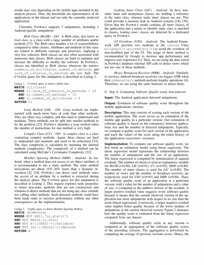
results may vary depending on the mobile apps included in theanalysis process. Thus, the thresholds are representative of allapplications in the dataset and not only the currently analyzedapplication.
Currently, PAPRIKA supports 7 antipatterns, including 4Android-specific antipatterns:
Blob Class (BLOB) - OO: A Blob class, also know asGod class, is a class with a large number of attributes and/ormethods [17]. The Blob class handles a lot of responsibilitiescompared to other classes. Attributes and methods of this classare related to different concepts and processes, implying avery low cohesion. Blob classes are also often associated withnumerous data classes. Blob classes are hard to maintain andincrease the difficulty to modify the software. In PAPRIKA,classes are identified as Blob classes whenever the metricsnumbers_of_attributes, number_of_methods andlack_of_cohesion_in_methods are very high. TheCYPHER query for this antipattern is described in Listing 1.
Listing 1. CYPHER query to detect a Blob class.MATCH (cl:Class)WHERE cl.lack_of_cohesion_in_methods > 20
AND cl.number_of_methods > 15AND cl.number_of_attributes > 8
RETURN cl
Long Method (LM) - OO: Long methods are imple-mented with much more lines of code than other methods.They are often very complex, and thus hard to understand andmaintain. These methods can be split into smaller methods tofix the problem [23]. PAPRIKA identifies a long method whenthe number of instructions for one method is very high.
Complex Class (CC) - OO: A complex class is a classcontaining complex methods. Again, these classes are hardto understand and maintain and need to be refactored [23].The class complexity is calculated by summing the internalmethods complexities. The complexity of a method can becalculated using McCabe’s Cyclomatic Complexity [32].
Member Ignoring Method (MIM) - Android: In An-droid, when a method does not access to an object attribute, itis recommended to use a static method. The static methodinvocations are about 15%–20% faster than a dynamic in-vocation [2], [18]. PAPRIKA can detect such methods sincethe access of an attribute by a method is extracted duringthe analysis phase. The CYPHER query for this antipattern isdescribed in Listing 2. This request explores node propertiesto return non-static methods that are not constructors andrelations to detect methods that are not using any class variablenor calling other methods. Such detected methods could havebeen made static to increase performance without any otherconsequences on the implementation.
Listing 2. Cypher query to detect Member Ignoring Method.MATCH (m:Method)WHERE NOT HAS(.‘is_static‘)AND NOT HAS(m.is_init)AND NOT m-[:USES]->(:Variable)AND NOT (m)-[:CALLS]->(:Method)RETURN m
Leaking Inner Class (LIC) - Android: In Java, non-static inner and anonymous classes are holding a referenceto the outer class, whereas static inner classes are not. Thiscould provoke a memory leak in Android systems [18], [30].Given that the PAPRIKA model contains all inner classes ofthe application and a metric to identify static class is attachedto classes, leaking inner classes are detected by a dedicatedquery in PAPRIKA.
UI Overdraw (UIO) - Android: The Android Frame-work API provides two methods in the Canvas Class(clipRect() quickReject()) to avoid the overdraw ofnon-modified part of the UI. The usage of these method isrecommended by Google to increase app performance andimprove user experience [1]. Thus, we are using the data storedin PAPRIKA database external API calls to detect views whichnot use one of these methods.
Heavy Broadcast Receiver (HBR) - Android: Similarlyto services, android broadcast receivers can trigger ANR whentheir onReceive() methods perform lengthy operations [4].Therefore, we are using the same heuristic to detect them.
E. Step 4: Computing Software Quality using Anti-patterns
Input: The Android application detected antipatterns.
Output: Evolution of software quality score throughout themobile applications versions.
Description: This step consists of scoring each version of themobile application. The score serves as an estimation of themobile app quality in a particular version. Our estimation ofsoftware quality is based on the consistency between applica-tions size and the number of detected antipatterns. Typically,we compute a quality score for each version of the applicationand track the values of the score along the entire history ofthe application (successive versions).
Implementation: To compute our software quality score, wefirst build an estimation model using linear regression. Thelinear regression model represents the relationship betweenthe number of antipatterns and the size of an application.The linear regression is computed by minimization of squaredresiduals. The number of classes is used at explanatory variablefor BLOB (r=0.90), LM (r=0.91), CC (r=0.92), MIM (r=0.80).The number of inner classes is used for LIC (r=0.80). Thenumber of views and the number of broadcast receivers arerespectively used for UIO (r=0.95) and HBR (r=0.88). Then,the software quality score of an application at a particularversion, with a value for the number of antipatterns and a valueof size, is computed as the additive inverse of the residual. Alarger positive residual value suggests worst software qualitybecause it means that the current observed version of the ap-plication has more antipatterns with respect to its size than thenorm (linear regression). Conversely, a larger negative residualvalue implies better quality because of the lower number ofantipatterns in the current observed version. Figure 2 ilustrateshow the quality score is estimated from the linear regressioncomputed from our dataset.
Additionally, software quality score at any version iscomputed as an aggregation of the software quality scoresof the preceding versions. The aggregation is performed bycomputing the average of previous versions scores. Hence, the
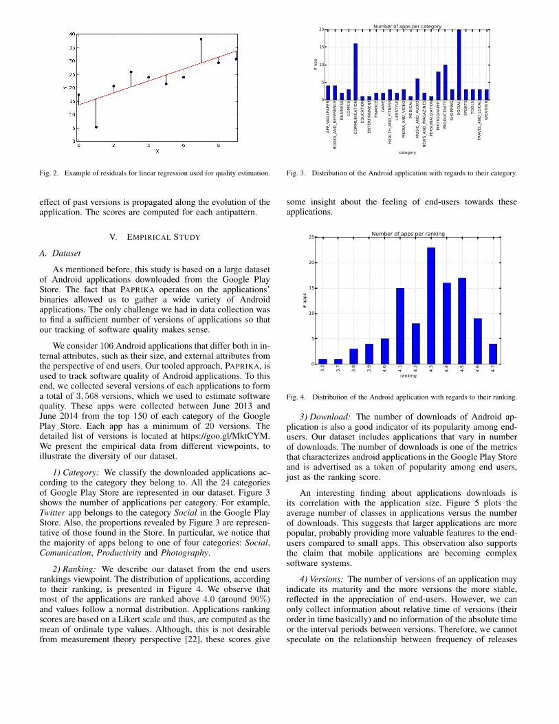
Fig. 2. Example of residuals for linear regression used for quality estimation.
effect of past versions is propagated along the evolution of theapplication. The scores are computed for each antipattern.
V. EMPIRICAL STUDY
A. Dataset
As mentioned before, this study is based on a large datasetof Android applications downloaded from the Google PlayStore. The fact that PAPRIKA operates on the applications’binaries allowed us to gather a wide variety of Androidapplications. The only challenge we had in data collection wasto find a sufficient number of versions of applications so thatour tracking of software quality makes sense.
We consider 106 Android applications that differ both in in-ternal attributes, such as their size, and external attributes fromthe perspective of end users. Our tooled approach, PAPRIKA, isused to track software quality of Android applications. To thisend, we collected several versions of each applications to forma total of 3, 568 versions, which we used to estimate softwarequality. These apps were collected between June 2013 andJune 2014 from the top 150 of each category of the GooglePlay Store. Each app has a minimum of 20 versions. Thedetailed list of versions is located at https://goo.gl/MktCYM.We present the empirical data from different viewpoints, toillustrate the diversity of our dataset.
1) Category: We classify the downloaded applications ac-cording to the category they belong to. All the 24 categoriesof Google Play Store are represented in our dataset. Figure 3shows the number of applications per category. For example,Twitter app belongs to the category Social in the Google PlayStore. Also, the proportions revealed by Figure 3 are represen-tative of those found in the Store. In particular, we notice thatthe majority of apps belong to one of four categories: Social,Comunication, Productivity and Photography.
2) Ranking: We describe our dataset from the end usersrankings viewpoint. The distribution of applications, accordingto their ranking, is presented in Figure 4. We observe thatmost of the applications are ranked above 4.0 (around 90%)and values follow a normal distribution. Applications rankingscores are based on a Likert scale and thus, are computed as themean of ordinale type values. Although, this is not desirablefrom measurement theory perspective [22], these scores give
APP_W
ALL
PA
PER
BO
OK
S_A
ND
_REFE
REN
CE
BU
SIN
ESS
CO
MIC
S
CO
MM
UN
ICA
TIO
N
ED
UC
ATIO
N
EN
TER
TA
INM
EN
T
FIN
AN
CE
GA
ME
HEA
LTH
_AN
D_F
ITN
ESS
LIFE
STYLE
MED
IA_A
ND
_VID
EO
MED
ICA
L
MU
SIC
_AN
D_A
UD
IO
NEW
S_A
ND
_MA
GA
ZIN
ES
PER
SO
NA
LIZ
ATIO
N
PH
OTO
GR
APH
Y
PR
OD
UC
TIV
ITY
SH
OPPIN
G
SO
CIA
L
SPO
RTS
TO
OLS
TR
AV
EL_
AN
D_L
OC
AL
WEA
TH
ER
category
0
5
10
15
20
# a
pp
Number of apps per category
Fig. 3. Distribution of the Android application with regards to their category.
some insight about the feeling of end-users towards theseapplications.
3.2
3.7
3.8
3.9
4.0
4.1
4.2
4.3
4.4
4.5
4.6
4.7
ranking
0
5
10
15
20
25
# a
pps
Number of apps per ranking
Fig. 4. Distribution of the Android application with regards to their ranking.
3) Download: The number of downloads of Android ap-plication is also a good indicator of its popularity among end-users. Our dataset includes applications that vary in numberof downloads. The number of downloads is one of the metricsthat characterizes android applications in the Google Play Storeand is advertised as a token of popularity among end users,just as the ranking score.
An interesting finding about applications downloads isits correlation with the application size. Figure 5 plots theaverage number of classes in applications versus the numberof downloads. This suggests that larger applications are morepopular, probably providing more valuable features to the end-users compared to small apps. This observation also supportsthe claim that mobile applications are becoming complexsoftware systems.
4) Versions: The number of versions of an application mayindicate its maturity and the more versions the more stable,reflected in the appreciation of end-users. However, we canonly collect information about relative time of versions (theirorder in time basically) and no information of the absolute timeor the interval periods between versions. Therefore, we cannotspeculate on the relationship between frequency of releases
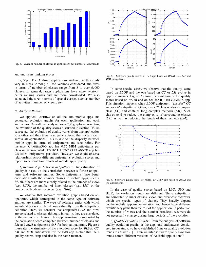
10000
50000
100000
500000
1000000
5000000
10000000
50000000
100000000
500000000
# downloads
0
500
1000
1500
2000
2500
3000
3500
4000
4500
avera
ge #
cla
sses
Average number of classes per download categories
Fig. 5. Average number of classes in applications per number of downloads.
and end users ranking scores.
5) Size: The Android applications analyzed in this studyvary in sizes. Among all the versions considered, the sizesin terms of number of classes range from 8 to over 9, 000classes. In general, larger applications have more versions,better ranking scores and are more downloaded. We alsocalculated the size in terms of special classes, such as numberof activities, number of views, etc.
B. Analysis Results
We applied PAPRIKA on all the 106 mobile apps andgenerated evolution graphs for each application and eachantipattern. Overall, we analyzed over 700 graphs representingthe evolution of the quality scores discussed in Section IV. Assuspected, the evolution of quality varies from one applicationto another and thus there is no general trend that reveals itselfacross all applications. This is due to the disparity betweenmobile apps in terms of antipatterns and size ratios. Forinstance, CAMERA360 app has 0.75 MIM antipatterns perclass on average while TO DO CALENDAR PLANNER app has2.5 MIM antipatterns per class. However, we could observerelationships across different antipatterns evolution scores andreport some evolution trends of mobile apps quality.
1) Relationships between antipatterns: Our estimation ofquality is based on the correlation between software antipat-terns and software entities. Some antipatterns have bettercorrelation with the number classes in mobile apps, such aBLOB, others are more closely related to the number of views(e.g., UIO), the number of inner classes (e.g., LIC) or thenumber of brodcast receivers (e.g., HBR).
We observe that software evolution graphs based on an-tipatterns, which correspond to the same type of softwareentities, are similar. The type of software entity with whichan antipattern is correlated comes directly from the antipatterndefinition. Here, we consider that antipatterns LM and MIMare correlated to classes although, in reality, they are correlatedto the methods of classes. This approximation is supported bythe correlation score computed between number of classes andLM and MIM antipatterns (0.8 for both antipatterns). Figure 6illustrates the similarity of the evolution score for BLOB, CC,LM and MIM antipatterns for the IMO app. Notice that the 4quality scores drop and rise in the same manner.
20
40
60
80
100
120
140
160
CC
0
200
400
600
800
1000
1200
MIM
0 5 10 15 20 25 30 35version
100
200
300
400
500
600
700
800
900
LM
0 5 10 15 20 25 30 35version
0
10
20
30
40
50
BLO
B
com.imo.android.imoim
Fig. 6. Software quality scores of IMO app based on BLOB, CC, LM andMIM antipatterns.
In some special cases, we observe that the quality scorebased on BLOB and the one based on CC or LM evolve inopposite manner. Figure 7 shows the evolution of the qualityscores based on BLOB and on LM for RETRO CAMERA app.This situation happens when BLOB antipattern “absorbs” CCand/or LM antipatterns. Often, a BLOB class is also a complexclass (CC) and contains long complex methods (LM). Suchclasses tend to reduce the complexity of surrounding classes(CC) as well as reducing the length of their methods (LM).
500
400
300
200
100
0
100
200
LM
0 5 10 15 20 25version
0
10
20
30
40
50
60
BLO
B
com.onemanwithcameralomo
Fig. 7. Software quality scores of RETRO CAMERA app based on BLOB andLM antipatterns.
In the case of quality scores based on LIC, UIO andHBR, the evolution trends are different. These antipatternsare correlated to inner classes, views and broadcast receivers,which are special types of classes. They heavily dependon the mobile app implementation and hence have differentevolutionary paths than the rest of the application. In particular,the number of views and the number broadcast receivers donot necessarily change during large periods of the evolution.
2) Quality Evolution Trends: From the analysis of softwarequality evolution graphs of the apps and antipatterns consid-ered in our study, we have established 5 major quality evolutiontrends to answer RQ1 : Can we infer software quality evolutiontrends across different versions of Android applications?
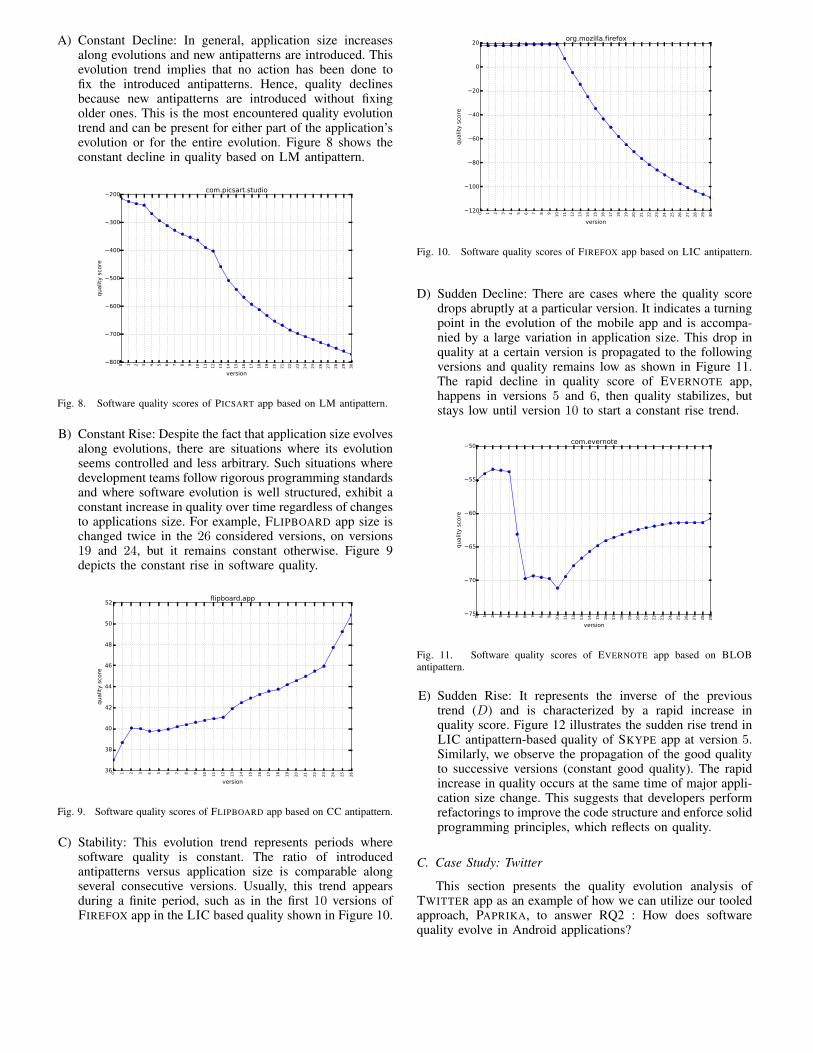
A) Constant Decline: In general, application size increasesalong evolutions and new antipatterns are introduced. Thisevolution trend implies that no action has been done tofix the introduced antipatterns. Hence, quality declinesbecause new antipatterns are introduced without fixingolder ones. This is the most encountered quality evolutiontrend and can be present for either part of the application’sevolution or for the entire evolution. Figure 8 shows theconstant decline in quality based on LM antipattern.
0 1 2 3 4 5 6 7 8 9
10
11
12
13
14
15
16
17
18
19
20
21
22
23
24
25
26
27
28
29
30
version
800
700
600
500
400
300
200
qualit
y s
core
com.picsart.studio
Fig. 8. Software quality scores of PICSART app based on LM antipattern.
B) Constant Rise: Despite the fact that application size evolvesalong evolutions, there are situations where its evolutionseems controlled and less arbitrary. Such situations wheredevelopment teams follow rigorous programming standardsand where software evolution is well structured, exhibit aconstant increase in quality over time regardless of changesto applications size. For example, FLIPBOARD app size ischanged twice in the 26 considered versions, on versions19 and 24, but it remains constant otherwise. Figure 9depicts the constant rise in software quality.
0 1 2 3 4 5 6 7 8 9
10
11
12
13
14
15
16
17
18
19
20
21
22
23
24
25
26
version
36
38
40
42
44
46
48
50
52
qualit
y s
core
flipboard.app
Fig. 9. Software quality scores of FLIPBOARD app based on CC antipattern.
C) Stability: This evolution trend represents periods wheresoftware quality is constant. The ratio of introducedantipatterns versus application size is comparable alongseveral consecutive versions. Usually, this trend appearsduring a finite period, such as in the first 10 versions ofFIREFOX app in the LIC based quality shown in Figure 10.
0 1 2 3 4 5 6 7 8 9
10
11
12
13
14
15
16
17
18
19
20
21
22
23
24
25
26
27
28
29
30
version
120
100
80
60
40
20
0
20
qualit
y s
core
org.mozilla.firefox
Fig. 10. Software quality scores of FIREFOX app based on LIC antipattern.
D) Sudden Decline: There are cases where the quality scoredrops abruptly at a particular version. It indicates a turningpoint in the evolution of the mobile app and is accompa-nied by a large variation in application size. This drop inquality at a certain version is propagated to the followingversions and quality remains low as shown in Figure 11.The rapid decline in quality score of EVERNOTE app,happens in versions 5 and 6, then quality stabilizes, butstays low until version 10 to start a constant rise trend.
0 1 2 3 4 5 6 7 8 9
10
11
12
13
14
15
16
17
18
19
20
21
22
23
24
25
26
27
28
29
version
75
70
65
60
55
50
qualit
y s
core
com.evernote
Fig. 11. Software quality scores of EVERNOTE app based on BLOBantipattern.
E) Sudden Rise: It represents the inverse of the previoustrend (D) and is characterized by a rapid increase inquality score. Figure 12 illustrates the sudden rise trend inLIC antipattern-based quality of SKYPE app at version 5.Similarly, we observe the propagation of the good qualityto successive versions (constant good quality). The rapidincrease in quality occurs at the same time of major appli-cation size change. This suggests that developers performrefactorings to improve the code structure and enforce solidprogramming principles, which reflects on quality.
C. Case Study: Twitter
This section presents the quality evolution analysis ofTWITTER app as an example of how we can utilize our tooledapproach, PAPRIKA, to answer RQ2 : How does softwarequality evolve in Android applications?
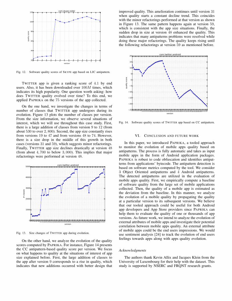
0 1 2 3 4 5 6 7 8 9
10
11
12
13
14
15
version
20
40
60
80
100
120
qualit
y s
core
com.skype.raider
Fig. 12. Software quality scores of SKYPE app based on LIC antipattern.
TWITTER app is given a ranking score of 4.1 by endusers. Also, it has been downloaded over 100M times, whichindicates its high popularity. One question worth asking: howdoes TWITTER quality evolved over time? To this end, weapplied PAPRIKA on the 75 versions of the app collected.
On the one hand, we investigate the changes in terms ofnumber of classes that TWITTER app undergoes during itsevolution. Figure 13 plots the number of classes per version.From the size information, we observe several situations ofinterest, which we will use throughout this case study. First,there is a large addition of classes from version 9 to 12 (fromabout 530 to over 2, 800). Second, the app size constantly risesfrom versions 19 to 47 and from versions 48 to 74. However,there is a size drop in the middle of this growth in bothcases (versions 31 and 59), which suggests minor refactorings.Finally, TWITTER app size declines drastically at version 48(from about 4, 700 to below 3, 000). This implies that majorrefactorings were performed at version 48.
0 1 2 3 4 5 6 7 8 91
01
11
21
31
41
51
61
71
81
92
02
12
22
32
42
52
62
72
82
93
03
13
23
33
43
53
63
73
83
94
04
14
24
34
44
54
64
74
84
95
05
15
25
35
45
55
65
75
85
96
06
16
26
36
46
56
66
76
86
97
07
17
27
37
47
5
version
0
1000
2000
3000
4000
5000
# c
lass
es
com.twitter.android
Fig. 13. Size changes of TWITTER app during evolution.
On the other hand, we analyze the evolution of the qualityscores computed by PAPRIKA. For instance, Figure 14 presentsthe CC antipattern-based quality score per version. We focuson what happens to quality at the situations of interest of appsize explained before. First, the large addition of classes tothe app after version 9 corresponds to a rise in quality, whichindicates that new additions occurred with better design that
improved quality. This amelioration continues until version 31when quality starts a constant decline trend. This coincideswith the minor refactorings performed at that version as shownin Figure 13. The same pattern happens again at version 59,which is consistent with the app size situations. Finally, thesudden drop in size at version 48 enhanced the quality. Thisindicates that many antipatterns problems were resolved whiledoing these major refactorings. The quality keeps rising untilthe following refactorings at version 59 as mentioned before.
0 1 2 3 4 5 6 7 8 91
01
11
21
31
41
51
61
71
81
92
02
12
22
32
42
52
62
72
82
93
03
13
23
33
43
53
63
73
83
94
04
14
24
34
44
54
64
74
84
95
05
15
25
35
45
55
65
75
85
96
06
16
26
36
46
56
66
76
86
97
07
17
27
37
47
5
version
25
20
15
10
5
0
5
10
15
20
qualit
y s
core
com.twitter.android
Fig. 14. Software quality scores of TWITTER app based on CC antipattern.
VI. CONCLUSION AND FUTURE WORK
In this paper, we introduced PAPRIKA, a tooled approachto monitor the evolution of mobile apps quality based onantipatterns. The process is fully automatic and takes as inputmobile apps in the form of Android application packages.PAPRIKA is robust to code obfuscation and identifies antipat-terns from applications’ bytecode. The antipattern detection isbased on software metrics computed by the tool. We consider3 Object Oriented antipatterns and 4 Android antipatterns.The detected antipatterns are utilized in the evaluation ofmobile apps quality. First, we empirically compute a baselineof software quality from the large set of mobile applicationscollected. Then, the quality of a mobile app is estimated asthe deviation from the baseline. In this manner, we analyzethe evolution of a mobile quality by propagating the qualityat a particular version to its subsequent versions. We believethat our tooled approach could be useful for both Androidapp developers and App Store providers since PAPRIKA canhelp them to evaluate the quality of one or thousands of appversions. As future work, we intend to analyze the evolution ofexternal attributes of mobile apps and investigate their potentialcorrelation between mobile apps quality. An external attributeof mobile apps could be the end users impressions. We woulduse sentiment analysis [24] to track the evolution of end usersfeelings towards apps along with apps quality evolution.
Acknowledgments
The authors thank Kevin Allix and Jacques Klein from theUniversity of Luxembourg for their help with the dataset. Thisstudy is supported by NSERC and FRQNT research grants.
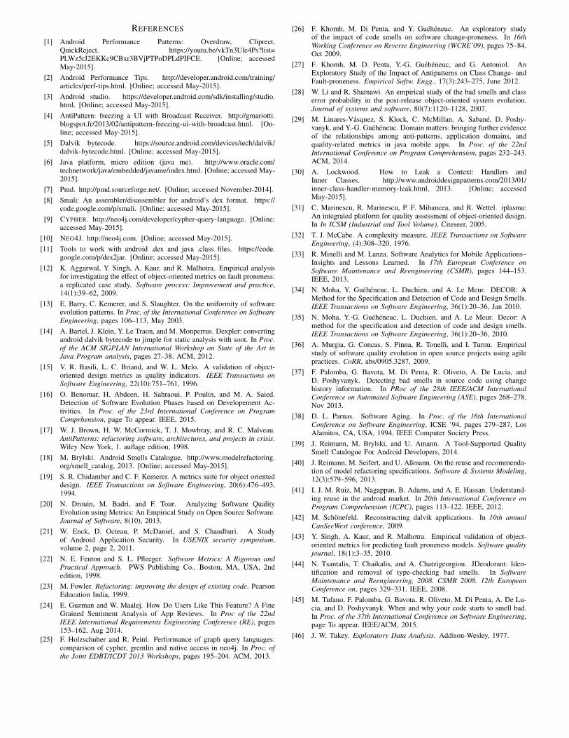
REFERENCES
[1] Android Performance Patterns: Overdraw, Cliprect,QuickReject. https://youtu.be/vkTn3Ule4Ps?list=PLWz5rJ2EKKc9CBxr3BVjPTPoDPLdPIFCE. [Online; accessedMay-2015].
[2] Android Performance Tips. http://developer.android.com/training/articles/perf-tips.html. [Online; accessed May-2015].
[3] Android studio. https://developer.android.com/sdk/installing/studio.html. [Online; accessed May-2015].
[4] AntiPattern: freezing a UI with Broadcast Receiver. http://gmariotti.blogspot.fr/2013/02/antipattern-freezing-ui-with-broadcast.html. [On-line; accessed May-2015].
[5] Dalvik bytecode. https://source.android.com/devices/tech/dalvik/dalvik-bytecode.html. [Online; accessed May-2015].
[6] Java platform, micro edition (java me). http://www.oracle.com/technetwork/java/embedded/javame/index.html. [Online; accessed May-2015].
[7] Pmd. http://pmd.sourceforge.net/. [Online; accessed November-2014].[8] Smali: An assembler/disassembler for android’s dex format. https://
code.google.com/p/smali. [Online; accessed May-2015].[9] CYPHER. http://neo4j.com/developer/cypher-query-language. [Online;
accessed May-2015].[10] NEO4J. http://neo4j.com. [Online; accessed May-2015].[11] Tools to work with android .dex and java .class files. https://code.
google.com/p/dex2jar. [Online; accessed May-2015].[12] K. Aggarwal, Y. Singh, A. Kaur, and R. Malhotra. Empirical analysis
for investigating the effect of object-oriented metrics on fault proneness:a replicated case study. Software process: Improvement and practice,14(1):39–62, 2009.
[13] E. Barry, C. Kemerer, and S. Slaughter. On the uniformity of softwareevolution patterns. In Proc. of the International Conference on SoftwareEngineering, pages 106–113, May 2003.
[14] A. Bartel, J. Klein, Y. Le Traon, and M. Monperrus. Dexpler: convertingandroid dalvik bytecode to jimple for static analysis with soot. In Proc.of the ACM SIGPLAN International Workshop on State of the Art inJava Program analysis, pages 27–38. ACM, 2012.
[15] V. R. Basili, L. C. Briand, and W. L. Melo. A validation of object-oriented design metrics as quality indicators. IEEE Transactions onSoftware Engineering, 22(10):751–761, 1996.
[16] O. Benomar, H. Abdeen, H. Sahraoui, P. Poulin, and M. A. Saied.Detection of Software Evolution Phases based on Developement Ac-tivities. In Proc. of the 23rd International Conference on ProgramComprhension, page To appear. IEEE, 2015.
[17] W. J. Brown, H. W. McCormick, T. J. Mowbray, and R. C. Malveau.AntiPatterns: refactoring software, architectures, and projects in crisis.Wiley New York, 1. auflage edition, 1998.
[18] M. Brylski. Android Smells Catalogue. http://www.modelrefactoring.org/smell catalog, 2013. [Online; accessed May-2015].
[19] S. R. Chidamber and C. F. Kemerer. A metrics suite for object orienteddesign. IEEE Transactions on Software Engineering, 20(6):476–493,1994.
[20] N. Drouin, M. Badri, and F. Tour. Analyzing Software QualityEvolution using Metrics: An Empirical Study on Open Source Software.Journal of Software, 8(10), 2013.
[21] W. Enck, D. Octeau, P. McDaniel, and S. Chaudhuri. A Studyof Android Application Security. In USENIX security symposium,volume 2, page 2, 2011.
[22] N. E. Fenton and S. L. Pfleeger. Software Metrics: A Rigorous andPractical Approach. PWS Publishing Co., Boston, MA, USA, 2ndedition, 1998.
[23] M. Fowler. Refactoring: improving the design of existing code. PearsonEducation India, 1999.
[24] E. Guzman and W. Maalej. How Do Users Like This Feature? A FineGrained Sentiment Analysis of App Reviews. In Proc of the 22ndIEEE International Requirements Engineering Conference (RE), pages153–162, Aug 2014.
[25] F. Holzschuher and R. Peinl. Performance of graph query languages:comparison of cypher, gremlin and native access in neo4j. In Proc. ofthe Joint EDBT/ICDT 2013 Workshops, pages 195–204. ACM, 2013.
[26] F. Khomh, M. Di Penta, and Y. Gueheneuc. An exploratory studyof the impact of code smells on software change-proneness. In 16thWorking Conference on Reverse Engineering (WCRE’09), pages 75–84,Oct 2009.
[27] F. Khomh, M. D. Penta, Y.-G. Gueheneuc, and G. Antoniol. AnExploratory Study of the Impact of Antipatterns on Class Change- andFault-proneness. Empirical Softw. Engg., 17(3):243–275, June 2012.
[28] W. Li and R. Shatnawi. An empirical study of the bad smells and classerror probability in the post-release object-oriented system evolution.Journal of systems and software, 80(7):1120–1128, 2007.
[29] M. Linares-Vasquez, S. Klock, C. McMillan, A. Sabane, D. Poshy-vanyk, and Y.-G. Gueheneuc. Domain matters: bringing further evidenceof the relationships among anti-patterns, application domains, andquality-related metrics in java mobile apps. In Proc. of the 22ndInternational Conference on Program Comprehension, pages 232–243.ACM, 2014.
[30] A. Lockwood. How to Leak a Context: Handlers andInner Classes. http://www.androiddesignpatterns.com/2013/01/inner-class-handler-memory-leak.html, 2013. [Online; accessedMay-2015].
[31] C. Marinescu, R. Marinescu, P. F. Mihancea, and R. Wettel. iplasma:An integrated platform for quality assessment of object-oriented design.In In ICSM (Industrial and Tool Volume). Citeseer, 2005.
[32] T. J. McCabe. A complexity measure. IEEE Transactions on SoftwareEngineering, (4):308–320, 1976.
[33] R. Minelli and M. Lanza. Software Analytics for Mobile Applications–Insights and Lessons Learned. In 17th European Conference onSoftware Maintenance and Reengineering (CSMR), pages 144–153.IEEE, 2013.
[34] N. Moha, Y. Gueheneuc, L. Duchien, and A. Le Meur. DECOR: AMethod for the Specification and Detection of Code and Design Smells.IEEE Transactions on Software Engineering, 36(1):20–36, Jan 2010.
[35] N. Moha, Y.-G. Gueheneuc, L. Duchien, and A. Le Meur. Decor: Amethod for the specification and detection of code and design smells.IEEE Transactions on Software Engineering, 36(1):20–36, 2010.
[36] A. Murgia, G. Concas, S. Pinna, R. Tonelli, and I. Turnu. Empiricalstudy of software quality evolution in open source projects using agilepractices. CoRR, abs/0905.3287, 2009.
[37] F. Palomba, G. Bavota, M. Di Penta, R. Oliveto, A. De Lucia, andD. Poshyvanyk. Detecting bad smells in source code using changehistory information. In PRoc of the 28th IEEE/ACM InternationalConference on Automated Software Engineering (ASE), pages 268–278,Nov 2013.
[38] D. L. Parnas. Software Aging. In Proc. of the 16th InternationalConference on Software Engineering, ICSE ’94, pages 279–287, LosAlamitos, CA, USA, 1994. IEEE Computer Society Press.
[39] J. Reimann, M. Brylski, and U. Amann. A Tool-Supported QualitySmell Catalogue For Android Developers, 2014.
[40] J. Reimann, M. Seifert, and U. Aßmann. On the reuse and recommenda-tion of model refactoring specifications. Software & Systems Modeling,12(3):579–596, 2013.
[41] I. J. M. Ruiz, M. Nagappan, B. Adams, and A. E. Hassan. Understand-ing reuse in the android market. In 20th International Conference onProgram Comprehension (ICPC), pages 113–122. IEEE, 2012.
[42] M. Schonefeld. Reconstructing dalvik applications. In 10th annualCanSecWest conference, 2009.
[43] Y. Singh, A. Kaur, and R. Malhotra. Empirical validation of object-oriented metrics for predicting fault proneness models. Software qualityjournal, 18(1):3–35, 2010.
[44] N. Tsantalis, T. Chaikalis, and A. Chatzigeorgiou. JDeodorant: Iden-tification and removal of type-checking bad smells. In SoftwareMaintenance and Reengineering, 2008. CSMR 2008. 12th EuropeanConference on, pages 329–331. IEEE, 2008.
[45] M. Tufano, F. Palomba, G. Bavota, R. Oliveto, M. Di Penta, A. De Lu-cia, and D. Poshyvanyk. When and why your code starts to smell bad.In Proc. of the 37th International Conference on Software Engineering,page To appear. IEEE/ACM, 2015.
[46] J. W. Tukey. Exploratory Data Analysis. Addison-Wesley, 1977.
[47] R. Vallee-Rai, P. Co, E. Gagnon, L. Hendren, P. Lam, and V. Sun-daresan. Soot-a java bytecode optimization framework. In Proc. ofthe conference of the Centre for Advanced Studies on Collaborativeresearch, page 13. IBM Press, 1999.
[48] E. Van Emden and L. Moonen. Java Quality Assurance by DetectingCode Smells. In Proc. of the 9th Working Conference on ReverseEngineering (WCRE’02), WCRE ’02, pages 97–, Washington, DC,USA, 2002. IEEE Computer Society.
[49] D. Verloop. Code Smells in the Mobile Applications Domain. PhDthesis, TU Delft, Delft University of Technology, 2013.
[50] G. Xie, J. Chen, and I. Neamtiu. Towards a better understanding ofsoftware evolution: An empirical study on open source software. InIEEE International Conference on Software Maintenance (ICSM’09).,pages 51–60, Sept 2009.
[51] Z. Xing and E. Stroulia. Understanding phases and styles of object-oriented systems’ evolution. In Intl. Conf. Softw. Maint., pages 242–251.
IEEE, 2004.[52] L. Xu. Techniques and Tools for Analyzing and Understanding Android
Applications. PhD thesis, University of California Davis, 2013.[53] A. Yamashita and L. Moonen. Do code smells reflect important
maintainability aspects? In 28th IEEE International Conference onSoftware Maintenance (ICSM), pages 306–315, Sept 2012.
[54] A. Yamashita and L. Moonen. Exploring the impact of inter-smellrelations on software maintainability: An empirical study. In Proc. ofthe 2013 International Conference on Software Engineering, ICSE ’13,pages 682–691, Piscataway, NJ, USA, 2013. IEEE Press.
[55] H. Zhang and S. Kim. Monitoring Software Quality Evolution forDefects. Software, IEEE, 27(4):58–64, July 2010.
[56] T. Zhu, Y. Wu, X. Peng, Z. Xing, and W. Zhao. Monitoring softwarequality evolution by analyzing deviation trends of modularity views.In Proc. of 18th Working Conference on Reverse Engineering, pages229–238, Oct 2011.
High-level Language Support for the Control of
Reconfigurations in Component-based Architectures
Frederico Alvares de Oliveira Jr., Eric Rutten, Lionel Seinturier
To cite this version:
Frederico Alvares de Oliveira Jr., Eric Rutten, Lionel Seinturier. High-level Language Sup-port for the Control of Reconfigurations in Component-based Architectures. 9th EuropeanConference on Software Architecture (ECSA), Sep 2015, Dubrovnick, Croatia. Springer, 9278,pp.285-293, 2015, LNCS. <http://ecsa-conference.org/2015/index.php>. <hal-01160612>
HAL Id: hal-01160612
https://hal.inria.fr/hal-01160612
Submitted on 9 Sep 2015
HAL is a multi-disciplinary open accessarchive for the deposit and dissemination of sci-entific research documents, whether they are pub-lished or not. The documents may come fromteaching and research institutions in France orabroad, or from public or private research centers.
L’archive ouverte pluridisciplinaire HAL, estdestinee au depot et a la diffusion de documentsscientifiques de niveau recherche, publies ou non,emanant des etablissements d’enseignement et derecherche francais ou etrangers, des laboratoirespublics ou prives.
Groupes de travail GLE et RIMEL
141
High-level Language Support for ReconfigurationControl in Component-based Architectures
Frederico Alvares1, Eric Rutten1, and Lionel Seinturier2
1 INRIA Grenoble, France– {frederico.alvares,eric.rutten}@inria.fr2 University of Lille 1 & INRIA Lille, France– [email protected]
Abstract. Architecting in the context of variability has become a realneed in todays software development. Modern software systems and theirarchitecture must adapt dynamically to events coming from the environ-ment (e.g., workload requested by users, changes in functionality) and theexecution platform (e.g., resource availability). Component-based archi-tectures have shown to be very suited for self-adaptation especially withtheir dynamical reconfiguration capabilities. However, existing solutionsfor reconfiguration often rely on low level, imperative, and non formallanguages. This paper presents Ctrl-F, a domain-specific language whoseobjective is to provide high-level support for describing adaptation be-haviours and policies in component-based architectures. It relies on reac-tive programming for formal verification and control of reconfigurations.We integrate Ctrl-F with the FraSCAti Service Component Architecturemiddleware platform, and apply it to the Znn.com self-adaptive casestudy.
1 Introduction
From tiny applications embedded in house appliances or automobiles to hugeCloud services, nowadays software-intensive systems have to fulfill a number ofrequirements in terms safety and Quality of Service (QoS) while facing highlydynamic environments (e.g., varying workloads and changing user requirements)and platforms (e.g., resource availability). This leads to the necessity to engineersuch software systems with principles of self-adaptiveness, i.e., to equip thesesoftware systems with capabilities to cope with dynamically changes.
Component-based Architecture. Software architecture and more specifically soft-ware components have played a very important role in self-adaptiveness. Besidesthe usual benefits of modularity and reuse, adaptability and reconfigurability arekey properties which are sought with this approach: one wants to be able to adaptthe component assemblies in order to cope with new requirements and new exe-cution conditions occurring at run-time. Component-based Architecture definesthe high-level structure of software systems by describing how they are organizedby the means of a composition of components [15], which are usually capturedby an Architecture Description Languages (ADL). In spite of the diversity ofADLs, the architectural elements proposed in almost all of them follow the same
Huitièmes journées nationales du GDR GPL – 8 au 10 juin 2016
142
2 Frederico Alvares de Oliveira Jr., Eric Rutten, Lionel Seinturier
conceptual basis [13]. A component is defined as the most elementary unit ofprocessing or data and it is usually decomposed into two parts: the implementa-tion and the interface. The implementation describes the internal behaviour ofthe component, whereas the interfaces define how the component should inter-act with the environment. A component can be defined as atomic or composite,i.e., composed of other components. A connector mediates diverse forms of in-teractions of inter-component communications, and configuration correspondsto a directed graph of components and connectors describing the application’sstructure. Other elements like attributes, constraints or architectural styles alsoappear in ADLs [13], but for brevity we omit further details on these elements.
Initial assemblies (or configurations) are usually defined with the help ofADLs, whereas adaptive behaviours are achieved by programming fine-grainedactions (e.g., to add, remove, connect elements), in either general-purpose lan-guages within reflective component-based middleware plaforms [20], or with thesupport of reconfiguration domain-specific languages (DSLs)[8]. This low levelof abstraction may turn the definition of transitions among configurations intoa very costly task, which consequently may lead to error-prone adaptive be-haviours. In fact, it may be non-trivial, especially for large and complex archi-tectures, to obtain assurances and guarantees about the result of these reconfig-uration behaviours. We claim that there is a need for a language, not only forthe definition of configurations in the form of component assemblies, but also forthe explicit specification of the transitions among them and the policies drivingwhen and under which conditions reconfigurations should be triggered.
This paper presents Ctrl-F, a language that extends classic ADLs with high-level constructs to express the dynamicity of component-based architectures. Inaddition to the usual description of assemblies (configurations), Ctrl-F also com-prises a set of constructs that are dedicated for the description of: (i) behaviouralaspects, that is, the order and/or conditions under which reconfigurations takeplace; and (ii) policies that have to be enforced all along the execution.
Heptagon/BZR. We formally define the semantics of Ctrl-F with Heptagon/BZR[10], a Reactive Language based on Finite State Automata (FSA). It allows forthe definition of generalized Moore machines, with mixed data-flow equationsand automata. A distinguished characteristics is that its compilation involvesformal tools for Discrete Controller Synthesis (DCS): a controller is automati-cally generated so as to enforce that a system behaves at runtime in concordancewith the specification. The Heptagon/BZR definition of Ctrl-F programs allowsto benefit from: (i) guarantees on the correctness of adaptive behaviours by eitherverification or control (i.e., by DCS); (ii) the compilation of adaptive behaviourstowards executable code in general purpose languages (e.g., Java or C). Due tospace limitation, the detailed definition is reported on elsewhere [1].
In the remainder of this paper, Sections 2 presents the self-adaptation casestudy Znn.com [7], used all along the paper. Section 3 presents the Ctrl-F lan-guage. Section 4 provides some details on its integration with a real componentplatform as well as the evaluation of its applicability through Znn.com. Relatedwork is discussed in Section 5 and Section 6 concludes this paper.
Groupes de travail GLE et RIMEL
143
High-level Language Support for Reconfiguration Control in Components 3
2 The Znn.com Example Application
Znn.com [7] is an experimental platform for self-adaptive applications, whichmimics a news website. Znn.com follows a typical client-server n-tiers architec-ture where a load balancer redirects requests from clients to a pool of replicatedservers. The number of active servers can be regulated in order to maintain agood trade-off between response time and resource utilization. Hence, the ob-jective of Znn.com is to provide news content to its clients/visitors within areasonable response time, while keeping costs as low as possible and/or undercontrol (i.e., constrained by a certain budget).
At times, the pool of servers is not large enough to provide the desired QoS.For instance, in order to face workload spikes, Znn.com could be forced to de-grade the content fidelity so as to require fewer resource to provide the same levelof QoS. For this, Znn.com servers are able to deliver news contents with threedifferent content fidelity: (i) high quality images, (ii) low quality images, and(iii) only text. The objectives are: (1) Keep the performance (response time) ashigh as possible; (2) Keep content fidelity as high as possible or above a certainthreshold; (3) Keep the number of active servers as low as possible or under acertain threshold. In order to achieve them, we may tune: (1) The number ofactive servers; (2) The content fidelity of each server.
As a running example for our proposal, in the next section, we extendZnn.com by enabling its replication in presence of different content providers:one specialized in soccer and another one specialized in politics. These two in-stances of Znn.com will be sharing the same physical infrastructure. Dependingon the contract signed between the service provider and his/her clients thatestablishes the terms of use of the service, Znn.com Service Provider can givemore or less priority to a certain client. For instance, during the World Cup thecontent provider specialized in soccer will always have priority over the otherone. Conversely, during the elections, the politics-specialized content provider isthe one that has the priority.
3 Ctrl-F Language
3.1 Overview and Common Concepts
Ctrl-F is our proposal for a domain-specific language that extends classic ADLswith high-level constructs for describing reconfigurations’ behaviour and policiesto be enforced all along the execution of the target system.
The abstract syntax of Ctrl-F can be divided into two parts: a static one,which is related to the common architectural concepts (components, connec-tions, configurations, etc.); and a dynamic one, which refers to reconfigurationbehaviours and policies that must be enforced regardless of the configuration.
The static part of Ctrl-F shares the same concepts of many existing ADLs(e.g., Fractal [6], Acme [13]). A component consists of a set of interfaces, a set ofevent ports, a set of attributes and a set of configurations. Interfaces define howa component can interact with other components. So they are used to express a
Huitièmes journées nationales du GDR GPL – 8 au 10 juin 2016
144
4 Frederico Alvares de Oliveira Jr., Eric Rutten, Lionel Seinturier
required functionality (client interface) that may be provided by another com-ponent and/or to express a provided functionally (server interface) that mightbe used by other components. Event Ports describe the events, of the givenEvent Type, a component is able to emit (port out) and/or listen to (port in).A configuration is defined as a set of instances of components, a set of bindingsconnecting server and client interfaces of those instances (i.e., an assembly),and/or a set of attribute assignments to values.
The dynamic part consists of a behaviour and a set of policies that can bedefined for each component. A behaviour takes the form of orders and conditions(w.r.t. events and attribute values) under which transitions between configura-tions (reconfigurations) take place. The policies are high-level objectives/con-straints, which may imply in the inhibition of some of those transitions.
The Znn.com example application of Section 2 can be modeled as a hierarchi-cal composition of four components: Main, Znn, LoadBalancer, and AppServer.These components are instantiated according to execution conditions, the systemcurrent state (architectural composition), adaptation behaviours and policies de-fined within each component. Listing 1.1 shows the definition of such componentswith the static part of Ctrl-F.
The Main component (lines 1-14) encompasses two instances of Znn, namelysoccer and politics within a single configuration (lines 7 and 8). The serverinterfaces of both instances (lines 9 and 10), which provides access to newsservices, are bound to the server interfaces of the Main component (lines 3 and4) in order for them to be accessed from outside. A policy to be enforced isdefined (line 13) and discussed in Section 3.3.
Component Znn (lines 16-33) consists of one provided interface (line 18)through which news can be requested. The component listens to events of typesoload (overload) and uload (underload) (lines 20 and 21), which are emittedby other components. In addition, the component also defines two attributes:consumption (line 23), which is used to express the level of consumption (interms of percentage of CPU) incurred by the component execution; and fidelity(line 24), which expresses the content fidelity level of the component.
Three configurations are defined for Znn component: conf1, conf2 and conf3.conf1 (lines 26-33) consists of one instance of each LoadBalancer and AppServer(lines 27 and 28); one binding to connect them (line 29), another binding toexpose the server interface of the LoadBalancer component as a server interfaceof the Znn component (line 30), and the attribute assignments (lines 31 and 32).The attribute fidelity corresponds to the counterpart of instance as1, whereasfor the consumption it corresponds to the sum of the consumptions of instancesas1 and lb. conf2 (lines 34-39) extends conf1 by adding one more instance ofAppServer, binding it to the LoadBalancer and redefining the attribute valueswith respect to the just-added component instance (as2 ).
In that case, the attribute fidelity values the average of the counterparts ofinstances as1 and as2 (line 37), whereas for the consumption the same logics isapplied so the consumption of the just-added instance is incorporated to the sumexpression (line 38). Due to lack of space we omit the definition of configuration
Groupes de travail GLE et RIMEL
145
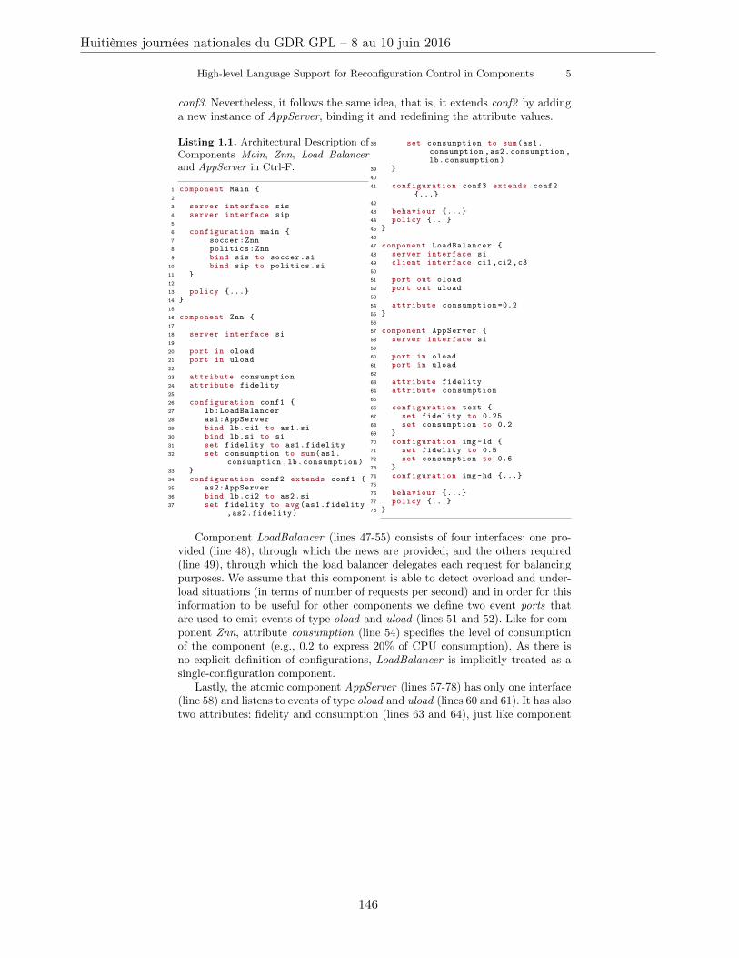
High-level Language Support for Reconfiguration Control in Components 5
conf3. Nevertheless, it follows the same idea, that is, it extends conf2 by addinga new instance of AppServer, binding it and redefining the attribute values.
Listing 1.1. Architectural Description ofComponents Main, Znn, Load Balancerand AppServer in Ctrl-F.
1 component Main {2
3 server interface sis4 server interface sip5
6 configuration main {7 soccer:Znn8 politics:Znn9 bind sis to soccer.si
10 bind sip to politics.si11 }12
13 policy {...}14 }15
16 component Znn {17
18 server interface si19
20 port in oload21 port in uload22
23 attribute consumption24 attribute fidelity25
26 configuration conf1 {27 lb:LoadBalancer28 as1:AppServer29 bind lb.ci1 to as1.si30 bind lb.si to si31 set fidelity to as1.fidelity32 set consumption to sum(as1.
consumption ,lb.consumption)33 }34 configuration conf2 extends conf1 {35 as2:AppServer36 bind lb.ci2 to as2.si37 set fidelity to avg(as1.fidelity
,as2.fidelity)
38 set consumption to sum(as1.consumption ,as2.consumption ,lb.consumption)
39 }40
41 configuration conf3 extends conf2{...}
42
43 behaviour {...}44 policy {...}45 }46
47 component LoadBalancer {48 server interface si49 client interface ci1 ,ci2 ,c350
51 port out oload52 port out uload53
54 attribute consumption =0.255 }56
57 component AppServer {58 server interface si59
60 port in oload61 port in uload62
63 attribute fidelity64 attribute consumption65
66 configuration text {67 set fidelity to 0.2568 set consumption to 0.269 }70 configuration img -ld {71 set fidelity to 0.572 set consumption to 0.673 }74 configuration img -hd {...}75
76 behaviour {...}77 policy {...}78 }
Component LoadBalancer (lines 47-55) consists of four interfaces: one pro-vided (line 48), through which the news are provided; and the others required(line 49), through which the load balancer delegates each request for balancingpurposes. We assume that this component is able to detect overload and under-load situations (in terms of number of requests per second) and in order for thisinformation to be useful for other components we define two event ports thatare used to emit events of type oload and uload (lines 51 and 52). Like for com-ponent Znn, attribute consumption (line 54) specifies the level of consumptionof the component (e.g., 0.2 to express 20% of CPU consumption). As there isno explicit definition of configurations, LoadBalancer is implicitly treated as asingle-configuration component.
Lastly, the atomic component AppServer (lines 57-78) has only one interface(line 58) and listens to events of type oload and uload (lines 60 and 61). It has alsotwo attributes: fidelity and consumption (lines 63 and 64), just like component
Huitièmes journées nationales du GDR GPL – 8 au 10 juin 2016
146
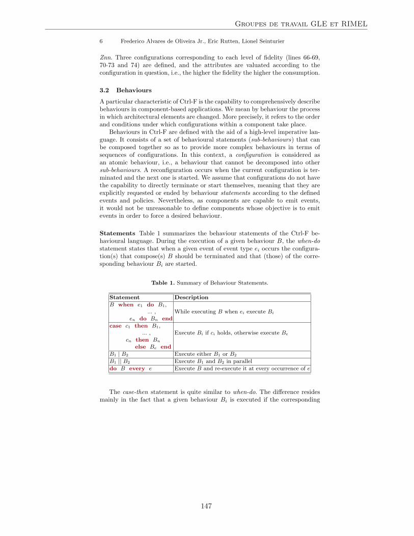
6 Frederico Alvares de Oliveira Jr., Eric Rutten, Lionel Seinturier
Znn. Three configurations corresponding to each level of fidelity (lines 66-69,70-73 and 74) are defined, and the attributes are valuated according to theconfiguration in question, i.e., the higher the fidelity the higher the consumption.
3.2 Behaviours
A particular characteristic of Ctrl-F is the capability to comprehensively describebehaviours in component-based applications. We mean by behaviour the processin which architectural elements are changed. More precisely, it refers to the orderand conditions under which configurations within a component take place.
Behaviours in Ctrl-F are defined with the aid of a high-level imperative lan-guage. It consists of a set of behavioural statements (sub-behaviours) that canbe composed together so as to provide more complex behaviours in terms ofsequences of configurations. In this context, a configuration is considered asan atomic behaviour, i.e., a behaviour that cannot be decomposed into othersub-behaviours. A reconfiguration occurs when the current configuration is ter-minated and the next one is started. We assume that configurations do not havethe capability to directly terminate or start themselves, meaning that they areexplicitly requested or ended by behaviour statements according to the definedevents and policies. Nevertheless, as components are capable to emit events,it would not be unreasonable to define components whose objective is to emitevents in order to force a desired behaviour.
Statements Table 1 summarizes the behaviour statements of the Ctrl-F be-havioural language. During the execution of a given behaviour B, the when-dostatement states that when a given event of event type ei occurs the configura-tion(s) that compose(s) B should be terminated and that (those) of the corre-sponding behaviour Bi are started.
Table 1. Summary of Behaviour Statements.
Statement Description
B when e1 do B1,... , While executing B when ei execute Bi
en do Bn end
case c1 then B1,... , Execute Bi if ci holds, otherwise execute Be
cn then Bn
else Be end
B1 | B2 Execute either B1 or B2
B1 || B2 Execute B1 and B2 in parallel
do B every e Execute B and re-execute it at every occurrence of e
The case-then statement is quite similar to when-do. The difference residesmainly in the fact that a given behaviour Bi is executed if the corresponding
Groupes de travail GLE et RIMEL
147
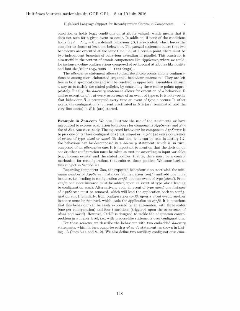
High-level Language Support for Reconfiguration Control in Components 7
condition ci holds (e.g., conditions on attribute values), which means that itdoes not wait for a given event to occur. In addition, if none of the conditionsholds (c1 ∧ ... ∧ cn = 0), a default behaviour (Be) is executed, which forces thecompiler to choose at least one behaviour. The parallel statement states that twobehaviours are executed at the same time, i.e., at a certain point, there must betwo independent branches of behaviour executing in parallel. This construct isalso useful in the context of atomic components like AppServer, where we could,for instance, define configurations composed of orthogonal attributes like fidelityand font size/color (e.g., text || font-huge).
The alternative statement allows to describe choice points among configura-tions or among more elaborated sequential behaviour statements. They are leftfree in local specifications and will be resolved in upper level assemblies, in sucha way as to satisfy the stated policies, by controlling these choice points appro-priately. Finally, the do-every statement allows for execution of a behaviour Band re-execution of it at every occurrence of an event of type e. It is noteworthythat behaviour B is preempted every time an event of type e occurs. In otherwords, the configuration(s) currently activated in B is (are) terminated, and thevery first one(s) in B is (are) started.
Example in Znn.com We now illustrate the use of the statements we haveintroduced to express adaptation behaviours for components AppServer and Znnthe of Znn.com case study. The expected behaviour for component AppServer isto pick one of its three configurations (text, img-ld or img-hd) at every occurrenceof events of type oload or uload. To that end, as it can be seen in Listing 1.2,the behaviour can be decomposed in a do-every statement, which is, in turn,composed of an alternative one. It is important to mention that the decision onone or other configuration must be taken at runtime according to input variables(e.g., income events) and the stated policies, that is, there must be a controlmechanism for reconfigurations that enforces those policies. We come back tothis subject in Section 4.1.
Regarding component Znn, the expected behaviour is to start with the min-imum number of AppServer instances (configuration conf1 ) and add one moreinstance, i.e., leading to configuration conf2, upon an event of type (oload). Fromconf2, one more instance must be added, upon an event of type oload leadingto configuration conf3. Alternatively, upon an event of type uload, one instanceof AppServer must be removed, which will lead the application back to config-uration conf1. Similarly, from configuration conf3, upon a uload event, anotherinstance must be removed, which leads the application to conf2. It is notoriousthat this behaviour can be easily expressed by an automaton, with three states(one per configuration) and four transitions (triggered upon the occurrence ofoload and uload). However, Ctrl-F is designed to tackle the adaptation controlproblem in a higher level, i.e., with process-like statements over configurations.
For these reasons, we describe the behaviour with two embedded do-everystatements, which in turn comprise each a when-do statement, as shown in List-ing 1.3 (lines 6-14 and 8-12). We also define two auxiliary configurations: emit-
Huitièmes journées nationales du GDR GPL – 8 au 10 juin 2016
148
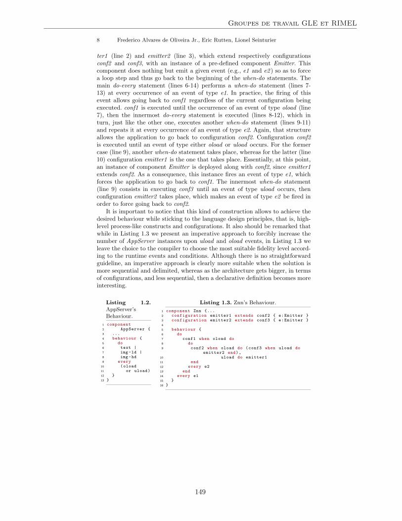
8 Frederico Alvares de Oliveira Jr., Eric Rutten, Lionel Seinturier
ter1 (line 2) and emitter2 (line 3), which extend respectively configurationsconf2 and conf3, with an instance of a pre-defined component Emitter. Thiscomponent does nothing but emit a given event (e.g., e1 and e2 ) so as to forcea loop step and thus go back to the beginning of the when-do statements. Themain do-every statement (lines 6-14) performs a when-do statement (lines 7-13) at every occurrence of an event of type e1. In practice, the firing of thisevent allows going back to conf1 regardless of the current configuration beingexecuted. conf1 is executed until the occurrence of an event of type oload (line7), then the innermost do-every statement is executed (lines 8-12), which inturn, just like the other one, executes another when-do statement (lines 9-11)and repeats it at every occurrence of an event of type e2. Again, that structureallows the application to go back to configuration conf2. Configuration conf2is executed until an event of type either oload or uload occurs. For the formercase (line 9), another when-do statement takes place, whereas for the latter (line10) configuration emitter1 is the one that takes place. Essentially, at this point,an instance of component Emitter is deployed along with conf2, since emitter1extends conf2. As a consequence, this instance fires an event of type e1, whichforces the application to go back to conf1. The innermost when-do statement(line 9) consists in executing conf3 until an event of type uload occurs, thenconfiguration emitter2 takes place, which makes an event of type e2 be fired inorder to force going back to conf2.
It is important to notice that this kind of construction allows to achieve thedesired behaviour while sticking to the language design principles, that is, high-level process-like constructs and configurations. It also should be remarked thatwhile in Listing 1.3 we present an imperative approach to forcibly increase thenumber of AppServer instances upon uload and oload events, in Listing 1.3 weleave the choice to the compiler to choose the most suitable fidelity level accord-ing to the runtime events and conditions. Although there is no straightforwardguideline, an imperative approach is clearly more suitable when the solution ismore sequential and delimited, whereas as the architecture gets bigger, in termsof configurations, and less sequential, then a declarative definition becomes moreinteresting.
Listing 1.2.AppServer’sBehaviour.
1 component2 AppServer {3 ...4 behaviour {5 do6 text |7 img -ld |8 img -hd9 every
10 (oload11 or uload)12 }13 }
Listing 1.3. Znn’s Behaviour.
1 component Znn {...2 configuration emitter1 extends conf2 { e:Emitter }3 configuration emitter2 extends conf3 { e:Emitter }4
5 behaviour {6 do7 conf1 when oload do8 do9 conf2 when oload do (conf3 when uload do
emitter2 end),10 uload do emitter111 end12 every e213 end14 every e115 }16 }
Groupes de travail GLE et RIMEL
149
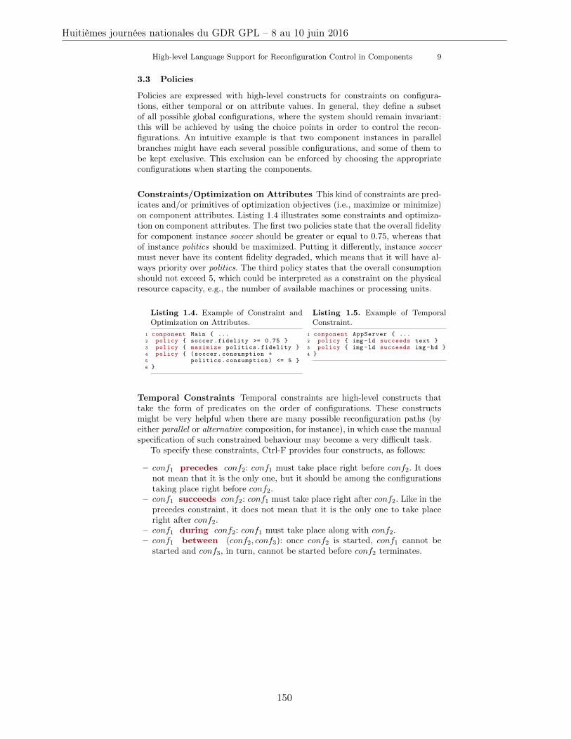
High-level Language Support for Reconfiguration Control in Components 9
3.3 Policies
Policies are expressed with high-level constructs for constraints on configura-tions, either temporal or on attribute values. In general, they define a subsetof all possible global configurations, where the system should remain invariant:this will be achieved by using the choice points in order to control the recon-figurations. An intuitive example is that two component instances in parallelbranches might have each several possible configurations, and some of them tobe kept exclusive. This exclusion can be enforced by choosing the appropriateconfigurations when starting the components.
Constraints/Optimization on Attributes This kind of constraints are pred-icates and/or primitives of optimization objectives (i.e., maximize or minimize)on component attributes. Listing 1.4 illustrates some constraints and optimiza-tion on component attributes. The first two policies state that the overall fidelityfor component instance soccer should be greater or equal to 0.75, whereas thatof instance politics should be maximized. Putting it differently, instance soccermust never have its content fidelity degraded, which means that it will have al-ways priority over politics. The third policy states that the overall consumptionshould not exceed 5, which could be interpreted as a constraint on the physicalresource capacity, e.g., the number of available machines or processing units.
Listing 1.4. Example of Constraint andOptimization on Attributes.
1 component Main { ...2 policy { soccer.fidelity >= 0.75 }3 policy { maximize politics.fidelity }4 policy { (soccer.consumption +5 politics.consumption) <= 5 }6 }
Listing 1.5. Example of TemporalConstraint.
1 component AppServer { ...2 policy { img -ld succeeds text }3 policy { img -ld succeeds img -hd }4 }
Temporal Constraints Temporal constraints are high-level constructs thattake the form of predicates on the order of configurations. These constructsmight be very helpful when there are many possible reconfiguration paths (byeither parallel or alternative composition, for instance), in which case the manualspecification of such constrained behaviour may become a very difficult task.
To specify these constraints, Ctrl-F provides four constructs, as follows:
– conf1 precedes conf2: conf1 must take place right before conf2. It doesnot mean that it is the only one, but it should be among the configurationstaking place right before conf2.
– conf1 succeeds conf2: conf1 must take place right after conf2. Like in theprecedes constraint, it does not mean that it is the only one to take placeright after conf2.
– conf1 during conf2: conf1 must take place along with conf2.– conf1 between (conf2, conf3): once conf2 is started, conf1 cannot be
started and conf3, in turn, cannot be started before conf2 terminates.
Huitièmes journées nationales du GDR GPL – 8 au 10 juin 2016
150
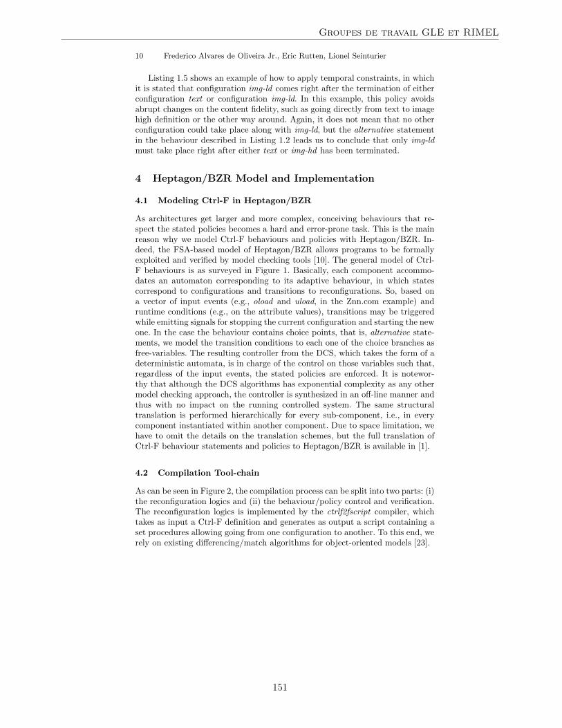
10 Frederico Alvares de Oliveira Jr., Eric Rutten, Lionel Seinturier
Listing 1.5 shows an example of how to apply temporal constraints, in whichit is stated that configuration img-ld comes right after the termination of eitherconfiguration text or configuration img-ld. In this example, this policy avoidsabrupt changes on the content fidelity, such as going directly from text to imagehigh definition or the other way around. Again, it does not mean that no otherconfiguration could take place along with img-ld, but the alternative statementin the behaviour described in Listing 1.2 leads us to conclude that only img-ldmust take place right after either text or img-hd has been terminated.
4 Heptagon/BZR Model and Implementation
4.1 Modeling Ctrl-F in Heptagon/BZR
As architectures get larger and more complex, conceiving behaviours that re-spect the stated policies becomes a hard and error-prone task. This is the mainreason why we model Ctrl-F behaviours and policies with Heptagon/BZR. In-deed, the FSA-based model of Heptagon/BZR allows programs to be formallyexploited and verified by model checking tools [10]. The general model of Ctrl-F behaviours is as surveyed in Figure 1. Basically, each component accommo-dates an automaton corresponding to its adaptive behaviour, in which statescorrespond to configurations and transitions to reconfigurations. So, based ona vector of input events (e.g., oload and uload, in the Znn.com example) andruntime conditions (e.g., on the attribute values), transitions may be triggeredwhile emitting signals for stopping the current configuration and starting the newone. In the case the behaviour contains choice points, that is, alternative state-ments, we model the transition conditions to each one of the choice branches asfree-variables. The resulting controller from the DCS, which takes the form of adeterministic automata, is in charge of the control on those variables such that,regardless of the input events, the stated policies are enforced. It is notewor-thy that although the DCS algorithms has exponential complexity as any othermodel checking approach, the controller is synthesized in an off-line manner andthus with no impact on the running controlled system. The same structuraltranslation is performed hierarchically for every sub-component, i.e., in everycomponent instantiated within another component. Due to space limitation, wehave to omit the details on the translation schemes, but the full translation ofCtrl-F behaviour statements and policies to Heptagon/BZR is available in [1].
4.2 Compilation Tool-chain
As can be seen in Figure 2, the compilation process can be split into two parts: (i)the reconfiguration logics and (ii) the behaviour/policy control and verification.The reconfiguration logics is implemented by the ctrlf2fscript compiler, whichtakes as input a Ctrl-F definition and generates as output a script containing aset procedures allowing going from one configuration to another. To this end, werely on existing differencing/match algorithms for object-oriented models [23].
Groupes de travail GLE et RIMEL
151
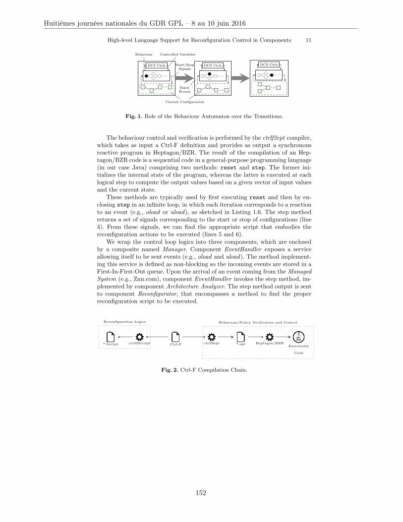
High-level Language Support for Reconfiguration Control in Components 11
...
DCS Ctrlr
...
...
DCS Ctrlr
...
...
DCS Ctrlr
...
Current Configuration
Behaviour
Start/StopSignals
InputEvents
Controlled Variables
Fig. 1. Role of the Behaviour Automaton over the Transitions.
The behaviour control and verification is performed by the ctrlf2ept compiler,which takes as input a Ctrl-F definition and provides as output a synchronousreactive program in Heptagon/BZR. The result of the compilation of an Hep-tagon/BZR code is a sequential code in a general-purpose programming language(in our case Java) comprising two methods: reset and step. The former ini-tializes the internal state of the program, whereas the latter is executed at eachlogical step to compute the output values based on a given vector of input valuesand the current state.
These methods are typically used by first executing reset and then by en-closing step in an infinite loop, in which each iteration corresponds to a reactionto an event (e.g., oload or uload), as sketched in Listing 1.6. The step methodreturns a set of signals corresponding to the start or stop of configurations (line4). From these signals, we can find the appropriate script that embodies thereconfiguration actions to be executed (lines 5 and 6).
We wrap the control loop logics into three components, which are enclosedby a composite named Manager. Component EventHandler exposes a serviceallowing itself to be sent events (e.g., oload and uload). The method implement-ing this service is defined as non-blocking so the incoming events are stored in aFirst-In-First-Out queue. Upon the arrival of an event coming from the ManagedSystem (e.g., Znn.com), component EventHandler invokes the step method, im-plemented by component Architecture Analyzer. The step method output is sentto component Reconfigurator, that encompasses a method to find the properreconfiguration script to be executed.
Ctrl-F ctrlf2ept *.ept Heptagon/BZRExecutable
Code
Behaviour/Policy Verification and Control
ctrlf2fscript*.fscript
Reconfiguration Logics
Fig. 2. Ctrl-F Compilation Chain.
Huitièmes journées nationales du GDR GPL – 8 au 10 juin 2016
152
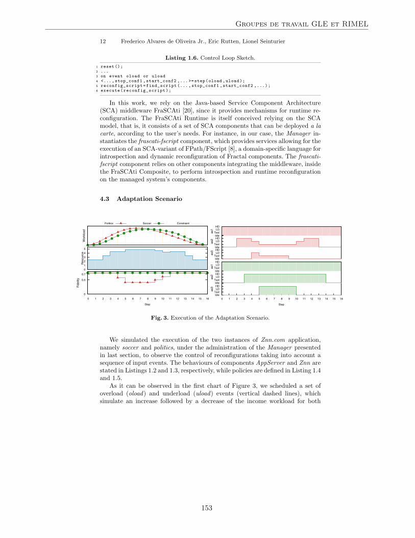
12 Frederico Alvares de Oliveira Jr., Eric Rutten, Lionel Seinturier
Listing 1.6. Control Loop Sketch.
1 reset();2 ...3 on event oload or uload4 <...,stop_conf1 ,start_conf2 ,...>= step(oload ,uload);5 reconfig_script=find_script (..., stop_conf1 ,start_conf2 ,...);6 execute(reconfig_script);
In this work, we rely on the Java-based Service Component Architecture(SCA) middleware FraSCAti [20], since it provides mechanisms for runtime re-configuration. The FraSCAti Runtime is itself conceived relying on the SCAmodel, that is, it consists of a set of SCA components that can be deployed a lacarte, according to the user’s needs. For instance, in our case, the Manager in-stantiates the frascati-fscript component, which provides services allowing for theexecution of an SCA-variant of FPath/FScript [8], a domain-specific language forintrospection and dynamic reconfiguration of Fractal components. The frascati-fscript component relies on other components integrating the middleware, insidethe FraSCAti Composite, to perform introspection and runtime reconfigurationon the managed system’s components.
4.3 Adaptation Scenario
Wor
kloa
d
Politics Soccer Constraint
0 1 2 3 4 5
Res
ourc
e
0
0.5
0.7
Fide
lity
IdleText
LDHD
as1
IdleText
LDHD
as2
IdleText
LDHD
as3
IdleText
LDHD
as1
IdleText
LDHD
as2
IdleText
LDHD
0 1 2 3 4 5 6 7 8 9 10 11 12 13 14 15 16
as3
Step
Wor
kloa
d
Politics Soccer Constraint
0 1 2 3 4 5
Res
ourc
e
0
0.5
0.7
Fide
lity
IdleText
LDHD
as1
IdleText
LDHD
as2
IdleText
LDHD
as3
IdleText
LDHD
as1
IdleText
LDHD
as2
IdleText
LDHD
0 1 2 3 4 5 6 7 8 9 10 11 12 13 14 15 16
as3
Step
Wor
kloa
d
Politics Soccer Constraint
0 1 2 3 4 5
Res
ourc
e
0
0.5
0.7
Fide
lity
IdleText
LDHD
as1
IdleText
LDHD
as2
IdleText
LDHD
as3
IdleText
LDHD
as1
IdleText
LDHD
as2
IdleText
LDHD
0 1 2 3 4 5 6 7 8 9 10 11 12 13 14 15 16
as3
Step
Fig. 3. Execution of the Adaptation Scenario.
We simulated the execution of the two instances of Znn.com application,namely soccer and politics, under the administration of the Manager presentedin last section, to observe the control of reconfigurations taking into account asequence of input events. The behaviours of components AppServer and Znn arestated in Listings 1.2 and 1.3, respectively, while policies are defined in Listing 1.4and 1.5.
As it can be observed in the first chart of Figure 3, we scheduled a set ofoverload (oload) and underload (uload) events (vertical dashed lines), whichsimulate an increase followed by a decrease of the income workload for both
Groupes de travail GLE et RIMEL
153
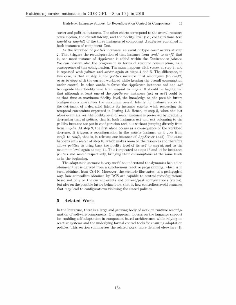
High-level Language Support for Reconfiguration Control in Components 13
soccer and politics instances. The other charts correspond to the overall resourceconsumption, the overall fidelity, and the fidelity level (i.e., configurations text,img-ld or img-hd) of the three instances of component AppServer contained inboth instances of component Znn.
As the workload of politics increases, an event of type oload occurs at step2. That triggers the reconfiguration of that instance from conf1 to conf2, thatis, one more instance of AppServer is added within the Znninstance politics.We can observe also the progression in terms of resource consumption, as aconsequence of this configuration. The same happens with soccer at step 3, andis repeated with politics and soccer again at steps 4 and 5. The difference, inthis case, is that at step 4, the politics instance must reconfigure (to conf3 )so as to cope with the current workload while keeping the overall consumptionunder control. In other words, it forces the AppServer instances as2 and as3to degrade their fidelity level from img-hd to img-ld. It should be highlightedthat although at least one of the AppServer instances (as2 or as3 ) could beat that time at maximum fidelity level, the knowledge on the possible futureconfigurations guarantees the maximum overall fidelity for instance soccer tothe detriment of a degraded fidelity for instance politics, while respecting thetemporal constraints expressed in Listing 1.5. Hence, at step 5, when the lastoload event arrives, the fidelity level of soccer instance is preserved by graduallydecreasing that of politics, that is, both instances as2 and as3 belonging to thepolitics instance are put in configuration text, but without jumping directly fromfrom img-hd. At step 9, the first uload occurs as a consequence of the workloaddecrease. It triggers a reconfiguration in the politics instance as it goes fromconf3 to conf2, that is, it releases one instance of AppServer (as3 ). The samehappens with soccer at step 10, which makes room on the resources and thereforeallows politics to bring back the fidelity level of its as2 to img-ld, and to themaximum level again at step 11. This is repeated at steps 13 and 14 for instancespolitics and soccer respectively, bringing their consumptions at the same levelsas in the beginning.
The adaptation scenario is very useful to understand the dynamics behind anManager that is derived from a synchronous reactive programming, which is inturn, obtained from Ctrl-F. Moreover, the scenario illustrates, in a pedagogicalway, how controllers obtained by DCS are capable to control reconfigurationsbased not only on the current events and current/past configurations (states),but also on the possible future behaviours, that is, how controllers avoid branchesthat may lead to configurations violating the stated policies.
5 Related Work
In the literature, there is a large and growing body of work on runtime reconfig-uration of software components. Our approach focuses on the language supportfor enabling self-adaptation in component-based architectures while relying onreactive systems and the underlying formal control tools for ensuring adaptationpolicies. This section summarizes the related work, more detailed elsewhere [1].
Huitièmes journées nationales du GDR GPL – 8 au 10 juin 2016
154
14 Frederico Alvares de Oliveira Jr., Eric Rutten, Lionel Seinturier
Classically, runtime adaption in software architectures is achieved by firstrelying on ADLs such as Acme [13] or Fractal [6] for an initial description of thesoftware structure and architecture, then by specifying fine-grained reconfigura-tion actions with dedicated languages like Plastik [3] or FPath/FScript [8], orsimply by defining Event-Condition-Actions (ECA) rules to lead the system tothe desired state. A harmful consequence is that the space of reachable configu-ration states is only known as side effect of those reconfiguration actions, whichmakes it difficult to ensure correct adaptive behaviours. Moreover, a drawbackof ECA rules is that, contrary to Ctrl-F, they cannot describe sequences of con-figurations. Even though, ECA rules can be expressed in Ctrl-F with a set ofwhen-do (for the E part) and case (for the C and A parts) statements in parallel.
Rainbow [12] is an autonomic framework that comes with Stitch, a domain-specific language allowing for the description of self-adaptation of Acme-describedapplications. It features system-level actions grouped into tactics, which in turn,are aggregated within a tree-like strategy path. We can draw an analogy be-tween tactics and the set of actions triggered upon a reconfiguration; as well asstrategies and behaviours in the Ctrl-F language. Nonetheless, alternative andparallel, as well as event-based constructs make Ctrl-F more expressive. Further-more, Ctrl-F’s formal model enables to ensure correct adaptation behaviours.
A body of work [2][21][22][22][5][17][4] focus on how to plan a set of actionsthat safely lead component-based systems to a target configuration. These ap-proaches are complementary to ours in the sense that our focus is on the choiceof a new configuration and its control. Once a new configuration chosen, werely on existing mechanisms to determine the plan of action actually leading thesystem from the current to the next configuration.
In [18], feature models are used to express variability in software systems. Atruntime, a resolution mechanism is used for determining which features shouldbe present so as to constitute configuration. In the same direction, Pascual etal. [19] propose an approach for optimal resolution of architectural variabilityspecified in the Common Variability Language (CVL) [14]. A drawback of thoseapproaches is that in the adaptation logics specified with feature models orCVL, there is no way to define stateful adaptation behaviours, i.e., sequences ofreconfigurations. The resolution is performed based on the current state and/orconstraints on the feature model. While in our approach, in the reactive modelbased on FSA, decisions are taken also based on the history of configurationswhich allows us to define more interesting adaptation behaviours and policies.
W.r.t. formal methods, Kouchnarenko and Weber [16] propose the use oftemporal logics to integrate temporal requirements to adaptation policies. Whilein this approach, enforcement and reflection are performed at runtime in orderto ensure correct behaviour, we rely on discrete controller synthesis.
As in our approach, in [11], authors also rely on Heptagon/BZR to modeladaptive behaviours of Fractal components. However, there is no high-level de-scription (e.g., ADL) like Ctrl-F, and reconfigurations are controlled at the levelof fine-grained reconfiguration actions, which can be considered time-consumingand difficult to scale. Delaval et al. [9] propose to have modular controllers that
Groupes de travail GLE et RIMEL
155
High-level Language Support for Reconfiguration Control in Components 15
can be coordinated so as to work together in a coherent manner. The approach iscomplementary to ours in the sense that it does not provide high-level languagesupport for describing those managers, although the authors provide interestingintuitions on a methodology to do so.
6 Conclusion
This paper presented Ctrl-F, a high-level domain-specific language that allowsfor the description of adaptation behaviours and policies of component-basedarchitectures. A distinguished feature of Ctrl-F is its formalization with thesynchronous reactive language Heptagon/BZR, which allows to benefit, amongother things, from formal tools for verification, control, and automatic generationof executable code. In order to show the language expressiveness, we applied itto Znn.com, a self-adaptive case study, and we integrated it with FraSCAti, aService Component Architecture middleware.
For future work, we intent to address issues of modularity and coordinationof controllers, as well as their distribution. The reactive language and modelswe rely on have recent results that can be exploited, and can lead to deploycontrollers taking into account the physical location of components.
References
1. Alvares, F., Rutten, E., Seinturier, L.: Behavioural Model-based Control for Au-tonomic Software Components. In: Proc. 12th Int. Conf. Autonomic Computing(ICAC’15). Grenoble, France. (extended version available as a Research Report:https://hal.inria.fr/hal-01103548) (Jul 2015)
2. Arshad, N., Heimbigner, D.: A Comparison of Planning Based Models for Compo-nent Reconfiguration. Research Report CU-CS-995-05, U. Colorado (Sep 2005)
3. Batista, T., Joolia, A., Coulson, G.: Managing dynamic reconfiguration incomponent-based systems. In: Proc. 2nd European Conference on Software Ar-chitecture. pp. 1–17. EWSA’05 (2005)
4. Becker, S., Dziwok, S., Gerking, C., Heinzemann, C., Schafer, W., Meyer, M.,Pohlmann, U.: The mechatronicuml method: Model-driven software engineeringof self-adaptive mechatronic systems. In: Companion Proceedings of the 36th In-ternational Conference on Software Engineering. pp. 614–615. ICSE Companion2014, ACM, New York, NY, USA (2014), http://doi.acm.org/10.1145/2591062.2591142
5. Boyer, F., Gruber, O., Pous, D.: Robust reconfigurations of component assemblies.In: Proc. 2013 Int. Conf. on Software Engineering. pp. 13–22. ICSE ’13 (2013)
6. Bruneton, E., Coupaye, T., Leclercq, M., Quema, V., Stefani, J.B.: An open compo-nent model and its support in java. In: Proc. International Symp. on Component-based Software Engineering (CBSE). Edinburgh, Scotland (May 2003)
7. Cheng, S.W., Garlan, D., Schmerl, B.: Evaluating the effectiveness of the rainbowself-adaptive system. In: Software Engineering for Adaptive and Self-ManagingSystems, 2009. SEAMS ’09. ICSE Workshop on. pp. 132–141 (May 2009)
8. David, P.C., Ledoux, T., Leger, M., Coupaye, T.: FPath & FScript: Languagesupport for navigation and reliable reconfiguration of Fractal architectures. Annalsof Telecommunications: Special Issue on Software Components (2008)
Huitièmes journées nationales du GDR GPL – 8 au 10 juin 2016
156

16 Frederico Alvares de Oliveira Jr., Eric Rutten, Lionel Seinturier
9. Delaval, G., Gueye, S.M.K., Rutten, E., De Palma, N.: Modular coordination ofmultiple autonomic managers. In: Proc. 17th Int. ACM Symp. on Component-based Software Engineering. pp. 3–12. CBSE ’14 (2014)
10. Delaval, G., Marchand, H., Rutten, E.: Contracts for modular discrete controllersynthesis. In: ACM International Conference on Languages, Compilers, and Toolsfor Embedded Systems (LCTES 2010). Stockholm, Sweden (Apr 2010)
11. Delaval, G., Rutten, E.: Reactive model-based control of reconfiguration in thefractal component-based model. In: 13th International Symposium on ComponentBased Software Engineering (CBSE 2010). Prague, Czech Republic (Jun 2010)
12. Garlan, D., Cheng, S.W., Huang, A.C., Schmerl, B., Steenkiste, P.: Rainbow:Architecture-based self-adaptation with reusable infrastructure. Computer 37(10),46–54 (Oct 2004)
13. Garlan, D., Monroe, R.T., Wile, D.: Acme: Architectural description of component-based systems. In: Leavens, G.T., Sitaraman, M. (eds.) Foundations of Component-Based Systems, pp. 47–68. Cambridge University Press (2000)
14. Haugen, O., Wasowski, A., Czarnecki, K.: Cvl: Common variability language. In:Proceedings of the 17th International Software Product Line Conference. pp. 277–277. SPLC ’13, ACM, New York, NY, USA (2013)
15. Jacobson, I., Griss, M., Jonsson, P.: Software reuse: architecture process and orga-nization for business success. ACM Press books, ACM Press (1997)
16. Kouchnarenko, O., Weber, J.F.: Adapting component-based systems at runtime viapolicies with temporal patterns. In: 10th Int. Symp. Formal Aspects of ComponentSoftware. LNCS, vol. 8348, pp. 234–253. Nanchang, China (2014)
17. Luckey, M., Nagel, B., Gerth, C., Engels, G.: Adapt cases: Extending use casesfor adaptive systems. In: Proceedings of the 6th International Symposium on Soft-ware Engineering for Adaptive and Self-Managing Systems. pp. 30–39. SEAMS’11, ACM, New York, NY, USA (2011), http://doi.acm.org/10.1145/1988008.1988014
18. Morin, B., Barais, O., Nain, G., Jezequel, J.M.: Taming dynamically adaptive sys-tems using models and aspects. In: Proc. 31st Int. Conf. on Software Engineering.pp. 122–132. ICSE ’09, IEEE (2009)
19. Pascual, G.G., Pinto, M., Fuentes, L.: Run-time support to manage architecturalvariability specified with cvl. In: Proc. 7th European Conf. on Software Architec-ture. pp. 282–298. ECSA’13 (2013)
20. Seinturier, L., Merle, P., Rouvoy, R., Romero, D., Schiavoni, V., Stefani, J.B.: Acomponent-based middleware platform for reconfigurable service-oriented architec-tures. Software: Practice and Experience 42(5), 559–583 (2012)
21. da Silva, C.E., de Lemos, R.: Dynamic plans for integration testing of self-adaptivesoftware systems. In: Proc. 6th Int. Symp. on Software Engineering for Adaptiveand Self-Managing Systems. pp. 148–157. SEAMS ’11 (2011)
22. Tichy, M., Klopper, B.: Planning self-adaption with graph transformations. In:Proc. 4th Int. Conf. on Applications of Graph Transformations with IndustrialRelevance. pp. 137–152. AGTIVE’11 (2012)
23. Xing, Z., Stroulia, E.: Umldiff: An algorithm for object-oriented design differencing.In: Proc. 20th IEEE/ACM Int. Conf. on Automated Software Engineering. pp. 54–65. ASE ’05 (2005)
Groupes de travail GLE et RIMEL
157

Huitièmes journées nationales du GDR GPL – 8 au 10 juin 2016
158

Session du groupe de travail IDMIngénierie Dirigée par les Modèles
159

Huitièmes journées nationales du GDR GPL – 8 au 10 juin 2016
160
Omniscient Debugging and Concurrent Executionof Heterogeneous Domain-Specific Models
Benoit Combemale
Inria and Univ. Rennes 1, [email protected]
1 Context and Motivations
In the software and systems modeling community, research on domain-specificmodeling languages (DSMLs) is focused on providing technologies for developinglanguages and tools that allow domain experts to develop system solutions effi-ciently. Unfortunately, the current lack of support for explicitly relating conceptsexpressed in different DSMLs makes it very difficult for software and system en-gineers to reason about information spread across models describing differentsystem aspects [2].
As a particular challenge, we investigate in this paper relationships between,possibly heterogeneous, behavioral models to support their concurrent execution.This is achieved first by following a modular executable metamodeling approach[3], which include an explicit model of concurrency (MoC) [4], domain-specificactions (DSA) [6], and a well-defined protocol between them (incl., mapping,feedback and callback) [7]. Then, the protocol is used for inferring a relevantbehavioral language interface supporting the definition of coordination patternsto be applied on the conforming executable models [8].
All the tooling of the approach is gathered within the GEMOC studio. TheGEMOC studio provides a language workbench, seamlessly integrated on top ofthe Eclipse Modeling Framework (EMF), for designing and composing executabledomain-specific modeling languages (xDSML). xDSMLs are then automaticallydeployed into a modeling workbench providing model execution (incl., graphicalanimation and omniscient debugging) and behavioral coordination of, possiblyheterogeneous, models.
2 Approach Overview
2.1 Sirius Animator: Engineering xDSMLs for model executability,animation and debugging
Domain-specific models are used in the development processes to reason andassess specific properties over the system under development as early as possible.This usually leads to a better and cheaper design as more alternatives can beexplored. While many models only represent structural aspects of systems, alarge amount express behavioral aspects of the same systems. Behavioral models
Groupe de travail IDM
161
are used in various areas (e.g., enterprise architecture, software and systemsengineering, scientific modeling. . . ), with very different underlying formalisms(e.g., business processes, orchestrations, functional chains, scenarios, protocoles,activity or state diagram, etc.).
To ensure that a behavioral model is correct with regard to its intendedbehavior, early dynamic validation and verification (V&V) techniques are re-quired, such as simulation, debugging, model checking or runtime verification.In particular, debugging is a common dynamic facility to observe and controlan execution in order to better understand a behavior or to look for the causeof a defect. Standard (stepwise) debugging only provides facilities to pause andstep forward during an execution, hence requiring developers to restart from thebeginning to give a second look at a state of interest. Omniscient debugging ex-tends stepwise debugging by relying on execution traces to enable free traversalof the states reached by a model, thereby allowing designers to “go back in time.”
Debugging, and all dynamic V&V techniques in general, require models to beexecutable, which can be achieved by defining the execution semantics of mod-eling languages (i.e. DSLs) used to describe them. The execution semantics of amodeling language can be implemented either as a compiler or as an interpreterto be applied on models conforming to the modeling language [1].
Despite the specificities of each modeling language captured into the syntaxand the execution semantics, it is possible to identify a common set of debug-ging facilities for all modeling languages: control of the execution (pause, resume,stop), representation of the current state during the execution (i.e., model ani-mation), breakpoint definition, step into/over/out and step forward/backward.To drastically reduce the development cost of domain-specific debuggers, Sir-ius Animator1 provides a tool-supported approach to complement a modelinglanguage with an execution semantics, and automatically get an advanced andextensible environment for model simulation, animation and debugging.
Sirius Animator provides a modular approach to complement an Ecore meta-model with:
– a Java-based interpreter, and– a Sirius-based representation of the execution state.
Both are automatically deployed, together with a generated efficient exe-cution trace metamodel, into an advanced omniscient debugging environmentproviding:
– an integration with the Eclipse debug UI (incl., the binding of the executionstate with the variable view),
– a generic execution engine with execution control facilities (pause, resume,stop),
– a generic control panel (incl. breakpoints, step into/over/out and step for-ward/backward), and
– a generic timeline.1 Cf. https://github.com/SiriusLab/ModelDebugging, and more information athttp://gemoc.org/breathe-life-into-your-designer
Huitièmes journées nationales du GDR GPL – 8 au 10 juin 2016
162
2.2 MoCCML: Reifying the concurrency concern into xDSMLspecifications
The emergence of modern concurrent systems (e.g., Cyber-Physical Systems andInternet of Things) and highly-parallel platforms (e.g., many-core, GPGPU anddistributed platforms) call for Domain-Specific Modeling Languages (DSMLs)where concurrency is of paramount importance. Such DSMLs are intended topropose constructs with rich concurrency semantics, which allow system design-ers to precisely define and analyze system behaviors. However, implementingthe execution semantics of such DSMLs is a particularly difficult task. Most ofthe time the concurrency model remains implicit and ad-hoc, embedded in theunderlying execution environment.
The lack of an explicit concurrency model prevents: the precise definition,the variation and the complete understanding of the DSML’s semantics, theeffective usage of concurrency-aware analysis techniques, and the exploitation ofthe concurrency model during the system refinement (e.g., during its allocationon a specific platform).
To address this issue, we have defined a concurrency-aware executable meta-modeling approach, which supports a modular definition of the execution seman-tics, including the concurrency model, the semantic rules (aka. domain-specificactions, DSA), and a well-defined and expressive communication protocol be-tween them [3]. The protocol supports both the mapping of the concurrencymodel to the semantic rules, and the feedback, possibly with data, from the se-mantic rules to the concurrency model [7]. The concurrent executable metamod-eling approach also comes with a dedicated meta-language, namely MoCCML,to define the concurrency model and the protocol, and an execution environmentto simulate and analyze behavioral models [4].
MoCCML is a declarative meta-language specifying constraints between theevents of a model of concurrency. At any moment during a run, an event that doesnot violate the constraints can occur. The constraints are grouped in librariesthat specify concurrency constraints. These constraints can also be of a differentkinds, for instance to express a deadline, a minimal throughput or a hardwaredeployment. They are eventually instantiated to define the execution model ofa specific model. The execution model is a symbolic representation of all theacceptable schedules for a particular model. To enable the automatic generationof the execution model, the concurrency model is weaved into the context ofspecific concepts from the abstract syntax of a DSML. This contextualizationis defined by a mapping between the elements of the abstract syntax and theconstraints of the concurrency model. The mapping defined in MoCCML is basedon the notion of domain-specific event (DSE). The separation of the mappingfrom the concurrency model makes the concurrency model independent of theDSML so that it can be reused, and semantic variation points can be managed fora single abstract syntax. From such description, for any instance of the abstractsyntax it is possible to automatically generate a dedicated execution model.
Groupe de travail IDM
163
In our approach, the execution model is acting as the configuration of ageneric execution engine that can be used for simulation or analysis of any modelconforming to the abstract syntax of the DSML.
MoCCML is defined by a metamodel (i.e., the abstract syntax) associatedto a formal structural operational semantics. MoCCML2 comes with a modeleditor combining textual and graphical notations, as well as analysis tools basedon the formal semantics for simulation and exhaustive exploration.
2.3 B-COoL: Coordination of xDSMLs for concurrent execution ofheterogeneous models
To capture the specification of coordination patterns between languages, a be-havioral interface is required at the language level. A language behavioral inter-face must abstract the behavioral semantics of a language, thus providing onlythe information required to coordinate it, i.e., a partial representation of concur-rency and time-related aspects. Furthermore, to avoid altering the coordinatedlanguage semantics, the specification of coordination patterns between languagesshould be non intrusive, i.e., it should keep separated the coordination and thecomputation concerns. In the previous subsection, elements of event structuresare reified at the language level to propose a behavioral interface based on sets ofevent types and contraints. Event types (named DSE for Domain Specific Event)are defined in the context of a metaclass of the abstract syntax, and abstract therelevant semantic (domain-specific) actions. Jointly with the DSE, related con-straints give a symbolic (intentional) representation of an event structure. Withsuch an interface, the concurrency and time-related aspects of the language be-havioral semantics are explicitly exposed and the coordination is event-drivenand non intrusive.
Then, for each model conforming to the language, the model behavioral in-terface is a specification, in intention, of an event structure whose events (namedMSE for Model Specific Event) are instances of the DSE defined in the languageinterface. While DSEs are attached to a metaclass, MSEs are linked to one ofits instances. The causality and conflict relations of the event structure are amodel-specific unfolding of the constraints specified in the language behavioralinterface. Just like event structures were initially introduced to unfold the exe-cution of Petri nets, we use them here to unfold the execution of models.
We propose to use DSE as “coordination points" to drive the execution oflanguages. These events are used as control points in two complementary ways: toobserve what happens inside the model, and to control what is allowed to happenor not. When required by the coordination, constraints are used to forbid or delaysome event occurrences. Forbidding occurrences reduces what can be done byindividual models. When several executions are allowed (i.e., nondeterminism),it gives some freedom to individual semantics for making their own choices.All this put together makes the DSE suitable to drive coordinated simulations
2 Cf. https://github.com/gemoc/concurrency
Huitièmes journées nationales du GDR GPL – 8 au 10 juin 2016
164
without being intrusive in the models. Coordination patterns are captured asconstraints at the language level on the DSE.
BCOoL is a dedicated (meta)language to explicitly capture the knowledgeabout system integration [8]. With BCOoL, an integrator can explicitly capturecoordination patterns at the language level. Specific operators are provided tobuild the coordination patterns and specify how the DSE of different languagebehavioral interfaces are combined and interact. From the BCOoL specification,an executable and formal coordination model can be generated by instantiatingall the constraints on all instances of DSE. Therefore, the generated coordinationmodel implements the coordination patterns defined at the language level.
The design of BCOoL is inspired by current structural composition lan-guages, relying on the matching and merging phases of syntactic model elements.A matching rule specifies what elements from different models are selected. Amerging rule specifies how the selected model elements are composed. In theseapproaches the specification is at the language level, but the application is be-tween models. Similarly, a BCOoL operator relies on a correspondence matchingand a coordination rule. The correspondence matching identifies what elementsfrom the behavioral interfaces (i.e., what instances of DSE) must be selected.The merging phase is replaced by a coordination rule. While in the structuralcase the merging operates on the syntax, the coordination rule operates on ele-ments of the semantics (i.e., instances of DSE). Thus, coordination rules specifythe, possibly timed, synchronizations and causality relationships between theinstances of DSE selected during the matching.
BCOoL3 comes with a textual editor to support the specification of coordina-tion patterns between xDSMLs, as well as a generative approach to instantiatea set of selected coordination patterns for a given set of models.
3 The GEMOC Studio
The GEMOC Studio is an Eclipse package, seamlessly integrated with the EclipseModelign Framework, that contains components supporting the GEMOCmethod-ology for building and composing executable Domain-Specific Modeling Lan-guages (DSMLs). It includes two workbenches: the GEMOC Language Work-bench and the GEMOC Modeling Workbench. The language workbench is in-tended to be used by language designers (aka domain experts), it allows tocomplement Ecore metamodels to build and compose executable DSMLs. TheModeling Workbench is intended to be used by domain designers, it allows tocreate and execute heterogeneous models conforming to executable DSMLs.
The GEMOC Studio results in various integrated tools that belong into eitherthe language workbench or the modeling workbench. The language workbenchput together the following tools seamlessly integrated to the Eclipse ModelingFramework (EMF)4:
3 Cf. https://github.com/gemoc/coordination4 Cf. https://eclipse.org/modeling/emf
Groupe de travail IDM
165
– Melange (http://melange-lang.org), a tool-supported meta-language to mod-ularly define executable modeling languages with execution functions anddata, and to extend (EMF-based) existing modeling languages [5].
– MoCCML, a tool-supported meta-language dedicated to the specification ofa Model of Concurrency and Communication (MoCC) and its mapping to aspecific abstract syntax of a modeling language [4].
– GEL, a tool-supported meta-language dedicated to the specification of theprotocol between the execution functions and the MoCC to support feedbackof the runtime data and to support the callback of other expected executionfunctions [7].
– BCOoL (http://timesquare.inria.fr/BCOoL), a tool-supported meta-languagededicated to the specification of language coordination patterns, to automat-ically coordinates the execution of, possibly heterogeneous, models [8].
– Sirius Animator, an extension to the model graphical syntax designer Sirius(http://www.eclipse.org/sirius) to create graphical animators for executablemodeling languages5.
The different concerns of an executable modeling language (as defined withthe tools of the language workbench) are automatically deployed into the mod-eling workbench that provides the following tools:
– A Java-based execution engine (parameterized with the specification of theexecution functions), possibly coupled with TimeSquare6 (parameterizedwith the MoCC), to support the concurrent execution and analysis of anyconforming models.
– A model animator parameterized by the graphical representation definedwith Sirius Animator to animate executable models.
– A generic control panel mapped to the Eclipse debug UI to control theexecution of a running model (pause, resume, and step forward/backward)and define breakpoints.
– A generic trace manager, which allows system designers to visualize, save,replay, and investigate different execution traces of their models.
– A generic event manager, which provides a user interface for injecting ex-ternal stimuli in the form of events during the simulation (e.g., to simulatethe environment).
– An heterogeneous coordination engine (parametrized with the specificationof the coordination in BCOoL), which provides runtime support to simulateheterogeneous executable models.
The GEMOC studio is open-source and domain-independent. The studio isavailable at http://gemoc.org/studio.
5 For more details on Sirius Animator, we refer the reader tohttp://siriuslab.github.io/talks/BreatheLifeInYourDesigner/slides
6 Cf. http://timesquare.inria.fr
Huitièmes journées nationales du GDR GPL – 8 au 10 juin 2016
166
4 Conclusion
The GEMOC studio provides the necessary tools to complement an EMF-basedmodeling language with a modular and formal behavioral semantics, possiblyincluding an explicit model of concurrency. Such an executable domain-specificmodeling language (xDSML) is automatically deployed in the modeling frame-work to support model execution, graphical animation, omniscient debuggingand concurrency analysis. The model of concurrency is also the support of thedefinition of coordination patterns between different xDSMLs. Such coordina-tion patterns are used to automatically generate the coordination between a setof specific conforming models.
The major scientific breakthroughs addressed by this work are i) the cross-fertilization of the algorithm theory and the concurrency theory to reify theconcurrency concern in the specification of an operational semantics of a DSML,ii) the characterization of an event-based behavioral language interface, and iii)the reification of the coordination concerns at the language level.
The tool-supported appraoch presented in this paper open various perspec-tives regarding model executability, including the coordination of discrete andcontinuous models, the co-simulation (incl., FMI), the definition of adaptableconcurrency model (e.g., design space exploration, optimizing compilers, codeadaptation, code obfuscation), as well as the support of live and collaborativemodeling.
Acknowledgement. This work is supported by the ANR INS Project GEMOC(ANR-12-INSE-0011) and The GEMOC Initiative (cf. http://gemoc.org/ins).
References
1. Combemale, B., Crégut, X., Garoche, P.L., Thirioux, X.: Essay on Semantics Defini-tion in MDE. An Instrumented Approach for Model Verification. Journal of Software4(9), 943–958 (Nov 2009)
2. Combemale, B., Deantoni, J., Baudry, B., France, R., Jézéquel, J.M., Gray, J.:Globalizing Modeling Languages. Computer pp. 68–71 (Jun 2014)
3. Combemale, B., Deantoni, J., Vara Larsen, M., Mallet, F., Barais, O., Baudry,B., France, R.: Reifying Concurrency for Executable Metamodeling. In: 6th Inter-national Conference on Software Language Engineering (SLE). Lecture Notes inComputer Science, Springer-Verlag (2013)
4. Deantoni, J., Issa Diallo, P., Teodorov, C., Champeau, J., Combemale, B.: Towardsa Meta-Language for the Concurrency Concern in DSLs. In: Design, Automationand Test in Europe Conference and Exhibition (DATE) (Mar 2015)
5. Degueule, T., Combemale, B., Blouin, A., Barais, O., Jézéquel, J.M.: Melange: AMeta-language for Modular and Reusable Development of DSLs. In: 8th Interna-tional Conference on Software Language Engineering (SLE) (Oct 2015)
6. Jézéquel, J.M., Combemale, B., Barais, O., Monperrus, M., Fouquet, F.: Mashupof Meta-Languages and its Implementation in the Kermeta Language Workbench.Software and Systems Modeling 14(2), 905–920 (2015)
Groupe de travail IDM
167

7. Latombe, F., Crégut, X., Combemale, B., Deantoni, J., Pantel, M.: Weaving Con-currency in eXecutable Domain-Specific Modeling Languages. In: 8th ACM SIG-PLAN International Conference on Software Language Engineering (SLE). ACM,Pittsburg, United States (2015)
8. Vara Larsen, M.E., Deantoni, J., Combemale, B., Mallet, F.: A Behavioral Coordi-nation Operator Language (BCOoL). In: International Conference on Model DrivenEngineering Languages and Systems (MODELS). p. 462. No. 18, ACM (Sep 2015)
Huitièmes journées nationales du GDR GPL – 8 au 10 juin 2016
168
Model-Driven Process Engineering for flexible yet sound process modeling, execution and verification
Reda Bendraou
Sorbonne Universités, UPMC Univ Paris 06, UMR 7606, F-75005, Paris, France
By capturing team’s best practices, task ordering, flows of artifacts, agent coordination and commu-nications, process models succeeded to become an important asset which ensures repeatability and quality in building software. In the context of large-scale industrial projects, they are more than vital and represent the means to foster the respect of project’s deadlines and reliability criteria.
For many years, process models have been used only for training and communication purposes. However, they are used more and more as inputs for PSEEs (Process-centered Software Engineering Environments) to be enacted. The enactment of a process model consists of improving the coordination between the project’s developers by automatically affecting the activities to the appropriate roles, rout-ing the artifacts from one activity into another and ensuring the monitoring of activity’s deadlines. The role of the PSEE is also to enforce the fact that the developers respect the execution order of the pro-cess’s activities and to make sure that they deliver the accurate outcomes. This is how a company can guarantee the repeatability of its development processes and thus, gains in maturity and reliability.
However, this is based on three strong assumptions: (i) the first, is that the process model is accu-rate and perfectly captures the right activities, milestones, artifacts and roles. This also means that it represents the best possible enactment of a process for a given project’s context. (ii) The second assumption is that the process’s agents are strictly following the process model and that they don’t take any personal initiative to perform the process differently. (iii) The third assumption is that the process model is sound and free of any inconsistencies. The notion of soundness here relates to the fact that there is no blocking state, unreachable activities, etc. while inconsistencies can be more relat-ed to some of the process’s business or organizational constraints that might be violated with one of the possible enactment scenarios of the process.
Regarding the first assumption, for companies that have adopted process modeling and depending on the context, process models represent the outcome of many years of experience, best practices and process iterations. In some domains such as health care or military procedures, these models are inten-sively tested and evaluated before they are used in real production projects. If some improvements are identified during process iterations, they usually have to undergo a test and validation phases before-hand to be integrated to the process model. However, in the software domain this assumption is not always satisfied. Development processes depend on too many human factors and resources which make them highly unpredictable. Due to unexpected project constraints, occasionally, process models may have to evolve or be adapted during the process enactment. Examples of such constraints are: canceling the execution of some process’s activities, switching the order of their execution or extend-ing their deadlines.
The second assumption is also related to the process domain. In critical processes, it is unthinkable that the agent deviates from the process model. This would have critical impacts on the safety of the process. However, in software processes, this is different. Empirical studies showed that most agents do not follow an assigned process 98% of the time. This comes from the fact that developers may be confronted with unanticipated situations which are not represented in the process model, future and unexpected project constraints or their ability to accomplish the activity according to their experience and intuitions.
Finally, regarding the third assumption, investigations on some process repositories demonstrated that between 10% [Mendling 09] to 50% [Vanhatalo 07] of process models are flawed and contain inconsistencies. If you consider some critical businesses, having unsound process models could be
Groupe de travail IDM
169
very harmful for the quality of the delivered services and products. The SOA (Service Oriented Archi-tecture) for instance heavily relies on representing the company’s valuable processes in terms of BPMN (Business Process Modeling Notation) process models. These BPMN models are then used to automatically derive the web services’ orchestration (calls) through a BPEL code (Business Process Execution Language). Having flawed BMPN process models would negatively impact this orchestra-tion.
These three strong, and evidently wrong, assumptions were exactly the reasons why we initiated our work on the detection and handling of deviations in process enactment as well as our work on process verification. They were also in a way, what led to the fact that developers and some process actors lose faith in process execution engines and monitoring tools. For the two last decades the proposed solu-tions were either too much restrictive forbidding any kind of deviations or too permissive and lacked the automatic support for decision making initiatives. Probably one sure yet obvious think I confirmed after 12 years working on the topic of processes, is that no one can ever force humans to follow a pro-cess! Once this fact is recognized, the only possible option is to compromise with the different factors intervening in the realization of a process and to bring flexibility in the way you want to achieve pro-cess’s goals. One could compare this to the notion of optimistic transactions in concurrent program-ming i.e. I am optimistic, I believe that everything will go as planned, but if any problem arises, I should be informed so I can act accordingly. Flexibility was one of our main driving goals in the dif-ferent contributions that will be presented in this document. However, as this will be demonstrated too, this was never achieved at the expense of formality and reliability aspects.
Our second driving goal was to work for a larger adoption of process technologies by the indus-try. At this aim, every approach we proposed these last 12 years is based on mainstream standards and frameworks and comes with an intuitive, user-friendly tool that can be integrated to mainstream mod-eling tools and development environments. One again, this was always based on solid and formal basis which remains a critical goal for us.
The presentation will go through the different contributions we made to face the above mentioned issues/assumptions. It essentially presents our work on detecting and handling deviations during pro-cess enactment [Almeida 10, 11, 13] and our work on process verification[Laurent 13, 14a, 14b]. Flex-ibility and a larger adoption were the driving goals but at the same time, these goals where challenged by various issues and research objectives. A detailed motivation of the issues and challenges we tried to solve under each topic is giving in the presentation. Each topic’s research objectives are justi-fied, after which the solutions we proposed are presented. Obviously, this would never be as exhaus-tive as the material that one can find in our published papers which remain the master source for more details.
It is worth noticing that these contributions are interdisciplinary and revolve around three main axes: Process Engineering, Model-Driven Engineering and Formal methods.
References
[Almeida 10] M.A. Almeida da Silva, R. Bendraou, X. Blanc and M-P. Gervais, "Early Deviation Detection in Modeling activi-ties of MDE Processes", in proceedings of MoDELS 2010, LNCS, Springer, October 3-8, 2010. [Almeida 11] M.A. Almeida da Silva, X. Blanc and R. Bendraou, "Deviation Management during Process Execution", in pro-ceedings of the 26th IEEE/ACM Int. Conf. On Automated Software Engineering (ASE 2011), November 2011, [Almeida 13] Marcos Aurélio Almeida da Silva, Xavier Blanc, Reda Bendraou, Marie-Pierre Gervais. "Experiments on the impact of deviations to process execution" in the ISI Journal (Ingénierie des Systèmes d’Information), 18(3) : 295-119 (2013) [Laurent 13] Laurent, Y., Bendraou, R., Gervais, M.P. : Generation of Process using Multi-Objective Genetic Algorithm. In : Proceedings of the 2013 International Conference on Software and Systems Process, ACM (2013), 161-165 [Laurent 14a] Y. Laurent, R. Bendraou, S. Baarir, M.‑P. Gervais : “Formalization of fUML: An Application to Process Verifica-tion”, CAiSE 2014, Springer, p347-363 [Laurent 14b]Y. Laurent, R. Bendraou, S. Baarir, M.-P. Gervais : Alloy4SPV : a Formal Framework for Software Process Veri-fication, in ECMFA, Lecture Notes in Computer Science, pp.83-100, (Springer) (2014) [Mendling 09] Jan Mendling. Empirical studies in process model verification. In Transactions on Petri Nets and Other Models of Concurrency II, pages 208–224. Springer, 2009. 3, 4 [Vanhatalo 07]J.Vanhatalo, H. Völzer, and F.Leymann. Faster and more focused control-flow analysis for business process models through sese decomposition. In ICSOC 2007, pages 43–55. Springer, 2007. 3, 33, 143
Huitièmes journées nationales du GDR GPL – 8 au 10 juin 2016
170
An Overview of OMG Specifications for Executable UML Mod-eling.
Arnaud Cuccuru, Jérémie Tatibouet, Sahar Guermazi, Sébastien Revol and
Sébastien Gérard CEA, LIST, Laboratory of Model Driven Engineering for Embedded Systems
P.C. 174, Gif-sur-Yvette, 91191, France <firstname.lastname>@cea.fr
The purpose of this presentation is to give an introduction on a series of OMG
standard specifications dealing with executable UML modeling, as well as to demon-strate concrete usages of these specifications.
In the first part of the talk, the following specifications are presented: fUML [1],
PSCS [2], PSSM [3], and Alf [4]. fUML (Semantics of a Foundational Subset for Executable UML Models) identifies a subset of the UML metamodel, and provides a formal execution model for it. Any model defined with this subset can be interpreted by the execution model. The subset mostly comprises UML Classes for structural modeling, and UML Activities for behavioral modeling. While voluntarily minimalis-tic, this subset is expressive enough to describe systems composed of communicating concurrent entities, with reactive behaviors. The fUML execution model is designed following the Visitor design pattern. Each (executable) element of the fUML abstract syntax is associated with a semantic visitor that describes its execution semantics.
PSCS (Precise Semantics of UML Composite Structures) extends fUML with the
ability to model structured classes, which can have ports, and an internal structure based on interconnected parts. These capabilities provide the basis for component-oriented modeling in UML. The fUML execution model is extended as well, in order to account for key aspects of composite structures. It includes aspects related to the life cycle of composite objects (instantiation/destruction of composite structures and their constituents) as well as the semantics of communications (propagation of re-quests and messages along ports and connectors).
PSSM (Precise Semantics of UML State Machines) is an ongoing standardization
effort, which aims at further extending fUML and PSCS with State Machine model-ing. State machines are one of the most used behavioral formalism in UML, and will significantly help in broadening the scope of application domains for these series of OMG specifications on executable UML modeling. At the time this presentation is given, an initial submission has already been voted (March 2016), and a revised sub-mission is scheduled for September 2016.
To conclude the first part of the talk, we introduce Alf, the Action Language for
fUML. The Alf specification focuses on syntactic aspects of executable UML model-
Groupe de travail IDM
171
ing, by providing a concrete and concise textual notation for fUML. Alf basically enables to program directly in UML. As such, it greatly improves the productivity of executable model designers.
In the second part of the talk, we highlight the added value of these specifications
with tooling and usage examples taken from actual CEA LIST R&D activities, which leverage their formal execution semantics for specific uses and/or application do-mains: Performing tradeoff analysis with discrete event simulation, controlling and observing systems with models at runtime, and evaluating executable UML models in a Cyber-Physical System co-simulation environment (by relying on the FMI – Func-tional Mockup Interface – co-simulation standard).
[1] Semantics of a foundational subset for executable UML models (fUML)
http://www.omg.org/spec/FUML/ [2] Precise semantics of UML composite structures (PSCS)
http://www.omg.org/spec/PSCS/ [3] Precise semantics of UML state machines RFP (PSSM)
http://www.omg.org/cgi-bin/doc.cgi?ad/2015-3-2 [4] Action language for foundational UML (Alf) http://www.omg.org/spec/ALF/
Huitièmes journées nationales du GDR GPL – 8 au 10 juin 2016
172

Session du groupe de travail IEIngénierie des Exigences
173

Huitièmes journées nationales du GDR GPL – 8 au 10 juin 2016
174
Utilisation des ontologies pour l’ingénierie des exigencesDriss Sadoun1
1 : INALCO, [email protected].
L’ingénierie des exigences (IE) consiste à comprendre ce que l’on a l’intention de concevoiravant de le concevoir. Elle repose sur la capture de connaissances pouvant provenir de diversessources et parties prenantes ayant leurs propres intérêts et points de vue. L’objectif principal estde permettre une compréhension commune, par les différents intervenants du système à concevoir,afin de guider et de faciliter sa réalisation. En général, cette compréhension est représentée sousla forme de documents écrits, ce qui correspond à la spécification des exigences.
La spécification d’exigences est un travail collaboratif. Les exigences doivent être simples etspécifiées dans un langage commun, qu’experts et non experts seront aptes à comprendre. Ellessont donc généralement écrites en langue naturelle (LN). En revanche, le manque de rigueur etl’ambiguïté inhérente aux textes rédigés en LN peut mener à des différences d’interprétation entreles parties prenantes et mener à des problèmes de conception. Ainsi, il n’est pas aisé de spécifierun ensemble complet et cohérent d’exigences. Les exigences et leur qualité ont alors tendance àévoluer au fil du processus de développement et de la compréhension du système à concevoir.L’amélioration des spécifications d’exigences passe entre autres par les phases d’analyse et devérification. Pour cela, elles doivent être représentées de telle sorte à pouvoir être traitées par desméthodes de vérification formelle.
Les spécifications formelles qui sont plus précises et concises que les spécifications LN consti-tuent un meilleur point de départ pour les étapes d’analyse, de vérification et de conception. Ilest plus aisé d’éviter les erreurs de conception en passant de spécifications formelles à une implé-mentation [Andrews et Gibbins, 1988]. Cependant, la complexité de leur syntaxe et, plus encore,leurs fondements mathématiques, les rendent difficilement compréhensibles pour une personne nonexperte. La validation des exigences dans leur forme finale requiert alors le plus souvent qu’ellessoient décrites en langue naturelle, de sorte à être contractuelles.
Lors de la conception d’un système, spécifications LN et spécifications formelles sont donccomplémentaires. Mener à terme un projet d’ingénierie impose l’emploi itératif de ces deux forma-lismes dans un processus évolutif. Gérer les transitions entre ces représentations est la clé du succèsde toute tâche d’ingénierie [Kitapci et Boehm, 2006]. La difficulté principale d’une telle transitionréside dans l’ampleur du fossé entre spécifications LN et spécifications formelles. Cette questiona été abordée par l’emploi de formalismes intermédiaires [Bajwa et al., 2012, Guissé et al., 2012,Njonko et El Abed, 2012, Sadoun, 2014] permettant de réduire ce fossé. La problématique est alorsde choisir une représentation suffisamment formelle et précise pour permettre un passage automa-tisé vers des spécifications formelles et suffisamment expressive pour représenter la sémantique deconnaissances formulées en langage naturel.
Au fil du temps, les langues naturelles ont évolué davantage pour répondre au besoin decommunication qu’au besoin de représentation [Russell et al., 1996]. De sorte que les connais-sances nécessaires à l’interprétation d’un texte en LN ne sont pas forcément toutes explicitées.Les connaissances dont l’inférence est supposée possible sont le plus souvent laissées implicites.Ces connaissances implicites peuvent être inférées à partir de connaissances partagées par le(s)rédacteur(s) et ses lecteurs.
Ces dernières années, les ontologies se sont imposées comme l’un des modèles de représenta-tion les plus simples et efficaces pour la description d’un domaine d’application. En effet, ellespermettent d’expliciter et de formaliser les concepts clés d’un domaine ainsi que leurs proprié-tés, définissant ainsi le vocabulaire conceptuel du domaine. Chaque élément de ce vocabulaire
1
Groupe de travail IE
175
doit posséder une interprétation unique, issue d’une compréhension commune et partagée. Cecadre unificateur permet de passer de jargons individuels à une terminologie commune, atténuantainsi les malentendus au sujet des termes et permettant de réduire la confusion terminologique etconceptuelle.
Le potentiel des ontologies comme moyen de représenter les connaissances d’un domaine, d’amé-liorer la compréhension commune, de préciser et d’organiser les connaissances, amène une quantitécroissante de travaux à s’intéresser à leur utilisation dans le domaine de l’ingénierie des exigences(IE). Notamment, pour la spécification [Souag., 2012, Al Balushi et al., 2013], l’interopérabilité[Boukhari et al., 2012], la validation [Körner et Brumm, 2010, Chniti et al., 2012] ou l’améliora-tion [Castañeda et al., 2012, Körner et Brumm, 2010] des d’exigences.
Les fondements logiques des ontologies permettent de décrire de manière formelle et donc inter-prétable par les machine, le comportement et les contraintes d’un système [Sadoun et al., 2011]. Ilest alors possible à l’aide de techniques de traitement automatique de la langue (TAL) d’exploiterles connaissances formalisées au sein d’une ontologie pour guider l’extraction automatique de nou-velles connaissances dans des spécifications d’exigences en langue naturelle [Sadoun et al., 2013b,Sadoun et al., 2013a]. Ces nouvelles connaissances peuvent alors s’ajouter aux connaissances del’ontologie pour représenter une instanciation particulière, celle de la spécification d’exigencesanalysée. En outre, les mécanismes d’inférence associés aux ontologies permettent non seule-ment de déduire des connaissances implicites ou erronées, mais aussi de vérifier la complétude,la cohérence et la conformité des connaissances modélisées [Sadoun et al., 2012]. Par ailleurs, leformalisme logique des ontologies autorise une transformation simple et intuitive de la représen-tation issue de l’analyse des spécification d’exigence LN vers un langage de spécification formel[Sadoun et al., 2014], permettant l’application de méthodes de vérification formelle. Enfin, l’onto-logie, en tant que modèle de représentation conçu pour capturer la sémantique du langage naturel,permet de garder une trace du lien entre les deux niveaux de spécifications et ainsi de faciliter lanavigation entre spécifications en langue naturelle et spécifications formelles [Sadoun, 2014].
Références[Al Balushi et al., 2013] Al Balushi, T. H., Sampaio, P. R. F. et Loucopoulos, P. (2013).
Eliciting and prioritizing quality requirements supported by ontologies : a case study using theelicito framework and tool. Expert Systems, 30(2):129–151.
[Andrews et Gibbins, 1988] Andrews, D. et Gibbins, P. (1988). An Introduction to Formal Me-thods of Software Development. An Introduction to Formal Methods of Software Development.McGraw-Hill Education.
[Bajwa et al., 2012] Bajwa, I. S., Bordbar, B., Lee, M. et Anastasakis, K. (2012). Nl2alloy :A tool to generate alloy from nl constraints. Journal of Digital Information Management, 10(6).
[Boukhari et al., 2012] Boukhari, I., Bellatreche, L. et Jean, S. (2012). An ontological pivotmodel to interoperate heterogeneous user requirements. In Proceedings of the 5th internatio-nal conference on Leveraging Applications of Formal Methods, Verification and Validation :applications and case studies - Volume Part II, ISoLA’12, pages 344–358.
[Castañeda et al., 2012] Castañeda, V., Ballejos, L. C. et Caliusco, M. L. (2012). Improvingthe quality of software requirements specifications with semantic web technologies. In WER.
[Chniti et al., 2012] Chniti, A., Albert, P. et Charlet, J. (2012). Gestion de la cohérence desrègles métier éditées à partir d’ontologies owl. In Actes de IC2011, pages 589–606.
[Guissé et al., 2012] Guissé, A., Lévy, F. et Nazarenko, A. (2012). From regulatory texts tobrms : how to guide the acquisition of business rules ? In Proceedings of the 6th internationalconference on Rules on the Web : research and applications (RuleML’12), pages 77–91.
[Kitapci et Boehm, 2006] Kitapci, H. et Boehm, B. W. (2006). Using a hybrid method forformalizing informal stakeholder requirements inputs. In Proceedings of the Fourth InternationaWorkshop on Comparative Evaluation in Requirements Engineering (CERE ’06), pages 48–59.
2
Huitièmes journées nationales du GDR GPL – 8 au 10 juin 2016
176
[Körner et Brumm, 2010] Körner, S. J. et Brumm, T. (2010). Natural language specificationimprovement with ontologies. International Journal of Semantic Computing (IJSC), 3(4):445–470.
[Njonko et El Abed, 2012] Njonko, P. et El Abed, W. (2012). From natural language busi-ness requirements to executable models via sbvr. In Systems and Informatics (ICSAI), 2012International Conference on.
[Russell et al., 1996] Russell, S. J., Norvig, P., Candy, J. F., Malik, J. M. et Edwards, D. D.(1996). Artificial intelligence : a modern approach. Prentice-Hall, Inc.
[Sadoun, 2014] Sadoun, D. (2014). Des spécifications en langage naturel aux spécifications for-melles via une ontologie comme modèle pivot. Thèse de doctorat, Univ. Paris 11.
[Sadoun et al., 2011] Sadoun, D., Dubois, C., Ghamri-Doudane, Y. et Grau, B. (2011). Anontology for the conceptualization of an intelligent environment and its operation. In 10thMexican International Conference on Artificial Intelligence (MICAI), pages 16–22.
[Sadoun et al., 2012] Sadoun, D., Dubois, C., Ghamri-Doudane, Y. et Grau, B. (2012). For-malisation en owl pour vérifier les spécifications d’un environnement intelligent. In Actes de laconférence RFIA.
[Sadoun et al., 2013a] Sadoun, D., Dubois, C., Ghamri-Doudane, Y. et Grau, B. (2013a).From natural language requirements to formal specification using an ontology. In 25th Inter-national Conference on Tools with Artificial Intelligence (ICTAI).
[Sadoun et al., 2013b] Sadoun, D., Dubois, C., Ghamri-Doudane, Y. et Grau, B. (2013b).Peuplement d’une ontologie guidé par l’identification d’instances de propriété. In Actes de la10e conférence TIA.
[Sadoun et al., 2014] Sadoun, D., Dubois, C., Ghamri-Doudane, Y. et Grau, B. (2014). For-mal rule representation and verification from natural language requirements using an ontology.In RuleML 2014, Prague, Czech Republic, pages 226–235.
[Souag., 2012] Souag., A. (2012). Vers une nouvelle génération de définition des exigences desécurité fondée sur l’utilisation des ontologies. In INFORSID, pages 583–590.
3
Groupe de travail IE
177

Huitièmes journées nationales du GDR GPL – 8 au 10 juin 2016
178
Vérification Formelle d’ObservateursOrientée Contexte
Ciprian Teodorov, Philippe [email protected],[email protected]
Lab-STICC, UMR CNRS 6285, ENSTA Bretagne, Brest.
Malgré la performance croissante des outils de model − checking, leur utilisa-tion reste difficile en contexte industriel. Leur intégration dans un processusd’ingénierie industriel est encore trop faible comparativement à l’énorme besoinde fiabilité dans les systèmes critiques. Cette contradiction trouve en partie sescauses dans la difficulté réelle de mettre en œuvre des concepts théoriques dansun contexte industriel. Une première difficulté liée à l’utilisation de ces tech-niques de vérification provient du problème bien identifié de l’explosion com-binatoire du nombre de comportements des modèles, induite par la complexitéinterne du logiciel qui doit être vérifié. Cela est particulièrement vrai dans le casdes systèmes embarqués temps réel, qui interagissent avec des environnementsimpliquant un grand nombre d’entités. Une autre difficulté est liée à l’expressionformelle des propriétés nécessaire à leur vérification. Traditionnellement, cetteexpression s’effectue à l’aide de formalismes tels que les logiques temporelles.Bien que ces logiques aient une grande expressivité, elles ne sont pas faciles àutiliser par des ingénieurs dans des contextes industriels.
L’approche développée dans nos travaux a pour vocation d’appréhender lesdifficultés mentionnées précédemment. Elle repose sur deux idées conjointes :d’une part, réduire les comportements du système à valider lors du model-checking de manière à repousser plus loin les limites de l’explosion combinatoireet, d’autre part, aider l’utilisateur à spécifier les propriétés formelles à vérifier.Pour cela, nous avons proposé un langage nommé CDL (Context DescriptionLanguage) [DBR11,DBRL12] pour la spécification de contextes et de propriétésformelles. Ce langage est associé à l’outil OBP1 qui permet d’explorer des mod-èles au format Fiacre [FGP+08] et prend en charge les descriptions CDL. Lesmodèles Fiacre peuvent provenir de chaînes de transformation de modèles décritsdans des formalismes de plus haut niveau tel que UML ou SysML et largementutilisés dans les équipes de développement. De nombreuses expérimentationsde cet outil ont été menées en collaboration avec des partenaires industriels[CLP14,TDR16].
Pour repousser plus loin les limites de l’explosion combinatoire, nous cher-chons, dans notre travail, à traiter deux sources de la complexité : la complexité1 Outil accessible librement avec documentation sous http://www.obpcdl.org.
Groupe de travail IE
179
externe (i.e., celle de l’environnement) et la complexité interne (i.e., celle dusystème). Plus précisément, cette approche cherche à réduire l’espace des com-portements possibles en considérant un modèle explicite de l’environnement dusystème. En d’autres termes, il s’agit de "fermer" le système avec l’ensemble descas d’utilisation de l’environnement auxquels il est sensé répondre, et unique-ment ceux-ci. La réduction est basée sur une description formelle de ces casd’utilisation, que nous nommons contextes, avec lesquels le système interagit.L’objectif est ainsi de guider le model-checker à concentrer ses efforts non plussur l’exploration de l’espace complet des comportements, qui peut être gigan-tesque, mais sur une restriction pertinente de ce dernier pour la vérification depropriétés spécifiques. La vérification de propriétés devient alors possible surl’espace d’états ainsi réduit. Cette méthode se base ainsi sur la connaissancequ’ont les concepteurs du système et leur expertise qui permet de spécifier demanière explicite l’environnement du système
Afin de rendre plus accessible l’expression de propriétés formelles, le langageCDL permet de définir les propriétés formelles basées sur des patrons de pro-priétés étendus à partir des propositions de [DAC99,SACO02,KC05]. Lors dela définition du langage CDL, nous avons inclus la possiblité pour l’utilisateurd’exprimer les propriétés à l’aide de patrons conjointement à la description descontextes. Les patrons qui ont été identifiés dans une première approche permet-tent d’exprimer des propriétés de réponse (Response), de prérequis (Precedence),d’absence (Absence), d’existence (Existence). Les propriétés font référence à desévènements détectables tels que des envois ou réceptions de signaux, des change-ments d’état de processus ou de variables. Ces formes de base peuvent ensuiteêtre enrichies par des options (Pre-arity, Post-arity, Immediacy, Precedency,Nullity, Repeatability) à l’aide d’annotations. Dans CDL, nous avons enrichi lespatrons avec la possibilité de manipuler des ensembles d’évènements, ordonnésou non, comme proposé par [JMM+99]. Les opérateurs AN et ALL précisentrespectivement si un évènement ou tous les évènements, ordonnés (Ordered) ounon (Combined), d’un ensemble d’évènements sont concernés par la propriété.
Une sémantique formelle des patrons CDL a été définie en COQ [SSMP09]et permet une transformation vers des automates observateurs acceptable parl’outil OBP. Un observateur est construit de manière à encoder une propriétélogique [ABBL98] et a pour rôle d’observer, partiellement et de manière nonintrusive, les évènements significatifs survenant dans le modèle du système àvalider. Lors de la simulation, il est composé, de manière synchrone, au modèleà observer. Les automates observateurs contiennent des états spéciaux appelésétats de rejet (reject). Lors de l’exploration exhaustive du résultat de cettecomposition, s’il existe une exécution faisant basculer l’observateur dans l’état derejet, la propriété encodée par l’observateur sera considérée fausse. Le diagnosticconsiste alors en une analyse d’accessibilité des états de rejet sur le graphed’exécution qui résulte de la composition du modèle à valider et de l’observateur.Dans ce cas, si aucun état de rejet n’est atteint, la propriété est vérifiée. Les
Huitièmes journées nationales du GDR GPL – 8 au 10 juin 2016
180
observateurs permettent ainsi d’exprimer des propriétés de sûreté, d’accessibilitéet de vivacité bornée.
Les perspectives de recherche sont nombreuses. Elles concernent la techniquede réduction des graphes, la formalisation de la composition d’observateurs etl’aide au diagnostics basé sur les données de retour des explorations de modèles.L’exposé proposé rendra compte des résultats déjà obtenus avec cette outil-lage sur des cas inspirés du domaine industriel. Les publications concernant nosrecherches sont accessibles sur le site http://www.obpcdl.org.
References
[ABBL98] L. Aceto, P. Bouyer, A. Burgueño, and K. G. Larsen. The power of reachabilitytesting for timed automata. In Proc. 18th Conf. Found. of Software Technologyand Theor. Comp. Sci. (FST&TCS’98), Chennai, India, Dec. 1998, volume 1530,pages 245–256. Springer, 1998.
[CLP14] Teodorov Ciprian, Leroux Luka, and Dhaussy Philippe. Context-aware verificationof a cruise-control system. In h International Conference on Model and DataEngineering (MEDI), Larnaca, Cyprus, September 2014.
[DAC99] Matthew B. Dwyer, George S. Avrunin, and James C. Corbett. Patterns in propertyspecifications for finite-state verification. In 21st Int. Conf. on Software Engineer-ing, pages 411–420. IEEE Computer Society Press, 1999.
[DBR11] Philippe Dhaussy, Frédéric Boniol, and Jean-Charles Roger. Reducing state explo-sion with context modeling for model-checking. In 13th IEEE International HighAssurance Systems Engineering Symposium, Hase, Boca Raton, USA, 2011.
[DBRL12] Philippe Dhaussy, Frédéric Boniol, Jean-Charles Roger, and Luka Leroux. Improv-ing model checking with context modelling. Advances in Software Engineering, ID547157:13 pages, 2012.
[FGP+08] Patrick Farail, Pierre Gaufillet, Florent Peres, Jean-Paul Bodeveix, Mamoun Fi-lali, Bernard Berthomieu, Saad Rodrigo, Francois Vernadat, Hubert Garavel, andFrédéric Lang. FIACRE: an intermediate language for model verification in theTOPCASED environment. In European Congress on Embedded Real-Time Soft-ware (ERTS), Toulouse, january 2008. SEE.
[JMM+99] Wil Janssen, Radu Mateescu, Sjouke Mauw, Peter Fennema, and Petra Van DerStappen. Model checking for managers. In SPIN, pages 92–107, 1999.
[KC05] S. Konrad and B. Cheng. Real-time specification patterns. In 27th Int. Conf. onSoftware Engineering (ICSE05), St Louis, MO, USA, 2005.
[SACO02] R. Smith, G.S. Avrunin, L. Clarke, and L. Osterweil. Propel: An approach sup-porting property elucidation. In 24st Int. Conf. on Software Engineering(ICSE02),St Louis, MO, USA, pages 11–21. ACM Press, 2002.
[SSMP09] Jagadish Suryadevara, Cristina Cerschi Seceleanu, Frédéric Mallet, and Paul Pet-tersson. The coq proof assistant references manual version 8.2. The Coq Develop-ment Team, February 2009.
[TDR16] Ciprian Teodorov, Philippe Dhaussy, and Luka Le Roux. Environment-drivenreachability for timed systems : Safety verification of an aircraft landing gear sys-tem. In (to be published) Int. Software Tools for Technology Transfer (STTT).Springer-Verlag, 2016.
Ciprian Teodorov est enseignant-chercheur au laboratoire Lab-STICC, UMR CNRS 6285, àl’ENSTA-Bretagne. Ses recherches sont orientées vers l’Ingénierie Dirigées par les Modèlespour l’industrialisation d’outils de preuve pour les systèmes embarqués et systèmes sur puce.
Groupe de travail IE
181

Avant intégrer l’équipe MOCS du Lab-STICC à l’ENSTA-Bretagne, il a été ingénieur CAO àDolphin Integration en charge principalement de l’intégration d’une nouvelle infrastructure desimulation VHDL dans le simulateur mixte SMASH. En 2011 il a obtenu le titre de docteuren informatique de l’Université de Bretagne Occidentale pour ses travaux sur une approchedirigée par les modèles pour la synthèse physique de circuits émergents nanométriques.
Philippe Dhaussy est professeur à l’ENSTA-Bretagne et membre de l’équipe MOCS auLab-STICC, UMR CNRS 6285. Son expertise et ses recherches sont orientées vers l’IngénierieDirigées par les Modèles et les techniques de validation formelle pour le développement de logi-ciels embarqués et temps réel. Après un parcours industriel (1980-1991), il a rejoint l’ENSTA-Bretagne et a contribué à la création du groupe de recherche en modélisation de systèmes etlogiciels embarqués, intégré au laboratoire Lab-STICC. Il a obtenu le titre de docteur (1994)à Telecom Bretagne et son habilitation à diriger des recherches en 2014.
Huitièmes journées nationales du GDR GPL – 8 au 10 juin 2016
182
Vers des systèmes logiciels auto-adaptatifs qui permettent la re-configuration lors de l’exécution
Raúl Mazo
Centre de Recherche en Informatique (CRI), Université Panthéon - Sorbonne, Paris 1
90 rue de Tolbiac, 75013 Paris – France {raul.mazo}@univ-paris1.fr
Abstract. Ce document présente le résumé de mon exposé lors des journées du GDR-GPL 2016. En particulier, ce résumé présente les enjeux, questions de recherche, fondements théoriques et résultats de la recherche que les chercheurs du Centre de Recherche en Informatique réalisent autour des systèmes logiciels auto-adaptatifs. De plus, il est accompagné de quelques références sur nos travaux relatifs à la présentation et quelques lectures recommandées pour en savoir plus.
1 Introduction
Les lignes de produits logiciels et une nouvelle génération de middleware et d’architectures orientées services, nées récemment, ont aidé à définir, mettre en œuvre et exécuter des systèmes capables d’adapter leur comportement en fonction de changements propres à eux ou de changements qui interviennent dans leur environnement et dans leurs conditions d'exécution. Ces systèmes permettent de faire des adaptations dynamiques face aux changements environnementaux. Il s’agit d’une méthode bien plus radicale que l’utilisation de simples adaptations contrôlées par des paramètres [1]. L'émergence d'un tel mécanisme d’auto-adaptation a de profondes implications dans le développement de logiciels. En particulier, il permet (i) le développement de logiciels pouvant fonctionner sur un large éventail de contextes sans avoir à énumérer comment le système doit se comporter dans chaque environnement; et (ii) le développement de logiciels pouvant être conçus et pouvant fonctionner en présence d’incertitudes [2] quant aux contextes qui peuvent survenir lors de l'exécution. En effet, grâce à la capacité d'auto-adaptation, les décisions de conception ne sont plus faites uniquement au moment de la conception mais aussi au moment de
Groupe de travail IE
183

l'exécution. Cela est possible uniquement si le système est capable de s’auto-surveiller (c’est-à-dire de surveiller ses propres états et ses exigences correspondantes) et de surveiller son environnement au moment de l'exécution. Donc, en utilisant les données de surveillance de l’état interne du système, du contexte et des exigences du domaine, chaque système peut déclencher ses propres adaptations si nécessaire. Toutefois, ces adaptations doivent être conduites par la nécessité de satisfaire de manière intelligente les exigences du système. Il existe actuellement un large fossé conceptuel entre ce que les systèmes auto-adaptatifs peuvent faire et ce qu'ils devraient faire lorsque les «changements» surviennent. Par exemple, comment un système peut-il tolérer le changement (par optimisation, par re-configuration, par mutation)? Quels genres de changements doit-on considérer (les changements des critères de qualité, de nouvelles exigences qui émergent, de nouveaux éléments de contexte, les changements d'état dans le système ou dans le contexte)? A quel moment doivent-ils être pris en compte (au moment de la conception, de l'exécution)? Anderson et al. [3] caractérisent les changement donnant lieu à des adaptations comme : prévu (pris en charge), prévisible (prévu pour) et imprévu (non prévu pour). L'adaptation dynamique, qui permet de satisfaire de nouvelles exigences, répond au changement imprévu. Quant aux systèmes entièrement autonomes, ils sont possibles, à ma connaissance, uniquement dans le domaine de la science-fiction, pour le moment. Les middleware adaptatifs et les architectures orientées services sont désormais en mesure de répondre aux changements prévus. En revanche, la conception de systèmes capables de faire face aux changements prévisibles mais non prévus au moment de la conception reste un vrai défi. Lorsqu’il sera relevé, la conception de systèmes auto-adaptatifs sera nettement améliorée. Cependant, même si l'adaptation consiste à optimiser un ensemble d’exigences fixes (comme cela est le cas pour les changements prévus et prévisibles), les techniques existantes pour raisonner sur les exigences ne sont pas suffisantes. En effet, il faut spécifier non seulement le comportement du système lorsque l'environnement est dans un état stable, mais aussi le comportement adaptatif (c’est-à-dire dans quelles circonstances le système doit s’adapter). Pire encore, si, comme cela est souvent le cas, la connaissance de l'environnement est incomplète au moment de la conception, le comportement du système doit être spécifié non seulement pour les contextes environnementaux que le système risque de rencontrer, selon les prévisions de l’analyste, mais aussi pour les contextes environnementaux que le système pourrait rencontrer mais qui n’auraient pas été considérés par l’analyste.
Huitièmes journées nationales du GDR GPL – 8 au 10 juin 2016
184

L'utilisation de lignes de produits logiciels peut être considérée comme une stratégie pour faire face à l'incertitude et à l'adaptation au changement venant des environnements d’exécution des systèmes dérivés, des systèmes dérivés eux mêmes, des exigences des clients et des exigences du marché de la ligne de produits. Contrairement aux systèmes auto-adaptatifs autonomes, la dérivation de nouvelles configurations à partir des lignes de produits implique généralement la satisfaction de nouveaux objectifs plutôt que la façon dont un ensemble d’objectifs fixes sont réalisés. En outre, certains des objectifs des lignes de produits ne sont pas définis lorsque la ligne est conçue, mais sont ajoutés par la suite. Dans ce cas, la mise en œuvre de ces nouvelles exigences devrait être liée à l'exécution. C’est ce que nous appelons une ligne de produits dynamique.
2 Quelques références sur mes travaux relatifs à la présentation
Dans les articles suivants, l'équipe du CRI étudie de nouvelles idées pour améliorer la façon dont les chercheurs et les industriels utilisent les techniques d'ingénierie des lignes de produits pour mettre en œuvre la re-configuration dynamique des systèmes (auto) adaptatifs. Sprovieri D., Diaz D., Hinkelmann K., Mazo R. Run-time planning of case-based business
processes. In the X International Conference on Research Challenges in Information Science (RCIS), IEEE Press, Grenoble-France (2016)
Kirsch-Pinheiro M., Mazo R., Souveyet C., Sprovieri D. Requirements Analysis for Context-oriented Systems. In the VII International Conference on Ambient Systems, Networks and Technologies (ANT), Madrid-España (2016)
Muñoz-Fernández J., Tamura G., Mazo R., Salinesi C. Towards a Requirements Specification Multi-View Framework for Self-Adaptive Systems. In CLEI electronic journal, Volume 18, Number 2, Paper 5 (2015)
Dounas L., Mazo R., Salinesi C., El-Beqqali O. Continuous Monitoring of Adaptive e-learning Systems Requirements. In the XII ACS/IEEE International Conference on Computer Systems and Applications (AICCSA), Marrakech-Morocco (2015)
Alférez G., Pelechano V., Mazo R., Salinesi C., Diaz D. Dynamic Adaptation of Service Compositions with Variability Models. The Journal of Systems & Software, Volume 91, pp. 24-47 (2014)
Sawyer P., Mazo R., Diaz D., Salinesi C., Hughes D. Constraint Programming as a Means to Manage Configurations in Self-Adaptive Systems. Special Issue in IEEE Computer Journal "Dynamic Software Product Lines", ISSN 0018-9162, vol. 45, Number 10, pp. 56-63 (2012)
Mazo R., Salinesi C., Diaz D., Djebbi O., Lora-Michiels A. Constraints: the Heart of Domain and Application Engineering in the Product Lines Engineering Strategy. International Journal of Information System Modeling and Design IJISMD. pp. 33-68. ISSN 1947-8186, eISSN 1947-819 (2012)
Groupe de travail IE
185
3 Autres lectures pour en savoir plus
E. Letier and A. van Lamsweerde. Reasoning about partial goal satisfaction for requirements and design engineering. Proc. of Twelfth ACM SIGSOFT International Symposium on Foundations of Software Engineering (2004)
W. Robinson. A requirements monitoring framework for enterprise systems. Requirements Engineering Journal, 11(1) (2005)
S. A. DeLoach and M. Miller. A goal model for adaptive complex systems. International Journal of Computational Intelligence: Theory and Practice, 5(2) (2010)
L. Baresi and L. Pasquale. Fuzzy goals for requirements-driven adaptation. Proc. Eighteenth International IEEE Requirements Engineering Conference (RE’10), Sydney, Australia (2010)
A. Lapouchnian. Exploiting requirements variability for software customization and adaptation. Ph.D. dissertation, University of Toronto (2011)
Amir Molzam Sharifloo, Andreas Metzger, Clément Quinton, Luciano Baresi and Klaus Pohl. Learning and Evolution in Dynamic Software Product Lines. In Proceedings of the 11th International Symposium on Software Engineering for Adaptive and Self-Managing Systems, SEAMS. To appear (2016)
References
[1] P. K. McKinley, S. M. Sadjadi, E. P. Kasten, and B. H. Cheng.: Composing adaptive software. IEEE Computer, 37(7) (2004)
[2] K. Welsh, P. Sawyer.: Understanding the Scope of Uncertainty in Dynamically Adaptive Systems. Proc. Sixteenth International Working Conference on Requirements Engineering: Foundations of Software Quality (REFSQ), Essen-Germany (2010)
[3] J. Andersson, R. Lemos, S. Malek, and D. Weyns.: Modeling dimensions of self-adaptive software systems,” in Software Engineering for Self-Adaptive Systems. Springer-Verlag (2009)
Huitièmes journées nationales du GDR GPL – 8 au 10 juin 2016
186

Session du groupe de travail LaMHALangages et Modèles de Haut-niveau pour la programmation paral-lèle, distribuée, de grilles de calcul et Applications
187

Huitièmes journées nationales du GDR GPL – 8 au 10 juin 2016
188
8th International Symposium onHigh-Level Parallel Programming and Applications (HLPP 2015)Pisa, ItaliaJuly 2-3, 2015
Multi-ML: Programming Multi-BSP Algorithms in ML
V. Allombert · F. Gava · J. Tesson
Abstract The multi-bsp model is an extension of the well known bsp bridg-ing model. It brings a tree based view of nested components to represent hi-erarchical architectures. In the past, we designed bsml for programming bspalgorithms in ml. We now propose the multi-ml language as an extension ofbsml for programming multi-bsp algorithms in ml.
Keywords bsp · multi-bsp · ml.
1 Introduction
Context of the work. Nowadays, parallel programming is the norm in manyareas but it remains a hard task. And the more complex the parallel architec-tures become, the harder the task of programming them efficiently is. As wemoved from unstructured sequential code cluttered with goto statement towardstructured code, there has been a move in parallel programming communityto leave unstructured parallelism, with pairwise communications, in favour ofglobal communication scheme [2,6,26] and of structured abstract models likebsp [2,33] or of higher-level concepts like algorithmic skeletons [15].
Programming in the context of a bridging model, such as bsp, allows to sim-plify the task of the programmer, to ease the reasoning on cost and to ensurea better portability from one system to another [2,22,33]. However, designinga programming language [17,21] for such a model requires to chose a trade-offbetween the possibility to control parallel aspects necessary for predictable effi-ciency (but which make programs more difficult to write, to prove and to port)and the abstraction of such features which are necessary to make programmingeasier —but which may hampers efficiency and performance prediction.
With flat homogeneous architectures, like clusters of mono-processors, bsphas been proved to be an effective target model for the design of efficient algo-rithms and languages [35]: while its structured nature allows to avoid deadlocksand non-determinism with little care and to reason on program correctness[13,36,37] and cost, it is general enough to express many algorithms [2]. Butmodern parallel architecture have now multiple layers of parallelism. For ex-ample, supercomputers are made of thousands of interconnected nodes, eachone carrying several multicores processors. Communications between distantnodes cannot be as fast as communications among the cores of a given proces-
LACL, University of Paris-East, Creteil, FranceE-mail: [email protected] · E-mail: {frederic.gava,julien.tesson}@univ-paris-est.fr
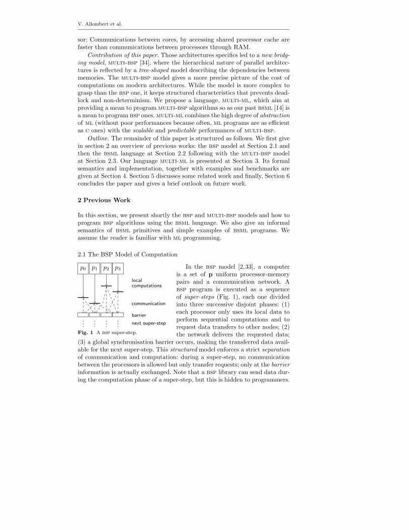
V. Allombert et al.
sor; Communications between cores, by accessing shared processor cache arefaster than communications between processors through RAM.
Contribution of this paper. Those architectures specifics led to a new bridg-ing model, multi-bsp [34], where the hierarchical nature of parallel architec-tures is reflected by a tree-shaped model describing the dependencies betweenmemories. The multi-bsp model gives a more precise picture of the cost ofcomputations on modern architectures. While the model is more complex tograsp than the bsp one, it keeps structured characteristics that prevents dead-lock and non-determinism. We propose a language, multi-ml, which aim atproviding a mean to program multi-bsp algorithms so as our past bsml [14] isa mean to program bsp ones. multi-ml combines the high degree of abstractionof ml (without poor performances because often, ml programs are as efficientas c ones) with the scalable and predictable performances of multi-bsp.
Outline. The remainder of this paper is structured as follows. We first givein section 2 an overview of previous works: the bsp model at Section 2.1 andthen the bsml language at Section 2.2 following with the multi-bsp modelat Section 2.3. Our language multi-ml is presented at Section 3. Its formalsemantics and implementation, together with examples and benchmarks aregiven at Section 4. Section 5 discusses some related work and finally, Section 6concludes the paper and gives a brief outlook on future work.
2 Previous Work
In this section, we present shortly the bsp and multi-bsp models and how toprogram bsp algorithms using the bsml language. We also give an informalsemantics of bsml primitives and simple examples of bsml programs. Weassume the reader is familiar with ml programming.
2.1 The BSP Model of Computation
localcomputations
p0 p1 p2 p3
communication
barrier
next super-step...
......
...Fig. 1 A bsp super-step.
In the bsp model [2,33], a computeris a set of p uniform processor-memorypairs and a communication network. Absp program is executed as a sequenceof super-steps (Fig. 1), each one dividedinto three successive disjoint phases: (1)each processor only uses its local data toperform sequential computations and torequest data transfers to other nodes; (2)the network delivers the requested data;
(3) a global synchronisation barrier occurs, making the transferred data avail-able for the next super-step. This structured model enforces a strict separationof communication and computation: during a super-step, no communicationbetween the processors is allowed but only transfer requests; only at the barrierinformation is actually exchanged. Note that a bsp library can send data dur-ing the computation phase of a super-step, but this is hidden to programmers.
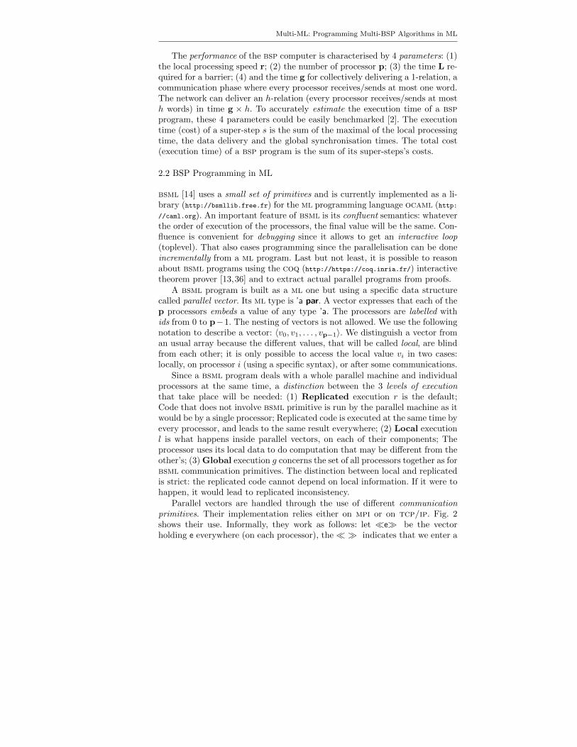
Multi-ML: Programming Multi-BSP Algorithms in ML
The performance of the bsp computer is characterised by 4 parameters: (1)the local processing speed r; (2) the number of processor p; (3) the time L re-quired for a barrier; (4) and the time g for collectively delivering a 1-relation, acommunication phase where every processor receives/sends at most one word.The network can deliver an h-relation (every processor receives/sends at mosth words) in time g × h. To accurately estimate the execution time of a bspprogram, these 4 parameters could be easily benchmarked [2]. The executiontime (cost) of a super-step s is the sum of the maximal of the local processingtime, the data delivery and the global synchronisation times. The total cost(execution time) of a bsp program is the sum of its super-steps’s costs.
2.2 BSP Programming in ML
bsml [14] uses a small set of primitives and is currently implemented as a li-brary (http://bsmllib.free.fr) for the ml programming language ocaml (http://caml.org). An important feature of bsml is its confluent semantics: whateverthe order of execution of the processors, the final value will be the same. Con-fluence is convenient for debugging since it allows to get an interactive loop(toplevel). That also eases programming since the parallelisation can be doneincrementally from a ml program. Last but not least, it is possible to reasonabout bsml programs using the coq (http://https://coq.inria.fr/) interactivetheorem prover [13,36] and to extract actual parallel programs from proofs.
A bsml program is built as a ml one but using a specific data structurecalled parallel vector. Its ml type is ’a par. A vector expresses that each of thep processors embeds a value of any type ’a. The processors are labelled withids from 0 to p−1. The nesting of vectors is not allowed. We use the followingnotation to describe a vector: 〈v0, v1, . . . , vp−1〉. We distinguish a vector froman usual array because the different values, that will be called local, are blindfrom each other; it is only possible to access the local value vi in two cases:locally, on processor i (using a specific syntax), or after some communications.
Since a bsml program deals with a whole parallel machine and individualprocessors at the same time, a distinction between the 3 levels of executionthat take place will be needed: (1) Replicated execution r is the default;Code that does not involve bsml primitive is run by the parallel machine as itwould be by a single processor; Replicated code is executed at the same time byevery processor, and leads to the same result everywhere; (2) Local executionl is what happens inside parallel vectors, on each of their components; Theprocessor uses its local data to do computation that may be different from theother’s; (3) Global execution g concerns the set of all processors together as forbsml communication primitives. The distinction between local and replicatedis strict: the replicated code cannot depend on local information. If it were tohappen, it would lead to replicated inconsistency.
Parallel vectors are handled through the use of different communicationprimitives. Their implementation relies either on mpi or on tcp/ip. Fig. 2shows their use. Informally, they work as follows: let �e� be the vectorholding e everywhere (on each processor), the � � indicates that we enter a
V. Allombert et al.
Primitive Level Type Informal semantics�e� g ’a par (if e:’a) 〈e, . . . , e〉pid g int par A predefined vector: i on processor i$v$ l ’a (if v: ’a par) vi on processor i, assumes v ≡ 〈v0, . . . , vp−1〉proj g ’a par→ (int→ ’a) 〈x0, . . . , xp−1〉 7→ (fun i→ xi)put g (int→ ’a)par→ (int→ ’a)par 〈f0, . . . , fp−1〉 7→〈(fun i→fi 0), . . . , (fun i→fi (p−1))〉
Fig. 2 Summary of the bsml primitives.
vector and switch to the local level. Replicated values are available inside thevectors. Now, only within a vector, to access to local information, we add thesyntax $x$ to read the vector x and get the local value it contains. The ids canbe accessed with the predefined vector pid. For example, using the toplevel fora simulated bsp machine with 3 processors:
# let vec1 = � ”HLPP” � in� $vec1$ˆ”, proc ”ˆ(string of int $pid$) � ;;
— : string par = <”HLPP, proc 0”, ”HLPP, proc 1”, ”HLPP, proc 2”>
The # symbol is the prompt that invites the user to enter an expression to beevaluated. Then, the toplevel gives the evaluated value with its type. Thanksto bsml confluence, it is ensured that the results of the toplevel or of theparallel implementation are identical.
The proj primitive is the only way to extract local values from a vector.Given a vector, it returns a function such that applied to the pid of a processor,the function returns the value of the vector at this processor. proj performscommunication to make local results available globally and ends the currentsuper-step. For example, if we want to convert a vector into a list, we write:
# let list of par vec = List.map (proj vec) procs;;— : val list of par : ’a par → ’a list = <fun># list of par � $pid$ � ;;— : int list = [0; 1; 2]
where procs is the list of ids [0; 1; · · · ;p-1].The put primitive is another communication primitive. It allows any local
value to be transferred to any other processor. It is also synchronous, andends the current super-step. The parameter of put is a vector that, at eachprocessor, holds a function of type (int→ ’a) returning the data to be sent toprocessor j when applied to j. The result of put is another vector of functions:At a processor j the function, when applied to i, yields the value received fromprocessor i by processor j. For example, a total exchange could be written:
# let total exchange vec =∣∣ let msg = put � fun dst → $vec$� in∣∣ ∣∣ � List.map $msg$ procs � ;;— : val total exchange : ’a par → ’a list par = <fun># total exchange � $pid$ � ;;— : int list par = <[0;1;2], [0;1;2], [0;1;2]>
where the bsp cost is (p−1)×s×g+L where s is the size of the biggest sent value.
2.3 The multi-bsp Model for Hierarchical Architectures
The multi-bsp model [34] is another bridging model as the original bsp, butadapted to clusters of multicores. The multi-bsp model introduces a visionwhere a hierarchical architecture is a tree structure of nested components (sub-machines) where the lowest stage (leaf) are processors and every other stage
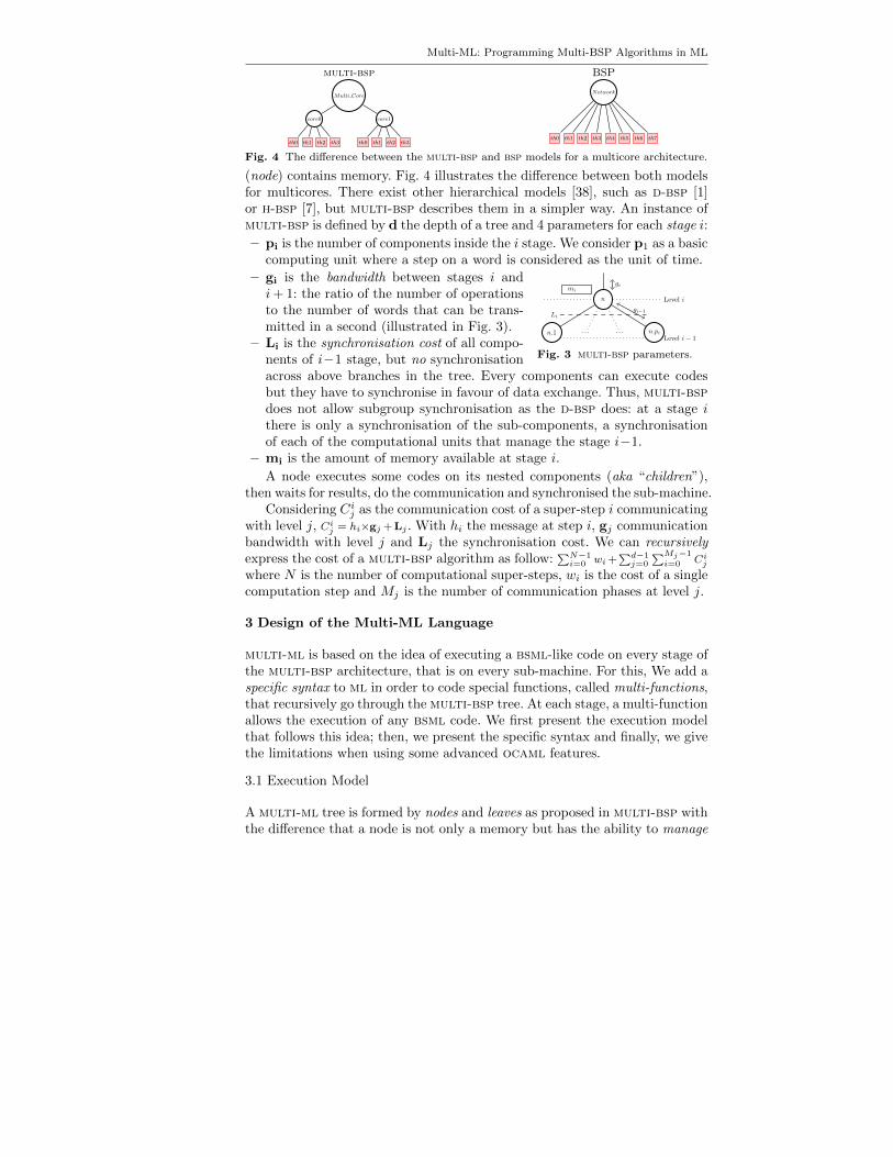
Multi-ML: Programming Multi-BSP Algorithms in ML
multi-bsp
Multi Core
core0
th0 th1 th2 th3
core1
th0 th1 th2 th3
BSP
Network
th0 th1 th2 th3 th4 th5 th6 th7
Fig. 4 The difference between the multi-bsp and bsp models for a multicore architecture.
(node) contains memory. Fig. 4 illustrates the difference between both modelsfor multicores. There exist other hierarchical models [38], such as d-bsp [1]or h-bsp [7], but multi-bsp describes them in a simpler way. An instance ofmulti-bsp is defined by d the depth of a tree and 4 parameters for each stage i:
– pi is the number of components inside the i stage. We consider p1 as a basiccomputing unit where a step on a word is considered as the unit of time.
Level i
Level i− 1
n
n.1 . . . . . . n.pi
gi
gi−1
mi
Li
Fig. 3 multi-bsp parameters.
– gi is the bandwidth between stages i andi + 1: the ratio of the number of operationsto the number of words that can be trans-mitted in a second (illustrated in Fig. 3).
– Li is the synchronisation cost of all compo-nents of i−1 stage, but no synchronisationacross above branches in the tree. Every components can execute codesbut they have to synchronise in favour of data exchange. Thus, multi-bspdoes not allow subgroup synchronisation as the d-bsp does: at a stage ithere is only a synchronisation of the sub-components, a synchronisationof each of the computational units that manage the stage i−1.
– mi is the amount of memory available at stage i.
A node executes some codes on its nested components (aka “children”),then waits for results, do the communication and synchronised the sub-machine.
Considering Cij as the communication cost of a super-step i communicating
with level j, Cij = hi×gj +Lj . With hi the message at step i, gj communication
bandwidth with level j and Lj the synchronisation cost. We can recursivelyexpress the cost of a multi-bsp algorithm as follow:
∑N−1i=0 wi +
∑d−1j=0
∑Mj−1
i=0 Cij
where N is the number of computational super-steps, wi is the cost of a singlecomputation step and Mj is the number of communication phases at level j.
3 Design of the Multi-ML Language
multi-ml is based on the idea of executing a bsml-like code on every stage ofthe multi-bsp architecture, that is on every sub-machine. For this, We add aspecific syntax to ml in order to code special functions, called multi-functions,that recursively go through the multi-bsp tree. At each stage, a multi-functionallows the execution of any bsml code. We first present the execution modelthat follows this idea; then, we present the specific syntax and finally, we givethe limitations when using some advanced ocaml features.
3.1 Execution Model
A multi-ml tree is formed by nodes and leaves as proposed in multi-bsp withthe difference that a node is not only a memory but has the ability to manage
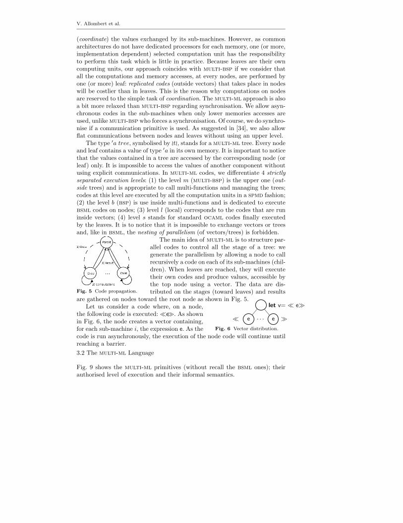
V. Allombert et al.
(coordinate) the values exchanged by its sub-machines. However, as commonarchitectures do not have dedicated processors for each memory, one (or more,implementation dependent) selected computation unit has the responsibilityto perform this task which is little in practice. Because leaves are their owncomputing units, our approach coincides with multi-bsp if we consider thatall the computations and memory accesses, at every nodes, are performed byone (or more) leaf: replicated codes (outside vectors) that takes place in nodeswill be costlier than in leaves. This is the reason why computations on nodesare reserved to the simple task of coordination. The multi-ml approach is alsoa bit more relaxed than multi-bsp regarding synchronisation. We allow asyn-chronous codes in the sub-machines when only lower memories accesses areused, unlike multi-bsp who forces a synchronisation. Of course, we do synchro-nise if a communication primitive is used. As suggested in [34], we also allowflat communications between nodes and leaves without using an upper level.
The type ′a tree, symbolised by oto, stands for a multi-ml tree. Every nodeand leaf contains a value of type ′a in its own memory. It is important to noticethat the values contained in a tree are accessed by the corresponding node (orleaf) only. It is impossible to access the values of another component withoutusing explicit communications. In multi-ml codes, we differentiate 4 strictlyseparated execution levels: (1) the level m (multi-bsp) is the upper one (out-side trees) and is appropriate to call multi-functions and managing the trees;codes at this level are executed by all the computation units in a spmd fashion;(2) the level b (bsp) is use inside multi-functions and is dedicated to executebsml codes on nodes; (3) level l (local) corresponds to the codes that are runinside vectors; (4) level s stands for standard ocaml codes finally executedby the leaves. It is to notice that it is impossible to exchange vectors or treesand, like in bsml, the nesting of parallelism (of vectors/trees) is forbidden.
Fig. 5 Code propagation.
The main idea of multi-ml is to structure par-allel codes to control all the stage of a tree: wegenerate the parallelism by allowing a node to callrecursively a code on each of its sub-machines (chil-dren). When leaves are reached, they will executetheir own codes and produce values, accessible bythe top node using a vector. The data are dis-tributed on the stages (toward leaves) and results
are gathered on nodes toward the root node as shown in Fig. 5.
e . . . e
let v= � e�
� �Fig. 6 Vector distribution.
Let us consider a code where, on a node,the following code is executed:�e�. As shownin Fig. 6, the node creates a vector containing,for each sub-machine i, the expression e. As thecode is run asynchronously, the execution of the node code will continue untilreaching a barrier.
3.2 The multi-ml Language
Fig. 9 shows the multi-ml primitives (without recall the bsml ones); theirauthorised level of execution and their informal semantics.
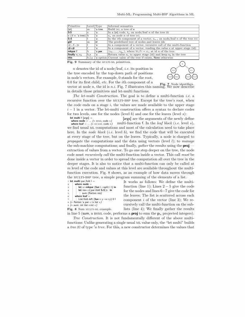
Multi-ML: Programming Multi-BSP Algorithms in ML
Primitive Level Type Informal semantics§e§ m ’a tree Build oeo, a tree of e$t$ s ’a In a §e§ code, tn on node/leaf n of the tree otov (if v: ’a tree) b ’a vn on node n of tree ovo,$v$ l ’a In the ith component of a vector, vn.i on node/leaf n of the tree ovogid m id The predefined tree of nodes and leaves ids�...f...� l ’a In a component of a vector, recursive call of the multi-function#x# l ’a In a component of a vector, reading the value x at upper stage (id)mkpar f b ’a par 〈v0, . . . , vpn 〉, where ∀i, f i = vi, at id n of the treefinally v1 v2 b,s ’a Return value v1 to upper stage (id) and keep v2 in the treethis b,l,s ’a option Current value of the tree if exists, None otherwise
Fig. 9 Summary of the multi-ml primitives.0
0.0
0.0.0 0.0.1
0.1
0.1.0 0.1.0
Fig. 7 Node identifiers.
n denotes the id of a node/leaf, i.e. its position inthe tree encoded by the top-down path of positionsin node’s vectors. For example, 0 stands for the root,0.0 for its first child, etc. For the ith component of avector at node n, the id is n.i. Fig. 7 illustrates this naming. We now describein details those primitives and let-multi functions.
The let-multi Construction. The goal is to define a multi-function i.e. arecursive function over the multi-bsp tree. Except for the tree’s root, whenthe code ends on a stage i, the values are made available to the upper stagei − 1 in a vector. The let-multi construction offers a syntax to declare codesfor two levels, one for the nodes (level b) and one for the leaves (level s):
let multi f [args] =where node = ... (∗ bsml code ∗)where leaf = ... (∗ ocaml code ∗)
[args] are the arguments of the newly definemulti-function f. In the leaf block (i.e. level s),
we find usual ml computations and most of the calculation need to take placehere. In the node block (i.e. level b), we find the code that will be executedat every stage of the tree, but on the leaves. Typically, a node is charged topropagate the computations and the data using vectors (level l); to managethe sub-machine computations; and finally, gather the results using the proj —extraction of values from a vector. To go one step deeper on the tree, the nodecode must recursively call the multi-function inside a vector. This call must bedone inside a vector in order to spread the computation all over the tree in thedeeper stages. It is also to notice that a multi-function can only be called atm level of the code and values at this level are available throughout the multi-function execution. Fig. 8 shows, as an example of how data moves throughthe multi-bsp tree, a simple program summing of the elements of a list.1 let multi par fold l =2
∣∣ where node =3
∣∣ ∣∣ let v=mkpar (fun i→split i l) in4
∣∣ ∣∣ let res=�par fold $v$� in5
∣∣ ∣∣ ∣∣ sum (flatten res)6
∣∣ where leaf =7
∣∣ ∣∣ List.fold left (fun x y→x+y) 0 l8 (∗ flatten:’a par→’a list ∗)9 (∗ sum: int list→int ∗)Fig. 8 Sum multi-ml example.
It works as follows: We define the multi-function (line 1); Lines 2 − 5 give the codefor the nodes and lines 6−7 give the code forthe leaves; The list is scattered across eachcomponent i of the vector (line 3); We re-cursively call the multi-function on the sub-lists (line 4); We finally gather the results
in line 5 (sum, a bsml code, performs a proj to sum the pn projected integers).
Tree Construction. It is not fundamentally different of the above multi-functions: Unlike generating a single usual ml value only, the “let multi” buildsa tree oto of type ′a tree. For this, a new constructor determines the values that
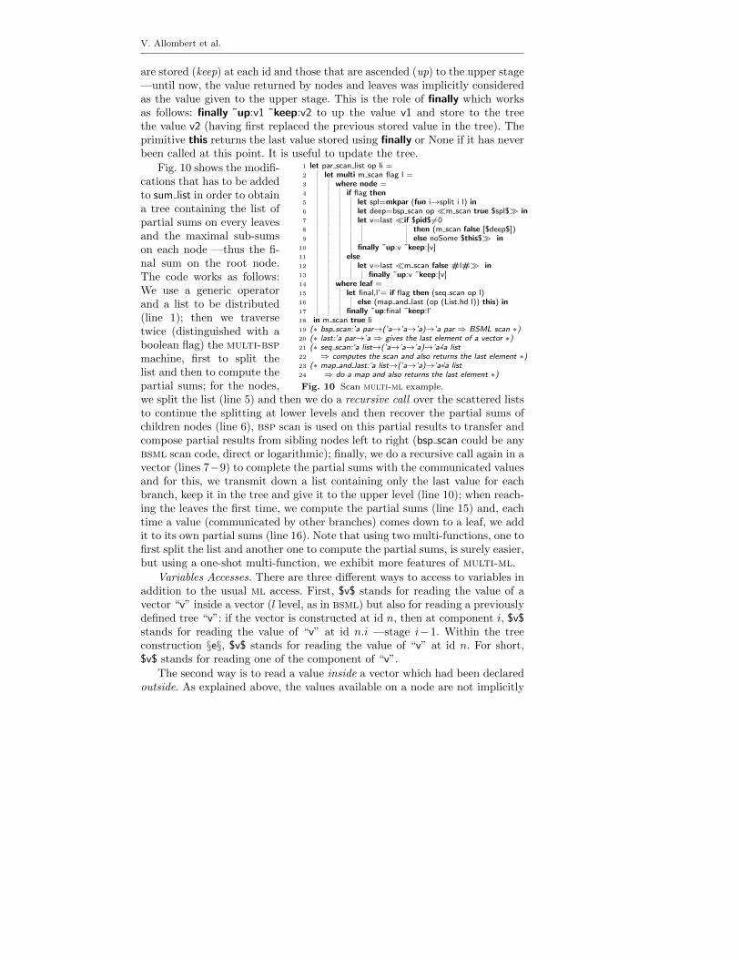
V. Allombert et al.
are stored (keep) at each id and those that are ascended (up) to the upper stage—until now, the value returned by nodes and leaves was implicitly consideredas the value given to the upper stage. This is the role of finally which worksas follows: finally ˜up:v1 ˜keep:v2 to up the value v1 and store to the treethe value v2 (having first replaced the previous stored value in the tree). Theprimitive this returns the last value stored using finally or None if it has neverbeen called at this point. It is useful to update the tree.
1 let par scan list op li =2
∣∣ let multi m scan flag l =3
∣∣ ∣∣ where node =4
∣∣ ∣∣ ∣∣ if flag then5
∣∣ ∣∣ ∣∣ ∣∣ let spl=mkpar (fun i→split i l) in6
∣∣ ∣∣ ∣∣ ∣∣ let deep=bsp scan op �m scan true $spl$� in7
∣∣ ∣∣ ∣∣ ∣∣ let v=last �if $pid$6=08
∣∣ ∣∣ ∣∣ ∣∣ ∣∣ ∣∣ then (m scan false [$deep$])9
∣∣ ∣∣ ∣∣ ∣∣ ∣∣ ∣∣ else noSome $this$� in10
∣∣ ∣∣ ∣∣ ∣∣ finally ˜up:v ˜keep:[v]11
∣∣ ∣∣ ∣∣ else12
∣∣ ∣∣ ∣∣ ∣∣ let v=last �m scan false #l#� in13
∣∣ ∣∣ ∣∣ ∣∣ ∣∣ finally ˜up:v ˜keep:[v]14
∣∣ ∣∣ where leaf =15
∣∣ ∣∣ ∣∣ let final,l’= if flag then (seq scan op l)16
∣∣ ∣∣ ∣∣ ∣∣ else (map and last (op (List.hd l)) this) in17
∣∣ ∣∣ ∣∣ finally ˜up:final ˜keep:l’18 in m scan true li19 (∗ bsp scan:’a par→(’a→’a→’a)→’a par ⇒ BSML scan ∗)20 (∗ last:’a par→’a ⇒ gives the last element of a vector ∗)21 (∗ seq scan:’a list→(’a→’a→’a)→’a∗’a list22 ⇒ computes the scan and also returns the last element ∗)23 (∗ map and last:’a list→(’a→’a)→’a∗’a list24 ⇒ do a map and also returns the last element ∗)Fig. 10 Scan multi-ml example.
Fig. 10 shows the modifi-cations that has to be addedto sum list in order to obtaina tree containing the list ofpartial sums on every leavesand the maximal sub-sumson each node —thus the fi-nal sum on the root node.The code works as follows:We use a generic operatorand a list to be distributed(line 1); then we traversetwice (distinguished with aboolean flag) the multi-bspmachine, first to split thelist and then to compute thepartial sums; for the nodes,we split the list (line 5) and then we do a recursive call over the scattered liststo continue the splitting at lower levels and then recover the partial sums ofchildren nodes (line 6), bsp scan is used on this partial results to transfer andcompose partial results from sibling nodes left to right (bsp scan could be anybsml scan code, direct or logarithmic); finally, we do a recursive call again in avector (lines 7−9) to complete the partial sums with the communicated valuesand for this, we transmit down a list containing only the last value for eachbranch, keep it in the tree and give it to the upper level (line 10); when reach-ing the leaves the first time, we compute the partial sums (line 15) and, eachtime a value (communicated by other branches) comes down to a leaf, we addit to its own partial sums (line 16). Note that using two multi-functions, one tofirst split the list and another one to compute the partial sums, is surely easier,but using a one-shot multi-function, we exhibit more features of multi-ml.
Variables Accesses. There are three different ways to access to variables inaddition to the usual ml access. First, $v$ stands for reading the value of avector “v” inside a vector (l level, as in bsml) but also for reading a previouslydefined tree “v”: if the vector is constructed at id n, then at component i, $v$stands for reading the value of “v” at id n.i —stage i−1. Within the treeconstruction §e§, $v$ stands for reading the value of “v” at id n. For short,$v$ stands for reading one of the component of “v”.
The second way is to read a value inside a vector which had been declaredoutside. As explained above, the values available on a node are not implicitly
Multi-ML: Programming Multi-BSP Algorithms in ML
available on the child nodes. It is thus necessary to copy them from a node to itssub-machines. For example, the code let x=1 in let vect=�x+1� is incorrectbecause “x” is not available on children. It is imperative to use �#x#+1�to copy the value of x from the b level into the vector (l level).
Outside a vector (g level), when the code is computing at id n, accessing toa tree t is implicitly reading its value at id n. Finally, gid is the predefined treeof nodes/leaves ids. Within the component i of a vector constructed on noden (l level), $gid$ stands for the id n.i whereas inside a §e§ code, it stands forthe identifier of the node evaluating e; at evaluation level g, gid stands for n(if executed at id n) and at evaluation level m, it is the tree of node identifiers.
A Convenient Tree Construction. For building a tree without using a multi-function (which induce communications), we add the §e§ syntax. It allows toexecute e on every nodes and leaves. One can read the values of a previouslydefined tree oto using the $t$ access in the code of e. In this way, using thepredefined tree gid, we can execute different codes on each components of atree without any need (and possibility) of communication between the stages.
A New Primitive. For performances reason, we chose to add the newprimitive mkpar. Indeed, in bsml, a replicated code is duplicated on everyprocessors so it is not necessary to take care of data transfer in code like:let lst=[...] in �split $pid$ lst� where lst is a large list and split a splittingfunction. With the multi-ml model, data are not distributed everywhere andwe have to transfer data explicitly. One can write �split $pid$ #lst#� butit is not useful to copy the whole list on every children in order to extract asub list and throw the rest. This is the reason why the mkpar compute first pn
values and then distribute them to the sub-machines thus building a vector.This method is more expensive for the node n in computation time, but itreduces drastically the amount of data transfers.
3.3 Current Limitations
Exceptions and Partially Evaluated Trees. Exceptional situations are handledin ocaml with a system of exceptions. In parallel, this is at least as relevant:if one processor triggers an exception during a computation, bsml [14] as wellas multi-ml have to deal with it, like ocaml would, and prevent a crash.
The problem is when an exception is raised locally (l level) on (at least)one processor but other processors continue to follow the execution stream,until they are stopped by the need of synchronisation. This happens when anexception escapes the scope of a parallel vector. Then, a crash can occur: aprocessor misses the global barrier. To prevent this situation, in [14], we intro-duce a specific handler of local exceptions that have not been caught locally.The structure trypar...withpar catches any exception and handles it as usualin ocaml. To do this, a barrier occurs and exceptions are communicated toall processors in order to allow a global decision to be taken. Furthermore, anyaccess to a vector that is in an incoherent state will raise again the exception.
For multi-ml, if an exception is no correctly handled in a stage, it must bepropagated to the upper stage at the next barrier —as in bsml. If an exception
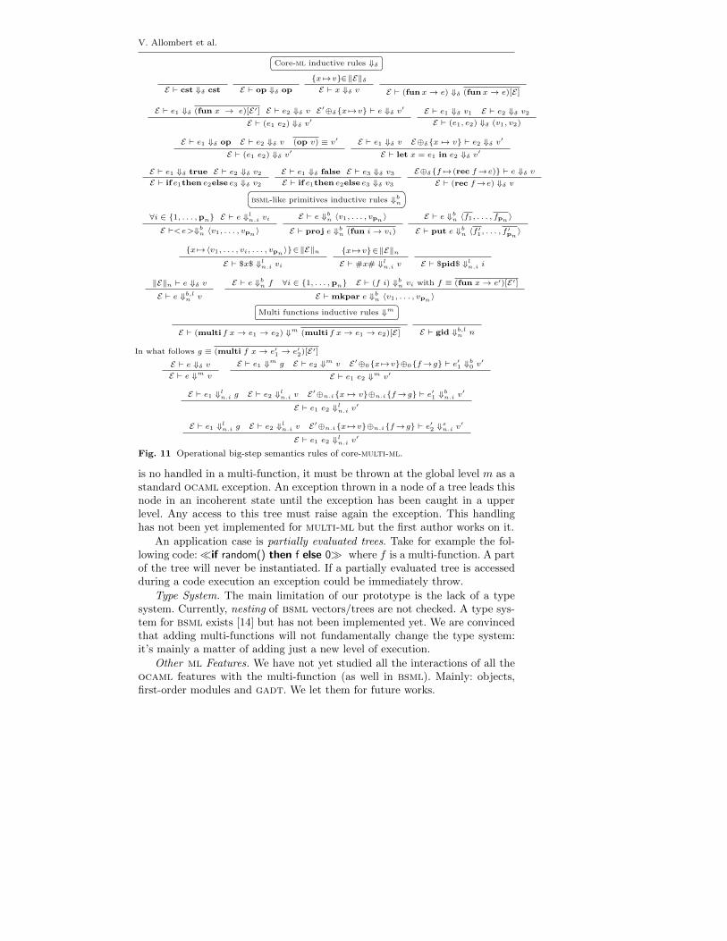
V. Allombert et al. �� ��Core-ml inductive rules ⇓δ
E ` cst ⇓δ cst E ` op ⇓δ op
{x 7→v}∈‖E‖δE ` x ⇓δ v E ` (fun x→ e) ⇓δ (fun x→ e)[E]
E ` e1 ⇓δ (fun x → e)[E′] E ` e2 ⇓δ v E′⊕δ{x 7→v} ` e ⇓δ v′
E ` (e1 e2) ⇓δ v′E ` e1 ⇓δ v1 E ` e2 ⇓δ v2
E ` (e1, e2) ⇓δ (v1, v2)
E ` e1 ⇓δ op E ` e2 ⇓δ v (op v) ≡ v′
E ` (e1 e2) ⇓δ v′E ` e1 ⇓δ v E⊕δ{x 7→ v} ` e2 ⇓δ v′
E ` let x = e1 in e2 ⇓δ v′
E ` e1 ⇓δ true E ` e2 ⇓δ v2
E ` if e1then e2else e3 ⇓δ v2
E ` e1 ⇓δ false E ` e3 ⇓δ v3
E ` if e1then e2else e3 ⇓δ v3
E⊕δ{f 7→(rec f→e)} ` e ⇓δ v
E ` (rec f→e) ⇓δ v�� ��bsml-like primitives inductive rules ⇓bn∀i ∈ {1, . . . ,pn} E ` e ⇓ln.i viE `<e>⇓bn 〈v1, . . . , vpn 〉
E ` e ⇓bn 〈v1, . . . , vpn 〉E ` proj e ⇓bn (fun i→ vi)
E ` e ⇓bn 〈f1, . . . , fpn 〉E ` put e ⇓bn 〈f ′1, . . . , f ′pn 〉
{x 7→〈v1, . . . , vi, . . . , vpn 〉}∈‖E‖nE ` $x$ ⇓ln.i vi
{x 7→v}∈‖E‖nE ` #x# ⇓ln.i v E ` $pid$ ⇓ln.i i
‖E‖n ` e ⇓δ v
E ` e ⇓b,ln v
E ` e ⇓bn f ∀i ∈ {1, . . . ,pn} E ` (f i) ⇓bn vi with f ≡ (fun x→ e′)[E′]E ` mkpar e ⇓bn 〈v1, . . . , vpn 〉�� ��Multi functions inductive rules ⇓m
E ` (multi f x→ e1 → e2) ⇓m (multi f x→ e1 → e2)[E] E ` gid ⇓b,ln n
In what follows g ≡ (multi f x→ e′1 → e′2)[E′]E ` e ⇓δ v
E ` e ⇓m v
E ` e1 ⇓m g E ` e2 ⇓m v E′⊕0{x 7→v}⊕0{f→g} ` e′1 ⇓b0 v′
E ` e1 e2 ⇓m v′
E ` e1 ⇓ln.i g E ` e2 ⇓ln.i v E′⊕n.i{x 7→ v}⊕n.i{f→g} ` e′1 ⇓bn.i v′
E ` e1 e2 ⇓ln.i v′
E ` e1 ⇓ln.i g E ` e2 ⇓ln.i v E′⊕n.i{x 7→v}⊕n.i{f→g} ` e′2 ⇓sn.i v′
E ` e1 e2 ⇓ln.i v′
Fig. 11 Operational big-step semantics rules of core-multi-ml.
is no handled in a multi-function, it must be thrown at the global level m as astandard ocaml exception. An exception thrown in a node of a tree leads thisnode in an incoherent state until the exception has been caught in a upperlevel. Any access to this tree must raise again the exception. This handlinghas not been yet implemented for multi-ml but the first author works on it.
An application case is partially evaluated trees. Take for example the fol-lowing code:�if random() then f else 0� where f is a multi-function. A partof the tree will never be instantiated. If a partially evaluated tree is accessedduring a code execution an exception could be immediately throw.
Type System. The main limitation of our prototype is the lack of a typesystem. Currently, nesting of bsml vectors/trees are not checked. A type sys-tem for bsml exists [14] but has not been implemented yet. We are convincedthat adding multi-functions will not fundamentally change the type system:it’s mainly a matter of adding just a new level of execution.
Other ml Features. We have not yet studied all the interactions of all theocaml features with the multi-function (as well in bsml). Mainly: objects,first-order modules and gadt. We let them for future works.
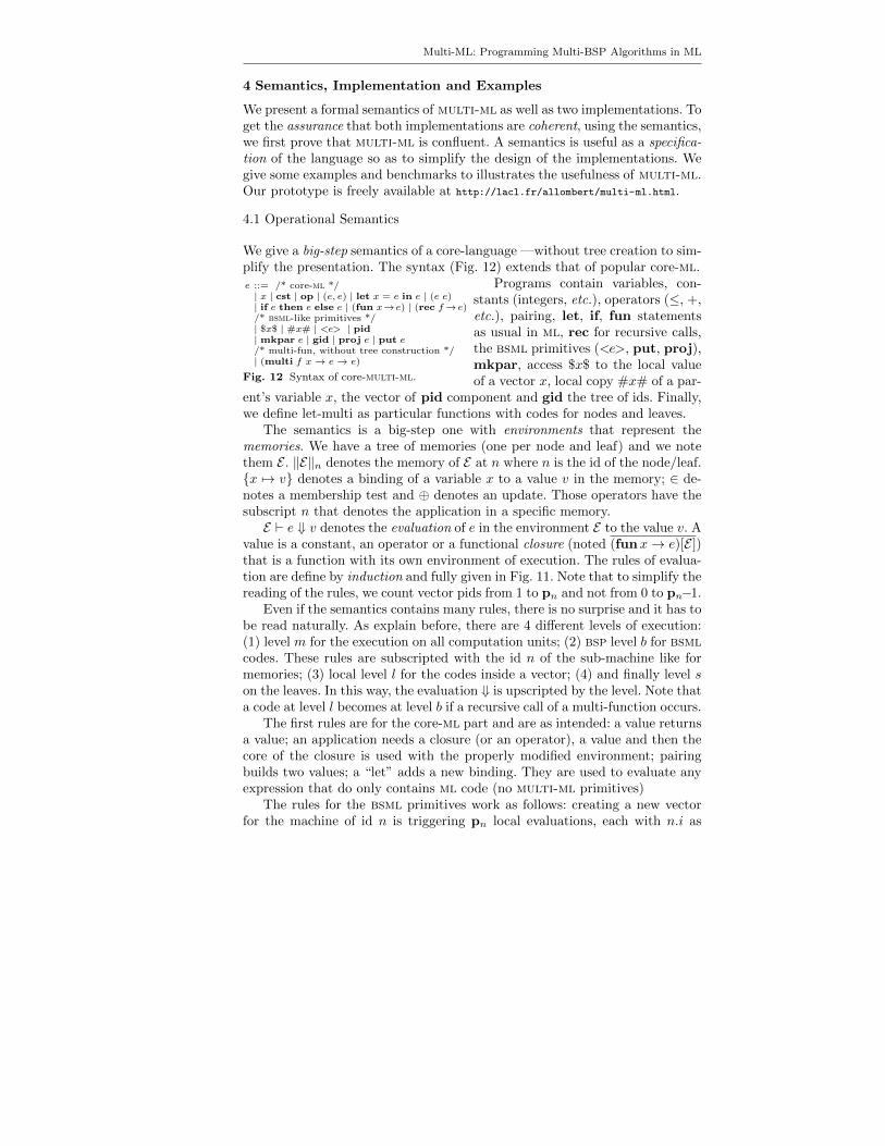
Multi-ML: Programming Multi-BSP Algorithms in ML
4 Semantics, Implementation and Examples
We present a formal semantics of multi-ml as well as two implementations. Toget the assurance that both implementations are coherent, using the semantics,we first prove that multi-ml is confluent. A semantics is useful as a specifica-tion of the language so as to simplify the design of the implementations. Wegive some examples and benchmarks to illustrates the usefulness of multi-ml.Our prototype is freely available at http://lacl.fr/allombert/multi-ml.html.
4.1 Operational Semantics
We give a big-step semantics of a core-language —without tree creation to sim-plify the presentation. The syntax (Fig. 12) extends that of popular core-ml.
e ::= /* core-ml */| x | cst | op | (e, e) | let x = e in e | (e e)| if e then e else e | (fun x→e) | (rec f→e)/* bsml-like primitives */| $x$ | #x# | <e> | pid| mkpar e | gid | proj e | put e/* multi-fun, without tree construction */| (multi f x→ e→ e)
Fig. 12 Syntax of core-multi-ml.
Programs contain variables, con-stants (integers, etc.), operators (≤, +,etc.), pairing, let, if, fun statementsas usual in ml, rec for recursive calls,the bsml primitives (<e>, put, proj),mkpar, access $x$ to the local valueof a vector x, local copy #x# of a par-
ent’s variable x, the vector of pid component and gid the tree of ids. Finally,we define let-multi as particular functions with codes for nodes and leaves.
The semantics is a big-step one with environments that represent thememories. We have a tree of memories (one per node and leaf) and we notethem E . ‖E‖n denotes the memory of E at n where n is the id of the node/leaf.{x 7→ v} denotes a binding of a variable x to a value v in the memory; ∈ de-notes a membership test and ⊕ denotes an update. Those operators have thesubscript n that denotes the application in a specific memory.E ` e ⇓ v denotes the evaluation of e in the environment E to the value v. A
value is a constant, an operator or a functional closure (noted (funx→ e)[E ])that is a function with its own environment of execution. The rules of evalua-tion are define by induction and fully given in Fig. 11. Note that to simplify thereading of the rules, we count vector pids from 1 to pn and not from 0 to pn−1.
Even if the semantics contains many rules, there is no surprise and it has tobe read naturally. As explain before, there are 4 different levels of execution:(1) level m for the execution on all computation units; (2) bsp level b for bsmlcodes. These rules are subscripted with the id n of the sub-machine like formemories; (3) local level l for the codes inside a vector; (4) and finally level son the leaves. In this way, the evaluation ⇓ is upscripted by the level. Note thata code at level l becomes at level b if a recursive call of a multi-function occurs.
The first rules are for the core-ml part and are as intended: a value returnsa value; an application needs a closure (or an operator), a value and then thecore of the closure is used with the properly modified environment; pairingbuilds two values; a “let” adds a new binding. They are used to evaluate anyexpression that do only contains ml code (no multi-ml primitives)
The rules for the bsml primitives work as follows: creating a new vectorfor the machine of id n is triggering pn local evaluations, each with n.i as
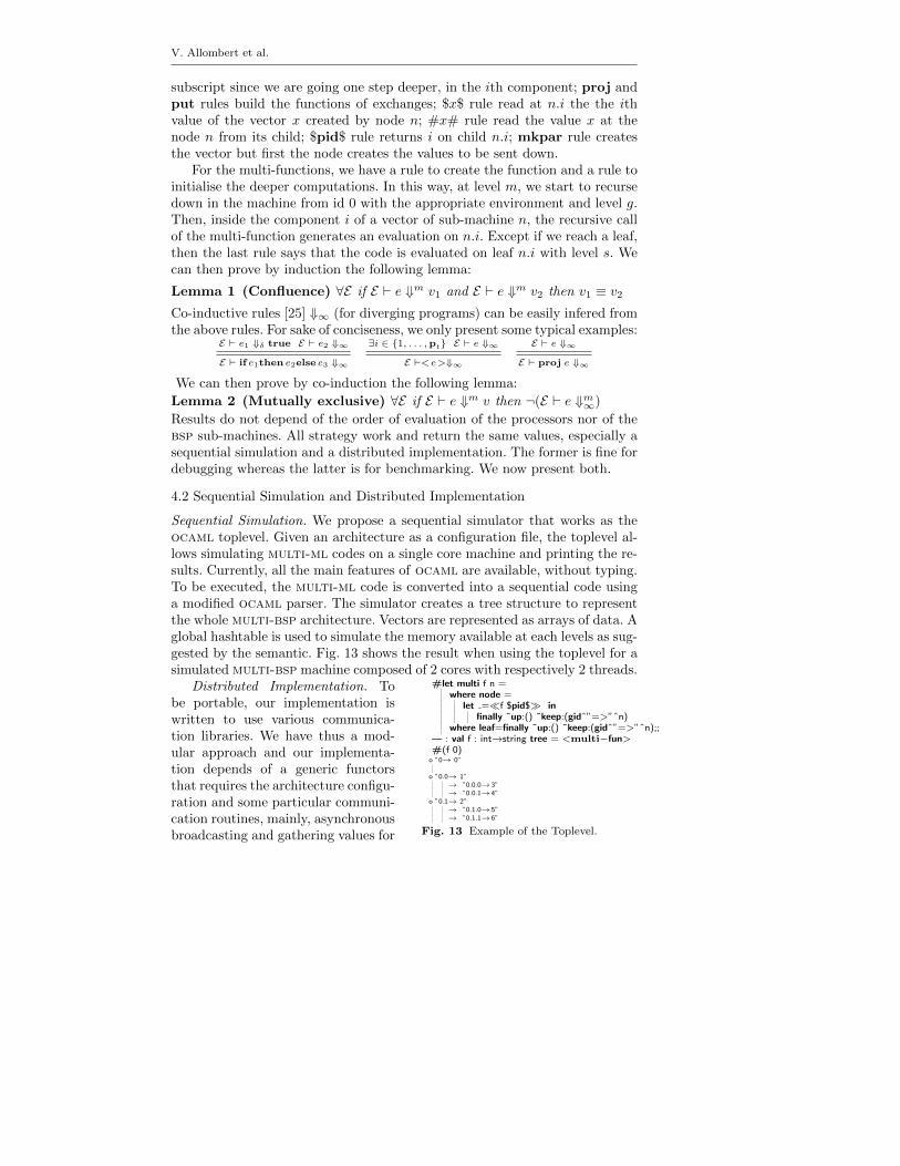
V. Allombert et al.
subscript since we are going one step deeper, in the ith component; proj andput rules build the functions of exchanges; $x$ rule read at n.i the the ithvalue of the vector x created by node n; #x# rule read the value x at thenode n from its child; $pid$ rule returns i on child n.i; mkpar rule createsthe vector but first the node creates the values to be sent down.
For the multi-functions, we have a rule to create the function and a rule toinitialise the deeper computations. In this way, at level m, we start to recursedown in the machine from id 0 with the appropriate environment and level g.Then, inside the component i of a vector of sub-machine n, the recursive callof the multi-function generates an evaluation on n.i. Except if we reach a leaf,then the last rule says that the code is evaluated on leaf n.i with level s. Wecan then prove by induction the following lemma:
Lemma 1 (Confluence) ∀E if E ` e ⇓m v1 and E ` e ⇓m v2 then v1 ≡ v2
Co-inductive rules [25] ⇓∞ (for diverging programs) can be easily infered fromthe above rules. For sake of conciseness, we only present some typical examples:
E ` e1 ⇓δ true E ` e2 ⇓∞E ` if e1then e2else e3 ⇓∞
∃i ∈ {1, . . . ,pt} E ` e ⇓∞E `<e>⇓∞
E ` e ⇓∞E ` proj e ⇓∞
We can then prove by co-induction the following lemma:
Lemma 2 (Mutually exclusive) ∀E if E ` e ⇓m v then ¬(E ` e ⇓m∞)
Results do not depend of the order of evaluation of the processors nor of thebsp sub-machines. All strategy work and return the same values, especially asequential simulation and a distributed implementation. The former is fine fordebugging whereas the latter is for benchmarking. We now present both.
4.2 Sequential Simulation and Distributed Implementation
Sequential Simulation. We propose a sequential simulator that works as theocaml toplevel. Given an architecture as a configuration file, the toplevel al-lows simulating multi-ml codes on a single core machine and printing the re-sults. Currently, all the main features of ocaml are available, without typing.To be executed, the multi-ml code is converted into a sequential code usinga modified ocaml parser. The simulator creates a tree structure to representthe whole multi-bsp architecture. Vectors are represented as arrays of data. Aglobal hashtable is used to simulate the memory available at each levels as sug-gested by the semantic. Fig. 13 shows the result when using the toplevel for asimulated multi-bsp machine composed of 2 cores with respectively 2 threads.
#let multi f n =∣∣ where node =∣∣ ∣∣ let =�f $pid$� in∣∣ ∣∣ ∣∣ finally ˜up:() ˜keep:(gidˆ”=>”ˆn)∣∣ where leaf=finally ˜up:() ˜keep:(gidˆ”=>”ˆn);;— : val f : int→string tree = <multi−fun>#(f 0)
o ”0→ 0”∣∣o ”0.0→ 1”∣∣ ∣∣ → ”0.0.0→3”∣∣ ∣∣ → ”0.0.1→4”o ”0.1→ 2”∣∣ ∣∣ → ”0.1.0→5”∣∣ ∣∣ → ”0.1.1→6”
Fig. 13 Example of the Toplevel.
Distributed Implementation. Tobe portable, our implementation iswritten to use various communica-tion libraries. We have thus a mod-ular approach and our implementa-tion depends of a generic functorsthat requires the architecture configu-ration and some particular communi-cation routines, mainly, asynchronousbroadcasting and gathering values for
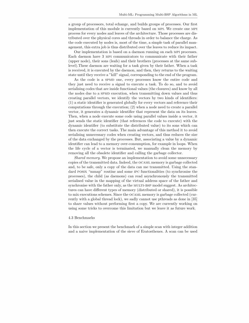
Multi-ML: Programming Multi-BSP Algorithms in ML
a group of processors, total echange, and builds groups of processes. Our firstimplementation of this module is currently based on mpi. We create one mpiprocess for every nodes and leaves of the architecture. Those processes are dis-tributed over the physical cores and threads in order to balance the charge. Asthe code executed by nodes is, most of the time, a simple task of parallel man-agement, this extra job is thus distributed over the leaves to reduce its impact.
Our implementation is based on a daemon running on each mpi processes.Each daemon have 3 mpi communicators to communicate with their father(upper node), their sons (leafs) and their brothers (processes at the same sub-level).These daemon are waiting for a task given by their father. When a taskis received, it is executed by the daemon, and then, they returns to the waitingstate until they receive a ”kill” signal, corresponding to the end of the program.
As the code is a spmd one, every processes know the entire code andthey just need to receive a signal to execute a task. To do so, and to avoidserialising codes that are inside functional values (the closures) and know by allthe nodes due to a spmd execution, when transmitting down values and thuscreating parallel vectors, we identify the vectors by two kinds of identifiers:(1) a static identifier is generated globally for every vectors and reference theircomputations through the execution; (2) when a node need to create a parallelvector, it generates a dynamic identifier that represent the data on its leaves.Then, when a node execute some code using parallel values inside a vector, itjust sends the static identifier (that references the code to execute) with thedynamic identifier (to substitute the distributed value) to its sons which canthen execute the correct tasks. The main advantage of this method it to avoidserialising unnecessary codes when creating vectors, and thus reduces the sizeof the data exchanged by the processes. But, associating a value by a dynamicidentifier can lead to a memory over-consumption, for example in loops. Whenthe life cycle of a vector is terminated, we manually clean the memory byremoving all the obsolete identifier and calling the garbage collector.
Shared memory. We propose an implementation to avoid some unnecessarycopies of the transmitted data. Indeed, the ocaml memory is garbage collectedand, to be safe, only a copy of the data can me transmitted. Using the stan-dard posix “mmap” routine and some ipc functionalities (to synchronise theprocesses), the child (as daemons) can read asynchronously the transmittedserialised value in the mapping of the virtual address space of the father andsynchronise with the father only, as the multi-bsp model suggest. As architec-tures can have different types of memory (distributed or shared), it is possibleto mix executions schemes. Since the ocaml memory is garbage collected (cur-rently with a global thread lock), we sadly cannot use pthreads as done in [35]to share values without performing first a copy. We are currently working onusing some tricks to overcome this limitation but we leave it as future work.
4.3 Benchmarks
In this section we present the benchmark of a simple scan with integer additionand a naive implementation of the sieve of Eratosthenes. A scan can be used
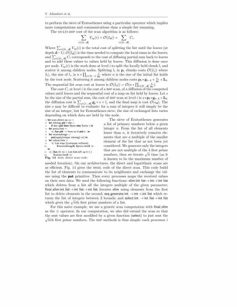
V. Allombert et al.
to perform the sieve of Eratosthenes using a particular operator which impliesmore computations and communications than a simple list summing.
The multi-bsp cost of the scan algorithm is as follows:∑
i∈[0...d[
Vsp(i) +O(|ld|) +∑
i∈[0...d[
Ci.
Where∑
i∈[0...d[ Vsp(i) is the total cost of splitting the list until the leaves (at
depth d−1); O(|ld|) is the time needed to compute the local sums in the leaves;and
∑i∈[0...d[ Ci corresponds to the cost of diffusing partial sum back to leaves
and to add these values to values held by leaves. This diffusion is done onceper node. Vsp(i) is the work done at level i to split the locally held chunk li andscatter it among children nodes. Splitting li in pi chunks costs O(|li|) where|li|, the size of li, is n ∗∏j∈[0...i[
1pj
where n is the size of the initial list holds
by the root node. Scattering it among children nodes costs pi ∗gi−1 + nipi
+Li.
The sequential list scan cost at leaves is O(|ld|) = O(n ∗∏i∈[0...d[1pi
).The cost Ci at level i is the cost of a bsp scan, of a diffusion of the computed
values until leaves and the sequential cost of a map on list held by leaves. Let sbe the size of the partial sum, the cost of bsp scan at level i is s∗pi∗gi−1+Li,the diffusion cost is
∑j∈]i...d] gj ∗ s + lj and the final map is cost O(sd). The
size s may be difficult to evaluate: for a sum of integers it will simply be thesize of an integer, but for Eratosthenes sieve, the size of exchanged lists variesdepending on which data are held by the node.1 let scan direct op vv =2 let mkmsg pid v dst =3 if dst<pid then None else Some v in4 let procs lists =5 � fun pid → from to 0 pid� in6 let receivedmsgs =7 put(apply(mkpar mkmsg) vv) in8 let values lists =9 � List.map ((compose noSome)
10 $receivedmsgs$) $procs lists$ �in
11 � (fun (h::t)→ List.fold left op h t )12 $values lists$ �Fig. 14 bsml direct scan code.
The sieve of Eratosthenes generatesa list of primary numbers below a giveninteger n. From the list of all elementslesser than n, it iteratively removes ele-ments that are a multiple of the smallerelement of the list that as not been yetconsidered. We generate only the integersthat are not multiple of the 4 first primenumbers, then we iterate
√n time (as it
is known to be the maximum number ofneeded iteration). On our architectures, the direct and logarithmic scans areas efficient. Fig. 14 gives the bsml code of the direct scan. This code buildthe list of elements to communicate to its neighbours and exchange the val-ues using the put primitive. Then every processes maps the received valueson their own data. We used the following functions: elim:int list→ int→ int listwhich deletes from a list all the integers multiple of the given parameter;final elim:int list→ int list→ int list iterates elim using elements from the firstlist to delete elements in the second; seq generate:int → int→ int list which re-turns the list of integers between 2 bounds; and select:int → int list→ int listwhich gives the
√nth first prime numbers of a list.
For this naive example, we use a generic scan computation with final elimas the ⊕ operator. In our computation, we also did extend the scan so thatthe sent values are first modified by a given function (select) to just sent the√nth first prime numbers. The bsp methods is thus simple: each processor i
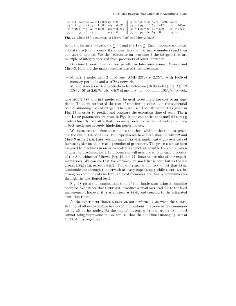
Multi-ML: Programming Multi-BSP Algorithms in ML
p0 = 4 g0 =∞ L0 = 149000 m0 = 0p1 = 2 g1 = 89 L1 = 1100 m1 = 64Gbp2 = 16 g2 = 6 L2 = 1800 m2 = 20Mbp3 = 0 g3 = 3 L3 = 0 m3 = 0
p0 = 8 g0 =∞ L0 = 195400 m0 = 0p1 = 2 g1 = 14 L1 = 472 m1 = 16Gbp2 = 4 g2 = 6 L2 = 800 m2 = 6Mbp2 = 0 g2 = 5 L2 = 0 m2 = 0
Fig. 15 Multi-BSP parameters of Mirev3 (left) and Mirev2 (right).
holds the integers between i× np + 1 and (i+ 1)× n
p . Each processor computes
a local sieve (the processor 0 contains thus the first prime numbers) and thenour scan is applied. We then eliminate on processor i the integers that aremultiple of integers received from processors of lower identifier.
Benchmark were done on two parallel architectures named Mirev2 andMirev3. Here are the main specifications of these machines:
– Mirev2: 8 nodes with 2 quad-core (AMD 2376) at 2.3Ghz with 16Gb ofmemory per node and a 1Gb/s network.
– Mirev3: 4 nodes with 2 hyper-threaded octo-core (16 threads) (Intel XEONE5−2650) at 2.6Ghz with 64Gb of memory per node and a 10Gb/s network.
The multi-bsp and bsp model can be used to estimate the cost of an algo-rithm. Thus, we estimated the cost of transferring values and the sequentialcost of summing lists of integer. Then, we used the bsp parameters given inFig. 15 in order to predict and compare the execution time of scan. The gand L bsp parameters are given in Fig.19, one can notice that until 64 cores gevolves linearly, but after that, too many cores access the network, producinga bottleneck and severely hindering performances.
We measured the time to compute the sieve without the time to gener-ate the initial list of values. The experiments have been done on Mirev2 andMirev3 using bsml (mpi version) and multi-ml implementations over lists ofincreasing size on an increasing number of processors. The processes have beenassigned to machines in order to scatter as much as possible the computationamong the machines, i.e. a 16 process run will uses one core on each processorof the 8 machines of Mirev3. Fig. 16 and 17 shows the results of our experi-mentations. We can see that the efficiency on small list is poor but as the listgrows, multi-ml exceeds bsml. This difference is due to the fact that bsmlcommunicates through the network at every super steps; while multi-ml fo-cusing on communications through local memories and finally communicatesthrough the distributed level.
Fig. 18 gives the computation time of the simple scan using a summingoperator. We can see that multi-ml introduce a small overhead due to the levelmanagement; however it is as efficient as bsml and concord to the estimatedexecution times.
As the experiment shows, multi-ml out-performs bsml when the multi-bsp model allows to confine heavy communications in a node before communi-cating with other nodes. For the sum of integers, where the multi-bsp modelcannot bring improvements, we can see that the additional managing cost ofmulti-ml is negligible.
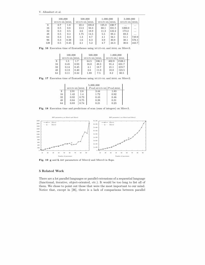
V. Allombert et al.
100 000 500 000 1 000 000 3 000 000multi-ml bsml multi-ml bsml multi-ml bsml multi-ml bsml
8 0.7 1.8 22.4 105.0 125.3 430.7 ... ...16 0.5 0.8 13.3 50.3 68.1 331.5 1200.0 ...32 0.3 0.5 2.6 18.9 11.3 122.2 173.2 ...48 0.5 0.4 1.75 14.5 5.5 88.4 69.3 ...64 0.3 0.3 1.3 8.7 4.1 56.1 51.1 749.996 0.3 0.38 1.6 6.3 3.9 30.8 38.1 576.1128 0.5 0.45 2.1 5.2 4.7 24.3 30.6 443.7
Fig. 16 Execution time of Eratosthenes using multi-ml and bsml on Mirev3.
100 000 500 000 1 000 000multi-ml bsml multi-ml bsml multi-ml bsml
8 1.5 1.7 64.5 106.1 402.9 1538.116 0.45 0.93 16.0 49.3 91.4 631.732 0.14 0.45 4.1 18.7 21.1 219.748 0.13 0.40 2.6 11.0 10.8 123.564 0.11 0.34 1.89 7.5 8.2 80.5
Fig. 17 Execution time of Eratosthenes using multi-ml and bsml on Mirev2.
5 000 000multi-ml bsml Pred multi-ml Pred bsml
8 2.91 2.8 3.44 1.8316 1.42 1.4 1.72 0.9232 0.92 0.73 0.43 0.4648 0.84 0.75 0.28 0.3164 0.83 0.74 0.21 0.23
Fig. 18 Execution time and predictions of scan (sum of integers) on Mirev3.
0
200
400
600
800
1000
1200
1400
1600
1800
2000
2200
10 20 30 40 50 60 70 80 90
Number of processors
BSP parameter g on Mirev3 and Mirev2
Mirev3
Mirev2
0
1e+06
2e+06
3e+06
4e+06
5e+06
6e+06
7e+06
8e+06
9e+06
10 20 30 40 50 60 70 80 90
Number of processors
BSP parameter L on Mirev3 and Mirev2
Mirev3
Mirev2
Fig. 19 g and L bsp parameters of Mirev2 and Mirev3 in flops.
5 Related Work
There are a lot parallel languages or parallel extensions of a sequential language(functional, iterative, object-oriented, etc.). It would be too long to list all ofthem. We chose to point out those that were the most important to our mind.Notice that, except in [26], there is a lack of comparisons between parallel
Multi-ML: Programming Multi-BSP Algorithms in ML
languages. It is difficult to compare them since many parameters have to betaken into account: efficiency, scalability, expressiveness, etc.
5.1 Programming Languages and Libraries for BSP like Computing
Historically, the first library for bsp computing was the bsplib [21] for thec language; it has been extended in the pub library [4] by adding subgroupsynchronisations, high performance operations and migration of threads. Forthe gpu architectures, a bsp library was provided in [23] with mainly drmaprimitives close to the bsplib’s ones.
For java, different libraries exist. The first one is [17]. There is also bsp-core [35] (also for c++). A library with scheduling and migration of bspthreads has been designed in [29] —the scheduling is implicit but the migrationcan be explicit. The library hama [32] is implemented using a “mapreduce-like” framework. We can also highlight the work of neststep [24] which isc/java library for bsp computing, which authorises nested computations incase of a cluster of multi-core but without any safety.
The bsml primitives were adapted for c++ [18]: the bsp++ library pro-vides nested computation in the case of a cluster of multi-cores (mpi+open-mp). But it is the responsibility of the programmer to avoid harmful nestedparallelism. bsml also inspired bsp-python [22] and bsp-haskell [28].
5.2 Functional Parallel Programming
A survey to parallel functional programming can be found in [20]. It has beenused as a basis for the following classification with some updates.
Data-parallel Languages. The first functional one was nesl [3]. This lan-guage allows to create particular arrays and nested computations within thesearrays. The abstract machine is responsible for the distribution of the dataover the available processors. For ml, there is manticore [12], an extensionof nesl with the dynamic creation of asynchronous threads and send/receivedprimitives. For gpu architectures, an extension of ocaml, using a special syn-tax for the kernels has been developed in [5].
sac (Single Assignment c) [16] is a lazy language (with a syntax close toc) for array processing. Some higher-order operations on multi-dimensionalarrays are provided and the compiler is responsible for generating an efficientparallel code. A data-parallel extension of haskell has been done in [10]where the language allows to create data arrays that are distributed acrossthe processors. And some specific operations permit to manipulate them.
The main drawback of all these languages is that cost analysis is hard todo since the system is responsible for the data distribution.
Explicit process creation. We found two extensions of haskell in this cat-egory: eden and gph [31]. Both use a small set of syntactic constructs forexplicit process creation. Their fine-grain parallelism, while providing enough
V. Allombert et al.
control to implement parallel algorithms efficiently, frees the programmer fromthe tedious task of managing low-level details of communications —which useslazy shared data. Processes are automatically managed by sophisticated run-time systems for shared memory machines or distributed ones.
As above, cost analysis is hard to do and, sometimes, the runtime fails todistribute correctly the data [31]; it introduces too much communication andthus a lack of scalability. Another distributed language is hume [19]. The mainadvantage of this language is that it is provided with a cost analysis of theprograms for real-time purpose but with limitations of the expressiveness.
Algorithmic skeletons. Skeletons are patterns of parallel computations [15].They can be seen as high-order functions that provide parallelism. They thusfall into the category of functional extensions. They are many skeleton libraries[15]. For ocaml, the most known work is the one of [11].
Distributed functional languages. In front of parallel functional languages,there are many concurrent extensions of functional languages such as erlang,clean or jocaml [27]. The latter is a concurrent extension of ocaml, whichadded explicit synchronisations of processes using specific patterns.
alice-ml [30] adds what is called a “future” for communicating values. Afuture is a placeholder for an undetermined result of a concurrent computation.When the computation delivers a result, the associated future is eliminated byglobally replacing it by the result value. The language also contains “promises”that are explicit handles of futures. scala is a functional extension of javawhich provides concurrency, using the actor model: mostly, creation of agentsthat can migrate across resources. Two others extensions of ocaml are [8] and[9]. The former uses spmd primitives with a kind of futures. The latter allowsmigration of threads that communicate using particular shared data.
All these languages have the same drawbacks: they are not deadlock andrace condition free; furthermore, they do not provide any cost model.
6 Conclusion and Future Work
6.1 Summary of the Contribution
The paper presents a language call multi-ml to program multi-bsp algo-rithms. It extends our previous bsml that has been designed for programmingbsp algorithms. They both have the following advantages: confluent opera-tional semantics; equivalence of the results for both toplevel and distributedimplementation; cost model and efficiency.
The multi-bsp model extends the bsp one as a hierarchical tree of nestedbsp machines. multi-ml extends bsml with a special syntax for define spe-cial recursive functions over this tree of nested machines, each of them pro-grammed using bsml. In a tree, nodes contain codes to manage the sub-machines whereas leaves perform the largest parts of the computation. In thiswork, we focus on the informal presentation of multi-ml, an operational se-mantics of a core-language and benchmarks of simple examples with a compar-
Multi-ML: Programming Multi-BSP Algorithms in ML
ison with predicted performances associated with the multi-bsp cost model.We also compare multi-ml codes with bsml ones as well as the performancesof both languages on a typical cluster of hyper-threaded multi-cores. As pre-dicted, multi-ml codes run faster when the cores share the network: there isno bottleneck; And the multi-core synchronisations are cheaper.
Compared to bsml, multi-ml have several drawbacks. First, the codes, thesemantics and the implementation are a bit more complex. Second, the costmodel associated to the program is more difficult to grasp: designing multi-bsp algorithms and programming them in multi-ml is more difficult thanusing bsml only. But, from our experience, we can say that it is not so hard.
6.2 Future Work
In a close future, we plan to axiomatise the multi-ml primitives inside coq,as we did for bsml in [13,36], in order to prove the correctness of multi-bspalgorithms. We also consider to formally prove that the implementations followthe formal semantics. We plan also to benchmark bigger examples. We thinkof model-checking problems and algebraic computations that better followhigh-level languages than intensive float operations can do.
But the most important work to do is the implementation of a type systemfor multi-ml to ensure a true safety of the codes: forbid nesting of vectors,forbid data-races if imperatives features, such as handling exceptions [14],are used. In the long term, the type system could be used to optimise thecompiler. Indeed, currently, even in the case of a share-memory architecture,only serialised values are exchanged between nodes. We consider implementinga dedicated concurrent garbage collector.
References
1. Beran, M.: Decomposable bsp Computers. In: Theory and Practice of Informatics (SOF-SEM), LNCS, vol. 1725, pp. 349–359. Springer (1999)
2. Bisseling, R.H.: Parallel Scientific Computation. A Structured Approach Using bsp andmpi. Oxford University Press (2004)
3. Blelloch, G.: nesl. Encyclopedia of Parallel Computing, pp. 1278–1283. Springer (2011)4. Bonorden, O., Judoiink, B., von Otte, I., Rieping, O.: The Paderborn University bsp
Library. Parallel Computing 29(2), 187–207 (2003)5. Bourgoin, M., Chailloux, E., Lamotte, J.L.: spoc: gpgpu Programming through Stream
Processing with ocaml. Parallel Processing Letters 22(2), 1–12 (2012)6. Cappello, F., Guermouche, A., Snir, M.: On Communication Determinism in hpc Appli-
cations. In: Computer Communications and Networks (ICCCN), pp. 1–8. IEEE (2010)7. Cha, H., Lee, D.: h-bsp: A Hierarchical bsp Computation Model. Journal of
Supercomputing 18(2), 179–200 (2001)8. Chailloux, E., Foisy, C.: A Portable Implementation for Objective Caml Flight. Parallel
Processing Letters 13(3), 425–436 (2003)9. Chailloux, E., Ravet, V., Verlaguet, J.: hirondml: Fair threads migrations for Objective
Caml. Parallel Processing Letters 18(1), 55–69 (2008)10. Chakravarty, M., Leshchinskiy, R., Jones, S., Keller, G., Marlow, S.: Data Parallel
haskell. In: Declarative Aspects of Multicore Prog. (DAMP), pp. 10–18. ACM (2007)

V. Allombert et al.
11. Cosmo, R.D., Li, Z., Pelagatti, S., Weis, P.: Skeletal Parallel Programming withocamlp3l 2.0. Parallel Processing Letters 18(1), 149–164 (2008)
12. Fluet, M., Rainey, M., Reppy, J., Shaw, A.: Implicitly-threaded Parallelism inmanticore. SIGPLAN Not. 43(9), 119–130 (2008)
13. Gava, F.: Formal Proofs of Functional bsp Programs. PPL 13(3), 365–376 (2003)14. Gesbert, L., Gava, F., Loulergue, F., Dabrowski, F.: Bulk Synchronous Parallel ml
with Exceptions. Future Generation Computer Systems 26, 486–490 (2010)15. Gonzalez-Velez, H., Leyton, M.: A Survey of Algorithmic Skeleton Frameworks.
Software, Practrice & Experience 40(12), 1135–1160 (2010)16. Grelck, C., Scholz, S.B.: Classes and Objects as Basis for i/o in sac. In: Implementation
of Functional Languages (IFL), pp. 30–44 (1995)17. Gu, Y., Le, B.S., Wentong, C.: jbsp: A bsp Programming Library in java. Journal of
Parallel and Distributed Computing 61(8), 1126–1142 (2001)18. Hamidouche, K., Falcou, J., Etiemble, D.: A Framework for an Automatic Hybrid mpi
+open-mp Code Generation. In: SpringSim (hpc), pp. 48–55. ACM (2011)19. Hammond, K.: The Dynamic Properties of hume: A Functionally-based Concurrent
Language with Bounded Time and Space Behaviour. In: Implementation of FunctionalLanguages (IFL), LNCS, vol. 2011, pp. 122–139. Springer (2000)
20. Hammond, K., Michaelson, G. (eds.): Research Directions in Parallel FunctionalProgramming. Springer (2000)
21. Hill, J.M.D., McColl, B., et al: bsplib: The bsp Programming Library. ParallelComputing 24, 1947–1980 (1998)
22. Hinsen, K., Langtangen, H.P., Skavhaug, O., Ødegard, A.: Using bsp and python toSimplify Parallel Programming. Future Generation Comp. Syst. 22(1-2), 123–157 (2006)
23. Hou, Q., Zhou, K., Guo, B.: bspgp: Bulk-Synchronous gpu Programming. ACM Trans.Graph. 27(3), pp. 1–30 (2008)
24. Keßler, C.W.: neststep: Nested Parallelism and Virtual Shared Memory for the bspModel. The Journal of Supercomputing 17(3), 245–262 (2000)
25. Leroy, X., Grall, H.: Coinductive Big-step Operational Semantics. Inf. Comput. 207(2),284–304 (2009)
26. Loidl, H.W., et al: Comparing Parallel Functional Languages: Programming andPerformance. Higher Order and Symb. Comp. 16(3), 203–251 (2003)
27. Mandel, L., Maranget, L.: Programming in jocaml. In: European Symposium onProgramming (ESOP), no. 4960 in LNCS, pp. 108–111. Springer (2008)
28. Miller, Q.: bsp in a Lazy Functional Context. In: Trends in Functional Programming,vol. 3. Intellect Books (2002)
29. da Rosa Righi, R., et al: migbsp: A Novel Migration Model for bsp ProcessesRe-scheduling. In: hpc and Communications (HPCC), pp. 585–590. IEEE (2009)
30. Rossberg, A.: Typed Open Programming – a Higher-order, Typed Approach toDynamic Modularity and Distribution. Ph.D. thesis, Universitat des Saarlandes (2007)
31. Scaife, N., Michaelson, G., Horiguchi, S.: Empirical Parallel Performance PredictionFrom Semantics-Based Profiling. Scalable Computing: Prac. and Exp. 7(3) (2006)
32. Seo, S., Yoon, et al: hama: An Efficient Matrix Computation with the MapReduceFramework. In: Cloud Computing (CloudCom), pp. 721–726. IEEE (2010)
33. Valiant, L.G.: A Bridging Model for Parallel Computation. Comm. of the ACM 33(8),103–111 (1990)
34. Valiant, L.G.: A Bridging Model for Multi-core Computing. J. Comput. Syst. Sci.77(1), 154–166 (2011)
35. Yzelman, A.N., Bisseling, R.H.: An Object-oriented bsp Library for Multicore Program-ming. Concurrency and Computation: Practice and Experience 24(5), 533–553 (2012)
36. Gesbert, L., Hu, Z., Loulergue, F., Matsuzaki, K., Tesson, J.: Systematic Developmentof Correct bsp Programs. In: PDCAT, pp. 334–340. IEEE (2010)
37. Fortin, J., Gava, F.: bsp-why: a Tool for Deductive Verification of bsp Algorithms withSubgroup ynchronization. Journal of Parallel Programming. To appear. 2015.
38. Li, C., Hains, G.: SGL: Towards a Bridging Model for Heterogeneous HierarchicalPlatforms IJHPCN. 7(2), pp. 139–151 (2012)
Organisation des structures de donnees :abstractions et impact sur les performances
Sylvain Jubertie, Joel Falcou, Ian Masliah
Laboratoire de Recherche en InformatiqueUniversite Paris-Sud 11
Faculte des Sciences d’Orsay - Bat 65091405 Orsay [email protected]
Abstract. L’optimisation de codes de calculs (simulations scientifiques,traitements d’images, etc) necessite souvent la reorganisation des struc-tures de donnees utilisees afin de pouvoir exploiter au mieux les pro-cesseurs et accelerateurs actuels. Les tableaux de structures (AoS : Arrayof Structures) sont ainsi souvent convertis en structures de tableaux (SoA: Structure of Arrays). Dans les codes de calculs effectuant les memesoperations sur les elements de chaque structure, cette transformationpermet d’exploiter les unites vectorielles des processeurs et accelerateurs.Cependant, cette structure de donnees (SoA) n’est pas communementcommunement utilisee par les developpeurs, ce qui peut affecter la main-tenabilite et l’evolutivite du code.L’approche proposee consiste en une couche d’abstraction independantede l’organisation des donnees en memoire de maniere a combiner les avan-tages des deux representations. Le developpeur conserve sa vision desdonnees organisees en structures, tandis que les donnees peuvent etrestockees dans une autre representation adaptee a l’architecture. Cetteabstraction est realisee en C++ a l’aide de differentes classes perme-ttant au developpeur de definir ses structures de donnees. L’interfaceproposee est similaire a celle des conteneurs de la bibliotheque standardSTL. Les resultats sur differents algorithmes montrent que cette couched’abstraction n’introduit pas de surcout en terme de performance parrapport a une version ecrite explicitement.
1 Introduction
L’ecriture et l’optimisation de codes de calculs se heurte au paradoxe suivant :d’une part, il faut simplifier leur programmation a l’aide de langages de haut-niveau afin de se focaliser sur le probleme a resoudre, d’autre part, il faut con-siderer des optimisations de bas-niveau qui necessitent une connaissance appro-fondie des architectures et une ecriture particuliere du code et des structures dedonnees. Par exemple, dans le cadre d’un traitement d’images, il est plus simplede se representer une image comme un tableau de pixels dotes de trois com-posantes, rouge, verte et bleue, et de definir des traitements sur cette structure,que de considerer cette image comme une structure de trois tableaux, chacun
Groupe de travail LaMHA
209
stockant une composante differente. Cependant, cette derniere representationest la plus adaptee lorsqu’il s’agit d’exploiter les unites vectorielles des pro-cesseurs et accelerateurs, permettant ainsi d’obtenir des facteurs d’accelerationsconsequents.
Les unites vectorielles sont presentes dans tous les processeurs moderneset permettent d’appliquer une operation sur un ensemble de donnees, appelevecteur, en une seule instruction, contrairement aux unites scalaires tradition-nelles qui appliquent une operation a une unique donnee a la fois. Les unites vec-torielles exploitent donc le parallelisme de donnees suivant le paradigme SIMD(Single Instruction on Multiple Data). Differentes implantations sont disponiblessuivant l’architecture du processeur ou de l’accelerateur considere. Ces implan-tations different dans la largeur du vecteur et dans les instructions disponibles.Les processeurs bases sur l’architecture ARM, presents par exemple dans lessmartphones, disposent d’une unite vectorielle appelee NEON capable de traiterun vecteur de 128 bits en une instruction, soit par exemple 4 entiers 32 bits,ou 4 nombres flottants en simple precision simultanement. Les processeurs basessur l’architecture x86 peuvent disposer d’une unite vectorielle appelee AVX per-mettant de traiter des vecteurs de 256 bits, soit 8 nombres flottants en simpleprecision ou 4 en double precision. Les accelerateurs de type GPU sont egalementconstitues d’unites vectorielles plus larges. Les unites des GPU Nvidia CUDApermettent ainsi de traiter 32 nombre flottants en une instruction.
Ne pas exploiter les unites vectorielles limite donc la performance exploitablea une fraction de la puissance maximale disponible. Cela est plus particulierementcritique pour les codes limites par la puissance de calcul et pas par la bande pas-sante. De nombreux travaux illustrent les gains obtenus par la transformationdes structures de donnees afin d’exploiter les unites vectoriels.
2 Realisation de l’abstraction
Notre approche propose plusieurs manieres d’organiser les structures de donneespresentant la meme interface. L’utilisateur peut ainsi utiliser une structure detype AoS pour ecrire son code puis basculer vers une autre representation sansavoir a modifier son code.
2.1 Definitions des structures
AoS. Une structure de type AoS est definie comme un vecteur de tuples :
template< typename . . . Types >c l a s s aos : p r i va t e std : : vector< std : : tuple< Types . . . > >
Les types des attributs de la structure peuvent etre de longueur arbitraire parl’utilisation des parametres variadiques des templates.
Pour definir une image dotee de 3 composantes, l’utilisateur peut declarer letype suivant :
us ing imageRGB = dod : : aos< u int8 t , u in t8 t , u i n t 8 t >;
Huitièmes journées nationales du GDR GPL – 8 au 10 juin 2016
210
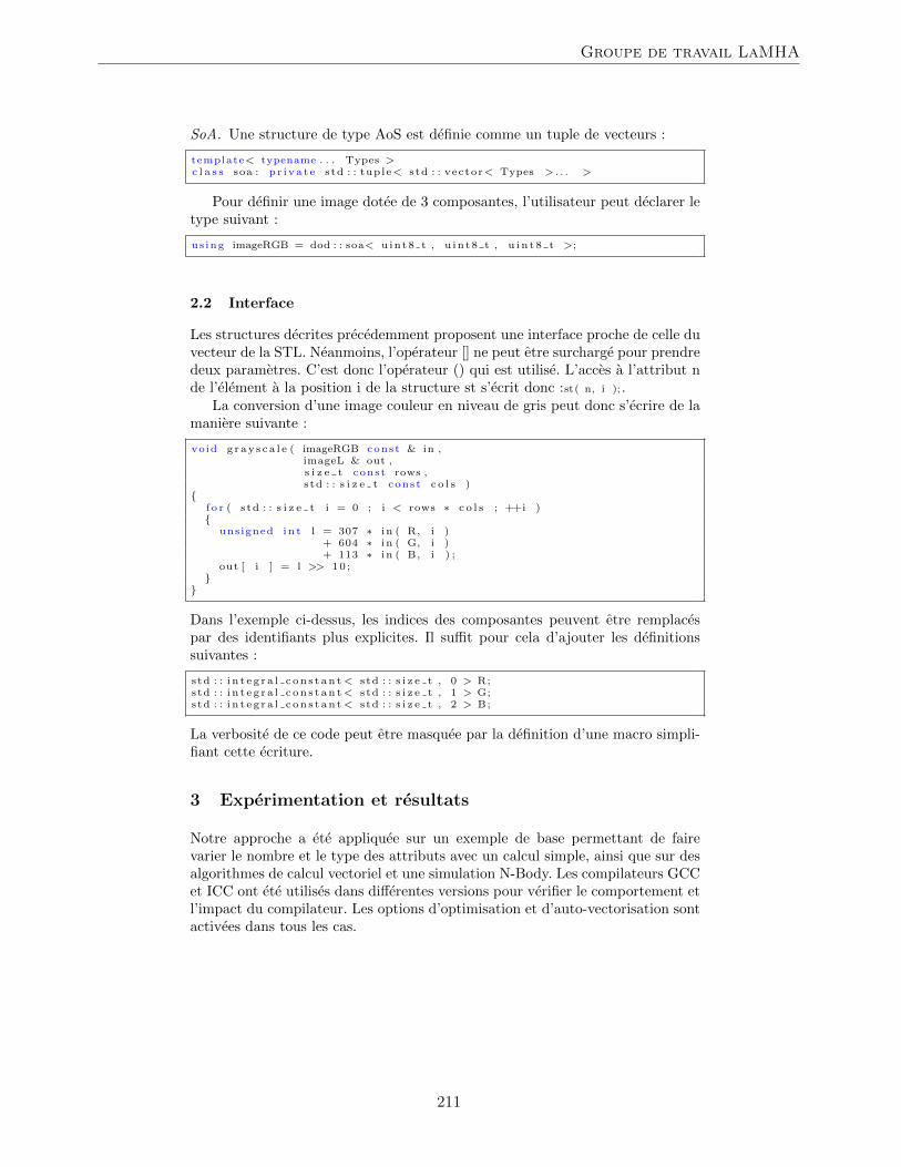
SoA. Une structure de type AoS est definie comme un tuple de vecteurs :
template< typename . . . Types >c l a s s soa : p r i va t e std : : tuple< std : : vector< Types > . . . >
Pour definir une image dotee de 3 composantes, l’utilisateur peut declarer letype suivant :
us ing imageRGB = dod : : soa< u int8 t , u in t8 t , u i n t 8 t >;
2.2 Interface
Les structures decrites precedemment proposent une interface proche de celle duvecteur de la STL. Neanmoins, l’operateur [] ne peut etre surcharge pour prendredeux parametres. C’est donc l’operateur () qui est utilise. L’acces a l’attribut nde l’element a la position i de la structure st s’ecrit donc :st( n, i ); .
La conversion d’une image couleur en niveau de gris peut donc s’ecrire de lamaniere suivante :
void g r ay s ca l e ( imageRGB const & in ,imageL & out ,s i z e t const rows ,std : : s i z e t const c o l s )
{f o r ( std : : s i z e t i = 0 ; i < rows ∗ c o l s ; ++i ){
unsigned in t l = 307 ∗ in ( R, i )+ 604 ∗ in ( G, i )+ 113 ∗ in ( B, i ) ;
out [ i ] = l >> 10 ;}
}
Dans l’exemple ci-dessus, les indices des composantes peuvent etre remplacespar des identifiants plus explicites. Il suffit pour cela d’ajouter les definitionssuivantes :
std : : i n t e g r a l c on s t an t< std : : s i z e t , 0 > R;std : : i n t e g r a l c on s t an t< std : : s i z e t , 1 > G;std : : i n t e g r a l c on s t an t< std : : s i z e t , 2 > B;
La verbosite de ce code peut etre masquee par la definition d’une macro simpli-fiant cette ecriture.
3 Experimentation et resultats
Notre approche a ete appliquee sur un exemple de base permettant de fairevarier le nombre et le type des attributs avec un calcul simple, ainsi que sur desalgorithmes de calcul vectoriel et une simulation N-Body. Les compilateurs GCCet ICC ont ete utilises dans differentes versions pour verifier le comportement etl’impact du compilateur. Les options d’optimisation et d’auto-vectorisation sontactivees dans tous les cas.
Groupe de travail LaMHA
211
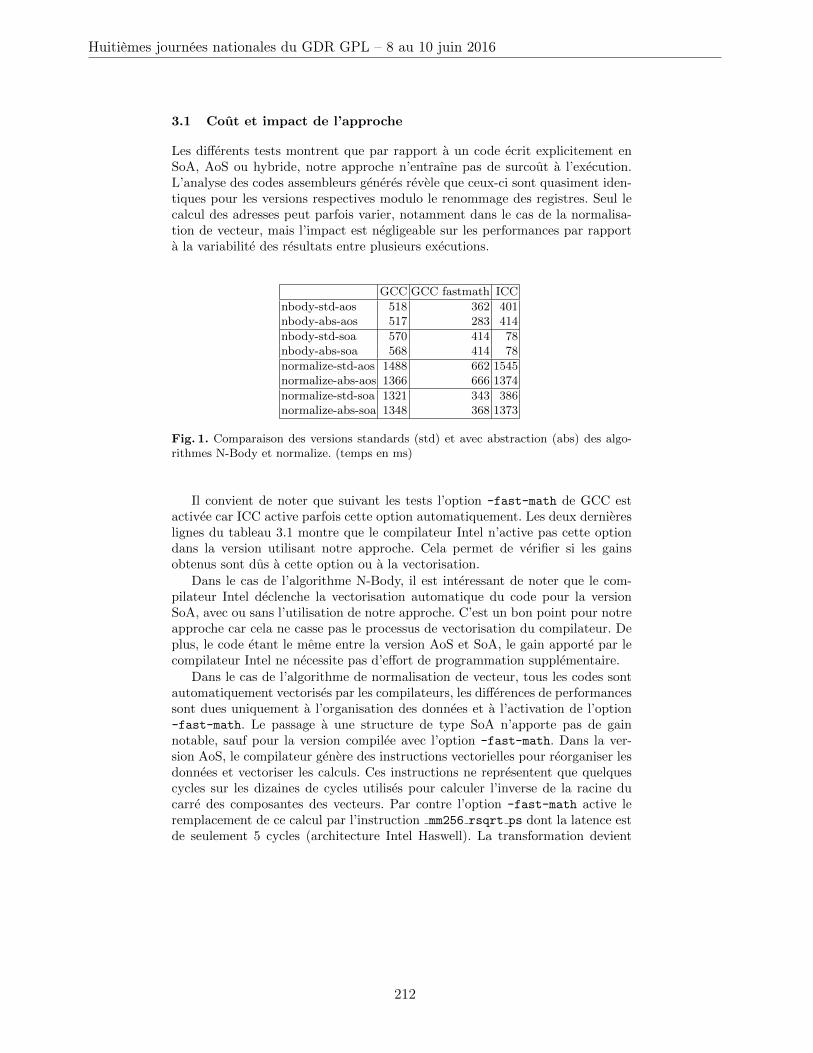
3.1 Cout et impact de l’approche
Les differents tests montrent que par rapport a un code ecrit explicitement enSoA, AoS ou hybride, notre approche n’entraıne pas de surcout a l’execution.L’analyse des codes assembleurs generes revele que ceux-ci sont quasiment iden-tiques pour les versions respectives modulo le renommage des registres. Seul lecalcul des adresses peut parfois varier, notamment dans le cas de la normalisa-tion de vecteur, mais l’impact est negligeable sur les performances par rapporta la variabilite des resultats entre plusieurs executions.
GCC GCC fastmath ICC
nbody-std-aos 518 362 401nbody-abs-aos 517 283 414
nbody-std-soa 570 414 78nbody-abs-soa 568 414 78
normalize-std-aos 1488 662 1545normalize-abs-aos 1366 666 1374
normalize-std-soa 1321 343 386normalize-abs-soa 1348 368 1373
Fig. 1. Comparaison des versions standards (std) et avec abstraction (abs) des algo-rithmes N-Body et normalize. (temps en ms)
Il convient de noter que suivant les tests l’option -fast-math de GCC estactivee car ICC active parfois cette option automatiquement. Les deux derniereslignes du tableau 3.1 montre que le compilateur Intel n’active pas cette optiondans la version utilisant notre approche. Cela permet de verifier si les gainsobtenus sont dus a cette option ou a la vectorisation.
Dans le cas de l’algorithme N-Body, il est interessant de noter que le com-pilateur Intel declenche la vectorisation automatique du code pour la versionSoA, avec ou sans l’utilisation de notre approche. C’est un bon point pour notreapproche car cela ne casse pas le processus de vectorisation du compilateur. Deplus, le code etant le meme entre la version AoS et SoA, le gain apporte par lecompilateur Intel ne necessite pas d’effort de programmation supplementaire.
Dans le cas de l’algorithme de normalisation de vecteur, tous les codes sontautomatiquement vectorises par les compilateurs, les differences de performancessont dues uniquement a l’organisation des donnees et a l’activation de l’option-fast-math. Le passage a une structure de type SoA n’apporte pas de gainnotable, sauf pour la version compilee avec l’option -fast-math. Dans la ver-sion AoS, le compilateur genere des instructions vectorielles pour reorganiser lesdonnees et vectoriser les calculs. Ces instructions ne representent que quelquescycles sur les dizaines de cycles utilises pour calculer l’inverse de la racine ducarre des composantes des vecteurs. Par contre l’option -fast-math active leremplacement de ce calcul par l’instruction mm256 rsqrt ps dont la latence estde seulement 5 cycles (architecture Intel Haswell). La transformation devient
Huitièmes journées nationales du GDR GPL – 8 au 10 juin 2016
212
donc plus couteuse par rapport au calcul dans ce mode ce qui explique le dou-blement des performance entre les versions AoS et SoA.
3.2 Comparaison entre representations
La comparaison entre les differentes versions de l’algorithme N-Body montre,dans le cas de l’utilisation du compilateur GCC, que les performances sont enretrait lors du passage a une structure de type SoA. En effet, l’utilisation deplusieurs tableaux necessite le stockage d’autant de pointeurs pour la manipula-tion des donnees, ce qui accroıt l’occupation des registres generaux disponiblesen nombre limite. Des experimentations sur notre programme de test montre queces registres sont rapidement satures et que le compilateur est oblige de genererdes operations sur la pile pour manipuler les pointeurs supplementaires. Suivantle contexte : nombre d’iterateurs manipules (boucles), pointeurs, ce phenomenepeut apparaıtre des l’utilisation de 5 a 6 tableaux. L’impact sur les performancesest particulierement important sur les codes dont le facteur limitant les perfor-mances est la bande passante. Dans le cas de l’algorithme N-Body, qui est limitepar la puissance de calcul, ce phenomene est largement efface par le gain apportepar la vectorisation comme le montre les resultats du compilateur Intel.
4 Conclusion
L’utilisation d’une approche permettant d’abstraire l’organisation des structuresde donnees permet a la fois au developpeur de se concentrer sur son application,tout en permettant la transformation des structures de donnees afin de pouvoirexploiter les unites vectorielles. Dans certains cas, le passage d’une structurede type AoS a SoA permet la vectorisation automatique du code par le com-pilateur. L’exemple de l’algorithme N-Body montre que les performances sontmultipliees par cinq dans ce cas. Toutefois, dans d’autres cas, le compilateur ar-rive a vectoriser des structures de donnees de type AoS ce qui peut etre benefiquesi la limitation est la puissance de calcul. Dans de nombreux cas egalement, lavectorisation reste a la charge du developpeur.
Ces travaux constituent une premiere etape d’un projet visant a abstrairel’organisation et la transformation des structures de donnees au developpeur.L’implantation d’une nouvelle structure de donnees hybride, aussi appelee AoSoA(Array of Structure of Array), combinant les avantages de la representation AoSet SoA est en cours. La possibilite de convertir la representation automatique-ment, suivant la representation fournie et l’architecture consideree est envisagee.En effet, de nombreuses bibliotheques fournissent des structures de donnees detype AoS, ce qui induit un surcout. Il est envisageable d’effectuer la conversionde structure a la volee lors du premier calcul sur les donnees.
Groupe de travail LaMHA
213

Huitièmes journées nationales du GDR GPL – 8 au 10 juin 2016
214
From BSP regular expressions to BSP automata
Thibaut Tachon1,2, Gaetan Hains1, Frederic Loulergue2, and Chong Li1
1 DPSL-DAL, Central Software Institute, Huawei Technologies, France2 LIFO, Universite d’Orleans, France
Abstract. The theory of finite automata has been recently adapted tobulk-synchronous parallel computing by introducing BSP words, BSPautomata and BSP regular expression. We propose here an algorithmthat, from a BSP regular expression, generates a BSP automaton recog-nizing the same language.
Keywords: BSP, automata, regular expressions
1 Introduction
Bulk synchronous parallel (BSP) is a model of parallel computing introducedby Valiant [5]. By adapting automata theory [4] to BSP, Hains [3] proposedBulk-Synchronous Parallel Automata (BSPA) to describe BSP computation, andBulk-Synchronous Parallel Regular Expressions (BSPRE) to describe BSP lan-guage. However, there was no automatical way to couple BSPA and BSPRE. Wesummarize here the (implemented) tranformation from BSPRE to BSPA.
2 BSP Word and Language
The set of symbols is denoted by Σ, and p denote the number of processors.
Definition 1. Elements of (Σ∗)p is called word-vectors. A BSP word over Σ isa sequence of word-vectors, i.e., a sequence of ((Σ∗)p)∗. A BSP language overΣ is a set of BSP words over Σ.
3 BSP Automata (BSPA)
Definition 2. A BSP automaton ~A is an hexa-tuple
({Qi}i∈[p], Σ, {δi}i∈[p], {qi0}i∈[p], {F i}i∈[p], ∆)
such that for every i, (Qi, Σ, δi, qi0, Fi) is a finite automaton3, and ∆ : ~Q → ~Q
is called the synchronization function where ~Q = (Q0× ...×Q(p−1)) is the set ofglobal states.
In other words a BSP automaton is a vector of sequential automata Ai overthe same alphabet Σ, together with a synchronization function (∆) that mapsstate-vectors to state-vectors.3 Qi is the finite set of states, δ the transition function, qi ∈ Qi the initial state, andF i ⊆ Qi the non-empty set of accepting states.
Groupe de travail LaMHA
215
4 BSP Regular Expressions (BSPRE)
We define the grammar of BSPRE (leftcolumn of the right-side table) and lan-guage of BSPRE (right column of theright-side table), where ri (=1...p−1) isa (scalar) regular expression. The typeof the language is:L : BSPRE → P(((Σ∗)p)∗).
Grammar: R Language: L(R)∅ { }ε {ε}
< r0, . . . , rp−1 > L(r0)× . . .× L(rp−1)R1;R2 L(R1)L(R2)R∗ L(R)∗
R1 +R2 L(R1) ∪ L(R2)
5 From BSPRE to BSPA
Types of a BSPRE, regular expression, automata, BSPA are, resctively, α bspre,α expr, α autom, α bspa, where α is the type of alphabet (set of symbols). Thefollowings describe an algorithm that, from a BSP regular expression, generatesa BSP automaton recognizing the same language.
1. Sequentialization : Σ bspre→ ((Σ × [p]) ∪ {; }) exprRemoving vectors by giving each symbol its removed-vector position.
2. Distribution : ((Σ × [p]) ∪ {; }) expr → ((Σ ∪ {; }) expr)pConstructing a vector of regular expression by puting each symbol to theassociated component and replicating semicolons in all vector components.
3. Transformation : ((Σ ∪ {; }) expr)p → ((Σ ∪ {; }) autom)p
Giving vector of NFA, each of them accepts its component of vector. Thealgorithm used for transformation was invented by Bruggemann-Klein [1]which is an improvement of Glushkov [2].
4. Synchronization : ((Σ ∪ {; }) autom)p → Σ bspaSemicolon-labelled transitions that were the same before the replication areglued together into an hyperedge (∆). The hyperedge connects all its tran-sitions’ NFA into one BSPA.
6 Conclusion
We have presented an algorithm to get a BSPA from a BSPRE. In the future,we will perform more complexity studies, in order to analyze the third step –transformation – of our algorithm that may be the bottleneck: quadratic in sizeof inputed BSPRE.
References
1. Anne Bruggemann-Klein. Regular expressions into finite automata. TheoreticalComputer Science, 120(2):197 – 213, 1993.
2. Pascal Caron and Djelloul Ziadi. Characterization of glushkov automata. TheoreticalComputer Science, 233(12):75 – 90, 2000.
3. G. Hains. Enumerated BSP automata. Technical report. DAL-TR-2016-1.4. S. C. Kleene. Representation of events in nerve nets and finite automata. Automata
Studies, pages 3–41, 1956.5. Leslie G. Valiant. A bridging model for parallel computation. Commun. ACM,
33(8):103–111, August 1990.
Huitièmes journées nationales du GDR GPL – 8 au 10 juin 2016
216

Session du groupe de travail MFDLMéthodes Formelles dans le Développement Logiciel
217

Huitièmes journées nationales du GDR GPL – 8 au 10 juin 2016
218
Un processus de développement Event-B pour desapplications distribuées
Badr Siala, Mohamed Tahar Bhiri, Jean-Paul Bodeveix et Mamoun FilaliUniversité de Sfax
IRIT CNRS UPS Université de Toulouse
Résumé
Nous présentons une méthodologie basée sur le raffinement manuel etautomatique pour le développement d’applications distribuées correctes parconstruction. À partir d’un modèle Event-B, le processus étudié définit desétapes successives pour décomposer et ordonnancer les calculs associés auxévénements et distribuer le code sur des composants. La spécification de cesdeux étapes est faite au travers de deux langages dédiés. Enfin, une implan-tation distribuée en BIP est générée. La correction du processus repose sur lacorrection des raffinements et de la traduction vers le code cible BIP.
1 Introduction
Les systèmes distribués demeurent difficiles à concevoir, construire et faireévoluer. Ceci est lié à la concurrence et au non déterminisme. Plusieurs forma-lismes tels que les algèbres de processus, ASM et TLA+ sont utilisés pour modéli-ser et raisonner sur la correction des systèmes distribués. Un spécifieur utilisant cesformalismes est censé modéliser des mécanismes de bas niveau tels que canaux decommunication et ordonnanceurs.
Dans cet article, nous proposons un support outillé d’aide à la conception sys-tème en utilisant une méthodologie basée sur des raffinements prouvés. Les sys-tèmes considérés sont vus comme un ensemble d’acteurs en interaction. Les pre-miers raffinements fournissent une vue centralisée du système. Ils sont construitsen prenant en compte progressivement les exigences du système. Ces raffinementssont exprimés à l’aide de machines abstraites décrites en Event-B [2]. Ensuite,nous proposons des schémas de raffinements destinés à prendre en compte la na-ture distribuée du système étudié. Ces schémas de raffinements sont guidés parl’utilsateur et les machines Event-B associées sont automatiquement générées. Enconséquence, on obtient un ensemble de machines qui interagissent, dont la com-position est prouvée correcte et conforme avec le niveau abstrait. Le système peutensuite être exécuté sur une plateforme distribuée via une traduction en BIP [3].Remarquons que notre objectif n’est pas d’automatiser complètement le proces-sus de distribution, mais de l’assister. Tout en restant modeste, la différence est
Groupe de travail MFDL
219
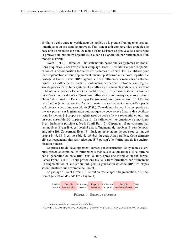
similaire à celle entre un vérificateur de modèle où la preuve d’un jugement est au-tomatique et un assistant de preuve où l’utilisateur doit composer des stratégies debase afin de résoudre son but. De même qu’un assistant de preuve aide à construirela preuve d’un but, notre objectif est d’aider à l’élaboration par raffinements d’unmodèle distribué.
Event-B et BIP admettent une sémantique basée sur les systèmes de transi-tions étiquetées. Ceci favorise leur couplage. Event-B est utilisée pour la spécifi-cation et la décomposition formelles des systèmes distribués. BIP est utilisée pourleur implantation et leur déploiement sur une plateforme à mémoire répartie. Lepassage d’Event-B vers BIP s’appuie sur des raffinements manuels et automa-tiques. Les raffinements manuels horizontaux permettent l’introduction progres-sive de propriétés du futur système. Les raffinements manuels verticaux permettentl’obtention de modèles Event-B traduisibles vers BIP : déterminisation d’actions etconcrétisation des données. Quant aux raffinements automatiques, nous en avonsélaboré deux sortes : l’une est appelée fragmentation (voir section 3) et l’autredistribution (voir section 4). Ces deux sortes de raffinement sont guidées par lespécifieur via deux langages dédiés (DSL). Cette démarche peut être comparée auxtravaux portant sur la génération automatique de code source à partir de spécifica-tions formelles. [4] propose un générateur de code efficace séquentiel en utilisantun sous-ensemble B0 impératif de B. Le raffinement automatique de machinesB est également possible grâce à l’outil Bart [5]. Cependant, il ne concerne pasles modèles Event-B et est destiné aux raffinements de modèles B vers le sous-ensemble B0. Concernant Event-B, plusieurs générateurs de code source ont étéproposés [6, 8]. Il est possible de générer du code Ada parallèle. Cette dernièrecible est cependant plus restrictive que BIP puisqu’elle n’offre que de la synchro-nisation binaire.
Le processus de développement correct par construction de systèmes distri-bués préconisé combine les raffinements manuels et automatiques. Il se terminepar la génération de code BIP. Dans la suite, après une introduction aux forma-lismes Event-B et BIP, nous présentons les deux transformations par raffinement(la fragmentation et la distribution), puis la génération de code BIP. Ces étapesseront illustrées sur l’exemple de l’hôtel 1.
Le passage d’Event-B vers BIP se fait en trois étapes : fragmentation, distribu-tion et génération de code (voir Figure 1).
Etape defragmentation
Etape dedistribution
Etape degénération de code
MachineEvent-B
RaffinementEvent-B
RaffinementEvent-B
CodeBIP
FIGURE 1 – Etapes du processus
1. Le texte complet est accessible via le lienhttps://dl.dropboxusercontent.com/u/98832434/hotelrefinements.html.
Huitièmes journées nationales du GDR GPL – 8 au 10 juin 2016
220
2 Event-B et BIP
2.1 Event-B
Event-B permet de décrire le comportement d’un système par une chaine deraffinements de machines abstraites. Une machine contient des événements, éven-tuellement paramétrés, faisant évoluer l’état de la machine tout en préservant uninvariant. Le non-déterminisme s’exprime dans le corps des événements grâce auxactions ( :∈ et :|) ou via leurs paramètres introduits dans la clause ANY et contraintspar les propriétés spécifiées dans la clause WHERE. Dans une optique de décom-position formelle d’une spécification centralisée en plusieurs composants Event-B,les contraintes d’un paramètre d’un événement partagé doivent être résolues loca-lement. Nous adressons ce problème ultérieurement.
Récemment, deux opérations ont été introduites dans Event-B : la compositionet la décomposition [7]. Elles ont pour but d’introduire la notion de composantdans la démarche de raffinement. Ces deux opérations sont reliées par la propriétésuivante : la composition des sous-composants produits par décomposition d’unmodèle doit raffiner ce modèle. Deux variantes ont été identifiées : par variablespartagées et par événements partagés. La première est adaptée aux systèmes à mé-moire partagée, tandis que la deuxième est plutôt adaptée aux systèmes distribués.Dans ce travail, nous nous intéressons à la composition/décomposition par événe-ments partagés. La plateforme Rodin offre un outil interactif [7] sous forme d’unplugin permettant la composition/décomposition par événements partagés. Dans lasection 4, nous situerons notre plugin de distribution vis-à-vis de ce plugin.
2.2 BIP
Le modèle de composant BIP comporte trois couches : Behavior, Interactionet Priority. La couche Behavior permet de décrire les aspects comportementauxdes composants atomiques tandis que les couches Interaction et Priority décriventles aspects architecturaux d’un système. Les contraintes de synchronisation entreles composants BIP sont exprimées par des interactions regroupées au sein de laconstruction connector de BIP tandis que les contraintes d’ordonnancement desinteractions sont exprimées grâce au concept Priority de BIP. En BIP, un compo-sant atomique englobe des données, des ports et un comportement. Les données(data) sont typées. Les ports (port) donnent accès à des données et constituentl’interface du composant. Le comportement est un ensemble de transitions définiespar un port, une garde et une fonction de mise à jour des données.
3 La fragmentation
Cette étape, dite de fragmentation, prend en entrée un modèle Event-B quel-conque (voir figure 1). Elle a pour but de réduire le non-déterminisme lié au cal-cul des paramètres locaux d’un événement. L’ordre de calcul des paramètres est
Groupe de travail MFDL
221
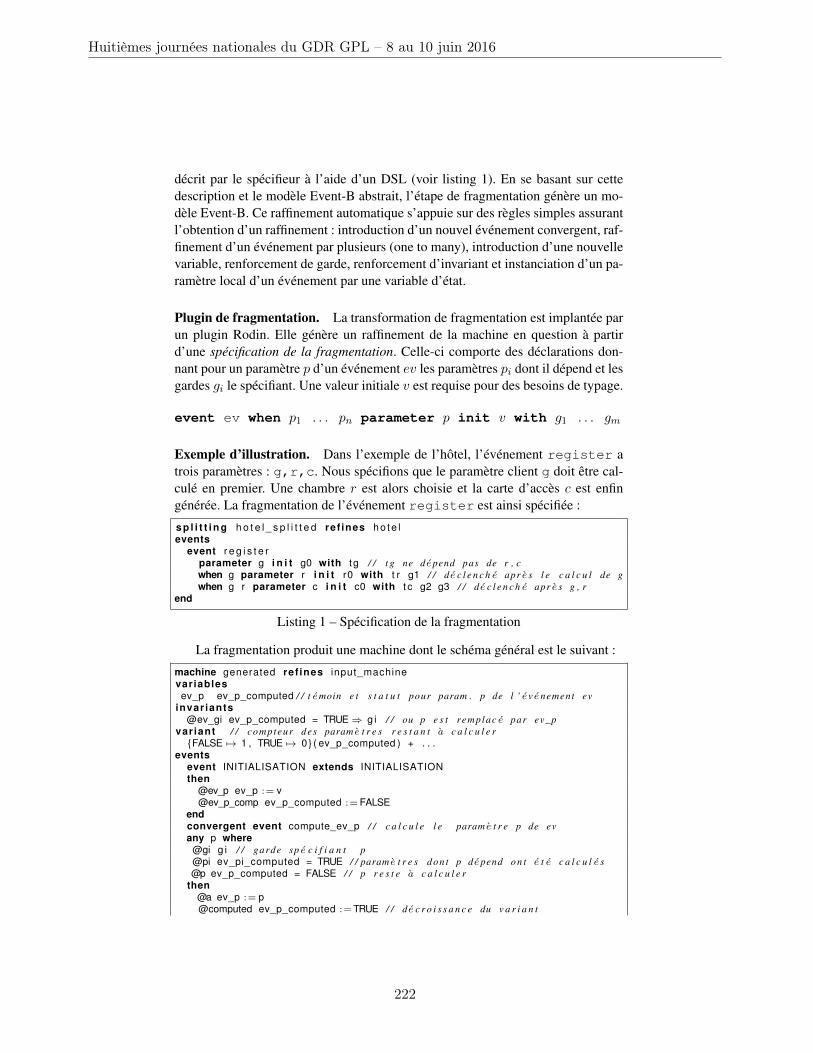
décrit par le spécifieur à l’aide d’un DSL (voir listing 1). En se basant sur cettedescription et le modèle Event-B abstrait, l’étape de fragmentation génère un mo-dèle Event-B. Ce raffinement automatique s’appuie sur des règles simples assurantl’obtention d’un raffinement : introduction d’un nouvel événement convergent, raf-finement d’un événement par plusieurs (one to many), introduction d’une nouvellevariable, renforcement de garde, renforcement d’invariant et instanciation d’un pa-ramètre local d’un événement par une variable d’état.
Plugin de fragmentation. La transformation de fragmentation est implantée parun plugin Rodin. Elle génère un raffinement de la machine en question à partird’une spécification de la fragmentation. Celle-ci comporte des déclarations don-nant pour un paramètre p d’un événement ev les paramètres pi dont il dépend et lesgardes gi le spécifiant. Une valeur initiale v est requise pour des besoins de typage.
event ev when p1 . . . pn parameter p init v with g1 . . . gm
Exemple d’illustration. Dans l’exemple de l’hôtel, l’événement register atrois paramètres : g,r,c. Nous spécifions que le paramètre client g doit être cal-culé en premier. Une chambre r est alors choisie et la carte d’accès c est enfingénérée. La fragmentation de l’événement register est ainsi spécifiée :
s p l i t t i n g h o t e l _ s p l i t t e d ref ines ho te levents
event r e g i s t e rparameter g i n i t g0 with tg / / t g ne d epend pas de r , cwhen g parameter r i n i t r0 with t r g1 / / d e c l e n c h e apr e s l e c a l c u l de gwhen g r parameter c i n i t c0 with t c g2 g3 / / d e c l e n c h e apr e s g , r
end
Listing 1 – Spécification de la fragmentation
La fragmentation produit une machine dont le schéma général est le suivant :
machine generated ref ines input_machinevariablesev_p ev_p_computed / / t emoin e t s t a t u t pour param . p de l ’ ev e nement ev
invar iants@ev_gi ev_p_computed = TRUE ⇒ g i / / ou p e s t remplac e par ev_p
var iant / / compteur des param e t r e s r e s t a n t a c a l c u l e r{FALSE 7→ 1 , TRUE 7→ 0 } ( ev_p_computed ) + . . .
eventsevent INITIALISATION extends INITIALISATIONthen
@ev_p ev_p := v@ev_p_comp ev_p_computed := FALSE
endconvergent event compute_ev_p / / c a l c u l e l e param e t r e p de evany p where
@gi g i / / garde sp e c i f i a n t p@pi ev_pi_computed = TRUE / / param e t r e s d on t p d epend o n t e t e c a l c u l e s@p ev_p_computed = FALSE / / p r e s t e a c a l c u l e r
then@a ev_p := p@computed ev_p_computed := TRUE / / d e c r o i s s a n c e du v a r i a n t
Huitièmes journées nationales du GDR GPL – 8 au 10 juin 2016
222
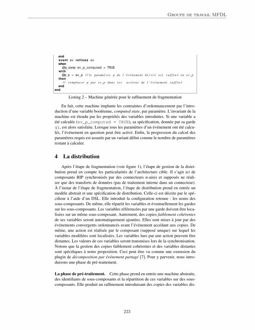
endevent ev ref ines evwhen
@p_comp ev_p_computed = TRUEwith
@p p = ev_p / / l e param e t r e p de l ’ ev e nement h e r i t e e s t r a f f i n e en ev_pthen
/ / r e m p l a c e r p par ev_p dans l e s a c t i o n s de l ’ ev e nement r a f f i n eend
end
Listing 2 – Machine générée pour le raffinement de fragmentation
En fait, cette machine implante les contraintes d’ordonnancement par l’intro-duction d’une variable booléenne, computed state, par paramètre. L’invariant de lamachine est étendu par les propriétés des variables introduites. Si une variable aété calculée (ev_p_computed = TRUE), sa spécification, donnée par sa gardegi, est alors satisfaite. Lorsque tous les paramètres d’un événement ont été calcu-lés, l’événement en question peut être activé. Enfin, la progression du calcul desparamètres requis est assurée par un variant défini comme le nombre de paramètresrestant à calculer.
4 La distribution
Après l’étape de fragmentation (voir figure 1), l’étape de gestion de la distri-bution prend en compte les particularités de l’architecture cible. Il s’agit ici decomposants BIP synchronisés par des connecteurs n-aires et supposés ne réali-ser que des transferts de données (pas de traitement interne dans un connecteur).À l’instar de l’étape de fragmentation, l’étape de distribution prend en entrée unmodèle abstrait et une spécification de distribution. Celle-ci est décrite par le spé-cifieur à l’aide d’un DSL. Elle introduit la configuration retenue : les noms dessous-composants. De même, elle répartit les variables et éventuellement les gardessur les sous-composants. Les variables référencées par une garde doivent être loca-lisées sur un même sous-composant. Autrement, des copies faiblement cohérentesde ses variables seront automatiquement ajoutées. Elles sont mises à jour par desévénements convergents ordonnancés avant l’événement accédant aux copies. Demême, une action est réalisée par le composant (supposé unique) sur lequel lesvariables modifiées sont localisées. Les variables lues par une action peuvent êtredistantes. Les valeurs de ces variables seront transmises lors de la synchronisation.Notons que la gestion des copies faiblement cohérentes et des variables distantessont spécifiques à notre proposition. Ceci peut être vu comme une extension duplugin de décomposition par événement partagé [7]. Pour y parvenir, nous intro-duisons une phase de pré-traitement.
La phase de pré-traitement. Cette phase prend en entrée une machine abstraite,des identifiants de sous-composants et la répartition de ces variables sur des sous-composants. Elle produit un raffinement introduisant des copies des variables dis-
Groupe de travail MFDL
223
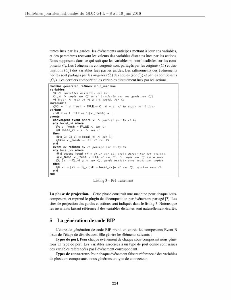
tantes lues par les gardes, les événements anticipés mettant à jour ces variables,et des paramètres recevant les valeurs des variables distantes lues par les actions.Nous supposons dans ce qui suit que les variables vi sont localisées sur les com-posants Ci. Les événements convergents sont partagés par les origines (Ci) et des-tinations (Cj) des variables lues par les gardes. Les raffinements des événementshérités sont partagés par les origines (Ci) des copies (sur Cj) et par les composants(Ck). Ces derniers comportent les variables directement lues par les actions.
machine generated ref ines input_machinevariables
v i / / v a r i a b l e s h e r i t e es , s u r CiCj_v i / / c o p i e s u r Cj de v i ( u t i l i s ee par une garde s u r Cj )v i _ f r e s h / / t r u e s i v i a e t e c o p i e , s u r Ci
invar iants@Cj_vi_f v i _ f r e s h = TRUE ⇒ Cj_v i = v i / / l a c o p i e e s t a j o u r
var iant{FALSE 7→ 1 , TRUE 7→ 0 } ( v i _ f r e s h ) + . . .
eventsconvergent event share_v i / / p a r t a g e par Ci e t Cjany l o c a l _ v i where
@g v i _ f r e s h = FALSE / / s u r Ci@l l o c a l _ v i = v i / / s u r Ci
then@to_Cj C j_v i := l o c a l _ v i / / s u r Cj@done v i _ f r e s h := TRUE / / s u r Ci
endevent ev ref ines ev / / p a r t a g e par Ci , Cj , Ckany l oca l_vk where
@vj_access loca l_vk = vk / / s u r Ck , acc e s d i r e c t par l e s a c t i o n s@vi_fresh v i _ f r e s h = TRUE / / s u r Ci , l a c o p i e s u r Cj e s t a j o u r@g [ v i := Cj_v i ] g / / s u r Cj , garde h e r i t ee avec acc e s aux c o p i e s
then@a v j := [ v i := Cj_v i ; vk := l oca l_vk ] e / / s u r Cj , s y n c h r o avec Ck
endend
Listing 3 – Pré-traitement
La phase de projection. Cette phase construit une machine pour chaque sous-composant, et reprend le plugin de décomposition par événement partagé [7]. Lessites de projection des gardes et actions sont indiqués dans le listing 3. Notons queles invariants faisant référence à des variables distantes sont naturellement écartés.
5 La génération de code BIP
L’étape de génération de code BIP prend en entrée les composants Event-Bissus de l’étape de distribution. Elle génère les éléments suivants :
Types de port. Pour chaque événement de chaque sous-composant nous géné-rons un type de port. Les variables associées à un type de port donné sont issuesdes variables référencées par l’événement correspondant.
Types de connecteur. Pour chaque événement faisant référence à des variablesde plusieurs composants, nous générons un type de connecteur.
Huitièmes journées nationales du GDR GPL – 8 au 10 juin 2016
224
Squelette de sous-composants. Pour chaque sous-composant, nous généronsun composant atomique BIP. Il comporte les variables du sous-composant ainsique les variables distantes appartenant à d’autres sous-composants, les instancesdes types de ports associés à ce sous-composant et, pour chaque événement, unetransition synchronisée sur l’instance du port correspondant.
Le composant composite. Il regroupe une instance de chaque sous-composantet connecteur. Chaque instance de connecteur admet une instance de port apparte-nant aux instances de sous-composants définies précédemment.
6 Conclusion
Nous avons présenté une méthode de développement de systèmes distribuéscorrects par construction. À partir d’une machine Event-B représentant un modèlecentralisé, nous appliquons deux types de raffinements automatiques (la fragmen-tation et la distribution) dont les paramètres sont déclarés par deux langages dédiés.Enfin, un modèle BIP exécutable sur une architecture répartie est produit. La cor-rection de cette méthode repose sur la correction des étapes de raffinement et de latraduction finale en code BIP.
Nous envisageons maintenant d’améliorer l’outillage de ce processus. Les trans-formations de modèles Event-B sont réalisées via xtext et xtend [1]. L’étape sui-vante sera la finalisation du générateur BIP.
Références[1] Language engineering for everyone ! https://eclipse.org/Xtext. Acc : 16-
01-06.[2] J.-R. Abrial. Modeling in Event-B : System and Software Engineering. Cambridge
University Press, New York, NY, USA, 1st edition, 2010.[3] A. Basu, S. Bensalem, M. Bozga, J. Combaz, M. Jaber, T.-H. Nguyen, and J. Sifakis.
Rigorous component-based system design using the bip framework. IEEE Software,28(3) :41–48, 2011.
[4] D. Bert, S. Boulmé, M.-L. Potet, A. Requet, and L. Voisin. Adaptable translator ofB specifications to embedded c programs. In K. Araki, S. Gnesi, and D. Mandrioli,editors, FME, volume 2805 of LNCS, pages 94–113. Springer, 2003.
[5] Clearsy. Bart (b automatic refinement tool). http://tools.clearsy.com/wp-content/uploads/sites/8/resources/BART_GUI_User_Manual.pdf.
[6] A. Edmunds and M. Butler. Tasking Event-B : An extension to Event-B for generatingconcurrent code. Event Dates : 2nd April 2011, February 2011.
[7] R. Silva and M. Butler. Shared event composition/decomposition in Event-B. InFMCO Formal Methods for Components and Objects, November 2010. Event Dates :29 November - 1 December 2010.
[8] N. K. Singh. Eb2all : An automatic code generation tool. In Using Event-B for CriticalDevice Software Systems, pages 105–141. Springer London, 2013.
Groupe de travail MFDL
225

Huitièmes journées nationales du GDR GPL – 8 au 10 juin 2016
226
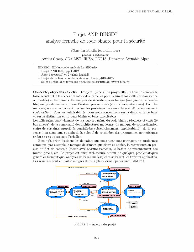
Projet ANR BINSECanalyse formelle de code binaire pour la sécurité
Sébastien Bardin (coordinateur)[email protected]
Airbus Group, CEA LIST, IRISA, LORIA, Université Grenoble Alpes
BINSEC : BINary-code analysis for SECurity– Projet ANR INS, appel 2012– Axes 1 (sécurité) et 2 (génie logiciel)– Projet de recherche fondamentale sur 4 ans (2013-2017)– Sujet : Techniques formelles d’analyse de sécurité au niveau binaire
Contexte, objectifs et défis. L’objectif général du projet BINSEC est de combler lefossé actuel entre le succès des méthodes formelles pour la sûreté logicielle (niveau sourceou modèle) et les besoins des analyses de sécurité niveau binaire (analyse de vulnérabi-lité, analyse de malware), pour l’instant peu outillées (approches syntaxiques). Pour lesmalware, nous nous concentrons sur les problèmes de camouflage et d’obscurcissement(obfuscation). Pour les vulnérabilités, nous nous concentrons sur la découverte de bugset sur la distinction entre bugs bénins et bugs exploitables.Les défis principaux viennent de la structure même du code binaire (données et contrôlebas niveau), de la complexité des architectures modernes, du manque de compréhensionclaire de certaines propriétés considérées (obscurcissement, exploitabilité), de la pré-sence d’un attaquant et enfin de la volonté de considérer des programmes non critiques(robustesse et passage à l’échelle).
Bien qu’a priori distincts, les domaines que nous attaquons partagent des problèmescommuns, par exemple le manque de sémantique claire et unifiée, la reconstruction pré-cise du flot de contrôle (même avec obscurcissement), le besoin de raisonnement basniveau précis, etc. Le projet est ainsi architecturé autour de quelques problématiquesgénérales (sémantique, analyses de base) sur lesquelles se basent les travaux applicatifs.Les résultats sont en partie intégrés dans la plate-forme open-source BINSEC.
Figure 1 – Aperçu du projet
Groupe de travail MFDL
227
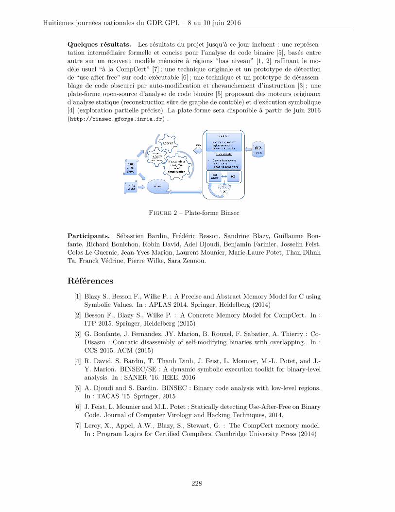
Quelques résultats. Les résultats du projet jusqu’à ce jour incluent : une représen-tation intermédiaire formelle et concise pour l’analyse de code binaire [5], basée entreautre sur un nouveau modèle mémoire à régions “bas niveau” [1, 2] raffinant le mo-dèle usuel “à la CompCert” [7] ; une technique originale et un prototype de détectionde “use-after-free” sur code exécutable [6] ; une technique et un prototype de désassem-blage de code obscurci par auto-modification et chevauchement d’instruction [3] ; uneplate-forme open-source d’analyse de code binaire [5] proposant des moteurs originauxd’analyse statique (reconstruction sûre de graphe de contrôle) et d’exécution symbolique[4] (exploration partielle précise). La plate-forme sera disponible à partir de juin 2016(http://binsec.gforge.inria.fr) .
Figure 2 – Plate-forme Binsec
Participants. Sébastien Bardin, Frédéric Besson, Sandrine Blazy, Guillaume Bon-fante, Richard Bonichon, Robin David, Adel Djoudi, Benjamin Farinier, Josselin Feist,Colas Le Guernic, Jean-Yves Marion, Laurent Mounier, Marie-Laure Potet, Than DihnhTa, Franck Védrine, Pierre Wilke, Sara Zennou.
Références[1] Blazy S., Besson F., Wilke P. : A Precise and Abstract Memory Model for C using
Symbolic Values. In : APLAS 2014. Springer, Heidelberg (2014)[2] Besson F., Blazy S., Wilke P. : A Concrete Memory Model for CompCert. In :
ITP 2015. Springer, Heidelberg (2015)[3] G. Bonfante, J. Fernandez, JY. Marion, B. Rouxel, F. Sabatier, A. Thierry : Co-
Disasm : Concatic disassembly of self-modifying binaries with overlapping. In :CCS 2015. ACM (2015)
[4] R. David, S. Bardin, T. Thanh Dinh, J. Feist, L. Mounier, M.-L. Potet, and J.-Y. Marion. BINSEC/SE : A dynamic symbolic execution toolkit for binary-levelanalysis. In : SANER ’16. IEEE, 2016
[5] A. Djoudi and S. Bardin. BINSEC : Binary code analysis with low-level regions.In : TACAS ’15. Springer, 2015
[6] J. Feist, L. Mounier and M.L. Potet : Statically detecting Use-After-Free on BinaryCode. Journal of Computer Virology and Hacking Techniques, 2014.
[7] Leroy, X., Appel, A.W., Blazy, S., Stewart, G. : The CompCert memory model.In : Program Logics for Certified Compilers. Cambridge University Press (2014)
Huitièmes journées nationales du GDR GPL – 8 au 10 juin 2016
228
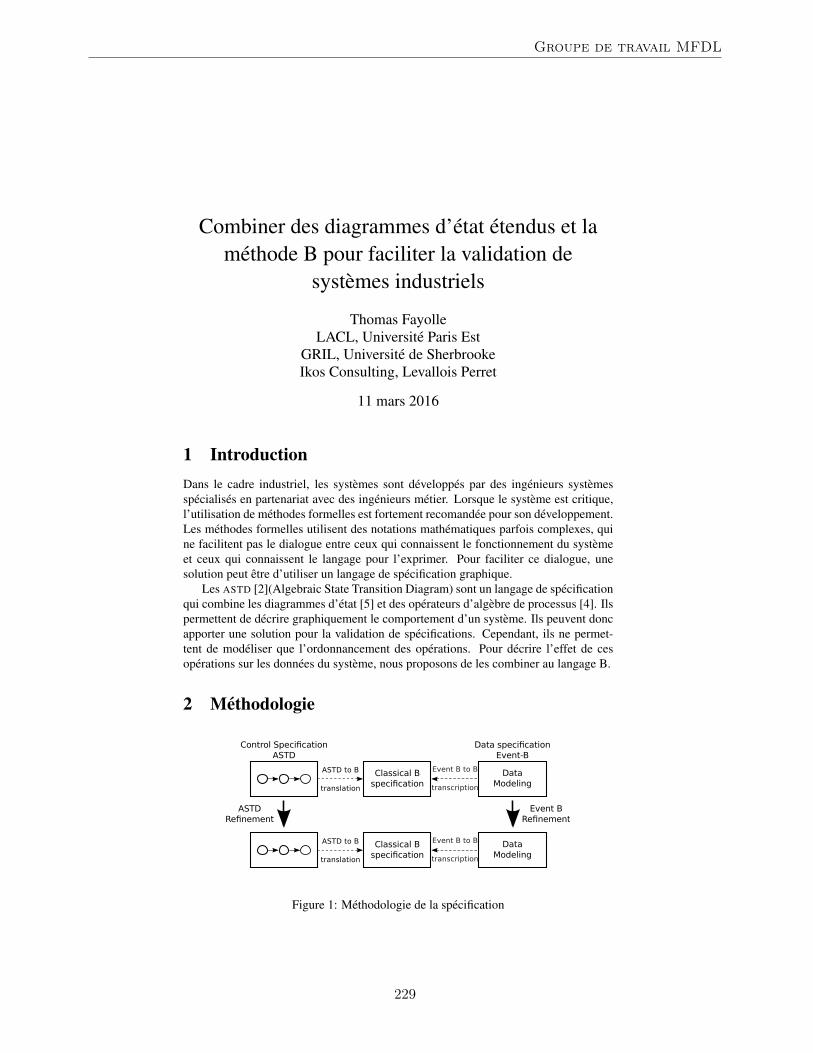
Combiner des diagrammes d’etat etendus et lamethode B pour faciliter la validation de
systemes industriels
Thomas FayolleLACL, Universite Paris Est
GRIL, Universite de SherbrookeIkos Consulting, Levallois Perret
11 mars 2016
1 IntroductionDans le cadre industriel, les systemes sont developpes par des ingenieurs systemesspecialises en partenariat avec des ingenieurs metier. Lorsque le systeme est critique,l’utilisation de methodes formelles est fortement recomandee pour son developpement.Les methodes formelles utilisent des notations mathematiques parfois complexes, quine facilitent pas le dialogue entre ceux qui connaissent le fonctionnement du systemeet ceux qui connaissent le langage pour l’exprimer. Pour faciliter ce dialogue, unesolution peut etre d’utiliser un langage de specification graphique.
Les ASTD [2](Algebraic State Transition Diagram) sont un langage de specificationqui combine les diagrammes d’etat [5] et des operateurs d’algebre de processus [4]. Ilspermettent de decrire graphiquement le comportement d’un systeme. Ils peuvent doncapporter une solution pour la validation de specifications. Cependant, ils ne permet-tent de modeliser que l’ordonnancement des operations. Pour decrire l’effet de cesoperations sur les donnees du systeme, nous proposons de les combiner au langage B.
2 Methodologie
Figure 1: Methodologie de la specification
Groupe de travail MFDL
229
Notre methode de specification combine le langage ASTD et le langage Event-B.Cette methode est resumee a la figure 1. Le systeme est modelise en deux parties.Son comportement dynamique est decrit dans la premiere partie en utilisant les ASTD(specification a gauche sur la figure 1). La deuxieme partie en Event-B decrit les mod-ifications apportees au modele de donnees (specification a droite sur la figure 1). Ellecontient un evenement pour chaque label de la specification ASTD. Lorsque la tran-sition est effectuee, le modele de donnees est modifie en suivant la specification del’evenement Event-B. La specification en B classique (partie centrale de la figure 1)permet d’assurer la coherence du systeme.
2.1 La specification ASTD
La specification ASTD modelise l’ordonnancement des operations en utilisant des no-tations graphiques des diagrammes d’etat et des operateurs des algebres de processus.La specification graphique facilite la validation tout en restant formelle. L’ajout desoperateurs des algebres de processus permet de modeliser des systemes dans lesquelsplusieurs processus fonctionnent en parallele, comme c’est le cas dans beaucoup desystemes industriels.
2.2 La specification Event-BLa specification ASTD modelise l’ordre des operations, tandis que la specificationEvent-B modelise les effets de chaque operation sur le modele de donnees. Elle con-tient un evenement pour chaque label de transition de la specification ASTD. Les in-variants Event-B traduisent les proprietes statiques, notamment les proprietes de surete.Les outils de la plateforme RODIN 1 permettent de generer et de prouver les obliga-tions de preuve associees a la preservation des invariants. Au contraire du raffinementde la methode B, le raffinement de la methode Event-B permet l’ajout de nouveauxevenements. Pour coller au raffinement des ASTD, c’est ce langage qui a ete choisipour la specification de la partie donnee.
2.3 Specification BPour un niveau de specification, la modelisation en B classique contient deux machines.La premiere est une traduction de la specification ASTD, la seconde est une transcrip-tion de la specification Event-B.
Un outil effectue la traduction automatique de la specification ASTD. Cette traduc-tion est effectuee suivant les regles definies dans [6]. Le mecanisme de la traductionpeut etre resume de la maniere suivante. Les etats des ASTD sont encodes par une vari-able d’etat B. Une operation B est ecrite pour chaque label de la specification ASTD.La precondition de cette operation verifie que les variables d’etat sont bien dans l’etatinitial de la transition. La postcondition met a jour les variables d’etat de maniere a cequ’elles correspondent a l’etat final de la transition.
De plus, nous souhaitons que les variables du modele de donnees soient modifieeslors de chaque transition. Puisqu’il n’est pas possible d’appeler un evenement Event-Bdans une specification en B classique, la specification Event-B est traduite en B. Lesvariables d’etat et les invariants de typage sont conserves. Les evenement sont reecritsen operation, la garde devient une precondition et la postcondition reste identique.
1http://event-b.org
Huitièmes journées nationales du GDR GPL – 8 au 10 juin 2016
230
Regrouper les deux specifications en une seule nous permet de verifier la coherenceglobale du systeme (c’est-a-dire un niveau de specification horizontal sur la figure 1).En effet, les proprietes statiques de la specification Event-B ne sont verifiees que si lesevenements sont executes quand leurs gardes sont vraies. La generation des obligationsde preuves de la methode B oblige a verifier que les preconditions des operations ap-pelees sont vraies au moment de l’appel. La preuve de ces obligations garantit que lesevenements du modele de donnees sont toujours executes quand leur garde est vraie.Pour prouver ces obligations, il est necessaire d’ajouter des invariants qui lient les vari-ables du modele de donnees aux etats de l’ASTD.
2.4 RaffinementLe raffinement du systeme est effectue en parallele sur les deux modeles. La specificationde l’ordonnancement des operations est effectuee en suivant la definition du raffinementpour les ASTD. Cette definition (donnee dans [3]) permet de garantir la preservation destraces. Le raffinement du modele de donnees suit la definition du raffinement Event-B.
3 ConclusionLa methode presentee dans cet article permet de modeliser graphiquement un systemecritique ce qui facilite la validation du systeme dans un domaine industriel. La methodea ete testee sur un exemple dans le cadre de la modelisation d’un systeme ferrovi-aire [1].
La modelisation de ce cas a permis de voir l’efficacite de la methode. Cependant,la preuve de la coherence globale du systeme s’est montree fastidieuse. Des travauxsont en cours pour simplifier les regles automatiques de traduction et definir des regleset des outils de raffinement pour les ASTD.
References[1] T. Fayolle. Specifying a Train System Using ASTD and the B Method. Technical
report, 2014. http://www.lacl.fr/~tfayolle.
[2] M. Frappier, F. Gervais, R. Laleau, B. Fraikin, and R. Saint-Denis. ExtendingStatecharts with Process Algebra Operators. Inovation in System Software Enge-neering, Volume 4, Number 3:285–292, 2008.
[3] M. Frappier, F. Gervais, R. Laleau, and J. Milhau. Refinement patterns for ASTDs.Formal Aspects of Computing, pages 1–23, 2012.
[4] M. Frappier and R. St-Denis. EB3 : an entity-based black-box specification methodfor information systems. Software and Systems Modeling, 2(2):134–149, July2003.
[5] D. Harel. Statecharts: A Visual Formalism for Complex Systems. Science ofComputer Programming, 8:231–274, 1987.
[6] J. Milhau. A formal integration of access control policies into information systems.Theses, Universite Paris-Est ; Universite de Sherbrooke, December 2011.
Groupe de travail MFDL
231

Huitièmes journées nationales du GDR GPL – 8 au 10 juin 2016
232
Vers un développement formel non incrémental
Thi-Kim-Dung Pham1,3, Catherine Dubois2, Nicole Levy1
1. Conservatoire National des Arts et Métiers, lab. Cedric, Paris
2. ENSIIE, lab. Samovar, Évry
3. University of Engineering and Technology, Vietnam National University, Hanoi
Résumé
Modularité, généricité, héritage sont des mécanismes qui facilitent le dévelop-pement et la vérification formelle de logiciels corrects par construction en per-mettant de réutiliser des spécifications, du code et/ou des preuves. Cependant leslignes de produits exploitent d’autres techniques de réutilisation ou de modifica-tion graduelle. Les méthodes formelles permettant la production de code correctpar construction (en B ou FoCaLiZe par exemple) ne sont pas bien adaptées à lavariabilité telle qu’elle apparaît dans les lignes de produits. Nous proposons d’ap-procher ce problème par la définition d’un langage formel, GFML, proche de lavariabilité mise en œuvre dans les lignes de produits permettant de spécifier, im-planter et prouver. Ce langage est compilé vers un formalisme existant, ici FoCa-LiZe. Cet article illustre par l’exemple une des constructions offertes par GFMLainsi que sa traduction en FoCaLiZe.
1 IntroductionNous aimerions construire des programmes corrects par construction, c’est-à-dire
qui répondent au cahier des charges, sont cohérents et complets. Il est effectivementpossible de le faire à l’aide de certaines méthodes qui utilisent des langages formelstels que B [1] ou FoCaLiZe [7]. Il faut alors définir les propriétés que le programmedoit vérifier et utiliser des outils de preuve pour prouver que l’on a bien suivi toutes lesétapes de la méthode.
Un des principaux problèmes de ces méthodes réside dans la difficulté à les appli-quer. On pourrait espérer que les méthodes de réutilisation facilitent le développement.Il existe plusieurs manières de réutiliser un programme. Par exemple, les méthodesorientées objets qui proposent de compléter ou de modifier, par héritage, une classed’objets. Le langage FoCaLiZe possède l’héritage et permet ainsi de réutiliser des spé-cifications, des programmes et des preuves.
Mais ce n’est pas suffisant. On aimerait réutiliser une fonctionnalité d’un pro-gramme mais pour l’utiliser dans un contexte différent. Il existe des mécanismes per-mettant de décrire les propriétés d’un contexte, indispensables pour un programme,sous la forme de paramètres de ce programme. En FoCaLiZe, les composants s’ap-pellent des espèces (species) et peuvent être paramétrés par des espèces représentantdes objets ou des propriétés du contexte requis.
Mais ce n’est pas encore suffisant. L’utilisation de la paramétrisation se révèle assezdifficile et restrictive.
Groupe de travail MFDL
233
En fait, pour réutiliser un programme (ou une partie d’un programme), il faut savoircomment il a été construit et connaître les décisions prises lors de son développement.
Le problème qui se pose est l’expression des savoirs-faire et leur réutilisation. Laréalité, c’est qu’il est bien difficile de décrire ou de formaliser ce savoir-faire. Maisc’est un des avantages des approches lignes de produits [4] qui permettent de dé-crire la succession des décisions à prendre et d’associer à chaque décision une solu-tion concrète sous la forme d’un morceau de code (asset). En général, les décisionsprises sont constructives : il s’agit d’ajouter une information, une fonctionnalité, unepropriété, etc. Dans ce cas, la composition des morceaux peut être définie simplement.
Mais qu’en est-il lorsque la décision prise à une étape est de modifier l’étape précé-dente et non seulement de rajouter quelque chose ? Comment formaliser des méthodesde réutilisation non incrémentales ?
Il existe des approches telle que celle de Thomas Thüm [13, 12] qui utilise les lignesde produits pour développer des programmes Java selon une approche par contrats àl’aide de pré et post-conditions. Il utilise le langage JML pour écrire les contrats et lestraduit ensuite en Coq pour les vérifier. C’est de là qu’est venue l’idée d’introduire unlangage dédié pour décrire la construction des modifications à apporter au code.
Notre proposition est de faciliter de telles étapes de développement, permettantde modifier une étape précédente, c’est-à-dire de modifier le code préalablement dé-fini, et prouvé. L’idée est d’introduire un langage d’expression de ces modifications etun compilateur réalisant la modification à opérer et générant le code. Le langage quenous proposons s’appelle GFML. Couplée à une approche lignes de produits, notredémarche permet de décrire des savoirs-faire qui ne sont pas purement incrémentauxmais peuvent passer par des étapes de remise en cause de développements préalables,tout en bénéficiant de l’approche de développement de code correct par construction.
Nous avons choisi d’illustrer notre démarche dans le cadre proposé par FoCaLiZe.En effet, il permet de définir à la fois spécifications, code et preuves, donc tous lesartefacts associés à une caractéristique d’une ligne de produits. D’autre part, FoCaLiZeadmet pour seul mécanisme de raffinement, l’enrichissement par héritage, ce qui laissebeaucoup de liberté.
La suite de cet article est structurée de la manière suivante. Dans un premier tempsnous allons étudier les constructions existantes en FoCaLiZe qui permettent de suivreun développement formel incrémental. Nous signalerons aussi les limites de ce modèle.Nous montrons à l’aide d’un exemple de compte bancaire un exemple de modificationsouhaitée, à savoir le renforcement d’une fonctionnalité tout en conservant au maxi-mum les preuves déjà faites. Cette modification peut être exprimée en FoCaLiZe àl’aide de l’utilisation conjointe de l’héritage et de la paramétrisation. Nous présentonsensuite l’expression de cette modification dans notre langage GFML et sa traduction enFoCaLiZe. Un avantage de cette approche est le fait qu’elle s’adapte très bien aux lignesde produits puisque la composition des morceaux associés à chaque étape entraîne unesuite de modifications et non seulement des enrichissements. L’approche générale estprésentée dans [8], nous détaillons ici, sur un exemple, une des constructions offertespar GFML et sa compilation en FoCaLiZe.
2 Le modèle FoCaLiZeL’environnement FoCaLiZe (anciennement FoCal) [7, 6] permet le développement
de programmes certifiés pas à pas, de la spécification à l’implantation. Cet environne-ment propose un langage également nommé FoCaLiZe et des outils d’analyse de code,
Huitièmes journées nationales du GDR GPL – 8 au 10 juin 2016
234
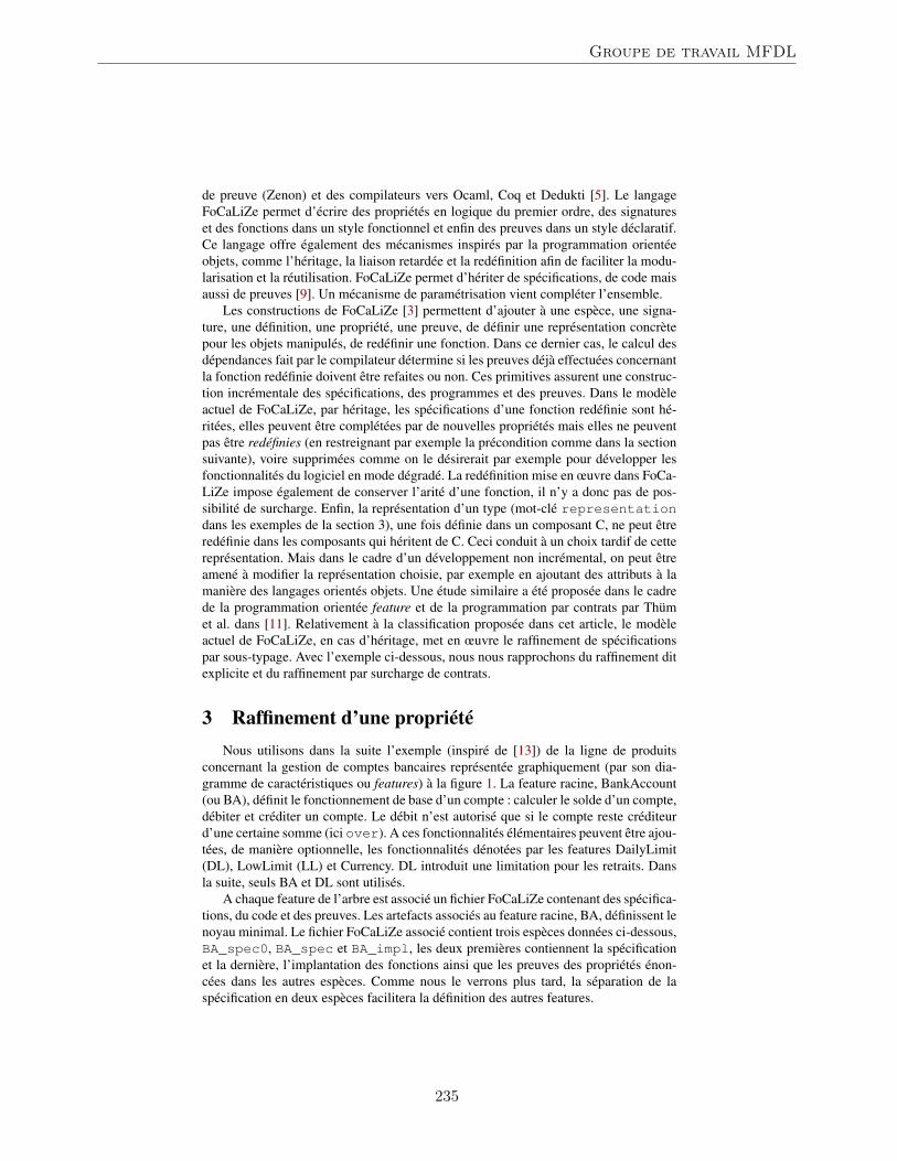
de preuve (Zenon) et des compilateurs vers Ocaml, Coq et Dedukti [5]. Le langageFoCaLiZe permet d’écrire des propriétés en logique du premier ordre, des signatureset des fonctions dans un style fonctionnel et enfin des preuves dans un style déclaratif.Ce langage offre également des mécanismes inspirés par la programmation orientéeobjets, comme l’héritage, la liaison retardée et la redéfinition afin de faciliter la modu-larisation et la réutilisation. FoCaLiZe permet d’hériter de spécifications, de code maisaussi de preuves [9]. Un mécanisme de paramétrisation vient compléter l’ensemble.
Les constructions de FoCaLiZe [3] permettent d’ajouter à une espèce, une signa-ture, une définition, une propriété, une preuve, de définir une représentation concrètepour les objets manipulés, de redéfinir une fonction. Dans ce dernier cas, le calcul desdépendances fait par le compilateur détermine si les preuves déjà effectuées concernantla fonction redéfinie doivent être refaites ou non. Ces primitives assurent une construc-tion incrémentale des spécifications, des programmes et des preuves. Dans le modèleactuel de FoCaLiZe, par héritage, les spécifications d’une fonction redéfinie sont hé-ritées, elles peuvent être complétées par de nouvelles propriétés mais elles ne peuventpas être redéfinies (en restreignant par exemple la précondition comme dans la sectionsuivante), voire supprimées comme on le désirerait par exemple pour développer lesfonctionnalités du logiciel en mode dégradé. La redéfinition mise en œuvre dans FoCa-LiZe impose également de conserver l’arité d’une fonction, il n’y a donc pas de pos-sibilité de surcharge. Enfin, la représentation d’un type (mot-clé representationdans les exemples de la section 3), une fois définie dans un composant C, ne peut êtreredéfinie dans les composants qui héritent de C. Ceci conduit à un choix tardif de cettereprésentation. Mais dans le cadre d’un développement non incrémental, on peut êtreamené à modifier la représentation choisie, par exemple en ajoutant des attributs à lamanière des langages orientés objets. Une étude similaire a été proposée dans le cadrede la programmation orientée feature et de la programmation par contrats par Thümet al. dans [11]. Relativement à la classification proposée dans cet article, le modèleactuel de FoCaLiZe, en cas d’héritage, met en œuvre le raffinement de spécificationspar sous-typage. Avec l’exemple ci-dessous, nous nous rapprochons du raffinement ditexplicite et du raffinement par surcharge de contrats.
3 Raffinement d’une propriétéNous utilisons dans la suite l’exemple (inspiré de [13]) de la ligne de produits
concernant la gestion de comptes bancaires représentée graphiquement (par son dia-gramme de caractéristiques ou features) à la figure 1. La feature racine, BankAccount(ou BA), définit le fonctionnement de base d’un compte : calculer le solde d’un compte,débiter et créditer un compte. Le débit n’est autorisé que si le compte reste créditeurd’une certaine somme (ici over). A ces fonctionnalités élémentaires peuvent être ajou-tées, de manière optionnelle, les fonctionnalités dénotées par les features DailyLimit(DL), LowLimit (LL) et Currency. DL introduit une limitation pour les retraits. Dansla suite, seuls BA et DL sont utilisés.
A chaque feature de l’arbre est associé un fichier FoCaLiZe contenant des spécifica-tions, du code et des preuves. Les artefacts associés au feature racine, BA, définissent lenoyau minimal. Le fichier FoCaLiZe associé contient trois espèces données ci-dessous,BA_spec0, BA_spec et BA_impl, les deux premières contiennent la spécificationet la dernière, l’implantation des fonctions ainsi que les preuves des propriétés énon-cées dans les autres espèces. Comme nous le verrons plus tard, la séparation de laspécification en deux espèces facilitera la définition des autres features.
Groupe de travail MFDL
235
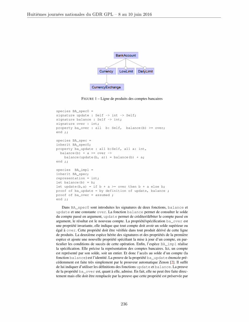
FIGURE 1 – Ligne de produits des comptes bancaires
species BA_spec0 =signature update : Self -> int -> Self;signature balance : Self -> int;signature over : int;property ba_over : all b: Self, balance(b) >= over;end ;;
species BA_spec =inherit BA_spec0;property ba_update : all b:Self, all a: int,
balance(b) + a >= over ->balance(update(b, a)) = balance(b) + a;
end ;;
species BA_impl =inherit BA_spec;representation = int;let balance(b) = b;let update(b,a) = if b + a >= over then b + a else b;proof of ba_update = by definition of update, balance ;proof of ba_over = assumed ;end ;;
Dans BA_spec0 sont introduites les signatures de deux fonctions, balance etupdate et une constante over. La fonction balance permet de consulter le soldedu compte passé en argument, update permet de créditer/débiter le compte passé enargument, le résultat est le nouveau compte. La propriété/spécification ba_over estune propriété invariante, elle indique que tout compte doit avoir un solde supérieur ouégal à over. Cette propriété doit être vérifiée dans tout produit dérivé de cette lignede produits. La deuxième espèce hérite des signatures et des propriétés de la premièreespèce et ajoute une nouvelle propriété spécifiant la mise à jour d’un compte, en par-ticulier les conditions de succès de cette opération. Enfin, l’espèce BA_impl réalisela spécification. Elle précise la représentation des comptes bancaires. Ici, un compteest représenté par son solde, soit un entier. Et donc l’accès au solde d’un compte (lafonction balance) est l’identité. La preuve de la propriété ba_update énoncée pré-cédemment est faite très simplement par le prouveur automatique Zenon [2]. Il suffitde lui indiquer d’utiliser les définitions des fonctions update et balance. La preuvede la propriété ba_over est, quant à elle, admise. En fait, elle ne peut être faite direc-tement mais elle doit être remplacée par la preuve que cette propriété est préservée par
Huitièmes journées nationales du GDR GPL – 8 au 10 juin 2016
236
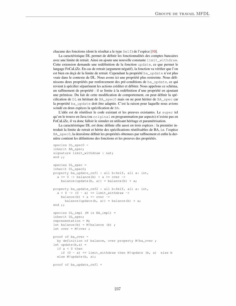
chacune des fonctions (dont le résultat a le type Self) de l’espèce [10].La caractéristique DL permet de définir les fonctionnalités des comptes bancaires
avec une limite de retrait. Ainsi on ajoute une nouvelle constante limit_withdraw.Cette extension demande une redéfinition de la fonction update, ce que permet lelangage FoCaLiZe. En cas de retrait (argument négatif), la fonction va vérifier que l’onest bien en deçà de la limite de retrait. Cependant la propriété ba_update n’est plusvraie dans le contexte de DL. Nous avons ici une propriété plus restreinte. Nous défi-nissons deux propriétés par renforcement des pré-conditions de ba_update, ce quirevient à spécifier séparément les actions créditer et débiter. Nous appelons ce schéma,un raffinement de propriété : il se limite à la redéfinition d’une propriété en ajoutantune prémisse. Du fait de cette modification de comportement, on peut définir la spé-cification de DL en héritant de BA_spec0 mais on ne peut hériter de BA_spec carla propriété ba_update doit être adaptée. C’est la raison pour laquelle nous avionsscindé en deux espèces la spécification de BA.
L’idée est de réutiliser le code existant et les preuves existantes. Le super telqu’on le trouve en Java (ou original en programmation par aspects) n’existe pas enFoCaLiZe, il va donc falloir le simuler en utilisant héritage et paramétrisation.
La caractéristique DL est donc définie elle aussi en trois espèces : la première in-troduit la limite de retrait et hérite des spécifications réutilisables de BA, i.e. l’espèceBA_spec0, la deuxième définit les propriétés obtenues par raffinement et enfin la der-nière contient les définitions des fonctions et les preuves des propriétés.
species DL_spec0 =inherit BA_spec;signature limit_withdraw : nat;end ;;
species DL_spec =inherit DL_spec0;property ba_update_ref1 : all b:Self, all a: int,
a >= 0 -> balance(b) + a >= over ->balance(update(b, a)) = balance(b) + a;
property ba_update_ref2 : all b:Self, all a: int,a < 0 -> (0 - a) <= limit_withdraw ->balance(b) + a >= over ->
balance(update(b, a)) = balance(b) + a;end ;;
species DL_impl (M is BA_impl) =inherit DL_spec;representation = M;let balance(b) = M!balance (b) ;let over = M!over ;
proof of ba_over =by definition of balance, over property M!ba_over ;
let update(b,a) =if a < 0 thenif (0 - a) <= limit_withdraw then M!update (b, a) else b
else M!update(b, a);
proof of ba_update_ref1 =
Groupe de travail MFDL
237
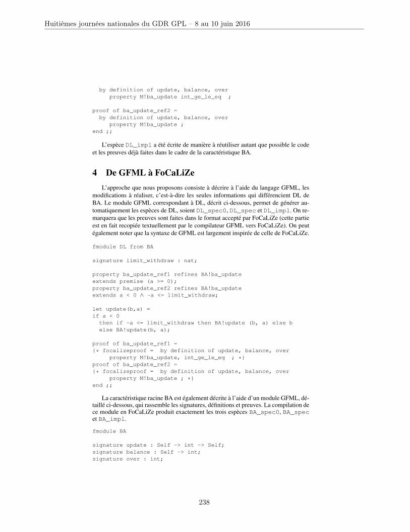
by definition of update, balance, overproperty M!ba_update int_ge_le_eq ;
proof of ba_update_ref2 =by definition of update, balance, over
property M!ba_update ;end ;;
L’espèce DL_impl a été écrite de manière à réutiliser autant que possible le codeet les preuves déjà faites dans le cadre de la caractéristique BA.
4 De GFML à FoCaLiZeL’approche que nous proposons consiste à décrire à l’aide du langage GFML, les
modifications à réaliser, c’est-à-dire les seules informations qui différencient DL deBA. Le module GFML correspondant à DL, décrit ci-dessous, permet de générer au-tomatiquement les espèces de DL, soient DL_spec0, DL_spec et DL_impl. On re-marquera que les preuves sont faites dans le format accepté par FoCaLiZe (cette partieest en fait recopiée textuellement par le compilateur GFML vers FoCaLiZe). On peutégalement noter que la syntaxe de GFML est largement inspirée de celle de FoCaLiZe.
fmodule DL from BA
signature limit_withdraw : nat;
property ba_update_ref1 refines BA!ba_updateextends premise (a >= 0);property ba_update_ref2 refines BA!ba_updateextends a < 0 ∧ -a <= limit_withdraw;
let update(b,a) =if a < 0
then if -a <= limit_withdraw then BA!update (b, a) else belse BA!update(b, a);
proof of ba_update_ref1 ={* focalizeproof = by definition of update, balance, over
property M!ba_update, int_ge_le_eq ; *}proof of ba_update_ref2 ={* focalizeproof = by definition of update, balance, over
property M!ba_update ; *}end ;;
La caractéristique racine BA est également décrite à l’aide d’un module GFML, dé-taillé ci-dessous, qui rassemble les signatures, définitions et preuves. La compilation dece module en FoCaLiZe produit exactement les trois espèces BA_spec0, BA_specet BA_impl.
fmodule BA
signature update : Self -> int -> Self;signature balance : Self -> int;signature over : int;
Huitièmes journées nationales du GDR GPL – 8 au 10 juin 2016
238
invariant property ba_over : all b: Self, balance(b) >= over;property ba_update : all b:Self, all a: int,
balance(b) + a >= over ->balance(update(b, a)) = balance(b) + a;
representation = int;
let balance(b) = b;let update(b,a) = if b + a >= over then b + a else b;
proof of ba_update ={* focalizeproof = by definition of update, balance ;*}
proof of ba_over = assumed ;end ;;
5 ConclusionDans cet article, nous avons présenté une approche de la construction non incré-
mentale de logiciels à l’aide d’un langage formel, GFML, proche de la variabilité miseen œuvre dans les lignes de produits et permettant de spécifier, implanter et prouverles étapes de développement par ajout ou modification. Ce langage est compilé vers unformalisme existant, ici FoCaLiZe. Nous avons illustré notre approche par l’exempleen ne présentant qu’une des constructions offertes par GFML et avons explicité sa tra-duction en FoCaLiZe.
GFML est un langage formel dont la sémantique est donnée par sa traduction enFoCaLiZe. Le compilateur de GFML vers FoCaLiZe est en cours de réalisation, enmême temps que la définition de différents opérateurs de développement liés à l’ap-proche lignes de produits. En plus de l’exemple donné d’ajout d’une pré-condition,citons l’ajout ou la modification d’un paramètre d’une fonction qui va avoir un im-pact partout où est appelée cette fonction. Les modifications calculées ont un impactsur les preuves déjà réalisées. L’opérateur décrit le travail à réaliser pour obtenir unenouvelle version prouvée du logiciel. Ainsi, l’ambition de GFML est de proposer auxconcepteurs de lignes de produits, un langage permettant de décrire les modificationsà apporter à une première version d’une caractéristique pour prendre en compte unenouvelle idée. Les constructions de GFML représentent des décisions et le compilateurles prend en compte pour générer le code correspondant.
Remerciements. Nous remercions François Pessaux pour son aide lors du développe-ment du traducteur.
Références[1] J. Abrial. On constructing large software systems. In J. van Leeuwen, editor, Al-
gorithms, Software, Architecture - Information Processing ’92, Volume 1, Procee-dings of the IFIP 12th World Computer Congress, Madrid, Spain, volume A-12of IFIP Transactions, pages 103–112. North-Holland, 1992.
[2] R. Bonichon, D. Delahaye, and D. Doligez. Zenon : An extensible automatedtheorem prover producing checkable proofs. In N. Dershowitz and A. Voron-kov, editors, Logic for Programming, Artificial Intelligence, and Reasoning, 14thInternational Conference, LPAR 2007, Yerevan, Armenia, October 15-19, 2007,
Groupe de travail MFDL
239
Proceedings, volume 4790 of Lecture Notes in Computer Science, pages 151–165.Springer, 2007.
[3] S. Boulmé. Spécification d’un environnement dédié à la programmation certifiéede bibliothèques de Calcul Formel. Thèse de doctorat, Université Paris 6, 2000.
[4] P. Clements and L. Northrop. Software Product Lines : Practices and Patterns.Addison-Wesley Professional, 2001.
[5] Dedukti. http://dedukti.gforge.inria.fr/.
[6] C. Dubois, T. Hardin, and V. Donzeau-Gouge. Building certified componentswithin FOCAL. In H. Loidl, editor, Revised Selected Papers from the Fifth Sym-posium on Trends in Functional Programming, TFP 2004, volume 5 of Trends inFunctional Programming, pages 33–48, 2006.
[7] FoCaLiZe. http://focalize.inria.fr/.
[8] T.-K.-Z. Pham, C. Dubois, and N. Levy. Towards correct-by-construction productvariants of a software product line : Gfml, a formal language for feature modules.In Proceedings 6th Workshop on Formal Methods and Analysis in SPL Enginee-ring, London, UK, 11 April 2015, volume 182 of EPTCS, pages 44–55, 2015.
[9] V. Prevosto and D. Doligez. Algorithms and proofs inheritance in the FOC lan-guage. J. Autom. Reasoning, 29(3-4) :337–363, 2002.
[10] R. Rioboo. Invariants for the focal language. Ann. Math. Artif. Intell., 56(3-4) :273–296, 2009.
[11] T. Thüm, I. Schaefer, M. Kuhlemann, S. Apel, and G. Saake. Applying designby contract to feature-oriented programming. In Fundamental Approaches toSoftware Engineering - 15th International Conference, FASE 2012, volume 7212of Lecture Notes in Computer Science, pages 255–269. Springer, 2012.
[12] T. Thüm. Product-line verification with feature-oriented contracts. In M. Pezzèand M. Harman, editors, Int’l Symposium on Software Testing and Analysis,ISSTA ’13, Lugano, Switzerland, July 15-20, 2013, pages 374–377. ACM, 2013.
[13] T. Thüm, I. Schaefer, M. Kuhlemann, and S. Apel. Proof composition for deduc-tive verification of software product lines. In Proc. Int’l Workshop Variability-intensive Systems Testing, Validation and Verification (VAST’11), pages 270–277.IEEE Computer Society, 2011.
Huitièmes journées nationales du GDR GPL – 8 au 10 juin 2016
240

Session du groupe de travail MTV2
Méthodes de test pour la validation et la vérification
241

Huitièmes journées nationales du GDR GPL – 8 au 10 juin 2016
242
Quelle confiance peut-on établirdans un système intelligent ?
Lydie du Bousquet1,2 , Masahide Nakamura31Univ. Grenoble Alpes, LIG, F-38000 Grenoble, France
2CNRS, LIG, F-38000 Grenoble, France3Kobe University, Japon
e-mail : [email protected], [email protected]
Résumé
De plus en plus, nous sommes confrontés à des systèmes intelligents(“smart systems”). Ce sont des systèmes supposés apprendre de leur environ-nement pour apporter des réponses les plus pertinentes possibles pour leursutilisateurs. Une caractéristique de ces systèmes est que leurs comportementsévoluent avec le temps. Dans le projet CNRS-PICS Safe-Smartness, collabo-ration entre le LIG et l’université de Kobe, nous étudions comment exprimerles propriétés d’oracle quant à la qualité d’un système intelligent.
Introduction Les systèmes intelligents (smart systems) sont caractérisés par leurcapacité à prédire ou à adapter leurs comportements à partir d’une analyse d’unensemble de données. Ce type d’application se retrouve dans différents domaines(domotique, médical, transport, ...). Selon la Royal Academy of Engineering, onpeut classer les systèmes intelligents en trois catégories 1. Ainsi, selon la façondont les données sont collectées et utilisées, ces systèmes permettent :
— d’aider les concepteurs à produire une nouvelle version de l’applicationplus efficace,
— de calculer et de présenter des informations à l’opérateur humain pour qu’ilpuisse prendre des décisions pertinentes par rapport à la situation,
— de choisir les actions à effectuer en fonction de la situation et de les exécu-ter, sans intervention humaine.
En ce qui concerne les deux dernières catégories, la question de la qualité dusystème prend toute son importance. Un tel système ne doit pas induire ses utili-sateurs en erreur et/ou ne doit pas exécuter des actions inappropriées. L’objet duprojet CNRS-PICS Safe-Smartness est d’établir des méthodes de validation pour cetype de systèmes. Dans la suite, illustrons les difficultés sur la base d’un exemple.
Exemple Soit un système de climatisation programmable “intelligent”. L’utilisa-teur peut programmer une heure h et une température t. Le système doit alors faire
1. http ://www.raeng.org.uk/publications/reports/smart-infrastructure-the-future
Groupe de travail MTV2
243
en sorte que la pièce considérée soit à la température t à l’heure h, tout en minimi-sant l’énergie nécessaire pour y parvenir. Pour cela, le système doit tenir compte del’inertie thermique, qui est propre à chaque pièce. Le système est donc doté d’unepartie “intelligente”, qui enregistre un certain nombre de facteurs et “apprend” lavitesse à laquelle la pièce se tempère en fonction de ces facteurs. Après le tempsd’apprentissage, le système doit choisir au mieux à quel moment démarrer pouratteindre la température t à l’heure fixée.
Propriétés attendues du système Un des premiers éléments à vérifier est doncque la pièce soit à la température t à l’heure h. Comme cela dépend de la pièce,il faut envisager de le faire à chaque exécution (monitoring). Pour autant, la non-satisfaction de cette propriété ne signifie pas forcément que le système est incorrect.Deux situations peuvent se produire. (a) L’utilisateur peut fixer un objectif impos-sible à atteindre ; par exemple demander à 7h55 que la pièce soit à 21 ˚C à 8h alorsque la température actuelle est de 10 ˚C. (b) L’objectif peut aussi être atteignable enthéorie, mais l’environnement réel ne pas le permettre ; par exemple, si une fenêtreest laissée ouverte en plein hiver.
Dans ces conditions, le système doit être en mesure de fournir une notificationsi l’objectif est jugé non-atteignable (e.g. 7h55 pour 8h et 11 ˚C d’écart). Il seraalors possible de valider si la notification est exacte (i.e. pertinente). La présencede faux-négatifs (notification “impossible” mais la température est atteinte dansles délais) et de faux-positifs (notification “possible” mais la température n’estfinalement pas atteinte dans les délais) est un indicateur de qualité du système .
Le système doit aussi être en mesure d’indiquer si les caractéristiques de l’envi-ronnement ont changé (e.g. inertie différente si fenêtre ouverte). Cela est nécessairepour faire la différence entre un dysfonctionnement du système et une anomalieponctuelle d’usage.
Par ailleurs, on attend du système qu’il minimise l’énergie nécessaire pour at-teindre l’objectif. Ici, on peut par exemple s’assurer que le système ne démarre pastrop tôt, c’est-à-dire qu’à partir du moment où le climatiseur commence à chauffer(resp. à refroidir) la pièce, il ne passe pas plusieurs fois en attente.
Mais ces propriétés ne permettent pas de s’assurer directement que le systèmeapprend correctement. L’apprentissage est un processus progressif. Pour décider dela qualité de l’apprentissage, il faut observer les exécutions successives et s’assurerque l’objectif est atteint de plus en plus souvent, et/ou de mieux en mieux (ici, enconsommant de moins en moins d’énergie). La difficulté ici est qu’il s’agit d’unetendance, qui peut se dégrader de temps à autre, en particulier si l’utilisateur changeses habitudes. Le fait que la tendance se dégrade pendant un temps ne signifie doncpas forcément que le système est incorrect, mais peut caractériser le fait qu’il entredans une nouvelle étape d’adaptation.
Les outils habituels d’expression et d’évaluation de propriétés ne sont pas adap-tés pour nos besoins. C’est pourquoi, l’objectif du projet Safe-Smartness est de pro-poser des moyens alternatifs pour exprimer et valider la qualité de l’apprentissage.
Huitièmes journées nationales du GDR GPL – 8 au 10 juin 2016
244
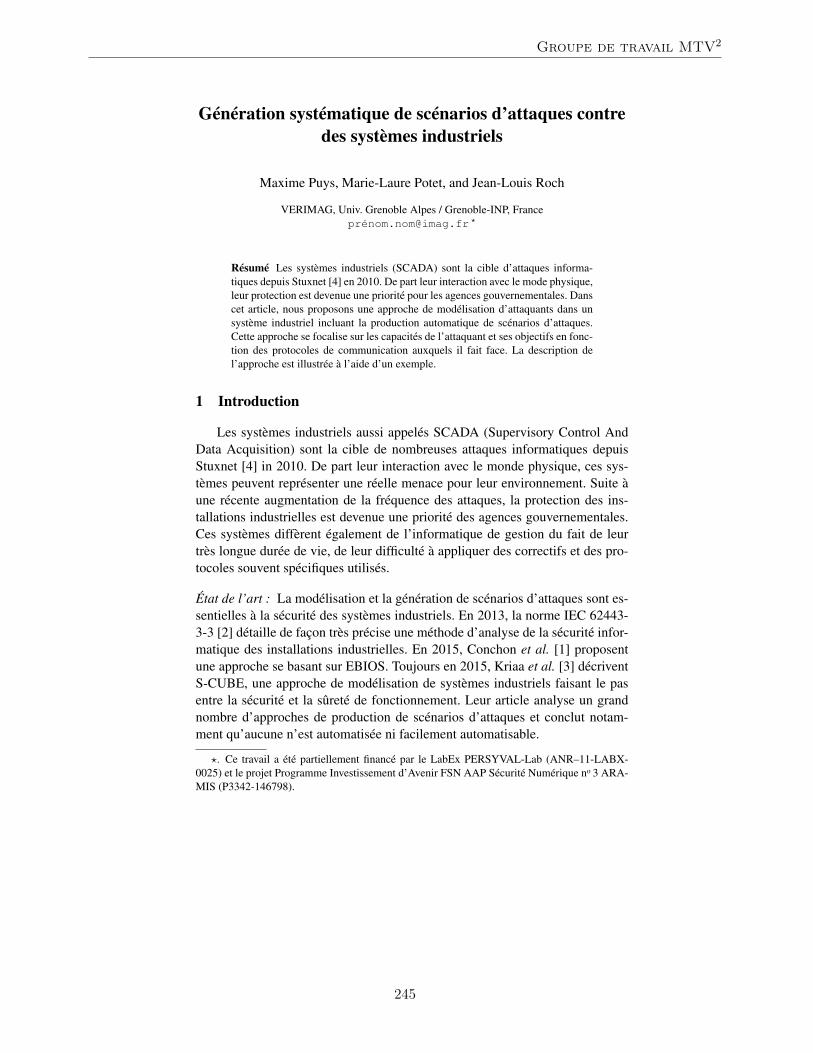
Génération systématique de scénarios d’attaques contredes systèmes industriels
Maxime Puys, Marie-Laure Potet, and Jean-Louis Roch
VERIMAG, Univ. Grenoble Alpes / Grenoble-INP, Francepré[email protected] ?
Résumé Les systèmes industriels (SCADA) sont la cible d’attaques informa-tiques depuis Stuxnet [4] en 2010. De part leur interaction avec le mode physique,leur protection est devenue une priorité pour les agences gouvernementales. Danscet article, nous proposons une approche de modélisation d’attaquants dans unsystème industriel incluant la production automatique de scénarios d’attaques.Cette approche se focalise sur les capacités de l’attaquant et ses objectifs en fonc-tion des protocoles de communication auxquels il fait face. La description del’approche est illustrée à l’aide d’un exemple.
1 Introduction
Les systèmes industriels aussi appelés SCADA (Supervisory Control AndData Acquisition) sont la cible de nombreuses attaques informatiques depuisStuxnet [4] in 2010. De part leur interaction avec le monde physique, ces sys-tèmes peuvent représenter une réelle menace pour leur environnement. Suite àune récente augmentation de la fréquence des attaques, la protection des ins-tallations industrielles est devenue une priorité des agences gouvernementales.Ces systèmes diffèrent également de l’informatique de gestion du fait de leurtrès longue durée de vie, de leur difficulté à appliquer des correctifs et des pro-tocoles souvent spécifiques utilisés.
État de l’art : La modélisation et la génération de scénarios d’attaques sont es-sentielles à la sécurité des systèmes industriels. En 2013, la norme IEC 62443-3-3 [2] détaille de façon très précise une méthode d’analyse de la sécurité infor-matique des installations industrielles. En 2015, Conchon et al. [1] proposentune approche se basant sur EBIOS. Toujours en 2015, Kriaa et al. [3] décriventS-CUBE, une approche de modélisation de systèmes industriels faisant le pasentre la sécurité et la sûreté de fonctionnement. Leur article analyse un grandnombre d’approches de production de scénarios d’attaques et conclut notam-ment qu’aucune n’est automatisée ni facilement automatisable.
?. Ce travail a été partiellement financé par le LabEx PERSYVAL-Lab (ANR–11-LABX-0025) et le projet Programme Investissement d’Avenir FSN AAP Sécurité Numérique no 3 ARA-MIS (P3342-146798).
Groupe de travail MTV2
245

Contributions : Nous proposons dans cet article une approche de modélisationd’attaquants basée à la fois sur l’infrastructure et les possibilités d’attaques dansun système industriel. Cette approche se base sur les composants d’une infra-structure et les canaux de communication entre ses composants [6]. Elle vise laproduction automatique de scénarios d’attaques. Nous nous focalisons sur l’at-taquant en modélisant sa position dans l’infrastructure, ses objectifs d’attaqueset les protocoles qu’il peut utiliser en tenant compte de leurs propriétés de sé-curité. Enfin, à l’aide d’une approche systématique, nous générons l’ensembledes scénarios d’attaques pour lesquels un attaquant est capable de réaliser l’unde ses objectifs face à un protocole donné.
Plan : La section 2 détaille la modélisation des attaquants et la production desscénarios d’attaques à l’aide d’un un exemple. Ensuite, la section 3 décrit com-ment nous souhaitons inclure cette approche dans une approche Model-BasedTesting plus globale. Enfin la section 4 conclut.
2 Approche de génération des scénarios d’attaques
Dans cette section, nous détaillons le formalisme utilisé dans notre modéli-sation des attaquants et comment exploiter cette modélisation pour générer desscénarios d’attaques. Cette approche est double. Elle propose dans un premiertemps d’étudier les objectifs des attaquants et comment ils pourraient les réaliser(approche descendante) avant de les mettre dans un second temps face aux pro-tections apportées par les protocoles de communication (approche ascendante).
2.1 Approche descendante
Nous commençons par définir l’ensemble des attaquants A et l’ensembledes objectifs d’attaquesO. Ces ensembles sont liés par la relationRObj entre unattaquant a et un objectif o tel queRObj ⊆ A×O si a cherche à atteindre o faitpartie de notre analyse de risque. Il va donc de soit que cette relation, fourniepar le concepteur du modèle doit tenir compte de la position des attaquantsdans l’architecture globale du système (ex. : un attaquant ne peut pas avoir pourobjectif la modification d’un message s’il n’y a jamais accès).
Exemple :Nous considérons l’infrastructure de communication en figure 1 où les atta-quants (en couleur) sont A = {ClientA, RouteurA} (un client et un routeurcompromis) et les objectifs d’attaques (tirés de recommandations gouvernemen-tales) considérés, sont O = {V olId, ContAuth,Alte, AlteC} avec :
— V olId = Vol d’identifiants,
Huitièmes journées nationales du GDR GPL – 8 au 10 juin 2016
246
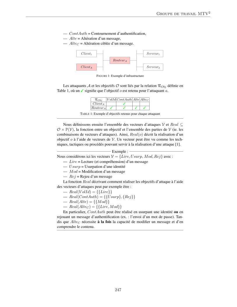
— ContAuth = Contournement d’authentification,— Alte = Altération d’un message,— AlteC = Altération ciblée d’un message.
ClientA
Client1
RouteurA
Serveur2
Serveur1
FIGURE 1: Exemple d’infrastructure
Les attaquants A et les objectifs O sont liés par la relation RObj définie enTable 1, où un 3 signifie que l’objectif o est retenu pour l’attaquant a.
RObj V olId ContAuth Alte AlteCClientA 3
RouteurA 3 3 3 3
TABLE 1: Exemple d’objectifs retenus pour chaque attaquant
Nous définissons ensuite l’ensemble des vecteurs d’attaques V et Real ⊆O × P(V), la fonction entre un objectif et l’ensemble des parties de V (ie. lescombinaisons de vecteurs d’attaques). Ainsi, Real(o) décrit la réalisation d’unobjectif o à l’aide de vecteurs de V . Un vecteur peut être vu comme les tech-niques, tactiques ou procédés pouvant servir à la réalisation d’une attaque [1].
Exemple :Nous considérons ici les vecteurs V = {Lire, Usurp, Mod,Rej} avec :
— Lire = Lecture (et compréhension) d’un message— Usurp = Usurpation d’une identité— Mod = Modification d’un message— Rej = Rejeu d’un messageLa fonction Real décrivant comment réaliser les objectifs d’attaque à l’aide
des vecteurs d’attaques peut par exemple être :— Real(V olId) = {{Lire}}— Real(ContAuth) = {{Usurp}, {Rej}}— Real(Alte) = {{Mod}}— Real(AlteC) = {{Lire,Mod}}En particulier, ContAuth peut être réalisé en usurpant une identité ou en
rejouant un message d’authentification (ex. : l’envoi d’un mot de passe). Tan-dis que AlteC nécessite à la fois la capacité de modifier un message et d’encomprendre le contenu.
Groupe de travail MTV2
247
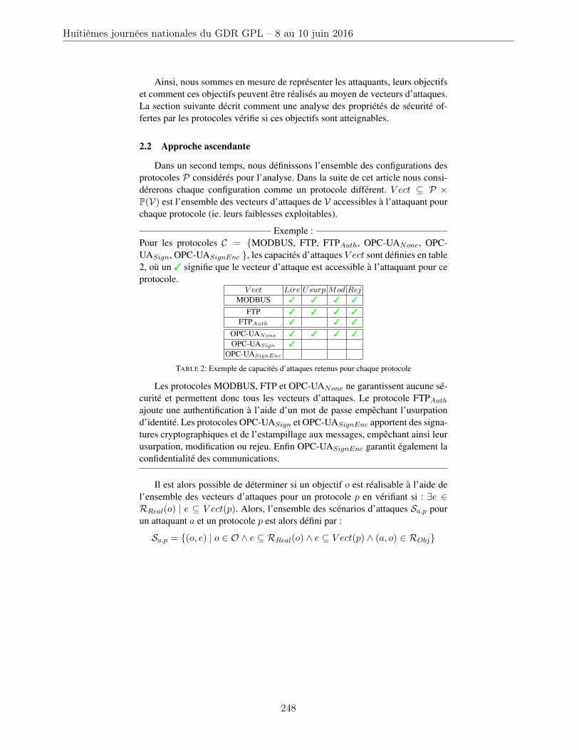
Ainsi, nous sommes en mesure de représenter les attaquants, leurs objectifset comment ces objectifs peuvent être réalisés au moyen de vecteurs d’attaques.La section suivante décrit comment une analyse des propriétés de sécurité of-fertes par les protocoles vérifie si ces objectifs sont atteignables.
2.2 Approche ascendante
Dans un second temps, nous définissons l’ensemble des configurations desprotocoles P considérés pour l’analyse. Dans la suite de cet article nous consi-dérerons chaque configuration comme un protocole différent. V ect ⊆ P ×P(V) est l’ensemble des vecteurs d’attaques de V accessibles à l’attaquant pourchaque protocole (ie. leurs faiblesses exploitables).
Exemple :Pour les protocoles C = {MODBUS, FTP, FTPAuth, OPC-UANone, OPC-UASign, OPC-UASignEnc }, les capacités d’attaques V ect sont définies en table2, où un 3 signifie que le vecteur d’attaque est accessible à l’attaquant pour ceprotocole.
V ect Lire Usurp Mod Rej
MODBUS 3 3 3 3
FTP 3 3 3 3
FTPAuth 3 3 3
OPC-UANone 3 3 3 3
OPC-UASign 3
OPC-UASignEnc
TABLE 2: Exemple de capacités d’attaques retenus pour chaque protocole
Les protocoles MODBUS, FTP et OPC-UANone ne garantissent aucune sé-curité et permettent donc tous les vecteurs d’attaques. Le protocole FTPAuth
ajoute une authentification à l’aide d’un mot de passe empêchant l’usurpationd’identité. Les protocoles OPC-UASign et OPC-UASignEnc apportent des signa-tures cryptographiques et de l’estampillage aux messages, empêchant ainsi leurusurpation, modification ou rejeu. Enfin OPC-UASignEnc garantit également laconfidentialité des communications.
Il est alors possible de déterminer si un objectif o est réalisable à l’aide del’ensemble des vecteurs d’attaques pour un protocole p en vérifiant si : ∃e ∈RReal(o) | e ⊆ V ect(p). Alors, l’ensemble des scénarios d’attaques Sa,p pourun attaquant a et un protocole p est alors défini par :
Sa,p = {(o, e) | o ∈ O ∧ e ⊆ RReal(o) ∧ e ⊆ V ect(p) ∧ (a, o) ∈ RObj}
Huitièmes journées nationales du GDR GPL – 8 au 10 juin 2016
248
L’ensemble des scénarios d’attaques à considérer dans le cadre d’une cam-pagne de test est alors l’ensemble des Sa,p, ∀a ∈ A et pour tous les protocolesde P que pourraient utiliser chaque attaquants.
Exemple :Dans notre exemple, si l’on suppose que ClientA communique via FTPAuth :
SClientA,FTPAuth= {(ContAuth,Rej)}
Cela s’explique par le fait que seul l’objectif ContAuth est considéré pourClientA (table 1) et qu’il est réalisable avec au moins l’un des vecteurs d’at-taques Usurp ou Rej dont le dernier est offert par FTPAuth. De même pourRouteurA qui est face à la fois à OPC-UANone et FTPAuth :
SRouteurA,OPC-UANone= {(V olId, Lire), (ContAuth, Usurp), (ContAuth,Rej),
(Alte,Mod), (AlteC , (Lire,Mod))}
SRouteurA,FTPAuth= {(V olId, Lire), (ContAuth,Rej), (Alte,Mod),
(AlteC , (Lire,Mod))}
3 Méthodologie globale
Notre objectif est d’utiliser cette phase d’analyse dans une approche glo-bale allant de la modélisation du système à la production automatique des pa-quets réseau implémentant et testant les attaques identifiées. Nous proposonsdonc une approche Model-Based Testing dans l’objectif de vérifier si les at-taques trouvées par l’approche sont effectivement jouables sur une plate-forme,voire de quantifier leur plausibilité. La figure 2 illustre la méthodologie que nousvoulons développer. L’approche part d’une architecture représentant les compo-sants du systèmes, les canaux de communication et les protocoles (similaire à lafigure 1) ; croisée avec des propriétés de sécurité spécifiant les objectifs des at-taquants. Ensuite, l’analyse présentée en section 2 permet d’obtenir les vecteursd’attaques à utiliser par des attaquants pour violer les propriétés de sécurité. Cesvecteurs sont ensuite concrétisés en paquets réseaux à l’aide d’une bibliothèquedécrivant comment implémenter les vecteurs pour chaque protocole (ex. : com-ment modifier un paquet OPC-UA). Enfin, ces paquets sont instanciés, soit demanière aléatoire, soit en fonction de la logique applicative de la plate-forme.Cette approche pourrait se généraliser aux systèmes d’information, mais elleexploite néanmoins des propriétés souvent présentes dans les systèmes indus-triels telles que l’absence de réseaux dynamiques, simplifiant la représentationde l’infrastructure.
Groupe de travail MTV2
249
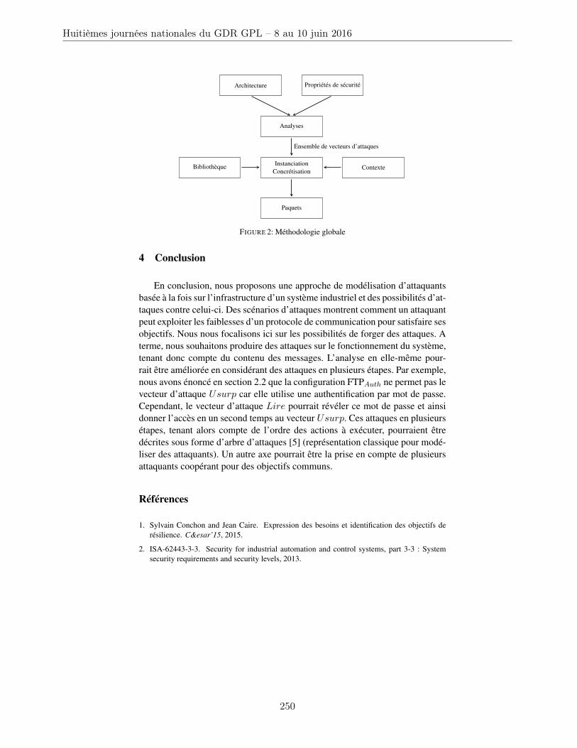
Architecture Propriétés de sécurité
Analyses
Bibliothèque
Paquets
ContexteInstanciation
Concrétisation
Ensemble de vecteurs d’attaques
FIGURE 2: Méthodologie globale
4 Conclusion
En conclusion, nous proposons une approche de modélisation d’attaquantsbasée à la fois sur l’infrastructure d’un système industriel et des possibilités d’at-taques contre celui-ci. Des scénarios d’attaques montrent comment un attaquantpeut exploiter les faiblesses d’un protocole de communication pour satisfaire sesobjectifs. Nous nous focalisons ici sur les possibilités de forger des attaques. Aterme, nous souhaitons produire des attaques sur le fonctionnement du système,tenant donc compte du contenu des messages. L’analyse en elle-même pour-rait être améliorée en considérant des attaques en plusieurs étapes. Par exemple,nous avons énoncé en section 2.2 que la configuration FTPAuth ne permet pas levecteur d’attaque Usurp car elle utilise une authentification par mot de passe.Cependant, le vecteur d’attaque Lire pourrait révéler ce mot de passe et ainsidonner l’accès en un second temps au vecteur Usurp. Ces attaques en plusieursétapes, tenant alors compte de l’ordre des actions à exécuter, pourraient êtredécrites sous forme d’arbre d’attaques [5] (représentation classique pour modé-liser des attaquants). Un autre axe pourrait être la prise en compte de plusieursattaquants coopérant pour des objectifs communs.
Références
1. Sylvain Conchon and Jean Caire. Expression des besoins et identification des objectifs derésilience. C&esar’15, 2015.
2. ISA-62443-3-3. Security for industrial automation and control systems, part 3-3 : Systemsecurity requirements and security levels, 2013.
Huitièmes journées nationales du GDR GPL – 8 au 10 juin 2016
250
3. S Kriaa, M Bouissou, and Y Laarouchi. A model based approach for SCADA safety andsecurity joint modelling : S-Cube. In IET System Safety and Cyber Security. IET DigitalLibrary, 2015.
4. Ralph Langner. Stuxnet : Dissecting a cyberwarfare weapon. Security & Privacy, IEEE,9(3) :49–51, 2011.
5. Bruce Schneier. Attack trees. Dr. Dobb’s journal, 24(12) :21–29, 1999.
6. Theodore J Williams. A Reference Model for Computer Integrated Manufacturing (CIM) : ADescription from the Viewpoint of Industrial Automation : Prepared by CIM Reference Mo-del Committee International Purdue Workshop on Industrial Computer Systems. InstrumentSociety of America, 1991.
Groupe de travail MTV2
251

Huitièmes journées nationales du GDR GPL – 8 au 10 juin 2016
252
MBeeTle - un outil pour la génération de tests à-la-volée
à l'aide de modèles ∗
Julien Lorrain1
Frédéric Dadeau1
Elizabeta Fourneret2
Bruno Legeard1,2
1Institut FEMTO-ST, Besançon, France2Smartesting Solutions & Services, Besançon, France
Résumé
Le Model-Based Testing est une activité permettant, à partir de la modélisation dusystème sous test (SUT), de générer des tests pour la validation du SUT par rapport auxspéci�cations de ce système. Cet article présente MBeeTle, un outil de génération de testà-la-volée pour le MBT, ainsi que ses principes et ces stratégies de génération. Il permetla recherche des anomalies profondes et la validation du modèle de test en générant etexécutant des pas de test sur la base d'une approche aléatoire. MBeeTle est présentéavec une expérimentation sur la une norme d'interfaces utilisateurs et logicielles pour lessystèmes d'exploitation (POSIX).
1 Introduction et contexte
Dans ce papier nous présentons MBeeTle, un outil de génération de test à-la-volée [1] basésur le Model-Based Testing (MBT) [2] pour l'exploration des systèmes sous test. Le MBTest une activité permettant de générer des tests abstraits à partir de la modélisation du SUTqui nécessite l'utilisation d'une couche d'adaptation a�n de les concrétiser pour pouvoir lesexécuter sur le SUT. La catégorie principale de génération de test est la génération dite hors-ligne, dont le principe est de générer des scénarios de test abstrait. Pour pouvoir les exécuterautomatiquement sur le SUT, il faut créer le lien entre les données abstraites du modèle etle SUT. C'est ici que la couche d'adaptation est nécessaire pour associer à chaque donnéeabstraite les informations de concrétisation permettant leur exécution sur le SUT. Une autrecatégorie de génération, implémentée dans l'outil MBeeTle, est la génération à-la-volée. Leprincipe est d'attendre le résultat du premier pas de test avant de générer les pas suivants. Ilest donc nécessaire de disposer de la couche d'adaptation pour mettre en ÷uvre cette méthode.Cette approche permet de générer des tests fonctionnels longs (i.e. plusieurs centaines de pasde test) basés sur les comportements modélisés du SUT.
∗Cet outil a en partie été réalisé lors des projets ANR ASTRID OSEP et ANR ASTRID maturationMBT_SEC.
Groupe de travail MTV2
253
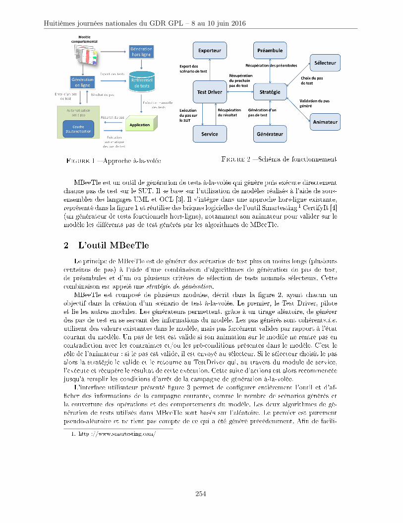
Figure 1 � Approche à-la-volée Figure 2 � Schéma de fonctionnement
MBeeTle est un outil de génération de tests à-la-volée qui génère puis exécute directementchaque pas de test sur le SUT. Il se base sur l'utilisation de modèles réalisés à l'aide de sous-ensembles des langages UML et OCL [3]. Il s'intègre dans une approche hors-ligne existante,représenté dans la �gure 1 et réutilise des briques logicielles de l'outil Smartesting 1 CertifyIt [4](un générateur de tests fonctionnels hors-ligne), notamment son animateur pour valider sur lemodèle les di�érents pas de test générés par les algorithmes de MBeeTle.
2 L'outil MBeeTle
Le principe de MBeeTle est de générer des scénarios de test plus ou moins longs (plusieurscentaines de pas) à l'aide d'une combinaison d'algorithmes de génération de pas de test,de préambules et d'un ou plusieurs critères de sélection de tests nommés sélecteurs. Cettecombinaison est appelé une stratégie de génération.
MBeeTle est composé de plusieurs modules, décrit dans la �gure 2, ayant chacun unobjectif dans la création d'un scénario de test à-la-volée. Le premier, le Test Driver, piloteet lie les autres modules. Les générateurs permettent, grâce à un tirage aléatoire, de générerdes pas de test en se servant des informations du modèle. Les pas générés sont cohérents,i.e.utilisent des valeurs existantes dans le modèle, mais pas forcément valides par rapport à l'étatcourant du modèle. Un pas de test est valide si son animation sur le modèle ne rentre pas encontradiction avec les contraintes et/ou les pré-conditions présentes dans le modèle. C'est lerôle de l'animateur : si le pas est valide, il est envoyé au sélecteur. Si le sélecteur choisit le pasalors la stratégie le valide et le retourne au TestDriver qui, au travers du module de service,l'exécute et récupère le résultat de cette exécution. Cette suite d'actions est alors recommencéejusqu'à remplir les conditions d'arrêt de la campagne de génération à-la-volée.
L'interface utilisateur présenté �gure 3 permet de con�gurer entièrement l'outil et d'af-�cher des informations de la campagne courante, comme le nombre de scénarios générés etla couverture des opérations et des comportements du modèle. Les deux algorithmes de gé-nération de tests utilisés dans MBeeTle sont basés sur l'aléatoire. Le premier est purementpseudo-aléatoire et ne tient pas compte de ce qui a été généré précédemment. A�n de facili-
1. http ://www.smartesting.com/
Huitièmes journées nationales du GDR GPL – 8 au 10 juin 2016
254
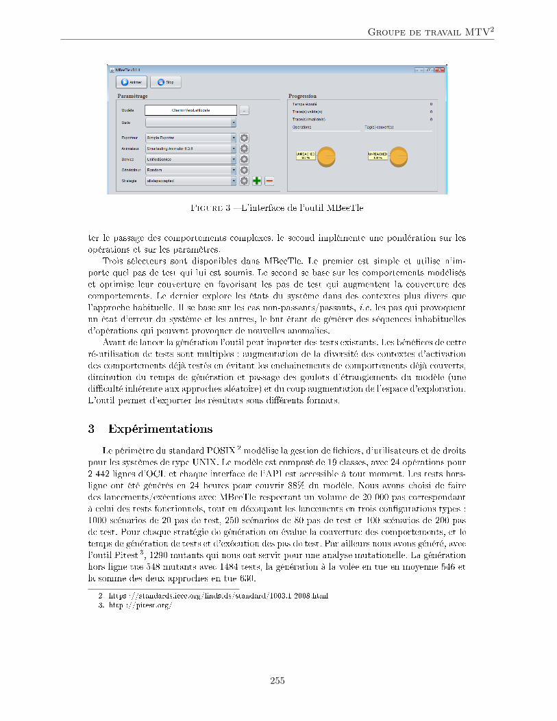
Figure 3 � L'interface de l'outil MBeeTle
ter le passage des comportements complexes, le second implémente une pondération sur lesopérations et sur les paramètres.
Trois sélecteurs sont disponibles dans MBeeTle. Le premier est simple et utilise n'im-porte quel pas de test qui lui est soumis. Le second se base sur les comportements modéliséset optimise leur couverture en favorisant les pas de test qui augmentent la couverture descomportements. Le dernier explore les états du système dans des contextes plus divers quel'approche habituelle. Il se base sur les cas non-passants/passants, i.e. les pas qui provoquentun état d'erreur du système et les autres, le but étant de générer des séquences inhabituellesd'opérations qui peuvent provoquer de nouvelles anomalies.
Avant de lancer la génération l'outil peut importer des tests existants. Les béné�ces de cetteré-utilisation de tests sont multiples : augmentation de la diversité des contextes d'activationdes comportements déjà testés en évitant les enchainements de comportements déjà couverts,diminution du temps de génération et passage des goulots d'étranglements du modèle (unedi�culté inhérente aux approches aléatoire) et du coup augmentation de l'espace d'exploration.L'outil permet d'exporter les résultats sous di�érents formats.
3 Expérimentations
Le périmètre du standard POSIX 2 modélise la gestion de �chiers, d'utilisateurs et de droitspour les systèmes de type UNIX. Le modèle est composé de 19 classes, avec 24 opérations pour2 442 lignes d'OCL et chaque interface de l'API est accessible à tout moment. Les tests hors-ligne ont été générés en 24 heures pour couvrir 88% du modèle. Nous avons choisi de fairedes lancements/exécutions avec MBeeTle respectant un volume de 20 000 pas correspondantà celui des tests fonctionnels, tout en découpant les lancements en trois con�gurations types :1000 scénarios de 20 pas de test, 250 scénarios de 80 pas de test et 100 scénarios de 200 pasde test. Pour chaque stratégie de génération on évalue la couverture des comportements, et letemps de génération de tests et d'exécution des pas de test. Par ailleurs nous avons généré, avecl'outil Pitest 3, 1290 mutants qui nous ont servit pour une analyse mutationelle. La générationhors-ligne tue 548 mutants avec 1484 tests, la génération à la volée en tue en moyenne 546 etla somme des deux approches en tue 630.
2. https ://standards.ieee.org/�ndstds/standard/1003.1-2008.html3. http ://pitest.org/
Groupe de travail MTV2
255
De cette expérimentation ressort que MBeeTle permet de couvrir rapidement plus de lamoitié des comportements du modèle (environ 16 minutes contre 3 heures pour la versionhors-ligne). En réutilisation des tests hors-ligne générés, on augmente signi�cativement lacouverture du modèle. Par ailleurs MBeeTle est capable de générer rapidement un volume depas de test conséquent (ici 20000 pas en 13,6 secondes en moyenne). De plus l'utilisation decette approche a permis de détecter des mutants di�érents de ceux détectés par l'approchehors-ligne.
Par ailleurs, l'application de l'approche à-la-volée sur cette expérimentation montre que lesartefacts de modélisation hors-ligne sont réutilisables avec un faible coût de main d'÷uvre pouradapter le banc de test pour une utilisation pas à pas. Il en ressort également que MBeeTlepeut être utilisé pour mettre au point le modèle en générant rapidement des scénarios de test.
4 Conclusion et perspectives
Nous avons présenté MBeeTle en association avec l'approche hors-ligne sur un modèlede taille réelle. Dans ce contexte il permet de compléter cette approche avec un faible coûtd'adaptation et une réutilisation complète des ressources et des outils mis en place. Il permetd'augmenter l'espace d'exploration pour activer des comportements dans d'autres contextes.Par ailleurs sur un autre cas d'étude, une implémentation de la norme PKCS#11 4, il a permisde montrer des erreurs dues a des fuites mémoires qui n'ont pas été trouvés par les outilsclassiques grâce à une utilisation intensive de l'outil 5.
Pour la suite, nous prévoyons d'adapter cette approche à-la-volée pour en faire une ap-proche de tests en-ligne où nous utiliserons le retour du SUT pour calculer le pas de testpour calculer le prochain. De part son aspect modulaire et ses stratégies paramétrables, desexpérimentations pour de la génération en-ligne (utilisation du retour d'exécution des pasde test pour décider du prochain pas de test à générer) [5] sont envisageables. Par ailleurspour améliorer son e�cacité, de nouvelles stratégies seront ajoutées pour palier aux di�cultésrencontrées, par exemple sur les modèles à goulots d'étranglements.
Références
[1] J.-C. Fernandez, C. Jard, T. Jéron, and C. Viho, �Using on-the-�y veri�cation techniques for thegeneration of test suites,� in Computer Aided Veri�cation, pp. 348�359, Springer, 1996.
[2] M. Utting and B. Legeard, Practical model-based testing : a tools approach. Morgan Kaufmann,2010.
[3] F. Bouquet, C. Grandpierre, B. Legeard, F. Peureux, N. Vacelet, and M. Utting, �A subset of preciseUML for model-based testing,� in Proceedings of the 3rd International Workshop on Advances in
Model Based Testing, pp. 95�104, 2007.
[4] F. Bouquet, C. Grandpierre, B. Legeard, and F. Peureux, �A test generation solution to automatesoftware testing,� in Proceedings of the 3rd International Workshop on Automation of Software
Test, AST '08, (New York, NY, USA), pp. 45�48, ACM, 2008.
[5] C. Pacheco, S. K. Lahiri, M. D. Ernst, and T. Ball, �Feedback-directed random test generation,�in Software Engineering, 2007. ICSE 2007. 29th International Conference on, pp. 75�84, IEEE,2007.
4. https ://www.emc.com/emc-plus/rsa-labs/standards-initiatives/pkcs-11-cryptographic-token-interface-standard.htm
5. http ://ucaat.etsi.org/2015/presentations/FEMTOST_FOURNERET.pdf
Huitièmes journées nationales du GDR GPL – 8 au 10 juin 2016
256
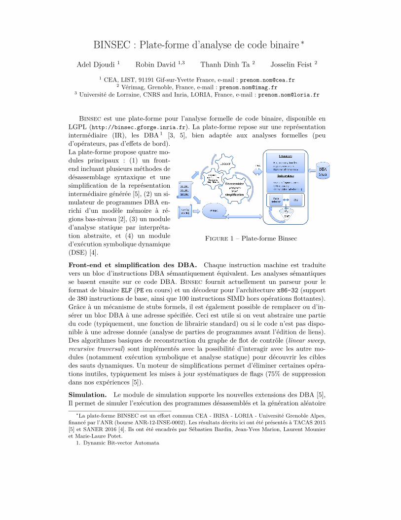
BINSEC : Plate-forme d’analyse de code binaire ∗
Adel Djoudi 1 Robin David 1,3 Thanh Dinh Ta 2 Josselin Feist 2
1 CEA, LIST, 91191 Gif-sur-Yvette France, e-mail : [email protected] Vérimag, Grenoble, France, e-mail : [email protected]
3 Université de Lorraine, CNRS and Inria, LORIA, France, e-mail : [email protected]
Binsec est une plate-forme pour l’analyse formelle de code binaire, disponible enLGPL (http://binsec.gforge.inria.fr). La plate-forme repose sur une représentationintermédiaire (IR), les DBA 1 [3, 5], bien adaptée aux analyses formelles (peu
Figure 1 – Plate-forme Binsec
d’opérateurs, pas d’effets de bord).La plate-forme propose quatre mo-dules principaux : (1) un front-end incluant plusieurs méthodes dedésassemblage syntaxique et unesimplification de la représentationintermédiaire générée [5], (2) un si-mulateur de programmes DBA en-richi d’un modèle mémoire à ré-gions bas-niveau [2], (3) un moduled’analyse statique par interpréta-tion abstraite, et (4) un moduled’exécution symbolique dynamique(DSE) [4].
Front-end et simplification des DBA. Chaque instruction machine est traduitevers un bloc d’instructions DBA sémantiquement équivalent. Les analyses sémantiquesse basent ensuite sur ce code DBA. Binsec fournit actuellement un parseur pour leformat de binaire ELF (PE en cours) et un décodeur pour l’architecture x86-32 (supportde 380 instructions de base, ainsi que 100 instructions SIMD hors opérations flottantes).Grâce à un mécanisme de stubs formels, il est également possible de remplacer ou d’in-sérer un bloc DBA à une adresse spécifiée. Ceci est utile si on veut abstraire une partiedu code (typiquement, une fonction de librairie standard) ou si le code n’est pas dispo-nible à une adresse donnée (analyse de parties de programmes avant l’édition de liens).Des algorithmes basiques de reconstruction du graphe de flot de contrôle (linear sweep,recursive traversal) sont implémentés avec la possibilité d’interagir avec les autre mo-dules (notamment exécution symbolique et analyse statique) pour découvrir les ciblesdes sauts dynamiques. Un moteur de simplifications permet d’éliminer certaines opéra-tions inutiles, typiquement les mises à jour systématiques de flags (75% de suppressiondans nos expériences [5]).
Simulation. Le module de simulation supporte les nouvelles extensions des DBA [5],Il permet de simuler l’exécution des programmes désassemblés et la génération aléatoire
∗La plate-forme BINSEC est un effort commun CEA - IRISA - LORIA - Université Grenoble Alpes,financé par l’ANR (bourse ANR-12-INSE-0002). Les résultats décrits ici ont été présentés à TACAS 2015[5] et SANER 2016 [4]. Ils ont été encadrés par Sébastien Bardin, Jean-Yves Marion, Laurent Mounieret Marie-Laure Potet.
1. Dynamic Bit-vector Automata
de tests (fuzzing). Trois modèles mémoire peuvent être sélectionnés : le modèle plat (lamémoire comme tableau d’octets), le modèle à régions standard – à la CompCert [6],ou un modèle à régions bas-niveau [2]. L’adoption du modèle à région bas-niveau estmotivée par sa capacité à permettre à la fois de profiter de l’abstraction offerte par lemodèle à régions standard et de donner une sémantique définie aux programmes basniveau.
Analyse statique. L’analyse statique permet d’inférer, à partir du code d’un pro-gramme et sans l’exécuter, des propriétés vraies pour toutes les exécutions de ce pro-gramme. L’analyse statique de programmes binaires permet d’analyser des exécutablesdont on ne dispose pas du code source, mais aussi de compléter les analyses appliquéesau niveau source avec des informations plus précises, car proches de la plateforme cible.Le module d’analyse statique de Binsec offre un calcul générique de point fixe abs-trait, paramétré par un domaine abstrait, afin de prototyper rapidement des analysesniveau binaire. L’implémentation actuelle permet une interaction avec le désassemblagesyntaxique pour la résolution sûre des cibles des sauts dynamiques, ainsi qu’un moded’analyse non-sûre (contrôlé par l’utilisateur) permettant par exemple de limiter lescibles des sauts dynamiques. L’interface est pour le moment limitée à des domainesnon-relationnels mais en cours d’extension pour profiter des domaines relationnels.
Exécution symbolique. BINSEC/SE [4] est un moteur d’exécution symbolique dy-namique, architecturé autour des trois composants principaux : le traceur, le noyaud’exécution symbolique et le sélecteur de chemins. Le traceur, appelé PINSEC, est arti-culé autour du framework Pin et permet de générer une trace pour des exécutables Linuxet Windows. Un système interactif permet d’échanger des messages avec le noyau DSEafin de faciliter l’instrumentation. Le noyau d’exécution symbolique permet de produirele prédicat de chemin (ensemble de contraintes sur les entrées du programme) d’une traceà partir de la représentation intermédiaire des DBA, puis d’en tester la satisfiabilité viaun solveur SMT. Enfin, le sélecteur de chemins permet de spécifier l’ordre dans lequelexplorer les chemins du programme, suivant la méthode décrite dans [1].
Expérimentations. Le moteur d’exécution symbolique a été testé sur des programmesde type coreutils (Unix) et malware (Windows), ainsi que sur des challenges de type “cra-ckme”. Le moteur d’analyse statique a été testé sur des programmes issus des benchmarksJuliet/samate du NIST.
Références[1] Bardin, S., Baufreton, P., Cornuet, N., Herrmann, P., Labbé, S. : Binary-level
Testing of Embedded Programs. In : QSIC 2013. IEEE, Los Alamitos (2013)[2] Blazy S., Besson F., Wilke P. : A Precise and Abstract Memory Model for C using
Symbolic Values. In : APLAS 2014. Springer, Heidelberg (2014)[3] Bardin S. , Herrmann P., Leroux J., Ly O., Tabary R., Vincent A. : The BINCOA
Framwork for Binary Code Analysis. In : CAV 2011. Springer, Heidelberg (2011)[4] R. David, S. Bardin, T. Thanh Dinh, J. Feist, L. Mounier, M.-L. Potet, and J.-
Y. Marion. BINSEC/SE : A dynamic symbolic execution toolkit for binary-levelanalysis. In : SANER ’16. IEEE, 2016
[5] A. Djoudi and S. Bardin. BINSEC : Binary code analysis with low-level regions.In : TACAS ’15. Springer, 2015
[6] Leroy, X., Appel, A.W., Blazy, S., Stewart, G. : The CompCert memory model.In : Program Logics for Certified Compilers. Cambridge University Press (2014)
Table ronde : Enseignement del’informatique dans le primaire et lesecondaire
259

Huitièmes journées nationales du GDR GPL – 8 au 10 juin 2016
260
Table ronde : Enseignement de l’informatique dans le primaire et le secondaire
Table ronde : Enseignement de l’informatique dans le primaire et lesecondaire
Animateur
Martin Quinson (IRISA, ENS Rennes)
Résumé de la table rondeLes nouveaux programmes scolaires font apparaître l’introduction de l’informatique dans le primaireet le secondaire à la rentrée 2016. Au delà de la simple utilisation de l’outil informatique, ceux-cienvisagent une introduction plus spécifique du code informatique et de la programmation (algorith-mique, représentation de l’information, fonctionnement d’un ordinateur, etc.) qui soulève un certainnombre de questions : que faire apprendre aux élèves en fonction de leur niveau ? comment formerles enseignants ? quelles sont les impacts sur l’enseignement supérieur et sur la société ? L’objectif decette table ronde est de mettre en avant les initiatives existantes pour introduire cette discipline dansles cursus scolaires et pour accompagner les formateurs dans cette démarche. Au travers de questionspréparées et de discussions avec la salle, cette table ronde vise à impliquer la communauté du GDRGPL dans cette évolution majeure des formations en informatique.
Biographie :Martin Quinson est professeur à l’ENS Rennes depuis 2015. Avant cela, il était depuis 2005 maîtrede conférences à Telecom Nancy, école de l’Université de Lorraine. Il enseigne ainsi depuis plus de 10ans les bases de la programmation à des débutants, en partie grâce à une plate-forme pédagogiquecomplète qu’il a co-développé. En matière de médiation scientifique, Martin Quinson est co-auteurd’activités d’initiation à l’informatique sans ordinateur pour des animations en classe ou en périsco-laire. Il a également participé à la rédaction d’un guide pédagogique de « La Main à la Pâte » pourl’informatique en primaire à paraître prochainement. Martin Quinson mène en parallèle des recherchessur l’étude de systèmes informatiques répartis à large échelle, de type cloud ou HPC.
Participants
Sylvie Boldo est chercheuse à l’Inria depuis 2005 sur la vérification formelle de programmes numé-riques. Elle est impliquée en vulgarisation scientifique : comité d’organisation du castor informatique,blog binaire.blog.lemonde.fr, revue interstices.info, formation des professeurs, exposés en col-lège. . .
Christian Buso est enseignant de mathématiques depuis 1984, actuellement au lycée Haag de Besan-çon. Intéressé très tôt par les possibilités de l’outil informatique pour cet enseignement, il a participépendant 15 ans à la formation continue des enseignants sur l’usage des TICE. Il a enseigné l’algorith-mique en seconde et première scientifique.
Philippe Marquet est enseignant-chercheur en informatique à l’université de Lille, travaille dansle domaine des systèmes embarqués et du parallélisme au sein d’une équipe Inria. Philippe Marquetest vice-président de la SIF, Société informatique de France, en charge de l’enseignement et de laformation. Il est particulièrement intéressé par une nécessaire éducation à l’informatique pour touteset tous, que ce soit par le biais de la médiation scientifique en informatique, ou de l’introductiond’enseignements de l’informatique.
261

Huitièmes journées nationales du GDR GPL – 8 au 10 juin 2016
Benjamin Wack est professeur agrégé de mathématiques. Après plusieurs années en collège et enlycée, il enseigne l’informatique dans l’UFR IM2AG à l’Université Grenoble Alpes et coordonne legroupe Algorithmique de l’IREM de Grenoble. Il a participé à la rédaction de manuels scolaires pourla spécialité ISN en terminale S et pour l’informatique de tronc commun en classes préparatoires.
262

Prix de thèse et Accessit du GDR Géniede la Programmation et du Logiciel
263

Huitièmes journées nationales du GDR GPL – 8 au 10 juin 2016
264
Prix de thèse
Prix du GDR GPL : From qualitative to quantitative program analy-sis : permissive enforcement of secure information flow
Auteur : Mounir Assaf (LSL - CEA LIST, CIDRE - Irisa/Inria/CentraleSupélec & Stevens Instituteof Technology)
Résumé :
Résumé : Les mécanismes de contrôle de flux d’information permettent d’analyser des programmesmanipulant de l’information sensible, afin de prévenir les fuites d’information.
Les contributions de cette thèse incluent des techniques d’analyse de programmes pour le contrôlede flux d’information tant qualitatif que quantitatif. Les techniques d’analyse qualitatives permettentla détection et la prévention des fuites d’information. Les techniques quantitatives vont au-delà de lasimple détection des fuites d’information, puisqu’elles permettent d’estimer ces fuites afin de décidersi elles sont négligeables.
Nous formalisons un moniteur hybride de flux d’information, combinant analyse statique et dyna-mique, pour un langage supportant des pointeurs et de l’aliasing. Ce moniteur permet de mettre enœuvre une propriété de non-interférence, garantissant l’absence de fuites d’information sensible. Nousproposons aussi une transformation de programmes, qui permet de tisser la spécification du moniteurau sein du programme cible. Cette transformation de programme permet de mettre on œuvre la pro-priété de non-interférence soit par analyse dynamique en exécutant le programme transformé, ou paranalyse statique en analysant le programme transformé grâce à des analyseurs statiques existants,sans avoir à les modifier.
Certains programmes, de par leur fonctionnement intrinsèque, font fuiter une quantité – jugéenégligeable – d’information sensible. Ces programme ne peuvent donc se conformer à des propriétéstelles que la non-interférence. Nous proposons une propriété de sécurité quantitative qui permetde relaxer la propriété de non-interférence, tout en assurant les même garanties de sécurité. Cettepropriété de secret relatif est basée sur une mesure existante de quantification des flux d’information :la min-capacité. Cette mesure permet de quantifier les fuites d’information vis-à-vis de la probabilitéqu’un attaquant puisse deviner le secret.
Nous proposons aussi des techniques d’analyse statique permettant de prouver qu’un programmerespecte la propriété de secret relatif. L’abstraction des cardinaux, une technique d’analyse par in-terprétation abstraite, permet de sur-approximer la mesure de min-capacité pour des programmesacceptant des entrées publiques et confidentielles, mais n’affichant le résultat de leurs calculs qu’à lafin de leur exécution. L’abstraction des arbres d’observation, quant à elle, supporte des programmespouvant afficher le résultat de leurs calculs au fur et à mesure de leur exécution. Cette dernière ana-lyse est paramétrée par l’abstraction des cardinaux. Elle s’appuie sur la combinatoire analytique afinde décrire les observations d’un attaquant et quantifier les fuites d’information pour prouver qu’unprogramme respecte la propriété de secret relatif.
Biographie :Mounir Assaf est chercheur postdoctoral au Stevens Institute of Technology, où il travaille avec DavidNaumann sur la rationalisation d’analyses de sécurité par interprétation abstraite et le développe-ments de nouvelles techniques en adoptant le point de vue calculatoire de cette théorie. Il a obtenuun doctorat en informatique de l’université de Rennes 1 en 2015, sous la direction de Julien Signoles(LSL, CEA LIST), Éric Totel et Frédéric Tronel (CIDRE, Irisa/Inria/CentraleSupélec). Sa thèse portesur l’analyse de programme pour la détection et la quantification des fuites d’information sensible.
265

Huitièmes journées nationales du GDR GPL – 8 au 10 juin 2016
266
Prix de thèse
Accessit : Méthodes formelles pour le respect de la vie privée parconstruction
Auteur : Thibaud Antignac (Privatics, laboratoire CITI, Inria Grenoble – Rhône-Alpes, INSA Lyon)
Résumé :Le respect de la vie privée par construction est de plus en plus mentionné comme une étape essen-tielle vers une meilleure protection de la vie privée. Les nouvelles technologies de l’information et dela communication donnent naissance à de nouveaux modèles d’affaires et de services. Ces services re-posent souvent sur l’exploitation de données personnelles à des fins de personnalisation. Alors que lesexigences de respect de la vie privée sont de plus en plus sous tension, il apparaît que les technologieselles-mêmes devraient être utilisées pour proposer des solutions davantage satisfaisantes. Les tech-nologies améliorant le respect de la vie privée ont fait l’objet de recherches approfondies et diversestechniques ont été développées telles que des anonymiseurs ou des mécanismes de chiffrement évolués.
Cependant, le respect de la vie privée par construction va plus loin que les technologies améliorantsimplement son respect. En effet, les exigences en terme de protection des données à caractère person-nel doivent être prises en compte au plus tôt lors du développement d’un système car elles peuventavoir un impact important sur l’ensemble de l’architecture de la solution. Cette approche peut doncêtre résumée comme « prévenir plutôt que guérir ».
Des principes généraux ont été proposés pour définir des critères réglementaires de respect de lavie privée. Ils impliquent des notions telles que la minimisation des données, le contrôle par le sujetdes données personnelles, la transparence des traitements ou encore la redevabilité. Ces principes nesont cependant pas suffisamment précis pour être directement traduits en fonctionnalités techniques.De plus, aucune méthode n’a été proposée jusqu’ici pour aider à la conception et à la vérification desystèmes respectueux de la vie privée.
Cette thèse propose une démarche de spécification, de conception et de vérification au niveauarchitectural. Cette démarche aide les concepteurs à explorer l’espace de conception d’un systèmede manière systématique. Elle est complétée par un cadre formel prenant en compte les exigences deconfidentialité et d’intégrité des données. Enfin, un outil d’aide à la conception permet aux concepteursnon-experts de vérifier formellement les architectures. Une étude de cas illustre l’ensemble de la dé-marche et montre comment ces différentes contributions se complètent pour être utilisées en pratique.
Biographie :Thibaud Antignac est post-doctorant à la Chalmers University of Technology à Göteborg, en Suède,depuis mars 2015. Il travaille avec David Sands et Gerardo Schneider sur des approches basées surle langage et le contrôle du flot d’information appliquées au respect de la vie privée. Il a obtenuun doctorat de l’INSA Lyon en 2015 et a mené ses recherches au sein de l’équipe Privatics d’InriaGrenoble – Rhône-Alpes au laboratoire CITI sous la direction de Daniel Le Métayer. Sa thèse portesur les méthodes formelles pour le respect de la vie privée par construction.
267

Ce document contient les actes des Huitièmes journées nationales du Groupement De RechercheCNRS du Génie de la Programmation et du Logiciel (GDR GPL) s’étant déroulées à FEMTO-ST -Université de Bourgogne Franche-Comté du 8 au 10 juin 2016.
Les contributions présentées dans ce document ont été sélectionnées par les différents groupes de travaildu GDR. Il s’agit de résumés, de nouvelles versions, de posters et de démonstrations qui correspondentà des travaux qui ont déjà été validés par les comités de programmes d’autres conférences et revueset dont les droits appartiennent exclusivement à leurs auteurs.