Embed Size (px)
Citation preview
Universite de Lausanne
Faculte de droit et des sciences criminelles
Ecole des sciences criminelles
Institut de police scientifique
Interpretation of Partial
Fingermarks Using an
Automated Fingerprint
Identification System
These de doctorat
Nicole M. Egli
Lausanne
2009

2
Remerciements
Sur le chemin vers l'aboutissement du présent travail, j'ai eu la chance d'avoir à
mes côtès un grand nombre de personnes, que j'aimerais remercier ici.
Je remercie le Professeur Christophe Champod, mon directeur de thèse, pour sa
disponibilité, son soutien, et pour m'avoir ouvert des voies, en particulier en me
permettant de m'impliquer dans un autre projet de recherche. De plus, tout en me
laissant libre de choisir ma voie, il m'a porté conseil tout au long de ce travail, en
y apportant son enthousiasme.
Je remercie le Président du jury, le Professeur Pierre Margot, directeur de l'Ecole
des sciences criminelles, non seulement d'avoir o�cié en tant que président du jury,
mais surtout de m'avoir donné la possibilité de me lancer dans cette aventure.
Ma gratitude va aussi aux membres du jury, le Dr Ian Evett et Jean-Christophe
Fondeur, pour avoir minutieusement et très rapidement lu ma thèse, et avoir apporté
leurs ré�exions sur le manuscrit et les options choisies.
Merci à mon partenaire, Alexandre Anthonioz qui me soutient activement, et m'a
soutenu particulièrement pour la thèse. En dehors de plein de choses, nous avons
pu discuter du sujet de ma thèse, et aussi ne pas en discuter parfois, ce qui est
extraordinaire.
Sans les �ches décadactylaires, qui ont été mises à la disposition de l'Institut de
police scienti�que, ce travail n'aurait pas pu être e�ectué. Ma gratitude profonde
va ainsi au service AFIS à Berne.
De plus, j'ai eu l'énorme chance de pouvoir directement utiliser ces �ches sous
une forme numérisée grâce à l'investissement personnel de Quentin Rossy. Je le
remercie ici pour ce travail dont j'ai pu pro�ter.
Pendant les deux dernières années de ma thèse, j'ai pu travailler au Forensic
Science Service d'une part, et à l'Institut de criminologie et de droit pénal d'autre
part. Ces deux organismes m'ont permis de travailler à temps partiel, et d'aménager
ce temps partiel de façon particulière. Je les remercie ici, ainsi que mes supérieurs
directs, le Docteur Cédric Neumann et le Professeur Marcelo Aebi, de tout mon
coeur. Je remercie de plus Cédric pour son amitié et les discussions animées et pour
moi extrêmement intéressantes et pro�tables.
D'autres personnes m'ont fait avancer énormément de par leur motivation, leurs
conseils, et leur amitié. Plus particulièrement, je tiens à remercier ici Romain
Voisard, le Professeur Pierre Esseiva, le Professeur Olivier Ribaux, le Professeur
Olivier Delémont et le Docteur Roberto Puch-Solis.

Je remercie mes parents pour leur amour inconditionnel, le fait de croire en moi,
de m'aider dans mes choix, et pour leur soutien constant. Il y a beaucoup de choses
qui m'ont été possible uniquement grâce à eux, leurs conseils et leur compréhension.
Un grand merci aussi à mes amis et collègues de l'ICDP, Sonia Lucia, Véronique
Jaquier et Joëlle Vuille en particulier, pour m'avoir supporté dans un certain nombre
de grands moments de stress.
Merci à Anne, pour son sourire perpétuel et son aide dans toutes les circonstances.
Merci à mes collègues de bureau et amis d'un peu partout, Sophie et Anuschka,
RayRay, les Charlies Angels, Emre, Andy, Marce, Isa, Florence, Line, Alex &
Réanne, Verena, Stéfane et Fred, Vanessa, et toutes les personnes que j'ai eu la
chance de côtoier pendant cette période.


Abstract
In the subject of �ngerprints, the rise of computers tools made it possible to create
powerful automated search algorithms. These algorithms allow, inter alia, to com-
pare a �ngermark to a �ngerprint database and therefore to establish a link between
the mark and a known source. With the growth of the capacities of these systems
and of data storage, as well as increasing collaboration between police services on
the international level, the size of these databases increases. The current challenge
for the �eld of �ngerprint identi�cation consists of the growth of these databases,
which makes it possible to �nd impressions that are very similar but coming from
distinct �ngers. However and simultaneously, this data and these systems allow a
description of the variability between di�erent impressions from a same �nger and
between impressions from di�erent �ngers. This statistical description of the within-
and between-�nger variabilities computed on the basis of minutiae and their relative
positions can then be utilized in a statistical approach to interpretation. The com-
putation of a likelihood ratio, employing simultaneously the comparison between
the mark and the print of the case, the within-variability of the suspects' �nger and
the between-variability of the mark with respect to a database, can then be based
on representative data. Thus, these data allow an evaluation which may be more
detailed than that obtained by the application of rules established long before the
advent of these large databases or by the specialists experience.
The goal of the present thesis is to evaluate likelihood ratios, computed based on
the scores of an automated �ngerprint identi�cation system when the source of the
tested and compared marks is known. These ratios must support the hypothesis
which it is known to be true. Moreover, they should support this hypothesis more
and more strongly with the addition of information in the form of additional minu-
tiae. For the modeling of within- and between-variability, the necessary data were
de�ned, and acquired for one �nger of a �rst donor, and two �ngers of a second
donor. The database used for between-variability includes approximately 600000
inked prints. The minimal number of observations necessary for a robust estima-
tion was determined for the two distributions used. Factors which in�uence these
distributions were also analyzed: the number of minutiae included in the con�g-
uration and the con�guration as such for both distributions, as well as the �nger
number and the general pattern for between-variability, and the orientation of the
minutiae for within-variability. In the present study, the only factor for which no
in�uence has been shown is the orientation of minutiae
The results show that the likelihood ratios resulting from the use of the scores
of an AFIS can be used for evaluation. Relatively low rates of likelihood ratios
supporting the hypothesis known to be false have been obtained. The maximum
rate of likelihood ratios supporting the hypothesis that the two impressions were
left by the same �nger when the impressions came from di�erent �ngers obtained
is of 5.2 %, for a con�guration of 6 minutiae. When a 7th then an 8th minutia
are added, this rate lowers to 3.2 %, then to 0.8 %. In parallel, for these same
con�gurations, the likelihood ratios obtained are on average of the order of 100,1000,
and 10000 for 6,7 and 8 minutiae when the two impressions come from the same
�nger. These likelihood ratios can therefore be an important aid for decision making.
Both positive evolutions linked to the addition of minutiae (a drop in the rates of
likelihood ratios which can lead to an erroneous decision and an increase in the value
of the likelihood ratio) were observed in a systematic way within the framework of
the study. Approximations based on 3 scores for within-variability and on 10 scores
for between-variability were found, and showed satisfactory results.


Résumé
Dans le domaine des empreintes digitales, l'essor des outils informatisés a permis de
créer de puissants algorithmes de recherche automatique. Ces algorithmes perme-
ttent, entre autres, de comparer une trace à une banque de données d'empreintes
digitales de source connue. Ainsi, le lien entre la trace et l'une de ces sources peut
être établi. Avec la croissance des capacités de ces systèmes, des potentiels de stock-
age de données, ainsi qu'avec une collaboration accrue au niveau international entre
les services de police, la taille des banques de données augmente. Le dé� actuel pour
le domaine de l'identi�cation par empreintes digitales consiste en la croissance de ces
banques de données, qui peut permettre de trouver des impressions très similaires
mais provenant de doigts distincts. Toutefois et simultanément, ces données et ces
systèmes permettent une description des variabilités entre di�érentes appositions
d'un même doigt, et entre les appositions de di�érents doigts, basées sur des larges
quantités de données. Cette description statistique de l'intra- et de l'intervariabilité
calculée à partir des minuties et de leurs positions relatives va s'insérer dans une
approche d'interprétation probabiliste. Le calcul d'un rapport de vraisemblance,
qui fait intervenir simultanément la comparaison entre la trace et l'empreinte du
cas, ainsi que l'intravariabilité du doigt du suspect et l'intervariabilité de la trace
par rapport à une banque de données, peut alors se baser sur des jeux de données
représentatifs. Ainsi, ces données permettent d'aboutir à une évaluation beaucoup
plus �ne que celle obtenue par l'application de règles établies bien avant l'avènement
de ces grandes banques ou par la seule expérience du spécialiste.
L'objectif de la présente thèse est d'évaluer des rapports de vraisemblance cal-
culés à partir des scores d'un système automatique lorsqu'on connaît la source des
traces testées et comparées. Ces rapports doivent soutenir l'hypothèse dont il est
connu qu'elle est vraie. De plus, ils devraient soutenir de plus en plus fortement
cette hypothèse avec l'ajout d'information sous la forme de minuties additionnelles.
Pour la modélisation de l'intra- et l'intervariabilité, les données nécessaires ont été
dé�nies, et acquises pour un doigt d'un premier donneur, et deux doigts d'un second
donneur. La banque de données utilisée pour l'intervariabilité inclut environ 600000
empreintes encrées. Le nombre minimal d'observations nécessaire pour une estima-
tion robuste a été déterminé pour les deux distributions utilisées. Des facteurs qui
in�uencent ces distributions ont, par la suite, été analysés: le nombre de minuties
inclus dans la con�guration et la con�guration en tant que telle pour les deux distri-
butions, ainsi que le numéro du doigt et le dessin général pour l'intervariabilité, et la
orientation des minuties pour l'intravariabilité. Parmi tous ces facteurs, l'orientation
des minuties est le seul dont une in�uence n'a pas été démontrée dans la présente
étude.
Les résultats montrent que les rapports de vraisemblance issus de l'utilisation des
scores de l'AFIS peuvent être utilisés à des �ns évaluatifs. Des taux de rapports
de vraisemblance relativement bas soutiennent l'hypothèse que l'on sait fausse. Le
taux maximal de rapports de vraisemblance soutenant l'hypothèse que les deux
impressions aient été laissées par le même doigt alors qu'en réalité les impressions
viennent de doigts di�érents obtenu est de 5.2%, pour une con�guration de 6 minu-
ties. Lorsqu'une 7ème puis une 8ème minutie sont ajoutées, ce taux baisse d'abord
à 3.2%, puis à 0.8%. Parallèlement, pour ces mêmes con�gurations, les rapports
de vraisemblance sont en moyenne de l'ordre de 100, 1000, et 10000 pour 6, 7 et
8 minuties lorsque les deux impressions proviennent du même doigt. Ces rapports
de vraisemblance peuvent donc apporter un soutien important à la prise de déci-
sion. Les deux évolutions positives liées à l'ajout de minuties (baisse des taux qui
peuvent amener à une décision erronée et augmentation de la valeur du rapport de
vraisemblance) ont été observées de façon systématique dans le cadre de l'étude.
Des approximations basées sur 3 scores pour l'intravariabilité et sur 10 scores pour
l'intervariabilité ont été trouvées, et ont montré des résultats satisfaisants.


Contents
Remerciements i
Abstract v
Résumé ix
Contents xiii
1 Introduction 1
2 Theoretical Foundations 7
2.1 History of �ngerprint identi�cation . . . . . . . . . . . . . . . . . . 7
2.2 The morphological development of �ngerprints . . . . . . . . . . . . 8
2.2.1 Morphogenesis . . . . . . . . . . . . . . . . . . . . . . . . . 10
2.2.2 Studies on heredity and factors in�uencing ridge development 11
2.3 The Identi�cation process . . . . . . . . . . . . . . . . . . . . . . . 13
2.3.1 Analysis . . . . . . . . . . . . . . . . . . . . . . . . . . . . . 14
2.3.2 Comparison . . . . . . . . . . . . . . . . . . . . . . . . . . . 14
2.3.3 Evaluation . . . . . . . . . . . . . . . . . . . . . . . . . . . . 16
2.4 Automated Fingerprint Identi�cation Systems . . . . . . . . . . . . 28
2.4.1 History . . . . . . . . . . . . . . . . . . . . . . . . . . . . . . 28
2.4.2 How it works . . . . . . . . . . . . . . . . . . . . . . . . . . 29
2.4.3 Concluding remarks on AFIS . . . . . . . . . . . . . . . . . 30
3 Methodology 33
3.1 Probabilistic approach . . . . . . . . . . . . . . . . . . . . . . . . . 33
3.1.1 Considerations for within- and between-�nger variability . . 35
3.2 The AFIS used . . . . . . . . . . . . . . . . . . . . . . . . . . . . . 36
3.3 The Hypotheses . . . . . . . . . . . . . . . . . . . . . . . . . . . . . 37
3.3.1 Hypothesis 1: Within Variability can be modelled using a
generally applicable probability density function . . . . . . . 37
3.3.2 Hypothesis 2: Between �nger variability can be modelled by
a generally applicable probability density function . . . . . . 41
xiii
4 Within-Finger Variability 43
4.1 Introduction . . . . . . . . . . . . . . . . . . . . . . . . . . . . . . . 43
4.2 Evaluation of sample size . . . . . . . . . . . . . . . . . . . . . . . . 43
4.2.1 Material and Methods . . . . . . . . . . . . . . . . . . . . . 43
4.2.2 Results . . . . . . . . . . . . . . . . . . . . . . . . . . . . . . 49
4.3 Comparison between marks, livescan images and rolled inked prints 57
4.3.1 Material and Methods . . . . . . . . . . . . . . . . . . . . . 58
4.3.2 Results . . . . . . . . . . . . . . . . . . . . . . . . . . . . . . 62
4.4 In�uence of the number of minutiae included in the con�guration . 87
4.4.1 Material and methods . . . . . . . . . . . . . . . . . . . . . 87
4.4.2 Results . . . . . . . . . . . . . . . . . . . . . . . . . . . . . . 87
4.5 Comparison between two minutiae con�gurations on the same �nger 90
4.5.1 Introduction . . . . . . . . . . . . . . . . . . . . . . . . . . . 90
4.5.2 Material and Methods . . . . . . . . . . . . . . . . . . . . . 90
4.5.3 Results . . . . . . . . . . . . . . . . . . . . . . . . . . . . . . 92
4.6 In�uence of the orientation of the minutiae . . . . . . . . . . . . . . 96
4.6.1 Material and Methods . . . . . . . . . . . . . . . . . . . . . 96
4.6.2 Results . . . . . . . . . . . . . . . . . . . . . . . . . . . . . . 97
4.7 Estimation of the parameters from the highest score possible for a
given con�guration . . . . . . . . . . . . . . . . . . . . . . . . . . . 98
4.7.1 Material and Methods . . . . . . . . . . . . . . . . . . . . . 98
4.7.2 Results . . . . . . . . . . . . . . . . . . . . . . . . . . . . . . 98
5 Between-Finger Variability 113
5.1 Introduction . . . . . . . . . . . . . . . . . . . . . . . . . . . . . . . 113
5.2 Description of the general patterns present in the database . . . . . 114
5.2.1 Material and methods . . . . . . . . . . . . . . . . . . . . . 114
5.3 Evaluation of sample size . . . . . . . . . . . . . . . . . . . . . . . . 117
5.3.1 Material and Methods . . . . . . . . . . . . . . . . . . . . . 117
5.3.2 Results . . . . . . . . . . . . . . . . . . . . . . . . . . . . . . 118
5.4 Dependence of between �nger variability on �nger number and gen-
eral pattern . . . . . . . . . . . . . . . . . . . . . . . . . . . . . . . 121
5.4.1 Introduction . . . . . . . . . . . . . . . . . . . . . . . . . . . 121
5.4.2 Material and Methods . . . . . . . . . . . . . . . . . . . . . 121
5.4.3 Results . . . . . . . . . . . . . . . . . . . . . . . . . . . . . . 122
5.5 Dependence of between �nger variability on the number and place-
ment of minutiae . . . . . . . . . . . . . . . . . . . . . . . . . . . . 136
5.5.1 Introduction . . . . . . . . . . . . . . . . . . . . . . . . . . . 136
5.5.2 Material and methods . . . . . . . . . . . . . . . . . . . . . 136
5.5.3 Results for increasing number of minutiae . . . . . . . . . . 137
5.5.4 Results for di�ering minutiae con�gurations . . . . . . . . . 138
5.5.5 Approximation of parameters . . . . . . . . . . . . . . . . . 140
5.5.6 Conclusions on between-�nger variability . . . . . . . . . . . 143
6 Testing of the di�erent approximations using Likelihood ratios 145
6.1 Introduction . . . . . . . . . . . . . . . . . . . . . . . . . . . . . . . 145
6.2 Material and methods . . . . . . . . . . . . . . . . . . . . . . . . . 146
6.3 Results on likelihood ratios . . . . . . . . . . . . . . . . . . . . . . . 148
6.4 Discussion of the results on the testing of LRs . . . . . . . . . . . . 172
7 Discussion 175
7.1 General approach . . . . . . . . . . . . . . . . . . . . . . . . . . . . 175
7.2 Within- �nger variability . . . . . . . . . . . . . . . . . . . . . . . . 177
7.3 Between-�nger variability . . . . . . . . . . . . . . . . . . . . . . . . 181
7.4 Likelihood ratios . . . . . . . . . . . . . . . . . . . . . . . . . . . . 183
7.4.1 Case example & application of the model to cases . . . . . . 186
7.5 Outlook . . . . . . . . . . . . . . . . . . . . . . . . . . . . . . . . . 189
8 Conclusion 195
Bibliography 199
Appendices 207
A Application of the parameter estimation to a new donor 211
A.1 Material and Methods . . . . . . . . . . . . . . . . . . . . . . . . . 211
A.2 Results . . . . . . . . . . . . . . . . . . . . . . . . . . . . . . . . . . 214
B Commands for score extraction 229
B.1 Data acquistion in the system . . . . . . . . . . . . . . . . . . . . . 229
B.2 Command lines for the extraction of marks or tenprints, the extrac-
tion of scores, and that of general patterns . . . . . . . . . . . . . . 229
C Matlab functions for the computations of Likelihood ratios and
Tippett plots 231
C.1 Function importing the data from the di�erent text-�les . . . . . . 231
C.2 Function for putting data into a vector format . . . . . . . . . . . . 232
C.3 The global function for the Tippett plots . . . . . . . . . . . . . . . 233
C.4 The function for computing LRs using di�erent options . . . . . . . 239
C.5 The function for actually plotting the Tippett plots . . . . . . . . . 242
C.6 Computing the approximated parameters for the between-�nger vari-
ability . . . . . . . . . . . . . . . . . . . . . . . . . . . . . . . . . . 244

Chapter 1
Introduction
Fingerprints as a means of identifying an individual from a latent print have been
used for more than a century. They were the forensic evidence which was perceived
as the most reliable, proving identity without doubt. This reference as a unique
feature even lead to expressions including the word "�ngerprint" being used to de-
scribe techniques that allowed the identi�cation of individuals or compounds (DNA
�ngerprinting, �ngerprint region of infrared spectra). In more recent years, approx-
imately since the 1990s, scrutiny on this type of evidence has increased. This is due
to overall increased scrutiny in United States courts on specialist and in particular
scienti�c evidence due to a change in jurisprudence based on, in particular, Daubert
v. Merrell Dow Pharmaceuticals, Inc. (1993), as well as two related court decisions,
General Electric Co. v. Joiner (1993) and Kumho Tire Co. v. Carmichael (1999).
While Daubert v. Merrel Dow and and General Electric Co. v. Joiner deal with
scienti�c evidence, in Kumho Tire Co. v. Carmichael, the court extends the crite-
ria established in the �rst two decisions to non-scienti�c expert testimony (Berger,
2000). Jointly with this �rst reason, the forensic identi�cation sciences (�ngerprints,
handwriting, tool marks, etc.) have also come under critical examination due to
the perceived gold standard set by DNA evidence (Saks and Koehler, 2005) that,
in order to be admitted by the courts, had to be researched very thoroughly.
Also, wrongful identi�cations of �ngerprints have been detected and published;
most recently, the wrongful identi�cation of Brandon May�eld in relation with the
Madrid bombings of 2004. The Spanish police found, on a bag containing explosives
and detonators, a latent �ngerprint. They launched an international search of this
�ngerprint through Interpol. The FBI searched this latent in their database and
found a match with Brandon May�eld, a lawyer. An identi�cation was carried out,
and veri�ed by 2 other examiners and, at a later point, by a third independent
examiner. The identi�cation was communicated to the Spanish police, who did not
agree with the FBI's identi�cation. Finally, the Spanish police identi�ed the latent
with the �nger of another person, communicated this identi�cation to the FBI, and
the FBI withdrew its identi�cation of Brandon May�eld (O�ce of the Inspector
General, 2006).
The identi�cation of Brandon May�eld is particularly interesting because of the
- 1 -
Chapter 1. Introduction
number of veri�cations carried out (3) and the individuals having made these ver-
i�cations. The examiners involved in this error are all well trained and highly
experienced; also, the fact that an independent expert also agreed with the original
identi�cation may be thought of as putting in question the usefulness of veri�cation.
This wrongful identi�cation (as well as others exposed) casts doubt on �ngerprint
identi�cation as it is practiced today. Once the fact that the identi�cation was
wrong was exposed (in the May�eld case, as well as in other cases), di�erences
between the mark and the non-matching print have been found and highlighted.
In some instances, these di�erences were the reason for the exposure of the fact
that the identi�cation was not valid. It remains that these di�erences were, in
the wrongful identi�cation, 'explained away'. This is one of the reasons for the
wrongful identi�cation highlighted in a report reviewing the FBI's identi�cation of
Brandon May�eld (O�ce of the Inspector General, 2006). This report, especially
the reasons for the wrongful identi�cation exposed in it, is enlightening. Reasons
for this wrongful identi�cation mentioned in the report are:
• The unusual similarity of the prints. The report mentions that this case
illustrates a particular hazard of the large databases of �ngerprints and the
powerful search algorithms, that jointly allow to �nd very similar �ngerprints.
• Bias from the known prints of May�eld. Here, the report highlights that
examiners were using backward reasoning from the known print in order to
infer on characteristics of the latent.
• Faulty reliance on extremely tiny (Level 3) details. In particular the report
remarks negatively on the practice of using similarities while dismissing or
discounting dissimilarities.
• Failure to assess the poor quality of similarities. The features used in the
identi�cation were quite unclear, and, according to the report, the quality of
the agreement was inadequate to support the conclusion of identi�cation.
• Failure to reexamine the latent print following a report by the Spanish police
that did not identify the mark to May�elds �ngerprint. Again, according to
the report, the FBI did not adequately examine the possibility of having erred
in identifying May�eld after learning the negative result from the Spanish
national police.
Some of these points, e.g. the unusual similarity of the prints, bias from the known
prints, and the failure to assess the poor quality of similarities, are extremely im-
portant. Arguably, the most alarming point here is the link between the use of
AFIS (Automated Fingerprint Identi�cation System) and the risk of �nding very
similar prints to the partial marks submitted. This problem, which will very cer-
tainly resurface, is an evident one. Also, databases are presently increasing, due to
political decisions and increased international collaboration (Schengen agreement in
- 2 -
Europe, where a centralized database of �ngerprints of non citizens is in operation).
Since in some jurisdictions (see also chapter 2.3.3), the decision of identi�cation is
based on the experience of the examiner, that is on his or her ability to recognize
the su�ciency of features to identify, this is troublesome. In fact, the personal ex-
perience of any human cannot even approach the numbers of �ngerprints which are
included in these databases (even admitting all of the prints seen are remembered),
and the closest matches are found and extracted from these databases. Such a sys-
tem may pose demands on the characteristic used, which is undoubtedly extremely
discriminating, that surpass the possibilities of latent to �ngerprint comparisons as
carried out presently.
Among these points mentioned is the bias introduced by using backward reason-
ing from the print, leading to the inference (or recognition) of characteristics on
the mark. This is bad practice, and has been recognized as such for a long time
(Ashbaugh, 1991). This bad practice does not seem to be quite as rarely used as
good practice would have it. Ashbaugh (1991) even goes so far as to say that it is a
common comparison procedural error to examine the clear image before the unclear
one.
'Explaining away' di�erences is mentioned among the reasons for this false iden-
ti�cation, and this could possibly be a recurrent observation in wrongful identi�ca-
tions. This interpretation (and active search) of di�erences is arguably one of the
most di�cult parts in �ngerprint comparison and evaluation. It is indeed far from
trivial to distinguish dissimilarities from discrepancies in some cases.
The failure to assess the poor quality of similarities seems linked to the failure
to assess the dissimilarities correctly. Both, from the author's point of view, stem
again from the individuals lack of experience; not the particular examiners' expe-
rience, which is, in the May�eld case at least, impressive and undisputed, but the
fact that no human can properly assess the rarity of the con�guration of features
observed when the two impressions have been matched in a database of millions
of �ngerprints. Then, when more similarities than have ever been observed pre-
viously between non-matching prints are observed in a case, this will lead to an
identi�cation, even when in reality the mark and print are from di�erent sources.
The reliance on extremely small details, that were only visible on one out of
ten of the ten print cards of the individual used for the identi�cation, is also a
cause for concern. It is indeed more than questionable to use characteristics for the
demonstration of similitude, when at the same time, lack of correspondence will be
automatically explained away. Di�erences are explained because they are deemed to
be due to di�erences in apposition and the characteristics used are not expected to
reproduce reliably. These are therefore characteristics that can be considered to be
used only for demonstrating identity of source and not for demonstrating di�erence
of source. This confers an inherently prejudicial quality to such features: the point
of view taken in the present thesis is that any feature, characteristic, or mark used
to support the proposition that a mark originated from a given source should also
- 3 -
Chapter 1. Introduction
have the capacity of supporting the converse view.
Furthermore, these small characteristics can be confused with artifacts (eg. back-
ground, matter on the latent) quite easily, particularly on a latent print which is
unclear. The author also thinks that these characteristics need research, in order
to investigate if truly they show enough variability between individuals to counter
the undisputedly high within source variability.
The present thesis may help to address some of these issues. On one hand, a
probabilistic approach is chosen. This means that the result of the evaluation of
a comparison between a mark and a print will be a measurement of the likelihood
of the correspondence of the features observed if both impressions come from the
same �nger put in relation with the likelihood of observing this correspondence if
the two impressions come from di�erent �ngers. These measurements are hoped to
aid in the proper assessment of the meaning of similarities as well as some of the
dissimilarities that are observed in a given comparison. Also, the fact that not an
absolute identi�cation (or exclusion) will result from these measurements presents
potential advantages. The result thus obtained clearly needs to be inserted into a
given case and used simultaneously with other elements as well as prior probabilities
(or only prior probabilities, that may have been updated by other elements) by the
trier of fact. This may aid to avoid some of the ill e�ects that may result from the
use of large databases.
The goal of this thesis is thus to use a pre-existing interpretational canvas for the
evaluation of forensic evidence including partial �ngermarks, the likelihood ratio.
The evidence is, in this study, considered to be the comparison between a partial
mark and a (potentially) matching print. The probabilistic tool developed here is
foreseen to be employed only once a possible match has been found; normal exclu-
sions based on clear di�erences are still considered to be carried out by examiners
before this step. The tool can nevertheless help the assessment of dissimilarities
that have not, in this �rst step, led to exclusion; indeed, a probability distribution
of the within-�nger variability is �tted to data obtained from comparisons between
impressions known to come from the same �nger. This distribution is then used for
the attribution of a probability to dissimilarities observed in a given comparison (by
way of the score value obtained). The evaluation of such dissimilarities is therefore
no longer binary in this step; it is an assessment of whether the dissimilarities are
reasonable under the hypothesis of both impressions coming from the same source.
The tool therefore only aids the examiners �nal decision concerning the value that
can be attributed to the comparison under evaluation, once the characteristics used
in the comparison have been noted. A proximity measure is then used in order to
quantify the 'similarity' between two minutiae con�gurations, originating from the
mark and the print, respectively. This proximity measure is the score such as it is
output by a particular AFIS. This system, and consequently the score, is used as a
'black box': how the score is computed is largely unknown and remains so after the
research. It is known that AFIS distinguish well between same source and di�erent
- 4 -
source impressions, even when one of these impressions is partial. The originality
of the present study resides therefore not in the interpretational canvas as such,
but in the measure used to assess the proximity of two minutiae con�gurations;
here, the scores issued from an AFIS are employed. AFIS are not, at the present
time, used for inference purposes, but only as tools for searching. The interest of
using these scores for inference is, �rst of all, the quality of this measure: scores
have been conceived and optimised with the precise goal of obtaining large numbers
when comparing a given con�guration on a mark to an inked print from the same
�nger, and obtaining low numbers when the mark is confronted to an inked print
from a di�erent �nger. These systems have been used and improved for over 20
years; and performance tests show regularly that some of these systems (such as
the system used here) ful�ll this task of distinguishing similar from di�erent impres-
sions remarkably well (Wilson et al., 2003). This score can therefore be expected
to be extremely useful in an evaluative setting, quite probably it is even the overall
best measure that can be found at the present point in time. Secondly, the use of
such systems is quite widespread, and the score obtained between the mark and
the inked print retained is therefore widely accessible. This signi�es that a tool
based on such scores may �nd widespread use without the need of, on the side of
interested parties, investment in new computer programs or the need of end-users
to learn the use of such new programs.
Since this direct use is only possible for identical systems, the present thesis can
also be used to guide the implementation of the use of scores from other systems
in the same canvas. The proper way of integrating the output of such systems in
a likelihood ratio, the data needed to properly model within- and between-�nger
variabilities as well as the entire data-acquition and treatment processes are made
as transparent as possible. Consequently, the establishment of such models on other
systems is straightforward and quick.
Some historical notes on the uses of �ngerprints will, in the following, precede
a brief introduction concerning the reasons for the undertaking of this research as
well as some notions on the characteristics of �ngerprints and a general description
of Automated Fingerprint Identi�cation Systems (AFIS). The working hypotheses
will be presented, and the remainder of the document is ordered by hypotheses
concerned with �rst within- and then between-�nger variability, where under each
heading both the data used and the results obtained are presented and discussed.
This separation is intended to give a clear picture of which part of the data a
particular conclusion is based on. A general discussion and conclusion of the overall
results follow and end the present thesis.
- 5 -

Chapter 2
Theoretical Foundations
2.1 History of �ngerprint identi�cation
Man has taken an interest in �ngerprints since prehistoric times. This is shown by
representations of hands or papillary patterns on the walls of caves of quaternary
men, as well as on potteries from the neolithic era (Locard, 1931). Texts by Cum-
mins and Midlo (1943) and Berry (1991) also establish early uses of �ngerprints,
which may indicate consciousness of the individuality of the patterns on the �ngers
or hands.
The �rst description of the ridges and furrows of friction ridge skin is due to
Nehemiah Grew (Berry and Stoney, 2001). A description and a classi�cation of
general patterns into 9 classes was established by Purkinje (1823) in his thesis, which
also discusses the functions of ridges, furrows and pores. None of these authors has
carried out any research on the possibility to identify using these characteristics,
nor on their permanence. Permanence has been shown later by Hermann Welker,
who made two inked prints of his palms in 1856 and in 1897, and who published the
two �gures (Welcker, 1898), as well as by Herschel, who took his prints in 1860 and
in 1890 (Berry and Stoney, 2001). Herschel also proposed to the Inspector of Jails
in Bengal, India, to take �ngerprints of all persons committed to prison to con�rm
their identities in 1877 (in what is called the �Hooghly letter�) (Berry and Stoney,
2001). Herschel did not propose the use of �ngerprints found on crime scenes, but
only the use of inked prints for the identi�cation of persons.
According to Berry and Stoney (2001) as well as Cole (2004), it is Thomas Taylor
who �rst proposes the use of �ngerprints found on crime scenes for identi�cation
purposes (Taylor, 1877), and not, as is generally accepted, Faulds (1880) (Cummins
and Midlo, 1943). Note that the possibility of identifying criminals on the basis of
the marks left on crime scenes precedes the demonstrations of permanence.
Classi�cation systems, allowing the identi�cation of recidivists even when, for ex-
ample, the recidivist gives a false name, have been proposed by several researchers.
A �rst system was presented by Galton in 1893 to a committee that was consid-
ering the Bertillon anthropometric system and its possible replacement (Berry and
Stoney, 2001). This �rst classi�cation system was only a foundation. Two people
- 7 -
Chapter 2. Theoretical Foundations
developed �ngerprint classi�cation systems that were used for decades afterwards
(notwithstanding slight modi�cations in some countries): Ivan Vucetich and Sir
Edward Henry (Berry and Stoney, 2001). The Galton-Henry system was the more
widely spread of the two, and was used in most countries both in Europe and North
America, while the Vucetich system was mostly used in South America.
From the beginning of the 20th century, therefore, �ngerprints started being used
for both the identi�cation of recidivists and the identi�cation of criminals on the
basis of latent prints found on crime scenes.
2.2 The morphological development of �ngerprints
There are three premises classically referred to in order to support �ngerprint iden-
ti�cation:
1. Each �ngerprint is unique
2. Fingerprints are permanent
3. Fingerprints are inalterable.
The last two premises mean that �ngerprints do not change (by themselves) and
cannot be changed voluntarily.
Since the decisions in Daubert (Daubert v. Merrell Dow Pharmaceuticals, Inc.,
1993) and Kumho (Kumho Tire Co. v. Carmichael, 1999), the examiner's capacity
to determine a common and unique source for a distorted and partial mark and
an inked print has been questioned more frequently. Since such a determination
is only possible if �ngerprints are unique, much e�ort has been focussed on the
con�rmation of �ngerprint unicity. Research on much data has been called for in
order to prove the individuality of �ngerprints. In the present thesis, �ngerprint
individuality is considered to be a point demonstrated not by the examination of
many prints but by morphogenesis. Individuality is furthermore not considered to
be particularly relevant: indeed, when considering what is sometimes put forward,
that each �ngerprint is di�erent when considered in su�cient detail, the point be-
comes eventually tautological. A second problem is that too detailed an analysis
does not permit repeatability anymore: the individuality of reproducible (or per-
manent) and partial information of the �ngerprint has not been proven, nor has
any assessment allowed to establish how much information would be truly unique
as well as still being permanent. This also shows the interrelatedness of the three
premises above: if in order to be unique, the �ngerprint needs to be examined in
too much detail, then this detail cannot be permanent, since it is known that cells
for example are replaced periodically (Wertheim, 2000). Inalterability, i.e. that
�ngerprints cannot be changed voluntarily, is not strictly true, and this premise
should therefore be abandoned: microsurgical intervention now indeed allows the
replacement of �ngerprints (using, for example, the volar skin of toes). Another
- 8 -
2.2. The morphological development of �ngerprints
concept, observable uniqueness, would be much more helpful than the postulates
that 'nature never repeats itself' or that �ngerprints are unique when observed in
su�cient detail, including the molecular level. Also, as Stoney (1991) highlights, it
is impossible to prove individuality using statistics; the result of statistical analysis
will be a probability of �nding two (partial) �ngerprints that are not distinguishable.
Broeders (2003) states the crux of the matter very clearly:
There are two major principles underpinning classical forensic identi�ca-
tion science. The �rst is the principle of uniqueness, summed up in the
phrase 'Nature never repeats itself', which is [...] echoed in claims like
'All �ngerprints/ears/voices are unique'. The second is the principle of
individualization, which says that every trace can be related to a unique
source.
The main problem here lies in the second of these assumptions. While
the �rst principle, that every object is unique, is an unproved assumption
which - in a philosophical but forensically trivial sense - is both necessar-
ily logically true and impossible to prove, it is the second principle that
is largely responsible for methodological problems surrounding forensic
identi�cation science. The real question is not if all physical traces are
unique and therefore theoretically capable of being uniquely identi�ed
with a particular source but whether they can always be so identi�ed
in the forensic context and using the methods and procedures employed
by the forensic scientist. That is also, or rather should be, the central
question in the currently raging �ngerprint debate.
Leaving aside the discussion of uniqueness: what has been shown satisfactorily is
that reproducible �ngerprint features are extremely varied between di�erent �ngers.
This is shown by morphogenesis, factors in�uencing this process, as well as regular
use and investigation of �ngerprints, including studies on twins (Jain et al., 2001;
Srihari et al., 2008).
As mentioned before, permanence, the second basis of �ngerprint identi�cation,
is linked to the features examined; it has been shown for minutiae and pores by the
description of the morphology of the skin, and has been furthermore empirically
shown on true handprints. However, even for these features, permanence is linked
to the method used for comparison. What has been shown is that two minutiae will
always have the same ridge count between them (and of course excluding scarring),
and will be positioned in the same way on the �nger over time. However, whether
the distance between them is constant or not is another matter entirely. Again,
variation over time should be measured with the same metric used to describe the
variation between �ngerprints in order to determine whether or not �ngerprints
from a same �nger are more similar to each other, even when they have been taken
at large time intervals, than �ngerprints of di�erent �ngers are.
In conclusion, therefore, individuality and permanence of �ngerprints are linked
concepts, both depending on the level of detail examined. Also, as the amount of
- 9 -
Chapter 2. Theoretical Foundations
information taken into account on a given impression increases, while individuality
will increase, permanence will decrease to the point where an impression is identical
only to itself and no other (not even to another impression from the same �nger).
Since the individuality as well as the permanence and immutability are based in
the morphogenesis, more particularly in the factors in�uencing the development of
ridge skin and the structure of friction ridge skin, these elements will be presented
here, although brie�y.
2.2.1 Morphogenesis
The formation of papillary ridges in the fetus is described by Babler (1991) as
well as by Wertheim and Maceo (2002) and summarised in Champod et al. (2004).
Furthermore, and excellent literature review is found in Kücken (2004) This section
is based on those sources.
During the 5th and 6th week of gestation, the hands of the fetus start to develop.
During the 6th week, formations corresponding to the �ngers are observed, and
interdigital notches appear. During the 7th week, �ngers start to di�erentiate in
the form of cartilage, the exterior morphology of the hand shows �nger formation
and the tissue between these �ngers disappears. At the same time, volar pads start
appearing, �rst on the palm, and then on the apical ventral region of the �ngers.
These localized elevations precede the formation of papillary ridges, that will form
on these pads. Between weeks 6.5 and 10.5, these pads grow rapidly, and separate
in the palm. Then, from weeks 11 to 16, the pads regress (or rather, grow less than
the hand and therefore disappear). During this time, the primary di�erentiation
of ridges also takes place. For a link between the shapes of volar pads and the
resulting general pattern of ridges, see Wertheim and Maceo (2002). The primary
ridges appear �rst as cell proliferations localized in the basal layer of the epidermis
at around the 10th week of gestation (according to Kücken (2004), the time of the
initiation of ridge formation given in the literature varies from the 10th to the 13th
week of pregnancy). These proliferations fuse together to form ledges. These ledges
are the primary ridges, which are still immature and will develop downward into the
dermis (Champod et al., 2004). Rather than speaking of 'fusing together' of ledges,
Kücken (2004) speaks of both cell proliferation and folding in the basal layer, citing
a number of authors. Also, he develops a mathematical model based on a buckling
process, controlled by stresses in the basal layer that mimicks observed ridges well.
While the hand is growing, the number of primary ridges increases; new ridges
form between the existing ones where gaps exist due to the expansion of the sur-
face (Ashbaugh, 2006). New developing ridges may also form bifurcations if their
development starts on the side of a developing ridge (Ashbaugh, 2002). Also, the
formation of ridges does not start simultaneously on the whole �nger surface: it
starts at the apex of the volar pad, along the nail furrow, and in the distal inter-
phalangeal �exion crease area (Champod et al., 2004). These three fronts advance
until the dermal surface is covered. The primary ridges de�ne the basic con�gura-
- 10 -
2.2. The morphological development of �ngerprints
tion of the volar skin surface (Babler, 1991). At the 14th week, sweat gland ducts
form at the bottom of the primary ridges and project into the dermis (Kücken,
2004). At 15 to 17 weeks gestational age, secondary ridges start to form (Babler,
1991). Simultaneously, primary ridge development terminates. It is then that ridges
appear on the surface of the epidermis as �ngerprints. Between the 17th and 24th
week, secondary ridges continue to grow. In the 24th week, bridges or anastomoses
start forming between primary and secondary ridges. Dermal papillae (or papillae
pegs) are formed between these bridges (Hale, 1952), which are characteristic of the
�nal dermal ridge (Babler, 1991).
The ridge pattern is de�nitely �xed in the dermis. New epidermal cells form in the
basal layer of the epidermis. The new cells are formed, and then progress simultane-
ously with neighboring cells from the basal layer to the skin surface, where they are
exfoliated (Wertheim and Maceo, 2002). Three types of attachments are described
by Maceo (2005): the primary/secondary ridge attachment, the basement mem-
brane zone and cell-to cell attachments. General structural support for the surface
ridges is ensured by the primary and secondary ridges at the bottom of the epider-
mis. The papillae pegs and epidermal anastomoses reinforce this system (Maceo,
2005). The basement membrane is generated by the basal cells of the epidermis and
the dermis and attaches the basal cells of the epidermis to the dermis. More specif-
ically, the basal cells of the epidermis have hemidesmosomes projecting �bers down
toward the dermis, while the dermis projects �bers up towards the epidermis; these
�bers projected by both the dermis and the epidermis make up a �brous sheet, the
basement membrane, that locks the two layers together. The third and �nal type
of attachment is the cell-to-cell attachment between the cells of the epidermis. Two
structures link these keratinocytes: Desmosomes and focal tight junctions. Desmo-
somes are on the cell surface and have �bers extending into the cells, while focal
tight junctions are small zones where the plasma membranes appear fused together
(Flaxman, 1974). Interestingly, the basal cells of primary ridges divide to create
transient-amplifying cells, i.e. cells that can divide while they are in the supra-basal
layer, while the basal cells of secondary ridges do not (i.e. cell division only occurs
at the stratum basale). Since the primary ridges correspond to the ridges on the
surface while the secondary ridges correspond to furrows, and that the ridges on
the surface are submitted to more friction than the furrows, and the primary ridges
therefore need to keep up a higher rate of creation of cells (Maceo, 2005). Since cells
originate in the basal layer, between the dermis and the epidermis, and move jointly
to the surface, only damage that alter this basal layer will result in permanent scars
visible on the surface (Champod et al., 2004).
2.2.2 Studies on heredity and factors in�uencing ridge devel-
opment
Simply put, studies have put forward that there clearly are genetic factors in�u-
encing ridge con�guration; however, it has also been shown that �ngerprints are
- 11 -
Chapter 2. Theoretical Foundations
not determined by genetics, therefore allowing for variation due to the environment
of the fetus. The �rst indication of a genetic component is that there are statis-
tical di�erences in the distributions of general patterns and ridge widths between
di�erent ethnic groups (Chakraborty, 1991). A second information indicating the
presence of genetic factors is that particular phenotypes in ridge patterns are linked
to hereditary diseases. These are even used to diagnose some diseases, in par-
ticular syndromes caused by changes in the number of chromosomes (Schaumann
and Opitz, 1991). A link between prenatal selection (spontaneous abortion) and
dermatoglyphs has also been shown by Babler (1978). There are, however, envi-
ronmental factors that cause syndromes including manifestations in the ridge skin,
such as alcohol consumption by the mother, some medications, as well as viral infec-
tions during pregnancy. Interestingly, experiences on monkeys have also shown that
the mother's psychological stress can provoke changes in papillary patterns (Schau-
mann and Opitz, 1991). Finally, family studies, generally based on general patterns
or ridge counts, also show genetic links. Studies on twins' �ngerprints have been
published (Jain et al., 2001, 2002; Srihari et al., 2008), that allow the observation
that the �ngerprints of identical twins can be discriminated but are more similar
than between random individuals or heterozygotic twins. This observation not only
shows that there are genetic as well as environmental e�ects, but also that these
two types of e�ects are still observed when using automated feature extraction and
matching on the minutiae level.
A genetic in�uence on �ngerprints has therefore been established; Jones (1991)
even suggests to ask systematically for ten-prints of family members (brothers, sis-
ters, parents) when a latent comparison leads to an exclusion while the print shows
similarities with the latent. According to Babler (1991), the genetic component in-
�uences the development of ridges indirectly through pad topography, growth rates,
and stress on the epidermis. A �nal important discovery concerning environmental
factors is that the resemblance between the total ridge count of brothers and sisters
in a family increases as family size increases. According to a hypothesis, this e�ect
of the family size is due to the changes of the amniotic environment, which is most
important between the �rst and the second pregnancy. This e�ect would therefore
be strongest in small families (Schaumann and Opitz, 1991). Also, although envi-
ronmental e�ects have been shown to exist, those known to exist (contrarily to the
amniotic environment hypothesis) result in illness (viruses, alcool, etc) and cannot,
therefore, be the kind of environmental in�uence that would explain that (or show
whether) all �ngerprints are distinguishable. The twin studies, however, do show
that there are environmental factors in�uencing the development of ridge skin in a
normal context. In both of the twin studies cited above (Jain et al., 2001, 2002;
Srihari et al., 2008) no false match was observed, but the studies were carried out on
fully rolled impressions, not in a forensic setting. With respect to this setting, one
single observation is interesting. In a pro�ciency test in 1995, a latent was included
along with the inked print of the twin (whether it was a homozygotic twin is not
- 12 -
2.3. The Identi�cation process
stated) of the actual donor of the latent. The rate of false identi�cations on this
comparison was of 19% (Cole, 2006), which does put into question the possibility of
systematically distinguishing one twin from another based on a latent print of small
size. The 81% of respondents who did not erroneously identify this latent to this
print do show, however, that even in this partial impression su�cient information
was present to determine that the mark did not come from this �nger.
2.3 The Identi�cation process
Currently, the procedure used in �ngerprint identi�cation is known under the acro-
nym ACE-V, which stands for Analysis, Comparison, Evaluation and Veri�cation
(Ashbaugh, 1991, 2000; McRoberts, 2002). While the analysis, comparison and
veri�cation steps will be treated here quite brie�y, the evaluation is the heart of the
present study; indeed, the goal of this thesis is to elaborate an evaluative tool that
could, in time, replace or complement present-day decision making in this step. It
may be worth noting that the other steps are far from being uncontroversial: the
number of features noted on any given mark will vary from examiner to examiner
(see 2.3.1 for details). In the comparison phase already some evaluative decisions are
taken by the examiner: whether a discrepancy is a di�erence leading to exclusion is
often decided in this phase. Finally, the setup of the veri�cation is much discussed:
must it be blind or not? Must only identi�cations be veri�ed? Who veri�es the
identi�cations carried out by a �ngerprint examiner? What happens when the
veri�er disagrees with the initial examiner? What are the consequences when the
initial examiner or the veri�er has made a mistake? While these questions are out
of the scope of the present thesis, they are of paramount importance when ACE-V
is implemented as a standard operating procedure.
It is in particular the analysis and the comparison phases that will have an impact
on a system composed of the examiner carrying out these steps, and then inputting
his or her results into an evaluative tool such as the one presented here. Indeed,
the exact minutiae marked in the analysis phase will have a direct impact on the
LRs generated by the evaluative tool. Also, most comparisons never reach a proper
evaluation phase: the print is excluded as being from the same source during com-
parison or declared insu�cient for comparison (sometimes identi�cation) purposes
in the end of the analysis phase. In most cases these exclusions will be true neg-
atives, but in some instances severe distortion or e�ects due to the substrate on
which the �ngerprint has been left may lead to divergent features that then lead to
exclusion, without an appropriate assessment of the origin of the di�erence. The
evaluative tool proposed here will, most certainly, only be used in cases where no dis-
crepancy is observed, and the examiners' question pertains to the value to attribute
to the correspondences observed between mark and print. This of course increases
the reliability of the system for cases where the result supports the prosecution hy-
pothesis: these are the cases where the system pro�ts the most from the synergies
- 13 -
Chapter 2. Theoretical Foundations
between the examiner and the evaluative tool, in the sense that these conclusions
will be reliable. The conclusions supporting the defense, however, will include all
false negatives attributable to the examiner, as well as all of those attributable to
the evaluative tool. We may therefore expect an increase in misleading evidence
in favor of the defense when using the system, but also a decrease in misleading
evidence in favor of the prosecution.
2.3.1 Analysis
In the course of the analysis phase, the mark (as well as the inked comparison
print) is observed in order to know which papillary surface it originates from, which
level of detail is present and what is the quality of the mark. Three levels of detail
are generally mentioned (SWGFAST, 2002; Interpol European Expert Group on
Fingerprint Identi�cation, 2004), where level 1 is the general pattern, level 2 are
the minutiae, or rather the speci�c ridge path, and level 3 are the �ner details: ridge
edges and pores. In the course of the analysis it is determined whether the general
pattern, the delta, minutiae and pores and ridge edges are visible. Also, the presence
of distortion, its direction and extent are determined. Ideally, all characteristics that
will be used in the comparison phase are marked during this analysis. The quality
of the overall impression, as well as a degree of con�dence in each characteristic
is established. Finally, the �ngerprint examiner judges whether or not the mark
shows features in su�cient quantity and quality to allow a meaningful comparison
(i.e. whether this mark can lead to an identi�cation or an exclusion).
It could be expected that, when two examiners analyze the same mark, that they
annotate the same characteristics; this is not the case. Even their number varies
(Langenburg, 2004; Evett and Williams, 1995). In the qualitative-quantitative ap-
proach to �ngerprint evaluation (this quantitative-qualitative approach is explained
below, in section 2.3.3). this is not seen as a problem: �rst of all, features need not
be numbered or counted; secondly, the only postulate is that two examiners with
the same training should arrive at the same conclusion (e.g. identi�cation, exclusion
or inconclusive) when comparing the same area of friction ridge skin (Ashbaugh,
1991), regardless of the features used to that e�ect. This comes down to the fact
that it does not really matter whether the characteristics they observe are the same
ones (or whether there is the same number).
2.3.2 Comparison
From a purely practical point of view, several methods are used that facilitate a
systematic comparison between the mark and print. These methods have been pub-
lished by Olsen and Lee (2001) and formalize eight fashions to compare a mark and
a print. These are the Osborn grid method, the Seymour trace method, the photo-
graphic strip method, the polygon method, the overlay method, the Osterburg grid
method (used for comparison as well as for subsequent evaluation), the microscopic
- 14 -
2.3. The Identi�cation process
triangulation method, and �nally the conventional method (Olsen and Lee, 2001).
All except the conventional method involve either grids or superposition, while the
conventional method relies on simple side-by-side comparison. As it's name indi-
cates, the conventional method is probably the one used most frequently. All other
methods do not accord very well with elastic distorsion between the two prints,
using either some grid or some kind of overlay or a combination of the two.
A ground rule in the comparison of �ngerprints is to always start on the mark, and
look for the feature seen on the mark on the print subsequently. The converse, to
look for features on the mark that have been observed on the print is not considered
good practice, as it can lead to the observation of features on the mark that are not
visible and are due to observer e�ect (Wertheim, 2000; Ashbaugh, 1991; O�ce of the
Inspector General, 2006). Observer e�ects in di�erent scienti�c endeavors are listed
in Risinger et al. (2002). These examples show how insidious such e�ects are. Even
the reading of dials is in�uenced by expectations (Risinger et al., 2002)! However,
observer e�ects are 'most potent where ambiguity is greatest' (Risinger et al., 2002).
In �ngerprint comparison, typically, the latent print is analyzed, and then used to
sift through a certain number of prints; the print that has been retained for further
comparison already has some features in common with the latent print, such as the
general pattern and a focal group. Then, more observations of similarities between
the two prints are added. There is a moment when every feature on the latent is
expected to be found on the inked print. Conversely, and notwithstanding the fact
that features must �rst be observed on the latent in order to counter as much as
possible observer e�ects, it should also be observed whether there are features on the
rolled inked print that should be present on the latent. These features would be in
the region where it is thought that the latent comes from, and there is no smudging
that would make that feature invisible. The in�uence of observer e�ects in this stage
can lead to the erroneous detection of correspondences, the erroneous non-detection
of di�erences, as well as to the 'explaining away' of detected di�erences. Also, while
the methodology (ACE-V) separates comparison and evaluation, the author believes
that most of the evaluation is terminated once the comparison phase is concluded:
indeed, the judgement of whether a feature is in correspondence, whether it is
important (i.e. of high value), whether a di�erence leads to exclusion or not, is
at least partly carried out during the comparison phase. It is therefore not only
in the evaluation (where observer e�ects certainly play a role also) but already
in the comparison phase that the in�uences of expectations on human perception
have an impact. To deny the possibility of observer e�ects in �ngerprint examiners
(Leadbetter, 2007) does not seem helpful at this point in time, and the extensive
research on such e�ects (although not, in general, directly applicable to �ngerprint
examination as such) does not suggest that observer e�ects (or context e�ects) are
easy to control by the scientist herself. In the �ngerprint context, observer e�ects
have been shown to exist even in experienced examiners (Dror et al., 2006).
- 15 -
Chapter 2. Theoretical Foundations
2.3.3 Evaluation
In the evaluation phase, one of several identi�cation criteria may be used. Two sets
of criteria are actually applied for the evaluation of �ngerprint criteria: numerical
standards and the so-called holistic or quantitative-qualitative approach. Constant
in these two approaches are the conclusions that result routinely: Identi�cation
(print and mark come from the same source), exclusion (print and mark do not
come from the same source) and �nally, inconclusive (insu�cient detail is present
to either individualise or exclude). This set of possible conclusions has even been set
as a requirement by the International Association of Identi�cation (Anon., 1980);
going against these accepted conclusions here results in the exclusion from this
professional body. The Scienti�c Working Group on Friction Ridge Analysis, Study
and Technology (SWGFAST), another North American group, also only admits
these three conclusions (SWGFAST, 2002, 2003).
Another constant requirement for all approaches is the importance of the ab-
sence of any discrepancy. A single unexplained di�erence must, according to all
approaches to evaluation discussed here, lead to exclusion.
Numerical Standards
Numerical standards, the need to observe a given number of correspondences be-
tween a mark and a print, have been used almost since the beginning of the iden-
ti�cation of latent prints. The bases for these standards are quite blurry; they are
probably based on several texts, suggesting di�erent numbers for those standards,
such as Locard's tripartite rule (Locard, 1931), a demonstration including 16 cor-
responding points in prints from di�erent �ngers by Bertillon (1912) (who tried
to highlight the importance of the absence of di�erences rather than the number
of corresponding minutiae), and Galton's probabilities (Galton, 1892). In 2002,
the inventory of the di�erent �ngerprint standards used in Europe were published
(Anon., 2002), and they range from 8 to 16. Two resolutions adopted by the �nger-
print profession (McCann, 1973; Margot and German, 1995) go in the direction of
abandoning numerical standards; the wording is almost identical. The 1973 resolu-
tion by the IAI (International Association for Identi�cation) reads:
...no valid basis exists at this time for requiring that a pre-determined
minimum number of friction ridge characteristics must be present in two
impressions in order to establish positive identi�cation. ...
The second resolution (Margot and German, 1995) replaces 'valid reason' by 'sci-
enti�c reason', since valid reasons can be found in national legal texts. Numerical
standards are still used in many countries, and even at the FBI, 12 points may be
used as a quality assurance measure (Budowle et al., 2006).
- 16 -
2.3. The Identi�cation process
Quantitative-Qualitative approach
Also called the 'holistic approach', since all details are taken into account, including
also their quality. This is the approach that has replaced numerical standards in the
countries where such a move has taken place. It has been described by Ashbaugh
(1991):
A print found at a crime scene may have one, two or all three levels of de-
tail, depending on its clarity. Often the various detail levels are present
to varying degrees in di�erent parts of the same print. Clarity, quality
and quantity of unique detail dictates the friction ridge area size required
for individualization (p 44)...Unclear prints display large accidental for-
mations with little intrinsic shape. In these instances identi�cations
are based more on quantity. (p 45)... Forensic identi�caion investiga-
tors, having varying degrees of knowledge and experience, perceive the
comparison di�erently. This also a�ects the size of friction ridge area
required for individualization. Di�erent levels of knowledge and experi-
ence coupled with available quality and quantity of ridge detail dictates
that a preset number or size of ridge detail cannot be established as
a basis for identi�cation. Examiners of equal experience and training
should arrive at an identical conclusion when comparing the same area
of friction ridges.
In this approach, the examiner therefore evaluates correspondences and divergences,
weighing quantity against quality. This evaluation is based on the experience and
the knowledge of the examiner in question; conclusions of examiners should cor-
respond if they have equal experience and training. This is, arguably, a reliable
method, as long as the exactitude of the examiners' conclusions is assessed regu-
larly. Also, and this joins a point made in the introduction, it is necessary for the
experience to be acquired in the same setting (under the same conditions) as the
ones under which it is applied. Also, the experience is only useful if it is acquired in
an environment where the conclusions arrived at by the examiner are tested against
some ground truth (Haber and Haber, 2008).
It does not make sense to consider untested opinions held by the examiner as
experience, since he cannot be shown to be wrong (if such was the case) and therefore
would not necessarily learn from that experience. Haber and Haber (2008) require
quantitative measurement of training and experience; this may not be su�cient.
Indeed, there may be di�erences in training and experience that cannot be measured
in quantitative units (such as the individuals' learning curve), and to standardize
training and experience in this sense will not lead to a valid assessment of the
examiners' competence. It is true, however, that when the evaluation is a function
of the examiners' training and experience as mentioned by Ashbaugh (1991), and
two examiners who have the same level of training and experience should arrive
at the same conclusion, then there should be some way of measuring these levels.
- 17 -
Chapter 2. Theoretical Foundations
Also, the most straightforward way to measure examiners' competence (which is,
in the end, the relevant question, rather than how much training and experience
they have), would be to base such an evaluation on �ngerprint examinations. To
measure it in this way would lead to circular reasoning if it is assessed whether two
examiners who have scored identically in the evaluation of competence also arrive
at identical conclusions in a comparison for testing whether they arrive at the same
conclusion. If they arrive at the same conclusion on the testing comparison, no
knowledge is gained (they were chosen because they concluded identically on a
batch of comparisons); on the contrary, if they score di�erently, that does nothing
to help sustain that two examiners of equal competence conclude identically. It
does not necessarily lead to refusal of this hypothesis: it can simply be argued that
the test to evaluate equal competency was not �t for that purpose (which would,
whatever the test, always be possible, since it was su�cient to include one more
comparison, in particular the one used as a test, in the evaluation to observe the
divergence between the examiners and conclude to di�erent levels of competence).
Now, an experiment meant to test observer e�ects (but whose results are quite
revealing for examiner repeatability in spite of this di�erent goal) may help here: if
the same examiner, past a certain number of years of experience, examines the same
print twice, he should also arrive at the same conclusion. This is not necessarily
the case, as shown by Dror et al. (2006). Now, while it is agreed that the sample
was small, that the context created in the study may not have mimicked casework
contexts, and that the examiners were submitted to a strong context e�ect, this
still casts much doubt on the claim that two examiners with the same training
and experience should arrive at a same conclusion for a given comparison. These
conclusions should, if this were the case, be independent of contextual bias, and it
is the author's view that it would be di�cult to better standardize the examiners'
competence than by observing twice the same person.
Since therefore the opinions of examiners cannot be considered simply the result
of their training and experience or their competence, all of which seem extremely
di�cult to standardise (if it is considered that opinions of examiners correspond if
they had the same training and experience), this approach does not seem promising.
A more transparent and easily explainable approach are statistical models that aid
the examiners decision, and some of these models are explained below.
Existing statistical models of �ngerprint features
Although not used presently in operational settings, it has been pro�ered to be the
way forward (Saks and Koehler, 2005). The use of statistical models will yield con-
clusions that are less than absolute, and may therefore be conceived of as lessening
the strength of �ngerprint evidence, but they build on solid observations of data.
The 'experience' that is included in these models in the form of repeated impres-
sions of the same �nger, as well as impressions of many di�erent �ngers, may not be
- 18 -
2.3. The Identi�cation process
perfect. In particular, imperfections concerning the description of the features used
(never all features that can be observed on a mark can be included), as well as the
way in which repeated impressions of the same �nger are acquired, will be present.
Their advantage is transparency: we can describe exactly what these models are
based on, the data, the assumptions, the modeling steps, and the features used: this
is not the case with the examiners' experience. Also, they can be tested, and the
error rates issued from such models can be de�ned, which is an advantage in the
current North American judical setting (Daubert vs Merrell Dow Pharmaceuticals,
Inc., 1993 and its progeny).
A selection of models is presented here in detail. Indeed, several models of so-
called �ngerprint individuality have been proposed, beginning with Galton (1892).
This initial model was followed by other models by Balthazard (1911), Roxburgh
(1933), Amy (1946, 1947), Kingston (1964), Osterburg et al. (1977), Stoney (1985);
Stoney and Thornton (1986, 1987), Champod (1996), Meagher et al. (1999),
Pankanti et al. (2002), Neumann et al. (2006, 2007), and Srihari and Srinivasan
(2007), as well as a proposition to weight the minutiae found in a comparison de-
pending on their type by Santamaria (1953), which is a notion also included in the
report of the second European Expert Group on Fingerprint identi�cation (Interpol
European Expert Group on Fingerprint Identi�cation, 2004). To be mentioned as
well are tests carried out using an automated �ngerprint comparison system, and
computing likelihood ratios from the scores of this system (Ramos-Castro et al.,
2005; Gonzalez-Rodriguez et al., 2005), which is very similar to the present study.
There are fundamental di�erences with the present work: the number of minutiae
used is not controlled, and the within-variability is modeled without giving much
consideration to the data used for this purpose. In Ramos-Castro et al. (2005), the
concept that scores as output by biometric systems can be used for the computation
of LRs is proven for �ngerprints.
Reviews of most of these models are proposed by Champod (1996) and Stoney
(2001), and the interested reader is referred to these reviews for all models predating
1996. The models described here will be the 50K study (due to the use of AFIS
in this test), the model of Neumann et al and the models by Pankanti et al. and
Srihari et al..
The 50 x 50K study This study was conducted for the demonstration of �nger-
print individuality in the context of a courtroom questioning of the use of �ngerprint
evidence in United States of America vs Byron Mitchell (1999), and has been dis-
cussed by Stoney (2001), Wayman (2000) and Kaye (2003). As the study's name
indicates, 50'000 �ngerprints were used, which makes it the study based on the
most data available to date. Furthermore, all of these �ngerprints were left loops
(Stoney, 2001). Each of these prints was matched against all of these prints, yield-
ing 2.5 billion comparisons, using the same algorithms as the FBI's AFIS. For each
print the best match obtained was this same print: note here that the same print is
- 19 -
Chapter 2. Theoretical Foundations
truly the exact same impression of a given �nger. However, there were cases were
another 'strong match' for this print was found, and these were subsequently found
to be other impressions of the same �nger. In a second step, partial prints including
approximately 20% of the rolled inked print were generated, and again compared
to the whole database. This comparison was a simulation of latent-to-print com-
parisons.
Once the scores had been obtained, the researchers �tted a normal distribution
to the scores issued from comparisons di�erent �ngerprints (Wayman, 2000). Based
on this assumption of normality, and the scores obtained when comparing the same
impression to itself, the probability associated with the z-score (the score obtained
when comparing the print to itself, reduced by the mean of the scores obtained
between di�erent �ngers and divided by the standard deviation of that distribution)
was computed as 1/1097 (Wayman, 2000; Stoney, 2001). Then, this number has been
multiplied by the world population (5.9 ·109) and thus the approximate chance that
two rolled �ngerprints on Earth are identical is claimed to be 59/1088. In the case
of the pseudo-latent print, an estimate for the 'rarity' of such a latent was carried
out for each number of features observed in the pseudo-latents. Again, based on
z-scores and normality assumptions, probabilities of between 1/1027 and 1/1097 are
obtained (Stoney, 2001).
Two major points are criticized in this model: the data used and the modeling
used. Indeed, the data included repeated prints from the same �ngers: the scores
issued from such comparisons have been excluded from the data before estimating
the probabilities. This is exactly the kind of data needed, however: what are the
scores obtained when comparing two di�erent impressions from the same �nger?
In �gure 2.1 the relationship between the scores used in this study and the data
that should have been used is shown. Although the illustration shown in �gure
2.1 is based on purely hypothetical distributions, the overall behavior is as shown.
The 50K study therefore yields much lower probabilities of duplication than what is
warranted in any application of �ngerprints. It is indeed trivial to show that twice
the same image of a �ngerprint will be exceedingly rare.
The simplistic modeling using a normal distribution (without testing whether
it actually �ts the data) is the second point criticized by Wayman (2000). It is
indeed doubtful that such scores would follow a normal distribution, since in another
context, such score data has been modeled using a log-normal or gamma distribution
(Wein and Baveja, 2005).
Finally, based on their probability that a non-mate print would match any �nger-
print, they compute the probability that any �ngerprint in the world would match
the print, simply multiplying the world population by the probability value previ-
ously obtained. This is a basic error according to Stoney (2001), but here minor
with respect to the other points mentioned above (although it will have a great
in�uence on the �nal result, if maintained).
- 20 -
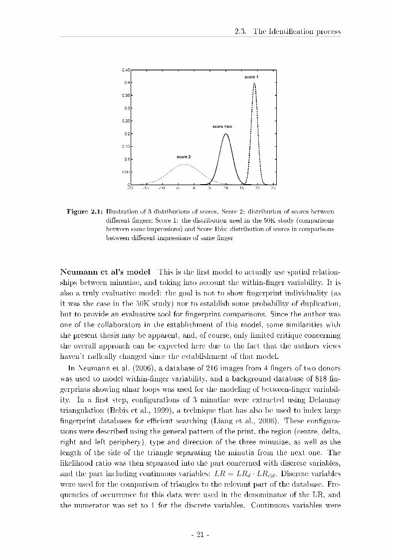
2.3. The Identi�cation process
Figure 2.1: Illustration of 3 distributions of scores. Score 2: distribution of scores between
di�erent �ngers; Score 1: the distribution used in the 50K study (comparisons
between same impressions) and Score 1bis: distribution of scores in comparisons
between di�erent impressions of same �nger
Neumann et al's model This is the �rst model to actually use spatial relation-
ships between minutiae, and taking into account the within-�nger variability. It is
also a truly evaluative model: the goal is not to show �ngerprint individuality (as
it was the case in the 50K study) nor to establish some probability of duplication,
but to provide an evaluative tool for �ngerprint comparisons. Since the author was
one of the collaborators in the establishment of this model, some similarities with
the present thesis may be apparent, and, of course, only limited critique concerning
the overall approach can be expected here due to the fact that the authors views
haven't radically changed since the establishment of that model.
In Neumann et al. (2006), a database of 216 images from 4 �ngers of two donors
was used to model within-�nger variability, and a background database of 818 �n-
gerprints showing ulnar loops was used for the modeling of between-�nger variabil-
ity. In a �rst step, con�gurations of 3 minutiae were extracted using Delaunay
triangulation (Bebis et al., 1999), a technique that has also be used to index large
�ngerprint databases for e�cient searching (Liang et al., 2006). These con�gura-
tions were described using the general pattern of the print, the region (centre, delta,
right and left periphery), type and direction of the three minutiae, as well as the
length of the side of the triangle separating the minutia from the next one. The
likelihood ratio was then separated into the part concerned with discrete variables,
and the part including continuous variables: LR = LRd · LRc|d. Discrete variables
were used for the comparison of triangles to the relevant part of the database. Fre-
quencies of occurrence for this data were used in the denominator of the LR, and
the numerator was set to 1 for the discrete variables. Continuous variables were
- 21 -
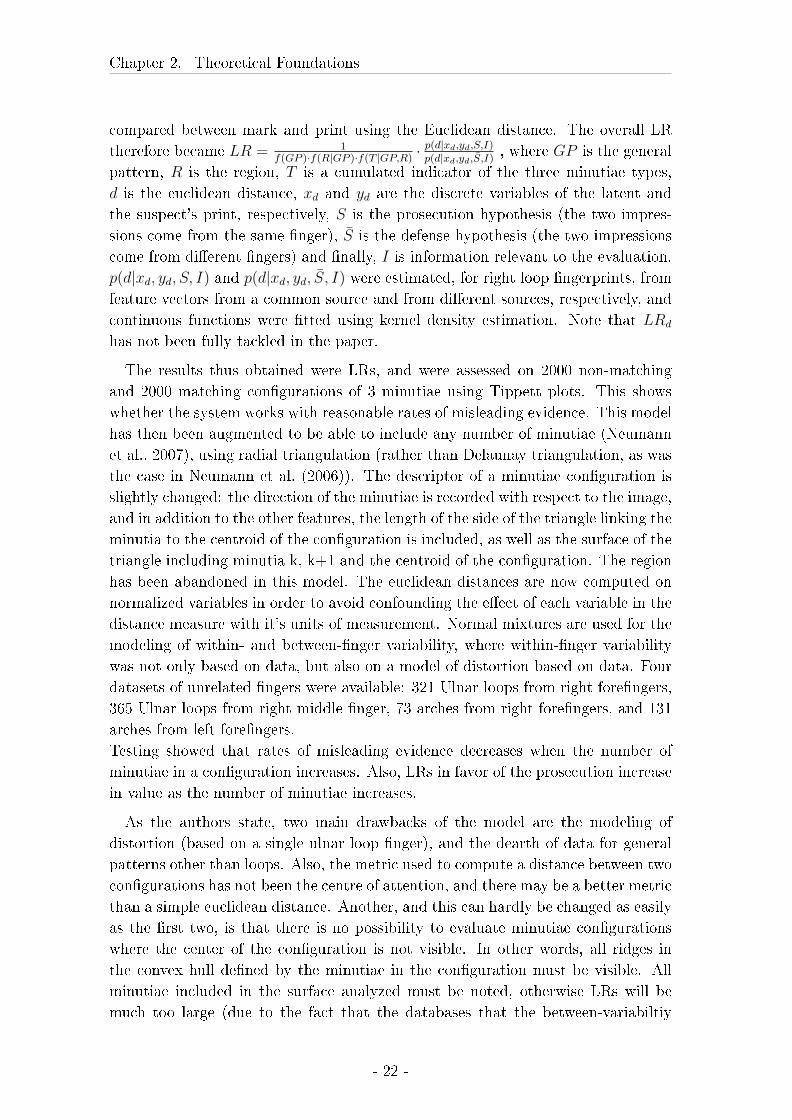
Chapter 2. Theoretical Foundations
compared between mark and print using the Euclidean distance. The overall LR
therefore became LR = 1f(GP )·f(R|GP )·f(T |GP,R)
· p(d|xd,yd,S,I)
p(d|xd,yd,S̄,I), where GP is the general
pattern, R is the region, T is a cumulated indicator of the three minutiae types,
d is the euclidean distance, xd and yd are the discrete variables of the latent and
the suspect's print, respectively, S is the prosecution hypothesis (the two impres-
sions come from the same �nger), S̄ is the defense hypothesis (the two impressions
come from di�erent �ngers) and �nally, I is information relevant to the evaluation.
p(d|xd, yd, S, I) and p(d|xd, yd, S̄, I) were estimated, for right loop �ngerprints, from
feature vectors from a common source and from di�erent sources, respectively, and
continuous functions were �tted using kernel density estimation. Note that LRd
has not been fully tackled in the paper.
The results thus obtained were LRs, and were assessed on 2000 non-matching
and 2000 matching con�gurations of 3 minutiae using Tippett plots. This shows
whether the system works with reasonable rates of misleading evidence. This model
has then been augmented to be able to include any number of minutiae (Neumann
et al., 2007), using radial triangulation (rather than Delaunay triangulation, as was
the case in Neumann et al. (2006)). The descriptor of a minutiae con�guration is
slightly changed: the direction of the minutiae is recorded with respect to the image,
and in addition to the other features, the length of the side of the triangle linking the
minutia to the centroid of the con�guration is included, as well as the surface of the
triangle including minutia k, k+1 and the centroid of the con�guration. The region
has been abandoned in this model. The euclidean distances are now computed on
normalized variables in order to avoid confounding the e�ect of each variable in the
distance measure with it's units of measurement. Normal mixtures are used for the
modeling of within- and between-�nger variability, where within-�nger variability
was not only based on data, but also on a model of distortion based on data. Four
datasets of unrelated �ngers were available: 321 Ulnar loops from right fore�ngers,
365 Ulnar loops from right middle �nger, 73 arches from right fore�ngers, and 131
arches from left fore�ngers.
Testing showed that rates of misleading evidence decreases when the number of
minutiae in a con�guration increases. Also, LRs in favor of the prosecution increase
in value as the number of minutiae increases.
As the authors state, two main drawbacks of the model are the modeling of
distortion (based on a single ulnar loop �nger), and the dearth of data for general
patterns other than loops. Also, the metric used to compute a distance between two
con�gurations has not been the centre of attention, and there may be a better metric
than a simple euclidean distance. Another, and this can hardly be changed as easily
as the �rst two, is that there is no possibility to evaluate minutiae con�gurations
where the center of the con�guration is not visible. In other words, all ridges in
the convex hull de�ned by the minutiae in the con�guration must be visible. All
minutiae included in the surface analyzed must be noted, otherwise LRs will be
much too large (due to the fact that the databases that the between-variabiltiy
- 22 -
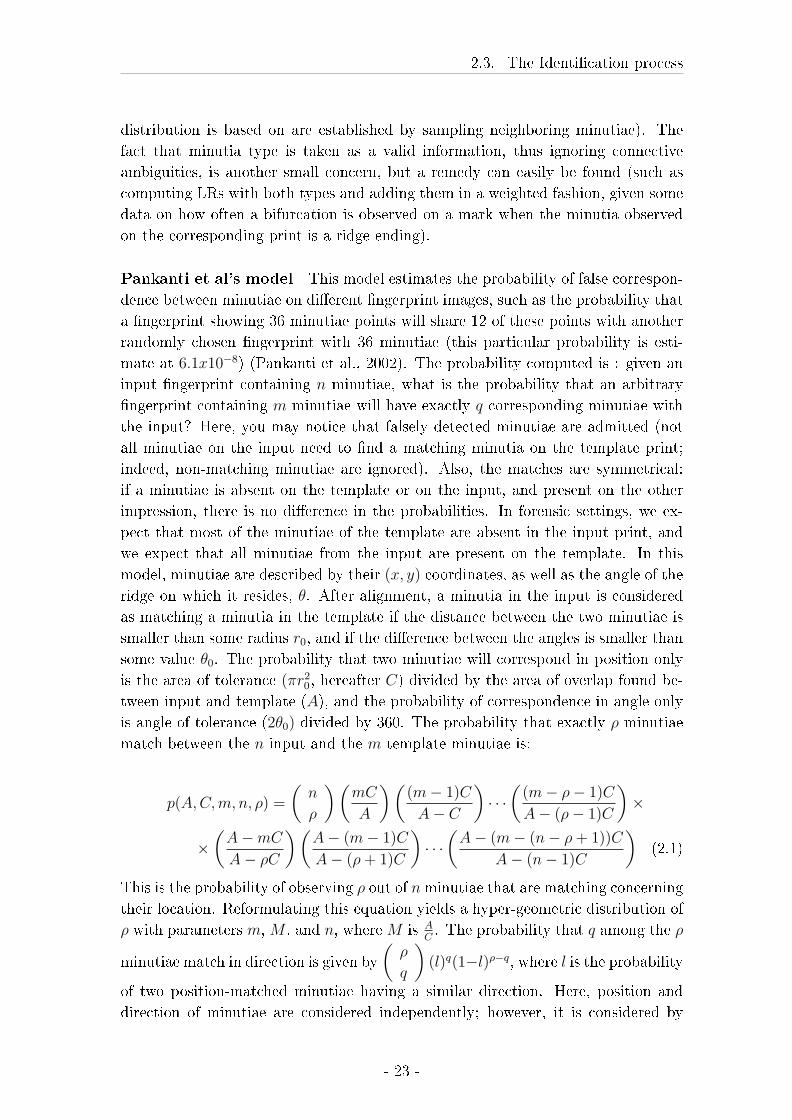
2.3. The Identi�cation process
distribution is based on are established by sampling neighboring minutiae). The
fact that minutia type is taken as a valid information, thus ignoring connective
ambiguities, is another small concern, but a remedy can easily be found (such as
computing LRs with both types and adding them in a weighted fashion, given some
data on how often a bifurcation is observed on a mark when the minutia observed
on the corresponding print is a ridge ending).
Pankanti et al's model This model estimates the probability of false correspon-
dence between minutiae on di�erent �ngerprint images, such as the probability that
a �ngerprint showing 36 minutiae points will share 12 of these points with another
randomly chosen �ngerprint with 36 minutiae (this particular probability is esti-
mate at 6.1x10⁻⁸) (Pankanti et al., 2002). The probability computed is : given an
input �ngerprint containing n minutiae, what is the probability that an arbitrary
�ngerprint containing m minutiae will have exactly q corresponding minutiae with
the input? Here, you may notice that falsely detected minutiae are admitted (not
all minutiae on the input need to �nd a matching minutia on the template print;
indeed, non-matching minutiae are ignored). Also, the matches are symmetrical:
if a minutiae is absent on the template or on the input, and present on the other
impression, there is no di�erence in the probabilities. In forensic settings, we ex-
pect that most of the minutiae of the template are absent in the input print, and
we expect that all minutiae from the input are present on the template. In this
model, minutiae are described by their (x, y) coordinates, as well as the angle of the
ridge on which it resides, θ. After alignment, a minutia in the input is considered
as matching a minutia in the template if the distance between the two minutiae is
smaller than some radius r0, and if the di�erence between the angles is smaller than
some value θ0. The probability that two minutiae will correspond in position only
is the area of tolerance (πr20, hereafter C) divided by the area of overlap found be-
tween input and template (A), and the probability of correspondence in angle only
is angle of tolerance (2θ0) divided by 360. The probability that exactly ρ minutiae
match between the n input and the m template minutiae is:
p(A, C,m, n, ρ) =
(n
ρ
) (mC
A
) ((m− 1)C
A− C
)· · ·
((m− ρ− 1)C
A− (ρ− 1)C
)×
×(
A−mC
A− ρC
) (A− (m− 1)C
A− (ρ + 1)C
)· · ·
(A− (m− (n− ρ + 1))C
A− (n− 1)C
)(2.1)
This is the probability of observing ρ out of n minutiae that are matching concerning
their location. Reformulating this equation yields a hyper-geometric distribution of
ρ with parameters m, M , and n, where M is AC. The probability that q among the ρ
minutiae match in direction is given by
(ρ
q
)(l)q(1−l)ρ−q, where l is the probability
of two position-matched minutiae having a similar direction. Here, position and
direction of minutiae are considered independently; however, it is considered by
- 23 -
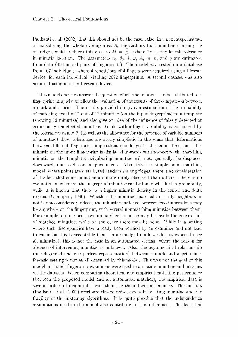
Chapter 2. Theoretical Foundations
Pankanti et al. (2002) that this should not be the case. Also, in a next step, instead
of considering the whole overlap area A, the authors that minutiae can only lie
on ridges, which reduces this area to M =aω
2r0, where 2r0 is the length tolerance
in minutia location. The parameters r0, θ0� l, ω, A, m, n, and q are estimated
from data (450 mated pairs of �ngerprints). The model was tested on a database
from 167 individuals, where 4 repetitions of 4 �ngers were acquired using a lifescan
device, for each individual, yielding 2672 �ngerprints. A second dataset was also
acquired using another livescan device.
This model does not answer the question of whether a latent can be attributed to a
�ngerprint uniquely, or allow the evaluation of the results of the comparison between
a mark and a print. The results provided do give an estimation of the probability
of matching exactly 12 out of 12 minutiae (on the input �ngerprint) to a template
(showing 12 minutiae) and also give an idea of the in�uence of falsely detected or
erroneously undetected minutiae. While within-�nger variability is considered by
the tolerances r0 and θ0 (as well as the allowance for the presence of variable numbers
of minutiae) these tolerances are overly simplistic in the sense that deformations
between di�erent �ngerprint impressions should go in the same direction. If a
minutia on the input �ngerprint is displaced upwards with respect to the matching
minutia on the template, neighboring minutiae will not, generally, be displaced
downward, due to distortion phenomena. Also, this is a simple point matching
model, where points are distributed randomly along ridges; there is no consideration
of the fact that some minutiae are more rarely observed than others. There is no
evaluation of where on the �ngerprint minutiae can be found with higher probability,
while it is known that there is a higher minutia density in the center and delta
regions (Champod, 1996). Whether the minutiae matched are truly neighbors or
not is not considered; indeed, the minutiae matched between two impressions may
be anywhere on the �ngerprint, with several nonmatching minutiae between them.
For example, on one print two unmatched minutiae may be inside the convex hull
of matched minutiae, while on the other there may be none. While in a setting
where such discrepancies have already been veri�ed by an examiner and not lead
to exclusion this is acceptable (since in a smudged mark we do not expect to see
all minutiae), this is not the case in an automated setting, where the reason for
absence of intervening minutiae is unknown. Also, the asymmetrical relationship
(one degraded and one perfect representation) between a mark and a print in a
forensic setting is not at all captured by this model. This was not the goal of this
model, although �ngerprint examiners were used to annotate minutiae and matches
on the datasets. When comparing theoretical and empirical matching performance
(between the proposed model and an automated matcher), the empirical data is
several orders of magnitude lower than the theoretical perfomance. The authors
(Pankanti et al., 2002) attribute this to noise, errors in locating minutiae and the
fragility of the matching algorithms. It is quite possible that the independence
assumptions used in the model also contribute to this di�erence. The fact that
- 24 -
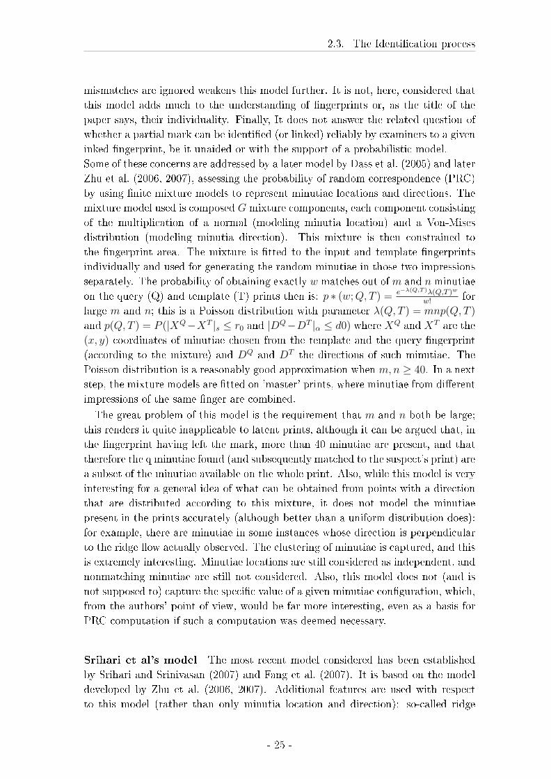
2.3. The Identi�cation process
mismatches are ignored weakens this model further. It is not, here, considered that
this model adds much to the understanding of �ngerprints or, as the title of the
paper says, their individuality. Finally, It does not answer the related question of
whether a partial mark can be identi�ed (or linked) reliably by examiners to a given
inked �ngerprint, be it unaided or with the support of a probabilistic model.
Some of these concerns are addressed by a later model by Dass et al. (2005) and later
Zhu et al. (2006, 2007), assessing the probability of random correspondence (PRC)
by using �nite mixture models to represent minutiae locations and directions. The
mixture model used is composed G mixture components, each component consisting
of the multiplication of a normal (modeling minutia location) and a Von-Mises
distribution (modeling minutia direction). This mixture is then constrained to
the �ngerprint area. The mixture is �tted to the input and template �ngerprints
individually and used for generating the random minutiae in those two impressions
separately. The probability of obtaining exactly w matches out of m and n minutiae
on the query (Q) and template (T) prints then is: p ∗ (w; Q, T ) = e−λ(Q,T )λ(Q,T )w
w!for
large m and n; this is a Poisson distribution with parameter λ(Q, T ) = mnp(Q, T )
and p(Q, T ) = P (|XQ−XT |s ≤ r0 and |DQ−DT |α ≤ d0) where XQ and XT are the
(x, y) coordinates of minutiae chosen from the template and the query �ngerprint
(according to the mixture) and DQ and DT the directions of such minutiae. The
Poisson distribution is a reasonably good approximation when m, n ≥ 40. In a next
step, the mixture models are �tted on 'master' prints, where minutiae from di�erent
impressions of the same �nger are combined.
The great problem of this model is the requirement that m and n both be large;
this renders it quite inapplicable to latent prints, although it can be argued that, in
the �ngerprint having left the mark, more than 40 minutiae are present, and that
therefore the q minutiae found (and subsequently matched to the suspect's print) are
a subset of the minutiae available on the whole print. Also, while this model is very
interesting for a general idea of what can be obtained from points with a direction
that are distributed according to this mixture, it does not model the minutiae
present in the prints accurately (although better than a uniform distribution does):
for example, there are minutiae in some instances whose direction is perpendicular
to the ridge �ow actually observed. The clustering of minutiae is captured, and this
is extremely interesting. Minutiae locations are still considered as independent, and
nonmatching minutiae are still not considered. Also, this model does not (and is
not supposed to) capture the speci�c value of a given minutiae con�guration, which,
from the authors' point of view, would be far more interesting, even as a basis for
PRC computation if such a computation was deemed necessary.
Srihari et al's model The most recent model considered has been established
by Srihari and Srinivasan (2007) and Fang et al. (2007). It is based on the model
developed by Zhu et al. (2006, 2007). Additional features are used with respect
to this model (rather than only minutia location and direction): so-called ridge
- 25 -
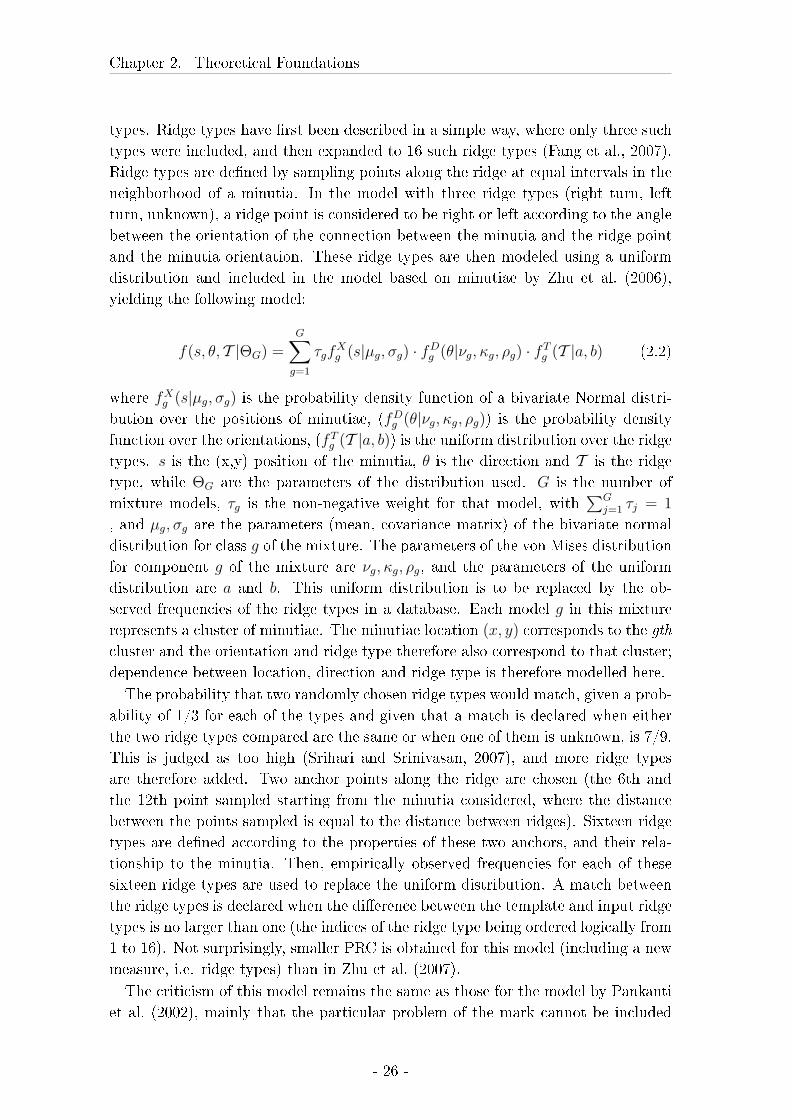
Chapter 2. Theoretical Foundations
types. Ridge types have �rst been described in a simple way, where only three such
types were included, and then expanded to 16 such ridge types (Fang et al., 2007).
Ridge types are de�ned by sampling points along the ridge at equal intervals in the
neighborhood of a minutia. In the model with three ridge types (right turn, left
turn, unknown), a ridge point is considered to be right or left according to the angle
between the orientation of the connection between the minutia and the ridge point
and the minutia orientation. These ridge types are then modeled using a uniform
distribution and included in the model based on minutiae by Zhu et al. (2006),
yielding the following model:
f(s, θ, T |ΘG) =G∑
g=1
τgfXg (s|µg, σg) · fD
g (θ|νg, κg, ρg) · fTg (T |a, b) (2.2)
where fXg (s|µg, σg) is the probability density function of a bivariate Normal distri-
bution over the positions of minutiae, (fDg (θ|νg, κg, ρg)) is the probability density
function over the orientations, (fTg (T |a, b)) is the uniform distribution over the ridge
types. s is the (x,y) position of the minutia, θ is the direction and T is the ridge
type, while ΘG are the parameters of the distribution used. G is the number of
mixture models, τg is the non-negative weight for that model, with∑G
j=1 τj = 1
, and µg, σg are the parameters (mean, covariance matrix) of the bivariate normal
distribution for class g of the mixture. The parameters of the von Mises distribution
for component g of the mixture are νg, κg, ρg, and the parameters of the uniform
distribution are a and b. This uniform distribution is to be replaced by the ob-
served frequencies of the ridge types in a database. Each model g in this mixture
represents a cluster of minutiae. The minutiae location (x, y) corresponds to the gth
cluster and the orientation and ridge type therefore also correspond to that cluster;
dependence between location, direction and ridge type is therefore modelled here.
The probability that two randomly chosen ridge types would match, given a prob-
ability of 1/3 for each of the types and given that a match is declared when either
the two ridge types compared are the same or when one of them is unknown, is 7/9.
This is judged as too high (Srihari and Srinivasan, 2007), and more ridge types
are therefore added. Two anchor points along the ridge are chosen (the 6th and
the 12th point sampled starting from the minutia considered, where the distance
between the points sampled is equal to the distance between ridges). Sixteen ridge
types are de�ned according to the properties of these two anchors, and their rela-
tionship to the minutia. Then, empirically observed frequencies for each of these
sixteen ridge types are used to replace the uniform distribution. A match between
the ridge types is declared when the di�erence between the template and input ridge
types is no larger than one (the indices of the ridge type being ordered logically from
1 to 16). Not surprisingly, smaller PRC is obtained for this model (including a new
measure, i.e. ridge types) than in Zhu et al. (2007).
The criticism of this model remains the same as those for the model by Pankanti
et al. (2002), mainly that the particular problem of the mark cannot be included
- 26 -
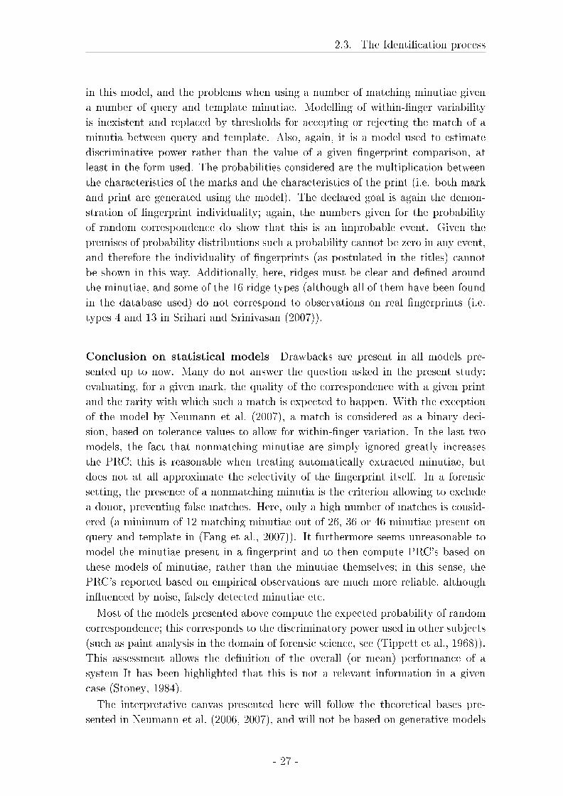
2.3. The Identi�cation process
in this model, and the problems when using a number of matching minutiae given
a number of query and template minutiae. Modelling of within-�nger variability
is inexistent and replaced by thresholds for accepting or rejecting the match of a
minutia between query and template. Also, again, it is a model used to estimate
discriminative power rather than the value of a given �ngerprint comparison, at
least in the form used. The probabilities considered are the multiplication between
the characteristics of the marks and the characteristics of the print (i.e. both mark
and print are generated using the model). The declared goal is again the demon-
stration of �ngerprint individuality; again, the numbers given for the probability
of random correspondence do show that this is an improbable event. Given the
premises of probability distributions such a probability cannot be zero in any event,
and therefore the individuality of �ngerprints (as postulated in the titles) cannot
be shown in this way. Additionally, here, ridges must be clear and de�ned around
the minutiae, and some of the 16 ridge types (although all of them have been found
in the database used) do not correspond to observations on real �ngerprints (i.e.
types 4 and 13 in Srihari and Srinivasan (2007)).
Conclusion on statistical models Drawbacks are present in all models pre-
sented up to now. Many do not answer the question asked in the present study:
evaluating, for a given mark, the quality of the correspondence with a given print
and the rarity with which such a match is expected to happen. With the exception
of the model by Neumann et al. (2007), a match is considered as a binary deci-
sion, based on tolerance values to allow for within-�nger variation. In the last two
models, the fact that nonmatching minutiae are simply ignored greatly increases
the PRC; this is reasonable when treating automatically extracted minutiae, but
does not at all approximate the selectivity of the �ngerprint itself. In a forensic
setting, the presence of a nonmatching minutia is the criterion allowing to exclude
a donor, preventing false matches. Here, only a high number of matches is consid-
ered (a minimum of 12 matching minutiae out of 26, 36 or 46 minutiae present on
query and template in (Fang et al., 2007)). It furthermore seems unreasonable to
model the minutiae present in a �ngerprint and to then compute PRC's based on
these models of minutiae, rather than the minutiae themselves; in this sense, the
PRC's reported based on empirical observations are much more reliable, although
in�uenced by noise, falsely detected minutiae etc.
Most of the models presented above compute the expected probability of random
correspondence; this corresponds to the discriminatory power used in other subjects
(such as paint analysis in the domain of forensic science, see (Tippett et al., 1968)).
This assessment allows the de�nition of the overall (or mean) performance of a
system It has been highlighted that this is not a relevant information in a given
case (Stoney, 1984).
The interpretative canvas presented here will follow the theoretical bases pre-
sented in Neumann et al. (2006, 2007), and will not be based on generative models
- 27 -
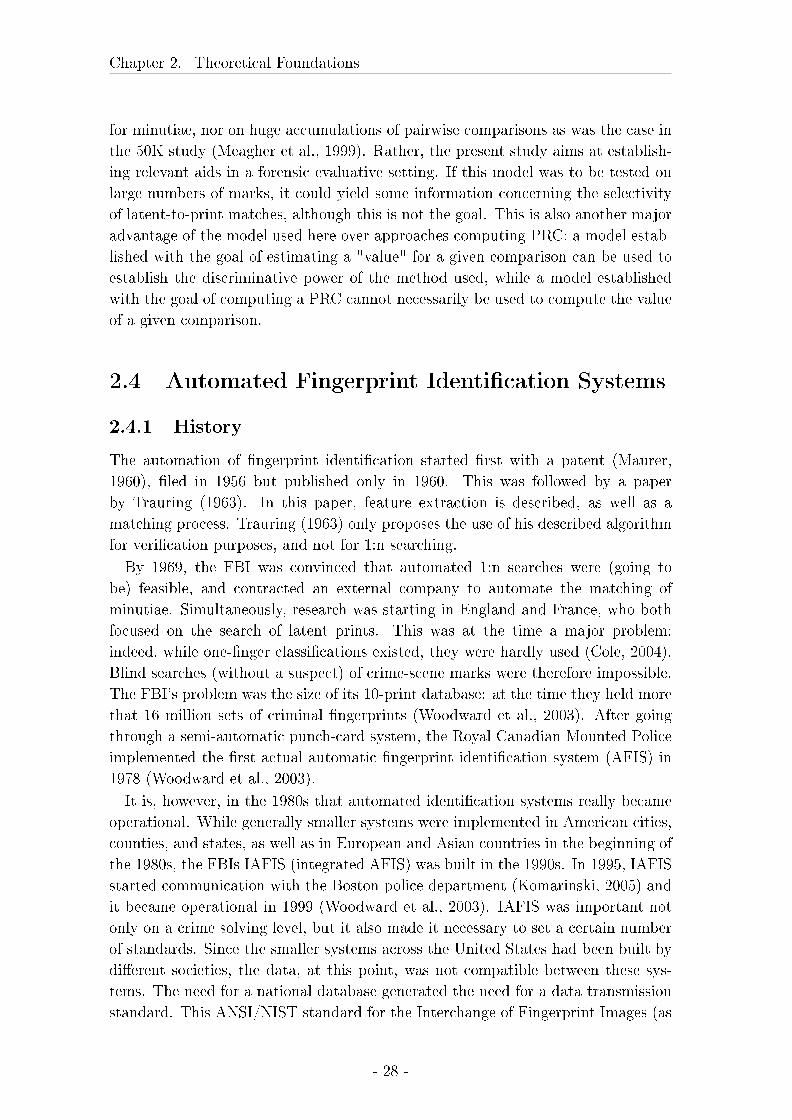
Chapter 2. Theoretical Foundations
for minutiae, nor on huge accumulations of pairwise comparisons as was the case in
the 50K study (Meagher et al., 1999). Rather, the present study aims at establish-
ing relevant aids in a forensic evaluative setting. If this model was to be tested on
large numbers of marks, it could yield some information concerning the selectivity
of latent-to-print matches, although this is not the goal. This is also another major
advantage of the model used here over approaches computing PRC: a model estab-
lished with the goal of estimating a "value" for a given comparison can be used to
establish the discriminative power of the method used, while a model established
with the goal of computing a PRC cannot necessarily be used to compute the value
of a given comparison.
2.4 Automated Fingerprint Identi�cation Systems
2.4.1 History
The automation of �ngerprint identi�cation started �rst with a patent (Maurer,
1960), �led in 1956 but published only in 1960. This was followed by a paper
by Trauring (1963). In this paper, feature extraction is described, as well as a
matching process. Trauring (1963) only proposes the use of his described algorithm
for veri�cation purposes, and not for 1:n searching.
By 1969, the FBI was convinced that automated 1:n searches were (going to
be) feasible, and contracted an external company to automate the matching of
minutiae. Simultaneously, research was starting in England and France, who both
focused on the search of latent prints. This was at the time a major problem:
indeed, while one-�nger classi�cations existed, they were hardly used (Cole, 2004).
Blind searches (without a suspect) of crime-scene marks were therefore impossible.
The FBI's problem was the size of its 10-print database: at the time they held more
that 16 million sets of criminal �ngerprints (Woodward et al., 2003). After going
through a semi-automatic punch-card system, the Royal Canadian Mounted Police
implemented the �rst actual automatic �ngerprint identi�cation system (AFIS) in
1978 (Woodward et al., 2003).
It is, however, in the 1980s that automated identi�cation systems really became
operational. While generally smaller systems were implemented in American cities,
counties, and states, as well as in European and Asian countries in the beginning of
the 1980s, the FBIs IAFIS (integrated AFIS) was built in the 1990s. In 1995, IAFIS
started communication with the Boston police department (Komarinski, 2005) and
it became operational in 1999 (Woodward et al., 2003). IAFIS was important not
only on a crime solving level, but it also made it necessary to set a certain number
of standards. Since the smaller systems across the United States had been built by
di�erent societies, the data, at this point, was not compatible between these sys-
tems. The need for a national database generated the need for a data transmission
standard. This ANSI/NIST standard for the Interchange of Fingerprint Images (as
- 28 -
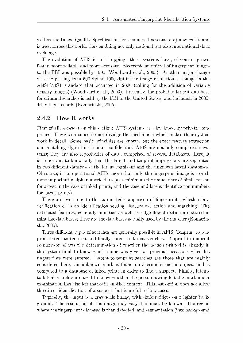
2.4. Automated Fingerprint Identi�cation Systems
well as the Image Quality Speci�cation for scanners, livescans, etc) now exists and
is used across the world, thus enabling not only national but also international data
exchange.
The evolution of AFIS is not stopping: these systems have, of course, grown
faster, more reliable and more accurate. Electronic submittal of �ngerprint images
to the FBI was possible by 1995 (Woodward et al., 2003). Another major change
was the passing from 500 dpi to 1000 dpi in the image resolution, a change in the
ANSI/NIST standard that occurred in 2000 (calling for the addition of variable
density images) (Woodward et al., 2003). Presently, the probably largest database
for criminal searches is held by the FBI in the United States, and included, in 2005,
46 million records (Komarinski, 2005).
2.4.2 How it works
First of all, a caveat on this section: AFIS systems are developed by private com-
panies. These companies do not divulge the mechanism which makes their system
work in detail. Some basic principles are known, but the exact feature extraction
and matching algorithms remain con�dential. AFIS are not only comparison sys-
tems; they are also repositories of data, comprised of several databases. Here, it
is important to know only that the latent and tenprint impressions are separated
in two di�erent databases: the latent cognizant and the unknown latent databases.
Of course, in an operational AFIS, more than only the �ngerprint image is stored,
most importantly alphanumeric data (as a minimum the name, date of birth, reason
for arrest in the case of inked prints, and the case and latent identi�cation numbers
for latent prints).
There are two steps to the automated comparison of �ngerprints, whether in a
veri�cation or in an identi�cation setting: feature extraction and matching. The
extracted features, generally minutiae as well as ridge �ow direction are stored in
minutiae databases; these are the databases actually used by the matcher (Komarin-
ski, 2005).
Three di�erent types of searches are generally possible in AFIS: Tenprint to ten-
print, latent to tenprint and �nally, latent to latent searches. Tenprint-to-tenprint
comparison allows the determination of whether the person printed is already in
the system (and to know which name was given on previous occasions when his
�ngerprints were entered. Latent-to-tenprint searches are those that are mainly
considered here: an unknown mark is found on a crime scene or object, and is
compared to a database of inked prints in order to �nd a suspect. Finally, latent-
to-latent searches are used to know whether the person having left the mark under
examination has also left marks in another context. This last option does not allow
the direct identi�cation of a suspect, but is useful to link cases.
Typically, the input is a gray scale image, with darker ridges on a lighter back-
ground. The resolution of this image may vary, but must be known. The region
where the �ngerprint is located is then detected, and segmentation (into background
- 29 -
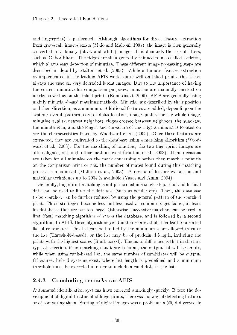
Chapter 2. Theoretical Foundations
and �ngerprint) is performed. Although algorithms for direct feature extraction
from gray-scale images exists (Maio and Maltoni, 1997), the image is then generally
converted to a binary (black and white) image. This demands the use of �lters,
such as Gabor �lters. The ridges are then generally thinned to a so-called skeleton,
which allows easy detection of minutiae. These di�erent image processing steps are
described in detail by Maltoni et al. (2003). While automatic feature extraction
as implemented in the leading AFIS works quite well on inked prints, this is not
always the case on very degraded latent images. Due to the importance of having
the correct minutiae for comparison purposes, minutiae are manually checked on
marks as well as on the inked prints (Komarinski, 2005). AFIS are generally using
mainly minutiae-based matching methods. Minutiae are described by their position
and their direction, as a minimum. Additional features are added, depending on the
system: overall pattern, core or delta location, image quality for the whole image,
minutiae quality, nearest neighbors, ridges crossed between neighbors, the quadrant
the minuta is in, and the length and curvature of the ridge a minutia is located on
are the characteristics listed by Woodward et al. (2003). Once these features are
extracted, they are confronted to the database using a matching algorithm (Wood-
ward et al., 2003). For the matching of minutiae, the two �ngerprint images are
often aligned, although other methods exist (Maltoni et al., 2003). Then, decisions
are taken for all minutiae on the mark concerning whether they match a minutia
on the comparison print or not; the number of mates found during this matching
process is maximised (Maltoni et al., 2003). A review of feature extraction and
matching techniques up to 2004 is available (Yager and Amin, 2004).
Generally, �ngerprint matching is not performed in a single step. First, additional
data can be used to �lter the database (such as gender etc). Then, the database
to be searched can be further reduced by using the general pattern of the searched
print. These strategies become less and less used as computers get faster, at least
for databases that are not too large. Otherwise, successive matchers can be used: a
�rst (fast) matching algorithm winnows the database, and is followed by a second
algorithm. In AFIS, these algorithms yield match scores, that then lead to a sorted
list of candidates. This list can be limited by the minimum score allowed to enter
the list (Threshold-based), or the list may be of prede�ned length, including the
prints with the highest scores (Rank-based). The main di�erence is that in the �rst
type of selection, if no matching candidate is found, the output list will be empty,
while when using rank-based list, the same number of candidates will be output.
Of course, hybrid systems exist, where list length is prede�ned and a minimum
threshold must be exceeded in order to include a candidate in the list.
2.4.3 Concluding remarks on AFIS
Automated identi�cation systems have emerged amazingly quickly. Before the de-
velopment of digital treatment of �ngerprints, there was no way of detecting features
or of comparing them. Storing of digital images was a problem: a 500 dpi greyscale
- 30 -
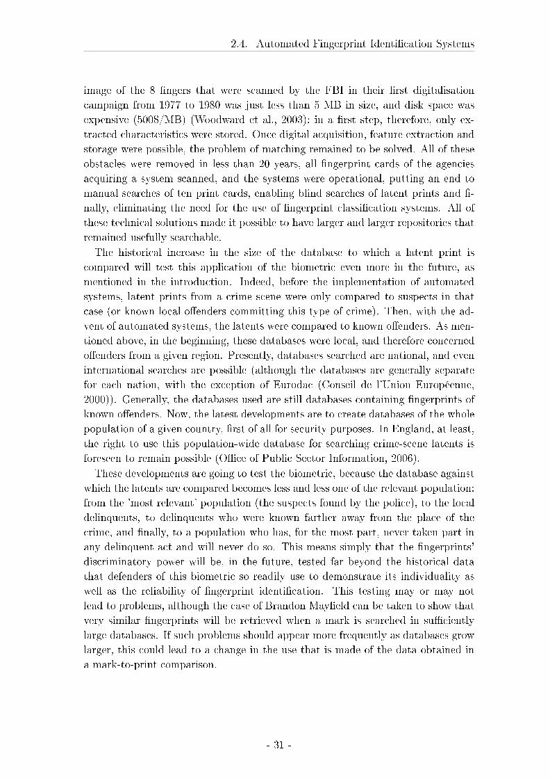
2.4. Automated Fingerprint Identi�cation Systems
image of the 8 �ngers that were scanned by the FBI in their �rst digitalisation
campaign from 1977 to 1980 was just less than 5 MB in size, and disk space was
expensive (500$/MB) (Woodward et al., 2003); in a �rst step, therefore, only ex-
tracted characteristics were stored. Once digital acquisition, feature extraction and
storage were possible, the problem of matching remained to be solved. All of these
obstacles were removed in less than 20 years, all �ngerprint cards of the agencies
acquiring a system scanned, and the systems were operational, putting an end to
manual searches of ten print cards, enabling blind searches of latent prints and �-
nally, eliminating the need for the use of �ngerprint classi�cation systems. All of
these technical solutions made it possible to have larger and larger repositories that
remained usefully searchable.
The historical increase in the size of the database to which a latent print is
compared will test this application of the biometric even more in the future, as
mentioned in the introduction. Indeed, before the implementation of automated
systems, latent prints from a crime scene were only compared to suspects in that
case (or known local o�enders committing this type of crime). Then, with the ad-
vent of automated systems, the latents were compared to known o�enders. As men-
tioned above, in the beginning, these databases were local, and therefore concerned
o�enders from a given region. Presently, databases searched are national, and even
international searches are possible (although the databases are generally separate
for each nation, with the exception of Eurodac (Conseil de l'Union Européenne,
2000)). Generally, the databases used are still databases containing �ngerprints of
known o�enders. Now, the latest developments are to create databases of the whole
population of a given country, �rst of all for security purposes. In England, at least,
the right to use this population-wide database for searching crime-scene latents is
foreseen to remain possible (O�ce of Public Sector Information, 2006).
These developments are going to test the biometric, because the database against
which the latents are compared becomes less and less one of the relevant population:
from the 'most relevant' population (the suspects found by the police), to the local
delinquents, to delinquents who were known farther away from the place of the
crime, and �nally, to a population who has, for the most part, never taken part in
any delinquent act and will never do so. This means simply that the �ngerprints'
discriminatory power will be, in the future, tested far beyond the historical data
that defenders of this biometric so readily use to demonstrate its individuality as
well as the reliability of �ngerprint identi�cation. This testing may or may not
lead to problems, although the case of Brandon May�eld can be taken to show that
very similar �ngerprints will be retrieved when a mark is searched in su�ciently
large databases. If such problems should appear more frequently as databases grow
larger, this could lead to a change in the use that is made of the data obtained in
a mark-to-print comparison.
- 31 -

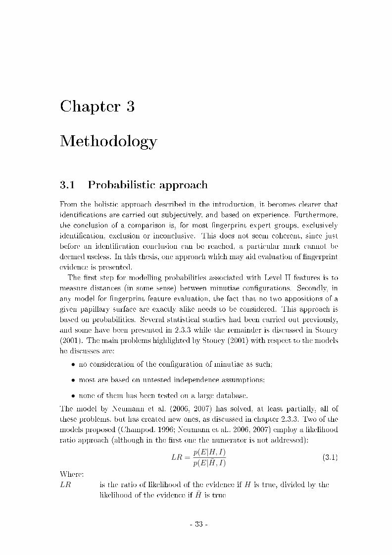
Chapter 3
Methodology
3.1 Probabilistic approach
From the holistic approach described in the introduction, it becomes clearer that
identi�cations are carried out subjectively, and based on experience. Furthermore,
the conclusion of a comparison is, for most �ngerprint expert groups, exclusively
identi�cation, exclusion or inconclusive. This does not seem coherent, since just
before an identi�cation conclusion can be reached, a particular mark cannot be
deemed useless. In this thesis, one approach which may aid evaluation of �ngerprint
evidence is presented.
The �rst step for modelling probabilities associated with Level II features is to
measure distances (in some sense) between minutiae con�gurations. Secondly, in
any model for �ngerprint feature evaluation, the fact that no two appositions of a
given papillary surface are exactly alike needs to be considered. This approach is
based on probabilities. Several statistical studies had been carried out previously,
and some have been presented in 2.3.3 while the remainder is discussed in Stoney
(2001). The main problems highlighted by Stoney (2001) with respect to the models
he discusses are:
• no consideration of the con�guration of minutiae as such;
• most are based on untested independence assumptions;
• none of them has been tested on a large database.
The model by Neumann et al. (2006, 2007) has solved, at least partially, all of
these problems, but has created new ones, as discussed in chapter 2.3.3. Two of the
models proposed (Champod, 1996; Neumann et al., 2006, 2007) employ a likelihood
ratio approach (although in the �rst one the numerator is not addressed):
LR =p(E|H, I)
p(E|H̄, I)(3.1)
Where:
LR is the ratio of likelihood of the evidence if H is true, divided by the
likelihood of the evidence if H̄ is true
- 33 -
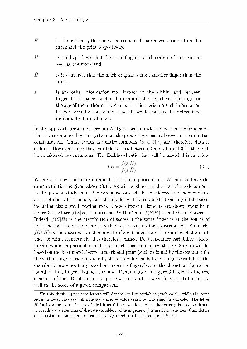
Chapter 3. Methodology
E is the evidence, the concordances and discordances observed on the
mark and the print respectively,
H is the hypothesis that the same �nger is at the origin of the print as
well as the mark and
H̄ is it's inverse, that the mark originates from another �nger than the
print.
I is any other information may impact on the within- and between
�nger distributions, such as for example the sex, the ethnic origin or
the age of the author of the crime. In this thesis, no such information
is ever formally considered, since it would have to be determined
individually for each case.
In the approach presented here, an AFIS is used in order to extract the 'evidence'.
The scores employed by the system are the proximity measure between two minutiae
con�guration. These scores are entire numbers (S ∈ N)1, and therefore data is
ordinal. However, since they can take values between 0 and above 10000 they will
be considered as continuous. The likelihood ratio that will be modeled is therefore
LR =f(s|H)
f(s|H̄)(3.2)
Where s is now the score obtained for the comparison, and H, and H̄ have the
same de�nition as given above (3.1). As will be shown in the rest of the document,
in the present study, minutiae con�gurations will be considered, no independence
assumptions will be made, and the model will be established on large databases,
including also a small testing step. These di�erent elements are shown visually in
�gure 3.1, where f(S|H) is noted as 'Within' and f(S|H̄) is noted as 'Between'.
Indeed, f(S|H) is the distribution of scores if the same �nger is at the source of
both the mark and the print; it is therefore a within-�nger distribution. Similarly,
f(S|H̄) is the distribution of scores if di�erent �ngers are the sources of the mark
and the print, respectively; it is therefore termed 'Between-�nger variability'. More
precisely, and in particular in the approach used here, since the AFIS score will be
based on the best match between mark and print (such as found by the examiner for
the within-�nger variability and by the system for the between-�nger variability) the
distributions are not truly based on the entire �nger, but on the closest con�guration
found on that �nger. 'Numerator' and 'Denominator' in �gure 3.1 refer to the two
elements of the LR, obtained using the within- and between-�nger distributions as
well as the score of a given comparison.
1In this thesis, upper case letters will denote random variables (such as S), while the same
letter in lower case (s) will indicate a precise value taken by this random variable. The letter
H for hypotheses has been excluded from this convention. Also, the letter p is used to denote
probability distributions of discrete variables, while in general f is used for densities. Cumulative
distribution functions, in both cases, are again indicated using capitals (P , F ).
- 34 -
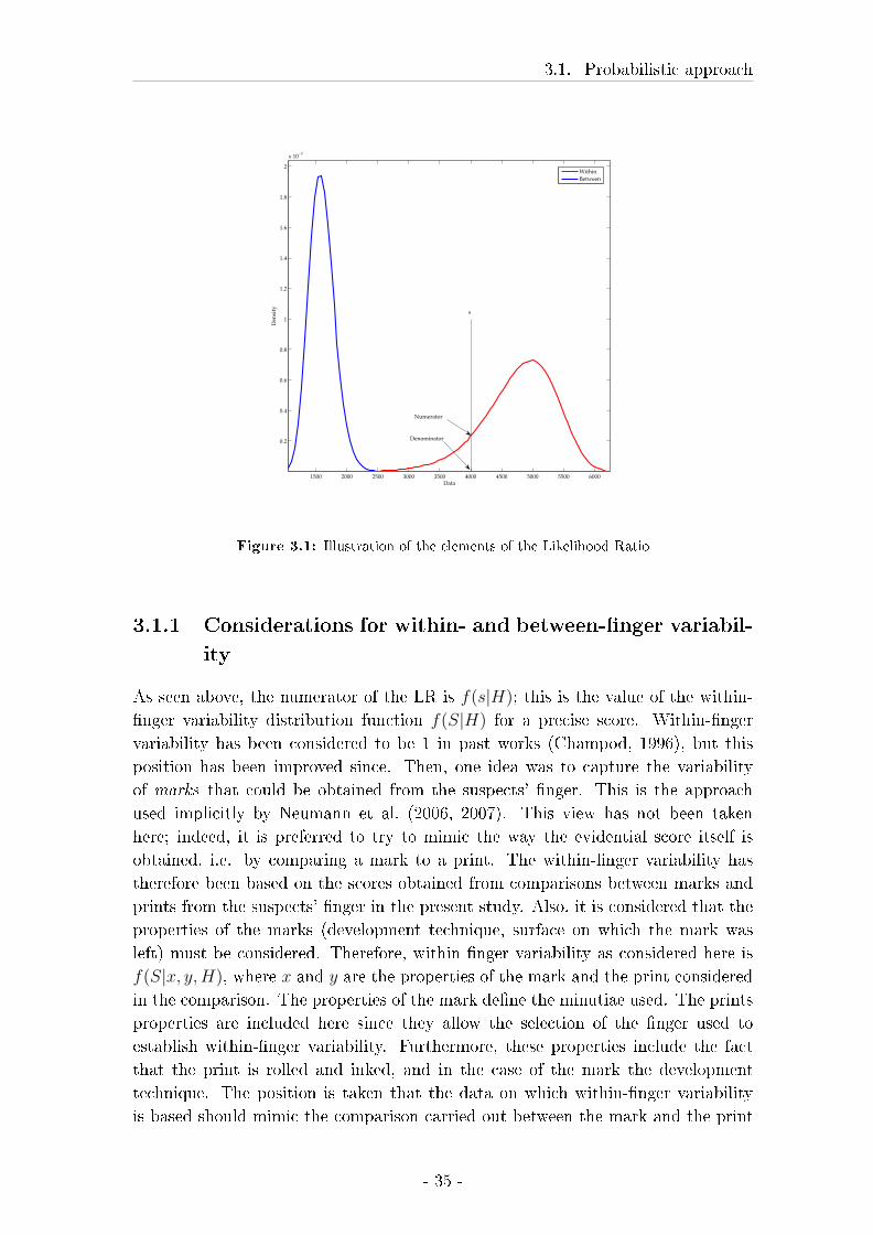
3.1. Probabilistic approach
1500 2000 2500 3000 3500 4000 4500 5000 5500 6000
0.2
0.4
0.6
0.8
1
1.2
1.4
1.6
1.8
2
x 10−3
Data
Den
sity
Within
Between
Numerator
Denominator
s
Figure 3.1: Illustration of the elements of the Likelihood Ratio
3.1.1 Considerations for within- and between-�nger variabil-
ity
As seen above, the numerator of the LR is f(s|H); this is the value of the within-
�nger variability distribution function f(S|H) for a precise score. Within-�nger
variability has been considered to be 1 in past works (Champod, 1996), but this
position has been improved since. Then, one idea was to capture the variability
of marks that could be obtained from the suspects' �nger. This is the approach
used implicitly by Neumann et al. (2006, 2007). This view has not been taken
here; indeed, it is preferred to try to mimic the way the evidential score itself is
obtained, i.e. by comparing a mark to a print. The within-�nger variability has
therefore been based on the scores obtained from comparisons between marks and
prints from the suspects' �nger in the present study. Also, it is considered that the
properties of the marks (development technique, surface on which the mark was
left) must be considered. Therefore, within �nger variability as considered here is
f(S|x, y, H), where x and y are the properties of the mark and the print considered
in the comparison. The properties of the mark de�ne the minutiae used. The prints
properties are included here since they allow the selection of the �nger used to
establish within-�nger variability. Furthermore, these properties include the fact
that the print is rolled and inked, and in the case of the mark the development
technique. The position is taken that the data on which within-�nger variability
is based should mimic the comparison carried out between the mark and the print
- 35 -
Chapter 3. Methodology
in question; that therefore, the distribution must be based on comparisons between
developed marks and inked prints, using the same number of each, in order to
capture the variation that could be present between any mark from the suspect,
and any print from that suspect. H, rather than being phrased as "the same �nger
is at the origin of the print as well as the mark" should be phrased, "the suspect's
�nger is at the origin of print and mark". In the �rst phrasing, it is understood that
that 'same �nger' is the suspect's, since the print is supposed to be of known origin.
But that hypothesis intimates that there is a generally applicable within variability
(e.g. that scores from a same source always behave in the same way, independent
of the exact source they are from), which mustn't be adapted for the case at hand,
exception made of the characteristics of the mark and the print. It is, however,
truly the second that will be modeled here. For each �nger, a within variability
distribution is established, based on repeated impressions of the suspects' �nger.
The between �nger variability f(S|H̄) will be written f(S|x, y, H̄). The mark is
compared to the database of �ngerprints, which warrants the conditioning by x, the
marks' characteristics. the conditioning by y can be left aside since f(S|x, y, H̄) =
f(S|x, H̄) · f(y|H̄) and that, under H̄, the probability of observing the suspects'
con�guration is 1.
For within-�nger variability, that will mimic as closely as possible the comparison
between the mark and the suspects' print, several prints will be used. The print (or
rather its set of characteristics extracted) is therefore considered to be a random
variable, where the constraint is that these repeated prints are acquired from the
suspects �nger that is under examination, and that they are acquired under the
same conditions as the comparison print used for the evidence score.
3.2 The AFIS used
The system used in the present study is a Sagem DMA. Also, several extensions
have been custom made for this study by SAGEM. The �rst one is for the automatic
acquisition of tenprint cards. It is called ei_batchscan.exe, and takes all �les stored
in a given directory. The �lenames must be of the form:
id.page0.0x0xWidthxHeightx500.raw,
and must therefore be in .raw format and at 500dpi. A second program allows the
de�nition of marks and prints to be automatically compared (raw_dump.py), and
the third allows the automated (and listwise) comparison of the selected marks and
prints (spec.exe). It is through this automated extraction/comparison process that
it possible to obtain all of the scores when a given mark is compared to all of the
�ngerprints in the system. An overview of the commands used to extract scores is
given in Appendix B.
- 36 -
3.3. The Hypotheses
A further tool programmed by SAGEM allows the extraction of the general pat-
terns attributed to the �ngerprints in the database (PatternExtractor.py).
All outputs are organised in text�les, and indexed by the prints' number (number
of the ten-print card and the �nger number).
The way in which this AFIS is organised includes 4 databases: the log database
(saving actions on the database), a WIP database (work in progress), the AFIS
database (including marks and tenprint cards) and an administration database.
Several processes linked to these databases and the task of the AFIS (storing, com-
paring, retrieving �ngerprints) exist.
3.3 The Hypotheses
Two main hypotheses have been tested here: the �rst one concerns within- and the
second one between-�nger variability. In both cases, ideally, a generally applicable
probability density function can be found; otherwise, the result of the testing of the
following hypotheses will be a guide on the acquisition of data for their estimation
on a case-by-case basis.
3.3.1 Hypothesis 1: Within Variability can be modelled us-
ing a generally applicable probability density function
Hypothesis 1a: The density used for modelling the within �nger vari-
ability becomes stable as a given number of observations is reached
Above a certain number of scores obtained, the within-variability density function
and, as a consequence, the numerator of the likelihood ratio for a given comparison
stabilises in the sense that addition of more data does not cause this distribution
to change much. In order to be able to give likelihood ratios which are robust, this
stability must be attained. This minimum number of comparisons for the estimation
of within-�nger variability must be known whether a generally applicable function
is, at a later point, found or not. Indeed, if a generally applicable distribution can
be determined, it is in the present study that this number of comparisons must be
obtained for the conclusions to be reliable and valid. If no such stable distribution is
found, this is a �rst step towards the description of the data that must be acquired
on a case-by-case basis. This hypothesis is tested in chapter 4, section 4.2.
Hypothesis 1b: Marks used for the modelling of within variability can
be substituted by livescan images or slaps from ten-print cards
If the within-�nger distribution is shown to be in�uenced only by the di�erence
between �at apposition of �ngers and rolled impressions, then marks can be sub-
stituted by any kind of �at impression. This hypothesis is intimately linked with
hypothesis 1d (that within �nger variability depends on the number and positioning
- 37 -
Chapter 3. Methodology
of minutiae). If, indeed, it is only the positioning and number of minutiae, rather
than the way of acquiring the �ngerprint image, that are decisive, then livescans or
inked prints could substitute marks for the estimation of the within-�nger variabil-
ity distribution. Rolled prints are not considered here as a substitute for marks,
since the distortion that is present on rolled prints is very distinctive and does not
generally correspond to distortions that are observed on marks. This replacement,
and the reason for the present hypothesis, is interesting if the distribution has to
be estimated separately for each case. The acquisition of �ngerprint images is in
all cases time-consuming; for the acquisition of repeated marks, however, the time
required is superior to the time needed for slaps or livescans, for several reasons.
First of all, on marks, it is far from certain that the particular minutia con�gu-
ration found on the evidence is present. This means that, while the number of
scores needed and therefore the number of marks where the con�guration is present
is determined under hypothesis 1a, the number of marks that actually have to be
developed is likely to be superior. Second, the development and imaging steps for
marks are time consuming and there is a need for equipment (working laboratory,
chemicals, imaging techniques, etc.) that is far superior to that of livescans or ink-
ing. This hypothesis is tested in chapter 4, section 4.3.
Hypothesis 1c: Within variability for the evaluation of a given mark can
be deduced from a generally applicable distribution
This hypothesis includes two subhypotheses, 1c.i and 1c.ii.
Hypothesis 1c.i: Within �nger variability is independent of general pat-
tern and �nger number
Hypothesis 1c.ii: Within �nger variability is independent of donor
Either of those hypotheses may be refuted. If the testing of 1c.i shows than within
variability is dependent on either �nger number or general pattern or both, gener-
ally applicable densities may still be found for each combination of general pattern
and �nger number, as long as hypothesis 1c.ii holds. Variables linked to the donor,
such as age and sex, will be investigated, and if they in�uence the density modelling
within variability, an investigation of the way in which those variables in�uence the
properties (resistance to pression) of the �nger cushion itself may be undertaken.
Also, the feasibility of �nding a generally applicable density depends on the results
of hypothesis 1d, since if the densities depend on the particular minutia con�gu-
ration, no such generally applicable distribution can be found. The results on this
hypothesis (and the subhypotheses) are inferred from the results obtained in section
4.5 of chapter 4.
- 38 -
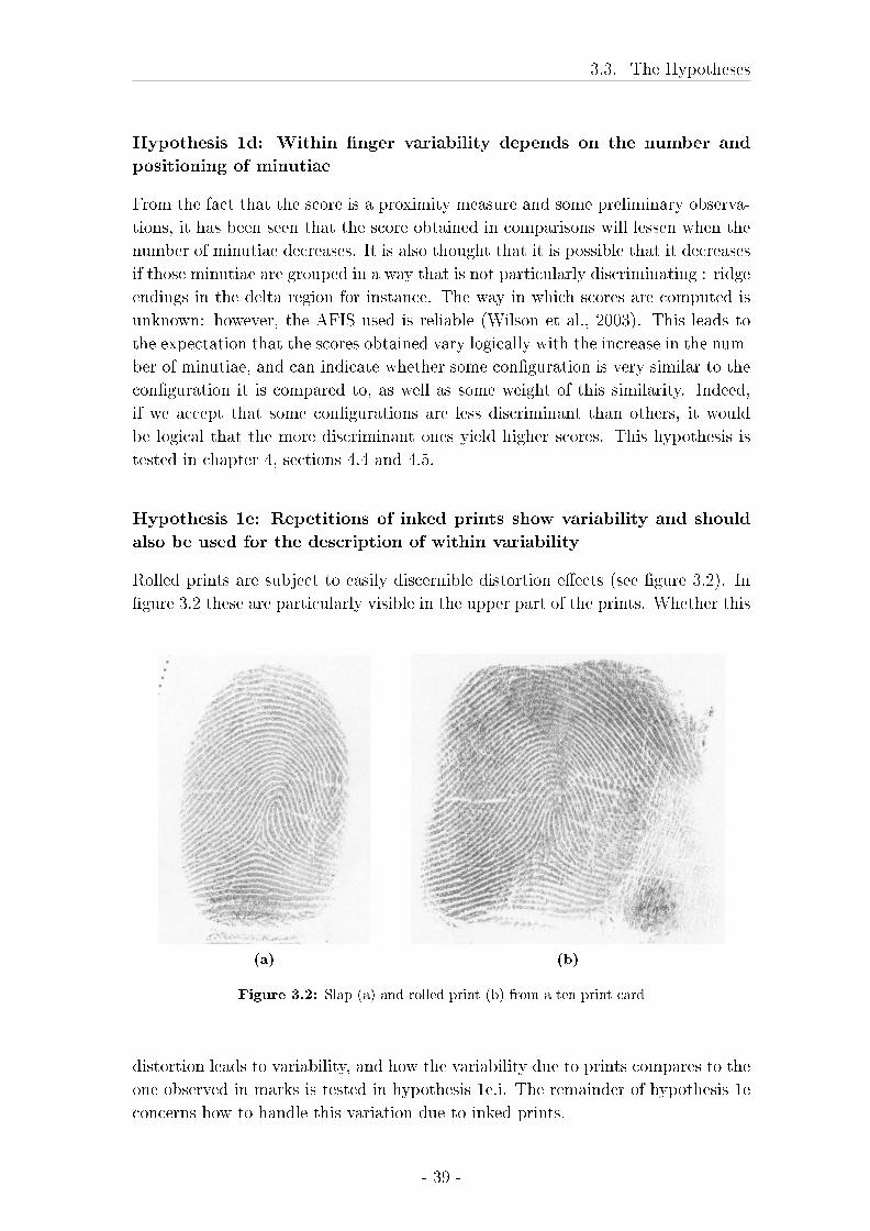
3.3. The Hypotheses
Hypothesis 1d: Within �nger variability depends on the number and
positioning of minutiae
From the fact that the score is a proximity measure and some preliminary observa-
tions, it has been seen that the score obtained in comparisons will lessen when the
number of minutiae decreases. It is also thought that it is possible that it decreases
if those minutiae are grouped in a way that is not particularly discriminating : ridge
endings in the delta region for instance. The way in which scores are computed is
unknown: however, the AFIS used is reliable (Wilson et al., 2003). This leads to
the expectation that the scores obtained vary logically with the increase in the num-
ber of minutiae, and can indicate whether some con�guration is very similar to the
con�guration it is compared to, as well as some weight of this similarity. Indeed,
if we accept that some con�gurations are less discriminant than others, it would
be logical that the more discriminant ones yield higher scores. This hypothesis is
tested in chapter 4, sections 4.4 and 4.5.
Hypothesis 1e: Repetitions of inked prints show variability and should
also be used for the description of within variability
Rolled prints are subject to easily discernible distortion e�ects (see �gure 3.2). In
�gure 3.2 these are particularly visible in the upper part of the prints. Whether this
(a) (b)
Figure 3.2: Slap (a) and rolled print (b) from a ten print card
distortion leads to variability, and how the variability due to prints compares to the
one observed in marks is tested in hypothesis 1e.i. The remainder of hypothesis 1e
concerns how to handle this variation due to inked prints.
- 39 -

Chapter 3. Methodology
Hypothesis 1e.i: Scores issued from the comparison of one mark to sev-
eral rolled inked prints show variation
This hypothesis is tested in section 4.3 of chapter 4. Furthermore, the importance
of this variation is compared between marks and prints. It is important to know not
only whether the prints show variation, but also whether the variance in scores due
to this variation is comparable, smaller or larger than the variance in scores due to
the variability of marks. The remainder of hypothesis 1.e intimately depends on the
results of this �rst hypothesis: if repeated inkings show much less variation than
marks, it is not feasible to decrease the number of marks acquired by using more
prints, nor to compare the number of marks to the same number of prints. These
methods would both arti�cially decrease within-�nger variability, since in this case,
the suspect's inked print could be thought of as being simply a good (and therefore
constant) representation of the �nger surface.
Hypothesis 1e.ii.: the number of marks used can be decreased when the
number of rolled inked prints is increased
It has been determined that variation was present in the rolled inked prints of a
given �nger. It is considered here that if such variation is present, there is no reason
to consider the one inked suspect's print as a given, and that therefore several inked
prints must be used. If this is considered to be true, there are two ways of using
the information obtained from repeated rolled inked prints:
1. Use the same number of marks as determined in the testing of hypothesis 1a,
and compare them to the same number of rolled inked prints, leading to n2
comparisons.
2. Decrease the number of marks used, and obtain n comparisons overall.
The second option is the one tested here. Also, if the increase in the number of
prints used sensibly reduces the variability present in the within-�nger distribution,
it does not seem reasonable to use quite as many inked prints as marks. This
hypothesis is tested in chapter 4, section 4.3.2 on page 81.
Hypothesis 1.e.iii.: marks can be replaced by the same number of slaps
or livescan images
This hypothesis is rather a reformulation of the general hypothesis 1b in view of
the results of hypotheses 1e.i and 1e.ii: it is not self-evident that if these kinds of
impressions could replace the total number of marks, that they can also replace the
potentially reduced number of marks after the non-refusal of hypothesis 1b.i. This
hypothesis is tested in the same section (4.3.2) as hypothesis 1e.ii.
- 40 -
3.3. The Hypotheses
3.3.2 Hypothesis 2: Between �nger variability can be mod-
elled by a generally applicable probability density func-
tion
Hypothesis 2a: The density used for modelling the between �nger vari-
ability becomes stable as a given number of observations is reached
An evaluation of the evolution of the between-variability distribution as the database
for between-variability increases is necessary, since it is thought that above a certain
number of tenprint cards, this density will remain stable, and that this number is
smaller than the database available. Again, and for the same reasons of robustness
as in 1a, it is necessary to reach that stage. If this is not possible, at least the
evolution of the between variability can be monitored. This hypothesis has been
tested in chapter 5, section 5.3.
Hypothesis 2b: Between �nger variability is independent of general pat-
tern and �nger number
The scores obtained when comparing a mark to the database containing only prints
from other �ngers than the one having left the mark may or may not be in�uenced
by the fact of choosing only comparisons from �ngers which show the same general
pattern and / or which are from a �nger with the same number. This hypothesis
will be tested for di�erent regions of the �nger: it is for instance possible that it
cannot be refuted for minutiae arrangements situated in the periphery, but that it
can be refuted for minutiae arrangements from the delta area. Chapter 5, section
5.4 presents the testing of this hypothesis.
Hypothesis 2c: Between �nger variability depends on the number and
placement of minutiae
As in hypothesis 1d for within-�nger variability, it seems reasonable to expect dis-
tributional di�erences between scores obtained for highly discriminant minutiae
con�gurations with respect to con�gurations that are less discriminant. Here, how-
ever, scores are expected to decrease as the minutia number increases or for more
discriminant con�gurations. These hypotheses are tested in section 5.5 of chapter
5.
- 41 -

Chapter 4
Within-Finger Variability
4.1 Introduction
The assessment of within-�nger variability is an important part of this thesis. Fun-
damentally, this chapter will help to address the question whether the distribution
of scores obtained when comparing marks to prints from the same source is general-
izable or not. It will also clarify how within-variability samples should be acquired
be it for such a generalizable distribution or on a case-to-case basis. It is grouped
according to hypotheses, where the samples used for the testing of these hypotheses
as well as the results are presented together. In the cases where one sample has been
used for the testing of several hypotheses, it is described only the �rst time. Sam-
ples are presented �rst by the description of the images. Furthermore, the minutiae
marked on these images are shown and described. Finally, the comparisons used
are de�ned. The �nal sample is the data obtained when comparing the minutia sets
chosen on the images to the comparison prints. Some of the following results have
been the subject of a Master thesis (Egli, 2005), and these will be declared.
4.2 Evaluation of sample size
4.2.1 Material and Methods
Images
It has been tested how many observations are necessary in order to obtain a robust
distribution. For this, livescan images have been used, and this sample size will
determine the number of developed marks to be acquired. Sample size determination
was done in the course of a master thesis (Egli, 2005).
704 images of the right thumb of one female donor have been acquired using a
livescan device (Smiths Heimann Biometrics, ACCO 1394). These images have a
resolution of 500ppi and are in bitmap (.bmp) format.
These 704 images are acquired under four di�erent distortion and pressure con-
ditions. 64 series of 11 images each have been acquired in two di�erent sessions,
- 43 -
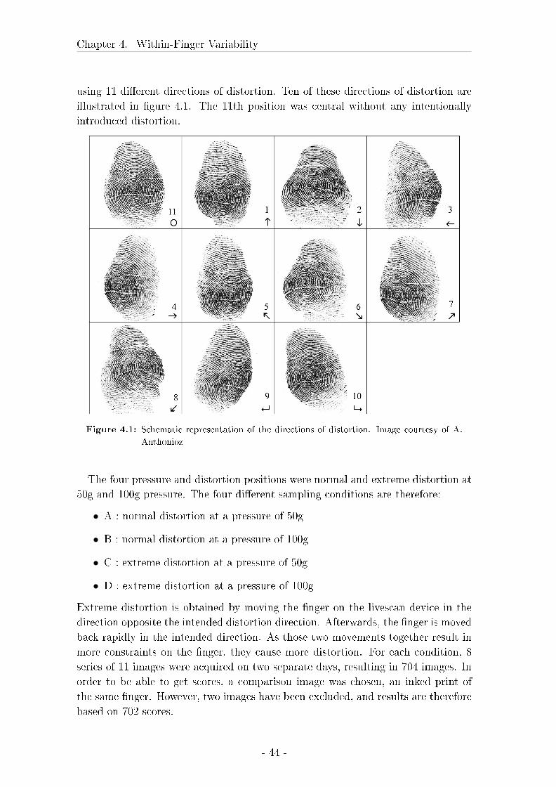
Chapter 4. Within-Finger Variability
using 11 di�erent directions of distortion. Ten of these directions of distortion are
illustrated in �gure 4.1. The 11th position was central without any intentionally
introduced distortion.
Figure 4.1: Schematic representation of the directions of distortion. Image courtesy of A.
Anthonioz
The four pressure and distortion positions were normal and extreme distortion at
50g and 100g pressure. The four di�erent sampling conditions are therefore:
• A : normal distortion at a pressure of 50g
• B : normal distortion at a pressure of 100g
• C : extreme distortion at a pressure of 50g
• D : extreme distortion at a pressure of 100g
Extreme distortion is obtained by moving the �nger on the livescan device in the
direction opposite the intended distortion direction. Afterwards, the �nger is moved
back rapidly in the intended direction. As those two movements together result in
more constraints on the �nger, they cause more distortion. For each condition, 8
series of 11 images were acquired on two separate days, resulting in 704 images. In
order to be able to get scores, a comparison image was chosen, an inked print of
the same �nger. However, two images have been excluded, and results are therefore
based on 702 scores.
- 44 -
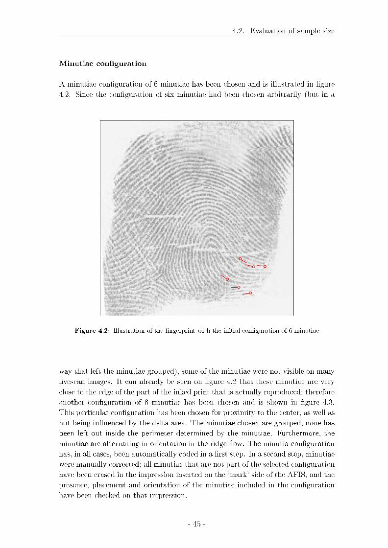
4.2. Evaluation of sample size
Minutiae con�guration
A minutiae con�guration of 6 minutiae has been chosen and is illustrated in �gure
4.2. Since the con�guration of six minutiae had been chosen arbitrarily (but in a
Figure 4.2: Illustration of the �ngerprint with the initial con�guration of 6 minutiae
way that left the minutiae grouped), some of the minutiae were not visible on many
livescan images. It can already be seen on �gure 4.2 that these minutiae are very
close to the edge of the part of the inked print that is actually reproduced; therefore
another con�guration of 6 minutiae has been chosen and is shown in �gure 4.3.
This particular con�guration has been chosen for proximity to the center, as well as
not being in�uenced by the delta area. The minutiae chosen are grouped, none has
been left out inside the perimeter determined by the minutiae. Furthermore, the
minutiae are alternating in orientation in the ridge �ow. The minutia con�guration
has, in all cases, been automatically coded in a �rst step. In a second step, minutiae
were manually corrected; all minutiae that are not part of the selected con�guration
have been erased in the impression inserted on the 'mark' side of the AFIS, and the
presence, placement and orientation of the minutiae included in the con�guration
have been checked on that impression.
- 45 -
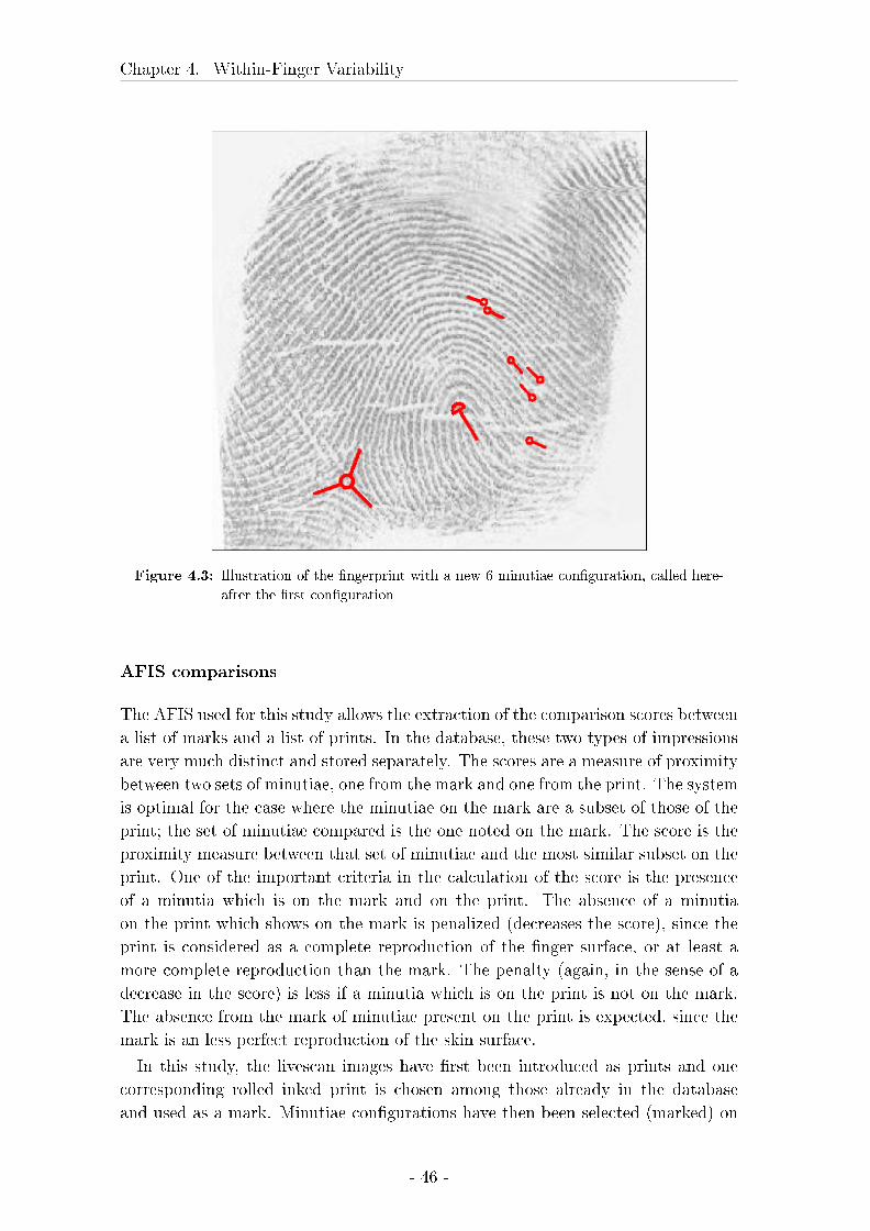
Chapter 4. Within-Finger Variability
Figure 4.3: Illustration of the �ngerprint with a new 6 minutiae con�guration, called here-
after the �rst con�guration
AFIS comparisons
The AFIS used for this study allows the extraction of the comparison scores between
a list of marks and a list of prints. In the database, these two types of impressions
are very much distinct and stored separately. The scores are a measure of proximity
between two sets of minutiae, one from the mark and one from the print. The system
is optimal for the case where the minutiae on the mark are a subset of those of the
print; the set of minutiae compared is the one noted on the mark. The score is the
proximity measure between that set of minutiae and the most similar subset on the
print. One of the important criteria in the calculation of the score is the presence
of a minutia which is on the mark and on the print. The absence of a minutia
on the print which shows on the mark is penalized (decreases the score), since the
print is considered as a complete reproduction of the �nger surface, or at least a
more complete reproduction than the mark. The penalty (again, in the sense of a
decrease in the score) is less if a minutia which is on the print is not on the mark.
The absence from the mark of minutiae present on the print is expected, since the
mark is an less perfect reproduction of the skin surface.
In this study, the livescan images have �rst been introduced as prints and one
corresponding rolled inked print is chosen among those already in the database
and used as a mark. Minutiae con�gurations have then been selected (marked) on
- 46 -
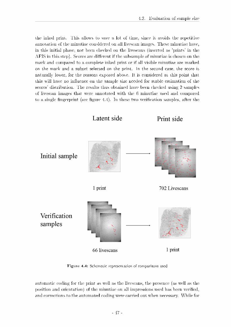
4.2. Evaluation of sample size
the inked print. This allows to save a lot of time, since it avoids the repetitive
annotation of the minutiae considered on all livescan images. These minutiae have,
in this initial phase, not been checked on the livescans (inserted as 'prints' in the
AFIS in this step). Scores are di�erent if the subsample of minutiae is chosen on the
mark and compared to a complete inked print or if all visible minutiae are marked
on the mark and a subset selected on the print. In the second case, the score is
naturally lower, for the reasons exposed above. It is considered at this point that
this will have no in�uence on the sample size needed for stable estimation of the
scores' distribution. The results thus obtained have been checked using 2 samples
of livescan images that were annotated with the 6 minutiae used and compared
to a single �ngerprint (see �gure 4.4). In these two veri�cation samples, after the
Figure 4.4: Schematic representation of comparisons used
automatic coding for the print as well as the livescans, the presence (as well as the
position and orientation) of the minutiae on all impressions used has been veri�ed,
and corrections to the automated coding were carried out when necessary. While for
- 47 -

Chapter 4. Within-Finger Variability
the livescans (inserted as marks into the AFIS in this phase) all minutiae not part of
the selected con�guration have been erased, on the inked print all minutiae found by
the automated extraction are kept; the only two operations carried out on prints are
the addition of minutiae missing among those from the selected con�guration and
the modi�cation of minutiae that are part of this con�guration if their placement
or orientation does not correspond to what would normally be expected.
If a stable distribution is obtained for less than 702 scores, the hypothesis that the
particular number of scores needed is su�cient will be tested by selecting the minu-
tiae set investigated on two subsamples including that number of livescans rather
than the print, and comparing the results on these two subsamples. It is considered
that if those two random samples also show a good correspondence between each
other, the population is considered to be well represented by them.
Quantile-Quantile plots
Quantile-Quantile (QQ-plots) or probability plots (Barnett, 1975; Hyndman and
Fan, 1996) will be largely used for the visual evaluation of �ts between distributions
throughout this thesis. They show the quantiles of the sample against theoretical
quantiles, or the quantile of one sample against the quantiles of another sample.
If F (x) is the cumulative distribution function (which can either be empirical
or a theoretical distribution) and 0 < p < 1, the quantiles of a distribution are
de�ned as Q(p) = F−1(p) = inf{x : F (x) ≥ p}. p is based on the sample of
observations. It is a vector of length n (the sample size), starting at 0.5n
and going
in steps of 1nup to n−0.5
n, where n is the number of observations in the sample. p
may change in function of the programs used, since these are the plotting positions,
and there is no unique rule concerning how these should be chosen. This plot is
therefore a graphical representation of the samples' observations against either the
theoretical quantiles of the chosen function or of the sample quantiles of two samples.
Deviations from a straight line indicate a bad �t be of the observed to the theoretical
distribution, or between the distributions of the two compared samples. When two
samples are plotted against each other, the values plotted are the corresponding
percentiles of the samples (in Matlab R©, the percentiles are again derived from p.
In this case of comparison between two empirical samples rather than between a
sample distribution and a theoretical distribution, the number of observations n
used is the one in the smaller sample). The theoretical quantiles for the Weibull
distribution are Q̂(p) = log( 11−p
).
- 48 -
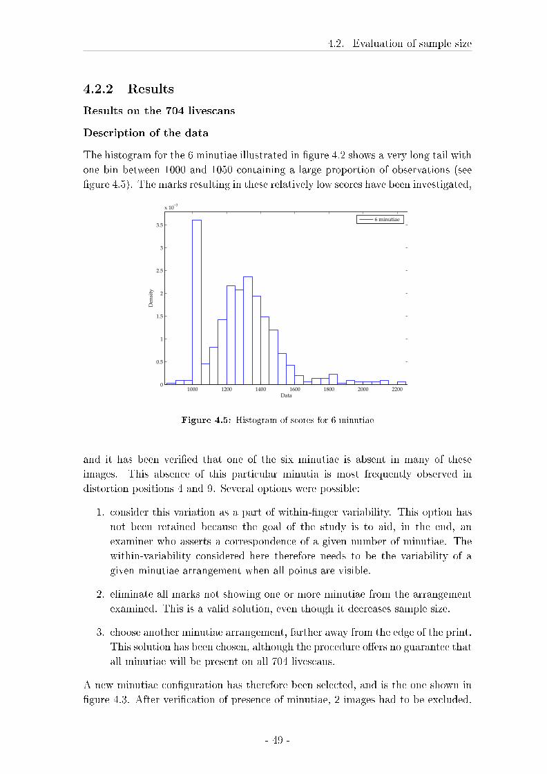
4.2. Evaluation of sample size
4.2.2 Results
Results on the 704 livescans
Description of the data
The histogram for the 6 minutiae illustrated in �gure 4.2 shows a very long tail with
one bin between 1000 and 1050 containing a large proportion of observations (see
�gure 4.5). The marks resulting in these relatively low scores have been investigated,
1000 1200 1400 1600 1800 2000 22000
0.5
1
1.5
2
2.5
3
3.5
x 10−3
Data
Den
sity
6 minutiae
Figure 4.5: Histogram of scores for 6 minutiae
and it has been veri�ed that one of the six minutiae is absent in many of these
images. This absence of this particular minutia is most frequently observed in
distortion positions 4 and 9. Several options were possible:
1. consider this variation as a part of within-�nger variability. This option has
not been retained because the goal of the study is to aid, in the end, an
examiner who asserts a correspondence of a given number of minutiae. The
within-variability considered here therefore needs to be the variability of a
given minutiae arrangement when all points are visible.
2. eliminate all marks not showing one or more minutiae from the arrangement
examined. This is a valid solution, even though it decreases sample size.
3. choose another minutiae arrangement, farther away from the edge of the print.
This solution has been chosen, although the procedure o�ers no guarantee that
all minutiae will be present on all 704 livescans.
A new minutiae con�guration has therefore been selected, and is the one shown in
�gure 4.3. After veri�cation of presence of minutiae, 2 images had to be excluded.
- 49 -
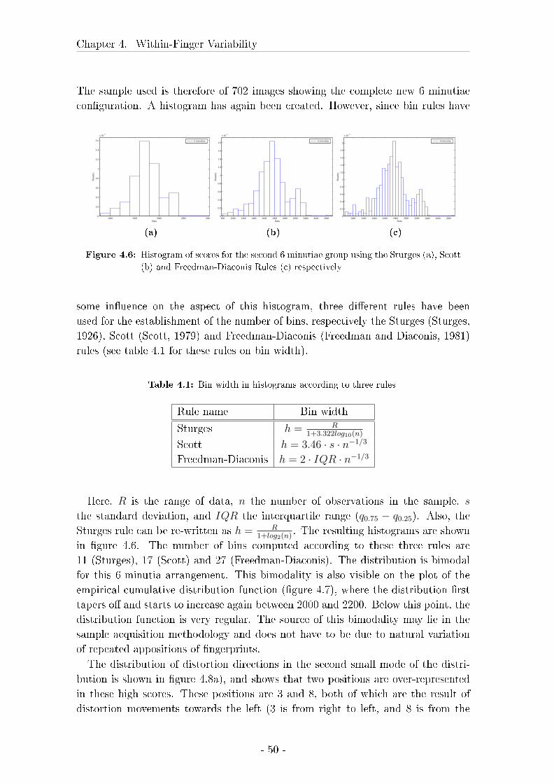
Chapter 4. Within-Finger Variability
The sample used is therefore of 702 images showing the complete new 6 minutiae
con�guration. A histogram has again been created. However, since bin rules have
1000 1500 2000 2500 30000
0.2
0.4
0.6
0.8
1
1.2
1.4
1.6
x 10−3
Data
Den
sity
6 minutiae
(a)
800 1000 1200 1400 1600 1800 2000 2200 2400 2600 28000
0.2
0.4
0.6
0.8
1
1.2
1.4
1.6
1.8
x 10−3
Data
Den
sity
6 minutiae
(b)
1000 1200 1400 1600 1800 2000 2200 2400 2600 28000
0.2
0.4
0.6
0.8
1
1.2
1.4
1.6
1.8
2
x 10−3
Data
Den
sity
6 minutiae
(c)
Figure 4.6: Histogram of scores for the second 6 minutiae group using the Sturges (a), Scott
(b) and Freedman-Diaconis Rules (c) respectively
some in�uence on the aspect of this histogram, three di�erent rules have been
used for the establishment of the number of bins, respectively the Sturges (Sturges,
1926), Scott (Scott, 1979) and Freedman-Diaconis (Freedman and Diaconis, 1981)
rules (see table 4.1 for these rules on bin width).
Table 4.1: Bin width in histograms according to three rules
Rule name Bin width
Sturges h = R1+3.322log10(n)
Scott h = 3.46 · s · n−1/3
Freedman-Diaconis h = 2 · IQR · n−1/3
Here, R is the range of data, n the number of observations in the sample, s
the standard deviation, and IQR the interquartile range (q0.75 − q0.25). Also, the
Sturges rule can be re-written as h = R1+log2(n)
. The resulting histograms are shown
in �gure 4.6. The number of bins computed according to these three rules are
11 (Sturges), 17 (Scott) and 27 (Freedman-Diaconis). The distribution is bimodal
for this 6-minutia arrangement. This bimodality is also visible on the plot of the
empirical cumulative distribution function (�gure 4.7), where the distribution �rst
tapers o� and starts to increase again between 2000 and 2200. Below this point, the
distribution function is very regular. The source of this bimodality may lie in the
sample acquisition methodology and does not have to be due to natural variation
of repeated appositions of �ngerprints.
The distribution of distortion directions in the second small mode of the distri-
bution is shown in �gure 4.8a), and shows that two positions are over-represented
in these high scores. These positions are 3 and 8, both of which are the result of
distortion movements towards the left (3 is from right to left, and 8 is from the
- 50 -
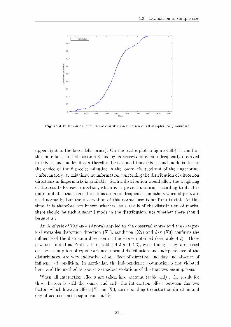
4.2. Evaluation of sample size
1000 1200 1400 1600 1800 2000 2200 2400 2600 28000
0.1
0.2
0.3
0.4
0.5
0.6
0.7
0.8
0.9
1
Data
Cu
mu
lati
ve
pro
bab
ilit
y
6 minutiae
Figure 4.7: Empirical cumulative distribution function of all samples for 6 minutiae
upper right to the lower left corner). On the scatterplot in �gure 4.8b), it can fur-
thermore be seen that position 8 has higher scores and is more frequently observed
in this second mode: it can therefore be assumed that this second mode is due to
the choice of the 6 precise minutiae in the lower left quadrant of the �ngerprint.
Unfortunately, at this time, no information concerning the distribution of distortion
directions in �ngermarks is available. Such a distribution would allow the weighting
of the results for each direction, which is at present uniform, according to it. It is
quite probable that some directions are more frequent than others when objects are
used normally, but the observation of this normal use is far from trivial. At this
time, it is therefore not known whether, as a result of the distribution of marks,
there should be such a second mode in the distribution, nor whether there should
be several.
An Analysis of Variance (Anova) applied to the observed scores and the categor-
ical variables distortion direction (X1), condition (X2) and day (X3) con�rms the
in�uence of the distortion direction on the scores obtained (see table 4.2). These
p-values (noted as Prob > F in tables 4.2 and 4.3), even though they are based
on the assumption of equal variance, normal distribution and independence of the
disturbances, are very indicative of an e�ect of direction and day and absence of
in�uence of condition. In particular, the independence assumption is not violated
here, and the method is robust to modest violations of the �rst two assumptions.
When all interaction e�ects are taken into account (table 4.3) , the result for
those factors is still the same, and only the interaction e�ect between the two
factors which have an e�ect (X1 and X3, corresponding to distortion direction and
day of acquisition) is signi�cant at 5%.
- 51 -
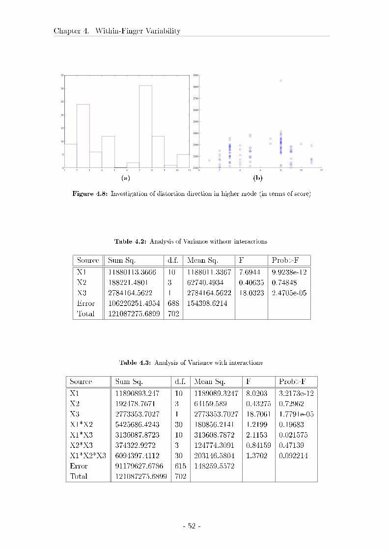
Chapter 4. Within-Finger Variability
1 2 3 4 5 6 7 8 9 10 110
5
10
15
20
25
30
35
(a)
0 2 4 6 8 10 122100
2200
2300
2400
2500
2600
2700
2800
2900
(b)
Figure 4.8: Investigation of distortion direction in higher mode (in terms of score)
Table 4.2: Analysis of Variance without interactions
Source Sum Sq. d.f. Mean Sq. F Prob>F
X1 11880113.3666 10 1188011.3367 7.6944 9.9238e-12
X2 188221.4801 3 62740.4934 0.40635 0.74848
X3 2784164.5622 1 2784164.5622 18.0323 2.4705e-05
Error 106226251.4954 688 154398.6214
Total 121087275.6899 702
Table 4.3: Analysis of Variance with interactions
Source Sum Sq. d.f. Mean Sq. F Prob>F
X1 11890893.247 10 1189089.3247 8.0203 3.2173e-12
X2 192478.7671 3 64159.589 0.43275 0.72962
X3 2773353.7027 1 2773353.7027 18.7061 1.7791e-05
X1*X2 5425686.4243 30 180856.2141 1.2199 0.19683
X1*X3 3136087.8723 10 313608.7872 2.1153 0.021575
X2*X3 374322.9272 3 124774.3091 0.84159 0.47139
X1*X2*X3 6094397.4112 30 203146.5804 1.3702 0.092214
Error 91179627.6786 615 148259.5572
Total 121087275.6899 702
- 52 -
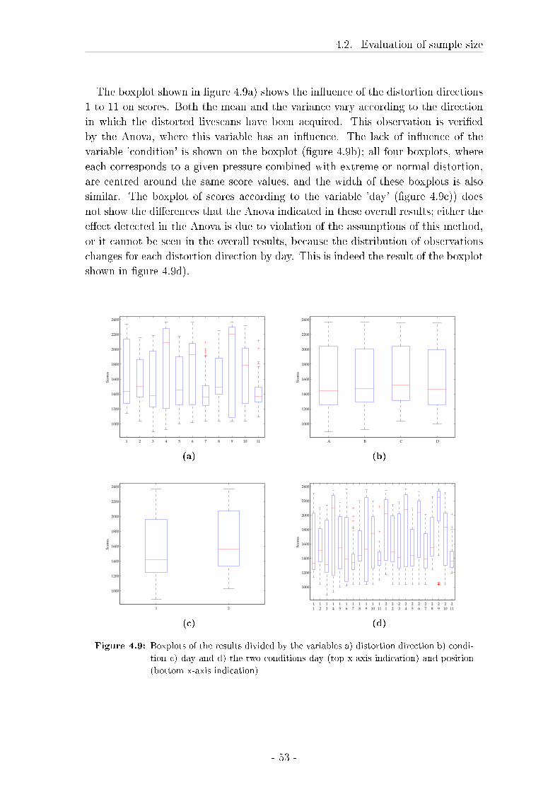
4.2. Evaluation of sample size
The boxplot shown in �gure 4.9a) shows the in�uence of the distortion directions
1 to 11 on scores. Both the mean and the variance vary according to the direction
in which the distorted livescans have been acquired. This observation is veri�ed
by the Anova, where this variable has an in�uence. The lack of in�uence of the
variable 'condition' is shown on the boxplot (�gure 4.9b); all four boxplots, where
each corresponds to a given pressure combined with extreme or normal distortion,
are centred around the same score values, and the width of these boxplots is also
similar. The boxplot of scores according to the variable 'day' (�gure 4.9c)) does
not show the di�erences that the Anova indicated in these overall results; either the
e�ect detected in the Anova is due to violation of the assumptions of this method,
or it cannot be seen in the overall results, because the distribution of observations
changes for each distortion direction by day. This is indeed the result of the boxplot
shown in �gure 4.9d).
1000
1200
1400
1600
1800
2000
2200
2400
Sco
res
1 2 3 4 5 6 7 8 9 10 11
(a)
1000
1200
1400
1600
1800
2000
2200
2400
Sco
res
A B C D
(b)
1000
1200
1400
1600
1800
2000
2200
2400
Sco
res
1 2
(c)
1000
1200
1400
1600
1800
2000
2200
2400
Sco
res
1
1
1
2
1
3
1
4
1
5
1
6
1
7
1
8
1
9
1
10
1
11
2
1
2
2
2
3
2
4
2
5
2
6
2
7
2
8
2
9
2
10
2
11
(d)
Figure 4.9: Boxplots of the results divided by the variables a) distortion direction b) condi-
tion c) day and d) the two conditions day (top x-axis indication) and position
(bottom x-axis indication)
- 53 -
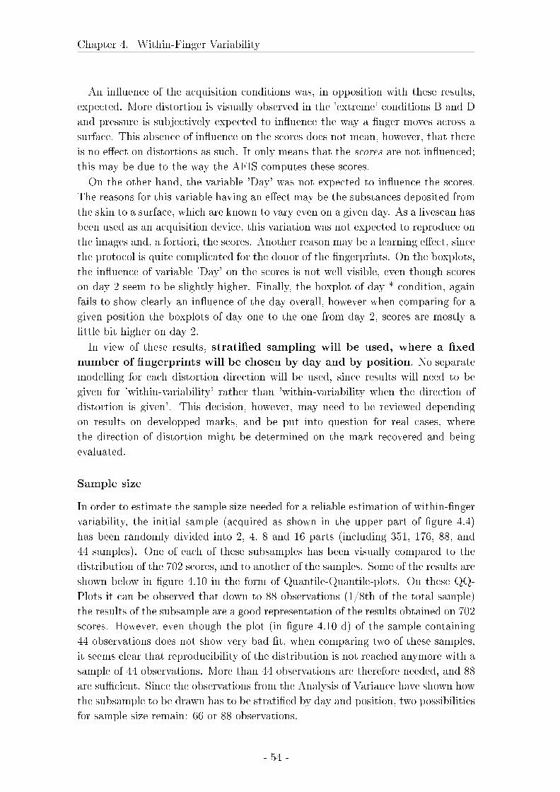
Chapter 4. Within-Finger Variability
An in�uence of the acquisition conditions was, in opposition with these results,
expected. More distortion is visually observed in the 'extreme' conditions B and D
and pressure is subjectively expected to in�uence the way a �nger moves across a
surface. This absence of in�uence on the scores does not mean, however, that there
is no e�ect on distortions as such. It only means that the scores are not in�uenced;
this may be due to the way the AFIS computes these scores.
On the other hand, the variable 'Day' was not expected to in�uence the scores.
The reasons for this variable having an e�ect may be the substances deposited from
the skin to a surface, which are known to vary even on a given day. As a livescan has
been used as an acquisition device, this variation was not expected to reproduce on
the images and, a fortiori, the scores. Another reason may be a learning e�ect, since
the protocol is quite complicated for the donor of the �ngerprints. On the boxplots,
the in�uence of variable 'Day' on the scores is not well visible, even though scores
on day 2 seem to be slightly higher. Finally, the boxplot of day * condition, again
fails to show clearly an in�uence of the day overall, however when comparing for a
given position the boxplots of day one to the one from day 2, scores are mostly a
little bit higher on day 2.
In view of these results, strati�ed sampling will be used, where a �xed
number of �ngerprints will be chosen by day and by position. No separate
modelling for each distortion direction will be used, since results will need to be
given for 'within-variability' rather than 'within-variability when the direction of
distortion is given'. This decision, however, may need to be reviewed depending
on results on developped marks, and be put into question for real cases, where
the direction of distortion might be determined on the mark recovered and being
evaluated.
Sample size
In order to estimate the sample size needed for a reliable estimation of within-�nger
variability, the initial sample (acquired as shown in the upper part of �gure 4.4)
has been randomly divided into 2, 4, 8 and 16 parts (including 351, 176, 88, and
44 samples). One of each of these subsamples has been visually compared to the
distribution of the 702 scores, and to another of the samples. Some of the results are
shown below in �gure 4.10 in the form of Quantile-Quantile-plots. On these QQ-
Plots it can be observed that down to 88 observations (1/8th of the total sample)
the results of the subsample are a good representation of the results obtained on 702
scores. However, even though the plot (in �gure 4.10 d) of the sample containing
44 observations does not show very bad �t, when comparing two of these samples,
it seems clear that reproducibility of the distribution is not reached anymore with a
sample of 44 observations. More than 44 observations are therefore needed, and 88
are su�cient. Since the observations from the Analysis of Variance have shown how
the subsample to be drawn has to be strati�ed by day and position, two possibilities
for sample size remain: 66 or 88 observations.
- 54 -
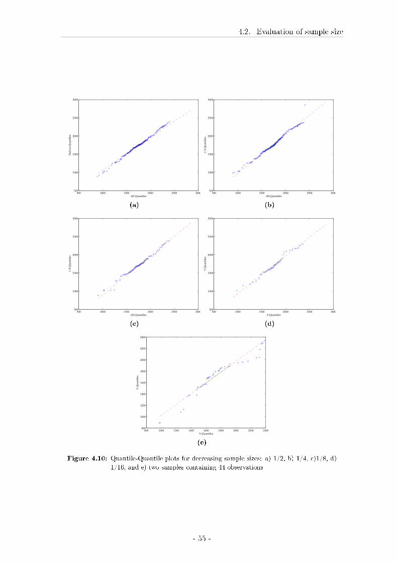
4.2. Evaluation of sample size
500 1000 1500 2000 2500 3000500
1000
1500
2000
2500
3000
All Quantiles
Halv
es
Qu
an
tile
s
(a)
500 1000 1500 2000 2500 3000500
1000
1500
2000
2500
3000
All Quantiles
1/
4 Q
uan
tile
s(b)
500 1000 1500 2000 2500 3000500
1000
1500
2000
2500
3000
All Quantiles
1/
8 Q
uan
tile
s
(c)
500 1000 1500 2000 2500 3000500
1000
1500
2000
2500
3000
X Quantiles
Y Q
uan
tile
s
(d)
800 1000 1200 1400 1600 1800 2000 2200 2400800
1000
1200
1400
1600
1800
2000
2200
2400
X Quantiles
Y Q
uan
tile
s
(e)
Figure 4.10: Quantile-Quantile plots for decreasing sample sizes: a) 1/2, b) 1/4, c)1/8, d)
1/16, and e) two samples containing 44 observations
- 55 -
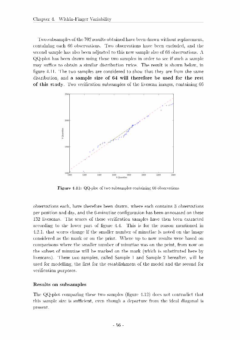
Chapter 4. Within-Finger Variability
Two subsamples of the 702 results obtained have been drawn without replacement,
containing each 66 observations. Two observations have been excluded, and the
second sample has also been adjusted to this new sample size of 66 observations. A
QQ-plot has been drawn using these two samples in order to see if such a sample
may su�ce to obtain a similar distribution twice. The result is shown below, in
�gure 4.11. The two samples are considered to show that they are from the same
distribution, and a sample size of 64 will therefore be used for the rest
of this study. Two veri�cation subsamples of the livescan images, containing 66
1000 1200 1400 1600 1800 2000 2200 24001000
1500
2000
2500
X Quantiles
Y Q
uan
tile
s
Figure 4.11: QQ-plot of two subsamples containing 66 observations
observations each, have therefore been drawn, where each contains 3 observations
per position and day, and the 6-minutiae con�guration has been annotated on these
132 livescans. The scores of these veri�cation samples have then been extracted
according to the lower part of �gure 4.4. This is for the reason mentioned in
4.2.1, that scores change if the smaller number of minutiae is noted on the image
considered as the mark or on the print. Where up to now results were based on
comparisons where the smaller number of minutiae was on the print, from now on
the subset of minutiae will be marked on the mark (which is substituted here by
livescans). These two samples, called Sample 1 and Sample 2 hereafter, will be
used for modelling, the �rst for the establishment of the model and the second for
veri�cation purposes.
Results on subsamples
The QQ-plot comparing these two samples (�gure 4.12) does not contradict that
this sample size is su�cient, even though a departure from the ideal diagonal is
present.
- 56 -
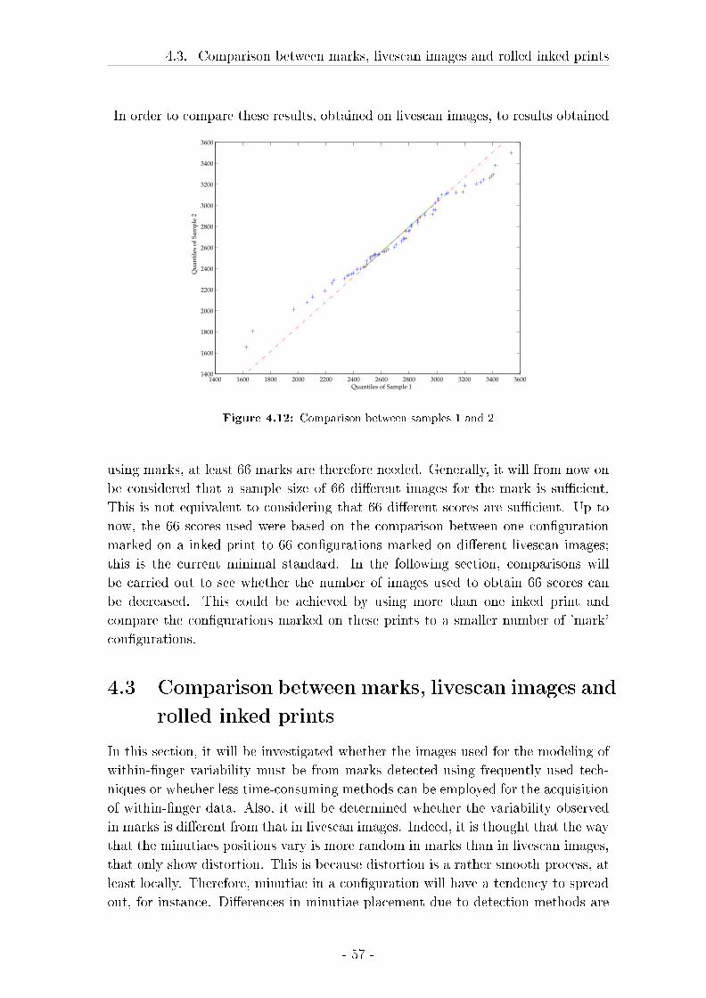
4.3. Comparison between marks, livescan images and rolled inked prints
In order to compare these results, obtained on livescan images, to results obtained
1400 1600 1800 2000 2200 2400 2600 2800 3000 3200 3400 36001400
1600
1800
2000
2200
2400
2600
2800
3000
3200
3400
3600
Quantiles of Sample 1
Qu
anti
les
of
Sam
ple
2
Figure 4.12: Comparison between samples 1 and 2
using marks, at least 66 marks are therefore needed. Generally, it will from now on
be considered that a sample size of 66 di�erent images for the mark is su�cient.
This is not equivalent to considering that 66 di�erent scores are su�cient. Up to
now, the 66 scores used were based on the comparison between one con�guration
marked on a inked print to 66 con�gurations marked on di�erent livescan images;
this is the current minimal standard. In the following section, comparisons will
be carried out to see whether the number of images used to obtain 66 scores can
be decreased. This could be achieved by using more than one inked print and
compare the con�gurations marked on these prints to a smaller number of 'mark'
con�gurations.
4.3 Comparison between marks, livescan images and
rolled inked prints
In this section, it will be investigated whether the images used for the modeling of
within-�nger variability must be from marks detected using frequently used tech-
niques or whether less time-consuming methods can be employed for the acquisition
of within-�nger data. Also, it will be determined whether the variability observed
in marks is di�erent from that in livescan images. Indeed, it is thought that the way
that the minutiaes positions vary is more random in marks than in livescan images,
that only show distortion. This is because distortion is a rather smooth process, at
least locally. Therefore, minutiae in a con�guration will have a tendency to spread
out, for instance. Di�erences in minutiae placement due to detection methods are
- 57 -
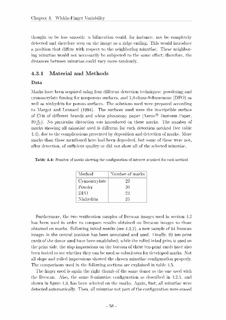
Chapter 4. Within-Finger Variability
thought to be less smooth: a bifurcation could, for instance, not be completely
detected and therefore seen on the image as a ridge ending. This would introduce
a position that di�ers with respect to the neighboring minutiae. These neighbor-
ing minutiae would not necessarily be subjected to the same e�ect; therefore, the
distances between minutiae could vary more randomly.
4.3.1 Material and Methods
Data
Marks have been acquired using four di�erent detection techniques: powdering and
cyanoacrylate fuming for nonporous surfaces, and 1,8-diaza-9-�uorenone (DFO) as
well as ninhydrin for porous surfaces. The solutions used were prepared according
to Margot and Lennard (1994). The surfaces used were the inscriptible surface
of CDs of di�erent brands and white photocopy paper (Xerox R© Business Paper,
80 gm2 ). No particular distortion was introduced on these marks. The number of
marks showing all minutiae used is di�erent for each detection method (see table
4.4), due to the complications presented by deposition and detection of marks. More
marks than those mentioned here had been deposited, but some of these were not,
after detection, of su�cient quality or did not show all of the selected minutiae.
Table 4.4: Number of marks showing the con�guration of interest acquired for each method
Method Number of marks
Cyanoacrylate 29
Powder 30
DFO 24
Ninhydrin 25
Furthermore, the two veri�cation samples of livescan images used in section 4.2
has been used in order to compare results obtained on livescan images to those
obtained on marks. Following initial results (see 4.3.2), a new sample of 64 livescan
images in the central position has been annotated and used. Finally, 80 ten-print
cards of the donor used have been established; while the rolled inked print is used on
the print side, the slap impressions on the bottom of these ten-print cards have also
been tested to see whether they can be used as substitutes for developed marks. Not
all slaps and rolled impressions showed the chosen minutiae con�guration properly.
The comparisons used in the following sections are explained in table 4.5.
The �nger used is again the right thumb of the same donor as the one used with
the livescan. Also, the same 6-minutiae con�guration as described in 4.2.1, and
shown in �gure 4.3, has been selected on the marks. Again, �rst, all minutiae were
detected automatically. Then, all minutiae not part of the con�guration were erased
- 58 -
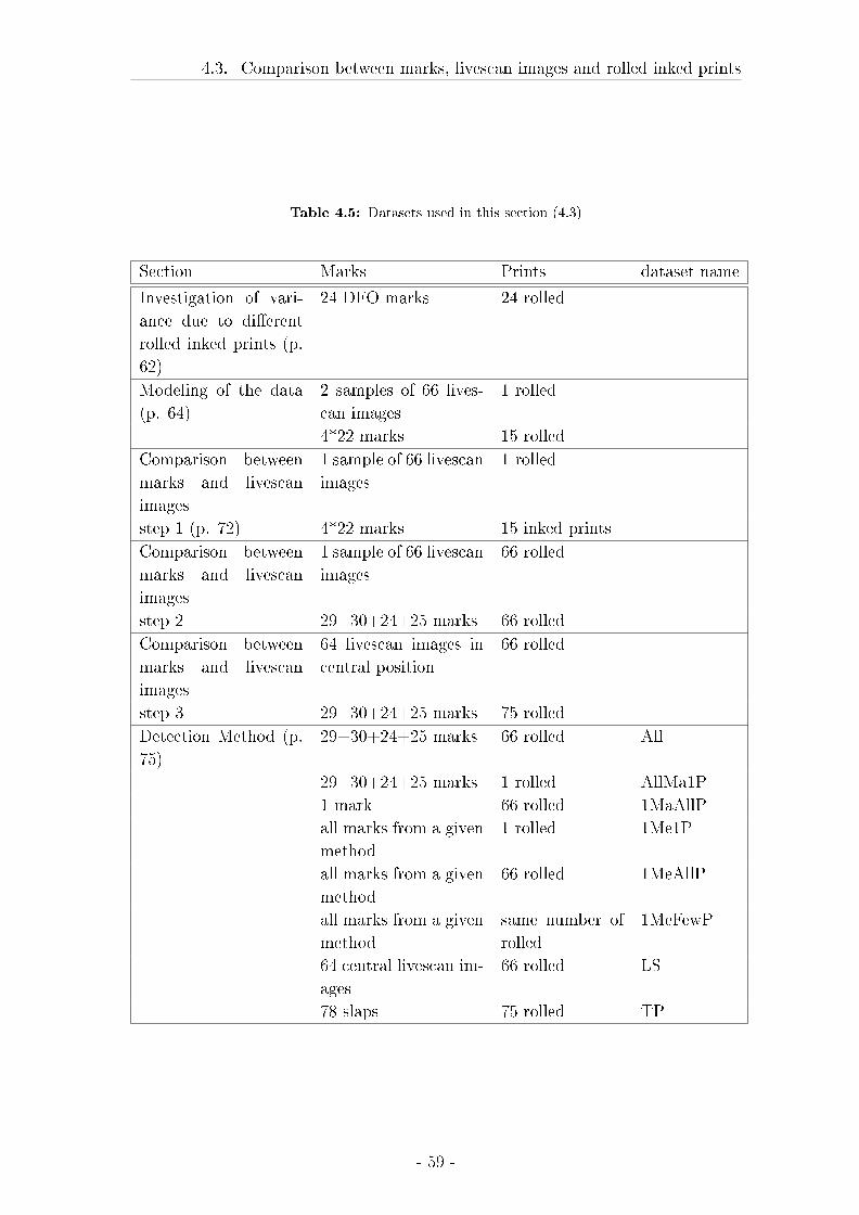
4.3. Comparison between marks, livescan images and rolled inked prints
Table 4.5: Datasets used in this section (4.3)
Section Marks Prints dataset name
Investigation of vari-
ance due to di�erent
rolled inked prints (p.
62)
24 DFO marks 24 rolled
Modeling of the data
(p. 64)
2 samples of 66 lives-
can images
1 rolled
4*22 marks 15 rolled
Comparison between
marks and livescan
images
1 sample of 66 livescan
images
1 rolled
step 1 (p. 72) 4*22 marks 15 inked prints
Comparison between
marks and livescan
images
1 sample of 66 livescan
images
66 rolled
step 2 29+30+24+25 marks 66 rolled
Comparison between
marks and livescan
images
64 livescan images in
central position
66 rolled
step 3 29+30+24+25 marks 75 rolled
Detection Method (p.
75)
29+30+24+25 marks 66 rolled All
29+30+24+25 marks 1 rolled AllMa1P
1 mark 66 rolled 1MaAllP
all marks from a given
method
1 rolled 1Me1P
all marks from a given
method
66 rolled 1MeAllP
all marks from a given
method
same number of
rolled
1MeFewP
64 central livescan im-
ages
66 rolled LS
78 slaps 75 rolled TP
- 59 -
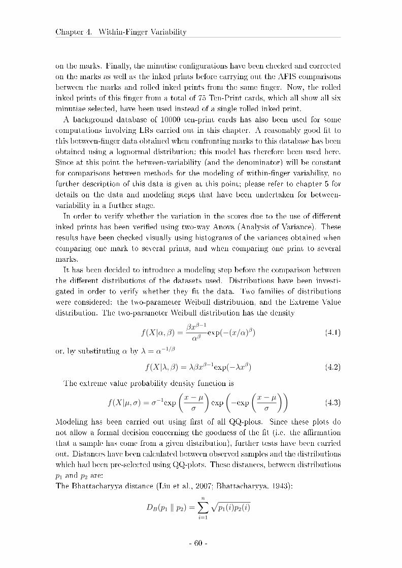
Chapter 4. Within-Finger Variability
on the marks. Finally, the minutiae con�gurations have been checked and corrected
on the marks as well as the inked prints before carrying out the AFIS comparisons
between the marks and rolled inked prints from the same �nger. Now, the rolled
inked prints of this �nger from a total of 75 Ten-Print cards, which all show all six
minutiae selected, have been used instead of a single rolled inked print.
A background database of 10000 ten-print cards has also been used for some
computations involving LRs carried out in this chapter. A reasonably good �t to
this between-�nger data obtained when confronting marks to this database has been
obtained using a lognormal distribution; this model has therefore been used here.
Since at this point the between-variability (and the denominator) will be constant
for comparisons between methods for the modeling of within-�nger variability, no
further description of this data is given at this point; please refer to chapter 5 for
details on the data and modeling steps that have been undertaken for between-
variability in a further stage.
In order to verify whether the variation in the scores due to the use of di�erent
inked prints has been veri�ed using two-way Anova (Analysis of Variance). These
results have been checked visually using histograms of the variances obtained when
comparing one mark to several prints, and when comparing one print to several
marks.
It has been decided to introduce a modeling step before the comparison between
the di�erent distributions of the datasets used. Distributions have been investi-
gated in order to verify whether they �t the data. Two families of distributions
were considered: the two-parameter Weibull distribution, and the Extreme Value
distribution. The two-parameter Weibull distribution has the density
f(X|α, β) =βxβ−1
αβexp(−(x/α)β) (4.1)
or, by substituting α by λ = α−1/β
f(X|λ, β) = λβxβ−1exp(−λxβ) (4.2)
The extreme value probability density function is
f(X|µ, σ) = σ−1exp
(x− µ
σ
)exp
(−exp
(x− µ
σ
))(4.3)
Modeling has been carried out using �rst of all QQ-plots. Since these plots do
not allow a formal decision concerning the goodness of the �t (i.e. the a�rmation
that a sample has come from a given distribution), further tests have been carried
out. Distances have been calculated between observed samples and the distributions
which had been pre-selected using QQ-plots. These distances, between distributions
p1 and p2 are:
The Bhattacharyya distance (Liu et al., 2007; Bhattacharyya, 1943):
DB(p1 ‖ p2) =n∑
i=1
√p1(i)p2(i)
- 60 -
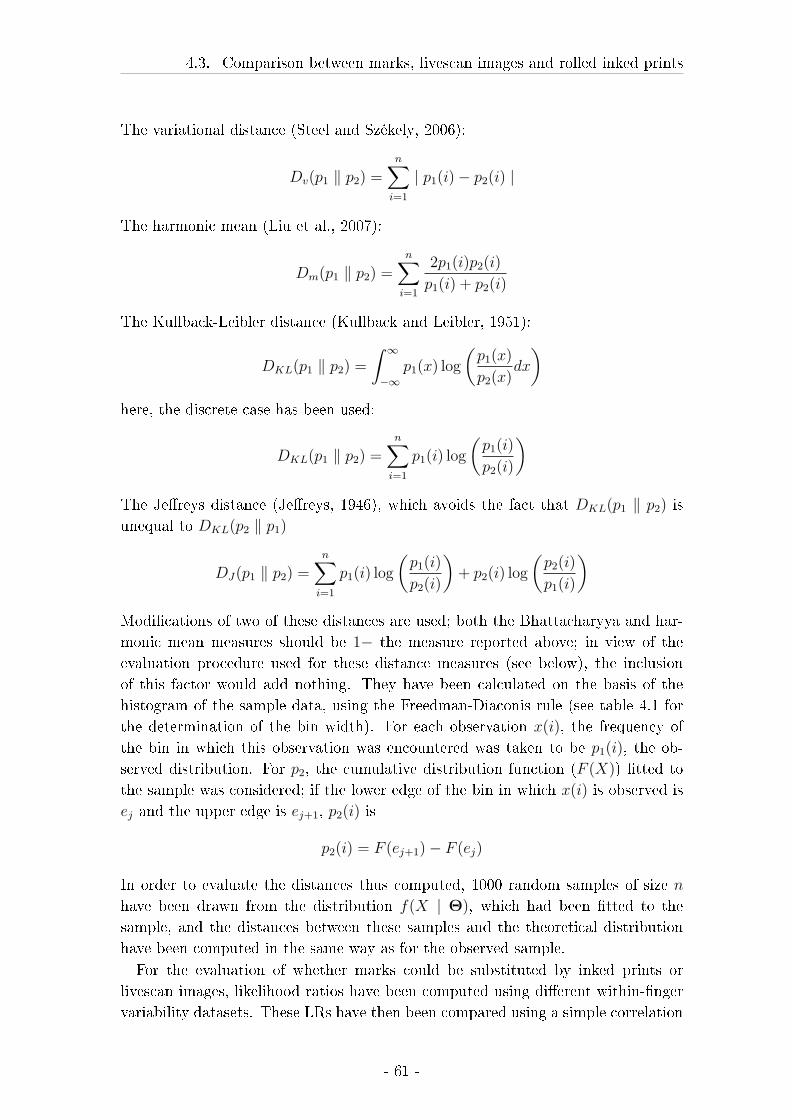
4.3. Comparison between marks, livescan images and rolled inked prints
The variational distance (Steel and Székely, 2006):
Dv(p1 ‖ p2) =n∑
i=1
| p1(i)− p2(i) |
The harmonic mean (Liu et al., 2007):
Dm(p1 ‖ p2) =n∑
i=1
2p1(i)p2(i)
p1(i) + p2(i)
The Kullback-Leibler distance (Kullback and Leibler, 1951):
DKL(p1 ‖ p2) =
∫ ∞
−∞p1(x) log
(p1(x)
p2(x)dx
)here, the discrete case has been used:
DKL(p1 ‖ p2) =n∑
i=1
p1(i) log
(p1(i)
p2(i)
)The Je�reys distance (Je�reys, 1946), which avoids the fact that DKL(p1 ‖ p2) is
unequal to DKL(p2 ‖ p1)
DJ(p1 ‖ p2) =n∑
i=1
p1(i) log
(p1(i)
p2(i)
)+ p2(i) log
(p2(i)
p1(i)
)Modi�cations of two of these distances are used; both the Bhattacharyya and har-
monic mean measures should be 1− the measure reported above; in view of the
evaluation procedure used for these distance measures (see below), the inclusion
of this factor would add nothing. They have been calculated on the basis of the
histogram of the sample data, using the Freedman-Diaconis rule (see table 4.1 for
the determination of the bin width). For each observation x(i), the frequency of
the bin in which this observation was encountered was taken to be p1(i), the ob-
served distribution. For p2, the cumulative distribution function (F (X)) �tted to
the sample was considered; if the lower edge of the bin in which x(i) is observed is
ej and the upper edge is ej+1, p2(i) is
p2(i) = F (ej+1)− F (ej)
In order to evaluate the distances thus computed, 1000 random samples of size n
have been drawn from the distribution f(X | Θ), which had been �tted to the
sample, and the distances between these samples and the theoretical distribution
have been computed in the same way as for the observed sample.
For the evaluation of whether marks could be substituted by inked prints or
livescan images, likelihood ratios have been computed using di�erent within-�nger
variability datasets. These LRs have then been compared using a simple correlation
- 61 -
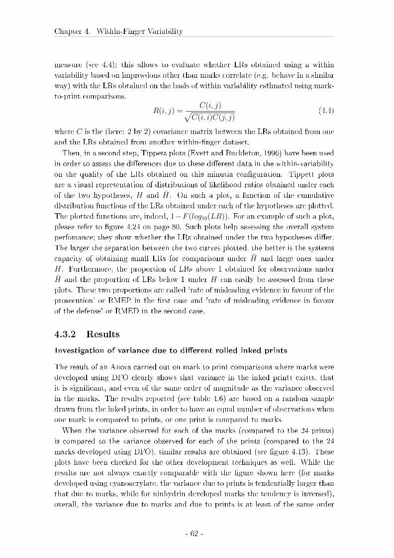
Chapter 4. Within-Finger Variability
measure (see 4.4); this allows to evaluate whether LRs obtained using a within
variability based on impressions other than marks correlate (e.g. behave in a similar
way) with the LRs obtained on the basis of within variability estimated using mark-
to-print comparisons.
R(i, j) =C(i, j)√
C(i, i)C(j, j)(4.4)
where C is the (here: 2 by 2) covariance matrix between the LRs obtained from one
and the LRs obtained from another within-�nger dataset.
Then, in a second step, Tippett plots (Evett and Buckleton, 1996) have been used
in order to assess the di�erences due to these di�erent data in the within-variability
on the quality of the LRs obtained on this minutia con�guration. Tippett plots
are a visual representation of distributions of likelihood ratios obtained under each
of the two hypotheses, H and H̄. On such a plot, a function of the cumulative
distribution functions of the LRs obtained under each of the hypotheses are plotted.
The plotted functions are, indeed, 1−F (log10(LR)). For an example of such a plot,
please refer to �gure 4.24 on page 80. Such plots help assessing the overall system
perfomance; they show whether the LRs obtained under the two hypotheses di�er.
The larger the separation between the two curves plotted, the better is the systems
capacity of obtaining small LRs for comparisons under H̄ and large ones under
H. Furthermore, the proportion of LRs above 1 obtained for observations under
H̄ and the proportion of LRs below 1 under H can easily be assessed from these
plots. These two proportions are called 'rate of misleading evidence in favour of the
prosecution' or RMEP in the �rst case and 'rate of misleading evidence in favour
of the defense' or RMED in the second case.
4.3.2 Results
Investigation of variance due to di�erent rolled inked prints
The result of an Anova carried out on mark to print comparisons where marks were
developed using DFO clearly shows that variance in the inked prints exists, that
it is signi�cant, and even of the same order of magnitude as the variance observed
in the marks. The results reported (see table 4.6) are based on a random sample
drawn from the inked prints, in order to have an equal number of observations when
one mark is compared to prints, or one print is compared to marks.
When the variance observed for each of the marks (compared to the 24 prints)
is compared to the variance observed for each of the prints (compared to the 24
marks developed using DFO), similar results are obtained (see �gure 4.13). These
plots have been checked for the other development techniques as well. While the
results are not always exactly comparable with the �gure shown here (for marks
developed using cyanoacrylate, the variance due to prints is tendentially larger than
that due to marks, while for ninhydrin developed marks the tendency is inversed),
overall, the variance due to marks and due to prints is at least of the same order
- 62 -
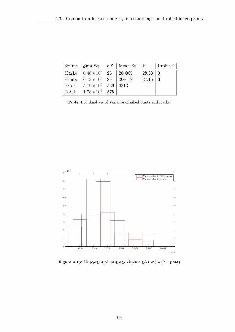
4.3. Comparison between marks, livescan images and rolled inked prints
Source Sum Sq. d.f. Mean Sq. F Prob>F
Marks 6.46 ∗ 106 23 280909 28.63 0
Prints 6.13 ∗ 106 23 266412 27.15 0
Error 5.19 ∗ 106 529 9813
Total 1.78 ∗ 107 575
Table 4.6: Analysis of Variance of inked prints and marks
1.0282 1.5318 2.0354 2.539 3.0426 3.5462 4.0498
x 104
0
1
2
3
4
5
6
7
8
9x 10
−5
Variance due to DFO−marks
Variance due to prints
Figure 4.13: Histograms of variances within marks and within prints
- 63 -
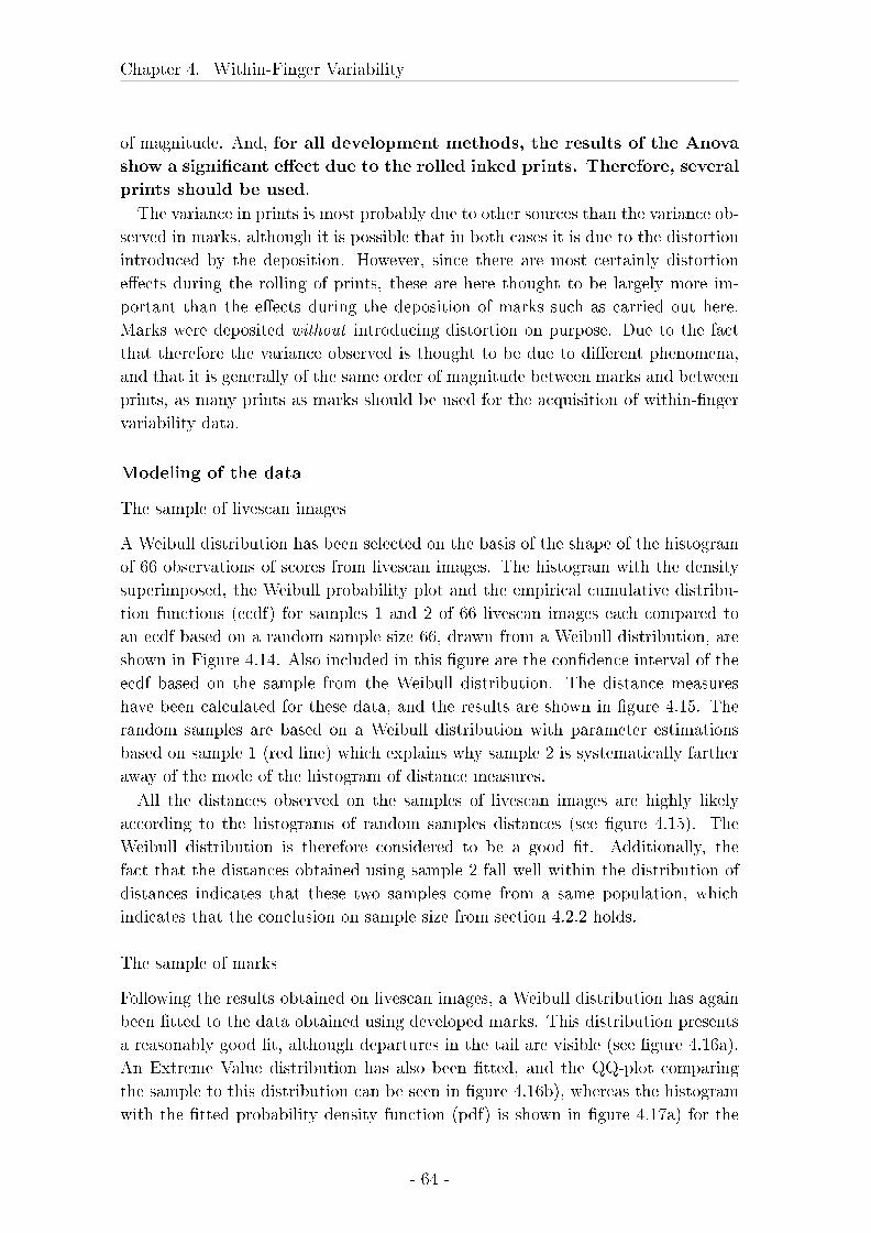
Chapter 4. Within-Finger Variability
of magnitude. And, for all development methods, the results of the Anova
show a signi�cant e�ect due to the rolled inked prints. Therefore, several
prints should be used.
The variance in prints is most probably due to other sources than the variance ob-
served in marks, although it is possible that in both cases it is due to the distortion
introduced by the deposition. However, since there are most certainly distortion
e�ects during the rolling of prints, these are here thought to be largely more im-
portant than the e�ects during the deposition of marks such as carried out here.
Marks were deposited without introducing distortion on purpose. Due to the fact
that therefore the variance observed is thought to be due to di�erent phenomena,
and that it is generally of the same order of magnitude between marks and between
prints, as many prints as marks should be used for the acquisition of within-�nger
variability data.
Modeling of the data
The sample of livescan images
A Weibull distribution has been selected on the basis of the shape of the histogram
of 66 observations of scores from livescan images. The histogram with the density
superimposed, the Weibull probability plot and the empirical cumulative distribu-
tion functions (ecdf) for samples 1 and 2 of 66 livescan images each compared to
an ecdf based on a random sample size 66, drawn from a Weibull distribution, are
shown in Figure 4.14. Also included in this �gure are the con�dence interval of the
ecdf based on the sample from the Weibull distribution. The distance measures
have been calculated for these data, and the results are shown in �gure 4.15. The
random samples are based on a Weibull distribution with parameter estimations
based on sample 1 (red line) which explains why sample 2 is systematically farther
away of the mode of the histogram of distance measures.
All the distances observed on the samples of livescan images are highly likely
according to the histograms of random samples distances (see �gure 4.15). The
Weibull distribution is therefore considered to be a good �t. Additionally, the
fact that the distances obtained using sample 2 fall well within the distribution of
distances indicates that these two samples come from a same population, which
indicates that the conclusion on sample size from section 4.2.2 holds.
The sample of marks
Following the results obtained on livescan images, a Weibull distribution has again
been �tted to the data obtained using developed marks. This distribution presents
a reasonably good �t, although departures in the tail are visible (see �gure 4.16a).
An Extreme Value distribution has also been �tted, and the QQ-plot comparing
the sample to this distribution can be seen in �gure 4.16b), whereas the histogram
with the �tted probability density function (pdf) is shown in �gure 4.17a) for the
- 64 -
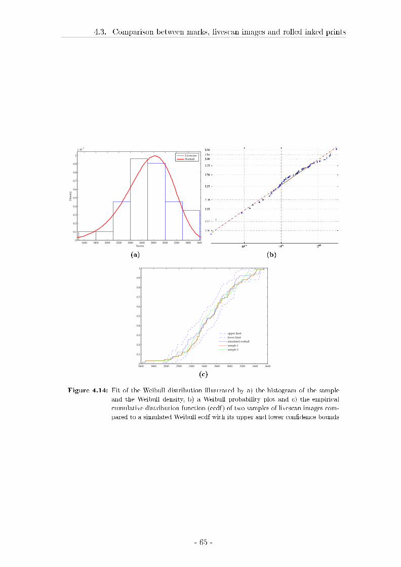
4.3. Comparison between marks, livescan images and rolled inked prints
1600 1800 2000 2200 2400 2600 2800 3000 3200 3400 36000
0.1
0.2
0.3
0.4
0.5
0.6
0.7
0.8
0.9
1
x 10−3
Scores
Den
sity
Livescans
Weibull
(a) (b)
1600 1800 2000 2200 2400 2600 2800 3000 3200 3400 36000
0.1
0.2
0.3
0.4
0.5
0.6
0.7
0.8
0.9
1
upper limit
lower limit
simulated weibull
sample 1
sample 2
(c)
Figure 4.14: Fit of the Weibull distribution illustrated by a) the histogram of the sample
and the Weibull density, b) a Weibull probability plot and c) the empirical
cumulative distribution function (ecdf) of two samples of livescan images com-
pared to a simulated Weibull ecdf with its upper and lower con�dence bounds
- 65 -
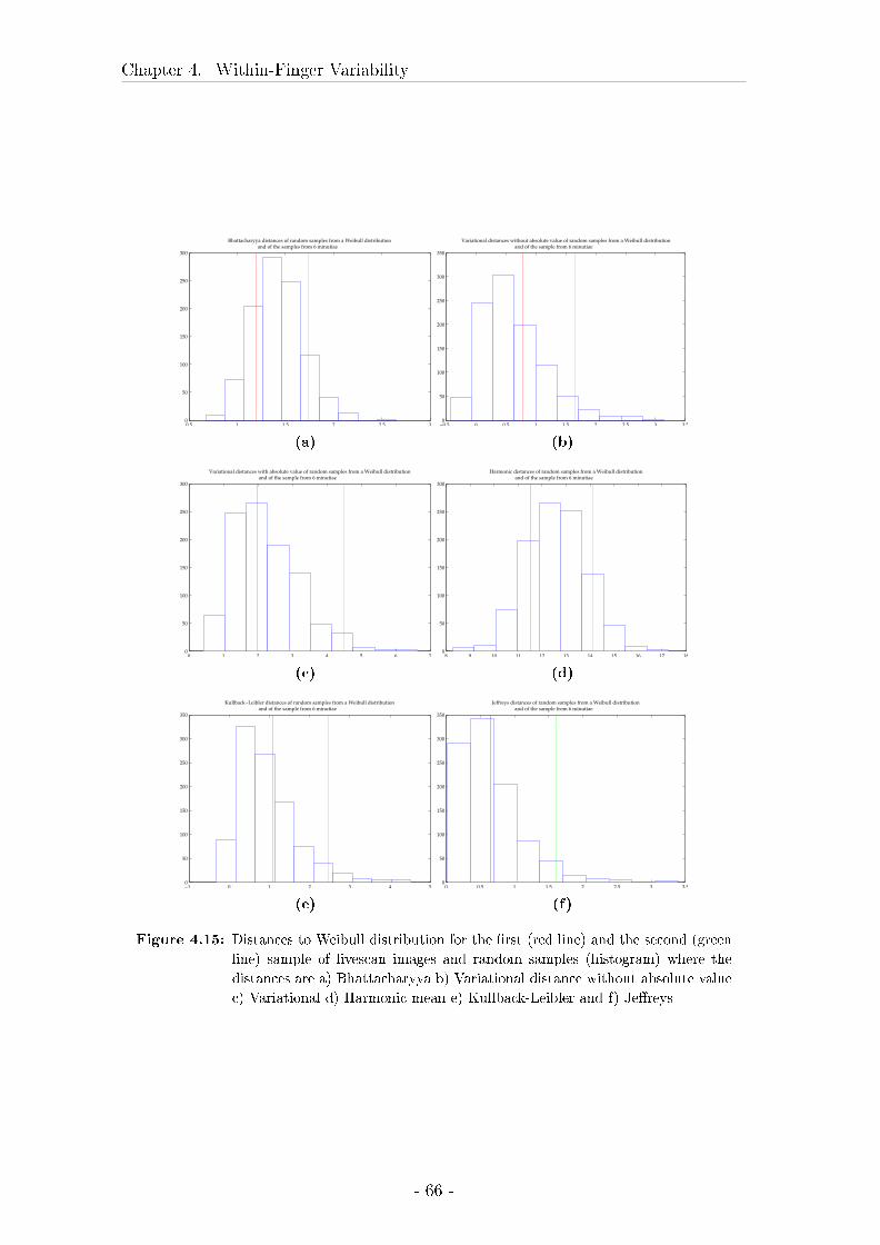
Chapter 4. Within-Finger Variability
0.5 1 1.5 2 2.5 30
50
100
150
200
250
300
Bhattacharyya distances of random samples from a Weibull distribution and of the samples from 6 minutiae
(a)
−0.5 0 0.5 1 1.5 2 2.5 3 3.50
50
100
150
200
250
300
350
Variational distances without absolute value of random samples from a Weibull distribution and of the sample from 6 minutiae
(b)
0 1 2 3 4 5 6 70
50
100
150
200
250
300
Variational distances with absolute value of random samples from a Weibull distribution and of the sample from 6 minutiae
(c)
8 9 10 11 12 13 14 15 16 17 180
50
100
150
200
250
300
Harmonic distances of random samples from a Weibull distribution and of the sample from 6 minutiae
(d)
−1 0 1 2 3 4 50
50
100
150
200
250
300
350
Kullback−Leibler distances of random samples from a Weibull distribution and of the sample from 6 minutiae
(e)
0 0.5 1 1.5 2 2.5 3 3.50
50
100
150
200
250
300
350
Jeffreys distances of random samples from a Weibull distribution and of the sample from 6 minutiae
(f)
Figure 4.15: Distances to Weibull distribution for the �rst (red line) and the second (green
line) sample of livescan images and random samples (histogram) where the
distances are a) Bhattacharyya b) Variational distance without absolute value
c) Variational d) Harmonic mean e) Kullback-Leibler and f) Je�reys
- 66 -
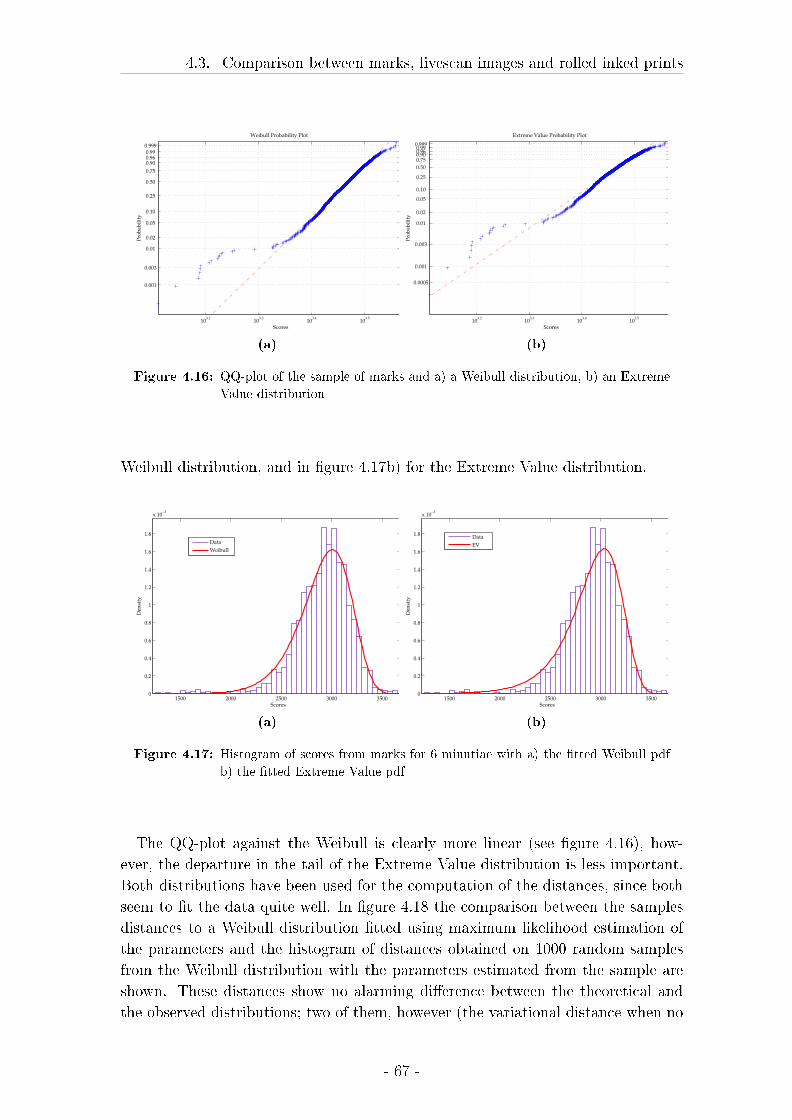
4.3. Comparison between marks, livescan images and rolled inked prints
103.2
103.3
103.4
103.5
0.001
0.003
0.01
0.02
0.05
0.10
0.25
0.50
0.75
0.90 0.96 0.99 0.999
Scores
Pro
bab
ilit
yWeibull Probability Plot
(a)
103.2
103.3
103.4
103.5
0.0005
0.001
0.003
0.01
0.02
0.05
0.10
0.25
0.50
0.75 0.90 0.96 0.99 0.999
Scores
Pro
bab
ilit
y
Extreme Value Probability Plot
(b)
Figure 4.16: QQ-plot of the sample of marks and a) a Weibull distribution, b) an Extreme
Value distribution
Weibull distribution, and in �gure 4.17b) for the Extreme Value distribution.
1500 2000 2500 3000 35000
0.2
0.4
0.6
0.8
1
1.2
1.4
1.6
1.8
x 10−3
Scores
Den
sity
Data
Weibull
(a)
1500 2000 2500 3000 35000
0.2
0.4
0.6
0.8
1
1.2
1.4
1.6
1.8
x 10−3
Scores
Den
sity
Data
EV
(b)
Figure 4.17: Histogram of scores from marks for 6 minutiae with a) the �tted Weibull pdf
b) the �tted Extreme Value pdf
The QQ-plot against the Weibull is clearly more linear (see �gure 4.16), how-
ever, the departure in the tail of the Extreme Value distribution is less important.
Both distributions have been used for the computation of the distances, since both
seem to �t the data quite well. In �gure 4.18 the comparison between the samples
distances to a Weibull distribution �tted using maximum likelihood estimation of
the parameters and the histogram of distances obtained on 1000 random samples
from the Weibull distribution with the parameters estimated from the sample are
shown. These distances show no alarming di�erence between the theoretical and
the observed distributions; two of them, however (the variational distance when no
- 67 -
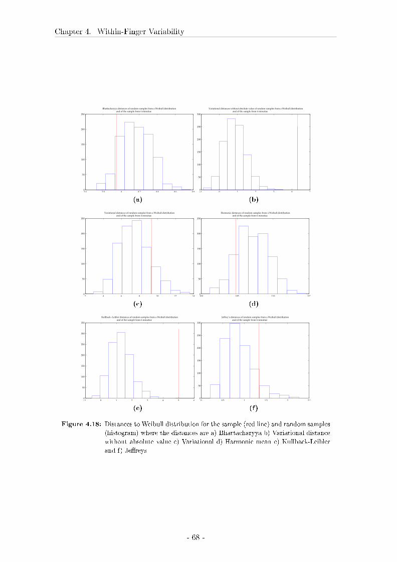
Chapter 4. Within-Finger Variability
3.6 3.8 4 4.2 4.4 4.6 4.80
50
100
150
200
250
Bhattacharyya distances of random samples from a Weibull distribution and of the sample from 6 minutiae
(a)
−1 0 1 2 3 4 50
50
100
150
200
250
300
Variational distances without absolute value of random samples from a Weibull distribution and of the sample from 6 minutiae
(b)
2 4 6 8 10 12 140
50
100
150
200
250
Variational distances of random samples from a Weibull distribution and of the sample from 6 minutiae
(c)
100 105 110 1150
50
100
150
200
250
Harmonic distances of random samples from a Weibull distribution and of the sample from 6 minutiae
(d)
−1 0 1 2 3 4 5 60
50
100
150
200
250
300
350
Kullback−Leibler distances of random samples from a Weibull distribution and of the sample from 6 minutiae
(e)
0 0.5 1 1.5 2 2.50
50
100
150
200
250
300
Jeffrey’s distances of random samples from a Weibull distribution and of the sample from 6 minutiae
(f)
Figure 4.18: Distances to Weibull distribution for the sample (red line) and random samples
(histogram) where the distances are a) Bhattacharyya b) Variational distance
without absolute value c) Variational d) Harmonic mean e) Kullback-Leibler
and f) Je�reys
- 68 -
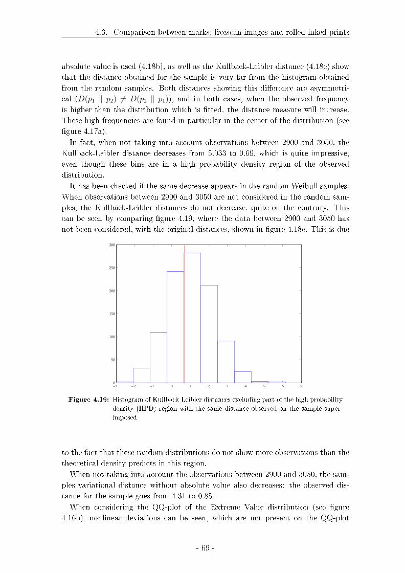
4.3. Comparison between marks, livescan images and rolled inked prints
absolute value is used (4.18b), as well as the Kullback-Leibler distance (4.18e) show
that the distance obtained for the sample is very far from the histogram obtained
from the random samples. Both distances showing this di�erence are asymmetri-
cal (D(p1 ‖ p2) 6= D(p2 ‖ p1)), and in both cases, when the observed frequency
is higher than the distribution which is �tted, the distance measure will increase.
These high frequencies are found in particular in the center of the distribution (see
�gure 4.17a).
In fact, when not taking into account observations between 2900 and 3050, the
Kullback-Leibler distance decreases from 5.033 to 0.69, which is quite impressive,
even though these bins are in a high probability density region of the observed
distribution.
It has been checked if the same decrease appears in the random Weibull samples.
When observations between 2900 and 3050 are not considered in the random sam-
ples, the Kullback-Leibler distances do not decrease, quite on the contrary. This
can be seen by comparing �gure 4.19, where the data between 2900 and 3050 has
not been considered, with the original distances, shown in �gure 4.18e. This is due
−3 −2 −1 0 1 2 3 4 5 6 70
50
100
150
200
250
300
Figure 4.19: Histogram of Kullback-Leibler distances excluding part of the high probability
density (HPD) region with the same distance observed on the sample super-
imposed
to the fact that these random distributions do not show more observations than the
theoretical density predicts in this region.
When not taking into account the observations between 2900 and 3050, the sam-
ples variational distance without absolute value also decreases: the observed dis-
tance for the sample goes from 4.31 to 0.85.
When considering the QQ-plot of the Extreme Value distribution (see �gure
4.16b), nonlinear deviations can be seen, which are not present on the QQ-plot
- 69 -
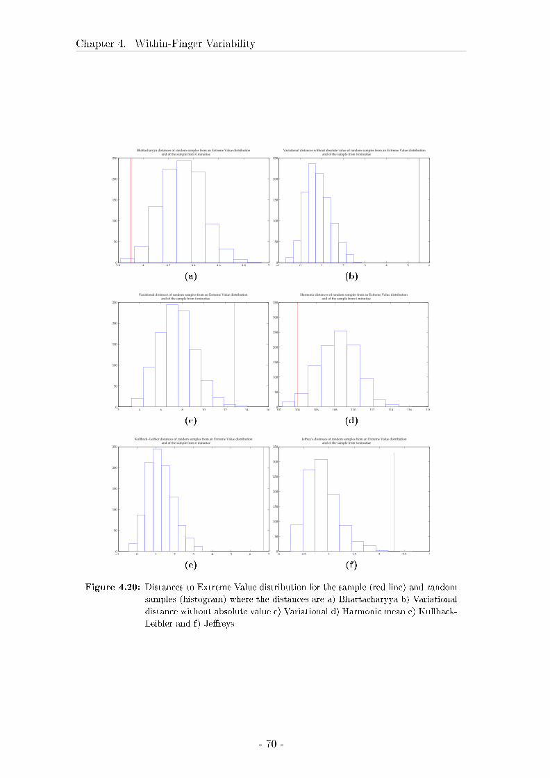
Chapter 4. Within-Finger Variability
3.8 4 4.2 4.4 4.6 4.8 50
50
100
150
200
250
Bhattacharyya distances of random samples from an Extreme Value distribution and of the sample from 6 minutiae
(a)
−1 0 1 2 3 4 5 60
50
100
150
200
250
Variational distances without absolute value of random samples from an Extreme Value distribution and of the sample from 6 minutiae
(b)
2 4 6 8 10 12 14 160
50
100
150
200
250
Variational distances of random samples from an Extreme Value distribution and of the sample from 6 minutiae
(c)
102 104 106 108 110 112 114 116 1180
50
100
150
200
250
300
350
Harmonic distances of random samples from an Extreme Value distribution and of the sample from 6 minutiae
(d)
−1 0 1 2 3 4 5 6 70
50
100
150
200
250
Kullback−Leibler distances of random samples from an Extreme Value distribution and of the sample from 6 minutiae
(e)
0 0.5 1 1.5 2 2.5 30
50
100
150
200
250
300
350
Jeffrey’s distances of random samples from an Extreme Value distribution and of the sample from 6 minutiae
(f)
Figure 4.20: Distances to Extreme Value distribution for the sample (red line) and random
samples (histogram) where the distances are a) Bhattacharyya b) Variational
distance without absolute value c) Variational d) Harmonic mean e) Kullback-
Leibler and f) Je�reys
- 70 -
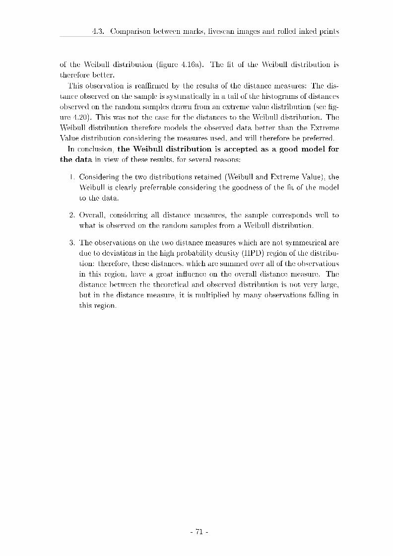
4.3. Comparison between marks, livescan images and rolled inked prints
of the Weibull distribution (�gure 4.16a). The �t of the Weibull distribution is
therefore better.
This observation is rea�rmed by the results of the distance measures: The dis-
tance observed on the sample is systmatically in a tail of the histograms of distances
observed on the random samples drawn from an extreme value distribution (see �g-
ure 4.20). This was not the case for the distances to the Weibull distribution. The
Weibull distribution therefore models the observed data better than the Extreme
Value distribution considering the measures used, and will therefore be preferred.
In conclusion, the Weibull distribution is accepted as a good model for
the data in view of these results, for several reasons:
1. Considering the two distributions retained (Weibull and Extreme Value), the
Weibull is clearly preferrable considering the goodness of the �t of the model
to the data.
2. Overall, considering all distance measures, the sample corresponds well to
what is observed on the random samples from a Weibull distribution.
3. The observations on the two distance measures which are not symmetrical are
due to deviations in the high probability density (HPD) region of the distribu-
tion: therefore, these distances, which are summed over all of the observations
in this region, have a great in�uence on the overall distance measure. The
distance between the theoretical and observed distribution is not very large,
but in the distance measure, it is multiplied by many observations falling in
this region.
- 71 -
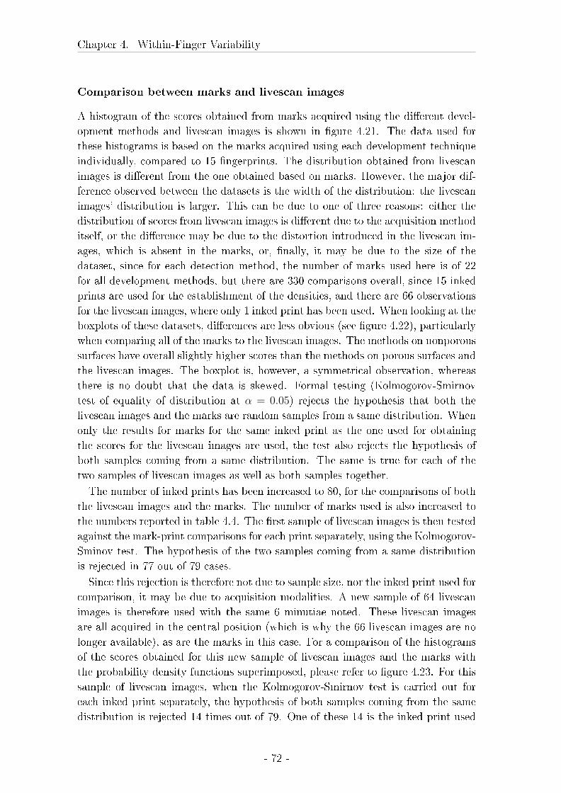
Chapter 4. Within-Finger Variability
Comparison between marks and livescan images
A histogram of the scores obtained from marks acquired using the di�erent devel-
opment methods and livescan images is shown in �gure 4.21. The data used for
these histograms is based on the marks acquired using each development technique
individually, compared to 15 �ngerprints. The distribution obtained from livescan
images is di�erent from the one obtained based on marks. However, the major dif-
ference observed between the datasets is the width of the distribution: the livescan
images' distribution is larger. This can be due to one of three reasons: either the
distribution of scores from livescan images is di�erent due to the acquisition method
itself, or the di�erence may be due to the distortion introduced in the livescan im-
ages, which is absent in the marks, or, �nally, it may be due to the size of the
dataset, since for each detection method, the number of marks used here is of 22
for all development methods, but there are 330 comparisons overall, since 15 inked
prints are used for the establishment of the densities, and there are 66 observations
for the livescan images, where only 1 inked print has been used. When looking at the
boxplots of these datasets, di�erences are less obvious (see �gure 4.22), particularly
when comparing all of the marks to the livescan images. The methods on nonporous
surfaces have overall slightly higher scores than the methods on porous surfaces and
the livescan images. The boxplot is, however, a symmetrical observation, whereas
there is no doubt that the data is skewed. Formal testing (Kolmogorov-Smirnov
test of equality of distribution at α = 0.05) rejects the hypothesis that both the
livescan images and the marks are random samples from a same distribution. When
only the results for marks for the same inked print as the one used for obtaining
the scores for the livescan images are used, the test also rejects the hypothesis of
both samples coming from a same distribution. The same is true for each of the
two samples of livescan images as well as both samples together.
The number of inked prints has been increased to 80, for the comparisons of both
the livescan images and the marks. The number of marks used is also increased to
the numbers reported in table 4.4. The �rst sample of livescan images is then tested
against the mark-print comparisons for each print separately, using the Kolmogorov-
Sminov test. The hypothesis of the two samples coming from a same distribution
is rejected in 77 out of 79 cases.
Since this rejection is therefore not due to sample size, nor the inked print used for
comparison, it may be due to acquisition modalities. A new sample of 64 livescan
images is therefore used with the same 6 minutiae noted. These livescan images
are all acquired in the central position (which is why the 66 livescan images are no
longer available), as are the marks in this case. For a comparison of the histograms
of the scores obtained for this new sample of livescan images and the marks with
the probability density functions superimposed, please refer to �gure 4.23. For this
sample of livescan images, when the Kolmogorov-Smirnov test is carried out for
each inked print separately, the hypothesis of both samples coming from the same
distribution is rejected 14 times out of 79. One of these 14 is the inked print used
- 72 -
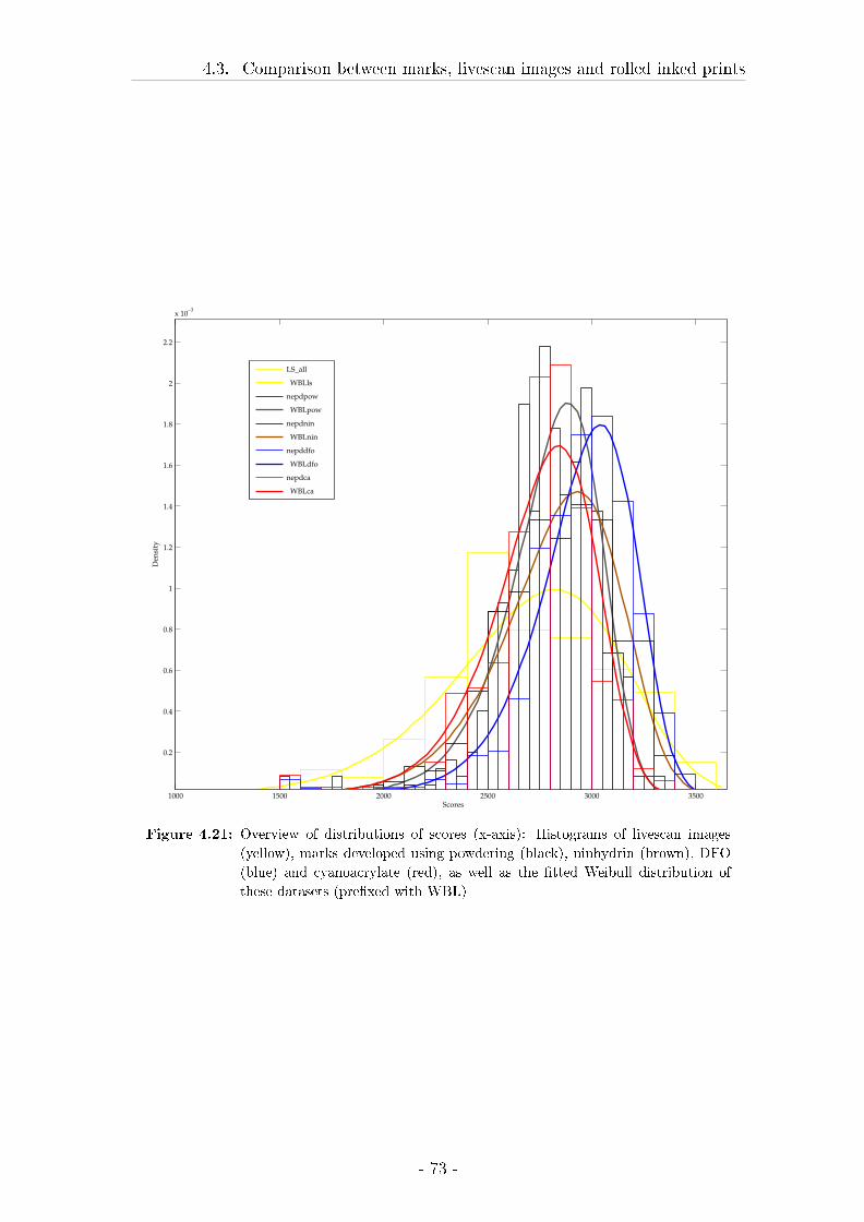
4.3. Comparison between marks, livescan images and rolled inked prints
1000 1500 2000 2500 3000 3500
0.2
0.4
0.6
0.8
1
1.2
1.4
1.6
1.8
2
2.2
x 10−3
Scores
Den
sity
LS_all
WBLls
nepdpow
WBLpow
nepdnin
WBLnin
nepddfo
WBLdfo
nepdca
WBLca
Figure 4.21: Overview of distributions of scores (x-axis): Histograms of livescan images
(yellow), marks developed using powdering (black), ninhydrin (brown), DFO
(blue) and cyanoacrylate (red), as well as the �tted Weibull distribution of
these datasets (pre�xed with WBL)
- 73 -
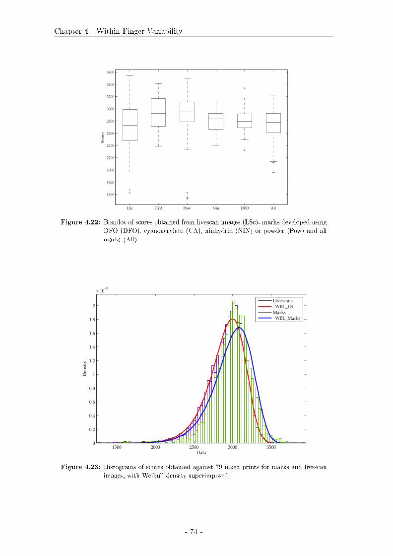
Chapter 4. Within-Finger Variability
LSc CYA Pow Nin DFO All
1600
1800
2000
2200
2400
2600
2800
3000
3200
3400
3600
Sco
res
Figure 4.22: Boxplot of scores obtained from livescan images (LSc), marks developed using
DFO (DFO), cyanoacrylate (CA), ninhydrin (NIN) or powder (Pow) and all
marks (All)
1500 2000 2500 3000 35000
0.2
0.4
0.6
0.8
1
1.2
1.4
1.6
1.8
2
x 10−3
Data
Den
sity
Livescans
WBL_LS
Marks
WBL_Marks
Figure 4.23: Histograms of scores obtained against 79 inked prints for marks and livescan
images, with Weibull density superimposed
- 74 -
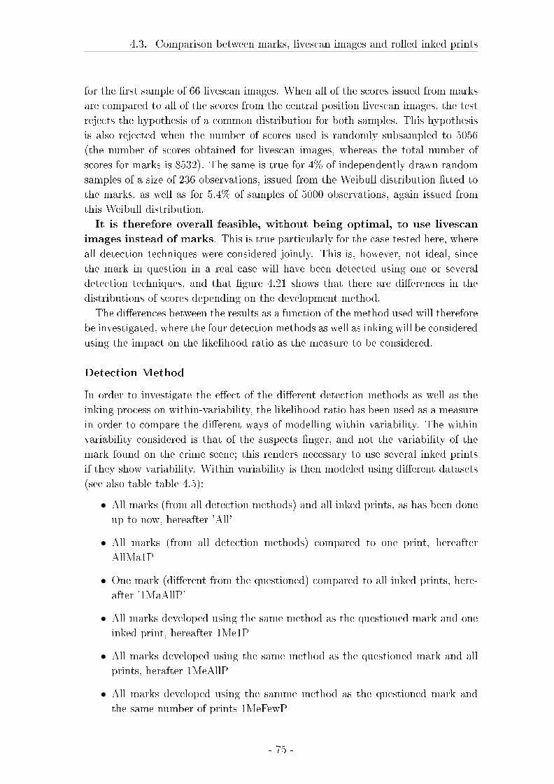
4.3. Comparison between marks, livescan images and rolled inked prints
for the �rst sample of 66 livescan images. When all of the scores issued from marks
are compared to all of the scores from the central position livescan images, the test
rejects the hypothesis of a common distribution for both samples. This hypothesis
is also rejected when the number of scores used is randomly subsampled to 5056
(the number of scores obtained for livescan images, whereas the total number of
scores for marks is 8532). The same is true for 4% of independently drawn random
samples of a size of 236 observations, issued from the Weibull distribution �tted to
the marks, as well as for 5.4% of samples of 5000 observations, again issued from
this Weibull distribution.
It is therefore overall feasible, without being optimal, to use livescan
images instead of marks. This is true particularly for the case tested here, where
all detection techniques were considered jointly. This is, however, not ideal, since
the mark in question in a real case will have been detected using one or several
detection techniques, and that �gure 4.21 shows that there are di�erences in the
distributions of scores depending on the development method.
The di�erences between the results as a function of the method used will therefore
be investigated, where the four detection methods as well as inking will be considered
using the impact on the likelihood ratio as the measure to be considered.
Detection Method
In order to investigate the e�ect of the di�erent detection methods as well as the
inking process on within-variability, the likelihood ratio has been used as a measure
in order to compare the di�erent ways of modelling within variability. The within
variability considered is that of the suspects �nger, and not the variability of the
mark found on the crime scene; this renders necessary to use several inked prints
if they show variability. Within variability is then modeled using di�erent datasets
(see also table table 4.5):
• All marks (from all detection methods) and all inked prints, as has been done
up to now, hereafter 'All'
• All marks (from all detection methods) compared to one print, hereafter
AllMa1P
• One mark (di�erent from the questioned) compared to all inked prints, here-
after '1MaAllP'
• All marks developed using the same method as the questioned mark and one
inked print, hereafter 1Me1P
• All marks developed using the same method as the questioned mark and all
prints, herafter 1MeAllP
• All marks developed using the samme method as the questioned mark and
the same number of prints 1MeFewP
- 75 -
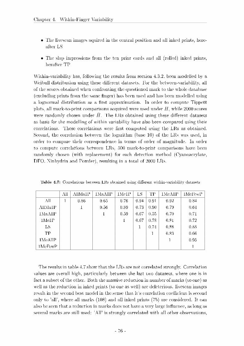
Chapter 4. Within-Finger Variability
• The livescan images aquired in the central position and all inked prints, here-
after LS
• The slap impressions from the ten print cards and all (rolled) inked prints,
herafter TP
Within-variability has, following the results from section 4.3.2, been modelled by a
Weibull distribution using these di�erent datasets. For the between-variability, all
of the scores obtained when confronting the questioned mark to the whole database
(excluding prints from the same �nger) has been used and has been modelled using
a lognormal distribution as a �rst approximation. In order to compute Tippett
plots, all mark-to-print comparisons acquired were used under H, while 2000 scores
were randomly chosen under H̄. The LRs obtained using these di�erent datasets
as basis for the modelling of within variability have also been compared using their
correlations. These correlations were �rst computed using the LRs as obtained.
Second, the correlation between the logarithm (base 10) of the LRs was used, in
order to compare their correspondence in terms of order of magnitude. In order
to compute correlations between LRs, 500 mark-to-print comparisons have been
randomly chosen (with replacement) for each detection method (Cyanoacrylate,
DFO, Ninhydrin and Powder), resulting in a total of 2000 LRs.
Table 4.7: Correlations between LRs obtained using di�erent within-variability datasets
All AllMa1P 1MaAllP 1Me1P LS TP 1MeAllP 1MeFewP
All 1 0.86 0.65 0.76 0.94 0.91 0.92 0.84
AllMa1P 1 0.56 0.89 0.73 0.90 0.79 0.64
1MaAllP 1 0.59 0.67 0.55 0.70 0.71
1Me1P 1 0.67 0.78 0.81 0.72
LS 1 0.74 0.88 0.88
TP 1 0.83 0.66
1MeAllP 1 0.95
1MeFewP 1
The results in table 4.7 show that the LRs are not correlated strongly. Correlation
values are overall high, particularly between the last two datasets, where one is in
fact a subset of the other. Both the massive reduction in number of marks (to one) as
well as the reduction in inked prints (to one as well) are deleterious. livescan images
result in the second best model in the sense that it's correlation coe�cient is second
only to 'all', where all marks (108) and all inked prints (75) are considered. It can
also be seen that a reduction in marks does not have a very large in�uence, as long as
several marks are still used: 'All' is strongly correlated with all other observations,
- 76 -
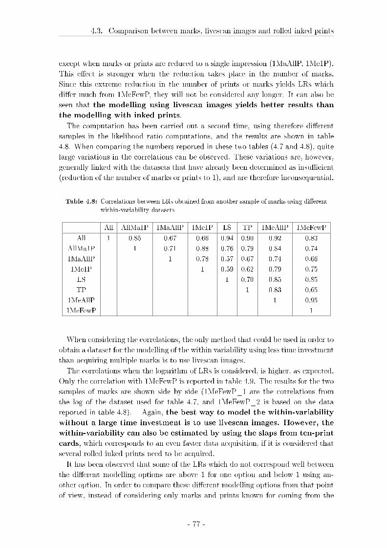
4.3. Comparison between marks, livescan images and rolled inked prints
except when marks or prints are reduced to a single impression (1MaAllP, 1Me1P).
This e�ect is stronger when the reduction takes place in the number of marks.
Since this extreme reduction in the number of prints or marks yields LRs which
di�er much from 1MeFewP, they will not be considered any longer. It can also be
seen that the modelling using livescan images yields better results than
the modelling with inked prints.
The computation has been carried out a second time, using therefore di�erent
samples in the likelihood ratio computations, and the results are shown in table
4.8. When comparing the numbers reported in these two tables (4.7 and 4.8), quite
large variations in the correlations can be observed. These variations are, however,
generally linked with the datasets that have already been determined as insu�cient
(reduction of the number of marks or prints to 1), and are therefore inconsequential.
Table 4.8: Correlations between LRs obtained from another sample of marks using di�erent
within-variability datasets
All AllMa1P 1MaAllP 1Me1P LS TP 1MeAllP 1MeFewP
All 1 0.85 0.67 0.66 0.94 0.90 0.92 0.83
AllMa1P 1 0.71 0.88 0.76 0.79 0.84 0.74
1MaAllP 1 0.78 0.57 0.67 0.74 0.66
1Me1P 1 0.59 0.62 0.79 0.75
LS 1 0.70 0.85 0.85
TP 1 0.83 0.65
1MeAllP 1 0.95
1MeFewP 1
When considering the correlations, the only method that could be used in order to
obtain a dataset for the modelling of the within variability using less time investment
than acquiring multiple marks is to use livescan images.
The correlations when the logarithm of LRs is considered, is higher, as expected.
Only the correlation with 1MeFewP is reported in table 4.9. The results for the two
samples of marks are shown side by side (1MeFewP_1 are the correlations from
the log of the dataset used for table 4.7, and 1MeFewP_2 is based on the data
reported in table 4.8). Again, the best way to model the within-variability
without a large time investment is to use livescan images. However, the
within-variability can also be estimated by using the slaps from ten-print
cards, which corresponds to an even faster data acquisition, if it is considered that
several rolled inked prints need to be acquired.
It has been observed that some of the LRs which do not correspond well between
the di�erent modelling options are above 1 for one option and below 1 using an-
other option. In order to compare these di�erent modelling options from that point
of view, instead of considering only marks and prints known for coming from the
- 77 -
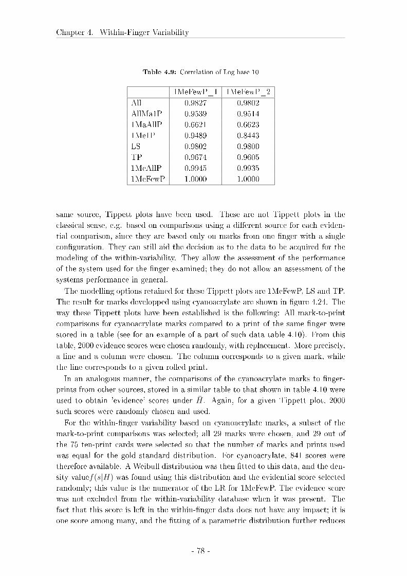
Chapter 4. Within-Finger Variability
Table 4.9: Correlation of Log base 10
1MeFewP_1 1MeFewP_2
All 0.9827 0.9802
AllMa1P 0.9539 0.9514
1MaAllP 0.6621 0.6623
1Me1P 0.9489 0.8443
LS 0.9802 0.9800
TP 0.9674 0.9605
1MeAllP 0.9945 0.9935
1MeFewP 1.0000 1.0000
same source, Tippett plots have been used. These are not Tippett plots in the
classical sense, e.g. based on comparisons using a di�erent source for each eviden-
tial comparison, since they are based only on marks from one �nger with a single
con�guration. They can still aid the decision as to the data to be acquired for the
modeling of the within-variability. They allow the assessment of the performance
of the system used for the �nger examined; they do not allow an assessment of the
systems performance in general.
The modelling options retained for these Tippett plots are 1MeFewP, LS and TP.
The result for marks developped using cyanoacrylate are shown in �gure 4.24. The
way these Tippett plots have been established is the following: All mark-to-print
comparisons for cyanoacrylate marks compared to a print of the same �nger were
stored in a table (see for an example of a part of such data table 4.10). From this
table, 2000 evidence scores were chosen randomly, with replacement. More precisely,
a line and a column were chosen. The column corresponds to a given mark, while
the line corresponds to a given rolled print.
In an analogous manner, the comparisons of the cyanoacrylate marks to �nger-
prints from other sources, stored in a similar table to that shown in table 4.10 were
used to obtain 'evidence' scores under H̄. Again, for a given Tippett plot, 2000
such scores were randomly chosen and used.
For the within-�nger variability based on cyanoacrylate marks, a subset of the
mark-to-print comparisons was selected; all 29 marks were chosen, and 29 out of
the 75 ten-print cards were selected so that the number of marks and prints used
was equal for the gold standard distribution. For cyanoacrylate, 841 scores were
therefore available. A Weibull distribution was then �tted to this data, and the den-
sity valuef(s|H) was found using this distribution and the evidential score selected
randomly; this value is the numerator of the LR for 1MeFewP. The evidence score
was not excluded from the within-variability database when it was present. The
fact that this score is left in the within-�nger data does not have any impact; it is
one score among many, and the �tting of a parametric distribution further reduces
- 78 -
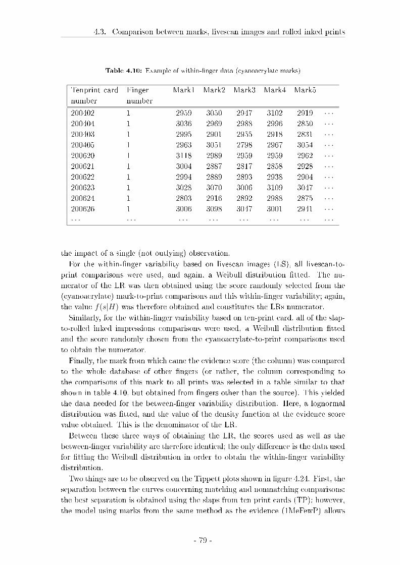
4.3. Comparison between marks, livescan images and rolled inked prints
Table 4.10: Example of within-�nger data (cyanoacrylate marks)
Tenprint card
number
Finger
number
Mark1 Mark2 Mark3 Mark4 Mark5
200402 1 2959 3050 2947 3102 2919 · · ·200404 1 3036 2969 2988 2996 2850 · · ·200403 1 2995 2901 2955 2918 2831 · · ·200405 1 2963 3051 2798 2967 3054 · · ·200620 1 3118 2989 2959 2959 2962 · · ·200621 1 3004 2887 2817 2858 2928 · · ·200622 1 2994 2889 2893 2938 2904 · · ·200623 1 3028 3070 3006 3109 3047 · · ·200624 1 2803 2916 2892 2988 2875 · · ·200626 1 3006 3098 3047 3001 2941 · · ·· · · · · · · · · · · · · · · · · · · · · · · ·
the impact of a single (not outlying) observation.
For the within-�nger variability based on livescan images (LS), all livescan-to-
print comparisons were used, and again, a Weibull distribution �tted. The nu-
merator of the LR was then obtained using the score randomly selected from the
(cyanoacrylate) mark-to-print comparisons and this within-�nger variability; again,
the value f(s|H) was therefore obtained and constitutes the LRs numerator.
Similarly, for the within-�nger variability based on ten-print card, all of the slap-
to-rolled inked impressions comparisons were used, a Weibull distribution �tted
and the score randomly chosen from the cyanoacrylate-to-print comparisons used
to obtain the numerator.
Finally, the mark from which came the evidence score (the column) was compared
to the whole database of other �ngers (or rather, the column corresponding to
the comparisons of this mark to all prints was selected in a table similar to that
shown in table 4.10, but obtained from �ngers other than the source). This yielded
the data needed for the between-�nger variability distribution. Here, a lognormal
distribution was �tted, and the value of the density function at the evidence score
value obtained. This is the denominator of the LR.
Between these three ways of obtaining the LR, the scores used as well as the
between-�nger variability are therefore identical; the only di�erence is the data used
for �tting the Weibull distribution in order to obtain the within-�nger variability
distribution.
Two things are to be observed on the Tippett plots shown in �gure 4.24. First, the
separation between the curves concerning matching and nonmatching comparisons:
the best separation is obtained using the slaps from ten print cards (TP); however,
the model using marks from the same method as the evidence (1MeFewP) allows
- 79 -
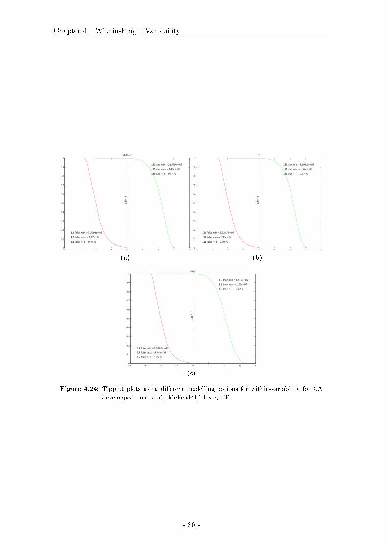
Chapter 4. Within-Finger Variability
−8 −6 −4 −2 0 2 4 6 80
0.1
0.2
0.3
0.4
0.5
0.6
0.7
0.8
0.9
1
LR true min =2.1339e−05
LR true max =1.48e+06
LR true < 1 0.37 %
LR false max =1.77e+01
LR false min =3.3991e−06
LR false > 1 0.45 %
LR
= 1
1MeFewP
(a)
−8 −6 −4 −2 0 2 4 6 80
0.1
0.2
0.3
0.4
0.5
0.6
0.7
0.8
0.9
1
LR true min =3.1082e−05
LR true max =1.54e+06
LR true < 1 0.37 %
LR false max =1.93e+01
LR false min =5.5347e−06
LR false > 1 0.50 %
LR
= 1
LS
(b)
−8 −6 −4 −2 0 2 4 6 80
0.1
0.2
0.3
0.4
0.5
0.6
0.7
0.8
0.9
1
LR true min =1.812e−05
LR true max =1.22e+07
LR true < 1 0.42 %
LR false max =8.94e+00
LR false min =3.5497e−06
LR false > 1 0.25 %
LR
= 1
slaps
(c)
Figure 4.24: Tippett plots using di�erent modelling options for within-variability for CA
developped marks, a) 1MeFewP b) LS c) TP
- 80 -
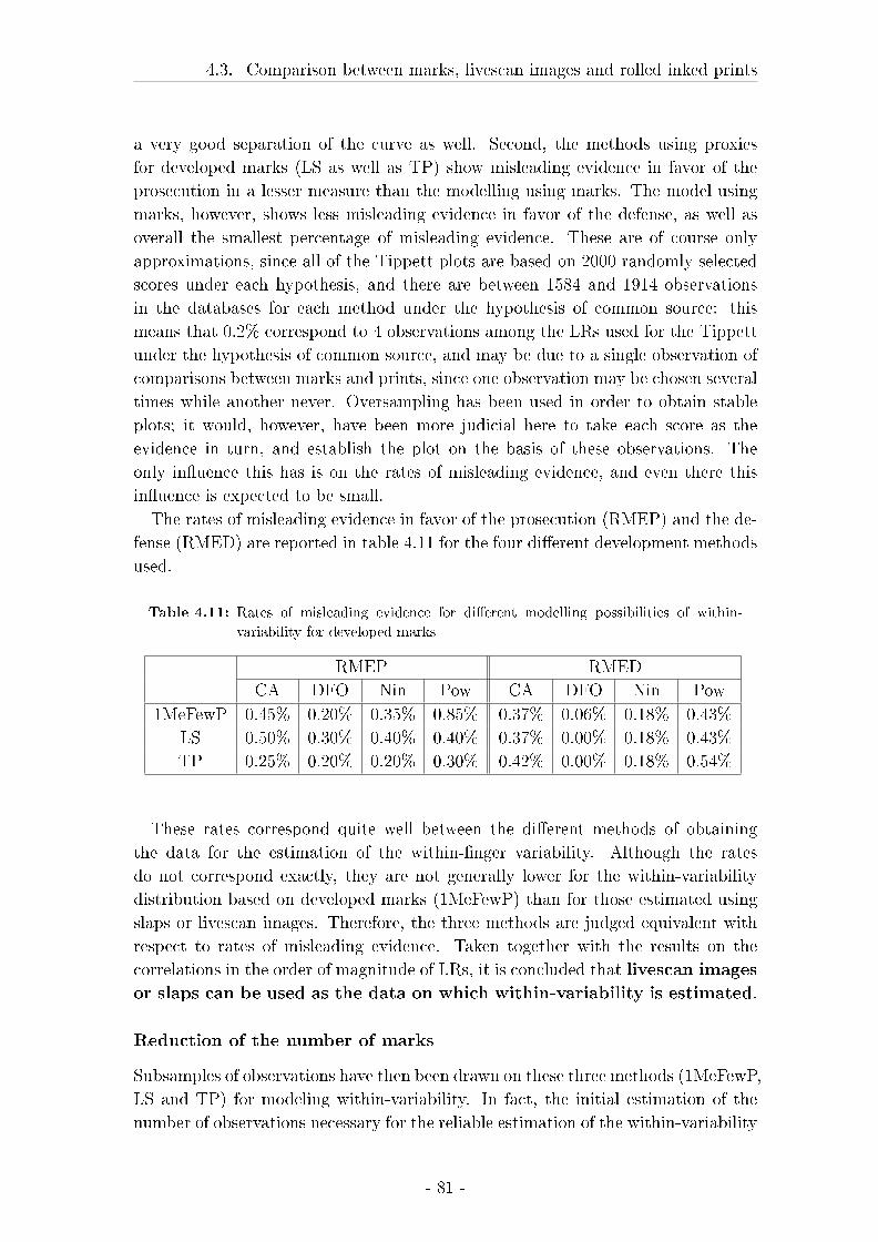
4.3. Comparison between marks, livescan images and rolled inked prints
a very good separation of the curve as well. Second, the methods using proxies
for developed marks (LS as well as TP) show misleading evidence in favor of the
prosecution in a lesser measure than the modelling using marks. The model using
marks, however, shows less misleading evidence in favor of the defense, as well as
overall the smallest percentage of misleading evidence. These are of course only
approximations, since all of the Tippett plots are based on 2000 randomly selected
scores under each hypothesis, and there are between 1584 and 1914 observations
in the databases for each method under the hypothesis of common source: this
means that 0.2% correspond to 4 observations among the LRs used for the Tippett
under the hypothesis of common source, and may be due to a single observation of
comparisons between marks and prints, since one observation may be chosen several
times while another never. Oversampling has been used in order to obtain stable
plots; it would, however, have been more judicial here to take each score as the
evidence in turn, and establish the plot on the basis of these observations. The
only in�uence this has is on the rates of misleading evidence, and even there this
in�uence is expected to be small.
The rates of misleading evidence in favor of the prosecution (RMEP) and the de-
fense (RMED) are reported in table 4.11 for the four di�erent development methods
used.
Table 4.11: Rates of misleading evidence for di�erent modelling possibilities of within-
variability for developed marks
RMEP RMED
CA DFO Nin Pow CA DFO Nin Pow
1MeFewP 0.45% 0.20% 0.35% 0.85% 0.37% 0.06% 0.18% 0.43%
LS 0.50% 0.30% 0.40% 0.40% 0.37% 0.00% 0.18% 0.43%
TP 0.25% 0.20% 0.20% 0.30% 0.42% 0.00% 0.18% 0.54%
These rates correspond quite well between the di�erent methods of obtaining
the data for the estimation of the within-�nger variability. Although the rates
do not correspond exactly, they are not generally lower for the within-variability
distribution based on developed marks (1MeFewP) than for those estimated using
slaps or livescan images. Therefore, the three methods are judged equivalent with
respect to rates of misleading evidence. Taken together with the results on the
correlations in the order of magnitude of LRs, it is concluded that livescan images
or slaps can be used as the data on which within-variability is estimated.
Reduction of the number of marks
Subsamples of observations have then been drawn on these three methods (1MeFewP,
LS and TP) for modeling within-variability. In fact, the initial estimation of the
number of observations necessary for the reliable estimation of the within-variability
- 81 -
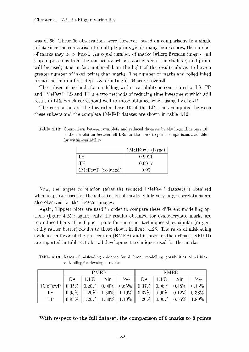
Chapter 4. Within-Finger Variability
was of 66. These 66 observations were, however, based on comparisons to a single
print; since the comparison to multiple prints yields many more scores, the number
of marks may be reduced. An equal number of marks (where livescan images and
slap impressions from the ten-print cards are considered as marks here) and prints
will be used; it is in fact not useful, in the light of the results above, to have a
greater number of inked prints than marks. The number of marks and rolled inked
prints chosen in a �rst step is 8, resulting in 64 scores overall.
The subset of methods for modelling within-variability is constituted of LS, TP
and 1MeFewP. LS and TP are two methods of reducing time investment which still
result in LRs which correspond well to those obtained when using 1MeFewP.
The correlations of the logarithm base 10 of the LRs thus computed between
these subsets and the complete 1MeFeP dataset are shown in table 4.12.
Table 4.12: Comparison between complete and reduced datasets by the logarithm base 10
of the correlation between all LRs for the mark-to-print comparisons available
for within-variability
1MetFewP (large)
LS 0.9911
TP 0.9917
1MeFewP (reduced) 0.99
Now, the largest correlation (after the reduced 1MeFewP dataset) is obtained
when slaps are used for the substitution of marks, while very large correlations are
also observed for the livescan images.
Again, Tippett plots are used in order to compare these di�erent modelling op-
tions (�gure 4.25); again, only the results obtained for cyanoacrylate marks are
reproduced here. The Tippett plots for the other techniques show similar (or gen-
erally rather better) results to those shown in �gure 4.25. The rates of misleading
evidence in favor of the prosecution (RMEP) and in favor of the defense (RMED)
are reported in table 4.13 for all development techniques used for the marks.
Table 4.13: Rates of misleading evidence for di�erent modelling possibilities of within-
variability for developed marks
RMEP RMED
CA DFO Nin Pow CA DFO Nin Pow
1MeFewP 0.35% 0.20% 0.00% 0.65% 0.37% 0.06% 0.48% 0.43%
LS 0.95% 1.20% 1.30% 1.10% 0.37% 0.00% 0.12% 0.38%
TP 0.95% 1.20% 1.30% 1.10% 1.20% 0.06% 0.55% 1.89%
With respect to the full dataset, the comparison of 8 marks to 8 prints
- 82 -
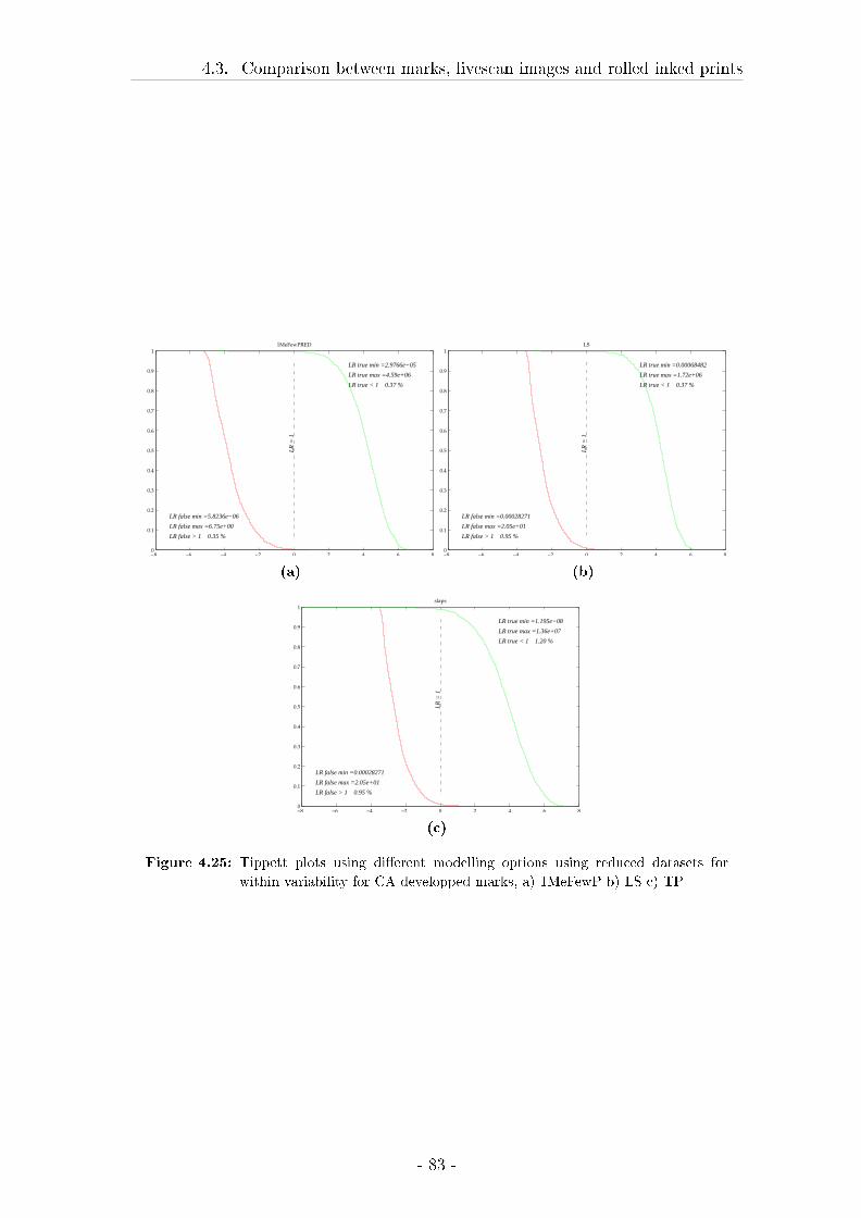
4.3. Comparison between marks, livescan images and rolled inked prints
−8 −6 −4 −2 0 2 4 6 80
0.1
0.2
0.3
0.4
0.5
0.6
0.7
0.8
0.9
1
LR true min =2.9766e−05
LR true max =4.59e+06
LR true < 1 0.37 %
LR false max =6.75e+00
LR false min =5.8236e−06
LR false > 1 0.35 %
LR
= 1
1MeFewPRED
(a)
−8 −6 −4 −2 0 2 4 6 80
0.1
0.2
0.3
0.4
0.5
0.6
0.7
0.8
0.9
1
LR true min =0.00068482
LR true max =1.72e+06
LR true < 1 0.37 %
LR false max =2.05e+01
LR false min =0.00028271
LR false > 1 0.95 %
LR
= 1
LS
(b)
−8 −6 −4 −2 0 2 4 6 80
0.1
0.2
0.3
0.4
0.5
0.6
0.7
0.8
0.9
1
LR true min =1.195e−08
LR true max =1.36e+07
LR true < 1 1.20 %
LR false max =2.05e+01
LR false min =0.00028271
LR false > 1 0.95 %
LR
= 1
slaps
(c)
Figure 4.25: Tippett plots using di�erent modelling options using reduced datasets for
within variability for CA developped marks, a) 1MeFewP b) LS c) TP
- 83 -
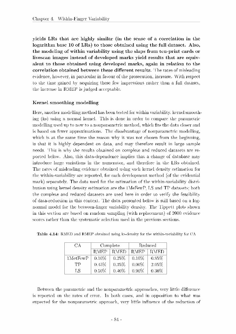
Chapter 4. Within-Finger Variability
yields LRs that are highly similar (in the sense of a correlation in the
logarithm base 10 of LRs) to those obtained using the full dataset. Also,
the modeling of within variability using the slaps from ten-print cards or
livescan images instead of developed marks yield results that are equiv-
alent to those obtained using developed marks, again in relation to the
correlation obtained between these di�erent results. The rates of misleading
evidence, however, in particular in favour of the prosecution, increase. With respect
to the time gained by acquiring these few impressions rather than a full dataset,
the increase in RMEP is judged acceptable.
Kernel smoothing modelling
Here, another modelling method has been tested for within variability, kernel smooth-
ing (ks) using a normal kernel. This is done in order to compare the parametric
modelling used up to now to a nonparametric method, which �ts the data closer and
is based on fewer approximations. The disadvantage of nonparametric modelling,
which is at the same time the reason why it was not chosen from the beginning,
is that it is highly dependent on data, and may therefore result in large sample
needs. This is why the results obtained on complete and reduced datasets are re-
ported below. Also, this data-dependence implies that a change of database may
introduce large variations in the numerator, and therefore in the LRs obtained.
The rates of misleading evidence obtained using such kernel density estimation for
the within-variability are reported, for each development method (of the evidential
mark) separately. The data used for the estimation of the within-variability distri-
bution using kernel density estimation are the 1MeFewP, LS and TP datasets; both
the complete and reduced datasets are used here in order to verify the feasibility
of data-reduction in this context. The data presented below is still based on a log-
normal model for the between-�nger variability density. The Tippett plots shown
in this section are based on random sampling (with replacement) of 2000 evidence
scores rather than the systematic selection used in the previous sections.
Table 4.14: RMED and RMEP obtained using ks-density for the within-variability for CA
CA Complete Reduced
RMEP RMED RMEP RMED
1MetFewP 0.10% 0.25% 0.10% 0.85%
TP 0.45% 0.35% 0.00% 2.05%
LS 0.50% 0.40% 0.90% 0.30%
Between the parametric and the nonparametric approaches, very little di�erence
is reported on the rates of error. In both cases, and in opposition to what was
expected for the nonparametric approach, very little in�uence of the reduction of
- 84 -
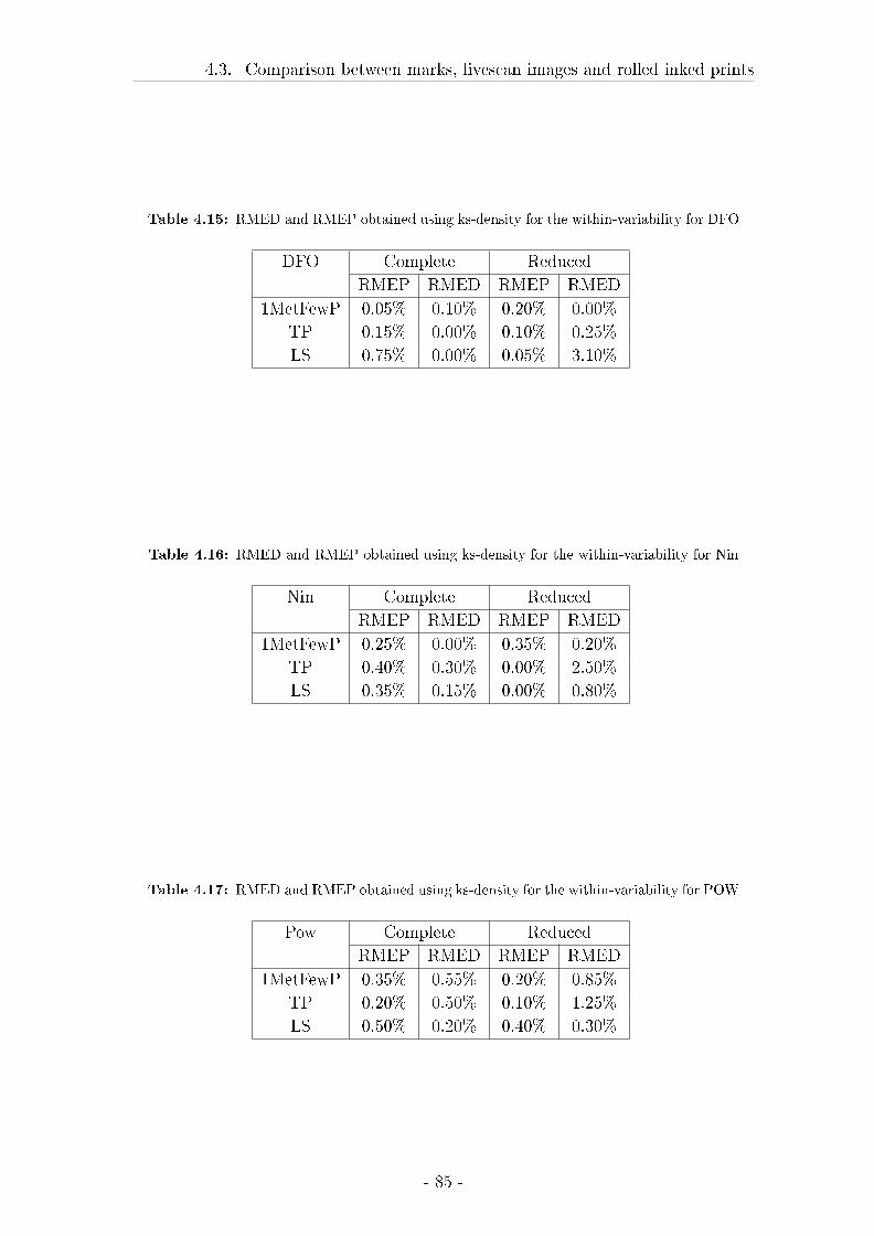
4.3. Comparison between marks, livescan images and rolled inked prints
Table 4.15: RMED and RMEP obtained using ks-density for the within-variability for DFO
DFO Complete Reduced
RMEP RMED RMEP RMED
1MetFewP 0.05% 0.10% 0.20% 0.00%
TP 0.15% 0.00% 0.10% 0.25%
LS 0.75% 0.00% 0.05% 3.10%
Table 4.16: RMED and RMEP obtained using ks-density for the within-variability for Nin
Nin Complete Reduced
RMEP RMED RMEP RMED
1MetFewP 0.25% 0.00% 0.35% 0.20%
TP 0.40% 0.30% 0.00% 2.50%
LS 0.35% 0.15% 0.00% 0.80%
Table 4.17: RMED and RMEP obtained using ks-density for the within-variability for POW
Pow Complete Reduced
RMEP RMED RMEP RMED
1MetFewP 0.35% 0.55% 0.20% 0.85%
TP 0.20% 0.50% 0.10% 1.25%
LS 0.50% 0.20% 0.40% 0.30%
- 85 -
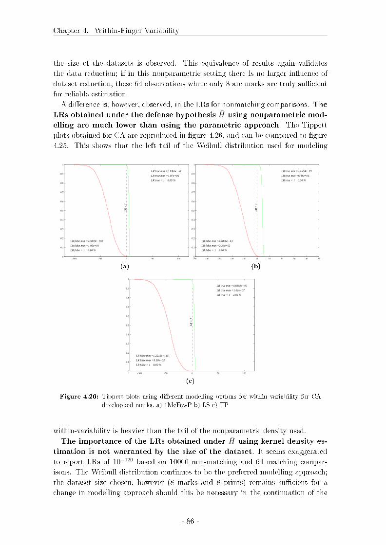
Chapter 4. Within-Finger Variability
the size of the datasets is observed. This equivalence of results again validates
the data reduction; if in this nonparametric setting there is no larger in�uence of
dataset reduction, these 64 observations where only 8 are marks are truly su�cient
for reliable estimation.
A di�erence is, however, observed, in the LRs for nonmatching comparisons. The
LRs obtained under the defense hypothesis H̄ using nonparametric mod-
elling are much lower than using the parametric approach. The Tippett
plots obtained for CA are reproduced in �gure 4.26, and can be compared to �gure
4.25. This shows that the left tail of the Weibull distribution used for modeling
−100 −50 0 50 1000
0.1
0.2
0.3
0.4
0.5
0.6
0.7
0.8
0.9
1
LR true min =2.1366e−51
LR true max =1.07e+06
LR true < 1 0.85 %
LR false max =1.05e+01
LR false min =5.9839e−102
LR false > 1 0.10 %
LR
= 1
(a)
−50 −40 −30 −20 −10 0 10 20 30 40 500
0.1
0.2
0.3
0.4
0.5
0.6
0.7
0.8
0.9
1
LR true min =2.4594e−19
LR true max =6.48e+05
LR true < 1 0.30 %
LR false max =2.36e+02
LR false min =3.4866e−43
LR false > 1 0.90 %
LR
= 1
(b)
−100 −50 0 50 1000
0.1
0.2
0.3
0.4
0.5
0.6
0.7
0.8
0.9
1
LR true min =4.0302e−45
LR true max =1.01e+07
LR true < 1 2.05 %
LR false max =5.10e−02
LR false min =1.2212e−115
LR false > 1 0.00 %
LR
= 1
(c)
Figure 4.26: Tippett plots using di�erent modelling options for within variability for CA
developped marks, a) 1MeFewP b) LS c) TP
within-variability is heavier than the tail of the nonparametric density used.
The importance of the LRs obtained under H̄ using kernel density es-
timation is not warranted by the size of the dataset. It seems exaggerated
to report LRs of 10−120 based on 10000 non-matching and 64 matching compar-
isons. The Weibull distribution continues to be the preferred modelling approach;
the dataset size chosen, however (8 marks and 8 prints) remains su�cient for a
change in modelling approach should this be necessary in the continuation of the
- 86 -
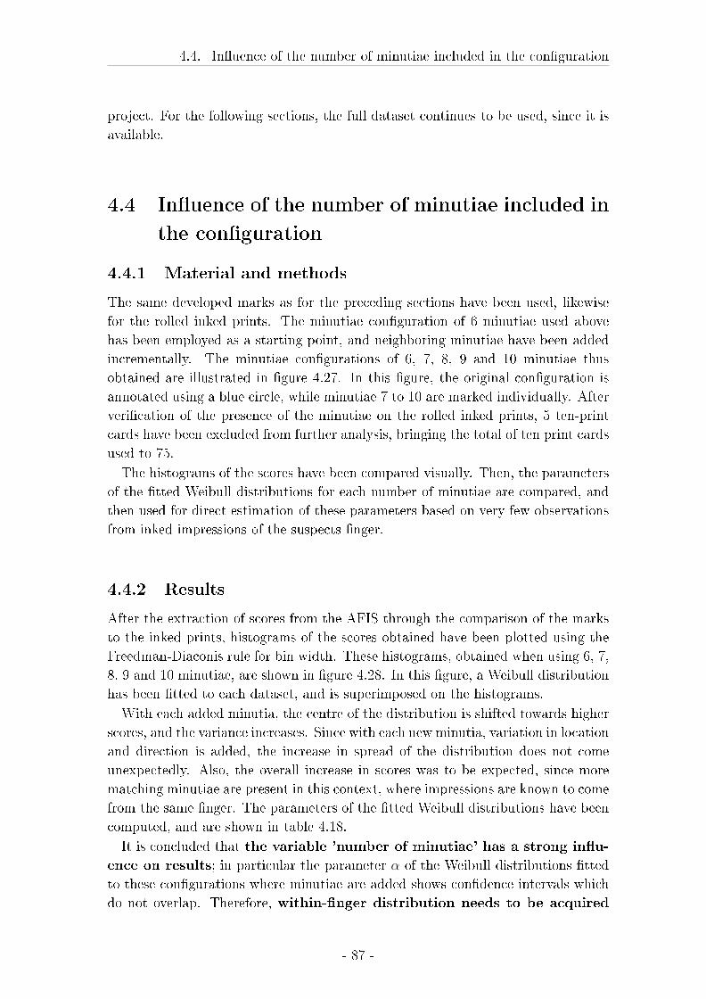
4.4. In�uence of the number of minutiae included in the con�guration
project. For the following sections, the full dataset continues to be used, since it is
available.
4.4 In�uence of the number of minutiae included in
the con�guration
4.4.1 Material and methods
The same developed marks as for the preceding sections have been used, likewise
for the rolled inked prints. The minutiae con�guration of 6 minutiae used above
has been employed as a starting point, and neighboring minutiae have been added
incrementally. The minutiae con�gurations of 6, 7, 8, 9 and 10 minutiae thus
obtained are illustrated in �gure 4.27. In this �gure, the original con�guration is
annotated using a blue circle, while minutiae 7 to 10 are marked individually. After
veri�cation of the presence of the minutiae on the rolled inked prints, 5 ten-print
cards have been excluded from further analysis, bringing the total of ten print cards
used to 75.
The histograms of the scores have been compared visually. Then, the parameters
of the �tted Weibull distributions for each number of minutiae are compared, and
then used for direct estimation of these parameters based on very few observations
from inked impressions of the suspects �nger.
4.4.2 Results
After the extraction of scores from the AFIS through the comparison of the marks
to the inked prints, histograms of the scores obtained have been plotted using the
Freedman-Diaconis rule for bin width. These histograms, obtained when using 6, 7,
8, 9 and 10 minutiae, are shown in �gure 4.28. In this �gure, a Weibull distribution
has been �tted to each dataset, and is superimposed on the histograms.
With each added minutia, the centre of the distribution is shifted towards higher
scores, and the variance increases. Since with each new minutia, variation in location
and direction is added, the increase in spread of the distribution does not come
unexpectedly. Also, the overall increase in scores was to be expected, since more
matching minutiae are present in this context, where impressions are known to come
from the same �nger. The parameters of the �tted Weibull distributions have been
computed, and are shown in table 4.18.
It is concluded that the variable 'number of minutiae' has a strong in�u-
ence on results; in particular the parameter α of the Weibull distributions �tted
to these con�gurations where minutiae are added shows con�dence intervals which
do not overlap. Therefore, within-�nger distribution needs to be acquired
- 87 -
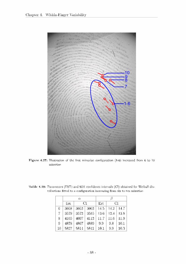
Chapter 4. Within-Finger Variability
Figure 4.27: Illustration of the �rst minutiae con�guration (1-6) increased from 6 to 10
minutiae
Table 4.18: Parameters (EST) and 95% con�dence intervals (CI) obtained for Weibull dis-
tributions �tted to a con�guration increasing from six to ten minutiae
α β
Est CI Est CI
6 3058 3053 3063 14.5 14.2 14.7
7 3579 3573 3585 13.6 13.4 13.8
8 4105 4097 4113 11.7 11.6 11.9
9 4878 4867 4889 9.9 9.8 10.1
10 5827 5814 5841 10.1 9.9 10.3
- 88 -
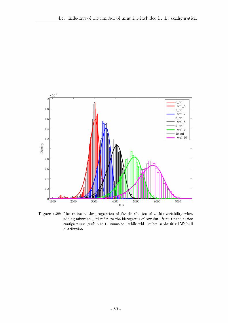
4.4. In�uence of the number of minutiae included in the con�guration
1000 2000 3000 4000 5000 6000 70000
0.2
0.4
0.6
0.8
1
1.2
1.4
1.6
1.8
2x 10
−3
Data
Den
sity
6_ori
wbl_6
7_ori
wbl_7
8_ori
wbl_8
9_ori
wbl_9
10_ori
wbl_10
Figure 4.28: Illustration of the progression of the distribution of within-variability when
adding minutiae._ori refers to the histograms of raw data from this minutiae
con�guration (with 6 to 10 minutiae), while wbl_ refers to the �tted Weibull
distribution
- 89 -
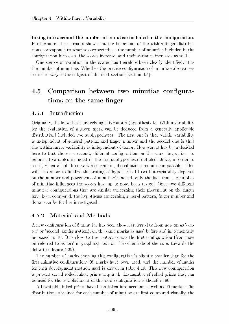
Chapter 4. Within-Finger Variability
taking into account the number of minutiae included in the con�guration.
Furthermore, these results show that the behaviour of the within-�nger distribu-
tions corresponds to what was expected: as the number of minutiae included in the
con�guration increases, the scores increase, and their variance increases as well.
One source of variation in the scores has therefore been clearly identi�ed: it is
the number of minutiae. Whether the precise con�guration of minutiae also causes
scores to vary is the subject of the next section (section 4.5).
4.5 Comparison between two minutiae con�gura-
tions on the same �nger
4.5.1 Introduction
Originally, the hypothesis underlying this chapter (hypothesis 1c: Within variability
for the evaluation of a given mark can be deduced from a generally applicable
distribution) included two subhypotheses. The �rst one is that within variability
is independent of general pattern and �nger number and the second one is that
the within �nger variability is independent of donor. However, it has been decided
here to �rst choose a second, di�erent con�guration on the same �nger, i.e. to
ignore all variables included in the two subhypotheses detailed above, in order to
see if, when all of these variables remain, distributions remain comparable. This
will also allow to �nalize the testing of hypothesis 1d (within-variability depends
on the number and placement of minutiae); indeed, only the fact that the number
of minutiae in�uences the scores has, up to now, been tested. Once two di�erent
minutiae con�gurations that are similar concerning their placement on the �nger
have been compared, the hypotheses concerning general pattern, �nger number and
donor can be further investigated.
4.5.2 Material and Methods
A new con�guration of 6 minutiae has been chosen (referred to from now on as 'cen-
ter' or 'second' con�guration), on the same marks as used before and incrementally
increased to 10. It is close to the center, as was the �rst con�guration (from now
on referred to as 'ori' in graphics), but on the other side of the core, towards the
delta (see �gure 4.29).
The number of marks showing this con�guration is slightly smaller than for the
�rst minutiae con�guration: 99 marks have been used, and the number of marks
for each development method used is shown in table 4.19. This new con�guration
is present on all rolled inked prints acquired: the number of rolled prints that can
be used for the establishment of this new con�guration is therefore 80.
All available inked prints have been taken into account as well as 99 marks. The
distributions obtained for each number of minutiae are �rst compared visually, the
- 90 -
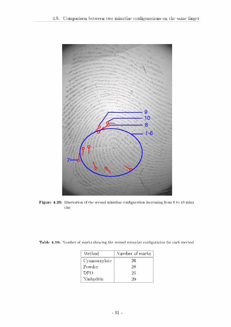
4.5. Comparison between two minutiae con�gurations on the same �nger
Figure 4.29: Illustration of the second minutiae con�guration increasing from 6 to 10 minu-
tiae
Table 4.19: Number of marks showing the second minutiae con�guration for each method
Method Number of marks
Cyanoacrylate 26
Powder 28
DFO 25
Ninhydrin 20
- 91 -
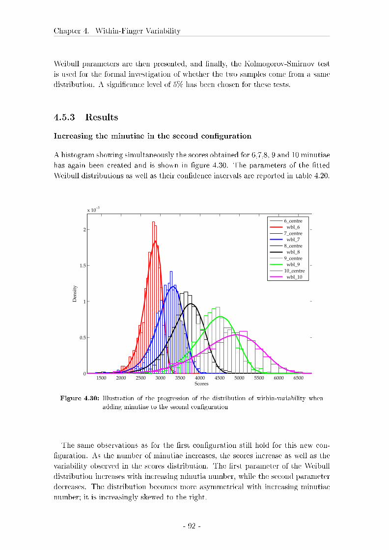
Chapter 4. Within-Finger Variability
Weibull parameters are then presented, and �nally, the Kolmogorov-Smirnov test
is used for the formal investigation of whether the two samples come from a same
distribution. A signi�cance level of 5% has been chosen for these tests.
4.5.3 Results
Increasing the minutiae in the second con�guration
A histogram showing simultaneously the scores obtained for 6,7,8, 9 and 10 minutiae
has again been created and is shown in �gure 4.30. The parameters of the �tted
Weibull distributions as well as their con�dence intervals are reported in table 4.20.
1500 2000 2500 3000 3500 4000 4500 5000 5500 6000 65000
0.5
1
1.5
2
x 10−3
Scores
Den
sity
6_centre
wbl_6
7_centre
wbl_7
8_centre
wbl_8
9_centre
wbl_9
10_centre
wbl_10
Figure 4.30: Illustration of the progression of the distribution of within-variability when
adding minutiae to the second con�guration
The same observations as for the �rst con�guration still hold for this new con-
�guration. As the number of minutiae increases, the scores increase as well as the
variability observed in the scores distribution. The �rst parameter of the Weibull
distribution increases with increasing minutia number, while the second parameter
decreases. The distribution becomes more asymmetrical with increasing minutiae
number; it is increasingly skewed to the right.
- 92 -
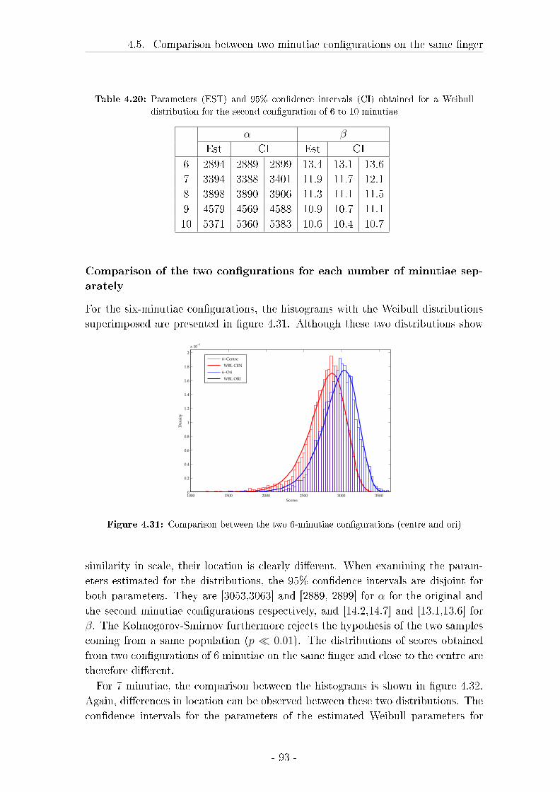
4.5. Comparison between two minutiae con�gurations on the same �nger
Table 4.20: Parameters (EST) and 95% con�dence intervals (CI) obtained for a Weibull
distribution for the second con�guration of 6 to 10 minutiae
α β
Est CI Est CI
6 2894 2889 2899 13.4 13.1 13.6
7 3394 3388 3401 11.9 11.7 12.1
8 3898 3890 3906 11.3 11.1 11.5
9 4579 4569 4588 10.9 10.7 11.1
10 5371 5360 5383 10.6 10.4 10.7
Comparison of the two con�gurations for each number of minutiae sep-
arately
For the six-minutiae con�gurations, the histograms with the Weibull distributions
superimposed are presented in �gure 4.31. Although these two distributions show
1000 1500 2000 2500 3000 35000
0.2
0.4
0.6
0.8
1
1.2
1.4
1.6
1.8
2
x 10−3
Scores
Den
sity
6−Centre
WBL CEN
6−Ori
WBL ORI
Figure 4.31: Comparison between the two 6-minutiae con�gurations (centre and ori)
similarity in scale, their location is clearly di�erent. When examining the param-
eters estimated for the distributions, the 95% con�dence intervals are disjoint for
both parameters. They are [3053,3063] and [2889, 2899] for α for the original and
the second minutiae con�gurations respectively, and [14.2,14.7] and [13.1,13.6] for
β. The Kolmogorov-Smirnov furthermore rejects the hypothesis of the two samples
coming from a same population (p � 0.01). The distributions of scores obtained
from two con�gurations of 6 minutiae on the same �nger and close to the centre are
therefore di�erent.
For 7 minutiae, the comparison between the histograms is shown in �gure 4.32.
Again, di�erences in location can be observed between these two distributions. The
con�dence intervals for the parameters of the estimated Weibull parameters for
- 93 -
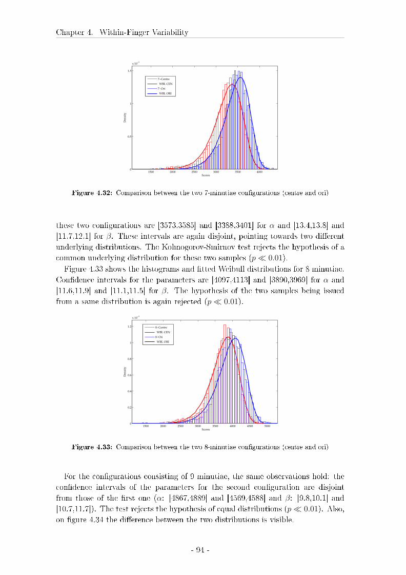
Chapter 4. Within-Finger Variability
1500 2000 2500 3000 3500 40000
0.5
1
1.5
x 10−3
Scores
Den
sity
7−Centre
WBL CEN
7−Ori
WBL ORI
Figure 4.32: Comparison between the two 7-minutiae con�gurations (centre and ori)
these two con�gurations are [3573,3585] and [3388,3401] for α and [13.4,13.8] and
[11.7,12.1] for β. These intervals are again disjoint, pointing towards two di�erent
underlying distributions. The Kolmogorov-Smirnov test rejects the hypothesis of a
common underlying distribution for these two samples (p � 0.01).
Figure 4.33 shows the histograms and �tted Weibull distributions for 8 minutiae.
Con�dence intervals for the parameters are [4097,4113] and [3890,3969] for α and
[11.6,11.9] and [11.1,11.5] for β. The hypothesis of the two samples being issued
from a same distribution is again rejected (p � 0.01).
1500 2000 2500 3000 3500 4000 4500 50000
0.2
0.4
0.6
0.8
1
1.2
x 10−3
Scores
Den
sity
8−Centre
WBL CEN
8−Ori
WBL ORI
Figure 4.33: Comparison between the two 8-minutiae con�gurations (centre and ori)
For the con�gurations consisting of 9 minutiae, the same observations hold: the
con�dence intervals of the parameters for the second con�guration are disjoint
from those of the �rst one (α: [4867,4889] and [4569,4588] and β: [9.8,10.1] and
[10.7,11.7]). The test rejects the hypothesis of equal distributions (p � 0.01). Also,
on �gure 4.34 the di�erence between the two distributions is visible.
- 94 -
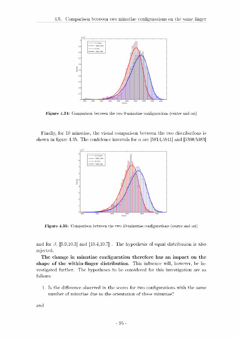
4.5. Comparison between two minutiae con�gurations on the same �nger
1500 2000 2500 3000 3500 4000 4500 5000 5500 60000
0.1
0.2
0.3
0.4
0.5
0.6
0.7
0.8
0.9
1
x 10−3
Scores
Den
sity
9−Centre
WBL CEN
9−Ori
WBL ORI
Figure 4.34: Comparison between the two 9-minutiae con�gurations (centre and ori)
Finally, for 10 minutiae, the visual comparison between the two distributions is
shown in �gure 4.35. The con�dence intervals for α are [5814,5841] and [5360,5383]
2000 3000 4000 5000 6000 70000
1
2
3
4
5
6
7
8
9
x 10−4
Scores
Den
sity
10−Centre
WBL CEN
10−Ori
WBL ORi
Figure 4.35: Comparison between the two 10-minutiae con�gurations (centre and ori)
and for β, [9.9,10.3] and [10.4,10.7] . The hypothesis of equal distribution is also
rejected.
The change in minutiae con�guration therefore has an impact on the
shape of the within-�nger distribution. This in�uence will, however, be in-
vestigated further. The hypotheses to be considered for this investigation are as
follows:
1. Is the di�erence observed in the scores for two con�gurations with the same
number of minutiae due to the orientation of these minutiae?
and
- 95 -
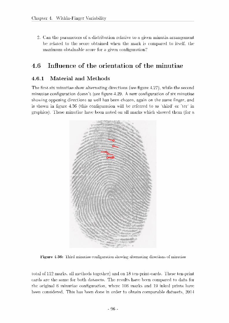
Chapter 4. Within-Finger Variability
2. Can the parameters of a distribution relative to a given minutia arrangement
be related to the score obtained when the mark is compared to itself, the
maximum obtainable score for a given con�guration?
4.6 In�uence of the orientation of the minutiae
4.6.1 Material and Methods
The �rst six minutiae show alternating directions (see �gure 4.27), while the second
minutiae con�guration doesn't (see �gure 4.29. A new con�guration of six minutiae
showing opposing directions as well has been chosen, again on the same �nger, and
is shown in �gure 4.36 (this con�guration will be referred to as 'third' or 'ter' in
graphics). These minutiae have been noted on all marks which showed them (for a
Figure 4.36: Third minutiae con�guration showing alternating directions of minutiae
total of 112 marks, all methods together) and on 18 ten-print-cards. These ten-print
cards are the same for both datasets. The results have been compared to data for
the original 6 minutiae con�guration, where 106 marks and 19 inked prints have
been considered. This has been done in order to obtain comparable datasets, 2014
- 96 -
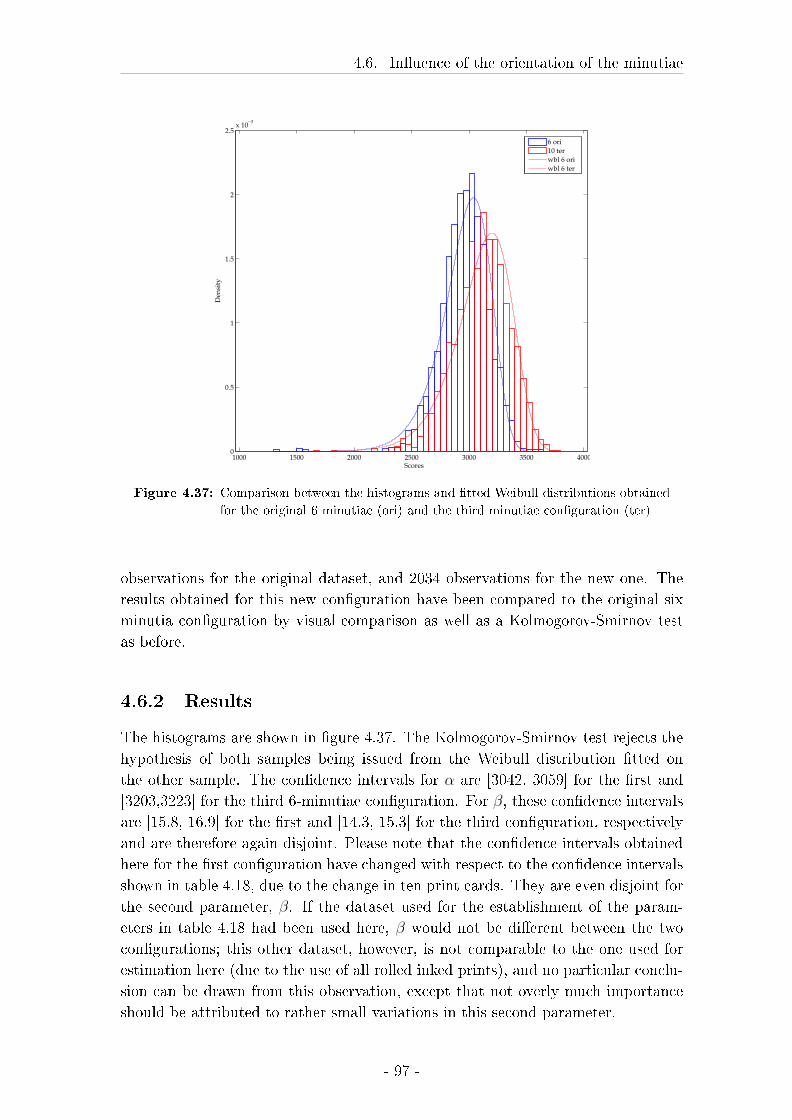
4.6. In�uence of the orientation of the minutiae
1000 1500 2000 2500 3000 3500 40000
0.5
1
1.5
2
2.5x 10
−3
Scores
Den
sity
6 ori
10 ter
wbl 6 ori
wbl 6 ter
Figure 4.37: Comparison between the histograms and �tted Weibull distributions obtained
for the original 6 minutiae (ori) and the third minutiae con�guration (ter)
observations for the original dataset, and 2034 observations for the new one. The
results obtained for this new con�guration have been compared to the original six
minutia con�guration by visual comparison as well as a Kolmogorov-Smirnov test
as before.
4.6.2 Results
The histograms are shown in �gure 4.37. The Kolmogorov-Smirnov test rejects the
hypothesis of both samples being issued from the Weibull distribution �tted on
the other sample. The con�dence intervals for α are [3042, 3059] for the �rst and
[3203,3223] for the third 6-minutiae con�guration. For β, these con�dence intervals
are [15.8, 16.9] for the �rst and [14.3, 15.3] for the third con�guration, respectively
and are therefore again disjoint. Please note that the con�dence intervals obtained
here for the �rst con�guration have changed with respect to the con�dence intervals
shown in table 4.18, due to the change in ten print cards. They are even disjoint for
the second parameter, β. If the dataset used for the establishment of the param-
eters in table 4.18 had been used here, β would not be di�erent between the two
con�gurations; this other dataset, however, is not comparable to the one used for
estimation here (due to the use of all rolled inked prints), and no particular conclu-
sion can be drawn from this observation, except that not overly much importance
should be attributed to rather small variations in this second parameter.
- 97 -
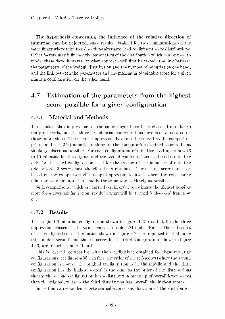
Chapter 4. Within-Finger Variability
The hypothesis concerning the in�uence of the relative direction of
minutiae can be rejected, since results obtained for two con�gurations on the
same �nger where minutiae directions alternate, lead to di�erent score distributions.
Other factors may in�uence the parameters of the distribution which can be used to
model these data; however, another approach will �rst be tested: the link between
the parameters of the Weibull distribution and the number of minutiae on one hand,
and the link between the parameters and the maximum obtainable score for a given
minutia con�guration on the other hand.
4.7 Estimation of the parameters from the highest
score possible for a given con�guration
4.7.1 Material and Methods
Three inked slap impressions of the same �nger have been chosen from the 80
ten print cards, and the three six-minutiae con�gurations have been annotated on
these impressions. These same impressions have also been used as the comparison
prints, and the (3*6) minutiae making up the con�gurations veri�ed so as to be as
similarly placed as possible. For each con�guration of minutiae used up to now (6
to 10 minutiae for the original and the second con�gurations used, and 6 minutiae
only for the third con�guration used for the testing of the in�uence of minutiae
orientation), 3 scores have therefore been obtained. These three scores are each
based on the comparison of a (slap) impression to itself, where the exact same
minutiae were annotated in exactly the same way as closely as possible.
Such comparisons, which are carried out in order to estimate the highest possible
score for a given con�guration, result in what will be termed 'self-scores' from now
on.
4.7.2 Results
The original 6-minutiae con�guration shown in �gure 4.27 resulted, for the three
impressions chosen, in the scores shown in table 4.21 under 'First'. The self-scores
of the con�guration of 6 minutiae shown in �gure 4.29 are reported in that same
table under 'Second', and the self-scores for the third con�guration (shown in �gure
4.36) are reported under 'Third'.
This is, overall, compatible with the distributions obtained for these minutiae
con�gurations (see �gure 4.38). In fact, the order of the self-scores (where the second
con�guration is lowest, the original con�guration is in the middle and the third
con�guration has the highest scores) is the same as the order of the distributions
shown: the second con�guration has a distribution made up of overall lower scores
than the original, whereas the third distribution has, overall, the highest scores.
Since this correspondence between self-scores and location of the distribution
- 98 -
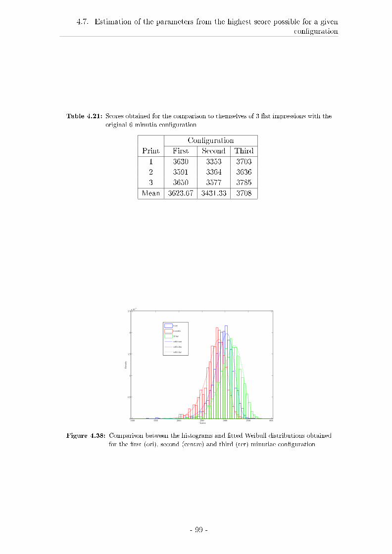
4.7. Estimation of the parameters from the highest score possible for a givencon�guration
Table 4.21: Scores obtained for the comparison to themselves of 3 �at impressions with the
original 6 minutia con�guration
Con�guration
Print First Second Third
1 3630 3353 3703
2 3591 3364 3636
3 3650 3577 3785
Mean 3623.67 3431.33 3708
1000 1500 2000 2500 3000 3500 40000
0.5
1
1.5
2
2.5x 10
−3
Scores
Den
sity
6 ori
6 centre
10 ter
wbl 6 ori
wbl 6 bis
wbl 6 ter
Figure 4.38: Comparison between the histograms and �tted Weibull distributions obtained
for the �rst (ori), second (centre) and third (ter) minutiae con�guration
- 99 -
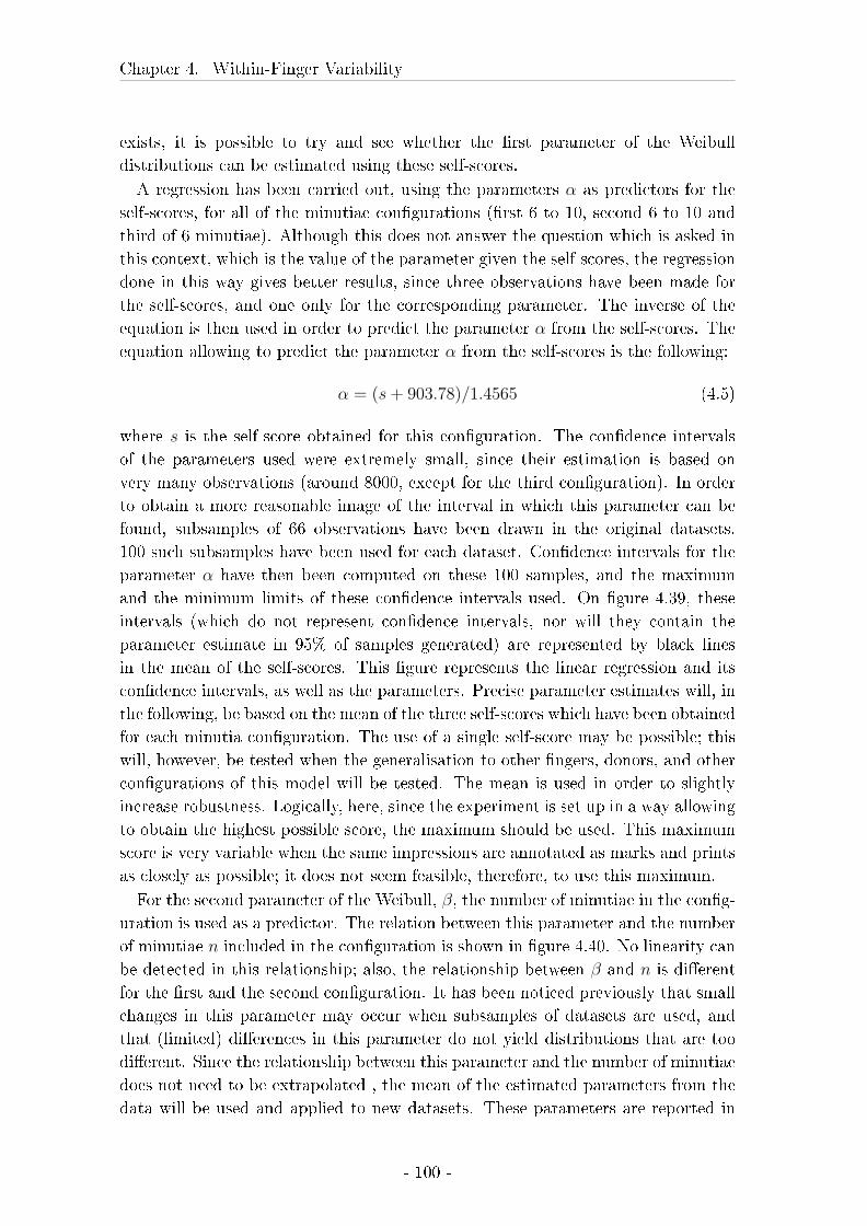
Chapter 4. Within-Finger Variability
exists, it is possible to try and see whether the �rst parameter of the Weibull
distributions can be estimated using these self-scores.
A regression has been carried out, using the parameters α as predictors for the
self-scores, for all of the minutiae con�gurations (�rst 6 to 10, second 6 to 10 and
third of 6 minutiae). Although this does not answer the question which is asked in
this context, which is the value of the parameter given the self-scores, the regression
done in this way gives better results, since three observations have been made for
the self-scores, and one only for the corresponding parameter. The inverse of the
equation is then used in order to predict the parameter α from the self-scores. The
equation allowing to predict the parameter α from the self-scores is the following:
α = (s + 903.78)/1.4565 (4.5)
where s is the self-score obtained for this con�guration. The con�dence intervals
of the parameters used were extremely small, since their estimation is based on
very many observations (around 8000, except for the third con�guration). In order
to obtain a more reasonable image of the interval in which this parameter can be
found, subsamples of 66 observations have been drawn in the original datasets.
100 such subsamples have been used for each dataset. Con�dence intervals for the
parameter α have then been computed on these 100 samples, and the maximum
and the minimum limits of these con�dence intervals used. On �gure 4.39, these
intervals (which do not represent con�dence intervals, nor will they contain the
parameter estimate in 95% of samples generated) are represented by black lines
in the mean of the self-scores. This �gure represents the linear regression and its
con�dence intervals, as well as the parameters. Precise parameter estimates will, in
the following, be based on the mean of the three self-scores which have been obtained
for each minutia con�guration. The use of a single self-score may be possible; this
will, however, be tested when the generalisation to other �ngers, donors, and other
con�gurations of this model will be tested. The mean is used in order to slightly
increase robustness. Logically, here, since the experiment is set up in a way allowing
to obtain the highest possible score, the maximum should be used. This maximum
score is very variable when the same impressions are annotated as marks and prints
as closely as possible; it does not seem feasible, therefore, to use this maximum.
For the second parameter of the Weibull, β, the number of minutiae in the con�g-
uration is used as a predictor. The relation between this parameter and the number
of minutiae n included in the con�guration is shown in �gure 4.40. No linearity can
be detected in this relationship; also, the relationship between β and n is di�erent
for the �rst and the second con�guration. It has been noticed previously that small
changes in this parameter may occur when subsamples of datasets are used, and
that (limited) di�erences in this parameter do not yield distributions that are too
di�erent. Since the relationship between this parameter and the number of minutiae
does not need to be extrapolated , the mean of the estimated parameters from the
data will be used and applied to new datasets. These parameters are reported in
- 100 -
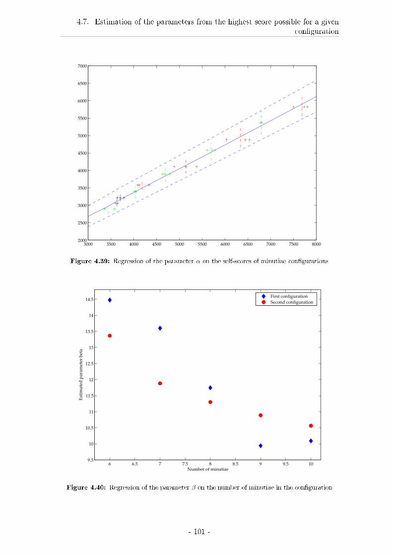
4.7. Estimation of the parameters from the highest score possible for a givencon�guration
3000 3500 4000 4500 5000 5500 6000 6500 7000 7500 80002000
2500
3000
3500
4000
4500
5000
5500
6000
6500
7000
Figure 4.39: Regression of the parameter α on the self-scores of minutiae con�gurations
6 6.5 7 7.5 8 8.5 9 9.5 109.5
10
10.5
11
11.5
12
12.5
13
13.5
14
14.5
Number of minutiae
Est
imat
ed p
aram
eter
bet
a
First configuration
Second configuration
Figure 4.40: Regression of the parameter β on the number of minutiae in the con�guration
- 101 -
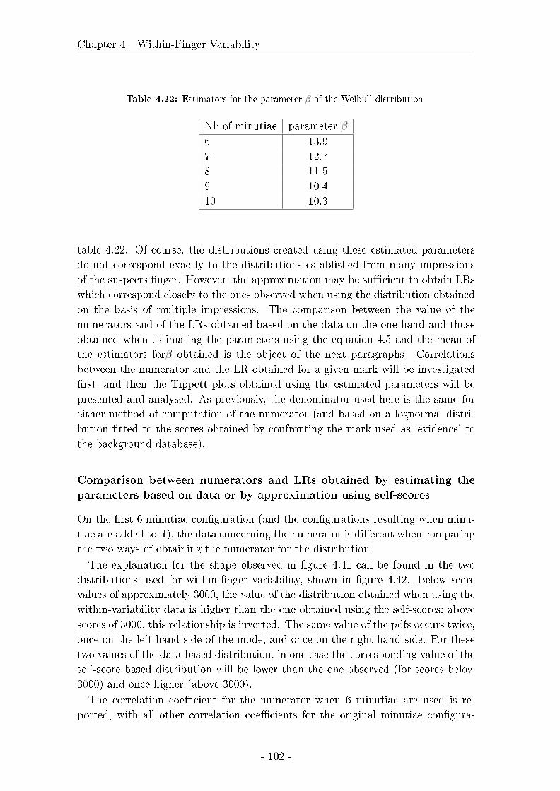
Chapter 4. Within-Finger Variability
Table 4.22: Estimators for the parameter β of the Weibull distribution
Nb of minutiae parameter β
6 13.9
7 12.7
8 11.5
9 10.4
10 10.3
table 4.22. Of course, the distributions created using these estimated parameters
do not correspond exactly to the distributions established from many impressions
of the suspects �nger. However, the approximation may be su�cient to obtain LRs
which correspond closely to the ones observed when using the distribution obtained
on the basis of multiple impressions. The comparison between the value of the
numerators and of the LRs obtained based on the data on the one hand and those
obtained when estimating the parameters using the equation 4.5 and the mean of
the estimators forβ obtained is the object of the next paragraphs. Correlations
between the numerator and the LR obtained for a given mark will be investigated
�rst, and then the Tippett plots obtained using the estimated parameters will be
presented and analysed. As previously, the denominator used here is the same for
either method of computation of the numerator (and based on a lognormal distri-
bution �tted to the scores obtained by confronting the mark used as 'evidence' to
the background database).
Comparison between numerators and LRs obtained by estimating the
parameters based on data or by approximation using self-scores
On the �rst 6 minutiae con�guration (and the con�gurations resulting when minu-
tiae are added to it), the data concerning the numerator is di�erent when comparing
the two ways of obtaining the numerator for the distribution.
The explanation for the shape observed in �gure 4.41 can be found in the two
distributions used for within-�nger variability, shown in �gure 4.42. Below score
values of approximately 3000, the value of the distribution obtained when using the
within-variability data is higher than the one obtained using the self-scores; above
scores of 3000, this relationship is inverted. The same value of the pdfs occurs twice,
once on the left hand side of the mode, and once on the right hand side. For these
two values of the data-based distribution, in one case the corresponding value of the
self-score based distribution will be lower than the one observed (for scores below
3000) and once higher (above 3000).
The correlation coe�cient for the numerator when 6 minutiae are used is re-
ported, with all other correlation coe�cients for the original minutiae con�gura-
- 102 -
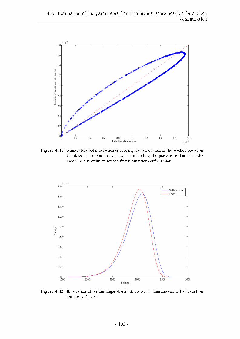
4.7. Estimation of the parameters from the highest score possible for a givencon�guration
0 0.2 0.4 0.6 0.8 1 1.2 1.4 1.6 1.8
x 10−3
0
0.2
0.4
0.6
0.8
1
1.2
1.4
1.6
1.8x 10
−3
Data based estimation
Esti
ma
tio
n b
ased
on
self
−sco
res
Figure 4.41: Numerators obtained when estimating the parameters of the Weibull based on
the data on the abscissa and when estimating the parameters based on the
model on the ordinate for the �rst 6-minutiae con�guration
1500 2000 2500 3000 3500 40000
0.2
0.4
0.6
0.8
1
1.2
1.4
1.6
1.8x 10
−3
Scores
Den
sity
Self−scores
Data
Figure 4.42: Illustration of within-�nger distributions for 6 minutiae estimated based on
data or self-scores
- 103 -
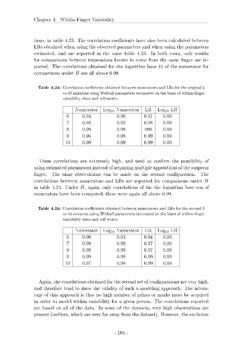
Chapter 4. Within-Finger Variability
tions, in table 4.23. The correlation coe�cients have also been calculated between
LRs obtained when using the observed parameters and when using the parameters
estimated, and are reported in the same table 4.23. In both cases, only results
for comparisons between impressions known to come from the same �nger are re-
ported. The correlations obtained for the logarithm base 10 of the numerator for
comparisons under H̄ are all above 0.99.
Table 4.23: Correlation coe�cients obtained between numerators and LRs for the original 6
to 10 minutiae using Weibull parameters estimated on the basis of within-�nger
variability data and self-scores
Numerator Log10 Numerator LR Log10 LR
6 0.94 0.96 0.97 0.99
7 0.88 0.92 0.98 0.99
8 0.99 0.99 098 0.99
9 0.96 0.98 0.99 0.99
10 0.99 0.99 0.99 0.99
These correlations are extremely high, and tend to con�rm the possibility of
using estimated parameters instead of acquiring multiple appositions of the suspects
�nger. The same observations can be made on the second con�guration. The
correlations between numerators and LRs are reported for comparisons under H
in table 4.24. Under H̄, again, only correlations of the the logarithm base ten of
numerators have been computed; these were again all above 0.99.
Table 4.24: Correlation coe�cients obtained between numerators and LRs for the second 6
to 10 minutiae using Weibull parameters estimated on the basis of within-�nger
variability data and self-scores
Numerator Log10 Numerator LR Log10 LR
6 0.90 0.93 0.94 0.98
7 0.99 0.99 0.97 0.99
8 0.98 0.99 0.97 0.99
9 0.99 0.99 0.99 0.99
10 0.97 0.98 0.99 0.99
Again, the correlations obtained for the second set of con�gurations are very high,
and therefore tend to show the validity of such a modeling approach. The advan-
tage of this approach is that no high number of prints or marks must be acquired
in order to model within variability for a given person. The correlations reported
are based on all of the data. In some of the datasets, very high observations are
present (outliers, which are very far away from the dataset). However, the exclusion
- 104 -
4.7. Estimation of the parameters from the highest score possible for a givencon�guration
of these data has been investigated in order to examine their in�uence on the corre-
lation coe�cient, and, even though the correlation decreases when excluding those
highest observations, it does not lower much when the log10 of the results are con-
sidered (from 1 to 0.99, for the second 10 minutia con�guration, where the 9 highest
observations had been excluded). This is also why the logarithms of numerators
have been preferred for the comparisons under H̄. It is indeed in these compar-
isons, where numerators need to be computed in the extreme tails of distributions,
that the largest di�erences were expected. However, it can now be con�rmed that
the order of magnitude between numerators (and consequently LRs) computed on
the basis of the approximation or estimations from data correspond, at least in
order of magnitude. The Tippett plots for the original con�guration, between 6
and 10 minutiae, are included below, juxtaposed with the Tippett plots where the
parameter estimates are based on the data.
These results show that, based on 3 slap impressions from one �nger,
within �nger variability can be estimated in an e�cient and not very
time-consuming way. While this approach has, up to now, been estab-
lished and tested on data from a single �nger, the results are promis-
ing. Tests have been carried out and are presented in the appendix and a further
chapter (appendix A and chapter 6) on another donor. It is possible that using
self-scores in this way, within-variability can be estimated without time-consuming
data-acquisition. If the approximation using self-scores holds for another donor,
within-variability is indeed a generalizable distribution, but only when taking into
account the selectivity of the con�guration used. This selectivity is here substituted
by the maximum score obtainable for that con�guration, which itself is approxi-
mated by using the AFIS to compare twice the same impression (and, for stability
of the measure, by taking the mean of 3 scores obtained in this fashion).
The application of parameter estimation from self-scores to two �ngers of another
donor (D2) is presented in Appendix A. Overall, the detailed evaluation of the
e�ect of the use of the approximation on the numerator, and therefore on the LRs
obtained, has shown that this approximation, although far from ideal, has very high
probabilities of yielding very similar values as the estimation based on the data for
both the donor on whose �nger the model is established, as well as for another
donor; generalizability is therefore possible. The results on donor 2 (presented in
Appendix A do show some problems, but generally, large divergences between the
approximated numerator values and those obtained from the data have a rather low
probability of occurring. Improvements to this approximation could certainly lower
the probability of obtaining numerator values that di�er by more than an order of
magnitude from what should be obtained, as seen from the data. The advantages
of direct modeling of these parameters will be discussed in detail in the general
discussion in chapter 7. Also, more work on the use of these approximated values is
presented at the end of the chapter on between variability, where the e�ect of the
approximations used on likelihood ratios is tested.
- 105 -
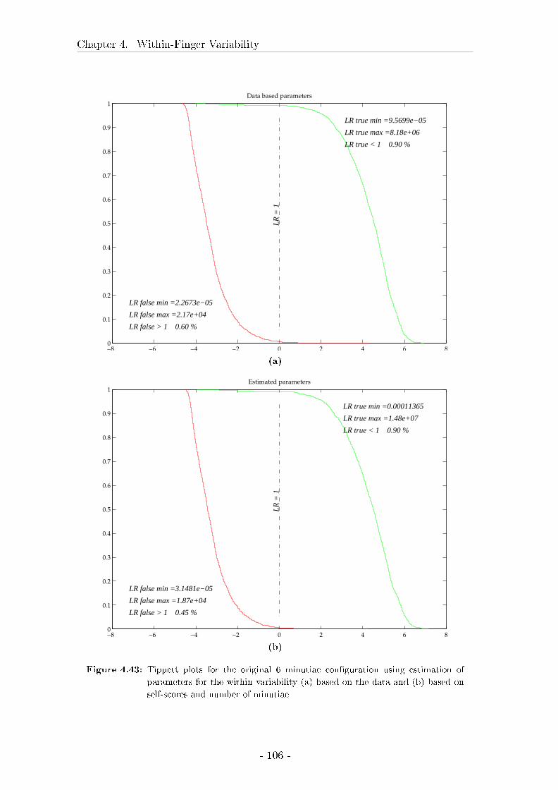
Chapter 4. Within-Finger Variability
−8 −6 −4 −2 0 2 4 6 80
0.1
0.2
0.3
0.4
0.5
0.6
0.7
0.8
0.9
1Data based parameters
LR true min =9.5699e−05
LR true max =8.18e+06
LR true < 1 0.90 %
LR false max =2.17e+04
LR false min =2.2673e−05
LR false > 1 0.60 %
LR
= 1
(a)
−8 −6 −4 −2 0 2 4 6 80
0.1
0.2
0.3
0.4
0.5
0.6
0.7
0.8
0.9
1Estimated parameters
LR true min =0.00011365
LR true max =1.48e+07
LR true < 1 0.90 %
LR false max =1.87e+04
LR false min =3.1481e−05
LR false > 1 0.45 %
LR
= 1
(b)
Figure 4.43: Tippett plots for the original 6 minutiae con�guration using estimation of
parameters for the within variability (a) based on the data and (b) based on
self-scores and number of minutiae
- 106 -
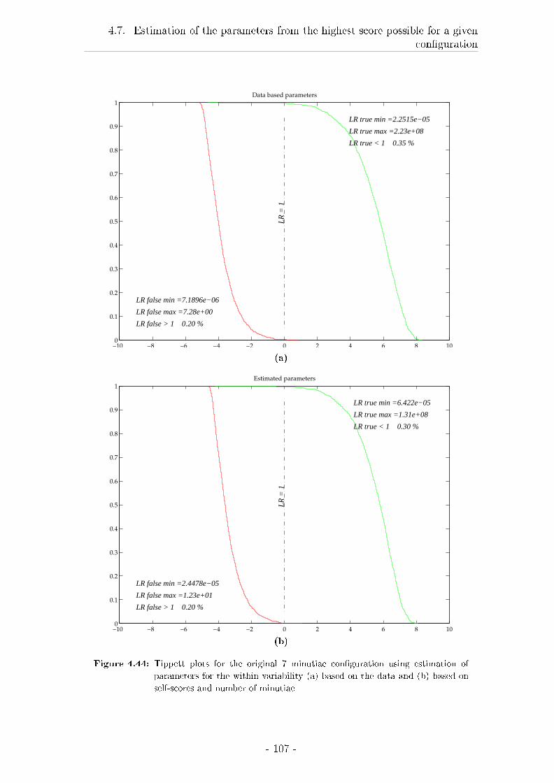
4.7. Estimation of the parameters from the highest score possible for a givencon�guration
−10 −8 −6 −4 −2 0 2 4 6 8 100
0.1
0.2
0.3
0.4
0.5
0.6
0.7
0.8
0.9
1Data based parameters
LR true min =2.2515e−05
LR true max =2.23e+08
LR true < 1 0.35 %
LR false max =7.28e+00
LR false min =7.1896e−06
LR false > 1 0.20 %
LR
= 1
(a)
−10 −8 −6 −4 −2 0 2 4 6 8 100
0.1
0.2
0.3
0.4
0.5
0.6
0.7
0.8
0.9
1Estimated parameters
LR true min =6.422e−05
LR true max =1.31e+08
LR true < 1 0.30 %
LR false max =1.23e+01
LR false min =2.4478e−05
LR false > 1 0.20 %
LR
= 1
(b)
Figure 4.44: Tippett plots for the original 7 minutiae con�guration using estimation of
parameters for the within variability (a) based on the data and (b) based on
self-scores and number of minutiae
- 107 -
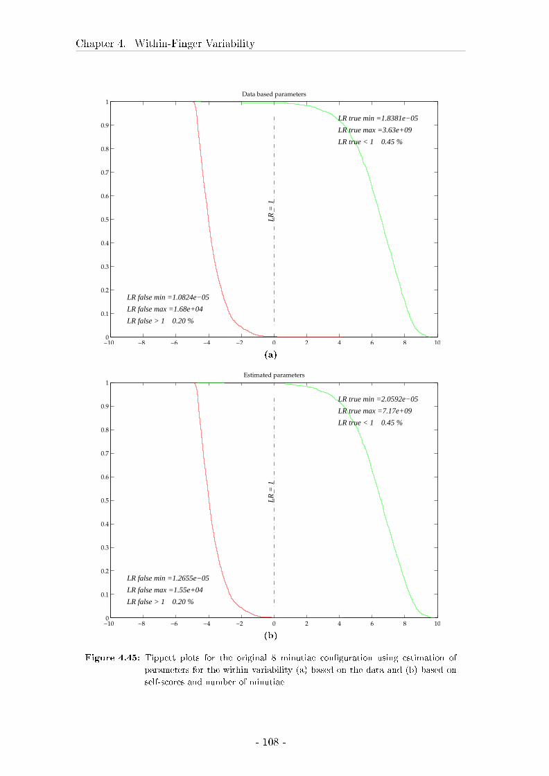
Chapter 4. Within-Finger Variability
−10 −8 −6 −4 −2 0 2 4 6 8 100
0.1
0.2
0.3
0.4
0.5
0.6
0.7
0.8
0.9
1Data based parameters
LR true min =1.8381e−05
LR true max =3.63e+09
LR true < 1 0.45 %
LR false max =1.68e+04
LR false min =1.0824e−05
LR false > 1 0.20 %
LR
= 1
(a)
−10 −8 −6 −4 −2 0 2 4 6 8 100
0.1
0.2
0.3
0.4
0.5
0.6
0.7
0.8
0.9
1Estimated parameters
LR true min =2.0592e−05
LR true max =7.17e+09
LR true < 1 0.45 %
LR false max =1.55e+04
LR false min =1.2655e−05
LR false > 1 0.20 %
LR
= 1
(b)
Figure 4.45: Tippett plots for the original 8 minutiae con�guration using estimation of
parameters for the within variability (a) based on the data and (b) based on
self-scores and number of minutiae
- 108 -
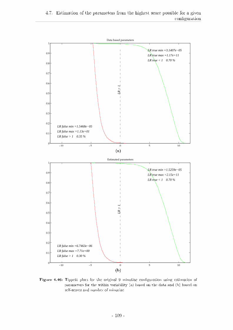
4.7. Estimation of the parameters from the highest score possible for a givencon�guration
−10 −5 0 5 100
0.1
0.2
0.3
0.4
0.5
0.6
0.7
0.8
0.9
1Data based parameters
LR true min =3.1407e−05
LR true max =1.17e+11
LR true < 1 0.70 %
LR false max =1.13e+01
LR false min =1.5468e−05
LR false > 1 0.35 %
LR
= 1
(a)
−10 −5 0 5 100
0.1
0.2
0.3
0.4
0.5
0.6
0.7
0.8
0.9
1Estimated parameters
LR true min =1.5259e−05
LR true max =2.15e+11
LR true < 1 0.70 %
LR false max =7.71e+00
LR false min =6.7463e−06
LR false > 1 0.30 %
LR
= 1
(b)
Figure 4.46: Tippett plots for the original 9 minutiae con�guration using estimation of
parameters for the within variability (a) based on the data and (b) based on
self-scores and number of minutiae
- 109 -
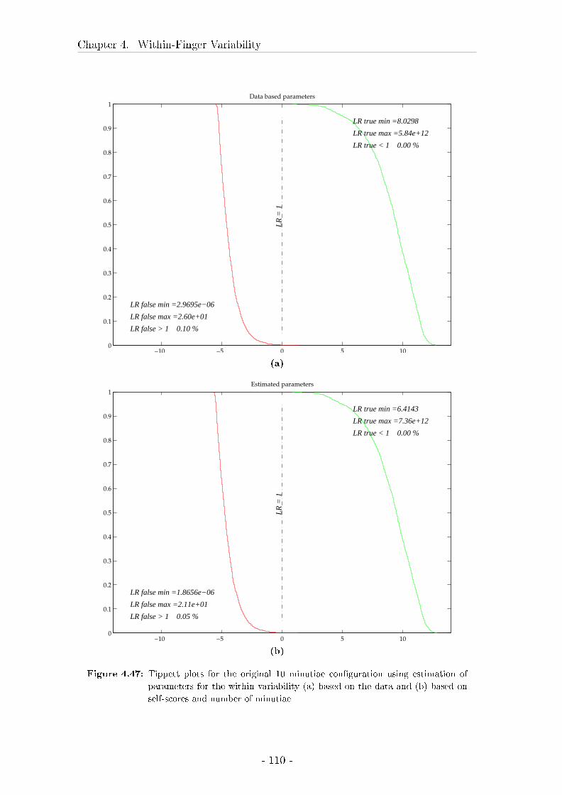
Chapter 4. Within-Finger Variability
−10 −5 0 5 100
0.1
0.2
0.3
0.4
0.5
0.6
0.7
0.8
0.9
1Data based parameters
LR true min =8.0298
LR true max =5.84e+12
LR true < 1 0.00 %
LR false max =2.60e+01
LR false min =2.9695e−06
LR false > 1 0.10 %
LR
= 1
(a)
−10 −5 0 5 100
0.1
0.2
0.3
0.4
0.5
0.6
0.7
0.8
0.9
1Estimated parameters
LR true min =6.4143
LR true max =7.36e+12
LR true < 1 0.00 %
LR false max =2.11e+01
LR false min =1.8656e−06
LR false > 1 0.05 %
LR
= 1
(b)
Figure 4.47: Tippett plots for the original 10 minutiae con�guration using estimation of
parameters for the within variability (a) based on the data and (b) based on
self-scores and number of minutiae
- 110 -

4.7. Estimation of the parameters from the highest score possible for a givencon�guration
The between-�nger modeling used here, in order to obtain distribution values,
does not truly allow a very precise estimation. Only the distribution of one mark
has been used; in a casework scenario, this mark would be known, here, it is not.
Therefore, these probabilities of obtaining scores above or below a certain value,
while allowing to form a general idea of the probability of exceeding a limit, is not
precise.
- 111 -

Chapter 5
Between-Finger Variability
5.1 Introduction
In order to be able to model the between-�nger variability, the same questions
need to be answered as those asked for the within-�nger variability. First of all, a
su�cient sample size needs to be determined, if this is possible with the dataset
available. Then, the main questions to be answered are whether the distribution
of scores obtained changes when only given general patterns or �nger numbers are
used. Of course, again, it needs to be investigated whether the between-�nger
distribution is dependent on the number and placement of minutiae: this time, this
investigation is possibly less relevant from an operational point of view. It may,
however, yield insights into the generalization possibilities of the distribution. It
may be interesting operationally not having to extract all of the comparison scores
of a mark to be evaluated when it is inserted into the database, then to �t a density
function to these scores, in order to obtain the value of f(s|H̄), but rather to have a
generally applicable density (or family of functions) that can be employed directly.
Not to �t a function to the data and only use observed frequencies is not a viable
option. This is due to the fact that scores in the regions where LRs will generally be
computed, in particular when H is actually true, are extremely scarce. The reason
why LRs lend support to one or the other hypothesis is that observations are very
improbable under one of the two hypotheses. The only way of not �tting a function
and computing LRs is to use the proportion of observations at a given score, and to
use some chosen constant for any score that hasn't been observed in the database,
such as 1/n, where n is the number of �ngerprints in the database. This would result
in the same probability for a score which is just above the highest score observed
and a score that is, for example, 1000 above the highest observed score. This is
not an approach which is considered rational here, since the probability decreases
with increasing scores (above the mode of the distribution). This would therefore
lead to unreasonably low LRs in support of H. Furthermore, while the extraction
of all scores when comparing a given mark to the whole database is possible with
the AFIS used here, this is due to a custom-made function (see B) allowing this
automated extraction of all scores when a mark is compared to the whole database.
- 113 -
Chapter 5. Between-Finger Variability
This is already an extension of 'normal' AFIS systems.
For these reasons, it is considered essential to �t a probability density function
to the between-�nger variability, and to try to reduce the data that needs to be
acquired for the estimation of this function.
The ten print cards used in this thesis as a reference database are those that
have been excluded from the Swiss central database when the central repository
was purged (in function of the age of the donor). Within the central database,
there are several sections: not only suspects' (and convicts') �ngerprints but also
immigrants' �ngerprints; it is not known whether the ten-print cards used come
from both databases, or are suspects' prints only. Not much is known about these
�ngerprints; they were excluded before the year 2003, when they were received at
the University of Lausanne; when exactly they were inserted, excluded and whether
the donors present are more frequently of particular ethnic groups than the general
population is unknown, but likely due to the evolution of the Swiss population over
the second half of the 20th century. A large majority of donors is male, however,
since tenprints of females are designated using a color code; otherwise, the tenprint
cards are totally anonymous.
For this reason, the frequencies of general patterns (as classi�ed automatically by
the system) are compared to frequencies previously published in the literature (see
chapter 5.2 below).
5.2 Description of the general patterns present in
the database
5.2.1 Material and methods
Here, the general patterns attributed automatically by the system have been used.
Four general patterns are used by the system: Right and left loop, whorl and arch;
an 'unknown' category is also used. The system automatically extracts ridge �ow,
and determines the placement of the centre and the delta(s); general pattern is then
attributed, most probably based on this information. Again, the way in which gen-
eral patterns are determined by the system is based on proprietary algorithms. The
system over-classi�es general patterns. This means that several general patterns
are attributed to some �ngers, so as not to exclude a part of the database from a
search based on an erroneous information. Indeed, it is far from trivial to attribute
general patterns to �ngerprints in an automated way. Therefore, rather than to risk
excluding a potential candidate print wrongly based on general pattern information,
all general patterns that the system considers to be possible given the character-
istics of a print, are saved. Frequencies of general patterns when not excluding
over-classi�ed prints are presented in table 5.1; here, every time a �nger has been
classi�ed as a given general pattern it has been considered as being of this pattern,
regardless of whether there was over-classi�cation of that pattern. This means that
- 114 -
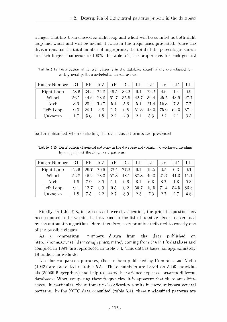
5.2. Description of the general patterns present in the database
a �nger that has been classed as right loop and whorl will be counted as both right
loop and whorl and will be included twice in the frequencies presented. Since the
divisor remains the total number of �ngerprints, the total of the percentages shown
for each �nger is superior to 100%. In table 5.2, the proportions for each general
Table 5.1: Distribution of general patterns in the database counting the over-classed for
each general pattern included in classi�cations
Finger Number RT RF RM RR RL LT LF LM LR LL
Right Loop 48.6 34.3 74.8 49.5 83.2 0.4 23.2 4.6 1.4 0.9
Whorl 56.1 44.6 28.0 61.7 35.6 42.7 39.4 25.5 48.9 27.7
Arch 3.9 20.4 12.7 5.4 5.6 5.4 21.4 16.3 7.2 7.7
Left Loop 0.5 26.1 3.6 1.7 0.8 61.3 43.3 75.9 64.3 87.4
Unknown 1.7 5.6 1.8 2.2 2.9 2.1 5.3 2.2 2.1 3.5
pattern obtained when excluding the over-classed prints are presented.
Table 5.2: Distribution of general patterns in the database not counting overclassed dividing
by uniquely attributed general patterns
Finger Number RT RF RM RR RL LT LF LM LR LL
Right Loop 43.6 26.7 70.6 38.4 77.2 0.1 10.5 0.5 0.3 0.1
Whorl 52.8 45.2 23.3 57.3 18.1 37.8 40.3 21.7 41.3 11.1
Arch 1.6 7.9 3.0 1.1 0.6 3.1 6.3 3.7 1.3 0.8
Left Loop 0.1 12.7 0.9 0.5 0.2 56.7 10.5 71.4 54.5 83.3
Unknown 1.8 7.5 2.2 2.7 3.9 2.3 7.3 2.7 2.7 4.8
Finally, in table 5.3, in presence of over-classi�cation, the print in question has
been counted to be within the �rst class in the list of possible classes determined
by the automatic algorithm. Here, therefore, each print is attributed to exactly one
of the possible classes.
As a comparison, numbers drawn from the data published on
http://home.att.net/ dermatoglyphics/mfre/, coming from the FBI's database and
compiled in 1993, are reproduced in table 5.4. This data is based on approximately
18 million individuals.
Also for comparison purposes, the numbers published by Cummins and Midlo
(1943) are presented in table 5.5. These numbers are based on 5000 individu-
als (50000 �ngerprints) and help to assess the variance expected between di�erent
databases. When comparing these frequencies, it is apparent that there are di�er-
ences. In particular, the automatic classi�cation results in more unknown general
patterns. In the NCIC data consulted (table 5.4), these unclassi�ed patterns are
- 115 -
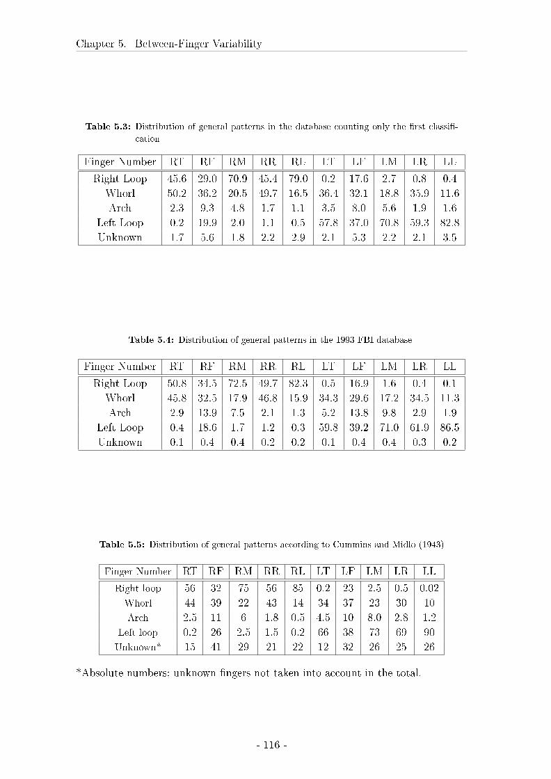
Chapter 5. Between-Finger Variability
Table 5.3: Distribution of general patterns in the database counting only the �rst classi�-
cation
Finger Number RT RF RM RR RL LT LF LM LR LL
Right Loop 45.6 29.0 70.9 45.4 79.0 0.2 17.6 2.7 0.8 0.4
Whorl 50.2 36.2 20.5 49.7 16.5 36.4 32.1 18.8 35.9 11.6
Arch 2.3 9.3 4.8 1.7 1.1 3.5 8.0 5.6 1.9 1.6
Left Loop 0.2 19.9 2.0 1.1 0.5 57.8 37.0 70.8 59.3 82.8
Unknown 1.7 5.6 1.8 2.2 2.9 2.1 5.3 2.2 2.1 3.5
Table 5.4: Distribution of general patterns in the 1993 FBI database
Finger Number RT RF RM RR RL LT LF LM LR LL
Right Loop 50.8 34.5 72.5 49.7 82.3 0.5 16.9 1.6 0.4 0.1
Whorl 45.8 32.5 17.9 46.8 15.9 34.3 29.6 17.2 34.5 11.3
Arch 2.9 13.9 7.5 2.1 1.3 5.2 13.8 9.8 2.9 1.9
Left Loop 0.4 18.6 1.7 1.2 0.3 59.8 39.2 71.0 61.9 86.5
Unknown 0.1 0.4 0.4 0.2 0.2 0.1 0.4 0.4 0.3 0.2
Table 5.5: Distribution of general patterns according to Cummins and Midlo (1943)
Finger Number RT RF RM RR RL LT LF LM LR LL
Right loop 56 32 75 56 85 0.2 23 2.5 0.5 0.02
Whorl 44 39 22 43 14 34 37 23 30 10
Arch 2.5 11 6 1.8 0.5 4.5 10 8.0 2.8 1.2
Left loop 0.2 26 2.5 1.5 0.2 66 38 73 69 90
Unknown* 15 41 29 21 22 12 32 26 25 26
*Absolute numbers; unknown �ngers not taken into account in the total.
- 116 -
5.3. Evaluation of sample size
missing or amputated �ngers as well as completely scarred patterns (NCIC Codes
XX and SR). In the automatically classi�ed data used here (tables 5.1, 5.2 and 5.3),
instances where the program considers all patterns possible are included in the 'un-
known' class. Similar proportions of patterns are obtained when comparing either
the over-classed for each pattern, or when taking into account only the �rst pattern
in case of over-classi�cation, to the FBI data. The FBI data used here is based on
males only, while the data in the system contains all ten print cards received from
the Swiss central database. Very few females are present, however, therefore this
cannot explain the di�erence observed.
The three tables established from the data used in the present thesis (tables 5.1,
5.2 and 5.3) show some divergences; in particular, when over-classi�ed �ngerprints
are not taken into account, fewer loops are obtained than when either all classes
are counted or when only the �rst pattern is counted. When all classi�cations are
counted, more whorls are present than when either over-classi�cations are excluded
or only the �rst classi�cation is taken into account.
Generally, the percentages obtained here are not completely divergent from the
previously published data. Some large di�erences are, however, present. In right
thumbs, here, more whorls than loops are detected, while both in the FBI database
and the database published by Cummins and Midlo (1943), more right loops than
whorls are present, for example. Trends are preserved (i.e. most radial loops are
found on fore�ngers with respect to the other �nger numbers), and di�erences are
similar in size as those observed between the two previously published data sources.
The �rst classi�cations are retained for further use, since they seem to be the least
dissimilar from this previously published data. This may indicate that the clas-
si�cations attributed to each �ngerprint are ordered in the sense that the most
probable general pattern is in the �rst place when using the automatic classi�cation
algorithm.
The di�erences between the general patterns in the presently used data
and the previously published works do not invalidate the use of our data,
since the relative frequencies of general patterns are comparable. This
database will therefore be considered as a random sample of �ngerprints
from a population of suspects, and be used as such.
5.3 Evaluation of sample size
5.3.1 Material and Methods
Images
The data used are the images of the right thumb of donor 1 that have already
been employed for the description of the within variability. These images are of
�ngermarks developed using DFO, Ninhydrin, dusting and Cyanoacrylate. As a
database, a maximum of 685'245 inked �ngerprints are used. These �ngerprints
- 117 -
Chapter 5. Between-Finger Variability
come from a little more than 68'524 ten print cards. The exact number of ten-
print cards is of 68543; this is not exactly the number of �ngerprints divided by 10,
because some of the ten print cards do not show all ten �ngers due to amputation
or momentary lesions. Such events result in scores of 0 and have been excluded
from the analyses. It is considered that they do not need to be considered in the
between �nger distribution.
Con�gurations
The same con�gurations as for the within variability of Donor 1 have been used.
These con�gurations are:
• The �rst con�guration, increasing from 6 to 10 minutiae, shown in �gure 4.27.
• A second con�guration, increasing from 6 to 10 minutiae, shown in �gure 4.29.
The scores �nally used are those issued from these 10 di�erent con�gurations,
divided by development method, compared to the database of �ngerprints.
Methods
Subsamples of the whole database have, as in section 4.2 where the sample size
for within variability was determined, been used. QQ-plots have been established
in order to investigate which minimum sample size allows the estimation of the
distribution of scores in a robust manner. It is, of course, possible that the overall
sample size, of 685245, is insu�cient, and that stability is therefore not attained.
This investigation will be carried out on the basis of one mark compared to the
database.
In a second step, the Kolmogorov-Smirnov test for the comparison of the distri-
bution of two samples has been used in order to assess whether two samples of a
given size result in acceptance of the hypothesis of equal distribution. Also, the
evolution of the test statistic, t = max(|F1(x) − F2(x)|), as a function of sample
size has been studied.
5.3.2 Results
First, successively smaller samples have been compared using QQ-plots. The plot
comparing two samples of 5353 observations is shown in �gure 5.1. The correspon-
dence between these two samples is very near perfect, leading to the conclusion
that this sample size is su�cient. It was then decided, since only few of the possible
QQ-plots for this sample size can be analysed, to take a more automated approach.
Divisors were chosen between 2 and 2048 (in steps of 2, resulting in sample
sizes of between 342622 and 335 scores). Then, two random samples of the overall
size divided by the divisor were drawn, and these samples were compared using
a Kolmogorov-Smirnov two sample test. The test statistic has then been plotted
- 118 -
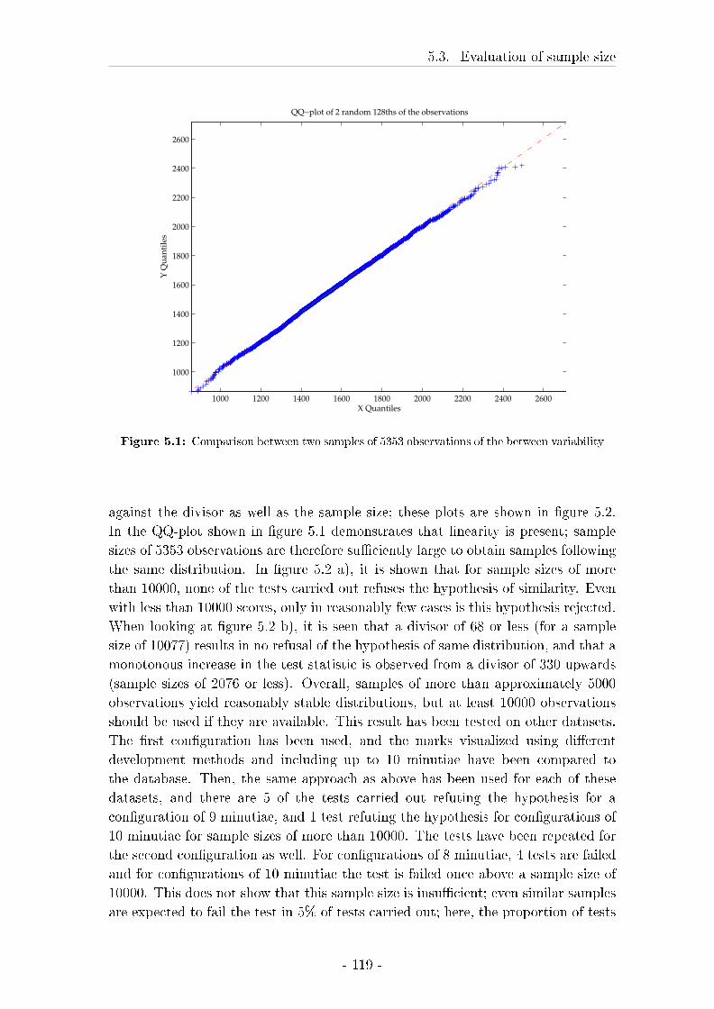
5.3. Evaluation of sample size
1000 1200 1400 1600 1800 2000 2200 2400 2600
1000
1200
1400
1600
1800
2000
2200
2400
2600
X Quantiles
Y Q
uan
tile
s
QQ−plot of 2 random 128ths of the observations
Figure 5.1: Comparison between two samples of 5353 observations of the between variability
against the divisor as well as the sample size; these plots are shown in �gure 5.2.
In the QQ-plot shown in �gure 5.1 demonstrates that linearity is present; sample
sizes of 5353 observations are therefore su�ciently large to obtain samples following
the same distribution. In �gure 5.2 a), it is shown that for sample sizes of more
than 10000, none of the tests carried out refuses the hypothesis of similarity. Even
with less than 10000 scores, only in reasonably few cases is this hypothesis rejected.
When looking at �gure 5.2 b), it is seen that a divisor of 68 or less (for a sample
size of 10077) results in no refusal of the hypothesis of same distribution, and that a
monotonous increase in the test statistic is observed from a divisor of 330 upwards
(sample sizes of 2076 or less). Overall, samples of more than approximately 5000
observations yield reasonably stable distributions, but at least 10000 observations
should be used if they are available. This result has been tested on other datasets.
The �rst con�guration has been used, and the marks visualized using di�erent
development methods and including up to 10 minutiae have been compared to
the database. Then, the same approach as above has been used for each of these
datasets, and there are 5 of the tests carried out refuting the hypothesis for a
con�guration of 9 minutiae, and 1 test refuting the hypothesis for con�gurations of
10 minutiae for sample sizes of more than 10000. The tests have been repeated for
the second con�guration as well. For con�gurations of 8 minutiae, 4 tests are failed
and for con�gurations of 10 minutiae the test is failed once above a sample size of
10000. This does not show that this sample size is insu�cient; even similar samples
are expected to fail the test in 5% of tests carried out; here, the proportion of tests
- 119 -
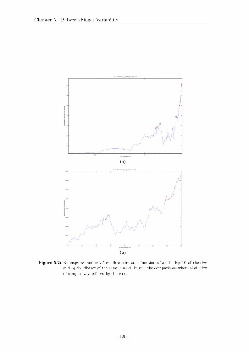
Chapter 5. Between-Finger Variability
104
105
0.01
0.02
0.03
0.04
0.05
0.06
0.07
KS Test Statistics against log sample size
Log of sample size
Ko
lmo
go
rov
Sm
irn
ov
Tes
t S
tati
stic
(a)
0 50 100 150 200 250 300 350 4000
0.01
0.02
0.03
0.04
0.05
0.06
0.07
0.08
Divisor of sample size
KS
tes
t st
atis
tic
for
2 sa
mp
les
KS Test Statistics against parts of the sample
(b)
Figure 5.2: Kolmogorov-Smirnov Test Statistics as a function of a) the log 10 of the size
and b) the divisor of the sample used. In red, the comparisons where similarity
of samples was refuted by the test.
- 120 -
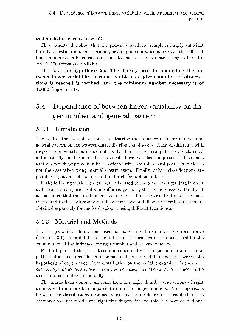
5.4. Dependence of between �nger variability on �nger number and generalpattern
that are failed remains below 5%.
These results also show that the presently available sample is largely su�cient
for reliable estimation. Furthermore, meaningful comparisons between the di�erent
�nger numbers can be carried out, since for each of these datasets (�ngers 1 to 10),
over 68500 scores are available.
Therefore, the hypothesis 2a: The density used for modelling the be-
tween �nger variability becomes stable as a given number of observa-
tions is reached is veri�ed, and the minimum number necessary is of
10000 �ngerprints.
5.4 Dependence of between �nger variability on �n-
ger number and general pattern
5.4.1 Introduction
The goal of the present section is to describe the in�uence of �nger number and
general pattern on the between-�nger distribution of scores. A major di�erence with
respect to previously published data is that here, the general patterns are classi�ed
automatically; furthermore, there is so-called overclassi�cation present. This means
that a given �ngerprint may be associated with several general patterns, which is
not the case when using manual classi�cation. Finally, only 4 classi�cations are
possible: right and left loop, whorl and arch (as well as unknown).
In the following section, a distribution is �tted to the between-�nger data in order
to be able to compare results on di�erent general patterns more easily. Finally, it
is considered that the development technique used for the visualization of the mark
confronted to the background database may have an in�uence; therefore results are
obtained separately for marks developed using di�erent techniques.
5.4.2 Material and Methods
The images and con�gurations used as marks are the same as described above
(section 5.3.1). As a database, the full set of ten print cards has been used for the
examination of the in�uence of �nger number and general pattern.
For both parts of the present section, concerned with �nger number and general
pattern, it is considered that as soon as a distributional di�erence is discovered, the
hypothesis of dependence of the distribution on the variable examined is shown. If
such a dependence exists, even in only some cases, then the variable will need to be
taken into account systematically.
The marks from donor 1 all come from her right thumb: observations of right
thumbs will therefore be compared to the other �nger numbers. No comparisons
between the distributions obtained when such a mark from the right thumb is
compared to right middle and right ring �ngers, for example, has been carried out.
- 121 -
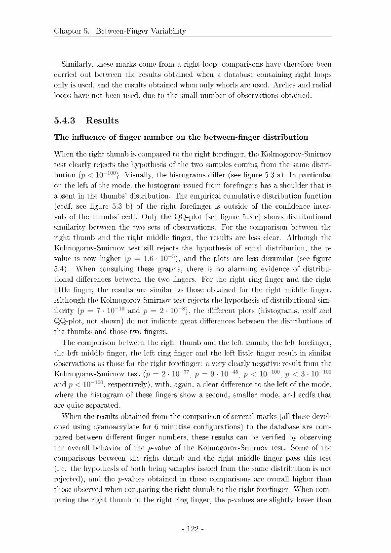
Chapter 5. Between-Finger Variability
Similarly, these marks come from a right loop; comparisons have therefore been
carried out between the results obtained when a database containing right loops
only is used, and the results obtained when only whorls are used. Arches and radial
loops have not been used, due to the small number of observations obtained.
5.4.3 Results
The in�uence of �nger number on the between-�nger distribution
When the right thumb is compared to the right fore�nger, the Kolmogorov-Smirnov
test clearly rejects the hypothesis of the two samples coming from the same distri-
bution (p < 10−100). Visually, the histograms di�er (see �gure 5.3 a). In particular
on the left of the mode, the histogram issued from fore�ngers has a shoulder that is
absent in the thumbs' distribution. The empirical cumulative distribution function
(ecdf, see �gure 5.3 b) of the right fore�nger is outside of the con�dence inter-
vals of the thumbs' ecdf. Only the QQ-plot (see �gure 5.3 c) shows distributional
similarity between the two sets of observations. For the comparison between the
right thumb and the right middle �nger, the results are less clear. Although the
Kolmogorov-Smirnov test sill rejects the hypothesis of equal distribution, the p-
value is now higher (p = 1.6 · 10−5), and the plots are less dissimilar (see �gure
5.4). When consulting these graphs, there is no alarming evidence of distribu-
tional di�erences between the two �ngers. For the right ring �nger and the right
little �nger, the results are similar to those obtained for the right middle �nger.
Although the Kolmogorov-Smirnov test rejects the hypothesis of distributional sim-
ilarity (p = 7 · 10−10 and p = 2 · 10−8), the di�erent plots (histograms, ecdf and
QQ-plot, not shown) do not indicate great di�erences between the distributions of
the thumbs and those two �ngers.
The comparison between the right thumb and the left thumb, the left fore�nger,
the left middle �nger, the left ring �nger and the left little �nger result in similar
observations as those for the right fore�nger: a very clearly negative result from the
Kolmogorov-Smirnov test (p = 2 · 10−77, p = 9 · 10−45, p < 10−100, p < 3 · 10−100
and p < 10−100, respectively), with, again, a clear di�erence to the left of the mode,
where the histogram of these �ngers show a second, smaller mode, and ecdfs that
are quite separated.
When the results obtained from the comparison of several marks (all those devel-
oped using cyanoacrylate for 6 minutiae con�gurations) to the database are com-
pared between di�erent �nger numbers, these results can be veri�ed by observing
the overall behavior of the p-value of the Kolmogorov-Smirnov test. Some of the
comparisons between the right thumb and the right middle �nger pass this test
(i.e. the hypothesis of both being samples issued from the same distribution is not
rejected), and the p-values obtained in these comparisons are overall higher than
those observed when comparing the right thumb to the right fore�nger. When com-
paring the right thumb to the right ring �nger, the p-values are slightly lower than
- 122 -
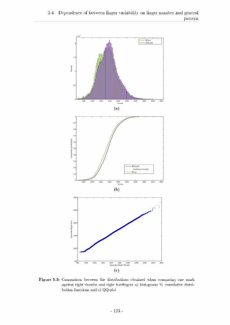
5.4. Dependence of between �nger variability on �nger number and generalpattern
1000 1200 1400 1600 1800 2000 2200 2400 2600 28000
0.5
1
1.5
2
x 10−3
Scores
Den
sity
RFore
RThumb
(a)
1000 1200 1400 1600 1800 2000 2200 2400 2600 28000
0.1
0.2
0.3
0.4
0.5
0.6
0.7
0.8
0.9
1
Scores
Cu
mu
lati
ve
pro
bab
ilit
y
RThumb
confidence bounds
RFore
(b)
800 1000 1200 1400 1600 1800 2000 2200 2400 2600 2800500
1000
1500
2000
2500
3000
Quantiles Right Thumb
Qu
anti
les
Rig
ht
Fo
re
(c)
Figure 5.3: Comparison between the distributions obtained when comparing one mark
against right thumbs and right fore�ngers a) histograms b) cumulative distri-
bution functions and c) QQ-plot
- 123 -
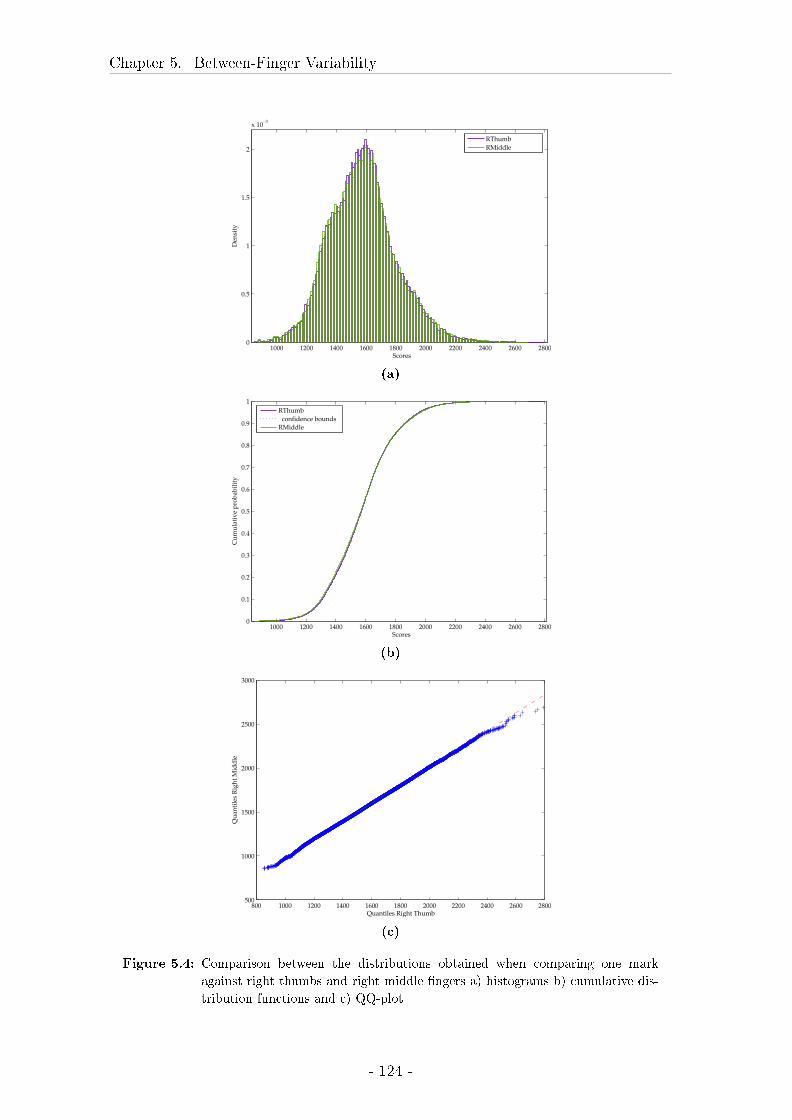
Chapter 5. Between-Finger Variability
1000 1200 1400 1600 1800 2000 2200 2400 2600 28000
0.5
1
1.5
2
x 10−3
Scores
Den
sity
RThumb
RMiddle
(a)
1000 1200 1400 1600 1800 2000 2200 2400 2600 28000
0.1
0.2
0.3
0.4
0.5
0.6
0.7
0.8
0.9
1
Scores
Cu
mu
lati
ve
pro
bab
ilit
y
RThumb
confidence bounds
RMiddle
(b)
800 1000 1200 1400 1600 1800 2000 2200 2400 2600 2800500
1000
1500
2000
2500
3000
Quantiles Right Thumb
Qu
anti
les
Rig
ht
Mid
dle
(c)
Figure 5.4: Comparison between the distributions obtained when comparing one mark
against right thumbs and right middle �ngers a) histograms b) cumulative dis-
tribution functions and c) QQ-plot
- 124 -
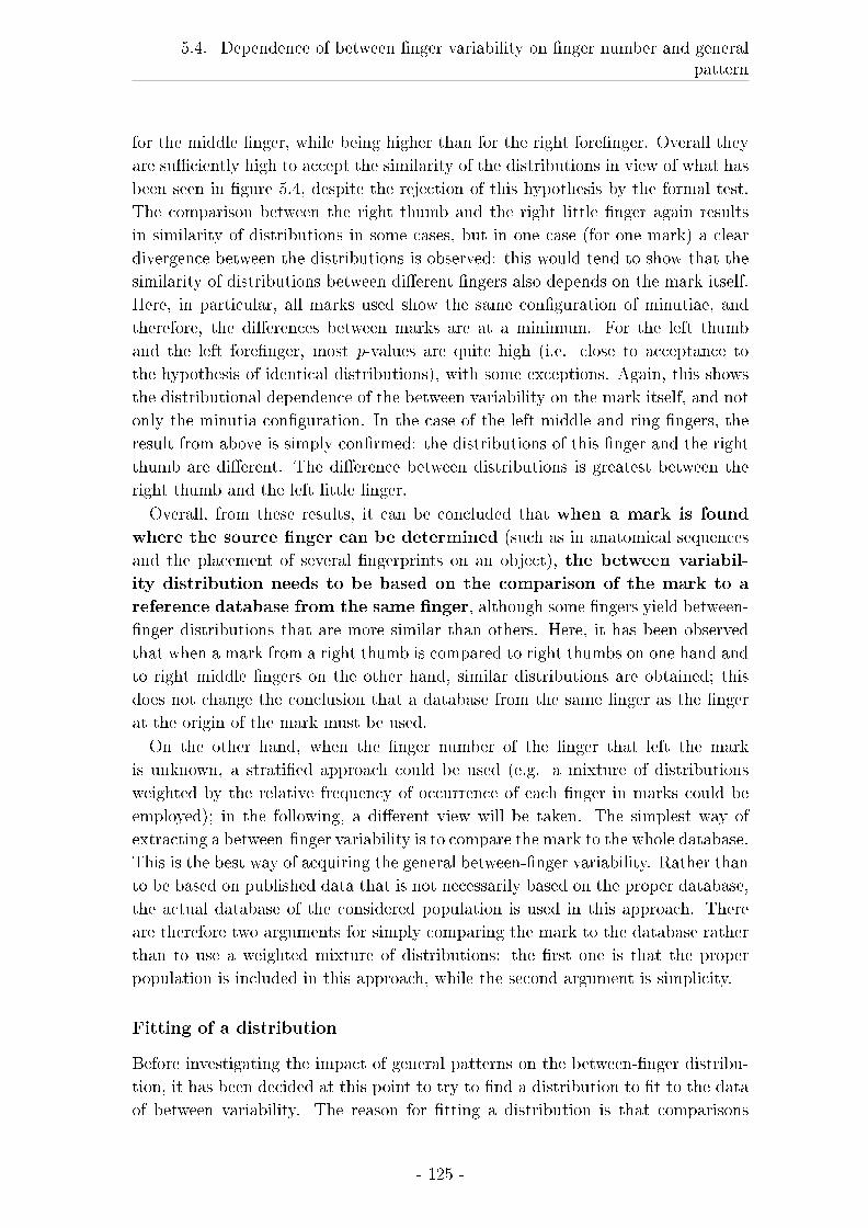
5.4. Dependence of between �nger variability on �nger number and generalpattern
for the middle �nger, while being higher than for the right fore�nger. Overall they
are su�ciently high to accept the similarity of the distributions in view of what has
been seen in �gure 5.4, despite the rejection of this hypothesis by the formal test.
The comparison between the right thumb and the right little �nger again results
in similarity of distributions in some cases, but in one case (for one mark) a clear
divergence between the distributions is observed: this would tend to show that the
similarity of distributions between di�erent �ngers also depends on the mark itself.
Here, in particular, all marks used show the same con�guration of minutiae, and
therefore, the di�erences between marks are at a minimum. For the left thumb
and the left fore�nger, most p-values are quite high (i.e. close to acceptance to
the hypothesis of identical distributions), with some exceptions. Again, this shows
the distributional dependence of the between variability on the mark itself, and not
only the minutia con�guration. In the case of the left middle and ring �ngers, the
result from above is simply con�rmed: the distributions of this �nger and the right
thumb are di�erent. The di�erence between distributions is greatest between the
right thumb and the left little �nger.
Overall, from these results, it can be concluded that when a mark is found
where the source �nger can be determined (such as in anatomical sequences
and the placement of several �ngerprints on an object), the between variabil-
ity distribution needs to be based on the comparison of the mark to a
reference database from the same �nger, although some �ngers yield between-
�nger distributions that are more similar than others. Here, it has been observed
that when a mark from a right thumb is compared to right thumbs on one hand and
to right middle �ngers on the other hand, similar distributions are obtained; this
does not change the conclusion that a database from the same �nger as the �nger
at the origin of the mark must be used.
On the other hand, when the �nger number of the �nger that left the mark
is unknown, a strati�ed approach could be used (e.g. a mixture of distributions
weighted by the relative frequency of occurrence of each �nger in marks could be
employed); in the following, a di�erent view will be taken. The simplest way of
extracting a between-�nger variability is to compare the mark to the whole database.
This is the best way of acquiring the general between-�nger variability. Rather than
to be based on published data that is not necessarily based on the proper database,
the actual database of the considered population is used in this approach. There
are therefore two arguments for simply comparing the mark to the database rather
than to use a weighted mixture of distributions: the �rst one is that the proper
population is included in this approach, while the second argument is simplicity.
Fitting of a distribution
Before investigating the impact of general patterns on the between-�nger distribu-
tion, it has been decided at this point to try to �nd a distribution to �t to the data
of between variability. The reason for �tting a distribution is that comparisons
- 125 -
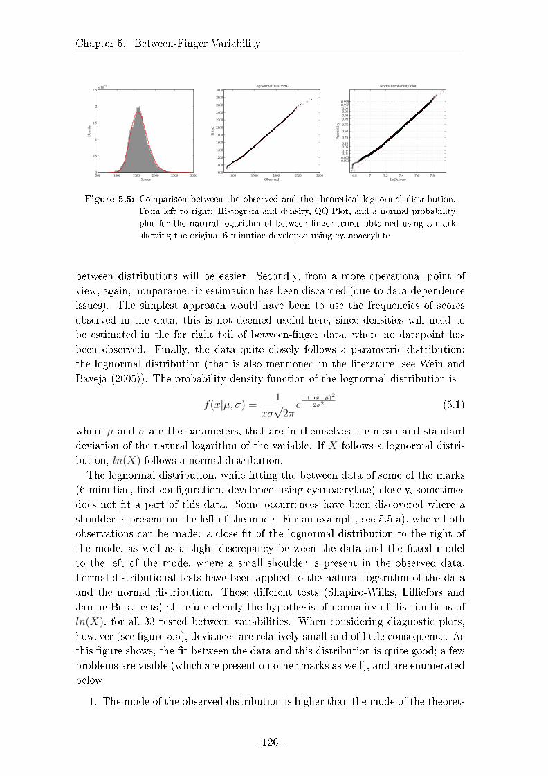
Chapter 5. Between-Finger Variability
500 1000 1500 2000 2500 30000
0.5
1
1.5
2
2.5x 10
−3
Scores
Den
sity
1000 1500 2000 2500 3000800
1000
1200
1400
1600
1800
2000
2200
2400
2600
2800
3000
Observed
Fit
ted
LogNormal: R=0.99942
6.8 7 7.2 7.4 7.6 7.8
0.0010.0030.01 0.02 0.05 0.10
0.25
0.50
0.75
0.90 0.95 0.98 0.99
0.9970.999
Ln(Scores)
Pro
bab
ilit
y
Normal Probability Plot
Figure 5.5: Comparison between the observed and the theoretical lognormal distribution.
From left to right: Histogram and density, QQ-Plot, and a normal probability
plot for the natural logarithm of between-�nger scores obtained using a mark
showing the original 6-minutiae developed using cyanoacrylate
between distributions will be easier. Secondly, from a more operational point of
view, again, nonparametric estimation has been discarded (due to data-dependence
issues). The simplest approach would have been to use the frequencies of scores
observed in the data; this is not deemed useful here, since densities will need to
be estimated in the far right tail of between-�nger data, where no datapoint has
been observed. Finally, the data quite closely follows a parametric distribution:
the lognormal distribution (that is also mentioned in the literature, see Wein and
Baveja (2005)). The probability density function of the lognormal distribution is
f(x|µ, σ) =1
xσ√
2πe−(lnx−µ)2
2σ2 (5.1)
where µ and σ are the parameters, that are in themselves the mean and standard
deviation of the natural logarithm of the variable. If X follows a lognormal distri-
bution, ln(X) follows a normal distribution.
The lognormal distribution, while �tting the between data of some of the marks
(6 minutiae, �rst con�guration, developed using cyanoacrylate) closely, sometimes
does not �t a part of this data. Some occurrences have been discovered where a
shoulder is present on the left of the mode. For an example, see 5.5 a), where both
observations can be made: a close �t of the lognormal distribution to the right of
the mode, as well as a slight discrepancy between the data and the �tted model
to the left of the mode, where a small shoulder is present in the observed data.
Formal distributional tests have been applied to the natural logarithm of the data
and the normal distribution. These di�erent tests (Shapiro-Wilks, Lilliefors and
Jarque-Bera tests) all refute clearly the hypothesis of normality of distributions of
ln(X), for all 33 tested between variabilities. When considering diagnostic plots,
however (see �gure 5.5), deviances are relatively small and of little consequence. As
this �gure shows, the �t between the data and this distribution is quite good; a few
problems are visible (which are present on other marks as well), and are enumerated
below:
1. The mode of the observed distribution is higher than the mode of the theoret-
- 126 -
5.4. Dependence of between �nger variability on �nger number and generalpattern
ical distribution. This di�erence may lead to the rejection of the hypothesis
that this data follows a lognormal distribution. Here, this di�erence is not
large enough to completely ignore this model for the data; indeed, at worst,
the di�erence in density observed is of a fraction of an order of magnitude.
2. On the QQ- and the normal probability plots, a deviation in the left tail is
visible. It concerns less than 1% of the data, and should not have an in�uence
on casework LRs that is of any consequence, since it concerns very small
scores. Generally, casework LRs are expected to be in the right tail of the
between-�nger distribution.
3. Small deviations are also present in the right tail, as evidenced again in the
QQ- and probability plots. These deviations are small enough to be reasonable
if the data is actually issued from a lognormal distribution.
The lognormal distribution also has many advantages, in particular as compared
to another approach that was considered, the mixture of normal distributions: �rst
of all, the lognormal distribution only models positive values, and the scores used
here are strictly positive (after the elimination of zeros due to �ngers that are
absent or to scarred for analysis). The use of a distribution that is de�ned in
the positive domain avoids truncating a distribution that includes zeros, or even
negative numbers. Secondly, the lognormal distribution is skewed to the left, i.e.
the tail where normally evidential scores will need to be evaluated is heavier than the
left tail, which is bounded. This not only corresponds well to the data as evidenced
by the quantile plots, but also has the advantage of letting this tail taper out slowly,
not yielding extremely small denominators of the LR too quickly. The goodness of
�t has also been tested on marks showing the �rst six-minutiae con�guration but
developed using the other methods (DFO, ninhydrin and powder). Examples of the
�ts obtained are shown in �gure 5.6. The lognormal distribution is, �nally,
accepted as a good model for the data.
For each development method, the parameters of the lognormal have been esti-
mated for all marks (still for the original con�guration of 6 minutiae). In �gure 5.7,
the estimated parameter µ is plotted for all marks developed using cyanoacrylate
with it's con�dence interval, once for the database of right thumbs showing right
loops only, and once when the mark in question is compared to the whole database
(all �ngers, all general patterns). We can see that �rst of all, the �rst parameter
(µ) estimated for the di�erent marks varies over and above what is included in
the con�dence intervals obtained for these marks. This shows an e�ect due to the
mark itself: even when the minutia con�guration (and therefore the �nger number,
general pattern, placement on the �nger and number of minutiae) and development
method remain constant, di�erent distributions are obtained for di�erent impres-
sions. The value of this parameter does not vary much, however; taking into account
that the estimation is based on 31224 observations for right loops on right thumbs,
the con�dence intervals are extremely small. On the other hand, it is observed that
- 127 -
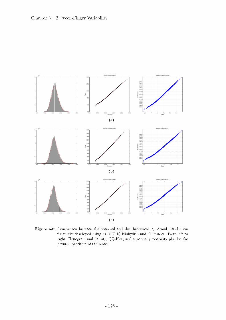
Chapter 5. Between-Finger Variability
500 1000 1500 2000 2500 30000
0.5
1
1.5
2
2.5x 10
−3
500 1000 1500 2000 2500 3000500
1000
1500
2000
2500
3000
Observed
Fit
ted
LogNormal: R=0.99917
6.8 7 7.2 7.4 7.6 7.8
0.0010.003
0.01 0.02
0.05 0.10
0.25
0.50
0.75
0.90 0.95
0.98 0.99
0.9970.999
Data
Pro
bab
ilit
y
Normal Probability Plot
(a)
500 1000 1500 2000 2500 30000
0.5
1
1.5
2
2.5x 10
−3
500 1000 1500 2000 2500 3000800
1000
1200
1400
1600
1800
2000
2200
2400
2600
2800
Observed
Fit
ted
LogNormal: R=0.99935
6.8 7 7.2 7.4 7.6 7.8
0.0010.003
0.01 0.02 0.05 0.10
0.25
0.50
0.75
0.90 0.95 0.98 0.99
0.9970.999
Data
Pro
bab
ilit
y
Normal Probability Plot
(b)
500 1000 1500 2000 2500 30000
0.5
1
1.5
2
2.5x 10
−3
500 1000 1500 2000 2500 3000800
1000
1200
1400
1600
1800
2000
2200
2400
2600
2800
Observed
Fit
ted
LogNormal: R=0.99893
6.8 7 7.2 7.4 7.6 7.8
0.0010.0030.01 0.02 0.05 0.10
0.25
0.50
0.75
0.90 0.95 0.98 0.99 0.9970.999
Data
Pro
bab
ilit
y
Normal Probability Plot
(c)
Figure 5.6: Comparison between the observed and the theoretical lognormal distribution
for marks developed using a) DFO b) Ninhydrin and c) Powder. From left to
right: Histogram and density, QQ-Plot, and a normal probability plot for the
natural logarithm of the scores
- 128 -
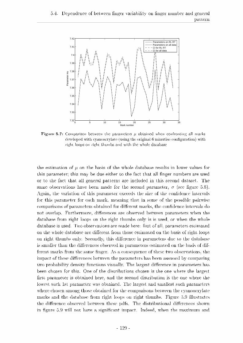
5.4. Dependence of between �nger variability on �nger number and generalpattern
0 5 10 15 20 25 30 357.32
7.33
7.34
7.35
7.36
7.37
7.38
7.39
7.4
7.41
7.42
Mark number
Par
amet
er m
u
Parameters on RL RTParameters on all dataCI for RL RTCI for all data
Figure 5.7: Comparison between the parameters µ obtained when confronting all marks
developed with cyanoacrylate (using the original 6 minutiae con�guration) with
right loops on right thumbs and with the whole database
the estimation of µ on the basis of the whole database results in lower values for
this parameter; this may be due either to the fact that all �nger numbers are used
or to the fact that all general patterns are included in this second dataset. The
same observations have been made for the second parameter, σ (see �gure 5.8).
Again, the variation of this parameter exceeds the size of the con�dence intervals
for this parameter for each mark, meaning that in some of the possible pairwise
comparisons of parameters obtained for di�erent marks, the con�dence intervals do
not overlap. Furthermore, di�erences are observed between parameters when the
database from right loops on the right thumbs only is is used, or when the whole
database is used. Two observations are made here: �rst of all, parameters estimated
on the whole database are di�erent from those estimated on the basis of right loops
on right thumbs only. Secondly, this di�erence in parameters due to the database
is smaller than the di�erences observed in parameters estimated on the basis of dif-
ferent marks from the same �nger. As a consequence of these two observations, the
impact of these di�erences between the parameters has been assessed by comparing
two probability density functions visually. The largest di�erence in parameters has
been chosen for this. One of the distributions chosen is the one where the largest
�rst parameter is obtained here, and the second distribution is the one where the
lowest such 1st parameter was obtained. The largest and smallest such parameters
where chosen among those obtained for the comparisons between the cyanoacrylate
marks and the database from right loops on right thumbs. Figure 5.9 illustrates
the di�erence observed between these pdfs. The distributional di�erences shown
in �gure 5.9 will not have a signi�cant impact. Indeed, when the maximum and
- 129 -
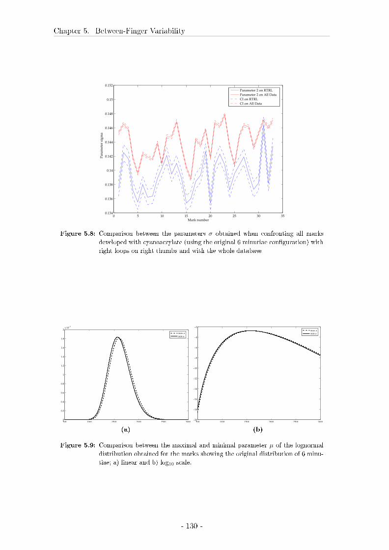
Chapter 5. Between-Finger Variability
0 5 10 15 20 25 30 350.134
0.136
0.138
0.14
0.142
0.144
0.146
0.148
0.15
0.152
Mark number
Par
amet
er s
igm
a
Parameter 2 on RTRL
Parameter 2 on All Data
CI on RTRL
CI on All Data
Figure 5.8: Comparison between the parameters σ obtained when confronting all marks
developed with cyanoacrylate (using the original 6 minutiae con�guration) with
right loops on right thumbs and with the whole database
500 1000 1500 2000 2500 30000
0.2
0.4
0.6
0.8
1
1.2
1.4
1.6
1.8
2x 10
−3
max a
min a
(a)
500 1000 1500 2000 2500 3000−20
−18
−16
−14
−12
−10
−8
−6
−4
−2
max a
min a
(b)
Figure 5.9: Comparison between the maximal and minimal parameter µ of the lognormal
distribution obtained for the marks showing the original distribution of 6 minu-
tiae; a) linear and b) log10 scale.
- 130 -
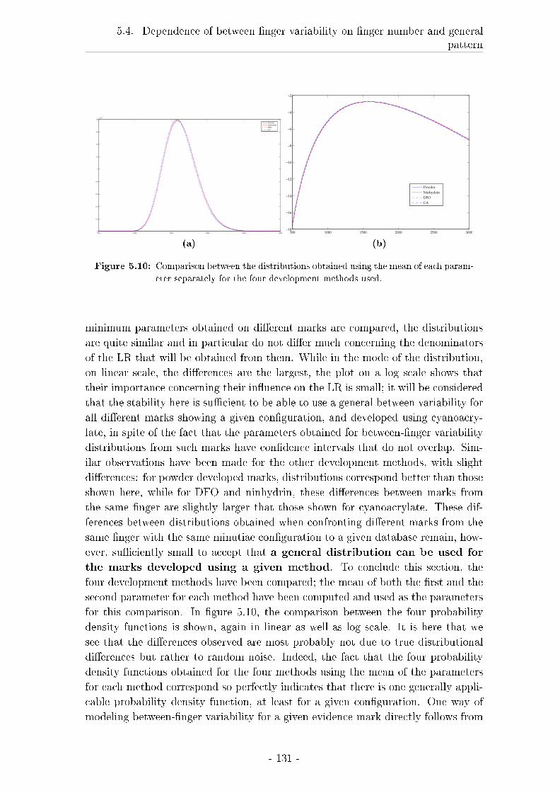
5.4. Dependence of between �nger variability on �nger number and generalpattern
500 1000 1500 2000 2500 30000
0.2
0.4
0.6
0.8
1
1.2
1.4
1.6
1.8x 10
−3
Powder
Ninhydrin
DFO
CA
(a)
500 1000 1500 2000 2500 3000−18
−16
−14
−12
−10
−8
−6
−4
−2
Powder
Ninhydrin
DFO
CA
(b)
Figure 5.10: Comparison between the distributions obtained using the mean of each param-
eter separately for the four development methods used.
minimum parameters obtained on di�erent marks are compared, the distributions
are quite similar and in particular do not di�er much concerning the denominators
of the LR that will be obtained from them. While in the mode of the distribution,
on linear scale, the di�erences are the largest, the plot on a log scale shows that
their importance concerning their in�uence on the LR is small; it will be considered
that the stability here is su�cient to be able to use a general between variability for
all di�erent marks showing a given con�guration, and developed using cyanoacry-
late, in spite of the fact that the parameters obtained for between-�nger variability
distributions from such marks have con�dence intervals that do not overlap. Sim-
ilar observations have been made for the other development methods, with slight
di�erences: for powder developed marks, distributions correspond better than those
shown here, while for DFO and ninhydrin, these di�erences between marks from
the same �nger are slightly larger that those shown for cyanoacrylate. These dif-
ferences between distributions obtained when confronting di�erent marks from the
same �nger with the same minutiae con�guration to a given database remain, how-
ever, su�ciently small to accept that a general distribution can be used for
the marks developed using a given method. To conclude this section, the
four development methods have been compared; the mean of both the �rst and the
second parameter for each method have been computed and used as the parameters
for this comparison. In �gure 5.10, the comparison between the four probability
density functions is shown, again in linear as well as log scale. It is here that we
see that the di�erences observed are most probably not due to true distributional
di�erences but rather to random noise. Indeed, the fact that the four probability
density functions obtained for the four methods using the mean of the parameters
for each method correspond so perfectly indicates that there is one generally appli-
cable probability density function, at least for a given con�guration. One way of
modeling between-�nger variability for a given evidence mark directly follows from
- 131 -
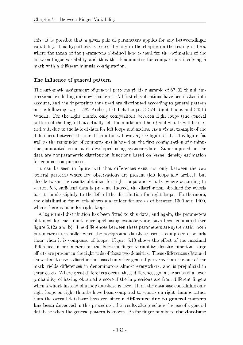
Chapter 5. Between-Finger Variability
this: it is possible that a given pair of parameters applies for any between-�nger
variability. This hypothesis is tested directly in the chapter on the testing of LRs,
where the mean of the parameters obtained here is used for the estimation of the
between-�nger variability and thus the denominator for comparisons involving a
mark with a di�erent minutia con�guration.
The in�uence of general pattern
The automatic assignment of general patterns yields a sample of 67402 thumb im-
pressions, excluding unknown patterns. All �rst classi�cations have been taken into
account, and the �ngerprints thus used are distributed according to general pattern
in the following way: 1582 Arches, 171 Left Loops, 31374 Right Loops and 34519
Whorls. For the right thumb, only comparisons between right loops (the general
pattern of the �nger that actually left the marks used here) and whorls will be car-
ried out, due to the lack of data for left loops and arches. As a visual example of the
di�erences between all four distributions, however, see �gure 5.11. This �gure (as
well as the remainder of comparisons) is based on the �rst con�guration of 6 minu-
tiae, annotated on a mark developed using cyanoacrylate. Superimposed on the
data are nonparametric distribution functions based on kernel density estimation
for comparison purposes.
It can be seen in �gure 5.11 that di�erences exist not only between the two
general patterns where few observations are present (left loops and arches), but
also between the results obtained for right loops and whorls, where according to
section 5.3, su�cient data is present. Indeed, the distribution obtained for whorls
has its mode slightly to the left of the distribution for right loops. Furthermore,
the distribution for whorls shows a shoulder for scores of between 1300 and 1400,
where there is none for right loops.
A lognormal distribution has been �tted to this data, and again, the parameters
obtained for each mark developed using cyanoacrylate have been compared (see
�gure 5.12a and b). The di�erences between these parameters are systematic: both
parameters are smaller when the background database used is composed of whorls
than when it is composed of loops. Figure 5.13 shows the e�ect of the maximal
di�erence in parameters on the between �nger variability density function; large
e�ects are present in the right tails of these two densities. These di�erences obtained
show that to use a distribution based on other general patterns than the one of the
mark yields di�erences in denominators almost everywhere, and is prejudicial in
these cases. Where great di�erences occur, these di�erences go in the sense of a lower
probability of having obtained a score if the impressions are from di�erent �ngers
when a whorl- instead of a loop database is used. Here, the database containing only
right loops on right thumbs have been compared to whorls on right thumbs rather
than the overall database; however, since a di�erence due to general pattern
has been detected in this procedure, the results also preclude the use of a general
database when the general pattern is known. As for �nger numbers, the database
- 132 -
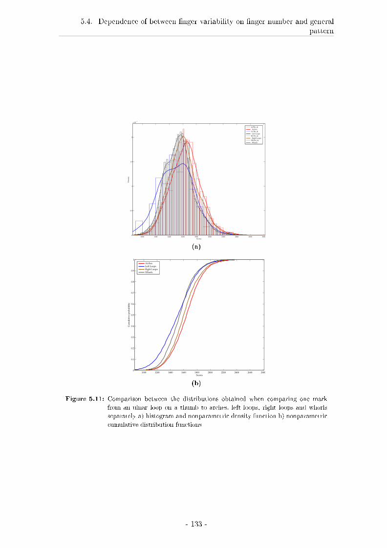
5.4. Dependence of between �nger variability on �nger number and generalpattern
1000 1200 1400 1600 1800 2000 2200 2400 2600 28000
0.5
1
1.5
2
x 10−3
Scores
Den
sity
ArTh(:,4)
Arches
LLTh(:,4)
Left Loops
RLTh(:,4)
Right Loops
WhTh(:,4)
Whorls
(a)
1000 1200 1400 1600 1800 2000 2200 2400 2600 28000
0.1
0.2
0.3
0.4
0.5
0.6
0.7
0.8
0.9
1
Scores
Cu
mu
lati
ve
pro
bab
ilit
y
Arches
Left Loops
Right Loops
Whorls
(b)
Figure 5.11: Comparison between the distributions obtained when comparing one mark
from an ulnar loop on a thumb to arches, left loops, right loops and whorls
separately a) histogram and nonparametric density function b) nonparametric
cumulative distribution functions
- 133 -
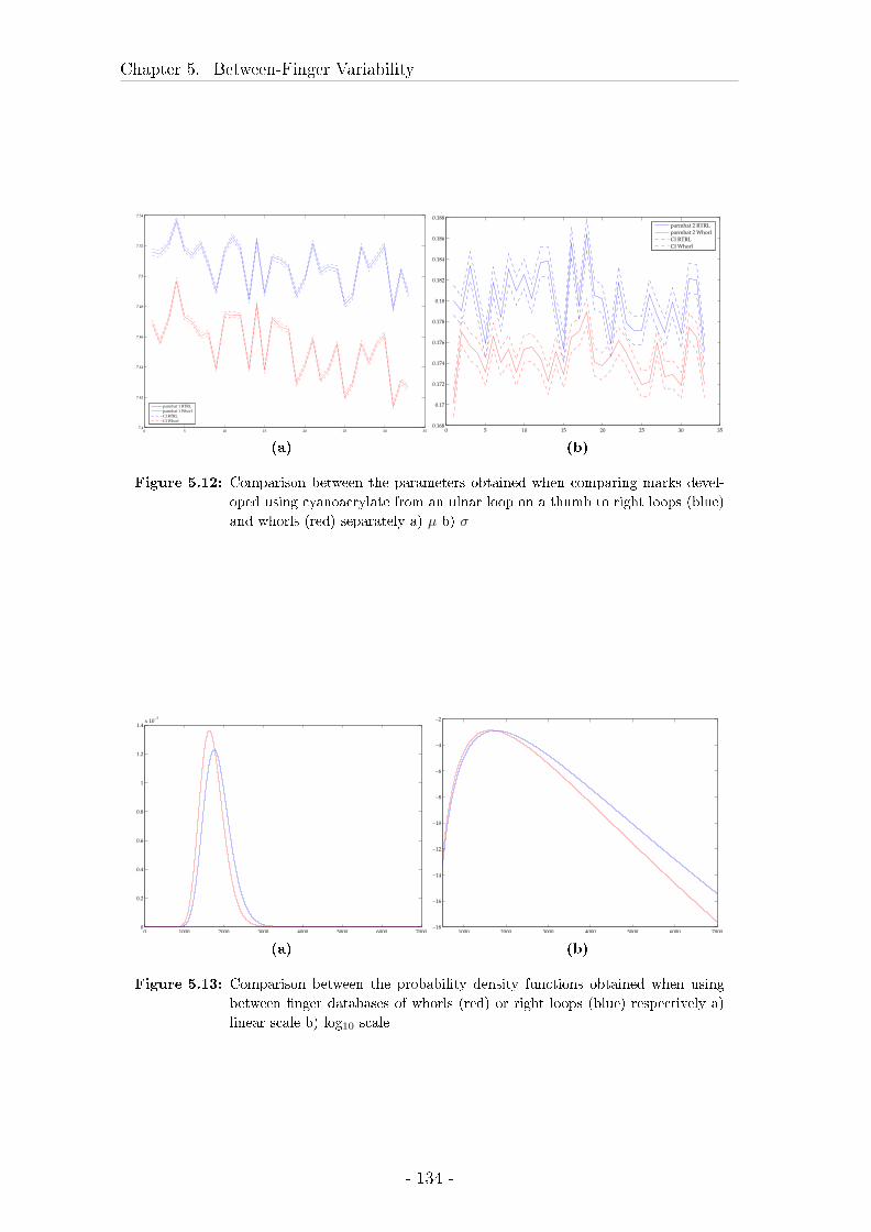
Chapter 5. Between-Finger Variability
0 5 10 15 20 25 30 357.4
7.42
7.44
7.46
7.48
7.5
7.52
7.54
parmhat 1 RTRL
parmhat 1 Whorl
CI RTRL
CI Whorl
(a)
0 5 10 15 20 25 30 350.168
0.17
0.172
0.174
0.176
0.178
0.18
0.182
0.184
0.186
0.188
parmhat 2 RTRL
parmhat 2 Whorl
CI RTRL
CI Whorl
(b)
Figure 5.12: Comparison between the parameters obtained when comparing marks devel-
oped using cyanoacrylate from an ulnar loop on a thumb to right loops (blue)
and whorls (red) separately a) µ b) σ
0 1000 2000 3000 4000 5000 6000 70000
0.2
0.4
0.6
0.8
1
1.2
1.4x 10
−3
(a)
1000 2000 3000 4000 5000 6000 7000−18
−16
−14
−12
−10
−8
−6
−4
−2
(b)
Figure 5.13: Comparison between the probability density functions obtained when using
between �nger databases of whorls (red) or right loops (blue) respectively a)
linear scale b) log10 scale
- 134 -
5.4. Dependence of between �nger variability on �nger number and generalpattern
chosen based on the mark must therefore be used. If the general pattern
is unknown, it is proposed here to still use the lognormal distribution (although
in these cases there is often a shoulder present) and to try and approximate the
parameters of the distribution of the 'same general pattern'. Indeed, here, the
possibility of using a distribution for the between-�nger variability that has the
correct shape and parameters for a 'same �nger and general pattern' distribution,
while this �nger and general pattern are unknown, may exist. Let us assume that
we have a mark that does not allow the determination of �nger number and general
pattern. In the present work, it has been shown, up to now, that when comparing a
mark to prints from the same �nger number and the same general pattern, we obtain
a lognormal distribution, while when the mark is compared to any �nger number and
any general pattern there is a shoulder to the left of the mode. Let us further assume
that we have a way of estimating the parameters of the lognormal distribution that
would be obtained when using only a database of �ngerprints that come from the
same (unknown) �nger number and the same, but unknown, general pattern as the
mark. The view is taken here that this distribution should be used, rather than
an estimation on the whole database. Estimation on the whole database would
correspond approximately to a strati�ed approach where distributions would be
�tted to each �nger number and each general pattern, and a combined denominator
were computed where each �nger number would have the same probability of 110,
and each general pattern would have the probability corresponding to its frequency
in the database. When using the whole database for the estimation of the between-
�nger distribution, this strati�cation would be unnecessary and it has the advantage
of taking automatically into account the fact that general pattern is not independent
of �nger number. The disadvantage is that the probability that the mark comes
from a given �nger should not be 110, but the frequency with which marks are left
by each �nger.
The view taken here is that the best approach, if feasible, is to use the 'same
�nger, same general pattern' distribution. The reason is that it is thought here
that the suspects' �nger retained, even initially, has a much larger than average
chance of coming from the same �nger number and general pattern as the mark.
This is due to the fact that strategies exist to 'estimate' �nger number and general
pattern on the basis of the mark, even if they are not visible. Some formations are
more frequent on certain �nger number / general pattern combinations and will be
searched on �ngers ful�lling these criteria �rst. This strategy does not amount to a
determination that would allow its use for a strati�ed estimation of between-�nger
distribution.
The results of the sections above show that the between-�nger variabil-
ity is dependent on �nger number. Therefore, and even if distributional
similarities exist between some �nger numbers, a database of the same
�nger as the one that the marks originates from should be used, if the
�nger that left the mark is known.
- 135 -
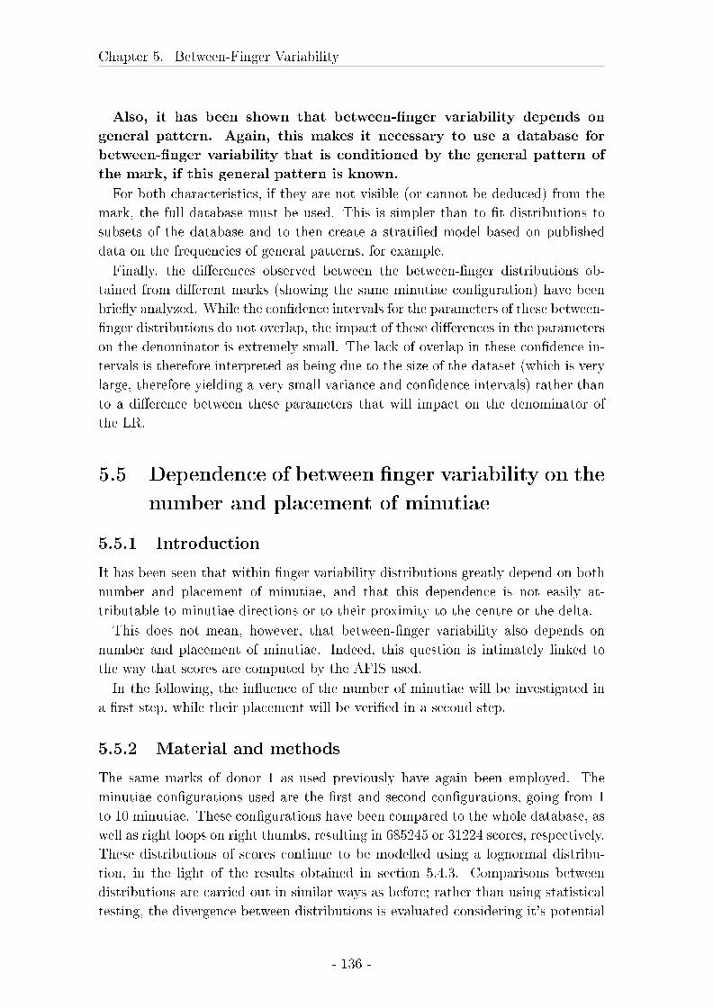
Chapter 5. Between-Finger Variability
Also, it has been shown that between-�nger variability depends on
general pattern. Again, this makes it necessary to use a database for
between-�nger variability that is conditioned by the general pattern of
the mark, if this general pattern is known.
For both characteristics, if they are not visible (or cannot be deduced) from the
mark, the full database must be used. This is simpler than to �t distributions to
subsets of the database and to then create a strati�ed model based on published
data on the frequencies of general patterns, for example.
Finally, the di�erences observed between the between-�nger distributions ob-
tained from di�erent marks (showing the same minutiae con�guration) have been
brie�y analyzed. While the con�dence intervals for the parameters of these between-
�nger distributions do not overlap, the impact of these di�erences in the parameters
on the denominator is extremely small. The lack of overlap in these con�dence in-
tervals is therefore interpreted as being due to the size of the dataset (which is very
large, therefore yielding a very small variance and con�dence intervals) rather than
to a di�erence between these parameters that will impact on the denominator of
the LR.
5.5 Dependence of between �nger variability on the
number and placement of minutiae
5.5.1 Introduction
It has been seen that within �nger variability distributions greatly depend on both
number and placement of minutiae, and that this dependence is not easily at-
tributable to minutiae directions or to their proximity to the centre or the delta.
This does not mean, however, that between-�nger variability also depends on
number and placement of minutiae. Indeed, this question is intimately linked to
the way that scores are computed by the AFIS used.
In the following, the in�uence of the number of minutiae will be investigated in
a �rst step, while their placement will be veri�ed in a second step.
5.5.2 Material and methods
The same marks of donor 1 as used previously have again been employed. The
minutiae con�gurations used are the �rst and second con�gurations, going from 1
to 10 minutiae. These con�gurations have been compared to the whole database, as
well as right loops on right thumbs, resulting in 685245 or 31224 scores, respectively.
These distributions of scores continue to be modelled using a lognormal distribu-
tion, in the light of the results obtained in section 5.4.3. Comparisons between
distributions are carried out in similar ways as before; rather than using statistical
testing, the divergence between distributions is evaluated considering it's potential
- 136 -
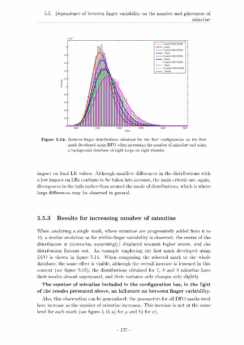
5.5. Dependence of between �nger variability on the number and placement ofminutiae
1000 1500 2000 2500 3000 35000
0.2
0.4
0.6
0.8
1
1.2
1.4
1.6
1.8
2
x 10−3
Data
Den
sity
6 minO DFO RTRL
6min
7 minO DFO RTRL
7min
8 minO DFO RTRL
8min
9 minO DFO RTRL
9min
10 minO DFO RTRL
10min
Figure 5.14: Between-�nger distributions obtained for the �rst con�guration on the �rst
mark developed using DFO when increasing the number of minutiae and using
a background database of right loops on right thumbs
impact on �nal LR values. Although manifest di�erences in the distributions with
a low impact on LRs continue to be taken into account, the main criteria are, again,
divergences in the tails rather than around the mode of distributions, which is where
large di�erences may be observed in general.
5.5.3 Results for increasing number of minutiae
When analyzing a single mark, where minutiae are progressively added from 6 to
10, a similar evolution as for within-�nger variability is observed: the centre of the
distribution is (somewhat surprisingly) displaced towards higher scores, and the
distribution �attens out. An example employing the �rst mark developed using
DFO is shown in �gure 5.14. When comparing the selected mark to the whole
database, the same e�ect is visible, although the overall increase is lessened in this
context (see �gure 5.15); the distributions obtained for 7, 8 and 9 minutiae have
their modes almost superposed, and their variance only changes only slightly.
The number of minutiae included in the con�guration has, in the light
of the results presented above, an in�uence on between �nger variability.
Also, this observation can be generalized: the parameters for all DFO marks used
here increase as the number of minutiae increases. This increase is not at the same
level for each mark (see �gure 5.16 a) for µ and b) for σ).
- 137 -
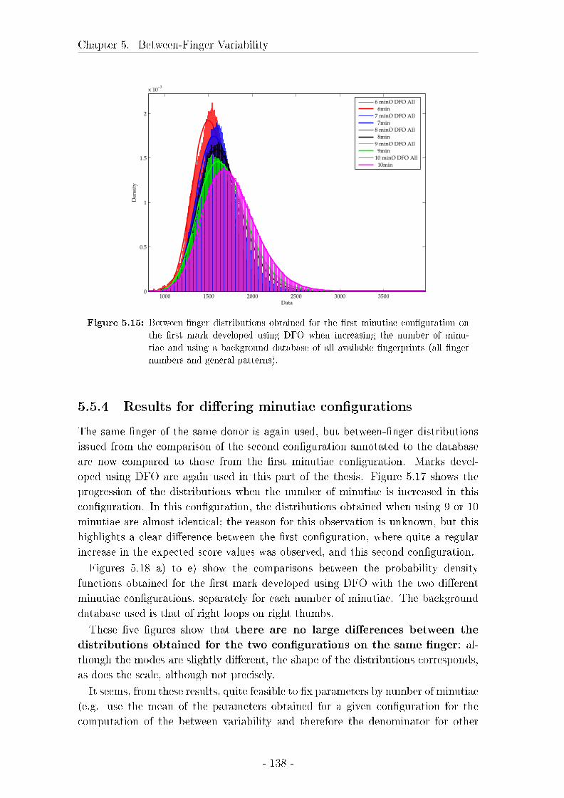
Chapter 5. Between-Finger Variability
1000 1500 2000 2500 3000 35000
0.5
1
1.5
2
x 10−3
Data
Den
sity
6 minO DFO All
6min
7 minO DFO All
7min
8 minO DFO All
8min
9 minO DFO All
9min
10 minO DFO All
10min
Figure 5.15: Between-�nger distributions obtained for the �rst minutiae con�guration on
the �rst mark developed using DFO when increasing the number of minu-
tiae and using a background database of all available �ngerprints (all �nger
numbers and general patterns).
5.5.4 Results for di�ering minutiae con�gurations
The same �nger of the same donor is again used, but between-�nger distributions
issued from the comparison of the second con�guration annotated to the database
are now compared to those from the �rst minutiae con�guration. Marks devel-
oped using DFO are again used in this part of the thesis. Figure 5.17 shows the
progression of the distributions when the number of minutiae is increased in this
con�guration. In this con�guration, the distributions obtained when using 9 or 10
minutiae are almost identical; the reason for this observation is unknown, but this
highlights a clear di�erence between the �rst con�guration, where quite a regular
increase in the expected score values was observed, and this second con�guration.
Figures 5.18 a) to e) show the comparisons between the probability density
functions obtained for the �rst mark developed using DFO with the two di�erent
minutiae con�gurations, separately for each number of minutiae. The background
database used is that of right loops on right thumbs.
These �ve �gures show that there are no large di�erences between the
distributions obtained for the two con�gurations on the same �nger: al-
though the modes are slightly di�erent, the shape of the distributions corresponds,
as does the scale, although not precisely.
It seems, from these results, quite feasible to �x parameters by number of minutiae
(e.g. use the mean of the parameters obtained for a given con�guration for the
computation of the between variability and therefore the denominator for other
- 138 -
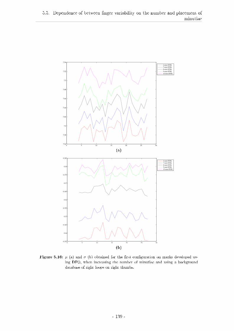
5.5. Dependence of between �nger variability on the number and placement ofminutiae
0 5 10 15 20 25 307.36
7.38
7.4
7.42
7.44
7.46
7.48
7.5
7.52
7.54
6 min RTRL
7 min RTRL
8 min RTRL
9 min RTRL
10 min RTRL
(a)
0 5 10 15 20 25 300.135
0.14
0.145
0.15
0.155
0.16
0.165
0.17
0.175
0.18
0.185
6 min RTRL
7 min RTRL
8 min RTRL
9 min RTRL
10 min RTRL
(b)
Figure 5.16: µ (a) and σ (b) obtained for the �rst con�guration on marks developed us-
ing DFO, when increasing the number of minutiae and using a background
database of right loops on right thumbs.
- 139 -
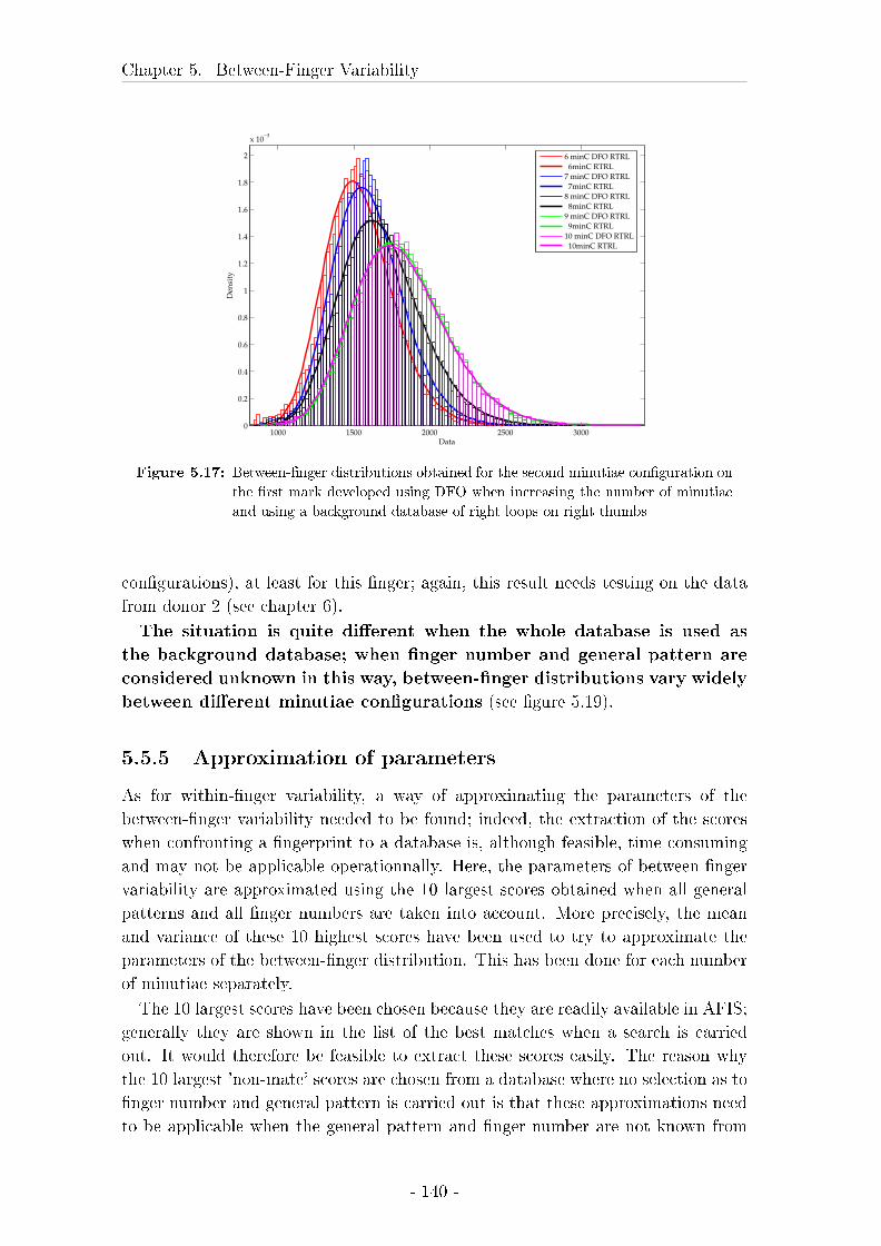
Chapter 5. Between-Finger Variability
1000 1500 2000 2500 30000
0.2
0.4
0.6
0.8
1
1.2
1.4
1.6
1.8
2
x 10−3
Data
Den
sity
6 minC DFO RTRL
6minC RTRL
7 minC DFO RTRL
7minC RTRL
8 minC DFO RTRL
8minC RTRL
9 minC DFO RTRL
9minC RTRL
10 minC DFO RTRL
10minC RTRL
Figure 5.17: Between-�nger distributions obtained for the second minutiae con�guration on
the �rst mark developed using DFO when increasing the number of minutiae
and using a background database of right loops on right thumbs
con�gurations), at least for this �nger; again, this result needs testing on the data
from donor 2 (see chapter 6).
The situation is quite di�erent when the whole database is used as
the background database; when �nger number and general pattern are
considered unknown in this way, between-�nger distributions vary widely
between di�erent minutiae con�gurations (see �gure 5.19).
5.5.5 Approximation of parameters
As for within-�nger variability, a way of approximating the parameters of the
between-�nger variability needed to be found; indeed, the extraction of the scores
when confronting a �ngerprint to a database is, although feasible, time consuming
and may not be applicable operationnally. Here, the parameters of between-�nger
variability are approximated using the 10 largest scores obtained when all general
patterns and all �nger numbers are taken into account. More precisely, the mean
and variance of these 10 highest scores have been used to try to approximate the
parameters of the between-�nger distribution. This has been done for each number
of minutiae separately.
The 10 largest scores have been chosen because they are readily available in AFIS;
generally they are shown in the list of the best matches when a search is carried
out. It would therefore be feasible to extract these scores easily. The reason why
the 10 largest 'non-mate' scores are chosen from a database where no selection as to
�nger number and general pattern is carried out is that these approximations need
to be applicable when the general pattern and �nger number are not known from
- 140 -
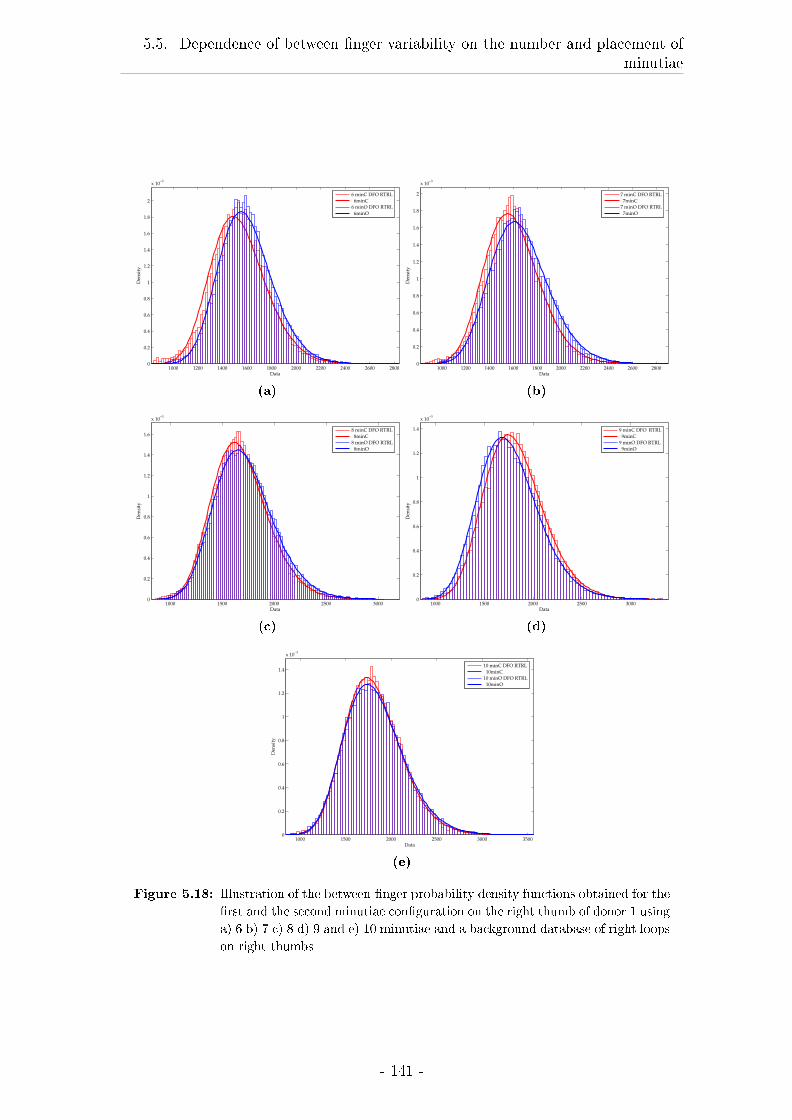
5.5. Dependence of between �nger variability on the number and placement ofminutiae
1000 1200 1400 1600 1800 2000 2200 2400 2600 28000
0.2
0.4
0.6
0.8
1
1.2
1.4
1.6
1.8
2
x 10−3
Data
Den
sity
6 minC DFO RTRL
6minC
6 minO DFO RTRL
6minO
(a)
1000 1200 1400 1600 1800 2000 2200 2400 2600 28000
0.2
0.4
0.6
0.8
1
1.2
1.4
1.6
1.8
2
x 10−3
Data
Den
sity
7 minC DFO RTRL
7minC
7 minO DFO RTRL
7minO
(b)
1000 1500 2000 2500 30000
0.2
0.4
0.6
0.8
1
1.2
1.4
1.6
x 10−3
Data
Den
sity
8 minC DFO RTRL
8minC
8 minO DFO RTRL
8minO
(c)
1000 1500 2000 2500 30000
0.2
0.4
0.6
0.8
1
1.2
1.4
x 10−3
Data
Den
sity
9 minC DFO RTRL
9minC
9 minO DFO RTRL
9minO
(d)
1000 1500 2000 2500 3000 35000
0.2
0.4
0.6
0.8
1
1.2
1.4
x 10−3
Data
Den
sity
10 minC DFO RTRL
10minC
10 minO DFO RTRL
10minO
(e)
Figure 5.18: Illustration of the between-�nger probability density functions obtained for the
�rst and the second minutiae con�guration on the right thumb of donor 1 using
a) 6 b) 7 c) 8 d) 9 and e) 10 minutiae and a background database of right loops
on right thumbs
- 141 -
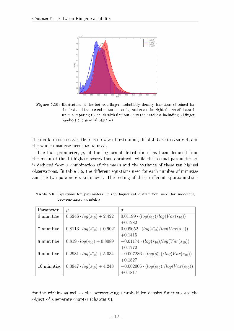
Chapter 5. Between-Finger Variability
1000 1200 1400 1600 1800 2000 2200 2400 2600 2800 30000
0.2
0.4
0.6
0.8
1
1.2
1.4
1.6
1.8
2x 10
−3
Data
Den
sity
6 minC
6 minC
6 minO
6 minO
Figure 5.19: Illustration of the between-�nger probability density functions obtained for
the �rst and the second minutiae con�guration on the right thumb of donor 1
when comparing the mark with 6 minutiae to the database including all �nger
numbers and general patterns
the mark; in such cases, there is no way of restraining the database to a subset, and
the whole database needs to be used.
The �rst parameter, µ, of the lognormal distribution has been deduced from
the mean of the 10 highest scores thus obtained, while the second parameter, σ,
is deduced from a combination of the mean and the variance of these ten highest
observations. In table 5.6, the di�erent equations used for each number of minutiae
and the two parameters are shown. The testing of these di�erent approximations
Table 5.6: Equations for parameters of the lognormal distribution used for modelling
between-�nger variability
Parameter µ σ
6 minutiae 0.6246 · log(s̄10) + 2.422 0.01199 · (log(s̄10)/log(V ar(s10))
+0.1282
7 minutiae 0.8113 · log(s̄10) + 0.9021 0.009652 · (log(s̄10)/log(V ar(s10))
+0.1415
8 minutiae 0.819 · log(s̄10) + 0.8089 −0.01174 · (log(s̄10)/log(V ar(s10))
+0.1772
9 minutiae 0.2981 · log(s̄10) + 5.034 −0.007286 · (log(s̄10)/log(V ar(s10))
+0.1827
10 minutiae 0.3947 · log(s̄10) + 4.248 −0.002005 · (log(s̄10)./log(V ar(s10))
+0.1817
for the within- as well as the between-�nger probability density functions are the
object of a separate chapter (chapter 6).
- 142 -
5.5. Dependence of between �nger variability on the number and placement ofminutiae
5.5.6 Conclusions on between-�nger variability
While considerations of variables in�uencing between-�nger distributions may seem
less interesting than those in�uencing within-�nger variability, some important anal-
yses of the behaviour of this distribution have been carried out in this chapter. If
no such description had �gured here, by default, it would have been possible op-
erationally to confront the mark of a case to an available database, extract all the
scores by conditioning on known factors of the mark (general pattern, �nger number)
and use some nonparametric estimation technique for obtaining the between-�nger
variability and the denominator of the LR.
First of all, a minimum number of comparisons necessary for obtaining a stable
distribution has been estimated. While it was suspected that the distributions
would depend on �nger number and general pattern, this has been shown here.
The same is true for the dependence on the number of minutiae and the behaviour
of the distribution when the number of minutiae is increased. Finally, the di�erences
obtained when di�erent minutiae con�gurations (or even di�erent marks with the
same minutia con�guration) are used have been observed. Also, it has been possible
to use a parametric distribution for the �tting of these scores, which is considered
as an advantage here for the same reasons as those discussed for the within-�nger
variability. The main reason is the possibility of obtaining robust estimates of the
density in regions of low probability, where often no observations will have been
made.
Finally, two possible ways of approximating the parameters of the between-�nger
distribution are proposed (and will be tested in the next chapter); the �rst one
is to use �xed parameters for each �nger number (computed as the mean of the
parameters obtained from the marks developed using DFO of the original minutiae
con�guration) and the second one is to use an approximation based on the largest
10 scores obtained when confronting the �ngerprint to the database. The 10 largest
scores were chosen since they are readily available from the results of the AFIS.
- 143 -

Chapter 6
Testing of the di�erent
approximations using Likelihood
ratios
6.1 Introduction
In the preceding chapters and sections, di�erent propositions for approximating the
distributions at the basis of the likelihood ratio have been made.
It has been proposed to estimate the parameters of the distribution of within-
�nger variability directly from three impressions compared to themselves. The
mean of the 3 scores thus obtained, that are a description of the maximal score
for a given con�guration, has been used for the approximation of these parameters.
These approximations have already been tested in the relevant section; the interest
of the present section is to test the joint e�ect of the approximations used in both
the numerator and the denominator.
For the between-�nger variability, several propositions remain untested: the cor-
relation between LRs obtained on full and reduced databases, where the reduced
database contains only 10'000 impressions, an approximation using �xed parame-
ters computed on the basis of the �rst minutiae con�guration observed on DFO-
developped marks of donor 1 (based on minutiae number only and using �xed
parameters for all di�erent con�gurations) and the approximation where the pa-
rameters of the between �nger variability distribution are estimated based on the
10 highest scores obtained in the database, or rather their mean and variance.
All of these propositions are tested on �rst on the �rst con�guration of donor 1,
and then on one �nger of another donor (donor 2). Impressions from this donor
have been developed using powdering only. Also, they have not been used for the
establishment of the approximations of the parameters.
- 145 -
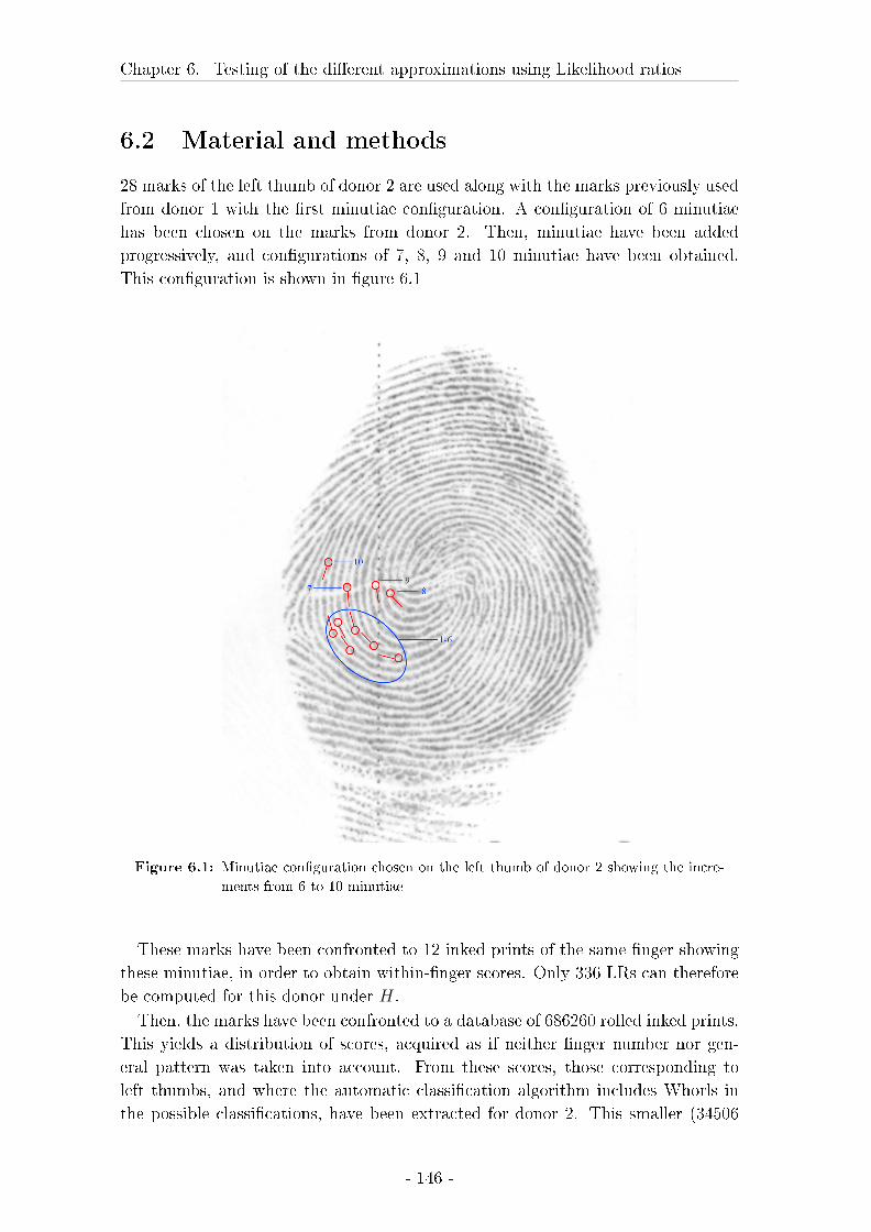
Chapter 6. Testing of the di�erent approximations using Likelihood ratios
6.2 Material and methods
28 marks of the left thumb of donor 2 are used along with the marks previously used
from donor 1 with the �rst minutiae con�guration. A con�guration of 6 minutiae
has been chosen on the marks from donor 2. Then, minutiae have been added
progressively, and con�gurations of 7, 8, 9 and 10 minutiae have been obtained.
This con�guration is shown in �gure 6.1
Figure 6.1: Minutiae con�guration chosen on the left thumb of donor 2 showing the incre-
ments from 6 to 10 minutiae
These marks have been confronted to 12 inked prints of the same �nger showing
these minutiae, in order to obtain within-�nger scores. Only 336 LRs can therefore
be computed for this donor under H.
Then, the marks have been confronted to a database of 686260 rolled inked prints.
This yields a distribution of scores, acquired as if neither �nger number nor gen-
eral pattern was taken into account. From these scores, those corresponding to
left thumbs, and where the automatic classi�cation algorithm includes Whorls in
the possible classi�cations, have been extracted for donor 2. This smaller (34506
- 146 -
6.2. Material and methods
impressions) dataset represents between variability when considering �nger number
and general pattern as known. The same strategy has been used for donor 2, where
right loops on right thumbs were retained (yielding 31224 scores).
Likelihood ratios obtained will �rst be described using Tippett plots. The eviden-
tial scores are chosen in the within- and the between-�nger databases, respectively.
The Tippett plots are constructed using 2000 LRs under H̄ and either all LRs ob-
tained for the available scores for LRs computed under H (when less than 2000
such scores are available) or 2000 LRs (when more than 2000 scores are available).
Less than 2000 scores are available for donor 2. When 2000 scores are randomly
selected, a strati�ed selection of scores has been used. The same number of scores
was randomly chosen for each mark separately (the code for this construction of
Tippett plots is given in appendix C). The number of scores selected from the re-
sults for each mark is 2000 divided by the total number of marks used; when the
result is not an integer, the next larger integer is used. Therefore, a number close
to but larger than 2000 is obtained. The evidential scores selected under H̄ are
always selected in the complete database of non-mate scores, even when reduced
databases are used for the evaluation of scores (e.g. a database of 10000 scores or
a database conditioned by �nger number or general pattern). Once the evidential
score is chosen, either the relevant databases for the computation of f(s|H) and
f(s|H̄) are chosen (e.g. for the within-�nger variability, all comparisons involving
the con�guration and for the between �nger variability the comparisons where the
'evidence' mark is used and compared against all impressions of the background
database, or a subset of this dataset depending on what is being tested), or the
appropriate approximations are used and the parameters thus obtained are directly
employed for the computation of the numerator and denominator values.
In a further step, the relationship between the di�erent likelihood ratios will be
examined: indeed, it is insu�cient to obtain similar distributions of likelihood ratios
as shown by Tippett plots. Rather, each LR obtained using the approximations has
to be close to the LR obtained on the data. Then, numerators and denominators are
also compared separately in some instances in order to complete the investigation of
the in�uence of the approximations. Linear plots are used for this comparison; the
same LRs as those used for the establishment of the Tippett plots are employed for
these graphs, e.g. exactly the same LRs are employed twice: once for the Tippett
plots and once for the establishment of these linear graphs. They are therefore
based on the same data and sampling processes as described for the Tippett plots.
Comparisons are carried out between estimation based on the data, for both the
numerator and the denominator and LRs obtained when both the numerator and the
denominator are based on approximations using much less data. Also, a reduction
in the data in the denominator estimation (to 10000 observations) is tested against
the results obtained when all available data is used. Overall, 5 di�erent ways of
computing LRs are compared:
1. data-based estimation for the within-variability, with a between-variability
- 147 -
Chapter 6. Testing of the di�erent approximations using Likelihood ratios
estimated on the whole database (all scores obtained when confronting the
evidential mark to the database of �ngerprints from other sources, without
conditioning by �nger number and general pattern)
2. approximated within-variability and a between-variability based on a reduced
dataset including all �nger numbers and general patterns, but where only
10000 observations are sampled randomly
3. data-based estimation for the within-variability, and a between-variability
based only on scores obtained from �ngerprints showing the same general
pattern/�nger number combination as that of the �nger that the mark origi-
nated from
4. approximated within-variability and a between-variability based on �xed pa-
rameters, that are the means of the parameters obtained for the �rst con�gu-
ration from donor 1 on marks developed using DFO confronted to a database
of right loops on right thumbs and �nally
5. approximated within- and between-variabilities using the equations and the
self-scores and 10 highest observations, respectively.
As all through the present thesis, a divergence of one order of magnitude in the
likelihood ratio is judged acceptable.
6.3 Results on likelihood ratios
A �rst series of Tippett plots presents the results obtained when using a background
database containing only right loops on right thumbs for the marks from donor 1
(see �gure 6.2) and a background database of only whorls on left thumbs for the
marks from donor 2 (see �gure 6.3). For these Tippett plots, both the within- and
the between-�nger variabilities are estimated on data and no approximation is used.
For the between-�nger variability only the �nger number and general pattern of the
�nger considered are included (right loops on right thumbs for donor 1 and whorls
on left thumbs for donor 2).
These Tippett plots show relatively high rates of misleading evidence, in partic-
ular in favour of the prosecution, for 6 and 7 minutiae for donor 2 (see table 6.1;
these rates are of 5.2% and 3.2%, respectively). Considering, however, that these
rates are for rather small con�gurations of minutiae, these rates are acceptable.
The value of these misleading LRs is, in some cases, quite high, in particularly
in favour of the defense. For example, as shown in table 6.1, the minimum value
of the logarithm base 10 under the prosecution hypothesis is of -4.4 for the �rst
minutiae con�guration of Donor 1. As it should be, the separation between the two
curves for impressions known to come from the same and di�erent �nger increases
with increasing numbers of minutiae. Although the rates of misleading evidence
- 148 -
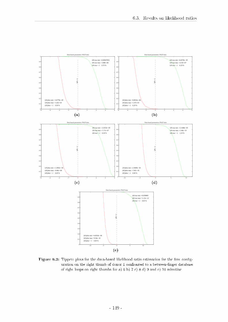
6.3. Results on likelihood ratios
−8 −6 −4 −2 0 2 4 6 80
0.1
0.2
0.3
0.4
0.5
0.6
0.7
0.8
0.9
1Data based parameters: FNGP data
LR true min =0.00047051
LR true max =3.88e+06
LR true < 1 0.70 %
LR false max =1.65e+01
LR false min =3.6779e−05
LR false > 1 0.30 %
LR
= 1
(a)
−8 −6 −4 −2 0 2 4 6 80
0.1
0.2
0.3
0.4
0.5
0.6
0.7
0.8
0.9
1Data based parameters: FNGP data
LR true min =6.6576e−05
LR true max =4.10e+07
LR true < 1 0.29 %
LR false max =1.07e+01
LR false min =9.8916e−06
LR false > 1 0.29 %
LR
= 1
(b)
−8 −6 −4 −2 0 2 4 6 80
0.1
0.2
0.3
0.4
0.5
0.6
0.7
0.8
0.9
1Data based parameters: FNGP data
LR true min =3.3533e−05
LR true max =7.17e+07
LR true < 1 0.34 %
LR false max =9.46e+00
LR false min =1.3092e−05
LR false > 1 0.29 %
LR
= 1
(c)
−10 −5 0 5 100
0.1
0.2
0.3
0.4
0.5
0.6
0.7
0.8
0.9
1Data based parameters: FNGP data
LR true min =5.1448e−05
LR true max =1.46e+10
LR true < 1 1.19 %
LR false max =7.81e−01
LR false min =2.4409e−05
LR false > 1 0.00 %
LR
= 1
(d)
−10 −5 0 5 100
0.1
0.2
0.3
0.4
0.5
0.6
0.7
0.8
0.9
1Data based parameters: FNGP data
LR true min =0.039869
LR true max =1.13e+12
LR true < 1 0.05 %
LR false max =9.56e−01
LR false min =4.6934e−06
LR false > 1 0.00 %
LR
= 1
(e)
Figure 6.2: Tippett plots for the data-based likelihood ratio estimation for the �rst con�g-
uration on the right thumb of donor 1 confronted to a between-�nger database
of right loops on right thumbs for a) 6 b) 7 c) 8 d) 9 and e) 10 minutiae
- 149 -
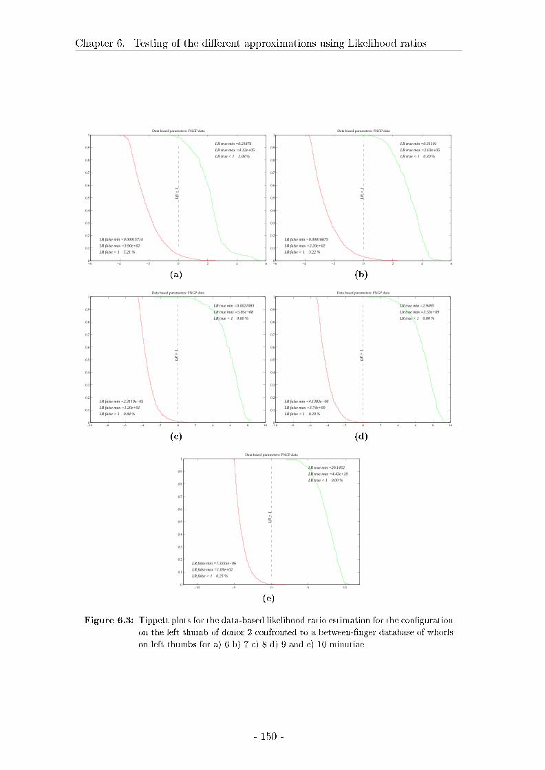
Chapter 6. Testing of the di�erent approximations using Likelihood ratios
−6 −4 −2 0 2 4 60
0.1
0.2
0.3
0.4
0.5
0.6
0.7
0.8
0.9
1Data based parameters: FNGP data
LR true min =0.21876
LR true max =4.12e+05
LR true < 1 2.08 %
LR false max =3.90e+02
LR false min =0.00015714
LR false > 1 5.21 %
LR
= 1
(a)
−6 −4 −2 0 2 4 60
0.1
0.2
0.3
0.4
0.5
0.6
0.7
0.8
0.9
1Data based parameters: FNGP data
LR true min =0.31101
LR true max =2.03e+05
LR true < 1 0.30 %
LR false max =2.20e+02
LR false min =0.00016675
LR false > 1 3.22 %
LR
= 1
(b)
−10 −8 −6 −4 −2 0 2 4 6 8 100
0.1
0.2
0.3
0.4
0.5
0.6
0.7
0.8
0.9
1Data based parameters: FNGP data
LR true min =0.0021083
LR true max =5.85e+08
LR true < 1 0.60 %
LR false max =1.20e+01
LR false min =2.3119e−05
LR false > 1 0.84 %
LR
= 1
(c)
−10 −8 −6 −4 −2 0 2 4 6 8 100
0.1
0.2
0.3
0.4
0.5
0.6
0.7
0.8
0.9
1Data based parameters: FNGP data
LR true min =2.9495
LR true max =3.53e+09
LR true < 1 0.00 %
LR false max =3.74e+00
LR false min =4.1383e−06
LR false > 1 0.20 %
LR
= 1
(d)
−10 −5 0 5 100
0.1
0.2
0.3
0.4
0.5
0.6
0.7
0.8
0.9
1Data based parameters: FNGP data
LR true min =20.1452
LR true max =4.43e+10
LR true < 1 0.00 %
LR false max =1.05e+02
LR false min =7.3335e−06
LR false > 1 0.25 %
LR
= 1
(e)
Figure 6.3: Tippett plots for the data-based likelihood ratio estimation for the con�guration
on the left thumb of donor 2 confronted to a between-�nger database of whorls
on left thumbs for a) 6 b) 7 c) 8 d) 9 and e) 10 minutiae
- 150 -
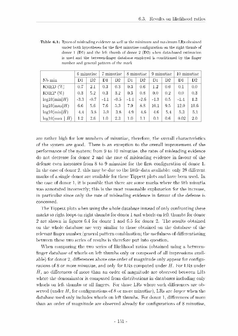
6.3. Results on likelihood ratios
Table 6.1: Rates of misleading evidence as well as the minimum and maximum LRs obtained
under both hypotheses for the �rst minutiae con�guration on the right thumb of
donor 1 (D1) and the left thumb of donor 2 (D2) when data-based estimation
is used and the between-�nger database employed is conditioned by the �nger
number and general pattern of the mark
6 minutiae 7 minutiae 8 minutiae 9 minutiae 10 minutiae
Nb min D1 D2 D1 D2 D1 D2 D1 D2 D1 D2
RMED (%) 0.7 2.1 0.3 0.3 0.3 0.6 1.2 0.0 0.1 0.0
RMEP (%) 0.3 5.2 0.3 3.2 0.3 0.8 0.0 0.2 0.0 0.3
log10(min|H) -3.3 -0.7 -4.1 -0.5 -4.4 -2.6 -4.3 0.5 -1.4 1.3
log10(max|H) 6.6 5.6 7.6 5.3 7.9 8.8 10.1 9.5 12.0 10.6
log10(min|H̄) -4.4 -3.8 -5.0 -3.8 -4.9 -4.6 -4.6 -5.4 -5.3 -5.1
log10(max | H̄) 1.2 2.6 1.0 2.3 1.0 1.1 -0.1 0.6 -0.02 2.0
are rather high for low numbers of minutiae, therefore, the overall characteristics
of the system are good. There is an exception to the overall improvement of the
performance of the system; from 9 to 10 minutiae, the rates of misleading evidence
do not decrease for donor 2 and the rate of misleading evidence in favour of the
defense even increases from 8 to 9 minutiae for the �rst con�guration of donor 1.
In the case of donor 2, this may be due to the little data available: only 28 di�erent
marks of a single donor are available for these Tippett plots and have been used. In
the case of donor 1, it is possible that there are some marks where the 9th minutia
was annotated incorrectly; this is the most reasonable explanation for the increase,
in particular since only the rate of misleading evidence in favour of the defense is
concerned.
The Tippett plots when using the whole database instead of only confronting these
marks to right loops on right thumbs for donor 1 and whorls on left thumbs for donor
2 are shown in �gures 6.4 for donor 1 and 6.5 for donor 2. The results obtained
on the whole database are very similar to those obtained on the database of the
relevant �nger number/general pattern combination; the usefulness of di�erentiating
between these two series of results is therefore put into question.
When comparing the two series of likelihood ratios (obtained using a between-
�nger database of whorls on left thumbs only or composed of all impressions avail-
able) for donor 2, di�erences above one order of magnitude only appear for con�gu-
rations of 8 or more minutiae, and only for LRs computed under H. For LRs under
H̄, no di�erences of more than an order of magnitude are observed between LRs
where the denominator is computed from distributions in databases including only
whorls on left thumbs or all �ngers. For those LRs where such di�erences are ob-
served (under H, for con�gurations of 8 or more minutiae), LRs are larger when the
database used only includes whorls on left thumbs. For donor 1, di�erences of more
than an order of magnitude are observed already for con�gurations of 8 minutiae,
- 151 -
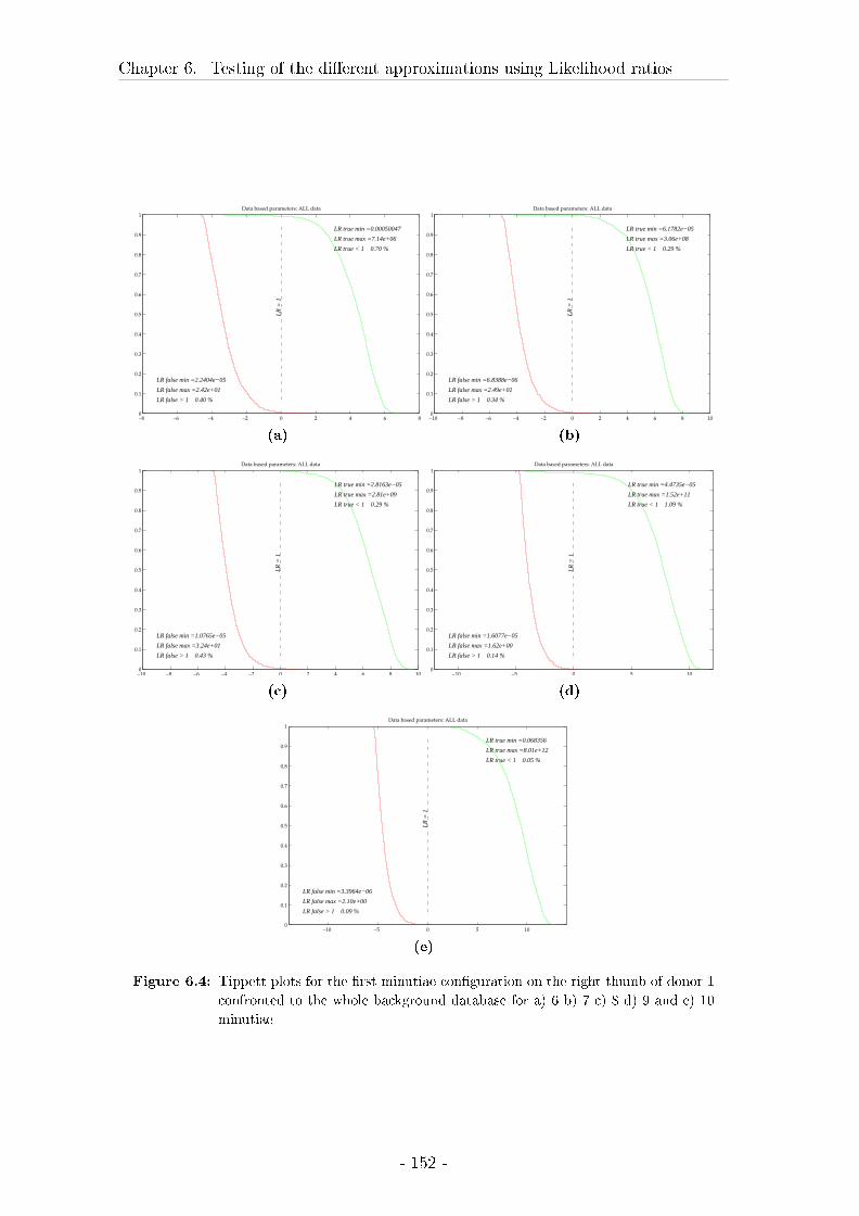
Chapter 6. Testing of the di�erent approximations using Likelihood ratios
−8 −6 −4 −2 0 2 4 6 80
0.1
0.2
0.3
0.4
0.5
0.6
0.7
0.8
0.9
1Data based parameters: ALL data
LR true min =0.00050047
LR true max =7.14e+06
LR true < 1 0.70 %
LR false max =2.42e+01
LR false min =2.2404e−05
LR false > 1 0.40 %
LR
= 1
(a)
−10 −8 −6 −4 −2 0 2 4 6 8 100
0.1
0.2
0.3
0.4
0.5
0.6
0.7
0.8
0.9
1Data based parameters: ALL data
LR true min =6.1782e−05
LR true max =3.06e+08
LR true < 1 0.29 %
LR false max =2.49e+01
LR false min =6.8388e−06
LR false > 1 0.34 %
LR
= 1
(b)
−10 −8 −6 −4 −2 0 2 4 6 8 100
0.1
0.2
0.3
0.4
0.5
0.6
0.7
0.8
0.9
1Data based parameters: ALL data
LR true min =2.8163e−05
LR true max =2.81e+09
LR true < 1 0.29 %
LR false max =3.24e+01
LR false min =1.0765e−05
LR false > 1 0.43 %
LR
= 1
(c)
−10 −5 0 5 100
0.1
0.2
0.3
0.4
0.5
0.6
0.7
0.8
0.9
1Data based parameters: ALL data
LR true min =4.4735e−05
LR true max =1.52e+11
LR true < 1 1.09 %
LR false max =1.62e+00
LR false min =1.6077e−05
LR false > 1 0.14 %
LR
= 1
(d)
−10 −5 0 5 100
0.1
0.2
0.3
0.4
0.5
0.6
0.7
0.8
0.9
1Data based parameters: ALL data
LR true min =0.068356
LR true max =8.01e+12
LR true < 1 0.05 %
LR false max =2.10e+00
LR false min =3.3964e−06
LR false > 1 0.09 %
LR
= 1
(e)
Figure 6.4: Tippett plots for the �rst minutiae con�guration on the right thumb of donor 1
confronted to the whole background database for a) 6 b) 7 c) 8 d) 9 and e) 10
minutiae
- 152 -
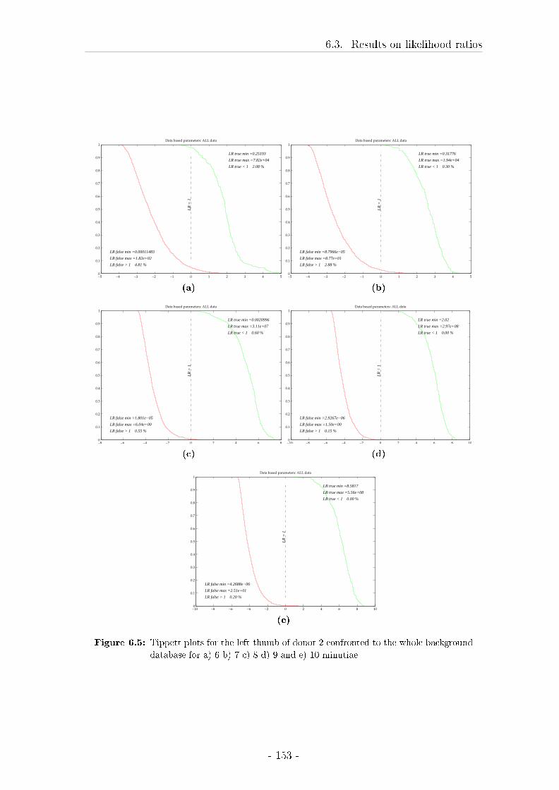
6.3. Results on likelihood ratios
−5 −4 −3 −2 −1 0 1 2 3 4 50
0.1
0.2
0.3
0.4
0.5
0.6
0.7
0.8
0.9
1Data based parameters: ALL data
LR true min =0.25193
LR true max =7.82e+04
LR true < 1 2.08 %
LR false max =1.82e+02
LR false min =0.00011483
LR false > 1 4.81 %
LR
= 1
(a)
−5 −4 −3 −2 −1 0 1 2 3 4 50
0.1
0.2
0.3
0.4
0.5
0.6
0.7
0.8
0.9
1Data based parameters: ALL data
LR true min =0.31776
LR true max =1.94e+04
LR true < 1 0.30 %
LR false max =8.77e+01
LR false min =8.7966e−05
LR false > 1 2.88 %
LR
= 1
(b)
−8 −6 −4 −2 0 2 4 6 80
0.1
0.2
0.3
0.4
0.5
0.6
0.7
0.8
0.9
1Data based parameters: ALL data
LR true min =0.0020996
LR true max =3.11e+07
LR true < 1 0.60 %
LR false max =6.04e+00
LR false min =1.801e−05
LR false > 1 0.55 %
LR
= 1
(c)
−10 −8 −6 −4 −2 0 2 4 6 8 100
0.1
0.2
0.3
0.4
0.5
0.6
0.7
0.8
0.9
1Data based parameters: ALL data
LR true min =2.02
LR true max =2.97e+08
LR true < 1 0.00 %
LR false max =1.50e+00
LR false min =2.9267e−06
LR false > 1 0.15 %
LR
= 1
(d)
−10 −8 −6 −4 −2 0 2 4 6 8 100
0.1
0.2
0.3
0.4
0.5
0.6
0.7
0.8
0.9
1Data based parameters: ALL data
LR true min =8.5817
LR true max =5.56e+08
LR true < 1 0.00 %
LR false max =2.51e+01
LR false min =4.2688e−06
LR false > 1 0.20 %
LR
= 1
(e)
Figure 6.5: Tippett plots for the left thumb of donor 2 confronted to the whole background
database for a) 6 b) 7 c) 8 d) 9 and e) 10 minutiae
- 153 -
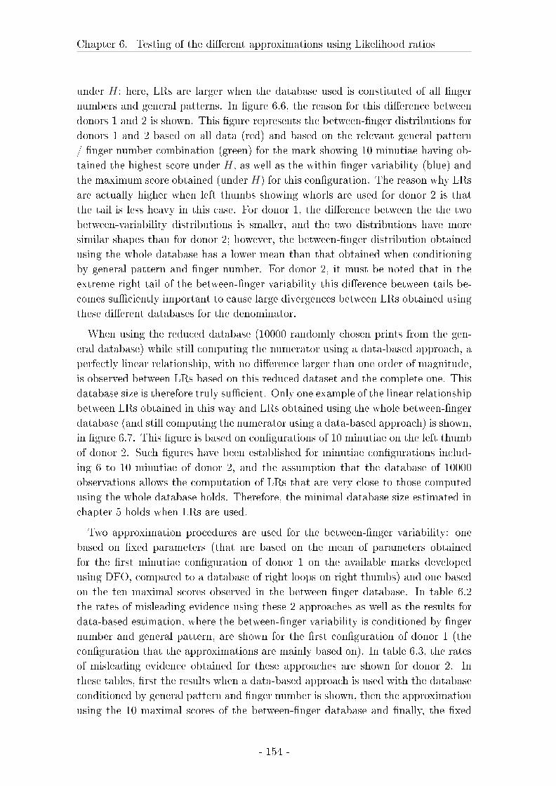
Chapter 6. Testing of the di�erent approximations using Likelihood ratios
under H; here, LRs are larger when the database used is constituted of all �nger
numbers and general patterns. In �gure 6.6, the reason for this di�erence between
donors 1 and 2 is shown. This �gure represents the between-�nger distributions for
donors 1 and 2 based on all data (red) and based on the relevant general pattern
/ �nger number combination (green) for the mark showing 10 minutiae having ob-
tained the highest score under H, as well as the within-�nger variability (blue) and
the maximum score obtained (under H) for this con�guration. The reason why LRs
are actually higher when left thumbs showing whorls are used for donor 2 is that
the tail is less heavy in this case. For donor 1, the di�erence between the the two
between-variability distributions is smaller, and the two distributions have more
similar shapes than for donor 2; however, the between-�nger distribution obtained
using the whole database has a lower mean than that obtained when conditioning
by general pattern and �nger number. For donor 2, it must be noted that in the
extreme right tail of the between-�nger variability this di�erence between tails be-
comes su�ciently important to cause large divergences between LRs obtained using
these di�erent databases for the denominator.
When using the reduced database (10000 randomly chosen prints from the gen-
eral database) while still computing the numerator using a data-based approach, a
perfectly linear relationship, with no di�erence larger than one order of magnitude,
is observed between LRs based on this reduced dataset and the complete one. This
database size is therefore truly su�cient. Only one example of the linear relationship
between LRs obtained in this way and LRs obtained using the whole between-�nger
database (and still computing the numerator using a data-based approach) is shown,
in �gure 6.7. This �gure is based on con�gurations of 10 minutiae on the left thumb
of donor 2. Such �gures have been established for minutiae con�gurations includ-
ing 6 to 10 minutiae of donor 2, and the assumption that the database of 10000
observations allows the computation of LRs that are very close to those computed
using the whole database holds. Therefore, the minimal database size estimated in
chapter 5 holds when LRs are used.
Two approximation procedures are used for the between-�nger variability: one
based on �xed parameters (that are based on the mean of parameters obtained
for the �rst minutiae con�guration of donor 1 on the available marks developed
using DFO, compared to a database of right loops on right thumbs) and one based
on the ten maximal scores observed in the between �nger database. In table 6.2
the rates of misleading evidence using these 2 approaches as well as the results for
data-based estimation, where the between-�nger variability is conditioned by �nger
number and general pattern, are shown for the �rst con�guration of donor 1 (the
con�guration that the approximations are mainly based on). In table 6.3, the rates
of misleading evidence obtained for these approaches are shown for donor 2. In
these tables, �rst the results when a data-based approach is used with the database
conditioned by general pattern and �nger number is shown, then the approximation
using the 10 maximal scores of the between-�nger database and �nally, the �xed
- 154 -
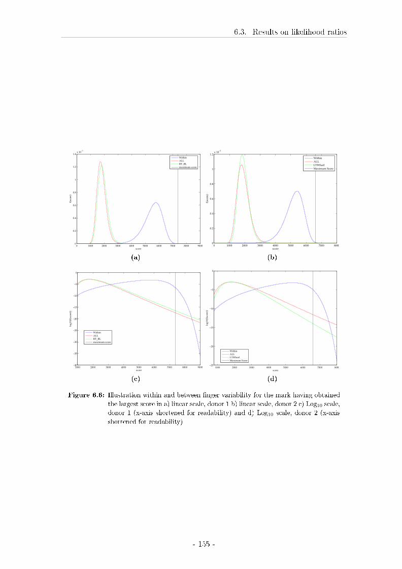
6.3. Results on likelihood ratios
0 1000 2000 3000 4000 5000 6000 7000 8000 90000
0.2
0.4
0.6
0.8
1
1.2
1.4x 10
−3
score
f(sc
ore
)
Within
ALL
RT_RL
maximum score
(a)
0 1000 2000 3000 4000 5000 6000 7000 80000
0.2
0.4
0.6
0.8
1
1.2x 10
−3
score
f(sc
ore
)
Within
ALL
LTWhorl
Maximum Score
(b)
1000 2000 3000 4000 5000 6000 7000 8000 9000−40
−35
−30
−25
−20
−15
−10
−5
0
score
log
10(f
(sco
re))
Within
ALL
RT_RL
maximum score
(c)
1000 2000 3000 4000 5000 6000 7000 8000−25
−20
−15
−10
−5
0
score
log
10(f
(sco
re))
Within
ALL
LTWhorl
Maximum Score
(d)
Figure 6.6: Illustration within and between �nger variability for the mark having obtained
the largest score in a) linear scale, donor 1 b) linear scale, donor 2 c) Log10 scale,
donor 1 (x-axis shortened for readability) and d) Log10 scale, donor 2 (x-axis
shortened for readability)
- 155 -
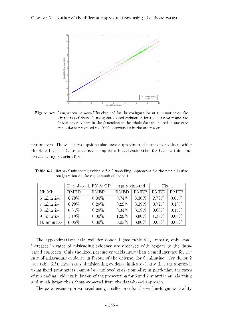
Chapter 6. Testing of the di�erent approximations using Likelihood ratios
−6 −4 −2 0 2 4 6 8 10−8
−6
−4
−2
0
2
4
6
8
10
12
log10(LRs) All data
log
10(L
Rs)
Red
dat
a 10
000
under bar(H)
under H
Figure 6.7: Comparison between LRs obtained for the con�guration of 10 minutiae on the
left thumb of donor 2, using data-based estimation for the numerator and the
denominator, where in the denominator the whole dataset is used in one case
and a dataset reduced to 10000 observations in the other case
parameters. These last two options also have approximated numerator values, while
the data-based LRs are obtained using data-based estimation for both within- and
between-�nger variability.
Table 6.2: Rates of misleading evidence for 3 modelling approaches for the �rst minutiae
con�guration on the right thumb of donor 1
Data-based, FN & GP Approximated Fixed
Nb Min RMED RMEP RMED RMEP RMED RMEP
6 minutiae 0.70% 0.30% 0.74% 0.30% 2.78% 0.05%
7 minutiae 0.29% 0.29% 0.29% 0.39% 0.72% 0.10%
8 minutiae 0.34% 0.29% 0.34% 0.19% 0.63% 0.14%
9 minutiae 1.19% 0.00% 1.29% 0.00% 1.38% 0.00%
10 minutiae 0.05% 0.00% 0.05% 0.00% 0.05% 0.00%
The approximations hold well for donor 1 (see table 6.2); mostly, only small
increases in rates of misleading evidence are observed with respect to the data-
based approach. Only the �xed parameter yields more than a small increase for the
rate of misleading evidence in favour of the defense, for 6 minutiae. For donor 2
(see table 6.3), these rates of misleading evidence indicate clearly that the approach
using �xed parameters cannot be employed operationnally; in particular, the rates
of misleading evidence in favour of the prosecution for 6 and 7 minutiae are alarming
and much larger than those expected from the data-based approach.
The parameters approximated using 3 self-scores for the within-�nger variability
- 156 -
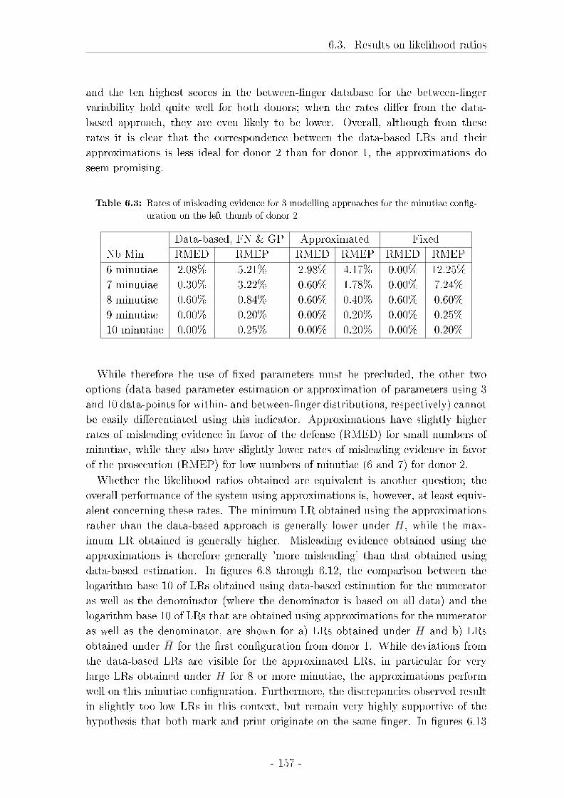
6.3. Results on likelihood ratios
and the ten highest scores in the between-�nger database for the between-�nger
variability hold quite well for both donors; when the rates di�er from the data-
based approach, they are even likely to be lower. Overall, although from these
rates it is clear that the correspondence between the data-based LRs and their
approximations is less ideal for donor 2 than for donor 1, the approximations do
seem promising.
Table 6.3: Rates of misleading evidence for 3 modelling approaches for the minutiae con�g-
uration on the left thumb of donor 2
Data-based, FN & GP Approximated Fixed
Nb Min RMED RMEP RMED RMEP RMED RMEP
6 minutiae 2.08% 5.21% 2.98% 4.17% 0.00% 12.25%
7 minutiae 0.30% 3.22% 0.60% 1.78% 0.00% 7.24%
8 minutiae 0.60% 0.84% 0.60% 0.40% 0.60% 0.60%
9 minutiae 0.00% 0.20% 0.00% 0.20% 0.00% 0.25%
10 minutiae 0.00% 0.25% 0.00% 0.20% 0.00% 0.20%
While therefore the use of �xed parameters must be precluded, the other two
options (data-based parameter estimation or approximation of parameters using 3
and 10 data-points for within- and between-�nger distributions, respectively) cannot
be easily di�erentiated using this indicator. Approximations have slightly higher
rates of misleading evidence in favor of the defense (RMED) for small numbers of
minutiae, while they also have slightly lower rates of misleading evidence in favor
of the prosecution (RMEP) for low numbers of minutiae (6 and 7) for donor 2.
Whether the likelihood ratios obtained are equivalent is another question; the
overall performance of the system using approximations is, however, at least equiv-
alent concerning these rates. The minimum LR obtained using the approximations
rather than the data-based approach is generally lower under H, while the max-
imum LR obtained is generally higher. Misleading evidence obtained using the
approximations is therefore generally 'more misleading' than that obtained using
data-based estimation. In �gures 6.8 through 6.12, the comparison between the
logarithm base 10 of LRs obtained using data-based estimation for the numerator
as well as the denominator (where the denominator is based on all data) and the
logarithm base 10 of LRs that are obtained using approximations for the numerator
as well as the denominator, are shown for a) LRs obtained under H and b) LRs
obtained under H̄ for the �rst con�guration from donor 1. While deviations from
the data-based LRs are visible for the approximated LRs, in particular for very
large LRs obtained under H for 8 or more minutiae, the approximations perform
well on this minutiae con�guration. Furthermore, the discrepancies observed result
in slightly too low LRs in this context, but remain very highly supportive of the
hypothesis that both mark and print originate on the same �nger. In �gures 6.13
- 157 -
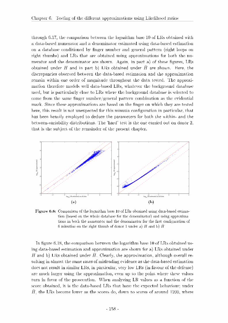
Chapter 6. Testing of the di�erent approximations using Likelihood ratios
through 6.17, the comparison between the logarithm base 10 of LRs obtained with
a data-based numerator and a denominator estimated using data-based estimation
on a database conditioned by �nger number and general pattern (right loops on
right thumbs) and LRs that are obtained using approximations for both the nu-
merator and the denominator are shown. Again, in part a) of these �gures, LRs
obtained under H and in part b) LRs obtained under H̄ are shown. Here, the
discrepancies observed between the data-based estimation and the approximation
remain within one order of magnitude throughout the data tested. The approxi-
mation therefore models well data-based LRs, whatever the background database
used, but is particularly close to LRs where the background database is selected to
come from the same �nger number/general pattern combination as the evidential
mark. Since these approximations are based on the �nger on which they are tested
here, this result is not unexpected for this minutia con�guration in particular, that
has been heavily employed to deduce the parameters for both the within- and the
between-variability distributions. The 'hard' test is the one carried out on donor 2,
that is the subject of the remainder of the present chapter.
−4 −2 0 2 4 6 8−4
−2
0
2
4
6
8
log10
LR estimated on all data
log
10 L
R a
pp
rox
imat
ed
(a)
−5 −4 −3 −2 −1 0 1 2−5
−4
−3
−2
−1
0
1
2
log10
LR estimated on all data
log
10 L
R a
pp
rox
imat
ed
(b)
Figure 6.8: Comparison of the logarithm base 10 of LRs obtained using data-based estima-
tion (based on the whole database for the denominator) and using approxima-
tions in both the numerator and the denominator for the �rst con�guration of
6 minutiae on the right thumb of donor 1 under a) H and b) H̄
In �gure 6.18, the comparison between the logarithm base 10 of LRs obtained us-
ing data-based estimation and approximation are shown for a) LRs obtained under
H and b) LRs obtained under H̄. Clearly, the approximation, although overall re-
sulting in almost the same rates of misleading evidence as the data-based estimation
does not result in similar LRs, in particular, very low LRs (in favour of the defense)
are much larger using the approximation, even up to the point where these values
turn in favor of the prosecution. When analyzing LR values as a function of the
score obtained, it is the data-based LRs that have the expected behaviour; under
H̄, the LRs become lower as the scores do, down to scores of around 1200, where
- 158 -

6.3. Results on likelihood ratios
−5 0 5 10−6
−4
−2
0
2
4
6
8
10
12
log10
LR estimated on all data
log
10 L
R a
pp
rox
imat
ed
(a)
−6 −5 −4 −3 −2 −1 0 1 2−6
−5
−4
−3
−2
−1
0
1
2
log10
LR estimated on all data
log
10 L
R a
pp
rox
imat
ed(b)
Figure 6.9: Comparison of the logarithm base 10 of LRs obtained using data-based estima-
tion (based on the whole database for the denominator) and using approxima-
tions in both the numerator and the denominator for the �rst con�guration of
7 minutiae on the right thumb of donor 1 under a) H and b) H̄
−5 0 5 10−5
0
5
10
log10
LR estimated on all data
log
10 L
R a
pp
rox
imat
ed
(a)
−5 −4 −3 −2 −1 0 1 2−5
−4
−3
−2
−1
0
1
2
log10
LR estimated on all data
log
10 L
R a
pp
rox
imat
ed
(b)
Figure 6.10: Comparison of the logarithm base 10 of LRs obtained using data-based esti-
mation (based on the whole database for the denominator) and using approxi-
mations in both the numerator and the denominator for the �rst con�guration
of 8 minutiae on the right thumb of donor 1 under a) H and b) H̄
- 159 -
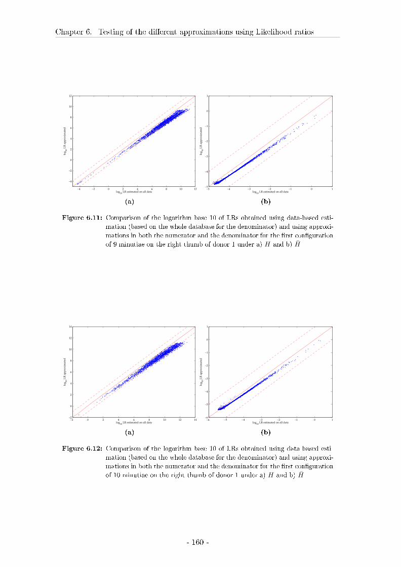
Chapter 6. Testing of the di�erent approximations using Likelihood ratios
−4 −2 0 2 4 6 8 10 12
−4
−2
0
2
4
6
8
10
12
log10
LR estimated on all data
log
10 L
R a
pp
rox
imat
ed
(a)
−5 −4 −3 −2 −1 0 1−5
−4
−3
−2
−1
0
1
log10
LR estimated on all data
log
10 L
R a
pp
rox
imat
ed(b)
Figure 6.11: Comparison of the logarithm base 10 of LRs obtained using data-based esti-
mation (based on the whole database for the denominator) and using approxi-
mations in both the numerator and the denominator for the �rst con�guration
of 9 minutiae on the right thumb of donor 1 under a) H and b) H̄
−2 0 2 4 6 8 10 12 14−2
0
2
4
6
8
10
12
14
log10
LR estimated on all data
log
10 L
R a
pp
rox
imat
ed
(a)
−6 −5 −4 −3 −2 −1 0 1−6
−5
−4
−3
−2
−1
0
1
log10
LR estimated on all data
log
10 L
R a
pp
rox
imat
ed
(b)
Figure 6.12: Comparison of the logarithm base 10 of LRs obtained using data-based esti-
mation (based on the whole database for the denominator) and using approxi-
mations in both the numerator and the denominator for the �rst con�guration
of 10 minutiae on the right thumb of donor 1 under a) H and b) H̄
- 160 -
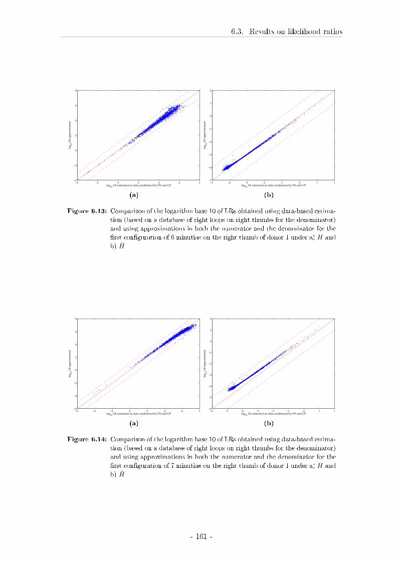
6.3. Results on likelihood ratios
−4 −2 0 2 4 6 8−4
−2
0
2
4
6
8
log10
LR estimated on data conditioned by FN and GP
log
10 L
R a
pp
rox
imat
ed
(a)
−5 −4 −3 −2 −1 0 1 2−5
−4
−3
−2
−1
0
1
2
log10
LR estimated on data conditioned by FN and GP
log
10 L
R a
pp
rox
imat
ed
(b)
Figure 6.13: Comparison of the logarithm base 10 of LRs obtained using data-based estima-
tion (based on a database of right loops on right thumbs for the denominator)
and using approximations in both the numerator and the denominator for the
�rst con�guration of 6 minutiae on the right thumb of donor 1 under a) H and
b) H̄
−6 −4 −2 0 2 4 6 8−6
−4
−2
0
2
4
6
8
log10
LR estimated on data conditioned by FN and GP
log
10 L
R a
pp
rox
imat
ed
(a)
−6 −5 −4 −3 −2 −1 0 1 2−6
−5
−4
−3
−2
−1
0
1
2
log10
LR estimated on data conditioned by FN and GP
log
10 L
R a
pp
rox
imat
ed
(b)
Figure 6.14: Comparison of the logarithm base 10 of LRs obtained using data-based estima-
tion (based on a database of right loops on right thumbs for the denominator)
and using approximations in both the numerator and the denominator for the
�rst con�guration of 7 minutiae on the right thumb of donor 1 under a) H and
b) H̄
- 161 -
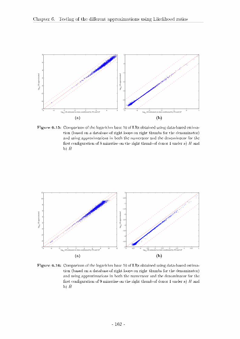
Chapter 6. Testing of the di�erent approximations using Likelihood ratios
−6 −4 −2 0 2 4 6 8−6
−4
−2
0
2
4
6
8
log10
LR estimated on data conditioned by FN and GP
log
10 L
R a
pp
rox
imat
ed
(a)
−5 −4 −3 −2 −1 0 1−5
−4
−3
−2
−1
0
1
log10
LR estimated on data conditioned by FN and GP
log
10 L
R a
pp
rox
imat
ed(b)
Figure 6.15: Comparison of the logarithm base 10 of LRs obtained using data-based estima-
tion (based on a database of right loops on right thumbs for the denominator)
and using approximations in both the numerator and the denominator for the
�rst con�guration of 8 minutiae on the right thumb of donor 1 under a) H and
b) H̄
−6 −4 −2 0 2 4 6 8 10 12−6
−4
−2
0
2
4
6
8
10
12
log10
LR estimated on data conditioned by FN and GP
log
10 L
R a
pp
rox
imat
ed
(a)
−5 −4.5 −4 −3.5 −3 −2.5 −2 −1.5 −1 −0.5 0−5
−4.5
−4
−3.5
−3
−2.5
−2
−1.5
−1
−0.5
0
log10
LR estimated on data conditioned by FN and GP
log
10 L
R a
pp
rox
imat
ed
(b)
Figure 6.16: Comparison of the logarithm base 10 of LRs obtained using data-based estima-
tion (based on a database of right loops on right thumbs for the denominator)
and using approximations in both the numerator and the denominator for the
�rst con�guration of 9 minutiae on the right thumb of donor 1 under a) H and
b) H̄
- 162 -
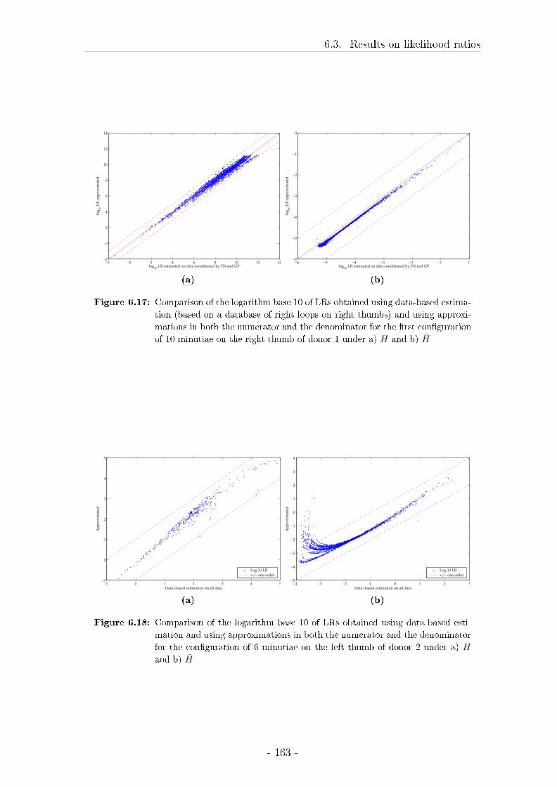
6.3. Results on likelihood ratios
−2 0 2 4 6 8 10 12 14−2
0
2
4
6
8
10
12
14
log10
LR estimated on data conditioned by FN and GP
log
10 L
R a
pp
rox
imat
ed
(a)
−6 −5 −4 −3 −2 −1 0−6
−5
−4
−3
−2
−1
0
log10
LR estimated on data conditioned by FN and GP
log
10 L
R a
pp
rox
imat
ed(b)
Figure 6.17: Comparison of the logarithm base 10 of LRs obtained using data-based estima-
tion (based on a database of right loops on right thumbs) and using approxi-
mations in both the numerator and the denominator for the �rst con�guration
of 10 minutiae on the right thumb of donor 1 under a) H and b) H̄
−1 0 1 2 3 4 5−1
0
1
2
3
4
5
Data−based estimation on all data
Ap
pro
xim
ated
Log 10 LR
+/− one order
(a)
−4 −3 −2 −1 0 1 2 3−5
−4
−3
−2
−1
0
1
2
3
4
Data−based estimation on all data
Ap
pro
xim
ated
Log 10 LR
+/− one order
(b)
Figure 6.18: Comparison of the logarithm base 10 of LRs obtained using data-based esti-
mation and using approximations in both the numerator and the denominator
for the con�guration of 6 minutiae on the left thumb of donor 2 under a) H
and b) H̄
- 163 -
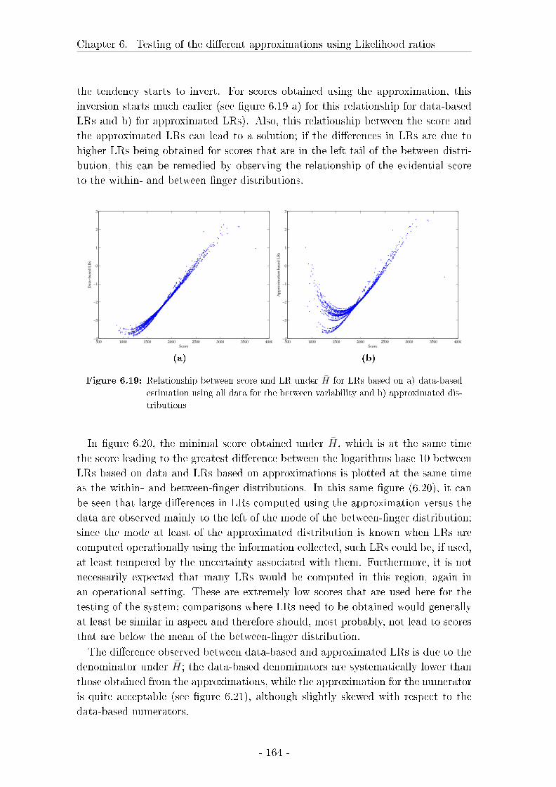
Chapter 6. Testing of the di�erent approximations using Likelihood ratios
the tendency starts to invert. For scores obtained using the approximation, this
inversion starts much earlier (see �gure 6.19 a) for this relationship for data-based
LRs and b) for approximated LRs). Also, this relationship between the score and
the approximated LRs can lead to a solution; if the di�erences in LRs are due to
higher LRs being obtained for scores that are in the left tail of the between distri-
bution, this can be remedied by observing the relationship of the evidential score
to the within- and between �nger distributions.
500 1000 1500 2000 2500 3000 3500 4000−4
−3
−2
−1
0
1
2
3
Score
Data
−b
ased
LR
s
(a)
500 1000 1500 2000 2500 3000 3500 4000−4
−3
−2
−1
0
1
2
3
Score
Ap
pro
xim
atio
n b
ased
LR
s
(b)
Figure 6.19: Relationship between score and LR under H̄ for LRs based on a) data-based
estimation using all data for the between variability and b) approximated dis-
tributions
In �gure 6.20, the minimal score obtained under H̄, which is at the same time
the score leading to the greatest di�erence between the logarithms base 10 between
LRs based on data and LRs based on approximations is plotted at the same time
as the within- and between-�nger distributions. In this same �gure (6.20), it can
be seen that large di�erences in LRs computed using the approximation versus the
data are observed mainly to the left of the mode of the between-�nger distribution;
since the mode at least of the approximated distribution is known when LRs are
computed operationally using the information collected, such LRs could be, if used,
at least tempered by the uncertainty associated with them. Furthermore, it is not
necessarily expected that many LRs would be computed in this region, again in
an operational setting. These are extremely low scores that are used here for the
testing of the system; comparisons where LRs need to be obtained would generally
at least be similar in aspect and therefore should, most probably, not lead to scores
that are below the mean of the between-�nger distribution.
The di�erence observed between data-based and approximated LRs is due to the
denominator under H̄; the data-based denominators are systematically lower than
those obtained from the approximations, while the approximation for the numerator
is quite acceptable (see �gure 6.21), although slightly skewed with respect to the
data-based numerators.
- 164 -
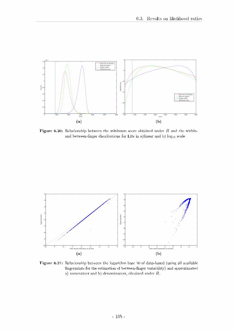
6.3. Results on likelihood ratios
0 1000 2000 3000 4000 5000 60000
0.2
0.4
0.6
0.8
1
1.2
1.4
1.6x 10
−3
score
f(sc
ore
)
Between (on all data)
Between approx
Within (data)
Minimum score
(a)
500 1000 1500 2000 2500 3000 3500 4000−25
−20
−15
−10
−5
0
score
log
10(f
(sco
re))
Between (on all data)
Between approx
Within (data)
Minimum score
(b)
Figure 6.20: Relationship between the minimum score obtained under H̄ and the within-
and between-�nger distributions for LRs in a)linear and b) log10 scale
−10 −9 −8 −7 −6 −5 −4 −3 −2−10
−9
−8
−7
−6
−5
−4
−3
−2
Data−based estimation on all data
Ap
pro
xim
ated
(a)
−11 −10 −9 −8 −7 −6 −5 −4 −3 −2−11
−10
−9
−8
−7
−6
−5
−4
−3
−2
Data−based estimation on all data
Ap
pro
xim
ated
(b)
Figure 6.21: Relationship between the logarithm base 10 of data-based (using all available
�ngerprints for the estimation of between-�nger variability) and approximated
a) numerators and b) denominators, obtained under H̄.
- 165 -
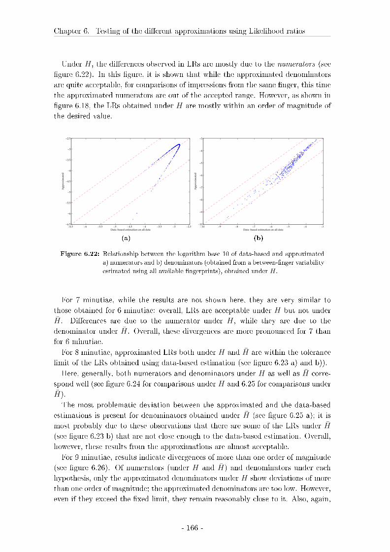
Chapter 6. Testing of the di�erent approximations using Likelihood ratios
Under H, the di�erences observed in LRs are mostly due to the numerators (see
�gure 6.22). In this �gure, it is shown that while the approximated denominators
are quite acceptable, for comparisons of impressions from the same �nger, this time
the approximated numerators are out of the accepted range. However, as shown in
�gure 6.18, the LRs obtained under H are mostly within an order of magnitude of
the desired value.
−6.5 −6 −5.5 −5 −4.5 −4 −3.5 −3 −2.5−6.5
−6
−5.5
−5
−4.5
−4
−3.5
−3
−2.5
Data−based estimation on all data
Ap
pro
xim
ated
(a)
−10 −9 −8 −7 −6 −5 −4 −3−10
−9
−8
−7
−6
−5
−4
−3
Data−based estimation on all data
Ap
pro
xim
ated
(b)
Figure 6.22: Relationship between the logarithm base 10 of data-based and approximated
a) numerators and b) denominators (obtained from a between-�nger variability
estimated using all available �ngerprints), obtained under H.
For 7 minutiae, while the results are not shown here, they are very similar to
those obtained for 6 minutiae: overall, LRs are acceptable under H but not under
H̄. Di�erences are due to the numerator under H, while they are due to the
denominator under H̄. Overall, these divergences are more pronounced for 7 than
for 6 minutiae.
For 8 minutiae, approximated LRs both under H and H̄ are within the tolerance
limit of the LRs obtained using data-based estimation (see �gure 6.23 a) and b)).
Here, generally, both numerators and denominators under H as well as H̄ corre-
spond well (see �gure 6.24 for comparisons under H and 6.25 for comparisons under
H̄).
The most problematic deviation between the approximated and the data-based
estimations is present for denominators obtained under H̄ (see �gure 6.25 a); it is
most probably due to these observations that there are some of the LRs under H̄
(see �gure 6.23 b) that are not close enough to the data-based estimation. Overall,
however, these results from the approximations are almost acceptable.
For 9 minutiae, results indicate divergences of more than one order of magnitude
(see �gure 6.26). Of numerators (under H and H̄) and denominators under each
hypothesis, only the approximated denominators under H show deviations of more
than one order of magnitude; the approximated denominators are too low. However,
even if they exceed the �xed limit, they remain reasonably close to it. Also, again,
- 166 -
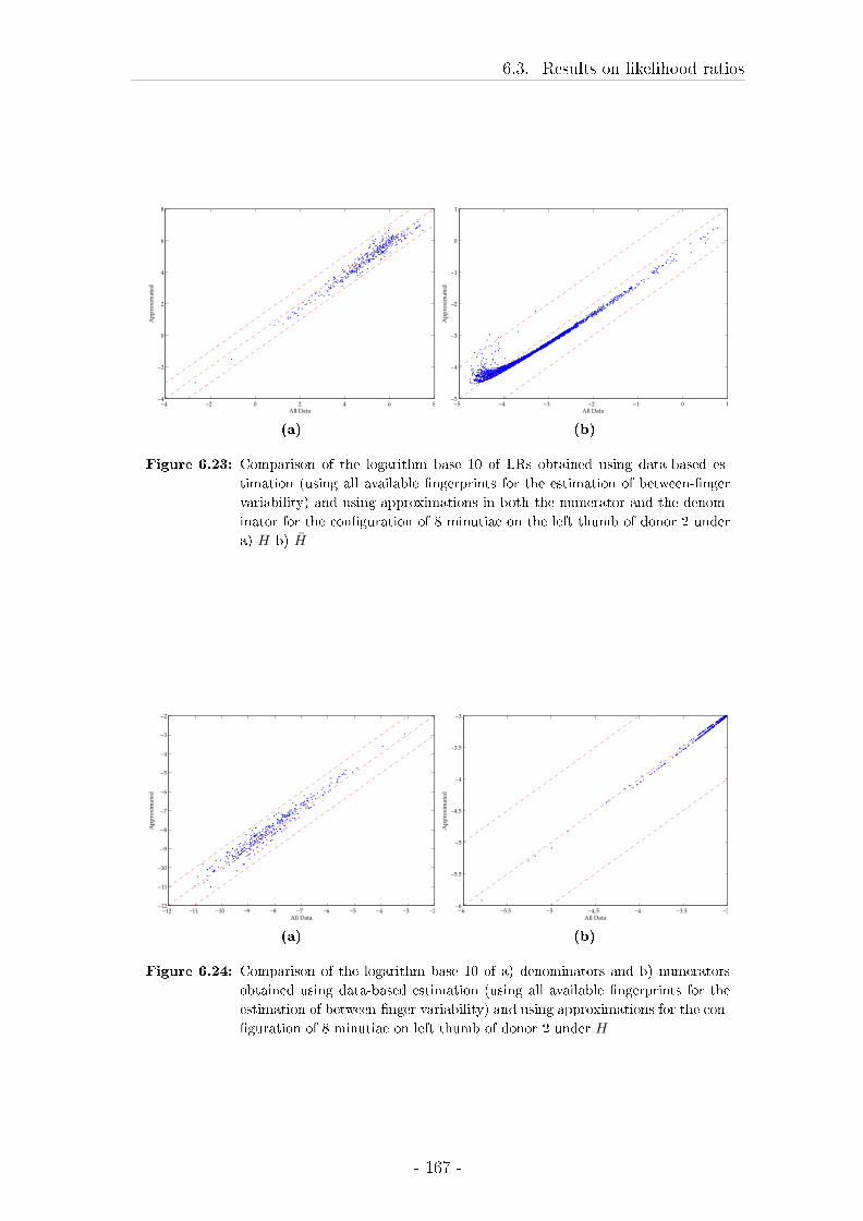
6.3. Results on likelihood ratios
−4 −2 0 2 4 6 8−4
−2
0
2
4
6
8
All Data
Ap
pro
xim
ated
(a)
−5 −4 −3 −2 −1 0 1−5
−4
−3
−2
−1
0
1
All Data
Ap
pro
xim
ated
(b)
Figure 6.23: Comparison of the logarithm base 10 of LRs obtained using data-based es-
timation (using all available �ngerprints for the estimation of between-�nger
variability) and using approximations in both the numerator and the denom-
inator for the con�guration of 8 minutiae on the left thumb of donor 2 under
a) H b) H̄
−12 −11 −10 −9 −8 −7 −6 −5 −4 −3 −2−12
−11
−10
−9
−8
−7
−6
−5
−4
−3
−2
All Data
Ap
pro
xim
ated
(a)
−6 −5.5 −5 −4.5 −4 −3.5 −3−6
−5.5
−5
−4.5
−4
−3.5
−3
All Data
Ap
pro
xim
ated
(b)
Figure 6.24: Comparison of the logarithm base 10 of a) denominators and b) numerators
obtained using data-based estimation (using all available �ngerprints for the
estimation of between-�nger variability) and using approximations for the con-
�guration of 8 minutiae on left thumb of donor 2 under H
- 167 -
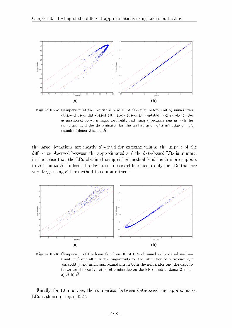
Chapter 6. Testing of the di�erent approximations using Likelihood ratios
−8 −7.5 −7 −6.5 −6 −5.5 −5 −4.5 −4 −3.5 −3 −2.5−8
−7.5
−7
−6.5
−6
−5.5
−5
−4.5
−4
−3.5
−3
−2.5
All Data
Ap
pro
xim
ated
(a)
−10 −9 −8 −7 −6 −5 −4−10
−9
−8
−7
−6
−5
−4
All Data
Ap
pro
xim
ated
(b)
Figure 6.25: Comparison of the logarithm base 10 of a) denominators and b) numerators
obtained using data-based estimation (using all available �ngerprints for the
estimation of between-�nger variability and using approximations in both the
numerator and the denominator for the con�guration of 8 minutiae on left
thumb of donor 2 under H̄
the large deviations are mostly observed for extreme values; the impact of the
di�erence observed between the approximated and the data-based LRs is minimal
in the sense that the LRs obtained using either method lend much more support
to H than to H̄. Indeed, the deviations observed here occur only for LRs that are
very large using either method to compute them.
0 1 2 3 4 5 6 7 8 90
1
2
3
4
5
6
7
8
9
All Data
Ap
pro
xim
ated
(a)
−6 −5 −4 −3 −2 −1 0 1−6
−5
−4
−3
−2
−1
0
1
All Data
Ap
pro
xim
ated
(b)
Figure 6.26: Comparison of the logarithm base 10 of LRs obtained using data-based es-
timation (using all available �ngerprints for the estimation of between-�nger
variability) and using approximations in both the numerator and the denom-
inator for the con�guration of 9 minutiae on the left thumb of donor 2 under
a) H b) H̄
Finally, for 10 minutiae, the comparison between data-based and approximated
LRs is shown in �gure 6.27.
- 168 -
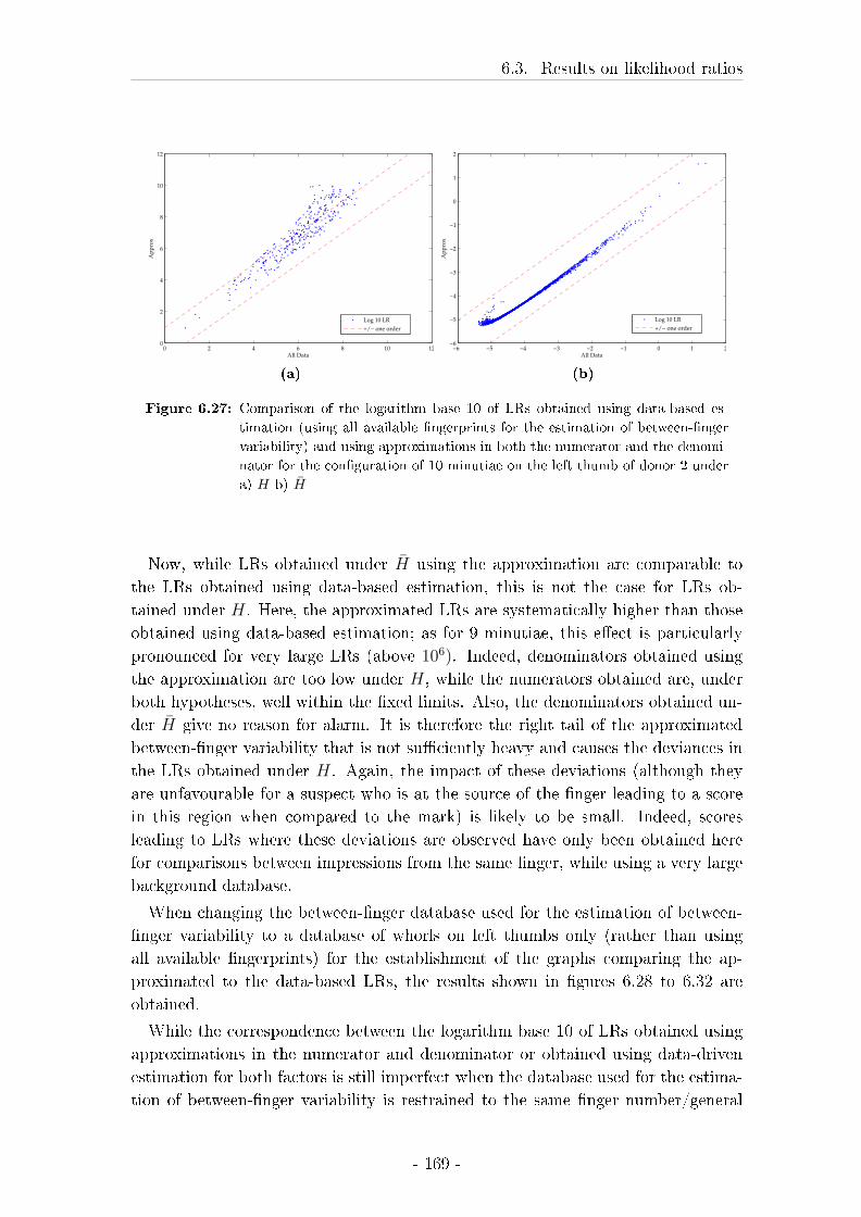
6.3. Results on likelihood ratios
0 2 4 6 8 10 120
2
4
6
8
10
12
All Data
Ap
pro
x
Log 10 LR
+/− one order
(a)
−6 −5 −4 −3 −2 −1 0 1 2−6
−5
−4
−3
−2
−1
0
1
2
All Data
Ap
pro
x
Log 10 LR
+/− one order
(b)
Figure 6.27: Comparison of the logarithm base 10 of LRs obtained using data-based es-
timation (using all available �ngerprints for the estimation of between-�nger
variability) and using approximations in both the numerator and the denomi-
nator for the con�guration of 10 minutiae on the left thumb of donor 2 under
a) H b) H̄
Now, while LRs obtained under H̄ using the approximation are comparable to
the LRs obtained using data-based estimation, this is not the case for LRs ob-
tained under H. Here, the approximated LRs are systematically higher than those
obtained using data-based estimation; as for 9 minutiae, this e�ect is particularly
pronounced for very large LRs (above 106). Indeed, denominators obtained using
the approximation are too low under H, while the numerators obtained are, under
both hypotheses, well within the �xed limits. Also, the denominators obtained un-
der H̄ give no reason for alarm. It is therefore the right tail of the approximated
between-�nger variability that is not su�ciently heavy and causes the deviances in
the LRs obtained under H. Again, the impact of these deviations (although they
are unfavourable for a suspect who is at the source of the �nger leading to a score
in this region when compared to the mark) is likely to be small. Indeed, scores
leading to LRs where these deviations are observed have only been obtained here
for comparisons between impressions from the same �nger, while using a very large
background database.
When changing the between-�nger database used for the estimation of between-
�nger variability to a database of whorls on left thumbs only (rather than using
all available �ngerprints) for the establishment of the graphs comparing the ap-
proximated to the data-based LRs, the results shown in �gures 6.28 to 6.32 are
obtained.
While the correspondence between the logarithm base 10 of LRs obtained using
approximations in the numerator and denominator or obtained using data-driven
estimation for both factors is still imperfect when the database used for the estima-
tion of between-�nger variability is restrained to the same �nger number/general
- 169 -
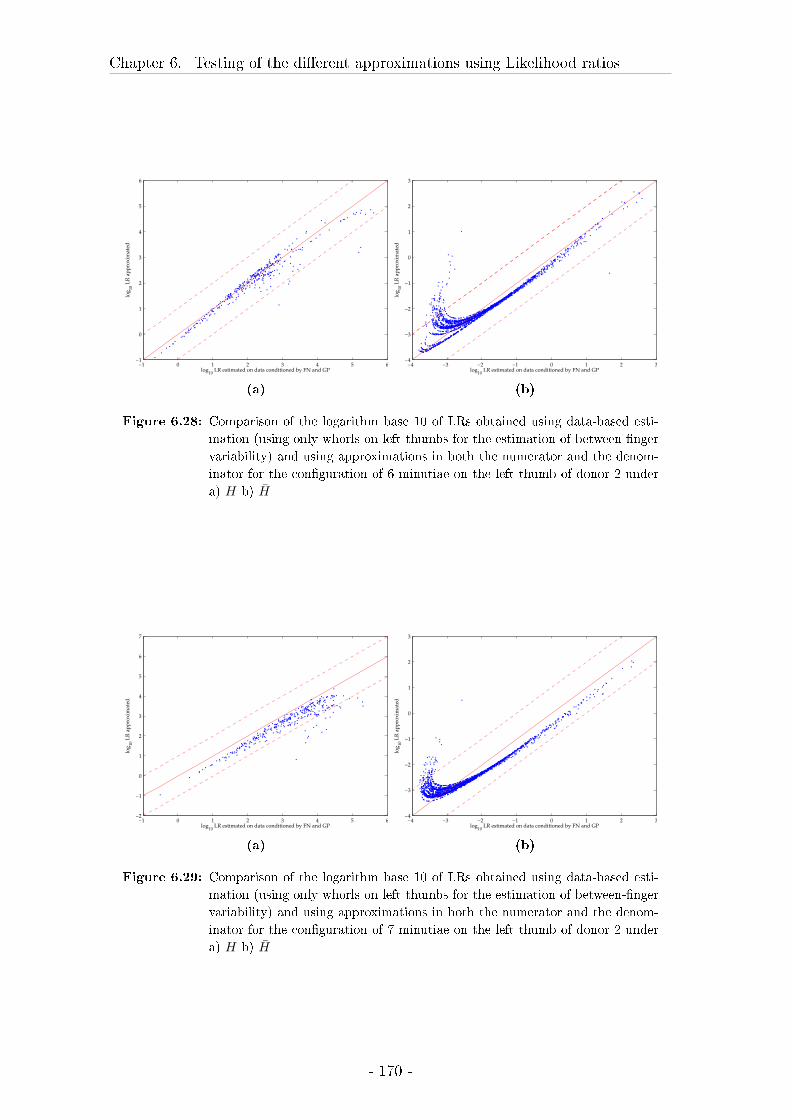
Chapter 6. Testing of the di�erent approximations using Likelihood ratios
−1 0 1 2 3 4 5 6−1
0
1
2
3
4
5
6
log10
LR estimated on data conditioned by FN and GP
log
10 L
R a
pp
rox
imat
ed
(a)
−4 −3 −2 −1 0 1 2 3−4
−3
−2
−1
0
1
2
3
log10
LR estimated on data conditioned by FN and GP
log
10 L
R a
pp
rox
imat
ed(b)
Figure 6.28: Comparison of the logarithm base 10 of LRs obtained using data-based esti-
mation (using only whorls on left thumbs for the estimation of between-�nger
variability) and using approximations in both the numerator and the denom-
inator for the con�guration of 6 minutiae on the left thumb of donor 2 under
a) H b) H̄
−1 0 1 2 3 4 5 6−2
−1
0
1
2
3
4
5
6
7
log10
LR estimated on data conditioned by FN and GP
log
10 L
R a
pp
rox
imat
ed
(a)
−4 −3 −2 −1 0 1 2 3−4
−3
−2
−1
0
1
2
3
log10
LR estimated on data conditioned by FN and GP
log
10 L
R a
pp
rox
imat
ed
(b)
Figure 6.29: Comparison of the logarithm base 10 of LRs obtained using data-based esti-
mation (using only whorls on left thumbs for the estimation of between-�nger
variability) and using approximations in both the numerator and the denom-
inator for the con�guration of 7 minutiae on the left thumb of donor 2 under
a) H b) H̄
- 170 -
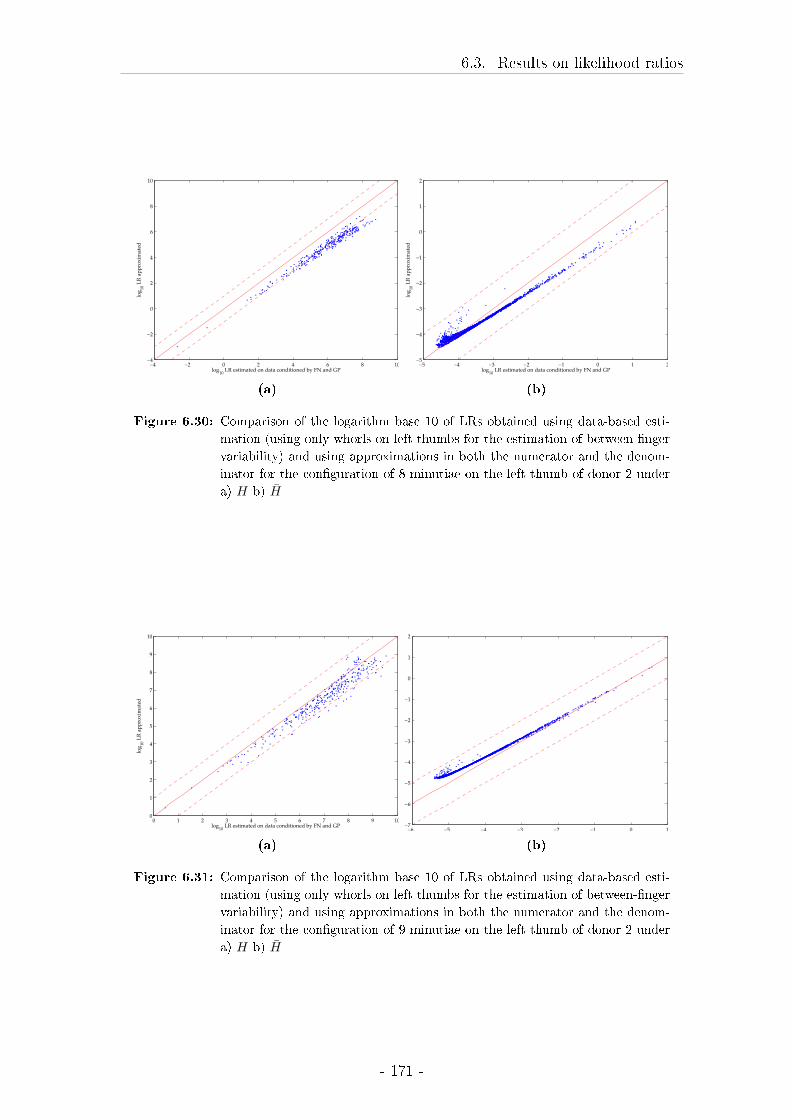
6.3. Results on likelihood ratios
−4 −2 0 2 4 6 8 10−4
−2
0
2
4
6
8
10
log10
LR estimated on data conditioned by FN and GP
log
10 L
R a
pp
rox
imat
ed
(a)
−5 −4 −3 −2 −1 0 1 2−5
−4
−3
−2
−1
0
1
2
log10
LR estimated on data conditioned by FN and GP
log
10 L
R a
pp
rox
imat
ed
(b)
Figure 6.30: Comparison of the logarithm base 10 of LRs obtained using data-based esti-
mation (using only whorls on left thumbs for the estimation of between-�nger
variability) and using approximations in both the numerator and the denom-
inator for the con�guration of 8 minutiae on the left thumb of donor 2 under
a) H b) H̄
0 1 2 3 4 5 6 7 8 9 100
1
2
3
4
5
6
7
8
9
10
log10
LR estimated on data conditioned by FN and GP
log
10 L
R a
pp
rox
imat
ed
(a)
−6 −5 −4 −3 −2 −1 0 1−7
−6
−5
−4
−3
−2
−1
0
1
2
(b)
Figure 6.31: Comparison of the logarithm base 10 of LRs obtained using data-based esti-
mation (using only whorls on left thumbs for the estimation of between-�nger
variability) and using approximations in both the numerator and the denom-
inator for the con�guration of 9 minutiae on the left thumb of donor 2 under
a) H b) H̄
- 171 -
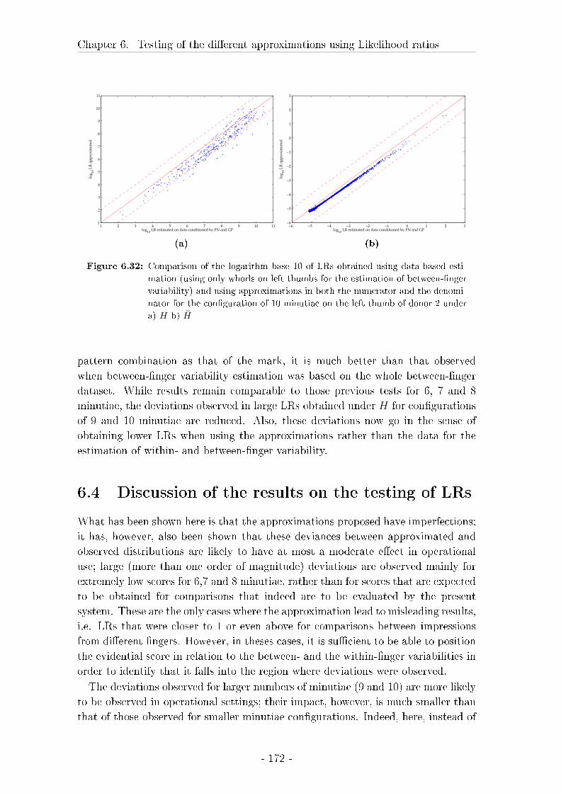
Chapter 6. Testing of the di�erent approximations using Likelihood ratios
1 2 3 4 5 6 7 8 9 10 111
2
3
4
5
6
7
8
9
10
11
log10
LR estimated on data conditioned by FN and GP
log
10 L
R a
pp
rox
imat
ed
(a)
−6 −5 −4 −3 −2 −1 0 1 2 3−6
−5
−4
−3
−2
−1
0
1
2
3
log10
LR estimated on data conditioned by FN and GP
log
10 L
R a
pp
rox
imat
ed
(b)
Figure 6.32: Comparison of the logarithm base 10 of LRs obtained using data-based esti-
mation (using only whorls on left thumbs for the estimation of between-�nger
variability) and using approximations in both the numerator and the denomi-
nator for the con�guration of 10 minutiae on the left thumb of donor 2 under
a) H b) H̄
pattern combination as that of the mark, it is much better than that observed
when between-�nger variability estimation was based on the whole between-�nger
dataset. While results remain comparable to those previous tests for 6, 7 and 8
minutiae, the deviations observed in large LRs obtained under H for con�gurations
of 9 and 10 minutiae are reduced. Also, these deviations now go in the sense of
obtaining lower LRs when using the approximations rather than the data for the
estimation of within- and between-�nger variability.
6.4 Discussion of the results on the testing of LRs
What has been shown here is that the approximations proposed have imperfections;
it has, however, also been shown that these deviances between approximated and
observed distributions are likely to have at most a moderate e�ect in operational
use; large (more than one order of magnitude) deviations are observed mainly for
extremely low scores for 6,7 and 8 minutiae, rather than for scores that are expected
to be obtained for comparisons that indeed are to be evaluated by the present
system. These are the only cases where the approximation lead to misleading results,
i.e. LRs that were closer to 1 or even above for comparisons between impressions
from di�erent �ngers. However, in theses cases, it is su�cient to be able to position
the evidential score in relation to the between- and the within-�nger variabilities in
order to identify that it falls into the region where deviations were observed.
The deviations observed for larger numbers of minutiae (9 and 10) are more likely
to be observed in operational settings; their impact, however, is much smaller than
that of those observed for smaller minutiae con�gurations. Indeed, here, instead of
- 172 -
6.4. Discussion of the results on the testing of LRs
very large LRs in favour of H, now, LRs that are even larger are obtained. This
is not unproblematic; however, upper and lower limits could be associated to these
LRs, which would be likely to solve this problem.
Furthermore, comparisons with data-based LRs where a between-�nger database
consisting only of �ngerprints with the same combination of general pattern and
�nger number resulted in even better correspondence between these data-based and
the approximated results. Therefore, while the degradation in correspondence for
donor 2 with respect to donor 1 is not negligible, it still yields acceptable or even
good results and is therefore a viable approach to operational implementation of
the computation of LRs based on scores as output by an AFIS.
This, although not very large, degradation of the correspondence between ap-
proximated and data-based LRs for donor 2 with respect to that of donor 1 does
not allow the direct application of approximations to casework. It is not possible
to know whether, in the case of another donor or a di�erent �nger number (such
as index �ngers) the approximation would hold as well as it has for donor 2. Since
there is a certain instability in the �t of the approximation to the data-based esti-
mation, which is evidenced by the di�erence between donors 1 and 2 observed here,
the approximation cannot be considered generalizable at this point. Further valida-
tion of this approach is relatively easy to carry out, even during application of the
model to casework using data-based estimation. During such data-based estima-
tion, all the necessary data for the approximation is acquired; the only additional
information needed for the approximation if data-based estimation is carried out are
the self-scores (but the images to acquire self-scores are needed for the data-based
estimation of within-�nger variability; only the insertion of 3 slap impressions as
'prints' into the system and their annotation to match as closely as possible that
used when they are inserted as 'marks' into the system are lacking).
The results obtained here do show that data-based LR estimation is
robust and yields overall low rates of misleading evidence and rather
large LRs in favour of the hypothesis known to be true. Furthermore,
both the rates of misleading evidence and the values of the LRs go in the
right direction as minutiae are added to the con�gurations; a decrease
of the rates of misleading evidence is generally observed, while LRs lend
more support to the true hypothesis as minutiae are added.
The approximations used are promising: divergences between the data-
based and approximated LRs are generally small and the conditions in
which they may be large are quite well de�ned. In the present work, no
precise threshold in terms of score or density values can be given, because the large
divergences generally depend not only on the probability density of one of the two
distributions, but on the relationship between the two. An example shown in this
chapter (see �gure 6.20) may be taken to aid the determination of a region where
approximation and data-based estimation do not correspond. However, in casework,
such very low scores are not expected to be observed. It is thought that in general
- 173 -

Chapter 6. Testing of the di�erent approximations using Likelihood ratios
such LR based evaluation would only be carried out when an examiner has carried
out the comparison and has not been able to exclude. Therefore, the con�gurations
of mark and print would already be more similar than those used here under H̄,
that are simply randomly sampled among all of the comparisons between the marks
from a known source and the �ngerprints known to come from di�erent sources.
- 174 -
Chapter 7
Discussion
7.1 General approach
The point of view that the evaluation of forensic evidence in general and �nger-
print evidence in particular can and should be carried out using statistical tools is
taken in this thesis. This point of view cannot be considered as new: it is the one
defended, for example, in Stoney (1985), Champod (1996) as well as Taroni and
Margot (2000), Champod and Evett (2001) and Saks and Koehler (2005). Also,
previous research has been carried out on statistical models in �ngerprints. Only
few used the likelihood ratio as the indicator of the probabilistic weight of the evi-
dence: the model by Neumann et al. (2006, 2007) and the one by Champod (1996).
The model by Neumann et al. (2006, 2007) is, however, the only one that estimates
a numerator for the likelihood ratio. The probabilistic approach remains quite con-
troversial, however, and even prohibited by professional bodies (SWGFAST, 2003;
Anon., 1980). These professional bodies indeed require that conclusions be absolute.
The view is taken here that while absolute conclusions may have had some reason
for being in the absence of statistical models that were reasonably well tested and
established on large datasets, now that such models become truly available, these
reasons certainly no longer exist. The reason why these absolute conclusions had
some grounds in that context is that it is, quite opposite to what should rationally
be expected, easier to defend absolute conclusions than probabilistic ones. While
absolute conclusions are accepted in court, subject to the experts' demonstration
of their capacity to reach such conclusions, the presentation of probabilistic data is
much harder, perhaps without reason. Such a presentation is subject to the veri-
�cation of each step, the assumptions, data, modeling and �nal result. This also
means that all that leads to the conclusion (i.e. the observations in the case, the
assumptions and models, the method and data on which this process is based as
well as the results of previous tests of the performance of this process) is (or can
be) made transparent.
The likelihood ratios generated by the models used for within- and between-
variability in the present thesis are not considered as being useful to the fact �nder
in the form of precise numbers. Although the result as such will be some high
- 175 -
Chapter 7. Discussion
precision number, it is not considered here that to take into account the precision is
useful. Take, as an example, an LR of 3.45672·108. Indeed, if the LRs computed are
undoubtedly quite robust concerning their exponent, it is very doubtful that with a
change of data, in particular in the within-�nger variability, the exact same number
would be obtained. Also, while the number is very useful for the combination of
di�erent items of evidence, it is not necessarily a great aid to comprehension. The
concept of likelihood ratios is not easy to explain, nor to understand. It is even
worse when very large numbers result from computations, that must be viewed in
a completely probabilistic setting in order to be understood properly; otherwise,
these numbers would inhibit rather than aid a fair assessment of evidence.
Furthermore, the models for within- and between-�nger variability that allow
to compute LRs must be viewed as the best possible representation of what they
should be. They are �rstly based on data, and this data is acquired in a given
way; this acquisition process, as well as the data itself, may lead to variations in the
within-�nger variability. Then, some way of obtaining f(s|H) and f(s|H̄) is devised
in any model to compute LRs; here, choices are involved. The choice made here
was to use a Weibull and a Lognormal distribution, �t them to the relevant data
as de�ned previously, and obtain the numerator and denominator values from these
distributions. These choices can and should be questioned, not only in the present
model, but in all models. While it is hoped that LRs computed using di�erent
models will be coherent, this needn't necessarily be the case; at least numerical
identity cannot be expected. Correspondence in the order of magnitude of LRs
should, however, be possible. Otherwise, the only way to interpret the values of the
di�erent models would be to scrutinize the premises of the di�erent models, and
make a reasoned choice between them.
It is because in general the exact values of LRs are not viewed as being particularly
useful in the communication of results (nor in the �nal decision made by the judge),
that errors of up to an order of magnitude (or up to a change in the value of the
exponent) have been allowed in all approximations made.
The results shown in the present thesis have been obtained by using a given
system: a Sagem DMA. The scores and distributions obtained are most certainly
not the same as those that would be obtained using any other AFIS. However,
the present work not only yields these system-speci�c results, but more interest-
ingly proposes a way of acquiring data for the establishment and testing of an
interpretative approach based on AFIS scores. The goal being to be able to obtain
likelihood ratios from these scores, practical approaches to the estimation of within-
and between-variability are proposed. While some of the options selected here may
not lead to general agreement (e.g. the use of parametric models for the within-
and between-�nger distributions), alternatives are mentioned and the reasons for
not choosing them are made clear; if a similar model was to be established on the
basis of a di�erent system, di�erent choices could be made.
One of the more salient choices made in the present thesis are the numbers of
- 176 -
7.2. Within- �nger variability
minutiae that have been investigated; only con�gurations of between 6 and 10 minu-
tiae have been used. While it is clear that not all numbers of minutiae can be
investigated, the precise limits de�ned here can be challenged. The lower limit was
chosen for practicability; indeed, very small con�gurations may be used, but in
practice the use of very small con�gurations would lead to a large amount of ad-
ditional work, mostly spent searching for very small con�gurations, that also have
the disadvantage of being di�cult to place on a �ngerprint. The precise number of
6 minutiae was chosen here because such con�gurations of minutiae can reasonably
be expected to be found on a comparison print without a necessarily huge time
investment. This is not true, for example, for con�gurations of 3 minutiae, where
the time needed to compare such a con�guration to a comparison print is rather
large. This is a subjective determination, and this number could be decreased, at
least to 5 minutiae (this number is the limit set at this time in the AFIS used for the
minimum number of minutiae needed to carry out a comparison using the system;
even this limit can be as low as 3 minutiae).
The upper limit used here, of 10 minutiae, was chosen because it was expected
that very large LRs could already be obtained for this number; otherwise, the
system would not have been considered as an evaluative tool performing well on
a very selective biometric which the �ngerprint is. Here, indeed, very large LRs
are obtained for 10 minutiae, showing that AFIS scores can usefully be employed
for evidential assessment using LRs. It would be interesting to adapt the model
to larger numbers of minutiae. If cases with larger numbers of minutiae did occur
before such an adaptation has been carried out, a subset of minutiae could be used.
A supplementary veri�cation step would need to be included in such a case. Indeed,
if any of the minutiae not considered in the LR computation initially was to lower
the score obtained when added, that would be an alarm signal indicating possibly
lack of correspondence between the mark and the print; such a minutiae would
necessarily need to be included in the minutiae set used for the computation of the
evidential score.
7.2 Within- �nger variability
Aminimal sample size necessary for the robust estimation of within-�nger variability
has been determined empirically. This minimum size is of 66 samples. This number
may be subject to changes due to the data acquisition process. Here, a bimodality
of the distribution of the results on 702 livescans had been observed (which may
have been due to the precise minutiae chosen and therefore not necessarily present
for any minutiae con�guration), and it is on this sample that the sample size was
based in a �rst step. This sample size may not be applicable to all other samples
of �ngerprints. In fact, the distribution of the scores is highly in�uenced by the
distortion directions used in the acquisition of within-�nger variability data; this
dependence of the distribution on the data acquisition process may also impact on
- 177 -
Chapter 7. Discussion
the sample size need when data is acquired in a very di�erent fashion than what
has been done here.
In the present thesis, livescans that were not particularly distorted have �nally
been used, thus obtaining a similar distribution to the one issued from developed
marks. The sample size chosen on the basis of distorted livescans has been veri�ed
on this new, undistorted data, and was su�cient to ensure reproducibility between
two samples of this size.
The examination of the second mode in this distribution from distorted livescan
images showed the dependence of the scores on distortion direction, and this has
been con�rmed by an Analysis of Variance. The data acquisition and modeling
of distortion is therefore an extremely complicated undertaking: the probability of
observing distortion in any direction is an unknown factor which in�uences directly
the distribution of scores obtained in within-variability. This has not been taken
into account in the present thesis: as soon as developed marks were employed, no
distortion was introduced on purpose.
The investigation of this 'real' distortion, which includes the probability of ob-
serving a given distortion as well as its e�ects on the distance observed between
two appositions of a given minutiae group, has already been a preoccupation in the
past; now it is clear that the data acquistion is not trivial in plani�cation. Here, a
uniform distribution has been used for the probability of observing a given distor-
tion direction in the acquisition of livescans; this way of acquiring data could, in
time, be replaced by using the probabilities of observing directions of distortion in
marks.
Further investigation of the e�ect of distortion on the distributions of scores would
therefore be interesting, in particular for cases where the presence of distortion can
be determined on the examined mark. However, in the present model, distorted
marks can already be evaluated; they will, according to what has been seen on
distorted livescan images in section 4.3.2, show a larger variance in scores. A model
based on such distorted marks would therefore yield higher LRs under H, for scores
that are not in the high probability density region (and lower LRs for scores that
are in this region). Under H̄, generally, LRs obtained using a model based on
distorted marks rather than the one proposed here would be expected to be rather
less favorable to the defense (since due to the higher variance in distorted marks
the tail of the within-�nger distribution would be heavier).
Apart from marks, the view is taken in the present work that inked prints should
also be considered for the modeling of within-�nger variability. It was thought
beforehand that the inked print could be considered as a constant. This (rolled)
inked print is acquired with the intention of having a faithful and reproducible
representation of the �ngerprint surface. The analyses carried out here have shown
that there is variation in these rolled inked prints, leading to distributions that are
similar to those obtained when comparing several marks and a single print.
Knowing that this variation is present, it has been considered that the within-
- 178 -
7.2. Within- �nger variability
�nger variability should take into account as many prints as marks. This is due to
the way in which within-�nger variability is considered here. It is not considered to
be a representation of the distortions that can be obtained from the suspects' �nger,
but rather a representation of the possible comparisons between marks and prints
from this �nger. It is not considered either that the variability obtained should
be as large as possible; rather, it should be realistic. The within-�nger variability
should, in the authors' view, mimick the mark to print comparison that yielded the
evidential score. Then, the probability of obtaining this evidential score is found in a
distribution of mark to print comparisons from a given �nger, where the inked prints
are acquired in the same way as the inked print that was used for obtaining the
evidential score, and the marks in the same way as the mark used for the evidential
score. This also means that the within �nger variability computed here could not
necessarily be applied in cases where the evidential comparison has been carried
out using a slap rather than a rolled print. However, the number of data to be
acquired, the distribution that can be �tted, and the fact that acquisition methods
must correspond have been determined here, and can easily be adapted to almost
any case scenario. Again, if distortion had been introduced into the marks acquired,
it is possible that more variation would have been present in the scores obtained
when using several marks and one print than when using several prints and one
mark. Therefore, the use of as many prints as marks would reduce the variability
of scores with respect to the use of a single print. Due to the fact that the within
�nger variability should mimic the way that the evidential score is obtained, a same
number of prints as marks should, in this circumstance, still be obtained.
In the present data-acquisition process, minutiae have been marked semi-auto-
matically; �rst, automatic detection was used and then, minutiae cleared, added
or modi�ed as needed. However, and perhaps in opposition to general practice,
the minutiae used here were visible precisely, concerning their position, type and
direction on the �ngerprint. If one of the minutiae selected was not precisely visible
on a given mark, this mark was not used any longer (even if the minutia could have
been placed approximatively); in this sense, only very clear minutiae were included
in the model. So while the present model does permit to give useful information
to a court for �ngerprints that show perhaps less minutiae than would be currently
used for identi�cation, these minutiae must be clearly de�ned on the mark (and the
print), which relativizes the increase in the number of cases that can be usefully
treated. It is considered in the present work that, for use in the model, it is su�cient
if only such clearly de�ned minutiae are used; an increase in the number of cases
where �ngerprints can be usefully employed is still expected if the model was to be
used operationally.
The estimation of within-�nger variability has then been simpli�ed using direct
estimation of parameters based on 3 so-called self-scores. These are the scores
obtained when inserting the same minutiae con�guration twice: once as a mark
and once as a print, in order to obtain the largest possible score for this minutiae
- 179 -
Chapter 7. Discussion
con�guration. This approximation could save a lot of time; also, the likelihood ratios
obtained when using it are generally close (i.e. less than an order of magnitude
greater or smaller) to those obtained when estimating the parameters based on
the data. Unfortunately, the tests using this approximation have shown that large
deviations (of more than one order of magnitude) in numerators are obtained when
using this approximation for scores that are in the far right tail of the within-
�nger distribution. While it is highly unlikely to obtain a score in this region, even
when comparing two impressions from the same �nger, these deviations remain
problematic.
Deviations from data-based LRs have been observed in particular in the tails of
the within-�nger distribution; generally, excellent results are obtained in particular
in the central part of the within-�nger distribution. Also, only very few occurrences
where estimation based on approximations lead to LRs that were in favour of the
hypothesis that was not the one under which they had been obtained were observed.
Generally, the impact of the deviations was minimal in the sense that, even in the
presence of a deviation of more than what is admitted here (one order of magnitude),
the overall impact of the LR should not have changed by much; if an LR of 108
had been obtained on the data, the approximations lead in some instances to LRs
of 106 or, conversely, 1010; in all of these cases, this is evidence that is very highly
supportive of the prosecution hypothesis, and it is doubtful that such di�erences
would lead to large di�erences concerning their impact on the decision maker's
conclusion.
The use of a parametric distribution also opens new possibilities; when consid-
ering that the data used here can be criticized (as is the case of any dataset) with
respect to the representation of distortion, it could be considered that the within
variability based on the data could be used as an indicator for the determination
of a 'better' distribution to be used. Here, parameters were approximated so as
to correspond as closely as possible to the data from the marks used. Since the
marks used, however, were not acquired using distortion, the approximated param-
eters could be adjusted such as to include the possibility of distortion. Since it
has been observed that livescans in the central position (without distortion) yield a
within-�nger distribution that is very close to that observed on marks, the e�ects
of distortion observed on the livescans could be integrated into the parameter esti-
mation. In the end, such a way of doing things would tend towards an intelligent
choice of parameters rather than towards even more extensive data-acquisition pro-
cedures that would always remain imperfect. For the reasons mentioned above (the
frequency with which marks that are distorted in any given direction is unknown),
data-based estimation is not any closer to 'reality' than such an intelligent choice of
parameters, that would take into account, of course, distortion as well as possibly
the placement of the minutia group in relation to a distortion direction, and some
indication of the quality of the marked minutiae.
Such an approach, where parameters are selected without being directly based on
- 180 -
7.3. Between-�nger variability
data, would, of course, render necessary a large validation step, using, for example,
likelihood ratio assessment techniques. The advantage of such an approach is that
likelihood ratio values could be optimized such that they would be large, and in
particular larger than 1, when H is known to be true, and small, in particular
smaller than 1, when H̄ is known to be true. The disadvantage is of course the
progressive abstraction of such a distribution: �rst, it is based very closely on
data. In a second step (the approximation of parameters) it is less dependent on
case speci�c data, and when such parameters are chosen as a function of general
theoretical knowledge, as well as some case speci�c data, such distributions are more
dependent on the knowledge than on larger amounts of data. While this removal
of data-dependence could be viewed as problematic, it is quite possible that such
distributions would yield more reliable results than data-based approaches, due to
the di�culty of proper data acquisition, in particular in the forensic �elds.
In general, a major advantage of using a model of within-�nger variability is that
it directly responds to one of the di�culties in �ngerprint identi�cation mentioned
in the introduction. The di�culty of distinguishing dissimilarities from discrepan-
cies, particularly when the comparison print has been chosen in a large database, is
greatly reduced by such a model. The within-�nger variability is a representation
of the scores that are expected if the two impressions come from a same �nger;
whenever the comparison between a mark and a print has a very low probability
of occurring under this hypothesis (and in particular when this comparison has a
higher probability of occurring if the two impressions come from di�erent �ngers),
the probability of being in the presence of a discrepancy rather than a dissimilarity
is increased. In this sense, the within-�nger variability model (as well as more gener-
ally the probabilistic approach proposed here) aids the examiner in this assessment
of the characteristics compared.
7.3 Between-�nger variability
The modeling of between-�nger variability is in many ways much more straightfor-
ward. There are less considerations concerning the data to be made; the mark is
confronted to the database of prints, yielding a distribution of scores.
The minimum number of prints to be included in such a database is quite low
(10000); on the other hand, this is a large number of univariate data for modeling.
This minimum number is much less subject to changes in the data acquisition
process than is the number of data in within �nger variability.
In this thesis, a database has been used where double entries are included; several
ten-print cards from the same person are, in some cases, present. Due to the time
investment necessary and the supposedly very small impact on the distribution of
scores, these double entries have not been tracked and eliminated. Furthermore, in
real cases with real databases, there are generally double entries for some individu-
als.
- 181 -
Chapter 7. Discussion
E�ects due to �nger number and general pattern have been observed, as well
as e�ects due to the marks used; di�erent distributions were obtained for di�erent
marks from the same �nger with the same minutiae con�guration. These e�ects
were sigini�cant. However, the very large sample size used results in very small
con�dence intervals for parameters. This in turn leads to rejection of similarity of
distributions although these distributions may be su�ciently close for our purpose:
to estimate LRs within one order of magnitude of the LR based on the proper data.
This is why, in some instances, the result of a formal test has been reconsidered in
favour of an analysis of the likely impact of the di�erences between distributions.
On second thought, the database to be used is less evident to determine than
noted in the introduction: should only the marks' characteristics (�nger number,
general pattern) be used, if known? Or should the suspect's �ngers' characteristics
also be considered to determine the database to be used? Should, generally, the
whole database be used? These characteristics of the suspects' �nger indicate that
the observed minutiae con�guration has more chances to appear on a given �nger
number and general pattern; in this sense, the second option is likely to be more
favourable to the suspect. The between variability distribution used would therefore
be f(S|x, yG, H̄), where yG represents the general characteristics (�nger number and
general pattern) of the suspects' �nger; both the suspect's and the marks' charac-
teristics are taken into account. If the suspects' characteristics are not used for
database determination, the between variability is f(S|x, H̄). Of course, if the sus-
pects' �ngers general characteristics are taken into account for the computation, the
probability of observing these characteristics should also be integrated, yielding a
denominator of f(s|x, yG, H̄)p(GP |FN)p(FN), where p(GP |FN) is the probability
of observing this general pattern (GP ) on the �nger number (FN) in question and
p(FN) is the probability of observing a crime scene mark from the �nger number in
question, which may be quite low (for little �ngers on the left hand, for example).
In the present thesis, the conditioning by the suspect's �nger number and general
pattern is not thought to be correct; however, the approximations used open a
new possibility for the computation of between-�nger variability. What has been
proposed here is an approach, using the approximations, where the between-�nger
variability estimated actually very closely approaches what would be obtained if
the marks �nger number and general pattern were known. This is considered the
best way of estimating between-�nger variability, since it takes into account that
the scores obtained will be slightly higher, overall, when comparing two impressions
from �ngers with the same �nger number / general pattern combination. This way
of modelling the between-�nger variability mimicks what would be obtained were
the marks general pattern and �nger number known (even if these two elements are
not present on the mark or cannot be deduced from other marks surrounding it).
Also, in this thesis, only two cases are considered: using the whole database,
or considering both the �nger number and the general pattern as �xed. Either of
these two characteristics can also be known on itself on the basis of the mark. To
- 182 -
7.4. Likelihood ratios
multiply the computations did not seem useful, however. The results presented
permit the assessment of the joint e�ect of these two factors, and it has been shown
that each factor has an e�ect. Therefore, when only one of the two factors is known,
the database used for the computation of the between-�nger variability should be
conditioned by this single factor.
7.4 Likelihood ratios
Tests using likelihood ratios have been carried out only for one �nger of donor 2,
who was not used for establishing any of the approximations used in the within-
and between variability.
Generally, results show rather high rates of misleading evidence in favor of the
prosecution for con�gurations including few minutiae. The values of these mislead-
ing likelihood ratios remain quite small: while they are misleading, they are only in
the order of 100. For larger numbers of minutiae, the performance of the system as
assessed here is good. Also, the examinations of whether approximated distributions
yield LRs that are comparable to those obtained using data-based estimation shows
that, except for low minutiae numbers (6 and 7), the approximations used are often
within one order of magnitude of the LRs obtained using data-based estimation.
Problems remain also for high minutiae numbers with these estimations; in LRs for
10 minutiae, the values are, in some instances, too high, due to the approximation
in the denominator when compared to data-based denominators estimated on the
basis of the entire database; this problem does not exist any longer when a database
that is restricted to the same �nger number and general pattern as that of the mark
is used.
Data reduction for a data-base approach has also been successful for the between-
�nger variability: only 10000 �ngerprints are necessary for a proper estimation of
between-�nger variability using the proposed parametric model.
Also, an unexpected e�ect of using the part of the database corresponding to the
suspects' �nger number and general pattern has been discovered; far from being
favorable, such a selection actually increases LRs obtained under H. This is due to
the fact that, when a smaller part of the database is selected, the right tail of the
between �nger variability is reduced, and therefore, denominator values decrease
faster as scores increase, leading to higher LRs in this right tail of between-�nger
variability.
The approximations proposed are, �nally, promising; they do yield appropriate
LR values in most cases. Also, divergences have been analysed, and a remedy can
easily be found; problematic deviations occur in the far left tail of the between-�nger
variability in some instances. These deviations may even lead to LRs above 1; they
are, however, easy to recognise by verifying that the score obtained is to the left of
the mode of the between-�nger distribution and that therefore, the LR should be
below 1. The only reason why these approximation should not necessarily be used
- 183 -
Chapter 7. Discussion
for casework yet is that the tests on one single di�erent donor have shown a slight
degradation of results; they are therefore not perfectly applicable to this donor,
and a few further tests would allow the assessment of whether these deviations risk
to be larger for other donors and �nger numbers. Indeed, it is expected that now
such large deviations will appear in such tests, since the �nger used for testing
has been chosen in order to show large di�erences with the �nger used for the
establishment of the approximations; nevertheless, if in the �rst few cases a within-
�nger variability based on 64 comparisons between 8 slaps and 8 rolled impressions
could be acquired, and the self-scores obtained as well, this could add greatly to
the con�dence in the approximations for within-�nger variability while a similar
approach (using the whole between-�nger database for the case itself, while checking
against the approximation) would do the same for between-�nger variability.
In two chapters, tail e�ects have been observed that are counterintuitive: in the
far left tail of between- and in the far right tail of within-�nger variability, LRs
invert their tendency. In the far right tail of the within-�nger variability, there is
a point where the right tail of the between-variability is again higher than the one
for the within-�nger variability. A score this high would support the defense rather
than the prosecution hypothesis, which may be counterintuitive at �rst sight. It
is, however, known that among AFIS results, the highest score is not always the
one matching the mark to the 'right' �nger, which is why AFIS results are passed
on to �ngerprint examiners. While during the present work, not one such higher
score from a di�erent �nger has been observed, it would be interesting to �nd
such an observation and compute the LR, in order to verify whether the system
presented here could even resist to such an event. In the far left tail of between
�nger variability, no such inversion between distributions has been observed, but it
may be possible.
The right tail of the between-variability is heavy; this is where LRs are expected
to be computed often in casework. If this tail is not heavy enough, very large LRs
are obtained for scores that are in the left tail of the within-�nger distribution; while
this may be mathematically correct (in the case where such a light tail was used for
the modelling of large values in the between-�nger variability), it poses problems
since such LRs may reach values such that the �nal decision concerning the source
of the �ngerprint is almost determined by the LR of the �ngerprint comparison. Ex-
tremely large LRs may therefore substitute classical identi�cation conclusions by a
number so large as to lead to the same e�ect. This is particularly problematic when
it is known that very large LRs are obtained by a system resulting in a non-negligble
proportion of misleading LRs (although these misleading LRs were not very large).
Substituting subjective 'identi�cation' opinions by numbers so high as to exceed hu-
man comprehension does not seem useful, especially since these numbers are based
on a certain number of hypotheses, beginning with data acquisition and ending
with modeling of the distributions, that are far from indisputable (or undisputed);
this is another reason why the numbers resulting from such an approach cannot be
- 184 -
7.4. Likelihood ratios
expected to be precise to the point where judgment based on their sheer size should
be passed. That is to say that the �nal LRs, while giving useful information, should
not be so large as to be overwhelming. Here, a heavy tailed distribution is used for
the between-�nger variability; while this is simply due to the fact that it �tted the
data well, it is considered an advantage, since very large LRs will not be obtained
for observations in the left tail of the within-�nger distribution. Such large LRs are
still obtained for very large scores. If they are obtained, they should simply not be
taken to mean something along the lines 'basically that means it's him', but still be
interpreted as likelihood ratios, and integrated into a case as such. Also, the model
used for obtaining such ratios should be viewed critically, and without forgetting
that generally, very large (or very small) LRs are obtained in the extreme tail of
one of the two distributions used, where very little (if any) data is present to inform
the model. This basically that the more extreme the LR, the larger the error that
is attached to it, and this is another reason why these numbers should be used with
caution. It remains that LRs are extremely useful; they substitute a subjective
assessment of rarity and correspondence by an assessment that is based on much
more data, including rare events that my never have been observed by a particular
individual. The datasets used in this thesis, for example, are probably far more
extensive than what is seen by an examiner throughout his career; furthermore, the
datasets used are clearly de�ned and of known origin, which can never be said of
datasets constituting experience. The systematic used of such models can therefore
be a valuable aid for the examiner and the court, simply by allowing all concerned
to pro�t from the large datasets that are available.
More than being just an aid, the model presented here allows a transparent way
of addressing two of the criteria established for scienti�c evidence in Daubert v.
Merrell Dow Pharmaceuticals, Inc. (1993). Error rates are known, and the method
has already been tested. Also, further testing can very easily be implemented, if
this is deemed necessary.
Also, the likelihood ratios obtained here have been shown to support the hypoth-
esis known to be true in a very large majority of cases; this model can therefore,
at least using the data-based estimation approach, be implemented immediately
in casework. Concerning the simpli�cations represented by the approximations of
parameters, the results obtained here are promising, but they are not considered
to be directly applicable to casework without any further testing. Since data-based
estimation necessarily implies that the impressions needed for the approximations
are available, and since the testing of the approximations against the data-based
estimation does not imply that the ground-truth of the case be known, such vali-
dation can be carried out while casework is done using the data-based estimation
techniques.
The easy application of the model established here is illustrated below, with a
case example that was already used in Egli et al. (2007).
- 185 -
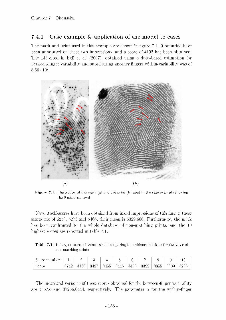
Chapter 7. Discussion
7.4.1 Case example & application of the model to cases
The mark and print used in this example are shown in �gure 7.1. 9 minutiae have
been annotated on these two impressions, and a score of 4192 has been obtained.
The LR cited in Egli et al. (2007), obtained using a data-based estimation for
between-�nger variability and substituting another �ngers within-variability was of
8.56 · 107.
(a) (b)
Figure 7.1: Illustration of the mark (a) and the print (b) used in the case example showing
the 9 minutiae used
Now, 3 self-scores have been obtained from inked impressions of this �nger; these
scores are of 6250, 6273 and 6466; their mean is 6329.66̄6. Furthermore, the mark
has been confronted to the whole database of non-matching prints, and the 10
highest scores are reported in table 7.1.
Table 7.1: 10 largest scores obtained when comparing the evidence mark to the database of
non-matching prints
Score number 1 2 3 4 5 6 7 8 9 10
Score 3742 3736 3487 3455 3446 3408 3399 3355 3309 3268
The mean and variance of these scores obtained for the between-�nger variability
are 3457.6 and 37256.044̄4, respectively. The parameter α for the within-�nger
- 186 -
7.4. Likelihood ratios
variability is therefore (s + 903.78)/1.4565 = 6329.6 + 903.78)/1.4565 = 4966.28,
which is larger than what had been used in Egli et al. (2007). The parameter β
being determined by the number of minutiae (9), it can be read o� from table 4.22
in chapter 4; it is of 10.4. This parameter is larger than what has been used in Egli
et al. (2007). The probability to be put in the numerator is therefore the value of the
Weibull probability density function with parameters (4966.28, 10.4) at a score of
4192; this value is 3.59·10−4. For the between-�nger distribution, the parameters are
both computed using the equations given in chapter 5. For 9 minutiae, the equation
for the �rst parameter is 0.2981·log(s̄10)+5.034 = 0.2981·log(3460.5)+5.034 = 7.46
and for the second parameter it is −0.007286 · (log(s̄10)/log(V ar(s10)) + 0.1827 =
−0.007286 · (log(3460.5)/log(25973.61)) + 0.1827 = 0.1768. The probability to be
used in the denominator can therefore be obtained at a value of 4192 of a lognormal
distribution with parameters (7.46,0.1771). This value is 2.46 · 10−9. When the
numerator is divided by the denominator, an LR of 1.45 ∗ 105 (rather than the LR
of 8.56 · 107 that had been obtained in Egli et al. (2007)).
It is considered in the present thesis that the computation of LRs should, for
the moment, rather be carried out using data-based estimation; this implies the
following steps:
1. Obtain the score between the evidential mark and the suspects print using all
minutiae visible on the mark. Ideally, only between 6 and 10 minutiae should
be used, since these are the numbers examined here. Since the only results
used in the following are the necessary sample size and the distributions �tted
to the data (that remain the same whatever the number of minutiae), more
or less minutiae could certainly also be used.
2. Obtain 8 mark substitutes and 8 rolled inked prints from the suspect. The
substitutes for marks can be either the slaps from 10-print cards, simulated
developed marks, or livescans acquired using distortion.
3. Annotate the minutiae used in the evidential score obtained in 1. on the
(pseudo-) marks and verify their presence on the rolled inked prints.
4. Obtain the scores for the 64 comparisons between marks and prints for within-
�nger variability.
5. Introduce these scores into any program allowing to �t distributions (here,
MatlabR© has been used), and �t a Weibull distribution in order to obtain the
parameters.
6. Introduce the evidential scores obtained in 1. and the parameters into a
function allowing to obtain a Weibull function value, and obtain the numerator
of the LR.
7. Obtain the scores when comparing the evidential mark to the remainder of
the database, taking care to eliminate any prints from the suspect either at
- 187 -

Chapter 7. Discussion
this step, or clear them from the data once the scores have been obtained.
This is the step that may pose the most problems; while here a custom-made
algorithm directly extracted these scores as a text-�le, this algorithm is not
generally available.
8. Introduce these between-�nger variability scores into a program allowing to
�t distributions and �t a log-normal distribution. This step may or may
not be preceded by a �ltering step, where only scores from the same general
pattern/�nger number combinations as those seen on the mark are present, or
a simple random subsampling step that allows the use of 10000 scores rather
than all that are extracted.
9. With the parameters obtained in step 8 and the evidential score from step 1,
obtain a function value from the lognormal probability density function at the
value of the score; this is the denominator.
10. Divide the numerator from step 6 by the denominator obtained in step 9 in
order to obtain a likelihood ratio.
The estimation of the LR based on approximation, which is not at this time the
method considered optimal, requires the following steps:
1. Obtain the score between the evidential mark and the suspects print using all
minutiae visible on the mark using a Sagem DMA. Only between 6 and 10
minutiae can be used here, since approximations are not available for other
numbers of minutiae.
2. Obtain 3 slap impressions from the suspects �nger, and insert each of them
into the system twice: once as a mark, and once as an inked print. Annotate
the minutiae used in the evidential mark on these slap impressions, taking care
to annotate them as similarly as possible on the identical impressions used on
the mark and the print side of the system. Obtain the three self-scores.
3. Compute the parameters for the within-�nger distribution using the equation
4.5 given in chapter 4 for α and reading the values for β o� table 4.22 in that
same chapter.
4. Launch a search of the evidential mark against the database and retain the
10 highest non-mate scores.
5. Obtain the parameters for the between-�nger distribution using the relevant
equations from table 5.6 in chapter 5.
6. Obtain the numerator and the denominator of the LR using the evidential
score and the Weibull and Lognormal distributions, using the relevant param-
eters computed in steps 3 and 5 above, and divide one by the other to obtain
the LR.
- 188 -
7.5. Outlook
7. Plot the within- and between variabilities as well as the evidential score ob-
tained, in order to verify that the score is not in the extreme left tail of the
between-�nger variability; if this is the case, use data-based estimation. This
extreme left tail is not de�ned as beginning at a speci�c score or density value.
Only the comparative plot of within- and between-�nger variability will allow
the determination of whether a given point is within this region. This region
will, on this plot, be close to the point where within-�nger variability becomes
greater than between-�nger variability, for very low scores.
If more than 10 minutiae are visible on the mark, and only a number of minutiae
tested in the present thesis should be used, these steps need to be carried out several
times (if the LR is above 1 in particular) in order to see whether one of the minutiae
not taken into account initially changes the LR to one that is below 1. If the LR is
below 1 using 10 minutiae, it is highly unreasonable to expect to obtain an LR above
1 when exchanging one minutia; it is even more unreasonable to expect that the
LR should be above 1 in this situation. While the number of steps required seems
impressive in these enumerations, there are only few of these steps that take time;
the annotation of the evidential mark and the control of the minutiae on the print,
as well as the marking of minutiae on marks / prints used for the acquisition of
within-�nger variability, and the extraction of scores for data-based between-�nger
variability as well as its insertion into another program. While the �rst two items
(annotation of minutiae) actually imply that a specialist is active on the system,
the last two don't; they take only computer time. The computation of parameters
and the numerator, denominator and LR are automated (see Appendix C); these
computations do not noticeably take time.
7.5 Outlook
While the model used here performs well, there are possible improvements. These
are situated in particular in the within-�nger variability. In the present thesis,
distortion has been taken into account in a limited way, although it has an e�ect on
within-�nger variability. While this was due to the di�culty of acquiring distorted
marks, the presented results also show that livescan images are a rather good proxy
in the context of AFIS scores, particularly when the minutiae noted must be clear so
as to allow to place them with exactitude, to determine their direction and ideally
their type.
Then, the approximation based on self-scores of the within-�nger variability
should be adapted to these new distributions, including distortion, obtained. The
inclusion of more distortion would lead to more variance in the within-�nger variabil-
ity than that modelled in the present thesis, and would therefore have an impact on
the equations linking the self-scores and the numbers of minutiae to the parameters
of the Weibull distribution. Also, in this step, it is possible to include theoretical
knowledge about within-�nger variability in these approximated parameters. Such
- 189 -
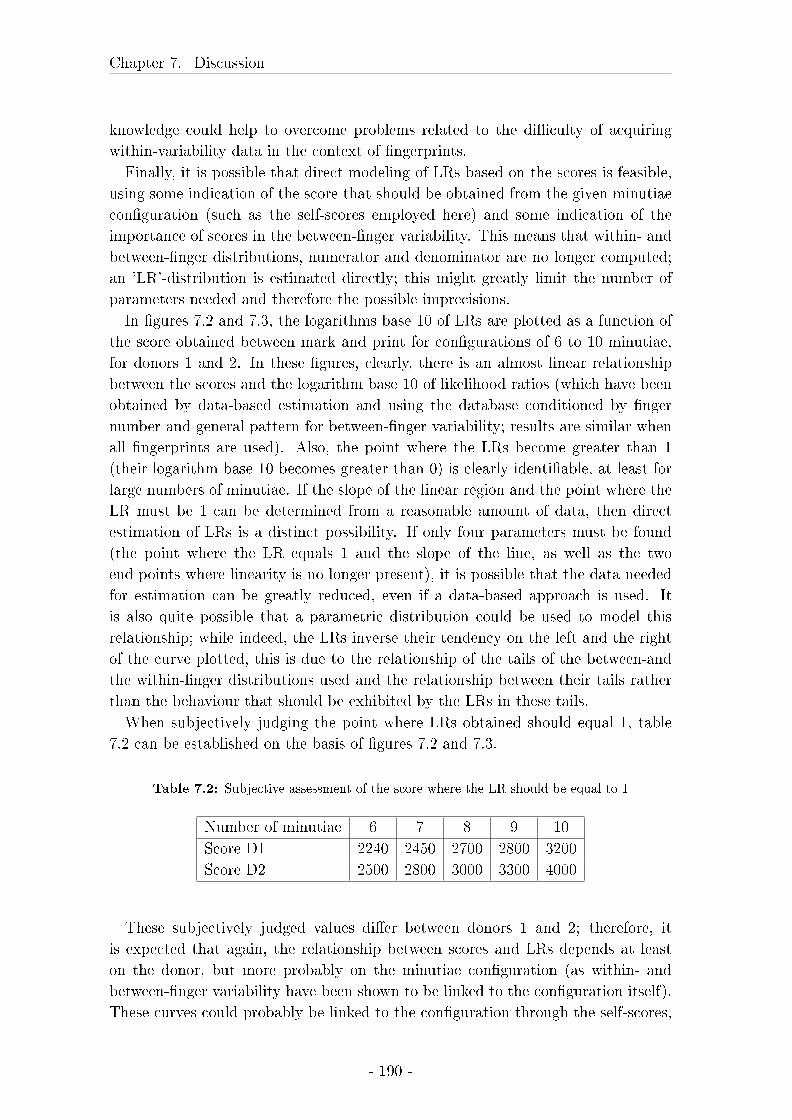
Chapter 7. Discussion
knowledge could help to overcome problems related to the di�culty of acquiring
within-variability data in the context of �ngerprints.
Finally, it is possible that direct modeling of LRs based on the scores is feasible,
using some indication of the score that should be obtained from the given minutiae
con�guration (such as the self-scores employed here) and some indication of the
importance of scores in the between-�nger variability. This means that within- and
between-�nger distributions, numerator and denominator are no longer computed;
an 'LR'-distribution is estimated directly; this might greatly limit the number of
parameters needed and therefore the possible imprecisions.
In �gures 7.2 and 7.3, the logarithms base 10 of LRs are plotted as a function of
the score obtained between mark and print for con�gurations of 6 to 10 minutiae,
for donors 1 and 2. In these �gures, clearly, there is an almost linear relationship
between the scores and the logarithm base 10 of likelihood ratios (which have been
obtained by data-based estimation and using the database conditioned by �nger
number and general pattern for between-�nger variability; results are similar when
all �ngerprints are used). Also, the point where the LRs become greater than 1
(their logarithm base 10 becomes greater than 0) is clearly identi�able, at least for
large numbers of minutiae. If the slope of the linear region and the point where the
LR must be 1 can be determined from a reasonable amount of data, then direct
estimation of LRs is a distinct possibility. If only four parameters must be found
(the point where the LR equals 1 and the slope of the line, as well as the two
end points where linearity is no longer present), it is possible that the data needed
for estimation can be greatly reduced, even if a data-based approach is used. It
is also quite possible that a parametric distribution could be used to model this
relationship; while indeed, the LRs inverse their tendency on the left and the right
of the curve plotted, this is due to the relationship of the tails of the between-and
the within-�nger distributions used and the relationship between their tails rather
than the behaviour that should be exhibited by the LRs in these tails.
When subjectively judging the point where LRs obtained should equal 1, table
7.2 can be established on the basis of �gures 7.2 and 7.3.
Table 7.2: Subjective assessment of the score where the LR should be equal to 1
Number of minutiae 6 7 8 9 10
Score D1 2240 2450 2700 2800 3200
Score D2 2500 2800 3000 3300 4000
These subjectively judged values di�er between donors 1 and 2; therefore, it
is expected that again, the relationship between scores and LRs depends at least
on the donor, but more probably on the minutiae con�guration (as within- and
between-�nger variability have been shown to be linked to the con�guration itself).
These curves could probably be linked to the con�guration through the self-scores,
- 190 -
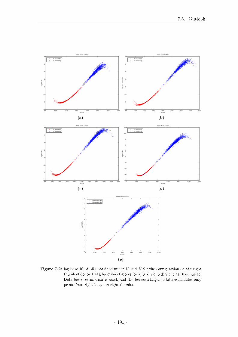
7.5. Outlook
500 1000 1500 2000 2500 3000 3500 4000−6
−4
−2
0
2
4
6
8
scores
log
10
LR
s
6min D1ori GPFN
LRs under Hd
LRs under Hp
(a)
500 1000 1500 2000 2500 3000 3500 4000 4500−6
−4
−2
0
2
4
6
8
scores
log
10
LR
s G
PF
N
7min D1oriGPFN
LRs under Hd
LRs under Hp
(b)
500 1000 1500 2000 2500 3000 3500 4000 4500 5000 5500−6
−4
−2
0
2
4
6
8
scores
log
10
LR
s
8min D1ori GPFN
LRs under Hd
LRs under Hp
(c)
0 1000 2000 3000 4000 5000 6000 7000−6
−4
−2
0
2
4
6
8
10
12
scores
log
10
LR
s
9min D1ori GPFN
LRs under Hd
LRs under Hp
(d)
0 1000 2000 3000 4000 5000 6000 7000 8000−6
−4
−2
0
2
4
6
8
10
12
14
scores
log
10
LR
s
10min D1ori GPFN
LRs under Hd
LRs under Hp
(e)
Figure 7.2: log base 10 of LRs obtained under H and H̄ for the con�guration on the right
thumb of donor 1 as a function of scores for a) 6 b) 7 c) 8 d) 9 and e) 10 minutiae.
Data-based estimation is used, and the between-�nger database includes only
prints from right loops on right thumbs.
- 191 -
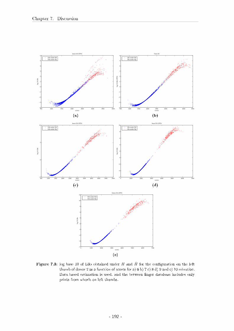
Chapter 7. Discussion
500 1000 1500 2000 2500 3000 3500 4000−4
−3
−2
−1
0
1
2
3
4
5
6
scores
log
10
LR
s
6min D2 GPFN
LRs under Hd
LRs under Hp
(a)
500 1000 1500 2000 2500 3000 3500 4000 4500−4
−3
−2
−1
0
1
2
3
4
5
6
scores
log
10
LR
s G
PF
N
7min D2
LRs under Hd
LRs under Hp
(b)
500 1000 1500 2000 2500 3000 3500 4000 4500 5000 5500−5
0
5
10
scores
log
10
LR
s
8min D2 GPFN
LRs under Hd
LRs under Hp
(c)
0 1000 2000 3000 4000 5000 6000 7000−6
−4
−2
0
2
4
6
8
10
scores
log
10
LR
s
9min D2 GPFN
LRs under Hd
LRs under Hp
(d)
0 1000 2000 3000 4000 5000 6000 7000−6
−4
−2
0
2
4
6
8
10
12
scores
log
10
LR
s
10min D2 GPFN
LRs under Hd
LRs under Hp
(e)
Figure 7.3: log base 10 of LRs obtained under H and H̄ for the con�guration on the left
thumb of donor 2 as a function of scores for a) 6 b) 7 c) 8 d) 9 and e) 10 minutiae.
Data-based estimation is used, and the between-�nger database includes only
prints from whorls on left thumbs.
- 192 -

7.5. Outlook
and of course through the maximum scores obtained from a database of non-mates.
This is considered here to be a very promising venue to be explored further.
- 193 -

Chapter 8
Conclusion
In the present thesis, a model allowing the evaluation of �ngerprint comparison
results using a likelihood ratio is proposed. A great advantage of this model is
the use of the scores output by an Automated Fingerprint Identi�cation System
(AFIS). Such systems have a long history of development, they are optimized for
the extraction of the relevant data (i.e. minutiae, in the present case), and they are
used for distinguishing same source from di�erent source �ngerprints. Therefore,
the proximity measure used in these systems had, a priori, a good chance of being
extremely useful when employed as a measure for evaluation purposes.
Data for the description of the variability of scores when impressions from one
�nger are compared using this system have been acquired, employing widely used
detection techniques. Then, the minimal number of repeated impressions for robust
estimation of this within-�nger variability has been determined, and a parametric
model �tted to this distribution of scores. Also, a precise description of the data that
should be used for the establishment of such a within-�nger variability distribution
has resulted from the work presented: rather than including only marks in this
within-�nger variability, the inclusion of rolled inked prints also allows to capture
the variability due to the rolling process, which introduces distortion e�ects as well.
It has been chosen here to include the same number of rolled inked prints as marks
in the data used for comparisons, which leads to the use of 8 marks (or substitutes,
e.g. slaps or live scan images) and 8 rolled inked prints.
Also, a background database of over 600 000 �ngerprints was available and has
been used. This database is far larger than any database that has been used pre-
viously for the examination of �ngerprint variability in forensic science, exception
made of one study (Meagher et al., 1999). On this large database, the in�uence of
�nger number and general pattern on the distribution of scores when a given mark
is compared to a large amount of di�erent prints could be explored. Also, again,
the minimum number of data for robust estimation of this distribution of scores has
been determined (10000 �ngerprints), and then, a parametric model �tted to this
distribution.
In a next step, for both within- and between-�nger distributions, data reduction
has been attempted. Direct approximation of parameters of the two distributions
- 195 -
Chapter 8. Conclusion
used is proposed, based on 3 and 10 datapoints for within- and between-�nger
variability, respectively.
Finally, in a testing step, the results obtained on the �nger used for the establish-
ment of models have been tested on the �nger of a di�erent donor. The results of
this testing step allow to determine the performance of the model as such, as well
as the results of the approximations.
While the model results in rates of misleading evidence that are quite high for low
numbers of minutiae (a maximum of 5.2% for 6 minutiae and 3.2% of misleading
evidence in favour of the prosecution for 7 minutiae for one of the two donors used),
these rates diminish as the number of minutiae included in con�gurations increases.
It is therefore a model that yields rational results in the sense that its performance
increases as the information available increases.
The second result of this testing step is that the approximations proposed yield
LRs that correspond well with those estimated on the basis of empirical data. The
immediate use of these approximations for casework purposes is seen as premature,
however, since only two known donors have truly been investigated here. This does
not preclude, in casework, to use the proposed data-based approach while acquiring
the necessary data to further check the approximations. If a data-based approach is
used in a given case, only 3 self-scores (based, for example, on slaps from ten-print
cards) need to be acquired; this seems feasible for validation purposes.
Overall, for within-�nger variability, the comparison of 8 'slap' impressions from
ten-print cards to the same number of rolled inked prints has been shown to result
in within-�nger distributions that are close to distributions based on developed
marks and inked prints acquired in the course of the present study. This remains
the preferred process for the acquisition of within-�nger variability. For between-
�nger variability, where automated extraction is possible, 10000 scores su�ce for
the estimation of the distribution.
Presently, a model that can be directly used in casework has been established,
tested and presented. This model needs the acquisition of repeated impressions from
the suspects �nger (8 ten-print cards with slap and rolled inked impressions), and
precise guidelines as to how LRs should be obtained are given in the discussion (on
page 187). While an approach where less data needs to be acquired is proposed and
yields promising results, it is not at this time considered as having been su�ciently
tested. There is a limitation to the generalizability of the results obtained in the
present work in the sense that they are intimately linked to a given AFIS: the Sagem
DMA. They are directly applicable only to the scores issued from this precise system.
The methodology and approach to the establishment and testing of this model are,
however, portable to other systems. The immediate application to casework is only
possible with this same system, however.
The model proposed addresses two of the issues that arise in Daubert v. Merrell
Dow Pharmaceuticals, Inc. (1993): the necessity of testing of any method used, and
the need for known error rates of this method. Also, due to the transparency of the
- 196 -
data used for its establishment, the modelling steps used and the testing carried
out, the present model can easily be subjected to peer reviewing.
Finally, and perhaps most importantly, the presented model represents a solution
to possible issues that could arise in the future, due to the increase in the size of the
databases used as a pool of suspects. This increase may lead to more similar �n-
gerprints being found than ever before. Should such problems arise, a probabilistic
model based on large amounts on data would certainly become a necessity. Even
if this increase in database size does not lead to any problems, the use of data to
underpin the evaluative process in a probabilistic context, while taking at the same
time advantage of the speci�c knowledge and expertise of �ngerprint examiners, is
in the present thesis seen as a promising future for �ngerprint examination.
Of course, this approach would be the most useful if it could be implemented
directly in an AFIS. This would allow for immediate modelling of between-�nger
variability based on the scores while at the moment, scores must be extracted from
the system and modelled in another program. Also, such an implementation would
make it possible to have speci�c tools for the acquisition of the data used for the
modelling of within-�nger variability. The probability of such an implementation
actually being carried out by a provider of such a system is unknown to the author.
It is certain, however, that it will be function of the clients' demands. At this point
in time, the demand for probabilistic evaluation of �ngerprint evidence is not made
by the �ngerprint community although mention is made of models based on AFIS
scores in a report from the National Institute of Justice (McClure, 2007).
Concerning future perspectives, more distortion, such as observed on livescan
images where distortion is voluntarily introduced, should be integrated into within-
�nger variability in order to verify the in�uence of such distortion on the model.
A di�erent approach is direct modelling of the likelihood ratio as a function of the
scores from the system; this seems a promising subject for future research. Indeed,
it is quite possible that, for a given minutiae con�guration, the relationship between
scores and LRs could be modelled without �rst modelling within- and between-�nger
variability separately. Such a direct approach would most certainly be easier and
quite possibly could also improve the precision and exactitude of estimates, since
fewer parameters would need to be estimated.
- 197 -

Bibliography
Amy, L., 1946. Valeur de la preuve dactyloscopique. Journal de la Société de
Statistique de Paris, 87:80�87.
Amy, L., 1947. Valeur de la preuve dactyloscopique II. Journal de la Société de
Statistique de Paris, 88:189�195.
Anon., 2002. European �ngerprint standards (A 'pointless' exercise). Fingerprint
Whorld, 28(107):19.
Anon., 1980. Resolution VII amended. Identi�cation News, 30:3.
Ashbaugh, D., 1991. Ridgeology. Journal of Forensic Identi�cation, 41(1):16�64.
Ashbaugh, D., 2000. Modernizing the �ngerprint science in the United Kingdom.
Fingerprint Whorld, 26:159�168.
Ashbaugh, D., 2002. Letter to the Editor. Fingerprint Whorld, 28(109)):162�164.
Ashbaugh, D. R.; Houck, M. M., 2006. Fingerprints and admissibility: Friction
ridges and science. Fingerprint Whorld, 32(123):21�42.
Babler, W. J., 1978. Prenatal selection and dermatoglyphic patterns. American
Journal of Physical Anthropology, 49(1):21�27.
Babler, W. J., 1991. Embryologic development of epidermal ridges and their con-
�gurations. In Plato, C. C., Garruto, R. M., Schaumann, B. A., Paul, N. W.,
editors, Dermatoglyphics � Science in Transition, volume 27 (2) of March of
Dimes Birth Defects Foundation, Birth Defects: Original Article Series, pages
95�112. Wiley-Liss, New York.
Balthazard, V., 1911. De l'identi�cation des empreintes digitales. Comptes rendus
des séances de l'Académie des sciences, 152:1862�1864.
Barnett, V., 1975. Probability plotting methods and order statistics. Applied Statis-
tics, 24(1):95�108.
Bebis, G., Deaconu, T., Georgiopoulos, M., 1999. Fingerprint identi�cation us-
ing Delaunay triangulation. In IEEE International Conference on Information
- 199 -
Bibliography
Intelligence and Systems, pages 452�459, Rockville, Maryland. IEEE Computer
Society, Washington DC.
Berger, M. A., 2000. The Supreme Court's trilogy on the admissibility of expert tes-
timony. In Reference Manual on Scienti�c Evidence, pages 9�38. Federal Judicial
Center, Washington, DC, USA.
Berry, J., 1991. The history and development of �ngerprinting. In Lee, H. C.,
Gaensslen, R. E., editors, Advances in Fingerprint Technology, Elsevier Series in
Forensic and Police Science, pages 1�38. Elsevier Science Publishing Co., Inc.,
New York.
Berry, J., Stoney, D., 2001. History and development of �ngerprinting. In Lee,
H. C., Gaensslen, R. E., editors, Advances in Fingerprint Technology, CRC Series
in Forensic and Police Science. CRC Press, Boca Raton, 2nd edition.
Bertillon, A., 1912. Les empreintes digitales. Archives d'anthropologie criminelle,
de médecine légale et de psychologie normale et pathologique, 27(217):36�52.
Bhattacharyya, A., 1943. On a measure of divergence between two statistical pop-
ulations de�ned by their population distributions. Bulletin of the Calcutta Math-
ematical society, 35:99�109.
Broeders, A. P. A., 2003. Forensic Evidence and International Courts and Tri-
bunals: Why bother, given the present state of play forensics? 17th International
Conference of the International Society for the Reform of Criminal Law. URL
http://www.isrcl.org/. (Last consulted: June 16, 2008).
Budowle, B., Buscaglia, J., Schwartz Perlmann, R., 2006. Review of the scien-
ti�c basis for friction ridge comparisons as a means of identi�cation: Com-
mittee �ndings and recommendations. Forensic Science Communications, 8
(1). URL http://www.fbi.gov/hq/lab/fsc/backissu/jan2006/research/
2006_01_research02.htm. (Last consulted: June 16, 2008).
Chakraborty, R., 1991. The role of heredity and environment on dermatoglyphic
traits. In Paul, N. W., editor, Dermatoglyphics - Science in Transition, pages
151�192. Wiley-Liss, New York.
Champod, C., 1996. Reconnaissance automatique et analyse statistique des minuties
sur les empreintes digitales. Thèse de doctorat, Université de Lausanne.
Champod, C., Evett, I. W., 2001. A probabilistic approach to �ngerprint evidence.
Journal of Forensic Identi�cation, 51(2):101�122.
Champod, C., Lennard, C. J., Margot, P., Stoilovic, M., 2004. Fingerprints and
other ridge skin impressions. CRC Press, Boca Raton, Florida.
- 200 -
Bibliography
Cole, S. A., 2004. History of �ngerprint pattern recognition. In Ratha, N., Bolle,
R., editors, Automatic Fingerprint Identi�cation Systems, pages 1�25. Springer-
Verlag, New York.
Cole, S. A., 2006. Is �ngerprint identi�cation valid? Rhetorics of reliability in
�ngerprint proponents' discourse. Law & Policy, 28(1):109�135.
Conseil de l'Union Européenne, 2000. Règlement (CE) no
2725/2000 du Conseil du 11 décembre 2000. http://eur-
lex.europa.eu/smartapi/cgi/sga_doc?smartapi!celexplus
!prod!DocNumber&lg=fr&type_doc=Regulation&an_doc=2000&nu_doc=2725.
(Last consulted: January 24, 2009).
Cummins, H. H., Midlo, C., 1943. Finger Prints, Palms and Soles. Blakiston,
Philadelphia.
Dass, S., Zhu, Y., Jain, A., 2005. Statistical models for assessing the individuality
of �ngerprints. Fourth IEEE Workshop on Automatic Identi�cation Advanced
Technologies, pages 3�9.
Daubert v. Merrell Dow Pharmaceuticals, Inc. 509 U.S. 579, 1993.
Dror, I., Charlton, D., Peron, A., 2006. Contextual information renders experts
vulnerable to making erroneous identi�cations. Forensic Science International,
156(1):74�78.
Egli, N. M., Champod, C., Margot, P., 2007. Evidence evaluation in �ngerprint
comparison and automated �ngerprint identi�cation systems-modelling within
�nger variability. Forensic Science International, 167(2-3):189�195.
Egli, N. M., 2005. Investigation of the possibility of modelling within-variability of
con�gurations of 6 minutiae using an automatic �ngerprint identi�cation system.
Master thesis, Université de Neuchâtel.
Evett, I. W., Buckleton, J. S., 1996. Statistical analysis of STR data. In Carracedo,
A., Brinkmann, B., Baer, W., editors, Advances in Forensic Haemogenetics 6,
pages 79�86. Springer Verlag, Heidelberg.
Evett, I., Williams, R., 1995. A review of the sixteen points �ngerprint standard in
England and Wales. Fingerprint Whorld, 21(82):125�143.
Fang, G., Srihari, S. N., Srinivasan, H., 2007. Generative models for �ngerprint
individuality using ridge types. In IAS '07: Proceedings of the Third International
Symposium on Information Assurance and Security, pages 423�428, Washington,
DC, USA. IEEE Computer Society.
Faulds, H., 1880. On the skin-furrows of the hand. Nature, 22(574):605.
- 201 -
Bibliography
Flaxman, B. A.; Nelson, B. K., 1974. Ultrastructural studies of the early junctional
zone formed by keratinocytes showing contact inhibition of movement in vitro.
The Journal of Investigative Dermatology, 63(4):326�330.
Freedman, D., Diaconis, P., 1981. On the histogram as a density estimator: L2
theory. Probability Theory and Related Fields, 57(4):453�476.
Galton, F., 1892. Finger Prints. McMillan, London.
General Electric Co. v. Joiner. 522 U.S. 136, 1993.
Gonzalez-Rodriguez, J., Fierrez-Aguilar, J., Ramos-Castro, D., Ortega-Garcia, J.,
2005. Bayesian analysis of �ngerprint, face and signature evidences with auto-
matic biometric systems. Forensic Science International, 155(2-3):126�140.
Haber, L., Haber, R., 2008. Scienti�c validation of �ngerprint evidence under
Daubert. Law, Probability and Risk, 7(2):87�109.
Hale, A. R., 1952. Morphogenesis of volar skin in the human fetus. American
Journal of Anatomy, 91(1):147�181.
Hyndman, R. J., Fan, Y., 1996. Sample quantiles in statistical packages. The
American Statistician, 50(4):361�365.
Interpol European Expert Group on Fingerprint Identi�cation, 2004. Method
for Fingerprint Identi�cation. Part II: Detailing the method using common
terminology and through the de�nition and application of shared principles.
http://www.interpol.int/Public/Forensic/�ngerprints/WorkingParties/
IEEGFI2/default.asp. (Last consulted: June 16, 2008).
Jain, A. K., Prabhakar, S., Pankanti, S., 2001. Twin test: On discriminability of
�ngerprints. In 3rd International Conference on Audio- and Video-Based Person
Authentication, pages 211�216, Sweden.
Jain, A. K., Prabhakar, S., Pankanti, S., 2002. On the similarity of identical twin
�ngerprints. Pattern Recognition, 35:2653�2663.
Je�reys, H., 1946. An invariant form for the prior probability in estimation prob-
lems. Proceedings of the Royal Statistical Society A, 186(1007):453�461.
Jones, T., 1991. Inherited characteristics in �ngerprints : (or theory of relativity).
The Print, 4(5):1�2.
Kaye, D. H., 2003. Questioning a courtroom proof of the uniqueness of �ngerprints.
International Statistical Review, 71(3):521�533.
Kingston, C. R., 1964. Probabilistic analysis of partial �ngerprint patterns. D. Crim.
Dissertation, University of California.
- 202 -
Bibliography
Komarinski, P., 2005. Automated Fingerprint Identi�cation Systems (AFIS). Else-
vier Academic Press, Burlington, MA.
Kücken, M., 2004. On the Formation of Fingerprints. PhD thesis, The University
of Arizona, Tucson.
Kullback, S., Leibler, R. A., 1951. On information and su�ciency. The Annals of
Mathematical Statistics, 22(1):79�86.
Kumho Tire Co. v. Carmichael. 119 S. Ct. 1167, 1999.
Langenburg, G. M., 2004. Pilot study: a statistical analysis of the ACE-V
methodology-analysis stage. Journal of Forensic Identi�cation, 54:64�79.
Leadbetter, M., 2007. Letter to the Editor. Fingerprint Whorld, 33(129):231.
Liang, X., Asano, T., Bishnu, A., 2006. Distorted �ngerprint indexing using minutia
detail and Delaunay triangle. In Proceedings of the 3rd International Symposium
on Voronoi Diagrams in Science and Engineering, pages 217�223. IEEE Com-
puter Society, 2006.
Liu, C., Yang, J., Shao, P., Gu, J., Yu, M., April 2007. Mean divergence measures for
multimodality medical image registration. Electrical and Computer Engineering,
2007. CCECE 2007. Canadian Conference on, pages 1171�1174. ISSN 0840-7789.
doi: 10.1109/CCECE.2007.297.
Locard, E., 1931. Traité de criminalistique - Les empreintes et les traces dans
l'enquête criminelle. Joannès Desvigne et ses �ls, Lyon.
Maceo, A. V., 2005. The basis for the uniqueness and persistence of scars in the
friction ridge skin. Fingerprint Whorld, 31(121):147�161.
Maio, D., Maltoni, D., 1997. Direct gray-scale minutiae detection in �ngerprints.
IEEE Transactions on PAMI, 19(1):27�40.
Maltoni, D., Maio, D., Jain, A. K., Prabhakar, S., 2003. Handbook of �ngerprint
recognition. Springer-Verlag.
Margot, P., German, E., 1995. Fingerprint identi�cation breakout meeting "Ne'urim
declaration". In Almog, J., Springer, E., editors, International Symposium on
Fingerprint Detection and Identi�cation, page 21, Ne'urim, Israel.
Margot, P., Lennard, C., 1994. Fingerprint Detection Techniques. Criminalistics
Series I. Institut de Police Scienti�que et de Criminologie � Université de Lau-
sanne, Lausanne, 6th revised edition.
Maurer, J. J. A., 1960. Method of and apparatus for automatic identi�cation of
�nger prints. http://www.freepatentsonline.com/2952181.html.
- 203 -
Bibliography
McCann, P. D., 1973. Report of the standardization committee of the International
Association for Identi�cation - August 1, 1973. Identi�cation News, 23(8):13�14.
McClure, D., 2007. Focus Group on Scienti�c and Forensic Evidence in the Court-
room. http://www.ncjrs.gov/pd�les1/nij/grants/220692.pdf, page 7. (Last con-
sulted: February 9, 2009).
McRoberts, A., 2002. Scienti�c Working Group on Friction Ridge Analysis, Study
and Technology (SWGFAST) Proposed Guidelines. Journal of Forensic Identi�-
cation, 52(3):264�347.
Meagher, S., Budowle, B., Ziesig, D., 1999. 50k vs. 50k �ngerprint comparison
test. United States of America vs. Byron Mitchell, U.S. District Court Eastern
District of Philadelphia. Government Exhibits 6-8 and 6-9 in Daubert Hearing
before Judge J. Curtis Joyner, July 8-9.
Neumann, C., Champod, C., Puch-Solis, R., Meuwly, D., Egli, N., Anthonioz,
A., Bromage-Gri�ths, A., 2006. Computation of likelihood ratios in �ngeprint
identication for con�gurations of three minutiae. Journal of Forensic Sciences,
51(6):1255�1266.
Neumann, C., Champod, C., Puch-Solis, R., Egli, N., Anthonioz, A., Bromage-
Gri�ths, A., 2007. Computation of likelihood ratios in �ngerprint identication
for con�gurations of any number of minutiae. Journal of Forensic Sciences, 52
(1):54�64.
O�ce of Public Sector Information, 2006. Identity cards act.
http://www.opsi.gov.uk/acts
/acts2006/ukpga_20060015_en_2#pb6l1g18. (Last consulted: June 19, 2008).
O�ce of the Inspector General, 2006. A review of the FBI's handling of the Brandon
May�eld case. Technical report, O�ce of the Inspector General.
Olsen, R., Lee, H. C., 2001. Identi�cation of latent prints. In Lee, H., Gaensslen,
R. E., editors, Advances in Fingerprint Technology. CRC Press, Boca Raton, 2nd
edition.
Osterburg, J. W., Parthasarathy, T., Raghavan, T. E. S., Sclove, S., 1977. Devel-
opment of a mathematical formula for the calculation of �ngerprint probabilities
based on individual characteristics. Journal of the American Statistical Associa-
tion, 72(360):772�778.
Pankanti, S., Prabhakar, S., Jain, A. K., 2002. On the individuality of �ngerprints.
IEEE Transactions on PAMI, 24(8):1010�1025.
Purkinje, J. E., 1823. Commentatio de examine physiologico organi visu et system-
atis cutanei. PhD thesis, Vratislaviae Typis Universitat.
- 204 -
Bibliography
Ramos-Castro, D., Gonzalez-Rodriguez, J., Champod, C., Fierrez-Aguilar, J.,
Ortega-Garcia, J., 2005. Between-source modelling for likelihood ratio computa-
tion in forensic biometric recognition. In Kanade, T., Jain, A., Ratha, N., editors,
AVBPA 2005, pages 1080�1089, 2005.
Risinger, M. D., Saks, M. J., Thompson, W., Rosenthal, R., 2002. The
Daubert/Kumho implications of observer e�ects in forensic science: hidden prob-
lems of expectation and suggestion. California Law Review, 90(1):1�56.
Roxburgh, T., 1933. On the evidential value of �nger prints. Sankhya : Indian
Journal of Statistics, 1:189�214.
Saks, M. J., Koehler, J. J., 2005. The coming paradigm shift in forensic identi�cation
science. Science, 309(5736):892�895.
Santamaria, B. F., 1953. Une nouvelle méthode d'évaluation des points caractéris-
tiques des crêtes papillaires. In Assemblée générale de la commission interna-
tionale de police criminelle, Oslo.
Schaumann, B. A., Opitz, J. M., 1991. Clinical aspects of dermatoglyphics. In Plato,
C. C., Garruto, R. M., Schaumann, B. A., Paul, N. W., editors, Dermatoglyphics
- Science in Transition, pages 193�228. Wiley-Liss, New York.
Scott, D. W., 1979. On optimal and data-based histograms. Biometrika, 66(3):
605�610.
Srihari, S. N., Srinivasan, H., 2007. Individuality of �ngerprints: Comparison of
models and measurements. CEDAR Technical Report TR-02-07. URL http:
//www.cedar.buffalo.edu/~srihari/papers/TR-02-07.pdf. (Last consulted:
June 20, 2008).
Srihari, S. N., Srinivasan, H., Fang, G., 2008. Discriminability of the �ngerprints of
twins. Journal of Forensic Identi�cation, 58(1):109�127.
Steel, M. A., Székely, L. A., 2006. On the variational distance of two trees. The
annals of applied probability, 16(3):1563�1575.
Stoney, D. A., 1984. Evaluation of associative evidence: Choosing the relevant
question. Journal of the Forensic Science Society, 24(5):473�482.
Stoney, D. A., 1985. Quantitative assessment of �ngerprint individuality. PhD
Dissertation, Berkeley, University of California.
Stoney, D. A., 1991. What made us ever think we could individualize using statis-
tics? Journal of the Forensic Science Society, 31(2):197�199.
- 205 -
Bibliography
Stoney, D. A., 2001. Measurement of �ngerprint individuality. In Lee, H., Gaensslen,
R. E., editors, Advances in Fingerprint Technology. CRC Press LLC, Boca Raton,
2nd edition.
Stoney, D. A., Thornton, J. I., 1986. A method for the description of minutia pairs
in epidermal ridge comparison. Journal of Forensic Sciences, 31(4):1217�1234.
Stoney, D. A., Thornton, J. I., 1987. A systematic study of epidermal ridge minutiae.
Journal of Forensic Sciences, 32(5):1182�1203.
Sturges, H. A., 1926. The choice of a class interval. Journal of the American
Statistical Association, 21(153):65�66.
SWGFAST, 2002. Friction ridge examination methodology for latent print examin-
ers. http://www.swgfast.org/Friction_Ridge_Examination_Methodology_
for_Latent_Print_Examiners_1.01.pdf. (Last consulted: June 25, 2008).
SWGFAST, 2003. Standards for conclusions.
http://www.swgfast.org/Standards_for_
Conclusions_ver_1_0.pdf. (Last consulted: June 16, 2008).
Taroni, F., Margot, P., 2000. Fingerprint evidence evaluation: Is it really so di�erent
to other evidence types? Science & Justice, 40(4):277�278.
Taylor, T., 1877. Hand marks under the microscope. American Journal of Mi-
croscopy and Popular Science; cited by Berry and Stoney (2001) and Cole (2004),
2.
Tippett, C. F., Emerson, V. J., Fereday, M. J., Lawton, F., Jones, L. T., Lampert,
S. M., 1968. The evidential value of the comparison of paint �akes from sources
other than vehicles. Journal of the Forensic Science Society, 8(2-3):61�65.
Trauring, M., 1963. Automatic comparison of �nger-ridge patterns. Nature, 197
(4871):938�940.
United States of America vs. Byron Mitchell, 1999. No. 02-2859. U.S. District
Court, Eastern District of Philadelphia.
Wayman, J. L., 2000. When bad science leads to good law: The disturbing
irony of the Daubert hearing in the case of U.S. v. Byron C. Mitchell. Biomet-
rics in Human Services, 4(1). URL http://www.engr.sjsu.edu/biometrics/
publications_daubert.html. (Last consulted: October 23, 2008).
Wein, L. M., Baveja, M., 2005. Using �ngerprint image quality to improve the
identi�cation performance of the U.S. Visitor and Immigrant Status Indicator
Technology program. PNAS, 102(21):7772�7775.
- 206 -
Bibliography
Welcker, H., 1898. Die Dauerhaftigkeit des Desseins der Riefchen und Fältchen der
Hände. Archiv für Anthropologie Zeitschrift für Naturgeschichte und Urgeschichte
des Menschen, 25:29�32.
Wertheim, K., Maceo, A., 2002. The critical stage of friction ridge and pattern
formation. Journal of Forensic Identi�cation, 52(1):35�85.
Wertheim, P. A., 2000. Scienti�c comparison and identi�cation of �ngerprint evi-
dence. Fingerprint Whorld, 26(101):95 � 106.
Wilson, C., Hicklin, R. A., Korves, H., Ulery, B., Zoep�, M., Bone, M., Grother,
P., Michaels, R., Otto, S., Watson, C., 2003. Fingerprint vendor technology
evaluation 2003. NISTIR 7123. URL http://fpvte.nist.gov/. (Last consulted:
April 7, 2008).
Woodward, J., Orlans, N., Higgins, P., 2003. Biometrics. McGraw-Hill, Ontario.
Yager, N., Amin, A., 2004. Fingerprint veri�cation based on minutiae features: a
review. Pattern Analysis and Applications, 7(1):94�113.
Zhu, Y., Dass, S. C., Jain, A. K., July 2006. Statistical models for assessing the indi-
viduality of �ngerprints. Technical Report MSU-CSE-06-25, Department of Com-
puter Science, Michigan State University, East Lansing, Michigan. URL http://
www.cse.msu.edu/cgi-user/web/tech/reports?Year=2006. (Last consulted:
June 27, 2008).
Zhu, Y., Dass, S. C., Jain, A. K., Sept. 2007. Statistical models for assessing the
individuality of �ngerprints. IEEE Transactions on Information Forensics and
Security, 2(3):391�401.
- 207 -


Appendices

Appendix A
Application of the parameter
estimation to a new donor
A.1 Material and Methods
Up to now, all results presented were based on a single �nger. Of course, the
interest of the results presented in section 4.7.2 is to be able to �nd a description of
the within variability of another donor based on very few impressions. Impressions
have therefore been acquired from a second donor. While the �rst donor was female,
right handed and had ulnar loops on the selected �ngers, the new donor is male, left
handed and has whorls on the selected �ngers. From this donor, two con�gurations,
again increasing from 6 to 10 minutiae, have been selected on two di�erent �ngers,
the left thumb and the left fore�nger. These con�gurations are shown in �gures A.1
and A.2, and will be referred to as LI_D2 and LT_D2 in graphics, respectively.
Since all the work on donor 1 has been carried out on images of the right thumb,
a maximum of di�erence is thus seeked. The parameters remaining similar between
these two donors are, to some extent, the corpulence, age, and occupation, as well
as the fact that the impressions acquired come, in both cases, from the dominant
hand (left for the left-handed donor 2 and right for the right-handed donor 1).
12 ten print cards were acquired of this second donor. Marks were acquired by
dusting with aluminium powder only. For the fore�nger, 34 marks showed the
minutiae selected, and for the thumb, 28 did.
These ten print cards and marks were compared, resulting in 408 and 336 AFIS
scores. Furthermore, using three slaps from the ten print cards, 'self-scores' were
again computed, for each con�guration and number of minutiae. The parameters
of the Weibull distributions �tted to these datasets were estimated �rst based on
the data, and then based on the equations shown above.
- 211 -
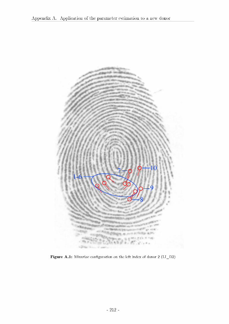
Appendix A. Application of the parameter estimation to a new donor
Figure A.1: Minutiae con�guration on the left index of donor 2 (LI_D2)
- 212 -
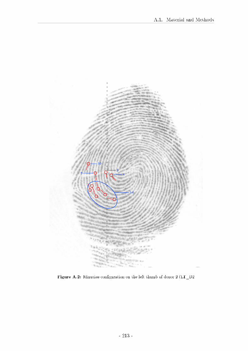
A.1. Material and Methods
Figure A.2: Minutiae con�guration on the left thumb of donor 2 (LT_D2
- 213 -
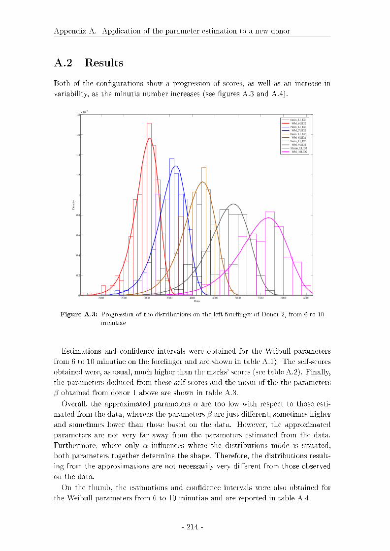
Appendix A. Application of the parameter estimation to a new donor
A.2 Results
Both of the con�gurations show a progression of scores, as well as an increase in
variability, as the minutia number increases (see �gures A.3 and A.4).
2000 2500 3000 3500 4000 4500 5000 5500 6000 65000
0.2
0.4
0.6
0.8
1
1.2
1.4
1.6
1.8x 10
−3
Data
Den
sity
6min_LI_D2
Wbl_6LID2
7min_LI_D2
Wbl_7LID2
8min_LI_D2
Wbl_8LID2
9min_LI_D2
Wbl_9LID2
10min_LI_D2
Wbl_10LID2
Figure A.3: Progression of the distributions on the left fore�nger of Donor 2, from 6 to 10
minutiae
Estimations and con�dence intervals were obtained for the Weibull parameters
from 6 to 10 minutiae on the fore�nger and are shown in table A.1). The self-scores
obtained were, as usual, much higher than the marks' scores (see table A.2). Finally,
the parameters deduced from these self-scores and the mean of the the parameters
β obtained from donor 1 above are shown in table A.3.
Overall, the approximated parameters α are too low with respect to those esti-
mated from the data, whereas the parameters β are just di�erent, sometimes higher
and sometimes lower than those based on the data. However, the approximated
parameters are not very far away from the parameters estimated from the data.
Furthermore, where only α in�uences where the distributions mode is situated,
both parameters together determine the shape. Therefore, the distributions result-
ing from the approximations are not necessarily very di�erent from those observed
on the data.
On the thumb, the estimations and con�dence intervals were also obtained for
the Weibull parameters from 6 to 10 minutiae and are reported in table A.4.
- 214 -
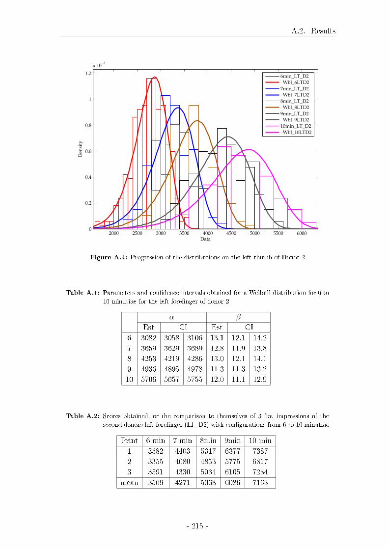
A.2. Results
2000 2500 3000 3500 4000 4500 5000 5500 60000
0.2
0.4
0.6
0.8
1
1.2
x 10−3
Data
Den
sity
6min_LT_D2
Wbl_6LTD2
7min_LT_D2
Wbl_7LTD2
8min_LT_D2
Wbl_8LTD2
9min_LT_D2
Wbl_9LTD2
10min_LT_D2
Wbl_10LTD2
Figure A.4: Progression of the distributions on the left thumb of Donor 2
Table A.1: Parameters and con�dence intervals obtained for a Weibull distribution for 6 to
10 minutiae for the left fore�nger of donor 2
α β
Est CI Est CI
6 3082 3058 3106 13.1 12.1 14.2
7 3659 3629 3689 12.8 11.9 13.8
8 4253 4219 4286 13.0 12.1 14.1
9 4936 4895 4978 11.3 11.3 13.2
10 5706 5657 5755 12.0 11.1 12.9
Table A.2: Scores obtained for the comparison to themselves of 3 �at impressions of the
second donors left fore�nger (LI_D2) with con�gurations from 6 to 10 minutiae
Print 6 min 7 min 8min 9min 10 min
1 3582 4403 5317 6377 7387
2 3355 4080 4853 5775 6817
3 3591 4330 5034 6105 7284
mean 3509 4271 5068 6086 7163
- 215 -
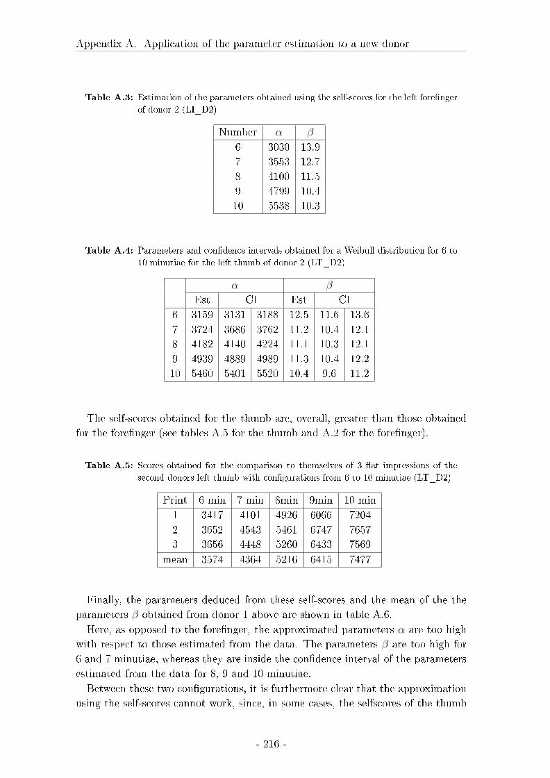
Appendix A. Application of the parameter estimation to a new donor
Table A.3: Estimation of the parameters obtained using the self-scores for the left fore�nger
of donor 2 (LI_D2)
Number α β
6 3030 13.9
7 3553 12.7
8 4100 11.5
9 4799 10.4
10 5538 10.3
Table A.4: Parameters and con�dence intervals obtained for a Weibull distribution for 6 to
10 minutiae for the left thumb of donor 2 (LT_D2)
α β
Est CI Est CI
6 3159 3131 3188 12.5 11.6 13.6
7 3724 3686 3762 11.2 10.4 12.1
8 4182 4140 4224 11.1 10.3 12.1
9 4939 4889 4989 11.3 10.4 12.2
10 5460 5401 5520 10.4 9.6 11.2
The self-scores obtained for the thumb are, overall, greater than those obtained
for the fore�nger (see tables A.5 for the thumb and A.2 for the fore�nger).
Table A.5: Scores obtained for the comparison to themselves of 3 �at impressions of the
second donors left thumb with con�gurations from 6 to 10 minutiae (LT_D2)
Print 6 min 7 min 8min 9min 10 min
1 3417 4101 4926 6066 7204
2 3652 4543 5461 6747 7657
3 3656 4448 5260 6433 7569
mean 3574 4364 5216 6415 7477
Finally, the parameters deduced from these self-scores and the mean of the the
parameters β obtained from donor 1 above are shown in table A.6.
Here, as opposed to the fore�nger, the approximated parameters α are too high
with respect to those estimated from the data. The parameters β are too high for
6 and 7 minutiae, whereas they are inside the con�dence interval of the parameters
estimated from the data for 8, 9 and 10 minutiae.
Between these two con�gurations, it is furthermore clear that the approximation
using the self-scores cannot work, since, in some cases, the selfscores of the thumb
- 216 -
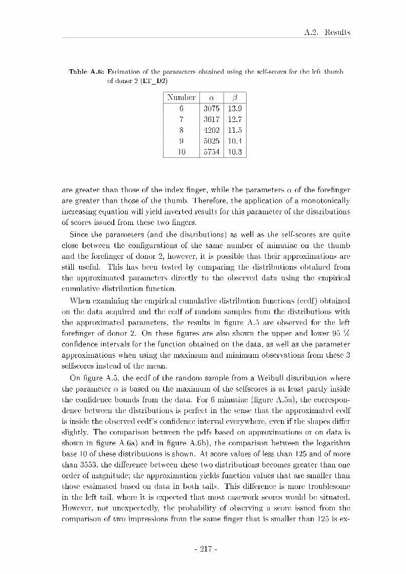
A.2. Results
Table A.6: Estimation of the parameters obtained using the self-scores for the left thumb
of donor 2 (LT_D2)
Number α β
6 3075 13.9
7 3617 12.7
8 4202 11.5
9 5025 10.4
10 5754 10.3
are greater than those of the index �nger, while the parameters α of the fore�nger
are greater than those of the thumb. Therefore, the application of a monotonically
increasing equation will yield inverted results for this parameter of the distributions
of scores issued from these two �ngers.
Since the parameters (and the distributions) as well as the self-scores are quite
close between the con�gurations of the same number of minutiae on the thumb
and the fore�nger of donor 2, however, it is possible that their approximations are
still useful. This has been tested by comparing the distributions obtained from
the approximated parameters directly to the observed data using the empirical
cumulative distribution function.
When examining the empirical cumulative distribution functions (ecdf) obtained
on the data acquired and the ecdf of random samples from the distributions with
the approximated parameters, the results in �gure A.5 are observed for the left
fore�nger of donor 2. On these �gures are also shown the upper and lower 95 %
con�dence intervals for the function obtained on the data, as well as the parameter
approximations when using the maximum and minimum observations from these 3
selfscores instead of the mean.
On �gure A.5, the ecdf of the random sample from a Weibull distribution where
the parameter α is based on the maximum of the selfscores is at least partly inside
the con�dence bounds from the data. For 6 minutiae (�gure A.5a), the correspon-
dence between the distributions is perfect in the sense that the approximated ecdf
is inside the observed ecdf's con�dence interval everywhere, even if the shapes di�er
slightly. The comparison between the pdfs based on approximations or on data is
shown in �gure A.6a) and in �gure A.6b), the comparison between the logarithm
base 10 of these distributions is shown. At score values of less than 125 and of more
than 3553, the di�erence between these two distributions becomes greater than one
order of magnitude; the approximation yields function values that are smaller than
those estimated based on data in both tails. This di�erence is more troublesome
in the left tail, where it is expected that most casework scores would be situated.
However, not unexpectedly, the probability of observing a score issued from the
comparison of two impressions from the same �nger that is smaller than 125 is ex-
- 217 -
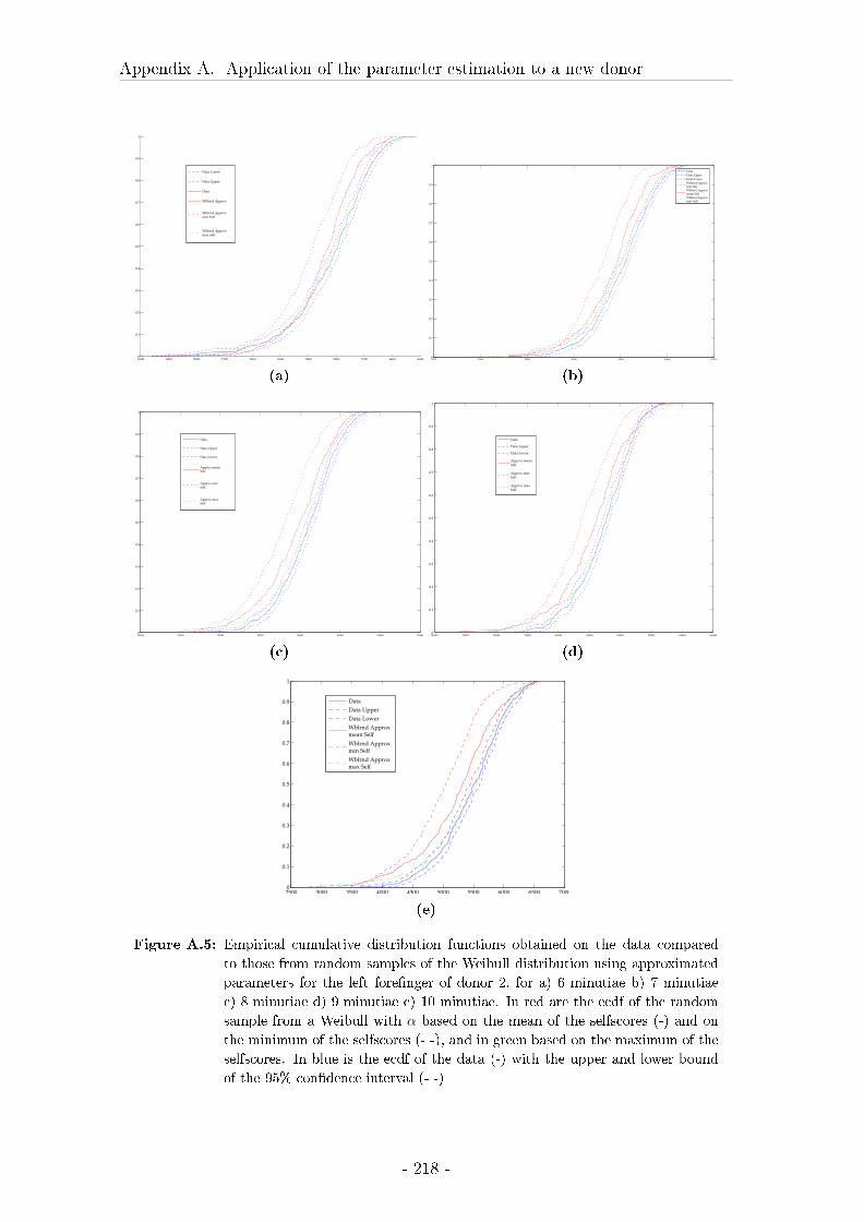
Appendix A. Application of the parameter estimation to a new donor
1600 1800 2000 2200 2400 2600 2800 3000 3200 3400 36000
0.1
0.2
0.3
0.4
0.5
0.6
0.7
0.8
0.9
1
Data Lower
Data Upper
Data
Wblrnd Approx
Wblrnd Approxmin Self
Wblrnd Approxmax Self
(a)
1500 2000 2500 3000 3500 4000 45000
0.1
0.2
0.3
0.4
0.5
0.6
0.7
0.8
0.9
1
Data
Data Upper
Data Lower
Wblrnd Approxmin SelfWblrnd Approxmean SelfWblrnd Approxmax Self
(b)
2000 2500 3000 3500 4000 4500 5000 55000
0.1
0.2
0.3
0.4
0.5
0.6
0.7
0.8
0.9
1
Data
Data Upper
Data Lower
Approx meanSelf
Approx minSelf
Approx maxSelf
(c)
2000 2500 3000 3500 4000 4500 5000 5500 6000 65000
0.1
0.2
0.3
0.4
0.5
0.6
0.7
0.8
0.9
1
Data
Data Upper
Data Lower
Approx meanSelf
Approx minSelf
Approx maxSelf
(d)
2500 3000 3500 4000 4500 5000 5500 6000 6500 70000
0.1
0.2
0.3
0.4
0.5
0.6
0.7
0.8
0.9
1
Data
Data Upper
Data Lower
Wblrnd Approxmean Self
Wblrnd Approxmin Self
Wblrnd Approxmax Self
(e)
Figure A.5: Empirical cumulative distribution functions obtained on the data compared
to those from random samples of the Weibull distribution using approximated
parameters for the left fore�nger of donor 2, for a) 6 minutiae b) 7 minutiae
c) 8 minutiae d) 9 minutiae e) 10 minutiae. In red are the ecdf of the random
sample from a Weibull with α based on the mean of the selfscores (-) and on
the minimum of the selfscores (- -), and in green based on the maximum of the
selfscores. In blue is the ecdf of the data (-) with the upper and lower bound
of the 95% con�dence interval (- -)
- 218 -
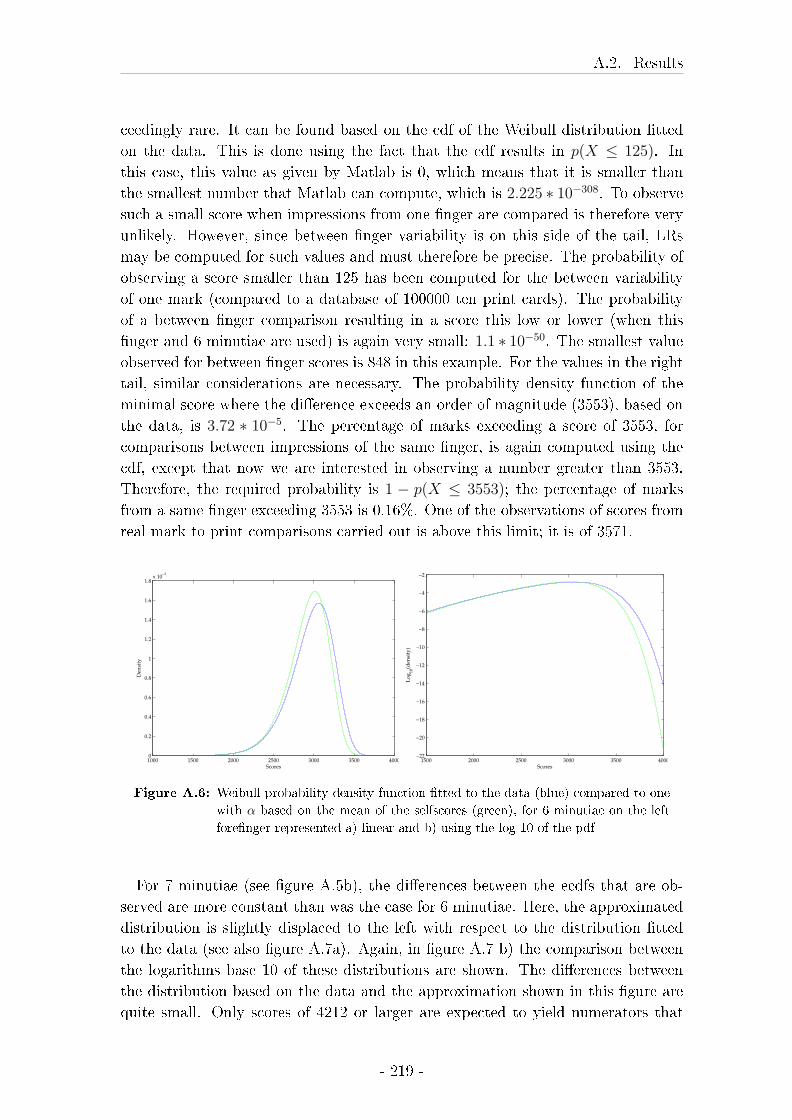
A.2. Results
ceedingly rare. It can be found based on the cdf of the Weibull distribution �tted
on the data. This is done using the fact that the cdf results in p(X ≤ 125). In
this case, this value as given by Matlab is 0, which means that it is smaller than
the smallest number that Matlab can compute, which is 2.225 ∗ 10−308. To observe
such a small score when impressions from one �nger are compared is therefore very
unlikely. However, since between-�nger variability is on this side of the tail, LRs
may be computed for such values and must therefore be precise. The probability of
observing a score smaller than 125 has been computed for the between variability
of one mark (compared to a database of 100000 ten print cards). The probability
of a between �nger comparison resulting in a score this low or lower (when this
�nger and 6 minutiae are used) is again very small: 1.1 ∗ 10−50. The smallest value
observed for between �nger scores is 848 in this example. For the values in the right
tail, similar considerations are necessary. The probability density function of the
minimal score where the di�erence exceeds an order of magnitude (3553), based on
the data, is 3.72 ∗ 10−5. The percentage of marks exceeding a score of 3553, for
comparisons between impressions of the same �nger, is again computed using the
cdf, except that now we are interested in observing a number greater than 3553.
Therefore, the required probability is 1 − p(X ≤ 3553); the percentage of marks
from a same �nger exceeding 3553 is 0.16%. One of the observations of scores from
real mark to print comparisons carried out is above this limit; it is of 3571.
1000 1500 2000 2500 3000 3500 40000
0.2
0.4
0.6
0.8
1
1.2
1.4
1.6
1.8x 10
−3
Scores
Den
sity
1500 2000 2500 3000 3500 4000−22
−20
−18
−16
−14
−12
−10
−8
−6
−4
−2
Scores
Lo
g10
(den
sity
)
Figure A.6: Weibull probability density function �tted to the data (blue) compared to one
with α based on the mean of the selfscores (green), for 6 minutiae on the left
fore�nger represented a) linear and b) using the log 10 of the pdf
For 7 minutiae (see �gure A.5b), the di�erences between the ecdfs that are ob-
served are more constant than was the case for 6 minutiae. Here, the approximated
distribution is slightly displaced to the left with respect to the distribution �tted
to the data (see also �gure A.7a). Again, in �gure A.7 b) the comparison between
the logarithms base 10 of these distributions are shown. The di�erences between
the distribution based on the data and the approximation shown in this �gure are
quite small. Only scores of 4212 or larger are expected to yield numerators that
- 219 -
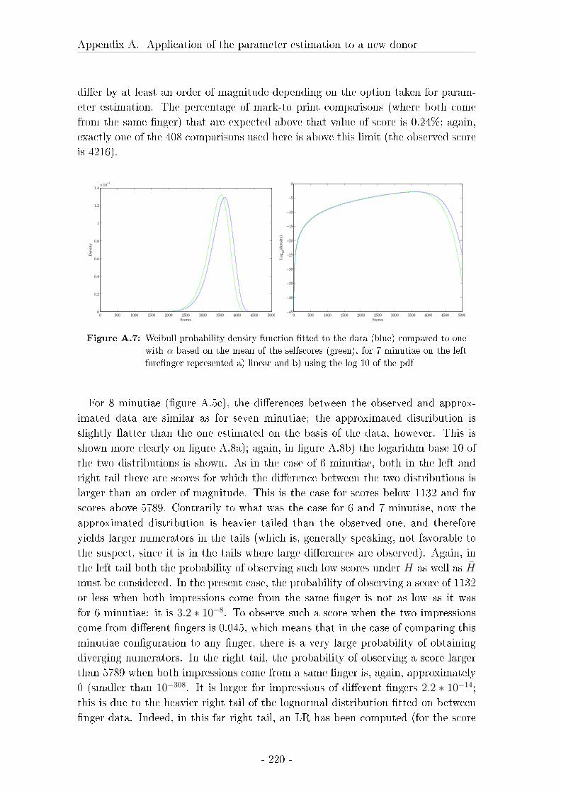
Appendix A. Application of the parameter estimation to a new donor
di�er by at least an order of magnitude depending on the option taken for param-
eter estimation. The percentage of mark-to print comparisons (where both come
from the same �nger) that are expected above that value of score is 0.24%; again,
exactly one of the 408 comparisons used here is above this limit (the observed score
is 4216).
0 500 1000 1500 2000 2500 3000 3500 4000 4500 50000
0.2
0.4
0.6
0.8
1
1.2
1.4x 10
−3
Scores
Den
sity
0 500 1000 1500 2000 2500 3000 3500 4000 4500 5000−45
−40
−35
−30
−25
−20
−15
−10
−5
0
Scores
Lo
g10
(den
sity
)
Figure A.7: Weibull probability density function �tted to the data (blue) compared to one
with α based on the mean of the selfscores (green), for 7 minutiae on the left
fore�nger represented a) linear and b) using the log 10 of the pdf
For 8 minutiae (�gure A.5c), the di�erences between the observed and approx-
imated data are similar as for seven minutiae; the approximated distribution is
slightly �atter than the one estimated on the basis of the data, however. This is
shown more clearly on �gure A.8a); again, in �gure A.8b) the logarithm base 10 of
the two distributions is shown. As in the case of 6 minutiae, both in the left and
right tail there are scores for which the di�erence between the two distributions is
larger than an order of magnitude. This is the case for scores below 1132 and for
scores above 5789. Contrarily to what was the case for 6 and 7 minutiae, now the
approximated distribution is heavier tailed than the observed one, and therefore
yields larger numerators in the tails (which is, generally speaking, not favorable to
the suspect, since it is in the tails where large di�erences are observed). Again, in
the left tail both the probability of observing such low scores under H as well as H̄
must be considered. In the present case, the probability of observing a score of 1132
or less when both impressions come from the same �nger is not as low as it was
for 6 minutiae: it is 3.2 ∗ 10−8. To observe such a score when the two impressions
come from di�erent �ngers is 0.045, which means that in the case of comparing this
minutiae con�guration to any �nger, there is a very large probability of obtaining
diverging numerators. In the right tail, the probability of observing a score larger
than 5789 when both impressions come from a same �nger is, again, approximately
0 (smaller than 10−308. It is larger for impressions of di�erent �ngers 2.2 ∗ 10−14;
this is due to the heavier right tail of the lognormal distribution �tted on between
�nger data. Indeed, in this far right tail, an LR has been computed (for the score
- 220 -
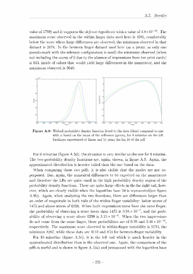
A.2. Results
value of 5789) and it supports the defense hypothesis with a value of 4.8∗10−10. The
maximum score observed in the within �nger data used here is 4981, comfortably
below the score where large di�erences are observed; the minimum observed in that
dataset is 2678. In the between �nger dataset used here (as a proxy, as only one
pseudo-mark with the relevant con�guration is used) the minimum observed (when
not including the scores of 0 due to the absence of impressions from ten print cards)
is 853, inside of values that would yield large di�erences in the numerator, and the
maximum observed is 3640.
1000 1500 2000 2500 3000 3500 4000 4500 5000 55000
0.2
0.4
0.6
0.8
1
1.2x 10
−3
Scores
Den
sity
1000 1500 2000 2500 3000 3500 4000 4500 5000 5500−16
−14
−12
−10
−8
−6
−4
−2
Scores
Lo
g10
(den
sity
)
Figure A.8: Weibull probability density function �tted to the data (blue) compared to one
with α based on the mean of the selfscores (green), for 8 minutiae on the left
fore�nger represented a) linear and b) using the log 10 of the pdf
For 9 minutiae (�gure A.5d), the situation is very similar to the one for 8 miutiae.
The two probability density functions are, again, shown, in �gure A.9. Again, the
approximated distribution is heavier tailed than the one based on the data.
When comparing those two pdfs, it is also visible that the modes are not su-
perposed. But, again, the numerical di�erences to be expected on the numerators
and therefore the LRs are quite small in the high probability density region of the
probability density functions. There are quite large e�ects in the far right tail, how-
ever, which are clearly visible when the logarithm base 10 is represented(see �gure
A.9b). Again, when analyzing the two functions, there are di�erences larger than
an order of magnitude in both tails of the within �nger variability: below scores of
1475 and above scores of 6298. When both impressions come from the same �nger,
the probability of observing a score lower than 1475 is 3.94 ∗ 10−7, and the prob-
ability of observing a score above 6298 is 3.15 ∗ 10−9. When the two impressions
do not come from the same �nger, these probabilities are of 0.35 and 3.46 ∗ 10−13,
respectively. The maximum score observed in within-�nger variability is 5734, the
minimum 3287, while these data are 4143 and 853 for between-�nger variability.
For 10 minutiae (�gure A.5e), it is the left tail which is much heavier in the
approximated distribution than in the observed one. Again, the comparison of the
pdfs is useful and is shown in �gure A.10a) and juxtaposed with the logarithm base
- 221 -
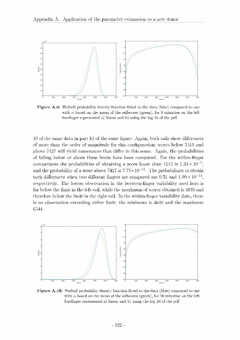
Appendix A. Application of the parameter estimation to a new donor
0 1000 2000 3000 4000 5000 6000 70000
0.1
0.2
0.3
0.4
0.5
0.6
0.7
0.8
0.9
1x 10
−3
Scores
Den
sity
1000 2000 3000 4000 5000 6000 7000−45
−40
−35
−30
−25
−20
−15
−10
−5
0
Scores
Lo
g10
(den
sity
)
Figure A.9: Weibull probability density function �tted to the data (blue) compared to one
with α based on the mean of the selfscores (green), for 9 minutiae on the left
fore�nger represented a) linear and b) using the log 10 of the pdf
10 of the same data in part b) of the same �gure. Again, both tails show di�erences
of more than the order of magnitude for this con�guration; scores below 1515 and
above 7427 will yield numerators that di�er in this sense. Again, the probabilities
of falling below or above these limits have been computed. For the within-�nger
comparisons the probabilities of obtaining a score lower than 1515 is 1.33 ∗ 10−7,
and the probability of a score above 7427 is 7.75∗10−11. The probabilities to obtain
such di�erences when two di�erent �ngers are compared are 0.31 and 1.99 ∗ 10−13,
respectively. The lowest observation in the between-�nger variability used here is
far below the limit in the left tail, while the maximum of scores obtained is 4639 and
therefore below the limit in the right tail. In the within-�nger variability data, there
is no observation exceeding either limit; the minimum is 3640 and the maximum
6544.
0 1000 2000 3000 4000 5000 6000 70000
1
2
3
4
5
6
7
8x 10
−4
Scores
Den
sity
0 1000 2000 3000 4000 5000 6000 7000−45
−40
−35
−30
−25
−20
−15
−10
−5
0
Scores
Lo
g10
(den
sity
)
Figure A.10: Weibull probability density function �tted to the data (blue) compared to one
with α based on the mean of the selfscores (green), for 10 minutiae on the left
fore�nger represented a) linear and b) using the log 10 of the pdf
- 222 -
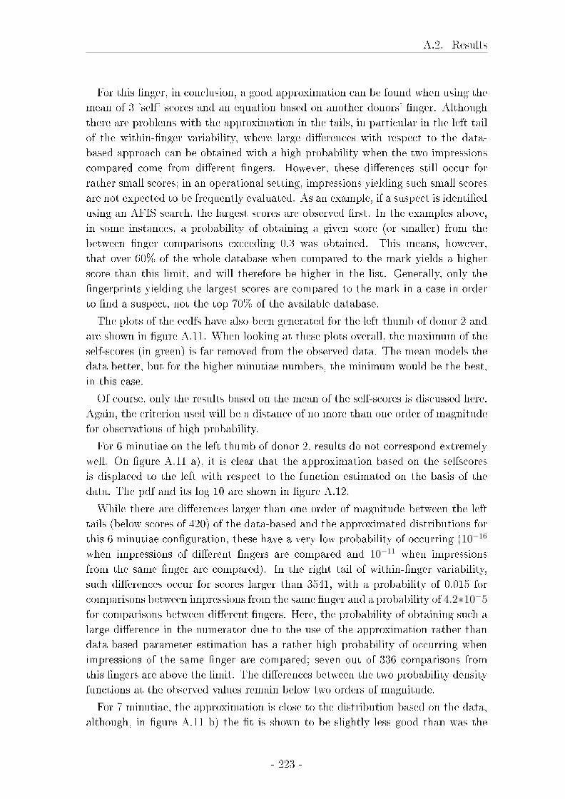
A.2. Results
For this �nger, in conclusion, a good approximation can be found when using the
mean of 3 'self' scores and an equation based on another donors' �nger. Although
there are problems with the approximation in the tails, in particular in the left tail
of the within-�nger variability, where large di�erences with respect to the data-
based approach can be obtained with a high probability when the two impressions
compared come from di�erent �ngers. However, these di�erences still occur for
rather small scores; in an operational setting, impressions yielding such small scores
are not expected to be frequently evaluated. As an example, if a suspect is identi�ed
using an AFIS search, the largest scores are observed �rst. In the examples above,
in some instances, a probability of obtaining a given score (or smaller) from the
between �nger comparisons exceeding 0.3 was obtained. This means, however,
that over 60% of the whole database when compared to the mark yields a higher
score than this limit, and will therefore be higher in the list. Generally, only the
�ngerprints yielding the largest scores are compared to the mark in a case in order
to �nd a suspect, not the top 70% of the available database.
The plots of the ecdfs have also been generated for the left thumb of donor 2 and
are shown in �gure A.11. When looking at these plots overall, the maximum of the
self-scores (in green) is far removed from the observed data. The mean models the
data better, but for the higher minutiae numbers, the minimum would be the best,
in this case.
Of course, only the results based on the mean of the self-scores is discussed here.
Again, the criterion used will be a distance of no more than one order of magnitude
for observations of high probability.
For 6 minutiae on the left thumb of donor 2, results do not correspond extremely
well. On �gure A.11 a), it is clear that the approximation based on the selfscores
is displaced to the left with respect to the function estimated on the basis of the
data. The pdf and its log 10 are shown in �gure A.12.
While there are di�erences larger than one order of magnitude between the left
tails (below scores of 420) of the data-based and the approximated distributions for
this 6 minutiae con�guration, these have a very low probability of occurring (10−16
when impressions of di�erent �ngers are compared and 10−11 when impressions
from the same �nger are compared). In the right tail of within-�nger variability,
such di�erences occur for scores larger than 3541, with a probability of 0.015 for
comparisons between impressions from the same �nger and a probability of 4.2∗10−5
for comparisons between di�erent �ngers. Here, the probability of obtaining such a
large di�erence in the numerator due to the use of the approximation rather than
data-based parameter estimation has a rather high probability of occurring when
impressions of the same �nger are compared; seven out of 336 comparisons from
this �ngers are above the limit. The di�erences between the two probability density
functions at the observed values remain below two orders of magnitude.
For 7 minutiae, the approximation is close to the distribution based on the data,
although, in �gure A.11 b) the �t is shown to be slightly less good than was the
- 223 -
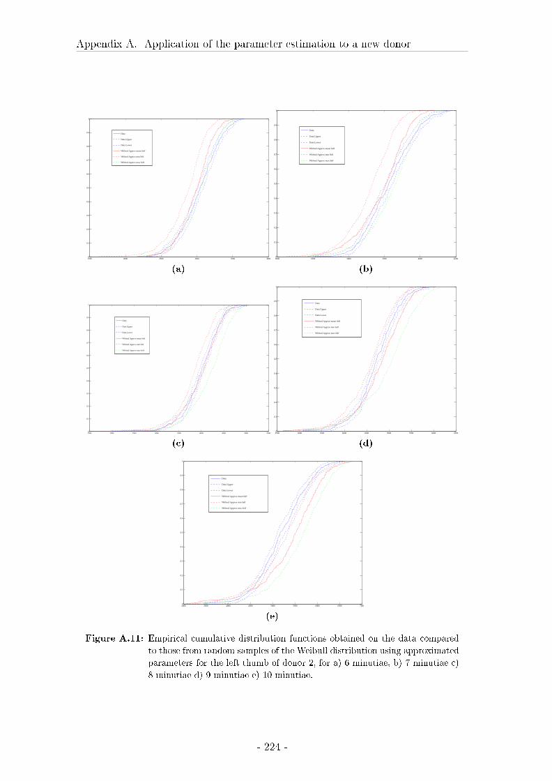
Appendix A. Application of the parameter estimation to a new donor
1500 2000 2500 3000 3500 40000
0.1
0.2
0.3
0.4
0.5
0.6
0.7
0.8
0.9
1
Data
Data Upper
Data Lower
Wblrnd Approx mean Self
Wblrnd Approx min Self
Wblrnd Approx max Self
(a)
2000 2500 3000 3500 4000 45000
0.1
0.2
0.3
0.4
0.5
0.6
0.7
0.8
0.9
1
Data
Data Upper
Data Lower
Wblrnd Approx mean Self
Wblrnd Approx min Self
Wblrnd Approx max Self
(b)
1500 2000 2500 3000 3500 4000 4500 5000 55000
0.1
0.2
0.3
0.4
0.5
0.6
0.7
0.8
0.9
1
Data
Data Upper
Data Lower
Wblrnd Approx mean Self
Wblrnd Approx min Self
Wblrnd Approx max Self
(c)
2500 3000 3500 4000 4500 5000 5500 6000 65000
0.1
0.2
0.3
0.4
0.5
0.6
0.7
0.8
0.9
1
Data
Data Upper
Data Lower
Wblrnd Approx mean Self
Wblrnd Approx min Self
Wblrnd Approx max Self
(d)
3000 3500 4000 4500 5000 5500 6000 6500 70000
0.1
0.2
0.3
0.4
0.5
0.6
0.7
0.8
0.9
1
Data
Data Upper
Data Lower
Wblrnd Approx mean Self
Wblrnd Approx min Self
Wblrnd Approx max Self
(e)
Figure A.11: Empirical cumulative distribution functions obtained on the data compared
to those from random samples of the Weibull distribution using approximated
parameters for the left thumb of donor 2, for a) 6 minutiae, b) 7 minutiae c)
8 minutiae d) 9 minutiae e) 10 minutiae.
- 224 -
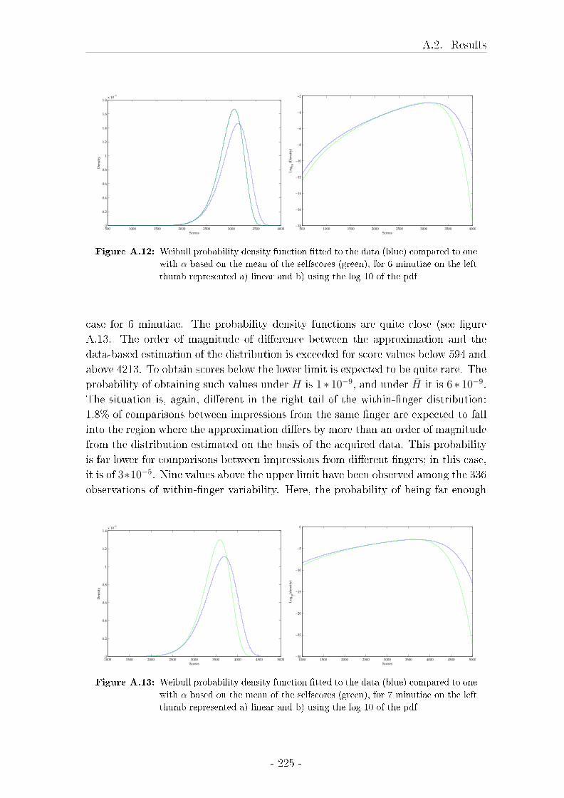
A.2. Results
500 1000 1500 2000 2500 3000 3500 40000
0.2
0.4
0.6
0.8
1
1.2
1.4
1.6
1.8x 10
−3
Scores
Den
sity
500 1000 1500 2000 2500 3000 3500 4000−18
−16
−14
−12
−10
−8
−6
−4
−2
Scores
Lo
g10
(D
ensi
ty)
Figure A.12: Weibull probability density function �tted to the data (blue) compared to one
with α based on the mean of the selfscores (green), for 6 minutiae on the left
thumb represented a) linear and b) using the log 10 of the pdf
case for 6 minutiae. The probability density functions are quite close (see �gure
A.13. The order of magnitude of di�erence between the approximation and the
data-based estimation of the distribution is exceeded for score values below 594 and
above 4213. To obtain scores below the lower limit is expected to be quite rare. The
probability of obtaining such values under H is 1 ∗ 10−9, and under H̄ it is 6 ∗ 10−9.
The situation is, again, di�erent in the right tail of the within-�nger distribution:
1.8% of comparisons between impressions from the same �nger are expected to fall
into the region where the approximation di�ers by more than an order of magnitude
from the distribution estimated on the basis of the acquired data. This probability
is far lower for comparisons between impressions from di�erent �ngers; in this case,
it is of 3∗10−5. Nine values above the upper limit have been observed among the 336
observations of within-�nger variability. Here, the probability of being far enough
1000 1500 2000 2500 3000 3500 4000 4500 50000
0.2
0.4
0.6
0.8
1
1.2
1.4x 10
−3
Scores
Den
sity
1000 1500 2000 2500 3000 3500 4000 4500 5000−30
−25
−20
−15
−10
−5
0
Scores
Lo
g10
(den
sity
)
Figure A.13: Weibull probability density function �tted to the data (blue) compared to one
with α based on the mean of the selfscores (green), for 7 minutiae on the left
thumb represented a) linear and b) using the log 10 of the pdf
- 225 -
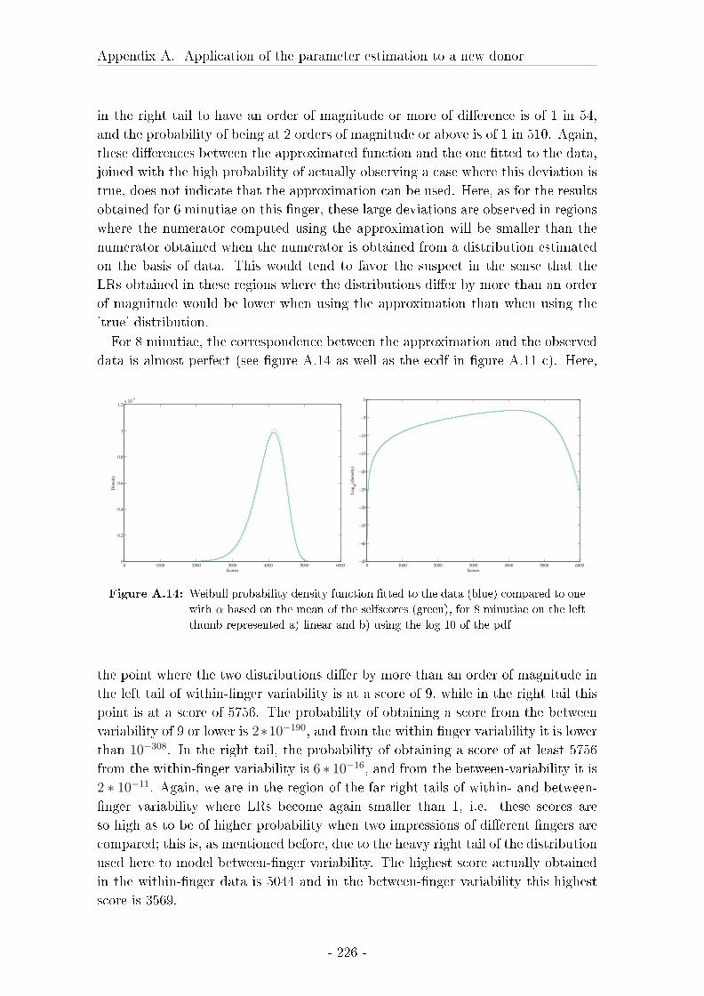
Appendix A. Application of the parameter estimation to a new donor
in the right tail to have an order of magnitude or more of di�erence is of 1 in 54,
and the probability of being at 2 orders of magnitude or above is of 1 in 510. Again,
these di�erences between the approximated function and the one �tted to the data,
joined with the high probability of actually observing a case where this deviation is
true, does not indicate that the approximation can be used. Here, as for the results
obtained for 6 minutiae on this �nger, these large deviations are observed in regions
where the numerator computed using the approximation will be smaller than the
numerator obtained when the numerator is obtained from a distribution estimated
on the basis of data. This would tend to favor the suspect in the sense that the
LRs obtained in these regions where the distributions di�er by more than an order
of magnitude would be lower when using the approximation than when using the
'true' distribution.
For 8 minutiae, the correspondence between the approximation and the observed
data is almost perfect (see �gure A.14 as well as the ecdf in �gure A.11 c). Here,
0 1000 2000 3000 4000 5000 60000
0.2
0.4
0.6
0.8
1
1.2x 10
−3
Scores
Den
sity
0 1000 2000 3000 4000 5000 6000−45
−40
−35
−30
−25
−20
−15
−10
−5
0
Scores
Lo
g10
(den
sity
)
Figure A.14: Weibull probability density function �tted to the data (blue) compared to one
with α based on the mean of the selfscores (green), for 8 minutiae on the left
thumb represented a) linear and b) using the log 10 of the pdf
the point where the two distributions di�er by more than an order of magnitude in
the left tail of within-�nger variability is at a score of 9, while in the right tail this
point is at a score of 5756. The probability of obtaining a score from the between
variability of 9 or lower is 2∗10−190, and from the within �nger variability it is lower
than 10−308. In the right tail, the probability of obtaining a score of at least 5756
from the within-�nger variability is 6 ∗ 10−16, and from the between-variability it is
2 ∗ 10−11. Again, we are in the region of the far right tails of within- and between-
�nger variability where LRs become again smaller than 1, i.e. these scores are
so high as to be of higher probability when two impressions of di�erent �ngers are
compared; this is, as mentioned before, due to the heavy right tail of the distribution
used here to model between-�nger variability. The highest score actually obtained
in the within-�nger data is 5044 and in the between-�nger variability this highest
score is 3569.
- 226 -
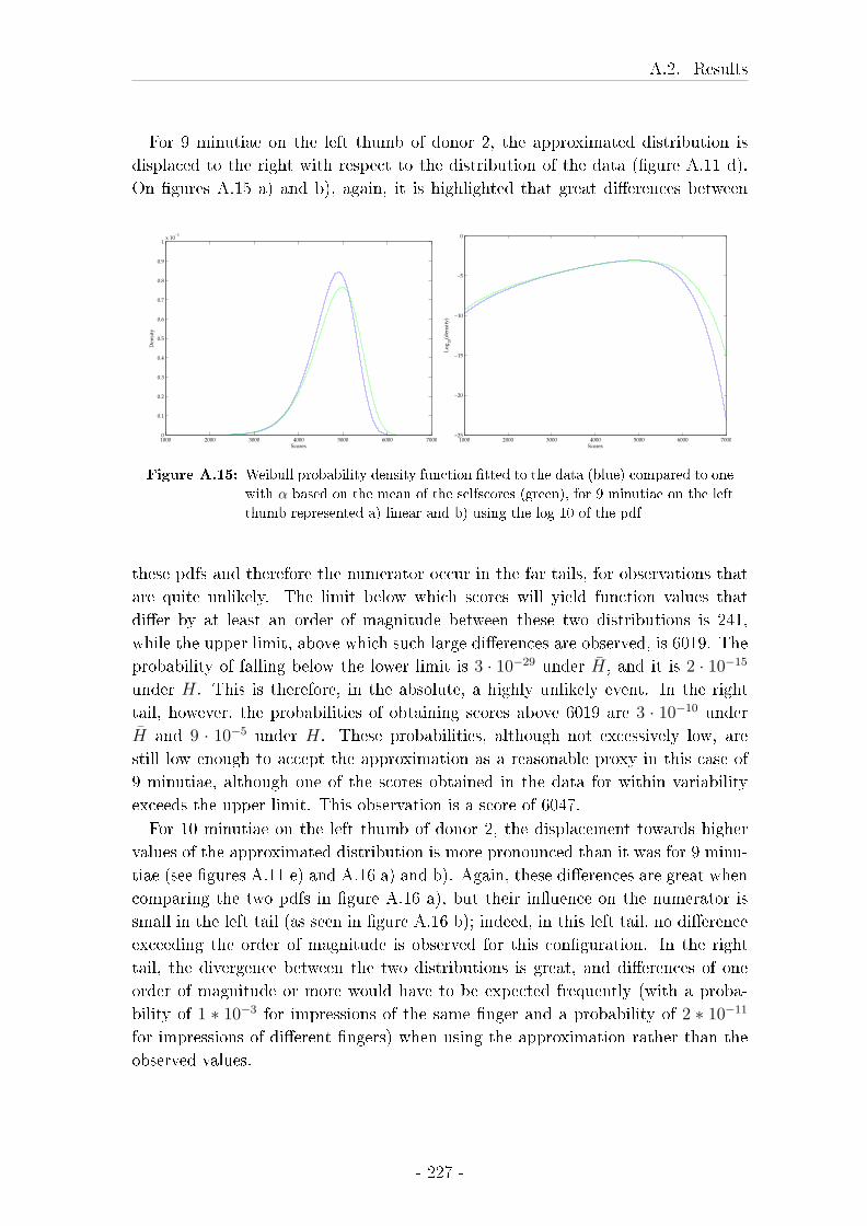
A.2. Results
For 9 minutiae on the left thumb of donor 2, the approximated distribution is
displaced to the right with respect to the distribution of the data (�gure A.11 d).
On �gures A.15 a) and b), again, it is highlighted that great di�erences between
1000 2000 3000 4000 5000 6000 70000
0.1
0.2
0.3
0.4
0.5
0.6
0.7
0.8
0.9
1x 10
−3
Scores
Den
sity
1000 2000 3000 4000 5000 6000 7000−25
−20
−15
−10
−5
0
ScoresL
og
10(d
ensi
ty)
Figure A.15: Weibull probability density function �tted to the data (blue) compared to one
with α based on the mean of the selfscores (green), for 9 minutiae on the left
thumb represented a) linear and b) using the log 10 of the pdf
these pdfs and therefore the numerator occur in the far tails, for observations that
are quite unlikely. The limit below which scores will yield function values that
di�er by at least an order of magnitude between these two distributions is 241,
while the upper limit, above which such large di�erences are observed, is 6019. The
probability of falling below the lower limit is 3 · 10−29 under H̄, and it is 2 · 10−15
under H. This is therefore, in the absolute, a highly unlikely event. In the right
tail, however, the probabilities of obtaining scores above 6019 are 3 · 10−10 under
H̄ and 9 · 10−5 under H. These probabilities, although not excessively low, are
still low enough to accept the approximation as a reasonable proxy in this case of
9 minutiae, although one of the scores obtained in the data for within variability
exceeds the upper limit. This observation is a score of 6047.
For 10 minutiae on the left thumb of donor 2, the displacement towards higher
values of the approximated distribution is more pronounced than it was for 9 minu-
tiae (see �gures A.11 e) and A.16 a) and b). Again, these di�erences are great when
comparing the two pdfs in �gure A.16 a), but their in�uence on the numerator is
small in the left tail (as seen in �gure A.16 b); indeed, in this left tail, no di�erence
exceeding the order of magnitude is observed for this con�guration. In the right
tail, the divergence between the two distributions is great, and di�erences of one
order of magnitude or more would have to be expected frequently (with a proba-
bility of 1 ∗ 10−3 for impressions of the same �nger and a probability of 2 ∗ 10−11
for impressions of di�erent �ngers) when using the approximation rather than the
observed values.
- 227 -
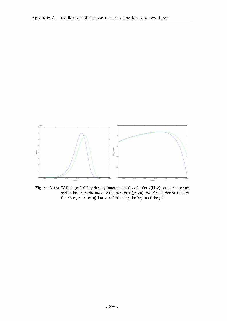
Appendix A. Application of the parameter estimation to a new donor
2000 3000 4000 5000 6000 7000 80000
1
2
3
4
5
6
7
8x 10
−4
Scores
Den
sity
2000 3000 4000 5000 6000 7000 8000−25
−20
−15
−10
−5
0
Scores
Lo
g10
(den
sity
)
Figure A.16: Weibull probability density function �tted to the data (blue) compared to one
with α based on the mean of the selfscores (green), for 10 minutiae on the left
thumb represented a) linear and b) using the log 10 of the pdf
- 228 -
Appendix B
Commands for score extraction
B.1 Data acquistion in the system
Three di�erent custom-made utilies have been used in the present work for the
direct extraction of scores and of general patterns. The �rst two are raw_dump.py
and spec.exe, for the extraction of scores and the third is PatternExtractor.py. It
is important that in the case�les (for latents) there be only one mark; otherwise,
spec.exe will not be able to automatically compute a score.
B.2 Command lines for the extraction of marks or
tenprints, the extraction of scores, and that of
general patterns
python raw_dump.py -f <Filename.txt> -D <ngaAFIS_DB> -s <SearchText> -l
Explanation of terms:
-f : allows to de�ne the �lename under which the output will be saved
-D: de�nition of the database to be used; generally, this will be ngaAFIS_DB, the
AFIS database
-s: which casenumbers / tenprints should be extracted. For tenprints, this is the
Family Name. * and ? have the usual meanings in this search.
-l: must be used if marks are extracted and not used if prints are extracted.
Command line for the automated extraction of scores based on the outputs of
raw_dump
spec.exe <MarksFilename.txt> <PrintsFilename.txt>
Command lines for the extraction of patterns
For marks:
- 229 -

Appendix B. Commands for score extraction
python PatternExtractor.py -l -D ngaAFIS_DB -o <output_directory>
The output �le will be called latent_pattern.txt and be found in the directory
de�ned under output_directory.
For prints
python PatternExtractor.py -p -D ngaAFIS_DB -o <output_directory>
The output �le will be called print_pattern.txt and be found in the directory
de�ned under output_directory.
- 230 -
Appendix C
Matlab functions for the
computations of Likelihood ratios
and Tippett plots
C.1 Function importing the data from the di�erent
text-�les
% This function lets the user manually select a directory (must not have
% the .DSStore �le inside) where the .txt �les of scores output by AFIS
% are to be found. The directory needs to be put in the Matlab path before
% using this function.
% There is one �le for each mark used, where the scores of this mark
% compared to all prints de�ned in the function extracting scores from
% AFIS are stored, along with the identi�er of the ten-print card and the
% �nger.
%
% Matlab version info below.
% ����������������������-
% MATLAB Version 7.0.1.24704 (R14) Service Pack 1
% ����������������������-
% MATLAB Version 7.0.1 (R14SP1)
% Curve Fitting Toolbox Version 1.1.2 (R14SP1)
% Image Processing Toolbox Version 5.0.1 (R14SP1)
% Neural Network Toolbox Version 4.0.4 (R14SP1)
% Statistics Toolbox Version 5.0.1 (R14SP1)
function results=import_�les_batch
%choose the directory
repertoire=uigetdir;
%list the �les in the directory
- 231 -
Appendix C. Matlab functions for the computations of Likelihood ratios andTippett plots
repertoire=dir(repertoire);
%number of �les
taille=size(repertoire,1);
%start with the 3rd, the �rst two are '.' and '..'
for �le=3:taille
%get the name for the �le
�chierName=repertoire(�le).name;
nout=taille-2;
%load the �le
savename=load(�chierName);
%put the data in the �rst two columns into the �rst two columns of
%the output
results(:,1:2)=savename(:,1:2);
%put the scores where they should go (into the �leth column of the
%output)
results(:,�le+1)=savename(:,3);
end
results;
C.2 Function for putting data into a vector format
% This function takes an array and reorganises the data in a vector.
%
% Matlab version info below.
% ����������������������-
% MATLAB Version 7.0.1.24704 (R14) Service Pack 1
% ����������������������-
% MATLAB Version 7.0.1 (R14SP1)
% Curve Fitting Toolbox Version 1.1.2 (R14SP1)
% Image Processing Toolbox Version 5.0.1 (R14SP1)
% Neural Network Toolbox Version 4.0.4 (R14SP1)
% Statistics Toolbox Version 5.0.1 (R14SP1)
function outvect=mettre_vect(Matrix_In)
j=1;
outvect=[];
taille=size(Matrix_In,2);
while j<taille+1
%add the current column of the array below all the data already
- 232 -

C.3. The global function for the Tippett plots
%stored in the vector.
outvect=[outvect;Matrix_in(:,j)];
j=j+1;
end
C.3 The global function for the Tippett plots
% The function makes tippett plots on randomly chosen comparisons in 2
% tables;
% The �rst table is made up of comparisons between impressions of the
% same �nger and the second one of comparisons between di�erent
% �ngers.
% In both tables, rows are �ngerprints, columns are �ngermarks.
% The �rst 3 columns are not scores, but 1) the identi�er of the
% ten-print card, 2) zeroes and 3) the �nger number. For comparisons
% between impressions from the same �nger, after
% importation, the �nger number must be chosen.
% Matlab version info below.
% ����������������������-
% MATLAB Version 7.0.1.24704 (R14) Service Pack 1
% ����������������������-
% MATLAB Version 7.0.1 (R14SP1)
% Curve Fitting Toolbox Version 1.1.2 (R14SP1)
% Image Processing Toolbox Version 5.0.1 (R14SP1)
% Neural Network Toolbox Version 4.0.4 (R14SP1)
% Statistics Toolbox Version 5.0.1 (R14SP1)
% The function outputs two matrices: 1) true and 2) false. True is
% based on comparisons where the impressions come from the same
% �nger and False on impressions from di�erent �ngers.
% The rows in these two tables correspond to the maximum 2000 observa-
% tions generated, while the columns are, in that order, the score,
% corresponding LRs computed using all data available (or rather, the
% database input for database_betweenALL, see inputs below) for the
% between-�nger variability, LRs computed using,for the between-
% �nger variability, only impressions that have the same �nger num-
% ber/general pattern combination as the mark (or rather the database
% input for database_betweenFNGP, see inputs below), the numerator
% corresponding to the scores based on data, the denominator based
% on all data (database_betweenALL), the denominator based on a
% database conditioned by general pattern and �nger number,LR based
% on �xed parameters for the denominator (and estimation for the
- 233 -

Appendix C. Matlab functions for the computations of Likelihood ratios andTippett plots
% numerator) LR based on a downsampled between-�nger database of
% 10000 observations selected from database_betweenALL and estimated
% numerator LR based on approximations for both numerator and deno-
% minator,numerator and denominator obtained using approximation,
% denominator obtained using �xed parameters and denominator based
% on the randomly downssampled database.
% Inputs are:
% number_of_data: the number of LRs to be obtained under
% both hypotheses; if for the data obtained
% when comparing impressions from the same
% �nger fewer observations are available,
% they will be used systematically for the
% Tippett plot (one after the other).
% 2000 have been used systematically.
% nbmin: the number of minutiae observed in the
% evidential comparison
% database_within: The database that contains all compari-
% sons between impressions from the same
% �nger.
% (rows=prints, columns=marks, �rst 3
% columns will be eliminated by the code).
% database_betweenALL: The database of all comparisons of the
% marks to the non-matching prints
% (rows=prints,
% columns=marks, �rst 3 columns will be
% eliminated by the code). Here,zeroes will
% be eliminated by the code and the
% columns will be sorted at one point;
% no need to prepare data.
% database_betweenFNGP; between-�nger database conditioned by
% �nger number and general pattern.
% selfscores: Three scores obtained on the basis of 3
% slap impressions compared to themselves
% (where the relevant minutiae for the
% case have been annotated as identically
% as possible on a given impression used
% once as a 'mark' and once as a 'print').
function [True,False]=TippettPlotDi�erent(number_of_data,nbmin,...
database_within,database_betweenALL,database_betweenFNGP,...
selfscores);
- 234 -

C.3. The global function for the Tippett plots
% de�ne counter; will be used for the storing of the results.
count1 = 1;
% prepare within and between �nger databases by taking out the
% �rst 3 columns.
database_within(:,1:3)=[];
database_betweenALL(:,1:3)=[];
database_betweenFNGP(:,1:3)=[];
%store the size of the within-�nger database
sizeIn=size(database_within);
%put within-�nger variability in a vector for �tting of the
%Weibull later; all data from within-�nger database is used
%for the �tting of the within-�nger distribution.
vector_within=mettre_vect(database_within);
% determine whether su�cient data is available in the within-
% �nger database for random selection of 'number of data'
% scores. If this is not the case, each score is used in turn.
if size(vector_within)<number_of_data
for istep = 1:sizeIn(2)
% for each column, corresponding to the comparisons of one mark
% to sizeIn(1) prints
vector_betweenALL=sort(database_betweenALL(:,istep),...
'descend');
%select the column corresponding to the mark in the
%between-�nger database; sort it.
vector_betweenFNGP=sort(database_betweenFNGP(:,istep),...
'descend');
% the same as previous line for second between-�nger
% database.
for jstep=1:sizeIn(1)
% systematically go through the scores for the
% selected mark.
withinLAT=database_within(jstep,istep);
%select evidence score from within-�nger database
% Compute relevant elements (LRs, numerators,
% denominators for
% the di�erent options) for the selected evidence.
% COMPARISONS UNDER H
[scoreT(count1),LR_E_APPROX_T(count1),...
LR_E_FIX_T(count1),LR_E_RED_T(count1),...
- 235 -
Appendix C. Matlab functions for the computations of Likelihood ratios andTippett plots
LRD_ALL_T(count1),LRD_FNGP_T(count1),...
NumE_T(count1),DenE_App_T(count1),...
DenE_Fix_T(count1),DenE_Red_T(count1),...
NumD_T(count1),DenD_All_T(count1),...
DenD_FNGP_T(count1)]=calculLRMany(withinLAT,...
nbmin,vector_within,vector_betweenALL,...
vector_betweenFNGP,selfscores);
%increment the counter
count1=count1+1;
end
%print istep, to know where you are at.
istep
end
%put results into the 'True' matrix in order to have fewer
%variables in output.
True=[scoreT',LRD_ALL_T',LRD_FNGP_T',NumD_T',DenD_All_T',...
DenDFNGP_T',LR_E_FIX_T',LR_E_RED_T',LR_E_APPROX_T',...
NumE_T',DenE_App_T',DenE_Fix_T',DenE_Red_T'];
%say when the computation of the LRs under H is �nished.
'Under H �nished'
% if there are more than 'number of data' observation in the
% within (strati�ed random selection will be used here;
% strati�cation is for reducing the time it takes to
% compute).
else
% compute the number of observations that will be selected
% from each column. Notice that the 'ceil' command rounds
% up; slightly more observations than number_of_data will
% be obtained.
numberPerColumn1=ceil(number_of_data/size(database_within,2));
for istep = 1:sizeIn(2) % again, go through the columns.
vector_betweenALL=sort(database_betweenALL(:,istep),...
'descend');
%select the column corresponding to the mark in the
%between-�nger database; sort it.
vector_betweenFNGP=sort(database_betweenFNGP(:,istep),...
'descend');
% the same as previous line for second between-�nger
% database.
placeWithin=randperm(size(database_within,1));
- 236 -
C.3. The global function for the Tippett plots
%randomly permutate numbers between 1 and the length of the
% vector corresponding to the comparison of 1 mark to
% several prints.
withinLAT=database_within(placeWithin(1:numberPerColumn1),...
istep);
%withinLAT is the vector of evidential scores that will be
%used for the computations of LRs etc.
for jstep=1:max(size(withinLAT))
% choose each of the evidential scores in turn.
% Compute relevant elements (LRs, numerators, denominators
% for the di�erent options) for the selected evidence.
%COMPARISONS UNDER H
[scoreT(count1),LR_E_APPROX_T(count1),...
LR_E_FIX_T(count1),LR_E_RED_T(count1),...
LRD_ALL_T(count1),LRD_FNGP_T(count1),...
NumE_T(count1),DenE_App_T(count1),...
DenE_Fix_T(count1),DenE_Red_T(count1),...
NumD_T(count1),DenD_All_T(count1),DenD_FNGP_T(count1)]...
=calculLRMany(withinLAT,nbmin,vector_within,...
vector_betweenALL,vector_betweenFNGP,selfscores);
% increment the counter for storing the results.
count1=count1+1;
end
%print istep, to know where you are at.
istep
end
end
True=[scoreT',LRD_ALL_T',LRD_FNGP_T',NumD_T',DenD_All_T',...
DenD_FNGP_T',LR_E_FIX_T',LR_E_RED_T',LR_E_APPROX_T',...
NumE_T',DenE_App_T',DenE_Fix_T',DenE_Red_T'];
'Under H �nished'
%here begin computations under Hbar
% create a new counter for these new results.
count2=1;
%Again, strati�ed random sampling is used for the selection of the
%evidential score. Again, the use of ceil will yield slightly more
%observations than what is de�ned by number_of_data.
numberPerColumn=ceil(number_of_data/size(database_betweenALL,2));
for kstep=1:size(database_betweenALL,2)
- 237 -

Appendix C. Matlab functions for the computations of Likelihood ratios andTippett plots
% select each column (corresponding to a mark each) in turn.
% randomly permutate numbers between 1 and the length of the vector
% corresponding to the comparison of 1 mark to several prints.
placebetw=randperm(size(database_betweenALL,1));
% select the evidential scores under Hbar, using the indices stored
% in placebetw. betweenLAT is a vector.
betweenLAT=database_betweenALL(placebetw(1:numberPerColumn),kstep);
%choose the proper between-�nger data for the latents, sort them.
vector_betweenALL=sort(database_betweenALL(:,kstep),'descend');
vector_betweenFNGP=sort(database_betweenFNGP(:,kstep),'descend');
for hstep=1:max(size(betweenLAT))
%for each evidential score, compute LRs etc.
[scoreF(count2),LR_E_APPROX_F(count2),LR_E_FIX_F(count2),...
LR_E_RED_F(count2),LRD_ALL_F(count2),...
LRD_FNGP_F(count2),NumE_F(count2),DenE_App_F(count2),...
DenE_Fix_F(count2),DenE_Red_F(count2),NumD_F(count2),...
DenD_All_F(count2),DenD_FNGP_F(count2)]...
=calculLRMany(betweenLAT(hstep),nbmin,...
vector_within,vector_betweenALL,vector_betweenFNGP,selfscores);
%Increment the counter for the results.
count2 = count2 + 1;
end
% print kstep to know how far it is.
kstep
end
%store results in a single variable.
False=[scoreF',LRD_ALL_F',LRD_FNGP_F',NumD_F',DenD_All_F',...
DenD_FNGP_F',LR_E_FIX_F',LR_E_RED_F',LR_E_APPROX_F',...
NumE_F',DenE_App_F',DenE_Fix_F',DenE_Red_F'];
% From now on, it's only plotting of Tippet plots using the data
% generated above.
% TAKEN AS IS FROM CEDRIC NEUMANNS CODING FOR A PROJECT
% FUNDED BY TSWG.
% FIGURE 1: DATA-BASED ESTIMATION IS USED FOR BOTH NUMER-
ATOR
%ANDDENOMINATOR,USING THEWHOLE BETWEEN-FINGER DATABASE
%FOR DENOMINATOR ESTIMATION (LRD_ALL_T AND LRD_ALL_F);
PlottingTippetts(LRD_ALL_T,LRD_ALL_F)
% FIGURE 2: DATA-BASED ESTIMATION IS USED FOR BOTH NUMERA-
TOR
- 238 -
C.4. The function for computing LRs using di�erent options
% AND DENOMINATOR, USING THE BETWEEN-FINGER DATABASE
% CONDITIONED BY GENERAL PATTERN AN FINGER NUMBER
% FOR DENOMINATOR ESTIMATION
% (LRD_FNGP_T AND LRD_FNGP_F);
PlottingTippetts(LRD_FNGP_T,LRD_FNGP_F)
% FIGURE 3: APPROXIMATION IS USED FOR BOTH NUMERATOR AND
%DENOMINATOR, USING FIXED PARAMETERS FOR THE BETWEEN-
% (FINGER DISTRIBUTION. LR_E_FIX_T AND LR_E_FIX_F);
PlottingTippetts(LR_E_FIX_T,LR_E_FIX_F)
% FIGURE 4: APPROXIMATION IS USED FOR THE NUMERATOR AND A
% REDUCED DATASET IS USED FOR ESTIMATION OF THE
%DENOMINATOR (LR_E_RED_T AND LR_E_RED_F);
PlottingTippetts(LR_E_RED_T,LR_E_RED_F)
% FIGURE 5 (LAST ONE): APPROXIMATION IS USED FOR BOTH THE
% NUMERATOR AND THE DENOMINATOR
% (LR_E_APPROX_T AND LR_E_APPROX_F);
PlottingTippetts(LR_E_APPROX_T,LR_E_APPROX_F)
C.4 The function for computing LRs using di�erent
options
% This function computes LRs (numerators and denominators) from the
% within and between data inserted. It also estimates the parameters
% for the between �nger variability (approximated and databased).
% It is made for being called by TippetPlotDi�erent.m.
%
% Matlab version info below.
% ����������������������-
% MATLAB Version 7.0.1.24704 (R14) Service Pack 1
% ����������������������-
% MATLAB Version 7.0.1 (R14SP1)
% Curve Fitting Toolbox Version 1.1.2 (R14SP1)
% Image Processing Toolbox Version 5.0.1 (R14SP1)
% Neural Network Toolbox Version 4.0.4 (R14SP1)
% Statistics Toolbox Version 5.0.1 (R14SP1)
%Input:
% EVIDENCE: an evidential score
% nbmin: the number of minutiae observed in the
% evidential comparison.
- 239 -
Appendix C. Matlab functions for the computations of Likelihood ratios andTippett plots
% vector_within: the vector of within-variability scores
% (obtained by comparing the suspects marks
% and prints using AFIS)
% database_betweenALL: the database of scores obtained when compa-
% ring the evidential mark to the whole
% database.
% database_betweenFNGP: the database (vector)of evidential scores
% obtained when comparing the evidence mark
% to a database of nonmatching prints that
% have the same �nger number and general
% pattern as the mark.
% selfscores Three scores obtained on the basis of 3
% slap impressions compared to themselves
% (where the relevant minutiae for the
case have been annotated as identically
% as possible on a given impression used
% once as a 'mark' and once as a 'print').
function [score,LR_E_APPROX,LR_E_FIX,LR_E_RED,LR_D_ALL,...
LR_D_FNGP,NumE,DenE_App,DenE_Fix,DenE_Red,NumD,...
DenD_All,DenD_FNGP]=calculLRMany(EVIDENCE,nbmin,vector_within,...
database_betweenALL,DatabaseBetweenFNGP,selfscores)
% Eliminate zeroes from between-�nger databases
database_betweenALL=database_betweenALL(database_betweenALL>0);
DatabaseBetweenFNGP=DatabaseBetweenFNGP(DatabaseBetweenFNGP>0);
% �t lognormal distribution to database of all �ngerprints
plognALL=logn�t(database_betweenALL);
% separate the two parameters into two variables
plogn1ALL=plognALL(1);
plogn2ALL=plognALL(2);
% �t lognormal to fngp database
plognFNGP=logn�t(DatabaseBetweenFNGP);
%separate the two parameters into two variables
plogn1FNGP=plognFNGP(1);
plogn2FNGP=plognFNGP(2);
%compute the approximated parameters for the between-�nger variability
[parmhatBetween1APPROX,parmhatBetween2APPROX]=...
compute_parmhat_betweenForTippett(database_betweenALL,nbmin);
%put the �xed parameters read o� elsewhere into two variables
parmhatBetween1FIX=7.50879430990458;
parmhatBetween2FIX=0.179001625332056;
% These two params are the mean of estimates obtained for 6oDFO on RTRL
- 240 -
C.4. The function for computing LRs using di�erent options
%randomly select 10000 observations from the 'All' database
p=randperm(max(size(database_betweenALL)));
ParmhatBetweenRED=logn�t(database_betweenALL(p(1:10000)));
% �t the Weibull distribution to the within-�nger data
estim=wbl�t(vector_within);
%prepare estimated parameters for the within-�nger variability
if nbmin==6
beta=13.9208240390902;
elseif nbmin==7
beta=12.7407795236924;
elseif nbmin==8
beta=11.5226744918335;
elseif nbmin==9
beta==10.4143410025036;
elseif nbmin==10
beta=10.3284587778818;
end
alpha=(mean(selfscores)+903.78)/1.4565;
%compute the numerator using the approximation
NumE=wblpdf(EVIDENCE(1,1),alpha,beta);
%compute the numerator using the data-based estimation
NumD=wblpdf(EVIDENCE(1,1),estim(1),estim(2));
%compute the denominators
%1) using all data
DenD_All=lognpdf(EVIDENCE(1,1),plogn1ALL,plogn2ALL);
%2) using fngp data
DenD_FNGP=lognpdf(EVIDENCE(1,1),plogn1FNGP,plogn2FNGP);
%3) using the approximation
DenE_App=lognpdf(EVIDENCE(1,1),parmhatBetween1APPROX,...
parmhatBetween2APPROX);
% 4) using the �xed parameters
DenE_Fix=lognpdf(EVIDENCE(1,1),...
parmhatBetween1FIX,parmhatBetween2FIX);
% 5) using the parametrs from the randomly reduced database
DenE_Red=lognpdf(EVIDENCE(1,1),ParmhatBetweenRED(1),...
ParmhatBetweenRED(2));
% divide numerators by denominators as needed
LR_D_ALL=NumD/DenD_All;
LR_D_FNGP=NumD/DenD_FNGP;
LR_E_APPROX=NumE/DenE_App;
LR_E_FIX=NumE/DenE_Fix;
- 241 -
Appendix C. Matlab functions for the computations of Likelihood ratios andTippett plots
% Here, numerator from data should be used; has been done manually in
% thesis from the outputs
LR_E_RED=NumE/DenE_Red;
%output the score for further use.
score=EVIDENCE;
C.5 The function for actually plotting the Tippett
plots
% This function takes di�erent LRs (obtained under H and
% Hbar) as input, and plots the Tippetts.
% Matlab version info below.
% ����������������������-
% MATLAB Version 7.0.1.24704 (R14) Service Pack 1
% ����������������������-
% MATLAB Version 7.0.1 (R14SP1)
% Curve Fitting Toolbox Version 1.1.2 (R14SP1)
% Image Processing Toolbox Version 5.0.1 (R14SP1)
% Neural Network Toolbox Version 4.0.4 (R14SP1)
% Statistics Toolbox Version 5.0.1 (R14SP1)
function PlottingTippetts(LRH,LRHbar)
% UNDER H
�gure
[yy,xx,n,emsg] = cdfcalc(log10(LRH));
k = length(xx);
n = reshape(repmat(1:k, 2, 1), 2*k, 1);
xCDF_true = [-Inf; xx(n); Inf];
yCDF_true = [0; 0; yy(1+n)];
% INVERSION OF THE CDF
yCDF_true = 1-yCDF_true;
plot(xCDF_true,yCDF_true,'g');
hold on;
% UNDER HBAR
[yy,xx,n,emsg] = cdfcalc(log10(LRHbar));
k = length(xx);
n = reshape(repmat(1:k, 2, 1), 2*k, 1);
xCDF_false = [-Inf; xx(n); Inf];
yCDF_false = [0; 0; yy(1+n)];
% INVERSION OF THE CDF
- 242 -
C.5. The function for actually plotting the Tippett plots
yCDF_false = 1-yCDF_false;
plot(xCDF_false,yCDF_false,'r');
title('Data based parameters: ALL data')
% rescale X axis
xlim_value=get(gca,'xlim');
tmp_xlim = max(abs(xlim_value(1)),xlim_value(2));
set(gca,'xlim',[-tmp_xlim, tmp_xlim]);
% LEGEND UNDER H
b=�nd(xCDF_true<=0);
text(0.8,0.93, ['\fontsize{12}\fontname{times}\it{LR true min =}'...
num2str(10�xCDF_true(2))],'horizontalalignment','left',...
'verticalalignment','middle','unit','norm');
text(0.8,0.88, ['\fontsize{12}\fontname{times}\it{LR true max =}'...
sprintf('%8.2o',10�(xCDF_true(size(xCDF_true,1)-1)))],...
'horizontalalignment','left','verticalalignment','middle',...
'unit','norm');
text(0.8,0.83, ['\fontsize{12}\fontname{times}\it{LR true < 1}' ...
sprintf('%8.2f',(100-100*yCDF_true(b(size(b,1))))) ' %'],...
'horizontalalignment','left','verticalalignment','middle',...
'unit','norm');
% put the legend into the graph
position_text = �ndobj(gca,'type','text');
s = get(position_text,'extent');
max_extent = max([s{1}(3),s{2}(3),s{3}(3)]);
t = get(position_text,'position');
if max_extent > 0.2
set(position_text(1),'position',[1-max_extent-0.01, t{1}(2), 0]);
set(position_text(2),'position',[1-max_extent-0.01, t{2}(2), 0]);
set(position_text(3),'position',[1-max_extent-0.01, t{3}(2), 0]);
end
% legend under Hbar
c=�nd(xCDF_false>=0);
text(0.05,0.12, ['\fontsize{12}\fontname{times}\it{LR false max =}'...
sprintf('%8.2o',10�(xCDF_false(size(xCDF_false,1)-1)))],...
'horizontalalignment','left','verticalalignment','middle',...
'unit','norm');
text(0.05,0.17, ['\fontsize{12}\fontname{times}\it{LR false min =}'...
num2str(10�xCDF_false(2))],'horizontalalignment','left',...
'verticalalignment','middle','unit','norm');
text(0.05,0.07, ['\fontsize{12}\fontname{times}\it{LR false > 1}' ...
- 243 -
Appendix C. Matlab functions for the computations of Likelihood ratios andTippett plots
sprintf('%8.2f',(100*yCDF_false(c(1)))) ' %'],...
'horizontalalignment','left','verticalalignment','middle',...
'unit','norm');
b=yCDF_true(b(size(b,1)));
line( [0,0],[yCDF_false(c(1))+0.05,b-0.05],'color',[0 0 0],...
'linestyle','-.');
text(0.49,0.49, ['\fontsize{12}\fontname{times}\it{LR = 1}'],...
'horizontalalignment','left','verticalalignment','middle',...
'unit','norm','rotation',90);
C.6 Computing the approximated parameters for
the between-�nger variability
%Takes the the ordered vector (without zeroes) of between-�nger data as
%input, as well as the number of minutiae in the evidential comparison, and
%computes the approximated parameters of the between-�nger distribution
% Matlab version info below.
% ����������������������-
% MATLAB Version 7.0.1.24704 (R14) Service Pack 1
% ����������������������-
% MATLAB Version 7.0.1 (R14SP1)
% Curve Fitting Toolbox Version 1.1.2 (R14SP1)
% Image Processing Toolbox Version 5.0.1 (R14SP1)
% Neural Network Toolbox Version 4.0.4 (R14SP1)
% Statistics Toolbox Version 5.0.1 (R14SP1)
function [parmhat1,parmhat2]...
=compute_parmhat_betweenForTippett(between_data,nbmin)
%Choose the �rst ten observations (the ten highest)
Datasorted=between_data(1:10);
%compute their mean
MeanDataS=mean(Datasorted);
%compute their variance
VarDataS=var(Datasorted);
%use the equations to obtain approximated parameters.
if nbmin==6
parmhat1=0.6246*log(MeanDataS)+2.422;
parmhat2=0.01199*(log(MeanDataS)./log(VarDataS))+0.1282;
elseif nbmin==7
parmhat1=0.8113*log(MeanDataS)+ 0.9021;
- 244 -

C.6. Computing the approximated parameters for the between-�nger variability
parmhat2=0.009652*(log(MeanDataS)./log(VarDataS))+0.1415;
elseif nbmin==8
parmhat1=0.819*log(MeanDataS)+0.8089 ;
parmhat2=-0.01174*(log(MeanDataS)./log(VarDataS))+0.1772;
elseif nbmin==9
parmhat1=0.2981*log(MeanDataS)+ 5.034;
parmhat2=-0.007286*(log(MeanDataS)./log(VarDataS))+0.1827;
elseif nbmin==10
parmhat1=0.3947*log(MeanDataS)+ 4.248;
parmhat2=-0.002005*(log(MeanDataS)./log(VarDataS))+0.1817;
end
- 245 -