AAllmmaa MMaatteerr SSttuuddiioorruumm –– UUnniivveerrssiittàà ddii BBoollooggnnaa

DOTTORATO DI RICERCA IN

Biodiversità ed Evoluzione

Ciclo XXVI

Settore Concorsuale di afferenza: 05/I1

Settore Scientifico disciplinare: BIO/18

Landscape ecology and genetics of the wolf in Italy

Presentata da: Pietro Milanesi

Coordinatore Dottorato Relatore

Prof.ssa Barbara Mantovani Prof. Ettore Randi

Dott. Romolo Caniglia

Esame finale anno 2014

1

A mia madre

2

The Wolves - Franz Marc, 1913

“ And when, on the still cold nights, he pointed his nose at a star and

howled long and wolf-like, it was his ancestors, dead and dust,

pointing nose at star and howling down through the centuries

and through him.”

The Call of the Wild - Jack London

3

INDEX

INTRODUCTION 4

MATERIALS AND METHODS 14

RESULTS 36

DISCUSSION 83

CONCLUSION 97

REFERENCES 100

LIST OF PAPERS 124

4

INTRODUCTION

Large carnivores are often used as focal species (indicator species, umbrella species) in

conservation strategies, especially when related to the maintenance of biodiversity. In fact, the

conservation of populations of large predators is achieved through the conservation of their habitat

and populations of their wild prey, influencing positively on the overall biodiversity. In addition,

predators require natural habitats, extensive and continuous or strongly connected to each other,

thus focusing attention on the importance of ecological corridors which benefit many other species

(Huber et al. 2002). Large carnivores have also a key role with regard to the regulation of the

populations of their prey: the wolf (Canis lupus), the lynx (Lynx lynx) and the bear (Ursus arctos)

preferentially prey animals young and inexperienced or old and sick, helping to control the growth

rates of the species prey. The wolf and the bear also feed on carrion, carrying out an activity of

'clean health', and this helps to prevent the onset of diseases, improving the health of the animals

(Breitenmoser 1998). Finally, the persecution of man towards predators requires effective

legislation and strict enforcement, especially because the long period of absence of large carnivores

in several regions of Italy has created many problems in the management of conflicts between the

presence of the species and the husbandry activities of the resident human population. For these

reasons, wolf, bear and lynx are protected both at international and national level: included in

Annex II of the Bern Convention ("strictly protected fauna species"), attachment II ("Animal and

plant species of Community interest whose conservation requires the designation of special areas of

conservation") and 4 ("Animal and plant species that require strict protection") of the Habitats

Directive, Annexes A and B of the Washington Convention (CITES) and Art. 2 of the Regulations

157/92 ("specially protected species"). The extraordinary ability to adapt to different ecological

conditions made the wolf the terrestrial mammal predator with the largest distribution range during

the Quaternary, covering, north of 20° N latitude, the entire North American continent, including

Mexico, Europe, Asia and Japan (Mech 1970, 1974). However, in historical times, the massive

eradication efforts carried out by humans since the 19th century, direct and indirect (reduction of

natural habitat and wild prey by hunters), resulted in a drastic reduction in both distribution and

abundance. During the 20th century the wolf also disappeared from almost all the territories of

continental Europe, surviving in small and fragmented populations in the Iberian, Hellenic and

Italian peninsula, in some territories of the former Yugoslavia and in the Scandinavian peninsula.

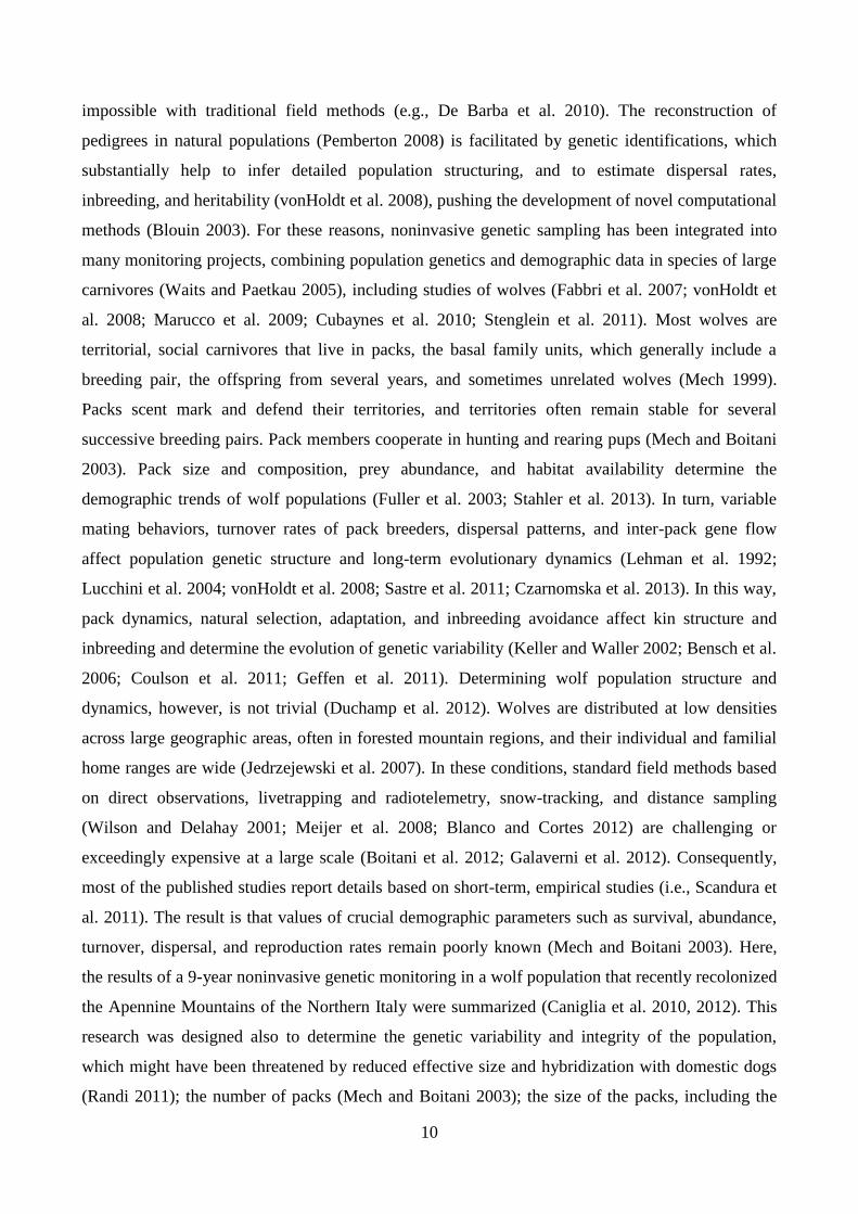
Actually, the European wolf range interests the Iberian Peninsula, which has a population of 1,500-

2,000 wolves (Blanco et al. 1990; Salvatori et al. 2005), the Balkan countries and the Hellenic

5

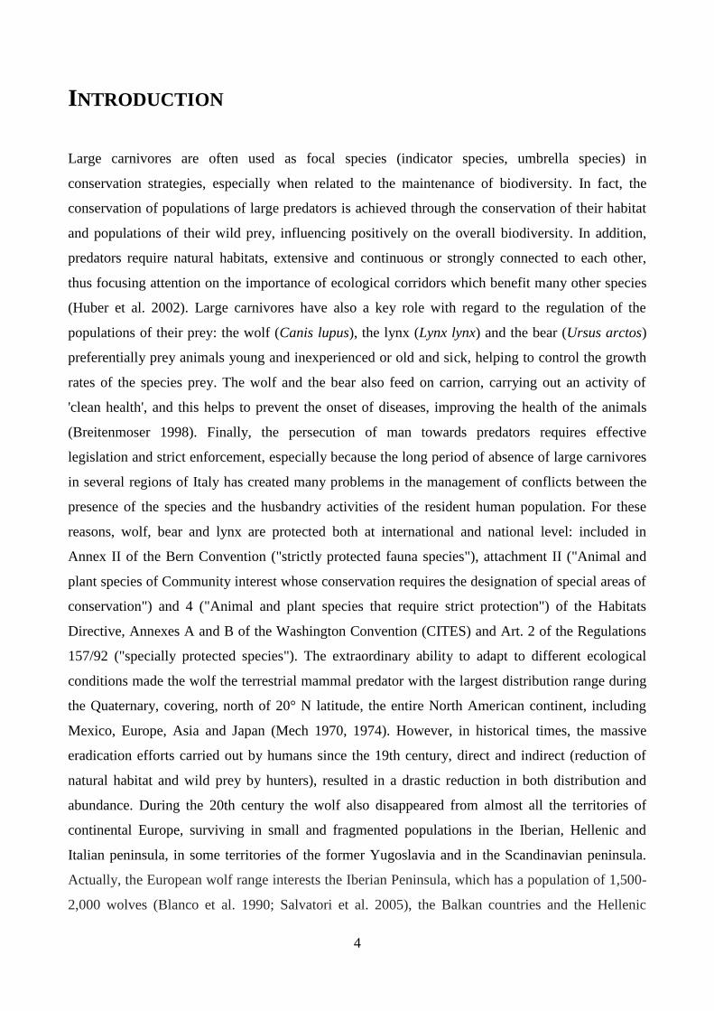
peninsula. In France, signs of recovery are in the Mercantour Massif in the Southern French Alps:

right through the Maritime Alps the wolf is gradually colonizing the South-western areas of the

Swiss Alps. To date, it is believed there are about 80 wolves in the French Alps, all from the

Apennines (Salvatori et al. 2005). Also in the rest of Europe wolf populations are growing or stable

and the low degree of human settlement of large areas of European Russia allows the maintenance

of high numerical amounts and it is also responsible for the slow processes of expansion of the

species toward the central-eastern countries such as Romania and Poland, where about 4,000 and

600-700 individuals are estimated respectively (Salvatori et al. 2005) confined to forest areas of

mountain territories. In northern Europe wolf populations are divided between the Scandinavian

peninsula, where it is estimated that about 200 people, and the Baltic States, whose wolves are from

Russia (Salvatori et al. 2005).

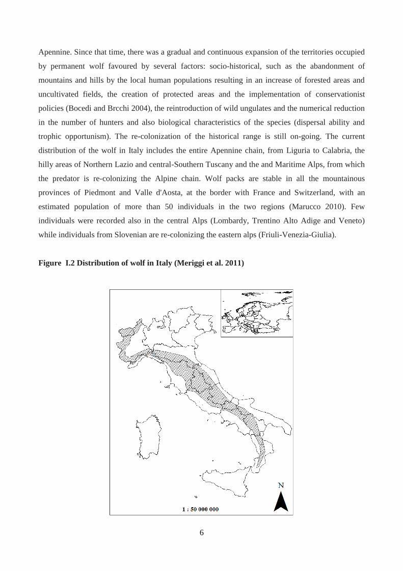
Figure I.I Distribution of wolf in Europe (in orange; http://www.lcie.org/)

In Italy, the wolf widespread over the entire peninsula until the mid-19th century, was exterminated

in the Alps at the end of that century and in Sicily island in 1940. Just in the last century, the

distribution of the species suffered a significant drop along the Apennine chain. At the end of the

50s it became very rare throughout the Tuscan-Emilian Apennines and in the following decade the

large number of species decreased dramatically to reach a historic bottleneck in the early '70s, when

Zimen and Boitani (1975) estimated the presence of about 100 wolves in the Southern-Central

6

Apennine. Since that time, there was a gradual and continuous expansion of the territories occupied

by permanent wolf favoured by several factors: socio-historical, such as the abandonment of

mountains and hills by the local human populations resulting in an increase of forested areas and

uncultivated fields, the creation of protected areas and the implementation of conservationist

policies (Bocedi and Brcchi 2004), the reintroduction of wild ungulates and the numerical reduction

in the number of hunters and also biological characteristics of the species (dispersal ability and

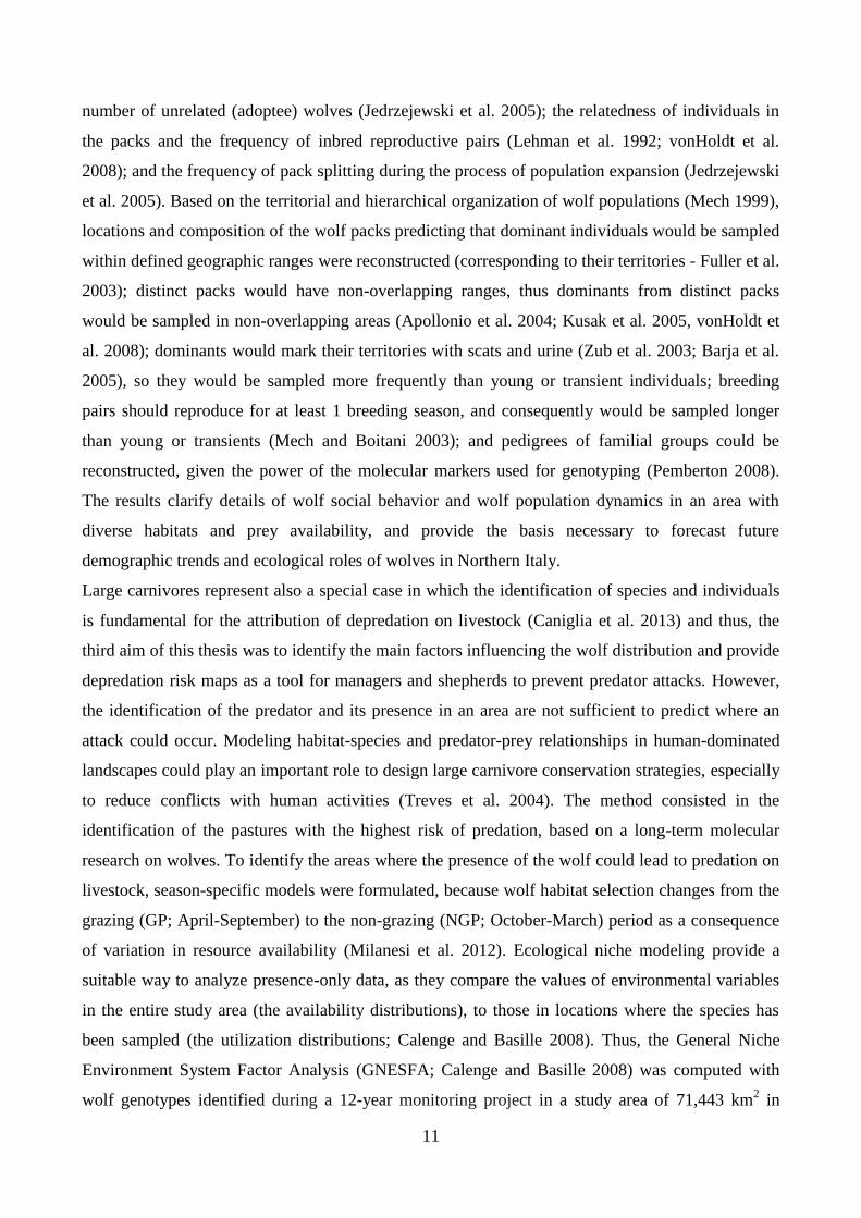
trophic opportunism). The re-colonization of the historical range is still on-going. The current

distribution of the wolf in Italy includes the entire Apennine chain, from Liguria to Calabria, the

hilly areas of Northern Lazio and central-Southern Tuscany and the and Maritime Alps, from which

the predator is re-colonizing the Alpine chain. Wolf packs are stable in all the mountainous

provinces of Piedmont and Valle d'Aosta, at the border with France and Switzerland, with an

estimated population of more than 50 individuals in the two regions (Marucco 2010). Few

individuals were recorded also in the central Alps (Lombardy, Trentino Alto Adige and Veneto)

while individuals from Slovenian are re-colonizing the eastern alps (Friuli-Venezia-Giulia).

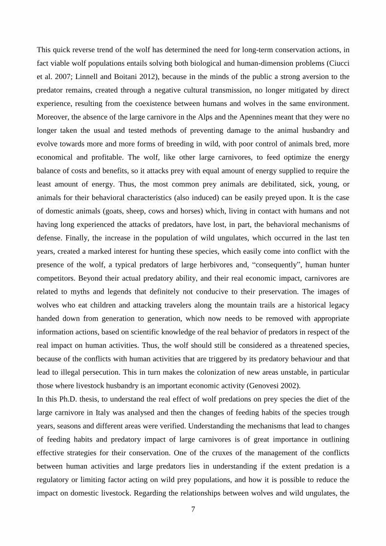
Figure I.2 Distribution of wolf in Italy (Meriggi et al. 2011)

7

This quick reverse trend of the wolf has determined the need for long-term conservation actions, in

fact viable wolf populations entails solving both biological and human-dimension problems (Ciucci

et al. 2007; Linnell and Boitani 2012), because in the minds of the public a strong aversion to the

predator remains, created through a negative cultural transmission, no longer mitigated by direct

experience, resulting from the coexistence between humans and wolves in the same environment.

Moreover, the absence of the large carnivore in the Alps and the Apennines meant that they were no

longer taken the usual and tested methods of preventing damage to the animal husbandry and

evolve towards more and more forms of breeding in wild, with poor control of animals bred, more

economical and profitable. The wolf, like other large carnivores, to feed optimize the energy

balance of costs and benefits, so it attacks prey with equal amount of energy supplied to require the

least amount of energy. Thus, the most common prey animals are debilitated, sick, young, or

animals for their behavioral characteristics (also induced) can be easily preyed upon. It is the case

of domestic animals (goats, sheep, cows and horses) which, living in contact with humans and not

having long experienced the attacks of predators, have lost, in part, the behavioral mechanisms of

defense. Finally, the increase in the population of wild ungulates, which occurred in the last ten

years, created a marked interest for hunting these species, which easily come into conflict with the

presence of the wolf, a typical predators of large herbivores and, “consequently”, human hunter

competitors. Beyond their actual predatory ability, and their real economic impact, carnivores are

related to myths and legends that definitely not conducive to their preservation. The images of

wolves who eat children and attacking travelers along the mountain trails are a historical legacy

handed down from generation to generation, which now needs to be removed with appropriate

information actions, based on scientific knowledge of the real behavior of predators in respect of the

real impact on human activities. Thus, the wolf should still be considered as a threatened species,

because of the conflicts with human activities that are triggered by its predatory behaviour and that

lead to illegal persecution. This in turn makes the colonization of new areas unstable, in particular

those where livestock husbandry is an important economic activity (Genovesi 2002).

In this Ph.D. thesis, to understand the real effect of wolf predations on prey species the diet of the

large carnivore in Italy was analysed and then the changes of feeding habits of the species trough

years, seasons and different areas were verified. Understanding the mechanisms that lead to changes

of feeding habits and predatory impact of large carnivores is of great importance in outlining

effective strategies for their conservation. One of the cruxes of the management of the conflicts

between human activities and large predators lies in understanding if the extent predation is a

regulatory or limiting factor acting on wild prey populations, and how it is possible to reduce the

impact on domestic livestock. Regarding the relationships between wolves and wild ungulates, the

8

main question is whether predation can regulate the populations of these prey species. Usually in a

prey-predator system regulation occurs when predation is density dependent and it stabilizes prey

populations at an equilibrium density. However, if predation is independent on density there is a

limiting effect and if it is inversely density dependent there is a dispensatory effect. In these cases

predation rate increases as prey density declines, causing the population to decline even faster; this

situation can occur when there is no switching by predators, there is no refuge for the prey, and

predators have an alternative prey source (Messier 1991, 1995; Marshal and Boutin 1999;

Jedrzejewski et al. 2002; Wittmer et al. 2005; Sinclair et al. 2006). In simple wolf-prey systems

wolf diet shifts according to changes in the relative abundance of the main prey, and shift dynamics

depend on the combined effects of preference, differential vulnerability and the relative abundance

of prey (Peterson and Ciucci 2003; Garrot et al. 2007). In areas with rich and abundant wild

ungulate guilds wolves prey upon the most abundant and profitable species, selecting gregarious

ones, young, and those in poor physical condition, and changing their preferences in relation to

species abundance (Okarma 1991; Huggard 1993a,b; Mattioli et al. 1995; Okarma 1995; Meriggi et

al. 1996; Poulle et al. 1997; Jedrzejewski et al. 2000; Mattioli et al. 2004; Gazzola et al. 2005,

Ansorge et al. 2006; Gazzola et al. 2007; Barja 2009). In areas with low wild ungulate abundance

livestock is the main prey and wild ungulates occur in wolf diet when livestock is not available or

when young wild ungulates are present (Cuesta et al. 1991; Meriggi et al. 1991, 1996; Okarma

1995; Meriggi and Lovari 1996; Vos 2000; Hovens and Tungalaktuja 2005). Moreover, predation

by wolves on livestock is dependent on the species, age class, rearing methods, and on the

availability of wild prey (Robel et al. 1981; Blanco et al. 1990; Meriggi et al. 1991; Boitani and

Ciucci 1993; Meriggi and Lovari 1996; Kaczensky 1999; Mech et al. 2000; Bradley and Pletscher

2005; Gazzola et al. 2008). In particular wolves select sheep and goats, and from cattle calves less

than 15 day old (Meriggi et al. 1991, 1996; Gazzola et al. 2008). High occurrence of livestock in

wolf diet was also recorded in areas of year-round grazing or where livestock is grazing unguarded

(Meriggi et al. 1996, Merkle et al. 2009) and damage is concentrated to a few farms, suggesting that

environment is also important in determining the probability of predation (Kaczensky 1999;

Schenone et al. 2004; Bradley and Pletscher 2005; Gazzola et al. 2008). From an analysis of the diet

of wolves in Mediterranean ranges, a close negative correlation was observed between the

frequency of occurrence of livestock and that of wild ungulates; this may mean that wolves prefer

wild prey, when available, to domestic ones (Meriggi and Lovari 1996). Where the availability of

wild ungulates is low and livestock is absent or inaccessible wolves use secondary prey species that

can be necessary dietary components in some seasons (Van Ballenberghe et al. 1975, Fritts and

Mech 1981, Fuller 1989, Chavez and Gese 2005). Moreover, several studies have shown some

9

important differences between wolf feeding habits in different study areas and periods. Wolf

feeding habits can also change over different periods within the same area, usually as a response to

the increase of wild ungulate populations. In Mediterranean countries in particular, a positive trend

of wild ungulate occurrence in wolf diet has been recorded in recent decades (Meriggi and Lovari

1996), and this is true also for recently settled wolf populations in Central Europe, where it seems

that the current diet is very different from that before wolf extinction (Ansorge et al. 2006). In fact,

also in Italy the diet of wolves markedly changed from the first studies carried out in the seventies

in the central Apennines to the recent ones performed in the Western Alps; in particular the diet of

wolves evolved towards a greater occurrence of large wild herbivores, becoming more and more

similar to that of North American and North-Eastern European areas (Meriggi and Lovari 1996).

Changes in the diet of wolves in Italy were identified and related to the use of wild ungulate

species, to the differences in large prey availability and to the richness and diversity of wild

ungulate communities. Moreover, the patterns of prey selection and their seasonal changes were

evaluated.

In this Ph.D. thesis, secondly, the distribution and population dynamics of wolves in the northern

Apennine was estimated using noninvasive genetic methods, because the expanding population also

spread in human-dominated areas, where the chances of hybridization with domestic dogs may

increase (Verardi et al. 2006; Godinho et al. 2011; Hindrikson et al. 2012; vonHoldt et al. 2013) and

the attribution of species locations could lead to mistaken estimates. The development of

noninvasive genetic methods has offered unique opportunities to implement long-term, wide-

ranging, and cost-effective research and monitoring programs (Schwartz et al. 2007; Brøseth et al.

2010; Ruiz-Gonzalez et al. 2013). Molecular techniques can provide more-exhaustive demographic

information than any other method (Lukacs et al. 2007). Reliable individual genotypes (DNA

fingerprinting) are obtained by analyzing DNA extracted from biological samples such as hair,

feces, urine, and blood traces that are noninvasively collected, without any direct human contact

with the animals (Waits and Paetkau 2005). Genotypes are used to count and locate individuals in

space and time and to reconstruct their genealogies and familial ranges (Creel et al. 2003; Schwartz

et al. 2007). The capture–recapture records of individual genotypes can be used to count the

minimum population size (Ernest et al. 2000; Lucchini et al. 2002; Gervasi et al. 2008) and to

estimate total abundance (Kohn et al. 1999; Mills et al. 2000; Lukacs and Burnham 2005). Although

low-quality DNA samples may generate genotyping errors (Broquet et al. 2007), these can be

minimized by using well-tested laboratory protocols and quality controls (Beja-Pereira et al. 2009).

Noninvasive genetics has been used to monitor the dynamics of endangered populations, obtaining

estimates of temporal trends of demographic and genetic parameters that would have been

10

impossible with traditional field methods (e.g., De Barba et al. 2010). The reconstruction of

pedigrees in natural populations (Pemberton 2008) is facilitated by genetic identifications, which

substantially help to infer detailed population structuring, and to estimate dispersal rates,

inbreeding, and heritability (vonHoldt et al. 2008), pushing the development of novel computational

methods (Blouin 2003). For these reasons, noninvasive genetic sampling has been integrated into

many monitoring projects, combining population genetics and demographic data in species of large

carnivores (Waits and Paetkau 2005), including studies of wolves (Fabbri et al. 2007; vonHoldt et

al. 2008; Marucco et al. 2009; Cubaynes et al. 2010; Stenglein et al. 2011). Most wolves are

territorial, social carnivores that live in packs, the basal family units, which generally include a

breeding pair, the offspring from several years, and sometimes unrelated wolves (Mech 1999).

Packs scent mark and defend their territories, and territories often remain stable for several

successive breeding pairs. Pack members cooperate in hunting and rearing pups (Mech and Boitani

2003). Pack size and composition, prey abundance, and habitat availability determine the

demographic trends of wolf populations (Fuller et al. 2003; Stahler et al. 2013). In turn, variable

mating behaviors, turnover rates of pack breeders, dispersal patterns, and inter-pack gene flow

affect population genetic structure and long-term evolutionary dynamics (Lehman et al. 1992;

Lucchini et al. 2004; vonHoldt et al. 2008; Sastre et al. 2011; Czarnomska et al. 2013). In this way,

pack dynamics, natural selection, adaptation, and inbreeding avoidance affect kin structure and

inbreeding and determine the evolution of genetic variability (Keller and Waller 2002; Bensch et al.

2006; Coulson et al. 2011; Geffen et al. 2011). Determining wolf population structure and

dynamics, however, is not trivial (Duchamp et al. 2012). Wolves are distributed at low densities

across large geographic areas, often in forested mountain regions, and their individual and familial

home ranges are wide (Jedrzejewski et al. 2007). In these conditions, standard field methods based

on direct observations, livetrapping and radiotelemetry, snow-tracking, and distance sampling

(Wilson and Delahay 2001; Meijer et al. 2008; Blanco and Cortes 2012) are challenging or

exceedingly expensive at a large scale (Boitani et al. 2012; Galaverni et al. 2012). Consequently,

most of the published studies report details based on short-term, empirical studies (i.e., Scandura et

al. 2011). The result is that values of crucial demographic parameters such as survival, abundance,

turnover, dispersal, and reproduction rates remain poorly known (Mech and Boitani 2003). Here,

the results of a 9-year noninvasive genetic monitoring in a wolf population that recently recolonized

the Apennine Mountains of the Northern Italy were summarized (Caniglia et al. 2010, 2012). This

research was designed also to determine the genetic variability and integrity of the population,

which might have been threatened by reduced effective size and hybridization with domestic dogs

(Randi 2011); the number of packs (Mech and Boitani 2003); the size of the packs, including the

11

number of unrelated (adoptee) wolves (Jedrzejewski et al. 2005); the relatedness of individuals in

the packs and the frequency of inbred reproductive pairs (Lehman et al. 1992; vonHoldt et al.

2008); and the frequency of pack splitting during the process of population expansion (Jedrzejewski

et al. 2005). Based on the territorial and hierarchical organization of wolf populations (Mech 1999),

locations and composition of the wolf packs predicting that dominant individuals would be sampled

within defined geographic ranges were reconstructed (corresponding to their territories - Fuller et al.

2003); distinct packs would have non-overlapping ranges, thus dominants from distinct packs

would be sampled in non-overlapping areas (Apollonio et al. 2004; Kusak et al. 2005, vonHoldt et

al. 2008); dominants would mark their territories with scats and urine (Zub et al. 2003; Barja et al.

2005), so they would be sampled more frequently than young or transient individuals; breeding

pairs should reproduce for at least 1 breeding season, and consequently would be sampled longer

than young or transients (Mech and Boitani 2003); and pedigrees of familial groups could be

reconstructed, given the power of the molecular markers used for genotyping (Pemberton 2008).

The results clarify details of wolf social behavior and wolf population dynamics in an area with

diverse habitats and prey availability, and provide the basis necessary to forecast future

demographic trends and ecological roles of wolves in Northern Italy.

Large carnivores represent also a special case in which the identification of species and individuals

is fundamental for the attribution of depredation on livestock (Caniglia et al. 2013) and thus, the

third aim of this thesis was to identify the main factors influencing the wolf distribution and provide

depredation risk maps as a tool for managers and shepherds to prevent predator attacks. However,

the identification of the predator and its presence in an area are not sufficient to predict where an

attack could occur. Modeling habitat-species and predator-prey relationships in human-dominated

landscapes could play an important role to design large carnivore conservation strategies, especially

to reduce conflicts with human activities (Treves et al. 2004). The method consisted in the

identification of the pastures with the highest risk of predation, based on a long-term molecular

research on wolves. To identify the areas where the presence of the wolf could lead to predation on

livestock, season-specific models were formulated, because wolf habitat selection changes from the

grazing (GP; April-September) to the non-grazing (NGP; October-March) period as a consequence

of variation in resource availability (Milanesi et al. 2012). Ecological niche modeling provide a

suitable way to analyze presence-only data, as they compare the values of environmental variables

in the entire study area (the availability distributions), to those in locations where the species has

been sampled (the utilization distributions; Calenge and Basille 2008). Thus, the General Niche

Environment System Factor Analysis (GNESFA; Calenge and Basille 2008) was computed with

wolf genotypes identified during a 12-year monitoring project in a study area of 71,443 km2 in

12

North-Central Apennines and South-Western Alps (Italy) and then, the resulting GP habitat

suitability maps was used to define depredation risks on livestock in pastures (Kaartinen et al. 2009;

Marucco and McIntire 2010). Even if wolves are protected by law in Italy and in most of the other

European countries, its predatory behavior could lead to heavy poaching, which is estimated to kill

c. 20% of the population each year in Italy (Lovari et al. 2007, Caniglia et al. 2010) and then,

conservation strategies, aimed at reducing conflicts with human presence and activities, should be

designed based on accurate population monitoring and predation risk assessment (Treves et al.

2004). The genetic analyses of all the collected presumed wolf scat samples, necessary for the

analyses, were performed at the Genetic Laboratory of the Istituto Superiore per la Protezione e la

Ricerca Ambientale (ISPRA).

By combining landscape ecology and population genetics aspects, in this thesis, finally landscape

genetics patterns of the wolf population in Italy were investigated. Landscape genetics assesses how

the environment affects the movement, dispersal or gene flow of species (Segelbacher et al. 2010)

and thus gives evidence of functional connectivity within landscapes (Holderegger et al. 2007;

Holderegger and Wagner 2008). Landscape genetics often uses least cost path (LCP; Cushman

2006) analysis from resistance surfaces to movement to measure ecological distances among

populations or individuals. These ecological distances are then correlated to genetic distances. In

LCP analysis, different levels of resistances to movement must be assigned to particular landscape

elements. These resistance values are mostly based on expert opinion (Clark et al. 2008; Lee-Yaw

et al. 2009; Murray et al. 2009) and have usually not been evaluated from empirical data such as

direct observations, dispersal behavior or GPS and radio-tracking (Stevens et al. 2006; Epps et al.

2007; Chietkiewicz and Boyce 2009). However, expert knowledge can lead to subjective

uncertainty and strongly influence the results of landscape genetic analysis (Cushman et al. 2010;

Cushman and Lewis 2010; Huck et al. 2010). Alternatively, habitat suitability models, based on

distribution data of species, could be applied as a potentially more objective means to assign

resistance values in LCP. Here, the reciprocal of the value of a habitat suitability model is directly

used as a values for the resistance to movement of particular landscape elements (Wang et al. 2008).

Expert knowledge is therefore not involved in the assignment of resistance values. The use of

habitat suitability models in landscape genetics is, however, not without caveats. First, there is often

bias in the locations of samples or observations, used for modeling habitat suitability, and species

might also have different detectability in different landscape elements (O’Brien et al. 2006).

Second, Spear et al. (2010) highlighted that suitability models mainly reflect the reproductive

habitat or the home range of species but not necessarily movement through the landscape during

dispersal. Habitat suitability models might therefore ignore critical features of inter-population

13

movement and dispersal. Nevertheless, Laiola and Tella (2006) and Wang et al. (2008) presented

two empirical applications of habitat suitability models in landscape genetics, which showed

significant correlations between genetic distances and resistance surfaces based on habitat

suitability. Similarly, Brown and Knowles (2012), Duckett et al. (2013) and Wang et al. (2013)

successfully used different types of habitat suitability models in landscape genetics. A large variety

of habitat suitability models have been developed during the recent years, and comparisons of

different methods were carried out to find the best model to define species distributions or to

forecast population expansions (Jones-Farrand et al. 2011). However, most of the landscape genetic

studies that applied habitat suitability modeling used only one particular habitat suitability model in

their analyses. Hitherto, no thorough comparison and evaluation of different habitat suitability

models, to assign resistance values in LCP modeling and landscape genetics, has been carried out.

The aim was to find habitat suitability models that provided highest efficiency in LCP prediction

and landscape genetic analysis. For this purpose, ten widely used habitat suitability models were

applied to identify suitable habitat and validated their efficiency. According to Wang et al. (2008)

and Pullinger and Johnson (2010), resistance values were calculated from the resulting habitat

suitability maps as 1 – habitat suitability. Ecological distances were determined as the length along

LCPs as well as straight-line Euclidean (geographical) distances (Etherington and Holland 2013;

Van Strien et al. 2012). Then, the power of the ecological distances obtained from the ten different

habitat suitability models was evaluated to explain genetic distances while also considering the

effects of Euclidean distance in a landscape genetic framework. Thus, partial Mantel tests, which

are traditionally used in landscape genetics, multiple regression on distance matrices, which is the

state of the art method of statistical analysis in landscape genetics, and fore-front mixed effect

models were applied (Van Strien et al. 2012). The data set consisted of about 1,000 wolves

originating from a long-term genetic monitoring program (12 years) across a large study area of

about 100,000 km2 in Italy. The landscape genetics analyses were performed at the Research Units

of Biodiversity and Conservation Biology if the WSL Swiss Federal Research Institute.

14

MATERIALS AND METHODS

M.1. Changes of wolf diet in Italy in relation to the increase of wild ungulate abundance

An analysis of the scientific papers about the feeding habits of wolves in Italy was carried out

taking into consideration the studies on the analysis of scats because they were more numerous than

those that used predation data. Studies published in scientific journals, degree, masters and PhD

theses, and unpublished reports were considered. If a study summarized results from more than one

study site, these were analyzed separately, i.e. per site.

For each study, the absolute percentage of occurrence (ratio between the number of times that a

prey occurs in the sample and the sample size) of seven food categories (Wild ungulates, Livestock,

Small mammals, Other vertebrates, Fruits, Other vegetables, Garbage) was considered and then the

percentage of occurrence calculated for each wild ungulate species. Moreover, the diet breadth was

calculated by the normalized Levins’ B index on food categories (Feisinger et al. 1981).

At a local level, the data on wolf diet from the Genova province (northern Apennines) from 1987 to

2005 was considered, computing for each year the frequency of occurrence of pooled wild

ungulates, and of each species that occurred in scats.

Population estimates of the different species of wild ungulates in Italy was extrapolated from Pavan

and Berretta Boera (1981), Pedrotti et al. (2001), and Apollonio (2004); the trend at national level

was obtained by extrapolation, assuming a constant numeric increase between time intervals

(years), thus obtaining a rate of increase that linearly decreases with the increase in population.

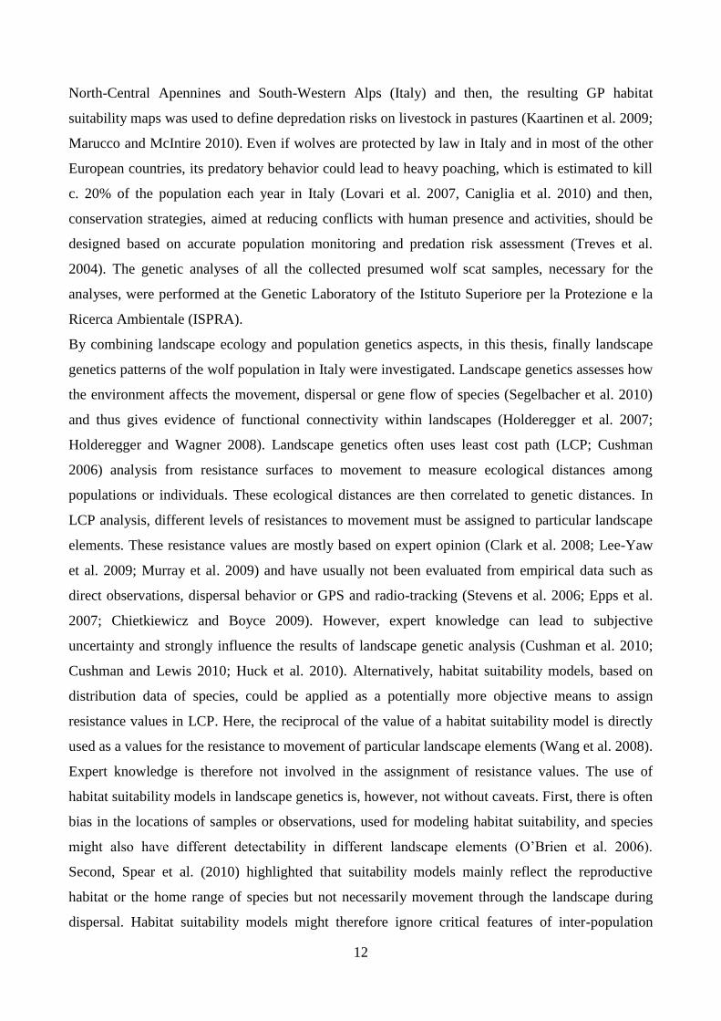
The diet composition of wolves among geographic areas was compared by nonparametric

multivariate analysis of variance (NPMANOVA; Anderson, 2001; Hammer, 2010) with

permutation (10,000 replicates) and pairwise comparisons with Bonferroni’s correction;

furthermore, each variable was tested with the Kruskall–Wallis test. For this aim the examined

studies were assigned to the following geographic areas: southern-central Apennines (Region

administrations: Umbria, Abruzzo, Calabria), northern Apennines (Region administrations:

Piedmont, Lombardy, Liguria, Emilia-Romagna, Tuscany), and western Alps (Region

administration: Piedmont) (Fig. M.1.1).

To show significant trends of wild ungulate and livestock use and of diet breadth, curve-fit analyses

were used with the time as independent variable. The same type of analysis was used to show the

type of relationships between wild prey usage and their abundance.

15

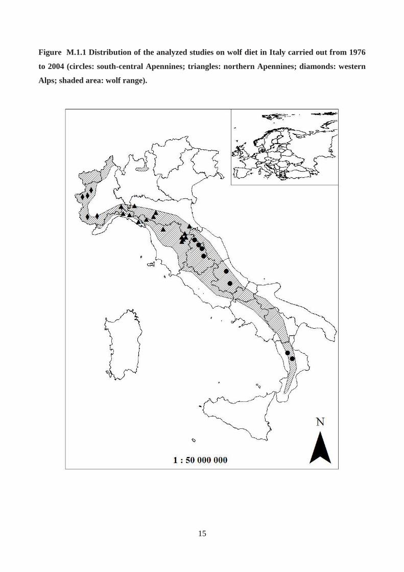
Figure M.1.1 Distribution of the analyzed studies on wolf diet in Italy carried out from 1976

to 2004 (circles: south-central Apennines; triangles: northern Apennines; diamonds: western

Alps; shaded area: wolf range).

16

M.2. Selection of wild ungulates by wolves in an area of the Northern Apennines (North

Italy)

Study area

in the study area covered an 860 km2 mountain area located in the western part of the Northern

Apennines (North Italy: 44°46’17.40’’N, 9°23’11.04’’E) with elevations of 500-1700 m a.s.l.. The

community of wild ungulates included, in order of abundance: wild boar (Sus scrofa), roe deer

(Capreolus capreolus, fallow deer (Dama dama), and red deer (Cervus elaphus). The last two

species were localized in two distinct parts of the study area, and the former two were widespread

over the whole territory. Wild boars shot by hunters increased from 600 individuals in the nineties

to 2650 in 2008, roe deer densities, estimated by drive and vantage point counts, increased from 5.9

per km2 in 2005 (the first year of census) to 8.6 per km

2 in 2008, fallow deer density averaged 1.9

per km2 from 2006 to 2008 (drive and vantage point counts), and red deer roaring males increased

from 22 in 2002 to 33 in 2008 (data from the Wildlife Services of the provinces of Piacenza and

Pavia). Livestock was present on pastures located on the ridges of mountain chains from April to

October; mainly cattle but also goats, sheep, and horses were free ranging during the grazing period.

Their numbers were constant over the last twenty years: cattle amounted to 1996 heads, goats and

sheep to 757, and horses to 157 (data from veterinary services of the provinces of Piacenza and

Pavia).

By snow-tracking, wolf-howling and camera-trapping, a presence of four main packs of wolves was

estimated in the study area, respectively of 7, 5, 4, and 2 individuals, and a small number of lone

wolves. The presence of free ranging or feral dogs has never been recorded in the study area and the

wolf was the only species of large carnivore present in this region.

Data collection

Itineraries traced on footpaths and randomly chosen (N=25) were selected among those existing in

the study area (total length = 168 km, average ± SD = 7.0 ± 2.3 km, min. = 2.8 km, max. = 11.3

km). From June 2007 to May 2008 all transects were covered once a season (winter: December to

February; spring: March to May; summer: June to August; autumn: September to November)

searching for wolf scats and signs of wild ungulate presence. On itineraries, all fresh wolf scats

were collected and wild ungulate signs were recorded (tracks, rooting, resting sites, wallowing, and

rubbing), in order to estimate the proportions of use and availability of the different species.

17

Diet analysis

Wolf diet was studied by scat analysis. Scats were preserved in PVC bags at -20°C for one month,

and then they were washed in water over 3 sieves with decreasing meshes (0.5-0.1 mm). Prey

species were identified from undigested remains: hairs, bones, hoofs, and nails (medium and large

sized mammals), hairs and mandibles (small mammals) seeds and leaves (fruits and plants).

Moreover, hairs were washed in alcohol and identified by microscopical observation of cortical

scales and medulla (Brunner and Coman 1974; Debrot et al. 1982; Teerink 1991; De Marinis and

Asprea 2006).

The proportion of prey was assessed for each scat as they were eaten (Kruuk and Parish 1981;

Meriggi et al. 1991, 1996; Meriggi and Lovari 1996) and each prey was assigned to one of the

following percent volumetric classes: <1%; 1-5%; 6-25%; 26-50%; 51-75%; 76-95%; >95%. All

the identified preys were grouped into 5 food categories (Wild ungulates, Livestock, Medium sized

mammals, Small mammals, and Vegetables). For each food category and species of wild and

domestic ungulates was calculated: i) percent frequency of occurrence (FO%), and ii) mean percent

volume considering all the examined scats (MV%). Moreover, for wild ungulate species, the

relative consumed biomass (%) was calculated following the method proposed by Floyd et al.

(1978) and using the regression equation formulated by Ciucci et al. (2001) on European prey

species of wolves:

y = 0.274 + 0.011x

where y is the biomass (kg) of prey for each collectable scat and x is the live weight of prey. The

average weight of wild boar and fallow deer was calculated from local data of shot individuals (59.4

kg and 56.5 kg respectively), while the average weight of roe deer and red deer were calculated

from literature data (roe deer: 20.7 kg, Soffiantini et al. 2006; red deer: 98.5 kg, Mattioli and

Nicoloso 2010).

Statistical analysis

The adequacy of sample size was assessed using the method proposed by Hass (2009). Brillouin

index (1956) was calculated:

where Hb is the diversity of prey in the sample, N is the total number of individual prey taxa in all

samples and ni is the number of individual prey taxa in the ith

category. A diversity curve was then

calculated by increments of two samples randomly taken. For each sample, a value of Hb was

calculated and then re-sampled 1,000 times by the bootstrap method to obtain a mean and 95%

Confidence Interval. Adequacy of sample size was determined by whether an asymptote was

18

reached in the diversity curve and in another curve calculated from the incremental change in each

Hb with the addition of two more samples. Both curves were plotted against the number of analyzed

scats.

Seasonal variations of the frequency of occurrence of food categories and ungulate species were

analysed by the Likelihood ratio test (exact test with permutation, 10,000 replicates). Seasonal

differences of the mean percent volume of food categories and ungulate species were tested by

Nonparametric Multivariate Analysis of Variance (NPMANOVA) with permutation (10,000

replicates) and pairwise comparisons using Bonferroni correction. Furthermore, each variable was

tested by the Kruskall-Wallis test with permutation (10,000 replicates) and pairwise comparisons

with adjusted P-values (Dunn 1964).

Wolf diet breadth was estimated in each season by the B Index (Feisinger et al. 1981):

Where pi is the proportion of usage of the ith

prey item and R is the number of prey items found in

the diet. The index ranges from 1/R (usage of one item only) to 1 (when all items are equally used).

To test for significant differences of the B index among seasons wolf scats were re-sampled 1,000

times by the bootstrap method and calculated the B index for each bootstrap sample, in order to

estimate the average and the confidence interval at 95% of the index distribution (Dixon 1993;

Hesterberg et al. 2005). Then, the superposition of confidence intervals between each pair of

seasons was verified. Wolf selection of wild ungulate species was evaluated by the Manly

preference index α (Manly et al. 2002):

Where OUPi is the observed usage proportion for the ith

species calculated from the estimated

biomass, and EUPi is that expected on the basis of the species availability (i.e. the proportion of

presence signs detected on itineraries for each species). When preference does not occur, αi= 1/n,

for each i= 1,...,n. If αi is greater than 1/n, then the species i is selected. Conversely, if αi is less than

1/n, species i is avoided. To test the reliability of the Manly index, wolf scats were re-sampled

1,000 times by the bootstrap method. Then, the average values and the 95% confidence intervals of

the Manly index was calculated in order to verify significant differences of the index values among

wild ungulate species and among seasons, and from the value 1/n. Finally, the wolf diet resulting

from the study with the wolf diet in the same area between 1988 and 1990 was compared. The

comparison was carried out through the Likelihood ratio test with permutation (10,000 replicates)

on frequency of occurrence of the food categories.

19

M.3. Noninvasive sampling and genetic variability, pack structure, and dynamics in an

expanding wolf population

Sample collection

Noninvasive samples (mainly scats) were collected from March 2000 to June 2009 by more than

150 trained collaborators, including staff of the Italian State Forestry Corps, park rangers, wildlife

managers, researchers, students, and volunteers. Although the external appearance of scats might

not reflect their age (Santini et al. 2007), collectors were trained to collect samples as fresh looking

as possible, excluding the most degraded ones. Feces were collected along a total of approximately

160 trails or country roads averaging about 6.1 km in length. Roads and trails were chosen

opportunistically based on known or predicted wolf presence, as assessed by field surveys of wolf

trails and snow tracks, documented kills, wolf-howling, or occasional direct observations,

approximately covering the entire range of stable wolf distribution in the study area. Roads and

trails were surveyed at least once per month, on average, either on foot or by car. Samples of

muscle tissue were obtained from wolves killed accidentally or illegally. Blood samples were

occasionally obtained during rescuing operations on wolves wounded or in poor health condition.

Fecal sample collection did not require any direct interaction with the animals. The tissue samples

were obtained from found-dead wolves legally collected by officers on behalf of the Italian Institute

for Environmental Protection and Research (Istituto Superiore per la Protezione e la Ricerca

Ambientale). No animal was sacrificed for the purposes of this study. Blood samples were obtained

from rescued animals by appropriately trained veterinary personnel. Anesthesia was used whenever

necessary to minimize any stress on the animals during handling procedures. All the procedures

followed guidelines approved by the American Society of Mammalogists (Sikes et al. 2011). The

coordinates of every sample (Fig. M.3.1) were recorded either on a 1:25,000 topographic map or by

global positioning system devices, then digitalized on ARCGIS 10.0 (ESRI, Redlands, California).

The large study area and long-term program did not allow us to standardize or randomize sampling

in space and time. Nevertheless, as highlighted in Jedrzejewski et al. (2008), heterogeneity should

not bias the results in any systematic way. Small external portions of scats and clean tissue

fragments were individually stored at -20°C in 10 vials of 95% ethanol. Blood samples were stored

at -20°C in 2 vials of a Trissodium dodecyl sulfate buffer. A total of 5,065 samples were collected

including 4,998 scats, 4 hair tufts, 2 urine stains found during snow-tracking, 57 samples of muscle

tissue obtained from wolves killed accidentally or illegally, and 4 blood samples obtained from live

trapped wolves. More feces were collected in autumn and winter (72.3%) than in spring and

summer. The average number of samples per year was 562.8 ± 334.7 for the entire study area, and

20

234.9 ± 174.2, 146.6 ± 101.4, and 160.9 ± 53.2 in the eastern, central, and western sectors,

respectively. DNA was automatically extracted using a MULTIPROBE IIEX Robotic Liquid

Handling System (Perkin Elmer, Weiterstadt, Germany) and QIAGEN QIAmp DNA stool or

DNeasy tissue extraction kits (Qiagen Inc., Hilden, Germany). All the individual genotypes were

assigned to their population of origin using 168 reference wolf genotypes (76 females and 92 males,

randomly selected from wolves found dead in the last 20 years across the entire wolf distribution in

Italy). All these animals showed the typical Italian wolf coat color pattern and neither

morphologically nor genetically detectable signs of hybridization (Randi 2008). A panel of

reference dog genotypes from 115 blood samples randomly selected from wolf-sized dogs (50

females and 65 males) living in rural areas in Italy was also used.

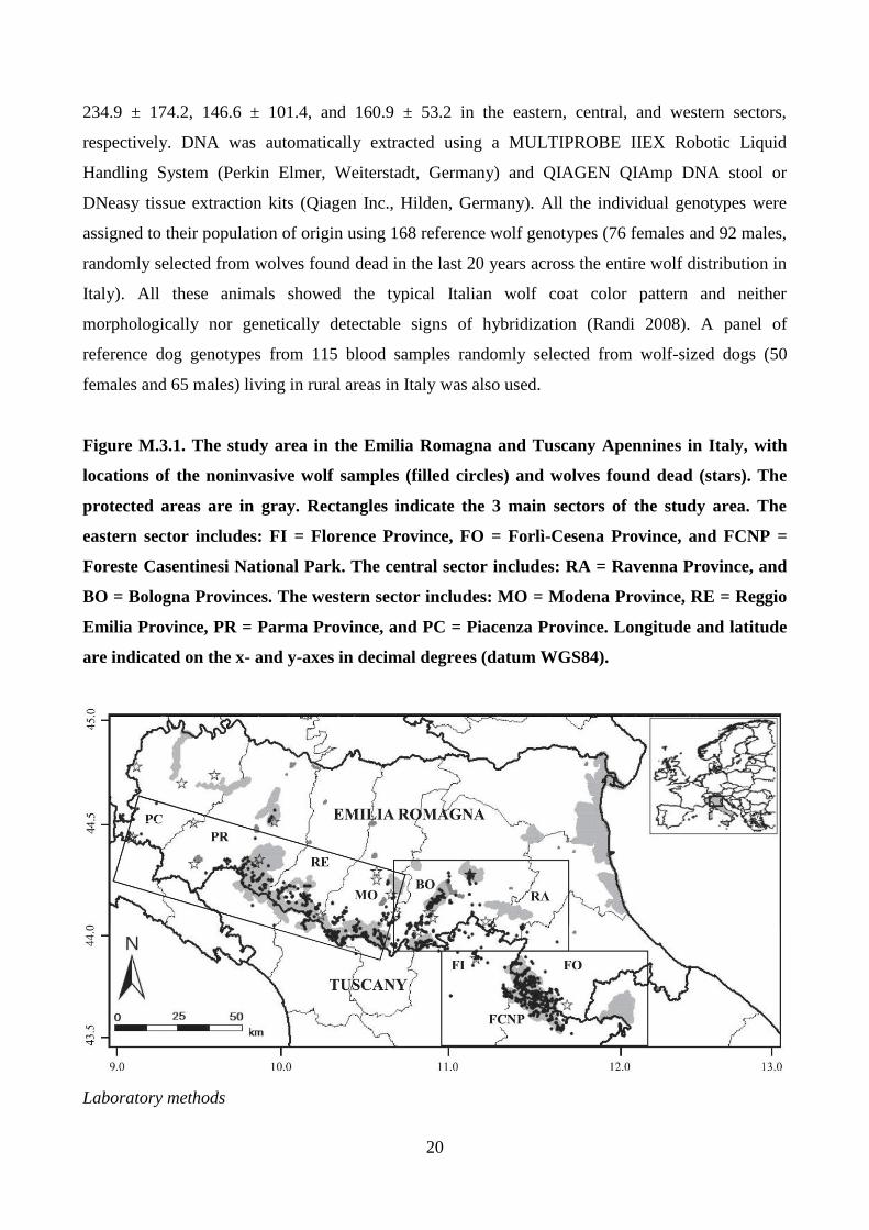
Figure M.3.1. The study area in the Emilia Romagna and Tuscany Apennines in Italy, with

locations of the noninvasive wolf samples (filled circles) and wolves found dead (stars). The

protected areas are in gray. Rectangles indicate the 3 main sectors of the study area. The

eastern sector includes: FI = Florence Province, FO = Forlì-Cesena Province, and FCNP =

Foreste Casentinesi National Park. The central sector includes: RA = Ravenna Province, and

BO = Bologna Provinces. The western sector includes: MO = Modena Province, RE = Reggio

Emilia Province, PR = Parma Province, and PC = Piacenza Province. Longitude and latitude

are indicated on the x- and y-axes in decimal degrees (datum WGS84).

Laboratory methods

21

Individual genotypes for samples were identified at 12 unlinked autosomal canine microsatellites

(short tandem repeats [STR]): 7 dinucleotides (CPH2, CPH4, CPH5, CPH8, CPH12, C09.250, and

C20.253) and 5 tetranucleotides (FH2004, FH2079, FH2088, FH2096, and FH2137), selected for

their high polymorphism and reliable scorability for wolves and dogs. Sex of samples was

determined using a polymerase chain reaction (PCR)–restriction fragment length polymorphism

assay of diagnostic ZFX/ZFY gene sequences (Caniglia et al. 2012, 2013, and references therein).

A panel of 6 STR (FH2004, FH2088, FH2096, and FH2137, CPH2, and CPH8) was used to identify

the genotypes with Hardy–Weinberg probability-of-identity (PID) among unrelated individuals,

PID = 8.2 x 10-6

, and expected fullsiblings, PIDsibs = 7.3 x 10-3

(Mills et al. 2000; Waits et al. 2001)

in the reference Italian wolves.

Another panel of 6 STR (FH2079, CPH4, CPH5, CPH12, C09.250, and C20.253), also selected for

their polymorphism and reliable scorability was used to increase the power of admixture and

kinship analyses, decreasing the PID values to PID = 7.7 x 10-9

and PIDsibs = 3.1 x 10-4

. Maternal

haplotypes were identified by sequencing 350 base pairs of the mitochondrial DNA (mtDNA)

control region, diagnostic for the haplotype W14, which is unique to the Italian wolf population,

using primers L-pro and H350 (Randi et al. 2000). Paternal haplotypes were identified by typing 4

Y-linked microsatellites (Y-STR): MS34A, MS34B, MSY41A, and MS41B (Sundqvist et al. 2001),

characterized by distinct allele frequencies in dogs and wolves (Iacolina et al. 2010).

Autosomal and Y-linked STR loci were amplified in 7 multiplexed primer mixes using the

QIAGEN Multiplex PCR Kit (Qiagen Inc.), a GeneAmp PCR System 9700 Thermal Cycler

(Applied Biosystems, Foster City, California), and the following thermal profile: 94°C for 15 min,

94°C for 30 s, 57°C for 90 s, 72°C for 60 s (40 cycles for scat, urine, and hair samples, and 35

cycles for muscle and blood samples), followed by a final extension step of 72°C for 10 min.

Amplifications were carried out in 10-μl volumes including 2 μl of DNA extraction solutions from

scat, urine, and hair samples, 1 μl from muscle or blood samples (corresponding to approximately

20–40 ng of DNA), 5 μl of QIAGEN Multiplex PCR Kit, 1 μl of QIAGEN Q solution (Qiagen

Inc.), 0.4 μM deoxynucleotide triphosphates, from 0.1 to 0.4 μl of 10 μM primer mix (forward and

reverse), and RNase-free water up to the final volume. The mtDNA control region was amplified in

a 10-μl PCR, including 1 or 2 ll of DNA solution, 0.3 pmol of the primers L-Pro and H350, using

the following thermal profile: 94°C for 2 min, 94°C for 15 s, 55°C for 15 s, 72°C for 30 s (40

cycles), followed by a final extension of 72°C for 5 min. PCR products were purified using

exonuclease/shrimp alkaline phosphatase (Exo-Sap; Amersham, Freiburg, Germany) and sequenced

in both directions using the ABI Big Dye Terminator kit (ABI Biosystems, Foster City, California)

with the following steps: 96°C for 10 s, 55°C for 5 s, and 60°C for 4 min of final extension (25

22

cycles). DNA from scat, urine, and hair samples was extracted, amplified, and genotyped in

separate rooms reserved only to low-template DNA samples, under sterile ultraviolet laminar flood

hoods, following a multiple- tube protocol (Caniglia et al. 2012), including both negative and

positive controls. Genotypes were obtained from blood and muscle DNA, replicating the analyses

twice. DNA sequences and microsatellites were analyzed in a 3130XL ABI automated sequencer

(Applied Biosystems), using the ABI software SEQSCAPE 2.5 for sequences, and GENEMAPPER

4.0 for microsatellites (Applied Biosystems).

Population structure, assignment, and identification of wolf x dog admixed genotypes

Individual genotypes were assigned to their population of origin (wolves or dogs) using

STRUCTURE 2.3.3 (Falush et al. 2003). STRUCTURE was ran with 5 replicates of 104 burn-in

followed by 105 iterations of the Monte Carlo Markov chains, selecting the ‘‘admixture’’ model

(each individual may have ancestry in more than 1 parental population), either assuming

independent or correlated allele frequencies. The optimal number of populations K was identified

using the ΔK procedure (Evanno et al. 2005). At the optimal K the average proportion of

membership (Qi) of the sampled populations (wolves or dogs) was assessed to the inferred clusters.

Genotypes were assigned to the Italian wolf or dog clusters at threshold qi = 95 (individual

proportion of Membership; Randi 2008), or identified them as admixed if their qi values were

intermediate. Putative wolf x dog hybrids were checked further using additional admixture analyses

on observed and simulated genotypes obtained by HYBRIDLAB (Nielsen et al. 2006) and using

diagnostic mtDNA and Y-STR haplotypes.

Genetic variability

Based on the assignment tests, all genotypes were grouped as those of wolves, dogs, or hybrids.

GENALEX 6.1 (Peakall and Smouse 2006) was used to estimate allele frequency by locus and

group, observed (HO) and expected unbiased (HE) heterozygosity, mean (NA) and expected (NE)

number of alleles per locus, number of private alleles, and PID and PIDsibs. The polymorphic

information content (PIC) was calculated using CERVUS 3.0.3 (Kalinowski et al. 2007). Wright’s

inbreeding estimator (FIS; Weir and Cockerham 1984) and departures from Hardy–Weinberg

equilibrium were computed using GENETIX 4.05 (Belkhir et al. 1996; 2004). FIS significance was

assessed using 10,000 random permutations of alleles in each population. The occurrence of null

alleles was tested in MICROCHECKER (Van Oosterhout et al. 2004). Inbreeding coefficient F of

Lynch and Ritland (1999) was estimated using COANCESTRY 1.0 (Wang 2011), with allele

frequencies and PCR error rates assessed from the sampled population and 95% confidence

23

intervals (CIs) generated through 1,000 bootstrapped simulations. The sequential Bonferroni

correction test for multiple comparisons was used to adjust significance levels for every analysis

(Rice 1989). Estimates of variability were express as the mean ± SD.

Identification of packs, pedigrees, and dispersal

All the genotypes that were sampled in restricted ranges (< 100 km2) at least 4 times and for periods

longer than 24 months were selected. Their spatial distributions was determined by 95% kernel

analysis, choosing band width using the least-squares cross-validation method (Seaman et al. 1999;

Kernohan et al. 2001), using the ADEHABITATHR package for R (Calenge 2006) and mapped

them using ARCGIS 10.0. According to spatial overlaps, individuals were split into distinct groups

that might correspond to packs, for which parentage analyses were performed. The complete

genealogy of each group were reconstructed using a maximum-likelihood approach implemented in

COLONY 2.0 (Wang and Santure 2009). For each area, as candidate parents all the individuals

sampled in the 1st year of sampling and more than 4 times in the same area were considered and as

candidate offspring all the individuals collected within the 95% kernel spatial distribution of each

pack and in a surrounding buffer area of approximately 17-km radius from the kernel (see

‘‘Results’’). COLONY was ran with allele frequencies and PCR error rates as estimated from all the

genotypes, assuming a 0.5 probability of including fathers and mothers in the candidate parental

pairs. To be sure that all the possible parentages were detected, the best maximum-likelihood

genealogies was compared to those obtained by an ‘‘open parentage analysis’’ in COLONY, using

all the males and females as candidate parents, and all the wolves sampled in the study area as

candidate offspring. The best maximum-likelihood genealogies reconstructed by COLONY were

compared with those obtained by a likelihood approach in CERVUS, based on the Mendelian

inheritance of the alleles, accepting only parent–offspring combinations with at most one-

twentyfourth allele incompatibilities, and father–son combinations with no incongruities at Y-STR

haplotypes. Parentage assignments were determined in CERVUS using natural log of likelihood

ratio scores for candidate parents, given the set of candidate offspring genotypes and the allele

frequencies in the whole population (when a natural log of likelihood ratio score was positive, the

candidate parent is the most likely true parent (Kalinowski et al. 2007). Simulations to determine

the likelihood of randomly selected parents was also performed. Natural log of likelihood ratio

values that were significant at 95% and 80% thresholds were considered. Natural log of likelihood

ratio scores were generated by simulating 10,000 offspring and 50 candidate males, allowing for

20% of the population to be unsampled, 20% incomplete multilocus genotypes, and the genotyping

error rate as empirically estimated from the data set (vonHoldt et al. 2008). Values of relatedness (r;

24

Queller and Goodnight 1989) were estimated within and among packs using KINGROUP 2.0

(Konovalov et al. 2004) and compared those with values of 1st order (parent–offspring plus full

siblings) and unrelated dyads estimated from 1,000 simulated pairs. A likelihood ratio test was used

with a primary hypothesis of r = 0.25 (half siblings or cousins) and r=0.50 (full-siblings or parent–

offspring) versus a null hypothesis of r = 0.00 (unrelated) to test for inbreeding within and among

packs, at the α = 0.05 level. Locations of individuals in the packs were used in ARCGIS 10.0 to

reconstruct the areas and centroids of the 95% kernel spatial distribution for each pack, and the

distances between centroids; reconstruct the minimum, median, and maximum distance of

genotypes to the pack centroids; and identify dispersing wolves. Individuals sequentially sampled in

different territories (> 17 km apart), or that reproduced in a pack different from their natal one were

identified as putative dispersers. Individuals that were not assigned to a pack and the dispersers that

did not establish in any pack were considered as potential floaters.

Spatial analyses

Fine-scale spatial genetic structure were assessed by multivariate spatial autocorrelation analyses of

geographical and genetic distances in SPAGEDI 1.2 (Hardy and Vekemans 2002) and estimated

through the autocorrelation kinship coefficient Fij (Loiselle et al. 1995), which is similar to Moran’s

I (Smouse and Peakall 1999) but is relatively unbiased even with low sampling variance. Fij was

calculated for distance classes that had been determined based on wolves’ home ranges and

following recommendations of Hardy and Vekemans (2002). Thus, the equal frequency method was

used, which assumes that more than 50% of all individuals were represented at least once in each

spatial interval. The 95% Fij CIs and the nonrandom spatial genetic structure were tested via 10,000

permutations and the effects of behavioral biases (sex-biased dispersal and pack relatedness) were

investigated by computing autocorrelations separately in males, females, and breeding pairs.

Correlations between geographic and genetic distance of individuals and packs were computed after

permuting the locations, similarly to a Mantel test (Mantel 1967). Whenever possible, additional

field information such as snow-tracking, wolf-howling, camera trapping, and occasional direct

observations were used to evaluate the reliability of the inferred pack structure and locations.

25

M.4. Non-invasive genetic sampling to predict species ecological niche and depredation risk

Study area

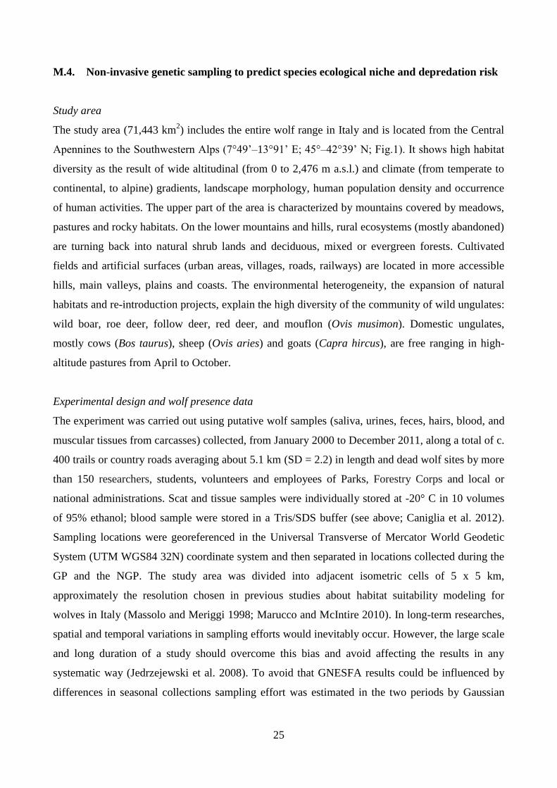
The study area (71,443 km2) includes the entire wolf range in Italy and is located from the Central

Apennines to the Southwestern Alps (7°49’–13°91’ E; 45°–42°39’ N; Fig.1). It shows high habitat

diversity as the result of wide altitudinal (from 0 to 2,476 m a.s.l.) and climate (from temperate to

continental, to alpine) gradients, landscape morphology, human population density and occurrence

of human activities. The upper part of the area is characterized by mountains covered by meadows,

pastures and rocky habitats. On the lower mountains and hills, rural ecosystems (mostly abandoned)

are turning back into natural shrub lands and deciduous, mixed or evergreen forests. Cultivated

fields and artificial surfaces (urban areas, villages, roads, railways) are located in more accessible

hills, main valleys, plains and coasts. The environmental heterogeneity, the expansion of natural

habitats and re-introduction projects, explain the high diversity of the community of wild ungulates:

wild boar, roe deer, follow deer, red deer, and mouflon (Ovis musimon). Domestic ungulates,

mostly cows (Bos taurus), sheep (Ovis aries) and goats (Capra hircus), are free ranging in high-

altitude pastures from April to October.

Experimental design and wolf presence data

The experiment was carried out using putative wolf samples (saliva, urines, feces, hairs, blood, and

muscular tissues from carcasses) collected, from January 2000 to December 2011, along a total of c.

400 trails or country roads averaging about 5.1 km (SD = 2.2) in length and dead wolf sites by more

than 150 researchers, students, volunteers and employees of Parks, Forestry Corps and local or

national administrations. Scat and tissue samples were individually stored at -20° C in 10 volumes

of 95% ethanol; blood sample were stored in a Tris/SDS buffer (see above; Caniglia et al. 2012).

Sampling locations were georeferenced in the Universal Transverse of Mercator World Geodetic

System (UTM WGS84 32N) coordinate system and then separated in locations collected during the

GP and the NGP. The study area was divided into adjacent isometric cells of 5 x 5 km,

approximately the resolution chosen in previous studies about habitat suitability modeling for

wolves in Italy (Massolo and Meriggi 1998; Marucco and McIntire 2010). In long-term researches,

spatial and temporal variations in sampling efforts would inevitably occur. However, the large scale

and long duration of a study should overcome this bias and avoid affecting the results in any

systematic way (Jedrzejewski et al. 2008). To avoid that GNESFA results could be influenced by

differences in seasonal collections sampling effort was estimated in the two periods by Gaussian

26

kernels (Elith et al. 2010). Then, differences in the resulting kernel maps were tested with a

Wilcoxon-signed rank test (Phillips et al. 2006; Rebelo and Jones 2010).

Predictor Variables

For the entire study area, data on ecological, topographic, trophic and anthropogenic features were

collected (Table M.4.1). Habitat diversity (Shannon Diversity Index) and land cover types were

obtained from the Coordination of Information on the Environment (CORINE Land Cover 2006, IV

Level; http://www.sinanet.isprambiente.it), the European land cover database. Topographic

variables were obtained from a Digital Elevation Model of Italy with a spatial resolution of 20 m

(http://www.sinanet.isprambiente.it). From this, aspect, slope and roughness were derived (rugged

terrain, topographically uneven, broken, or rocky and steep). Prey species availability and

abundance are the main food resources and affect the distribution of wolves. In the analysis the

abundance of wild ungulate prey over the study area was included (Carnevali et al. 2009) and the

Shannon diversity index for wild prey was calculated, since the occurrence of more than one species

influences the wolf habitat suitability (Massolo and Meriggi 1998, Ciucci et al. 2003). The

abundance and Shannon diversity Index of domestic prey was derived from the Agricultural Italian

Census (http://censimentoagricoltura.istat.it). As human factors, the presence and distance form

artificial surfaces, as well as the human and hunter densities were considered (http://dati.istat.it). All

variables were re-sampled to a resolution (5,000 m cell size) using ArcGIS 10 (ESRI, Redlands,

California).

27

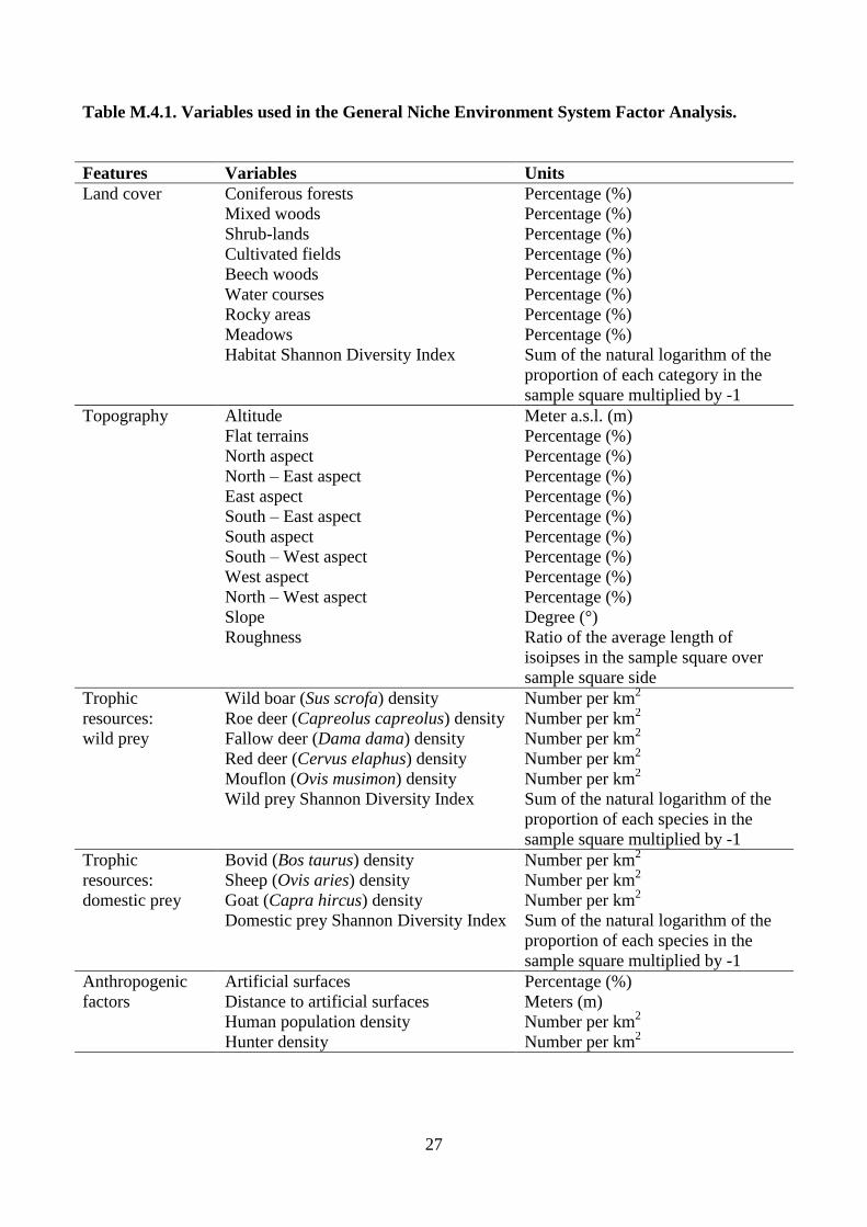
Table M.4.1. Variables used in the General Niche Environment System Factor Analysis.

Features Variables Units

Land cover Coniferous forests Percentage (%)

Mixed woods Percentage (%)

Shrub-lands Percentage (%)

Cultivated fields Percentage (%)

Beech woods Percentage (%)

Water courses Percentage (%)

Rocky areas Percentage (%)

Meadows Percentage (%)

Habitat Shannon Diversity Index Sum of the natural logarithm of the

proportion of each category in the

sample square multiplied by -1

Topography Altitude Meter a.s.l. (m)

Flat terrains Percentage (%)

North aspect Percentage (%)

North – East aspect Percentage (%)

East aspect Percentage (%)

South – East aspect Percentage (%)

South aspect Percentage (%)

South – West aspect Percentage (%)

West aspect Percentage (%)

North – West aspect Percentage (%)

Slope Degree (°)

Roughness Ratio of the average length of

isoipses in the sample square over

sample square side

Trophic

resources:

wild prey

Wild boar (Sus scrofa) density Number per km2

Roe deer (Capreolus capreolus) density Number per km2

Fallow deer (Dama dama) density Number per km2

Red deer (Cervus elaphus) density Number per km2

Mouflon (Ovis musimon) density Number per km2

Wild prey Shannon Diversity Index Sum of the natural logarithm of the

proportion of each species in the

sample square multiplied by -1

Trophic

resources:

domestic prey

Bovid (Bos taurus) density Number per km2

Sheep (Ovis aries) density Number per km2

Goat (Capra hircus) density Number per km2

Domestic prey Shannon Diversity Index Sum of the natural logarithm of the

proportion of each species in the

sample square multiplied by -1

Anthropogenic

factors

Artificial surfaces Percentage (%)

Distance to artificial surfaces Meters (m)

Human population density Number per km2

Hunter density Number per km2

28

Modeling methods

Wolf samples were genotyped following the methods showed in M.3 (Caniglia et al. 2014). The

locations of genotyped wolf samples were used to rank each cell as ‘used’ if at least one wolf

genotype was sampled within its boundary. Used and available sites were compared (all the cells of

the study area) through a niche-based approach, GNESFA. It identified the relations between the

availability and utilization distributions with several advantages: it doesn’t rely on any population

structure hypotheses (autocorrelation), it extracts non-correlated components, it is especially suited

to analyse presence-only data and compute habitat suitability maps (Basille 2008). Two measures of

the species ecological niche are provided: the marginality (the direction in which the species differs

from the average conditions of the whole area) and the specialization (the ratio between the

variance of available conditions and the variance of conditions used by the species; Hirzel et al.

2001; Basille 2008). GNESFA encompasses three complementary analyses: the Factor Analysis of

the Niche Taking the Environmental as the Reference (FANTER; Calenge and Basille 2008); the

Mahalanobis Distance Factor Analysis (MADIFA; Calenge et al. 2008); the Ecological Niche

Factor Analysis (ENFA; Hirzel et al. 2001). The FANTER is centered on the availability

distribution and identifies the variables affecting the shape, the central tendency and the spread of

the niche relative to the environment considered, showing how the niche in the ecological space

differs from the study area; both the first and the last components in the analysis were considered

because the formers explained the marginality, whereas the latters the specialization (Calenge and

Basille 2008). The MADIFA is centered on the utilization distributions and determines whether the

environment is similar to that occupied by the species; the more similar the conditions in a location

are to the centroid of the ecological niche (the optimum of the species), the smaller is the

Mahalanobis distance (D2) and the more suitable the habitat is at that location (Calenge et al. 2008;

Knegt et al. 2011). The mean D2 over the available area was used as a measure of habitat selectivity

regarding independent variables and the relationship between D2 and the range considered was

analyzed. MADIFA combines marginality and specialization into a single measure of habitat

selection (Calenge and Basille 2008). Finally, the ENFA is centered both on the utilization and the

availability distribution (Calenge and Basille 2008); marginality is fully explained by the first

factor, while specialization by the others. For further details, see Calenge and Basille (2008).

Wolf potential distribution, model validation and predation risk

Wolf locations were bootstrapped with replacement 1,000 times a season to obtain potential

distribution maps estimated by MADIFA, the best method in the GNESFA framework to compute

appropriate suitability maps (Calenge et al. 2008). To provide an assessment of MADIFA’s power,

29

the predicted values were compared with the real ones through the use of (i) Receiver Operator

Characteristics (ROC) curves (Fawcett 2004; Ko et al. 2011), (ii) correct classification rate (CCR;

Ahmadi et al. 2013), (iii) Cohen’s kappa (k) (Manel et al. 2001) and (iv) the Boyce’ Index (B)

(Boyce et al. 2002; Jones-Farrand et al. 2011). Combining MADIFA’s predictions, the wolf average

(± SD) potential distributions was calculated. Assuming that an increase in wolf suitability

corresponds to an increase in depredation risk (Kaartinen et al. 2009; Marucco and McIntire 2010),

the risk probability of pastures was estimated by calculating the probability of wolf presence during

the GP in all meadows available for livestock breeding.

The statistical analyses presented here were computed in the open-source software R

(http://www.R-project.org/).

30

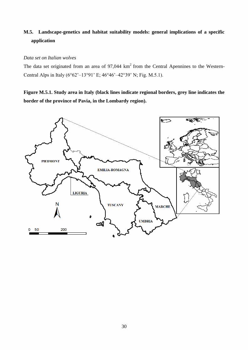
M.5. Landscape-genetics and habitat suitability models: general implications of a specific

application

Data set on Italian wolves

The data set originated from an area of 97,044 km2

from the Central Apennines to the Western-

Central Alps in Italy (6°62’–13°91’ E; 46°46’–42°39’ N; Fig. M.5.1).

Figure M.5.1. Study area in Italy (black lines indicate regional borders, grey line indicates the

border of the province of Pavia, in the Lombardy region).

31

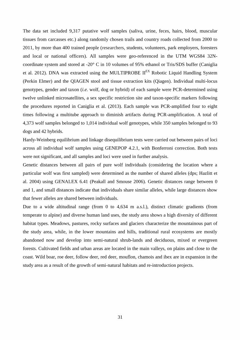
The data set included 9,317 putative wolf samples (saliva, urine, feces, hairs, blood, muscular

tissues from carcasses etc.) along randomly chosen trails and country roads collected from 2000 to

2011, by more than 400 trained people (researchers, students, volunteers, park employers, foresters

and local or national officers). All samples were geo-referenced in the UTM WGS84 32N-

coordinate system and stored at -20° C in 10 volumes of 95% ethanol or Tris/SDS buffer (Caniglia

et al. 2012). DNA was extracted using the MULTIPROBE IIEX

Robotic Liquid Handling System

(Perkin Elmer) and the QIAGEN stool and tissue extraction kits (Qiagen). Individual multi-locus

genotypes, gender and taxon (i.e. wolf, dog or hybrid) of each sample were PCR-determined using

twelve unlinked microsatellites, a sex specific restriction site and taxon-specific markers following

the procedures reported in Caniglia et al. (2013). Each sample was PCR-amplified four to eight

times following a multitube approach to diminish artifacts during PCR-amplification. A total of

4,373 wolf samples belonged to 1,014 individual wolf genotypes, while 350 samples belonged to 93

dogs and 42 hybrids.

Hardy-Weinberg equilibrium and linkage disequilibrium tests were carried out between pairs of loci

across all individual wolf samples using GENEPOP 4.2.1, with Bonferroni correction. Both tests

were not significant, and all samples and loci were used in further analysis.

Genetic distances between all pairs of pure wolf individuals (considering the location where a

particular wolf was first sampled) were determined as the number of shared alleles (dps; Hazlitt et

al. 2004) using GENALEX 6.41 (Peakall and Smouse 2006). Genetic distances range between 0

and 1, and small distances indicate that individuals share similar alleles, while large distances show

that fewer alleles are shared between individuals.

Due to a wide altitudinal range (from 0 to 4,634 m a.s.l.), distinct climatic gradients (from

temperate to alpine) and diverse human land uses, the study area shows a high diversity of different

habitat types. Meadows, pastures, rocky surfaces and glaciers characterize the mountainous part of

the study area, while, in the lower mountains and hills, traditional rural ecosystems are mostly

abandoned now and develop into semi-natural shrub-lands and deciduous, mixed or evergreen

forests. Cultivated fields and urban areas are located in the main valleys, on plains and close to the

coast. Wild boar, roe deer, follow deer, red deer, mouflon, chamois and ibex are in expansion in the

study area as a result of the growth of semi-natural habitats and re-introduction projects.

32

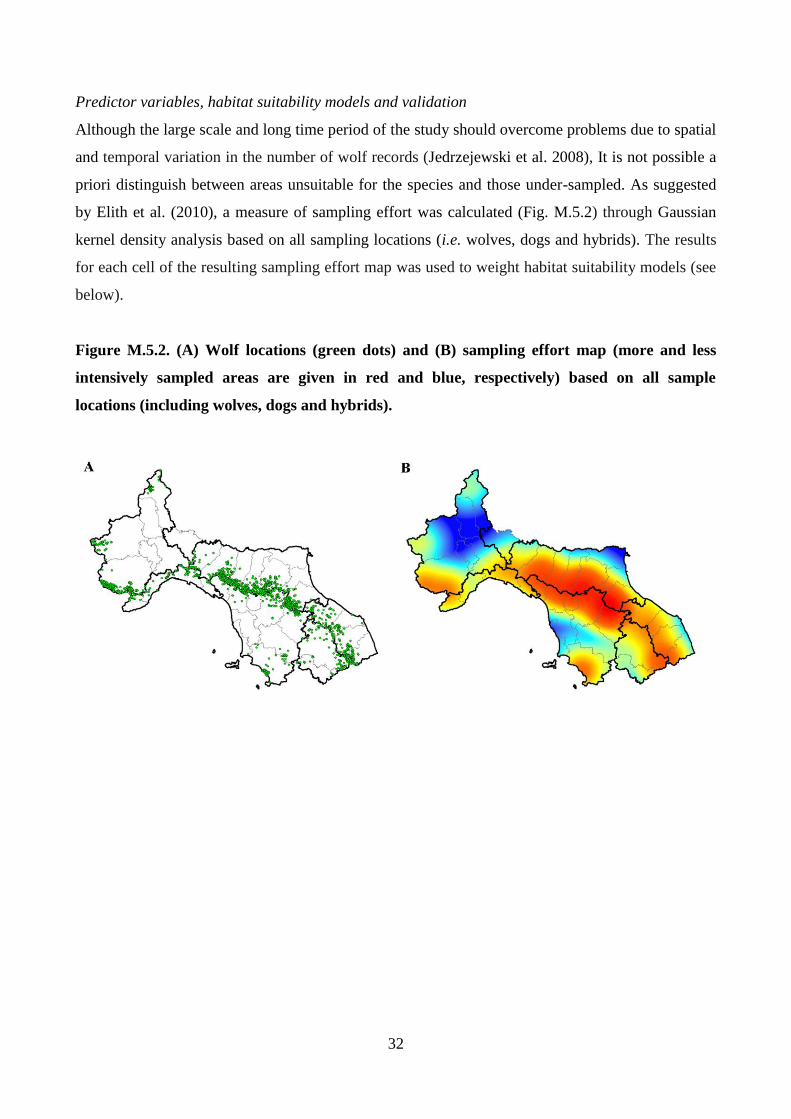
Predictor variables, habitat suitability models and validation

Although the large scale and long time period of the study should overcome problems due to spatial

and temporal variation in the number of wolf records (Jedrzejewski et al. 2008), It is not possible a

priori distinguish between areas unsuitable for the species and those under-sampled. As suggested

by Elith et al. (2010), a measure of sampling effort was calculated (Fig. M.5.2) through Gaussian

kernel density analysis based on all sampling locations (i.e. wolves, dogs and hybrids). The results

for each cell of the resulting sampling effort map was used to weight habitat suitability models (see

below).

Figure M.5.2. (A) Wolf locations (green dots) and (B) sampling effort map (more and less

intensively sampled areas are given in red and blue, respectively) based on all sample

locations (including wolves, dogs and hybrids).

33

Data on ecological, topographic, prey and anthropogenic features of the study area were collected.

CORINE Land cover level IV (European Environment Agency 2006) provided information on

habitat diversity and land cover types in the study area (Table M.4.1). Topographic variables,

namely altitude, aspect, slope and landscape roughness were obtained from a digital elevation

model of Italy with a spatial resolution of 20 m (Table M.4.1). As prey resources play an important

role in predator distribution (Jedrzejewski et al. 2008; Milanesi et al. submitted), also the abundance

of wild ungulates obtained from the Italian wild ungulates’ database was included (Carnevali et al.

2009). The Shannon diversity index of wild prey was calculated, since more than one prey species

influences habitat suitability for wolves (Ciucci et al. 2003). Moreover, the presence and distance

from artificial elements (i.e. urban areas, villages, roads, railways) as well as human and hunter

densities was considered (Table M.4.1).

Marucco and McIntire (2010) defined the average distance a wolf moves per dispersal time step of

1,000 m. This value was used as grid cell size for the analysis but, since spatial scale can affect

landscape analysis (Cushman 2006; Wasserman et al. 2010; Keller et al. 2013; Mateo Sanchez et al.

2013), additionally grid sizes of 500 m and 2,000 m were considered to investigate the effects of

grid cell size on habitat suitability and landscape genetic analysis. All variables were re-sampled to

focus resolution in ARCGIS 10 (ESRI). All wolf sampling locations (including relocations) were

employed to classify each cell as either "used", if at least one wolf genotype was sampled within its

boundaries or "available" otherwise. The ten currently most widely used habitat suitability methods

were chosen. Five different machine learning methods, namely classification tree analysis (CTA;

Breiman et al. 1984), boosted regression trees (BRT; Friedman et al. 2001), random forest (RF;

Breiman 2001), maximum entropy (MAXENT; Phillips et al. 2006) and artificial neural network

(ANN; Ripley 2007), three regression models, i.e. generalized linear models (GLM; McCullagh and

Nelder 1989), generalized additive models (GAM; Hastie and Tibshirani 1990) and multiple

adaptive regression splines (MARS; Friedman 1991), a factor analysis, i.e, factorial decomposition

of Mahalanobis distances (MADIFA; Calenge et al. 2008), and flexible discriminant analysis

(FDA; Hastie et al. 1994) were applied.

Sampling effort map values per cell (see above) were used as weights in MADIFA, as a bias grid in

MAXENT and as case weights in all the other methods. Habitat suitability values range between 0

and 1, and a threshold value of 0.5 (Bailey et al. 2002) was considered to discriminate between

areas suitable and unsuitable for wolves.

With the fractal dimension index (McGarigal et al. 2002), it was verified whether resolution (i.e.

500 m, 1,000 m and 2,000 m; see above) affected habitat suitability models. To provide an

assessment of model efficiency, the probability values of wolf occurrence predicted by habitat

34

suitability models with the original ones were compared by the use of (i) receiver operator

characteristics curves (ROC; Fawcett 2004; Ko et al. 2011), (ii) Cohen’s kappa (k; Manel et al.

2001) and (iii) Boyce’ index (Boyce et al. 2002; Jones-Farrand et al. 2011). ROC varies from 0

(worse than a random model, 0.5) to 1 (perfect model), K and Boyce’ index vary from −1 to 1

(positive values indicate predictions consistent with the evaluation dataset, zero indicates that the

model is similar to a random model and negative values indicate incorrect models; Hirzel et al.

2006). A random subsample of 50% of all wolf locations was used to calibrate models and the

remnant 50% to validate them.

Resistance surfaces and least coast paths

Habitat suitability values generated by each of the ten above methods were converted into resistance

to movement values. Resistances were calculated as 1 – habitat suitability per cell (Wang et al.

2008; Pullinger and Johnson, 2010; Spear et al. 2010). Higher resistance values indicate higher

costs to animal movement, while lower values represent lower cost levels. LCP analysis was carried

out based on resistance surfaces on the location where wolves had been firstly sampled. The length

of each LCP was calculated between all pairs of wolves and used it as a measure of ecological

distance. In addition, a buffer of 5,000 m around each path was considered (because 10,000 m is

approximately the square root of the average home range size of a wolf pack; Caniglia et al. in

press) to evaluate the efficiency of LCPs as ecological corridors. For this aim, wolf relocations (N =

3,359) was used and the validation methods described further above. Finally, straight-line Euclidean

distances were generated among each pair of wolves.

Landscape genetic analysis

The effect of isolation by resistance was investigated by assessing the relationship between genetic

and ecological distances using three statistical procedures currently used in landscape genetics: (i)

partial Mantel tests (Legendre 2000); (ii) multiple regression on distance matrices (MRDM;

Legendre and Fortin 2010; Keller et al. 2013) and (iii) linear mixed effect models (Selkoe et al.

2010). 10,000 permutations were used to assess significance. Euclidean distances were included as

an independent matrix in MRDM and linear effect models while, in partial Mantel tests, they were

used as a second explanatory matrix. In linear mixed effect models, also a Toeplitz covariance

matrix was considered (Selkoe et al. 2010). The efficiency of the ten different habitat suitability

models to explain genetic distances was evaluated based on R2-values and partial regression

coefficients β in MRDM and linear mixed effect models and as r-values in partial Mantel tests. R2

values from MRDM, linear effect models and partial Mantel tests cannot be directly compared to

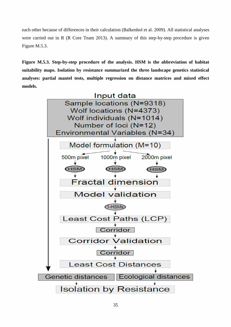
35

each other because of differences in their calculation (Balkenhol et al. 2009). All statistical analyses

were carried out in R (R Core Team 2013). A summary of this step-by-step procedure is given

Figure M.5.3.

Figure M.5.3. Step-by-step procedure of the analysis. HSM is the abbreviation of habitat

suitability maps. Isolation by resistance summarized the three landscape genetics statistical

analyses: partial mantel tests, multiple regression on distance matrices and mixed effect

models.

36

RESULTS

R.1. Changes of wolf diet in Italy in relation to the increase of wild ungulate abundance

Differences among geographic areas

Twenty studies on the wolf diet in Italy were analysed for a total of 28 different study areas, 4 of

them carried out in the western Alps, 9 in northern Apennines, and 7 in South-central Apennines

(Table R.1.1).

Wolf diet was significantly different among geographic areas both considering food categories (F =

7.16, P = 0.0002), and the species of wild ungulate prey (F = 7.08, P < 0.0001). Considering food

categories, pairwise comparisons showed significant differences between South-central and

northern Apennines (P = 0.001) and between South-central Apennines and western Alps (P =

0.003), instead considering wild ungulate species significant differences resulted for all

comparisons (P ≤ 0.0005 in all cases). Conversely, diet breadth was not significantly different

among geographic areas (H = 0.77, df = 2, P = 0.679).

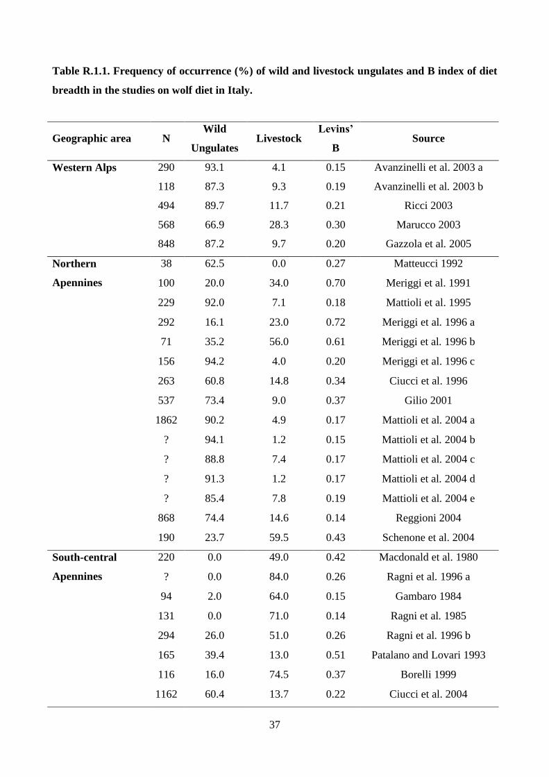
37

Table R.1.1. Frequency of occurrence (%) of wild and livestock ungulates and B index of diet

breadth in the studies on wolf diet in Italy.

Geographic area N Wild

Ungulates Livestock

Levins’

B Source

Western Alps 290 93.1 4.1 0.15 Avanzinelli et al. 2003 a

118 87.3 9.3 0.19 Avanzinelli et al. 2003 b

494 89.7 11.7 0.21 Ricci 2003

568 66.9 28.3 0.30 Marucco 2003

848 87.2 9.7 0.20 Gazzola et al. 2005

Northern

Apennines

38 62.5 0.0 0.27 Matteucci 1992

100 20.0 34.0 0.70 Meriggi et al. 1991

229 92.0 7.1 0.18 Mattioli et al. 1995

292 16.1 23.0 0.72 Meriggi et al. 1996 a

71 35.2 56.0 0.61 Meriggi et al. 1996 b

156 94.2 4.0 0.20 Meriggi et al. 1996 c

263 60.8 14.8 0.34 Ciucci et al. 1996

537 73.4 9.0 0.37 Gilio 2001

1862 90.2 4.9 0.17 Mattioli et al. 2004 a

? 94.1 1.2 0.15 Mattioli et al. 2004 b

? 88.8 7.4 0.17 Mattioli et al. 2004 c

? 91.3 1.2 0.17 Mattioli et al. 2004 d

? 85.4 7.8 0.19 Mattioli et al. 2004 e

868 74.4 14.6 0.14 Reggioni 2004

190 23.7 59.5 0.43 Schenone et al. 2004

South-central

Apennines

220 0.0 49.0 0.42 Macdonald et al. 1980

? 0.0 84.0 0.26 Ragni et al. 1996 a

94 2.0 64.0 0.15 Gambaro 1984

131 0.0 71.0 0.14 Ragni et al. 1985

294 26.0 51.0 0.26 Ragni et al. 1996 b

165 39.4 13.0 0.51 Patalano and Lovari 1993

116 16.0 74.5 0.37 Borelli 1999

1162 60.4 13.7 0.22 Ciucci et al. 2004

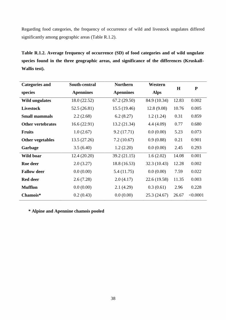
38

Regarding food categories, the frequency of occurrence of wild and livestock ungulates differed

significantly among geographic areas (Table R.1.2).

Table R.1.2. Average frequency of occurrence (SD) of food categories and of wild ungulate

species found in the three geographic areas, and significance of the differences (Kruskall-

Wallis test).

Categories and

species

South-central

Apennines

Northern

Apennines

Western

Alps H P

Wild ungulates 18.0 (22.52) 67.2 (29.50) 84.9 (10.34) 12.83 0.002

Livestock 52.5 (26.81) 15.5 (19.46) 12.8 (9.08) 10.76 0.005

Small mammals 2.2 (2.68) 6.2 (8.27) 1.2 (1.24) 0.31 0.859

Other vertebrates 16.6 (22.91) 13.2 (21.34) 4.4 (4.09) 0.77 0.680

Fruits 1.0 (2.67) 9.2 (17.71) 0.0 (0.00) 5.23 0.073

Other vegetables 13.5 (27.26) 7.2 (10.67) 0.9 (0.88) 0.21 0.901

Garbage 3.5 (6.40) 1.2 (2.20) 0.0 (0.00) 2.45 0.293

Wild boar 12.4 (20.20) 39.2 (21.15) 1.6 (2.02) 14.08 0.001

Roe deer 2.0 (3.27) 18.8 (16.53) 32.3 (10.43) 12.28 0.002

Fallow deer 0.0 (0.00) 5.4 (11.75) 0.0 (0.00) 7.59 0.022

Red deer 2.6 (7.28) 2.0 (4.17) 22.6 (19.58) 11.35 0.003

Mufflon 0.0 (0.00) 2.1 (4.29) 0.3 (0.61) 2.96 0.228

Chamois* 0.2 (0.43) 0.0 (0.00) 25.3 (24.67) 26.67 <0.0001

* Alpine and Apennine chamois pooled

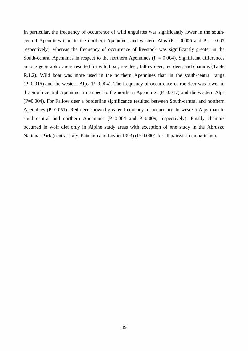
39

In particular, the frequency of occurrence of wild ungulates was significantly lower in the south-

central Apennines than in the northern Apennines and western Alps (P = 0.005 and P = 0.007

respectively), whereas the frequency of occurrence of livestock was significantly greater in the

South-central Apennines in respect to the northern Apennines (P = 0.004). Significant differences

among geographic areas resulted for wild boar, roe deer, fallow deer, red deer, and chamois (Table

R.1.2). Wild boar was more used in the northern Apennines than in the south-central range

(P=0.016) and the western Alps (P=0.004). The frequency of occurrence of roe deer was lower in

the South-central Apennines in respect to the northern Apennines (P=0.017) and the western Alps

(P=0.004). For Fallow deer a borderline significance resulted between South-central and northern

Apennines (P=0.051). Red deer showed greater frequency of occurrence in western Alps than in

south-central and northern Apennines (P=0.004 and P=0.009, respectively). Finally chamois

occurred in wolf diet only in Alpine study areas with exception of one study in the Abruzzo

National Park (central Italy, Patalano and Lovari 1993) (P<0.0001 for all pairwise comparisons).

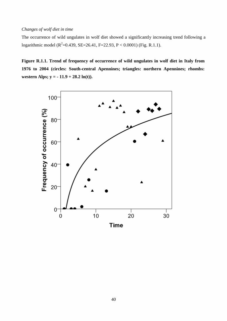
40

Changes of wolf diet in time

The occurrence of wild ungulates in wolf diet showed a significantly increasing trend following a

logarithmic model (R2=0.439, SE=26.41, F=22.93, P < 0.0001) (Fig. R.1.1).

Figure R.1.1. Trend of frequency of occurrence of wild ungulates in wolf diet in Italy from

1976 to 2004 (circles: South-central Apennines; triangles: northern Apennines; rhombs:

western Alps; y = - 11.9 + 28.2 ln(t)).

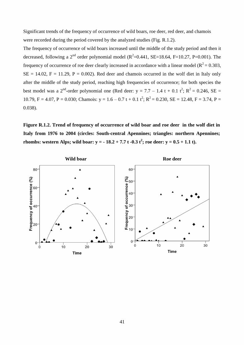
41

Significant trends of the frequency of occurrence of wild boars, roe deer, red deer, and chamois

were recorded during the period covered by the analyzed studies (Fig. R.1.2).

The frequency of occurrence of wild boars increased until the middle of the study period and then it

decreased, following a 2nd

order polynomial model (R2=0.441, SE=18.64, F=10.27, P=0.001). The

frequency of occurrence of roe deer clearly increased in accordance with a linear model (R2

= 0.303,

SE = 14.02, F = 11.29, P = 0.002). Red deer and chamois occurred in the wolf diet in Italy only

after the middle of the study period, reaching high frequencies of occurrence; for both species the

best model was a 2nd

-order polynomial one (Red deer: y = 7.7 – 1.4 t + 0.1 t2; R

2 = 0.246, SE =

10.79, F = 4.07, P = 0.030; Chamois: y = 1.6 – 0.7 t + 0.1 t2; R

2 = 0.230, SE = 12.48, F = 3.74, P =

0.038).

Figure R.1.2. Trend of frequency of occurrence of wild boar and roe deer in the wolf diet in

Italy from 1976 to 2004 (circles: South-central Apennines; triangles: northern Apennines;

rhombs: western Alps; wild boar: y = - 18.2 + 7.7 t -0.3 t2; roe deer: y = 0.5 + 1.1 t).

Wild boar Roe deer

42

Both for the frequency of occurrence of livestock and for diet breadth negative and significant

relationships with the frequency of occurrence of wild ungulates were found; in particular for

livestock the best model was a linear one (R2

= 0.756, SE = 12.88, F = 87.93, P < 0.0001), whereas

for diet breadth a 2nd

-order polynomial model was selected (R2

= 0.421, SE = 0.13, F = 10.83, P <

0.0001). In accordance with this model the B index increased until intermediate values of the

frequency of occurrence of wild ungulates and then decreased (Figg. R.1.3 and R.1.4).

Figure R.1.3. Relationship between frequency of occurrence of livestock and wild ungulates in

wolf diet in Italy (y = 62.2 – 0.7 x).

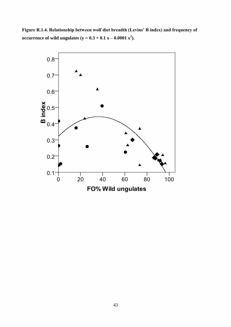
43

Figure R.1.4. Relationship between wolf diet breadth (Levins’ B index) and frequency of

occurrence of wild ungulates (y = 0.3 + 0.1 x – 0.0001 x2).

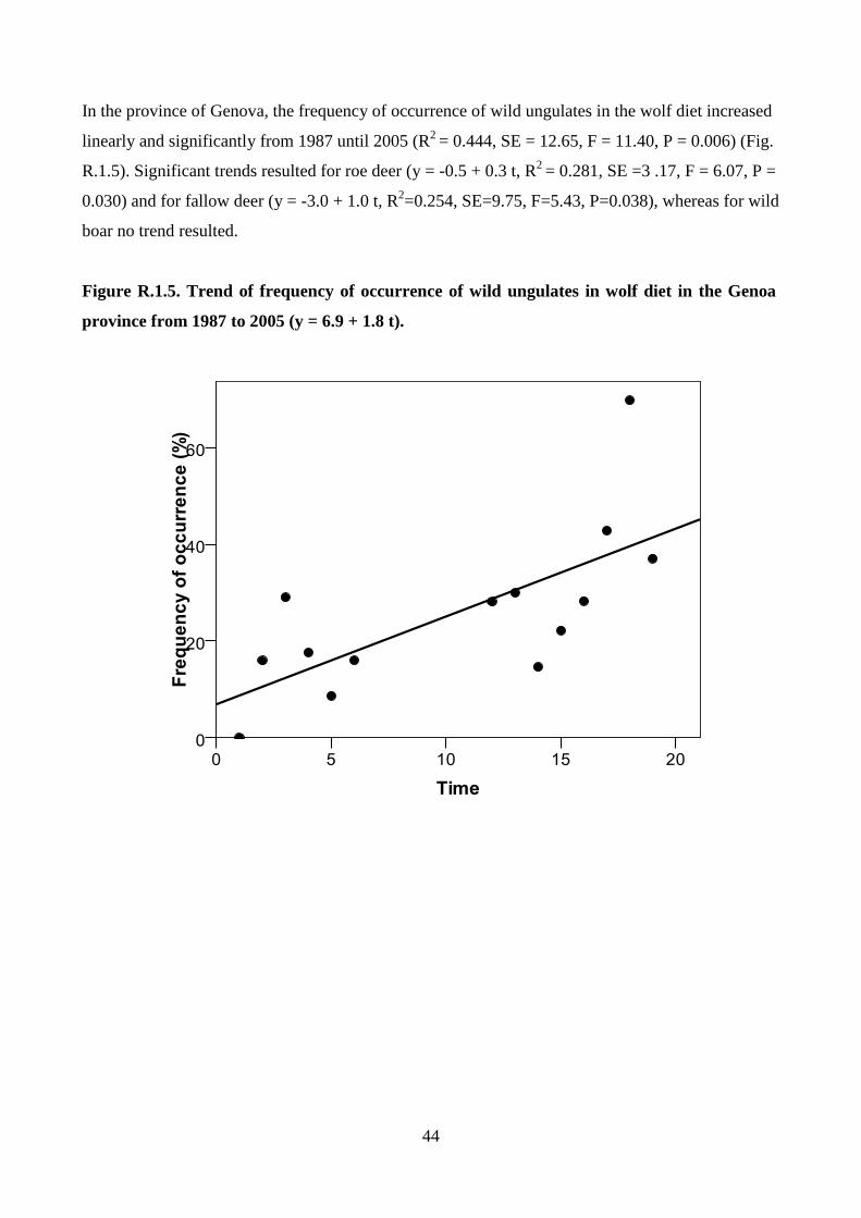
44

In the province of Genova, the frequency of occurrence of wild ungulates in the wolf diet increased

linearly and significantly from 1987 until 2005 (R2

= 0.444, SE = 12.65, F = 11.40, P = 0.006) (Fig.

R.1.5). Significant trends resulted for roe deer (y = -0.5 + 0.3 t, R2

= 0.281, SE =3 .17, F = 6.07, P =

0.030) and for fallow deer (y = -3.0 + 1.0 t, R2=0.254, SE=9.75, F=5.43, P=0.038), whereas for wild

boar no trend resulted.

Figure R.1.5. Trend of frequency of occurrence of wild ungulates in wolf diet in the Genoa

province from 1987 to 2005 (y = 6.9 + 1.8 t).

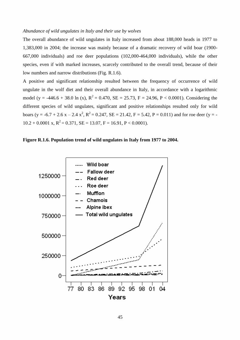
45

Abundance of wild ungulates in Italy and their use by wolves

The overall abundance of wild ungulates in Italy increased from about 188,000 heads in 1977 to

1,383,000 in 2004; the increase was mainly because of a dramatic recovery of wild boar (1900-

667,000 individuals) and roe deer populations (102,000-464,000 individuals), while the other

species, even if with marked increases, scarcely contributed to the overall trend, because of their

low numbers and narrow distributions (Fig. R.1.6).

A positive and significant relationship resulted between the frequency of occurrence of wild

ungulate in the wolf diet and their overall abundance in Italy, in accordance with a logarithmic

model (y = -446.6 + 38.0 ln (x), R2

= 0.470, SE = 25.73, F = 24.96, P < 0.0001). Considering the

different species of wild ungulates, significant and positive relationships resulted only for wild

boars (y = -6.7 + 2.6 x – 2.4 x2, R

2 = 0.247, SE = 21.42, F = 5.42, P = 0.011) and for roe deer (y = -

10.2 + 0.0001 x, R2

= 0.371, SE = 13.07, F = 16.91, P < 0.0001).

Figure R.1.6. Population trend of wild ungulates in Italy from 1977 to 2004.

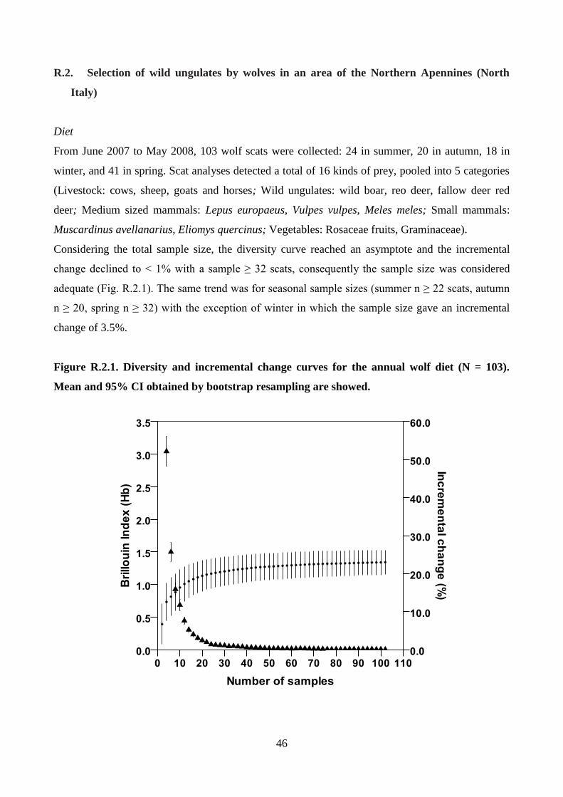
46

R.2. Selection of wild ungulates by wolves in an area of the Northern Apennines (North

Italy)

Diet

From June 2007 to May 2008, 103 wolf scats were collected: 24 in summer, 20 in autumn, 18 in

winter, and 41 in spring. Scat analyses detected a total of 16 kinds of prey, pooled into 5 categories

(Livestock: cows, sheep, goats and horses; Wild ungulates: wild boar, reo deer, fallow deer red

deer; Medium sized mammals: Lepus europaeus, Vulpes vulpes, Meles meles; Small mammals:

Muscardinus avellanarius, Eliomys quercinus; Vegetables: Rosaceae fruits, Graminaceae).

Considering the total sample size, the diversity curve reached an asymptote and the incremental

change declined to < 1% with a sample ≥ 32 scats, consequently the sample size was considered

adequate (Fig. R.2.1). The same trend was for seasonal sample sizes (summer n ≥ 22 scats, autumn

n ≥ 20, spring n ≥ 32) with the exception of winter in which the sample size gave an incremental

change of 3.5%.

Figure R.2.1. Diversity and incremental change curves for the annual wolf diet (N = 103).

Mean and 95% CI obtained by bootstrap resampling are showed.

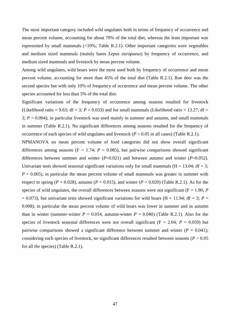
47

The most important category included wild ungulates both in terms of frequency of occurrence and

mean percent volume, accounting for about 70% of the total diet, whereas the least important was

represented by small mammals (<10%; Table R.2.1). Other important categories were vegetables

and medium sized mammals (mainly hares Lepus europaeus) by frequency of occurrence, and

medium sized mammals and livestock by mean percent volume.

Among wild ungulates, wild boars were the most used both by frequency of occurrence and mean

percent volume, accounting for more than 45% of the total diet (Table R.2.1). Roe deer was the

second species but with only 10% of frequency of occurrence and mean percent volume. The other

species accounted for less than 5% of the total diet.

Significant variations of the frequency of occurrence among seasons resulted for livestock

(Likelihood ratio = 9.63; df = 3; P = 0.033) and for small mammals (Likelihood ratio = 13.27; df =

3; P = 0.004); in particular livestock was used mainly in summer and autumn, and small mammals

in summer (Table R.2.1). No significant differences among seasons resulted for the frequency of

occurrence of each species of wild ungulates and livestock (P > 0.05 in all cases) (Table R.2.1).

NPMANOVA on mean percent volume of food categories did not show overall significant

differences among seasons (F = 1.74; P = 0.085), but pairwise comparisons showed significant

differences between summer and winter (P=0.021) and between autumn and winter (P=0.052).

Univariate tests showed seasonal significant variations only for small mammals (H = 13.04; df = 3;

P = 0.005), in particular the mean percent volume of small mammals was greater in summer with

respect to spring (P = 0.028), autumn (P = 0.015), and winter (P = 0.020) (Table R.2.1). As for the

species of wild ungulates, the overall differences between seasons were not significant (F = 1.90; P

= 0.073), but univariate tests showed significant variations for wild boars (H = 11.94; df = 3; P =

0.008); in particular the mean percent volume of wild boars was lower in summer and in autumn

than in winter (summer-winter P = 0.014, autumn-winter P = 0.040) (Table R.2.1). Also for the

species of livestock seasonal differences were not overall significant (F = 2.04; P = 0.059) but

pairwise comparisons showed a significant difference between summer and winter (P = 0.041);

considering each species of livestock, no significant differences resulted between seasons (P > 0.05

for all the species) (Table R.2.1).

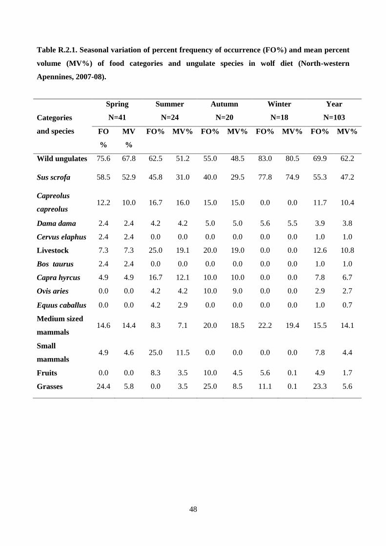
48

Table R.2.1. Seasonal variation of percent frequency of occurrence (FO%) and mean percent

volume (MV%) of food categories and ungulate species in wolf diet (North-western

Apennines, 2007-08).

Categories

and species

Spring

N=41

Summer

N=24

Autumn

N=20

Winter

N=18

Year

N=103

FO

%

MV

%

FO% MV% FO% MV% FO% MV% FO% MV%

Wild ungulates 75.6 67.8 62.5 51.2 55.0 48.5 83.0 80.5 69.9 62.2

Sus scrofa 58.5 52.9 45.8 31.0 40.0 29.5 77.8 74.9 55.3 47.2

Capreolus

capreolus 12.2 10.0 16.7 16.0 15.0 15.0 0.0 0.0 11.7 10.4

Dama dama 2.4 2.4 4.2 4.2 5.0 5.0 5.6 5.5 3.9 3.8

Cervus elaphus 2.4 2.4 0.0 0.0 0.0 0.0 0.0 0.0 1.0 1.0

Livestock 7.3 7.3 25.0 19.1 20.0 19.0 0.0 0.0 12.6 10.8

Bos taurus 2.4 2.4 0.0 0.0 0.0 0.0 0.0 0.0 1.0 1.0

Capra hyrcus 4.9 4.9 16.7 12.1 10.0 10.0 0.0 0.0 7.8 6.7

Ovis aries 0.0 0.0 4.2 4.2 10.0 9.0 0.0 0.0 2.9 2.7

Equus caballus 0.0 0.0 4.2 2.9 0.0 0.0 0.0 0.0 1.0 0.7

Medium sized

mammals 14.6 14.4 8.3 7.1 20.0 18.5 22.2 19.4 15.5 14.1

Small

mammals 4.9 4.6 25.0 11.5 0.0 0.0 0.0 0.0 7.8 4.4

Fruits 0.0 0.0 8.3 3.5 10.0 4.5 5.6 0.1 4.9 1.7

Grasses 24.4 5.8 0.0 3.5 25.0 8.5 11.1 0.1 23.3 5.6

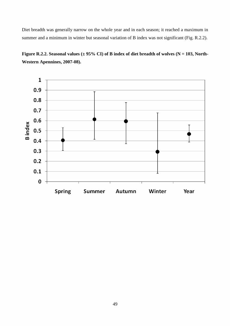
49

Diet breadth was generally narrow on the whole year and in each season; it reached a maximum in

summer and a minimum in winter but seasonal variation of B index was not significant (Fig. R.2.2).

Figure R.2.2. Seasonal values (± 95% CI) of B index of diet breadth of wolves (N = 103, North-

Western Apennines, 2007-08).

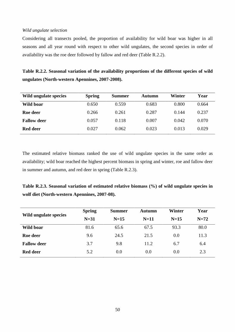
50

Wild ungulate selection

Considering all transects pooled, the proportion of availability for wild boar was higher in all

seasons and all year round with respect to other wild ungulates, the second species in order of

availability was the roe deer followed by fallow and red deer (Table R.2.2).

Table R.2.2. Seasonal variation of the availability proportions of the different species of wild

ungulates (North-western Apennines, 2007-2008).

Wild ungulate species Spring Summer Autumn Winter Year

Wild boar 0.650 0.559 0.683 0.800 0.664

Roe deer 0.266 0.261 0.287 0.144 0.237

Fallow deer 0.057 0.118 0.007 0.042 0.070

Red deer 0.027 0.062 0.023 0.013 0.029

The estimated relative biomass ranked the use of wild ungulate species in the same order as

availability; wild boar reached the highest percent biomass in spring and winter, roe and fallow deer

in summer and autumn, and red deer in spring (Table R.2.3).

Table R.2.3. Seasonal variation of estimated relative biomass (%) of wild ungulate species in

wolf diet (North-western Apennines, 2007-08).

Wild ungulate species Spring

N=31

Summer

N=15

Autumn

N=11

Winter

N=15

Year

N=72

Wild boar 81.6 65.6 67.5 93.3 80.0

Roe deer 9.6 24.5 21.5 0.0 11.3

Fallow deer 3.7 9.8 11.2 6.7 6.4

Red deer 5.2 0.0 0.0 0.0 2.3

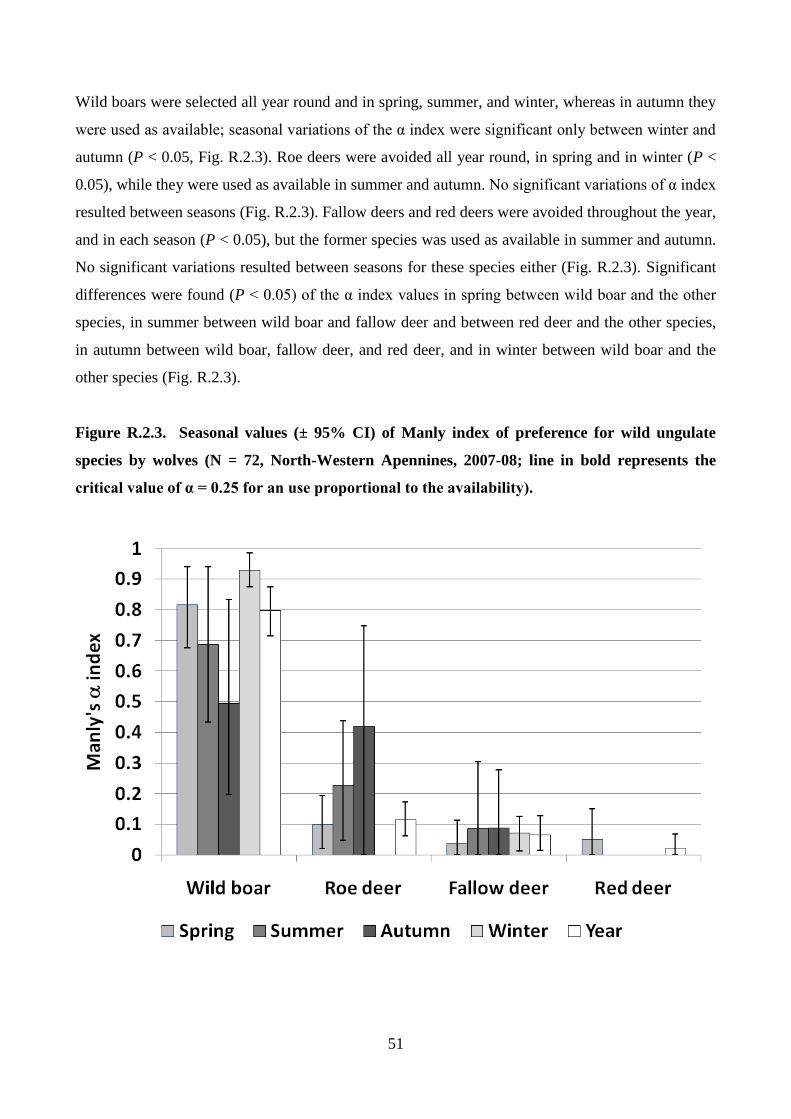
51

Wild boars were selected all year round and in spring, summer, and winter, whereas in autumn they

were used as available; seasonal variations of the α index were significant only between winter and

autumn (P < 0.05, Fig. R.2.3). Roe deers were avoided all year round, in spring and in winter (P <

0.05), while they were used as available in summer and autumn. No significant variations of α index

resulted between seasons (Fig. R.2.3). Fallow deers and red deers were avoided throughout the year,

and in each season (P < 0.05), but the former species was used as available in summer and autumn.

No significant variations resulted between seasons for these species either (Fig. R.2.3). Significant

differences were found (P < 0.05) of the α index values in spring between wild boar and the other

species, in summer between wild boar and fallow deer and between red deer and the other species,

in autumn between wild boar, fallow deer, and red deer, and in winter between wild boar and the

other species (Fig. R.2.3).

Figure R.2.3. Seasonal values (± 95% CI) of Manly index of preference for wild ungulate

species by wolves (N = 72, North-Western Apennines, 2007-08; line in bold represents the

critical value of α = 0.25 for an use proportional to the availability).

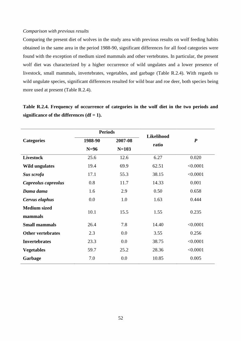
52

Comparison with previous results

Comparing the present diet of wolves in the study area with previous results on wolf feeding habits

obtained in the same area in the period 1988-90, significant differences for all food categories were

found with the exception of medium sized mammals and other vertebrates. In particular, the present

wolf diet was characterized by a higher occurrence of wild ungulates and a lower presence of

livestock, small mammals, invertebrates, vegetables, and garbage (Table R.2.4). With regards to

wild ungulate species, significant differences resulted for wild boar and roe deer, both species being

more used at present (Table R.2.4).

Table R.2.4. Frequency of occurrence of categories in the wolf diet in the two periods and

significance of the differences (df = 1).

Categories

Periods Likelihood

ratio P 1988-90

N=96

2007-08

N=103

Livestock 25.6 12.6 6.27 0.020

Wild ungulates 19.4 69.9 62.51 <0.0001

Sus scrofa 17.1 55.3 38.15 <0.0001

Capreolus capreolus 0.8 11.7 14.33 0.001

Dama dama 1.6 2.9 0.50 0.658

Cervus elaphus 0.0 1.0 1.63 0.444

Medium sized

mammals 10.1 15.5 1.55 0.235

Small mammals 26.4 7.8 14.40 <0.0001

Other vertebrates 2.3 0.0 3.55 0.256

Invertebrates 23.3 0.0 38.75 <0.0001

Vegetables 59.7 25.2 28.36 <0.0001

Garbage 7.0 0.0 10.85 0.005

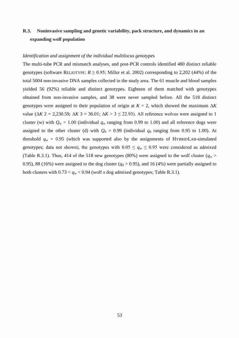
53

R.3. Noninvasive sampling and genetic variability, pack structure, and dynamics in an

expanding wolf population

Identification and assignment of the individual multilocus genotypes

The multi-tube PCR and mismatch analyses, and post-PCR controls identified 480 distinct reliable

genotypes (software RELIOTYPE: R ≥ 0.95; Miller et al. 2002) corresponding to 2,202 (44%) of the

total 5004 non-invasive DNA samples collected in the study area. The 61 muscle and blood samples

yielded 56 (92%) reliable and distinct genotypes. Eighteen of them matched with genotypes

obtained from non-invasive samples, and 38 were never sampled before. All the 518 distinct

genotypes were assigned to their population of origin at K = 2, which showed the maximum ΔK

value (ΔK 2 = 2,230.59; ΔK 3 = 36.01; ΔK > 3 ≤ 22.93). All reference wolves were assigned to 1

cluster (w) with Qw = 1.00 (individual qw ranging from 0.99 to 1.00) and all reference dogs were

assigned to the other cluster (d) with Qd = 0.99 (individual qd ranging from 0.95 to 1.00). At

threshold qw = 0.95 (which was supported also by the assignments of HYBRIDLAB-simulated

genotypes; data not shown), the genotypes with 0.05 ≤ qw ≤ 0.95 were considered as admixed

(Table R.3.1). Thus, 414 of the 518 new genotypes (80%) were assigned to the wolf cluster (qw >

0.95), 88 (16%) were assigned to the dog cluster (qd > 0.95), and 16 (4%) were partially assigned to

both clusters with 0.73 < qw < 0.94 (wolf x dog admixed genotypes; Table R.3.1).

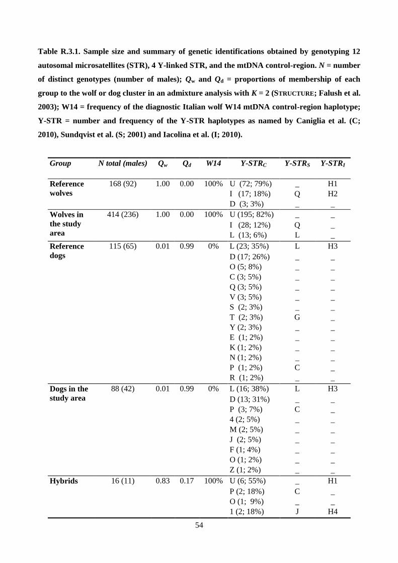
54

Table R.3.1. Sample size and summary of genetic identifications obtained by genotyping 12

autosomal microsatellites (STR), 4 Y-linked STR, and the mtDNA control-region. N = number

of distinct genotypes (number of males); Qw and Qd = proportions of membership of each

group to the wolf or dog cluster in an admixture analysis with K = 2 (STRUCTURE; Falush et al.

2003); W14 = frequency of the diagnostic Italian wolf W14 mtDNA control-region haplotype;

Y-STR = number and frequency of the Y-STR haplotypes as named by Caniglia et al. (C;

2010), Sundqvist et al. (S; 2001) and Iacolina et al. (I; 2010).

Group N total (males) Qw Qd W14 Y-STRC Y-STRS Y-STRI

Reference

wolves

168 (92) 1.00 0.00 100% U (72; 79%) _ H1

I (17; 18%) Q H2

D (3; 3%) _ _

Wolves in

the study

area

414 (236) 1.00 0.00 100% U (195; 82%) _ _

I (28; 12%) Q _

L (13; 6%) L _

Reference

dogs

115 (65) 0.01 0.99 0% L (23; 35%) L H3

D (17; 26%) _ _

O (5; 8%) _ _

C (3; 5%) _ _

Q (3; 5%) _ _

V (3; 5%) _ _

S (2; 3%) _ _

T (2; 3%) G _

Y (2; 3%) _ _

E (1; 2%) _ _

K (1; 2%) _ _

N (1; 2%) _ _

P (1; 2%) C _

R (1; 2%) _ _

Dogs in the

study area

88 (42) 0.01 0.99 0% L (16; 38%) L H3

D (13; 31%) _ _

P (3; 7%) C _

4 (2; 5%) _ _

M (2; 5%) _ _

J (2; 5%) _ _

F (1; 4%) _ _

O (1; 2%) _ _

Z (1; 2%) _ _

Hybrids 16 (11) 0.83 0.17 100% U (6; 55%) _ H1

P (2; 18%) C _

O (1; 9%) _ _

1 (2; 18%) J H4

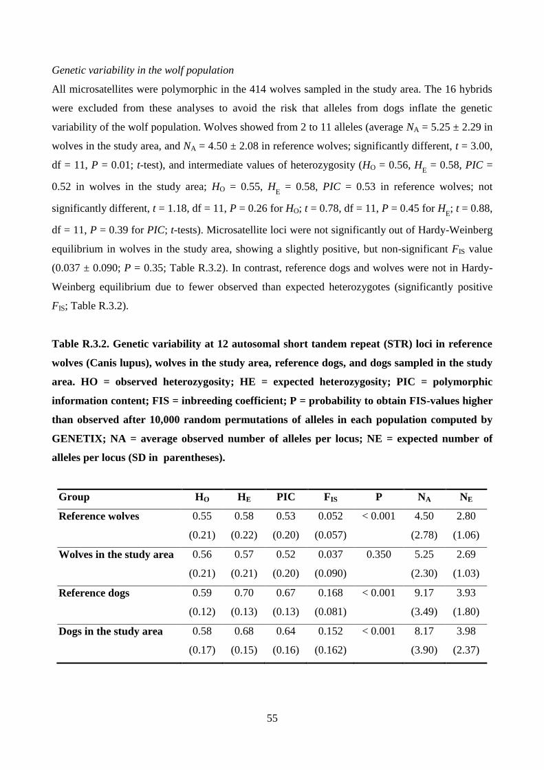
55

Genetic variability in the wolf population

All microsatellites were polymorphic in the 414 wolves sampled in the study area. The 16 hybrids

were excluded from these analyses to avoid the risk that alleles from dogs inflate the genetic

variability of the wolf population. Wolves showed from 2 to 11 alleles (average NA = 5.25 ± 2.29 in

wolves in the study area, and NA = 4.50 ± 2.08 in reference wolves; significantly different, t = 3.00,

df = 11, P = 0.01; t-test), and intermediate values of heterozygosity (HO = 0.56, HE = 0.58, PIC =

0.52 in wolves in the study area; HO = 0.55, HE = 0.58, PIC = 0.53 in reference wolves; not

significantly different, t = 1.18, df = 11, P = 0.26 for HO; t = 0.78, df = 11, P = 0.45 for HE; t = 0.88,

df = 11, P = 0.39 for PIC; t-tests). Microsatellite loci were not significantly out of Hardy-Weinberg

equilibrium in wolves in the study area, showing a slightly positive, but non-significant FIS value

(0.037 ± 0.090; P = 0.35; Table R.3.2). In contrast, reference dogs and wolves were not in Hardy-

Weinberg equilibrium due to fewer observed than expected heterozygotes (significantly positive

FIS; Table R.3.2).

Table R.3.2. Genetic variability at 12 autosomal short tandem repeat (STR) loci in reference

wolves (Canis lupus), wolves in the study area, reference dogs, and dogs sampled in the study

area. HO = observed heterozygosity; HE = expected heterozygosity; PIC = polymorphic

information content; FIS = inbreeding coefficient; P = probability to obtain FIS-values higher

than observed after 10,000 random permutations of alleles in each population computed by

GENETIX; NA = average observed number of alleles per locus; NE = expected number of

alleles per locus (SD in parentheses).

Group HO HE PIC FIS P NA NE

Reference wolves 0.55

(0.21)

0.58

(0.22)

0.53

(0.20)

0.052

(0.057)

< 0.001 4.50

(2.78)

2.80

(1.06)

Wolves in the study area 0.56

(0.21)

0.57

(0.21)

0.52

(0.20)

0.037

(0.090)

0.350

5.25

(2.30)

2.69

(1.03)

Reference dogs 0.59

(0.12)

0.70

(0.13)

0.67

(0.13)

0.168

(0.081)

< 0.001 9.17

(3.49)

3.93

(1.80)

Dogs in the study area 0.58

(0.17)

0.68

(0.15)

0.64

(0.16)

0.152

(0.162)

< 0.001 8.17

(3.90)

3.98

(2.37)

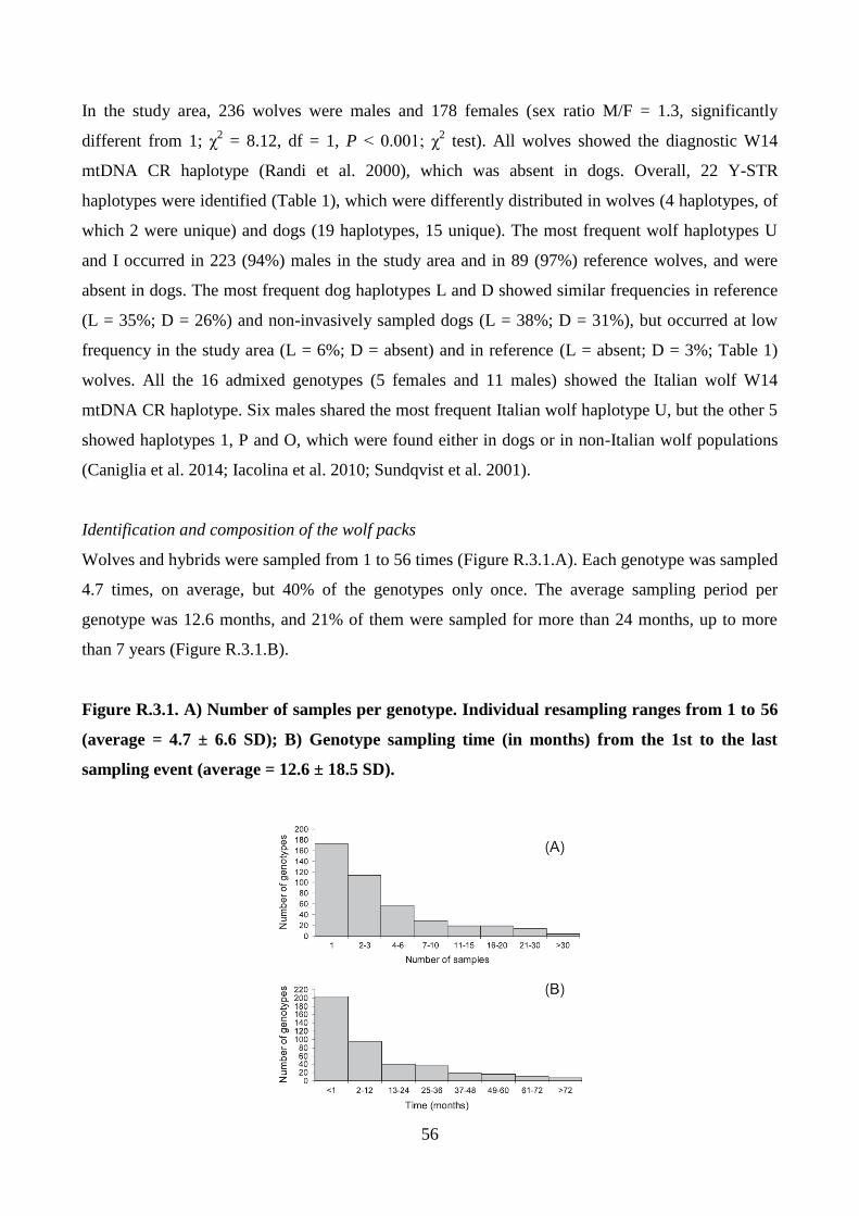
56

In the study area, 236 wolves were males and 178 females (sex ratio M/F = 1.3, significantly

different from 1; χ2 = 8.12, df = 1, P < 0.001; χ

2 test). All wolves showed the diagnostic W14

mtDNA CR haplotype (Randi et al. 2000), which was absent in dogs. Overall, 22 Y-STR

haplotypes were identified (Table 1), which were differently distributed in wolves (4 haplotypes, of

which 2 were unique) and dogs (19 haplotypes, 15 unique). The most frequent wolf haplotypes U

and I occurred in 223 (94%) males in the study area and in 89 (97%) reference wolves, and were

absent in dogs. The most frequent dog haplotypes L and D showed similar frequencies in reference

(L = 35%; D = 26%) and non-invasively sampled dogs (L = 38%; D = 31%), but occurred at low

frequency in the study area (L = 6%; D = absent) and in reference (L = absent; D = 3%; Table 1)

wolves. All the 16 admixed genotypes (5 females and 11 males) showed the Italian wolf W14

mtDNA CR haplotype. Six males shared the most frequent Italian wolf haplotype U, but the other 5

showed haplotypes 1, P and O, which were found either in dogs or in non-Italian wolf populations

(Caniglia et al. 2014; Iacolina et al. 2010; Sundqvist et al. 2001).

Identification and composition of the wolf packs

Wolves and hybrids were sampled from 1 to 56 times (Figure R.3.1.A). Each genotype was sampled

4.7 times, on average, but 40% of the genotypes only once. The average sampling period per

genotype was 12.6 months, and 21% of them were sampled for more than 24 months, up to more

than 7 years (Figure R.3.1.B).

Figure R.3.1. A) Number of samples per genotype. Individual resampling ranges from 1 to 56

(average = 4.7 ± 6.6 SD); B) Genotype sampling time (in months) from the 1st to the last

sampling event (average = 12.6 ± 18.5 SD).

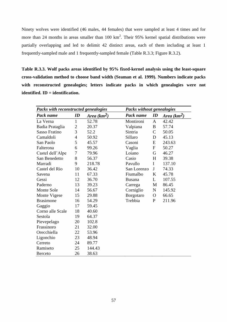
57

Ninety wolves were identified (46 males, 44 females) that were sampled at least 4 times and for

more than 24 months in areas smaller than 100 km2. Their 95% kernel spatial distributions were

partially overlapping and led to delimit 42 distinct areas, each of them including at least 1

frequently-sampled male and 1 frequently-sampled female (Table R.3.3; Figure R.3.2).

Table R.3.3. Wolf packs areas identified by 95% fixed-kernel analysis using the least-square

cross-validation method to choose band width (Seaman et al. 1999). Numbers indicate packs

with reconstructed genealogies; letters indicate packs in which genealogies were not

identified. ID = identification.

Packs with reconstructed genealogies Packs without genealogies

Pack name ID Area (km2) Pack name ID Area (km2)

La Verna 1 52.78 Montironi A 42.42

Badia Prataglia 2 20.37 Valpiana B 57.74

Sasso Fratino 3 52.2 Sintria C 50.05

Camaldoli 4 50.92 Sillaro D 45.13

San Paolo 5 45.57 Casoni E 243.63

Falterona 6 99.26 Vaglia F 50.27

Castel dell’Alpe 7 79.96 Loiano G 46.27

San Benedetto 8 56.37 Casio H 39.38

Marradi 9 218.78 Pavullo I 137.10

Castel del Rio 10 36.42 San Lorenzo J 74.33

Savena 11 67.33 Fiumalbo K 45.78

Gessi 12 36.70 Busana L 107.55

Paderno 13 39.23 Carrega M 86.45

Monte Sole 14 56.67 Corniglio N 145.92

Monte Vigese 15 29.88 Borgotaro O 66.65

Brasimone 16 54.29 Trebbia P 211.96

Gaggio 17 59.45

Corno alle Scale 18 40.60

Sestola 19 64.37

Pievepelago 20 102.8

Frassinoro 21 32.00

Orecchiella 22 53.96

Ligonchio 23 48.94

Cerreto 24 89.77

Ramiseto 25 144.43

Berceto 26 38.63

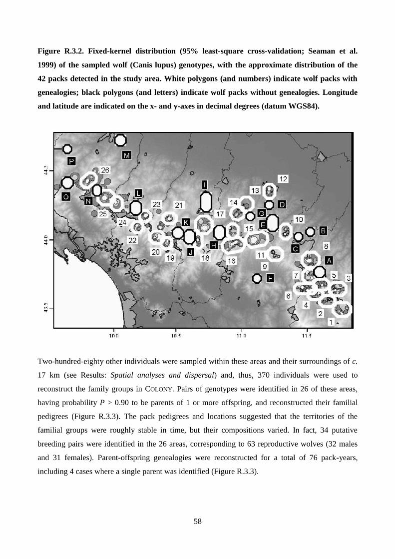
58

Figure R.3.2. Fixed-kernel distribution (95% least-square cross-validation; Seaman et al.

1999) of the sampled wolf (Canis lupus) genotypes, with the approximate distribution of the

42 packs detected in the study area. White polygons (and numbers) indicate wolf packs with

genealogies; black polygons (and letters) indicate wolf packs without genealogies. Longitude

and latitude are indicated on the x- and y-axes in decimal degrees (datum WGS84).

Two-hundred-eighty other individuals were sampled within these areas and their surroundings of c.

17 km (see Results: Spatial analyses and dispersal) and, thus, 370 individuals were used to

reconstruct the family groups in COLONY. Pairs of genotypes were identified in 26 of these areas,

having probability P > 0.90 to be parents of 1 or more offspring, and reconstructed their familial

pedigrees (Figure R.3.3). The pack pedigrees and locations suggested that the territories of the

familial groups were roughly stable in time, but their compositions varied. In fact, 34 putative

breeding pairs were identified in the 26 areas, corresponding to 63 reproductive wolves (32 males

and 31 females). Parent-offspring genealogies were reconstructed for a total of 76 pack-years,

including 4 cases where a single parent was identified (Figure R.3.3).

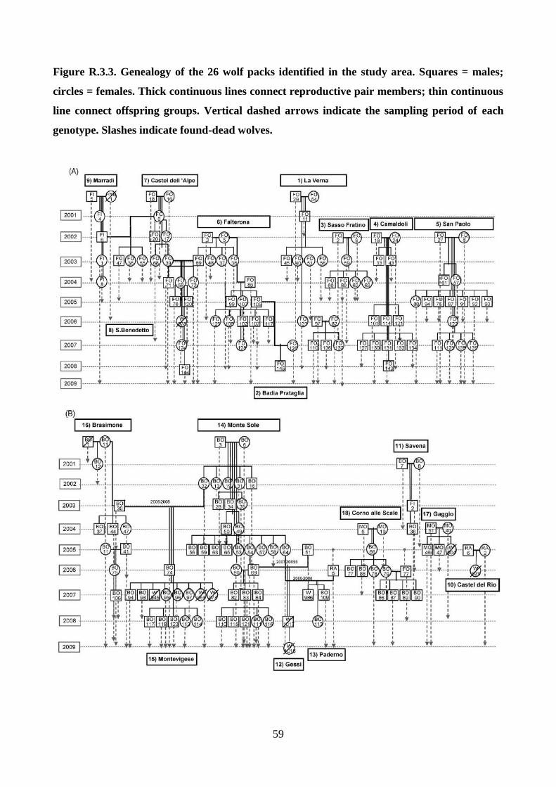
59

Figure R.3.3. Genealogy of the 26 wolf packs identified in the study area. Squares = males;

circles = females. Thick continuous lines connect reproductive pair members; thin continuous

line connect offspring groups. Vertical dashed arrows indicate the sampling period of each

genotype. Slashes indicate found-dead wolves.

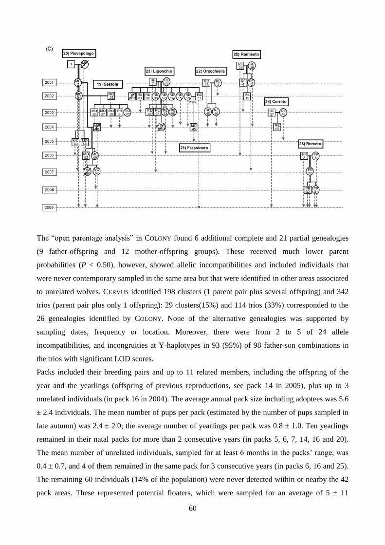
60

The “open parentage analysis” in COLONY found 6 additional complete and 21 partial genealogies

(9 father-offspring and 12 mother-offspring groups). These received much lower parent

probabilities (P < 0.50), however, showed allelic incompatibilities and included individuals that

were never contemporary sampled in the same area but that were identified in other areas associated

to unrelated wolves. CERVUS identified 198 clusters (1 parent pair plus several offspring) and 342

trios (parent pair plus only 1 offspring): 29 clusters(15%) and 114 trios (33%) corresponded to the

26 genealogies identified by COLONY. None of the alternative genealogies was supported by

sampling dates, frequency or location. Moreover, there were from 2 to 5 of 24 allele

incompatibilities, and incongruities at Y-haplotypes in 93 (95%) of 98 father-son combinations in

the trios with significant LOD scores.

Packs included their breeding pairs and up to 11 related members, including the offspring of the

year and the yearlings (offspring of previous reproductions, see pack 14 in 2005), plus up to 3

unrelated individuals (in pack 16 in 2004). The average annual pack size including adoptees was 5.6

± 2.4 individuals. The mean number of pups per pack (estimated by the number of pups sampled in

late autumn) was 2.4 ± 2.0; the average number of yearlings per pack was 0.8 ± 1.0. Ten yearlings

remained in their natal packs for more than 2 consecutive years (in packs 5, 6, 7, 14, 16 and 20).

The mean number of unrelated individuals, sampled for at least 6 months in the packs’ range, was

0.4 ± 0.7, and 4 of them remained in the same pack for 3 consecutive years (in packs 6, 16 and 25).

The remaining 60 individuals (14% of the population) were never detected within or nearby the 42

pack areas. These represented potential floaters, which were sampled for an average of 5 ± 11

61

months, up to 6 years. Those included 15 of the 16 hybrids, since only 1 (HY1F) was identified as a

member of a known pack.

Relatedness and inbreeding

A matrix of pairwise relatedness among all the individuals included in the packs showed that 33

(94%) of the 34 breeding pairs were significantly unrelated (P < 0.05; likelihood ratio test). Parents

RE17M and RE18F in pack 21 showed a significant first-order relationship (brother and sister; P =

0.011), also confirming the genealogy of their natal pack, 23 (Figure R.3.3). The mean inbreeding

coefficient of the breeding pairs was F = -0.02 (-0.25 – 0.30, 95% CI) ranging from -0.15 (-0.40 –

0.25) in pack 4 to 0.35 (0.09 – 0.73) in pack 7 (Table R.3.4). The observed heterozygosity did not

differ significantly between breeding pairs (HO = 0.57 ± 0.15, n = 34) and their offspring (HO = 0.54

± 0.22, n = 179; t = 1.52, df = 33, P = 0.67; t-test), or between breeders (HO = 0.57 ± 0.48, n = 63)

and non-breeders (HO = 0.56 ± 1.15, n = 367; t = 2.35, df = 62, P = 0.93; t-test; Table R.3.4).

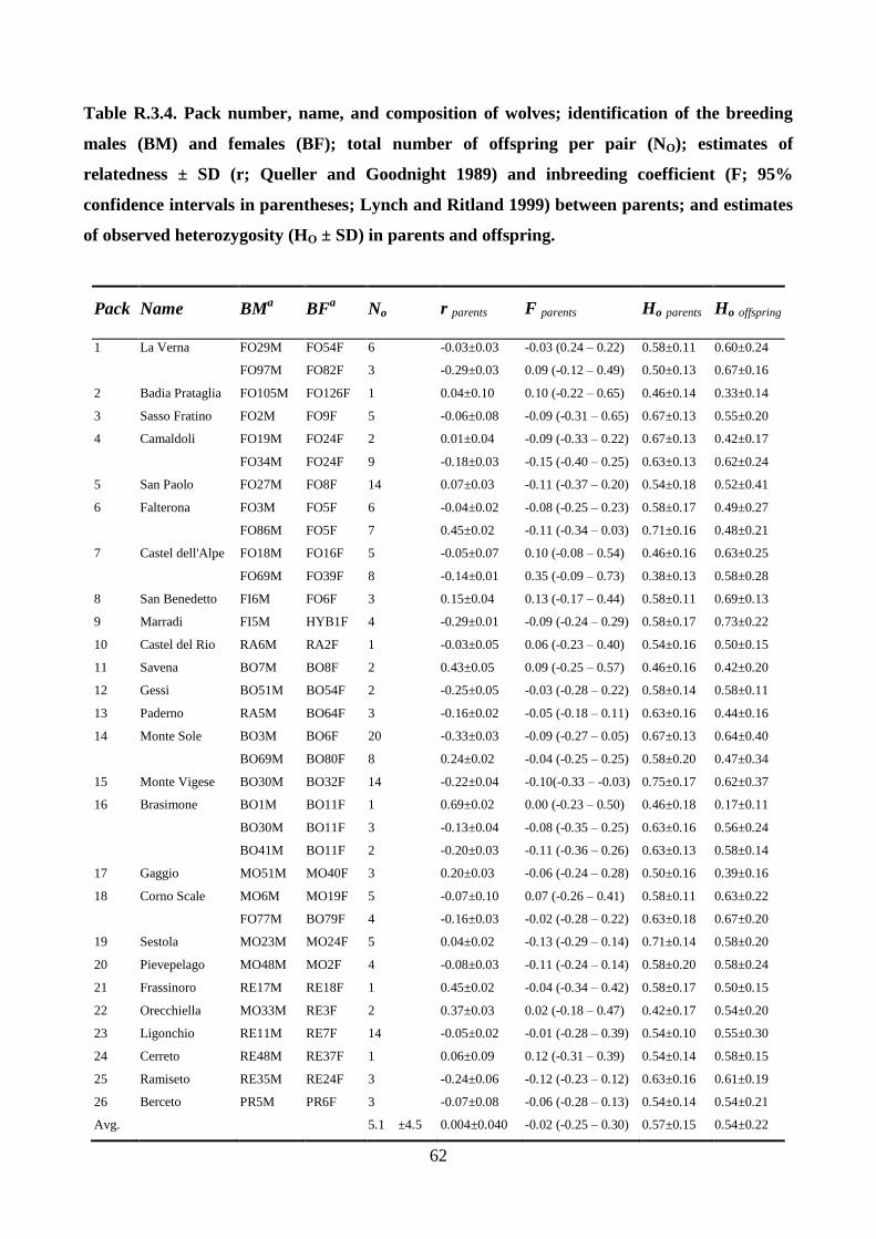
62

Table R.3.4. Pack number, name, and composition of wolves; identification of the breeding

males (BM) and females (BF); total number of offspring per pair (NO); estimates of

relatedness ± SD (r; Queller and Goodnight 1989) and inbreeding coefficient (F; 95%

confidence intervals in parentheses; Lynch and Ritland 1999) between parents; and estimates

of observed heterozygosity (HO ± SD) in parents and offspring.

Pack Name BMa BF

a No r parents F parents Ho parents Ho offspring

1 La Verna FO29M FO54F 6 -0.03±0.03 -0.03 (0.24 – 0.22) 0.58±0.11 0.60±0.24

FO97M FO82F 3 -0.29±0.03 0.09 (-0.12 – 0.49) 0.50±0.13 0.67±0.16

2 Badia Prataglia FO105M FO126F 1 0.04±0.10 0.10 (-0.22 – 0.65) 0.46±0.14 0.33±0.14

3 Sasso Fratino FO2M FO9F 5 -0.06±0.08 -0.09 (-0.31 – 0.65) 0.67±0.13 0.55±0.20

4 Camaldoli FO19M FO24F 2 0.01±0.04 -0.09 (-0.33 – 0.22) 0.67±0.13 0.42±0.17

FO34M FO24F 9 -0.18±0.03 -0.15 (-0.40 – 0.25) 0.63±0.13 0.62±0.24

5 San Paolo FO27M FO8F 14 0.07±0.03 -0.11 (-0.37 – 0.20) 0.54±0.18 0.52±0.41

6 Falterona FO3M FO5F 6 -0.04±0.02 -0.08 (-0.25 – 0.23) 0.58±0.17 0.49±0.27

FO86M FO5F 7 0.45±0.02 -0.11 (-0.34 – 0.03) 0.71±0.16 0.48±0.21

7 Castel dell'Alpe FO18M FO16F 5 -0.05±0.07 0.10 (-0.08 – 0.54) 0.46±0.16 0.63±0.25

FO69M FO39F 8 -0.14±0.01 0.35 (-0.09 – 0.73) 0.38±0.13 0.58±0.28

8 San Benedetto FI6M FO6F 3 0.15±0.04 0.13 (-0.17 – 0.44) 0.58±0.11 0.69±0.13

9 Marradi FI5M HYB1F 4 -0.29±0.01 -0.09 (-0.24 – 0.29) 0.58±0.17 0.73±0.22

10 Castel del Rio RA6M RA2F 1 -0.03±0.05 0.06 (-0.23 – 0.40) 0.54±0.16 0.50±0.15

11 Savena BO7M BO8F 2 0.43±0.05 0.09 (-0.25 – 0.57) 0.46±0.16 0.42±0.20

12 Gessi BO51M BO54F 2 -0.25±0.05 -0.03 (-0.28 – 0.22) 0.58±0.14 0.58±0.11

13 Paderno RA5M BO64F 3 -0.16±0.02 -0.05 (-0.18 – 0.11) 0.63±0.16 0.44±0.16

14 Monte Sole BO3M BO6F 20 -0.33±0.03 -0.09 (-0.27 – 0.05) 0.67±0.13 0.64±0.40

BO69M BO80F 8 0.24±0.02 -0.04 (-0.25 – 0.25) 0.58±0.20 0.47±0.34

15 Monte Vigese BO30M BO32F 14 -0.22±0.04 -0.10(-0.33 – -0.03) 0.75±0.17 0.62±0.37

16 Brasimone BO1M BO11F 1 0.69±0.02 0.00 (-0.23 – 0.50) 0.46±0.18 0.17±0.11

BO30M BO11F 3 -0.13±0.04 -0.08 (-0.35 – 0.25) 0.63±0.16 0.56±0.24

BO41M BO11F 2 -0.20±0.03 -0.11 (-0.36 – 0.26) 0.63±0.13 0.58±0.14

17 Gaggio MO51M MO40F 3 0.20±0.03 -0.06 (-0.24 – 0.28) 0.50±0.16 0.39±0.16

18 Corno Scale MO6M MO19F 5 -0.07±0.10 0.07 (-0.26 – 0.41) 0.58±0.11 0.63±0.22

FO77M BO79F 4 -0.16±0.03 -0.02 (-0.28 – 0.22) 0.63±0.18 0.67±0.20

19 Sestola MO23M MO24F 5 0.04±0.02 -0.13 (-0.29 – 0.14) 0.71±0.14 0.58±0.20

20 Pievepelago MO48M MO2F 4 -0.08±0.03 -0.11 (-0.24 – 0.14) 0.58±0.20 0.58±0.24

21 Frassinoro RE17M RE18F 1 0.45±0.02 -0.04 (-0.34 – 0.42) 0.58±0.17 0.50±0.15

22 Orecchiella MO33M RE3F 2 0.37±0.03 0.02 (-0.18 – 0.47) 0.42±0.17 0.54±0.20

23 Ligonchio RE11M RE7F 14 -0.05±0.02 -0.01 (-0.28 – 0.39) 0.54±0.10 0.55±0.30

24 Cerreto RE48M RE37F 1 0.06±0.09 0.12 (-0.31 – 0.39) 0.54±0.14 0.58±0.15

25 Ramiseto RE35M RE24F 3 -0.24±0.06 -0.12 (-0.23 – 0.12) 0.63±0.16 0.61±0.19

26 Berceto PR5M PR6F 3 -0.07±0.08 -0.06 (-0.28 – 0.13) 0.54±0.14 0.54±0.21

Avg. 5.1 ±4.5 0.004±0.040 -0.02 (-0.25 – 0.30) 0.57±0.15 0.54±0.22

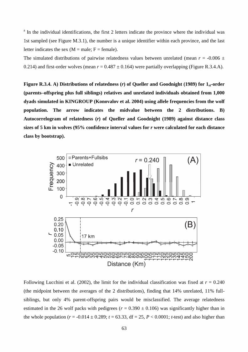
63

a In the individual identifications, the first 2 letters indicate the province where the individual was

1st sampled (see Figure M.3.1), the number is a unique identifier within each province, and the last

letter indicates the sex (M = male; F = female).

The simulated distributions of pairwise relatedness values between unrelated (mean r = -0.006 ±

0.214) and first-order wolves (mean r = 0.487 ± 0.164) were partially overlapping (Figure R.3.4.A).

Figure R.3.4. A) Distributions of relatedness (r) of Queller and Goodnight (1989) for 1st-order

(parents–offspring plus full siblings) relatives and unrelated individuals obtained from 1,000

dyads simulated in KINGROUP (Konovalov et al. 2004) using allele frequencies from the wolf

population. The arrow indicates the midvalue between the 2 distributions. B)

Autocorrelogram of relatedness (r) of Queller and Goodnight (1989) against distance class

sizes of 5 km in wolves (95% confidence interval values for r were calculated for each distance

class by bootstrap).

Following Lucchini et al. (2002), the limit for the individual classification was fixed at r = 0.240

(the midpoint between the averages of the 2 distributions), finding that 14% unrelated, 11% full-

siblings, but only 4% parent-offspring pairs would be misclassified. The average relatedness

estimated in the 26 wolf packs with pedigrees (r = 0.390 ± 0.106) was significantly higher than in

the whole population (r = -0.014 ± 0.289; t = 63.33, df = 25, P < 0.0001; t-test) and also higher than

64

the fixed midpoint (r = 0.240; t = 21.48, df = 25, P < 0.0001; t-test). Values of relatedness within

wolf packs were variable, ranging from r = 0.240 ± 0.181 (in pack 1) to r = 0.682 ± 0.271 (in pack

11).

Spatial analyses and dispersal

The 95% kernel analysis showed that the packs were settled in a minimum total area of 3122 km2

(1/6 of the sampling area of 19,171 km2; Figure R.3.2). The average 95% kernel area of individuals

belonging to packs was 35.72 ± 20.20 km2 (ranging from 4.51 to 170.64 km

2); the average pack

area was 74.34 ± 51.69 km2 (ranging from 20.37 to 243.63 km

2; 42 packs) or 60.02 ± 41.39 km

2

(ranging from 20.37 to 218.62 km2) when computed for the 26 areas with reconstructed genealogies

(Table R.3.3). The autocorrelation of kinship vs. the logarithmic inter-individual distance was

significantly negative (b = -0.013 ± 0.010; P < 0.001). Positive values of the Fij kinship coefficient

at short distances indicated that geographically closer wolves had higher-than-expected kinship,

while negative values at long distances highlighted isolation-by-distance (IBD, Figure R.3.4.B). The

x-intercept on the autocorrelogram suggested that within 17 km wolves are more closely related to

one another than on average across the population. Thus, 27 wolves that were successively sampled

in different locations farther than 17 km and 10 wolves that stably settled in a pack different from

their original one, but at shorter distances were considered as potential dispersers (Table R.3.5).

Twenty wolves (54%) dispersed south-east to north-west, towards the Alps. The average dispersal

distance was 52.97 ± 40.17 km. Dispersal was significantly male-biased (26 individuals, χ2 = 6.06,

df =1, P < 0.01; χ2 test), as suggested also by autocorrelation analyses in male and female distance

classes, which showed higher relatedness among females (r = 0.090; 11 km) than males (r = 0.070;

20 km). There were 22 (59%) of the 37 dispersers that apparently settled in a new pack, and 14 of

them (38%) also became breeders: 2 males established and reproduced in already existing packs,

and 12 (5 males and 7 females) founded their own new packs. In comparison, only 5 (26%) of 19

known non-dispersing individuals (wolves born and sampled in the same pack for at least 3 years)

became breeders in their natal pack (4 females and 1 male). Other 15 dispersers (13 males and 2

females) were never detected in association with a known pack (2), or were born in a known pack

(13) but dispersed to unoccupied areas, thus representing other potential cases of floaters.

Wolves dispersing short distances (19.2 km, on average) apparently had higher likelihood (F =

27.71, df = 1, P < 0.0001; one way ANOVA test) to reproduce in new packs than wolves moving

longer distance (73.5 km, on average). The founders were born in areas close to the centroids of the

new packs, mapping at an average distance of 17.5 ± 12.2 km, thus explaining why the observed

IBD and autocorrelations dropped at a short geographical distance.

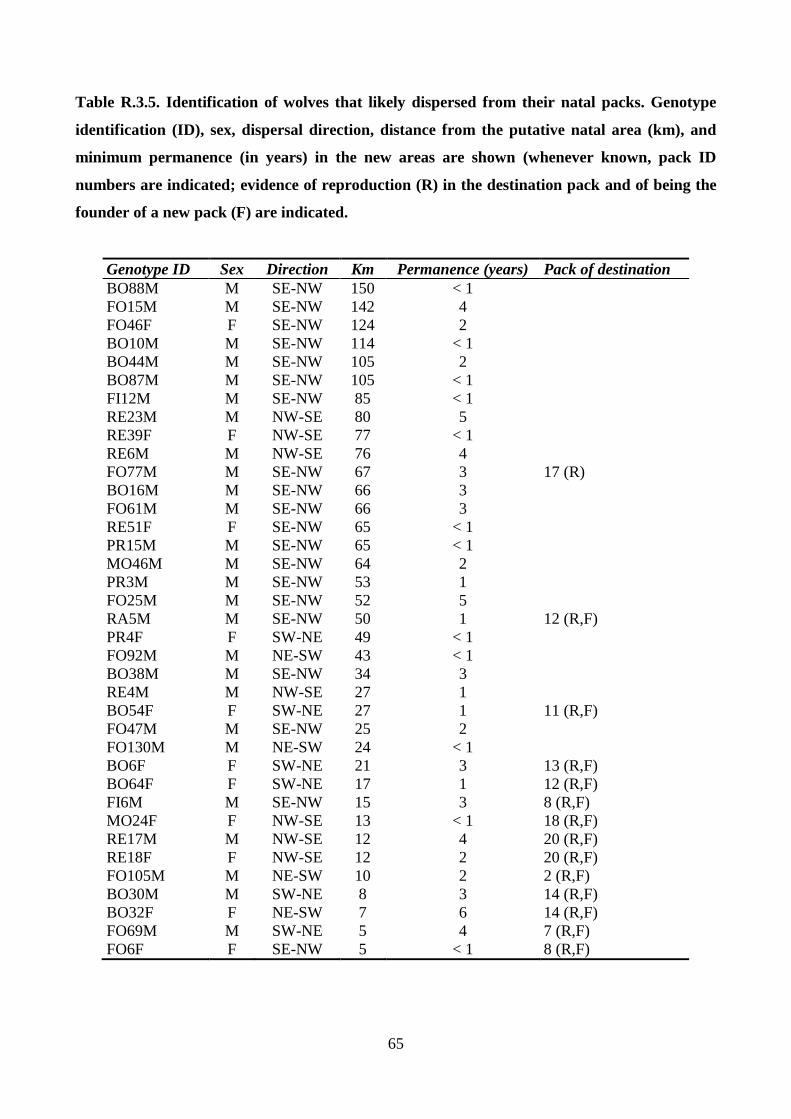
65

Table R.3.5. Identification of wolves that likely dispersed from their natal packs. Genotype

identification (ID), sex, dispersal direction, distance from the putative natal area (km), and

minimum permanence (in years) in the new areas are shown (whenever known, pack ID

numbers are indicated; evidence of reproduction (R) in the destination pack and of being the

founder of a new pack (F) are indicated.

Genotype ID Sex Direction Km Permanence (years) Pack of destination

BO88M M SE-NW 150 < 1

FO15M M SE-NW 142 4

FO46F F SE-NW 124 2

BO10M M SE-NW 114 < 1

BO44M M SE-NW 105 2

BO87M M SE-NW 105 < 1

FI12M M SE-NW 85 < 1

RE23M M NW-SE 80 5

RE39F F NW-SE 77 < 1

RE6M M NW-SE 76 4

FO77M M SE-NW 67 3 17 (R)

BO16M M SE-NW 66 3

FO61M M SE-NW 66 3

RE51F F SE-NW 65 < 1

PR15M M SE-NW 65 < 1

MO46M M SE-NW 64 2

PR3M M SE-NW 53 1

FO25M M SE-NW 52 5

RA5M M SE-NW 50 1 12 (R,F)

PR4F F SW-NE 49 < 1

FO92M M NE-SW 43 < 1

BO38M M SE-NW 34 3

RE4M M NW-SE 27 1

BO54F F SW-NE 27 1 11 (R,F)

FO47M M SE-NW 25 2

FO130M M NE-SW 24 < 1

BO6F F SW-NE 21 3 13 (R,F)

BO64F F SW-NE 17 1 12 (R,F)

FI6M M SE-NW 15 3 8 (R,F)

MO24F F NW-SE 13 < 1 18 (R,F)

RE17M M NW-SE 12 4 20 (R,F)

RE18F F NW-SE 12 2 20 (R,F)

FO105M M NE-SW 10 2 2 (R,F)

BO30M M SW-NE 8 3 14 (R,F)

BO32F F NE-SW 7 6 14 (R,F)

FO69M M SW-NE 5 4 7 (R,F)

FO6F F SE-NW 5 < 1 8 (R,F)

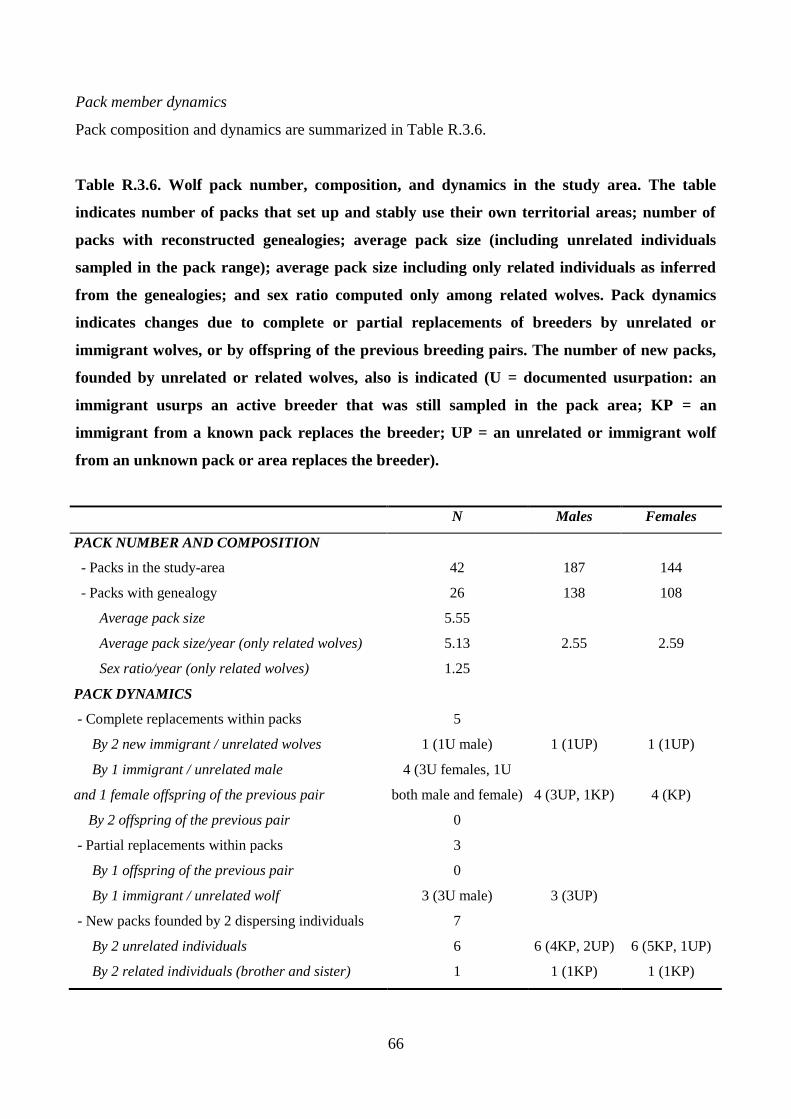
66

Pack member dynamics

Pack composition and dynamics are summarized in Table R.3.6.

Table R.3.6. Wolf pack number, composition, and dynamics in the study area. The table

indicates number of packs that set up and stably use their own territorial areas; number of

packs with reconstructed genealogies; average pack size (including unrelated individuals

sampled in the pack range); average pack size including only related individuals as inferred

from the genealogies; and sex ratio computed only among related wolves. Pack dynamics

indicates changes due to complete or partial replacements of breeders by unrelated or

immigrant wolves, or by offspring of the previous breeding pairs. The number of new packs,

founded by unrelated or related wolves, also is indicated (U = documented usurpation: an

immigrant usurps an active breeder that was still sampled in the pack area; KP = an

immigrant from a known pack replaces the breeder; UP = an unrelated or immigrant wolf

from an unknown pack or area replaces the breeder).

N Males Females

PACK NUMBER AND COMPOSITION

- Packs in the study-area 42 187 144

- Packs with genealogy 26 138 108

Average pack size 5.55

Average pack size/year (only related wolves) 5.13 2.55 2.59

Sex ratio/year (only related wolves) 1.25

PACK DYNAMICS

- Complete replacements within packs 5

By 2 new immigrant / unrelated wolves 1 (1U male) 1 (1UP) 1 (1UP)

By 1 immigrant / unrelated male

and 1 female offspring of the previous pair

4 (3U females, 1U

both male and female) 4 (3UP, 1KP) 4 (KP)

By 2 offspring of the previous pair 0

- Partial replacements within packs 3

By 1 offspring of the previous pair 0

By 1 immigrant / unrelated wolf 3 (3U male) 3 (3UP)

- New packs founded by 2 dispersing individuals 7

By 2 unrelated individuals 6 6 (4KP, 2UP) 6 (5KP, 1UP)

By 2 related individuals (brother and sister) 1 1 (1KP) 1 (1KP)

67

In the eastern sector of the study area (lower-right side of Figure R.3.2) The complete genealogies

were reconstructed in 9 of the 12 documented packs (Figure R.3.3.A). The breeding pairs in 6 packs

were stable throughout the study (packs 2, 3, 4, 5, 8 and 9, detected from 1 to 6 years; average 3.5

years). In pack 1 (La Verna), both parents detected since 2001 were completely substituted in 2006

by a new breeding pair of unknown familial origin that reproduced in 2007. Other packs showed

more complex dynamics. Offspring from packs 9 (Marradi) and 7 (Castel dell’Alpe) joined in a

breeding pair that in 2002 founded a new pack in-between (8; San Benedetto). Pack 7 showed a

turnover of the reproductive pair identified in 2001, which apparently disappeared in 2003, when it

was replaced by a female offspring born in 2002 and by an unrelated immigrant male born in 2002

in pack 6 (Falterona). The reproductive male in pack 6 was replaced in 2004 by an immigrant male

of unknown familial origin. A male offspring of the new Falterona pack established a new pack in

2007 in an adjacent area (2; Badia Prataglia), mating with an unrelated female of unknown familial

origin. The number of detected packs increased from 7 (in 2001-2002) to 9 (in 2008-2009). Both the

new packs filled new areas. Three of the original 7 packs (43%) were genetically connected through

replacements (1) or new pack foundations (2). The presence of 6 of the 7 packs identified in 2001 in

this sector was confirmed by wolf-howling sessions (Caniglia et al. 2010), which also confirmed the

presence of 8 packs in 2006.

In the central part of the study area (Figure R.3.2), complete genealogies were reconstructed in 9

(packs 10 – 18) of the 15 mapped packs (Figure R.3.3.B). In 6 packs (10, 11, 12, 13, 15 and 17) the

breeding pair did not change during the study. In other 2 packs (14; Monte Sole; 18; Corno alle

Scale), on the contrary, the breeding pairs were completely substituted by females offspring and

immigrant males of unknown familial origin. In pack 16 (Brasimone) the female BO11F reproduced

from 2001 to 2008, but the breeding males changed 3 times (in 2003, 2004 and 2006). One of them,

BO30M, later colonized an adjacent territory and established a new pack (15; Monte Vigese) with a

female born in 2002 in pack 14 (Monte Sole). Two females from pack 14 originated 2 new groups,

pack 12 (Gessi) in 2007, and 13 (Paderno) in 2008, with 2 males of unknown familial origin. 1 of

them, male RA5M, was sampled 2 years before about 50 km apart in a straight line, similar to male

FO77M, which replaced the previous breeder in pack 18 (Corno alle Scale). Thus, in this central

region of the study area, pack interchanges involved 3 (33%) of 9 genealogies. Replacements

involved each time the immigration of unrelated males that mated with resident females. Three new

packs (12, 13 and 15) originated from unrelated individuals migrating from neighbouring zones and

filling new areas. Packs increased from 6 (in 2001-2004) to 8 (in 2008), although it was not possible

to reconstruct all their genealogies. Whenever carried out, field surveys confirmed the results from

genetic data: the minimum number of wolves was confirmed by snow-tracking in packs 10, 11, 14,

68

16 and 18 (Caniglia et al. 2010); wolf-howling detected reproductions in packs 10, 11, 12, 14, 15,

16 and 18 (Caniglia et al. 2010); camera trapping confirmed two reproductions and the minimum

number of wolves in pack 18 (Galaverni et al. 2012).

Eight pedigrees (Figure R.3.3.C) were reconstructed in the 15 packs identified in the western sector

of the study area (upper-left part of Figure R.3.2). In pack 20 (Pievepelago), a female offspring

colonized an adjacent territory and founded a new pack (19, Sestola) with a male of unknown

genealogy, whereas her sister substituted their mother as a breeder in 2004. A case of incestuous

mating was detected in 2003: a brother and a sister from pack 23 (Ligonchio) mated and originated

the new pack 21 (Frassinoro). Other 4 packs were apparently not interconnected by any exchange of

immigrant or dispersal individuals. The number of packs increased from 6 (in 2001-2003) to 8 (in

2008), although it was not possible to reconstruct all their genealogies, and the 2 new packs filled

vacant areas. Four packs were confirmed by wolf-howling in 2002 (packs 19, 20, 22, 24), and 6 (19,

20, 22, 23, 24 and 25) by snow-tracking between 2002 and 2004 (Life project LIFE00NAT/IT/7214

final report).

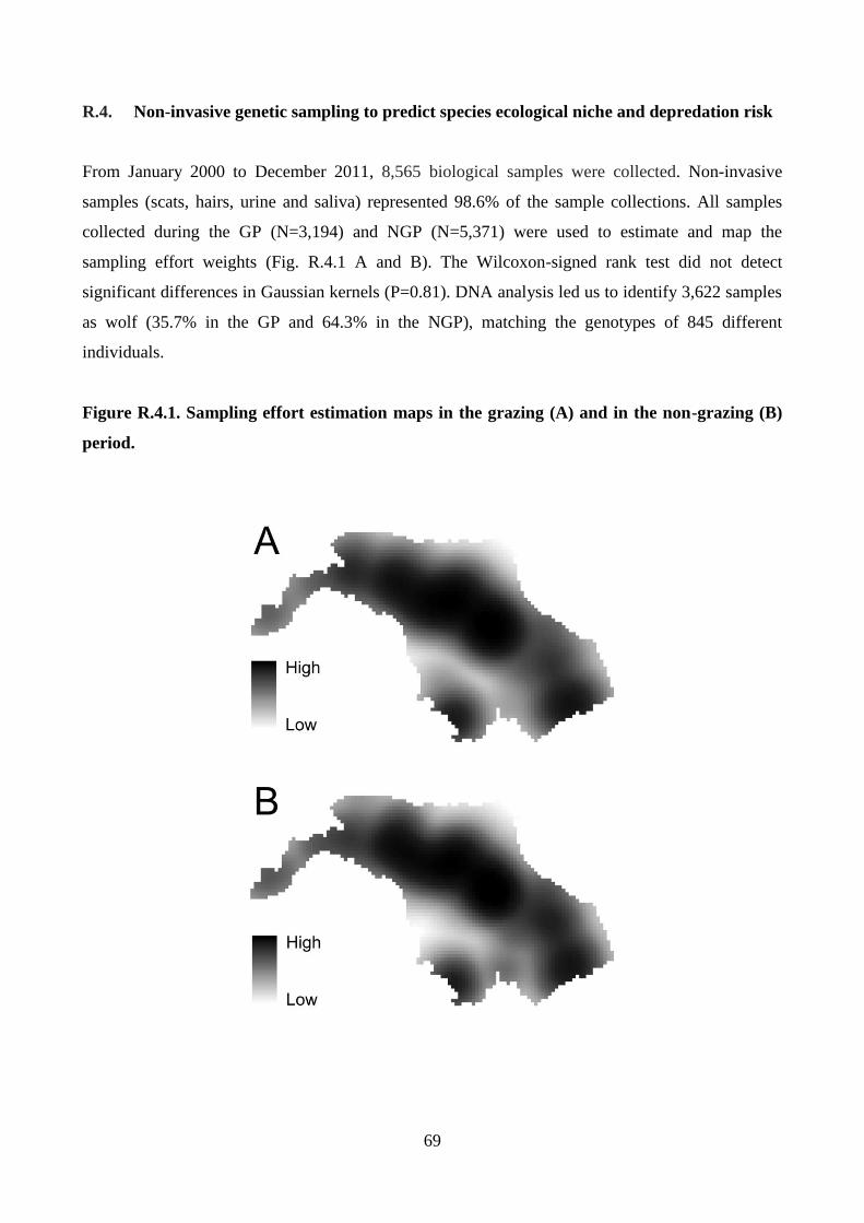
69

R.4. Non-invasive genetic sampling to predict species ecological niche and depredation risk

From January 2000 to December 2011, 8,565 biological samples were collected. Non-invasive

samples (scats, hairs, urine and saliva) represented 98.6% of the sample collections. All samples

collected during the GP (N=3,194) and NGP (N=5,371) were used to estimate and map the

sampling effort weights (Fig. R.4.1 A and B). The Wilcoxon-signed rank test did not detect

significant differences in Gaussian kernels (P=0.81). DNA analysis led us to identify 3,622 samples

as wolf (35.7% in the GP and 64.3% in the NGP), matching the genotypes of 845 different

individuals.

Figure R.4.1. Sampling effort estimation maps in the grazing (A) and in the non-grazing (B)

period.

70

Wolf samples collected during the GP (N=1,292) and NGP (N= 2,330) were used in the GNESFA.

During both the GP and the NGP, the eigenvalue diagrams of FANTER indicated a break after the

first and before the last eigenvalue (Fig. R.4.2). In the GP, the first component (F1=5.72) was

mainly correlated to meadows (R=0.65), altitude (R=0.53), mixed woods (R=0.32), roughness

(R=0.32) slope (R=0.32), sheep density (R=0.16), and cultivated fields (R=-0.33) while the last one

(L1=0.02) was mainly related to water courses (R=-0.73), artificial surfaces (R=0.67), human

density (R=-0.38) and wild boar density (R=0.22). In the NGP, the variables manly related to the

first component (F1=5.51) were beech wood cover (R=0.88), altitude (R=0.47) and hunter density

(R=-0.14), whereas the last component (L1=0.01) was mainly related to distance and presence of

artificial surfaces (R=-0.37 and R=0.82, respectively), flat terrains (R=0.60), human density

(R=0.46) and North exposition (R=-0.37). In the GP, the eigenvalue of the MADIFA indicated a

break after the second eigenvalue (Fig. R.4.2) and therefore the first two components were

considered (F1= 34.38; F2=24.78). Also in this case a similar configuration of the eigenvalues was

recorded during the NGP (F1= 30.67; F2=22.97; Fig. 3). MADIFA results highlighted correlations

between the first axes and slope (R=0.46), roughness (R=0.44), North-Western exposure (0.37),

altitude (R=0.37), meadows (R=0.33), distance and presence of artificial surfaces (R=0.48 and R=-

0.92, respectively), habitat diversity (R=0.25), sheep density (R=0.22) flat terrains (R=-0.54), and

human density (R=-0.52). The second component was mainly related to water course (R=0.99), flat

terrains (R=0.34) and wild boar density (R=0.19). During the NGP similar relations between

variables and components were found except for the beech woods (R=0.36) and the meadows

(R=0.16). ENFA showed breaks after the first specialization eigenvalue both in the GP and in the

NGP (Fig. R.4.2). Thus, only marginality and the first specialization components were considered.

In the GP marginality (M=8.47) was mainly related to meadows (R=0.45), altitude (R=0.41), terrain

roughness (R=0.31) habitat diversity (R=0.21), red deer density (R=0.18) and cultivated fields (R=-

0.31), while the specialization factor (S=29.37) was related to artificial surfaces (R=0.61), terrain

roughness (R=0.37), wild boar density (R=0.18), wild prey diversity (R=0.17) and water courses

(R=-0.59). A similar pattern was observed in the NGP (M=8.46; S1=26.46; Fig. R.4.2), with a

higher relation between marginality and beech woods (R=0.44) than with meadows (R=0.35).

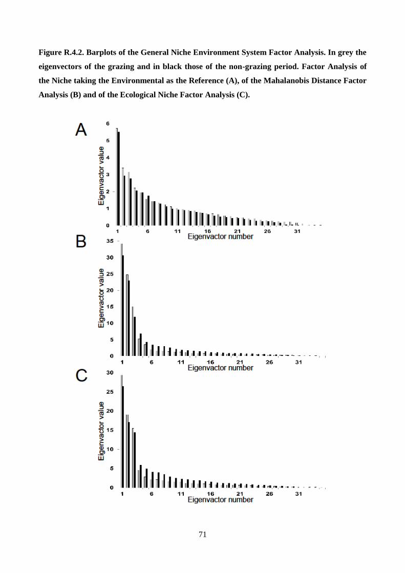
71

Figure R.4.2. Barplots of the General Niche Environment System Factor Analysis. In grey the

eigenvectors of the grazing and in black those of the non-grazing period. Factor Analysis of

the Niche taking the Environmental as the Reference (A), of the Mahalanobis Distance Factor

Analysis (B) and of the Ecological Niche Factor Analysis (C).

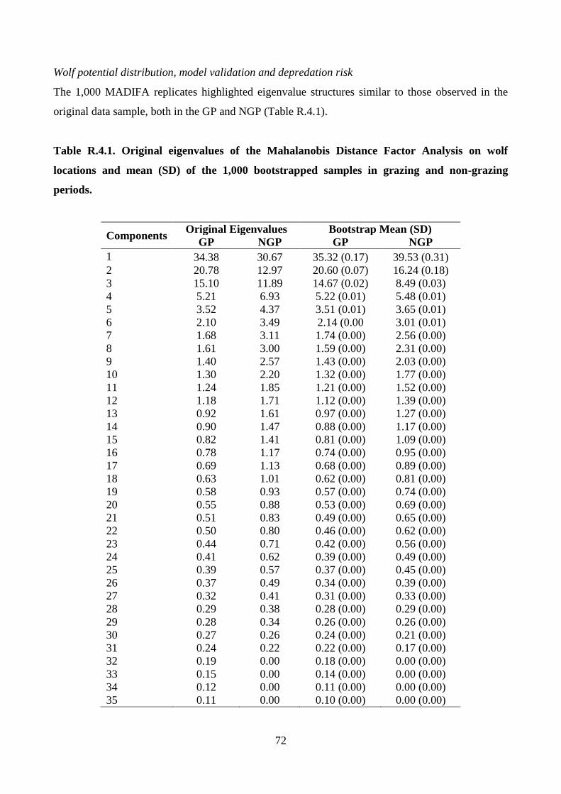
72

Wolf potential distribution, model validation and depredation risk

The 1,000 MADIFA replicates highlighted eigenvalue structures similar to those observed in the

original data sample, both in the GP and NGP (Table R.4.1).

Table R.4.1. Original eigenvalues of the Mahalanobis Distance Factor Analysis on wolf

locations and mean (SD) of the 1,000 bootstrapped samples in grazing and non-grazing

periods.

Components Original Eigenvalues Bootstrap Mean (SD)

GP NGP GP NGP

1 34.38 30.67 35.32 (0.17) 39.53 (0.31)

2 20.78 12.97 20.60 (0.07) 16.24 (0.18)

3 15.10 11.89 14.67 (0.02) 8.49 (0.03)

4 5.21 6.93 5.22 (0.01) 5.48 (0.01)

5 3.52 4.37 3.51 (0.01) 3.65 (0.01)

6 2.10 3.49 2.14 (0.00 3.01 (0.01)

7 1.68 3.11 1.74 (0.00) 2.56 (0.00)

8 1.61 3.00 1.59 (0.00) 2.31 (0.00)

9 1.40 2.57 1.43 (0.00) 2.03 (0.00)

10 1.30 2.20 1.32 (0.00) 1.77 (0.00)

11 1.24 1.85 1.21 (0.00) 1.52 (0.00)

12 1.18 1.71 1.12 (0.00) 1.39 (0.00)

13 0.92 1.61 0.97 (0.00) 1.27 (0.00)

14 0.90 1.47 0.88 (0.00) 1.17 (0.00)

15 0.82 1.41 0.81 (0.00) 1.09 (0.00)

16 0.78 1.17 0.74 (0.00) 0.95 (0.00)

17 0.69 1.13 0.68 (0.00) 0.89 (0.00)

18 0.63 1.01 0.62 (0.00) 0.81 (0.00)

19 0.58 0.93 0.57 (0.00) 0.74 (0.00)

20 0.55 0.88 0.53 (0.00) 0.69 (0.00)

21 0.51 0.83 0.49 (0.00) 0.65 (0.00)

22 0.50 0.80 0.46 (0.00) 0.62 (0.00)

23 0.44 0.71 0.42 (0.00) 0.56 (0.00)

24 0.41 0.62 0.39 (0.00) 0.49 (0.00)

25 0.39 0.57 0.37 (0.00) 0.45 (0.00)

26 0.37 0.49 0.34 (0.00) 0.39 (0.00)

27 0.32 0.41 0.31 (0.00) 0.33 (0.00)

28 0.29 0.38 0.28 (0.00) 0.29 (0.00)

29 0.28 0.34 0.26 (0.00) 0.26 (0.00)

30 0.27 0.26 0.24 (0.00) 0.21 (0.00)

31 0.24 0.22 0.22 (0.00) 0.17 (0.00)

32 0.19 0.00 0.18 (0.00) 0.00 (0.00)

33 0.15 0.00 0.14 (0.00) 0.00 (0.00)

34 0.12 0.00 0.11 (0.00) 0.00 (0.00)

35 0.11 0.00 0.10 (0.00) 0.00 (0.00)

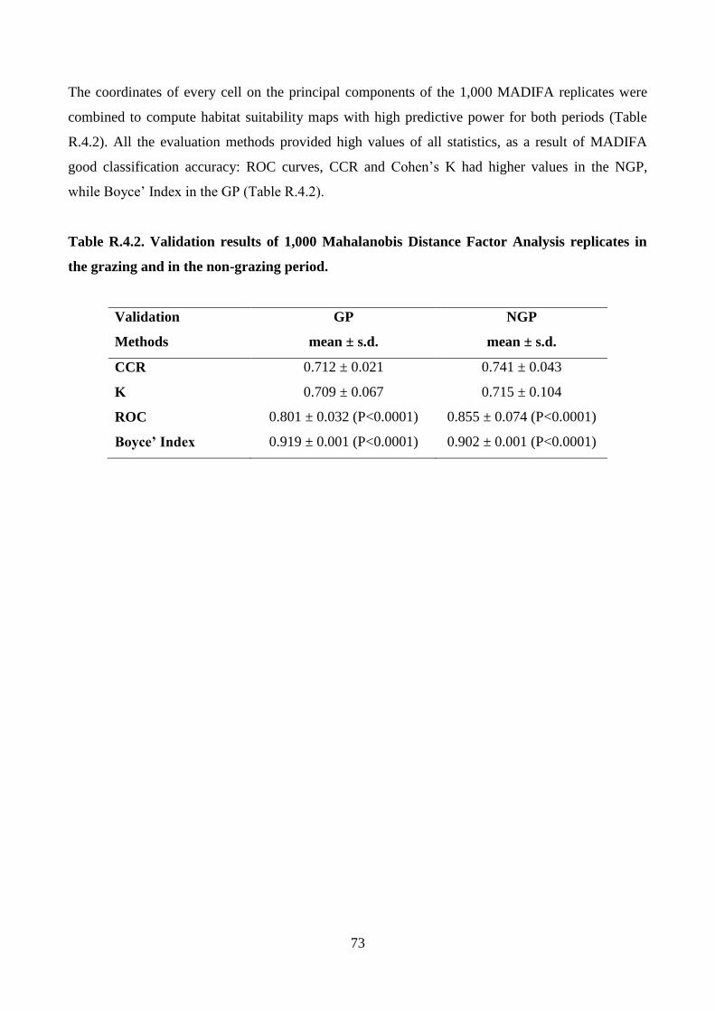
73

The coordinates of every cell on the principal components of the 1,000 MADIFA replicates were

combined to compute habitat suitability maps with high predictive power for both periods (Table

R.4.2). All the evaluation methods provided high values of all statistics, as a result of MADIFA

good classification accuracy: ROC curves, CCR and Cohen’s K had higher values in the NGP,

while Boyce’ Index in the GP (Table R.4.2).

Table R.4.2. Validation results of 1,000 Mahalanobis Distance Factor Analysis replicates in

the grazing and in the non-grazing period.

Validation

Methods

GP

mean ± s.d.

NGP

mean ± s.d.

CCR 0.712 ± 0.021 0.741 ± 0.043

K 0.709 ± 0.067 0.715 ± 0.104

ROC 0.801 ± 0.032 (P<0.0001) 0.855 ± 0.074 (P<0.0001)

Boyce’ Index 0.919 ± 0.001 (P<0.0001) 0.902 ± 0.001 (P<0.0001)

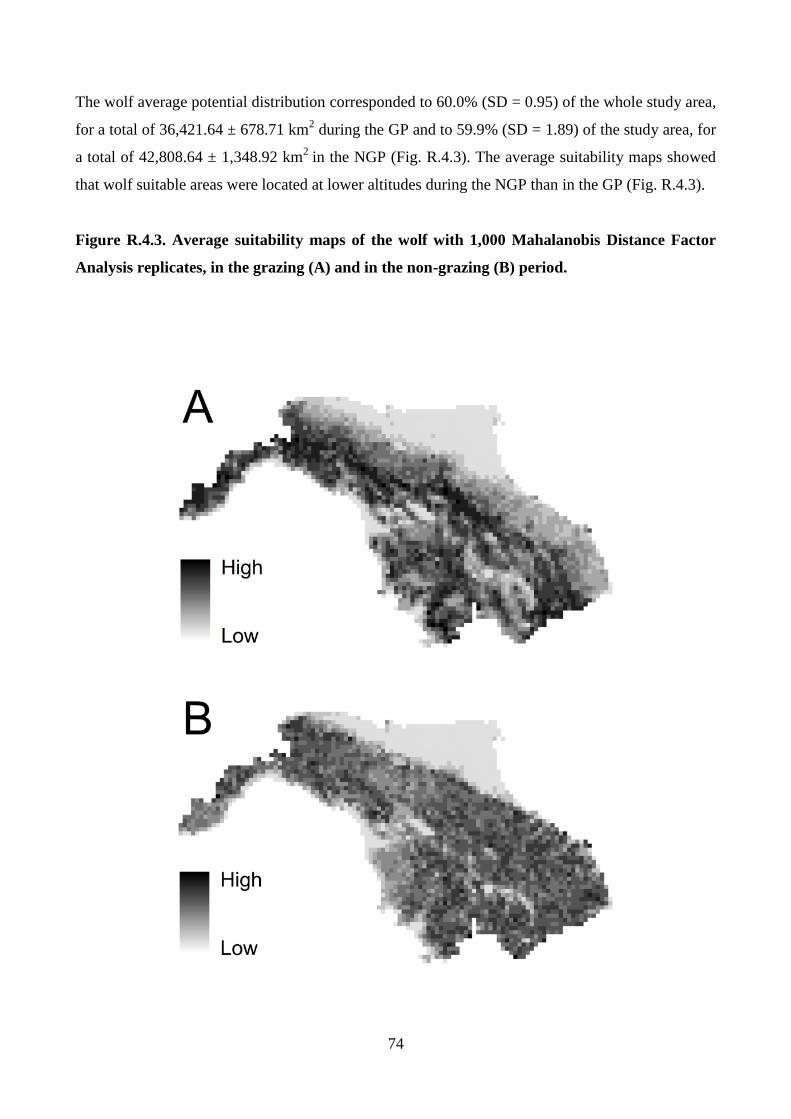
74

The wolf average potential distribution corresponded to 60.0% (SD = 0.95) of the whole study area,

for a total of 36,421.64 ± 678.71 km2 during the GP and to 59.9% (SD = 1.89) of the study area, for

a total of 42,808.64 ± 1,348.92 km2

in the NGP (Fig. R.4.3). The average suitability maps showed

that wolf suitable areas were located at lower altitudes during the NGP than in the GP (Fig. R.4.3).

Figure R.4.3. Average suitability maps of the wolf with 1,000 Mahalanobis Distance Factor

Analysis replicates, in the grazing (A) and in the non-grazing (B) period.

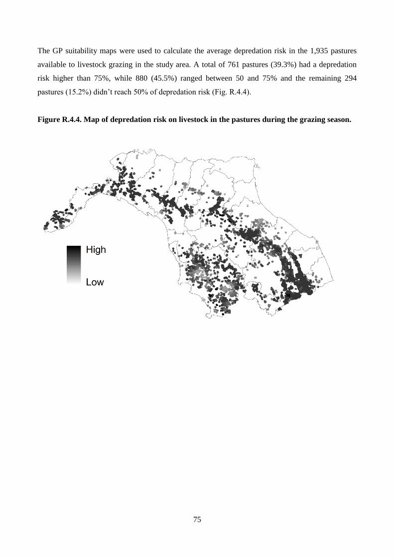
75

The GP suitability maps were used to calculate the average depredation risk in the 1,935 pastures

available to livestock grazing in the study area. A total of 761 pastures (39.3%) had a depredation

risk higher than 75%, while 880 (45.5%) ranged between 50 and 75% and the remaining 294

pastures (15.2%) didn’t reach 50% of depredation risk (Fig. R.4.4).

Figure R.4.4. Map of depredation risk on livestock in the pastures during the grazing season.

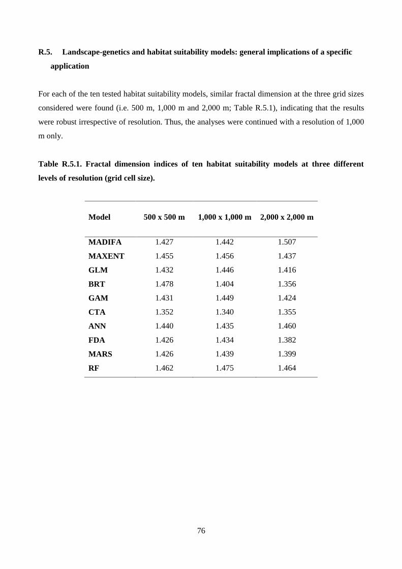
76

R.5. Landscape-genetics and habitat suitability models: general implications of a specific

application

For each of the ten tested habitat suitability models, similar fractal dimension at the three grid sizes

considered were found (i.e. 500 m, 1,000 m and 2,000 m; Table R.5.1), indicating that the results

were robust irrespective of resolution. Thus, the analyses were continued with a resolution of 1,000

m only.

Table R.5.1. Fractal dimension indices of ten habitat suitability models at three different

levels of resolution (grid cell size).

Model 500 x 500 m 1,000 x 1,000 m 2,000 x 2,000 m

MADIFA 1.427 1.442 1.507

MAXENT 1.455 1.456 1.437

GLM 1.432 1.446 1.416

BRT 1.478 1.404 1.356

GAM 1.431 1.449 1.424

CTA 1.352 1.340 1.355

ANN 1.440 1.435 1.460

FDA 1.426 1.434 1.382

MARS 1.426 1.439 1.399

RF 1.462 1.475 1.464

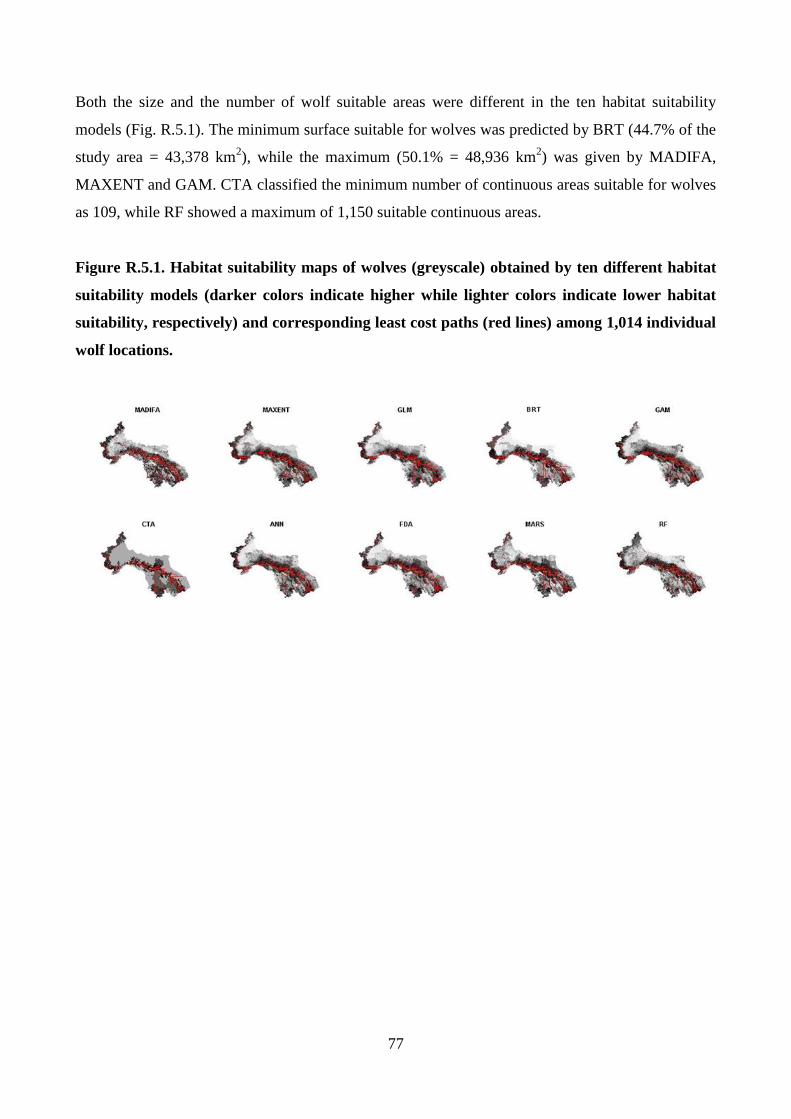
77

Both the size and the number of wolf suitable areas were different in the ten habitat suitability

models (Fig. R.5.1). The minimum surface suitable for wolves was predicted by BRT (44.7% of the

study area = 43,378 km2), while the maximum (50.1% = 48,936 km

2) was given by MADIFA,

MAXENT and GAM. CTA classified the minimum number of continuous areas suitable for wolves

as 109, while RF showed a maximum of 1,150 suitable continuous areas.

Figure R.5.1. Habitat suitability maps of wolves (greyscale) obtained by ten different habitat

suitability models (darker colors indicate higher while lighter colors indicate lower habitat

suitability, respectively) and corresponding least cost paths (red lines) among 1,014 individual

wolf locations.

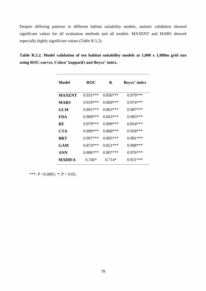
78

Despite differing patterns in different habitat suitability models, statistic validation showed

significant values for all evaluation methods and all models. MAXENT and MARS showed

especially highly significant values (Table R.5.2).

Table R.5.2. Model validation of ten habitat suitability models at 1,000 x 1,000m grid size

using ROC-curves, Cohen’ kappa(K) and Boyce’ index.

Model ROC K Boyce’ index

MAXENT 0.931*** 0.856*** 0.979***

MARS 0.919*** 0.869*** 0.974***

GLM 0.891*** 0.863*** 0.987***

FDA 0.908*** 0.843*** 0.983***

RF 0.979*** 0.899*** 0.854***

CTA 0.899*** 0.868*** 0.958***

BRT 0.907*** 0.805*** 0.981***

GAM 0.874*** 0.821*** 0.988***

ANN 0.886*** 0.807*** 0.976***

MADIFA 0.746* 0.714* 0.931***

***: P <0.0001; *: P < 0.05.

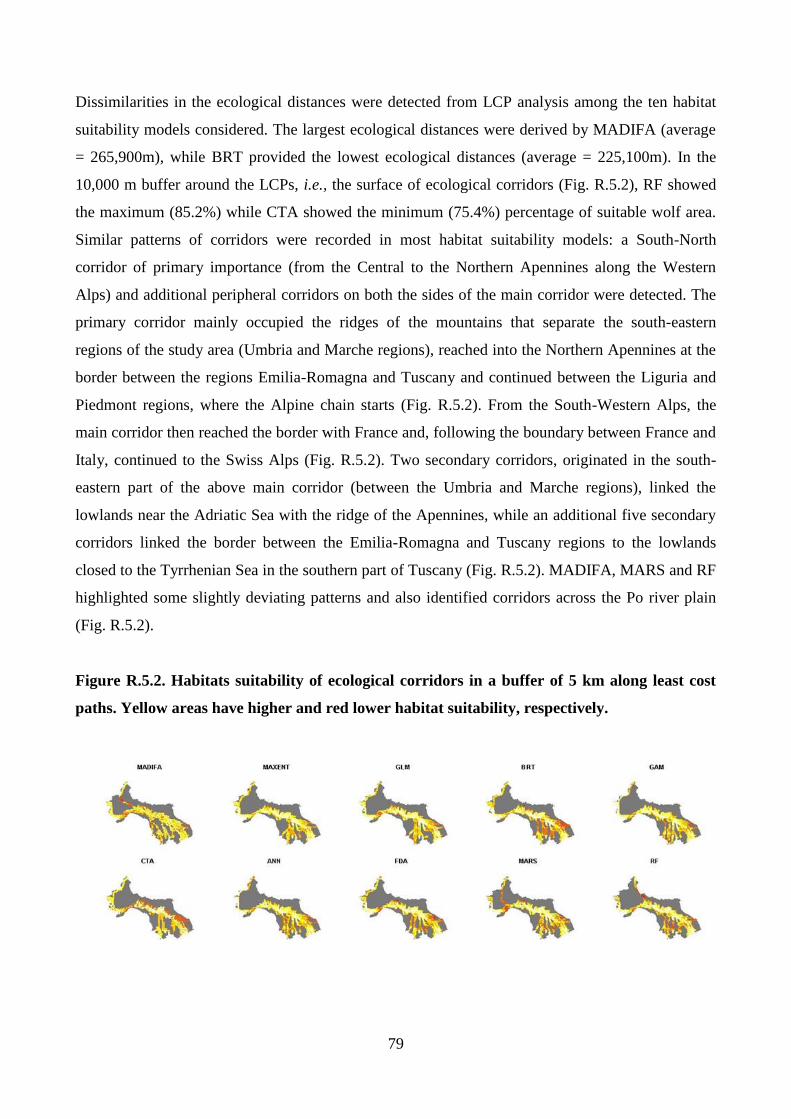
79

Dissimilarities in the ecological distances were detected from LCP analysis among the ten habitat

suitability models considered. The largest ecological distances were derived by MADIFA (average

= 265,900m), while BRT provided the lowest ecological distances (average = 225,100m). In the

10,000 m buffer around the LCPs, i.e., the surface of ecological corridors (Fig. R.5.2), RF showed

the maximum (85.2%) while CTA showed the minimum (75.4%) percentage of suitable wolf area.

Similar patterns of corridors were recorded in most habitat suitability models: a South-North

corridor of primary importance (from the Central to the Northern Apennines along the Western

Alps) and additional peripheral corridors on both the sides of the main corridor were detected. The

primary corridor mainly occupied the ridges of the mountains that separate the south-eastern

regions of the study area (Umbria and Marche regions), reached into the Northern Apennines at the

border between the regions Emilia-Romagna and Tuscany and continued between the Liguria and

Piedmont regions, where the Alpine chain starts (Fig. R.5.2). From the South-Western Alps, the

main corridor then reached the border with France and, following the boundary between France and

Italy, continued to the Swiss Alps (Fig. R.5.2). Two secondary corridors, originated in the south-

eastern part of the above main corridor (between the Umbria and Marche regions), linked the

lowlands near the Adriatic Sea with the ridge of the Apennines, while an additional five secondary

corridors linked the border between the Emilia-Romagna and Tuscany regions to the lowlands

closed to the Tyrrhenian Sea in the southern part of Tuscany (Fig. R.5.2). MADIFA, MARS and RF

highlighted some slightly deviating patterns and also identified corridors across the Po river plain

(Fig. R.5.2).

Figure R.5.2. Habitats suitability of ecological corridors in a buffer of 5 km along least cost

paths. Yellow areas have higher and red lower habitat suitability, respectively.

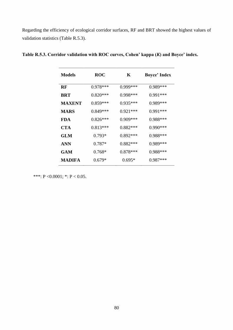
80

Regarding the efficiency of ecological corridor surfaces, RF and BRT showed the highest values of

validation statistics (Table R.5.3).

Table R.5.3. Corridor validation with ROC curves, Cohen’ kappa (K) and Boyce’ index.

Models ROC K Boyce’ Index

RF 0.978*** 0.999*** 0.989***

BRT 0.820*** 0.998*** 0.991***

MAXENT 0.859*** 0.935*** 0.989***

MARS 0.849*** 0.921*** 0.991***

FDA 0.826*** 0.909*** 0.988***

CTA 0.813*** 0.882*** 0.990***

GLM 0.793* 0.892*** 0.988***

ANN 0.787* 0.882*** 0.989***

GAM 0.768* 0.878*** 0.988***

MADIFA 0.679* 0.695* 0.987***

***: P <0.0001; *: P < 0.05.

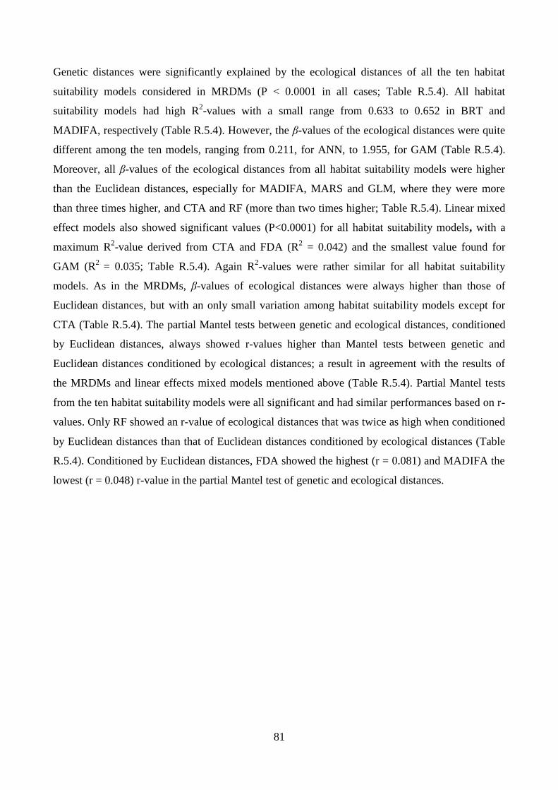
81

Genetic distances were significantly explained by the ecological distances of all the ten habitat

suitability models considered in MRDMs (P < 0.0001 in all cases; Table R.5.4). All habitat

suitability models had high R2-values with a small range from 0.633 to 0.652 in BRT and

MADIFA, respectively (Table R.5.4). However, the β-values of the ecological distances were quite

different among the ten models, ranging from 0.211, for ANN, to 1.955, for GAM (Table R.5.4).

Moreover, all β-values of the ecological distances from all habitat suitability models were higher

than the Euclidean distances, especially for MADIFA, MARS and GLM, where they were more

than three times higher, and CTA and RF (more than two times higher; Table R.5.4). Linear mixed

effect models also showed significant values (P<0.0001) for all habitat suitability models, with a

maximum R2-value derived from CTA and FDA (R

2 = 0.042) and the smallest value found for

GAM (R2

= 0.035; Table R.5.4). Again R2-values were rather similar for all habitat suitability

models. As in the MRDMs, β-values of ecological distances were always higher than those of

Euclidean distances, but with an only small variation among habitat suitability models except for

CTA (Table R.5.4). The partial Mantel tests between genetic and ecological distances, conditioned

by Euclidean distances, always showed r-values higher than Mantel tests between genetic and

Euclidean distances conditioned by ecological distances; a result in agreement with the results of

the MRDMs and linear effects mixed models mentioned above (Table R.5.4). Partial Mantel tests

from the ten habitat suitability models were all significant and had similar performances based on r-

values. Only RF showed an r-value of ecological distances that was twice as high when conditioned

by Euclidean distances than that of Euclidean distances conditioned by ecological distances (Table

R.5.4). Conditioned by Euclidean distances, FDA showed the highest (r = 0.081) and MADIFA the

lowest (r = 0.048) r-value in the partial Mantel test of genetic and ecological distances.

82

Table R.5.4. Landscape genetic analysis with multiple regression on distance matrices

(MRDM), linear mixed effects models (LMEM) and partial Mantel tests (PMT). R2values for

full models and β-values for ecological and Euclidean distances (EcDs and EuDs, respectively)

in MRDM and LMEM have been shown. R-values for PMT of ecological and Euclidean

models are also given.

MRDM LMEM PMT

Model R2

EcDs

β

EuDs

Β R

2

EcDs

β

EuDs

β

EcDs| EuDs

r

EuDs| EcDs

r

MADIFA 0.652* 0.797* 0.201* 0.037 1.053* 1.049* 0.048* 0.025*

MARS 0.643* 0.491* 0.146* 0.039 0.932* 0.761* 0.062* 0.032*

GLM 0.640* 0.404* 0.132* 0.039 0.945* 0.763* 0.068* 0.037*

CTA 0.637* 0.317* 0.119* 0.042 1.417* 0.554* 0.078* 0.049*

RF 0.635* 0.245* 0.106* 0.038 1.033* 0.841* 0.058* 0.028*

GAM 0.634* 1.955* 0.993* 0.035 1.141* 1.029* 0.075* 0.046*

ANN 0.634* 0.211* 0.102* 0.041 1.478* 1.401* 0.078* 0.049*

FDA 0.634* 1.564* 0.935* 0.042 1.311* 1.104* 0.081* 0.048*

MAXENT 0.633* 1.796* 0.961* 0.038 1.278* 1.183* 0.078* 0.049*

BRT 0.633* 0.815* 0.748* 0.041 1.418* 1.212* 0.077* 0.045*

***: P <0.0001.

83

DISCUSSION

Wolf diet was markedly different between geographic areas, in particular for wild ungulates and

livestock. The studies carried out in the south-central Apennines showed an important use of

livestock, whereas in the northern Apennines wild ungulate occurrence increases while in the

western Alps the use of livestock was negligible and the diet was characterized by large wild

herbivores. These differences agree with changes of abundance and density of wild ungulate

populations in the Italian peninsula. Several researchers have found a nearly complete dependence

of wolves on wild ungulate populations in several European study areas, distributed from North-

East to South-West (Okarma 1995). In Finland elk (Alces alces) is the primary prey of wolves;

reindeer is, however, an important part of wolf diet in summer, autumn and early winter, when their

remains comprise roughly 20–50% of all food items identified in wolf scats (Kojola et al. 2004).

Also in Sweden, elk is the dominant prey species reaching 95.6% of biomass ingested (Sand et al.

2008). In Poland red deer is the main prey of wolves, followed by wild boar and roe deer (Smietana

and Klimek 1993; Jedrzejewski et al. 2002). In Germany a study carried out in an area recently

colonized by wolves showed that wild ungulates were 99% of wolf diet in biomass (Ansorge et al.

2006). In the Mercantour National Park (French Western Alps) wild ungulates amounted up to 97 %

of the wolf diet (Poulle et al. 1997). In some areas of the Iberian Peninsula wolves feed mainly on

wild ungulates (Cuesta et al. 1991; Nores et al. 2008; Barja 2009). In Italy, wild herbivores

represent the bulk of wolf diet in the Northern Apennines and in the Western Alps, reaching up to

90% of frequency of occurrence and mean percent volume (Matteucci 1992; Mattioli et al. 1995,

2004; Meriggi et al. 1996; Capitani et al. 2004; Gazzola et al. 2005; Meriggi et al. 2011). However,

in several areas of the Mediterranean range of wolves in recent times a high occurrence of livestock

has also been recorded (Ragni et al. 1996; Schenone et al. 2004; Migli et al. 2005; Meriggi et al.

2011).

Richness and abundance of wild ungulate communities in Italy follow a north-south gradient, from

the Alps to the southern Apennines where some species (i. e. red and roe deer) are localized and at

low densities (Pedrotti et al. 2001, Apollonio 2004). Moreover livestock abundance and husbandry

method, as well as the proportions of different species, show great differences from the Alps to the

Apennines and in the different parts of the Apennine chain, with consequences on domestic prey

availability and, in turn on wolf feeding habits (ISTAT 2003).

Wolf diet in the three geographic areas (Western Alps, Northern and South-Central Apennines)

differed also in the specific composition of the wild ungulate component; in particular differences

84

were recorded for wild boar, roe deer, red deer, and chamois. The use of wild boars increased from

the south-central to the northern Apennines and decreased markedly in the western Alps; the

occurrence of roe and red deer in wolf diet increased in a regular fashion from south to north,

reaching the maximum in the western Alps study areas. Finally chamois occurred in the wolf diet

only in the Alps if, excluding a limited occurrence of Apennine chamois (Rupicapra pyrenaica

ornata) in a study carried out in the Abruzzo National Park (Patalano and Lovari 1993); this was

because of the lack of chamois population in the Apennines, apart a few areas in which there have

been no studies carried out. The use of wild ungulate species by wolves seems related to their

availability at range level, but locally there can be exceptions because of behavioral characteristics

and accessibility of the different species (Huggard 1993, Meriggi and Lovari 1996, Meriggi et al.

1996). In particular, in some areas wolves select species that live in large groups, are easy to detect

and on which predator can carry out targeted hunting, as opposed to other solitary species for which

predation rates mainly depend on encounter rate (Huggard 1993, Meriggi et al. 1996, Jedrzejewski

et al. 2002). In Italy wild boar is the most important prey species unlike other Palearctic areas where

red deer is the key species for wolves and wild boar is usually the second species (Reig and

Jedrzejewski 1988, Jedrzejewski et al. 1992, Śmietana and Klimek 1993, Jedrzejewska et al. 1994,

Okarma 1995, Meriggi and Lovari 1996, Gula 2004). The high use of wild boar in Italy can be

explained as follow: i) the species lives in large groups easily detectable by a predator, ii) births

occur all year round, particularly in spring-summer (Meriggi et al. 1988), iii) sub-adults leave

matriarchal groups in coincidence with the new births, so becoming easier to prey upon (Heck and

Raschke 1980, Mauget et al. 1984).

The second species in importance in wolf diets in Italy was the roe deer, widespread and abundant

particularly in the northern Apennines and in the Alps; roe deer, when present at high density, can

be a profitable prey for wolves because of the high encounter rate and low handling time (Curio

1976, Huggard 1993, Meriggi et al. 1996, Meriggi and Lovari 1996, Jedrzejewski et al. 2002).

Moreover, from north American and European studies it has been noted that the size of wolf prey is

related to the pack size (Thurber and Peterson 1993, Schmidt and Mech 1997, Hayes et al. 2000,

Jedrzejewski et al. 2002); in Europe and particularly in the Mediterranean region, wolf packs are

family groups of few individuals, usually from 2 to 4 and they rarely exceed 6 members (Boitani

1992, Boitani and Ciucci 1993, Meriggi et al. 1996, Schenone et al. 2004). As a consequence,

predation upon roe deer can satisfy food requirements of small packs, also allowing complete

consumption of prey in a short time (Jedrzejewski et al. 2002).

Red deer was the third species in order of importance in the wolf diet and the fourth after the Fallow

deer in the northern Apennines. Also in the western Alps, where 37.4% of the Italian population of

85

red deer is present and where wild boar is limited to small and fragmented populations, red deer is

the third most used species after roe deer and chamois. In western Alps, the chamois is the most

abundant ungulate, nevertheless, it represents the second species in the wolf diet. This can be due to

a better adaptation to snow conditions and steeper topography of Alpine valley leading to a low

profitability of this prey species. Moreover the presence of pastures interspersed with conifer forests

at low altitude in western Alps, could contribute to an easy approach by wolves to their main prey

(roe deer and red deer) during winter season (Gazzola et al. 2007).

In Italy wild ungulate communities have more species with higher population densities than other

North European and North American situations; this leads to a greater flexibility in prey choice by

wolves to satisfy food requirements of pack members in different seasons (Okarma 1985,

Jedrzejewski et al. 2002, Peterson and Ciucci 2003, Melis et al. 2006, 2009).

The analysis evidenced an increasing trend of wild ungulate use by wolves not only at a national,

but also at regional and local scales. If the trend had been detected only at national level it could

have been the case that it was influenced by the increase in information on wolf feeding ecology in

the areas recently re-colonized by the species (i.e. the northern Apennines and the western Alps),

where wild ungulate populations are more abundant and communities have a greater richness

(Apollonio 2004, Gazzola et al. 2007). Moreover the use of wild ungulates could be influenced by

the difference in livestock availability and husbandry methods among geographic areas. However,

the increased occurrence of wild ungulate in wolf diet in the same region or study areas in

subsequent times is possibly dependent on the increase of prey populations (Ragni et al. 1985,

1996, Meriggi et al. 1991, 1996, Gilio 2001, Schenone et al. 2004, Meriggi and Schenone 2007). In

particular in the study area in the province of Genova the occurrence of wild ungulates in the wolf

diet ranged from 0% in 1987 to 70% in 2004; in the same period the hunting bags of wild boars in

the area occupied by wolves increased from 606 to 2067 heads and roe and fallow deer counts

showed marked increases of population densities (roe deer: from 21 per km2 in 1997 to 53.4 per

km2 in 2005; Fallow deer: from 0.7 per km

2 in 1994 to 20.2 per km

2 in 2005. Genoa Province

Wildlife Service unpublished data). Likewise, in the Pollino National Park (southern Italy) an initial

study on wolf diet found an occurrence of wild ungulates of 16% (Borelli 1999), whereas

afterwards wild ungulates increased up to 60.4% (Ciucci et al. 2004). Also in the Umbria region

(central Italy) the frequency of occurrence of wild ungulates increased in a ten year period from 0%

to 26% (Ragni et al. 1985, Ragni et al. 1996).

The species of wild ungulates for which significant trends were found included wild boar, roe deer,

red deer, and chamois. The use of wild boar by wolves increased until the mid-nineties whereupon

it decreased; this trend could be due on one hand to the shift of diet studies in the recently colonized

86

areas of the western Alps where population densities of wild boars are lower than in the Apennines

(Pedrotti et al. 2001, Apollonio 2004), and on the other hand to the increase of the use of other wild

ungulate species such as the roe deer. Roe deer occurrence increased linearly in the diet of wolves,

showing that this specie could be a highly profitable prey for wolves. As for red deer and chamois,

the marked increase in the wolf diet in recent years is mostly due to the contribution of the studies

carried out in Alpine areas.

Together with the increase of wild ungulates, a significant reduction of livestock in the wolf diet

resulted; the negative and highly significant relationship between the two frequencies of occurrence

suggests that when wolves can choose between the two prey categories, they may prefer wild prey.

This result agrees with the findings of Meriggi and Lovari (1996) for the Mediterranean area, and it

seems a constant of the predatory behavior of wolves in Europe, even if shifts from this model can

be evidenced at a local scale (Okarma 1995, Cozza et al. 1996, Poulle et al. 1997). According to the

Optimal Foraging theory (Stephen and Krebs 1986, Huges 1993), wolves would prefer domestic

herbivores instead of wild ones because of: i) their highly clumped distribution in few and known

pastures (reduction of search time and greater opportunity of prey choice), ii) their low capability of

detecting and avoiding predators due to domestication (greater probability of successfully attacking

the prey), iii) their low efficiency of escape behavior (reduction of attack failures). However,

disturbance by man can make domestic prey less profitable than wild ones; in particular wolves risk

being killed and they have a high probability of not exploiting carcasses to the full (Meriggi et al.

1996). As with the frequency of occurrence of livestock, also diet breadth was negatively and

significantly related to the occurrence of wild ungulates; however this relationship shows an

increase of diet breadth up to medium values of wild ungulate occurrence (40-50%), after which it

then drops. This result suggests that when wild herbivores are scarce, wolves are forced to use

alternative food sources (e.g. small mammals, lagomorphs, fruits, and garbage). In southern Europe

wolves tend to prey upon wild ungulates, but locally they can adopt a less specialized diet, in order

to survive in areas with low availability of both wild and domestic large herbivores (Okarma 1995,

Meriggi and Lovari 1996, Meriggi et al. 1996, Peterson and Ciucci 2003).

By considering the seasonal effects on the trophic ecology of the carnivore significant seasonal

changes only for livestock and small mammals were recorded; in particular livestock was more used

in summer and early autumn, when it reaches its maximum abundance after the births on pastures,

and small mammals were preyed upon mainly in summer when their abundance increases because

of reproduction (Kikkawa 1964; Bergstedt 1965; Montgomery 1989; Giordano and Meriggi 2009).

A low occurrence of livestock in wolf diet, mainly in the grazing season, is usually linked to the

presence of a rich and diverse wild ungulate community that lives in the Northern Apennines.

87

Reduced availability of large wild prey can cause an increase of livestock depredation (Fritts and

Mech, 1981; Meriggi and Lovari 1996; Gazzola et al. 2008, Meriggi et al. 2011). In the Northern

Apennines wolves select wild boars particularly in spring, summer, and winter, whereas roe deer

and fallow deer are used as available in summer and autumn, and avoided in spring and winter. Red

deer are always avoided. These findings are in agreement with the results of other researches carried

out on wolf feeding ecology in the Northern Apennines (Meriggi et al. 1996; Capitani et al. 2004;

Mattioli et al. 2004), but not with other studies in Europe and in the Western Alps (Jedrzejewski et

al. 2002; Kojola et al. 2004; Gazzola et al. 2005, 2007; Ansorge 2006; Sand et al. 2008). The higher

selection of wild boar was found in spring and summer can be due to the peak of births in these

seasons, and to the fact that sub-adults leave matriarchal groups in coincidence with the new births,

so becoming easier to prey upon (Heck and Raschke 1980, Mauget et al. 1984; Meriggi et al. 1996;

Capitani et al. 2004). Moreover, it seems that wild boars are particularly preyed upon in areas with

severe winters and deep snow cover, which could be an explanation for the increase of the use of

this species in winter (Okarma et al. 1995; Capitani et al. 2004). In a period of 20 years the diet of

wolves in in the Northern Apennines changed markedly, with an increase of wild ungulate use and a

decrease of livestock and other food categories that can be considered alternative nourishment by

wolves in areas where large herbivores are lacking, or in periods of scarcity of preferred prey. These

differences between the two study periods agree with changes of abundance and density of wild

ungulate populations in the Northern Apennines, and mirror large scale changes in wolf diet

recorded in Southern Europe in the period corresponding to wolf population recovery and wolf

range enlargement (Meriggi and Lovari 1996; Meriggi et al. 2011). Wild boars and roe deer were

present in the study area also in 1988-90, the former species already being widespread at that time

and the latter being rare; their abundance dramatically increased over twenty years as demonstrated

by the number of hunted wild boars and by the results from roe deer monitoring. Fallow deer

abundance has probably slightly increased since the late eighties but this species is still at low

density, occupying 48.8% of the study area. Red deer were absent from the study area at the

beginning of the nineties, and the present population originated from a few individuals that escaped

from an enclosure; now red deer range represents 17.4% of the study area. The patterns of

distribution and the trend of density of the wild ungulate community recorded in the study area can

explain the marked increase of occurrences of wild boar and roe deer in wolf diet and of the slight

increase of fallow and red deer.

Once analysed the impacts on the wild and domestic preys, the population structure of wolf was

investigated. Molecular identifications of DNA samples noninvasively collected over 9 years led us

to obtain the most complete description to date of the distribution range and demographic structure

88

of a wolf population living in a wide area of the Apennine Mountains. 414 distinct wolf genotypes

were detected (plus 88 dogs and 16 wolf3dog hybrids) in a population that is estimated to average

187 ± 78 wolves (data extrapolated from results described by Caniglia et al. 2012). 42 packs were

located and fully reconstructed the genealogies for 26 of them. Through the identification of

resident wolves in packs the number and destiny of dispersers was inferred and a rough estimate of

floaters was obtained. The wealth of information gathered by noninvasive genetic sampling projects

of this kind could have not been obtained with any other monitoring tool at a comparable cost

(Galaverni et al. 2012). This study relied on molecular identifications of samples that were collected

year-round by trained collaborators. Although accurate selection of fresh scat samples was not

guaranteed, genotyping success was comparable to values reported in other noninvasive genetic

studies of carnivores (e.g., 14–63% in otters, 54% in wolverines, 48–61% in wolves, and 45% in

pine martens as reported by Ruiz-Gonzalez et al. 2013). Moreover, the absence of seasonal effects

(Santini et al. 2007) indicates that large-scale surveys could focus either on winter (e.g., sampling

on snow tracks; Lucchini et al. 2002) or summer sampling (e.g., at rendezvous sites; Stenglein et al.

2011). Nonsystematic sampling procedures may miss portions of the target population, particularly

in areas difficult to access or that were recently colonized. However, fully randomized sampling

schemes will probably remain too expensive for monitoring elusive, low-density, and widespread

large carnivores (Duchamp et al. 2012). Through nonsystematic, but protracted, noninvasive genetic

sampling it is possible to reconstruct detailed wolf pack territory maps, which facilitate the

identification of distribution gaps and the design of optimally allocated transects in predefined

sampling grid cells. This approach is useful in monitoring demographic and genetic trends in

wolves and other species of canids and elusive carnivores, also found in regions where dense forest

cover or absence of snow periods prevent the use of field-monitoring methods (Blanco and Cortes

2012).

A main benefit of this noninvasive genetic approach was the inference of wild pedigrees, reliability

of which depends upon the proportion of sampled parents (which, in theory, should almost all be

sampled), and the power of the genetic markers to exclude or assign each individual to a single

parental class with high probability (Kalinowski et al. 2007; Pemberton 2008). In this study

independent estimates of the proportion of sampled parents were not obtained, because no field

method was practicable at such a large scale. However, simulations showed that the risk to

misidentify parent–offspring dyads was small (4%), and kinship analyses consistently partitioned

the samples into a set of well-supported trios or dyads (parent–offspring and full-siblings) versus a

set of unsupported kinships. Pack identifications and their genealogies can be used as working

hypotheses to provide real-time descriptions of wolf colonization patterns, eventually indicating

89

obstacles to dispersal and local patches of inbreeding or hybridization, which should be quickly

managed by appropriate conservation actions. The continuing wolf expansion in human dominated

landscapes, where free-ranging dogs are frequent and disturbance is heavy, increases hybridization

risks. The 16 hybrids found in the study area correspond to approximately 4% of the sampled

individuals. Similar frequencies were reported in Iberia (Godinho et al. 2011), the Baltic countries

(Hindrikson et al. 2012), and wolves randomly collected from the entire distribution range in Italy

(Verardi et al. 2006). Despite hybridization, all the studied wolf populations in Europe remain

genetically distinct from dogs (Verardi et al. 2006; Godinho et al. 2011; Hindrikson et al. 2012),

suggesting that backcrossing in wolves is not frequent or it is constrained by natural selection

(Randi 2011). However, most published wolf studies used fewer than 40–50 microsatellites and

have limited power to identify hybrids beyond the first 2 or 3 generations of backcrossing in

populations diverging at FST , 0.10–0.15 (Vaha and Primmer 2006). Improved identifications of

admixed genotypes will be obtained not simply by expanding the number of markers, which will be

unsustainable in conservation projects, but by genotyping limited numbers of very informative

mutations (Axelsson et al. 2013; vonHoldt et al. 2013). Forthcoming conservation genomic

approaches (Steiner et al. 2013) will provide more efficient tools for deeper assessments of

hybridization (Rutledge et al. 2012). Improved molecular identification methods and more

comprehensive data sets, however, should be analyzed in proper logical frameworks. In this

perspective straight assessments of hybrid frequency should be integrated with genealogical

reconstructions to identify the number and locations of the original hybrid packs that contribute to

the diffusion of hybrid individuals. Because of Allee effects and their genetic consequences

(Roques et al. 2012), wolf x dog hybridization could be more frequent at the edges of expanding

populations (see also Godinho et al. 2011). Large-scale, noninvasive genetic monitoring of

expanding populations will help to test this prediction, and will contribute to designing efficient

plans to contrast hybridization. Spatial and temporal dynamics of hybridization and backcrossing in

wolves and other canids are conditioned by landscape features and anthropogenic factors (Benson

and Patterson 2013). Georeferenced genotype data and habitat variables could be modeled,

reconstructing maps of hybridization risk, thus providing important resources for the monitoring

and management of hybridizing canid populations.

Wolf pack territories are regionally variable and reflect latitudinal clines or variation in prey density

and composition (Fuller et al. 2003; Ciucci et al. 2009). The ranges of the 42 pack territories in the

study area (74 ± 52 km2) as estimated by noninvasive genetics was smaller than in other wolf

populations in Europe (80–300km2; Kusak et al. 2005; Jedrzejewski et al. 2007) and North America

(100–800 km2; Mech 1999; Fuller et al. 2003), but similar to estimates from previous studies in

90

comparable ecological contexts in Italy (approximately 50–200 km2; Apollonio et al. 2004;

Scandura et al. 2011). As hypothesized, neighboring packs in the Apennine Mountains have mostly

non-overlapping territories. The observed inter-pack distance (8–16 km) compares well to the limit

of nonrandom genetic structure estimated by autocorrelation analyses (17 km) as well as with

results from other studies (Apollonio et al. 2004; Scandura et al. 2011). The spatial distributions of

noninvasive samples are conditioned by sample collection and certainly biased the estimate of pack

territories, which are probably closer to pack core areas than to their wider home ranges. Large-

scale noninvasive genetic monitoring offers preliminary, perhaps coarse, estimates of pack territory

sizes and shapes that could be determined with more details by global positioning system or radio-

tracking studies, which, however, remain difficult and expensive in widespread populations of

wolves and other canids. The reconstruction of wolf core ranges through noninvasive genetic

sampling indicated that pack locations are stable in time, although pack composition is variable

because of high turnover rates of the parental pairs. Pack locations indicate territories that are highly

suitable to sustain wolf presence and reproduction, and are useful to field biologists and managers

to plan more efficient field monitoring (e.g., wolf-howling) and conservation activities (e.g.,

prevention of livestock depredations). Estimating pack size is conditioned by methodological

constraints and published data are extremely variable (Blanco and Cortes 2012). Pack size could

evolve, at least in part, to maximize group hunting success, thus it should vary according to the

composition of the main prey communities (MacNulty et al. 2009). The average pack size in this

study (5.5 6 2.4) falls within the range of wolves in Europe (Fuller et al. 2003; Mech and Boitani

2003; Nowak et al. 2008; Marucco et al. 2009), suggesting that genetic and field methods produce

comparable results. Assuming that 70% of packs reproduce each year, on average (Hayes and

Harestad 2000), the mean annual population in the study area would be approximately 162 wolves,

plus approximately 14–17% of floaters (which represent a temporary status of individuals that may

later immigrate and eventually mate into existing packs; e.g., wolf 302M; vonHoldt et al. 2008).

These estimate of floaters is slightly higher than those reported in other studies (10–15%; Fuller et

al. 2003), but can be biased because some packs and genealogies may have been missed because of

insufficient sampling. Genetic estimates of pack size can be compared to independent estimates

obtained through implemented bioacoustic methods (Root-Gutteridge et al. 2013), and applied to

presence–absence and capture–recapture surveys of wolf and other carnivore populations.

Inbreeding may reduce adaptability and increase demographic stochasticity in cooperative-breeding

species and in small isolated populations. A number of inbreeding-avoidance behaviors, including

juvenile dispersal, hierarchical control of reproductions, extra-pair reproduction, and pack turnover

have evolved in carnivores (vonHoldt et al. 2008). In this case study, the reconstruction of multi-

91

generation pedigrees indicated that inbreeding was a rare exception: all mating events involved

unrelated individuals, with the exception of 1 brother–sister pair that founded a new pack after a

probable splitting. Pack turnover was high (27%), and new packs were founded by unrelated

wolves. Replacers were mainly unrelated males (67%) that apparently replaced dead or not

resampled wolves, mating with offspring females that replaced their mothers within the natal pack

(50% of the cases). This mechanism guarantees the production of offspring unrelated to the

previous males (Jedrzejewski et al. 2005) and at the same time maintains pack stability. Ialso

observed cases of complete replacements of the breeding pairs by 2 unrelated immigrant wolves,

and partial replacement of the male breeder by an immigrant, unrelated wolf. Inever observed

replacer immigrant females mating with the pack males, nor complete replacements of both

breeders by 2 of their offspring (vonHoldt et al. 2008). Multiple litters per year in a pack or extra-

pair reproductions, which may constitute exceptional events favored by extreme conditions of food

availability or in highly exploited packs (vonHoldt et al. 2008; Stenglein et al. 2011), which is not

the case in the target population, were never detected. The frequency of these behavioral

mechanisms is variable in the studied wolf populations (vonHoldt et al. 2008; Stenglein et al. 2011),

but all concur to minimize inbreeding and its negative consequences on fitness. All studies

published so far (Sillero-Zubiri et al. 1996; Randall et al. 2007; vonHoldt et al. 2008) indicate that

juvenile dispersal, pairing, and pack turnover concur to favor gene flow among packs in canids.

Furthermore, Geffen et al. (2011) and Sparkman et al. (2012) suggested that selection for

inbreeding avoidance may be weak in canids, because the low probability of kin encounters is

enough to prevent inbreeding. Wild genealogies, validated by genetic identifications at

nonfunctional and putatively neutral markers (such as microsatellites), can be used to test for

hypothetical inbreeding-avoidance mechanisms, for instance by typing functional genes involved in

kin recognition, such as genes in the major histocompatibility complex (Aguilar et al. 2004) and the

olfactory receptors (Quignon et al. 2012), thus opening new ways to behavioral genetic studies in

wild populations.

Individual replacements and new pack foundations detected in the study area were due to short-

distance migrants. About 37% of dispersers became breeders in new or in already existing packs,

ensuring inter-pack connection and gene flow. This mechanism helps in maintaining high genetic

connections among adjacent packs, reduces within-pack relatedness and indicates that short-term

effective gene flow is limited to a few kilometers around the pack territory (Scandura et al. 2011).

On the other hand, long-distance dispersal provides a faster way to colonize new suitable areas

during the early phase of population expansion (Fabbri et al. 2007). In both cases, dispersal is

mostly male-biased. The average observed heterozygosity was not significantly different between

92

breeding pairs and their offspring, and between breeding and non-breeding individuals, further

excluding major intergeneration shifts toward more inbred or more heterozygous offspring cohorts

(Bensch et al. 2006; vonHoldt et al. 2008). This diversity of mating schemes reflects the dynamic

condition of the expanding wolf population in Italy. However, poaching and incidental killings, the

major causes of wolf mortality in Italy (Ciucci et al. 2007), are among the main determinants of

pack instability. Fourteen wolves found dead were assigned to known packs; 10 of them were found

within 1 year from the presumed pack foundation and 4 were killed by poaching and car accidents.

Although expanding wolf populations can sustain high levels of human-caused mortality (Stenglein

et al. 2011), its reduction would help to maintain the social structure of the packs and ensure the

long-term conservation of the population. Moreover, high mortality and pack disruption may

increase the risk of hybridization with dogs in expanding canid populations, particularly at the edge

of the expansion waves.

Accurate seasonal suitability maps were provided and the pastures with the highest predation risk

were identified, starting from previous suitability models about wolf distribution (Massolo and

Meriggi 1998; Corsi et al. 1999; Marucco and McIntire 2010). To do it, for the first time the

ecological niche of the wolf in Italy was described based on long-term genetic sampling. The main

habitat factors affecting the ecological niche of the wolf were represented by geo-morphological

conditions (altitude, slope and roughness), the availability of food resource and refuges sites, and

human disturbance. Topographic variables were important to define suitable wolf habitats in

mountain areas, as they represent important refuges for the species (Jedrzejewski et al. 2005;

Hebblewhite and Merrill 2008; Ahmadi et al. 2013). In the study area, and throughout Italy, wolves

mostly occupy intermediate elevations (Falcucci et al. 2013). Higher altitudes were used during the

GP, due to a higher abundance of domestic and wild prey and avoidance of high human activities on

valleys (Eggermann et al. 2011). Lower areas were used in the NGP, also as a response of adverse

climate (Massolo and Meriggi 1998; Glenz et al. 2001). Wolf presence was related also to

intermediate slopes and terrains with high roughness, which represent ideal shelter for den sites

(Person and Russell 2009; Ahmadi et al. 2013). These characteristics can provide the maximum

concealment for wolves, abundance of prey, and high efficiency in hunting, combined with the least

human activity due to limited accessibility (Carroll et al. 2003, Laporte et al. 2010, Ahmadi et al.

2013). Significant correlations between wolf presence and the amount of mixed and beech woods

were found. These provided food resources for wolves, such as wild boar and deer populations

(Meriggi et al. 2011; Milanesi et al. 2012) and safe den sites (Jedrzejewski et al. 2004; 2005). Open

areas affected positively the wolf presence as they represent pastures for livestock during the GP

(Eggermann et al. 2011) and foraging sites for deer (Abbas et al. 2013). To fully interpret habitat

93

use and selection by wolves, human disturbance, particularly by hunters, was considered as it

affects the individual behavior and performance of wolves (Gaillard et al. 2010) and the density and

amount of food resources. In the study area, wolf habitats were characterized by low human and

hunter density, as in other parts of Europe (Nilsson 2003; Jedrzejewski et al. 2005; Anwar et al.

2009). Although several studies suggested that wolves can survive in human-altered landscapes

(Bateman and Fleming 2012; Llaneza et al. 2012; Dellinger et al. 2013), an avoidance of

settlements and infrastructures was recorded, which can determine behavioral modifications in

terms of movement rate, dispersal, habitat selection and increased mortality rate (Houle et al. 2010;

Lesmerises et al. 2012). Both in North America and Europe, the most suitable habitats for wolves

show a low human impact and high abundance and diversity of prey (Gehring and Potter 2005;

Potvin et al. 2005; Jedrzejewski et al. 2008; Falcucci et al. 2013; Ahmadi et al. 2013). According to

previous researches in Italy (Massolo and Meriggi 1998, Meriggi et al. 2011; Milanesi et al. 2012)

and in Europe (Barja 2009; Nowak et al. 2011; Wagner et al. 2012), the presence of the wolf is

significantly affected by food resources. In fact, wild ungulate (wild boar, roe deer, and red deer)

diversity and abundance affected positively the presence of the carnivore, whereas the density of

fallow deer and mouflon did not affect the wolf presence, probably because these species are used

as supplementary prey (Nowak et al. 2011; Lanszki et al. 2012; Wagner et al. 2012). On the other

side, during the GP, livestock was an important factor to define the wolf ecological niche in the

study area. In particular, a strong relationship between wolf presence and the density of sheep was

found, in agreement with Suryawanshi et al. (2013). Thus, this results turned out to be consistent

with other published studies (Massolo and Meriggi 1998; Jedrzejewski et al. 2005; Eggermann et al.

2011; Ahmadi et al. 2013) and, as shown by the evaluation methods, the models were well

parameterized and calibrated, underlining the effectiveness of the methods. For these reasons the

resulting suitability maps were used to classify the depredation risk on pastures identifying the

pastures with the highest risk of large carnivore attack (39.3% of the total) where preventing tools

may be primarily posed.

Another way to use habitat suitability models was explored in combination with population genetics

information, in a landscape genetics framework. The use of habitat suitability models in landscape

genetics has recently increased to provide resistance surfaces used in LCP calculation (Laiola and

Tella 2006; Wang et al. 2008; 2013; Brown and Knowles 2012; Duckett et al. 2013). However, a

comparison of different habitat suitability methods had not been carried out so far. In this context,

the study provides for the first time information about the effectiveness of ten widely used habitat

suitability models in landscape genetic analyses. All the habitat suitability models used in the

present study showed significant validation statistics for predicting wolf occurrence, especially for

94

MAXENT and MARS, as a result of their efficiency in forecasting species occurrence (Leathwick

et al. 2006; Hastie et al. 1994; Elith et al. 2008, 2010). Qualitatively, similar results were found

comparing ecological and Euclidean distances, irrespective of the habitat suitability model or

landscape genetic statistical analysis used. Ecological distances always better explained genetic

distances (and thus gene flow) than Euclidean distances. However, while ecological distances did

only change within relatively narrow limits among different habitat suitability models, their β-

values or r-values considerably changed among different landscape genetic statistical methods (i.e.

MRDMs, linear mixed effects models and partial Mantel tests). Thus, different statistical

procedures come up with similar qualitative but not with the same quantitative results. Linear mixed

effect models and partial Mantel tests showed β- and r-values of a similar order, while those of

MRDMs differed substantially. For MRDMs, the highest spread in the correlation of ecological and

genetic distances was recorded, while in linear mixed effect models and partial Mantel tests the

spread was lower. It is hardly possible to directly compare the performance of different landscape

genetic statistical approaches based on R2-values, because of different computation and therefore

different meanings (Balkenhol et al. 2009). However, the R2

values of MRDMs in the study were

similar to those found in other landscape genetic studies using LCPs based on expert knowledge

(e.g. Clark et al. 2008), and the same held true for linear mixed effect models (e.g. Goldizen et al.

2009; Selkoe et al. 2010). The r-values of partial Mantel tests were similar to those found by

Braunisch et al. (2010), which were also based on habitat suitability, and to those of other authors

who used LCPs based on expert knowledge (e.g. Cushman and Lewis 2010; Shirk et al. 2010).

However, they were substantially lower than the values found in other studies (e.g. Lee-Yaw et al.

2009; Andrew et al. 2012). The R2-values were in agreement with other studies that used MRDMs

(Balkenhol et al. 2009; Legendre and Fortin 2010; Storfer et al. 2010; Keller et al. 2013). Even if

MADIFA, GAM, MAXENT and FDA in concert with an MRDM framework seemed to better

perform than other habitat models or landscape genetic statistical analyses, it is strongly encouraged

that researchers test several habitat suitability models and landscape genetics methods to avoid

single model uncertainties. The effect of spatial scale on the ten different habitat suitability models

showed similar patterns at the three considered spatial scales. Thus, wolves react similarly to

landscape at a resolution of 500 – 2,000 m. Thus, as the spatial scale between 500 – 2,000 m did not

affect wolf distribution in any significant way, a resolution of 1,000 m seems appropriate for

conservation planning. This results were in contrast with those found for another species of large

carnivore, the brown bear, in North-Western Spain, which showed significant differences in the

distribution models at different spatial-scales (Sánchez et al. 2013), probably because of different

species living in different habitat and areas. The validation statistics of all the ecological corridors

95

were highly significant (P < 0.0001). RF showed the highest values of validation of the ROC curve

statistic, followed by MAXENT, MARS, FDA and BRT. Similar patterns of evaluation were found

in the K statistic: RF had the highest value, followed by BRT, MAXENT, MARS and FDA. The

Boyce’ index generally showed values higher than the other two validation methods, as a result of

significant accuracy of particular habitat suitability models in corridors classification (Wang et al.

2008; Squires et al. 2013). Thus, some methods clearly performed better than others in the present

study. However because all the habitat suitability models and ecological corridors worked

reasonably well, the use of all of them is suggested to increase inference power and to validate

landscape genetic results (Balkenhol et al. 2009). Thorough knowledge of the utilization, predictive

power and limitations of habitat suitability models is fundamental for their application in landscape

genetics (Thomassen et al. 2010).

The results showed that ecological corridors of wolves in Italy are clearly affected by ecological

features, as confirmed by the comparison between ecological and Euclidean distances. Patch

occupancy and movement of species are affected by the interaction of many factors such as

physiological constraints, environmental factors and behavioral patterns (Squires et al. 2013;

Milanesi et al. submitted). Therefore, numerous species distribution models, developed over the last

decade (Huck et al. 2010), have been used by conservation practitioners to reduce this complexity

and to define suitable habitat and ecological corridors for endangered species (Marmion et al.

2008). For the first time, specific spatial corridors for wolves were extrapolated in highly

fragmented areas (Marucco and McIntire 2010), such as lowlands between the Adriatic and the

Tyrrhenian Sea to the ridge of the Apennines (Marche Region) and those in the Southern and

Western Alps. Combining ecological corridors based on habitat suitability with genetic structure

(Holderegger and Wagner 2008), whether corridors provide functional connectivity for the wolves

in Italy was tested. Even if the ten habitat suitability models showed some differences in the

potential distribution of wolves (Figure R.5.1), they all agreed that wolf connectivity in Italy was

basically maintained by one main corridor. It started on the edges of the mountains that separate f

Umbria and Marche Regions in the Central Apennines and, following the border between Emilia-

Romagna and Tuscany Regions, where it reached the South-Western Alps between Liguria and

Piedmont Regions, it reached the boundary of the French and Swiss Alps. This South-North

corridor thus connects the central part of the Northern Apennines with the Alps (Valière et al.

2003; Figure R.5.2). This major connection was also suggested by Fabbri et al. (2007), confirming

that the Apennine Italian wolf population served as a source of immigrants to the Alps. This

corridor, providing functional connectivity between suitable wolf areas, plays a crucial role for the

conservation of wolves in Southern and Central Europe. Potentially this holds true for other

96

expanding species too, because the corridor turns "suitable habitat" into "accessible habitat"

(Eigenbrod et al. 2008). Some secondary corridors on both sides of the Apennines in the southern

part of the study area were detected (Figure R.5.2). They connected the primary corridor to the

more peripheral and low elevation parts of the wolf distribution in Italy in the south-eastern part of

the study area, i.e. the lowlands in front of the Adriatic Sea (Marche Region), and in the south-

western part of Tuscany, closed to the Tyrrhenian Sea (Figure R.5.2). In the Italian lowlands,

wolves are currently re-colonizing parts of their historical distribution range. MADIFA, MARS and

RF identified also some corridors across the Po plain. Several protected areas (e.g. Ticino Regional

Park and the Natura 2000 Network) do not only harbor suitable habitats for wolves and their prey

but provide functional connectivity in this region too, though the large width of river Po

(approximately 500m) is usually considered as a natural barrier to animal movement (Lucchini et al.

2004). LCP analysis, based on habitat suitability models and landscape genetic analysis, allowed us

to also to detect gaps in the corridor network for wolves in Italy. A primary gap was identified,

separating the Northern Apennines from the Central Alps in the Lombardy Region (Figure R.5.2),

likely due to the high level of human activities in this area, even if protected areas are available.

Another gap (between western Liguria and Piedmont) at the beginning of the Alpine chain was

detected, again probably due to human disturbance and infrastructure.

97

CONCLUSIONS

Wolves in Italy prefer wild ungulates, while the occurrence of livestock decreases, especially in the

Alps. This is certainly positive as a solution to the problems of human attitudes towards the wolf in

the areas of new colonization, even if the effects on wild ungulate populations should be deeply

studied. In Europe wolves seem to have a limiting effect only on red deer, for which predation

accounts up to 40% of their total mortality (32% in the western Alps, Gazzola et al. 2007), whereas

for the other species of wild ungulates the main limiting factors are habitat, food supply, climate,

hunting, and traffic accidents (Okarma 1995, Jedrzejewski et al. 2002, Melis et al. 2006, 2009,

Gazzola et al. 2007). In Italy, considering the present and potential densities of wild ungulate

populations and the specific richness of the guilds, it is not plausible that wolf predations can be a

limiting effect. In fact, in Italy the mild climate and the high productive habitats can reduce the

impact of predation, possibly because of a better ability of ungulate species to compensate for

predation losses by higher reproduction rate (Jedrzejewska and Jedrzejewski 2005, Melis et al.

2009). The shift in wolf diet recorded in the Northern Apennines towards an increasing use of wild

ungulates and a decreasing of anthropogenic food sources is a clear example and can strongly

contribute to the recovery in wolf numbers and conservation. In fact it seems that both over wolf

range and at local level the use of large wild herbivores and livestock by wolves are negatively

correlated (Meriggi and Lovari 1996; Meriggi et al. 2011); this can mitigate wolf-man conflicts and

remove a strong motive for the illegal killing of wolves.

Thus, also temporal trends in abundance and density are key parameters for wildlife conservation,

even if they are challenging to obtain in widespread elusive species such as some carnivores

(Boitani et al. 2012). Extensive noninvasive genetic sampling and molecular identifications,

possibly integrated with field data, provide the kind of genetic and demographic information needed

by conservation programs of wolves and other carnivores. Although the results showed in this thesis

may not be generalized to other populations, the empirical data obtained in this study can be used to

perform demographic analyses (Caniglia et al. 2012) and monitor future demographic trends in the

Apennine Mountain wolf population. Such a large genetic database has been essential also to

implement maps of predation risk and predictive habitat models of wolf expansion. In fact, habitat

suitability models and predation risk maps were developed. By providing detailed information on

the highest-risk pastures, the spatial approach should help farmers and public administrations to

identify areas where anti-predation tools may be primarily posed, especially when economic

resources are limited and inadequate for all the pastures. Therefore, the development and use of

98

season-specific habitat suitability models as a decision-support tool to prevent livestock

depredations is strongly suggested. The appropriate location of anti-predatory devices can reduce

human-carnivore conflicts in areas where large carnivores are already present and to prevent their

attacks in new colonization areas. Thus, the approach selected, based on true-presence-only data,

offers a robust framework to interpret the dynamics of the wolf population, fundamental for the

conservation of the species. As GNESFA may provide different outputs, corresponding to different

points of view of the niche-environment system, its application is suggest to a large range of

ecological contexts, to define the ecological niche and the main resources necessary for the target

species. This approach could be used to identify habitat features of prime importance and should be

preserved or reinforced for optimal management choices. Suitability models can provide

information to design the best management policy at a large-scale, essential for the conservation of

large predators. Since poaching and conflicts with human activities are among the most critical

factors in carnivore conservation, increasing the coexistence and acceptance by people through the

application of cost-effective prevention tools is mandatory.

From the landscape genetics point of view, the use of habitat suitability models is relatively new

and this study showed how different landscape genetic statistical analyses might have stronger

effects on results than the applied habitat suitability models have. Therefore it is strongly suggested

that researchers use different habitat suitability models in a landscape genetic framework. They

should also apply different landscape genetic statistical analyses to discriminate those effects that

are due to methodological issues from the effects caused by real ecological processes. Habitat

suitability models in combination with genetic data have been effective in predicting functional

ecological corridors for wolves in Italy. This provides useful information for public administrations

and managers on functional connectivity not only based on the potential distribution of the species

but also verified based on empirical genetic data. Areas with low functional resistance to animal

movement could be promoted to implement mitigation measures. In particular, the gap should be

closed by artificial under- and overpasses across roads and highways, to avoid road kills and

increase landscape connectivity (Huck et al. 2010), while forest cover and natural habitat types

should be increased. Furthermore, the combined approach (Figure M.5.3) could also be used to

assess whether females and males differ in their preferred landscape features for movement or

whether dispersal is significantly higher in males (Caniglia et al. in press).For these reasons, it is

suggested that conservation management for dispersal and gene flow should be based on an

assessment of both, structural and functional connectivity (Manel and Holderegger 2013) following

a step-by-step procedure (such as showed in Figure M.5.3). Moreover, validation at different steps

99

of analysis is fundamental to avoid the computation of unsuitable LCPs and ecological corridors

due to inappropriate habitat suitability models.

Several aspects of the ecology and genetics of the large carnivore were investigated in this thesis

and many information to plan long-term species conservation were provided to reduce human-

carnivore conflicts. In fact, in Italy the impact of wolves on livestock is decreasing, evolving in a

sustainable use of wild ungulates, prevention tools should be posed only on specific pastures and

ecological corridors provide good way for the dispersion of wolves and continuous gene-flow.

However, illegal killing still represents a problem for species stability and thus should be strongly

reduced, providing economical resources to prevent wolf attack and inform/educate local

populations on the real impact of wolves on domestic and wild prey.

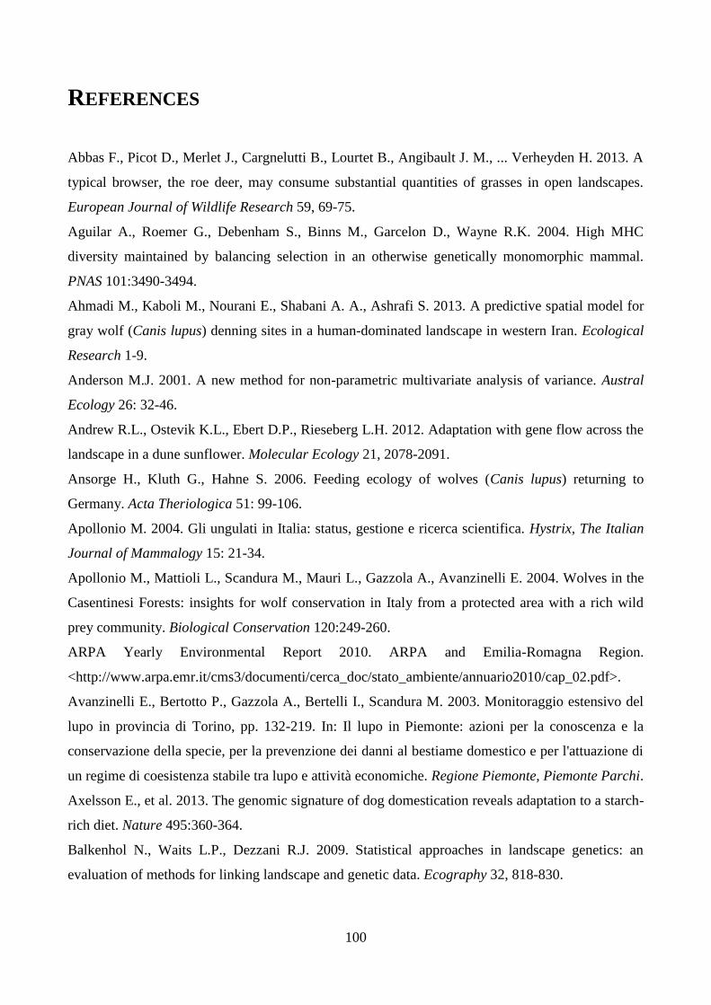
100

REFERENCES

Abbas F., Picot D., Merlet J., Cargnelutti B., Lourtet B., Angibault J. M., ... Verheyden H. 2013. A

typical browser, the roe deer, may consume substantial quantities of grasses in open landscapes.

European Journal of Wildlife Research 59, 69-75.

Aguilar A., Roemer G., Debenham S., Binns M., Garcelon D., Wayne R.K. 2004. High MHC

diversity maintained by balancing selection in an otherwise genetically monomorphic mammal.

PNAS 101:3490-3494.

Ahmadi M., Kaboli M., Nourani E., Shabani A. A., Ashrafi S. 2013. A predictive spatial model for

gray wolf (Canis lupus) denning sites in a human-dominated landscape in western Iran. Ecological

Research 1-9.

Anderson M.J. 2001. A new method for non-parametric multivariate analysis of variance. Austral

Ecology 26: 32-46.

Andrew R.L., Ostevik K.L., Ebert D.P., Rieseberg L.H. 2012. Adaptation with gene flow across the

landscape in a dune sunflower. Molecular Ecology 21, 2078-2091.

Ansorge H., Kluth G., Hahne S. 2006. Feeding ecology of wolves (Canis lupus) returning to

Germany. Acta Theriologica 51: 99-106.

Apollonio M. 2004. Gli ungulati in Italia: status, gestione e ricerca scientifica. Hystrix, The Italian

Journal of Mammalogy 15: 21-34.

Apollonio M., Mattioli L., Scandura M., Mauri L., Gazzola A., Avanzinelli E. 2004. Wolves in the

Casentinesi Forests: insights for wolf conservation in Italy from a protected area with a rich wild

prey community. Biological Conservation 120:249-260.

ARPA Yearly Environmental Report 2010. ARPA and Emilia-Romagna Region.

<http://www.arpa.emr.it/cms3/documenti/cerca_doc/stato_ambiente/annuario2010/cap_02.pdf>.

Avanzinelli E., Bertotto P., Gazzola A., Bertelli I., Scandura M. 2003. Monitoraggio estensivo del

lupo in provincia di Torino, pp. 132-219. In: Il lupo in Piemonte: azioni per la conoscenza e la

conservazione della specie, per la prevenzione dei danni al bestiame domestico e per l'attuazione di

un regime di coesistenza stabile tra lupo e attività economiche. Regione Piemonte, Piemonte Parchi.

Axelsson E., et al. 2013. The genomic signature of dog domestication reveals adaptation to a starch-

rich diet. Nature 495:360-364.

Balkenhol N., Waits L.P., Dezzani R.J. 2009. Statistical approaches in landscape genetics: an

evaluation of methods for linking landscape and genetic data. Ecography 32, 818-830.

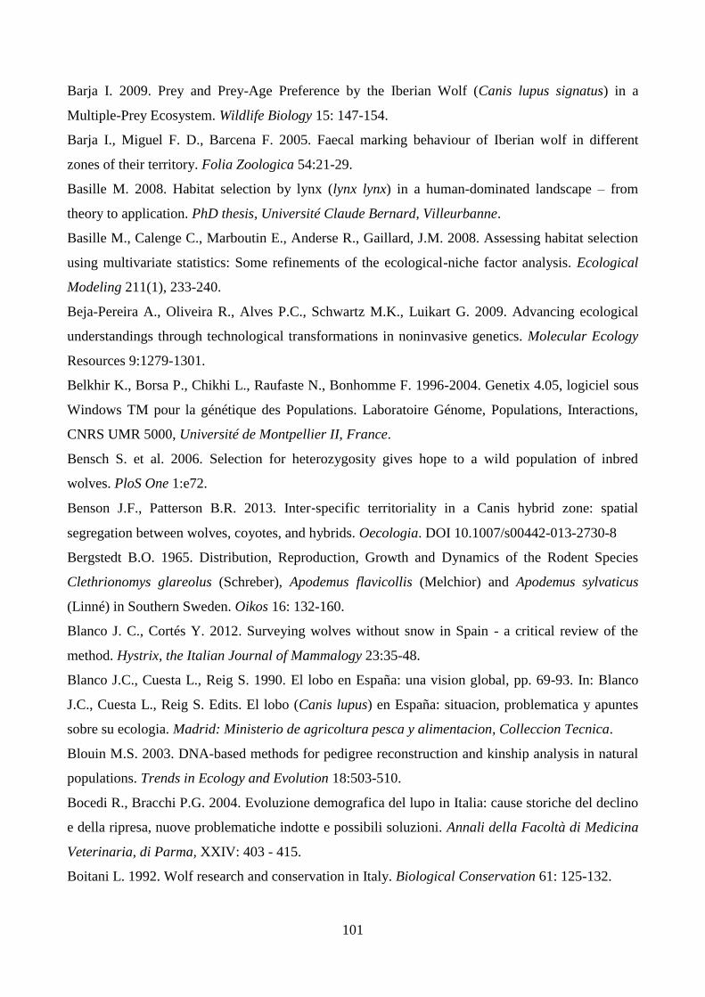
101

Barja I. 2009. Prey and Prey-Age Preference by the Iberian Wolf (Canis lupus signatus) in a

Multiple-Prey Ecosystem. Wildlife Biology 15: 147-154.

Barja I., Miguel F. D., Barcena F. 2005. Faecal marking behaviour of Iberian wolf in different

zones of their territory. Folia Zoologica 54:21-29.

Basille M. 2008. Habitat selection by lynx (lynx lynx) in a human-dominated landscape – from

theory to application. PhD thesis, Université Claude Bernard, Villeurbanne.

Basille M., Calenge C., Marboutin E., Anderse R., Gaillard, J.M. 2008. Assessing habitat selection

using multivariate statistics: Some refinements of the ecological-niche factor analysis. Ecological

Modeling 211(1), 233-240.

Beja-Pereira A., Oliveira R., Alves P.C., Schwartz M.K., Luikart G. 2009. Advancing ecological

understandings through technological transformations in noninvasive genetics. Molecular Ecology

Resources 9:1279-1301.

Belkhir K., Borsa P., Chikhi L., Raufaste N., Bonhomme F. 1996-2004. Genetix 4.05, logiciel sous

Windows TM pour la génétique des Populations. Laboratoire Génome, Populations, Interactions,

CNRS UMR 5000, Université de Montpellier II, France.

Bensch S. et al. 2006. Selection for heterozygosity gives hope to a wild population of inbred

wolves. PloS One 1:e72.

Benson J.F., Patterson B.R. 2013. Inter‑specific territoriality in a Canis hybrid zone: spatial

segregation between wolves, coyotes, and hybrids. Oecologia. DOI 10.1007/s00442-013-2730-8

Bergstedt B.O. 1965. Distribution, Reproduction, Growth and Dynamics of the Rodent Species

Clethrionomys glareolus (Schreber), Apodemus flavicollis (Melchior) and Apodemus sylvaticus

(Linné) in Southern Sweden. Oikos 16: 132-160.

Blanco J. C., Cortés Y. 2012. Surveying wolves without snow in Spain - a critical review of the

method. Hystrix, the Italian Journal of Mammalogy 23:35-48.

Blanco J.C., Cuesta L., Reig S. 1990. El lobo en España: una vision global, pp. 69-93. In: Blanco

J.C., Cuesta L., Reig S. Edits. El lobo (Canis lupus) en España: situacion, problematica y apuntes

sobre su ecologia. Madrid: Ministerio de agricoltura pesca y alimentacion, Colleccion Tecnica.

Blouin M.S. 2003. DNA-based methods for pedigree reconstruction and kinship analysis in natural

populations. Trends in Ecology and Evolution 18:503-510.

Bocedi R., Bracchi P.G. 2004. Evoluzione demografica del lupo in Italia: cause storiche del declino

e della ripresa, nuove problematiche indotte e possibili soluzioni. Annali della Facoltà di Medicina

Veterinaria, di Parma, XXIV: 403 - 415.

Boitani L. 1992. Wolf research and conservation in Italy. Biological Conservation 61: 125-132.

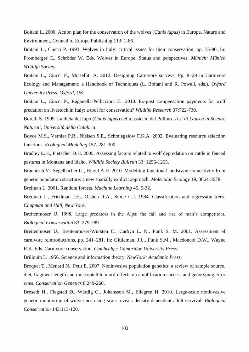
102

Boitani L. 2000. Action plan for the conservation of the wolves (Canis lupus) in Europe. Nature and

Environment, Council of Europe Publishing 113: 1-86.

Boitani L., Ciucci P. 1993. Wolves in Italy: critical issues for their conservation, pp. 75-90. In:

Promberger C., Schröder W. Eds. Wolves in Europe. Status and perspectives. Münich: Münich

Wildlife Society.

Boitani L., Ciucci P., Mortelliti A. 2012. Designing Carnivore surveys. Pp. 8–29 in Carnivore

Ecology and Management: a Handbook of Techniques (L. Boitani and R. Powell, eds.). Oxford

University Press, Oxford, UK.

Boitani L., Ciucci P., Raganella-Pelliccioni E.. 2010. Ex-post compensation payments for wolf

predation on livestock in Italy: a tool for conservation? Wildlife Research 37:722-730.

Borelli S. 1999. La dieta del lupo (Canis lupus) nel massiccio del Pollino. Tesi di Laurea in Scienze

Naturali, Università della Calabria.

Boyce M.S., Vernier P.R., Nielsen S.E., Schmiegelow F.K.A. 2002. Evaluating resource selection

functions. Ecological Modeling 157, 281-300.

Bradley E.H., Pletscher D.H. 2005. Assessing factors related to wolf depredation on cattle in fenced

pastures in Montana and Idaho. Wildlife Society Bulletin 33: 1256-1265.

Braunisch V., Segelbacher G., Hirzel A.H. 2010. Modelling functional landscape connectivity from

genetic population structure: a new spatially explicit approach. Molecular Ecology 19, 3664-3678.

Breiman L. 2001. Random forests. Machine Learning 45, 5-32.

Breiman L., Friedman J.H., Olshen R.A., Stone C.J. 1984. Classification and regression trees.

Chapman and Hall, New York.

Breitenmoser U. 1998. Large predators in the Alps: the fall and rise of man’s competitors.

Biological Conservation 83: 279-289.

Breitenmoser U., Breitenmoser-Würsten C., Carbyn L. N., Funk S. M. 2001. Assessment of

carnivore reintroductions, pp. 241–281. In: Gittleman, J.L., Funk S.M., Macdonald D.W., Wayne

R.K. Eds. Carnivore conservation. Cambridge: Cambridge University Press.

Brillouin L. 1956. Science and information theory. NewYork: Academic Press.

Broquet T., Menard N., Petit E. 2007. Noninvasive population genetics: a review of sample source,

diet, fragment length and microsatellite motif effects on amplification success and genotyping error

rates. Conservation Genetics 8:249-260.

Brøseth H., Flagstad Ø., Wärdig C., Johansson M., Ellegren H. 2010. Large-scale noninvasive

genetic monitoring of wolverines using scats reveals density dependent adult survival. Biological

Conservation 143:113-120.

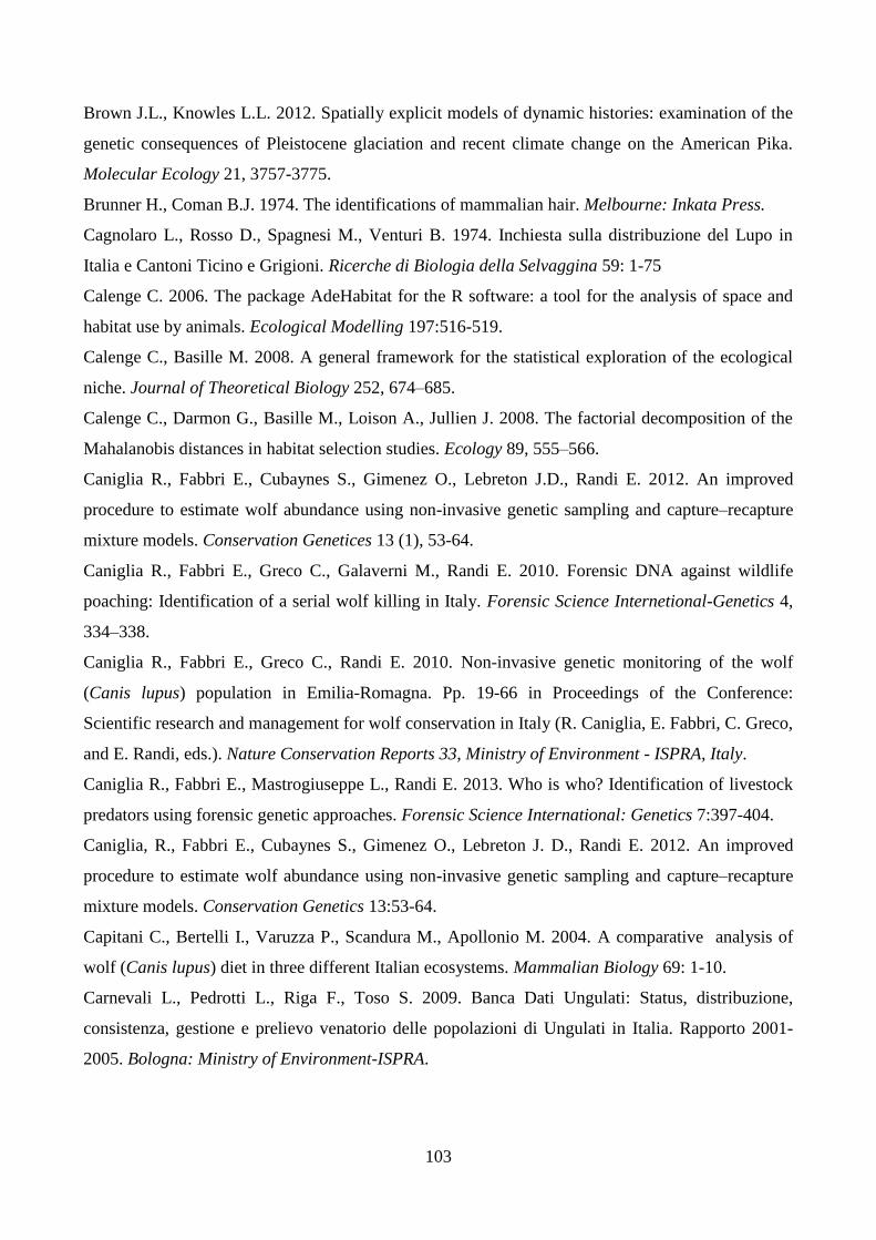
103

Brown J.L., Knowles L.L. 2012. Spatially explicit models of dynamic histories: examination of the

genetic consequences of Pleistocene glaciation and recent climate change on the American Pika.

Molecular Ecology 21, 3757-3775.

Brunner H., Coman B.J. 1974. The identifications of mammalian hair. Melbourne: Inkata Press.

Cagnolaro L., Rosso D., Spagnesi M., Venturi B. 1974. Inchiesta sulla distribuzione del Lupo in

Italia e Cantoni Ticino e Grigioni. Ricerche di Biologia della Selvaggina 59: 1-75

Calenge C. 2006. The package AdeHabitat for the R software: a tool for the analysis of space and

habitat use by animals. Ecological Modelling 197:516-519.

Calenge C., Basille M. 2008. A general framework for the statistical exploration of the ecological

niche. Journal of Theoretical Biology 252, 674–685.

Calenge C., Darmon G., Basille M., Loison A., Jullien J. 2008. The factorial decomposition of the

Mahalanobis distances in habitat selection studies. Ecology 89, 555–566.

Caniglia R., Fabbri E., Cubaynes S., Gimenez O., Lebreton J.D., Randi E. 2012. An improved

procedure to estimate wolf abundance using non-invasive genetic sampling and capture–recapture

mixture models. Conservation Genetices 13 (1), 53-64.

Caniglia R., Fabbri E., Greco C., Galaverni M., Randi E. 2010. Forensic DNA against wildlife

poaching: Identification of a serial wolf killing in Italy. Forensic Science Internetional-Genetics 4,

334–338.

Caniglia R., Fabbri E., Greco C., Randi E. 2010. Non-invasive genetic monitoring of the wolf

(Canis lupus) population in Emilia-Romagna. Pp. 19-66 in Proceedings of the Conference:

Scientific research and management for wolf conservation in Italy (R. Caniglia, E. Fabbri, C. Greco,

and E. Randi, eds.). Nature Conservation Reports 33, Ministry of Environment - ISPRA, Italy.

Caniglia R., Fabbri E., Mastrogiuseppe L., Randi E. 2013. Who is who? Identification of livestock

predators using forensic genetic approaches. Forensic Science International: Genetics 7:397-404.

Caniglia, R., Fabbri E., Cubaynes S., Gimenez O., Lebreton J. D., Randi E. 2012. An improved

procedure to estimate wolf abundance using non-invasive genetic sampling and capture–recapture

mixture models. Conservation Genetics 13:53-64.

Capitani C., Bertelli I., Varuzza P., Scandura M., Apollonio M. 2004. A comparative analysis of

wolf (Canis lupus) diet in three different Italian ecosystems. Mammalian Biology 69: 1-10.

Carnevali L., Pedrotti L., Riga F., Toso S. 2009. Banca Dati Ungulati: Status, distribuzione,

consistenza, gestione e prelievo venatorio delle popolazioni di Ungulati in Italia. Rapporto 2001-

2005. Bologna: Ministry of Environment-ISPRA.

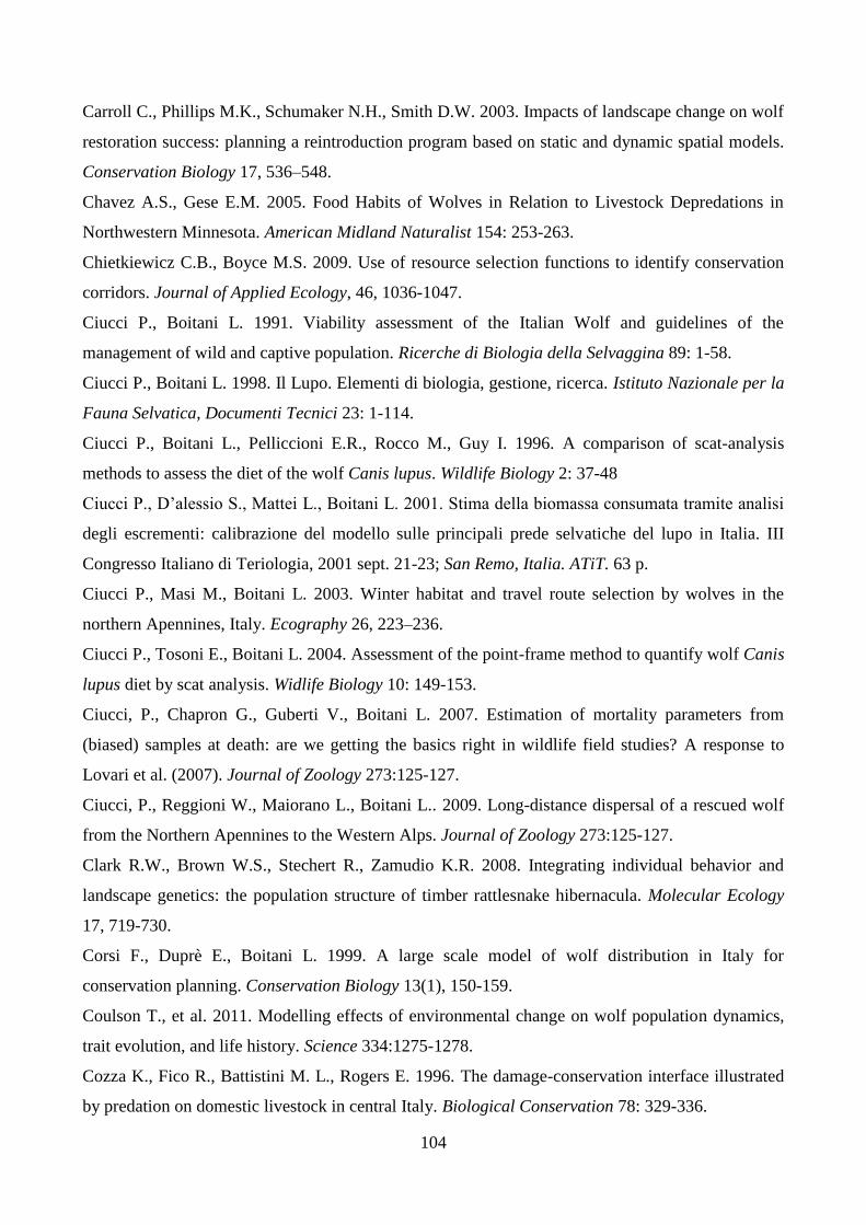
104

Carroll C., Phillips M.K., Schumaker N.H., Smith D.W. 2003. Impacts of landscape change on wolf

restoration success: planning a reintroduction program based on static and dynamic spatial models.

Conservation Biology 17, 536–548.

Chavez A.S., Gese E.M. 2005. Food Habits of Wolves in Relation to Livestock Depredations in

Northwestern Minnesota. American Midland Naturalist 154: 253-263.

Chietkiewicz C.B., Boyce M.S. 2009. Use of resource selection functions to identify conservation

corridors. Journal of Applied Ecology, 46, 1036-1047.

Ciucci P., Boitani L. 1991. Viability assessment of the Italian Wolf and guidelines of the

management of wild and captive population. Ricerche di Biologia della Selvaggina 89: 1-58.

Ciucci P., Boitani L. 1998. Il Lupo. Elementi di biologia, gestione, ricerca. Istituto Nazionale per la

Fauna Selvatica, Documenti Tecnici 23: 1-114.

Ciucci P., Boitani L., Pelliccioni E.R., Rocco M., Guy I. 1996. A comparison of scat-analysis

methods to assess the diet of the wolf Canis lupus. Wildlife Biology 2: 37-48

Ciucci P., D’alessio S., Mattei L., Boitani L. 2001. Stima della biomassa consumata tramite analisi

degli escrementi: calibrazione del modello sulle principali prede selvatiche del lupo in Italia. III

Congresso Italiano di Teriologia, 2001 sept. 21-23; San Remo, Italia. ATiT. 63 p.

Ciucci P., Masi M., Boitani L. 2003. Winter habitat and travel route selection by wolves in the

northern Apennines, Italy. Ecography 26, 223–236.

Ciucci P., Tosoni E., Boitani L. 2004. Assessment of the point-frame method to quantify wolf Canis

lupus diet by scat analysis. Widlife Biology 10: 149-153.

Ciucci, P., Chapron G., Guberti V., Boitani L. 2007. Estimation of mortality parameters from

(biased) samples at death: are we getting the basics right in wildlife field studies? A response to

Lovari et al. (2007). Journal of Zoology 273:125-127.

Ciucci, P., Reggioni W., Maiorano L., Boitani L.. 2009. Long-distance dispersal of a rescued wolf

from the Northern Apennines to the Western Alps. Journal of Zoology 273:125-127.

Clark R.W., Brown W.S., Stechert R., Zamudio K.R. 2008. Integrating individual behavior and

landscape genetics: the population structure of timber rattlesnake hibernacula. Molecular Ecology

17, 719-730.

Corsi F., Duprè E., Boitani L. 1999. A large scale model of wolf distribution in Italy for

conservation planning. Conservation Biology 13(1), 150-159.

Coulson T., et al. 2011. Modelling effects of environmental change on wolf population dynamics,

trait evolution, and life history. Science 334:1275-1278.

Cozza K., Fico R., Battistini M. L., Rogers E. 1996. The damage-conservation interface illustrated

by predation on domestic livestock in central Italy. Biological Conservation 78: 329-336.

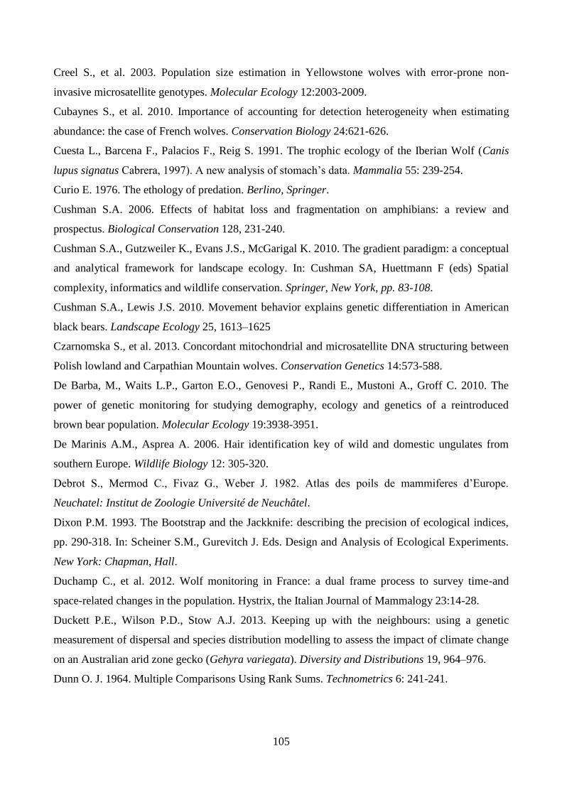
105

Creel S., et al. 2003. Population size estimation in Yellowstone wolves with error-prone non-

invasive microsatellite genotypes. Molecular Ecology 12:2003-2009.

Cubaynes S., et al. 2010. Importance of accounting for detection heterogeneity when estimating

abundance: the case of French wolves. Conservation Biology 24:621-626.

Cuesta L., Barcena F., Palacios F., Reig S. 1991. The trophic ecology of the Iberian Wolf (Canis

lupus signatus Cabrera, 1997). A new analysis of stomach’s data. Mammalia 55: 239-254.

Curio E. 1976. The ethology of predation. Berlino, Springer.

Cushman S.A. 2006. Effects of habitat loss and fragmentation on amphibians: a review and

prospectus. Biological Conservation 128, 231-240.

Cushman S.A., Gutzweiler K., Evans J.S., McGarigal K. 2010. The gradient paradigm: a conceptual

and analytical framework for landscape ecology. In: Cushman SA, Huettmann F (eds) Spatial

complexity, informatics and wildlife conservation. Springer, New York, pp. 83-108.

Cushman S.A., Lewis J.S. 2010. Movement behavior explains genetic differentiation in American

black bears. Landscape Ecology 25, 1613–1625

Czarnomska S., et al. 2013. Concordant mitochondrial and microsatellite DNA structuring between

Polish lowland and Carpathian Mountain wolves. Conservation Genetics 14:573-588.

De Barba, M., Waits L.P., Garton E.O., Genovesi P., Randi E., Mustoni A., Groff C. 2010. The

power of genetic monitoring for studying demography, ecology and genetics of a reintroduced

brown bear population. Molecular Ecology 19:3938-3951.

De Marinis A.M., Asprea A. 2006. Hair identification key of wild and domestic ungulates from

southern Europe. Wildlife Biology 12: 305-320.

Debrot S., Mermod C., Fivaz G., Weber J. 1982. Atlas des poils de mammiferes d’Europe.

Neuchatel: Institut de Zoologie Université de Neuchâtel.

Dixon P.M. 1993. The Bootstrap and the Jackknife: describing the precision of ecological indices,

pp. 290-318. In: Scheiner S.M., Gurevitch J. Eds. Design and Analysis of Ecological Experiments.

New York: Chapman, Hall.

Duchamp C., et al. 2012. Wolf monitoring in France: a dual frame process to survey time-and

space-related changes in the population. Hystrix, the Italian Journal of Mammalogy 23:14-28.

Duckett P.E., Wilson P.D., Stow A.J. 2013. Keeping up with the neighbours: using a genetic

measurement of dispersal and species distribution modelling to assess the impact of climate change

on an Australian arid zone gecko (Gehyra variegata). Diversity and Distributions 19, 964–976.

Dunn O. J. 1964. Multiple Comparisons Using Rank Sums. Technometrics 6: 241-241.

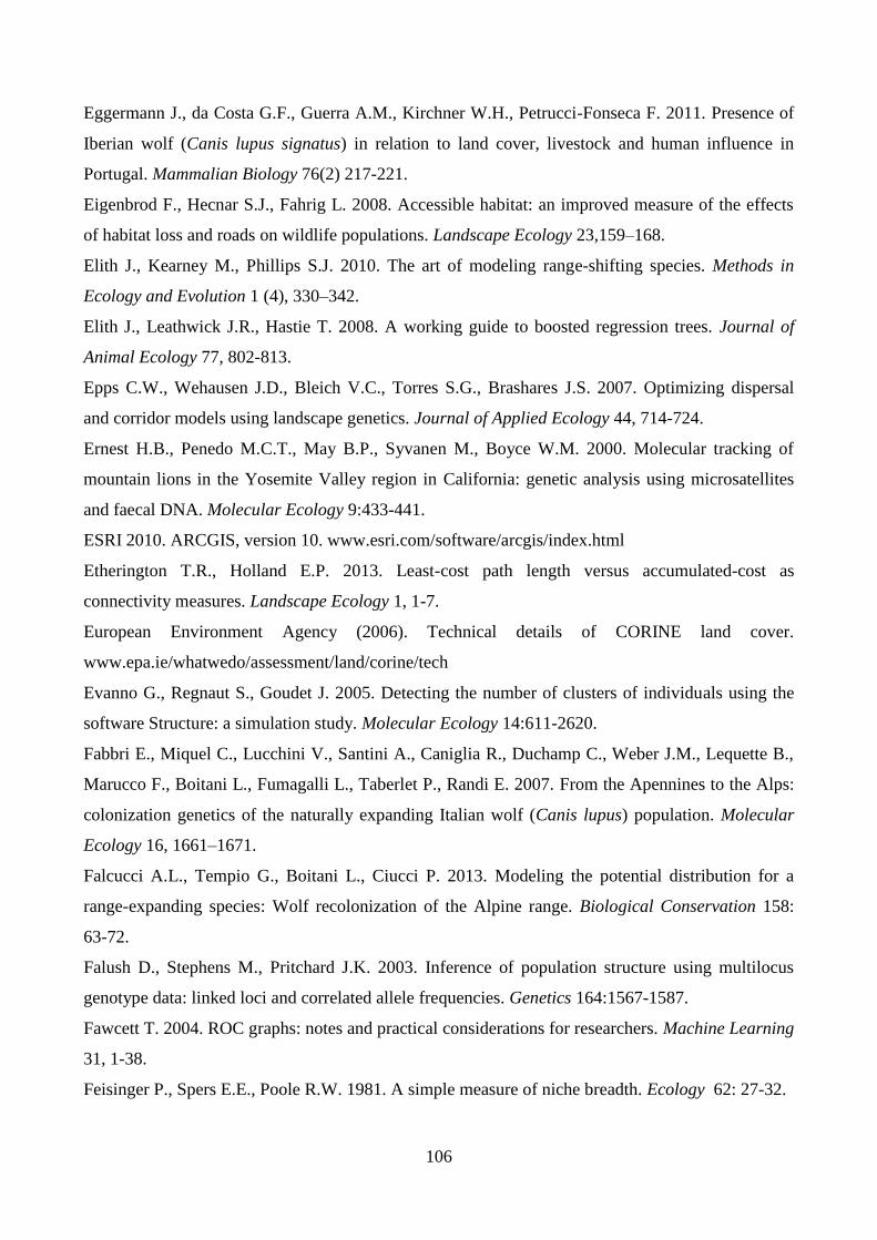
106

Eggermann J., da Costa G.F., Guerra A.M., Kirchner W.H., Petrucci-Fonseca F. 2011. Presence of

Iberian wolf (Canis lupus signatus) in relation to land cover, livestock and human influence in

Portugal. Mammalian Biology 76(2) 217-221.

Eigenbrod F., Hecnar S.J., Fahrig L. 2008. Accessible habitat: an improved measure of the effects

of habitat loss and roads on wildlife populations. Landscape Ecology 23,159–168.

Elith J., Kearney M., Phillips S.J. 2010. The art of modeling range-shifting species. Methods in

Ecology and Evolution 1 (4), 330–342.

Elith J., Leathwick J.R., Hastie T. 2008. A working guide to boosted regression trees. Journal of

Animal Ecology 77, 802-813.

Epps C.W., Wehausen J.D., Bleich V.C., Torres S.G., Brashares J.S. 2007. Optimizing dispersal

and corridor models using landscape genetics. Journal of Applied Ecology 44, 714-724.

Ernest H.B., Penedo M.C.T., May B.P., Syvanen M., Boyce W.M. 2000. Molecular tracking of

mountain lions in the Yosemite Valley region in California: genetic analysis using microsatellites

and faecal DNA. Molecular Ecology 9:433-441.

ESRI 2010. ARCGIS, version 10. www.esri.com/software/arcgis/index.html

Etherington T.R., Holland E.P. 2013. Least-cost path length versus accumulated-cost as

connectivity measures. Landscape Ecology 1, 1-7.

European Environment Agency (2006). Technical details of CORINE land cover.

www.epa.ie/whatwedo/assessment/land/corine/tech

Evanno G., Regnaut S., Goudet J. 2005. Detecting the number of clusters of individuals using the

software Structure: a simulation study. Molecular Ecology 14:611-2620.

Fabbri E., Miquel C., Lucchini V., Santini A., Caniglia R., Duchamp C., Weber J.M., Lequette B.,

Marucco F., Boitani L., Fumagalli L., Taberlet P., Randi E. 2007. From the Apennines to the Alps:

colonization genetics of the naturally expanding Italian wolf (Canis lupus) population. Molecular

Ecology 16, 1661–1671.

Falcucci A.L., Tempio G., Boitani L., Ciucci P. 2013. Modeling the potential distribution for a

range-expanding species: Wolf recolonization of the Alpine range. Biological Conservation 158:

63-72.

Falush D., Stephens M., Pritchard J.K. 2003. Inference of population structure using multilocus

genotype data: linked loci and correlated allele frequencies. Genetics 164:1567-1587.

Fawcett T. 2004. ROC graphs: notes and practical considerations for researchers. Machine Learning

31, 1-38.

Feisinger P., Spers E.E., Poole R.W. 1981. A simple measure of niche breadth. Ecology 62: 27-32.

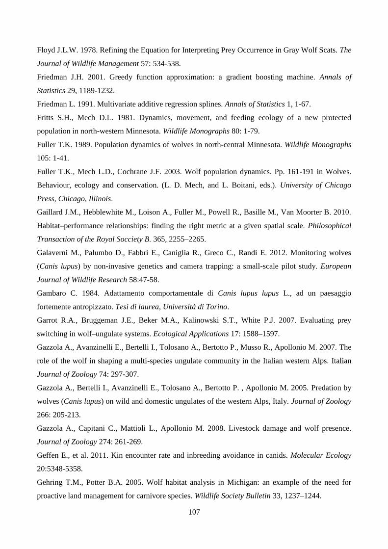
107

Floyd J.L.W. 1978. Refining the Equation for Interpreting Prey Occurrence in Gray Wolf Scats. The

Journal of Wildlife Management 57: 534-538.

Friedman J.H. 2001. Greedy function approximation: a gradient boosting machine. Annals of

Statistics 29, 1189-1232.

Friedman L. 1991. Multivariate additive regression splines. Annals of Statistics 1, 1-67.

Fritts S.H., Mech D.L. 1981. Dynamics, movement, and feeding ecology of a new protected

population in north-western Minnesota. Wildlife Monographs 80: 1-79.

Fuller T.K. 1989. Population dynamics of wolves in north-central Minnesota. Wildlife Monographs

105: 1-41.

Fuller T.K., Mech L.D., Cochrane J.F. 2003. Wolf population dynamics. Pp. 161-191 in Wolves.

Behaviour, ecology and conservation. (L. D. Mech, and L. Boitani, eds.). University of Chicago

Press, Chicago, Illinois.

Gaillard J.M., Hebblewhite M., Loison A., Fuller M., Powell R., Basille M., Van Moorter B. 2010.

Habitat–performance relationships: finding the right metric at a given spatial scale. Philosophical

Transaction of the Royal Socciety B. 365, 2255–2265.

Galaverni M., Palumbo D., Fabbri E., Caniglia R., Greco C., Randi E. 2012. Monitoring wolves

(Canis lupus) by non-invasive genetics and camera trapping: a small-scale pilot study. European

Journal of Wildlife Research 58:47-58.

Gambaro C. 1984. Adattamento comportamentale di Canis lupus lupus L., ad un paesaggio

fortemente antropizzato. Tesi di laurea, Università di Torino.

Garrot R.A., Bruggeman J.E., Beker M.A., Kalinowski S.T., White P.J. 2007. Evaluating prey

switching in wolf–ungulate systems. Ecological Applications 17: 1588–1597.

Gazzola A., Avanzinelli E., Bertelli I., Tolosano A., Bertotto P., Musso R., Apollonio M. 2007. The

role of the wolf in shaping a multi-species ungulate community in the Italian western Alps. Italian

Journal of Zoology 74: 297-307.

Gazzola A., Bertelli I., Avanzinelli E., Tolosano A., Bertotto P. , Apollonio M. 2005. Predation by

wolves (Canis lupus) on wild and domestic ungulates of the western Alps, Italy. Journal of Zoology

266: 205-213.

Gazzola A., Capitani C., Mattioli L., Apollonio M. 2008. Livestock damage and wolf presence.

Journal of Zoology 274: 261-269.

Geffen E., et al. 2011. Kin encounter rate and inbreeding avoidance in canids. Molecular Ecology

20:5348-5358.

Gehring T.M., Potter B.A. 2005. Wolf habitat analysis in Michigan: an example of the need for

proactive land management for carnivore species. Wildlife Society Bulletin 33, 1237–1244.

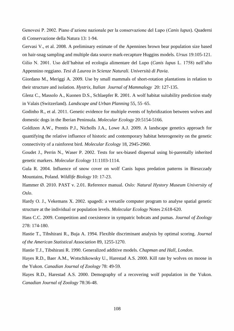
108

Genovesi P. 2002. Piano d’azione nazionale per la conservazione del Lupo (Canis lupus). Quaderni

di Conservazione della Natura 13: 1-94.

Gervasi V., et al. 2008. A preliminary estimate of the Apennines brown bear population size based

on hair-snag sampling and multiple data source mark-recapture Huggins models. Ursus 19:105-121.

Gilio N. 2001. Uso dell’habitat ed ecologia alimentare del Lupo (Canis lupus L. 1758) nell’alto

Appennino reggiano. Tesi di Laurea in Scienze Naturali. Università di Pavia.

Giordano M., Meriggi A. 2009. Use by small mammals of short-rotation plantations in relation to

their structure and isolation. Hystrix, Italian Journal of Mammalogy 20: 127-135.

Glenz C., Massolo A., Kuonen D.S., Schlaepfer R. 2001. A wolf habitat suitability prediction study

in Valais (Switzerland). Landscape and Urban Planning 55, 55–65.

Godinho R., et al. 2011. Genetic evidence for multiple events of hybridization between wolves and

domestic dogs in the Iberian Peninsula. Molecular Ecology 20:5154-5166.

Goldizen A.W., Prentis P.J., Nicholls J.A., Lowe A.J. 2009. A landscape genetics approach for

quantifying the relative influence of historic and contemporary habitat heterogeneity on the genetic

connectivity of a rainforest bird. Molecular Ecology 18, 2945-2960.

Goudet J., Perrin N., Waser P. 2002. Tests for sex-biased dispersal using bi-parentally inherited

genetic markers. Molecular Ecology 11:1103-1114.

Gula R. 2004. Influence of snow cover on wolf Canis lupus predation patterns in Bieszczady

Mountains, Poland. Wildlife Biology 10: 17-23.

Hammer Ø. 2010. PAST v. 2.01. Reference manual. Oslo: Natural Hystory Museum University of

Oslo.

Hardy O. J., Vekemans X. 2002. spagedi: a versatile computer program to analyse spatial genetic

structure at the individual or population levels. Molecular Ecology Notes 2:618-620.

Hass C.C. 2009. Competition and coexistence in sympatric bobcats and pumas. Journal of Zoology

278: 174-180.

Hastie T., Tibshirani R., Buja A. 1994. Flexible discriminant analysis by optimal scoring. Journal

of the American Statistical Association 89, 1255-1270.

Hastie T.J., Tibshirani R. 1990. Generalized additive models. Chapman and Hall, London.

Hayes R.D., Baer A.M., Wotschikowsky U., Harestad A.S. 2000. Kill rate by wolves on moose in

the Yukon. Canadian Journal of Zoology 78: 49-59.

Hayes R.D., Harestad A.S. 2000. Demography of a recovering wolf population in the Yukon.

Canadian Journal of Zoology 78:36-48.

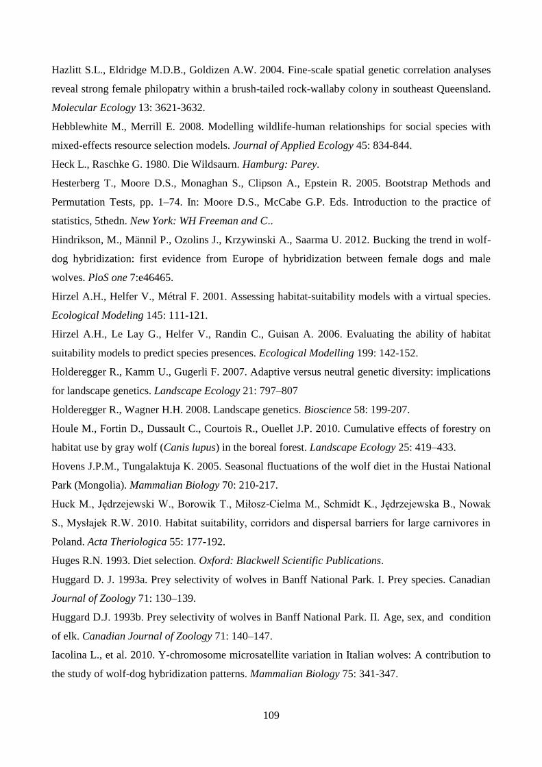
109

Hazlitt S.L., Eldridge M.D.B., Goldizen A.W. 2004. Fine-scale spatial genetic correlation analyses

reveal strong female philopatry within a brush-tailed rock-wallaby colony in southeast Queensland.

Molecular Ecology 13: 3621-3632.

Hebblewhite M., Merrill E. 2008. Modelling wildlife-human relationships for social species with

mixed-effects resource selection models. Journal of Applied Ecology 45: 834-844.

Heck L., Raschke G. 1980. Die Wildsaurn. Hamburg: Parey.

Hesterberg T., Moore D.S., Monaghan S., Clipson A., Epstein R. 2005. Bootstrap Methods and

Permutation Tests, pp. 1–74. In: Moore D.S., McCabe G.P. Eds. Introduction to the practice of

statistics, 5thedn. New York: WH Freeman and C..

Hindrikson, M., Männil P., Ozolins J., Krzywinski A., Saarma U. 2012. Bucking the trend in wolf-

dog hybridization: first evidence from Europe of hybridization between female dogs and male

wolves. PloS one 7:e46465.

Hirzel A.H., Helfer V., Métral F. 2001. Assessing habitat-suitability models with a virtual species.

Ecological Modeling 145: 111-121.

Hirzel A.H., Le Lay G., Helfer V., Randin C., Guisan A. 2006. Evaluating the ability of habitat

suitability models to predict species presences. Ecological Modelling 199: 142-152.

Holderegger R., Kamm U., Gugerli F. 2007. Adaptive versus neutral genetic diversity: implications

for landscape genetics. Landscape Ecology 21: 797–807

Holderegger R., Wagner H.H. 2008. Landscape genetics. Bioscience 58: 199-207.

Houle M., Fortin D., Dussault C., Courtois R., Ouellet J.P. 2010. Cumulative effects of forestry on

habitat use by gray wolf (Canis lupus) in the boreal forest. Landscape Ecology 25: 419–433.

Hovens J.P.M., Tungalaktuja K. 2005. Seasonal fluctuations of the wolf diet in the Hustai National

Park (Mongolia). Mammalian Biology 70: 210-217.

Huck M., Jędrzejewski W., Borowik T., Miłosz-Cielma M., Schmidt K., Jędrzejewska B., Nowak

S., Mysłajek R.W. 2010. Habitat suitability, corridors and dispersal barriers for large carnivores in

Poland. Acta Theriologica 55: 177-192.

Huges R.N. 1993. Diet selection. Oxford: Blackwell Scientific Publications.

Huggard D. J. 1993a. Prey selectivity of wolves in Banff National Park. I. Prey species. Canadian

Journal of Zoology 71: 130–139.

Huggard D.J. 1993b. Prey selectivity of wolves in Banff National Park. II. Age, sex, and condition

of elk. Canadian Journal of Zoology 71: 140–147.

Iacolina L., et al. 2010. Y-chromosome microsatellite variation in Italian wolves: A contribution to

the study of wolf-dog hybridization patterns. Mammalian Biology 75: 341-347.

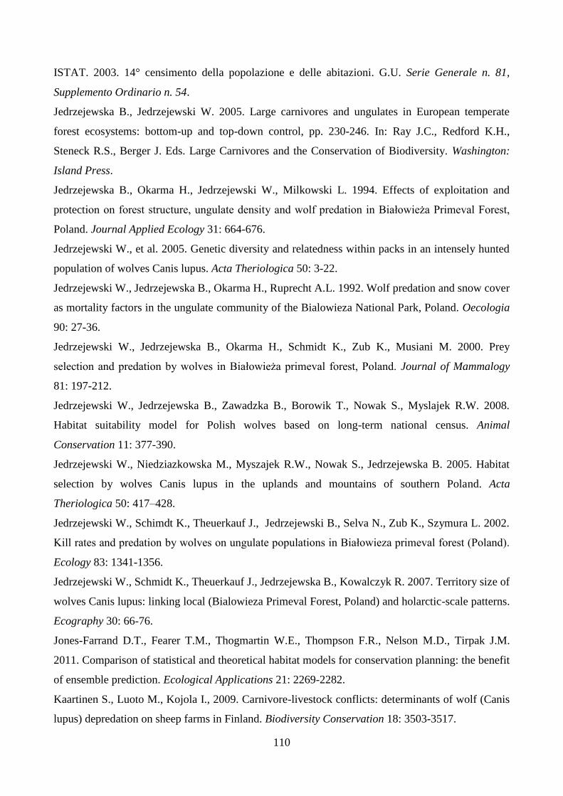
110

ISTAT. 2003. 14° censimento della popolazione e delle abitazioni. G.U. Serie Generale n. 81,

Supplemento Ordinario n. 54.

Jedrzejewska B., Jedrzejewski W. 2005. Large carnivores and ungulates in European temperate

forest ecosystems: bottom-up and top-down control, pp. 230-246. In: Ray J.C., Redford K.H.,

Steneck R.S., Berger J. Eds. Large Carnivores and the Conservation of Biodiversity. Washington:

Island Press.

Jedrzejewska B., Okarma H., Jedrzejewski W., Milkowski L. 1994. Effects of exploitation and

protection on forest structure, ungulate density and wolf predation in Białowieża Primeval Forest,

Poland. Journal Applied Ecology 31: 664-676.

Jedrzejewski W., et al. 2005. Genetic diversity and relatedness within packs in an intensely hunted

population of wolves Canis lupus. Acta Theriologica 50: 3-22.

Jedrzejewski W., Jedrzejewska B., Okarma H., Ruprecht A.L. 1992. Wolf predation and snow cover

as mortality factors in the ungulate community of the Bialowieza National Park, Poland. Oecologia

90: 27-36.

Jedrzejewski W., Jedrzejewska B., Okarma H., Schmidt K., Zub K., Musiani M. 2000. Prey

selection and predation by wolves in Białowieża primeval forest, Poland. Journal of Mammalogy

81: 197-212.

Jedrzejewski W., Jedrzejewska B., Zawadzka B., Borowik T., Nowak S., Myslajek R.W. 2008.

Habitat suitability model for Polish wolves based on long-term national census. Animal

Conservation 11: 377-390.

Jedrzejewski W., Niedziazkowska M., Myszajek R.W., Nowak S., Jedrzejewska B. 2005. Habitat

selection by wolves Canis lupus in the uplands and mountains of southern Poland. Acta

Theriologica 50: 417–428.

Jedrzejewski W., Schimdt K., Theuerkauf J., Jedrzejewski B., Selva N., Zub K., Szymura L. 2002.

Kill rates and predation by wolves on ungulate populations in Białowieza primeval forest (Poland).

Ecology 83: 1341-1356.

Jedrzejewski W., Schmidt K., Theuerkauf J., Jedrzejewska B., Kowalczyk R. 2007. Territory size of

wolves Canis lupus: linking local (Bialowieza Primeval Forest, Poland) and holarctic-scale patterns.

Ecography 30: 66-76.

Jones-Farrand D.T., Fearer T.M., Thogmartin W.E., Thompson F.R., Nelson M.D., Tirpak J.M.

2011. Comparison of statistical and theoretical habitat models for conservation planning: the benefit

of ensemble prediction. Ecological Applications 21: 2269-2282.

Kaartinen S., Luoto M., Kojola I., 2009. Carnivore-livestock conflicts: determinants of wolf (Canis

lupus) depredation on sheep farms in Finland. Biodiversity Conservation 18: 3503-3517.

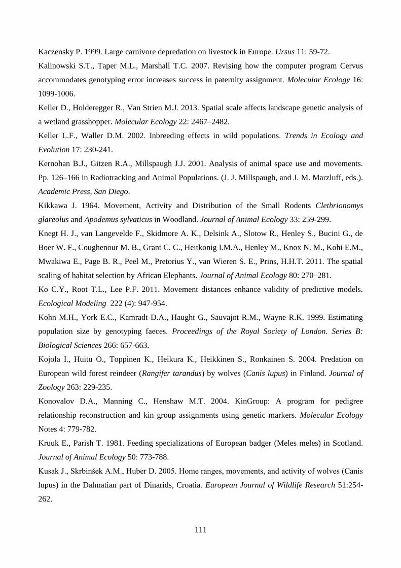
111

Kaczensky P. 1999. Large carnivore depredation on livestock in Europe. Ursus 11: 59-72.

Kalinowski S.T., Taper M.L., Marshall T.C. 2007. Revising how the computer program Cervus

accommodates genotyping error increases success in paternity assignment. Molecular Ecology 16:

1099-1006.

Keller D., Holderegger R., Van Strien M.J. 2013. Spatial scale affects landscape genetic analysis of

a wetland grasshopper. Molecular Ecology 22: 2467–2482.

Keller L.F., Waller D.M. 2002. Inbreeding effects in wild populations. Trends in Ecology and

Evolution 17: 230-241.

Kernohan B.J., Gitzen R.A., Millspaugh J.J. 2001. Analysis of animal space use and movements.

Pp. 126–166 in Radiotracking and Animal Populations. (J. J. Millspaugh, and J. M. Marzluff, eds.).

Academic Press, San Diego.

Kikkawa J. 1964. Movement, Activity and Distribution of the Small Rodents Clethrionomys

glareolus and Apodemus sylvaticus in Woodland. Journal of Animal Ecology 33: 259-299.

Knegt H. J., van Langevelde F., Skidmore A. K., Delsink A., Slotow R., Henley S., Bucini G., de

Boer W. F., Coughenour M. B., Grant C. C., Heitkonig I.M.A., Henley M., Knox N. M., Kohi E.M.,

Mwakiwa E., Page B. R., Peel M., Pretorius Y., van Wieren S. E., Prins, H.H.T. 2011. The spatial

scaling of habitat selection by African Elephants. Journal of Animal Ecology 80: 270–281.

Ko C.Y., Root T.L., Lee P.F. 2011. Movement distances enhance validity of predictive models.

Ecological Modeling 222 (4): 947-954.

Kohn M.H., York E.C., Kamradt D.A., Haught G., Sauvajot R.M., Wayne R.K. 1999. Estimating

population size by genotyping faeces. Proceedings of the Royal Society of London. Series B:

Biological Sciences 266: 657-663.

Kojola I., Huitu O., Toppinen K., Heikura K., Heikkinen S., Ronkainen S. 2004. Predation on

European wild forest reindeer (Rangifer tarandus) by wolves (Canis lupus) in Finland. Journal of

Zoology 263: 229-235.

Konovalov D.A., Manning C., Henshaw M.T. 2004. KinGroup: A program for pedigree

relationship reconstruction and kin group assignments using genetic markers. Molecular Ecology

Notes 4: 779-782.

Kruuk E., Parish T. 1981. Feeding specializations of European badger (Meles meles) in Scotland.

Journal of Animal Ecology 50: 773-788.

Kusak J., Skrbinšek A.M., Huber D. 2005. Home ranges, movements, and activity of wolves (Canis

lupus) in the Dalmatian part of Dinarids, Croatia. European Journal of Wildlife Research 51:254-

262.

112

Laporte I., Muhly T.B., Pitt J.A., Alexander M., Musiani M. 2010. Effects of Wolves on Elk and

Cattle Behaviors: Implications for Livestock Production and Wolf Conservation. Plos Biology 5(8):

e11954.

Leathwick J.R., Elith J., Hastie T. 2006. Comparative performance of generalized additive models

and multivariate adaptive regression splines for statistical modelling of species distributions.

Ecological Modelling 199: 188-196.

Lee-Yaw J.A., Davidson A., McRae B.H., Green D.M. 2009. Do landscape processes predict

phylogeographic patterns in the wood frog? Molecular Ecology 18: 1863-1874.

Legendre P. 2000. Comparison of permutation methods for the partial correlation and partial Mantel

tests. Journal of Statistical Computation and Simulation 67: 37-73.

Legendre P., Fortin M.J. 2010. Comparison of the Mantel test and alternative approaches for

detecting complex multivariate relationships in the spatial analysis of genetic data. Molecular

Ecology Resources 10: 831-844.

Lehman N., Clarkson P., Mech L.D., Meier T.J., Wayne R.K. 1992. The use of DNA fingerprinting

and mitochondrial DNA to study genetic relationships within and among wolf packs. Behavioral

Ecology and Sociobiology 30: 83-94.

Leonard J.A., Vila C., Wayne R.K. 2005. Legacy lost: genetic variability and population size of

extirpated US grey wolves (Canis lupus). Molecolar Ecology 14: 9-17.

Lesmerises F., Dussault C., St-Laurent M. H. 2012. Wolf habitat selection is shaped by human

activities in a highly managed boreal forest. Forest Ecology and Management 276: 125-131.

Life project LIFE00NAT/IT/7214 final report. 2004.

http://www.parcofrignano.it/binary/parco_del_frignano/progetti/Rapporto_finale_Life_lupo_2004.1

213275329.pdf>.

Linnel J.D.C., Brøseth H., Solberg E.J., Brainerd S.M. 2005. The origins of the southern

Scandinavian wolf (Canis lupus) population: potential for natural immigration in relation to

dispersal distances, geography and Baltic ice. Wildlife Biology 11: 383-391.

Linnell J.D., Boitani L. 2012. Building biological realism into wolf management policy: the

development of the population approach in Europe. Hystrix, the Italian Journal of Mammalogy 23:

80-91.

Loiselle B.A., Sork V.L., Nason J., Graham C. 1995. Spatial genetic structure of a tropical

understory shrub, Psychotria officinalis (Rubiaceae). American Journal of Botany 82: 1420-1425.

Long R.A., MacKay P., Ray J., Zielinski W. 2008. Noninvasive survey methods for carnivores.

Island Press, Washington.

113

Lucchini V., Fabbri E., Marucco F., Ricci S., Boitani L., Randi E. 2002. Non-invasive molecular

tracking of colonizing wolf (Canis lupus) packs in the western Italian Alps. Molecular Ecology 11:

857-868.

Lucchini V., Galov A., Randi E. 2004. Evidence of genetic distinction and long-term population

decline in wolves (Canis lupus) in the Italian Apennines. Molecular Ecology 13:523-536.

Lukacs P.M., Burnham K.P. 2005. Review of capture–recapture methods applicable to noninvasive

genetic sampling. Molecular Ecology 14: 3909-3919.

Lukacs P.M., Eggert L.S., Burnham K.P. 2007. Estimating population size from multiple detections

with non-invasive genetic data. Wildlife Biology in Practice 3: 83-92.

Lynch M., Ritland K. 1999. Estimation of pairwise relatedness with molecular markers. Genetics

152: 1753-1766.

Macdonald D.W., Boitani L., Barrasso P. 1980. Foxes, wolves and conservation in the Abruzzo

mountains. Biogeographica 18: 223-235.

MacNulty D.R., Smith D.W., Vucetich J.A., Mech D.L., Stahler D.R., Packer C. 2011. Predatory

senescence in ageing wolves. Ecological Letters 12: 1347-1356.

Manel S., Holderegger R., 2013. Ten years of landscape genetics. Trends in Ecology and Evolution

28: 614–621.

Manel S., Williams H.C., Ormerod S.J. 2001. Evaluating presence–absence models in ecology: the

need to account for prevalence. Journal of Applied Ecology 38: 921–931.

Manly B.F.J., McDonald L.L., Thomas D.L., McDonald T.L., Erickson W.P. 2002. Resource

selection by animals: statistical design and analysis for field studies. 2nd edition. Dordrecht,

Boston, London: Kluwer Press.

Mantel N. 1967. The detection of disease clustering and a generalized regression approach. Cancer

Research 27: 209-220.

Marmion M., Parviainen M., Luoto M., Heikkinen R.K., Thuiller W. 2009. Evaluation of consensus

methods in predictive species distribution modelling. Diversity and Distributions 15: 59-69.

Marshal J.P., Boutin S. 1999. Power analysis of wolf-moose functional responses. Journal Wildlife

Management 63: 396-402.

Marucco F. 2003. Studio intensivo dei lupi nelle Alpi Liguri, pp. 84-132. In: Il lupo in Piemonte:

azioni per la conoscenza e la conservazione della specie, per la prevenzione dei danni al bestiame

domestico e per l'attuazione di un regime di coesistenza stabile tra lupo e attività economiche.

Regione Piemonte, Piemonte Parchi.

114

Marucco F. Pletscher D.H., Boitani L., Schwartz M.K., Pilgrim K.L., Lebreton J.D. 2009. Wolf

survival and population trend using non-invasive capture-recapture techniques in the Western Alps.

Journal of Applied Ecology 46(5): 1003-1010.

Marucco F., McIntire E.J.B. 2010. Predicting spatio-temporal recolonization of large carnivore

populations and livestock depredation risk: wolves in the Italian Alps. Journal of Applied Ecology

47: 789–798.

Marucco F., Pletscher D.H., Boitani L., Schwartz M.K., Pilgrim K.L., Lebreton J.D. 2009. Wolf

survival and population trend using non-invasive capture-recapture techniques in the Western Alps.

Journal of Applied Ecology 46: 1003-1010.

Massolo A., Meriggi A. 1996. A new guideline for wolf management: modelling habitat suitability.

Journal of Wildlife Research 1: 282-286.

Massolo A., Meriggi A. 1998. Factors affecting habitat occupancy by wolves in Northern

Apennines (North-Italy): a model of habitat suitability. Ecography 21: 97-107.

Matteucci C. 1992. Preliminary data on the ecology of a wolf (Canis lupus) population in northern

Italy, pp. 367-370. In: Global Trends in Wildlife Management Vol. II. Bobek B., Perzanowski K.,

Regelin W.L. Eds. Krakow-Warszava: Swiat Press.

Mattioli L., Apollonio M., Mazzarone V., Centofanti E. 1995. Wolf food habits and wild ungulate

availability in the Foreste Casentinesi National Park, Italy. Acta Theriologica 40: 387-402.

Mattioli L., Capitani C., Avanzinelli E., Bertelli I., Gazzola A., Apollonio M. 2004. Predation by

wolves (Canis lupus) on roe deer (Capreolus capreolus) in the north-eastern Apennines, Italy.

Journal of Zoology 264: 249-258.

Mattioli L., Nicoloso S. 2010. Il Cervo. Biologia e gestione, percorso didattico. Integrazioni 2010.

Appunti di gestione faunistica 2. Italia: Edizioni D.R.E.Am.

Mauget R., Campan R., Spitz F., Dardaillon M., Janeau G., Pépin D. 1984. Synthèse de

connaissances actuelles sur la biologie du Sanglier, perspectives de recherche, pp. 15-50. In: Spitz

F., Pépin D. Eds. Symposium International sur le Sanglier. Colloques de l’I.N.R.A., 22.

McCullagh P., Nelder J.A. 1989. Generalized linear models. Chapman and Hall, London.

McGarigal K., Cushman S.A., Neel M.C., Ene E. 2002. FRAGSTATS: spatial pattern analysis

program for categorical maps. University of Massachusetts, Amherst.

Mech L.D. 1999. Alpha status, dominance, and division of labor in wolf packs. 77:1196-1203.

Mech L.D., 1970. The wolf. The ecology and behaviour of an endangered species. Univ. of

Minnesota Press. Minneapolis. 68.

Mech L.D., 1974. Canis lupus. Manmmalian Species 37:1-6.

115

Mech L.D., Harper E.K., Meier T.J., Paul W.J. 2000. Assessing factors that may predispose

Minnesota farms to wolf predation on cattle. Wildlife Society Bulletin 28: 623-629.

Mech, L.D., Boitani L. 2003. Wolf social ecology. Pp. 1-34 in Wolves: behaviour, ecology, and

conservation (L. D. Mech and L. Boitani, eds). University of Chicago Press, Chicago, Illinois.

Meijer T., Noren K., Hellstrom P., Dalen L., Angerbjorn A. 2008. Estimating population parameters

in a threatened arctic fox population using molecular tracking and traditional field methods. Animal

Conservation 11:330-338.

Melis C., Jedrzejewska B., Apollonio M., Barton K.A., Jedrzejewski W., Linnell J.D.C., Kojola I.,

Kusak J., Adamic M., Ciuti S., Delehan I., Dykyy I., Krapinec K., Mattioli L., Sagaydak A.,

Samchuk N., Schmidt K., Shkvyrya M., Sidorovich V.E., Zawadzka B., Zhyla S. 2009. Predation

has a greater impact in less productive environments variation in roe deer Capreolus capreolus

population density across Europe. Global Ecology and Biogeography 18: 724–734.

Melis C., Szafranska P.A., Jedrzejewska B., Barton K. 2006. Biogeographical variation in the

density of wild boar (Sus scrofa) in western Eurasia. Journal of Biogeography 33: 803-811.

Meriggi A., Brangi A., Matteucci C., Sacchi O. 1996. The feeding habits of wolves in relation to

large prey availability in northern Italy. Ecography 19: 287-295.

Meriggi A., Brangi A., Schenone L., Signorelli D., Milanesi P. 2011. Changes of wolf (Canis lupus)

diet in Italy in relation to the increase of wild ungulate abundance. Ethology Ecology and Evolution

23 (1): 1-17.

Meriggi A., Lovari S. 1996. A review of wolf predation in southern Europe: does the wolf prefer

wild prey to livestock? Journal of Applied Ecology 33: 1561-1571.

Meriggi A., Rosa P., Brangi A., Matteucci C. 1991. Habitat use and diet in the wolf in northern

Italy. Acta Theriologica 36: 141-151.

Meriggi A., Schenone L. 2007. Il Lupo in provincia di Genova. Genova: Provincia di Genova.

Meriggi A., Stoppani N., Cesaris C., Zacchetti D., Barbieri F. 1988. Analisi degli abbattimenti di

Cinghiale (Sus scrofa) nell’Appennino settentrionale lombardo. Supplemento Ricerche di Biologia

della Selvaggina 14: 641-642.

Merkle J.A., Krausman P.R., Stark D.W., Oakleaf J. K., Ballard W.B. 2009. Summer Diet of the

Mexican Gray Wolf (Canis lupus baileyi). The Southwestern Naturalist 54: 480-485.

Messier F. 1991. The significance of limiting and regulating factors on the demography of moose

and white-tailed deer. Journal Animal Ecology 60: 377-393.

Migli D., Youlatos D., Iliopoulos Y. 2005. Winter food habits of wolves in central Greece. Journal

of Biological Research 4: 217 – 220.

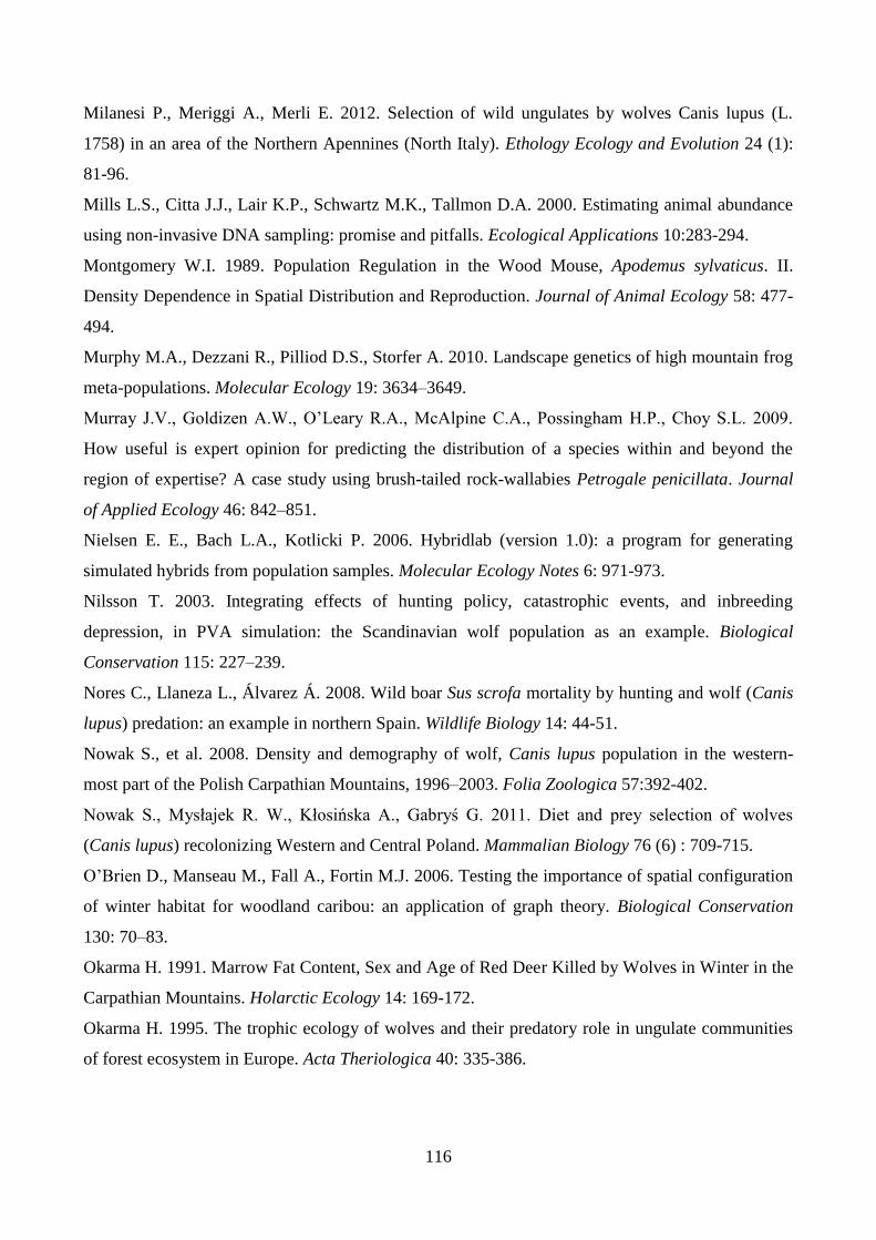
116

Milanesi P., Meriggi A., Merli E. 2012. Selection of wild ungulates by wolves Canis lupus (L.

1758) in an area of the Northern Apennines (North Italy). Ethology Ecology and Evolution 24 (1):

81-96.

Mills L.S., Citta J.J., Lair K.P., Schwartz M.K., Tallmon D.A. 2000. Estimating animal abundance

using non-invasive DNA sampling: promise and pitfalls. Ecological Applications 10:283-294.

Montgomery W.I. 1989. Population Regulation in the Wood Mouse, Apodemus sylvaticus. II.

Density Dependence in Spatial Distribution and Reproduction. Journal of Animal Ecology 58: 477-

494.

Murphy M.A., Dezzani R., Pilliod D.S., Storfer A. 2010. Landscape genetics of high mountain frog

meta-populations. Molecular Ecology 19: 3634–3649.

Murray J.V., Goldizen A.W., O’Leary R.A., McAlpine C.A., Possingham H.P., Choy S.L. 2009.

How useful is expert opinion for predicting the distribution of a species within and beyond the

region of expertise? A case study using brush-tailed rock-wallabies Petrogale penicillata. Journal

of Applied Ecology 46: 842–851.

Nielsen E. E., Bach L.A., Kotlicki P. 2006. Hybridlab (version 1.0): a program for generating

simulated hybrids from population samples. Molecular Ecology Notes 6: 971-973.

Nilsson T. 2003. Integrating effects of hunting policy, catastrophic events, and inbreeding

depression, in PVA simulation: the Scandinavian wolf population as an example. Biological

Conservation 115: 227–239.

Nores C., Llaneza L., Álvarez Á. 2008. Wild boar Sus scrofa mortality by hunting and wolf (Canis

lupus) predation: an example in northern Spain. Wildlife Biology 14: 44-51.

Nowak S., et al. 2008. Density and demography of wolf, Canis lupus population in the western-

most part of the Polish Carpathian Mountains, 1996–2003. Folia Zoologica 57:392-402.

Nowak S., Mysłajek R. W., Kłosińska A., Gabryś G. 2011. Diet and prey selection of wolves

(Canis lupus) recolonizing Western and Central Poland. Mammalian Biology 76 (6) : 709-715.

O’Brien D., Manseau M., Fall A., Fortin M.J. 2006. Testing the importance of spatial configuration

of winter habitat for woodland caribou: an application of graph theory. Biological Conservation

130: 70–83.

Okarma H. 1991. Marrow Fat Content, Sex and Age of Red Deer Killed by Wolves in Winter in the

Carpathian Mountains. Holarctic Ecology 14: 169-172.

Okarma H. 1995. The trophic ecology of wolves and their predatory role in ungulate communities

of forest ecosystem in Europe. Acta Theriologica 40: 335-386.

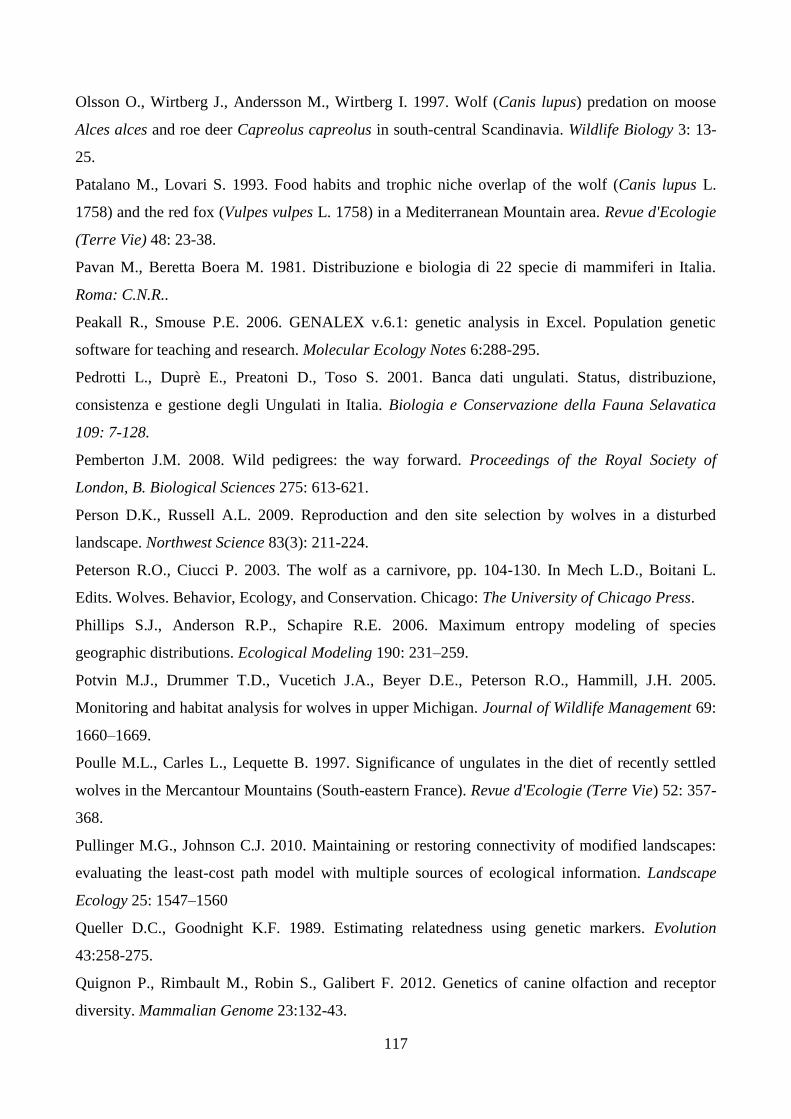
117

Olsson O., Wirtberg J., Andersson M., Wirtberg I. 1997. Wolf (Canis lupus) predation on moose

Alces alces and roe deer Capreolus capreolus in south-central Scandinavia. Wildlife Biology 3: 13-

25.

Patalano M., Lovari S. 1993. Food habits and trophic niche overlap of the wolf (Canis lupus L.

1758) and the red fox (Vulpes vulpes L. 1758) in a Mediterranean Mountain area. Revue d'Ecologie

(Terre Vie) 48: 23-38.

Pavan M., Beretta Boera M. 1981. Distribuzione e biologia di 22 specie di mammiferi in Italia.

Roma: C.N.R..

Peakall R., Smouse P.E. 2006. GENALEX v.6.1: genetic analysis in Excel. Population genetic

software for teaching and research. Molecular Ecology Notes 6:288-295.

Pedrotti L., Duprè E., Preatoni D., Toso S. 2001. Banca dati ungulati. Status, distribuzione,

consistenza e gestione degli Ungulati in Italia. Biologia e Conservazione della Fauna Selavatica

109: 7-128.

Pemberton J.M. 2008. Wild pedigrees: the way forward. Proceedings of the Royal Society of

London, B. Biological Sciences 275: 613-621.

Person D.K., Russell A.L. 2009. Reproduction and den site selection by wolves in a disturbed

landscape. Northwest Science 83(3): 211-224.

Peterson R.O., Ciucci P. 2003. The wolf as a carnivore, pp. 104-130. In Mech L.D., Boitani L.

Edits. Wolves. Behavior, Ecology, and Conservation. Chicago: The University of Chicago Press.

Phillips S.J., Anderson R.P., Schapire R.E. 2006. Maximum entropy modeling of species

geographic distributions. Ecological Modeling 190: 231–259.

Potvin M.J., Drummer T.D., Vucetich J.A., Beyer D.E., Peterson R.O., Hammill, J.H. 2005.

Monitoring and habitat analysis for wolves in upper Michigan. Journal of Wildlife Management 69:

1660–1669.

Poulle M.L., Carles L., Lequette B. 1997. Significance of ungulates in the diet of recently settled

wolves in the Mercantour Mountains (South-eastern France). Revue d'Ecologie (Terre Vie) 52: 357-

368.

Pullinger M.G., Johnson C.J. 2010. Maintaining or restoring connectivity of modified landscapes:

evaluating the least-cost path model with multiple sources of ecological information. Landscape

Ecology 25: 1547–1560

Queller D.C., Goodnight K.F. 1989. Estimating relatedness using genetic markers. Evolution

43:258-275.

Quignon P., Rimbault M., Robin S., Galibert F. 2012. Genetics of canine olfaction and receptor

diversity. Mammalian Genome 23:132-43.

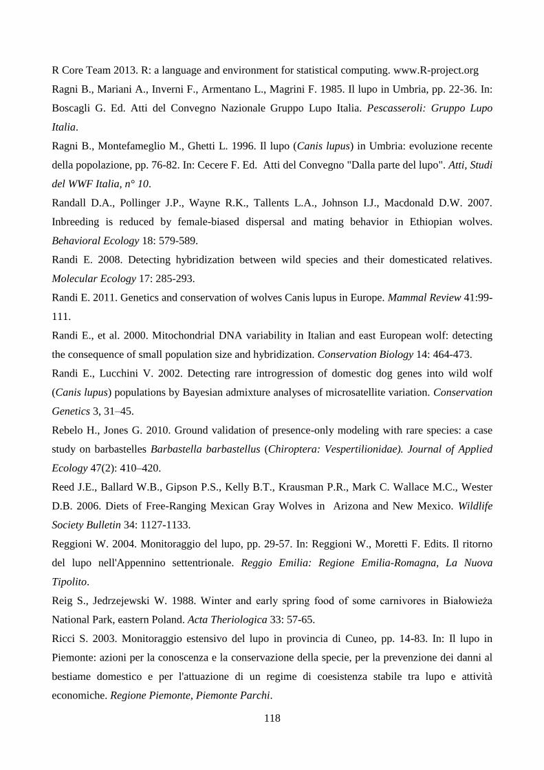
118

R Core Team 2013. R: a language and environment for statistical computing. www.R-project.org

Ragni B., Mariani A., Inverni F., Armentano L., Magrini F. 1985. Il lupo in Umbria, pp. 22-36. In:

Boscagli G. Ed. Atti del Convegno Nazionale Gruppo Lupo Italia. Pescasseroli: Gruppo Lupo

Italia.

Ragni B., Montefameglio M., Ghetti L. 1996. Il lupo (Canis lupus) in Umbria: evoluzione recente

della popolazione, pp. 76-82. In: Cecere F. Ed. Atti del Convegno "Dalla parte del lupo". Atti, Studi

del WWF Italia, n° 10.

Randall D.A., Pollinger J.P., Wayne R.K., Tallents L.A., Johnson I.J., Macdonald D.W. 2007.

Inbreeding is reduced by female-biased dispersal and mating behavior in Ethiopian wolves.

Behavioral Ecology 18: 579-589.

Randi E. 2008. Detecting hybridization between wild species and their domesticated relatives.

Molecular Ecology 17: 285-293.

Randi E. 2011. Genetics and conservation of wolves Canis lupus in Europe. Mammal Review 41:99-

111.

Randi E., et al. 2000. Mitochondrial DNA variability in Italian and east European wolf: detecting

the consequence of small population size and hybridization. Conservation Biology 14: 464-473.

Randi E., Lucchini V. 2002. Detecting rare introgression of domestic dog genes into wild wolf

(Canis lupus) populations by Bayesian admixture analyses of microsatellite variation. Conservation

Genetics 3, 31–45.

Rebelo H., Jones G. 2010. Ground validation of presence-only modeling with rare species: a case

study on barbastelles Barbastella barbastellus (Chiroptera: Vespertilionidae). Journal of Applied

Ecology 47(2): 410–420.

Reed J.E., Ballard W.B., Gipson P.S., Kelly B.T., Krausman P.R., Mark C. Wallace M.C., Wester

D.B. 2006. Diets of Free-Ranging Mexican Gray Wolves in Arizona and New Mexico. Wildlife

Society Bulletin 34: 1127-1133.

Reggioni W. 2004. Monitoraggio del lupo, pp. 29-57. In: Reggioni W., Moretti F. Edits. Il ritorno

del lupo nell'Appennino settentrionale. Reggio Emilia: Regione Emilia-Romagna, La Nuova

Tipolito.

Reig S., Jedrzejewski W. 1988. Winter and early spring food of some carnivores in Białowieża

National Park, eastern Poland. Acta Theriologica 33: 57-65.

Ricci S. 2003. Monitoraggio estensivo del lupo in provincia di Cuneo, pp. 14-83. In: Il lupo in

Piemonte: azioni per la conoscenza e la conservazione della specie, per la prevenzione dei danni al

bestiame domestico e per l'attuazione di un regime di coesistenza stabile tra lupo e attività

economiche. Regione Piemonte, Piemonte Parchi.

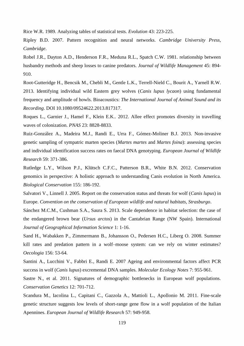
119

Rice W.R. 1989. Analyzing tables of statistical tests. Evolution 43: 223-225.

Ripley B.D. 2007. Pattern recognition and neural networks. Cambridge University Press,

Cambridge.

Robel J.R., Dayton A.D., Henderson F.R., Meduna R.L., Spatch C.W. 1981. relationship between

husbandry methods and sheep losses to canine predators. Journal of Wildlife Management 45: 894-

910.

Root-Gutteridge H., Bencsik M., Chebli M., Gentle L.K., Terrell-Nield C., Bourit A., Yarnell R.W.

2013. Identifying individual wild Eastern grey wolves (Canis lupus lycaon) using fundamental

frequency and amplitude of howls. Bioacoustics: The International Journal of Animal Sound and its

Recording. DOI 10.1080/09524622.2013.817317.

Roques L., Garnier J., Hamel F., Klein E.K.. 2012. Allee effect promotes diversity in travelling

waves of colonization. PNAS 23: 8828-8833.

Ruiz-González A., Madeira M.J., Randi E., Urra F., Gómez-Moliner B.J. 2013. Non-invasive

genetic sampling of sympatric marten species (Martes martes and Martes foina): assessing species

and individual identification success rates on faecal DNA genotyping. European Journal of Wildlife

Research 59: 371-386.

Rutledge L.Y., Wilson P.J., Klütsch C.F.C., Patterson B.R., White B.N. 2012. Conservation

genomics in perspective: A holistic approach to understanding Canis evolution in North America.

Biological Conservation 155: 186-192.

Salvatori V., Linnell J. 2005. Report on the conservation status and threats for wolf (Canis lupus) in

Europe. Convention on the conservation of European wildlife and natural habitats, Strasburgo.

Sánchez M.C.M., Cushman S.A., Saura S. 2013. Scale dependence in habitat selection: the case of

the endangered brown bear (Ursus arctos) in the Cantabrian Range (NW Spain). International

Journal of Geographical Information Science 1: 1-16.

Sand H., Wabakken P., Zimmermann B., Johansson O., Pedersen H.C., Liberg O. 2008. Summer

kill rates and predation pattern in a wolf–moose system: can we rely on winter estimates?

Oecologia 156: 53-64.

Santini A., Lucchini V., Fabbri E., Randi E. 2007 Ageing and environmental factors affect PCR

success in wolf (Canis lupus) excremental DNA samples. Molecular Ecology Notes 7: 955-961.

Sastre N., et al. 2011. Signatures of demographic bottlenecks in European wolf populations.

Conservation Genetics 12: 701-712.

Scandura M., Iacolina L., Capitani C., Gazzola A., Mattioli L., Apollonio M. 2011. Fine-scale

genetic structure suggests low levels of short-range gene flow in a wolf population of the Italian

Apennines. European Journal of Wildlife Research 57: 949-958.

120

Schenone L., Aristarchi C., Meriggi A. 2004. Ecologia del Lupo (Canis lupus) in provincia di

Genova: distribuzione, consistenza, alimentazione e impatto sulla zootecnia. Hystrix, Italian

Journal of Mammalogy 15: 49-66.

Schmidt P.A., Mech L.D. 1997. Wolf pack size and food acquisition. American Naturalist 150:

513-517.

Schwartz M.K., Luikart G., Waples R.S. 2007. Genetic monitoring as a promising tool for

conservation and management. Trends in Ecology and Evolution 22: 25-33.

Seaman D.E., Millspaugh J.J., Kernohan B.J., Brundige G.C., Raedeke K.J., Gitzen R.A. 1999.

Effects of Sample Size on Kernel Home Range Estimates. Journal of Wildlife Management 63: 739-

747.

Segelbacher G., Cushman S.A., Epperson B.K., Fortin M.J., Francois O., Hardy O.J., Holderegger

R., Taberlet P., Waits L.P., Manel S. 2010. Applications of landscape genetics in conservation

biology: concepts and challenges. Conservation Genetics 11: 375–385.

Shirk A.J., Wallin D.O., Cushman S.A., Rice C.G., Warheit K.I. 2010. Inferring landscape effects

on gene flow: a new model selection framework. Molecular Ecology 19: 3603-3619.

Sillero-Zubiri C., King A.A., MacDonald D.W. 1996. Rabies and mortality in Ethiopian wolves

(Canis simensis). Journal of Wildlife Diseases 32: 80-86.

Sinclair A.R.E., Fryxell J.M., Caughley G. 2006. Wildlife ecology conservation and management.

Second Edition. Oxford: Blackwell Science.

Śmietana W., Klimek A. 1993. Diet of wolves in the Bieszczady Mountains, Poland. Acta

Theriologica 42: 241-252.

Smith D., Meier T., Geffen E., Mech L.D., Burch J.W., Adams L.G., Wayne R.K. 1997. Is incest

common in gray wolf packs? Behavioral Ecology 8: 384-391.

Smith D.W., Peterson R.O., Houston D.B. 2003. Yellowstone after wolves. BioScience 53: 330-

340.

Smouse P.E., Paekall R. 1999. Spatial autocorrelation analysis of individual multiallele and

multilocus genetic structure. Heredity 82: 561-573.

Soffiantini C.S., Lazzini C., Sabbioni A., Zanon A., Beretti V. 2006. Growth curves in roe deer

population of Massa-Carrara province. Annali della Facoltà di Medicina Veterinaria di Parma 26:

319-334

Sparkman A.M., Adams J.M., Steury T.D., Waits L.P., Murray D.L. 2012. Pack social dynamics

and inbreeding avoidance in the cooperatively breeding red wolf. Behavioral Ecology 23: 1186-

1194

121

Spear S.F., Balkenhol N., Fortin M.J., McRae B.H., Scribner K. 2010. Use of resistance surfaces for

landscape genetic studies: considerations for parameterization and analysis. Molecular Ecology 19,

3576–3591.

Squires J.R., DeCesare N.J., Olson L.E., Kolbe J.A., Hebblewhite M., Parks S.A. 2013. Combining

resource selection and movement behavior to predict corridors for Canada lynx at their southern

range periphery. Biological Conservation 157: 187-195.

Stahler D.R., Macnulty D.R., Wayne R.K., Vonholdt B., Smith D.W., Pelletier F. 2012. The

adaptive value of morphological, behavioural and life-history traits in reproductive female wolves.

The Journal of Animal Ecology 73: 1300-1306.

Steiner C.C., Putnam A.S., Hoeck P.E.A., Ryder O.A. 2013. Conservation Genomics of Threatened

Animal Species. Annual. Review of Animal Bioscience 1:261-281.

Stenglein J. L., Waits L.P., Ausband D.E., Zager P., Mack C.M. 2011. Estimating gray wolf pack

size and family relationships using noninvasive genetic sampling at rendezvous sites. Journal of

Mammalogy 92:784-795.

Stephen D.W., Krebs J.R. 1986. Foraging theory. Princeton: Princeton University Press.

Stevens V.M., Verkenne C., Vandewoestijne S., Wesselingh R.A., Baguette M. 2006. Gene flow

and functional connectivity in the natterjack toad. Molecular Ecology 15: 2333-2344.

Storfer A., Murphy M.A., Spear S.F., Holderegger R., Waits L.P. 2010. Landscape genetics: where

are we now? Molecular Ecology 19: 3496-3514.

Sundqvist A.K., Ellegren H., Olivier M., Vilà C. 2001. Y chromosome haplotyping in Scandinavian

wolves (Canis lupus) based on microsatellite markers. Molecular Ecology 10:1959-1966.

Suryawanshi K. R., Bhatnagar Y. V., Redpath S., Mishra C. 2013. People, predators and

perceptions: patterns of livestock depredation by snow leopards and wolves. Journal of Applied

Ecology.

Teerink B.J. 1991. Hair of West-European mammals. Cambridge: Cambridge University Press.

Thomassen H.A., Cheviron Z.A., Freedman A.H., Harrigan R.J., Wayne R.K., Smith T.B. 2010.

Spatial modelling and landscape-level approaches for visualizing intra-specific variation. Molecular

Ecology 19: 3532-3548.

Thurber J.M., Peterson R.O. 1993. Effects of population density and pack size on the foraging

ecology of gray wolves. Journal of Mammalogy 74: 879-889.

Treves A., Naughton-Treves L., Harper K., Mladenoff D.J., Rose R.A., Sickley T.A., Wagner C.,

Holzapfel M., Kluth G., Reinhardt I., Ansorge H. 2012. Wolf (Canis lupus) feeding habits during

the first eight years of its occurrence in Germany. Mammalian Biology 77 (3) : 196-203.

122

Vaha J. P., Primmer C.R. 2006. Efficiency of model-based Bayesian methods for detecting hybrid

individuals under different hybridization scenarios and with different numbers of loci. Molecular

Ecology 15: 63-72.

Valière N., Fumagalli L., Gielly L., Miquel C., Lequette B., Poulle M.L., Weber J.M., Arlettaz R.,

Taberlet P. 2003. Long-distance wolf recolonization of France and Switzerland inferred from non-

invasive genetic sampling over a period of 10years. Animal Conservation 6: 83–92.

Van Ballenberghe V., Erickson A.W., D. Byman D. 1975. Ecology of the timber wolf in

northeastern Minnesota. Wildlife Monographs 43: 1-43.

Van Oosterhout C., Hutchinson W.F., Wills D.P.M., Shipley P. 2004. Microchecker: software for

identifying and correcting genotyping errors in microsatellite data. Molecular Ecology Notes 4:535-

538.

Van Strien M.J., Keller D., Holderegger R. 2012. A new analytical approach to landscape genetic

modelling: least-cost transect analysis and linear mixed models. Molecular Ecology 21: 4010–4023.

Verardi A., Lucchini V., Randi E. 2006. Detecting introgressive hybridization between free-ranging

domestic dogs and wild wolves (Canis lupus) by admixture linkage disequilibrium analysis.

Molecular Ecology 15: 2845-2855.

Vilà C., et al. 2003. Rescue of a severely bottlenecked wolf (Canis lupus) population by a single

immigrant. Proceedings of the Royal Society of London Series B: Biological Sciences 270: 91-7.

vonHoldt B.M., Pollinger J.P., Earl D.A., Parker H.G., Ostrander E.A., Wayne R.K. 2012.

Identification of recent hybridization between gray wolves and domesticated dogs by SNP

genotyping. Mammalian Genome 24:80-88.

vonHoldt B.M., Stahler D.R., Smith D.W., Earl D.A., Pollinger J.P., Wayne R.K. 2008. The

genealogy and genetic viability of reintroduced Yellowstone grey wolves. Molecular Ecology 17:

252-274.

Vos J. 2000. Food habits and livestock depredation of two Iberian wolf packs (Canis lupus

signatus) in the north of Portugal. Journal of Zoology 251: 457-462.

Vucetich J.A., Peterson R.O. 2009. Wolf and Moose Dynamics on Isle Royale. Recovery of grey

wolves in the Great Lakes Region of the United States. An Endangered Species Success Story.

Springer New York : 35-48.

Waits L.P., Luikart G., Taberlet P. 2001. Estimating the probability of identity among genotypes in

natural populations: cautions and guidelines. Molecular Ecology 10: 249-256.

Waits L.P., Paetkau D. 2005. Noninvasive genetic sampling tools for wild- life biologists: a review

of applications and recommendations for accurate data collection. Journal of Wildlife Management

69: 1419-1433.

123

Wang I.J., Glor R.E., Losos J.B. 2013. Quantifying the roles of ecology and geography in spatial

genetic divergence. Ecologyl Letters 16: 175-182.

Wang J. 2011. COANCESTRY: a program for simulating, estimating and analysing relatedness and

inbreeding coefficients. Molecular Ecology Resources 11:141-145.

Wang J., Santure A.W. 2009. Parentage and sibship inference from multi-locus genotype data under

polygamy. Genetics 181:1579-1594.

Wang Y.H., Yang K.C., Bridgman C.L., Lin L.K. 2008. Habitat suitability modeling to correlate

gene flow with landscape connectivity. Landscape Ecology 23: 989–1000.

Wasserman T.N., Cushman S.A., Schwartz M.K., Wallin D.O. 2010. Spatial scaling and multi-

model inference in landscape genetics: Martes americana in northern Idaho. Landscape Ecology 25

Wayne R.K., Hedrick P. 2011. Genetics and wolf conservation in the American West: lessons and

challenges. Heredity 107:16-19.

Weir B.S., Cockerham C.C. 1984. Estimating F-statistic for the analysis of population structure.

Evolution 38: 1358-1370.

Wilson G.J., Delahay R.J. 2001. A review of methods to estimate the abundance of terrestrial

carnivores using field signs and observation. Wildlife Research 28:151-164.

Wittmer H.U., Sinclair A.R.E., McLellan B.N. 2005. The role of predation in the decline and

extirpation of woodland caribou. Oecologia 144: 257–267.

Zimen E., Boitani L., 1975. Number and distribution of wolves in Italy. Saugetierkunde 40:102-

112.

Zub K., Theuerkauf J., Jedrzejewski W. 2003. Wolf pack territory marking in the Bialowieza

Primeval Forest (Poland). Behaviour 140: 635-648.

124

LIST OF PAPERS

1. MERIGGI A., BRANGI A., SCHENONE L., SIGNORELLI D., MILANESI P., 2011. Changes

of wolf (Canis lupus) diet in Italy in relation to the increase of wild ungulate abundance.

Ethology, Ecology & Evolution, 23 (3) : 195 – 210.

2. MILANESI P., MERIGGI A., MERLI E., 2012. Selection of wild ungulates by wolves (Canis

lupus L.1758) in an area of the Northern Apennines. Ethology, Ecology & Evolution, 24 (1) :

81–96.

3. CANIGLIA R., FABBRI E., GALAVERNI M., MILANESI P., RANDI E., 2014. Genetic

variability, pack structure and dynamics in an expanding gray wolf population. Journal of

Mammalogy (in press.).

4. DONDINA O., MERIGGI A., DAGRADI V., PERVERSI M., MILANESI P., 2014. Wolf

predation on livestock in an area of Northern Italy and prediction of damage risk. Ethology,

Ecology & Evolution (in press.).

5. DAGRADI V., DONDINA O., PERVERSI M., MILANESI P., LOMBARDINI M.,

RAVIGLIONE S., REPOSSI A., MERIGGI A., 2014. Short term responses of wolves feeding

habits to changes of wild and domestic ungulate abundance in Northern Italy. Italian Journal of

Zoology (submitted).

6. MILANESI P., CANIGLIA R., FABBRI E., GALAVERNI M., MERIGGI A., RANDI E.,

2014. Non-invasive genetic sampling to predict species ecological niche and depredation risk:

12-years of monitoring on the Italian wolf. Animal Conservation (submitted).

7. MILANESI P., HOLDEREGGER R., CANIGLIA R., FABBRI E., RANDI E., 2014.

Landscape-genetics and habitat suitability models: general implications of a specific

application. Molecular Ecology (submitted).

125

ACKNOWLEDGEMENTS

I greatly thank everybody who allowed me the achievement of this PhD Thesis in a pleasant way:

especially my Professor and Supervisor Ettore Randi who made possible the achievement of one of

my career aims: the PhD; Dott. Romolo Caniglia who taught me most of my knowledge about non-

invasive genetics and for support me as a brother; Dott. Alberto Meriggi for his ecological lessons.

Dott. Elena Fabbri and Dott. Marco Galaverni for their fundamental suggestions. Prof. Barbara

Mantovani for her lessons in the 3 years of PhD course and the final supervision of this thesis.

I greatly thank Prof. Rolf Holderegger who gave me the chance to spend a period at WSL allowing

me to analyze data in a landscape genetics framework with the hope to produce a great PhD thesis,

who considered me as a son during my whole Swiss period. I greatly thank Dott. Kurt Bollmann for

his clear comments and suggestions on my studies.

I greatly thank also:

- My father who strongly supported me and always helped me to face each difficulties;

- Francesca who deeply changed my life giving me the most beautiful feelings of these years;

- All my friends and collegous : Silvana, Edoardo, Aritz, Francesca, Chiara, Federica, Désirée,

Laura, Matteo, Jeremy, Florian, Stefan, Frank, Saran, René, Martin and Felix.

A special thank goes to everybody who took care of the samples and field information collection.