NOVATECH 2010

1

Ability of software SWMM to simulate transient sewer smooth pressurization

Capacité du logiciel SWMM à simuler une mise sous pression temporaire du réseau d'assainissement

G. B. Ferreri, G. Freni and P. Tomaselli

Dipartimento di Ingegneria Idraulica ed Applicazioni Ambientali, Università di Palermo (Dept. of Hydraulic Engineering and Environmental Applications, University of Palermo), Viale delle Scienze, Ed. 8, I-90128 Palermo, Italy. E-mail: giofer@idra.unipa.it, freni@idra.unipa.it, kobelak@libero.it

RÉSUMÉ

A la suite d’événements pluviaux importants ou d’une défaillance du réseau, le remplissage des égouts (pressurisation) et des débordements peuvent se produire. Plusieurs logiciels sont généralement utilisés pour simuler les inondations dans les réseaux d’assainissement et les résultats sont habituellement fiables et solides. Les modèles mathématiques basés sur l'équation de l'élan sont plus appropriés pour simuler correctement la variation de pressurisation mais les modèles basés sur l'équation de l'énergie sont très populaires en raison de leur plus grande simplicité par rapport aux premiers. Dans cet article, basé sur des tests réalisés en laboratoire sur un tuyau, la capacité du logiciel SWMM (modèle de gestion des eaux pluviales, sans doute le logiciel le plus populaire pour les réseaux d’assainissement) à simuler la mise sous pression transitoire a été étudiée. De nombreux tests ont été effectués en utilisant SWMM, en variant la distance dans le temps et l'espace ainsi que la largeur de la fente de Preissmann afin d'examiner les performances du logiciel même dans des fourchettes de paramètres plus étendus que ceux utilisés d'habitude lors des applications pratiques. La comparaison entre les montées subites simulées et expérimentales nous permet de tirer des conclusions intéressantes sur l'efficacité de SWMM pour simuler la pressurisation aussi bien que sur le choix des ces paramètres.

ABSTRACT

As a consequence of heavy rainfall events or network malfunctioning, filling of sewers (pressurization) and network overflowing may occur. Several models are commonly used to simulate floods in drainage networks and their results are usually thought to be reliable and robust. Actually, mathematical models based on the momentum equation appear to be more suitable in correctly simulating the pressurization moving jump but models based on the energy equation are much more popular because of their greater simplicity in comparison to the former ones. In this paper, on the basis of laboratory pipe tests, the ability of software SWMM (Storm Water Management Model, probably the most popular software for drainage networks) to simulate transient pressurization is studied. Many numerical tests were carried out by SWMM varying the spatial and time steps as well as the Preissmann slot width in order to examine the performances of the software along even wider intervals of these parameters than usual in practical applications. The comparison between simulated and experimental surges allows one to draw interesting conclusions on the effectiveness of SWMM in simulating pressurization as well as on the choice of the parameters themselves.

KEYWORDS Numerical modelling, Pressurization, Transition, Unsteady flow, Urban drainage.

SESSION 2.3

2

1 INTRODUCTION

Urban drainage networks are generally designed to operate in a free-surface flow condition, with filling ratios being less than 0.7-0.8. However, in particular circumstances (downpour, network malfunctioning, etc.), filling of several or all the sewers and network overflowing may occur, with flooding of streets and cellars. From the technical literature we learn that transition from free-surface to pressurized flow may generate noticeable pressure oscillations, usually indicated as “water-hammer phenomena” (e. g., Song, 1976; Hamam and McCorquodale, 1982; Song et al., 1983; Li and McCorquodale, 1999; Zhou et al., 2002) and believed to be able to damage the network. In spite of this, pressurization transient has not been studied exhaustively. Most of the few studies dealing with pressurization were made considering a drastic reduction in the discharge in the downstream end of a pipe, which is likely to be the situation yielding the most intense oscillation phenomena.

Testing by Ciraolo and Ferreri (2007), in which pressurization transient was started off by sudden closing of the downstream tank outlet, showed that actually pressurization can occur following two distinct patterns, called by the authors “smooth” and “abrupt”. Smooth pressurization occurs when the bore front consequent on the closing operation does not reach the pipe crown (lower flow rates and pipe slopes) and the pipe pressurizes by gradual rising of the free-surface after the front passing. Abrupt pressurization, instead, occurs when the bore front goes over the pipe crown (higher flow rates and/or slopes) and each pipe section is suddenly pressurized since it is reached by the front itself. The authors observed intense oscillations, analogous to those indicated in the literature as of water-hammer, in abrupt pressurization only. However, as we shall see, lower but noticeable pressure oscillations occur in smooth pressurization too. The analysis of the experimental diagrams allowed Ciraolo and Ferreri to recognize that pressure oscillations are not yielded by water-hammer phenomena but by pulsations of air pockets entrapped in water flow during pressurization, as they migrate along the sewers and are released through the manholes. This conclusion is corroborated by mathematical modelling results for abrupt pressurization by Ciraolo and Ferreri (2008a, b) as well as by laboratory tests by Vasconcelos and Wright (2005) and by Zhou et al. (2002).

Although abrupt pressurization is more dangerous from the point of view of ejection of manhole covers and sewer stability, smooth pressurization is much more frequent. Note that network pressurization is not necessarily consequent on exceptional events, since its occurrence depends on many factors, such as previous network filling ratio, network maintenance, malfunctioning of control devices, pump stops, etc.. Therefore, reliable mathematical simulation of smooth pressurization is very desirable, and this is the topic of the present paper.

Actually, only a few experimental studies on smooth pressurization are found in the technical literature, among which the best-known are those by Wiggert (1972), Capart et al. (1997) and Trajkovic et al. (1998). The former studied pipe pressurization caused by gradual rising of the upstream-tank level, and mathematically simulated the bore propagation by means of a model based on a characteristic method and the pressurized stage by means of the usual equations of a rigid column. The latter two, instead, performed experiments aiming at validating mathematical models based on de Saint-Venant (DSV) equations in a conservative form, with the help of the Preissmann slot, the equations being solved by means of “shock-capturing” schemes (e. g., Garcia-Navarro and Saviron, 1992). On the whole, these models matched experimental results rather well, showing that they are suited for the purpose. However, it is to be stressed that, because of the Preissmann slot, such models do not allow either the presence and migration of pulsating air pockets or the formation of negative pressures, in already pressurized sewers, to be taken into account. Therefore, in order to avoid this drawback, the experiments both of Capart et al. and of Trajkovic et al. were performed adopting low flow rates and initial filling ratios, so that air capture proved negligible.

In order for air pocket and negative pressures to be taken into account in the modelling of network pressurization, Song (1976) and Song et al. (1983) proposed models coupling de Saint-Venant equations for free-surface flow and pressurized compressible flow equations for pressurized flow, both solved by means of a characteristic method. The air presence was taken into account by reducing the acoustic wave celerity. By contrast, Vasconcelos et al. (2006) proposed a model which split the pressure in pressurized sewers into two parts. The surcharge one, which could even be negative, was expressed as a function of the elastic sewer deformation. This expedient allowed the authors to adopt the equations of incompressible fluids having, however, a finite wave celerity, as in de Saint-Venant free-surface flow equations. The presence of air pockets, once again, was taken into account by means of a suitable wave celerity. The model reasonably matches some laboratory tests in which, however, no air entrapment in the liquid column was ensured.

NOVATECH 2010

3

Other relevant examples of approaching drainage network modelling are found in Ridgway and Kumpala (2007, 2008). However, in spite of the aforesaid and other still ongoing studies, the great majority of practical sewer modelling applications (network design or simulation or management) are based on more robust solving schemes of DSV equations which were not specifically developed for reproducing pressurization. Among them we can mention INFOWORKS (Wallingford HR, 1998), MOUSE (Danish Hydraulic Institute, 1995) and SWMM (Huber et al., 1984). All these models use DSV equations solved in the non conservative form with the help of the Preissmann slot. Some other models, instead, are contrived without the Preissmann slot, like for instance DORA (Double ORder Approximation; see: Noto, 1999; Noto and Tucciarelli, 2001). Their results are usually thought to be reliable and robust, at least for practical purposes. This conviction is effectively based on the fact that they have been widely used for many years and on the physical congruence of the results obtained. Practical reliability and robustness, however, concern situations in which each sewer works either in a free-surface or in a pressure condition, whereas no specific studies have been made on the behaviour of these softwares during transition from one to the other condition.

In this paper, on the basis of previous laboratory tests on a pipe between two tanks, the ability of SWMM, probably the most popular software for drainage networks, to simulate smooth pressurization transient is examined in depth.

2 SWMM EQUATIONS AND CHARACTERISTICS

SWMM uses a link-node description of the sewer system which facilitates the discrete representation of the physical prototype and the mathematical solution of the gradually-varied DSV continuity and momentum equations. The primary dependent variable in the links is the flow rate, Q. The solution is for the average flow in each link, assumed to be constant over a time step. In the numerical solution, flow velocity and cross sectional area, or depth, are variable in the link. The nodes are the storage elements of the system, and the related heads, H, are the primary dependent variables, which are assumed to be changing in time but constant throughout any one node.

The continuity and the momentum equations are reported in the following, while a detailed discussion of single terms can be found in the literature (e. g., Lai, 1986):

q

s

Vh

t

h

(1)

h

V

g

qSS

s

h

s

V

g

V

t

V

g f

0

1 (2)

where h is the water depth, V the average velocity, q the lateral inflow/outflow (if present), g gravity acceleration, S0 the sewer slope, Sf the friction slope, which is usually expressed by the Manning or Chezy formulas, s the abscissa and t the time.

The numerical integration of the two hydraulic equations is accomplished by means of the improved polygon or modified Euler method. The results prove to be relatively accurate and, provided certain constraints are followed, are stable too (Huber et al., 1984).

The total sequence for computation of link flow rates and node heads is the following:

1 computing half-step flow rates in all the links at time t+∆t/2 on the basis of preceding full-step head values at the nodes;

2 computing half-step flow rate transfers through weirs, orifices and pumps at time t+∆t/2 on the basis of preceding full-step head values at transfer junctions;

3 computing half-step node heads at time t+∆t/2 on the basis of the average of preceding full-step and current half-step flow rates in all the links as well as of the current half-step flow rate transfers;

4 computing full-step flow rates in all the links at time t+∆t on the basis of half-step node heads;

5 computing full-step flow transfers at time t+∆t on the basis of current half-step heads at weirs, orifices and pump nodes;

6 computing full-step heads at time t+∆t for all the nodes on the basis of the average of preceding full-step and current full-step flow rates as well as of flow transfers at the current full-step.

SESSION 2.3

4

Trs1 Trs 2 Trs3 Trs4 Trs5

TrsUTrsD

Downstream tankUpstream tank

PiezometersPiezometersPiezometer

Outlet

Inlet

6.25 1.436.176.190.36 5.94

Sec. a Sec. b Sec. c

26.09

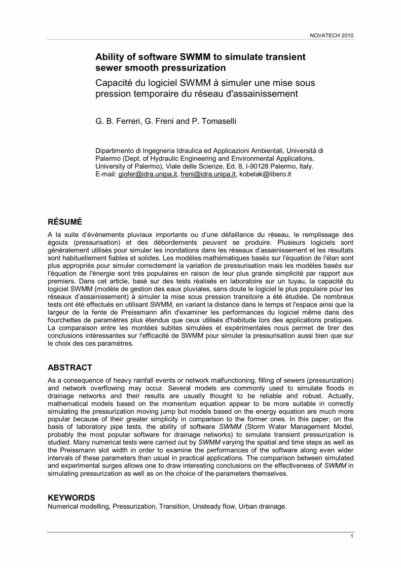
Fig. 1 – Experimental equipment, with transducer locations along the pipe.

3 EXPERIMENTAL RESULTS

Laboratory testing was described in detail by Ciraolo and Ferreri (2007); here only the essential information is given. The equipment (Fig. 1) consisted of a Plexiglas circular pipe between two iron tanks, which had length L=26.09 m, inner diameter D=244 mm and an adjustable slope. Both tanks had spillways whose crests were located 1 m from the bottom for blocking the level rising after pipe pressurization. The equipment on the whole outlined a sewer conduit between two manholes; the coming into operation of the spillways simulated street flooding. The sudden closing of a sharp sluice-gate set at the outlet of the downstream tank triggered off fast tank filling and the consequent start of pipe pressurization. The flow rate entering the system was gauged by an electromagnetic meter. Pressure gauging in the pipe and in the tanks during transient was performed by seven transducers (five along the pipe), whose locations and serial numbers are shown in Fig. 1.

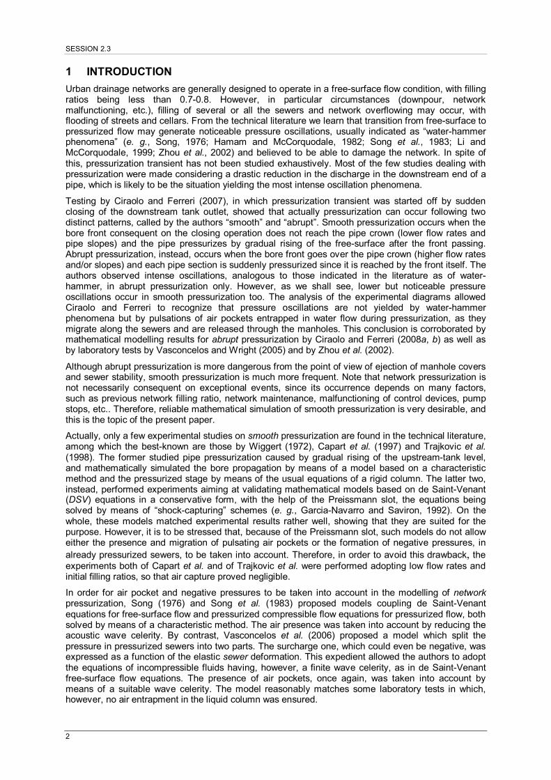
Smooth pressurization only occurred in the runs having the lower flow rates (Q = 15 and 20 dm3/s) and slopes (S0 = 0.2 and 0.6%). The front consequent on the closing operation did not reach the pipe crown and a bore began to migrate upstream along the pipe (Fig. 2a) causing sudden rising of the free surface which, however, remained below the pipe crown. After the front passing, as the downstream tank filled the free surface began to rise gradually (Fig. 2b), with a more or less uniform rise-rate along the pipe, until the pipe pressurized starting from the downstream end. Before pressurization concluded, the bore had reached the upstream tank and the latter had begun to fill, then submerging the pipe inlet. Eventually a moderate air quantity remained entrapped between the rising liquid flow and the pipe crown, in the form of a long and thin pocket, even longer than a half pipe length. The pocket then split into some smaller ones, each a few metres long, which migrated upstream to be finally released through the tank. When in the upstream and downstream tanks the levels were reached for which the overflowed flow rates equalled the supply flow rate Q, pipe pressures stabilized at the new steady flow values (Fig. 2c). During smooth pressurization pressure oscillations exhibited lower intensity than those indicated in the literature as of water-hammer.

III

IIIIV

V

III

IIIIV

V

III

IIIIV

V

Fig. 2 – Phases of system pressurization: a) wave front formation without pressurization; b) backward pressurization; c) steady state after pressurization.

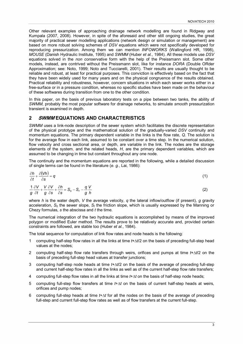
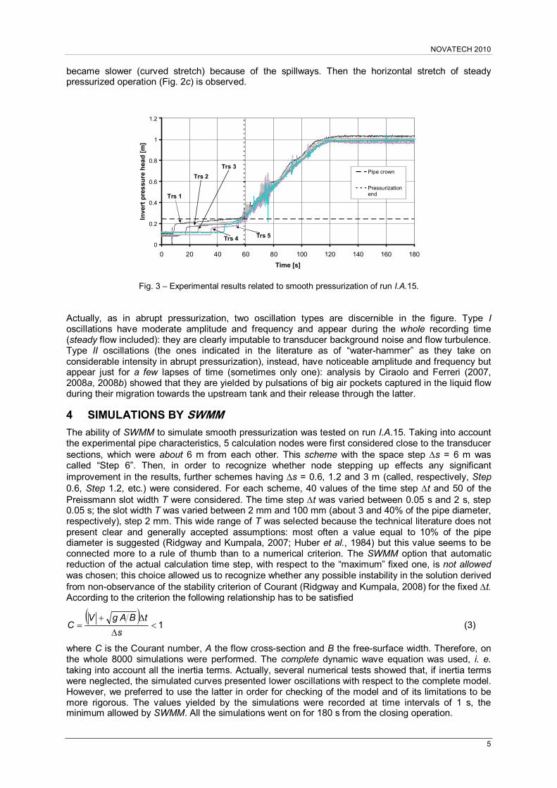
Fig. 3 shows, as an example, the experimental results relative to run I.A.15 (run cycle I, run group A, flow rate Q=15 dm3/s); the pipe slope was S0=0.2%. The figure shows the chronological diagrams of the pressure heads of the pipe invert in sections 1-5 of transducers. The front passing (Fig. 2a) is easily identifiable from the sudden pressure increase; the total pressure (flow depth plus front height) does not reach the pipe crown (broken horizontal line). The times at which the front reaches the transducer sections indicate a practically constant celerity. The next first ascending stretch, which mirrors the downstream tank filling (Fig. 2b), refers to the pipe pressurization; practically equal diagram slopes vouch for about uniform free-surface rise rate along the pipe. After the front outflow in the upstream tank (marked by a vertical dotted line), there follows a second ascending stretch with a considerably higher slope, because this tank too began filling. The filling first was faster but then

(a) (c) (b)

NOVATECH 2010

5

became slower (curved stretch) because of the spillways. Then the horizontal stretch of steady pressurized operation (Fig. 2c) is observed.

0

0.2

0.4

0.6

0.8

1

1.2

0 20 40 60 80 100 120 140 160 180

Time [s]

Inve

rt p

res

sure

hea

d [

m]

Pipe crown

Pressurizationend

Trs 4 Trs 5

Trs 3

Trs 2

Trs 1

Fig. 3 – Experimental results related to smooth pressurization of run I.A.15.

Actually, as in abrupt pressurization, two oscillation types are discernible in the figure. Type I oscillations have moderate amplitude and frequency and appear during the whole recording time (steady flow included): they are clearly imputable to transducer background noise and flow turbulence. Type II oscillations (the ones indicated in the literature as of “water-hammer” as they take on considerable intensity in abrupt pressurization), instead, have noticeable amplitude and frequency but appear just for a few lapses of time (sometimes only one): analysis by Ciraolo and Ferreri (2007, 2008a, 2008b) showed that they are yielded by pulsations of big air pockets captured in the liquid flow during their migration towards the upstream tank and their release through the latter.

4 SIMULATIONS BY SWMM

The ability of SWMM to simulate smooth pressurization was tested on run I.A.15. Taking into account the experimental pipe characteristics, 5 calculation nodes were first considered close to the transducer sections, which were about 6 m from each other. This scheme with the space step s = 6 m was called “Step 6”. Then, in order to recognize whether node stepping up effects any significant improvement in the results, further schemes having s = 0.6, 1.2 and 3 m (called, respectively, Step 0.6, Step 1.2, etc.) were considered. For each scheme, 40 values of the time step t and 50 of the Preissmann slot width T were considered. The time step t was varied between 0.05 s and 2 s, step 0.05 s; the slot width T was varied between 2 mm and 100 mm (about 3 and 40% of the pipe diameter, respectively), step 2 mm. This wide range of T was selected because the technical literature does not present clear and generally accepted assumptions: most often a value equal to 10% of the pipe diameter is suggested (Ridgway and Kumpala, 2007; Huber et al., 1984) but this value seems to be connected more to a rule of thumb than to a numerical criterion. The SWMM option that automatic reduction of the actual calculation time step, with respect to the “maximum” fixed one, is not allowed was chosen; this choice allowed us to recognize whether any possible instability in the solution derived from non-observance of the stability criterion of Courant (Ridgway and Kumpala, 2008) for the fixed t. According to the criterion the following relationship has to be satisfied

1

s

tBAgVC (3)

where C is the Courant number, A the flow cross-section and B the free-surface width. Therefore, on the whole 8000 simulations were performed. The complete dynamic wave equation was used, i. e. taking into account all the inertia terms. Actually, several numerical tests showed that, if inertia terms were neglected, the simulated curves presented lower oscillations with respect to the complete model. However, we preferred to use the latter in order for checking of the model and of its limitations to be more rigorous. The values yielded by the simulations were recorded at time intervals of 1 s, the minimum allowed by SWMM. All the simulations went on for 180 s from the closing operation.

SESSION 2.3

6

The Manning coefficient for friction loss was assumed to be 0.01 s/m1/3, by means of steady flow tests. Discharge coefficients of spillways and sluice-gate (not watertight) were determined by calibration as the values yielding the best simulated curves.

The “quality” of a simulation was evaluated through the Normalized Standard Deviation (NSD) between the simulated and the experimental invert pressure heads divided by the average value of measured invert pressure. Actually, since the equations used by SWMM are not able to simulate oscillations of either type I (noise and turbulence) or type II (air pocket pulsations), in order for the simulation-experiment comparison to prove more reliable the experimental curves (Fig. 3) were filtered out of all the oscillations and “mean” curves were obtained. In practice, each experimental curve was divided into several segments, each interpolated by polynomials up to the 6th degree. From now on, we will assume as “experimental” surge the mean one. Note that simulation of pressure oscillations during pressurization is weighty for sewer stability analysis but not for studying filling of network and sewer flow rates during floods, as stated by Ciraolo and Ferreri (2008a).

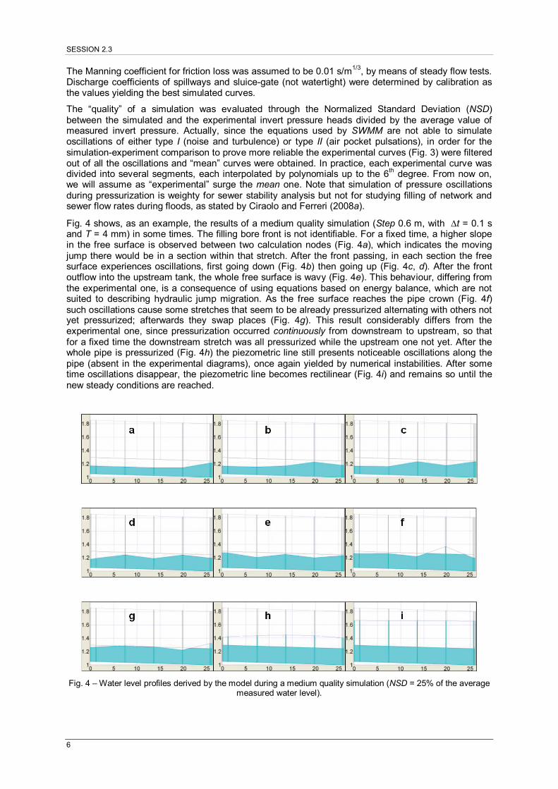
Fig. 4 shows, as an example, the results of a medium quality simulation (Step 0.6 m, with t = 0.1 s and T = 4 mm) in some times. The filling bore front is not identifiable. For a fixed time, a higher slope in the free surface is observed between two calculation nodes (Fig. 4a), which indicates the moving jump there would be in a section within that stretch. After the front passing, in each section the free surface experiences oscillations, first going down (Fig. 4b) then going up (Fig. 4c, d). After the front outflow into the upstream tank, the whole free surface is wavy (Fig. 4e). This behaviour, differing from the experimental one, is a consequence of using equations based on energy balance, which are not suited to describing hydraulic jump migration. As the free surface reaches the pipe crown (Fig. 4f) such oscillations cause some stretches that seem to be already pressurized alternating with others not yet pressurized; afterwards they swap places (Fig. 4g). This result considerably differs from the experimental one, since pressurization occurred continuously from downstream to upstream, so that for a fixed time the downstream stretch was all pressurized while the upstream one not yet. After the whole pipe is pressurized (Fig. 4h) the piezometric line still presents noticeable oscillations along the pipe (absent in the experimental diagrams), once again yielded by numerical instabilities. After some time oscillations disappear, the piezometric line becomes rectilinear (Fig. 4i) and remains so until the new steady conditions are reached.

Fig. 4 – Water level profiles derived by the model during a medium quality simulation (NSD = 25% of the average measured water level).

NOVATECH 2010

7

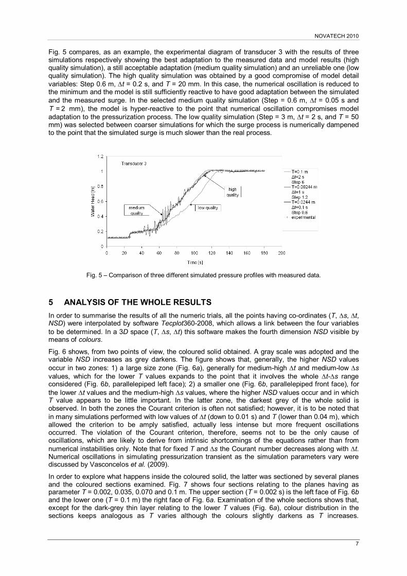
Fig. 5 compares, as an example, the experimental diagram of transducer 3 with the results of three simulations respectively showing the best adaptation to the measured data and model results (high quality simulation), a still acceptable adaptation (medium quality simulation) and an unreliable one (low quality simulation). The high quality simulation was obtained by a good compromise of model detail variables: Step 0.6 m, t = 0.2 s, and T = 20 mm. In this case, the numerical oscillation is reduced to the minimum and the model is still sufficiently reactive to have good adaptation between the simulated and the measured surge. In the selected medium quality simulation (Step = 0.6 m, t = 0.05 s and

2=T mm), the model is hyper-reactive to the point that numerical oscillation compromises model adaptation to the pressurization process. The low quality simulation (Step = 3 m, t = 2 s, and T = 50 mm) was selected between coarser simulations for which the surge process is numerically dampened to the point that the simulated surge is much slower than the real process.

Fig. 5 – Comparison of three different simulated pressure profiles with measured data.

5 ANALYSIS OF THE WHOLE RESULTS

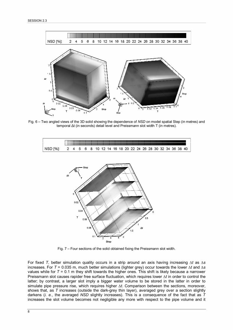
In order to summarise the results of all the numeric trials, all the points having co-ordinates (T, s, t, NSD) were interpolated by software Tecplot360-2008, which allows a link between the four variables to be determined. In a 3D space (T, s, t) this software makes the fourth dimension NSD visible by means of colours.

Fig. 6 shows, from two points of view, the coloured solid obtained. A gray scale was adopted and the variable NSD increases as grey darkens. The figure shows that, generally, the higher NSD values occur in two zones: 1) a large size zone (Fig. 6a), generally for medium-high t and medium-low s values, which for the lower T values expands to the point that it involves the whole t-s range considered (Fig. 6b, parallelepiped left face); 2) a smaller one (Fig. 6b, parallelepiped front face), for the lower t values and the medium-high s values, where the higher NSD values occur and in which T value appears to be little important. In the latter zone, the darkest grey of the whole solid is observed. In both the zones the Courant criterion is often not satisfied; however, it is to be noted that in many simulations performed with low values of t (down to 0.01 s) and T (lower than 0.04 m), which allowed the criterion to be amply satisfied, actually less intense but more frequent oscillations occurred. The violation of the Courant criterion, therefore, seems not to be the only cause of oscillations, which are likely to derive from intrinsic shortcomings of the equations rather than from numerical instabilities only. Note that for fixed T and s the Courant number decreases along with t. Numerical oscillations in simulating pressurization transient as the simulation parameters vary were discussed by Vasconcelos et al. (2009).

In order to explore what happens inside the coloured solid, the latter was sectioned by several planes and the coloured sections examined. Fig. 7 shows four sections relating to the planes having as parameter T = 0.002, 0.035, 0.070 and 0.1 m. The upper section (T = 0.002 s) is the left face of Fig. 6b and the lower one (T = 0.1 m) the right face of Fig. 6a. Examination of the whole sections shows that, except for the dark-grey thin layer relating to the lower T values (Fig. 6a), colour distribution in the sections keeps analogous as T varies although the colours slightly darkens as T increases.

SESSION 2.3

8

 

Fig. 6 – Two angled views of the 3D solid showing the dependence of NSD on model spatial Step (in metres) and temporal ∆t (in seconds) detail level and Preissmann slot width T (in metres).

 

Fig. 7 – Four sections of the solid obtained fixing the Preissmann slot width.

For fixed T, better simulation quality occurs in a strip around an axis having increasing t as s increases. For T = 0.035 m, much better simulations (lighter grey) occur towards the lower t and s values while for T = 0.1 m they shift towards the higher ones. This shift is likely because a narrower Preissmann slot causes rapider free surface fluctuation, which requires lower t in order to control the latter; by contrast, a larger slot imply a bigger water volume to be stored in the latter in order to simulate pipe pressure rise, which requires higher t. Comparison between the sections, moreover, shows that, as T increases (outside the dark-grey thin layer), averaged grey over a section slightly darkens (i. e., the averaged NSD slightly increases). This is a consequence of the fact that as T increases the slot volume becomes not negligible any more with respect to the pipe volume and it

NOVATECH 2010

9

dampens the filling process, as it was shown in Fig. 5. Note that the highest T value of our tests (0.1 m) is about 40% of the pipe diameter. For more usual T values (T/D = 0.05-0.1, i. e. T = 1.22-2.44 cm in our application), better simulation quality is gained with relatively low t and s values. Nevertheless, a possible pitfall for the modeller may arise from highly detailed models in which numerical instability can play a major role, compromising the reliability of simulation results. Therefore, the more detailed is the model, the more important is the selection of an appropriate combination of spatial and temporal resolutions s and t to be combined with the right value of Preissmann slot width T.

As an overall comment, the analysis demonstrated effectively good SWMM solution robustness in simulating the mean pressurization surge (filtered out of actual oscillations yielded by air pocket pulsations) in a wide range of values of the three simulation parameters (s, t and T) thus ensuring the modeller reliability of model solutions for practical applications in which errors in the range of 20% with respect to the actual average may still be acceptable. Of course, simulation of actual pressure oscillations due to air pocket pulsations is a topic to be solved by suited modelling.

6 CONCLUSIONS

The increasing importance of mathematical simulation models in planning, management and design of urban drainage networks requires development and employment of reliable and stable models able to simulate the various hydraulic phenomena occurring in the network. One of these phenomena is pressurization transient, which is very frequent in practice but still little known. Actually, the results of popular models relating to this transient are usually considered to be reliable although specific investigation has not been carried out.

The ability of SWMM, probably the most popular drainage network software, to simulate smooth pressurization caused by drastic reduction in the downstream discharge is examined in this paper. SWMM uses de Saint-Venant equations with the help of the Preissmann slot. The ability of SWMM to simulate pressurization was tested by comparison of simulation results with an experimental surge measured in a laboratory pipe. To this aim, the surge was previously filtered out of pressure oscillations yielded by air pocket pulsations, which are not considered at all by the SWMM model.

A large number of simulations were performed with variation in the space and time steps as well as the slot width, in order for the effects of each parameter on the simulation results to be recognized. The simulation quality was evaluated by the normalized standard deviation between the simulated and experimental surges in five measurement pipe-sections. The standard deviation values of all the simulations were then processed together with the related simulation parameter values using Tecplot360 software, which makes it possible to interpolate relations between four variables (space step, time step, slot width, normalized standard deviation) to be displayed in a 3D space, by representation of the fourth variable (the standard deviation) by a colour scale. On the whole, the comparison pointed out a complex picture of the SWMM model in simulating smooth pressurization: the model shows a generally modest ability to simulate smooth pressurization unless the model detail parameters are wisely selected not to be either excessively coarse or excessively detailed. This behaviour is probably due to the equations based on energy conservation which are in themselves unsuited to describe a typically dissipative phenomenon like the moving jump. At the same time, for a “reasonable” range of values, the model provides a robust estimation of the pressurization transient, except for oscillations due to air pocket pulsations, providing errors within 20% which may be still usable at the practical level.

ACKNOWLEDGEMENTS

The contributions of the writers to the present paper are on equal terms and they sign the paper in alphabetical order. The writers wish to thank Dr. Dora Ferreri and Dr. Emanuele Di Lucia, who with dedication and systematic work carried out the experiments and made the measurements available for the present paper.

LIST OF REFERENCES Capart, H., Sillen, X. and Zech, Y. (1997). Numerical and experimental water transients in sewer

pipes. Journal of Hydraulic Research, 35(5), 659-670.

Cardle, J. A., Song, C. C. S. and Yuan, M. (1989). Measurement of mixed transient flows. Journal of

SESSION 2.3

10

the Hydraulics Division, ASCE, 115(2), 169-182.

Ciraolo, G. and Ferreri, G.B. (2008a). Sewer pressurization modelling by a rigid-column method. Proc. of 11th International Conference on Urban Drainage - 11th ICUD, Edinburgh, Scotland (UK), August 31st-September 5th, CD-ROM.

Ciraolo G. e Ferreri G. B. (2008b). Mathematical modelling of pressure oscillations in sewer pressurization. Proc. of 11th International Conference on Urban Drainage - 11th ICUD, Edinburgh, Scotland (UK), August 31st-September 5th, CD-ROM.

Danish Hydraulic Institute (1995). MOUSE user manual, Version 3.3. Høersholm, Denmark.

Guo, Q. and Song, C.C.S. (1990). Surging in urban storm drainage systems. Journal of Hydraulic Engineering, ASCE, 116(12), 1523-1537.

Hamam, M.A. and McCorquodale, J.A. (1982). Transient conditions in the transition from gravity to surcharged sewer flow. Canadian Journal of Civil Engineering, 9(2), 189-196.

Huber, W. C., Heaney, J. P., Nix, S. J., Dickinson, R. E. and Polmann, D. J. (1984). Storm Water Management Model. User's Manual Ver. III. U.S. Environmental Protection Agency.

Lai, Ch. (1986). Numerical modelling of unsteady open-channel flow. Advances in Hydroscience, Ben Chie Yen (ed.), Vol. 14, Academic Press, New York.

Li, J. and McCorquodale, J.A. (1999). Modeling mixed flow in storm sewers. Journal of Hydraulic Engineering, ASCE, 125(11), 1170-1180.

Noto, L. (1999). Hydrodynamic propagation models in urban drainage networks: state of the art and innovative proposals (in Italian; original title: Modelli di propagazione idrodinamica in reti di drenaggio urbano: stato dell’arte e proposte innovative). PhD Thesis, Dipartimento di Meccanica dei Fluidi ed Ingegneria Offshore (Dept. of Fluid Mechanics and Offshore Engineering), University of Reggio Calabria (Italy).

Noto, L. and Tucciarelli, T. (2001). DORA algorithm for network flow models with improved stability and convergence properties. Journal of Hydraulic Engineering, ASCE, 127(5), 380-391.

Ridgway, R.E. and Kumpala, G. (2007). Surge modeling in sewers using the transient analysis program (TAP). Contemporary Modeling of Urban Water Systems, Monograph 15, CHI Toronto (Ontario), Canada, 133-146.

Ridgway, R.E. and Kumpala, G. (2008). Surge modeling in sewers using alternative hydraulic software Programs. Reliable Modeling of Urban Water Systems, Monograph 16, CHI Toronto (Ontario), Canada, 155-164.

Song, C.C.S. (1976). Two-phase flow hydraulic transient model for storm sewer systems. Proc. of 2nd International Conference on Pressure Surges, BHRA Fluid Engineering, Cranfield, Bedford (England), 17-34.

Trajkovic, B., Ivetic, M., Calomino, F. and D’Ippolito, A. (1999). Investigation of transition from free surface to pressurized flow in a circular pipe. Water Science and Technology, 39(9), 105-112.

Vasconcelos, J.G. and Wright, S.J. (2005). Experimental investigation of surges in a stormwater storage tunnel. Journal of Hydraulic Engineering, 131(10), 853-861.

Vasconcelos, J.G., Wright, S.J. and Roe, P.L. (2006). Improved simulation of flow regime transition in sewers: two-component pressure approach. Journal of Hydraulic Engineering, 132(6), 553-562.

Vasconcelos, J.G., Wright, S.J. and Roe, P.L. (2009). Numerical oscillations in pipe-filling bore predictions by shock-capturing models. Journal of Hydraulic Engineering, 135(4), 296-305.

Wallingford HR Hydroworks (1998). Infoworks Software. Wallingford (Oxfordshire), UK.

Wiggert, D.C. (1972). Transient flow in free-surface, pressurized systems. Journal of the Hydraulic Division, ASCE, 98(1), 11-27.

Zhou, F., Hicks, F.E. and Steffler, P.M. (2002a). Transient flow in a rapidly filling horizontal pipe containing trapped air. Journal of Hydraulic Engineering, 128(6), 625-634.