CFD actuator disk solutions

for a helicopter rotor in

hover flight

« Solutions MFN d’un système de disque pour rotor d’hélicoptère en vol stationnaire »

Supervisor: Antonio Filippone

Chef de formation: Jean Pierre Chollet Tuteur de stage: Jolanta Lewandowska

Sept 2003

DESS Modélisation & Simulation en Mécanique Département Mécanique Université Joseph Fourier

Grenoble France

Mechanical, Aerospace and Manufacturing Engineering dept

University of Manchester Institute of Science and Technology

United Kingdom

2

“Users should approach all software with prudent caution and healthy skepticism, for the

history of science and engineering,including the still-young history of software engineering,

is littered with failed promises.”

Henry Petroski, “Failed Promises”

American Scientist, Vol. 82, Jan-Feb. 1994, pp.6-9.

3

Contents Preface Symbols and notations Abstract - Résumé

A First Approach

Comparison of a CFD model – Semi-analitical Method

- 1 - Fundamentals of rotor aerodynamics: Momentum theory • Conservation laws of fluid mechanics • Application to hovering rotor • Rotor Power • Pressure variation

- 2 - Exact actuator disk solutions for non-uniform heavy loading and slipstream contraction developed by J.T.Conway.

• General problem • Propellers with slipstream rotation

- 3 - Data provided by Conway (1998) - 4 - First CFD approach of the problem - 5 - CFD simulation of the problem

• First grid • Second grid

B

Second Approach “Blade Element Momentum (BEM)” and “CFD” coupled Calculations

for helicopter in Hover flight - 1 - Theoretical work

1.1. Actuator disc model 1.2. Blade Element Theory

- 2 - Programme generation 2.1. Algorithm 2.2. Subroutine 2.3. Structure of the programme

- 3 - Results and discussion - 4 - Data implementation in FLUENT

4.1. Implementation 4.2. Geometry and Meshes 4.3. Numerical Procedure 4.4 Results and discussion

o Validation with the total pressure and thrust o Streamlines functions o Dynamic Pressure on the disc o Velocity profiles o Velocity on the z-axis

Conclusion Appendices References

4

Preface

This research work was carried out at the Department of Manufacturing and Aerospace

Mechanical Engineering department of UMIST (University of Manchester Science and

Technology) under the supervision of Dr Antonio Filippone.

My thanks go to my supervisor Dr Antonio Filippone for his guidance, encouragement and

valuable comments throughout the process of this work. Moreover, he has given me the

chance to work in his research group, what is and will be a great experience for my whole life.

Many grateful thanks to the “Fluent Guru” Vassilis Karanikolis for his assistance and his

kindness.

A warm thank you to colleagues of the Department for their kindness and for their

consideration: Charles Moulinec (UMIST Post-doctor), Guilhem Laurans (“Centrale Nantes”

student), Romain Pruniere (“INPG h.m.g.” student), David Tung (“ENSEM” student), Reza

Issa (UMIST Thesis student), Jason Bassi (UMIST Thesis student), Ran Xenon (UMIST

MPhil student), Toshi Fujii (UMIST MSc student) and the others…

Merci à mes parents pour m’avoir soutenu dans toutes mes démarches, que ce soit pour ce

stage mais également pour l’ensemble de mes études depuis l’école primaire.

Enfin, je remercie celle qui m’a accompagné dans cette aventure aussi bien humaine que

professionnelle, pour son soutien de chaque instant, pour sa patience à mon égard, et pour sa

foi en mes folies.

5

Symbols and notations

a Axial induction a’ Tangential induction A Rotor area C Chord length CL Lift coefficient CD Drag coefficient Cp Pressure coefficient Ct Tangential force coefficient Cn Axial force coefficient D Drag force Ft Tangential force pr. meter Fn Axial force pr. meter k Turbulent kinetic energy L Lift force m& Mass flow rate N Number of blades p Static pressure P Total pressure Pn Pressure in tangential direction Pt Pressure in axial direction r Local radius R Rotor radius Re Reynolds number T Thrust force V0 Wind speed Vrel Relative speed Vr Velocity component in Radial direction Vt Velocity component in Tangential direction Vz Velocity component in Axial direction α Angle of attack ε Turbulent dissipation φ Angle of the relative velocity

ν Laminar viscosity ν t Eddy viscosity ω Angular velocity ρ Density σ Solidity of rotor ∞ Conditions at infinity

6

Abstract

The aim of this paper is to develop a CFD model in order to simplify the modeling of the flow

induced by a helicopter rotor in hover flight. The main rotor blades are considered as a whole

disc where diverse velocities and pressures are applied. If this simplification provides good

results, the modeler will obtain high-quality approximations of the aerodynamic flow induced

by the helicopter blades, whatever its number and its geometry design.

Two approaches are extended in order to validate this simple model:

The purpose of the first part is to apply as boundary conditions, the data provided by a

mathematical study realized by J.T. Conway. The interest is to check if it is possible to input

the initial conditions in commercial CFD code Fluent 5.5 and compare the results obtained

with the mathematical ones. In fact, the different velocities above and below have to be

evaluated in order to validate the model.

The second approach is more ambitious because a FORTRAN program is created in order to

predict the thrust and tangential forces on each blade. The predicted data will then be

implemented within the CFD code Fluent 6.1. Eventually, an evaluation and a validation of

this new model is done.

Whatever the approach, the purpose is to obtain a simple method that enables the simulation

of the flow induced by helicopter rotor in hover flight. If this methodology is approved, it

should be easy to apply to other cases.

7

Résumé

La finalité de ce stage est de développer une méthode de simulation numérique qui

simplifierait la modélisation des écoulements induits par les rotors d’hélicoptères en vol

stationnaire. Le principe premier est de considérer les pâles du rotor principal comme un

disque plein duquel des pressions et des vitesses débitantes seraient générées.

Si la méthodologie est approuvée, le modélisateur aura la possibilité de travailler avec un

modèle de haute qualité définissant l’écoulement d’air quelque soient le nombre de pâles ou la

géométrie de cette dernière.

Deux approches sont abordées afin de valider ce projet :

Le propos de la première partie est d’appliquer en conditions limites, les données fournies par

une étude mathématique réalisée par J.T.Conway. L’intérêt est de savoir s’il est possible

d’introduire ces conditions dans Fluent 5.5 et de comparer les résultats avec ceux obtenus par

la méthode mathématique.

La seconde approche est plus ambitieuse puisque un programme FORTRAN est généré afin

de prédire la poussée et les forces tangentielles sur chaque pâle. Les données sont ensuite

implantées dans le code commercial Fluent 6.1. Finalement, une évaluation des résultats et

leurs validations est faite.

Quelque soit l’approche, le but cette démarche est de créer une méthode simple qui soit

capable de simuler l’écoulement induit par les pâles d’un rotor principal d’hélicoptère en vol

stationnaire. Si cette méthodologie est approuvée, il devrait être facile de l’employer dans

d’autres cas beaucoup plus complexes.

8

A First Approach Comparison of a

CFD model – Semi-analitical Method

- 1 -

Fundamentals of rotor aerodynamics: Momentum theory

• Conservation laws of fluid mechanics

• Application to hovering rotor

• Rotor Power

• Pressure variation

- 2 -

Exact actuator disk solutions for non-uniform heavy loading and slipstream

contraction developed by J.T.Conway.

• General problem

• Propellers with slipstream rotation

- 3 -

Data provided by Conway (1998)

- 4 -

First CFD approach of the problem

- 5 -

CFD simulation of the problem

• First grid

• Second grid

9

- 1 -

Fundamentals of rotor aerodynamics

Momentum theory

Hover is a unique flight condition. Here, the rotor has zero forward speed and zero vertical

speed. The rotor flow field is, therefore, axisymmetric. With the measurements of the velocity

field near and below a hovering rotor, we can note that the fluid velocity increases smoothly

as it is entrained into and through the rotor disk plane. There is no jump in the velocity across

the disk, although thrust is produced, so there must be a jump in pressure over the disk. With

physical pictures of the hovering rotor flow, it is possible to apply a mathematical solution to

this problem. Consider the application of three basic conservation laws (conservation of mass,

momentum and energy) to the rotor and it flow field.

This approach is called momentum theory, and was first developed by Rankine (1865) for

marine propellers. The theory was developed further by Froude (1889) and Betz (1920). The

main difference between Rankine and Froude theories is in the treatment of the rotor disk as a

series of elementary rings, versus the treatment of the disk as a whole.

Conservation laws of fluid mechanics

In the general approach to the problem, it will be assumed that the flow through the rotor is

one dimensional, quasi steady, incompressible and inviscid. Consider an ideal fluid, that is,

one of that generates no viscous shear between fluid elements. Therefore, induced losses are a

sole source of losses in the fluid, with other losses resulting from the action of viscosity being

assumed negligible.

10

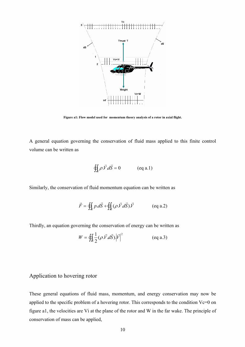
Figure a1: Flow model used for momentum theory analysis of a rotor in axial flight.

A general equation governing the conservation of fluid mass applied to this finite control

volume can be written as

0.. =∫∫ SdVS

rrρ (eq a.1)

Similarly, the conservation of fluid momentum equation can be written as

VSdVSdpFSS

rrrrr)...(. ∫∫∫∫ += ρ (eq a.2)

Thirdly, an equation governing the conservation of energy can be written as 2

)...(21 VSdVW

S

rrr∫∫= ρ (eq a.3)

Application to hovering rotor

These general equations of fluid mass, momentum, and energy conservation may now be

applied to the specific problem of a hovering rotor. This corresponds to the condition Vc=0 on

figure a1, the velocities are Vi at the plane of the rotor and W in the far wake. The principle of

conservation of mass can be applied,

11

dSVdSVm ∫∫∫∫ ==∞ 2

....rr

& ρρ (eq a.4)

The principle of conservation of fluid momentum gives the relationship between the rotor

thrust T, and the net time rate of change momentum out of the control volume (Newton’s

second law),

VSdVVSdVTFrrrrrrr

)..()..(0∫∫∫∫ −==

∞ρρ (eq a.5)

Because in hovering flight, the velocity well upstream of the rotor is quiescent, the second

term is zero,

VSdVTrrr

)..(∫∫∞= ρ (eq a.6)

wmT .&= (eq a.7)

From the principle of conservation of energy, the work done on the rotor is equal to the gain

in energy of the fluid per unit time. The power consumed by the rotor is P and this results in

the equation,

2

0

2 )..(21)..(

21 VSdVVSdVP

rrrrrr∫∫∫∫ −=

∞ρρ (eq a.8)

2)..(21 VSdVP

rrr∫∫∞= ρ (eq a.9)

2.21 wmP &= (eq a.10)

12

Rotor Power

It has been shown previously that momentum theory can be used to relate the rotor thrust to

the induced velocity at the rotor disk by using the equation

2...2.)..( ivAwmVSdVT ρρ === ∫∫∞ &

rrr (eq a.11)

So, the power required to hover is given by

ATvTP i ρ2

.2/3

== (eq a.12)

2...2 ivAP ρ= (eq a.13)

This power, called ideal power, is entirely induced in nature because the contributions of

viscous effects have not been considered in the present level of analysis.

Pressure variation

The pressure variation through the rotor flow field in the hover state can be found from the

application of Bernoulli’s equation along the streamline above and below the rotor disk. This

equation cannot be applied across the disk, because the pressure jump is a result of energy

addition by the rotor.

210 .

21

ivppp ρ+== ∞ (eq a.14)

Below the disk, between 2 and ∞ , the application of Bernoulli’s equation gives

222 .

21.

21 wpvp i ρρ +=+ ∞ (eq a.15)

13

So, one can write

ATppp =−=∆ 12 (eq a.16)

The momentum method has permitted a preliminary evaluation of rotor performance in hover.

Despite this advantage in providing an insight into the basic theory of the rotor problem, it has

many limitations. For example, it provides no information about the distribution of load over

the blade. That is the reason why some people are currently developing mathematical theories

about heavily loaded actuator disk with non-uniform loading.

- 2 - Exact actuator disk solutions for non-uniform heavy loading and

slipstream contraction developed by J.T.Conway.

(J. Fluid Mech. (1998) Vol. 365, pp 235-267)

A semi analytical method has been developed to solve for the inviscid incompressible flow

induced by a heavily loaded actuator disk with non-uniform loading. This method is an

extension of the analytical theory of Conway (1995) for the linearized actuator disk and is

exact for an incompressible perfect fluid.

General problem

In a recent publication in 1995, Conway derived analytical solutions for the entire flow field

induced by a linearized actuator disk with essentially arbitrary radial load distribution. The

method was based on the construction of the velocities and vector potential of the ring vortex

as integrals over the allowed values of the separation constant of the solutions of Laplace’s

14

equations in cylindrical coordinates. The velocities calculated by this method were finite and

continuous everywhere.

The purpose of the article dated on 1998, is to present the extension of this method to the

generalised nonlinear actuator disk, subject to the important restriction that the vortex density

in the slipstream remains bounded.

Propellers with slipstream rotation

This case will be studied with a commercial CFD code. These results will be applied on the

disk later with the set boundary conditions.

The whole mathematical theory is available in the Journal of Fluid Mechanics. To summarise

this article without going into too much detail, it provides three velocity profiles in different

points above and below the heavy disk. So, it would be possible to know if the numerical

calculations made with “Fluent 5.5” and “Fluent 6.0” give results close in comparison to the

mathematical predictions.

- 3 - Data provided by Conway (1998)

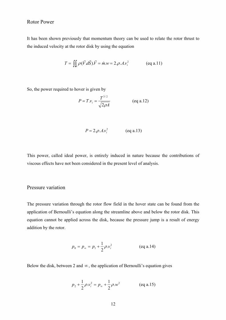
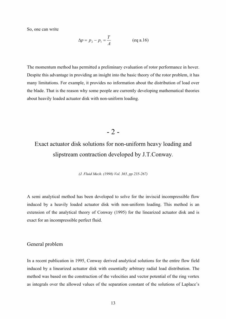
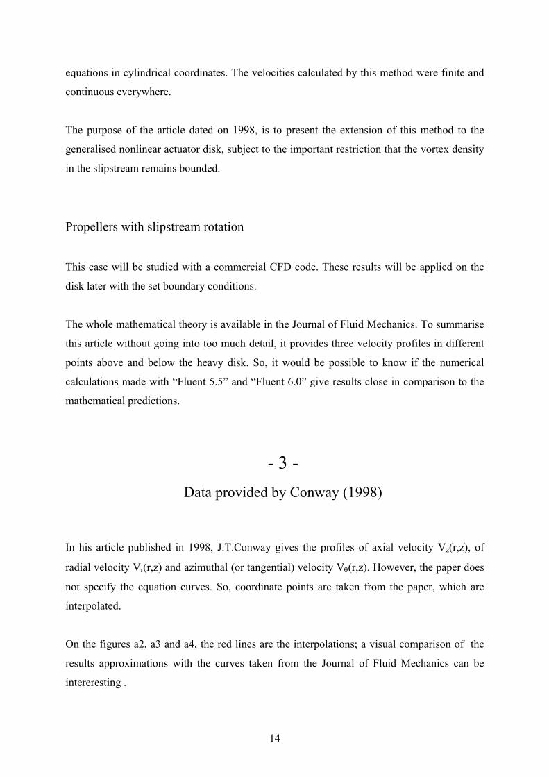
In his article published in 1998, J.T.Conway gives the profiles of axial velocity Vz(r,z), of

radial velocity Vr(r,z) and azimuthal (or tangential) velocity Vθ(r,z). However, the paper does

not specify the equation curves. So, coordinate points are taken from the paper, which are

interpolated.

On the figures a2, a3 and a4, the red lines are the interpolations; a visual comparison of the

results approximations with the curves taken from the Journal of Fluid Mechanics can be

intereresting .

15

Radial Velocity

-0.3

-0.25

-0.2

-0.15

-0.1

-0.05

0

0.05

0.1

0 0.2 0.4 0.6 0.8 1

r/R

Vr/U

Figure a2: Radial velocity profile as function of the radial coordinates r normalised on the rotor.

Azimuthal velocity

-0.050

0.050.1

0.150.2

0.250.3

0.350.4

0.45

0 0.2 0.4 0.6 0.8 1

r/R

Vo/U

Figure a3: Azimuthal velocity profile as function of the radial coordinates r normalised on the rotor.

Axial velocity

-0.05

0

0.05

0.1

0.15

0.2

0.25

0.3

0 0.2 0.4 0.6 0.8 1

r/R

Vz/U

Figure a4: Axial velocity profile as function of the radial coordinates r normalised on the rotor.

16

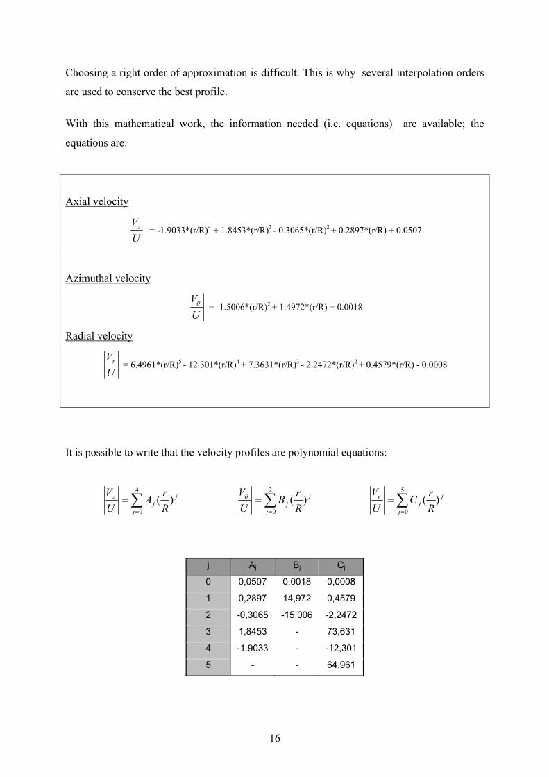
Choosing a right order of approximation is difficult. This is why several interpolation orders

are used to conserve the best profile.

With this mathematical work, the information needed (i.e. equations) are available; the

equations are:

Axial velocity

UVz = -1.9033*(r/R)4 + 1.8453*(r/R)3 - 0.3065*(r/R)2 + 0.2897*(r/R) + 0.0507

Azimuthal velocity

UVθ = -1.5006*(r/R)2 + 1.4972*(r/R) + 0.0018

Radial velocity

UVr = 6.4961*(r/R)5 - 12.301*(r/R)4 + 7.3631*(r/R)3 - 2.2472*(r/R)2 + 0.4579*(r/R) - 0.0008

It is possible to write that the velocity profiles are polynomial equations:

∑=

=4

0)(

j

jj

z

RrA

UV

∑=

=2

0)(

j

jj R

rBUVθ ∑

=

=5

0)(

j

jj

r

RrC

UV

j Aj Bj Cj

0 0,0507 0,0018 0,0008

1 0,2897 14,972 0,4579

2 -0,3065 -15,006 -2,2472

3 1,8453 - 73,631

4 -1.9033 - -12,301

5 - - 64,961

17

- 4 -

First CFD approach of the problem

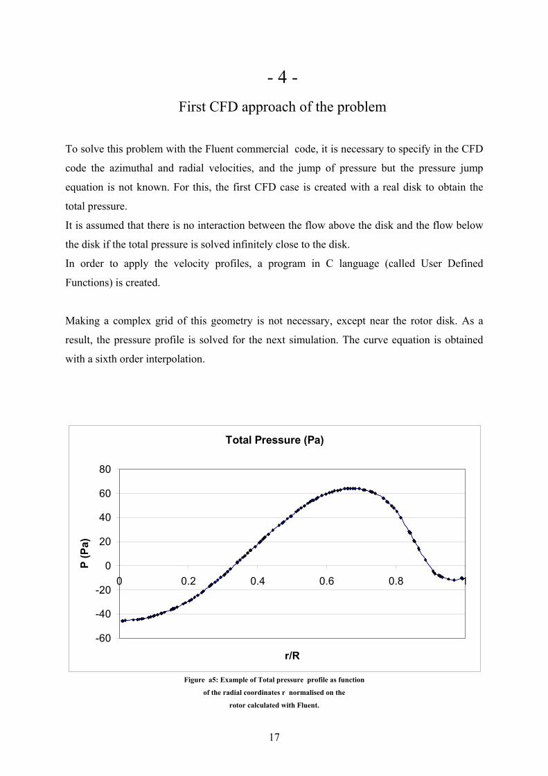
To solve this problem with the Fluent commercial code, it is necessary to specify in the CFD

code the azimuthal and radial velocities, and the jump of pressure but the pressure jump

equation is not known. For this, the first CFD case is created with a real disk to obtain the

total pressure.

It is assumed that there is no interaction between the flow above the disk and the flow below

the disk if the total pressure is solved infinitely close to the disk.

In order to apply the velocity profiles, a program in C language (called User Defined

Functions) is created.

Making a complex grid of this geometry is not necessary, except near the rotor disk. As a

result, the pressure profile is solved for the next simulation. The curve equation is obtained

with a sixth order interpolation.

Total Pressure (Pa)

-60

-40

-20

0

20

40

60

80

0 0.2 0.4 0.6 0.8 1

r/R

P (P

a)

Figure a5: Example of Total pressure profile as function

of the radial coordinates r normalised on the

rotor calculated with Fluent.

18

- 5 - CFD simulation of the problem

The geometry is quite simple because there is only a disk (without thickness) in a square

domain. The only difficulty is limiting the size of the domain (for the reason that the meshes

would be too numerous) but it cannot be too small (because no interaction with the

boundaries would exist).

First grid

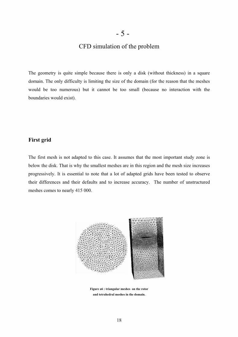
The first mesh is not adapted to this case. It assumes that the most important study zone is

below the disk. That is why the smallest meshes are in this region and the mesh size increases

progressively. It is essential to note that a lot of adapted grids have been tested to observe

their differences and their defaults and to increase accuracy. The number of unstructured

meshes comes to nearly 415 000.

Figure a6 : triangular meshes on the rotor

and tetrahedral meshes in the domain.

19

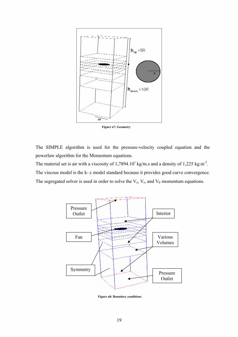
Figure a7: Geometry

The SIMPLE algorithm is used for the pressure-velocity coupled equation and the

powerlaw algorithm for the Momentum equations.

The material set is air with a viscosity of 1,7894.105 kg/m.s and a density of 1,225 kg.m-3.

The viscous model is the k- ε model standard because it provides good curve convergence.

The segregated solver is used in order to solve the Vz, Vr, and Vθ momentum equations.

Figure a8: Boundary conditions

Pressure Outlet

Symmetry

Fan

Interior

Various Volumes

Pressure Outlet

20

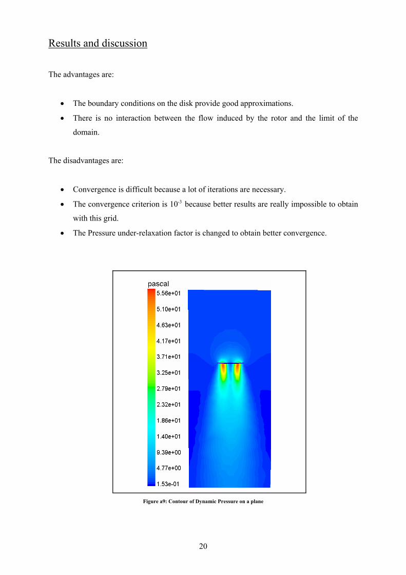
Results and discussion

The advantages are:

• The boundary conditions on the disk provide good approximations.

• There is no interaction between the flow induced by the rotor and the limit of the

domain.

The disadvantages are:

• Convergence is difficult because a lot of iterations are necessary.

• The convergence criterion is 10-3 because better results are really impossible to obtain

with this grid.

• The Pressure under-relaxation factor is changed to obtain better convergence.

Figure a9: Contour of Dynamic Pressure on a plane

21

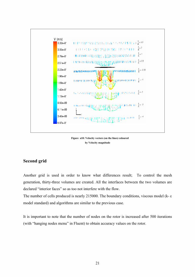
Figure a10: Velocity vectors (on the lines) coloured

by Velocity magnitude

Second grid

Another grid is used in order to know what differences result; To control the mesh

generation, thirty-three volumes are created. All the interfaces between the two volumes are

declared “interior faces” so as too not interfere with the flow.

The number of cells produced is nearly 215000. The boundary conditions, viscous model (k- ε

model standard) and algorithms are similar to the previous case.

It is important to note that the number of nodes on the rotor is increased after 500 iterations

(with “hanging nodes menu” in Fluent) to obtain accuracy values on the rotor.

22

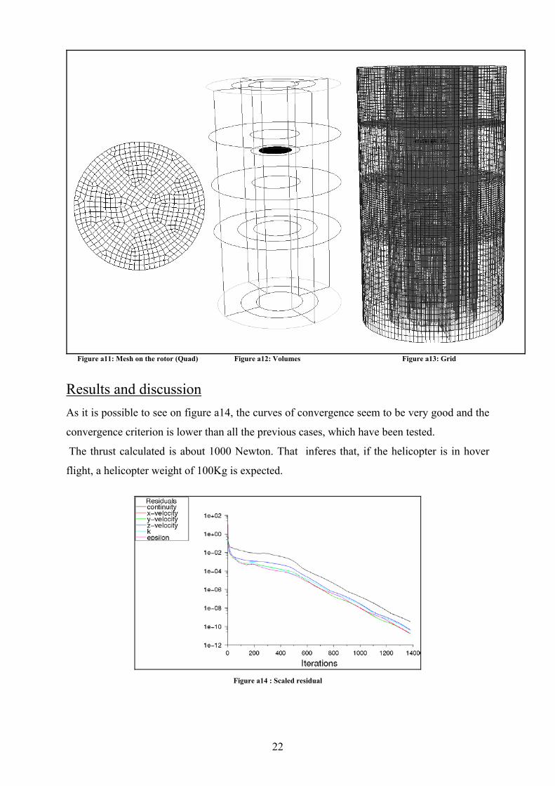
Figure a11: Mesh on the rotor (Quad) Figure a12: Volumes Figure a13: Grid

Results and discussion As it is possible to see on figure a14, the curves of convergence seem to be very good and the

convergence criterion is lower than all the previous cases, which have been tested.

The thrust calculated is about 1000 Newton. That inferes that, if the helicopter is in hover

flight, a helicopter weight of 100Kg is expected.

Figure a14 : Scaled residual

23

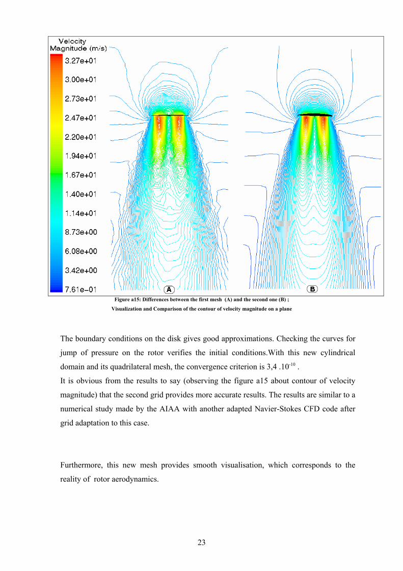
Figure a15: Differences between the first mesh (A) and the second one (B) ;

Visualization and Comparison of the contour of velocity magnitude on a plane

The boundary conditions on the disk gives good approximations. Checking the curves for

jump of pressure on the rotor verifies the initial conditions.With this new cylindrical

domain and its quadrilateral mesh, the convergence criterion is 3,4 .10-10 .

It is obvious from the results to say (observing the figure a15 about contour of velocity

magnitude) that the second grid provides more accurate results. The results are similar to a

numerical study made by the AIAA with another adapted Navier-Stokes CFD code after

grid adaptation to this case.

Furthermore, this new mesh provides smooth visualisation, which corresponds to the

reality of rotor aerodynamics.

24

On figure a15.A, the contour of velocity magnitude depends of the number and especially

the node shapes. In opposition to this problem, the second mesh provides results

independent of the grid.

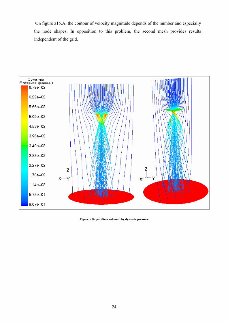
Figure a16: pathlines coloured by dynamic pressure

25

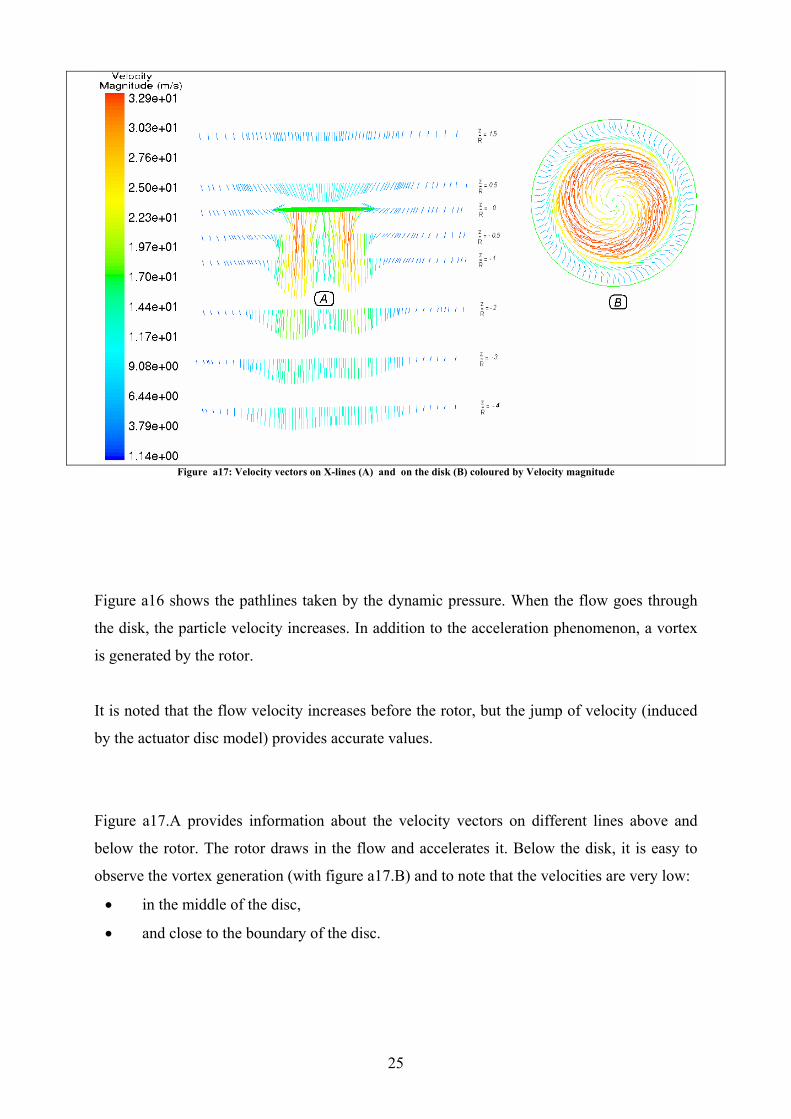
Figure a17: Velocity vectors on X-lines (A) and on the disk (B) coloured by Velocity magnitude

Figure a16 shows the pathlines taken by the dynamic pressure. When the flow goes through

the disk, the particle velocity increases. In addition to the acceleration phenomenon, a vortex

is generated by the rotor.

It is noted that the flow velocity increases before the rotor, but the jump of velocity (induced

by the actuator disc model) provides accurate values.

Figure a17.A provides information about the velocity vectors on different lines above and

below the rotor. The rotor draws in the flow and accelerates it. Below the disk, it is easy to

observe the vortex generation (with figure a17.B) and to note that the velocities are very low:

• in the middle of the disc,

• and close to the boundary of the disc.

26

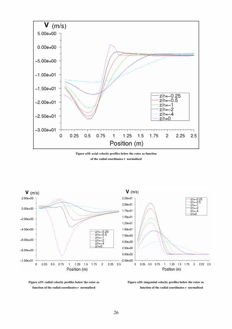
Figure a18: axial velocity profiles below the rotor as function

of the radial coordinates r normalised

Figure a19: radial velocity profiles below the rotor as Figure a20: tangential velocity profiles below the rotor as

function of the radial coordinates r normalised function of the radial coordinates r normalised

27

Figures a18, a19 and a20 show the different velocity profiles as a funtion of the radius at

different z coordinates. Considering the axial velocity, the results are not similar to Conway’s,

especially after the coordinate 1−=Rz . It is not surprising because the analitical method used

in his work is so different than the one proposed by the CFD commercial code Fluent 5.5.

To summarise, three velocity profiles and one jump pressure profile must be applied. Even if

applying the velocities and pressure values required is not simple, a good approximation can

be made in order to obtain the right thrust value.

For this example:

The mass flow rate provided by the rotor is:

m& =50.467 kg/s

The velocity magnitude integral on the rotor is:

43.61.2

=∫∫ dSVr

m3.s-1

Vaverage= S43.61

Vaverage =19.55 m.s-1

An approximation of the thrust induced by the rotor is given as:

averageVmT .&=

T= 986.82 N

28

In hover flight, the weight of the helicopter should be approximately 100,59 kg. In order to

know with accuracy this weight, it would be insightful to introduce the fuselage and its

characteristics (like the vertical drag CDv) in the calculation.

A real rotor would give a higher thrust value. For this, if CFD simulations should be realised

in the future, the jump of pressure will be more realistic but the velocity profiles should be

identical.

Even if the CFD calculations do not provide perfect and expected results, knowledge has been

developed in order to, in the next chapter, obtain a complete study.

29

B Second Approach

“Blade Element Momentum (BEM)” and “CFD” coupled Calculations for Helicopter in Hover Flight

1. Theoretical work

1.1. Actuator disc model

1.2. Blade Element Theory 2. Programme generation

2.1. Algorithm

2.2. Subroutine

2.3. Structure of the programme 3. Results and discussion 4. Data implementation in FLUENT

4.1. Implementation 4.2. Geometry and Meshes 4.3. Numerical Procedure 4.4 Results and discussion

• Validation with the total pressure and thrust • Streamlines functions • Dynamic Pressure on the disc • Velocity profiles • Velocity on the z-axis

30

The main interest of this part is to develop a FORTRAN programme in order to obtain the

Thrust and Tangential forces distribution. From this, It is possible to implement these Forces

in the CFD commercial code FLUENT via the Actuator Disc Model, with the purpose to

determine the flow induced by this modeling method.

Various methods can be used to calculate the aerodynamic forces acting on the blades of a

wind turbine. The most advanced is numerical methods solving the Navier-Stokes equations

for the global compressible flow as well as the flow near the blades. The two major

approaches to calculate the forces are the Actuator Disc Model and the Blade Element Model.

In the following sections, a brief introduction of both mentioned methods are presented.

1. Theoretical work.

This theoretical part is a summary of a thesis written by Anders Ahlström, entitled

“Simulating Dynamical Behaviour of Wind Power Structures” (Royal Institute of Technology

Department of Mechanics, in Stockholm (2002)). The introduction focus on the qualitative

results and the basic assumptions that are made.

1.1. Actuator disc model

The actuator disc model is based on Bernoulli’s equation and energy balances. It’s assumed

that the rotor is replaced by an actuator disc, through which the static pressure decreases

discontinuously. The fluid is assumed incompressible.

31

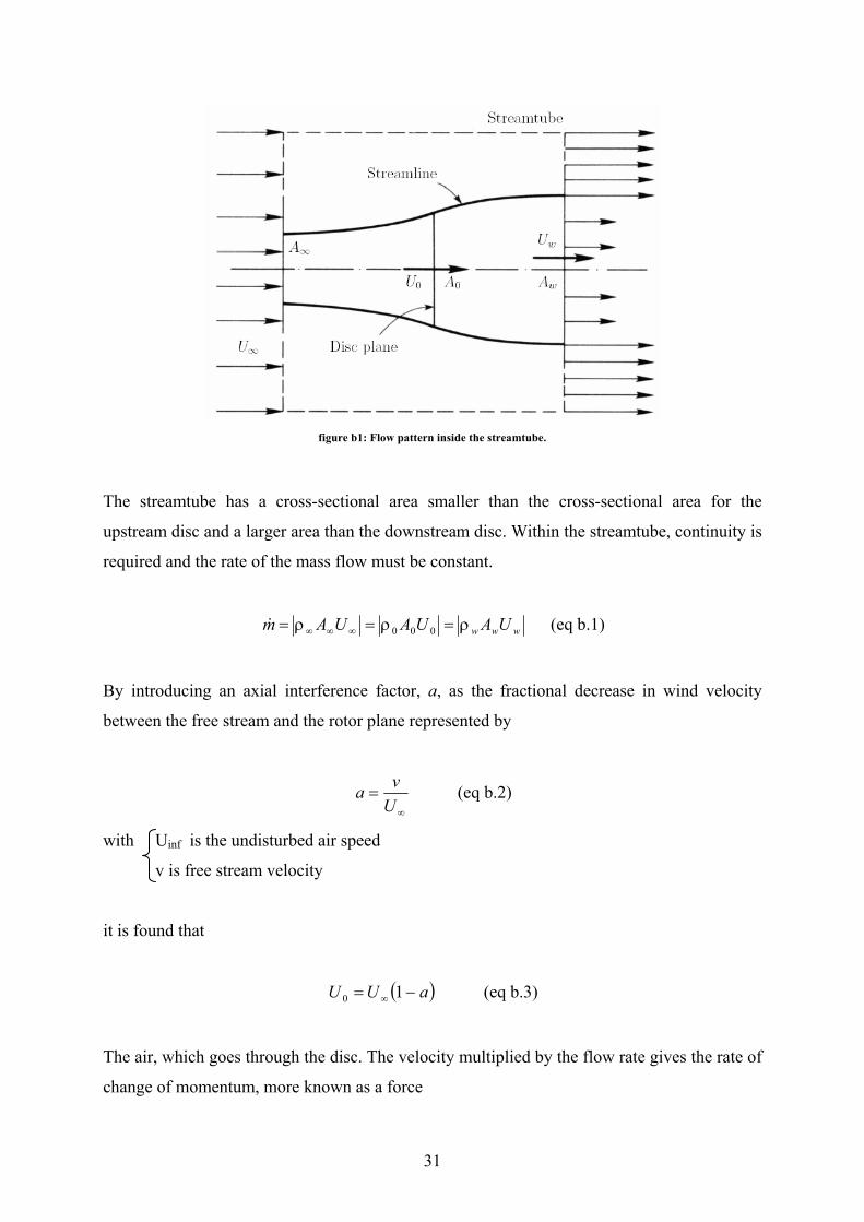
figure b1: Flow pattern inside the streamtube.

The streamtube has a cross-sectional area smaller than the cross-sectional area for the

upstream disc and a larger area than the downstream disc. Within the streamtube, continuity is

required and the rate of the mass flow must be constant.

www UAUAUAm ρ=ρ=ρ= ∞∞∞ 000& (eq b.1)

By introducing an axial interference factor, a, as the fractional decrease in wind velocity

between the free stream and the rotor plane represented by

∞

=U

va (eq b.2)

with Uinf is the undisturbed air speed

v is free stream velocity

it is found that

( )aUU −= ∞ 10 (eq b.3)

The air, which goes through the disc. The velocity multiplied by the flow rate gives the rate of

change of momentum, more known as a force

32

( )wUUmT −= ∞& (eq b.4)

Combining the equations above with the fact that the change of momentum comes entirely

from the pressure difference across the actuator disc, it is obtained that

( ) ( )aUUUpp w −−=− ∞∞−+ 1.. 000 ρ (eq b.5)

To obtain the pressure difference, the Bernoulli´s equation is applied separately to the

upstream and downstream section of the streamtube. For the upstream section it becomes

+∞∞ +ρ=+ρ 0

20

2

21

21 pUpU (eq b.6)

Similarly, for the downstream

−∞ +ρ=+ρ 0

20

2

21

21 pUpU w (eq b.7)

Subtracting (eq b.7) from (eq b.6) yields

( )2200 2

1wUUpp −ρ=− ∞

−+ (eq b.8)

As the fluid is incompressible, Equation (eq b.8) and (eq b.5) gives

( )aUU w 21 −= ∞ (eq b.9)

The force, T, is obtained by substituting (eq b.9), (eq b.3) and (eq b.1) into (eq b.4), which

gives

( )aaUAT −ρ= ∞ 12 20 (eq b.10)

33

Combining (eq b.3), (eq b.9) and the rate of work done by the force, P = T.U0, the power

extraction from the air is obtained as

( )230 12 aaUAP −ρ= ∞ (eq b.11)

or, by introducing the dimensionless power-coefficient, ( )21 aaC p −=

pCUAP 302 ∞ρ= (eq b.12)

The power-coefficient represents the efficiency of the turbine, which depends on variables

like the wind speed, the rotor speed and the pitch angle. The coefficient shows how much of

the kinetic energy in the air stream that is transformed into mechanical energy.

1.2. Blade Element Theory

While using of aero elastic codes in design calculations, the aerodynamic method has to be

efficient CPU time. The Blade Element Momentum (BEM) theory, has been shown to give

good accuracy with respect to time cost.

In this method, the turbine blades are divided into a number of independent elements along

the length of the blade. At each section, a force balance is applied involving 2D section lift

and drag with the thrust and torque produced by the section. At the same time, a balance of

axial and angular momentum is applied. This produces a set of non-linear equations, which

can be solved numerically for each blade section.

34

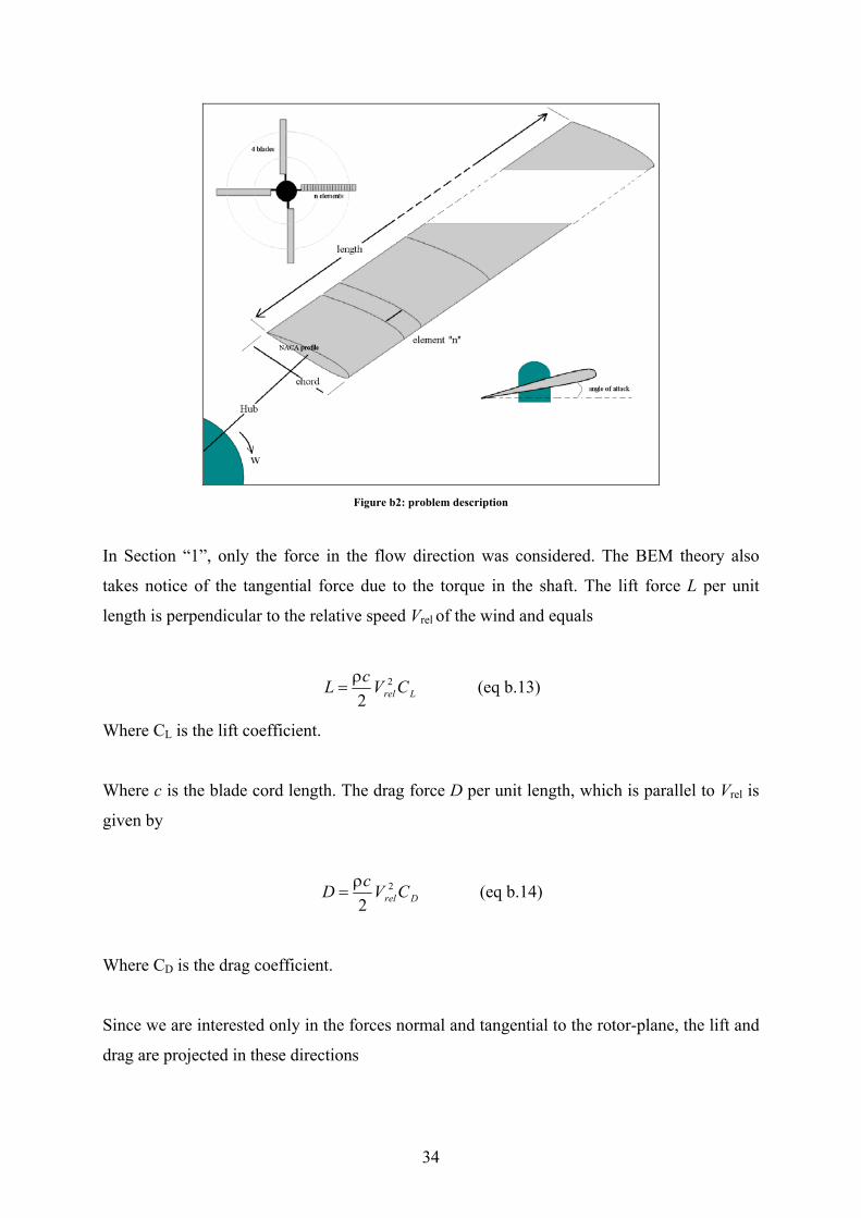
Figure b2: problem description

In Section “1”, only the force in the flow direction was considered. The BEM theory also

takes notice of the tangential force due to the torque in the shaft. The lift force L per unit

length is perpendicular to the relative speed Vrel of the wind and equals

Lrel CVcL 2

2ρ

= (eq b.13)

Where CL is the lift coefficient.

Where c is the blade cord length. The drag force D per unit length, which is parallel to Vrel is

given by

Drel CVcD 2

2ρ

= (eq b.14)

Where CD is the drag coefficient.

Since we are interested only in the forces normal and tangential to the rotor-plane, the lift and

drag are projected in these directions

35

FN = L cos φ + Dsin φ (eq b.15)

And

FT = L sin φ . Dcos φ (eq b.16)

The theory requires information about the lift and drag aerofoil coefficients CL and CD. Those

coefficients are generally given as functions of the angle of incidence (see Figure).

α = φ - θ (eq b.17)

where α is the angle of attack

ϕ is the angle of the relative velocity

Further, it is seen that

( )( )wra

Ua′+

−=ϕ ∞

11

tan (eq b.18)

In practice, the coefficients are obtained from a 2D wind-tunnel test. If α exceeds about 150,

the blade will stall. This means that the boundary layer on the upper surface becomes

turbulent, which will results in a radical increase of drag and a decrease of lift. The lift and

drag coefficients need to be projected in the same way as the forces FN and FT. CN and CT are

calculated as follow:

CN = CL cos φ + CD sin φ (eq b.19)

And

CT = CL sin φ - CD cos φ (eq b.20)

Further, a solidify σ is defined as the fraction of the annular area in the control volume, which

is covered by the blades

36

Disc

Blades

AreaArea

=σ (eq b.21a)

so in the cylinder system of coordinate ),,( zr ψ ,

( ) ( )rNrcr

π=σ

2 (eq b.21b)

where N denotes the number of blades.

The normal force dT and the torque dQ on the control volume of thickness dr, is since FN and

FT are forces per length

( )drCc

aUN.

1.

22

φ−

ρ== ∞2N sin

N 21.drN.F dT (eq b.22)

and

( )( )drrCc

aawrUT ...

.1.1..

.φφ

ρ cos sin

N 21.drr.N.F dQ T

′+−== ∞ (eq b.23)

Finally, the two induction factors are declared by

1.

sin412

+σ

φ=

NC

a (eq b.24)

1.

cossin41

−=′

TC

a

σφφ

(eq b.25)

37

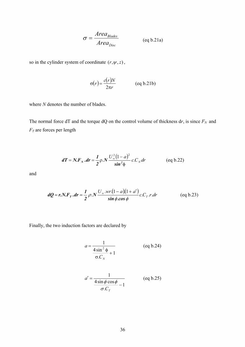
Figure b3: The local forces and velocity components on the blade

2. Programming

2.1. Algorithm

All necessary equations have now been derived for the BEM model. Since the different

control volumes are assumed to be independent, each strip may be treated separately and

therefore the results for one radius can be computed before solving for another radius.

For each control volume, the algorithm can be divided into eight steps:

1. Initialize a and a’, typically a0 = a0’ = 0.

2. Compute the flow angle, φ, using (eq b.18).

3. Compute the local angle of attack using (eq b.17).

38

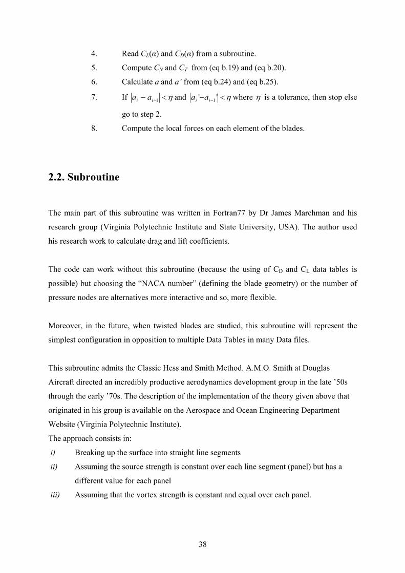
4. Read CL(α) and CD(α) from a subroutine.

5. Compute CN and CT from (eq b.19) and (eq b.20).

6. Calculate a and a’ from (eq b.24) and (eq b.25).

7. If η<− −1ii aa and η<− − '' 1ii aa where η is a tolerance, then stop else

go to step 2.

8. Compute the local forces on each element of the blades.

2.2. Subroutine

The main part of this subroutine was written in Fortran77 by Dr James Marchman and his

research group (Virginia Polytechnic Institute and State University, USA). The author used

his research work to calculate drag and lift coefficients.

The code can work without this subroutine (because the using of CD and CL data tables is

possible) but choosing the “NACA number” (defining the blade geometry) or the number of

pressure nodes are alternatives more interactive and so, more flexible.

Moreover, in the future, when twisted blades are studied, this subroutine will represent the

simplest configuration in opposition to multiple Data Tables in many Data files.

This subroutine admits the Classic Hess and Smith Method. A.M.O. Smith at Douglas

Aircraft directed an incredibly productive aerodynamics development group in the late ’50s

through the early ’70s. The description of the implementation of the theory given above that

originated in his group is available on the Aerospace and Ocean Engineering Department

Website (Virginia Polytechnic Institute).

The approach consists in:

i) Breaking up the surface into straight line segments

ii) Assuming the source strength is constant over each line segment (panel) but has a

different value for each panel

iii) Assuming that the vortex strength is constant and equal over each panel.

39

2.2.1. Subroutine principles

The subroutine defines the surface for NACA four or five digit airfoil shapes and

automatically places panels on that surface. It gives the chosen airfoil shape and the pressure

coefficient distribution.

With the information about the induced angle of attack, it is possible to calculate the pressure

coefficients, i.e. the lift and drag coefficients. As it was shown in the first part, the steps of the

programme are as following:

1. Data’s inputs are the NACA number of the uniform blade, and the induced angle of

attack (which is calculated by the main programme).

2. All the nodes of the body shape are solved in order to calculate everywhere the

pressure coefficients.

3. Coefficients of linear system are determined.

4. Solutions of linear algebraic system by Gaussian elimination with partial pivoting are

found.

5. The pressure distribution is determined.

6. Finally, the lift and drag coefficients are computed. Cd and Cl are input in the main

programme.

The above-mentioned steps are followed at each iteration. It is easy to understand that this

programme needs a lot of memory for the computer used. That is why a nodes limit will

be applied in the future.

2.2.2. Example

In order to show how this subroutine works, an example is made for this configuration:

40

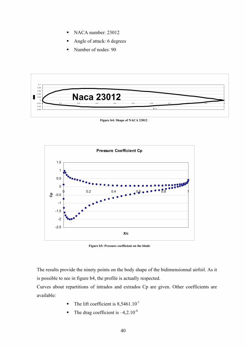
NACA number: 23012

Angle of attack: 6 degrees

Number of nodes: 90

Naca 23012-0.06

-0.04

-0.02

0

0.02

0.04

0.06

0.08

0.1

0 0.1 0.2 0.3 0.4 0.5 0.6 0.7 0.8 0.9 1

X / c

Figure b4: Shape of NACA 23012

Pressure Coefficient Cp

-2.5

-2

-1.5

-1

-0.5

0

0.5

1

1.5

0 0.2 0.4 0.6 0.8 1

X/c

Cp

Figure b5: Pressure coefficient on the blade

The results provide the ninety points on the body shape of the bidimensionnal airfoil. As it

is possible to see in figure b4, the profile is actually respected.

Curves about repartitions of intrados and extrados Cp are given. Other coefficients are

available:

The lift coefficient is 8,5461.10-1

The drag coefficient is –4,2.10-4

41

The interest is not to know the shape or the Cp but the programme needs this data to solve

equations and to get CD and CL. These coefficients are input in the main programme.

To conclude, it’s assumed that this subroutine (which will be integrated in the main

programme) works and provides accurate results.

This Smith-Hess panel method for single element lifting airfoil in 2-D incompressible

flow will be used in the next chapter but it’s admitted that this subroutine is independent

of the Reynolds number.

2.3. Structure of the programme

INPUT:

General Blades characteristics Blades geometry

Number of Elements Angle of attack. NACA number

∞U Radial velocity Chord

Number of blades Length

Hub

42

Initialisations

Compute the flow angle φ: ( )( ) ra

Ua..1

1tan

ωϕ

′+−

= ∞

Compute the local angle of attack. Subroutine:

α = φ - θ Method for single element lifting airfoil in 2-d (incompressible flow)

Set coordinates of nodes on body surface.

CL(α) and CD(α) compute with The pressure distribution is the aerofoil subroutines. determined.

Lift and Drag coefficients (CL(α)

and CD(α)) are computed.

Compute CN and CT by: CN = CL cos φ + CD sin φ CT = CL sin φ - CD cos φ

Calculate a and a’ from equations below:

1

.sin4

12

+σ

φ=

NC

a1

.cossin41

−=′

TC

a

σφφ

Tests

(a-aprevious<ε ) and (a’-a’previous<ε ’) No Satisfied Satisfied

OUTPUT Compute the local forces on each element of the

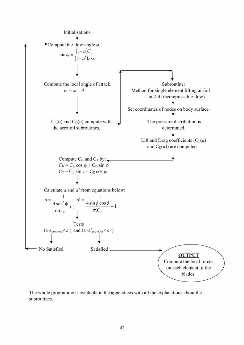
blades. The whole programme is available in the appendices with all the explanations about the subroutines.

43

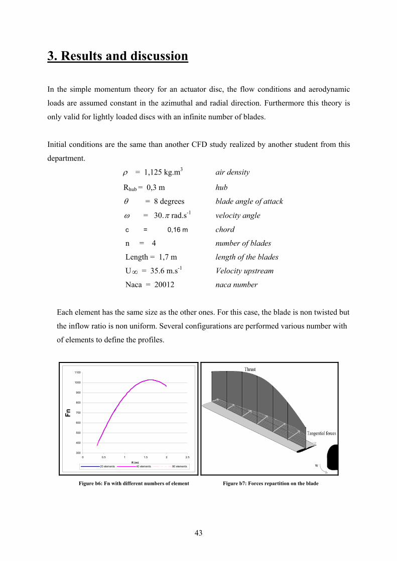
3. Results and discussion

In the simple momentum theory for an actuator disc, the flow conditions and aerodynamic

loads are assumed constant in the azimuthal and radial direction. Furthermore this theory is

only valid for lightly loaded discs with an infinite number of blades.

Initial conditions are the same than another CFD study realized by another student from this

department.

ρ = 1,125 kg.m3 air density

Rhub = 0,3 m hub

θ = 8 degrees blade angle of attack

ω = 30.π rad.s-1 velocity angle

c = 0,16 m chord

n = 4 number of blades

Length = 1,7 m length of the blades

U ∞ = 35.6 m.s-1 Velocity upstream

Naca = 20012 naca number

Each element has the same size as the other ones. For this case, the blade is non twisted but

the inflow ratio is non uniform. Several configurations are performed various number with

of elements to define the profiles.

300

400

500

600

700

800

900

1000

1100

0 0.5 1 1.5 2 2.5

R (m)

Fn

20 elements 40 elements 80 elements

Figure b6: Fn with different numbers of element Figure b7: Forces repartition on the blade

44

The results compared themselves when the numbers of blades changes, in order to check the

behaviour of T. Three numbers are tested: 20,40,80.

If the total thrust on the four blades is quantified, it’s easy to conclude that the results are

quite similar:

For 20 elt, T1 = 5811,749 N;

For 40 elt, T2 = 5760,633 N;

For 80 elt, T3 = 5734,453 N;

It seems that T tends a constant value when the number of element increases. For example,

the numerical error between T1 and T3 are: 1,33%.

In order to compare the results given by the Fortran programme with another works, the same

initial conditions are taken. The number of 60 elements is chosen because it’s good alternative

between the time and memory costs and the forces repartition accuracy.

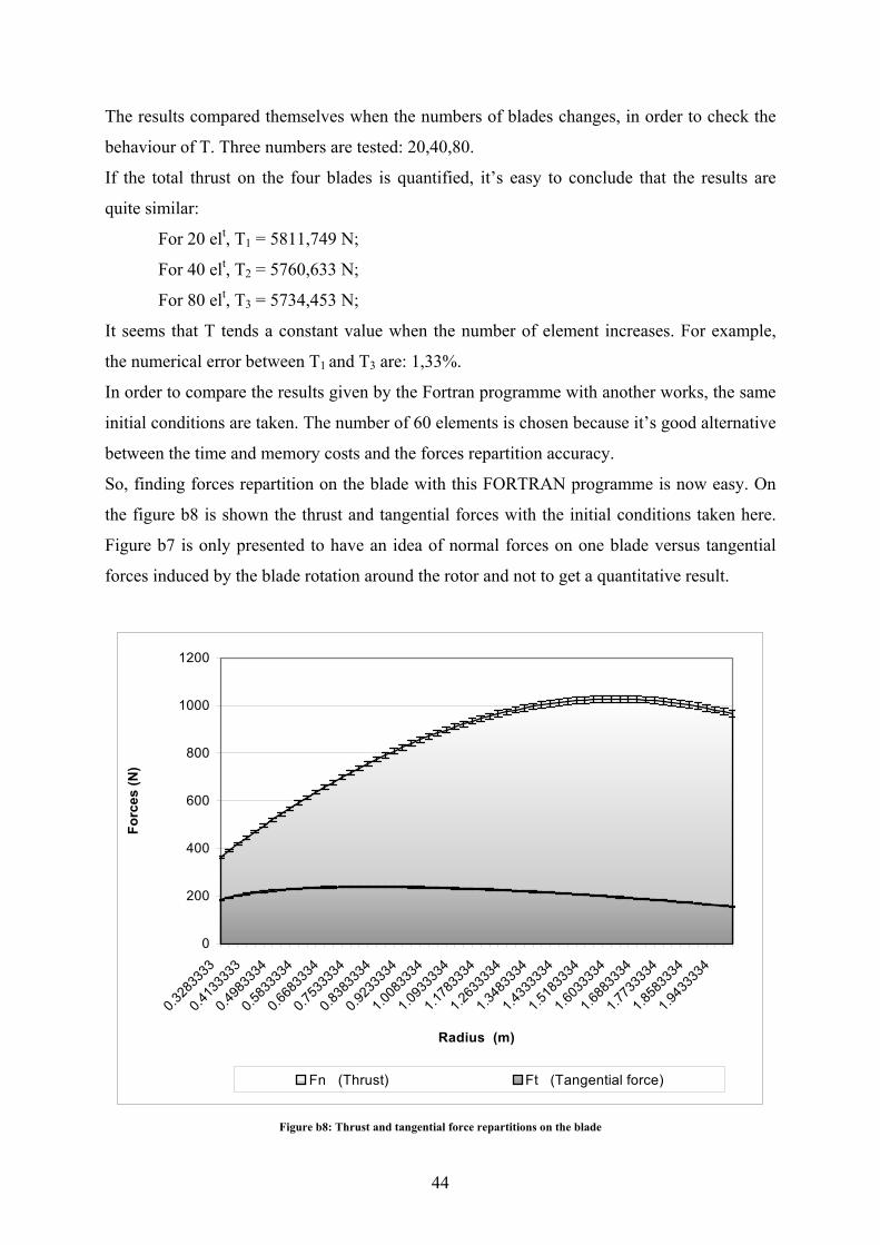
So, finding forces repartition on the blade with this FORTRAN programme is now easy. On

the figure b8 is shown the thrust and tangential forces with the initial conditions taken here.

Figure b7 is only presented to have an idea of normal forces on one blade versus tangential

forces induced by the blade rotation around the rotor and not to get a quantitative result.

0

200

400

600

800

1000

1200

0.328

3333

0.413

3333

0.498

3334

0.583

3334

0.668

3334

0.753

3334

0.838

3334

0.923

3334

1.008

3334

1.093

3334

1.178

3334

1.263

3334

1.348

3334

1.433

3334

1.518

3334

1.603

3334

1.688

3334

1.773

3334

1.858

3334

1.943

3334

Radius (m)

Forc

es (N

)

Fn (Thrust) Ft (Tangential force)

Figure b8: Thrust and tangential force repartitions on the blade

45

As can been seen on the figure b8, the error bars are very small when it is compared to the

tangential forces values. Representative results are revealed that the thrust Fn is bigger than Ft

everywhere. Obviously, the NACA profile is studied to provide this effect. The tangential

force decreases after 0.6m-Radius in opposition to the thrust, which increases until 1.7 m

radius and decreases a little bit at the end of the blade.

Moreover, the thrust is big after 1-meter radius. So, if the blade were divided in two parts, the

bigger forces would be on the second one. This problem could damage the rigidity of the

blade because there is not a good force repartition. That is the reason why aerodynamicists

twist the blade in order to reduce the thrust at the end of the blade. Another way to reduce

these too higher forces is to apply flapping angle; indeed, even if it is small (3-6 degrees), the

flapping angle represents the balance between the aerodynamic and centrifugal forces.

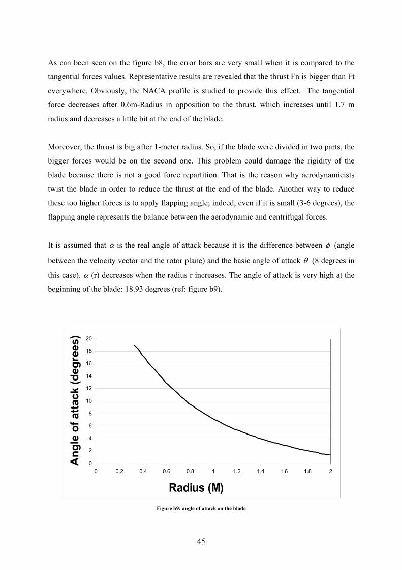
It is assumed that α is the real angle of attack because it is the difference between φ (angle

between the velocity vector and the rotor plane) and the basic angle of attack θ (8 degrees in

this case). α (r) decreases when the radius r increases. The angle of attack is very high at the

beginning of the blade: 18.93 degrees (ref: figure b9).

0

2

4

6

8

10

12

14

16

18

20

0 0.2 0.4 0.6 0.8 1 1.2 1.4 1.6 1.8 2

Radius (M)

Ang

le o

f atta

ck (d

egre

es)

Figure b9: angle of attack on the blade

46

The data tables providing all the numerical results with the number of iterations made after

calculations convergence are available in the appendices. To conclude this chapter, T and Q

are given: the total thrust induced by the four blades of the helicopter is calculated: 5734.45

N. In this case, the total Torque is about 1445.45 N.m.

The next step is to use these values of T and Q as input of Fluent Software.

4. Data implementation in FLUENT

The strategy adopted here is to input the data’s provided by the previous programme in

Fluent. This work represents BEM and CFD coupled calculations.

4.1. Implementation

As in the above method using the momentum theory, the input for the calculations was the

blade forces per unit blade length in axial and tangential direction, Fn and Ft, respectively.

The Pressures Pn and Pt in axial and tangential direction, respectively, are applied to the

actuator disc were derived from the blade forces as follows:

2...RNF

ANF

P bnbnn π

== (eq b.26)

2...RNF

ANF

P btbtt π

== (eq b.27)

Where A is the solid disk area,

Nb is the number of blades,

r is the radius.

The Pressure boundary conditions are applied with the Dynamic Pressure expressed 2.21 Vρ

with User Define Function programmed in C (That does not include the term of static

47

pressure); the vector directions are input for each element on the disc because of UDF

imputation.

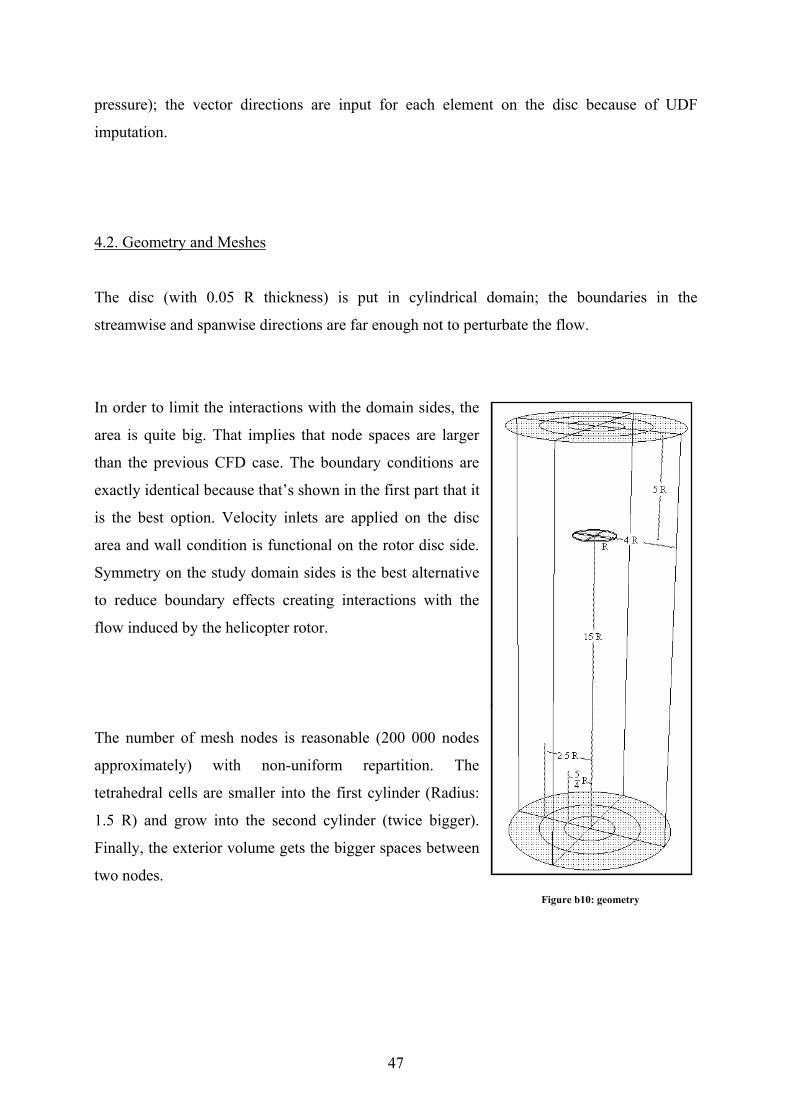
4.2. Geometry and Meshes

The disc (with 0.05 R thickness) is put in cylindrical domain; the boundaries in the

streamwise and spanwise directions are far enough not to perturbate the flow.

In order to limit the interactions with the domain sides, the

area is quite big. That implies that node spaces are larger

than the previous CFD case. The boundary conditions are

exactly identical because that’s shown in the first part that it

is the best option. Velocity inlets are applied on the disc

area and wall condition is functional on the rotor disc side.

Symmetry on the study domain sides is the best alternative

to reduce boundary effects creating interactions with the

flow induced by the helicopter rotor.

T

The number of mesh nodes is reasonable (200 000 nodes

approximately) with non-uniform repartition. The

tetrahedral cells are smaller into the first cylinder (Radius:

1.5 R) and grow into the second cylinder (twice bigger).

Finally, the exterior volume gets the bigger spaces between

two nodes. Figure b10: geometry

48

User Define Function is used with the purpose of imposing the pressure repartitions and its

direction vectors on FLUENT. This C program adapted to FLUENT implementation is

available in the “appendix 5“.

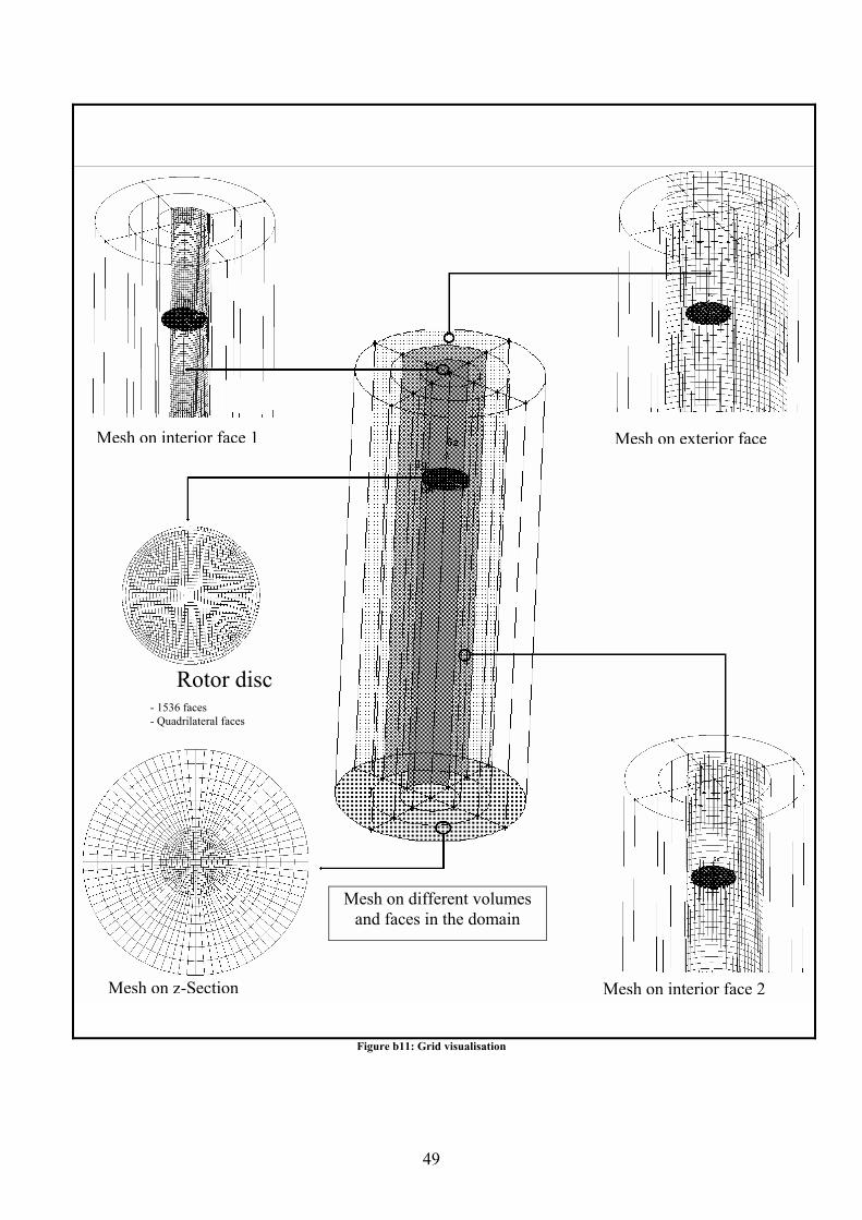
With the aim of obtaining accuracy data implementation on the rotor, the number of cells on

the disc is multiplied with FLUENT until being equal to 1536 quadrilateral faces.

49

Figure b11: Grid visualisation

Rotor disc - 1536 faces - Quadrilateral faces

Mesh on interior face 1

Mesh on interior face 2

Mesh on exterior face

Mesh on z-Section

Mesh on different volumes and faces in the domain

50

4.3. Numerical Procedure

In this case, a turbulent flow is simulated through a real disc. A two-equations RANS model

is used, the ε−k model. All the ε−k models have similar forms, with transport equations

for k and ε . The major differences are the method of calculating turbulent viscosity, the

turbulent Prandtl numbers governing the turbulent diffusion of k and ε , the generation and

destruction terms in the ε equation. The ε−k RNG model is applied because it is derived

from the instantaneous Navier-Stokes equations, using a mathematical technique called

"renormalization group" (RNG) methods. The analytical derivation results in a model with

constants different from those in the standard ε−k model, and additional terms and functions

in the transport equations for k and ε . The main interest is that the RNG model in FLUENT

provides an option to account for the effects of swirl or rotation by modifying the turbulent

viscosity appropriately.

Obviously, the calculation is a steady case. The implicit scheme (Segregated) is privileged to

explicit scheme providing difficult convergences. The algorithm, which solves the continuity

and momentum equations, is Powerlaw. The Pressure-Velocity coupling solved to get the

convergence by the SIMPLE C algorithm. The Standard under relaxation factors are used

(Pressure factor: 0.3, Momentum factor: 0.7, Turbuence kinetic energy and turbulent

dissipation rate: 0.8).

4.4 Results and discussion

• Validation with the total pressure and thrust

It’s important to check the thrust provided by FLUENT in order to validate the

implementation by the using of dynamic pressure distribution way described by the previous

relations; As the commercial CFD code is not able to calculate this Force alone, velocity

magnitude profile is defined and sixth order interpolated in order to calculate the Thrust and

the mass flow rate induced by the actuator.

51

It’s assumed that the Thrust is given by the following formula:

),(..),(. θθρ rVdSrVTrr

∫∫= (eq b.28)

A first apprximation is to simplify the equation multiplying the mass flow rate with average

velocity Vr

:

VmTr

& .=

So, the mass flow rate definition becomes:

dSrVm .),(.∫∫= θρr

&

θθρ ddrrrVm ...),(.∫∫=r

&

It’s assumed that 0),(=

∂∂

θθrV

r

;

drrrVmRr

Rr

.).(.21

0

∫=

=

=r

& π

On the other hand, ∫−=

1

0

)(1

01

R

R

drrVRR

Vrr

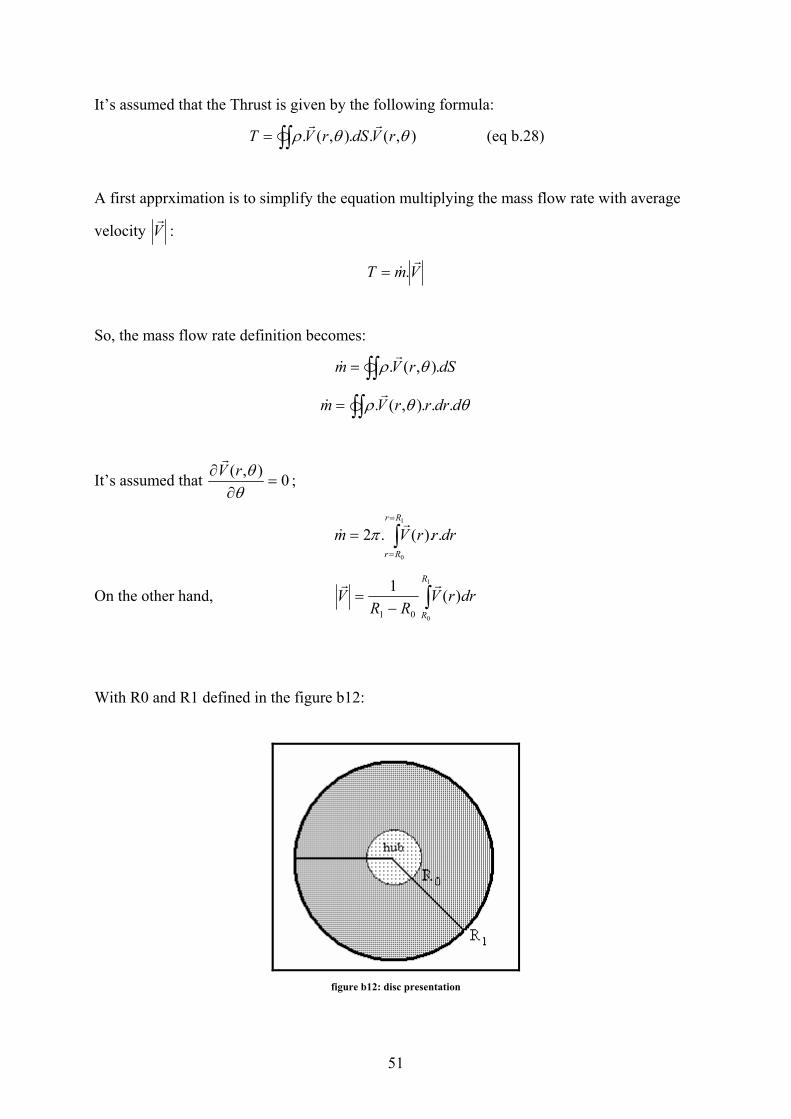
With R0 and R1 defined in the figure b12:

figure b12: disc presentation

52

With the velocity curve integration, the results are obtained:

1.1439.271 −= skgm&

1.05452.21 −= smVr

In these conditions, the thrust is found to be equal to:

T = 5708.805 N

To extend the comparison, an estimation of the errors is made It’s admitted that TFluent is the

Thrust provided by Fluent, and Tprog is the Thrust given by the FORTRAN programme which

inputs into the commercial CFD code:

prog

Fluentprog

T

TT −=ξ

%472.4=ξ is the estimated error during the implementation of the data into

the CFD code using this methodology.

The thrust provided is only an approximation of the real thrust for the reason that 4.472 %

error is declared. To reduce ξ , finer grid should be used, but it would increase the calculation

time too much.

To conclude, a supercomputer would have authorized the mesh improving, necessary if better

implementation is desired. Furthermore, a CFD code adaptive to helicopter aerodynamics

should be tried to check if more exactness is possible with this kind of method.

53

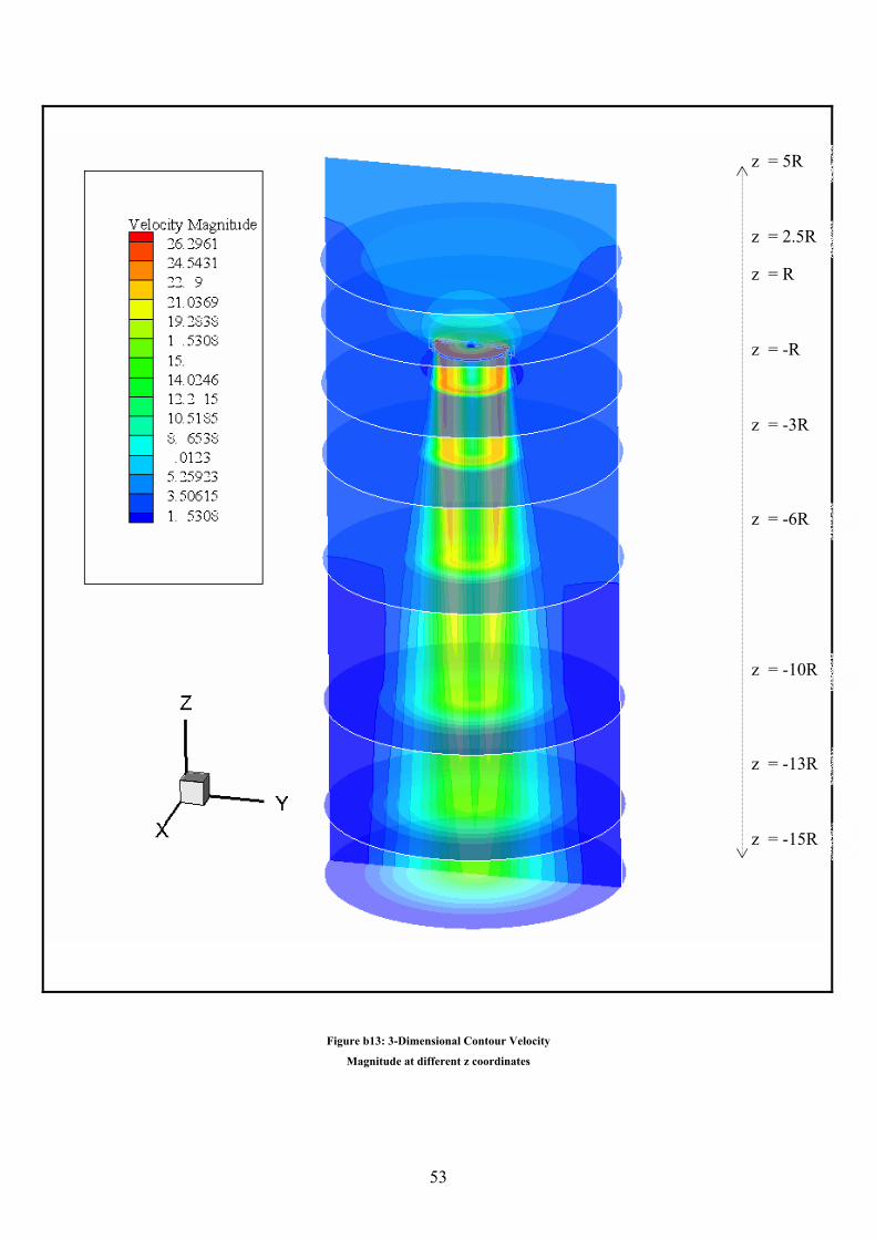
Figure b13: 3-Dimensional Contour Velocity

Magnitude at different z coordinates

z = R

z = -R

z = -3R

z = -6R

z = 2.5R

z = -13R

z = -15R

z = -10R

z = 5R

54

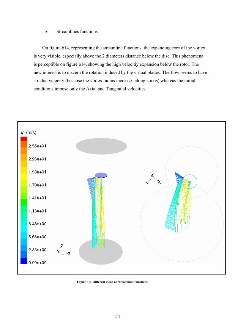
• Streamlines functions

On figure b14, representing the streamline functions, the expanding core of the vortex

is very visible, especially above the 2 diameters distance below the disc. This phenomena

is perceptible on figure b14, showing the high velocitiy expansion below the rotor. The

new interest is to discern the rotation induced by the virtual blades. The flow seems to have

a radial velocity (because the vortex radius increases along z-axis) whereas the initial

conditions impose only the Axial and Tangential velocities.

Figure b14: different views of Streamlines Functions

55

The software is able to give an idea about vorticity measuring the rotation of a fluid element

as it moves in the flow field defined by the following relation:

Vr

×∇=ζ

The high vorticity zones are situated below the disc where the radius is defined by

{r∈[0;0.5] ∪ [1.75;2.5]}. The streamline function and vorticity visualisations suggest that the

vortex generation is higher if r > 3R/4 (ref appendix).

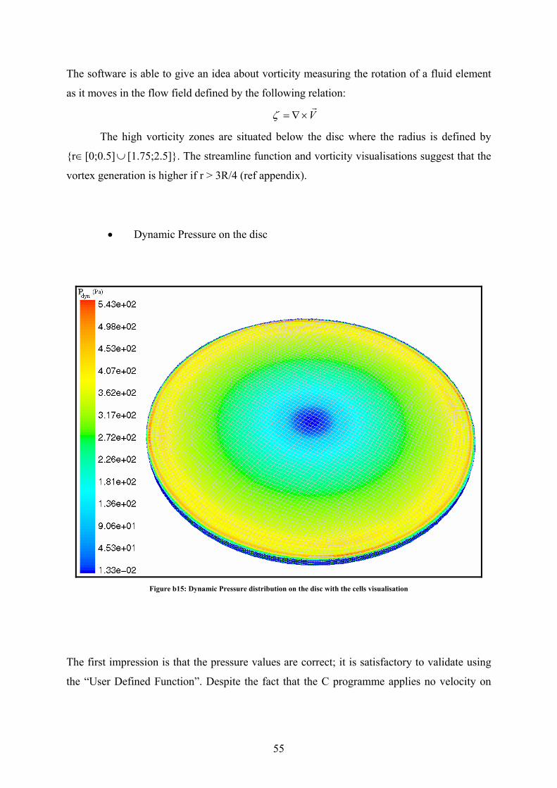
• Dynamic Pressure on the disc

Figure b15: Dynamic Pressure distribution on the disc with the cells visualisation

The first impression is that the pressure values are correct; it is satisfactory to validate using

the “User Defined Function”. Despite the fact that the C programme applies no velocity on

56

the Hub (r < 0.3m), the Dynamic Pressure values are not equal to zero. That includes that the

flow induced by the rotor which also induces velocities in the domain (0 < r < 0.3).

This issue is not too important if the Pressure values in the Hub (approximately 1.33 10-2) are

considered.

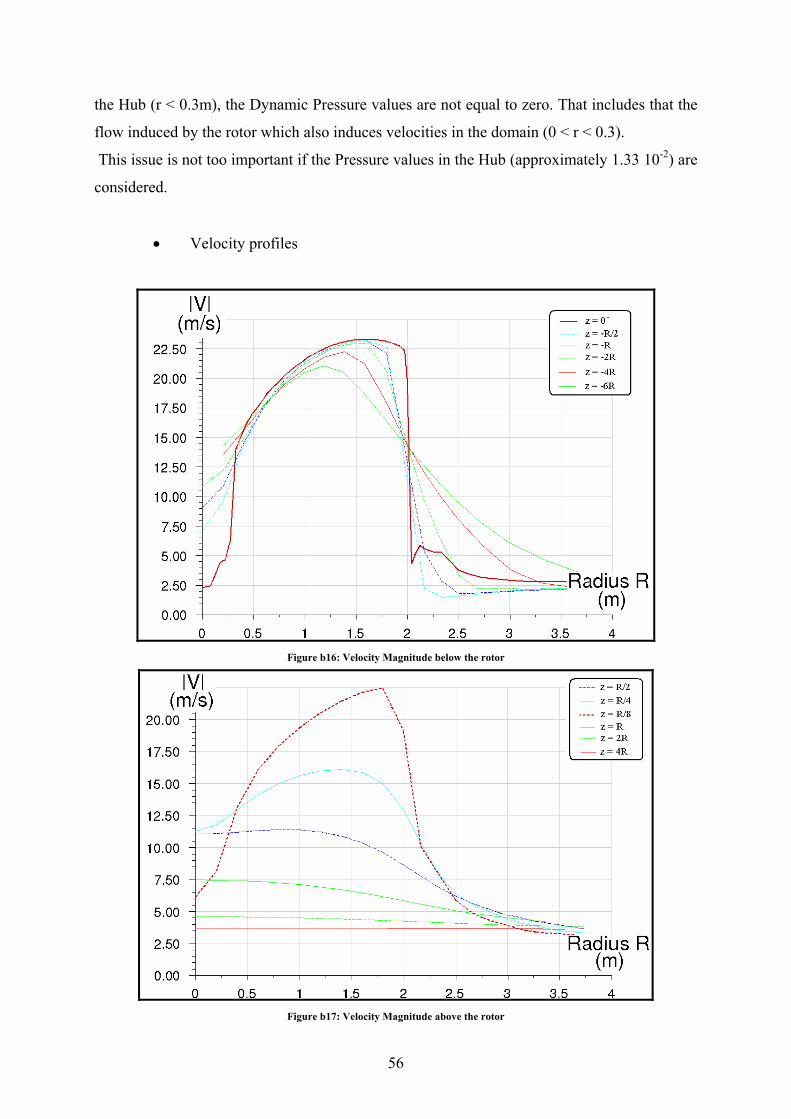
• Velocity profiles

Figure b16: Velocity Magnitude below the rotor

Figure b17: Velocity Magnitude above the rotor

57

On figure b16, the velocity profiles on lines of control are shown at diverse z coordinates

above and below the whole disc. It is fundamental to note the discontinuity on the line z=0-

which shows the limitations of this grid. In fact, small vortices on the disc sides can appear in

the real case but its shapes are generally different. In the domain defined by {r∈[0.3;2]}, the

velocity repartitions are validated by the software. Using an UDF is the best way to force the

non-uniform loading.

The profiles are increasingly flattened when the lines of control are far away. This reveals the

vortex core is expanding. The domain size limits seems to be excellent because nothing

important happens after 3.5 meters radius even though the domain is a 8 meter radius cylinder

to limit interactions with the boudaries.

Figure b17 shows the flow drawn in by the actuator disc. The velocities increase

progressively, especially in the sector r = R. Even if the flow induced continually gains speed

close to the whole disc, a low velocity zone is identified at z=R/8 (z=0.25m); the simplest

explanation is the implementation on the disc of the “drawn in” velocity between r=0.3 m and

r=2m; checking mass flow rate theory shows that this induces low velocities in the radius

{r∈[0;0.3]} simulating the hub of the helicopter rotor system.

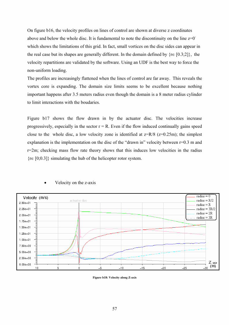
• Velocity on the z-axis

Figure b18: Velocity along Z-axis

58

Figure b18 shows the velocity magnitude along the Z-axis. The velocity on the “R=0” line

increases below the rotor (especially after the coordinates z = R/2) and stops its progression at

13.R after the whole disc. Numerically, it is not similar to the curves provided by the one-

dimensional Momentum theory, but it is assumed that both curves have the same profile.

For the two lines taken at 0.5R and R, the maximum velocity is on the rotor (z = 0 ± 0.1m ). It

is interesting to note that the velocity increases progressively after the rotor.

59

The BEM is a powerful tool for aerodynamic researchers on helicopter rotors. The idea

consists of representing the airloads on two-dimensional sections of the blades and integrating

their effects in order to find the performance of the rotor as a whole. Whereas simple

momentum theory, the blade element approach allows the imputations of blade tip speed,

blade loading…

The flow induced by the programme calculation by the way of using CFD code has been

reviewed. However, it should be inlightling to compare these results with experimental works

or other CFD approaches. But with not enough time, this paper will end without real

comparison with other data , which is a huge limitation to this work.

60

Conclusion Firstly, a comparison between the data provided by a mathematical study realised by J.T.

Conway and a CFD modeling has been made. The methodology and knowledge are employed

for the second part.

Secondly, the ideas of combining loading distributions solved with a FORTRAN programme

implemented in the commercial CFD code is reviewed. The principles of imputing the blades

characteristics in order to obtain lift and drag forces on each blade have been developed.

Because of the importance of Reynolds number and Mach number in the force distribution,

this method shows its limitations.

It will be possible for other people in the Aerospace and Mechanical Engineering department

in UMIST to follow these model studies, in order to ameliorate and compare this results with

experimental data.

The goal of the aerodynamic modeling work is to be able to predict the entire flow field

around the helicopter rotor and its airframe whatever the flight conditions. Even if this aim

has not been achieved, this work is a step forward to that goal.

61

Appendices

Appendix 1 C program to apply three velocity profiles

Appendix 2 C program to specify “two velocity profiles”

And “jump pressure profile”

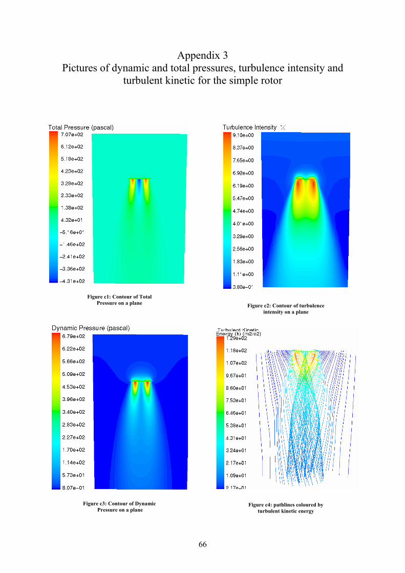
Appendix 3 Pictures of dynamic and total pressures, turbulence intensity and turbulent kinetic for the

simple rotor

Appendix 4 Pictures of velocity magnitude, axial velocity, radial velocity and tangential velocity on the

simple rotor

Appendix 5 FORTRAN Program

Appendix 6 Velocity vectors for the BEM-CFD approach

62

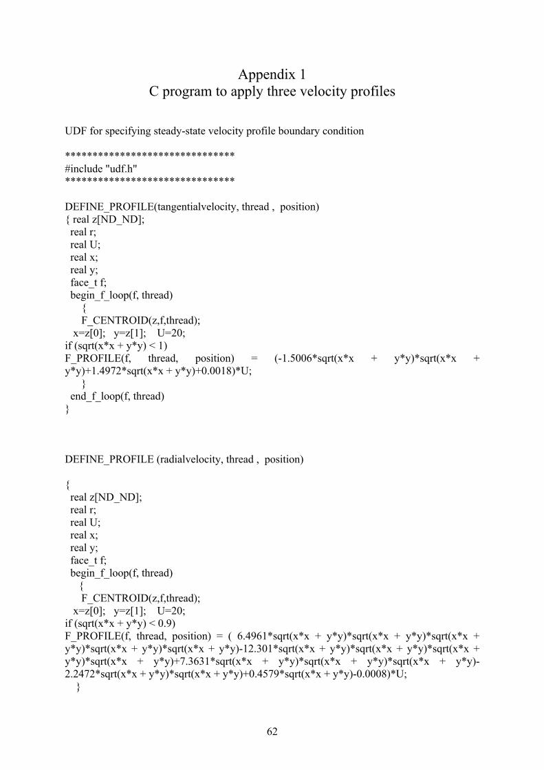
Appendix 1 C program to apply three velocity profiles

UDF for specifying steady-state velocity profile boundary condition ******************************* #include "udf.h" ******************************* DEFINE_PROFILE(tangentialvelocity, thread , position) { real z[ND_ND]; real r; real U; real x; real y; face_t f; begin_f_loop(f, thread) { F_CENTROID(z,f,thread); x=z[0]; y=z[1]; U=20; if (sqrt(x*x + y*y) < 1) F_PROFILE(f, thread, position) = (-1.5006*sqrt(x*x + y*y)*sqrt(x*x + y*y)+1.4972*sqrt(x*x + y*y)+0.0018)*U; } end_f_loop(f, thread) } DEFINE_PROFILE (radialvelocity, thread , position) { real z[ND_ND]; real r; real U; real x; real y; face_t f; begin_f_loop(f, thread) { F_CENTROID(z,f,thread); x=z[0]; y=z[1]; U=20; if (sqrt(x*x + y*y) < 0.9) F_PROFILE(f, thread, position) = ( 6.4961*sqrt(x*x + y*y)*sqrt(x*x + y*y)*sqrt(x*x + y*y)*sqrt(x*x + y*y)*sqrt(x*x + y*y)-12.301*sqrt(x*x + y*y)*sqrt(x*x + y*y)*sqrt(x*x + y*y)*sqrt(x*x + y*y)+7.3631*sqrt(x*x + y*y)*sqrt(x*x + y*y)*sqrt(x*x + y*y)-2.2472*sqrt(x*x + y*y)*sqrt(x*x + y*y)+0.4579*sqrt(x*x + y*y)-0.0008)*U; }

63

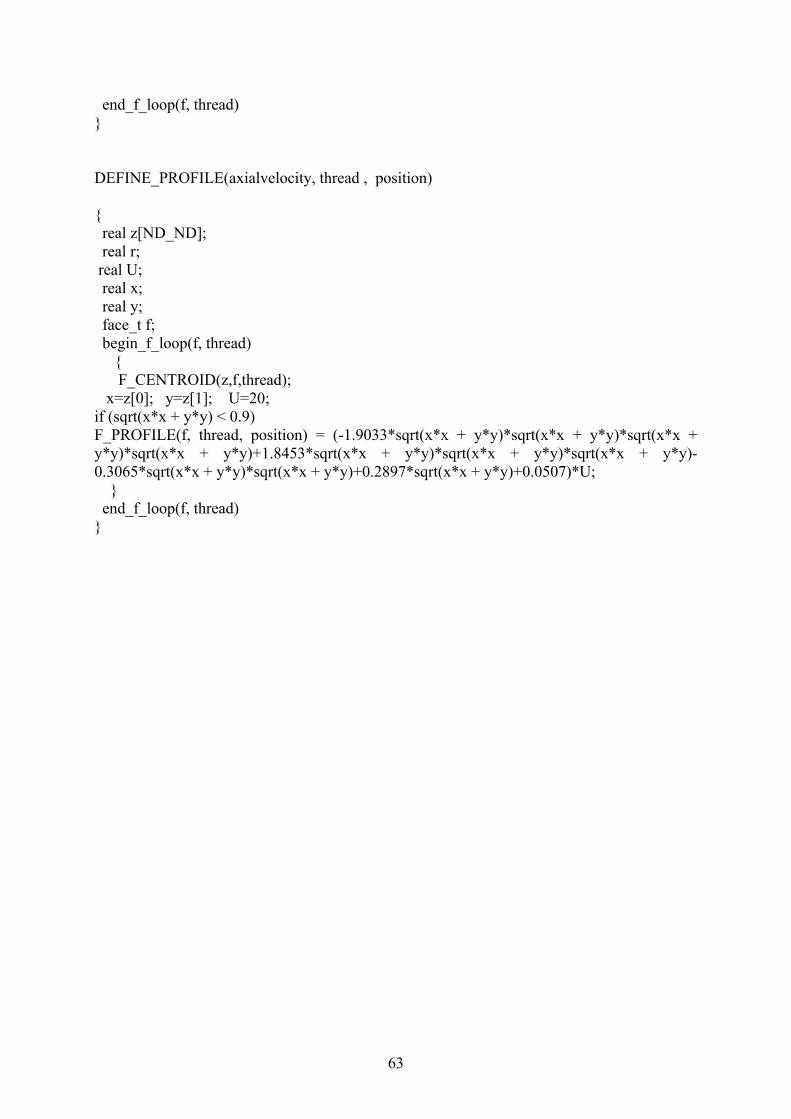
end_f_loop(f, thread) } DEFINE_PROFILE(axialvelocity, thread , position) { real z[ND_ND]; real r; real U; real x; real y; face_t f; begin_f_loop(f, thread) { F_CENTROID(z,f,thread); x=z[0]; y=z[1]; U=20; if (sqrt(x*x + y*y) < 0.9) F_PROFILE(f, thread, position) = (-1.9033*sqrt(x*x + y*y)*sqrt(x*x + y*y)*sqrt(x*x + y*y)*sqrt(x*x + y*y)+1.8453*sqrt(x*x + y*y)*sqrt(x*x + y*y)*sqrt(x*x + y*y)-0.3065*sqrt(x*x + y*y)*sqrt(x*x + y*y)+0.2897*sqrt(x*x + y*y)+0.0507)*U; } end_f_loop(f, thread) }

64

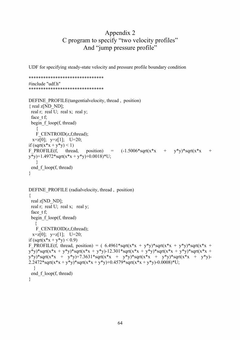
Appendix 2 C program to specify “two velocity profiles”

And “jump pressure profile”

UDF for specifying steady-state velocity and pressure profile boundary condition ******************************* #include "udf.h" ******************************* DEFINE_PROFILE(tangentialvelocity, thread , position) { real z[ND_ND]; real r; real U; real x; real y; face_t f; begin_f_loop(f, thread) { F_CENTROID(z,f,thread); x=z[0]; y=z[1]; U=20; if (sqrt(x*x + y*y) < 1) F_PROFILE(f, thread, position) = (-1.5006*sqrt(x*x + y*y)*sqrt(x*x + y*y)+1.4972*sqrt(x*x + y*y)+0.0018)*U; } end_f_loop(f, thread) } DEFINE_PROFILE (radialvelocity, thread , position) { real z[ND_ND]; real r; real U; real x; real y; face_t f; begin_f_loop(f, thread) { F_CENTROID(z,f,thread); x=z[0]; y=z[1]; U=20; if (sqrt(x*x + y*y) < 0.9) F_PROFILE(f, thread, position) = ( 6.4961*sqrt(x*x + y*y)*sqrt(x*x + y*y)*sqrt(x*x + y*y)*sqrt(x*x + y*y)*sqrt(x*x + y*y)-12.301*sqrt(x*x + y*y)*sqrt(x*x + y*y)*sqrt(x*x + y*y)*sqrt(x*x + y*y)+7.3631*sqrt(x*x + y*y)*sqrt(x*x + y*y)*sqrt(x*x + y*y)-2.2472*sqrt(x*x + y*y)*sqrt(x*x + y*y)+0.4579*sqrt(x*x + y*y)-0.0008)*U; } end_f_loop(f, thread) }

65

DEFINE_PROFILE(Pressionaxiale, thread , position) { real z[ND_ND]; real r; real U; real x; real y; face_t f; begin_f_loop(f, thread) { F_CENTROID(z,f,thread); x=z[0]; y=z[1]; if (sqrt(x*x + y*y) < 1) F_PROFILE(f, thread, position) = ( 8521*sqrt(x*x + y*y)*sqrt(x*x + y*y)*sqrt(x*x + y*y)*sqrt(x*x + y*y)*sqrt(x*x + y*y)*sqrt(x*x + y*y)-21947*sqrt(x*x + y*y)*sqrt(x*x + y*y)*sqrt(x*x + y*y)*sqrt(x*x + y*y)*sqrt(x*x + y*y)+20741*sqrt(x*x + y*y)*sqrt(x*x + y*y)*sqrt(x*x + y*y)*sqrt(x*x + y*y)-9669.3*sqrt(x*x + y*y)*sqrt(x*x + y*y)*sqrt(x*x + y*y)+2578.2*sqrt(x*x + y*y)*sqrt(x*x + y*y)-192.33*sqrt(x*x + y*y)-41.65); } end_f_loop(f, thread) }

66

Appendix 3 Pictures of dynamic and total pressures, turbulence intensity and

turbulent kinetic for the simple rotor

Figure c1: Contour of Total Pressure on a plane

Figure c3: Contour of Dynamic Pressure on a plane

Figure c2: Contour of turbulence intensity on a plane

Figure c4: pathlines coloured by turbulent kinetic energy

67

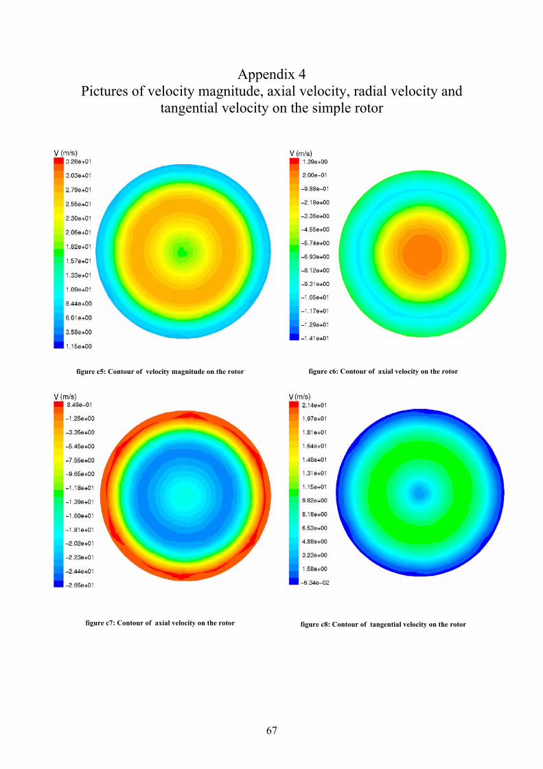
Appendix 4 Pictures of velocity magnitude, axial velocity, radial velocity and

tangential velocity on the simple rotor

figure c5: Contour of velocity magnitude on the rotor

figure c7: Contour of axial velocity on the rotor

figure c6: Contour of axial velocity on the rotor

figure c8: Contour of tangential velocity on the rotor

68

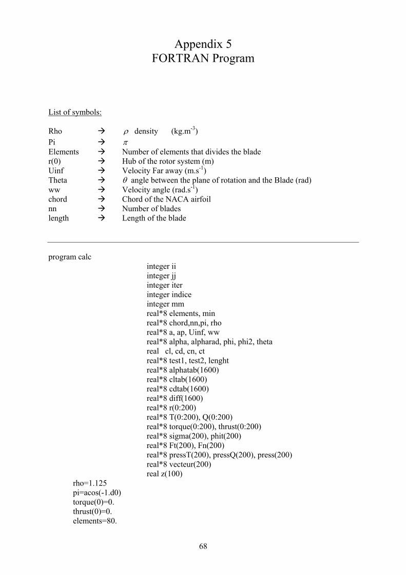
Appendix 5 FORTRAN Program

List of symbols: Rho ρ density (kg.m-3) Pi π Elements Number of elements that divides the blade r(0) Hub of the rotor system (m) Uinf Velocity Far away (m.s-1) Theta θ angle between the plane of rotation and the Blade (rad) ww Velocity angle (rad.s-1) chord Chord of the NACA airfoil nn Number of blades length Length of the blade program calc integer ii integer jj integer iter integer indice integer mm real*8 elements, min real*8 chord,nn,pi, rho real*8 a, ap, Uinf, ww real*8 alpha, alpharad, phi, phi2, theta real cl, cd, cn, ct real*8 test1, test2, lenght real*8 alphatab(1600) real*8 cltab(1600) real*8 cdtab(1600) real*8 diff(1600) real*8 r(0:200) real*8 T(0:200), Q(0:200) real*8 torque(0:200), thrust(0:200) real*8 sigma(200), phit(200) real*8 Ft(200), Fn(200) real*8 pressT(200), pressQ(200), press(200) real*8 vecteur(200) real z(100) rho=1.125 pi=acos(-1.d0) torque(0)=0. thrust(0)=0. elements=80.

69

r(0)=0.3 Uinf=35.6 theta=8*pi/180 ww=30*pi chord=0.16 nn=4.0 lenght=1.7 do jj=1,elements r(jj)=(lenght/elements)+r(jj-1) enddo do jj=1,elements a=0. ap=0. iter=0 test1=1. test2=1. cn=0. ct=0. cd=0. cl=0. sigma(jj)=(chord*nn)/(2*pi*r(jj)) 100 do while (abs(a-test1).GT.1.e-5.and.abs(ap-test2).GT.1.e-5) test1=a test2=ap phi=(atan(((1-a)*Uinf)/((1+ap)*ww*r(jj)))) alpha=(phi-theta) phit(jj)=alpha*180/pi open(20,file='tables1.dat',status='unknown') write(20,*) alpha close(unit=20) call panel open(21,file='tables2.dat',status='unknown') read(21,*) cd, cl close(unit=21) iter=iter+1

70

cn = cl*cos(phi) + cd*sin(phi) ct = cl*sin(phi) - cd*cos(phi) a= 1/(((4*sin(phi)*sin(phi))/(sigma(jj)*cn))+1) ap= 1/(((4*sin(phi)*cos(phi))/(sigma(jj)*ct))-1) write(04,*) jj, iter, alpha, cl, cd, a, ap enddo T(jj)=(rho*nn*Uinf*Uinf*(1-a)*(1-a)*chord*cn)/ . (2*sin(phi)*sin(phi)) Q(jj)=( (rho*nn*Uinf*(1-a)*(1+ap)*ww*r(jj)*chord*ct) / . (2*sin(phi)*cos(phi))) Fn(jj)=(rho*Uinf*Uinf*(1-a)*(1-a)*chord*cn)/ . (2*sin(phi)*sin(phi)) Ft(jj)=( (rho*Uinf*(1-a)*(1+ap)*ww*r(jj)*chord*ct) / . (2*sin(phi)*cos(phi))) thrust(jj)=nn*Fn(jj)*(r(jj)-r(jj-1))+thrust(jj-1) torque(jj)=nn*Ft(jj)*(r(jj)-r(jj-1))+torque(jj-1) pressT(jj)=nn*Fn(jj)*(r(jj)-r(jj-1))*chord/(pi*r(jj)*r(jj)) pressQ(jj)=nn*Ft(jj)*(r(jj)-r(jj-1))*chord/(pi*r(jj)*r(jj)) press(jj)=sqrt(pressT(jj)*pressT(jj) . +pressQ(jj)*pressQ(jj)) vecteur(jj)=pressQ(jj)/pressT(jj) write(60,*) r(jj) write(61,*) iter write(62,*) alpha write(63,*) Fn(jj) write(64,*) Ft(jj) write(11,*) vecteur(jj) write(10,*) pression(jj) write(09,*) r(jj) enddo write(*,*) '********************' write(*,*) 'the thrust is (N)' write(*,*) thrust(elements) write(*,*) 'the Torque is (N.m) ' write(*,*) torque(elements) write(*,*) '*********************'

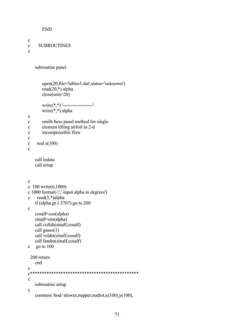
71

END c c SUBROUTINES c subroutine panel open(20,file='tables1.dat',status='unknown') read(20,*) alpha close(unit=20) write(*,*) '-------------------' write(*,*) alpha c c smith-hess panel method for single c element lifting airfoil in 2-d c incompressible flow c c real z(100) c call indata call setup c c 100 write(6,1000) c 1000 format(///,' input alpha in degrees') c read(5,*)alpha if (alpha.gt.1.5707) go to 200 c cosalf=cos(alpha) sinalf=sin(alpha) call cofish(sinalf,cosalf) call gauss(1) call veldis(sinalf,cosalf) call fandm(sinalf,cosalf) c go to 100 200 return end c c********************************************** c subroutine setup c common /bod/ nlower,nupper,nodtot,x(100),y(100),

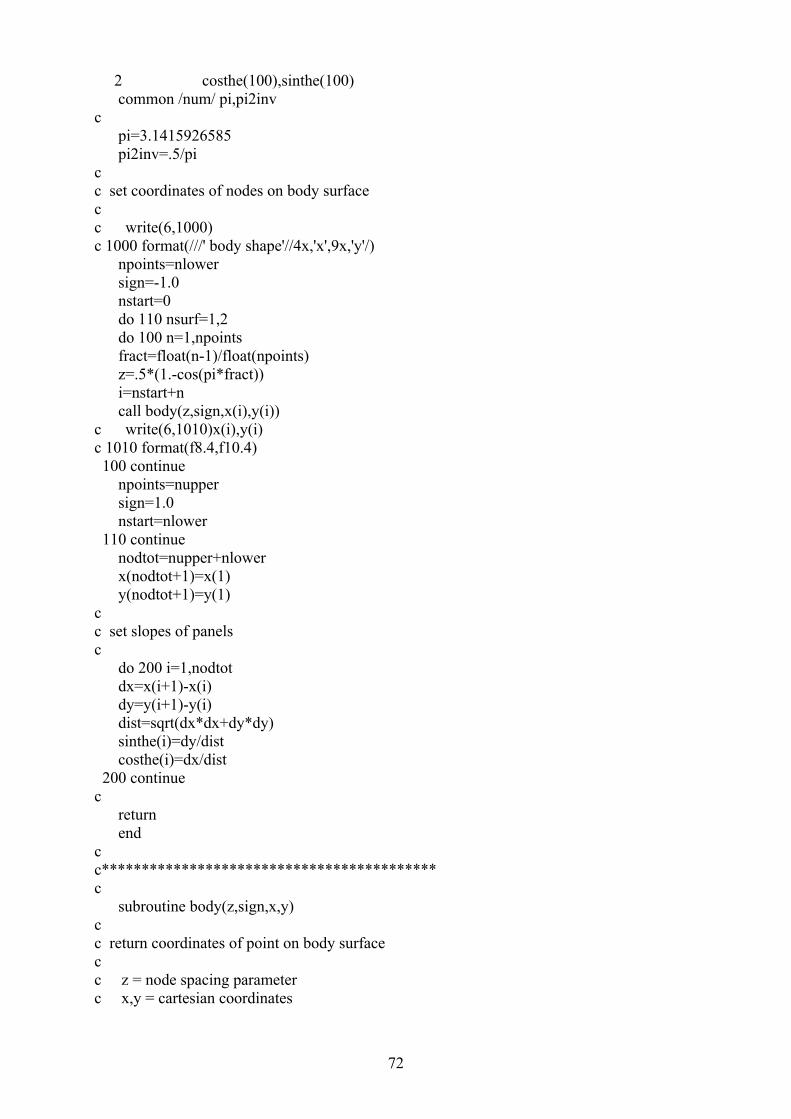
72

2 costhe(100),sinthe(100) common /num/ pi,pi2inv c pi=3.1415926585 pi2inv=.5/pi c c set coordinates of nodes on body surface c c write(6,1000) c 1000 format(///' body shape'//4x,'x',9x,'y'/) npoints=nlower sign=-1.0 nstart=0 do 110 nsurf=1,2 do 100 n=1,npoints fract=float(n-1)/float(npoints) z=.5*(1.-cos(pi*fract)) i=nstart+n call body(z,sign,x(i),y(i)) c write(6,1010)x(i),y(i) c 1010 format(f8.4,f10.4) 100 continue npoints=nupper sign=1.0 nstart=nlower 110 continue nodtot=nupper+nlower x(nodtot+1)=x(1) y(nodtot+1)=y(1) c c set slopes of panels c do 200 i=1,nodtot dx=x(i+1)-x(i) dy=y(i+1)-y(i) dist=sqrt(dx*dx+dy*dy) sinthe(i)=dy/dist costhe(i)=dx/dist 200 continue c return end c c****************************************** c subroutine body(z,sign,x,y) c c return coordinates of point on body surface c c z = node spacing parameter c x,y = cartesian coordinates

73

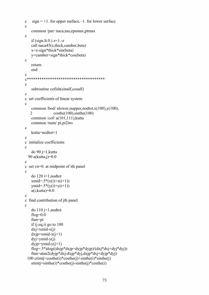
c sign = +1. for upper surface, -1. for lower surface c common /par/ naca,tau,epsmax,ptmax c if (sign.lt.0.) z=1.-z call naca45(z,thick,camber,beta) x=z-sign*thick*sin(beta) y=camber+sign*thick*cos(beta) c return end c c************************************* c subroutine cofish(sinalf,cosalf) c c set coefficients of linear system c common /bod/ nlower,nupper,nodtot,x(100),y(100), 2 costhe(100),sinthe(100) common /cof/ a(101,111),kutta common /num/ pi,pi2inv c kutta=nodtot+1 c c initialize coefficients c do 90 j=1,kutta 90 a(kutta,j)=0.0 c c set vn=0. at midpoint of ith panel c do 120 i=1,nodtot xmid=.5*(x(i)+x(i+1)) ymid=.5*(y(i)+y(i+1)) a(i,kutta)=0.0 c c find contribution of jth panel c do 110 j=1,nodtot flog=0.0 ftan=pi if (j.eq.i) go to 100 dxj=xmid-x(j) dxjp=xmid-x(j+1) dyj=ymid-y(j) dyjp=ymid-y(j+1) flog=.5*alog((dxjp*dxjp+dyjp*dyjp)/(dxj*dxj+dyj*dyj)) ftan=atan2(dyjp*dxj-dxjp*dyj,dxjp*dxj+dyjp*dyj) 100 ctimtj=costhe(i)*costhe(j)+sinthe(i)*sinthe(j) stimtj=sinthe(i)*costhe(j)-sinthe(j)*costhe(i)

74

a(i,j)=pi2inv*(ftan*ctimtj+flog*stimtj) b=pi2inv*(flog*ctimtj-ftan*stimtj) a(i,kutta)=a(i,kutta)+b if ((i.gt.1).and.(i.lt.nodtot)) go to 110 c c if ith panel touches trailing edge, add contribution c to kutta condition c a(kutta,j)=a(kutta,j)-b a(kutta,kutta)=a(kutta,kutta)+a(i,j) 110 continue c c fill in known sides c a(i,kutta+1)=sinthe(i)*cosalf-costhe(i)*sinalf 120 continue a(kutta,kutta+1)=-(costhe(1)+costhe(nodtot))*cosalf 2 -(sinthe(1)+sinthe(nodtot))*sinalf c return end c c********************************* c subroutine veldis(sinalf,cosalf) c c compute and print out pressure distribution c common /bod/ nlower,nupper,nodtot,x(100),y(100), 2 costhe(100),sinthe(100) common /cof/ a(101,111),kutta common /cpd/ cp(100) common /num/ pi,pi2inv dimension q(150) c c write(6,1000) c 1000 format(///' pressure distribution'//4x,'x',8x,'cp'/) c c retrieve solution from a-matrix c do 50 i=1,nodtot 50 q(i)=a(i,kutta+1) gamma=a(kutta,kutta+1) c c find vt and cp at midpoint of ith panel c do 130 i=1,nodtot xmid=.5*(x(i)+x(i+1)) ymid=.5*(y(i)+y(i+1)) vtang=cosalf*costhe(i)+sinalf*sinthe(i) c

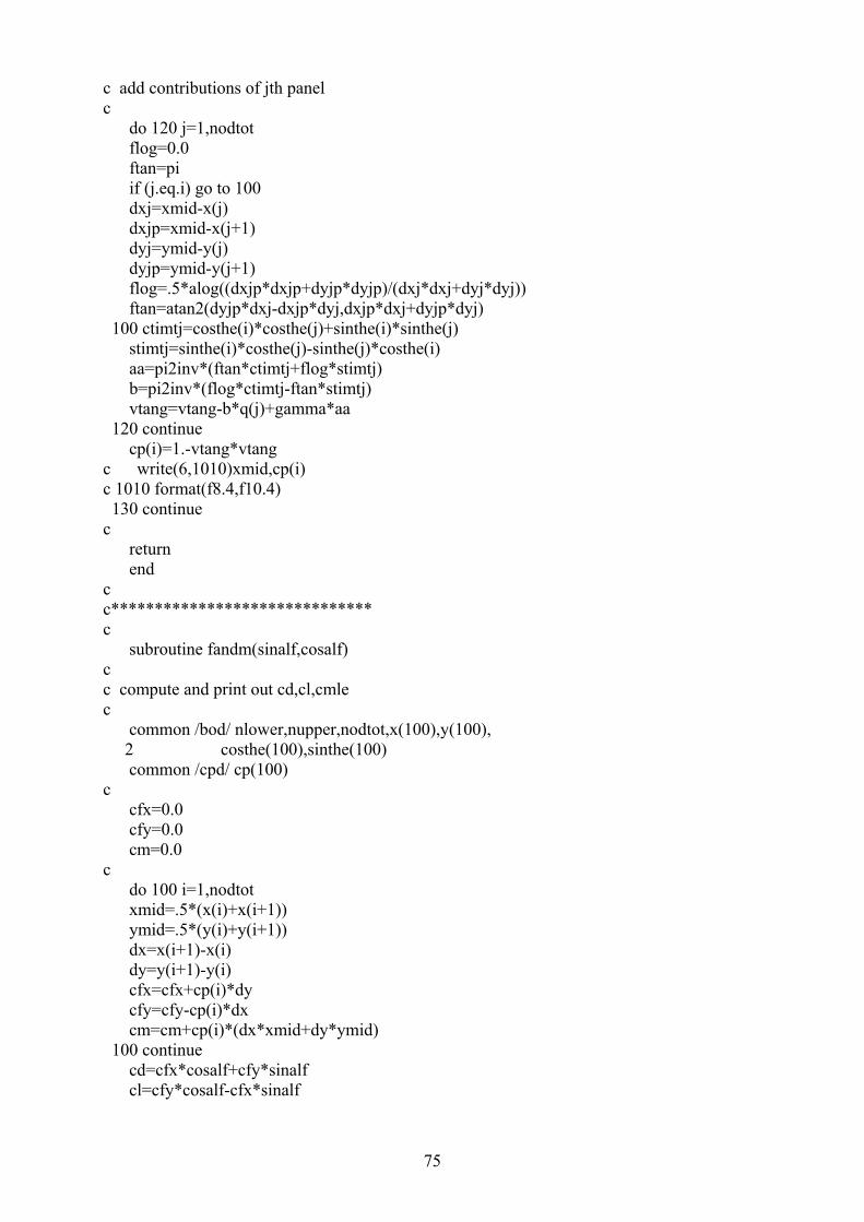
75

c add contributions of jth panel c do 120 j=1,nodtot flog=0.0 ftan=pi if (j.eq.i) go to 100 dxj=xmid-x(j) dxjp=xmid-x(j+1) dyj=ymid-y(j) dyjp=ymid-y(j+1) flog=.5*alog((dxjp*dxjp+dyjp*dyjp)/(dxj*dxj+dyj*dyj)) ftan=atan2(dyjp*dxj-dxjp*dyj,dxjp*dxj+dyjp*dyj) 100 ctimtj=costhe(i)*costhe(j)+sinthe(i)*sinthe(j) stimtj=sinthe(i)*costhe(j)-sinthe(j)*costhe(i) aa=pi2inv*(ftan*ctimtj+flog*stimtj) b=pi2inv*(flog*ctimtj-ftan*stimtj) vtang=vtang-b*q(j)+gamma*aa 120 continue cp(i)=1.-vtang*vtang c write(6,1010)xmid,cp(i) c 1010 format(f8.4,f10.4) 130 continue c return end c c****************************** c subroutine fandm(sinalf,cosalf) c c compute and print out cd,cl,cmle c common /bod/ nlower,nupper,nodtot,x(100),y(100), 2 costhe(100),sinthe(100) common /cpd/ cp(100) c cfx=0.0 cfy=0.0 cm=0.0 c do 100 i=1,nodtot xmid=.5*(x(i)+x(i+1)) ymid=.5*(y(i)+y(i+1)) dx=x(i+1)-x(i) dy=y(i+1)-y(i) cfx=cfx+cp(i)*dy cfy=cfy-cp(i)*dx cm=cm+cp(i)*(dx*xmid+dy*ymid) 100 continue cd=cfx*cosalf+cfy*sinalf cl=cfy*cosalf-cfx*sinalf

76

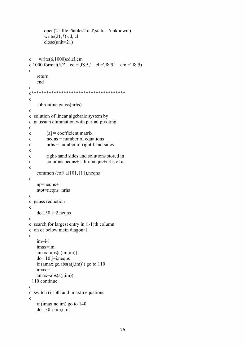
open(21,file='tables2.dat',status='unknown') write(21,*) cd, cl close(unit=21) c write(6,1000)cd,cl,cm c 1000 format(////' cd =',f8.5,' cl =',f8.5,' cm =',f8.5) c return end c c************************************** c subroutine gauss(nrhs) c c solution of linear algebraic system by c gaussian elimination with partial pivoting c c [a] = coefficient matrix c neqns = number of equations c nrhs = number of right-hand sides c c right-hand sides and solutions stored in c columns neqns+1 thru neqns+nrhs of a c common /cof/ a(101,111),neqns c np=neqns+1 ntot=neqns+nrhs c c gauss reduction c do 150 i=2,neqns c c search for largest entry in (i-1)th column c on or below main diagonal c im=i-1 imax=im amax=abs(a(im,im)) do 110 j=i,neqns if (amax.ge.abs(a(j,im))) go to 110 imax=j amax=abs(a(j,im)) 110 continue c c switch (i-1)th and imaxth equations c if (imax.ne.im) go to 140 do 130 j=im,ntot

77

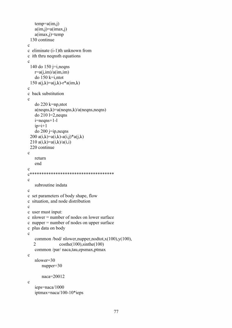
temp=a(im,j) a(im,j)=a(imax,j) a(imax,j)=temp 130 continue c c eliminate (i-1)th unknown from c ith thru neqnsth equations c 140 do 150 j=i,neqns r=a(j,im)/a(im,im) do 150 k=i,ntot 150 a(j,k)=a(j,k)-r*a(im,k) c c back substitution c do 220 k=np,ntot a(neqns,k)=a(neqns,k)/a(neqns,neqns) do 210 l=2,neqns i=neqns+1-l ip=i+1 do 200 j=ip,neqns 200 a(i,k)=a(i,k)-a(i,j)*a(j,k) 210 a(i,k)=a(i,k)/a(i,i) 220 continue c return end c c************************************ c subroutine indata c c set parameters of body shape, flow c situation, and node distribution c c user must input: c nlower = number of nodes on lower surface c nupper = number of nodes on upper surface c plus data on body c common /bod/ nlower,nupper,nodtot,x(100),y(100), 2 costhe(100),sinthe(100) common /par/ naca,tau,epsmax,ptmax c nlower=30 nupper=30 naca=20012 c ieps=naca/1000 iptmax=naca/100-10*ieps

78

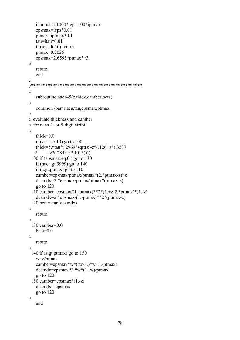
itau=naca-1000*ieps-100*iptmax epsmax=ieps*0.01 ptmax=iptmax*0.1 tau=itau*0.01 if (ieps.lt.10) return ptmax=0.2025 epsmax=2.6595*ptmax**3 c return end c c********************************************** c subroutine naca45(z,thick,camber,beta) c common /par/ naca,tau,epsmax,ptmax c c evaluate thickness and camber c for naca 4- or 5-digit airfoil c thick=0.0 if (z.lt.1.e-10) go to 100 thick=5.*tau*(.2969*sqrt(z)-z*(.126+z*(.3537 2 -z*(.2843-z*.1015)))) 100 if (epsmax.eq.0.) go to 130 if (naca.gt.9999) go to 140 if (z.gt.ptmax) go to 110 camber=epsmax/ptmax/ptmax*(2.*ptmax-z)*z dcamdx=2.*epsmax/ptmax/ptmax*(ptmax-z) go to 120 110 camber=epsmax/(1.-ptmax)**2*(1.+z-2.*ptmax)*(1.-z) dcamdx=2.*epsmax/(1.-ptmax)**2*(ptmax-z) 120 beta=atan(dcamdx) c return c 130 camber=0.0 beta=0.0 c return c 140 if (z.gt.ptmax) go to 150 w=z/ptmax camber=epsmax*w*((w-3.)*w+3.-ptmax) dcamdx=epsmax*3.*w*(1.-w)/ptmax go to 120 150 camber=epsmax*(1.-z) dcamdx=-epsmax go to 120 c end

79

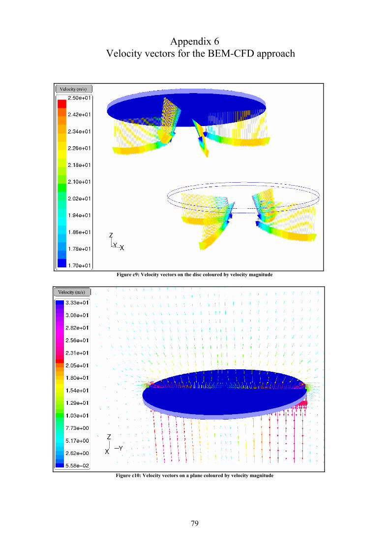
Appendix 6 Velocity vectors for the BEM-CFD approach

Figure c9: Velocity vectors on the disc coloured by velocity magnitude

Figure c10: Velocity vectors on a plane coloured by velocity magnitude

80

References

Rotary-wing aerodynamics Vol 1: basic theories of rotor aerodynamics Vol 2 : performance prediction of helicopter

W.Z.Stepniewsky and C.N.Keys Dover publications, Inc., New York. Exact actuator disk solutions for non-uniform heavy loading and slipstream contraction J.T.Conway (J. Fluid Mech. (1998) Vol. 365, pp 235-267) Principles of Helicopter Aerodynamics J. Gordon Leishman Cambridge Aerospace Series Simulating Dynamical Behaviour of Wind Power Structures Anders Ahlström Licentiate Thesis, Stockholm, 2002 Royal Institute of Technology - Department of Mechanics AERFORCE: Subroutine Package for unsteady Blade-Element/Momentum Calculations. Anders Björck Flygtekniska Forsoksanstalten The Aeronautical Research Institute of Sweden Actuator disc modelling for helicopter rotor Frederic Le Chuiton DLR – Institute of Aerodynamics and Flow technology Braunschweigh, Germany Airfoil Characteristics for Wind Turbines Christian Bak, Peter Fuglsang, Niels N. Sørensen, Helge Aagaard Madsen Risø National Laboratory (March 1999) Wen Zhong Shen, Jens Nørkær Sørensen Technical University of Denmark AIAA publications (V22 Osprey) American Institute of Aeronautic and Astronautic