Chapitre 1 : Emergence du chaos

Objectifs du chapitre

> Introduire la notion de chaos

> Illustrer quelques systèmes chaotiques

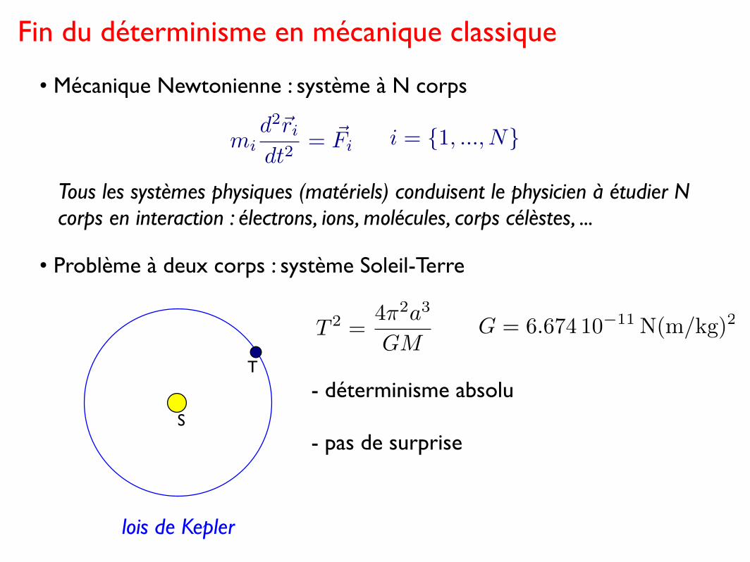
Fin du déterminisme en mécanique classique

• Mécanique Newtonienne : système à N corps

• Problème à deux corps : système Soleil-Terre

lois de Kepler

mid2⌃ri

dt2= ⌃Fi

S

T

T 2 =4�2a3

GM

i = {1, ..., N}

Tous les systèmes physiques (matériels) conduisent le physicien à étudier N corps en interaction : électrons, ions, molécules, corps célèstes, ...

G = 6.674 10�11 N(m/kg)2

- déterminisme absolu

- pas de surprise

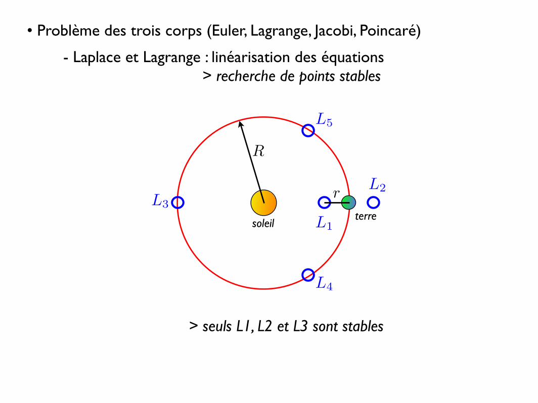
• Problème des trois corps (Euler, Lagrange, Jacobi, Poincaré)

- Laplace et Lagrange : linéarisation des équations > recherche de points stables

soleilterreL1

L2L3

L4

L5

R

r

> seuls L1, L2 et L3 sont stables

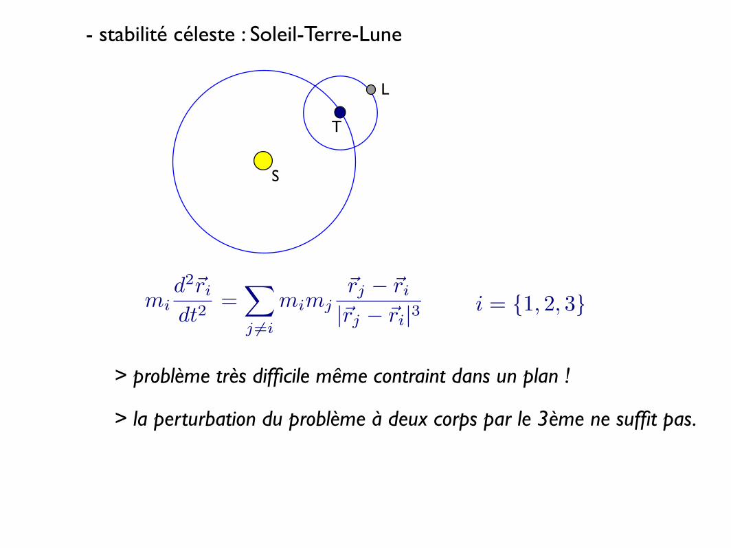
- stabilité céleste : Soleil-Terre-Lune

> problème très difficile même contraint dans un plan !

mid2⇧ri

dt2=

�

j �=i

mimj⇧rj � ⇧ri

|⇧rj � ⇧ri|3 i = {1, 2, 3}

S

T

L

> la perturbation du problème à deux corps par le 3ème ne suffit pas.

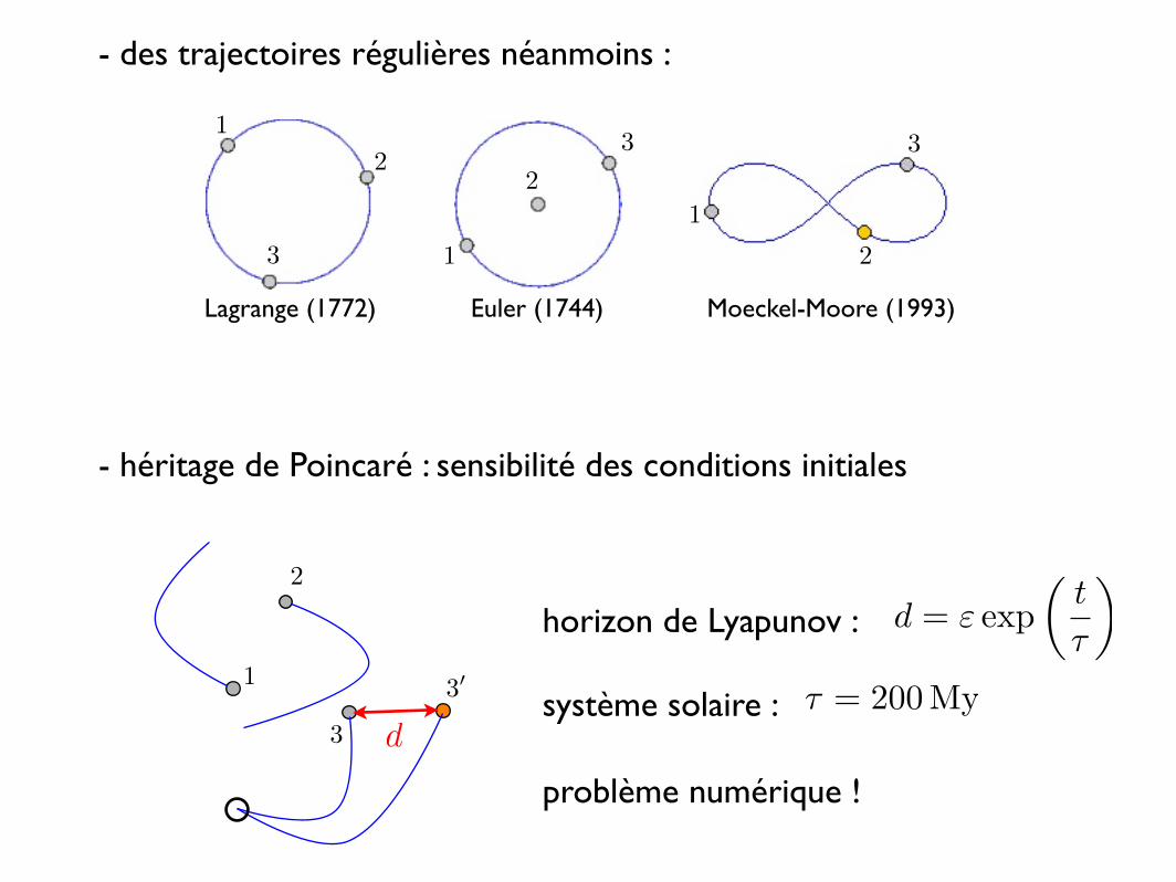
- des trajectoires régulières néanmoins :

Euler (1744)Lagrange (1772) Moeckel-Moore (1993)

- héritage de Poincaré : sensibilité des conditions initiales

système solaire :

horizon de Lyapunov : d = ⇥ exp�

t

�

⇥

� = 200 Myd

problème numérique !

1

2

3

30

3

2

1

3

2

1

1

2

3

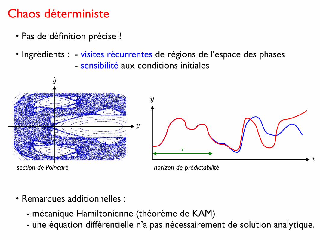
Chaos déterministe

• Remarques additionnelles :

• Ingrédients : - visites récurrentes de régions de l’espace des phases- sensibilité aux conditions initiales

t

y

�

• Pas de définition précise !

y

y

section de Poincaré horizon de prédictabilité

- mécanique Hamiltonienne (théorème de KAM)- une équation différentielle n’a pas nécessairement de solution analytique.

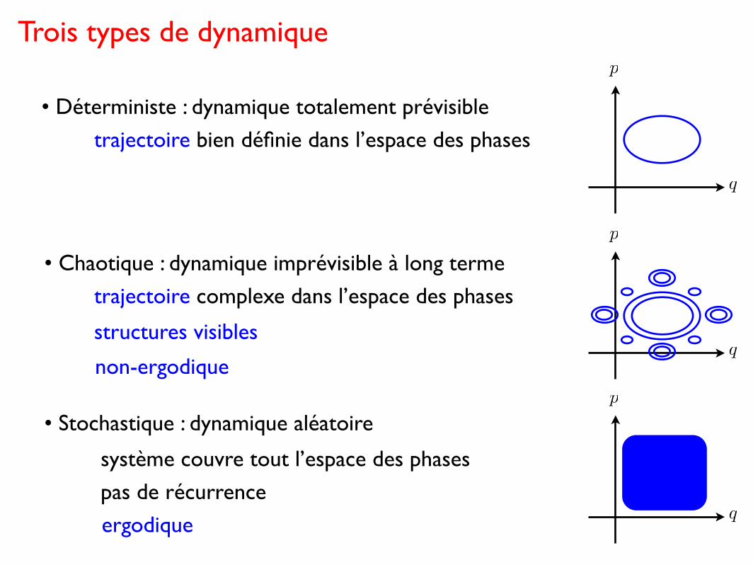
Trois types de dynamique

• Déterministe : dynamique totalement prévisible

• Chaotique : dynamique imprévisible à long terme

• Stochastique : dynamique aléatoire

trajectoire bien définie dans l’espace des phases

trajectoire complexe dans l’espace des phases

structures visibles

système couvre tout l’espace des phases

p

q

p

q

p

q

pas de récurrence

ergodique

non-ergodique

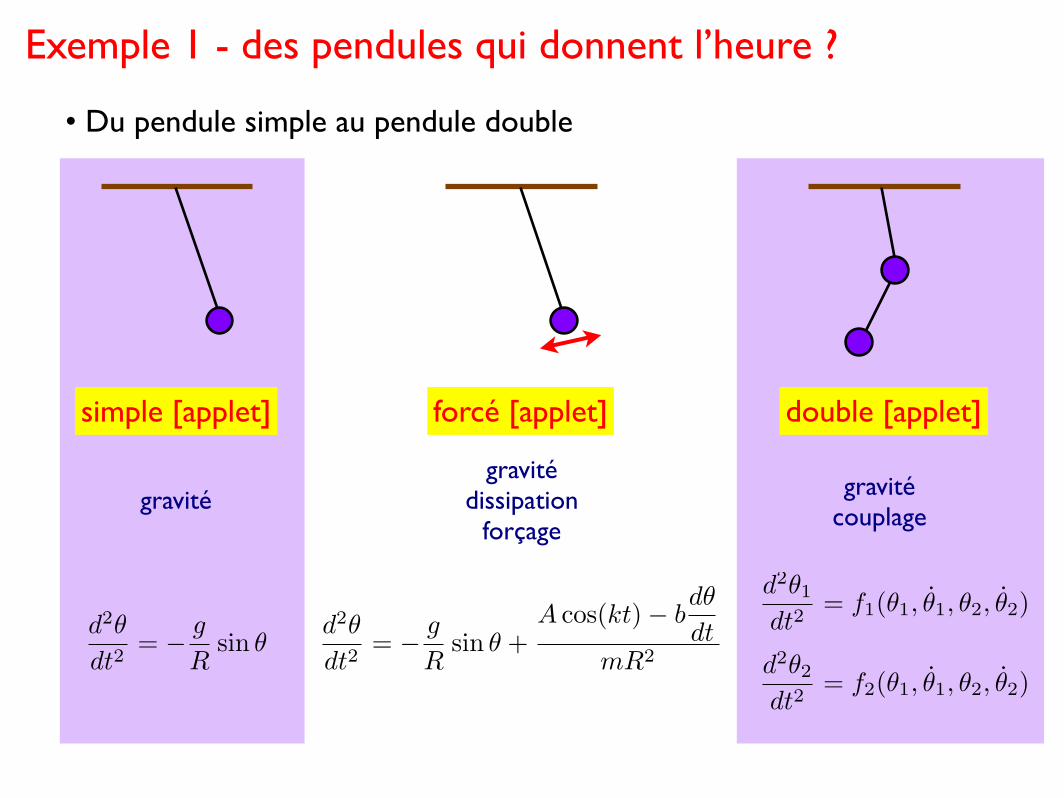
Exemple 1 - des pendules qui donnent l’heure ?

• Du pendule simple au pendule double

simple [applet] forcé [applet] double [applet]

d2�

dt2= � g

Rsin � +

A cos(kt)� bd�

dtmR2

d2�

dt2= � g

Rsin �

gravitégravité

dissipationforçage

gravitécouplage

d2�1

dt2= f1(�1, �1, �2, �2)

d2�2

dt2= f2(�1, �1, �2, �2)

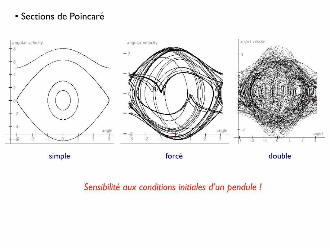
• Sections de Poincaré

simple forcé double

Sensibilité aux conditions initiales d’un pendule !

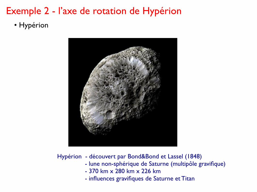
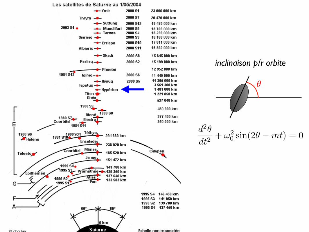
Exemple 2 - l’axe de rotation de Hypérion

Hypérion - découvert par Bond&Bond et Lassel (1848) - lune non-sphérique de Saturne (multipôle gravifique) - 370 km x 280 km x 226 km - influences gravifiques de Saturne et Titan

• Hypérion

✓

d2✓

dt2+ !2

0 sin(2✓ �mt) = 0

inclinaison p/r orbite

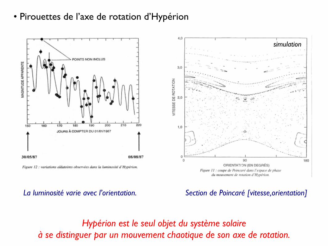
• Pirouettes de l’axe de rotation d’Hypérion

simulation

La luminosité varie avec l’orientation. Section de Poincaré [vitesse,orientation]

Hypérion est le seul objet du système solaire à se distinguer par un mouvement chaotique de son axe de rotation.

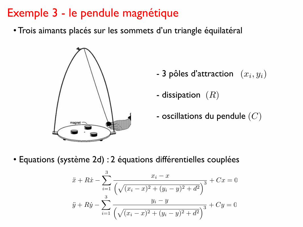
Exemple 3 - le pendule magnétique• Trois aimants placés sur les sommets d’un triangle équilatéral

• Equations (système 2d) : 2 équations différentielles couplées

x + Rx�3⇤

i=1

xi � x�⌅

(xi � x)2 + (yi � y)2 + d2⇥3 + Cx = 0

y + Ry �3⇤

i=1

yi � y�⌅

(xi � x)2 + (yi � y)2 + d2⇥3 + Cy = 0

- 3 pôles d’attraction

- dissipation

- oscillations du pendule

(xi, yi)

(R)

(C)

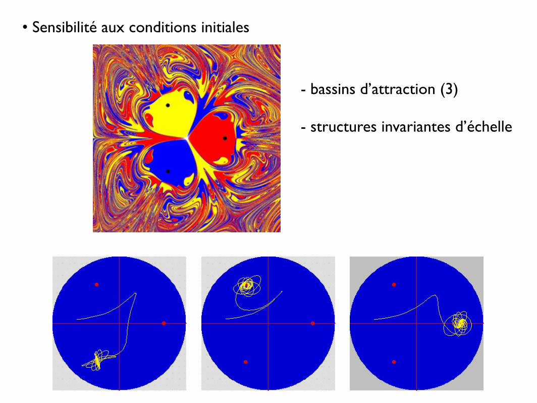
• Sensibilité aux conditions initiales

- bassins d’attraction (3)

- structures invariantes d’échelle

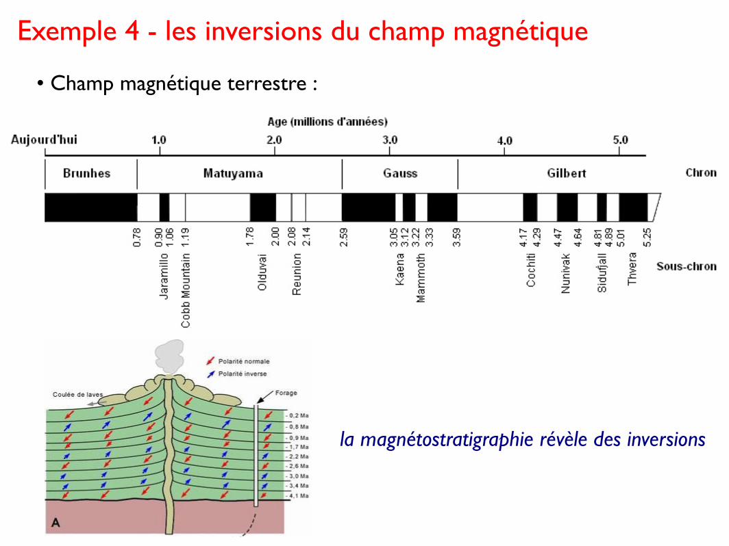
Exemple 4 - les inversions du champ magnétique

• Champ magnétique terrestre :

la magnétostratigraphie révèle des inversions

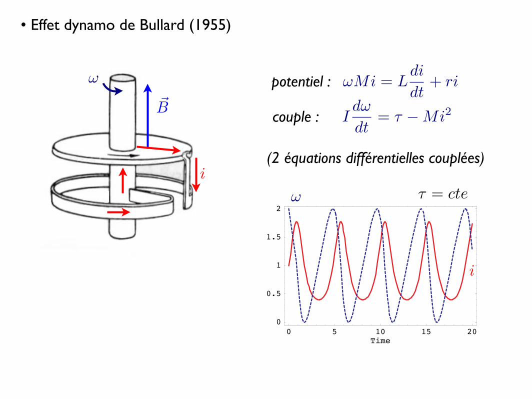
• Effet dynamo de Bullard (1955)

�

⇥B

potentiel :

couple :

i

!Mi = Ldi

dt+ ri

Id!

dt= ⌧ �Mi2

(2 équations différentielles couplées) 2

0 5 10 15 20Time

0

0.5

1

1.5

2

Figure 2: Numerical integration of Bullard’s single disk sys-tem, plotted in arbitrary units. Pictured as a solid red curve isthe current with time, and as a dashed blue curve is the angu-lar velocity with time. The initial parameters are !0 = 2 andI = 1, while the constants are M = L = I = ⌧

ext

= R = 1,for simplicity. The system is approximately periodic, but doesdisplay nonuniform current and angular velocity, despite aconstant external applied torque.

angular velocity of the disk, I is the current runningthrough the system, I is the rotational inertia of thedisk, and ⌧

ext

is the externally applied torque drivingthe disk. We cannot analytically solve this system, butwe can study some special cases, and it can be read-ily integrated numerically. Steady state solutions to thesystem must have I ⌘ I0 and ! ⌘ !0, or both the currentand angular velocity constant. Thus, considering steadystates, our system of equations simplifies to

!0MI0 = 0 + RI0,

0 = ⌧ext

�M (I0)2 . (2)

So, we now have a simple algebraic system, and we find!0 = R/M and I0 =

p⌧ext

/M .

Next, we numerically integrate the system to observe howa more general solution behaves. The results of this inte-gration, shown in figure 2, display a general trend of thesystem, that the current never changes sign, and so themagnetic field never reverses.

To validate this assertion, we look at the phase-spaceplot shown in figure 3. We find a closed orbit, as wewould expect for a periodic solution. Further, we noticethat there exists a separatrix between the positive andnegative current regions, explaining why the currentnever changes signs. Unfortunately, this means that theBullard model can never explain the magnetic reversalof the Sun.

-2 -1 0 1 2Current

-2

-1

0

1

2

AngularVelocity

Figure 3: The same numerical integration of Bullard’s singledisk system done in figure 2, viewed in phase-space with ar-bitrary units. The vector field shown represents the initialvalues of the time derivatives of angular velocity and current,and the curve is the actual orbit taken by the system in figure3. Note that there is a clear separatrix between the positiveand negative current regimes, which prevents the current fromchanging signs.

�1�2

i2

i1Disk 1

Disk 2

Figure 4: Rikitake’s system of coupled disks. Each disk has aseparate (and possibly unequal) rotational inertia I, appliedexternal torque ⌧

ext

, mutual inductance M , and resistanceR. They are each rotating at angular velocity !, and havethe current I. The quantities that apply to the first disk aredenoted with a subscript “1”, and the quantities pertinent tothe second disk have a subscript “2” [5].

III. RIKITAKE’S DYNAMO

Rikitake’s system, pictured in figure 4, consists of twoBullard dynamos coupled together such that the wire ofone disk is wrapped around the other. The equations ofmotion are[5]

!

i

⌧ = cte

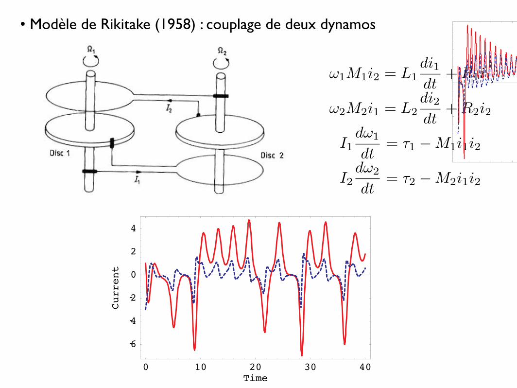
• Modèle de Rikitake (1958) : couplage de deux dynamos

!1M1i2 = L1di1dt

+R1i1

!2M2i1 = L2di2dt

+R2i2

I1d!1

dt= ⌧1 �M1i1i2

I2d!2

dt= ⌧2 �M2i1i2

3

!1M1I2 = L1dI1

dt+ R1I1,

!2M2I1 = L2dI2

dt+ R2I2,

I1d!1

dt= ⌧1 �M1I1I2,

I2d!2

dt= ⌧2 �M2I1I2. (3)

Similar to the equations of motion for the Bullard system,these equations are also nonlinear and cannot be solvedexactly. Thus, we resort to numerical methods.

We integrate the Rikitake equations to obtain the solu-tions shown in figure 5, which exhibits current reversals.Besides just current reversal, the phase-space plots in fig-ure 6 show that the orbits do not close, and so the systemis chaotic.

The sun is thought to exhibit such chaotic reversals ofmagnetic polarity[6], so the Rikitake system is much morelikely to be a good candidate for a toy model for the sunthan the Bullard dynamo. Unfortunately, two coupleddisk dynamos do not resemble the spherical geometryof the sun, and frictional forces, as we will see in thenext section, tend to decrease the chaotic behavior of thesystem, presenting another problem.

IV. HIDE’S MODIFICATION

In 1995, Raymond Hide found a disturbing problem withthe Rikitake dynamo, which dramatically impacted itsfeasibility as a physical model[7]. In an e↵ort to make

0 10 20 30 40Time

-6

-4

-2

0

2

4

Current

Figure 5: Numerical integration of the Rikitake System, plot-ted with arbitrary units. The solid red curve is I1, and thedashed blue curve is I2. The system starts with the initialconditions I1(0) = 1, I2(0) = �3, !1(0) = 4, and !2(0) = �2.Note that as in the Bullard integration, all the constants wereset to unity for simplicity, and so the units are arbitrary.

-6 -4 -2 0 2 4 6Current

-2

0

2

4

6

8

AngularVelocity

Figure 6: Phase-space plot of the first disk in the numericalintegration done in figure 5, plotted with arbitrary units. Thesolid red curve is the first disk system, and the dashed bluecurve is the second. The arbitrary time runs from t = 0 tot = 600.

0 50 100 150 200Time

-4

-2

0

2

Current

Figure 7: Numerical integration of the Hide system, plotted inarbitrary units. The solid red curve is the current in the firstdisk, and the dashed blue curve is the current in the second.The initial parameters were the same as in figure 5, and thedamping terms were k1 = k2 = 0.06. The system does exhibitchaotic reversals initially, but oscillations are quickly dampedout.

the system more physical, Hide included damping termsin the two Rikitake torque equations. Hide’s equationswere

!1M1I2 = L1dI1

dt+ R1I1,

!2M2I1 = L2dI2

dt+ R2I2,

I1d!1

dt= ⌧1 �M1I1I2 � k1!1,

I2d!2

dt= ⌧2 �M2I1I2 � k2!2, (4)

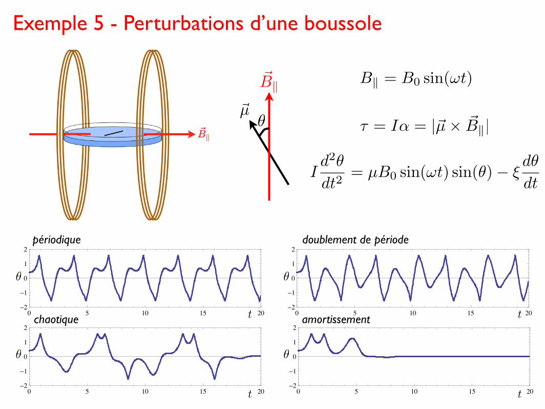
Exemple 5 - Perturbations d’une boussole

~Bk

~µ✓

Bk = B0 sin(!t)

� = I� = |�µ� �B�|

Id2✓

dt2= µB0 sin(!t) sin(✓)� ⇠

d✓

dt

0 5 10 15 20-2

-1

0

1

2

0 5 10 15 20-2

-1

0

1

2

0 5 10 15 20-2

-1

0

1

2

0 5 10 15 20-2

-1

0

1

2

✓

✓✓

✓

t

t

t

t

périodique doublement de période

chaotique amortissement