Cliquez pour modifier le style du titre

Cliquez pour modifier le style des sous-titres du masque

1

Variational & ensemble data assimilation

at Météo-France

L. Berre, G. Desroziers, H. Varella, L. Raynaud, C. Loo

Météo-France (CNRM/GAME)

Plan of the talk

� Numerical Weather Prediction and Data Assimilation

� Ensembles and Error Covariances

� Preconditioning methods

1. Numerical Weather Prediction

and Data Assimilation

The two main ingredients of weather forecasting

What will be the weather tomorrow ?

Bjerknes (1904) :

In order to do a good forecast, we need to :

� know the atmospheric evolution laws(~ modeling) ;

� know the atmospheric state at initial time (~ data assimilation).

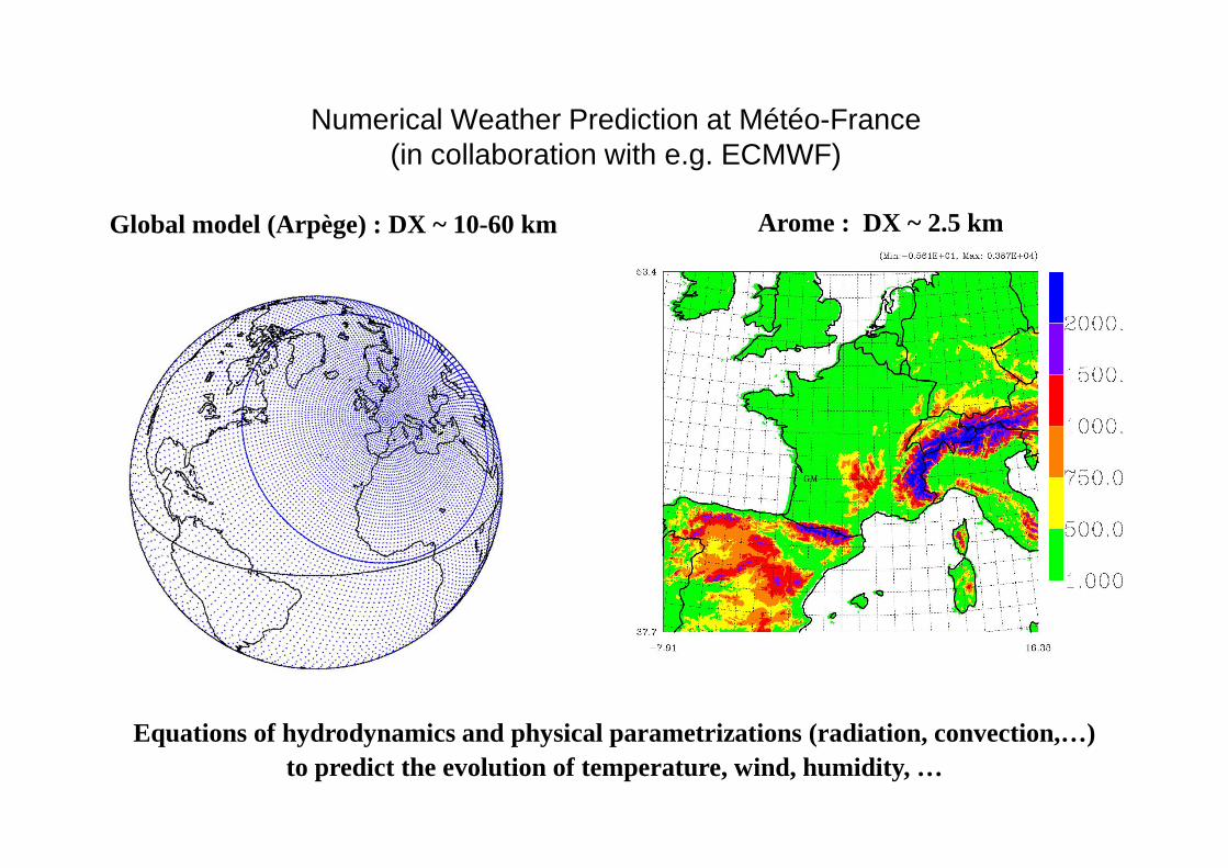
Global model (Arpège) : DX ~ 10-60 km

Numerical Weather Prediction at Météo-France(in collaboration with e.g. ECMWF)

Arome : DX ~ 2.5 km

Equations of hydrodynamics and physical parametrizations (radiation, convection,…) to predict the evolution of temperature, wind, humidity, …

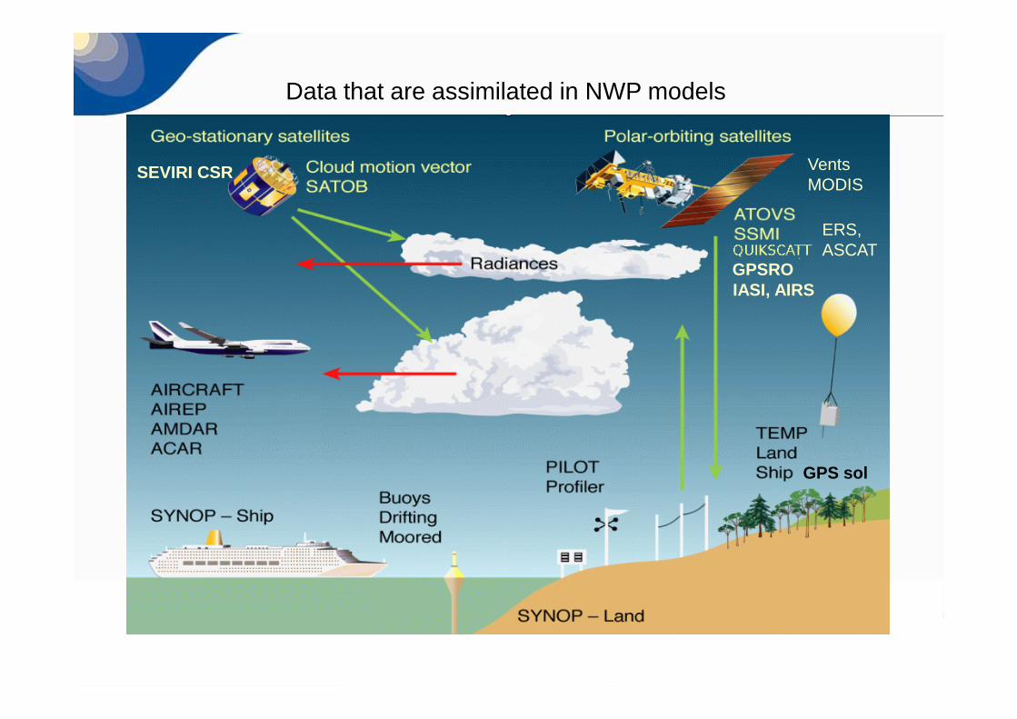
GPSRO

GPS sol

IASI, AIRS

SEVIRI CSR

Data that are assimilated in NWP models

ERS, ASCAT

Vents MODIS

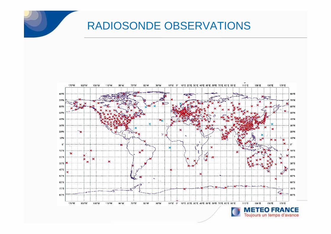
RADIOSONDE OBSERVATIONS

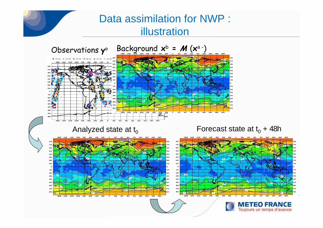
Data assimilation for NWP :illustration

Observations yo

Analyzed state at t0 Forecast state at t0 + 48h

Background xb = M (xa -)

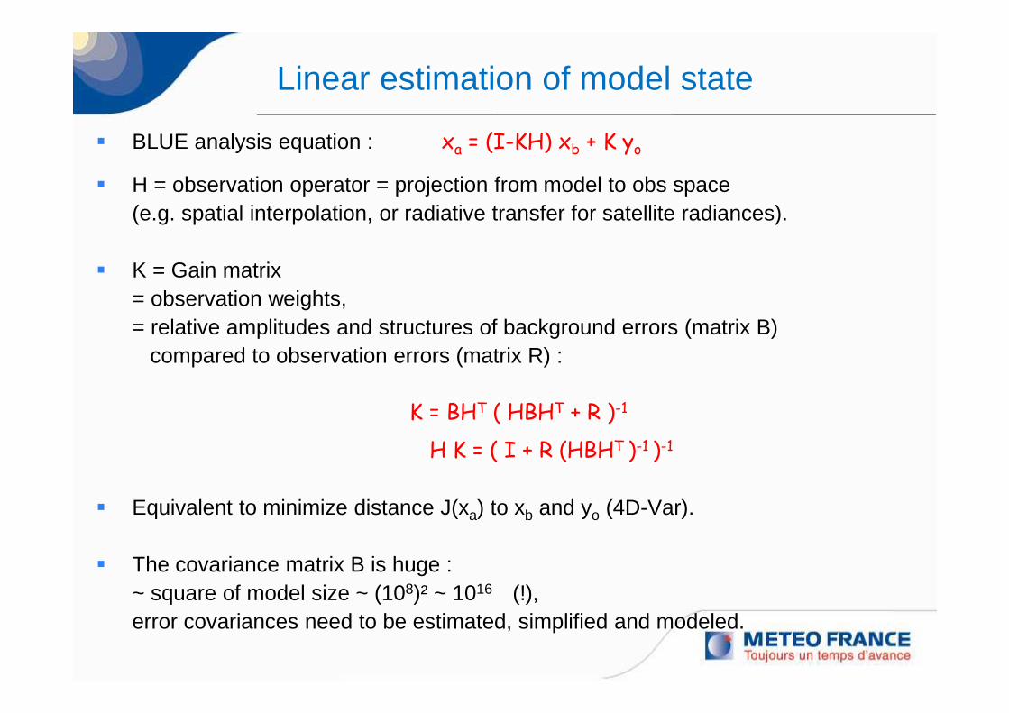
Linear estimation of model state

� BLUE analysis equation : xa = (I-KH) xb + K yo

� H = observation operator = projection from model to obs space(e.g. spatial interpolation, or radiative transfer for satellite radiances).

� K = Gain matrix = observation weights,= relative amplitudes and structures of background errors (matrix B)

compared to observation errors (matrix R) :

K = BHT ( HBHT + R )-1

H K = ( I + R (HBHT )-1 )-1

� Equivalent to minimize distance J(xa) to xb and yo (4D-Var).

� The covariance matrix B is huge :~ square of model size ~ (108)² ~ 1016 (!), error covariances need to be estimated, simplified and modeled.

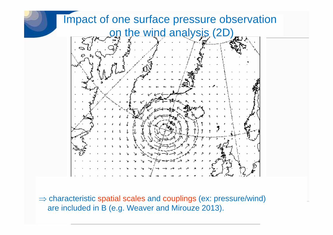
⇒ characteristic spatial scales and couplings (ex: pressure/wind)are included in B (e.g. Weaver and Mirouze 2013).

Impact of one surface pressure observationon the wind analysis (2D)

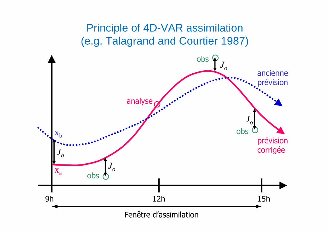
Principle of 4D-VAR assimilation(e.g. Talagrand and Courtier 1987)

9h 12h 15h

Fenêtre d’assimilation

Jb

Jo

Jo

Jo

obs

obs

obs

analyse

xa

xbprévisioncorrigée

ancienneprévision

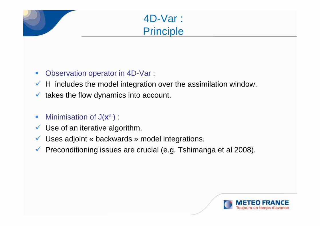
4D-Var :Principle

� Observation operator in 4D-Var :� H includes the model integration over the assimilation window.� takes the flow dynamics into account.

� Minimisation of J(xa ) :� Use of an iterative algorithm.� Uses adjoint « backwards » model integrations.� Preconditioning issues are crucial (e.g. Tshimanga et al 2008).

2. Ensemble Data Assimilation

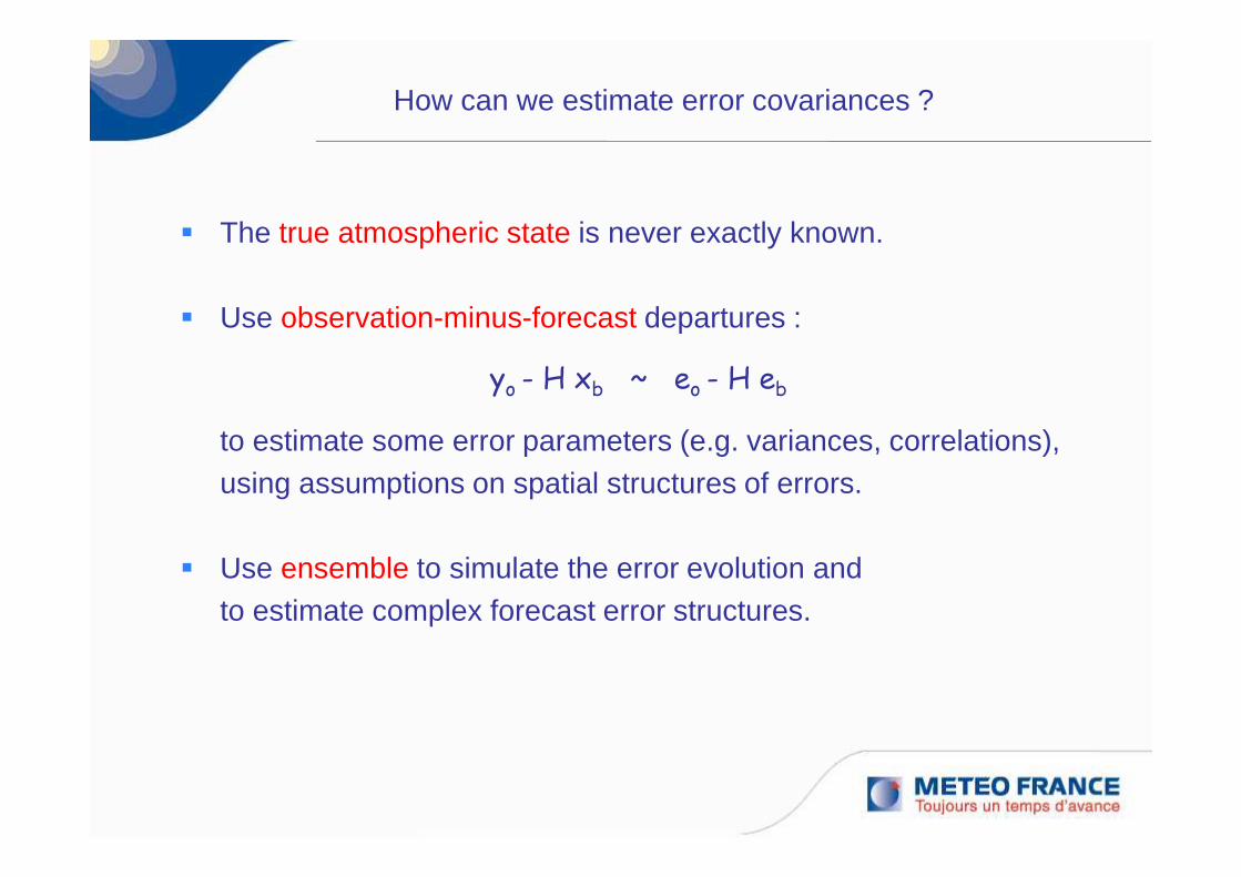
How can we estimate error covariances ?

� The true atmospheric state is never exactly known.

� Use observation-minus-forecast departures :

yo - H xb ~ eo - H eb

to estimate some error parameters (e.g. variances, correlations),using assumptions on spatial structures of errors.

� Use ensemble to simulate the error evolution and to estimate complex forecast error structures.

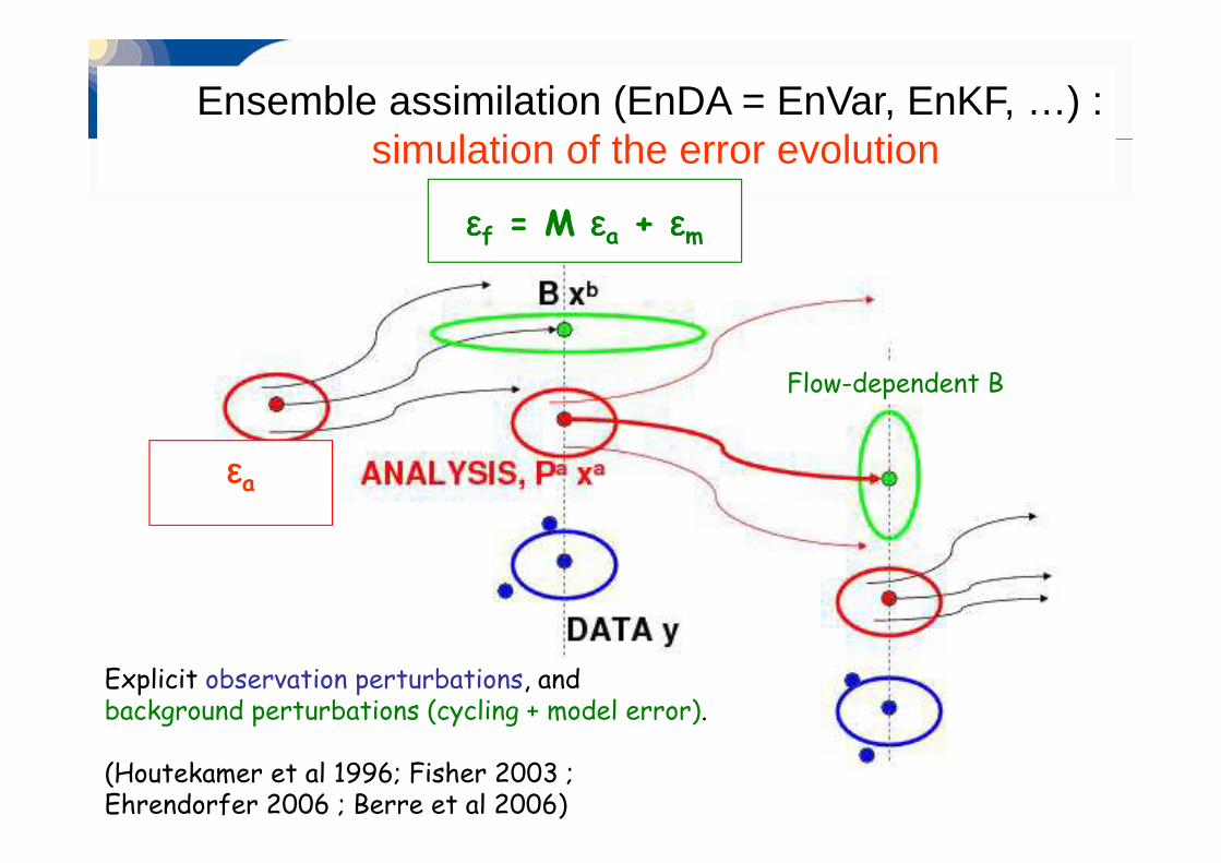
Explicit observation perturbations, andbackground perturbations (cycling + model error).

(Houtekamer et al 1996; Fisher 2003 ;Ehrendorfer 2006 ; Berre et al 2006)

Ensemble assimilation (EnDA = EnVar, EnKF, …) :simulation of the error evolution

Flow-dependent B

εεεεf = M εεεεa + εεεεm

εεεεa

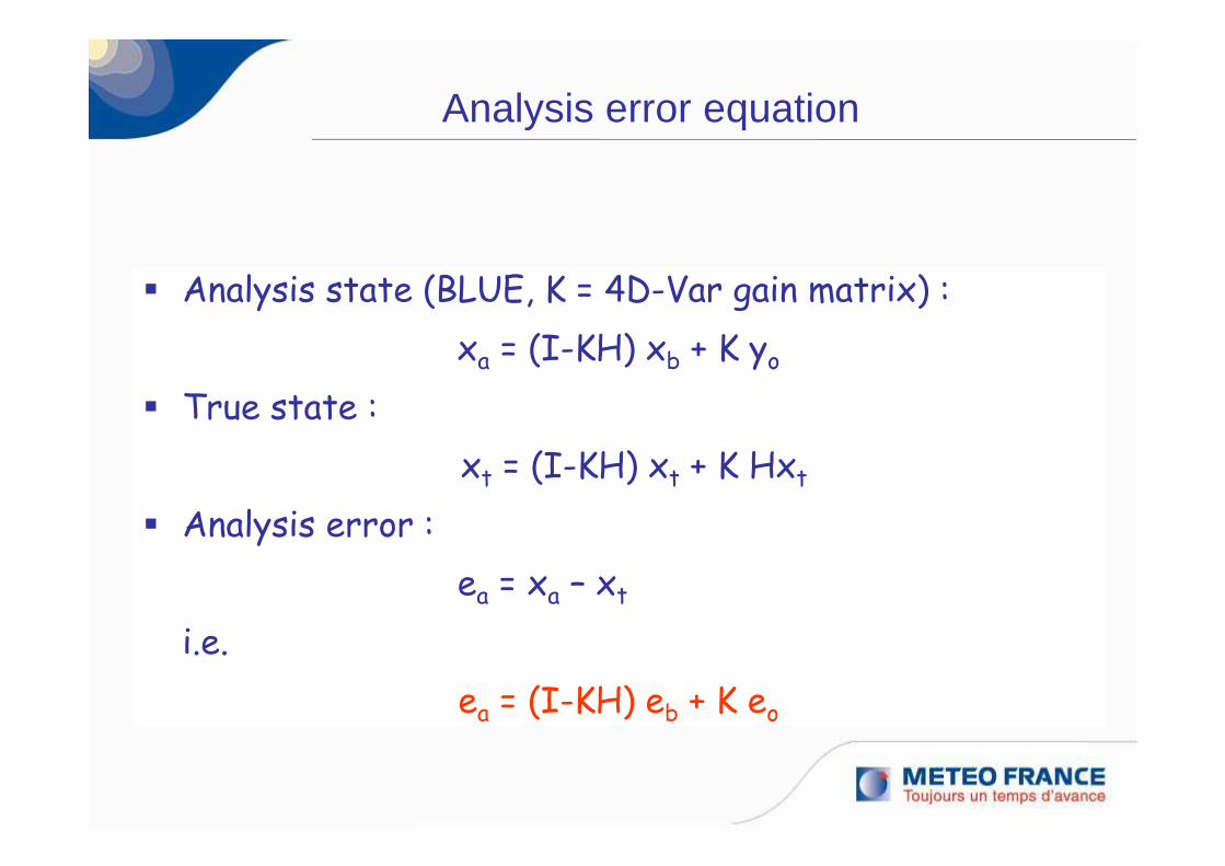
Analysis error equation

� Analysis state (BLUE, K = 4D-Var gain matrix) :

xa = (I-KH) xb + K yo

� True state :

xt = (I-KH) xt + K Hxt

� Analysis error :

ea = xa – xt

i.e.

ea = (I-KH) eb + K eo

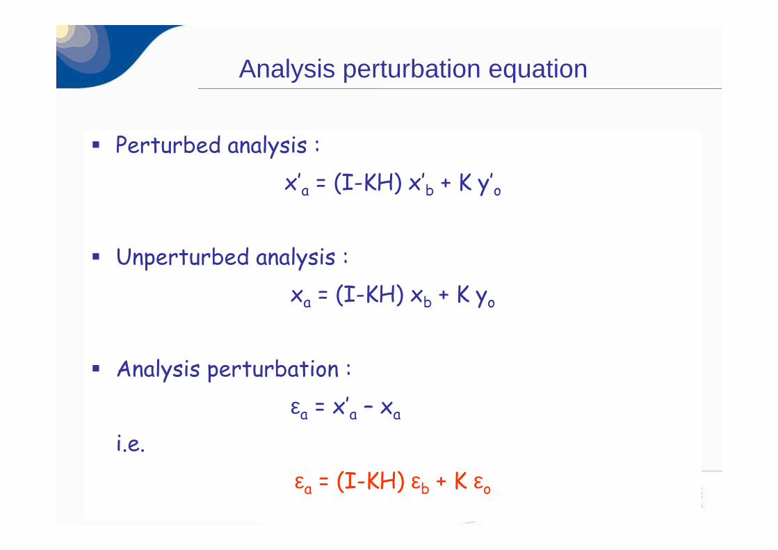
Analysis perturbation equation

� Perturbed analysis :

x’a = (I-KH) x’b + K y’o

� Unperturbed analysis :

xa = (I-KH) xb + K yo

� Analysis perturbation :

εa = x’a – xa

i.e.

εa = (I-KH) εb + K εo

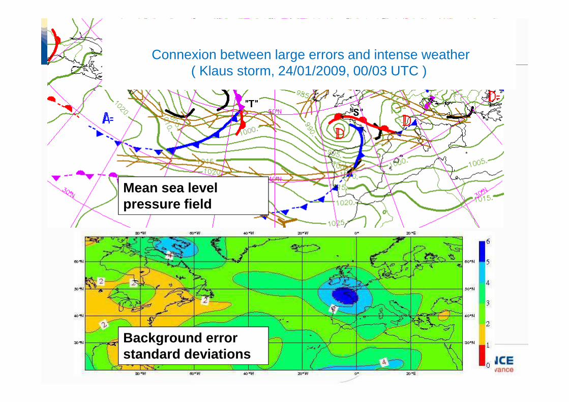
Background error standard deviations

Connexion between large errors and intense weather ( Klaus storm, 24/01/2009, 00/03 UTC )

Mean sea level pressure field

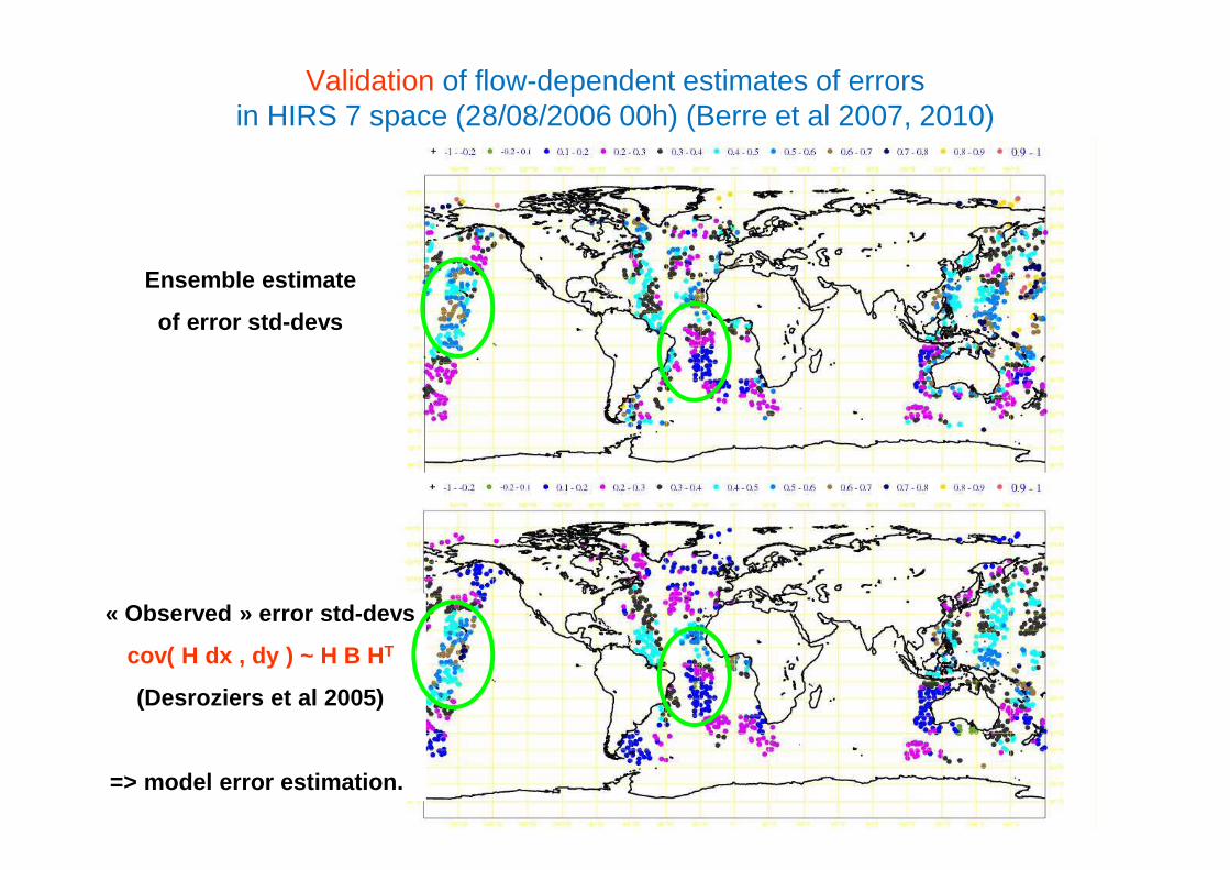
Validation of flow-dependent estimates of errors in HIRS 7 space (28/08/2006 00h) (Berre et al 2007, 2010)

Ensemble estimate

of error std-devs

« Observed » error std-devs

cov( H dx , dy ) ~ H B H T

(Desroziers et al 2005)

=> model error estimation.

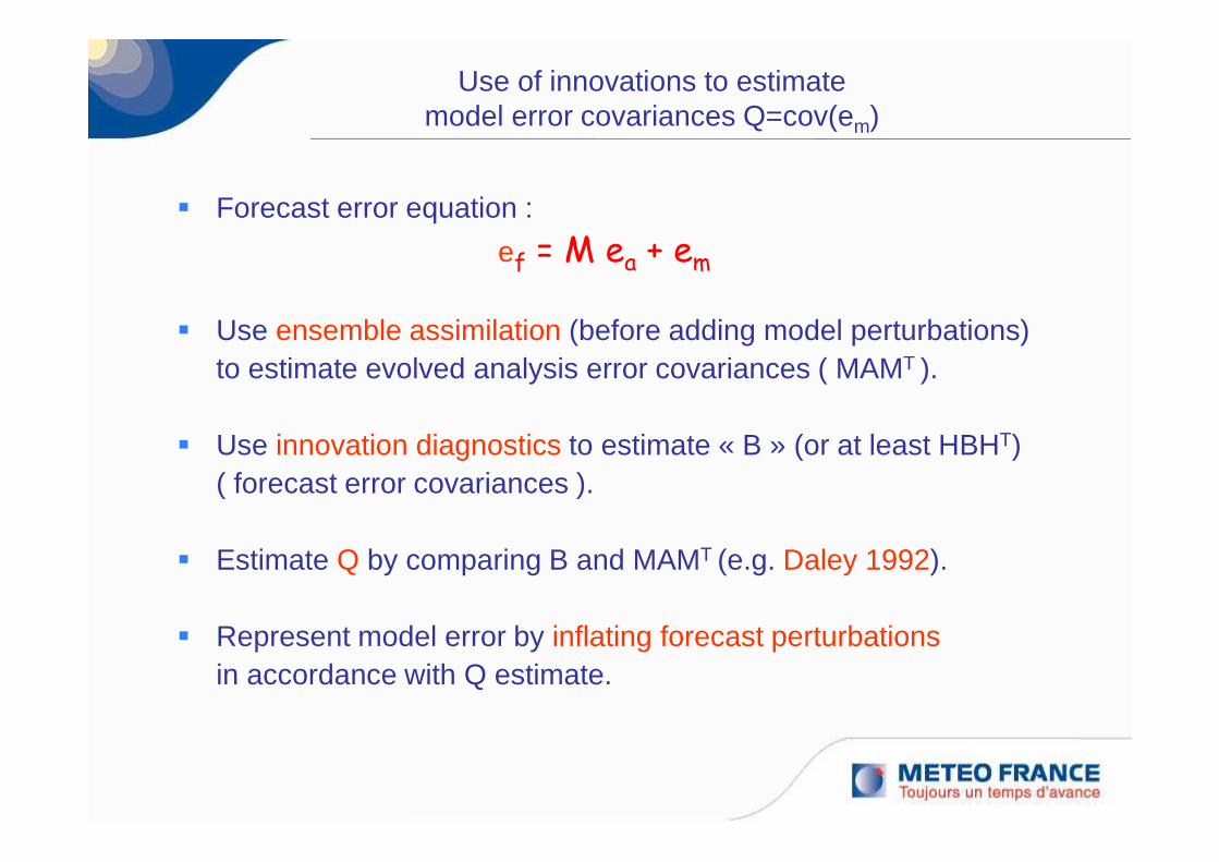
Use of innovations to estimatemodel error covariances Q=cov(em)

� Forecast error equation :

ef = M ea + em

� Use ensemble assimilation (before adding model perturbations)to estimate evolved analysis error covariances ( MAMT ).

� Use innovation diagnostics to estimate « B » (or at least HBHT)( forecast error covariances ).

� Estimate Q by comparing B and MAMT (e.g. Daley 1992).

� Represent model error by inflating forecast perturbationsin accordance with Q estimate.

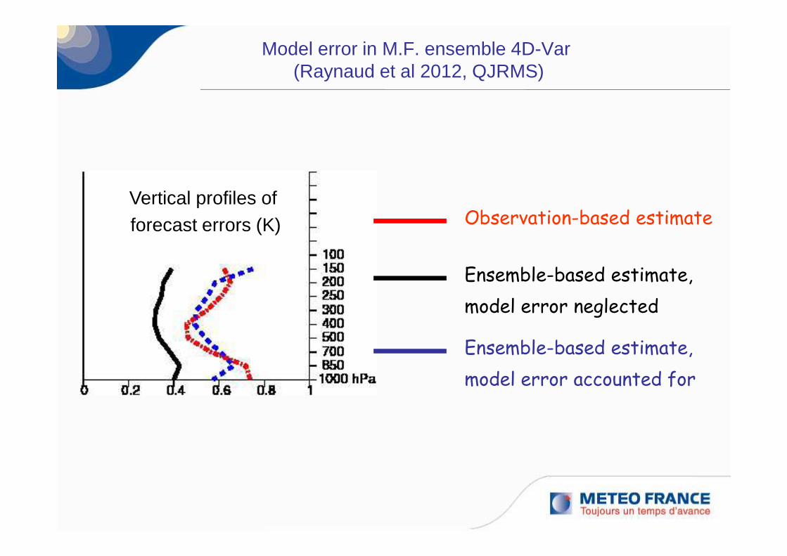
Model error in M.F. ensemble 4D-Var(Raynaud et al 2012, QJRMS)

Ensemble-based estimate,

model error neglected

Ensemble-based estimate,

model error accounted for

Observation-based estimateVertical profiles of forecast errors (K)

Wavelet modelling of flow-dependent correlations

� Spectral block-diagonal approach :

homogeneous correlations from EnDA.

� Wavelet block-diagonal approach :

heterogeneous correlations from EnDA.

⇒ Ecmwf : static heterogeneous correlations (Fisher 2003),

Météo-France : flow-dependent correlations (Varella et al 2011, 2013).

⇒ Implicit use of local spatial averages :

spatial filtering of sampling noise (Berre and Desroziers 2010).

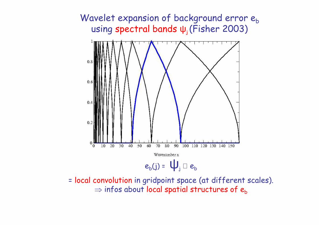
Wavelet expansion of background error eb

using spectral bands ψj (Fisher 2003)

eb(j) = ψj ⊗ eb

= local convolution in gridpoint space (at different scales).⇒ infos about local spatial structures of eb

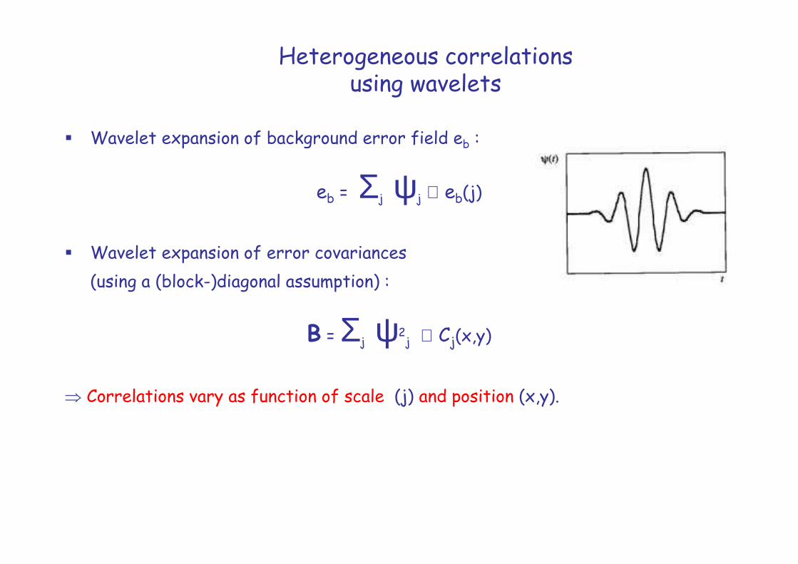
Heterogeneous correlations using wavelets

� Wavelet expansion of background error field eb :

eb = Σj ψj ⊗ eb(j)

� Wavelet expansion of error covariances

(using a (block-)diagonal assumption) :

B = Σj ψ2j ⊗ Cj(x,y)

⇒ Correlations vary as function of scale (j) and position (x,y).

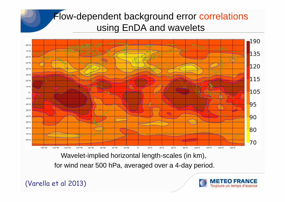
Flow-dependent background error correlationsusing EnDA and wavelets

Wavelet-implied horizontal length-scales (in km), for wind near 500 hPa, averaged over a 4-day period.

(Varella et al 2013)

3. Preconditioning issues

and conclusions

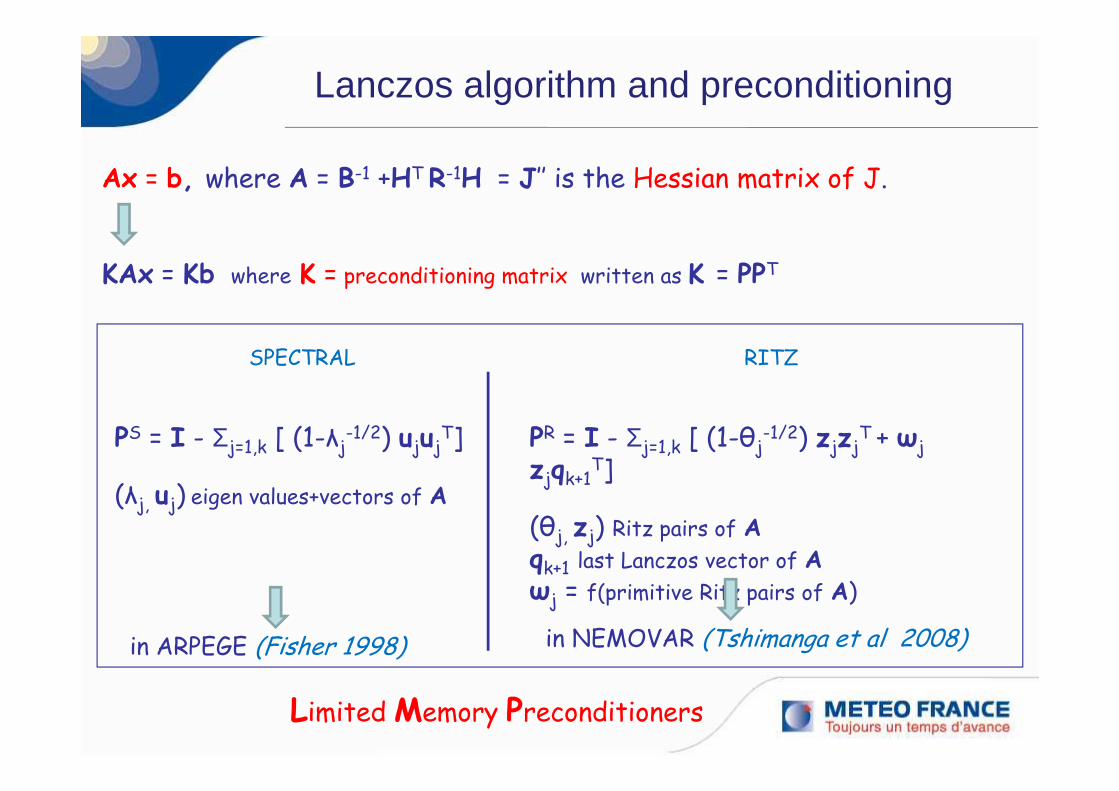
Lanczos algorithm and preconditioning

Ax = b, where A = B-1 +HT R-1H = J’’ is the Hessian matrix of J.

KAx = Kb where K = preconditioning matrix written as K = PPT

SPECTRAL

PS = I - Σj=1,k [ (1-λj-1/2) ujuj

T]

(λj, uj) eigen values+vectors of A

RITZ

PR = I - Σj=1,k [ (1-θj-1/2) zjzj

T + ωj

zjqk+1T]

(θj, zj) Ritz pairs of Aqk+1 last Lanczos vector of Aωj = f(primitive Ritz pairs of A)

in ARPEGE (Fisher 1998) in NEMOVAR (Tshimanga et al 2008)

Limited Memory Preconditioners

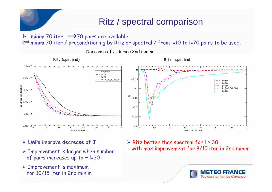
Ritz / spectral comparison

1st minim 70 iter 70 pairs are available 2nd minim 70 iter / preconditioning by Ritz or spectral / from l=10 to l=70 pairs to be used.

Ritz (spectral) Ritz - spectral

Decrease of J during 2nd minim

� LMPs improve decrease of J

� Improvement is larger when numberof pairs increases up to ~ l=30

� Improvement is maximum for 10/15 iter in 2nd minim

� Ritz better than spectral for l ≥ 30 with max improvement for 8/10 iter in 2nd minim

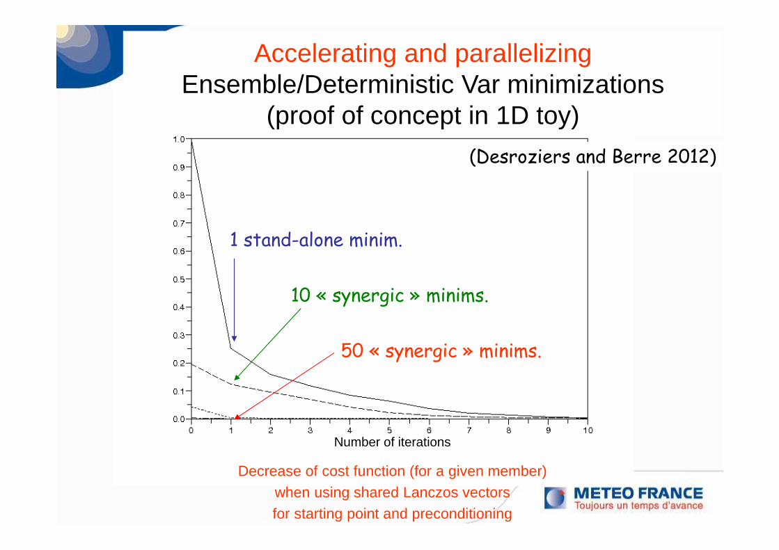
Accelerating and parallelizingEnsemble/Deterministic Var minimizations

(proof of concept in 1D toy)

Decrease of cost function (for a given member)when using shared Lanczos vectorsfor starting point and preconditioning

1 stand-alone minim.

10 « synergic » minims.

50 « synergic » minims.

Number of iterations

(Desroziers and Berre 2012)

Conclusions

� Data assimilation is vital for weather forecasting (NWP).

� Many issues and methods are transversal in geosciences (see e.g. A. Weaver’s presentation).

� Variational techniques for 4D aspects and flexibility,including preconditioning issues (e.g. Gürol 2013).

� Ensemble methods for error simulation and covariance estimation.

� Observations for validation of error covariances, and for estimation of model errors.

Summary w.r.t. ADTAO

� Flow-dependent error correlations in wavelet space (Varella et al 2012, Fisher 2003).

� Estimation of model error covariances (Raynaud et al 2012, Daget et al 2009).

� Preconditioning of 4D-Var (Tshimanga et al 2008, Desroziers and Berre 2012).

� ADTAO project is a very good framework for transversal research collaborations (e.g. CERFACS).

� The combination of variational and ensemble methodsis a crucial research axis (4DEnVar, AVENUE project).

References

Berre, L. and G. Desroziers, 2010:Filtering of Background Error Variances and Correlationsby Local Spatial Averaging: A Review.Mon. Wea. Rev., 138, 3693-3720.

Desroziers, G. and Berre, L., 2012 : Accelerating and parallelizing minimizations in ensemble and deterministic variational assimilations. QJRMS., 138, 1599–1610.

Varella, H., Berre, L., and Desroziers, G., 2011 :Diagnostic and impact studies of a wavelet formulation of background error correlations in a global model. QJRMS, 137, 1369-1379.

Raynaud, L., L. Berre, and G. Desroziers, 2012 :Accounting for model error in the Meteo-France ensembledata assimilation system. QJRMS, 138, 249-262.

Thank you

for your attention

Applications of EnDA at M.F.

� Flow-dependent background error variances (oper 2008)

(for all variables including humidity and unbalanced variables)

⇒ for obs. quality control and for analysis (minimization).

� Flow-dependent background error correlations experimented

using wavelet filtering properties (Varella et al 2011, 2012).

� Initialisation of M.F. ensemble prediction (PEARP) by EnDA (2009) :

EnDA is now a major component of PEARP.

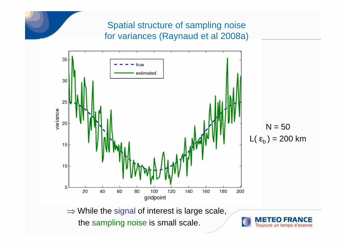
N = 50L( εb ) = 200 km

Spatial structure of sampling noisefor variances (Raynaud et al 2008a)

⇒ While the signal of interest is large scale,the sampling noise is small scale.

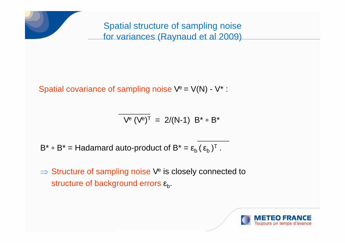
Spatial structure of sampling noisefor variances (Raynaud et al 2009)

Spatial covariance of sampling noise Ve = V(N) - V* :

Ve (Ve)T = 2/(N-1) B* ° B*

B* ° B* = Hadamard auto-product of B* = εb ( εb )T .

⇒ Structure of sampling noise Ve is closely connected to structure of background errors εb.

(Raynaud et al 2008a)

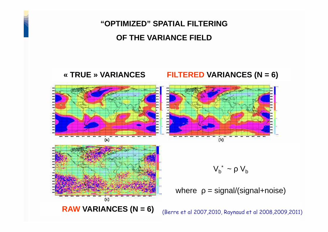
“OPTIMIZED” SPATIAL FILTERING

OF THE VARIANCE FIELD

Vb* ~ ρ Vb

where ρ = signal/(signal+noise)

« TRUE » VARIANCES FILTERED VARIANCES (N = 6)

RAW VARIANCES (N = 6) (Berre et al 2007,2010, Raynaud et al 2008,2009,2011)