Embed Size (px)
Citation preview

Concept design and market screening of a surface fatigue test rig
David Franklin
Master of Science Thesis MMK 2015:114 MKN 159
KTH Industrial Engineering and Management
Machine Design
SE-100 44 STOCKHOLM

iii
Examensarbete MMK 2015:114 MKN 159
Konceptutveckling av en provningsrigg för
ytutmattning
David Franklin
Godkänt
2015-12-11
Examinator
Ulf Sellgren
Handledare
Ulf Sellgren
Uppdragsgivare
Swerea KIMAB
Kontaktperson
Paul Janiak
Sammanfattning Swerea KIMAB är ett av Europas ledande institut för metalliska material med spetskompetens
inom ett flertal områden. KIMAB’s stora fördel är dess öppna interna struktur där alla grupper
och projekt kan dela information och kunskap emellan avdelningarna. Efter att KIMAB flyttade
till nya lokaler uppmärksammades det att den kontaktutmattningsrigg de använt under flera år
började läcka olja och inte längre var optimal för dagens projekt. Eftersom kontaktutmattning
kommer att bli ett viktigare inslag i framtiden då nya legeringar kommer att ersätta befintliga i
exempelvis kugghjul, så skapades detta examensjobb som en grund för hur en ny rigg skall
införskaffas.
Detta examensjobb har som mål att beskriva KIMAB’s behov i en testrigg samt att göra en
marknadsundersökning efter befintliga riggar. Därefter skall ett förslag designas på hur en
testrigg som är anpassas just för KIMAB’s behov skall kunna byggas. Dessa delar skall sedan
ligga som grund för hur KIMAB skall gå vidare i införskaffandet av en ny rigg.
Examensarbetets grund ligger i en litteraturstudie i kontaktutmattningsskador samt
mekanismerna bakom dessa skador och hur de kan påverkas i ett test scenario. Denna kunskap
användes för att undersöka marknaden efter lämpliga riggar som kan uppfylla kraven. Därefter
skapades ett antal koncept som utvärderades under ett möte på KIMAB. Det koncept som valdes
har därefter designats för att vara så användarvänligt och tillförlitligt som möjligt.
När konceptet var färdigställt och prisuppgifter hämtats in på merparten av delarna så har en
kostnads och tidskalkyl utförts för att låta läsaren avgöra vilket alternativ som passar bäst för
KIMAB. Detta val måste baseras på framtida projekt och hur marknaden ser ut för beställning av
kontaktutmattningsprover.
Nyckelord: kontaktutmattning, testrigg, två cylindersrigg, utmattningsrigg, kuggtandssimulering

iv
v
Master of Science Thesis MMK 2015:114 MKN 159
Concept design and market screening of a
surface fatigue test rig
David Franklin
Approved
2015-12-11
Examiner
Ulf Sellgren
Supervisor
Ulf Sellgren
Commissioner
Swerea KIMAB
Contact person
Paul Janiak
Abstract Swerea KIMAB is one of Europe’s leading institutes for metallic materials and excels in many
different areas. KIMAB’s main advantage is its open internal structure where all groups and
projects can share information and knowledge between the sections. After moving to new
premises it was noted that the surface fatigue test rig that had been used had started to leak oil
and was no longer suitable for new projects. Because surface fatigue testing will be of
importance in the future for the development of new alloys that will replace existing alloys in for
example gears, this thesis was created as a foundation for how a new test rig should be acquired.
This thesis goal is to describe KIMAB’s requirements in a test rig and to do a market screening
over existing solutions for test rigs. Thereafter a designed concept shall be developed for
KIMAB’s specific requirements and describe how it should be made. These different parts will
be the ground for how KIMAB should continue in the acquisition of a new rig.
The base of the thesis is a literature study in surface fatigue, its mechanics and how these can be
affected to give the desired test scenario. This information is used to make a market screening for
suitable test rigs that fulfils the requirements. Thereafter a concept generation is made and
evaluated during a meeting on KIMAB. The chosen concept will then be designed to be user
friendly, robust and as reliable as possible.
When the final concept is done and quotes from manufacturers have been gathered for most of
the parts in the design, a time and cost estimation was made to give the reader the chance of
deciding which alternative is the most suitable for KIMAB. This choice has to be made with
regard to future projects and how the market will develop for the ordering of surface fatigue
testing.
Keywords: surface fatigue, test rig, twin disc test rig, gear teeth simulation.

vi

vii
FORWORD
Detta är rätt ställe att tacka för hjälp, råd, samarbete och inspiration för det presenterade
projektet. Detta kapitel, som är valfritt, skrivs med Times New Roman, 12 pt och 6 pt för, med
raka höger- och vänsterkanter. Lämna två tomma rader innan texten.
Förordet avslutas lampligtvis med de båda raderna Namn och Plats, månad och år. Dessa båda
rader skrivs med Times New Roman 12 pt och högerjusterat. Namn–raden skall ha 36 pt före,
medan Plats, månad och år skall ha 12 pt före.
Namn
Plats, månad och år

viii
ix
NOMENCLATUR
Notations
Symbol Beskrivning
E Young´s modulus (Pa)
r Radius (m)
t Thickness (m)
ν Poisson’s ratio
𝑃𝑚 Mean contact pressure (Pa)
𝑃𝑚𝑎𝑥 Maximum contact pressure (Pa)
R’ Effective contact radius (m)
E’ Effective modulus of elasticity (Pa)
𝑅𝑎, 𝑅𝑧, 𝑅𝑘 Surface roughness
σ Tensile stress (Pa)
Abbreviations
CAD Computer Aided Design
FEM Finite Element Method
RCF Rolling Contact Fatigue
CEMC Compact Electromechanical Cylinder
x
TABLE OF CONTENTS
SAMMANFATTNING (SWEDISH) iii
ABSTRACT v
FORWORD vii
NOMENCLATUR ix
TABLE OF NONTENTS x
1 INTRODUCTION 1
1.1 Background 1
1.2 Purpose 1
1.3 Delimitations 2
1.4 Method 2
2 FRAME OF REFERENCE 3
2.1 Failure modes of machine elements 3
2.2 The Mechanics behind failure modes 7
2.3 Market screening of surface fatigue testing machines 15
3 EVALUATION OF MARKET SCREENING 25
4 DESIGN PROCESS 31
4.1 Concept generation 31
4.2 Concept evaluation 36
4.3 Design of parts 37
4.4 Sensors 48
xi
5 FINAL CONCEPT 53
5.1 System description 53
5.2 Additional systems 59
5.3 Cost and time estimations 60
6 DISCUSSION AND CONCLUSSION 63
6.1 Discussion 63
6.2 Conclussions 63
7 FURTHER DEVELOPMENT AND FUTURE WORK 65
7.1 Further development 65
7.2 Future work 65
8 REFERENCES 67
Appendix A: EXTRA INFORMATION 69
Appendix B: MATLAB CODE 72

xii
1
1 INTRODUCTION
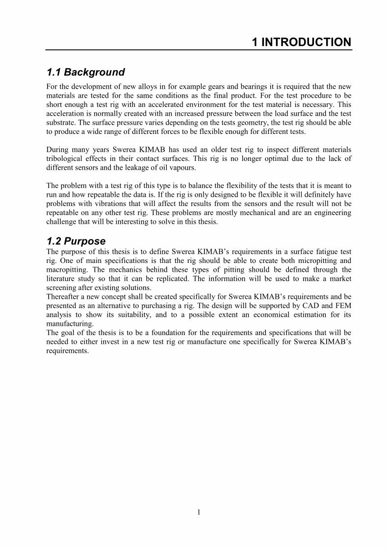
1.1 Background
For the development of new alloys in for example gears and bearings it is required that the new
materials are tested for the same conditions as the final product. For the test procedure to be
short enough a test rig with an accelerated environment for the test material is necessary. This
acceleration is normally created with an increased pressure between the load surface and the test
substrate. The surface pressure varies depending on the tests geometry, the test rig should be able
to produce a wide range of different forces to be flexible enough for different tests.
During many years Swerea KIMAB has used an older test rig to inspect different materials
tribological effects in their contact surfaces. This rig is no longer optimal due to the lack of
different sensors and the leakage of oil vapours.
The problem with a test rig of this type is to balance the flexibility of the tests that it is meant to
run and how repeatable the data is. If the rig is only designed to be flexible it will definitely have
problems with vibrations that will affect the results from the sensors and the result will not be
repeatable on any other test rig. These problems are mostly mechanical and are an engineering
challenge that will be interesting to solve in this thesis.
1.2 Purpose The purpose of this thesis is to define Swerea KIMAB’s requirements in a surface fatigue test
rig. One of main specifications is that the rig should be able to create both micropitting and
macropitting. The mechanics behind these types of pitting should be defined through the
literature study so that it can be replicated. The information will be used to make a market
screening after existing solutions.
Thereafter a new concept shall be created specifically for Swerea KIMAB’s requirements and be
presented as an alternative to purchasing a rig. The design will be supported by CAD and FEM
analysis to show its suitability, and to a possible extent an economical estimation for its
manufacturing.
The goal of the thesis is to be a foundation for the requirements and specifications that will be
needed to either invest in a new test rig or manufacture one specifically for Swerea KIMAB’s
requirements.
2
1.3 Delimitations
The focus of this report will be on the concept that will be generated, if more than one concept is
viable only one will be chosen to be designed to its full extent in CAD. The concepts focus will
be on the geometry and the alignment of test cylinder against load disc, drive line from the test
and to the motor together with different sensors.
- The test rig will be designed after the produced requirements and requests that Swerea
KIMAB has in accordance with the specifications.
- No detail drawings will be made.
- FEM analysis will be made on parts that are in risk of eigenfrequencies.
- No prototype will be made in the thesis.
- The software will only be researched for a better understanding of the parts involved and
an economical estimation.
1.4 Method
In this thesis a literature study will be made on tribology and test rigs as a foundation for the
concept generation and concept evaluation. To begin with, the tribological effects of micropittin
and macropitting has to be defined so that they can be recreated in the test rig. Concepts will be
evaluated with CAD and FEM software and a Pughs matrix which is an evaluation matrix.
3
2 FRAME OF REFERENCE
2.1 Failure modes of machine elements Machine elements can fail in many ways, but most of these failure modes can be avoided by the
right design that takes all possible failures in consideration. Usually when a machine is designed,
every element cannot be designed to withstand everything because of weight or economical
limitations. The limitations on a machine element are the reason for its life expectancy in service.
For example ball bearings have a life expectancy based on a number of revolutions with a
maximum load. In this report we are interested in the failure modes in gears, camshafts and other
rolling contact elements. Failure modes that can be found in bearings are described in Table 2.1.
According to the ISO 15243 failure mode classification for bearing damage, there are six main
failures for rolling elements. Within the six main categories in the table below it is the fatigue
failure that the report will focus on and define the mechanics behind.
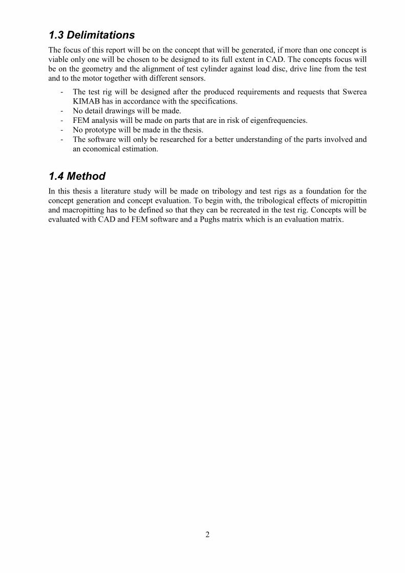
Table 2.1. ISO 15243 failure mode classification for bearing damage
2.1.1 Sub-surface and Surface initiated fatigue This type of fatigue is called Hertzian contact fatigue or rolling contact fatigue and will be
shortened to RCF. According to Anton van Beek (Beek, 2009) there are normal fatigue failure
and premature fatigue failure. The normal fatigue failure is sub-surface initiated and always
occurs due to material fatigue. Premature fatigue failure on the other hand can occur for a lot of
different reasons, for example misalignment which increases the load and mishandling or shock
which can generate cracks that will propagate. The premature failures can appear as either sub-
surface or surface initiated damages as shown in the Figure 2.1. These two types of fatigue are
also the two sub categories from ISO 15243. (Alfredsson, 2012)
1. Fatigue 1.1 Subsurface fatigue
1.2 Surface initiated fatigue
2. Wear 2.1 Abrasive Wear
2.2 Adhesive Wear
3. Corrosion 3.1 Moisture corrosion
3.2 Frictional corrosion
4. Electrical erosion 4.1 Excessive voltage
4.2 Current leakage
5. Plastic deformation
5.1 Overload
5.2 Indentation from debris
5.3 Indentation by handling
6. Fracture
6.1 Forced fracture
6.2 Fatigue fracture
6.3 Thermal cracking
4
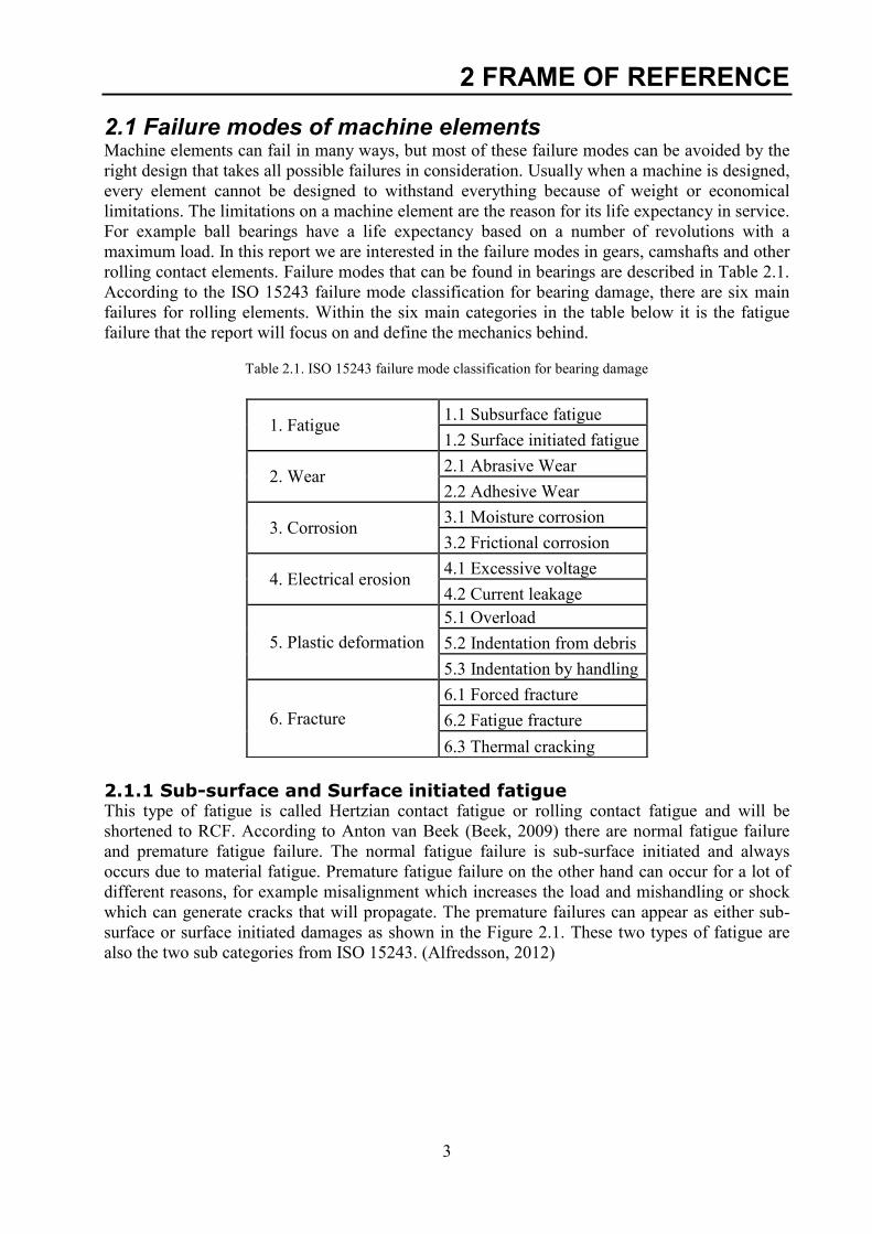
Figure 2.1. Sub-surface and surface initiation (Alfredsson, 2012)
During a rolling contact, singular points on the surface will for each revolution go into the loaded
zone where it will reach the maximum force of the load. Depending on the amount of force,
speed and heat, the repetition of this loading cycle will change the material structure and finally
fracture the sub surface. The first damage to appear is micro cracks approximately 0.1 to 0.5mm
below the surface which can propagate in to flaking. (Beek, 2009)
Figure 2.2. Shear stress as a function of depth between sliding-rolling contact surfaces
(SWEREA Kimab, fatigue presentation)
Surface initiated fatigue appears due to high local stress in the surface of the contact. The stress
can be caused by too little lubrication or the usage of the wrong type of lubricant which results in
metal to metal contact. All rolling contacts experience some sliding or slip in the rolling contact.
This slip promotes fatigue damage and can result in micro cracks and micro spalling that usually
starts in the asperities. The spalls are in some literature also referred to as flaking.
5
2.1.2 Spalling Spalling is when a part or flake of a material is detached from the main body of material.
Mechanical spalling occurs at points with high stress concentrations such as asperities or places
with brinelling. In a brinelling point the maximum shear stress is below the surface which can
result in a sub-surface initiation that shears the spall off once it has reached a critical point.
Points with higher amounts of asperities can progress from micro pitting into progressive macro
pitting that occurs when pits coalesce and form larger, irregular craters, (Beek, 2009). A
fragment that breaks of when spalling occurs tends to be thicker than the surface hardened case
and can, in some cases be prevented with a deeper hardening.
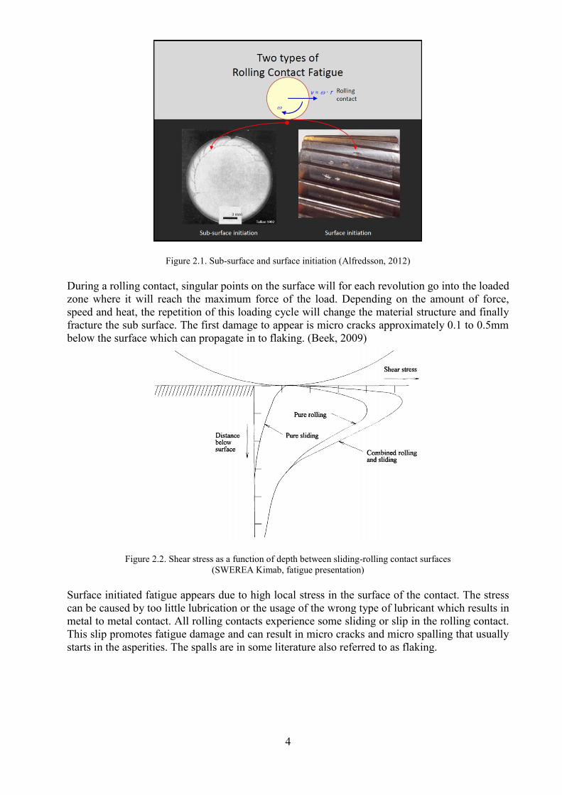
Spalling can have a lot of different shapes, and surface initiated spalling usually have a typical
characteristic that has been referred to as triangular, v-shaped, sea-shell shaped or fan-shaped
crack, (Hannes, 2014). The angle created at the apex of the crater is typical and referred to as a
spall opening angle and is marked in Figure 2.3 below.
Figure. 2.3. The triangular shape of a surface initiated flaking, the red arrow shows the rolling direction.
(Alfredsson, 2012)
Spalling does not always start with this v-shaped entry point since it can also have a more
indistinguishable source if macro pits coalesce into a larger crater.
6
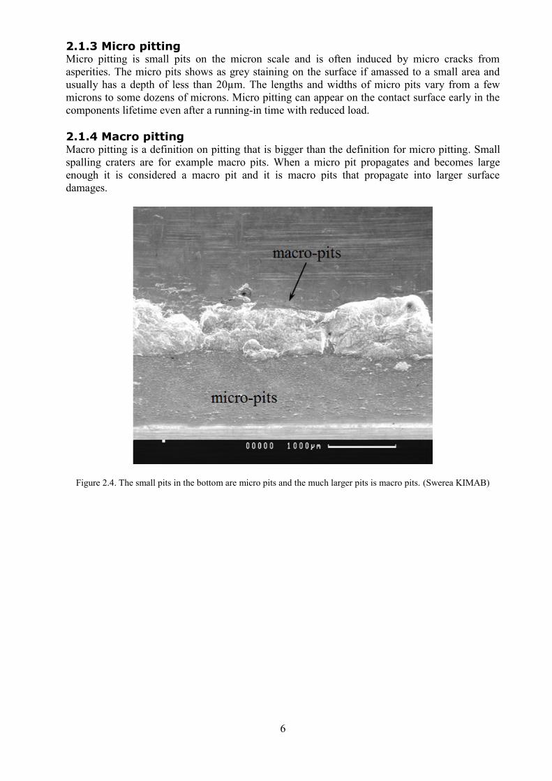
2.1.3 Micro pitting Micro pitting is small pits on the micron scale and is often induced by micro cracks from
asperities. The micro pits shows as grey staining on the surface if amassed to a small area and
usually has a depth of less than 20µm. The lengths and widths of micro pits vary from a few
microns to some dozens of microns. Micro pitting can appear on the contact surface early in the
components lifetime even after a running-in time with reduced load.
2.1.4 Macro pitting Macro pitting is a definition on pitting that is bigger than the definition for micro pitting. Small
spalling craters are for example macro pits. When a micro pit propagates and becomes large
enough it is considered a macro pit and it is macro pits that propagate into larger surface
damages.
Figure 2.4. The small pits in the bottom are micro pits and the much larger pits is macro pits. (Swerea KIMAB)
7
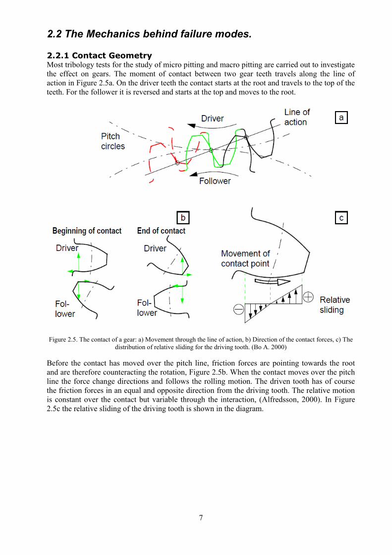
2.2 The Mechanics behind failure modes. 2.2.1 Contact Geometry Most tribology tests for the study of micro pitting and macro pitting are carried out to investigate
the effect on gears. The moment of contact between two gear teeth travels along the line of
action in Figure 2.5a. On the driver teeth the contact starts at the root and travels to the top of the
teeth. For the follower it is reversed and starts at the top and moves to the root.
Figure 2.5. The contact of a gear: a) Movement through the line of action, b) Direction of the contact forces, c) The
distribution of relative sliding for the driving tooth. (Bo A. 2000)
Before the contact has moved over the pitch line, friction forces are pointing towards the root
and are therefore counteracting the rotation, Figure 2.5b. When the contact moves over the pitch
line the force change directions and follows the rolling motion. The driven tooth has of course
the friction forces in an equal and opposite direction from the driving tooth. The relative motion
is constant over the contact but variable through the interaction, (Alfredsson, 2000). In Figure
2.5c the relative sliding of the driving tooth is shown in the diagram.
8
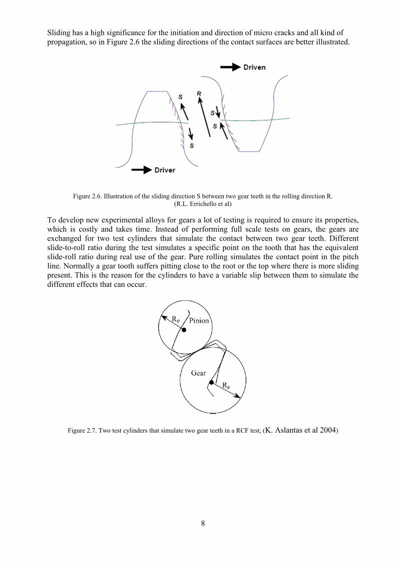
Sliding has a high significance for the initiation and direction of micro cracks and all kind of
propagation, so in Figure 2.6 the sliding directions of the contact surfaces are better illustrated.
Figure 2.6. Illustration of the sliding direction S between two gear teeth in the rolling direction R.
(R.L. Errichello et al)
To develop new experimental alloys for gears a lot of testing is required to ensure its properties,
which is costly and takes time. Instead of performing full scale tests on gears, the gears are
exchanged for two test cylinders that simulate the contact between two gear teeth. Different
slide-to-roll ratio during the test simulates a specific point on the tooth that has the equivalent
slide-roll ratio during real use of the gear. Pure rolling simulates the contact point in the pitch
line. Normally a gear tooth suffers pitting close to the root or the top where there is more sliding
present. This is the reason for the cylinders to have a variable slip between them to simulate the
different effects that can occur.
Figure 2.7. Two test cylinders that simulate two gear teeth in a RCF test, (K. Aslantas et al 2004)
9
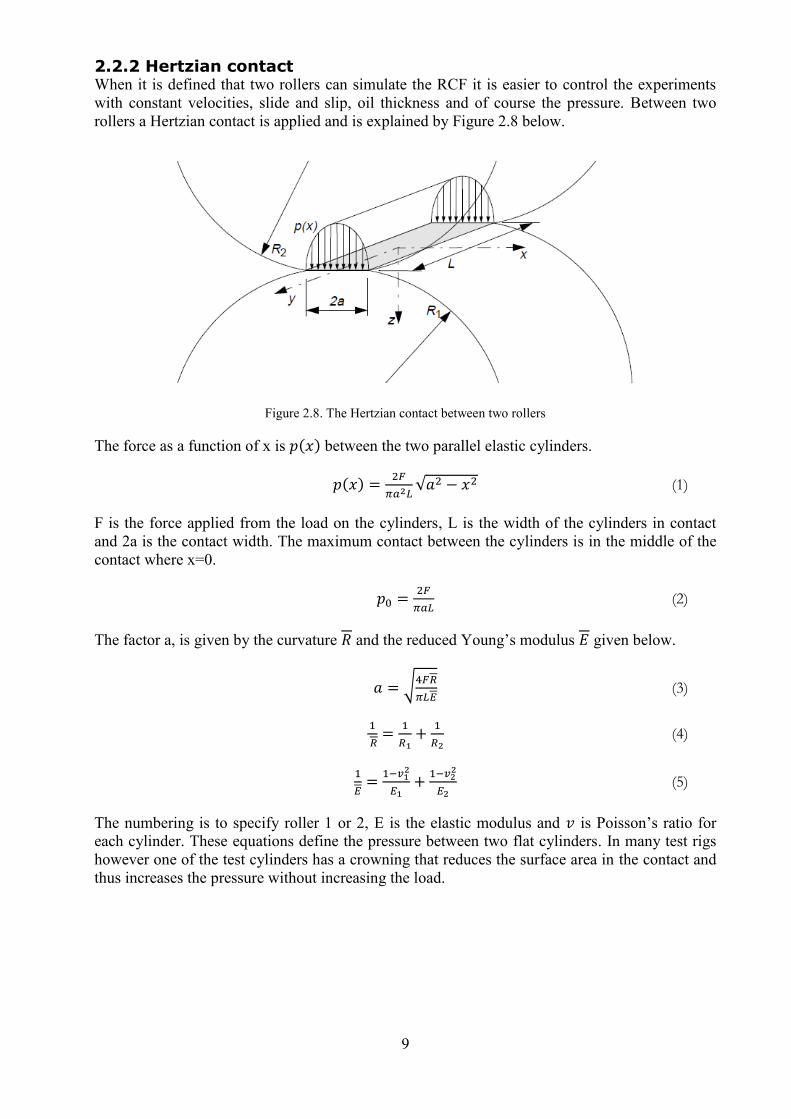
2.2.2 Hertzian contact When it is defined that two rollers can simulate the RCF it is easier to control the experiments
with constant velocities, slide and slip, oil thickness and of course the pressure. Between two
rollers a Hertzian contact is applied and is explained by Figure 2.8 below.
Figure 2.8. The Hertzian contact between two rollers
The force as a function of x is 𝑝(𝑥) between the two parallel elastic cylinders.
𝑝(𝑥) =2𝐹
𝜋𝑎2𝐿√𝑎2 − 𝑥2 (1)
F is the force applied from the load on the cylinders, L is the width of the cylinders in contact
and 2a is the contact width. The maximum contact between the cylinders is in the middle of the
contact where x=0.
𝑝0 =2𝐹
𝜋𝑎𝐿 (2)
The factor a, is given by the curvature 𝑅 and the reduced Young’s modulus 𝐸 given below.
𝑎 = √4𝐹𝑅
𝜋𝐿𝐸 (3)
1
𝑅=
1
𝑅1+
1
𝑅2 (4)
1
𝐸=
1−𝑣12
𝐸1+
1−𝑣22
𝐸2 (5)
The numbering is to specify roller 1 or 2, E is the elastic modulus and 𝑣 is Poisson’s ratio for
each cylinder. These equations define the pressure between two flat cylinders. In many test rigs
however one of the test cylinders has a crowning that reduces the surface area in the contact and
thus increases the pressure without increasing the load.
10
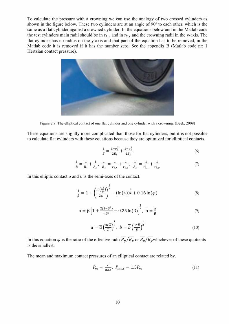
To calculate the pressure with a crowning we can use the analogy of two crossed cylinders as
shown in the figure below. These two cylinders are at an angle of 90º to each other, which is the
same as a flat cylinder against a crowned cylinder. In the equations below and in the Matlab code
the test cylinders main radii should be in 𝑟1,𝑥 and in 𝑟2,𝑥 and the crowning radii in the y-axis. The
flat cylinder has no radius on the y-axis and that part of the equation has to be removed, in the
Matlab code it is removed if it has the number zero. See the appendix B (Matlab code nr: 1
Hertzian contact pressure).
Figure 2.9. The elliptical contact of one flat cylinder and one cylinder with a crowning. (Beek, 2009)
These equations are slightly more complicated than those for flat cylinders, but it is not possible
to calculate flat cylinders with these equations because they are optimized for elliptical contacts.
1
𝐸=
1−𝑣12
2𝐸1+
1−𝑣22
2𝐸2 (6)
1
𝑅=
1
𝑅𝑥+
1
𝑅𝑦,
1
𝑅𝑥=
1
𝑟1,𝑥+
1
𝑟1,𝑦,
1
𝑅𝑦=
1
𝑟2,𝑥+
1
𝑟2,𝑦 (7)
In this elliptic contact a and b is the semi-axes of the contact.
1
𝛽= 1 + (
ln(16
𝜑)
2𝜑)
1
2
− (ln(4))1
2 + 0.16 ln(𝜑) (8)
a = β [1 +2(1−β2)
πβ2 − 0.25 ln(β)]
1
3, b =
a
β (9)
𝑎 = 𝑎 (3𝐹𝑅
𝐸)
1
3, 𝑏 = 𝑏 (
3𝐹𝑅
𝐸)
1
3 (10)
In this equation 𝜑 is the ratio of the effective radii 𝑅𝑦 𝑅𝑥⁄ or 𝑅𝑥 𝑅𝑦⁄ whichever of these quotients
is the smallest.
The mean and maximum contact pressures of an elliptical contact are related by.
𝑃𝑚 = 𝐹
𝜋𝑎𝑏, 𝑃𝑚𝑎𝑥 = 1.5𝑃𝑚 (11)
11
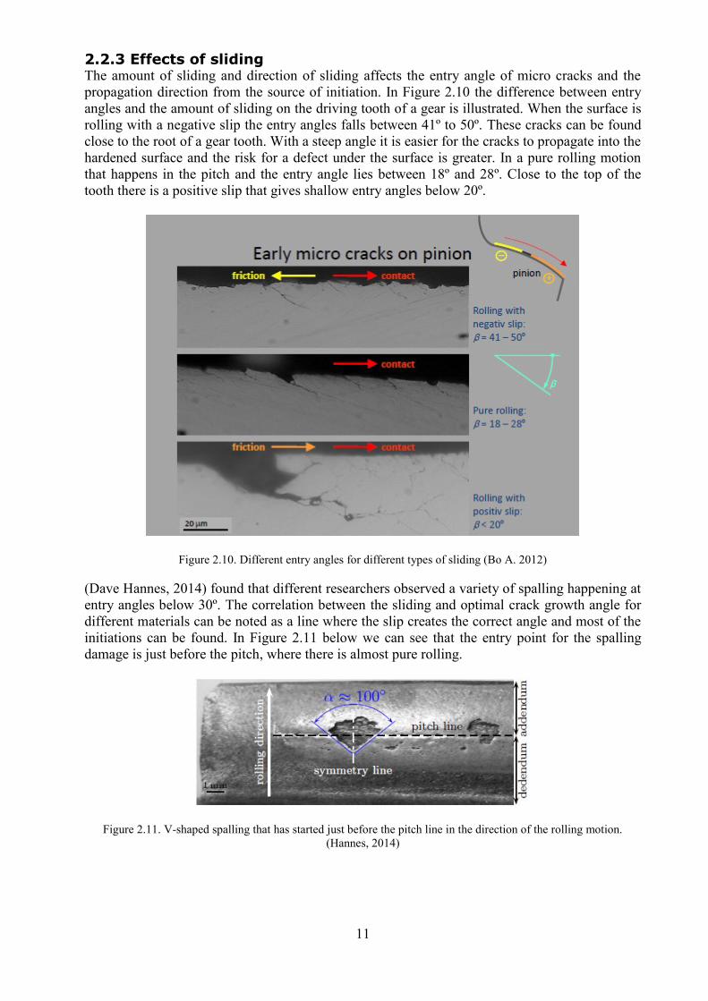
2.2.3 Effects of sliding The amount of sliding and direction of sliding affects the entry angle of micro cracks and the
propagation direction from the source of initiation. In Figure 2.10 the difference between entry
angles and the amount of sliding on the driving tooth of a gear is illustrated. When the surface is
rolling with a negative slip the entry angles falls between 41º to 50º. These cracks can be found
close to the root of a gear tooth. With a steep angle it is easier for the cracks to propagate into the
hardened surface and the risk for a defect under the surface is greater. In a pure rolling motion
that happens in the pitch and the entry angle lies between 18º and 28º. Close to the top of the
tooth there is a positive slip that gives shallow entry angles below 20º.
Figure 2.10. Different entry angles for different types of sliding (Bo A. 2012)
(Dave Hannes, 2014) found that different researchers observed a variety of spalling happening at
entry angles below 30º. The correlation between the sliding and optimal crack growth angle for
different materials can be noted as a line where the slip creates the correct angle and most of the
initiations can be found. In Figure 2.11 below we can see that the entry point for the spalling
damage is just before the pitch, where there is almost pure rolling.
Figure 2.11. V-shaped spalling that has started just before the pitch line in the direction of the rolling motion.
(Hannes, 2014)
12
2.2.4 Surface hardness Contact surfaces in mechanical parts need to be hardened to withstand higher loads during
rotational movement at high peripheral velocity. There are different kinds of surface treatments
to acquire the desired hardness. Some of them are case hardening, carburizing, press quenching,
LCP/High pressure gas quench, gas nitriding and induction hardening (Bugliarello et al). The
type of heat treatment that is used varies depending on the material and the application.
A common reason for hardness to affect pitting in rolling contacts is for the subsurface shear
stresses to produce plastic deformation in the martensitic structure from below. (Shaffer, 1996).
Other effects from the hardening that can affect pitting, is that carbides might crack, or hard
inclusions might increase the stresses. The hardening depth can also affect how spalling and
macro pitting is propagating. After the hardening process residual tensile stresses occur in the
surface, which if they are too great can quicken the propagation of cracks.
The hardness can also affect the surface roughness in how easy or hard it is to grind the material
after hardening and how resistant it is to wear.
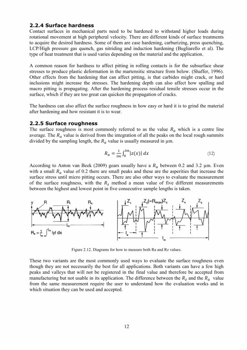
2.2.5 Surface roughness The surface roughness is most commonly referred to as the value 𝑅𝑎 which is a centre line
average. The 𝑅𝑎 value is derived from the integration of all the peaks on the local rough summits
divided by the sampling length, the 𝑅𝑎 value is usually measured in µm.
𝑅𝑎 =1
𝑙𝑚∫ |𝑧(𝑥)| 𝑑𝑥
𝑙𝑚
0 (12)
According to Anton van Beek (2009) gears usually have a 𝑅𝑎 between 0.2 and 3.2 µm. Even
with a small 𝑅𝑎 value of 0.2 there are small peaks and these are the asperities that increase the
surface stress until micro pitting occurs. There are also other ways to evaluate the measurement
of the surface roughness, with the 𝑅𝑧 method a mean value of five different measurements
between the highest and lowest point in five consecutive sample lengths is taken.
Figure 2.12. Diagrams for how to measure both Ra and Rz values.
These two variants are the most commonly used ways to evaluate the surface roughness even
though they are not necessarily the best for all applications. Both variants can have a few high
peaks and valleys that will not be registered in the final value and therefore be accepted from
manufacturing but not usable in its application. The difference between the 𝑅𝑧 and the 𝑅𝑎 value
from the same measurement require the user to understand how the evaluation works and in
which situation they can be used and accepted.
13
For the measurement of a surface that is going to be exposed to surface fatigue the demand for a
controllable surface roughness is going to be higher. The more peaks there are the longer the run-
in-time has to be where a lower load and speed is required to wear down the asperities until the
surface reaches a carrying roughness. The carrying roughness is when the surface can support the
load without any further wear. The valley depths also affect the amount of oil that stays on the
surface and that affects the creation of oil films and supports the formation of tribofilms.
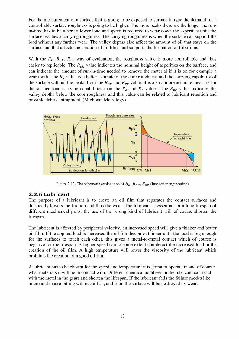
With the 𝑅𝑘, 𝑅𝑝𝑘, 𝑅𝑣𝑘 way of evaluation, the roughness value is more controllable and thus
easier to replicable. The 𝑅𝑝𝑘 value indicates the nominal height of asperities on the surface, and
can indicate the amount of run-in-time needed to remove the material if it is on for example a
gear tooth. The 𝑅𝑘 value is a better estimate of the core roughness and the carrying capability of
the surface without the peaks from the 𝑅𝑝𝑘 and 𝑅𝑣𝑘 value. It is also a more accurate measure for
the surface load carrying capabilities than the 𝑅𝑎 and 𝑅𝑧 values. The 𝑅𝑣𝑘 value indicates the
valley depths below the core roughness and this value can be related to lubricant retention and
possible debris entrapment. (Michigan Metrology)
Figure 2.13. The schematic explanation of 𝑅𝑘, 𝑅𝑝𝑘, 𝑅𝑣𝑘 (Inspectionengineering)
2.2.6 Lubricant The purpose of a lubricant is to create an oil film that separates the contact surfaces and
drastically lowers the friction and thus the wear. The lubricant is essential for a long lifespan of
different mechanical parts, the use of the wrong kind of lubricant will of course shorten the
lifespan.
The lubricant is affected by peripheral velocity, an increased speed will give a thicker and better
oil film. If the applied load is increased the oil film becomes thinner until the load is big enough
for the surfaces to touch each other, this gives a metal-to-metal contact which of course is
negative for the lifespan. A higher speed can to some extent counteract the increased load in the
creation of the oil film. A high temperature will lower the viscosity of the lubricant which
prohibits the creation of a good oil film.
A lubricant has to be chosen for the speed and temperature it is going to operate in and of course
what materials it will be in contact with. Different chemical additives in the lubricant can react
with the metal in the gears and shorten the lifespan. If the lubricant fails the failure modes like
micro and macro pitting will occur fast, and soon the surface will be destroyed by wear.
14
To calculate the oil thickness the equation described by Professor Andy Olver from the Imperial
College of London is used. (A. Olver)
ℎ0
𝑅𝑥′ = 3�̅�0.68�̅�0.49�̅�−0.073(1 − 𝑒−0.96(𝑅𝑦
′ 𝑅𝑥′⁄ )) (13)
ℎ𝐶
𝑅𝑥′ = 3. 06�̅�0.68�̅�0.49�̅�−0.073(1 − 𝑒−3.36(𝑅𝑦
′ 𝑅𝑥′⁄ )) (14)
The values of ℎ0 and ℎ𝐶 is the local oil film thickness for two points in the contact and should be
in the range of a few tenths of a µm for the oil film to be bearing. According to this equation the
speed parameter has the largest effect on the film thickness, and a higher speed will increase the
thickness. The load parameter which has a negative effect on the thickness is easily countered by
an increased speed.
Speed parameter �̅� =𝑈𝜂0
𝐸′𝑅𝑥′2 (15)
Material parameter �̅� = 𝛼𝐸′ (16)
Load parameter (elliptical contact) �̅� =𝑊
𝐸′𝑅𝑥′2 (17)
See the Matlab code in appendix B code nr: 2 for more information.
2.2.7 Peripheral velocity The peripheral velocity is given by the radius of the test cylinder and the axial speed. If the speed
is increased it can have a positive effect on the creation of the oil film but it is also possible that
it increases the temperature between the test cylinders which is negative for the oil film. By
increasing the speed the test will take a shorter time which of course is very positive. According
to (A Oila et al, 2005) micropitting occurs most readily at speeds in the range of 4-10 m/s.
2.2.8 Applied load The load is the factor that is easiest to use for the acceleration of a test. If the load is under a
gears specified load capacity it can take years before the test breaks. That is why the load is
increased until the surface pressure is so great that it starts to form micropitting early in the test.
2.2.9 Temperature The temperature mainly affects the lubricant. If the temperature is increased the viscosity of the
lubricant will decrease. A lower viscosity of the lubricant usually means a thinner oil film that
gives more contact between the surfaces, and more contact gives a higher risk of pitting.
15
2.3 Market screening of surface fatigue testing machines Regarding accelerated fatigue testing machines there has never been any standard for two roller
test rigs. The companies or research centers that are interested in these test rigs usually have to
build their own machine. There are a few machines on the market from different manufacturers
such as Phoenix Tribology Ltd, PCS Instruments, LRI Lewis research Inc. or FZG at the
Technical University of Munich. These machines use different concepts to test different factors
of the fatigue mechanics.
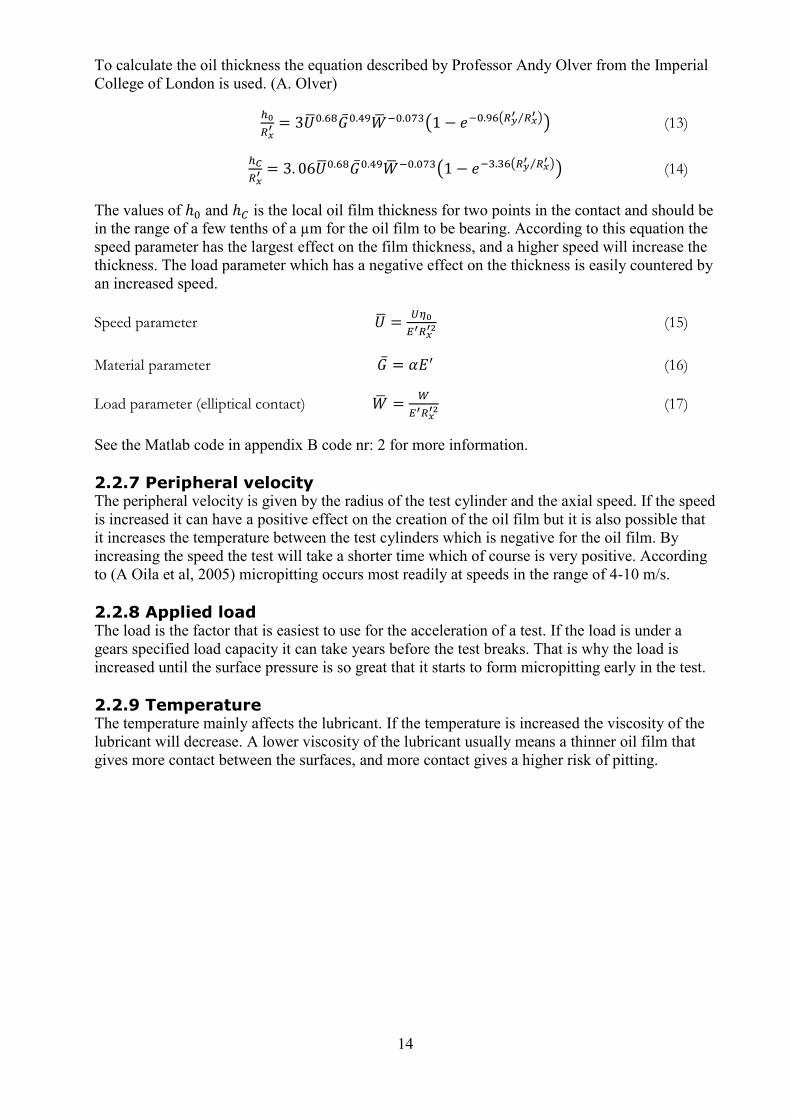
2.3.1 FZG The most frequently used machine in different research papers that focuses on micro and macro
pitting is the back to back FZG test rig. This test rig does not use test cylinders but modelled
gears, which makes it possible to see all of the effects on a highly loaded gear but the cost for
each test is higher.
Figure 2.14. The back-to-back gear test rig, from FZG.
The difference in results between this test rig and others that implement twin-disc test rollers is
that the peripheral speed and slip changes along the gear tooth which makes it impossible to base
the test on those specified factors. The reason for this machine to be well used in different
research papers is probably because both prototype gears and gears in mass production can be
tested in a controlled environment close to the reality. There are not that many other machines on
the market that is purchasable which of course affect the usage of this particular machine. There
are different companies and institutes that sell the service of full contact fatigue testing with
twin-disc test rigs, among them there is FZG and WZL which both are universities in Germany.
16
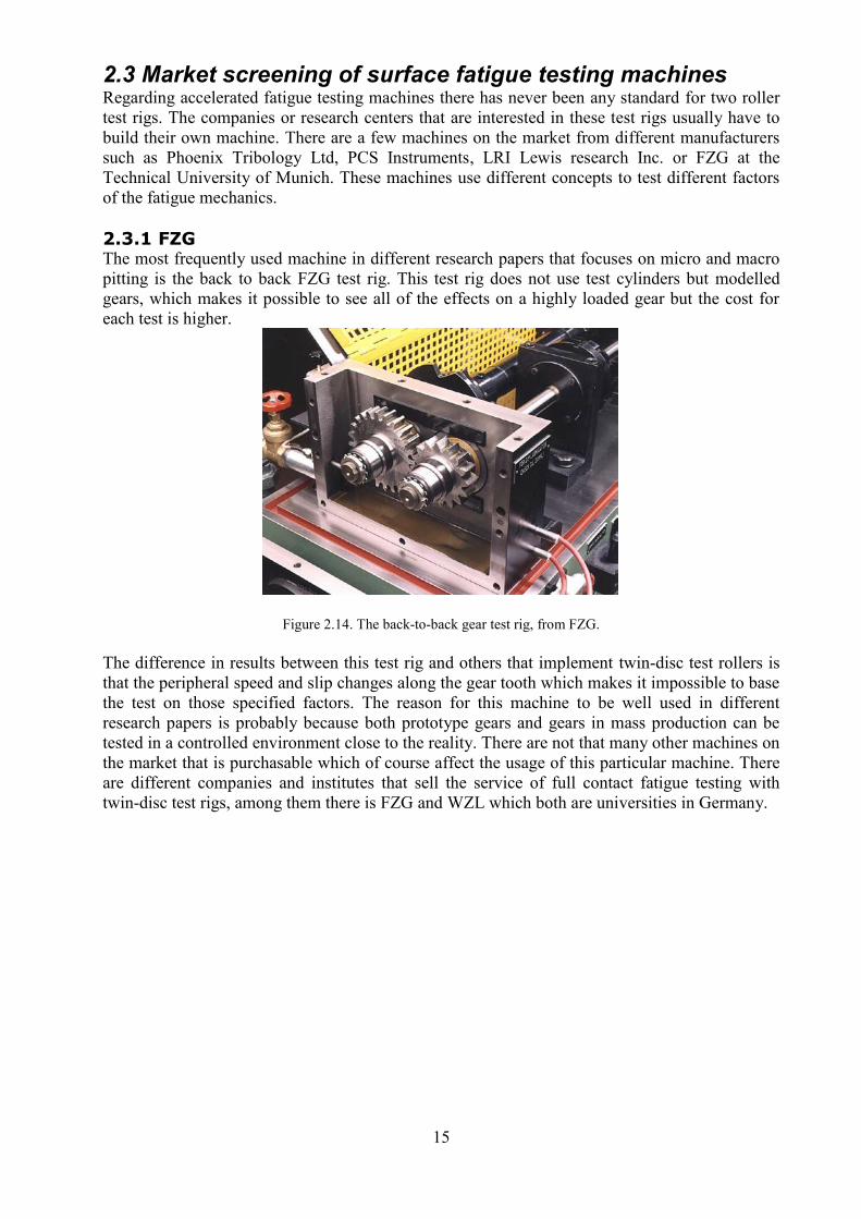
2.3.2 TE 74 Another test rig that has come up in research papers is the twin-disc test rig TE74 from Phoenix
Tribology. This test rig has been used in eight different research papers according to the
company. The test cylinder is mounted on the axle with one bearing on each side that distributes
the normal force evenly over the axle. The axle is then connected through a cardan shaft to the
pulley and a belt drive to the engine. The lower cylinder is also connected with a torque
transducer for measuring the friction torque created by the test.
Figure 2.15. A CAD rendering of the TE74s setup with cardan shafts and loading mechanism (Phoenix Tribology)
As can be seen in Figure 2.15 the cylinders are mounted one above the other and not horizontally
beside each other. This is because of the loading mechanism that presses down on the topmost
axle. The loading mechanism is based on a lever arm that pivots around an axle and is pressed
upwards by a servo controlled pneumatic bellows actuator with a force transducer feedback. In
the Figure 2.16 below the TE74H (high capacity) is shown with its two 30kW engines, the rest of
the drive system is covered from view by safety covers.
Figure 2.16. The TE74H with two 30kW engines. (Phoenix Tribology)
17
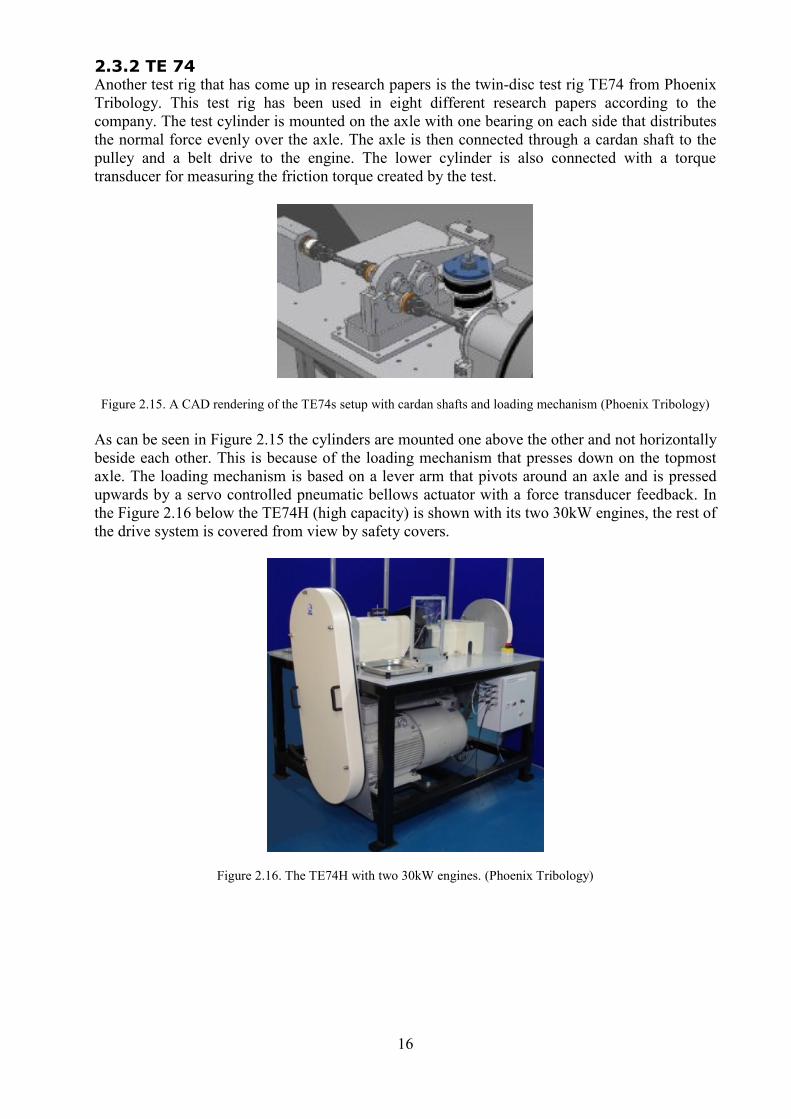
2.3.3 TE 72 The next test rig of interest is the TE72 also from Phoenix tribology. It is based on the same
structure as the TE74 but has a few differences. The TE72 is aligned horizontally with the load
applied from the side and not from above. It is also mounted with an overhang that simplifies the
mounting and dismounting of the disc and cylinder.
Figure 2.17. A CAD rendering of the TE72s setup with cardan shafts and loading mechanism (Phoenix Tribology)
This machine, like the TE74 can be ordered with different engines and loading mechanics for
higher requirements on the tests. The standard TE72 is rated for 3000 rpm and a load of 5kN,
and it is possible to change the axle distance for more flexibility in the dimensioning of the test
cylinder and load disc.
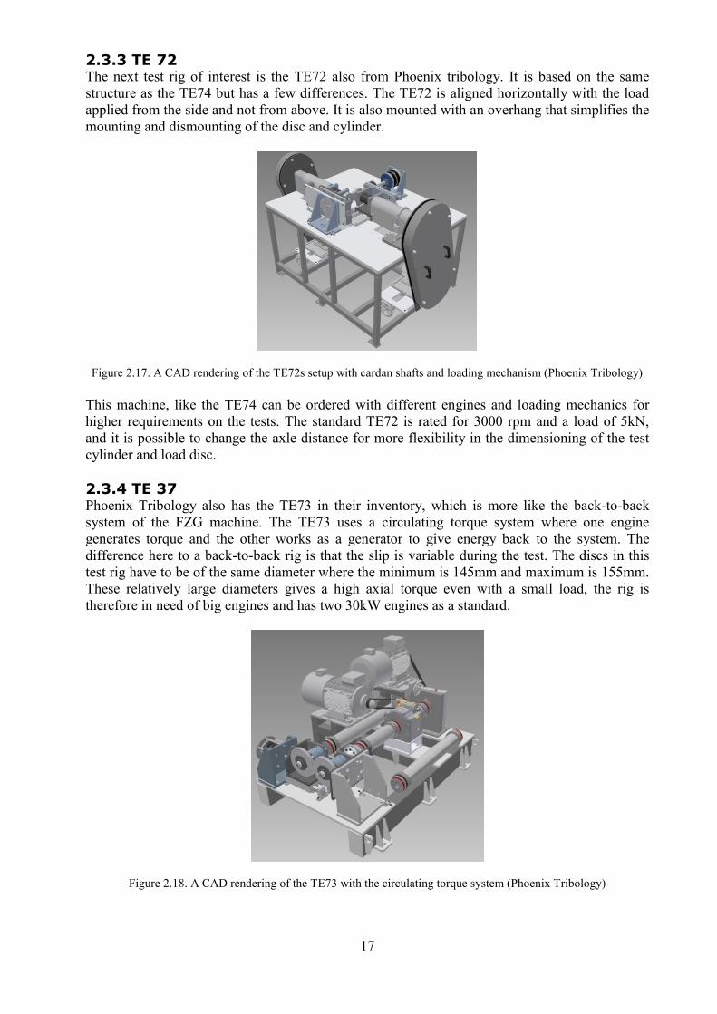
2.3.4 TE 37 Phoenix Tribology also has the TE73 in their inventory, which is more like the back-to-back
system of the FZG machine. The TE73 uses a circulating torque system where one engine
generates torque and the other works as a generator to give energy back to the system. The
difference here to a back-to-back rig is that the slip is variable during the test. The discs in this
test rig have to be of the same diameter where the minimum is 145mm and maximum is 155mm.
These relatively large diameters gives a high axial torque even with a small load, the rig is
therefore in need of big engines and has two 30kW engines as a standard.
Figure 2.18. A CAD rendering of the TE73 with the circulating torque system (Phoenix Tribology)
18
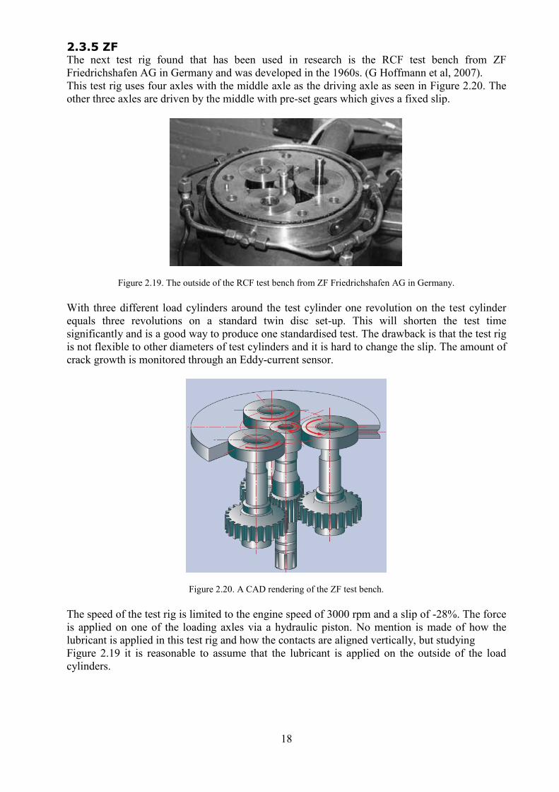
2.3.5 ZF The next test rig found that has been used in research is the RCF test bench from ZF
Friedrichshafen AG in Germany and was developed in the 1960s. (G Hoffmann et al, 2007).
This test rig uses four axles with the middle axle as the driving axle as seen in Figure 2.20. The
other three axles are driven by the middle with pre-set gears which gives a fixed slip.
Figure 2.19. The outside of the RCF test bench from ZF Friedrichshafen AG in Germany.
With three different load cylinders around the test cylinder one revolution on the test cylinder
equals three revolutions on a standard twin disc set-up. This will shorten the test time
significantly and is a good way to produce one standardised test. The drawback is that the test rig
is not flexible to other diameters of test cylinders and it is hard to change the slip. The amount of
crack growth is monitored through an Eddy-current sensor.
Figure 2.20. A CAD rendering of the ZF test bench.
The speed of the test rig is limited to the engine speed of 3000 rpm and a slip of -28%. The force
is applied on one of the loading axles via a hydraulic piston. No mention is made of how the
lubricant is applied in this test rig and how the contacts are aligned vertically, but studying
Figure 2.19 it is reasonable to assume that the lubricant is applied on the outside of the load
cylinders.
19
2.3.6 Wedeven Associates Inc There are other companies that use the same system with one test cylinder and three load
cylinders. One of these is very similar to the ZF test bench and is made by Wedeven Associates
Inc.
Figure 2.21. The WAMmp Micropitting test rig from Wedeven Associates Inc.
These test conditions are made to simulate the integral raceways of planetary gears and
especially for the testing of materials in helicopter transmissions. This test rig can have a load of
7.1kN and a peripheral velocity of 10m/s on the load discs, the slip can be changed to ±10%.
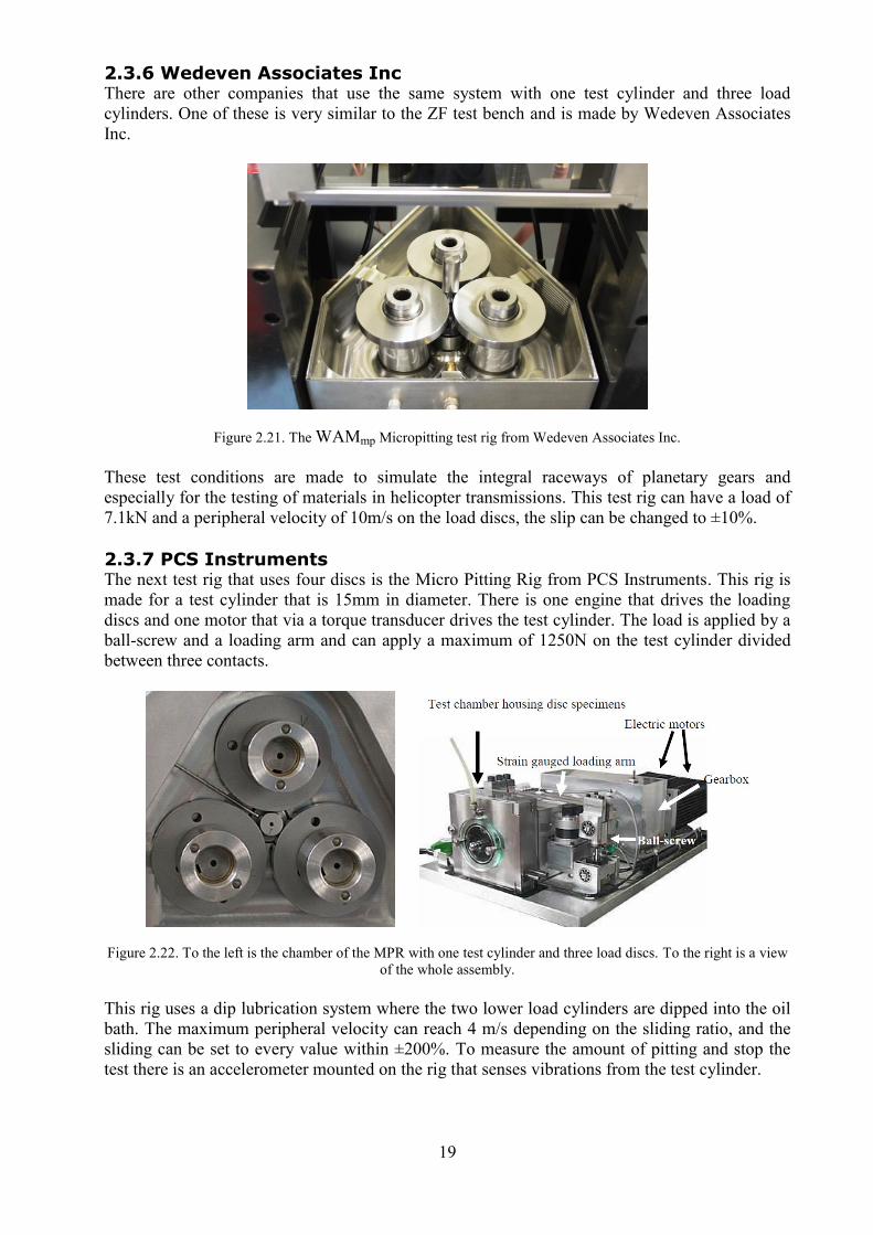
2.3.7 PCS Instruments The next test rig that uses four discs is the Micro Pitting Rig from PCS Instruments. This rig is
made for a test cylinder that is 15mm in diameter. There is one engine that drives the loading
discs and one motor that via a torque transducer drives the test cylinder. The load is applied by a
ball-screw and a loading arm and can apply a maximum of 1250N on the test cylinder divided
between three contacts.
Figure 2.22. To the left is the chamber of the MPR with one test cylinder and three load discs. To the right is a view
of the whole assembly.
This rig uses a dip lubrication system where the two lower load cylinders are dipped into the oil
bath. The maximum peripheral velocity can reach 4 m/s depending on the sliding ratio, and the
sliding can be set to every value within ±200%. To measure the amount of pitting and stop the
test there is an accelerometer mounted on the rig that senses vibrations from the test cylinder.
20
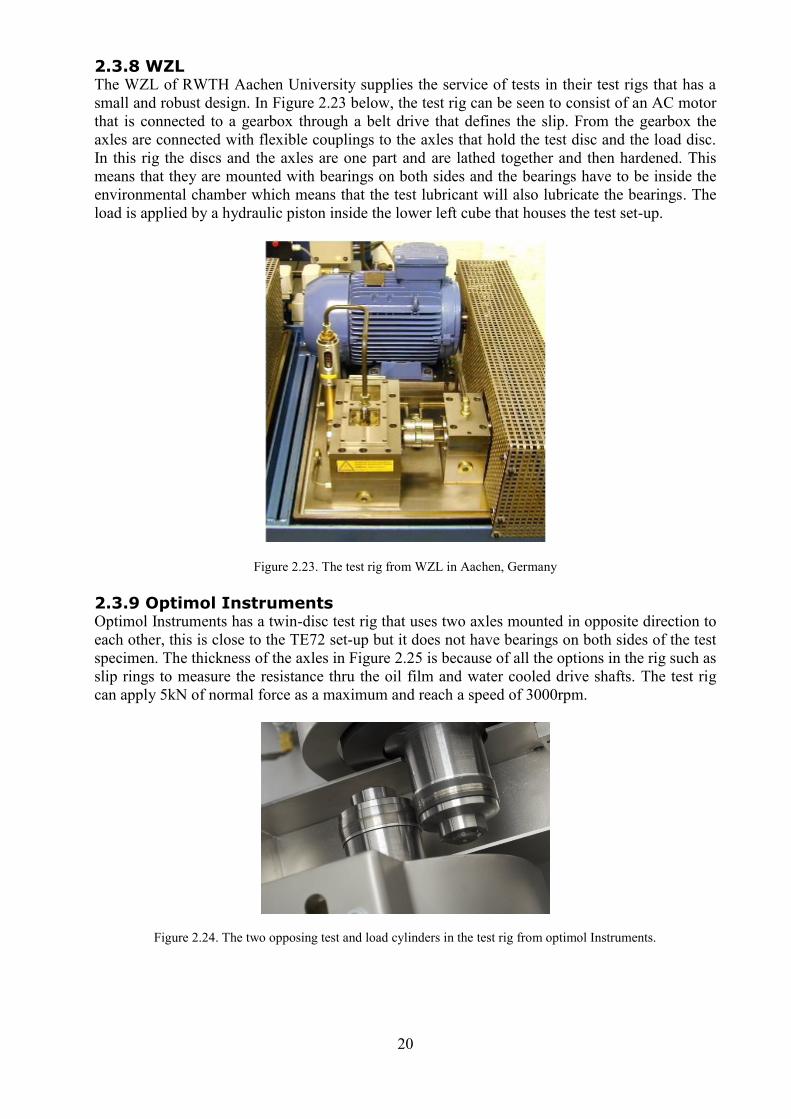
2.3.8 WZL The WZL of RWTH Aachen University supplies the service of tests in their test rigs that has a
small and robust design. In Figure 2.23 below, the test rig can be seen to consist of an AC motor
that is connected to a gearbox through a belt drive that defines the slip. From the gearbox the
axles are connected with flexible couplings to the axles that hold the test disc and the load disc.
In this rig the discs and the axles are one part and are lathed together and then hardened. This
means that they are mounted with bearings on both sides and the bearings have to be inside the
environmental chamber which means that the test lubricant will also lubricate the bearings. The
load is applied by a hydraulic piston inside the lower left cube that houses the test set-up.
Figure 2.23. The test rig from WZL in Aachen, Germany
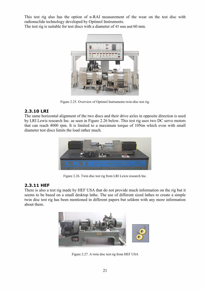
2.3.9 Optimol Instruments Optimol Instruments has a twin-disc test rig that uses two axles mounted in opposite direction to
each other, this is close to the TE72 set-up but it does not have bearings on both sides of the test
specimen. The thickness of the axles in Figure 2.25 is because of all the options in the rig such as
slip rings to measure the resistance thru the oil film and water cooled drive shafts. The test rig
can apply 5kN of normal force as a maximum and reach a speed of 3000rpm.
Figure 2.24. The two opposing test and load cylinders in the test rig from optimol Instruments.
21
This test rig also has the option of n-RAI measurement of the wear on the test disc with
radionuclide technology developed by Optimol Instruments.
The test rig is suitable for test discs with a diameter of 45 mm and 60 mm.
Figure 2.25. Overview of Optimol Instruments twin-disc test rig.
2.3.10 LRI The same horizontal alignment of the two discs and their drive axles in opposite direction is used
by LRI Lewis research Inc. as seen in Figure 2.26 below. This test rig uses two DC servo motors
that can reach 4000 rpm. It is limited to a maximum torque of 10Nm which even with small
diameter test discs limits the load rather much.
Figure 2.26. Twin disc test rig from LRI Lewis research Inc.
2.3.11 HEF There is also a test rig made by HEF USA that do not provide much information on the rig but it
seems to be based on a small desktop lathe. The use of different sized lathes to create a simple
twin disc test rig has been mentioned in different papers but seldom with any more information
about them.
Figure 2.27. A twin disc test rig from HEF USA
22
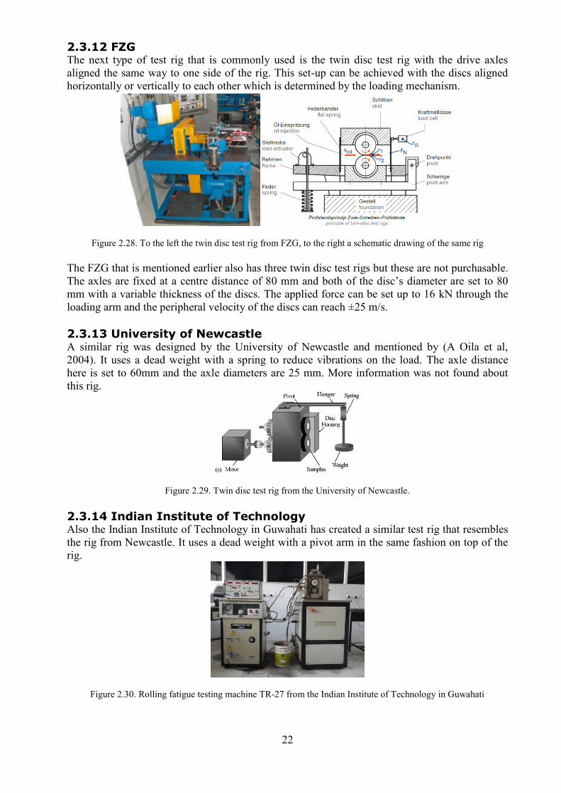
2.3.12 FZG The next type of test rig that is commonly used is the twin disc test rig with the drive axles
aligned the same way to one side of the rig. This set-up can be achieved with the discs aligned
horizontally or vertically to each other which is determined by the loading mechanism.
Figure 2.28. To the left the twin disc test rig from FZG, to the right a schematic drawing of the same rig
The FZG that is mentioned earlier also has three twin disc test rigs but these are not purchasable.
The axles are fixed at a centre distance of 80 mm and both of the disc’s diameter are set to 80
mm with a variable thickness of the discs. The applied force can be set up to 16 kN through the
loading arm and the peripheral velocity of the discs can reach ±25 m/s.
2.3.13 University of Newcastle A similar rig was designed by the University of Newcastle and mentioned by (A Oila et al,
2004). It uses a dead weight with a spring to reduce vibrations on the load. The axle distance
here is set to 60mm and the axle diameters are 25 mm. More information was not found about
this rig.
Figure 2.29. Twin disc test rig from the University of Newcastle.
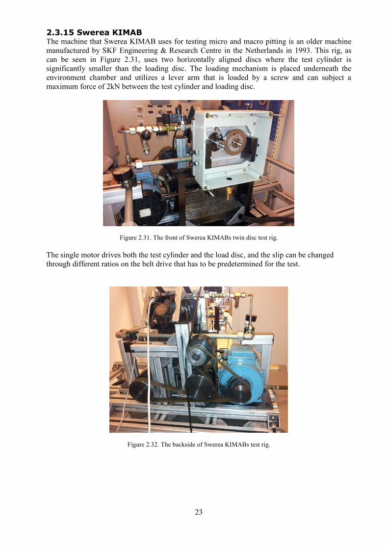
2.3.14 Indian Institute of Technology Also the Indian Institute of Technology in Guwahati has created a similar test rig that resembles
the rig from Newcastle. It uses a dead weight with a pivot arm in the same fashion on top of the
rig.
Figure 2.30. Rolling fatigue testing machine TR-27 from the Indian Institute of Technology in Guwahati
23
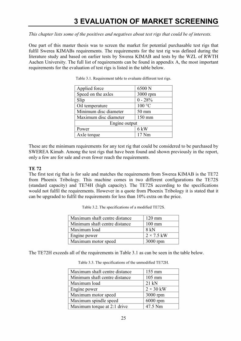
2.3.15 Swerea KIMAB The machine that Swerea KIMAB uses for testing micro and macro pitting is an older machine
manufactured by SKF Engineering & Research Centre in the Netherlands in 1993. This rig, as
can be seen in Figure 2.31, uses two horizontally aligned discs where the test cylinder is
significantly smaller than the loading disc. The loading mechanism is placed underneath the
environment chamber and utilizes a lever arm that is loaded by a screw and can subject a
maximum force of 2kN between the test cylinder and loading disc.
Figure 2.31. The front of Swerea KIMABs twin disc test rig.
The single motor drives both the test cylinder and the load disc, and the slip can be changed
through different ratios on the belt drive that has to be predetermined for the test.
Figure 2.32. The backside of Swerea KIMABs test rig.

24
25
3 EVALUATION OF MARKET SCREENING
This chapter lists some of the positives and negatives about test rigs that could be of interests.
One part of this master thesis was to screen the market for potential purchasable test rigs that
fulfil Swerea KIMABs requirements. The requirements for the test rig was defined during the
literature study and based on earlier tests by Swerea KIMAB and tests by the WZL of RWTH
Aachen University. The full list of requirements can be found in appendix A, the most important
requirements for the evaluation of test rigs is listed in the table below.
Table 3.1. Requirement table to evaluate different test rigs.
Applied force 6500 N
Speed on the axles 3000 rpm
Slip 0 - 28%
Oil temperature 100 °C
Minimum disc diameter 50 mm
Maximum disc diameter 150 mm
Engine output
Power 6 kW
Axle torque 17 Nm
These are the minimum requirements for any test rig that could be considered to be purchased by
SWEREA Kimab. Among the test rigs that have been found and shown previously in the report,
only a few are for sale and even fewer reach the requirements.
TE 72
The first test rig that is for sale and matches the requirements from Swerea KIMAB is the TE72
from Phoenix Tribology. This machine comes in two different configurations the TE72S
(standard capacity) and TE74H (high capacity). The TE72S according to the specifications
would not fulfil the requirements. However in a quote from Phoenix Tribology it is stated that it
can be upgraded to fulfil the requirements for less than 10% extra on the price.
Table 3.2. The specifications of a modified TE72S.
Maximum shaft centre distance 120 mm
Minimum shaft centre distance 100 mm
Maximum load 8 kN
Engine power 2 × 7.5 kW
Maximum motor speed 3000 rpm
The TE72H exceeds all of the requirements in Table 3.1 as can be seen in the table below.
Table 3.3. The specifications of the unmodified TE72H.
Maximum shaft centre distance 155 mm
Minimum shaft centre distance 105 mm
Maximum load 21 kN
Engine power 2 × 30 kW
Maximum motor speed 3000 rpm
Maximum spindle speed 6000 rpm
Maximum torque at 2:1 drive 47.5 Nm
26
According to a quote from Phoenix Tribology the TE72S can also be modified to further
accommodate later expansions in the requirements. The TE 72S is reasonable priced with the
modified test rigs price at £88 000. The TE72H has a price that is the double of the TE72S at
£173 560. The software running the test rig is COMPEND 2000 which is developed by Phoenix
Tribology and is a freeware.
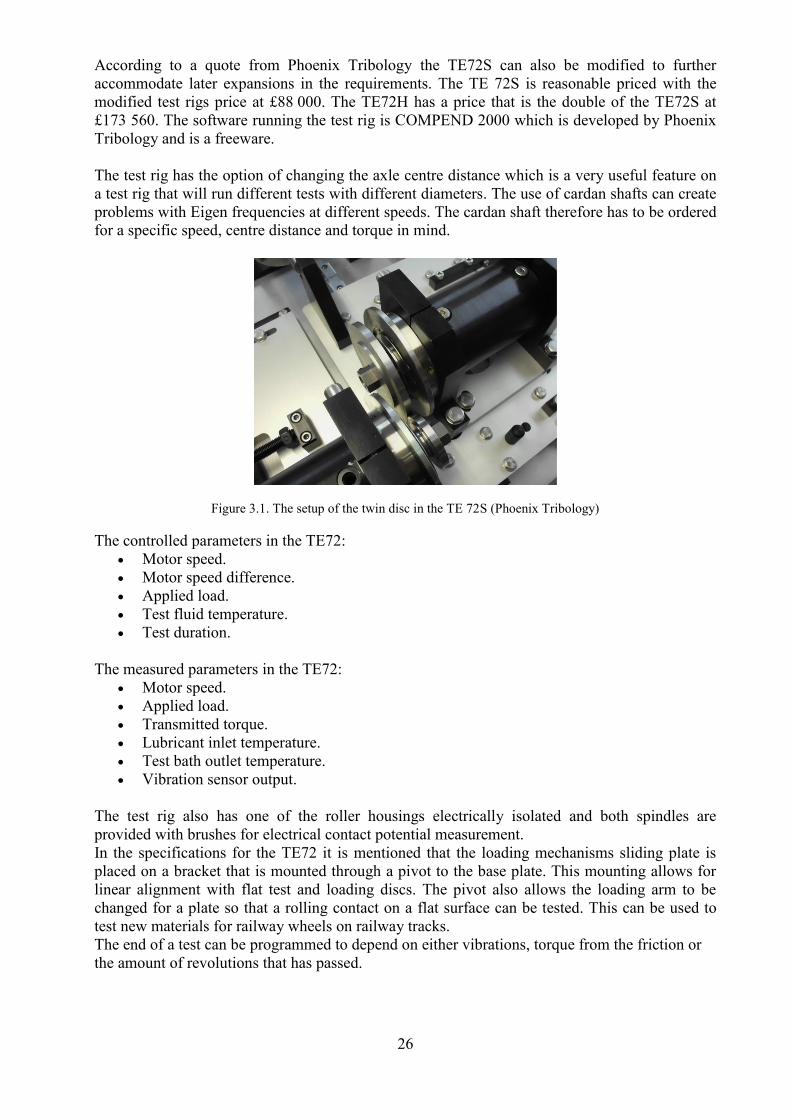
The test rig has the option of changing the axle centre distance which is a very useful feature on
a test rig that will run different tests with different diameters. The use of cardan shafts can create
problems with Eigen frequencies at different speeds. The cardan shaft therefore has to be ordered
for a specific speed, centre distance and torque in mind.
Figure 3.1. The setup of the twin disc in the TE 72S (Phoenix Tribology)
The controlled parameters in the TE72:
Motor speed.
Motor speed difference.
Applied load.
Test fluid temperature.
Test duration.
The measured parameters in the TE72:
Motor speed.
Applied load.
Transmitted torque.
Lubricant inlet temperature.
Test bath outlet temperature.
Vibration sensor output.
The test rig also has one of the roller housings electrically isolated and both spindles are
provided with brushes for electrical contact potential measurement.
In the specifications for the TE72 it is mentioned that the loading mechanisms sliding plate is
placed on a bracket that is mounted through a pivot to the base plate. This mounting allows for
linear alignment with flat test and loading discs. The pivot also allows the loading arm to be
changed for a plate so that a rolling contact on a flat surface can be tested. This can be used to
test new materials for railway wheels on railway tracks.
The end of a test can be programmed to depend on either vibrations, torque from the friction or
the amount of revolutions that has passed.
27
Summary of the TE 72
TE72S
Positives
- The test rig fulfils the requirements with small modifications.
- The price is reasonable for this test rig.
- It is possible to change the axle distance which makes it flexible.
- Possibility to test rolling on flat surfaces.
Negatives
- The cardan shafts might have problems with eigenfrequencies.
TE72H
Positives
- The test rig exceeds the requirements without modifications.
- It is possible to change the axle distance which makes it flexible.
- Possibility to test rolling on flat surfaces.
Negatives
- The cardan shafts can get problems with eigenfrequencies.
- The price is more than twice of the TE72S
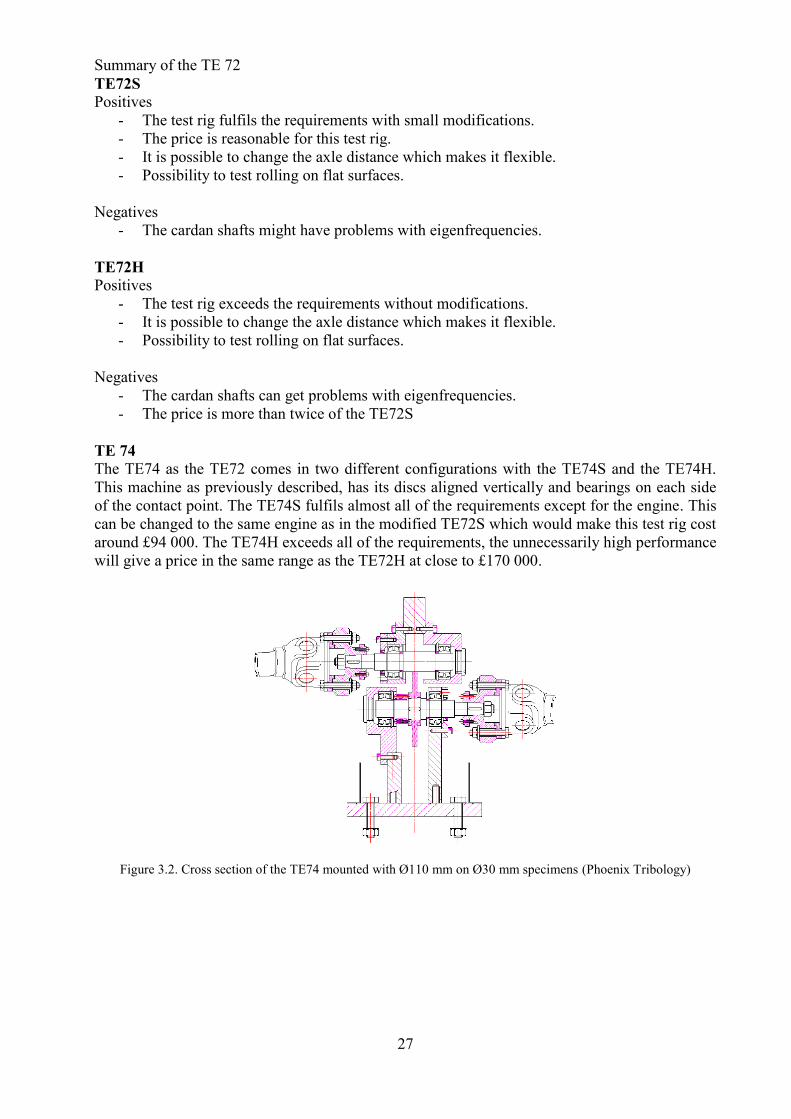
TE 74
The TE74 as the TE72 comes in two different configurations with the TE74S and the TE74H.
This machine as previously described, has its discs aligned vertically and bearings on each side
of the contact point. The TE74S fulfils almost all of the requirements except for the engine. This
can be changed to the same engine as in the modified TE72S which would make this test rig cost
around £94 000. The TE74H exceeds all of the requirements, the unnecessarily high performance
will give a price in the same range as the TE72H at close to £170 000.
Figure 3.2. Cross section of the TE74 mounted with Ø110 mm on Ø30 mm specimens (Phoenix Tribology)
28
The specifications for the TE74S are shown in Table 3.4 below.
Table 3.4. The specifications of the unmodified TE74S.
The use of bearings on each side of the disc creates the need for the bearing to be inside the
lubricated environment. To change the test discs the cardan shafts has to be dismounted and then
the bearings removed from the axle and then the test discs can be removed. This mounting and
dismounting sequence gets harder with everything inside the oil bath which will increase the
setup time for each test.
A direct difference between the TE74 and the TE72 is that the TE72 is prepared with isolated
bearings to measure resistance between contact points and the TE74 is as a standard equipped to
measure this resistance.
The controlled parameters in the TE74:
Motor speed.
Motor speed difference.
Applied load.
Test fluid temperature.
Test duration.
The measured parameters in the TE74:
Motor speed.
Applied load.
Transmitted torque.
Lubricant inlet temperature.
Test bath outlet temperature.
Vibration sensor output.
Electrical contact resistance.
Summary of the TE 74
TE74S
Positives
- The test rig fulfils the requirements with small modifications.
- The price is reasonable for this test rig.
- It is possible to test very small test discs
Negatives
- The cardan shafts might have problems with Eigen frequencies.
- Long setup time between tests.
- It is not possible to change the axle distance.
Shaft centre distance 40 mm
Maximum Roller Difference 65 mm on 15mm
Maximum load 12 kN
Engine power 2 × 5.5 kW
Maximum motor speed 3000 rpm
Maximum spindle speed 6000 rpm
Maximum torque at 2:1 drive 8.75 Nm
29
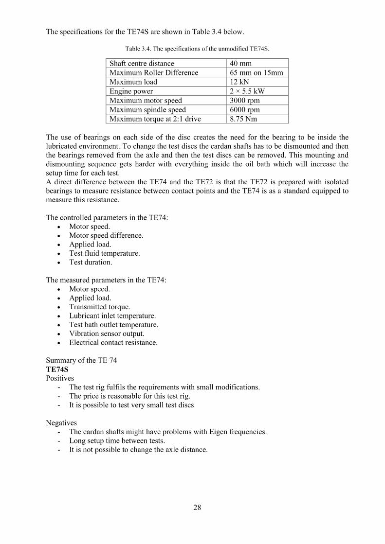
Optimol Instruments The test rig from Optimol Instruments fulfils the requirements except for the load, which does
not meet the requirements, although it is close. The test rig has some of the most advanced
sensors that can be found for twin disc test rigs so a comparison is of interest. In Figure 3.3
below and the earlier Figure 2.24, 2.25 show the test rig from Optimol Instruments.
Figure 3.3. Optimol Instruments twin disc test rig.
Most of the sensors and parts that are not needed for the setup of the simplest tests are optional
for this test rig. The basic machine comes with two 11 kW, 3000 rpm engines with a maximum
torque of 36 Nm and a load system that applies 10 – 5000 N. This setup costs 184.000€ and with
the optional parts listed below the price goes up.
Device-specific software, PC
Software for programming dynamic setpoint profiles
Normal force range: 3 - 5000 N
Water-cooled drive shafts
Temperature measurement of one disk
Lubrication gap measurement
Measurement of electrical resistance between test specimens
Measurement of noise emission between test specimens
Climate unit
Oil pump
n-RAI measurement of nano-wear with radionuclide technology
The n-RAI measurement device is developed by Optimol Instruments and seems to be a very
accurate way of measuring the surface of the test disc. Including all optional features, the cost
would be 259.420€
Summary of the twin disc test rig from Optimol Instruments.
Positives
- Good control of the test with many different sensors.
- Short setup time between tests.
Negatives
- Does not fulfil the load requirements.
- A high price for the machine.

30
31
4 DESIGN PROCESS
This chapter describes the design process and how the concept was chosen
4.1 Concept generation After studying the mechanics behind micro- and macro-pitting and different test rigs that has
been used in research papers, the first decision to be made was how to align the test cylinders to
each other. The design of how to align the cylinders will determine the possibilities of driving
the axles and applying the load, especially if smaller diameters of the test cylinders are to be
used.
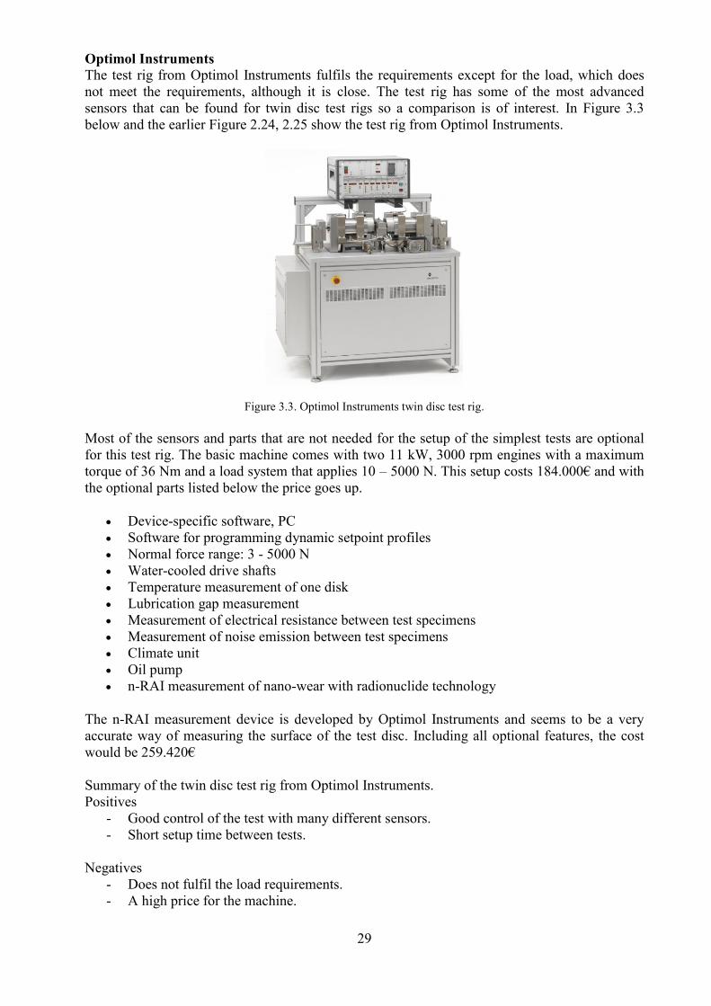
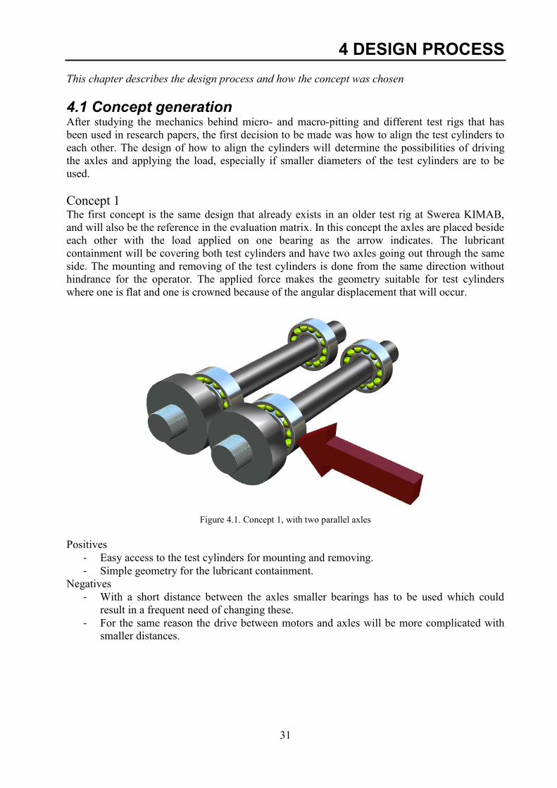
Concept 1 The first concept is the same design that already exists in an older test rig at Swerea KIMAB,
and will also be the reference in the evaluation matrix. In this concept the axles are placed beside
each other with the load applied on one bearing as the arrow indicates. The lubricant
containment will be covering both test cylinders and have two axles going out through the same
side. The mounting and removing of the test cylinders is done from the same direction without
hindrance for the operator. The applied force makes the geometry suitable for test cylinders
where one is flat and one is crowned because of the angular displacement that will occur.
Figure 4.1. Concept 1, with two parallel axles
Positives
- Easy access to the test cylinders for mounting and removing.
- Simple geometry for the lubricant containment.
Negatives
- With a short distance between the axles smaller bearings has to be used which could
result in a frequent need of changing these.
- For the same reason the drive between motors and axles will be more complicated with
smaller distances.
32
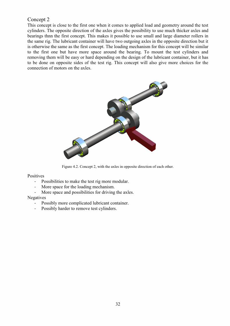
Concept 2 This concept is close to the first one when it comes to applied load and geometry around the test
cylinders. The opposite direction of the axles gives the possibility to use much thicker axles and
bearings thnn the first concept. This makes it possible to use small and large diameter rollers in
the same rig. The lubricant container will have two outgoing axles in the opposite direction but it
is otherwise the same as the first concept. The loading mechanism for this concept will be similar
to the first one but have more space around the bearing. To mount the test cylinders and
removing them will be easy or hard depending on the design of the lubricant container, but it has
to be done on opposite sides of the test rig. This concept will also give more choices for the
connection of motors on the axles.
Figure 4.2. Concept 2, with the axles in opposite direction of each other.
Positives
- Possibilities to make the test rig more modular.
- More space for the loading mechanism.
- More space and possibilities for driving the axles.
Negatives
- Possibly more complicated lubricant container.
- Possibly harder to remove test cylinders.
33
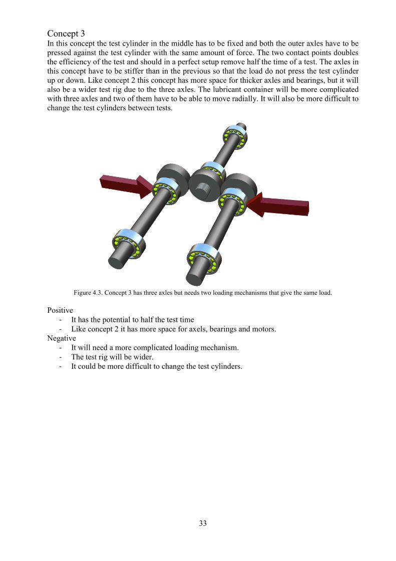
Concept 3 In this concept the test cylinder in the middle has to be fixed and both the outer axles have to be
pressed against the test cylinder with the same amount of force. The two contact points doubles
the efficiency of the test and should in a perfect setup remove half the time of a test. The axles in
this concept have to be stiffer than in the previous so that the load do not press the test cylinder
up or down. Like concept 2 this concept has more space for thicker axles and bearings, but it will
also be a wider test rig due to the three axles. The lubricant container will be more complicated
with three axles and two of them have to be able to move radially. It will also be more difficult to
change the test cylinders between tests.
Figure 4.3. Concept 3 has three axles but needs two loading mechanisms that give the same load.
Positive
- It has the potential to half the test time
- Like concept 2 it has more space for axels, bearings and motors.
Negative
- It will need a more complicated loading mechanism.
- The test rig will be wider.
- It could be more difficult to change the test cylinders.
34
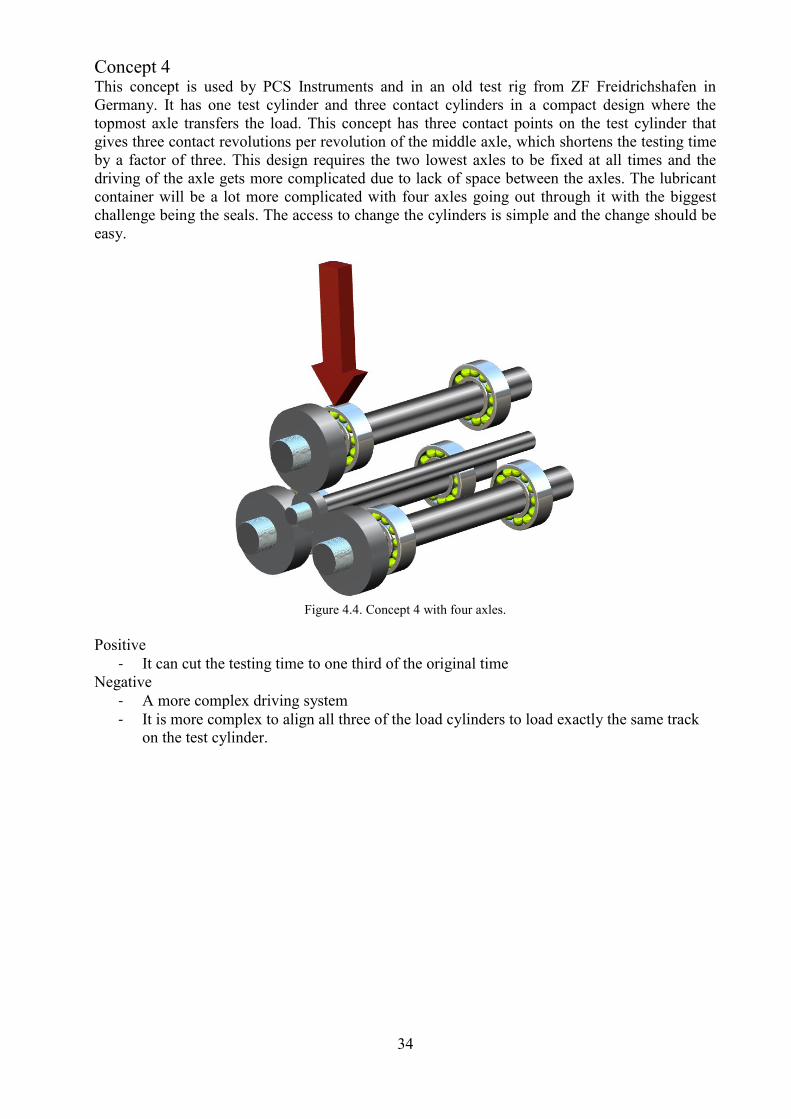
Concept 4 This concept is used by PCS Instruments and in an old test rig from ZF Freidrichshafen in
Germany. It has one test cylinder and three contact cylinders in a compact design where the
topmost axle transfers the load. This concept has three contact points on the test cylinder that
gives three contact revolutions per revolution of the middle axle, which shortens the testing time
by a factor of three. This design requires the two lowest axles to be fixed at all times and the
driving of the axle gets more complicated due to lack of space between the axles. The lubricant
container will be a lot more complicated with four axles going out through it with the biggest
challenge being the seals. The access to change the cylinders is simple and the change should be
easy.
Figure 4.4. Concept 4 with four axles.
Positive
- It can cut the testing time to one third of the original time
Negative
- A more complex driving system
- It is more complex to align all three of the load cylinders to load exactly the same track
on the test cylinder.
35
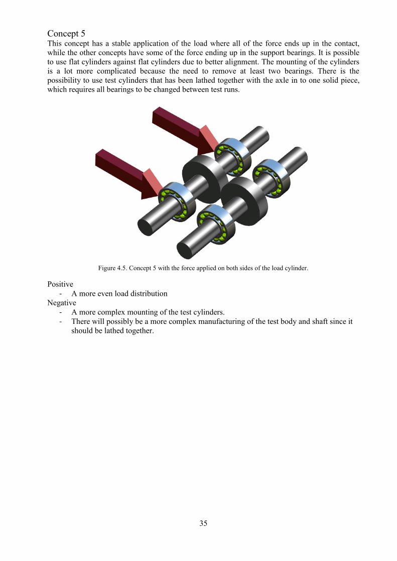
Concept 5 This concept has a stable application of the load where all of the force ends up in the contact,
while the other concepts have some of the force ending up in the support bearings. It is possible
to use flat cylinders against flat cylinders due to better alignment. The mounting of the cylinders
is a lot more complicated because the need to remove at least two bearings. There is the
possibility to use test cylinders that has been lathed together with the axle in to one solid piece,
which requires all bearings to be changed between test runs.
Figure 4.5. Concept 5 with the force applied on both sides of the load cylinder.
Positive
- A more even load distribution
Negative
- A more complex mounting of the test cylinders.
- There will possibly be a more complex manufacturing of the test body and shaft since it
should be lathed together.
36
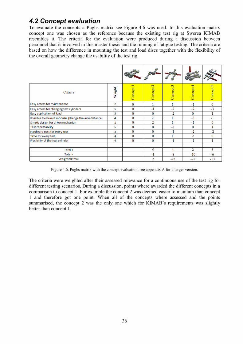
4.2 Concept evaluation To evaluate the concepts a Pughs matrix see Figure 4.6 was used. In this evaluation matrix
concept one was chosen as the reference because the existing test rig at Swerea KIMAB
resembles it. The criteria for the evaluation were produced during a discussion between
personnel that is involved in this master thesis and the running of fatigue testing. The criteria are
based on how the difference in mounting the test and load discs together with the flexibility of
the overall geometry change the usability of the test rig.
Figure 4.6. Pughs matrix with the concept evaluation, see appendix A for a larger version.
The criteria were weighted after their assessed relevance for a continuous use of the test rig for
different testing scenarios. During a discussion, points where awarded the different concepts in a
comparison to concept 1. For example the concept 2 was deemed easier to maintain than concept
1 and therefore got one point. When all of the concepts where assessed and the points
summarised, the concept 2 was the only one which for KIMAB’s requirements was slightly
better than concept 1.
37
4.3 Design of parts With the concept of the shaft alignment decided, the requirements from Table 3.1 was used as a
minimum and extended to a full requirement specification for a test rig that would suit KIMAB’s
needs. The complete specification can be found in appendix A. Some of the minimum
requirements were of course increased for the rig to be more flexible when it comes to new tests.
The new design specification can be found in Table 4.1 below.
Table 4.1. The design specifications for Swerea KIMABs test rig.
Maximum load 10 kN
Minimum speed 3000 rpm
Variable axle distance 40 to 150 mm
Oil inlet heater 20 to 110 °C
Maximum weight 1000 kg
Maximum width 900 mm
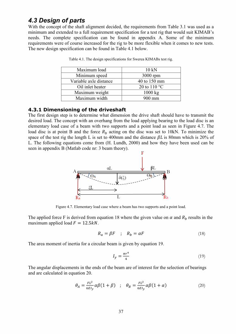
4.3.1 Dimensioning of the driveshaft The first design step is to determine what dimension the drive shaft should have to transmit the
desired load. The concept with an overhang from the load applying bearing to the load disc is an
elementary load case of a beam with two supports and a point load as seen in Figure 4.7. The
load disc is at point B and the force 𝑅𝑏 acting on the disc was set to 10kN. To minimize the
space of the test rig the length L is set to 400mm and the distance 𝛽𝐿 is 80mm which is 20% of
L. The following equations come from (H. Lundh, 2000) and how they have been used can be
seen in appendix B (Matlab code nr: 3 beam theory).
Figure 4.7. Elementary load case where a beam has two supports and a point load.
The applied force F is derived from equation 18 where the given value on 𝛼 and 𝑅𝑏 results in the
maximum applied load 𝐹 = 12.5𝑘𝑁.
𝑅𝑎 = 𝛽𝐹 ; 𝑅𝑏 = 𝛼𝐹 (18)
The area moment of inertia for a circular beam is given by equation 19.
𝐼𝑦 =𝜋𝑟4
4 (19)
The angular displacements in the ends of the beam are of interest for the selection of bearings
and are calculated in equation 20.
𝜃𝐴 =𝐹𝐿2
6𝐸𝐼𝑦𝛼𝛽(1 + 𝛽) ; 𝜃𝐵 =
𝐹𝐿2
6𝐸𝐼𝑦𝛼𝛽(1 + 𝛼) (20)
38
The displacement 𝛿(𝜉) is given by equation 21.
𝛿(𝜉) =𝐹𝐿3
6𝐸𝐼𝑦𝛽[(1 − 𝛽2)𝜉 − 𝜉3] 𝑓𝑜𝑟 𝜉 ≤ 𝛼 (2.1)
The maximum bending torque is found in the point where the load is applied, and is calculated
with equation 22.
𝑀𝑚𝑎𝑥 = 𝑅𝑏𝛽𝐿(Error! Reference source not found.2)
To use these equations and their results, the maximum tension 𝜎𝑚𝑎𝑥 is calculated in equation 23.
|𝜎|𝑚𝑎𝑥 =|𝑀|𝑚𝑎𝑥
𝐼𝑦
𝑟
(23)
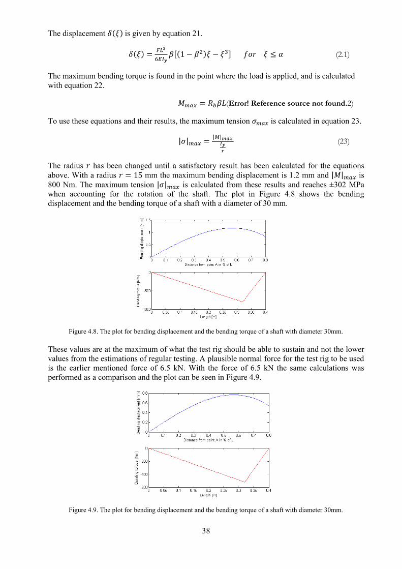
The radius 𝑟 has been changed until a satisfactory result has been calculated for the equations
above. With a radius 𝑟 = 15 mm the maximum bending displacement is 1.2 mm and |𝑀|𝑚𝑎𝑥 is
800 Nm. The maximum tension |𝜎|𝑚𝑎𝑥 is calculated from these results and reaches ±302 MPa
when accounting for the rotation of the shaft. The plot in Figure 4.8 shows the bending
displacement and the bending torque of a shaft with a diameter of 30 mm.
Figure 4.8. The plot for bending displacement and the bending torque of a shaft with diameter 30mm.
These values are at the maximum of what the test rig should be able to sustain and not the lower
values from the estimations of regular testing. A plausible normal force for the test rig to be used
is the earlier mentioned force of 6.5 kN. With the force of 6.5 kN the same calculations was
performed as a comparison and the plot can be seen in Figure 4.9.
Figure 4.9. The plot for bending displacement and the bending torque of a shaft with diameter 30mm.
39
With the same shaft dimensions the Table 4.2 below shows a comparison of the results between
normal usage and maximum usage. Included in the table is also the angular change at the ends A
and B on the shaft.
Table 4.2. A comparison between a load of 10 kN and 6.5 kN on the shaft
10 kN
|𝑀|𝑚𝑎𝑥 800 Nm
|𝜎|𝑚𝑎𝑥 ±302 MPa
𝛿(𝜉)𝑚𝑎𝑥 1.2 mm
𝜃𝐴 0.0078°
𝜃𝐵 0.0117°
6.5 kN
|𝑀|𝑚𝑎𝑥 520 Nm
|𝜎|𝑚𝑎𝑥 ±196 MPa
𝛿(𝜉)𝑚𝑎𝑥 0.76 mm
𝜃𝐴 0.0051°
𝜃𝐵 0.0076°
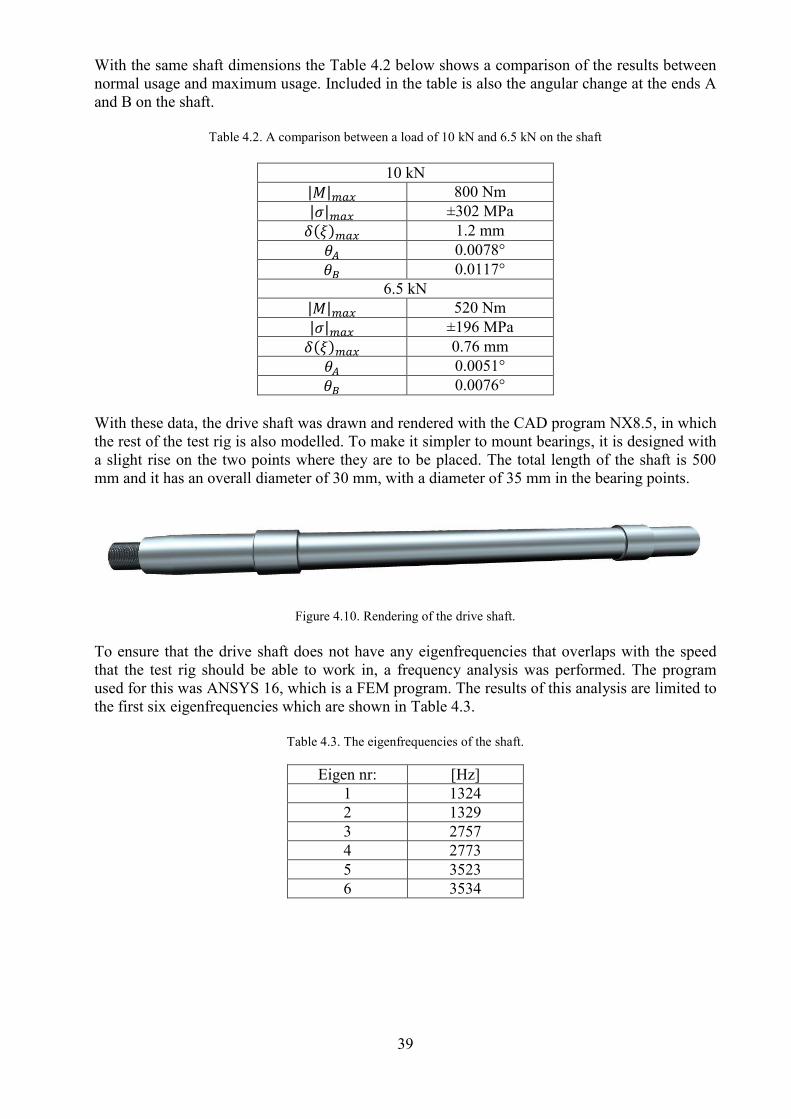
With these data, the drive shaft was drawn and rendered with the CAD program NX8.5, in which
the rest of the test rig is also modelled. To make it simpler to mount bearings, it is designed with
a slight rise on the two points where they are to be placed. The total length of the shaft is 500
mm and it has an overall diameter of 30 mm, with a diameter of 35 mm in the bearing points.
Figure 4.10. Rendering of the drive shaft.
To ensure that the drive shaft does not have any eigenfrequencies that overlaps with the speed
that the test rig should be able to work in, a frequency analysis was performed. The program
used for this was ANSYS 16, which is a FEM program. The results of this analysis are limited to
the first six eigenfrequencies which are shown in Table 4.3.
Table 4.3. The eigenfrequencies of the shaft.
Eigen nr: [Hz]
1 1324
2 1329
3 2757
4 2773
5 3523
6 3534
40
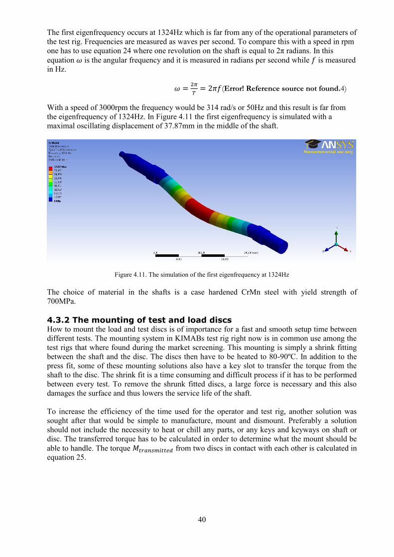
The first eigenfrequency occurs at 1324Hz which is far from any of the operational parameters of
the test rig. Frequencies are measured as waves per second. To compare this with a speed in rpm
one has to use equation 24 where one revolution on the shaft is equal to 2π radians. In this
equation 𝜔 is the angular frequency and it is measured in radians per second while 𝑓 is measured
in Hz.
𝜔 =2𝜋
𝑇= 2𝜋𝑓(Error! Reference source not found.4)
With a speed of 3000rpm the frequency would be 314 rad/s or 50Hz and this result is far from
the eigenfrequency of 1324Hz. In Figure 4.11 the first eigenfrequency is simulated with a
maximal oscillating displacement of 37.87mm in the middle of the shaft.
Figure 4.11. The simulation of the first eigenfrequency at 1324Hz
The choice of material in the shafts is a case hardened CrMn steel with yield strength of
700MPa.
4.3.2 The mounting of test and load discs How to mount the load and test discs is of importance for a fast and smooth setup time between
different tests. The mounting system in KIMABs test rig right now is in common use among the
test rigs that where found during the market screening. This mounting is simply a shrink fitting
between the shaft and the disc. The discs then have to be heated to 80-90ºC. In addition to the
press fit, some of these mounting solutions also have a key slot to transfer the torque from the
shaft to the disc. The shrink fit is a time consuming and difficult process if it has to be performed
between every test. To remove the shrunk fitted discs, a large force is necessary and this also
damages the surface and thus lowers the service life of the shaft.
To increase the efficiency of the time used for the operator and test rig, another solution was
sought after that would be simple to manufacture, mount and dismount. Preferably a solution
should not include the necessity to heat or chill any parts, or any keys and keyways on shaft or
disc. The transferred torque has to be calculated in order to determine what the mount should be
able to handle. The torque 𝑀𝑡𝑟𝑎𝑛𝑠𝑚𝑖𝑡𝑡𝑒𝑑 from two discs in contact with each other is calculated in
equation 25.
41
𝑀𝑡𝑟𝑎𝑛𝑠𝑚𝑖𝑡𝑡𝑒𝑑 = 𝐹𝜇𝑟 (25)
The force 𝐹 is the designed maximum for the discs 10 kN and the friction coefficient 𝜇 is set to a
value of 0.1 which is what the test and load discs are manufactured for. The radius 𝑟 of the discs
is set to 25 mm, the result is 𝑀𝑡𝑟𝑎𝑛𝑠𝑚𝑖𝑡𝑡𝑒𝑑 = 25 Nm.
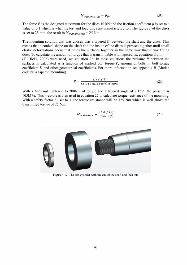
The mounting solution that was chosen was a tapered fit between the shaft and the discs. This
means that a conical shape on the shaft and the inside of the discs is pressed together until small
elastic deformations occur that holds the surfaces together in the same way that shrink fitting
does. To calculate the amount of torque that is transmittable with tapered fit, equations from
(T. Hicks, 2006) were used, see equation 26. In these equations the pressure 𝑃 between the
surfaces is calculated as a function of applied bolt torque 𝑇, amount of bolts 𝑛, bolt torque
coefficient 𝐾 and other geometrical coefficients. For more information see appendix B (Matlab
code nr: 4 tapered mounting).
𝑃 =2𝑇𝑛 𝑐𝑜𝑠(𝜃)
𝐾𝑏(𝐷+𝑑)𝜋𝐿(𝜇 cos(𝜃)+sin (𝜃)) (26)
With a M20 nut tightened to 200Nm of torque and a tapered angle of 7.125º, the pressure is
105MPa. This pressure is then used in equation 27 to calculate torque resistance of the mounting.
With a safety factor 𝑆𝐹 set to 3, the torque resistance will be 125 Nm which is well above the
transmitted torque of 25 Nm.
𝑀𝑟𝑒𝑠𝑖𝑠𝑡𝑎𝑛𝑐𝑒 =𝜇𝑃𝜋𝐿(𝐷+𝑑)2
𝑆𝐹8 cos (𝜃) (27)
Figure 4.12. The test cylinder with the end of the shaft and lock nut.
42
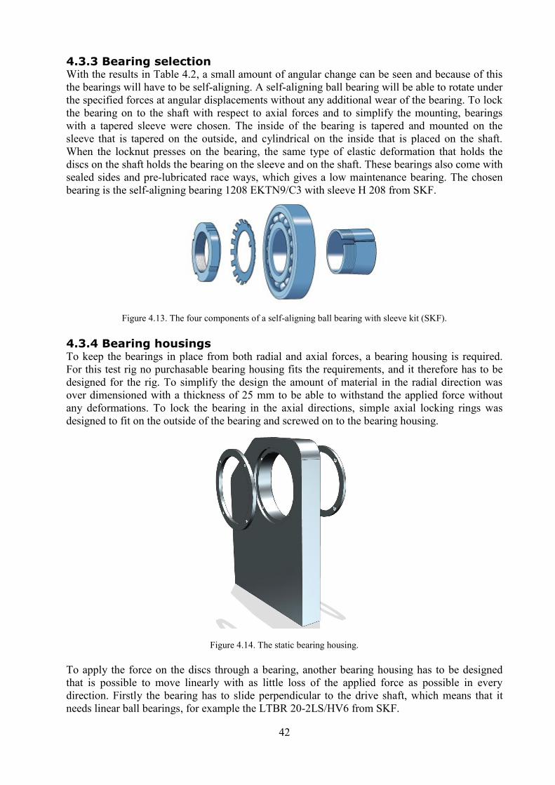
4.3.3 Bearing selection With the results in Table 4.2, a small amount of angular change can be seen and because of this
the bearings will have to be self-aligning. A self-aligning ball bearing will be able to rotate under
the specified forces at angular displacements without any additional wear of the bearing. To lock
the bearing on to the shaft with respect to axial forces and to simplify the mounting, bearings
with a tapered sleeve were chosen. The inside of the bearing is tapered and mounted on the
sleeve that is tapered on the outside, and cylindrical on the inside that is placed on the shaft.
When the locknut presses on the bearing, the same type of elastic deformation that holds the
discs on the shaft holds the bearing on the sleeve and on the shaft. These bearings also come with
sealed sides and pre-lubricated race ways, which gives a low maintenance bearing. The chosen
bearing is the self-aligning bearing 1208 EKTN9/C3 with sleeve H 208 from SKF.
Figure 4.13. The four components of a self-aligning ball bearing with sleeve kit (SKF).
4.3.4 Bearing housings To keep the bearings in place from both radial and axial forces, a bearing housing is required.
For this test rig no purchasable bearing housing fits the requirements, and it therefore has to be
designed for the rig. To simplify the design the amount of material in the radial direction was
over dimensioned with a thickness of 25 mm to be able to withstand the applied force without
any deformations. To lock the bearing in the axial directions, simple axial locking rings was
designed to fit on the outside of the bearing and screwed on to the bearing housing.
Figure 4.14. The static bearing housing.
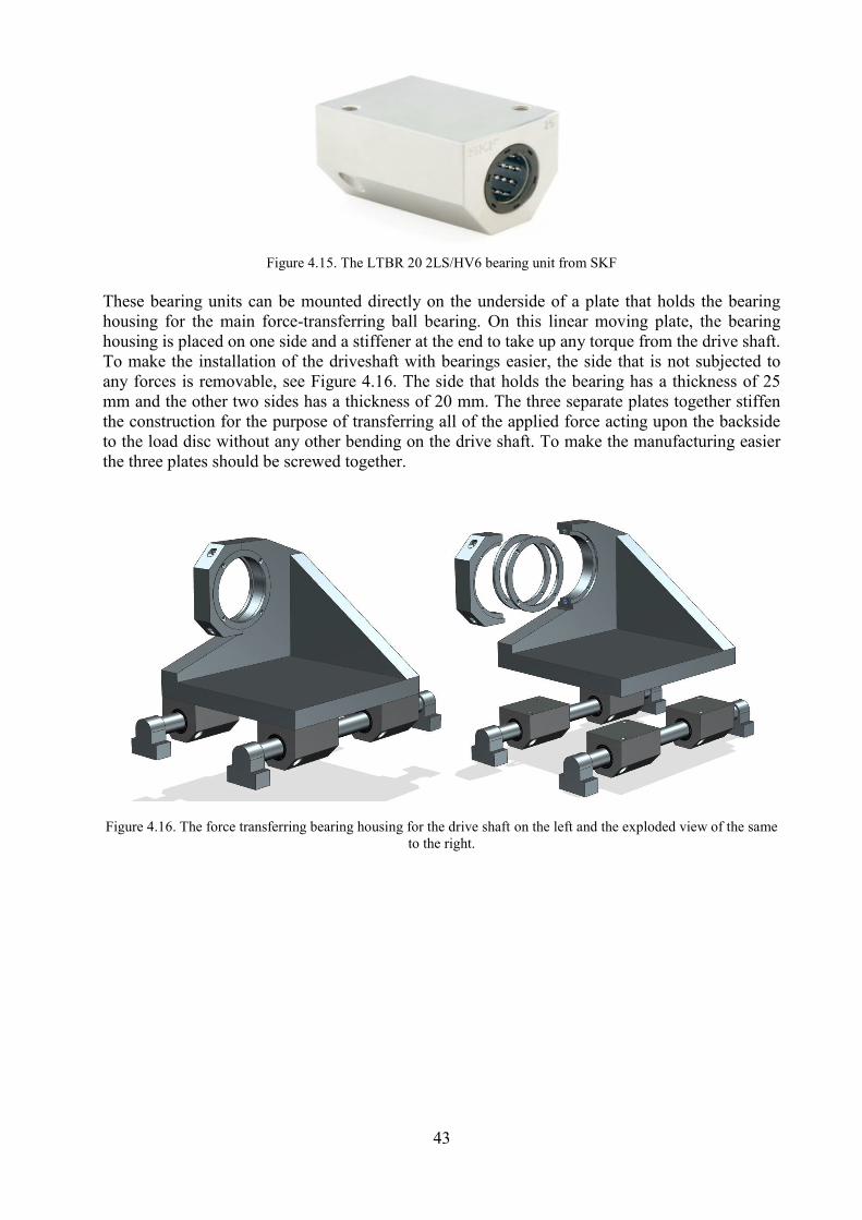
To apply the force on the discs through a bearing, another bearing housing has to be designed
that is possible to move linearly with as little loss of the applied force as possible in every
direction. Firstly the bearing has to slide perpendicular to the drive shaft, which means that it
needs linear ball bearings, for example the LTBR 20-2LS/HV6 from SKF.
43
Figure 4.15. The LTBR 20 2LS/HV6 bearing unit from SKF
These bearing units can be mounted directly on the underside of a plate that holds the bearing
housing for the main force-transferring ball bearing. On this linear moving plate, the bearing
housing is placed on one side and a stiffener at the end to take up any torque from the drive shaft.
To make the installation of the driveshaft with bearings easier, the side that is not subjected to
any forces is removable, see Figure 4.16. The side that holds the bearing has a thickness of 25
mm and the other two sides has a thickness of 20 mm. The three separate plates together stiffen
the construction for the purpose of transferring all of the applied force acting upon the backside
to the load disc without any other bending on the drive shaft. To make the manufacturing easier
the three plates should be screwed together.
Figure 4.16. The force transferring bearing housing for the drive shaft on the left and the exploded view of the same
to the right.
44
4.3.5 Choice of motor To decide the type of motor that would best serve this test rig, the requirements has to be
examined again. Firstly the torque generated from the test cylinder and load disc has to be
calculated with regard to the applied pressure and geometry of the tests cylinders. The motor has
to be able to drive the test rig with the highest amount of specified force between the discs,
which are 10 kN. For a test with that amount of force it is reasonable that the cylinder should not
exceed a diameter of 50mm. The torque of a rotating contact is specified in equation 28 with the
force 𝐹 the friction in the contact 𝜇 = 0.1 and the radius 𝑟 of the cylinder.
𝑀𝑠ℎ𝑎𝑓𝑡 = 𝐹𝜇𝑟 (28)
With the specified values the highest torque should be 25 Nm, the more probable force of 6.5 kN
gives a torque of 16.25 Nm. These results give the first idea of what the motors should be able to
handle during a test. To visualize how speed of the motors and the geometry of the test cylinders
correlate to each other different parameters were plotted against a rising diameter of the disc as
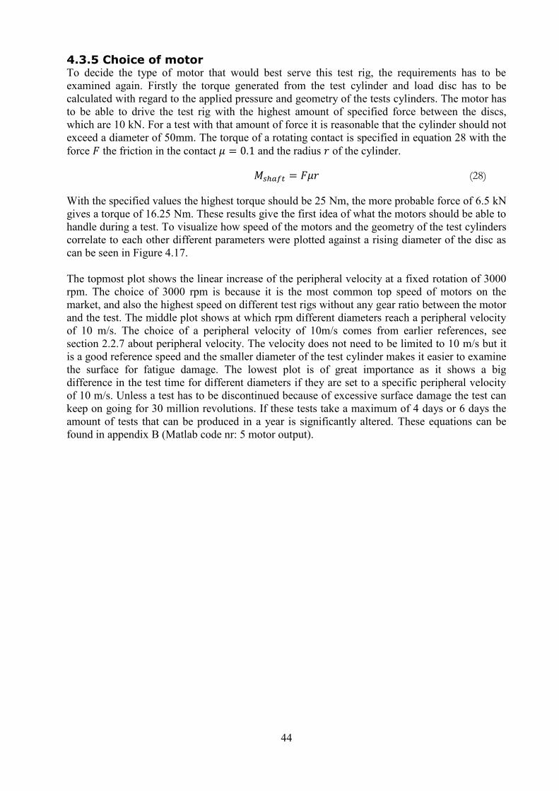
can be seen in Figure 4.17.
The topmost plot shows the linear increase of the peripheral velocity at a fixed rotation of 3000
rpm. The choice of 3000 rpm is because it is the most common top speed of motors on the
market, and also the highest speed on different test rigs without any gear ratio between the motor
and the test. The middle plot shows at which rpm different diameters reach a peripheral velocity
of 10 m/s. The choice of a peripheral velocity of 10m/s comes from earlier references, see
section 2.2.7 about peripheral velocity. The velocity does not need to be limited to 10 m/s but it
is a good reference speed and the smaller diameter of the test cylinder makes it easier to examine
the surface for fatigue damage. The lowest plot is of great importance as it shows a big
difference in the test time for different diameters if they are set to a specific peripheral velocity
of 10 m/s. Unless a test has to be discontinued because of excessive surface damage the test can
keep on going for 30 million revolutions. If these tests take a maximum of 4 days or 6 days the
amount of tests that can be produced in a year is significantly altered. These equations can be
found in appendix B (Matlab code nr: 5 motor output).
45
Figure 4.17. Three different plots to compare what happens when the test cylinders diameter is changed.
From these results, it can be concluded that the goal is a small diameter test cylinder that can be
driven at a high rpm, preferably around 5000 rpm. It is also of interest to see how much work the
motor has to put out to reach these results.
𝑃 = 𝜏 ∗ 𝜔 (29)
Where 𝜏 is the load in Nm and 𝜔 is angular velocity in 𝑟𝑎𝑑/𝑠.
With the maximum of 25 Nm and a speed of 3000 rpm we get a work of 7853 W. With the more
plausible load of 16.25 Nm at the same speed we get a work of 5105 W.
The other aspect of the motor is that it should be possible to control its angular velocity very
accurately for the slip to be controlled and the test to be repeatable. With these data the motor
manufacturer ABB in Västerås was contacted to see what they recommended and to give a quote
on a motor.
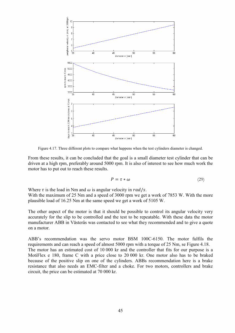
ABB’s recommendation was the servo motor BSM 100C-6150. The motor fulfils the
requirements and can reach a speed of almost 5000 rpm with a torque of 25 Nm, se Figure 4.18.
The motor has an estimated cost of 10 000 kr and the controller that fits for our purpose is a
MotiFlex e 180, frame C with a price close to 20 000 kr. One motor also has to be braked
because of the positive slip on one of the cylinders. ABBs recommendation here is a brake
resistance that also needs an EMC-filter and a choke. For two motors, controllers and brake
circuit, the price can be estimated at 70 000 kr.
46
Figure 4.18. Performance graph of the BSM 100c-6150 (Baldor)
4.3.6 Design of environment box The container that surrounds the test and load disc has a couple of important purposes, and that is
to contain all of the excess lubricant both in liquid form and as a gas. It should keep the test
environment as clean as possible from foreign particles that can contaminate the test. It should
keep the temperature even during the test and it should if possible be simple to change the discs.
The inlet and outlet of the lubricant will be through the sides and also a bushing for a surface
damage sensor should be possible to place in it.
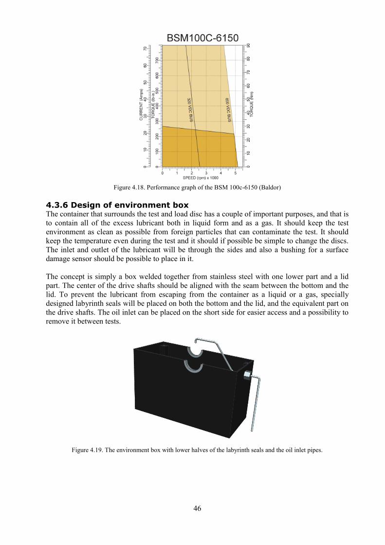
The concept is simply a box welded together from stainless steel with one lower part and a lid
part. The center of the drive shafts should be aligned with the seam between the bottom and the
lid. To prevent the lubricant from escaping from the container as a liquid or a gas, specially
designed labyrinth seals will be placed on both the bottom and the lid, and the equivalent part on
the drive shafts. The oil inlet can be placed on the short side for easier access and a possibility to
remove it between tests.
Figure 4.19. The environment box with lower halves of the labyrinth seals and the oil inlet pipes.
47
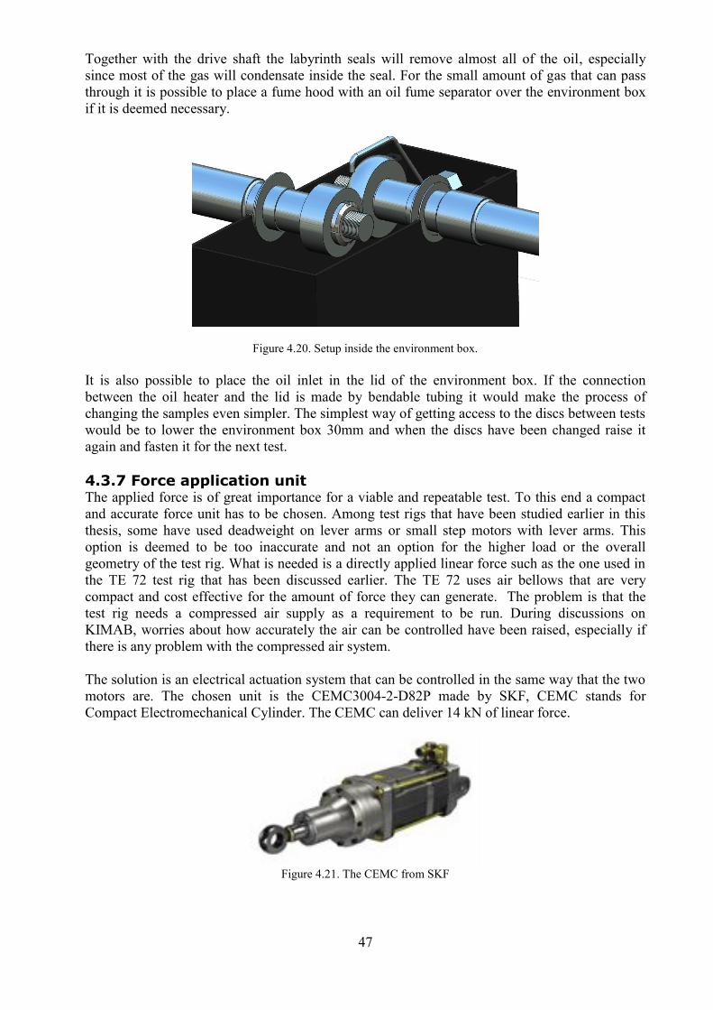
Together with the drive shaft the labyrinth seals will remove almost all of the oil, especially
since most of the gas will condensate inside the seal. For the small amount of gas that can pass
through it is possible to place a fume hood with an oil fume separator over the environment box
if it is deemed necessary.
Figure 4.20. Setup inside the environment box.
It is also possible to place the oil inlet in the lid of the environment box. If the connection
between the oil heater and the lid is made by bendable tubing it would make the process of
changing the samples even simpler. The simplest way of getting access to the discs between tests
would be to lower the environment box 30mm and when the discs have been changed raise it
again and fasten it for the next test.
4.3.7 Force application unit The applied force is of great importance for a viable and repeatable test. To this end a compact
and accurate force unit has to be chosen. Among test rigs that have been studied earlier in this
thesis, some have used deadweight on lever arms or small step motors with lever arms. This
option is deemed to be too inaccurate and not an option for the higher load or the overall
geometry of the test rig. What is needed is a directly applied linear force such as the one used in
the TE 72 test rig that has been discussed earlier. The TE 72 uses air bellows that are very
compact and cost effective for the amount of force they can generate. The problem is that the
test rig needs a compressed air supply as a requirement to be run. During discussions on
KIMAB, worries about how accurately the air can be controlled have been raised, especially if
there is any problem with the compressed air system.
The solution is an electrical actuation system that can be controlled in the same way that the two
motors are. The chosen unit is the CEMC3004-2-D82P made by SKF, CEMC stands for
Compact Electromechanical Cylinder. The CEMC can deliver 14 kN of linear force.
Figure 4.21. The CEMC from SKF
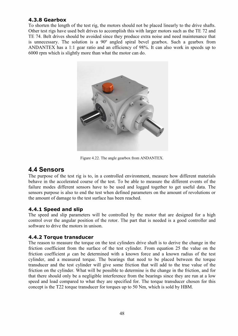
48
4.3.8 Gearbox To shorten the length of the test rig, the motors should not be placed linearly to the drive shafts.
Other test rigs have used belt drives to accomplish this with larger motors such as the TE 72 and
TE 74. Belt drives should be avoided since they produce extra noise and need maintenance that
is unnecessary. The solution is a 90º angled spiral bevel gearbox. Such a gearbox from
ANDANTEX has a 1:1 gear ratio and an efficiency of 98%. It can also work in speeds up to
6000 rpm which is slightly more than what the motor can do.
Figure 4.22. The angle gearbox from ANDANTEX.
4.4 Sensors The purpose of the test rig is to, in a controlled environment, measure how different materials
behave in the accelerated course of the test. To be able to measure the different events of the
failure modes different sensors have to be used and logged together to get useful data. The
sensors purpose is also to end the test when defined parameters on the amount of revolutions or
the amount of damage to the test surface has been reached.
4.4.1 Speed and slip The speed and slip parameters will be controlled by the motor that are designed for a high
control over the angular position of the rotor. The part that is needed is a good controller and
software to drive the motors in unison.
4.4.2 Torque transducer The reason to measure the torque on the test cylinders drive shaft is to derive the change in the
friction coefficient from the surface of the test cylinder. From equation 25 the value on the
friction coefficient 𝜇 can be determined with a known force and a known radius of the test
cylinder, and a measured torque. The bearings that need to be placed between the torque
transducer and the test cylinder will give some friction that will add to the true value of the
friction on the cylinder. What will be possible to determine is the change in the friction, and for
that there should only be a negligible interference from the bearings since they are run at a low
speed and load compared to what they are specified for. The torque transducer chosen for this
concept is the T22 torque transducer for torques up to 50 Nm, which is sold by HBM.
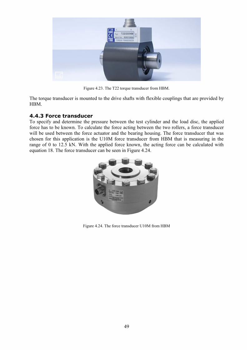
49
Figure 4.23. The T22 torque transducer from HBM.
The torque transducer is mounted to the drive shafts with flexible couplings that are provided by
HBM.
4.4.3 Force transducer To specify and determine the pressure between the test cylinder and the load disc, the applied
force has to be known. To calculate the force acting between the two rollers, a force transducer
will be used between the force actuator and the bearing housing. The force transducer that was
chosen for this application is the U10M force transducer from HBM that is measuring in the
range of 0 to 12.5 kN. With the applied force known, the acting force can be calculated with
equation 18. The force transducer can be seen in Figure 4.24.
Figure 4.24. The force transducer U10M from HBM
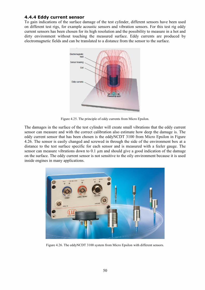
50
4.4.4 Eddy current sensor To gain indications of the surface damage of the test cylinder, different sensors have been used
on different test rigs, for example acoustic sensors and vibration sensors. For this test rig eddy
current sensors has been chosen for its high resolution and the possibility to measure in a hot and
dirty environment without touching the measured surface. Eddy currents are produced by
electromagnetic fields and can be translated to a distance from the sensor to the surface.
Figure 4.25. The principle of eddy currents from Micro Epsilon.
The damages in the surface of the test cylinder will create small vibrations that the eddy current
sensor can measure and with the correct calibration also estimate how deep the damage is. The
eddy current sensor that has been chosen is the eddyNCDT 3100 from Micro Epsilon in Figure
4.26. The sensor is easily changed and screwed in through the side of the environment box at a
distance to the test surface specific for each sensor and is measured with a feeler gauge. The
sensor can measure vibrations down to 0.1 µm and should give a good indication of the damage
on the surface. The eddy current sensor is not sensitive to the oily environment because it is used
inside engines in many applications.
Figure 4.26. The eddyNCDT 3100 system from Micro Epsilon with different sensors.

51
4.4.5 Controller and software To control the test rig, a controller is needed that can translate analogue signals from the sensors
and the motors to digital signals that can be programmed in a graphical interface. The company
that has provided these hardware to software interfaces for KIMAB before, recommended the
DOLI EDC580V controller. This controller has eight channels and can control all of the
controllable and measuring parts of the test rig simultaneously.
Figure 4.27. The controller EDC580V from DOLI
The same company has also given an estimate for the coding of the software to three weeks. This
is also the part of the master thesis that can evolve into a completely separate work since this
thesis is limited to the mechanics and not an in-depth study of control systems. It is therefore
possible to find another solution for the controls and software for example with LabVIEW, but
this is left for future works on the test rig.

52
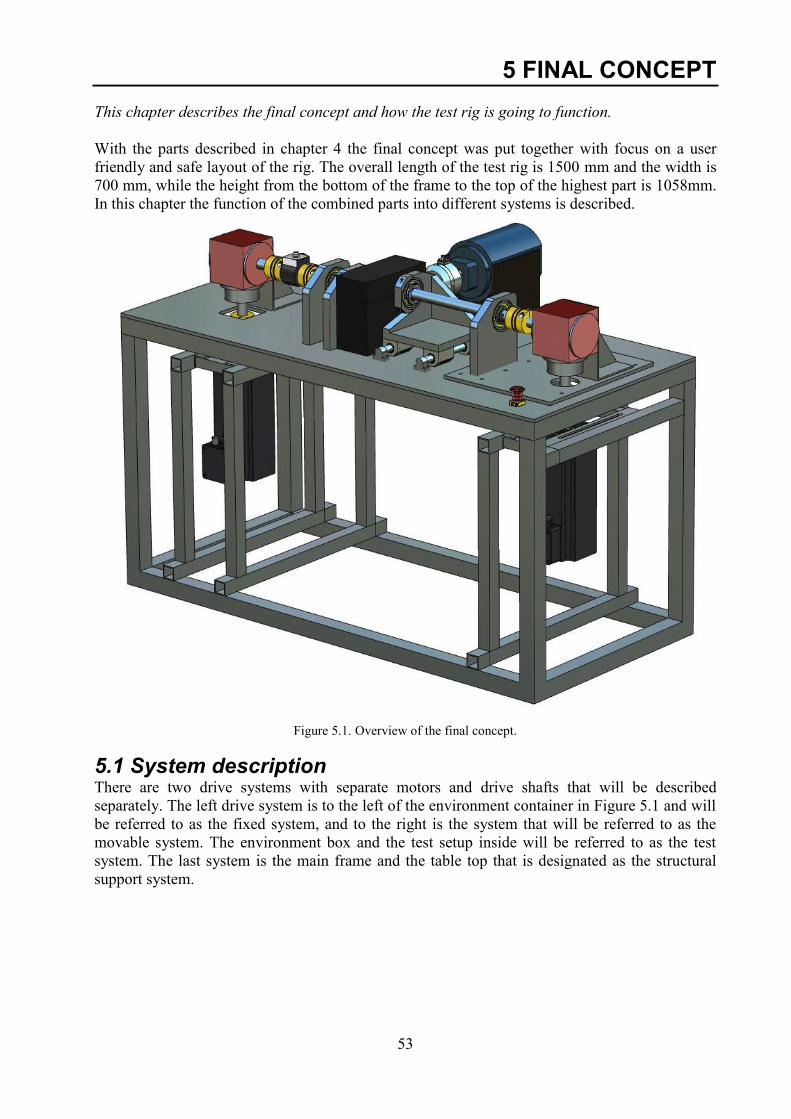
53
5 FINAL CONCEPT
This chapter describes the final concept and how the test rig is going to function.
With the parts described in chapter 4 the final concept was put together with focus on a user
friendly and safe layout of the rig. The overall length of the test rig is 1500 mm and the width is
700 mm, while the height from the bottom of the frame to the top of the highest part is 1058mm.
In this chapter the function of the combined parts into different systems is described.
Figure 5.1. Overview of the final concept.
5.1 System description There are two drive systems with separate motors and drive shafts that will be described
separately. The left drive system is to the left of the environment container in Figure 5.1 and will
be referred to as the fixed system, and to the right is the system that will be referred to as the
movable system. The environment box and the test setup inside will be referred to as the test
system. The last system is the main frame and the table top that is designated as the structural
support system.
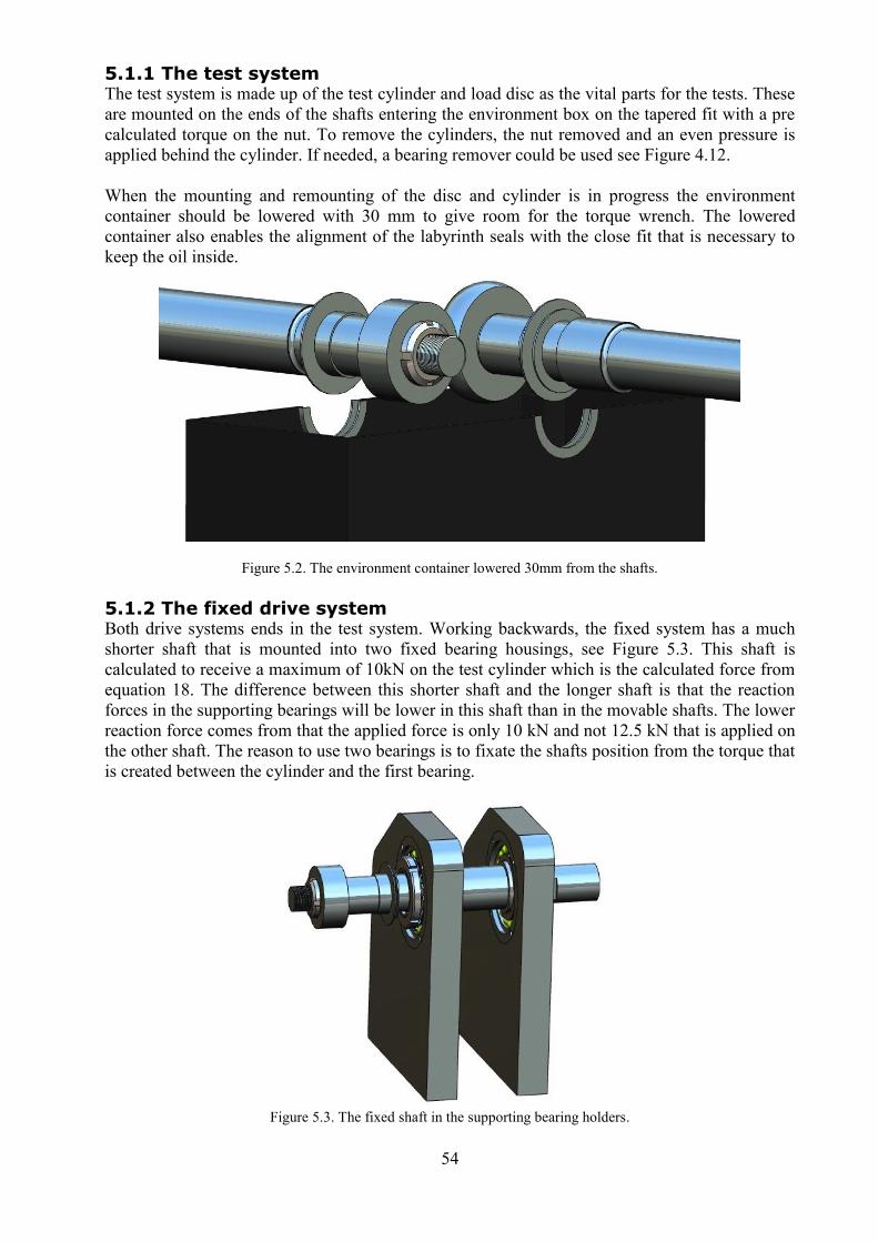
54
5.1.1 The test system The test system is made up of the test cylinder and load disc as the vital parts for the tests. These
are mounted on the ends of the shafts entering the environment box on the tapered fit with a pre
calculated torque on the nut. To remove the cylinders, the nut removed and an even pressure is
applied behind the cylinder. If needed, a bearing remover could be used see Figure 4.12.
When the mounting and remounting of the disc and cylinder is in progress the environment
container should be lowered with 30 mm to give room for the torque wrench. The lowered
container also enables the alignment of the labyrinth seals with the close fit that is necessary to
keep the oil inside.
Figure 5.2. The environment container lowered 30mm from the shafts.
5.1.2 The fixed drive system Both drive systems ends in the test system. Working backwards, the fixed system has a much
shorter shaft that is mounted into two fixed bearing housings, see Figure 5.3. This shaft is
calculated to receive a maximum of 10kN on the test cylinder which is the calculated force from
equation 18. The difference between this shorter shaft and the longer shaft is that the reaction
forces in the supporting bearings will be lower in this shaft than in the movable shafts. The lower
reaction force comes from that the applied force is only 10 kN and not 12.5 kN that is applied on
the other shaft. The reason to use two bearings is to fixate the shafts position from the torque that
is created between the cylinder and the first bearing.
Figure 5.3. The fixed shaft in the supporting bearing holders.
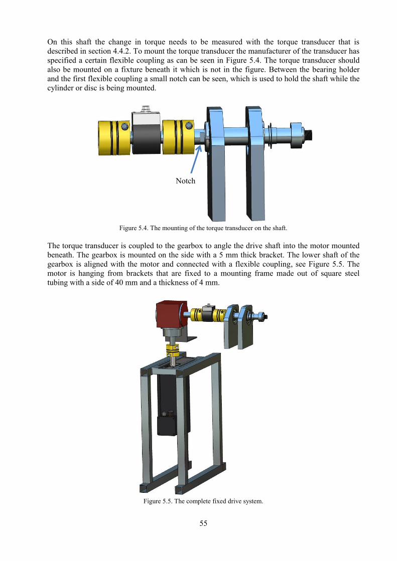
55
On this shaft the change in torque needs to be measured with the torque transducer that is
described in section 4.4.2. To mount the torque transducer the manufacturer of the transducer has
specified a certain flexible coupling as can be seen in Figure 5.4. The torque transducer should
also be mounted on a fixture beneath it which is not in the figure. Between the bearing holder
and the first flexible coupling a small notch can be seen, which is used to hold the shaft while the
cylinder or disc is being mounted.
Figure 5.4. The mounting of the torque transducer on the shaft.
The torque transducer is coupled to the gearbox to angle the drive shaft into the motor mounted
beneath. The gearbox is mounted on the side with a 5 mm thick bracket. The lower shaft of the
gearbox is aligned with the motor and connected with a flexible coupling, see Figure 5.5. The
motor is hanging from brackets that are fixed to a mounting frame made out of square steel
tubing with a side of 40 mm and a thickness of 4 mm.
Figure 5.5. The complete fixed drive system.
Notch
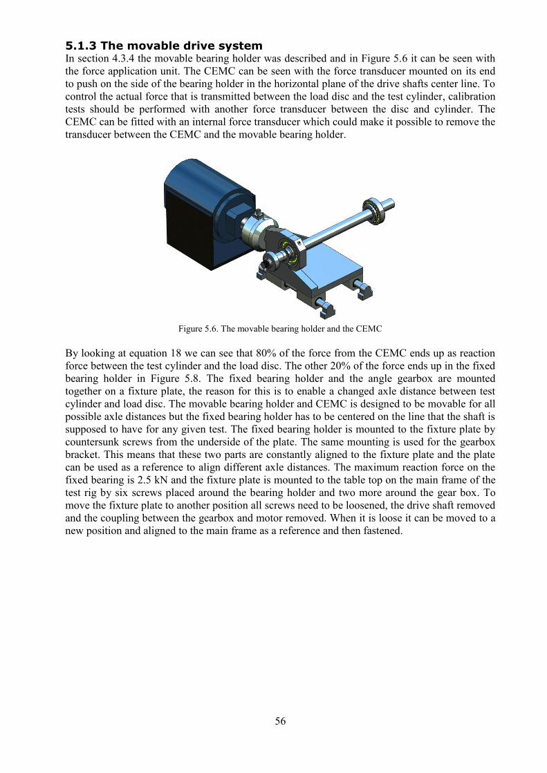
56
5.1.3 The movable drive system In section 4.3.4 the movable bearing holder was described and in Figure 5.6 it can be seen with
the force application unit. The CEMC can be seen with the force transducer mounted on its end
to push on the side of the bearing holder in the horizontal plane of the drive shafts center line. To
control the actual force that is transmitted between the load disc and the test cylinder, calibration
tests should be performed with another force transducer between the disc and cylinder. The
CEMC can be fitted with an internal force transducer which could make it possible to remove the
transducer between the CEMC and the movable bearing holder.
Figure 5.6. The movable bearing holder and the CEMC
By looking at equation 18 we can see that 80% of the force from the CEMC ends up as reaction
force between the test cylinder and the load disc. The other 20% of the force ends up in the fixed
bearing holder in Figure 5.8. The fixed bearing holder and the angle gearbox are mounted
together on a fixture plate, the reason for this is to enable a changed axle distance between test
cylinder and load disc. The movable bearing holder and CEMC is designed to be movable for all
possible axle distances but the fixed bearing holder has to be centered on the line that the shaft is
supposed to have for any given test. The fixed bearing holder is mounted to the fixture plate by
countersunk screws from the underside of the plate. The same mounting is used for the gearbox
bracket. This means that these two parts are constantly aligned to the fixture plate and the plate
can be used as a reference to align different axle distances. The maximum reaction force on the
fixed bearing is 2.5 kN and the fixture plate is mounted to the table top on the main frame of the
test rig by six screws placed around the bearing holder and two more around the gear box. To
move the fixture plate to another position all screws need to be loosened, the drive shaft removed
and the coupling between the gearbox and motor removed. When it is loose it can be moved to a
new position and aligned to the main frame as a reference and then fastened.
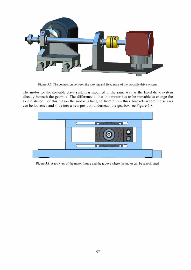
57
Figure 5.7. The connection between the moving and fixed parts of the movable drive system.
The motor for the movable drive system is mounted in the same way as the fixed drive system
directly beneath the gearbox. The difference is that this motor has to be movable to change the
axle distance. For this reason the motor is hanging from 5 mm thick brackets where the screws
can be loosened and slide into a new position underneath the gearbox see Figure 5.8.
Figure 5.8. A top view of the motor fixture and the groove where the motor can be repositioned.
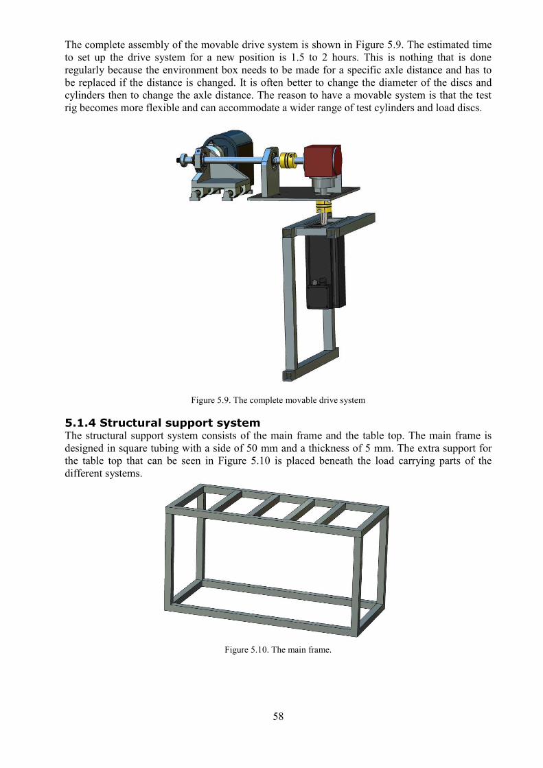
58
The complete assembly of the movable drive system is shown in Figure 5.9. The estimated time
to set up the drive system for a new position is 1.5 to 2 hours. This is nothing that is done
regularly because the environment box needs to be made for a specific axle distance and has to
be replaced if the distance is changed. It is often better to change the diameter of the discs and
cylinders then to change the axle distance. The reason to have a movable system is that the test
rig becomes more flexible and can accommodate a wider range of test cylinders and load discs.
Figure 5.9. The complete movable drive system
5.1.4 Structural support system The structural support system consists of the main frame and the table top. The main frame is
designed in square tubing with a side of 50 mm and a thickness of 5 mm. The extra support for
the table top that can be seen in Figure 5.10 is placed beneath the load carrying parts of the
different systems.
Figure 5.10. The main frame.
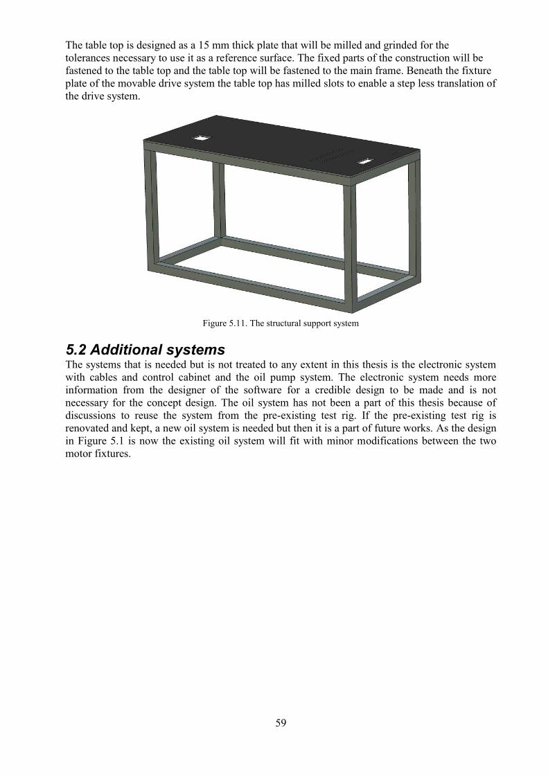
59
The table top is designed as a 15 mm thick plate that will be milled and grinded for the
tolerances necessary to use it as a reference surface. The fixed parts of the construction will be
fastened to the table top and the table top will be fastened to the main frame. Beneath the fixture
plate of the movable drive system the table top has milled slots to enable a step less translation of
the drive system.
Figure 5.11. The structural support system
5.2 Additional systems The systems that is needed but is not treated to any extent in this thesis is the electronic system
with cables and control cabinet and the oil pump system. The electronic system needs more
information from the designer of the software for a credible design to be made and is not
necessary for the concept design. The oil system has not been a part of this thesis because of
discussions to reuse the system from the pre-existing test rig. If the pre-existing test rig is
renovated and kept, a new oil system is needed but then it is a part of future works. As the design
in Figure 5.1 is now the existing oil system will fit with minor modifications between the two
motor fixtures.
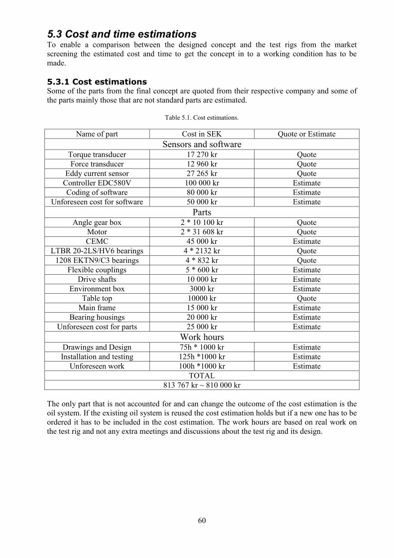
60
5.3 Cost and time estimations To enable a comparison between the designed concept and the test rigs from the market
screening the estimated cost and time to get the concept in to a working condition has to be
made.
5.3.1 Cost estimations Some of the parts from the final concept are quoted from their respective company and some of
the parts mainly those that are not standard parts are estimated.
Table 5.1. Cost estimations.
Name of part Cost in SEK Quote or Estimate
Sensors and software Torque transducer 17 270 kr Quote
Force transducer 12 960 kr Quote
Eddy current sensor 27 265 kr Quote
Controller EDC580V 100 000 kr Estimate
Coding of software 80 000 kr Estimate
Unforeseen cost for software 50 000 kr Estimate
Parts Angle gear box 2 * 10 100 kr Quote
Motor 2 * 31 608 kr Quote
CEMC 45 000 kr Estimate
LTBR 20-2LS/HV6 bearings 4 * 2132 kr Quote
1208 EKTN9/C3 bearings 4 * 832 kr Quote
Flexible couplings 5 * 600 kr Estimate
Drive shafts 10 000 kr Estimate
Environment box 3000 kr Estimate
Table top 10000 kr Quote
Main frame 15 000 kr Estimate
Bearing housings 20 000 kr Estimate
Unforeseen cost for parts 25 000 kr Estimate
Work hours Drawings and Design 75h * 1000 kr Estimate
Installation and testing 125h *1000 kr Estimate
Unforeseen work 100h *1000 kr Estimate
TOTAL
813 767 kr ~ 810 000 kr
The only part that is not accounted for and can change the outcome of the cost estimation is the
oil system. If the existing oil system is reused the cost estimation holds but if a new one has to be
ordered it has to be included in the cost estimation. The work hours are based on real work on
the test rig and not any extra meetings and discussions about the test rig and its design.
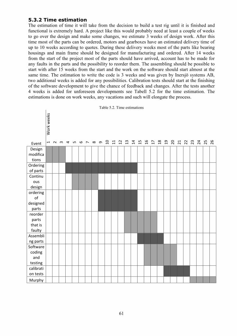
61
5.3.2 Time estimation The estimation of time it will take from the decision to build a test rig until it is finished and
functional is extremely hard. A project like this would probably need at least a couple of weeks
to go over the design and make some changes, we estimate 3 weeks of design work. After this
time most of the parts can be ordered, motors and gearboxes have an estimated delivery time of
up to 10 weeks according to quotes. During these delivery weeks most of the parts like bearing
housings and main frame should be designed for manufacturing and ordered. After 14 weeks
from the start of the project most of the parts should have arrived, account has to be made for
any faults in the parts and the possibility to reorder them. The assembling should be possible to
start with after 15 weeks from the start and the work on the software should start almost at the
same time. The estimation to write the code is 3 weeks and was given by Inersjö systems AB,
two additional weeks is added for any possibilities. Calibration tests should start at the finishing
of the software development to give the chance of feedback and changes. After the tests another
4 weeks is added for unforeseen developments see Tabell 5.2 for the time estimation. The
estimations is done on work weeks, any vacations and such will elongate the process.
Table 5.2. Time estimations
Wo
rk w
eeks
Event 1 2 3 4 5 6 7 8 9 1
0
11
12
13
14
15
16
17
18
19
20
21
22
23
24
25
26
Design modifica
tions
Ordering of parts
Continuous
design
ordering of
designed parts
reorder parts that is faulty
Assembling parts
Software coding
and testing
calibration tests
Murphy

62
63
6 DISCUSSION AND CONCLUSIONS
This chapter provides a discussion around KIMAB’s requirements and how both the concept test
rig and the recommended test rig from Phoenix tribology fulfils them and the conclusions that
can be drawn from this thesis.
6.1 Discussion
The requirements that KIMAB has in a test rig is based on potential clients requirements, to fulfil
the requirements of a broad range of clients the test rig has to be flexible. Both of the test rigs are
flexible enough to undertake the projects of the known project clients. The TE 72S has the
advantage over a manufactured rig in that KIMAB is not a company that manufactures machines.
It is therefore not a part of the core business to create a rig like this and that makes it even harder
to manufacture because there is no routine for a project like this. The possibility to have a client
support from Phoenix tribology is also of importance, especially if there is any problems with the
rig in the future and it has to be repaired. There is also a possibility to ask earlier byers of the
same rig about their experience with the rig and to ask them about test samples to see if they
match the expectations.
A decision to develop and manufacture a rig should be considered when the concept rig can be a
good tool in requiring new clients. With the newest sensors on the market and a robust design it
can compete with the TE 72S. The time and price can of course increase above the estimations in
this thesis but it is not likely to exceed them with an amount that will make the rig too costly in
the end. The advantage of the concept rig is that when it is built it can easily be duplicated to a
lower cost and shorter time. This is more advantageous because tests take a lot of time and if
there is enough projects that need surface fatigue testing more rigs will be needed.
To decide between the two alternatives KIMAB has to make an estimation of the markets future
in surface fatigue testing. If there is a moderate amount of projects in the future that need a new
rig fairly quickly then the TE 72S is the obvious choice. If there is an estimation of a slowly
increasing demand for surface fatigue testing that allows for the longer manufacturing time with
the possibility of more rigs later on, it could be a good idea to develop the concept.
6.2 conclusions
The conclusions is shown in points below.
KIMAB is in need of a new surface fatigue test rig.
Two alternatives that fulfils the requirements is presented.
The decision between the alternatives depends on estimations of future projects.
In pure performance the concept is better than the TE 72S.
More unforeseen events can appear around the development of the concept then buying
the TE 72S.
It is easier to manufacture further test rigs after the first is made.

64
65
7 FURTHER DEVELOPMENT AND FUTURE WORK
In this chapter the further development needed for the test rig and future work is presented.
7.1 Further development
To realise the concept into a working test rig some extra work is needed.
One critical point is to make a bigger frequency analyse of the complete test rig in order to find
any potential problems that could arise. The student version of ANSYS that was used did not
allow any more than one part at a time to be analysed. The equations would need to be
recalculated by a second party to ensure that they are correct.
The software is the part of the test rig that is the most complicated and also the part where most
of the problems can occur. The biggest risk with the development of a test rig is the calibration
of the sensors to the software to ensure that the data is correct. Before anything is ordered or
decided a software developer needs to be consulted on every part that is going to be connected to
the software.
7.2 Future work
In case that the decision lands on the purchasable test rig the future work entails a further study
of the rig and probably a visit to the manufacturer and possibly to any company that has
previously ordered the same rig.
If the choice is on the concept rig all of the equations and designs has to be scrutinised to find
any flaws in the reasoning and to determine if there is any better way of designing the parts. This
thesis is a foundation for the choices that KIMAB has to acquire a new test rig. Especially the
software are of importance to the concept rig, more work has to be put on the evaluation of
different software and developers of these.

66
67
8 REFERENCES
Anton van Beek, Advanced engineering design, Lifetime performance and reliability, 2009.
Bo Alfredsson, Lecture 16, contact mechanics, 2012.
Bo Alfredsson, A Study on Contact Fatigue Mechanisms, Doctoral Thesis no. 44, 2000.
R.L. Errichello, C. Hewette and R. Eckert, Point-Surface-Origin Macropitting Caused by
Geometric Stress Concentration
K. Aslantas¸, S. Tas¸getiren, A study of spur gear pitting formation and life prediction, 2004
On fatigue crack growth modelling of surface initiated rolling contact fatigue Dave Hannes,
using the asperity point load mechanism Doctoral Thesis no. 85, 2014
W.A glaeser and S.J Shaffer, Battelle Laboratories. ASM Handbook, Volume 19: Fatigue and
Fracture ASM Handbook Committee, p 331-336. 1996
Nicholas Bugliarello, Biji George, Don Giessel, Dan McCurdy, Ron Perkins, Steve
Richardson & Craig Zimmerman, Heat Treat Processes for Gears
Available at: http://www.gearsolutions.com/article/detail/6005/heat-treat-processes-for-gears
[Accessed 10-09-2015]
Inspection engineering [online]
Available at: http://www.inspectionengineering.com/Images/SurfaceFinishExplain.pdf
[Accessed 30-09-2015]
Michigan metrology [online]
Available at: http://www.michmet.com/2d_stylus_parameters_rkrpkrvk.htm
[Accessed 30-09-2015]
A. Oila, S.J. Bull, Assessment of the factors influencing micropitting
in rolling/sliding contacts, 2004
Dr.-Ing. Gottfried Hoffmann and William Jandeska, PhD. Effects on rolling contact fatigue
performance. 2007
Andy Olver, professor of tribology, department of mechanical engineering, Imperial college of
London. Lecture on the Effect of lubricant properties on EHL film thickness and traction
http://www.nrel.gov/wind/pdfs/day1_sessioni_3_imperial_olver.pdf
[Accessed 24-10-2015]
Hans Lundh, Grundläggande hållfastighetslära, 2000.
68
AccessEngineering [online]
Tyler G. Hicks: Handbook of Mechanical Engineering Calculations, Second Edition.
ANALYZING TAPER FITS FOR MANUFACTURING AND DESIGN, Chapter (McGraw-Hill
Professional, 2006 1998),
Available at:
https://www.google.se/url?sa=t&rct=j&q=&esrc=s&source=web&cd=1&ved=0ahUKEwikyaSt0
dTJAhXlLHIKHWQ9ADwQFggeMAA&url=http%3A%2F%2Faccessengineeringlibrary.com%
2Fpdfdownload%2F%3FcontentId%3Dhandbook-of-mechanical-engineering-calculations-
second-
edition%2Fp2000e9d699726_73001&usg=AFQjCNG0w_D_ymEDOmuN4bvkMRR4aKPrmA
&sig2=VwkkEEz2ulm57pjnQJ3KvQ&bvm=bv.109910813,d.bGQ&cad=rja
[Accessed 08-09-2015]
Baldor [online]
http://www2.baldor.com/products/servomotors/c_series/perf_graph.asp?catalognumber=BSM10
0C-6150AF
[Accessed 23-11-2015]
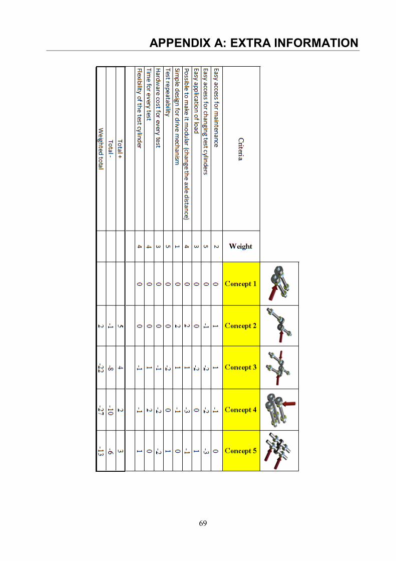
69
APPENDIX A: EXTRA INFORMATION
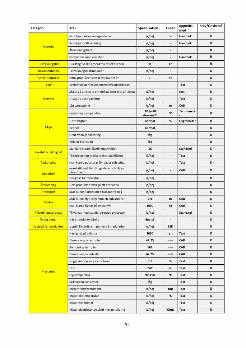
70
Kategori Krav Specifikation Enhet uppmätt med
Krav/Önskemål
Material
lämpliga mekaniska egenskaper ja/nej - Handbok K
lämpliga för tillverkning ja/nej - Handbok K
Återvinningsbara ja/nej - K
kompatibel med alla oljor ja/nej - Handbok Ö
Tillverkningstid Hur lång tid ska produkten ta att tillverka <1 år Ö
Dokumentation Tillverkningsinstruktioner ja/nej - K
Antal produkter Antal produkter som tillverkas per år 1 st K
Tester Kvalitetstester för att kontrollera prestandan - Test K
Säkerhet
Ska ej gå att starta om rörliga delar inte är täckta ja/nej - test K
Utsug av olja i gasform ja/nej - Test K
Låg tyngdpunkt ja/nej m CAD K
Miljö
omgivningstemperatur 10 to 40 degrees C
°C Termometer
K
Luftfuktighet normal % Hygrometer K
Renhet normal - K
Grad av dålig hantering låg - K
Risk för korrosion låg - K
Kvalitet & pålitlighet Standardiserad tillverkningskvalitet ISO - Standard K
Tillräckligt hög kvalitet säkrar pålitlighet ja/nej - Test K
Packetering skall kunna paketeras för väder och stötar ja/nej - Test K
Underhåll
enkel åtkomst för rörliga delar och oljiga utrymmen
ja/nej - CAD K
Designas för rena ytor ja/nej - K
Återvinning Hela produkten skall gå att återvinna ja/nej - K
Transport Skall kunna skickas med transportbolag ja/nej - K
Storlek Skall kunna flyttas genom en industridörr 0.9 m CAD K
skall kunna flyttas på en pallyft 1000 kg CAD K
Tillverkningsprocess Tillverkas med standardiserade processer ja/nej - Standard K
Färdig design När är designen färdig dec-15 - K
kostnad för produkten Upptill likvärdiga maskiner på marknaden ja/nej SEK Ö
Prestanda
Hastighet på axlarna 3000 rpm Test K
Dimension på testrulle 42.25 mm CAD K
Bombering lastrulle 166 mm CAD K
Dimension på lastrulle 42.25 mm CAD K
Noggrann styrning av motorer 0.1 % Test K
Last 6500 N Test K
Oljetemperatur 90-110 °C Test K
Skillnad mellan tester låg - Test K
Mäter friktionsmoment ja/nej Nm Test Ö
Mäter oljetemperatur ja/nej °C Test K
Mäter vibrationer ja/nej - Test K
Mäter elektrisktmotstånd mellan rullarna ja/nej Ohm Test Ö

71
Höghastighetsfilmning av testrulle ja/nej - Test Ö
Mäter pålagd last ja/nej N Test K
Bullernivå < 80 dB Test K
Livslängd på produkten Hur lång tid beräknas produkten användas > 10 year K
Standarder & Specifikationer
Arbetsstandard för giftig gas ISO - Standard K
Maskindirektivet AFS - Standard K
Eldragning efter standard ISO - Standard K

72
APPENDIX B: MATLAB CODE
En bilaga är den naturliga platsen för detalj- eller extra information som skulle göra rapporten
Matlab code nr: 1 Hertzian contact pressure close clc clear all
%% reference %Anton van Beek %Advanced engineering design %2009 edition %code by David Franklin
%% OPERATING PARAMETERS F = 1:10:10000; %Applied force [N]
%% SOLID PARAMETERS %Poisson's ratio v v1 = 0.29; v2 = 0.29;
%Young's modulus E [Pa] E1 = 206.8*10^9; E2 = 206.8*10^9; %Reduced Young's modulus
Ep = 1/(((1-v1^2)/(2*E1))+((1-v2^2)/(2*E2))); %Radius of test cylinders [m] r1x =21.125*10^-3; r1y =0; r2x =21.125*10^-3; r2y =166*10^-3;
%% removes radius =0 in the equation if r1x == 0 Rxp = 1/((1/r2x)); elseif r2x == 0 Rxp = 1/((1/r1x)); else Rxp = 1/((1/r1x)+(1/r2x)); end
if r2y == 0 Ryp = 1/((1/r1y)); elseif r1y == 0 Ryp = 1/((1/r2y)); else Ryp = 1/((1/r1y)+(1/r2y)); end
Rp = 1/((1/Rxp)+(1/Ryp)); %Effective contact radius Rp
%% %phi is the ratio of the effective radii if (Ryp/Rxp) > (Rxp/Ryp) phi = (Rxp/Ryp); elseif (Rxp/Ryp)>(Ryp/Rxp) phi = (Ryp/Rxp); end
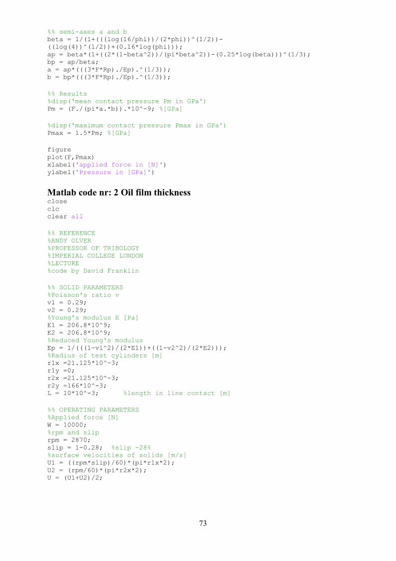
73
%% semi-axes a and b beta = 1/(1+(((log(16/phi))/(2*phi))^(1/2))-
((log(4))^(1/2))+(0.16*log(phi))); ap = beta*(1+((2*(1-beta^2))/(pi*beta^2))-(0.25*log(beta)))^(1/3); bp = ap/beta; a = ap*(((3*F*Rp)./Ep).^(1/3)); b = bp*(((3*F*Rp)./Ep).^(1/3));
%% Results %disp('mean contact pressure Pm in GPa') Pm = (F./(pi*a.*b)).*10^-9; %[GPa]
%disp('maximum contact pressure Pmax in GPa') Pmax = 1.5*Pm; %[GPa]
figure plot(F,Pmax) xlabel('applied force in [N]') ylabel('Pressure in [GPa]')
Matlab code nr: 2 Oil film thickness close clc clear all
%% REFERENCE %ANDY OLVER %PROFESSOR OF TRIBOLOGY %IMPERIAL COLLEGE LONDON %LECTURE %code by David Franklin
%% SOLID PARAMETERS %Poisson's ratio v v1 = 0.29; v2 = 0.29; %Young's modulus E [Pa] E1 = 206.8*10^9; E2 = 206.8*10^9; %Reduced Young's modulus Ep = 1/(((1-v1^2)/(2*E1))+((1-v2^2)/(2*E2))); %Radius of test cylinders [m] r1x =21.125*10^-3; r1y =0; r2x =21.125*10^-3; r2y =166*10^-3; L = 10*10^-3; %length in line contact [m]
%% OPERATING PARAMETERS %Applied force [N] W = 10000; %rpm and slip rpm = 2870; slip = 1-0.28; %slip -28% %surface velocities of solids [m/s] U1 = ((rpm*slip)/60)*(pi*r1x*2); U2 = (rpm/60)*(pi*r2x*2); U = (U1+U2)/2;
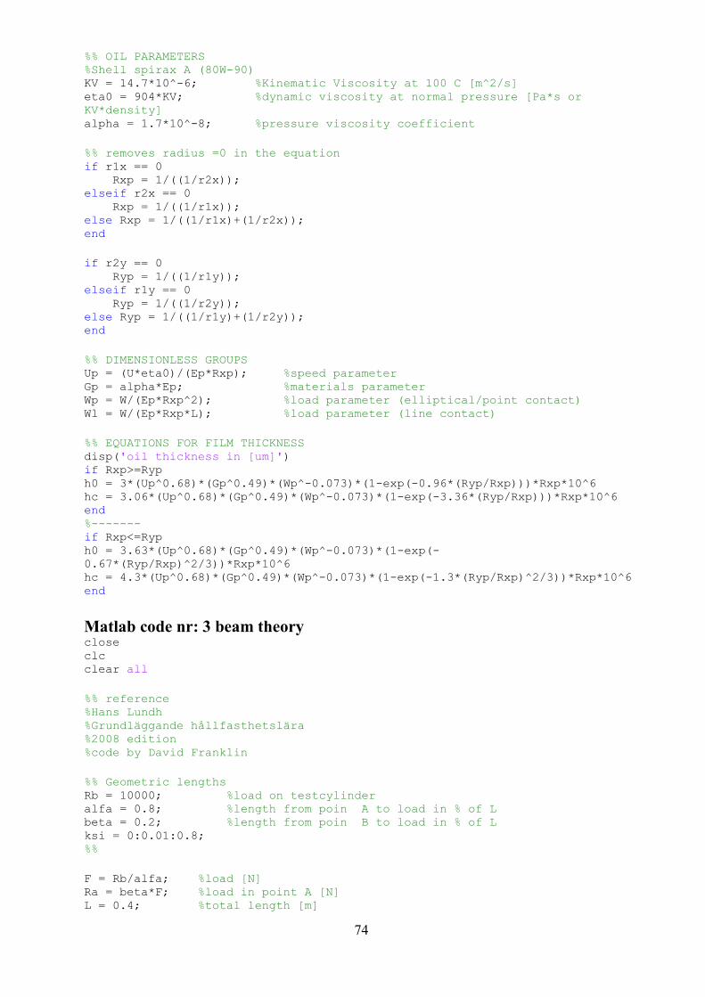
74
%% OIL PARAMETERS %Shell spirax A (80W-90) KV = 14.7*10^-6; %Kinematic Viscosity at 100 C [m^2/s] eta0 = 904*KV; %dynamic viscosity at normal pressure [Pa*s or
KV*density] alpha = 1.7*10^-8; %pressure viscosity coefficient
%% removes radius =0 in the equation if r1x == 0 Rxp = 1/((1/r2x)); elseif r2x == 0 Rxp = 1/((1/r1x)); else Rxp = 1/((1/r1x)+(1/r2x)); end
if r2y == 0 Ryp = 1/((1/r1y)); elseif r1y == 0 Ryp = 1/((1/r2y)); else Ryp = 1/((1/r1y)+(1/r2y)); end
%% DIMENSIONLESS GROUPS Up = (U*eta0)/(Ep*Rxp); %speed parameter Gp = alpha*Ep; %materials parameter Wp = W/(Ep*Rxp^2); %load parameter (elliptical/point contact) Wl = W/(Ep*Rxp*L); %load parameter (line contact)
%% EQUATIONS FOR FILM THICKNESS disp('oil thickness in [um]') if Rxp>=Ryp h0 = 3*(Up^0.68)*(Gp^0.49)*(Wp^-0.073)*(1-exp(-0.96*(Ryp/Rxp)))*Rxp*10^6 hc = 3.06*(Up^0.68)*(Gp^0.49)*(Wp^-0.073)*(1-exp(-3.36*(Ryp/Rxp)))*Rxp*10^6 end %------- if Rxp<=Ryp h0 = 3.63*(Up^0.68)*(Gp^0.49)*(Wp^-0.073)*(1-exp(-
0.67*(Ryp/Rxp)^2/3))*Rxp*10^6 hc = 4.3*(Up^0.68)*(Gp^0.49)*(Wp^-0.073)*(1-exp(-1.3*(Ryp/Rxp)^2/3))*Rxp*10^6 end
Matlab code nr: 3 beam theory close clc clear all
%% reference %Hans Lundh %Grundläggande hållfasthetslära %2008 edition %code by David Franklin
%% Geometric lengths Rb = 10000; %load on testcylinder alfa = 0.8; %length from poin A to load in % of L beta = 0.2; %length from poin B to load in % of L ksi = 0:0.01:0.8; %%
F = Rb/alfa; %load [N] Ra = beta*F; %load in point A [N] L = 0.4; %total length [m]

75
rmm = 15; %axial radii [mm] r = rmm*10^-3; %axial radii [m] I = (pi*r^4)/4; %böjtröghetsmoment E = 206.8*10^9; %Young's modulus E [Pa]
%% %s.99 disp('utböjningsvinklar i A och B') phiA = ((F*L^2)/(6*E*I))*((alfa*beta)*(1+beta)) %utböjningsvinkel i pkt A phiB = ((F*L^2)/(6*E*I))*((alfa*beta)*(1+alfa)) %utböjningsvinkel i pkt B
disp('nedböjning vid applicerad kraft i [mm]') deltaksi = (((F*L^3)/(6*E*I))*(beta*(((1-beta^2)*ksi)-ksi.^3)))*1000;
%utböjning i last punkten deltaalfa = ((F*L^3)/(3*E*I))*alfa^2*beta^2; %utböjning i last punkten delta = deltaalfa*1000
%% figure ax1 = subplot(2,1,1); ax2 = subplot(2,1,2); plot(ax1,ksi,deltaksi) ylabel(ax1,'Bending displacment [mm]') xlabel(ax1,'Distance from point A in % of L')
%% Torque along the axel %s.71-72 x1 = 0:0.01:(alfa*L); M1 = -Ra*x1; Mf = -alfa*beta*F*L; x2 = alfa*L:0.01:L; M2 = -alfa*F*L*(1-(x2/L));
plot(ax2,x1,M1,'r',x2,M2,'r') xlabel(ax2,'Length [m]') ylabel(ax2,'Bending torque [Nm]') %% Tension %s.85-86 disp('The maximal tension sigma, is +-sigmamax [MPa]') sigmamax = -Mf*(r/I)/10^6 %% bending in the test cylinders axel disp('bending in the test cylinders axel [mm]') Lt = beta*L; delta = F*Lt^3/(3*E*I)*10^3
Matlab code nr: 4 Tapered mounting close clc clear all %% Reference
%Tyler G. Hicks: Handbook of Mechanical Engineering Calculations, Second
Edition. %ANALYZING TAPER FITS FOR MANUFACTURING AND DESIGN, Chapter (McGraw-Hill %Professional, 2006 1998), AccessEngineering %Code by David Franklin
%% Solid parameters D = 30*10^-3; %large diameter of tapering [m] d = 25*10^-3; %small diameter of tapering [m] L = 20*10^-3; %length of tapering contact [m] phi = 7.125; %angle of tapering [degrees]
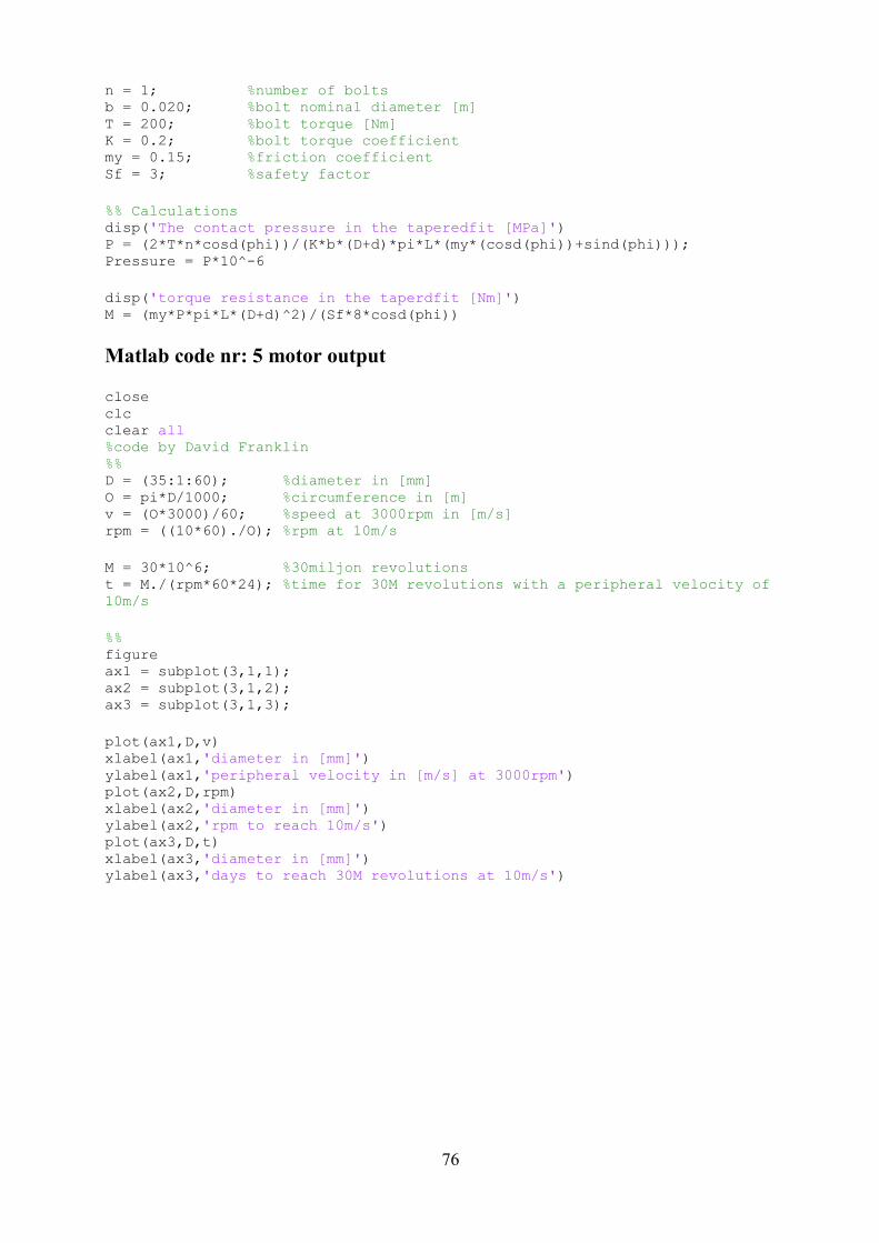
76
n = 1; %number of bolts b = 0.020; %bolt nominal diameter [m] T = 200; %bolt torque [Nm] K = 0.2; %bolt torque coefficient my = 0.15; %friction coefficient Sf = 3; %safety factor
%% Calculations disp('The contact pressure in the taperedfit [MPa]') P = (2*T*n*cosd(phi))/(K*b*(D+d)*pi*L*(my*(cosd(phi))+sind(phi))); Pressure = P*10^-6
disp('torque resistance in the taperdfit [Nm]') M = (my*P*pi*L*(D+d)^2)/(Sf*8*cosd(phi))
Matlab code nr: 5 motor output close clc clear all %code by David Franklin %% D = (35:1:60); %diameter in [mm] O = pi*D/1000; %circumference in [m] v = (O*3000)/60; %speed at 3000rpm in [m/s] rpm = ((10*60)./O); %rpm at 10m/s
M = 30*10^6; %30miljon revolutions t = M./(rpm*60*24); %time for 30M revolutions with a peripheral velocity of
10m/s
%% figure ax1 = subplot(3,1,1); ax2 = subplot(3,1,2); ax3 = subplot(3,1,3);
plot(ax1,D,v) xlabel(ax1,'diameter in [mm]') ylabel(ax1,'peripheral velocity in [m/s] at 3000rpm') plot(ax2,D,rpm) xlabel(ax2,'diameter in [mm]') ylabel(ax2,'rpm to reach 10m/s') plot(ax3,D,t) xlabel(ax3,'diameter in [mm]') ylabel(ax3,'days to reach 30M revolutions at 10m/s')