CONTRIBUTION No 55

PAR / BY

Steven HABERMAN

Grande -Bretagne / United Kingdom

94 APPROCHE STOCHASTIQUE DES ~ T H o D E S DE CON!3TlTUTION DE CAISSE DE RETRAlTE

RESUME

On &t un d l e rnaMrnatique qui facilite la cornparaison des diffCrentes rn6thodes de mtitution & cake & retraite. On suppose d'abord que les taux de remkment m t albatoires, puis qu'ils sont reprCsends par un rnod2le autorCgressif de l'amplitude correspondante de l'ineet. Des expressions de la variabilid des contributions et du niveau du fonds peuvent en &re M v h . Ceci conduit une discussion de la mCthode "optimale" de umstituticm du fonds. Une description plus &taillk de la d thode est donnee dam la thtse de doctorat de Dufresne (1986) et dam les recents articles dlHaberman et Dufresne (1987) et de Dufresne (1988, 1989). Les rCsultats mathhatiques de la troisitrne partie sont p r h t t % et discuds plus lcmguement dam un r k n t document de travail (Haberman. 1989).

STOCHASTIC APPROACH TO PENSION WNDING METHODS 95

PROFESSOR S. HABERMAN (CITY UNIVERSITY)

ABSTRACT

A mathematical model is described which facilitates the comparison of different pension funding methods. Rates of return are assumed firstly to be random and then to be represented by an autoregressive model for the corresponding force of interest. Expressions for the variability of contributions and fund levels can be derived This leads to a discussion of the "optimal" method of funding. A fuller description of the approach is given in Dufresne's doctoral thesis (1986) and in recent papers by Haberman and Dufresne (1987) and Dufresne (1988, 1989). The mathematical results of section 3 are ~esented and discussed at greater length in a recent working paper (Haberman (1989)).

96 STOCHAS'IIC APPROACH 'ID PENSION FUNDINO METHODS

1. TYPES OF FUNDING METHOD

Broadly, there are two types of h d i n g methods.

With individual funding methods (e.g. Projected Unit Credit and Enay Age Normal), the normal c a t (NC) and the actuarial liability (AL) are calculated separately for each member and then summed to give the totals for the population under consideration.

With aggregate funding methods (e.g. Aggregate and Attained Age Normal), there is no hypothecation of normal cost or actuarial liability to individuals ; instead the group is considered as an entity, ab initio.

kt C (t) and F (t) be the overall contribution and Fund level at time t f a a particular pension scheme.

For an individual funding method,

where NC (x,t) is the normal cost for a member aged x at time t, C denotes summation over the membership subdivided by attained age and ADJ (t) is an adjustment to the contribution rate at time t, representing the liquidatim of the unfunded liability at time t, UL (t). UL (t) is defined by

where AL (x,t) is the actuarial liability for a member aged x at time t.

For an aggregate method, the overall contribution is directly related to the difference between the Fesent value of future benefits and the fund. Specifically,

where S (t) is the payroll at time t, PVB (t) is the present value of fum benefits (of all members includmg pensioners) at time t and PVS (t) is the present value of future salaries (of active members) at time t.

This paper considers the behaviour of C (t) and F (t) in the presence of random investment returns.

At any time t, a valuation is carried out to estimate C (t) and F (t) based only on the scheme membership at time t. However, as t changes, we do allow for new entrants to the membership so that the population remains stationary - see assumptions below.

S. HABERMAN 97

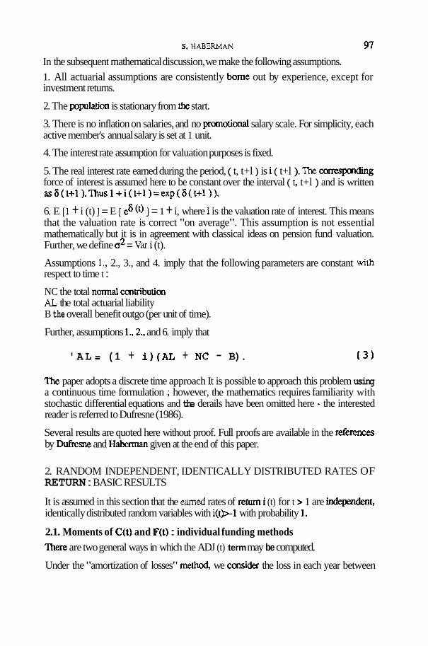
In the subsequent mathematical discussion, we make the following assumptions. 1. All actuarial assumptions are consistently borne out by experience, except for investment returns.

2. The population is stationary from h e start.

3. There is no inflation on salaries, and no promotional salary scale. For simplicity, each active member's annual salary is set at 1 unit.

4. The interest rate assumption for valuation purposes is fixed.

5. The real interest rate earned during the period, ( t, t+l ) is i ( t+l ). The comespding force of interest is assumed here to be constant over the interval ( t, t+l ) and is written as6(t+l).Thusl+i(t+l)=exp(6(t+l)).

6. E [l + i (t) ] = E [ e6 (t) ] = 1 + i, where i is the valuation rate of interest. This means that the valuation rate is correct "on average". This assumption is not essential mathematically but it is in agreement with classical ideas on pension fund valuation. Further, we define a2 = Var i (t).

Assumptions 1.. 2., 3., and 4. imply that the following parameters are constant with respect to time t :

NC the total normal contribution AL the total actuarial liability B the overall benefit outgo (per unit of time).

Further, assumptions 1.. 2.. and 6. imply that

' A L = ( 1 + i)(AL + NC - B). ( 3 )

?he paper adopts a discrete time approach It is possible to approach this problem using a continuous time formulation ; however, the mathematics requires familiarity with stochastic differential equations and the derails have been omitted here - the interested reader is referred to Dufresne (1986).

Several results are quoted here without proof. Full proofs are available in the referem by Dufresne and Haberman given at the end of this paper.

2. RANDOM INDEPENDENT, IDENTICALLY DISTRIBUTED RATES OF RETURN : BASIC RESULTS

It is assumed in this section that the earned rates of retum i (t) for t > 1 are independent, identically distributed random variables with i(t)>-1 with probability 1.

2.1. Moments of C(t) and F(t) : individual funding methods mere are two general ways in which the ADJ (t) term may be computed.

Under the "amortization of losses" method, we consider the loss in each year between

98 STOCHASTIC APPROACH m PENSION FUNDING METHOB

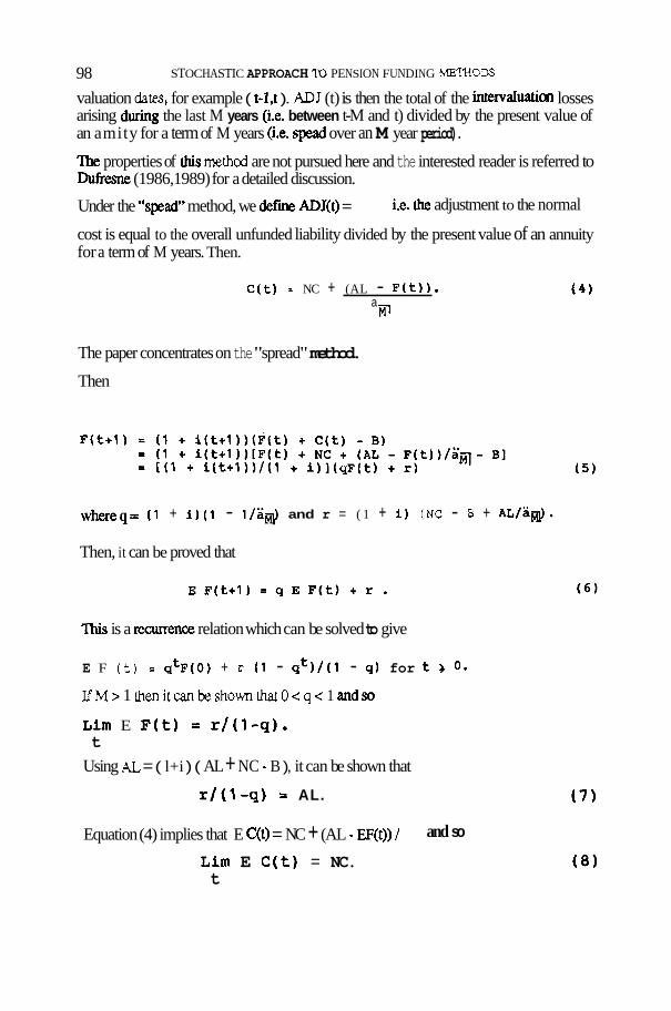
valuation dates, for example ( t-1,t ). ADJ (t) is then the total of the intervaluation losses arising during the last M years (i.e. between t-M and t) divided by the present value of an amity for a term of M years (i.e. sped over an M year period).

?he properties of this method are not pursued here and the interested reader is referred to Dufresne (1986,1989) for a detailed discussion.

Under the "spead" method, we defm ADJ(t) = i.e. the adjustment to the normal

cost is equal to the overall unfunded liability divided by the present value of an annuity for a term of M years. Then.

C ( t ) = NC + (AL - ~ ( t ) ) . a m

The paper concentrates on the "spread" method.

Then

whereq= ( 1 + i ) ( 1 - l / a a ) and r = ( 1 + i ) (NC - B + AL/ ;~@.

Then, it can be proved that

'Ihis is a recurrence relation which can be solved to give

E F (t) = q t ~ ( ~ ) + r ( 1 - q t ) / ( l - q ) for t 0.

I fM> 1 thenitcanbeshownrhatO<q< 1 andso

Lim E F(t) = r/(1-q). t

Using AL = ( l+i ) ( AL + NC - B ), it can be shown that

r/(l -q) = AL.

Equation (4) implies that E C(t) = NC + (AL - EF(t)) 1 and so

Lim E C(t) = NC. t

S. HABERMAN

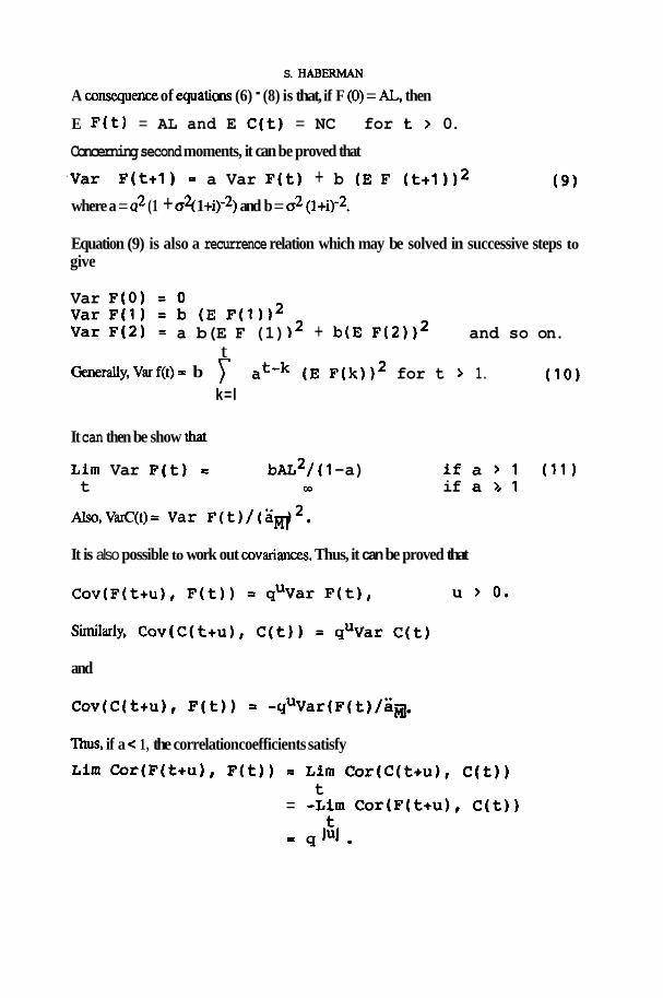
A cansequeslce of equatim (6) - (8) is that, if F (0) = AL, then

E F(t) = AL and E C(t) = NC for t > 0.

Concerning second moments, it can be proved that

.Var F(t+l) = a Var F(t) + b (E F (t+1)12 ( 9 ) where a = q2 (1 + oq 1 +i)-2) and b = o2 (1 +ir2.

Equation (9) is also a recurrence relation which may be solved in successive steps to give

Var F(0) = 0 var ~ ( 1 ) = b (E ~ ( 1 1 1 2 Var F(2) = a b(E F (1) l 2 + b ( E ~ ( 2 ) ) ~ and so on.

t Generally,Varf(t)= b at-k (E ~ ( k ) l 2 for t > 1. (10)

k=l

It can then be show that

Lim Var F(t) = ~ A L ~ / ( I -a) i f a > 1 (11) t OD if a b l

It is also possible to work out covariances. Thus, it can be proved that

and

Thus, if a < 1, the correlation coefficients satisfy

~ i m Cor(F(t+u), F(t)) = Lim Cor(C(t+u), C(t)) t

= -Lim Cor(F(t+u), C(t))

100 STOCHASTIC APPROACH TO PENSION FUNDING METHODS

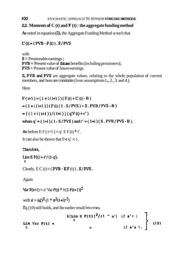
2.2. Moments of C (t) and F (t) : the aggregate funding method

As noted in equation (2). the Aggregate Funding Method is such that

with S = Pensionable earnings ; PVB = Present value of future benefits (including pensioners) ; PVS = Present value of future earnings.

S, PVB and PVS are aggregate values. relating to the whole population of current members, and here are constants (from assumptions 1 ., 2., 3. and 4.).

Here

As before E F ( t+l ) = q' E F (t) + r'. It can also be shown that 0 < q' c 1.

Clearly, E C (t) = ( PVB - E F (t) ) . S / PVS.

Again

Vu F(t+l ) = a' Var F(t) + b(E ~ ( t + l ) ] ~

wiih a' = (& (1 + a*(~+i)-*)

Eq (10) still holds, and the earlier result becomes

b[Lim E ~(t)]~/(1 - a') if a ' < 1 t

Lim Var F(t) = t 01 if a') 1.

S. HABERMAN 101

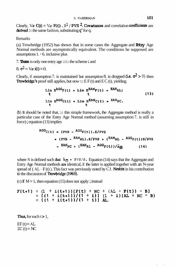
Clearly, Var C(t) = Var F(t)) . s2 / PVS 2. Covariances and correlation coeficients are &rived in the same fashion, substituting q' for q.

Remarks

(a) Trowbridge (1952) has shown that in some cases the Aggregate and Entry Age Normal methods are asymptotically equivalent. The conditions he supposed are assumptions 1. - 6. inclusive plus

7. There is only one entry age into the scheme ; and

8. o2 = Var i(t) = 0.

Clearly, if assumption 7. is maintained but assumption 8. is dropped (ia. o2 > 0) then 'hwbridge's proof still applies, but now to E F (t) and E C (t), yielding

(b) It should be noted that, in this simple framework, the Aggregate method is really a particular case of the Entry Age Normal method (assuming assumption 7. is still in force) ; equation (13) implies

where N is defined such that 'im = PVS/S. Equation (14) says that the Aggregate and Entry Age Normal methods are identical, if the latter is applied together with an N-year spread of ( AL - F (t) ), This fact was previously noted by CJ. Nesbiu in his contribution to the discussion of Trowbridge (1%3).

(c) If M = 1, then equation (15) does not apply ; instead

F(t+l) = (1 + i(t+l ))[F(t) + NC + (AL - F(t)) - Bl = [(I + i(t+l))/(l + i)] (1 + i)(AL + NC - B) = [(I + i(t+l))/(l + i)l AL.

'Ihus, for each t > 1,

EF (t) = AL EC (t) = NC

102 STOCHASTIC APPROACH TO PENSION FUNDING METHODS

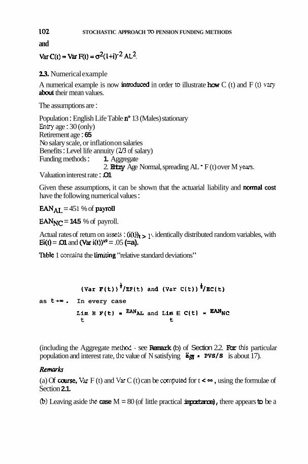
and

23. Numerical example

A numerical example is now introducsd in order to illustrate how C (t) and F (1) vary about their mean values.

The assumptions are :

Population : English Life Table no 13 (Males) stationary Enuy age : 30 (only) Retirement age : 65 No salary scale, or inflation on salaries Benefits : Level life annuity (2/3 of salary) Funding methods : 1. Aggregate

2. Entry Age Normal, spreading AL - F (t) over M years. Valuation interest rate : .O1

Given these assumptions, it can be shown that the actuarial liability and normal cost have the following numerical values :

€ANAL = 45 1 % of payroll

EANNc = 14.5 % of payroll.

Actual rates of return on assets : (i(~))~, 11, identically distributed random variables, with Ei(t) = .O1 and (Var i(t))# = .05 (=a).

nble 1 contains the limiting "relative standard deviations"

as t- . In every case

L i m E F(t) = E A N ~ ~ and Lirn E C ( t ) = E A N ~ ~ t t

(including the Aggregate method - see Remark (b) of Section 2.2. For this particular population and interest rate, the value of N satisfying as E pvsls is about 17).

Remath (a) Of course, Var F (t) and Var C (t) can be computed for t < - , using the formulae of Section 2.1.

(b) Leaving aside the case M = 80 (of little practical importance), there appears to be a

S. HABERMAN 1 03

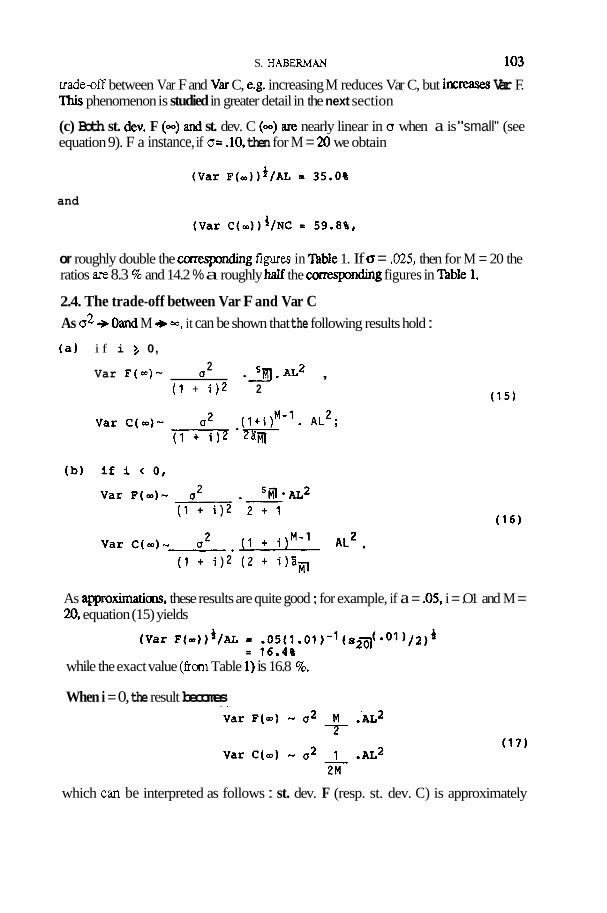
trade-off between Var F and Var C, e.g. increasing M reduces Var C, but increw Var F. 'Ihis phenomenon is studied in greater detail in the next section

(c) Both st. dev. F (m) and st. dev. C (m) are nearly linear in o when a is "small" (see equation 9). F a instance, if a= .lo, then for M = 24) we obtain

and

or roughly double the cu-respondmg figures in nble 1. If a = .025, then for M = 20 the ratios are 8.3 % and 14.2 % a roughly half the ms-g figures in nble 1.

2.4. The trade-off between Var F and Var C As a2 + Oand M + -, it can be shown that the following results hold :

( a ) i f i 3 0,

Var F(-)- (J 2 3 . A L ~ ,

( I + i ) 2 2

As approximatim, these results are quite good ; for example, if a = .05, i = .O1 and M = 20, equation (15) yields

while the exact value (from Table 1) is 16.8 8.

When i = 0, the result becomes

which can be interpreted as follows : st. dev. F (resp. st. dev. C) is approximately

1 w STOCHASTIC APPROACH TO PENSION FUNDING METHODS

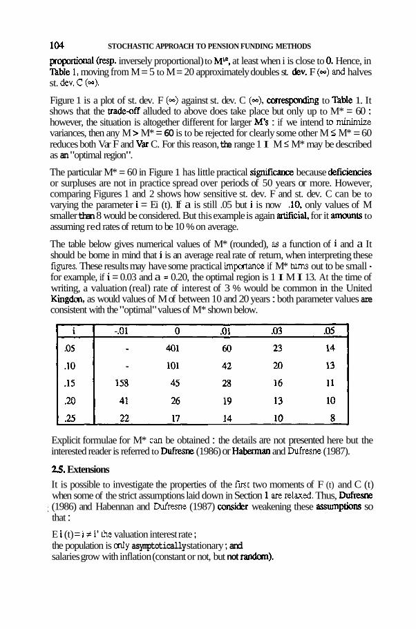
proportional (rap. inversely proportional) to Mn, at least when i is close to 0. Hence, in nble 1, moving from M = 5 to M = 20 approximately doubles st. &v. F (=) and halves st. dev. C (-).

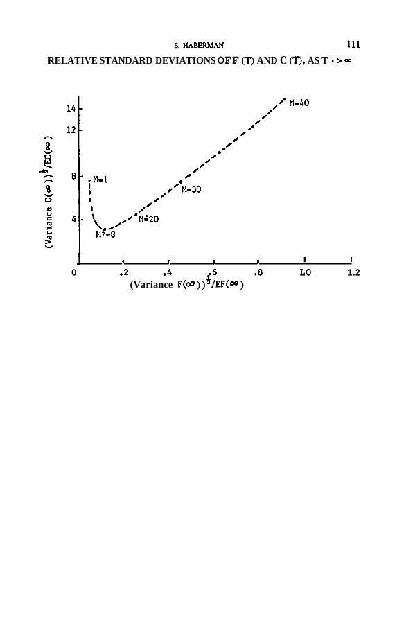
Figure 1 is a plot of st. dev. F (-) against st. dev. C (-), comes-g to 'hble 1. It shows that the tradeaff alluded to above does take place but only up to M* = 60 ; however, the situation is altogether different for larger M's : if we intend to minimize variances, then any M > M* = 60 is to be rejected for clearly some other M I M* = 60 reduces both Var F and Var C. For this reason, the range 1 I M I M* may be described as an "optimal region".

The particular M* = 60 in Figure 1 has little practical si@icance because defciencies or surpluses are not in practice spread over periods of 50 years or more. However, comparing Figures 1 and 2 shows how sensitive st. dev. F and st. dev. C can be to varying the parameter i = Ei (t). If a is still .05 but i is now .lo, only values of M smaller than 8 would be considered. But this example is again arwcial, for it amaunts to assuming red rates of return to be 10 % on average.

The table below gives numerical values of M* (rounded), as a function of i and a It should be bome in mind that i is an average real rate of return, when interpreting these fiw. These results may have some practical importance if M* turns out to be small - for example, if i = 0.03 and a = 0.20, the optimal region is 1 I M I 13. At the time of writing, a valuation (real) rate of interest of 3 % would be common in the United Kingdm, as would values of M of between 10 and 20 years : both parameter values are consistent with the "optimal" values of M* shown below.

Explicit formulae for M* can be obtained : the details are not presented here but the interested reader is referred to Dufresne (1986) or Haberman and Dufresne (1987).

25. Extensions It is possible to investigate the properties of the fmt two moments of F (t) and C (t) when some of the strict assumptions laid down in Section 1 are relaxed. Thus, Dufresne

: (1986) and Habennan and Dufmne (1987) consider weakening these asswnptim so that :

E i (t) = i + i' h e valuation interest rate ; the population is only asymptotically stationary ; and salaries grow with inflation (constant or not, but not randam).

S. HABERMAN 105

In section 3, we move away from the assumption that earned rates of interest are independent and identically distributed random variables.

3. AUTOREGRESSIVE RATES OF RETURN : BASIC RESULTS

It is apparent from the discussion in Section 2 that the equations for the moments of F (t) and C (I) are of the same type for individual and aggregate hnding methods. This section, therefore, considers only one type, viz individual funding methods.

In order to investigate the effects of autoregressive models for the earned real rate of return, the paper follows the suggestion of Panjer and Bellhouse (1980) and considers the corresponding force of interest and assume that it is constant over the interval of time ( t, t+l ) : the notation used will be (t+l ).

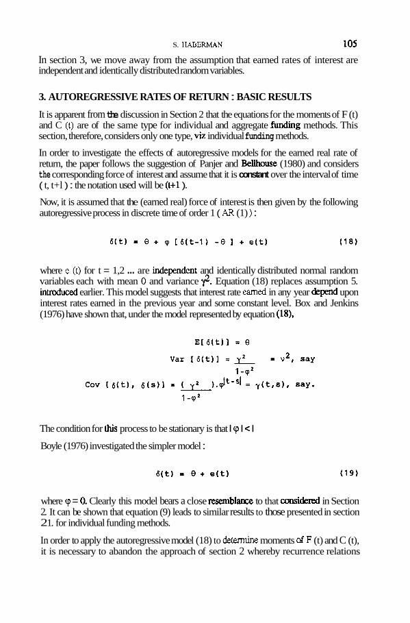
Now, it is assumed that the (earned real) force of interest is then given by the following autoregressive process in discrete time of order 1 ( AR (1) ) :

where c (I) for t = 1,2 ... are independcnt and identically distributed normal random variables each with mean 0 and variance y2. Equation (18) replaces assumption 5. inuoduced earlier. This model suggests that interest rate earned in any year depend upon interest rates earned in the previous year and some constant level. Box and Jenkins (1976) have shown that, under the model represented by equation (18).

The condition for this process to be stationary is that I cp I < I

Boyle (1976) investigated the simpler model :

where cp = 0. Clearly this model bears a close resemb1an;e to that considered in Section 2. It can be shown that equation (9) leads to similar results to those presented in section 2 1. for individual funding methods.

In order to apply the autoregressive model (18) to determine moments of F (t) and C (t), it is necessary to abandon the approach of section 2 whereby recurrence relations

106 STOCHASTIC APPROACH TO PENSION FUNDING METHODS

between, for example, E F ( t+l ) and E F (t) were sought. The presence of a dependence on the past in the autoregressive model would make such an approach problematic.

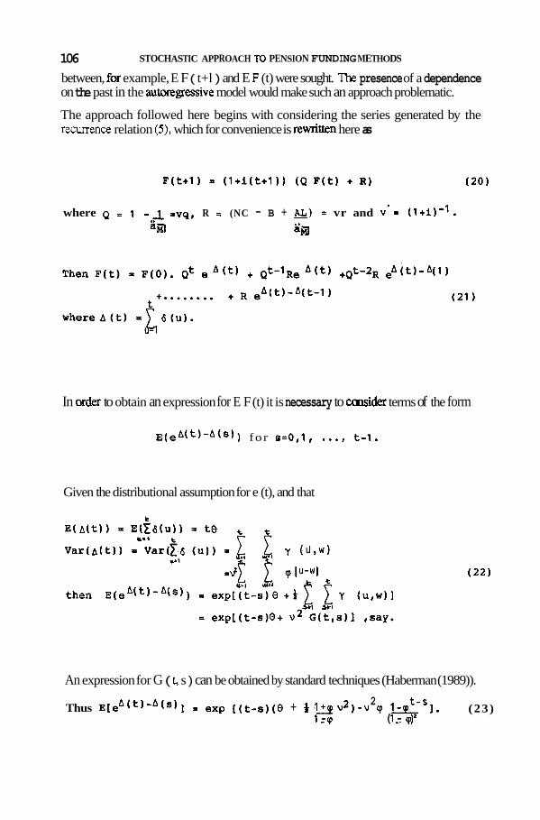
The approach followed here begins with considering the series generated by the recurrence relation (3, which for convenience is rewritten here as

where Q = 1 - A =vq, R = (NC - B + &) = vr and v'x ( l + i ) - ' . 23 iis

In order to obtain an expression for E F (t) it is necessary to ccmider terms of the form

~ ( e ~ ( ~ ) - * ( ~ ) ) for s=0,1 , ..., t - 1 .

Given the distributional assumption for e (t), and that

An expression for G ( t, s ) can be obtained by standard techniques (Haberman (1989)).

2 Thus E [ ~ ~ ( ~ ) - * ( s ) ] = exp [ ( t - s ) ( Q + f . 1 2 u 2 ) - v cp l&-']. ( 23 )

1 ZQ (1 s cp)=

S. IIABERMAN

If the subsidiary parameters c = exp ( O + f I + v2) and

d =v2q(1 -q) -' , 73 are introduced,

- t - s .-d(l-cP 1 ,

'Ihe sccond term is of the form of the present value in conventional life contingencies of a temporary annuity based on Gompem's a Makeham's law of mortality.

In section 2.1., it was noted that 0 < q < 1.

1 -Q = q exp = q i f 9 = 0.

For convergence as t -> -, we require cQ < 1. And we note that cp< 1.

It can then be shown that

If Q=O then c = exp (Q+iv2) = 1 +i and d=0, and

hence Lim E F(t) 3 r as in equation (7). t+- 1 =q

Then E C(t) = NC + AL - E (F(t)) from equation (4). %l

To obtain an explicit expression for Vat ( F (t) ), it will be necessary to consider E ( F (t) )2, which itself will depend on terms of the form

E(,A(t) -A(s) + A (t) - A ( r ) )

forr,s=O, 1 , ..., t-1.

108 STOCHASTIC APPROACH TO PENSION FUNDING METHODS

Without loss of generality, we consider r > s.

Given the distributional assurnptim for e (t), Haberman (1989) has shown that, for r >s,

where, in this case of an AR (1) model,

For convenience, we can write

and it has been shown by Haberman (1989) that H (4 r, s ) simplifies to :

For convenience, we will take F (0) = 0. +.I c-4

~ h ~ ~ , ~ ( ~ ( t ) ) 2 = E [ C c e A ( t ) d ( ~ ) e A ( t ) - A ( r ) Q ~ - ~ - ~ Qt-l-r R2] -so

'Then, it has been shown by Haberman (1989) that

where d =dcp , c = exp (O+b(l*cp)v 2 ) , Q=vq, R=vr a s before and ( 1 - , 1 2 (1-9)

S. HABERMAN

We note that cp < 1, by assumption,

and that Qc = Q exp I @ + t ( l + L v 2 1 = q exp (Q;-? 1-9

For convergence, as t + =, we require Qc < 1 and Q%W < 1. -

Then, Lim Var F(t) = e-3d ~ R ~ Q C ~ W +e-4d (29) t-- ( 1 -Qc ) ( 1 - Q ~ C W ) (1-Q CW)

Then, formulae for Lim Var C(t) = Var2F(t) may be obtained. t-- ("R3

The next step would be to investigate the existence of an "optimal" M* as in section 2.4. (for the case of r a n d a rates of return). 'Ihis wak is currently in progress and it may be possible to report furher results at the AFlR Colloquium.

4. CONCLUSIONS

The variability of contributions (C) and fund levels (F) resulting from random (real) rates of return has been studied mathematically. The funding methods considered are the Aggregate Method and those Individual Methods that prescribe the n o m l cost to be adjusted by the Werence between the actuarial liability and the current fund, divided by the present value of an annuity for a tenn of "h4" years. A simple demographic/f~nancial model permits the derivation of formulae for the fmt two moments of F and C, when earned (real) rates of return from an independent identically distributed sequence of random variables. The way these moments &pend on M has then analysed, with the help of a numerical example. The approach has been extended to include the case of an autoregressive model for the earned (real) rate of return Expressions for the fmt two moments of C (t) and F (t) have been obtained and reported and their detailed properties are currently under investigation.

110 STOCHASTIC APPROACH TO PENSION FUNDING METHODS

REFERENCES

Box, G.E.P. and Jenkins, G.M. (1976). Time Series Analysis, 2nd Edition. San Francism, Holden Day.

Boyle, P.P. (1976). Rates of Return as Randam Variables. Journal of Risk and Insurance. 43,693-713.

Dufresne, D., (1986). The Dynamics of Pension Funding. Ph.D. Thesis. The City University, London

Dufresne, D. (1988). Moments of Pension Fund Conaibutim &d Fund Levels when Rates of Retum are Random. Journal of Institute of Actuaries. 115,545-544.

Dufresne, D. (1989). Stability of Pension Systems when Rates of Return are Random. Insurance : Mathematics and Economics, 8,71-76.

Haberman, S. (1989). Variability of Pension Contributions and Fund Levels with Random and Autoregressive Rates of Retum ARCH. To appear.

Habeman, S. and Dufresne, D. (1987). The Mathematics of Pension Funding. m t e d to the Institute of Actuaries Convention : "The Actuary in Pensions - a Time of Change". Harrogate. September 1987.

Panjer H.H. and Bellhouse, D.R. (1980). Stochastic Modelling of Interest Rate with Applications to Life Contingencies. Joumal of Risk and Insurance. 47,91-110.

Trowbridge, C.L. (1952). The Fundamentals of Pension Funding. Transactions of Society of Actuaries. 4,1743.

llowbridge, C.L. (1963). The Unfunded Present Value Family of Pension Funding Methods. Transactions of Society of Actuaries. 15,151-169.

S. HABERMAN 11 1

RELATIVE STANDARD DEVIATIONS OFF (T) AND C (T), AS T - > -

J I I 1 1 I I

0 .2 .4 .a LO 1.2 1 (Variance F(o0 ) ) /EF(M )

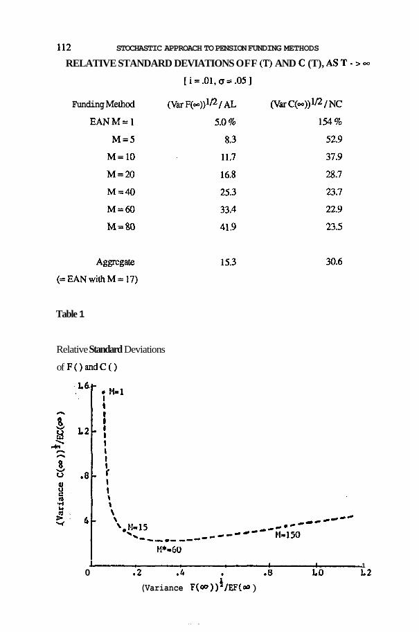
112 STOCHASTIC APPROACH TO PENSION FUNDING METHODS

RELATIVE STANDARD DEVIATIONS OFF (T) AND C (T), AS T - > m

[i=.01,0=:.05]

Funding Method

E A N M = l

M = 5

M=lO

M=20

M=40

M=60

M=80

Table 1

Relative Standard Deviations

of F() andC ( )

J I 1 0 .2 .4 .8 LO L2 i (Variance F(o0)) /EF(oo )