Embed Size (px)
Citation preview
Mémoire
d’Habilitation à diriger des recherches
présenté
devant l’Université de Toulouse
par
Jordi Inglada
Centre d’Études Spatiales de la BiosphèreUMR 5126 CNES, CNRS, IRD, UPS
Contributions à l’analyse d’images d’observation de la Terrepour la production de cartes d’occupation des sols et le suivi
des changements dans des contextes opérationnels
Soutenu le XXX 2011 devant la commission d’examen
Composition du Jury
Président: Xxx Xxxxxx
Rapporteurs: Xxx Xxxxxx
Xxx Xxxxxx
Xxx Xxxxxx
Examinateurs: Xxx Xxxxxx
Xxx Xxxxxx
Xxx Xxxxxx

Table des matières
Table des matières 1
I Synthèse des travaux 5
1 Introduction 71.1 Risques et catastrophes majeures . . . . . . . . . . . . . . . . . . . . . . . . . . . 8
1.1.1 La Charte et le rôle de PM . . . . . . . . . . . . . . . . . . . . . . . . . . . 81.1.2 Le développement d’outils . . . . . . . . . . . . . . . . . . . . . . . . . . . 91.1.3 La déclinaison en axes de R&D . . . . . . . . . . . . . . . . . . . . . . . . 9
1.1.3.1 Le recalage d’images . . . . . . . . . . . . . . . . . . . . . . . . . 91.1.3.2 La détection de changements . . . . . . . . . . . . . . . . . . . . 101.1.3.3 Les mesures de similarité . . . . . . . . . . . . . . . . . . . . . . 11
1.1.4 Les projets européens . . . . . . . . . . . . . . . . . . . . . . . . . . . . . . 111.2 Valorisation et promotion des images satellite à haute résolution . . . . . . . . . 11
1.2.1 Spot 5 et la notion d’objet . . . . . . . . . . . . . . . . . . . . . . . . . . . 121.2.1.1 La classification supervisée . . . . . . . . . . . . . . . . . . . . . 121.2.1.2 L’extraction de primitives . . . . . . . . . . . . . . . . . . . . . . 12
1.2.2 Orfeo et l’interprétation de scènes . . . . . . . . . . . . . . . . . . . . . . 131.2.2.1 Le raisonnement spatial . . . . . . . . . . . . . . . . . . . . . . . 141.2.2.2 Mise à jour de bases de données cartographiques . . . . . . . . . 14
1.3 Conclusion . . . . . . . . . . . . . . . . . . . . . . . . . . . . . . . . . . . . . . . . 14
2 Mesures de similarité pour le recalage d’images et la détection de changements 172.1 Les mesures de dépendance statistique . . . . . . . . . . . . . . . . . . . . . . . . 17
2.1.1 Le coefficient de corrélation . . . . . . . . . . . . . . . . . . . . . . . . . . 172.1.2 Généralisation : interprétation probabiliste . . . . . . . . . . . . . . . . . 182.1.3 Mesures multi-capteurs . . . . . . . . . . . . . . . . . . . . . . . . . . . . 18
2.1.3.1 Mesures utilisant les valeurs radiométriques et les probabilités 192.1.3.2 Mesures utilisant seulement les probabilités . . . . . . . . . . . 19
2.2 Le recalage d’images . . . . . . . . . . . . . . . . . . . . . . . . . . . . . . . . . . 222.2.1 Modélisation du problème de mise en correspondance d’images . . . . . 22
1
2 TABLE DES MATIÈRES
2.2.2 Modélisation de la déformation géométrique . . . . . . . . . . . . . . . . 232.2.3 Artefacts d’interpolation . . . . . . . . . . . . . . . . . . . . . . . . . . . . 24
2.3 La détection de changements . . . . . . . . . . . . . . . . . . . . . . . . . . . . . . 252.3.1 Comparaison de densités de probabilité . . . . . . . . . . . . . . . . . . . 252.3.2 Mesures de dépendance . . . . . . . . . . . . . . . . . . . . . . . . . . . . 272.3.3 Classification supervisée . . . . . . . . . . . . . . . . . . . . . . . . . . . . 28
2.3.3.1 Sélection de primitives . . . . . . . . . . . . . . . . . . . . . . . . 292.3.3.2 Optimisation du noyau . . . . . . . . . . . . . . . . . . . . . . . 302.3.3.3 Simplification de la fonction de décision . . . . . . . . . . . . . 31
3 Classification pour la reconnaissance d’objets 333.1 Introduction . . . . . . . . . . . . . . . . . . . . . . . . . . . . . . . . . . . . . . . 333.2 Classes d’objets . . . . . . . . . . . . . . . . . . . . . . . . . . . . . . . . . . . . . 333.3 Chaîne de traitement . . . . . . . . . . . . . . . . . . . . . . . . . . . . . . . . . . 343.4 Description des imagettes . . . . . . . . . . . . . . . . . . . . . . . . . . . . . . . 343.5 Résultats . . . . . . . . . . . . . . . . . . . . . . . . . . . . . . . . . . . . . . . . . 35
4 Raisonnement spatial pour l’interprétation de scènes 374.1 Motivation . . . . . . . . . . . . . . . . . . . . . . . . . . . . . . . . . . . . . . . . 374.2 Region connection calculus et son extension . . . . . . . . . . . . . . . . . . . . . 37
4.2.1 Le RCC-8 . . . . . . . . . . . . . . . . . . . . . . . . . . . . . . . . . . . . . 374.2.2 La reconnaissance d’objets avec le RCC-8 . . . . . . . . . . . . . . . . . . 38
4.2.2.1 La segmentation . . . . . . . . . . . . . . . . . . . . . . . . . . . 384.2.2.2 Matching de graphes . . . . . . . . . . . . . . . . . . . . . . . . . 39
4.2.3 Extensions du RCC-8 . . . . . . . . . . . . . . . . . . . . . . . . . . . . . . 404.3 Les relations spatiales floues . . . . . . . . . . . . . . . . . . . . . . . . . . . . . . 41
4.3.1 Exemple de relation spatiale : les objets alignés . . . . . . . . . . . . . . . 414.3.2 Interprétation de scènes . . . . . . . . . . . . . . . . . . . . . . . . . . . . 43
5 Comparaison image/base de données 455.1 Introduction . . . . . . . . . . . . . . . . . . . . . . . . . . . . . . . . . . . . . . . 455.2 Architecture globale . . . . . . . . . . . . . . . . . . . . . . . . . . . . . . . . . . . 455.3 Éléments focaux . . . . . . . . . . . . . . . . . . . . . . . . . . . . . . . . . . . . . 475.4 Utilisation de la théorie des croyances . . . . . . . . . . . . . . . . . . . . . . . . 475.5 Résultats . . . . . . . . . . . . . . . . . . . . . . . . . . . . . . . . . . . . . . . . . 49
6 Perspectives de recherche 516.1 Les produits attendus . . . . . . . . . . . . . . . . . . . . . . . . . . . . . . . . . . 516.2 Les contraintes . . . . . . . . . . . . . . . . . . . . . . . . . . . . . . . . . . . . . . 526.3 Les solutions : . . . . . . . . . . . . . . . . . . . . . . . . . . . . . . . . . . . . . . 53
6.3.1 Modélisation de comportements temporels . . . . . . . . . . . . . . . . . 536.3.2 Le multi-capteur . . . . . . . . . . . . . . . . . . . . . . . . . . . . . . . . 536.3.3 Les informations exogènes . . . . . . . . . . . . . . . . . . . . . . . . . . . 53
TABLE DES MATIÈRES 3
6.3.3.1 Les modèles physiques . . . . . . . . . . . . . . . . . . . . . . . . 546.3.3.2 Les connaissances du domaine . . . . . . . . . . . . . . . . . . . 54
6.4 La classification . . . . . . . . . . . . . . . . . . . . . . . . . . . . . . . . . . . . . 546.5 La détection de changements . . . . . . . . . . . . . . . . . . . . . . . . . . . . . . 55
II Curriculum Vitae 57
7 Cursus professionnel 597.1 Formation . . . . . . . . . . . . . . . . . . . . . . . . . . . . . . . . . . . . . . . . 597.2 Expérience professionnelle . . . . . . . . . . . . . . . . . . . . . . . . . . . . . . . 59
8 Liste des publications 618.1 Chapitres de livre . . . . . . . . . . . . . . . . . . . . . . . . . . . . . . . . . . . . 618.2 Articles de revue à comité de lecture . . . . . . . . . . . . . . . . . . . . . . . . . 618.3 Communications dans des colloques avec comité de lecture . . . . . . . . . . . . 62
9 Liste des mémoires et diplômes encadrés (2001-2011) 719.1 Stages . . . . . . . . . . . . . . . . . . . . . . . . . . . . . . . . . . . . . . . . . . . 719.2 Thèses de doctorat . . . . . . . . . . . . . . . . . . . . . . . . . . . . . . . . . . . . 72
10 Participation à des modules d’enseignement 7510.1 Traitement du signal radar . . . . . . . . . . . . . . . . . . . . . . . . . . . . . . . 7510.2 Traitement d’images radar . . . . . . . . . . . . . . . . . . . . . . . . . . . . . . . 7510.3 Traitement d’images pour les risques . . . . . . . . . . . . . . . . . . . . . . . . . 7510.4 Orfeo Toolbox . . . . . . . . . . . . . . . . . . . . . . . . . . . . . . . . . . . . . . 75
11 Projets 7711.1 EEE-SPN (2002) . . . . . . . . . . . . . . . . . . . . . . . . . . . . . . . . . . . . . 7711.2 Robin (2005-2006) . . . . . . . . . . . . . . . . . . . . . . . . . . . . . . . . . . . . 7711.3 GMOSS (2005-2008) . . . . . . . . . . . . . . . . . . . . . . . . . . . . . . . . . . 7711.4 PREVIEW (2005-2008) . . . . . . . . . . . . . . . . . . . . . . . . . . . . . . . . . 7811.5 SAFER (2009-2012) . . . . . . . . . . . . . . . . . . . . . . . . . . . . . . . . . . . 78
12 Autres activités liées à la recherche 8112.1 Organisation de séminaires et colloques . . . . . . . . . . . . . . . . . . . . . . . 8112.2 Jurys de thèse . . . . . . . . . . . . . . . . . . . . . . . . . . . . . . . . . . . . . . 8112.3 Travail éditorial . . . . . . . . . . . . . . . . . . . . . . . . . . . . . . . . . . . . . 83
Bibliographie 85
III Annexes 89
13 Recalage d’images 91

4 TABLE DES MATIÈRES
14 Détection de changements 121
15 Reconnaissance d’objets 163
16 Raisonnement spatial 177
17 Mise à jour de cartes numériques 215
18 Traitements opérationnels 229
Première partie
Synthèse des travaux
5

1 Introduction
Ce mémoire synthétise les travaux de recherche que j’ai mené au CNES depuis mon arrivéeen octobre 2000. Ces travaux ont été guidés par 2 axes principaux.
Le premier axe concerne l’utilisation opérationnelle des images satellite pour l’aide à lagestion de crise suite à des catastrophes majeures. On constate qu’il s’agit d’un axe applicatif –avec un ensemble de contraintes qui seront détaillées par la suite – ce qui peut sembler étrangepour des recherches menées au CNES.
Le deuxième axe concerne le travail sur l’exploitation d’images à haute et très haute ré-solution, soit dans un cadre de valorisation de systèmes spatiaux existants – Spot 5 – oudans un cadre de préparation à l’utilisation de données de systèmes en développement – Or-feo/Pléiades et plus récemment Venµs et Sentinelle-2. Ces axes sont plus classiques dans lepérimètre des compétences du CNES.
7

8 CHAPITRE 1. INTRODUCTION
1.1 Risques et catastrophes majeures
1.1.1 La Charte et le rôle de PM
Peu avant mon arrivée au Cnes pour un post-doc, le Cnes et l’Agence spatiale européenneont signé en avril 2000 une charte qui avait comme objectif de rendre disponible l’accès à desdonnées satellite pour les services d’aide et de secours :
La Charte internationale vise à offrir un système unifié d’acquisition et de livraison des donnéessatellites dans les cas de catastrophes d’origine naturelle ou humaine par l’entremise d’utilisateursautorisés. Chaque agence membre s’est engagée à fournir des ressources à l’appui de la Charte etcontribue ainsi à atténuer les répercussions de telles catastrophes sur la vie des gens et sur la pro-priété. 1
Le Cnes et l’ESA ont été ensuite rejoints par l’Agence spatiale canadienne, la NOAA (USA)et l’ISRO (Inde). La Charte compte aujourd’hui 10 membres.
Les procédures pour l’activation de la Charte par des utilisateurs autorisés ont été crééesdès le début. Il en a été de même pour ce qui concerne la définition des responsabilités desdifférents acteurs ainsi que pour les mécanismes de demande d’acquisition des différents sa-tellites disponibles. En revanche, rien n’était prévu pour ce qui concernait l’utilisation desimages acquises. Les utilisateurs finaux étant des opérationnels de la gestion des crises, la miseà disposition d’images satellites brutes s’est avérée peu adaptée dès la première activation.
J’ai eu l’occasion de participer aux côtés du chef de projet de la première activation de laCharte, Francesco Sarti, lors des 2 tremblements de terre de janvier 2001 au Salvador. Dèsnos premiers échanges téléphoniques avec les équipes de la Sécurité civile française envoyéssur place, nous avons pu constater l’abîme à combler entre la matrice de pixels (qui plus est,radar !) que nous avions sur nos écrans et le besoin d’information précise du pompier sur leterrain.
Pour cette activation nous avons tant bien que mal réussi à produire des cartes de chan-gements avant-après mais de façon artisanale et sans beaucoup de confiance sur les résultats.Pour les activations suivantes, nous nous sommes appuyé sur les spécialistes de l’interprétationd’images du Sertit. Ceci a permis de livrer des produits de meilleure qualité, mais beaucoupde questions restaient à résoudre pour rendre ces images vraiment utiles sur le terrain :
1. Quelle est l’information utile pour l’opérationnel ? Il s’agit ici de la définition des pro-duits cartographiques à produire. Je n’ai pas travaillé sur ce sujet.
2. Comment standardiser les procédures de façon à les rendre les moins dépendantes pos-sible de l’interprète intervenu ou de la donnée utilisée.
3. Comment réduire les délais de mise à disposition de l’information ?
Ces questions ont motivé de développement d’outils ainsi que la définition d’axes de re-cherche.
1. http ://www.disasterscharter.org/

1.1. RISQUES ET CATASTROPHES MAJEURES 9
1.1.2 Le développement d’outils
Une façon de générer des produits – cartes de dégâts – reproductibles et dans des délaisréduits était d’automatiser les traitements. Ceci nous a motivé à proposer ce qui a ensuite étéla Chaîne Risques et dont j’ai programmé une première maquette pendant mon postdoc. LeCnes a ensuite alloué un budget qui nous a permis d’industrialiser l’outil qui a ensuite faitobjet de validation et de nouveaux développements dans le cadre de projets européens.
Cette chaîne avait une architecture très simple composée de 3 blocs :
1. La mise en géométrie des images (recalage et ortho-rectification)
2. La détection de changements
3. L’interprétation des changements
L’objectif était de rendre les 2 premières étapes automatiques. La division QTIS (Qualité ettraitement de l’imagerie spatiale) avait des outils qui permettaient de réaliser quasi complè-tement la partie géométrique. En revanche rien n’existait pour la détection de changements,même si certains croyaient qu’une simple différence d’images pouvait être utilisée pour cettedétection.
Nous n’avons jamais vraiment envisagé d’automatiser l’interprétation des changements,mais nous avons développé des outils d’aide à l’interprétation, notamment dans la thèse deTarek Habib.
1.1.3 La déclinaison en axes de R&D
La confrontation avec les besoins des utilisateurs de la Charte ainsi qu’avec les contraintes,notamment en termes de délais ont permis d’identifier les maillons manquants dans l’archi-tecture idéale de la Chaîne Risques.
1.1.3.1 Le recalage d’images
Le premier manque que nous avons identifié concernait le recalage d’images. En effet, lesoutils maison Cnes pour les corrections géométriques (modélisation de la prise de vue, me-sures de décalages locaux), bien que précis, rapides et validés, ne permettaient de couvrir quecertains des besoins des applications liées aux catastrophes.
Les outils existants avaient été conçus dans un contexte mono-capteur ou, tout du moins,pour des images issues de capteurs similaires. Dans le cas de catastrophes, on ne peut pasattendre l’arrivée d’images qui soient similaires à celles que l’on retrouve dans les archives etavec lesquelles on envisage de procéder à une détection de changements.
Un autre cas non couvert par les outils disponibles à l’époque était la modélisation géomé-trique de la prise de vues des capteurs autres que ceux du Cnes.
Ces 2 points durs nous ont orienté vers des recherches sur le recalage sans modèle de prisede vue et la mise en correspondance d’images de modalités différentes. Le premier point n’estplus d’actualité aujourd’hui, car des bibliothèques libres de modélisation de capteurs ainsi quela généralisation de l’utilisation des modèles de fractions rationnelles rendent la modélisationgéométrique relativement accessible. Nous ne nous y attarderons donc pas.

10 CHAPITRE 1. INTRODUCTION
Nous détaillerons surtout l’estimation de décalages locaux pour les images multi-capteurs.Les contributions majeures ont été liées au recalage optique-radar [18] et à la gestion d’artefactslors de l’interpolation des images [19]
1.1.3.2 La détection de changements
Même si la littérature sur les méthodes de détection de changements abrupts sur des couplesd’images était relativement riche à l’époque, il fallait évaluer les approches proposées en termesde leur utilité pour les contextes opérationnels. Les critères pour le choix de méthodes étaientles suivants :
1. temps de calcul
2. robustesse aux conditions d’acquisition
3. possibilité d’utiliser des données multi-capteur
4. degré d’automatisation
Nous sommes arrivés à la conclusion que, pour les résolutions décamétriques, les approchesbasées sur des fenêtres locales étaient les plus appropriées et nous avons identifié les point durssuivants :
1. Sur les images optiques, le mesures de différence (même en utilisant les moyennes surdes voisinages locaux) sont trop sensibles aux conditions d’acquisition (angle de prise devue, éclairages solaire). Il faut leur préférer des approches basées sur des statistiques.
2. Sur les images SAR de même incidence, le rapport de moyennes locales est assez robuste
3. Sur les images SAR acquises avec des incidences – même légèrement – différentes, il estnécessaire d’utiliser des descriptions statistiques des voisinages.
Enfin, dans le contexte multi-capteur (optique-radar) la littérature était inexistante, et lesquelques essais que nous avons réalisés sont restés au stade de prometteurs.
Du fait que dans les premières années de la Charte très souvent les premières images dispo-nibles étaient des acquisitions SAR, beaucoup de mes travaux on porté là dessus. J’ai d’abordtravaillé sur les images d’incidences différentes suite à l’éruption du Volcan Nyiragongo en2002 en faisant des comparaisons entre des distributions de probabilité locales [13]. J’ai en-suite travaillé avec Grégoire Mercier sur l’extension de cette approche à des distributions quel-conques avec un calcul rapide pouvant être étendu au cas multi-échelles [16]. Enfin, en colla-boration avec Jean-Yves Tourneret, pendant la thèse de Florent Chatelain, nous avons travaillésur l’estimation de l’information mutuelle pour le cas particulier des lois Gamma [6, 5].
Tout ce qui a été dit jusqu’ici sur la détection de changements n’est pas directement utilepour la production de cartes d’impact, car entre 2 images entourant un événement d’intérêtil y a toujours des changements qui sont normaux et donc pas intéressants dans le contexteapplicatif.
La séparation entre changement d’intérêt et changement non intéressant peut être envisa-gée de beaucoup de façons différentes (classification post-détection, détecteur par comparaisonde classifications, etc.).
Nous avons seulement abordé l’approche qui consiste à faire une classification superviséeà 2 classes (changement et non changement), ce qui a été le sujet de la thèse de Tarek Habib.

1.2. VALORISATION ET PROMOTION DES IMAGES SATELLITE À HAUTE RÉSOLUTION11
1.1.3.3 Les mesures de similarité
Le recalage d’images et la détection de changements abrupts sont 2 étapes consécutivesd’une chaîne de production de cartes de dégâts, par exemple. Ces 2 étapes ont beaucoup depoints en commun :
– le recalage d’images peut être entendu comme la recherche d’une déformation entre 2images permettant de les rendre les plus similaires possibles
– la détection de changements sur des images parfaitement superposables peut être poséecomme la recherche de régions où le degré de similarité est inférieur à un seuil donné.
On voit dès lors que la notion de similarité est le point commun entre ces 2 procédures.Ceci a fait que le travail sur les mesures de similarité, et plus précisément celles basées sur desstatistiques sur des voisinages locaux, est devenu un axe majeur des travaux de recherche quisont synthétisés dans ce mémoire.
1.1.4 Les projets européens
Si la contribution à la Charte a été le déclencheur des travaux cités précédemment, lecontexte opérationnel des activations pour des catastrophes réelles n’est pas le plus propicepour le développement et la validation des méthodes de traitement et d’analyse des images.
Le Cnes a évidemment mis en place des budgets de recherche et de développement logicielpour la conception de nouvelles méthodes, leur validation et leur intégration dans la ChaîneRisques.
Nous avons aussi pu approfondir et valoriser ces travaux dans le cadre de 2 projets du Pro-gramme cadre de recherche et développement (PCRD) de l’Union Européenne. Ces 2 projets,Preview et Safer, dont le deuxième est une suite pré-opérationnelle des résultats de recherchedu premier, ont permis de :
1. Continuer à développer et améliorer des méthodes de recalage automatique d’images etde détection de changements
2. Intégrer ces méthodes au sein de la Chaîne Risques
3. Valider les résultats par des thématiciens experts de l’interprétation d’images pour lescatastrophes.
Mon rôle dans ces projets a été principalement de développer des algorithmes et de suivrel’industrialisation du logiciel.
1.2 Valorisation et promotion des images satellite à haute résolution
Un des intérêts principaux du CNES dans le développement des applications de l’imageriede télédétection est la valorisation des capteurs développés (par le Cnes ou par ses partenaires).Lors de mon arrivée au CNES, Spot 5 était en phase finale de développement (le lancement aeu lieu en juin 2002) et le développement de Pléiades commençait.
Le développement d’outils méthodologiques dans le cadre de ces projets a guidé les axes derecherche décrits dans cette section.
12 CHAPITRE 1. INTRODUCTION
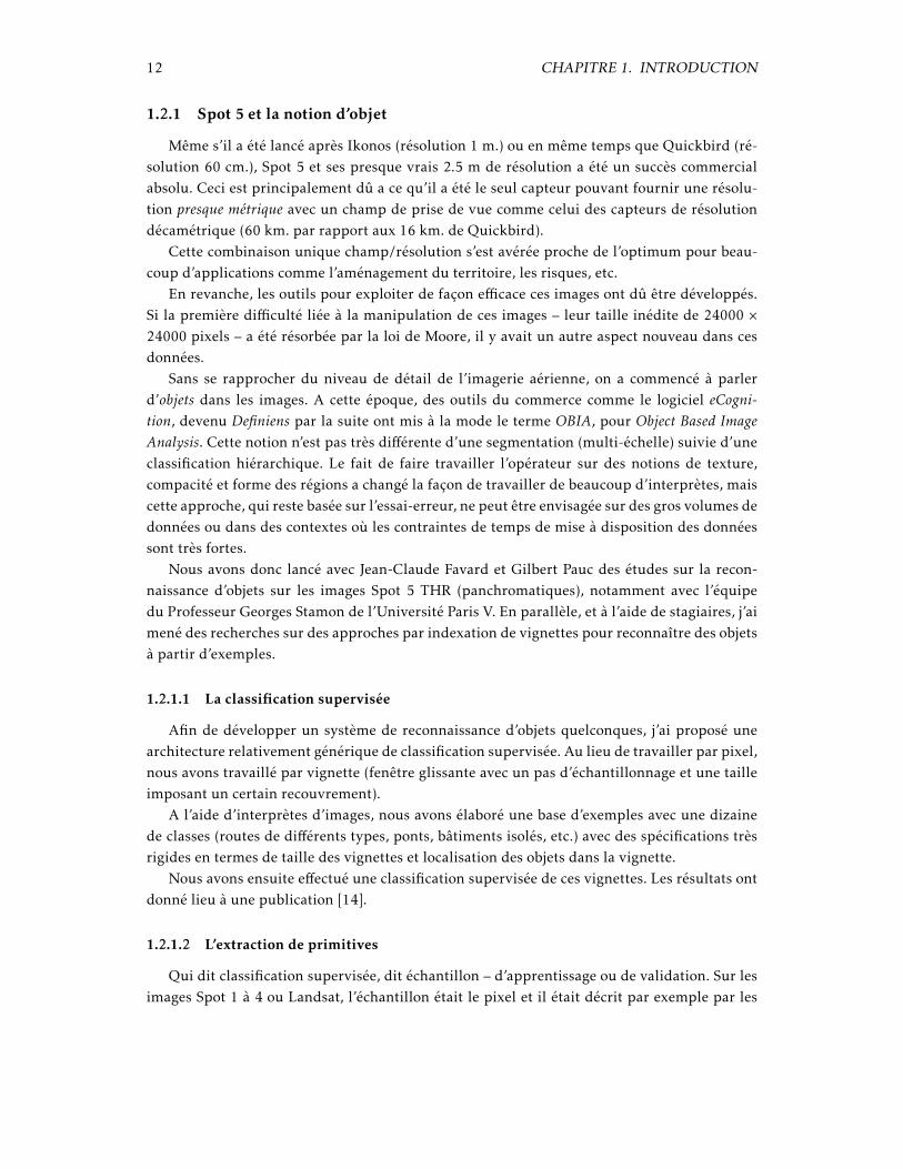
1.2.1 Spot 5 et la notion d’objet
Même s’il a été lancé après Ikonos (résolution 1 m.) ou en même temps que Quickbird (ré-solution 60 cm.), Spot 5 et ses presque vrais 2.5 m de résolution a été un succès commercialabsolu. Ceci est principalement dû a ce qu’il a été le seul capteur pouvant fournir une résolu-tion presque métrique avec un champ de prise de vue comme celui des capteurs de résolutiondécamétrique (60 km. par rapport aux 16 km. de Quickbird).
Cette combinaison unique champ/résolution s’est avérée proche de l’optimum pour beau-coup d’applications comme l’aménagement du territoire, les risques, etc.
En revanche, les outils pour exploiter de façon efficace ces images ont dû être développés.Si la première difficulté liée à la manipulation de ces images – leur taille inédite de 24000 ×24000 pixels – a été résorbée par la loi de Moore, il y avait un autre aspect nouveau dans cesdonnées.
Sans se rapprocher du niveau de détail de l’imagerie aérienne, on a commencé à parlerd’objets dans les images. A cette époque, des outils du commerce comme le logiciel eCogni-tion, devenu Definiens par la suite ont mis à la mode le terme OBIA, pour Object Based ImageAnalysis. Cette notion n’est pas très différente d’une segmentation (multi-échelle) suivie d’uneclassification hiérarchique. Le fait de faire travailler l’opérateur sur des notions de texture,compacité et forme des régions a changé la façon de travailler de beaucoup d’interprètes, maiscette approche, qui reste basée sur l’essai-erreur, ne peut être envisagée sur des gros volumes dedonnées ou dans des contextes où les contraintes de temps de mise à disposition des donnéessont très fortes.
Nous avons donc lancé avec Jean-Claude Favard et Gilbert Pauc des études sur la recon-naissance d’objets sur les images Spot 5 THR (panchromatiques), notamment avec l’équipedu Professeur Georges Stamon de l’Université Paris V. En parallèle, et à l’aide de stagiaires, j’aimené des recherches sur des approches par indexation de vignettes pour reconnaître des objetsà partir d’exemples.
1.2.1.1 La classification supervisée
Afin de développer un système de reconnaissance d’objets quelconques, j’ai proposé unearchitecture relativement générique de classification supervisée. Au lieu de travailler par pixel,nous avons travaillé par vignette (fenêtre glissante avec un pas d’échantillonnage et une tailleimposant un certain recouvrement).
A l’aide d’interprètes d’images, nous avons élaboré une base d’exemples avec une dizainede classes (routes de différents types, ponts, bâtiments isolés, etc.) avec des spécifications trèsrigides en termes de taille des vignettes et localisation des objets dans la vignette.
Nous avons ensuite effectué une classification supervisée de ces vignettes. Les résultats ontdonné lieu à une publication [14].
1.2.1.2 L’extraction de primitives
Qui dit classification supervisée, dit échantillon – d’apprentissage ou de validation. Sur lesimages Spot 1 à 4 ou Landsat, l’échantillon était le pixel et il était décrit par exemple par les

1.2. VALORISATION ET PROMOTION DES IMAGES SATELLITE À HAUTE RÉSOLUTION13
réflectances dans différentes bandes spectrales ou par des indices (NDVI, par exemple).La classification consistait donc à demander à l’algorithme d’apprendre à reconnaître des
pixels de blé, par exemple. Dans le cas de vignettes d’images panchromatiques décrivant, di-sons, un rond-point, ce ne sont pas les valeurs des pixels qui décrivent les classes d’objets, maisplutôt les formes et la géométrie.
Nous avons donc travaillé sur ce type de caractérisation [39].
1.2.2 Orfeo et l’interprétation de scènes
Dès 2003, j’ai commencé à travailler sur la préparation à l’utilisation des données Pléiades,dans le cadre du Programme d’accompagnement Orfeo du Cnes.
Par rapport aux précédentes missions optiques d’observation de la Terre du Cnes, ce pro-gramme préparatoire était beaucoup plus ambitieux. Il a été organisé en 2 volets :
– le volet thématique visant à recueillir les besoins des utilisateurs et à mener des étudesde potentialité des données, puis de validation des résultats ;
– le volet méthodologique, dont je suis devenu responsable en 2005, qui visait à mener desactions de recherche pour développer des nouvelles méthodes nécessaires pour répondreaux besoins des utilisateurs.
Le travail d’animateur du volet méthodologique m’a permis de faire un état de l’art desméthodes existantes (dont j’ai coordonné la rédaction avec des chercheurs d’une vingtaine delaboratoires de recherche en traitement des images). Cet état de l’art a ensuite permis d’alimen-ter les axes de recherche financés par le Cnes dans le domaine de l’extraction d’information àpartir d’images à haute résolution. Les moyens du Cnes pour soutenir ce type de recherchesont les suivants :
– Les bourses de recherche (thèse et post-doc). Dans ce contexte ont été financées les thèsesde Vincent Poulain et Carolina Vanegas.
– Les contrats de R&T via les Dossiers d’Axes Techniques (DAT). J’ai été responsable duDAT OT-4 de 2005 à 2009 qui a financé une moyenne de 10 contrats par an avec unbudget moyen de 500 k¤. J’ai aussi piloté plusieurs contrats chaque année dans ce cadre.
– Les études internes et les stages. Dans ce contexte, j’ai encadré en moyenne 2 stages paran qui ont servi à démarrer des travaux sur le raisonnement spatial (Julien Michel), ladétection de changements entre images et données vecteur (Vincent Poulain), la fusionoptique/SAR (Jan Wegner), la segmentation interactive d’objets (Julien Osman), la gé-nération automatique de cartes d’occupation des sols (Christophe Lay, Malik Ciss), ladétection de changements orientée objets (Éric Koun).
Le travail de recherche que j’ai mené pour le Programme Orfeo s’articule autour de 2 thé-matiques qui couvrent bien les besoins méthodologiques liés aux données Pléiades et CosmoSkymed :
1. Le raisonnement spatial pour la reconnaissance d’objets complexes.
2. L’utilisation d’images à haute résolution pour la mise à jour de cartes numériques auformat vecteur.

14 CHAPITRE 1. INTRODUCTION
1.2.2.1 Le raisonnement spatial
Le recueil des besoins des utilisateurs thématiques Orfeo nous a permis – avec Jean-ClaudeFavard et Hélène de Boissezon – d’identifier un ensemble d’objets d’intérêt. La liste d’objetsainsi constituée était bien différente de ce que nous avions pu avoir pour les images moinsrésolues. Il s’agissait d’abord d’une liste très longue et constituée d’objets soit complexes, soitavec une variabilité intra-classe très importante.
À la différence de ce que nous avons fait pour les images Spot 5 en termes de reconnaissanced’objets, il n’était pas possible d’utiliser les approches de classification par vignette pour lareconnaissance d’objets complexes.
C’est en 2005 que j’ai passé du temps à étudier la bibliographie qui m’a permis de mettreen place un programme de recherche sur l’utilisation des techniques de raisonnement spatialpour l’interprétation de scènes de type Pléiades. Les premiers développements méthodolo-giques ont démarré avec le stage de Julien Michel sur l’évaluation du système RCC-8 et se sontcontinués par la suite par des améliorations de la procédure mise en place et l’intégration dansun système d’apprentissage supervisé [17].
Dans le cadre de la thèse d’Ahed Alboody nous avons étendu ce système de raisonnement.La thèse de Carolina Vanegas nous a mené vers les techniques floues pour la mise en place
de relations spatiales autres que celles purement topologiques du RCC-8.
1.2.2.2 Mise à jour de bases de données cartographiques
Les bases de données cartographiques numériques étant de plus en plus utilisées dans laplupart des applications thématiques de la télédétection, il a été nécessaire de se poser la ques-tion de comment les intégrer dans des approches d’analyse d’images.
L’utilisation de ces cartes numériques – qui se présentent sous la forme d’objets vectorisés(points, lignes, polygones) avec des attributs associés – se fait le plus souvent dans un contextede mise à jour : l’image satellitaire est plus récente que la carte et sert à l’actualiser.
Si beaucoup de travaux existaient pour des résolutions plus fines (photographie aérienne)ou pour des nomenclatures bien spécifiques, nous n’avons pas trouvé d’approche génériquepermettant d’utiliser des types d’imagerie variés pour des nomenclatures quelconques. Le tra-vail de thèse de Vincent Poulain – qui a suivi son stage de M2 – a consisté à démontrer qu’uneapproche générique pouvait être mise en place. Cette approche accepte en entrée des imagesoptiques et SAR de résolutions allant de 50 cm. à 5 m. et peut être facilement adaptée à destypes de nomenclatures – objets – différents en définissant un ensemble d’éléments focaux etleurs descripteurs associés [27].
1.3 Conclusion
Ce chapitre a présenté un survol rapide des activités de recherché menées sur les 10 der-nières années. Il a été montré comment 2 cadres applicatifs déterminés par les activités duCnes ont permis de définir des axes de recherche cohérents.
La suite du document présentera les contributions principales dans ces différents domaines

1.3. CONCLUSION 15
d’activité. J’éviterai de donner beaucoup de détails et renverrai le lecteur intéressé vers lespublications dans les annexes.

2 Mesures de similarité pour le recalage d’images
et la détection de changements
Pour les images de résolution moins fine qu’environ 5 m., le problème du recalage et celuide la détection de changements sont en quelque sorte des duaux :
– le recalage, en supposant qu’il n’y a pas de changements entre les images à recaler,consiste à trouver la déformation géométrique permettant de rendre ces images les plussimilaires possibles ;
– la détection de changements, en supposant que les images sont parfaitement recalées,consiste à détecter les régions où la similarité locale est faible.
Cette façon de présenter ces 2 problèmes est volontairement vague afin de rendre évidentle lien entre eux. Les aspects particuliers de chacun des 2 problèmes et les contributions à leurrésolution seront présentés dans les sections 2.2 et 2.3.
Dans la section suivante nous nous intéressons à l’outil de base qui sera utilisé par la suitedans les 2 cas : les mesures de similarité statistique.
2.1 Les mesures de dépendance statistique
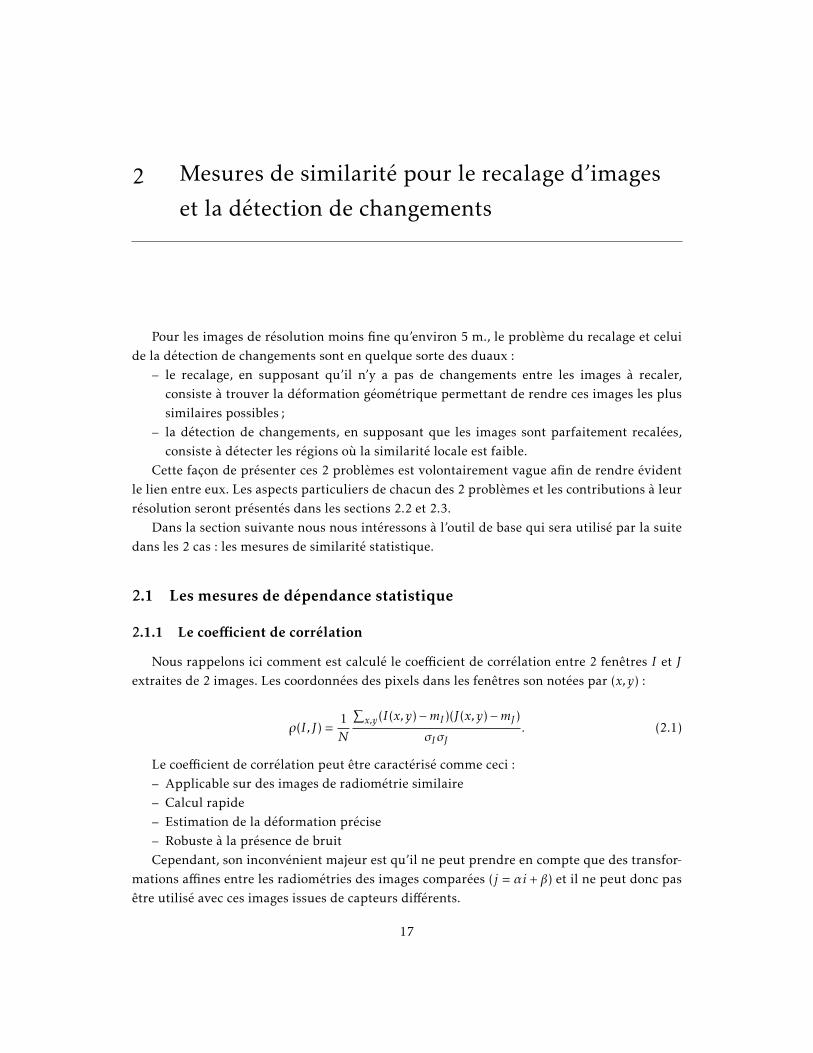
2.1.1 Le coefficient de corrélation
Nous rappelons ici comment est calculé le coefficient de corrélation entre 2 fenêtres I et Jextraites de 2 images. Les coordonnées des pixels dans les fenêtres son notées par (x,y) :
ρ(I, J) =1N
∑x,y(I(x,y)−mI )(J(x,y)−mJ )
σIσJ. (2.1)
Le coefficient de corrélation peut être caractérisé comme ceci :– Applicable sur des images de radiométrie similaire– Calcul rapide– Estimation de la déformation précise– Robuste à la présence de bruitCependant, son inconvénient majeur est qu’il ne peut prendre en compte que des transfor-
mations affines entre les radiométries des images comparées (j = αi + β) et il ne peut donc pasêtre utilisé avec ces images issues de capteurs différents.
17
18CHAPITRE 2. MESURES DE SIMILARITÉ POUR LE RECALAGE D’IMAGES ET LA
DÉTECTION DE CHANGEMENTS
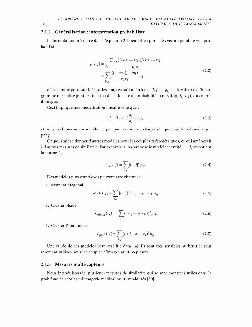
2.1.2 Généralisation : interprétation probabiliste
La formulation présentée dans l’équation 2.1 peut être approché avec un point de vue pro-babiliste :
ρ(I, J) =1N
∑x,y(I(x,y)−mI )(J(x,y)−mJ )
σIσJ
=∑(i,j)
(i −mI )(j −mJ )σIσJ
pij
(2.2)
où la somme porte sur la liste des couples radiométriques (i, j), et pij est la valeur de l’histo-gramme normalisé joint (estimation de la densité de probabilité jointe, ddp, fij (i, j)) du coupled’images.
Ceci implique une modélisation linéaire telle que :
j = (i −mI )σJσI
+mJ , (2.3)
et nous évaluons sa vraisemblance par pondération de chaque chaque couple radiométriquepar pij .
On pourrait se donner d’autres modèles pour les couples radiométriques, ce qui amèneraità d’autres mesures de similarité. Par exemple, si on suppose le modèle identité, i = j, on obtientla norme Ln :
Ln(I, J) =∑i,j
|i − j |npij , (2.4)
Des modèles plus complexes peuvent être obtenus :
1. Moment diagonal :
MD(I, J) =∑i,j
|i − j | (i + j − σI − σJ )pij , (2.5)
1. Cluster Shade :
Cshade(I, J) =∑i,j
(i + j − σI − σJ )3pij , (2.6)
1. Cluster Prominence :
Cpro(I, J) =∑i,j
(i + j − σI − σJ )4pij . (2.7)
Une étude de ces modèles peut être lue dans [4]. Ils sont très sensibles au bruit et sontrarement utilisés pour les couples d’images multi-capteurs.
2.1.3 Mesures multi-capteurs
Nous introduisons ici plusieurs mesures de similarité qui se sont montrées utiles dans leproblème de recalage d’imagerie médical multi-modalités [30].
2.1. LES MESURES DE DÉPENDANCE STATISTIQUE 19
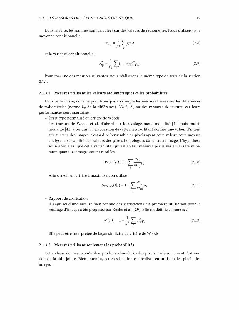
Dans la suite, les sommes sont calculées sur des valeurs de radiométrie. Nous utiliserons lamoyenne conditionnelle :
mI |j =1pj
∑i
ipij ; (2.8)
et la variance conditionnelle :
σ2I |j =
1pj
∑i
(i −mI |j )2pij . (2.9)
Pour chacune des mesures suivantes, nous réaliserons le même type de tests de la section2.1.1.
2.1.3.1 Mesures utilisant les valeurs radiométriques et les probabilités
Dans cette classe, nous ne prendrons pas en compte les mesures basées sur les différencesde radiométries (norme Ln de la différence) [33, 8, 2], ou des mesures de texture, car leursperformances sont mauvaises.
– Écart type normalisé ou critère de WoodsLes travaux de Woods et al. d’abord sur le recalage mono-modalité [40] puis multi-modalité [41] a conduit à l’élaboration de cette mesure. Étant donnée une valeur d’inten-sité sur une des images, c’est à dire l’ensemble de pixels ayant cette valeur, cette mesureanalyse la variabilité des valeurs des pixels homologues dans l’autre image. L’hypothèsesous-jacente est que cette variabilité (qui est en fait mesurée par la variance) sera mini-mum quand les images seront recalées :
Woods(I |J) =∑j
σI |jmI |j
pj (2.10)
Afin d’avoir un critère à maximiser, on utilise :
SWoods(I |J) = 1−∑j
σI |jmI |j
pj (2.11)
– Rapport de corrélationIl s’agit ici d’une mesure bien connue des statisticiens. Sa première utilisation pour lerecalage d’images a été proposée par Roche et al. [29]. Elle est définie comme ceci :
η2(I |J) = 1− 1
σ2I
∑j
σ2I |jpj (2.12)
Elle peut être interprétée de façon similaire au critère de Woods.
2.1.3.2 Mesures utilisant seulement les probabilités
Cette classe de mesures n’utilise pas les radiométries des pixels, mais seulement l’estima-tion de la ddp jointe. Bien entendu, cette estimation est réalisée en utilisant les pixels desimages !
20CHAPITRE 2. MESURES DE SIMILARITÉ POUR LE RECALAGE D’IMAGES ET LA
DÉTECTION DE CHANGEMENTS
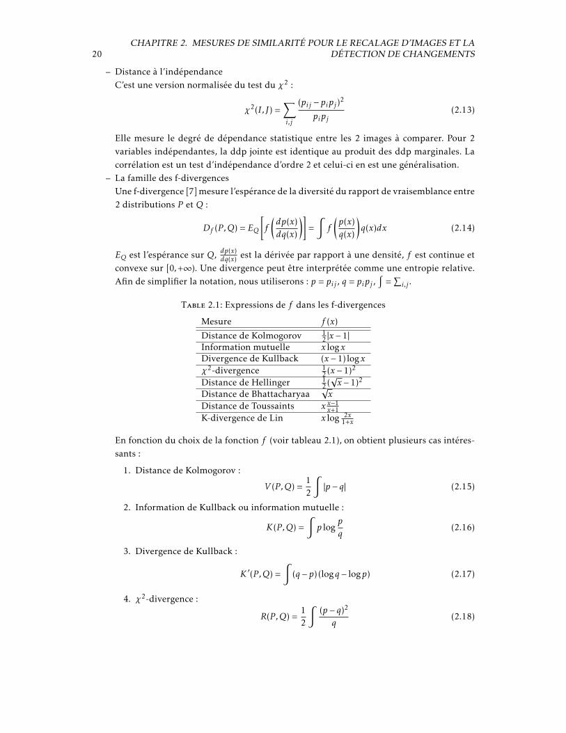
– Distance à l’indépendanceC’est une version normalisée du test du χ2 :
χ2(I, J) =∑i,j
(pij − pipj )2
pipj(2.13)
Elle mesure le degré de dépendance statistique entre les 2 images à comparer. Pour 2variables indépendantes, la ddp jointe est identique au produit des ddp marginales. Lacorrélation est un test d’indépendance d’ordre 2 et celui-ci en est une généralisation.
– La famille des f-divergencesUne f-divergence [7] mesure l’espérance de la diversité du rapport de vraisemblance entre2 distributions P et Q :
Df (P ,Q) = EQ
[f
(dp(x)dq(x)
)]=
∫f
(p(x)q(x)
)q(x)dx (2.14)
EQ est l’espérance sur Q, dp(x)dq(x) est la dérivée par rapport à une densité, f est continue et
convexe sur [0,+∞). Une divergence peut être interprétée comme une entropie relative.Afin de simplifier la notation, nous utiliserons : p = pij , q = pipj ,
∫=
∑i,j .
Table 2.1: Expressions de f dans les f-divergences
Mesure f (x)
Distance de Kolmogorov 12 |x − 1|
Information mutuelle x logxDivergence de Kullback (x − 1)logxχ2-divergence 1
2 (x − 1)2
Distance de Hellinger 12 (√x − 1)2
Distance de Bhattacharyaa√x
Distance de Toussaints x x−1x+1
K-divergence de Lin x log 2x1+x
En fonction du choix de la fonction f (voir tableau 2.1), on obtient plusieurs cas intéres-sants :
1. Distance de Kolmogorov :
V (P ,Q) =12
∫|p − q| (2.15)
2. Information de Kullback ou information mutuelle :
K(P ,Q) =∫p log
p
q(2.16)
3. Divergence de Kullback :
K ′(P ,Q) =∫
(q − p) (logq − logp) (2.17)
4. χ2-divergence :
R(P ,Q) =12
∫(p − q)2
q(2.18)
2.1. LES MESURES DE DÉPENDANCE STATISTIQUE 21
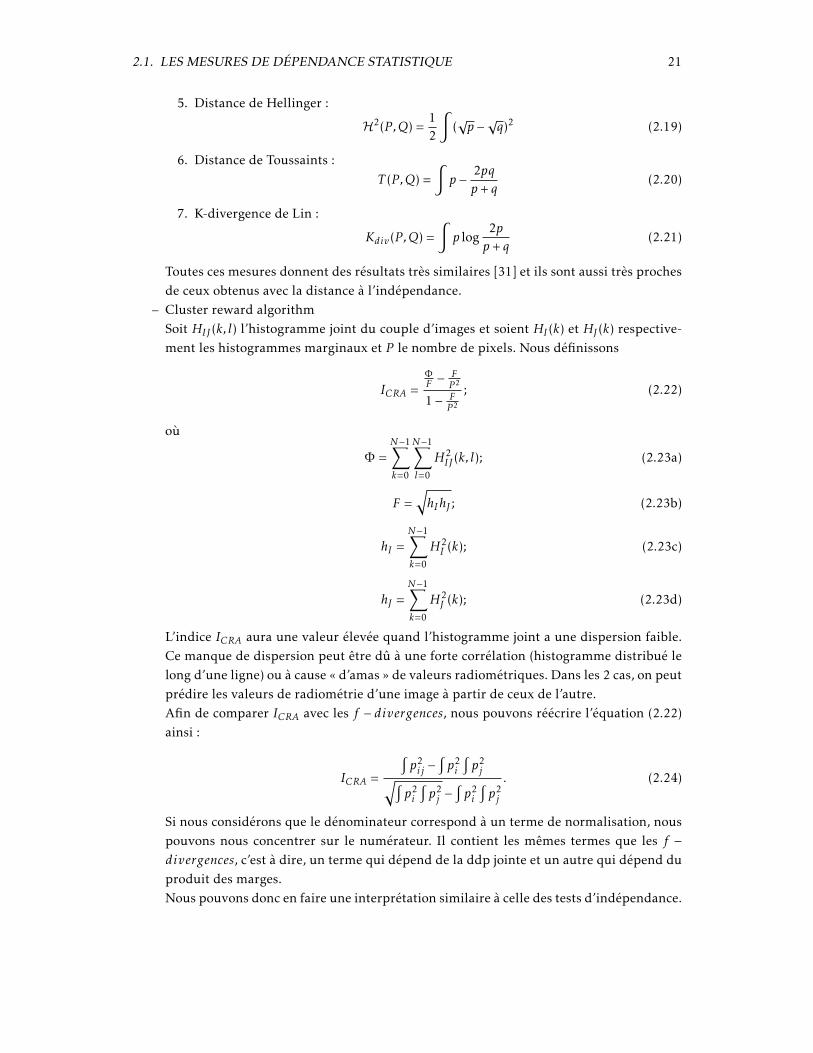
5. Distance de Hellinger :
H2(P ,Q) =12
∫(√p −√q)2 (2.19)
6. Distance de Toussaints :T (P ,Q) =
∫p −
2pqp+ q
(2.20)
7. K-divergence de Lin :
Kdiv(P ,Q) =∫p log
2pp+ q
(2.21)
Toutes ces mesures donnent des résultats très similaires [31] et ils sont aussi très prochesde ceux obtenus avec la distance à l’indépendance.
– Cluster reward algorithmSoit HIJ (k, l) l’histogramme joint du couple d’images et soient HI (k) et HJ (k) respective-ment les histogrammes marginaux et P le nombre de pixels. Nous définissons
ICRA =ΦF −
FP 2
1− FP 2
; (2.22)
où
Φ =N−1∑k=0
N−1∑l=0
H2IJ (k, l); (2.23a)
F =√hIhJ ; (2.23b)
hI =N−1∑k=0
H2I (k); (2.23c)
hJ =N−1∑k=0
H2J (k); (2.23d)
L’indice ICRA aura une valeur élevée quand l’histogramme joint a une dispersion faible.Ce manque de dispersion peut être dû à une forte corrélation (histogramme distribué lelong d’une ligne) ou à cause « d’amas » de valeurs radiométriques. Dans les 2 cas, on peutprédire les valeurs de radiométrie d’une image à partir de ceux de l’autre.Afin de comparer ICRA avec les f − divergences, nous pouvons réécrire l’équation (2.22)ainsi :
ICRA =
∫p2ij −
∫p2i
∫p2j√∫
p2i
∫p2j −
∫p2i
∫p2j
. (2.24)
Si nous considérons que le dénominateur correspond à un terme de normalisation, nouspouvons nous concentrer sur le numérateur. Il contient les mêmes termes que les f −divergences, c’est à dire, un terme qui dépend de la ddp jointe et un autre qui dépend duproduit des marges.Nous pouvons donc en faire une interprétation similaire à celle des tests d’indépendance.
22CHAPITRE 2. MESURES DE SIMILARITÉ POUR LE RECALAGE D’IMAGES ET LA
DÉTECTION DE CHANGEMENTS
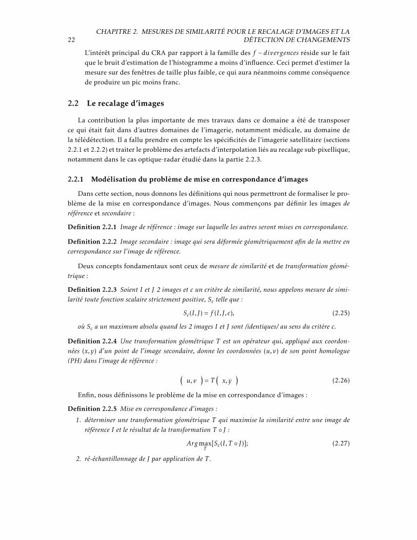
L’intérêt principal du CRA par rapport à la famille des f − divergences réside sur le faitque le bruit d’estimation de l’histogramme a moins d’influence. Ceci permet d’estimer lamesure sur des fenêtres de taille plus faible, ce qui aura néanmoins comme conséquencede produire un pic moins franc.
2.2 Le recalage d’images
La contribution la plus importante de mes travaux dans ce domaine a été de transposerce qui était fait dans d’autres domaines de l’imagerie, notamment médicale, au domaine dela télédétection. Il a fallu prendre en compte les spécificités de l’imagerie satellitaire (sections2.2.1 et 2.2.2) et traiter le problème des artefacts d’interpolation liés au recalage sub-pixellique,notamment dans le cas optique-radar étudié dans la partie 2.2.3.
2.2.1 Modélisation du problème de mise en correspondance d’images
Dans cette section, nous donnons les définitions qui nous permettront de formaliser le pro-blème de la mise en correspondance d’images. Nous commençons par définir les images deréférence et secondaire :
Definition 2.2.1 Image de référence : image sur laquelle les autres seront mises en correspondance.
Definition 2.2.2 Image secondaire : image qui sera déformée géométriquement afin de la mettre encorrespondance sur l’image de référence.
Deux concepts fondamentaux sont ceux de mesure de similarité et de transformation géomé-trique :
Definition 2.2.3 Soient I et J 2 images et c un critère de similarité, nous appelons mesure de simi-larité toute fonction scalaire strictement positive, Sc telle que :
Sc(I, J) = f (I, J, c), (2.25)
où Sc a un maximum absolu quand les 2 images I et J sont /identiques/ au sens du critère c.
Definition 2.2.4 Une transformation géométrique T est un opérateur qui, appliqué aux coordon-nées (x,y) d’un point de l’image secondaire, donne les coordonnées (u,v) de son point homologue(PH) dans l’image de référence : (
u,v)
= T(x,y
)(2.26)
Enfin, nous définissons le problème de la mise en correspondance d’images :
Definition 2.2.5 Mise en correspondance d’images :
1. déterminer une transformation géométrique T qui maximise la similarité entre une image deréférence I et le résultat de la transformation T ◦ J :
ArgmaxT
[Sc(I,T ◦ J)]; (2.27)
2. ré-échantillonnage de J par application de T .

2.2. LE RECALAGE D’IMAGES 23
2.2.2 Modélisation de la déformation géométrique
La transformation géométrique de la définition 2.2.4 est utilisée pour la correction de ladéformation entre 2 images à mettre en correspondance. Cette déformation, contient des in-formations qui sont liées à la scène observée ainsi qu’aux conditions d’acquisition. Ces défor-mations peuvent être classés en 3 types en fonction de leur origine physique :
1. déformation liées à l’attitude moyenne du capteur (angle d’incidence, éventuel pilotageen lacet de la plate-forme) ;
2. déformations liées à la parallaxe (principalement dues au relief) ;
3. déformations liées à l’évolution de l’attitude pendant l’acquisition (micro-vibrations pré-sentes sur les capteurs de
Ces déformations sont caractérisées par leurs fréquence et amplitude. Elles sont présentéessur le tableau suivant :
Amplitude Fréquence spatiale
Attitude moyenne Forte Faible
Parallaxe Moyenne Forte et moyenne
Changement d’attitude Faible Faible et moyenne
En fonction du type de déformation à corriger, son modèle sera différent. Par exemple, si laseule déformation à corriger est celle introduite par l’attitude moyenne, un modèle physiquede la géométrie d’acquisition, indépendant du contenu de l’image sera suffisant. Si le capteurn’est pas bien connu, cette déformation sera approchée par un modèle analytique. Quand lesdéformations à modéliser contiennent des hautes fréquences, les modèles analytiques ne sontpas adaptés. Dans ce cas un échantillonnage fin de la déformation, de type grille de déforma-tion, doit être utilisé.
Les points suivants résument le problème de la modélisation des déformations :
1. Un modèle analytique est une approximation de la déformation. Il est souvent obtenucomme ceci :
a) Directement à partir d’une modélisation physique sans utiliser le contenu de l’image.
b) Par estimation des paramètres d’un modèle a priori. Les paramètres peuvent êtreestimés :
i. Par résolution d’équations en utilisant des PH (qui eux mêmes peuvent êtreobtenus manuellement ou de façon automatique).
ii. Par maximisation d’une mesure de similarité globale.
2. Une grille de déformation est un échantillonnage de la déformation.
Ce dernier point implique que le pas d’échantillonnage de la grille doit être suffisammentpetit afin de prendre en compte les déformations de haute fréquence (théorème de Shannon).Bien entendu, si les déformations ne sont pas stationnaires – ce qui est souvent le cas pour desdéformations liées au relief – l’échantillonnage peut être irrégulier.
24CHAPITRE 2. MESURES DE SIMILARITÉ POUR LE RECALAGE D’IMAGES ET LA
DÉTECTION DE CHANGEMENTS
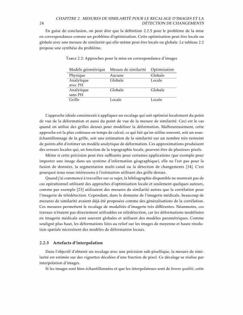
En guise de conclusion, on peut dire que la définition 2.2.5 pose le problème de la miseen correspondance comme un problème d’optimisation. Cette optimisation peut être locale ouglobale avec une mesure de similarité qui elle-même peut être locale ou globale. Le tableau 2.2propose une synthèse du problème.
Table 2.2: Approches pour la mise en correspondance d’images
Modèle géométrique Mesure de similarité Optimisation
Physique Aucune GlobaleAnalytique Globale Localeavec PHAnalytique Globale Globalesans PHGrille Locale Locale
L’approche idéale consisterait à appliquer un recalage qui soit optimisé localement du pointde vue de la déformation et aussi du point de vue de la mesure de similarité. Ceci est le casquand on utilise des grilles denses pour modéliser la déformation. Malheureusement, cetteapproche est la plus coûteuse en temps de calcul, ce qui fait qu’on utilise souvent, soit un sous-échantillonnage de la grille, soit une estimation de la similarité sur un nombre très restreintde points afin d’estimer un modèle analytique de déformation. Ces approximations produisentdes erreurs locales qui, en fonction de la topographie locale, peuvent être de plusieurs pixels.
Même si cette précision peut être suffisante pour certaines applications (par exemple pourimporter une image dans un système d’information géographique), elle ne l’est pas pour lafusion de données, la segmentation multi-canal ou la détection de changements [34]. C’estpourquoi nous nous intéressons à l’estimation utilisant des grille denses.
Quand j’ai commencé à travailler sur ce sujet, la bibliographie disponible ne montrait pas decas opérationnel utilisant des approches d’optimisation locale et seulement quelques auteurs,comme par exemple [23] utilisaient des mesures de similarité autres que la corrélation pourl’imagerie de télédétection. Cependant, dans le domaine de l’imagerie médicale, beaucoup demesures de similarité avaient déjà été proposées comme des généralisations de la corrélation.Ces mesures permettent le recalage de modalités d’imagerie très différentes. Néanmoins, cestravaux n’étaient pas directement utilisables en télédétection, car les déformations modéliséesen imagerie médicale sont souvent globales et utilisent des modèles paramétriques. Commesouligné plus haut, les déformations liées au relief sur les images de moyenne et haute résolu-tion spatiale nécessitent des modèles de déformation locaux.
2.2.3 Artefacts d’interpolation
Dans l’objectif d’obtenir un recalage avec une précision sub-pixellique, la mesure de simi-larité est estimée sur des vignettes décalées d’une fraction de pixel. Ce décalage se réalise parinterpolation d’images.
Si les images sont bien échantillonnées et que les interpolateurs sont de bonne qualité, cette
2.3. LA DÉTECTION DE CHANGEMENTS 25
opération de passe sans encombre. Nous ferons ici abstraction du problème de l’échantillon-nage des images – même si beaucoup de capteurs spatiaux ne respectent pas le critère de Shan-non.
Étant donné que cette opération d’interpolation est coûteuse et a priori réalisée quelques di-zaines de fois par pixel des l’image, il est habituel d’utiliser des interpolations rapides. Le coûtde calcul d’une interpolation est proportionnel à la longueur (en échantillons) du filtre utilisé.La qualité de l’interpolation a une dépendance inversée par rapport à cette même longueur.
Ces interpolations approchées ne se traduisent pas seulement par des résultats bruités, maispar des artefacts avec une structure qui n’est pas spatialement aléatoire. Ceci nous a motivé àrechercher l’origine de ces artefacts et les façons de les atténuer.
Ce problème d’artefacts d’interpolation avait déjà été analysé en imagerie médicale dansle cadre limité de modèles de déformation analytiques et pour l’information mutuelle [26, 35,21]. Nous avons généralisé ce travail en le rendant indépendant de la mesure de similarité etdu modèle de déformation utilisé.
Dans [19] nous avons donné une description analytique du problème en montrant que :
1. Les artefacts étaient dus à la dépendance du degré de lissage de l’interpolateur avec ledécalage sub-pixellique appliqué
2. Ces artefacts sont d’autant plus forts que l’image interpolée est bruitée
3. Un lissage préalable des images permet d’atténuer les artefacts.
2.3 La détection de changements
La détection de changements entre les images de télédétection est rendue difficile à causede plusieurs effets, souvent présents simultanément :
1. Différence de point de vue entre les acquisitions : même dans le cas d’images parfai-tement recalées, les effets d’incidence (de la lumière ou de l’onde SAR) peuvent rendreles images différentes du point de vue de la mesure physique, même en absence de toutchangement.
2. Les différences d’éclairage et d’atmosphère peuvent changer aussi la mesure radiomé-trique
Ces 2 phénomènes, ajoutés au fait que les 2 acquisitions à comparer peuvent avoir été ob-tenues par des capteurs différents, font que des approches simples de mesure de variation, ycompris les mesures de corrélation, s’avèrent souvent inutiles.
Nous nous sommes donc orienté vers des mesures statistiques faisant peu d’hypothèses surles distributions des données. Nous les avons spécialisées dans le cas du radar pour aller plusloin dans la qualité de la détection.
2.3.1 Comparaison de densités de probabilité
Une des premières approches mises en place a été celle de comparer les statistiques localesdans un voisinage du pixel d’intérêt entre les 2 dates d’acquisition.
26CHAPITRE 2. MESURES DE SIMILARITÉ POUR LE RECALAGE D’IMAGES ET LA
DÉTECTION DE CHANGEMENTS
Il faut bien noter ici que nous n’estimons pas la dépendance entre les 2 dates (similaritéentre les pixels), mais bien une distance entre les densités de probabilité.
La première contribution dans ce domaine a été d’utiliser une estimation paramétrique desdensités de probabilité à l’aide du système de Pearson pour ensuite l’injecter dans la divergencede Kullback-Leibler [13]. Ceci a permis d’obtenir des résultats meilleurs que ceux obtenus parle détecteur du rapport de moyennes et celui de la distance Euclidienne entre les densités deprobabilité.
L’inconvénient de cette approche était, d’un côté le coût calculatoire de l’intégration nu-mérique dans la divergence de Kullback-Leibler, et d’un autre côté, la limitation aux lois dusystème de Pearson. Avec Grégoire Mercier, nous avons étendu cette approche à des lois quel-conques, mais proches de la loi normale [16]. L’idée était de développer la densité de proba-bilité de chacune des images en série autour d’une Gaussienne, c’est le développent en séried’Edgeworth qui permet d’obtenir une expression qui ne dépend que des cumulants et quicontient très peu de coefficients si la densité n’est pas très différente de la Gaussienne.
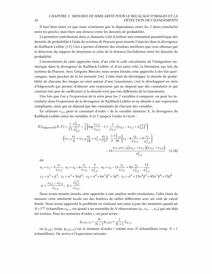
Une fois que l’on a l’expression de la série pour les 2 variables à comparer, on peut les in-troduire dans l’expression de la divergence de Kullback-Leibler et on aboutit à une expressioncompliquée, mais qui ne dépend que des cumulants de chacune des variables.
En utilisant κX;i pour le cumulant d’ordre i de la variable aléatoire X, la divergence deKullback-Leibler entre les variables X et Y jusqu’à l’ordre 4 s’écrit :
KLEdgeworth(X,Y ) =1
12
κ2X′ ;3
κ2X;2
+12
(log
κY ;2
κX;2− 1 +
1κY ;2
(κX;1 −κY ;1 +κ1/2
X;2
)2)
−(κY ′ ;3
a1
6+κY ′ ;4
a2
24+κ2
Y ′ ;3a3
72
)− 1
2
κ2Y ′ ;3
36
c6 − 6c4
κX;2+ 9
c2
κ2Y ;2
− 10
κX′ ;3κY ′ ;3(κX;1 −κY ;1
)(κX;2 −κY ;2
)κ6Y ;2
(2.28)
où
a1 = c3 − 3ακY ;2
; a2 = c4 − 6c2
κY ;2+
3
κ2Y ;2
; a3 = c6 − 15c4
κY ;2+ 45
c2
κ2Y ;2
− 15
κ3Y ;2
c2 = α2 + β2; c3 = α3 + 3αβ2; c4 = α4 + 6α2β2 + 3β4; c6 = α6 + 15α4β2 + 45α2β4 + 15β6
α =κX;1 −κY ;1
κY ;2; β =
κ1/2X;2
κY ;2.
Nous avons ensuite étendu cette approche à une analyse multi-résolutions, l’idée étant demesurer cette similarité locale sur des fenêtres de tailles différentes avec un coût de calcullimité. Nous avons approché le problème en réalisant une mise à jour des moments quand unN +1me échantillon xN+1 est ajouté à un ensemble deN observations {x1,x2, . . . ,xN } qui ont déjàété traitées. Pour les moments d’ordre r, on peut écrire :
µr,[N+1] =N
N + 1µr,[N ] +
1N + 1
xrN+1.
où µr,[N ] (resp. µr,[N+1]) est le moment d’ordre r estimé avec N échantillons (resp. N + 1échantillons). On arrive à l’expression suivante :
2.3. LA DÉTECTION DE CHANGEMENTS 27
µ1,[N ] =1Ns1,[N ] (2.29)
µr,[N ] =1N
r∑`=0
(r`
)(−µ1,[N ]
)r−`s`,[N ],
où la notation sr,[N ] =∑Ni=1 x
ri a été utilisée. On peut ainsi mettre à jour le calcul des moments
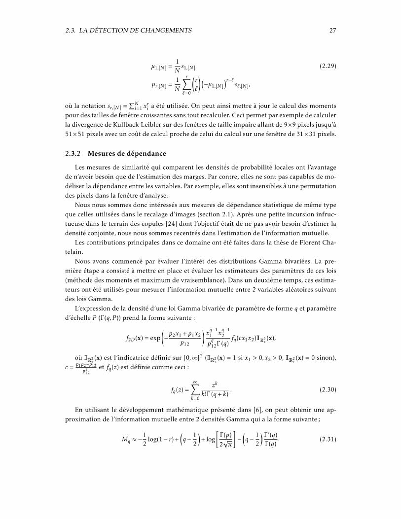
pour des tailles de fenêtre croissantes sans tout recalculer. Ceci permet par exemple de calculerla divergence de Kullback-Leibler sur des fenêtres de taille impaire allant de 9×9 pixels jusqu’à51×51 pixels avec un coût de calcul proche de celui du calcul sur une fenêtre de 31×31 pixels.
2.3.2 Mesures de dépendance
Les mesures de similarité qui comparent les densités de probabilité locales ont l’avantagede n’avoir besoin que de l’estimation des marges. Par contre, elles ne sont pas capables de mo-déliser la dépendance entre les variables. Par exemple, elles sont insensibles à une permutationdes pixels dans la fenêtre d’analyse.
Nous nous sommes donc intéressés aux mesures de dépendance statistique de même typeque celles utilisées dans le recalage d’images (section 2.1). Après une petite incursion infruc-tueuse dans le terrain des copules [24] dont l’objectif était de ne pas avoir besoin d’estimer ladensité conjointe, nous nous sommes recentrés dans l’estimation de l’information mutuelle.
Les contributions principales dans ce domaine ont été faites dans la thèse de Florent Cha-telain.
Nous avons commencé par évaluer l’intérêt des distributions Gamma bivariées. La pre-mière étape a consisté à mettre en place et évaluer les estimateurs des paramètres de ces lois(méthode des moments et maximum de vraisemblance). Dans un deuxième temps, ces estima-teurs ont été utilisés pour mesurer l’information mutuelle entre 2 variables aléatoires suivantdes lois Gamma.
L’expression de la densité d’une loi Gamma bivariée de paramètre de forme q et paramètred’échelle P (Γ (q,P )) prend la forme suivante :
f2D (x) = exp(−p2x1 + p1x2
p12
)xq−11 x
q−12
pq12Γ (q)
fq(cx1x2)IR
2+(x),
où IR
2+(x) est l’indicatrice définie sur [0,∞[2 (I
R2+(x) = 1 si x1 > 0,x2 > 0, I
R2+(x) = 0 sinon),
c = p1p2−p12p2
12et fq(z) est définie comme ceci :
fq(z) =∞∑k=0
zk
k!Γ (q+ k). (2.30)
En utilisant le développement mathématique présenté dans [6], on peut obtenir une ap-proximation de l’information mutuelle entre 2 densités Gamma qui a la forme suivante ;
Mq ≈ −12
log(1− r) +(q − 1
2
)+ log
[Γ (p)2√π
]−(q − 1
2
)Γ ′(q)Γ (q)
. (2.31)

28CHAPITRE 2. MESURES DE SIMILARITÉ POUR LE RECALAGE D’IMAGES ET LA
DÉTECTION DE CHANGEMENTS
avec r le coefficient de corrélation.L’intérêt de cette expression est qu’une fois le paramètre q des lois Gamma des marges
estimé, le coût d’estimation de l’information mutuelle est le même que celui de la corrélation.La limitation de cette technique est l’hypothèse de lois marginales avec le même paramètre
de forme. Afin de lever cette limitation, la deuxième partie de la thèse de Florent Chatelaina consisté à développer des estimateurs pour ce qu’on a appelé les lois Gamma multivariéesmulticapteurs. Les résultats principaux ont été présentés dans [5] et le lecteur intéressé estinvité à en consulter les détails.
2.3.3 Classification supervisée
Les techniques de détection de changements présentées plus haut ont un inconvénient ma-jeur : elles ne sont pas capables de distinguer entre les changements intéressants et les autres.Même si les mesures de similarité utilisées sont robustes aux changements d’illumination, d’in-cidence, etc. elles ne font pas de différence entre les différents types de changements.
Dans le cas de la génération de cartes de dégâts suite à des catastrophes naturelles (inon-dations, tremblements de terre, etc.), il est nécessaire de distinguer les zones qui ont changésuite à l’événement catastrophique des zones qui ont eu une évolution normale (évolution dela végétation, par exemple).
Face à ce problème difficile, il nous a semblé nécessaire de placer un opérateur au sein dusystème de détection de changements, plutôt que de le placer après pour réaliser une sélectiondes changements pertinents.
L’architecture de la chaîne de changements proposée était simple. Il s’agissait de réaliserune classification à 2 classes (changement intéressant et la classe complémentaire). Nous avonsabordé ce problème avec une approche pixel – les résolutions des satellites disponibles dansla Charte à l’époque ne justifiaient pas l’approche objet – et les primitives utilisées pour lacaractérisation des pixels étaient toutes trouvées : les valeurs des pixels eux-mêmes et desindicateurs de changements simples (différences, ratios, corrélations).
Nous avons choisi un classifieur de type SVM à cause de sa capacité à travailler avec peud’échantillons d’apprentissage – données par un opérateur en temps réel – et aussi parce queles SVM permettent de travailler dans des espaces de primitives à grande dimension.
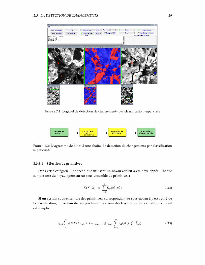
Une mise en oeuvre logicielle (figure 2.1) a été mise à disposition de photo-interprètes quil’ont validée dans le cadre du projet FP7 PREVIEW.
Cette position du problème à donné lieu à la thèse de Tarek Habib. Ce travail de thèse a eucomme objectif d’optimiser cette chaîne et de donner à l’opérateur la possibilité d’agir sur uncurseur qui règle le compromis temps de calcul / qualité de la détection.
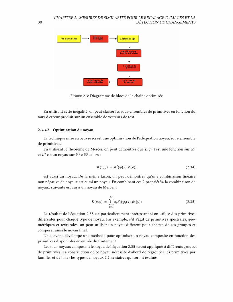
Le point de départ est donc une chaîne très simple où l’on extrait des primitives à partirdes images à comparer, puis on applique une fonction de décision obtenue par classificationsupervisée (figure 2.2).
La figure 2.3 présente en rouge les étapes sur lesquelles des contributions ont été réalisées.
2.3. LA DÉTECTION DE CHANGEMENTS 29
Figure 2.1: Logiciel de détection de changements par classification supervisée
Figure 2.2: Diagramme de blocs d’une chaîne de détection de changements par classificationsupervisée.
2.3.3.1 Sélection de primitives
Dans cette catégorie, une technique utilisant un noyau additif a été développée. Chaquecomposante du noyau opère sur un sous-ensemble de primitives :
K(Xi ,Xj ) =n∑l=1
Kγ (xγi ,xγj ) (2.32)
Si un certain sous-ensemble des primitives, correspondant au sous-noyau Kγ est retiré dela classification, un vecteur de test produira une erreur de classification si la condition suivantest remplie :
ytest
m∑i=1
yiβiK(Xtest ,Xi) + ytestb ≤ ytest
m∑i=1
yiβiKγ (xγi ,xγtest) (2.33)
30CHAPITRE 2. MESURES DE SIMILARITÉ POUR LE RECALAGE D’IMAGES ET LA
DÉTECTION DE CHANGEMENTS
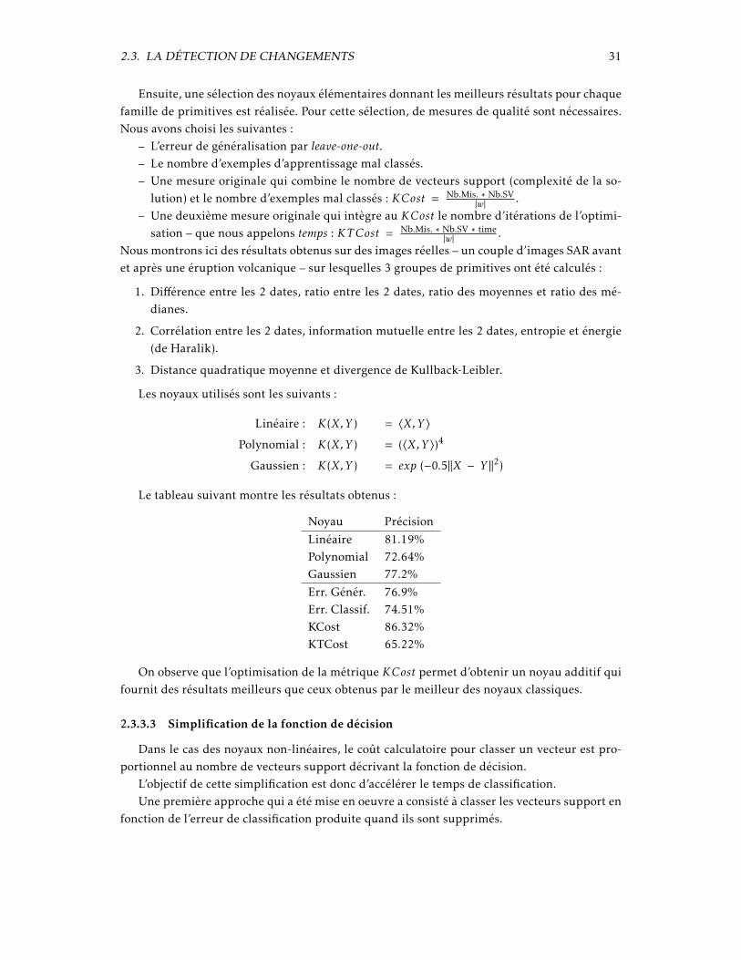
Figure 2.3: Diagramme de blocs de la chaîne optimisée
En utilisant cette inégalité, on peut classer les sous-ensembles de primitives en fonction dutaux d’erreur produit sur un ensemble de vecteurs de test.
2.3.3.2 Optimisation du noyau
La technique mise en oeuvre ici est une optimisation de l’adéquation noyau/sous-ensemblede primitives.
En utilisant le théorème de Mercer, on peut démontrer que si ψ(·) est une fonction sur Rp
et K ′ est un noyau sur Rp ×Rp, alors :
K(x,y) = K ′(ψ(x),ψ(y)) (2.34)
est aussi un noyau. De la même façon, on peut démontrer qu’une combinaison linéairenon négative de noyaux est aussi un noyau. En combinant ces 2 propriétés, la combinaison denoyaux suivante est aussi un noyau de Mercer :
K(x,y) =M∑i=1
aiKi(ψi(x),ψi(y)) (2.35)
Le résultat de l’équation 2.35 est particulièrement intéressant si on utilise des primitivesdifférentes pour chaque type de noyau. Par exemple, s’il s’agit de primitives spectrales, géo-métriques et texturales, on peut utiliser un noyau différent pour chacun de ces groupes etcomposer ainsi le noyau final.
Nous avons développé une méthode pour optimiser un noyau composite en fonction desprimitives disponibles en entrée du traitement.
Les sous-noyaux composant le noyau de l’équation 2.35 seront appliqués à différents groupesde primitives. La construction de ce noyau nécessite d’abord de regrouper les primitives parfamilles et de lister les types de noyaux élémentaires qui seront évalués.
2.3. LA DÉTECTION DE CHANGEMENTS 31
Ensuite, une sélection des noyaux élémentaires donnant les meilleurs résultats pour chaquefamille de primitives est réalisée. Pour cette sélection, de mesures de qualité sont nécessaires.Nous avons choisi les suivantes :
– L’erreur de généralisation par leave-one-out.– Le nombre d’exemples d’apprentissage mal classés.– Une mesure originale qui combine le nombre de vecteurs support (complexité de la so-
lution) et le nombre d’exemples mal classés : KCost = Nb.Mis. ∗ Nb.SV|w| .
– Une deuxième mesure originale qui intègre au KCost le nombre d’itérations de l’optimi-sation – que nous appelons temps : KTCost = Nb.Mis. ∗ Nb.SV ∗ time
|w| .Nous montrons ici des résultats obtenus sur des images réelles – un couple d’images SAR avantet après une éruption volcanique – sur lesquelles 3 groupes de primitives ont été calculés :
1. Différence entre les 2 dates, ratio entre les 2 dates, ratio des moyennes et ratio des mé-dianes.
2. Corrélation entre les 2 dates, information mutuelle entre les 2 dates, entropie et énergie(de Haralik).
3. Distance quadratique moyenne et divergence de Kullback-Leibler.
Les noyaux utilisés sont les suivants :
Linéaire : K(X,Y ) = 〈X,Y 〉
Polynomial : K(X,Y ) = (〈X,Y 〉)4
Gaussien : K(X,Y ) = exp (−0.5‖X − Y ‖2)
Le tableau suivant montre les résultats obtenus :
Noyau Précision
Linéaire 81.19%Polynomial 72.64%Gaussien 77.2%
Err. Génér. 76.9%Err. Classif. 74.51%KCost 86.32%KTCost 65.22%
On observe que l’optimisation de la métrique KCost permet d’obtenir un noyau additif quifournit des résultats meilleurs que ceux obtenus par le meilleur des noyaux classiques.
2.3.3.3 Simplification de la fonction de décision
Dans le cas des noyaux non-linéaires, le coût calculatoire pour classer un vecteur est pro-portionnel au nombre de vecteurs support décrivant la fonction de décision.
L’objectif de cette simplification est donc d’accélérer le temps de classification.Une première approche qui a été mise en oeuvre a consisté à classer les vecteurs support en
fonction de l’erreur de classification produite quand ils sont supprimés.

32CHAPITRE 2. MESURES DE SIMILARITÉ POUR LE RECALAGE D’IMAGES ET LA
DÉTECTION DE CHANGEMENTS
Une deuxième approche plus originale a consisté à développer en série de Taylor l’expres-sion analytique de la surface de décision :
f (xtest) = sgn
m∑i=1
αiyik(xtest ,xi) + b
. (2.36)
Pour ce faire, il faut choisir un ensemble d’origines autour desquelles le développementest réalisé. Les paramètres qui permettent de régler le compromis entre le temps de calcul etla précision de la classification sont le nombre d’origines (le nombre de séries) et l’ordre desséries.
Les résultats obtenus ont montré que l’on peut gagner un facteur 10 en temps de calcul avecune perte de 10% à 20% sur la qualité de la classification.
3 Classification pour la reconnaissance d’objets
3.1 Introduction
Notre objectif est de mettre au point un système de classification d’objets dans des imagessatellitaires à haute résolution (de type Spot 5). L’une des particularités de l’imagerie hauterésolution est que l’information réside principalement dans la géométrie de l’image ; ainsi, unrond-point y sera mieux caractérisé par sa forme que par sa texture.
Nous avons choisi de ne prendre en compte que l’aspect géométrique des objets considérés,sans tenir compte de la radiométrie, de la texture, etc. Cela a des avantages car le système estalors indépendant de la bande spectrale ou de la saison à laquelle sont prises les images.
De plus, nous avons adopté une approche qui consiste à explorer l’image à analyser defaçon séquentielle et travailler avec des vignettes de taille 100 pixels × 100 pixels. Sur chaquevignette, nous demandons au système de déterminer la classe de l’objet centré dans la zoned’analyse. Pour ce faire, nous utilisons une procédure de classification supervisée à partir d’unapprentissage sur une base d’exemples.
Ainsi, la reconnaissance d’objets au sens où nous l’entendons consiste à effectuer une clas-sification de l’objet présent dans une fenêtre d’analyse et ce à partir d’une caractérisation de lagéométrie de l’imagette.
Ce travail a été réalisé avec l’aide de plusieurs stagiaires : Olivier Caignart, Léonard Potieret Jérome Tagnères. Les résultats obtenus ont donné lieu à un article de revue [14].
3.2 Classes d’objets
Nous avons choisi de nous intéresser à des objets qui peuvent être intéressants dans lesapplications de cartographie rapide. Les classes choisies sont les suivantes :
1. BT bâtiments isolés ;
2. CH chemins ;
3. CR croisements ;
4. PT ponts ;
5. RD routes départementales ;
6. RN routes nationales ;
7. RP ronds-point ;
33

34 CHAPITRE 3. CLASSIFICATION POUR LA RECONNAISSANCE D’OBJETS
8. RS routes secondaires ;
9. VF voies ferrées ;
10. ZP zones pavillonnaires.
Par ailleurs, nous avons ajouté une 11e classe d’objets :– AU autres.Il faut noter que la prise en compte des routes dans la liste des classes nous sert à mieux ca-
ractériser la classe de rejet, mais qu’en aucun cas nous avons envisagé de faire une détection deroutes avec l’approche de reconnaissance d’objets décrite dans ce document. En effet, d’autrestechniques de détection de routes beaucoup plus efficaces existent dans la littérature.
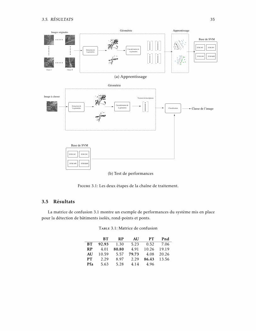
3.3 Chaîne de traitement
La chaîne de traitement comprend trois étapes :
1. L’apprentissage est réalisé à partir d’un pourcentage des imagettes ; ce pourcentage peut-être fixé à n’importe quelle valeur. On détermine le vecteur caractéristique (ou vecteurdes descripteurs) de chacune d’elles à partir de différents traitements (moments com-plexes, transformée de Fourier-Mellin, etc.), puis on fournit les vecteurs ainsi détermi-nés au classifieur qui va déterminer la surface de séparation optimale pour chacun descouples de classes.
2. Le test de performances est à son tour effectué, à partir des imagettes restantes. On dé-termine là encore les vecteurs caractéristiques, puis on les soumet au classifieur selon lastratégie « un contre un » présentée un peu plus loin.
3. L’application à une image complète consiste à essayer de reconnaître les objets dans uneimage de grande taille par balayage séquentiel et application du système de classificationissu de l’apprentissage. Cette étape n’est pas été mise en œuvre.
Les deux premières étapes sont représentées sur la figure 3.1.
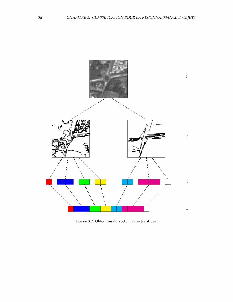
3.4 Description des imagettes
La figure 3.2 illustre l’obtention du vecteur caractéristique de dimension N pour chacunedes imagettes ; voici la signification des quatre étapes apparentes :
– Étape 1 imagette d’origine ;– Étape 2 extraction d’information ;– Étape 3 calcul des vecteurs des différents traitements ;– Étape 4 concaténation pour former le vecteur caractéristique.Les études sur la sélection de primitives n’ont pas permis de réduire de façon significative le
nombre de composantes du vecteur descripteur. La robustesse des SVM au phénomène de Hu-ghes – l’augmentation de la dimensionalité de l’espace de descripteurs nécessiterait beaucoupd’échantillons– nous a permis d’obtenir des résultats satisfaisants.
3.5. RÉSULTATS 35
la géométrieCarcatérisation de
Classe 1 Classe N
la géométrieExtraction de
Images originalesGéométrie Apprentissage
SVM 1#2 SVM 2#3
SVM 1#N SVM K#N
Base de SVM
(a) Apprentissage
la géométrieCarcatérisation de
SVM 1#2 SVM 2#3
SVM 1#N SVM K#N
Base de SVM
Classificationla géométrieExtraction de
Géométrie
Image à classerVecteur de descripteurs
Classe de l’image
(b) Test de performances
Figure 3.1: Les deux étapes de la chaîne de traitement.
3.5 Résultats
La matrice de confusion 3.1 montre un exemple de performances du système mis en placepour la détection de bâtiments isolés, rond-points et ponts.
Table 3.1: Matrice de confusion
BT RP AU PT PndBT 92.93 1.30 5.23 0.52 7.06RP 4.01 80.80 4.91 10.26 19.19AU 10.59 5.57 79.73 4.08 20.26PT 2.29 8.97 2.29 86.43 13.56Pfa 5.63 5.28 4.14 4.96
36 CHAPITRE 3. CLASSIFICATION POUR LA RECONNAISSANCE D’OBJETS
1
2
3
4
Figure 3.2: Obtention du vecteur caractéristique.
4 Raisonnement spatial pour l’interprétation de
scènes
4.1 Motivation
L’utilisation de primitives de bas niveau comme celles utilisées dans le chapitre 3 ne per-met pas de décrire de façon efficace des objets complexes ou composites. Dans les images à ré-solution métrique et sub-métrique, beaucoup d’objets deviennent des objets composites. Cetterecherche a donc été motivée par les activités de préparation à l’utilisation des images Pléiades.
La diversité des objets d’intérêt identifiées par les utilisateurs thématiques impliqués dansle Programme préparatoire Orfeo a mis en évidence que, si on voulait échapper à une miseen oeuvre de chaînes spécifiques par type d’objet, des outils puissants de description à hautniveau d’abstraction sémantique étaient nécessaires. Nous nous sommes donc orientés vers lesoutils de description qualitative.
Ces outils peuvent être classés en 2 grandes familles :
1. Approches qualitatives du raisonnement métrique : on introduit l’incertitude et l’impré-cision dans des descripteurs spatiaux classiques.
2. Approches topologiques : représentation qualitative de l’espace.
Nous avons commencé nos travaux par le 2ème point ci dessus, notamment sur l’utilisa-tion du Region Connexion Calculus et ses extensions (stage de Julien Michel et études associées[17] et thèse d’Ahed Alboody [1]). Puis nous avons aussi abordé les approches qualitatives duraisonnement métrique via les relations spatiales floues (thèse de Carolina Vanegas [36]).
4.2 Region connection calculus et son extension
4.2.1 Le RCC-8
Le Region Connection Calculus (RCC) [12] est basé sur la notion de connexion entre couplesde régions de l’espace. Ces connexions appartiennent à un ensemble fini de possibilités. Diffé-rents RCCs peuvent donc être obtenus en fonction du nombre de connexions considérées. Unde ces systèmes, le RCC-8, est spécialement intéressant, car il est composé d’un ensemble derelations exhaustives et mutuellement exclusives. Ces propriétés rendent le raisonnement plussimple. La figure 4.1 montre les 8 relations qui vont de la déconnexion (DC) jusqu’à l’équiva-
37
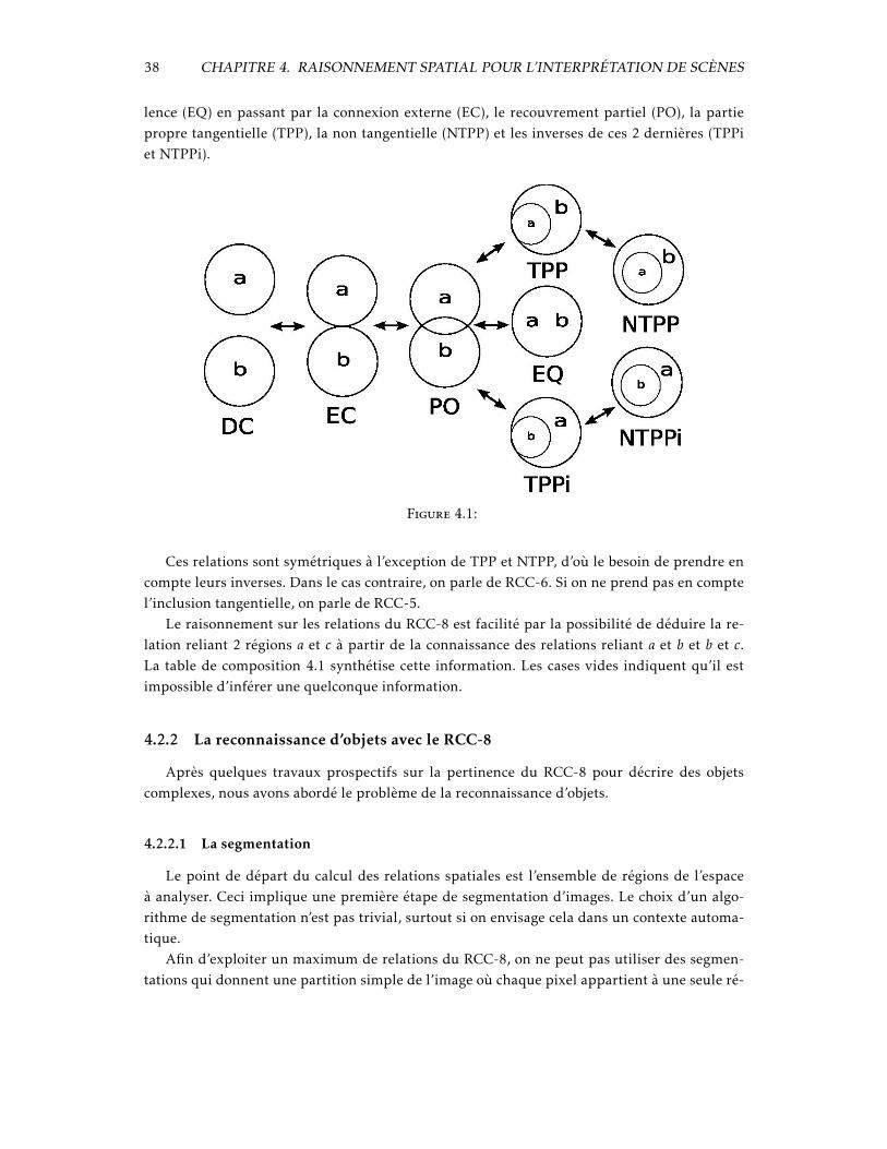
38 CHAPITRE 4. RAISONNEMENT SPATIAL POUR L’INTERPRÉTATION DE SCÈNES
lence (EQ) en passant par la connexion externe (EC), le recouvrement partiel (PO), la partiepropre tangentielle (TPP), la non tangentielle (NTPP) et les inverses de ces 2 dernières (TPPiet NTPPi).
Figure 4.1:
Ces relations sont symétriques à l’exception de TPP et NTPP, d’où le besoin de prendre encompte leurs inverses. Dans le cas contraire, on parle de RCC-6. Si on ne prend pas en comptel’inclusion tangentielle, on parle de RCC-5.
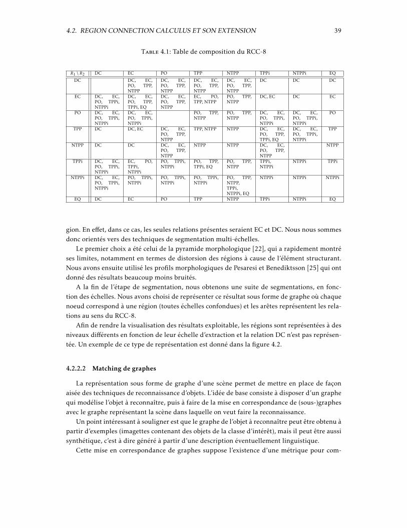
Le raisonnement sur les relations du RCC-8 est facilité par la possibilité de déduire la re-lation reliant 2 régions a et c à partir de la connaissance des relations reliant a et b et b et c.La table de composition 4.1 synthétise cette information. Les cases vides indiquent qu’il estimpossible d’inférer une quelconque information.
4.2.2 La reconnaissance d’objets avec le RCC-8
Après quelques travaux prospectifs sur la pertinence du RCC-8 pour décrire des objetscomplexes, nous avons abordé le problème de la reconnaissance d’objets.
4.2.2.1 La segmentation
Le point de départ du calcul des relations spatiales est l’ensemble de régions de l’espaceà analyser. Ceci implique une première étape de segmentation d’images. Le choix d’un algo-rithme de segmentation n’est pas trivial, surtout si on envisage cela dans un contexte automa-tique.
Afin d’exploiter un maximum de relations du RCC-8, on ne peut pas utiliser des segmen-tations qui donnent une partition simple de l’image où chaque pixel appartient à une seule ré-
4.2. REGION CONNECTION CALCULUS ET SON EXTENSION 39
Table 4.1: Table de composition du RCC-8
R1 \R2 DC EC PO TPP NTPP TPPi NTPPi EQ
DC DC, EC,PO, TPP,NTPP
DC, EC,PO, TPP,NTPP
DC, EC,PO, TPP,NTPP
DC, EC,PO, TPP,NTPP
DC DC DC
EC DC, EC,PO, TPPi,NTPPi
DC, EC,PO, TPP,TPPi, EQ
DC, EC,PO, TPP,NTPP
EC, PO,TPP, NTPP
PO, TPP,NTPP
DC, EC DC EC
PO DC, EC,PO, TPPi,NTPPi
DC, EC,PO, TPPi,NTPPi
PO, TPP,NTPP
PO, TPP,NTPP
DC, EC,PO, TPPi,NTPPi
DC, EC,PO, TPPi,NTPPi
PO
TPP DC DC, EC DC, EC,PO, TPP,NTPP
TPP, NTPP NTPP DC, EC,PO, TPP,TPPi, EQ
DC, EC,PO, TPPi,NTPPi
TPP
NTPP DC DC DC, EC,PO, TPP,NTPP
NTPP NTPP DC, EC,PO, TPP,NTPP
NTPP
TPPi DC, EC,PO, TPPi,NTPPi
EC, PO,TPPi,NTPPi
PO, TPPi,NTPPi
PO, TPP,TPPi, EQ
PO, TPP,NTPP
TPPi,NTPPi
NTPPi TPPi
NTPPi DC, EC,PO, TPPi,NTPPi
PO, TPPi,NTPPi
PO, TPPi,NTPPi
PO, TPPi,NTPPi
PO, TPP,NTPP,TPPi,NTPPi, EQ
NTPPi NTPPi NTPPi
EQ DC EC PO TPP NTPP TPPi NTPPi EQ
gion. En effet, dans ce cas, les seules relations présentes seraient EC et DC. Nous nous sommesdonc orientés vers des techniques de segmentation multi-échelles.
Le premier choix a été celui de la pyramide morphologique [22], qui a rapidement montréses limites, notamment en termes de distorsion des régions à cause de l’élément structurant.Nous avons ensuite utilisé les profils morphologiques de Pesaresi et Benediktsson [25] qui ontdonné des résultats beaucoup moins bruités.
A la fin de l’étape de segmentation, nous obtenons une suite de segmentations, en fonc-tion des échelles. Nous avons choisi de représenter ce résultat sous forme de graphe où chaquenoeud correspond à une région (toutes échelles confondues) et les arêtes représentent les rela-tions au sens du RCC-8.
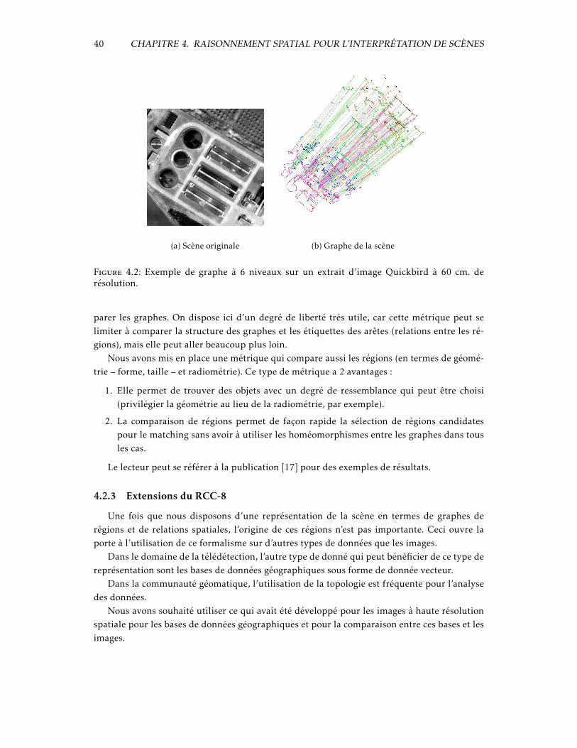
Afin de rendre la visualisation des résultats exploitable, les régions sont représentées à desniveaux différents en fonction de leur échelle d’extraction et la relation DC n’est pas représen-tée. Un exemple de ce type de représentation est donné dans la figure 4.2.
4.2.2.2 Matching de graphes
La représentation sous forme de graphe d’une scène permet de mettre en place de façonaisée des techniques de reconnaissance d’objets. L’idée de base consiste à disposer d’un graphequi modélise l’objet à reconnaître, puis à faire de la mise en correspondance de (sous-)graphesavec le graphe représentant la scène dans laquelle on veut faire la reconnaissance.
Un point intéressant à souligner est que le graphe de l’objet à reconnaître peut être obtenu àpartir d’exemples (imagettes contenant des objets de la classe d’intérêt), mais il peut être aussisynthétique, c’est à dire généré à partir d’une description éventuellement linguistique.
Cette mise en correspondance de graphes suppose l’existence d’une métrique pour com-
40 CHAPITRE 4. RAISONNEMENT SPATIAL POUR L’INTERPRÉTATION DE SCÈNES
(a) Scène originale (b) Graphe de la scène
Figure 4.2: Exemple de graphe à 6 niveaux sur un extrait d’image Quickbird à 60 cm. derésolution.
parer les graphes. On dispose ici d’un degré de liberté très utile, car cette métrique peut selimiter à comparer la structure des graphes et les étiquettes des arêtes (relations entre les ré-gions), mais elle peut aller beaucoup plus loin.
Nous avons mis en place une métrique qui compare aussi les régions (en termes de géomé-trie – forme, taille – et radiométrie). Ce type de métrique a 2 avantages :
1. Elle permet de trouver des objets avec un degré de ressemblance qui peut être choisi(privilégier la géométrie au lieu de la radiométrie, par exemple).
2. La comparaison de régions permet de façon rapide la sélection de régions candidatespour le matching sans avoir à utiliser les homéomorphismes entre les graphes dans tousles cas.
Le lecteur peut se référer à la publication [17] pour des exemples de résultats.
4.2.3 Extensions du RCC-8
Une fois que nous disposons d’une représentation de la scène en termes de graphes derégions et de relations spatiales, l’origine de ces régions n’est pas importante. Ceci ouvre laporte à l’utilisation de ce formalisme sur d’autres types de données que les images.
Dans le domaine de la télédétection, l’autre type de donné qui peut bénéficier de ce type dereprésentation sont les bases de données géographiques sous forme de donnée vecteur.
Dans la communauté géomatique, l’utilisation de la topologie est fréquente pour l’analysedes données.
Nous avons souhaité utiliser ce qui avait été développé pour les images à haute résolutionspatiale pour les bases de données géographiques et pour la comparaison entre ces bases et lesimages.

4.3. LES RELATIONS SPATIALES FLOUES 41
Dans la thèse d’Ahed Alboody, les travaux se sont orientés vers l’enrichissement du RCC-8.En effet, les régions issues des bases de données géographiques, sont presque exclusivementreliées par des relations DC et EC, ce qui limite l’expressivité d’une analyse à base de RCC-8.Nous avons travaillé sur la spécialisation des relations du RCC-8 afin de prendre en compte lenombre d’intersections entre les régions (lignes et points).
Ceci a permis de générer un grand nombre de relations possibles entre les régions. Cesrelations ont été appliquées à la détection de changements entre images et bases de données.
Une incursion dans le domaine du flou a aussi été réalisée.
4.3 Les relations spatiales floues
Les relations de connexion modélisées par le Region Connection Calculus, même avec les ex-tensions proposées dans la thèse d’Ahed Alboody, restent d’un niveau sémantique relativementpeu élevé.
Lors qu’on essaie de décrire des objets complexes, il est utile de travailler à un niveau d’abs-traction plus élevé qui se rapproche des descriptions linguistiques qui peuvent être élaboréespar un interprète humain.
Les notions de parallélisme, d’alignement, d’entourage ou de traverse permettent de construiredes descriptions comme « la maison est entre le jardin et la route », « les bateaux son alignés lelong du quai », « le jardin entoure la piscine » ou « le chemin traverse le parc ».
Cependant, quand on essaie de mesurer ces relations entre les objets d’une image, on nepeut pas se limiter à des réponses binaires du type « les objets sont parallèles ». Toutes lesnotions citées plus haut peuvent être accompagnées d’un degré de satisfaction.
Ces réflexions ont été le point de départ des travaux de recherche menés dans la thèse deCarolina Vanegas que j’ai co-encadrée avec Isabelle Bloch.
4.3.1 Exemple de relation spatiale : les objets alignés
Parmi les relations spatiales floues développées dans la thèse de Carolina Vanegas, je pro-pose ici un zoom sur l’alignement d’objets.
On suppose que l’image a été segmentée et nous construisons un graphe d’adjacence desobjets de l’image. Nous construisons aussi son graphe dual qui contiendra de l’information surl’orientation relative des objets. Les groupes d’objets satisfaisant un critère flou sur leur ali-gnement local seront extraits du graphe. Ces groupes sont des candidats pour les alignementsglobaux.
L’outil choisi pour mesurer l’orientation relative entre 2 objets, est l’histogramme d’orien-tations défini comme suit : Soient a et b 2 objets de l’image I, l’histogramme des angles entrea et b (de a par rapport à b) est obtenu en calculant pour chaque paire de points pa ∈ a etpb ∈ b l’angle entre le segment qui les unit et l’axe horizontal, qui est noté ∠(pa,pb). Ces anglespermettent de construire un histogramme normalisé :
Ha(b)(θ) =
∑pa∈a,pb∈b|∠(pa,pb)=θ 1
maxφ∈[0,2π)∑pa∈a,pb∈b|∠(pa,pb)=φ 1
. (4.1)
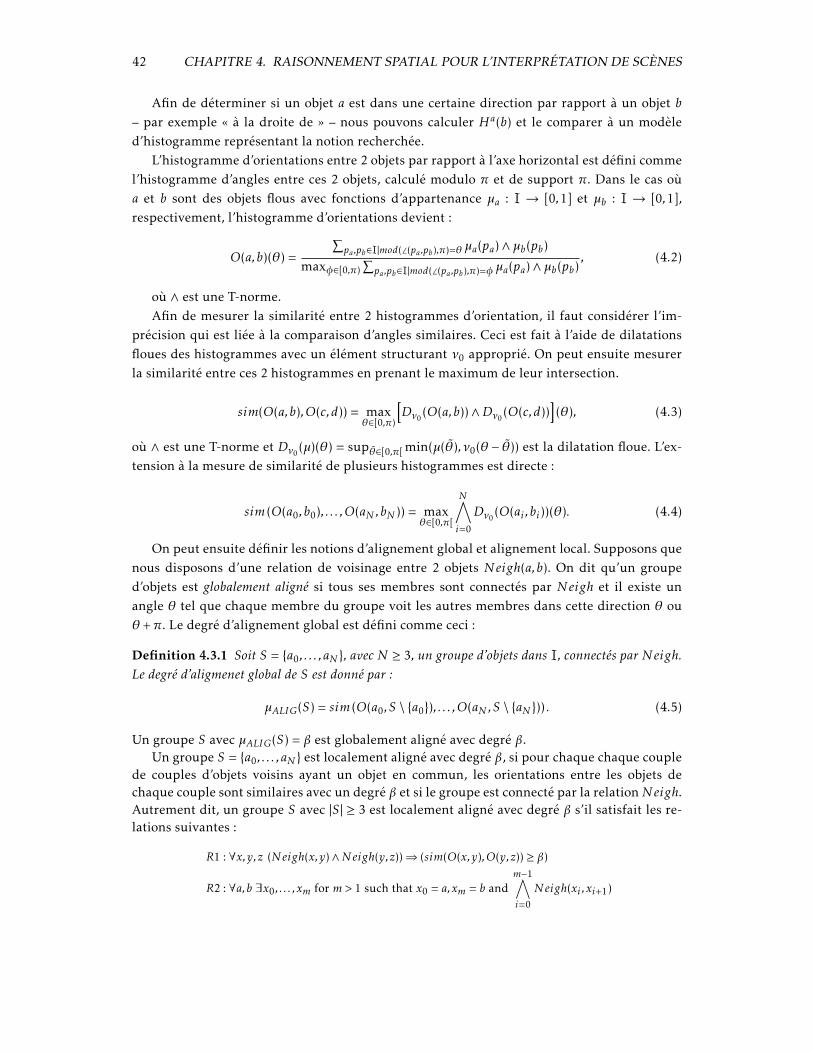
42 CHAPITRE 4. RAISONNEMENT SPATIAL POUR L’INTERPRÉTATION DE SCÈNES
Afin de déterminer si un objet a est dans une certaine direction par rapport à un objet b– par exemple « à la droite de » – nous pouvons calculer Ha(b) et le comparer à un modèled’histogramme représentant la notion recherchée.
L’histogramme d’orientations entre 2 objets par rapport à l’axe horizontal est défini commel’histogramme d’angles entre ces 2 objets, calculé modulo π et de support π. Dans le cas oùa et b sont des objets flous avec fonctions d’appartenance µa : I → [0,1] et µb : I → [0,1],respectivement, l’histogramme d’orientations devient :
O(a,b)(θ) =
∑pa,pb∈I|mod(∠(pa,pb),π)=θ µa(pa)∧µb(pb)
maxφ∈[0,π)∑pa,pb∈I|mod(∠(pa,pb),π)=φµa(pa)∧µb(pb)
, (4.2)
où ∧ est une T-norme.Afin de mesurer la similarité entre 2 histogrammes d’orientation, il faut considérer l’im-
précision qui est liée à la comparaison d’angles similaires. Ceci est fait à l’aide de dilatationsfloues des histogrammes avec un élément structurant ν0 approprié. On peut ensuite mesurerla similarité entre ces 2 histogrammes en prenant le maximum de leur intersection.
sim(O(a,b),O(c,d)) = maxθ∈[0,π)
[Dν0
(O(a,b))∧Dν0(O(c,d))
](θ), (4.3)
où ∧ est une T-norme et Dν0(µ)(θ) = supθ∈[0,π[ min(µ(θ),ν0(θ − θ)) est la dilatation floue. L’ex-
tension à la mesure de similarité de plusieurs histogrammes est directe :
sim (O(a0,b0), . . . ,O(aN ,bN )) = maxθ∈[0,π[
N∧i=0
Dν0(O(ai ,bi))(θ). (4.4)
On peut ensuite définir les notions d’alignement global et alignement local. Supposons quenous disposons d’une relation de voisinage entre 2 objets Neigh(a,b). On dit qu’un grouped’objets est globalement aligné si tous ses membres sont connectés par Neigh et il existe unangle θ tel que chaque membre du groupe voit les autres membres dans cette direction θ ouθ +π. Le degré d’alignement global est défini comme ceci :
Definition 4.3.1 Soit S = {a0, . . . , aN }, avec N ≥ 3, un groupe d’objets dans I, connectés par Neigh.Le degré d’aligmenet global de S est donné par :
µALIG(S) = sim (O(a0,S \ {a0}), . . . ,O(aN ,S \ {aN })) . (4.5)
Un groupe S avec µALIG(S) = β est globalement aligné avec degré β.Un groupe S = {a0, . . . , aN } est localement aligné avec degré β, si pour chaque chaque couple
de couples d’objets voisins ayant un objet en commun, les orientations entre les objets dechaque couple sont similaires avec un degré β et si le groupe est connecté par la relationNeigh.Autrement dit, un groupe S avec |S | ≥ 3 est localement aligné avec degré β s’il satisfait les re-lations suivantes :
R1 : ∀x,y,z (Neigh(x,y)∧Neigh(y,z))⇒ (sim(O(x,y),O(y,z)) ≥ β)
R2 : ∀a,b ∃x0, . . . ,xm for m > 1 such that x0 = a,xm = b andm−1∧i=0
Neigh(xi ,xi+1)
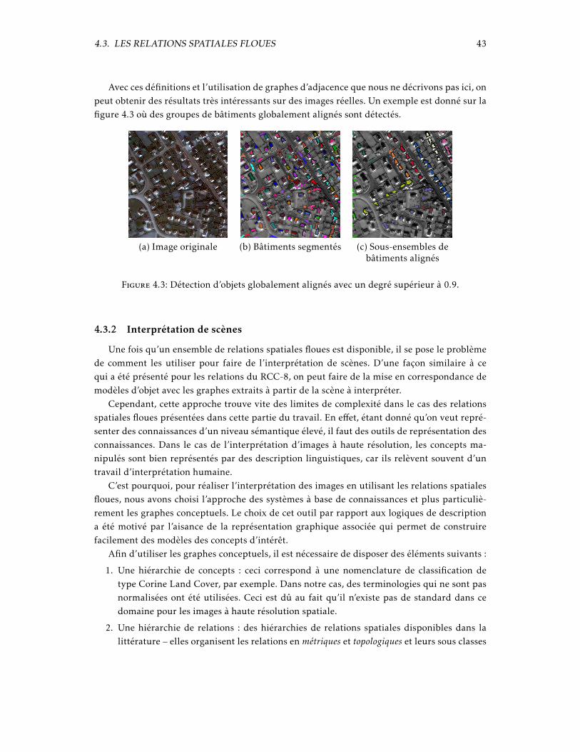
4.3. LES RELATIONS SPATIALES FLOUES 43
Avec ces définitions et l’utilisation de graphes d’adjacence que nous ne décrivons pas ici, onpeut obtenir des résultats très intéressants sur des images réelles. Un exemple est donné sur lafigure 4.3 où des groupes de bâtiments globalement alignés sont détectés.
(a) Image originale (b) Bâtiments segmentés (c) Sous-ensembles debâtiments alignés
Figure 4.3: Détection d’objets globalement alignés avec un degré supérieur à 0.9.
4.3.2 Interprétation de scènes
Une fois qu’un ensemble de relations spatiales floues est disponible, il se pose le problèmede comment les utiliser pour faire de l’interprétation de scènes. D’une façon similaire à cequi a été présenté pour les relations du RCC-8, on peut faire de la mise en correspondance demodèles d’objet avec les graphes extraits à partir de la scène à interpréter.
Cependant, cette approche trouve vite des limites de complexité dans le cas des relationsspatiales floues présentées dans cette partie du travail. En effet, étant donné qu’on veut repré-senter des connaissances d’un niveau sémantique élevé, il faut des outils de représentation desconnaissances. Dans le cas de l’interprétation d’images à haute résolution, les concepts ma-nipulés sont bien représentés par des description linguistiques, car ils relèvent souvent d’untravail d’interprétation humaine.
C’est pourquoi, pour réaliser l’interprétation des images en utilisant les relations spatialesfloues, nous avons choisi l’approche des systèmes à base de connaissances et plus particuliè-rement les graphes conceptuels. Le choix de cet outil par rapport aux logiques de descriptiona été motivé par l’aisance de la représentation graphique associée qui permet de construirefacilement des modèles des concepts d’intérêt.
Afin d’utiliser les graphes conceptuels, il est nécessaire de disposer des éléments suivants :
1. Une hiérarchie de concepts : ceci correspond à une nomenclature de classification detype Corine Land Cover, par exemple. Dans notre cas, des terminologies qui ne sont pasnormalisées ont été utilisées. Ceci est dû au fait qu’il n’existe pas de standard dans cedomaine pour les images à haute résolution spatiale.
2. Une hiérarchie de relations : des hiérarchies de relations spatiales disponibles dans lalittérature – elles organisent les relations en métriques et topologiques et leurs sous classes

44 CHAPITRE 4. RAISONNEMENT SPATIAL POUR L’INTERPRÉTATION DE SCÈNES
distance et directionnelles et adjacence, recouvrement, etc. – ont été étendues pour y inclureles relations floues développées ici.
3. Les graphes des concepts d’intérêt qui seront recherchés dans les images.
Le problème de recherche de concepts d’intérêt dans une image peut être abordé avec lesapproches suivantes, organisées par difficulté croissante :
1. Image dont les régions sont étiquetées et pour lesquelles on ne considère que des relationsnon floues.
2. Image étiquetée en considérant les relations floues.
3. Image non étiquetée et relations floues.
La notion d’étiquette correspond ici à l’identification du concept associé à chaque région del’image (classification suivant la nomenclature hiérarchique).
Une fois que la hiérarchie de concepts, la hiérarchie de relations et les graphes conceptuelsdes objets d’intérêt sont disponibles, on peut mettre en oeuvre la recherche des objets dans desscènes complexes.
L’approche qui a été choisie pour rechercher le graphe d’un objet d’intérêt dan une imageest celle des CSP (Constraint Satisfaction Problems). Un CSP [3], est défini par le triplet P =〈X ,D,C〉 où X est l’ensemble de variables qui représente une caractéristique des objets du pro-blème – les noeuds du graphe conceptuel dans notre cas –, D est l’ensemble représentant lesvaleurs possibles des variables – les régions de l’image – et C sont les contraintes du problème– les relations spatiales.
Afin d’exploiter les relations spatiales floues, nous avons utilisé les Fuzzy CSP [9].
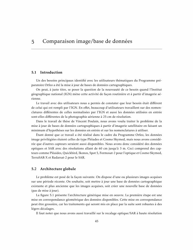
5 Comparaison image/base de données
5.1 Introduction
Un des besoins principaux identifié avec les utilisateurs thématiques du Programme pré-paratoire Orfeo a été la mise à jour de bases de données cartographiques.
On peut, à juste titre, se poser la question de la nouveauté de ce besoin quand l’Institutgéographique national (IGN) mène cette activité de façon routinière et à partir d’imagerie aé-rienne.
Le travail avec des utilisateurs nous a permis de constater que leur besoin était différentde celui qui est rempli par l’IGN. En effet, beaucoup d’utilisateurs travaillent sur des nomen-clatures différentes de celles normalisées par l’IGN et aussi les données utilisées en entréesont-elles différentes de la photographie aérienne à 25 cm de résolution.
Dans le travail de thèse de Vincent Poulain, nous avons voulu traiter le problème de lamise à jour de bases de données cartographiques à partir d’imagerie satellitaire en faisant unminimum d’hypothèses sur les données en entrée et sur les nomenclatures à utiliser.
Étant donné que ce travail a été réalisé dans le cadre du Programme Orfeo, les donnéesimage privilégiées étaient celles de type Pléiades et Cosmo Skymed, mais nous avons considé-rée que d’autres capteurs seraient aussi disponibles. Nous avons donc considéré des donnéesoptiques et SAR avec des résolutions allant de 60 cm jusqu’à 3 m. Ceci comprend des cap-teurs comme Pléaides, Quickbird, Ikonos, Spot 5, Formosat-2 pour l’optique et Cosmo Skymed,TerraSAR-X et Radarsat-2 pour le SAR.
5.2 Architecture globale
Le problème est posé de la façon suivante. On dispose d’une ou plusieurs images acquisessur une période récente. On souhaite, soit mettre à jour une base de données cartographiqueexistante et plus ancienne que les images acquises, soit créer une nouvelle base de données(pas de mise à jour).
La figure 5.1 présente l’architecture générique mise en oeuvre. La première étape est unemise en correspondance géométrique des données disponibles. Cette mise en correspondancepeut être grossière, car les traitements qui seront mis en place par la suite sont robustes à deslégers décalages.
Il faut noter que nous avons aussi travaillé sur le recalage optique/SAR à haute résolution
45
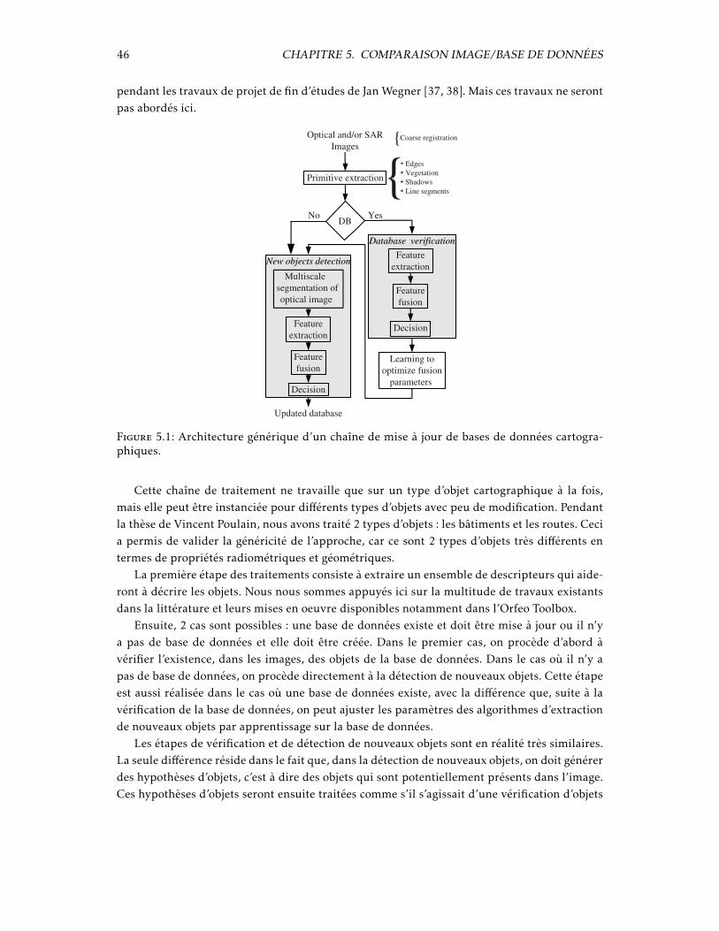
46 CHAPITRE 5. COMPARAISON IMAGE/BASE DE DONNÉES
pendant les travaux de projet de fin d’études de Jan Wegner [37, 38]. Mais ces travaux ne serontpas abordés ici.
New objects detectionNew objects detection
Optical and/or SARImages
Database verificationDatabase verification
Learning to optimize fusion
parameters
Primitive extraction
Updated database
Multiscale segmentation of optical image
➔ Edges➔ Vegetation➔ Shadows➔ Line segments{
{Coarse registration
DBYesNo
Feature extraction
Decision
Feature fusion
Decision
Feature extraction
Feature fusion
Figure 5.1: Architecture générique d’un chaîne de mise à jour de bases de données cartogra-phiques.
Cette chaîne de traitement ne travaille que sur un type d’objet cartographique à la fois,mais elle peut être instanciée pour différents types d’objets avec peu de modification. Pendantla thèse de Vincent Poulain, nous avons traité 2 types d’objets : les bâtiments et les routes. Cecia permis de valider la généricité de l’approche, car ce sont 2 types d’objets très différents entermes de propriétés radiométriques et géométriques.
La première étape des traitements consiste à extraire un ensemble de descripteurs qui aide-ront à décrire les objets. Nous nous sommes appuyés ici sur la multitude de travaux existantsdans la littérature et leurs mises en oeuvre disponibles notamment dans l’Orfeo Toolbox.
Ensuite, 2 cas sont possibles : une base de données existe et doit être mise à jour ou il n’ya pas de base de données et elle doit être créée. Dans le premier cas, on procède d’abord àvérifier l’existence, dans les images, des objets de la base de données. Dans le cas où il n’y apas de base de données, on procède directement à la détection de nouveaux objets. Cette étapeest aussi réalisée dans le cas où une base de données existe, avec la différence que, suite à lavérification de la base de données, on peut ajuster les paramètres des algorithmes d’extractionde nouveaux objets par apprentissage sur la base de données.
Les étapes de vérification et de détection de nouveaux objets sont en réalité très similaires.La seule différence réside dans le fait que, dans la détection de nouveaux objets, on doit générerdes hypothèses d’objets, c’est à dire des objets qui sont potentiellement présents dans l’image.Ces hypothèses d’objets seront ensuite traitées comme s’il s’agissait d’une vérification d’objets
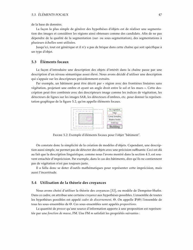
5.3. ÉLÉMENTS FOCAUX 47
de la base de données.La façon la plus simple de générer des hypothèses d’objets est de réaliser une segmenta-
tion des images et considérer les régions ainsi obtenues comme des candidats. Afin de ne pasdépendre de la qualité de la segmentation (sur- ou sous-segmentation), des segmentations àplusieurs échelles sont utilisées.
Jusqu’ici, tout est générique et il n’y a pas de brique dans cette chaîne qui soit spécifique àun type d’objet.
5.3 Éléments focaux
La façon d’introduire une description des objets d’intérêt dans la chaîne passe par unedescription d’un niveau sémantique assez élevé. Nous avons décidé d’utiliser une descriptionqui s’appuie sur les descripteurs précédemment extraits.
Par exemple, un bâtiment peut être décrit par « région avec des frontières linéaires sansvégétation, projetant une ombre et ayant un angle droit entre le sol et les murs ». Cette des-cription peut être combinée avec des descripteurs image comme les indices de végétation, lesdétecteurs de lignes sur les images SAR, les détecteurs d’ombres, etc. pour donner la représen-tation graphique de la figure 5.2, qu’on appelle éléments focaux.
No vegetation
Edge
Linear boundary
Shadow border
SAR line
Building
Figure 5.2: Exemple d’éléments focaux pour l’objet "bâtiment".
On constate donc la simplicité de la création de modèles d’objets. Cependant, une descrip-tion aussi simple, ne permet pas de détecter des objets avec une précision suffisante. Ceci est dûau fait que la description linguistique, comme nous l’avons montré dans la section 4.3, est sou-vent entachée d’imprécision. Par exemple, dans le cas des bâtiments, dire qu’ils ne contiennentpas de végétation n’est pas toujours juste.
Il a fallu donc se doter d’outils mathématiques pour représenter cette imprécision, maisaussi l’incertitude.
5.4 Utilisation de la théorie des croyances
Nous avons choisi d’utiliser la théorie des croyances [32], ou modèle de Dempster-Shafer.Dans ce cadre, on attribue une certaine croyance aux hypothèses possibles. L’ensemble de toutesles hypothèses possibles est appelé cadre de discernement, Θ. On appelle P(Θ) l’ensemble detous les sous-ensembles de Θ. Ces sous-ensembles sont appelés propositions.
La quantité de preuve qu’une source d’information apporte à une proposition est représen-tée par une fonction de masse, FM. Une FM m satisfait les propriétés suivantes :
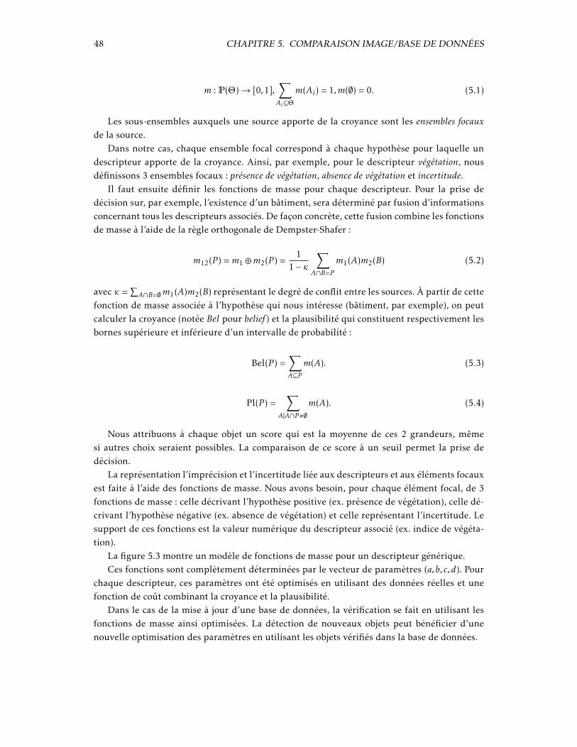
48 CHAPITRE 5. COMPARAISON IMAGE/BASE DE DONNÉES
m : P(Θ)→ [0,1],∑Ai⊆Θ
m(Ai) = 1,m(∅) = 0. (5.1)
Les sous-ensembles auxquels une source apporte de la croyance sont les ensembles focauxde la source.
Dans notre cas, chaque ensemble focal correspond à chaque hypothèse pour laquelle undescripteur apporte de la croyance. Ainsi, par exemple, pour le descripteur végétation, nousdéfinissons 3 ensembles focaux : présence de végétation, absence de végétation et incertitude.
Il faut ensuite définir les fonctions de masse pour chaque descripteur. Pour la prise dedécision sur, par exemple, l’existence d’un bâtiment, sera déterminé par fusion d’informationsconcernant tous les descripteurs associés. De façon concrète, cette fusion combine les fonctionsde masse à l’aide de la règle orthogonale de Dempster-Shafer :
m12(P ) =m1 ⊕m2(P ) =1
1−κ
∑A∩B=P
m1(A)m2(B) (5.2)
avec κ =∑A∩B=∅m1(A)m2(B) représentant le degré de conflit entre les sources. À partir de cette
fonction de masse associée à l’hypothèse qui nous intéresse (bâtiment, par exemple), on peutcalculer la croyance (notée Bel pour belief ) et la plausibilité qui constituent respectivement lesbornes supérieure et inférieure d’un intervalle de probabilité :
Bel(P ) =∑A⊆P
m(A). (5.3)
Pl(P ) =∑
A|A∩P,∅m(A). (5.4)
Nous attribuons à chaque objet un score qui est la moyenne de ces 2 grandeurs, mêmesi autres choix seraient possibles. La comparaison de ce score à un seuil permet la prise dedécision.
La représentation l’imprécision et l’incertitude liée aux descripteurs et aux éléments focauxest faite à l’aide des fonctions de masse. Nous avons besoin, pour chaque élément focal, de 3fonctions de masse : celle décrivant l’hypothèse positive (ex. présence de végétation), celle dé-crivant l’hypothèse négative (ex. absence de végétation) et celle représentant l’incertitude. Lesupport de ces fonctions est la valeur numérique du descripteur associé (ex. indice de végéta-tion).
La figure 5.3 montre un modèle de fonctions de masse pour un descripteur générique.Ces fonctions sont complètement déterminées par le vecteur de paramètres (a,b,c,d). Pour
chaque descripteur, ces paramètres ont été optimisés en utilisant des données réelles et unefonction de coût combinant la croyance et la plausibilité.
Dans le cas de la mise à jour d’une base de données, la vérification se fait en utilisant lesfonctions de masse ainsi optimisées. La détection de nouveaux objets peut bénéficier d’unenouvelle optimisation des paramètres en utilisant les objets vérifiés dans la base de données.
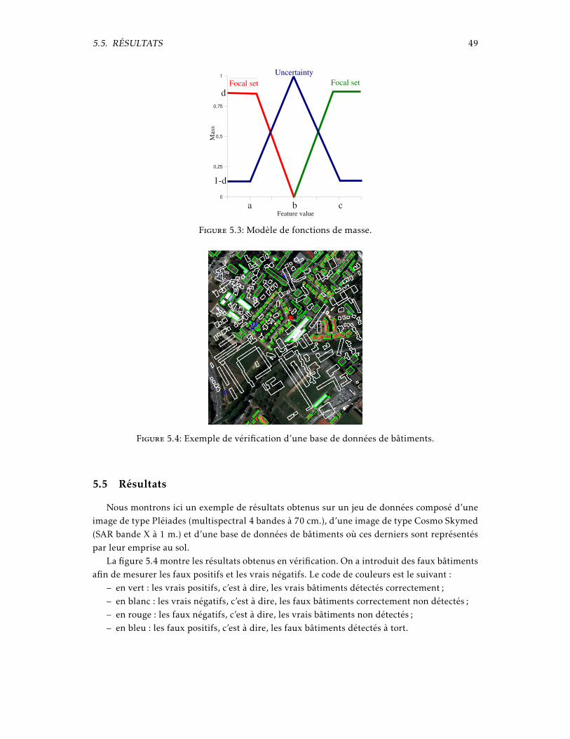
5.5. RÉSULTATS 49
0
0,25
0,5
0,75
1 UncertaintyFocal setFocal set
Feature valueM
ass
a b c
d
1d
Figure 5.3: Modèle de fonctions de masse.
Figure 5.4: Exemple de vérification d’une base de données de bâtiments.
5.5 Résultats
Nous montrons ici un exemple de résultats obtenus sur un jeu de données composé d’uneimage de type Pléiades (multispectral 4 bandes à 70 cm.), d’une image de type Cosmo Skymed(SAR bande X à 1 m.) et d’une base de données de bâtiments où ces derniers sont représentéspar leur emprise au sol.
La figure 5.4 montre les résultats obtenus en vérification. On a introduit des faux bâtimentsafin de mesurer les faux positifs et les vrais négatifs. Le code de couleurs est le suivant :
– en vert : les vrais positifs, c’est à dire, les vrais bâtiments détectés correctement ;– en blanc : les vrais négatifs, c’est à dire, les faux bâtiments correctement non détectés ;– en rouge : les faux négatifs, c’est à dire, les vrais bâtiments non détectés ;– en bleu : les faux positifs, c’est à dire, les faux bâtiments détectés à tort.
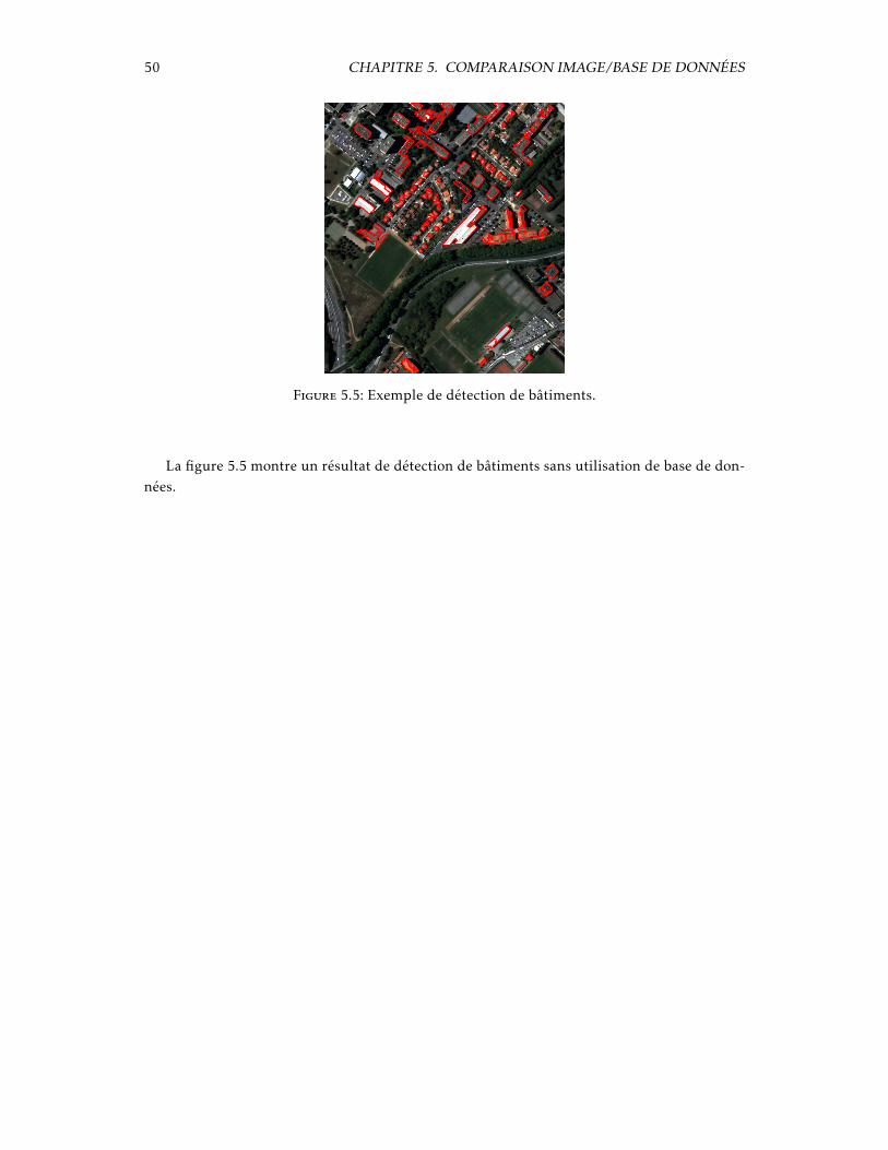
50 CHAPITRE 5. COMPARAISON IMAGE/BASE DE DONNÉES
Figure 5.5: Exemple de détection de bâtiments.
La figure 5.5 montre un résultat de détection de bâtiments sans utilisation de base de don-nées.

6 Perspectives de recherche
Comme il a pu être constaté tout au long des chapitres précédents, mes travaux de re-cherche ont été guidés par les besoins du Cnes en ce qui concerne le traitement des images deses capteurs, que ce soit en valorisation quand ils existaient déjà, ou que ce soit en préparationà l’utilisation.
Dès 2008, l’équipe du projet Venµs nous a sollicité pour des supports ponctuels sur le trai-tement de séries multi-temporelles. Nous avons décidé de commencer un travail de fond sur letraitement de ce type de données, car, peu après Venµs, le programme des Sentinelles de l’ESAdoit être opérationnel.
La caractéristique particulière de ce type de données est d’avoir un échantillonnage tempo-rel très fin – allant jusqu’à une acquisition tous les 2 ou 3 jours – tout en gardant une résolutionspatiale élevée (de l’ordre de 10 m.) et une résolution spectrale très riche en optique (une di-zaine de bandes spectrales sur le visible et l’infra-rouge).
L’arrivée des données fournies par le programme des Sentinelles permettra le développe-ment de services et d’applications qui ne peuvent être mis en place que grâce à une revisitecourte et systématique de la surface de la Terre.
Le défi principal posé par ces données est le passage à l’échelle des techniques et des ser-vices actuels. Ce passage à l’échelle devra s’opérer sur les aspects suivants :
1. volume de données à gérer pour un site donnée ;
2. emprise et diversité spatiale – géographique – des zones traitées ;
3. assurance qualité des produits livrés.
6.1 Les produits attendus
Étant donné le contexte de passage à l’échelle cité ci-dessus, un certain niveau de standardi-sation peut être nécessaire. Trois familles de produits permettent de couvrir un grand nombrede besoins :
1. Cartes d’occupation des sols
2. Cartes de variables climatiques essentielles (ECVs, GCOS Essential Climate VariablesMatrix)
3. Produits d’alerte aux changements
51
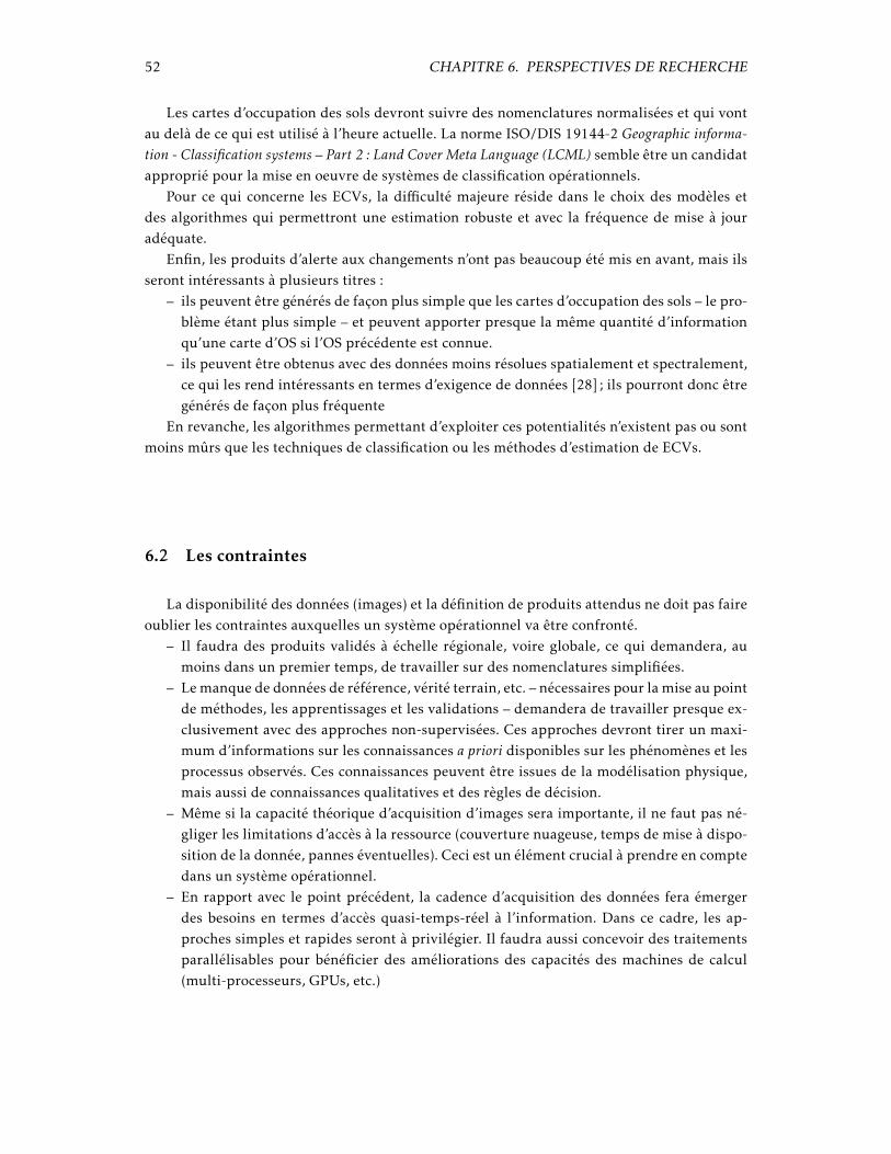
52 CHAPITRE 6. PERSPECTIVES DE RECHERCHE
Les cartes d’occupation des sols devront suivre des nomenclatures normalisées et qui vontau delà de ce qui est utilisé à l’heure actuelle. La norme ISO/DIS 19144-2 Geographic informa-tion - Classification systems – Part 2 : Land Cover Meta Language (LCML) semble être un candidatapproprié pour la mise en oeuvre de systèmes de classification opérationnels.
Pour ce qui concerne les ECVs, la difficulté majeure réside dans le choix des modèles etdes algorithmes qui permettront une estimation robuste et avec la fréquence de mise à jouradéquate.
Enfin, les produits d’alerte aux changements n’ont pas beaucoup été mis en avant, mais ilsseront intéressants à plusieurs titres :
– ils peuvent être générés de façon plus simple que les cartes d’occupation des sols – le pro-blème étant plus simple – et peuvent apporter presque la même quantité d’informationqu’une carte d’OS si l’OS précédente est connue.
– ils peuvent être obtenus avec des données moins résolues spatialement et spectralement,ce qui les rend intéressants en termes d’exigence de données [28] ; ils pourront donc êtregénérés de façon plus fréquente
En revanche, les algorithmes permettant d’exploiter ces potentialités n’existent pas ou sontmoins mûrs que les techniques de classification ou les méthodes d’estimation de ECVs.
6.2 Les contraintes
La disponibilité des données (images) et la définition de produits attendus ne doit pas faireoublier les contraintes auxquelles un système opérationnel va être confronté.
– Il faudra des produits validés à échelle régionale, voire globale, ce qui demandera, aumoins dans un premier temps, de travailler sur des nomenclatures simplifiées.
– Le manque de données de référence, vérité terrain, etc. – nécessaires pour la mise au pointde méthodes, les apprentissages et les validations – demandera de travailler presque ex-clusivement avec des approches non-supervisées. Ces approches devront tirer un maxi-mum d’informations sur les connaissances a priori disponibles sur les phénomènes et lesprocessus observés. Ces connaissances peuvent être issues de la modélisation physique,mais aussi de connaissances qualitatives et des règles de décision.
– Même si la capacité théorique d’acquisition d’images sera importante, il ne faut pas né-gliger les limitations d’accès à la ressource (couverture nuageuse, temps de mise à dispo-sition de la donnée, pannes éventuelles). Ceci est un élément crucial à prendre en comptedans un système opérationnel.
– En rapport avec le point précédent, la cadence d’acquisition des données fera émergerdes besoins en termes d’accès quasi-temps-réel à l’information. Dans ce cadre, les ap-proches simples et rapides seront à privilégier. Il faudra aussi concevoir des traitementsparallélisables pour bénéficier des améliorations des capacités des machines de calcul(multi-processeurs, GPUs, etc.)
6.3. LES SOLUTIONS : 53
6.3 Les solutions :
Pour répondre à l’attente des utilisateurs en termes de produits, de leur qualité et de leurfréquence de mise à jour, il y a principalement 2 pistes à poursuivre : l’utilisation d’un maxi-mum de capteurs disponibles et l’utilisation efficace d’informations exogènes aux données detélédétection.
6.3.1 Modélisation de comportements temporels
La dimension temporelle doit être traitée de façon différente à celle de la dimension spa-tiale des images. Le suivi des dynamiques temporelles est souvent la seule façon d’accéderà certaines informations. Les techniques de description et manipulation de séries temporellesdoivent être capables de s’affranchir d’abord des problèmes d’échantillonnage irrégulier : mêmesi le satellite a un cycle régulier, les aléas de la couverture nuageuse rendent des images inutili-sables. Un autre problème qu’il faut prendre en compte est celui des comportements temporelsdécalés ou distordus. C’est dans ce cadre que nous avons proposé la thèse de François Petitjean.
6.3.2 Le multi-capteur
Les algorithmes capables d’ingérer des données issues de capteurs différents permettrontd’augmenter la fréquence de mise à jour des produits. Ils doivent aussi permettre d’améliorer laqualité de certains de ces produits ou même d’accéder à des grandeurs autrement inaccessibles,mais nous n’abordons pas ces aspects ici. En effet, dans un cadre opérationnel, il faut envisagerles traitements multi-capteurs comme un mode dégradé quand la donnée nominale n’est pasdisponible, et non pas comme une exigence pour la livraison d’un produit.
Le terme multi-capteur est vague. Il peut être décliné à, au moins, 3 niveaux.
1. Capteurs de même classe : Venµs, Sentinelle-2, LDCM. On peut dans ces cas utiliser, avecpeu d’adaptation, les mêmes chaînes de traitement pour toutes les données.
2. Capteurs avec des résolutions différentes. À l’horizon sur lequel nous nous plaçons, lesexemples sont Sentinelle-2 avec Proba-V ou Sentinelle-3. On utilise ici la complémen-tarité entre haute résolution spatiale/spectrale et très haute résolution temporelle pourassurer une mise à jour très fréquente des informations. Des techniques spécifiques pourla fusion multi-résolution doivent être développées.
3. Optique/SAR : typiquement Sentinelle-1 et Sentinelle-2. On essaiera ici de bénéficier del’aspect tous temps du SAR pour assurer une production systématique d’informations.Les propriétés physiques des 2 types de capteurs étant complètement différentes, un ni-veau d’indirection devra être ajouté aux algorithmes (passage par des grandeurs inter-médiaires comme les classes ou les changements).
6.3.3 Les informations exogènes
L’utilisation de données exogènes dans la génération de produits à base d’imagerie satelliteest classique (MNT, carte de référence, donnée météo, etc.). Le terme information exogène va

54 CHAPITRE 6. PERSPECTIVES DE RECHERCHE
au delà de cette notion de donnée ancillaire en ajoutant 2 nouvelles composantes : les modèlesphysiques et les connaissances du domaine.
6.3.3.1 Les modèles physiques
Leur utilisation pour l’assimilation des données de télédétection ne peut être envisagée quepour l’estimation de variables physiques. Souvent, les modèles ne peuvent pas être envisagésdans des contextes opérationnels à cause de leur coût de calcul ou de leur besoin de paramètresnon disponibles.
Nous envisageons ici leur utilisation comme outil de sélection de traitements. En effet, desmodèles simples – spatialisables – peuvent être utilisés pour décider quels sont les traitementsà mettre en place par la suite. Un exemple de ce type d’approche consiste à se servir de modèlesde croissance de la végétation pour réaliser un premier niveau de classification et pouvoirensuite utiliser des classifieurs spécialisés sur certaines familles de classes.
Les modèles à prendre peuvent être des types suivants :– TSVA : transfert sol-végétation-atmosphère ;– croissance/fonctionnement de la végétation ;– réflectance (feuilles, sol) ;– transfert radiatif ;– capteur : bandes spectrales, fonction de transfert de modulation, etc.Nous avons commencé à travailler sur ces aspects lors du séjour de Germain Forestier au
CNES [11, 10]. Une application de cette approche aux séries multi-temporelles a été dévelop-pée pour comparer les performances de classification entre Formosat-2 et les futurs Venµs etSentinelle-2 [15].
6.3.3.2 Les connaissances du domaine
Il s’agit ici d’utiliser des informations décrivant les phénomènes et les processus d’intérêt,mais sans passer par une modélisation physique ou mathématique. Sans rentrer, en tout casdans un premier temps, dans les domaines de la modélisation qualitative ou de la soft dataassimilation, on peut envisager d’utiliser des terminologies et des règles décrivant, par exemple,les pratiques agricoles.
Comme dans le cas des modèles physiques, ce type de méthode est envisagée comme étapepréalable à la classification, mais elle peut être aussi utilisée pour valider/invalider des résul-tats de classification.
6.4 La classification
Les méthodes de classification, notamment celles qui sont développées au CESBIO depuisdes années sont robustes et performantes. Des nouveaux développements sont en cours etvisent principalement à mettre en oeuvre des techniques de reconnaissance de classes (passageentre l’étiquette non thématique issue d’une classification non-supervisée vers l’identificationdu nom thématique de la classe).

6.5. LA DÉTECTION DE CHANGEMENTS 55
Nous nous intéressons ici à la stratégie à mettre en oeuvre pour utiliser ces méthodes dansun environnement opérationnel, dont les contraintes ont été décrites plus haut. Cette stratégieest composée des modules suivants :
1. Choix de la donnée à fournir à l’algorithme de classification : s’agit-il de réflectances,d’indices, de variables estimées ?
2. Choix de la fenêtre temporelle à utiliser pour la génération de la classification : parmi lesimages disponibles à un instant donné, quelles sont celles qui peuvent apporter le plusd’information ? Comment aborder le compromis entre quantité d’information et volumede données à traiter ?
3. Comment pondérer ou ajuster les résultats d’une classification en utilisant des donnéesde référence ?
4. Comment décomposer le problème de génération d’une carte d’occupation des sols ensous-problèmes plus facilement traitables par les algorithmes de classification ?
6.5 La détection de changements
Pour certaines applications, il peut être très utile d’avoir un produit qui, même sans décrireles classes d’occupation des sols, met en évidence les évolutions des surfaces. Ces évolutionspeuvent être analysées au niveau des réflectances observées, au niveau d’indices dérivées oupar le biais d’autres grandeurs d’intérêt.
Ces produits d’analyse d’évolution des surfaces peuvent être contraints par une classifi-cation existante. Par exemple, si l’on s’intéresse à l’étude du travail du sol, la détection dechangements peut être limitée à la classe sol nu issue d’une classification.
Inversement, un produit d’alerte aux changements peut être fourni en entrée d’une classi-fication pour discriminer 2 classes très similaires, mais avec des évolutions temporelles légère-ment différentes.
Les travaux existants en détection de changements sont souvent focalisés sur les problèmesà 2 dates avec un changement abrupt entre les 2. Il faudra ici développer des techniques pou-vant profiter d’un grand nombre d’images et éventuellement les étendre au cas multi-capteur(notamment multi-échelles).


Deuxième partie
Curriculum Vitae
57


7 Cursus professionnel
7.1 Formation
– 9/2000. Doctorat en Traitement du Signal et Télécommunications de l’Université de Rennes-1 : Étude des signatures radar à la surface de l’océan de la topographie sous-marine.
– 9/1997. DEA Signal Télécommunications Image et Radar de l’Université de Rennes 1.– 9/1997. Ingénieur Télécom, ENST Bretagne. Spécialité Signal et Images.– 9/1997 Ingénieur Télécom, ETSET Barcelone, Université Polytechnique de Catalogne.
Spécialité Communications.
7.2 Expérience professionnelle
– Depuis 3/2010 : Chercheur au Centre d’études spatiales de la biosphère, CESBIO– 12/2001-3/2010 : Ingénieur au Centre national d’études spatiales, CNES.
– Animateur du Volet méthodologique du Programme d’accompagnement ORFEO.– Chef du projet ORFEO Toolbox.– Responsable du Dossier d’axe technique OT4 : Méthodes d’extraction d’information des
images.– Chargé de la R&D en extraction d’information des images de télédétection pour des
applications opérationnelles et multitemporelles :– détection de changements ;– reconnaissance d’objets ;– mise en correspondance d’images multi-capteurs ;– mesures de similarité.
– Chef de projet pour la Charte Internationale Espace et Catastrophes Majeures.– 10/2000 - 12/2001 : Chercheur sous contrat au CNES (Centre de Toulouse). Sujet d’étude :
Développement de techniques de fusion d’imagerie spatiale (optique et radar) dans lecadre d’études multitemporelles appliquées aux risques naturels.
59


8 Liste des publications
8.1 Chapitres de livre
1. Andreas Wimmer, Iris Lingenfelder, Charles Beumier, Jordi Inglada, Simon J. Caseley :Feature Recognition Techniques. Dans B. Jasani, M. Pesaresi, S. Schneiderbauer and G.Zeug (Eds.), Remote Sensing from Space – Supporting International Peace and Security.Springer, 2009. Pages 105-118.
2. Ahed Alboody, Florence Sèdes, Jordi Inglada : Enriching The Qualitative Spatial Reaso-ning System RCC8. Dans : Qualitative Spatio-Temporal Representation and Reasoning :Trends and Future Directions. Shyamanta M. Hazarika (Eds.), Information Science Refe-rence, août 2010.
8.2 Articles de revue à comité de lecture
1. Jordi Inglada, René Garello : On Rewriting the Imaging Mechanism of Underwater Bot-tom Topography by Synthetic Aperture Radar as a Volterra Series Expansion. IEEE Jour-nal of Oceanic Engineering, vol. 27, no. 3, pp. 665-674, July 2002.
2. Jordi Inglada, Jean-Marc Le Caillec, René Garello : Inversion of Imaging Mechanisms byRegularization of Inverse Volterra Models. Signal Processing, vol. 84, no. 6, p. 1021–1034,2004.
3. Jordi Inglada, Alain Giros : On the possibility of automatic multi-sensor image registra-tion. IEEE Transactions on Geoscience and Remote Sensing, vol. 42, no. 10, p. 2104–2120,October 2004.
4. Jordi Inglada, Jean-Claude Souyris, Caroline Henry, Céline Tison : Incoherent SAR pola-rimetric analysis over point targets. IEEE Geoscience and Remote Sensing Letters, vol. 3,no. 2, p. 246–249, April 2006.
5. Jordi Inglada, Vincent Muron, Damien Pichard, Thomas Feuvrier : Analysis of Artifactsin Subpixel Remote Sensing Image Registration, IEEE Transactions on Geoscience andRemote Sensing, vol. 45, no. 1, p. 254–264, January 2007.
6. Jordi Inglada, Grégoire Mercier : A Statistical Similarity Measure for Change Detectionin Multitemporal SAR Images and its Extension to Multiscale Change Analysis, IEEE
61
62 CHAPITRE 8. LISTE DES PUBLICATIONS
Transactions on Geoscience and Remote Sensing, Volume : 45, Issue : 5, Part 2 May 2007,pages 1432-1445.
7. Florent Chatelain, Jean-Yves Tourneret, Jordi Inglada, André Ferrari : Bivariate GammaDistributions for Image Registration and Change Detection, IEEE Transactions on ImageProcessing, Volume 16, Issue 7, July 2007, pages 1796-1806.
8. Jordi Inglada : Automatic recognition of man-made objects in high resolution opticalremote sensing images by SVM classification of geometric image features. ISPRS Journalof Photogrammetry and Remote Sensing. ISPRS Journal of Photogrammetry and RemoteSensing Volume 62, Issue 3, August 2007, Pages 236-248.
9. Florent Chatelain, Jean-Yves Tourneret, Jordi Inglada, Change Detection in MultisensorSAR Images Using Multivariate Gamma Distributions, IEEE Transactions on Image Pro-cessing. Volume : 17, Issue : 3, March 2008.
10. Jordi Inglada, Julien Michel : Qualitative Spatial Reasoning for High-Resolution RemoteSensing Image Analysis. IEEE Transactions on Geoscience and Remote Sensing, Volume47, Issue 2, February 2009, Pages 599-612.
11. Tarek Habib, Jordi Inglada, Grégoire Mercier, Jocelyn Chanussot, Support Vector Reduc-tion in SVM Algorithm for Abrupt Change Detection in Remote Sensing. IEEE Geoscienceand Remote Sensing Letters, Volume 6, Issue 3, July 2009, Pages 606-610.
12. G. Licciardi, F. Pacifici, D. Tuia, S. Prasad, T. West, F. Giacco, C. Thiel, J. Inglada, E.Christophe, J. Chanussot and P. Gamba : Decision Fusion for the Classification of Hyper-spectral Data : Outcome of the 2008 GRS-S Data Fusion Contest. IEEE Transactions onGeoscience and Remote Sensing, Volume 47, Issue 11, November 2009, Pages :3857-3865.
13. E. Christophe, J. Michel, and J. Inglada : Remote sensing processing : from multicore toGPU, IEEE Journal of Selected Topics in Applied Earth Observations and Remote Sensing.Accepté. 2010.
14. V. Poulain, J. Inglada, M. Spigai, J-Y. Tourneret and P. Marthon : High resolution opticaland SAR image fusion for building database updating. IEEE Transactions on Geoscienceand Remote Sensing, Accepté, 2011.
15. María Carolina Vanegas, Isabelle Bloch, Jordi Inglada : Alignment and parallelism forthe description of objects in high resolution remote sensing images, Computer Visionand Image Understanding. Soumis.
16. François Petitjean, Jordi Inglada, Pierre Gançarski : Satellite Image Time Series Analysisunder Time Warping, IEEE Transactions on Geoscience and Remote Sensing. Soumis.
8.3 Communications dans des colloques avec comité de lecture
1. Jordi Inglada, René Garello, Alfred Ramamonjiarisoa, Hafed Hahhi, Martine Deveaux :Comparison of two models for the imaging mechanism of underwater bottom topogra-phy by synthetic aperture radar. Proceedings of the International Geoscience And Re-mote Sensing Symposium 1998. Seattle, Washington, USA.

8.3. COMMUNICATIONS DANS DES COLLOQUES AVEC COMITÉ DE LECTURE 63
2. Jordi Inglada, René Garello : Volterra Model for the Imaging Mechanism of Ocean Sur-face Currents by Synthetic Aperture Radar. Proceedings of the International GeoscienceAnd Remote Sensing Symposium 1999. Hamburg, Germany.
3. Jordi Inglada, René Garello : Depth Estimation and 3D Topography Reconstruction fromSAR Images Showing Underwater Bottom Topography Signatures. Proceedings of theInternational Geoscience And Remote Sensing Symposium 1999. Hamburg, Germany.
4. Jordi Inglada, René Garello : Volterra Model for the Study of Wave-Current Interactionas Described by the Action Balance Equation Proceedings of the 9th (1999) InternationalOffshore and Polar Engineering Conference and Exhibition, ISOPE-99.Brest, France.
5. Jordi Inglada, René Garello : Underwater Bottom Topography Estimation from SARImages by Regularization of the Inverse Imaging Mechanism. Proceedings of the Inter-national Geoscience And Remote Sensing Symposium 2000. Honolulu, HI, USA.
6. Jordi Inglada, René Garello : Nonlinear Model for the Imaging Mechanism of OceanSurface Currents by SAR Using a Quadratic Source Function. Proceedings of the Interna-tional Geoscience And Remote Sensing Symposium 2000. Honolulu, HI, USA.
7. Jordi Inglada, René Garello : Model for the Imaging Mechanism of Ocean Surface Cur-rents by SAR. Application to Underwater Bottom Topography Estimation. Proceedingsof the Second International Symposium on Physics in Signal and Image Processing. Mar-seille, France. 2001.
8. Luc Pigeon, Jordi Inglada, Basel Solaiman : Genetic algorithms for multi-agent fusionsystem learning. Proceedings of the SPIE 15th Annual International Symposium on Ae-rospace/Defense Sensing, Simulation and Controls, AeroSense, 16-20 April 2001, Or-lando, FL, USA.
9. Jordi Inglada, Frédéric Adragna : Automatic Multi-Sensor Image Regsitration Algorithmby Edge Matching Using Genetic Algorithms. Proceedings of the International Geos-cience And Remote Sensing Symposium 2001. Sydney, Australia.
10. Jordi Inglada, Francesco Sarti, Philippe Durand, Frédéric Adragna, Jean-Luc Bessis : Theemergency of El Salvador in the frame of the International Charter Space and MajorDisasters, X Simposio Brasileiro do Sensoramiento Remoto, Foz do Iguazu, Brasil, 2001.
11. Francesco Sarti, Jordi Inglada, Robert Landry, Thierry Pultz : Risk management usingremote sensing data : moving from scientific to operational applications, X Simposio Bra-sileiro do Sensoramiento Remoto, Foz do Iguazu, Brasil, 2001.
12. Jordi Inglada, Frédéric Adragna : Blind Source Separation Applied to MultitemporalSeries of Differential SAR Interferograms. Proceedings of the International GeoscienceAnd Remote Sensing Symposium 2002. Toronto, Canada.
13. Jordi Inglada : Similarity Measures for Multisensor Remote Sensing Images. Proceedingsof the International Geoscience And Remote Sensing Symposium 2002. Toronto, Canada.
14. Frédéric Adragna, Mihai Datcu, Irena Hajnsek, Jordi Inglada, Kostas Papathanassiou,David Petit, Marco Quartulli, Jean-Claude Souyris : Information extraction from high

64 CHAPITRE 8. LISTE DES PUBLICATIONS
resolution SAR data. Proceedings of European Conference on Signal Processing, EUSIP-CO’02, September 2002, Toulouse, France.
15. Jordi Inglada : Change Detection on SAR Images by Using a Parametric Estimation of theKullback-Leibler Divergence. Proceedings of the International Geoscience And RemoteSensing Symposium 2003. Toulouse, France.
16. Francesco Sarti, Jordi Inglada, Jean-Luc Bessis : The two Emergencies of El Salvador inthe Frame of the International Charter Espace and Major Disasters. Proceedings of theInternational Geoscience And Remote Sensing Symposium 2003. Toulouse, France.
17. Alain Arnaud, Javier Duro, Jordi Inglada, Michael Eineder, Nico Adam and Ramon Hans-sen : ASAR/ERS interferometry over stable points. Proceedings of the International Geos-cience And Remote Sensing Symposium 2003. Toulouse, France.
18. Jordi Inglada, Jean-Claude Favard, Hervé Yesou, Stephen Clandillon, Claude Bestault :Lava flow Mapping during the Nyiragongo January 2002 eruption over the City of Gomain the Frame of the International Charter Espace and Major Disasters. Proceedings of theInternational Geoscience And Remote Sensing Symposium 2003. Toulouse, France.
19. Hervé Yesou, Stephen Clandillon, Bernard Allenbach, Claude Bestault, Paul de Fraipont,Jordi Inglada, Jean-Claude Favard : A constellation of Advantages with SPOT SWIR andVHR SPOT 5 data for Flood Extent Mapping during the September 2002 Gard Event(France). Proceedings of the International Geoscience And Remote Sensing Symposium2003. Toulouse, France.
20. Jordi Inglada, Alain Giros : On the real capabilities of remote sensing for disaster ma-nagement - Feedback from real cases. Proceedings of the International Geoscience AndRemote Sensing Symposium 2004. Anchorage, Alaska, USA.
21. Jordi Inglada, Alain Giros : Automatic man made object recognition in high resolutionremote sensing images. Proceedings of the International Geoscience And Remote SensingSymposium 2004. Anchorage, Alaska, USA.
22. Hélène Vadon and Jordi Inglada : CNES research and development, and available soft-ware, in the framework of space images based risk and disaster management. Procee-dings of the First International Symposium on Geo-information for Disaster Manage-ment’ (Gi4DM), Delft, The Netherlands, March 21-23, 2005
23. Jordi Inglada : Use of pre-conscious vision and geometric characterizations for automaticman-made object recognition. Proceedings of the International Geoscience And RemoteSensing Symposium 2005. Seoul, Korea.
24. Jordi Inglada, Hélène Vadon : Fine registration of Spot5 and Envisat/ASAR images andortho-image production : a fully automatic approach. Proceedings of the InternationalGeoscience And Remote Sensing Symposium 2005. Seoul, Korea.
25. Florent Chatelain, Jean-Yves Tourneret, Jordi Inglada, André Ferrari : Parameter Esti-mation for Multivariate Gamma Distributions. European Signal Processing Conference -EUSIPCO. Firenze (Italy), 4-8 April 2006.

8.3. COMMUNICATIONS DANS DES COLLOQUES AVEC COMITÉ DE LECTURE 65
26. Jordi Inglada, Vincent Muron, Damien Pichard, Thomas Feuvrier : Analysis of Arte-facts in Sub-Pixel Remote Sensing Image Registration. ISPRS Commision 1 Symposium.Marne-la-Vallée (France), 3-6 July 2006.
27. David Petit, Guillaume Oller, Jordi Inglada : On the Use of SAR and Optical ImagesCombination. ISPRS Commision 1 Symposium. Marne-la-Vallée (France), 3-6 July 2006.
28. Jordi Inglada, Grégoire Mercier : The Multiscale Change Profile : a Statistical SimilarityMeasure for Change Detection in Multitemporal SAR Images. IEEE International Geos-cience and Remote Sensing Symposium - IGARSS, Denver - Colorado (USA), 31 July - 4August 2006.
29. Grégoire Mercier, Stéphane Derrode, Wojciech Pieczynski, Jean-Marie Nicolas, Anne Joannic-Chardin, Jordi Inglada : Copula-based Stochastic Kernels for Abrupt Change Detection.IEEE International Geoscience and Remote Sensing Symposium - IGARSS, Denver - Co-lorado (USA), 31 July - 4 August 2006.
30. Vito Alberga, Mahamadou Idrissa, Vinciane Lacroix, Jordi Inglada : Performance Estima-tion of Similarity Measures of Multi-Sensor Images for Change Detection Applications.International Workshop on the Analysis of Multi-temporal Remote Sensing Images, 2007.MultiTemp 2007. 18-20 July 2007.
31. Vito Alberga, Mahamadou Idrissa, Vinciane Lacroix, Jordi Inglada : Comparison of si-milarity measures of multi-sensor images for change detection applications. IEEE Inter-national Geoscience and Remote Sensing Symposium - IGARSS, Barcelona, Spain, 23-27July 2007.
32. Jordi Inglada, Julien Michel : Spatial Reasoning and Multiscale Segmentation for ObjectRecognition in HR Optical Remote Sensing Images. IEEE International Geoscience andRemote Sensing Symposium - IGARSS, Barcelona, Spain, 23-27 July 2007.
33. Tarek Habib, Jocelyn Chanussot, Jordi Inglada, Grégoire Mercier : Abrupt change detec-tion on multitemporal remote sensing images. A statistical overview of methodologiesapplied on real cases. IEEE International Geoscience and Remote Sensing Symposium -IGARSS, Barcelona, Spain, 23-27 July 2007.
34. Selma Cherchali, Jordi Inglada : Rapid mapping Service in risk and disaster managementin the frame of PREVIEW project. 2007 CIG/ISPRS Joint Conference (May 22 - 25, 2007,Toronto, Ontario, Canada).
35. Emmanuel Christophe, Jordi Inglada : Robust road extraction for high resolution sa-tellite images. IEEE International Conference on Image Processing. San Antonio TexasSeptember 16-19, 2007.
36. Jan Dirk Wegner, Jordi Inglada, Céline Tison : Image analysis of fused SAR and opticalimages deploying open source software library OTB. ISPRS Hannover Workshop 2007.High-Resolution Earth Imaging for Geospatial Information.
37. Emmanuel Christophe, Jordi Inglada, Alain Giros : ORFEO Toolbox : a complete solu-tion for mapping from high resolution satellite images, XXI Congress, The InternationalSociety for Photogrammetry and Remote Sensing, ISPRS’08. Beijing, China, July 2008.
66 CHAPITRE 8. LISTE DES PUBLICATIONS
38. Jordi Inglada, Emmanuel Christophe, Hélène de Boissezon : From satellite images to ope-rational applications : generic tools for specific user needs. Space Appli 2008. Toulouse,France April 2008.
39. Jordi Inglada, Emmanuel Christophe, Sylvie Marzocchi-Polizzi, Hélène de Boissezon,Benoît Boissin. ORFEO Toolbox : an open source library of image processing algorithmsfor SAR and optical high resolution images. ESA-EUSC 2008 : Image Information Mining :pursuing automation of geospatial intelligence for environment and security. Torrejon deArdoz, Spain, February 2008.
40. Jordi Inglada, Julien Michel, Thomas Feuvrier : A generic framework for disparity mapestimation between multi-sensor remote sensing images. International Geoscience andRemote Sensing Symposium, IGARSS 2008.
41. Julien Michel, Jordi Inglada : Multi-scale segmentation and optimized computation ofspatial reasoning graphs for object detection in remote sensing images. InternationalGeoscience and Remote Sensing Symposium, IGARSS 2008.
42. Vincent Poulain, Jordi Inglada, Marc Spigai : High resolution remote sensing image ana-lysis with exogenous data : a generic framework. International Geoscience and RemoteSensing Symposium, IGARSS 2008.
43. Tarek Habib, Jordi Inglada, Grégoire Mercier, Jocelyn Chanussot : Speeding up supportvector machine (SVM) image classification by a kernel series expansion. InternationalConference on Image Processing, ICIP 2008.
44. Tarek Habib, Jordi Inglada, Grégoire Mercier, Jocelyn Chanussot : On the use of a newadditive kernel for change detection using SVM. International Geoscience and RemoteSensing Symposium, IGARSS 2008.
45. Grégoire Mercier, Jordi Inglada : Change detection with misregistration errors. Interna-tional Geoscience and Remote Sensing Symposium, IGARSS 2008.
46. Tarek Habib, Jordi Inglada, Grégoire Mercier, Jocelyn Chanussot : Assessment of fea-ture selection techniques for support vector machine classification of satellite imagery.International Geoscience and Remote Sensing Symposium, IGARSS 2008.
47. Ahed Alboody, Jordi Inglada, Florence Sèdes : Post-classification and spatial reasoning :a new approach to change detection for updating GIS databasis. Information and Com-munication Technologies : From Theory to Applications, 2008. ICTTA 2008. 3rd Interna-tional Conference on.
48. Ahed Alboody, Jordi Inglada, Florence Sèdes : Enriching the Spatial Reasoning SystemRCC8. ACM SIGSPATIAL International Conference on Advances in Geographic Informa-tion Systems, ACM GIS 2008.
49. Ahed Alboody, Jordi Inglada, Florence Sèdes : Analysis of satellite imagery for updatingspatio-temporal databases : Application to GIS and CLC. International Conference onGeographic Information Systems, ICGIS 2008.
50. Jan Wegner, Céline Tison, Jordi Inglada : Automatic Fusion of SAR and Optical Imagerybased on Line Features. 7th European Conference on Synthetic Aperture Radar, EUSAR2008.

8.3. COMMUNICATIONS DANS DES COLLOQUES AVEC COMITÉ DE LECTURE 67
51. Yves Auda, Danièle Ducrot, Jean-Philippe Gastellu, Olivier Hagolle, Philippe Maison-grande, Jordi Inglada : Enjeux et perspectives de la télédétection multitemporelle à TrèsHaute Résolution Spatiale. Journées Scientifiques de l’AUF 2008.
52. S. Aksoy, B. Ozdemir, S. Eckert, F. Kayitakire, M. Pesaresi, O. Aytekin, C. C. Borel, J. Cech,E. Christophe, S. Duzgun, A. Erener, K. Ertugay, E. Hussain, J. Inglada, S. Lefevre, O. Ok,D. K. San, R. Sara, J. Shan, J. Soman, I. Ulusoy, and R. Witz : Performance evaluation ofbuilding detection and digital surface model extraction algorithms : Outcomes of thePRRS 2008 Algorithm Performance Contest, in IAPR Workshop on Pattern Recognitionin Remote Sensing (PRRS 2008), Tampa, FL, USA, dec 2008.
53. A. Alboody, J. Inglada and F. Sèdes : Enriching the Spatial Reasoning System RCC8, In16th ACM SIGSPATIAL International Conference on Advances in Geographic Informa-tion Systems (ACM GIS 2008), The SIGSPATIAL Special, Vol. 1, n. 1, PP.14-20, March2009.
54. A. Alboody, F. Sèdes and J. Inglada : Multi-Level Topological Relations of the Spatial Rea-soning System RCC-8, In Proceedings of The First International Conference on Advancesin Databases, Knowledge, and Data Applications (DBKDA 2009), IARIA Conferences -GlobeNet2009, IEEE Computer Society, PP. 13-21, March 2009.
55. A. Alboody, F. Sèdes and J. Inglada : Fuzzy Intersection and Difference Model for Topolo-gical Relations, In International Fuzzy Systems Association World Congress and Confe-rence of the European Society for Fuzzy Logic and Technology (IFSA- EUSFLAT 2009),Calouste Gulbenkian Foundation, Lisbon, Portugal, 20-24 July 2009. Vol. IFSA-EUSFLAT2009 Proceedings, IFSA-EUSFLAT 2009 Proceedings, PP. 1079-1084, 2009.
56. J. Osman, J. Inglada and E. Christophe : Interactive object segmentation in high reso-lution satellite images, IEEE International Geoscience and Remote Sensing Symposium,IGARSS’09, Cape Town, South Africa, jul 2009.
57. J. Inglada and E. Christophe : The Orfeo toolbox remote sensing image processing soft-ware, IEEE International Geoscience and Remote Sensing Symposium, IGARSS’09, CapeTown, South Africa, jul 2009.
58. E. Christophe and J. Inglada : Object counting in high resolution remote sensing imageswith OTB, IEEE International Geoscience and Remote Sensing Symposium, IGARSS’09,Cape Town, South Africa, jul 2009.
59. V. Poulain, J. Inglada, M. Spigai, J-Y. Tourneret, P. Marthon : High resolution remotesensing image analysis with exogenous data : a generic framework, IEEE InternationalGeoscience and Remote Sensing Symposium, IGARSS’09, Cape Town, South Africa, jul2009.
60. Otmane Lahlou, Julien Michel, Damien Pichard, Jordi Inglada : Assessment of interestpoints detection algorithms in OTB, , IEEE International Geoscience and Remote SensingSymposium, IGARSS’09, Cape Town, South Africa, jul 2009.
61. Julien Michel, Thomas Feuvrier, Jordi Inglada : Reference algorithm implementations inOTB : Textbook cases, IEEE International Geoscience and Remote Sensing Symposium,IGARSS’09, Cape Town, South Africa, jul 2009.

68 CHAPITRE 8. LISTE DES PUBLICATIONS
62. Jean-Yves Tourneret, Vincent Poulain, Marie Chabert, Jordi Inglada : Similarity measurebetween vector data bases and optical images for change detection, IEEE InternationalGeoscience and Remote Sensing Symposium, IGARSS’09, Cape Town, South Africa, jul2009.
63. Julien Michel, Cyrille Valladeau, Jordi Inglada : Focus pre-processing chain for objectdetection in high resolution remote sensing images, IEEE International Geoscience andRemote Sensing Symposium, IGARSS’09, Cape Town, South Africa, jul 2009.
64. Stéphane May, Jordi Inglada : Urban area detection and segmentation using OTB, IEEEInternational Geoscience and Remote Sensing Symposium, IGARSS’09, Cape Town, SouthAfrica, jul 2009.
65. Maria Carolina Vanegas, Isabelle Bloch, Jordi Inglada : Fuzzy spatial relations for highresolution remote sensing image analysis : The case of « to go across », IEEE InternationalGeoscience and Remote Sensing Symposium, IGARSS’09, Cape Town, South Africa, jul2009.
66. Germain Forestier, Cédric Wemmert, Pierre Gancarski, Jordi Inglada : Mining MultipleSatellite Sensor Data Using Collaborative Clustering. Proceedings of the 2009 IEEE In-ternational Conference on Data Mining, Pages : 501-506, 2009.
67. Germain Forestier, Jordi Inglada, Cédric Wemmert, Pierre Gancarski : Mining spectrallibraries to study sensors’ discrimination ability. SPIE Europe Remote Sensing, Vol. 7478,9 pages, Berlin, Germany, September 2009
68. E. Christophe and J. Inglada : Orfeo Toolbox : from satellite images to geographic infor-mation, Free and Open Source Software for Geospatial, FOSS4G 2009, Sydney, Australia,oct 2009.
69. A. Alboody, F. Sèdes and J. Inglada : Modeling Topological Relations between UncertainSpatial Regions in Geo-spatial Databases : Uncertain Intersection and Difference Topolo-gical Model, In The Second International Conference on Advances in Databases, Know-ledge, and Data Applications (DBKDA2010), Menuires, The Three Valleys, France, IEEEComputer Society, PP. 7-15, 11-16 Avril 2010.
70. E. Christophe, J. Inglada, and J. Maudlin : Crowd-sourcing satellite image analysis, IEEEInternational Geoscience and Remote Sensing Symposium, IGARSS’10, Honolulu, HI,USA, jul 2010.
71. E. Christophe, M. Grizonnet, J. Michel, J. Inglada, and T. Dhar : Bringing the raster pro-cessing algorithms of the Orfeo Toolbox Monteverdi in QGIS, Free and Open Source Soft-ware for Geospatial, FOSS4G 2010, Barcelona, Spain, sep 2010.
72. Jordi Inglada, Sébastien Garrigues : Land-cover maps from partially cloudy multi-temporalimage series : optimal temporal sampling and cloud removal. IEEE International Geos-cience and Remote Sensing Symposium, IGARSS’10, Honolulu, HI, USA, jul 2010.
73. Vincent Poulain, Jordi Inglada, Marc Spigai, Jean-Yves Tourneret, Philippe Marthon :High resolution optical and SAR image fusion for road database updating. IEEE Interna-tional Geoscience and Remote Sensing Symposium, IGARSS’10, Honolulu, HI, USA, jul2010.

8.3. COMMUNICATIONS DANS DES COLLOQUES AVEC COMITÉ DE LECTURE 69
74. Julien Michel, Julien Malik, Jordi Inglada : Lazy yet efficient land-cover map generationfor HR optical images. IEEE International Geoscience and Remote Sensing Symposium,IGARSS’10, Honolulu, HI, USA, jul 2010.
75. Jordi Inglada, Julien Michel : Using approximation and randomness to speed-up in-tensive linear filtering. IEEE International Geoscience and Remote Sensing Symposium,IGARSS’10, Honolulu, HI, USA, jul 2010.
76. María Carolina Vanegas, Isabelle Bloch, Jordi Inglada : Detection of aligned objects forhigh resolution image understanding. IEEE International Geoscience and Remote Sen-sing Symposium, IGARSS’10, Honolulu, HI, USA, jul 2010.
77. Marie Chabert, Jean-Yves Tourneret, Vincent Poulain, Jordi Inglada : Logistic regressionfor detecting changes between databases and remote sensing images. IEEE InternationalGeoscience and Remote Sensing Symposium, IGARSS’10, Honolulu, HI, USA, jul
78. J. Inglada, O. Hagolle, G. Dedieu : Assessment of the land cover classification accuracyof Venus image time series with respect to Formosat-2. RAQRS 2010, Valencia, Espagne.
79. G. Dedieu, O. Hagolle, M. Huc, M. Claverie, D. Courault, V. Debaecker, J.-F. Dejoux,V. Demarez, B. Duchemin, D. Ducrot, P. Ferrier, J. Inglada, A. Karnieli, L. Kergoat, C.Marais-Sicre, B. Mougenot, E. Mougin, V. Rivalland, Y. Yaniv : The VENuS mission andthe benefits of Earth observation with high spatial and temporal resolutions. RAQRS2010, Valencia, Espagne.
80. J. Inglada, J. F. Dejoux, C. Marais-Sicre, M. Huc, O. Hagolle, F. Baup, G. Dedieu, D. Du-crot : Use of dense time series of high resolution optical and radar images for changedetection and land use classification. RAQRS 2010, Valencia, Espagne.
81. Julien Michel, Jordi Inglada, Julien Malik : Object based and geo-spatial image analy-sis : a semi-automatic pre-operational system. SPIE Remote Sensing Europe, Toulouse,September 2010.

9 Liste des mémoires et diplômes encadrés
(2001-2011)
9.1 Stages
1. Peggy Malgat (Ingénieur) 2001. Estimation de décalages entre images SAR pour la me-sure de déformations. École Nationale Supérieure des Télécommunications de Bretagne.Brest, France.
2. Jocelyn Briand (Ingénieur) 2002. Analyse temps-fréquence de données SAR à haute réso-lution. École Nationale Supérieure d’Électrotechnique, d’Électronique, d’Informatique,d’Hydraulique et des Télécommunications / Institut National Polytechnique de Toulouse.France.
3. Julien Pellier (Ingénieur) 2003. Mesures de similarité multi-capteurs pour les images detélédétection. École Nationale Supérieure de l’Électronique et de ses Applications. Cergy-Pontoise. France.
4. Olivier Caignart (DEA) 2003. Reconnaissance d’objets sur les images de télédétectionà haute résolution. École Nationale Supérieure de Physique de Strasbourg / UniversitéLouis Pasteur de Strasbourg. France.
5. Léonard Potier (Ingénieur) 2004. Caractérisations géométriques de haut niveau pour lareconnaissance d’objets. École Nationale Supérieure d’Ingénieurs Électriciens de Gre-noble / Institut National Polytechnique de Grenoble. France.
6. François Bignalet-Cazalet (Ingénieur) 2004. Mise en correspondance d’images de télédé-tection sans modèle de prise de vue. École Nationale Supérieure de l’Aéronautique et del’Espace. Toulouse. France.
7. Yann Le Meur (DEA) 2004. Segmentation de séries d’images multi-temporelles. École Na-tionale Supérieure d’Ingénieurs Électriciens de Grenoble / Institut National Polytech-nique de Grenoble. France.
8. Aurélie Allan-Grandvalet (Ingénieur) 2005. Mise en correspondance d’images de télédé-tection sans modèle de prise de vue. École Supérieure de Chimie Physique Électroniquede Lyon. France.
9. Jérôme Tagnères (Master Professionnel), 2005. Reconnaissance d’objets dans les images àhaute résolution. Université Paul Sabatier - Toulouse 3.
71

72 CHAPITRE 9. LISTE DES MÉMOIRES ET DIPLÔMES ENCADRÉS (2001-2011)
10. Julien Michel (Master Recherche), 2006. Raisonnement spatial pour l’analyse d’images àhaute résolution. École Nationale Supérieure des Télécommunications de Bretagne. Brest,France.
11. Vincent Poulain (Master Recherche), 2007. Détection de changements entre images etbases de données vectorielles. Institut National Polytechnique de Toulouse. Toulouse,France.
12. Miarintsoa Ramanantsimiavona (Ingénieur), 2007. Intégration de modèles géométriquede capteurs satellitaires dans l’ORFEO Toolbox. ENSEEIHT. Toulouse, France.
13. Jan Dirk Wegner (MSc), 2007. Fusion d’images optiques et radar à haute résolution spa-tiale. Université de Hanovre, Allemagne.
14. Julien Osman (Ingénieur), 2008. Segmentation supervisée d’objets dans les images HR.ENSIEG. Grenoble. France.
15. Christophe Lay (Ingénieur), 2008. Génération automatique de cartes d’occupation dessols par classification SVM. ESTIA. Bayonne. France.
16. Eric Koun (Ingénieur), 2009. Détection de changements orientée objets. ENSIEG, Gre-noble. France.
17. Malik Ciss (Ingénieur), 2009. Classification de séries d’images multi-temporelles. EN-SEEIHT. Toulouse, France.
18. Benoît Beguet (Master Recherche), 2010. Détection, caractérisation et suivi de change-ments d’état des sols résultants de pratiques agricoles. Institut EGID. Bordeaux. France.
9.2 Thèses de doctorat
1. Amandine Robin : Détection de changements et classification sous-pixelliques en imageriesatellitaire. Dirigée par Sylvie Le Hégarat-Mascle et Lionel Moisan. Université Paris Des-cartes. Soutenue le 21/05/2007. Co-encadrement (20%).
2. Florent Chatelain : Lois Gamma multivariées pour le traitement d’images radar. Dirigée parJean-Yves Tourneret. Institut National Polytechnique de Toulouse. Soutenue le 25/10/2007.Co-encadrement (25%).
3. Tarek Habib : Mesures de similarités pour la détection de changements abrupts en imageriesatellitaire multicapteurs. Dirigée par Jocelyn Chanussot et Grégoire Mercier. Institut Na-tional Polytechnique de Grenoble. Soutenue le 2/12/2008. Co-encadrement (50%).
4. Vincent Poulain : Fusion d’images optique et radar à haute résolution pour la mise à jour debases de données cartographiques. Dirigée par Philippe Marthon et Jean-Yves Tourneret.Institut National Polytechnique de Toulouse. Soutenue le 22/10/2010. Co-encadrement(70%).
5. María Carolina Vanegas Orozco : Spatial relations and spatial reasoning for the interpreta-tion of Earth observation images using a structural model. Dirigée par Isabelle Bloch. Télé-com ParisTech. Soutenue le 13/01/2011. Co-encadrement (30%).

9.2. THÈSES DE DOCTORAT 73
6. Ahed Alboody : Analyse et Interprétation d’images de télédétection et intégration dans desSystèmes d’Information Géographique. Dirigée par Florence Sèdes. Univertité Paul Sabatier- Toulouse 3. Soutenance prévue en 2011. Co-encadrement (50%).
7. François Petitjean : Classification non supervisée de séries temporelles d’images satellites hé-térogènes. Dirigée par Pierre Gançarski. Université de Strasbourg. Soutenance prévue en2012. Co-encadrement (50%).


10 Participation à des modules d’enseignement
10.1 Traitement du signal radar
De 2001 à 2003 j’ai enseigné à l’ENST Bretagne un module de 12 heures sur le traitementdu signal radar. Les aspects abordés étaient :
– le bilan de liaison– les formes d’onde– les radars de détection– les radars Doppler– les radars imageurs
10.2 Traitement d’images radar
Depuis 2002 j’enseigne un module de 3 h sur le traitement des images SAR en 3ème annéeà Supaéro et en 2ème année à l’ENSICA. Depuis 2009, ce module est aussi enseigné à l’EN-SEEIHT en 3ème année. Il présente les sujets suivants :
– la modélisation et le filtrage du speckle– la détection (cibles, contours)– la segmentation et la classification
10.3 Traitement d’images pour les risques
Suite à mes activités de recherche et développement sur le traitement d’images pour lescatastrophes naturelles, j’ai été sollicité à plusieurs reprises à réaliser des formations, typique-ment sur une journée, sur ce sujet.
J’ai eu l’occasion de donner ces formations au GDTA à 2 reprises en 2003 et 2004.Plus récemment, une formation pratique (sur le logiciel Monteverdi) a été mise en place à
Télécom Paristech dans le cadre des formations ATHENS.
10.4 Orfeo Toolbox
L’intérêt suscité par l’Orfeo Toolbox a crée une demande de formation pour des utilisateurs.J’ai mis en place un programme de formation sur une durée de 3 à 4 jours qui comprend :
75

76 CHAPITRE 10. PARTICIPATION À DES MODULES D’ENSEIGNEMENT
– Pré-requis de programmation en C++– Concepts et approche des traitements dans OTB– Géométrie des images
– Modèles de capteur– Recalage d’images– Projections cartographiques– Ortho-rectification
– Radiométrie des images– Étalonnage absolu– Corrections atmosphériques
– Extraction de primitives– Indices radiométriques– Statistiques, textures– Moments géométriques– Morphologie mathématique
– Segmentation d’images– Ligne de partage des eaux– Croissance de régions– Mean-shift
– Classification d’images– K-moyennes– SVM– Classification orientée objets
Cette formation a été dispensée à la Maison de la Télédétection, au CESBIO, à TélécomParisTech et à l’École Royale Militaire de Bruxelles. Elle a ensuite été sous-traitée à la sociétéC-S, titulaire du contrat de développement industriel de l’OTB.

11 Projets
Mes travaux de recherche ont eu des liens avec des projets en partenariat avec d’autresorganismes. J’en liste ici les principaux.
11.1 EEE-SPN (2002)
Le projet EEE-SPN (Exploitation d’ERS et ENVISAT en utilisant la technique des pointsstables) a été financé par l’ESA avec l’objectif de développer des techniques intérférométriquespermettant d’utiliser de façon conjointe les données des 2 générations de satellites radar euro-péens.
Le consortium de partenaires était composé de : Altamira Information, CNES, DLR et l’Uni-versité de Delft. Les travaux de ce projet ont donné lieu aux travaux publiés dans [20].
11.2 Robin (2005-2006)
Ce projet a eu comme objectifs de produire des banques d’images, des vérités terrain et descomparaisons d’algorithmes pour la reconnaissance d’objets dans les images. Les approchesanalysées ont été :
– la détection de classes d’objets ;– la détection générique d’objets ;– la reconnaissance d’objets ;– la catégorisation d’images.Le projet a été financé par les Ministères de la Défense et de la Recherche dans le cadre
Technovision. Le consortium de partenaires était composé de : Bertin technologies, CNES, Cy-bernetix, DGA, EADS, INRIA, ONERA, MBDA, SAGEM et THALES.
Le projet a duré 2 ans. J’ai participé à la définition des spécifications d’une base d’imagesd’objets cartographiques extraits de scènes Spot 5 et à la définition des épreuves d’évaluationd’algorithmes.
11.3 GMOSS (2005-2008)
Global Monitoring for Security and Stability était une réseau d’excellence de la ligne aéronau-tique et espace du 6ème PCRD.
77
78 CHAPITRE 11. PROJETS
L’objectif de ce réseau a été de faire travailler ensemble les acteurs de la recherche dans ledomaine de la sécurité civile afin d’acquérir et de développer les connaissances et l’expériencenécessaires à développer des capacités d’observation globale en utilisant l’imagerie satellitaire.Les technologies et la recherche résidant dans le périmètre de GMOSS étaient :
1. Les méthodes, algorithmes et logiciels génériques pour l’interprétation automatique et lavisualisation d’images, y compris l’extraction de primitives, la reconnaissance d’objets etla détection de changements.
2. Les technologies nécessaires à fournir :
a) la surveillance et le contrôle de traités internationaux sur les contrôla et la prolifé-ration d’armes de destruction massive ;
b) l’estimation de la dynamique des populations à grande échelle ;
c) la surveillance d’infrastructures et de frontières ;
d) l’analyse de menaces à la sécurité des biens et des personnes et les besoins d’échangesd’information entre décideurs pour la gestion de crise.
Le réseau était composé de 22 partenaires dont l’UNOSAT, le DLR, l’EUSC, le CEA, leCNES, l’École Royale Militaire de Bruxelles ou les sociétés privées comme QinetiQ ou Defi-niens.
J’ai participé aux activités de recherche dans le domaine des outils et algorithmes géné-riques, et plus particulièrement aux tâches sur l’extraction de primitives et la détection dechangements.
11.4 PREVIEW (2005-2008)
PREVIEW, Prevention Information and Early Warning, était un projet financé par l’UnionEuropéenne dans le cadre du 6ème PCRD. Son objectif était de développer, au niveau européen,des nouveaux services de géo-information pour les risques naturels et industriels.
Le projet comptait avec 58 partenaires de 15 pays impliquant des chercheurs, des agencesspatiales, des industriels et des utilisateurs comme les protections civiles.
Beaucoup d’activités de recherche sur la détection de changement, le recalage d’imagesainsi que la validation de la Chaîne Risques ont réalisées dans le cadre de PREVIEW.
11.5 SAFER (2009-2012)
SAFER (Services and Applications For Emergency Response) est un projet européen financédans le cadre de GMES. Il sert à préparer la mise en oeuvre opérationnelle du service GMESEmergency Response.
L’objectif principal de SAFER est de fournir des capacités de cartographie rapide en réponseà des évènements catastrophiques.
Le consortium est constitué de 54 partenaires de 16 pays. Il constitue une suite logique auprojet PREVIEW.

11.5. SAFER (2009-2012) 79
Dans ma dernière année passée à SI/AP j’ai participé aux premier mois de ce projet sur lemême type de tâches qui m’ont occupé dans le cadre de PREVIEW.


12 Autres activités liées à la recherche
12.1 Organisation de séminaires et colloques
– De la séparation de sources à l’analyse en composantes indépendantes. Centres de Com-pétences Techniques CNES. 28 Juin 2001. Toulouse.– Présentation : Analyse multi-dimensionelle et ACI.
– Mesures de similarités en traitement des images. Centres de Compétences TechniquesCNES. 18 avril 2003. Toulouse.– Présentation : Mesures de similarités multi-capteurs.
– Session Change Detection Techniques du IEEE International Geoscience and Remote SensingSymposium, Juin 2003.
– Non-gaussienneté, non-stationnarité et non-linéarité. Centres de Compétences TechniquesCNES. 21 juin 2004. Toulouse.– Présentation : Non-gaussienneté en traitement du signal.
– Session Open Source Initiatives for Remote Sensing du IEEE International Geoscience andRemote Sensing Symposium, Juillet 2009.
– Session Change Detection and Multitemporal Image Analysis du IEEE International Geos-cience and Remote Sensing Symposium, Juillet 2010.
– Tutoriel Pragmatic Remote Sensing - A hands-on approach dans le cadre du IEEE Interna-tional Geoscience and Remote Sensing Symposium, Juillet 2010.
– Session Change Detection and Multitemporal Image Analysis du IEEE International Geos-cience and Remote Sensing Symposium, Juillet 2011.
12.2 Jurys de thèse
1. Virginie Amberg : Analyse de scènes péri-urbaines à partir d’images radar haute résolution– Application à l’extraction semi-automatique du réseau routier. Dirigée par Philippe Mar-thon. Institut National Polytechnique de Toulouse. 10/11/2005.
2. Vincent Martin : Contribution des filtres LPTV et des techniques d’interpolation au tatouagenumérique. Dirigée par Bernard Lacaze et Marie Chabert. Institut National Polytechniquede Toulouse. 28/11/2006.
3. Olivier D’hondt : Analyse spatiale de texture non stationnaire dans les images SAR. Dirigéepar Éric Pottier. Université de Rennes 1. 0/02/2006.
81

82 CHAPITRE 12. AUTRES ACTIVITÉS LIÉES À LA RECHERCHE
4. Amandine Robin : Détection de changements et classification sous-pixelliques en imageriesatellitaire. Dirigée par Sylvie Le Hégarat-Mascle et Lionel Moisan. Université Paris Des-cartes. 21/05/2007.
5. Florent Chatelain : Lois Gamma multivariées pour le traitement d’images radar. Dirigée parJean-Yves Toureneret. Institut National Polytechnique de Toulouse. 25/10/2007.
6. Mathieu Fauvel : Spectral and spatial methods for the classification of urban remote sensingdata. Dirigée par Jocelyn Chanussot et Jon Atli Benediktsson. Institut National Polytech-nique de Grenoble. Novembre 2007.
7. Jérémie Jakubowicz : La recherche des alignements dans les images digitales et ses applica-tions à l’imagerie satellitaire. Dirigée par Jean-Michel Morel. École Normale Supérieure deCachan. 30/11/2007.
8. Avik Bhattacharya : Indexing of Satellite Images Using Structural Information. Dirigée parMichel Roux et Josiane Zerubia. Télécom ParisTech. 14/12/2007.
9. Mihai Costache : Support Vector Machines et méthodes bayésiennes pour l’apprentissage sé-mantique fondé sur des catégories : recherche dans les bases de données d’imagerie satellitaire.Dirigée par Henri Maître et Mihai Datcu. Télécom ParisTech. 12/09/2008
10. Anne-Lise Chesnel : Quantification de dégâts sur le bâti liés aux catastrophes majeures parimages satellite multimodales très haute résolution. Dirigée par Lucien Wald. Mines Paris-Tech. 15/09/2008.
11. Alexandre Fournier : Détection de cibles par une analyse des perturbations de la texture.École Nationale Supérieure de l’Aéronautique et de l’Espace, ISAE, 31/10/2008.
12. Tarek Habib : Mesures de similarités pour la détection de changements abrupts en imageriesatellitaire multicapteurs. Dirigée par Jocelyn Chanussot et Grégoire Mercier. Institut Na-tional Polytechnique de Grenoble. 2/12/2008.
13. Marie Lauginie Liénou : Apprentissage automatique des classes d’occupation du sol et repré-sentation en mots visuels des images satellitaires. Dirigée par Henri Maître et Mihai Datcu.Télécom ParisTech. 2/03/2009.
14. Julien Radoux : Updating land cover maps by GIS-driven analysis of very high resolution sa-tellite images. Dirigée par Pierre Defourny. Université Catholique de Louvain. 13/01/2010.
15. Aymen El Ghoul : Phase fields for network extraction from images. Dirigée par Ian Jermynet Josiane Zerubia. Université de Nice - Sophia Antipolis. 12/09/2010
16. Vincent Poulain : Fusion d’images optique et radar à haute résolution pour la mise à jour debases de données cartographiques. Dirigée par Philippe Marthon et Jean-Yves Toureneret.Institut National Polytechnique de Toulouse. 22/10/2010.
17. Hélène Sportouche : Extraction et reconstruction des bâtiments en milieu urbain à partird’images optiques et radar à haute résolution. Dirigée par Florence Tupin. Télécom Paris-Tech. 10/12/2010
18. María Carolina Vanegas Orozco : Spatial relations and spatial reasoning for the interpreta-tion of Earth observation images using a structural model. Dirigée par Isabelle Bloch. Télé-com ParisTech. 13/01/2011.

12.3. TRAVAIL ÉDITORIAL 83
12.3 Travail éditorial
– Éditeur associé de IEEE Transactions on Geoscience and Remote Sensing depuis février2008.
– Relecteur pour IEEE Transactions on Geoscience and Remote Sensing.– Relecteur pour IEEE Geoscience and Remote Sensing Letters.– Relecteur pour IEEE Transactions on Image Processing.– Relecteur pour the International Journal of Remote Sensing.– Relecteur pour IEE Proceedings - Vision, Image and Signal Processing.– Relecteur pour IEE Electronics Letters.– Relecteur pour Remote Sensing of Environment.– Membre du Technical Program Committee du IEEE International Geoscience and Remote
Sensing Symposium 2003.– Membre du comité de programme de SPIE Remote Sensing Europe 2010

Bibliographie
[1] Ahed Alboody, Florence Sèdes, and Jordi Inglada. Enriching the qualitative spatial rea-soning system rcc8. In Shyamanta M. Hazarika, editor, Qualitative Spatio-Temporal Re-presentation and Reasoning : Trends and Future Directions. Information Science Reference,2010.
[2] A. Apicella, J.S. Kippenhan, and J.H. Nagel. Fast multi-modality image matching. In SPIE,Medical Imaging III : Image Processing, volume 1092, pages 252–263, 1989.
[3] C. Bessière. Constraint propagation. In Foundations of Artificial Intelligence, volume 2,pages 29–83. Elsevier, 2006.
[4] M. Bro-Nielsen. Medical Image Registration and Surgery Simulation. PhD thesis, TechnicalUniversity of Denmark, aug 1996.
[5] Florent Chatelain, Jean-Yves Tourneret, and Jordi Inglada. Change detection in multi-sensor sar images using multivariate gamma distributions. IEEE Transactions on ImageProcessing, 17(3), 2008.
[6] Florent Chatelain, Jean-Yves Tourneret, Jordi Inglada, and André Ferrari. Bivariategamma distributions for image registration and change detection. IEEE Transactions onImage Processing, 16(7) :1796–1806, 2007.
[7] I. Csiszar. Information type measures of difference of probability distributions and indi-rect observations. Studia Sci. Math. Hungar., 2 :299–318, 1967.
[8] E. de Castro and C. Morandi. Registration of translated and rotated images using fi-nite Fourier transforms. IEEE Transactions on Pattern Analysis and Machine Intelligence,9(5) :700–703, 1987.
[9] Didier Dubois and Henri Prade. Possibility theory, probability theory and multiple-valued logics : A clarification. Annals of Mathematics and Artificial Intelligence, 32(1-4) :35–66, 2001.
[10] Germain Forestier, Jordi Inglada, Cédric Wemmert, and Pierre Gancarski. Mining spectrallibraries to study sensors’ discrimination ability. In SPIE Europe Remote Sensing, volume7478, Berlin, Germany, September 2009.
85
86 BIBLIOGRAPHIE
[11] Germain Forestier, Cédric Wemmert, Pierre Gancarski, and Jordi Inglada. Mining mul-tiple satellite sensor data using collaborative clustering. In Proceedings of the 2009 IEEEInternational Conference on Data Mining, pages 501–506, 2009.
[12] N. M. Gotts, J. M. Gooday, and A. G. Cohn. A connection based approach to common-sense topological description and reasoning. Topology for philosophers, 79(1) :51–75, 1996.
[13] J. Inglada. Change detection on SAR images by using a parametric estimation of theKullback-Leibler divergence. In Proc of the IEEE International Geoscience and Remote Sen-sing Symposium (IGARSS), Toulouse, France, July, 21-25 2003.
[14] J. Inglada. Automatic recognition of man-made objects in high resolution optical remotesensing images by SVM classification of geometric image features. ISPRS Journal of Pho-togrammetry and Remote Sensing, 62(3) :236–248, 2007.
[15] J. Inglada, O. Hagolle, and G. Dedieu. Assessment of the land cover classification accuracyof venus image time series with respect to formosat-2. In Proceedings of Recent Advancesin Quatitative Remote Sensing, Valencia, Spain, 2010.
[16] J. Inglada and G. Mercier. A new statistical similarity measure for change detection inmultitemporal SAR images and its extension to multiscale change analysis. IEEE Transac-tions on Geoscience and Remote Sensing, 45(5) :1432, 2007.
[17] J. Inglada and J. Michel. Qualitative spatial reasoning for high-resolution remote sen-sing image analysis. IEEE Transactions on Geoscience and Remote Sensing, 47(2) :599–612,February 2009.
[18] Jordi Inglada and Alain Giros. On the possibility of automatic multi-sensor image regis-tration. IEEE Trans. Geosci. Remote Sensing, 42(10), October 2004.
[19] Jordi Inglada, Vincent Muron, Damien Pichard, and Thomas Feuvrier. Analysis of arti-facts in sub-pixel remote sensing image registration. In ISPRS Commission I Symposium.,Marne-la-Vallé. France, June 2006.
[20] Jordi Inglada, Jean-Claude Souyris, Caroline Henry, and Céline Tison. Incoherent sarpolarimetric analysis over point targets. IEEE Geoscience and Remote Sensing Letters,3(2) :246–249, April 2006.
[21] Jim Xiuquan Ji, Hao Pan, and Zhi-Pei Lang. Further Analysis of Interpolation Effects inMutual Information-Based Image Registration. IEEE Trans. Med. Imaging, 22(9) :1131–1119, 2003.
[22] Florence Laporterie. Représentations hiérarchiques d’images avec des pyramides morpholo-giques. application à l’analyse et à la fusion spatio-temporelle de données en observation dela terre. Thèse de doctorat, École Nationale Supérieure de l’Aéronautique et de l’Espace,Toulouse, 2002.
[23] J. Le Moigne, A. Cole-Rhodes, R. Eastman, K. Johnson, J. Morisette, N.S. Netanyahu, H.S.Stone, and I. Zavorin. Earth Science Imagery Registration. In International Geoscience andRemote Sensing Symposium, IGARSS 2003, CD-ROM, 2003.
BIBLIOGRAPHIE 87
[24] Grégoire Mercier, Stéphane Derrode, Wojciech Pieczynski, Jean-Marie Nicolas, AnneJoannic-Chardin, and Jordi Inglada. Copula-based stochastic kernels for abrupt changedetection. In IEEE International Geoscience and Remote Sensing Symposium - IGARSS, Den-ver - Colorado (USA), July 2006.
[25] Martino Pesaresi and Jon Atli Benediktsson. A new approach for the morphological seg-mentation of high-resolution satellite imagery. IEEE Transactions on Geoscience and RemoteSensing, 39(2) :309–320, february 2001.
[26] Josien P. W. Pluim, J. B. Antoine Maintz, and Max A. Viergever. Interpolation Artefacts inMutual Information-Based Image Registration. Computer Vision and Image Understanding,(77) :211–232, 2000.
[27] V. Poulain, J. Inglada, M. Spigai, J-Y. Tourneret, and P. Marthon. High resolution opticaland sar image fusion for building database updating. IEEE Transactions on Geoscience andRemote Sensing, 47(2) :599–612, February 2011.
[28] Amandine Robin. Détection de changements et classification sous-pixelliques en imageriesatellitaire. Thèse de doctorat, Université Paris Descartes, Paris, 2007.
[29] A. Roche, G. Malandain, X. Pennec, and N. Ayache. The correlation ratio as a new simila-rity measure for multimodal image registration. In MICCAI’98, Cambridge, Massachusetts,pages 1115–1124, October 1998.
[30] D. Sarrut. Recalage multimodal et plate-forme d’imagerie médicale à accès distant. PhD thesis,Université Lumière Lyon 2, January 2000.
[31] D. Sarrut and S. Miguet. Similarity measures form image registration. In European Work-shop on Content-Based Multimedia Indexing, Toulouse, France., pages 263–270, October1999.
[32] Philippe Smets. What is dempster-shafer’s model ? In Advances in the Dempster-Shafertheory of evidence, pages 5–34. John Wiley & Sons, Inc., New York, NY, USA, 1994.
[33] P. Thévenaz, U.E. Ruttimann, and M. Unser. Iterative multi-scale registration withoutlandmarks. IEEE Transactions on Image Processing, 7(1) :27–41, 1998.
[34] J.R.G. Townshend, C.O. Justice, C. Gurney, and J. McManus. The impact of misregistrationon change detection. IEEE Transactions on Geoscience and Remote Sensing, 30(5) :1054–1060, sept 1992.
[35] Jeffrey Tsao. Interpolation Artifacts in Multimodality Image Registration Based on Maxi-mization of Mutual Information. IEEE Trans. Med. Imaging, 22(7) :854–864, 2003.
[36] María Carolina Vanegas, Isabelle Bloch, and Jordi Inglada. Alignment and parallelism forthe description of objects in high resolution remote sensing images. Computer Vision andImage Understanding. Under review., 2011.
[37] Jan Dirk Wegner, Jordi Inglada, and Céline Tison. Image analysis of fused sar and opticalimages deploying open source software library otb. In ISPRS Hannover Workshop. High-Resolution Earth Imaging for Geospatial Information, 2007.

88 BIBLIOGRAPHIE
[38] Jan Dirk Wegner, Céline Tison, and Jordi Inglada. Automatic fusion of sar and opticalimagery based on line features. In 7th European Conference on Synthetic Aperture Radar,EUSAR, 2008.
[39] Andreas Wimmer, Iris Lingenfelder, Charles Beumier, Jordi Inglada, and Simon J. Caseley.Feature recognition techniques. In S. Schneiderbauer B. Jasani, M. Pesaresi and G. Zeug,editors, Remote Sensing from Space – Supporting International Peace and Security, chapter 8,pages 105–118. Springer, 2009.
[40] R.P. Woods, S.R. Cherry, and J.C. Mazziota. Rapid automated algorithm for aligning andreslicing PET images. Journal of Computer Assisted Tomography, 16(4) :620–633, 1992.
[41] R.P. Woods, J.C. Mazziota, and S.R. Cherry. MRI-PET registration with automated algo-rithm. Journal of Computer Assisted Tomography, 17(4) :536–546, 1993.
Troisième partie
Annexes
89


13 Recalage d’images
91
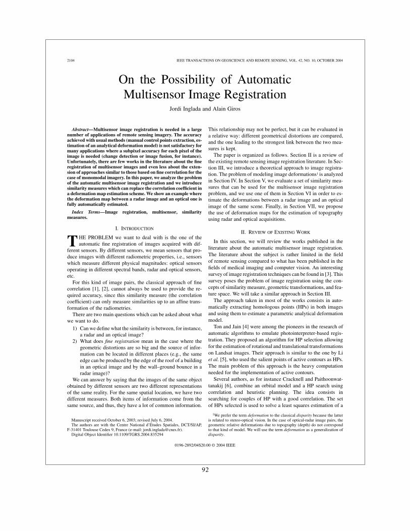
2104 IEEE TRANSACTIONS ON GEOSCIENCE AND REMOTE SENSING, VOL. 42, NO. 10, OCTOBER 2004
On the Possibility of AutomaticMultisensor Image Registration
Jordi Inglada and Alain Giros
Abstract—Multisensor image registration is needed in a largenumber of applications of remote sensing imagery. The accuracyachieved with usual methods (manual control points extraction, es-timation of an analytical deformation model) is not satisfactory formany applications where a subpixel accuracy for each pixel of theimage is needed (change detection or image fusion, for instance).Unfortunately, there are few works in the literature about the fineregistration of multisensor images and even less about the exten-sion of approaches similar to those based on fine correlation for thecase of monomodal imagery. In this paper, we analyze the problemof the automatic multisensor image registration and we introducesimilarity measures which can replace the correlation coefficient ina deformation map estimation scheme. We show an example wherethe deformation map between a radar image and an optical one isfully automatically estimated.
Index Terms—Image registration, multisensor, similaritymeasures.
I. INTRODUCTION
THE PROBLEM we want to deal with is the one of theautomatic fine registration of images acquired with dif-
ferent sensors. By different sensors, we mean sensors that pro-duce images with different radiometric properties, i.e., sensorswhich measure different physical magnitudes: optical sensorsoperating in different spectral bands, radar and optical sensors,etc.
For this kind of image pairs, the classical approach of finecorrelation [1], [2], cannot always be used to provide the re-quired accuracy, since this similarity measure (the correlationcoefficient) can only measure similarities up to an affine trans-formation of the radiometries.
There are two main questions which can be asked about whatwe want to do.
1) Can we define what the similarity is between, for instance,a radar and an optical image?
2) What does fine registration mean in the case where thegeometric distortions are so big and the source of infor-mation can be located in different places (e.g., the sameedge can be produced by the edge of the roof of a buildingin an optical image and by the wall–ground bounce in aradar image)?
We can answer by saying that the images of the same objectobtained by different sensors are two different representationsof the same reality. For the same spatial location, we have twodifferent measures. Both items of information come from thesame source, and thus, they have a lot of common information.
Manuscript received October 6, 2003; revised July 6, 2004.The authors are with the Centre National d’Études Spatiales, DCT/SI/AP,
F-31401 Toulouse Cedex 9, France (e-mail: [email protected]).Digital Object Identifier 10.1109/TGRS.2004.835294
This relationship may not be perfect, but it can be evaluated ina relative way: different geometrical distortions are compared,and the one leading to the strongest link between the two mea-sures is kept.
The paper is organized as follows. Section II is a review ofthe existing remote sensing image registration literature. In Sec-tion III, we introduce a theoretical approach to image registra-tion. The problem of modeling image deformations1 is analyzedin Section IV. In Section V, we evaluate a set of similarity mea-sures that can be used for the multisensor image registrationproblem, and we use one of them in Section VI in order to es-timate the deformations between a radar image and an opticalimage of the same scene. Finally, in Section VII, we proposethe use of deformation maps for the estimation of topographyusing radar and optical acquisitions.
II. REVIEW OF EXISTING WORK
In this section, we will review the works published in theliterature about the automatic multisensor image registration.The literature about the subject is rather limited in the fieldof remote sensing compared to what has been published in thefields of medical imaging and computer vision. An interestingsurvey of image registration techniques can be found in [3]. Thissurvey poses the problem of image registration using the con-cepts of similarity measure, geometric transformations, and fea-ture space. We will take a similar approach in Section III.
The approach taken in most of the works consists in auto-matically extracting homologous points (HPs) in both imagesand using them to estimate a parametric analytical deformationmodel.
Ton and Jain [4] were among the pioneers in the research ofautomatic algorithms to emulate photointerpreter-based regis-tration. They proposed an algorithm for HP selection allowingfor the estimation of rotational and translational transformationson Landsat images. Their approach is similar to the one by Liet al. [5], who used the salient points of active contours as HPs.The main problem of this approach is the heavy computationneeded for the implementation of active contours.
Several authors, as for instance Cracknell and Paithoonwat-tanakij [6], combine an orbital model and a HP search usingcorrelation and heuristic planning. The idea consists insearching for couples of HP with a good correlation. The setof HPs selected is used to solve a least squares estimation of a
1We prefer the term deformation to the classical disparity because the latteris related to stereo-optical vision. In the case of optical-radar image pairs, thegeometric relative deformations due to topography (depth) do not correspondto that kind of model. We will use the term deformation as a generalization ofdisparity.
0196-2892/04$20.00 © 2004 IEEE
92
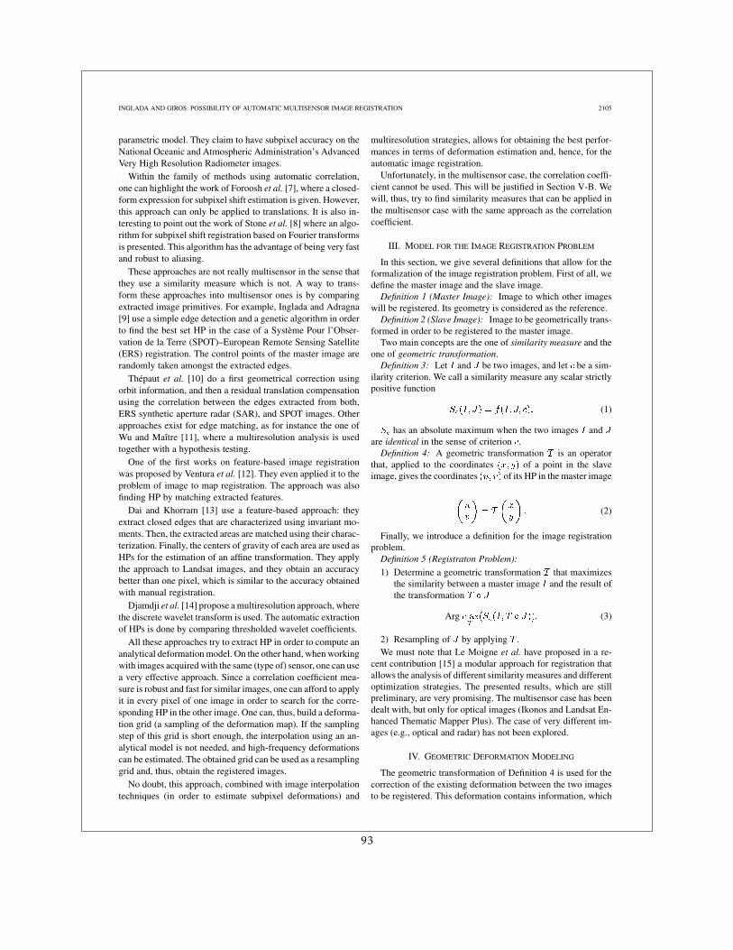
INGLADA AND GIROS: POSSIBILITY OF AUTOMATIC MULTISENSOR IMAGE REGISTRATION 2105
parametric model. They claim to have subpixel accuracy on theNational Oceanic and Atmospheric Administration’s AdvancedVery High Resolution Radiometer images.
Within the family of methods using automatic correlation,one can highlight the work of Foroosh et al. [7], where a closed-form expression for subpixel shift estimation is given. However,this approach can only be applied to translations. It is also in-teresting to point out the work of Stone et al. [8] where an algo-rithm for subpixel shift registration based on Fourier transformsis presented. This algorithm has the advantage of being very fastand robust to aliasing.
These approaches are not really multisensor in the sense thatthey use a similarity measure which is not. A way to trans-form these approaches into multisensor ones is by comparingextracted image primitives. For example, Inglada and Adragna[9] use a simple edge detection and a genetic algorithm in orderto find the best set HP in the case of a Système Pour l’Obser-vation de la Terre (SPOT)–European Remote Sensing Satellite(ERS) registration. The control points of the master image arerandomly taken amongst the extracted edges.
Thépaut et al. [10] do a first geometrical correction usingorbit information, and then a residual translation compensationusing the correlation between the edges extracted from both,ERS synthetic aperture radar (SAR), and SPOT images. Otherapproaches exist for edge matching, as for instance the one ofWu and Maître [11], where a multiresolution analysis is usedtogether with a hypothesis testing.
One of the first works on feature-based image registrationwas proposed by Ventura et al. [12]. They even applied it to theproblem of image to map registration. The approach was alsofinding HP by matching extracted features.
Dai and Khorram [13] use a feature-based approach: theyextract closed edges that are characterized using invariant mo-ments. Then, the extracted areas are matched using their charac-terization. Finally, the centers of gravity of each area are used asHPs for the estimation of an affine transformation. They applythe approach to Landsat images, and they obtain an accuracybetter than one pixel, which is similar to the accuracy obtainedwith manual registration.
Djamdji et al. [14] propose a multiresolution approach, wherethe discrete wavelet transform is used. The automatic extractionof HPs is done by comparing thresholded wavelet coefficients.
All these approaches try to extract HP in order to compute ananalytical deformation model. On the other hand, when workingwith images acquired with the same (type of) sensor, one can usea very effective approach. Since a correlation coefficient mea-sure is robust and fast for similar images, one can afford to applyit in every pixel of one image in order to search for the corre-sponding HP in the other image. One can, thus, build a deforma-tion grid (a sampling of the deformation map). If the samplingstep of this grid is short enough, the interpolation using an an-alytical model is not needed, and high-frequency deformationscan be estimated. The obtained grid can be used as a resamplinggrid and, thus, obtain the registered images.
No doubt, this approach, combined with image interpolationtechniques (in order to estimate subpixel deformations) and
multiresolution strategies, allows for obtaining the best perfor-mances in terms of deformation estimation and, hence, for theautomatic image registration.
Unfortunately, in the multisensor case, the correlation coeffi-cient cannot be used. This will be justified in Section V-B. Wewill, thus, try to find similarity measures that can be applied inthe multisensor case with the same approach as the correlationcoefficient.
III. MODEL FOR THE IMAGE REGISTRATION PROBLEM
In this section, we give several definitions that allow for theformalization of the image registration problem. First of all, wedefine the master image and the slave image.
Definition 1 (Master Image): Image to which other imageswill be registered. Its geometry is considered as the reference.
Definition 2 (Slave Image): Image to be geometrically trans-formed in order to be registered to the master image.
Two main concepts are the one of similarity measure and theone of geometric transformation.
Definition 3: Let and be two images, and let be a sim-ilarity criterion. We call a similarity measure any scalar strictlypositive function
(1)
has an absolute maximum when the two images andare identical in the sense of criterion .
Definition 4: A geometric transformation is an operatorthat, applied to the coordinates of a point in the slaveimage, gives the coordinates of its HP in the master image
(2)
Finally, we introduce a definition for the image registrationproblem.
Definition 5 (Registraton Problem):
1) Determine a geometric transformation that maximizesthe similarity between a master image and the result ofthe transformation
Arg (3)
2) Resampling of by applying .We must note that Le Moigne et al. have proposed in a re-
cent contribution [15] a modular approach for registration thatallows the analysis of different similarity measures and differentoptimization strategies. The presented results, which are stillpreliminary, are very promising. The multisensor case has beendealt with, but only for optical images (Ikonos and Landsat En-hanced Thematic Mapper Plus). The case of very different im-ages (e.g., optical and radar) has not been explored.
IV. GEOMETRIC DEFORMATION MODELING
The geometric transformation of Definition 4 is used for thecorrection of the existing deformation between the two imagesto be registered. This deformation contains information, which
93
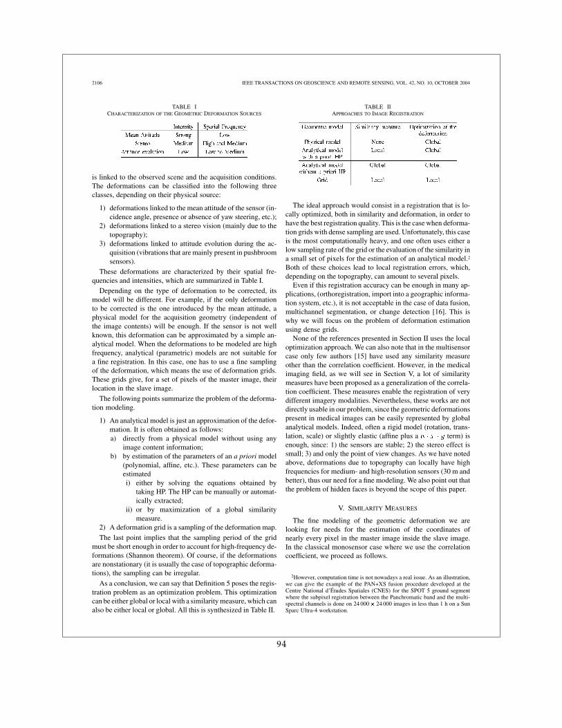
2106 IEEE TRANSACTIONS ON GEOSCIENCE AND REMOTE SENSING, VOL. 42, NO. 10, OCTOBER 2004
TABLE ICHARACTERIZATION OF THE GEOMETRIC DEFORMATION SOURCES
is linked to the observed scene and the acquisition conditions.The deformations can be classified into the following threeclasses, depending on their physical source:
1) deformations linked to the mean attitude of the sensor (in-cidence angle, presence or absence of yaw steering, etc.);
2) deformations linked to a stereo vision (mainly due to thetopography);
3) deformations linked to attitude evolution during the ac-quisition (vibrations that are mainly present in pushbroomsensors).
These deformations are characterized by their spatial fre-quencies and intensities, which are summarized in Table I.
Depending on the type of deformation to be corrected, itsmodel will be different. For example, if the only deformationto be corrected is the one introduced by the mean attitude, aphysical model for the acquisition geometry (independent ofthe image contents) will be enough. If the sensor is not wellknown, this deformation can be approximated by a simple an-alytical model. When the deformations to be modeled are highfrequency, analytical (parametric) models are not suitable fora fine registration. In this case, one has to use a fine samplingof the deformation, which means the use of deformation grids.These grids give, for a set of pixels of the master image, theirlocation in the slave image.
The following points summarize the problem of the deforma-tion modeling.
1) An analytical model is just an approximation of the defor-mation. It is often obtained as follows:a) directly from a physical model without using any
image content information;b) by estimation of the parameters of an a priori model
(polynomial, affine, etc.). These parameters can beestimatedi) either by solving the equations obtained by
taking HP. The HP can be manually or automat-ically extracted;
ii) or by maximization of a global similaritymeasure.
2) A deformation grid is a sampling of the deformation map.
The last point implies that the sampling period of the gridmust be short enough in order to account for high-frequency de-formations (Shannon theorem). Of course, if the deformationsare nonstationary (it is usually the case of topographic deforma-tions), the sampling can be irregular.
As a conclusion, we can say that Definition 5 poses the regis-tration problem as an optimization problem. This optimizationcan be either global or local with a similarity measure, which canalso be either local or global. All this is synthesized in Table II.
TABLE IIAPPROACHES TO IMAGE REGISTRATION
The ideal approach would consist in a registration that is lo-cally optimized, both in similarity and deformation, in order tohave the best registration quality. This is the case when deforma-tion grids with dense sampling are used. Unfortunately, this caseis the most computationally heavy, and one often uses either alow sampling rate of the grid or the evaluation of the similarity ina small set of pixels for the estimation of an analytical model.2
Both of these choices lead to local registration errors, which,depending on the topography, can amount to several pixels.
Even if this registration accuracy can be enough in many ap-plications, (orthoregistration, import into a geographic informa-tion system, etc.), it is not acceptable in the case of data fusion,multichannel segmentation, or change detection [16]. This iswhy we will focus on the problem of deformation estimationusing dense grids.
None of the references presented in Section II uses the localoptimization approach. We can also note that in the multisensorcase only few authors [15] have used any similarity measureother than the correlation coefficient. However, in the medicalimaging field, as we will see in Section V, a lot of similaritymeasures have been proposed as a generalization of the correla-tion coefficient. These measures enable the registration of verydifferent imagery modalities. Nevertheless, these works are notdirectly usable in our problem, since the geometric deformationspresent in medical images can be easily represented by globalanalytical models. Indeed, often a rigid model (rotation, trans-lation, scale) or slightly elastic (affine plus a term) isenough, since: 1) the sensors are stable; 2) the stereo effect issmall; 3) and only the point of view changes. As we have notedabove, deformations due to topography can locally have highfrequencies for medium- and high-resolution sensors (30 m andbetter), thus our need for a fine modeling. We also point out thatthe problem of hidden faces is beyond the scope of this paper.
V. SIMILARITY MEASURES
The fine modeling of the geometric deformation we arelooking for needs for the estimation of the coordinates ofnearly every pixel in the master image inside the slave image.In the classical monosensor case where we use the correlationcoefficient, we proceed as follows.
2However, computation time is not nowadays a real issue. As an illustration,we can give the example of the PAN+XS fusion procedure developed at theCentre National d’Études Spatiales (CNES) for the SPOT 5 ground segmentwhere the subpixel registration between the Panchromatic band and the multi-spectral channels is done on 24 000� 24 000 images in less than 1 h on a SunSparc Ultra-4 workstation.
94
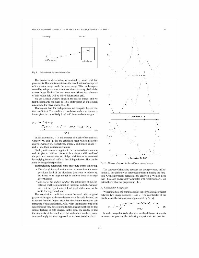
INGLADA AND GIROS: POSSIBILITY OF AUTOMATIC MULTISENSOR IMAGE REGISTRATION 2107
Fig. 1. Estimation of the correlation surface.
The geometric deformation is modeled by local rigid dis-placements. One wants to estimate the coordinates of each pixelof the master image inside the slave image. This can be repre-sented by a displacement vector associated to every pixel of themaster image. Each of the two components (lines and columns)of this vector field will be called deformation grid.
We use a small window taken in the master image, and wetest the similarity for every possible shift within an explorationarea inside the slave image (Fig. 1).
That means that, for each position, we compute the correla-tion coefficient. The result is a correlation surface whose max-imum gives the most likely local shift between both images
(4)
In this expression, is the number of pixels of the analysiswindow; and are the estimated mean values inside theanalysis window of, respectively, image and image ; andand are their standard deviations.
Quality criteria can be applied to the estimated maximum inorder to give a confidence factor to the estimated shift: width ofthe peak, maximum value, etc. Subpixel shifts can be measuredby applying fractional shifts to the sliding window. This can bedone by image interpolation.
The interesting parameters of the procedure are the following.
• The size of the exploration area: it determines the com-putational load of the algorithm (we want to reduce it),but it has to be large enough in order to cope with largedeformations.
• The size of the sliding window: the robustness of the cor-relation coefficient estimation increases with the windowsize, but the hypothesis of local rigid shifts may not bevalid for large windows.
The correlation coefficient cannot be used with originalgray-level images in the multisensor case. It could be used onextracted features (edges, etc.), but the feature extraction canintroduce localization errors. Also, when the images come fromsensors using very different modalities, it can be difficult to findsimilar features in both images. In this case, one can try to findthe similarity at the pixel level, but with other similarity mea-sures and apply the same approach as we have just described.
Fig. 2. Measure of �(�x) for three different pairs of images.
The concept of similarity measure has been presented in Def-inition 3. The difficulty of the procedure lies in finding the func-tion , which properly represents the criterion . We also needthat be easily and robustly estimated with small windows. Weextend here what we proposed in [17].
A. Correlation Coefficient
We remind here the computation of the correlation coefficientbetween two image windows and . The coordinates of thepixels inside the windows are represented by
(5)
In order to qualitatively characterize the different similaritymeasures we propose the following experiment. We take two
95
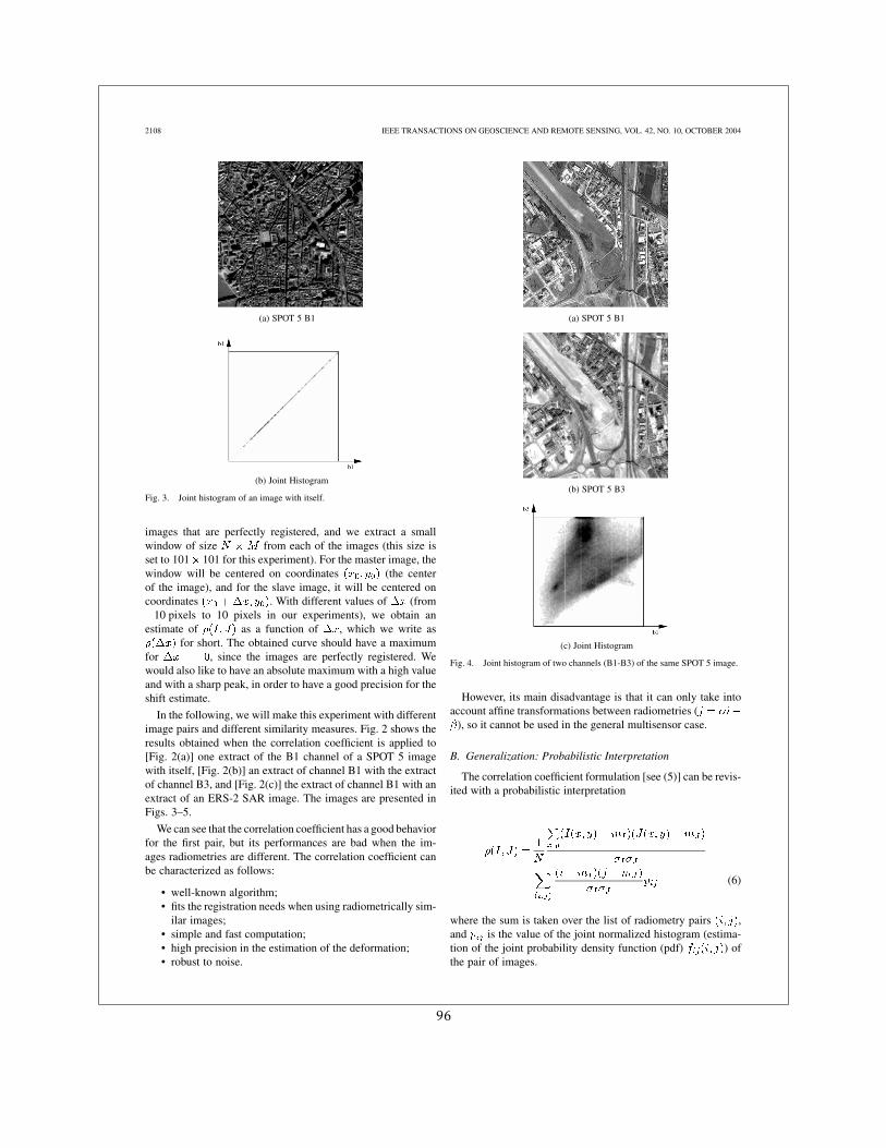
2108 IEEE TRANSACTIONS ON GEOSCIENCE AND REMOTE SENSING, VOL. 42, NO. 10, OCTOBER 2004
(a) SPOT 5 B1
(b) Joint Histogram
Fig. 3. Joint histogram of an image with itself.
images that are perfectly registered, and we extract a smallwindow of size from each of the images (this size isset to 101 101 for this experiment). For the master image, thewindow will be centered on coordinates (the centerof the image), and for the slave image, it will be centered oncoordinates . With different values of (from
10 pixels to 10 pixels in our experiments), we obtain anestimate of as a function of , which we write as
for short. The obtained curve should have a maximumfor , since the images are perfectly registered. Wewould also like to have an absolute maximum with a high valueand with a sharp peak, in order to have a good precision for theshift estimate.
In the following, we will make this experiment with differentimage pairs and different similarity measures. Fig. 2 shows theresults obtained when the correlation coefficient is applied to[Fig. 2(a)] one extract of the B1 channel of a SPOT 5 imagewith itself, [Fig. 2(b)] an extract of channel B1 with the extractof channel B3, and [Fig. 2(c)] the extract of channel B1 with anextract of an ERS-2 SAR image. The images are presented inFigs. 3–5.
We can see that the correlation coefficient has a good behaviorfor the first pair, but its performances are bad when the im-ages radiometries are different. The correlation coefficient canbe characterized as follows:
• well-known algorithm;• fits the registration needs when using radiometrically sim-
ilar images;• simple and fast computation;• high precision in the estimation of the deformation;• robust to noise.
(a) SPOT 5 B1
(b) SPOT 5 B3
(c) Joint Histogram
Fig. 4. Joint histogram of two channels (B1-B3) of the same SPOT 5 image.
However, its main disadvantage is that it can only take intoaccount affine transformations between radiometries (
), so it cannot be used in the general multisensor case.
B. Generalization: Probabilistic Interpretation
The correlation coefficient formulation [see (5)] can be revis-ited with a probabilistic interpretation
(6)
where the sum is taken over the list of radiometry pairs ,and is the value of the joint normalized histogram (estima-tion of the joint probability density function (pdf) ) ofthe pair of images.
96
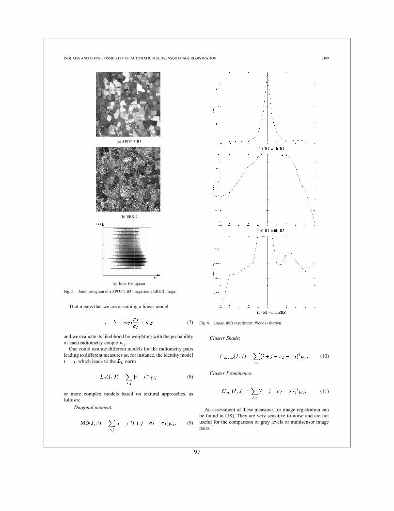
INGLADA AND GIROS: POSSIBILITY OF AUTOMATIC MULTISENSOR IMAGE REGISTRATION 2109
(a) SPOT 5 B3
(b) ERS-2
(c) Joint Histogram
Fig. 5. Joint histogram of a SPOT 5 B3 image and a ERS-2 image.
That means that we are assuming a linear model
(7)
and we evaluate its likelihood by weighting with the probabilityof each radiometry couple .
One could assume different models for the radiometry pairsleading to different measures as, for instance, the identity model
, which leads to the norm
(8)
or more complex models based on textural approaches, asfollows:
Diagonal moment:
MD (9)
Fig. 6. Image shift experiment: Woods criterion.
Cluster Shade:
(10)
Cluster Prominence:
(11)
An assessment of these measures for image registration canbe found in [18]. They are very sensitive to noise and are notuseful for the comparison of gray levels of multisensor imagepairs.
97
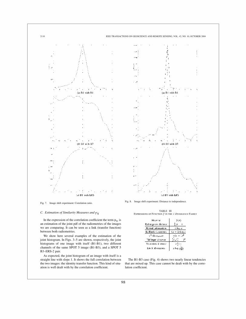
2110 IEEE TRANSACTIONS ON GEOSCIENCE AND REMOTE SENSING, VOL. 42, NO. 10, OCTOBER 2004
Fig. 7. Image shift experiment: Correlation ratio.
C. Estimation of Similarity Measures and
In the expression of the correlation coefficient the term isan estimation of the joint pdf of the radiometries of the imageswe are comparing. It can be seen as a link (transfer function)between both radiometries.
We show here several examples of the estimation of thejoint histogram. In Figs. 3–5 are shown, respectively, the jointhistograms of one image with itself (B1-B1), two differentchannels of the same SPOT 5 image (B1-B3), and a SPOT 5B3–ERS-2 pair.
As expected, the joint histogram of an image with itself is astraight line with slope 1. It shows the full correlation betweenthe two images: the identity transfer function. This kind of situ-ation is well dealt with by the correlation coefficient.
Fig. 8. Image shift experiment: Distance to independence.
TABLE IIIEXPRESSIONS OF FUNCTION f IN THE f -DIVERGENCE FAMILY
The B1-B3 case (Fig. 4) shows two nearly linear tendenciesthat are mixed up. This case cannot be dealt with by the corre-lation coefficient.
98
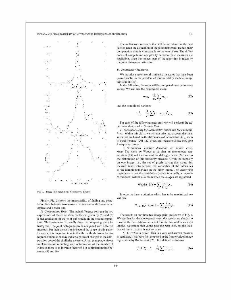
INGLADA AND GIROS: POSSIBILITY OF AUTOMATIC MULTISENSOR IMAGE REGISTRATION 2111
Fig. 9. Image shift experiment: Kolmogorov distance.
Finally, Fig. 5 shows the impossibility of finding any corre-lation link between two sensors, which are as different as anoptical and a radar one.
1) Computation Time: The main difference between the twoexpressions of the correlation coefficient given by (5) and (6)is the estimation of the joint pdf needed in the second expres-sion. This estimation is usually done by computing the jointhistogram. The joint histogram can be computed with differentmethods, but their discussion is beyond the scope of this paper.However, it is important to note that the method chosen for his-togram computation may induce significant changes in the com-putation cost of the similarity measure. As an example, with ourimplementation (counting with optimization of the number ofclasses), there is an increase factor of 4 in computation time be-tween (5) and (6).
The multisensor measures that will be introduced in the nextsection need the estimation of the joint histogram. Hence, theircomputation time is comparable to the one of (6). The differ-ences of computation complexity between these measures arenegligible, since the longest part of the algorithm is taken bythe joint histogram estimation.
D. Multisensor Measures
We introduce here several similarity measures that have beenproved useful in the problem of multimodality medical imageregistration [19].
In the following, the sums will be computed over radiometryvalues. We will use the conditional mean
(12)
and the conditional variance
(13)
For each of the following measures, we will perform the ex-periment described in Section V-A.
1) Measures Using the Radiometry Values and the Probabil-ities: Within this class, we will not take into account the mea-sures that are based on the differences of radiometries ( normof the difference) [20]–[22] or textural measures, since they givelow-quality results.
a) Normalized sandard deviation or Woods crite-rion: The work by Woods et al. first on monomodal reg-istration [23] and then on multimodal registration [24] lead tothe elaboration of this similarity measure. Given the intensityon one image, i.e., the set of pixels having this value, thismeasure takes into account the variability of the intensitiesof the homologous pixels in the other image. The underlyinghypothesis is that this variability (which is actually a measureof variance) will be minimum when the images are registered
Woods (14)
In order to have a criterion which has to be maximized, wewill use
(15)
The results on our three test image pairs are shown in Fig. 6.We see that for the monosensor case, the results are similar tothose of the correlation coefficient. For the two multisensor ex-amples, we obtain high values near the zero-shift, but the loca-tion of these maxima is not accurate.
b) Correlation ratio: This is a very well known measurein statistics. It has been first proposed in the framework of imageregistration by Roche et al. [25]. It is defined as follows:
(16)
99
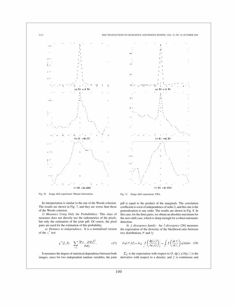
2112 IEEE TRANSACTIONS ON GEOSCIENCE AND REMOTE SENSING, VOL. 42, NO. 10, OCTOBER 2004
Fig. 10. Image shift experiment: Mutual information.
Its interpretation is similar to the one of the Woods criterion.The results are shown in Fig. 7, and they are worse than thoseof the Woods criterion.
2) Measures Using Only the Probabilities: This class ofmeasures does not directly use the radiometries of the pixels,but only the estimation of the joint pdf. Of course, the pixelpairs are used for the estimation of this probability.
a) Distance to independence: It is a normalized versionof the test
(17)
It measures the degree of statistical dependence between bothimages, since for two independent random variables, the joint
Fig. 11. Image shift experiment: CRA.
pdf is equal to the product of the marginals. The correlationcoefficient is a test of independence of order 2, and this one is thegeneralization to any order. The results are shown in Fig. 8. Inthis case, for the three pairs, we obtain an absolute maximum forthe zero-shift case, which is sharp enough for a robust automaticdetection.
b) -divergence family: An -divergence [26] measuresthe expectation of the diversity of the likelihood ratio betweentwo distributions and
(18)
is the expectation with respect to ; is thederivative with respect to a density; and is continuous and
100
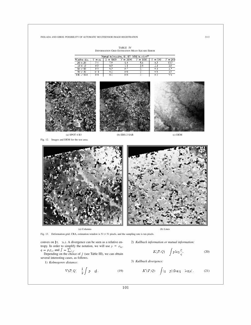
INGLADA AND GIROS: POSSIBILITY OF AUTOMATIC MULTISENSOR IMAGE REGISTRATION 2113
TABLE IVDEFORMATION GRID ESTIMATION MEAN SQUARE ERROR
(a) SPOT 4 B3 (b) ERS-2 SAR (c) DEM
Fig. 12. Images and DEM for the test area.
(a) Columns (b) Lines
Fig. 13. Deformation grid. CRA, estimation window is 51� 51 pixels, and the sampling rate is ten pixels.
convex on . A divergence can be seen as a relative en-tropy. In order to simplify the notation, we will use ,
, and .Depending on the choice of (see Table III), we can obtain
several interesting cases, as follows.
1) Kolmogorov distance:
(19)
2) Kullback information or mutual information:
(20)
3) Kullback divergence:
(21)
101
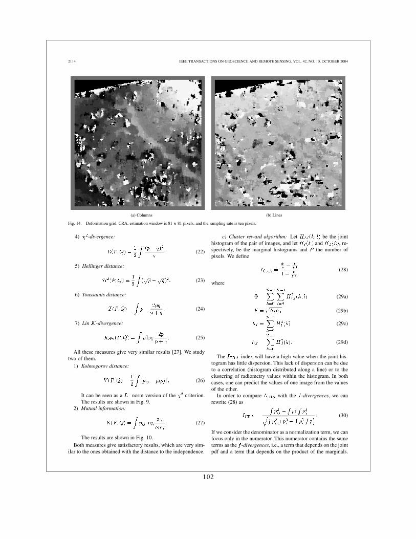
2114 IEEE TRANSACTIONS ON GEOSCIENCE AND REMOTE SENSING, VOL. 42, NO. 10, OCTOBER 2004
(a) Columns (b) Lines
Fig. 14. Deformation grid. CRA, estimation window is 81� 81 pixels, and the sampling rate is ten pixels.
4) -divergence:
(22)
5) Hellinger distance:
(23)
6) Toussaints distance:
(24)
7) Lin -divergence:
(25)
All these measures give very similar results [27]. We studytwo of them.
1) Kolmogorov distance:
(26)
It can be seen as a norm version of the criterion.The results are shown in Fig. 9.
2) Mutual information:
(27)
The results are shown in Fig. 10.Both measures give satisfactory results, which are very sim-
ilar to the ones obtained with the distance to the independence.
c) Cluster reward algorithm: Let be the jointhistogram of the pair of images, and let and , re-spectively, be the marginal histograms and the number ofpixels. We define
(28)
where
(29a)
(29b)
(29c)
(29d)
The index will have a high value when the joint his-togram has little dispersion. This lack of dispersion can be dueto a correlation (histogram distributed along a line) or to theclustering of radiometry values within the histogram. In bothcases, one can predict the values of one image from the valuesof the other.
In order to compare with the -divergences, we canrewrite (28) as
(30)
If we consider the denominator as a normalization term, we canfocus only in the numerator. This numerator contains the sameterms as the -divergences, i.e., a term that depends on the jointpdf and a term that depends on the product of the marginals.
102
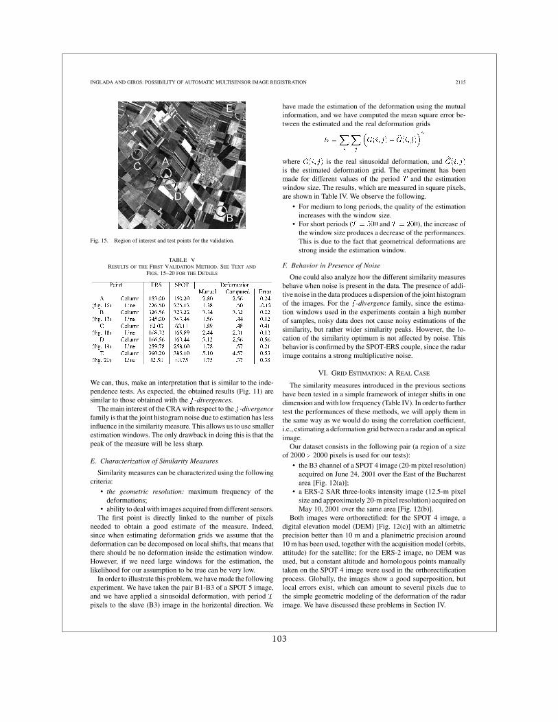
INGLADA AND GIROS: POSSIBILITY OF AUTOMATIC MULTISENSOR IMAGE REGISTRATION 2115
Fig. 15. Region of interest and test points for the validation.
TABLE VRESULTS OF THE FIRST VALIDATION METHOD. SEE TEXT AND
FIGS. 15–20 FOR THE DETAILS
We can, thus, make an interpretation that is similar to the inde-pendence tests. As expected, the obtained results (Fig. 11) aresimilar to those obtained with the -divergences.
The main interest of the CRA with respect to the -divergencefamily is that the joint histogram noise due to estimation has lessinfluence in the similarity measure. This allows us to use smallerestimation windows. The only drawback in doing this is that thepeak of the measure will be less sharp.
E. Characterization of Similarity Measures
Similarity measures can be characterized using the followingcriteria:
• the geometric resolution: maximum frequency of thedeformations;
• ability to deal with images acquired from different sensors.The first point is directly linked to the number of pixels
needed to obtain a good estimate of the measure. Indeed,since when estimating deformation grids we assume that thedeformation can be decomposed on local shifts, that means thatthere should be no deformation inside the estimation window.However, if we need large windows for the estimation, thelikelihood for our assumption to be true can be very low.
In order to illustrate this problem, we have made the followingexperiment. We have taken the pair B1-B3 of a SPOT 5 image,and we have applied a sinusoidal deformation, with periodpixels to the slave (B3) image in the horizontal direction. We
have made the estimation of the deformation using the mutualinformation, and we have computed the mean square error be-tween the estimated and the real deformation grids
where is the real sinusoidal deformation, andis the estimated deformation grid. The experiment has beenmade for different values of the period and the estimationwindow size. The results, which are measured in square pixels,are shown in Table IV. We observe the following.
• For medium to long periods, the quality of the estimationincreases with the window size.
• For short periods ( and ), the increase ofthe window size produces a decrease of the performances.This is due to the fact that geometrical deformations arestrong inside the estimation window.
F. Behavior in Presence of Noise
One could also analyze how the different similarity measuresbehave when noise is present in the data. The presence of addi-tive noise in the data produces a dispersion of the joint histogramof the images. For the -divergence family, since the estima-tion windows used in the experiments contain a high numberof samples, noisy data does not cause noisy estimations of thesimilarity, but rather wider similarity peaks. However, the lo-cation of the similarity optimum is not affected by noise. Thisbehavior is confirmed by the SPOT-ERS couple, since the radarimage contains a strong multiplicative noise.
VI. GRID ESTIMATION: A REAL CASE
The similarity measures introduced in the previous sectionshave been tested in a simple framework of integer shifts in onedimension and with low frequency (Table IV). In order to furthertest the performances of these methods, we will apply them inthe same way as we would do using the correlation coefficient,i.e., estimating a deformation grid between a radar and an opticalimage.
Our dataset consists in the following pair (a region of a sizeof 2000 2000 pixels is used for our tests):
• the B3 channel of a SPOT 4 image (20-m pixel resolution)acquired on June 24, 2001 over the East of the Bucharestarea [Fig. 12(a)];
• a ERS-2 SAR three-looks intensity image (12.5-m pixelsize and approximately 20-m pixel resolution) acquired onMay 10, 2001 over the same area [Fig. 12(b)].
Both images were orthorectified: for the SPOT 4 image, adigital elevation model (DEM) [Fig. 12(c)] with an altimetricprecision better than 10 m and a planimetric precision around10 m has been used, together with the acquisition model (orbits,attitude) for the satellite; for the ERS-2 image, no DEM wasused, but a constant altitude and homologous points manuallytaken on the SPOT 4 image were used in the orthorectificationprocess. Globally, the images show a good superposition, butlocal errors exist, which can amount to several pixels due tothe simple geometric modeling of the deformation of the radarimage. We have discussed these problems in Section IV.
103
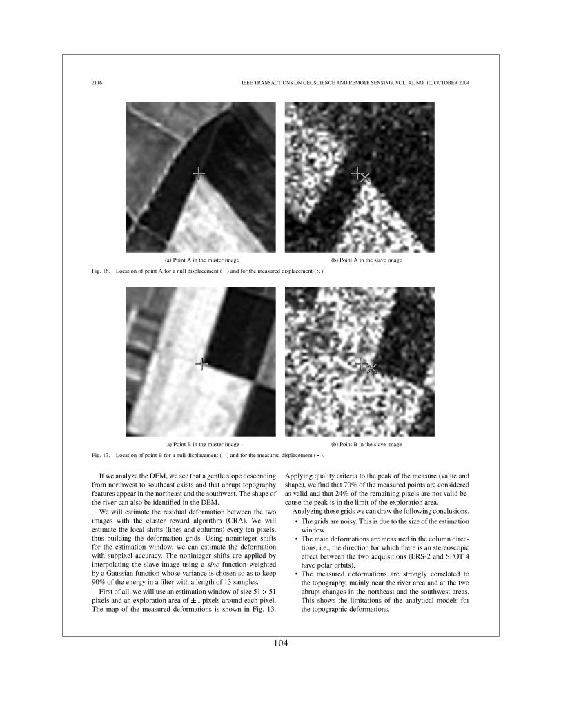
2116 IEEE TRANSACTIONS ON GEOSCIENCE AND REMOTE SENSING, VOL. 42, NO. 10, OCTOBER 2004
(a) Point A in the master image (b) Point A in the slave image
Fig. 16. Location of point A for a null displacement (+) and for the measured displacement (�).
(a) Point B in the master image (b) Point B in the slave image
Fig. 17. Location of point B for a null displacement (+) and for the measured displacement (�).
If we analyze the DEM, we see that a gentle slope descendingfrom northwest to southeast exists and that abrupt topographyfeatures appear in the northeast and the southwest. The shape ofthe river can also be identified in the DEM.
We will estimate the residual deformation between the twoimages with the cluster reward algorithm (CRA). We willestimate the local shifts (lines and columns) every ten pixels,thus building the deformation grids. Using noninteger shiftsfor the estimation window, we can estimate the deformationwith subpixel accuracy. The noninteger shifts are applied byinterpolating the slave image using a sinc function weightedby a Gaussian function whose variance is chosen so as to keep90% of the energy in a filter with a length of 13 samples.
First of all, we will use an estimation window of size 51 51pixels and an exploration area of pixels around each pixel.The map of the measured deformations is shown in Fig. 13.
Applying quality criteria to the peak of the measure (value andshape), we find that 70% of the measured points are consideredas valid and that 24% of the remaining pixels are not valid be-cause the peak is in the limit of the exploration area.
Analyzing these grids we can draw the following conclusions.
• The grids are noisy. This is due to the size of the estimationwindow.
• The main deformations are measured in the column direc-tions, i.e., the direction for which there is an stereoscopiceffect between the two acquisitions (ERS-2 and SPOT 4have polar orbits).
• The measured deformations are strongly correlated tothe topography, mainly near the river area and at the twoabrupt changes in the northeast and the southwest areas.This shows the limitations of the analytical models forthe topographic deformations.
104
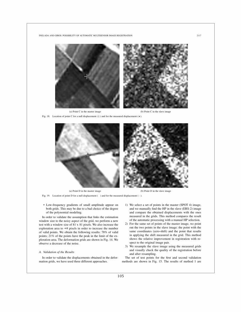
INGLADA AND GIROS: POSSIBILITY OF AUTOMATIC MULTISENSOR IMAGE REGISTRATION 2117
(a) Point C in the master image (b) Point C in the slave image
Fig. 18. Location of point C for a null displacement (+) and for the measured displacement (�).
(a) Point D in the master image (b) Point D in the slave image
Fig. 19. Location of point D for a null displacement (+) and for the measured displacement (�).
• Low-frequency gradients of small amplitude appear onboth grids. This may be due to a bad choice of the degreeof the polynomial modeling.
In order to validate the assumption that links the estimationwindow size to the noisy aspect of the grid, we perform a newtest with a window size of 81 81 pixels. We also increase theexploration area to pixels in order to increase the numberof valid points. We obtain the following results: 78% of validpoints; 21% of the points have the peak in the limit of the ex-ploration area. The deformation grids are shown in Fig. 14. Weobserve a decrease of the noise.
A. Validation of the Results
In order to validate the displacements obtained in the defor-mation grids, we have used three different approaches.
1) We select a set of points in the master (SPOT 4) image,and we manually find the HP in the slave (ERS-2) imageand compare the obtained displacements with the onesmeasured in the grids. This method compares the resultof the automatic processing with a manual HP selection.
2) For the same set of points of the master image, we pointout the two points in the slave image: the point with thesame coordinates (zero-shift) and the point that resultsin applying the shift measured in the grid. This methodshows the relative improvement in registration with re-spect to the original image pair.
3) We resample the slave image using the measured gridsand visually check the quality of the registration beforeand after resampling.
The set of test points for the first and second validationmethods are shown in Fig. 15. The results of method 1 are
105
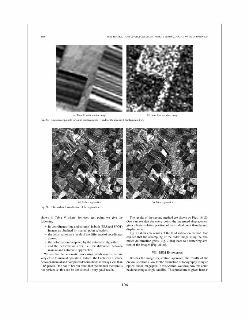
2118 IEEE TRANSACTIONS ON GEOSCIENCE AND REMOTE SENSING, VOL. 42, NO. 10, OCTOBER 2004
(a) Point E in the master image (b) Point E in the slave image
Fig. 20. Location of point E for a null displacement (+) and for the measured displacement (�).
(a) Before registration (b) After registration
Fig. 21. Checkerboard visualization of the registration.
shown in Table V where, for each test point, we give thefollowing:
• its coordinates (line and column) in both (ERS and SPOT)images as obtained by manual point selection;
• the deformation as a result of the difference of coordinatesabove;
• the deformation computed by the automatic algorithm;• and the deformation error, i.e., the difference between
manual and automatic approaches.We see that the automatic processing yields results that are
very close to manual operation. Indeed, the Euclidean distancebetween manual and computed deformations is always less than0.65 pixels. One has to bear in mind that the manual measure isnot perfect, so this can be considered a very good result.
The results of the second method are shown on Figs. 16–20.One can see that for every point, the measured displacementgives a better relative position of the studied point than the nulldisplacement.
Fig. 21 shows the results of the third validation method. Onecan see that the resampling of the radar image using the esti-mated deformation grids [Fig. 21(b)] leads to a better registra-tion of the images [Fig. 21(a)].
VII. DEM ESTIMATION
Besides the image registration approach, the results of theprevious section allow for the estimation of topography using anoptical-radar image pair. In this section, we show how this couldbe done using a single satellite. This procedure is given here as
106
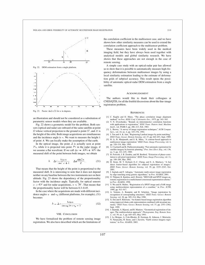
INGLADA AND GIROS: POSSIBILITY OF AUTOMATIC MULTISENSOR IMAGE REGISTRATION 2119
Fig. 22. DEM estimation from a single platform.
Fig. 23. Factor sin 2�=2 for � in degrees.
an illustration and should not be considered as a substitution ofparametric sensor models when they are available.
Fig. 22 shows a geometric model for the problem. Both sen-sors (optical and radar) are onboard of the same satellite at point
whose vertical projection to the ground is point , and isthe height of the orbit. Both image acquisitions are simultaneousand the incidence angle is . We want to measure the heightof point . We can locally make the assumption of flat earth.
In the optical image, the point is actually seen at point, while it is projected into point in the radar image, if
we assume a flat wavefront. If we call themeasured shift of the point between both images, we obtain
(31)
That means that the height of the point is proportional to themeasured shift. It is interesting to note that it does not dependneither on any baseline between the two instruments nor on theiraltitude. Fig. 23 shows the dependency of the proportionalityfactor with the incidence angle. Typically, for optical sensors
and for radar acquisitions, . That means thatthe proportionality factor will be between 0.3–0.45.
In the case where the acquisitons are made with different inci-dence angles and (different platforms, for example), (31)becomes
(32)
VIII. CONCLUSION
We have formalized the problem of remote sensing imageregistration. We also have described which are the limitations of
the correlation coefficient in the multisensor case, and we haveshown how other similarity measures can be used to extend thecorrelation coefficient approach to the multisensor problem.
These measures have been widely used in the medicalimaging field, but they have always been used together withanalytical models and global similarity research. We haveshown that these approaches are not enough in the case ofremote sensing.
A simple case study with an optical-radar pair has allowedus to show that it is possible to automatically measure high-fre-quency deformations between multisensor images by using alocal similarity estimation leading to the estimate of deforma-tion grids of subpixel accuracy. This result opens the possi-bility of automatic optical-radar DEM estimation from a singlesatellite.
ACKNOWLEDGMENT
The authors would like to thank their colleagues atCNES/QTIS, for all the fruitful discussions about the fine-imageregistration problem.
REFERENCES
[1] C. Kuglin and D. Hines, “The phase correlation image alignmentmethod,” in Proc. IEEE Conf. Cybernetics Soc., 1975, pp. 163–165.
[2] V. N. Dvorchenko, “Bounds on (deterministic) correlation functionswith applications to registration,” IEEE Trans. Pattern Anal. MachineIntell., vol. PAMI-5, pp. 206–213, Feb. 1983.
[3] L. Brown, “A survey of image registration techniques,” ACM Comput.Surv., vol. 24, no. 4, pp. 325–376, 1992.
[4] J. Ton and A. K. Jain, “Registering Landsat images by point matching,”IEEE Trans. Geosci. Remote Sensing, vol. 27, pp. 642–651, Sept. 1989.
[5] H. Li, B. Manjunath, and S. K. Mitra, “A contour-based approach tomultisensor image registration,” IEEE Trans. Image Processing, vol. 4,pp. 320–334, Mar. 1995.
[6] A. Cracknell and K. Paithoonwattanakij, “Fast automatic registration forsatellite imagery by heuristic planning,” Proc. Inst. Elect. Eng., vol. 136,no. 5, pp. 221–225, 1989.
[7] H. Foroosh, J. B. Zerubia, and M. Berthod, “Extension of phase-corre-lation to sub-pixel registration,” IEEE Trans. Image Processing, vol. 11,pp. 188–200, Mar. 2002.
[8] H. Stone, M. T. Orchard, E.-C. Cheng, and S. A. Martucci, “A fastdirect fourier-based algorithm for subpixel registration of images,”IEEE Trans. Geosci. Remote Sensing, vol. 39, pp. 2235–2243, Oct.2001.
[9] J. Inglada and F. Adragna, “Automatic multi-sensor image registrationby edge matching using genetic algorithms,” in Proc. IGARSS, 2001.
[10] O. Thépaut, K. Kpalma, and J. Ronsin, “ERS SAR and SPOT images au-tomatic registration in a multichannel consensual segmentation scheme,”in Proc. IGARSS, 1998.
[11] Y. Wu and H. Maître, “Registration of a SPOT image and a SAR imageusing multiresolution representation of a coastline,” in Proc. ICPR,1990, pp. 913–917.
[12] A. Ventura, A. Rampini, and R. Schettini, “Image registration byrecognition of corresponding structures,” IEEE Trans. Geosci. RemoteSensing, vol. 28, pp. 305–314, May 1990.
[13] X. Dai and S. Khorram, “An feature-based image registration algorithmusing improved chain-code representation combined with invariant mo-ments,” IEEE Trans. Geosci. Remote Sensing, vol. 37, pp. 2351–2362,Sept. 1999.
[14] J. Djamdji, A. Bijaoui, and R. Maniere, “Geometrical registration of im-ages: The multiresolution approach,” Photogramm. Eng. Remote Sens.J., vol. 59, no. 5, pp. 645–653, May 1993.
[15] J. Le Moigne, A. Cole-Rhodes, R. Eastman, K. Johnson, J. Morisette,N. Netanyahu, H. Stone, and I. Zavorin, “Earth science imagery regis-tration,” in Proc. IGARSS, 2003.
107
2120 IEEE TRANSACTIONS ON GEOSCIENCE AND REMOTE SENSING, VOL. 42, NO. 10, OCTOBER 2004
[16] J. Townshend, C. Justice, C. Gurney, and J. McManus, “The impactof misregistration on change detection,” IEEE Trans. Geosci. RemoteSensing, vol. 30, pp. 1054–1060, Sept. 1992.
[17] J. Inglada, “Similarity measures for multisensor remote sensing images,”in Proc. IGARSS, 2002.
[18] M. Bro-Nielsen, “Medical image registration and surgery simulation,”Ph.D. dissertation, Tech.Univ. Denmark, Lyngby, Denmark, 1996.
[19] D. Sarrut, “Recalage multimodal et plate-forme d’imagerie médicale àaccès distant,” Ph.D. dissertation, Univ. Lumière Lyon 2, Lyon, France,2000.
[20] P. Thévenaz, U. Ruttimann, and M. Unser, “Iterative multi-scale regis-tration without landmarks,” IEEE Trans. Image Processing, vol. 7, pp.27–41, Jan. 1998.
[21] E. de Castro and C. Morandi, “Registration of translated and rotated im-ages using finite Fourier transforms,” IEEE Trans. Pattern Anal. Ma-chine Intell., vol. PAMI-9, pp. 700–703, May 1987.
[22] A. Apicella, J. Kippenhan, and J. Nagel, “Fast multi-modality imagematching,” Proc. SPIE, vol. 1092, pp. 252–263, 1989.
[23] R. Woods, S. Cherry, and J. Mazziota, “Rapid automated algorithm foraligning and reslicing PET images,” J. Comput. Assist. Tomogr., vol. 16,no. 4, pp. 620–633, 1992.
[24] R. Woods, J. Mazziota, and S. Cherry, “MRI-PET registration withautomated algorithm,” J. Comput. Assist. Tomogr., vol. 17, no. 4, pp.536–546, 1993.
[25] A. Roche, G. Malandain, X. Pennec, and N. Ayache, “The correlationratio as a new similarity measure for multimodal image registration,” inProc. MICCAI, Cambridge, MA, Oct. 1998, pp. 1115–1124.
[26] I. Csiszar, “Information type measures of difference of probability dis-tributions and indirect observations,” Studia Sci. Math. Hungar., vol. 2,pp. 299–318, 1967.
[27] D. Sarrut and S. Miguet, “Similarity measures form image registra-tion,” in Proc. Eur. Workshop on Content-Based Multimedia Indexing,Toulouse, France, Oct. 1999, pp. 263–270.
Jordi Inglada received the telecommunicationsengineer degree from both Universitat Politècnicade Catalunya, Catalunya, Spain, and the ÉcoleNationale Supérieure des Télécommunications deBretagne, Brest, France, in 1997, and the Ph.D.degree in signal processing and telecommunicationsfrom Université de Rennes 1, Rennes, France, in2000.
He has been since been with the Centre Nationald’Études Spatiales, Toulouse, France, working in thefield of remote sensing image processing. He is in
charge for the development of image processing algorithms for the operationalexploitation of earth observation images, mainly in the fields of image registra-tion, change detection, and object recognition.
Alain Giros received the physics engineer degreefrom École Nationale Supérieure de Physique deMarseille, Marseille, France, in 1982, with a special-ization in optics and image processing.
He has since been with the Centre Nationald’Études Spatiales (CNES), Toulouse, France. Hebegan his carrier in the SPOT 1 project team wherehe was responsible of the whole image processingsoftware. Then, he was responsible for the develop-ment of several image processing systems, includingDALI (the worldwide catalog of SPOT images),
several image quality assessment systems for SPOT, and the VegetationUser Services Facility. Interested in automated image registration since themid-1990s, he has been promoting this research subject at CNES. He is now incharge of the development of image processing techniques mainly in the fieldof image time series processing, automated registration, and image informationmining.
108
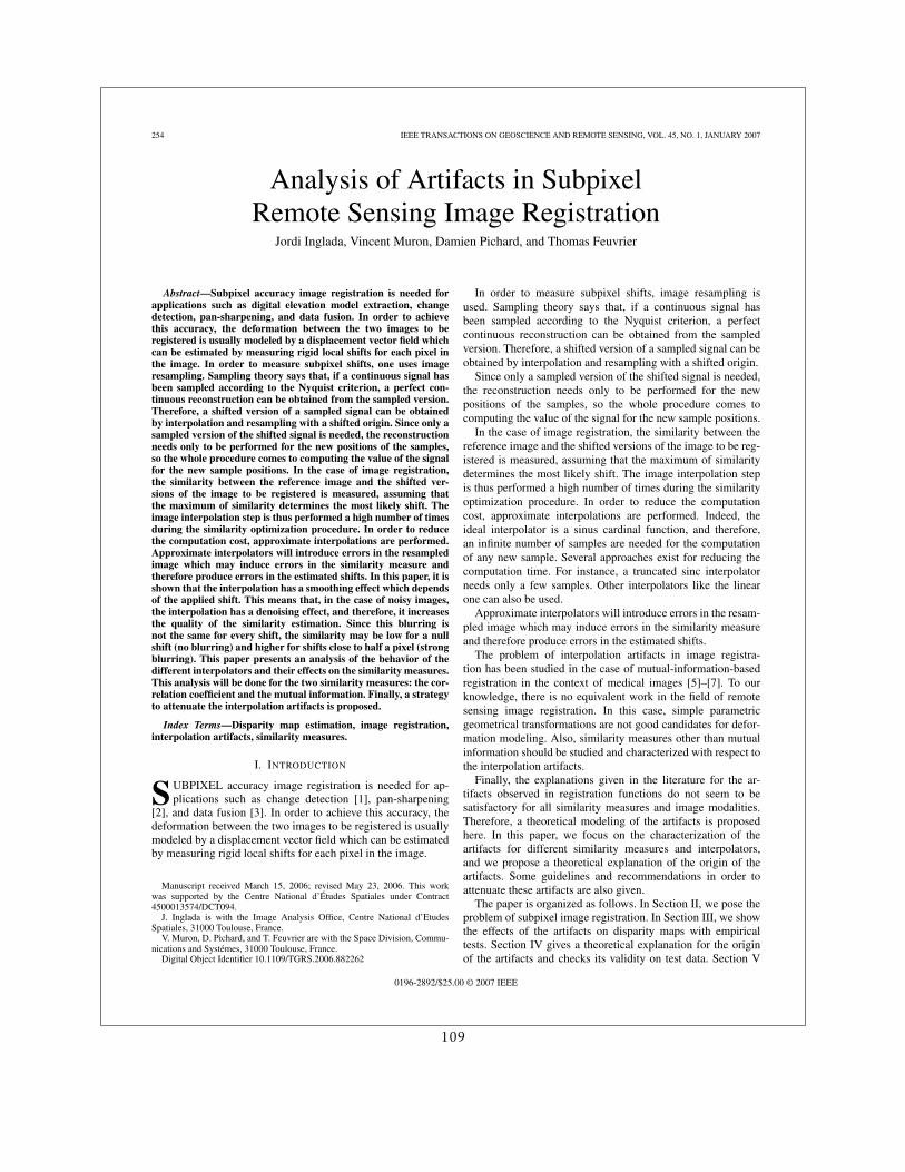
254 IEEE TRANSACTIONS ON GEOSCIENCE AND REMOTE SENSING, VOL. 45, NO. 1, JANUARY 2007
Analysis of Artifacts in SubpixelRemote Sensing Image Registration
Jordi Inglada, Vincent Muron, Damien Pichard, and Thomas Feuvrier
Abstract—Subpixel accuracy image registration is needed forapplications such as digital elevation model extraction, changedetection, pan-sharpening, and data fusion. In order to achievethis accuracy, the deformation between the two images to beregistered is usually modeled by a displacement vector field whichcan be estimated by measuring rigid local shifts for each pixel inthe image. In order to measure subpixel shifts, one uses imageresampling. Sampling theory says that, if a continuous signal hasbeen sampled according to the Nyquist criterion, a perfect con-tinuous reconstruction can be obtained from the sampled version.Therefore, a shifted version of a sampled signal can be obtainedby interpolation and resampling with a shifted origin. Since only asampled version of the shifted signal is needed, the reconstructionneeds only to be performed for the new positions of the samples,so the whole procedure comes to computing the value of the signalfor the new sample positions. In the case of image registration,the similarity between the reference image and the shifted ver-sions of the image to be registered is measured, assuming thatthe maximum of similarity determines the most likely shift. Theimage interpolation step is thus performed a high number of timesduring the similarity optimization procedure. In order to reducethe computation cost, approximate interpolations are performed.Approximate interpolators will introduce errors in the resampledimage which may induce errors in the similarity measure andtherefore produce errors in the estimated shifts. In this paper, it isshown that the interpolation has a smoothing effect which dependsof the applied shift. This means that, in the case of noisy images,the interpolation has a denoising effect, and therefore, it increasesthe quality of the similarity estimation. Since this blurring isnot the same for every shift, the similarity may be low for a nullshift (no blurring) and higher for shifts close to half a pixel (strongblurring). This paper presents an analysis of the behavior of thedifferent interpolators and their effects on the similarity measures.This analysis will be done for the two similarity measures: the cor-relation coefficient and the mutual information. Finally, a strategyto attenuate the interpolation artifacts is proposed.
Index Terms—Disparity map estimation, image registration,interpolation artifacts, similarity measures.
I. INTRODUCTION
SUBPIXEL accuracy image registration is needed for ap-plications such as change detection [1], pan-sharpening
[2], and data fusion [3]. In order to achieve this accuracy, thedeformation between the two images to be registered is usuallymodeled by a displacement vector field which can be estimatedby measuring rigid local shifts for each pixel in the image.
Manuscript received March 15, 2006; revised May 23, 2006. This workwas supported by the Centre National d’Études Spatiales under Contract4500013574/DCT094.
J. Inglada is with the Image Analysis Office, Centre National d’EtudesSpatiales, 31000 Toulouse, France.
V. Muron, D. Pichard, and T. Feuvrier are with the Space Division, Commu-nications and Systémes, 31000 Toulouse, France.
Digital Object Identifier 10.1109/TGRS.2006.882262
In order to measure subpixel shifts, image resampling isused. Sampling theory says that, if a continuous signal hasbeen sampled according to the Nyquist criterion, a perfectcontinuous reconstruction can be obtained from the sampledversion. Therefore, a shifted version of a sampled signal can beobtained by interpolation and resampling with a shifted origin.
Since only a sampled version of the shifted signal is needed,the reconstruction needs only to be performed for the newpositions of the samples, so the whole procedure comes tocomputing the value of the signal for the new sample positions.
In the case of image registration, the similarity between thereference image and the shifted versions of the image to be reg-istered is measured, assuming that the maximum of similaritydetermines the most likely shift. The image interpolation stepis thus performed a high number of times during the similarityoptimization procedure. In order to reduce the computationcost, approximate interpolations are performed. Indeed, theideal interpolator is a sinus cardinal function, and therefore,an infinite number of samples are needed for the computationof any new sample. Several approaches exist for reducing thecomputation time. For instance, a truncated sinc interpolatorneeds only a few samples. Other interpolators like the linearone can also be used.
Approximate interpolators will introduce errors in the resam-pled image which may induce errors in the similarity measureand therefore produce errors in the estimated shifts.
The problem of interpolation artifacts in image registra-tion has been studied in the case of mutual-information-basedregistration in the context of medical images [5]–[7]. To ourknowledge, there is no equivalent work in the field of remotesensing image registration. In this case, simple parametricgeometrical transformations are not good candidates for defor-mation modeling. Also, similarity measures other than mutualinformation should be studied and characterized with respect tothe interpolation artifacts.
Finally, the explanations given in the literature for the ar-tifacts observed in registration functions do not seem to besatisfactory for all similarity measures and image modalities.Therefore, a theoretical modeling of the artifacts is proposedhere. In this paper, we focus on the characterization of theartifacts for different similarity measures and interpolators,and we propose a theoretical explanation of the origin of theartifacts. Some guidelines and recommendations in order toattenuate these artifacts are also given.
The paper is organized as follows. In Section II, we pose theproblem of subpixel image registration. In Section III, we showthe effects of the artifacts on disparity maps with empiricaltests. Section IV gives a theoretical explanation for the originof the artifacts and checks its validity on test data. Section V
0196-2892/$25.00 © 2007 IEEE
109
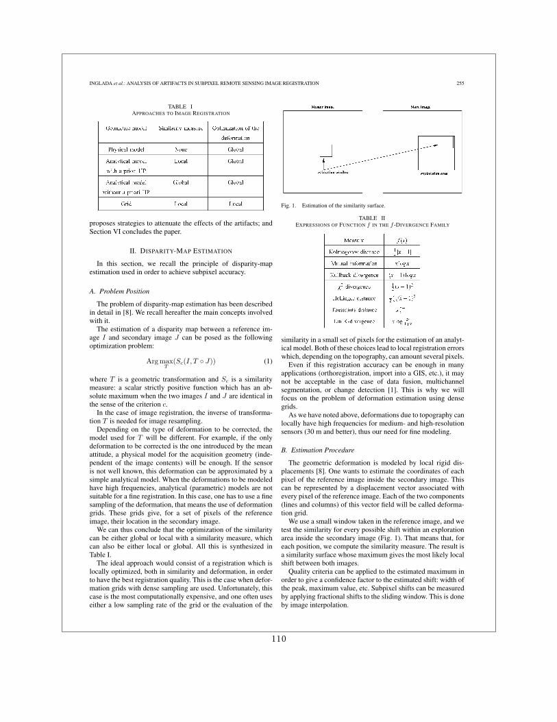
INGLADA et al.: ANALYSIS OF ARTIFACTS IN SUBPIXEL REMOTE SENSING IMAGE REGISTRATION 255
TABLE IAPPROACHES TO IMAGE REGISTRATION
proposes strategies to attenuate the effects of the artifacts; andSection VI concludes the paper.
II. DISPARITY-MAP ESTIMATION
In this section, we recall the principle of disparity-mapestimation used in order to achieve subpixel accuracy.
A. Problem Position
The problem of disparity-map estimation has been describedin detail in [8]. We recall hereafter the main concepts involvedwith it.
The estimation of a disparity map between a reference im-age I and secondary image J can be posed as the followingoptimization problem:
Arg maxT
(Sc(I, T ◦ J)) (1)
where T is a geometric transformation and Sc is a similaritymeasure: a scalar strictly positive function which has an ab-solute maximum when the two images I and J are identical inthe sense of the criterion c.
In the case of image registration, the inverse of transforma-tion T is needed for image resampling.
Depending on the type of deformation to be corrected, themodel used for T will be different. For example, if the onlydeformation to be corrected is the one introduced by the meanattitude, a physical model for the acquisition geometry (inde-pendent of the image contents) will be enough. If the sensoris not well known, this deformation can be approximated by asimple analytical model. When the deformations to be modeledhave high frequencies, analytical (parametric) models are notsuitable for a fine registration. In this case, one has to use a finesampling of the deformation, that means the use of deformationgrids. These grids give, for a set of pixels of the referenceimage, their location in the secondary image.
We can thus conclude that the optimization of the similaritycan be either global or local with a similarity measure, whichcan also be either local or global. All this is synthesized inTable I.
The ideal approach would consist of a registration which islocally optimized, both in similarity and deformation, in orderto have the best registration quality. This is the case when defor-mation grids with dense sampling are used. Unfortunately, thiscase is the most computationally expensive, and one often useseither a low sampling rate of the grid or the evaluation of the
Fig. 1. Estimation of the similarity surface.
TABLE IIEXPRESSIONS OF FUNCTION f IN THE f -DIVERGENCE FAMILY
similarity in a small set of pixels for the estimation of an analyt-ical model. Both of these choices lead to local registration errorswhich, depending on the topography, can amount several pixels.
Even if this registration accuracy can be enough in manyapplications (orthoregistration, import into a GIS, etc.), it maynot be acceptable in the case of data fusion, multichannelsegmentation, or change detection [1]. This is why we willfocus on the problem of deformation estimation using densegrids.
As we have noted above, deformations due to topography canlocally have high frequencies for medium- and high-resolutionsensors (30 m and better), thus our need for fine modeling.
B. Estimation Procedure
The geometric deformation is modeled by local rigid dis-placements [8]. One wants to estimate the coordinates of eachpixel of the reference image inside the secondary image. Thiscan be represented by a displacement vector associated withevery pixel of the reference image. Each of the two components(lines and columns) of this vector field will be called deforma-tion grid.
We use a small window taken in the reference image, and wetest the similarity for every possible shift within an explorationarea inside the secondary image (Fig. 1). That means that, foreach position, we compute the similarity measure. The result isa similarity surface whose maximum gives the most likely localshift between both images.
Quality criteria can be applied to the estimated maximum inorder to give a confidence factor to the estimated shift: width ofthe peak, maximum value, etc. Subpixel shifts can be measuredby applying fractional shifts to the sliding window. This is doneby image interpolation.
110
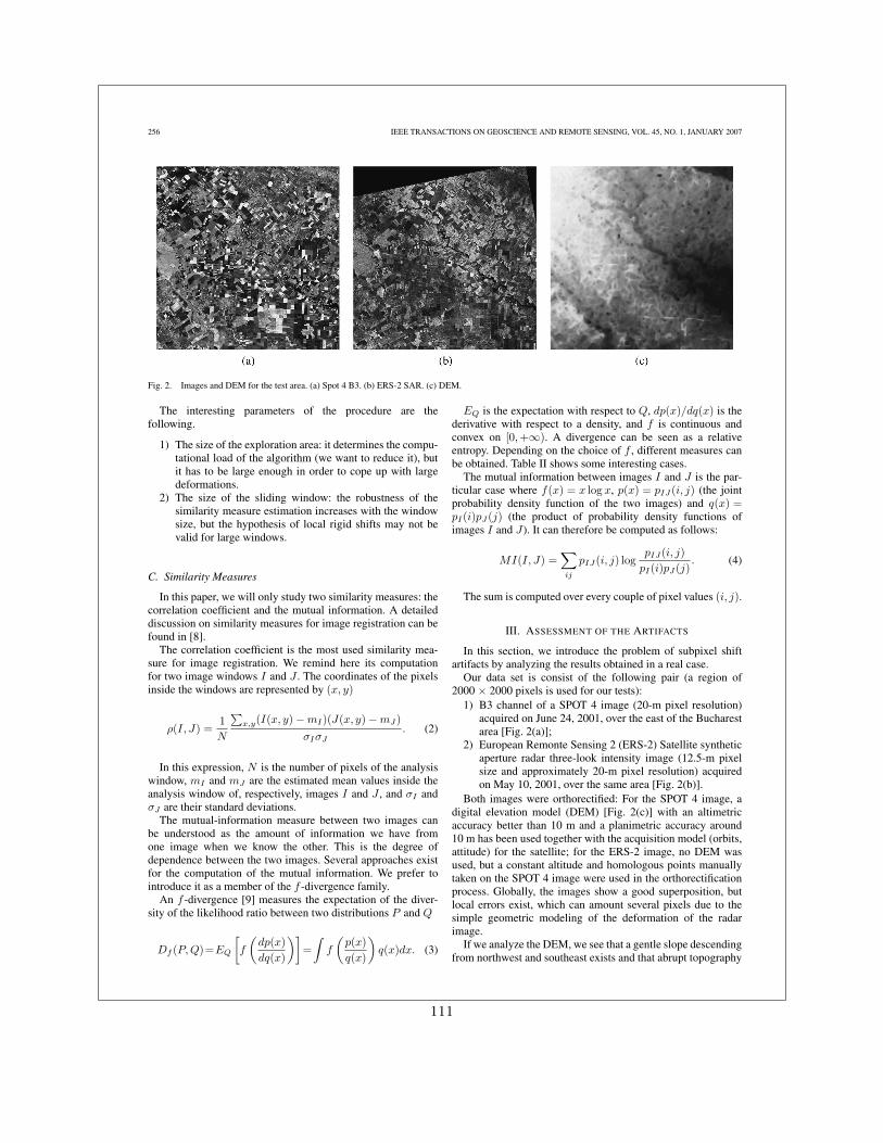
256 IEEE TRANSACTIONS ON GEOSCIENCE AND REMOTE SENSING, VOL. 45, NO. 1, JANUARY 2007
Fig. 2. Images and DEM for the test area. (a) Spot 4 B3. (b) ERS-2 SAR. (c) DEM.
The interesting parameters of the procedure are thefollowing.
1) The size of the exploration area: it determines the compu-tational load of the algorithm (we want to reduce it), butit has to be large enough in order to cope up with largedeformations.
2) The size of the sliding window: the robustness of thesimilarity measure estimation increases with the windowsize, but the hypothesis of local rigid shifts may not bevalid for large windows.
C. Similarity Measures
In this paper, we will only study two similarity measures: thecorrelation coefficient and the mutual information. A detaileddiscussion on similarity measures for image registration can befound in [8].
The correlation coefficient is the most used similarity mea-sure for image registration. We remind here its computationfor two image windows I and J . The coordinates of the pixelsinside the windows are represented by (x, y)
ρ(I, J) =1
N
∑x,y(I(x, y) − mI)(J(x, y) − mJ)
σIσJ. (2)
In this expression, N is the number of pixels of the analysiswindow, mI and mJ are the estimated mean values inside theanalysis window of, respectively, images I and J , and σI andσJ are their standard deviations.
The mutual-information measure between two images canbe understood as the amount of information we have fromone image when we know the other. This is the degree ofdependence between the two images. Several approaches existfor the computation of the mutual information. We prefer tointroduce it as a member of the f -divergence family.
An f -divergence [9] measures the expectation of the diver-sity of the likelihood ratio between two distributions P and Q
Df (P,Q)=EQ
[f
(dp(x)
dq(x)
)]=
∫f
(p(x)
q(x)
)q(x)dx. (3)
EQ is the expectation with respect to Q, dp(x)/dq(x) is thederivative with respect to a density, and f is continuous andconvex on [0,+∞). A divergence can be seen as a relativeentropy. Depending on the choice of f , different measures canbe obtained. Table II shows some interesting cases.
The mutual information between images I and J is the par-ticular case where f(x) = x log x, p(x) = pIJ (i, j) (the jointprobability density function of the two images) and q(x) =pI(i)pJ (j) (the product of probability density functions ofimages I and J). It can therefore be computed as follows:
MI(I, J) =∑
ij
pIJ (i, j) logpIJ(i, j)
pI(i)pJ (j). (4)
The sum is computed over every couple of pixel values (i, j).
III. ASSESSMENT OF THE ARTIFACTS
In this section, we introduce the problem of subpixel shiftartifacts by analyzing the results obtained in a real case.
Our data set is consist of the following pair (a region of2000 × 2000 pixels is used for our tests):
1) B3 channel of a SPOT 4 image (20-m pixel resolution)acquired on June 24, 2001, over the east of the Bucharestarea [Fig. 2(a)];
2) European Remonte Sensing 2 (ERS-2) Satellite syntheticaperture radar three-look intensity image (12.5-m pixelsize and approximately 20-m pixel resolution) acquiredon May 10, 2001, over the same area [Fig. 2(b)].
Both images were orthorectified: For the SPOT 4 image, adigital elevation model (DEM) [Fig. 2(c)] with an altimetricaccuracy better than 10 m and a planimetric accuracy around10 m has been used together with the acquisition model (orbits,attitude) for the satellite; for the ERS-2 image, no DEM wasused, but a constant altitude and homologous points manuallytaken on the SPOT 4 image were used in the orthorectificationprocess. Globally, the images show a good superposition, butlocal errors exist, which can amount several pixels due to thesimple geometric modeling of the deformation of the radarimage.
If we analyze the DEM, we see that a gentle slope descendingfrom northwest and southeast exists and that abrupt topography
111
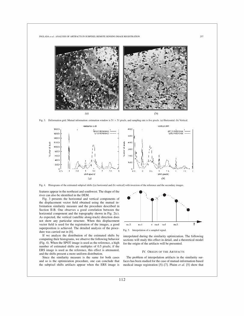
INGLADA et al.: ANALYSIS OF ARTIFACTS IN SUBPIXEL REMOTE SENSING IMAGE REGISTRATION 257
Fig. 3. Deformation grid. Mutual information: estimation window is 51 × 51 pixels, and sampling rate is five pixels. (a) Horizontal. (b) Vertical.
Fig. 4. Histograms of the estimated subpixel shifts [(a) horizontal and (b) vertical] with inversion of the reference and the secondary images.
features appear in the northeast and southwest. The shape of theriver can also be identified in the DEM.
Fig. 3 presents the horizontal and vertical components ofthe displacement vector field obtained using the mutual in-formation similarity measure and the procedure described inSection II-B. One observes a good correlation between thehorizontal component and the topography shown in Fig. 2(c).As expected, the vertical (satellite along-track) direction doesnot show any particular structure. When this displacementvector field is used for the registration of the images, a goodsuperposition is achieved. The detailed analysis of the proce-dure was carried out in [8].
If we analyze the distribution of the estimated shifts bycomputing their histograms, we observe the following behavior(Fig. 4). When the SPOT image is used as the reference, a highnumber of estimated shifts are multiples of 0.5 pixels; if theERS image is used as the reference, this effect is attenuated,and the shifts present a more uniform distribution.
Since the similarity measure is the same for both casesand so is the optimization procedure, one can conclude thatthe subpixel shifts artifacts appear when the ERS image is
Fig. 5. Interpolation of a sampled signal.
interpolated during the similarity optimization. The followingsections will study this effect in detail, and a theoretical modelfor the origin of the artifacts will be presented.
IV. ORIGIN OF THE ARTIFACTS
The problem of interpolation artifacts in the similarity sur-faces has been studied for the case of mutual-information-basedmedical image registration [5]–[7]. Pluim et al. [5] show that
112
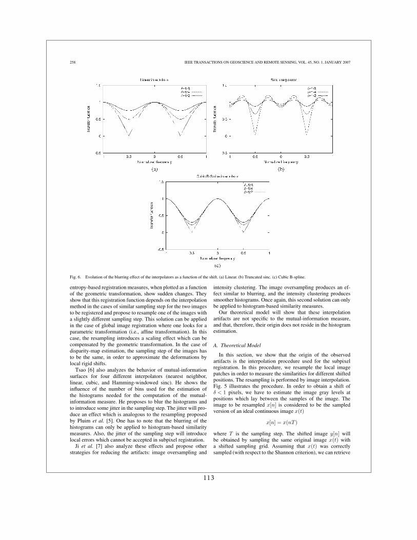
258 IEEE TRANSACTIONS ON GEOSCIENCE AND REMOTE SENSING, VOL. 45, NO. 1, JANUARY 2007
Fig. 6. Evolution of the blurring effect of the interpolators as a function of the shift. (a) Linear. (b) Truncated sinc. (c) Cubic B-spline.
entropy-based registration measures, when plotted as a functionof the geometric transformation, show sudden changes. Theyshow that this registration function depends on the interpolationmethod in the cases of similar sampling step for the two imagesto be registered and propose to resample one of the images witha slightly different sampling step. This solution can be appliedin the case of global image registration where one looks for aparametric transformation (i.e., affine transformation). In thiscase, the resampling introduces a scaling effect which can becompensated by the geometric transformation. In the case ofdisparity-map estimation, the sampling step of the images hasto be the same, in order to approximate the deformations bylocal rigid shifts.
Tsao [6] also analyzes the behavior of mutual-informationsurfaces for four different interpolators (nearest neighbor,linear, cubic, and Hamming-windowed sinc). He shows theinfluence of the number of bins used for the estimation ofthe histograms needed for the computation of the mutual-information measure. He proposes to blur the histograms andto introduce some jitter in the sampling step. The jitter will pro-duce an effect which is analogous to the resampling proposedby Pluim et al. [5]. One has to note that the blurring of thehistograms can only be applied to histogram-based similaritymeasures. Also, the jitter of the sampling step will introducelocal errors which cannot be accepted in subpixel registration.
Ji et al. [7] also analyze these effects and propose otherstrategies for reducing the artifacts: image oversampling and
intensity clustering. The image oversampling produces an ef-fect similar to blurring, and the intensity clustering producessmoother histograms. Once again, this second solution can onlybe applied to histogram-based similarity measures.
Our theoretical model will show that these interpolationartifacts are not specific to the mutual-information measure,and that, therefore, their origin does not reside in the histogramestimation.
A. Theoretical Model
In this section, we show that the origin of the observedartifacts is the interpolation procedure used for the subpixelregistration. In this procedure, we resample the local imagepatches in order to measure the similarities for different shiftedpositions. The resampling is performed by image interpolation.Fig. 5 illustrates the procedure. In order to obtain a shift ofδ < 1 pixels, we have to estimate the image gray levels atpositions which lay between the samples of the image. Theimage to be resampled x[n] is considered to be the sampledversion of an ideal continuous image x(t)
x[n] = x(nT )
where T is the sampling step. The shifted image y[n] willbe obtained by sampling the same original image x(t) witha shifted sampling grid. Assuming that x(t) was correctlysampled (with respect to the Shannon criterion), we can retrieve
113
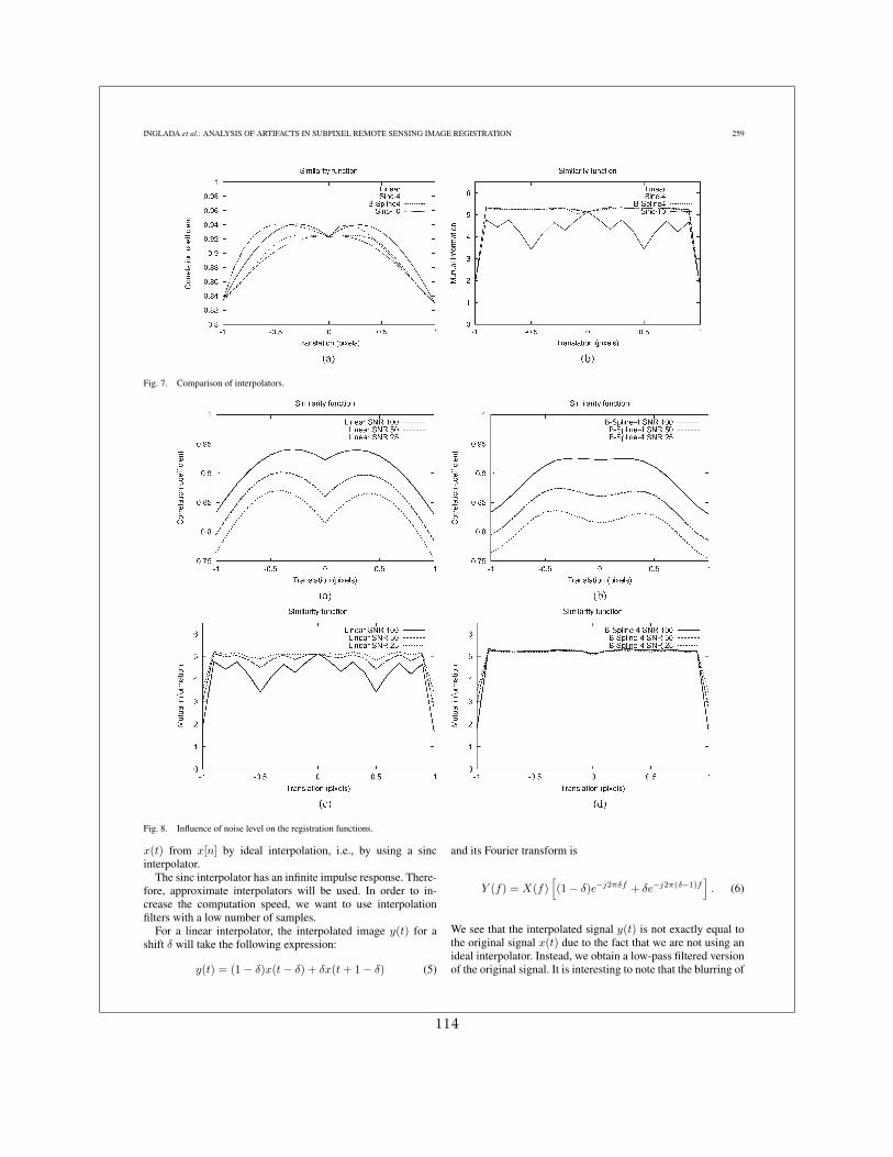
INGLADA et al.: ANALYSIS OF ARTIFACTS IN SUBPIXEL REMOTE SENSING IMAGE REGISTRATION 259
Fig. 7. Comparison of interpolators.
Fig. 8. Influence of noise level on the registration functions.
x(t) from x[n] by ideal interpolation, i.e., by using a sincinterpolator.
The sinc interpolator has an infinite impulse response. There-fore, approximate interpolators will be used. In order to in-crease the computation speed, we want to use interpolationfilters with a low number of samples.
For a linear interpolator, the interpolated image y(t) for ashift δ will take the following expression:
y(t) = (1 − δ)x(t − δ) + δx(t + 1 − δ) (5)
and its Fourier transform is
Y (f) = X(f)[(1 − δ)e−j2πδf + δe−j2π(δ−1)f
]. (6)
We see that the interpolated signal y(t) is not exactly equal tothe original signal x(t) due to the fact that we are not using anideal interpolator. Instead, we obtain a low-pass filtered versionof the original signal. It is interesting to note that the blurring of
114
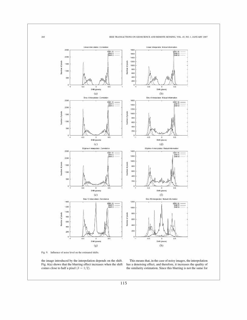
260 IEEE TRANSACTIONS ON GEOSCIENCE AND REMOTE SENSING, VOL. 45, NO. 1, JANUARY 2007
Fig. 9. Influence of noise level on the estimated shifts.
the image introduced by the interpolation depends on the shift.Fig. 6(a) shows that the blurring effect increases when the shiftcomes close to half a pixel (δ = 1/2).
This means that, in the case of noisy images, the interpolationhas a denoising effect, and therefore, it increases the quality ofthe similarity estimation. Since this blurring is not the same for
115
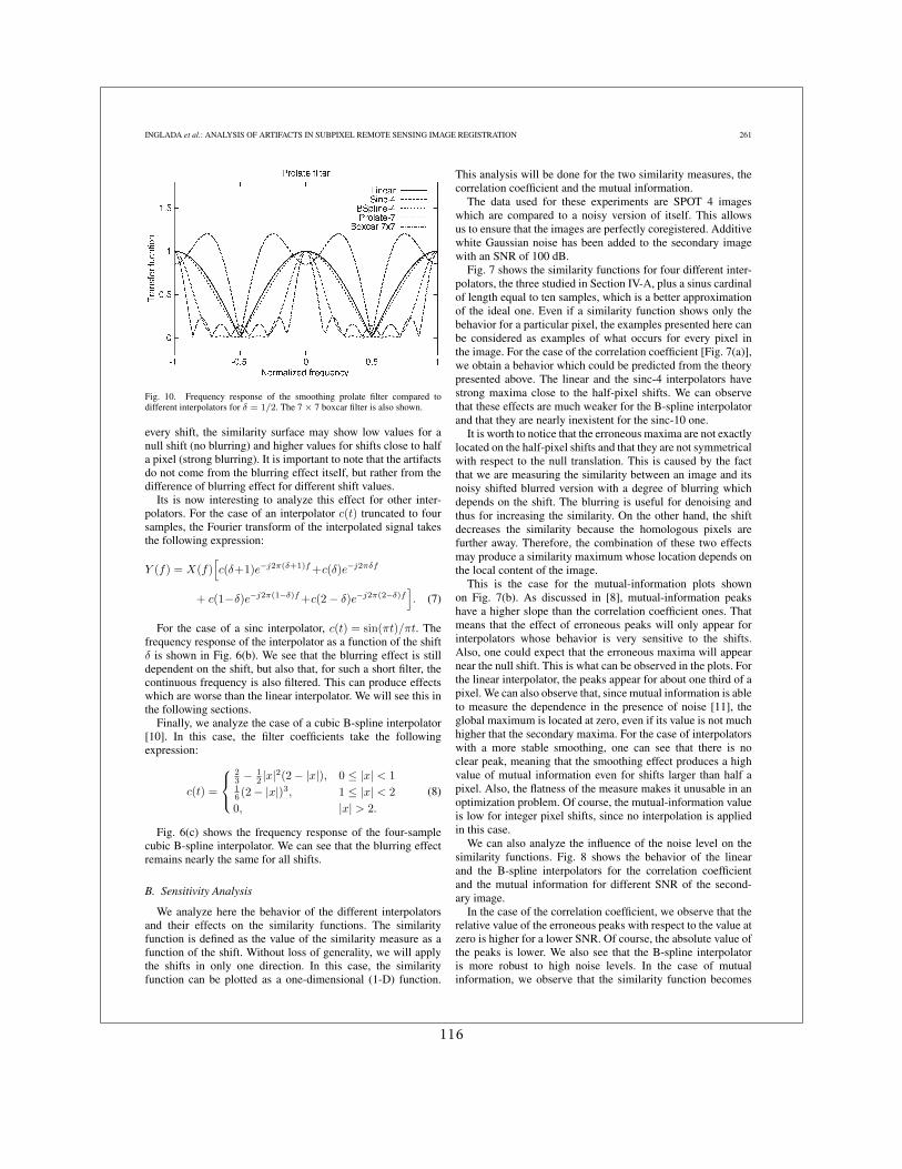
INGLADA et al.: ANALYSIS OF ARTIFACTS IN SUBPIXEL REMOTE SENSING IMAGE REGISTRATION 261
Fig. 10. Frequency response of the smoothing prolate filter compared todifferent interpolators for δ = 1/2. The 7 × 7 boxcar filter is also shown.
every shift, the similarity surface may show low values for anull shift (no blurring) and higher values for shifts close to halfa pixel (strong blurring). It is important to note that the artifactsdo not come from the blurring effect itself, but rather from thedifference of blurring effect for different shift values.
Its is now interesting to analyze this effect for other inter-polators. For the case of an interpolator c(t) truncated to foursamples, the Fourier transform of the interpolated signal takesthe following expression:
Y (f) = X(f)[c(δ+1)e−j2π(δ+1)f +c(δ)e−j2πδf
+ c(1−δ)e−j2π(1−δ)f +c(2 − δ)e−j2π(2−δ)f]. (7)
For the case of a sinc interpolator, c(t) = sin(πt)/πt. Thefrequency response of the interpolator as a function of the shiftδ is shown in Fig. 6(b). We see that the blurring effect is stilldependent on the shift, but also that, for such a short filter, thecontinuous frequency is also filtered. This can produce effectswhich are worse than the linear interpolator. We will see this inthe following sections.
Finally, we analyze the case of a cubic B-spline interpolator[10]. In this case, the filter coefficients take the followingexpression:
c(t) =
23 − 1
2 |x|2(2 − |x|), 0 ≤ |x| < 116 (2 − |x|)3, 1 ≤ |x| < 2
0, |x| > 2.
(8)
Fig. 6(c) shows the frequency response of the four-samplecubic B-spline interpolator. We can see that the blurring effectremains nearly the same for all shifts.
B. Sensitivity Analysis
We analyze here the behavior of the different interpolatorsand their effects on the similarity functions. The similarityfunction is defined as the value of the similarity measure as afunction of the shift. Without loss of generality, we will applythe shifts in only one direction. In this case, the similarityfunction can be plotted as a one-dimensional (1-D) function.
This analysis will be done for the two similarity measures, thecorrelation coefficient and the mutual information.
The data used for these experiments are SPOT 4 imageswhich are compared to a noisy version of itself. This allowsus to ensure that the images are perfectly coregistered. Additivewhite Gaussian noise has been added to the secondary imagewith an SNR of 100 dB.
Fig. 7 shows the similarity functions for four different inter-polators, the three studied in Section IV-A, plus a sinus cardinalof length equal to ten samples, which is a better approximationof the ideal one. Even if a similarity function shows only thebehavior for a particular pixel, the examples presented here canbe considered as examples of what occurs for every pixel inthe image. For the case of the correlation coefficient [Fig. 7(a)],we obtain a behavior which could be predicted from the theorypresented above. The linear and the sinc-4 interpolators havestrong maxima close to the half-pixel shifts. We can observethat these effects are much weaker for the B-spline interpolatorand that they are nearly inexistent for the sinc-10 one.
It is worth to notice that the erroneous maxima are not exactlylocated on the half-pixel shifts and that they are not symmetricalwith respect to the null translation. This is caused by the factthat we are measuring the similarity between an image and itsnoisy shifted blurred version with a degree of blurring whichdepends on the shift. The blurring is useful for denoising andthus for increasing the similarity. On the other hand, the shiftdecreases the similarity because the homologous pixels arefurther away. Therefore, the combination of these two effectsmay produce a similarity maximum whose location depends onthe local content of the image.
This is the case for the mutual-information plots shownon Fig. 7(b). As discussed in [8], mutual-information peakshave a higher slope than the correlation coefficient ones. Thatmeans that the effect of erroneous peaks will only appear forinterpolators whose behavior is very sensitive to the shifts.Also, one could expect that the erroneous maxima will appearnear the null shift. This is what can be observed in the plots. Forthe linear interpolator, the peaks appear for about one third of apixel. We can also observe that, since mutual information is ableto measure the dependence in the presence of noise [11], theglobal maximum is located at zero, even if its value is not muchhigher that the secondary maxima. For the case of interpolatorswith a more stable smoothing, one can see that there is noclear peak, meaning that the smoothing effect produces a highvalue of mutual information even for shifts larger than half apixel. Also, the flatness of the measure makes it unusable in anoptimization problem. Of course, the mutual-information valueis low for integer pixel shifts, since no interpolation is appliedin this case.
We can also analyze the influence of the noise level on thesimilarity functions. Fig. 8 shows the behavior of the linearand the B-spline interpolators for the correlation coefficientand the mutual information for different SNR of the second-ary image.
In the case of the correlation coefficient, we observe that therelative value of the erroneous peaks with respect to the value atzero is higher for a lower SNR. Of course, the absolute value ofthe peaks is lower. We also see that the B-spline interpolatoris more robust to high noise levels. In the case of mutualinformation, we observe that the similarity function becomes
116
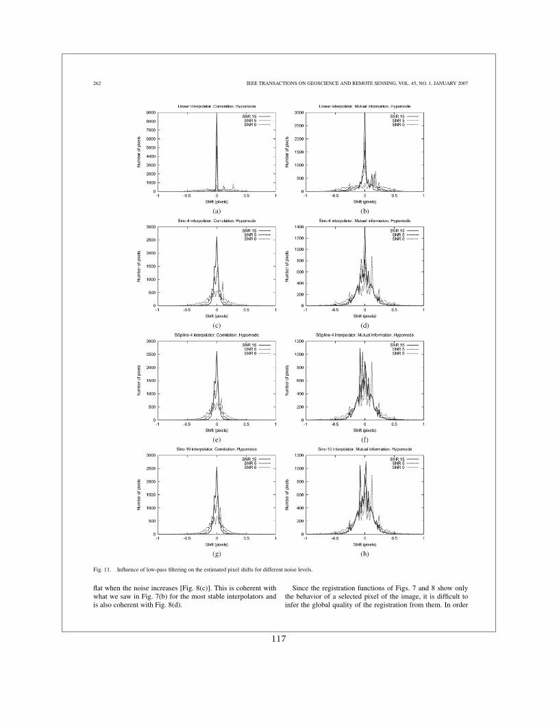
262 IEEE TRANSACTIONS ON GEOSCIENCE AND REMOTE SENSING, VOL. 45, NO. 1, JANUARY 2007
Fig. 11. Influence of low-pass filtering on the estimated pixel shifts for different noise levels.
flat when the noise increases [Fig. 8(c)]. This is coherent withwhat we saw in Fig. 7(b) for the most stable interpolators andis also coherent with Fig. 8(d).
Since the registration functions of Figs. 7 and 8 show onlythe behavior of a selected pixel of the image, it is difficult toinfer the global quality of the registration from them. In order
117
INGLADA et al.: ANALYSIS OF ARTIFACTS IN SUBPIXEL REMOTE SENSING IMAGE REGISTRATION 263
to study the global quality, we will analyze the histograms ofthe estimated shifts. We will study the different combinationsof interpolators (linear, sinc-4, cubic B-spline, and sinc-10),similarity measures (correlation coefficient and mutual infor-mation), and noise level. The results are shown in Fig. 9.
As for the previous simulations, 1-D shifts have been applied.In terms of noise influence, one observes that, the higher theSNR, the lower the number of shifts at a multiple of 0.5 pixels.We also observe that, when the SNR increases, the peaks moveclose to the null shift.
If we compare the interpolators for a given SNR, say15 dB, we see that the better the interpolator (linear is worst,then sinc-4, B-spline, and sinc-10 is the best), the higher thenumber of pixels for which the estimated shift is close to zero,which is the expected value. This is true for both similaritymeasures.
V. ATTENUATION OF THE ARTIFACTS
As it has been stated above, we are interested in usingshort interpolating filters, since the interpolation is performeda high number of times during the similarity optimizationprocedure. As we have shown above, the interpolation artifactsare produced by the blurring effects of the interpolators. Moreprecisely, the origin of the artifacts is not the blurring effectitself but rather the difference of blurring intensity as a functionof the applied shift. We have shown, for instance, that, even ifthe B-spline interpolator has a stronger blurring effect than thelinear interpolator, since its blurring remains nearly constantfor all shifts, it has better performances for the disparity-mapestimation.
The strategy proposed here for reducing the interpolationartifacts is a very simple one. Since the interpolator is going tointroduce a blurring effect, we can smooth the secondary imagewith a filter whose transfer function is identical (in modulus)to the maximum blurring effect of the interpolator. This can bedone in a preprocessing step.
However, when observing Fig. 6, we see that the evolutionof the blurring effect may not be only related to the highestfrequencies of the signal, and therefore, selecting the transferfunction of the preprocessing filter could be tricky.
For instance, choosing a simple boxcar filter for preprocess-ing can produce artifacts introduced by the secondary lobes ofthe filter. These lobes come from the windowing used for thetruncation of the filter’s impulse response.
In order to study the improvement of the subpixel shiftestimation for the different interpolators, we choose to use thesame smoothing filter for all of them. In order to reduce thesecondary lobes of the smoothing filter and to assure a shortimpulse response, we propose to use a prolate function [12],[13]. The prolate filter is one class of the nonrecursive finiteimpulse response filters. It is superior to other filters in this classin that it has a maximum energy concentration in the frequencypassband and minimum ringing in the time domain.
A prolate filter with seven samples is shown in Fig. 10 and iscompared to the maximum smoothing for several interpolators.The frequency response of the 7 × 7 boxcar filter, with itssecondary lobes, is also shown.
Fig. 11 shows the same kind of analysis as Fig. 9, but with theuse of the prolate filter as a preprocessing step for the secondary
image. The first remark we can make is that the peaks at multi-ples of 0.5 pixels have vanished for both similarity measuresand for all interpolators. The behavior of the correlation isalways better than that of the mutual information.
We also see that, for the high SNR values, the best resultsare obtained for the linear interpolator. However, for low SNRvalues, the better the interpolator, the better are the estimatedshifts. We can also see that, for the mutual-information case,good results are only obtained with the linear and the sinc-4interpolators, and for the highest SNR value.
VI. CONCLUSION
This paper has presented the problem of interpolation-induced artifacts in the procedure of disparity-map estimationused for subpixel image registration. The problem has beenintroduced with a real case, where the presence of wronglyestimated shifts when a radar image is interpolated have beenshown.
A theoretical explanation of the origin of the artifacts hasbeen given, and it demonstrated that the blurring effect ofthe interpolator, which is dependent on the applied shift, isresponsible for the errors observed in the registration functions.
Several interpolators have been compared under differentSNR conditions. Finally, it has been shown that a preprocessingstep which smoothes the secondary interpolated image cansolve the problem. However, attention has to be paid to thechoice of the smoothing filter. Indeed, simple filters, as theboxcar one, have to be avoided since they present secondarylobes for the frequencies where the interpolation artifacts occur.
Even if the solution presented here allows for an improve-ment of the estimation of subpixel-accuracy disparity maps,more work has to be done in order to:
1) analyze the effects of the interpolation for other imagemodalities, as infrared data, for example;
2) study the influence of image resolution and type of land-scape in the quality of the estimated shifts;
3) propose edge-preserving smoothing filters which, com-bined with different interpolators, could help to attenuatethe interpolation artifacts at the same time that theypreserve high-frequency content which can be useful fora precise disparity estimation.
REFERENCES
[1] J. Townshend, C. Justice, C. Gurney, and J. McManus, “The impact ofmisregistration on change detection,” IEEE Trans. Geosci. Remote Sens.,vol. 30, no. 5, pp. 1054–1060, Sep. 1992.
[2] G. Cliche, F. Bonn, and P. Teillet, “Integration of the SPOT Pan channelinto its spectral mode for image sharpness enhancement,” Photogramm.Eng. Remote Sens., vol. 51, pp. 311–316, Mar. 1985.
[3] P. Chavez, S. Sides, and J. Anderson, “Comparison of three differentmethods to merge multiresolution and multispectral data: TM & SPOTpan,” Photogramm. Eng. Remote Sens., vol. 57, no. 3, pp. 295–303, 1991.
[4] T. Toutin, “Multi-source data fusion with an integrated and unified geo-metric modeling,” EARSeL Adv. Remote Sens., vol. 4, no. 2, pp. 118–129,1995.
[5] J. P. W. Pluim, J. B. A. Maintz, and M. A. Viergever, “Interpolationartefacts in mutual information-based image registration,” Comput. Vis.Image Underst., vol. 77, no. 2, pp. 211–232, Feb. 2000.
[6] J. Tsao, “Interpolation artifacts in multimodality image registration basedon maximization of mutual information,” IEEE Trans. Med. Imag.,vol. 22, no. 7, pp. 854–864, Jul. 2003.
[7] J. X. Ji, H. Pan, and Z.-P. Lang, “Further analysis of interpolation effectsin mutual information-based image registration,” IEEE Trans. Med. Imag.,vol. 22, no. 9, pp. 1119–1131, Sep. 2003.
118
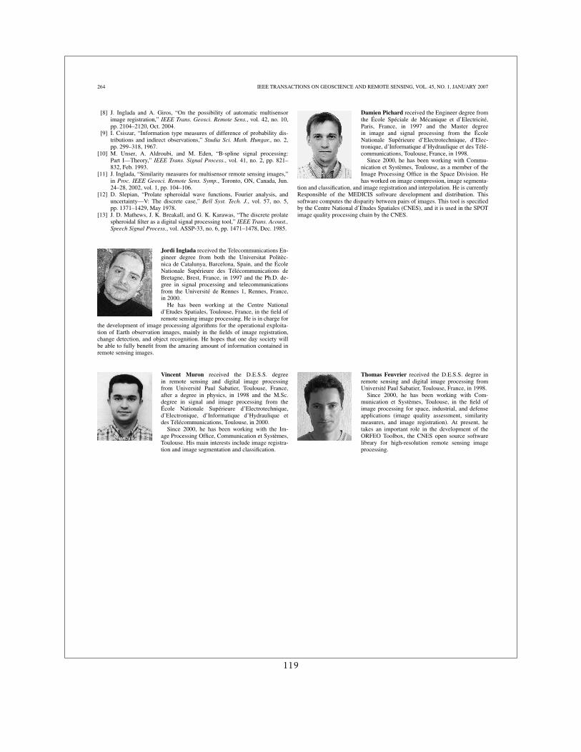
264 IEEE TRANSACTIONS ON GEOSCIENCE AND REMOTE SENSING, VOL. 45, NO. 1, JANUARY 2007
[8] J. Inglada and A. Giros, “On the possibility of automatic multisensorimage registration,” IEEE Trans. Geosci. Remote Sens., vol. 42, no. 10,pp. 2104–2120, Oct. 2004.
[9] I. Csiszar, “Information type measures of difference of probability dis-tributions and indirect observations,” Studia Sci. Math. Hungar., no. 2,pp. 299–318, 1967.
[10] M. Unser, A. Aldroubi, and M. Eden, “B-spline signal processing:Part I—Theory,” IEEE Trans. Signal Process., vol. 41, no. 2, pp. 821–832, Feb. 1993.
[11] J. Inglada, “Similarity measures for multisensor remote sensing images,”in Proc. IEEE Geosci. Remote Sens. Symp., Toronto, ON, Canada, Jun.24–28, 2002, vol. 1, pp. 104–106.
[12] D. Slepian, “Prolate spheroidal wave functions, Fourier analysis, anduncertainty—V: The discrete case,” Bell Syst. Tech. J., vol. 57, no. 5,pp. 1371–1429, May 1978.
[13] J. D. Mathews, J. K. Breakall, and G. K. Karawas, “The discrete prolatespheroidal filter as a digital signal processing tool,” IEEE Trans. Acoust.,Speech Signal Process., vol. ASSP-33, no. 6, pp. 1471–1478, Dec. 1985.
Jordi Inglada received the Telecommunications En-gineer degree from both the Universitat Politèc-nica de Catalunya, Barcelona, Spain, and the ÉcoleNationale Supérieure des Télécommunications deBretagne, Brest, France, in 1997 and the Ph.D. de-gree in signal processing and telecommunicationsfrom the Université de Rennes 1, Rennes, France,in 2000.
He has been working at the Centre Nationald’Etudes Spatiales, Toulouse, France, in the field ofremote sensing image processing. He is in charge for
the development of image processing algorithms for the operational exploita-tion of Earth observation images, mainly in the fields of image registration,change detection, and object recognition. He hopes that one day society willbe able to fully benefit from the amazing amount of information contained inremote sensing images.
Vincent Muron received the D.E.S.S. degreein remote sensing and digital image processingfrom Université Paul Sabatier, Toulouse, France,after a degree in physics, in 1998 and the M.Sc.degree in signal and image processing from theÉcole Nationale Supérieure d’Electrotechnique,d’Electronique, d’Informatique d’Hydraulique etdes Télécommunications, Toulouse, in 2000.
Since 2000, he has been working with the Im-age Processing Office, Communication et Systèmes,Toulouse. His main interests include image registra-tion and image segmentation and classification.
Damien Pichard received the Engineer degree fromthe École Spéciale de Mécanique et d’Electricité,Paris, France, in 1997 and the Master degreein image and signal processing from the ÉcoleNationale Supérieure d’Electrotechnique, d’Elec-tronique, d’Informatique d’Hydraulique et des Télé-communications, Toulouse, France, in 1998.
Since 2000, he has been working with Commu-nication et Systèmes, Toulouse, as a member of theImage Processing Office in the Space Division. Hehas worked on image compression, image segmenta-
tion and classification, and image registration and interpolation. He is currentlyResponsible of the MEDICIS software development and distribution. Thissoftware computes the disparity between pairs of images. This tool is specifiedby the Centre National d’Etudes Spatiales (CNES), and it is used in the SPOTimage quality processing chain by the CNES.
Thomas Feuvrier received the D.E.S.S. degree inremote sensing and digital image processing fromUniversité Paul Sabatier, Toulouse, France, in 1998.
Since 2000, he has been working with Com-munication et Systèmes, Toulouse, in the field ofimage processing for space, industrial, and defenseapplications (image quality assessment, similaritymeasures, and image registration). At present, hetakes an important role in the development of theORFEO Toolbox, the CNES open source softwarelibrary for high-resolution remote sensing imageprocessing.
119


14 Détection de changements
121
1796 IEEE TRANSACTIONS ON IMAGE PROCESSING, VOL. 16, NO. 7, JULY 2007
Bivariate Gamma Distributions for ImageRegistration and Change Detection
Florent Chatelain, Jean-Yves Tourneret, Member, IEEE, Jordi Inglada, and André Ferrari
Abstract—This paper evaluates the potential interest of usingbivariate gamma distributions for image registration and changedetection. The first part of this paper studies estimators for theparameters of bivariate gamma distributions based on the max-imum likelihood principle and the method of moments. The per-formance of both methods are compared in terms of estimatedmean square errors and theoretical asymptotic variances. The mu-tual information is a classical similarity measure which can be usedfor image registration or change detection. The second part of thepaper studies some properties of the mutual information for bi-variate Gamma distributions. Image registration and change de-tection techniques based on bivariate gamma distributions are fi-nally investigated. Simulation results conducted on synthetic andreal data are very encouraging. Bivariate gamma distributions aregood candidates allowing us to develop new image registration al-gorithms and new change detectors.
Index Terms—Correlation coefficient, image change detection,image registration, maximum likelihood, multivariate gamma dis-tributions, mutual information.
I. INTRODUCTION
THE univariate gamma distribution is uniquely defined inmany statistical textbooks. However, extensions defining
multivariate gamma distributions (MGDs) are more controver-sial. For instance, a full chapter of [1] is devoted to this problem(see also references therein). Most journal authors assume that avector is distributed according to an MGD ifthe marginal distributions of are univariate gamma distribu-tions. However, the family of distributions satisfying this con-dition is very large. In order to reduce the size of the family ofMGDs, S. Bar Lev, and P. Bernardoff recently defined MGDs bythe form of their moment generating function or Laplace trans-forms [2], [3]. The main contribution of this paper is to eval-uate these distributions as candidates for image registration andchange detection.
Given two remote sensing images of the same scene , thereference, and , the secondary image, the registration problemcan be defined as follows: determine a geometric transformation
Manuscript received March 30, 2006; revised February 4, 2007. This workwas supported in part by CNES under contract 2005/2561 and in part by theCNRS under MathSTIC Action 80/0244. The associate editor coordinating thereview of this manuscript and approving it for publication was Dr. JacquesBlanc-Talon.
F. Chatelain and J.-Y. Tourneret are with IRIT/ENSEEIHT/TéSA,31071 Toulouse cedex 7, France (e-mail: [email protected];[email protected]).
J. Inglada is with CNES, 31401 Toulouse cedex 9, France (e-mail: [email protected]).
A. Ferrari is with LUAN, Université de Nice-Sophia-Antipolis, 06108 Nicecedex 2, France (e-mail: [email protected]).
Digital Object Identifier 10.1109/TIP.2007.896651
which maximizes the correlation coefficient between imageand the result of the transformation . A fine modeling of
the geometric deformation is required for the estimation of thecoordinates of every pixel of the reference image inside the sec-ondary image. The geometric deformation is modeled by localrigid displacements [4]. The key element of the image regis-tration problem is the estimation of the correlation coefficientbetween the images. This is usually done with an estimationwindow in the neighborhood of each pixel. In order to estimatethe local rigid displacements with a good geometric resolution,one needs the smallest estimation window. However, this leadsto estimations which may not be robust enough. In order to per-form high-quality estimations with a small number of samples,we propose to introduce a priori knowledge about the image sta-tistics. In the case of power radar images, it is well known thatthe marginal distributions of pixels are gamma distributions [5].Therefore, MGDs seem good candidates for the robust estima-tion of the correlation coefficient between radar images.
The change detection problem can be defined as follows.Consider two co-registered synthetic aperture radar (SAR)intensity images and acquired at two different dates and
. Our objective is to produce a map representing the changesoccurred in the scene between time and time . The finalgoal of a change detection analysis is to produce a binary mapcorresponding to the two classes: change and no change. Theproblem can be decomposed into two steps: 1) generation ofa change image and 2) thresholding of the change image inorder to produce the binary change map. The overall detectionperformance will depend on both, the quality of the changeimage and the quality of the thresholding. In this work, wechoose to concentrate on the first step of the procedure, that is,the generation of an indicator of change for each pixel in theimage. The change indicator can be obtained by computing thelocal correlation between both images, for each pixel position.For interesting approaches in the field of unsupervised changeimage thresholding, the reader can refer to the works of Bruz-zone and Fernández Prieto [6], [7], Bruzzone and Serpico [8],and Bazi et al. [9]. The change indicator can also be usefulby itself. Indeed, the end user of a change map often wants,not only the binary information given after thresholding, butalso an indicator of the change amplitude. In order to evaluatethe quality of a change image independently of the choice ofthe thresholding algorithm, one can study the evolution of theprobability of detection as a function of the probability of falsealarm, when a sequence of constant thresholds is used for thewhole image. As in the image registration problem, a smallestimation window is required in order to obtain a high-resolu-tion detector, that is, a detector being able to identify changes
1057-7149/$25.00 © 2007 IEEE
122
CHATELAIN et al.: BIVARIATE GAMMA DISTRIBUTIONS FOR IMAGE REGISTRATION 1797
with a small spatial extent. Again, the introduction of a prioriknowledge through MGDs may improve the estimation accu-racy when a small number of samples is used.
This paper is organized as follows. Section II recalls someimportant results on MGDs. Section III studies estimators of theunknown parameters of a bivariate gamma distribution (BGD).These estimators are based on the classical maximum likelihoodmethod and method of moments. Section IV studies interestingproperties of the mutual information for BGDs. The applicationto image registration and change detection is discussed in Sec-tion V. Conclusions are finally reported in Section VI.
II. MULTIVARIATE GAMMA DISTRIBUTIONS
A. Definitions
A polynomial with respect to is affineif the one variable polynomial can be written
(for any ), where and are polynomialswith respect to the s with . A random vector
is distributed according to an MGD on withshape parameter and scale parameter (denoted as
) if its moment generating function (also called Laplacetransform) is defined as follows [3]:
(1)
where and is an affine polynomial. It is important tonote the following points.
• The affine polynomial has to satisfy appropriate condi-tions including . In the general case, determiningnecessary and sufficient conditions on the pair suchthat exist is a difficult problem. The reader is in-vited to look at [3] for more details.
• By setting for in (1), we obtain the Laplacetransform of , which is clearly a gamma distribution withshape parameter and scale parameter , where is thecoefficient of in .
A BGD corresponds to the particular case and is de-fined by its moment generating function
(2)
with the following conditions:
(3)
In the bidimensional case, (3) are necessary and sufficient con-ditions for (2) to be the moment generating function of a proba-bility distribution defined on . Note again that (2) impliesthat the marginal distributions of and are “gamma distri-butions” (denoted as and ) withthe following densities:
where is the indicator function defined on( if , else), for .Here, is the usual gamma function defined in [10, p. 255].
B. Bivariate Gamma pdf
Obtaining tractable expressions for the probability densityfunction (pdf) of a MGD defined by (1) is a challengingproblem. However, in the bivariate case, the problem is muchsimpler. Straightforward computations allow to obtain thefollowing density (see [1, p. 436] for a similar result)
where and is defined as follows:
(4)
Note that is related to the confluent hypergeometric func-tion (see [1, p. 462]).
C. BGD Moments
The Taylor series expansion of the Laplace transform canbe written
(5)
The moments of a BGD can be obtained by differentiating (5).For instance, the mean and variance of (denoted and
respectively) can be expressed as follows:
(6)
for 1, 2. Similarly, the covariance and correla-tion coefficient of a BGD can be easily computed
(7)
(8)
It is important to note that for a known value of , a BGD isfully characterized by which willbe denoted in the remaining of the paper. In-deed, and are obviously related by a one-to-onetransformation. Note also that the conditions (3) ensure that thecovariance and correlation coefficient of the couple areboth positive.
More computations allow to obtain a general formula for themoments , for , of a BGD
(9)where is the Pochhammer symbol defined by and
123
1798 IEEE TRANSACTIONS ON IMAGE PROCESSING, VOL. 16, NO. 7, JULY 2007
for any integer (see [10, p. 256]). The mutual information ofa BGD is related to the moments of and for1, 2. Straightforward computations detailed in Appendices I andII yield the following results:
(10)
(11)
where is the digamma function and isthe Gauss’s hypergeometric function (see [10, pp. 555–566]).
III. PARAMETER ESTIMATION
This section addresses the problem of estimating theunknown parameter vector from independent vectors
, where is distributed ac-cording to a BGD with parameter vector . Note that theparameter is assumed to be known here, as in most practicalapplications. However, this assumption could be relaxed.
A. Maximum Likelihood Method
1) Principles: The maximum likelihood (ML) method canbe applied in the bivariate case since a closed-formexpression of the density is available.1 In this particular case,after removing the terms which do not depend on , the log-likelihood function can be written as follows:
(12)
where , andis the sample mean of for , 2. By differentiating thelog-likelihood with respect to , and , and by noting that
, the following set of equations is obtained:
(13)
(14)
where
(15)
The maximum likelihood estimators (MLEs) of and arethen easily obtained from these equations
(16)
1The problem is much more complicated in the general case where d > 2
since there is no tractable expression for the MGD density. In this case, thecoefficients of P can be estimated by maximizing an appropriate compositelikelihood criterion such as the pairwise log-likelihood. The reader is invited toconsult [11] for more details.
After replacing and by their MLEs in (14), we can easilyshow that the MLE of is obtained by computing the root
of the following function:
(17)
where
This is achieved by using a Newton–Raphson procedure initial-ized by the standard correlation coefficient estimator [definedin (25)]. The convergence of the Newton–Raphson procedure isgenerally obtained after few iterations.
2) Performance: The asymptotic properties of the MLestimators and can be easily derived from themoments of the univariate gamma distributions and
. These estimators are obviously unbiased, convergentand efficient. However, the performance of is more difficultto study. Of course, the MLE is known to be asymptoticallyunbiased and asymptotically efficient, under mild regularityconditions. Thus, the mean square error (MSE) of the estimatescan be approximated for large data records by the Cramér–Raolower bound (CRLB). For unbiased estimators, the CRLBs ofthe unknown parameters , and can be computed byinverting the Fisher information matrix, whose elements aredefined by
(18)
where . However this com-putation is difficult because of the term appearing in thelog-likelihood. In such situation, it is very usual to approximatethe expectations by using Monte Carlo methods. More specif-ically, this approach consists of approximating the elements ofthe Fisher information matrix as follows:
(19)
where is distributed according to the BGD of densityand is the number of Monte Carlo runs.
B. Method of Moments
1) Principles: This section briefly recalls the principle of themethod of moments. Consider a function andthe statistic of size defined as
(20)
where is usually chosen such that is composed of em-pirical moments. Denote as
(21)
The moment estimator of is constructed as follows:
(22)
124
CHATELAIN et al.: BIVARIATE GAMMA DISTRIBUTIONS FOR IMAGE REGISTRATION 1799
where . By considering the function
the following result is obtained:
(23)The unknown parameters can then be expressed asfunctions of . For instance, the fol-lowing relations are obtained:
(24)
yielding the standard estimators
(25)
2) Performance: The asymptotic performance of the esti-mator can be derived by imitating the results of [12] derivedin the context of time series analysis. A key point of these proofsis the assumption which is verified herein byapplying the strong law of large numbers to (20). As a result,the asymptotic MSE of can be derived
(26)
where is the Jacobian matrix of the vector at pointand
(27)
In the previous example, according to (24), isdefined as follows:
(28)
The partial derivatives of and with respect to ,are trivial. By denoting ,
those of can be expressed as
(29)
The elements of can be computed from the moments ofwhich are obtained by differentiating the Laplace trans-
form (2). The asymptotic MSEs (26) are then computed by using(9).
IV. MUTUAL INFORMATION FOR BGDs
Some limitations of the standard estimated correlation coef-ficient can be alleviated by using other similarity measures [4].These similarity measures include the well-known mutual infor-mation. The mutual information of a BGD of shape parameter
and scale parameter can be defined as fol-lows:
(30)where and are the marginal densities of thevector and is its joint pdf. This sectionshows that the mutual information of BGDs is related to the cor-relation coefficient by a one-to-one transformation. Interestingapproximations of this mutual information for andare also derived.
A. Numerical Evaluation of the Mutual Information
By replacing the densities , and bytheir analytical expressions, the following results can be ob-tained:
(31)
The first terms of can be easily expressed as afunction of by using the mean of a univariate gamma distribu-tion given in (6). The mutual information canthen be expressed as follows:
(32)
However, a simple closed-form expression forcannot be obtained, requiring to
use a numerical procedure for its computation.The numerical evaluation of can be significantly simplified
by noting that and have the same mutualinformation for any . Indeed, this property impliesthe following result:
(33)
where . As a consequence,can be computed by replacing
by , where . This expec-tation can be precomputed for all possible values of and for
, simplifying the numerical evaluation of .Moreover, it is interesting to note that (33) shows that the
mutual information and the correlation are related by aone-to-one transformation. Consequently, and should pro-vide similar performance for image registration and change de-
125
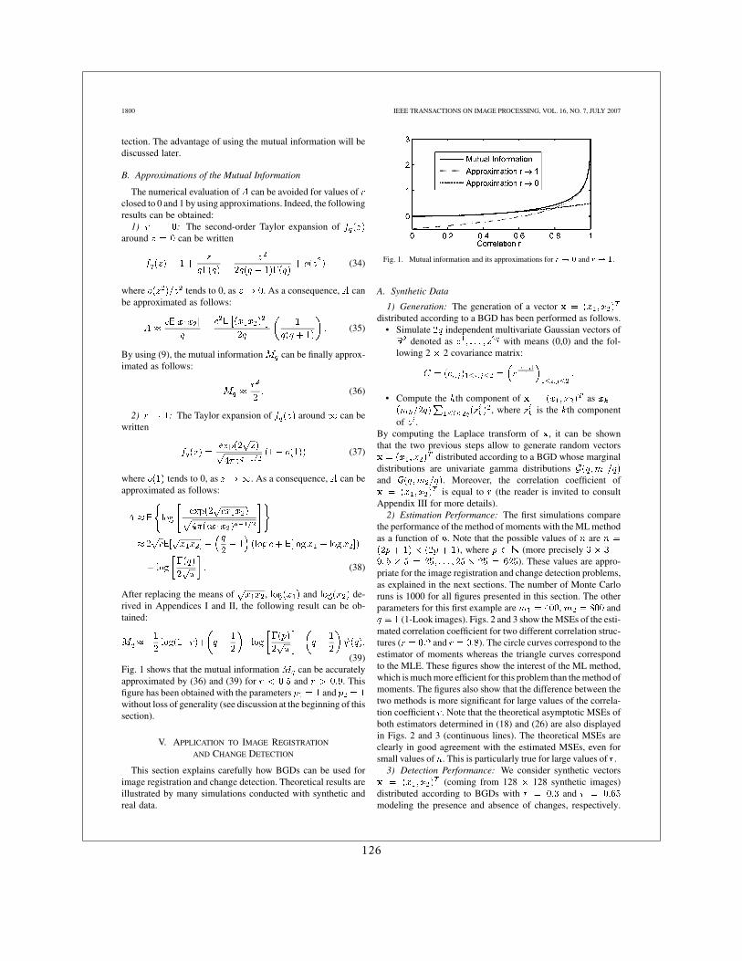
1800 IEEE TRANSACTIONS ON IMAGE PROCESSING, VOL. 16, NO. 7, JULY 2007
tection. The advantage of using the mutual information will bediscussed later.
B. Approximations of the Mutual Information
The numerical evaluation of can be avoided for values ofclosed to 0 and 1 by using approximations. Indeed, the followingresults can be obtained:
1) : The second-order Taylor expansion ofaround can be written
(34)
where tends to 0, as . As a consequence, canbe approximated as follows:
(35)
By using (9), the mutual information can be finally approx-imated as follows:
(36)
2) : The Taylor expansion of around can bewritten
(37)
where tends to 0, as . As a consequence, can beapproximated as follows:
(38)
After replacing the means of , and de-rived in Appendices I and II, the following result can be ob-tained:
(39)Fig. 1 shows that the mutual information can be accuratelyapproximated by (36) and (39) for and . Thisfigure has been obtained with the parameters andwithout loss of generality (see discussion at the beginning of thissection).
V. APPLICATION TO IMAGE REGISTRATION
AND CHANGE DETECTION
This section explains carefully how BGDs can be used forimage registration and change detection. Theoretical results areillustrated by many simulations conducted with synthetic andreal data.
Fig. 1. Mutual information and its approximations for r ! 0 and r ! 1.
A. Synthetic Data
1) Generation: The generation of a vectordistributed according to a BGD has been performed as follows.
• Simulate independent multivariate Gaussian vectors ofdenoted as with means (0,0) and the fol-
lowing 2 2 covariance matrix:
• Compute the th component of as, where is the th component
of .By computing the Laplace transform of , it can be shownthat the two previous steps allow to generate random vectors
distributed according to a BGD whose marginaldistributions are univariate gamma distributionsand . Moreover, the correlation coefficient of
is equal to (the reader is invited to consultAppendix III for more details).
2) Estimation Performance: The first simulations comparethe performance of the method of moments with the ML methodas a function of . Note that the possible values of are
, where (more precisely). These values are appro-
priate for the image registration and change detection problems,as explained in the next sections. The number of Monte Carloruns is 1000 for all figures presented in this section. The otherparameters for this first example are , and
(1-Look images). Figs. 2 and 3 show the MSEs of the esti-mated correlation coefficient for two different correlation struc-tures ( and ). The circle curves correspond to theestimator of moments whereas the triangle curves correspondto the MLE. These figures show the interest of the ML method,which is much more efficient for this problem than the method ofmoments. The figures also show that the difference between thetwo methods is more significant for large values of the correla-tion coefficient . Note that the theoretical asymptotic MSEs ofboth estimators determined in (18) and (26) are also displayedin Figs. 2 and 3 (continuous lines). The theoretical MSEs areclearly in good agreement with the estimated MSEs, even forsmall values of . This is particularly true for large values of .
3) Detection Performance: We consider synthetic vectors(coming from 128 128 synthetic images)
distributed according to BGDs with andmodeling the presence and absence of changes, respectively.
126
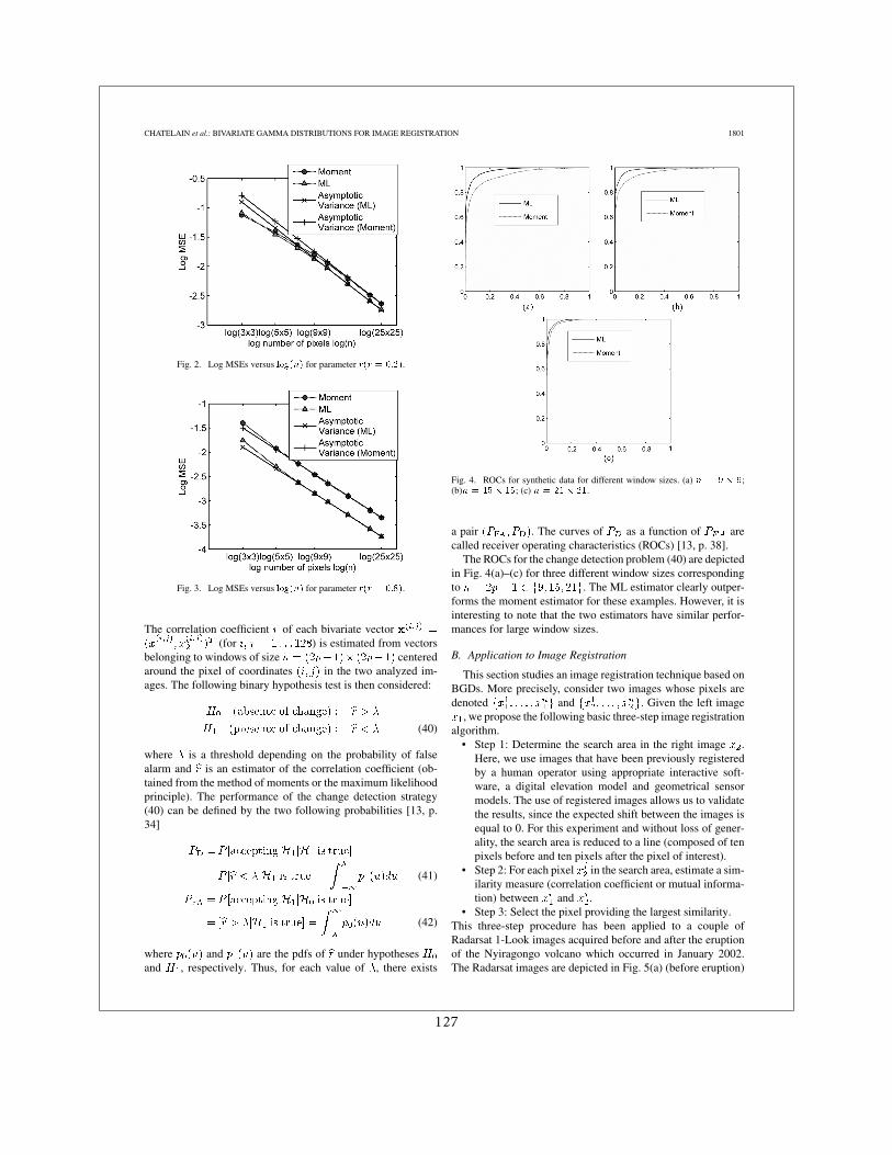
CHATELAIN et al.: BIVARIATE GAMMA DISTRIBUTIONS FOR IMAGE REGISTRATION 1801
Fig. 2. Log MSEs versus log(n) for parameter r(r = 0:2).
Fig. 3. Log MSEs versus log(n) for parameter r(r = 0:8).
The correlation coefficient of each bivariate vector(for ) is estimated from vectors
belonging to windows of size centeredaround the pixel of coordinates in the two analyzed im-ages. The following binary hypothesis test is then considered:
(40)
where is a threshold depending on the probability of falsealarm and is an estimator of the correlation coefficient (ob-tained from the method of moments or the maximum likelihoodprinciple). The performance of the change detection strategy(40) can be defined by the two following probabilities [13, p.34]
(41)
(42)
where and are the pdfs of under hypothesesand , respectively. Thus, for each value of , there exists
Fig. 4. ROCs for synthetic data for different window sizes. (a) n = 9 � 9;(b)n = 15 � 15; (c) n = 21� 21.
a pair . The curves of as a function of arecalled receiver operating characteristics (ROCs) [13, p. 38].
The ROCs for the change detection problem (40) are depictedin Fig. 4(a)–(c) for three different window sizes correspondingto . The ML estimator clearly outper-forms the moment estimator for these examples. However, it isinteresting to note that the two estimators have similar perfor-mances for large window sizes.
B. Application to Image Registration
This section studies an image registration technique based onBGDs. More precisely, consider two images whose pixels aredenoted and . Given the left image
, we propose the following basic three-step image registrationalgorithm.
• Step 1: Determine the search area in the right image .Here, we use images that have been previously registeredby a human operator using appropriate interactive soft-ware, a digital elevation model and geometrical sensormodels. The use of registered images allows us to validatethe results, since the expected shift between the images isequal to 0. For this experiment and without loss of gener-ality, the search area is reduced to a line (composed of tenpixels before and ten pixels after the pixel of interest).
• Step 2: For each pixel in the search area, estimate a sim-ilarity measure (correlation coefficient or mutual informa-tion) between and .
• Step 3: Select the pixel providing the largest similarity.This three-step procedure has been applied to a couple ofRadarsat 1-Look images acquired before and after the eruptionof the Nyiragongo volcano which occurred in January 2002.The Radarsat images are depicted in Fig. 5(a) (before eruption)
127
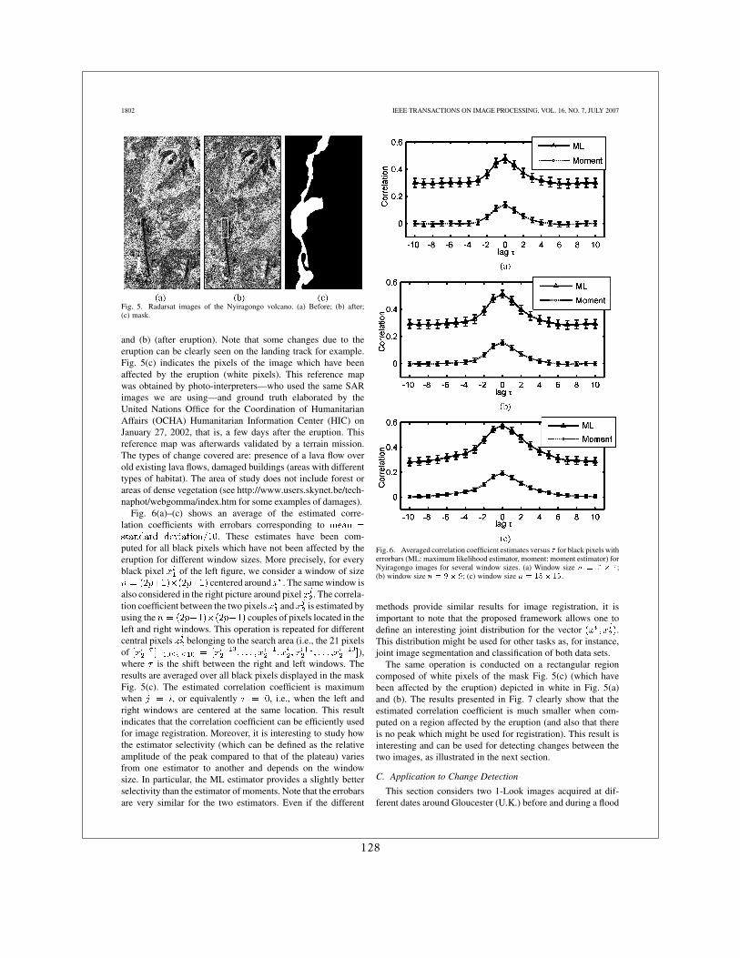
1802 IEEE TRANSACTIONS ON IMAGE PROCESSING, VOL. 16, NO. 7, JULY 2007
Fig. 5. Radarsat images of the Nyiragongo volcano. (a) Before; (b) after;(c) mask.
and (b) (after eruption). Note that some changes due to theeruption can be clearly seen on the landing track for example.Fig. 5(c) indicates the pixels of the image which have beenaffected by the eruption (white pixels). This reference mapwas obtained by photo-interpreters—who used the same SARimages we are using—and ground truth elaborated by theUnited Nations Office for the Coordination of HumanitarianAffairs (OCHA) Humanitarian Information Center (HIC) onJanuary 27, 2002, that is, a few days after the eruption. Thisreference map was afterwards validated by a terrain mission.The types of change covered are: presence of a lava flow overold existing lava flows, damaged buildings (areas with differenttypes of habitat). The area of study does not include forest orareas of dense vegetation (see http://www.users.skynet.be/tech-naphot/webgomma/index.htm for some examples of damages).
Fig. 6(a)–(c) shows an average of the estimated corre-lation coefficients with errobars corresponding to
. These estimates have been com-puted for all black pixels which have not been affected by theeruption for different window sizes. More precisely, for everyblack pixel of the left figure, we consider a window of size
centered around . The same window isalso considered in the right picture around pixel . The correla-tion coefficient between the two pixels and is estimated byusing the couples of pixels located in theleft and right windows. This operation is repeated for differentcentral pixels belonging to the search area (i.e., the 21 pixelsof ),where is the shift between the right and left windows. Theresults are averaged over all black pixels displayed in the maskFig. 5(c). The estimated correlation coefficient is maximumwhen , or equivalently , i.e., when the left andright windows are centered at the same location. This resultindicates that the correlation coefficient can be efficiently usedfor image registration. Moreover, it is interesting to study howthe estimator selectivity (which can be defined as the relativeamplitude of the peak compared to that of the plateau) variesfrom one estimator to another and depends on the windowsize. In particular, the ML estimator provides a slightly betterselectivity than the estimator of moments. Note that the errobarsare very similar for the two estimators. Even if the different
Fig. 6. Averaged correlation coefficient estimates versus � for black pixels witherrorbars (ML: maximum likelihood estimator, moment: moment estimator) forNyiragongo images for several window sizes. (a) Window size n = 7 � 7;(b) window size n = 9� 9; (c) window size n = 15� 15.
methods provide similar results for image registration, it isimportant to note that the proposed framework allows one todefine an interesting joint distribution for the vector .This distribution might be used for other tasks as, for instance,joint image segmentation and classification of both data sets.
The same operation is conducted on a rectangular regioncomposed of white pixels of the mask Fig. 5(c) (which havebeen affected by the eruption) depicted in white in Fig. 5(a)and (b). The results presented in Fig. 7 clearly show that theestimated correlation coefficient is much smaller when com-puted on a region affected by the eruption (and also that thereis no peak which might be used for registration). This result isinteresting and can be used for detecting changes between thetwo images, as illustrated in the next section.
C. Application to Change Detection
This section considers two 1-Look images acquired at dif-ferent dates around Gloucester (U.K.) before and during a flood
128
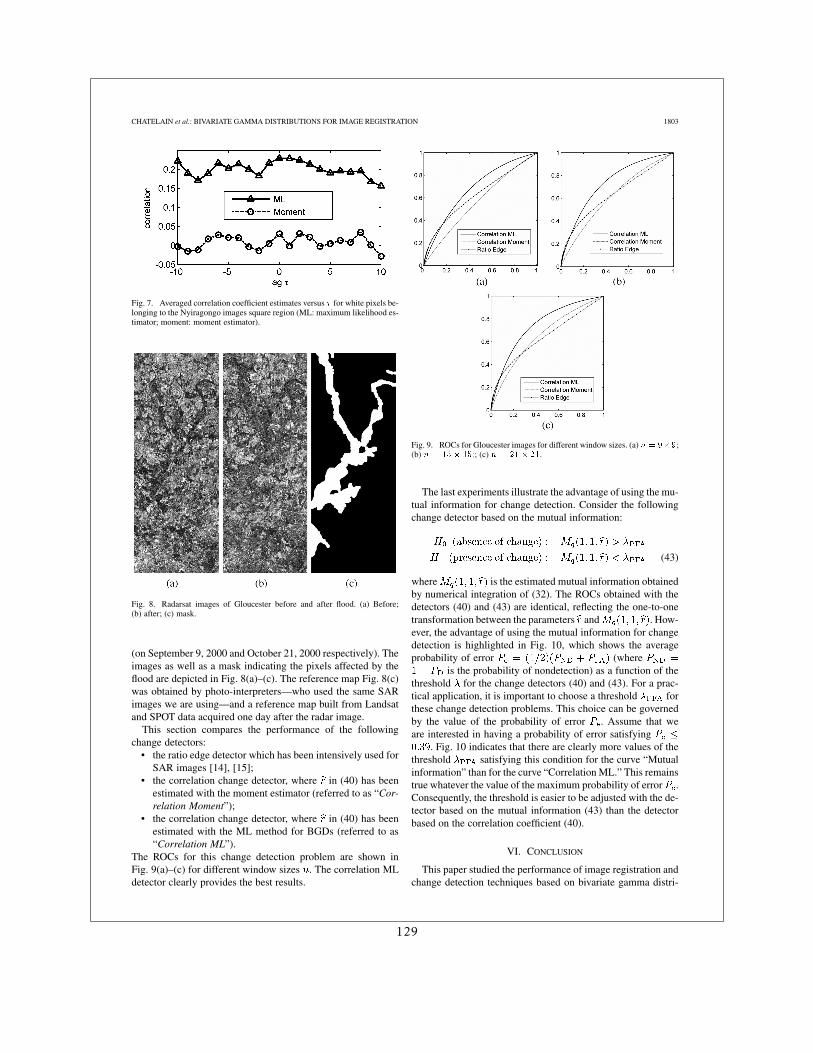
CHATELAIN et al.: BIVARIATE GAMMA DISTRIBUTIONS FOR IMAGE REGISTRATION 1803
Fig. 7. Averaged correlation coefficient estimates versus � for white pixels be-longing to the Nyiragongo images square region (ML: maximum likelihood es-timator; moment: moment estimator).
Fig. 8. Radarsat images of Gloucester before and after flood. (a) Before;(b) after; (c) mask.
(on September 9, 2000 and October 21, 2000 respectively). Theimages as well as a mask indicating the pixels affected by theflood are depicted in Fig. 8(a)–(c). The reference map Fig. 8(c)was obtained by photo-interpreters—who used the same SARimages we are using—and a reference map built from Landsatand SPOT data acquired one day after the radar image.
This section compares the performance of the followingchange detectors:
• the ratio edge detector which has been intensively used forSAR images [14], [15];
• the correlation change detector, where in (40) has beenestimated with the moment estimator (referred to as “Cor-relation Moment”);
• the correlation change detector, where in (40) has beenestimated with the ML method for BGDs (referred to as“Correlation ML”).
The ROCs for this change detection problem are shown inFig. 9(a)–(c) for different window sizes . The correlation MLdetector clearly provides the best results.
Fig. 9. ROCs for Gloucester images for different window sizes. (a) n = 9�9;(b) n = 15 � 15;; (c) n = 21� 21.
The last experiments illustrate the advantage of using the mu-tual information for change detection. Consider the followingchange detector based on the mutual information:
(43)
where is the estimated mutual information obtainedby numerical integration of (32). The ROCs obtained with thedetectors (40) and (43) are identical, reflecting the one-to-onetransformation between the parameters and . How-ever, the advantage of using the mutual information for changedetection is highlighted in Fig. 10, which shows the averageprobability of error (where
is the probability of nondetection) as a function of thethreshold for the change detectors (40) and (43). For a prac-tical application, it is important to choose a threshold forthese change detection problems. This choice can be governedby the value of the probability of error . Assume that weare interested in having a probability of error satisfying
. Fig. 10 indicates that there are clearly more values of thethreshold satisfying this condition for the curve “Mutualinformation” than for the curve “Correlation ML.” This remainstrue whatever the value of the maximum probability of error .Consequently, the threshold is easier to be adjusted with the de-tector based on the mutual information (43) than the detectorbased on the correlation coefficient (40).
VI. CONCLUSION
This paper studied the performance of image registration andchange detection techniques based on bivariate gamma distri-
129
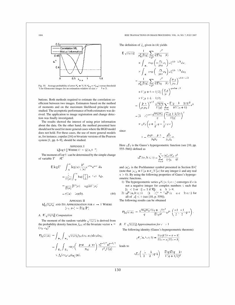
1804 IEEE TRANSACTIONS ON IMAGE PROCESSING, VOL. 16, NO. 7, JULY 2007
Fig. 10. Average probability of errorP = 1=2(P +P ) versus threshold� for Gloucester images for an estimation window of size n = 9� 9.
butions. Both methods required to estimate the correlation co-efficient between two images. Estimators based on the methodof moments and on the maximum likelihood principle werestudied. The asymptotic performance of both estimators was de-rived. The application to image registration and change detec-tion was finally investigated.
The results showed the interest of using prior informationabout the data. On the other hand, the method presented hereshould not be used for more general cases where the BGD modeldoes not hold. For these cases, the use of more general modelsas, for instance, copulas [16] or bivariate versions of the Pearsonsystem [1, pp. 6–9], should be studied.
APPENDIX IWHERE
The moment of can be determined by the simple changeof variable
(44)
APPENDIX IIAND ITS APPROXIMATION FOR WHERE
A. Computation
The moment of the random variable is derived fromthe probability density function of the bivariate vector
The definition of given in (4) yields
since
Here is the Gauss’s hypergeometric function (see [10, pp.555–566]) defined as
and is the Pochlammer symbol presented in Section II-C(note that for any integer and any real
). By using the following properties of Gauss’s hyperge-ometric functions.
1) The hypergeometric series converges if isnot a negative integer for complex numbers such that
or if .2) for
all of (see [10, p. 559]).The following results can be obtained
B. Approximation for
The following identity (Gauss’s hypergeometric theorem):
leads to
130
CHATELAIN et al.: BIVARIATE GAMMA DISTRIBUTIONS FOR IMAGE REGISTRATION 1805
and to the following first-order Taylor expansion around :
where tends to 0, as . Using
for
the previous Taylor expansion can be written
Finally
APPENDIX IIIGENERATION OF SYNTHETIC DATA DISTRIBUTED
ACCORDING TO BGDs
This appendix shows that the vector where(where is the th component
of , with )is distributed according to a BGD whose marginals are Gammadistributions and and whose correla-tion coefficient is . By using the independence between vec-tors , the Laplace transform of evaluated at
can be written
where
By using the probability density function of a bivariate normaldistribution , the Laplace transform can be finally ex-pressed as
where is the identity matrix in dimension 2. According to thedefinition (2), the vector is distributed according to a BGDwith shape parameter and scale parameters ,
, . Property, (8) ensures that thecorrelation coefficient of is .
ACKNOWLEDGMENT
The authors would like to thank A. Crouzil and G. Letacfor fruitful discussions regarding image registration and mul-tivariate gamma distributions, respectively.
REFERENCES
[1] S. Kotz, N. Balakrishnan, and N. L. Johnson, Continuous MultivariateDistributions, 2nd ed. New York: Wiley, 2000, vol. 1.
[2] S. B. Lev, D. Bshouty, P. Enis, G. Letac, I. L. Lu, and D. Richards,“The diagonal natural exponential families and their classification,” J.Theoret. Probl., vol. 7, pp. 883–928, 1994.
[3] P. Bernardoff, “Which multivariate Gamma distributions are infinitelydivisible?,” Bernoulli, 2006.
[4] J. Inglada and A. Giros, “On the possibility of automatic multi-sensorimage registration,” IEEE Trans. Geosci. Remote Sens., vol. 42, no. 10,pp. 2104–2120, Oct. 2004.
[5] T. F. Bush and F. T. Ulaby, “Fading characteristics of panchromaticradar backscatter from selected agricultural targets,” NASA STI/ReconTech. Rep., Dec. 1973, vol. 75, p. 18460.
[6] L. Bruzzone and D. F. Prieto, “Automatic analysis of the differenceimage for unsupervised change detection,” IEEE Trans. Geosci. Re-mote Sens., vol. 38, no. 3, pp. 1171–1182, May 2000.
[7] L. Bruzzone and D. F. Prieto, “An adaptive parcel-based technique forunsupervised change detection,” Int. J. Remote Sens., vol. 21, no. 4, pp.817–822, 2000.
[8] L. Bruzzone and S. Serpico, “An iterative technique for the detection ofland-cover transitions in multitemporal remote-sensing images,” IEEETrans. Geosci. Remote Sens., vol. 35, no. 7, pp. 858–867, Jul. 1997.
[9] Y. Bazi, L. Bruzzone, and F. Melgani, “An unsupervised approachbased on the generalized Gaussian model to automatic change detec-tion in multitemporal SAR images,” IEEE Trans. Geosci. Remote Sens.,vol. 43, no. 4, pp. 874–887, Apr. 2005.
[10] M. Abramowitz and I. Stegun, Handbook of Mathematical Func-tions. New York: Dover, 1972.
[11] F. Chatelain and J.-Y. Tourneret, “Composite likelihood estimation formultivariate mixed poisson distributions,” presented at the IEEE Work-shop Statistical Signal Processing, Bordeaux, France, Jul. 2005.
[12] B. Porat and B. Friedlander, “Performance analysis of parameter esti-mation algorithms based on high-order moments,” Int. J. Adapt. Con-trol Signal Process., vol. 3, pp. 191–229, 1989.
[13] H. L. Van Trees, Detection, Estimation, and Modulation Theory: PartI. New York: Wiley, 1968.
[14] R. Touzi, A. Lopés, and P. Bousquet, “A statistical and geometricaledge detector for SAR images,” IEEE Trans. Geosci. Remote Sens.,vol. 26, no. 11, pp. 764–773, Nov. 1988.
[15] E. J. M. Rignot and J. J. van Zyl, “Change detection techniques forERS-1 SAR data,” IEEE Trans. Geosci. Remote Sens., vol. 31, no. 7,pp. 896–906, Jul. 1993.
[16] R. B. Nelsen, An Introduction to Copulas. New York: Springer-Verlag, 1999, vol. 139.
Florent Chatelain was born in Paris, France, in1981. He received the Eng. degree in computersciences and applied mathematics from ENSIMAG,Grenoble, France, and the M.Sc. degree in appliedmathematics from the University Joseph Fourierof Grenoble, both in June 2004. He is currentlypursuing the Ph.D. degree with the Signal andCommunication Group, IRIT Laboratory, Toulouse,France.
His research interests are centered around multi-variate statistics applied to image processing.
131
1806 IEEE TRANSACTIONS ON IMAGE PROCESSING, VOL. 16, NO. 7, JULY 2007
Jean-Yves Tourneret (M’94) received the Ingénieurdegree in electrical engineering from the EcoleNationale Supérieure d’Electronique, d’Electrotech-nique, d’Informatique et d’Hydraulique, Toulouse(ENSEEIHT), France, and the Ph.D. degree from theNational Polytechnic Institute, Toulouse, in 1992.
He is currently a Professor with the University ofToulouse (ENSEEIHT). He is a member of the IRITLaboratory (UMR 5505 of the CNRS), where his re-search activity is centered around estimation, detec-tion, and classification of non-Gaussian and nonsta-
tionary processes.Dr. Tourneret was the Program Chair of the European Conference on Signal
Processing (EUSIPCO), which was held in Toulouse in 2002. He was also amember of the organizing committee for the International Conference on Acous-tics, Speech, and Signal Processing (ICASSP) held in Toulouse in 2006. Hehas been a member of different technical committees, including the Signal Pro-cessing Theory and Methods (SPTM) Committee of the IEEE Signal ProcessingSociety.
Jordi Inglada received the TelecommunicationsEngineer degree in 1997 from both the UniversitatPolitècnica de Catalunya, Catalunya, Spain, and theÉcole Nationale Supérieure des Télécommunica-tions de Bretagne, and the Ph.D. degree in signalprocessing and telecommunications in 2000 fromUniversité de Rennes 1, Rennes, France.
He is with the Centre National d’Études Spatiales,French Space Agency, Toulouse, France, working inthe field of remote sensing image processing. He isin charge of the development of image processing al-
gorithms for the operational exploitation of earth observation images, mainly inthe fields of image registration, change detection and object recognition.
André Ferrari was born in Senlis, France, on June2, 1964. He received the engineering degree fromÉcole Centrale de Lyon, Lyon, France, in 1988, theM.S. degree in 1989, and the Ph.D. from Universityof Nice Sophia-Antipolis (UNSA), France, in 1992,all in electrical and computer engineering.
From 1993 to 2005, he was an Associate Professorat UNSA. Since 2005, he has been a Professor atthe Astrophysics Laboratory, UNSA. His currentresearch interests are in modeling and data pro-cessing in statistical optics with a particular interest
in Astrophysics.
132
IEEE TRANSACTIONS ON IMAGE PROCESSING, VOL. 17, NO. 3, MARCH 2008 249
Change Detection in Multisensor SAR ImagesUsing Bivariate Gamma Distributions
Florent Chatelain, Jean-Yves Tourneret, and Jordi Inglada
Abstract—This paper studies a family of distributions con-structed from multivariate gamma distributions to model thestatistical properties of multisensor synthetic aperture radar(SAR) images. These distributions referred to as multisensormultivariate gamma distributions (MuMGDs) are potentiallyinteresting for detecting changes in SAR images acquired bydifferent sensors having different numbers of looks. The first partof this paper compares different estimators for the parameters ofMuMGDs. These estimators are based on the maximum likelihoodprinciple, the method of inference function for margins, and themethod of moments. The second part of the paper studies changedetection algorithms based on the estimated correlation coefficientof MuMGDs. Simulation results conducted on synthetic and realdata illustrate the performance of these change detectors.
Index Terms—Change detection, correlation coefficient, max-imum likelihood, multivariate gamma distributions.
I. INTRODUCTION
COMBINING information acquired from multiple sensorshas become very popular in many signal and image pro-
cessing applications. In the case of earth observation applica-tions, there are two reasons for that. The first one is that the fu-sion of the data produced by different types of sensors providesa complementarity which overcomes the limitations of a specifickind of sensor. The other reason is that, often, in operational ap-plications, the user does not have the possibility to choose thedata to work with and has to use the available archive images orthe first acquisition available after an event of interest. This isparticularly true for monitoring applications where image regis-tration and change detection approaches have to be implementedon different types of data [1], [2].
Both image registration and change detection techniques con-sists of comparing two images , the reference, and , the sec-ondary image, acquired over the same landscape—scene—attwo different dates. Usually, the reference image is obtainedfrom an archive and the acquisition of the secondary image isscheduled after an abrupt change, like a natural disaster. In thecase of the change detection, the goal is producing an indicatorof change for each pixel of the region of interest. This indicator
Manuscript received November 15, 2007; revised December 9, 2007. Thiswork was supported in part by CNES under Contract 2005/2561 and in part bythe CNRS under MathSTIC Action No. 80/0244. The associate editor coordi-nating the review of this manuscript and approving it for publication was Dr.Jacques Blanc-Talon.
F. Chatelain and J.-Y. Tourneret are with the IRIT/ENSEEIHT/TéSA,31071 Toulouse cedex 7, France (e-mail: [email protected];[email protected]).
J. Inglada is with the CNES, 31401 Toulouse cedex 9, France (e-mail: [email protected]).
Digital Object Identifier 10.1109/TIP.2008.916047
of change is the result of applying locally a similarity measureto the two images. This similarity measure is usually chosen asthe correlation coefficient or other statistical feature in order todeal with noisy data.
The estimation of the similarity measure is performed locallyfor each pixel position. Since a statistical estimation has to beperformed, and only one realization of the random variable isavailable, the images are supposed to be locally stationary andthe ergodicity assumption allows to make estimates using sev-eral neighbor pixels. This neighborhood is the so-called estima-tion window. In order for the stationarity assumption to hold,this estimation window has to be small. On the other hand, ro-bust statistical estimates need a high number of samples. There-fore, the key point of the estimation of the similarity measure isto perform high quality estimates with a small number of sam-ples. One way to do so is to introduce a priori knowledge aboutthe image statistics.
In the case of power radar images, it is well known that thepixels are marginally distributed according to gamma distribu-tions [3]. Therefore, multivariate gamma distributions (havingunivariate gamma margins) seem good candidates for the ro-bust estimation of the correlation coefficient between radar im-ages. When multidate power radar images are acquired fromdifferent sensors, the numbers of looks associated with the dif-ferent images can be different. As the number of looks is theshape parameter of the gamma distribution, this leads to studymultivariate gamma distributions whose margins have differentshape parameters.
A family of multivariate gamma distributions has been re-cently defined by Bar Lev and Bernardoff [4], [5]. These dis-tributions are defined from an appropriate moment generatingfunction. Their margins are distributed according to univariategamma distributions having the same shape parameter. Theyhave recently shown interesting properties for registration andchange detection in SAR images acquired by the same sensor(i.e., for images having the same number of looks) [6], [7]. Thispaper studies a new family of multivariate distributions whosemargins are univariate gamma distributions with different shapeparameters referred to as multisensor multivariate gamma dis-tributions (MuMGDs). The application of MuBGDs to changedetection in SAR images is also investigated.
This paper is organized as follows. Section II recalls impor-tant results on monosensor multivariate gamma distributions(MoMGDs). Section III defines the family of MuMGDs consid-ered for change detection in multisensor SAR images. SectionIV studies the maximum likelihood estimator (MLE), the infer-ence function for margins (IFM) estimator, and the estimator ofmoments for the unknown parameters of MuMGDs. Section Vpresents some simulation results illustrating the performance ofMuMGDs for parameter estimation and change detection on
1057-7149/$25.00 © 2008 IEEE
133
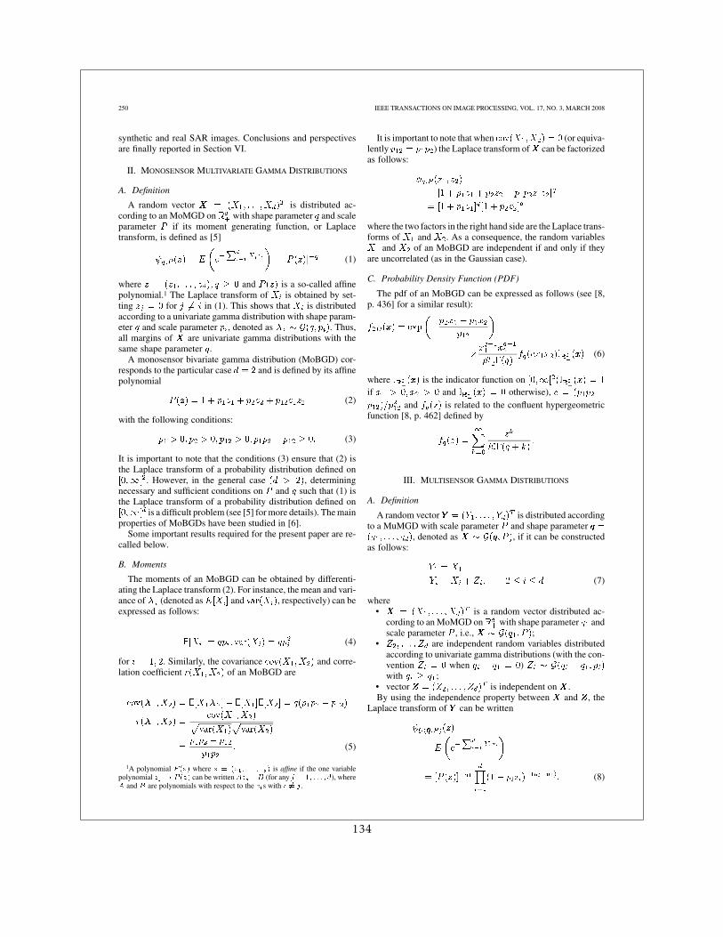
250 IEEE TRANSACTIONS ON IMAGE PROCESSING, VOL. 17, NO. 3, MARCH 2008
synthetic and real SAR images. Conclusions and perspectivesare finally reported in Section VI.
II. MONOSENSOR MULTIVARIATE GAMMA DISTRIBUTIONS
A. Definition
A random vector is distributed ac-cording to an MoMGD on with shape parameter and scaleparameter if its moment generating function, or Laplacetransform, is defined as [5]
(1)
where and is a so-called affinepolynomial.1 The Laplace transform of is obtained by set-ting for in (1). This shows that is distributedaccording to a univariate gamma distribution with shape param-eter and scale parameter , denoted as . Thus,all margins of are univariate gamma distributions with thesame shape parameter .
A monosensor bivariate gamma distribution (MoBGD) cor-responds to the particular case and is defined by its affinepolynomial
(2)
with the following conditions:
(3)
It is important to note that the conditions (3) ensure that (2) isthe Laplace transform of a probability distribution defined on
. However, in the general case , determiningnecessary and sufficient conditions on and such that (1) isthe Laplace transform of a probability distribution defined on
is a difficult problem (see [5] for more details). The mainproperties of MoBGDs have been studied in [6].
Some important results required for the present paper are re-called below.
B. Moments
The moments of an MoBGD can be obtained by differenti-ating the Laplace transform (2). For instance, the mean and vari-ance of (denoted as and , respectively) can beexpressed as follows:
(4)
for . Similarly, the covariance and corre-lation coefficient of an MoBGD are
(5)
1A polynomial P (zzz) where zzz = (z ; . . . ; z ) is affine if the one variablepolynomial z 7! P (zzz) can be written Az +B (for any j = 1; . . . ; d), whereA and B are polynomials with respect to the z s with i 6= j .
It is important to note that when (or equiva-lently ) the Laplace transform of can be factorizedas follows:
where the two factors in the right hand side are the Laplace trans-forms of and . As a consequence, the random variables
and of an MoBGD are independent if and only if theyare uncorrelated (as in the Gaussian case).
C. Probability Density Function (PDF)
The pdf of an MoBGD can be expressed as follows (see [8,p. 436] for a similar result):
(6)
where is the indicator function onif and otherwise),
and is related to the confluent hypergeometricfunction [8, p. 462] defined by
III. MULTISENSOR GAMMA DISTRIBUTIONS
A. Definition
A random vector is distributed accordingto a MuMGD with scale parameter and shape parameter
, denoted as , if it can be constructedas follows:
(7)
where• is a random vector distributed ac-
cording to an MoMGD on with shape parameter andscale parameter , i.e., ;
• are independent random variables distributedaccording to univariate gamma distributions (with the con-vention when )with ;
• vector is independent on .By using the independence property between and , the
Laplace transform of can be written
(8)
134
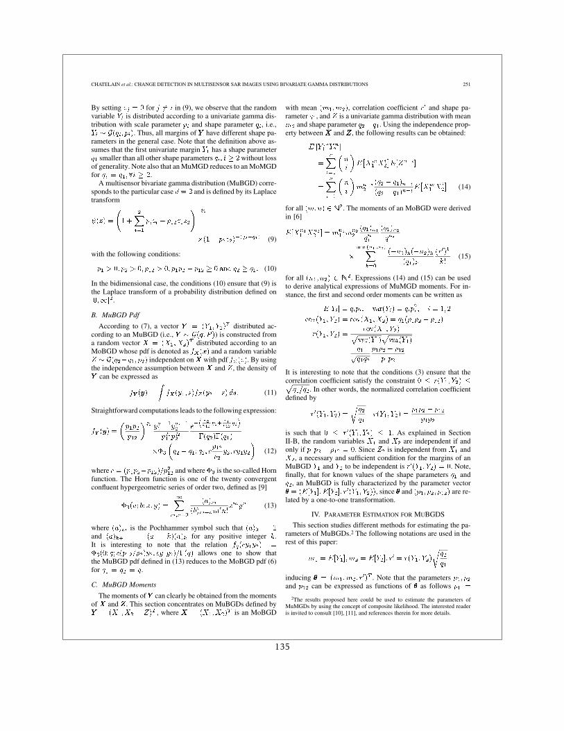
CHATELAIN et al.: CHANGE DETECTION IN MULTISENSOR SAR IMAGES USING BIVARIATE GAMMA DISTRIBUTIONS 251
By setting for in (9), we observe that the randomvariable is distributed according to a univariate gamma dis-tribution with scale parameter and shape parameter , i.e.,
. Thus, all margins of have different shape pa-rameters in the general case. Note that the definition above as-sumes that the first univariate margin has a shape parameter
smaller than all other shape parameters without lossof generality. Note also that an MuMGD reduces to an MoMGDfor .
A multisensor bivariate gamma distribution (MuBGD) corre-sponds to the particular case and is defined by its Laplacetransform
(9)
with the following conditions:
(10)
In the bidimensional case, the conditions (10) ensure that (9) isthe Laplace transform of a probability distribution defined on
.
B. MuBGD Pdf
According to (7), a vector distributed ac-cording to an MuBGD (i.e., ) is constructed froma random vector distributed according to anMoBGD whose pdf is denoted as and a random variable
independent on with pdf . By usingthe independence assumption between and , the density of
can be expressed as
(11)
Straightforward computations leads to the following expression:
(12)
where and where is the so-called Hornfunction. The Horn function is one of the twenty convergentconfluent hypergeometric series of order two, defined as [9]
(13)
where is the Pochhammer symbol such thatand for any positive integer .It is interesting to note that the relation
allows one to show thatthe MuBGD pdf defined in (13) reduces to the MoBGD pdf (6)for .
C. MuBGD Moments
The moments of can clearly be obtained from the momentsof and . This section concentrates on MuBGDs defined by
, where is an MoBGD
with mean , correlation coefficient and shape pa-rameter , and is a univariate gamma distribution with mean
and shape parameter . Using the independence prop-erty between and , the following results can be obtained:
(14)
for all . The moments of an MoBGD were derivedin [6]
(15)
for all . Expressions (14) and (15) can be usedto derive analytical expressions of MuMGD moments. For in-stance, the first and second order moments can be written as
It is interesting to note that the conditions (3) ensure that thecorrelation coefficient satisfy the constraint
. In other words, the normalized correlation coefficientdefined by
is such that . As explained in SectionII-B, the random variables and are independent if andonly if . Since is independent from and
, a necessary and sufficient condition for the margins of anMuBGD and to be independent is . Note,finally, that for known values of the shape parameters and
, an MuBGD is fully characterized by the parameter vector, since and are re-
lated by a one-to-one transformation.
IV. PARAMETER ESTIMATION FOR MUBGDS
This section studies different methods for estimating the pa-rameters of MuBGDs.2 The following notations are used in therest of this paper:
inducing . Note that the parametersand can be expressed as functions of as follows
2The results proposed here could be used to estimate the parameters ofMuMGDs by using the concept of composite likelihood. The interested readeris invited to consult [10], [11], and references therein for more details.
135
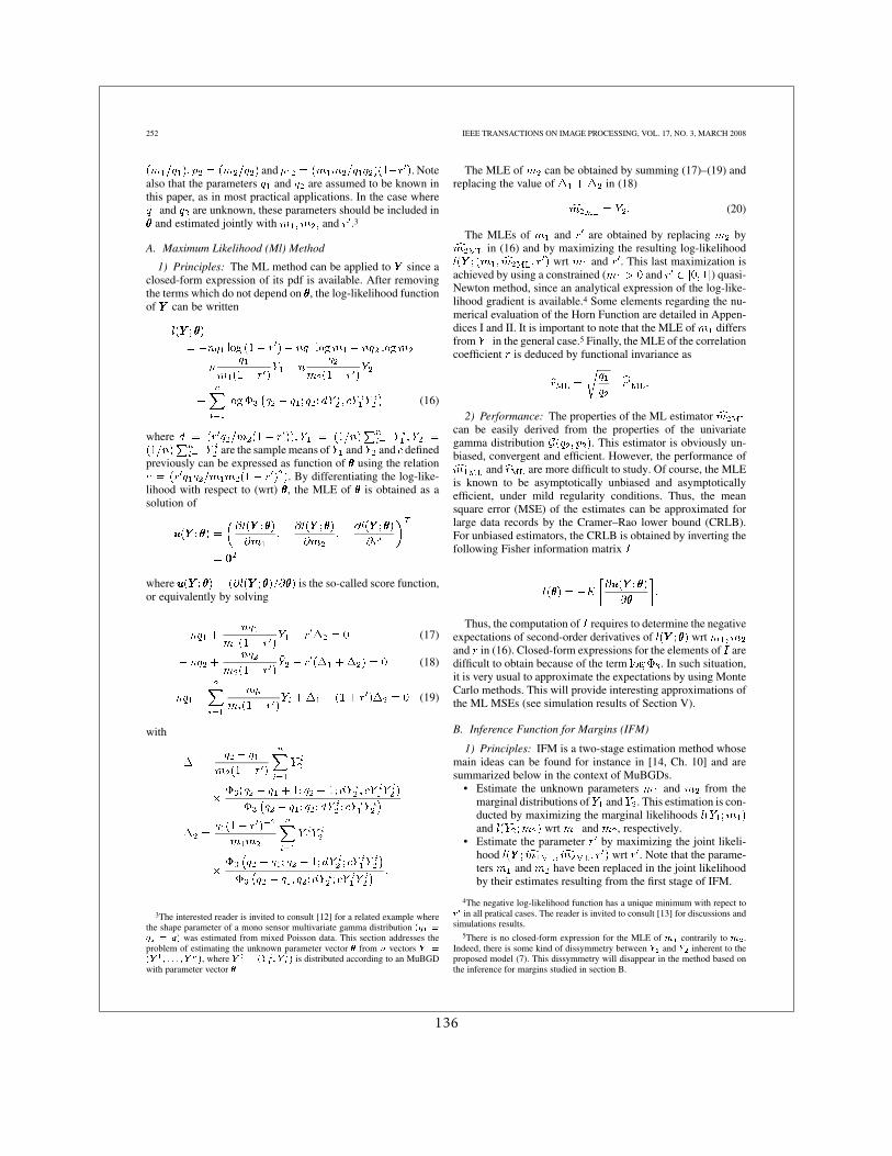
252 IEEE TRANSACTIONS ON IMAGE PROCESSING, VOL. 17, NO. 3, MARCH 2008
and . Notealso that the parameters and are assumed to be known inthis paper, as in most practical applications. In the case where
and are unknown, these parameters should be included inand estimated jointly with and .3
A. Maximum Likelihood (Ml) Method
1) Principles: The ML method can be applied to since aclosed-form expression of its pdf is available. After removingthe terms which do not depend on , the log-likelihood functionof can be written
(16)
whereare the sample means of and and defined
previously can be expressed as function of using the relation. By differentiating the log-like-
lihood with respect to (wrt) , the MLE of is obtained as asolution of
where is the so-called score function,or equivalently by solving
(17)
(18)
(19)
with
3The interested reader is invited to consult [12] for a related example wherethe shape parameter of a mono sensor multivariate gamma distribution (q =q = q) was estimated from mixed Poisson data. This section addresses theproblem of estimating the unknown parameter vector ��� from n vectors YYY =(YYY ; . . . ; YYY ), where YYY = (Y ; Y ) is distributed according to an MuBGDwith parameter vector ���
The MLE of can be obtained by summing (17)–(19) andreplacing the value of in (18)
(20)
The MLEs of and are obtained by replacing byin (16) and by maximizing the resulting log-likelihood
wrt and . This last maximization isachieved by using a constrained ( and ) quasi-Newton method, since an analytical expression of the log-like-lihood gradient is available.4 Some elements regarding the nu-merical evaluation of the Horn Function are detailed in Appen-dices I and II. It is important to note that the MLE of differsfrom in the general case.5 Finally, the MLE of the correlationcoefficient is deduced by functional invariance as
2) Performance: The properties of the ML estimatorcan be easily derived from the properties of the univariategamma distribution . This estimator is obviously un-biased, convergent and efficient. However, the performance of
and are more difficult to study. Of course, the MLEis known to be asymptotically unbiased and asymptoticallyefficient, under mild regularity conditions. Thus, the meansquare error (MSE) of the estimates can be approximated forlarge data records by the Cramer–Rao lower bound (CRLB).For unbiased estimators, the CRLB is obtained by inverting thefollowing Fisher information matrix
Thus, the computation of requires to determine the negativeexpectations of second-order derivatives of wrtand in (16). Closed-form expressions for the elements of aredifficult to obtain because of the term . In such situation,it is very usual to approximate the expectations by using MonteCarlo methods. This will provide interesting approximations ofthe ML MSEs (see simulation results of Section V).
B. Inference Function for Margins (IFM)
1) Principles: IFM is a two-stage estimation method whosemain ideas can be found for instance in [14, Ch. 10] and aresummarized below in the context of MuBGDs.
• Estimate the unknown parameters and from themarginal distributions of and . This estimation is con-ducted by maximizing the marginal likelihoodsand wrt and , respectively.
• Estimate the parameter by maximizing the joint likeli-hood wrt . Note that the parame-ters and have been replaced in the joint likelihoodby their estimates resulting from the first stage of IFM.
4The negative log-likelihood function has a unique minimum with repect tor in all pratical cases. The reader is invited to consult [13] for discussions andsimulations results.
5There is no closed-form expression for the MLE of m contrarily to m .Indeed, there is some kind of dissymmetry between Y and Y inherent to theproposed model (7). This dissymmetry will disappear in the method based onthe inference for margins studied in section B.
136
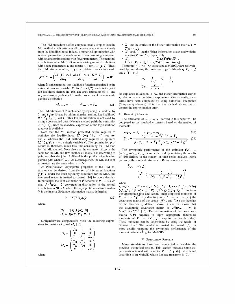
CHATELAIN et al.: CHANGE DETECTION IN MULTISENSOR SAR IMAGES USING BIVARIATE GAMMA DISTRIBUTIONS 253
The IFM procedure is often computationally simpler than theML method which estimates all the parameters simultaneouslyfrom the joint likelihood. Indeed, a numerical optimization withseveral parameters is much more time-consuming comparedwith several optimizations with fewer parameters. The marginaldistributions of an MuBGD are univariate gamma distributionswith shape parameters and means , for . Thus,the IFM estimators of are obtained as a solution of
where is the marginal log-likelihood function associated to theunivariate random variable , for , and is the jointlog-likelihood defined in (16). The IFM estimators of and
are classically obtained from the properties of the univariategamma distribution
(21)
The IFM estimator of is obtained by replacing and byand in (16) and by minimizing the resulting log-likelihood
wrt . This last minimization is achieved byusing a constrained quasi-Newton method (with the constraint
), since an analytical expression of the log-likelihoodgradient is available.
Note that the ML method presented before requires tooptimize the log-likelihood wrtand whereas the IFM method only requires to optimize
wrt a single variable . The optimization pro-cedure is, therefore, much less time-consuming for IFM thanfor the ML method. Note also that the estimator of is thesame for the ML and IFM methods. Finally, it is interesting topoint out that the joint likelihood is the product of univariategamma pdfs when . As a consequence, the ML and IFMestimators are the same when .
2) Performance: Asymptotic properties of the IFM es-timator can be derived from the set of inferences functions
under the usual regularity conditions for the MLE (theinterested reader is invited to consult [14] for more details).In particular, the IFM estimator of denoted as is suchthat converges in distribution to the normaldistribution , where the asymptotic covariance matrixV is the inverse Godambe information matrix defined as
(22)
where
Straightforward computations yield the following expres-sions for matrices and [15]:
where
• are the entries of the Fisher information matrix,;
• and are the Fisher information associated with themargins and , respectively;
•
The terms associated to MuBGDs are easily de-rived by considering the univariate log-likelihoodsand
As explained in Section IV-A2, the Fisher information entriesdo not have closed-form expressions. Consequently, these
terms have been computed by using numerical integration(Simpson quadrature). Note that this method allows one tocontrol the approximation error.
C. Method of Moments
The estimators of derived in this paper will becompared to the standard estimators based on the method ofmoments
(23)
(24)
The asymptotic performance of the estimatorcan be derived by imitating the results
of [16] derived in the context of time series analysis. Moreprecisely, the moment estimator of can be rewritten as
where
containsthe appropriate first and second order empirical moments of
. By denoting as thecovariance matrix of the vector and the jacobianof the function defined above, it can be shown thatthe asymptotic covariance matrix of is
[16]. The determination of the covariancematrix requires to know appropriate theoreticalmoments of (up to the fourth order).These moments can be determined by using the results ofSection III-C. The reader is invited to consult [6] formore details regarding the asymptotic performance of themoment estimator for MuBGDs.
V. SIMULATION RESULTS
Many simulations have been conducted to validate theprevious theoretical results. This section presents some ex-periments obtained with a vector distributedaccording to an MuBGD whose Laplace transform is (9).
137
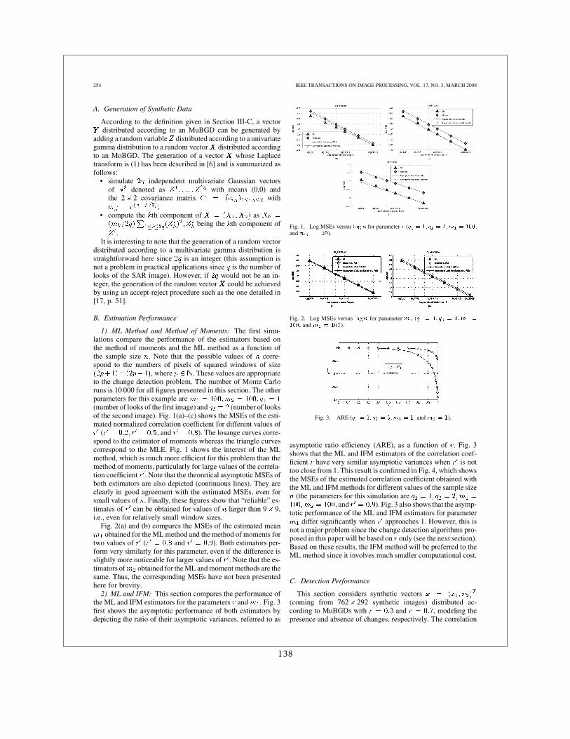
254 IEEE TRANSACTIONS ON IMAGE PROCESSING, VOL. 17, NO. 3, MARCH 2008
A. Generation of Synthetic Data
According to the definition given in Section III-C, a vectordistributed according to an MuBGD can be generated by
adding a random variable distributed according to a univariategamma distribution to a random vector distributed accordingto an MoBGD. The generation of a vector whose Laplacetransform is (1) has been described in [6] and is summarized asfollows:
• simulate independent multivariate Gaussian vectorsof denoted as with means (0,0) andthe 2 2 covariance matrix with
;• compute the th component of as
being the th component of.
It is interesting to note that the generation of a random vectordistributed according to a multivariate gamma distribution isstraightforward here since is an integer (this assumption isnot a problem in practical applications since is the number oflooks of the SAR image). However, if would not be an in-teger, the generation of the random vector could be achievedby using an accept-reject procedure such as the one detailed in[17, p. 51].
B. Estimation Performance
1) ML Method and Method of Moments: The first simu-lations compare the performance of the estimators based onthe method of moments and the ML method as a function ofthe sample size . Note that the possible values of corre-spond to the numbers of pixels of squared windows of size
, where . These values are appropriateto the change detection problem. The number of Monte Carloruns is 10 000 for all figures presented in this section. The otherparameters for this example are(number of looks of the first image) and (number of looksof the second image). Fig. 1(a)–(c) shows the MSEs of the esti-mated normalized correlation coefficient for different values of
( and ). The losange curves corre-spond to the estimator of moments whereas the triangle curvescorrespond to the MLE. Fig. 1 shows the interest of the MLmethod, which is much more efficient for this problem than themethod of moments, particularly for large values of the correla-tion coefficient . Note that the theoretical asymptotic MSEs ofboth estimators are also depicted (continuous lines). They areclearly in good agreement with the estimated MSEs, even forsmall values of . Finally, these figures show that “reliable” es-timates of can be obtained for values of larger than 9 9,i.e., even for relatively small window sizes.
Fig. 2(a) and (b) compares the MSEs of the estimated meanobtained for the ML method and the method of moments for
two values of ( and ). Both estimators per-form very similarly for this parameter, even if the difference isslightly more noticeable for larger values of . Note that the es-timators of obtained for the ML and moment methods are thesame. Thus, the corresponding MSEs have not been presentedhere for brevity.
2) ML and IFM: This section compares the performance ofthe ML and IFM estimators for the parameters and . Fig. 3first shows the asymptotic performance of both estimators bydepicting the ratio of their asymptotic variances, referred to as
Fig. 1. Log MSEs versus logn for parameter r (q = 1; q = 2;m = 100;and m = 100).
Fig. 2. Log MSEs versus logn for parameter m (q = 1; q = 2;m =100; and m = 100).
Fig. 3. ARE (q = 1; q = 5;m = 1; and m = 1).
asymptotic ratio efficiency (ARE), as a function of . Fig. 3shows that the ML and IFM estimators of the correlation coef-ficient have very similar asymptotic variances when is nottoo close from 1. This result is confirmed in Fig. 4, which showsthe MSEs of the estimated correlation coefficient obtained withthe ML and IFM methods for different values of the sample size
(the parameters for this simulation areand ). Fig. 3 also shows that the asymp-
totic performance of the ML and IFM estimators for parameterdiffer significantly when approaches 1. However, this is
not a major problem since the change detection algorithms pro-posed in this paper will be based on only (see the next section).Based on these results, the IFM method will be preferred to theML method since it involves much smaller computational cost.
C. Detection Performance
This section considers synthetic vectors(coming from 762 292 synthetic images) distributed ac-cording to MuBGDs with and , modeling thepresence and absence of changes, respectively. The correlation
138
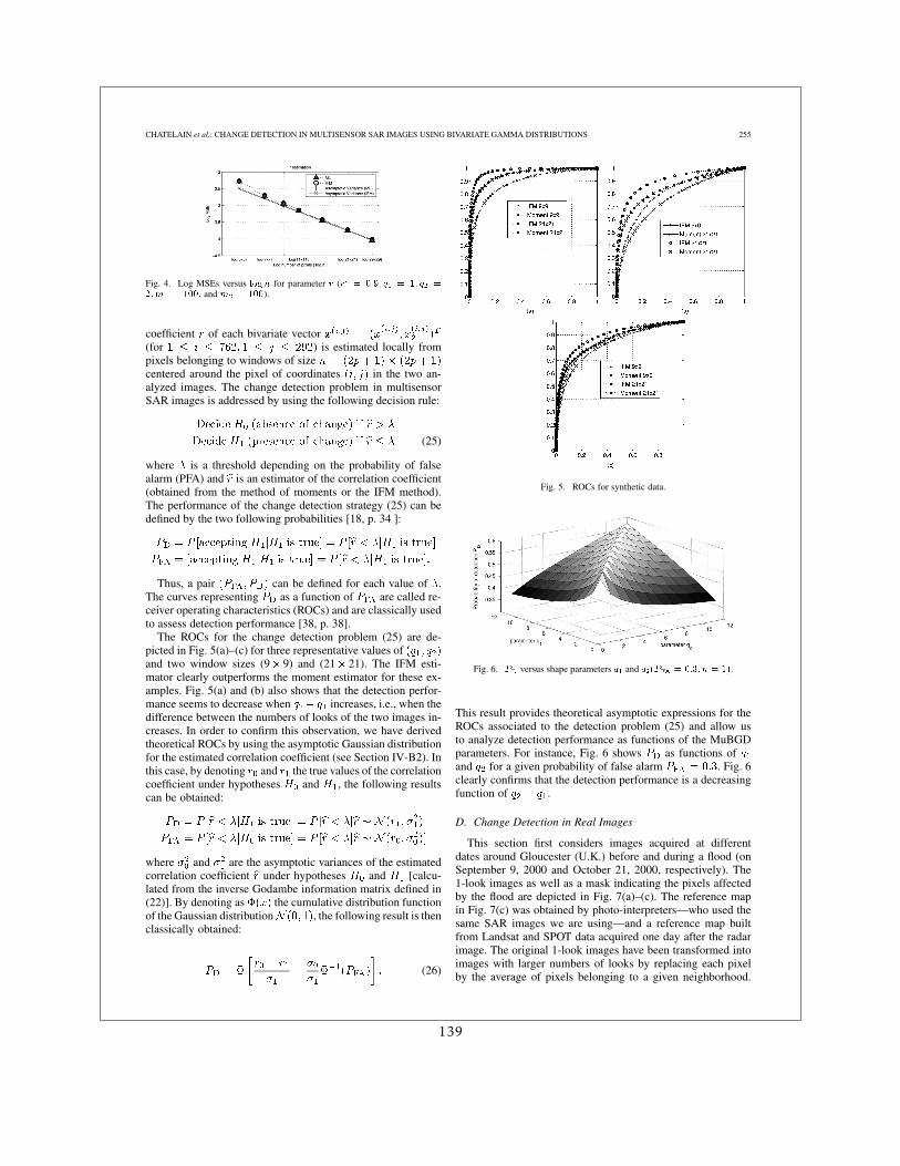
CHATELAIN et al.: CHANGE DETECTION IN MULTISENSOR SAR IMAGES USING BIVARIATE GAMMA DISTRIBUTIONS 255
Fig. 4. Log MSEs versus logn for parameter r (r = 0:9; q = 1; q =2;m = 100; and m = 100).
coefficient of each bivariate vector(for ) is estimated locally frompixels belonging to windows of sizecentered around the pixel of coordinates in the two an-alyzed images. The change detection problem in multisensorSAR images is addressed by using the following decision rule:
(25)
where is a threshold depending on the probability of falsealarm (PFA) and is an estimator of the correlation coefficient(obtained from the method of moments or the IFM method).The performance of the change detection strategy (25) can bedefined by the two following probabilities [18, p. 34 ]:
Thus, a pair can be defined for each value of .The curves representing as a function of are called re-ceiver operating characteristics (ROCs) and are classically usedto assess detection performance [38, p. 38].
The ROCs for the change detection problem (25) are de-picted in Fig. 5(a)–(c) for three representative values ofand two window sizes (9 9) and (21 21). The IFM esti-mator clearly outperforms the moment estimator for these ex-amples. Fig. 5(a) and (b) also shows that the detection perfor-mance seems to decrease when increases, i.e., when thedifference between the numbers of looks of the two images in-creases. In order to confirm this observation, we have derivedtheoretical ROCs by using the asymptotic Gaussian distributionfor the estimated correlation coefficient (see Section IV-B2). Inthis case, by denoting and the true values of the correlationcoefficient under hypotheses and , the following resultscan be obtained:
where and are the asymptotic variances of the estimatedcorrelation coefficient under hypotheses and [calcu-lated from the inverse Godambe information matrix defined in(22)]. By denoting as the cumulative distribution functionof the Gaussian distribution , the following result is thenclassically obtained:
(26)
Fig. 5. ROCs for synthetic data.
Fig. 6. P versus shape parameters q and q (P = 0:3; n = 1).
This result provides theoretical asymptotic expressions for theROCs associated to the detection problem (25) and allow usto analyze detection performance as functions of the MuBGDparameters. For instance, Fig. 6 shows as functions ofand for a given probability of false alarm . Fig. 6clearly confirms that the detection performance is a decreasingfunction of .
D. Change Detection in Real Images
This section first considers images acquired at differentdates around Gloucester (U.K.) before and during a flood (onSeptember 9, 2000 and October 21, 2000, respectively). The1-look images as well as a mask indicating the pixels affectedby the flood are depicted in Fig. 7(a)–(c). The reference mapin Fig. 7(c) was obtained by photo-interpreters—who used thesame SAR images we are using—and a reference map builtfrom Landsat and SPOT data acquired one day after the radarimage. The original 1-look images have been transformed intoimages with larger numbers of looks by replacing each pixelby the average of pixels belonging to a given neighborhood.
139
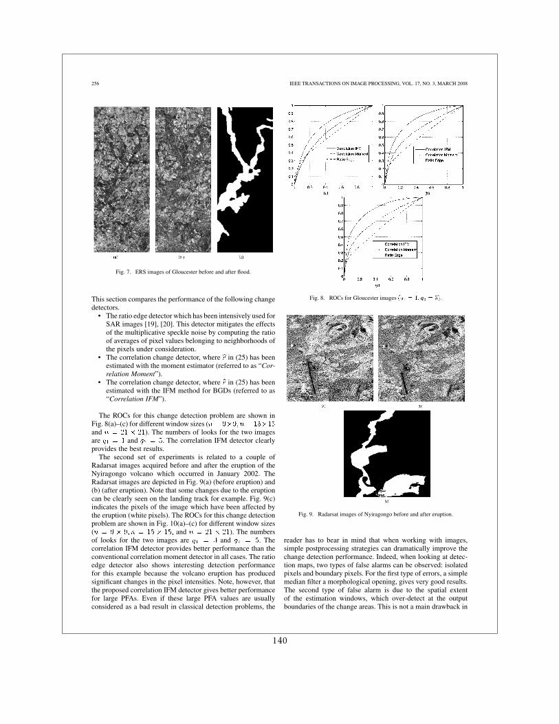
256 IEEE TRANSACTIONS ON IMAGE PROCESSING, VOL. 17, NO. 3, MARCH 2008
Fig. 7. ERS images of Gloucester before and after flood.
This section compares the performance of the following changedetectors.
• The ratio edge detector which has been intensively used forSAR images [19], [20]. This detector mitigates the effectsof the multiplicative speckle noise by computing the ratioof averages of pixel values belonging to neighborhoods ofthe pixels under consideration.
• The correlation change detector, where in (25) has beenestimated with the moment estimator (referred to as “Cor-relation Moment”).
• The correlation change detector, where in (25) has beenestimated with the IFM method for BGDs (referred to as“Correlation IFM”).
The ROCs for this change detection problem are shown inFig. 8(a)–(c) for different window sizes (and ). The numbers of looks for the two imagesare and . The correlation IFM detector clearlyprovides the best results.
The second set of experiments is related to a couple ofRadarsat images acquired before and after the eruption of theNyiragongo volcano which occurred in January 2002. TheRadarsat images are depicted in Fig. 9(a) (before eruption) and(b) (after eruption). Note that some changes due to the eruptioncan be clearly seen on the landing track for example. Fig. 9(c)indicates the pixels of the image which have been affected bythe eruption (white pixels). The ROCs for this change detectionproblem are shown in Fig. 10(a)–(c) for different window sizes( and ). The numbersof looks for the two images are and . Thecorrelation IFM detector provides better performance than theconventional correlation moment detector in all cases. The ratioedge detector also shows interesting detection performancefor this example because the volcano eruption has producedsignificant changes in the pixel intensities. Note, however, thatthe proposed correlation IFM detector gives better performancefor large PFAs. Even if these large PFA values are usuallyconsidered as a bad result in classical detection problems, the
Fig. 8. ROCs for Gloucester images (q = 1; q = 5).
Fig. 9. Radarsat images of Nyiragongo before and after eruption.
reader has to bear in mind that when working with images,simple postprocessing strategies can dramatically improve thechange detection performance. Indeed, when looking at detec-tion maps, two types of false alarms can be observed: isolatedpixels and boundary pixels. For the first type of errors, a simplemedian filter a morphological opening, gives very good results.The second type of false alarm is due to the spatial extentof the estimation windows, which over-detect at the outputboundaries of the change areas. This is not a main drawback in
140
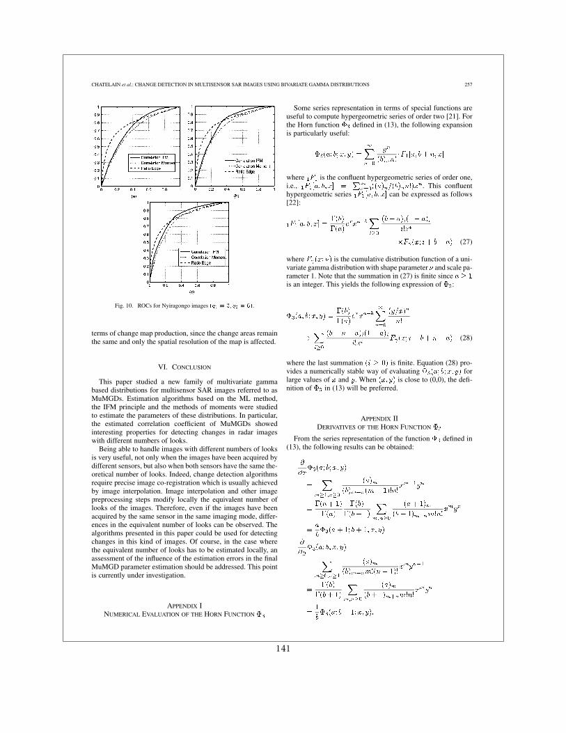
CHATELAIN et al.: CHANGE DETECTION IN MULTISENSOR SAR IMAGES USING BIVARIATE GAMMA DISTRIBUTIONS 257
Fig. 10. ROCs for Nyiragongo images (q = 3; q = 6).
terms of change map production, since the change areas remainthe same and only the spatial resolution of the map is affected.
VI. CONCLUSION
This paper studied a new family of multivariate gammabased distributions for multisensor SAR images referred to asMuMGDs. Estimation algorithms based on the ML method,the IFM principle and the methods of moments were studiedto estimate the parameters of these distributions. In particular,the estimated correlation coefficient of MuMGDs showedinteresting properties for detecting changes in radar imageswith different numbers of looks.
Being able to handle images with different numbers of looksis very useful, not only when the images have been acquired bydifferent sensors, but also when both sensors have the same the-oretical number of looks. Indeed, change detection algorithmsrequire precise image co-registration which is usually achievedby image interpolation. Image interpolation and other imagepreprocessing steps modify locally the equivalent number oflooks of the images. Therefore, even if the images have beenacquired by the same sensor in the same imaging mode, differ-ences in the equivalent number of looks can be observed. Thealgorithms presented in this paper could be used for detectingchanges in this kind of images. Of course, in the case wherethe equivalent number of looks has to be estimated locally, anassessment of the influence of the estimation errors in the finalMuMGD parameter estimation should be addressed. This pointis currently under investigation.
APPENDIX INUMERICAL EVALUATION OF THE HORN FUNCTION
Some series representation in terms of special functions areuseful to compute hypergeometric series of order two [21]. Forthe Horn function defined in (13), the following expansionis particularly useful:
where is the confluent hypergeometric series of order one,i.e., . This confluenthypergeometric series can be expressed as follows[22]:
(27)
where is the cumulative distribution function of a uni-variate gamma distribution with shape parameter and scale pa-rameter 1. Note that the summation in (27) is finite sinceis an integer. This yields the following expression of :
(28)
where the last summation is finite. Equation (28) pro-vides a numerically stable way of evaluating forlarge values of and . When is close to (0,0), the defi-nition of in (13) will be preferred.
APPENDIX IIDERIVATIVES OF THE HORN FUNCTION
From the series representation of the function defined in(13), the following results can be obtained:
141
258 IEEE TRANSACTIONS ON IMAGE PROCESSING, VOL. 17, NO. 3, MARCH 2008
REFERENCES
[1] J. Inglada, “Similarity measures for multisensor remote sensing im-ages,” in Proc. IEEE IGARSS, Toronto, ON, Canada, Jun. 2002, pp.104–106.
[2] J. Inglada and A. Giros, “On the possibility of automatic multi-sensorimage registration,” IEEE Trans. Geosci. Remote Sens., vol. 42, no. 10,pp. 2104–2120, Oct. 2004.
[3] T. F. Bush and F. T. Ulaby, “Fading characteristics of panchromaticradar backscatter from selected agricultural targets,” IEEE Trans.Geosci. Remote Sens., vol. 13, no. 4, pp. 149–157, Apr. 1975.
[4] S. B. Lev, D. Bshouty, P. Enis, G. Letac, I. L. Lu, and D. Richards,“The diagonal natural exponential families and their classification,” J.Oftheoret. Probab., vol. 7, no. 4, pp. 883–928, Oct. 1994.
[5] P. Bernardoff, “Which multivariate gamma distributions are infinitelydivisible?,” Bernoulli, vol. 12, no. 1, pp. 169–189, 2006.
[6] F. Chatelain, J.-Y. Tourneret, A. Ferrari, and J. Inglada, “Bivariategamma distributions for image registration and change detection,”IEEE Trans. Image Process., vol. 16, no. 7, pp. 169–1796, Jul. 2006.
[7] F. Chatelain, J.-Y. Tourneret, J. Inglada, and A. Ferrari, “Parameterestimation for multivariate gamma distributions. Application to imageregistration,” presented at the EUSIPCO, Florence, Italy, Sep. 2006.
[8] S. Kotz, N. Balakrishnan, and N. L. Johnson, Continuous MultivariateDistributions, 2nd ed. New York: Wiley, 2000, vol. 1.
[9] F. O. A. Erdlyi, W. Magnus, and F. Tricomi, Higher TranscendentalFunctions. New York: Krieger, 1981, vol. 1.
[10] B. G. Lindsay, “Composite likelihood methods,” Contempory Math.,vol. 50, pp. 221–239, 1988.
[11] C. C. Heyde, Quasi-Likelihood and Its Application. A General Ap-proach to Optimal Parameter Estimation. New York: Springer, 1997.
[12] F. Chatelain and J.-Y. Tourneret, “Composite likelihood estimation formultivariate mixed Poisson distributions,” in Proc. IEEE-SP WorkshopStatist. Signal Processing, Bordeaux, France, Jul. 2005, pp. 49–54.
[13] F. Chatelain and J.-Y. Tourneret, “Estimating the correlation coeffi-cient of bivariate gamma distributions using the maximum likelihoodprinciple and the inference functions for margins,” Tech. Rep., Univ.Toulouse (IRIT/ENSEEIHT), Toulouse, France, May 2007 [Online].Available: http://florent.chatelain.free.fr/Publi/ChatelainTechRe-port07.pdf, available at
[14] H. Joe, Multivariate Models and Dependence Concepts. London,U.K.: Chapman & Hall, May 1997, vol. 73.
[15] H. Joe, “Asymptotic efficiency of the two-stage estimation method forcopula-based models,” J. Multivar. Anal., vol. 94, no. 2, pp. 401–419,2005.
[16] B. Porat and B. Friedlander, “Performance analysis of parameter esti-mation algorithms based on high-order moments,” Int. J. Adapt. Con-trol Signal Process., vol. 3, pp. 191–229, 1989.
[17] C. P. Robert and G. Casella, Monte Carlo Statistical Methods, 2nded. New York: Springer, 2004.
[18] H. L. Van Trees, Detection, Estimation, and Modulation Theory: PartI. New York: Wiley, 1968.
[19] R. Touzi, A. Lopés, and P. Bousquet, “A statistical and geometricaledge detector for SAR images,” IEEE Trans. Geosci. Remote Sens.,vol. 26, no. 6, pp. 764–773, Nov. 1988.
[20] E. J. M. Rignot and J. J. van Zyl, “Change detection techniques forERS-1 SAR data,” IEEE Trans. Geosci. Remote Sens., vol. 31, no. 4,pp. 896–906, Apr. 1993.
[21] F. D. Colavecchia and G. Gasaneo, “FL: A code to compute Appell’sF hypergeometric function,” Comput. Phys. Commun., vol. 157, pp.32–38, Feb. 2004.
[22] K. E. Muller, “Computing the confluent hypergeometric function,M (a,b, x),” Numer. Math., vol. 90, no. 1, pp. 179–196, Nov. 2001.
Florent Chatelain received the Eng. degree incomputer sciences and applied mathematics fromENSIMAG, Grenoble, France, and the M.Sc. degreein applied mathematics from the University JosephFourier of Grenoble, France, both in June 2004,and the Ph.D. degree in signal processing from theSignal and Communication Group, IRIT Laboratory,National Polytechnic Institute of Toulouse, France,in 2007.
He is currently a Postdoctoral Researcher at theINRIA Sophia Antipolis Mediterranée Laboratory,
France, within the Ariana group. His research interests are centered aroundmultivariate statistics applied to image processing and applications of stochasticgeometry to the analysis of images.
Jean-Yves Tourneret received the Ingénieur degreein electrical engineering from the Ecole NationaleSupérieure d’Electronique, d’Electrotechnique,d’Informatique et d’Hydraulique, Toulouse (EN-SEEIHT), France, and the Ph.D. degree from theNational Polytechnic Institute, Toulouse, in 1992.
He is currently a Professor with the University ofToulouse (ENSEEIHT). He is a member of the IRITLaboratory (UMR 5505 of the CNRS), where his re-search activity is centered around estimation, detec-tion, and the classification of non-Gaussian and non-
stationary processes.Dr. Tourneret was the Program Chair of the European Conference on Signal
Processing (EUSIPCO), which was held in Toulouse, France, in 2002. He wasalso a member of the organizing committee for the International Conference onAcoustics, Speech, and Signal Processing (ICASSP) held in Toulouse in 2006.He has been a member of different technical committees, including the SignalProcessing Theory and Methods (SPTM) Committee of the IEEE Signal Pro-cessing Society.
Jordi Inglada received the Telecommunicationsengineer degree from the Universitat Politècnicade Catalunya, Spain, and from the École NationaleSupérieure des Télécommunications de Bretagne,France, in 1997, and the Ph.D. degree in signal pro-cessing and telecommunications from the Universitéde Rennes 1, France, in 2000.
He is with the Centre National d’Études Spatiales,French Space Agency, Toulouse, France, where heworks in the field of remote sensing image pro-cessing. He is in charge of the development of image
processing algorithms for the operational exploitation of Earth Observationimages, mainly in the fields of image registration, change detection, and objectrecognition.
142
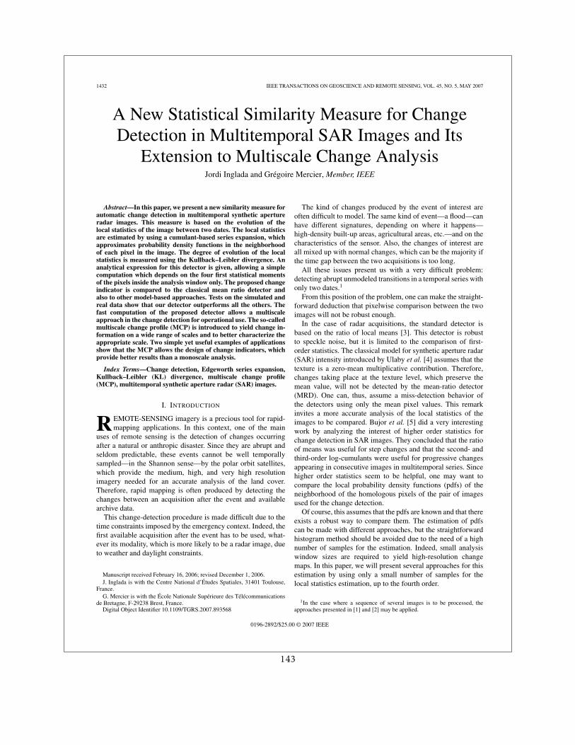
1432 IEEE TRANSACTIONS ON GEOSCIENCE AND REMOTE SENSING, VOL. 45, NO. 5, MAY 2007
A New Statistical Similarity Measure for ChangeDetection in Multitemporal SAR Images and Its
Extension to Multiscale Change AnalysisJordi Inglada and Grégoire Mercier, Member, IEEE
Abstract—In this paper, we present a new similarity measure forautomatic change detection in multitemporal synthetic apertureradar images. This measure is based on the evolution of thelocal statistics of the image between two dates. The local statisticsare estimated by using a cumulant-based series expansion, whichapproximates probability density functions in the neighborhoodof each pixel in the image. The degree of evolution of the localstatistics is measured using the Kullback–Leibler divergence. Ananalytical expression for this detector is given, allowing a simplecomputation which depends on the four first statistical momentsof the pixels inside the analysis window only. The proposed changeindicator is compared to the classical mean ratio detector andalso to other model-based approaches. Tests on the simulated andreal data show that our detector outperforms all the others. Thefast computation of the proposed detector allows a multiscaleapproach in the change detection for operational use. The so-calledmultiscale change profile (MCP) is introduced to yield change in-formation on a wide range of scales and to better characterize theappropriate scale. Two simple yet useful examples of applicationsshow that the MCP allows the design of change indicators, whichprovide better results than a monoscale analysis.
Index Terms—Change detection, Edgeworth series expansion,Kullback–Leibler (KL) divergence, multiscale change profile(MCP), multitemporal synthetic aperture radar (SAR) images.
I. INTRODUCTION
R EMOTE-SENSING imagery is a precious tool for rapid-mapping applications. In this context, one of the main
uses of remote sensing is the detection of changes occurringafter a natural or anthropic disaster. Since they are abrupt andseldom predictable, these events cannot be well temporallysampled—in the Shannon sense—by the polar orbit satellites,which provide the medium, high, and very high resolutionimagery needed for an accurate analysis of the land cover.Therefore, rapid mapping is often produced by detecting thechanges between an acquisition after the event and availablearchive data.
This change-detection procedure is made difficult due to thetime constraints imposed by the emergency context. Indeed, thefirst available acquisition after the event has to be used, what-ever its modality, which is more likely to be a radar image, dueto weather and daylight constraints.
Manuscript received February 16, 2006; revised December 1, 2006.J. Inglada is with the Centre National d’Études Spatiales, 31401 Toulouse,
France.G. Mercier is with the École Nationale Supérieure des Télécommunications
de Bretagne, F-29238 Brest, France.Digital Object Identifier 10.1109/TGRS.2007.893568
The kind of changes produced by the event of interest areoften difficult to model. The same kind of event—a flood—canhave different signatures, depending on where it happens—high-density built-up areas, agricultural areas, etc.—and on thecharacteristics of the sensor. Also, the changes of interest areall mixed up with normal changes, which can be the majority ifthe time gap between the two acquisitions is too long.
All these issues present us with a very difficult problem:detecting abrupt unmodeled transitions in a temporal series withonly two dates.1
From this position of the problem, one can make the straight-forward deduction that pixelwise comparison between the twoimages will not be robust enough.
In the case of radar acquisitions, the standard detector isbased on the ratio of local means [3]. This detector is robustto speckle noise, but it is limited to the comparison of first-order statistics. The classical model for synthetic aperture radar(SAR) intensity introduced by Ulaby et al. [4] assumes that thetexture is a zero-mean multiplicative contribution. Therefore,changes taking place at the texture level, which preserve themean value, will not be detected by the mean-ratio detector(MRD). One can, thus, assume a miss-detection behavior ofthe detectors using only the mean pixel values. This remarkinvites a more accurate analysis of the local statistics of theimages to be compared. Bujor et al. [5] did a very interestingwork by analyzing the interest of higher order statistics forchange detection in SAR images. They concluded that the ratioof means was useful for step changes and that the second- andthird-order log-cumulants were useful for progressive changesappearing in consecutive images in multitemporal series. Sincehigher order statistics seem to be helpful, one may want tocompare the local probability density functions (pdfs) of theneighborhood of the homologous pixels of the pair of imagesused for the change detection.
Of course, this assumes that the pdfs are known and that thereexists a robust way to compare them. The estimation of pdfscan be made with different approaches, but the straightforwardhistogram method should be avoided due to the need of a highnumber of samples for the estimation. Indeed, small analysiswindow sizes are required to yield high-resolution changemaps. In this paper, we will present several approaches for thisestimation by using only a small number of samples for thelocal statistics estimation, up to the fourth order.
1In the case where a sequence of several images is to be processed, theapproaches presented in [1] and [2] may be applied.
0196-2892/$25.00 © 2007 IEEE
143
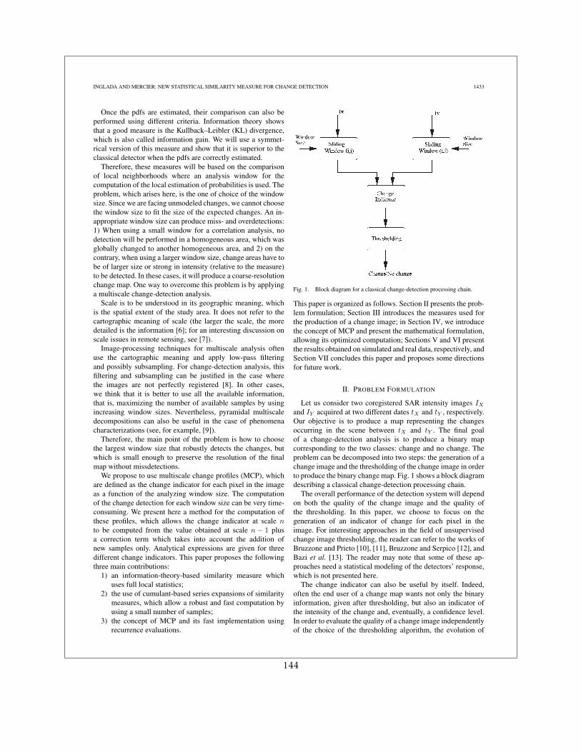
INGLADA AND MERCIER: NEW STATISTICAL SIMILARITY MEASURE FOR CHANGE DETECTION 1433
Once the pdfs are estimated, their comparison can also beperformed using different criteria. Information theory showsthat a good measure is the Kullback–Leibler (KL) divergence,which is also called information gain. We will use a symmet-rical version of this measure and show that it is superior to theclassical detector when the pdfs are correctly estimated.
Therefore, these measures will be based on the comparisonof local neighborhoods where an analysis window for thecomputation of the local estimation of probabilities is used. Theproblem, which arises here, is the one of choice of the windowsize. Since we are facing unmodeled changes, we cannot choosethe window size to fit the size of the expected changes. An in-appropriate window size can produce miss- and overdetections:1) When using a small window for a correlation analysis, nodetection will be performed in a homogeneous area, which wasglobally changed to another homogeneous area, and 2) on thecontrary, when using a larger window size, change areas have tobe of larger size or strong in intensity (relative to the measure)to be detected. In these cases, it will produce a coarse-resolutionchange map. One way to overcome this problem is by applyinga multiscale change-detection analysis.
Scale is to be understood in its geographic meaning, whichis the spatial extent of the study area. It does not refer to thecartographic meaning of scale (the larger the scale, the moredetailed is the information [6]; for an interesting discussion onscale issues in remote sensing, see [7]).
Image-processing techniques for multiscale analysis oftenuse the cartographic meaning and apply low-pass filteringand possibly subsampling. For change-detection analysis, thisfiltering and subsampling can be justified in the case wherethe images are not perfectly registered [8]. In other cases,we think that it is better to use all the available information,that is, maximizing the number of available samples by usingincreasing window sizes. Nevertheless, pyramidal multiscaledecompositions can also be useful in the case of phenomenacharacterizations (see, for example, [9]).
Therefore, the main point of the problem is how to choosethe largest window size that robustly detects the changes, butwhich is small enough to preserve the resolution of the finalmap without missdetections.
We propose to use multiscale change profiles (MCP), whichare defined as the change indicator for each pixel in the imageas a function of the analyzing window size. The computationof the change detection for each window size can be very time-consuming. We present here a method for the computation ofthese profiles, which allows the change indicator at scale nto be computed from the value obtained at scale n − 1 plusa correction term which takes into account the addition ofnew samples only. Analytical expressions are given for threedifferent change indicators. This paper proposes the followingthree main contributions:
1) an information-theory-based similarity measure whichuses full local statistics;
2) the use of cumulant-based series expansions of similaritymeasures, which allow a robust and fast computation byusing a small number of samples;
3) the concept of MCP and its fast implementation usingrecurrence evaluations.
Fig. 1. Block diagram for a classical change-detection processing chain.
This paper is organized as follows. Section II presents the prob-lem formulation; Section III introduces the measures used forthe production of a change image; in Section IV, we introducethe concept of MCP and present the mathematical formulation,allowing its optimized computation; Sections V and VI presentthe results obtained on simulated and real data, respectively, andSection VII concludes this paper and proposes some directionsfor future work.
II. PROBLEM FORMULATION
Let us consider two coregistered SAR intensity images IX
and IY acquired at two different dates tX and tY , respectively.Our objective is to produce a map representing the changesoccurring in the scene between tX and tY . The final goalof a change-detection analysis is to produce a binary mapcorresponding to the two classes: change and no change. Theproblem can be decomposed into two steps: the generation of achange image and the thresholding of the change image in orderto produce the binary change map. Fig. 1 shows a block diagramdescribing a classical change-detection processing chain.
The overall performance of the detection system will dependon both the quality of the change image and the quality ofthe thresholding. In this paper, we choose to focus on thegeneration of an indicator of change for each pixel in theimage. For interesting approaches in the field of unsupervisedchange image thresholding, the reader can refer to the works ofBruzzone and Prieto [10], [11], Bruzzone and Serpico [12], andBazi et al. [13]. The reader may note that some of these ap-proaches need a statistical modeling of the detectors’ response,which is not presented here.
The change indicator can also be useful by itself. Indeed,often the end user of a change map wants not only the binaryinformation, given after thresholding, but also an indicator ofthe intensity of the change and, eventually, a confidence level.In order to evaluate the quality of a change image independentlyof the choice of the thresholding algorithm, the evolution of
144
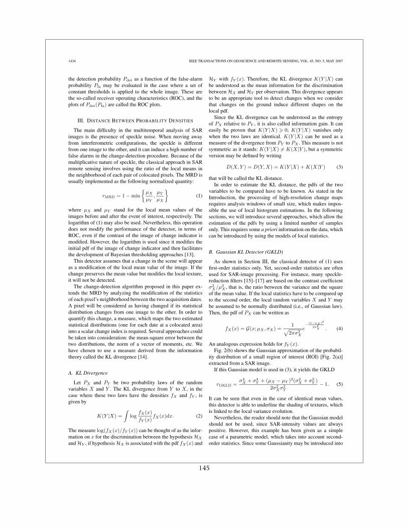
1434 IEEE TRANSACTIONS ON GEOSCIENCE AND REMOTE SENSING, VOL. 45, NO. 5, MAY 2007
the detection probability Pdet as a function of the false-alarmprobability Pfa may be evaluated in the case where a set ofconstant thresholds is applied to the whole image. These arethe so-called receiver operating characteristics (ROC), and theplots of Pdet(Pfa) are called the ROC plots.
III. DISTANCE BETWEEN PROBABILITY DENSITIES
The main difficulty in the multitemporal analysis of SARimages is the presence of speckle noise. When moving awayfrom interferometric configurations, the speckle is differentfrom one image to the other, and it can induce a high number offalse alarms in the change-detection procedure. Because of themultiplicative nature of speckle, the classical approach in SARremote sensing involves using the ratio of the local means inthe neighborhood of each pair of colocated pixels. The MRD isusually implemented as the following normalized quantity:
rMRD = 1 − min
{µX
µY,µY
µX
}(1)
where µX and µY stand for the local mean values of theimages before and after the event of interest, respectively. Thelogarithm of (1) may also be used. Nevertheless, this operationdoes not modify the performance of the detector, in terms ofROC, even if the contrast of the image of change indicator ismodified. However, the logarithm is used since it modifies theinitial pdf of the image of change indicator and then facilitatesthe development of Bayesian thresholding approaches [13].
This detector assumes that a change in the scene will appearas a modification of the local mean value of the image. If thechange preserves the mean value but modifies the local texture,it will not be detected.
The change-detection algorithm proposed in this paper ex-tends the MRD by analyzing the modification of the statisticsof each pixel’s neighborhood between the two acquisition dates.A pixel will be considered as having changed if its statisticaldistribution changes from one image to the other. In order toquantify this change, a measure, which maps the two estimatedstatistical distributions (one for each date at a colocated area)into a scalar change index is required. Several approaches couldbe taken into consideration: the mean-square error between thetwo distributions, the norm of a vector of moments, etc. Wehave chosen to use a measure derived from the informationtheory called the KL divergence [14].
A. KL Divergence
Let PX and PY be two probability laws of the randomvariables X and Y . The KL divergence from Y to X , in thecase where these two laws have the densities fX and fY , isgiven by
K(Y |X) =
∫log
fX(x)
fY (x)fX(x)dx. (2)
The measure log(fX(x)/fY (x)) can be thought of as the infor-mation on x for the discrimination between the hypothesis HX
and HY , if hypothesis HX is associated with the pdf fX(x) and
HY with fY (x). Therefore, the KL divergence K(Y |X) canbe understood as the mean information for the discriminationbetween HX and HY per observation. This divergence appearsto be an appropriate tool to detect changes when we considerthat changes on the ground induce different shapes on thelocal pdf.
Since the KL divergence can be understood as the entropyof PX relative to PY , it is also called information gain. It caneasily be proven that K(Y |X) � 0; K(Y |X) vanishes onlywhen the two laws are identical. K(Y |X) can be used as ameasure of the divergence from PY to PX . This measure is notsymmetric as it stands: K(Y |X) �= K(X|Y ), but a symmetricversion may be defined by writing
D(X,Y ) = D(Y,X) = K(Y |X) + K(X|Y ) (3)
that will be called the KL distance.In order to estimate the KL distance, the pdfs of the two
variables to be compared have to be known. As stated in theIntroduction, the processing of high-resolution change mapsrequires analysis windows of small size, which makes impos-sible the use of local histogram estimations. In the followingsections, we will introduce several approaches, which allow theestimation of the pdfs by using a limited number of samplesonly. This requires some a priori information on the data, whichcan be introduced by using the models of local statistics.
B. Gaussian KL Detector (GKLD)
As shown in Section III, the classical detector of (1) usesfirst-order statistics only. Yet, second-order statistics are oftenused for SAR-image processing. For instance, many speckle-reduction filters [15]–[17] are based on the contrast coefficientσ2
X/µ2X , that is, the ratio between the variance and the square
of the mean value. If the local statistics have to be compared upto the second order, the local random variables X and Y maybe assumed to be normally distributed (i.e., of Gaussian law).Then, the pdf of PX can be written as
fX(x) = G(x;µX , σX) =1√
2πσ2X
e− (x−µX )2
2σ2X . (4)
An analogous expression holds for fY (x).Fig. 2(b) shows the Gaussian approximation of the probabil-
ity distribution of a small region of interest (ROI) [Fig. 2(a)]extracted from a SAR image.
If this Gaussian model is used in (3), it yields the GKLD
rGKLD =σ4
X + σ4Y + (µX − µY )2(σ2
X + σ2Y )
2σ2Xσ2
Y
− 1. (5)
It can be seen that even in the case of identical mean values,this detector is able to underline the shading of textures, whichis linked to the local variance evolution.
Nevertheless, the reader should note that the Gaussian modelshould not be used, since SAR-intensity values are alwayspositive. However, this example has been given as a simplecase of a parametric model, which takes into account second-order statistics. Since some Gaussianity may be introduced into
145
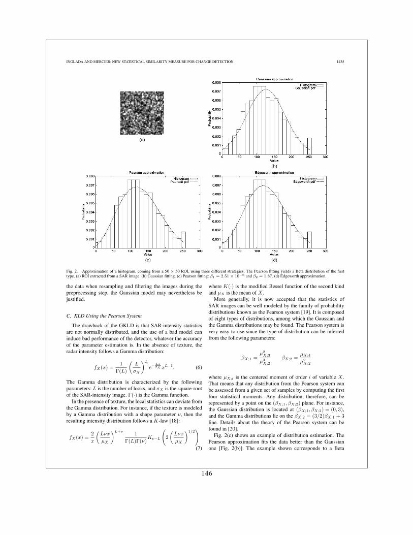
INGLADA AND MERCIER: NEW STATISTICAL SIMILARITY MEASURE FOR CHANGE DETECTION 1435
Fig. 2. Approximation of a histogram, coming from a 50 × 50 ROI, using three different strategies. The Pearson fitting yields a Beta distribution of the firsttype. (a) ROI extracted from a SAR image. (b) Gaussian fitting. (c) Pearson fitting: β1 = 2.51 × 10⁻⁶ and β2 = 1.87. (d) Edgeworth approximation.
the data when resampling and filtering the images during thepreprocessing step, the Gaussian model may nevertheless bejustified.
C. KLD Using the Pearson System
The drawback of the GKLD is that SAR-intensity statisticsare not normally distributed, and the use of a bad model caninduce bad performance of the detector, whatever the accuracyof the parameter estimation is. In the absence of texture, theradar intensity follows a Gamma distribution:
fX(x) =1
Γ(L)
(L
σX
)L
e− Lx
σX xL−1. (6)
The Gamma distribution is characterized by the followingparameters: L is the number of looks, and σX is the square-rootof the SAR-intensity image. Γ(·) is the Gamma function.
In the presence of texture, the local statistics can deviate fromthe Gamma distribution. For instance, if the texture is modeledby a Gamma distribution with a shape parameter ν, then theresulting intensity distribution follows a K-law [18]:
fX(x) =2
x
(Lνx
µX
)L+ν1
Γ(L)Γ(ν)Kν−L
(2
(Lνx
µX
)1/2)
(7)
where K(·) is the modified Bessel function of the second kindand µX is the mean of X .
More generally, it is now accepted that the statistics ofSAR images can be well modeled by the family of probabilitydistributions known as the Pearson system [19]. It is composedof eight types of distributions, among which the Gaussian andthe Gamma distributions may be found. The Pearson system isvery easy to use since the type of distribution can be inferredfrom the following parameters:
βX;1 =µ2
X;3
µ3X;2
βX;2 =µX;4
µ2X;2
where µX;i is the centered moment of order i of variable X .That means that any distribution from the Pearson system canbe assessed from a given set of samples by computing the firstfour statistical moments. Any distribution, therefore, can berepresented by a point on the (βX;1, βX;2) plane. For instance,the Gaussian distribution is located at (βX;1, βX;2) = (0, 3),and the Gamma distributions lie on the βX;2 = (3/2)βX;1 + 3line. Details about the theory of the Pearson system can befound in [20].
Fig. 2(c) shows an example of distribution estimation. ThePearson approximation fits the data better than the Gaussianone [Fig. 2(b)]. The example shown corresponds to a Beta
146
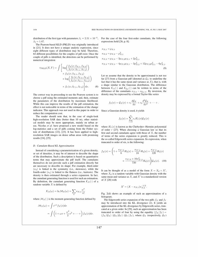
1436 IEEE TRANSACTIONS ON GEOSCIENCE AND REMOTE SENSING, VOL. 45, NO. 5, MAY 2007
distribution of the first type with parameters β1 = 2.51 × 10⁻⁶,β2 = 1.87.
The Pearson-based KLD (PKLD) was originally introducedin [21]. It does not have a unique analytic expression, sinceeight different types of distribution may be held. Therefore,64 different possibilities for the couples of pdf exist. Once thecouple of pdfs is identified, the detection can be performed bynumerical integration
rPKLD(X,Y ) =
∫ [log
(fX(x;βX;1, βX;2)
fY (x;βY ;1, βY ;2)
)
× fX(x;βX;1, βX;2)
+ log
(fY (x;βY ;1, βY ;2)
fX(x;βX;1, βX;2)
)
× fY (x;βY ;1, βY ;2)
]dx. (8)
The correct way in proceeding to use the Pearson system is tochoose a pdf using the estimated moments and, then, estimatethe parameters of the distribution by maximum likelihood.While this can improve the results of the pdf estimation, theeffect is not noticeable in terms of the estimation of the changeindicator. This approach was not used in this paper in order toreduce the computation cost.
The reader should note that, in the case of single-lookhigh-resolution SAR data (better than 10 m), other statisti-cal models may be more appropriate, mainly on urban ar-eas. Nicolas et al. have proposed a new model based on thelog-statistics and a set of pdfs coming from the Fisher sys-tem of distributions [22], [23]. It has been applied to high-resolution SAR images on dense urban areas with promisingresults [24], [25].
D. Cumulant-Based KL Approximation
Instead of considering a parameterization of a given density,or set of densities, it may be of interest to describe the shapeof the distribution. Such a description is based on quantitativeterms that may approximate the pdf itself. The cumulantsthemselves do not provide such a pdf estimation directly butare necessary to describe its shape: For example, third-order(κ3) is linked to the symmetry (i.e., skewness), while thefourth-order (κ4) is linked to the flatness (i.e., kurtosis). Thedensity is then estimated through a series expansion. In fact,the cumulant generating function is used for such an estimation.By definition, the cumulant generating function KX(·) of arandom variable X is defined by
KX(ω) = lnMX(ω) =∑
n
κX;nωn
n!
where MX(·) is the moment-generating function defined by
MX(ω) =
∫eωxfX(x)dx
=
∫ (1 + ωx +
ω2
2x2 + · · · +
)fX(x)dx.
For the case of the four first-order cumulants, the followingexpressions hold [26, p. 8]:
κX;1 =µX;1
κX;2 =µX;2 − µ2X;1
κX;3 =µX;3 − 3µX;2µX;1 + 2µ3X;1
κX;4 =µX;4 − 4µX;3µX;1 − 3µ2X;2 + 12µX;2µ
2X;1 − 6µ4
X;1.
(9)
Let us assume that the density to be approximated is not toofar [27] from a Gaussian pdf (denoted as GX to underline thefact that it has the same mean and variance as X), that is, witha shape similar to the Gaussian distribution. The differencebetween KX(·) and KGX (·) can be written in terms of thedifference of the cumulants κX;n − κGX ;n. By inversion, thedensity may be expressed by a formal Taylor-like series
fX(x) = GX(x) + c1dGX
dx+ c2
d2GX
dx2+ · · · + .
Since a Gaussian density is used, it yields
fX(x) =
∞∑
r=0
crHr(x)GX(x)
where Hr(x) is known as the Chebyshev–Hermite polynomialof order r [27]. When choosing a Gaussian law so that itsfirst and second cumulants agree with those of X , the numberof terms of the series expansion is greatly reduced. This isthe so-called Edgeworth series expansion. Its expression, whentruncated to order of six, is the following:
fX(x) =
(1 +
κX′;3
6H3(x) +
κX′;4
24H4(x) +
κX′;5
120H5(x)
+κX′;6 + 10κ2
X′;3
720H6(x)
)GX(x). (10)
It can be thought of as a model of the form X = XG + X ′,where XG is a random variable with Gaussian density with thesame mean and variance as X , and X ′ is a standardized versionof X [28] with
X ′ = (X − κX;1)κ−1/2X;2 .
Fig. 2(d) shows an example of such an approximation of ahistogram.
The Edgeworth series expansion of the two pdfs fX and fY
may be introduced into the KL divergence (2). It yields anapproximation of the KL divergence by Edgeworth series, trun-cated at a given order. In [29], such an approximation has beentruncated to order of four by using the equality (fX/fY ) =(fX/GX) (GX/GY ) (GY /fY ), where GX (respectively, GY )
147
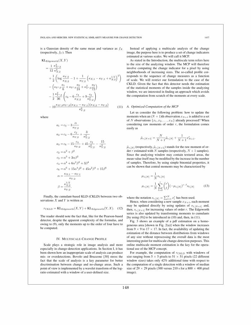
INGLADA AND MERCIER: NEW STATISTICAL SIMILARITY MEASURE FOR CHANGE DETECTION 1437
is a Gaussian density of the same mean and variance as fX
(respectively, fY ). Then
KLEdgeworth(X,Y )
=1
12
κ2X′;3
κ2X;2
+1
2
(log
κY ;2
κX;2− 1 +
1
κY ;2
(κX;1 − κY ;1 + κ
1/2X;2
)2)
−(κY ′;3
a1
6+ κY ′;4
a2
24+ κ2
Y ′;3a3
72
)
− 1
2
κ2Y ′;3
36
(c6 − 6
c4κX;2
+ 9c2
κ2Y ;2
)
− 10κX′;3κY ′;3(κX;1 − κY ;1)(κX;2 − κY ;2)
κ6Y ;2
(11)
where
a1 = c3 − 3α
κY ;2
a2 = c4 − 6c2
κY ;2+
3
κ2Y ;2
a3 = c6 − 15c4
κY ;2+ 45
c2κ2
Y ;2
− 15
κ3Y ;2
c2 =α2 + β2
c3 =α3 + 3αβ2
c4 =α4 + 6α2β2 + 3β4
c6 =α6 + 15α4β2 + 45α2β4 + 15β6
α =κX;1 − κY ;1
κY ;2
β =κ
1/2X;2
κY ;2.
Finally, the cumulant-based KLD (CKLD) between two ob-servations X and Y is written as
rCKLD = KLEdgeworth(X,Y ) + KLEdgeworth(Y,X). (12)
The reader should note the fact that, like for the Pearson-baseddetector, despite the apparent complexity of the formulas, andowing to (9), only the moments up to the order of four have tobe computed.
IV. MULTISCALE-CHANGE PROFILE
Scale plays a strategic role in image analysis and moreespecially in change-detection applications. In Section I, it hasbeen shown how an inappropriate scale of analysis can producemis- or overdetections. Bovolo and Bruzzone [30] stress thefact that the scale of analysis is a key parameter for betterdiscrimination between change and no-change areas. Such apoint of view is implemented by a wavelet transform of the log-ratio estimated with a window of a user-defined size.
Instead of applying a multiscale analysis of the changeimage, the purpose here is to produce a set of change indicatorsestimated at various scales. We will call it MCP.
As stated in the Introduction, the multiscale term refers hereto the size of the analyzing window. The MCP will thereforeinvolve computing the change indicator for a pixel by usingneighborhoods of increasing sizes. The so-called profile cor-responds to the sequence of change measures as a functionof scale. We will restrict our formulation to the case of theCKLD. Given the fact that this detector needs the estimationof the statistical moments of the samples inside the analyzingwindow, we are interested in finding an approach which avoidsthe computation from scratch of the moments at every scale.
A. Optimized Computation of the MCP
Let us consider the following problem: how to update themoments when an (N + 1)th observation xN+1 is added to a setof N observations {x1, x2, . . . , xN} already processed? Whenconsidering raw moments of order r, the formulation comeseasily as
µr,[N+1] =N
N + 1µr,[N ] +
1
N + 1xr
N+1.
µr,[N ] (respectively, µr,[N+1]) stands for the raw moment of or-der r estimated with N samples (respectively, N + 1 samples).Since the analyzing window may contain textured areas, themean value itself may be modified by the increase in the numberof samples. Therefore, by using simple binomial properties, itcan be shown that central moments may be characterized by
µ1,[N ] =1
Ns1,[N ]
µr,[N ] =1
N
r∑
=0
(r
)(−µ1,[N ])
r− s ,[N ] (13)
where the notation sr,[N ] =∑N
i=1 xri has been used.
Hence, when considering a new sample xN+1, each momentmay be updated directly by using updates of s1,[N+1] and,then, sr,[N+1] for increasing values of order r. The Edgeworthseries is also updated by transforming moments to cumulants[by using (9)] to be introduced in (10) and, then, in (11).
Fig. 3 shows an example of a pdf estimation on a homo-geneous area [shown in Fig. 2(a)] when the window increasesfrom 9 × 9 to 17 × 17. In fact, the availability of updating theestimation of the distance between distributions from windowsof any size without reprocessing the overall data is the mostinteresting point for multiscale change-detection purposes. Thisonline multiscale moment estimation is the key for the opera-tional use of the MCP concept.
For example, the computation of rCKLD with windows ofsize ranging from 5 × 5 pixels to 51 × 51 pixels (22 differentwindow sizes) takes only 42% additional time with respect tothe computation of a single detection with a window of mediansize of 29 × 29 pixels (300 versus 210 s for a 800 × 400 pixelimage).
148
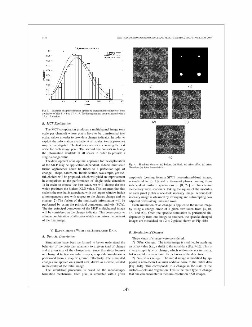
1438 IEEE TRANSACTIONS ON GEOSCIENCE AND REMOTE SENSING, VOL. 45, NO. 5, MAY 2007
Fig. 3. Example of a pdf estimation update by increasing the sample set froma window of size 9 × 9 to 17 × 17. The histogram has been estimated with a17 × 17 window.
B. MCP Exploitation
The MCP computation produces a multichannel image (onescale per channel) whose pixels have to be transformed intoscalar values in order to provide a change indicator. In order toexploit the information available at all scales, two approachesmay be investigated. The first one consists in choosing the bestscale for each image pixel. The second one consists in fusingthe information available at all scales in order to provide asingle-change value.
The development of an optimal approach for the exploitationof the MCP may be application-dependent. Indeed, multiscalefusion approaches could be tuned to a particular type ofchange—shape, nature, etc. In this section, two simple, yet use-ful, choices will be proposed, which will yield an improvementin comparison to the performance of single scale detection:1) In order to choose the best scale, we will choose the onewhich produces the highest KLD value. This assumes that thisscale is the one that is associated with the largest window insidea homogeneous area with respect to the classes change and nochange. 2) The fusion of the multiscale information will beperformed by using the principal component analysis (PCA).The first principal component of the MCP multichannel imagewill be considered as the change indicator. This corresponds toa linear combination of all scales which maximizes the contrastof the final image.
V. EXPERIMENTS WITH THE SIMULATED DATA
A. Data-Set Description
Simulations have been performed to better understand thebehavior of the detectors relatively to a given kind of changeand a given size of the change area. Since this study focuseson change detection on radar images, a speckle simulation isperformed from a map of ground reflectivity. The simulatedchanges are applied on a small area, drawn as a circle, locatedin the center of the initial image.
The simulation procedure is based on the radar-image-formation mechanism. Each pixel is simulated with a given
Fig. 4. Simulated data set. (a) Before. (b) Mask. (c) After offset. (d) AfterGaussian. (e) After deterministic.
amplitude (coming from a SPOT near-infrared-band image,normalized to [0, 1]) and a thousand phases coming fromindependent uniform generations in [0, 2π] to characterizeelementary wave scatterers. Taking the square of the modulusof each pixel yields a one-look intensity image. A four-lookintensity image is obtained by averaging and subsampling twoadjacent pixels along lines and rows.
Each simulation of an change is applied to the initial imageby using a change circle of a given size taken from {5, 10,15, and 20}. Once the speckle simulation is performed (in-dependently from one image to another), the speckle-changedimages are mosaicked on a 2 × 2 grid as shown on Fig. 4(b).
B. Simulation of Changes
Three kinds of change were considered.1) Offset Change: The initial image is modified by applying
an offset value (i.e., a shift) to the inital data [Fig. 4(c)]. This isa very simple type of change, which seldom occurs in reality,but is useful to characterize the behavior of the detectors.
2) Gaussian Change: The initial image is modified by ap-plying a zero-mean Gaussian additive noise to the initial data[Fig. 4(d)]. This corresponds to a change in the state of thesurface—field and vegetation. This is the main type of changethat one can encounter in medium-resolution SAR images.
149
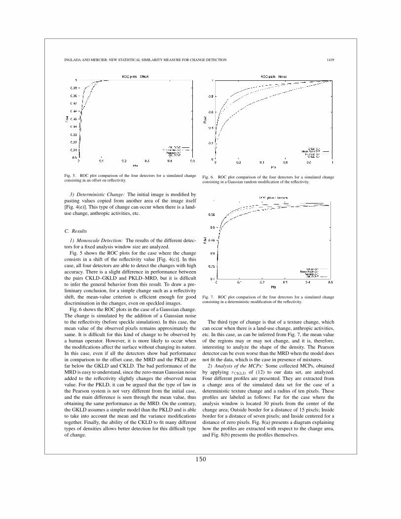
INGLADA AND MERCIER: NEW STATISTICAL SIMILARITY MEASURE FOR CHANGE DETECTION 1439
Fig. 5. ROC plot comparison of the four detectors for a simulated changeconsisting in an offset on reflectivity.
3) Deterministic Change: The initial image is modified bypasting values copied from another area of the image itself[Fig. 4(e)]. This type of change can occur when there is a land-use change, anthropic activities, etc.
C. Results
1) Monoscale Detection: The results of the different detec-tors for a fixed analysis window size are analyzed.
Fig. 5 shows the ROC plots for the case where the changeconsists in a shift of the reflectivity value [Fig. 4(c)]. In thiscase, all four detectors are able to detect the changes with highaccuracy. There is a slight difference in performance betweenthe pairs CKLD–GKLD and PKLD–MRD, but it is difficultto infer the general behavior from this result. To draw a pre-liminary conclusion, for a simple change such as a reflectivityshift, the mean-value criterion is efficient enough for gooddiscrimination in the changes, even on speckled images.
Fig. 6 shows the ROC plots in the case of a Gaussian change.The change is simulated by the addition of a Gaussian noiseto the reflectivity (before speckle simulation). In this case, themean value of the observed pixels remains approximately thesame. It is difficult for this kind of change to be observed bya human operator. However, it is more likely to occur whenthe modifications affect the surface without changing its nature.In this case, even if all the detectors show bad performancein comparison to the offset case, the MRD and the PKLD arefar below the GKLD and CKLD. The bad performance of theMRD is easy to understand, since the zero-mean Gaussian noiseadded to the reflectivity slightly changes the observed meanvalue. For the PKLD, it can be argued that the type of law inthe Pearson system is not very different from the initial case,and the main difference is seen through the mean value, thusobtaining the same performance as the MRD. On the contrary,the GKLD assumes a simpler model than the PKLD and is ableto take into account the mean and the variance modificationstogether. Finally, the ability of the CKLD to fit many differenttypes of densities allows better detection for this difficult typeof change.
Fig. 6. ROC plot comparison of the four detectors for a simulated changeconsisting in a Gaussian random modification of the reflectivity.
Fig. 7. ROC plot comparison of the four detectors for a simulated changeconsisting in a deterministic modification of the reflectivity.
The third type of change is that of a texture change, whichcan occur when there is a land-use change, anthropic activities,etc. In this case, as can be inferred from Fig. 7, the mean valueof the regions may or may not change, and it is, therefore,interesting to analyze the shape of the density. The Pearsondetector can be even worse than the MRD when the model doesnot fit the data, which is the case in presence of mixtures.
2) Analysis of the MCPs: Some collected MCPs, obtainedby applying rCKLD of (12) to our data set, are analyzed.Four different profiles are presented. They are extracted froma change area of the simulated data set for the case of adeterministic texture change and a radius of ten pixels. Theseprofiles are labeled as follows: Far for the case where theanalysis window is located 30 pixels from the center of thechange area; Outside border for a distance of 15 pixels; Insideborder for a distance of seven pixels; and Inside centered for adistance of zero pixels. Fig. 8(a) presents a diagram explaininghow the profiles are extracted with respect to the change area,and Fig. 8(b) presents the profiles themselves.
150
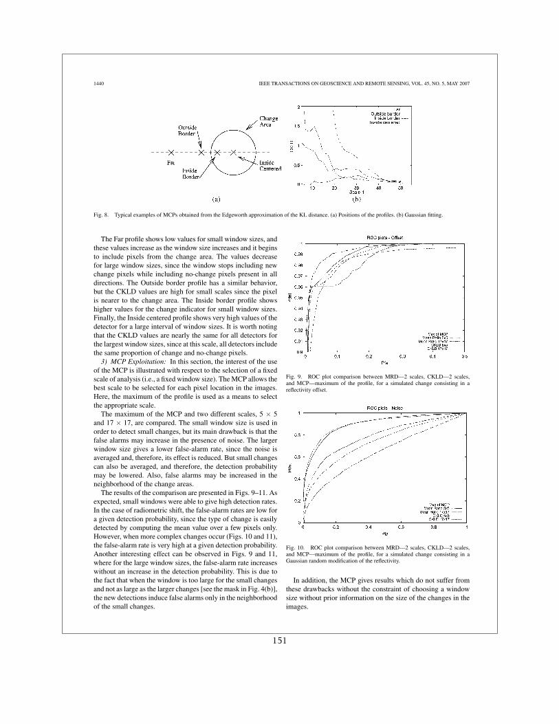
1440 IEEE TRANSACTIONS ON GEOSCIENCE AND REMOTE SENSING, VOL. 45, NO. 5, MAY 2007
Fig. 8. Typical examples of MCPs obtained from the Edgeworth approximation of the KL distance. (a) Positions of the profiles. (b) Gaussian fitting.
The Far profile shows low values for small window sizes, andthese values increase as the window size increases and it beginsto include pixels from the change area. The values decreasefor large window sizes, since the window stops including newchange pixels while including no-change pixels present in alldirections. The Outside border profile has a similar behavior,but the CKLD values are high for small scales since the pixelis nearer to the change area. The Inside border profile showshigher values for the change indicator for small window sizes.Finally, the Inside centered profile shows very high values of thedetector for a large interval of window sizes. It is worth notingthat the CKLD values are nearly the same for all detectors forthe largest window sizes, since at this scale, all detectors includethe same proportion of change and no-change pixels.
3) MCP Exploitation: In this section, the interest of the useof the MCP is illustrated with respect to the selection of a fixedscale of analysis (i.e., a fixed window size). The MCP allows thebest scale to be selected for each pixel location in the images.Here, the maximum of the profile is used as a means to selectthe appropriate scale.
The maximum of the MCP and two different scales, 5 × 5and 17 × 17, are compared. The small window size is used inorder to detect small changes, but its main drawback is that thefalse alarms may increase in the presence of noise. The largerwindow size gives a lower false-alarm rate, since the noise isaveraged and, therefore, its effect is reduced. But small changescan also be averaged, and therefore, the detection probabilitymay be lowered. Also, false alarms may be increased in theneighborhood of the change areas.
The results of the comparison are presented in Figs. 9–11. Asexpected, small windows were able to give high detection rates.In the case of radiometric shift, the false-alarm rates are low fora given detection probability, since the type of change is easilydetected by computing the mean value over a few pixels only.However, when more complex changes occur (Figs. 10 and 11),the false-alarm rate is very high at a given detection probability.Another interesting effect can be observed in Figs. 9 and 11,where for the large window sizes, the false-alarm rate increaseswithout an increase in the detection probability. This is due tothe fact that when the window is too large for the small changesand not as large as the larger changes [see the mask in Fig. 4(b)],the new detections induce false alarms only in the neighborhoodof the small changes.
Fig. 9. ROC plot comparison between MRD—2 scales, CKLD—2 scales,and MCP—maximum of the profile, for a simulated change consisting in areflectivity offset.
Fig. 10. ROC plot comparison between MRD—2 scales, CKLD—2 scales,and MCP—maximum of the profile, for a simulated change consisting in aGaussian random modification of the reflectivity.
In addition, the MCP gives results which do not suffer fromthese drawbacks without the constraint of choosing a windowsize without prior information on the size of the changes in theimages.
151
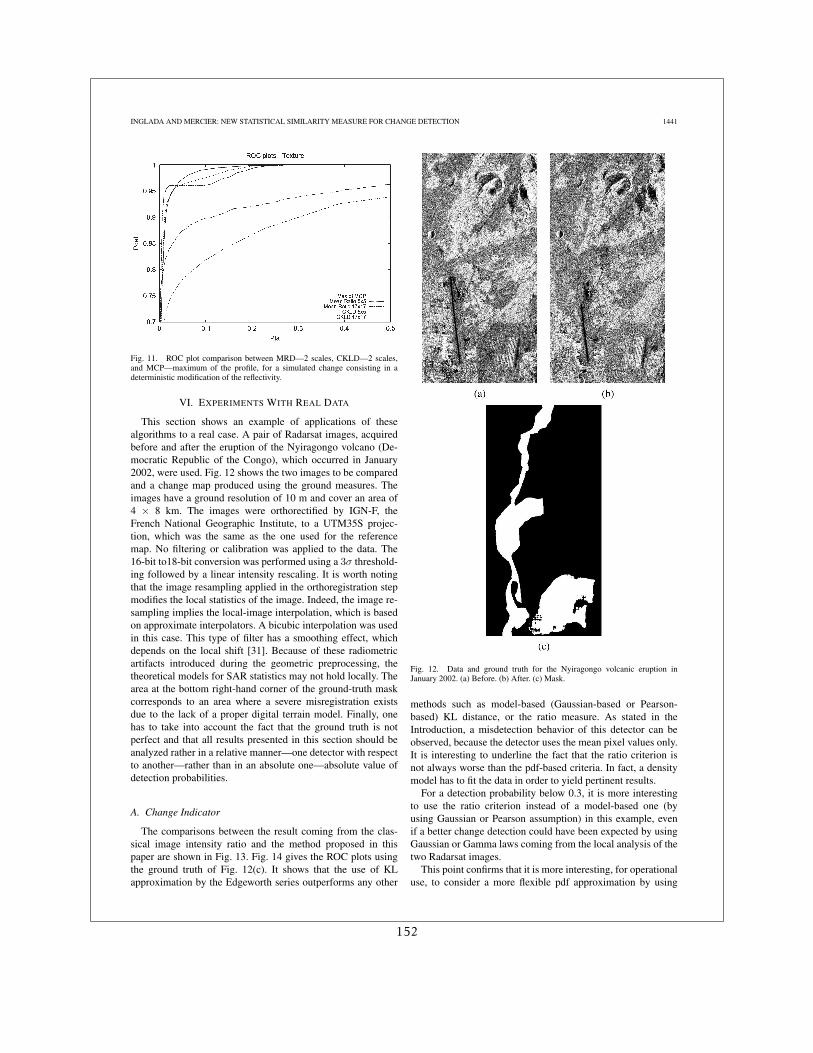
INGLADA AND MERCIER: NEW STATISTICAL SIMILARITY MEASURE FOR CHANGE DETECTION 1441
Fig. 11. ROC plot comparison between MRD—2 scales, CKLD—2 scales,and MCP—maximum of the profile, for a simulated change consisting in adeterministic modification of the reflectivity.
VI. EXPERIMENTS WITH REAL DATA
This section shows an example of applications of thesealgorithms to a real case. A pair of Radarsat images, acquiredbefore and after the eruption of the Nyiragongo volcano (De-mocratic Republic of the Congo), which occurred in January2002, were used. Fig. 12 shows the two images to be comparedand a change map produced using the ground measures. Theimages have a ground resolution of 10 m and cover an area of4 × 8 km. The images were orthorectified by IGN-F, theFrench National Geographic Institute, to a UTM35S projec-tion, which was the same as the one used for the referencemap. No filtering or calibration was applied to the data. The16-bit to18-bit conversion was performed using a 3σ threshold-ing followed by a linear intensity rescaling. It is worth notingthat the image resampling applied in the orthoregistration stepmodifies the local statistics of the image. Indeed, the image re-sampling implies the local-image interpolation, which is basedon approximate interpolators. A bicubic interpolation was usedin this case. This type of filter has a smoothing effect, whichdepends on the local shift [31]. Because of these radiometricartifacts introduced during the geometric preprocessing, thetheoretical models for SAR statistics may not hold locally. Thearea at the bottom right-hand corner of the ground-truth maskcorresponds to an area where a severe misregistration existsdue to the lack of a proper digital terrain model. Finally, onehas to take into account the fact that the ground truth is notperfect and that all results presented in this section should beanalyzed rather in a relative manner—one detector with respectto another—rather than in an absolute one—absolute value ofdetection probabilities.
A. Change Indicator
The comparisons between the result coming from the clas-sical image intensity ratio and the method proposed in thispaper are shown in Fig. 13. Fig. 14 gives the ROC plots usingthe ground truth of Fig. 12(c). It shows that the use of KLapproximation by the Edgeworth series outperforms any other
Fig. 12. Data and ground truth for the Nyiragongo volcanic eruption inJanuary 2002. (a) Before. (b) After. (c) Mask.
methods such as model-based (Gaussian-based or Pearson-based) KL distance, or the ratio measure. As stated in theIntroduction, a misdetection behavior of this detector can beobserved, because the detector uses the mean pixel values only.It is interesting to underline the fact that the ratio criterion isnot always worse than the pdf-based criteria. In fact, a densitymodel has to fit the data in order to yield pertinent results.
For a detection probability below 0.3, it is more interestingto use the ratio criterion instead of a model-based one (byusing Gaussian or Pearson assumption) in this example, evenif a better change detection could have been expected by usingGaussian or Gamma laws coming from the local analysis of thetwo Radarsat images.
This point confirms that it is more interesting, for operationaluse, to consider a more flexible pdf approximation by using
152
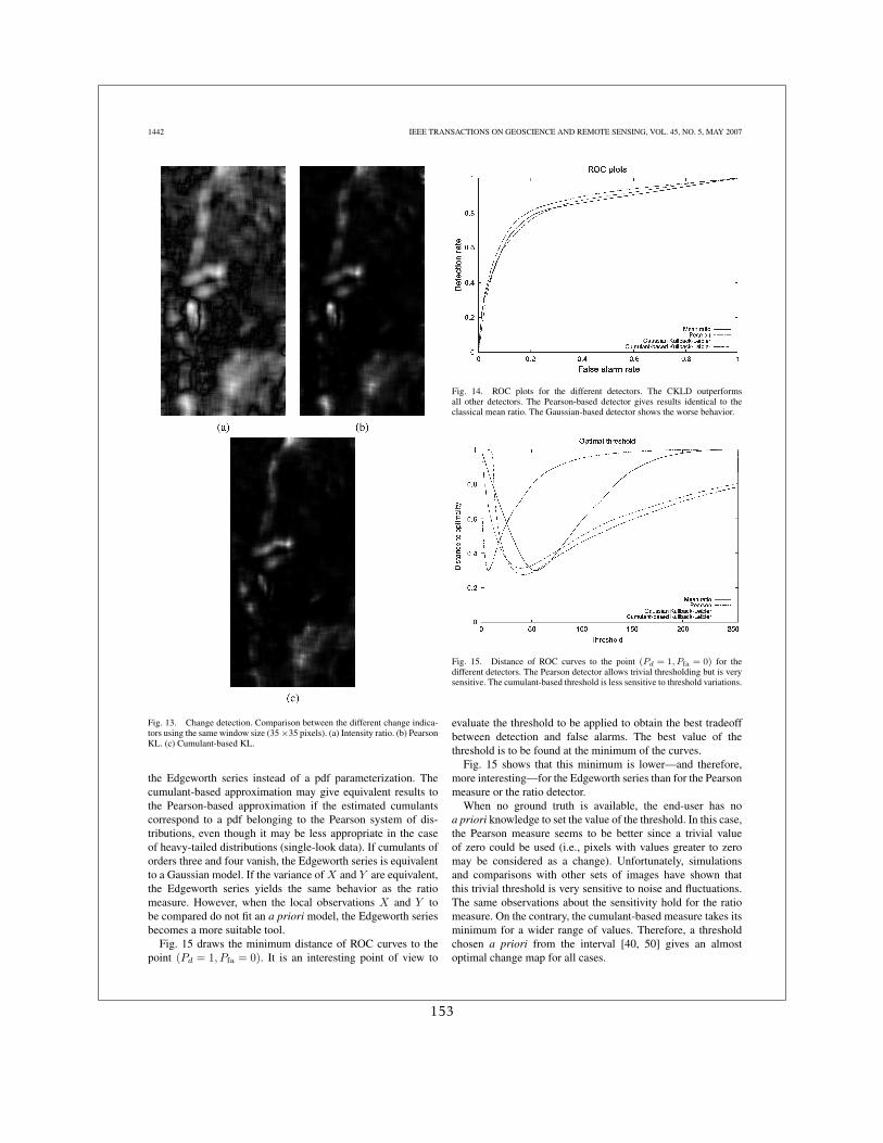
1442 IEEE TRANSACTIONS ON GEOSCIENCE AND REMOTE SENSING, VOL. 45, NO. 5, MAY 2007
Fig. 13. Change detection. Comparison between the different change indica-tors using the same window size (35 ×35 pixels). (a) Intensity ratio. (b) PearsonKL. (c) Cumulant-based KL.
the Edgeworth series instead of a pdf parameterization. Thecumulant-based approximation may give equivalent results tothe Pearson-based approximation if the estimated cumulantscorrespond to a pdf belonging to the Pearson system of dis-tributions, even though it may be less appropriate in the caseof heavy-tailed distributions (single-look data). If cumulants oforders three and four vanish, the Edgeworth series is equivalentto a Gaussian model. If the variance of X and Y are equivalent,the Edgeworth series yields the same behavior as the ratiomeasure. However, when the local observations X and Y tobe compared do not fit an a priori model, the Edgeworth seriesbecomes a more suitable tool.
Fig. 15 draws the minimum distance of ROC curves to thepoint (Pd = 1, Pfa = 0). It is an interesting point of view to
Fig. 14. ROC plots for the different detectors. The CKLD outperformsall other detectors. The Pearson-based detector gives results identical to theclassical mean ratio. The Gaussian-based detector shows the worse behavior.
Fig. 15. Distance of ROC curves to the point (Pd = 1, Pfa = 0) for thedifferent detectors. The Pearson detector allows trivial thresholding but is verysensitive. The cumulant-based threshold is less sensitive to threshold variations.
evaluate the threshold to be applied to obtain the best tradeoffbetween detection and false alarms. The best value of thethreshold is to be found at the minimum of the curves.
Fig. 15 shows that this minimum is lower—and therefore,more interesting—for the Edgeworth series than for the Pearsonmeasure or the ratio detector.
When no ground truth is available, the end-user has noa priori knowledge to set the value of the threshold. In this case,the Pearson measure seems to be better since a trivial valueof zero could be used (i.e., pixels with values greater to zeromay be considered as a change). Unfortunately, simulationsand comparisons with other sets of images have shown thatthis trivial threshold is very sensitive to noise and fluctuations.The same observations about the sensitivity hold for the ratiomeasure. On the contrary, the cumulant-based measure takes itsminimum for a wider range of values. Therefore, a thresholdchosen a priori from the interval [40, 50] gives an almostoptimal change map for all cases.
153
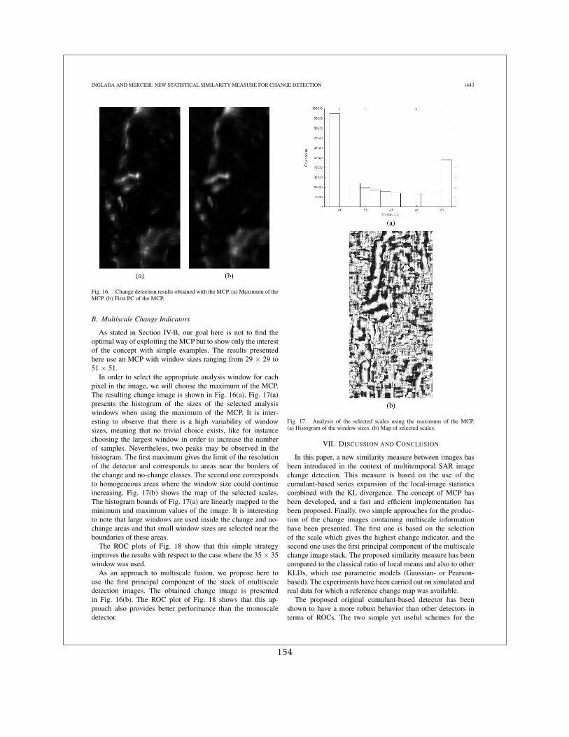
INGLADA AND MERCIER: NEW STATISTICAL SIMILARITY MEASURE FOR CHANGE DETECTION 1443
Fig. 16. Change detection results obtained with the MCP. (a) Maximum of theMCP. (b) First PC of the MCP.
B. Multiscale Change Indicators
As stated in Section IV-B, our goal here is not to find theoptimal way of exploiting the MCP but to show only the interestof the concept with simple examples. The results presentedhere use an MCP with window sizes ranging from 29 × 29 to51 × 51.
In order to select the appropriate analysis window for eachpixel in the image, we will choose the maximum of the MCP.The resulting change image is shown in Fig. 16(a). Fig. 17(a)presents the histogram of the sizes of the selected analysiswindows when using the maximum of the MCP. It is inter-esting to observe that there is a high variability of windowsizes, meaning that no trivial choice exists, like for instancechoosing the largest window in order to increase the numberof samples. Nevertheless, two peaks may be observed in thehistogram. The first maximum gives the limit of the resolutionof the detector and corresponds to areas near the borders ofthe change and no-change classes. The second one correspondsto homogeneous areas where the window size could continueincreasing. Fig. 17(b) shows the map of the selected scales.The histogram bounds of Fig. 17(a) are linearly mapped to theminimum and maximum values of the image. It is interestingto note that large windows are used inside the change and no-change areas and that small window sizes are selected near theboundaries of these areas.
The ROC plots of Fig. 18 show that this simple strategyimproves the results with respect to the case where the 35 × 35window was used.
As an approach to multiscale fusion, we propose here touse the first principal component of the stack of multiscaledetection images. The obtained change image is presentedin Fig. 16(b). The ROC plot of Fig. 18 shows that this ap-proach also provides better performance than the monoscaledetector.
Fig. 17. Analysis of the selected scales using the maximum of the MCP.(a) Histogram of the window sizes. (b) Map of selected scales.
VII. DISCUSSION AND CONCLUSION
In this paper, a new similarity measure between images hasbeen introduced in the context of multitemporal SAR imagechange detection. This measure is based on the use of thecumulant-based series expansion of the local-image statisticscombined with the KL divergence. The concept of MCP hasbeen developed, and a fast and efficient implementation hasbeen proposed. Finally, two simple approaches for the produc-tion of the change images containing multiscale informationhave been presented. The first one is based on the selectionof the scale which gives the highest change indicator, and thesecond one uses the first principal component of the multiscalechange image stack. The proposed similarity measure has beencompared to the classical ratio of local means and also to otherKLDs, which use parametric models (Gaussian- or Pearson-based). The experiments have been carried out on simulated andreal data for which a reference change map was available.
The proposed original cumulant-based detector has beenshown to have a more robust behavior than other detectors interms of ROCs. The two simple yet useful schemes for the
154
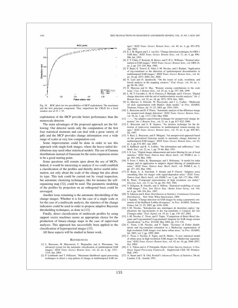
1444 IEEE TRANSACTIONS ON GEOSCIENCE AND REMOTE SENSING, VOL. 45, NO. 5, MAY 2007
Fig. 18. ROC plots for two possibilities of MCP exploitation: The maximumand the first principal component. They outperform the CKLD for a fixedwindow size of 35 × 35.
exploitation of the MCP provide better performance than themonoscale detector.
The main advantages of the proposed approach are the fol-lowing: Our detector needs only the computation of the firstfour statistical moments and can deal with a great variety ofpdfs and the MCP provides change information over a widerange of scales at very low computation cost.
Some improvements could be done in order to use thisapproach with single-look images, where the heavy-tailed dis-tributions may need other statistical models. The use of Gammadistributions instead of Gaussian for the series expansion seemsto be a good starting point.
Some questions still remain open about the use of MCPs.Indeed, it would be interesting to analyze if we could establisha classification of the profiles and thereby derive useful infor-mation, not only about the scale of the change but also aboutits type. This task could be carried out by visual inspection,but automatic clustering techniques, like for instance the self-organizing map [32], could be used. The parametric modelingof the profiles by projection on an orthogonal basis could beenvisaged.
Another issue remaining is the automatic thresholding of thechange images. Whether it is for the case of a single scale orfor the case of a multiscale analysis, the statistics of the changeindicators could be used in order to propose adaptive Bayesianthresholding techniques, as done in [13].
Finally, direct classification of multiscale profiles by usingsupport vector machines seems an appropriate choice for theproduction of binary-change maps in the case of supervisedanalyses. This approach has successfully been applied to theclassification of hyperspectral images [33].
All these aspects will be studied in future work.
REFERENCES
[1] L. Bruzzone, M. Marconcini, U. Wegmuller, and A. Wiesmann, “Anadvanced system for the automatic classification of multitemporal SARimages,” IEEE Trans. Geosci. Remote Sens., vol. 42, no. 6, pp. 1321–1334, Jun. 2004.
[2] P. Lombardo and T. Pellizzeri, “Maximum likelihood signal processingtechniques to detect a step pattern of change in multitemporal SAR im-
ages,” IEEE Trans. Geosci. Remote Sens., vol. 40, no. 4, pp. 853–870,Apr. 2002.
[3] E. J. M. Rignot and J. J. van Zyl, “Change detection techniques for ERS-1SAR data,” IEEE Trans. Geosci. Remote Sens., vol. 31, no. 4, pp. 896–906, Jul. 1993.
[4] F. T. Ulaby, F. Kouyate, B. Brisco, and T. H. L. Williams, “Textural infor-mation in SAR images,” IEEE Trans. Geosci. Remote Sens., vol. GRS-24,no. 2, pp. 235–245, Mar. 1986.
[5] F. Bujor, E. Trouvé, E. Valet, J.-M. Nicolas, and J. Rudant, “Applicationof log-cumulants to the detection of spatiotemporal discontinuities inmultitemporal SAR images,” IEEE Trans. Geosci. Remote Sens., vol. 42,no. 10, pp. 2073–2084, Oct. 2004.
[6] N. Lam and D. Quattrochi, “On the issues of scale, resolution, andfractal analysis in the mapping sciences,” Prof. Geogr., vol. 44, no. 1,pp. 88–98, 1992.
[7] D. Marceau and G. Hay, “Remote sensing contributions to the scaleissue,” Can. J. Remote Sens., vol. 25, no. 4, pp. 357–366, 1999.
[8] L. M. T. Carvalho, L. M. G. Fonseca, F. Murtagh, and J. Clevers, “Digitalchange detection with the aid of multiresolution wavelet analysis,” Int. J.Remote Sens., vol. 22, no. 18, pp. 3871–3876, Dec. 2001.
[9] G. Mercier, S. Derrode, W. Pieczynski, and J. L. Caillec, “Multiscaleoil slick segmentation with Markov chain model,” in Proc. IGARSS,Toulouse, France, Jul. 21–25, 2003, pp. 3501–3503.
[10] L. Bruzzone and D. F. Prieto, “Automatic analysis of the difference imagefor unsupervised change detection,” IEEE Trans. Geosci. Remote Sens.,vol. 38, no. 3, pp. 1171–1182, May 2000.
[11] ——, “An adaptive parcel-based technique for unsupervised change de-tection,” Int. J. Remote Sens., vol. 21, no. 4, pp. 817–822, 2000.
[12] L. Bruzzone and S. B. Serpico, “An iterative technique for the de-tection of land-cover transitions in multitemporal remote-sensing im-ages,” IEEE Trans. Geosci. Remote Sens., vol. 35, no. 4, pp. 858–867,Jul. 1997.
[13] Y. Bazi, L. Bruzzone, and F. Melgani, “An unsupervised approach basedon the generalized Gaussian model to automatic change detection inmultitemporal SAR images,” IEEE Trans. Geosci. Remote Sens., vol. 43,no. 4, pp. 874–887, Apr. 2005.
[14] S. Kullback and R. A. Leibler, “On information and sufficiency,” Ann.Math. Stat., vol. 22, no. 1, pp. 79–86, Mar. 1951.
[15] J.-S. Lee, “Digital image enhancement and noise filtering by use of localstatistics,” IEEE Trans. Pattern Anal. Mach. Intell., vol. PAMI-2, no. 1,pp. 165–168, Mar. 1980.
[16] V. Frost, J. Stiles, K. Shanmugan, and J. Holtzman, “A model for radarimages and its application to adaptive digital filtering of multiplicativenoise,” IEEE Trans. Pattern Anal. Mach. Intell., vol. PAMI-4, no. 2,pp. 157–165, Mar. 1982.
[17] D. Kuan, A. A. Sawchuk, T. Strand, and P. Chavel, “Adaptive noisesmoothing filter for images with signal-dependent noise,” IEEE Trans.Pattern Anal. Mach. Intell., vol. PAMI-7, no. 2, pp. 165–177, Mar. 1985.
[18] K. Ward, “Compound representation of high resolution sea clutter,”Electron. Lett., vol. 17, no. 16, pp. 561–565, 1981.
[19] Y. Delignon, R. Garello, and A. Hillion, “Statistical modelling of oceanSAR images,” Proc. Inst. Electr. Eng.—Radar Sonar Navig., vol. 144,no. 6, pp. 348–354, Dec. 1997.
[20] N. Johnson and S. Kotz, Distributions in Statistics: Continuous UnivariateDistributions. New York: Wiley Interscience, 1969.
[21] J. Inglada, “Change detection on SAR images by using a parametric esti-mation of the Kullback-Leibler divergence,” in Proc. IGARSS, Toulouse,France, Jul. 21–25, 2003, pp. 4104–4106.
[22] J.-M. Nicolas, “Introduction aux statistiques de deuxième espèce: Ap-plications des log-moments et des log-cumulants à l’analyse des loisd’images radar,” Trait. Signal, vol. 19, no. 3, pp. 139–167, 2002.
[23] J.-M. Nicolas, C. Tison, and F. Tupin, “Comparison of Beta1-Beta2 dia-gram and Logcumulant2-Logcumulant3 diagram for SAR image textureclassification,” in Proc. EUSAR, May 2004, pp. 133–136.
[24] C. Tison, J.-M. Nicolas, and F. Tupin, “Accuracy of Fisher distrib-utions and log-cumulant estimation in a Markovian segmentation ofhigh resolution SAR images over dense urban areas,” in Proc. IGARSS,Jul. 2003, vol. 3, pp. 1999–2001.
[25] C. Tison, J. Nicolas, F. Tupin, and H. Maître, “A new statistical modelof urban areas in high resolution SAR images for Markovian segmenta-tion,” IEEE Trans. Geosci. Remote Sens., vol. 42, no. 10, pp. 2046–2057,Oct. 2004.
[26] C. L. Nikias and A. P. Petropulu, Higher-Order Spectra Analysis: A Non-linear Signal Processing Framework. Englewoods Cliff, NJ: Prentice-Hall, 1993.
[27] A. Stuart and J. K. Ord, Kendall’s Advanced Theory of Statistics, 5th ed.London, U.K.: Arnold, 1991.
155
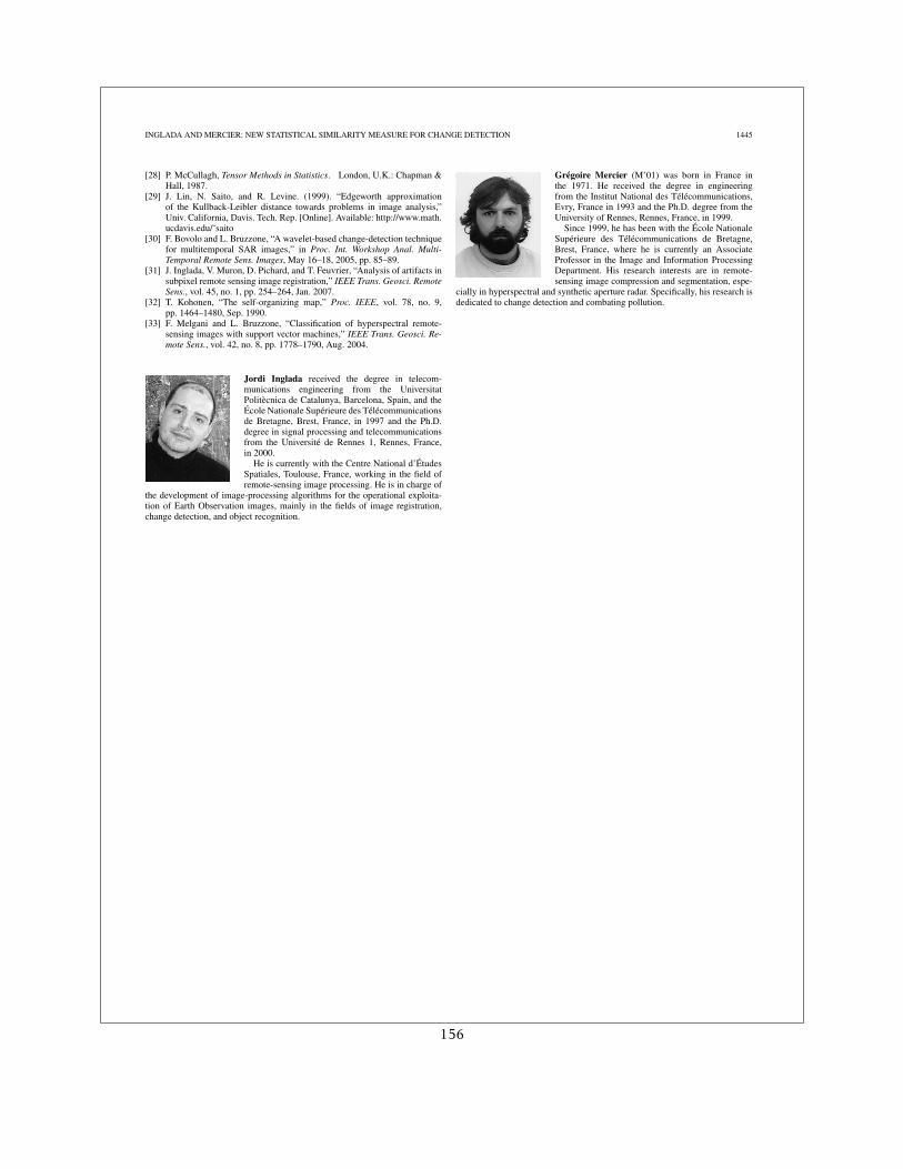
INGLADA AND MERCIER: NEW STATISTICAL SIMILARITY MEASURE FOR CHANGE DETECTION 1445
[28] P. McCullagh, Tensor Methods in Statistics. London, U.K.: Chapman &Hall, 1987.
[29] J. Lin, N. Saito, and R. Levine. (1999). “Edgeworth approximationof the Kullback-Leibler distance towards problems in image analysis,”Univ. California, Davis. Tech. Rep. [Online]. Available: http://www.math.ucdavis.edu/˜saito
[30] F. Bovolo and L. Bruzzone, “A wavelet-based change-detection techniquefor multitemporal SAR images,” in Proc. Int. Workshop Anal. Multi-Temporal Remote Sens. Images, May 16–18, 2005, pp. 85–89.
[31] J. Inglada, V. Muron, D. Pichard, and T. Feuvrier, “Analysis of artifacts insubpixel remote sensing image registration,” IEEE Trans. Geosci. RemoteSens., vol. 45, no. 1, pp. 254–264, Jan. 2007.
[32] T. Kohonen, “The self-organizing map,” Proc. IEEE, vol. 78, no. 9,pp. 1464–1480, Sep. 1990.
[33] F. Melgani and L. Bruzzone, “Classification of hyperspectral remote-sensing images with support vector machines,” IEEE Trans. Geosci. Re-mote Sens., vol. 42, no. 8, pp. 1778–1790, Aug. 2004.
Jordi Inglada received the degree in telecom-munications engineering from the UniversitatPolitècnica de Catalunya, Barcelona, Spain, and theÉcole Nationale Supérieure des Télécommunicationsde Bretagne, Brest, France, in 1997 and the Ph.D.degree in signal processing and telecommunicationsfrom the Université de Rennes 1, Rennes, France,in 2000.
He is currently with the Centre National d’ÉtudesSpatiales, Toulouse, France, working in the field ofremote-sensing image processing. He is in charge of
the development of image-processing algorithms for the operational exploita-tion of Earth Observation images, mainly in the fields of image registration,change detection, and object recognition.
Grégoire Mercier (M’01) was born in France inthe 1971. He received the degree in engineeringfrom the Institut National des Télécommunications,Evry, France in 1993 and the Ph.D. degree from theUniversity of Rennes, Rennes, France, in 1999.
Since 1999, he has been with the École NationaleSupérieure des Télécommunications de Bretagne,Brest, France, where he is currently an AssociateProfessor in the Image and Information ProcessingDepartment. His research interests are in remote-sensing image compression and segmentation, espe-
cially in hyperspectral and synthetic aperture radar. Specifically, his research isdedicated to change detection and combating pollution.
156
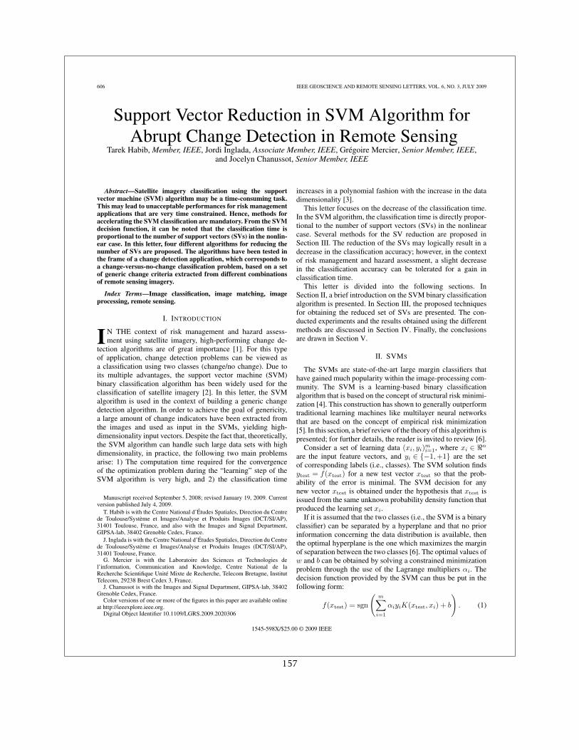
606 IEEE GEOSCIENCE AND REMOTE SENSING LETTERS, VOL. 6, NO. 3, JULY 2009
Support Vector Reduction in SVM Algorithm forAbrupt Change Detection in Remote Sensing
Tarek Habib, Member, IEEE, Jordi Inglada, Associate Member, IEEE, Grégoire Mercier, Senior Member, IEEE,and Jocelyn Chanussot, Senior Member, IEEE
Abstract—Satellite imagery classification using the supportvector machine (SVM) algorithm may be a time-consuming task.This may lead to unacceptable performances for risk managementapplications that are very time constrained. Hence, methods foraccelerating the SVM classification are mandatory. From the SVMdecision function, it can be noted that the classification time isproportional to the number of support vectors (SVs) in the nonlin-ear case. In this letter, four different algorithms for reducing thenumber of SVs are proposed. The algorithms have been tested inthe frame of a change detection application, which corresponds toa change-versus-no-change classification problem, based on a setof generic change criteria extracted from different combinationsof remote sensing imagery.
Index Terms—Image classification, image matching, imageprocessing, remote sensing.
I. INTRODUCTION
IN THE context of risk management and hazard assess-ment using satellite imagery, high-performing change de-
tection algorithms are of great importance [1]. For this typeof application, change detection problems can be viewed asa classification using two classes (change/no change). Due toits multiple advantages, the support vector machine (SVM)binary classification algorithm has been widely used for theclassification of satellite imagery [2]. In this letter, the SVMalgorithm is used in the context of building a generic changedetection algorithm. In order to achieve the goal of genericity,a large amount of change indicators have been extracted fromthe images and used as input in the SVMs, yielding high-dimensionality input vectors. Despite the fact that, theoretically,the SVM algorithm can handle such large data sets with highdimensionality, in practice, the following two main problemsarise: 1) The computation time required for the convergenceof the optimization problem during the “learning” step of theSVM algorithm is very high, and 2) the classification time
Manuscript received September 5, 2008; revised January 19, 2009. Currentversion published July 4, 2009.
T. Habib is with the Centre National d’Études Spatiales, Direction du Centrede Toulouse/Système et Images/Analyse et Produits Images (DCT/SI/AP),31401 Toulouse, France, and also with the Images and Signal Department,GIPSA-lab, 38402 Grenoble Cedex, France.
J. Inglada is with the Centre National d’Études Spatiales, Direction du Centrede Toulouse/Système et Images/Analyse et Produits Images (DCT/SI/AP),31401 Toulouse, France.
G. Mercier is with the Laboratoire des Sciences et Technologies del’information, Communication and Knowledge, Centre National de laRecherche Scientifique Unité Mixte de Recherche, Telecom Bretagne, InstitutTelecom, 29238 Brest Cedex 3, France.
J. Chanussot is with the Images and Signal Department, GIPSA-lab, 38402Grenoble Cedex, France.
Color versions of one or more of the figures in this paper are available onlineat http://ieeexplore.ieee.org.
Digital Object Identifier 10.1109/LGRS.2009.2020306
increases in a polynomial fashion with the increase in the datadimensionality [3].
This letter focuses on the decrease of the classification time.In the SVM algorithm, the classification time is directly propor-tional to the number of support vectors (SVs) in the nonlinearcase. Several methods for the SV reduction are proposed inSection III. The reduction of the SVs may logically result in adecrease in the classification accuracy; however, in the contextof risk management and hazard assessment, a slight decreasein the classification accuracy can be tolerated for a gain inclassification time.
This letter is divided into the following sections. InSection II, a brief introduction on the SVM binary classificationalgorithm is presented. In Section III, the proposed techniquesfor obtaining the reduced set of SVs are presented. The con-ducted experiments and the results obtained using the differentmethods are discussed in Section IV. Finally, the conclusionsare drawn in Section V.
II. SVMS
The SVMs are state-of-the-art large margin classifiers thathave gained much popularity within the image-processing com-munity. The SVM is a learning-based binary classificationalgorithm that is based on the concept of structural risk minimi-zation [4]. This construction has shown to generally outperformtraditional learning machines like multilayer neural networksthat are based on the concept of empirical risk minimization[5]. In this section, a brief review of the theory of this algorithm ispresented; for further details, the reader is invited to review [6].
Consider a set of learning data (xi, yi)mi=1, where xi ∈ �n
are the input feature vectors, and yi ∈ {−1,+1} are the setof corresponding labels (i.e., classes). The SVM solution findsytest = f(xtest) for a new test vector xtest so that the prob-ability of the error is minimal. The SVM decision for anynew vector xtest is obtained under the hypothesis that xtest isissued from the same unknown probability density function thatproduced the learning set xi.
If it is assumed that the two classes (i.e., the SVM is a binaryclassifier) can be separated by a hyperplane and that no priorinformation concerning the data distribution is available, thenthe optimal hyperplane is the one which maximizes the marginof separation between the two classes [6]. The optimal values ofw and b can be obtained by solving a constrained minimizationproblem through the use of the Lagrange multipliers αi. Thedecision function provided by the SVM can thus be put in thefollowing form:
f(xtest) = sgn
(m∑
i=1
αiyiK(xtest, xi) + b
). (1)
1545-598X/$25.00 © 2009 IEEE
157
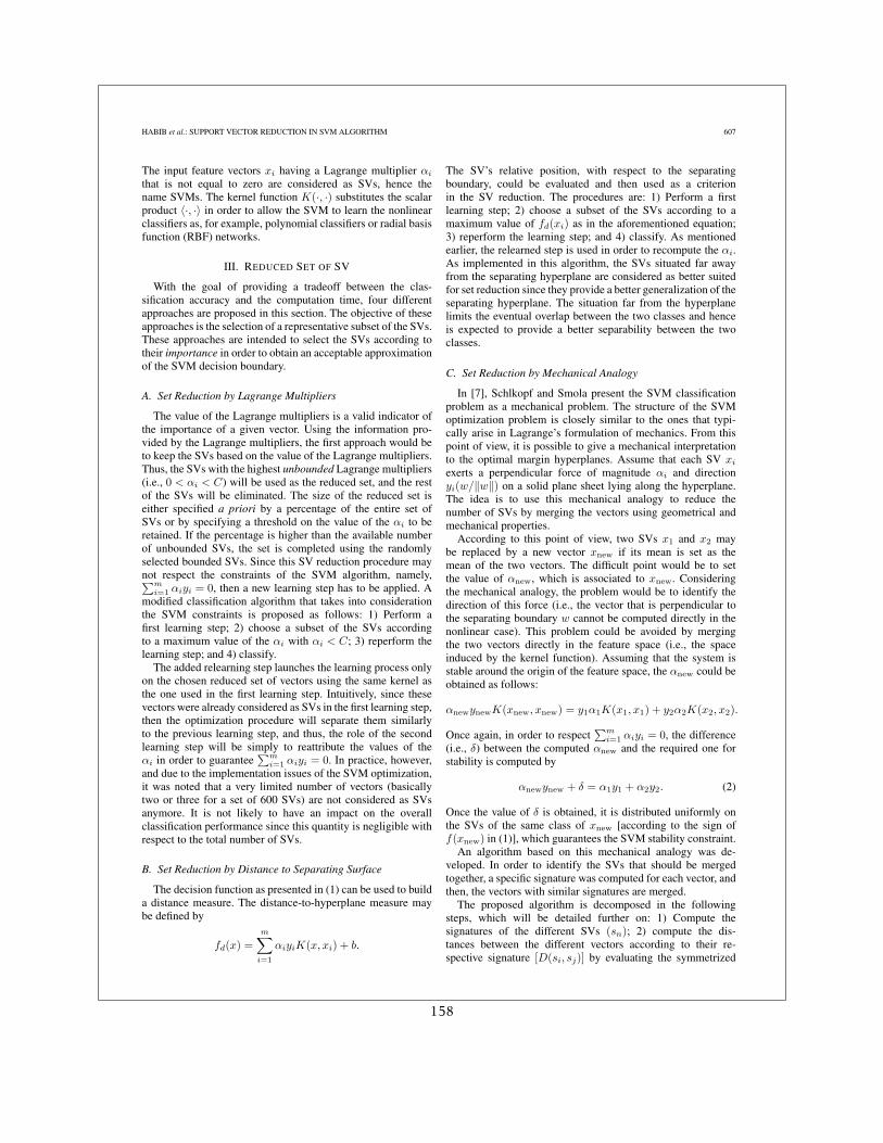
HABIB et al.: SUPPORT VECTOR REDUCTION IN SVM ALGORITHM 607
The input feature vectors xi having a Lagrange multiplier αi
that is not equal to zero are considered as SVs, hence thename SVMs. The kernel function K(·, ·) substitutes the scalarproduct 〈·, ·〉 in order to allow the SVM to learn the nonlinearclassifiers as, for example, polynomial classifiers or radial basisfunction (RBF) networks.
III. REDUCED SET OF SV
With the goal of providing a tradeoff between the clas-sification accuracy and the computation time, four differentapproaches are proposed in this section. The objective of theseapproaches is the selection of a representative subset of the SVs.These approaches are intended to select the SVs according totheir importance in order to obtain an acceptable approximationof the SVM decision boundary.
A. Set Reduction by Lagrange Multipliers
The value of the Lagrange multipliers is a valid indicator ofthe importance of a given vector. Using the information pro-vided by the Lagrange multipliers, the first approach would beto keep the SVs based on the value of the Lagrange multipliers.Thus, the SVs with the highest unbounded Lagrange multipliers(i.e., 0 < αi < C) will be used as the reduced set, and the restof the SVs will be eliminated. The size of the reduced set iseither specified a priori by a percentage of the entire set ofSVs or by specifying a threshold on the value of the αi to beretained. If the percentage is higher than the available numberof unbounded SVs, the set is completed using the randomlyselected bounded SVs. Since this SV reduction procedure maynot respect the constraints of the SVM algorithm, namely,∑m
i=1 αiyi = 0, then a new learning step has to be applied. Amodified classification algorithm that takes into considerationthe SVM constraints is proposed as follows: 1) Perform afirst learning step; 2) choose a subset of the SVs accordingto a maximum value of the αi with αi < C; 3) reperform thelearning step; and 4) classify.
The added relearning step launches the learning process onlyon the chosen reduced set of vectors using the same kernel asthe one used in the first learning step. Intuitively, since thesevectors were already considered as SVs in the first learning step,then the optimization procedure will separate them similarlyto the previous learning step, and thus, the role of the secondlearning step will be simply to reattribute the values of theαi in order to guarantee
∑mi=1 αiyi = 0. In practice, however,
and due to the implementation issues of the SVM optimization,it was noted that a very limited number of vectors (basicallytwo or three for a set of 600 SVs) are not considered as SVsanymore. It is not likely to have an impact on the overallclassification performance since this quantity is negligible withrespect to the total number of SVs.
B. Set Reduction by Distance to Separating Surface
The decision function as presented in (1) can be used to builda distance measure. The distance-to-hyperplane measure maybe defined by
fd(x) =
m∑
i=1
αiyiK(x, xi) + b.
The SV’s relative position, with respect to the separatingboundary, could be evaluated and then used as a criterionin the SV reduction. The procedures are: 1) Perform a firstlearning step; 2) choose a subset of the SVs according to amaximum value of fd(xi) as in the aforementioned equation;3) reperform the learning step; and 4) classify. As mentionedearlier, the relearned step is used in order to recompute the αi.As implemented in this algorithm, the SVs situated far awayfrom the separating hyperplane are considered as better suitedfor set reduction since they provide a better generalization of theseparating hyperplane. The situation far from the hyperplanelimits the eventual overlap between the two classes and henceis expected to provide a better separability between the twoclasses.
C. Set Reduction by Mechanical Analogy
In [7], Schlkopf and Smola present the SVM classificationproblem as a mechanical problem. The structure of the SVMoptimization problem is closely similar to the ones that typi-cally arise in Lagrange’s formulation of mechanics. From thispoint of view, it is possible to give a mechanical interpretationto the optimal margin hyperplanes. Assume that each SV xi
exerts a perpendicular force of magnitude αi and directionyi(w/‖w‖) on a solid plane sheet lying along the hyperplane.The idea is to use this mechanical analogy to reduce thenumber of SVs by merging the vectors using geometrical andmechanical properties.
According to this point of view, two SVs x1 and x2 maybe replaced by a new vector xnew if its mean is set as themean of the two vectors. The difficult point would be to setthe value of αnew, which is associated to xnew. Consideringthe mechanical analogy, the problem would be to identify thedirection of this force (i.e., the vector that is perpendicular tothe separating boundary w cannot be computed directly in thenonlinear case). This problem could be avoided by mergingthe two vectors directly in the feature space (i.e., the spaceinduced by the kernel function). Assuming that the system isstable around the origin of the feature space, the αnew could beobtained as follows:
αnewynewK(xnew, xnew) = y1α1K(x1, x1) + y2α2K(x2, x2).
Once again, in order to respect∑m
i=1 αiyi = 0, the difference(i.e., δ) between the computed αnew and the required one forstability is computed by
αnewynew + δ = α1y1 + α2y2. (2)
Once the value of δ is obtained, it is distributed uniformly onthe SVs of the same class of xnew [according to the sign off(xnew) in (1)], which guarantees the SVM stability constraint.
An algorithm based on this mechanical analogy was de-veloped. In order to identify the SVs that should be mergedtogether, a specific signature was computed for each vector, andthen, the vectors with similar signatures are merged.
The proposed algorithm is decomposed in the followingsteps, which will be detailed further on: 1) Compute thesignatures of the different SVs (sn); 2) compute the dis-tances between the different vectors according to their re-spective signature [D(si, sj)] by evaluating the symmetrized
158
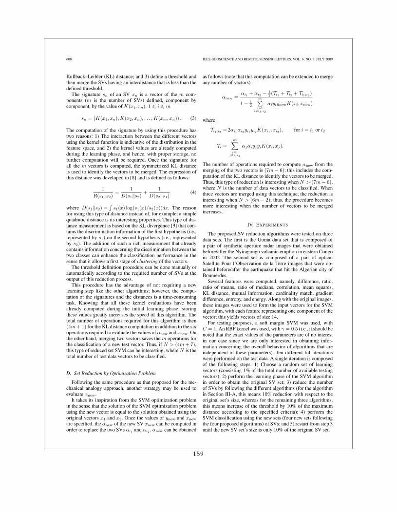
608 IEEE GEOSCIENCE AND REMOTE SENSING LETTERS, VOL. 6, NO. 3, JULY 2009
Kullback–Leibler (KL) distance; and 3) define a threshold andthen merge the SVs having an interdistance that is less than thedefined threshold.
The signature sn of an SV xn is a vector of the m com-ponents (m is the number of SVs) defined, component bycomponent, by the value of K(xi, xn), 1 � i � m
sn = (K(x1, xn),K(x2, xn), . . . ,K(xm, xn)) . (3)
The computation of the signature by using this procedure hastwo reasons: 1) The interaction between the different vectorsusing the kernel function is indicative of the distribution in thefeature space, and 2) the kernel values are already computedduring the learning phase, and hence, with proper storage, nofurther computation will be required. Once the signature forall the m vectors is computed, the symmetrized KL distanceis used to identify the vectors to be merged. The expression ofthis distance was developed in [8] and is defined as follows:
1
R(s1, s2)=
1
D(s1‖s2)+
1
D(s2‖s1)(4)
where D(s1‖s2) =∫
s1(x) log(s1(x)/s2(x))dx. The reasonfor using this type of distance instead of, for example, a simplequadratic distance is its interesting properties. This type of dis-tance measurement is based on the KL divergence [9] that con-tains the discrimination information of the first hypothesis (i.e.,represented by s1) on the second hypothesis (i.e., representedby s2). The addition of such a rich measurement that alreadycontains information concerning the discrimination between thetwo classes can enhance the classification performance in thesense that it allows a first stage of clustering of the vectors.
The threshold definition procedure can be done manually orautomatically according to the required number of SVs at theoutput of this reduction process.
This procedure has the advantage of not requiring a newlearning step like the other algorithms; however, the compu-tation of the signatures and the distances is a time-consumingtask. Knowing that all these kernel evaluations have beenalready computed during the initial learning phase, storingthese values greatly increases the speed of this algorithm. Thetotal number of operations required for this algorithm is then(4m + 1) for the KL distance computation in addition to the sixoperations required to evaluate the values of αnew and xnew. Onthe other hand, merging two vectors saves the m operations forthe classification of a new test vector. Thus, if N > (4m + 7),this type of reduced set SVM can be interesting, where N is thetotal number of test data vectors to be classified.
D. Set Reduction by Optimization Problem
Following the same procedure as that proposed for the me-chanical analogy approach, another strategy may be used toevaluate αnew.
It takes its inspiration from the SVM optimization problemin the sense that the solution of the SVM optimization problemusing the new vector is equal to the solution obtained using theoriginal vectors x1 and x2. Once the values of ynew and xnew
are specified, the αnew of the new SV xnew can be computed inorder to replace the two SVs αi1 and αi2 . αnew can be obtained
as follows (note that this computation can be extended to mergeany number of vectors):
αnew =αi1 + αi2 − 1
2 (Ti1 + Ti2 + Ti1;i2)
1 − 12
m∑i=1
i�=i1,i2
αiyiynewK(xi, xnew)
where
Ti1;i2 = 2αi1αi2yi1yi2K(xi1 , xi2), for i = i1 or i2
Ti =
m∑
j=1j �=i1i2
αjαiyjyiK(xi, xj).
The number of operations required to compute αnew from themerging of the two vectors is (7m − 6); this includes the com-putation of the KL distance to identify the vectors to be merged.Thus, this type of reduction is interesting when N > (7m − 6),where N is the number of data vectors to be classified. Whenthree vectors are merged using this technique, the reduction isinteresting when N > (6m − 2); thus, the procedure becomesmore interesting when the number of vectors to be mergedincreases.
IV. EXPERIMENTS
The proposed SV reduction algorithms were tested on threedata sets. The first is the Goma data set that is composed ofa pair of synthetic aperture radar images that were obtainedbefore/after the Nyiragongo volcanic eruption in eastern Congoin 2002. The second set is composed of a pair of opticalSatellite Pour l’Observation de la Terre images that were ob-tained before/after the earthquake that hit the Algerian city ofBoumerdes.
Several features were computed, namely, difference, ratio,ratio of means, ratio of medians, correlation, mean squares,KL distance, mutual information, cardinality match, gradientdifference, entropy, and energy. Along with the original images,these images were used to form the input vectors for the SVMalgorithm, with each feature representing one component of thevector; this yields vectors of size 14.
For testing purposes, a soft margin SVM was used, withC = 1. An RBF kernel was used, with γ = 0.5 (i.e., it should benoted that the exact values of the parameters are of no interestin our case since we are only interested in obtaining infor-mation concerning the overall behavior of algorithms that areindependent of these parameters). Ten different full iterationswere performed on the test data. A single iteration is composedof the following steps: 1) Choose a random set of learningvectors (consisting 1% of the total number of available testingvectors); 2) perform the learning phase of the SVM algorithmin order to obtain the original SV set; 3) reduce the numberof SVs by following the different algorithms (for the algorithmin Section III-A, this means 10% reduction with respect to theoriginal set’s size, whereas for the remaining three algorithms,this means increase of the threshold by 10% of the maximumdistance according to the specified criteria); 4) perform theSVM classification using the new sets (four new sets followingthe four proposed algorithms) of SVs; and 5) restart from step 3until the new SV set’s size is only 10% of the original SV set.
159
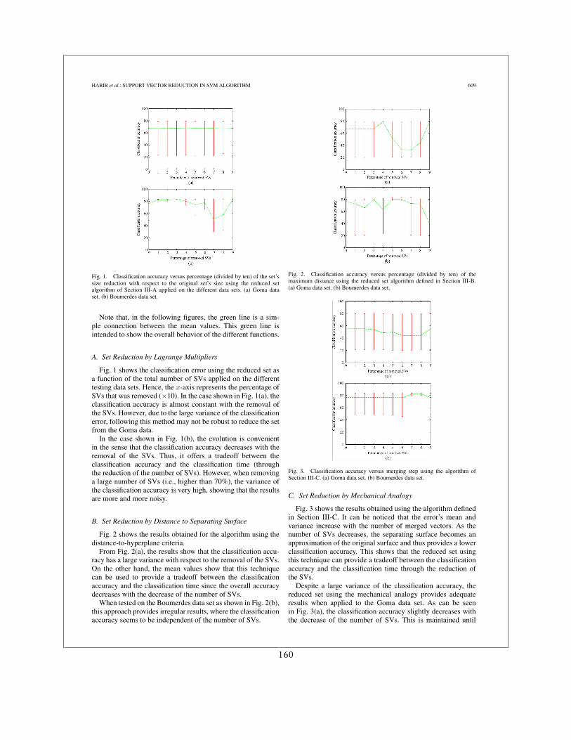
HABIB et al.: SUPPORT VECTOR REDUCTION IN SVM ALGORITHM 609
Fig. 1. Classification accuracy versus percentage (divided by ten) of the set’ssize reduction with respect to the original set’s size using the reduced setalgorithm of Section III-A applied on the different data sets. (a) Goma dataset. (b) Boumerdes data set.
Note that, in the following figures, the green line is a sim-ple connection between the mean values. This green line isintended to show the overall behavior of the different functions.
A. Set Reduction by Lagrange Multipliers
Fig. 1 shows the classification error using the reduced set asa function of the total number of SVs applied on the differenttesting data sets. Hence, the x-axis represents the percentage ofSVs that was removed (×10). In the case shown in Fig. 1(a), theclassification accuracy is almost constant with the removal ofthe SVs. However, due to the large variance of the classificationerror, following this method may not be robust to reduce the setfrom the Goma data.
In the case shown in Fig. 1(b), the evolution is convenientin the sense that the classification accuracy decreases with theremoval of the SVs. Thus, it offers a tradeoff between theclassification accuracy and the classification time (throughthe reduction of the number of SVs). However, when removinga large number of SVs (i.e., higher than 70%), the variance ofthe classification accuracy is very high, showing that the resultsare more and more noisy.
B. Set Reduction by Distance to Separating Surface
Fig. 2 shows the results obtained for the algorithm using thedistance-to-hyperplane criteria.
From Fig. 2(a), the results show that the classification accu-racy has a large variance with respect to the removal of the SVs.On the other hand, the mean values show that this techniquecan be used to provide a tradeoff between the classificationaccuracy and the classification time since the overall accuracydecreases with the decrease of the number of SVs.
When tested on the Boumerdes data set as shown in Fig. 2(b),this approach provides irregular results, where the classificationaccuracy seems to be independent of the number of SVs.
Fig. 2. Classification accuracy versus percentage (divided by ten) of themaximum distance using the reduced set algorithm defined in Section III-B.(a) Goma data set. (b) Boumerdes data set.
Fig. 3. Classification accuracy versus merging step using the algorithm ofSection III-C. (a) Goma data set. (b) Boumerdes data set.
C. Set Reduction by Mechanical Analogy
Fig. 3 shows the results obtained using the algorithm definedin Section III-C. It can be noticed that the error’s mean andvariance increase with the number of merged vectors. As thenumber of SVs decreases, the separating surface becomes anapproximation of the original surface and thus provides a lowerclassification accuracy. This shows that the reduced set usingthis technique can provide a tradeoff between the classificationaccuracy and the classification time through the reduction ofthe SVs.
Despite a large variance of the classification accuracy, thereduced set using the mechanical analogy provides adequateresults when applied to the Goma data set. As can be seenin Fig. 3(a), the classification accuracy slightly decreases withthe decrease of the number of SVs. This is maintained until
160
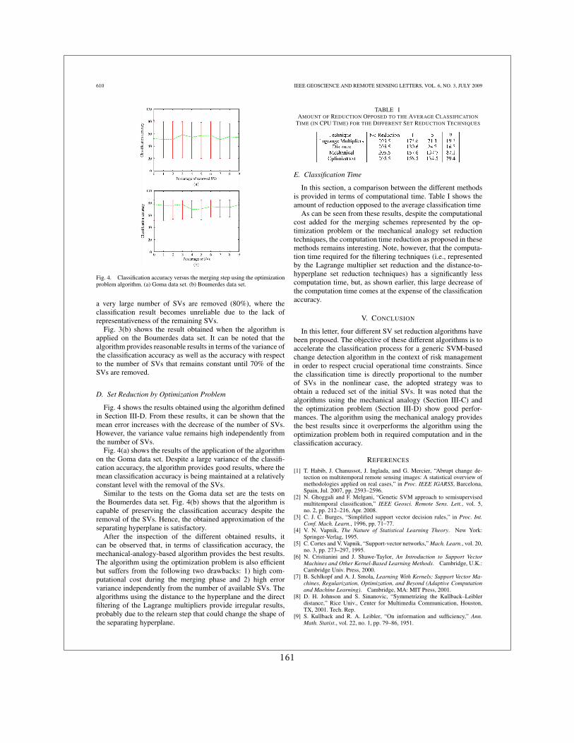
610 IEEE GEOSCIENCE AND REMOTE SENSING LETTERS, VOL. 6, NO. 3, JULY 2009
Fig. 4. Classification accuracy versus the merging step using the optimizationproblem algorithm. (a) Goma data set. (b) Boumerdes data set.
a very large number of SVs are removed (80%), where theclassification result becomes unreliable due to the lack ofrepresentativeness of the remaining SVs.
Fig. 3(b) shows the result obtained when the algorithm isapplied on the Boumerdes data set. It can be noted that thealgorithm provides reasonable results in terms of the variance ofthe classification accuracy as well as the accuracy with respectto the number of SVs that remains constant until 70% of theSVs are removed.
D. Set Reduction by Optimization Problem
Fig. 4 shows the results obtained using the algorithm definedin Section III-D. From these results, it can be shown that themean error increases with the decrease of the number of SVs.However, the variance value remains high independently fromthe number of SVs.
Fig. 4(a) shows the results of the application of the algorithmon the Goma data set. Despite a large variance of the classifi-cation accuracy, the algorithm provides good results, where themean classification accuracy is being maintained at a relativelyconstant level with the removal of the SVs.
Similar to the tests on the Goma data set are the tests onthe Boumerdes data set. Fig. 4(b) shows that the algorithm iscapable of preserving the classification accuracy despite theremoval of the SVs. Hence, the obtained approximation of theseparating hyperplane is satisfactory.
After the inspection of the different obtained results, itcan be observed that, in terms of classification accuracy, themechanical-analogy-based algorithm provides the best results.The algorithm using the optimization problem is also efficientbut suffers from the following two drawbacks: 1) high com-putational cost during the merging phase and 2) high errorvariance independently from the number of available SVs. Thealgorithms using the distance to the hyperplane and the directfiltering of the Lagrange multipliers provide irregular results,probably due to the relearn step that could change the shape ofthe separating hyperplane.
TABLE IAMOUNT OF REDUCTION OPPOSED TO THE AVERAGE CLASSIFICATION
TIME (IN CPU TIME) FOR THE DIFFERENT SET REDUCTION TECHNIQUES
E. Classification Time
In this section, a comparison between the different methodsis provided in terms of computational time. Table I shows theamount of reduction opposed to the average classification time
As can be seen from these results, despite the computationalcost added for the merging schemes represented by the op-timization problem or the mechanical analogy set reductiontechniques, the computation time reduction as proposed in thesemethods remains interesting. Note, however, that the computa-tion time required for the filtering techniques (i.e., representedby the Lagrange multiplier set reduction and the distance-to-hyperplane set reduction techniques) has a significantly lesscomputation time, but, as shown earlier, this large decrease ofthe computation time comes at the expense of the classificationaccuracy.
V. CONCLUSION
In this letter, four different SV set reduction algorithms havebeen proposed. The objective of these different algorithms is toaccelerate the classification process for a generic SVM-basedchange detection algorithm in the context of risk managementin order to respect crucial operational time constraints. Sincethe classification time is directly proportional to the numberof SVs in the nonlinear case, the adopted strategy was toobtain a reduced set of the initial SVs. It was noted that thealgorithms using the mechanical analogy (Section III-C) andthe optimization problem (Section III-D) show good perfor-mances. The algorithm using the mechanical analogy providesthe best results since it overperforms the algorithm using theoptimization problem both in required computation and in theclassification accuracy.
REFERENCES
[1] T. Habib, J. Chanussot, J. Inglada, and G. Mercier, “Abrupt change de-tection on multitemporal remote sensing images: A statistical overview ofmethodologies applied on real cases,” in Proc. IEEE IGARSS, Barcelona,Spain, Jul. 2007, pp. 2593–2596.
[2] N. Ghoggali and F. Melgani, “Genetic SVM approach to semisupervisedmultitemporal classification,” IEEE Geosci. Remote Sens. Lett., vol. 5,no. 2, pp. 212–216, Apr. 2008.
[3] C. J. C. Burges, “Simplified support vector decision rules,” in Proc. Int.Conf. Mach. Learn., 1996, pp. 71–77.
[4] V. N. Vapnik, The Nature of Statistical Learning Theory. New York:Springer-Verlag, 1995.
[5] C. Cortes and V. Vapnik, “Support-vector networks,” Mach. Learn., vol. 20,no. 3, pp. 273–297, 1995.
[6] N. Cristianini and J. Shawe-Taylor, An Introduction to Support VectorMachines and Other Kernel-Based Learning Methods. Cambridge, U.K.:Cambridge Univ. Press, 2000.
[7] B. Schlkopf and A. J. Smola, Learning With Kernels: Support Vector Ma-chines, Regularization, Optimization, and Beyond (Adaptive Computationand Machine Learning). Cambridge, MA: MIT Press, 2001.
[8] D. H. Johnson and S. Sinanovic, “Symmetrizing the Kullback–Leiblerdistance,” Rice Univ., Center for Multimedia Communication, Houston,TX, 2001. Tech. Rep.
[9] S. Kullback and R. A. Leibler, “On information and sufficiency,” Ann.Math. Statist., vol. 22, no. 1, pp. 79–86, 1951.
161


15 Reconnaissance d’objets
163
Autho
r's
pers
onal
co
py
Automatic recognition of man-made objects in high resolutionoptical remote sensing images by SVM classification
of geometric image features
Jordi Inglada
CNES - DCT/SI/AP, 18, Avenue Edouard Belin, 31401 Toulouse Cedex 09, France
Received 6 December 2005; received in revised form 11 May 2007; accepted 15 May 2007Available online 27 June 2007
Abstract
With the advent of Earth Observation satellite sensors producing images in the visible wavelengths with resolutions better than5 m, it is now possible to recognize man-made objects which were not visible at lower resolutions. Because of the size and theincreasing quantity of remote sensing images, tools are needed for computer aided interpretation.
In this work we present an image processing system for the detection and recognition of man-made objects in high resolutionoptical remote sensing images. Detection is understood here as finding a small rectangular area in the image containing an object.Recognition is the attribution of a class label. These algorithms are based on learning methods and on an example data base whichcontains eleven classes of objects. The examples (more that 150 for each class) have been manually extracted from SPOT 5 THRimages (2.5 m resolution).
In order to build a system which is independent of the type of object to be recognized, we have used a supervised learningapproach based on support vector machines. The system learns a generic model for each class of objects by using a geometriccharacterization of the examples in the data base.
The main novelty of this paper is the use of a high number of geometric image features which allows to characterise severalclasses of objects with different geometric properties using a supervised learning approach. The results show the possibility ofdiscrimination of several classes of objects with classification rates higher than 80%.© 2007 International Society for Photogrammetry and Remote Sensing, Inc. (ISPRS). Published by Elsevier B.V. All rightsreserved.
Keywords: Object recognition; Man-made objects; Support vector machines; Geometrical moments
1. Introduction
Earth observation images with resolutions better than5 m allow the visual recognition of man-made objects ofcartographic interest. Sensors with resolutions close to1 m or better allow a better discrimination of this kind of
objects, but they usually have swath widths which aretoo small (less than 20 km) for mass production of mapsused in town and country planning. Therefore, sensorssuch as SPOT 5 which combine a high resolution(2.5 m) and a wide swath (60 km) increase the interest ofthe use of satellite images in this application field.
Satellite data allow the possibility of making rapidmapping in the case of natural hazards, for instance. Thiskind of application is submitted to strong time constraints.
ISPRS Journal of Photogrammetry & Remote Sensing 62 (2007) 236–248www.elsevier.com/locate/isprsjprs
E-mail address: [email protected].
0924-2716/$ - see front matter © 2007 International Society for Photogrammetry and Remote Sensing, Inc. (ISPRS). Published by Elsevier B.V.All rights reserved.doi:10.1016/j.isprsjprs.2007.05.011
164
Autho
r's
pers
onal
co
py
However, the exploitation images of such a large sizecontaining a high density of information is time-consuming and also very difficult to analyze by a photo-interpreter. Indeed, more than 400 analysis screens areneeded for one scene. We aim at providing photo-interpreters with tools which help them in their visualanalysis task. From the user point of view, it is interestingto have a tool which is able to point out where in thewholeimage a particular kind of object is present, eventuallygiving some kind of confidence ratio.
The main goal of this paper is to investigate thepossibility of recognising objects in high resolutionremote sensing images using a generic approach, that is,an approach which is not object dependent.
One of the main difficulties of image processingtasks when moving from images with resolutionscoarser than 10 m to metric resolution ones, is beingable to deal with the high complexity of the imagecontent. This high complexity is mainly due to the factthat, from a user point of view, the elements of interestare not only individual pixels or surfaces, but complex,structured objects.
While the land cover analysis of medium and lowresolution images can be addressed with a pixel-wiseapproach, the specificity of high resolution images isthat we are interested in objects that can only be definedby their shape and their neighborhood. Therefore, it isdifficult to implement generic image processing systemswhich are based on the classical two-step – featureextraction plus classification – approach.
On the other hand, manipulation of high levelconcepts with rule-based systems seems to loose thegenericity of the former approach. Indeed, for the objectrecognition problem, one could take the approach ofmanually defining a geometric template for each objectand try to match it in the image. Unfortunately, the highvariability inside the different classes of objects makesthis approach difficult to exploit.
The main problem in our domain is the one ofrecognising classes of objects instead of specific objects.While the detection and recognition of objects usingspecific approaches – tuned to the class of object to beextracted – has been dealt with for a long time incomputer vision (especially in the military), little workhas been published about the detection and recognitionof classes of objects in remote sensing images withgeneric approaches — not specific to a particular classof object.
For instance, the literature about automatic roadextraction proposes methods where the roads aremodeled as a network of intersections and links betweenthe intersections Baumgartner et al. (1999), or extracted
using explicitly formulated scale-dependent modelsHinz and Baumgartner (2003). The review workpresented in Mena (2003) lists a high number ofmethods, but they are all specific to roads or networks.The object extraction from remote sensing imagesliterature also presents a large variety of methods forbuilding extraction, but, again, they are specific to thisclass of objects. Many methods use stereo image pairsFraser et al. (2002); Gülch et al. (1998). Other methodsneed important a priori knowledge about the surround-ing of a building Gerke et al. (2001).
Related works dealing with the problem of informa-tion retrieval from remote sensing image archives exist,Datcu et al. (1998, 2003), Schroeder et al. (1998, 2000),Dell'Acqua and Gamba (2001), Daschiel and Datcu(2005); and should inspire our approach. Indeed, theseworks show that the use of relevant features and aclassification in a feature space allow the retrieval ofrelevant information for a high-level semantics definedby a user by means of a small set of examples.
However, the problem of information retrieval fromlarge data bases has different constraints than theproblem of object recognition in a single image. Indeed,the so-called image mining systems work with hundredsto thousands of images which need to be indexed in avery smart way in order to permit a short response timeto the user which interacts in real time with the system.Since each user's query may be different, a great efforthas to be made in order to build a system which is able tolink the user semantics with the low-level imagefeatures. On the other hand, all the possible images areknown to the system – thus all the events of theprobability space –, so the use of Bayesian learning isthe most suited and elegant way to proceed. As far as weknow, these systems do not try to retrieve compositeobjects, but only classes which can be defined byradiometric properties in a pixel-wise approach.
In the object recognition problem that we mean tosolve, only a few examples are available to train thesystem because of the high cost of example data baseconstruction. Furthermore, each image to process is anew image to the system, so the solution of finding thescene in the data base which best explains the observeddata, Datcu et al. (1998), is not suited to our problem.
The goal of this work is to investigate the possibilityof automatically detecting and recognising objects inhigh resolution remote sensing images. Detection isunderstood as finding a small rectangular area in theimage containing the object. Recognition is theattribution of a class label to the detected object. Theobject recognition task can be performed after adetection step. Another possible approach is to apply
237J. Inglada / ISPRS Journal of Photogrammetry & Remote Sensing 62 (2007) 236–248
165
Autho
r's
pers
onal
co
py
the recognition algorithms to every possible position ofan analysing window within the image. While thissecond approach is less prone to misdetections, it iscomputationally expensive and should be avoided inoperational systems. Our solution is based in a quickpre-processing step which aims to detect the areas wherethere may potentially be objects of interest. This isachieved by a pre-segmentation of a low resolutionversion of the image. This segmentation is based onvisual perception models, Thorpe et al. (2001). This is acritical step of any recognition system but the details ofthe pre-processing task are out of the scope of this paper.Assuming that this pre-processing step is available, wecan proceed to a sequential scan of the interest areas anddirectly apply the recognition approach presented in thispaper. A robust recognition algorithm should beinvariant to scale, rotation and illumination. This willlimit the use of object appearance models, Pope andLowe (1996), Hamdan et al. (2001). Another popularapproach is template matching approach, Veltkamp andHagedoorn (1999), but the difficulty here is finding thecorrect templates which are able to deal with intra-classvariability. In order to cope with this difficulty, we canadopt a supervised learning approach, that is, we willmake the system learn from an example data base. Fromthis example data base, a model for each class of objectscan be automatically obtained. The system will thereforelearn to classify image patches containing the object inthe center. This constraint imposed to the learning stepwill allow a precise localisation of the detected objectswhen performing the image scanning in the detectionand recognition phase. That means that for objects largerthat the analysing window, multiple detections will beobserved, each one for each window position.
The most popular approach for building object modelsfrom an example data base is principal componentanalysis, PCA, which has led to the eigenfaces approach,Turk and Pentland (1991), Turk (2001): one assumes thatthe set of pixels of each example in the data base is arandom vector and the principal component analysis isperformed in order to obtain a set of eigenvectors (theeigenfaces) which are used as a decomposition basis.Unfortunately, this approach is very constraining on thecharacteristics of the data base in terms of pose andillumination. In the case of data base constitution fromremote sensing images, these constraints are too high.Variants of this approach have been presented as forinstance Borgne et al. (2004), where IndependentComponent Analysis is used instead of PCA. Ourexperiments with these approaches have been unsuccess-ful. We think that the problem is that a small number ofexamples with a high intra-class variability does not allow
to obtain relevant principal or independent components.Indeed, this kind of analysis has given good results forproblems where the intra-class variability is low andwhere the example data-base is built under controlledconditions (illumination, etc.).
The remaining of this paper is organised as follows.Section 2 describes the approach chosen for our system.The geometrical characterization of objects is presented inSection 3 and the feature vector classification approachis described in Section 4. Section 5 presents the perfor-mances of the system and discusses several possibil-ities for its optimization. Finally, Section 6 presents ourconclusions.
2. The chosen approach
In order to implement a system which is generic withrespect to the types of objects to be recognised, we adopt ageneric feature extraction plus classification approach andchoose to use a high number of geometrical descriptors inorder to cope with the great diversity of possibilities forthe objects of interest. We are thus facing a problem ofsupervised classification in a high dimensional featurespace and with only several tenths of examples availableper class. This limitation is a practical one in realapplications due to data availability problems and cost ofdata base production. In order to overcome the curse ofdimensionality and, at the same time, preventing to looseinformationwith a dimensionality reduction approach, wechoose to use the support vector machines (SVM).
The goal of our recognition system is to correctly labelthe image patches received as input. In order to do so eachimage patch will be characterized by a description vectorwhich will be used in a supervised classification scheme.An operational recognition system can then be built bysequentially scanning full SPOT5 scenes.
In order to have a system which is robust toillumination, spectral band and vegetation changes, wewill only use the geometry of the images. Indeed, thekind of objects we are trying to detect are very welldefined by the spatial attributes of their edges and theuse of textures can introduce a source of variability –illumination and seasonal effects for instance – that weshould avoid. The training phase will use a subset of theexample data base. Each image patch will be processedin order to obtain a description vector (Section 3) whichwill be fed to the learning engine (see Section 4). Thedescription vector will only contain geometry informa-tion, but this fact is not taken into account by thelearning scheme.
In order to evaluate the performances of the system,the image patches which were not used in the training
238 J. Inglada / ISPRS Journal of Photogrammetry & Remote Sensing 62 (2007) 236–248
166
Autho
r's
pers
onal
co
py
phase will be used. Each image patch will be used tocompute a description vector which will be classified bythe system obtained during the training phase. Theperformances of the system can then be evaluated bycomputing confusion matrices.
The example data base has been built by CNESphoto-interpreters using SPOT5 THR images (panchro-matic band with 2.5 m pixel sampling). We have definedten object classes: isolated buildings (IB), paths andtracks (PT), crossroads (CR), bridges (BR), wide roads(WR), highways (HW), round-abouts (RA), narrowroads (NR), railways (RW), suburbs (SB).
While we are only interested in three of these classes(IB, RA, BR), we have included the others in order tobetter characterize the rejection class. We have alsocreated a supplementary class called OT (other) in orderto take into account the different possible landscapes.The road classes are also very interesting, but they canbe extracted by algorithms which allow the reconstruc-tion of the whole road network using contextualapproaches, Rochery et al. (2003), Stoica et al. (2004),Baumgartner et al. (1999), Hinz and Baumgartner(2003). For a complete list of references see the reviewwork of Mena (2003).
For each class, more than 150 examples have beenentered in the data base. Each example is a 100×100pixels image patch with the object in the center of theimage. Since objects of different classes can appear inthe same image patch, the object centering is importantin order to lift ambiguities for the learning algorithms.This will also hopefully produce detectors which have agood localization (small footprint) so multiple detec-tions for adjacent patches can be avoided when scanninga large image. Each image patch is thus labelled asbelonging to the class of the object located in the center.Fig. 1 shows one example for each class in the data base.Additional examples have been created by applyingrotations and symmetries.
The SPOT5 scenes used for the data base have beenchosen over different areas in France (Toulouse,Marseille and Strasbourg) and one area in the U.S.A(San Diego, CA).
3. Geometrical characterization of objects
We aim at characterizing the objects by usinggeometric information. In the remote sensing field, littlework exploiting the use of geometrical shape descriptorsfor recognition exists. Dell'Acqua and Gamba (2001)used the point diffusion technique, PDT, but thisapproach is only efficient in the case where the objectof interest has well defined boundaries. In our case, one
object will be characterized by several sets of bound-aries. The PDT is very useful for the comparison ofindividual closed, deterministic shapes, but it does notseem suited for our problem.
We need to be able to statistically compare sets ofshapes, but also other geometric descriptions. We will usetwo kinds of features: region boundaries and alignments.
Alignments (that is edges and lines) are extractedusing the Gestalt approach proposed by Desolneux et al.(2000). In this context, an event is consideredmeaningful if the expectation of its occurrence wouldbe very small in a random image. One can thus considerthat in a random image the direction of the gradient of agiven point is uniformly distributed, and that neighbour-ing pixels have a very low probability of having thesame gradient direction. This algorithm gives a set ofstraight line segments defined by the two extremitycoordinates.
Region boundaries are also extracted by using thesame principle but applied on the topographic map – thelevel-lines of the surface obtained when assuming thatthe pixel grey-level is an elevation value – of the image,Desolneux et al. (2001). Since we are exploiting levellines, we can obtain closed regions.
An example of the kind of extraction which can beobtained is shown in Fig. 2.
Once the geometry has been extracted, it must becoded as a description vector of a fixed length. This isachieved by the computation of a set of features. Thesefeatures can be classified in two groups: low-levelfeatures and high-level features.
3.1. Low-level geometry features
Two types of low-level descriptors computed fromregion edges will be used: the geometric invariants andthe Fourier–Mellin descriptors.
3.1.1. Geometric momentsUsing the algebraic moment theory, H. Ming-Kuel
obtained a family of seven invariants with respect toplanar transformations called Hu invariants, Hu (1962).Those invariants can be seen as nonlinear combinationsof complex geometric moments:
cpq ¼Z þl
�l
Z þl
�lðxþ iyÞpðx� iyÞqf ðx; yÞdxdy; ð1Þ
where x and y are the coordinates of the image f (x, y), iis the imaginary unit and p+q is the order of cpq. Thegeometric moments are particularly useful in the case ofscale changes. Hu invariants have been very much used
239J. Inglada / ISPRS Journal of Photogrammetry & Remote Sensing 62 (2007) 236–248
167
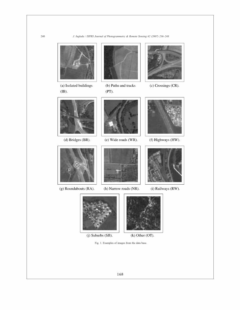
Autho
r's
pers
onal
co
py
Fig. 1. Examples of images from the data base.
240 J. Inglada / ISPRS Journal of Photogrammetry & Remote Sensing 62 (2007) 236–248
168
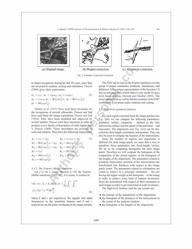
Autho
r's
pers
onal
co
py
in object recognition during the last 30 years, since theyare invariant to rotation, scaling and translation. Flusser(2000) gives their expressions:
u1 ¼ c11; u2 ¼ c20c02; u3 ¼ c30c03;
u4 ¼ c21c12;u5 ¼ Reðc30c312Þ; u6 ¼ Reðc21c212Þ;u7 ¼ Imðc30c312Þ:
ð2Þ
Dudani et al. (1977) have used these invariants forthe recognition of aircraft silhouettes. Flusser and Sukhave used them for image registration, Flusser and Suk(1994). They have been modified and improved byseveral authors. Flusser used these moments in order toproduce a new family of descriptors of order higher than3, Flusser (2000). These descriptors are invariant toscale and rotation. They have the following expressions:
w1 ¼ c11 ¼ u1; w2 ¼ c21c12 ¼ u4;
w3 ¼ Reðc20c212Þ ¼ u6; w4 ¼ Imðc20c212Þ;w5 ¼ Reðc30c312Þ ¼ u5; w6 ¼ Imðc30c312Þ ¼ u7:
w7 ¼ c22; w8 ¼ Reðc31c212Þ;w9 ¼ Imðc31c212Þ; w10 ¼ Reðc40c412Þ;w11 ¼ Imðc40c412Þ:
ð3Þ
3.1.2. The Fourier–Mellin transformLet f (r) be a causal function (rN0), the Fourier–
Mellin transform, FMT, of f, if it exists, is written as:
8ðk; vÞa ℤ�ℝ;Mf ðk; vÞ ¼ 12p
Z l
0
Z 2p
0
f ðr; hÞr�ive�ikhdhdrr; ð4Þ
where k and v are respectively the angular and radialfrequencies in the transform domain and θ and rrespectively are the polar coordinates in the image domain.
The FMTcan be seen as the Fourier transform over thegroup of planar similarities (rotations, translations, anddilations). It is a unique representation of the function f. Ithas several properties which make it very useful for greylevel image analysis, Derrode and Ghorbel (2001). Themost important for us will be that the modulus of the FMTcoefficients is invariant under rotations and scaling.
3.2. High-level geometry features
For each region extracted from the image patches (seeFig. 2(b)) we can compute the following parameters:perimeter, surface, compacity – defined as the ratiobetween the surface and the square of the perimeter – andbarycenter. The alignments (see Fig. 2(c)) can be des-cribed by their length, orientation, and position. They canalso be used to compute the location of the intersections.
Since the number of regions and alignments isdifferent for each image patch, we must find a way totransform these parameters into fixed-length vectors.We do so by computing histograms for each imagepatch. Therefore we will compute the histogram of thecompacities of the closed regions, or the histogram ofthe lengths of the alignments. The parameters related topositions (barycenter, position of the intersections) aretransformed into distances with respect to the imagepatch center. The parameters related to orientations arecoded as relative to a principal orientation – the onehaving the higher weight in the histogram – in the imagein order to achieve some kind of rotation invariance.Sizes are normalized with respect to their maximum ineach image in order to get some kind of scale invariance.
The high-level features used by our system are:
• the entropy of the orientations of the alignments;• the histogram of the distances of the intersections tothe center of the analysis window;
• the histogram of the lengths of the alignments;
Fig. 2. Examples of geometry extraction.
241J. Inglada / ISPRS Journal of Photogrammetry & Remote Sensing 62 (2007) 236–248
169
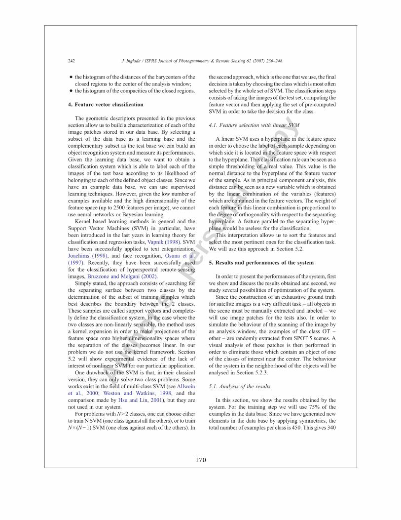
Autho
r's
pers
onal
co
py
• the histogram of the distances of the barycenters of theclosed regions to the center of the analysis window;
• the histogram of the compacities of the closed regions.
4. Feature vector classification
The geometric descriptors presented in the previoussection allow us to build a characterization of each of theimage patches stored in our data base. By selecting asubset of the data base as a learning base and thecomplementary subset as the test base we can build anobject recognition system and measure its performances.Given the learning data base, we want to obtain aclassification system which is able to label each of theimages of the test base according to its likelihood ofbelonging to each of the defined object classes. Since wehave an example data base, we can use supervisedlearning techniques. However, given the low number ofexamples available and the high dimensionality of thefeature space (up to 2500 features per image), we cannotuse neural networks or Bayesian learning.
Kernel based learning methods in general and theSupport Vector Machines (SVM) in particular, havebeen introduced in the last years in learning theory forclassification and regression tasks, Vapnik (1998). SVMhave been successfully applied to text categorization,Joachims (1998), and face recognition, Osuna et al.(1997). Recently, they have been successfully usedfor the classification of hyperspectral remote-sensingimages, Bruzzone and Melgani (2002).
Simply stated, the approach consists of searching forthe separating surface between two classes by thedetermination of the subset of training samples whichbest describes the boundary between the 2 classes.These samples are called support vectors and complete-ly define the classification system. In the case where thetwo classes are non-linearly separable, the method usesa kernel expansion in order to make projections of thefeature space onto higher dimensionality spaces wherethe separation of the classes becomes linear. In ourproblem we do not use the kernel framework. Section5.2 will show experimental evidence of the lack ofinterest of nonlinear SVM for our particular application.
One drawback of the SVM is that, in their classicalversion, they can only solve two-class problems. Someworks exist in the field of multi-class SVM (see Allweinet al., 2000; Weston and Watkins, 1998, and thecomparison made by Hsu and Lin, 2001), but they arenot used in our system.
For problems with NN2 classes, one can choose eitherto train N SVM (one class against all the others), or to trainN×(N−1) SVM (one class against each of the others). In
the second approach,which is the one thatwe use, the finaldecision is taken by choosing the class which ismost oftenselected by the whole set of SVM. The classification stepsconsists of taking the images of the test set, computing thefeature vector and then applying the set of pre-computedSVM in order to take the decision for the class.
4.1. Feature selection with linear SVM
A linear SVM uses a hyperplane in the feature spacein order to choose the label of each sample depending onwhich side it is located in the feature space with respectto the hyperplane. This classification rule can be seen as asimple thresholding of a real value. This value is thenormal distance to the hyperplane of the feature vectorof the sample. As in principal component analysis, thisdistance can be seen as a new variable which is obtainedby the linear combination of the variables (features)which are contained in the feature vectors. The weight ofeach feature in this linear combination is proportional tothe degree of orthogonality with respect to the separatinghyperplane. A feature parallel to the separating hyper-plane would be useless for the classification.
This interpretation allows us to sort the features andselect the most pertinent ones for the classification task.We will use this approach in Section 5.2.
5. Results and performances of the system
In order to present the performances of the system, firstwe show and discuss the results obtained and second, westudy several possibilities of optimization of the system.
Since the construction of an exhaustive ground truthfor satellite images is a very difficult task – all objects inthe scene must be manually extracted and labeled – wewill use image patches for the tests also. In order tosimulate the behaviour of the scanning of the image byan analysis window, the examples of the class OT –other – are randomly extracted from SPOT 5 scenes. Avisual analysis of these patches is then performed inorder to eliminate those which contain an object of oneof the classes of interest near the center. The behaviourof the system in the neighborhood of the objects will beanalysed in Section 5.2.3.
5.1. Analysis of the results
In this section, we show the results obtained by thesystem. For the training step we will use 75% of theexamples in the data base. Since we have generated newelements in the data base by applying symmetries, thetotal number of examples per class is 450. This gives 340
242 J. Inglada / ISPRS Journal of Photogrammetry & Remote Sensing 62 (2007) 236–248
170
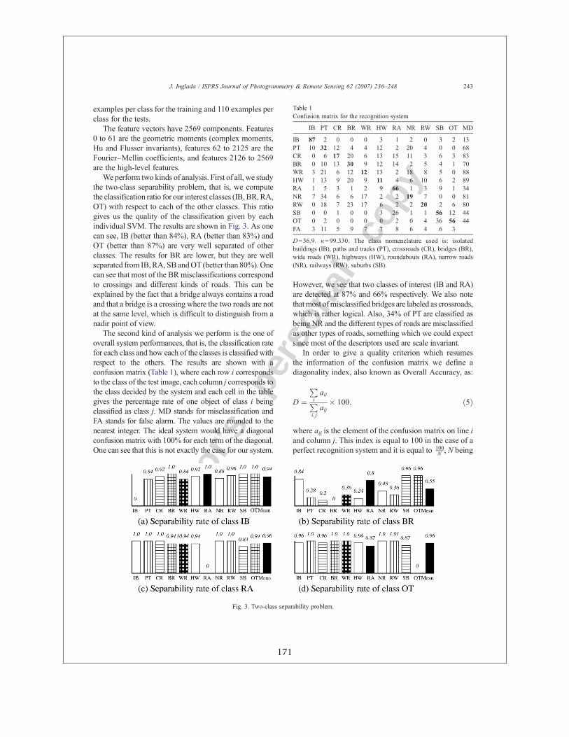
Autho
r's
pers
onal
co
py
examples per class for the training and 110 examples perclass for the tests.
The feature vectors have 2569 components. Features0 to 61 are the geometric moments (complex moments,Hu and Flusser invariants), features 62 to 2125 are theFourier–Mellin coefficients, and features 2126 to 2569are the high-level features.
We perform two kinds of analysis. First of all, we studythe two-class separability problem, that is, we computethe classification ratio for our interest classes (IB,BR,RA,OT) with respect to each of the other classes. This ratiogives us the quality of the classification given by eachindividual SVM. The results are shown in Fig. 3. As onecan see, IB (better than 84%), RA (better than 83%) andOT (better than 87%) are very well separated of otherclasses. The results for BR are lower, but they are wellseparated from IB, RA, SB andOT (better than 80%). Onecan see that most of the BR misclassifications correspondto crossings and different kinds of roads. This can beexplained by the fact that a bridge always contains a roadand that a bridge is a crossing where the two roads are notat the same level, which is difficult to distinguish from anadir point of view.
The second kind of analysis we perform is the one ofoverall system performances, that is, the classification ratefor each class and how each of the classes is classified withrespect to the others. The results are shown with aconfusion matrix (Table 1), where each row i correspondsto the class of the test image, each column j corresponds tothe class decided by the system and each cell in the tablegives the percentage rate of one object of class i beingclassified as class j. MD stands for misclassification andFA stands for false alarm. The values are rounded to thenearest integer. The ideal system would have a diagonalconfusion matrix with 100% for each term of the diagonal.One can see that this is not exactly the case for our system.
However, we see that two classes of interest (IB and RA)are detected at 87% and 66% respectively. We also notethatmost ofmisclassified bridges are labeled as crossroads,which is rather logical. Also, 34% of PT are classified asbeing NR and the different types of roads are misclassifiedas other types of roads, something which we could expectsince most of the descriptors used are scale invariant.
In order to give a quality criterion which resumesthe information of the confusion matrix we define adiagonality index, also known as Overall Accuracy, as:
D ¼PiaiiP
i; jaij
� 100; ð5Þ
where aij is the element of the confusion matrix on line iand column j. This index is equal to 100 in the case of aperfect recognition system and it is equal to 100
N , N being
Table 1Confusion matrix for the recognition system
IB PT CR BR WR HW RA NR RW SB OT MD
IB 87 2 0 0 0 3 1 2 0 3 2 13PT 10 32 12 4 4 12 2 20 4 0 0 68CR 0 6 17 20 6 13 15 11 3 6 3 83BR 0 10 13 30 9 12 14 2 5 4 1 70WR 3 21 6 12 12 13 2 18 8 5 0 88HW 1 13 9 20 9 11 4 6 10 6 2 89RA 1 5 3 1 2 9 66 1 3 9 1 34NR 7 34 6 6 17 2 2 19 7 0 0 81RW 0 18 7 23 17 6 2 2 20 2 6 80SB 0 0 1 0 0 3 26 1 1 56 12 44OT 0 2 0 0 0 0 2 0 4 36 56 44FA 3 11 5 9 7 7 8 6 4 6 3
D=36.9. κ=99.330. The class nomenclature used is: isolatedbuildings (IB), paths and tracks (PT), crossroads (CR), bridges (BR),wide roads (WR), highways (HW), roundabouts (RA), narrow roads(NR), railways (RW), suburbs (SB).
Fig. 3. Two-class separability problem.
243J. Inglada / ISPRS Journal of Photogrammetry & Remote Sensing 62 (2007) 236–248
171
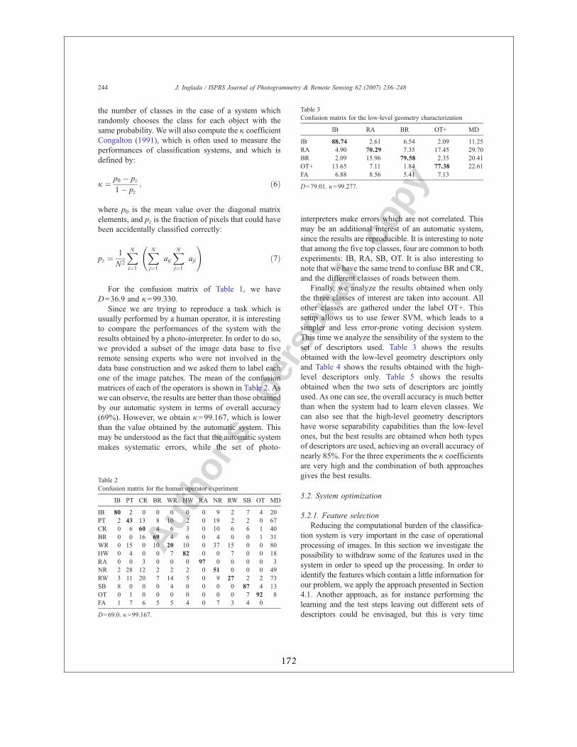
Autho
r's
pers
onal
co
py
the number of classes in the case of a system whichrandomly chooses the class for each object with thesame probability. We will also compute the κ coefficientCongalton (1991), which is often used to measure theperformances of classification systems, and which isdefined by:
j ¼ p0 � pz1� pz
; ð6Þ
where p0 is the mean value over the diagonal matrixelements, and pz is the fraction of pixels that could havebeen accidentally classified correctly:
pz ¼ 1N2
XNi¼1
XNj¼1
aijXNj¼1
aji
!ð7Þ
For the confusion matrix of Table 1, we haveD=36.9 and κ=99.330.
Since we are trying to reproduce a task which isusually performed by a human operator, it is interestingto compare the performances of the system with theresults obtained by a photo-interpreter. In order to do so,we provided a subset of the image data base to fiveremote sensing experts who were not involved in thedata base construction and we asked them to label eachone of the image patches. The mean of the confusionmatrices of each of the operators is shown in Table 2. Aswe can observe, the results are better than those obtainedby our automatic system in terms of overall accuracy(69%). However, we obtain κ=99.167, which is lowerthan the value obtained by the automatic system. Thismay be understood as the fact that the automatic systemmakes systematic errors, while the set of photo-
interpreters make errors which are not correlated. Thismay be an additional interest of an automatic system,since the results are reproducible. It is interesting to notethat among the five top classes, four are common to bothexperiments: IB, RA, SB, OT. It is also interesting tonote that we have the same trend to confuse BR and CR,and the different classes of roads between them.
Finally, we analyze the results obtained when onlythe three classes of interest are taken into account. Allother classes are gathered under the label OT+. Thissetup allows us to use fewer SVM, which leads to asimpler and less error-prone voting decision system.This time we analyze the sensibility of the system to theset of descriptors used. Table 3 shows the resultsobtained with the low-level geometry descriptors onlyand Table 4 shows the results obtained with the high-level descriptors only. Table 5 shows the resultsobtained when the two sets of descriptors are jointlyused. As one can see, the overall accuracy is much betterthan when the system had to learn eleven classes. Wecan also see that the high-level geometry descriptorshave worse separability capabilities than the low-levelones, but the best results are obtained when both typesof descriptors are used, achieving an overall accuracy ofnearly 85%. For the three experiments the κ coefficientsare very high and the combination of both approachesgives the best results.
5.2. System optimization
5.2.1. Feature selectionReducing the computational burden of the classifica-
tion system is very important in the case of operationalprocessing of images. In this section we investigate thepossibility to withdraw some of the features used in thesystem in order to speed up the processing. In order toidentify the features which contain a little information forour problem, we apply the approach presented in Section4.1. Another approach, as for instance performing thelearning and the test steps leaving out different sets ofdescriptors could be envisaged, but this is very time
Table 2Confusion matrix for the human operator experiment
IB PT CR BR WR HW RA NR RW SB OT MD
IB 80 2 0 0 0 0 0 9 2 7 4 20PT 2 43 13 8 10 2 0 19 2 2 0 67CR 0 6 60 4 6 3 0 10 6 6 1 40BR 0 0 16 69 4 6 0 4 0 0 1 31WR 0 15 0 10 20 10 0 37 15 0 0 80HW 0 4 0 0 7 82 0 0 7 0 0 18RA 0 0 3 0 0 0 97 0 0 0 0 3NR 2 28 12 2 2 2 0 51 0 0 0 49RW 3 11 20 7 14 5 0 9 27 2 2 73SB 8 0 0 0 4 0 0 0 0 87 4 13OT 0 1 0 0 0 0 0 0 0 7 92 8FA 1 7 6 5 5 4 0 7 3 4 0
D=69.0. κ=99.167.
Table 3Confusion matrix for the low-level geometry characterization
IB RA BR OT+ MD
IB 88.74 2.61 6.54 2.09 11.25RA 4.90 70.29 7.35 17.45 29.70BR 2.09 15.96 79.58 2.35 20.41OT+ 13.65 7.11 1.84 77.38 22.61FA 6.88 8.56 5.41 7.13
D=79.01. κ=99.277.
244 J. Inglada / ISPRS Journal of Photogrammetry & Remote Sensing 62 (2007) 236–248
172
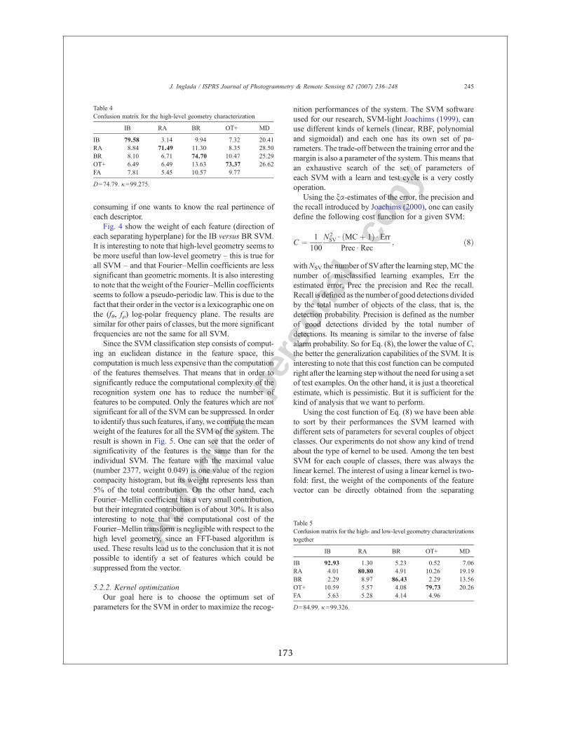
Autho
r's
pers
onal
co
pyconsuming if one wants to know the real pertinence ofeach descriptor.
Fig. 4 show the weight of each feature (direction ofeach separating hyperplane) for the IB versus BR SVM.It is interesting to note that high-level geometry seems tobe more useful than low-level geometry – this is true forall SVM – and that Fourier–Mellin coefficients are lesssignificant than geometric moments. It is also interestingto note that the weight of the Fourier–Mellin coefficientsseems to follow a pseudo-periodic law. This is due to thefact that their order in the vector is a lexicographic one onthe (fθ, fρ) log-polar frequency plane. The results aresimilar for other pairs of classes, but the more significantfrequencies are not the same for all SVM.
Since the SVM classification step consists of comput-ing an euclidean distance in the feature space, thiscomputation is much less expensive than the computationof the features themselves. That means that in order tosignificantly reduce the computational complexity of therecognition system one has to reduce the number offeatures to be computed. Only the features which are notsignificant for all of the SVM can be suppressed. In orderto identify thus such features, if any, we compute themeanweight of the features for all the SVM of the system. Theresult is shown in Fig. 5. One can see that the order ofsignificativity of the features is the same than for theindividual SVM. The feature with the maximal value(number 2377, weight 0.049) is one value of the regioncompacity histogram, but its weight represents less than5% of the total contribution. On the other hand, eachFourier–Mellin coefficient has a very small contribution,but their integrated contribution is of about 30%. It is alsointeresting to note that the computational cost of theFourier–Mellin transform is negligible with respect to thehigh level geometry, since an FFT-based algorithm isused. These results lead us to the conclusion that it is notpossible to identify a set of features which could besuppressed from the vector.
5.2.2. Kernel optimizationOur goal here is to choose the optimum set of
parameters for the SVM in order to maximize the recog-
nition performances of the system. The SVM softwareused for our research, SVM-light Joachims (1999), canuse different kinds of kernels (linear, RBF, polynomialand sigmoidal) and each one has its own set of pa-rameters. The trade-off between the training error and themargin is also a parameter of the system. This means thatan exhaustive search of the set of parameters ofeach SVM with a learn and test cycle is a very costlyoperation.
Using the ξα-estimates of the error, the precision andthe recall introduced by Joachims (2000), one can easilydefine the following cost function for a given SVM:
C ¼ 1100
N 2SVd ðMCþ 1Þd Err
Precd Rec; ð8Þ
withNSV the number of SVafter the learning step, MC thenumber of misclassified learning examples, Err theestimated error, Prec the precision and Rec the recall.Recall is defined as the number of good detections dividedby the total number of objects of the class, that is, thedetection probability. Precision is defined as the numberof good detections divided by the total number ofdetections. Its meaning is similar to the inverse of falsealarm probability. So for Eq. (8), the lower the value ofC,the better the generalization capabilities of the SVM. It isinteresting to note that this cost function can be computedright after the learning stepwithout the need for using a setof test examples. On the other hand, it is just a theoreticalestimate, which is pessimistic. But it is sufficient for thekind of analysis that we want to perform.
Using the cost function of Eq. (8) we have been ableto sort by their performances the SVM learned withdifferent sets of parameters for several couples of objectclasses. Our experiments do not show any kind of trendabout the type of kernel to be used. Among the ten bestSVM for each couple of classes, there was always thelinear kernel. The interest of using a linear kernel is two-fold: first, the weight of the components of the featurevector can be directly obtained from the separating
Table 5Confusion matrix for the high- and low-level geometry characterizationstogether
IB RA BR OT+ MD
IB 92.93 1.30 5.23 0.52 7.06RA 4.01 80.80 4.91 10.26 19.19BR 2.29 8.97 86.43 2.29 13.56OT+ 10.59 5.57 4.08 79.73 20.26FA 5.63 5.28 4.14 4.96
D=84.99. κ=99.326.
Table 4Confusion matrix for the high-level geometry characterization
IB RA BR OT+ MD
IB 79.58 3.14 9.94 7.32 20.41RA 8.84 71.49 11.30 8.35 28.50BR 8.10 6.71 74.70 10.47 25.29OT+ 6.49 6.49 13.63 73.37 26.62FA 7.81 5.45 10.57 9.77
D=74.79. κ=99.275.
245J. Inglada / ISPRS Journal of Photogrammetry & Remote Sensing 62 (2007) 236–248
173
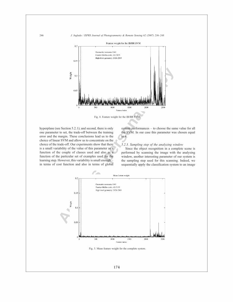
Autho
r's
pers
onal
co
py
hyperplane (see Section 5.2.1); and second, there is onlyone parameter to set, the trade-off between the trainingerror and the margin. These conclusions lead us to thechoice of linear SVM and allow us to concentrate on thechoice of the trade-off. Our experiments show that thereis a small variability of the value of this parameter as afunction of the couple of classes used and also as afunction of the particular set of examples used for thelearning step. However, this variability is small enough –in terms of cost function and also in terms of global
system performances – to choose the same value for allthe SVM. In our case this parameter was chosen equalto 4.
5.2.3. Sampling step of the analyzing windowSince the object recognition in a complete scene is
performed by scanning the image with the analysingwindow, another interesting parameter of our system isthe sampling step used for this scanning. Indeed, wesequentially apply the classification system to an image
Fig. 5. Mean feature weight for the complete system.
Fig. 4. Feature weight for the IB/BR SVM.
246 J. Inglada / ISPRS Journal of Photogrammetry & Remote Sensing 62 (2007) 236–248
174
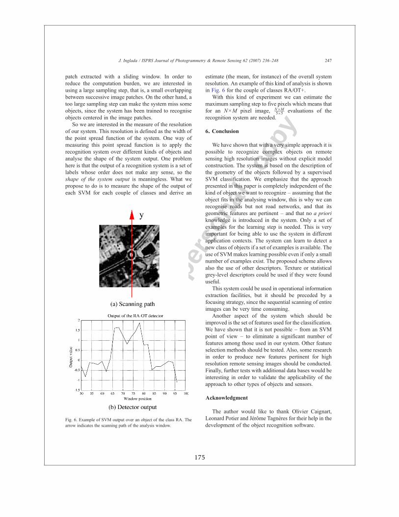
Autho
r's
pers
onal
co
py
patch extracted with a sliding window. In order toreduce the computation burden, we are interested inusing a large sampling step, that is, a small overlappingbetween successive image patches. On the other hand, atoo large sampling step can make the system miss someobjects, since the system has been trained to recogniseobjects centered in the image patches.
So we are interested in the measure of the resolutionof our system. This resolution is defined as the width ofthe point spread function of the system. One way ofmeasuring this point spread function is to apply therecognition system over different kinds of objects andanalyse the shape of the system output. One problemhere is that the output of a recognition system is a set oflabels whose order does not make any sense, so theshape of the system output is meaningless. What wepropose to do is to measure the shape of the output ofeach SVM for each couple of classes and derive an
estimate (the mean, for instance) of the overall systemresolution. An example of this kind of analysis is shownin Fig. 6 for the couple of classes RA/OT+.
With this kind of experiment we can estimate themaximum sampling step to five pixels which means thatfor an N×M pixel image, N�M
5�5 evaluations of therecognition system are needed.
6. Conclusion
We have shown that with a very simple approach it ispossible to recognize complex objects on remotesensing high resolution images without explicit modelconstruction. The system is based on the description ofthe geometry of the objects followed by a supervisedSVM classification. We emphasize that the approachpresented in this paper is completely independent of thekind of object we want to recognize – assuming that theobject fits in the analysing window, this is why we canrecognise roads but not road networks, and that itsgeometric features are pertinent – and that no a prioriknowledge is introduced in the system. Only a set ofexamples for the learning step is needed. This is veryimportant for being able to use the system in differentapplication contexts. The system can learn to detect anew class of objects if a set of examples is available. Theuse of SVMmakes learning possible even if only a smallnumber of examples exist. The proposed scheme allowsalso the use of other descriptors. Texture or statisticalgrey-level descriptors could be used if they were founduseful.
This system could be used in operational informationextraction facilities, but it should be preceded by afocusing strategy, since the sequential scanning of entireimages can be very time consuming.
Another aspect of the system which should beimproved is the set of features used for the classification.We have shown that it is not possible – from an SVMpoint of view – to eliminate a significant number offeatures among those used in our system. Other featureselection methods should be tested. Also, some researchin order to produce new features pertinent for highresolution remote sensing images should be conducted.Finally, further tests with additional data bases would beinteresting in order to validate the applicability of theapproach to other types of objects and sensors.
Acknowledgment
The author would like to thank Olivier Caignart,Leonard Potier and Jérôme Tagnères for their help in thedevelopment of the object recognition software.
Fig. 6. Example of SVM output over an object of the class RA. Thearrow indicates the scanning path of the analysis window.
247J. Inglada / ISPRS Journal of Photogrammetry & Remote Sensing 62 (2007) 236–248
175
Autho
r's
pers
onal
co
py
References
Allwein, E.L., Schapire, R.E., Singer, Y., 2000. Reducing multiclass tobinary: a unifying approach for margin classifiers. Proceedings17th International Conference on Machine Learning. MorganKaufmann, San Francisco, CA, pp. 9–16.
Baumgartner, A., Steger, C., Mayer, H., Eckstein, W., Ebner, H., 1999.Automatic road extraction based onmulti-scale, grouping, and context.Photogrammetric Engineering & Remote Sensing 65 (7), 777–785.
Borgne, H.L., Guérin-Dugué, A., Antoniadis, A., 2004. Representa-tion of images for classification with independent features. PatternRecognition Letters 25 (2), 141–154.
Bruzzone, L., Melgani, F., 2002. Support vector machines for classificationof hyperspectral remote-sensing images. IEEE InternationalGeoscienceand Remote Sensing Symposium, IGARSS, vol. 1, pp. 506–508. Jun.
Congalton, R., 1991. A review of assessing the accuracy of classifica-tions of remotely sensed data. Remote Sensing of Environment 37(1), 35–46.
Daschiel, H., Datcu, M., 2005. Information mining in remote sensingimage archives: system evaluation. IEEE Transactions onGeoscience and Remote Sensing 43 (1), 188–199 Jan.
Datcu, M., Seidel, K., Walessa, M., 1998. Spatial information retrievalfrom remote-sensing images — Part I: information theoreticalperspective. IEEE Transactions on Geoscience and RemoteSensing 36 (5), 1431–1445.
Datcu, M., Daschiel, H., Pelizzari, A., Quartulli, M., Galoppo, A.,Colapicchioni, A., Pastori, M., Seidel, K., Marchetti, P.G., 2003.Informationmining in remote sensing image archives: systemconcepts.IEEE Transactions on Geoscience and Remote Sensing 41 (12),2923–2936.
Dell'Acqua, F., Gamba, P., 2001. Query-by-shape in meteorologicalimage archives using the point diffusion technique. IEEE Transac-tions on Geoscience and Remote Sensing 39 (9), 1834–1843.
Derrode, S., Ghorbel, F., 2001. Robust and efficient Fourier–Mellintransform approximations for gray-level image reconstructionand complete invariant description. Computer Vision and ImageUnderstanding 83 (1), 57–78.
Desolneux, A., Moisan, L., Morel, J.-M., 2000. Meaningfulalignments. International Journal of Computer Vision 40 (1), 7–23.
Desolneux, A., Moisan, L., Morel, J.-M., 2001. Edge detection byHelmholtz principle. Journal of Mathematical Imaging and Vision14 (3), 271–284.
Dudani, S., Breeding, K., McGhee, R., 1977. Aircraft identification bymoments invariants. IEEETransactions onComputers 26 (1), 39–45.
Flusser, J., 2000. On the independence of rotation moment invariants.Pattern Recognition 33 (9), 1405–1410.
Fraser, C., Baltsavias, E., Gruen, A., 2002. Processing of Ikonos imageryfor submetre 3D positioning and building extraction. ISPRS Journalof Photogrammetry and Remote Sensing 56 (3), 177–194.
Gerke, M., Heipke, C., Straub, B.-M., 2001. Building extraction fromaerial imagery using a generic scene model and invariant geometricmoments. Proceedings of the IEEE/ISPRS jointWorkshop onRemoteSensing and Data Fusion over Urban Areas, November 8–9th 2001,University of Pavia, Rome (Italy), pp. 85–89.
Gülch, E., Müller, H., Läbe, T., Ragia, L., 1998. On the performance ofsemi-automatic building extraction. International Archives ofPhotogrammetry and Remote Sensing 32 (Part 3/1), 331–338.
Hamdan, R., Heitz, F., Thoraval, L., 2001. Modèles probabilistesd'apparence: une représentation approchée de faible complexité.Traitement du Signal 18 (3).
Hinz, S., Baumgartner, A., 2003. Automatic extraction of urban roadnetworks from multi-view aerial imagery. ISPRS Journal ofPhotogrammetry and Remote Sensing 58 (1–2), 83–98.
Hsu, C., Lin, C., 2001. A comparison of methods for multi-classsupport vector machines. Technical Report, Department ofComputer Science and Information Engineering. National TaiwanUniversity, Taipei, Taiwan, p. 19.
Hu, M.K., 1962. Visual pattern recognition by moment invariants.IEEE Transactions on Information Theory 8 (2), 179–187.
Flusser, J., Suk, T., 1994. A moment based approach to registration ofimage with affine geometric distortion. IEEE Transactions onGeoscience and Remote Sensing 32 (2), 382–387.
Joachims, T., 1998. Text categorization with support vector machines:learning with many relevant features. In: Nédellec, Claire,Rouveirol, Céline (Eds.), Proceedings of the European Conferenceon Machine Learning. Springer, pp. 137–142.
Joachims, T., 1999. Making large-scale SVM learning practical.In: Schlkopf, B., Burges, C., Smola, A. (Eds.), Advances in KernelMethods — Support Vector Learning. MIT Press.
Joachims, T., 2000. Estimating the Generalization Performance of aSVM Efficiently. Proceedings of the International Conference onMachine Learning. Morgan Kaufman.
Mena, J., 2003. State of the art on automatic road extraction for GISupdate: a novel classification. Pattern Recognition Letters 24 (16),3037–3058.
Osuna, E., Freund, R., Girosi, F., 1997. Training support vectormachines: an application to face detection. Proceedings of IEEEComputer Vision and Pattern Recognition Conference, pp. 130–136.
Pope, A.A., Lowe, D.G., 1996. Learning appearance models for objectrecognition. International Workshop on Object Representation forComputer Vision, Cambridge, UK, pp. 201–219.
Rochery, M., Jermyn, I.H., Zerubia, J., 2003. Higher order activecontours and their application to the detection of line networks insatellite imagery. Proc. IEEE Workshop Variational, Geometricand Level Set Methods in Computer Vision, at ICCV, Nice, France.
Schroeder, M., Rehrauer, H., Seidel, K., Datcu, M., 1998. Spatialinformation retrieval from remote-sensing images — Part II:Gibbs–Markov random fields. IEEE Transactions on Geoscienceand Remote Sensing 36 (5), 1446–1455.
Schroeder, M., Rehrauer, H., Seidel, K., Datcu, M., 2000. Interactivelearning and probabilistic retrieval in remote sensing image archives.IEEE Transactions on Geoscience and Remote Sensing 38 (5),2288–2298.
Stoica, R., Descombes, X., Zerubia, J., 2004. A Gibbs point processfor road extraction from remotely sensed images. InternationalJournal of Computer Vision 57 (2), 121–136.
Thorpe, S., Delorme, A., Rullen, R.V., 2001. Spike-based strategies forrapid processing. Neural Networks 14 (6–7), 715–725.
Turk, M., 2001. A random walk through eigenspace. IEICETransactions on Information Systems E84-D (12), 1586–1695.
Turk, M., Pentland, A.P., 1991. Eigenfaces for recognition. Journal ofCognitive Neuroscience 3 (1), 71–86.
Vapnik, V., 1998. Statistical Learning Theory. John Wiley and Sons,NewYork.
Veltkamp, R., Hagedoorn, M., 1999. State-of-the-art in ShapeMatching. Tech. Rep. UU-CS-1999-27. Utrecht University, TheNetherlands.
Weston, J., Watkins, C., 1998. Multi-class support vector machines.Tech. Rep. CSD-TR-98-04, Department of Computer Science,Royal Holloway, University of London, Egham, TW20 0EX, UK.
248 J. Inglada / ISPRS Journal of Photogrammetry & Remote Sensing 62 (2007) 236–248
176

16 Raisonnement spatial
177
IEEE TRANSACTIONS ON GEOSCIENCE AND REMOTE SENSING, VOL. 47, NO. 2, FEBRUARY 2009 599
Qualitative Spatial Reasoning for High-ResolutionRemote Sensing Image Analysis
Jordi Inglada and Julien Michel
Abstract—High-resolution (HR) remote-sensing images allowus to access new kinds of information. Classical techniques forimage analysis, such as pixel-based classifications or region-basedsegmentations, do not allow to fully exploit the richness of thiskind of images. Indeed, for many applications, we are interestedin complex objects which can only be identified and analyzed bystudying the relationships between the elementary objects whichcompose them. In this paper, the use of a spatial reasoning tech-nique called region connection calculus for the analysis of HRremote-sensing images is presented. A graph-based representationof the spatial relationships between the regions of an image isused within a graph-matching procedure in order to implementan object detection algorithm.
Index Terms—Graph theory, image analysis, image representa-tions, spatial reasoning.
I. INTRODUCTION
B ECAUSE of the diversity of sensors and the increaseof their spatial resolution and repetitivity, the automatic
analysis of images is a crucial asset in the remote-sensingfield. It is therefore needed to design and implement newimage analysis techniques which are able to perform complexprocessing in an efficient manner. In this context, much workhas been done for the automatic information extraction fromremote-sensing images aiming to provide a set of features anddescriptors which are compact and parsimonious in order tofeed them into learning systems. This type of features comeoften from low-level processing and are not able to capturethe richness and complexity of high-resolution (HR) images.Indeed, the improvement of the spatial resolution makes thatthe objects of interest are not any more limited to several pixels,but they are represented by large areas containing subobjects.This kind of objects cannot efficiently be described by textures,edges, etc.
Recent publications present interesting advances in therecognition of particular objects as buildings [1] or urban areas[2], but this kind of approaches are not generic enough to dealwith different types of objects.
It is therefore useful to use techniques which are able to dealwith higher levels of abstraction for the representation and the
Manuscript received December 7, 2007; revised March 13, 2008 andJuly 4, 2008. First published November 25, 2008; current version publishedJanuary 28, 2009.
J. Inglada is with the Centre National d’Études Spatiales, 31401 Toulouse,France (e-mail: [email protected]).
J. Michel is with the Communications et Systèmes, 31506 Toulouse, France(e-mail: [email protected]).
Color versions of one or more of the figures in this paper are available onlineat http://ieeexplore.ieee.org.
Digital Object Identifier 10.1109/TGRS.2008.2003435
manipulation of the information contained in the images. Inthis paper, we will use spatial reasoning techniques in orderto describe complex objects. We have chosen to use the well-known region connection calculus (RCC8) [3] in order todescribe the relationships between the regions of an image.
The regions used for the spatial reasoning are obtainedwith a multiscale segmentation based on geodesic morphology[4]. The mathematical morphology approach has been selectedbecause, in contrast to linear multiscale approaches, it allowsone to select objects in terms of their size. This has been shownto be interesting in meter and submeter resolution images fordetecting vehicles, buildings, etc. Our algorithm is able toproduce regions superimposing across the scales.
This allows one to exploit the full extent of the RCC8relationships set. The regions and their relationships are rep-resented by means of an attributed relational graph (ARG)where the nodes represent the regions and the arcs representthe RCC8 relationships. The ARG can be made more completeby adding region attributes to the nodes, as for instance shapeand radiometric features.
Finally, object detection and recognition can be seen as agraph-matching problem for which efficient algorithms can beimplemented. In these context, a greedy search combined witha graph metric which is able to use all the information containedin the ARG has been implemented.
In this paper, the theoretical basis of the approach andexamples of application to real images will be presented.
This paper is organized as follows. Section II introduces theprinciples of RCC. Section III presents the approach used forimage segmentation. Section IV presents the graph-matchingproblem. Section V describes the implementation of the pro-cedure. Section VII presents some example of results on realimages. Section VIII draws some conclusions.
II. RCC
A. Spatial Reasoning
The spatial organization of the objects in images gives animportant information for the recognition and interpretationtasks, particularly when the objects are located in complexenvironments as it is usually the case in remote-sensing HRimages.
Spatial reasoning can be defined as the set of techniquesfor the manipulation of the description of physical objects bytaking into account their mutual interactions expressed in termsof their shapes, sizes, positions, orientations, and plausiblemovements [5].
There are several space logics. Different theories use dif-ferent primitive features: points, lines, polygons, etc. The base
0196-2892/$25.00 © 2008 IEEE
178
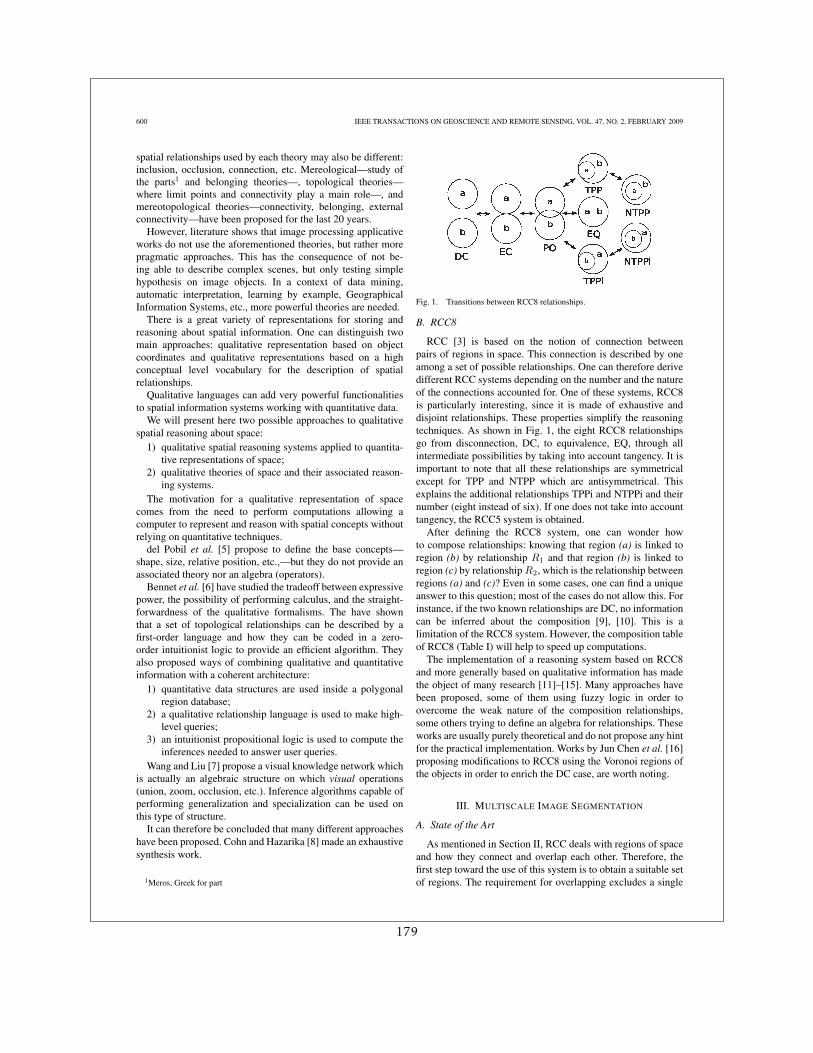
600 IEEE TRANSACTIONS ON GEOSCIENCE AND REMOTE SENSING, VOL. 47, NO. 2, FEBRUARY 2009
spatial relationships used by each theory may also be different:inclusion, occlusion, connection, etc. Mereological—study ofthe parts1 and belonging theories—, topological theories—where limit points and connectivity play a main role—, andmereotopological theories—connectivity, belonging, externalconnectivity—have been proposed for the last 20 years.
However, literature shows that image processing applicativeworks do not use the aforementioned theories, but rather morepragmatic approaches. This has the consequence of not be-ing able to describe complex scenes, but only testing simplehypothesis on image objects. In a context of data mining,automatic interpretation, learning by example, GeographicalInformation Systems, etc., more powerful theories are needed.
There is a great variety of representations for storing andreasoning about spatial information. One can distinguish twomain approaches: qualitative representation based on objectcoordinates and qualitative representations based on a highconceptual level vocabulary for the description of spatialrelationships.
Qualitative languages can add very powerful functionalitiesto spatial information systems working with quantitative data.
We will present here two possible approaches to qualitativespatial reasoning about space:
1) qualitative spatial reasoning systems applied to quantita-tive representations of space;
2) qualitative theories of space and their associated reason-ing systems.
The motivation for a qualitative representation of spacecomes from the need to perform computations allowing acomputer to represent and reason with spatial concepts withoutrelying on quantitative techniques.
del Pobil et al. [5] propose to define the base concepts—shape, size, relative position, etc.,—but they do not provide anassociated theory nor an algebra (operators).
Bennet et al. [6] have studied the tradeoff between expressivepower, the possibility of performing calculus, and the straight-forwardness of the qualitative formalisms. The have shownthat a set of topological relationships can be described by afirst-order language and how they can be coded in a zero-order intuitionist logic to provide an efficient algorithm. Theyalso proposed ways of combining qualitative and quantitativeinformation with a coherent architecture:
1) quantitative data structures are used inside a polygonalregion database;
2) a qualitative relationship language is used to make high-level queries;
3) an intuitionist propositional logic is used to compute theinferences needed to answer user queries.
Wang and Liu [7] propose a visual knowledge network whichis actually an algebraic structure on which visual operations(union, zoom, occlusion, etc.). Inference algorithms capable ofperforming generalization and specialization can be used onthis type of structure.
It can therefore be concluded that many different approacheshave been proposed. Cohn and Hazarika [8] made an exhaustivesynthesis work.
1Meros, Greek for part
Fig. 1. Transitions between RCC8 relationships.
B. RCC8
RCC [3] is based on the notion of connection betweenpairs of regions in space. This connection is described by oneamong a set of possible relationships. One can therefore derivedifferent RCC systems depending on the number and the natureof the connections accounted for. One of these systems, RCC8is particularly interesting, since it is made of exhaustive anddisjoint relationships. These properties simplify the reasoningtechniques. As shown in Fig. 1, the eight RCC8 relationshipsgo from disconnection, DC, to equivalence, EQ, through allintermediate possibilities by taking into account tangency. It isimportant to note that all these relationships are symmetricalexcept for TPP and NTPP which are antisymmetrical. Thisexplains the additional relationships TPPi and NTPPi and theirnumber (eight instead of six). If one does not take into accounttangency, the RCC5 system is obtained.
After defining the RCC8 system, one can wonder howto compose relationships: knowing that region (a) is linked toregion (b) by relationship R1 and that region (b) is linked toregion (c) by relationship R2, which is the relationship betweenregions (a) and (c)? Even in some cases, one can find a uniqueanswer to this question; most of the cases do not allow this. Forinstance, if the two known relationships are DC, no informationcan be inferred about the composition [9], [10]. This is alimitation of the RCC8 system. However, the composition tableof RCC8 (Table I) will help to speed up computations.
The implementation of a reasoning system based on RCC8and more generally based on qualitative information has madethe object of many research [11]–[15]. Many approaches havebeen proposed, some of them using fuzzy logic in order toovercome the weak nature of the composition relationships,some others trying to define an algebra for relationships. Theseworks are usually purely theoretical and do not propose any hintfor the practical implementation. Works by Jun Chen et al. [16]proposing modifications to RCC8 using the Voronoi regions ofthe objects in order to enrich the DC case, are worth noting.
III. MULTISCALE IMAGE SEGMENTATION
A. State of the Art
As mentioned in Section II, RCC deals with regions of spaceand how they connect and overlap each other. Therefore, thefirst step toward the use of this system is to obtain a suitable setof regions. The requirement for overlapping excludes a single
179
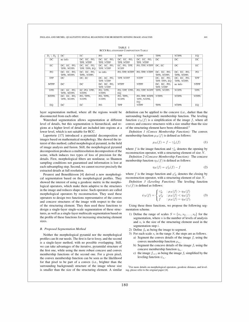
INGLADA AND MICHEL: QUALITATIVE SPATIAL REASONING FOR HR REMOTE-SENSING IMAGE ANALYSIS 601
TABLE IRCC8 RELATIONSHIP COMPOSITION TABLE
layer segmentation method, where all the regions would bedisconnected from each other.
Watershed segmentation allows segmentation at differentlevel of details, but this segmentation is hierarchical, and re-gions at a higher level of detail are included into regions at alower level, which is not suitable for RCC.
Laporterie [17] introduced a pyramidal decomposition ofimages based on mathematical morphology. She showed the in-terest of this method, called morphological pyramid, in the fieldof image analysis and fusion. Still, the morphological pyramiddecomposition produces a multiresolution decomposition of thescene, which induces two types of loss of precision for thedetails. First, morphological filters are nonlinear, so Shannonsampling conditions not guaranteed and information is lost ateach subsampling step. Second, we cannot recover precisely theextracted details at full resolution.
Pesaresi and Benediktsson [4] derived a new morphologi-cal segmentation based on the morphological profiles. Theyshowed the interest of using a geodesic metric in the morpho-logical operators, which make them adaptive to the structuresin the image and reduces shape noise. Such operators are calledmorphological operators by reconstruction. They used theseoperators to design two functions representative of the convexand concave structures of the image with respect to the sizeof the structuring element. They then used these functions todesign a single-layer single-scale segmentation of these struc-tures, as well as a single-layer multiscale segmentation based onthe profile of these functions for increasing structuring elementsizes.
B. Proposed Segmentation Method
Neither the morphological pyramid nor the morphologicalprofiles can fit our needs. The first is far to lossy, and the secondis a single-layer method, with no possible overlapping. Still,we can take advantages of the iterative, pyramidal structure ofthe first one, while using the more robust concave and convexmembership functions of the second one. For a given pixel,the convex membership function can be seen as the likelihoodfor that pixel to be part of a convex (i.e., brighter than thesurrounding background) structure of the image whose sizeis smaller than the size of the structuring element. A similar
definition can be applied to the concave (i.e., darker than thesurrounding background) membership function. The levelingfunction ψN (f) is a simplification of the image f , where allconvex and concave structures with a size smaller than the sizeof the structuring element have been obliterated.2
Definition 1 (Convex Membership Function): The convexmembership function μN (f) is defined as follows:
μN (f) = f − γ∗N (f) (1)
where f is the image function and γ∗N denotes the opening by
reconstruction operator, with a structuring element of size N .Definition 2 (Concave Membership Function): The concave
membership function ηN (f) is defined as follows:
ηN (f) = ϕ∗N (f) − f (2)
where f is the image function and ϕ∗N denotes the closing by
reconstruction operator, with a structuring element of size N .Definition 3 (Leveling Function): The leveling function
ψN (f) is defined as follows:
ψN (f) =
⎧⎨⎩
γ∗N : μN (f) > ηN (f)
ϕ∗N : μN (f) < ηN (f)
f : μN (f) = ηN (f).(3)
Using these three functions, we propose the following seg-mentation scheme.
1) Define the range of scales S = {s1, s2, . . . , s2} for thesegmentation, where n is the number of levels of analysisand si is the size of the structuring element used in thesegmentation step i.
2) Define f0 as being the image to segment.3) For each scale si in the range S, the steps are as follows.
a) Segment the convex details of the image fi using theconvex membership function μsi
.b) Segment the concave details of the image fi using the
concave membership function ηsi.
c) the image fi+1 as being the image fi simplified by theleveling function ψsi
.
2For more details on morphological operators, geodesic distance, and level-ing, please refer to the original paper [4].
180
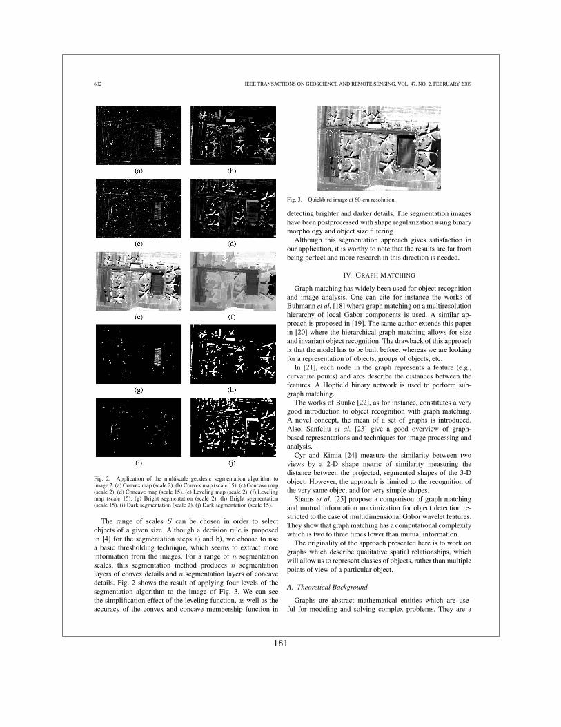
602 IEEE TRANSACTIONS ON GEOSCIENCE AND REMOTE SENSING, VOL. 47, NO. 2, FEBRUARY 2009
Fig. 2. Application of the multiscale geodesic segmentation algorithm toimage 2. (a) Convex map (scale 2). (b) Convex map (scale 15). (c) Concave map(scale 2). (d) Concave map (scale 15). (e) Leveling map (scale 2). (f) Levelingmap (scale 15). (g) Bright segmentation (scale 2). (h) Bright segmentation(scale 15). (i) Dark segmentation (scale 2). (j) Dark segmentation (scale 15).
The range of scales S can be chosen in order to selectobjects of a given size. Although a decision rule is proposedin [4] for the segmentation steps a) and b), we choose to usea basic thresholding technique, which seems to extract moreinformation from the images. For a range of n segmentationscales, this segmentation method produces n segmentationlayers of convex details and n segmentation layers of concavedetails. Fig. 2 shows the result of applying four levels of thesegmentation algorithm to the image of Fig. 3. We can seethe simplification effect of the leveling function, as well as theaccuracy of the convex and concave membership function in
Fig. 3. Quickbird image at 60-cm resolution.
detecting brighter and darker details. The segmentation imageshave been postprocessed with shape regularization using binarymorphology and object size filtering.
Although this segmentation approach gives satisfaction inour application, it is worthy to note that the results are far frombeing perfect and more research in this direction is needed.
IV. GRAPH MATCHING
Graph matching has widely been used for object recognitionand image analysis. One can cite for instance the works ofBuhmann et al. [18] where graph matching on a multiresolutionhierarchy of local Gabor components is used. A similar ap-proach is proposed in [19]. The same author extends this paperin [20] where the hierarchical graph matching allows for sizeand invariant object recognition. The drawback of this approachis that the model has to be built before, whereas we are lookingfor a representation of objects, groups of objects, etc.
In [21], each node in the graph represents a feature (e.g.,curvature points) and arcs describe the distances between thefeatures. A Hopfield binary network is used to perform sub-graph matching.
The works of Bunke [22], as for instance, constitutes a verygood introduction to object recognition with graph matching.A novel concept, the mean of a set of graphs is introduced.Also, Sanfeliu et al. [23] give a good overview of graph-based representations and techniques for image processing andanalysis.
Cyr and Kimia [24] measure the similarity between twoviews by a 2-D shape metric of similarity measuring thedistance between the projected, segmented shapes of the 3-Dobject. However, the approach is limited to the recognition ofthe very same object and for very simple shapes.
Shams et al. [25] propose a comparison of graph matchingand mutual information maximization for object detection re-stricted to the case of multidimensional Gabor wavelet features.They show that graph matching has a computational complexitywhich is two to three times lower than mutual information.
The originality of the approach presented here is to work ongraphs which describe qualitative spatial relationships, whichwill allow us to represent classes of objects, rather than multiplepoints of view of a particular object.
A. Theoretical Background
Graphs are abstract mathematical entities which are use-ful for modeling and solving complex problems. They are a
181
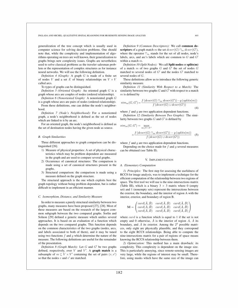
INGLADA AND MICHEL: QUALITATIVE SPATIAL REASONING FOR HR REMOTE-SENSING IMAGE ANALYSIS 603
generalization of the tree concept which is usually used incomputer science for solving decision problems. One shouldnote that, while the complexity and implementation of algo-rithms operating on trees are well known, their generalization tographs brings new complexity issues. Graphs are neverthelessused to solve classical problems as the traveler salesman prob-lem or the representation of complex structures as for instanceneural networks. We will use the following definition.
Definition 4 (Graph): A graph G is made of a finite setof nodes V and a set E of binary relationships on V × Vcalled arcs.
To types of graphs can be distinguished.Definition 5 (Oriented Graph): An oriented graph G is a
graph whose arcs are couples of nodes (ordered relationship).Definition 6 (Nonoriented Graph): A nonoriented graph G
is a graph whose arcs are pairs of nodes (ordered relationship).From these definitions, one can define the node’s neighbor-
hood.Definition 7 (Node’s Neighborhood): For a nonoriented
graph, a node’s neighborhood is defined as the set of nodeswhich are linked to it by an arc.
For an oriented graph, the node’s neighborhood is defined asthe set of destination nodes having the given node as source.
B. Graph Similarities
Three different approaches to graph comparison can be dis-tinguished [26].
1) Measure of physical properties: A set of physical charac-teristics which may be problem dependent are measuredin the graph and are used to compare several graphs.
2) Occurrence of canonical structures: The comparison ismade using a set of canonical structures present in thegraphs.
3) Structural comparison: the comparison is made using ameasure defined on the graph structure.
The structural approach is the one which exploits best thegraph topology without being problem dependent, but is ratherdifficult to implement in an efficient manner.
C. Isomorphism, Distance, and Similarity Measure
In order to measure a purely structural similarity between twographs, many measures have been proposed [27], [28]. Most ofthese measures are based on the research of the largest com-mon subgraph between the two compared graphs. Sorlin andSolnon [29] defined a generic measure which unifies severalapproaches. It is based on an evaluation of a function whichdepends on the two compared graphs. This function dependson the common characteristics of the two graphs (nodes, arcs,and labels associated to both of them), and it may be tunedusing two functions f and g which determine the nature of themeasure. The following definitions are useful for the remainderof the presentation.
Definition 8 (Graph Match): Let G and G′ be two graphsdefined, respectively, over V and V ′. A graph match is asubsample of m ⊆ V × V ′ containing the set of pairs (v, v′)so that the nodes v and v′ are matched.
Definition 9 (Common Descriptors): We call common de-scriptors of a graph match m the set descr(G) �m descr(G′),where the operator �m stands for the set of all nodes, node’slabels, arcs, and arc’s labels which are common to G and G′
within a match m.Definition 10 (Split Nodes): We call Split nodes or splits(m)
of a match m of two graphs G and G′ the set of nodes Gmatched to several nodes of G′ and the nodes G′ matched toseveral nodes of G.
These definitions allow us to introduce the following genericsimilarity measure.
Definition 11 (Similarity With Respect to a Match): Thesimilarity between two graphs G and G′ with respect to a matchm is defined by
simm(G,G′)=f (descr(G) �m descr(G′))−g (splits(m))
f (descr(G) ∪ descr(G′))(4)
where f and g are two application dependent functions.Definition 12 (Similarity Between Two Graphs): The simi-
larity between two graphs G and G′ is defined by
simm(G,G′) = maxm⊆V ×V ′
×f (descr(G) �m descr(G′)) − g (splits(m))
f (descr(G) ∪ descr(G′))(5)
where f and g are two application dependent functions.Depending on the choice made for f and g several measures
can be obtained (see Table II).
V. IMPLEMENTATION
A. Elementary Computation
1) Principles: The first step for assessing the usefulness ofRCC8 for image analysis, was to implement a technique for theefficient computation of the relationship between two regions ofspace. The first tool we will use is the nine-intersections matrix(Table III), which is a binary 3 × 3 matrix where 0 (emptyset) and 1 (nonempty sets) represent the intersections betweenthe exterior, the boundary, and the interior of region A with theinterior, exterior, and boundary of region B.
M =
⎛⎝
card(A, B) card(A, B) card(A, B)card(A, B) card(A, B) card(A, B)card(A, B) card(A, B) card(A, B)
⎞⎠
where card is a function which is equal to 1 if the set is notempty and 0 otherwise, A is the interior of region A, A itsboundary, and A its exterior. Among the 29 possible matri-ces, only eight are physically plausible, and they correspondto the eight RCC8 relationships. Being able to compute thenine-intersections matrix for a pair of regions of space meansknowing the RCC8 relationship between them.
2) Optimization: This method has a main drawback: itscomplexity. This complexity is dependent on the image size.This is particularly annoying, since remote-sensing images arevery large, while the regions of interest may be small. There-fore, using masks which have the same size of the image can
182
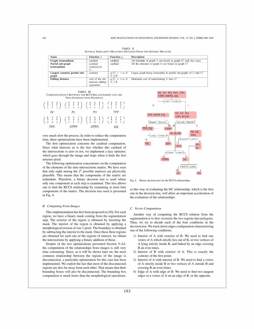
604 IEEE TRANSACTIONS ON GEOSCIENCE AND REMOTE SENSING, VOL. 47, NO. 2, FEBRUARY 2009
TABLE IISEVERAL SIMILARITY MEASURES OBTAINED FROM THE GENERIC MEASURE
TABLE IIICORRESPONDENCE BETWEEN THE RCC8 RELATIONSHIPS AND THE
NINE-INTERSECTIONS MATRICES
very much slow the process. In order to reduce the computationtime, three optimizations have been implemented.
The first optimization concerns the cardinal computation.Since what interests us is the fact whether this cardinal ofthe intersections is zero or not, we implement a lazy operator,which goes through the image and stops when it finds the firstnonzero pixel.
The following optimization concentrates on the computationof the elements of the nine-intersections matrix. We have seenthat only eight among the 29 possible matrices are physicallyplausible. This means that the components of the matrix areredundant. Therefore, a binary decision tree is used whereonly one component at each step is examined. This tree allowsone to find the RCC8 relationship by examining at most fourcomponents of the matrix. The decision tree used is presentedin Fig. 4.
B. Computing From Images
This implementation has first been proposed in [30]. For eachregion, we have a binary mask coming from the segmentationstep. The exterior of the region is obtained by inverting themask. The interior of the region is obtained by applying amorphological erosion of size 1 pixel. The boundary is obtainedby subtracting the interior to the mask. Once these three regionsare obtained for each one of the regions of interest, we obtainthe intersections by applying a binary addition of those.
Despite of the two optimizations presented Section V-A2,the computation of the relationships from images is still verytime consuming. Since, as it will be shown later on, the mostcommon relationship between the regions of the image isdisconnection, a particular optimization for this case has beenimplemented. We exploit the fact that most of the disconnectedregions are also far away from each other. That means that theirbounding boxes will also be disconnected. The bounding boxcomputation is much faster than the morphological operations,
Fig. 4. Binary decision tree for the RCC8 relationships.
so this way of evaluating the DC relationship, which is the firstone in the decision tree, will allow an important acceleration ofthe evaluation of the relationships.
C. Vector Computation
Another way of computing the RCC8 relation from thesegmentation is to first vectorize the two regions into polygons.Then, we try to decide each of the four conditions in thedecision tree. We track down edges configuration characterizingone of the following conditions.
1) Interior of A with exterior of B: We need to find onevertex of A which strictly lies out of B, or two vertices ofA lying strictly inside B, and linked by an edge crossingB an even times.
2) Interior of B with exterior of A: This is exactly thecontrary of the first point.
3) Interior of A with interior of B: We need to find a vertexof A strictly inside B or two vertices of A outside B andcrossing B an even times.
4) Edge of A with edge of B: We need to find two tangentedges or a vertex of A on an edge of B, or the opposite.
183
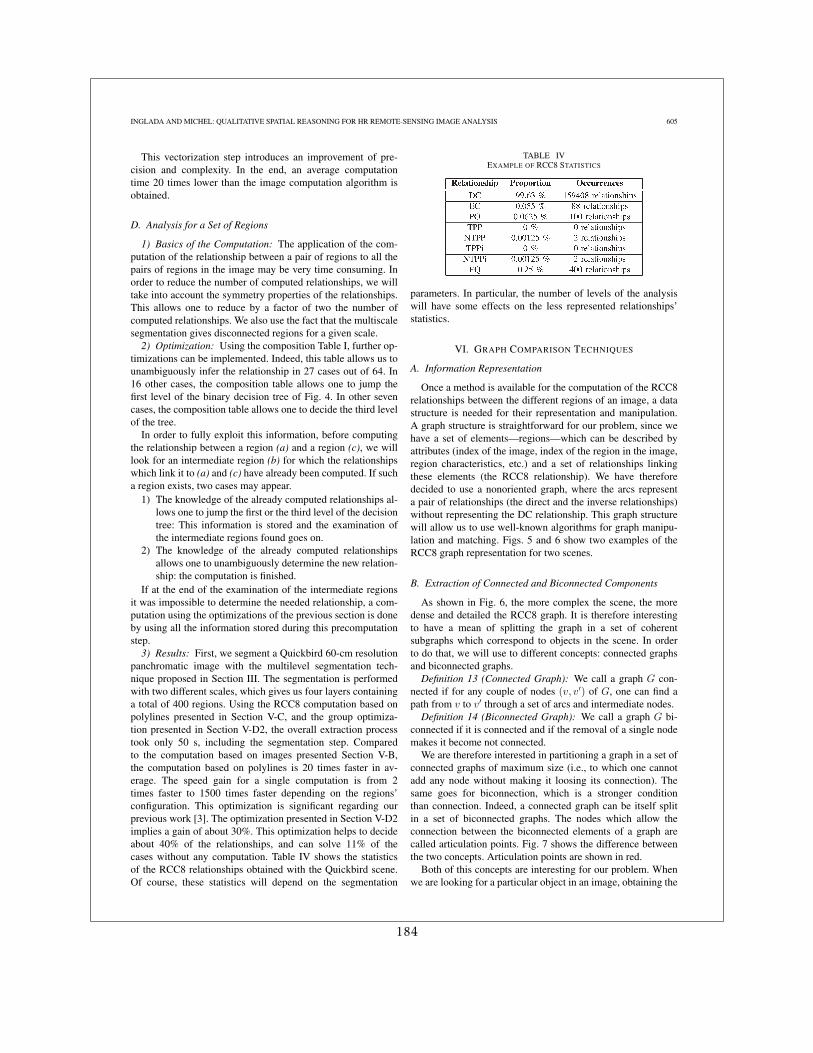
INGLADA AND MICHEL: QUALITATIVE SPATIAL REASONING FOR HR REMOTE-SENSING IMAGE ANALYSIS 605
This vectorization step introduces an improvement of pre-cision and complexity. In the end, an average computationtime 20 times lower than the image computation algorithm isobtained.
D. Analysis for a Set of Regions
1) Basics of the Computation: The application of the com-putation of the relationship between a pair of regions to all thepairs of regions in the image may be very time consuming. Inorder to reduce the number of computed relationships, we willtake into account the symmetry properties of the relationships.This allows one to reduce by a factor of two the number ofcomputed relationships. We also use the fact that the multiscalesegmentation gives disconnected regions for a given scale.
2) Optimization: Using the composition Table I, further op-timizations can be implemented. Indeed, this table allows us tounambiguously infer the relationship in 27 cases out of 64. In16 other cases, the composition table allows one to jump thefirst level of the binary decision tree of Fig. 4. In other sevencases, the composition table allows one to decide the third levelof the tree.
In order to fully exploit this information, before computingthe relationship between a region (a) and a region (c), we willlook for an intermediate region (b) for which the relationshipswhich link it to (a) and (c) have already been computed. If sucha region exists, two cases may appear.
1) The knowledge of the already computed relationships al-lows one to jump the first or the third level of the decisiontree: This information is stored and the examination ofthe intermediate regions found goes on.
2) The knowledge of the already computed relationshipsallows one to unambiguously determine the new relation-ship: the computation is finished.
If at the end of the examination of the intermediate regionsit was impossible to determine the needed relationship, a com-putation using the optimizations of the previous section is doneby using all the information stored during this precomputationstep.
3) Results: First, we segment a Quickbird 60-cm resolutionpanchromatic image with the multilevel segmentation tech-nique proposed in Section III. The segmentation is performedwith two different scales, which gives us four layers containinga total of 400 regions. Using the RCC8 computation based onpolylines presented in Section V-C, and the group optimiza-tion presented in Section V-D2, the overall extraction processtook only 50 s, including the segmentation step. Comparedto the computation based on images presented Section V-B,the computation based on polylines is 20 times faster in av-erage. The speed gain for a single computation is from 2times faster to 1500 times faster depending on the regions’configuration. This optimization is significant regarding ourprevious work [3]. The optimization presented in Section V-D2implies a gain of about 30%. This optimization helps to decideabout 40% of the relationships, and can solve 11% of thecases without any computation. Table IV shows the statisticsof the RCC8 relationships obtained with the Quickbird scene.Of course, these statistics will depend on the segmentation
TABLE IVEXAMPLE OF RCC8 STATISTICS
parameters. In particular, the number of levels of the analysiswill have some effects on the less represented relationships’statistics.
VI. GRAPH COMPARISON TECHNIQUES
A. Information Representation
Once a method is available for the computation of the RCC8relationships between the different regions of an image, a datastructure is needed for their representation and manipulation.A graph structure is straightforward for our problem, since wehave a set of elements—regions—which can be described byattributes (index of the image, index of the region in the image,region characteristics, etc.) and a set of relationships linkingthese elements (the RCC8 relationship). We have thereforedecided to use a nonoriented graph, where the arcs representa pair of relationships (the direct and the inverse relationships)without representing the DC relationship. This graph structurewill allow us to use well-known algorithms for graph manipu-lation and matching. Figs. 5 and 6 show two examples of theRCC8 graph representation for two scenes.
B. Extraction of Connected and Biconnected Components
As shown in Fig. 6, the more complex the scene, the moredense and detailed the RCC8 graph. It is therefore interestingto have a mean of splitting the graph in a set of coherentsubgraphs which correspond to objects in the scene. In orderto do that, we will use to different concepts: connected graphsand biconnected graphs.
Definition 13 (Connected Graph): We call a graph G con-nected if for any couple of nodes (v, v′) of G, one can find apath from v to v′ through a set of arcs and intermediate nodes.
Definition 14 (Biconnected Graph): We call a graph G bi-connected if it is connected and if the removal of a single nodemakes it become not connected.
We are therefore interested in partitioning a graph in a set ofconnected graphs of maximum size (i.e., to which one cannotadd any node without making it loosing its connection). Thesame goes for biconnection, which is a stronger conditionthan connection. Indeed, a connected graph can be itself splitin a set of biconnected graphs. The nodes which allow theconnection between the biconnected elements of a graph arecalled articulation points. Fig. 7 shows the difference betweenthe two concepts. Articulation points are shown in red.
Both of this concepts are interesting for our problem. Whenwe are looking for a particular object in an image, obtaining the
184
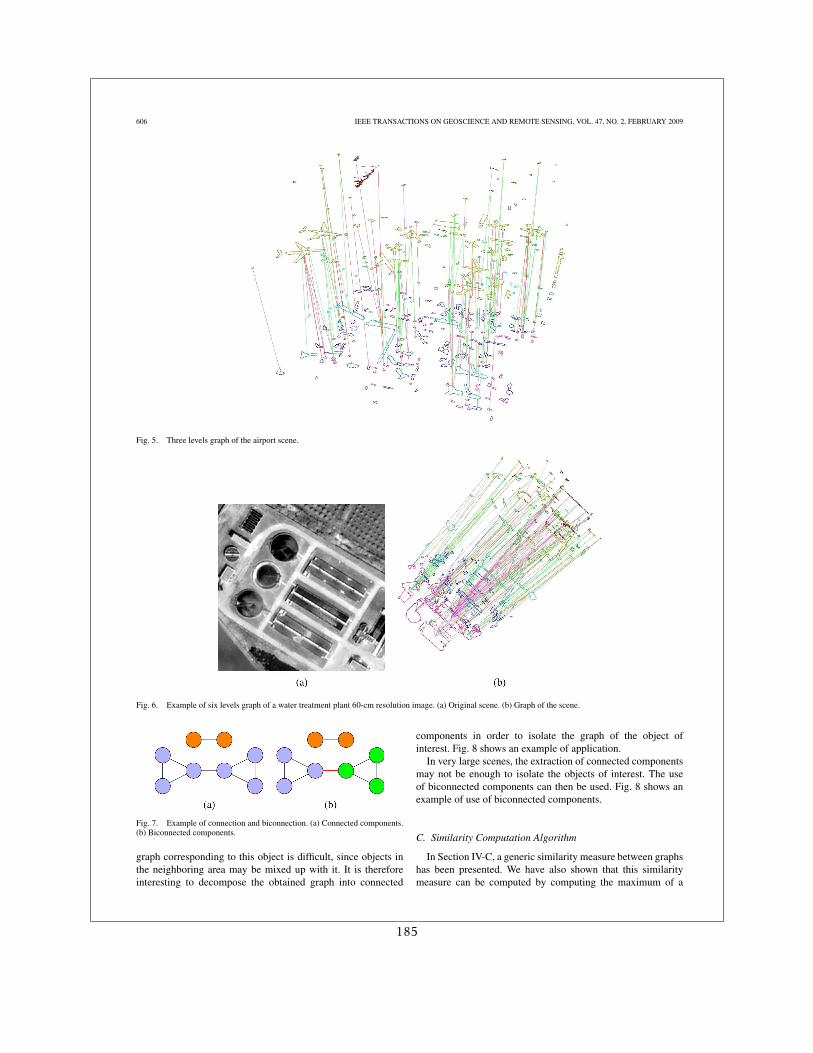
606 IEEE TRANSACTIONS ON GEOSCIENCE AND REMOTE SENSING, VOL. 47, NO. 2, FEBRUARY 2009
Fig. 5. Three levels graph of the airport scene.
Fig. 6. Example of six levels graph of a water treatment plant 60-cm resolution image. (a) Original scene. (b) Graph of the scene.
Fig. 7. Example of connection and biconnection. (a) Connected components.(b) Biconnected components.
graph corresponding to this object is difficult, since objects inthe neighboring area may be mixed up with it. It is thereforeinteresting to decompose the obtained graph into connected
components in order to isolate the graph of the object ofinterest. Fig. 8 shows an example of application.
In very large scenes, the extraction of connected componentsmay not be enough to isolate the objects of interest. The useof biconnected components can then be used. Fig. 8 shows anexample of use of biconnected components.
C. Similarity Computation Algorithm
In Section IV-C, a generic similarity measure between graphshas been presented. We have also shown that this similaritymeasure can be computed by computing the maximum of a
185
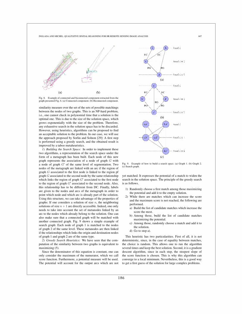
INGLADA AND MICHEL: QUALITATIVE SPATIAL REASONING FOR HR REMOTE-SENSING IMAGE ANALYSIS 607
Fig. 8. Example of connected and biconnected component extracted from thegraph presented Fig. 6. (a) Connected component. (b) Biconnected component.
similarity measure over the set of the sets of possible matchingsbetween the nodes of two graphs. This is an NP-hard problem,i.e., one cannot check in polynomial time that a solution is theoptimal one. This is due to the size of the solution space, whichgrows exponentially with the size of the problem. Therefore,any exhaustive search in the solution space has to be discarded.However, using heuristics, algorithms can be proposed to findan acceptable solution to the problem. In our case, we will usethe approach proposed by Sorlin and Solnon [29]: A first stepis performed using a greedy search, and the obtained result isimproved by a taboo metaheuristics.
1) Building the Search Space: In order to implement thesetwo algorithms, a representation of the search space under theform of a metagraph has been built. Each node of this newgraph represents the association of a node of graph G witha node of graph G′ of the same level of segmentation. Twonodes of the metagraph are linked with an arc if the region ofgraph G associated to the first node is linked to the region pfgraph G associated to the second node by the same relationshipwhich links the region of graph G′ associated to the first nodeto the region of graph G′ associated to the second node. Also,this relationship has to be different from DC. Finally, labelsare given to the nodes and arcs of the metagraph in order topoint which node and which arc is already part of the solution.Using this structure, we can take advantage of the properties ofgraphs: If one considers a solution of size n, the neighboringsolutions of size n + 1 are directly accessible. Indeed, one onlyneeds to take into account the set of metanodes linked by anarc to the nodes which already belong to the solution. One canalso make sure that a connected graph will be matched withanother connected graph. Fig. 9 shows a simple example ofsearch graph: Each node of graph 1 is matched to the nodesof graph 2 of the same level. These metanodes are then linkedif the relationships which links the origin and destination nodesof graph 1 and graph 2 are of the same type.
2) Greedy Search Heuristics: We have seen that the com-putation of the similarity between two graphs is equivalent tomaximizing (5).
Since the denominator of this equation is constant, one canonly consider the maximum of the numerator, which we callscore function. Furthermore, a potential measure will be used.The potential will account for the output arcs which are not
Fig. 9. Example of how to build a search space. (a) Graph 1. (b) Graph 2.(c) Search graph.
yet matched. It expresses the potential of a match to widen thesearch in the solution space. The principle of the greedy searchis as follows.
1) Randomly choose a first match among those maximizingthe potential and add it to the empty solution.
2) While there are matches which can increase the scoreand the maximum score is not reached, the following areperformed.a) Build the list of candidate matches which increase the
score the most.b) Among those, build the list of candidate matches
maximizing the potential.c) Among those, randomly choose a match and add it to
the solution.d) Go to step a).
This heuristic has two particularities. First of all, it is notdeterministic, since, in the case of equality between matches,the choice is random. This allows one to run the algorithmseveral times and keep the best solution. Second, it is a gradientdescent algorithm, since in each step, the steepest slope ofthe score function is chosen. This is why this algorithm canconverge to a local minimum. Nevertheless, this is a good wayto get a first guess of the solution for large complex problems.
186
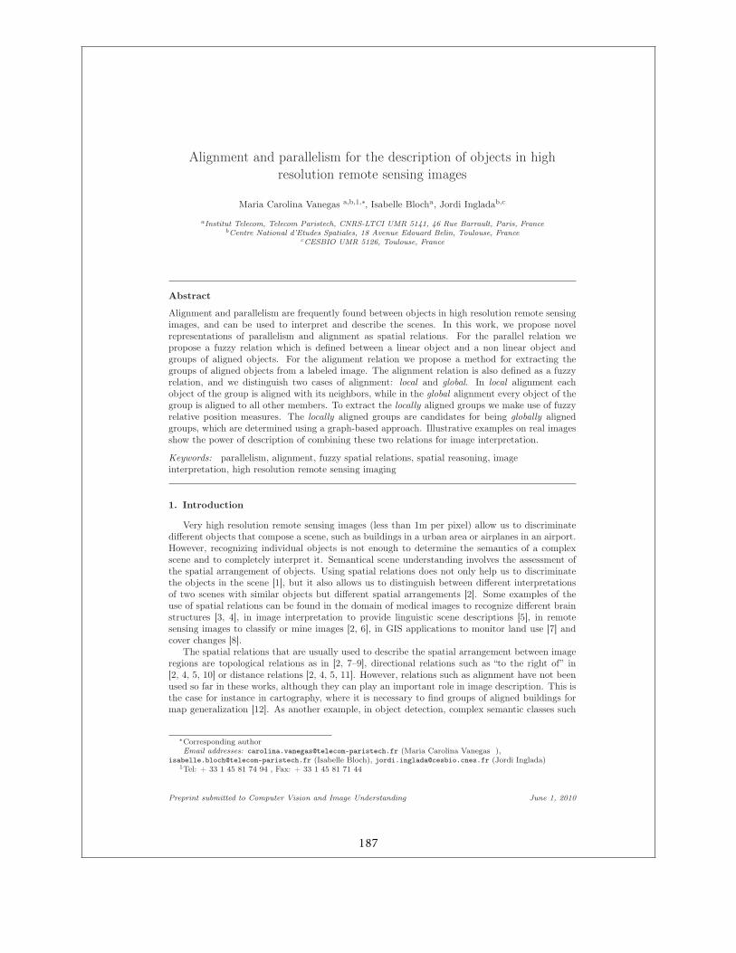
Alignment and parallelism for the description of objects in high
resolution remote sensing images
Maria Carolina Vanegas a,b,1,∗, Isabelle Blocha, Jordi Ingladab,c
aInstitut Telecom, Telecom Paristech, CNRS-LTCI UMR 5141, 46 Rue Barrault, Paris, FrancebCentre National d’Etudes Spatiales, 18 Avenue Edouard Belin, Toulouse, France
cCESBIO UMR 5126, Toulouse, France
Abstract
Alignment and parallelism are frequently found between objects in high resolution remote sensingimages, and can be used to interpret and describe the scenes. In this work, we propose novelrepresentations of parallelism and alignment as spatial relations. For the parallel relation wepropose a fuzzy relation which is defined between a linear object and a non linear object andgroups of aligned objects. For the alignment relation we propose a method for extracting thegroups of aligned objects from a labeled image. The alignment relation is also defined as a fuzzyrelation, and we distinguish two cases of alignment: local and global. In local alignment eachobject of the group is aligned with its neighbors, while in the global alignment every object of thegroup is aligned to all other members. To extract the locally aligned groups we make use of fuzzyrelative position measures. The locally aligned groups are candidates for being globally alignedgroups, which are determined using a graph-based approach. Illustrative examples on real imagesshow the power of description of combining these two relations for image interpretation.
Keywords: parallelism, alignment, fuzzy spatial relations, spatial reasoning, imageinterpretation, high resolution remote sensing imaging
1. Introduction
Very high resolution remote sensing images (less than 1m per pixel) allow us to discriminatedifferent objects that compose a scene, such as buildings in a urban area or airplanes in an airport.However, recognizing individual objects is not enough to determine the semantics of a complexscene and to completely interpret it. Semantical scene understanding involves the assessment ofthe spatial arrangement of objects. Using spatial relations does not only help us to discriminatethe objects in the scene [1], but it also allows us to distinguish between different interpretationsof two scenes with similar objects but different spatial arrangements [2]. Some examples of theuse of spatial relations can be found in the domain of medical images to recognize different brainstructures [3, 4], in image interpretation to provide linguistic scene descriptions [5], in remotesensing images to classify or mine images [2, 6], in GIS applications to monitor land use [7] andcover changes [8].
The spatial relations that are usually used to describe the spatial arrangement between imageregions are topological relations as in [2, 7–9], directional relations such as “to the right of” in[2, 4, 5, 10] or distance relations [2, 4, 5, 11]. However, relations such as alignment have not beenused so far in these works, although they can play an important role in image description. This isthe case for instance in cartography, where it is necessary to find groups of aligned buildings formap generalization [12]. As another example, in object detection, complex semantic classes such
∗Corresponding authorEmail addresses: [email protected] (Maria Carolina Vanegas ),
[email protected] (Isabelle Bloch), [email protected] (Jordi Inglada)1Tel: + 33 1 45 81 74 94 , Fax: + 33 1 45 81 71 44
Preprint submitted to Computer Vision and Image Understanding June 1, 2010
187
as parking areas (car parking lots, ports, truck parking lots or airports) comprise aligned groupsof vehicles. Therefore, the identification of aligned groups of transport vehicles can be useful fordetecting instantiations of these complex classes. Alignment is often linked to the parallel relation.For example, in object recognition the aligned groups of airplanes in an airport are parallel to theterminal buildings, or the aligned groups of boats in the ports are parallel to the deck. Anotherexample is the determination of urban spatial patterns like groups of aligned houses parallel toother aligned groups of houses in residential areas.
In this paper, we propose representations of the parallelism and alignment relations as spatialrelations between objects. Our objective is to define these relations taking into account theirsemantics. However, these relations are vague and imprecise when they are evaluated between ob-jects of different sizes for the case of alignment, and between objects of different spatial extensionsfor the case of parallelism. Therefore we propose to define them as fuzzy spatial relations to copewith such imprecisions.
This paper is organized as follows. Section 2 reviews some of the models of alignment andparallelism in computer vision. Section 3 introduces the definitions of local alignment and globalalignment. A method for extracting the locally aligned groups is then proposed. In this methodwe construct a neighborhood graph of the objects of the image, and its dual graph where weincorporate information about the relative direction of the objects, evaluated using fuzzy measuresof relative position. The groups of objects satisfying the fuzzy criterion of being locally aligned areextracted from the dual graph. These groups are the candidates for being globally aligned. Section4 discusses the issues related to the definition of the parallel relation when dealing with objectsor groups of aligned objects. An original definition of parallelism is then proposed, matching therequirements. Finally, in Section 5 we apply the relations to objects in satellite images to illustratetheir behavior and their usefulness in scene understanding.
2. Alignment and parallelism in computer vision
Both parallelism and alignment between low level features have been widely studied in com-puter vision. Some examples are parallelism between segments [13–19], alignment between groupsof points [20, 21] and alignments between linear segments [13, 20] as collinearity on digital images.Most of these works are inscribed within the framework of perceptual organization. Their firstobjective is to find how to organize low level features, such as edge segments, into groups, such asaligned segments or parallel segments. The groups are evaluated according to their perceptuallysignificance based on the grouping laws of the Gestalt theory [22, 23]. Their second objective isto differentiate the groupings that arise from the structure of a scene from those that arise due toaccidents of view point or position [13].
The objective of perceptual organization in computer vision and our objective are different.Perceptual organization deals with how these relations take place among low level features andtheir meaningfulness according to the image’s structure, while we are interested in defining theserelations for objects in the image taking into account their semantics. Anyway, it is importantto review the work that has been done on studying these relations as grouping laws between lowlevel features in digital images, in order to understand how these relations have been modeled.
Parallelism between two linear segments is usually modeled as a relation that should satisfythree constraints. The first one is that both segments should have a small angular difference. Thesecond one is that the perpendicular distance between the two segments should be small and thelast one is that there should be a high overlap between them [14]. There exist different approachesto integrate these three constraints into a model and measure the meaningfulness of the relation.Lowe [13] was one of the first to model parallelism to perform perceptual grouping: for everycouple of linear segments having a perpendicular separation d and an angular difference θ, heassigns a significant value to establish that it has not been originated by an accident of viewpoint.The significant value is used to determine the expected number of lines for a given perpendicularseparation and an angular difference. In fact, this value is proportional to the prior probabilityof appearance and it is inversely proportional to the angular difference and the perpendicularseparation. In [14] the constraint about overlapping is introduced and it is determined by the
2
188
orthogonal projection of one segment over the other and vice-versa. The meaningful segments arethen obtained by applying a threshold on the measured values of the constraints. Fuzzy approacheshave been proposed in [16–18, 24, 25], leading to a measure of the degree of parallelism betweentwo linear segments, in which trapezoid type functions are used to evaluate to which degree thethree constraints are satisfied. The three degrees are combined in a conjunctive way.
Parallelism between curves has been modeled as a type of symmetry [15, 16]. In [15] the authorsconsider that two curves are parallel if their respective orthogonal distances from the symmetryaxis are almost equal. In [26] and [27] parallelism is modeled as a matching problem where twocurves are parallel if there is a point-wise correspondence. In both works the parallelism is treatedas a shape matching problem.
Previous works focused on parallelism between crisp linear segments. However, when dealingwith objects extracted from images, it is important to consider parallelism between fuzzy linearobjects. Indeed, the object extraction processes can introduce imprecision, and therefore we are notalways dealing with crisp linear objects or segments. In Sec. 4 we will give some definitions aboutparallelism between fuzzy linear objects. The definitions of parallelism presented in this paperdiffer from those of the previous works in the sense that we are defining the relation consideringits semantics, and we are not worried about whether or not the detected parallelism is an accidentof the view point or position. We are interested in the conditions that have to be satisfied todecide whether two objects are parallel or not.
For the case of alignment, several methods to determine the alignment between points methodsrelying on the Hough transform [20] or the Radon transform [28] have been proposed. Other exam-ples are the identification of aligned segments which have the same orientations as the alignment[13, 18, 20, 21, 24]. However, alignment extraction as a high level feature has been less studied.One example is the work of [29], where an algorithm to detect aligned groups of buildings in mapsis presented. In this algorithm buildings with aligned barycenters are extracted, and the qualityof the alignments is evaluated based on the criteria of proximity and similarity laws of Gestalttheory.
The above mentioned methods for determining alignment focused on extracting groups of ob-jects with aligned barycenters. Consequently, it is not possible to apply them directly to determineif a group of heterogeneous objects (according to shape and size) is aligned, since neither the sizenor the shape of the objects are considered. An example of this will be given in Sec. 3.1. Similarlyas for parallelism, the previously proposed alignment relations have not been extended to dealwith fuzzy objects.
Due to the fact that parallelism and alignment in computer vision have been studied betweenlow-level features in the perceptual organization domain, they have been treated in an independentmanner, and they are used to organize low level features but they are not combined. However,when dealing with objects and observing these relations as spatial relations, it is interesting tocombine them in order to determine when two groups of aligned objects are parallel, or when agroup of aligned objects is parallel to another object. These kinds of combinations give us moreinformation about the scene and can be meaningful for the description. This point will be furtherdeveloped in the following sections.
3. Alignment
Alignment can be defined as the spatial property possessed by a group of objects arranged ina straight line2. As it was highlighted by the Gestalt theory, alignment should be seen as a whole[20]: if we observe each element of the group individually, then the alignment property is lost.Having to look at it as a whole makes alignment detection a difficult task, since in order to detectan aligned group of objects we have to identify its members, but to know if an object belongs toan aligned group the alignment has to be already identified. In this part we study the differentapproaches to model alignment, and introduce the notions of local and global alignment.
2Definition taken from ThinkMap Visual Thesaurus http://www.visualthesaurus.com/
3
189
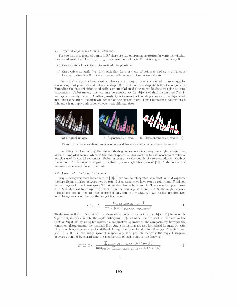
3.1. Different approaches to model alignment
For the case of a group of points in R2 there are two equivalent strategies for verifying whetherthey are aligned. Let A = {a1, . . . , an} be a group of points in R2. A is aligned if and only if:
(i) there exists a line L that intersects all the points, or
(ii) there exists an angle θ ∈ [0, π) such that for every pair of points ai and aj (i 6= j), aj islocated in direction θ or θ + π from ai with respect to the horizontal axis.
The first strategy has been used to identify if a group of points is aligned in an image, byconsidering that points should fall into a strip [30], the thinner the strip the better the alignment.Extending the first definition to identify a group of aligned objects can be done by using objects’barycenters. Unfortunately this will only be appropriate for objects of similar sizes (see Fig. 1)and approximately convex. Another possibility is to search a thin strip where all the objects fallinto, but the width of the strip will depend on the objects’ sizes. Thus the notion of falling into athin strip is not appropriate for objects with different sizes.
(a) Original image. (b) Segmented objects. (c) Barycenters of objects in (b).
Figure 1: Example of an aligned group of objects of different sizes and with non-aligned barycenters.
The difficulty of extending the second strategy relies in determining the angle between twoobjects. One alternative, which is the one proposed in this work, is to use measures of relativeposition used in spatial reasoning. Before entering into the details of the method, we introducethe notion of orientation histogram, inspired by the angle histogram of [31]. This notion is afundamental concept for our method.
3.2. Angle and orientation histograms
Angle histograms were introduced in [31]. They can be interpreted as a function that capturesthe directional position between two objects. Let us assume we have two objects A and B definedby two regions in the image space I, that we also denote by A and B. The angle histogram fromA to B is obtained by computing, for each pair of points pa ∈ A and pb ∈ B, the angle betweenthe segment joining them and the horizontal axis, denoted by ∠(pa, pb) [32]. Angles are organizedin a histogram normalized by the largest frequency:
HA(B)(θ) =
∑pa∈A,pb∈B|∠(pa,pb)=θ 1
maxφ∈[0,2π)
∑pa∈a,pb∈b|∠(pa,pb)=φ 1
. (1)
To determine if an object A is in a given direction with respect to an object B (for example“right of”), we can compute the angle histogram HA(B) and compare it with a template for therelation “right of” by using for instance a conjunctive operator or the compatibility between thecomputed histogram and the template [31]. Angle histograms are also formalized for fuzzy objects.Given two fuzzy objects A and B defined through their membership functions µA : I → [0, 1] andµB : I → [0, 1] in the image space I, respectively, it is possible to define the angle histogrambetween A and B by considering the membership of each point to the fuzzy set:
HA(B)(θ) =
∑pa,pb∈I|∠(pa,pb)=θ µA(pa) ∧ µB(pb)
maxφ∈[0,2π)
∑pa,pb∈I|∠(pa,pb)=φ µA(pa) ∧ µB(pb)
, (2)
4
190
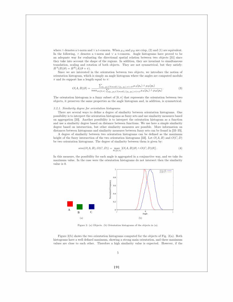
where ∧ denotes a t-norm and ∨ a t-conorm. When µA and µB are crisp, (2) and (1) are equivalent.In the following, ∧ denotes a t-norm and ∨ a t-conorm. Angle histograms have proved to bean adequate way for evaluating the directional spatial relation between two objects [31] sincethey take into account the shape of the regions. In addition, they are invariant to simultaneoustranslation, scaling and rotation of both objects. They are not symmetrical, but they satisfy:HA(B)(θ) = HB(A)(θ + π).
Since we are interested in the orientation between two objects, we introduce the notion oforientation histogram, which is simply an angle histogram where the angles are computed moduloπ and its support has a length equal to π:
O(A, B)(θ) =
∑pa,pb∈I|mod(∠(pa,pb),π)=θ µA(pa) ∧ µB(pb)
maxφ∈[0,π)
∑pa,pb∈I|mod(∠(pa,pb),π)=φ µA(pa) ∧ µB(pb)
. (3)
The orientation histogram is a fuzzy subset of [0, π[ that represents the orientation between twoobjects, it preserves the same properties as the angle histogram and, in addition, is symmetrical.
3.2.1. Similarity degree for orientation histograms
There are several ways to define a degree of similarity between orientation histograms. Onepossibility is to interpret the orientation histograms as fuzzy sets and use similarity measures basedon aggregation [33]. Another possibility is to interpret the orientation histogram as a functionand use a similarity degree based on distance between functions. We use here a simple similaritydegree based on intersection, but other similarity measures are possible. More information ondistances between histograms and similarity measures between fuzzy sets can be found in [33–35].
A degree of similarity between two orientation histograms can be defined as the maximumheight of the fuzzy intersection of the two orientation histograms [33]. Let O(A, B) and O(C, D)be two orientation histograms. The degree of similarity between them is given by:
sim(O(A, B), O(C, D)) = maxθ∈[0,π)
[O(A, B)(θ) ∧ O(C, D)(θ)] . (4)
In this measure, the possibility for each angle is aggregated in a conjunctive way, and we take itsmaximum value. In the case were the orientation histograms do not intersect then the similarityvalue is 0.
AB C
(a)
0
0.2
0.4
0.6
0.8
1
0
Nor
mal
ized
Fre
quen
cy
Angle
π2
−π2
O(A,B)O(B,C)
(b)
Figure 2: (a) Objects. (b) Orientation histograms of the objects in (a).
Figure 2(b) shows the two orientation histograms computed for the objects of Fig. 2(a). Bothhistograms have a well defined maximum, showing a strong main orientation, and these maximumvalues are close to each other. Therefore a high similarity value is expected. However, if the
5
191
min operator is used as a t-norm in (4), the similarity value between the two histograms is 0.67.This non-high value is due to the comparison of the value for each angle separately, since theaggregation is done for every angle. However, in this context referring to an orientation equal toan angle θ actually represents the quantity “approximately θ”. Therefore, in order to compare iftwo orientation histograms are similar, it is important to consider the imprecision that is linkedto the comparison of two angles that are approximately the same. When a fuzzy morphologicaldilation [36] is performed on an orientation histogram using a structuring element ν0, then thehigh values of the histogram will be propagated to the similar angle values according to ν0. Thestructuring element ν0 is designed such that ν0(θ − θ) represents the degree to which θ and θ are“approximately” equal, and in our experiments we modeled ν0 as a trapezoid function:
ν0(θ) =
1 if |θ| ≤ t1t2−|θ|t2−t1
if t1 < |θ| ≤ t2
0 if |θ| > t2,
(5)
where t1 and t2 represent the parameters of a trapezoid function. The parameters t1 and t2 arerelated to the imprecision linked to computing angles in a discrete grid, as is the case for images.This imprecision is a function of the distance between the points for which the angle is computed:the greater the distance between the points, the more precise is the calculation. However, in ourexperiments, since most of the time we are dealing with objects which have a similar distancebetween them, we have chosen to use:
t1 = arcsin
(1
0.5daverage
)(6)
t2 = arcsin
(1
0.25daverage
)(7)
where daverage is the average distance in pixels between the “neighbor” object’s barycenters. Thisvalues have been used in all experiments, and did not required any fine tuning of the parameters.
By performing a morphological dilation of O(A, B) with the structuring element ν0 we introducethe imprecision to all the angles in O(A, B) (as in [37]). For this reason, the similarity should becomputed using the dilated orientation histograms, and (4) becomes:
sim(O(A, B), O(C, D)) = maxθ∈[0,π)
[Dν0(O(A, B))(θ) ∧ Dν0
(O(C, D))(θ)] , (8)
where Dν0(O(X, Y )) is the dilation of O(X, Y ) by a structuring element ν0 and it is given by
Dν0(µ)(θ) = supθ∈[0, π[ min(µ(θ), νx(θ − θ)) [36].
Figure 3(a) shows the result of performing a morphological dilation of the orientation his-tograms of Fig. 2(b). The parameters of Eqs. 6 and 7 are t1 ≈ 0.07 and t2 ≈ 0.12 for thestructuring element. The similarity value between the histograms obtained with Eq. (8) is 0.93which is more consistent with the perceived orientation of the objects than the value obtained byapplying Eq. (4).
When orientation histograms are not similar (see Fig.4) we obtain a zero similarity value, asdesired.
This measure of similarity can be extended to compare several orientation histograms. Let{O(Ai, Aj)}N
i=0,j 6=i be a set of orientation histograms, the similarity degree between them is equalto:
sim(O(A0, A1), . . . , O(Ai, Aj), . . . O(AN , AN−1)) = maxφ∈[0,π[
N∧
i=0,j 6=i
Dν0(O(Ai, Aj))(φ) (9)
3.3. Definition and identification of aligned groups of objects
We consider a set of objects A = {A0, . . . , An} and want to determine the subsets of alignedgroups of A. For the sake of clarity we will call them globally aligned groups. First we identify the
6
192
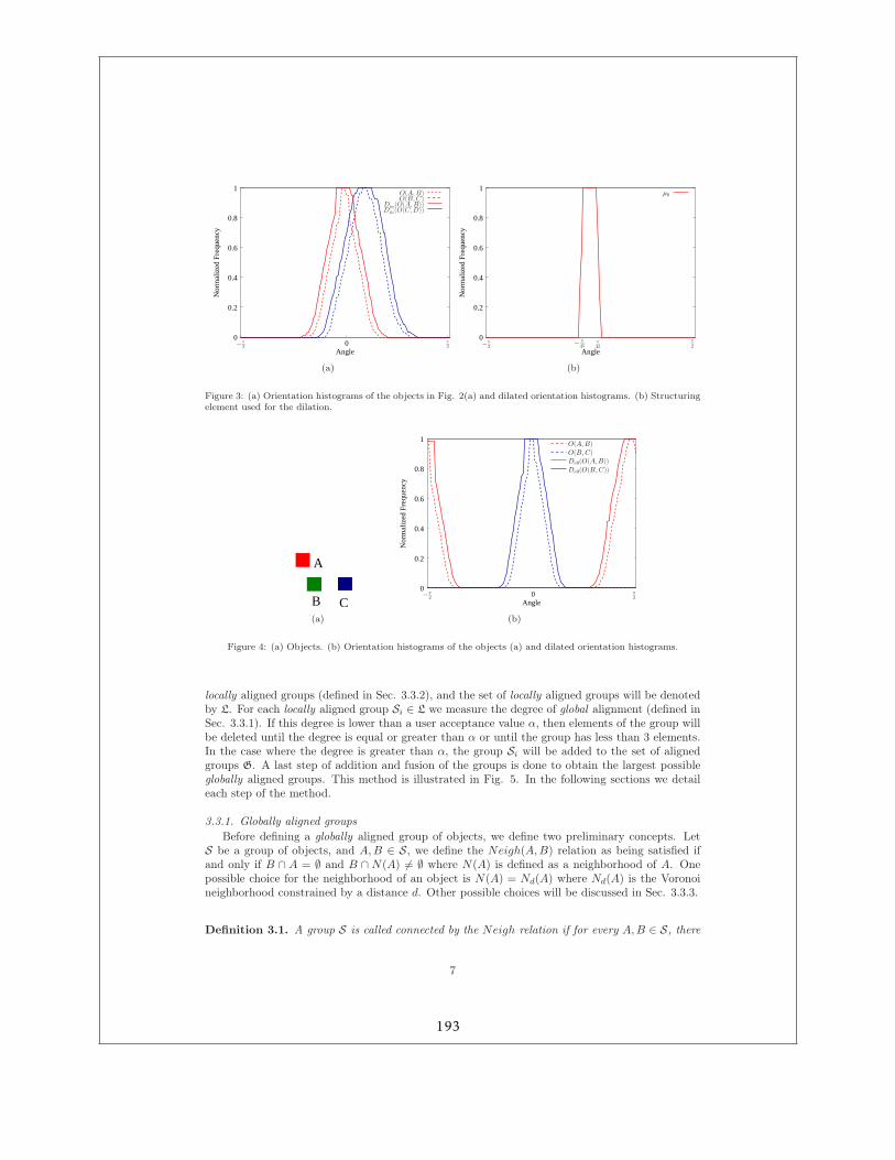
0
0.2
0.4
0.6
0.8
1
0
Nor
mal
ized
Fre
quen
cy
Angle−π
2π2
O(A,B)O(B,C)
Dµ0(O(A,B))
Dµ0(O(C,D))
(a)
0
0.2
0.4
0.6
0.8
1
Nor
mal
ized
Fre
quen
cy
Angle−π
2π45
µ0
π2− π
45
(b)
Figure 3: (a) Orientation histograms of the objects in Fig. 2(a) and dilated orientation histograms. (b) Structuringelement used for the dilation.
B C
A
(a)
0
0.2
0.4
0.6
0.8
1
0
Nor
mal
ized
Fre
quen
cy
Angle
O(A,B)O(B,C)Dν0(O(A,B))Dν0(O(B,C))
−π2
π2
(b)
Figure 4: (a) Objects. (b) Orientation histograms of the objects (a) and dilated orientation histograms.
locally aligned groups (defined in Sec. 3.3.2), and the set of locally aligned groups will be denotedby L. For each locally aligned group Si ∈ L we measure the degree of global alignment (defined inSec. 3.3.1). If this degree is lower than a user acceptance value α, then elements of the group willbe deleted until the degree is equal or greater than α or until the group has less than 3 elements.In the case where the degree is greater than α, the group Si will be added to the set of alignedgroups G. A last step of addition and fusion of the groups is done to obtain the largest possibleglobally aligned groups. This method is illustrated in Fig. 5. In the following sections we detaileach step of the method.
3.3.1. Globally aligned groups
Before defining a globally aligned group of objects, we define two preliminary concepts. LetS be a group of objects, and A, B ∈ S, we define the Neigh(A, B) relation as being satisfied ifand only if B ∩ A = ∅ and B ∩ N(A) 6= ∅ where N(A) is defined as a neighborhood of A. Onepossible choice for the neighborhood of an object is N(A) = Nd(A) where Nd(A) is the Voronoineighborhood constrained by a distance d. Other possible choices will be discussed in Sec. 3.3.3.
Definition 3.1. A group S is called connected by the Neigh relation if for every A, B ∈ S, there
7
193
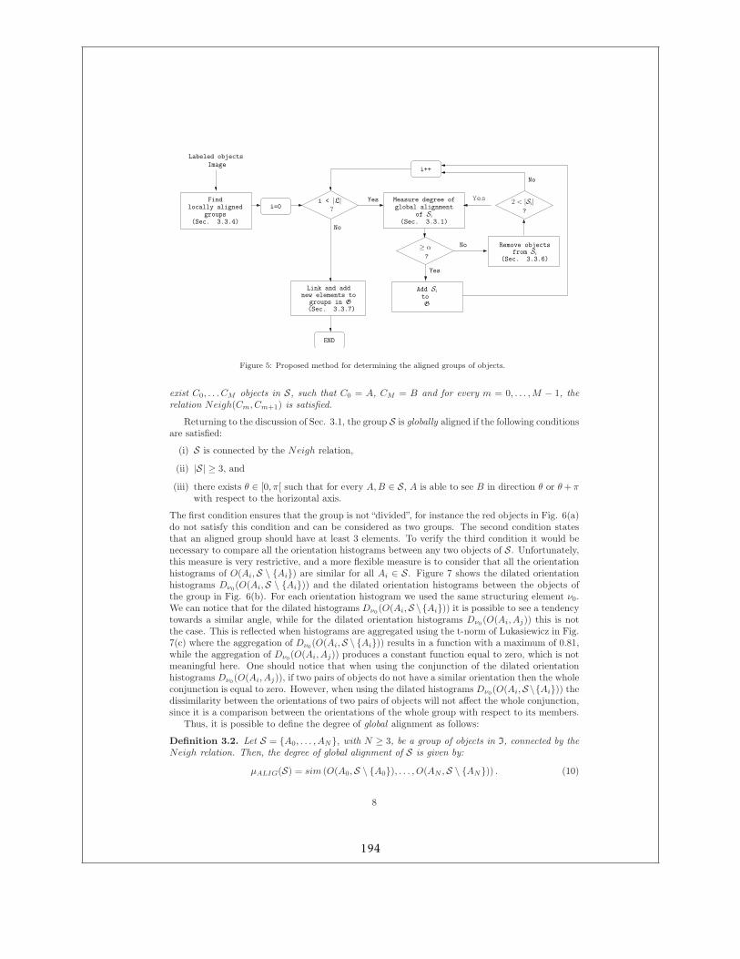
?
Yes i < |L|
≥ α
?
No
No
Yes
Yes
toG
Add Si
Labeled objectsImage
Findlocally aligned
i++
i=0
END
No
groups(Sec. 3.3.4)
of Si
Measure degree ofglobal alignment
(Sec. 3.3.1)
Remove objectsfrom Si
(Sec. 3.3.6)
new elements toLink and add
groups in G(Sec. 3.3.7)
2 < |Si|?
Figure 5: Proposed method for determining the aligned groups of objects.
exist C0, . . . CM objects in S, such that C0 = A, CM = B and for every m = 0, . . . , M − 1, therelation Neigh(Cm, Cm+1) is satisfied.
Returning to the discussion of Sec. 3.1, the group S is globally aligned if the following conditionsare satisfied:
(i) S is connected by the Neigh relation,
(ii) |S| ≥ 3, and
(iii) there exists θ ∈ [0, π[ such that for every A, B ∈ S, A is able to see B in direction θ or θ + πwith respect to the horizontal axis.
The first condition ensures that the group is not “divided”, for instance the red objects in Fig. 6(a)do not satisfy this condition and can be considered as two groups. The second condition statesthat an aligned group should have at least 3 elements. To verify the third condition it would benecessary to compare all the orientation histograms between any two objects of S. Unfortunately,this measure is very restrictive, and a more flexible measure is to consider that all the orientationhistograms of O(Ai, S \ {Ai}) are similar for all Ai ∈ S. Figure 7 shows the dilated orientationhistograms Dν0
(O(Ai, S \ {Ai})) and the dilated orientation histograms between the objects ofthe group in Fig. 6(b). For each orientation histogram we used the same structuring element ν0.We can notice that for the dilated histograms Dν0
(O(Ai, S \{Ai})) it is possible to see a tendencytowards a similar angle, while for the dilated orientation histograms Dν0
(O(Ai, Aj)) this is notthe case. This is reflected when histograms are aggregated using the t-norm of Lukasiewicz in Fig.7(c) where the aggregation of Dν0
(O(Ai, S \ {Ai})) results in a function with a maximum of 0.81,while the aggregation of Dν0
(O(Ai, Aj)) produces a constant function equal to zero, which is notmeaningful here. One should notice that when using the conjunction of the dilated orientationhistograms Dν0
(O(Ai, Aj)), if two pairs of objects do not have a similar orientation then the wholeconjunction is equal to zero. However, when using the dilated histograms Dν0
(O(Ai, S \{Ai})) thedissimilarity between the orientations of two pairs of objects will not affect the whole conjunction,since it is a comparison between the orientations of the whole group with respect to its members.
Thus, it is possible to define the degree of global alignment as follows:
Definition 3.2. Let S = {A0, . . . , AN}, with N ≥ 3, be a group of objects in I, connected by theNeigh relation. Then, the degree of global alignment of S is given by:
µALIG(S) = sim (O(A0, S \ {A0}), . . . , O(AN , S \ {AN})) . (10)
8
194
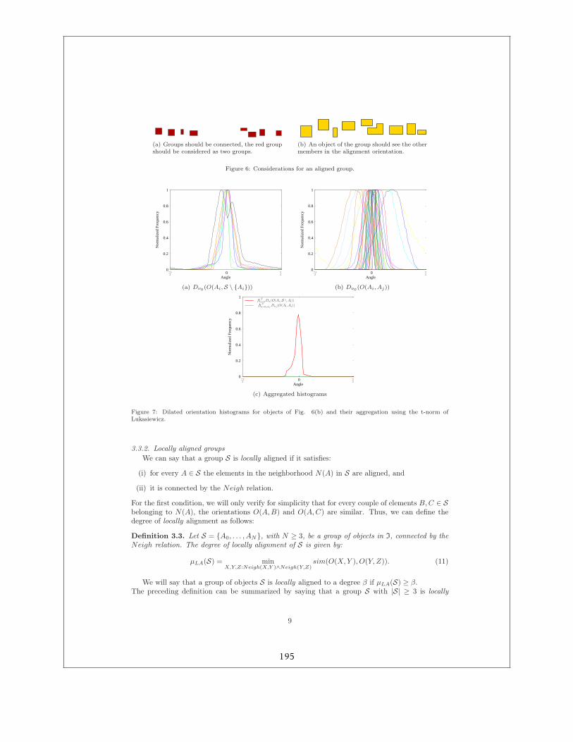
(a) Groups should be connected, the red groupshould be considered as two groups.
(b) An object of the group should see the othermembers in the alignment orientation.
Figure 6: Considerations for an aligned group.
0
0.2
0.4
0.6
0.8
1
0
Nor
mal
ized
Fre
quen
cy
Angle
−π2
π2
(a) Dν0 (O(Ai,S \ {Ai}))
0
0.2
0.4
0.6
0.8
1
0
Nor
mal
ized
Fre
quen
cy
Angle
−π2
π2
(b) Dν0 (O(Ai, Aj))
0
0.2
0.4
0.6
0.8
1
0
Nor
mal
ized
Fre
quen
cy
Angle
−π2
π2
∧Ni=0Dνi
(O(Ai,S \ Ai))∧Ni=0,i 6=j Dνij
(O(Ai, Aj))
(c) Aggregated histograms
Figure 7: Dilated orientation histograms for objects of Fig. 6(b) and their aggregation using the t-norm ofLukasiewicz.
3.3.2. Locally aligned groups
We can say that a group S is locally aligned if it satisfies:
(i) for every A ∈ S the elements in the neighborhood N(A) in S are aligned, and
(ii) it is connected by the Neigh relation.
For the first condition, we will only verify for simplicity that for every couple of elements B, C ∈ Sbelonging to N(A), the orientations O(A, B) and O(A, C) are similar. Thus, we can define thedegree of locally alignment as follows:
Definition 3.3. Let S = {A0, . . . , AN}, with N ≥ 3, be a group of objects in I, connected by theNeigh relation. The degree of locally alignment of S is given by:
µLA(S) = minX,Y,Z:Neigh(X,Y )∧Neigh(Y,Z)
sim(O(X, Y ), O(Y, Z)). (11)
We will say that a group of objects S is locally aligned to a degree β if µLA(S) ≥ β.The preceding definition can be summarized by saying that a group S with |S| ≥ 3 is locally
9
195
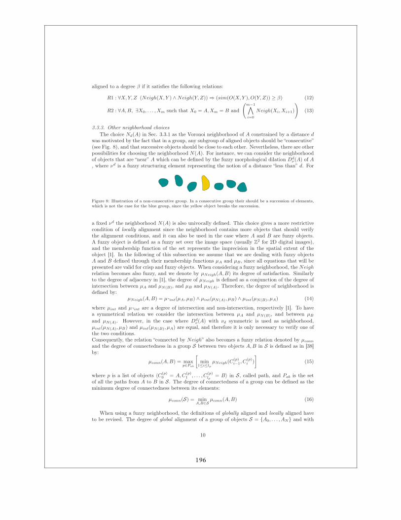
aligned to a degree β if it satisfies the following relations:
R1 : ∀X, Y, Z (Neigh(X, Y ) ∧ Neigh(Y, Z)) ⇒ (sim(O(X, Y ), O(Y, Z)) ≥ β) (12)
R2 : ∀A, B, ∃X0, . . . , Xm such that X0 = A, Xm = B and
(m−1∧
i=0
Neigh(Xi, Xi+1)
)(13)
3.3.3. Other neighborhood choices
The choice Nd(A) in Sec. 3.3.1 as the Voronoi neighborhood of A constrained by a distance dwas motivated by the fact that in a group, any subgroup of aligned objects should be “consecutive”(see Fig. 8), and that successive objects should be close to each other. Nevertheless, there are otherpossibilities for choosing the neighborhood N(A). For instance, we can consider the neighborhoodof objects that are “near” A which can be defined by the fuzzy morphological dilation Dd
ν(A) of A, where νd is a fuzzy structuring element representing the notion of a distance “less than” d. For
Figure 8: Illustration of a non-consecutive group. In a consecutive group their should be a succession of elements,which is not the case for the blue group, since the yellow object breaks the succession.
a fixed νd the neighborhood N(A) is also univocally defined. This choice gives a more restrictivecondition of locally alignment since the neighborhood contains more objects that should verifythe alignment conditions, and it can also be used in the case where A and B are fuzzy objects.A fuzzy object is defined as a fuzzy set over the image space (usually Z2 for 2D digital images),and the membership function of the set represents the imprecision in the spatial extent of theobject [1]. In the following of this subsection we assume that we are dealing with fuzzy objectsA and B defined through their membership functions µA and µB , since all equations that will bepresented are valid for crisp and fuzzy objects. When considering a fuzzy neighborhood, the Neighrelation becomes also fuzzy, and we denote by µNeigh(A, B) its degree of satisfaction. Similarlyto the degree of adjacency in [1], the degree of µNeigh is defined as a conjunction of the degree ofintersection between µA and µN(B), and µB and µN(A). Therefore, the degree of neighborhood isdefined by:
µNeigh(A, B) = µqint(µA, µB) ∧ µint(µN(A), µB) ∧ µint(µN(B), µA) (14)
where µint and µqint are a degree of intersection and non-intersection, respectively [1]. To havea symmetrical relation we consider the intersection between µA and µN(B), and between µB
and µN(A). However, in the case where Ddν(A) with νd symmetric is used as neighborhood,
µint(µN(A), µB) and µint(µN(B), µA) are equal, and therefore it is only necessary to verify one ofthe two conditions.Consequently, the relation “connected by Neigh” also becomes a fuzzy relation denoted by µconn
and the degree of connectedness in a group S between two objects A, B in S is defined as in [38]by:
µconn(A, B) = maxp∈Pab
[min
1≤i≤lpµNeigh(C
(p)i−1, C
(p)i )
](15)
where p is a list of objects 〈C(p)0 = A, C
(p)1 , . . . , C
(p)lp
= B〉 in S, called path, and Pab is the setof all the paths from A to B in S. The degree of connectedness of a group can be defined as theminimum degree of connectedness between its elements:
µconn(S) = minA,B∈S
µconn(A, B) (16)
When using a fuzzy neighborhood, the definitions of globally aligned and locally aligned haveto be revised. The degree of global alignment of a group of objects S = {A0, . . . , AN} and with
10
196
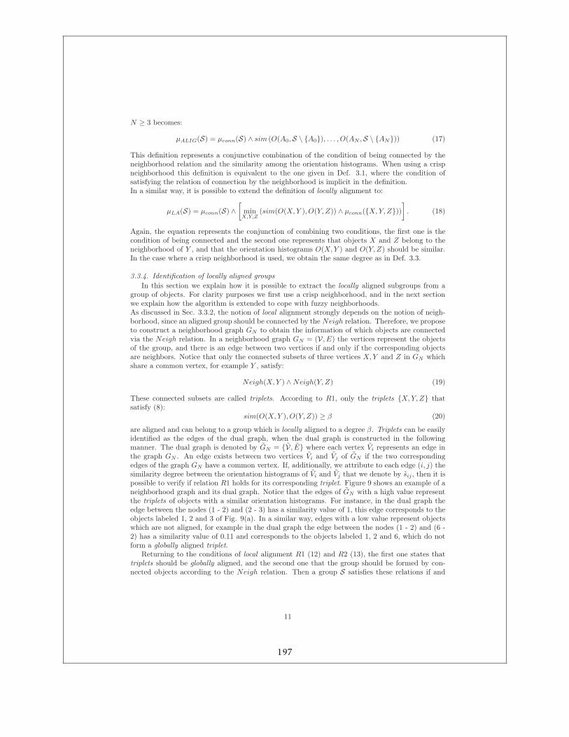
N ≥ 3 becomes:
µALIG(S) = µconn(S) ∧ sim (O(A0, S \ {A0}), . . . , O(AN , S \ {AN})) (17)
This definition represents a conjunctive combination of the condition of being connected by theneighborhood relation and the similarity among the orientation histograms. When using a crispneighborhood this definition is equivalent to the one given in Def. 3.1, where the condition ofsatisfying the relation of connection by the neighborhood is implicit in the definition.In a similar way, it is possible to extend the definition of locally alignment to:
µLA(S) = µconn(S) ∧[
minX,Y,Z
(sim(O(X, Y ), O(Y, Z)) ∧ µconn({X, Y, Z}))
]. (18)
Again, the equation represents the conjunction of combining two conditions, the first one is thecondition of being connected and the second one represents that objects X and Z belong to theneighborhood of Y , and that the orientation histograms O(X, Y ) and O(Y, Z) should be similar.In the case where a crisp neighborhood is used, we obtain the same degree as in Def. 3.3.
3.3.4. Identification of locally aligned groups
In this section we explain how it is possible to extract the locally aligned subgroups from agroup of objects. For clarity purposes we first use a crisp neighborhood, and in the next sectionwe explain how the algorithm is extended to cope with fuzzy neighborhoods.As discussed in Sec. 3.3.2, the notion of local alignment strongly depends on the notion of neigh-borhood, since an aligned group should be connected by the Neigh relation. Therefore, we proposeto construct a neighborhood graph GN to obtain the information of which objects are connectedvia the Neigh relation. In a neighborhood graph GN = (V, E) the vertices represent the objectsof the group, and there is an edge between two vertices if and only if the corresponding objectsare neighbors. Notice that only the connected subsets of three vertices X, Y and Z in GN whichshare a common vertex, for example Y , satisfy:
Neigh(X, Y ) ∧ Neigh(Y, Z) (19)
These connected subsets are called triplets. According to R1, only the triplets {X, Y, Z} thatsatisfy (8):
sim(O(X, Y ), O(Y, Z)) ≥ β (20)
are aligned and can belong to a group which is locally aligned to a degree β. Triplets can be easilyidentified as the edges of the dual graph, when the dual graph is constructed in the followingmanner. The dual graph is denoted by GN = {V , E} where each vertex Vi represents an edge inthe graph GN . An edge exists between two vertices Vi and Vj of GN if the two correspondingedges of the graph GN have a common vertex. If, additionally, we attribute to each edge (i, j) thesimilarity degree between the orientation histograms of Vi and Vj that we denote by sij , then it ispossible to verify if relation R1 holds for its corresponding triplet. Figure 9 shows an example of aneighborhood graph and its dual graph. Notice that the edges of GN with a high value representthe triplets of objects with a similar orientation histograms. For instance, in the dual graph theedge between the nodes (1 - 2) and (2 - 3) has a similarity value of 1, this edge corresponds to theobjects labeled 1, 2 and 3 of Fig. 9(a). In a similar way, edges with a low value represent objectswhich are not aligned, for example in the dual graph the edge between the nodes (1 - 2) and (6 -2) has a similarity value of 0.11 and corresponds to the objects labeled 1, 2 and 6, which do notform a globally aligned triplet.
Returning to the conditions of local alignment R1 (12) and R2 (13), the first one states thattriplets should be globally aligned, and the second one that the group should be formed by con-nected objects according to the Neigh relation. Then a group S satisfies these relations if and
11
197
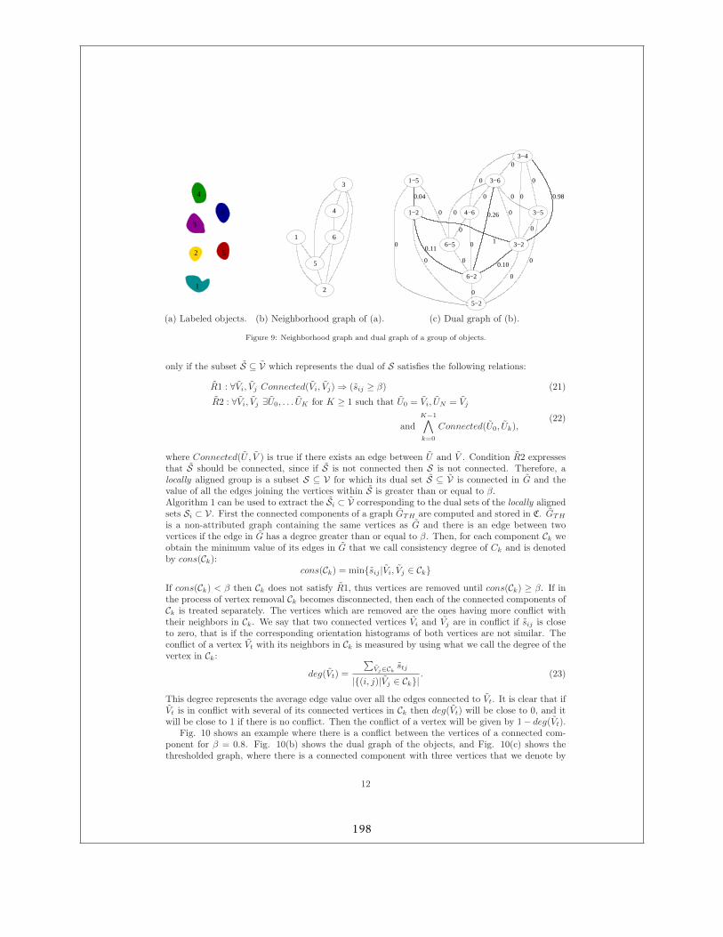
1
2
3
4
5
6
(a) Labeled objects.
1
5
2
3
4
6
(b) Neighborhood graph of (a).
3−4
5−2
1−2
6−5 3−2
6−2
3−6
3−54−6
1−5
0.04
0
0
0
0
0
0 0.98
0
0
0
0
0
0
0
0
0
0
0
0
0.11
0.26
0.10
1
(c) Dual graph of (b).
Figure 9: Neighborhood graph and dual graph of a group of objects.
only if the subset S ⊆ V which represents the dual of S satisfies the following relations:
R1 : ∀Vi, Vj Connected(Vi, Vj) ⇒ (sij ≥ β) (21)
R2 : ∀Vi, Vj ∃U0, . . . UK for K ≥ 1 such that U0 = Vi, UN = Vj
and
K−1∧
k=0
Connected(U0, Uk),(22)
where Connected(U , V ) is true if there exists an edge between U and V . Condition R2 expressesthat S should be connected, since if S is not connected then S is not connected. Therefore, alocally aligned group is a subset S ⊆ V for which its dual set S ⊆ V is connected in G and thevalue of all the edges joining the vertices within S is greater than or equal to β.Algorithm 1 can be used to extract the Si ⊂ V corresponding to the dual sets of the locally alignedsets Si ⊂ V. First the connected components of a graph GTH are computed and stored in C. GTH
is a non-attributed graph containing the same vertices as G and there is an edge between twovertices if the edge in G has a degree greater than or equal to β. Then, for each component Ck weobtain the minimum value of its edges in G that we call consistency degree of Ck and is denotedby cons(Ck):
cons(Ck) = min{sij |Vi, Vj ∈ Ck}If cons(Ck) < β then Ck does not satisfy R1, thus vertices are removed until cons(Ck) ≥ β. If inthe process of vertex removal Ck becomes disconnected, then each of the connected components ofCk is treated separately. The vertices which are removed are the ones having more conflict withtheir neighbors in Ck. We say that two connected vertices Vi and Vj are in conflict if sij is closeto zero, that is if the corresponding orientation histograms of both vertices are not similar. Theconflict of a vertex Vt with its neighbors in Ck is measured by using what we call the degree of thevertex in Ck:
deg(Vt) =
∑Vj∈Ck
stj
|{(i, j)|Vj ∈ Ck}|. (23)
This degree represents the average edge value over all the edges connected to Vt. It is clear that ifVt is in conflict with several of its connected vertices in Ck then deg(Vt) will be close to 0, and itwill be close to 1 if there is no conflict. Then the conflict of a vertex will be given by 1 − deg(Vt).
Fig. 10 shows an example where there is a conflict between the vertices of a connected com-ponent for β = 0.8. Fig. 10(b) shows the dual graph of the objects, and Fig. 10(c) shows thethresholded graph, where there is a connected component with three vertices that we denote by
12
198
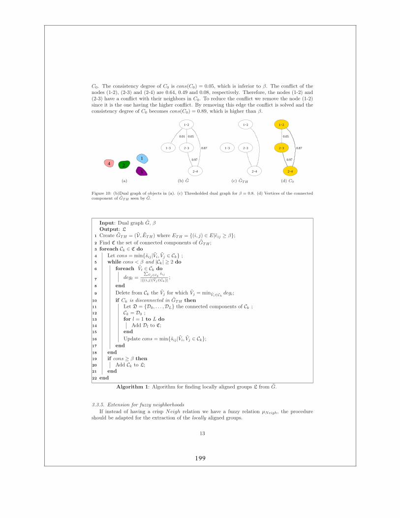
C0. The consistency degree of C0 is cons(C0) = 0.05, which is inferior to β. The conflict of thenodes (1-2), (2-3) and (2-4) are 0.64, 0.49 and 0.08, respectively. Therefore, the nodes (1-2) and(2-3) have a conflict with their neighbors in C0. To reduce the conflict we remove the node (1-2)since it is the one having the higher conflict. By removing this edge the conflict is solved and theconsistency degree of C0 becomes cons(C0) = 0.89, which is higher than β.
1
3
4 2
(a)
1−2
1−3 2−3
2−4
0.01 0.05
0.87
0.97
(b) G
1−2
1−3 2−3
2−4
(c) GTH
1−2
2−3
2−4
0.05
0.87
0.97
(d) C0
Figure 10: (b)Dual graph of objects in (a). (c) Thresholded dual graph for β = 0.8. (d) Vertices of the connectedcomponent of GTH seen by G.
Input: Dual graph G, βOutput: LCreate GTH = (V , ETH) where ETH = {(i, j) ∈ E|eij ≥ β};1
Find C the set of connected components of GTH ;2
foreach Ck ∈ C do3
Let cons = min{sij |Vi, Vj ∈ Ck} ;4
while cons < β and |Ck| ≥ 2 do5
foreach Vt ∈ Ck do6
degt =
∑Vj∈Ck
sij
|{(i,j)|Vj∈Ck}|;
7
end8
Delete from Ck the Vj for which Vj = minVi∈Ckdegi;9
if Ck is disconnected in GTH then10
Let D = {D0, . . . , DL} the connected components of Ck ;11
Ck = D0 ;12
for l = 1 to L do13
Add Dl to C;14
end15
Update cons = min{sij |Vi, Vj ∈ Ck};16
end17
end18
if cons ≥ β then19
Add Ck to L;20
end21
end22
Algorithm 1: Algorithm for finding locally aligned groups L from G.
3.3.5. Extension for fuzzy neighborhoods
If instead of having a crisp Neigh relation we have a fuzzy relation µNeigh, the procedureshould be adapted for the extraction of the locally aligned groups.
13
199
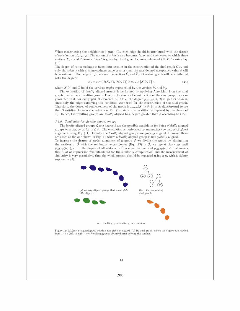
When constructing the neighborhood graph GN each edge should be attributed with the degreeof satisfaction of µNeigh. The notion of triplets also becomes fuzzy, and the degree to which threevertices X, Y and Z form a triplet is given by the degree of connectedness of {X, Y, Z} using Eq.(16).The degree of connectedness is taken into account in the construction of the dual graph GN , andonly the triplets with a connectedness value greater than the user defined acceptance value β willbe considered. Each edge (i, j) between the vertices Vi and Vj of the dual graph will be attributedwith the degree:
sij = sim(O(X, Y ), O(Y, Z)) ∧ µconn({X, Y, Z}), (24)
where X, Y and Z build the vertices triplet represented by the vertices Vi and Vj .The extraction of locally aligned groups is performed by applying Algorithm 1 on the dual
graph. Let S be a resulting group. Due to the choice of construction of the dual graph, we canguarantee that, for every pair of elements A, B ∈ S the degree µNeigh(A, B) is greater than β,since only the edges satisfying this condition were used for the construction of the dual graph.Therefore, the degree of connectedness of the group is µconn(S) ≥ β. It is straightforward to seethat S satisfies the second condition of Eq. (18) since this condition is imposed by the choice ofsij . Hence, the resulting groups are locally aligned to a degree greater than β according to (18).
3.3.6. Candidates for globally aligned groups
The locally aligned groups L to a degree β are the possible candidates for being globally alignedgroups to a degree α, for α ≤ β. The evaluation is performed by measuring the degree of globalalignment using Eq. (11). Usually the locally aligned groups are globally aligned. However thereare cases as the one shown in Fig. 11 where a locally aligned group is not globally aligned.To increase the degree of global alignment of a group S we divide the group by eliminatingthe vertices in S with the minimum vertex degree (Eq. 23) in S, we repeat this step untilµALIG(S) ≥ α. If the degree of all vertices in S is equal to one, and µALIG(S) < α it meansthat a lot of imprecision was introduced for the similarity computation, and the measurement ofsimilarity is very permissive, thus the whole process should be repeated using a ν0 with a tightersupport in (9).
(a) Locally aligned group, that is not glob-
ally aligned.(b) Correspondingdual graph.
(c) Resulting groups after group division.
Figure 11: (a)Locally aligned group which is not globally aligned. (b) Its dual graph, where the objects are labeledfrom 1 to 7 (left to right). (c) Resulting groups obtained after solving the conflict.
14
200
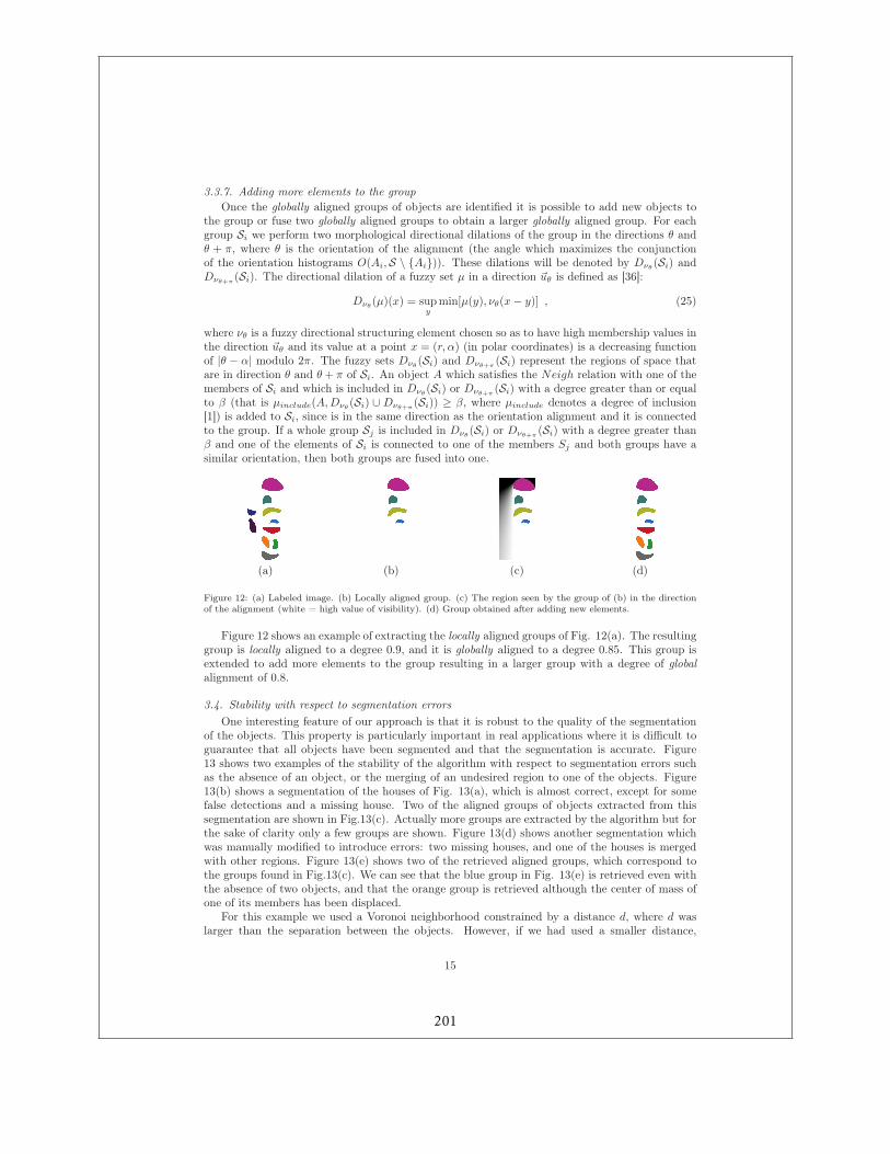
3.3.7. Adding more elements to the group
Once the globally aligned groups of objects are identified it is possible to add new objects tothe group or fuse two globally aligned groups to obtain a larger globally aligned group. For eachgroup Si we perform two morphological directional dilations of the group in the directions θ andθ + π, where θ is the orientation of the alignment (the angle which maximizes the conjunctionof the orientation histograms O(Ai, S \ {Ai})). These dilations will be denoted by Dνθ
(Si) andDνθ+π
(Si). The directional dilation of a fuzzy set µ in a direction ~uθ is defined as [36]:
Dνθ(µ)(x) = sup
ymin[µ(y), νθ(x − y)] , (25)
where νθ is a fuzzy directional structuring element chosen so as to have high membership values inthe direction ~uθ and its value at a point x = (r, α) (in polar coordinates) is a decreasing functionof |θ − α| modulo 2π. The fuzzy sets Dνθ
(Si) and Dνθ+π(Si) represent the regions of space that
are in direction θ and θ + π of Si. An object A which satisfies the Neigh relation with one of themembers of Si and which is included in Dνθ
(Si) or Dνθ+π(Si) with a degree greater than or equal
to β (that is µinclude(A, Dνθ(Si) ∪ Dνθ+π
(Si)) ≥ β, where µinclude denotes a degree of inclusion[1]) is added to Si, since is in the same direction as the orientation alignment and it is connectedto the group. If a whole group Sj is included in Dνθ
(Si) or Dνθ+π(Si) with a degree greater than
β and one of the elements of Si is connected to one of the members Sj and both groups have asimilar orientation, then both groups are fused into one.
(a) (b) (c) (d)
Figure 12: (a) Labeled image. (b) Locally aligned group. (c) The region seen by the group of (b) in the directionof the alignment (white = high value of visibility). (d) Group obtained after adding new elements.
Figure 12 shows an example of extracting the locally aligned groups of Fig. 12(a). The resultinggroup is locally aligned to a degree 0.9, and it is globally aligned to a degree 0.85. This group isextended to add more elements to the group resulting in a larger group with a degree of globalalignment of 0.8.
3.4. Stability with respect to segmentation errors
One interesting feature of our approach is that it is robust to the quality of the segmentationof the objects. This property is particularly important in real applications where it is difficult toguarantee that all objects have been segmented and that the segmentation is accurate. Figure13 shows two examples of the stability of the algorithm with respect to segmentation errors suchas the absence of an object, or the merging of an undesired region to one of the objects. Figure13(b) shows a segmentation of the houses of Fig. 13(a), which is almost correct, except for somefalse detections and a missing house. Two of the aligned groups of objects extracted from thissegmentation are shown in Fig.13(c). Actually more groups are extracted by the algorithm but forthe sake of clarity only a few groups are shown. Figure 13(d) shows another segmentation whichwas manually modified to introduce errors: two missing houses, and one of the houses is mergedwith other regions. Figure 13(e) shows two of the retrieved aligned groups, which correspond tothe groups found in Fig.13(c). We can see that the blue group in Fig. 13(e) is retrieved even withthe absence of two objects, and that the orange group is retrieved although the center of mass ofone of its members has been displaced.
For this example we used a Voronoi neighborhood constrained by a distance d, where d waslarger than the separation between the objects. However, if we had used a smaller distance,
15
201
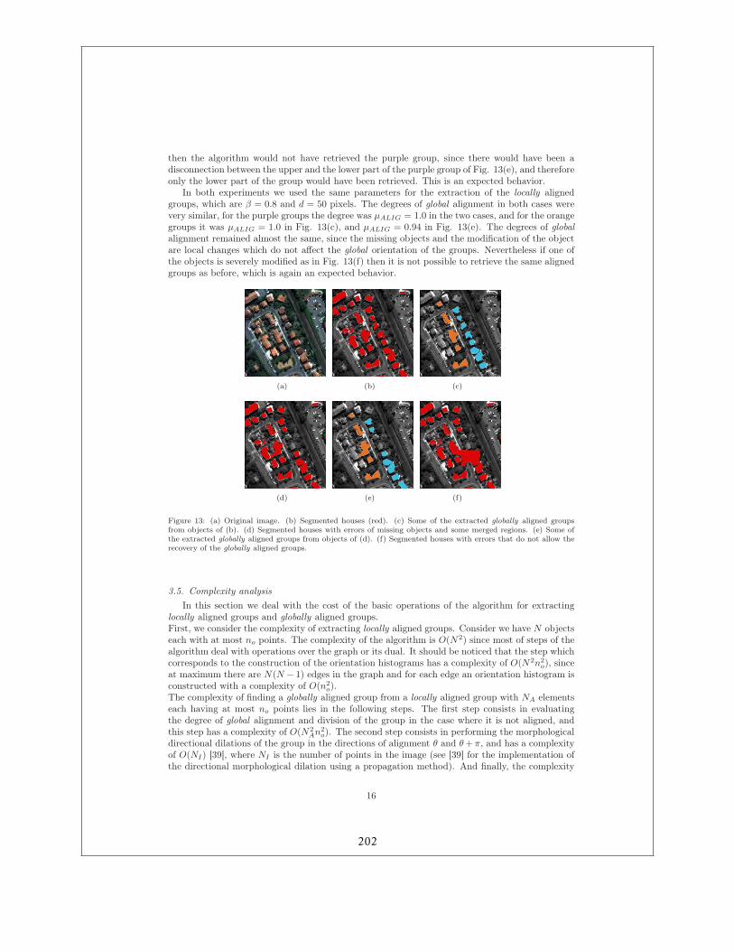
then the algorithm would not have retrieved the purple group, since there would have been adisconnection between the upper and the lower part of the purple group of Fig. 13(e), and thereforeonly the lower part of the group would have been retrieved. This is an expected behavior.
In both experiments we used the same parameters for the extraction of the locally alignedgroups, which are β = 0.8 and d = 50 pixels. The degrees of global alignment in both cases werevery similar, for the purple groups the degree was µALIG = 1.0 in the two cases, and for the orangegroups it was µALIG = 1.0 in Fig. 13(c), and µALIG = 0.94 in Fig. 13(e). The degrees of globalalignment remained almost the same, since the missing objects and the modification of the objectare local changes which do not affect the global orientation of the groups. Nevertheless if one ofthe objects is severely modified as in Fig. 13(f) then it is not possible to retrieve the same alignedgroups as before, which is again an expected behavior.
(a) (b) (c)
(d) (e) (f)
Figure 13: (a) Original image. (b) Segmented houses (red). (c) Some of the extracted globally aligned groupsfrom objects of (b). (d) Segmented houses with errors of missing objects and some merged regions. (e) Some ofthe extracted globally aligned groups from objects of (d). (f) Segmented houses with errors that do not allow therecovery of the globally aligned groups.
3.5. Complexity analysis
In this section we deal with the cost of the basic operations of the algorithm for extractinglocally aligned groups and globally aligned groups.First, we consider the complexity of extracting locally aligned groups. Consider we have N objectseach with at most no points. The complexity of the algorithm is O(N2) since most of steps of thealgorithm deal with operations over the graph or its dual. It should be noticed that the step whichcorresponds to the construction of the orientation histograms has a complexity of O(N2n2
o), sinceat maximum there are N(N − 1) edges in the graph and for each edge an orientation histogram isconstructed with a complexity of O(n2
o).The complexity of finding a globally aligned group from a locally aligned group with NA elementseach having at most no points lies in the following steps. The first step consists in evaluatingthe degree of global alignment and division of the group in the case where it is not aligned, andthis step has a complexity of O(N2
An2o). The second step consists in performing the morphological
directional dilations of the group in the directions of alignment θ and θ + π, and has a complexityof O(NI) [39], where NI is the number of points in the image (see [39] for the implementation ofthe directional morphological dilation using a propagation method). And finally, the complexity
16
202
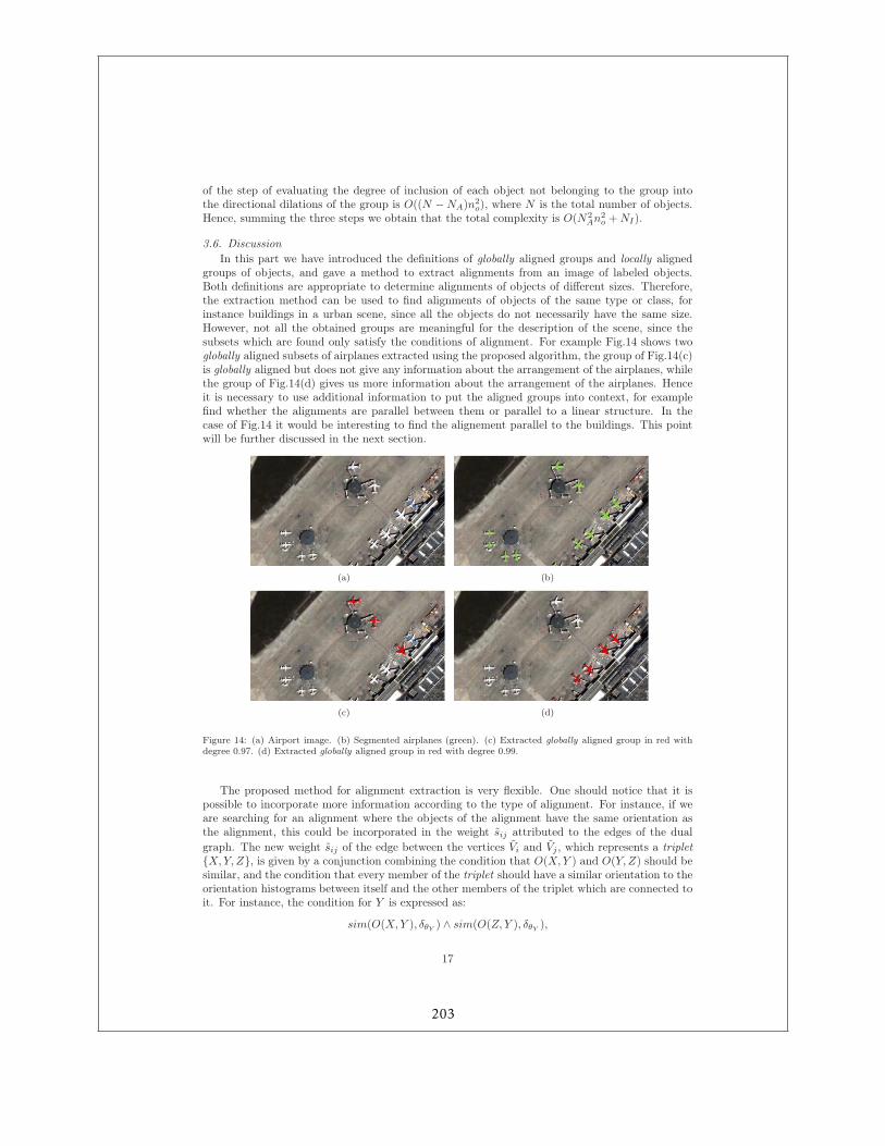
of the step of evaluating the degree of inclusion of each object not belonging to the group intothe directional dilations of the group is O((N − NA)n2
o), where N is the total number of objects.Hence, summing the three steps we obtain that the total complexity is O(N2
An2o + NI).
3.6. Discussion
In this part we have introduced the definitions of globally aligned groups and locally alignedgroups of objects, and gave a method to extract alignments from an image of labeled objects.Both definitions are appropriate to determine alignments of objects of different sizes. Therefore,the extraction method can be used to find alignments of objects of the same type or class, forinstance buildings in a urban scene, since all the objects do not necessarily have the same size.However, not all the obtained groups are meaningful for the description of the scene, since thesubsets which are found only satisfy the conditions of alignment. For example Fig.14 shows twoglobally aligned subsets of airplanes extracted using the proposed algorithm, the group of Fig.14(c)is globally aligned but does not give any information about the arrangement of the airplanes, whilethe group of Fig.14(d) gives us more information about the arrangement of the airplanes. Henceit is necessary to use additional information to put the aligned groups into context, for examplefind whether the alignments are parallel between them or parallel to a linear structure. In thecase of Fig.14 it would be interesting to find the alignement parallel to the buildings. This pointwill be further discussed in the next section.
(a) (b)
(c) (d)
Figure 14: (a) Airport image. (b) Segmented airplanes (green). (c) Extracted globally aligned group in red withdegree 0.97. (d) Extracted globally aligned group in red with degree 0.99.
The proposed method for alignment extraction is very flexible. One should notice that it ispossible to incorporate more information according to the type of alignment. For instance, if weare searching for an alignment where the objects of the alignment have the same orientation asthe alignment, this could be incorporated in the weight sij attributed to the edges of the dual
graph. The new weight sij of the edge between the vertices Vi and Vj , which represents a triplet{X, Y, Z}, is given by a conjunction combining the condition that O(X, Y ) and O(Y, Z) should besimilar, and the condition that every member of the triplet should have a similar orientation to theorientation histograms between itself and the other members of the triplet which are connected toit. For instance, the condition for Y is expressed as:
sim(O(X, Y ), δθY) ∧ sim(O(Z, Y ), δθY
),
17
203
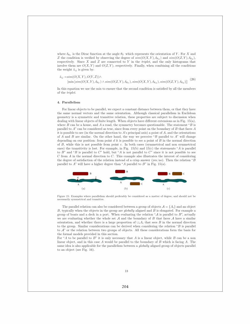
where δθYis the Dirac function at the angle θY which represents the orientation of Y . For X and
Z the condition is verified by observing the degree of sim(O(X, Y ), δθX) and sim(O(Z, Y ), δθZ
),respectively. Since X and Z are connected to Y in the triplet, and the only histograms thatinvolve them are O(X, Y ) and O(Z, Y ), respectively. Finally, when combining all the conditionsthe weight sij is given by:
sij =sim(O(X, Y ), O(Y, Z))∧[min [sim(O(X, Y ), δθY
) ∧ sim(O(Z, Y ), δθY), sim(O(X, Y ), δθX
), sim(O(Z, Y ), δθZ)]]
(26)
In this equation we use the min to ensure that the second condition is satisfied by all the membersof the triplet.
4. Parallelism
For linear objects to be parallel, we expect a constant distance between them, or that they havethe same normal vectors and the same orientation. Although classical parallelism in Euclideangeometry is a symmetric and transitive relation, these properties are subject to discussion whendealing with linear objects of finite length. When objects have different extensions as in Fig. 15(a),where B can be a house, and A a road, the symmetry becomes questionable. The statement “B isparallel to A” can be considered as true, since from every point on the boundary of B that faces Ait is possible to see (in the normal direction to A’s principal axis) a point of A, and the orientationsof A and B are similar. On the other hand, the way we perceive “B parallel to A” will changedepending on our position: from point d it is possible to see a point of B in the normal directionof B, while this is not possible from point c. In both cases (symmetrical and non symmetricalones) the transitivity is lost. For example, in Fig. 15(b) and 15(c) the statements “A is parallelto B” and “B is parallel to C” hold, but “A is not parallel to C” since it is not possible to seeC from A in the normal direction to C. This example also illustrates the interest of consideringthe degree of satisfaction of the relation instead of a crisp answer (yes/no). Then the relation “Bparallel to A” will have a higher degree than “A parallel to B” in Fig. 15(a).
B
A
d c������
������
������
������
(a)
A
B
C
(b)
A
B C
(c)
Figure 15: Examples where parallelism should preferably be considered as a matter of degree, and should not benecessarily symmetrical and transitive.
The parallel relation can also be considered between a group of objects A = {Ai} and an objectB, typically when the objects in the group are globally aligned and B is elongated. For example agroup of boats and a deck in a port. When evaluating the relation “A is parallel to B”, actuallywe are evaluating whether the whole set A and the boundary of B that faces A have a similarorientation, and whether there is a large proportion of ∪iAi that sees B in the normal directionto the group. Similar considerations can be derived when considering the relation “B is parallelto A” or the relation between two groups of objects. All these considerations form the basis forthe formal models provided in this section.For “A to be parallel to B” it is only necessary that A is a linear object, while B can be a nonlinear object, and in this case A would be parallel to the boundary of B which is facing A. Thesame idea is also applicable for the parallelism between a globally aligned group of objects parallelto an object (see Fig. 16).
18
204
Figure 16: A group of globally aligned objects parallel to a non-linear object.
4.1. Parallelism with (fuzzy) linear objects
In this section we propose a definition of parallelism between a fuzzy linear object3 and a fuzzyobject, including the particular case of crisp linear segments, and taking into account the abovementioned considerations. Suppose A is a linear object and B an object that it is not necessarilylinear, let θA be the orientation of A and ~uθA+ π
2be the normal unit vector to the principal axis
of A. Then, according to the considerations of the previous section, the degree of satisfaction ofthe relation “A is parallel to B” depends on two conditions:
(i) There should be a large proportion of A that sees B in the direction ~uθA+ π2.
(ii) The orientation of A and the orientation of the boundary of B that is facing A and that isseen by A in the direction ~uθA+ π
2should be similar.
Both conditions deal with the notion of visibility. Let p be a point, X be a fuzzy object withmembership function µX and ~uθ a vector with angle θ with respect to the x-axis. Then the subsetof X that is seen by p in the direction ~uθ , that we denote by Xvis(p,θ), is equal to the intersectionof X with the visual field of p, when p observes in the direction ~uθ. The visual field is representedas a morphological directional dilation in the direction θ of p. The set Xvis(p,θ) is a fuzzy set withmembership function µXvis(p,θ), where µXvis(p,θ)(x) represents the degree to which x is in X andis seen by p in the direction ~uθ:
µXvis(p,θ)(x) = µX(x) ∧ Dνθ(p)(x), (27)
where Dνθ(p)(x) is the morphological directional dilation defined in Eq. (25).
Let Y be a fuzzy object with membership function µY not intersecting X. We denote by Xvis(Y,θ)
the subset of X that is seen by the points on the boundary of Y , i.e the subset of X that is seenby Y , and it is defined by:
µXvis(Y,θ)(x) = µX(x) ∧ Dνθ(µY )(x). (28)
Fig.17 shows two objects A and B, and Bvis(A,θA+ π2 ), where θA is the orientation of A. When A
and B are linear segments, Avis(B,θA+ π2 ) can be interpreted as the projection of B onto A.
For the first condition of parallelism, we are interested in the proportion of A that sees B inthe direction ~uθA+ π
2. This subset is equivalent to Avis(B,θA−π
2 ), since the degree to which a pointx ∈ A sees B in the direction ~uθA+ π
2is equivalent to the degree to which the point is seen by B in
the direction ~uθA−π2. Therefore, the proportion of A that sees B in the normal direction ~uθA+ π
2
is equal to the fuzzy hypervolume of Avis(B,θA−π2 ) over the fuzzy hypervolume of A, where the
fuzzy hypervolume Vn of a fuzzy set µ is given by: Vn(µ) =∑
x∈I µ(x) [1]. Hence, the proportionis equal to:
Vn(µAvis(B,θA−π2 ))
Vn(µA)
3We consider that an object is linear if the ratio of its principal axis given bycyy+cxx−
√(cxx+cyy)2−4(cxxcyy−c2xy)
cyy+cxx+√
(cxx+cyy)2−4(cxxcyy−c2xy)where C =
(cxx cxycyx cyy
)corresponds to the second moments matrix,
is high [40].
19
205
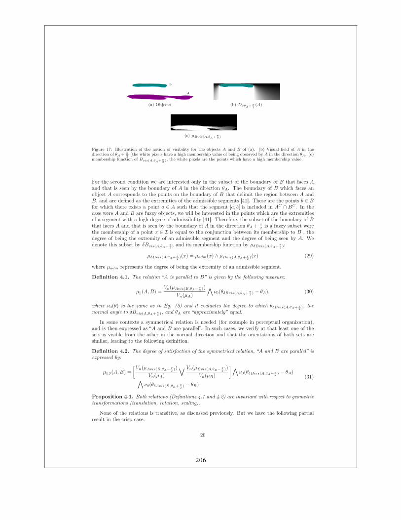
B
A
(a) Objects (b) DνθA+ π2(A)
(c) µBvis(A,θA+ π2
)
Figure 17: Illustration of the notion of visibility for the objects A and B of (a). (b) Visual field of A in thedirection of θA + π
2(the white pixels have a high membership value of being observed by A in the direction θA. (c)
membership function of Bvis(A,θA+ π2
), the white pixels are the points which have a high membership value.
For the second condition we are interested only in the subset of the boundary of B that faces Aand that is seen by the boundary of A in the direction θA. The boundary of B which faces anobject A corresponds to the points on the boundary of B that delimit the region between A andB, and are defined as the extremities of the admissible segments [41]. These are the points b ∈ Bfor which there exists a point a ∈ A such that the segment ]a, b[ is included in AC ∩ BC . In thecase were A and B are fuzzy objects, we will be interested in the points which are the extremitiesof a segment with a high degree of admissibility [41]. Therefore, the subset of the boundary of Bthat faces A and that is seen by the boundary of A in the direction θA + π
2 is a fuzzy subset werethe membership of a point x ∈ I is equal to the conjunction between its membership to B , thedegree of being the extremity of an admissible segment and the degree of being seen by A. Wedenote this subset by δBvis(A,θA+ π
2 ) and its membership function by µδBvis(A,θA+ π2 ):
µδBvis(A,θA+ π2 )(x) = µadm(x) ∧ µBvis(A,θA+ π
2 )(x) (29)
where µadm represents the degree of being the extremity of an admissible segment.
Definition 4.1. The relation “A is parallel to B” is given by the following measure:
µ‖(A, B) =Vn(µAvis(B,θA−π
2 ))
Vn(µA)
∧ν0(θδBvis(A,θA+ π
2 ) − θA), (30)
where ν0(θ) is the same as in Eq. (5) and it evaluates the degree to which θδBvis(A,θA+ π2 ), the
normal angle to δBvis(A,θA+ π2 ), and θA are “approximately” equal.
In some contexts a symmetrical relation is needed (for example in perceptual organization),and is then expressed as “A and B are parallel”. In such cases, we verify at that least one of thesets is visible from the other in the normal direction and that the orientations of both sets aresimilar, leading to the following definition.
Definition 4.2. The degree of satisfaction of the symmetrical relation, “A and B are parallel” isexpressed by:
µ‖S(A, B) =
[Vn(µAvis(B,θA−π
2 ))
Vn(µA)
∨ Vn(µBvis(A,θB−π2 ))
Vn(µB)
]∧ν0(θδBvis(A,θA+ π
2 ) − θA)
∧ν0(θδAvis(B,θB+ π
2 ) − θB)
(31)
Proposition 4.1. Both relations (Definitions 4.1 and 4.2) are invariant with respect to geometrictransformations (translation, rotation, scaling).
None of the relations is transitive, as discussed previously. But we have the following partialresult in the crisp case:
20
206
Proposition 4.2. Let A, B, C be linear crisp segments, if µ‖(A, B) = 1 , µ‖(B, C) = 1 andθA = θB = θC , then µ‖(A, C) = 1.
This result shows that in the crisp case we have transitivity. To have the transitivity property,it is necessary that θA = θB = θC , since ν0(θA − θB) = 1 and ν0(θB − θC) = 1 do not implyν0(θA − θC) = 1 due to the tolerance value t1 of the function ν0 (see Eq. 5). To have thetransitivity without imposing the condition θA = θB = θC , it is necessary that ν0 is a linearfunction (i.e. t1 = 0). But this is restrictive.
It is clear that both relations are reflexive. However, depending on the context we may notwant to consider intersecting objects as parallel. In this case, it is necessary to combine in aconjunctive way the previous degree (Def. 4.1 or 4.2) with a degree of non-intersection betweenthe two sets.
4.2. Parallelism with a globally aligned group of objects
When considering parallelism with a globally aligned group of objects, the group has a similarrole as the linear object in the definitions introduced in the previous section. When defining therelation with a group there is a modification, with respect to the case of a linear object, in theway the visibility constraint is computed, this modification will be discussed in the following.
4.2.1. A group of globally aligned objects parallel to an object
Let S = {A0, . . . , AN} be a group of globally aligned objects, as defined in Sec. 3.3.1, and letB be another object. For S to be parallel to B it is necessary that there is a large portion of S thatsees B, and this is computed in the same way as for the case of parallelism between a linear objectand an object. For the second condition we need to create the fuzzy set βS which is composed ofthe union of the regions between two consecutive elements of S. βS can be constructed using thedefinition that involves the convex hull presented in [41]. In Fig. 18(b) an example of the regionβS of a group S is shown in light purple. From Fig. 18(a) we can see that the boundary of B thatfaces S and that is visible by S depends on the separation between the members of the group.However, it is desirable that the degree of parallelism of a group to an object is independentof the separation of its members, since if we add more elements to a group without changingits orientation or its extension the degree of alignment to the object should remain the same.Therefore, in order to have a degree of parallelism independent of the separation of the membersof the group we should use βS in the second condition of parallelism. Then, the second conditionbecomes that the boundary of B that faces S and that is visible by βS or by S should have thesame orientation as the orientation of the alignment of S.
Finally, we define the relation as:
Definition 4.3. The degree of satisfaction of the relation “S is parallel to B” is given by:
µ‖(S, B) =Vn(∨iµAivis(B,θs−π
2 ))
Vn(∨µAi)
∧ν0(θδBvis(βs∪S,θs+ π
2 ) − θS), (32)
where θs is the orientation of the alignment of the group S.
In this definition, the first part of the equation represents that there should be a large portionof the union of all the Ai ∈ S that see B, and the second part evaluates the degree of similaritybetween the orientation of the group and the orientation of the boundary of the object seen bythe group in the direction θs + π
2 .
4.2.2. A linear object parallel to a globally aligned group of objects
Using the same notations as above, suppose B is a fuzzy linear object. Then for “B is parallelto S ” to be true, it is necessary that B has a similar orientation to the orientation of the alignmentof S, and that there is a large proportion of B that sees the group of objects or βS . As in Def.4.3 it is necessary to use S ∪ βS in order to assure that the parallel relation is independent of theseparation of the element of S.
21
207
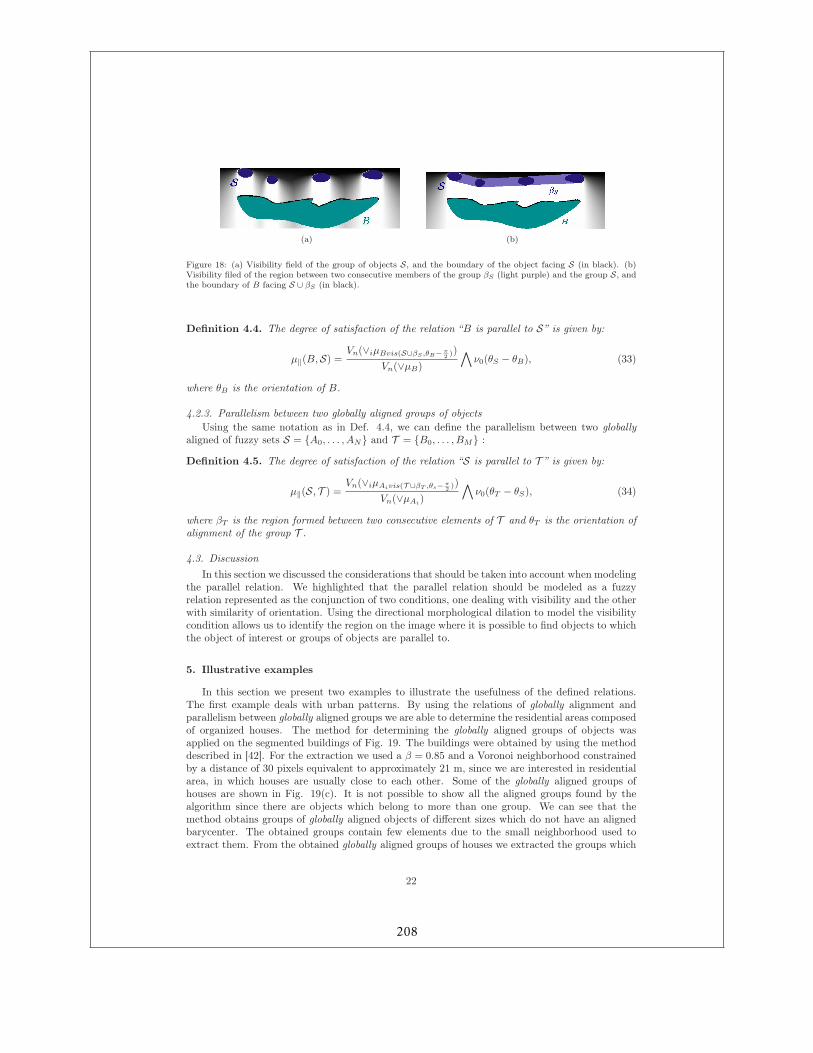
(a) (b)
Figure 18: (a) Visibility field of the group of objects S, and the boundary of the object facing S (in black). (b)Visibility filed of the region between two consecutive members of the group βS (light purple) and the group S, andthe boundary of B facing S ∪ βS (in black).
Definition 4.4. The degree of satisfaction of the relation “B is parallel to S” is given by:
µ‖(B, S) =Vn(∨iµBvis(S∪βS ,θB−π
2 ))
Vn(∨µB)
∧ν0(θS − θB), (33)
where θB is the orientation of B.
4.2.3. Parallelism between two globally aligned groups of objects
Using the same notation as in Def. 4.4, we can define the parallelism between two globallyaligned of fuzzy sets S = {A0, . . . , AN} and T = {B0, . . . , BM} :
Definition 4.5. The degree of satisfaction of the relation “S is parallel to T ” is given by:
µ‖(S, T ) =Vn(∨iµAivis(T ∪βT ,θs−π
2 ))
Vn(∨µAi)
∧ν0(θT − θS), (34)
where βT is the region formed between two consecutive elements of T and θT is the orientation ofalignment of the group T .
4.3. Discussion
In this section we discussed the considerations that should be taken into account when modelingthe parallel relation. We highlighted that the parallel relation should be modeled as a fuzzyrelation represented as the conjunction of two conditions, one dealing with visibility and the otherwith similarity of orientation. Using the directional morphological dilation to model the visibilitycondition allows us to identify the region on the image where it is possible to find objects to whichthe object of interest or groups of objects are parallel to.
5. Illustrative examples
In this section we present two examples to illustrate the usefulness of the defined relations.The first example deals with urban patterns. By using the relations of globally alignment andparallelism between globally aligned groups we are able to determine the residential areas composedof organized houses. The method for determining the globally aligned groups of objects wasapplied on the segmented buildings of Fig. 19. The buildings were obtained by using the methoddescribed in [42]. For the extraction we used a β = 0.85 and a Voronoi neighborhood constrainedby a distance of 30 pixels equivalent to approximately 21 m, since we are interested in residentialarea, in which houses are usually close to each other. Some of the globally aligned groups ofhouses are shown in Fig. 19(c). It is not possible to show all the aligned groups found by thealgorithm since there are objects which belong to more than one group. We can see that themethod obtains groups of globally aligned objects of different sizes which do not have an alignedbarycenter. The obtained groups contain few elements due to the small neighborhood used toextract them. From the obtained globally aligned groups of houses we extracted the groups which
22
208
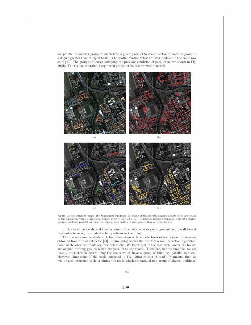
are parallel to another group or which have a group parallel to it and is close to another group toa degree greater than or equal to 0.8. The spatial relation “close to” was modeled in the same wayas in [43]. The groups of houses satisfying the previous condition of parallelism are shown in Fig.19(d). The regions containing organized groups of houses are well detected.
(a) (b)
(c) (d)
Figure 19: (a) Original image. (b) Segmented buildings. (c) Some of the globally aligned subsets of houses foundby the algorithm with a degree of alignment greater than 0.85. (d). Clusters of houses belonging to globally alignedgroups which are parallel and near to other groups with a degree greater than or equal to 0.8.
In this example we showed that by using the spatial relations of alignment and parallelism itis possible to recognize spatial urban patterns in the image.
The second example deals with the elimination of false detections of roads near urban areasobtained from a road extractor [44]. Figure 20(a) shows the result of a road detection algorithm.Some of the obtained roads are false detections. We know that in the residential areas, the housesare aligned forming groups which are parallel to the roads. Therefore, in this example, we aremainly interested in determining the roads which have a group of buildings parallel to them.However, since some of the roads extracted in Fig. 20(a) consist of road’s fragments, then wewill be also interested in determining the roads which are parallel to a group of aligned buildings.
23
209
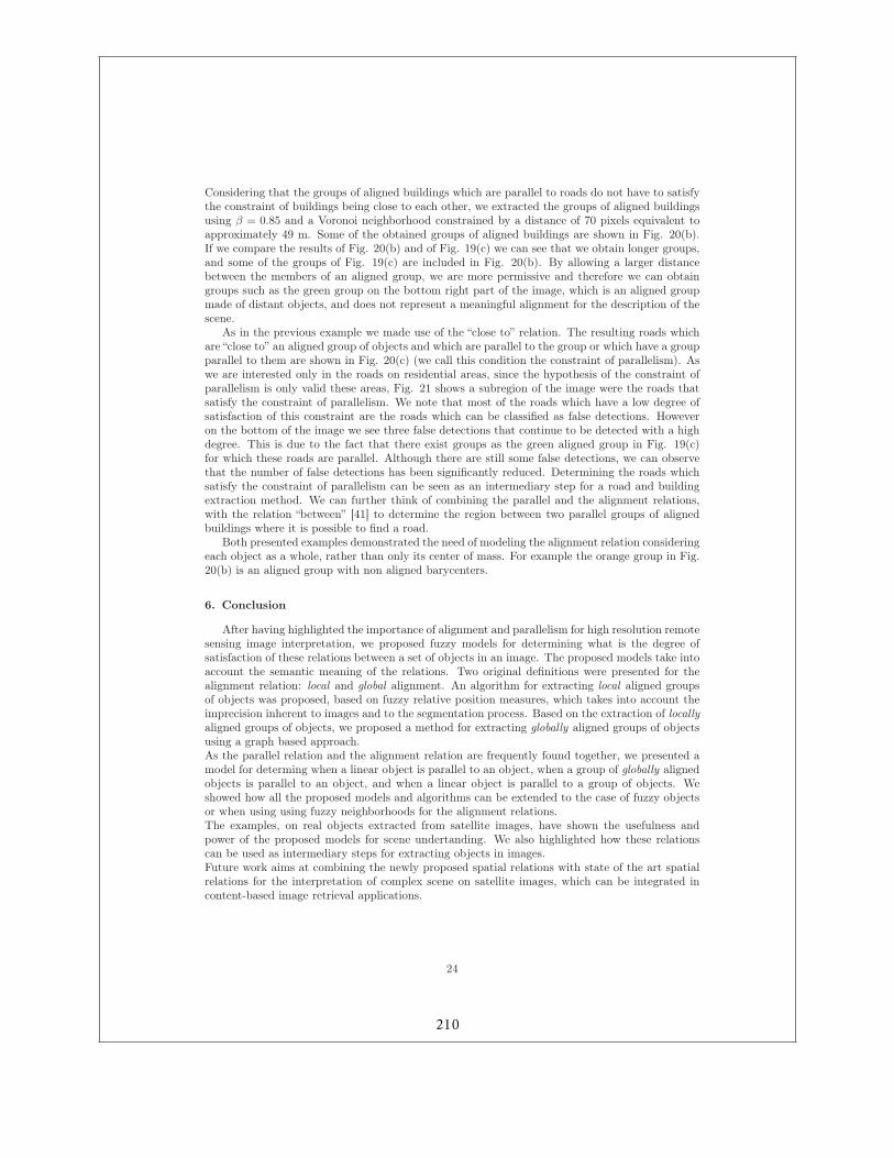
Considering that the groups of aligned buildings which are parallel to roads do not have to satisfythe constraint of buildings being close to each other, we extracted the groups of aligned buildingsusing β = 0.85 and a Voronoi neighborhood constrained by a distance of 70 pixels equivalent toapproximately 49 m. Some of the obtained groups of aligned buildings are shown in Fig. 20(b).If we compare the results of Fig. 20(b) and of Fig. 19(c) we can see that we obtain longer groups,and some of the groups of Fig. 19(c) are included in Fig. 20(b). By allowing a larger distancebetween the members of an aligned group, we are more permissive and therefore we can obtaingroups such as the green group on the bottom right part of the image, which is an aligned groupmade of distant objects, and does not represent a meaningful alignment for the description of thescene.
As in the previous example we made use of the “close to” relation. The resulting roads whichare “close to” an aligned group of objects and which are parallel to the group or which have a groupparallel to them are shown in Fig. 20(c) (we call this condition the constraint of parallelism). Aswe are interested only in the roads on residential areas, since the hypothesis of the constraint ofparallelism is only valid these areas, Fig. 21 shows a subregion of the image were the roads thatsatisfy the constraint of parallelism. We note that most of the roads which have a low degree ofsatisfaction of this constraint are the roads which can be classified as false detections. Howeveron the bottom of the image we see three false detections that continue to be detected with a highdegree. This is due to the fact that there exist groups as the green aligned group in Fig. 19(c)for which these roads are parallel. Although there are still some false detections, we can observethat the number of false detections has been significantly reduced. Determining the roads whichsatisfy the constraint of parallelism can be seen as an intermediary step for a road and buildingextraction method. We can further think of combining the parallel and the alignment relations,with the relation “between” [41] to determine the region between two parallel groups of alignedbuildings where it is possible to find a road.
Both presented examples demonstrated the need of modeling the alignment relation consideringeach object as a whole, rather than only its center of mass. For example the orange group in Fig.20(b) is an aligned group with non aligned barycenters.
6. Conclusion
After having highlighted the importance of alignment and parallelism for high resolution remotesensing image interpretation, we proposed fuzzy models for determining what is the degree ofsatisfaction of these relations between a set of objects in an image. The proposed models take intoaccount the semantic meaning of the relations. Two original definitions were presented for thealignment relation: local and global alignment. An algorithm for extracting local aligned groupsof objects was proposed, based on fuzzy relative position measures, which takes into account theimprecision inherent to images and to the segmentation process. Based on the extraction of locallyaligned groups of objects, we proposed a method for extracting globally aligned groups of objectsusing a graph based approach.As the parallel relation and the alignment relation are frequently found together, we presented amodel for determing when a linear object is parallel to an object, when a group of globally alignedobjects is parallel to an object, and when a linear object is parallel to a group of objects. Weshowed how all the proposed models and algorithms can be extended to the case of fuzzy objectsor when using using fuzzy neighborhoods for the alignment relations.The examples, on real objects extracted from satellite images, have shown the usefulness andpower of the proposed models for scene undertanding. We also highlighted how these relationscan be used as intermediary steps for extracting objects in images.Future work aims at combining the newly proposed spatial relations with state of the art spatialrelations for the interpretation of complex scene on satellite images, which can be integrated incontent-based image retrieval applications.
24
210
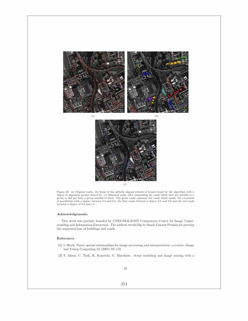
(a) (b)
(c)
Figure 20: (a) Original roads. (b) Some of the globally aligned subsets of houses found by the algorithm with adegree of alignment greater than 0.85. (c) Obtained roads, after eliminating the roads which were not parallel to agroup or did not have a group parallel to them. The green roads represent the roads which satisfy the constraintof parallelism with a degree between 0.3 and 0.5, the blue roads between a degree 0.5 and 0.8 and the red roadsbetween a degree of 0.8 and 1.0.
Acknowledgements
This work was partialy founded by CNES-DLR-ENST Competence Center for Image Under-standing and Information Extraction. The authors would like to thank Vincent Poulain for provingthe segmentations of buildings and roads.
References
[1] I. Bloch, Fuzzy spatial relationships for image processing and interpretation: a review, Imageand Vision Computing 23 (2005) 89–110.
[2] S. Aksoy, C. Tusk, K. Koperski, G. Marchisio, Scene modeling and image mining with a
25
211
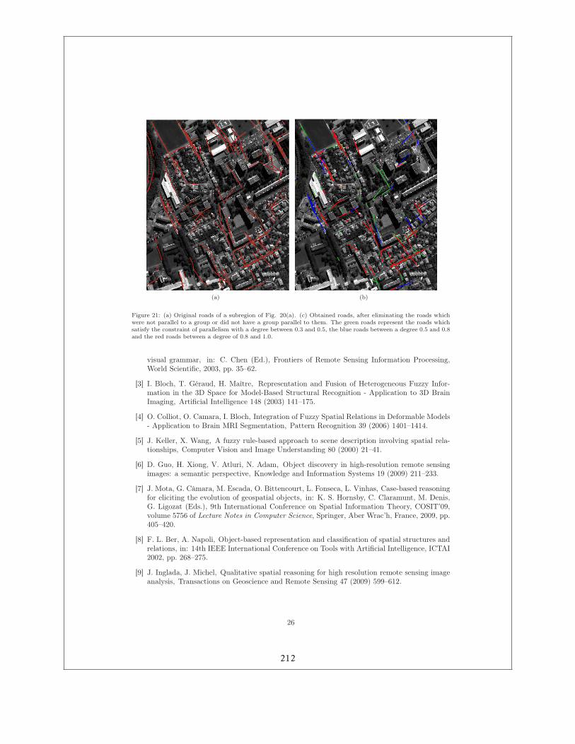
(a) (b)
Figure 21: (a) Original roads of a subregion of Fig. 20(a). (c) Obtained roads, after eliminating the roads whichwere not parallel to a group or did not have a group parallel to them. The green roads represent the roads whichsatisfy the constraint of parallelism with a degree between 0.3 and 0.5, the blue roads between a degree 0.5 and 0.8and the red roads between a degree of 0.8 and 1.0.
visual grammar, in: C. Chen (Ed.), Frontiers of Remote Sensing Information Processing,World Scientific, 2003, pp. 35–62.
[3] I. Bloch, T. Géraud, H. Maître, Representation and Fusion of Heterogeneous Fuzzy Infor-mation in the 3D Space for Model-Based Structural Recognition - Application to 3D BrainImaging, Artificial Intelligence 148 (2003) 141–175.
[4] O. Colliot, O. Camara, I. Bloch, Integration of Fuzzy Spatial Relations in Deformable Models- Application to Brain MRI Segmentation, Pattern Recognition 39 (2006) 1401–1414.
[5] J. Keller, X. Wang, A fuzzy rule-based approach to scene description involving spatial rela-tionships, Computer Vision and Image Understanding 80 (2000) 21–41.
[6] D. Guo, H. Xiong, V. Atluri, N. Adam, Object discovery in high-resolution remote sensingimages: a semantic perspective, Knowledge and Information Systems 19 (2009) 211–233.
[7] J. Mota, G. Câmara, M. Escada, O. Bittencourt, L. Fonseca, L. Vinhas, Case-based reasoningfor eliciting the evolution of geospatial objects, in: K. S. Hornsby, C. Claramunt, M. Denis,G. Ligozat (Eds.), 9th International Conference on Spatial Information Theory, COSIT’09,volume 5756 of Lecture Notes in Computer Science, Springer, Aber Wrac’h, France, 2009, pp.405–420.
[8] F. L. Ber, A. Napoli, Object-based representation and classification of spatial structures andrelations, in: 14th IEEE International Conference on Tools with Artificial Intelligence, ICTAI2002, pp. 268–275.
[9] J. Inglada, J. Michel, Qualitative spatial reasoning for high resolution remote sensing imageanalysis, Transactions on Geoscience and Remote Sensing 47 (2009) 599–612.
26
212
[10] A. Deruyver, Y. Hodé, L. Brun, Image interpretation with a conceptual graph: Labelingover-segmented images and detection of unexpected objects, Artificial Intelligence 173 (2009)1245–1265.
[11] J. Metzger, F. L. Ber, A. Napoli, Modeling and representing structures for analyzing spatialorganization in agronomy, in: A. de Moor, W. Lex, B. Ganter (Eds.), Conceptual Structuresfor Knowledge Creation and Communication, 11th International Conference on ConceptualStructures, ICCS 2003 Dresden, Germany, volume 2746 of Lecture Notes in Computer Science,Springer, 2003, pp. 215–228.
[12] S. Steiniger, R. Weibel, Relations among map objects in cartographic generalization, Car-tography and Geographic Information Science 34 (2007) 175–197.
[13] D. G. Lowe, Three-dimensional object recognition from single two-dimensional images, Ar-tificial intelligence 31 (1987) 355–395.
[14] R. Mohan, R. Nevatia, Using perceptual organization to extract 3D structures, IEEE Trans-actions on Pattern Analysis and Machine Intelligence 11 (1989) 1121–1139.
[15] R. Mohan, R. Nevatia, Perceptual organization for scene segmentation and description, IEEETransactions on Pattern Analysis and Machine Intelligence 14 (1992) 616–635.
[16] H.-B. Kang, E. Walker, Perceptual grouping based on fuzzy sets, in: IEEE InternationalConference on Fuzzy Systems, 1992, pp. 651–659.
[17] J. Rouco, M. Penas, M. Penedo, M. Ortega, C. Alonso-Montes, Artificial Intelligence Tech-niques and Recognition-Certainty Measure of Pairwise Line Segment Perceptual Relations Us-ing Fuzzy Logic, in: Iberoamerican Congress on Pattern Recognition, volume 4756, Springer,2007, pp. 477–486.
[18] A. L. Ralescu, J. G. Shanahan, Perceptual organization for inferring object boundaries in animage, Pattern Recognition 32 (1999) 1923–1933.
[19] S. Sarkar, K. L. Boyer, Perceptual organization in computer vision: A review and a proposalfor a classificatory structure, IEEE Transactions on Systems, Man, and Cybernetics 23 (1993)382–399.
[20] A. Desolneux, L. Moisan, J. M. Morel, From Gestalt Theory to Image Analysis: A Probabilis-tic Approach, volume 34 of Interdisciplinary Applied Mathematics, Springer-Verlag, 2008.
[21] M. Ortner, X. Descombes, J. Zerubia, Building outline extraction from digital elevationmodels using marked point processes, International Journal of Computer Vision 72 (2007)107–132.
[22] M. Wertheimer, Laws of organization in perceptual forms., in: W. H. Ellis (Ed.), SourceBook of Gestalt Psychology, Routledge and Kegan Paul, London, 1938.
[23] K. Koffka, Principles of Gestalt Psychology, Harcourt-Brace, New York, 1935.
[24] H. Kang, E. Walker, Characterizing and controlling approximation in hierarchical perceptualgrouping, Fuzzy Sets and Systems 65 (1994) 187–223.
[25] S. Toh, Extracting viewpoint invariance relations using fuzzy sets, in: Proceedings of theIntelligent Vehicles’ 92 Symposium, 1992, pp. 325–329.
[26] H. Ip, W. Wong, Detecting perceptually parallel curves: Criteria and force driven optimiza-tion, Computer Vision and Image Understanding 68 (1997) 190–208.
[27] D. Shen, W. Wong, H. Ip, Affine-invariant image retrieval by correspondence matching ofshapes, Image and Vision Computing 17 (1999) 489–499.
27
213
[28] L. Likforman-Sulem, A. Hanimyan, C. Faure, Extracting lines on handwritten documents byperceptual grouping, in: Proceedings of the Third International Conference on DocumentAnalysis and Recognition, ICDAR 1995, volume 2, p. 774.
[29] S. Christophe, A. Ruas, Detecting Building Alignments for Generalisation Purposes, in:Advances in Spatial Data Handling: 10th International Symposium on Spatial Data Handling,2002, pp. 419–432.
[30] A. Desolneux, L. Moisan, J. Morel, A grouping principle and four applications, IEEE Trans-actions on Pattern Analysis and Machine Intelligence 25 (2003) 508–513.
[31] K. Miyajima, A. Ralescu, Spatial organization in 2D segmented images: Representation andrecognition of primitive spatial relations, Fuzzy Sets and Systems 65 (1994) 225–236.
[32] I. Bloch, A. Ralescu, Directional relative position between objects in image processing: acomparison between fuzzy approaches, Pattern Recognition 36 (2003) 1563–1582.
[33] R. Zwick, E. Carlstein, D. V. Budescu, Measures of similarity among fuzzy concepts: Acomparative analysis, International Journal of Approximate Reasoning 1 (1987) 221–242.
[34] I. Bloch, On fuzzy distances and their use in image processing under imprecision, PatternRecognition 32 (1999) 1873–1895.
[35] J. Rabin, J. Delon, Y. Gousseau, Circular earth mover’s distance for the comparison of localfeatures, in: International Conference on Pattern Recognition, ICPR 2008, pp. 1–4.
[36] I. Bloch, H. Maître, Fuzzy Mathematical Morphologies: A Comparative Study, PatternRecognition 28 (1995) 1341–1387.
[37] I. Bloch, C. Pellot, F. Sureda, A. Herment, Fuzzy Modelling and Fuzzy Mathematical Mor-phology applied to 3D Reconstruction of Blood Vessels by Multi-Modality Data Fusion, in:D. D. R. Yager, H. Prade (Eds.), Fuzzy Set Methods in Information Engineering: A GuidedTour of Applications, John Wiley and Sons, New-York, 1996, pp. 93–110.
[38] A. Rosenfeld, Fuzzy digital topology, Information and Control 40 (1979) 76–87.
[39] I. Bloch, Fuzzy Relative Position between Objects in Image Processing: a MorphologicalApproach, IEEE Transactions on Pattern Analysis and Machine Intelligence 21 (1999) 657–664.
[40] M. Peura, J. Iivarinen, Efficiency of simple shape descriptors, in: Third International Work-shop on Visual Form, VF 1997, pp. 443–451.
[41] I. Bloch, O. Colliot, R. Cesar, On the Ternary Spatial Relation Between, IEEE Transactionson Systems, Man, and Cybernetics SMC-B 36 (2006) 312–327.
[42] V. Poulain, J. Inglada, M. Spigai, J.-V. Tourneret, P. Marthon, Fusion of high resolutionotical and SAR images with vector data bases for change detection, in: IEEE InternationalGeoscience and Remote Sensing Symposium, IGARSS 2009.
[43] C. Hudelot, J. Atif, I. Bloch, Fuzzy spatial relation ontology for image interpretation, FuzzySets Systems 159 (2008) 1929–1951.
[44] V. Poulain, J. Inglada, M. Spigai, J.-V. Tourneret, P. Marthon, High resolution optical andsar image fusion for road database updating, in: IEEE International Geoscience and RemoteSensing Symposium, IGARSS 2010, Hawaii.
28
214

17 Mise à jour de cartes numériques
215
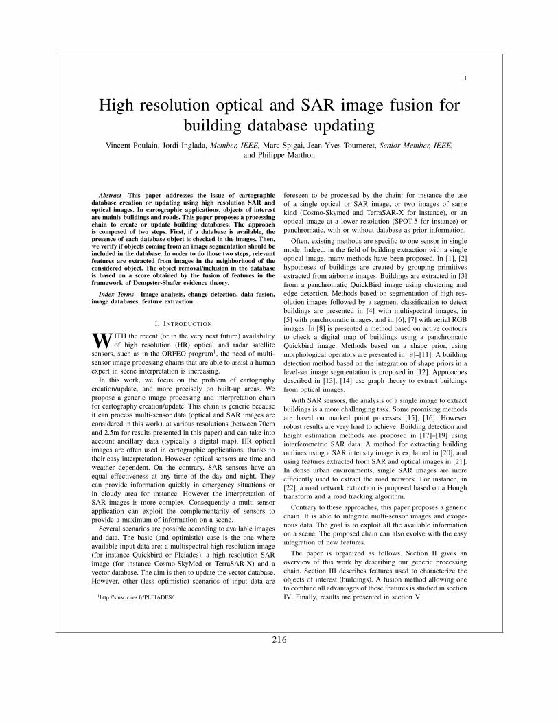
1
High resolution optical and SAR image fusion forbuilding database updating
Vincent Poulain, Jordi Inglada, Member, IEEE, Marc Spigai, Jean-Yves Tourneret, Senior Member, IEEE,and Philippe Marthon
Abstract—This paper addresses the issue of cartographicdatabase creation or updating using high resolution SAR andoptical images. In cartographic applications, objects of interestare mainly buildings and roads. This paper proposes a processingchain to create or update building databases. The approachis composed of two steps. First, if a database is available, thepresence of each database object is checked in the images. Then,we verify if objects coming from an image segmentation should beincluded in the database. In order to do those two steps, relevantfeatures are extracted from images in the neighborhood of theconsidered object. The object removal/inclusion in the databaseis based on a score obtained by the fusion of features in theframework of Dempster-Shafer evidence theory.
Index Terms—Image analysis, change detection, data fusion,image databases, feature extraction.
I. INTRODUCTION
W ITH the recent (or in the very next future) availabilityof high resolution (HR) optical and radar satellite
sensors, such as in the ORFEO program1, the need of multi-sensor image processing chains that are able to assist a humanexpert in scene interpretation is increasing.
In this work, we focus on the problem of cartographycreation/update, and more precisely on built-up areas. Wepropose a generic image processing and interpretation chainfor cartography creation/update. This chain is generic becauseit can process multi-sensor data (optical and SAR images areconsidered in this work), at various resolutions (between 70cmand 2.5m for results presented in this paper) and can take intoaccount ancillary data (typically a digital map). HR opticalimages are often used in cartographic applications, thanks totheir easy interpretation. However optical sensors are time andweather dependent. On the contrary, SAR sensors have anequal effectiveness at any time of the day and night. Theycan provide information quickly in emergency situations orin cloudy area for instance. However the interpretation ofSAR images is more complex. Consequently a multi-sensorapplication can exploit the complementarity of sensors toprovide a maximum of information on a scene.
Several scenarios are possible according to available imagesand data. The basic (and optimistic) case is the one whereavailable input data are: a multispectral high resolution image(for instance Quickbird or Pleiades), a high resolution SARimage (for instance Cosmo-SkyMed or TerraSAR-X) and avector database. The aim is then to update the vector database.However, other (less optimistic) scenarios of input data are
1http://smsc.cnes.fr/PLEIADES/
foreseen to be processed by the chain: for instance the useof a single optical or SAR image, or two images of samekind (Cosmo-Skymed and TerraSAR-X for instance), or anoptical image at a lower resolution (SPOT-5 for instance) orpanchromatic, with or without database as prior information.
Often, existing methods are specific to one sensor in singlemode. Indeed, in the field of building extraction with a singleoptical image, many methods have been proposed. In [1], [2]hypotheses of buildings are created by grouping primitivesextracted from airborne images. Buildings are extracted in [3]from a panchromatic QuickBird image using clustering andedge detection. Methods based on segmentation of high res-olution images followed by a segment classification to detectbuildings are presented in [4] with multispectral images, in[5] with panchromatic images, and in [6], [7] with aerial RGBimages. In [8] is presented a method based on active contoursto check a digital map of buildings using a panchromaticQuickbird image. Methods based on a shape prior, usingmorphological operators are presented in [9]–[11]. A buildingdetection method based on the integration of shape priors in alevel-set image segmentation is proposed in [12]. Approachesdescribed in [13], [14] use graph theory to extract buildingsfrom optical images.
With SAR sensors, the analysis of a single image to extractbuildings is a more challenging task. Some promising methodsare based on marked point processes [15], [16]. Howeverrobust results are very hard to achieve. Building detection andheight estimation methods are proposed in [17]–[19] usinginterferometric SAR data. A method for extracting buildingoutlines using a SAR intensity image is explained in [20], andusing features extracted from SAR and optical images in [21].In dense urban environments, single SAR images are moreefficiently used to extract the road network. For instance, in[22], a road network extraction is proposed based on a Houghtransform and a road tracking algorithm.
Contrary to these approaches, this paper proposes a genericchain. It is able to integrate multi-sensor images and exoge-nous data. The goal is to exploit all the available informationon a scene. The proposed chain can also evolve with the easyintegration of new features.
The paper is organized as follows. Section II gives anoverview of this work by describing our generic processingchain. Section III describes features used to characterize theobjects of interest (buildings). A fusion method allowing oneto combine all advantages of these features is studied in sectionIV. Finally, results are presented in section V.
216
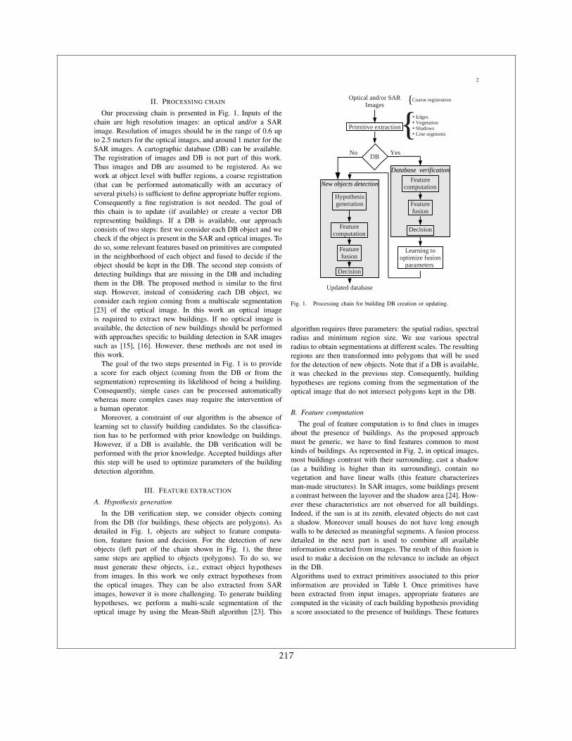
2
II. PROCESSING CHAIN
Our processing chain is presented in Fig. 1. Inputs of thechain are high resolution images: an optical and/or a SARimage. Resolution of images should be in the range of 0.6 upto 2.5 meters for the optical images, and around 1 meter for theSAR images. A cartographic database (DB) can be available.The registration of images and DB is not part of this work.Thus images and DB are assumed to be registered. As wework at object level with buffer regions, a coarse registration(that can be performed automatically with an accuracy ofseveral pixels) is sufficient to define appropriate buffer regions.Consequently a fine registration is not needed. The goal ofthis chain is to update (if available) or create a vector DBrepresenting buildings. If a DB is available, our approachconsists of two steps: first we consider each DB object and wecheck if the object is present in the SAR and optical images. Todo so, some relevant features based on primitives are computedin the neighborhood of each object and fused to decide if theobject should be kept in the DB. The second step consists ofdetecting buildings that are missing in the DB and includingthem in the DB. The proposed method is similar to the firststep. However, instead of considering each DB object, weconsider each region coming from a multiscale segmentation[23] of the optical image. In this work an optical imageis required to extract new buildings. If no optical image isavailable, the detection of new buildings should be performedwith approaches specific to building detection in SAR imagessuch as [15], [16]. However, these methods are not used inthis work.
The goal of the two steps presented in Fig. 1 is to providea score for each object (coming from the DB or from thesegmentation) representing its likelihood of being a building.Consequently, simple cases can be processed automaticallywhereas more complex cases may require the intervention ofa human operator.
Moreover, a constraint of our algorithm is the absence oflearning set to classify building candidates. So the classifica-tion has to be performed with prior knowledge on buildings.However, if a DB is available, the DB verification will beperformed with the prior knowledge. Accepted buildings afterthis step will be used to optimize parameters of the buildingdetection algorithm.
III. FEATURE EXTRACTION
A. Hypothesis generation
In the DB verification step, we consider objects comingfrom the DB (for buildings, these objects are polygons). Asdetailed in Fig. 1, objects are subject to feature computa-tion, feature fusion and decision. For the detection of newobjects (left part of the chain shown in Fig. 1), the threesame steps are applied to objects (polygons). To do so, wemust generate these objects, i.e., extract object hypothesesfrom images. In this work we only extract hypotheses fromthe optical images. They can be also extracted from SARimages, however it is more challenging. To generate buildinghypotheses, we perform a multi-scale segmentation of theoptical image by using the Mean-Shift algorithm [23]. This
New objects detectionNew objects detection
Optical and/or SARImages
Database verificationDatabase verification
Learning to optimize fusion
parameters
Primitive extraction
Updated database
Hypothesis generation
➔ Edges➔ Vegetation➔ Shadows➔ Line segments{
{Coarse registration
DBYesNo
Feature computation
Decision
Feature fusion
Decision
Feature computation
Feature fusion
Fig. 1. Processing chain for building DB creation or updating.
algorithm requires three parameters: the spatial radius, spectralradius and minimum region size. We use various spectralradius to obtain segmentations at different scales. The resultingregions are then transformed into polygons that will be usedfor the detection of new objects. Note that if a DB is available,it was checked in the previous step. Consequently, buildinghypotheses are regions coming from the segmentation of theoptical image that do not intersect polygons kept in the DB.
B. Feature computation
The goal of feature computation is to find clues in imagesabout the presence of buildings. As the proposed approachmust be generic, we have to find features common to mostkinds of buildings. As represented in Fig. 2, in optical images,most buildings contrast with their surrounding, cast a shadow(as a building is higher than its surrounding), contain novegetation and have linear walls (this feature characterizesman-made structures). In SAR images, some buildings presenta contrast between the layover and the shadow area [24]. How-ever these characteristics are not observed for all buildings.Indeed, if the sun is at its zenith, elevated objects do not casta shadow. Moreover small houses do not have long enoughwalls to be detected as meaningful segments. A fusion processdetailed in the next part is used to combine all availableinformation extracted from images. The result of this fusion isused to make a decision on the relevance to include an objectin the DB.Algorithms used to extract primitives associated to this priorinformation are provided in Table I. Once primitives havebeen extracted from input images, appropriate features arecomputed in the vicinity of each building hypothesis providinga score associated to the presence of buildings. These features
217
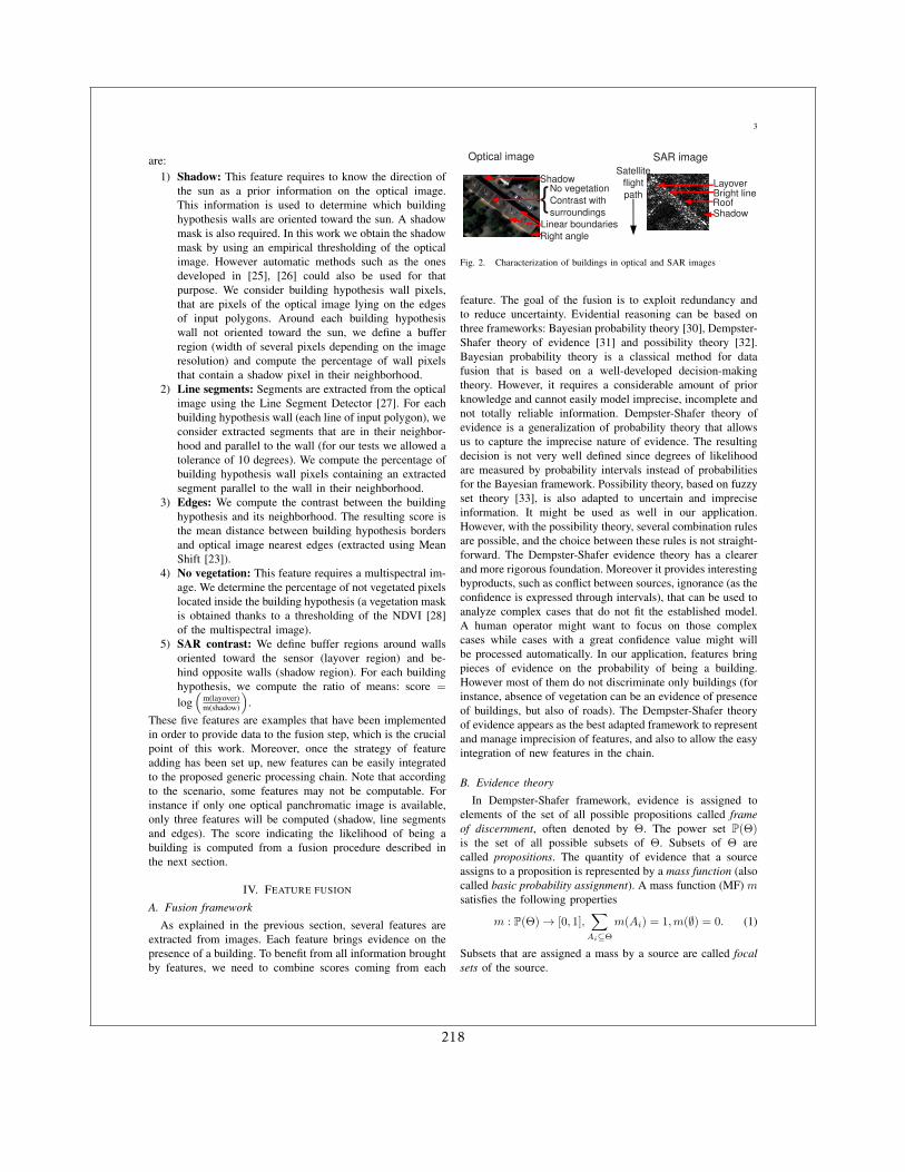
3
are:1) Shadow: This feature requires to know the direction of
the sun as a prior information on the optical image.This information is used to determine which buildinghypothesis walls are oriented toward the sun. A shadowmask is also required. In this work we obtain the shadowmask by using an empirical thresholding of the opticalimage. However automatic methods such as the onesdeveloped in [25], [26] could also be used for thatpurpose. We consider building hypothesis wall pixels,that are pixels of the optical image lying on the edgesof input polygons. Around each building hypothesiswall not oriented toward the sun, we define a bufferregion (width of several pixels depending on the imageresolution) and compute the percentage of wall pixelsthat contain a shadow pixel in their neighborhood.
2) Line segments: Segments are extracted from the opticalimage using the Line Segment Detector [27]. For eachbuilding hypothesis wall (each line of input polygon), weconsider extracted segments that are in their neighbor-hood and parallel to the wall (for our tests we allowed atolerance of 10 degrees). We compute the percentage ofbuilding hypothesis wall pixels containing an extractedsegment parallel to the wall in their neighborhood.
3) Edges: We compute the contrast between the buildinghypothesis and its neighborhood. The resulting score isthe mean distance between building hypothesis bordersand optical image nearest edges (extracted using MeanShift [23]).
4) No vegetation: This feature requires a multispectral im-age. We determine the percentage of not vegetated pixelslocated inside the building hypothesis (a vegetation maskis obtained thanks to a thresholding of the NDVI [28]of the multispectral image).
5) SAR contrast: We define buffer regions around wallsoriented toward the sensor (layover region) and be-hind opposite walls (shadow region). For each buildinghypothesis, we compute the ratio of means: score =
log(
m(layover)m(shadow)
).
These five features are examples that have been implementedin order to provide data to the fusion step, which is the crucialpoint of this work. Moreover, once the strategy of featureadding has been set up, new features can be easily integratedto the proposed generic processing chain. Note that accordingto the scenario, some features may not be computable. Forinstance if only one optical panchromatic image is available,only three features will be computed (shadow, line segmentsand edges). The score indicating the likelihood of being abuilding is computed from a fusion procedure described inthe next section.
IV. FEATURE FUSION
A. Fusion framework
As explained in the previous section, several features areextracted from images. Each feature brings evidence on thepresence of a building. To benefit from all information broughtby features, we need to combine scores coming from each
Shadow
Linear boundaries
No vegetationContrast with surroundings
{Right angle
LayoverBright lineRoofShadow
Satellite flight path
Optical image SAR image
Fig. 2. Characterization of buildings in optical and SAR images
feature. The goal of the fusion is to exploit redundancy andto reduce uncertainty. Evidential reasoning can be based onthree frameworks: Bayesian probability theory [30], Dempster-Shafer theory of evidence [31] and possibility theory [32].Bayesian probability theory is a classical method for datafusion that is based on a well-developed decision-makingtheory. However, it requires a considerable amount of priorknowledge and cannot easily model imprecise, incomplete andnot totally reliable information. Dempster-Shafer theory ofevidence is a generalization of probability theory that allowsus to capture the imprecise nature of evidence. The resultingdecision is not very well defined since degrees of likelihoodare measured by probability intervals instead of probabilitiesfor the Bayesian framework. Possibility theory, based on fuzzyset theory [33], is also adapted to uncertain and impreciseinformation. It might be used as well in our application.However, with the possibility theory, several combination rulesare possible, and the choice between these rules is not straight-forward. The Dempster-Shafer evidence theory has a clearerand more rigorous foundation. Moreover it provides interestingbyproducts, such as conflict between sources, ignorance (as theconfidence is expressed through intervals), that can be used toanalyze complex cases that do not fit the established model.A human operator might want to focus on those complexcases while cases with a great confidence value might willbe processed automatically. In our application, features bringpieces of evidence on the probability of being a building.However most of them do not discriminate only buildings (forinstance, absence of vegetation can be an evidence of presenceof buildings, but also of roads). The Dempster-Shafer theoryof evidence appears as the best adapted framework to representand manage imprecision of features, and also to allow the easyintegration of new features in the chain.
B. Evidence theory
In Dempster-Shafer framework, evidence is assigned toelements of the set of all possible propositions called frameof discernment, often denoted by Θ. The power set P(Θ)is the set of all possible subsets of Θ. Subsets of Θ arecalled propositions. The quantity of evidence that a sourceassigns to a proposition is represented by a mass function (alsocalled basic probability assignment). A mass function (MF) msatisfies the following properties
m : P(Θ)→ [0, 1],∑
Ai⊆Θ
m(Ai) = 1,m(∅) = 0. (1)
Subsets that are assigned a mass by a source are called focalsets of the source.
218
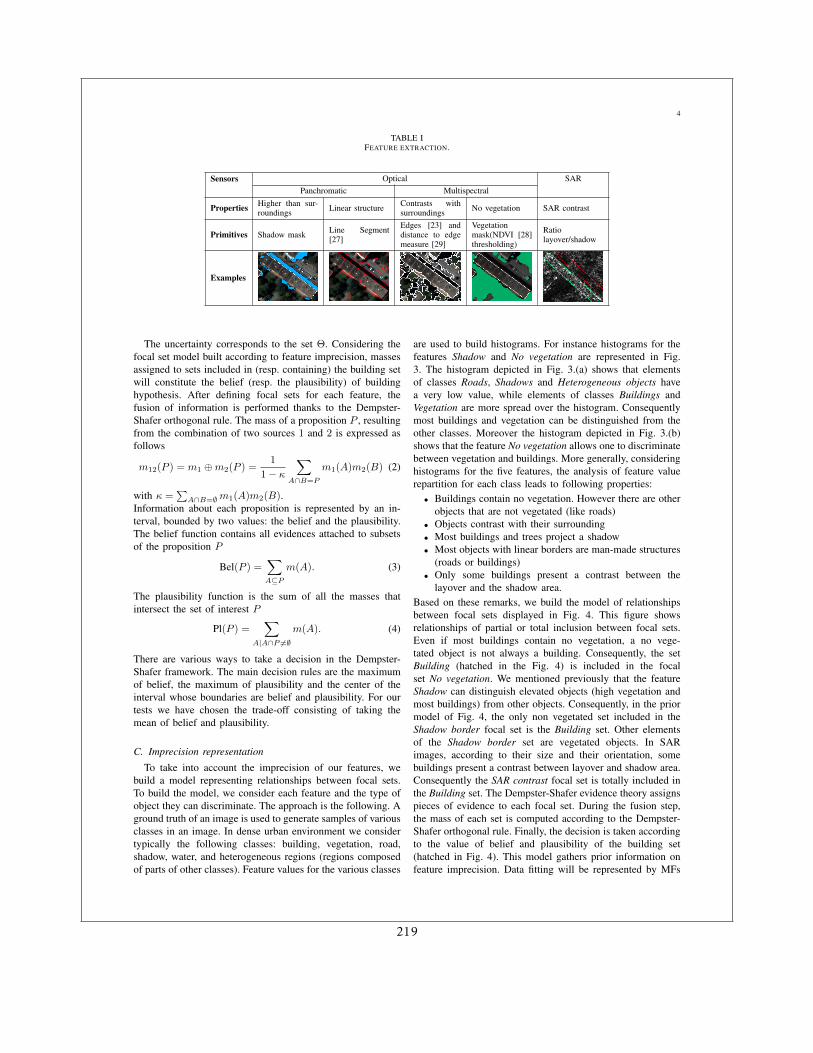
4
TABLE IFEATURE EXTRACTION.
Sensors Optical SARPanchromatic Multispectral
Properties Higher than sur-roundings Linear structure Contrasts with
surroundings No vegetation SAR contrast
Primitives Shadow mask Line Segment[27]
Edges [23] anddistance to edgemeasure [29]
Vegetationmask(NDVI [28]thresholding)
Ratiolayover/shadow
Examples
The uncertainty corresponds to the set Θ. Considering thefocal set model built according to feature imprecision, massesassigned to sets included in (resp. containing) the building setwill constitute the belief (resp. the plausibility) of buildinghypothesis. After defining focal sets for each feature, thefusion of information is performed thanks to the Dempster-Shafer orthogonal rule. The mass of a proposition P , resultingfrom the combination of two sources 1 and 2 is expressed asfollows
m12(P ) = m1 ⊕m2(P ) =1
1− κ∑
A∩B=P
m1(A)m2(B) (2)
with κ =∑
A∩B=∅m1(A)m2(B).Information about each proposition is represented by an in-terval, bounded by two values: the belief and the plausibility.The belief function contains all evidences attached to subsetsof the proposition P
Bel(P ) =∑
A⊆Pm(A). (3)
The plausibility function is the sum of all the masses thatintersect the set of interest P
Pl(P ) =∑
A|A∩P 6=∅m(A). (4)
There are various ways to take a decision in the Dempster-Shafer framework. The main decision rules are the maximumof belief, the maximum of plausibility and the center of theinterval whose boundaries are belief and plausibility. For ourtests we have chosen the trade-off consisting of taking themean of belief and plausibility.
C. Imprecision representation
To take into account the imprecision of our features, webuild a model representing relationships between focal sets.To build the model, we consider each feature and the type ofobject they can discriminate. The approach is the following. Aground truth of an image is used to generate samples of variousclasses in an image. In dense urban environment we considertypically the following classes: building, vegetation, road,shadow, water, and heterogeneous regions (regions composedof parts of other classes). Feature values for the various classes
are used to build histograms. For instance histograms for thefeatures Shadow and No vegetation are represented in Fig.3. The histogram depicted in Fig. 3.(a) shows that elementsof classes Roads, Shadows and Heterogeneous objects havea very low value, while elements of classes Buildings andVegetation are more spread over the histogram. Consequentlymost buildings and vegetation can be distinguished from theother classes. Moreover the histogram depicted in Fig. 3.(b)shows that the feature No vegetation allows one to discriminatebetween vegetation and buildings. More generally, consideringhistograms for the five features, the analysis of feature valuerepartition for each class leads to following properties:• Buildings contain no vegetation. However there are other
objects that are not vegetated (like roads)• Objects contrast with their surrounding• Most buildings and trees project a shadow• Most objects with linear borders are man-made structures
(roads or buildings)• Only some buildings present a contrast between the
layover and the shadow area.Based on these remarks, we build the model of relationshipsbetween focal sets displayed in Fig. 4. This figure showsrelationships of partial or total inclusion between focal sets.Even if most buildings contain no vegetation, a no vege-tated object is not always a building. Consequently, the setBuilding (hatched in the Fig. 4) is included in the focalset No vegetation. We mentioned previously that the featureShadow can distinguish elevated objects (high vegetation andmost buildings) from other objects. Consequently, in the priormodel of Fig. 4, the only non vegetated set included in theShadow border focal set is the Building set. Other elementsof the Shadow border set are vegetated objects. In SARimages, according to their size and their orientation, somebuildings present a contrast between layover and shadow area.Consequently the SAR contrast focal set is totally included inthe Building set. The Dempster-Shafer evidence theory assignspieces of evidence to each focal set. During the fusion step,the mass of each set is computed according to the Dempster-Shafer orthogonal rule. Finally, the decision is taken accordingto the value of belief and plausibility of the building set(hatched in Fig. 4). This model gathers prior information onfeature imprecision. Data fitting will be represented by MFs
219
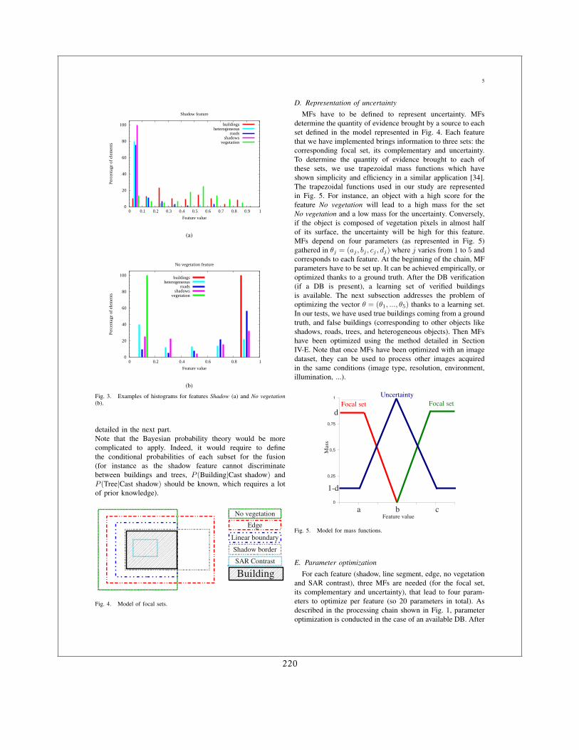
5
0
20
40
60
80
100
0 0.1 0.2 0.3 0.4 0.5 0.6 0.7 0.8 0.9 1
Perc
enta
ge o
f el
emen
ts
Feature value
Shadow feature
buildingsheterogeneous
roadsshadows
vegetation
(a)
0
20
40
60
80
100
0 0.2 0.4 0.6 0.8 1
Perc
enta
ge o
f el
emen
ts
Feature value
No vegetation feature
buildingsheterogeneous
roadsshadows
vegetation
(b)
Fig. 3. Examples of histograms for features Shadow (a) and No vegetation(b).
detailed in the next part.Note that the Bayesian probability theory would be morecomplicated to apply. Indeed, it would require to definethe conditional probabilities of each subset for the fusion(for instance as the shadow feature cannot discriminatebetween buildings and trees, P (Building|Cast shadow) andP (Tree|Cast shadow) should be known, which requires a lotof prior knowledge).
No vegetation
Edge
Linear boundary
Shadow border
BuildingSAR Contrast
Fig. 4. Model of focal sets.
D. Representation of uncertainty
MFs have to be defined to represent uncertainty. MFsdetermine the quantity of evidence brought by a source to eachset defined in the model represented in Fig. 4. Each featurethat we have implemented brings information to three sets: thecorresponding focal set, its complementary and uncertainty.To determine the quantity of evidence brought to each ofthese sets, we use trapezoidal mass functions which haveshown simplicity and efficiency in a similar application [34].The trapezoidal functions used in our study are representedin Fig. 5. For instance, an object with a high score for thefeature No vegetation will lead to a high mass for the setNo vegetation and a low mass for the uncertainty. Conversely,if the object is composed of vegetation pixels in almost halfof its surface, the uncertainty will be high for this feature.MFs depend on four parameters (as represented in Fig. 5)gathered in θj = (aj , bj , cj , dj) where j varies from 1 to 5 andcorresponds to each feature. At the beginning of the chain, MFparameters have to be set up. It can be achieved empirically, oroptimized thanks to a ground truth. After the DB verification(if a DB is present), a learning set of verified buildingsis available. The next subsection addresses the problem ofoptimizing the vector θ = (θ1, ..., θ5) thanks to a learning set.In our tests, we have used true buildings coming from a groundtruth, and false buildings (corresponding to other objects likeshadows, roads, trees, and heterogeneous objects). Then MFshave been optimized using the method detailed in SectionIV-E. Note that once MFs have been optimized with an imagedataset, they can be used to process other images acquiredin the same conditions (image type, resolution, environment,illumination, ...).
0
0,25
0,5
0,75
1 UncertaintyFocal setFocal set
Feature value
Mas
s
a b c
d
1d
Fig. 5. Model for mass functions.
E. Parameter optimization
For each feature (shadow, line segment, edge, no vegetationand SAR contrast), three MFs are needed (for the focal set,its complementary and uncertainty), that lead to four param-eters to optimize per feature (so 20 parameters in total). Asdescribed in the processing chain shown in Fig. 1, parameteroptimization is conducted in the case of an available DB. After
220
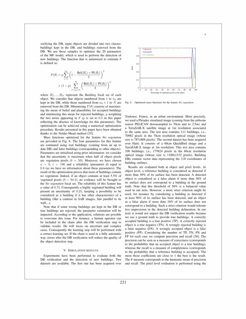
6
verifying the DB, input objects are divided into two classes:buildings kept in the DB, and buildings removed from theDB. We use those samples to optimize the 20 parametersof the MF model, which is used to perform the detection ofnew buildings. The function that is minimized to estimate θis defined as:
F (θ) = p
n0∑
i=1
(1− Bel(Bi) + Pl(Bi)
2
)2
+ (1− p)N∑
i=n0+1
(Bel(Bi) + Pl(Bi)
2
)2
where B1, ..., BN represent the Building focal set of eachobject. We consider that objects numbered from 1 to n0 arekept in the DB, while those numbered from n0 + 1 to N areremoved from the DB. Minimizing F (θ) consists of maximiz-ing the mean of belief and plausibility for accepted buildingsand minimizing this mean for rejected buildings, p weightingthe two terms appearing in F (p is set to 0.5 in this paperreflecting the absence of knowledge for this parameter). Theoptimization can be achieved using a numerical optimizationprocedure. Results presented in this paper have been obtainedthanks to the Nelder-Mead method [35].
Mass functions optimized for the feature No vegetationare provided in Fig. 6. The four parameters for this featureare estimated using real buildings (coming from an up todate DB) and false buildings (corresponding to other objects).Parameters are initialized using prior information: we considerthat the uncertainty is maximum when half of object pixelsare vegetation pixels (b = 50). Moreover, we have chosena = 0, c = 100 and a reliability (parameter d) equal to0.8 (as we have no information about these parameters). Theresult of the optimization proves that most of buildings containno vegetation. Indeed, if an object contains at least 5.5% ofvegetated pixels (b = 94.5), no evidence will be brought tothe No vegetation focal set. The reliability of this feature hasa value of 0.75. Consequently a highly vegetated building willpresent an uncertainty of 0.25, keeping a possibility to beconsidered as a building if it has other characteristics of abuilding (like a contrast in SAR images, line parallel to itswall,...).
Note that if some wrong buildings are kept in the DB ortrue buildings are rejected, the parameter estimation will beimpacted. According to the application, solutions are possibleto overcome this issue. For instance, a human operator canbe included in the chain after the DB verification step tovalidate results. He will focus on uncertain and complexcases. Consequently the learning step will be performed witha correct learning set. If the chain is used in a fully automaticway, errors after the DB verification will reduce the quality ofthe object detection step.
V. SIMULATION RESULTS
Experiments have been performed to evaluate both theDB verification and the detection of new buildings. Twodatasets are available. The first one has been acquired over
0
0.2
0.4
0.6
0.8
1
0 10 20 30 40 50 60 70 80 90 100
Mas
s
Percentage of vegetation pixels in the object
Vegetation
No Vegetation
Uncertainty
Fig. 6. Optimized mass functions for the feature No vegetation.
Toulouse, France, in an urban environment. More precisely,we used a Pleiades simulated image (coming from the airbornesensor PELICAN downsampled to 70cm and to 2.5m) anda TerraSAR-X satellite image at 1m resolution associatedto the same area. The test area contains 111 buildings, i.e.,70982 pixels in the 70cm resolution optical image (whosesize is 787x888 pixels). The second dataset has been acquiredover Haiti. It consists of a 60cm QuickBird image and aTerraSAR-X image at 1m resolution. This test area contains100 buildings, i.e., 175824 pixels in the 60cm resolutionoptical image (whose size is 1100x1332 pixels). BuildingDBs contain vector data representing the 2-D coordinates ofbuilding outlines.
Results are evaluated both at object and pixel levels. Atobject level, a reference building is considered as detected ifmore than 50% of its surface has been detected. A detectedobject is considered as a false alarm if more than 50% ofits surface does not correspond to a building in the groundtruth. Note that this threshold of 50% is a balanced valueused in our tests. However, a more strict criterion might beused, for instance by considering a building as detected ifat least 90% of its surface has been detected, and an objectas a false alarm if more than 10% of its surface does notcorrespond to a building. Such a strict criterion would tolerateless imprecision in the detected building delineation. In ourtests it would not impact the DB verification results becausewe use a ground truth to provide true buildings. A correctlyaccepted building is a true positive (TP). A correctly rejectedobject is a true negative (TN). A wrongly rejected building isa false negative (FN). A wrongly accepted object is a falsepositive (FP). Considering the number of TP, TN, FN andFP for each case we compute precision and recall [36]. Theprecision can be seen as a measure of correctness (correspondsto the probability that an accepted object is a true building),whereas the recall is a measure of completeness (correspondsto the probability that a reference building is accepted). Themore those coefficients are close to 1 the best is the result.The F-measure corresponds to the harmonic mean of precisionand recall. The pixel level evaluation is performed using the
221
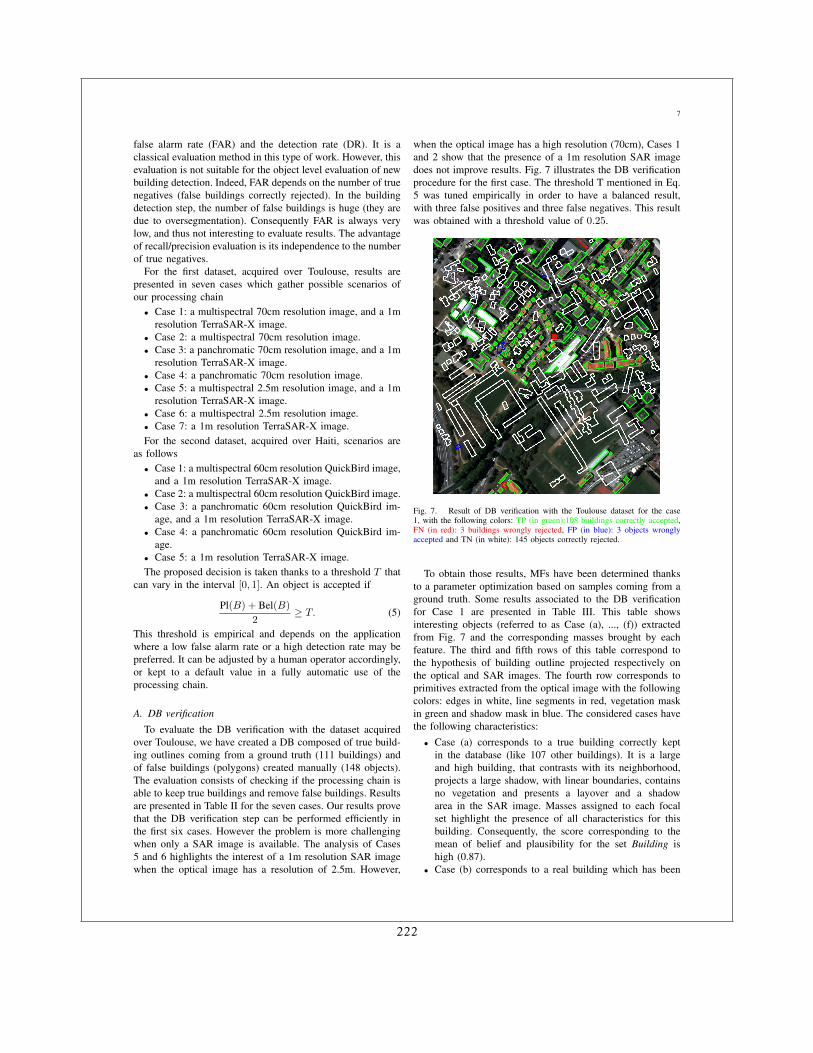
7
false alarm rate (FAR) and the detection rate (DR). It is aclassical evaluation method in this type of work. However, thisevaluation is not suitable for the object level evaluation of newbuilding detection. Indeed, FAR depends on the number of truenegatives (false buildings correctly rejected). In the buildingdetection step, the number of false buildings is huge (they aredue to oversegmentation). Consequently FAR is always verylow, and thus not interesting to evaluate results. The advantageof recall/precision evaluation is its independence to the numberof true negatives.
For the first dataset, acquired over Toulouse, results arepresented in seven cases which gather possible scenarios ofour processing chain• Case 1: a multispectral 70cm resolution image, and a 1m
resolution TerraSAR-X image.• Case 2: a multispectral 70cm resolution image.• Case 3: a panchromatic 70cm resolution image, and a 1m
resolution TerraSAR-X image.• Case 4: a panchromatic 70cm resolution image.• Case 5: a multispectral 2.5m resolution image, and a 1m
resolution TerraSAR-X image.• Case 6: a multispectral 2.5m resolution image.• Case 7: a 1m resolution TerraSAR-X image.For the second dataset, acquired over Haiti, scenarios are
as follows• Case 1: a multispectral 60cm resolution QuickBird image,
and a 1m resolution TerraSAR-X image.• Case 2: a multispectral 60cm resolution QuickBird image.• Case 3: a panchromatic 60cm resolution QuickBird im-
age, and a 1m resolution TerraSAR-X image.• Case 4: a panchromatic 60cm resolution QuickBird im-
age.• Case 5: a 1m resolution TerraSAR-X image.The proposed decision is taken thanks to a threshold T that
can vary in the interval [0, 1]. An object is accepted if
Pl(B) + Bel(B)
2≥ T. (5)
This threshold is empirical and depends on the applicationwhere a low false alarm rate or a high detection rate may bepreferred. It can be adjusted by a human operator accordingly,or kept to a default value in a fully automatic use of theprocessing chain.
A. DB verification
To evaluate the DB verification with the dataset acquiredover Toulouse, we have created a DB composed of true build-ing outlines coming from a ground truth (111 buildings) andof false buildings (polygons) created manually (148 objects).The evaluation consists of checking if the processing chain isable to keep true buildings and remove false buildings. Resultsare presented in Table II for the seven cases. Our results provethat the DB verification step can be performed efficiently inthe first six cases. However the problem is more challengingwhen only a SAR image is available. The analysis of Cases5 and 6 highlights the interest of a 1m resolution SAR imagewhen the optical image has a resolution of 2.5m. However,
when the optical image has a high resolution (70cm), Cases 1and 2 show that the presence of a 1m resolution SAR imagedoes not improve results. Fig. 7 illustrates the DB verificationprocedure for the first case. The threshold T mentioned in Eq.5 was tuned empirically in order to have a balanced result,with three false positives and three false negatives. This resultwas obtained with a threshold value of 0.25.
Fig. 7. Result of DB verification with the Toulouse dataset for the case1, with the following colors: TP (in green):108 buildings correctly accepted,FN (in red): 3 buildings wrongly rejected, FP (in blue): 3 objects wronglyaccepted and TN (in white): 145 objects correctly rejected.
To obtain those results, MFs have been determined thanksto a parameter optimization based on samples coming from aground truth. Some results associated to the DB verificationfor Case 1 are presented in Table III. This table showsinteresting objects (referred to as Case (a), ..., (f)) extractedfrom Fig. 7 and the corresponding masses brought by eachfeature. The third and fifth rows of this table correspond tothe hypothesis of building outline projected respectively onthe optical and SAR images. The fourth row corresponds toprimitives extracted from the optical image with the followingcolors: edges in white, line segments in red, vegetation maskin green and shadow mask in blue. The considered cases havethe following characteristics:• Case (a) corresponds to a true building correctly kept
in the database (like 107 other buildings). It is a largeand high building, that contrasts with its neighborhood,projects a large shadow, with linear boundaries, containsno vegetation and presents a layover and a shadowarea in the SAR image. Masses assigned to each focalset highlight the presence of all characteristics for thisbuilding. Consequently, the score corresponding to themean of belief and plausibility for the set Building ishigh (0.87).
• Case (b) corresponds to a real building which has been
222
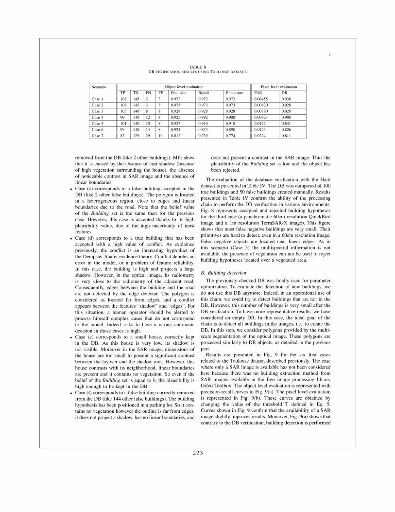
8
TABLE IIDB VERIFICATION RESULTS USING TOULOUSE DATASET.
Scenario Object level evaluation Pixel level evaluationTP TN FN FP Precision Recall F-measure FAR DR
Case 1 108 145 3 3 0.973 0.973 0.973 0.00455 0.938Case 2 108 145 3 3 0.973 0.973 0.973 0.00420 0.920Case 3 103 140 8 8 0.928 0.928 0.928 0.00790 0.920Case 4 99 140 12 8 0.925 0.892 0.908 0.00823 0.900Case 5 101 140 10 8 0.927 0.910 0.918 0.0127 0.841Case 6 97 140 14 8 0.924 0.874 0.898 0.0123 0.826Case 7 82 129 29 19 0.812 0.739 0.774 0.0224 0.811
removed from the DB (like 2 other buildings). MFs showthat it is caused by the absence of cast shadow (becauseof high vegetation surrounding the house), the absenceof noticeable contrast in SAR image and the absence oflinear boundaries.
• Case (c) corresponds to a false building accepted in theDB (like 2 other false buildings). The polygon is locatedin a heterogeneous region, close to edges and linearboundaries due to the road. Note that the belief valueof the Building set is the same than for the previouscase. However, this case is accepted thanks to its highplausibility value, due to the high uncertainty of mostfeatures.
• Case (d) corresponds to a true building that has beenaccepted with a high value of conflict. As explainedpreviously, the conflict is an interesting byproduct ofthe Dempster-Shafer evidence theory. Conflict denotes anerror in the model, or a problem of feature reliability.In this case, the building is high and projects a largeshadow. However, in the optical image, its radiometryis very close to the radiometry of the adjacent road.Consequently, edges between the building and the roadare not detected by the edge detector. The polygon isconsidered as located far from edges, and a conflictappears between the features “shadow” and “edges”. Forthis situation, a human operator should be alerted toprocess himself complex cases that do not correspondto the model. Indeed risks to have a wrong automaticdecision in those cases is high.
• Case (e) corresponds to a small house, correctly keptin the DB. As this house is very low, its shadow isnot visible. Moreover in the SAR image, dimensions ofthe house are too small to present a significant contrastbetween the layover and the shadow area. However, thishouse contrasts with its neighborhood, linear boundariesare present and it contains no vegetation. So even if thebelief of the Building set is equal to 0, the plausibility ishigh enough to be kept in the DB.
• Case (f) corresponds to a false building correctly removedfrom the DB (like 144 other false buildings). The buildinghypothesis has been positioned in a parking lot. So it con-tains no vegetation however the outline is far from edges,it does not project a shadow, has no linear boundaries, and
does not present a contrast in the SAR image. Thus theplausibility of the Building set is low and the object hasbeen rejected.
The evaluation of the database verification with the Haitidataset is presented in Table IV. The DB was composed of 100true buildings and 50 false buildings created manually. Resultspresented in Table IV confirm the ability of the processingchain to perform the DB verification in various environments.Fig. 8 represents accepted and rejected building hypothesesfor the third case (a panchromatic 60cm resolution QuickBirdimage and a 1m resolution TerraSAR-X image). This figureshows that most false negative buildings are very small. Theirprimitives are hard to detect, even in a 60cm resolution image.False negative objects are located near linear edges. As inthis scenario (Case 3) the multispectral information is notavailable, the presence of vegetation can not be used to rejectbuilding hypotheses located over a vegetated area.
B. Building detection
The previously checked DB was finally used for parameteroptimization. To evaluate the detection of new buildings, wedo not use this DB anymore. Indeed, in an operational use ofthis chain, we could try to detect buildings that are not in theDB. However, this number of buildings is very small after theDB verification. To have more representative results, we haveconsidered an empty DB. In this case, the ideal goal of thechain is to detect all buildings in the images, i.e., to create theDB. In this step, we consider polygons provided by the multi-scale segmentation of the optical image. These polygons areprocessed similarly to DB objects, as detailed in the previouspart.
Results are presented in Fig. 9 for the six first casesrelated to the Toulouse dataset described previously. The casewhere only a SAR image is available has not been consideredhere because there was no building extraction method fromSAR images available in the free image processing libraryOrfeo Toolbox. The object level evaluation is represented withprecision-recall curves in Fig. 9(a). The pixel level evaluationis represented in Fig. 9(b). These curves are obtained bychanging the value of the threshold T defined in Eq. 5.Curves shown in Fig. 9 confirm that the availability of a SARimage slightly improves results. Moreover, Fig. 9(a) shows thatcontrary to the DB verification, building detection is performed
223
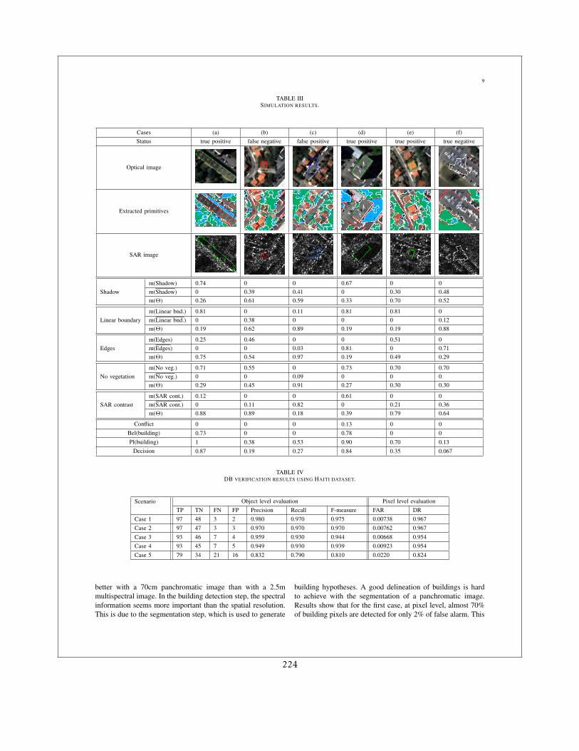
9
TABLE IIISIMULATION RESULTS.
Cases (a) (b) (c) (d) (e) (f)Status true positive false negative false positive true positive true positive true negative
Optical image
Extracted primitives
SAR image
m(Shadow) 0.74 0 0 0.67 0 0Shadow m(Shadow) 0 0.39 0.41 0 0.30 0.48
m(Θ) 0.26 0.61 0.59 0.33 0.70 0.52
m(Linear bnd.) 0.81 0 0.11 0.81 0.81 0Linear boundary m(Linear bnd.) 0 0.38 0 0 0 0.12
m(Θ) 0.19 0.62 0.89 0.19 0.19 0.88
m(Edges) 0.25 0.46 0 0 0.51 0Edges m(Edges) 0 0 0.03 0.81 0 0.71
m(Θ) 0.75 0.54 0.97 0.19 0.49 0.29
m(No veg.) 0.71 0.55 0 0.73 0.70 0.70No vegetation m(No veg.) 0 0 0.09 0 0 0
m(Θ) 0.29 0.45 0.91 0.27 0.30 0.30
m(SAR cont.) 0.12 0 0 0.61 0 0SAR contrast m(SAR cont.) 0 0.11 0.82 0 0.21 0.36
m(Θ) 0.88 0.89 0.18 0.39 0.79 0.64
Conflict 0 0 0 0.13 0 0Bel(building) 0.73 0 0 0.78 0 0Pl(building) 1 0.38 0.53 0.90 0.70 0.13
Decision 0.87 0.19 0.27 0.84 0.35 0.067
TABLE IVDB VERIFICATION RESULTS USING HAITI DATASET.
Scenario Object level evaluation Pixel level evaluationTP TN FN FP Precision Recall F-measure FAR DR
Case 1 97 48 3 2 0.980 0.970 0.975 0.00738 0.967Case 2 97 47 3 3 0.970 0.970 0.970 0.00762 0.967Case 3 93 46 7 4 0.959 0.930 0.944 0.00668 0.954Case 4 93 45 7 5 0.949 0.930 0.939 0.00923 0.954Case 5 79 34 21 16 0.832 0.790 0.810 0.0220 0.824
better with a 70cm panchromatic image than with a 2.5mmultispectral image. In the building detection step, the spectralinformation seems more important than the spatial resolution.This is due to the segmentation step, which is used to generate
building hypotheses. A good delineation of buildings is hardto achieve with the segmentation of a panchromatic image.Results show that for the first case, at pixel level, almost 70%of building pixels are detected for only 2% of false alarm. This
224
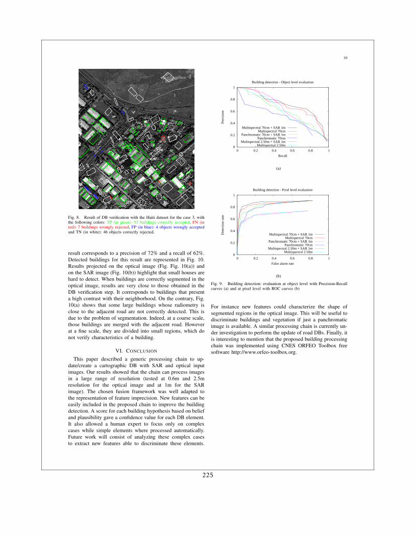
10
Fig. 8. Result of DB verification with the Haiti dataset for the case 3, withthe following colors: TP (in green): 93 buildings correctly accepted, FN (inred): 7 buildings wrongly rejected, FP (in blue): 4 objects wrongly acceptedand TN (in white): 46 objects correctly rejected.
result corresponds to a precision of 72% and a recall of 62%.Detected buildings for this result are represented in Fig. 10.Results projected on the optical image (Fig. Fig. 10(a)) andon the SAR image (Fig. 10(b)) highlight that small houses arehard to detect. When buildings are correctly segmented in theoptical image, results are very close to those obtained in theDB verification step. It corresponds to buildings that presenta high contrast with their neighborhood. On the contrary, Fig.10(a) shows that some large buildings whose radiometry isclose to the adjacent road are not correctly detected. This isdue to the problem of segmentation. Indeed, at a coarse scale,those buildings are merged with the adjacent road. Howeverat a fine scale, they are divided into small regions, which donot verify characteristics of a building.
VI. CONCLUSION
This paper described a generic processing chain to up-date/create a cartographic DB with SAR and optical inputimages. Our results showed that the chain can process imagesin a large range of resolution (tested at 0.6m and 2.5mresolution for the optical image and at 1m for the SARimage). The chosen fusion framework was well adapted tothe representation of feature imprecision. New features can beeasily included in the proposed chain to improve the buildingdetection. A score for each building hypothesis based on beliefand plausibility gave a confidence value for each DB element.It also allowed a human expert to focus only on complexcases while simple elements where processed automatically.Future work will consist of analyzing these complex casesto extract new features able to discriminate these elements.
0
0.2
0.4
0.6
0.8
1
0 0.2 0.4 0.6 0.8 1
Prec
isio
n
Recall
Building detection - Object level evaluation
Multispectral 70cm + SAR 1mMultispectral 70cm
Panchromatic 70cm + SAR 1mPanchromatic 70cm
Multispectral 2.50m + SAR 1mMultispectral 2.50m
(a)
0
0.2
0.4
0.6
0.8
1
0 0.2 0.4 0.6 0.8 1
Det
ectio
n ra
te
False alarm rate
Building detection - Pixel level evaluation
Multispectral 70cm + SAR 1mMultispectral 70cm
Panchromatic 70cm + SAR 1mPanchromatic 70cm
Multispectral 2.50m + SAR 1mMultispectral 2.50m
(b)
Fig. 9. Building detection: evaluation at object level with Precision-Recallcurves (a) and at pixel level with ROC curves (b)
For instance new features could characterize the shape ofsegmented regions in the optical image. This will be useful todiscriminate buildings and vegetation if just a panchromaticimage is available. A similar processing chain is currently un-der investigation to perform the update of road DBs. Finally, itis interesting to mention that the proposed building processingchain was implemented using CNES ORFEO Toolbox freesoftware http://www.orfeo-toolbox.org.
225
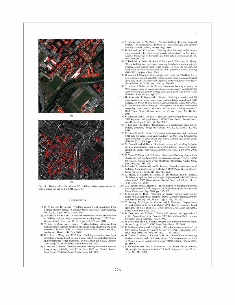
11
(a)
(b)
Fig. 10. Building detection without DB: building outlines projected on theoptical image (a) and on the SAR image (b)
REFERENCES
[1] C. A. Lin and R. Nevatia, “Building detection and description froma single intensity image,” Computer Vision and Image Understanding,vol. 72, no. 2, pp. 101–121, Nov. 1998.
[2] A. Katartzis and H. Sahli, “A stochastic framework for the identificationof building rooftops using a single remote sensing image,” IEEE Trans.Geosci. Remote Sens., vol. 46, no. 1, pp. 259–271, Jan. 2008.
[3] Y. Wei, Z. Zhao, and J. Song, “Urban building extraction fromhigh-resolution satellite panchromatic image using clustering and edgedetection,” in Proc. IEEE Int. Geosci. Remote Sens. Symp. (IGARSS),Anchorage, Alaska, USA, Sep. 2004.
[4] Z. J. Liu, J. Wang, and W. P. Liu, “Building extraction from highresolution imagery based on multi-scale object oriented classificationand probabilistic Hough transform,” in Proc. IEEE Int. Geosci. RemoteSens. Symp. (IGARSS), Seoul, South Korea, Jul. 2005.
[5] L. Wei and V. Prinet, “Building detection from high-resolution satelliteimage using probability model,” in Proc. IEEE Int. Geosci. RemoteSens. Symp. (IGARSS), Seoul, South Korea, Jul. 2005.
[6] S. Muller and D. W. Zaum, “Robust building detection in aerialimages,” in International Archives of Photogrammetry and RemoteSensing (IAPRS), Vienna, Austria, Aug. 2005.
[7] B. Sirmacek and C. Unsalan, “Building detection from aerial imagesusing invariant color features and shadow information,” in 23rd Inter-national Symposium on Computer and Information Sciences, ISCIS ’08,Oct. 2008, pp. 1–5.
[8] T. Bailloeul, V. Prinet, B. Serra, P. Marthon, P. Chen, and H. Zhang,“Urban building land use change mapping from high resolution satelliteimagery, active contours and Hough voting,” in Proc. 9th InternationalSymposium on Physical Measurements and Signature in Remote Sensing(ISPMSRS), Beijing, China, 2005.
[9] O. Aytekin, I. Ulusoy, E. Z. Abacioglu, and E. Gokcay, “Building detec-tion in high resolution remotely sensed images based on morphologicaloperators,” in 4th International Conference on Recent Advances in SpaceTechnologies, RAST ’09, Jun. 2009, pp. 376–379.
[10] S. Lefevre, J. Weber, and D. Sheeren, “Automatic building extraction inVHR images using advanced morphological operators,” in IEEE/ISPRSJoint Workshop on Remote Sensing and Data Fusion over Urban Areas(URBAN), Paris, France, Apr. 2007.
[11] H. Sportouche, F. Tupin, and L. Denise, “Building extraction and 3Dreconstruction in urban areas from high-resolution optical and SARimagery,” in Urban Remote Sensing Event, Shanghai, China, May 2009.
[12] K. Karantzalos and N. Paragios, “Recognition-driven two-dimensionalcompeting priors toward automatic and accurate building detection,”IEEE Trans. Geosci. Remote Sens., vol. 47, no. 1, pp. 133–144, Jan.2009.
[13] B. Sirmacek and C. Unsalan, “Urban-area and building detection usingSIFT keypoints and graph theory,” IEEE Trans. Geosci. Remote Sens.,vol. 47, no. 4, pp. 1156–1167, Apr. 2009.
[14] T. Kim and J. P. Muller, “Development of a graph-based approach forbuilding detection,” Image Vis. Comput., vol. 17, no. 1, pp. 3–17, Jan.1999.
[15] M. Quartulli and M. Datcu, “Information extraction from high resolutionSAR data for urban scene understanding,” in Proc. 2nd GRSS/ISPRSJoint workshop on data fusion and remote sensing over urban areas(URBAN 2003), 2003, pp. 115–119.
[16] M. Quartulli and M. Datcu, “Stochastic geometrical modeling for built-up area understanding from a single SAR intensity image with meterresolution,” IEEE Trans. Geosci. Remote Sens., vol. 42, pp. 1996–2003,2004.
[17] C. Tison, F. Tupin, and H. Maitre, “Retrieval of building shapes fromshadows in high resolution SAR interferometric images,” in Proc. IEEEInt. Geosci. Remote Sens. Symp. (IGARSS), Anchorage, Alaska, USA,Sep. 2004, pp. 1788–1791.
[18] P. Gamba, B. Houshmand, and M. Saccani, “Detection and extraction ofbuildings from interferometric SAR data,” IEEE Trans. Geosci. RemoteSens., vol. 38, no. 1, pp. 611–617, Jan. 2000.
[19] A. Thiele, E. Cadario, K. Schulz, U. Thoennessen, and U. Soergel,“Building recognition from multi-aspect high-resolution InSAR data inurban areas,” IEEE Trans. Geosci. Remote Sens., vol. 45, no. 11, pp.3583–3593, Nov. 2007.
[20] A. J. Bennett and D. Blacknell, “The extraction of building dimensionsfrom high resolution SAR imagery,” in Proceedings of the InternationalRadar Conference, Sep. 2003, pp. 182–187.
[21] F. Tupin and M. Roux, “Detection of building outlines based on thefusion of SAR and optical features,” ISPRS Journal of Photogrammetryand Remote Sensing, vol. 58, no. 1, pp. 71–82, Jun. 2003.
[22] V. Amberg, M. Spigai, M. Coulon, and P. Marthon, “Improvementof road extraction in high resolution SAR data by a context-basedapproach,” in Proc. IEEE Int. Geosci. Remote Sens. Symp. (IGARSS),Seoul, South Korea, Jul. 2005.
[23] D. Comaniciu and P. Meer, “Mean shift analysis and applications,”in The Proceedings of the Seventh IEEE International Conference onComputer Vision, Kerkyra, Greece, 1999.
[24] D. Massonnet and J. C. Souyris, Imaging with synthetic aperture radar,chapter 3, pp. 165–167, CRC Press, Boca Raton, FL, 2008.
[25] K. S. Gudmundsson and F. Cagatin, “Complex shadow extraction,” inInternational Society for Optical Engineering (SPIE), San Diego, CA ,USA, Aug. 2008, vol. 7072, pp. 707211.1–707211.10.
[26] H. T. Guo, Y. Zhang, J. Lu, and G. W. Jin, “Research on the buildingshadow extraction and elimination method,” in International Archivesof Photogrammetry and Remote Sensing (IAPRS), Beijing, China, 2008,pp. 569–574.
[27] R. Grompone Von Gioi, J. Jakubowicz, J. M. Morel, and G. Randall,“On straight line segment detection,” J. Math. Imaging Vis., vol. 32, no.3, pp. 313–347, 2008.
226
12
[28] C. J. Tucker, “Red and photographic infrared linear combinations formonitoring vegetation,” Remote Sensing of Environment, pp. 127–150,1979.
[29] P. E. Danielsson, “Euclidean distance mapping,” Computer Graphicsand Image Processing, vol. 14, 1980.
[30] R. Duda and P. Hart, Pattern Classification and Scene Analysis, pp.98–105, John Wiley and Sons, 1973.
[31] P. Smets, “What is Dempster-Shafer’s model?,” in Advances in theDempster-Shafer theory of evidence, pp. 5–34. John Wiley & Sons, Inc.,New York, USA, 1994.
[32] D. Dubois and H. Prade, “Possibility theory, probability theory andmultiple-valued logics: A clarification,” Annals of Mathematics andArtificial Intelligence, vol. 32, no. 1-4, pp. 35–66, 2001.
[33] L. A. Zadeh, “Fuzzy sets as a basis for a theory of possibility,” FuzzySets Syst., vol. 100, pp. 9–34, 1999.
[34] F. Tupin, I. Bloch, and H. Maitre, “A first step toward automaticinterpretation of SAR images using evidential fusion of several structuredetectors,” IEEE Trans. Geosci. Remote Sens., vol. 37, no. 3, pp. 1327–1343, May 1999.
[35] J. A. Nelder and R. Mead, “A simplex method for function minimiza-tion,” The Computer Journal, vol. 7, no. 4, pp. 308–313, Jan. 1965.
[36] J. Davis and M. Goadrich, “The relationship between precision-recalland ROC curves,” in ICML ’06: Proceedings of the 23rd internationalconference on Machine learning, New York, NY, USA, 2006, pp. 233–240, ACM.
Vincent Poulain was born in Dieppe, France, in1983. He received the Engineer degree in electricalengineering and signal processing from ENSEEIHT,Toulouse, France, in 2007 and the Ph.D. degreein image processing in 2010 from the NationalPolytechnic Institute of Toulouse, France. He joinedThales Group in 2010 where he is currently workingin the field of remote sensing image processing.
Jordi Inglada received the Telecommunications En-gineer degree from both the Universitat Politecnicade Catalunya, Barcelona, Spain, and the Ecole Na-tionale Superieure des Telecommunications de Bre-tagne, Brest, France, in 1997 and the Ph.D. degreein signal processing and telecommunications in 2000from Universite de Rennes 1, Rennes, France. He iscurrently with the Centre National dtudes Spatiales(French Space Agency), Toulouse, France, workingin the field of remote sensing image processingat the CESBIO laboratory. He is in charge of the
development of image processing algorithms for the operational exploitationof Earth observation images, mainly in the field of multitemporal imageanalysis for land use and cover change. Dr. Inglada is an Associate Editor ofthe IEEE TRANSACTIONS ON GEOSCIENCE AND REMOTE SENSING.
Marc Spigai was born in Marseille, France, 1965.He received the Engineering degree in signal and im-age processing from the Ecole Nationale Superieuredes Telecommunications de Bretagne (Telecom Bre-tagne), France (1989). From 1990 to 1998, he workson signal and data processing at Thales System Air-borne, Elancourt France. From 1998 to 2000 he wasHead of a research team on fusion of radar, visionand navigation for driving assistance at Renault,Guyancourt, France. He joined Thales Alenia Space,Toulouse, France, in 2000, where he currently works
on SAR signal and image processing at the Observation Systems and RadarsUnit.
Jean-Yves Tourneret (SM’08) received theingenieur degree in electrical engineering fromENSEEIHT (Toulouse, France) in 1989 andthe Ph.D. degree from the National PolytechnicInstitute from Toulouse in 1992. He is currentlya professor in the university of Toulouse and amember of the IRIT laboratory (UMR 5505 of theCNRS). His research activities are centered aroundstatistical signal processing with a particular interestto MCMC methods. He was the program chairof the European conference on signal processing
(EUSIPCO). He was also member of the organizing committee for theinternational conference ICASSP’06 which was held in Toulouse (France) in2006. He has been a member of different technical committees includingthe Signal Processing Theory and Methods (SPTM) committee of the IEEESignal Processing Society (2001 − 2007, 2010 − present). He is currentlyserving as an associate editor for the IEEE TRANSACTIONS ON SIGNALPROCESSING.
Philippe Marthon received the engineering degreeand the Ph.D. degree in computer science fromthe Ecole Nationale Superieure d’Electrotechnique,d’Electronique, d’Informatique et d’Hydraulique deToulouse (ENSEEIHT), Toulouse, France, in 1975and 1978, respectively, and the Doctorat d’EtatDegree from the Institut National Polytechniquede Toulouse (INPT), in 1987. He has publishedover 80 scientific articles in international journalsand conferences. His research interests include sys-temics, operations research, remote sensing image
processing and computer vision. He is currently Professor at ENSEEIHT andResearch Scientist at the Institut de Recherche en Informatique de Toulouse(IRIT).
227


18 Traitements opérationnels
229
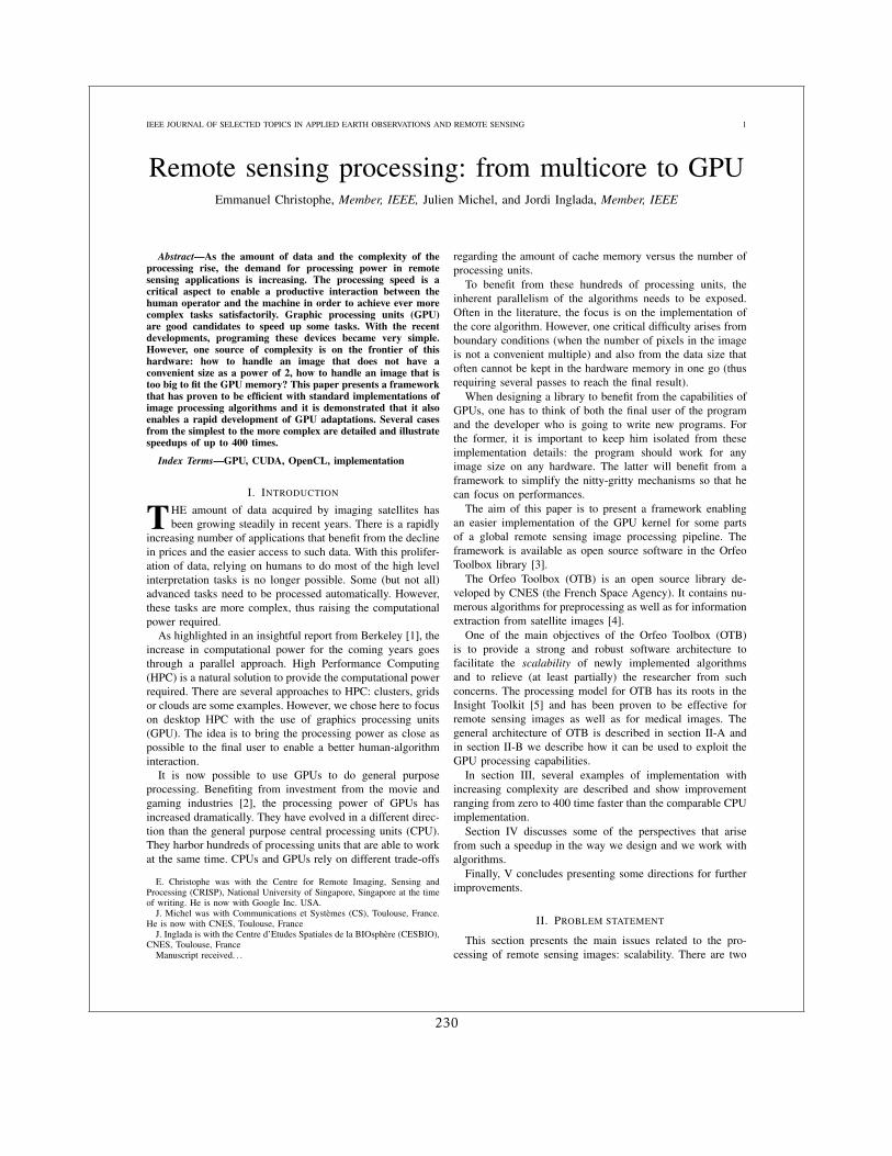
IEEE JOURNAL OF SELECTED TOPICS IN APPLIED EARTH OBSERVATIONS AND REMOTE SENSING 1
Remote sensing processing: from multicore to GPUEmmanuel Christophe, Member, IEEE, Julien Michel, and Jordi Inglada, Member, IEEE
Abstract—As the amount of data and the complexity of theprocessing rise, the demand for processing power in remotesensing applications is increasing. The processing speed is acritical aspect to enable a productive interaction between thehuman operator and the machine in order to achieve ever morecomplex tasks satisfactorily. Graphic processing units (GPU)are good candidates to speed up some tasks. With the recentdevelopments, programing these devices became very simple.However, one source of complexity is on the frontier of thishardware: how to handle an image that does not have aconvenient size as a power of 2, how to handle an image that istoo big to fit the GPU memory? This paper presents a frameworkthat has proven to be efficient with standard implementations ofimage processing algorithms and it is demonstrated that it alsoenables a rapid development of GPU adaptations. Several casesfrom the simplest to the more complex are detailed and illustratespeedups of up to 400 times.
Index Terms—GPU, CUDA, OpenCL, implementation
I. INTRODUCTION
THE amount of data acquired by imaging satellites hasbeen growing steadily in recent years. There is a rapidly
increasing number of applications that benefit from the declinein prices and the easier access to such data. With this prolifer-ation of data, relying on humans to do most of the high levelinterpretation tasks is no longer possible. Some (but not all)advanced tasks need to be processed automatically. However,these tasks are more complex, thus raising the computationalpower required.
As highlighted in an insightful report from Berkeley [1], theincrease in computational power for the coming years goesthrough a parallel approach. High Performance Computing(HPC) is a natural solution to provide the computational powerrequired. There are several approaches to HPC: clusters, gridsor clouds are some examples. However, we chose here to focuson desktop HPC with the use of graphics processing units(GPU). The idea is to bring the processing power as close aspossible to the final user to enable a better human-algorithminteraction.
It is now possible to use GPUs to do general purposeprocessing. Benefiting from investment from the movie andgaming industries [2], the processing power of GPUs hasincreased dramatically. They have evolved in a different direc-tion than the general purpose central processing units (CPU).They harbor hundreds of processing units that are able to workat the same time. CPUs and GPUs rely on different trade-offs
E. Christophe was with the Centre for Remote Imaging, Sensing andProcessing (CRISP), National University of Singapore, Singapore at the timeof writing. He is now with Google Inc. USA.
J. Michel was with Communications et Systemes (CS), Toulouse, France.He is now with CNES, Toulouse, France
J. Inglada is with the Centre d’Etudes Spatiales de la BIOsphere (CESBIO),CNES, Toulouse, France
Manuscript received. . .
regarding the amount of cache memory versus the number ofprocessing units.
To benefit from these hundreds of processing units, theinherent parallelism of the algorithms needs to be exposed.Often in the literature, the focus is on the implementation ofthe core algorithm. However, one critical difficulty arises fromboundary conditions (when the number of pixels in the imageis not a convenient multiple) and also from the data size thatoften cannot be kept in the hardware memory in one go (thusrequiring several passes to reach the final result).
When designing a library to benefit from the capabilities ofGPUs, one has to think of both the final user of the programand the developer who is going to write new programs. Forthe former, it is important to keep him isolated from theseimplementation details: the program should work for anyimage size on any hardware. The latter will benefit from aframework to simplify the nitty-gritty mechanisms so that hecan focus on performances.
The aim of this paper is to present a framework enablingan easier implementation of the GPU kernel for some partsof a global remote sensing image processing pipeline. Theframework is available as open source software in the OrfeoToolbox library [3].
The Orfeo Toolbox (OTB) is an open source library de-veloped by CNES (the French Space Agency). It contains nu-merous algorithms for preprocessing as well as for informationextraction from satellite images [4].
One of the main objectives of the Orfeo Toolbox (OTB)is to provide a strong and robust software architecture tofacilitate the scalability of newly implemented algorithmsand to relieve (at least partially) the researcher from suchconcerns. The processing model for OTB has its roots in theInsight Toolkit [5] and has been proven to be effective forremote sensing images as well as for medical images. Thegeneral architecture of OTB is described in section II-A andin section II-B we describe how it can be used to exploit theGPU processing capabilities.
In section III, several examples of implementation withincreasing complexity are described and show improvementranging from zero to 400 time faster than the comparable CPUimplementation.
Section IV discusses some of the perspectives that arisefrom such a speedup in the way we design and we work withalgorithms.
Finally, V concludes presenting some directions for furtherimprovements.
II. PROBLEM STATEMENT
This section presents the main issues related to the pro-cessing of remote sensing images: scalability. There are two
230
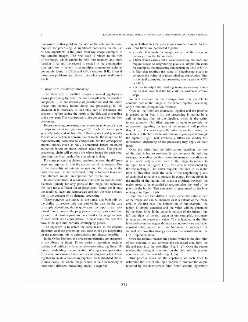
2 IEEE JOURNAL OF SELECTED TOPICS IN APPLIED EARTH OBSERVATIONS AND REMOTE SENSING
dimensions to this problem: the size of the data and the timerequired for processing. A significant bottleneck for the useof new algorithms is the jump from toy image examples toreal satellite images. The first issue is related to the sizeof the image which cannot be held into memory any more(section II-A) and the second is related to the computationtime and how to benefit from multiple computation units ascommonly found in CPUs and GPUs (section II-B). Even ifthose two problems are related, they play a part at differentlevels.
A. Image size scalability: streaming
The sheer size of satellite images – several gigabytes –makes processing by usual methods inapplicable on standardcomputers. It is not desirable or possible to load the entireimage into memory before doing any processing. In thissituation, it is necessary to load only part of the image andprocess it before saving the result to the disk and proceedingto the next part. This corresponds to the concept of on-the-flowprocessing.
Remote sensing processing can be seen as a chain of eventsor steps that lead to a final output [6]. Each of these steps isgenerally independent from the following ones and generallyfocuses on a particular domain. For example, the image can beradiometrically corrected to compensate for the atmosphericeffects, indices (such as NDVI) computed, before an objectextraction based on these indexes takes place. The typicalprocessing chain will process the whole image for each step,returning the final result after everything is done.
For some processing chains, iterations between the differentsteps are required to find the correct set of parameters. Dueto the variability of satellite images and the variety of thetasks that need to be performed, fully automated tasks arerare. Humans are still an important part of the loop.
In these conditions, it is valuable to be able to provide somefeedback quickly for only parts of the image and reprocessthis part for a different set of parameters. Better yet if onlythe modified steps are reprocessed and not the whole chain;this is the concept of on-demand processing.
These concepts are linked in the sense that both rely onthe ability to process only one part of the data. In the caseof simple algorithms, this is quite easy: the input is just splitinto different non-overlapping pieces that are processed oneby one. But most algorithms do consider the neighborhoodof each pixel. As a consequence, in most cases, the data willhave to be split into partially overlapping pieces.
The objective is to obtain the same result as the originalalgorithm as if the processing was done in one go. Dependingon the algorithm, this is unfortunately not always possible.
In the Orfeo Toolbox, the processing elements are organizedin the library as filters. Filters perform operations such asreading and writing the data, but also processing, e.g. linear fil-tering, thresholding or classification. Writing a new application(or a new processing chain) consists of plugging a few filterstogether to create a processing pipeline. As highlighted above,in most cases, the whole image cannot be held in memory atonce and a different processing model is required.
Figure 1 illustrates the process on a simple example. In thiscase, four filters are connected together:
• a reader that loads the image, or part of the image inmemory from the file on disk;
• a filter which carries out a local processing that does notrequire access to neighboring pixels (a simple thresholdfor example), the processing can happen on CPU or GPU;
• a filter that requires the value of neighboring pixels tocompute the value of a given pixel (a convolution filteris a typical example), the processing can happen on CPUor GPU;
• a writer to output the resulting image in memory into afile on disk, note that the file could be written in severalsteps.
We will illustrate on this example how it is possible tocompute part of the image in the whole pipeline, occurringonly a minimal computation overhead.
Once all the filters are connected together and the pipelineis created as in Fig. 1 (a), the processing is started by acall on the last filter of the pipeline, which is the writerin our example. This filter requests its input to provide theinformation regarding the size of the image it will produce(Fig. 1 (b)). The reader gets the information by reading themeta-data of the file and the information is propagated throughthe pipeline (Fig. 1 (c)). Eventually, filters can modify thisinformation, depending on the processing they apply on theirinput.
Once the writer has the information regarding the sizeof the data it has to produce, it can compute the splittingstrategy: depending on the maximum memory specification,it will select only a small area of the image to request toits input filter. In Figure 1 (d), this area is represented bythe red rectangle. The writer requests this area to its input:filter 2. This filter needs the value of the neighboring pixelsof each pixel to be able to process its output. For the pixels inthe middle of the region, this is not a problem, however, theregion needs to be expanded to accommodate the need of thepixels at the border. This extension is represented by the bluerectangle in Figure 1 (d).
Here, there are two different cases: either the value is partof the image and can be obtained, or it is outside of the imagearea. In the first case (the bottom line in our example), theregion is simply extended and the value will be generatedby the input filter. If the value is outside of the image (top,left and right of the red region in our example), a strategyis necessary to create this value. This is handled at the filterlevel and several strategies (boundary conditions) are available:constant value, mirror, zero flux Neumann. In section III-B,we will see how this strategy can ease the constraints on theGPU implementation.
Once the request reaches the reader, which is the first filterof our pipeline, it can generate the requested area from thefile and pass it to the next filter (Fig. 1 (e)). Once the regionreaches the writer, it is written on the disk and the processcontinues with the next tile (Fig. 1 (f)).
This process relies on the capability of each filter todetermine the size of the input needed to produce the outputrequired by the downstream filter. Some specific algorithms
231
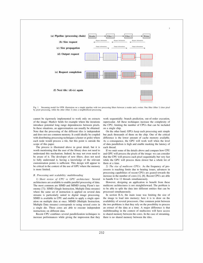
3
(a) Pipeline (processing chain) Reader Filter 1 Filter 2 Writer
(b) Size requestRequest informationRequest informationRequest information
(c) Size propagationOutput informations Output informations Output informations
(d) Output request
(e) Request completion
(f) Next tile: (d)-(e) again
Fig. 1. Streaming model for OTB: illustration on a simple pipeline with two processing filters between a reader and a writer. One filter (filter 1) does pixelby pixel processing, while the other (filter 2) does a neighborhood processing.
cannot be rigorously implemented to work only on extractsof the image: Markov fields for example where the iterationsintroduce potential long range dependencies between pixels.In these situations, an approximation can usually be obtained.Note that the processing of the different tiles is independentand does not use common memory. It could ideally be coupledwith distributing processing techniques (cluster or grids) whereeach node would process a tile, but this point is outside thescope of this paper.
The process is illustrated above in great detail, but it isworth mentioning that the user of the library does not need tounderstand this mechanism. Indeed, he may not even need tobe aware of it. The developer of new filters, does not needto fully understand it, having a knowledge of the relevantcustomization points is sufficient. This design will appear tobe critical in the context of the use of GPU where the memoryis more limited.
B. Processing unit scalability: multithreading1) Short review of CPU vs GPU architecture: Several
architectures are available to enable parallel processing of data.The most common are SIMD and MIMD (using Flynn’s tax-onomy [7]). SIMD (Single Instruction, Multiple Data streams)where the same set of instruction is applied on several datastreams is particularly suited to digital image processing.SIMD is available in CPU and enable to apply a single oper-ation on multiple data at once. MIMD (Multiple Instruction,Multiple Data streams) corresponds to using several cores ina single die. These cores are able to execute independentinstructions on different data.
Recent CPU combines several parallelization techniques toincrease performances while giving the impression that they
work sequentially: branch prediction, out-of-order execution,superscalar. All these techniques increase the complexity ofthe CPU, limiting the number of CPUs that can be includedon a single chip.
On the other hand, GPUs keep each processing unit simplebut pack thousands of them on the chip. One of the criticaldifference is the lower amount of cache memory available.As a consequence, the GPU will work well when the levelof data parallelism is high and enable masking the latency ofeach thread.
If we omit some of the details above and compare how CPUand GPU will process the pixels of the image: we can considerthat the CPU will process each pixel sequentially but very fastwhile the GPU will process them slower but a whole lot ofthem at a time.
2) The rise of multicore CPUs: As the frequency of pro-cessors is reaching limits due to heating issues, advances inprocessing capabilities of recent CPUs are geared towards theincrease in the number of cores [1], [8]. Recent CPUs are ableto handle 8 to 12 threads simultaneously.
However, designing an application to benefit from thesemulticore architectures is not straightforward. The problem isto be able to split the data into different entities that can beprocessed simultaneously.
In section II-A, the main issue was limiting the size ofthe image to load into memory; here it is to draw on theavailability of several processors. One common point betweenthe two problems is that they rely on the possibility to processan extract of the data at a time. A major difference is thatmultithreading in the context of multicores will have accessto shared memory between the cores. In the case of streaming,there is no shared memory between the tiles.
232
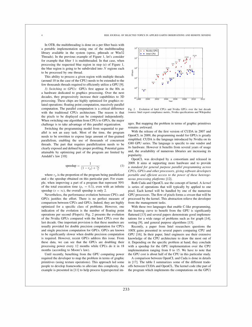
4 IEEE JOURNAL OF SELECTED TOPICS IN APPLIED EARTH OBSERVATIONS AND REMOTE SENSING
In OTB, the multithreading is done on a per filter basis witha portable implementation using one of the multithreadinglibrary available in the system (sproc, pthreads or Win32Threads). In the previous example of Figure 1, let’s considerfor example that filter 1 is multithreaded. In that case, whenprocessing the requested blue region in step (e) of Figure 1,the blue region is going to be subdivided into N regions eachto be processed by one thread.
This ability to process a given region with multiple threads(around 10 in the case of the CPU) needs to be extended to thefew thousands threads required to efficiently utilize a GPU [9].
3) Switching to GPUs: GPUs first appear in the 80s asa hardware dedicated to graphics processing. Over the nextdecades, they progressively increase their capabilities to 3Dprocessing. These chips are highly optimized for graphics re-lated operations: floating point computation, massively parallelcomputation. The parallel computation is a critical differencewith the traditional CPUs architecture. The reason is thatthe pixels to be displayed can be computed independently.When switching one algorithm from CPUs to GPUs, the majorchallenge is to take advantage of this parallel organization.
Switching the programming model from sequential to par-allel is not an easy task. Most of the time, the programneeds to be rewritten to expose large amount of fine-grainedparallelism, enabling the use of thousands of concurrentthreads. The part that requires parallelization needs to beclearly exposed and defined by proper profiling. Potential gainsattainable by optimizing part of the program are limited byAmdahl’s law [10]:
speedup =1
(1− rp) +rps
(1)
where rp is the proportion of the program being parallelizedand s the speedup obtained on this particular part. For exam-ple, when improving a part of a program that represent 50%of the total execution time (pr = 0.5), even with an infinitespeedup (s =∞), the overall speedup is only 2.
Nevertheless, the performance evolution between CPUs andGPUs justifies the effort. There is no perfect measure ofcomparison between CPUs and GPUs. Indeed, they are highlyoptimized for a specific class of problems. However, oneindication of the evolution is the number of floating pointoperations per second (Flops/s). Fig. 2 presents the evolutionof the Nvidia GPUs compared with the Intel CPUs over thelast decade. One important provision is that these numbers areusually provided for double precision computation for CPUsand single precision computation for GPUs. GPUs are knownto be significantly slower when double precision computationis required. However, recent GPUs address this issue. Fromthese data, we can see that the GPUs are doubling theirprocessing power every 12 months while CPUs do it in 18months (according to Moore’s law).
Until recently, benefiting from the GPU computing powerrequired the developer to map the problem in terms of graphicprimitives (using texture operations). This approach led somepeople to develop frameworks to alleviate this complexity. Anexample is presented in [11] to help process hyperspectral im-
1998 2000 2002 2004 2006 2008 2010 2012Year
10-1
100
101
102
103
104
GFl
op/s
NV11
NV25
NV38
NV40
G70
G71
G80
GT200GF100
P3-450
705765
Xeon-MP
X5355
E6300
i7-940i7-975
Nvidia GPUIntel CPU
Fig. 2. Evolution of Intel CPUs and Nvidia GPUs over the last decade(source: Intel export compliance metric, Nvidia specifications and Wikipedia)
ages. But mapping the problem in terms of graphic primitivesremains awkward.
With the release of the first version of CUDA in 2007 andOpenCL in 2009, the programming model for GPUs is greatlysimplified. CUDA is the language introduced by Nvidia on itsG80 GPU series. The language is specific to one vendor andits hardware. However it benefits from several years of usageand, the availability of numerous libraries are increasing itspopularity.
OpenCL was developed by a consortium and released in2009. It aims at supporting more hardware and to providea standard for general purpose parallel programming acrossCPUs, GPUs and other processors, giving software developersportable and efficient access to the power of these heteroge-neous processing platforms [12].
Both Cuda and OpenCL use the concept of kernel. A kernelis series of operations that will typically by applied to onepixel. Each kernel will be handled by one of the numerousGPU processors. The flow of pixels forms a stream that will beprocessed by the kernel. This abstraction relieve the developerfrom the management tasks.
With these two languages that enable C-like programming,the learning curve to benefit from the GPU is significantlyflattened [13] and several papers demonstrate good implemen-tations for a wide range of problems such as for graph [14],sorting [9], and general purpose algorithms [15].
Recently, a paper from Intel researchers questions the100X gains presented in several papers comparing CPU andGPU [16]. In their paper, Intel engineers use their extensiveknowledge of the CPU architecture to draw the most out ofit. Depending on the specific problem at hand, they concludewith a speedup for the GPU implementation over the CPUimplementation ranging from 0 to 15. We have to note thatthe GPU cost is about half of the CPU in this particular study.
A comparison between OpenCL and Cuda is done in detailsin [17]. The table I summarizes some of the different trade-offs between CUDA and OpenCL. The kernel code (the part ofthe program which implements the computations on the GPU)
233
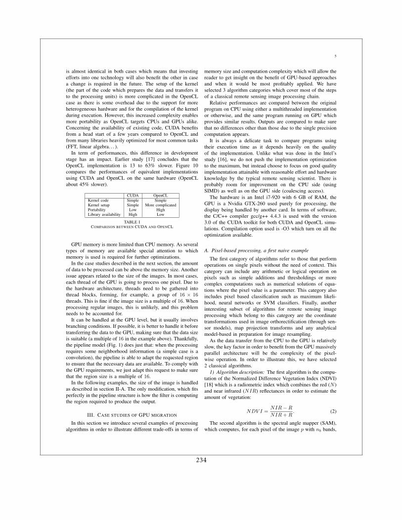
5
is almost identical in both cases which means that investingefforts into one technology will also benefit the other in casea change is required in the future. The setup of the kernel(the part of the code which prepares the data and transfers itto the processing units) is more complicated in the OpenCLcase as there is some overhead due to the support for moreheterogeneous hardware and for the compilation of the kernelduring execution. However, this increased complexity enablesmore portability as OpenCL targets CPUs and GPUs alike.Concerning the availability of existing code, CUDA benefitsfrom a head start of a few years compared to OpenCL andfrom many libraries heavily optimized for most common tasks(FFT, linear algebra. . . ).
In term of performances, this difference in developmentstage has an impact. Earlier study [17] concludes that theOpenCL implementation is 13 to 63% slower. Figure 10compares the performances of equivalent implementationsusing CUDA and OpenCL on the same hardware (OpenCLabout 45% slower).
CUDA OpenCLKernel code Simple SimpleKernel setup Simple More complicatedPortability Low HighLibrary availability High Low
TABLE ICOMPARISON BETWEEN CUDA AND OPENCL
GPU memory is more limited than CPU memory. As severaltypes of memory are available special attention to whichmemory is used is required for further optimizations.
In the case studies described in the next section, the amountof data to be processed can be above the memory size. Anotherissue appears related to the size of the images. In most cases,each thread of the GPU is going to process one pixel. Due tothe hardware architecture, threads need to be gathered intothread blocks, forming, for example, a group of 16 × 16threads. This is fine if the image size is a multiple of 16. Whenprocessing regular images, this is unlikely, and this problemneeds to be accounted for.
It can be handled at the GPU level, but it usually involvesbranching conditions. If possible, it is better to handle it beforetransferring the data to the GPU, making sure that the data sizeis suitable (a multiple of 16 in the example above). Thankfully,the pipeline model (Fig. 1) does just that: when the processingrequires some neighborhood information (a simple case is aconvolution), the pipeline is able to adapt the requested regionto ensure that the necessary data are available. To comply withthe GPU requirements, we just adapt this request to make surethat the region size is a multiple of 16.
In the following examples, the size of the image is handledas described in section II-A. The only modification, which fitsperfectly in the pipeline structure is how the filter is computingthe region required to produce the output.
III. CASE STUDIES OF GPU MIGRATION
In this section we introduce several examples of processingalgorithms in order to illustrate different trade-offs in terms of
memory size and computation complexity which will allow thereader to get insight on the benefit of GPU-based approachesand when it would be most profitably applied. We haveselected 3 algorithm categories which cover most of the stepsof a classical remote sensing image processing chain.
Relative performances are compared between the originalprogram on CPU using either a multithreaded implementationor otherwise, and the same program running on GPU whichprovides similar results. Outputs are compared to make surethat no differences other than those due to the single precisioncomputation appears.
It is always a delicate task to compare programs usingtheir execution time as it depends heavily on the qualityof the implementation. Unlike what was done in the Intel’sstudy [16], we do not push the implementation optimizationto the maximum, but instead choose to focus on good qualityimplementation attainable with reasonable effort and hardwareknowledge by the typical remote sensing scientist. There isprobably room for improvement on the CPU side (usingSIMD) as well as on the GPU side (coalescing access).
The hardware is an Intel i7-920 with 6 GB of RAM, theGPU is a Nvidia GTX-260 used purely for processing, thedisplay being handled by another card. In terms of software,the C/C++ compiler gcc/g++ 4.4.3 is used with the version3.0 of the CUDA toolkit for both CUDA and OpenCL simu-lations. Compilation option used is -O3 which turn on all theoptimization available.
A. Pixel-based processing, a first naive example
The first category of algorithms refer to those that performoperations on single pixels without the need of context. Thiscategory can include any arithmetic or logical operation onpixels such as simple additions and thresholdings or morecomplex computations such as numerical solutions of equa-tions where the pixel value is a parameter. This category alsoincludes pixel based classification such as maximum likeli-hood, neural networks or SVM classifiers. Finally, anotherinteresting subset of algorithms for remote sensing imageprocessing which belong to this category are the coordinatetransformations used in image orthorectification (through sen-sor models), map projection transforms and any analyticalmodel-based in preparation for image resampling.
As the data transfer from the CPU to the GPU is relativelyslow, the key factor in order to benefit from the GPU massivelyparallel architecture will be the complexity of the pixel-wise operation. In order to illustrate this, we have selected2 classical algorithms.
1) Algorithm description: The first algorithm is the compu-tation of the Normalized Difference Vegetation Index (NDVI)[18] which is a radiometric index which combines the red (N )and near infrared (NIR) reflectances in order to estimate theamount of vegetation:
NDV I =NIR−RNIR+R
. (2)
The second algorithm is the spectral angle mapper (SAM),which computes, for each pixel of the image p with nb bands,
234
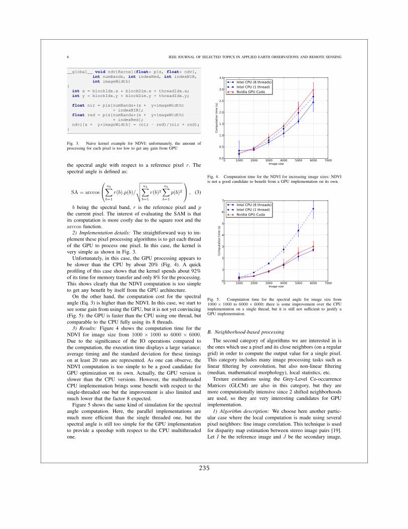
6 IEEE JOURNAL OF SELECTED TOPICS IN APPLIED EARTH OBSERVATIONS AND REMOTE SENSING
__global__ void ndviKernel(float* pix, float* ndvi,int numBands, int indexRed, int indexNIR,int imageWidth)
{int x = blockIdx.x * blockDim.x + threadIdx.x;int y = blockIdx.y * blockDim.y + threadIdx.y;
float nir = pix[numBands*(x + y*imageWidth)+ indexNIR];
float red = pix[numBands*(x + y*imageWidth)+ indexRed];
ndvi[x + y*imageWidth] = (nir - red)/(nir + red);}
Fig. 3. Naive kernel example for NDVI: unfortunately, the amount ofprocessing for each pixel is too low to get any gain from GPU
the spectral angle with respect to a reference pixel r. Thespectral angle is defined as:
SA = arccos
nb∑
b=1
r(b).p(b)/
√√√√nb∑
b=1
r(b)2nb∑
b=1
p(b)2
, (3)
b being the spectral band, r is the reference pixel and pthe current pixel. The interest of evaluating the SAM is thatits computation is more costly due to the square root and thearccos function.
2) Implementation details: The straightforward way to im-plement these pixel processing algorithms is to get each threadof the GPU to process one pixel. In this case, the kernel isvery simple as shown in Fig. 3.
Unfortunately, in this case, the GPU processing appears tobe slower than the CPU by about 20% (Fig. 4). A quickprofiling of this case shows that the kernel spends about 92%of its time for memory transfer and only 8% for the processing.This shows clearly that the NDVI computation is too simpleto get any benefit by itself from the GPU architecture.
On the other hand, the computation cost for the spectralangle (Eq. 3) is higher than the NDVI. In this case, we start tosee some gain from using the GPU, but it is not yet convincing(Fig. 5): the GPU is faster than the CPU using one thread, butcomparable to the CPU fully using its 8 threads.
3) Results: Figure 4 shows the computation time for theNDVI for image size from 1000 × 1000 to 6000 × 6000.Due to the significance of the IO operations compared tothe computation, the execution time displays a large variance;average timing and the standard deviation for these timingson at least 20 runs are represented. As one can observe, theNDVI computation is too simple to be a good candidate forGPU optimization on its own. Actually, the GPU version isslower than the CPU versions. However, the multithreadedCPU implementation brings some benefit with respect to thesingle-threaded one but the improvement is also limited andmuch lower that the factor 8 expected.
Figure 5 shows the same kind of simulation for the spectralangle computation. Here, the parallel implementations aremuch more efficient than the single threaded one, but thespectral angle is still too simple for the GPU implementationto provide a speedup with respect to the CPU multithreadedone.
0 1000 2000 3000 4000 5000 6000 7000Image size
0.0
0.5
1.0
1.5
2.0
2.5
3.0
3.5
Com
puta
tion t
ime (
s)
Intel CPU (8 threads)Intel CPU (1 thread)Nvidia GPU Cuda
Fig. 4. Computation time for the NDVI for increasing image sizes: NDVIis not a good candidate to benefit from a GPU implementation on its own.
0 1000 2000 3000 4000 5000 6000 7000Image size
0
1
2
3
4
5
6
7
Com
puta
tion t
ime (
s)
Intel CPU (8 threads)Intel CPU (1 thread)Nvidia GPU Cuda
Fig. 5. Computation time for the spectral angle for image size from1000 × 1000 to 6000 × 6000: there is some improvement over the CPUimplementation on a single thread, but it is still not sufficient to justify aGPU implementation.
B. Neighborhood-based processing
The second category of algorithms we are interested in isthe ones which use a pixel and its close neighbors (on a regulargrid) in order to compute the output value for a single pixel.This category includes many image processing tasks such aslinear filtering by convolution, but also non-linear filtering(median, mathematical morphology), local statistics, etc.
Texture estimations using the Grey-Level Co-occurrenceMatrices (GLCM) are also in this category, but they aremore computationally intensive since 2 shifted neighborhoodsare used, so they are very interesting candidates for GPUimplementation.
1) Algorithm description: We choose here another partic-ular case where the local computation is made using severalpixel neighbors: fine image correlation. This technique is usedfor disparity map estimation between stereo image pairs [19].Let I be the reference image and J be the secondary image,
235
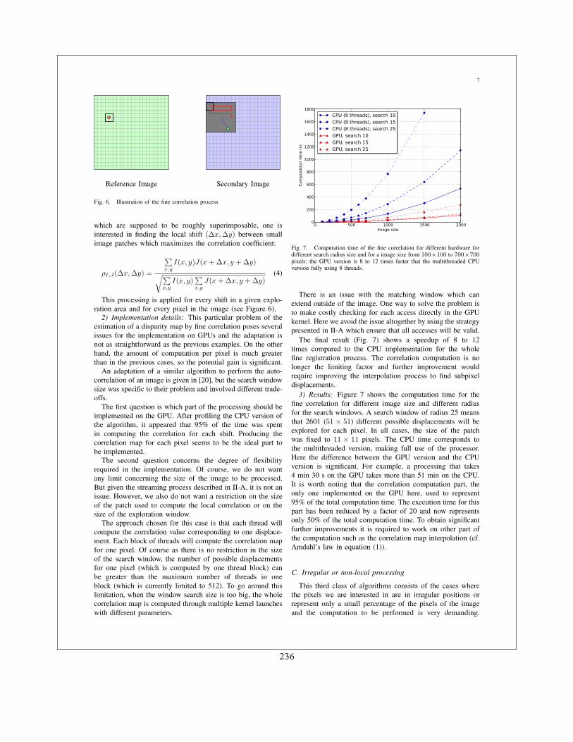
7
Reference Image Secondary Image
Fig. 6. Illustration of the fine correlation process
which are supposed to be roughly superimposable, one isinterested in finding the local shift (∆x,∆y) between smallimage patches which maximizes the correlation coefficient:
ρI,J(∆x,∆y) =
∑x,yI(x, y)J(x+ ∆x, y + ∆y)
√∑x,yI(x, y)
∑x,yJ(x+ ∆x, y + ∆y)
(4)
This processing is applied for every shift in a given explo-ration area and for every pixel in the image (see Figure 6).
2) Implementation details: This particular problem of theestimation of a disparity map by fine correlation poses severalissues for the implementation on GPUs and the adaptation isnot as straightforward as the previous examples. On the otherhand, the amount of computation per pixel is much greaterthan in the previous cases, so the potential gain is significant.
An adaptation of a similar algorithm to perform the auto-correlation of an image is given in [20], but the search windowsize was specific to their problem and involved different trade-offs.
The first question is which part of the processing should beimplemented on the GPU. After profiling the CPU version ofthe algorithm, it appeared that 95% of the time was spentin computing the correlation for each shift. Producing thecorrelation map for each pixel seems to be the ideal part tobe implemented.
The second question concerns the degree of flexibilityrequired in the implementation. Of course, we do not wantany limit concerning the size of the image to be processed.But given the streaming process described in II-A, it is not anissue. However, we also do not want a restriction on the sizeof the patch used to compute the local correlation or on thesize of the exploration window.
The approach chosen for this case is that each thread willcompute the correlation value corresponding to one displace-ment. Each block of threads will compute the correlation mapfor one pixel. Of course as there is no restriction in the sizeof the search window, the number of possible displacementsfor one pixel (which is computed by one thread block) canbe greater than the maximum number of threads in oneblock (which is currently limited to 512). To go around thislimitation, when the window search size is too big, the wholecorrelation map is computed through multiple kernel launcheswith different parameters.
0 500 1000 1500 2000Image size
0
200
400
600
800
1000
1200
1400
1600
1800
Com
puta
tion t
ime (
s)
CPU (8 threads), search 10CPU (8 threads), search 15CPU (8 threads), search 25GPU, search 10GPU, search 15GPU, search 25
Fig. 7. Computation time of the fine correlation for different hardware fordifferent search radius size and for a image size from 100×100 to 700×700pixels: the GPU version is 8 to 12 times faster that the multithreaded CPUversion fully using 8 threads.
There is an issue with the matching window which canextend outside of the image. One way to solve the problem isto make costly checking for each access directly in the GPUkernel. Here we avoid the issue altogether by using the strategypresented in II-A which ensure that all accesses will be valid.
The final result (Fig. 7) shows a speedup of 8 to 12times compared to the CPU implementation for the wholefine registration process. The correlation computation is nolonger the limiting factor and further improvement wouldrequire improving the interpolation process to find subpixeldisplacements.
3) Results: Figure 7 shows the computation time for thefine correlation for different image size and different radiusfor the search windows. A search window of radius 25 meansthat 2601 (51 × 51) different possible displacements will beexplored for each pixel. In all cases, the size of the patchwas fixed to 11 × 11 pixels. The CPU time corresponds tothe multithreaded version, making full use of the processor.Here the difference between the GPU version and the CPUversion is significant. For example, a processing that takes4 min 30 s on the GPU takes more than 51 min on the CPU.It is worth noting that the correlation computation part, theonly one implemented on the GPU here, used to represent95% of the total computation time. The execution time for thispart has been reduced by a factor of 20 and now representsonly 50% of the total computation time. To obtain significantfurther improvements it is required to work on other part ofthe computation such as the correlation map interpolation (cf.Amdahl’s law in equation (1)).
C. Irregular or non-local processing
This third class of algorithms consists of the cases wherethe pixels we are interested in are in irregular positions orrepresent only a small percentage of the pixels of the imageand the computation to be performed is very demanding.
236
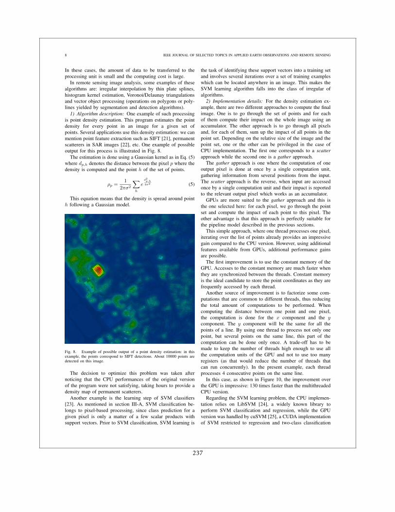
8 IEEE JOURNAL OF SELECTED TOPICS IN APPLIED EARTH OBSERVATIONS AND REMOTE SENSING
In these cases, the amount of data to be transferred to theprocessing unit is small and the computing cost is large.
In remote sensing image analysis, some examples of thesealgorithms are: irregular interpolation by thin plate splines,histogram kernel estimation, Voronoi/Delaunay triangulationsand vector object processing (operations on polygons or poly-lines yielded by segmentation and detection algorithms).
1) Algorithm description: One example of such processingis point density estimation. This program estimates the pointdensity for every point in an image for a given set ofpoints. Several applications use this density estimation: we canmention point feature extraction such as SIFT [21], permanentscatterers in SAR images [22], etc. One example of possibleoutput for this process is illustrated in Fig. 8.
The estimation is done using a Gaussian kernel as in Eq. (5)where dp,h denotes the distance between the pixel p where thedensity is computed and the point h of the set of points.
ρp =1
2πσ2
∑
h
ed2p,h
2σ2 (5)
This equation means that the density is spread around pointh following a Gaussian model.
Fig. 8. Example of possible output of a point density estimation: in thisexample, the points correspond to SIFT detections. About 10000 points aredetected on this image.
The decision to optimize this problem was taken afternoticing that the CPU performances of the original versionof the program were not satisfying, taking hours to provide adensity map of permanent scatterers.
Another example is the learning step of SVM classifiers[23]. As mentioned in section III-A, SVM classification be-longs to pixel-based processing, since class prediction for agiven pixel is only a matter of a few scalar products withsupport vectors. Prior to SVM classification, SVM learning is
the task of identifying these support vectors into a training setand involves several iterations over a set of training exampleswhich can be located anywhere in an image. This makes theSVM learning algorithm falls into the class of irregular ofalgorithms.
2) Implementation details: For the density estimation ex-ample, there are two different approaches to compute the finalimage. One is to go through the set of points and for eachof them compute their impact on the whole image using anaccumulator. The other approach is to go through all pixelsand, for each of them, sum up the impact of all points in thepoint set. Depending on the relative size of the image and thepoint set, one or the other can be privileged in the case ofCPU implementation. The first one corresponds to a scatterapproach while the second one is a gather approach.
The gather approach is one where the computation of oneoutput pixel is done at once by a single computation unit,gathering information from several positions from the input.The scatter approach is the reverse, when input are accessedonce by a single computation unit and their impact is reportedto the relevant output pixel which works as an accumulator.
GPUs are more suited to the gather approach and this isthe one selected here: for each pixel, we go through the pointset and compute the impact of each point to this pixel. Theother advantage is that this approach is perfectly suitable forthe pipeline model described in the previous sections.
This simple approach, where one thread processes one pixel,iterating over the list of points already provides an impressivegain compared to the CPU version. However, using additionalfeatures available from GPUs, additional performance gainsare possible.
The first improvement is to use the constant memory of theGPU. Accesses to the constant memory are much faster whenthey are synchronized between the threads. Constant memoryis the ideal candidate to store the point coordinates as they arefrequently accessed by each thread.
Another source of improvement is to factorize some com-putations that are common to different threads, thus reducingthe total amount of computations to be performed. Whencomputing the distance between one point and one pixel,the computation is done for the x component and the ycomponent. The y component will be the same for all thepoints of a line. By using one thread to process not only onepoint, but several points on the same line, this part of thecomputation can be done only once. A trade-off has to bemade to keep the number of threads high enough to use allthe computation units of the GPU and not to use too manyregisters (as that would reduce the number of threads thatcan run concurrently). In the present example, each threadprocesses 4 consecutive points on the same line.
In this case, as shown in Figure 10, the improvement overthe GPU is impressive: 130 times faster than the multithreadedCPU version.
Regarding the SVM learning problem, the CPU implemen-tation relies on LibSVM [24], a widely known library toperform SVM classification and regression, while the GPUversion was handled by cuSVM [25], a CUDA implementationof SVM restricted to regression and two-class classification
237
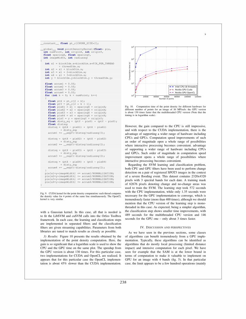
9
__constant__ float pt_c[CHUNK_SIZE*2];
__global__ void pointDensityKernel(float* pix,int numPoint, int originX, int originY,float spacingX, float spacingY,int imageWidth, int radiussq)
{int x1 = blockIdx.x*blockDim.x*PIX_PER_THREAD
+ threadIdx.x;int x2 = x1 + blockDim.x;int x3 = x1 + 2*blockDim.x;int x4 = x1 + 3*blockDim.x;int y = blockIdx.y*blockDim.y + threadIdx.y;
float accum1 = 0.0f;float accum2 = 0.0f;float accum3 = 0.0f;float accum4 = 0.0f;for (int k = 0; k < numPoint; k++){
float ptX = pt_c[2 * k];float ptY = pt_c[2 * k + 1];float pixX1 = x1 * spacingX + originX;float pixX2 = x2 * spacingX + originX;float pixX3 = x3 * spacingX + originX;float pixX4 = x4 * spacingX + originX;float pixY = y * spacingY + originY;float disty_sq = (ptY - pixY) * (ptY - pixY);float distsq;distsq = (ptX - pixX1) * (ptX - pixX1)
+ disty_sq;accum1 += __expf(-distsq/radiussq/2);
distsq = (ptX - pixX2) * (ptX - pixX2)+ disty_sq;
accum2 += __expf(-distsq/radiussq/2);
distsq = (ptX - pixX3) * (ptX - pixX3)+ disty_sq;
accum3 += __expf(-distsq/radiussq/2);
distsq = (ptX - pixX4) * (ptX - pixX4)+ disty_sq;
accum4 += __expf(-distsq/radiussq/2);}pix[x1+y*imageWidth] += accum1/NORMALIZATION;pix[x2+y*imageWidth] += accum2/NORMALIZATION;pix[x3+y*imageWidth] += accum3/NORMALIZATION;pix[x4+y*imageWidth] += accum4/NORMALIZATION;
}
Fig. 9. CUDA kernel for the point density computation: each thread computesthe density value for 4 points of the same line simultaneously. The OpenCLkernel is very similar.
with a Gaussian kernel. In this case, all that is needed isto fit the LibSVM and cuSVM calls into the Orfeo Toolboxframework. In each case, the learning and classification stepsare implemented in separated filters and the classificationfilters are given streaming capabilities. Parameters from bothlibraries are tuned to match results as closely as possible.
3) Results: Figure 10 presents the results obtained by theimplementation of the point density computation. Here, thegain is so significant that a logarithm scale is used to show theCPU and the GPU time on the same plot. The speedup fromthe GPU version is about 130 times. For this particular case,two implementations for CUDA and OpenCL are realized. Itappears that for this particular case the OpenCL implemen-tation is about 45% slower than the CUDA implementation.
0 20000 40000 60000 80000 100000 120000Number of points
100
101
102
103
104
Com
puta
tion t
ime (
s)
Intel CPU (8 threads)Nvidia GPU CudaNvidia GPU OpenCL
Fig. 10. Computation time of the point density for different hardware fordifferent number of points for an image of 36 MPixels: the GPU versionis about 130 times faster that the multithreaded CPU version (Note that thetiming is in logarithm scale).
However, the gain compared to the CPU is still impressive,and with respect to the CUDA implementation, there is theadvantage of supporting a wider range of hardware includingCPUs and GPUs. Computation speed improvements of suchan order of magnitude open a whole range of possibilitieswhere interactive processing becomes convenient. advantageof supporting a wider range of hardware including CPUsand GPUs. Such order of magnitude in computation speedimprovement opens a whole range of possibilities whereinteractive processing becomes convenient.
Regarding the SVM learning and classification problem,both CPU and GPU filters have been used to perform changedetection on a pair of registered SPOT5 images in the contextof a severe flooding event. This dataset contains 2320x4320pixels with 3 spectral bands for each date. A training maskof 62676 pixels denoting change and no-change areas wasused to train the SVM. The learning step took 572 secondswith the CPU implementation, while only 1.35 seconds werenecessary for the GPU implementation to converge, which istremendously faster (more than 400 times), although we shouldmention that the CPU version of the learning step is mono-threaded in this case. As expected, being a simpler algorithm,the classification step shows smaller time improvements, with489 seconds for the multithreaded CPU version and 146seconds for the GPU one – only about 3 times faster.
IV. DISCUSSION AND PERSPECTIVES
As we have seen in the previous sections, some classesof algorithms can benefit tremendously from a GPU imple-mentation. Typically, these algorithms can be identified asalgorithms that do mostly local processing (limited distanceimpact) and intensive computation for each pixel. We haveseen for example that the SAM is at the lower bound interms of computation to make it valuable to implement onGPU for an image with 4 bands (fig. 5). In that particularcase, the limit appears to be a few hundred operations (mainly
238
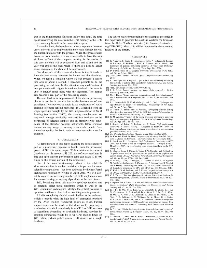
10 IEEE JOURNAL OF SELECTED TOPICS IN APPLIED EARTH OBSERVATIONS AND REMOTE SENSING
due to the trigonometric function). Below this limit, the timespent transferring the data from the CPU memory to the GPUovercomes any benefit in the computation speed.
Above this limit, the benefits can be very important. In somecases, they can be so important that they could change the waythe human interacts with the process. When the process takeshours, or even minutes, it is not conceivable to have the usersit down in front of the computer, waiting for the results. Inthis case, the data will be processed from end to end and theuser will exploit the final result. If there is a need to adjustsome parameters, the data will be reprocessed.
One drawback of this classical scheme is that it tends tolimit the interactivity between the human and the algorithm.When we reach a situation where we can process a screensize area in about a second, it becomes possible to do theprocessing in real time. In this situation, any modification ofany parameter will trigger immediate feedback: the user isable to interact much more with the algorithm. The humancan become a real part of the processing chain.
This can lead to an improvement of the classic processingchains in use, but it can also lead to the development of newparadigms. One obvious example is the application of activelearning to remote sensing problems [26]. Benefiting from themajor speed-up brought by the GPU implementation of SVMlearning (see section III-C3), the training samples selectionstep could change drastically: near real-time feedback on thepertinence of selected samples and on primitive-wise confi-dence of the classifier becomes achievable. Other commonremote sensing image processing tasks could benefit fromimmediate quality feedback, such as image co-registration forinstance.
V. CONCLUSIONS
As demonstrated in this paper, adapting the most expensivepart of a processing pipeline to benefit from the processingpower of GPUs is quite simple. With a minimum investment(hardware cost is around US$ 200, the software used here isfree and open source), performance gains can attain 10 to 400times on the critical portion of the processing.
One of the main shortcomings, which is the relativelyslow computation in double precision – important for somescientific computations – has been addressed by the new Fermiarchitecture released by Nvidia in April 2010. We will defi-nitely witness an increasing number of GPU implementationsfor remote sensing processing algorithms in the near future.
Still, benefiting from this massive speed-up requires oneto carefully select those algorithms which fit well in theGPU computing architecture, identify the critical sections tooptimize, and have a close look at how things are implemented.
All this complexity should remain hidden to the end-user,which is exactly what the high level of abstraction providedby the Orfeo Toolbox framework allows us to do. Furtherimprovements can be made in that direction by proposing amechanism to switch seamlessly from CPU to GPU versionsof algorithms depending on available hardware. Another in-teresting perspective would be to run GPU-enabled filters onGPU blades, which gather several GPU devices on a singlehardware.
The source code corresponding to the examples presented inthis paper used to generate the results is available for downloadfrom the Orfeo Toolbox web site (http://www.orfeo-toolbox.org/OTB-GPU). Most of it will be integrated in the upcomingreleases of the library.
REFERENCES
[1] K. Asanovıc, R. Bodik, B. Catanzaro, J. Gebis, P. Husbands, K. Keutzer,D. Patterson, W. Plishker, J. Shalf, S. Williams, and K. Yelick, “Thelandscape of parallel computing research: A view from Berkeley,”University of California, Berkeley, Tech. Rep., Dec. 2006.
[2] D. Blythe, “Rise of the graphic processor,” Proceedings of the IEEE,vol. 96, no. 5, May 2008.
[3] “The Orfeo Toolbox software guide,” http://www.orfeo-toolbox.org,2010.
[4] E. Christophe and J. Inglada, “Open source remote sensing: Increasingthe usability of cutting-edge algorithms,” IEEE Geoscience and RemoteSensing Newsletter, Mar. 2009.
[5] “ITK, the Insight Toolkit,” http://www.itk.org.[6] J. R. Schott, Remote sensing: the image chain approach. Oxford
University Press US, 2007.[7] M. J. Flynn, “Some computer organizations and their effectiveness,”
IEEE Transactions on Computers, vol. 21, no. 9, pp. 948–960, Sep.1972.
[8] J. L. Manferdelli, N. K. Govindaraju, and C. Crall, “Challenges andopportunities in many-code computing,” Proceedings of the IEEE,vol. 96, no. 5, May 2008.
[9] N. Satish, M. Harris, and M. Garland, “Designing efficient sortingalgorithms for manycore GPUs,” in IEEE International Symposium onParallel & Distributed Processing, May 2009.
[10] G. M. Amdahl, “Validity of the single-processor approach to achievinglarge scale computing capabilities,” in AFIPS Conference Proceedings,vol. 30, Apr. 1967, pp. 483–485.
[11] J. Setoain, M. Prieto, C. Tenllado, and F. Tirado, High performancecomputing in remote sensing. Chapman & Hall/CRC, 2007, ch.Real-time onboard phyperspectral image processing using programmablegraphic hardware, pp. 411–451.
[12] The OpenCL Specification, Khronos Group Std. 1.0, Dec. 2008.[13] D. Kirk and W.-M. W. Hwu, Programming Massively Parallel Proces-
sors: A Hands-on Approach. Elsevier Science & Technology, 2010.[14] P. Harish and P. J. Narayanan, High Performance Computing – HiPC
2007, ser. Lecture Notes in Computer Science. Springer Berlin /Heidelberg, 2007, ch. Accelerating large graph algorithms on the GPUusing CUDA.
[15] S. Che, M. Boyer, J. Meng, D. Tarjan, J. W. Sheaffer, and K. Skadron,“A performance study of general-purpose applications on graphics pro-cessors using CUDA,” Journal of Parallel and Distributed Computing,vol. 68, no. 10, pp. 1370–1380, Oct. 2008.
[16] V. W. Lee, C. Kim, J. Chhugani, M. Deisher, D. Kim, A. D. Nguyen,N. Satish, M. Smelyanskiy, S. Chennupaty, P. Hammarlund, R. Singhal,and P. Dubey, “Debunking the 100X GPU vs. CPU myth: an evaluationof throughput computing on CPU and GPU,” pp. 451–460, Jun. 2010.
[17] K. Karimi, N. G. Dickson, and F. Hamze, “A performance comparisonof CUDA and OpenCL,” CoRR, vol. abs/1005.2581, 2010.
[18] C. J. Tucker, “Red and photographic infrared linear combinations formonitoring vegetation,” Remote Sensing of Environment, no. 8, pp. 127–150, 1979.
[19] J. Inglada and A. Giros, “On the possibility of automatic multi-sensorimage registration,” IEEE Transactions on Geoscience and RemoteSensing, vol. 42, no. 10, Oct. 2004.
[20] P. J. Lu, H. Oki, C. A. Frey, G. E. Chamitoff, L. Chiao, B. J. Au,M. Christiansen, A. B. Schofield, D. A. Weitz, P. J. Lu, D. A. Weitz,H. Oki, C. A. Frey, G. E. Chamitoff, L. Chiao, E. M. Fincke, D. M.Tani, P. A. Whitson, J. N. Williams, W. V. Meyer, R. J. Sicker,B. J. Au, M. Christiansen, and A. B. Schofield, “Orders-of-magnitudeperformance increases in GPU-accelerated correlation of images fromthe international space station,” Journal of Real-Time Image Processing,2009.
[21] D. G. Lowe, “Distinctive image features from scale-invariant keypoints,”International Journal of Computer Vision, vol. 60, pp. 91–110, Feb.2004.
[22] A. Ferretti, C. Prati, and F. Rocca, “Permanent scatterers in SARinterferometry,” IEEE Transactions on Geoscience and Remote Sensing,vol. 39, pp. 8–20, Jan. 2001.
239
11
[23] V. Vapnik, Statistical learning theory. John Wiley and Sons, NewYork,1998.
[24] C.-C. Chang and C.-J. Lin, “LIBSVM: a library for support vectormachines,” http://www.csie.ntu.edu.tw/∼cjlin/libsvm, 2001.
[25] A. Carpenter, “cuSVM: A CUDA implementation of support vector clas-sification and regression,” http://patternsonascreen.net/cuSVMDesc.pdf,Jan. 2009.
[26] D. Tuia, F. Ratle, F. Pacifici, M. F. Kanevski, and W. J. Emery,“Active learning methods for remote sensing image classification,” IEEETransactions on Geoscience and Remote Sensing, vol. 47, no. 7, pp.2218–2232, Jul. 2009.
Emmanuel Christophe received the Engineeringdegree in Telecommunications from Ecole NationaleSuperieure des Telecommunications de Bretagne,Brest, France and the DEA in Telecommunicationsand image processing from University of Rennes 1in 2003. In October 2006, he received the PhDdegree from Supaero and University of Toulouse inhyperspectral image compression and image quality.He has been a visiting scholar in 2006 at RensselaerPolytechnic Institute, Troy, NY, USA. From 2006to 2008, he was a research engineer at CNES, the
French Space Agency, focusing on information extraction for high resolutionoptical images. Between 2008 and 2010, he moved to Singapore at CRISP,National University of Singapore, where he was tackling new challenges forremote sensing in tropical areas. He is now with Google Inc. in California.
Julien Michel recieved the Telecommunications En-gineer degree from the Ecole Nationale Superieuredes Telecommunications de Bretagne, Brest, France,in 2006. From 2006 to 2010, he has been with Com-munications et Systemes, Toulouse, France, wherehe has been working on studies and developmentsin the field of remote sensing image processing. Heis now with the Centre National d’Etudes Spatiales(French Space Agency), Toulouse, France, where heis in charge of the development of image processingalgorithms for the exploitation of Earth observation
images, mainly in the field of Very High Resolution image analysis.
Jordi Inglada received the Telecommunications En-gineer degree from both the Universitat Politecnicade Catalunya, Barcelona, Spain, and the Ecole Na-tionale Superieure des Telecommunications de Bre-tagne, Brest, France, in 1997 and the Ph.D. de-gree in signal processing and telecommunications in2000 from Universite de Rennes 1, Rennes, France.He is currently with the Centre National d’EtudesSpatiales (French Space Agency), Toulouse, France,working in the field of remote sensing image pro-cessing at the CESBIO laboratory. He is in charge
of the development of image processing algorithms for the operationalexploitation of Earth observation images, mainly in the field of multitemporalimage analysis for land use and cover change. Dr. Inglada is an AssociateEditor of the IEEE Transactions on Geoscience and Remote Sensing.
240


![The 2016 Android Developer Toolbox [DEVOXX]](https://img.pdfslide.fr/doc/110x75/5875ee2a1a28ab7d5a8b7ad9/the-2016-android-developer-toolbox-devoxx.jpg)