THE JOURNAL OF CHEMICAL PHYSICS 146, 124905 (2017)

Density functional theory and simulations of colloidal triangular prismsMatthieu Marechal,1,a) Simone Dussi,2,a) and Marjolein Dijkstra21Institut fur Theoretische Physik, Universitat Erlangen-Nurnberg, Staudtstr. 7, 91058 Erlangen, Germany2Soft Condensed Matter, Debye Institute for Nanomaterials Science, Utrecht University, Princetonplein 5, 3584CC Utrecht, The Netherlands

(Received 3 January 2017; accepted 24 February 2017; published online 31 March 2017)

Nanopolyhedra form a versatile toolbox to investigate the effect of particle shape on self-assembly.Here we consider rod-like triangular prisms to gauge the effect of the cross section of the rods on liquidcrystal phase behavior. We also take this opportunity to implement and test a previously proposedversion of fundamental measure density functional theory (0D-FMT). Additionally, we perform MonteCarlo computer simulations and we employ a simpler Onsager theory with a Parsons-Lee correction.Surprisingly and disappointingly, 0D-FMT does not perform better than the Tarazona and Rosenfeld’sversion of fundamental measure theory (TR-FMT). Both versions of FMT perform somewhat betterthan the Parsons-Lee theory. In addition, we find that the stability regime of the smectic phase islarger for triangular prisms than for spherocylinders and square prisms. Published by AIP Publishing.[http://dx.doi.org/10.1063/1.4978502]

I. INTRODUCTION

Recent advances in colloid synthesis techniques allowthe preparation of colloids and nanoparticles with a largernumber of distinct polyhedral shapes and sizes ranging fromthe nanometer to the micrometer.1–3 With this great vari-ety of available polyhedral shapes, polyhedra are attractiveas a toolbox for investigating the effect of shape on self-assembly.4–9 This requires efficient theories or computersimulations to guide future synthesis efforts. In fact, a syn-ergy of the two types of techniques could be used: First,a reliable and efficient, but approximate, theory predictsthe phase behavior for a large range of parameters. Sub-sequently, particle-resolved computer simulations improveon these predictions at the cost of a greater computationaleffort.

A range of theoretical techniques exist for hard bod-ies: The fluid and the crystal can be described using scaledparticle theory and cell theory, respectively, while the mostsuitable non-phenomenological theory for liquid crystalsis density functional theory (DFT).10,11 Density functionaltheory is a continuum theory for systems that are inho-mogeneous or anisotropic either due to applied externalfields10,12,13 or spontaneous symmetry breaking.14–16 For hardspheres, the most successful DFT is fundamental measuretheory (FMT)15,17,18 or an extension.19–22 FMT is stronglybased on geometry, which makes the extension to non-spherical particles12,13,23,24 more elegant than for previousDFTs for anisotropic particles.25–28 FMT has been success-fully applied to polyhedra with moderate shape anisotropy.29

More recent advances,30,31,33 after which the smectic phaseof rods can be described, were not implemented inRef. 29.

a)M. Marechal and S. Dussi contributed equally to this work.

The existence of polyhedral nanorods3,34–36 and the obser-vation of smectic-like ordering of these rods34,35 motivatedus to consider the effect of polyhedral shape on the liquid-crystal phases of rod-like particles. Furthermore, polyhedralrods present a good system to test the recent advances fromRefs. 30–33 for shapes other than spherocylinders and to inves-tigate the performance of a fully non-empirical version ofFMT (see Sec. III) which has not yet been applied to non-spherical particles. We chose the triangular prisms as the rod-like polyhedron to consider as it is the prism that differs themost from the spherocylinder. Computer simulations of squareprisms (also known as cuboids or tetragonal parallelepipeds)have already been performed37,38 showing the expected liquidcrystal phases for sufficient elongation.

This paper is organized as follows: First, we present themodel and its parameters in Sec. II. In the subsequent section(Sec. III), we first present the two versions of FMT we will con-sider. In Sec. IV, we describe a simpler (Onsager-like) theory;the performance of the more complicated FMT will be com-pared to this theory for the nematic phase. Sec. VI contains ourresults. Finally, we will summarize our results in Sec. VII andcompare them to results for other particles shapes. The appen-dices contain details considering the implementation of FMTfor general shapes (in Appendix A) and the specialization topolyhedra (in Appendix B).

II. MODEL

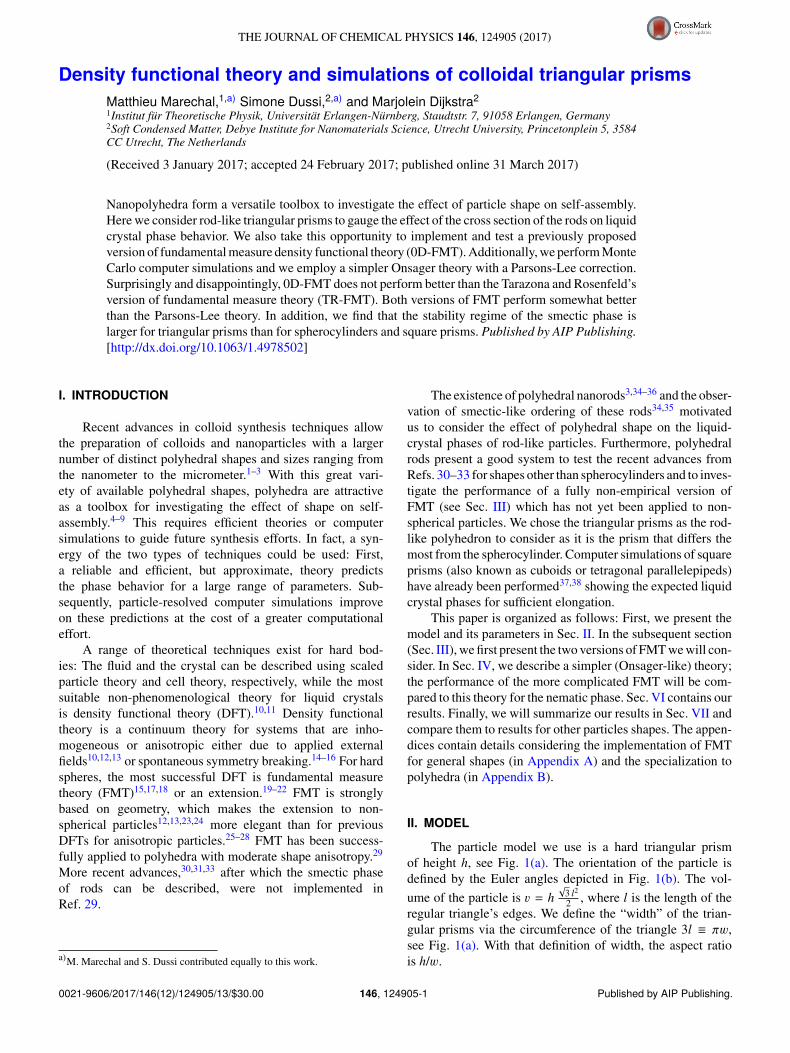
The particle model we use is a hard triangular prismof height h, see Fig. 1(a). The orientation of the particle isdefined by the Euler angles depicted in Fig. 1(b). The vol-

ume of the particle is 3 = h√

3 l2

2 , where l is the length of theregular triangle’s edges. We define the “width” of the trian-gular prisms via the circumference of the triangle 3l ≡ π4,see Fig. 1(a). With that definition of width, the aspect ratiois h/4.

0021-9606/2017/146(12)/124905/13/$30.00 146, 124905-1 Published by AIP Publishing.

124905-2 Marechal, Dussi, and Dijkstra J. Chem. Phys. 146, 124905 (2017)

FIG. 1. (a) Triangular prism with an equilateral base. The height of the particleis h whereas the width 4 of the prism is defined as the circumference over π.(b) The Euler angles defining the orientation $ of a particle where the z axisis aligned with the nematic director. θ is the polar angle, φ is the azimuthalangle (not shown), and ψ is the particle internal angle.

III. DENSITY FUNCTIONAL THEORY: FUNDAMENTALMEASURE THEORY

Density functional theory is specifically designed to han-dle inhomogeneous mixtures of anisotropic particles describedby a density profile ρs(r,$), which expresses the local den-sity of particles of species s orientation $ at position r, where$ denotes the three Euler angles. The grand potential—thethermodynamic potential of the ensemble where the chemicalpotentials µs, the volume V, and the temperature T are heldfixed—can be written as a sum over three parts

Ω[ρ] = Fid[ρ] + Fexc[ρ]

+∑

s

∫d$

∫drρs(r,$)[V ext

s (r,$) − µs], (1)

where V exts (r,$) is the external potential. The first term in the

grand potential Ω is the ideal gas free energy,10

Fid[ρ] = kBT∑

s

∫ ∫ρs(r,$)log[ρs(r,$)V] − 1 d$ dr,

(2)where kB is Boltzmann’s constant and V is the irrelevant ther-mal volume, which is the result of the integrals over themomenta conjugate to r and$. We will use the (approximate)excess free energy Fexc from fundamental measure theory(FMT).

In FMT12,13,15,17,39 and variants,19,20 hard-particle sys-tems are connected to geometry by identifying a particle withspecies s and coordinates (r,$) with the set of points in itsinterior Bs(r,$). There are different versions of FMT, but allof them have an excess free energy of the form

Fexc[ρ] ≡ kBT∫

dr3∑

k=1

Φk

(nα[ρ](r)

)(3)

in three dimensions, where theΦk are functions of the (mixed)weighted densities nα[ρ] that we will define shortly

Φ(nα

)= −n0 log(1 − n3) +

n12

1 − n3+ C

n222

(1 − n3)2. (4)

The differences between versions of FMT lie in the definitionsof n12 and n222 and whether C , 1 is used to improve the thirdvirial coefficient. The weighted densities nα for 0 ≤ α ≤ 3have units of (length)α−3 (n1 and n2 are introduced for laterreference). These are related to the geometry of the particles,namely the topology, the integrated mean curvature, the sur-face area, and the volume of the particles for α = 0, 1, 2, and3, respectively. These are related to the geometry of the inter-sections of n particles. A mixed40 weighted density nA withmulti-index A = α1 · · · αn has units of length to the power∑n

i=1(αi − 3), such that each term in Eq. (4) has the units ofdensity. Usually n12 and n222 are written in terms of a (ten-sor) product of single-index weighted densities of a tensorialnature.

The original version of FMT by Rosenfeld for hardspheres17 has the disadvantage that it predicts the crystal ofhard spheres to be unstable at all densities. To resolve this, anFMT for hard spheres was derived by demanding that the the-ory is exact in the so-called zero-dimensional limit, which isrelated to the crystal in the close-packed limit.41 In this limit,the system is confined to such a great extent that only one par-ticle with discrete positions and orientations fits in the volumeof the system (in this case, the density profile is a sum of deltafunctions).18,41 The resulting non-empirical version of FMT,which we will call 0D-FMT, can also be derived by approxi-mating the virial series42 and resumming the series to a closedform. This theory was deemed too unwieldy to use in FMT cal-culations for the hard sphere crystal, because n222 could notbe written in terms of single-index weighted densities (unlikeprevious versions); moreover, its prediction for the third virialcoefficient of hard spheres is off. In the same publication18

in which 0D-FMT was first derived, Tarazona and Rosenfeldsolved both problems by approximating n222 as an expressioncontaining tensorial weighted densities of rank two and lessand adjusting C in Eq. (4) such that FMT yields the exact thirdvirial coefficient for hard spheres; we will refer to Tarazonaand Rosenfeld’s version of FMT as TR-FMT. Later, additionalimprovements were proposed that lead to a very accurate DFTfor hard spheres.15,19–22

After extending FMT to non-spherical particles, Rosen-feld realized that his original FMT would never predict a stablenematic phase.39 A more careful extension of n12 to non-spherical particles by Hansen-Goos and Mecke did lead toa DFT that can also describe the nematic phase,12,13 while thefunctional can still be expressed in tensorial weighted densitiesof rank two and lower. However, an empirical rescaling wasrequired for an accurate description of the isotropic–nematictransition. Afterwards,30 it was found that the smectic phasewas stable in a similarly extended TR-FMT but not in the morerecent improved theories. Finally, it is possible to calculaten12 exactly for non-spherical particles either by a direct cal-culation, which is computationally expensive, or an improvedexpansion in tensorial weighted densities.31 We consider thistheory as the proper extension of TR-FMT to non-sphericalparticles and refer to it simply as “TR-FMT.” The predictionsof TR-FMT for liquid crystals of hard spherocylinders aregenerally accurate, see Ref. 33 for an overview. Moreover,the semi-empirical constant introduced in Ref. 12 is removedfrom the theory. Nevertheless, the constant C , 1 in front of

124905-3 Marechal, Dussi, and Dijkstra J. Chem. Phys. 146, 124905 (2017)

the expression for n222 is still somewhat empirical; further-more, its value is obtained for hard spheres and thus might notbe appropriate for non-spherical particles. For these reasons,we will also consider 0D-FMT, which has no adjustable con-stants (C = 1) and thus might be more robust under changesof the particle shape.

We will now give expressions for the weighted densitiesin the 0D-FMT functional and, subsequently, provide the dif-ferences between 0D-FMT and TR-FMT. First, the weighteddensity, n3, is defined using an integral of the density profileover the particle volume

n3[ρ](r) =∑

s

∫d$

∫Bs(0,$)

dp ρs(r − p,$). (5)

Note that the integral over p runs over the interior of a par-ticle centered around the origin; after a variable substitutionp → r′ = r − p, Eq. (5) may also be interpreted as the sumover all species of the integral over all particle positions r′ andorientations such that r lies inside Bs(r′,$), the interior of aparticle at r′. The other weighted densities are defined usingan integral over the particle surface in addition to an integralover the particle’s orientations and a sum over the species (ifapplicable) or repeated integrals of this type, for which wedefine the shorthands∫

d<

∂Bs(0,$)

≡∑

s

∫d$

∫∂Bs(0,$)

d2p, (6)

∫∂Bs(0,$)n

d<n ≡

∫∂Bs1 (0,$1)

d<1 · · ·

∫∂Bsn (0,$n)

d<n, (7)

and finally, we define ρ(r −<i) ≡ ρsi (r − pi,$i), where d2pdenotes a surface area element at a point p on the boundary∂Bs(0,$) and <i = (pi, si,$i). With these shorthands, the(mixed) weighted density nA, where A has n components, reads

nA[ρ](r) =∫∂Bs(0,$)n

d<n QA

(<n

) n∏i=1

ρ(r −<i). (8)

Similarly as for n3, suitable variable substitutions allow theinterpretation of Eq. (8) as the average of QA over all particlepositions, orientations, and species such that r simultaneouslylies on the surfaces of all n particles.

The function QA

(<n

)with <i = (pi, si,$i) for i

= 1, . . . , n depends on the principal moments of curvatureκii and κiii , the corresponding directions vii and viii and the nor-mal vector ni of the surface ∂Bsi (0,$i) at the point pi for alli = 1, . . . , n. The explicit expressions for QA read

Q0(<1) ≡K1

4π, (9)

Q12(<2) ≡κii1(vi1 · n2)2 + κi1(vii1 · n2)2

4π(1 + n1 · n2), (10)

Q222(<3) ≡ |(n1 × n2) · n3 |2π − 3 α(n1, n2, n3)

24π, (11)

where Ki = κiiκiii is the Gaussian curvature and α(n1, n2, n3)

is the angle between the two cross products,43 n1 × n2 andn2 × n3.

The only quantities that are different in TR-FMT com-pared to 0D-FMT are the value for the adjustable constantC = 9 and the form for Q222,18

Q222(<3) ' QTR222(<3) ≡

148π

[n1 · (n2 × n3)]2, (12)

which reduces to Q222 in the limit that the normal vectorsbecome parallel.42

The high dimensionality of the integrals over <n in thedefinition of the mixed weighted densities n12 for TR-FMT and0D-FMT and n222 for 0D-FMT makes it difficult to evaluatethem (practically impossible in case of n222 for the smecticphase). Therefore, we follow Wertheim44 in expanding thenA in terms of spherical harmonics. While this expansion isnew in the case of n222 and has never been applied to FMT, the(analytic) calculation of the coefficients is somewhat involved,so we present it in Appendix A. The result has the typical formfor FMT

n12(r) =∑~l

n(~l)1 (r)n(~l)

2 (r), (13)

n222(r) =∑~l1,~l2,~l3

C(~l1,~l2,~l3)222 n(~l1)

2 (r)n(~l2)2 (r)n(~l3)

2 (r), (14)

where~li = (li, mi) with the degree li and order mi of a spher-

ical harmonic and the weighted densities n(~l)α for α = 1, 2 are

defined by

n(~l)α (r) =

∑s

∫d$

[∫dr′ 4(~l)

α (r − r′, s,$)ρs($, r′)]

, (15)

where the expression in square brackets is a convolution of aweight function and the density profile that can be efficientlycalculated using fast Fourier transforms (see Appendix B).

Here, 4(~l)α (r, s,$) are the weight functions (proportional to

a one-dimensional delta-function) defined in Eqs. (A40)–(A42). The method for calculating the weighted densities forpolyhedra is given in Appendix B and Ref. 29.

For the minimization of the grand potential with respectto the density profile, we employ either a variational approach,where the density profile is parametrized as described inRef. 30, or we perform a full minimization using Picarditeration on a grid.48 In either case, the density profile iscalculated on a two-dimensional grid consisting of equidis-tant points in the z-direction and, in the θ-direction, eithera fine equidistant grid or the points from a modifiedGauss-Legendre quadrature. For the modified Gauss-Legendrequadrature, we first performed a variable transformationθ→ x = sinh(λ cos θ) with λ chosen such that cosh(λθ)approximates the expected θ-dependence of the densityprofile (see Ref. 49 for the reasoning behind perform-ing such a variable transformation). We also performedfull minimizations on three-dimensional (z, θ,ψ) grids, butwe never found significant ψ-dependence of the densityprofile.

IV. SECOND-VIRIAL DFT:ISOTROPIC-NEMATIC TRANSITION

To describe the isotropic-nematic transition, we also usea second-virial (Onsager-like50) density functional theory that

124905-4 Marechal, Dussi, and Dijkstra J. Chem. Phys. 146, 124905 (2017)

we compare against results from FMT and simulations. In thiscase, we do not fully consider the biaxial nature of the particleshape in the description of the nematic order. In particular, weassume that the single-particle density of the homogeneousbulk nematic phase can be written as ρ(r,$) = ρ ϕ(θ), withρ = N/V = η/3 the number density, V the volume of thesystem, 3 the particle volume, and η the packing fraction ofthe system. The orientation distribution function ϕ dependsonly on the polar angle θ (see Fig. 1(b)) and the free energy ofthe system is

βF [ϕ]V

= ρ(logV ρ − 1) + 4π2 ρ

∫d cos θ ϕ(θ) log ϕ(θ)

+ G(η)ρ2

2

∫d cos θ d cos θ ′E(θ, θ ′)ϕ(θ)ϕ(θ ′)

(16)

with β = 1/kBT , V the irrelevant thermal volume, and G(η)= (1− 3

4η)/(1 − η)2 the Parsons-Lee correction factor.51,52 Theexcluded volume between two particles with orientation$ and$′, respectively, and separated by a distance r is given by

E(θ, θ ′) = −∫

dφ dφ′ dψ dψ ′dr f (r,$,$′) (17)

with f (r,$,$′) = exp(−βU(r,$,$′)) − 1 the Mayer func-tion, U(r,$,$′) the (hard-core) pair potential, and φ andψ the azimuthal and internal angle (see Fig. 1(b)). In prac-tice, the excluded volume is computed by performing a MonteCarlo (MC) integration over many randomly generated pairsof particles, by checking if they overlap using an algorithmbased on the Robust and Accurate Polygon Interface Detec-tion (RAPID) library.53 This procedure has been already used,for example, to describe the chiral nematic order in similar sys-tems composed of twisted triangular prisms.54 In summary, theexcluded volume used as input for the (Parsons-Lee) Onsagertheory is an average over the particle internal angle. The free-energy functional is minimized subject to the normalizationcondition ∫ d$ϕ(θ) = 1. The resulting non-linear equationfor the orientation distribution function reads

ϕ(θ) =1Z

exp

(− ρG(η)

∫d cos θ ′

E(θ, θ ′)

4π2ϕ(θ ′)

), (18)

where Z is a normalization constant. Eq. (18) is solved self-consistently at fixed density ρ by using a discrete grid for thepolar angle θ (see, e.g., Ref. 55). The resulting equilibriumorientation distribution function ϕeq(θ) is used to calculate therelevant thermodynamic and structural quantities, such as thenematic order parameter

S =∫

dθ

[32

cos2(θ) −12

]ϕeq(θ). (19)

V. COMPUTER SIMULATIONS

To study the phase behavior of hard elongated triangularprisms, we employ standard Monte Carlo (MC) simulationseither in the NPT or in the NVT ensemble.56 We use N= 2000 particles with different aspect ratios h/4 ∈ [3.0, 6.0]and several millions of MC steps are performed for typicalruns. For NVT -MC simulations, each MC step consists on

average of N /2 attempts of translating a random particle andN /2 attempts of rotating a random particle. For NPT -MC sim-ulations, an additional attempt to either scale isotropically thevolume or to change only one edge of the cuboidal simula-tion box is tried at each MC step. The particles interact via ahard-core potential only. To detect overlaps between particles,we use an algorithm, based on the RAPID library,53 that con-sists in detecting the intersections between the (rectangular ortriangular) faces of the polyhedral particles.

To quantify the orientational and positional order in thesystem, we use standard order parameters. First, we constructthe nematic order parameter tensor

Qαβ =1N

N∑i=1

[32

uiαuiβ −δαβ

2

], (20)

where α, β = x, y, z component, u denotes the particle longaxis, N is the number of particles, and δαβ the Kronecker delta.After diagonalizing Q, we identify the (scalar) order parame-ter S as the maximum eigenvalue. The associated eigenvectorcorresponds to the nematic director n. Similar nematic orderparameter tensors can be calculated considering the short andthe medium particle axes, thereby probing oblate (or discotic-like) order in the system. Furthermore, it is also possible toquantify the degree of (macroscopic) biaxial alignment of anematic phase by defining an additional order parameter, as,for example, used in Ref. 57. However, for the particle shapesstudied in the present work, we observe only the formationof uniaxial prolate (or calamitic) nematic phases. The resultson similar particle shapes forming prolate and biaxial nematicphases have been anticipated in Ref. 54 and will be reportedin detail elsewhere.

To identify the phase transition to a smectic phase, wemonitor the onset of positional order along the nematic direc-tor n and we calculate the smectic order parameter definedas

τ = maxl∈ℝ

N∑j=1

exp

(2πl

irj · n)

, (21)

where rj denotes the position of particle j.

VI. RESULTS

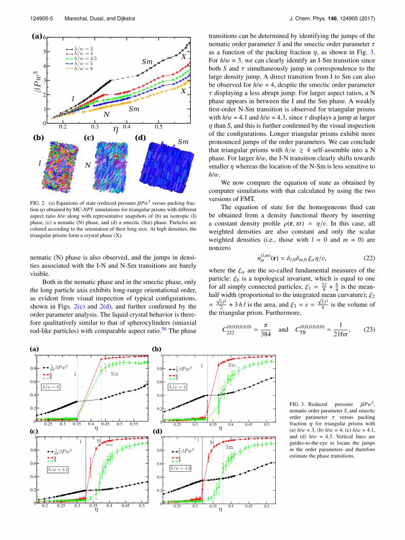
We first report the liquid crystal behavior of hard trian-gular prisms as obtained using MC simulations that will becompared below with the theoretical predictions. The equa-tion of state is obtained after long equilibration runs in theNPT ensemble, typically expanding from close-packed con-figurations, and averaging the density over equilibrated con-figurations generated in the last ∼106 MC steps. In Fig. 2(a),we plot the reduced pressure βP43, with β = 1/kBT , T thetemperature, and kB the Boltzmann constant, as a functionof the packing fraction η for some of the systems stud-ied. We find an isotropic (I) phase at low densities and acrystal (X) phase at high densities for all the aspect ratiosh/4 ∈ [3.0, 6.0]. For h/4 = 3, we observe a clear jump inthe density that corresponds to a first-order transition fromI to a smectic (Sm) phase. In the case of longer particles, a

124905-5 Marechal, Dussi, and Dijkstra J. Chem. Phys. 146, 124905 (2017)

FIG. 2. (a) Equations of state (reduced pressure βP43 versus packing frac-tion η) obtained by MC-NPT simulations for triangular prisms with differentaspect ratio h/4 along with representative snapshots of (b) an isotropic (I)phase, (c) a nematic (N) phase, and (d) a smectic (Sm) phase. Particles arecolored according to the orientation of their long axis. At high densities, thetriangular prisms form a crystal phase (X).

nematic (N) phase is also observed, and the jumps in densi-ties associated with the I-N and N-Sm transitions are barelyvisible.

Both in the nematic phase and in the smectic phase, onlythe long particle axis exhibits long-range orientational order,as evident from visual inspection of typical configurations,shown in Figs. 2(c) and 2(d), and further confirmed by theorder parameter analysis. The liquid crystal behavior is there-fore qualitatively similar to that of spherocylinders (uniaxialrod-like particles) with comparable aspect ratio.58 The phase

transitions can be determined by identifying the jumps of thenematic order parameter S and the smectic order parameter τas a function of the packing fraction η, as shown in Fig. 3.For h/4 = 3, we can clearly identify an I-Sm transition sinceboth S and τ simultaneously jump in correspondence to thelarge density jump. A direct transition from I to Sm can alsobe observed for h/4 = 4, despite the smectic order parameterτ displaying a less abrupt jump. For larger aspect ratios, a Nphase appears in between the I and the Sm phase. A weaklyfirst-order N-Sm transition is observed for triangular prismswith h/4 = 4.1 and h/4 = 4.3, since τ displays a jump at largerη than S, and this is further confirmed by the visual inspectionof the configurations. Longer triangular prisms exhibit morepronounced jumps of the order parameters. We can concludethat triangular prisms with h/4 & 4 self-assemble into a Nphase. For larger h/4, the I-N transition clearly shifts towardssmaller η whereas the location of the N-Sm is less sensitive toh/4.

We now compare the equation of state as obtained bycomputer simulations with that calculated by using the twoversions of FMT.

The equation of state for the homogeneous fluid canbe obtained from a density functional theory by insertinga constant density profile ρ(r,$) = η/3. In this case, allweighted densities are also constant and only the scalarweighted densities (i.e., those with l = 0 and m = 0) arenonzero

n(l,m)α (r) = δl,0δm,0 ξαη/3, (22)

where the ξα are the so-called fundamental measures of theparticle: ξ0 is a topological invariant, which is equal to onefor all simply connected particles; ξ1 =

3 l8 + h

4 is the mean-half width (proportional to the integrated mean curvature); ξ2

=√

3 l2

2 + 3 h l is the area, and ξ3 = 3 =√

3 l2

4 is the volume ofthe triangular prism. Furthermore,

C(0,0,0,0,0,0)222 =

π

384and C(0,0,0,0,0,0)

TR =1

216π, (23)

FIG. 3. Reduced pressure βP43,nematic order parameter S, and smecticorder parameter τ versus packingfraction η for triangular prisms with(a) h/4 = 3, (b) h/4 = 4, (c) h/4 = 4.1,and (d) h/4 = 4.3. Vertical lines areguides-to-the-eye to locate the jumpsin the order parameters and thereforeestimate the phase transitions.

124905-6 Marechal, Dussi, and Dijkstra J. Chem. Phys. 146, 124905 (2017)

see Subsection 2 of Appendix A. Therefore, the pressure ascalculated from−(∂F/∂V )N with F = F [ρ]= Fid[ρ]+Fexc[ρ]from FMT reads

βPρ=

1 + (c1 − 2) η + (2 c2 − c1 + 1) η2

(1 − η)3, (24)

where c1 =ξ1 ξ2ξ3

and c2 =C(0,0,0,0,0,0)222

ξ32

ξ23= π

384ξ3

2

ξ23

for 0D-FMT

and c2 = 9C(0,0,0,0,0,0)TR

ξ32

ξ23= 1

24πξ3

2

ξ23

for TR-FMT. For TR-FMT,

Eq. (24) is the usual scaled particle equation of state, whichreduces to the Percus-Yevick equation of state (from the com-pressibility route) for spheres. The EOS from 0D-FMT isnot a very good one for the homogeneous fluid of spheres,18

but it is interesting to see how it performs for triangularprisms. For the nematic phase and the smectic phase, wecalculated the pressure within TR-FMT and 0D-FMT bynumerically calculating the derivative −(∂F/∂V )N , wherethe free energy F was obtained by minimizing F [ρ] withrespect to ρ at a constant average density using a variationalapproach.30

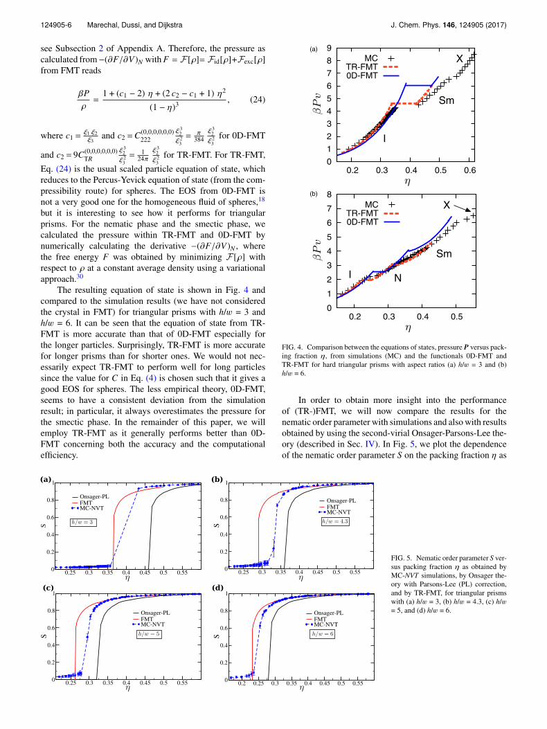
The resulting equation of state is shown in Fig. 4 andcompared to the simulation results (we have not consideredthe crystal in FMT) for triangular prisms with h/4 = 3 andh/4 = 6. It can be seen that the equation of state from TR-FMT is more accurate than that of 0D-FMT especially forthe longer particles. Surprisingly, TR-FMT is more accuratefor longer prisms than for shorter ones. We would not nec-essarily expect TR-FMT to perform well for long particlessince the value for C in Eq. (4) is chosen such that it gives agood EOS for spheres. The less empirical theory, 0D-FMT,seems to have a consistent deviation from the simulationresult; in particular, it always overestimates the pressure forthe smectic phase. In the remainder of this paper, we willemploy TR-FMT as it generally performs better than 0D-FMT concerning both the accuracy and the computationalefficiency.

FIG. 4. Comparison between the equations of states, pressure P versus pack-ing fraction η, from simulations (MC) and the functionals 0D-FMT andTR-FMT for hard triangular prisms with aspect ratios (a) h/4 = 3 and (b)h/4 = 6.

In order to obtain more insight into the performanceof (TR-)FMT, we will now compare the results for thenematic order parameter with simulations and also with resultsobtained by using the second-virial Onsager-Parsons-Lee the-ory (described in Sec. IV). In Fig. 5, we plot the dependenceof the nematic order parameter S on the packing fraction η as

FIG. 5. Nematic order parameter S ver-sus packing fraction η as obtained byMC-NVT simulations, by Onsager the-ory with Parsons-Lee (PL) correction,and by TR-FMT, for triangular prismswith (a) h/4 = 3, (b) h/4 = 4.3, (c) h/4= 5, and (d) h/4 = 6.

124905-7 Marechal, Dussi, and Dijkstra J. Chem. Phys. 146, 124905 (2017)

obtained by the three different methods, for triangular prismswith different h/4. We observe that Onsager-PL theory largelyoverestimates the packing fraction at which the I-N transitionoccurs, confirming the known drawback of such a theory. Onthe other hand, FMT predictions for the jump of S match wellwith the simulation results for triangular prisms with h/4 = 3,for which only the I-Sm transition occurs. On the other hand,as soon as the N phase becomes stable, e.g., for h/4 = 4.3, theFMT underestimates the packing fraction associated with thejump of S. However, upon increasing aspect ratio h/4, the dis-crepancy diminishes and already for h/4 = 6 a good agreementfor the I-N transition is obtained.

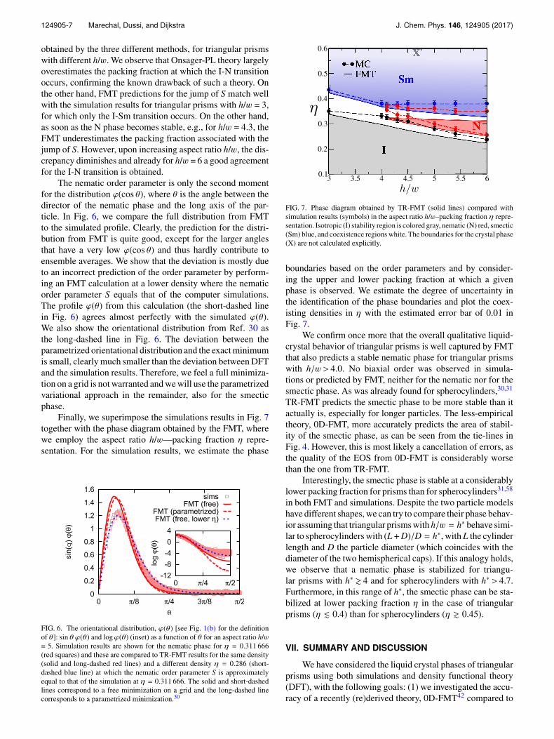
The nematic order parameter is only the second momentfor the distribution ϕ(cos θ), where θ is the angle between thedirector of the nematic phase and the long axis of the par-ticle. In Fig. 6, we compare the full distribution from FMTto the simulated profile. Clearly, the prediction for the distri-bution from FMT is quite good, except for the larger anglesthat have a very low ϕ(cos θ) and thus hardly contribute toensemble averages. We show that the deviation is mostly dueto an incorrect prediction of the order parameter by perform-ing an FMT calculation at a lower density where the nematicorder parameter S equals that of the computer simulations.The profile ϕ(θ) from this calculation (the short-dashed linein Fig. 6) agrees almost perfectly with the simulated ϕ(θ).We also show the orientational distribution from Ref. 30 asthe long-dashed line in Fig. 6. The deviation between theparametrized orientational distribution and the exact minimumis small, clearly much smaller than the deviation between DFTand the simulation results. Therefore, we feel a full minimiza-tion on a grid is not warranted and we will use the parametrizedvariational approach in the remainder, also for the smecticphase.

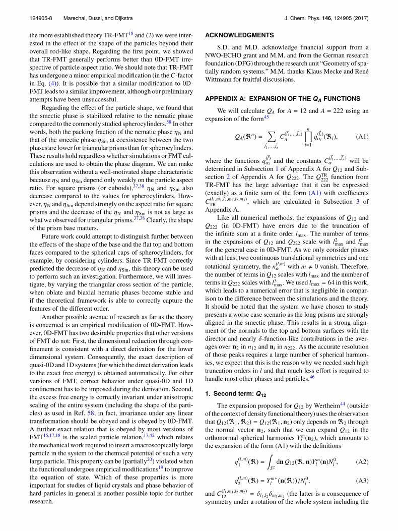
Finally, we superimpose the simulations results in Fig. 7together with the phase diagram obtained by the FMT, wherewe employ the aspect ratio h/4—packing fraction η repre-sentation. For the simulation results, we estimate the phase

FIG. 6. The orientational distribution, ϕ(θ) [see Fig. 1(b) for the definitionof θ]: sin θ ϕ(θ) and logϕ(θ) (inset) as a function of θ for an aspect ratio h/4= 5. Simulation results are shown for the nematic phase for η = 0.311 666(red squares) and these are compared to TR-FMT results for the same density(solid and long-dashed red lines) and a different density η = 0.286 (short-dashed blue line) at which the nematic order parameter S is approximatelyequal to that of the simulation at η = 0.311 666. The solid and short-dashedlines correspond to a free minimization on a grid and the long-dashed linecorresponds to a parametrized minimization.30

FIG. 7. Phase diagram obtained by TR-FMT (solid lines) compared withsimulation results (symbols) in the aspect ratio h/4–packing fraction η repre-sentation. Isotropic (I) stability region is colored gray, nematic (N) red, smectic(Sm) blue, and coexistence regions white. The boundaries for the crystal phase(X) are not calculated explicitly.

boundaries based on the order parameters and by consider-ing the upper and lower packing fraction at which a givenphase is observed. We estimate the degree of uncertainty inthe identification of the phase boundaries and plot the coex-isting densities in η with the estimated error bar of 0.01 inFig. 7.

We confirm once more that the overall qualitative liquid-crystal behavior of triangular prisms is well captured by FMTthat also predicts a stable nematic phase for triangular prismswith h/4 > 4.0. No biaxial order was observed in simula-tions or predicted by FMT, neither for the nematic nor for thesmectic phase. As was already found for spherocylinders,30,31

TR-FMT predicts the smectic phase to be more stable than itactually is, especially for longer particles. The less-empiricaltheory, 0D-FMT, more accurately predicts the area of stabil-ity of the smectic phase, as can be seen from the tie-lines inFig. 4. However, this is most likely a cancellation of errors, asthe quality of the EOS from 0D-FMT is considerably worsethan the one from TR-FMT.

Interestingly, the smectic phase is stable at a considerablylower packing fraction for prisms than for spherocylinders31,58

in both FMT and simulations. Despite the two particle modelshave different shapes, we can try to compare their phase behav-ior assuming that triangular prisms with h/4 = h∗ behave simi-lar to spherocylinders with (L + D)/D = h∗, with L the cylinderlength and D the particle diameter (which coincides with thediameter of the two hemispherical caps). If this analogy holds,we observe that a nematic phase is stabilized for triangu-lar prisms with h∗ & 4 and for spherocylinders with h∗ > 4.7.Furthermore, in this range of h∗, the smectic phase can be sta-bilized at lower packing fraction η in the case of triangularprisms (η . 0.4) than for spherocylinders (η & 0.45).

VII. SUMMARY AND DISCUSSION

We have considered the liquid crystal phases of triangularprisms using both simulations and density functional theory(DFT), with the following goals: (1) we investigated the accu-racy of a recently (re)derived theory, 0D-FMT42 compared to

124905-8 Marechal, Dussi, and Dijkstra J. Chem. Phys. 146, 124905 (2017)

the more established theory TR-FMT18 and (2) we were inter-ested in the effect of the shape of the particles beyond theiroverall rod-like shape. Regarding the first point, we showedthat TR-FMT generally performs better than 0D-FMT irre-spective of particle aspect ratio. We should note that TR-FMThas undergone a minor empirical modification (in the C-factorin Eq. (4)). It is possible that a similar modification to 0D-FMT leads to a similar improvement, although our preliminaryattempts have been unsuccessful.

Regarding the effect of the particle shape, we found thatthe smectic phase is stabilized relative to the nematic phasecompared to the commonly studied spherocylinders.58 In otherwords, both the packing fraction of the nematic phase ηN andthat of the smectic phase ηSm at coexistence between the twophases are lower for triangular prisms than for spherocylinders.These results hold regardless whether simulations or FMT cal-culations are used to obtain the phase diagram. We can makethis observation without a well-motivated shape characteristicbecause ηN and ηSm depend only weakly on the particle aspectratio. For square prisms (or cuboids),37,38 ηN and ηSm alsodecrease compared to the values for spherocylinders. How-ever, ηN and ηSm depend strongly on the aspect ratio for squareprisms and the decrease of the ηN and ηSm is not as large aswhat we observed for triangular prisms.37,38 Clearly, the shapeof the prism base matters.

Future work could attempt to distinguish further betweenthe effects of the shape of the base and the flat top and bottomfaces compared to the spherical caps of spherocylinders, forexample, by considering cylinders. Since TR-FMT correctlypredicted the decrease of ηN and ηSm, this theory can be usedto perform such an investigation. Furthermore, we will inves-tigate, by varying the triangular cross section of the particle,when oblate and biaxial nematic phases become stable andif the theoretical framework is able to correctly capture thefeatures of the different order.

Another possible avenue of research as far as the theoryis concerned is an empirical modification of 0D-FMT. How-ever, 0D-FMT has two desirable properties that other versionsof FMT do not: First, the dimensional reduction through con-finement is consistent with a direct derivation for the lowerdimensional system. Consequently, the exact description ofquasi-0D and 1D systems (for which the direct derivation leadsto the exact free energy) is obtained automatically. For otherversions of FMT, correct behavior under quasi-0D and 1Dconfinement has to be imposed during the derivation. Second,the excess free energy is correctly invariant under anisotropicscaling of the entire system (including the shape of the parti-cles) as used in Ref. 58; in fact, invariance under any lineartransformation should be obeyed and is obeyed by 0D-FMT.A further exact relation that is obeyed by most versions ofFMT15,17,18 is the scaled particle relation,17,42 which relatesthe mechanical work required to insert a macroscopically largeparticle in the system to the chemical potential of such a verylarge particle. This property can be (partially20) violated whenthe functional undergoes empirical modifications19 to improvethe equation of state. Which of these properties is moreimportant for studies of liquid crystals and phase behavior ofhard particles in general is another possible topic for furtherresearch.

ACKNOWLEDGMENTS

S.D. and M.D. acknowledge financial support from aNWO-ECHO grant and M.M. and from the German researchfoundation (DFG) through the research unit “Geometry of spa-tially random systems.” M.M. thanks Klaus Mecke and ReneWittmann for fruitful discussions.

APPENDIX A: EXPANSION OF THE QA FUNCTIONS

We will calculate QA for A = 12 and A = 222 using anexpansion of the form45

QA(<n) =∑

~l1,...,~ln

C(~l1,...,~ln)A

n∏i=1

q(~li)αi (<i), (A1)

where the functions q(~l)αi and the constants C(~l1,...,~ln)

α will bedetermined in Subsection 1 of Appendix A for Q12 and Sub-section 2 of Appendix A for Q222. The QTR

222 function fromTR-FMT has the large advantage that it can be expressed(exactly) as a finite sum of the form (A1) with coefficientsC(l1,m1,l2,m2,l2,m3)

TR , which are calculated in Subsection 3 ofAppendix A.

Like all numerical methods, the expansions of Q12 andQ222 (in 0D-FMT) have errors due to the truncation ofthe infinite sum at a finite order lmax. The number of termsin the expansions of Q12 and Q222 scale with l2

max and l5max

for the general case in 0D-FMT. As we only consider phaseswith at least two continuous translational symmetries and onerotational symmetry, the n(l,m)

α with m , 0 vanish. Therefore,the number of terms in Q12 scales with lmax and the number ofterms in Q222 scales with l3

max. We used lmax = 64 in this work,which leads to a numerical error that is negligible in compar-ison to the difference between the simulations and the theory.It should be noted that the system we have chosen to studypresents a worse case scenario as the long prisms are stronglyaligned in the smectic phase. This results in a strong align-ment of the normals to the top and bottom surfaces with thedirector and nearly δ-function-like contributions in the aver-ages over n2 in n12 and ni in n222. As the accurate resolutionof those peaks requires a large number of spherical harmon-ics, we expect that this is the reason why we needed such hightruncation orders in l and that much less effort is required tohandle most other phases and particles.46

1. Second term: Q12

The expansion proposed for Q12 by Wertheim44 (outsideof the context of density functional theory) uses the observationthat Q12(<1,<2) = Q12(<1, n2) only depends on<2 throughthe normal vector n2, such that we can expand Q12 in theorthonormal spherical harmonics Ym

l (n2), which amounts tothe expansion of the form (A1) with the definitions

q(l,m)1 (<) =

∫S2

dn Q12(<, n)Yml (n)N0

l , (A2)

q(l,m)2 (<) = Ym

l∗ (n(<)

)/N0

l , (A3)

and C(l1,m1,l2,m2)12 = δl1,l2δm1,m2 (the latter is a consequence of

symmetry under a rotation of the whole system including the

124905-9 Marechal, Dussi, and Dijkstra J. Chem. Phys. 146, 124905 (2017)

density profile and the external potential). We divided q(l,m)2 by

N0l =√

(2l + 1)/(4π) to simplify the expression for q(l,m)1 with

l = 0, 1 and to recover the usual scalar FMT weighted densitiesnα for α = 1, 2: n(0,0)

α = nα.An analytical form for q(l,m)

1 has been obtained byWertheim (who uses a different notation)44 and we will givehis calculation in our notation now.

The conceptually difficult step in the calculations of both

q(l,m)1 and C(~l1,~l2,~l3)

222 involves parametrizing the normal vectorsin the (innermost) integral using spherical coordinates withrespect to a properly chosen basis bi and subsequently usingthe property of the spherical harmonics

YTl (θ ′, φ′) = YT

l (θ, φ)Dl(R), (A4)

where R is the rotation from the lab frame, ei, to the basisbi, i.e., bi = Rei; the angles φ, θ, φ′, and θ ′ are defined by(cos φe1 + sin φe2) sin θ + cos θe3 = (cos φ′b1 + sin φ′b2) sin θ ′

+ cos θ ′b3; Y l is a (2l + 1)-dimensional (column) vector withcomponents Ym

l for−l ≤ m ≤ l; andDl is the Wigner D matrixof order l with components Dl

mn for −l ≤ m, n ≤ l.For q(l,m)

1 , we write the normal vector n2 as

(cos φ12 vi1 + sin φ12 vii1) sin θ12 + cos θ12 n1, (A5)

that is, we use the basis bi = vi1, vii1, n1. We obtain (see alsoRef. 44)

Q12(<2) =(1 − cos θ12)

4π[H1 − ∆κ1 cos(2φ12)]. (A6)

We will expand this in spherical harmonics, which can bewritten as

Yml (θ, φ) = im−|m |N |m |l P |m |l (cos θ)eimφ , (A7)

with the prefactor

Nml ≡

√2l + 1

4πNm

l ≡

√2l + 1

4π(l − m)!(l + m)!

. (A8)

The factor im |m | in Eq. (A7) is just a concise way of writing(1)m if m < 0 and im |m | = 1 if m ≥ 0. Using these defini-tions, the coefficients in the expansion of the Q12 kernel inspherical harmonics Ym

l (θ12, φ12) are (after dividing out the

normalization factor N |m |l )

Q(l,m)12 /N |m |l =

∫ ∫dθdφ sin θ

(1 − cos θ)4π

× [H1 − ∆κ1 cos(2φ)]Ym

l∗(θ, φ)

N |m |l

=

∫ 1

−1dz [P0

0(z) − P01(z)]

×

(H1

2δm,0P0

l (z) −∆κ1

4[δm,2 + δm,−2

]P2

l (z)

)= H1(δl,0 −

13 δl,1)δm,0 −

14∆κ1

[δm,2 + δm,−2

]×

∫dz(1 − z)P2

l (z). (A9)

Note that the factor im |m | is always equal to one here, as m isalways even. The integral over z can be written as∫

dz(1 − z)P2l (z) =

∫dz(1 − z)(1 − z2)

d2Pl(z)

dz2

= 4(−1)l −

∫dz(2 − 6z)Pl(z)

=

4(−1)l l ≥ 2,

0 l < 2,(A10)

where we used partial integration, P0(z) = 1 and P1(z)= z and the orthogonality of the Legendre polynomials:∫

1−1 dzPk(z)Pl(z) = 2δk,l/(2l + 1).

With these expressions and Eq. (A4), we obtain

q(l,m)1 (<) =

l∑n=−l

Dlmn

(RT (<)

)W (1)

ln (<), (A11)

where Dlmn are the Wigner-D matrices, RT (<) denotes the

orientation of the axis system (vi1, vii1, n1) and

W (1)ln (<1) =

H14π δn,0 l = 0

−H14π δn,0 l = 1

−(−1)l∆κ1N0l N2

l [δn,2 + δn,−2] l ≥ 2

(A12)

with H1 =12 (κi1 + κii1) the mean curvature and∆κ1 =

12 (κi1 − κ

ii1).

Note that both qα transform as the complex conjugatesof the spherical harmonics do under a rotation, i.e., via thecomplex conjugate of Eq. (A4).

2. Third term in 0D-FMT: Q222

The remaining Q-function, Q222, only depends on the nor-mal vectors ni for i = 1,2,3 so that it can also be expandedin spherical harmonics. The resulting expansion containsthe same functions q(l,m)

2 as for Q12 while the constantsread

C(l1,m1,l2,m2,l3,m3)222 =

∫(S2)3

dn3Q222(n3)3∏

i=1

Ymili

(ni)N0li

. (A13)

We will calculate these coefficients in this section.The explicit expression for α(n1, n2, n3) reads

α(n1, n2, n3) = arccos( G(n1 × n2) · G(n2 × n3)

), (A14)

where r = r/|r| is the direction of a vector r. We first performthe integral C(1)(n1, n2)l3

m3= 24πN0

l3 ∫dn3 Q222(n1, n2, n3)

Ym3l3

(n3) with 8πQ222 = |n1 · (n2 × n3)|[

2π3 − α(n1, n2, n3)

].

Express the unit vector n3 in the angles θ and φ by

n3 = sin θ(cos φ b1 + sin φ b2) + cos θ b3, (A15)

where b2 = Gn2 × n1, b3 = n2, and b1 = b2 × b3. As a resultof the transformation (A4) of the Ym

l under a change of basis

from the lab frame ei to the aforementioned frame bi,

C(1)(n1, n2)l3m3=

l∑k=−l

Dm3k(R12)C(2)(n1, n2)l3k , (A16)

where R12 is the rotation defined by bi =R12ei (see Eq. (A30)for an explicit expression). Here, C(2)(n1, n2)l

m equals

N0l3

∫ ∫dθ dφ sin θ Q222

(n1, n2, n3(θ, φ)

)Ym

l (θ, φ). (A17)

124905-10 Marechal, Dussi, and Dijkstra J. Chem. Phys. 146, 124905 (2017)

We can simplify α(n1, n2, n3) by using the two equalities

G(n1 × n2) · G(n2 × n3) = −b2 ·G(b3 × n3

)= − cos φ, (A18)

|n3 · (n1 × n2)| = |sin θ | |sin φ| |n1 × n2 |. (A19)

Subsequently, we use

arcos(−cos φ) = π − |φ| for −π < φ < π (A20)

to write

C(2)(n1, n2)lm

|n1 × n2 |= N0

l

∫ π

0dθ

∫ π

−π

dφ sin2θ |sin φ|

×

(|φ| −

π

3

)Ym

l (θ, φ). (A21)

With the expression (A7) for the spherical harmonics, theintegral (A21) becomes

C(2)(n1, n2)lm = (2l + 1) |n1 × n2 |I

lmJm (A22)

with the following two integrals:

I lm ≡

Nml

2

∫ π

0dθ sin2θ Pm

l (cos θ), (A23)

Jm ≡1

2π

∫ π

−π

dφ |sin φ|(|φ| −

π

3

)eimφ

=

∫ π

0dφ sin φ

(φ

π−

13

)cos(mφ)

=

− 14 m = ±1

1−2(−1)m

3(m2−1)otherwise

. (A24)

The symmetries of Pml (cos(π − θ)) = (−1)lPm

l (cos(θ)) underθ → π − θ cause the l + m odd θ integrals to vanish and sin θ= P1

1(cos θ) and the orthogonality of the associated Legendrepolynomials with equal m causes the m = ±1 terms to vanishfor all l , 1.

Now we calculate I lm for even l + m and m ≥ 0, which can

be simplified using√1 − x2Pm

l (x) =1

2l + 1

[Pm+1

l−1 (x) − Pm+1l+1 (x)

](A25)

and the integral Oml ≡ ∫

1−1 dx Pm

l (x),

Oml = (−1)m2m−1m

Γ(

l2

)Γ

(12 (m + l + 1)

)Γ

(l+32

)Γ

(l−m+2

2

) (A26)

for l + m even and m ≤ l, otherwise the integral is zero. Here,Γ is the gamma function and we have used the conventionPm

l (x) = 0 if m > l. The result for I lm is

I lm =

Nml

4l + 2

[Ol−1

m+1 − Ol+1m+1

]. (A27)

The behavior of Pml (x) under m → −m can be used to calculate

I lm(x) = (−1)mI l

−m(x) for negative m.To proceed, we need the explicit form of R12 and we need

to define the Wigner D matrices more precisely: If R(φ, θ,ψ)is defined as

R(φ, θ,ψ) = Rz(φ)Ry(θ)Rz(ψ), (A28)

where Rz and Ry denote counter-clockwise rotations arounde3 and e1, respectively, then Dl

m,n(R(φ, θ,ψ))=Dlm,n(φ, θ,ψ)

≡ dlm,n(θ) exp(−i[mφ + nψ] where dl

m,n(θ) is the Wigner dmatrix.

Subsequently, we introduce another basis ci =R(φ2,θ2, 0)ei, where θ2 and φ2 are the spherical angles of n2 suchthat c3 =n2. We express n1 with respect to this basis asn1 = (cos φ12c1 + sin φ12c2) sin θ12 + cos θ12c3. Then

n2 × n1 = (cos φ12c2 − sin φ12c1) sin θ12, (A29)

which shows that b2 can be found by a counter-clockwiserotation of c2 around c3 by an angle −φ12; therefore,bi = R(φ2, θ2, 0)Rz(−φ12)R(φ2, θ2, 0)−1ci = R(φ2, θ2, 0)Rz

(−φ12)ei for all i = 1,2,3. This shows that

R12 = R(φ2, θ2, 0)Rz(−φ12). (A30)

Eq. (A29) also implies that |n2 ×n1 | = sin θ12 as 0 ≤ θ12 ≤ π.Now we can use Dl3

m3p(R12)=Dl3m3p(φ2, θ2,−φ12)=Dl3

m3p

(φ2, θ2, 0) exp(ipφ12), and the transformation rule forthe spherical harmonics YT

l1(n1)=YT

l1(θ12, φ12)Dl1 (R12) [see

Eq. (A4)] to write

C(3)(n2)l1l3m1m3

≡ N0l1

∫dn1 C(1)(n1, n2)l3

m3Ym1

l1(n1)

=

l1∑p=−l1

l3∑k=−l3

Dl1m1k(φ2, θ2, 0)

×Dl3m3p(φ2, θ2, 0)C(4)

l1,k,pI l3p Jp,

(A31)

where

C(4)l1,k,p = N0

l1

∫ ∫dθ12dφ12 sin2θ12 eipφ12 Y k

l1(θ12, φ12)

= δk,−p(2l1 + 1)I l1−p. (A32)

The final integration over n2 in C(~l1,~l2,~l3)222 reads

C(~l1,~l2,~l3)222 =

18π

∫dn2 C(3)(n2)l1l3

m1m3Nm2

0 Ym2l2

(n2)

= C0l1l2l3

lmin13∑

p=−lmin13

(l1 l2 l3m1 m2 m3

) (l1 l2 l3−p 0 p

)I l1−pI l3

p Jp

≡

(l1 l2 l3m1 m2 m3

)C ′l1l2l3 , (A33)

where lmin13 = minl1, l3 and C0

l1l2l3= 1

8π

∏3i=1(2li + 1). In

the first step of Eq. (A33), we used N0l2

Ym2l2

(θ2, φ2)= 2l2+14π

Dl2m20(φ2, θ2, 0) and we applied the property of the Wigner D

matrices∫ ∫sin θdθdφDl1

m1,−p(φ, θ, 0)Dl2m2,0(φ, θ, 0)Dl3

m3,p(φ, θ, 0)

= 4π

(l1 l2 l3m1 m2 m3

) (l1 l2 l3−p 0 p

), (A34)

a special case of the result from Appendix V of Brink andSatchler.59

The properties of Jm, I lm (I l

m = 0 if l + m odd), and theWigner 3-j symbols cause the C ′l1l2l3 to be zero for all l1, l2,and l3 where l2 or l1 + l3 is odd or where l1 , l3 = 1 or l3 , l1 = 1.

124905-11 Marechal, Dussi, and Dijkstra J. Chem. Phys. 146, 124905 (2017)

3. Third term in TR-FMT: QTR222

The coefficients C(~l1,~l2,~l3)TR can be calculated similarly as

above, as expression (12) reads

QTR222 =

148π

[sin θ sin φ sin θ12]2 (A35)

when expressed using the angles defined in Subsection 2 ofthe Appendix. The result has the same form as Eq. (A33) withI lm and Jm replaced by

(ITR)lm ≡

Nml

2

∫ π

0dθ sin3θ Pm

l (cos θ) (A36)

and

(JTR)m ≡1

2π

∫ π

−π

dφ sin2φ eimφ

=12δm,0 −

14

(δm,2 + δm,−2

), (A37)

respectively, and C0l1l2l3

replaced by 148π

∏3i=1(2li + 1). For m

= 0, (ITR)lm is easily calculated as (1 z2) = 2(P0(z)P2(z))/3.

For m=± 2, we used the technique from Eq. (A10) and∂2 (1 − z2)

2/ ∂z2 = 4(1−3z2)= 8P2(z). Inserting these expres-

sions in the integral of (ITR)lm and again applying the orthog-

onality of the Legendre polynomial lead to

(ITR)l0 =

23

[δl,0 −

δl,2

5

], (A38)

(ITR)l±2 =

4

5√

6δl,2 (A39)

[as (JTR)m = 0 for m < −2, 0, 2, the other (ITR)lm are not

required].

4. Weight functions

It is common in fundamental measure theory to defineweight functions (strictly speaking, most of these are distribu-tions), which become in our case

40(<) = Q0(<)42(<), (A40)

4(k)α = q(k)

α 42(<) for α = 1, 2, (A41)

43(<) =

1 r ∈ Bs(0,$)0 otherwise

, (A42)

where 42 is proportional to a one-dimensional δ-function suchthat ∫

dr f (r)42(r, s,$) =∫∂Bs(0,$)

f (r) d2p (A43)

for any function f (see Ref. 13 for an explicit expression for theδ-function). To have a unified notation for all weight functions,

we define n(~0)α ≡ nα forα = 0, 3 and apply similar definitions for

the weight functions 4α. With these definitions, all weighteddensities have the form of Eq. 15.

APPENDIX B: APPLICATION TO POLYHEDRA

Fundamental measure theory is formulated above forsmooth particles with a well-defined, finite curvature every-where on their surface. For polyhedra, the particles have to

be smoothened by replacing the edges by cylinder sectionsand the vertices by spherical sections.29 The resulting scalarweight functions 40, 41, 42, and 43 were obtained in Ref. 29along with the vectorial and tensorial weight functions, whichwill be replaced by the 4(l,m)

α in this work. We start by analyti-cally calculating the Fourier transforms (FTs) 4(l,m)

α (k, s,$)of the weight functions in Eqs. (A40)–(A42). Using theseweight functions and the Fourier transformed density profileρ(k, s,$), we can efficiently calculate the weighted densitiesby performing an inverse Fourier transform on the FT weighteddensity

n(l,m)α (k) =

∑s

∫d$ 4

(l,m)α (k, s,$) ρ(k, s,$), (B1)

where we have used the convolution theorem to write theconvolution in Eq. (15) as a product in Fourier space. For apolyhedron with species s and orientation $ (we suppress thedependence on s and$ for brevity), the analytical expressionsfor the Fourier transformed weight functions read29

4(l,m)α (k) =

Nα∑j=1

ξ(l,m)α,j δα,j(k), (B2)

where we have divided the polyhedron into N3 irregular tetra-hedra, S3,j, and, consequently, its surface into N2 triangles,S2,j, while N1 is the number of edges, S1,j, of the poly-hedron and N0 is the number of vertices, S0,j.47 This sub-division of the surface and interior of the particle in thesesimplices Sα,j allows the following closed form to be derivedfor the Fourier transform δα,j(k):

δα,j(k) ≡∫

Sα,j

e−ik ·rdαr

= α!|Sα,j |

α+1∑n=1

exp(−ik · rα,j,n)∏α+1m=1,m,n ik · (rα,j,m − rα,j,n)

, (B3)

where |Sα,j | is 1 for α = 0 and it is equal to the length, area,and volume of the jth edge, triangle, and irregular tetrahedronfor α = 1, 2, and 3, respectively, of the polyhedron. Also, thenth vertex of the jth α-simplex is denoted by rα,j,n. The k-independent ξ(l,m)

α,j consist of scalars

ξ(0,0)0,j ≡

2π −

Fj∑k=1

∠j,k

/4π, (B4)

ξ(0,0)1,j ≡ σjφj/8π, (B5)

ξ(0,0)2,j ≡ 1, (B6)

ξ(0,0)3,j ≡ 1, (B7)

which are of course the same as for the previous FMT forpolyhedra29 and spherical-harmonic-like functions

ξ(l,m)1,j ≡ −σj

φj

8π

〈Dlm0〉j l = 1

N0l N2

l [〈Dlm2〉j + 〈Dl

m2〉j] l > 1, (B8)

ξ(l,m)2,j ≡ q(l,m)

2 = Yml∗ (nj

)/N0

l , (B9)

where ∠j,k is the opening angle of face k of the F j faces joinedat vertex j, φj denotes the angle between the two normals, na

j

124905-12 Marechal, Dussi, and Dijkstra J. Chem. Phys. 146, 124905 (2017)

and nbj of the faces joined in edge j, σj is one (minus one) if

the surface near edge j is locally convex (concave), 〈Dlm0〉j is

the average of Dlmn(RT ) over the infinitesimally thin cylinder

section replacing edge j, and finally nj is the normal of facej. The expressions for ξ(0,0)

3,j and ξ(l,m)2,j can be found by simply

performing the Fourier integrals in the definition of the 4,29

taking into account that the normal of a face is constant. Thescalar ξ(0,0)

0,j was already calculated in Ref. 29 by applyingthe Gauss-Bonnet theorem to the spherical section replacingthe vertex to find the integrated Gaussian curvature; we willnot repeat this calculation here. Finally, we will calculate ξ(l,m)

1,j

in Appendix C where also the analytical expression for 〈Dlm0〉j

is given.Note that this whole calculation depends on the species s

and orientation $ of the polyhedron such that it has to berepeated for every distinct polyhedral shape. However, fordifferent orientations of the same polyhedron, δα,j(k) onlydepends on the direction of k in the body-fixed frame ofthe polyhedron, while the relation ξ(l,m)

α →∑l

k=−l Dlmk(R)ξ(l,k)

α

under a rotation of the polyhedron by R can be used to avoidhaving to completely recalculate ξ(l,m)

α for every orientation.

APPENDIX C: CALCULATION OF THE WIGNERMATRIX AVERAGED OVER AN EDGE

As mentioned above, we replace each edge j by a cylinderof radius R (see the supplementary material of Ref. 29 formore details about the procedure). The cylinder section can beparametrized by an angle γ and a coordinate z along the lengthof the cylinder. The γ integrals in ξ(l,m)

j,1 have the form

limR→0

R

Hj(r)∆κj

∫ φj/2

−φj/2dγDl

mn(RT (γ)

), (C1)

where the γ dependence of RT has been made explicit. The(constant) principal curvatures on the cylinder section readκI

j = 1/R and κIIj = 0 such that H j = 1/2R and ∆κj = 1/2R. As a

result, the integral above becomes 〈Dlmn〉j φj/2 with

〈Dlmn〉j =

1φj

∫ φj/2

−φj/2dγDl

mn(RT (γ)

). (C2)

We define a basis

b1 =Gna

j + nbj , (C3)

b2 =Gnb

j − naj , (C4)

and

b3 =Gna

j × nbj (C5)

such that the orientation (rotation with respect to the lab frame)RT (γ) can be written as RjRγ, where Rj is the orientation ofthe frame b1, b2, b3 and the rotation, Rγ, has Euler anglesψ = π/2, θ = π/2, and φ= γ. Therefore, we can use the trans-formation of the Wigner-D matrix under rotations to writeDl

mn(RT (γ)

)=

∑lp=−l D

lmp

(Rj

)Dl

pn(Rγ) in Eq. (C1). Due to

the choice of axes, the Wigner-D matrix Dlpn(Rγ) becomes

Dlpn(0, π/2, π/2)e−ipγ. As a result, the average Wigner matrix

becomes

〈Dlmn〉j =

l∑p=−l

Dlmp

(Rj

) 1φj

∫ φj/2

−φj/2dγDl

pn(Rγ)

=

l∑p=−l

Dlmp

(Rj

)Dl

pn(0, π/2, π/2)sinc(pφj/2)/2, (C6)

where sinc(x) = sin(x)/x.

1J. Gong, G. Li, and Z. Tang, Nano Today 7, 564 (2012).2L. Zhang, W. Niu, and G. Xu, Nano Today 7, 586 (2012).3Y. Xia, Y. Xiong, B. Lim, and S. Skrabalak, Angew. Chem., Int. Ed. 48, 60(2009).

4P. F. Damasceno, M. Engel, and S. C. Glotzer, Science 337, 453 (2012).5M. Dijkstra, Adv. Chem. Phys. 156, 35 (2015).6S. Torquato and Y. Jiao, Nature 460, 876 (2009).7U. Agarwal and F. A. Escobedo, Nat. Mater. 10, 230 (2011).8A. P. Gantapara, J. de Graaf, R. van Roij, and M. Dijkstra, Phys. Rev. Lett.111, 015501 (2013).

9F. Smallenburg, L. Filion, M. Marechal, and M. Dijkstra, Proc. Natl. Acad.Sci. U. S. A. 109, 17886 (2012).

10R. Evans, Adv. Phys. 28, 143 (1979).11P. Tarazona, J. Cuesta, and Y. Martınez-Raton, in Theory and Simulation

of Hard-Sphere Fluids and Related Systems, Lecture Notes in Physics,Vol. 753, edited by A. Mulero (Springer, Berlin, Heidelberg, 2008),pp. 247–341.

12H. Hansen-Goos and K. Mecke, Phys. Rev. Lett. 102, 018302 (2009).13H. Hansen-Goos and K. Mecke, J. Phys.: Condens. Matter 22, 364107

(2010).14H. Lowen, Phys. Rep. 237, 249 (1994).15P. Tarazona, Phys. Rev. Lett. 84, 694 (2000).16Y. Singh, Phys. Rep. 207, 351 (1991).17Y. Rosenfeld, Phys. Rev. Lett. 63, 980 (1989).18P. Tarazona and Y. Rosenfeld, Phys. Rev. E 55, R4873 (1997).19R. Roth, R. Evans, A. Lang, and G. Kahl, J. Phys.: Condens. Matter 14,

12063 (2002).20H. Hansen-Goos and R. Roth, J. Phys.: Condens. Matter 18, 8413 (2006).21M. Oettel, S. Gorig, A. Hartel, H. Lowen, M. Radu, and T. Schilling, Phys.

Rev. E 82, 051404 (2010).22A. Hartel, M. Oettel, R. E. Rozas, S. U. Egelhaaf, J. Horbach, and H. Lowen,

Phys. Rev. Lett. 108, 226101 (2012).23Y. Rosenfeld, M. Schmidt, H. Lowen, and P. Tarazona, J. Phys.: Condens.

Matter 8, L577 (1996).24M. Marechal, H. H. Goetzke, A. Hartel, and H. Lowen, J. Chem. Phys. 135,

234510 (2011).25A. M. Somoza and P. Tarazona, Phys. Rev. A 41, 965 (1990).26A. Poniewierski and R. Hołyst, Phys. Rev. Lett. 61, 2461 (1988).27H. Graf and H. Lowen, J. Phys.: Condens. Matter 11, 1435 (1999).28E. Velasco, L. Mederos, and D. E. Sullivan, Phys. Rev. E 62, 3708 (2000).29M. Marechal and H. Lowen, Phys. Rev. Lett. 110, 137801 (2013).30R. Wittmann, M. Marechal, and K. Mecke, J. Chem. Phys. 141, 064103

(2014).31R. Wittmann, M. Marechal, and K. Mecke, Europhys. Lett. 109, 26003

(2015).32R. Wittmann, M. Marechal, and K. Mecke, Phys. Rev. E 91, 052501 (2015).33R. Wittmann, M. Marechal, and K. Mecke, J. Phys.: Condens. Matter 28,

244003 (2016).34K. An, N. Lee, J. Park, S. C. Kim, Y. Hwang, J.-G. Park, J.-Y. Kim,

J.-H. Park, M. J. Han, J. Yu, and T. Hyeon, J. Am. Chem. Soc. 128, 9753(2006).

35B. Pietrobon, M. McEachran, and V. Kitaev, ACS Nano 3, 21 (2009).36B. Wiley, Y. Sun, and Y. Xia, Acc. Chem. Res. 40, 1067 (2007).37B. S. John and F. A. Escobedo, J. Phys. Chem. B 109, 23008 (2005).38B. S. John, C. Juhlin, and F. A. Escobedo, J. Chem. Phys. 128, 044909

(2008).39Y. Rosenfeld, Phys. Rev. E 50, R3318 (1994).40The term “mixed” comes from integral geometry, see Ref. 32 for the

connection.41Y. Rosenfeld, M. Schmidt, H. Lowen, and P. Tarazona, Phys. Rev. E 55,

4245 (1997).

124905-13 Marechal, Dussi, and Dijkstra J. Chem. Phys. 146, 124905 (2017)

42M. Marechal, S. Korden, and K. Mecke, Phys. Rev. E 90, 042131(2014).

43The functions Q12 and Q222 are given here in a form that is not sym-metric under exchange of indices, which results in shorter expressionsthan the equivalent explicitly symmetric forms in Refs. 13 and 24,Appendix B.

44M. S. Wertheim, Mol. Phys. 83, 519 (1994).45Such an expansion can be quite easily shown to exist by an application of the

Stone-Weierstrass theorem from [M. H. Stone, Math. Mag. 21, 237 (1948)]to the subfamily of the continuous functions on ∂Bs(0,$)n generated byall continuous functions of the form fi(<n) = f (<i) for i = 1, . . . , n with fany continuous function on ∂Bs(0,$).

46Nevertheless, the scaling of all z-coordinates in the whole system (bothpositions and the particles themselves) by a factor D/L used in Ref.58 to study the system for L/D→∞ will also lead to strongly alignednormal vectors for any type of rod-like particle with a typical diame-ter D and length L in the limit L/D→∞. For this reason, we aban-doned an approach that scaled the system to that of less elongatedpolyhedra. We thought initially that such an approach would allow usto use the simpler edFMT that already works well for mildly non-spherical particles, but clearly the scaling had exactly the opposite effect

that we required a much more complicated theory with high truncationorders.

47Note that for the triangular prisms considered here, the calculation couldhave been optimized somewhat by taking advantage of the rectangular sidefaces.

48R. Roth, J. Phys.: Condens. Matter 22, 063102 (2010).49D. Frenkel and A. J. C. Ladd, J. Chem. Phys. 81, 3188 (1984).50L. Onsager, Ann. N. Y. Acad. Sci. 51, 627 (1949).51J. D. Parsons, Phys. Rev. A 19, 1225 (1979).52S. D. Lee, J. Chem. Phys. 87, 4972 (1987).53RAPID - Robust and Accurate Polygon Interference Detection,

GAMMA Research Group at the University of North Carolina, 1997,http://gamma.cs.unc.edu/OBB/.

54S. Dussi and M. Dijkstra, Nat. Commun. 7, 11175 (2016).55R. van Roij, Eur. J. Phys. 26, S57 (2005).56D. Frenkel and B. Smit, Understanding Molecular Simulation (Academic

Press, 2002).57P. J. Camp and M. Allen, J. Chem. Phys. 106, 6681 (1997).58P. Bolhuis and D. Frenkel, J. Chem. Phys. 106, 666 (1997).59D. M. Brink and G. R. Satchler, Angular Momentum, 2nd ed. (Oxford

University Press, 1968).