http://lib.ulg.ac.be http://matheo.ulg.ac.be

Development and validation of a numerical latent heat thermal energy storage

model with application in a CSP-biomass system

Auteur : Kohnen, Oliver

Promoteur(s) : Dewallef, Pierre

Faculté : Faculté des Sciences appliquées

Diplôme : Master en ingénieur civil électromécanicien, à finalité approfondie

Année académique : 2015-2016

URI/URL : http://hdl.handle.net/2268.2/1675

Avertissement à l'attention des usagers :

Tous les documents placés en accès ouvert sur le site le site MatheO sont protégés par le droit d'auteur. Conformément

aux principes énoncés par la "Budapest Open Access Initiative"(BOAI, 2002), l'utilisateur du site peut lire, télécharger,

copier, transmettre, imprimer, chercher ou faire un lien vers le texte intégral de ces documents, les disséquer pour les

indexer, s'en servir de données pour un logiciel, ou s'en servir à toute autre fin légale (ou prévue par la réglementation

relative au droit d'auteur). Toute utilisation du document à des fins commerciales est strictement interdite.

Par ailleurs, l'utilisateur s'engage à respecter les droits moraux de l'auteur, principalement le droit à l'intégrité de l'oeuvre

et le droit de paternité et ce dans toute utilisation que l'utilisateur entreprend. Ainsi, à titre d'exemple, lorsqu'il reproduira

un document par extrait ou dans son intégralité, l'utilisateur citera de manière complète les sources telles que

mentionnées ci-dessus. Toute utilisation non explicitement autorisée ci-avant (telle que par exemple, la modification du

document ou son résumé) nécessite l'autorisation préalable et expresse des auteurs ou de leurs ayants droit.

University of LiegeFaculty of Applied Science

Master thesis

Development and validation of anumerical latent heat thermal energystorage model with application in a

CSP-biomass system

Author: KOHNEN Oliver

Submitted in fulfillment of the requirementsfor the degree of Master of Science in

Electromecanical Civil Engineering

Academic year 2015-2016

Development and validation of a numerical latent heatthermal energy storage model with application in a

CSP-biomass system

Submitted in fulfillment of the requirementsfor the degree of Master of Science in

Electromecanical Civil Engineering by Kohnen Oliver

This Thesis has been written at:

AIT (Austrian Institute of Technology) GmbHEnergy DepartmentBuiness case of Sustainable Thermal Energy Systems (TES)Giefinggasse 21210 Vienna, Austria

Examination Committee:

Prof. DEWALLEF Pierre, ULg (Adviser)Prof. QUOILIN Sylvain, ULgProf. LEMORT Vincent, ULgProf. LEONARD Gregoire, ULgDr. HENGSTBERGER Florian, AIT (Supervisor)

Declaration

I, Kohnen Oliver, declare that this thesis titled, Development and validationof a numerical latent heat thermal energy storage model with application ina CSP-biomass system, and the work presented in it are my own. I confirmthat:

• Where any part of this thesis has previously been submitted for a degreeor any other qualification at this University or any other institution,this has been clearly stated.

• Where I have consulted the published work of others, this is alwaysclearly attributed.

• Where I have quoted from the work of others, the source is alwaysgiven. With the exception of such quotations, this thesis is entirely myown work.

• I have acknowledged all main sources of help.

• Where the thesis is based on work done by myself jointly with others,I have made clear exactly what was done by others and what I havecontributed myself.

Signed:

Date: 10.08.2016

i

Acknowledgements

I am very grateful to Dr. Florian Hengstberger, who made this workpossible. I wish to thank him for his countless explanations and advises,

which have been essential for this work.

I would like to thank Adriano Desideri, for providing me the numeric modelof the CSP-biomass system and for answering corresponding questions.

I am also grateful to Professor Pierre Dewallef, for his commitment tomake my stay in Austria possible.

A special thanks goes to all the members of the Sustainable Thermal EnergySystems business case (TES) of the AIT, who warmly welcomed me, as well

as my diploma colleagues, who provided an excellent atmosphere.

Last but not least, I would like to thank my family, my friends andespecially my girlfriend for their unwavering support, even in the distance.

ii

Abstract

This master thesis relates to the development of a latent heat thermal energystorage (LHTES) model and the validation against experimental measure-ment data.Two 2D numeric models based on the ThermoCycle Modelica library usingdifferent model approaches have been established:A white-box discretized and a grey-box single-node model have been devel-oped. The models account for the temperature dependence of all materialproperties of phase change material (PCM), storage and heat transfer fluid(HTF).Validation of both models based on experimental data from a LHTES lab-scaled prototype with partial and full charging and discharging has beenperformed. The statistical analysis proved the validity and usefulness of themodel parameter sets. Differences between both models in terms of estimatedparameters, relative errors and simulation times are presented and analysed.After the optimized model parameters have been found, the validated dis-cretized white-box PCM storage model is integrated in a practical applicationto improve the overall system efficiency.The application scenario consists in a concentrated solar power (CSP) biomasscombined heat and power (CHP) system based on organic Rankine cycle(ORC) technology developed in the framework of the EU founded BRICKERproject. The PCM storage is introduced to the solar field in order to maxi-mize the solar generated energy and hence reduce the biomass consummation.A comparison with a thermocline storage concludes this work.

iii

Contents

Declaration i

Acknowledgements ii

Abstract iii

Table of Contents vi

Nomenclature vii

1 Introduction 11.1 Latent heat storages . . . . . . . . . . . . . . . . . . . . . . . 11.2 BRICKER CSP-biomass plant . . . . . . . . . . . . . . . . . . 21.3 Goal of this work . . . . . . . . . . . . . . . . . . . . . . . . . 21.4 Organization of the report . . . . . . . . . . . . . . . . . . . . 3

2 Literature review 42.1 PCM storage . . . . . . . . . . . . . . . . . . . . . . . . . . . 4

2.1.1 Generalities . . . . . . . . . . . . . . . . . . . . . . . . 42.1.2 Storage design . . . . . . . . . . . . . . . . . . . . . . . 52.1.3 Comparison to sensible heat storages . . . . . . . . . . 62.1.4 Subcooling . . . . . . . . . . . . . . . . . . . . . . . . . 82.1.5 Phase change materials . . . . . . . . . . . . . . . . . . 92.1.6 Applications . . . . . . . . . . . . . . . . . . . . . . . . 112.1.7 Laboratory prototype PCM storage . . . . . . . . . . . 12

2.2 ThermoCycle Modelica library . . . . . . . . . . . . . . . . . . 172.3 Application: BRICKER CSP-biomass plant . . . . . . . . . . 19

2.3.1 Generalities . . . . . . . . . . . . . . . . . . . . . . . . 192.3.2 System background . . . . . . . . . . . . . . . . . . . . 20

iv

2.3.3 Control strategy . . . . . . . . . . . . . . . . . . . . . . 21

3 Numeric modelling 233.1 Discretized PCM storage model . . . . . . . . . . . . . . . . . 23

3.1.1 Heat transfer fluid (HTF) model . . . . . . . . . . . . . 253.1.2 Tubes and fines models . . . . . . . . . . . . . . . . . . 283.1.3 Phase change material (PCM) model . . . . . . . . . . 303.1.4 Stored energy . . . . . . . . . . . . . . . . . . . . . . . 353.1.5 State of charge . . . . . . . . . . . . . . . . . . . . . . 363.1.6 Model implementation in Modelica . . . . . . . . . . . 373.1.7 Storage parameters . . . . . . . . . . . . . . . . . . . . 39

3.2 Single-node model . . . . . . . . . . . . . . . . . . . . . . . . . 423.2.1 Heat transfer . . . . . . . . . . . . . . . . . . . . . . . 423.2.2 Model implementation in Modelica . . . . . . . . . . . 483.2.3 Storage parameters . . . . . . . . . . . . . . . . . . . . 52

4 Model validation:Results and discussion 554.1 Discretized PCM storage model . . . . . . . . . . . . . . . . . 55

4.1.1 Introduction . . . . . . . . . . . . . . . . . . . . . . . . 554.1.2 Parameter optimization . . . . . . . . . . . . . . . . . 574.1.3 Charging experiment . . . . . . . . . . . . . . . . . . . 574.1.4 Discharging experiment . . . . . . . . . . . . . . . . . . 654.1.5 Total cycle: Charging-discharging experiment . . . . . 714.1.6 Experiment result comparison . . . . . . . . . . . . . . 754.1.7 Partial load . . . . . . . . . . . . . . . . . . . . . . . . 77

4.2 Single node PCM storage model . . . . . . . . . . . . . . . . . 784.2.1 Heat transfer version 1 . . . . . . . . . . . . . . . . . . 794.2.2 Model validation . . . . . . . . . . . . . . . . . . . . . 814.2.3 Heat transfer versions: Comparison . . . . . . . . . . . 844.2.4 Charging and discharging experiment . . . . . . . . . . 854.2.5 Comparison with discretized model . . . . . . . . . . . 86

5 Model application:CSP - biomass system 925.1 PCM storage sizing . . . . . . . . . . . . . . . . . . . . . . . . 92

5.1.1 Melting temperature . . . . . . . . . . . . . . . . . . . 935.2 System simulation . . . . . . . . . . . . . . . . . . . . . . . . . 96

v

5.2.1 Solar fraction . . . . . . . . . . . . . . . . . . . . . . . 1005.3 Comparison with a thermocline storage . . . . . . . . . . . . . 101

5.3.1 Thermocline storage: Generalities . . . . . . . . . . . . 1015.3.2 Results . . . . . . . . . . . . . . . . . . . . . . . . . . . 101

5.4 System simplification . . . . . . . . . . . . . . . . . . . . . . . 1035.5 Conclusion . . . . . . . . . . . . . . . . . . . . . . . . . . . . . 104

6 Conclusion 105

Bibliography 108

Appendix 109

vi

Nomenclature

am mass fraction of molten PCM [-]

A area [m2]

Aap storage inner cross section area [m2]

Afins,tot total fin area [m2]

AU heat transfer coefficient [W K−1]

cp specific heat capacity [J kg−1 K−1]

clp average specific heat capacity between T 0 and Tm [J kg−1 K−1]

csp average specific heat capacity between Tm and T f [J kg−1 K−1]

cp apparent specific heat capacity [J kg−1 K−1]

cov covariance matrix

dfins fin thickness [m]

∆T transition width of the apparent specific heat capacity peak [K]

E thermal energy [kW h]

f solar fraction [-]

h specific enthalpy [J K−1]

lhex total heat exchanger length [m]

L latent heat of fusion [J kg−1]

m mass [kg]

m mass flow [kg s−1]

N number of model cell components [-]

Nu Nusselt number [-]

Ntube number of HTF tubes in the storage[-]

perr relative error [-]

vii

Pr Prandtl number [-]

q heat flux [W m2]

Qstored quantity of heat stored [J]

Q thermal power [W]

r radial position [m]

R heat resistance [m2 K W−1]

Re Reynolds number [-]

T temperature [◦C]

Tm PCM melting temperature [◦C]

u specific internal energy [J kg−1]

U coefficient of heat transfer [W m−2 K−1]

V volume [m3]

v velocity [m s−1]

x axial position [m]

Greek Symbols

δ elements of the covariance matrix

λ thermal conductivity [W K−1]

µ location parameter of a normal distribution

ν kinematic viscosity [m2 s−1]

π circle constant (=3.1415...) [-]

ρ density [kg m−3]

σ scale parameter of a normal distribution

φ probability distribution function

viii

Subscripts and Superscripts

? reference value

0 initial value

1 related to PCM model 1

2 related to PCM model 2

ax axial direction

BM biomass

ex exhaust/outlet

f final

F fins

H heat transfer fluid

in inner

out outer

P phase change material

SF solar field

su supply/inlet

tot total

T tube

W tube wall (including fins)

Acronyms

BMB biomass boiler

CHP combined heat and power

CSP concentrated solar power

DNI direct normal irradiation [W m−2]

DSC differential scanning calorimetry

HDPE high density polyethylene

HEX heat exchanger

HTF heat transfer fluid

HVAC heating, ventilation and air conditioning

ix

LHS latent heat storage

LHTES latent heat thermal energy storage

ORC organic Rankine cycle

PCM phase change material

SF solar field

SOC state of charge

TES thermal energy storage

VSP vertical sump pump

x

Chapter 1

Introduction

1.1 Latent heat storages

The last 30 years were characterized by an significant increase in energy con-sumption, leading to substantial growth of greenhouse gases in atmosphereand, as consequence, to climatic changes. Last circumstance necessitate moreeffective utilization of energy in all sectors of human activity. Many countriessubsidize the development of energy saving technologies and systems basedon use of non-combustible renewable energy sources. Thermal energy stor-age plays significant role in developing the specified technologies [17].Theyare key elements for the effective thermal management in process heat andpower generation. A thermal energy storage is indispensable for solar thermalapplications when flexibility and dispatchability are demanded. The storagesact as a buffer between energy demand and supply, thereby allowing bothsystems to be run independently from one another [19].In the last three decades, latent heat thermal energy storages (LHTES) basedon phase change materials (PCMs) have been subject to considerable re-search. They offer a significantly higher energy density compared to sensibleheat storage systems [27]. The storage process is almost isothermal at themelting temperature of the phase change material [11]. Most of the phasechange problems consider temperature ranges between 0 ◦C and 60 ◦C suit-able for domestic heating applications [8]. However, latent heat storage above100 ◦C are of particular interesting for high temperature applications becauseof the lower pressure than steam accumulators or pressurized water tanks,leading to cheaper investment costs for the tanks [28]. As most PCMs suffer

1

from low thermal conductivity, heat transfer enhancement techniques haveto be used to effectively charge and discharge latent heat storages. [27] [8].

1.2 BRICKER CSP-biomass plant

The system is developed in the framework of the EU founded BRICKERproject, aimed to develop scalable, replicable, high energy efficient, zero emis-sions and cost effective energy systems, to refurbish existing public-ownednon-residential buildings [1]. It consists in a concentrated solar power (CSP)biomass combined heat and power (CHP) system based on organic Rankinecycle (ORC) technology. Coupled with heat recovery ventilation technologyand novel insulation material, the CHP system has the aim of reducing theenergy consumption of buildings by up to 50 % [12].

1.3 Goal of this work

This thesis aims at developing a numeric model of a latent heat thermalenergy storage and its validation by experimental data of a laboratory stor-age prototype. Two models will be developed using different modelling ap-proaches.A waste of solar thermal energy occurs in the CSP-biomass system intro-duced above, when there is an superior solar irradiation. Using a thermalstorage, for example a LHTES, the excess of generated solar power can bestored and used in low-sunlight hours. The implementation of the PCM stor-age aims to increase the solar fraction, meaning to maximise the total solargenerated energy of the system.

2

1.4 Organization of the report

After this short introduction of latent heat storages and their practical appli-cation, a literature review on PCM storages in general (generalities, storagedesigns, materials) as well as a system background of the CSP-biomass sys-tem will be given in chapter 2.Chapter 3 treats the model set-up for the discretized and single-node model,presented in 3.1 and 3.2, respectively. Detailed mathematical models foreach component and heat transfer between will be demonstrated. The im-plementation in Dymola, a Modelica based dynamic modelling environment,is presented at the end of each model component section.The validation of the models is treated in chapter 4.1 for the discretized and4.2 for the single-node model. The parameter optimization followed by astatistical analyse is given thereby. The result of storage implementation tothe CSP-biomass system are presented in section 5.This thesis ends with a summary of the achieved results.

3

Chapter 2

Literature review

2.1 PCM storage

2.1.1 Generalities

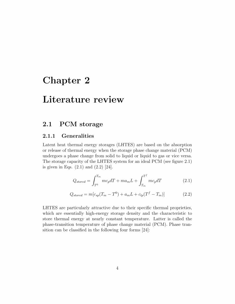
Latent heat thermal energy storages (LHTES) are based on the absorptionor release of thermal energy when the storage phase change material (PCM)undergoes a phase change from solid to liquid or liquid to gas or vice versa.The storage capacity of the LHTES system for an ideal PCM (see figure 2.1)is given in Eqs. (2.1) and (2.2) [24].

Qstored =

∫ Tm

T 0

mcpdT +mamL+

∫ T f

Tm

mcpdT (2.1)

Qstored = m[csp(Tm − T 0) + amL+ clp(Tf − Tm)] (2.2)

LHTES are particularly attractive due to their specific thermal proprieties,which are essentially high-energy storage density and the characteristic tostore thermal energy at nearly constant temperature. Latter is called thephase-transition temperature of phase change material (PCM). Phase tran-sition can be classified in the following four forms [24]:

4

• In solid–solid transitions, thermal energy is stored as the material istransformed from one crystalline phase to another. This storage phe-nomena has generally small latent heat and small volume changes thansolid–liquid transitions. However, solid–solid phase change materialsoffer the advantages of less severe container requirements and a greaterdesign flexibility.[24]. In the case of thermal storage applications, rela-tively few solid-solid PCMs with suitable heats of fusion and transitiontemperatures have been identified so far [14].

• Solid–gas and liquid–gas transitions have the highest latent heat ofphase transition, compared to the other methods. Their large volumechange during the phase transition is associated with containment prob-lems due to pressure rise [24]. They are therefore rarely considered forpractical applications [14].

• Solid–liquid transformations have smaller latent heat than liquid–gas.However, these transformations involve only a small change in volume.It is of the order of 10% or less [24].

The phase change from solid to liquid or vice versa is preferred because theoperating pressure is lower than liquid to gas or solid to gas phase changes[11]. In the following we will base our review exclusively on materials usedfor solid-liquid phase change.

2.1.2 Storage design

There are three basic components that all latent heat thermal energy storageshave in common [14]:

• A phase change material that undergoes the phase transition in aspecific operating temperature range and where the the thermal energyis stored as the latent heat of fusion (L).

• A container for the PCM.

• A heat exchanging surface for transferring thermal energy from theheat transfer fluid to the PCM and vice versa.

5

Therefore, the development of a LHTES system requires an excellent under-standing of two essentially subjects: heat storage materials (PCMs) and heatexchangers. A special design of the heat exchanger to be used is needed, dueto the low thermal conductivity of PCMs in general [24].

There are several storage designs developed over the years. The most commonconcept are:

Shell and tube

The shell and tube design is based on a (finned) heat exchanger placed intank containing the PCM [28]. A labscale prototype of the last design con-figuration is presented in section 2.1.7.

Macro-encapsulation

The macro-encapsulation storage design consists in the inclusion of PCM’ssuch as paraffin in form of small packages such as tubes, pouches, spheres,panels or other containers. They can serve directly as heat exchangers or canbe incorporated in building products [18].

Micro-encapsulation

Micro-encapsulation is characterized by the encapsulation of solid or liquidparticles of 1µm to 1000µm diameter with a solid shell. Physical processesusing this method are spray drying, centrifugal and fluidized bed processes,or coating processes e.g. in rolling cylinders [21]. Advantages of micro-encapsulation are the improvement of heat transfer to the HTF due to thelarge surface to volume ratio of the capsules. A potential drawback of micro-encapsulation is however the possible increase in subcooling chance [21]. Thesubcooling phenomena is presented in section 2.1.4.

2.1.3 Comparison to sensible heat storages

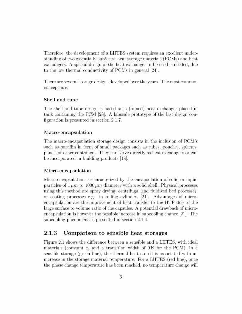
Figure 2.1 shows the difference between a sensible and a LHTES, with idealmaterials (constant cp and a transition width of 0 K for the PCM). In asensible storage (green line), the thermal heat stored is associated with anincrease in the storage material temperature. For a LHTES (red line), oncethe phase change temperature has been reached, no temperature change will

6

occur until all PCM has changed its phase. For temperatures different fromthe phase change temperature, the latent heat storage behaves like a sensiblestorage [22].

Figure 2.1: Comparison of sensible and latent heat storages in terms of tem-perature profile as a function of stored heat

In reality, the phase transition does not occur at a constant temperature(isothermal process), but in a certain temperature range, so that the hori-zontal line in figure 2.1 is a slightly increasing curve. For many materials,this transition temperature width is only of just a few degrees (about 10 K),so a nearly constant temperature profile can be archived around the phasechange temperature. Consequently, thermal systems needing rather smoothand constant supply temperature profiles benefit from this storage technol-ogy [22].

7

2.1.4 Subcooling

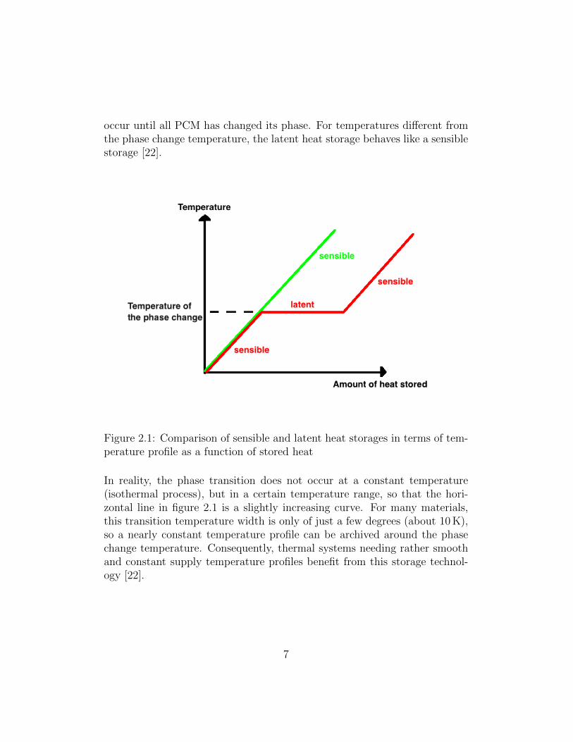
Many phase change materials do not solidify immediately when the melting/-solidification temperature is reached. Crystallization often occurs well belowthe melting temperature. This effect is called subcooling or supercooling. Itseffect on the temperature evolution is presented in figure 2.2 [21].

Figure 2.2: Effect of subcooling on a latent heat storage

During the melting process, there is no difference whether a PCM showssub-cooling or not. But during release of thermal energy, the latent heat isnot released when the melting temperature is reached due to subcooling. Itmakes it necessary to reduce the temperature well below the phase changetemperature to release the latent heat stored in the material. If nucleationdoes not happen at all, only sensible energy is stored and the latent heat offusion is not released at all. Subcooling can therefore be a serious problemin technical applications of PCM [21].

8

2.1.5 Phase change materials

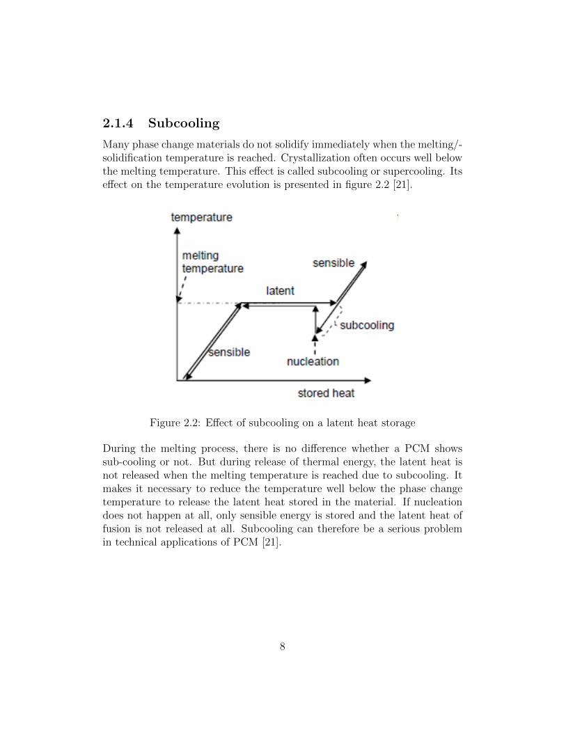
The selection a PCM for a particular application is guided by the operatingtemperature of the heating or cooling and should be matched to the PCMtransition temperature. Furthermore, the latent heat should be as high aspossible, to limit the storage size. High thermal conductivity would providehigher charging and discharging rates of the stored energy.Nowadays a large number of phase change materials are available in any re-quired temperature range [24].A classification of PCMs is given in figure 2.3.

Figure 2.3: Classification of energy storage materials [7]

As no single PCM can have all properties for an ideal storage media, theavailable materials have to be used and it has to be tried to compensatethe poor material properties by an appropriate storage design. For examplemetallic fins can be implemented into the storage to increase the thermalconductivity of the storage material [24].

9

PCM can be divided into the following main classes:

1. Organic PCMsOrganic materials are classified as paraffin and non-paraffins:

• Paraffin wax consists of a mixture of n-alkanes of the type

CH3–(CH2)n–CH3

Both the phase transition temperature and latent heat increasewith chain length [24].

• The non-paraffin organic are among the phase change materialsthe most numerous class. Unlike the paraffins which have verysimilar properties, each of these materials have its own specificproperties. The largest part of the class is composed of Esters,fattyacids, alcohol’s and glycol’s [24].

Organic materials are characterized by congruent melting, meaningthe propriety of repeated melting and freezing without phase segre-gation and subsequent degradation of the latent heat of fusion. Fur-thermore they crystallize with little or no subcooling and are usuallynon-corrosive [24].

2. Inorganic PCMs

Inorganic materials are further classified as salt hydrate and metallics.These phase change materials show little and there is no degradationof heat of fusion with cycling [24].

• Salt hydrates are made of alloys of inorganic salts and waterforming a crystalline solid. Its general formula is AB-nH2O. Thesolid–liquid transformation of salt hydrates consists in a dehydra-tion of the salt, although this process is comparable with ther-modynamic melting or solidification. At the melting point the

10

hydrate crystals breakup into a lower hydrate and water [24]:

AB-nH2O → AB-mH2O + (n−m)H2O

or anhydrous salt and water:

AB-nH2O → AB + n H20

One problem with the most salt hydrates is the fact that the re-leased water from the crystallization process is not sufficient todissolve all the present solid phase. Due to density difference, thelower hydrate settles down at the bottom of the container. Thiseffect is called phase separation and consists in the main source ofproblem for the implementation of this PCM type [24].

• Metallics: This category contains the low melting metals andmetal eutectic. Due to their high weight and cost, these metallicshave not yet been seriously considered as phase change materials.However, when volume reduction is a main issue, they are goodalternative because of the high heat of fusion [24].

3. EutecticsAn eutectic is a composition of two or more materials. In the caseof their utilization as phase change materials, eutectics nearly alwaysmelt and freeze without segregation. Since they solidify to an intimatemixture of crystals, they leave little opportunity for the components toseparate. During the melting process, both components liquefy simul-taneously, again without separation [24].

2.1.6 Applications

The applications of PCM storages can be divided into two main groups:thermal protection or inertia and energy storage. The main differencebetween the two fields relates to the thermal conductivity of the phase changematerial. In several applications in thermal protection it is appropriate tohave low conductivity values, where as in storage systems low conductivityvalues can cause real problems since the capacity to absorb or release the

11

thermal energy is highly limited [27].The most common applications where PCM are considered or already in useare [15] [27] [28]:

• Ice storages for HVAC applications

• Concentrated solar power

• Waste heat recovery in industrial processes

• Solar thermal systems

• Conservation and transport of temperature sensitive materials (food,etc.)

• Building applications (PCM integrated in walls, ceilings, etc.)

2.1.7 Laboratory prototype PCM storage

In the following section, a lab-scale shell and tube latent heat storage proto-type is presented. It has been developed at the sustainable thermal energysystem department of the Austrian Institute of Technology (AIT) in Vienna,Austria. Several measurement experiment have been realized by the labo-ratory staff. The results are used to validate the numeric storage modelsdeveloped in the frame of this thesis. An in-depth discussion of the measure-ments are important for the validation understanding.A full documentary of this storage prototype can be found in [28].

Storage design

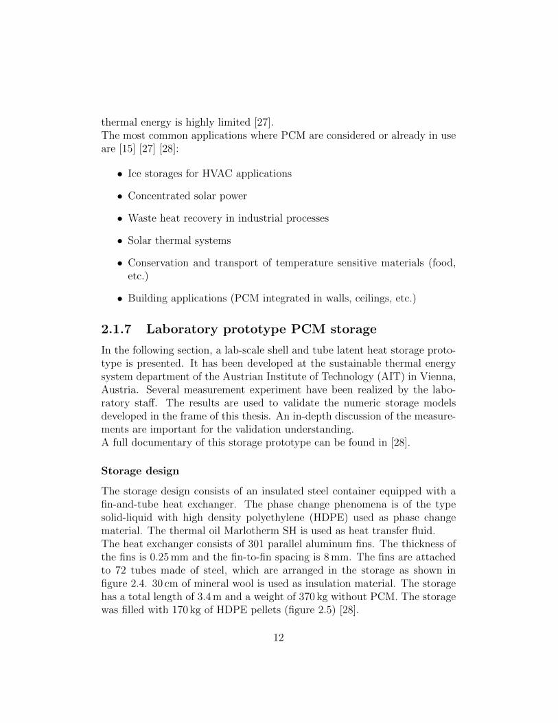
The storage design consists of an insulated steel container equipped with afin-and-tube heat exchanger. The phase change phenomena is of the typesolid-liquid with high density polyethylene (HDPE) used as phase changematerial. The thermal oil Marlotherm SH is used as heat transfer fluid.The heat exchanger consists of 301 parallel aluminum fins. The thickness ofthe fins is 0.25 mm and the fin-to-fin spacing is 8 mm. The fins are attachedto 72 tubes made of steel, which are arranged in the storage as shown infigure 2.4. 30 cm of mineral wool is used as insulation material. The storagehas a total length of 3.4 m and a weight of 370 kg without PCM. The storagewas filled with 170 kg of HDPE pellets (figure 2.5) [28].

12

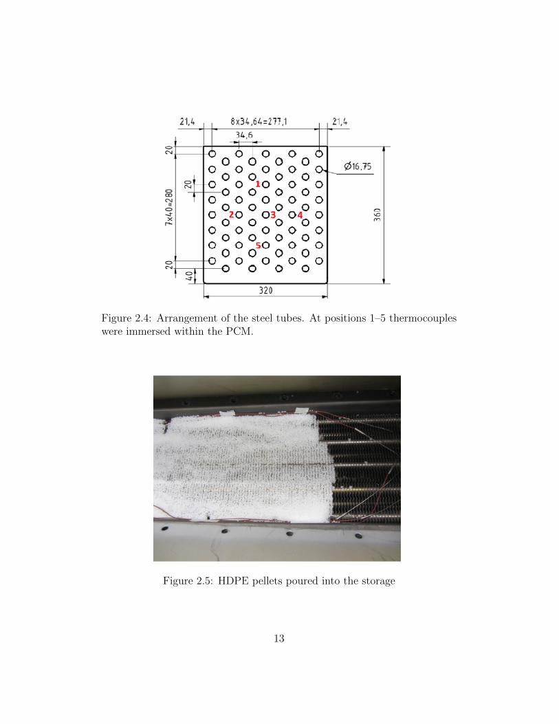
Figure 2.4: Arrangement of the steel tubes. At positions 1–5 thermocoupleswere immersed within the PCM.

Figure 2.5: HDPE pellets poured into the storage

13

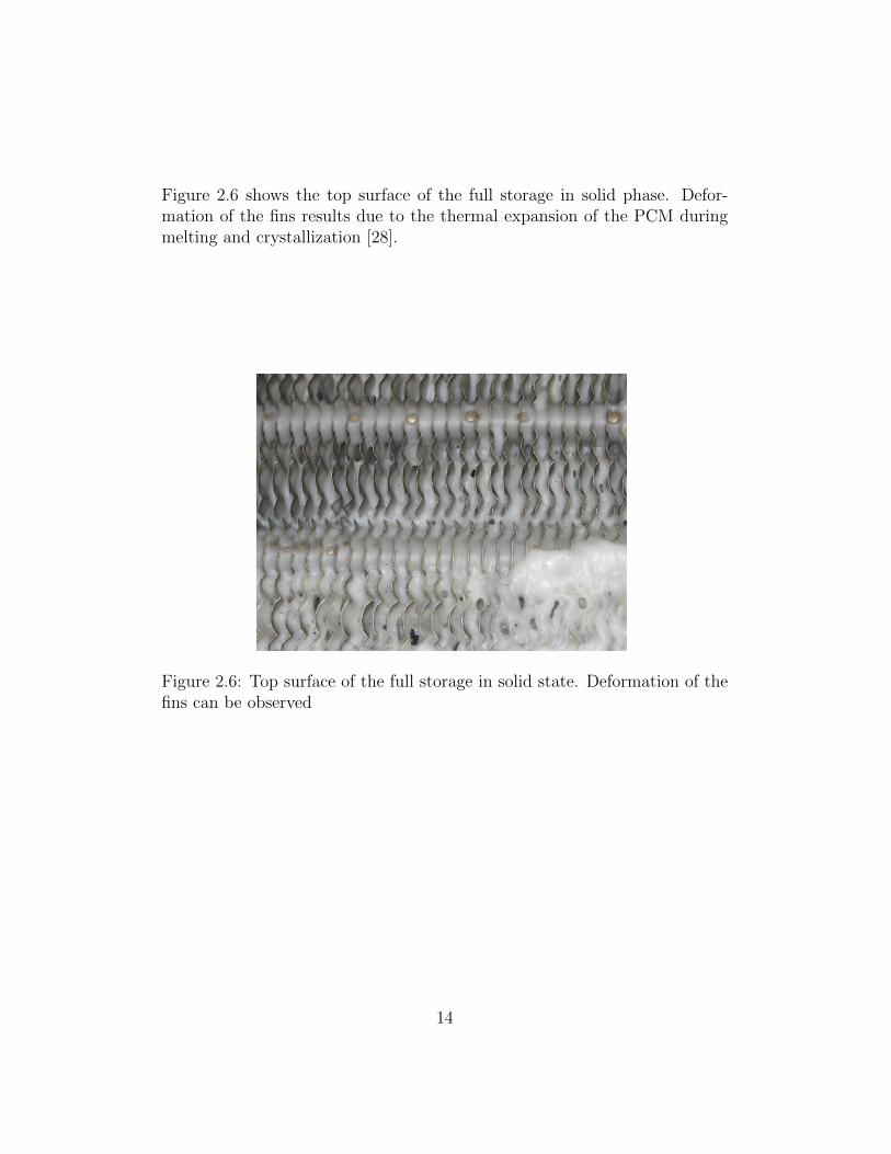
Figure 2.6 shows the top surface of the full storage in solid phase. Defor-mation of the fins results due to the thermal expansion of the PCM duringmelting and crystallization [28].

Figure 2.6: Top surface of the full storage in solid state. Deformation of thefins can be observed

14

Polymers as phase change materials

Polymers as phase change materials have rarely been used in latent heat stor-ages up to now. However, this material class has some interesting advantages[28]:

• Large industrial availability ensuring high material quality

• Low material prize, especially for commodity plastics

• An existing professional recycling industry causing further material costreduction

• Chemical and physical properties can be modified by compoundingadditives into the raw polymer

Especially high density polyethylene (HDPE) turned out to be suitablefor this application frame because of its high enthalpy, prize and large-scaleavailability [28].

Experimental setup

To characterize the storage, it was connected to a thermostat (Lauda ITH350).Inlet and outlet temperatures were measured using resistance thermome-ters and the mass flow was recorded with a clamp-on ultrasonic flow meter(Flexim Fluxus F601). The PCM temperatures were measured by thermo-couples in four equidistant layers along the length-axis of the storage, eachlayer contains 5 sensors as illustrated in in figure 2.4 [28].

Figure 2.7 shows measurement results where the storage was charged from105 ◦C to 155 ◦C and discharged from 155 ◦C to 105 ◦C at a constant massflow of 0.41 kg/s.The resulting plateaus, which are typical for a LHTES, at the melting tem-perature can clearly be observed [28].

15

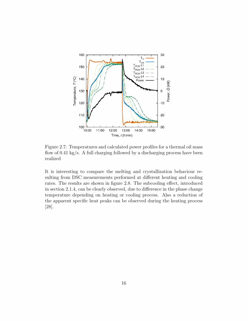
Figure 2.7: Temperatures and calculated power profiles for a thermal oil massflow of 0.41 kg/s. A full charging followed by a discharging process have beenrealized

It is interesting to compare the melting and crystallization behaviour re-sulting from DSC measurements performed at different heating and coolingrates. The results are shown in figure 2.8. The subcooling effect, introducedin section 2.1.4, can be clearly observed, due to difference in the phase changetemperature depending on heating or cooling process. Also a reduction ofthe apparent specific heat peaks can be observed during the heating process[28].

16

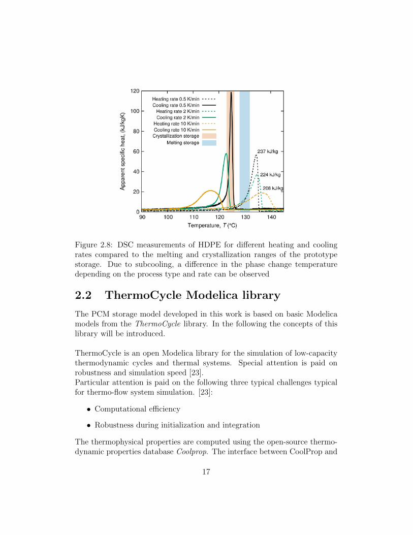
Figure 2.8: DSC measurements of HDPE for different heating and coolingrates compared to the melting and crystallization ranges of the prototypestorage. Due to subcooling, a difference in the phase change temperaturedepending on the process type and rate can be observed

2.2 ThermoCycle Modelica library

The PCM storage model developed in this work is based on basic Modelicamodels from the ThermoCycle library. In the following the concepts of thislibrary will be introduced.

ThermoCycle is an open Modelica library for the simulation of low-capacitythermodynamic cycles and thermal systems. Special attention is paid onrobustness and simulation speed [23].Particular attention is paid on the following three typical challenges typicalfor thermo-flow system simulation. [23]:

• Computational efficiency

• Robustness during initialization and integration

The thermophysical properties are computed using the open-source thermo-dynamic properties database Coolprop. The interface between CoolProp and

17

Modelica is based on the Coolprop2Modelica library, a modified version ofthe ExternalMedia library [23] [2].

The intention of the library is to furnish a entirely open-source solution forthe computation of thermophysical substance properties, using CoolProp,and the simulation of complex thermodynamic systems with their controlstrategy. Compared to similar libraries used in the modelling of thermo-flowsystems as for example ThermoPower or ThermoSysPro, the ThermoCyclelibrary contains diverse models dedicated to the model small-scale thermalsystems, such as volumetric compressors used in simulations of heat pumpor refrigeration cycles.The key features of the library are the following [23]:

• Designed for system level simulations

• Full compatibility with other Modelica libraries due to the use of streamconnectors

• Ability to handle reverse flows and flow reversals

• Various numerical robustness strategies implemented in the compo-nents and accessible through Boolean parameters

• Limited levels of hierarchical modelling causing high model readability

The components provided in the library are designed to be as generic aspossible [23].The full documentation of the ThermoCycle library can be found in [23].

18

2.3 Application: BRICKER CSP-biomass plant

The PCM storage model developed in this work is integrated into a practicalapplication to analyse the resulting differences in terms of system behaviour.Especially thermal solar plants can increase their efficiency by using a ther-mal storage dedicated to balance the differences between supply and demandof solar power. A review of different types of thermal storages used in hightemperature solar plants for power generation can be found in [20].The use of a PCM storage gives the advantage of a lower storage volume dueto the high energy density and a nearly isothermal storage outlet temperatureprofile (see section 2.1.5). Latter argument is beneficial for system componentneeding constant supply temperatures, as for example ORC power genera-tors. Furthermore, the investment costs for a PCM storage are possibly lowerthan for sensible large thermal-oil tanks or molten salt storages.

2.3.1 Generalities

In the last decades, concentrated solar power (CSP) systems have been in-creasingly considered worldwide as a key technology for meeting the renew-able energy demand [12]. The total current CSP capacity is still small dueto the large investment costs. Only 3.6 GWel were installed by the end of2013 [12]. One approach to attain competitiveness to other power plantssystems consists in hybridization with a second source of energy [12]. It hasnot only the benefit of a cost reduction but it also provides thermal powercontinuity when the solar source is unavailable during night or on cloudyday. Several plants worldwide have demonstrated the advantages of this so-lution [12]. In regard of the renewable power generation, the hybridization ofCSP technology with biomass has gained attention. Recently, CHP systemsusing organic Rankine cycle (ORC) technology integrated with an hybridCSP-biomass heat source, have been investigated [12]. In order to stimu-late the development of such technologies, the European Union founded theBRICKER project. It aims to develop a scalable, replicable, high energy ef-ficient, zero emissions and cost effective CSP-Biomass trigeneration system,based on ORC technology, to refurbish existing public-owned non-residentialbuildings. The CHP unit together with lightweight facades, and phase changematerial insulation technology, is expected to reduce the building energy con-sumption by at least 50 % [1]. Three systems are being developed in Spain,

19

Belgium and Turkey to demonstrate the concept feasibility [12]. The systempresented in this work is situated in Cacares, Spain.

2.3.2 System background

As introduced in section 1.2, the system consists in a solar power (CSP)biomass combined heat and power (CHP) system based on organic Rankinecycle (ORC) technology, developed for building applications.The system is composed by two main loops as shown in figure 2.9.The first loop contains 4 mains components:

• Solar field (SF)

• biomass combustion boiler (BMB)

• Oil-water heat exchanger (HXI)

• ORC power block

Referring on figure 2.9, the heat transfer fluid is first preheated through theparabolic solar collectors of the solar field (a to b), characterized by a totalcollector area of 54 m2 [12].The thermal oil TherminolSP, is selected as heat transfer fluid. It is mainlyused for CSP applications thanks to its low operating pressure, high thermalstability (up to 335 ◦C) and good heat transfer characteristics[12].The preheated HTF (thermal oil) is heated up the nominal ORC temperaturein a biomass combustion boiler (d to e). It is then transferred to the ORCsystem for electricity production (h) and to the oil-water heat exchanger (fto g) delivering additional heat to the second loop [12].

Loop II comprises following components:

• Absorption chiller

• ORC condenser cooling side

• Secondary side of HXI

• Connection to the thermal load of the building

20

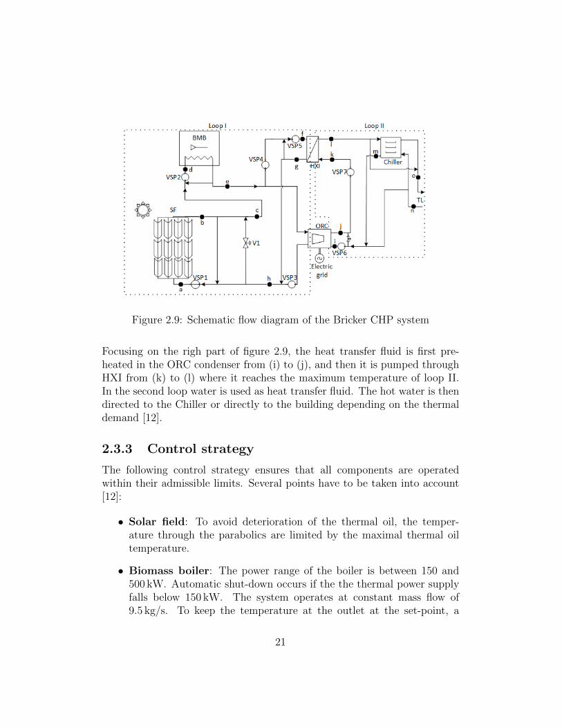
Figure 2.9: Schematic flow diagram of the Bricker CHP system

Focusing on the righ part of figure 2.9, the heat transfer fluid is first pre-heated in the ORC condenser from (i) to (j), and then it is pumped throughHXI from (k) to (l) where it reaches the maximum temperature of loop II.In the second loop water is used as heat transfer fluid. The hot water is thendirected to the Chiller or directly to the building depending on the thermaldemand [12].

2.3.3 Control strategy

The following control strategy ensures that all components are operatedwithin their admissible limits. Several points have to be taken into account[12]:

• Solar field: To avoid deterioration of the thermal oil, the temper-ature through the parabolics are limited by the maximal thermal oiltemperature.

• Biomass boiler: The power range of the boiler is between 150 and500 kW. Automatic shut-down occurs if the the thermal power supplyfalls below 150 kW. The system operates at constant mass flow of9.5 kg/s. To keep the temperature at the outlet at the set-point, a

21

recirculation circuit and an internal control which regulates the amountof biomass burned is implemented.

• ORC unit: A constant temperature at the evaporator of 245 ◦C witha maximal deviation of 20 K as well as constant mass flow of 2.5 kg/sis required.

• Absorption chiller: As for the ORC system, a constant supply tem-perature with a maximal deviation of 5 K can be handled. A propercontrol of the oil-water heat exchanger is required to respect the bound-aries.

In general, high control of the solar field is needed to insure safe biomassboiler operation in order to avoid a biomass shut-down. As shown in figure2.9, The solar field is equipped with a recirculation and a bypass stream toreach this objective. The fluid valve regulating the mass flow in the bypassstream is controlled by the boiler inlet temperature. The bypass is activatedif the biomass supply temperature exceeds the maximal temperature leadingto shut-down. By activating the solar field bypass, the thermal oil recirculatesin the collectors tubes due to the pump VSP1 which circulates at constantmass flow [12].When the outlet temperature of the solar field overpasses the set-point, auto-matic defocusing of the parabolic collectors occurs, reducing the solar powergeneration [12].In the case, the heat rejected from the ORC’s condenser is not sufficient tosatisfy the thermal load of the building, extra power has to be supplied to thesecond loop via the additional oil-water heat exchanger HXI. A temperaturesensor in point (l) controls heat exchange rate in HXI via pump VSP4 inorder to respect the set point for the absorption chiller supply. Using VSP5at constant speed in combination with a recirculation circuit, constant massflow in HXI is obtained [12].

22

Chapter 3

Numeric modelling

3.1 Discretized PCM storage model

In the following a white-box discretized model of the shell and tube LHTESdescribed in section 2.1.7 is presented. It is a white box model based on phys-ical material parameters and heat transfer processes. All simulated variablesrepresent realistic physical values.The model considers convective heat transfer between HTF and the tubewall, heat conduction in axial direction in the tube, heat exchange with thePCM and thermal conduction in radial and axial direction inside the PCM.The phase change phenomena is modelled using an apparent heat capacitymethod with two different models [25]. It describes the specific heat capacityof the PCM as a function of temperature with a significant increasing aroundthe melting temperature. A detailed method description can be found in sec-tion 3.1.3.For all tubes, equal mass flow of the HTF and equal temperature distribu-tion on the shell and tube side has been considered. Therefore, only onetube is considered in the model and boundary effects near to the limit of thestorage device, e.g. energy losses to the surrounding, are ignored [25]. Thealuminum fins are taken into account only indirectly by an increase in thethermal conductivity of the PCM. Concerning the thermal capacity of thefins, it is lumped into the thermal capacity of the tube wall.

Figure3.1 schematizes the main ideas of the model set-up. The storage isdivided into equal cuboids, one for each HTF tube, see sub-figure (1). As

23

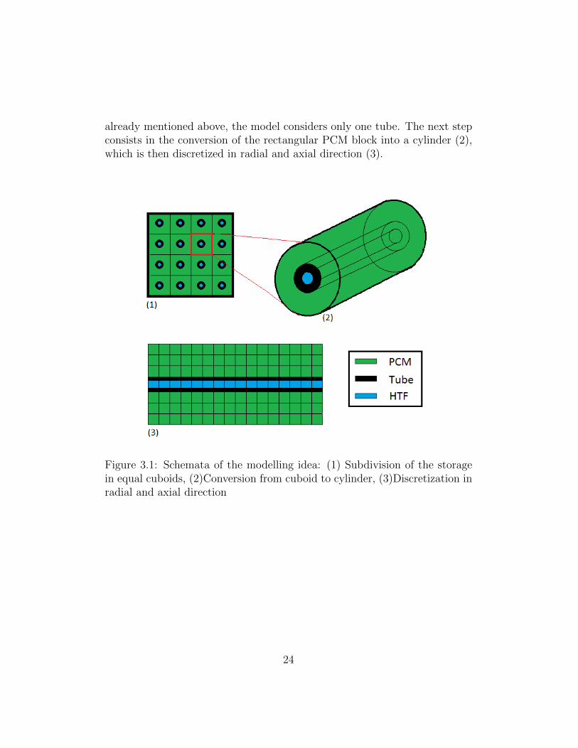
already mentioned above, the model considers only one tube. The next stepconsists in the conversion of the rectangular PCM block into a cylinder (2),which is then discretized in radial and axial direction (3).

Figure 3.1: Schemata of the modelling idea: (1) Subdivision of the storagein equal cuboids, (2)Conversion from cuboid to cylinder, (3)Discretization inradial and axial direction

24

3.1.1 Heat transfer fluid (HTF) model

The forced convective mass flow of the HTF in the tube is modelled in theaxial direction x. Heat transfer to the tube inner wall is considered only. Ra-dial fluid flow, axial heat conduction in the fluid, viscous dissipation, externalforces and compressibility have been neglected [10] [25]. The internal energyequation in Eq. (3.1) is expressed in terms of HTF temperature TH withdu = cp(T )dT using specific heat capacity for incompressible fluids cp ≈ cv.

ρHcp,H∂TH∂t

= −vHρHcp,H∂TH∂x− 2

rinqH (3.1)

The initial and boundary conditions for Eq. (3.1) are:

TH(t = 0, x) = T 0H(x), TH(t, x = 0) = T su

H (t) (3.2)

Furthermore, the fluid velocity vH depends on the mass flow mH,total:

vH =mH,total

nTπ(rin)2ρH(3.3)

It has to be noted that in Eq. (3.1) density changes, induced by local tem-perature changes, are neglected [25]. In Eqs. (3.1) and (3.3), rin presents thetube inner radius.

Heat transfer

qH represents the heat flux density, i.e. the heat transfer from fluid to thetube. qH is calculated using the heat transfer coefficient U:

qH = U(TH − TW ) (3.4)

In Eq. (3.4), TH and TW are the HTF and inner tube wall temperatures atthe axial position x, respectively. The heat transfer coefficient U is calculatedfrom the dimensionless numbers and correlations for forced convective heattransfer inside a tube introduced below [26] [25].

Nu =U · dinλH

, Re =vH · dinνH

, Pr =νH · ρH · cp,H

λH(3.5)

25

In Eq. (3.5), din = 2rin, λH is the thermal conductivity and νH is thekinematic viscosity of the HTF. Except for ρH(T ) all other HTF proper-ties are temperature dependent. The corresponding correlations are given inEqs.(3.6) to (3.9) where T is the temperature in [◦C] [25].

ρH = c1T + c2 [kg/m3], with c1 = −0.71482, c2 = 1058.4 (3.6)

cp,H = c1T + c2 [J/kgK], with c1 = 3.7263, c2 = 1474.5 (3.7)

λH = c1T + c2 [W/mK], with c1 = −0.00013184, c2 = 0.13326 (3.8)

µH = c1T−c2 · 10−6 [m2/s], with c1 = 10113, c2 = 1.755 (3.9)

The coefficients result from a fitting of the HTF thermophysical propertiesto measured data taken from product information.

The local Nusselt number for fully developed turbulent flow with Re ≥ 104

is [26]:

Nux =(ξ/8)Re Pr

1 + 12.7√ξ/8(Pr2/3 − 1)

[1 +

1

3(din/x)2/3

]with ξ = (1.8 log10Re11.5)−2

(3.10)

The local Nusselt number at any point x in a pipe with laminar flow (Re ≤2300) reads [26]:

Nux,T =

{(3.66)3+(0.7)3+

[1.077 3

√Re Pr(din/x)−0.7

]3

+

[1

2

( 2

1 + 22Pr

)1/6

(Re Pr din/x)1/2

]3}1/3

(3.11)

In the transition region between laminar and turbulent flow with 2300 ≤ Re≤ 104 the local Nusselt number is:

26

Nu = (1− γ)Nulam,2300 + γNuturb,104

with γ =Re− 2300

104 − 2300, 0 ≤ γ ≤ 1

(3.12)

In Eq. (3.12), the local value of Nulam,2300 is calculated using Eq. (3.11) withRe=2300 and Nuturb,104 is calculated from Eq. (3.10) with Re=104.

Implementation in Modelica

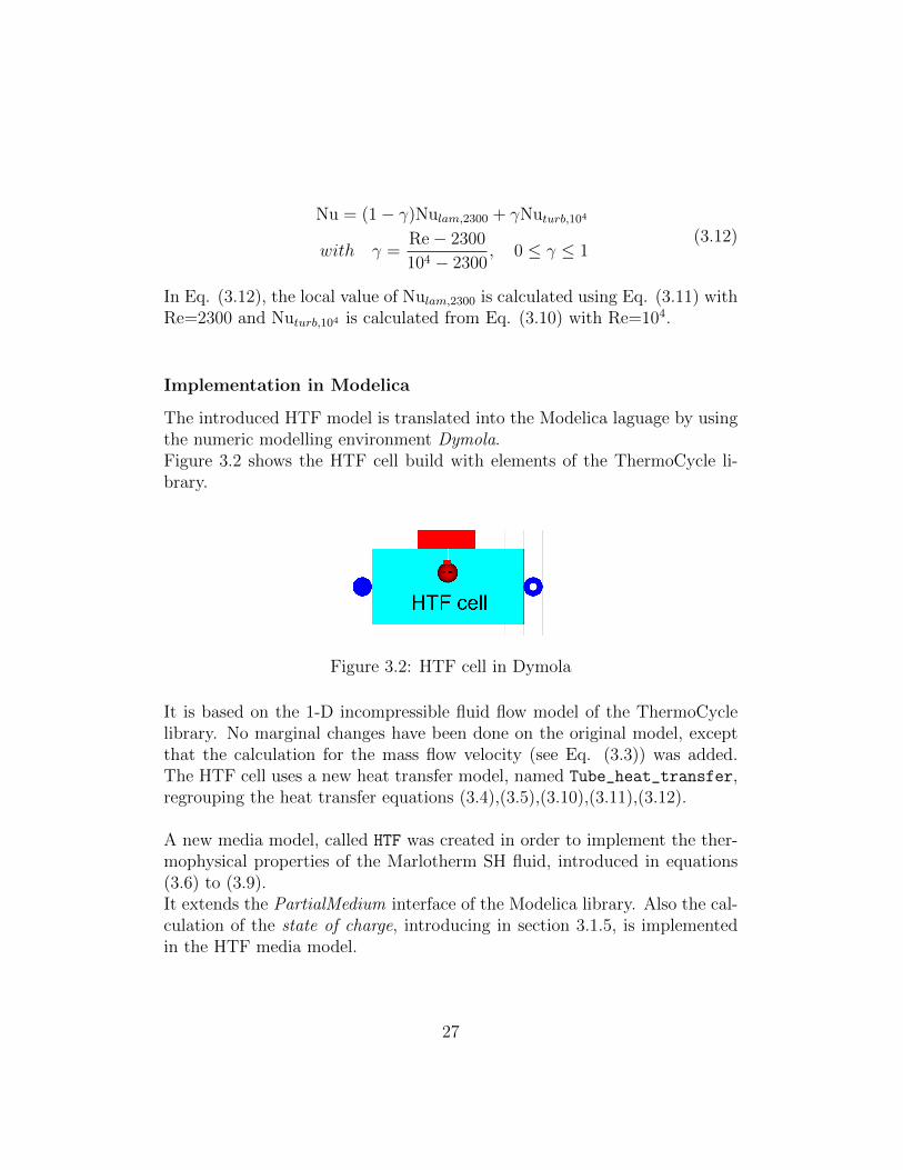
The introduced HTF model is translated into the Modelica laguage by usingthe numeric modelling environment Dymola.Figure 3.2 shows the HTF cell build with elements of the ThermoCycle li-brary.

Figure 3.2: HTF cell in Dymola

It is based on the 1-D incompressible fluid flow model of the ThermoCyclelibrary. No marginal changes have been done on the original model, exceptthat the calculation for the mass flow velocity (see Eq. (3.3)) was added.The HTF cell uses a new heat transfer model, named Tube_heat_transfer,regrouping the heat transfer equations (3.4),(3.5),(3.10),(3.11),(3.12).

A new media model, called HTF was created in order to implement the ther-mophysical properties of the Marlotherm SH fluid, introduced in equations(3.6) to (3.9).It extends the PartialMedium interface of the Modelica library. Also the cal-culation of the state of charge, introducing in section 3.1.5, is implementedin the HTF media model.

27

3.1.2 Tubes and fines models

The wall temperature TW is modelled assuming a constant temperature inradial direction, so that there is no temperature gradient in the tube wall inradial direction. Heat conduction in axial direction and heat transfer at theinner and outer tube wall are considered only.The internal energy equation, Eq. (3.13), is expressed in terms of the tubewall temperature TW and the inner energy du = cp(T )dT [25].

(Aρcp)W∂TW∂t

= AT∂

∂x

(λT∂TW∂x

)+2π(rinqH − routqP ) (3.13)

The initial and boundary conditions are:

TW (t = 0, x) = T 0W (x), λT

∂TW∂x

∣∣∣∣t,x=0

= 0, λT∂TW∂x

∣∣∣∣t,x=L

= 0 (3.14)

The heat capacity of the fins is added to the heat capacity of the tube wall:(Aρcp)W = (ATρT cp,T + AFρF cp,F ), with the subscripts T and F indicat-ing the tube and fin, respectively. AT and AF are the corresponding cross-sectional areas. In Eq. (3.13), λT corresponds to the thermal conductivitycoefficient of the tube, qH and qP represent heat flux densities from the HTFto the tube inner wall (see Eq. (3.4)) and from the wall to the PCM (see Eq.(3.15)), respectively. Finally, rin is the inner and rout the outer tube radius.

qP = λP∂TP∂r

∣∣∣∣r=rout

(3.15)

All properties are temperature dependent with correlations given in Eqs.(3.16)-(3.18). TThe coefficients have been determined by fitting the proper-ties to measured data from hf-DSC and Laser Flash Analysis [25]:

ρT = c1T + c2 [kg/m3], with c1 = −0.3067, c2 = 7718.19 (3.16)

cp,T = c1T + c2 [J/Kg/K], with c1 = 0.4188, c2 = 338.96 (3.17)

28

λT = 50 [W/m/K] (3.18)

Implementation in Modelica

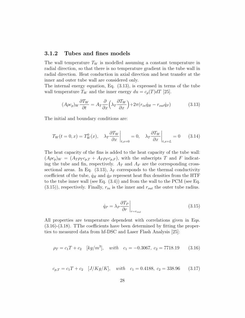
Figure 3.3 shows the tube wall cell model in Dymola environment.

Figure 3.3: Tube wall cell in Dymola

The tube wall cell possess four heat ports for the heat transfer in radial (topand bottom port) and axial (right and left port) direction. The componentis based on the MetalWallL model of the ThermoCycle library, representinga lumped tube of solid material.Axial conductive heat transfer described by λT has been added. ThereforeEq. (3.13) is discretized in axial direction using a central difference scheme.

Figure 3.4 schematizes the discretization of the tube wall.

The resulting heat flux in axial direction is given by Eq. (3.19):

qi,i+1W,ax =

λT∆x/2

(T i,i+1W − T i

W ) with ∆x = lcell =lhexNax

(3.19)

Where lhex, the total length of the heat exchanger tube and Nax the dis-cretization rate or number of cells in axial direction.

In addition to the heat transfer, calculations for the heat exchange surfacesof the tube wall have been added. There are three exchange surfaces:

- Arad,in: Inner tube surface, used for radial heat transfer HTF-Tube

Arad,in = π · din · lcell (3.20)

29

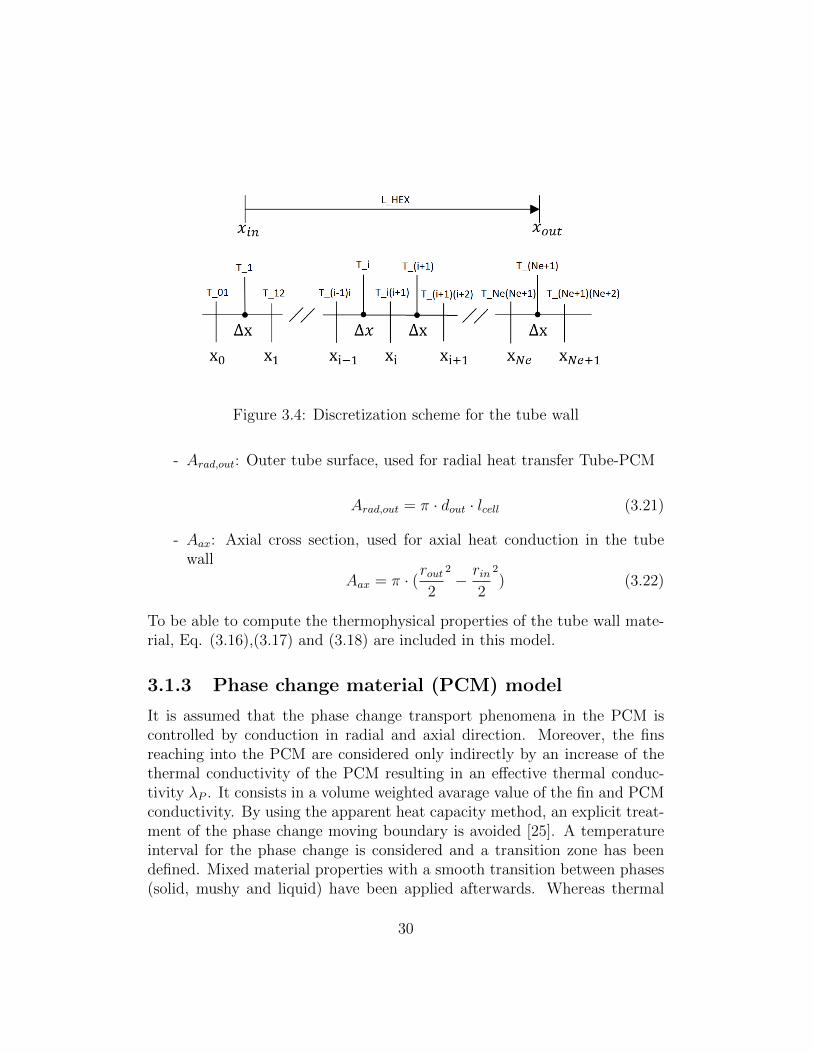
Figure 3.4: Discretization scheme for the tube wall

- Arad,out: Outer tube surface, used for radial heat transfer Tube-PCM

Arad,out = π · dout · lcell (3.21)

- Aax: Axial cross section, used for axial heat conduction in the tubewall

Aax = π · (rout2

2

− rin2

2

) (3.22)

To be able to compute the thermophysical properties of the tube wall mate-rial, Eq. (3.16),(3.17) and (3.18) are included in this model.

3.1.3 Phase change material (PCM) model

It is assumed that the phase change transport phenomena in the PCM iscontrolled by conduction in radial and axial direction. Moreover, the finsreaching into the PCM are considered only indirectly by an increase of thethermal conductivity of the PCM resulting in an effective thermal conduc-tivity λP . It consists in a volume weighted avarage value of the fin and PCMconductivity. By using the apparent heat capacity method, an explicit treat-ment of the phase change moving boundary is avoided [25]. A temperatureinterval for the phase change is considered and a transition zone has beendefined. Mixed material properties with a smooth transition between phases(solid, mushy and liquid) have been applied afterwards. Whereas thermal

30

conductivity and heat capacity are considered to vary with phases and tem-perature, constant density has been assumed. Thus, material velocity due todensity changes and their impact on the integration domain can be neglected[25].

The internal energy equation for the PCM is expressed in terms of the PCMtemperature TP and the apparent heat capacity as shown in Eq. (3.23 withdu = cP (T )dT . Thermal conduction in the PCM around the tube is consid-ered in radial and axial direction. For temperature dependent λP and cP ,we obtain in cylindrical coordinates [9][6]:

ρP cP∂TP∂t

=1

r

∂

∂r

(rλP

∂TP∂r

)+∂

∂x

(λP∂TP∂x

)(3.23)

A cylindrical PCM domain is considered ranging from the outer tube radiusrout to rend. The latter is determined from the cross-section of the storagefilled with PCM [25]:

rend =√Aap/Ntube/π + r2

out (3.24)

Eq. (3.23) is solved with the following initial and boundary conditions:

TP (t = 0, r) = T 0P (r), TP (t, r = rout) = TW (t),

λP∂TP∂r

∣∣∣∣t,r=rend

= 0, λP∂TP∂x

∣∣∣∣t,x=0

= 0, λP∂TP∂x

∣∣∣∣t,x=lhex

= 0(3.25)

The PCM properties ρP and λP change significantly for solid and liquid phase.However, in the model ρP is set to 850 kg/m3 (density variations neglected).The correlation for λP is given in Eq. (3.26). To determine the correlationcoefficients, PCM material properties have beenfitted to measured data from hf-DSC and laser flash analysis [25].

λP =c1

1 + exp(c4(T − c2))+ c3 [W/m/K]

with c1 = 0.41857, c2 = 96.162, c3 = 0.15406, c4 = 0.036647(3.26)

The correlation for the apparent specific heat capacity cP (TP ) reads:

31

cP = 1000(cp,P + b1φ), with cp,P = a0 + a1TP (3.27)

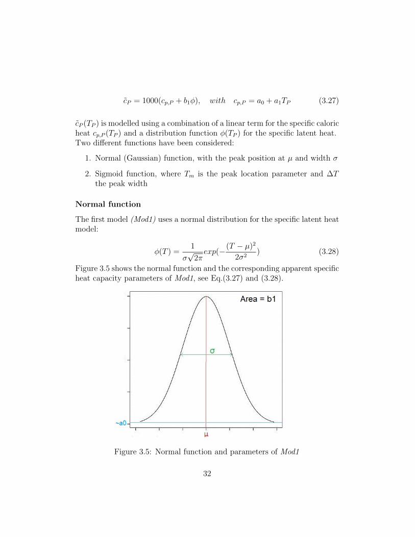
cP (TP ) is modelled using a combination of a linear term for the specific caloricheat cp,P (TP ) and a distribution function φ(TP ) for the specific latent heat.Two different functions have been considered:

1. Normal (Gaussian) function, with the peak position at µ and width σ

2. Sigmoid function, where Tm is the peak location parameter and ∆Tthe peak width

Normal function

The first model (Mod1) uses a normal distribution for the specific latent heatmodel:

φ(T ) =1

σ√

2πexp(−(T − µ)2

2σ2) (3.28)

Figure 3.5 shows the normal function and the corresponding apparent specificheat capacity parameters of Mod1, see Eq.(3.27) and (3.28).

Figure 3.5: Normal function and parameters of Mod1

32

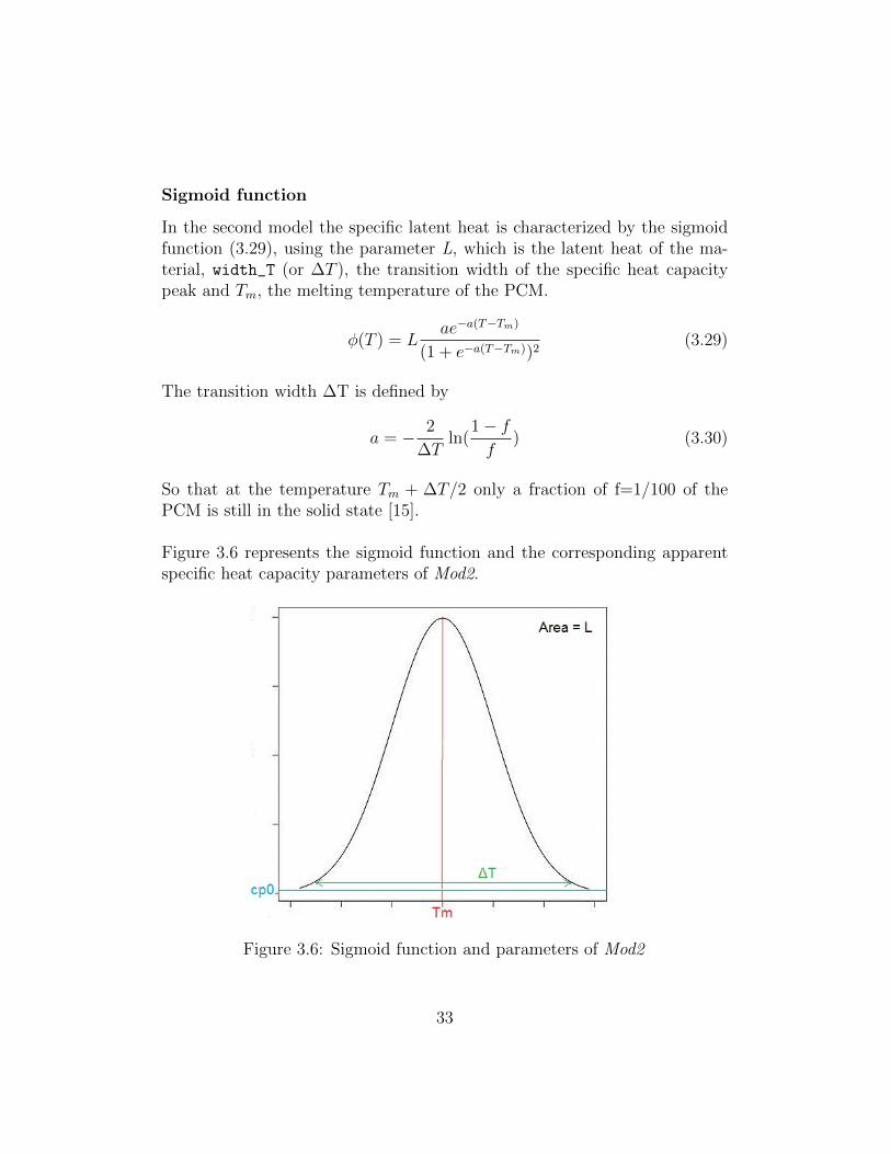
Sigmoid function

In the second model the specific latent heat is characterized by the sigmoidfunction (3.29), using the parameter L, which is the latent heat of the ma-terial, width_T (or ∆T ), the transition width of the specific heat capacitypeak and Tm, the melting temperature of the PCM.

φ(T ) = Lae−a(T−Tm)

(1 + e−a(T−Tm))2(3.29)

The transition width ∆T is defined by

a = − 2

∆Tln(

1− ff

) (3.30)

So that at the temperature Tm + ∆T/2 only a fraction of f=1/100 of thePCM is still in the solid state [15].

Figure 3.6 represents the sigmoid function and the corresponding apparentspecific heat capacity parameters of Mod2.

Figure 3.6: Sigmoid function and parameters of Mod2

33

Implementation in Modelica

Figure 3.7 shows the PCM cell model in the Dymola interface.

Figure 3.7: PCM cell in Dymola

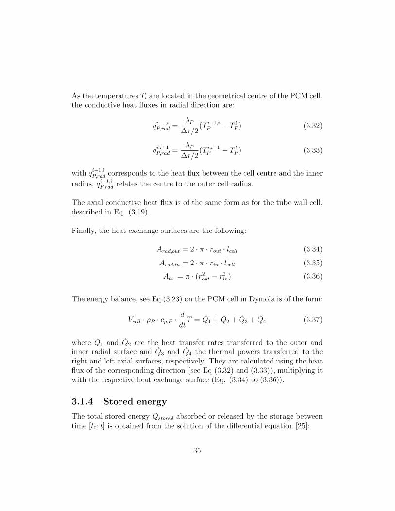
The PCM cell possesses four heat ports for the heat transfer in radial (topand bottom port) and axial (right and left port) direction. Unlike the tubewall model, heat conduction in radial direction is considered. Therefore Eq.(3.23) is discretized not only in axial but also in radial direction. The ax-ial discretization has been taken from the tube wall discretization, see Eq.(3.19), where λT is replaced by λP .A scheme of the radial discretization is shown in figure 3.8.

Figure 3.8: Radial discretization scheme

The PCM cell width in radial direction is given by

∆r = rout − rin (3.31)

34

As the temperatures Ti are located in the geometrical centre of the PCM cell,the conductive heat fluxes in radial direction are:

qi−1,iP,rad =

λP∆r/2

(T i−1,iP − T i

P ) (3.32)

qi,i+1P,rad =

λP∆r/2

(T i,i+1P − T i

P ) (3.33)

with qi−1,iP,rad corresponds to the heat flux between the cell centre and the inner

radius, qi−1,iP,rad relates the centre to the outer cell radius.

The axial conductive heat flux is of the same form as for the tube wall cell,described in Eq. (3.19).

Finally, the heat exchange surfaces are the following:

Arad,out = 2 · π · rout · lcell (3.34)

Arad,in = 2 · π · rin · lcell (3.35)

Aax = π · (r2out − r2

in) (3.36)

The energy balance, see Eq.(3.23) on the PCM cell in Dymola is of the form:

Vcell · ρP · cp,P ·d

dtT = Q1 + Q2 + Q3 + Q4 (3.37)

where Q1 and Q2 are the heat transfer rates transferred to the outer andinner radial surface and Q3 and Q4 the thermal powers transferred to theright and left axial surfaces, respectively. They are calculated using the heatflux of the corresponding direction (see Eq (3.32) and (3.33)), multiplying itwith the respective heat exchange surface (Eq. (3.34) to (3.36)).

3.1.4 Stored energy

The total stored energy Qstored absorbed or released by the storage betweentime [t0; t] is obtained from the solution of the differential equation [25]:

35

dQstored

dt= mH,total

∫ TH(x=L)

TH(x=0)

cp,H(T )dT, Qstored(t = 0) = Q0stored (3.38)

with Q0stored being the initial absorbed energy at time t=0.

3.1.5 State of charge

The state of charge (SOC) is a parameter which indicates the extend to whicha LHTES is charged relative to storable latent heat [25]. The values for SOCrange from 0 to 1 with 1 meaning the PCM is fully molten and 0 correspondsto solid PCM only. The local SOC(TP ) is obtained from the integration ofthe latent heat φ(TP ) in Eq. (3.27) [25].

SOC(TP ) =

∫ TP

−∞φ(T )dT with

∫ +∞

−∞φ(T )dT = 1 (3.39)

In time domain we get:

∂SOC(TP )

∂t=∂SOC(TP )

∂TP

∂TP∂t

= φ(TP )∂TP∂t

(3.40)

With TP and SOC being functions of r and x, the global SOCtot of thecomplete storage is computed as mean value by integration in radial andaxial direction [25].

dSOCtot

dt=

∫ L

0

∫ rend

rout

∂SOC(TP )∂t

r dr dx∫ L

0

∫ rendr dr dx

rout

, SOCtot(t = 0) = SOC0tot (3.41)

with SOC0tot being the initial state of charge at time t = 0.

Case of the Sigmoid functionThe Sigmoid function has the benefit that its integral is given by an ana-

lytic expression. As the integral of the specific latent heat gives the state ofcharge (see Eq. (3.39)), we get an analytic expression for the SOC expressedin Eq. (3.42)

SOC(T ) =1

L

∫ T

0

φ(T ′)dT ′ =1

1 + e−a(T−Tm)(3.42)

36

3.1.6 Model implementation in Modelica

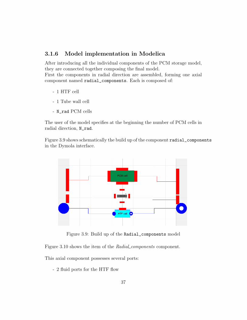
After introducing all the individual components of the PCM storage model,they are connected together composing the final model.First the components in radial direction are assembled, forming one axialcomponent named radial_components. Each is composed of:

- 1 HTF cell

- 1 Tube wall cell

- N_rad PCM cells

The user of the model specifies at the beginning the number of PCM cells inradial direction, N_rad.

Figure 3.9 shows schematically the build up of the component radial_componentsin the Dymola interface.

Figure 3.9: Build up of the Radial_components model

Figure 3.10 shows the item of the Radial components component.

This axial component possesses several ports:

- 2 fluid ports for the HTF flow

37

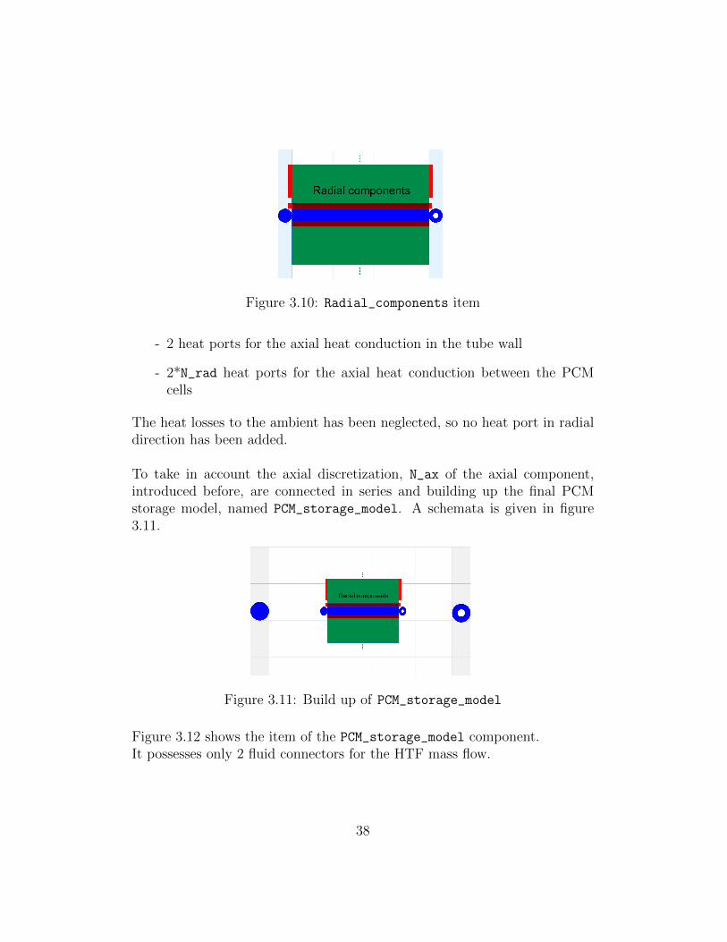
Figure 3.10: Radial_components item

- 2 heat ports for the axial heat conduction in the tube wall

- 2*N_rad heat ports for the axial heat conduction between the PCMcells

The heat losses to the ambient has been neglected, so no heat port in radialdirection has been added.

To take in account the axial discretization, N_ax of the axial component,introduced before, are connected in series and building up the final PCMstorage model, named PCM_storage_model. A schemata is given in figure3.11.

Figure 3.11: Build up of PCM_storage_model

Figure 3.12 shows the item of the PCM_storage_model component.It possesses only 2 fluid connectors for the HTF mass flow.

38

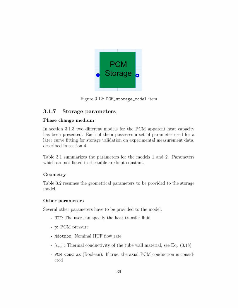
Figure 3.12: PCM_storage_model item

3.1.7 Storage parameters

Phase change medium

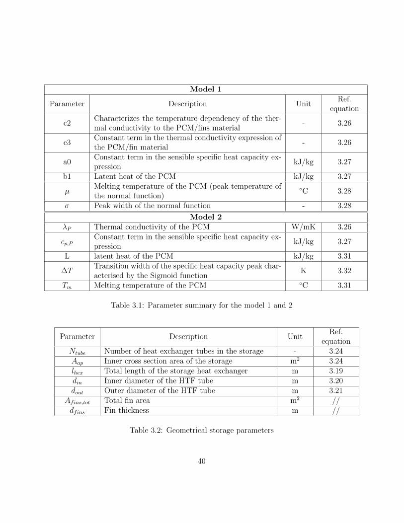
In section 3.1.3 two different models for the PCM apparent heat capacityhas been presented. Each of them possesses a set of parameter used for alater curve fitting for storage validation on experimental measurement data,described in section 4.

Table 3.1 summarizes the parameters for the models 1 and 2. Parameterswhich are not listed in the table are kept constant.

Geometry

Table 3.2 resumes the geometrical parameters to be provided to the storagemodel.

Other parameters

Several other parameters have to be provided to the model:

- HTF: The user can specify the heat transfer fluid

- p: PCM pressure

- Mdotnom: Nominal HTF flow rate

- λwall: Thermal conductivity of the tube wall material, see Eq. (3.18)

- PCM_cond_ax (Boolean): If true, the axial PCM conduction is consid-ered

39

Model 1

Parameter Description UnitRef.

equation

c2Characterizes the temperature dependency of the ther-mal conductivity to the PCM/fins material

- 3.26

c3Constant term in the thermal conductivity expression ofthe PCM/fin material

- 3.26

a0Constant term in the sensible specific heat capacity ex-pression

kJ/kg 3.27

b1 Latent heat of the PCM kJ/kg 3.27

µMelting temperature of the PCM (peak temperature ofthe normal function)

◦C 3.28

σ Peak width of the normal function - 3.28

Model 2λP Thermal conductivity of the PCM W/mK 3.26

cp,PConstant term in the sensible specific heat capacity ex-pression

kJ/kg 3.27

L latent heat of the PCM kJ/kg 3.31

∆TTransition width of the specific heat capacity peak char-acterised by the Sigmoid function

K 3.32

Tm Melting temperature of the PCM ◦C 3.31

Table 3.1: Parameter summary for the model 1 and 2

Parameter Description UnitRef.

equationNtube Number of heat exchanger tubes in the storage - 3.24Aap Inner cross section area of the storage m2 3.24lhex Total length of the storage heat exchanger m 3.19din Inner diameter of the HTF tube m 3.20dout Outer diameter of the HTF tube m 3.21

Afins,tot Total fin area m2 //dfins Fin thickness m //

Table 3.2: Geometrical storage parameters

40

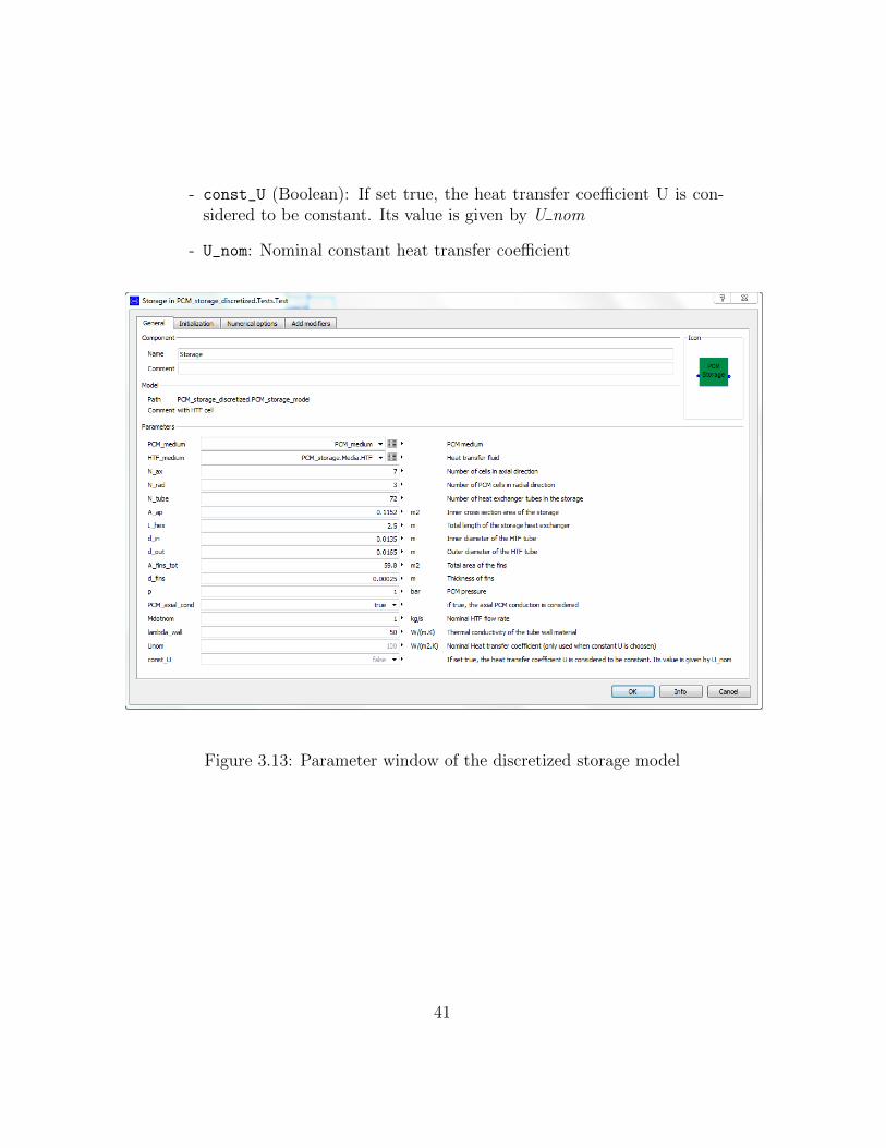
- const_U (Boolean): If set true, the heat transfer coefficient U is con-sidered to be constant. Its value is given by U nom

- U_nom: Nominal constant heat transfer coefficient

Figure 3.13: Parameter window of the discretized storage model

41

3.2 Single-node model

This section consists in the presentation of a grey-box single node modelof the same LHTES as for the white-box discretized model in the previouschapter.The difference consists in the fact that for this model, no discretization inaxial and radial direction is applied. Therefore, the PCM model is composedof only one axial component modelling the HTF, tube wall, PCM and heattransfer between.

This model consists in a grey-box model, meaning that the simulated ther-mal variables of the storage as well as the medium storage parameters don’trepresent the real physical values. The thermophysical processes in the stor-age interior can’t be predicted with this model, so a new storage cannot bedesigned based on this model.In the later model validation (see chapter 4.2), the parameters are adaptedso as the storage outlet temperature fits the measurement. Other internalthermal characteristics (PCM temperature, etc.) can’t be predicted by thismodel. In this case the discretized model must be used.The aim was to create a fast, simple and slim model which exterior charac-teristics (HTF oulet temperature) fit to existing storage characteristics.

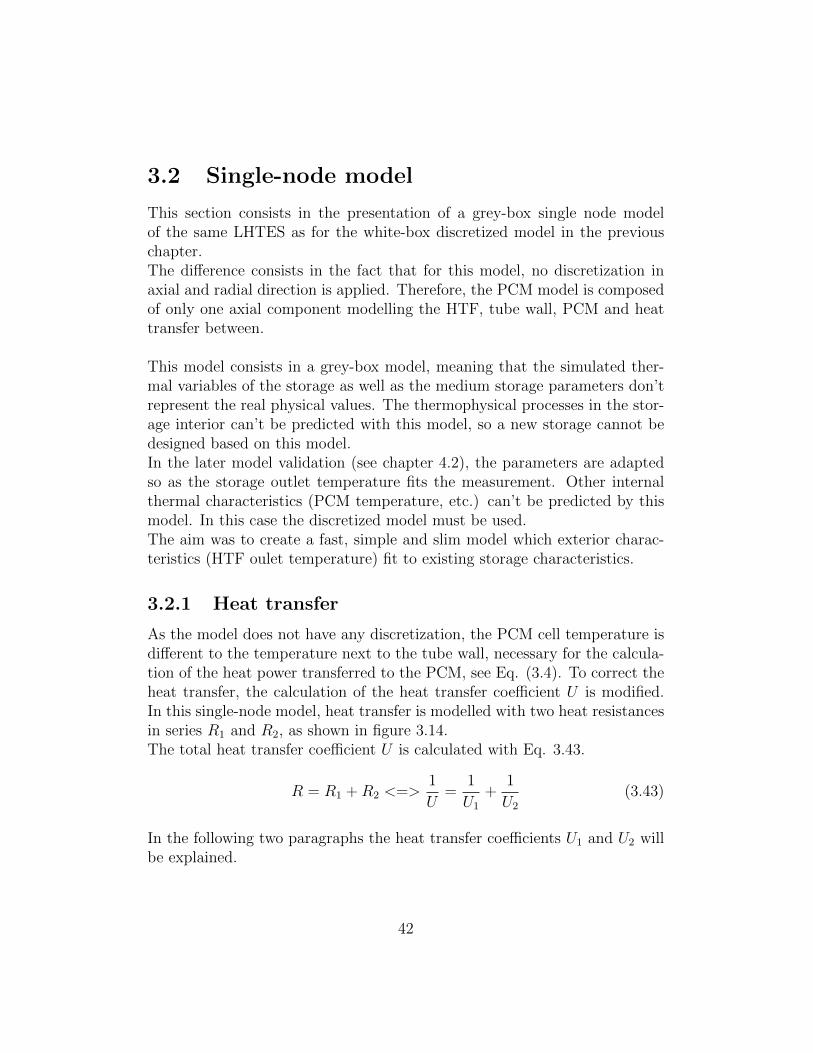
3.2.1 Heat transfer

As the model does not have any discretization, the PCM cell temperature isdifferent to the temperature next to the tube wall, necessary for the calcula-tion of the heat power transferred to the PCM, see Eq. (3.4). To correct theheat transfer, the calculation of the heat transfer coefficient U is modified.In this single-node model, heat transfer is modelled with two heat resistancesin series R1 and R2, as shown in figure 3.14.The total heat transfer coefficient U is calculated with Eq. 3.43.

R = R1 +R2 <=>1

U=

1

U1

+1

U2

(3.43)

In the following two paragraphs the heat transfer coefficients U1 and U2 willbe explained.

42

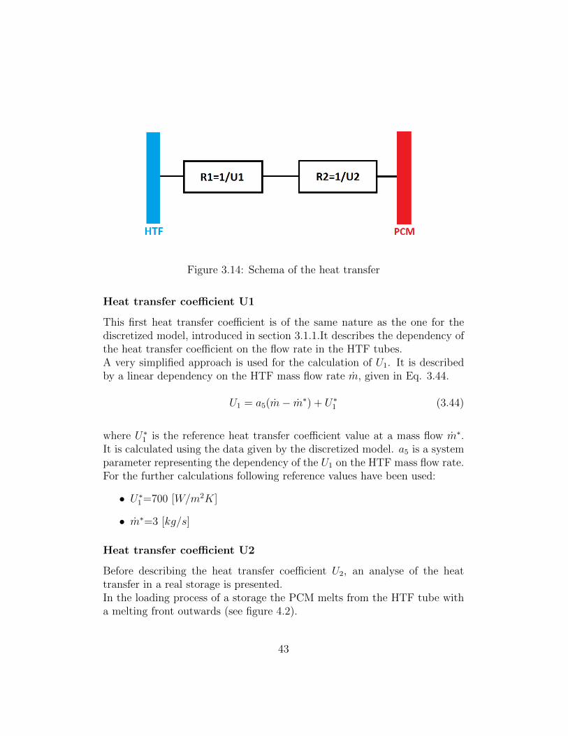
Figure 3.14: Schema of the heat transfer

Heat transfer coefficient U1

This first heat transfer coefficient is of the same nature as the one for thediscretized model, introduced in section 3.1.1.It describes the dependency ofthe heat transfer coefficient on the flow rate in the HTF tubes.A very simplified approach is used for the calculation of U1. It is describedby a linear dependency on the HTF mass flow rate m, given in Eq. 3.44.

U1 = a5(m− m∗) + U∗1 (3.44)

where U∗1 is the reference heat transfer coefficient value at a mass flow m∗.It is calculated using the data given by the discretized model. a5 is a systemparameter representing the dependency of the U1 on the HTF mass flow rate.For the further calculations following reference values have been used:

• U∗1 =700 [W/m2K]

• m∗=3 [kg/s]

Heat transfer coefficient U2

Before describing the heat transfer coefficient U2, an analyse of the heattransfer in a real storage is presented.In the loading process of a storage the PCM melts from the HTF tube witha melting front outwards (see figure 4.2).

43

As the temperature near the tube wall increases quickly over the melting tem-perature, the thermal power transferred to the PCM decreases. The morePCM is in molten state (high SOC), the more decreases the power deliveredto the PCM. Figure 3.15 shows this behaviour. The curve has been generatedwith simulation data of the discretized model.

Figure 3.15: Thermal heat power HTF-PCM as a function of the globalstorage SOC

The lumped heat transfer conductance AU, can be easily be deduced by thethermal power using Eq. 3.45:

AU =QH

TH,avg − Tmwith TH,avg =

T suH + T ex

H

2(3.45)

and Tm the melting temperature of the PCM.

44

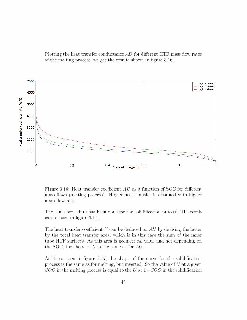
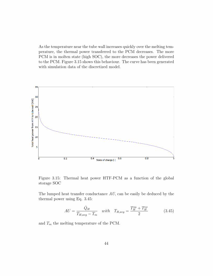
Plotting the heat transfer conductance AU for different HTF mass flow ratesof the melting process, we get the results shown in figure 3.16.

Figure 3.16: Heat transfer coefficient AU as a function of SOC for differentmass flows (melting process). Higher heat transfer is obtained with highermass flow rate

The same procedure has been done for the solidification process. The resultcan be seen in figure 3.17.

The heat transfer coefficient U can be deduced on AU by devising the latterby the total heat transfer area, which is in this case the sum of the innertube HTF surfaces. As this area is geometrical value and not depending onthe SOC, the shape of U is the same as for AU .

As it can seen in figure 3.17, the shape of the curve for the solidificationprocess is the same as for melting, but inverted. So the value of U at a givenSOC in the melting process is equal to the U at 1−SOC in the solidification

45

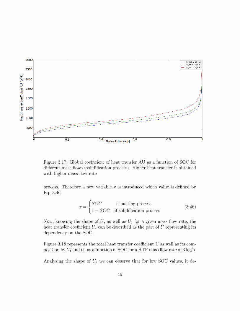
Figure 3.17: Global coefficient of heat transfer AU as a function of SOC fordifferent mass flows (solidification process). Higher heat transfer is obtainedwith higher mass flow rate

process. Therefore a new variable x is introduced which value is defined byEq. 3.46.

x =

{SOC if melting process

1− SOC if solidification process(3.46)

Now, knowing the shape of U , as well as U1 for a given mass flow rate, theheat transfer coefficient U2 can be described as the part of U representing itsdependency on the SOC.

Figure 3.18 represents the total heat transfer coefficient U as well as its com-position by U1 and U1 as a function of SOC for a HTF mass flow rate of 3 kg/s.

Analysing the shape of U2 we can observe that for low SOC values, it de-

46

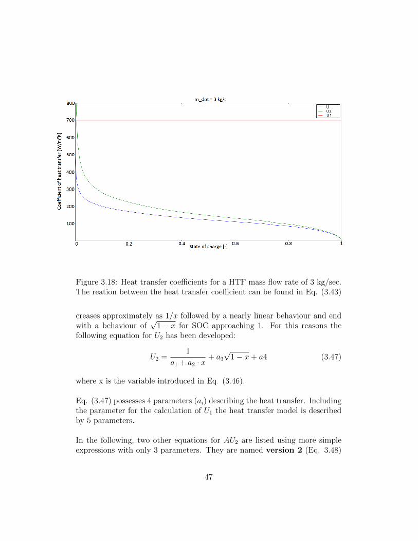
Figure 3.18: Heat transfer coefficients for a HTF mass flow rate of 3 kg/sec.The reation between the heat transfer coefficient can be found in Eq. (3.43)

creases approximately as 1/x followed by a nearly linear behaviour and endwith a behaviour of

√1− x for SOC approaching 1. For this reasons the

following equation for U2 has been developed:

U2 =1

a1 + a2 · x+ a3

√1− x+ a4 (3.47)

where x is the variable introduced in Eq. (3.46).

Eq. (3.47) possesses 4 parameters (ai) describing the heat transfer. Includingthe parameter for the calculation of U1 the heat transfer model is describedby 5 parameters.

In the following, two other equations for AU2 are listed using more simpleexpressions with only 3 parameters. They are named version 2 (Eq. 3.48)

47

and version 3 (Eq. 3.49). Version 1 correspond to the initial expression inEq. (3.47).

U2 = a1(1− x)a2 + a3 (3.48)

U2 =a1

1 + xa2+ a3 (3.49)

A comparison in results between the versions can be found in section 4.2.3.

For the later model validation is does not make any difference if the parameteroptimization is done for the calculation of U (resp. U1 and U2) or AU (resp.AU1 and AU2), because the heat transfer surface is a constant that wouldnot modify the equation for the heat transfer coefficient calculation (see Eq.3.43). In the case of the AU adaptation, the optimized parameters wouldinclude the heat transfer surface, so that there is no further need to define aspecific geometrical parameter for this heat transfer area. Using this method,the model needs less geometrical parameters.For our model validation, both approaches will be analysed. As we knowexactly the geometrical dimensions of the storage, the pure coefficient ofheat transfer U can be parametrized. The heat transfer coefficient AU isused, when the heat exchanger geometry is unknown.

3.2.2 Model implementation in Modelica

As for the discretized model, three main components compose the single nodemodel:

• HTF component

• Tube wall component

• PCM component

Heat transfer fluid

The HTF component calculates the fluid state of the HTF and regulates theheat transfer to the tube wall by using modified heat transfer components of

48

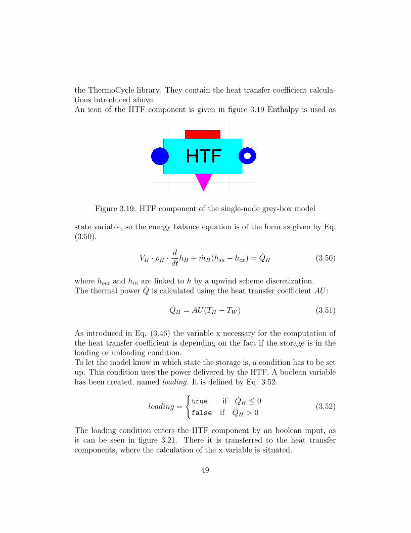
the ThermoCycle library. They contain the heat transfer coefficient calcula-tions introduced above.An icon of the HTF component is given in figure 3.19 Enthalpy is used as

Figure 3.19: HTF component of the single-node grey-box model

state variable, so the energy balance equation is of the form as given by Eq.(3.50).

VH · ρH ·d

dthH + mH(hsu − hex) = QH (3.50)

where hout and hin are linked to h by a upwind scheme discretization.The thermal power Q is calculated using the heat transfer coefficient AU :

QH = AU(TH − TW ) (3.51)

As introduced in Eq. (3.46) the variable x necessary for the computation ofthe heat transfer coefficient is depending on the fact if the storage is in theloading or unloading condition.To let the model know in which state the storage is, a condition has to be setup. This condition uses the power delivered by the HTF. A boolean variablehas been created, named loading. It is defined by Eq. 3.52.

loading =

{true if QH ≤ 0

false if QH > 0(3.52)

The loading condition enters the HTF component by an boolean input, asit can be seen in figure 3.21. There it is transferred to the heat transfercomponents, where the calculation of the x variable is situated.

49

Tube wall

The tube wall component models the thermal heat capacity of the heatexchanger. No thermal conductance inside the tube is assumed. There-fore the temperature of the tube wall corresponds to the PCM temperature(TP = TW ).The energy balance of the tube wall is given in Eq. (3.53), where temperatureis chosen as state variable.

mW · cP,W ·d

dtTW = QP − QH (3.53)

The component item is the same as for the discretized model, see figure 3.3.

Phase change material

As the discretized model, the single-node model uses the apparent heat ca-pacity method to model the melting process. The sigmoid function (Mod2)is implemented only in this model.The energy balance of the specified mass of PCM, with temperature as statevariable is given in Eq. (3.54).

mP · cp,P ·d

dtTP = −QP (3.54)

Unlike the discretized PCM component, the single node model componentpossesses only one thermal port, because there is no further need for the axialand radial heat conduction between multiple PCM cells.Figure 3.20 shows the item of the PCM component.

Figure 3.20: PCM component in the single node model

50

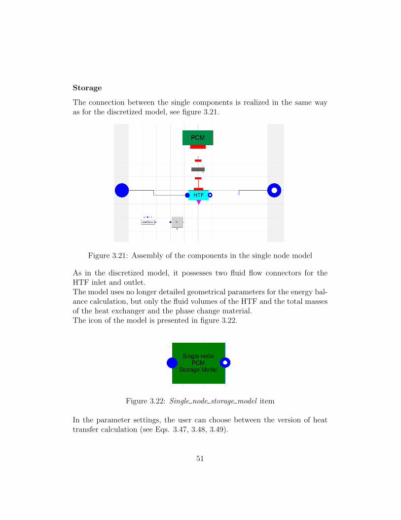
Storage

The connection between the single components is realized in the same wayas for the discretized model, see figure 3.21.

Figure 3.21: Assembly of the components in the single node model

As in the discretized model, it possesses two fluid flow connectors for theHTF inlet and outlet.The model uses no longer detailed geometrical parameters for the energy bal-ance calculation, but only the fluid volumes of the HTF and the total massesof the heat exchanger and the phase change material.The icon of the model is presented in figure 3.22.

Figure 3.22: Single node storage model item

In the parameter settings, the user can choose between the version of heattransfer calculation (see Eqs. 3.47, 3.48, 3.49).

51

3.2.3 Storage parameters

Phase change medium

As already mentioned in section 3.2.2, the phase change medium model usedin the single-node model is Model 2 from section 3.1.3. The parameters canbe found in table 3.1.Only difference to the discretized model, consists in the fact that there is nolonger necessity of the parameter λP , which is lumped into the overall heattransfer coefficient.In fact, λP characterizes the heat transfer in the PCM. Multiplied by theheat conduction width it corresponds to the heat transfer coefficient betweenthe PCM cells.In the single-node model, the heat transfer coefficient is computed by externalequations depending on the SOC, including the information of the thermalconductivity of the PCM.By consequence, there are only 4 PCM parameters in the case of the singlenode model: cp,P ,L,∆T, Tm.

Heat transfer

Depending on the heat transfer version used, the user has to specify theparameters a1, a2, a3, a4, a5 for the version 1 and a1, a2, a3, a5 for version 2and version 3.

Geometry

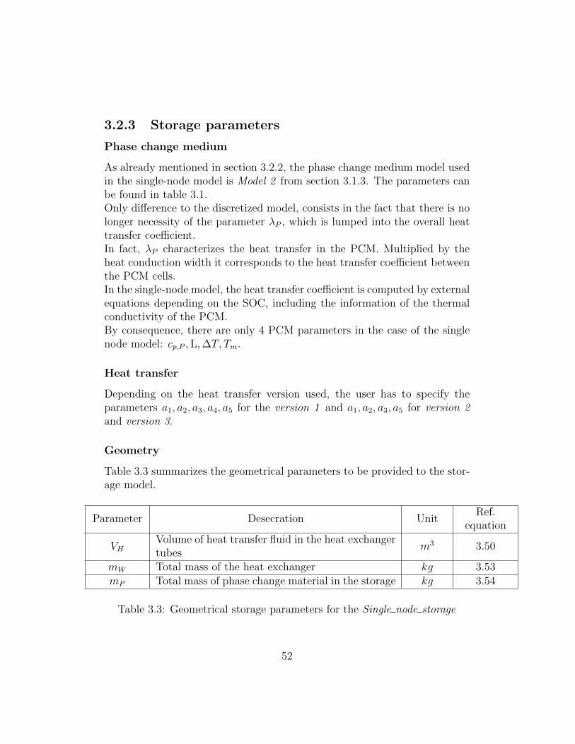
Table 3.3 summarizes the geometrical parameters to be provided to the stor-age model.

Parameter Desecration UnitRef.

equation

VHVolume of heat transfer fluid in the heat exchangertubes

m3 3.50

mW Total mass of the heat exchanger kg 3.53mP Total mass of phase change material in the storage kg 3.54

Table 3.3: Geometrical storage parameters for the Single node storage

52

Other parameters

Several other parameters have to be provided to the model:

- HTF: The user can specify the heat transfer fluid

- Mdotnom: Nominal HTF flow rate

- heat_transfer: The user can choice between different heat transfercalculation expression (version 1-3 and constant)

- cP,W : Specific heat capacity of the heat exchanger material

- U_nom: Heat transfer value if the constant model is chosen

Further simplifications could have been done. For example the thermal ca-pacity of the heat exchanger could be included into the phase change mate-rial. In this case mW and cP,W can be eliminated from the parameter list.Furthermore, the HTF fluid volume is not mandatory. In fact, VH can beeliminated by omitting the derivative part in Eq.(3.50).

53

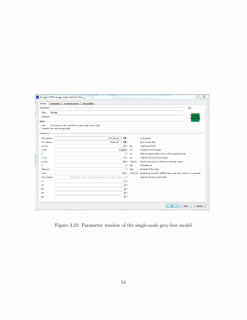
Figure 3.23: Parameter window of the single-node grey-box model

54

Chapter 4

Model validation:Results and discussion

4.1 Discretized PCM storage model

4.1.1 Introduction

In the following the results of the model validation for the discretized PCMstorage mode are presented. The parameter determination based on a modelsimulation fitting to experimental data are analysed. A statistical analysis,treating correlation and error estimation, of the model parameters is included.

As introduced in section 3.1.3, two different models are considered (Mod1,Mod2) each with a different set of parameters. As described in section 3.1.3,they differ in the correlation used to model the apparent heat capacity cPand thermal conductivity λP .

Three experiments have been considered. The first consists in a charging,the second in a discharging and in the last the two were combined in a to-tal changing-discharging cycle. In every experiment, the HTF flow rate iskept constant with low flows and laminar flow conditions in the pipes withReynolds Numbers of 2100-2220. In the charging experiment the HTF stor-age inlet temperature is increased from approximately 105 to 155 ◦C and inthe discharging experiment reduced from 155 to 105 ◦C.

55

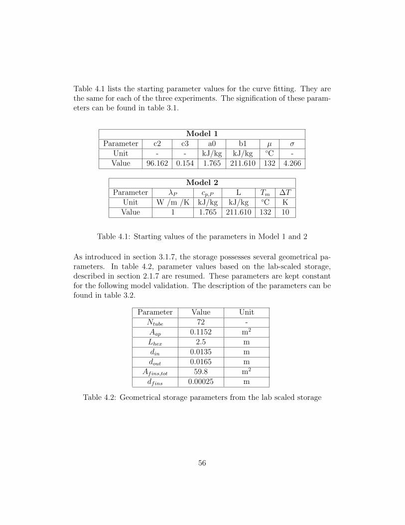
Table 4.1 lists the starting parameter values for the curve fitting. They arethe same for each of the three experiments. The signification of these param-eters can be found in table 3.1.

Model 1Parameter c2 c3 a0 b1 µ σ

Unit - - kJ/kg kJ/kg ◦C -Value 96.162 0.154 1.765 211.610 132 4.266

Model 2Parameter λP cp,P L Tm ∆T

Unit W /m /K kJ/kg kJ/kg ◦C KValue 1 1.765 211.610 132 10

Table 4.1: Starting values of the parameters in Model 1 and 2

As introduced in section 3.1.7, the storage possesses several geometrical pa-rameters. In table 4.2, parameter values based on the lab-scaled storage,described in section 2.1.7 are resumed. These parameters are kept constantfor the following model validation. The description of the parameters can befound in table 3.2.

Parameter Value UnitNtube 72 -Aap 0.1152 m2

Lhex 2.5 mdin 0.0135 mdout 0.0165 m

Afins,tot 59.8 m2

dfins 0.00025 m

Table 4.2: Geometrical storage parameters from the lab scaled storage

56

4.1.2 Parameter optimization

In order to validate the PCM storage model on experimental measurementdata, the PCM storage parameters, presented in table 4.1, are optimized tofit the simulation outlet temperature results on the experimental curves.The said optimization has been realised using a Python-based optimizer fromthe SciPy package. A documentation of the optimizer can be found in [4].To run simulations out of a Python-script, the Simulator class of the Build-ingsPy package has been employed. The corresponding documentation isprovided in [5].A least-square method has been used to fit the simulation data curve on themeasurements one. It takes an error vector as input, which corresponds tothe differences for simulation and measurement data in outlet temperaturesfor each time step. The optimizer tries du minimise this error, by varyingthe PCM storage parameters.To archive model validation for different HTF mass flows, the optimizationhas been done by providing the sum of two error vectors resulting of simu-lations with different HTF mass flows to the optimizer. Simulations with 1kg/s and 0.35 kg /s have been considered.Beside the fact that the SciPy optimizer returns an optimized parameter set,it also provides the covariance matrix of the parameters, which will be usedfor further statistical analyses.

4.1.3 Charging experiment

Model validation

In the single charging experiment, the HTF inlet temperature is kept constantaround 155 ◦C over a time of 9000 seconds, with an initial uniform storagePCM temperature of 105 ◦C. Figure 4.1 represents the inlet temperatureprofiles for different mass flows. After an initial increasing, the temperatureis kept constant. The storage outlet temperature is then fitted to the mea-surement using a parameter optimization.

57

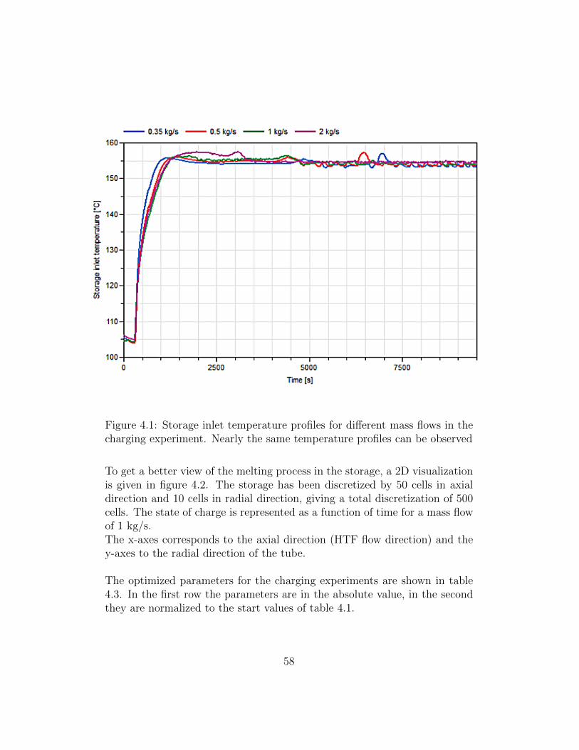
Figure 4.1: Storage inlet temperature profiles for different mass flows in thecharging experiment. Nearly the same temperature profiles can be observed

To get a better view of the melting process in the storage, a 2D visualizationis given in figure 4.2. The storage has been discretized by 50 cells in axialdirection and 10 cells in radial direction, giving a total discretization of 500cells. The state of charge is represented as a function of time for a mass flowof 1 kg/s.The x-axes corresponds to the axial direction (HTF flow direction) and they-axes to the radial direction of the tube.

The optimized parameters for the charging experiments are shown in table4.3. In the first row the parameters are in the absolute value, in the secondthey are normalized to the start values of table 4.1.

58

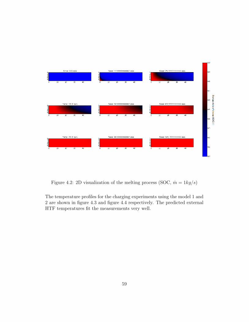
Figure 4.2: 2D visualization of the melting process (SOC, m = 1kg/s)

The temperature profiles for the charging experiments using the model 1 and2 are shown in figure 4.3 and figure 4.4 respectively. The predicted externalHTF temperatures fit the measurements very well.

59

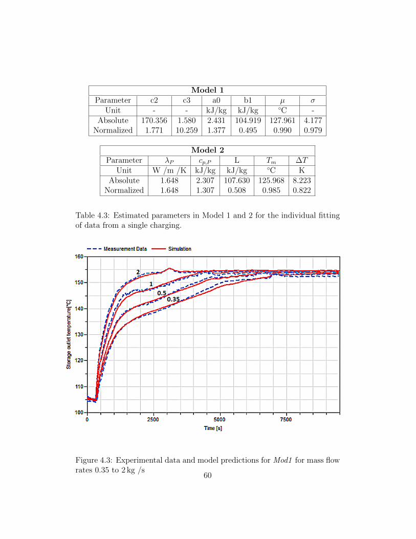
Model 1Parameter c2 c3 a0 b1 µ σ

Unit - - kJ/kg kJ/kg ◦C -Absolute 170.356 1.580 2.431 104.919 127.961 4.177

Normalized 1.771 10.259 1.377 0.495 0.990 0.979

Model 2Parameter λP cp,P L Tm ∆T

Unit W /m /K kJ/kg kJ/kg ◦C KAbsolute 1.648 2.307 107.630 125.968 8.223

Normalized 1.648 1.307 0.508 0.985 0.822

Table 4.3: Estimated parameters in Model 1 and 2 for the individual fittingof data from a single charging.

Figure 4.3: Experimental data and model predictions for Mod1 for mass flowrates 0.35 to 2 kg /s

60

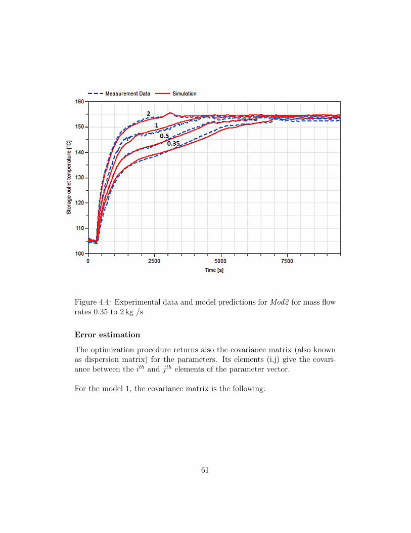
Figure 4.4: Experimental data and model predictions for Mod2 for mass flowrates 0.35 to 2 kg /s

Error estimation

The optimization procedure returns also the covariance matrix (also knownas dispersion matrix) for the parameters. Its elements (i,j) give the covari-ance between the ith and jth elements of the parameter vector.

For the model 1, the covariance matrix is the following:

61

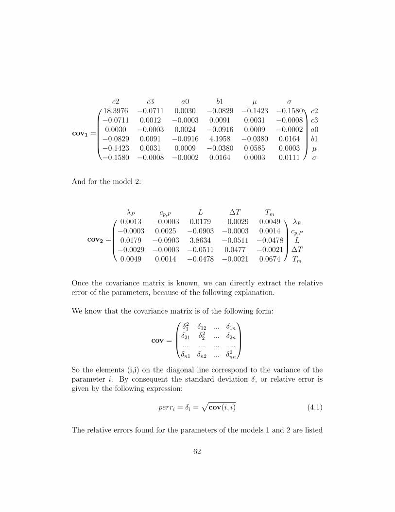
cov1 =

c2 c3 a0 b1 µ σ

18.3976 −0.0711 0.0030 −0.0829 −0.1423 −0.1580 c2−0.0711 0.0012 −0.0003 0.0091 0.0031 −0.0008 c30.0030 −0.0003 0.0024 −0.0916 0.0009 −0.0002 a0−0.0829 0.0091 −0.0916 4.1958 −0.0380 0.0164 b1−0.1423 0.0031 0.0009 −0.0380 0.0585 0.0003 µ−0.1580 −0.0008 −0.0002 0.0164 0.0003 0.0111 σ

And for the model 2:

cov2 =

λP cp,P L ∆T Tm

0.0013 −0.0003 0.0179 −0.0029 0.0049 λP−0.0003 0.0025 −0.0903 −0.0003 0.0014 cp,P0.0179 −0.0903 3.8634 −0.0511 −0.0478 L−0.0029 −0.0003 −0.0511 0.0477 −0.0021 ∆T0.0049 0.0014 −0.0478 −0.0021 0.0674 Tm

Once the covariance matrix is known, we can directly extract the relativeerror of the parameters, because of the following explanation.

We know that the covariance matrix is of the following form:

cov =

δ2

1 δ12 ... δ1n

δ21 δ22 ... δ2n

... ... ... ....δn1 δn2 ... δ2

nn

So the elements (i,i) on the diagonal line correspond to the variance of theparameter i. By consequent the standard deviation δ, or relative error isgiven by the following expression:

perri = δi =√

cov(i, i) (4.1)

The relative errors found for the parameters of the models 1 and 2 are listed

62

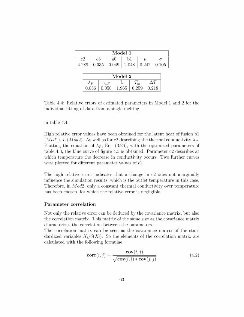
Model 1c2 c3 a0 b1 µ σ

4.289 0.035 0.049 2.048 0.242 0.105

Model 2λP cp,P L Tm ∆T

0.036 0.050 1.965 0.259 0.218

Table 4.4: Relative errors of estimated parameters in Model 1 and 2 for theindividual fitting of data from a single melting

in table 4.4.

High relative error values have been obtained for the latent heat of fusion b1(Mod1), L (Mod2). As well as for c2 describing the thermal conductivity λP .Plotting the equation of λP , Eq. (3.26), with the optimized parameters oftable 4.3, the blue curve of figure 4.5 is obtained. Parameter c2 describes atwhich temperature the decrease in conductivity occurs. Two further curveswere plotted for different parameter values of c2.

The high relative error indicates that a change in c2 odes not marginallyinfluence the simulation results, which is the outlet temperature in this case.Therefore, in Mod2, only a constant thermal conductivity over temperaturehas been chosen, for which the relative error is negligible.

Parameter correlation

Not only the relative error can be deduced by the covariance matrix, but alsothe correlation matrix. This matrix of the same size as the covariance matrixcharacterizes the correlation between the parameters.The correlation matrix can be seen as the covariance matrix of the stan-dardized variables Xi/δ(Xi). So the elements of the correlation matrix arecalculated with the following formulae:

corr(i, j) =cov(i, j)√

cov(i, i) ∗ cov(j, j)(4.2)

63

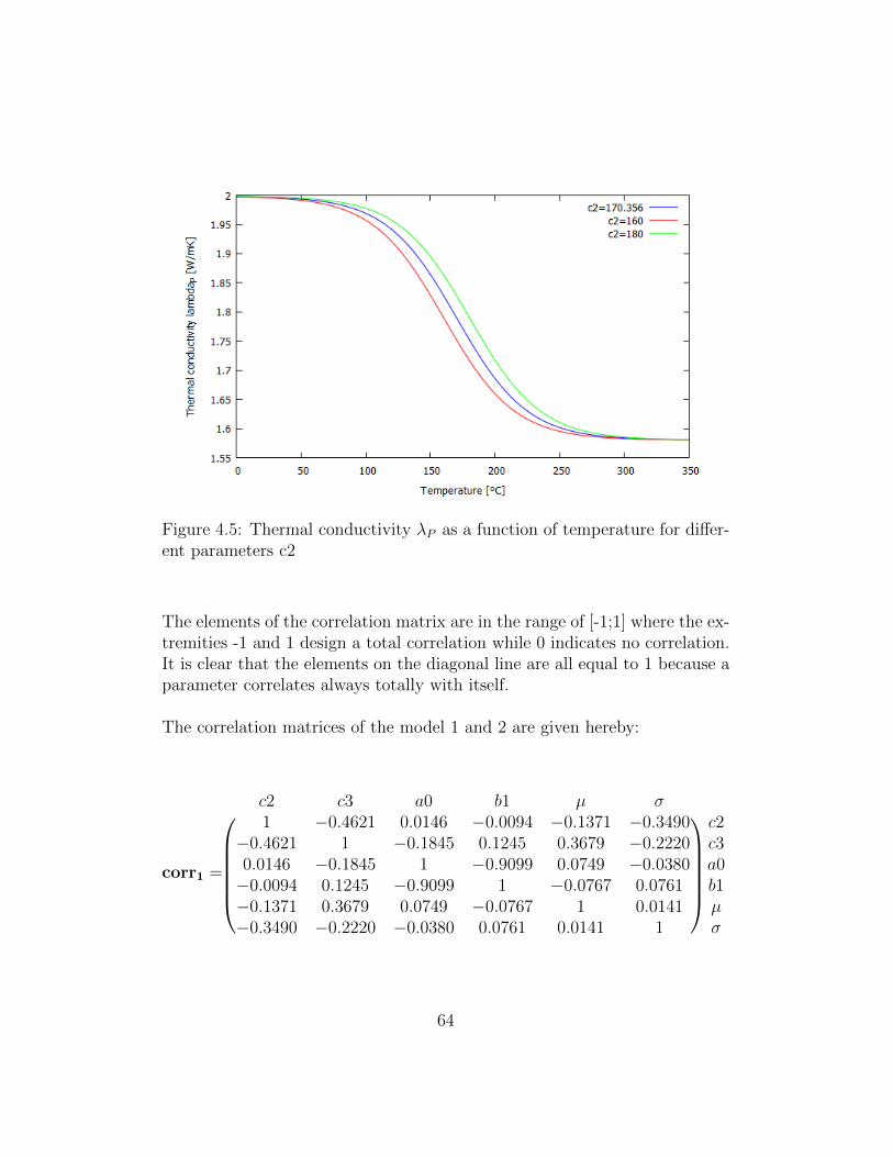
Figure 4.5: Thermal conductivity λP as a function of temperature for differ-ent parameters c2

The elements of the correlation matrix are in the range of [-1;1] where the ex-tremities -1 and 1 design a total correlation while 0 indicates no correlation.It is clear that the elements on the diagonal line are all equal to 1 because aparameter correlates always totally with itself.

The correlation matrices of the model 1 and 2 are given hereby:

corr1 =

c2 c3 a0 b1 µ σ

1 −0.4621 0.0146 −0.0094 −0.1371 −0.3490 c2

−0.4621 1 −0.1845 0.1245 0.3679 −0.2220 c30.0146 −0.1845 1 −0.9099 0.0749 −0.0380 a0−0.0094 0.1245 −0.9099 1 −0.0767 0.0761 b1−0.1371 0.3679 0.0749 −0.0767 1 0.0141 µ−0.3490 −0.2220 −0.0380 0.0761 0.0141 1 σ

64

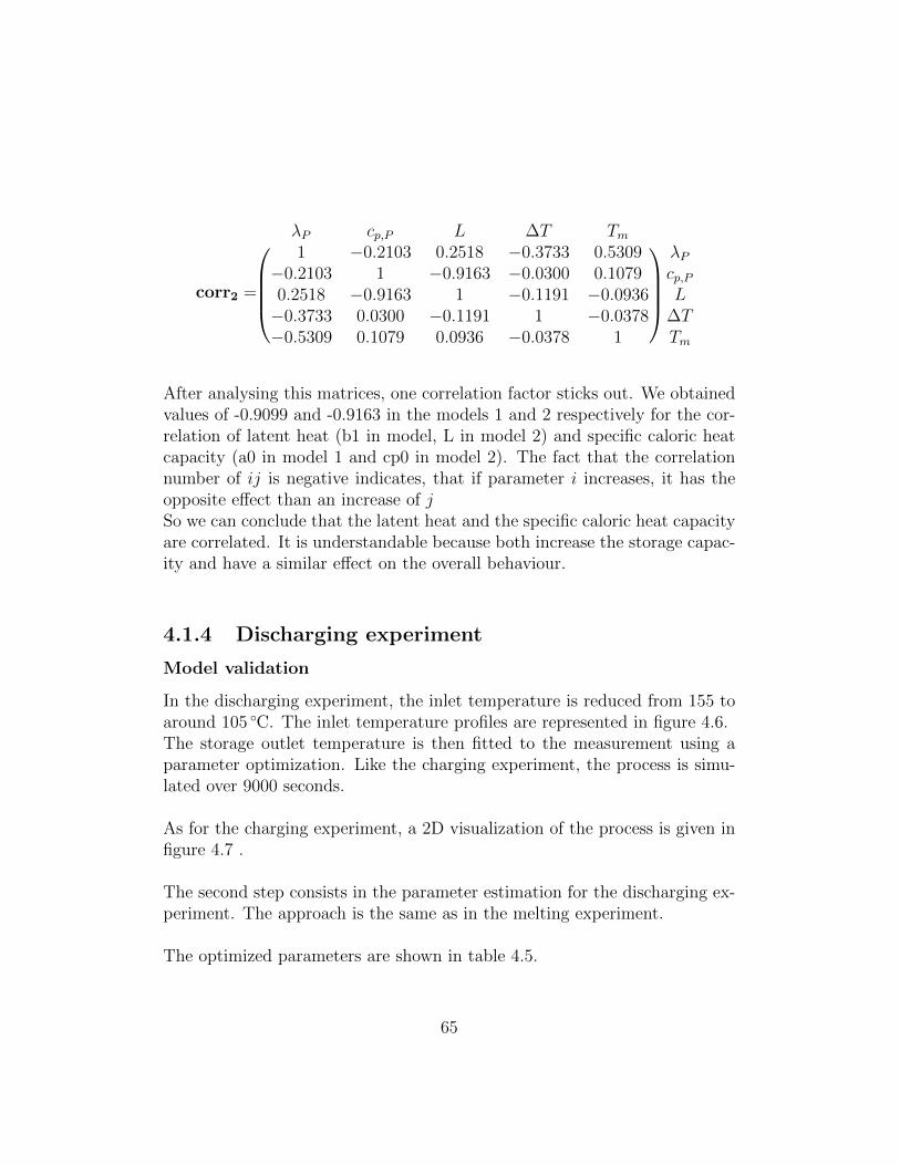
corr2 =

λP cp,P L ∆T Tm

1 −0.2103 0.2518 −0.3733 0.5309 λP−0.2103 1 −0.9163 −0.0300 0.1079 cp,P0.2518 −0.9163 1 −0.1191 −0.0936 L−0.3733 0.0300 −0.1191 1 −0.0378 ∆T−0.5309 0.1079 0.0936 −0.0378 1 Tm

After analysing this matrices, one correlation factor sticks out. We obtainedvalues of -0.9099 and -0.9163 in the models 1 and 2 respectively for the cor-relation of latent heat (b1 in model, L in model 2) and specific caloric heatcapacity (a0 in model 1 and cp0 in model 2). The fact that the correlationnumber of ij is negative indicates, that if parameter i increases, it has theopposite effect than an increase of jSo we can conclude that the latent heat and the specific caloric heat capacityare correlated. It is understandable because both increase the storage capac-ity and have a similar effect on the overall behaviour.

4.1.4 Discharging experiment

Model validation

In the discharging experiment, the inlet temperature is reduced from 155 toaround 105 ◦C. The inlet temperature profiles are represented in figure 4.6.The storage outlet temperature is then fitted to the measurement using aparameter optimization. Like the charging experiment, the process is simu-lated over 9000 seconds.

As for the charging experiment, a 2D visualization of the process is given infigure 4.7 .

The second step consists in the parameter estimation for the discharging ex-periment. The approach is the same as in the melting experiment.

The optimized parameters are shown in table 4.5.

65

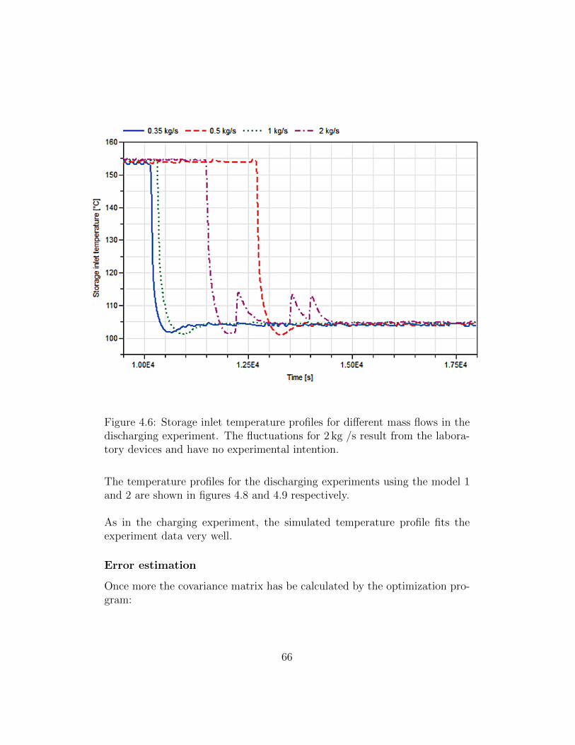
Figure 4.6: Storage inlet temperature profiles for different mass flows in thedischarging experiment. The fluctuations for 2 kg /s result from the labora-tory devices and have no experimental intention.

The temperature profiles for the discharging experiments using the model 1and 2 are shown in figures 4.8 and 4.9 respectively.

As in the charging experiment, the simulated temperature profile fits theexperiment data very well.

Error estimation

Once more the covariance matrix has be calculated by the optimization pro-gram:

66

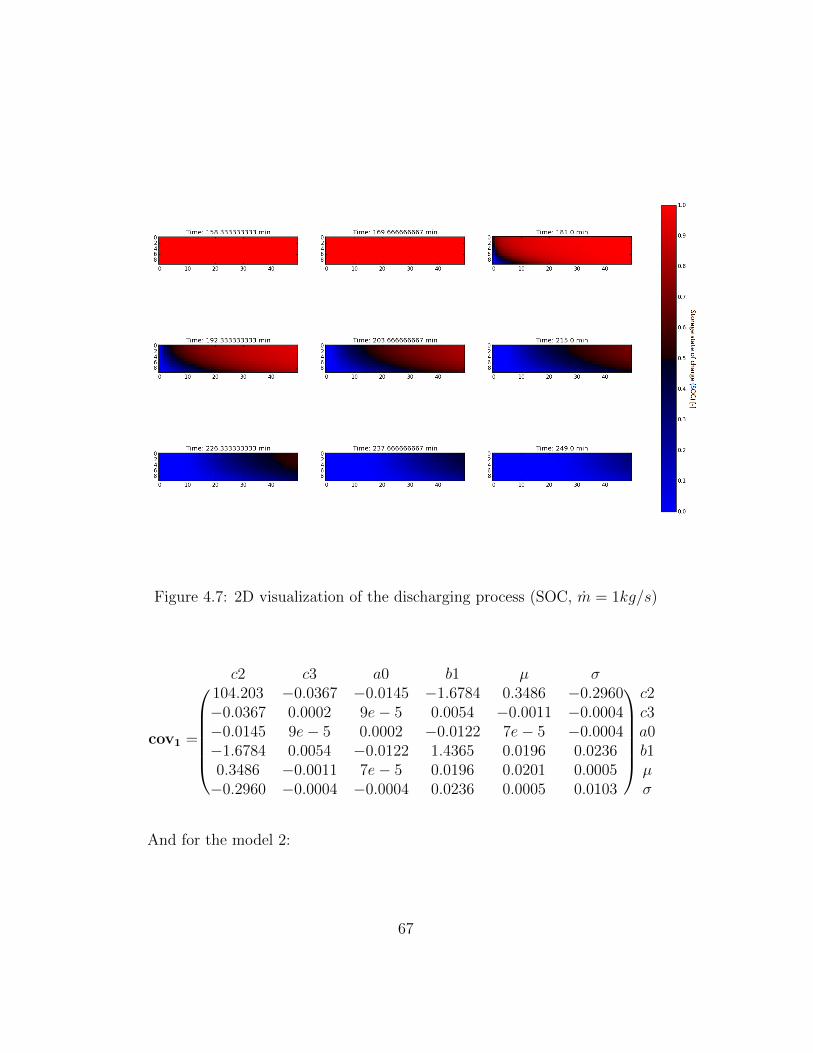
Figure 4.7: 2D visualization of the discharging process (SOC, m = 1kg/s)

cov1 =

c2 c3 a0 b1 µ σ

104.203 −0.0367 −0.0145 −1.6784 0.3486 −0.2960 c2−0.0367 0.0002 9e− 5 0.0054 −0.0011 −0.0004 c3−0.0145 9e− 5 0.0002 −0.0122 7e− 5 −0.0004 a0−1.6784 0.0054 −0.0122 1.4365 0.0196 0.0236 b10.3486 −0.0011 7e− 5 0.0196 0.0201 0.0005 µ−0.2960 −0.0004 −0.0004 0.0236 0.0005 0.0103 σ

And for the model 2:

67

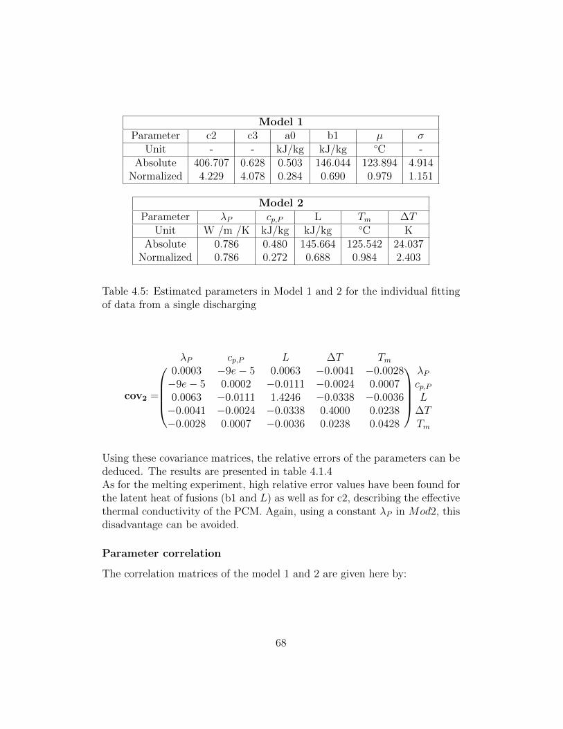
Model 1Parameter c2 c3 a0 b1 µ σ

Unit - - kJ/kg kJ/kg ◦C -Absolute 406.707 0.628 0.503 146.044 123.894 4.914

Normalized 4.229 4.078 0.284 0.690 0.979 1.151

Model 2Parameter λP cp,P L Tm ∆T

Unit W /m /K kJ/kg kJ/kg ◦C KAbsolute 0.786 0.480 145.664 125.542 24.037

Normalized 0.786 0.272 0.688 0.984 2.403

Table 4.5: Estimated parameters in Model 1 and 2 for the individual fittingof data from a single discharging

cov2 =

λP cp,P L ∆T Tm

0.0003 −9e− 5 0.0063 −0.0041 −0.0028 λP−9e− 5 0.0002 −0.0111 −0.0024 0.0007 cp,P0.0063 −0.0111 1.4246 −0.0338 −0.0036 L−0.0041 −0.0024 −0.0338 0.4000 0.0238 ∆T−0.0028 0.0007 −0.0036 0.0238 0.0428 Tm

Using these covariance matrices, the relative errors of the parameters can bededuced. The results are presented in table 4.1.4As for the melting experiment, high relative error values have been found forthe latent heat of fusions (b1 and L) as well as for c2, describing the effectivethermal conductivity of the PCM. Again, using a constant λP in Mod2, thisdisadvantage can be avoided.

Parameter correlation

The correlation matrices of the model 1 and 2 are given here by:

68

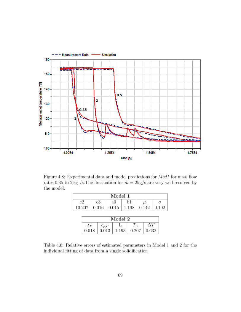
Figure 4.8: Experimental data and model predictions for Mod1 for mass flowrates 0.35 to 2 kg /s.The fluctuation for m = 2kg/s are very well resolved bythe model.

Model 1c2 c3 a0 b1 µ σ

10.207 0.016 0.015 1.198 0.142 0.102

Model 2λP cp,P L Tm ∆T

0.018 0.013 1.193 0.207 0.632

Table 4.6: Relative errors of estimated parameters in Model 1 and 2 for theindividual fitting of data from a single solidification

69

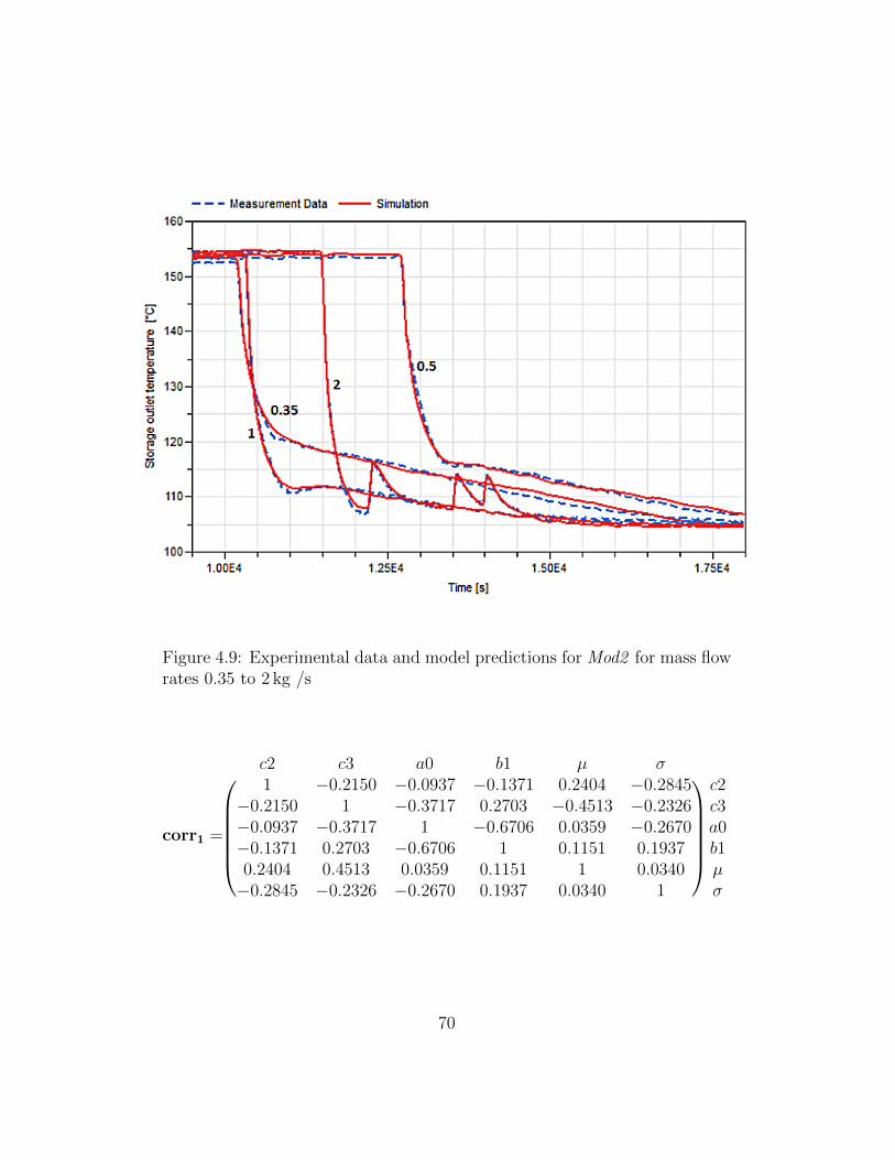
Figure 4.9: Experimental data and model predictions for Mod2 for mass flowrates 0.35 to 2 kg /s

corr1 =

c2 c3 a0 b1 µ σ

1 −0.2150 −0.0937 −0.1371 0.2404 −0.2845 c2

−0.2150 1 −0.3717 0.2703 −0.4513 −0.2326 c3−0.0937 −0.3717 1 −0.6706 0.0359 −0.2670 a0−0.1371 0.2703 −0.6706 1 0.1151 0.1937 b10.2404 0.4513 0.0359 0.1151 1 0.0340 µ−0.2845 −0.2326 −0.2670 0.1937 0.0340 1 σ

70

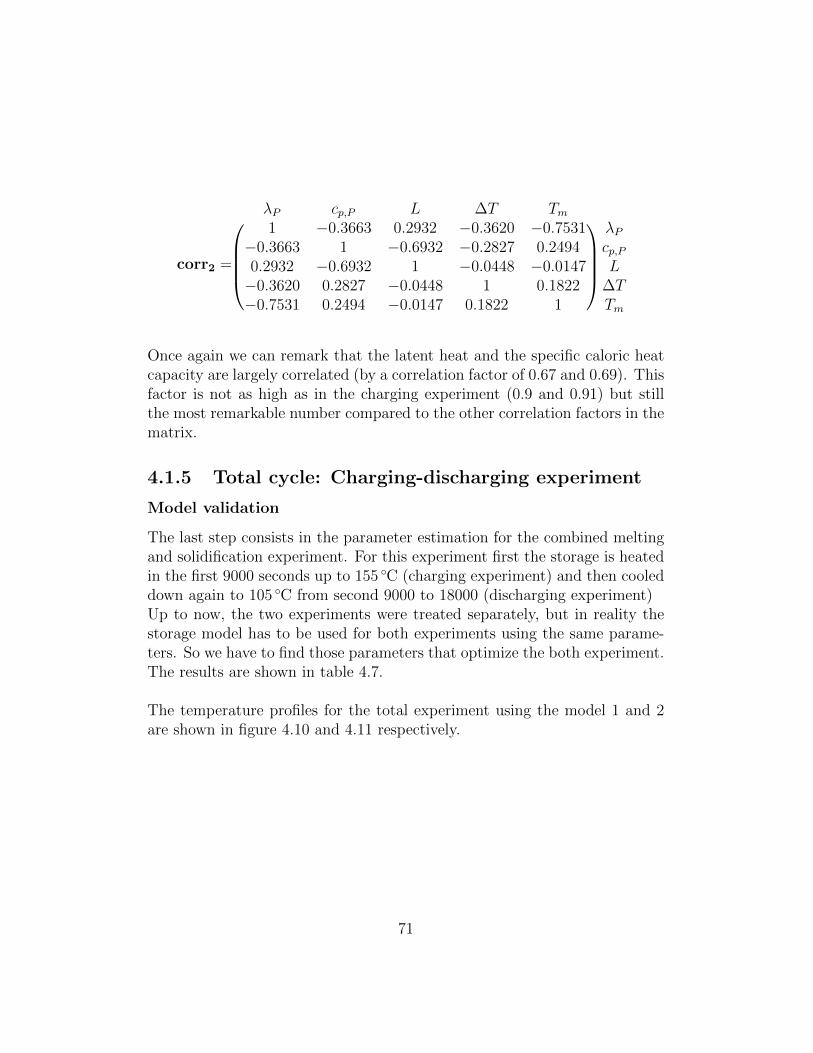
corr2 =

λP cp,P L ∆T Tm

1 −0.3663 0.2932 −0.3620 −0.7531 λP−0.3663 1 −0.6932 −0.2827 0.2494 cp,P0.2932 −0.6932 1 −0.0448 −0.0147 L−0.3620 0.2827 −0.0448 1 0.1822 ∆T−0.7531 0.2494 −0.0147 0.1822 1 Tm

Once again we can remark that the latent heat and the specific caloric heatcapacity are largely correlated (by a correlation factor of 0.67 and 0.69). Thisfactor is not as high as in the charging experiment (0.9 and 0.91) but stillthe most remarkable number compared to the other correlation factors in thematrix.

4.1.5 Total cycle: Charging-discharging experiment

Model validation

The last step consists in the parameter estimation for the combined meltingand solidification experiment. For this experiment first the storage is heatedin the first 9000 seconds up to 155 ◦C (charging experiment) and then cooleddown again to 105 ◦C from second 9000 to 18000 (discharging experiment)Up to now, the two experiments were treated separately, but in reality thestorage model has to be used for both experiments using the same parame-ters. So we have to find those parameters that optimize the both experiment.The results are shown in table 4.7.

The temperature profiles for the total experiment using the model 1 and 2are shown in figure 4.10 and 4.11 respectively.

71

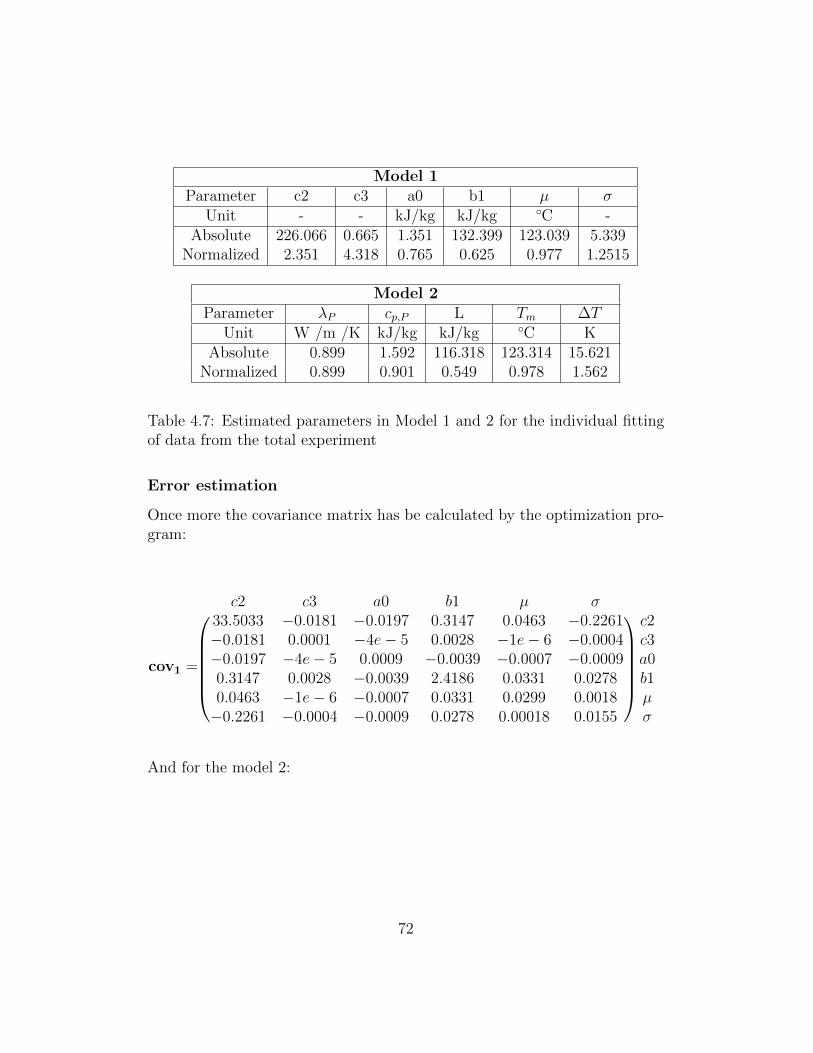
Model 1Parameter c2 c3 a0 b1 µ σ

Unit - - kJ/kg kJ/kg ◦C -Absolute 226.066 0.665 1.351 132.399 123.039 5.339

Normalized 2.351 4.318 0.765 0.625 0.977 1.2515

Model 2Parameter λP cp,P L Tm ∆T

Unit W /m /K kJ/kg kJ/kg ◦C KAbsolute 0.899 1.592 116.318 123.314 15.621

Normalized 0.899 0.901 0.549 0.978 1.562

Table 4.7: Estimated parameters in Model 1 and 2 for the individual fittingof data from the total experiment

Error estimation

Once more the covariance matrix has be calculated by the optimization pro-gram:

cov1 =

c2 c3 a0 b1 µ σ

33.5033 −0.0181 −0.0197 0.3147 0.0463 −0.2261 c2−0.0181 0.0001 −4e− 5 0.0028 −1e− 6 −0.0004 c3−0.0197 −4e− 5 0.0009 −0.0039 −0.0007 −0.0009 a00.3147 0.0028 −0.0039 2.4186 0.0331 0.0278 b10.0463 −1e− 6 −0.0007 0.0331 0.0299 0.0018 µ−0.2261 −0.0004 −0.0009 0.0278 0.00018 0.0155 σ

And for the model 2:

72

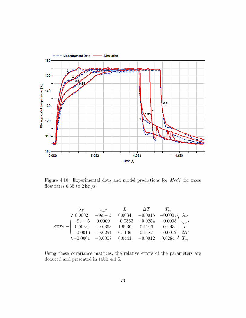
Figure 4.10: Experimental data and model predictions for Mod1 for massflow rates 0.35 to 2 kg /s

cov2 =

λP cp,P L ∆T Tm

0.0002 −9e− 5 0.0034 −0.0016 −0.0001 λP−9e− 5 0.0009 −0.0363 −0.0254 −0.0008 cp,P0.0034 −0.0363 1.9930 0.1106 0.0443 L−0.0016 −0.0254 0.1106 0.1187 −0.0012 ∆T−0.0001 −0.0008 0.0443 −0.0012 0.0284 Tm

Using these covariance matrices, the relative errors of the parameters arededuced and presented in table 4.1.5.

73

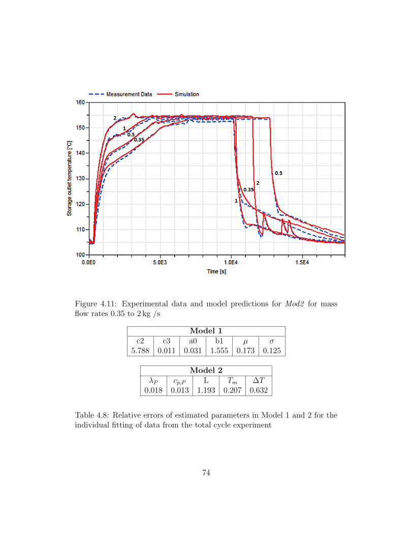
Figure 4.11: Experimental data and model predictions for Mod2 for massflow rates 0.35 to 2 kg /s

Model 1c2 c3 a0 b1 µ σ

5.788 0.011 0.031 1.555 0.173 0.125

Model 2λP cp,P L Tm ∆T

0.018 0.013 1.193 0.207 0.632

Table 4.8: Relative errors of estimated parameters in Model 1 and 2 for theindividual fitting of data from the total cycle experiment

74

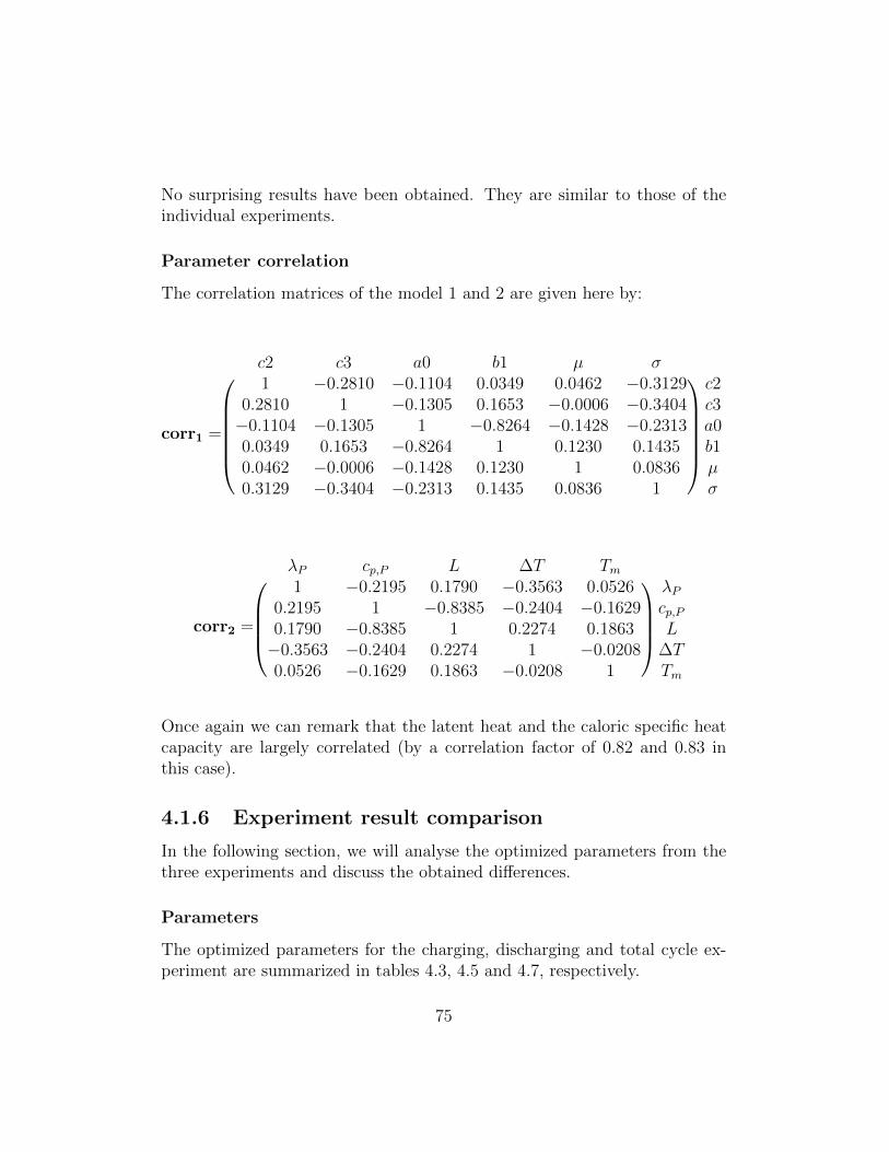
No surprising results have been obtained. They are similar to those of theindividual experiments.

Parameter correlation

The correlation matrices of the model 1 and 2 are given here by:

corr1 =

c2 c3 a0 b1 µ σ

1 −0.2810 −0.1104 0.0349 0.0462 −0.3129 c2

0.2810 1 −0.1305 0.1653 −0.0006 −0.3404 c3−0.1104 −0.1305 1 −0.8264 −0.1428 −0.2313 a00.0349 0.1653 −0.8264 1 0.1230 0.1435 b10.0462 −0.0006 −0.1428 0.1230 1 0.0836 µ0.3129 −0.3404 −0.2313 0.1435 0.0836 1 σ

corr2 =

λP cp,P L ∆T Tm

1 −0.2195 0.1790 −0.3563 0.0526 λP0.2195 1 −0.8385 −0.2404 −0.1629 cp,P0.1790 −0.8385 1 0.2274 0.1863 L−0.3563 −0.2404 0.2274 1 −0.0208 ∆T0.0526 −0.1629 0.1863 −0.0208 1 Tm

Once again we can remark that the latent heat and the caloric specific heatcapacity are largely correlated (by a correlation factor of 0.82 and 0.83 inthis case).

4.1.6 Experiment result comparison

In the following section, we will analyse the optimized parameters from thethree experiments and discuss the obtained differences.

Parameters

The optimized parameters for the charging, discharging and total cycle ex-periment are summarized in tables 4.3, 4.5 and 4.7, respectively.

75

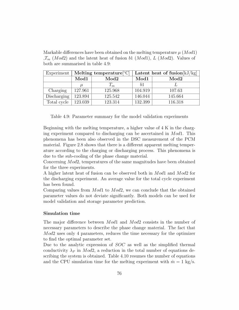
Markable differences have been obtained on the melting temperature µ (Mod1),Tm (Mod2) and the latent heat of fusion b1 (Mod1), L (Mod2). Values ofboth are summarised in table 4.9:

Experiment Melting temperature[◦C] Latent heat of fusion[kJ/kg]Mod1 Mod2 Mod1 Mod2µ Tm b1 L

Charging 127.961 125.968 104.919 107.63Discharging 123.894 125.542 146.044 145.664Total cycle 123.039 123.314 132.399 116.318

Table 4.9: Parameter summary for the model validation experiments

Beginning with the melting temperature, a higher value of 4 K in the charg-ing experiment compared to discharging can be ascertained in Mod1. Thisphenomena has been also observed in the DSC measurement of the PCMmaterial. Figure 2.8 shows that there is a different apparent melting temper-ature according to the charging or discharging process. This phenomena isdue to the sub-cooling of the phase change material.Concerning Mod2, temperatures of the same magnitudes have been obtainedfor the three experiments.A higher latent heat of fusion can be observed both in Mod1 and Mod2 forthe discharging experiment. An average value for the total cycle experimenthas been found.Comparing values from Mod1 to Mod2, we can conclude that the obtainedparameter values do not deviate significantly. Both models can be used formodel validation and storage parameter prediction.

Simulation time

The major difference between Mod1 and Mod2 consists in the number ofnecessary parameters to describe the phase change material. The fact thatMod2 uses only 4 parameters, reduces the time necessary for the optimizerto find the optimal parameter set.Due to the analytic expression of SOC as well as the simplified thermalconductivity λP in Mod2, a reduction in the total number of equations de-scribing the system is obtained. Table 4.10 resumes the number of equationsand the CPU simulation time for the melting experiment with m = 1 kg/s.

76

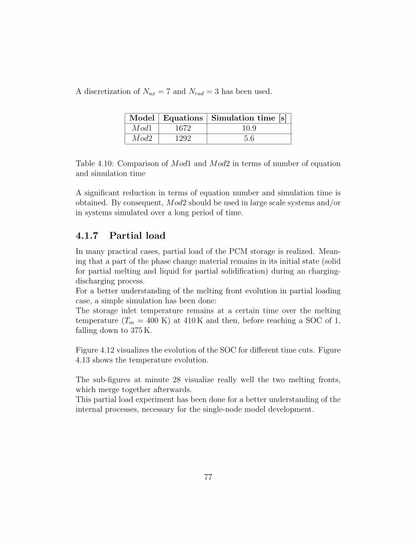
A discretization of Nax = 7 and Nrad = 3 has been used.

Model Equations Simulation time [s]Mod1 1672 10.9Mod2 1292 5.6

Table 4.10: Comparison of Mod1 and Mod2 in terms of number of equationand simulation time

A significant reduction in terms of equation number and simulation time isobtained. By consequent, Mod2 should be used in large scale systems and/orin systems simulated over a long period of time.

4.1.7 Partial load

In many practical cases, partial load of the PCM storage is realized. Mean-ing that a part of the phase change material remains in its initial state (solidfor partial melting and liquid for partial solidification) during an charging-discharging process.For a better understanding of the melting front evolution in partial loadingcase, a simple simulation has been done:The storage inlet temperature remains at a certain time over the meltingtemperature (Tm = 400 K) at 410 K and then, before reaching a SOC of 1,falling down to 375 K.

Figure 4.12 visualizes the evolution of the SOC for different time cuts. Figure4.13 shows the temperature evolution.

The sub-figures at minute 28 visualize really well the two melting fronts,which merge together afterwards.This partial load experiment has been done for a better understanding of theinternal processes, necessary for the single-node model development.

77

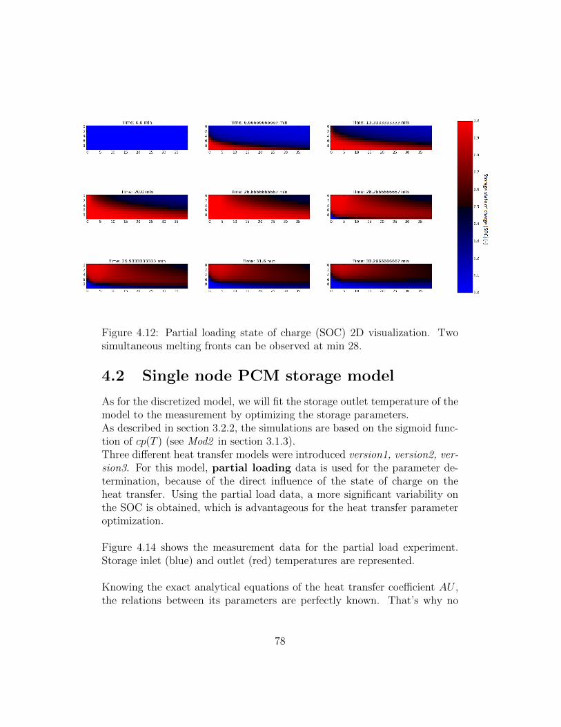
Figure 4.12: Partial loading state of charge (SOC) 2D visualization. Twosimultaneous melting fronts can be observed at min 28.

4.2 Single node PCM storage model

As for the discretized model, we will fit the storage outlet temperature of themodel to the measurement by optimizing the storage parameters.As described in section 3.2.2, the simulations are based on the sigmoid func-tion of cp(T ) (see Mod2 in section 3.1.3).Three different heat transfer models were introduced version1, version2, ver-sion3. For this model, partial loading data is used for the parameter de-termination, because of the direct influence of the state of charge on theheat transfer. Using the partial load data, a more significant variability onthe SOC is obtained, which is advantageous for the heat transfer parameteroptimization.

Figure 4.14 shows the measurement data for the partial load experiment.Storage inlet (blue) and outlet (red) temperatures are represented.

Knowing the exact analytical equations of the heat transfer coefficient AU ,the relations between its parameters are perfectly known. That’s why no

78

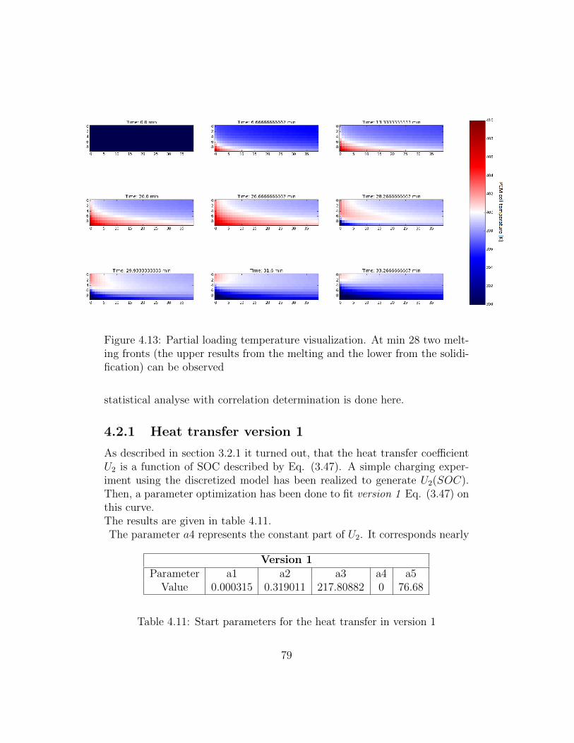
Figure 4.13: Partial loading temperature visualization. At min 28 two melt-ing fronts (the upper results from the melting and the lower from the solidi-fication) can be observed

statistical analyse with correlation determination is done here.

4.2.1 Heat transfer version 1

As described in section 3.2.1 it turned out, that the heat transfer coefficientU2 is a function of SOC described by Eq. (3.47). A simple charging exper-iment using the discretized model has been realized to generate U2(SOC).Then, a parameter optimization has been done to fit version 1 Eq. (3.47) onthis curve.The results are given in table 4.11.The parameter a4 represents the constant part of U2. It corresponds nearly

Version 1Parameter a1 a2 a3 a4 a5

Value 0.000315 0.319011 217.80882 0 76.68

Table 4.11: Start parameters for the heat transfer in version 1

79

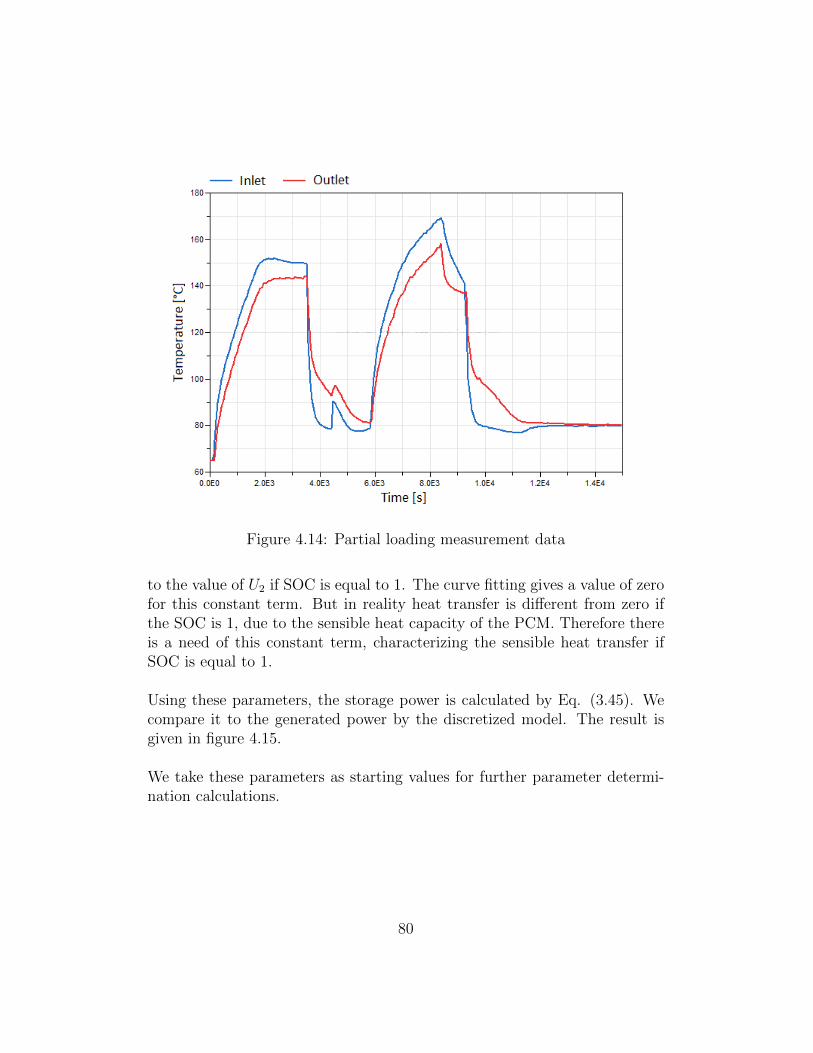
Figure 4.14: Partial loading measurement data

to the value of U2 if SOC is equal to 1. The curve fitting gives a value of zerofor this constant term. But in reality heat transfer is different from zero ifthe SOC is 1, due to the sensible heat capacity of the PCM. Therefore thereis a need of this constant term, characterizing the sensible heat transfer ifSOC is equal to 1.

Using these parameters, the storage power is calculated by Eq. (3.45). Wecompare it to the generated power by the discretized model. The result isgiven in figure 4.15.

We take these parameters as starting values for further parameter determi-nation calculations.

80

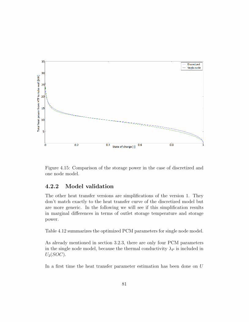
Figure 4.15: Comparison of the storage power in the case of discretized andone node model.

4.2.2 Model validation

The other heat transfer versions are simplifications of the version 1. Theydon’t match exactly to the heat transfer curve of the discretized model butare more generic. In the following we will see if this simplification resultsin marginal differences in terms of outlet storage temperature and storagepower.

Table 4.12 summarizes the optimized PCM parameters for single node model.

As already mentioned in section 3.2.3, there are only four PCM parametersin the single node model, because the thermal conductivity λP is included inU2(SOC).

In a first time the heat transfer parameter estimation has been done on U

81

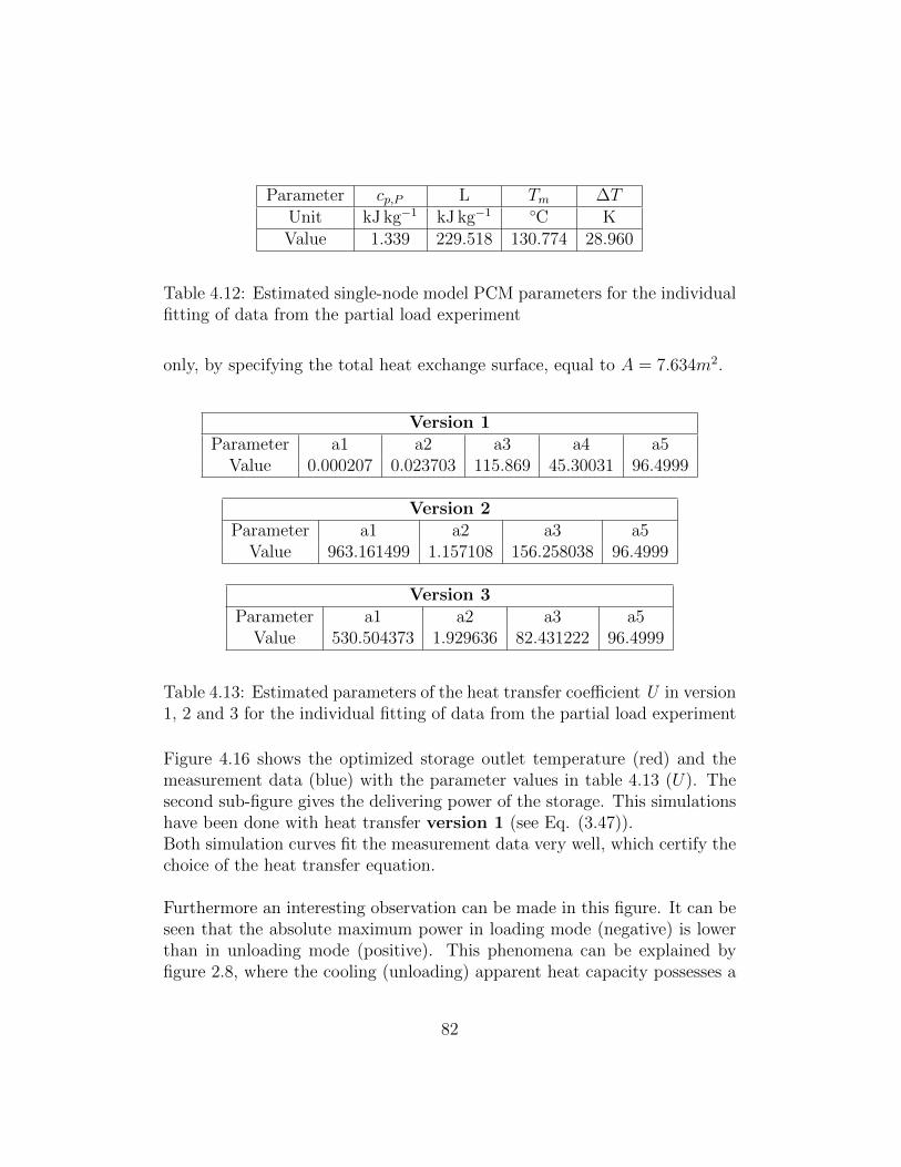
Parameter cp,P L Tm ∆TUnit kJ kg−1 kJ kg−1 ◦C KValue 1.339 229.518 130.774 28.960

Table 4.12: Estimated single-node model PCM parameters for the individualfitting of data from the partial load experiment

only, by specifying the total heat exchange surface, equal to A = 7.634m2.

Version 1Parameter a1 a2 a3 a4 a5

Value 0.000207 0.023703 115.869 45.30031 96.4999

Version 2Parameter a1 a2 a3 a5

Value 963.161499 1.157108 156.258038 96.4999

Version 3Parameter a1 a2 a3 a5

Value 530.504373 1.929636 82.431222 96.4999

Table 4.13: Estimated parameters of the heat transfer coefficient U in version1, 2 and 3 for the individual fitting of data from the partial load experiment

Figure 4.16 shows the optimized storage outlet temperature (red) and themeasurement data (blue) with the parameter values in table 4.13 (U). Thesecond sub-figure gives the delivering power of the storage. This simulationshave been done with heat transfer version 1 (see Eq. (3.47)).Both simulation curves fit the measurement data very well, which certify thechoice of the heat transfer equation.

Furthermore an interesting observation can be made in this figure. It can beseen that the absolute maximum power in loading mode (negative) is lowerthan in unloading mode (positive). This phenomena can be explained byfigure 2.8, where the cooling (unloading) apparent heat capacity possesses a

82

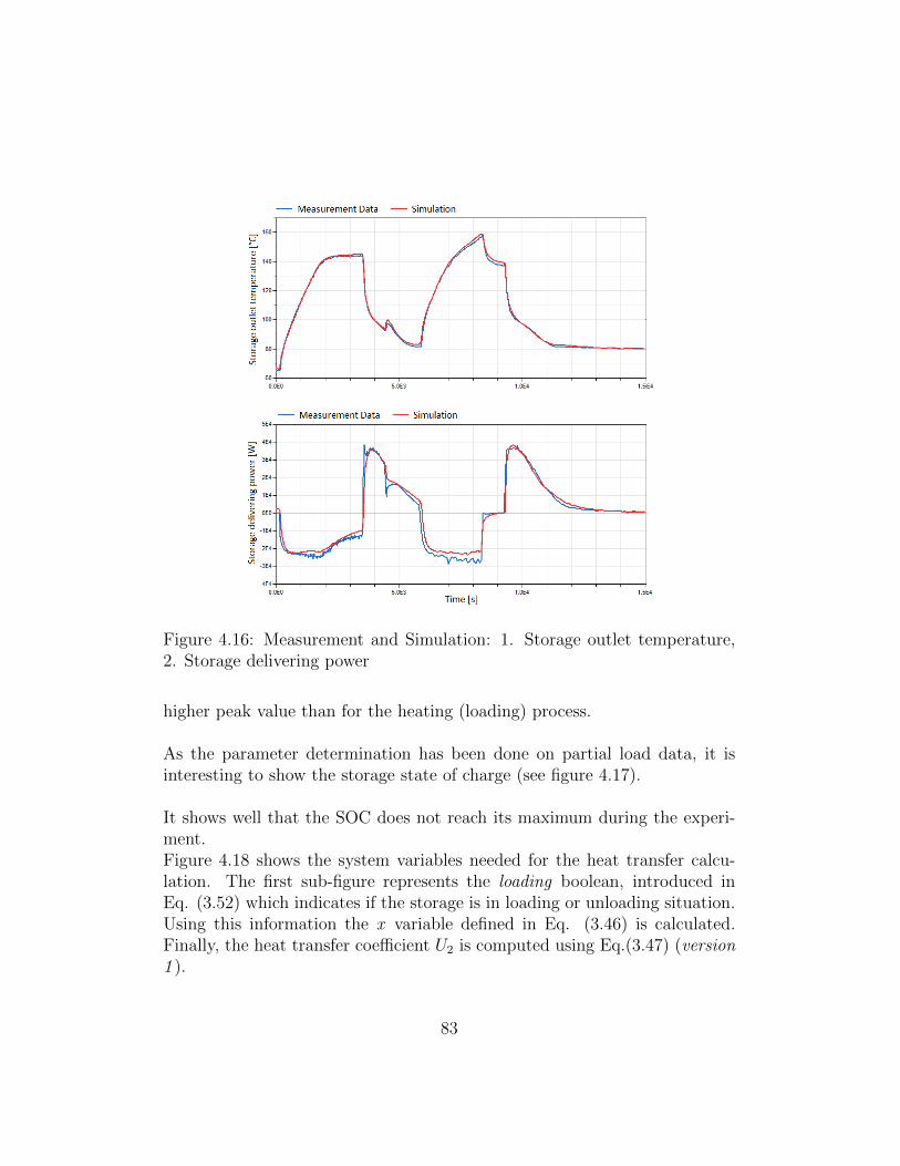
Figure 4.16: Measurement and Simulation: 1. Storage outlet temperature,2. Storage delivering power

higher peak value than for the heating (loading) process.

As the parameter determination has been done on partial load data, it isinteresting to show the storage state of charge (see figure 4.17).

It shows well that the SOC does not reach its maximum during the experi-ment.Figure 4.18 shows the system variables needed for the heat transfer calcu-lation. The first sub-figure represents the loading boolean, introduced inEq. (3.52) which indicates if the storage is in loading or unloading situation.Using this information the x variable defined in Eq. (3.46) is calculated.Finally, the heat transfer coefficient U2 is computed using Eq.(3.47) (version1 ).

83

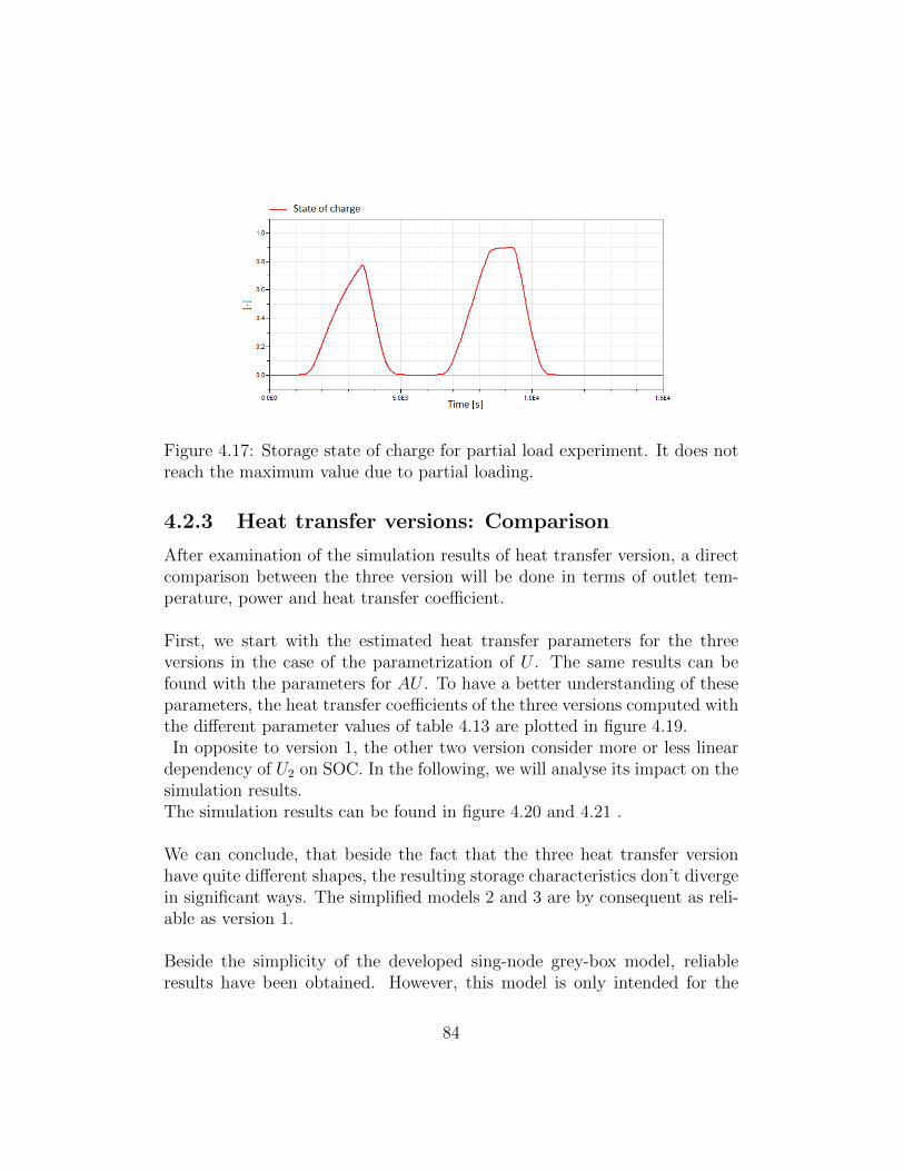
Figure 4.17: Storage state of charge for partial load experiment. It does notreach the maximum value due to partial loading.

4.2.3 Heat transfer versions: Comparison

After examination of the simulation results of heat transfer version, a directcomparison between the three version will be done in terms of outlet tem-perature, power and heat transfer coefficient.

First, we start with the estimated heat transfer parameters for the threeversions in the case of the parametrization of U . The same results can befound with the parameters for AU . To have a better understanding of theseparameters, the heat transfer coefficients of the three versions computed withthe different parameter values of table 4.13 are plotted in figure 4.19.In opposite to version 1, the other two version consider more or less linear

dependency of U2 on SOC. In the following, we will analyse its impact on thesimulation results.The simulation results can be found in figure 4.20 and 4.21 .

We can conclude, that beside the fact that the three heat transfer versionhave quite different shapes, the resulting storage characteristics don’t divergein significant ways. The simplified models 2 and 3 are by consequent as reli-able as version 1.

Beside the simplicity of the developed sing-node grey-box model, reliableresults have been obtained. However, this model is only intended for the

84

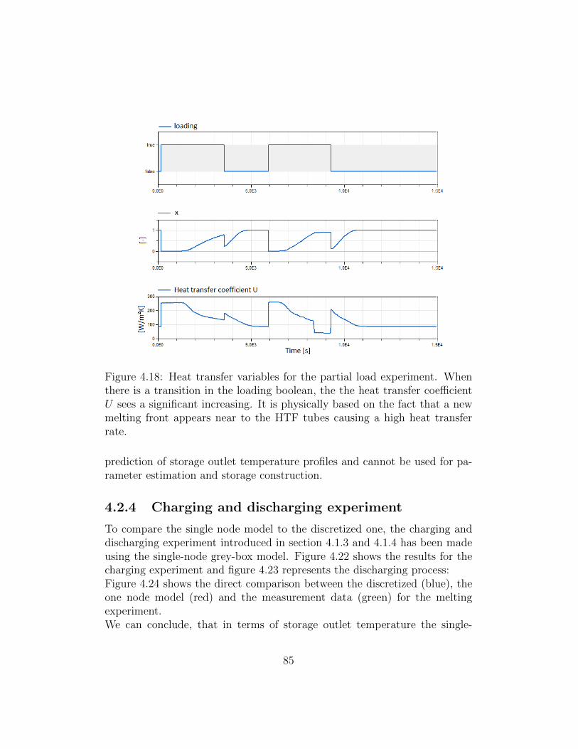
Figure 4.18: Heat transfer variables for the partial load experiment. Whenthere is a transition in the loading boolean, the the heat transfer coefficientU sees a significant increasing. It is physically based on the fact that a newmelting front appears near to the HTF tubes causing a high heat transferrate.

prediction of storage outlet temperature profiles and cannot be used for pa-rameter estimation and storage construction.

4.2.4 Charging and discharging experiment

To compare the single node model to the discretized one, the charging anddischarging experiment introduced in section 4.1.3 and 4.1.4 has been madeusing the single-node grey-box model. Figure 4.22 shows the results for thecharging experiment and figure 4.23 represents the discharging process:Figure 4.24 shows the direct comparison between the discretized (blue), theone node model (red) and the measurement data (green) for the meltingexperiment.We can conclude, that in terms of storage outlet temperature the single-

85

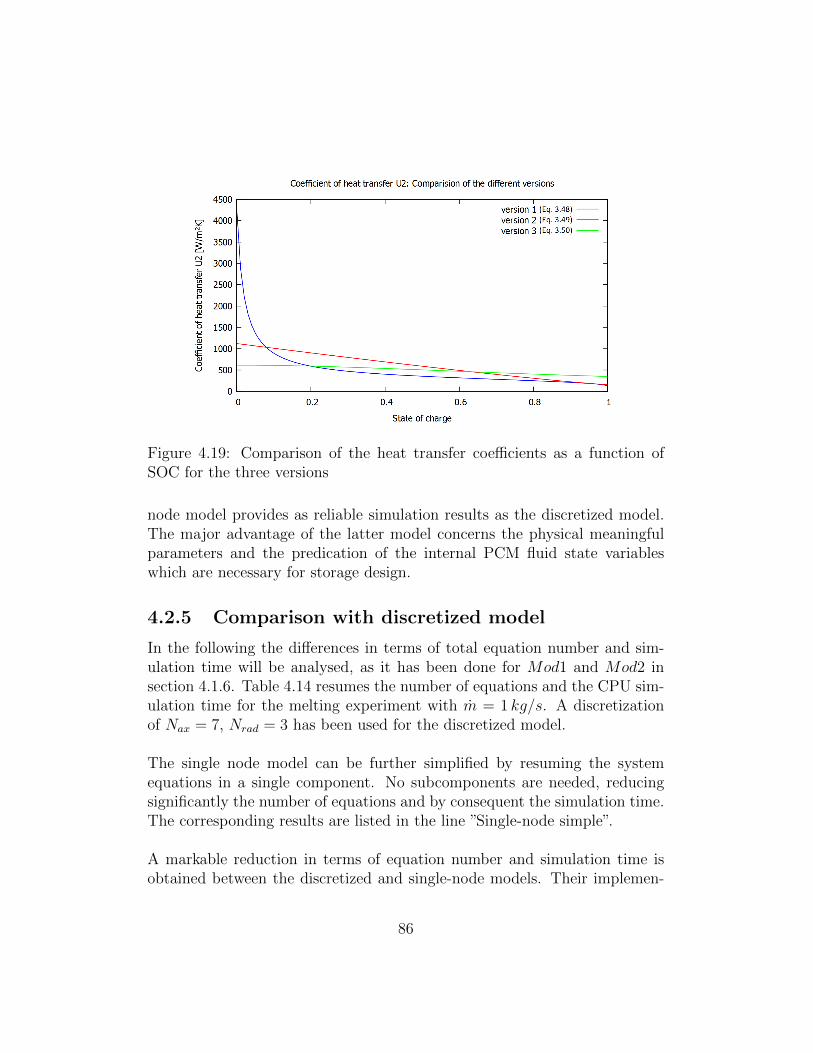
Figure 4.19: Comparison of the heat transfer coefficients as a function ofSOC for the three versions

node model provides as reliable simulation results as the discretized model.The major advantage of the latter model concerns the physical meaningfulparameters and the predication of the internal PCM fluid state variableswhich are necessary for storage design.

4.2.5 Comparison with discretized model

In the following the differences in terms of total equation number and sim-ulation time will be analysed, as it has been done for Mod1 and Mod2 insection 4.1.6. Table 4.14 resumes the number of equations and the CPU sim-ulation time for the melting experiment with m = 1 kg/s. A discretizationof Nax = 7, Nrad = 3 has been used for the discretized model.

The single node model can be further simplified by resuming the systemequations in a single component. No subcomponents are needed, reducingsignificantly the number of equations and by consequent the simulation time.The corresponding results are listed in the line ”Single-node simple”.

A markable reduction in terms of equation number and simulation time isobtained between the discretized and single-node models. Their implemen-

86

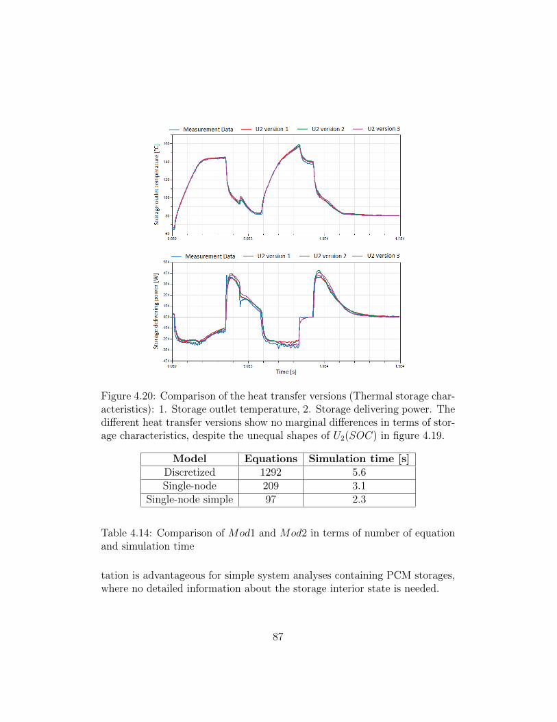
Figure 4.20: Comparison of the heat transfer versions (Thermal storage char-acteristics): 1. Storage outlet temperature, 2. Storage delivering power. Thedifferent heat transfer versions show no marginal differences in terms of stor-age characteristics, despite the unequal shapes of U2(SOC) in figure 4.19.

Model Equations Simulation time [s]Discretized 1292 5.6Single-node 209 3.1

Single-node simple 97 2.3

Table 4.14: Comparison of Mod1 and Mod2 in terms of number of equationand simulation time

tation is advantageous for simple system analyses containing PCM storages,where no detailed information about the storage interior state is needed.

87

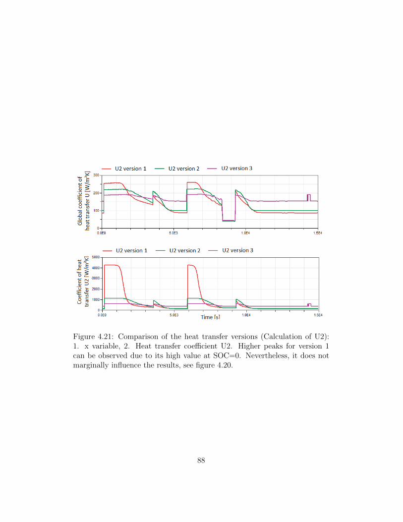
Figure 4.21: Comparison of the heat transfer versions (Calculation of U2):1. x variable, 2. Heat transfer coefficient U2. Higher peaks for version 1can be observed due to its high value at SOC=0. Nevertheless, it does notmarginally influence the results, see figure 4.20.

88

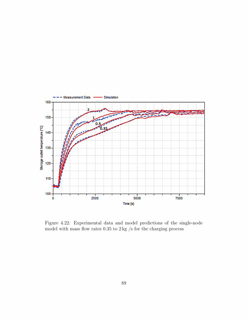
Figure 4.22: Experimental data and model predictions of the single-nodemodel with mass flow rates 0.35 to 2 kg /s for the charging process

89

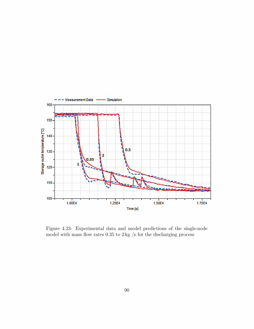
Figure 4.23: Experimental data and model predictions of the single-nodemodel with mass flow rates 0.35 to 2 kg /s for the discharging process

90

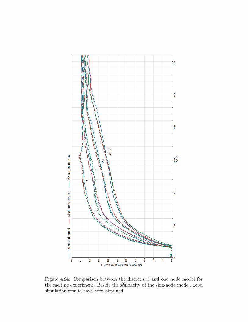
Figure 4.24: Comparison between the discretized and one node model forthe melting experiment. Beside the simplicity of the sing-node model, goodsimulation results have been obtained.

91

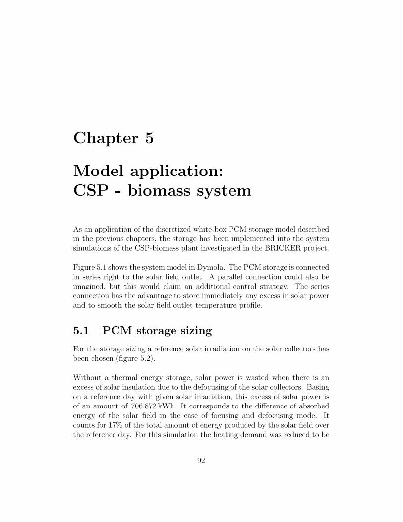
Chapter 5

Model application:CSP - biomass system

As an application of the discretized white-box PCM storage model describedin the previous chapters, the storage has been implemented into the systemsimulations of the CSP-biomass plant investigated in the BRICKER project.

Figure 5.1 shows the system model in Dymola. The PCM storage is connectedin series right to the solar field outlet. A parallel connection could also beimagined, but this would claim an additional control strategy. The seriesconnection has the advantage to store immediately any excess in solar powerand to smooth the solar field outlet temperature profile.

5.1 PCM storage sizing

For the storage sizing a reference solar irradiation on the solar collectors hasbeen chosen (figure 5.2).

Without a thermal energy storage, solar power is wasted when there is anexcess of solar insulation due to the defocusing of the solar collectors. Basingon a reference day with given solar irradiation, this excess of solar power isof an amount of 706.872 kWh. It corresponds to the difference of absorbedenergy of the solar field in the case of focusing and defocusing mode. Itcounts for 17% of the total amount of energy produced by the solar field overthe reference day. For this simulation the heating demand was reduced to be

92

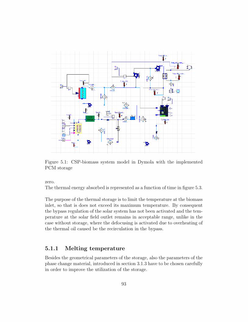
Figure 5.1: CSP-biomass system model in Dymola with the implementedPCM storage

zero.The thermal energy absorbed is represented as a function of time in figure 5.3.

The purpose of the thermal storage is to limit the temperature at the biomassinlet, so that is does not exceed its maximum temperature. By consequentthe bypass regulation of the solar system has not been activated and the tem-perature at the solar field outlet remains in acceptable range, unlike in thecase without storage, where the defocusing is activated due to overheating ofthe thermal oil caused be the recirculation in the bypass.

5.1.1 Melting temperature

Besides the geometrical parameters of the storage, also the parameters of thephase change material, introduced in section 3.1.3 have to be chosen carefullyin order to improve the utilization of the storage.

93

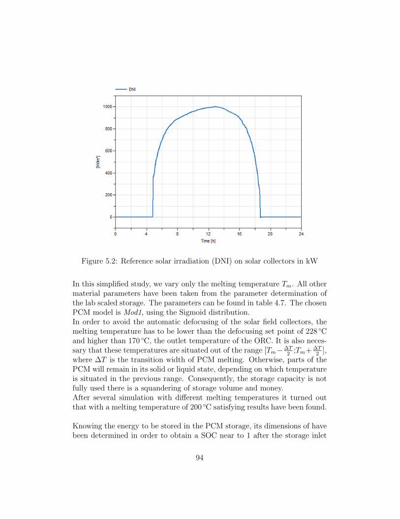
Figure 5.2: Reference solar irradiation (DNI) on solar collectors in kW

In this simplified study, we vary only the melting temperature Tm. All othermaterial parameters have been taken from the parameter determination ofthe lab scaled storage. The parameters can be found in table 4.7. The chosenPCM model is Mod1, using the Sigmoid distribution.In order to avoid the automatic defocusing of the solar field collectors, themelting temperature has to be lower than the defocusing set point of 228 ◦Cand higher than 170 ◦C, the outlet temperature of the ORC. It is also neces-sary that these temperatures are situated out of the range [Tm−∆T

2;Tm+ ∆T

2],

where ∆T is the transition width of PCM melting. Otherwise, parts of thePCM will remain in its solid or liquid state, depending on which temperatureis situated in the previous range. Consequently, the storage capacity is notfully used there is a squandering of storage volume and money.After several simulation with different melting temperatures it turned outthat with a melting temperature of 200 ◦C satisfying results have been found.

Knowing the energy to be stored in the PCM storage, its dimensions of havebeen determined in order to obtain a SOC near to 1 after the storage inlet

94

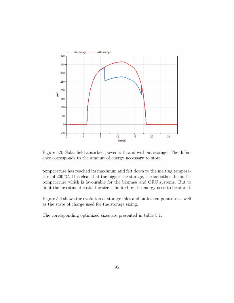
Figure 5.3: Solar field absorbed power with and without storage. The differ-ence corresponds to the amount of energy necessary to store.

temperature has reached its maximum and felt down to the melting tempera-ture of 200 ◦C. It is clear that the bigger the storage, the smoother the outlettemperature which is favourable for the biomass and ORC systems. But tolimit the investment costs, the size is limited by the energy need to be stored.

Figure 5.4 shows the evolution of storage inlet and outlet temperature as wellas the state of charge used for the storage sizing.

The corresponding optimized sizes are presented in table 5.1:

95

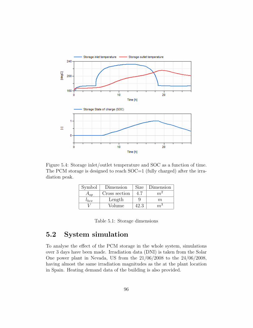
Figure 5.4: Storage inlet/outlet temperature and SOC as a function of time.The PCM storage is designed to reach SOC=1 (fully charged) after the irra-diation peak.

Symbol Dimension Size DimensionAap Cross section 4.7 m2

lhex Length 9 mV Volume 42.3 m3

Table 5.1: Storage dimensions

5.2 System simulation

To analyse the effect of the PCM storage in the whole system, simulationsover 3 days have been made. Irradiation data (DNI) is taken from the SolarOne power plant in Nevada, US from the 21/06/2008 to the 24/06/2008,having almost the same irradiation magnitudes as the at the plant locationin Spain. Heating demand data of the building is also provided.

96

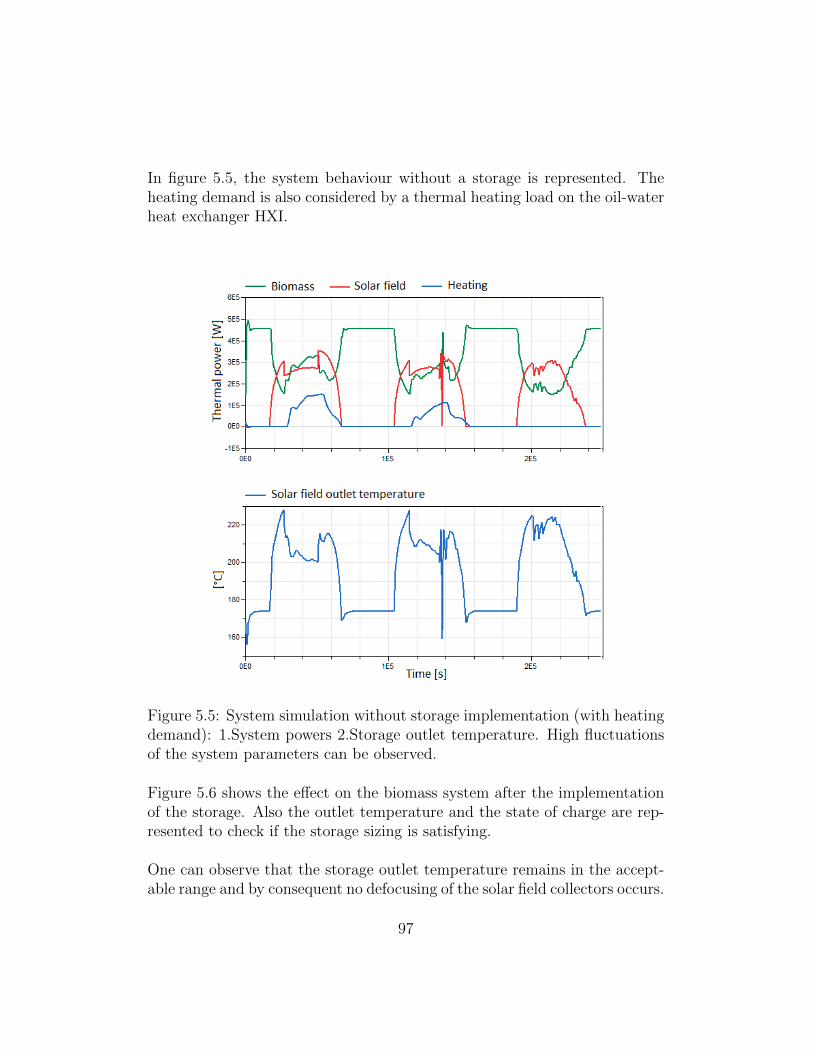
In figure 5.5, the system behaviour without a storage is represented. Theheating demand is also considered by a thermal heating load on the oil-waterheat exchanger HXI.

Figure 5.5: System simulation without storage implementation (with heatingdemand): 1.System powers 2.Storage outlet temperature. High fluctuationsof the system parameters can be observed.

Figure 5.6 shows the effect on the biomass system after the implementationof the storage. Also the outlet temperature and the state of charge are rep-resented to check if the storage sizing is satisfying.

One can observe that the storage outlet temperature remains in the accept-able range and by consequent no defocusing of the solar field collectors occurs.

97

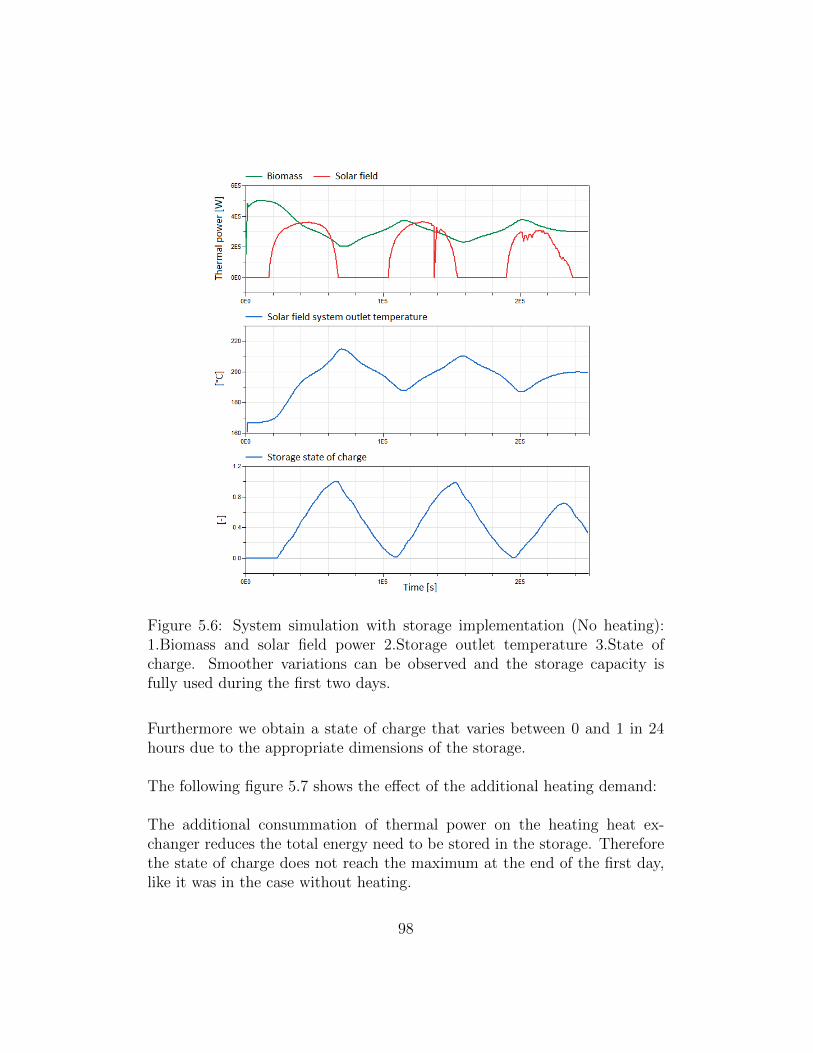
Figure 5.6: System simulation with storage implementation (No heating):1.Biomass and solar field power 2.Storage outlet temperature 3.State ofcharge. Smoother variations can be observed and the storage capacity isfully used during the first two days.

Furthermore we obtain a state of charge that varies between 0 and 1 in 24hours due to the appropriate dimensions of the storage.

The following figure 5.7 shows the effect of the additional heating demand:

The additional consummation of thermal power on the heating heat ex-changer reduces the total energy need to be stored in the storage. Thereforethe state of charge does not reach the maximum at the end of the first day,like it was in the case without heating.

98

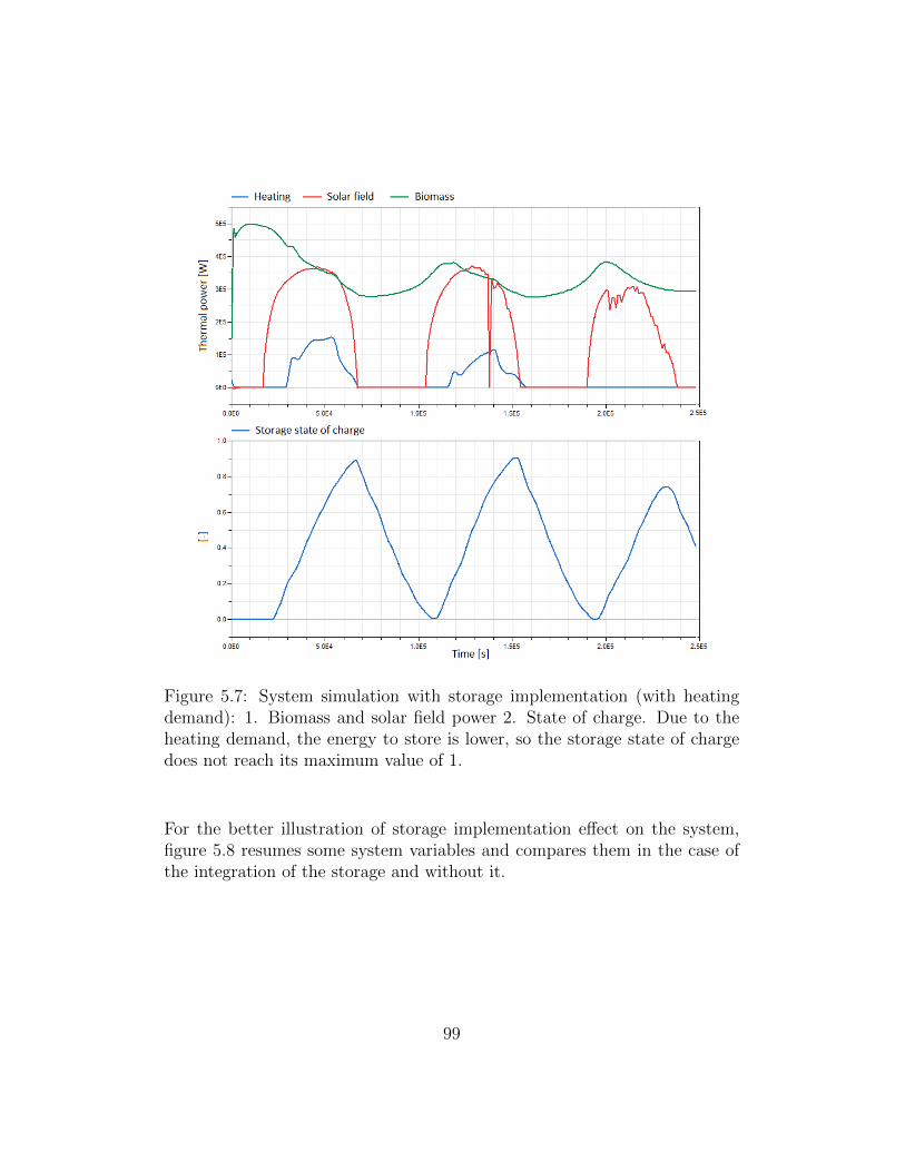
Figure 5.7: System simulation with storage implementation (with heatingdemand): 1. Biomass and solar field power 2. State of charge. Due to theheating demand, the energy to store is lower, so the storage state of chargedoes not reach its maximum value of 1.

For the better illustration of storage implementation effect on the system,figure 5.8 resumes some system variables and compares them in the case ofthe integration of the storage and without it.

99

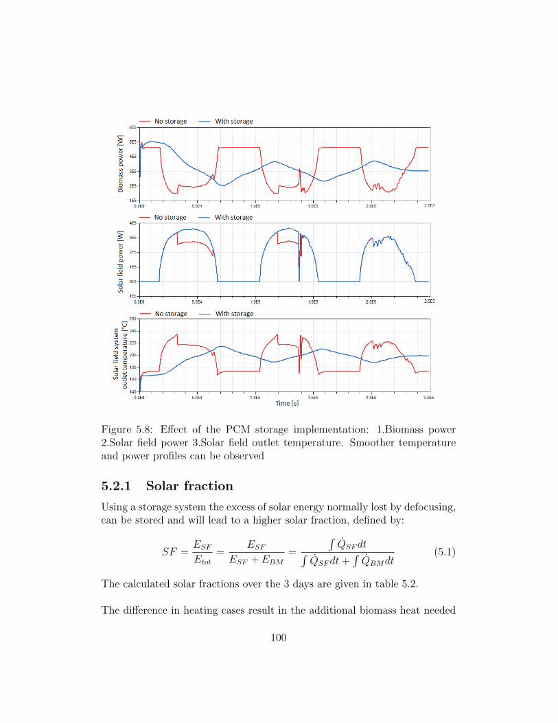
Figure 5.8: Effect of the PCM storage implementation: 1.Biomass power2.Solar field power 3.Solar field outlet temperature. Smoother temperatureand power profiles can be observed

5.2.1 Solar fraction

Using a storage system the excess of solar energy normally lost by defocusing,can be stored and will lead to a higher solar fraction, defined by:

SF =ESF

Etot

=ESF

ESF + EBM

=

∫QSFdt∫

QSFdt+∫QBMdt

(5.1)

The calculated solar fractions over the 3 days are given in table 5.2.

The difference in heating cases result in the additional biomass heat needed

100

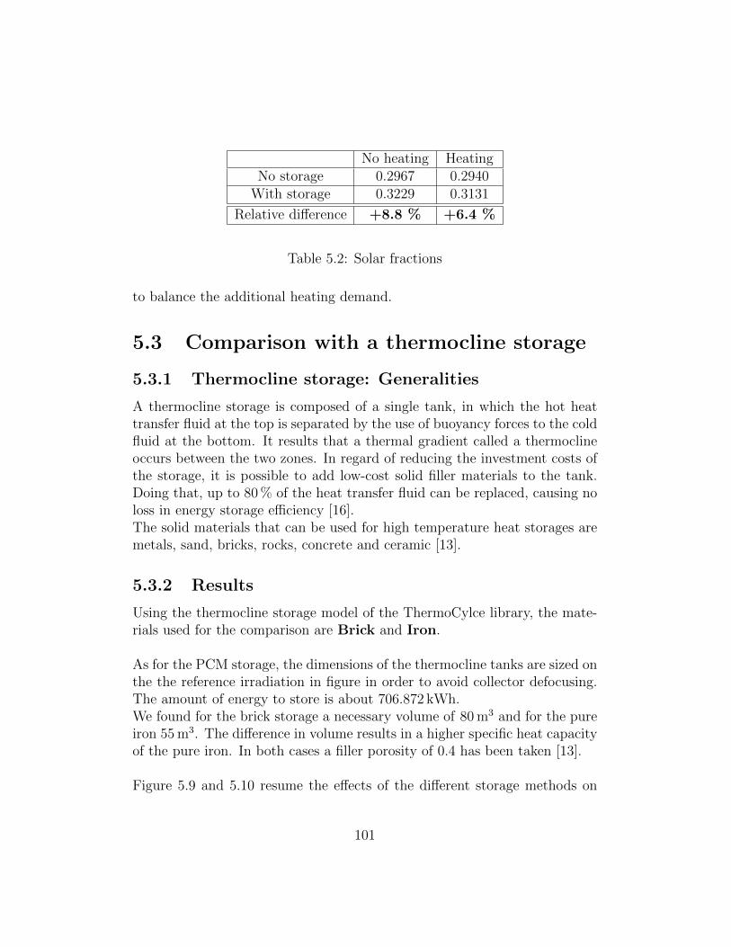
No heating HeatingNo storage 0.2967 0.2940

With storage 0.3229 0.3131

Relative difference +8.8 % +6.4 %

Table 5.2: Solar fractions

to balance the additional heating demand.

5.3 Comparison with a thermocline storage

5.3.1 Thermocline storage: Generalities

A thermocline storage is composed of a single tank, in which the hot heattransfer fluid at the top is separated by the use of buoyancy forces to the coldfluid at the bottom. It results that a thermal gradient called a thermoclineoccurs between the two zones. In regard of reducing the investment costs ofthe storage, it is possible to add low-cost solid filler materials to the tank.Doing that, up to 80 % of the heat transfer fluid can be replaced, causing noloss in energy storage efficiency [16].The solid materials that can be used for high temperature heat storages aremetals, sand, bricks, rocks, concrete and ceramic [13].

5.3.2 Results

Using the thermocline storage model of the ThermoCylce library, the mate-rials used for the comparison are Brick and Iron.

As for the PCM storage, the dimensions of the thermocline tanks are sized onthe the reference irradiation in figure in order to avoid collector defocusing.The amount of energy to store is about 706.872 kWh.We found for the brick storage a necessary volume of 80 m3 and for the pureiron 55 m3. The difference in volume results in a higher specific heat capacityof the pure iron. In both cases a filler porosity of 0.4 has been taken [13].

Figure 5.9 and 5.10 resume the effects of the different storage methods on

101

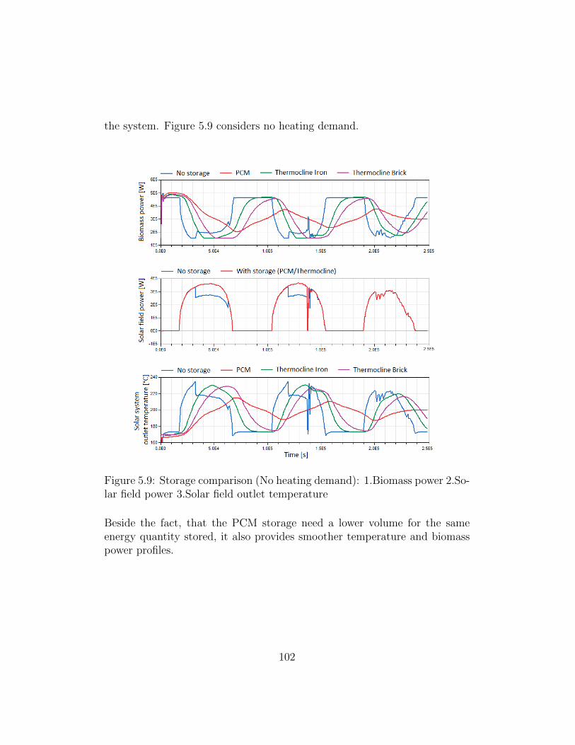
the system. Figure 5.9 considers no heating demand.

Figure 5.9: Storage comparison (No heating demand): 1.Biomass power 2.So-lar field power 3.Solar field outlet temperature

Beside the fact, that the PCM storage need a lower volume for the sameenergy quantity stored, it also provides smoother temperature and biomasspower profiles.

102

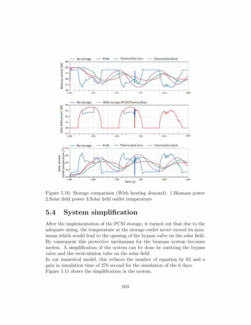
Figure 5.10: Storage comparison (With heating demand): 1.Biomass power2.Solar field power 3.Solar field outlet temperature

5.4 System simplification

After the implementation of the PCM storage, it turned out that due to theadequate sizing, the temperature at the storage outlet never exceed its max-imum which would lead to the opening of the bypass valve on the solar field.By consequent this protective mechanism for the biomass system becomesuseless. A simplification of the system can be done by omitting the bypassvalve and the recirculation tube on the solar field.In our numerical model, this reduces the number of equation by 62 and again in simulation time of 270 second for the simulation of the 6 days.Figure 5.11 shows the simplification in the system.

103

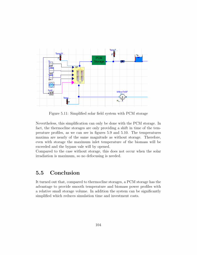
Figure 5.11: Simplified solar field system with PCM storage

Nevertheless, this simplification can only be done with the PCM storage. Infact, the thermocline storages are only providing a shift in time of the tem-perature profiles, as we can see in figures 5.9 and 5.10. The temperaturesmaxima are nearly of the same magnitude as without storage. Therefore,even with storage the maximum inlet temperature of the biomass will beexceeded and the bypass vale will by opened.Compared to the case without storage, this does not occur when the solarirradiation is maximum, so no defocusing is needed.

5.5 Conclusion

It turned out that, compared to thermocline storages, a PCM storage has theadvantage to provide smooth temperature and biomass power profiles witha relative small storage volume. In addition the system can be significantlysimplified which reduces simulation time and investment costs.

104

Chapter 6

Conclusion

Two numeric models, a white-box discretized and a grey-box single nodemode, of a latent heat thermal energy storage and their validation on ex-perimental measurement data of a laboratory storage prototype have beenpresented in this work. The discretized model consist in a complex model des-tined to predict real physical parameters for storage design. The single-nodemodel, in contrast, uses a simple approach for system simulation and curvefitting where internal storage thermophysical processes are not necessary tobe simulated. The phase change material behaviour have been characterizedby an apparent heat capacity method described by parameter sets of differentPCM model approaches.The validation of both model types on experimental data, showed that thesimulation prediction fit the measurement values very well. Further statis-tical analyses proved the adequate choice of the parameter sets and showedthe differences in PCM models. A comparison between the PCM models interms of optimized parameter results and simulation time has been provided,as well as a comparison in simulation time between discretized and single-node model approach.The validated discretized LHTES model has finally included in the CSP-biomass system to improve its solar fraction. It turned out that the use ofa latent heat storage provides both, the advantage to store eventual solarpower excess, increasing the solar fraction, and generating a smooth biomassinlet temperature profile causing less fluctuating boiler power.

105

Bibliography

[1] http://www.bricker-project.com/. [Online; accessed 11-July-2016].

[2] http://www.thermocycle.net. [Online; accessed 29-July-2016].

[3] http://www.ewp.rpi.edu/hartford/~ernesto/S2006/CHT/Notes/

ch03.pdf. [Online; accessed 14-April-2016].

[4] http://www.docs.scipy.org/doc/scipy/reference/tutorial/

optimize.html. [Online; accessed 2-March-2016].

[5] http://www.simulationresearch.lbl.gov/modelica/buildingspy/

simulate.html. [Online; accessed 2-March-2016].

[6] M.B. Abd-el Malek and M.M. Helal. Group method solution for solv-ing nonlinear heat diffusion problems. Applied mathematical modelling,30:930–940, 2006.

[7] A. Abhat. Low temperature latent heat thermal energy storage: heatstorage materials. Solar Energy, 30:313–332, 1983.

[8] F. Agyenim, N. Hewitt, P. Eames, and M. Smyth. A review of materials,heat transfer and phase change problem formulation for latent heat ther-mal energy storage systems (lhtess). Renewable and Sustainable EnergyReviews, 14:615–628, 2010.

[9] H.D. Baehr and K. Stephan. Warme- und Stoffubertragung, Vol. 3.Springer, Berlin, 1994.

[10] R.B. Bird, W.E. Stewart, and E.N. Lightfoot. Transport phenomena.John Wiley, 2007.

106

[11] M. Costa, D. Buddhi, and A. Oliva. Numerical simulations of a latentheat thermal energy storage system with enhanced heat conduction.Energy conversion management, 39:319–330, 1998.

[12] A. Desideri, S. Amicabile, F. Alberti, S. Vitali-Nari, S. Quoilin,L. Crema, and V. Lemort. Dynamic modeling and control strategiesanalysis of a novel small csp biomass plant for cogeneration applicationsin building. In Solar World Congress 2015, Daegu, Korea.

[13] H. Grirate, H. Agalit, N. Zari, A. Elmchaouri, S. Molina, and R. Cou-turier. Experimental and numerical investigation of potential filler ma-terials for thermal oil thermocline storage. Solar Energy, 131:260–274,2016.

[14] S.M. Hasnain. Review on suitable thermal energy storage technologies,part 1: Heat storage materials and techniques. Energy conversion man-agement, 11:1127–1138, 1998.

[15] F. Hengstberger, C. Zauner, K. Resch, S. Holper, and M. Grobbauer.High temperature phase change materials for the overheating protectionof facade integrated solar thermal collectors. Energy and Building, 124,2016.

[16] J.-F. Hoffmann, T. Fasquelle, V. Goetz, and X. Py. A thermoclinethermal energy storage system with filler materials for concentrated so-lar power plants: Experimental data and numerical model sensitivityto different experimental tank scales. Applied Thermal Engineering,100:753–761, 2016.

[17] Murat M. Kensisarin. High-temperature phase change materials forthermal energy storage. Renewable and Sustainable Energy Reviews,14:955–970, 2010.

[18] Saba Khan. A review - an optimization of macroencapsulated paraffinused in solar latent heat storage unit. International Journal of Engi-neering and Technical Research, 2016.

[19] Doerte Laing, Tomas Bauer, Nils Breidenbach, Bernd Hachmann,and Maike Johnson. Development of high temperature phase-change-material storages. Applied Energy, 109:497–504, 2013.

107

[20] Marc Medrano, Gil Antoni, Ingrid Martorell, Xavi Potau, and Luisa F.Cabeza. State of the art on high-temperature thermal energy storagefor power generation. part 2—case studies. Renewable and SustainableEnergy Reviews, 14:56–72, 2010.

[21] Harald Megling and Luisa F. Cabeza. Heat and cold storage with PCM.Springer, Berlin, 2008.

[22] H. Mehling, P. Schossig, and D. Kalz. Latent heat storage in buildings,storing heat and cold in a compact and demand-oriented manner. BINEInformationsdienst, 1, 2009.

[23] S. Quoilin, A. Desideri, J. Wronski, I. Bell, and V. Lemort. Thermocycle:A modelica library for the simulation of thermodynamic systems. 2014.

[24] Atul Sharma, V.V. Tyagi, C.R. Chen, and D. Buddhi. Review on ther-mal energy storage with phase change materials and applications. Re-newable and Sustainable Energy Reviews, 13:318–345, 2009.

[25] Barz Tilman, Christoph Zauner, Daniel Langer, Diana Lopez Cardenas,Florian Hengstberger, Mariano Nicolas Cruz Bournazou, and KlemensMarx. Experimental analysis and numerical modeling of a shell and tubeheat storage unit with phase change materials. Industrial and Engineer-ing Chemistry Research, 55:8154–8164, 2016.

[26] VDI-Gesellschaft Verfahrenstechnik und Chemieingenieurwesen. VDIHeat Atlas. Springer, Berlin, 2010.

[27] B. Zalba, J. M. Marn, L. F. Cabeza, and H. Mehling. Review on thermalenergy storage with phase change: materials, heat transfer analysis andapplications. Applied thermal engineering, 23:251–283, 2003.

[28] Christoph Zauner, Florian Hengstberger, Mark Etzel, Daniel Lager,Rene Hofmann, and Heimo Walter. Experimental characterization andsimulation of a fin-tube latent heat storage using high density polyethy-lene as pcm. Applied Energy, 179:237–246, 2016.

108

List of Figures

2.1 Comparison of sensible and latent heat storages in terms oftemperature profile as a function of stored heat . . . . . . . . 7

2.2 Effect of subcooling on a latent heat storage . . . . . . . . . . 82.3 Classification of energy storage materials [7] . . . . . . . . . . 92.4 Arrangement of the steel tubes. At positions 1–5 thermocou-

ples were immersed within the PCM. . . . . . . . . . . . . . . 132.5 HDPE pellets poured into the storage . . . . . . . . . . . . . . 132.6 Top surface of the full storage in solid state. Deformation of

the fins can be observed . . . . . . . . . . . . . . . . . . . . . 142.7 Temperatures and calculated power profiles for a thermal oil

mass flow of 0.41 kg/s. A full charging followed by a discharg-ing process have been realized . . . . . . . . . . . . . . . . . . 16

2.8 DSC measurements of HDPE for different heating and coolingrates compared to the melting and crystallization ranges ofthe prototype storage. Due to subcooling, a difference in thephase change temperature depending on the process type andrate can be observed . . . . . . . . . . . . . . . . . . . . . . . 17

2.9 Schematic flow diagram of the Bricker CHP system . . . . . . 21

3.1 Schemata of the modelling idea: (1) Subdivision of the stor-age in equal cuboids, (2)Conversion from cuboid to cylinder,(3)Discretization in radial and axial direction . . . . . . . . . . 24

3.2 HTF cell in Dymola . . . . . . . . . . . . . . . . . . . . . . . . 273.3 Tube wall cell in Dymola . . . . . . . . . . . . . . . . . . . . . 293.4 Discretization scheme for the tube wall . . . . . . . . . . . . . 303.5 Normal function and parameters of Mod1 . . . . . . . . . . . 323.6 Sigmoid function and parameters of Mod2 . . . . . . . . . . . 333.7 PCM cell in Dymola . . . . . . . . . . . . . . . . . . . . . . . 343.8 Radial discretization scheme . . . . . . . . . . . . . . . . . . . 34

109

3.9 Build up of the Radial_components model . . . . . . . . . . . 373.10 Radial_components item . . . . . . . . . . . . . . . . . . . . 383.11 Build up of PCM_storage_model . . . . . . . . . . . . . . . . . 383.12 PCM_storage_model item . . . . . . . . . . . . . . . . . . . . 393.13 Parameter window of the discretized storage model . . . . . . 413.14 Schema of the heat transfer . . . . . . . . . . . . . . . . . . . 433.15 Thermal heat power HTF-PCM as a function of the global

storage SOC . . . . . . . . . . . . . . . . . . . . . . . . . . . . 443.16 Heat transfer coefficient AU as a function of SOC for different

mass flows (melting process). Higher heat transfer is obtainedwith higher mass flow rate . . . . . . . . . . . . . . . . . . . . 45

3.17 Global coefficient of heat transfer AU as a function of SOCfor different mass flows (solidification process). Higher heattransfer is obtained with higher mass flow rate . . . . . . . . . 46

3.18 Heat transfer coefficients for a HTF mass flow rate of 3 kg/sec.The reation between the heat transfer coefficient can be foundin Eq. (3.43) . . . . . . . . . . . . . . . . . . . . . . . . . . . . 47

3.19 HTF component of the single-node grey-box model . . . . . . 493.20 PCM component in the single node model . . . . . . . . . . . 503.21 Assembly of the components in the single node model . . . . . 513.22 Single node storage model item . . . . . . . . . . . . . . . . . 513.23 Parameter window of the single-node grey-box model . . . . . 54

4.1 Storage inlet temperature profiles for different mass flows inthe charging experiment. Nearly the same temperature pro-files can be observed . . . . . . . . . . . . . . . . . . . . . . . 58

4.2 2D visualization of the melting process (SOC, m = 1kg/s) . . 594.3 Experimental data and model predictions for Mod1 for mass

flow rates 0.35 to 2 kg /s . . . . . . . . . . . . . . . . . . . . . 604.4 Experimental data and model predictions for Mod2 for mass

flow rates 0.35 to 2 kg /s . . . . . . . . . . . . . . . . . . . . . 614.5 Thermal conductivity λP as a function of temperature for dif-

ferent parameters c2 . . . . . . . . . . . . . . . . . . . . . . . 644.6 Storage inlet temperature profiles for different mass flows in

the discharging experiment. The fluctuations for 2 kg /s resultfrom the laboratory devices and have no experimental intention. 66

4.7 2D visualization of the discharging process (SOC, m = 1kg/s) 67

110

4.8 Experimental data and model predictions for Mod1 for massflow rates 0.35 to 2 kg /s.The fluctuation for m = 2kg/s arevery well resolved by the model. . . . . . . . . . . . . . . . . . 69

4.9 Experimental data and model predictions for Mod2 for massflow rates 0.35 to 2 kg /s . . . . . . . . . . . . . . . . . . . . . 70

4.10 Experimental data and model predictions for Mod1 for massflow rates 0.35 to 2 kg /s . . . . . . . . . . . . . . . . . . . . . 73

4.11 Experimental data and model predictions for Mod2 for massflow rates 0.35 to 2 kg /s . . . . . . . . . . . . . . . . . . . . . 74

4.12 Partial loading state of charge (SOC) 2D visualization. Twosimultaneous melting fronts can be observed at min 28. . . . . 78

4.13 Partial loading temperature visualization. At min 28 two melt-ing fronts (the upper results from the melting and the lowerfrom the solidification) can be observed . . . . . . . . . . . . . 79

4.14 Partial loading measurement data . . . . . . . . . . . . . . . . 804.15 Comparison of the storage power in the case of discretized and

one node model. . . . . . . . . . . . . . . . . . . . . . . . . . . 814.16 Measurement and Simulation: 1. Storage outlet temperature,

2. Storage delivering power . . . . . . . . . . . . . . . . . . . 834.17 Storage state of charge for partial load experiment. It does

not reach the maximum value due to partial loading. . . . . . 844.18 Heat transfer variables for the partial load experiment. When

there is a transition in the loading boolean, the the heat trans-fer coefficient U sees a significant increasing. It is physicallybased on the fact that a new melting front appears near to theHTF tubes causing a high heat transfer rate. . . . . . . . . . . 85

4.19 Comparison of the heat transfer coefficients as a function ofSOC for the three versions . . . . . . . . . . . . . . . . . . . . 86

4.20 Comparison of the heat transfer versions (Thermal storagecharacteristics): 1. Storage outlet temperature, 2. Storagedelivering power. The different heat transfer versions show nomarginal differences in terms of storage characteristics, despitethe unequal shapes of U2(SOC) in figure 4.19. . . . . . . . . . 87

4.21 Comparison of the heat transfer versions (Calculation of U2):1. x variable, 2. Heat transfer coefficient U2. Higher peaksfor version 1 can be observed due to its high value at SOC=0.Nevertheless, it does not marginally influence the results, seefigure 4.20. . . . . . . . . . . . . . . . . . . . . . . . . . . . . . 88

111

4.22 Experimental data and model predictions of the single-nodemodel with mass flow rates 0.35 to 2 kg /s for the chargingprocess . . . . . . . . . . . . . . . . . . . . . . . . . . . . . . . 89

4.23 Experimental data and model predictions of the single-nodemodel with mass flow rates 0.35 to 2 kg /s for the dischargingprocess . . . . . . . . . . . . . . . . . . . . . . . . . . . . . . . 90

4.24 Comparison between the discretized and one node model forthe melting experiment. Beside the simplicity of the sing-nodemodel, good simulation results have been obtained. . . . . . . 91

5.1 CSP-biomass system model in Dymola with the implementedPCM storage . . . . . . . . . . . . . . . . . . . . . . . . . . . 93

5.2 Reference solar irradiation (DNI) on solar collectors in kW . . 945.3 Solar field absorbed power with and without storage. The

difference corresponds to the amount of energy necessary tostore. . . . . . . . . . . . . . . . . . . . . . . . . . . . . . . . . 95

5.4 Storage inlet/outlet temperature and SOC as a function oftime. The PCM storage is designed to reach SOC=1 (fullycharged) after the irradiation peak. . . . . . . . . . . . . . . . 96

5.5 System simulation without storage implementation (with heat-ing demand): 1.System powers 2.Storage outlet temperature.High fluctuations of the system parameters can be observed. . 97

5.6 System simulation with storage implementation (No heating):1.Biomass and solar field power 2.Storage outlet temperature3.State of charge. Smoother variations can be observed andthe storage capacity is fully used during the first two days. . . 98

5.7 System simulation with storage implementation (with heatingdemand): 1. Biomass and solar field power 2. State of charge.Due to the heating demand, the energy to store is lower, sothe storage state of charge does not reach its maximum valueof 1. . . . . . . . . . . . . . . . . . . . . . . . . . . . . . . . . 99

5.8 Effect of the PCM storage implementation: 1.Biomass power2.Solar field power 3.Solar field outlet temperature. Smoothertemperature and power profiles can be observed . . . . . . . . 100

5.9 Storage comparison (No heating demand): 1.Biomass power2.Solar field power 3.Solar field outlet temperature . . . . . . . 102

5.10 Storage comparison (With heating demand): 1.Biomass power2.Solar field power 3.Solar field outlet temperature . . . . . . . 103

112

5.11 Simplified solar field system with PCM storage . . . . . . . . . 104

113

List of Tables

3.1 Parameter summary for the model 1 and 2 . . . . . . . . . . . 403.2 Geometrical storage parameters . . . . . . . . . . . . . . . . . 403.3 Geometrical storage parameters for the Single node storage . . 52

4.1 Starting values of the parameters in Model 1 and 2 . . . . . . 564.2 Geometrical storage parameters from the lab scaled storage . . 564.3 Estimated parameters in Model 1 and 2 for the individual

fitting of data from a single charging. . . . . . . . . . . . . . . 604.4 Relative errors of estimated parameters in Model 1 and 2 for

the individual fitting of data from a single melting . . . . . . . 634.5 Estimated parameters in Model 1 and 2 for the individual

fitting of data from a single discharging . . . . . . . . . . . . . 684.6 Relative errors of estimated parameters in Model 1 and 2 for

the individual fitting of data from a single solidification . . . . 694.7 Estimated parameters in Model 1 and 2 for the individual

fitting of data from the total experiment . . . . . . . . . . . . 724.8 Relative errors of estimated parameters in Model 1 and 2 for

the individual fitting of data from the total cycle experiment . 744.9 Parameter summary for the model validation experiments . . . 764.10 Comparison of Mod1 and Mod2 in terms of number of equa-

tion and simulation time . . . . . . . . . . . . . . . . . . . . . 774.11 Start parameters for the heat transfer in version 1 . . . . . . . 794.12 Estimated single-node model PCM parameters for the individ-

ual fitting of data from the partial load experiment . . . . . . 824.13 Estimated parameters of the heat transfer coefficient U in ver-

sion 1, 2 and 3 for the individual fitting of data from the partialload experiment . . . . . . . . . . . . . . . . . . . . . . . . . . 82

4.14 Comparison of Mod1 and Mod2 in terms of number of equa-tion and simulation time . . . . . . . . . . . . . . . . . . . . . 87

114

5.1 Storage dimensions . . . . . . . . . . . . . . . . . . . . . . . . 965.2 Solar fractions . . . . . . . . . . . . . . . . . . . . . . . . . . . 101

115