Embed Size (px)
Citation preview
Université de Nice-Sophia Antipolis
École doctorale STIC
THÈSEpour obtenir le titre de
Docteur en Sciencesde l’UNIVERSITÉ de Nice-Sophia Antipolis
Mention : Automatique, Traitement du Signal et des Images
présentée par
Marie OGER
Model-based techniquesfor flexible speech and audio coding
Thèse dirigée parMarc ANTONINI, Directeur de Recherche CNRS
Equipe d’accueil : CReATIVe, Laboratoire I3S, UNSA-CNRSet
Stéphane RAGOTEquipe d’accueil : TPS, Laboratoire SSTP, France Télécom R&D
Lannion
soutenance prévue le 13 décembre 2007
Jury:
Robert M. Gray Université de Stanford RapporteurPierre Duhamel CNRS Paris RapporteurMarc Antonini CNRS Sophia Antipolis Directeur de thèseStéphane Ragot France Télécom Lannion Directeur de thèseMichel Barlaud Université de Nice-Sophia Antipolis ExaminateurGeneviève Baudoin ESIEE Paris ExaminateurChristine Guillemot INRIA Rennes ExaminateurBastiaan Kleijn KTH Stockholm Examinateur

ii
Acronyms
3GPP 3rd Generation Partnership Project
AAC Advanced Audio Coding
AbS Analysis-by -Synthesis
ACELP Algebraic Code Excited Linear Prediction
ACR Absolute Category Rating
ADPCM Adaptive Differential Pulse Code Modulation
AMR-WB Adaptive Multi Rate-Wideband
AMR-WB+ Extended Adaptive Multi-Rate Wideband
ATC Adaptive Transform Codec
BER Bit Error Rates
BSAC Bit-Sliced Arithmetic Coding
CCR Comparative Category Rating
CELP Code Excited Linear Predictive
CMOS Comparison Mean Opinion Score
DCR Degradation Category Rating
DCT Discrete Cosine Transform
DMOS Degradation Mean Opinion Score
DPCM Differential Pulse Code Modulation
DWT Discrete Wavelet Transform
e-AAC+ Enhanced High Efficiency Advanced Audio Coding
EM Expectation Maximization
iv
FEC Frame Error Concealment
FER Frame Error Rate
FFT Fast Fourier Transform
HE-AAC High Efficiency AAC
GMM Gaussian Mixture Model
i.i.d. Independent and Identically Distributed
IP Internet Protocol
ISDN Integrated Services Digital Network
ISO International Standardization Organization
ITU International Telecommunications Union
JBIG Joint Bi-level Image experts Group
JPEG Joint Photographic Experts Group
KLT Karhunen-Loeve transform
LPC Linear Prediction Coding
LSB Least Significant Bit
LSF Linear Spectrum Frequency
LSP Linear Spectrum Pair
LTP Long-Term Prediction
MBMS Multimedia Broadcast and Multicast Service
MDCT Modified Discrete Transform
MLT Modulated Lapped Transform
MMS Multimedia Messaging Service
MOS Mean Opinion Score
MPEG Moving Picture Expert Group
M/S Mid/Side
MSB Most Significant Bit
v
MSE Mean Square Error
MUSHRA Multi Stimulus test with Hidden Reference and Anchors
NMR Noise to Mask Ratio
OLQA Objective Listening Quality Assessment
ONRA Objective Noise Reduction Assessment
PCA Principal Component Analysis
PDF Probability Density Function
PEAQ Perceptual Evaluation of Audio Quality
PESQ Perceptual Evaluation of Speech Quality
PSS Packet-Switched Streaming
QMF Quadrature Mirror Filter
RAM Random-Access Memory
ROM Read-Only Memory
SBR Spectral Band Replication
SPIHT Set Partitioning In Hierarchical Trees
SPL Sound Pressure Level
TCX Transform Coded Excitation
TDAC Time-Domain Aliasing Cancellation
TDBWE Time-Domain BandWidth Extension
TNS Temporal Noise Shaping
TwinVQ Transform-domain Weighted Interleave Vector Quantization
VoIP Voice over IP
VQ Vector Quantization

vi
Contents
1 Introduction 1
2 State of art in speech and audio coding 52.1 Attributes of Speech and Audio Coder . . . . . . . . . . . . . . . . . 5
2.1.1 Bitrate, bandwidth and quality . . . . . . . . . . . . . . . . . 52.1.2 Complexity . . . . . . . . . . . . . . . . . . . . . . . . . . . . 72.1.3 Delay . . . . . . . . . . . . . . . . . . . . . . . . . . . . . . . 82.1.4 Channel-error sensitivity . . . . . . . . . . . . . . . . . . . . . 8
2.2 Speech and Audio Coding Model . . . . . . . . . . . . . . . . . . . . 82.2.1 CELP coding . . . . . . . . . . . . . . . . . . . . . . . . . . . 92.2.2 Perceptual transform coding . . . . . . . . . . . . . . . . . . . 102.2.3 Universal speech/audio coding . . . . . . . . . . . . . . . . . . 122.2.4 Parametric Bandwidth extension with side information . . . . 122.2.5 Parametric stereo coding . . . . . . . . . . . . . . . . . . . . . 12
2.3 Wideband and Super-Wideband Coding Standards for Cellular Net-works . . . . . . . . . . . . . . . . . . . . . . . . . . . . . . . . . . . . 132.3.1 ITU-T G.722 . . . . . . . . . . . . . . . . . . . . . . . . . . . 132.3.2 ITU-T G.722.1 (Siren 7) and G.722.1 Annex C (Siren 14) . . . 142.3.3 ITU-T G.722.2 (also 3GPP AMR-WB) . . . . . . . . . . . . . 152.3.4 ITU-T G.729.1 . . . . . . . . . . . . . . . . . . . . . . . . . . 162.3.5 AMR-WB+ codec . . . . . . . . . . . . . . . . . . . . . . . . 172.3.6 e-AAC+ codec . . . . . . . . . . . . . . . . . . . . . . . . . . 18
2.4 Streaming Standards for Audio Coding . . . . . . . . . . . . . . . . . 182.4.1 MPEG-1/2 Layer III . . . . . . . . . . . . . . . . . . . . . . . 192.4.2 MPEG-4 AAC,BSAC and AAC+ . . . . . . . . . . . . . . . . 20
2.5 Conclusion . . . . . . . . . . . . . . . . . . . . . . . . . . . . . . . . . 23
3 Tools for Flexible Signal Compression 253.1 Scalar Quantization . . . . . . . . . . . . . . . . . . . . . . . . . . . . 25
3.1.1 Distortion . . . . . . . . . . . . . . . . . . . . . . . . . . . . . 263.1.2 Uniform scalar quantization . . . . . . . . . . . . . . . . . . . 263.1.3 Uniform scalar quantizer with deadzone . . . . . . . . . . . . 27
3.2 Generalized Gaussian modeling . . . . . . . . . . . . . . . . . . . . . 27
viii Contents
3.2.1 Definition of the generalized Gaussian pdf . . . . . . . . . . . 273.2.2 Estimation of the shape parameter α . . . . . . . . . . . . . . 293.2.3 Estimation examples for speech . . . . . . . . . . . . . . . . . 32
3.3 Gaussian mixture models (GMMs) . . . . . . . . . . . . . . . . . . . 323.3.1 Principle of Gaussian mixture models . . . . . . . . . . . . . . 323.3.2 Expectation-maximization algorithm . . . . . . . . . . . . . . 34
3.4 Model-Based Bit Allocation . . . . . . . . . . . . . . . . . . . . . . . 353.4.1 Asymptotic model-based bit allocation . . . . . . . . . . . . . 363.4.2 Non asymptotic model-based bit allocation . . . . . . . . . . . 38
3.5 Arithmetic Coding . . . . . . . . . . . . . . . . . . . . . . . . . . . . 403.5.1 Principles of arithmetic coding . . . . . . . . . . . . . . . . . . 403.5.2 Example . . . . . . . . . . . . . . . . . . . . . . . . . . . . . . 41
3.6 Subjective Test Methodology . . . . . . . . . . . . . . . . . . . . . . . 423.7 Conclusion . . . . . . . . . . . . . . . . . . . . . . . . . . . . . . . . . 43
4 Flexible quantization of LPC coefficients 454.1 Background: LPC Quantization . . . . . . . . . . . . . . . . . . . . . 464.2 Previous Works on GMM-Based LSF Vector Quantization . . . . . . 47
4.2.1 Principle of GMMs-based LSF vector quantization . . . . . . . 484.2.2 GMM-based quantizer design . . . . . . . . . . . . . . . . . . 48
4.3 Proposed Model-Based LSF Vector Quantization . . . . . . . . . . . . 524.3.1 Model-based quantizer design . . . . . . . . . . . . . . . . . . 534.3.2 Lloyd-Max quantization for a generalized Gaussian pdf . . . . 544.3.3 Initialization of bit allocation for KLT coefficients with a gen-
eralized Gaussian model . . . . . . . . . . . . . . . . . . . . . 554.4 Inclusion of a prediction . . . . . . . . . . . . . . . . . . . . . . . . . 55
4.4.1 AR predictive coding . . . . . . . . . . . . . . . . . . . . . . . 554.4.2 MA predictive coding . . . . . . . . . . . . . . . . . . . . . . . 57
4.5 Experimental results for predictive model-based LPC quantization . . 584.5.1 Shape parameters of generalized Gaussian models . . . . . . . 584.5.2 Spectral distortion statistics . . . . . . . . . . . . . . . . . . . 594.5.3 Complexity . . . . . . . . . . . . . . . . . . . . . . . . . . . . 60
4.6 Conclusion . . . . . . . . . . . . . . . . . . . . . . . . . . . . . . . . . 61
5 Flexible Multirate Transform Coding based on Stack-Run Coding 635.1 Stack-Run Coding . . . . . . . . . . . . . . . . . . . . . . . . . . . . 64
5.1.1 Representation of an integer sequence by a quaternary alphabet 655.1.2 Context-based adaptive arithmetic coding . . . . . . . . . . . 655.1.3 Example of stack-run coding . . . . . . . . . . . . . . . . . . . 66
5.2 Transform Audio Coding with Stack-Run Coding . . . . . . . . . . . 675.2.1 Proposed encoder . . . . . . . . . . . . . . . . . . . . . . . . . 675.2.2 Bit allocation . . . . . . . . . . . . . . . . . . . . . . . . . . . 685.2.3 Proposed decoder . . . . . . . . . . . . . . . . . . . . . . . . . 69
5.3 Inclusion of a Model-Based Deadzone . . . . . . . . . . . . . . . . . . 70
Contents ix
5.3.1 Optimization of the deadzone . . . . . . . . . . . . . . . . . . 715.3.2 Optimization of the deadzone for a centroid set to mid-value . 74
5.4 Experimental Results and Discussion . . . . . . . . . . . . . . . . . . 745.4.1 Optimization of the deadzone . . . . . . . . . . . . . . . . . . 755.4.2 Spectral distortion statistics for LPC quantization . . . . . . . 765.4.3 Objective quality results . . . . . . . . . . . . . . . . . . . . . 765.4.4 Subjective quality results . . . . . . . . . . . . . . . . . . . . . 765.4.5 Delay and complexity . . . . . . . . . . . . . . . . . . . . . . . 78
5.5 Conclusion . . . . . . . . . . . . . . . . . . . . . . . . . . . . . . . . . 79
6 Flexible Embedded Transform Coding based on Bit Plane Coding 816.1 Related work . . . . . . . . . . . . . . . . . . . . . . . . . . . . . . . 826.2 Bit Plane Coding . . . . . . . . . . . . . . . . . . . . . . . . . . . . . 83
6.2.1 Bit plane mapping . . . . . . . . . . . . . . . . . . . . . . . . 836.2.2 Example of bit plane mapping . . . . . . . . . . . . . . . . . . 846.2.3 Different ways to format the bitstream . . . . . . . . . . . . . 84
6.3 Proposed Bit-Sliced Arithmetic Coding with Model-Based Probabilities 866.3.1 Estimation of model-based probabilities . . . . . . . . . . . . . 866.3.2 Estimation of bit planes probabilities . . . . . . . . . . . . . . 87
6.4 Transform Audio Coding with Model-Based Bit Plane Coding . . . . 956.4.1 Encoder . . . . . . . . . . . . . . . . . . . . . . . . . . . . . . 956.4.2 Bit allocation . . . . . . . . . . . . . . . . . . . . . . . . . . . 966.4.3 Decoder . . . . . . . . . . . . . . . . . . . . . . . . . . . . . . 97
6.5 Experimental Results and Discussion . . . . . . . . . . . . . . . . . . 976.5.1 Objective quality results . . . . . . . . . . . . . . . . . . . . . 986.5.2 Subjective quality results . . . . . . . . . . . . . . . . . . . . . 996.5.3 Complexity . . . . . . . . . . . . . . . . . . . . . . . . . . . . 99
6.6 Conclusion . . . . . . . . . . . . . . . . . . . . . . . . . . . . . . . . . 100
7 Conclusion 101

x Contents
List of Figures
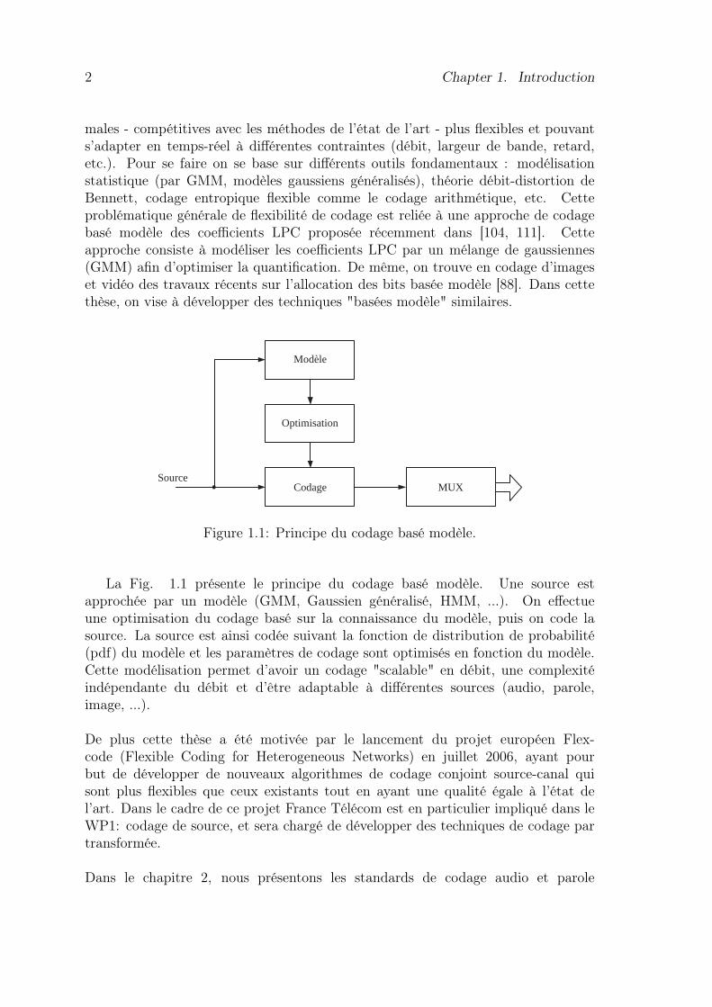
1.1 Principe du codage basé modèle. . . . . . . . . . . . . . . . . . . . . . 2
2.1 Bandwidth for different applications [48]. . . . . . . . . . . . . . . . . 62.2 Quality of coder model. . . . . . . . . . . . . . . . . . . . . . . . . . . 72.3 Block diagram of the CELP synthesis model. . . . . . . . . . . . . . . 92.4 Block coding of perceptual transform coding. . . . . . . . . . . . . . . 102.5 The absolute threshold of human hearing in quiet [55]. . . . . . . . . 112.6 Principle of the MDCT. . . . . . . . . . . . . . . . . . . . . . . . . . 112.7 Block diagram of G.722. . . . . . . . . . . . . . . . . . . . . . . . . . 132.8 Frequency response of low- and high-pass QMF filters in G.722 . . . . 142.9 Block diagram of G.722.1. . . . . . . . . . . . . . . . . . . . . . . . . 142.10 Block diagram of G.722.2. . . . . . . . . . . . . . . . . . . . . . . . . 152.11 Frequency response of down/up- sampling and pass-band filter in
G.722.2. . . . . . . . . . . . . . . . . . . . . . . . . . . . . . . . . . . 162.12 Block diagram of G.729.1 encoder. . . . . . . . . . . . . . . . . . . . 172.13 Block diagram of G.729.1 decoder (in the absence of frame erasures). 172.14 Block diagram of AMR-WB+ encoder. . . . . . . . . . . . . . . . . . 182.15 Block diagram of e-AAC+ encoder. . . . . . . . . . . . . . . . . . . . 192.16 Principle of GMMM-based LSF vector quantization. . . . . . . . . . . 192.17 Block diagram of MPEG-4 encoder. . . . . . . . . . . . . . . . . . . . 202.18 Block diagram of MPEG-2/4 AAC encoder. . . . . . . . . . . . . . . 212.19 Block diagram of MPEG-4 HE-AAC encoder. . . . . . . . . . . . . . 222.20 Example of Bit sliced Coding. . . . . . . . . . . . . . . . . . . . . . . 22
3.1 Staircase Character of the uniform quantizer . . . . . . . . . . . . . . 263.2 Difference between scalar quantizer with or without deadzone. . . . . 273.3 Example of probability density function . . . . . . . . . . . . . . . . . 283.4 Estimation procedure for the shape parameter α . . . . . . . . . . . . 293.5 Examples of MDCT coefficient modeling. . . . . . . . . . . . . . . . . 333.6 Arithmetic coding process. . . . . . . . . . . . . . . . . . . . . . . . . 413.7 Interface of the test. . . . . . . . . . . . . . . . . . . . . . . . . . . . 42
4.1 Principle of GMM-based LSF vector quantization. . . . . . . . . . . . 494.2 Quantizer design based on GMMs. . . . . . . . . . . . . . . . . . . . 50
xii List of Figures
4.3 Coding of uncorrelated Gaussian components by companded VQ. . . 504.4 Model-based LSF vector quantization. . . . . . . . . . . . . . . . . . 534.5 Model-based LSF quantization design. . . . . . . . . . . . . . . . . . 544.6 Coding of uncorrelated Gaussian components by Lloyd-Max quantizer. 544.7 Inclusion of a prediction in the model-based quantizer. . . . . . . . . 564.8 Switch between the two predictive models. . . . . . . . . . . . . . . . 564.9 Principle of model-based VQ with AR predictive coding. . . . . . . . 564.10 Principle of model-based VQ with opened-loop predictive coding. . . 574.11 Normalized histograms p(zj) of data samples zj=1...16 compared with
a Gaussian model with pα=2(z) = gα=2(z)× q. . . . . . . . . . . . . . 58
5.1 Proposed model-based transform coder. . . . . . . . . . . . . . . . . . 635.2 Principle of stack-run coding. . . . . . . . . . . . . . . . . . . . . . . 645.3 Example of stack-run coding. . . . . . . . . . . . . . . . . . . . . . . 665.4 Block diagram of the proposed predictive transform encoder. . . . . . 675.5 Bit allocation before the rate control (24 kbit/s) . . . . . . . . . . . . 705.6 Block diagram of the proposed predictive transform decoder. . . . . . 705.7 Block diagram of the proposed predictive transform encoder with a
deadzone quantizer. . . . . . . . . . . . . . . . . . . . . . . . . . . . . 715.8 Optimal deadzone for an uniform scalar quantizer with centroid (as-
suming a generalized Gaussian model). . . . . . . . . . . . . . . . . . 725.9 Optimal deadzone for an uniform scalar quantizer with centroid set
to mid-value (assuming a generalized Gaussian model). . . . . . . . . 745.10 Example of dead-zone optimization on a French female speaker sample. 755.11 Average WB-PESQ score (centroid set to mid-value)with noise injection. 775.12 Average WB-PESQ score (centroid) with noise injection. . . . . . . . 775.13 AB test results at 24 kbit/s. . . . . . . . . . . . . . . . . . . . . . . . 785.14 AB test results for speech at 24 kbit/s. . . . . . . . . . . . . . . . . . 79
6.1 Proposed model-based transform coder. . . . . . . . . . . . . . . . . . 816.2 Principle of bit plane coding. . . . . . . . . . . . . . . . . . . . . . . . 836.3 Example of bit plane mapping. . . . . . . . . . . . . . . . . . . . . . 846.4 Different bitstream format. . . . . . . . . . . . . . . . . . . . . . . . . 856.5 Example of probabilities estimation for a Laplacian distribution (zero
mean unit variance) with uniform scalar quantization of stepsize q. . . 876.6 Example of binary estimation for each bit plane Pk. . . . . . . . . . . 896.7 Example of conditional probability for each bit plane Pk. . . . . . . . 926.8 Example of conditional probability with only two contexts for each
bit plane Pk. . . . . . . . . . . . . . . . . . . . . . . . . . . . . . . . 946.9 Block diagram of the proposed bit plane transform encoder. . . . . . 956.10 Block diagram of the proposed bit plane transform decoder. . . . . . 976.11 Average wideband PESQ score (without noise injection). . . . . . . . 986.12 Comparison of bit plane coding with encoding/decoding at the same
bitrate or different ones (without noise injection). . . . . . . . . . . . 99

List of Figures xiii
7.1 Schéma de l’encodage CELP modifié en utilisant un modèle. . . . . . 1017.2 Schéma de l’encodeur par transformée, modifié en utilisant un modèle. 102

xiv List of Figures
List of Tables
3.1 Probabilities for a fixed model {a, e, i, o, u}. . . . . . . . . . . . . . . 413.2 CMOS for the AB test. . . . . . . . . . . . . . . . . . . . . . . . . . . 42
4.1 Shape parameters αj=1...16 estimated on the training database of vec-tors z. . . . . . . . . . . . . . . . . . . . . . . . . . . . . . . . . . . . 59
4.2 Results for switched AR(1)/MA(1) predictive LSF quantization vsAMR-WB LPC quantization: comparison between companded SQand model-based LM quantization. . . . . . . . . . . . . . . . . . . . 60
5.1 Bit allocation for the stack-run predictive transform audio coding. . . 695.2 Bit allocation for the coding scheme with deadzone. . . . . . . . . . . 725.3 Spectral distortion for the quantization of A(z/γ) with 40 bits. . . . . 76
6.1 Bit allocation for the bit plane transform audio coding. . . . . . . . . 97

xvi List of Tables
Chapter 1
Introduction
Avec l’évolution continue des technologies et des services de communication, lesréseaux (d’accès et coeur) et les terminaux sont devenus très hétérogènes. En effet,les communications peuvent passer par le réseau téléphonique commuté (RTC),les liens mobiles (GSM, wi-fi, bluetooth), les modems (ADSL, FTTH,...), etc. Deplus, on trouve des combinés téléphoniques en bande étroite, des téléphones HDen bande élargie, des soft phones (PC communiquant), des mobiles multi-usages,etc. En plus de cette hétérogénéité, on assiste actuellement à une importanteprolifération des standards de codage de parole et audio. Ces standards ont étédéveloppés en majorité pour répondre aux besoins successifs du marché pour desapplications de téléphonie fixe (G.711, G.729), téléphonie mobile (GSM-FR, HR,EFR, AMR-NR, WB, QCELP, EVRC), multimédia de masse (MPEG), visiophonie,visioconférence (G.722, G.722.1, G.722.1C), voix sur IP (G.723.1, G.729B, G.729.1).
Cette hétérogénéité des réseaux et des terminaux ainsi que la prolifération destandards spécifiques amènent naturellement à chercher de nouveaux modèlesde codage qui soient généraux, adaptés à de multiples scénarios d’applications.En terme de technique de codage, la plupart des standards de codage de paroleexistants sont peu flexibles : ils utilisent notamment des tables de quantificationvectorielle stockées, une allocation des bits fixe à certains paramètres de codage,et leurs performances sont souvent optimisées pour un certain point de fonction-nement (type de signal parole/musique, largeur de bande, débit). Il existe desalgorithmes multi-débits - par exemple AMR-NB et -WB, VMR-WB ou G.729.1- qui sont plus flexibles que les algorithmes à débit fixe mais ils ne font quecombiner plusieurs codeurs. En codage audio, il existe de nombreux standardscouvrant des configurations multiples (en débit, largeur de bande), tels que lescodeurs MPEG-1/2 Layer III ou MPEG-4 AAC, mais ils ne sont adaptés qu’à desapplications de stockage et diffusion, ils ne donnent pas une bonne qualité pour laparole à bas débit et nécessitent également un stockage des tables de quantifica-tion (codage de Huffman) ; le codage MPEG-4 BSAC a les mêmes inconvénientsmême s’il est plus adapté à l’hétérogénéité des réseaux de par sa nature hiérarchique.
L’objectif de la thèse est donc de développer des techniques de codage opti-
1
2 Chapter 1. Introduction
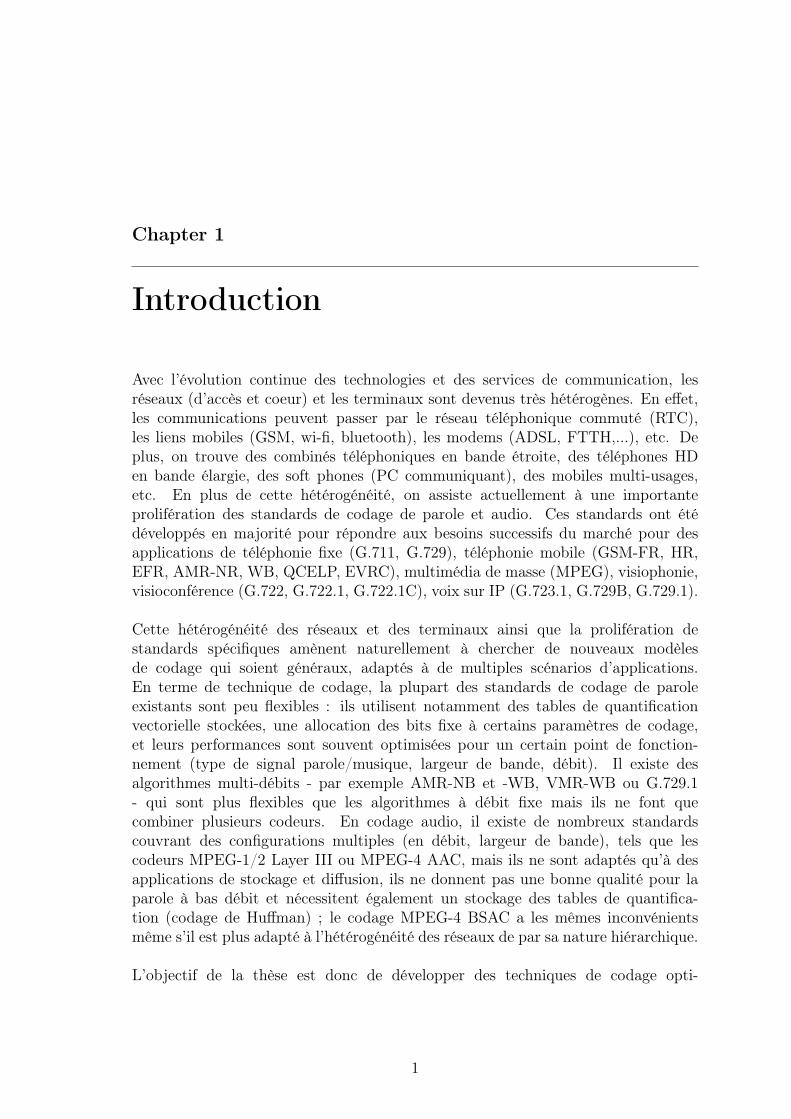
males - compétitives avec les méthodes de l’état de l’art - plus flexibles et pouvants’adapter en temps-réel à différentes contraintes (débit, largeur de bande, retard,etc.). Pour se faire on se base sur différents outils fondamentaux : modélisationstatistique (par GMM, modèles gaussiens généralisés), théorie débit-distortion deBennett, codage entropique flexible comme le codage arithmétique, etc. Cetteproblématique générale de flexibilité de codage est reliée à une approche de codagebasé modèle des coefficients LPC proposée récemment dans [104, 111]. Cetteapproche consiste à modéliser les coefficients LPC par un mélange de gaussiennes(GMM) afin d’optimiser la quantification. De même, on trouve en codage d’imageset vidéo des travaux récents sur l’allocation des bits basée modèle [88]. Dans cettethèse, on vise à développer des techniques "basées modèle" similaires.
Codage
Optimisation
Modèle
MUX Source
Figure 1.1: Principe du codage basé modèle.
La Fig. 1.1 présente le principe du codage basé modèle. Une source estapprochée par un modèle (GMM, Gaussien généralisé, HMM, ...). On effectueune optimisation du codage basé sur la connaissance du modèle, puis on code lasource. La source est ainsi codée suivant la fonction de distribution de probabilité(pdf) du modèle et les paramètres de codage sont optimisés en fonction du modèle.Cette modélisation permet d’avoir un codage "scalable" en débit, une complexitéindépendante du débit et d’être adaptable à différentes sources (audio, parole,image, ...).
De plus cette thèse a été motivée par le lancement du projet européen Flex-code (Flexible Coding for Heterogeneous Networks) en juillet 2006, ayant pourbut de développer de nouveaux algorithmes de codage conjoint source-canal quisont plus flexibles que ceux existants tout en ayant une qualité égale à l’état del’art. Dans le cadre de ce projet France Télécom est en particulier impliqué dans leWP1: codage de source, et sera chargé de développer des techniques de codage partransformée.
Dans le chapitre 2, nous présentons les standards de codage audio et parole
3
en bande élargie qui existent actuellement. Ces standards sont voués à desapplications bien précises et on se propose de les classer en deux catégories: lescodeurs conversationnels et ceux pour le stockage et la transmission d’information.La principale différence entre ces deux catégories étant le délai du codeur. Cescodeurs serviront de références aux codeurs que nous proposons.
Dans le chapitre 3, nous présentons des outils pour la mise en oeuvre d’uncodeur flexible. En particulier, nous présentons les deux modèles utilisés dans nostravaux : le modèle Gaussien généralisé et le mélange de Gaussiennes (GMM).Nous rappellerons aussi l’allocation des bits dans le cas d’une source Gaussiennegénéralisée proposée dans [88]. De plus nous présentons le principe du codagearithmétique [62, 126] qui sera utilisé dans nos codeurs. Finalement, la procédurepour les tests d’écoute mis en oeuvre pour vérifier la qualité d’un codeur estprésentée.
Dans le chapitre 4, nous présentons une technique de codage flexible basémodèle des coefficients LPC. Des méthodes de codage modélisant les coefficientsLPC par un mélange de Gaussiennes (GMM) afin d’optimiser la quantificationont été proposées dans [104, 111]. Nous proposons d’améliorer ces techniques enapprochant l’erreur de prediction des coefficients LPC par un modèle Gaussiengénéralisé. Nous comparons les performances du quantificateur proposé avec celuiutilisé dans le codeur ITU-T G.722.2 [40] pour la quantification des coefficientsLPC. Le quantificateur proposé présente des performances équivalentes tout enétant moins complexes, en pouvant s’adapter à différents débits et en ayant un coûtde stockage faible.
Dans le chapitre 5, nous présentons un codeur par transformée utilisant lecodage stack-run. Cette technique de codage est couramment utilisée en images[122, 121, 125] mais n’a jamais été utilisée pour le codage audio. Nous proposonsdonc un codeur dont les coefficients après la transformation MDCT sont modéliséspar une Gaussienne généralisée. Le modèle Gaussien généralisé est utilisé pourl’allocation des bits dans le codeur et pour optimiser la taille de la zone morte dansle quantificateur scalaire. Les performances de ce codeur sont comparées avec cellesdu codeur ITU-T G.722.1 [39]. La qualité du codeur est meilleure que celle ducodeur ITU-T G.722.1 à bas débit et équivalente à haut débit. Par contre, bien quel’utilisation du modèle permette de diminuer la complexité de l’allocation de débit,la complexité de calcul du codeur avec codage stack-run est plus importante quecelle du codeur ITU-T G.722.1, tandis que le coût mémoire est faible. L’utilisationdu modèle nous permet d’avoir un schéma de codage plus flexible et ayant unebonne qualité pour la parole et l’audio.
Dans le chapitre 6, nous présentons un codeur par transformée utilisant lecodage par plan de bits [109, 90, 59]. L’avantage de cette technique de codage estd’être scalable en débit. Nous proposons d’utiliser le modèle Gaussien généralisé
4 Chapter 1. Introduction
afin d’initialiser les tables de probabilités du codage arithmétique utilisé dans lecodage par plan de bits. Ainsi, les tables de probabilités utilisées dans le codagearithmétique sont plus proche de la source et les performances du codage en sontaméliorées. Les performances de ce codeur sont comparées avec celle du codeuravec codage stack-run et celle du codeur ITU-T G.722.1. La qualité du codeur estinférieure à celle du codeur avec codage stack-run à bas débit et équivalente à hautdébit. Par contre, la complexité de calcul est plus faible que dans le cas du codeuravec codage stack-run car la boucle de contrôle du débit n’est pas nécessaire.
Enfin, dans le chapitre 7, nous présentons un bilan des travaux effectués du-rant cette thèse et des perspectives pour la suite de ces travaux.
Chapter 2
State of art in speech and audiocoding
Nowadays, many speech and audio coding standards are available. They are oftendesigned for specific applications and constraints. Those coders were build in or-der to response to the successive needs of the market for conventional telephones(G.711, G.729), cellular networks (GSM-FR, HR, EFR, AMR-NR, WB, QCELP,EVRC), multimedia, videophone, videoconference (G.722, G.722.1, G.722.1C), orvoice over IP (G.723.1, G.729B, G.729.1). Here, only wideband (50-7000 Hz) orsuper-wideband (50-14000 Hz) speech and audio standards are presented. Wide-band and super-wideband coders are the most recent and ITU-T still have works inprogress on those coders. Also, we compared our works with ITU-T G.722.1 [39].
This chapter is organized as follows. Main attributes of speech and audio coderare given in Section 2.1. In Section 2.2, coding methods are presented. Three classesof models have been chosen: analysis by synthesis coding which is the common modelin speech coding, perceptual transform coding which is mainly for audio coding anduniversal coding for both speech and music coding. Then wideband and super-wideband standards for cellular networks are presented in Section 2.3. A review ofstreaming standards for audio coding is done in Section 2.4 before concluding inSection 2.5.
2.1 Attributes of Speech and Audio CoderThe main attributes of speech and audio coder are: bitrate and quality, complexity,frame size and algorithmic delay and channel-error sensitivity. In general there is atrade-off between all these attributes.
2.1.1 Bitrate, bandwidth and quality
The bitrate (in kbit/s) measures the efficiency of the coding algorithm. The bitrateof a coder can be fixed or variable. Lower bitrates, 800 to 4800 bit/s are used forsecure telephony applications. For the last wideband or super-wideband codec thebitrate goes up to 64 kbit/s.
5
6 Chapter 2. State of art in speech and audio coding
The quality is linked to the bandwidth of the input signal. We can classify speechand audio coders depending on the bandwith of the input signal (mono):
• In the telephone band, 300-3400 Hz, speech is muffled and there is not enoughband for music.
• The wideband, 50-7000 Hz, has a quality for speech and music equivalent toAM radio.
• The super-wideband, 50-14000 Hz, has a good quality for both speech andmusic and is close to the FM band.
• The hifi band, 20-15000 Hz, has a good quality for both speech and music andis equivalent to the FM band.
• The 20-20000 Hz band is used for CD quality applications.
• The 20-24000 Hz band is used for "perfect" quality applications such as record-ing studio, cinema or DVD.
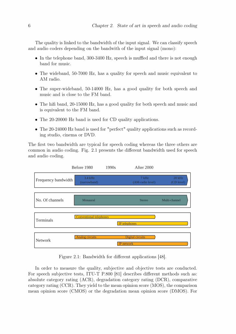
The first two bandwidth are typical for speech coding whereas the three others arecommon in audio coding. Fig. 2.1 presents the different bandwidth used for speechand audio coding.
Frequency bandwidth
No. Of channels
Terminals
Network
Before 1980 1990s After 2000
3.4 kHz (narrowband)
7 kHz (AM-radio level)
20 kHz (CD level)
Monaural Stereo Multi-channel
Conventional telephones
IP telephones
Analog circuits Digital circuits
IP network
Figure 2.1: Bandwidth for different applications [48].
In order to measure the quality, subjective and objective tests are conducted.For speech subjective tests, ITU-T P.800 [81] describes different methods such as:absolute category rating (ACR), degradation category rating (DCR), comparativecategory rating (CCR). They yield to the mean opinion score (MOS), the comparisonmean opinion score (CMOS) or the degradation mean opinion score (DMOS). For
2.1. Attributes of Speech and Audio Coder 7
audio signals ITU-T BS.1116 and BS.1534 [18, 20] propose methodologies for sub-jective test. The multi stimulus test with hidden reference and anchors (MUSHRA)or BS.1534 is a common quality test when there is important degradations in thesignal [20].
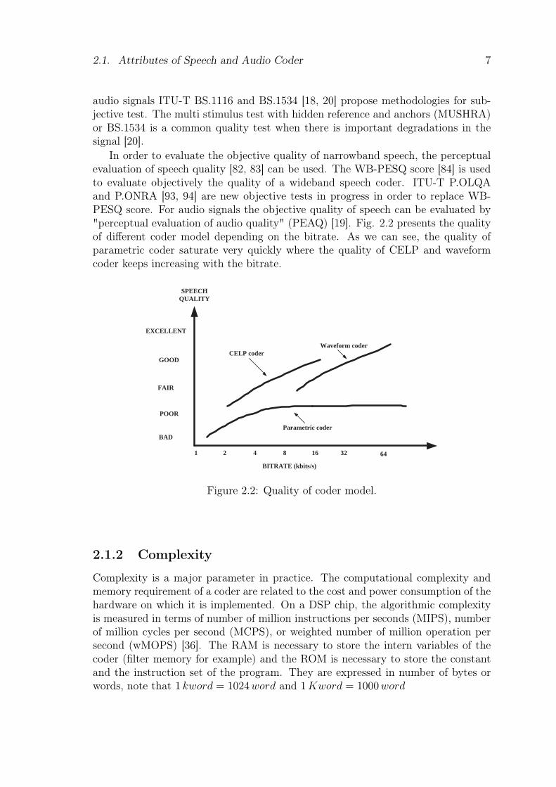
In order to evaluate the objective quality of narrowband speech, the perceptualevaluation of speech quality [82, 83] can be used. The WB-PESQ score [84] is usedto evaluate objectively the quality of a wideband speech coder. ITU-T P.OLQAand P.ONRA [93, 94] are new objective tests in progress in order to replace WB-PESQ score. For audio signals the objective quality of speech can be evaluated by"perceptual evaluation of audio quality" (PEAQ) [19]. Fig. 2.2 presents the qualityof different coder model depending on the bitrate. As we can see, the quality ofparametric coder saturate very quickly where the quality of CELP and waveformcoder keeps increasing with the bitrate.
CELP coder
Parametric coder
Waveform coder
EXCELLENT
GOOD
FAIR
POOR
BAD
SPEECH QUALITY
BITRATE (kbits/s)
1 2 4 8 16 32 64
Figure 2.2: Quality of coder model.
2.1.2 Complexity
Complexity is a major parameter in practice. The computational complexity andmemory requirement of a coder are related to the cost and power consumption of thehardware on which it is implemented. On a DSP chip, the algorithmic complexityis measured in terms of number of million instructions per seconds (MIPS), numberof million cycles per second (MCPS), or weighted number of million operation persecond (wMOPS) [36]. The RAM is necessary to store the intern variables of thecoder (filter memory for example) and the ROM is necessary to store the constantand the instruction set of the program. They are expressed in number of bytes orwords, note that 1 kword = 1024 word and 1 Kword = 1000 word
8 Chapter 2. State of art in speech and audio coding
2.1.3 Delay
In two-way communications, according to the E-model [35] if the end-to-end delayis between 0-150 ms it is acceptable for most of applications. If the end-to-end delayis between 150-400 ms it is acceptable for applications where interactivity is notimportant. If the end-to-end delay is more than 400 ms it is not acceptable for con-versational tasks. Contrary to conversational applications, one-way communication(storage, streaming,...) do not have strong constraints on delay in general. Usually,the delay introduced by the coder is in the order of the framesize.
2.1.4 Channel-error sensitivity
In many applications the bitstream sent by the encoder may be corrupted by channelerrors. There are two types of errors: bit errors or frame erasures (packet losses),both may occur in random or burst sequence. The robustness against bit errors canbe improved by proper index assignment, the use of error detection/correction codes.Frame erasures are concealed using embedded coding, multiple description coding,or encoder-side redundancy. In practice conversational coders are often tested with0.1 to 1 bits error rates (BER) and1% to 6% frame error rates (FER).
2.2 Speech and Audio Coding Model
We may classify speech and audio coding methods depending on the underlyingcoding model. We have chosen three classes of models that are current state of theart in speech and audio coding:
• Analysis by Synthesis (AbS) coding which is a linear predictive coding inwhich parameters are estimated by waveform matching [106] and is currentlythe most widely used speech coding approach.
• Perceptual transform coding which consists in a coder based on psychoacousticprinciple [55, 54] and is the basis of audio coding.
• Universal speech/audio coding which is robust against the type of inputs(speech, audio). In general a multimode approach is used.
In addition we review some important tools:
• Parametric bandwidth extension algorithm [29, 52, 51] which is a process ofexpanding the frequency range (bandwidth) of a signal using low bit rate sideinformation.
• Parametric Stereo coding [16, 17].
2.2. Speech and Audio Coding Model 9
2.2.1 CELP coding
The code-excited linear-predictive (CELP) model is based on a source-filter modeland is one of the most popular speech coding technique [106]. For a signal intelephone bandwidth, CELP coding has a good quality for bitrate from 6 to 16kbit/s. For a wideband signal, CELP coding has a good quality for bitrate from 10to 24 kbit/s. CELP is based mainly on the knowledge of the source (model) and onthe receiver (perceptual filter).
This technique is based on an all-pole synthesis filter that models the short-termspectral envelope:
H (z) =1
A(z)=
1
1 +n∑
i=1
aiz−i
(2.1)
where n and ai are respectively the model’s order and the Linear Prediction Coef-ficient (LPC) [68, 73]. A(z) is the prediction filter obtained using linear-prediction.
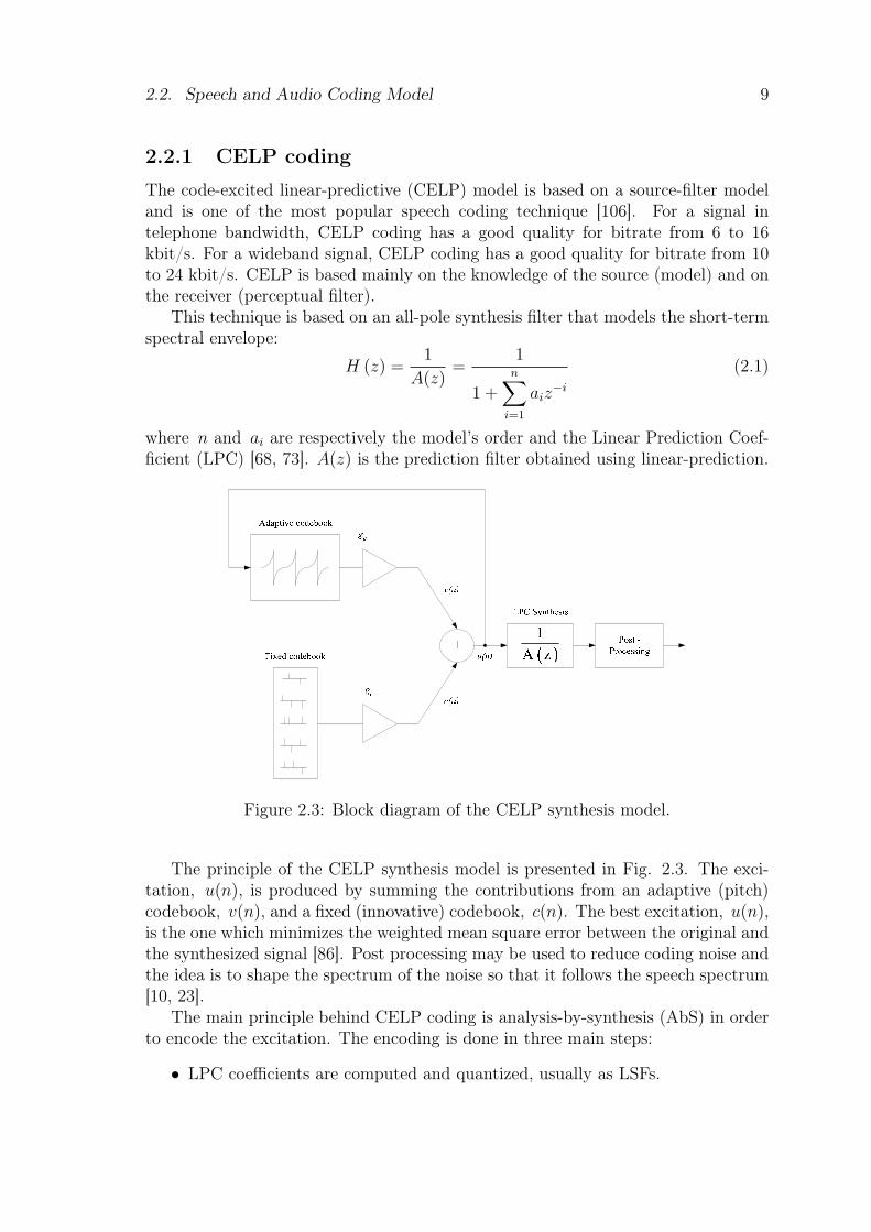
Figure 2.3: Block diagram of the CELP synthesis model.
The principle of the CELP synthesis model is presented in Fig. 2.3. The exci-tation, u(n), is produced by summing the contributions from an adaptive (pitch)codebook, v(n), and a fixed (innovative) codebook, c(n). The best excitation, u(n),is the one which minimizes the weighted mean square error between the original andthe synthesized signal [86]. Post processing may be used to reduce coding noise andthe idea is to shape the spectrum of the noise so that it follows the speech spectrum[10, 23].
The main principle behind CELP coding is analysis-by-synthesis (AbS) in orderto encode the excitation. The encoding is done in three main steps:
• LPC coefficients are computed and quantized, usually as LSFs.
10 Chapter 2. State of art in speech and audio coding
• The adaptive codebook gain is searched in order to have the best pitch com-bination using AbS. Algebraic coding methods are usually implemented toreduce the CELP codebook search complexity [9].
• The fixed codebook gain is searched for the best entry using AbS.
2.2.2 Perceptual transform coding
Perceptual transform coding
Time/Frequency Analysis
Psychoacoustic model
Quantization
Bit allocation
E n
t r o p
y c o d
i n g
M U
X
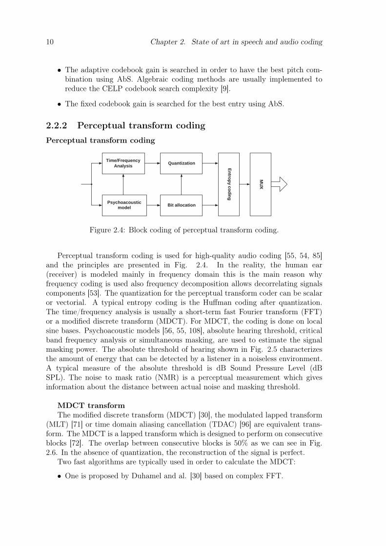
Figure 2.4: Block coding of perceptual transform coding.
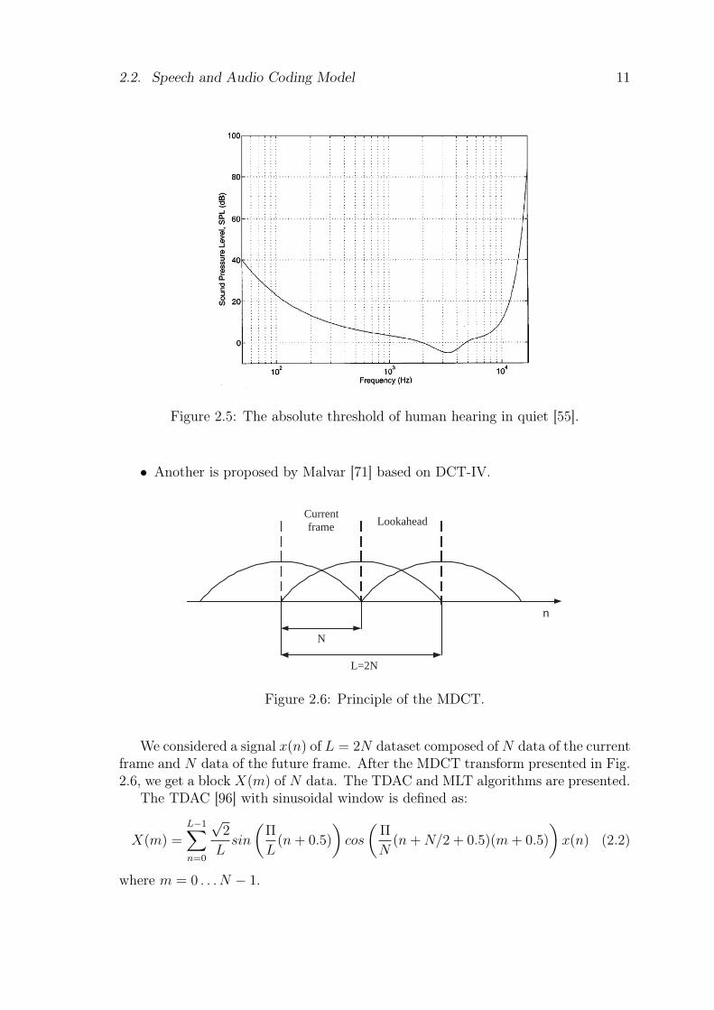
Perceptual transform coding is used for high-quality audio coding [55, 54, 85]and the principles are presented in Fig. 2.4. In the reality, the human ear(receiver) is modeled mainly in frequency domain this is the main reason whyfrequency coding is used also frequency decomposition allows decorrelating signalscomponents [53]. The quantization for the perceptual transform coder can be scalaror vectorial. A typical entropy coding is the Huffman coding after quantization.The time/frequency analysis is usually a short-term fast Fourier transform (FFT)or a modified discrete transform (MDCT). For MDCT, the coding is done on localsine bases. Psychoacoustic models [56, 55, 108], absolute hearing threshold, criticalband frequency analysis or simultaneous masking, are used to estimate the signalmasking power. The absolute threshold of hearing shown in Fig. 2.5 characterizesthe amount of energy that can be detected by a listener in a noiseless environment.A typical measure of the absolute threshold is dB Sound Pressure Level (dBSPL). The noise to mask ratio (NMR) is a perceptual measurement which givesinformation about the distance between actual noise and masking threshold.
MDCT transformThe modified discrete transform (MDCT) [30], the modulated lapped transform
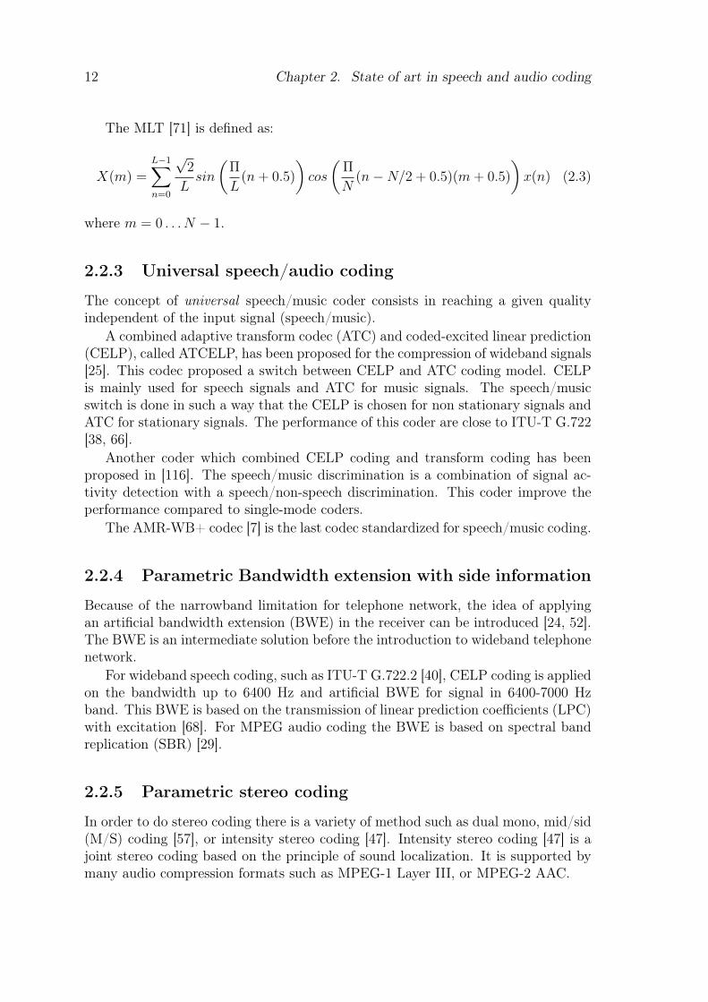
(MLT) [71] or time domain aliasing cancellation (TDAC) [96] are equivalent trans-form. The MDCT is a lapped transform which is designed to perform on consecutiveblocks [72]. The overlap between consecutive blocks is 50% as we can see in Fig.2.6. In the absence of quantization, the reconstruction of the signal is perfect.
Two fast algorithms are typically used in order to calculate the MDCT:
• One is proposed by Duhamel and al. [30] based on complex FFT.
2.2. Speech and Audio Coding Model 11
Figure 2.5: The absolute threshold of human hearing in quiet [55].
• Another is proposed by Malvar [71] based on DCT-IV.
Current frame Lookahead
N
L=2N
n
Figure 2.6: Principle of the MDCT.
We considered a signal x(n) of L = 2N dataset composed of N data of the currentframe and N data of the future frame. After the MDCT transform presented in Fig.2.6, we get a block X(m) of N data. The TDAC and MLT algorithms are presented.
The TDAC [96] with sinusoidal window is defined as:
X(m) =L−1∑n=0
√2
Lsin
(Π
L(n + 0.5)
)cos
(Π
N(n + N/2 + 0.5)(m + 0.5)
)x(n) (2.2)
where m = 0 . . . N − 1.
12 Chapter 2. State of art in speech and audio coding
The MLT [71] is defined as:
X(m) =L−1∑n=0
√2
Lsin
(Π
L(n + 0.5)
)cos
(Π
N(n−N/2 + 0.5)(m + 0.5)
)x(n) (2.3)
where m = 0 . . . N − 1.
2.2.3 Universal speech/audio coding
The concept of universal speech/music coder consists in reaching a given qualityindependent of the input signal (speech/music).
A combined adaptive transform codec (ATC) and coded-excited linear prediction(CELP), called ATCELP, has been proposed for the compression of wideband signals[25]. This codec proposed a switch between CELP and ATC coding model. CELPis mainly used for speech signals and ATC for music signals. The speech/musicswitch is done in such a way that the CELP is chosen for non stationary signals andATC for stationary signals. The performance of this coder are close to ITU-T G.722[38, 66].
Another coder which combined CELP coding and transform coding has beenproposed in [116]. The speech/music discrimination is a combination of signal ac-tivity detection with a speech/non-speech discrimination. This coder improve theperformance compared to single-mode coders.
The AMR-WB+ codec [7] is the last codec standardized for speech/music coding.
2.2.4 Parametric Bandwidth extension with side information
Because of the narrowband limitation for telephone network, the idea of applyingan artificial bandwidth extension (BWE) in the receiver can be introduced [24, 52].The BWE is an intermediate solution before the introduction to wideband telephonenetwork.
For wideband speech coding, such as ITU-T G.722.2 [40], CELP coding is appliedon the bandwidth up to 6400 Hz and artificial BWE for signal in 6400-7000 Hzband. This BWE is based on the transmission of linear prediction coefficients (LPC)with excitation [68]. For MPEG audio coding the BWE is based on spectral bandreplication (SBR) [29].
2.2.5 Parametric stereo coding
In order to do stereo coding there is a variety of method such as dual mono, mid/sid(M/S) coding [57], or intensity stereo coding [47]. Intensity stereo coding [47] is ajoint stereo coding based on the principle of sound localization. It is supported bymany audio compression formats such as MPEG-1 Layer III, or MPEG-2 AAC.
2.3. Wideband and Super-Wideband Coding Standards for Cellular Networks 13
2.3 Wideband and Super-Wideband Coding Stan-dards for Cellular Networks
In this section the wideband and super-wideband coding standards for cellular net-works are presented. We restricted ourselves to wideband and super-wideband cod-ing because it is the future of the network and also because we compared our worksto wideband codec. Standards presented here were designed specifically for audio-videoconferencing, wideband telephony or voice over IP (VoIP) applications whichmeans that the delay of the coder is an important parameter.
The wideband coders (G.722, G.722.1, G.722.2 and G.729.1) and the super-wideband (AMR-WB+, e-AAC+) coders are presented. A review of the ITU-Tstandards for narrowband has been done in [86, Chap.2].
ITU-T is working on G.711 coder [37] in order to do an extension of the narrow-band into wideband. They are also working on a extension of G.729.1 [41] up tosuper-wideband, which is called for the moment EV-VBR.
2.3.1 ITU-T G.722
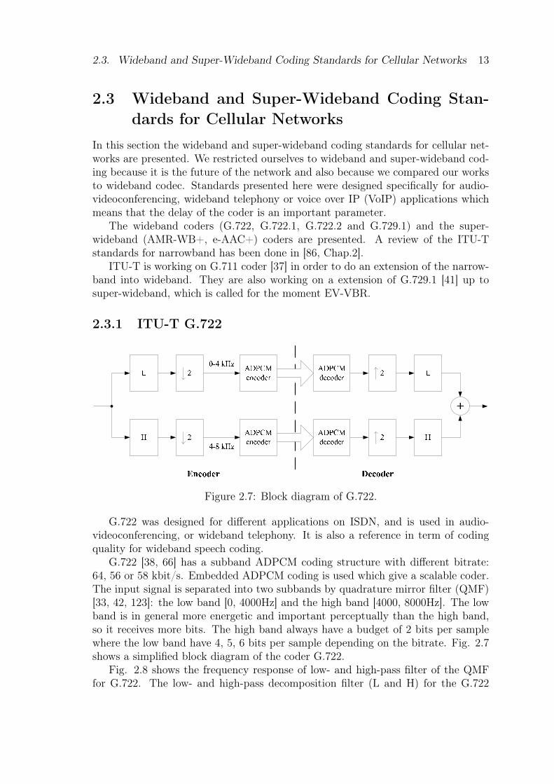
Figure 2.7: Block diagram of G.722.
G.722 was designed for different applications on ISDN, and is used in audio-videoconferencing, or wideband telephony. It is also a reference in term of codingquality for wideband speech coding.
G.722 [38, 66] has a subband ADPCM coding structure with different bitrate:64, 56 or 58 kbit/s. Embedded ADPCM coding is used which give a scalable coder.The input signal is separated into two subbands by quadrature mirror filter (QMF)[33, 42, 123]: the low band [0, 4000Hz] and the high band [4000, 8000Hz]. The lowband is in general more energetic and important perceptually than the high band,so it receives more bits. The high band always have a budget of 2 bits per samplewhere the low band have 4, 5, 6 bits per sample depending on the bitrate. Fig. 2.7shows a simplified block diagram of the coder G.722.
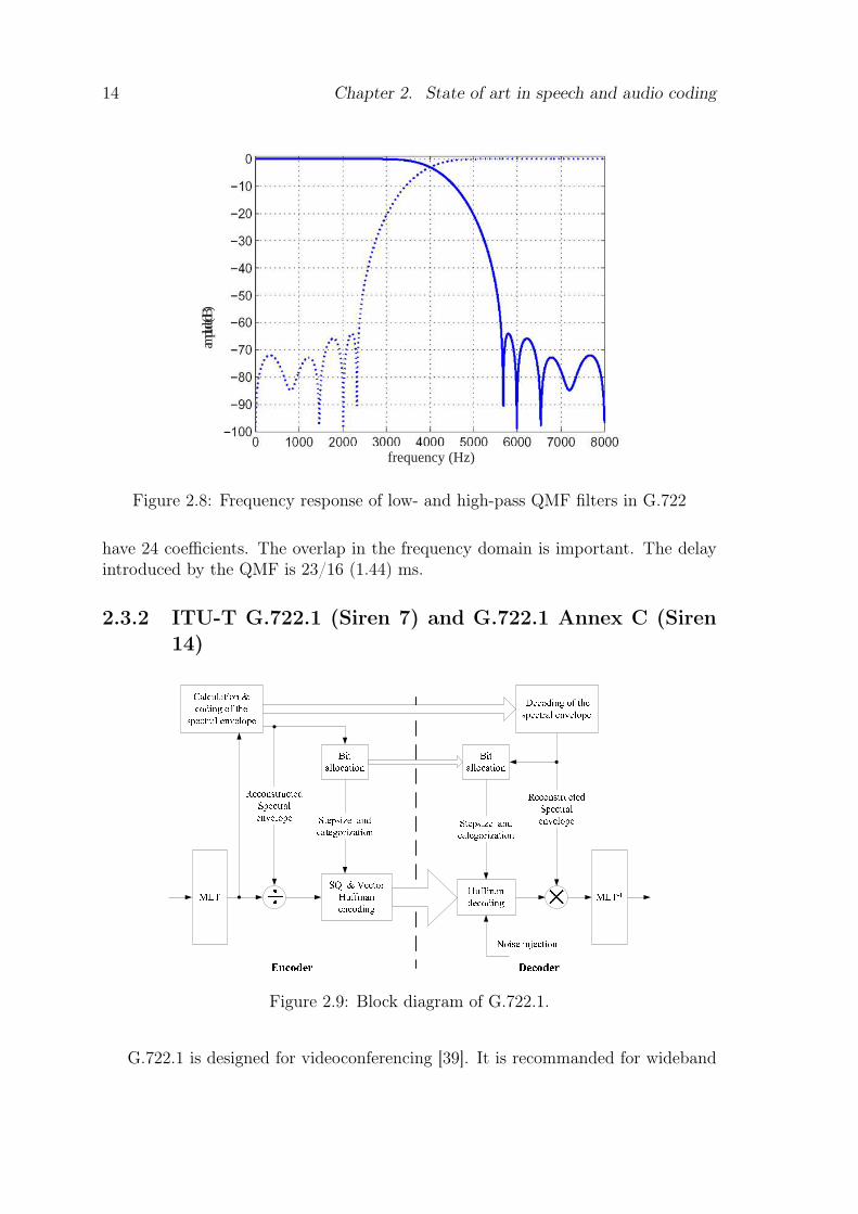
Fig. 2.8 shows the frequency response of low- and high-pass filter of the QMFfor G.722. The low- and high-pass decomposition filter (L and H) for the G.722
14 Chapter 2. State of art in speech and audio coding
frequency (Hz)
a m p l
i t u d
e ( d
B )
Figure 2.8: Frequency response of low- and high-pass QMF filters in G.722
have 24 coefficients. The overlap in the frequency domain is important. The delayintroduced by the QMF is 23/16 (1.44) ms.
2.3.2 ITU-T G.722.1 (Siren 7) and G.722.1 Annex C (Siren14)
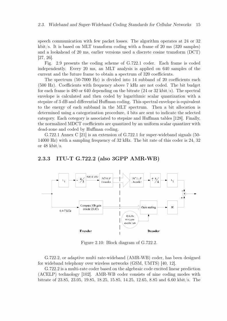
Figure 2.9: Block diagram of G.722.1.
G.722.1 is designed for videoconferencing [39]. It is recommanded for wideband
2.3. Wideband and Super-Wideband Coding Standards for Cellular Networks 15
speech communication with few packet losses. The algorithm operates at 24 or 32kbit/s. It is based on MLT transform coding with a frame of 20 ms (320 samples)and a lookahead of 20 ms, earlier versions used a discrete cosine transform (DCT)[27, 26].
Fig. 2.9 presents the coding scheme of G.722.1 coder. Each frame is codedindependently. Every 20 ms, an MLT analysis is applied on 640 samples of thecurrent and the future frame to obtain a spectrum of 320 coefficients.
The spectrum (50-7000 Hz) is divided into 14 subband of 20 coefficients each(500 Hz). Coefficients with frequency above 7 kHz are not coded. The bit budgetfor each frame is 480 or 640 depending on the bitrate (24 or 32 kbit/s). The spectralenvelope is calculated and then coded by logarithmic scalar quantization with astepsize of 3 dB and differential Huffman coding. This spectral envelope is equivalentto the energy of each subband in the MLT spectrum. Then a bit allocation isdetermined using a categorization procedure, 4 bits are sent to indicate the selectedcategory. Each cotegory is associated to stepsize and Huffman tables [128]. Finally,the normalized MDCT coefficients are quantized by an uniform scalar quantizer withdead-zone and coded by Huffman coding.
G.722.1 Annex C [21] is an extension of G.722.1 for super-wideband signals (50-14000 Hz) with a sampling frequency of 32 kHz. The bit rate of this coder is 24, 32or 48 kbit/s.
2.3.3 ITU-T G.722.2 (also 3GPP AMR-WB)
Figure 2.10: Block diagram of G.722.2.
G.722.2, or adaptive multi rate-wideband (AMR-WB) coder, has been designedfor wideband telephony over wireless networks (GSM, UMTS) [40, 12].
G.722.2 is a multi-rate coder based on the algebraic code excited linear prediction(ACELP) technology [102]. AMR-WB coder consists of nine coding modes withbitrate of 23.85, 23.05, 19.85, 18.25, 15.85, 14.25, 12.65, 8.85 and 6.60 kbit/s. The
16 Chapter 2. State of art in speech and audio coding
signal is sampled at 16 kHz and each frame has a size of 20 ms and a lookahead of20 ms. ACELP coding is applied to the low band (50-6400 Hz) whereas in the highband (6400-7000 Hz) the signal is coded by with band extension as shown in Fig.2.10. The bandwidth extension, except at 23.85 kbit/s, is done by a 16 kHz randomexcitation and no parameters are transmitted to the decoder. At 23.85 kbit/s highband gain are transmitted to the decoder using 4 bits per subframe.
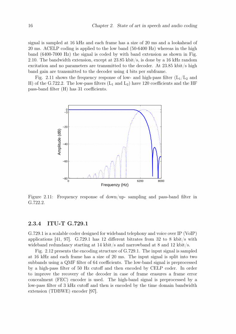
Fig. 2.11 shows the frequency response of low- and high-pass filter (L1/L2 andH) of the G.722.2. The low-pass filters (L1 and L2) have 120 coefficients and the HFpass-band filter (H) has 31 coefficients.
0 6200 8000−80
−60
−40
−20
−30
Frequenzy (Hz)
Am
plitu
de (
dB)
Figure 2.11: Frequency response of down/up- sampling and pass-band filter inG.722.2.
2.3.4 ITU-T G.729.1
G.729.1 is a scalable coder designed for wideband telephony and voice over IP (VoIP)applications [41, 97]. G.729.1 has 12 different bitrates from 32 to 8 kbit/s withwideband redundancy starting at 14 kbit/s and narrowband at 8 and 12 kbit/s.
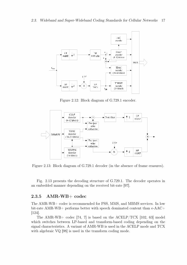
Fig. 2.12 presents the encoding structure of G.729.1. The input signal is sampledat 16 kHz and each frame has a size of 20 ms. The input signal is split into twosubbands using a QMF filter of 64 coefficients. The low-band signal is preprocessedby a high-pass filter of 50 Hz cutoff and then encoded by CELP coder. In orderto improve the recovery of the decoder in case of frame erasures a frame errorconcealment (FEC) encoder is used. The high-band signal is preprocessed by alow-pass filter of 3 kHz cutoff and then is encoded by the time domain bandwidthextension (TDBWE) encoder [97].
2.3. Wideband and Super-Wideband Coding Standards for Cellular Networks 17
Figure 2.12: Block diagram of G.729.1 encoder.
Figure 2.13: Block diagram of G.729.1 decoder (in the absence of frame erasures).
Fig. 2.13 presents the decoding structure of G.729.1. The decoder operates inan embedded manner depending on the received bit-rate [97].
2.3.5 AMR-WB+ codec
The AMR-WB+ codec is recommended for PSS, MMS, and MBMS services. In lowbit-rate AMR-WB+ performs better with speech dominated content than e-AAC+[124].
The AMR-WB+ codec [74, 7] is based on the ACELP/TCX [102, 63] modelwhich switches between LP-based and transform-based coding depending on thesignal characteristics. A variant of AMR-WB is used in the ACELP mode and TCXwith algebraic VQ [98] is used in the transform coding mode.
18 Chapter 2. State of art in speech and audio coding
MUX
HF encoding
HF encoding
ACELP / TCX encoding
Stereo encoding
P r e p r o c e s s i n g a n d a n a l y s i s f i l t e r b a n k
L HF
R HF
M HF
M LF
L LF
R LF
Stereo parameters
Mono LF parameters
Right/mono HF parameters
Left HF parameters
Input Left signal L
Input Right signal R
Input Mono signal M
M LF
S LF
D o w
n m i x i n g
( L , R
) t o ( M , S )
mode
Mono operation
Figure 2.14: Block diagram of AMR-WB+ encoder.
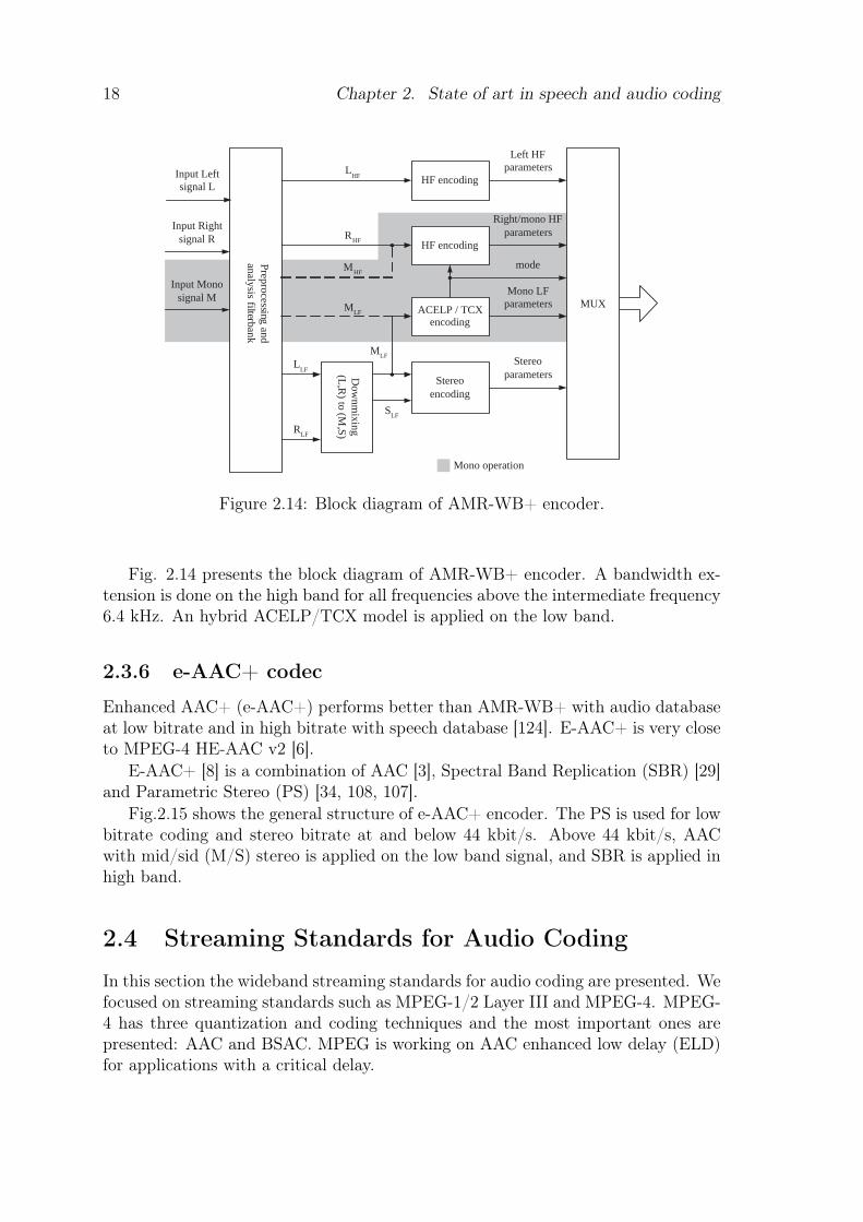
Fig. 2.14 presents the block diagram of AMR-WB+ encoder. A bandwidth ex-tension is done on the high band for all frequencies above the intermediate frequency6.4 kHz. An hybrid ACELP/TCX model is applied on the low band.
2.3.6 e-AAC+ codec
Enhanced AAC+ (e-AAC+) performs better than AMR-WB+ with audio databaseat low bitrate and in high bitrate with speech database [124]. E-AAC+ is very closeto MPEG-4 HE-AAC v2 [6].
E-AAC+ [8] is a combination of AAC [3], Spectral Band Replication (SBR) [29]and Parametric Stereo (PS) [34, 108, 107].
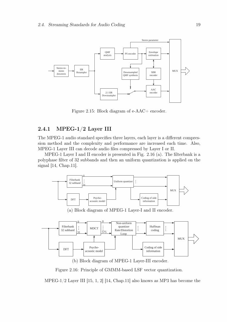
Fig.2.15 shows the general structure of e-AAC+ encoder. The PS is used for lowbitrate coding and stereo bitrate at and below 44 kbit/s. Above 44 kbit/s, AACwith mid/sid (M/S) stereo is applied on the low band signal, and SBR is applied inhigh band.
2.4 Streaming Standards for Audio Coding
In this section the wideband streaming standards for audio coding are presented. Wefocused on streaming standards such as MPEG-1/2 Layer III and MPEG-4. MPEG-4 has three quantization and coding techniques and the most important ones arepresented: AAC and BSAC. MPEG is working on AAC enhanced low delay (ELD)for applications with a critical delay.
2.4. Streaming Standards for Audio Coding 19
Downsampled QMF synthesis
AAC encoder
MUX
PS encoder Envelope estimation
2:1 IIR Downsampler
QMF analysis
SBR encoder
Stereo parameter
IIR Resampler
Stereo-to- mono
downmix
Figure 2.15: Block diagram of e-AAC+ encoder.
2.4.1 MPEG-1/2 Layer III
The MPEG-1 audio standard specifies three layers, each layer is a different compres-sion method and the complexity and performance are increased each time. Also,MPEG-1 Layer III can decode audio files compressed by Layer I or II.
MPEG-1 Layer I and II encoder is presented in Fig. 2.16 (a). The filterbank is apolyphase filter of 32 subbands and then an uniform quantization is applied on thesignal [14, Chap.11].
Filterbank 32 subband
Psycho- acoustic model
Uniform quantizer
MUX
…
0
31
DFT Coding of side information
…
(a) Block diagram of MPEG-1 Layer-I and II encoder.
Filterbank 32 subband
MDCT
Psycho- acoustic model
Non-uniform quantizer
Rate/Distortion Loop
MUX
…
… .
0
31
0
575
DFT
Huffman coding
Coding of side information
… .
… .
(b) Block diagram of MPEG-1 Layer-III encoder.
Figure 2.16: Principle of GMMM-based LSF vector quantization.
MPEG-1/2 Layer III [15, 1, 2] [14, Chap.11] also knows as MP3 has become the
20 Chapter 2. State of art in speech and audio coding
most widely used coding format for music on Internet. The size of audio files arelimited and so the downloading time on Internet. The recommended bit rate is 32to 320 kbit/s for MPEG-1 Layer III and 8-160 kbits/s for MPEG-2 Layer III. Theblock diagram of MPEG-1 and 2 Layer III is presented in Fig. 2.16 (b).
The filterbank is an hybrid filterbank which is a cascade of two filterbanks. First,a polyphase filterbank already used in MPEG-1 Layer II and III is applied on thesignal. Then a MDCT transform of 36 coefficients (12 samples for short window) isused in order to have a better compression level [14, Chap.11].
A rate-distortion optimization is done with a system of two nested iteration loopsfor the quantization [103, 15]. Quantization is done via a power-law quantizer. Thus,bit are set in order to reduce the quantization noise. The quantized values are codingby Huffman coding.
2.4.2 MPEG-4 AAC,BSAC and AAC+
Quantization and Coding
Perceptual model
Gain control and filterbank
Spectral processing: TNS LTP Intensity/Coupling Prediction PNS M/S
MUX
Twin-VQ: Spectral
normalization interleavedVQ
AAC: Quantization Huffman coding
BSAC: Quantization Bit plane
arithmetic coding
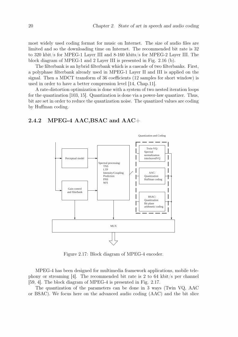
Figure 2.17: Block diagram of MPEG-4 encoder.
MPEG-4 has been designed for multimedia framework applications, mobile tele-phony or streaming [4]. The recommended bit rate is 2 to 64 kbit/s per channel[59, 4]. The block diagram of MPEG-4 is presented in Fig. 2.17.
The quantization of the parameters can be done in 3 ways (Twin VQ, AACor BSAC). We focus here on the advanced audio coding (AAC) and the bit slice
2.4. Streaming Standards for Audio Coding 21
arithmetic coding (BSAC).
MPEG-4 AAC and extension AAC+ (or HE-AAC)
Rate/Distortion Control
Quantization Scale Factors
Entropy coding
M/S Prediction Intensity / Coupling
TNS Filter Bank
MUX
Gain Control
Perceptual Model
Quantization & coding
Spectral Processing
Figure 2.18: Block diagram of MPEG-2/4 AAC encoder.
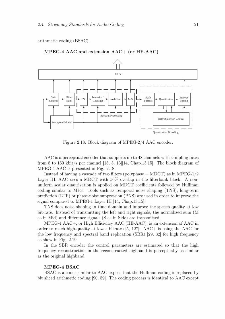
AAC is a perceptual encoder that supports up to 48 channels with sampling ratesfrom 8 to 160 kbit/s per channel [15, 3, 13][14, Chap.13,15]. The block diagram ofMPEG-4 AAC is presented in Fig. 2.18.
Instead of having a cascade of two filters (polyphase + MDCT) as in MPEG-1/2Layer III, AAC uses a MDCT with 50% overlap in the filterbank block. A non-uniform scalar quantization is applied on MDCT coefficients followed by Huffmancoding similar to MP3. Tools such as temporal noise shaping (TNS), long-termprediction (LTP) or phase-noise suppression (PNS) are used in order to improve thesignal compared to MPEG-1 Layer III [14, Chap.13,15].
TNS does noise shaping in time domain and improve the speech quality at lowbit-rate. Instead of transmitting the left and right signals, the normalized sum (Mas in Mid) and difference signals (S as in Side) are transmitted.
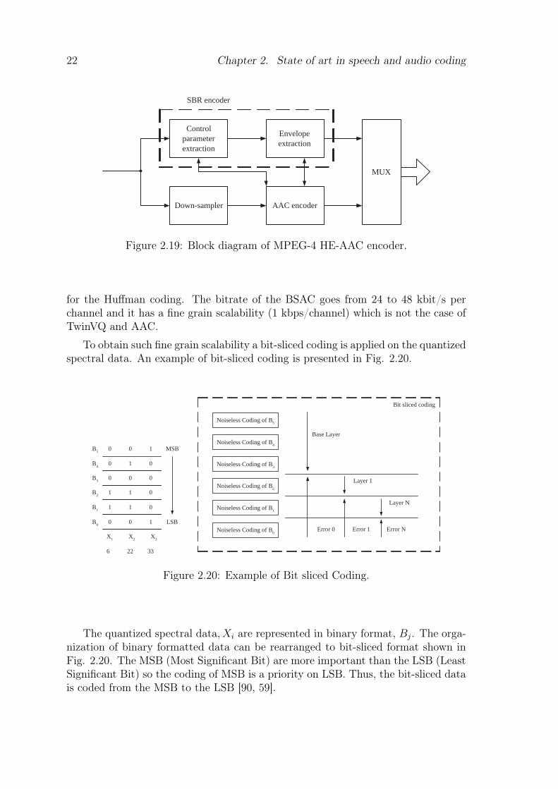
MPEG-4 AAC+, or High Efficiency AAC (HE-AAC), is an extension of AAC inorder to reach high-quality at lower bitrates [5, 127]. AAC+ is using the AAC forthe low frequency and spectral band replication (SBR) [29, 32] for high frequencyas show in Fig. 2.19.
In the SBR encoder the control parameters are estimated so that the highfrequency reconstruction in the reconstructed highband is perceptually as similaras the original highband.
MPEG-4 BSACBSAC is a coder similar to AAC expect that the Huffman coding is replaced by
bit sliced arithmetic coding [90, 59]. The coding process is identical to AAC except
22 Chapter 2. State of art in speech and audio coding
Control parameter extraction
Envelope extraction
Down-sampler AAC encoder
MUX
SBR encoder
Figure 2.19: Block diagram of MPEG-4 HE-AAC encoder.
for the Huffman coding. The bitrate of the BSAC goes from 24 to 48 kbit/s perchannel and it has a fine grain scalability (1 kbps/channel) which is not the case ofTwinVQ and AAC.
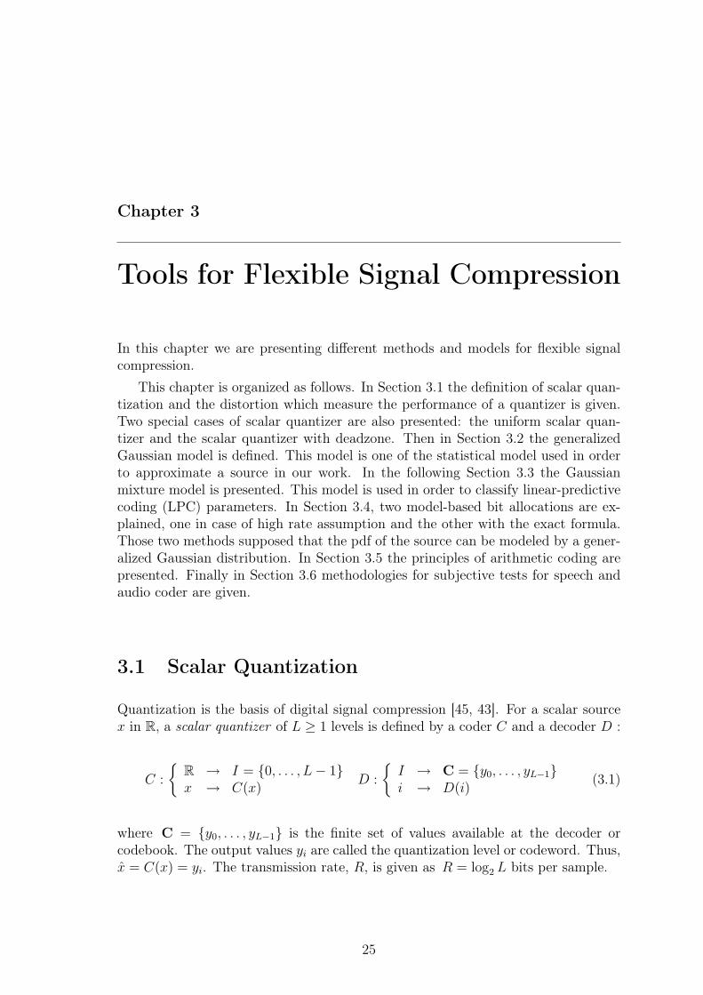
To obtain such fine grain scalability a bit-sliced coding is applied on the quantizedspectral data. An example of bit-sliced coding is presented in Fig. 2.20.
B 5 0 0 1
B 4 0 1 0
B 2 1 1 0
B 3 0 0 0
B 1 1 1 0
B 0 0 0 1
X 1 X 2 X 3
6 22 33
MSB
LSB
Noiseless Coding of B 5
Noiseless Coding of B 4
Noiseless Coding of B 3
Noiseless Coding of B 2
Noiseless Coding of B 1
Noiseless Coding of B 0
Base Layer
Error 0 Error 1 Error N
Layer 1
Layer N
Bit sliced coding
Figure 2.20: Example of Bit sliced Coding.
The quantized spectral data,Xi are represented in binary format, Bj. The orga-nization of binary formatted data can be rearranged to bit-sliced format shown inFig. 2.20. The MSB (Most Significant Bit) are more important than the LSB (LeastSignificant Bit) so the coding of MSB is a priority on LSB. Thus, the bit-sliced datais coded from the MSB to the LSB [90, 59].

2.5. Conclusion 23
2.5 ConclusionIn this chapter a review of wideband and super-wideband standard for streamingor cellular network applications has been done. Those standards are based on threemodels: analysis by synthesis coding which is widely used for speech coding, per-ceptual transform coding which is for audio coding and universal coding for bothspeech and music coding. Our objectives is to present a model-based coding methodwith the same performance than the standards but with more flexibility in terms ofapplications, bitrates, signals (speech/music).

24 Chapter 2. State of art in speech and audio coding
Chapter 3
Tools for Flexible Signal Compression
In this chapter we are presenting different methods and models for flexible signalcompression.
This chapter is organized as follows. In Section 3.1 the definition of scalar quan-tization and the distortion which measure the performance of a quantizer is given.Two special cases of scalar quantizer are also presented: the uniform scalar quan-tizer and the scalar quantizer with deadzone. Then in Section 3.2 the generalizedGaussian model is defined. This model is one of the statistical model used in orderto approximate a source in our work. In the following Section 3.3 the Gaussianmixture model is presented. This model is used in order to classify linear-predictivecoding (LPC) parameters. In Section 3.4, two model-based bit allocations are ex-plained, one in case of high rate assumption and the other with the exact formula.Those two methods supposed that the pdf of the source can be modeled by a gener-alized Gaussian distribution. In Section 3.5 the principles of arithmetic coding arepresented. Finally in Section 3.6 methodologies for subjective tests for speech andaudio coder are given.
3.1 Scalar Quantization
Quantization is the basis of digital signal compression [45, 43]. For a scalar sourcex in R, a scalar quantizer of L ≥ 1 levels is defined by a coder C and a decoder D :
C :
{R → I = {0, . . . , L− 1}x → C(x)
D :
{I → C = {y0, . . . , yL−1}i → D(i)
(3.1)
where C = {y0, . . . , yL−1} is the finite set of values available at the decoder orcodebook. The output values yi are called the quantization level or codeword. Thus,x = C(x) = yi. The transmission rate, R, is given as R = log2 L bits per sample.
25
26 Chapter 3. Tools for Flexible Signal Compression
3.1.1 Distortion
For a stationnary source x of pdf p(x), the performance of the quantizer is usuallymeasured by the average distortion:
D = E [d (x, C(x))] =
∫
Rd (x, C(x)) p(x) dx (3.2)
where E[.] is the expectation. The most commonly used distortion measure is thesquare error defined by:
d(x, x) = (x− x)2 (3.3)
The mean square error (MSE) is defined as:
D = E[(x− C(x))2] =
∑i∈I
∫
Ri
(x− yi)2 p(x) dx (3.4)
where Ri is the cell decision defined as:
Ri = {x ∈ Rn|C(x) = i} (3.5)
where Ri
⋂Rj = ∅ if i 6= j. The MSE distortion is simple to use but it does not
match well subjective quality for speech or audio signals.
3.1.2 Uniform scalar quantization
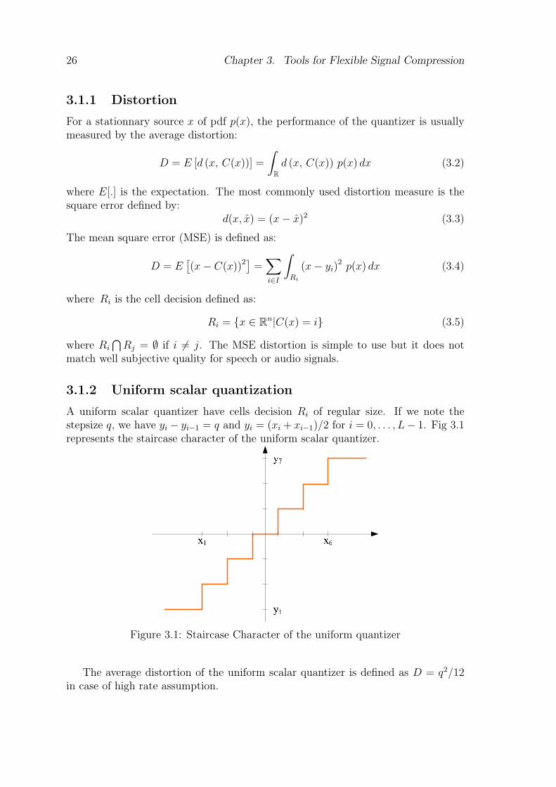
A uniform scalar quantizer have cells decision Ri of regular size. If we note thestepsize q, we have yi − yi−1 = q and yi = (xi + xi−1)/2 for i = 0, . . . , L− 1. Fig 3.1represents the staircase character of the uniform scalar quantizer.
Figure 3.1: Staircase Character of the uniform quantizer
The average distortion of the uniform scalar quantizer is defined as D = q2/12in case of high rate assumption.
3.2. Generalized Gaussian modeling 27
3.1.3 Uniform scalar quantizer with deadzone
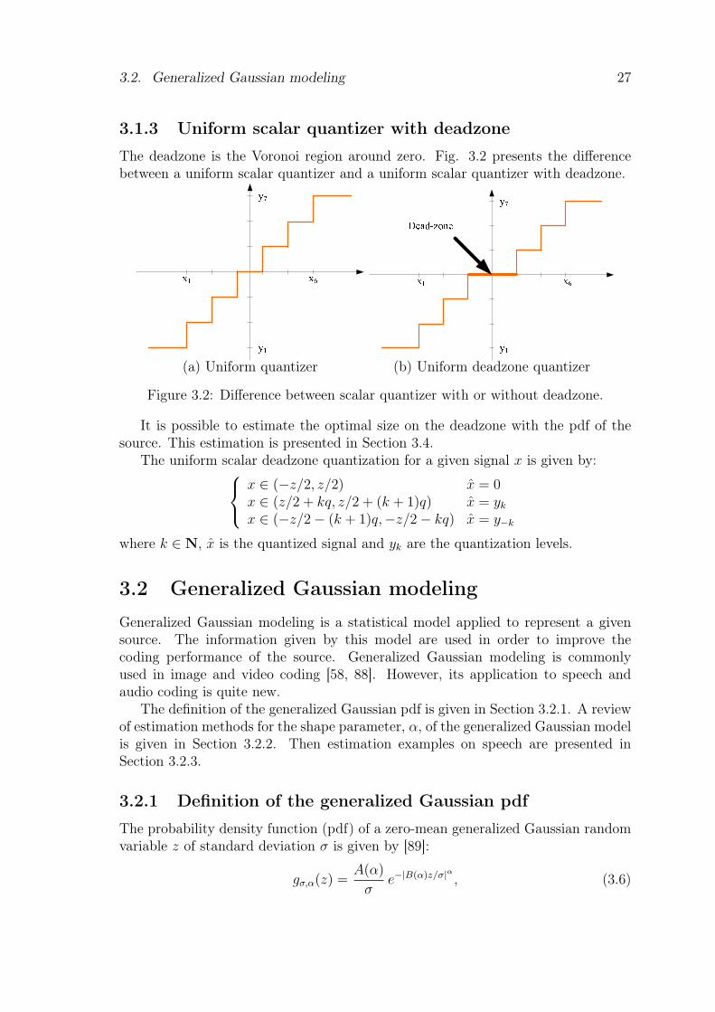
The deadzone is the Voronoi region around zero. Fig. 3.2 presents the differencebetween a uniform scalar quantizer and a uniform scalar quantizer with deadzone.
(a) Uniform quantizer (b) Uniform deadzone quantizer
Figure 3.2: Difference between scalar quantizer with or without deadzone.
It is possible to estimate the optimal size on the deadzone with the pdf of thesource. This estimation is presented in Section 3.4.
The uniform scalar deadzone quantization for a given signal x is given by:
x ∈ (−z/2, z/2) x = 0x ∈ (z/2 + kq, z/2 + (k + 1)q) x = yk
x ∈ (−z/2− (k + 1)q,−z/2− kq) x = y−k
where k ∈ N, x is the quantized signal and yk are the quantization levels.
3.2 Generalized Gaussian modelingGeneralized Gaussian modeling is a statistical model applied to represent a givensource. The information given by this model are used in order to improve thecoding performance of the source. Generalized Gaussian modeling is commonlyused in image and video coding [58, 88]. However, its application to speech andaudio coding is quite new.
The definition of the generalized Gaussian pdf is given in Section 3.2.1. A reviewof estimation methods for the shape parameter, α, of the generalized Gaussian modelis given in Section 3.2.2. Then estimation examples on speech are presented inSection 3.2.3.
3.2.1 Definition of the generalized Gaussian pdf
The probability density function (pdf) of a zero-mean generalized Gaussian randomvariable z of standard deviation σ is given by [89]:
gσ,α(z) =A(α)
σe−|B(α)z/σ|α , (3.6)
28 Chapter 3. Tools for Flexible Signal Compression
where α is a shape parameter describing the exponential rate of decay and the tailof the density function. The parameters A(α) and B(α) are given by:
A(α) =αB(α)
2Γ(1/α)and B(α) =
√Γ(3/α)
Γ(1/α), (3.7)
where Γ(.) is the Gamma function defined as:
Γ(α) =
∫ ∞
0
e−ttα+1 dt. (3.8)
The Laplacian and Gaussian distributions correspond to the special case α = 1 and2 respectively:
Laplacian distribution : gσ,α=1(x) =1√2σ
e√
2|x|σ (3.9)
Gaussian distribution : gσ,α=2(x) =1√2πσ
ex2
2σ2 (3.10)
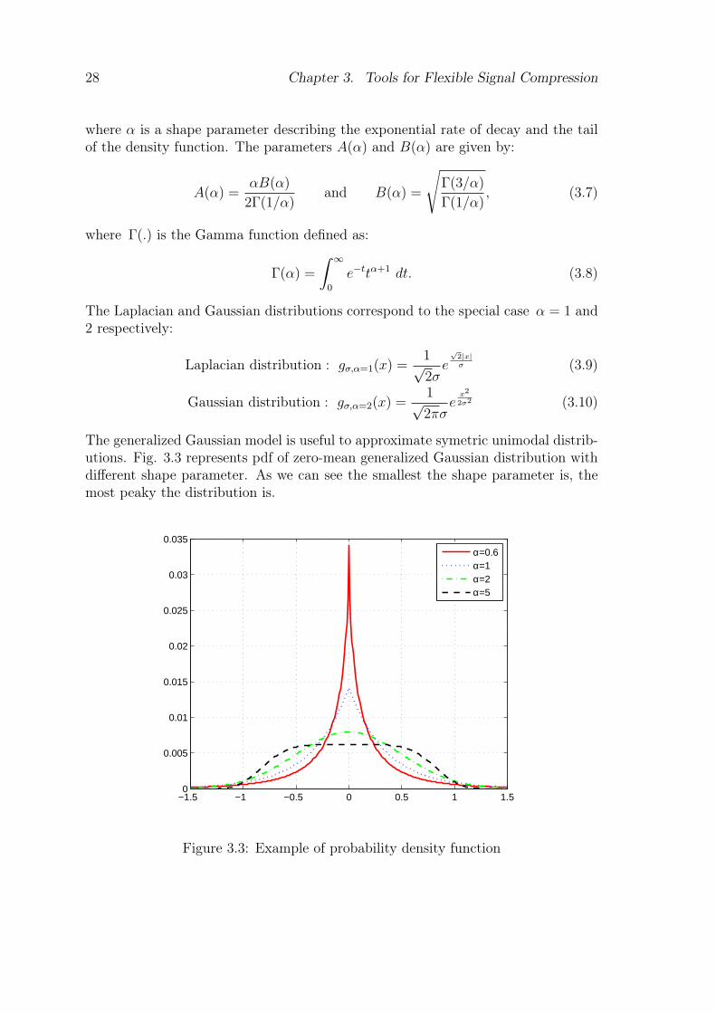
The generalized Gaussian model is useful to approximate symetric unimodal distrib-utions. Fig. 3.3 represents pdf of zero-mean generalized Gaussian distribution withdifferent shape parameter. As we can see the smallest the shape parameter is, themost peaky the distribution is.
−1.5 −1 −0.5 0 0.5 1 1.50
0.005
0.01
0.015
0.02
0.025
0.03
0.035
α=0.6α=1α=2α=5
Figure 3.3: Example of probability density function
3.2. Generalized Gaussian modeling 29
3.2.2 Estimation of the shape parameter α
Estimation methods of the shape parameter α are reviewed here. We classify estima-tion methods in "closed loop" and in "open loop". "Closed loop" methods estimateα by minimizing a distance criterion between data and model, while "open loop"methods provide an estimate of α without any distance criterion.
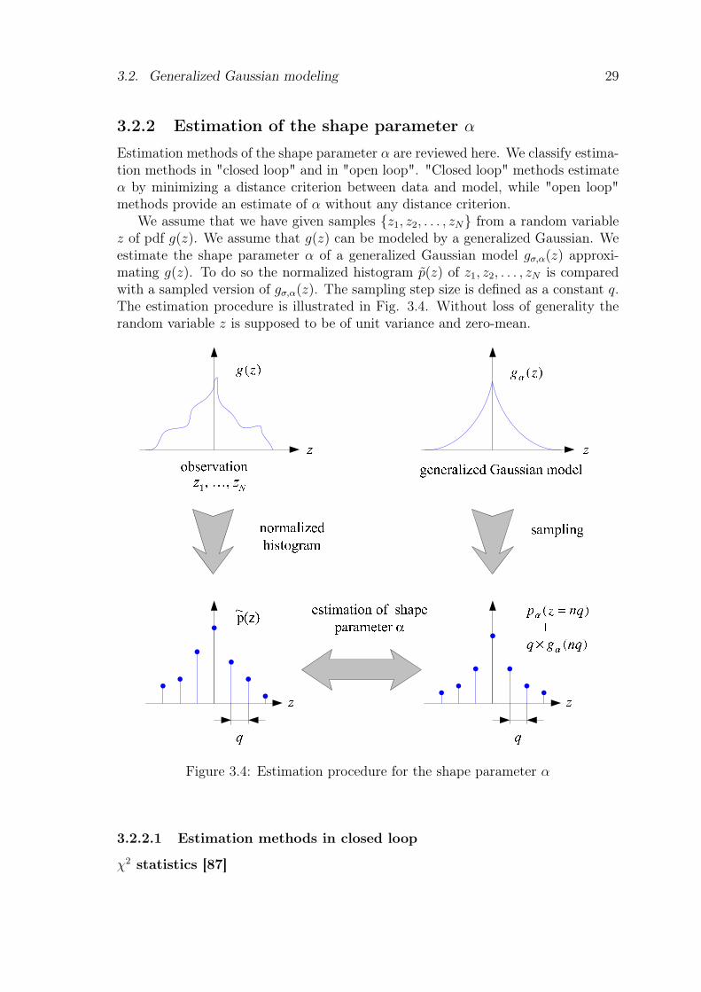
We assume that we have given samples {z1, z2, . . . , zN} from a random variablez of pdf g(z). We assume that g(z) can be modeled by a generalized Gaussian. Weestimate the shape parameter α of a generalized Gaussian model gσ,α(z) approxi-mating g(z). To do so the normalized histogram p(z) of z1, z2, . . . , zN is comparedwith a sampled version of gσ,α(z). The sampling step size is defined as a constant q.The estimation procedure is illustrated in Fig. 3.4. Without loss of generality therandom variable z is supposed to be of unit variance and zero-mean.
Figure 3.4: Estimation procedure for the shape parameter α
3.2.2.1 Estimation methods in closed loop
χ2 statistics [87]
30 Chapter 3. Tools for Flexible Signal Compression
The χ2 statistics evaluates a kind of distance between two probability densityfunctions. We use here a χ2 distance given by:
χ2(α) =∑
z=...,−q,0,q,...
(p(z)− pα(z))2
p(z) + pα(z), (3.11)
where pα(z) = gα(z)× q.The estimated shape parameter is obtained by minimization of:
α = arg minα
χ2(α) (3.12)
Kolmogorov-Smirnov statistic [87]The Kolmogorov-Smirnov statistic is defined as:
KS(α) = maxz
|G(z)−Gα(z)| (3.13)
where G(z) and Gα(z) are the distributions:
G(z) =
z/q∑n=−∞
p(nq) and Gα(z) =
z/q∑n=−∞
pα(nq) (3.14)
The estimated shape parameter α is found by minimization of:
α = arg minα
KS(α) (3.15)
Kullback-Leibler divergence [61]The Kullback-Leibler divergence is given by:
D(p||pα) = −∑
z=...,−q,0,q,...
pα(z) logp(z)
pα(z)(3.16)
The estimated shape parameter α is obtained by minimizing this measure betweenthe histogram p and the generalized Gaussian model:
α = arg minα
D(p||pα) (3.17)
3.2.2.2 Estimation methods in open loop
Several methods are omitted here, e.g. ML estimation [58].
Estimation based on kurtosis (κα)For a generalized gaussian source z of shape parameter α, the kurtosis κα is given
by [87]:
κα =E(z4)
E(z2)2=
Γ(5/α)Γ(1/α)
Γ(3/α)2(3.18)
3.2. Generalized Gaussian modeling 31
It can be verified that log κα is approximatively a linear function of 1/α [89]:
log κα ≈ 1.447
α+ 0.345 (3.19)
Based on this approximation, the shape parameter α can be estimated as [89]:
α ≈ 1.447
ln κ− 0.345, (3.20)
where κ is estimated from the data:
κ =1n
∑ni=1 z4
i(1n
∑ni=1 z2
i
)2 (3.21)
Method proposed by Mallat [69]A relation between the variance E(z2), the mean of the absolute value E(|z|)
and the shape parameter α is given by [89]:
E(|z|)√E(z2)
=Γ(2/α)√
Γ(1/α)Γ(3/α)= F (α) (3.22)
The shape parameter α can be estimated as:
α = F−1
(m1√m2
)(3.23)
where m1 = 1n
∑ni=1 z2
i and m2 = 1n
∑ni=1 |zi|.
Estimation based on differential entropy (hα)The differential entropy of a generalized Gaussian distribution is given by [89]:
hα =1
2log2
[4Γ(1/α)3
α2Γ(3/α)
]+
1
α log 2(3.24)
Based on high rate quantization theory, it can be shown that the entropy rate Rof the quantized random variable z and the differential entropy h(z) are related asfollows [45]:
R ≈ h(z)− log2 q (3.25)
The estimated shape parameter α is given by [60]:
α = h−1α
[R + log2 q
](3.26)
where R is the estimated entropy rate of z:
R = −∑
z=...,−q,0,q,...
p(z) log2 p(z) (3.27)
32 Chapter 3. Tools for Flexible Signal Compression
3.2.3 Estimation examples for speech
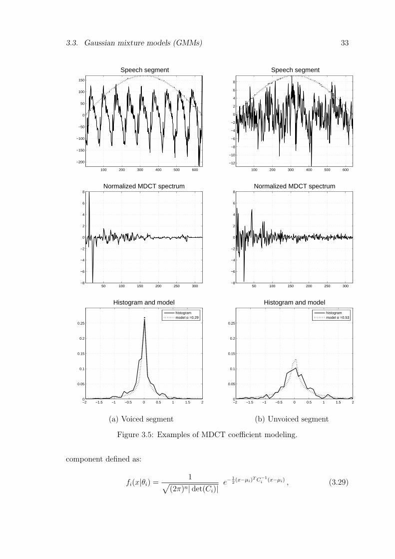
The results given by the various methods proposed before in order to estimate theshape parameter α of a pdf for a given source are quite similar. "Open-loop" methodsare slightly better than "closed-loop" but there complexity is more important. Sofor practical implementation, we choose to work with a "closed-loop" method andarbitrary we choose Mallat’s method [69].
Figure 3.5 shows how the distribution of normalized MDCT coefficients can beapproximated by a generalized Gaussian model. Both voiced and unvoiced speechexamples are considered. The input signals in time domain (top) are sampled at 16kHz and transformed by MDCT with a sinusoidal window of 40 ms. The MDCTspectrum of a given frame (middle), comprising 320 coefficients, is normalized byits root mean square (r.m.s.). The histogram of normalized MDCT coefficients ismodeled by a generalized Gaussian pdf (bottom). The estimated shape parameteris estimated using Mallat’s method [69], for voiced speech α = 0.29 and for unvoicedspeech α = 0.53, so the value of α is somehow related to the voicing of the signal.Note that the value of α would be closer to 2 (Gaussian case) for unvoiced speech ifthe signals in time domain were linear predictive residuals. However these examplesindicate that generalized Gaussian modeling can provide a good approximation ofthe MDCT spectrum distribution for speech signals. These observations can beextended to music signals.
3.3 Gaussian mixture models (GMMs)
A Gaussian mixture model (GMM) is a weighted sum of Gaussian densities. It is asemi-parametric model determined by the weights, the means and the covariancesmatrices of the gaussian component [100]. GMM has been developed for vector quan-tization (VQ) of linear-predictive coding (LPC) parameters [46, 113]. It providesquantization schemes with low complexity and independent from the bitrate.
The principle of Gaussian mixture models (GMMs) is given in Section 3.3.1. Theexpectation-maximization (EM) algorithm which is a practical method to estimatethe parameters of the Gaussian mixture is presented in Section 3.3.2.
3.3.1 Principle of Gaussian mixture models
We follow here the notations of [46]. A Gaussian mixture model (GMM) is definedas a weighted sum of Gaussian densities :
f(x|Θ) =M∑i=1
ρi fi(x|θi) , (3.28)
where x, ρi and fi(x|θi) are respectively a vector of dimension n, the mixture weightssuch as
∑Mi=1 ρi = 1 and the Gaussian probability density function of the i-th GMM
3.3. Gaussian mixture models (GMMs) 33
100 200 300 400 500 600
−200
−150
−100
−50
0
50
100
150
Speech segment
100 200 300 400 500 600
−12
−10
−8
−6
−4
−2
0
2
4
6
8
Speech segment
50 100 150 200 250 300−8
−6
−4
−2
0
2
4
6
8Normalized MDCT spectrum
50 100 150 200 250 300−8
−6
−4
−2
0
2
4
6
8Normalized MDCT spectrum
−2 −1.5 −1 −0.5 0 0.5 1 1.5 20
0.05
0.1
0.15
0.2
0.25
Histogram and model
histogrammodel α =0.29
−2 −1.5 −1 −0.5 0 0.5 1 1.5 20
0.05
0.1
0.15
0.2
0.25
Histogram and model
histogrammodel α =0.53
(a) Voiced segment (b) Unvoiced segment
Figure 3.5: Examples of MDCT coefficient modeling.
component defined as:
fi(x|θi) =1√
(2π)n| det(Ci)|e−
12(x−µi)
T C−1i (x−µi) , (3.29)
34 Chapter 3. Tools for Flexible Signal Compression
where µi and Ci are respectively the mean vector and the covariance matrix of thei-th GMM component. As a result, a Gaussian mixture model is determined by itsparameters:
Θ = {ρ1, . . . , ρM , θ1, . . . , θM} (3.30)
whereθi = {µi, Ci} (3.31)
In order to estimate the parameters of each Gaussian in the model the expectation-maximization (EM) algorithm [28, 100] is a practical and commonly used method.
3.3.2 Expectation-maximization algorithm
The EM algorithm is an iterative algorithm to find the maximum-likelihood estimateof the parameters of a distribution from a given data set when the data is incompleteor has missing values [100]. The algorithm guarantees convergence to a locallyoptimal solution.
In the special case of Gaussian mixture model the incomplete-data log likelihoodexpression from the data x is given by:
log (L (Θ|x)) =n∑
j=1
log (f(xj|Θ)) =n∑
j=1
log
(M∑i=1
ρi fi(xi|θj)
)(3.32)
which is difficult to optimize because it is a log of the sum. If we consider thatthe data x are incomplete, and consider the existence of unobserved data items y(whose values inform us which component density "generated" each data item) thelog likelihood expression is simplified:
log (L (Θ|x, y)) =n∑
j=1
log(ρyj
fyj(xj|θyj
))
(3.33)
The problem is that we do not know the values of y, so we assume y is a randomvector.
Expectation step (E-step)Θopt = {ρopt
1 , . . . , ρoptM , θopt
1 , . . . , θoptM } are noted as the appropriate parameters for
the likelihood L (Θopt|x, y). Using Baye’s rule we can write the relationship:
f(yj|xj, Θ
opt)
=ρyj
fyj(xj|θopt
yj)
M∑i=1
ρi fi(xj|θopti )
(3.34)
We also have the relationship:
f(y|x, Θopt
)=
n∏j=1
f(yj|xj, Θ
opt)
(3.35)
3.4. Model-Based Bit Allocation 35
We try to find the function Q (Θ|Θopt) which is defined as the expected value of thecomplete data log-likelihood with respect to the unknown data given the observationdata. After simplification, we have the relationship:
Q (Θ|Θopt
)=
M∑i=1
n∑j=1
log (ρifi (xj|θi)) f(i|xj, Θ
opt)
(3.36)
=M∑i=1
n∑j=1
log (ρi) f(i|xj, Θ
opt)
+M∑i=1
n∑j=1
log (fi (xj|θi)) f(i|xj, Θ
opt)
This expression has to be maximized. It is possible to maximize the term containingρi and the term containing θi independently since they are not related.
Maximization step (M-step)In order to find the expression of ρi, we introduce Lagrange multiplier λ under
the constraint that∑M
i=1 ρi = 1, and we have the following relationship:
∂
∂ρi
[M∑i=1
n∑j=1
log (ρi) f(i|xj, Θ
opt)
+ λ
(M∑i=1
ρi − 1
)]= 0 (3.37)
So we get:n∑
j=1
1
ρi
f(i|xj, Θ
opt)
+ λ = 0 (3.38)
By summing over j, we get λ = −n and so we have the following relationship:
ρi =1
n
n∑j=1
f(i|xj, Θ
opt)
(3.39)
The estimate of the new parameters are as follows:
ρnewi =
1
n
n∑j=1
f(i|xj, Θ
opt)
(3.40)
µnewi =
∑nj=1 xjf (i|xj, Θ
opt)∑nj=1 f (i|xj, Θopt)
(3.41)
Cnewi =
∑nj=1 f (i|xj, Θ
opt) (xj − µnewi ) (xj − µnew
i )T
∑nj=1 f (i|xj, Θopt)
(3.42)
3.4 Model-Based Bit Allocation
Model-based bit allocation has been studied in [88] for image coding, we proposedto use it for speech and audio coding. The objectif is to improve the performance of
36 Chapter 3. Tools for Flexible Signal Compression
quantization by having a stepsize which is appropriated for the source. The modelused here is the generalized Gaussian model.
The problem of bit allocation is an optimization under constraint. We considerthe encoding of N zero-mean random variables x1, . . . , xN of variances σ2 with re-spect to the mean square error criterion. We assume that the variables xi have ageneralized Gaussian pdf gσ,α(x) of shape parameter α. The variables xi are codedby scalar quantization with the same step size q. We assume that the sequence ofintegers obtained after scalar quantization is encoded by ideal entropy coding. For agiven bit allocation B in bits per sample, the bit allocation problem is to minimizethe distortion D under the constraint that
∑Ni=1 bi ≤ B. Solving this problem is
the minimization of a function with Lagrangian techniques. The criterion J(bi, λ) isdefined as
J(bi, λ) = D − λ
(N∑
i=1
bi −B
)(3.43)
where λ is the Lagrange multiplier.We presented here two cases, one with the hypothesis that we are in high reso-
lution and the other one with the correct formula. This work has been developed in[88].
3.4.1 Asymptotic model-based bit allocation
We follow here the notations of [45] with regards to transform coding and bit alloca-tion. In case of high resolution the mean square error D resulting from the encodingof N random variables xi is given by [45]:
D ≈N∑
i=1
hσ22−2bi (3.44)
where the constant hi is a function of the pdf of the variable xi and bi is the numberof bits per sample used to code xi. For a generalized Gaussian pdf, h is given by[89]:
h =Γ(1/α)3
3α2Γ(3/α)e2/α, (3.45)
where α is the shape parameter of the distribution xi. The distortion D given inEq. (3.44) can be minimized with Lagrangian techniques. The criterion J(bi, λ) isdefined as
J(bi, λ) = D − λ
(N∑
i=1
bi −B
)(3.46)
where λ is the Lagrange multiplier.
3.4. Model-Based Bit Allocation 37
The derivative of J(bi, λ) with respect to bi and λ is given by:
∂J
∂bi
= −2 ln(2)hσ22−2bi + λ = 0 (3.47)
∂J
∂λ=
N∑i=1
bi −B = 0 (3.48)
From Eq. 3.47 we can write:
log2
(2 ln(2)hσ2
)− 2bi = log2 (λ) (3.49)
So the optimal bitrate is given by:
bi = −1
2log2(λ) +
1
2log2
(2 ln(2)hσ2
)(3.50)
We used the relationship obtained in Eq. 3.50 into Eq. 3.48:
N∑i=1
(1
2log2(λ) +
1
2log2
(2 ln(2)hσ2
))−B = 0 (3.51)
So:
−N∑
i=1
log2 λ = 2B +N∑
i=1
log2
1
2 ln(2)hσ2(3.52)
And finally, we have:
λ = 2−2B2 ln(2)hσ2 . (3.53)
The relationship gives the optimal Lagrangian parameter λopt. With this value of λthe Eq. 3.47 becomes:
D =λopt
2 ln(2). (3.54)
Furthermore for high-resolution scalar uniform quantization with step size q, wehave [45]:
D =q2
12. (3.55)
From (3.54) and (3.55) we find that the optimal stepsize is:
q =
√6λopt
ln(2). (3.56)
38 Chapter 3. Tools for Flexible Signal Compression
3.4.2 Non asymptotic model-based bit allocation
The quantization mean square error DQ resulting for the encoding of N randomvariables xi is given by [45]:
DQ =
∫ z2
−z/2
x2gσ,αdx + 2+∞∑m=1
∫ z2+mq
z2+(m−1)q
(x− xm)2 gσ,α(x)dx (3.57)
where xm is the centroid of each quantization level m defined as :
xm =
∫ z/2+mq
−z/2+(m−1)qxgσ,αdx
∫ z/2+mq
−z/2+(m−1)qgσ,α(x)dx
(3.58)
After simplifying we have the following relationship:
DQ = σ2 + 2+∞∑m=1
x2m
∫ z/2+mq
−z/2+(m−1)q
gσ,α(x)dx− 4+∞∑m=1
xm
∫ z/2+mq
−z/2+(m−1)q
xgσ,αdx (3.59)
By using Eq. 3.58 we can write that:
DQ = σ2 − 2+∞∑m=1
(∫ z/2+mq
−z/2+(m−1)qxgσ,α(x)dx
)2
∫ z/2+mq
−z/2+(m−1)qgσ,α(x)dx
(3.60)
So the mean square error D is a function of four parameters which are the stepsizeq, the deadzone z, the shape parameter α and the variance σ2. If we consider afunction fn,m
(α, z
σ, q
σ
)defined as:
fn,m
(α,
z
σ,q
σ
)=
∫ z/2σ+mq/2σ
z/2σ+(m−1)q/2σ
xng1,α(x)dx , (3.61)
the Eq. 3.60 is simplified into:
DQ = σ2
[1− 2
+∞∑m=1
f1,m
(α, z
σ, q
σ
)
f0,m
(α, z
σ, q
σ
)]
. (3.62)
So we finally have [88]:
DQ = σ2D(α,
z
σ,q
σ
), (3.63)
where
D(α,
z
σ,q
σ
)= 1− 2
+∞∑m=1
f1,m
(α, z
σ, q
σ
)
f0,m
(α, z
σ, q
σ
) . (3.64)
3.4. Model-Based Bit Allocation 39
In the special case where the centroid is set to mid-value the distortion D is givenby [88]:
D(α,
z
σ,q
σ
)= 1 + 2
+∞∑m=1
(z
2σ+
(m− 1
2
)q
σ
)2
f0,m
(α,
z
σ,q
σ
)
−4+∞∑m=1
(z
2σ+
(m− 1
2
)q
σ
)f1,m
(α,
z
σ,q
σ
)(3.65)
The bit rate is defined as:
b = −+∞∑
m=−∞(m) log2 Pr(m) (3.66)
where Pr(m) is the probability of having the quantization level m. The generalizedGaussian distribution is symmetrical so we have the relationship Pr(m) = Pr(−m)and finally:
b = Pr(0 log2 p(0))− 2+∞∑m=1
p(m) log2 Pr(m) (3.67)
where Pr(m) is defined as:
Pr(m) =
∫ z/2+mq/2
z/2+(m−1)q
g1,α(x)dx = f0,m
(α,
z
σ,q
σ
)(3.68)
and p(0) is defined as:
p(0) =
∫ z/2
−z/2
g1,α(x)dx = f0,0
(α,
z
σ
). (3.69)
The bit rate is also a function of four parameters which are the stepsize q, thedeadzone z, the shape parameter α and the variance σ2. The bit rate is defined as[88]:
b(α,
z
σ,q
σ
)= −f0,0
(α,
z
σ
)log2 f0,0
(α,
z
σ
)
−2+∞∑m=1
f0,m
(α,
z
σ,q
σ
)log2 f0,m
(α,
z
σ,q
σ
)(3.70)
The solution of the allocation problem can be find by introducing the criterionJ(z, q, λ) defined as:
J(z, q, λ) =(α,
z
σ,q
σ
)− λ
(b(α,
z
σ,q
σ
)−B
)(3.71)
where λ is the Lagrange multiplier.The solution of this equation is presented in [88] and leads to a system of equation
which gives charts in order to find the optimal stepsize q under the bit budgetconstraint.
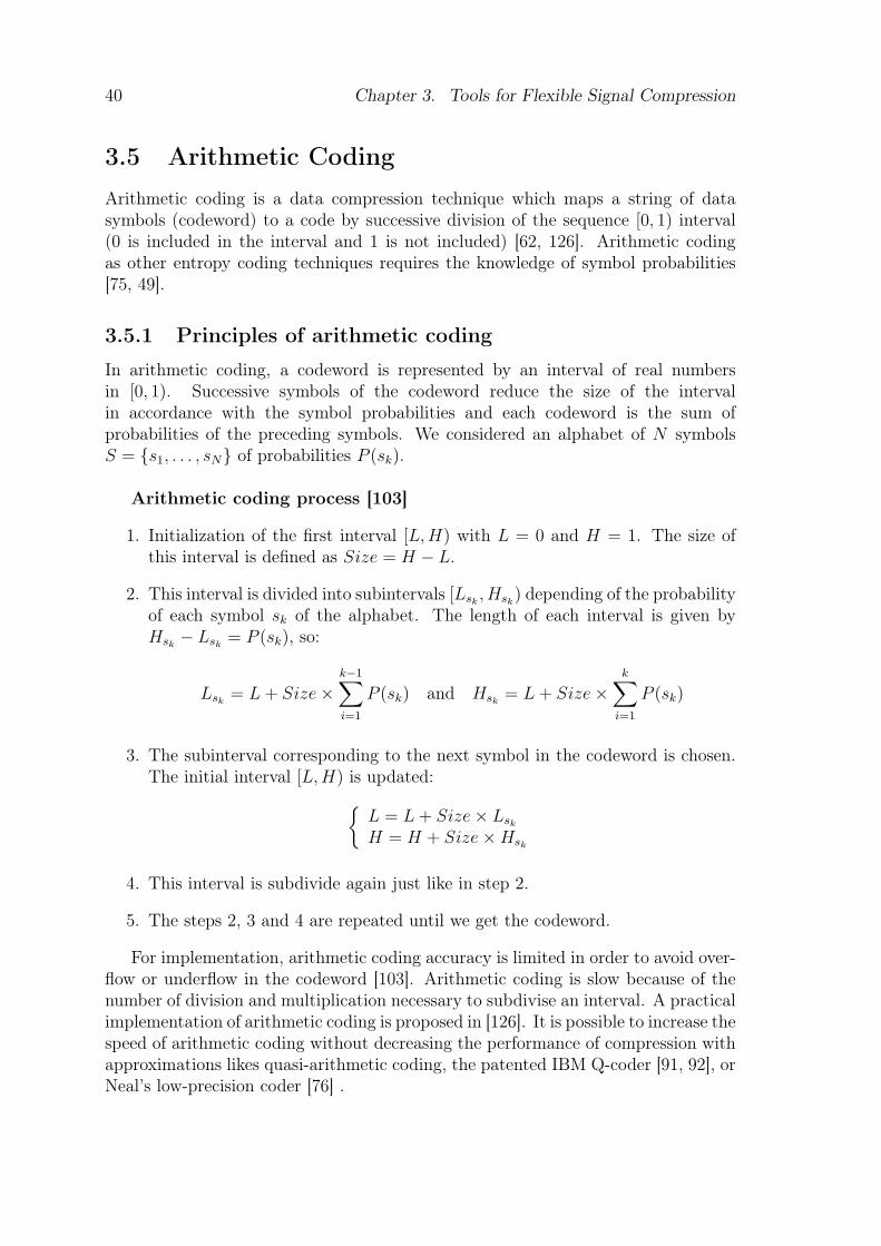
40 Chapter 3. Tools for Flexible Signal Compression
3.5 Arithmetic CodingArithmetic coding is a data compression technique which maps a string of datasymbols (codeword) to a code by successive division of the sequence [0, 1) interval(0 is included in the interval and 1 is not included) [62, 126]. Arithmetic codingas other entropy coding techniques requires the knowledge of symbol probabilities[75, 49].
3.5.1 Principles of arithmetic coding
In arithmetic coding, a codeword is represented by an interval of real numbersin [0, 1). Successive symbols of the codeword reduce the size of the intervalin accordance with the symbol probabilities and each codeword is the sum ofprobabilities of the preceding symbols. We considered an alphabet of N symbolsS = {s1, . . . , sN} of probabilities P (sk).
Arithmetic coding process [103]
1. Initialization of the first interval [L,H) with L = 0 and H = 1. The size ofthis interval is defined as Size = H − L.
2. This interval is divided into subintervals [Lsk, Hsk
) depending of the probabilityof each symbol sk of the alphabet. The length of each interval is given byHsk
− Lsk= P (sk), so:
Lsk= L + Size×
k−1∑i=1
P (sk) and Hsk= L + Size×
k∑i=1
P (sk)
3. The subinterval corresponding to the next symbol in the codeword is chosen.The initial interval [L, H) is updated:
{L = L + Size× Lsk
H = H + Size×Hsk
4. This interval is subdivide again just like in step 2.
5. The steps 2, 3 and 4 are repeated until we get the codeword.
For implementation, arithmetic coding accuracy is limited in order to avoid over-flow or underflow in the codeword [103]. Arithmetic coding is slow because of thenumber of division and multiplication necessary to subdivise an interval. A practicalimplementation of arithmetic coding is proposed in [126]. It is possible to increase thespeed of arithmetic coding without decreasing the performance of compression withapproximations likes quasi-arithmetic coding, the patented IBM Q-coder [91, 92], orNeal’s low-precision coder [76] .
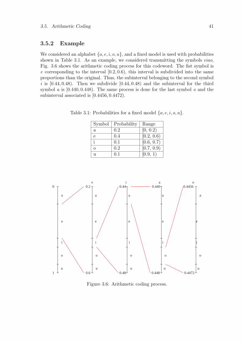
3.5. Arithmetic Coding 41
3.5.2 Example
We considered an alphabet {a, e, i, o, u}, and a fixed model is used with probabilitiesshown in Table 3.1. As an example, we considered transmitting the symbols eiao,Fig. 3.6 shows the arithmetic coding process for this codeword. The fist symbol ise corresponding to the interval [0.2, 0.6), this interval is subdivided into the sameproportions than the original. Thus, the subinterval belonging to the second symboli is [0.44, 0.48). Then we subdivide [0.44, 0.48) and the subinterval for the thirdsymbol a is [0.440, 0.448). The same process is done for the last symbol o and thesubinterval associated is [0.4456, 0.4472).
Table 3.1: Probabilities for a fixed model {a, e, i, o, u}.
Symbol Probability Rangea 0.2 [0, 0.2)e 0.4 [0.2, 0.6)i 0.1 [0.6, 0.7)o 0.2 [0.7, 0.9)u 0.1 [0.9, 1)
a a a a
e e e e e
a
i i i i i
o o o o o
u u u u u
e i a o 0
1
0.2
0.6
0.44
0.448 0.48
0.440 0.4456
0.4472
Figure 3.6: Arithmetic coding process.
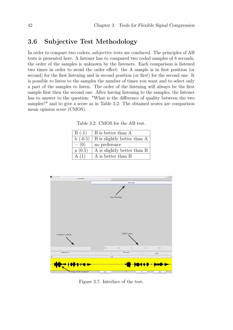
42 Chapter 3. Tools for Flexible Signal Compression
3.6 Subjective Test Methodology
In order to compare two coders, subjective tests are conduced. The principles of ABtests is presented here. A listener has to compared two coded samples of 8 seconds,the order of the samples is unknown by the listeners. Each comparison is listenedtwo times in order to avoid the order effect: the A sample is in first position (orsecond) for the first listening and in second position (or first) for the second one. Itis possible to listen to the samples the number of times you want and to select onlya part of the samples to listen. The order of the listening will always be the firstsample first then the second one. After having listening to the samples, the listenerhas to answer to the question: "What is the difference of quality between the twosamples?" and to give a score as in Table 3.2. The obtained scores are comparisonmean opinion score (CMOS).
Table 3.2: CMOS for the AB test.
B (-1) B is better than Ab (-0.5) B is slightly better than A= (0) no preferencea (0.5) A is slightly better than BA (1) A is better than B
CMOS score Listener’s initials
Image of the sample
Start listening
Figure 3.7: Interface of the test.
3.7. Conclusion 43
Fig. 3.7 presents the interface of the listening test. The listener can start thetest whenever he wants to and he can listen to a selected part of a sample. Theimage of the sample does not change from sample a to sample B, so the listener doesnot have information on the sample is listening.
3.7 ConclusionIn this chapter we presented different methods and models for flexible signal compres-sion. Two statistical models used to approximate the source have been presented:generalized Gaussian model and Gaussian mixture model. GMM will be used toclassify linear-predictive coding (LPC) parameters. Principles of model-based bitallocation have also been presented. The model-based bit allocation is used in orderto estimate the optimal stepsize and the optimal deadzone for the scalar quantizer.

44 Chapter 3. Tools for Flexible Signal Compression
Chapter 4
Flexible quantization of LPCcoefficients
A parametric approach based on Gaussian mixture model (GMM) has been de-veloped for vector quantization (VQ) of linear-predictive coding (LPC) parameters[46, 113]. This approach has brought interest in the design of model-based quantiza-tion methods as opposed to standard constrained VQ requiring stochastic codebooktraining based on a given source database. Several variants of GMM-based LPCquantization have been proposed including predictive methods [113, 80].
In this chapter we present a new model-based coding method to represent thelinear-predictive coding (LPC) parameters of wideband speech signals (sampled at 16kHz). The LPC coefficients are transformed into line spectrum frequencies (LSF) andquantized by switched AR(1)/MA(1) predictive Karhunen-Loeve transform (KLT)coding. KLT coding is equivalent to source coding with singular value decomposition(SVD) or principal component analysis (PCA).
The main contribution of this work lies in the use of improved quantizationto represent the (transformed) prediction error of LSF parameters. GeneralizedGaussian modeling is applied for this purpose.
This chapter is organized as follows. In Section 4.1 we present shortly the princi-ples of LPC quantization. Previous works on GMM-based LSF vector quantizationare presented in Section 4.2, references are given and the GMM-based LSF quan-tizer of [111] is described. Then in Section 4.3 the proposed LSF vector quantizer isdescribed. This quantizer is based on principal component analysis (PCA) with oneGaussian and the quantizer is build on a generalized Gaussian model. In Section4.4 the proposed quantizer is modified by introducing a predictive scheme. Thisprediction can be done by moving-average (MA) or autoregressive (AR) model. Ex-perimental results for predictive KLT coding are presented in Section 4.5 beforeconcluding in Section 4.6.
Part of this work was presented at EUSIPCO’06 [78]
45
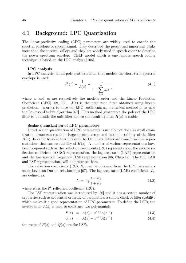
46 Chapter 4. Flexible quantization of LPC coefficients
4.1 Background: LPC QuantizationThe linear-predictive coding (LPC) parameters are widely used to encode thespectral envelope of speech signal. They described the perceptual important peaksmore than the spectral valleys and they are widely used in speech coder to describethe power spectrum envelop. CELP model which is one famous speech codingtechnique is based on the LPC analysis [106].
LPC analysisIn LPC analysis, an all-pole synthesis filter that models the short-term spectral
envelope is used:
H (z) =1
A(z)=
1
1 +n∑
i=1
aiz−i
(4.1)
where n and ai are respectively the model’s order and the Linear PredictionCoefficient (LPC) [68, 73]. A(z) is the prediction filter obtained using linear-prediction. In order to have the LPC coefficients ai, a classical method is to usedthe Levinson-Durbin algorithm [67]. This method guarantees the poles of the LPCfilter to be inside the unit filter and so the resulting filter H(z) is stable.
Scalar quantization of LPC parametersDirect scalar quantization of LPC parameters is usually not done as small quan-
tization errors can result in large spectral errors and in the instability of the filterH(z). In order to solve this problem the LPC parameters are transformed in repre-sentations that ensure stability of H(z). A number of various representations havebeen proposed such as the reflection coefficients (RC) representation, the arcsine re-flection coefficient (ASRC) representation, the log-area ratio (LAR) representationand the line spectral frequency (LSF) representation [86, Chap.12]. The RC, LARand LSF representations will be presented here.
The reflection coefficients (RC), Ki, can be obtained from the LPC parametersusing Levinson-Durbin relationships [67]. The log-area ratio (LAR) coefficients, Li,are defined as:
Li = log1−Ki
1 + Ki
(4.2)
where Ki is the ith reflection coefficient (RC).The LSF representation was introduced by [50] and it has a certain number of
properties such as sequential ordering of parameters, a simple check of filter stabilitywhich makes it a good representation of LPC parameters. To define the LSFs, theinverse filter A(z) is used to construct two polynomials:
P (z) = A(z) + zn+1A(z−1) (4.3)Q(z) = A(z)− zn+1A(z−1) (4.4)
the roots of P (z) and Q(z) are the LSFs.
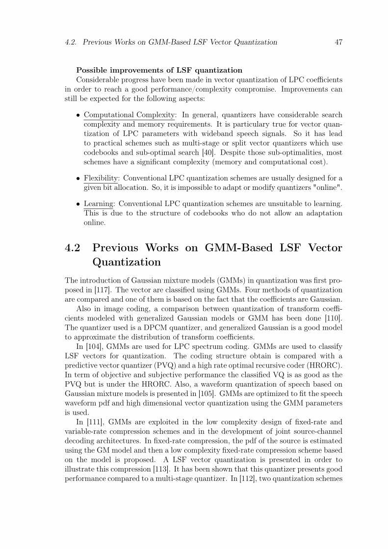
4.2. Previous Works on GMM-Based LSF Vector Quantization 47
Possible improvements of LSF quantizationConsiderable progress have been made in vector quantization of LPC coefficients
in order to reach a good performance/complexity compromise. Improvements canstill be expected for the following aspects:
• Computational Complexity: In general, quantizers have considerable searchcomplexity and memory requirements. It is particulary true for vector quan-tization of LPC parameters with wideband speech signals. So it has leadto practical schemes such as multi-stage or split vector quantizers which usecodebooks and sub-optimal search [40]. Despite those sub-optimalities, mostschemes have a significant complexity (memory and computational cost).
• Flexibility: Conventional LPC quantization schemes are usually designed for agiven bit allocation. So, it is impossible to adapt or modify quantizers "online".
• Learning: Conventional LPC quantization schemes are unsuitable to learning.This is due to the structure of codebooks who do not allow an adaptationonline.
4.2 Previous Works on GMM-Based LSF VectorQuantization
The introduction of Gaussian mixture models (GMMs) in quantization was first pro-posed in [117]. The vector are classified using GMMs. Four methods of quantizationare compared and one of them is based on the fact that the coefficients are Gaussian.
Also in image coding, a comparison between quantization of transform coeffi-cients modeled with generalized Gaussian models or GMM has been done [110].The quantizer used is a DPCM quantizer, and generalized Gaussian is a good modelto approximate the distribution of transform coefficients.
In [104], GMMs are used for LPC spectrum coding. GMMs are used to classifyLSF vectors for quantization. The coding structure obtain is compared with apredictive vector quantizer (PVQ) and a high rate optimal recursive coder (HRORC).In term of objective and subjective performance the classified VQ is as good as thePVQ but is under the HRORC. Also, a waveform quantization of speech based onGaussian mixture models is presented in [105]. GMMs are optimized to fit the speechwaveform pdf and high dimensional vector quantization using the GMM parametersis used.
In [111], GMMs are exploited in the low complexity design of fixed-rate andvariable-rate compression schemes and in the development of joint source-channeldecoding architectures. In fixed-rate compression, the pdf of the source is estimatedusing the GM model and then a low complexity fixed-rate compression scheme basedon the model is proposed. A LSF vector quantization is presented in order toillustrate this compression [113]. It has been shown that this quantizer presents goodperformance compared to a multi-stage quantizer. In [112], two quantization schemes
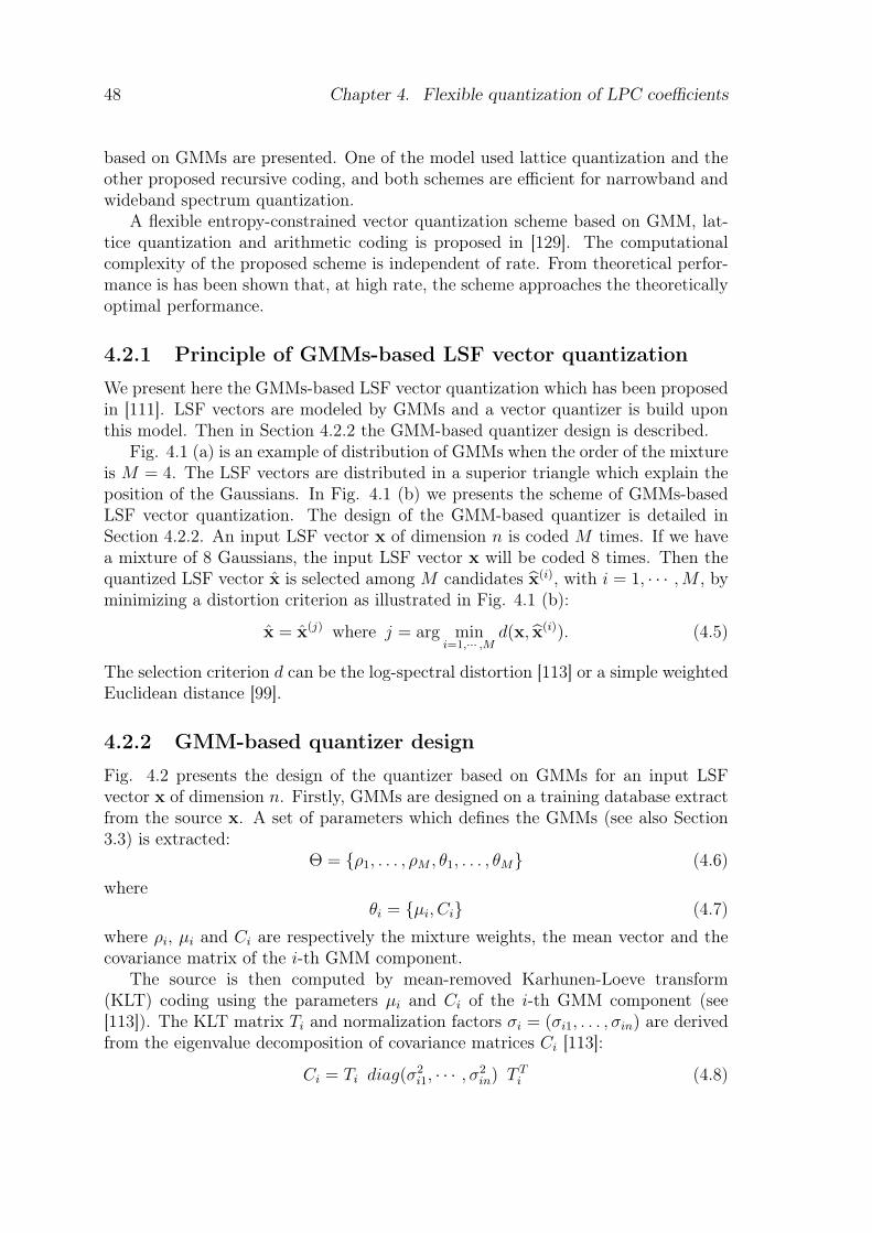
48 Chapter 4. Flexible quantization of LPC coefficients
based on GMMs are presented. One of the model used lattice quantization and theother proposed recursive coding, and both schemes are efficient for narrowband andwideband spectrum quantization.
A flexible entropy-constrained vector quantization scheme based on GMM, lat-tice quantization and arithmetic coding is proposed in [129]. The computationalcomplexity of the proposed scheme is independent of rate. From theoretical perfor-mance is has been shown that, at high rate, the scheme approaches the theoreticallyoptimal performance.
4.2.1 Principle of GMMs-based LSF vector quantization
We present here the GMMs-based LSF vector quantization which has been proposedin [111]. LSF vectors are modeled by GMMs and a vector quantizer is build uponthis model. Then in Section 4.2.2 the GMM-based quantizer design is described.
Fig. 4.1 (a) is an example of distribution of GMMs when the order of the mixtureis M = 4. The LSF vectors are distributed in a superior triangle which explain theposition of the Gaussians. In Fig. 4.1 (b) we presents the scheme of GMMs-basedLSF vector quantization. The design of the GMM-based quantizer is detailed inSection 4.2.2. An input LSF vector x of dimension n is coded M times. If we havea mixture of 8 Gaussians, the input LSF vector x will be coded 8 times. Then thequantized LSF vector x is selected among M candidates x(i), with i = 1, · · · ,M , byminimizing a distortion criterion as illustrated in Fig. 4.1 (b):
x = x(j) where j = arg mini=1,··· ,M
d(x, x(i)). (4.5)
The selection criterion d can be the log-spectral distortion [113] or a simple weightedEuclidean distance [99].
4.2.2 GMM-based quantizer design
Fig. 4.2 presents the design of the quantizer based on GMMs for an input LSFvector x of dimension n. Firstly, GMMs are designed on a training database extractfrom the source x. A set of parameters which defines the GMMs (see also Section3.3) is extracted:
Θ = {ρ1, . . . , ρM , θ1, . . . , θM} (4.6)
whereθi = {µi, Ci} (4.7)
where ρi, µi and Ci are respectively the mixture weights, the mean vector and thecovariance matrix of the i-th GMM component.
The source is then computed by mean-removed Karhunen-Loeve transform(KLT) coding using the parameters µi and Ci of the i-th GMM component (see[113]). The KLT matrix Ti and normalization factors σi = (σi1, . . . , σin) are derivedfrom the eigenvalue decomposition of covariance matrices Ci [113]:
Ci = Ti diag(σ2i1, · · · , σ2
in) T Ti (4.8)
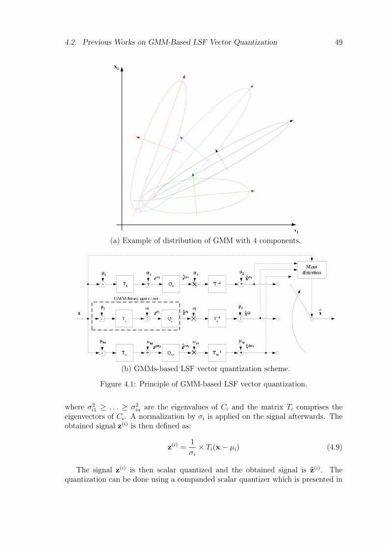
4.2. Previous Works on GMM-Based LSF Vector Quantization 49
(a) Example of distribution of GMM with 4 components.
(b) GMMs-based LSF vector quantization scheme.
Figure 4.1: Principle of GMM-based LSF vector quantization.
where σ2i1 ≥ . . . ≥ σ2
in are the eigenvalues of Ci and the matrix Ti comprises theeigenvectors of Ci. A normalization by σi is applied on the signal afterwards. Theobtained signal z(i) is then defined as:
z(i) =1
σi
× Ti(x− µi) (4.9)
The signal z(i) is then scalar quantized and the obtained signal is z(i). Thequantization can be done using a companded scalar quantizer which is presented in
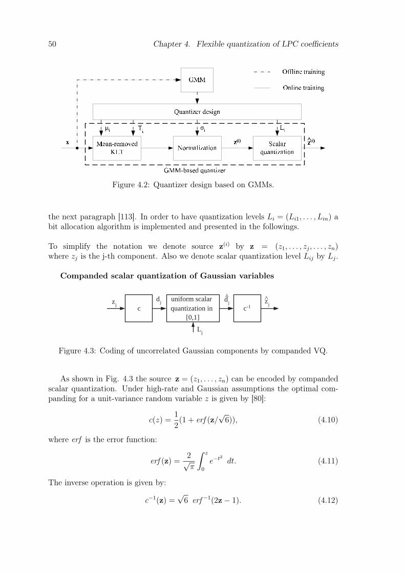
50 Chapter 4. Flexible quantization of LPC coefficients
Figure 4.2: Quantizer design based on GMMs.
the next paragraph [113]. In order to have quantization levels Li = (Li1, . . . , Lin) abit allocation algorithm is implemented and presented in the followings.
To simplify the notation we denote source z(i) by z = (z1, . . . , zj, . . . , zn)where zj is the j-th component. Also we denote scalar quantization level Lij by Lj.
Companded scalar quantization of Gaussian variables
uniform scalar quantization in
[0,1] c c -1
d j ^
L j
d j z j z j ^
Figure 4.3: Coding of uncorrelated Gaussian components by companded VQ.
As shown in Fig. 4.3 the source z = (z1, . . . , zn) can be encoded by compandedscalar quantization. Under high-rate and Gaussian assumptions the optimal com-panding for a unit-variance random variable z is given by [80]:
c(z) =1
2(1 + erf (z/
√6)), (4.10)
where erf is the error function:
erf (z) =2√π
∫ z
0
e−t2 dt. (4.11)
The inverse operation is given by:
c−1(z) =√
6 erf −1(2z− 1). (4.12)
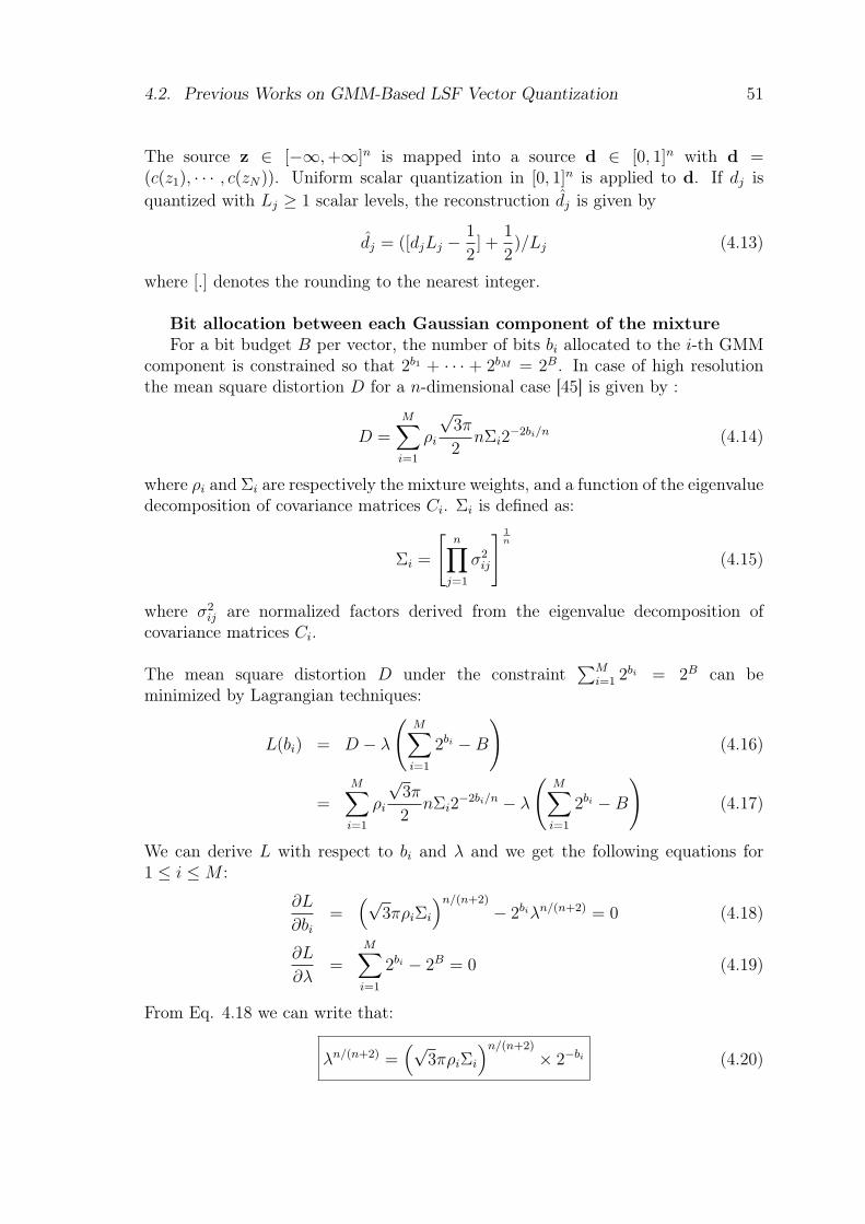
4.2. Previous Works on GMM-Based LSF Vector Quantization 51
The source z ∈ [−∞, +∞]n is mapped into a source d ∈ [0, 1]n with d =(c(z1), · · · , c(zN)). Uniform scalar quantization in [0, 1]n is applied to d. If dj isquantized with Lj ≥ 1 scalar levels, the reconstruction dj is given by
dj = ([djLj − 1
2] +
1
2)/Lj (4.13)
where [.] denotes the rounding to the nearest integer.
Bit allocation between each Gaussian component of the mixtureFor a bit budget B per vector, the number of bits bi allocated to the i-th GMM
component is constrained so that 2b1 + · · · + 2bM = 2B. In case of high resolutionthe mean square distortion D for a n-dimensional case [45] is given by :
D =M∑i=1
ρi
√3π
2nΣi2
−2bi/n (4.14)
where ρi and Σi are respectively the mixture weights, and a function of the eigenvaluedecomposition of covariance matrices Ci. Σi is defined as:
Σi =
[n∏
j=1
σ2ij
] 1n
(4.15)
where σ2ij are normalized factors derived from the eigenvalue decomposition of
covariance matrices Ci.
The mean square distortion D under the constraint∑M
i=1 2bi = 2B can beminimized by Lagrangian techniques:
L(bi) = D − λ
(M∑i=1
2bi −B
)(4.16)
=M∑i=1
ρi
√3π
2nΣi2
−2bi/n − λ
(M∑i=1
2bi −B
)(4.17)
We can derive L with respect to bi and λ and we get the following equations for1 ≤ i ≤ M :
∂L
∂bi
=(√
3πρiΣi
)n/(n+2)
− 2biλn/(n+2) = 0 (4.18)
∂L
∂λ=
M∑i=1
2bi − 2B = 0 (4.19)
From Eq. 4.18 we can write that:
λn/(n+2) =(√
3πρiΣi
)n/(n+2)
× 2−bi (4.20)
52 Chapter 4. Flexible quantization of LPC coefficients
So we have the following relationship:
2bi =
(√3πρiΣi
λ
)n/(n+2)
(4.21)
We are summing Eq. 4.21 on i so:
M∑i=1
2bi = 2B =M∑i=1
(√3πρiΣi
λ
)n/(n+2)
(4.22)
=
√3π
λn/(n+2)×
M∑i=1
(ρiΣi)n/(n+2) (4.23)
=2bi
(ρiΣi)n/(n+2)
×M∑i=1
(ρiΣi)n/(n+2) (4.24)
Finally we have the relationship between the number of bits bi allocated to the i-thGMM component and the bit budget B given as:
2bi = 2B (ρiΣi)n/(n+2)
M∑i=1
(ρiΣi)n/(n+2)
(4.25)
Bit allocation between each KLT coefficientsThe bit allocation between each quantization level Lj is done by a greedy algo-
rithm [45]. Given a bit budget bi and the covariance matrix diag(σ21, · · · , σ2
n) theallocation procedure consists of the following steps:
1. Initialize: Lj = 1, j = 1, · · · , n.
2. While∏n
j=1 Lj ≤ 2bi , Lk := Lk + 1 where k = arg maxj=1,··· ,n(σj/mj)2
3. While∏n
j=1 Lj ≤ 2bi , Lk := Lk + 1 where k tests all positions from 1 to n
sorted according to (σj/mj)2, j = 1, · · · , n.
The principle of this algorithm is to give bits to the most needed quantizer. Theinitialization of the quantization level Lj can take into account the distribution ofthe coefficients.
4.3 Proposed Model-Based LSF Vector Quantiza-tion
In order to improve the performance of the GMM-based LSF VQ in terms of com-plexity , flexibility and learning, we proposed to include a model-based quantizer.
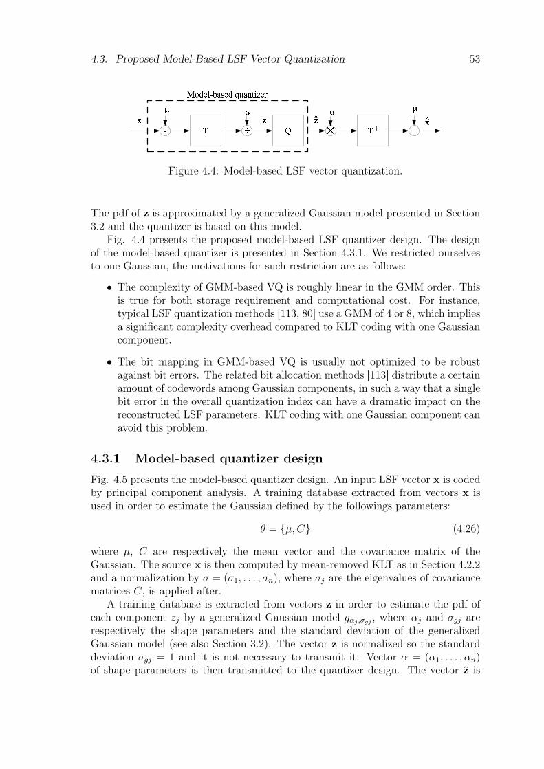
4.3. Proposed Model-Based LSF Vector Quantization 53
Figure 4.4: Model-based LSF vector quantization.
The pdf of z is approximated by a generalized Gaussian model presented in Section3.2 and the quantizer is based on this model.
Fig. 4.4 presents the proposed model-based LSF quantizer design. The designof the model-based quantizer is presented in Section 4.3.1. We restricted ourselvesto one Gaussian, the motivations for such restriction are as follows:
• The complexity of GMM-based VQ is roughly linear in the GMM order. Thisis true for both storage requirement and computational cost. For instance,typical LSF quantization methods [113, 80] use a GMM of 4 or 8, which impliesa significant complexity overhead compared to KLT coding with one Gaussiancomponent.
• The bit mapping in GMM-based VQ is usually not optimized to be robustagainst bit errors. The related bit allocation methods [113] distribute a certainamount of codewords among Gaussian components, in such a way that a singlebit error in the overall quantization index can have a dramatic impact on thereconstructed LSF parameters. KLT coding with one Gaussian component canavoid this problem.
4.3.1 Model-based quantizer design
Fig. 4.5 presents the model-based quantizer design. An input LSF vector x is codedby principal component analysis. A training database extracted from vectors x isused in order to estimate the Gaussian defined by the followings parameters:
θ = {µ,C} (4.26)
where µ, C are respectively the mean vector and the covariance matrix of theGaussian. The source x is then computed by mean-removed KLT as in Section 4.2.2and a normalization by σ = (σ1, . . . , σn), where σj are the eigenvalues of covariancematrices C, is applied after.
A training database is extracted from vectors z in order to estimate the pdf ofeach component zj by a generalized Gaussian model gαj ,σgj
, where αj and σgj arerespectively the shape parameters and the standard deviation of the generalizedGaussian model (see also Section 3.2). The vector z is normalized so the standarddeviation σgj = 1 and it is not necessary to transmit it. Vector α = (α1, . . . , αn)of shape parameters is then transmitted to the quantizer design. The vector z is
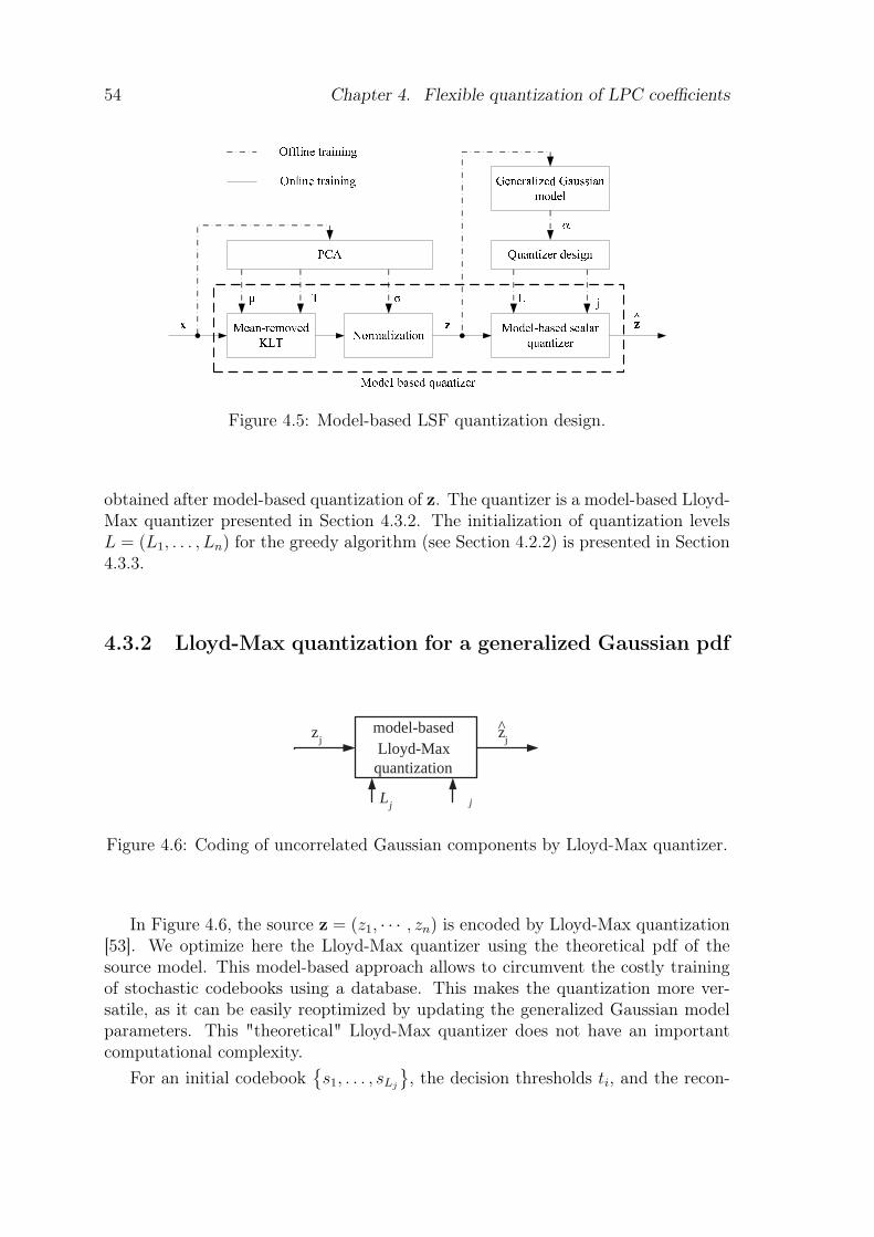
54 Chapter 4. Flexible quantization of LPC coefficients
Figure 4.5: Model-based LSF quantization design.
obtained after model-based quantization of z. The quantizer is a model-based Lloyd-Max quantizer presented in Section 4.3.2. The initialization of quantization levelsL = (L1, . . . , Ln) for the greedy algorithm (see Section 4.2.2) is presented in Section4.3.3.
4.3.2 Lloyd-Max quantization for a generalized Gaussian pdf
model-based Lloyd-Max quantization
L j
j
z j z j ^
Figure 4.6: Coding of uncorrelated Gaussian components by Lloyd-Max quantizer.
In Figure 4.6, the source z = (z1, · · · , zn) is encoded by Lloyd-Max quantization[53]. We optimize here the Lloyd-Max quantizer using the theoretical pdf of thesource model. This model-based approach allows to circumvent the costly trainingof stochastic codebooks using a database. This makes the quantization more ver-satile, as it can be easily reoptimized by updating the generalized Gaussian modelparameters. This "theoretical" Lloyd-Max quantizer does not have an importantcomputational complexity.
For an initial codebook{s1, . . . , sLj
}, the decision thresholds ti, and the recon-
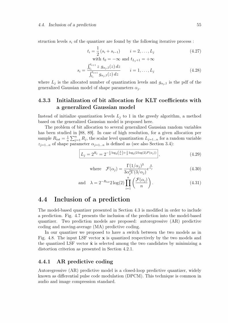
4.4. Inclusion of a prediction 55
struction levels si of the quantizer are found by the following iterative process :
ti =1
2(si + si−1) i = 2, . . . , Lj (4.27)
with t0 = −∞ and tLj+1 = +∞
si =
∫ ti+1
tiz gαj ,1(z) dz
∫ ti+1
tigαj ,1(z) dz
i = 1, . . . , Lj (4.28)
where Lj is the allocated number of quantization levels and gαj ,1 is the pdf of thegeneralized Gaussian model of shape parameters αj.
4.3.3 Initialization of bit allocation for KLT coefficients witha generalized Gaussian model
Instead of initialize quantization levels Lj to 1 in the greedy algorithm, a methodbased on the generalized Gaussian model is proposed here.
The problem of bit allocation to several generalized Gaussian random variableshas been studied in [88, 89]. In case of high resolution, for a given allocation persample Rtot = 1
n
∑nj=1 Rj, the scalar level quantization Lj=1...n for a random variable
zj=1...n of shape parameter αj=1...n is defined as (see also Section 3.4):
Lj = 2Rj = 2−12
log2(λn)+ 1
2log2(2 log(2)F(αj)) , (4.29)
where F(αj) =Γ(1/αj)
3
3α2jΓ(3/αj)
e2
αj (4.30)
and λ = 2−Rtot2 log(2)n∏
i=1
(F(αj)
n
). (4.31)
4.4 Inclusion of a predictionThe model-based quantizer presented in Section 4.3 is modified in order to includea prediction. Fig. 4.7 presents the inclusion of the prediction into the model-basedquantizer. Two prediction models are proposed: autoregressive (AR) predictivecoding and moving-average (MA) predictive coding.
In our quantizer we proposed to have a switch between the two models as inFig. 4.8. The input LSF vector x is quantized respectively by the two models andthe quantized LSF vector x is selected among the two candidates by minimizing adistortion criterion as presented in Section 4.2.1.
4.4.1 AR predictive coding
Autoregressive (AR) predictive model is a closed-loop predictive quantizer, widelyknown as differential pulse code modulation (DPCM). This technique is common inaudio and image compression standard.
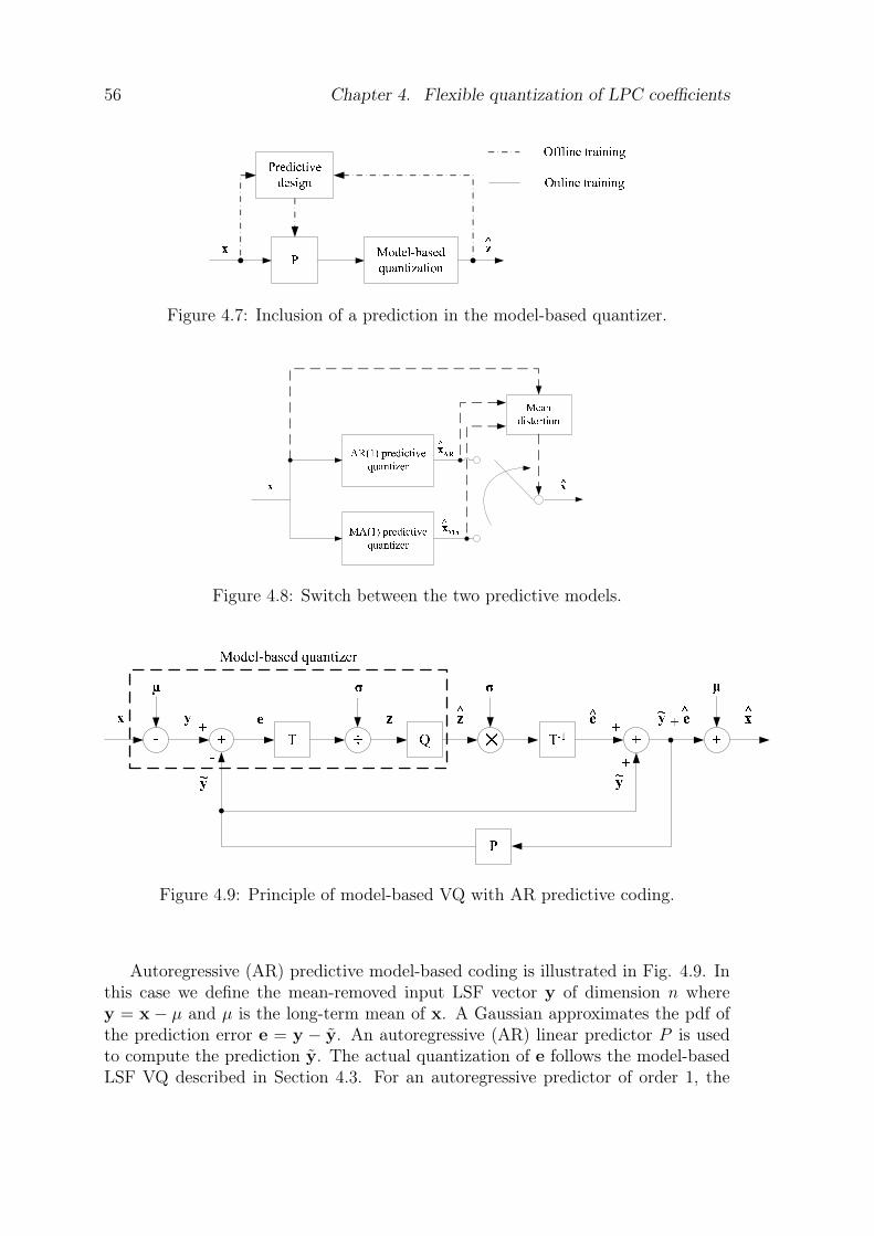
56 Chapter 4. Flexible quantization of LPC coefficients
Figure 4.7: Inclusion of a prediction in the model-based quantizer.
Figure 4.8: Switch between the two predictive models.
Figure 4.9: Principle of model-based VQ with AR predictive coding.
Autoregressive (AR) predictive model-based coding is illustrated in Fig. 4.9. Inthis case we define the mean-removed input LSF vector y of dimension n wherey = x − µ and µ is the long-term mean of x. A Gaussian approximates the pdf ofthe prediction error e = y − y. An autoregressive (AR) linear predictor P is usedto compute the prediction y. The actual quantization of e follows the model-basedLSF VQ described in Section 4.3. For an autoregressive predictor of order 1, the
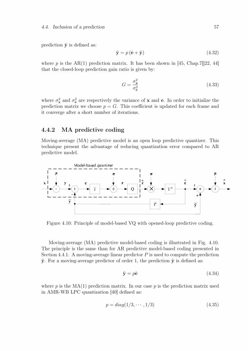
4.4. Inclusion of a prediction 57
prediction y is defined as:y = p (e + y) (4.32)
where p is the AR(1) prediction matrix. It has been shown in [45, Chap.7][22, 44]that the closed-loop prediction gain ratio is given by:
G =σ2
x
σ2e
(4.33)
where σ2x and σ2
e are respectively the variance of x and e. In order to initialize theprediction matrix we choose p = G. This coefficient is updated for each frame andit converge after a short number of iterations.
4.4.2 MA predictive coding
Moving-average (MA) predictive model is an open loop predictive quantizer. Thistechnique present the advantage of reducing quantization error compared to ARpredictive model.
Figure 4.10: Principle of model-based VQ with opened-loop predictive coding.
Moving-average (MA) predictive model-based coding is illustrated in Fig. 4.10.The principle is the same than for AR predictive model-based coding presented inSection 4.4.1. A moving-average linear predictor P is used to compute the predictiony. For a moving-average predictor of order 1, the prediction y is defined as:
y = pe (4.34)
where p is the MA(1) prediction matrix. In our case p is the prediction matrix usedin AMR-WB LPC quantization [40] defined as:
p = diag(1/3, · · · , 1/3) (4.35)
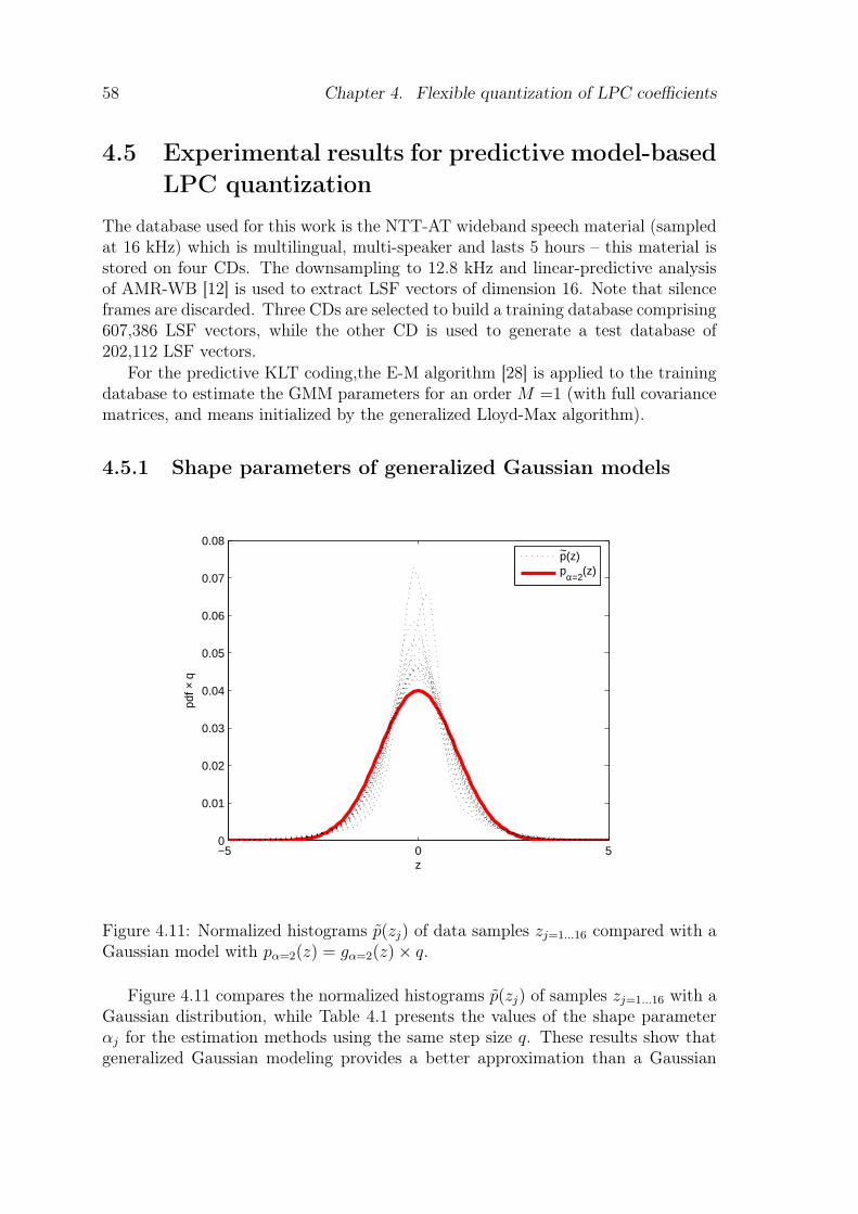
58 Chapter 4. Flexible quantization of LPC coefficients
4.5 Experimental results for predictive model-basedLPC quantization
The database used for this work is the NTT-AT wideband speech material (sampledat 16 kHz) which is multilingual, multi-speaker and lasts 5 hours – this material isstored on four CDs. The downsampling to 12.8 kHz and linear-predictive analysisof AMR-WB [12] is used to extract LSF vectors of dimension 16. Note that silenceframes are discarded. Three CDs are selected to build a training database comprising607,386 LSF vectors, while the other CD is used to generate a test database of202,112 LSF vectors.
For the predictive KLT coding,the E-M algorithm [28] is applied to the trainingdatabase to estimate the GMM parameters for an order M =1 (with full covariancematrices, and means initialized by the generalized Lloyd-Max algorithm).
4.5.1 Shape parameters of generalized Gaussian models
−5 0 50
0.01
0.02
0.03
0.04
0.05
0.06
0.07
0.08
z
pdf ×
q
~p(z)pα=2
(z)
Figure 4.11: Normalized histograms p(zj) of data samples zj=1...16 compared with aGaussian model with pα=2(z) = gα=2(z)× q.
Figure 4.11 compares the normalized histograms p(zj) of samples zj=1...16 with aGaussian distribution, while Table 4.1 presents the values of the shape parameterαj for the estimation methods using the same step size q. These results show thatgeneralized Gaussian modeling provides a better approximation than a Gaussian
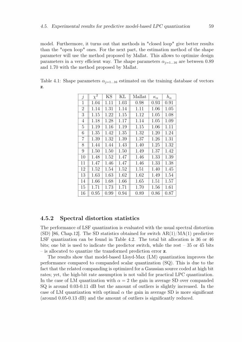
4.5. Experimental results for predictive model-based LPC quantization 59
model. Furthermore, it turns out that methods in "closed loop" give better resultsthan the "open loop" ones. For the next part, the estimation method of the shapeparameter will use the method proposed by Mallat. This allows to optimize designparameters in a very efficient way. The shape parameters αj=1...16 are between 0.89and 1.70 with the method proposed by Mallat.
Table 4.1: Shape parameters αj=1...16 estimated on the training database of vectorsz.
j χ2 KS KL Mallat κα hα
1 1.04 1.11 1.03 0.98 0.93 0.912 1.14 1.31 1.14 1.11 1.06 1.053 1.15 1.22 1.15 1.12 1.05 1.084 1.18 1.28 1.17 1.14 1.05 1.095 1.19 1.16 1.19 1.15 1.06 1.116 1.35 1.42 1.35 1.32 1.20 1.247 1.39 1.32 1.39 1.37 1.26 1.318 1.44 1.44 1.43 1.40 1.25 1.329 1.50 1.50 1.50 1.49 1.37 1.4210 1.48 1.52 1.47 1.46 1.33 1.3911 1.47 1.46 1.47 1.46 1.33 1.3812 1.52 1.54 1.52 1.51 1.40 1.4513 1.63 1.63 1.62 1.62 1.49 1.5414 1.66 1.68 1.66 1.65 1.51 1.5715 1.71 1.73 1.71 1.70 1.56 1.6116 0.95 0.99 0.94 0.89 0.86 0.87
4.5.2 Spectral distortion statistics
The performance of LSF quantization is evaluated with the usual spectral distortion(SD) [86, Chap.12]. The SD statistics obtained for switch AR(1)/MA(1) predictiveLSF quantization can be found in Table 4.2. The total bit allocation is 36 or 46bits; one bit is used to indicate the predictor switch, while the rest – 35 or 45 bits– is allocated to quantize the transformed prediction error z.
The results show that model-based Lloyd-Max (LM) quantization improves theperformance compared to companded scalar quantization (SQ). This is due to thefact that the related companding is optimized for a Gaussian source coded at high bitrates; yet, the high-bit rate assumption is not valid for practical LPC quantization.In the case of LM quantization with α = 2 the gain in average SD over compandedSQ is around 0.03-0.11 dB but the amount of outliers is slightly increased. In thecase of LM quantization with optimal α the gain in average SD is more significant(around 0.05-0.13 dB) and the amount of outliers is significantly reduced.
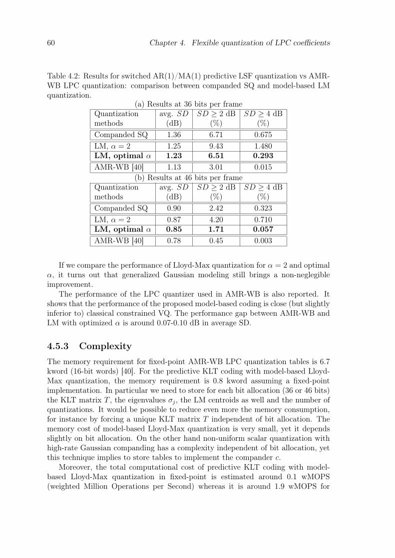
60 Chapter 4. Flexible quantization of LPC coefficients
Table 4.2: Results for switched AR(1)/MA(1) predictive LSF quantization vs AMR-WB LPC quantization: comparison between companded SQ and model-based LMquantization.
(a) Results at 36 bits per frameQuantization avg. SD SD ≥ 2 dB SD ≥ 4 dBmethods (dB) (%) (%)Companded SQ 1.36 6.71 0.675LM, α = 2 1.25 9.43 1.480LM, optimal α 1.23 6.51 0.293AMR-WB [40] 1.13 3.01 0.015
(b) Results at 46 bits per frameQuantization avg. SD SD ≥ 2 dB SD ≥ 4 dBmethods (dB) (%) (%)Companded SQ 0.90 2.42 0.323LM, α = 2 0.87 4.20 0.710LM, optimal α 0.85 1.71 0.057AMR-WB [40] 0.78 0.45 0.003
If we compare the performance of Lloyd-Max quantization for α = 2 and optimalα, it turns out that generalized Gaussian modeling still brings a non-neglegibleimprovement.
The performance of the LPC quantizer used in AMR-WB is also reported. Itshows that the performance of the proposed model-based coding is close (but slightlyinferior to) classical constrained VQ. The performance gap between AMR-WB andLM with optimized α is around 0.07-0.10 dB in average SD.
4.5.3 Complexity
The memory requirement for fixed-point AMR-WB LPC quantization tables is 6.7kword (16-bit words) [40]. For the predictive KLT coding with model-based Lloyd-Max quantization, the memory requirement is 0.8 kword assuming a fixed-pointimplementation. In particular we need to store for each bit allocation (36 or 46 bits)the KLT matrix T , the eigenvalues σj, the LM centroids as well and the number ofquantizations. It would be possible to reduce even more the memory consumption,for instance by forcing a unique KLT matrix T independent of bit allocation. Thememory cost of model-based Lloyd-Max quantization is very small, yet it dependsslightly on bit allocation. On the other hand non-uniform scalar quantization withhigh-rate Gaussian companding has a complexity independent of bit allocation, yetthis technique implies to store tables to implement the compander c.
Moreover, the total computational cost of predictive KLT coding with model-based Lloyd-Max quantization in fixed-point is estimated around 0.1 wMOPS(weighted Million Operations per Second) whereas it is around 1.9 wMOPS for
4.6. Conclusion 61
AMR-WB LPC quantization.
4.6 ConclusionIn this chapter we presented a predictive KLT quantization method using gener-alized Gaussian modeling for wideband LSF speech parameters. This method wascompared to AMR-WB LPC quantization [40] and to GMM-based LSF quantizerpresented by [113]. The proposed method has much lower complexity (computa-tion cost, storage requirement) and similar performance in term of average SD thanAMR-WB LPC quantization. The number of outliers in the proposed method ismore important than AMR-WB quantization (2 times at 36 bits per frame and 4times at 46 bits per frame), but the percentage is too small to affect the quality at 46bits per frame and it might affect it a little at 36 bits per frame [86, Chap.12]. Thepdf knowledge of (transformed) prediction error of LSF parameters improves theperformance (average SD and percentage of outliers) compared to GMM-based LSFquantizer and the complexity is equivalent. We have presented a model-based pre-dictive quantizer method using the generalized Gaussian model which performs aswell as standard coding methods and improves GMM-based coding. This techniquehas been applied for LSF parameters but could be used for any signals.

62 Chapter 4. Flexible quantization of LPC coefficients
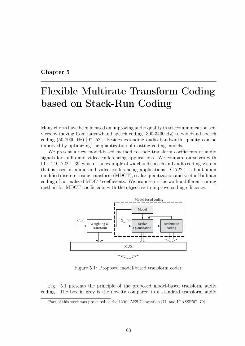
Chapter 5
Flexible Multirate Transform Codingbased on Stack-Run Coding
Many efforts have been focused on improving audio quality in telecommunication ser-vices by moving from narrowband speech coding (300-3400 Hz) to wideband speechcoding (50-7000 Hz) [97, 52]. Besides extending audio bandwidth, quality can beimproved by optimizing the quantization of existing coding models.
We present a new model-based method to code transform coefficients of audiosignals for audio and video conferencing applications. We compare ourselves withITU-T G.722.1 [39] which is an example of wideband speech and audio coding systemthat is used in audio and video conferencing applications. G.722.1 is built uponmodified discrete cosine transform (MDCT), scalar quantization and vector Huffmancoding of normalized MDCT coefficients. We propose in this work a different codingmethod for MDCT coefficients with the objective to improve coding efficiency.
x(n)
MUX
Scalar Quantization
Model
X pre (k) Weighting &
Transform Arithmetic
coding
Model-based coding
Figure 5.1: Proposed model-based transform coder.
Fig. 5.1 presents the principle of the proposed model-based transform audiocoding. The box in grey is the novelty compared to a standard transform audio
Part of this work was presented at the 120th AES Convention [77] and ICASSP’07 [79]
63
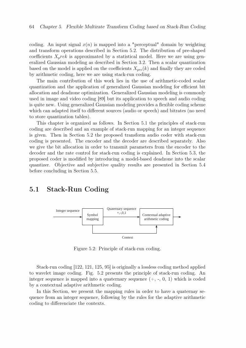
64 Chapter 5. Flexible Multirate Transform Coding based on Stack-Run Coding
coding. An input signal x(n) is mapped into a "perceptual" domain by weightingand transform operations described in Section 5.2. The distribution of pre-shapedcoefficients Xprek is approximated by a statistical model. Here we are using gen-eralized Gaussian modeling as described in Section 3.2. Then a scalar quantizationbased on the model is applied on the coefficients Xpre(k) and finally they are codedby arithmetic coding, here we are using stack-run coding.
The main contribution of this work lies in the use of arithmetic-coded scalarquantization and the application of generalized Gaussian modeling for efficient bitallocation and deadzone optimization. Generalized Gaussian modeling is commonlyused in image and video coding [89] but its application to speech and audio codingis quite new. Using generalized Gaussian modeling provides a flexible coding schemewhich can adapted itself to different sources (audio or speech) and bitrates (no needto store quantization tables).
This chapter is organized as follows. In Section 5.1 the principles of stack-runcoding are described and an example of stack-run mapping for an integer sequenceis given. Then in Section 5.2 the proposed transform audio coder with stack-runcoding is presented. The encoder and the decoder are described separately. Alsowe give the bit allocation in order to transmit parameters from the encoder to thedecoder and the rate control for stack-run coding is explained. In Section 5.3, theproposed coder is modified by introducing a model-based deadzone into the scalarquantizer. Objective and subjective quality results are presented in Section 5.4before concluding in Section 5.5.
5.1 Stack-Run Coding
Integer sequence
Context
Quaternary sequence +,-,0,1
Symbol mapping
Contextual adaptive arithmetic coding
Figure 5.2: Principle of stack-run coding.
Stack-run coding [122, 121, 125, 95] is originally a lossless coding method appliedto wavelet image coding. Fig. 5.2 presents the principle of stack-run coding. Aninteger sequence is mapped into a quaternary sequence (+, -, 0, 1) which is codedby a contextual adaptive arithmetic coding.
In this Section, we present the mapping rules in order to have a quaternay se-quence from an integer sequence, following by the rules for the adaptive arithmeticcoding to differenciate the contexts.
5.1. Stack-Run Coding 65
5.1.1 Representation of an integer sequence by a quaternaryalphabet
The integer sequence is partionned into two contexts: sequence of zeros ("runs")and non-zero integers ("stack").
A stack is a non-zero integers written in binary format. So, we get a columnof bits with the most significant bit (MSB) at the top and the least significant bit(LSB) at the bottom. This binary representation is unsigned and sign informationis considered apart.
A run is a sequence of zeros, the length of the sequence is written in binaryformat which is ordered from LSB to MSB.
The symbols alphabet have the following meanings [121, 122]:
• "0" is used to signify a bit value of 0 in stack encoding.
• "1" is used for a bit value of 1 in stack encoding, but it is not used for theMSB (symbols "+" or "-" to give the stack sign).
• "+" is used to represent the positive MSB of stack and for a bit value of 1 inrepresenting run lengths.
• "-" is used to represent the negative MSB of stack and for a bit value of 0 inrepresenting run lengths.
Only "+" and "-" symbols are used to code runs, "0" and "1" are used to codeda bit value for a stack. The MSB of each stack is replaced by "+" if the associatecoefficient is positive and "-" if it is negative. The mapping rules ensure that thestack-run conversion is reversible.
5.1.2 Context-based adaptive arithmetic coding
In order to distinguish a stack of absolute value 1, which will be represented onlyby "+" or "-" if we considered the mapping rules, from a run the absolute value ofstack is incremented by one. For example the binary representation of +1 is "+0"instead of "+" and the binary representation of -8 is "-001" instead of "-000".
In representing stack, the symbols "+" and "-" are used simultaneously to encodethe sign coefficients and bit plane location of the MSB. Another gain can be obtainedin representation of the run lengths, which are ordered from LSB to MSB. Becauseall binary run lengths start with 1, the final "+" (MSB) can be omitted for mostrun-lengths representation without loss of information. The only potential problemis the representation of a run of length one which will not be representable if allMSB "+" symbols were eliminated. In order to avoid this problem, the MSB "+"symbols are retained for all runs of length 2k − 1 where k is a positive integer. Forexample a run length of value 10 is represented by "-+-" instead of "-+-+".
For the contextual arithmetic coding, the run context is the symbol for the runlengths associated with the LSB of the stack and the stack context is the rest of the
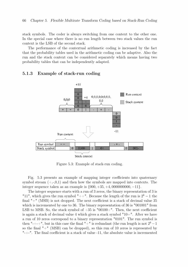
66 Chapter 5. Flexible Multirate Transform Coding based on Stack-Run Coding
stack symbols. The coder is always switching from one context to the other one.In the special case where there is no run length between two stack values the runcontext is the LSB of the second stack.
The performance of the contextual arithmetic coding is increased by the factthat the probability tables used in the arithmetic coding can be adaptive. Also therun and the stack context can be considered separately which means having twoprobability tables that can be independently adapted.
5.1.3 Example of stack-run coding
Figure 5.3: Example of stack-run coding.
Fig. 5.3 presents an example of mapping integer coefficients into quaternarysymbol stream (+,-,0,1) and then how the symbols are mapped into contexts. Theinteger sequence taken as an example is {000, +35, +4, 0000000000,−11}.
The integer sequence starts with a run of 3 zeros, the binary representation of 3 is"11", which gives the run symbol "++". Because the length of the run is 2k− 1 thefinal "+" (MSB) is not dropped. The next coefficient is a stack of decimal value 35which is incremented by one to 36. The binary representation of 36 is "001001" fromLSB to MSB. So, the stack symbol of +35 is "00100+". Then, the next coefficientis again a stack of decimal value 4 which gives a stack symbol "10+". After we havea run of 10 zeros correspond to a binary representation "0101". The run symbol isthen "-+-+", but in this case the final "+" is redundant (the run length is not 2k−1so the final "+" (MSB) can be dropped), so this run of 10 zeros is represented by"-+-". The final coefficient is a stack of value -11, the absolute value is incremented
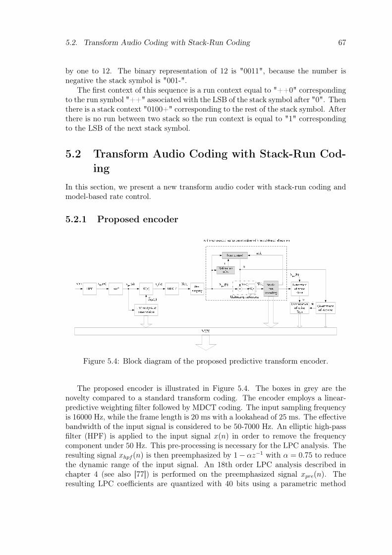
5.2. Transform Audio Coding with Stack-Run Coding 67
by one to 12. The binary representation of 12 is "0011", because the number isnegative the stack symbol is "001-".
The first context of this sequence is a run context equal to "++0" correspondingto the run symbol "++" associated with the LSB of the stack symbol after "0". Thenthere is a stack context "0100+" corresponding to the rest of the stack symbol. Afterthere is no run between two stack so the run context is equal to "1" correspondingto the LSB of the next stack symbol.
5.2 Transform Audio Coding with Stack-Run Cod-ing
In this section, we present a new transform audio coder with stack-run coding andmodel-based rate control.
5.2.1 Proposed encoder
Figure 5.4: Block diagram of the proposed predictive transform encoder.
The proposed encoder is illustrated in Figure 5.4. The boxes in grey are thenovelty compared to a standard transform coding. The encoder employs a linear-predictive weighting filter followed by MDCT coding. The input sampling frequencyis 16000 Hz, while the frame length is 20 ms with a lookahead of 25 ms. The effectivebandwidth of the input signal is considered to be 50-7000 Hz. An elliptic high-passfilter (HPF) is applied to the input signal x(n) in order to remove the frequencycomponent under 50 Hz. This pre-processing is necessary for the LPC analysis. Theresulting signal xhpf (n) is then preemphasized by 1− αz−1 with α = 0.75 to reducethe dynamic range of the input signal. An 18th order LPC analysis described inchapter 4 (see also [77]) is performed on the preemphasized signal xpre(n). Theresulting LPC coefficients are quantized with 40 bits using a parametric method
68 Chapter 5. Flexible Multirate Transform Coding based on Stack-Run Coding
based on a Gaussian mixture model (GMM) [113] in the linear spectrum frequency(LSF) domain. The pre-emphasized signal is filtered by a perceptual weighting filter:
W (z) =A(z/γ)
1− βz−1(5.1)
where β = 0.75 is a tilt parameter and γ = 0.92. The coefficients of W (z) areupdated every 5 ms by interpolating LSF parameters to smooth the evolution ofthe spectral envelope. A MDCT analysis is applied on the weighted signal xw(n).The MDCT is implemented using the fast algorithm of [30] which is based on acomplex FFT. Then the MDCT coefficients X(k) are pre-shaped to emphasize lowfrequencies, similar to 3GPP AMR-WB+ [7]. Preshaping [11] is used to correctthe imperfect masking of W (z), in particular for signals with a frequency around300-500 Hz. The pre-shaped coefficients Xpre(k) are divided by a step size q and theresulting spectrum Y (k) is quantized by uniform scalar quantization with stepsizeq. For a given spectrum Y (k) the spectrum Y (k) after quantization is defined as:
Y (k) = [Y (k)] =
[Xpre(k)
q
](5.2)
where [.] represents the rounding to the nearest integer. Only the first 280 coefficientsof the Y (k) spectrum corresponding to the 0-7000 Hz band are coded; the last 40coefficients are discarded. The integer sequence Y (k) is encoded by stack-run coding[122].
The rate control consists in finding the appropriate step size q so that the num-ber of bits, nbit, used for stack-run coding matches the asymptotic allocated bitbudget as described in Section 3.4. The distribution of Xpre(k) is approximated bya generalized Gaussian model and the shape parameter α is estimated using Mal-lat’s method presented in Section 3.2.2 (see also [69]). Then a noise level estimationis performed on the spectrum Y (k) after stack-run coding. The noise floor σ isestimated as:
σ = r.m.s. {Xpre(k) |Y (k) = 0} (5.3)
with the additional constraint that Y (k) must belong to a long zero run to be reallyconsidered in the above r.m.s. calculation. The step size q is scalar quantized in logdomain with 7 bits. The noise floor σ is quantized by coding the ratio σ/q in lineardomain with 3 bits.
5.2.2 Bit allocation
Static distributions of bits to parametersThe parameters of the proposed coder are the Line Spectrum Frequency (LSF)
parameters, the step size, and the noise floor level. The bit allocation to theparameters is detailed in Table 5.1, where Btot is the total number of bits per frame.For instance at 24 kbit/s, Btot = 480 bits. The allocation (in bits per sample) tostack-run coding is B = (Btot − 50)/280, where 280 is the number of coefficients
5.2. Transform Audio Coding with Stack-Run Coding 69
in each frame and 50(40 + 7 + 3) is the number of bits needed to transmit theparameters to the decoder.
Table 5.1: Bit allocation for the stack-run predictive transform audio coding.Parameter Number of bitsLSF 40Step size q 7Noise floor σ 3Stack-run coding Btot-50Total Btot
Rate control for stack-run codingFig. 5.5 gives the bit allocation for the stack-run coding before the rate control.
This example is done on a female French sample of 8 seconds coded at 24 kbit/s.As we can see, there is a biais between the number of bit using highrate estimatedstepsize and the number of bits per frame. This biais of approximatively 84 bitscould be explained by two types of mismatch:
• The highrate assumption made in the asymptotic model-based bit allocationis not verified. At 24 kbit/s the bit budget is 270 bits per frame which givesan average bitrate of 430/280 ≈ 1.5 bits/sample.
• The theory supposed that we have an ideal entropy coder which minimizes theentropy of order zero. But in practice we have an adaptive stack-run codingwhich minimizes entropy of higher order.
A bisection search for rate control is done in order to be within bit budget constraintfor stack-run coding.
5.2.3 Proposed decoder
The decoder in error-free conditions is illustrated in Figure 5.6. The decoded LSFparameters are interpolated every 5 ms and converted to LPC coefficients. Thereconstructed spectrum Y (k) is given by:
Y (k) = q Y (k) (5.4)
where Y (k) is found by stack-run decoding. In order to improve quality, in particularto avoid musical noise, a noise injection is applied on Y (k). A noise of magnitude ±σis injected in all zero sequences longer than 20 coefficients in Y (k). The spectrumX(k) is de-shaped in a way similar to 3GPP AMR-WB+ and transformed in timedomain using the inverse MDCT and overlap-add algorithm described in [30]. Aninverse perceptual filter W (z)−1 is applied on xw(n) in order to shape the codingnoise introduced in the MDCT domain. The response of W (z)−1 is similar to a short-term masking curve and its coefficients are updated every 5 ms by LSF interpolation.The signal x(n) is deemphasized to find the synthesis x(n).
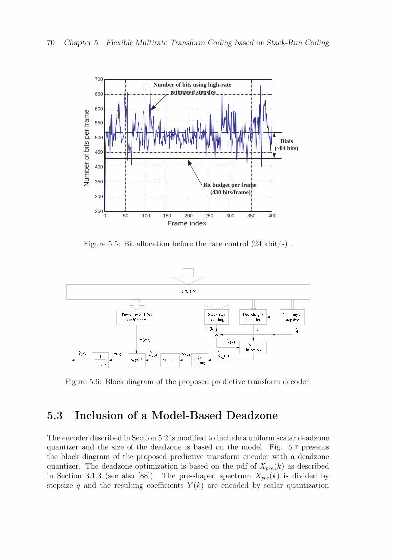
70 Chapter 5. Flexible Multirate Transform Coding based on Stack-Run Coding
0 50 100 150 200 250 300 350 400 250
300
350
400
450
500
550
600
650
700
Num
ber
of b
its p
er fr
ame
Frame index
Budget=430 bits/frame
Bit budget per frame (430 bits/frame)
Biais (~84 bits)
Number of bits using high-rate estimated stepsize
Figure 5.5: Bit allocation before the rate control (24 kbit/s) .
Figure 5.6: Block diagram of the proposed predictive transform decoder.
5.3 Inclusion of a Model-Based Deadzone
The encoder described in Section 5.2 is modified to include a uniform scalar deadzonequantizer and the size of the deadzone is based on the model. Fig. 5.7 presentsthe block diagram of the proposed predictive transform encoder with a deadzonequantizer. The deadzone optimization is based on the pdf of Xpre(k) as describedin Section 3.1.3 (see also [88]). The pre-shaped spectrum Xpre(k) is divided bystepsize q and the resulting coefficients Y (k) are encoded by scalar quantization
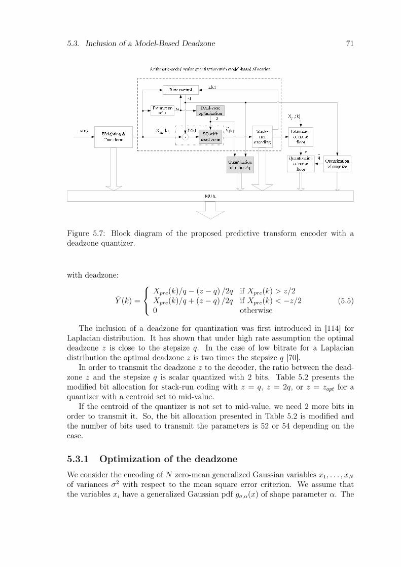
5.3. Inclusion of a Model-Based Deadzone 71
Figure 5.7: Block diagram of the proposed predictive transform encoder with adeadzone quantizer.
with deadzone:
Y (k) =
Xpre(k)/q − (z − q) /2q if Xpre(k) > z/2Xpre(k)/q + (z − q) /2q if Xpre(k) < −z/20 otherwise
(5.5)
The inclusion of a deadzone for quantization was first introduced in [114] forLaplacian distribution. It has shown that under high rate assumption the optimaldeadzone z is close to the stepsize q. In the case of low bitrate for a Laplaciandistribution the optimal deadzone z is two times the stepsize q [70].
In order to transmit the deadzone z to the decoder, the ratio between the dead-zone z and the stepsize q is scalar quantized with 2 bits. Table 5.2 presents themodified bit allocation for stack-run coding with z = q, z = 2q, or z = zopt for aquantizer with a centroid set to mid-value.
If the centroid of the quantizer is not set to mid-value, we need 2 more bits inorder to transmit it. So, the bit allocation presented in Table 5.2 is modified andthe number of bits used to transmit the parameters is 52 or 54 depending on thecase.
5.3.1 Optimization of the deadzone
We consider the encoding of N zero-mean generalized Gaussian variables x1, . . . , xN
of variances σ2 with respect to the mean square error criterion. We assume thatthe variables xi have a generalized Gaussian pdf gσ,α(x) of shape parameter α. The
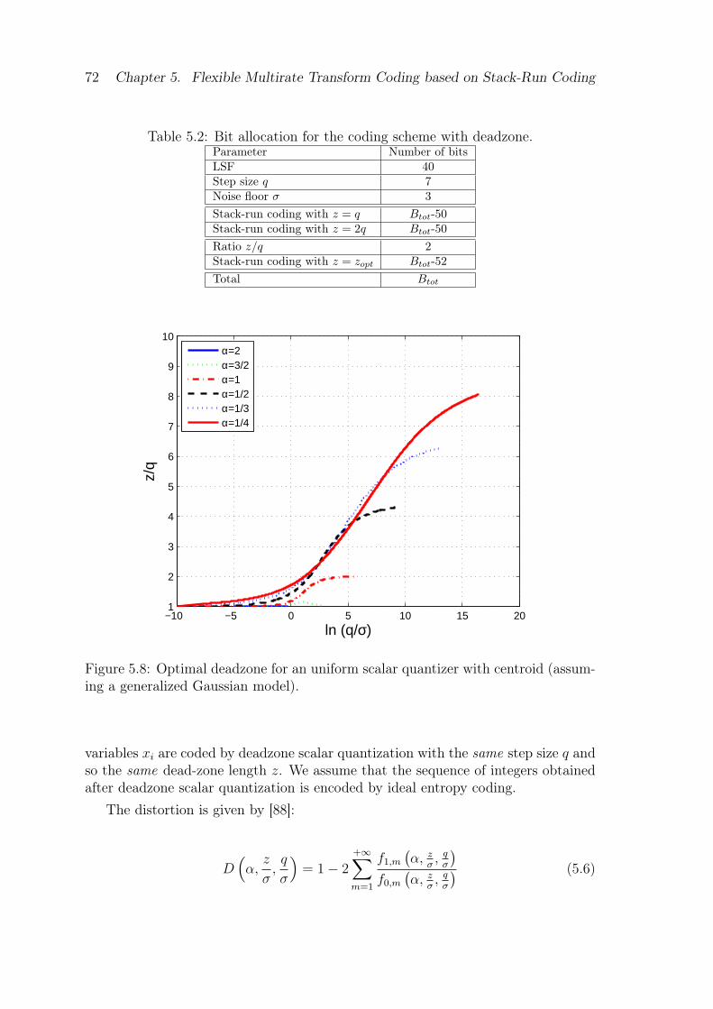
72 Chapter 5. Flexible Multirate Transform Coding based on Stack-Run Coding
Table 5.2: Bit allocation for the coding scheme with deadzone.Parameter Number of bitsLSF 40Step size q 7Noise floor σ 3Stack-run coding with z = q Btot-50Stack-run coding with z = 2q Btot-50Ratio z/q 2Stack-run coding with z = zopt Btot-52Total Btot
−10 −5 0 5 10 15 201
2
3
4
5
6
7
8
9
10
ln (q/σ)
z/q
α=2α=3/2α=1α=1/2α=1/3α=1/4
Figure 5.8: Optimal deadzone for an uniform scalar quantizer with centroid (assum-ing a generalized Gaussian model).
variables xi are coded by deadzone scalar quantization with the same step size q andso the same dead-zone length z. We assume that the sequence of integers obtainedafter deadzone scalar quantization is encoded by ideal entropy coding.
The distortion is given by [88]:
D(α,
z
σ,q
σ
)= 1− 2
+∞∑m=1
f1,m
(α, z
σ, q
σ
)
f0,m
(α, z
σ, q
σ
) (5.6)
5.3. Inclusion of a Model-Based Deadzone 73
where α is the shape parameter of xi and fn,m
(α, z
σ, q
σ
)is a function defined as:
fn,m
(α,
z
σ,q
σ
)=
∫ z/2σ+mq/2σ
z/2σ+(m−1)q/2σ
xng1,α(x)dx (5.7)
The bit rate is given by [88]:
b(α,
z
σ,q
σ
)= −f0,0
(α,
z
σ
)log2 f0,0
(α,
z
σ
)
−2+∞∑m=1
f0,m
(α,
z
σi
,q
σ
)log2 f0,m
(αi,
z
σ,q
σ
)(5.8)
where f0,0
(α, z
σ
)is a function defined as:
f0,0
(α,
z
σ
)=
∫ z/2σ
z/2σ
xng1,α(x)dx (5.9)
For a given bit allocation B in bits per sample, the bit allocation problem is tominimize the distortion D under the constraint that
∑Ni=1 b
(α, z
σ, q
σ
) ≤ B. The
distortion D(α, z
σ, q
σi
)can be minimized with Lagrangian techniques. The criterion
J(z, q, λ) is defined as
J(z, q, λ) =N∑
i=1
D(α,
z
σ,q
σ
)− λ
(N∑
i=1
b(α,
z
σ,q
σ
)−B
)(5.10)
where λ is the Lagrange multiplier. It can be shown that the optimal deadzone z isgiven by the solution to the equation [89]:
∂D∂z
(α, z
σ , qσ
)∂b∂z
(α, z
σ , qσ
) =
∂D∂q
(α, z
σ , qσ
)∂b∂q
(α, z
σ , qσ
) (5.11)
From Eq. 5.11 we have a relationship between ln (q/σ) and z/q. So for practicalimplementation, we store tables of this relationship for shape parameters α. Fig.5.8 presents charts in order to have the optimal deadzone z depending of the shapeparameter α, the stepsize q and the variance σ. As we can see, when q is gettingsmaller (high bitrate) we have z = q. For lower bitrate, z is more important than qwhich means that we have more zeros.
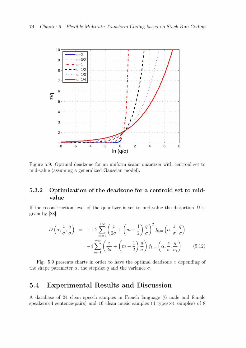
74 Chapter 5. Flexible Multirate Transform Coding based on Stack-Run Coding
−8 −6 −4 −2 0 2 4 6 81
2
3
4
5
6
7
8
9
10
ln (q/σ)
z/q
α=2α=3/2α=1α=1/2α=1/3α=1/4
Figure 5.9: Optimal deadzone for an uniform scalar quantizer with centroid set tomid-value (assuming a generalized Gaussian model).
5.3.2 Optimization of the deadzone for a centroid set to mid-value
If the reconstruction level of the quantizer is set to mid-value the distortion D isgiven by [88]:
D(α,
z
σ,q
σ
)= 1 + 2
+∞∑m=1
(z
2σ+
(m− 1
2
)q
σ
)2
f0,m
(α,
z
σ,q
σ
)
−4+∞∑m=1
(z
2σ+
(m− 1
2
)q
σ
)f1,m
(α,
z
σ,
q
σi
)(5.12)
Fig. 5.9 presents charts in order to have the optimal deadzone z depending ofthe shape parameter α, the stepsize q and the variance σ.
5.4 Experimental Results and Discussion
A database of 24 clean speech samples in French language (6 male and femalespeakers×4 sentence-pairs) and 16 clean music samples (4 types×4 samples) of 8
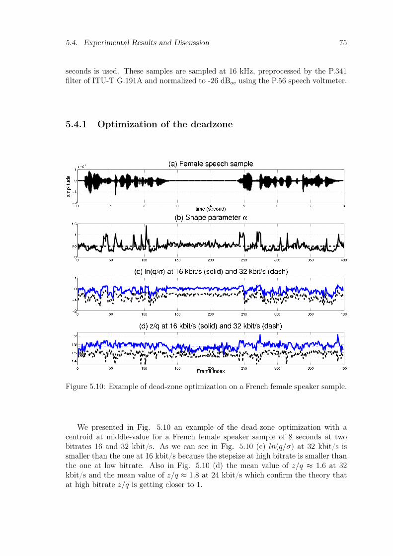
5.4. Experimental Results and Discussion 75
seconds is used. These samples are sampled at 16 kHz, preprocessed by the P.341filter of ITU-T G.191A and normalized to -26 dBov using the P.56 speech voltmeter.
5.4.1 Optimization of the deadzone
Figure 5.10: Example of dead-zone optimization on a French female speaker sample.
We presented in Fig. 5.10 an example of the dead-zone optimization with acentroid at middle-value for a French female speaker sample of 8 seconds at twobitrates 16 and 32 kbit/s. As we can see in Fig. 5.10 (c) ln(q/σ) at 32 kbit/s issmaller than the one at 16 kbit/s because the stepsize at high bitrate is smaller thanthe one at low bitrate. Also in Fig. 5.10 (d) the mean value of z/q ≈ 1.6 at 32kbit/s and the mean value of z/q ≈ 1.8 at 24 kbit/s which confirm the theory thatat high bitrate z/q is getting closer to 1.
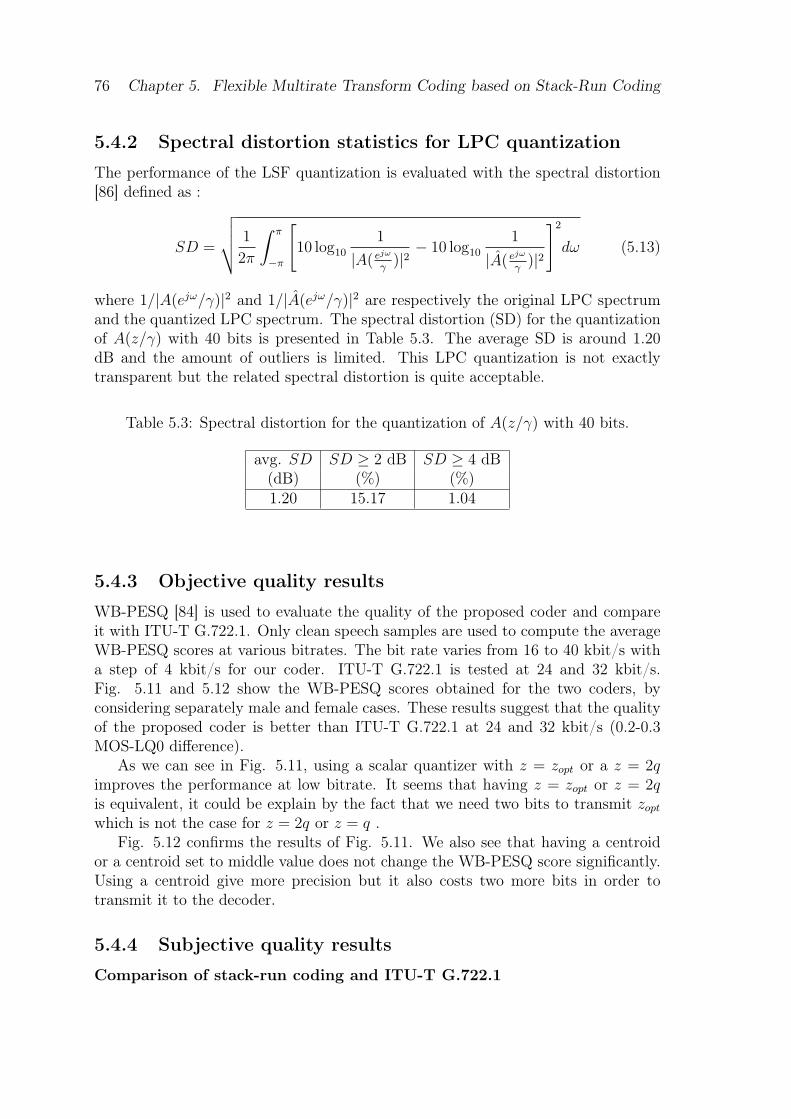
76 Chapter 5. Flexible Multirate Transform Coding based on Stack-Run Coding
5.4.2 Spectral distortion statistics for LPC quantization
The performance of the LSF quantization is evaluated with the spectral distortion[86] defined as :
SD =
√√√√ 1
2π
∫ π
−π
[10 log10
1
|A( ejω
γ)|2 − 10 log10
1
|A( ejω
γ)|2
]2
dω (5.13)
where 1/|A(ejω/γ)|2 and 1/|A(ejω/γ)|2 are respectively the original LPC spectrumand the quantized LPC spectrum. The spectral distortion (SD) for the quantizationof A(z/γ) with 40 bits is presented in Table 5.3. The average SD is around 1.20dB and the amount of outliers is limited. This LPC quantization is not exactlytransparent but the related spectral distortion is quite acceptable.
Table 5.3: Spectral distortion for the quantization of A(z/γ) with 40 bits.
avg. SD SD ≥ 2 dB SD ≥ 4 dB(dB) (%) (%)1.20 15.17 1.04
5.4.3 Objective quality results
WB-PESQ [84] is used to evaluate the quality of the proposed coder and compareit with ITU-T G.722.1. Only clean speech samples are used to compute the averageWB-PESQ scores at various bitrates. The bit rate varies from 16 to 40 kbit/s witha step of 4 kbit/s for our coder. ITU-T G.722.1 is tested at 24 and 32 kbit/s.Fig. 5.11 and 5.12 show the WB-PESQ scores obtained for the two coders, byconsidering separately male and female cases. These results suggest that the qualityof the proposed coder is better than ITU-T G.722.1 at 24 and 32 kbit/s (0.2-0.3MOS-LQ0 difference).
As we can see in Fig. 5.11, using a scalar quantizer with z = zopt or a z = 2qimproves the performance at low bitrate. It seems that having z = zopt or z = 2qis equivalent, it could be explain by the fact that we need two bits to transmit zopt
which is not the case for z = 2q or z = q .Fig. 5.12 confirms the results of Fig. 5.11. We also see that having a centroid
or a centroid set to middle value does not change the WB-PESQ score significantly.Using a centroid give more precision but it also costs two more bits in order totransmit it to the decoder.
5.4.4 Subjective quality results
Comparison of stack-run coding and ITU-T G.722.1
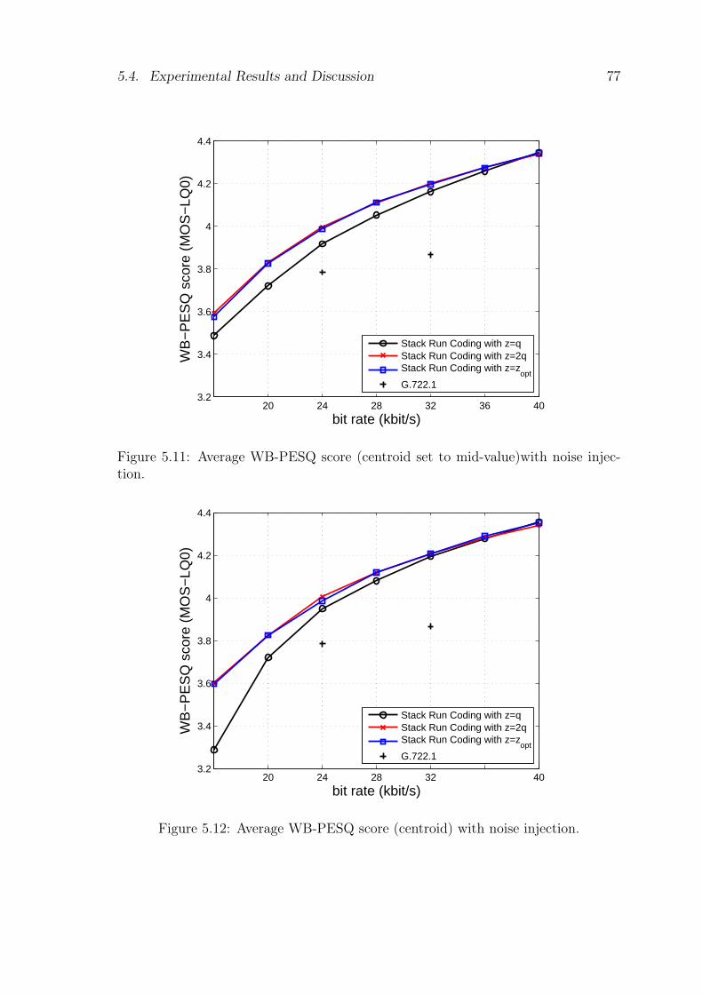
5.4. Experimental Results and Discussion 77
20 24 28 32 36 403.2
3.4
3.6
3.8
4
4.2
4.4
bit rate (kbit/s)
WB
−P
ES
Q s
core
(M
OS
−LQ
0)
Stack Run Coding with z=qStack Run Coding with z=2qStack Run Coding with z=z
opt
G.722.1
Figure 5.11: Average WB-PESQ score (centroid set to mid-value)with noise injec-tion.
20 24 28 32 403.2
3.4
3.6
3.8
4
4.2
4.4
bit rate (kbit/s)
WB
−P
ES
Q s
core
(M
OS
−LQ
0)
Stack Run Coding with z=qStack Run Coding with z=2qStack Run Coding with z=z
opt
G.722.1
Figure 5.12: Average WB-PESQ score (centroid) with noise injection.
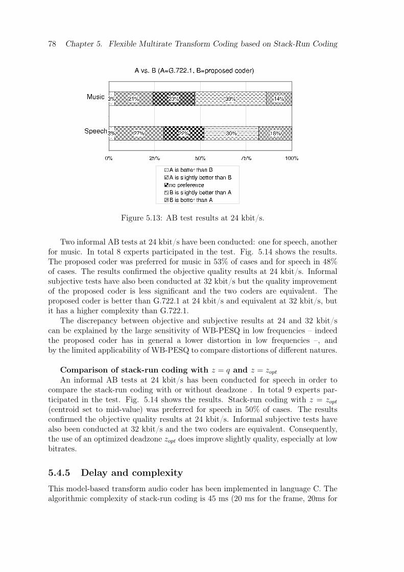
78 Chapter 5. Flexible Multirate Transform Coding based on Stack-Run Coding
Figure 5.13: AB test results at 24 kbit/s.
Two informal AB tests at 24 kbit/s have been conducted: one for speech, anotherfor music. In total 8 experts participated in the test. Fig. 5.14 shows the results.The proposed coder was preferred for music in 53% of cases and for speech in 48%of cases. The results confirmed the objective quality results at 24 kbit/s. Informalsubjective tests have also been conducted at 32 kbit/s but the quality improvementof the proposed coder is less significant and the two coders are equivalent. Theproposed coder is better than G.722.1 at 24 kbit/s and equivalent at 32 kbit/s, butit has a higher complexity than G.722.1.
The discrepancy between objective and subjective results at 24 and 32 kbit/scan be explained by the large sensitivity of WB-PESQ in low frequencies – indeedthe proposed coder has in general a lower distortion in low frequencies –, andby the limited applicability of WB-PESQ to compare distortions of different natures.
Comparison of stack-run coding with z = q and z = zopt
An informal AB tests at 24 kbit/s has been conducted for speech in order tocompare the stack-run coding with or without deadzone . In total 9 experts par-ticipated in the test. Fig. 5.14 shows the results. Stack-run coding with z = zopt
(centroid set to mid-value) was preferred for speech in 50% of cases. The resultsconfirmed the objective quality results at 24 kbit/s. Informal subjective tests havealso been conducted at 32 kbit/s and the two coders are equivalent. Consequently,the use of an optimized deadzone zopt does improve slightly quality, especially at lowbitrates.
5.4.5 Delay and complexity
This model-based transform audio coder has been implemented in language C. Thealgorithmic complexity of stack-run coding is 45 ms (20 ms for the frame, 20ms for
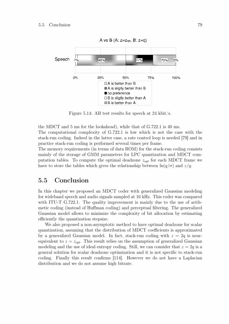
5.5. Conclusion 79
Figure 5.14: AB test results for speech at 24 kbit/s.
the MDCT and 5 ms for the lookahead), while that of G.722.1 is 40 ms.The computational complexity of G.722.1 is low which is not the case with thestack-run coding. Indeed in the latter case, a rate control loop is needed [79] and inpractice stack-run coding is performed several times per frame.The memory requirements (in terms of data ROM) for the stack-run coding consistsmainly of the storage of GMM parameters for LPC quantization and MDCT com-putation tables. To compute the optimal deadzone zopt for each MDCT frame wehave to store the tables which gives the relationship between ln(q/σ) and z/q.
5.5 ConclusionIn this chapter we proposed an MDCT coder with generalized Gaussian modelingfor wideband speech and audio signals sampled at 16 kHz. This coder was comparedwith ITU-T G.722.1. The quality improvement is mainly due to the use of arith-metic coding (instead of Huffman coding) and perceptual filtering. The generalizedGaussian model allows to minimize the complexity of bit allocation by estimatingefficiently the quantization stepsize.
We also proposed a non-asymptotic method to have optimal deadzone for scalarquantization, assuming that the distribution of MDCT coefficients is approximatedby a generalized Gaussian model. In fact, stack-run coding with z = 2q is near-equivalent to z = zopt. This result relies on the assumption of generalized Gaussianmodeling and the use of ideal entropy coding. Still, we can consider that z = 2q is ageneral solution for scalar deadzone optimization and it is not specific to stack-runcoding. Finally this result confirms [114]. However we do not have a Laplaciandistribution and we do not assume high bitrate.

80 Chapter 5. Flexible Multirate Transform Coding based on Stack-Run Coding
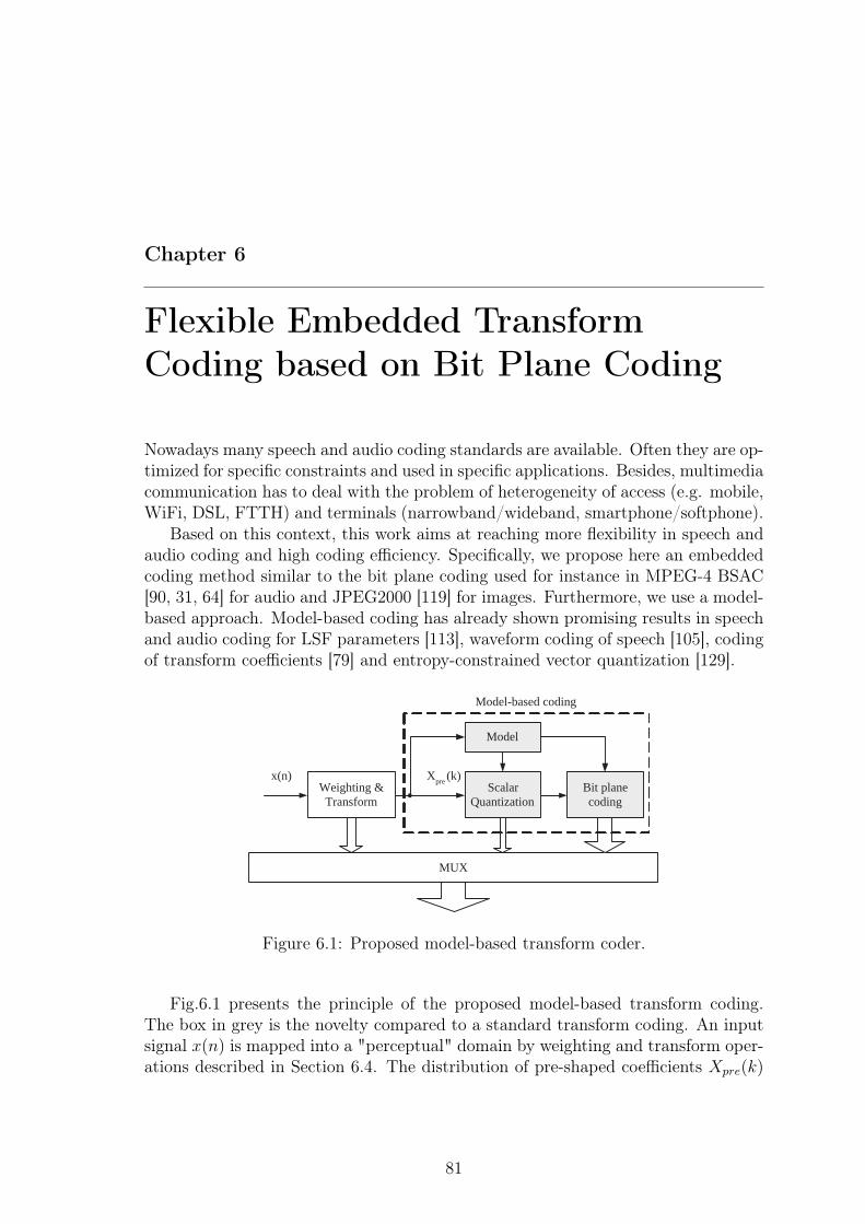
Chapter 6
Flexible Embedded TransformCoding based on Bit Plane Coding
Nowadays many speech and audio coding standards are available. Often they are op-timized for specific constraints and used in specific applications. Besides, multimediacommunication has to deal with the problem of heterogeneity of access (e.g. mobile,WiFi, DSL, FTTH) and terminals (narrowband/wideband, smartphone/softphone).
Based on this context, this work aims at reaching more flexibility in speech andaudio coding and high coding efficiency. Specifically, we propose here an embeddedcoding method similar to the bit plane coding used for instance in MPEG-4 BSAC[90, 31, 64] for audio and JPEG2000 [119] for images. Furthermore, we use a model-based approach. Model-based coding has already shown promising results in speechand audio coding for LSF parameters [113], waveform coding of speech [105], codingof transform coefficients [79] and entropy-constrained vector quantization [129].
x(n)
MUX
Scalar Quantization
Model
X pre (k) Weighting &
Transform Bit plane coding
Model-based coding
Figure 6.1: Proposed model-based transform coder.
Fig.6.1 presents the principle of the proposed model-based transform coding.The box in grey is the novelty compared to a standard transform coding. An inputsignal x(n) is mapped into a "perceptual" domain by weighting and transform oper-ations described in Section 6.4. The distribution of pre-shaped coefficients Xpre(k)
81
82 Chapter 6. Flexible Embedded Transform Coding based on Bit Plane Coding
is approximated by generalized Gaussian modeling as described in Section 3.2. Theinformation from the model are then used for the quantization and the arithmeticcoding. A scalar quantization based on the model is applied on the coefficientsXpre(k) and finally they are coded by model-based arithmetic coding, here we areusing bit plane coding. The main difference with the coder presented in Chapter 5is that the model is also used for arithmetic coding.
The main contributions of this work lies in the use of bit plane coded scalarquantization and the application of generalized Gaussian model for probabilitiesinitialization of the bit plane coding.
This chapter is organized as follows. A review of related work to bit plane codingis first presented in Section 6.1. Bit plane coding is presented in Section 6.4. Thenin Section 6.3 the model-based initialization of probabilities for adaptive arithmeticcoding is presented. Three methods are presented, two conditional probabilities esti-mation and one non-conditional. Conditional probability used the information frombit planes previously encoded. In Section 6.4, the proposed embedded transformcoding based on bit plane coding is explained. Objective and Subjective results arepresented in Section 6.5 before concluding in Section 6.6.
6.1 Related work
In image coding, zero-tree quantization described first in [109] and later refinedwith the set partitioning in hierarchical trees (SPIHT) algorithm [101], combinesordered bitplane coding with significance maps [109]. This algorithm is based onthe idea that spectral component with more energy content should be transmittedbefore other components. JBIG [115] is a lossless image compression of one-bit-per-pixel image data using an arithmetic coding knows as the Q-coder [91]. Itbases the probabilities of each bit on the previous bits and the previous lines of thepicture. In JPEG2000 [118, 120, 119], an embedded block coding algorithm basedon discrete wavelet transform (DWT) subbands with dead-zone quantization andbit plane coding is used.
In audio coding, ordered bit plane coding is used in MPEG-4 BSAC [90, 59] asdescribed in Section 2.4.2. But, BSAC coder requires the use of arithmetic codingwhich increase computational complexity, and the bitrate granularity is limited to 1kbit/s. Also, an Embedded Audio Coding (EAC) [64] based on a embedded bit planecoding with an implicit auditory masking is used for audio storage and streaming. Itperforms better than the audio standard such as MP3 [1, 2]. An algorithm based onthe SPIHT zero tree coding with a new method of arranging transform coefficients[31] is used for audio coding.
In MPEG-4 video standard [65], the quantized discrete transform (DCT) coeffi-cients are coded using a bit plane coding method.
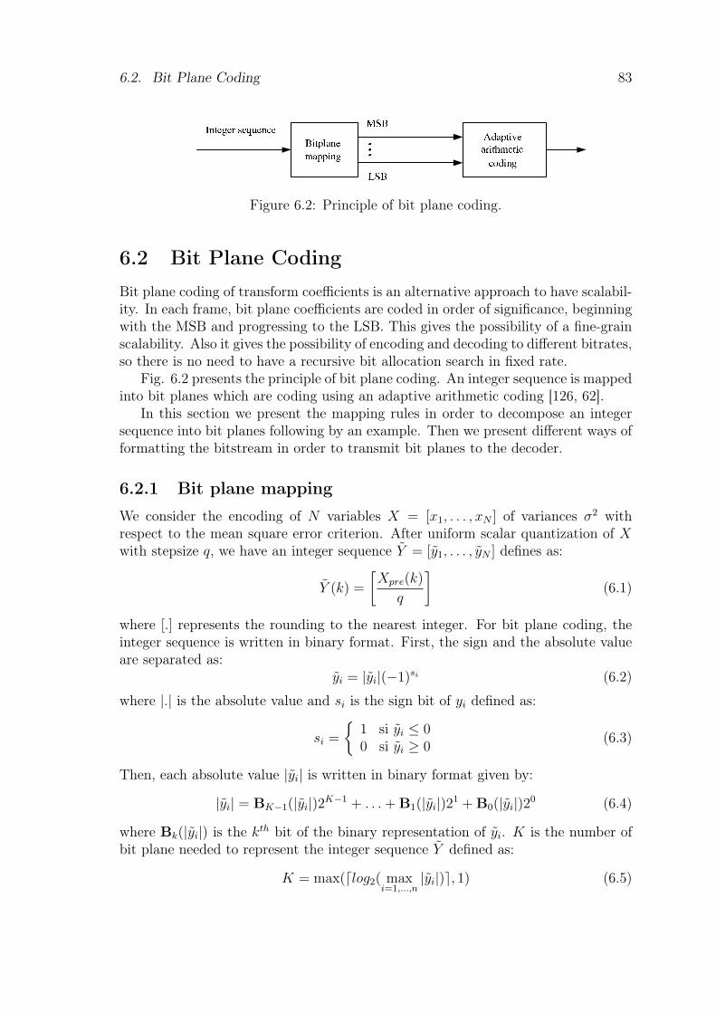
6.2. Bit Plane Coding 83
Figure 6.2: Principle of bit plane coding.
6.2 Bit Plane CodingBit plane coding of transform coefficients is an alternative approach to have scalabil-ity. In each frame, bit plane coefficients are coded in order of significance, beginningwith the MSB and progressing to the LSB. This gives the possibility of a fine-grainscalability. Also it gives the possibility of encoding and decoding to different bitrates,so there is no need to have a recursive bit allocation search in fixed rate.
Fig. 6.2 presents the principle of bit plane coding. An integer sequence is mappedinto bit planes which are coding using an adaptive arithmetic coding [126, 62].
In this section we present the mapping rules in order to decompose an integersequence into bit planes following by an example. Then we present different ways offormatting the bitstream in order to transmit bit planes to the decoder.
6.2.1 Bit plane mapping
We consider the encoding of N variables X = [x1, . . . , xN ] of variances σ2 withrespect to the mean square error criterion. After uniform scalar quantization of Xwith stepsize q, we have an integer sequence Y = [y1, . . . , yN ] defines as:
Y (k) =
[Xpre(k)
q
](6.1)
where [.] represents the rounding to the nearest integer. For bit plane coding, theinteger sequence is written in binary format. First, the sign and the absolute valueare separated as:
yi = |yi|(−1)si (6.2)
where |.| is the absolute value and si is the sign bit of yi defined as:
si =
{1 si yi ≤ 00 si yi ≥ 0
(6.3)
Then, each absolute value |yi| is written in binary format given by:
|yi| = BK−1(|yi|)2K−1 + . . . + B1(|yi|)21 + B0(|yi|)20 (6.4)
where Bk(|yi|) is the kth bit of the binary representation of yi. K is the number ofbit plane needed to represent the integer sequence Y defined as:
K = max(dlog2( maxi=1,...,n
|yi|)e, 1) (6.5)
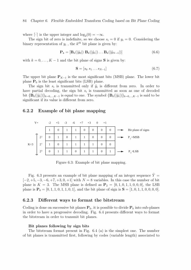
84 Chapter 6. Flexible Embedded Transform Coding based on Bit Plane Coding
where d·e is the upper integer and log2(0) = −∞.The sign bit of zero is indefinite, so we choose si = 0 if yi = 0. Considering the
binary representation of yi , the kth bit plane is given by:
Pk = [Bk(|y0|) Bk(|y1|) . . .Bk(|yN−1|)] (6.6)
with k = 0, . . . , K − 1 and the bit plane of signs S is given by:
S = [s0 s1 . . . sN−1] (6.7)
The upper bit plane PK−1 is the most significant bits (MSB) plane. The lower bitplane P0 is the least significant bits (LSB) plane.
The sign bit si is transmitted only if yi is different from zero. In order tohave partial decoding, the sign bit si is transmitted as soon as one of decodedbit {Bk(|yi|)}k=0,...,K−1 is equal to one. The symbol {Bk(|yi|)}k=0,...,K−1 is said to besignificant if its value is different from zero.
6.2.2 Example of bit plane mapping
1 0 1 1 0 0 0 0
0 1 0 1 1 0 0 0
1 0 1 1 1 1 0 0
0 1 1 0 1 1 0 1
-2 +5 -3 -6 +7 +3 0 +1 Y=
2 2
2 1
2 0
K=3
Bit plane of signs
P 2 =MSB
P 0 = LSB
Figure 6.3: Example of bit plane mapping.
Fig. 6.3 presents an example of bit plane mapping of an integer sequence Y =[−2, +5,−3,−6, +7, +3, 0, +1] with N = 8 variables. In this case the number of bitplane is K = 3. The MSB plane is defined as P2 = [0, 1, 0, 1, 1, 0, 0, 0], the LSBplane is P0 = [0, 1, 1, 0, 1, 1, 0, 1], and the bit plane of sign is S = [1, 0, 1, 1, 0, 0, 0, 0].
6.2.3 Different ways to format the bitstream
Coding is done on successive bit planes Pk, it is possible to divide Pk into sub-planesin order to have a progressive decoding. Fig. 6.4 presents different ways to formatthe bitstream in order to transmit bit planes.
Bit planes following by sign bitsThe bitstream format present in Fig. 6.4 (a) is the simplest one. The number
of bit planes is transmitted first, following by codes (variable length) associated to
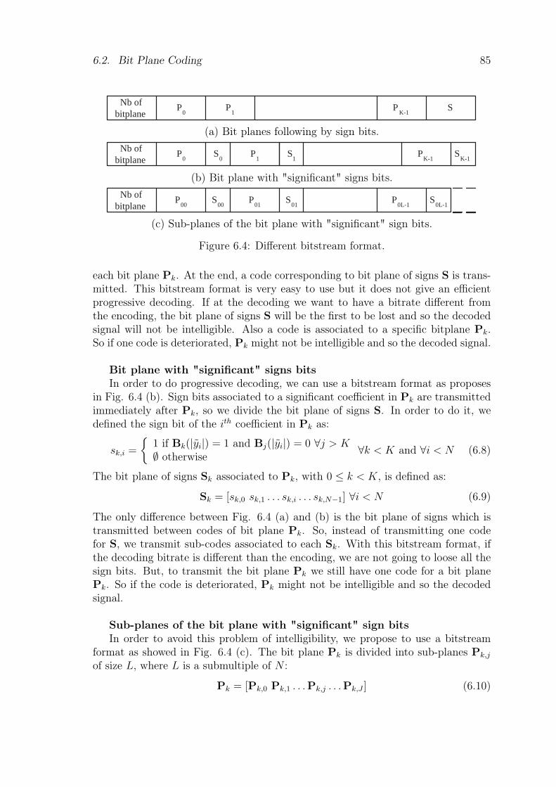
6.2. Bit Plane Coding 85
P 0
P 1
P K-1
S Nb of bitplane
(a) Bit planes following by sign bits.
P 0
P 1
P K-1
S K-1
S 0
S 1
Nb of bitplane
(b) Bit plane with "significant" signs bits.
P 00
P 01
P 0L-1
S 0L-1
S 00
S 01
Nb of bitplane
(c) Sub-planes of the bit plane with "significant" sign bits.
Figure 6.4: Different bitstream format.
each bit plane Pk. At the end, a code corresponding to bit plane of signs S is trans-mitted. This bitstream format is very easy to use but it does not give an efficientprogressive decoding. If at the decoding we want to have a bitrate different fromthe encoding, the bit plane of signs S will be the first to be lost and so the decodedsignal will not be intelligible. Also a code is associated to a specific bitplane Pk.So if one code is deteriorated, Pk might not be intelligible and so the decoded signal.
Bit plane with "significant" signs bitsIn order to do progressive decoding, we can use a bitstream format as proposes
in Fig. 6.4 (b). Sign bits associated to a significant coefficient in Pk are transmittedimmediately after Pk, so we divide the bit plane of signs S. In order to do it, wedefined the sign bit of the ith coefficient in Pk as:
sk,i =
{1 if Bk(|yi|) = 1 and Bj(|yi|) = 0 ∀j > K∅ otherwise ∀k < K and ∀i < N (6.8)
The bit plane of signs Sk associated to Pk, with 0 ≤ k < K, is defined as:
Sk = [sk,0 sk,1 . . . sk,i . . . sk,N−1] ∀i < N (6.9)
The only difference between Fig. 6.4 (a) and (b) is the bit plane of signs which istransmitted between codes of bit plane Pk. So, instead of transmitting one codefor S, we transmit sub-codes associated to each Sk. With this bitstream format, ifthe decoding bitrate is different than the encoding, we are not going to loose all thesign bits. But, to transmit the bit plane Pk we still have one code for a bit planePk. So if the code is deteriorated, Pk might not be intelligible and so the decodedsignal.
Sub-planes of the bit plane with "significant" sign bitsIn order to avoid this problem of intelligibility, we propose to use a bitstream
format as showed in Fig. 6.4 (c). The bit plane Pk is divided into sub-planes Pk,j
of size L, where L is a submultiple of N :
Pk = [Pk,0 Pk,1 . . .Pk,j . . .Pk,J ] (6.10)
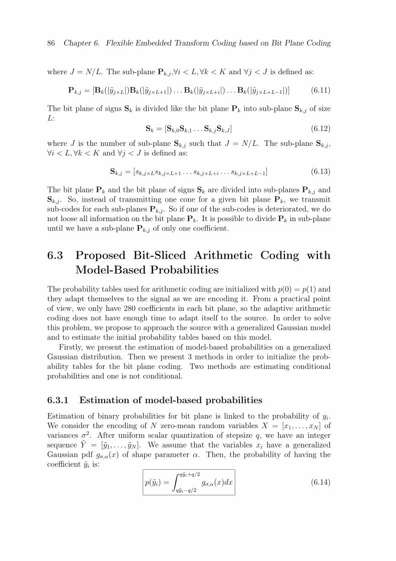
86 Chapter 6. Flexible Embedded Transform Coding based on Bit Plane Coding
where J = N/L. The sub-plane Pk,j,∀i < L, ∀k < K and ∀j < J is defined as:
Pk,j = [Bk(|yj×L|)Bk(|yj×L+1|) . . .Bk(|yj×L+i|) . . .Bk(|yj×L+L−1|)] (6.11)
The bit plane of signs Sk is divided like the bit plane Pk into sub-plane Sk,j of sizeL:
Sk = [Sk,0Sk,1 . . .Sk,jSk,J ] (6.12)
where J is the number of sub-plane Sk,j such that J = N/L. The sub-plane Sk,j,∀i < L, ∀k < K and ∀j < J is defined as:
Sk,j = [sk,j×Lsk,j×L+1 . . . sk,j×L+i . . . sk,j×L+L−1] (6.13)
The bit plane Pk and the bit plane of signs Sk are divided into sub-planes Pk,j andSk,j. So, instead of transmitting one cone for a given bit plane Pk, we transmitsub-codes for each sub-planes Pk,j. So if one of the sub-codes is deteriorated, we donot loose all information on the bit plane Pk. It is possible to divide Pk in sub-planeuntil we have a sub-plane Pk,j of only one coefficient.
6.3 Proposed Bit-Sliced Arithmetic Coding withModel-Based Probabilities
The probability tables used for arithmetic coding are initialized with p(0) = p(1) andthey adapt themselves to the signal as we are encoding it. From a practical pointof view, we only have 280 coefficients in each bit plane, so the adaptive arithmeticcoding does not have enough time to adapt itself to the source. In order to solvethis problem, we propose to approach the source with a generalized Gaussian modeland to estimate the initial probability tables based on this model.
Firstly, we present the estimation of model-based probabilities on a generalizedGaussian distribution. Then we present 3 methods in order to initialize the prob-ability tables for the bit plane coding. Two methods are estimating conditionalprobabilities and one is not conditional.
6.3.1 Estimation of model-based probabilities
Estimation of binary probabilities for bit plane is linked to the probability of yi.We consider the encoding of N zero-mean random variables X = [x1, . . . , xN ] ofvariances σ2. After uniform scalar quantization of stepsize q, we have an integersequence Y = [y1, . . . , yN ]. We assume that the variables xi have a generalizedGaussian pdf gσ,α(x) of shape parameter α. Then, the probability of having thecoefficient yi is:
p(yi) =
∫ qyi+q/2
qyi−q/2
gσ,α(x)dx (6.14)
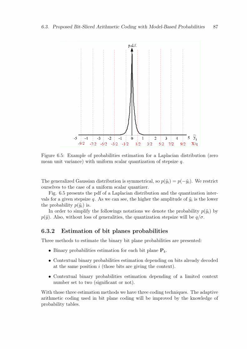
6.3. Proposed Bit-Sliced Arithmetic Coding with Model-Based Probabilities 87
Figure 6.5: Example of probabilities estimation for a Laplacian distribution (zeromean unit variance) with uniform scalar quantization of stepsize q.
The generalized Gaussian distribution is symmetrical, so p(yi) = p(−yi). We restrictourselves to the case of a uniform scalar quantizer.
Fig. 6.5 presents the pdf of a Laplacian distribution and the quantization inter-vals for a given stepsize q. As we can see, the higher the amplitude of yi is the lowerthe probability p(yi) is.
In order to simplify the followings notations we denote the probability p(yi) byp(y). Also, without loss of generalities, the quantization stepsize will be q/σ.
6.3.2 Estimation of bit planes probabilities
Three methods to estimate the binary bit plane probabilities are presented:
• Binary probabilities estimation for each bit plane Pk.
• Contextual binary probabilities estimation depending on bits already decodedat the same position i (those bits are giving the context).
• Contextual binary probabilities estimation depending of a limited contextnumber set to two (significant or not).
With those three estimation methods we have three coding techniques. The adaptivearithmetic coding used in bit plane coding will be improved by the knowledge ofprobability tables.
88 Chapter 6. Flexible Embedded Transform Coding based on Bit Plane Coding
6.3.2.1 Adaptive arithmetic coding with model-based initialization ofbinary probabilities tables
In this case the initialization of probability tables is based on the generalizedGaussian modeling of variables X. So the initialization of tables will not bep(0) = p(1), but it will be linked to the distribution of the source.
Calculation of binary probabilitiesThe probability of having the kth bit of the binary decomposition of y equal to
zero is given by:p(Bk(|y|) = 0) = p(y)× δBk(|y|),0 (6.15)
with
δx,y =
{1 if x = y0 if x 6= y
The probability of having zero in the bit plane Pk is given by:
p(bk = 0| |y| ≤ M) =p(bk = 0, |y| ≤ M)
p(|y| ≤ M)(6.16)
where bk and M are respectively a random variable representing any bit in Pk andthe higher integer we can have on K bit planes, M = 2K − 1.
The probability is dependent of the number of bit plane K and so, to the numberof coded integers. We supposed that the number of bit plane is transmitted to thedecoder, and so it is available at the coder and the decoder.
Generalized Gaussian model is infinite and the uniform scalar quantizer is finiteand determined by the number of bit planes K. So, the probability of having |y| ≤ Mis not equal to one and is the sum of probabilities of variables y with |y| ≤ M :
p(|y| ≤ M) =M∑
y=−M
p(y) (6.17)
The probability of having bk = 0 and |y| ≤ M is the sum of probabilities ofvariables Bk(|y| = 0 with |y| ≤ M :
p(bk = 0, |y| ≤ M) =M∑
y=−M
p(Bk(|y|) = 0) (6.18)
In order to simplify the followings notations we denote the probability p(bk = 0||y| ≤M) by pM(bk = 0). So, the probability of having zero in Pk is given by:
pM(bk = 0) =1
M∑y=−M
p(y)
×M∑
y=−M
p(y)× δBk(|y|),0 (6.19)
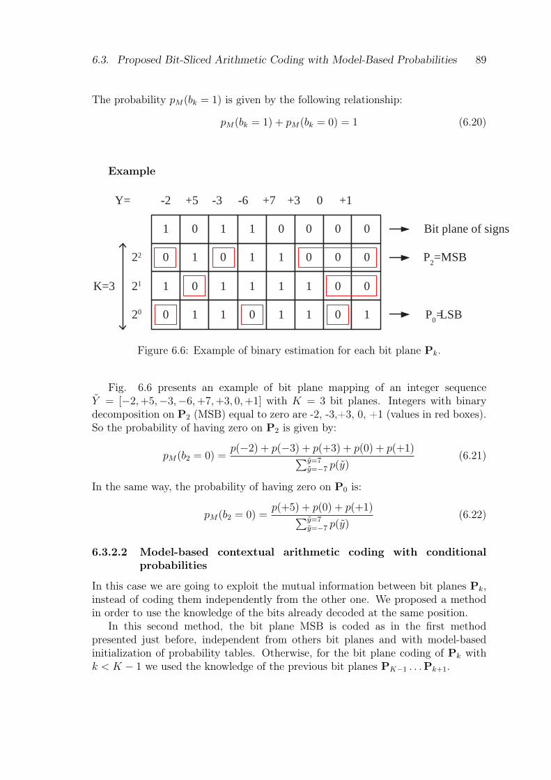
6.3. Proposed Bit-Sliced Arithmetic Coding with Model-Based Probabilities 89
The probability pM(bk = 1) is given by the following relationship:
pM(bk = 1) + pM(bk = 0) = 1 (6.20)
Example
1 0 1 1 0 0 0 0
0 1 0 1 1 0 0 0
1 0 1 1 1 1 0 0
0 1 1 0 1 1 0 1
-2 +5 -3 -6 +7 +3 0 +1 Y=
2 2
2 1
2 0
K=3
Bit plane of signs
P 2 =MSB
P 0 = LSB
Figure 6.6: Example of binary estimation for each bit plane Pk.
Fig. 6.6 presents an example of bit plane mapping of an integer sequenceY = [−2, +5,−3,−6, +7, +3, 0, +1] with K = 3 bit planes. Integers with binarydecomposition on P2 (MSB) equal to zero are -2, -3,+3, 0, +1 (values in red boxes).So the probability of having zero on P2 is given by:
pM(b2 = 0) =p(−2) + p(−3) + p(+3) + p(0) + p(+1)∑y=7
y=−7 p(y)(6.21)
In the same way, the probability of having zero on P0 is:
pM(b2 = 0) =p(+5) + p(0) + p(+1)∑y=7
y=−7 p(y)(6.22)
6.3.2.2 Model-based contextual arithmetic coding with conditionalprobabilities
In this case we are going to exploit the mutual information between bit planes Pk,instead of coding them independently from the other one. We proposed a methodin order to use the knowledge of the bits already decoded at the same position.
In this second method, the bit plane MSB is coded as in the first methodpresented just before, independent from others bit planes and with model-basedinitialization of probability tables. Otherwise, for the bit plane coding of Pk withk < K − 1 we used the knowledge of the previous bit planes PK−1 . . .Pk+1.
90 Chapter 6. Flexible Embedded Transform Coding based on Bit Plane Coding
Calculation of the probability of the context ck(|y|)By context ck(|y|), we defined the binary decomposition of y in bit planes before
Pk ordered from LSB to MSB. For example, the binary decomposition of 6 is 011from LSB to MSB and the context of the LSB (0) will be 11.
For every bit plane expect the MSB (k < K − 1), the context of the binarydecomposition of y, ck(|y|), is defined as:
ck(|y|) =K−1∑
j=k+1
Bj(|y|)2j |y| < M ∀k < K (6.23)
The number of contexts in Pk is N = 2K−k−1. We defined Ck has a vector containingall the possible contexts in Pk :
Ck = [ck(0), . . . , ck(n), . . . , ck(N − 1)] (6.24)
For example, if we have K = 3 bit planes and if we are in P1, we have 4 contextsand C1 = [00, 01, 10, 11].
The probability of having the context ck(|y|) in Pk equal to ck(n) is given by:
p (ck(|y|) = ck(n)) = p (y)×K−1∏
j=k+1
δBj(|y|),Bj(n) (6.25)
We are checking that the binary decomposition of |y| and n are of the same onprevious bit planes PK−1 . . .Pk+1. If it is the same then p (ck(|y|) = ck(n)) = p (y)otherwise p (ck(|y|) = ck(n)) = 0.
Calculation of the conditional probabilityWe considered the a priori knowledge of the context (bit planes of rank k to
K − 1) to code Pk. The conditional probability of having the value zero on Pk withknowing the context ck(n) for k < K − 1 is defined as:
pM (bk = 0|ck = ck(n)) =pM (bk = 0, ck = ck(n))
pM (ck = ck(n))(6.26)
where bk and ck are respectively a random variable representing any bit in Pk anda random variable representing any context in Pk.
The probability of having the context ck equal to ck(n) and |y| ≤ M is given bythe relationship:
pM (ck = ck(n)) =p (ck = ck(n), |y| ≤ M)
p(|y| ≤ M)(6.27)
where p(|y| ≤ M) =∑M
y=−M p(y). The probability of having ck = ck(n) and |y| ≤ M
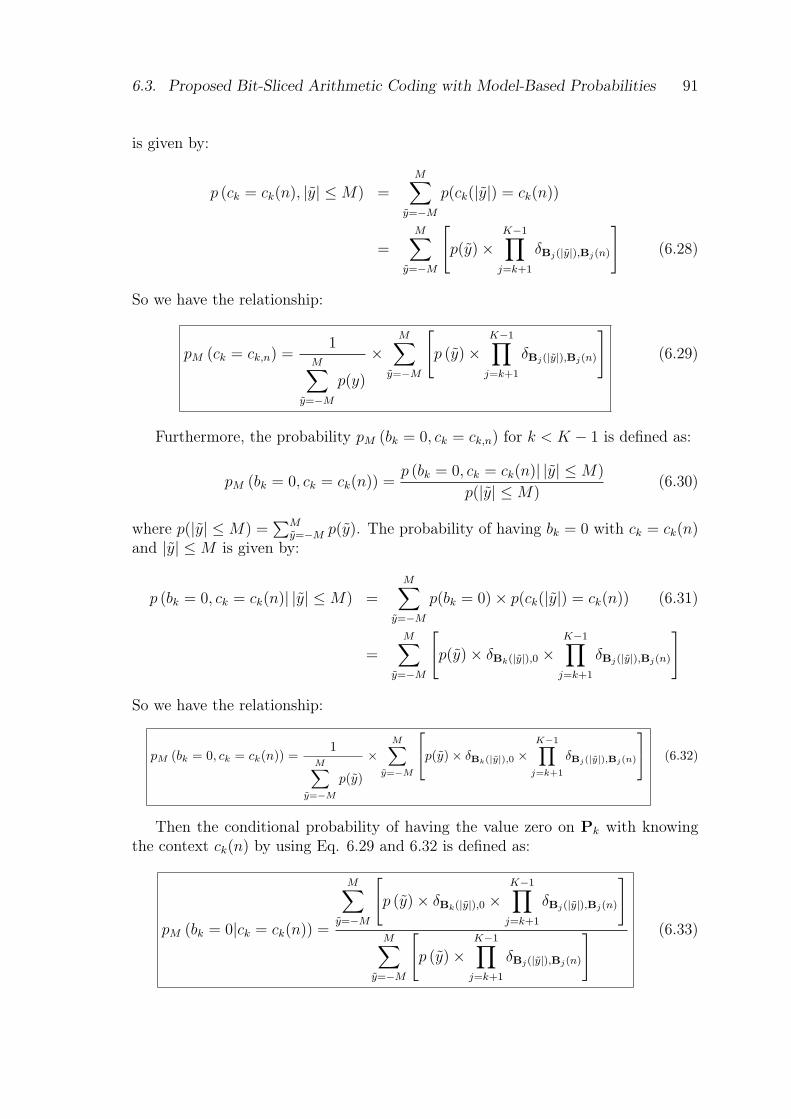
6.3. Proposed Bit-Sliced Arithmetic Coding with Model-Based Probabilities 91
is given by:
p (ck = ck(n), |y| ≤ M) =M∑
y=−M
p(ck(|y|) = ck(n))
=M∑
y=−M
[p(y)×
K−1∏
j=k+1
δBj(|y|),Bj(n)
](6.28)
So we have the relationship:
pM (ck = ck,n) =1
M∑y=−M
p(y)
×M∑
y=−M
[p (y)×
K−1∏
j=k+1
δBj(|y|),Bj(n)
](6.29)
Furthermore, the probability pM (bk = 0, ck = ck,n) for k < K − 1 is defined as:
pM (bk = 0, ck = ck(n)) =p (bk = 0, ck = ck(n)| |y| ≤ M)
p(|y| ≤ M)(6.30)
where p(|y| ≤ M) =∑M
y=−M p(y). The probability of having bk = 0 with ck = ck(n)and |y| ≤ M is given by:
p (bk = 0, ck = ck(n)| |y| ≤ M) =M∑
y=−M
p(bk = 0)× p(ck(|y|) = ck(n)) (6.31)
=M∑
y=−M
[p(y)× δBk(|y|),0 ×
K−1∏
j=k+1
δBj(|y|),Bj(n)
]
So we have the relationship:
pM (bk = 0, ck = ck(n)) =1
M∑
y=−M
p(y)
×M∑
y=−M
p(y)× δBk(|y|),0 ×
K−1∏
j=k+1
δBj(|y|),Bj(n)
(6.32)
Then the conditional probability of having the value zero on Pk with knowingthe context ck(n) by using Eq. 6.29 and 6.32 is defined as:
pM (bk = 0|ck = ck(n)) =
M∑y=−M
[p (y)× δBk(|y|),0 ×
K−1∏
j=k+1
δBj(|y|),Bj(n)
]
M∑y=−M
[p (y)×
K−1∏
j=k+1
δBj(|y|),Bj(n)
] (6.33)
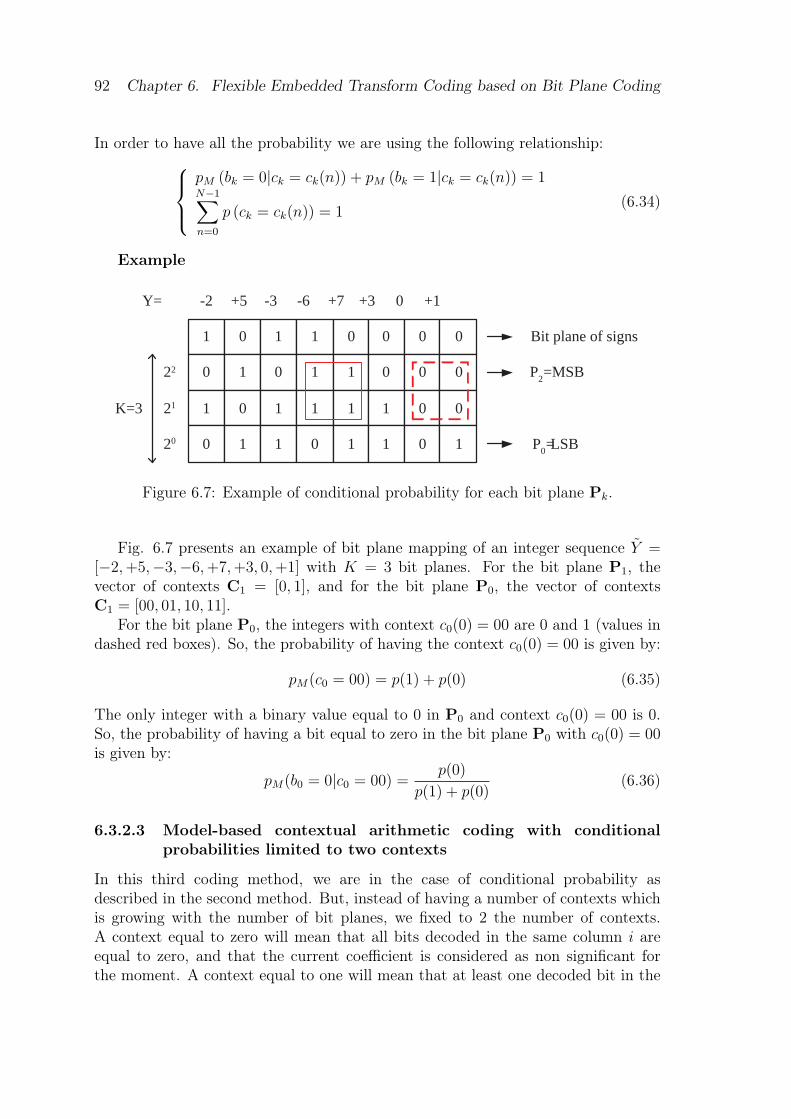
92 Chapter 6. Flexible Embedded Transform Coding based on Bit Plane Coding
In order to have all the probability we are using the following relationship:
pM (bk = 0|ck = ck(n)) + pM (bk = 1|ck = ck(n)) = 1N−1∑n=0
p (ck = ck(n)) = 1(6.34)
Example
1 0 1 1 0 0 0 0
0 1 0 1 1 0 0 0
1 0 1 1 1 1 0 0
0 1 1 0 1 1 0 1
-2 +5 -3 -6 +7 +3 0 +1 Y=
2 2
2 1
2 0
K=3
Bit plane of signs
P 2 =MSB
P 0 = LSB
Figure 6.7: Example of conditional probability for each bit plane Pk.
Fig. 6.7 presents an example of bit plane mapping of an integer sequence Y =[−2, +5,−3,−6, +7, +3, 0, +1] with K = 3 bit planes. For the bit plane P1, thevector of contexts C1 = [0, 1], and for the bit plane P0, the vector of contextsC1 = [00, 01, 10, 11].
For the bit plane P0, the integers with context c0(0) = 00 are 0 and 1 (values indashed red boxes). So, the probability of having the context c0(0) = 00 is given by:
pM(c0 = 00) = p(1) + p(0) (6.35)
The only integer with a binary value equal to 0 in P0 and context c0(0) = 00 is 0.So, the probability of having a bit equal to zero in the bit plane P0 with c0(0) = 00is given by:
pM(b0 = 0|c0 = 00) =p(0)
p(1) + p(0)(6.36)
6.3.2.3 Model-based contextual arithmetic coding with conditionalprobabilities limited to two contexts
In this third coding method, we are in the case of conditional probability asdescribed in the second method. But, instead of having a number of contexts whichis growing with the number of bit planes, we fixed to 2 the number of contexts.A context equal to zero will mean that all bits decoded in the same column i areequal to zero, and that the current coefficient is considered as non significant forthe moment. A context equal to one will mean that at least one decoded bit in the
6.3. Proposed Bit-Sliced Arithmetic Coding with Model-Based Probabilities 93
column i was equal to one, and so the current coefficient is significant.
Calculation of the probability of the contextFor every bit plane expect the MSB (k < K − 1), we defined the context ck(|y|)
in Pk as:
ck(|y|) =
{1 if ∃Bj(|y|) = 1 for j = k + 1, . . . , K − 10 otherwise (6.37)
The probability of having the context ck(|y|) in Pk equal to zero is given by:
p (ck(|y|) = 0) = p(y)×K−1∏
j=k+1
δBj(|y|),0 (6.38)
We are checking that the binary decomposition of y is equal to zero. If it is the casethen p (ck(|y|) = 0) = p(y) otherwise p (ck(|y|) = 0) = 0.
Calculation of the conditional probability limited to two contextsWe used the a priori knowledge of the context (bit plane of rank k to K − 1) to
code Pk. The conditional probability of having the value zero with only two contexts(significant or non-significant) in Pk is defined as:
pM (bk = 0|ck = 0) =pM (bk = 0, ck = 0)
pM (ck = 0)(6.39)
where bk and ck are respectively a random variable representing any bit in Pk anda random variable representing any context in Pk.
The probability pM (ck = 0) has already been defined in Eq. 6.29, in this caseck(n) = 0:
pM (ck = 0) =1
M∑y=−M
p(y)
×M∑
y=−M
[p(y)×
K−1∏
j=k+1
δBj(|y|)|,0
](6.40)
The probability pM (bk = 0, ck = 0) has already been defined in Eq. 6.32, in thiscase ck(n) = 0:
pM (bk = 0, ck = 0) =1
M∑y=−M
p(y)
×M∑
y=−M
[p(y)×
K−1∏
j=k
δBj(|y|),0
](6.41)
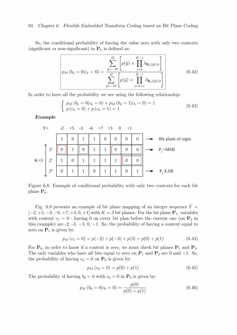
94 Chapter 6. Flexible Embedded Transform Coding based on Bit Plane Coding
So, the conditional probability of having the value zero with only two contexts(significant or non-significant) in Pk is defined as:
pM (bk = 0|ck = 0) =
M∑y=−M
[p(y)×
K−1∏
j=k
δBj(|y|),0
]
M∑y=−M
[p(y)×
K−1∏
j=k+1
δBj(|y|),0
] (6.42)
In order to have all the probability we are using the following relationship:{
pM (bk = 0|ck = 0) + pM (bk = 1|ck = 0) = 1p (ck = 0) + p (ck = 1) = 1
(6.43)
Example
1 0 1 1 0 0 0 0
0 1 0 1 1 0 0 0
1 0 1 1 1 1 0 0
0 1 1 0 1 1 0 1
-2 +5 -3 -6 +7 +3 0 +1 Y=
2 2
2 1
2 0
K=3
Bit plane of signs
P 2 =MSB
P 0 = LSB
Figure 6.8: Example of conditional probability with only two contexts for each bitplane Pk.
Fig. 6.8 presents an example of bit plane mapping of an integer sequence Y =[−2, +5,−3,−6, +7, +3, 0, +1] with K = 3 bit planes. For the bit plane P1, variableswith context c1 = 0 - having 0 on every bit plan before the current one (on P2 inthis example) are -2, -3, +3, 0, +1. So, the probability of having a context equal tozero on P1 is given by:
pM (c1 = 0) = p(−2) + p(−3) + p(3) + p(0) + p(1) (6.44)
For P0, in order to know if a context is zero, we must check bit planes P1 and P2.The only variables who have all bits equal to zero on P1 and P2 are 0 and +1. So,the probability of having c0 = 0 on P0 is given by:
pM (c0 = 0) = p(0) + p(1) (6.45)
The probability of having b0 = 0 with c0 = 0 in P0 is given by:
pM (b0 = 0|c0 = 0) =p(0)
p(0) + p(1)(6.46)
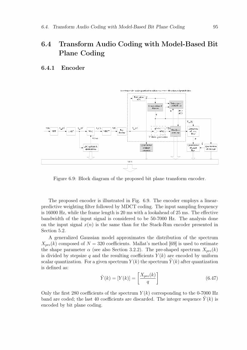
6.4. Transform Audio Coding with Model-Based Bit Plane Coding 95
6.4 Transform Audio Coding with Model-Based BitPlane Coding
6.4.1 Encoder
Figure 6.9: Block diagram of the proposed bit plane transform encoder.
The proposed encoder is illustrated in Fig. 6.9. The encoder employs a linear-predictive weighting filter followed by MDCT coding. The input sampling frequencyis 16000 Hz, while the frame length is 20 ms with a lookahead of 25 ms. The effectivebandwidth of the input signal is considered to be 50-7000 Hz. The analysis doneon the input signal x(n) is the same than for the Stack-Run encoder presented inSection 5.2.
A generalized Gaussian model approximates the distribution of the spectrumXpre(k) composed of N = 320 coefficients. Mallat’s method [69] is used to estimatethe shape parameter α (see also Section 3.2.2). The pre-shaped spectrum Xpre(k)is divided by stepsize q and the resulting coefficients Y (k) are encoded by uniformscalar quantization. For a given spectrum Y (k) the spectrum Y (k) after quantizationis defined as:
Y (k) = [Y (k)] =
[Xpre(k)
q
](6.47)
Only the first 280 coefficients of the spectrum Y (k) corresponding to the 0-7000 Hzband are coded; the last 40 coefficients are discarded. The integer sequence Y (k) isencoded by bit plane coding.
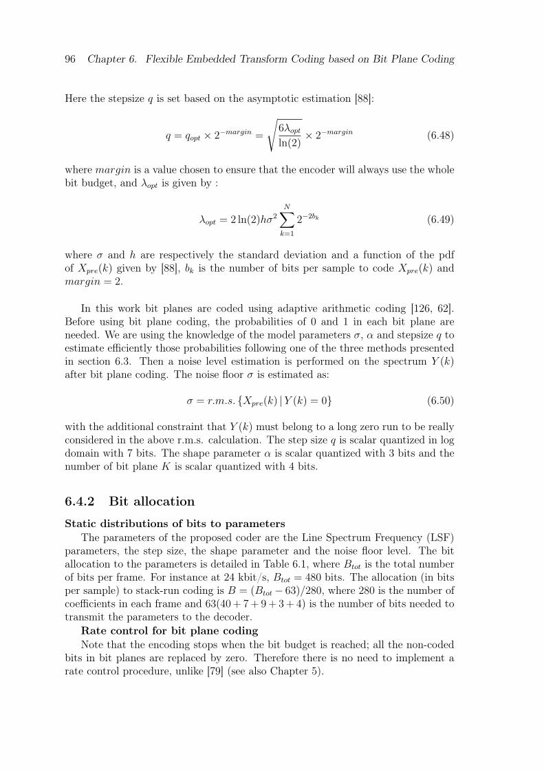
96 Chapter 6. Flexible Embedded Transform Coding based on Bit Plane Coding
Here the stepsize q is set based on the asymptotic estimation [88]:
q = qopt × 2−margin =
√6λopt
ln(2)× 2−margin (6.48)
where margin is a value chosen to ensure that the encoder will always use the wholebit budget, and λopt is given by :
λopt = 2 ln(2)hσ2
N∑
k=1
2−2bk (6.49)
where σ and h are respectively the standard deviation and a function of the pdfof Xpre(k) given by [88], bk is the number of bits per sample to code Xpre(k) andmargin = 2.
In this work bit planes are coded using adaptive arithmetic coding [126, 62].Before using bit plane coding, the probabilities of 0 and 1 in each bit plane areneeded. We are using the knowledge of the model parameters σ, α and stepsize q toestimate efficiently those probabilities following one of the three methods presentedin section 6.3. Then a noise level estimation is performed on the spectrum Y (k)after bit plane coding. The noise floor σ is estimated as:
σ = r.m.s. {Xpre(k) |Y (k) = 0} (6.50)
with the additional constraint that Y (k) must belong to a long zero run to be reallyconsidered in the above r.m.s. calculation. The step size q is scalar quantized in logdomain with 7 bits. The shape parameter α is scalar quantized with 3 bits and thenumber of bit plane K is scalar quantized with 4 bits.
6.4.2 Bit allocation
Static distributions of bits to parametersThe parameters of the proposed coder are the Line Spectrum Frequency (LSF)
parameters, the step size, the shape parameter and the noise floor level. The bitallocation to the parameters is detailed in Table 6.1, where Btot is the total numberof bits per frame. For instance at 24 kbit/s, Btot = 480 bits. The allocation (in bitsper sample) to stack-run coding is B = (Btot− 63)/280, where 280 is the number ofcoefficients in each frame and 63(40 + 7 + 9 + 3 + 4) is the number of bits needed totransmit the parameters to the decoder.
Rate control for bit plane codingNote that the encoding stops when the bit budget is reached; all the non-coded
bits in bit planes are replaced by zero. Therefore there is no need to implement arate control procedure, unlike [79] (see also Chapter 5).
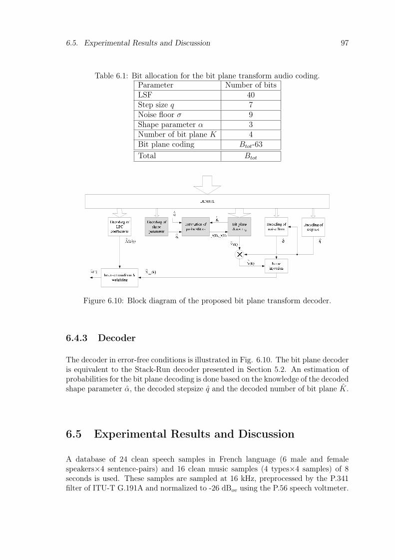
6.5. Experimental Results and Discussion 97
Table 6.1: Bit allocation for the bit plane transform audio coding.Parameter Number of bitsLSF 40Step size q 7Noise floor σ 9Shape parameter α 3Number of bit plane K 4Bit plane coding Btot-63Total Btot
Figure 6.10: Block diagram of the proposed bit plane transform decoder.
6.4.3 Decoder
The decoder in error-free conditions is illustrated in Fig. 6.10. The bit plane decoderis equivalent to the Stack-Run decoder presented in Section 5.2. An estimation ofprobabilities for the bit plane decoding is done based on the knowledge of the decodedshape parameter α, the decoded stepsize q and the decoded number of bit plane K.
6.5 Experimental Results and Discussion
A database of 24 clean speech samples in French language (6 male and femalespeakers×4 sentence-pairs) and 16 clean music samples (4 types×4 samples) of 8seconds is used. These samples are sampled at 16 kHz, preprocessed by the P.341filter of ITU-T G.191A and normalized to -26 dBov using the P.56 speech voltmeter.
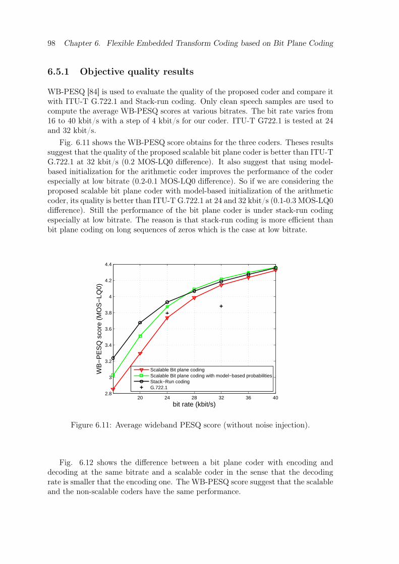
98 Chapter 6. Flexible Embedded Transform Coding based on Bit Plane Coding
6.5.1 Objective quality results
WB-PESQ [84] is used to evaluate the quality of the proposed coder and compare itwith ITU-T G.722.1 and Stack-run coding. Only clean speech samples are used tocompute the average WB-PESQ scores at various bitrates. The bit rate varies from16 to 40 kbit/s with a step of 4 kbit/s for our coder. ITU-T G722.1 is tested at 24and 32 kbit/s.
Fig. 6.11 shows the WB-PESQ score obtains for the three coders. Theses resultssuggest that the quality of the proposed scalable bit plane coder is better than ITU-TG.722.1 at 32 kbit/s (0.2 MOS-LQ0 difference). It also suggest that using model-based initialization for the arithmetic coder improves the performance of the coderespecially at low bitrate (0.2-0.1 MOS-LQ0 difference). So if we are considering theproposed scalable bit plane coder with model-based initialization of the arithmeticcoder, its quality is better than ITU-T G.722.1 at 24 and 32 kbit/s (0.1-0.3 MOS-LQ0difference). Still the performance of the bit plane coder is under stack-run codingespecially at low bitrate. The reason is that stack-run coding is more efficient thanbit plane coding on long sequences of zeros which is the case at low bitrate.
20 24 28 32 36 402.8
3
3.2
3.4
3.6
3.8
4
4.2
4.4
bit rate (kbit/s)
WB
−P
ES
Q s
core
(M
OS
−LQ
0)
Scalable Bit plane codingScalable Bit plane coding with model−based probabilitiesStack−Run codingG.722.1
Figure 6.11: Average wideband PESQ score (without noise injection).
Fig. 6.12 shows the difference between a bit plane coder with encoding anddecoding at the same bitrate and a scalable coder in the sense that the decodingrate is smaller that the encoding one. The WB-PESQ score suggest that the scalableand the non-scalable coders have the same performance.
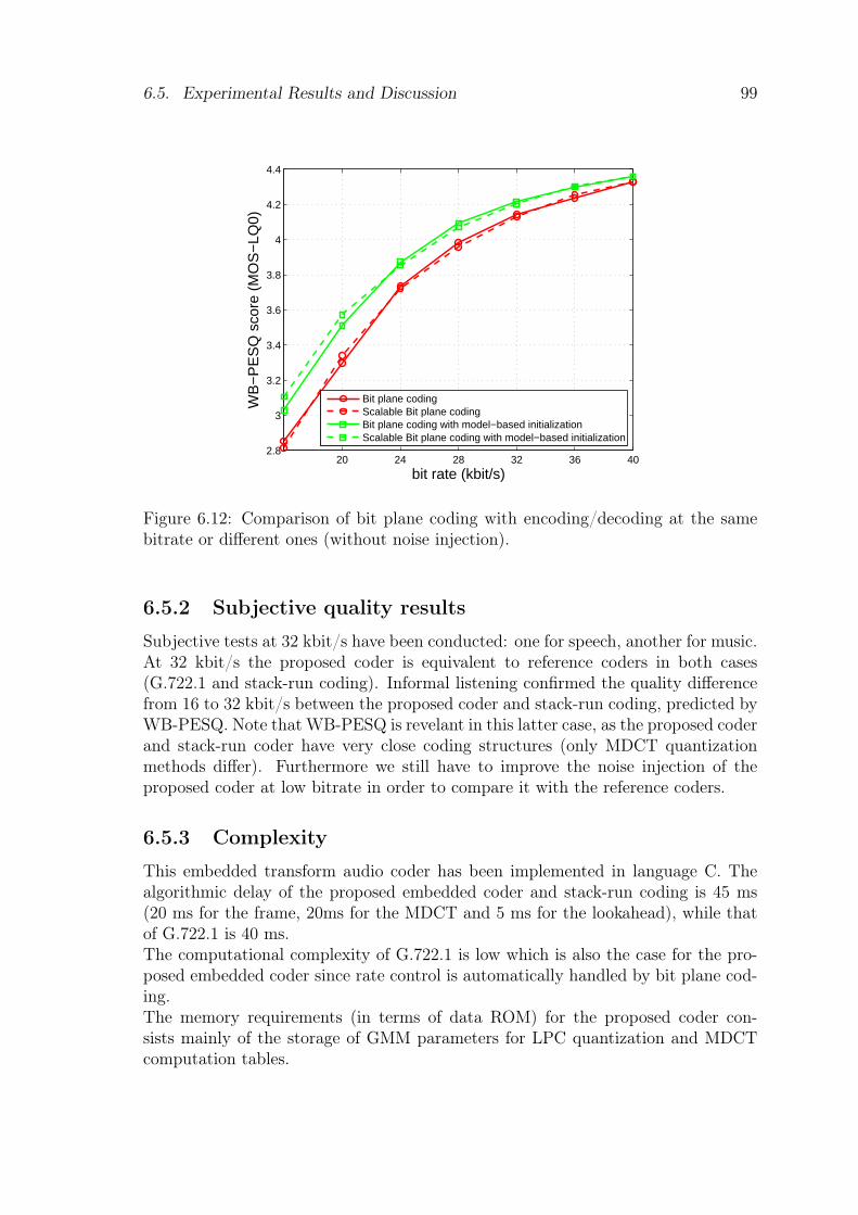
6.5. Experimental Results and Discussion 99
20 24 28 32 36 402.8
3
3.2
3.4
3.6
3.8
4
4.2
4.4
bit rate (kbit/s)
WB
−P
ES
Q s
core
(M
OS
−LQ
0)
Bit plane codingScalable Bit plane codingBit plane coding with model−based initializationScalable Bit plane coding with model−based initialization
Figure 6.12: Comparison of bit plane coding with encoding/decoding at the samebitrate or different ones (without noise injection).
6.5.2 Subjective quality results
Subjective tests at 32 kbit/s have been conducted: one for speech, another for music.At 32 kbit/s the proposed coder is equivalent to reference coders in both cases(G.722.1 and stack-run coding). Informal listening confirmed the quality differencefrom 16 to 32 kbit/s between the proposed coder and stack-run coding, predicted byWB-PESQ. Note that WB-PESQ is revelant in this latter case, as the proposed coderand stack-run coder have very close coding structures (only MDCT quantizationmethods differ). Furthermore we still have to improve the noise injection of theproposed coder at low bitrate in order to compare it with the reference coders.
6.5.3 Complexity
This embedded transform audio coder has been implemented in language C. Thealgorithmic delay of the proposed embedded coder and stack-run coding is 45 ms(20 ms for the frame, 20ms for the MDCT and 5 ms for the lookahead), while thatof G.722.1 is 40 ms.The computational complexity of G.722.1 is low which is also the case for the pro-posed embedded coder since rate control is automatically handled by bit plane cod-ing.The memory requirements (in terms of data ROM) for the proposed coder con-sists mainly of the storage of GMM parameters for LPC quantization and MDCTcomputation tables.
100 Chapter 6. Flexible Embedded Transform Coding based on Bit Plane Coding
6.6 ConclusionIn this chapter we proposed an embedded speech and audio coder based on gener-alized Gaussian modeling and bit plane coding. This coder was compared againstITU-T G.722.1 and stack-run audio coding. The generalized Gaussian model allowsto estimate efficiently symbol probability in bit planes. This model-based approachbrings an improvement of 0.1-0.4 MOS-LQ0 compared with a baseline bit planecoder. The proposed coder reaches a performance similar to non-embedded codingsuch as stack-run coding or ITU-T G.722.1, which is remarkable. Further work willbe focused on improving quality at low bit rates to reduce the performance penaltyand to handle multiple constraints (e.g. sampling frequency, frame length, runs ofzeros) of bitstream scalability.
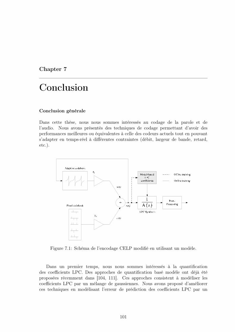
Chapter 7
Conclusion
Conclusion générale
Dans cette thèse, nous nous sommes intéressés au codage de la parole et del’audio. Nous avons présentés des techniques de codage permettant d’avoir desperformances meilleures ou équivalentes à celle des codeurs actuels tout en pouvants’adapter en temps-réel à différentes contraintes (débit, largeur de bande, retard,etc.).
Figure 7.1: Schéma de l’encodage CELP modifié en utilisant un modèle.
Dans un premier temps, nous nous sommes intéressés à la quantificationdes coefficients LPC. Des approches de quantification basé modèle ont déjà étéproposées récemment dans [104, 111]. Ces approches consistent à modéliser lescoefficients LPC par un mélange de gaussiennes. Nous avons proposé d’améliorerces techniques en modélisant l’erreur de prédiction des coefficients LPC par un
101
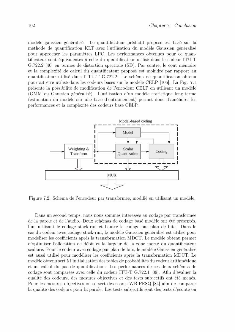
102 Chapter 7. Conclusion
modèle gaussien généralisé. Le quantificateur prédictif proposé est basé sur laméthode de quantification KLT avec l’utilisation du modèle Gaussien généralisépour approcher les paramètres LPC. Les performances obtenues pour ce quan-tificateur sont équivalentes à celle du quantificateur utilisé dans le codeur ITU-TG.722.2 [40] en termes de distortion spectrale (SD). Par contre, le coût mémoireet la complexité de calcul du quantificateur proposé est moindre par rapport auquantificateur utilisé dans l’ITU-T G.722.2. Le schéma de quantification obtenupourrait être utilisé dans les codeurs basés sur le modèle CELP [106]. La Fig. 7.1présente la possibilité de modification de l’encodeur CELP en utilisant un modèle(GMM ou Gaussien généralisé). L’utilisation d’un modèle statistique long-terme(estimation du modèle sur une base d’entraînement) permet donc d’améliorer lesperformances et la complexité des codeurs basé CELP.
MUX
Scalar Quantization
Model
Weighting & Transform Coding
Model-based coding
Figure 7.2: Schéma de l’encodeur par transformée, modifié en utilisant un modèle.
Dans un second temps, nous nous sommes intéressés au codage par transforméede la parole et de l’audio. Deux schémas de codage basé modèle ont été présentés,l’un utilisant le codage stack-run et l’autre le codage par plan de bits. Dans lecas du codeur avec codage stack-run, le modèle Gaussien généralisé est utilisé pourmodéliser les coefficients après la transformation MDCT. Le modèle obtenu permetd’optimiser l’allocation de débit et la largeur de la zone morte du quantificateurscalaire. Pour le codeur avec codage par plan de bits, le modèle Gaussien généraliséest aussi utilisé pour modéliser les coefficients après la transformation MDCT. Lemodèle obtenu sert à l’initialisation des tables de probabilités du codeur arithmétiqueet au calcul du pas de quantification. Les performances de ces deux schémas decodage sont comparées avec celle du codeur ITU-T G.722.1 [39]. Afin d’évaluer laqualité des codeurs, des mesures objectives et des tests subjectifs ont été menés.Pour les mesures objectives on se sert des scores WB-PESQ [84] afin de comparerla qualité des codeurs pour la parole. Les tests subjectifs sont des tests d’écoute où
103
l’auditeur compare la qualité des codeurs pour la parole et la musique. Plusieurs testssubjectifs ont été effectués afin de comparer le codeur de référence ITU-T G.722.1avec le codeur avec codage stack-run et celui avec codage par plan de bits. Dans le casdes mesures objectives ou pour les tests subjectifs, la qualité des codeurs proposésest meilleure que celle du codeur ITU-T G.722.1 à bas débit et est équivalente àhaut débit. La qualité du codeur avec codage stack-run est meilleure que celle aveccodage par plan de bits à bas débit et elle est équivalente à haut débit. Par contre,la complexité de calcul est plus importante car il nécessite une boucle de contrôledu débit qui est coûteuse en calcul. Les schémas de codage obtenus pourraient trèsbien être utilisés pour modifier les codeurs par transformées [55, 54, 85]. La Fig.7.2 présente la modification du schéma de codage par transformées avec l’utilisationdu modèle Gaussien généralisé. L’utilisation d’un modèle statistique court-terme(estimation du modèle en ligne sur un nombre limité de coefficients) permet doncd’améliorer la flexibilité des codeurs par transformée en leur permettant de s’adapteren temps-réel à différentes contraintes (débit, largeur de bande, retard, etc.).

104 Chapter 7. Conclusion
Publications and Patents
Publications
1. M. Oger, S. Ragot and M. Antonini, Codage basé modèle des paramètres LPCpour la compression de la paole, in Proc. Coresa, Rennes, France, November2005.
2. M. Oger, J. Bensa, S. Ragot and M. Antonini, Stack-Run Audio Coding, in120th AES convention, Preprint 6805, Paris, France, May 2006.
3. M. Oger, S. Ragot and M. Antonini, Low-complexity wideband LSF quantizationby predictive KLT coding and generalized Gaussian modeling, in Proc. Eusipco,Florence, Italy, September 2006.
4. M. Oger, S. Ragot and M. Antonini, Transform audio coding with arithmetic-coded scalar quantization and model-based bit allocation, Proc. IEEE Interna-tional Conference on Acoustics, Speech and Signal Processing (ICASSP), p. 545-548, Hawaii, USA, April 2007.
Patents
1. S. Ragot, M. Oger and M. Antonini, Codage et décodage algébrique optimisé,FR-07 53414.
2. M. Oger, T. M. N. Hoang, S. Ragot and M. Antonini, Codage/Décodage modèleplans de bits, FR-07 06001
Publications submitted
1. M. Oger, S. Ragot and M. Antonini, Model-based deadzone optimization forstack-run coding with uniform scalar quantization, Proc. IEEE InternationalConference on Acoustics, Speech and Signal Processing (ICASSP), Las Vegas,USA, April 2008.
106 Chapter 7. Conclusion
2. T. M. N. Hoang, M. Oger, S. Ragot and M. Antonini, Embedded transformcoding of audio signals by model-based bit plane coding, Proc. IEEE InternationalConference on Acoustics, Speech and Signal Processing (ICASSP), Las Vegas,USA, April 2008.
Publications to be submitted1. M. Oger, T. M. N. Hoang , S. Ragot and M. Antonini, Flexible embedded trans-
form coding of audio signals by model-based bit plane coding, will be submittedto IEEE Trans. on Signal Processing.
Bibliography
[1] ISO/IEC 11172-3. Coding of moving pictures and associated audio for digitalstorage media at up to 1.5 Mbit/s-audio part. Nov. 1993.
[2] ISO/IEC 13818-3. Information technology - Generic coding of moving picturesand associated audio information - Part 3: Audio. 1998.
[3] ISO/IEC 13818-7. Information technology - Generic coding of moving picturesand associated audio information - Part 7: Advanced Audio Coding. 2003.
[4] ISO/IEC 14496-3. Information technology - Coding of Audio-visual objects -Part 3: Audio. 2001.
[5] ISO/IEC 14496-3/Amd.1. Information technology - Coding of Audio-visualobjects - Part 3: Audio - Amd.1: Bandwidth extension. 2003.
[6] ISO/IEC 14496-3/Amd.2. Information technology - Coding of Audio-visualobjects - Part 3: Audio - Amd.2: Parametric coding for high-quality audio.2004.
[7] 3GPP TS 26.290. Audio codec processing functions; Extended Adaptive Multi-Rate - Wideband (AMR-WB+) codec; Transcoding functions. 2005.
[8] 3GPP TS 26.403. Enhanced aacPlus general audio codec; Encoder specificationAAC part. 2006.
[9] J. P. Adoul and C. Lamblin. A comparison of some algabraic structures forCELP coding of speech. Proc. IEEE International Conference on Acoustics,Speech and Signal Processing (ICASSP), pages 1953–1956, 1987.
[10] B. S. Atal and M. R. Schroeder. Predictive coding of speech and subjectiveerror criteria. IEEE Trans. Acoust. Speech, Signal Processing, ASSP-27:247–254, jun 1979.
[11] B. Bessette. Methods and devices for low-frequency emphasis during audiocompression based on acelp/tcx.
108 Bibliography
[12] B. Bessette, R. Salami, R. Lefebvre, M. Jelinek, J. Rotola-Pukkila, J. Vainio,H. Mikkola, and K. Järvinen. The Adaptative Multirate Wideband speechcodec (AMR-WB). IEEE Trans. Speech and Audio Proc., 10(8):620–636, 2002.
[13] M. Bosi, K. Brandenburg, S. Quakenbush, L. Fielder, K. Akagiri, H. Fuchs,M. Dietz, J. Herre, G. davidson, and Y. Oikawa. Iso/iec mpeg-2 AdvancedAudio Coding. Journal of the Audio Engineering Society, 45(10):789–814,1997.
[14] M. Bosi and R. E. Goldberg. Introduction to digital audio coding and standards.Kluwer Academic Publishers, 2003.
[15] K. Brandenburg. MP3 and AAC explained. Presented at the AES 17th Inter-national Conference on High Quality Audio Coding, page Preprint 23, 1999.
[16] J. Breebart, S. van de Par, A. Kohlrausch, and E. Schuijers. High-qualityparametric spatial audio coding at low bit rates. Presented at the AES 116thConvention, page Preprint 6072, 2004.
[17] J. Breebart, S. van de Par, A. Kohlrausch, and E. Schuijers. Parametric codingof stereo audio. Journal Appl. Signal Process., 9:1305–1322, 2005.
[18] ITU-R Rec BS.1116. Methods for the subjective assessment of small impair-ments in audio systems including multichannel sound systems. Oct 1997.
[19] ITU-R Rec BS.1387. Method for objective measurements of perceived audioquality. Nov 2001.
[20] ITU-R Rec BS.1534. Method for the subjective assessment of intermediatequality levels of coding systems. Jan 2003.
[21] ITU-T G.722.1 Annex C. Coding at 24 kbit/s and 32 kbit/s for Hand-freeOperations in Systems with Low Frame Loss-Annex C. 2004.
[22] P. C. Chang and R. M. Gray. Gradient algorithmes for designing predictivevector quantizers. IEEE Trans. on Acoustics Speech and Signal Proc., ASSP-34:679–690, Aug 1986.
[23] J. H. Chen and A. Gersho. Adaptive postfiltering for quality enhancement ofcoded speech. IEEE Trans. on Speech and Audio Proc., 3:59–71, jan 1995.
[24] Y. M. Cheng, D. O’Shaughnessy, and P. Mermelstein. Statisical recovery ofwideband speech from narrowband speech. IEEE Trans. on Speech and AudioProc., 2:544–548, 1992.
[25] P. Combescure and al. A 16, 24, 32 kbit/s wideband speech coding based onacelp. Proc. IEEE International Conference on Acoustics, Speech and SignalProcessing (ICASSP), 1:5–8, Mar 1999.
Bibliography 109
[26] A. Crossman. A variable bit rate audio coder for videoconferencing. IEEEworkshop on Speech and Coding for Telecommunication, pages 29–30, 1993.
[27] A. Crossman. A fixed bit rate wideband codec for uw in isdn videotelephony.IEEE workshop on Speech and Coding for Telecommunication, pages 29–30,1994.
[28] A. Dempster, N. Laird, and D. Rubin. Maximum likelihood from incompletedata via the em algorithm. JRSSB, 39(1):1–38, 1977.
[29] M. Dietz, L. Liljeryd, K. Kjörling, and O. Kunz. Spectral Band Replication,a novel approach in audio coding. Presented at the AES 112th Convention,page Preprint 5553, May 2002.
[30] P. Duhamel, Y. Mahieux, and J. P. Petit. A fast algorithm for the imple-mentation of filter bank based on time domain aliasing cancellation. Proc.IEEE International Conference on Acoustics, Speech and Signal Processing(ICASSP), pages 2209–2212, May 1991.
[31] C. Dunn. Efficient audio coding with fine-grain scalability. Presented at theAES 111th Convention, page Preprint 5492, 2001.
[32] P. Ekstrand. Bandwith extension of audio signals by Spectral Band Replica-tion. Proc. IEEE Benelux Workshop on Model based Processing and CodingAudio (MPCA-2002), pages 53–58, Nov 2002.
[33] D. Esteban and C. Galand. Application of quadrature mirror filters to splitband voice coding schemes. Proc. IEEE International Conference on Acoustics,Speech and Signal Processing (ICASSP), pages 191–195, 1977.
[34] C. Faller and F. Baumgarte. Estimation of auditory spatial cues for binauralcue coding. Proc. IEEE International Conference on Acoustics, Speech andSignal Processing (ICASSP), 2:1801–1804, 2002.
[35] ITU-T Rec G.108. Application of the E-model: A planning guide. Sept 1999.
[36] ITU-T Rec G.191. Software tools for speech and audio coding standardization.Sept 2005.
[37] ITU-T G.711. Pulse code modulation (PCM) of voice frequencies. 1988.
[38] ITU-T G.722. 7 kHz audio-coding within 64 kbit/s. 1988.
[39] ITU-T G.722.1. Coding at 24 kbit/s and 32 kbit/s for Hand-free Operations inSystems with Low Frame Loss. 1999.
[40] ITU-T G.722.2. Wideband Coding of Speech at Around 16 kbit/s using Adap-tative Multirate Wideband. 2002.
110 Bibliography
[41] ITU-T G.729.1. G.729 based Embedded Variable bit-rate coder: An 8-32 kbit/sscalable wideband coder bitstream interoperable with G.729. 2006.
[42] C. R. Galand and H. J. Nussbaumer. New quadrature mirror filter structures.IEEE Trans. Acoust. speech Signal Proc., ASP-32(3):522–530, 1984.
[43] A. Gersho. Principles of quantization. IEEE Trans. on Circuit and systems,25(7):427–436, jul. 1978.
[44] A. Gersho and V. Cuperman. Vector quantization: a pattern-matching tech-nique for speech coding. IEEE Communications Magazine, 21:15–21, Dec.1983.
[45] A. Gersho and R. M. Gray. Vector Quantization and Signal Compression.Kluwer Academic Publishers, 1993.
[46] P. Hedelin and J. Skoglund. Vector quantization based on Gaussian mixturemodels. IEEE Trans. Speech and Audio Proc., 8(4):385–401, Jul. 2000.
[47] J. Herre, K. Brandenburg, and D. Lederer. Intensity stereo coding. Presentedat the 96th AES Convention, page Preprint 3799, 1994.
[48] Y. Hiwasaki, T. Mori, H. Ohmuro, J. Ikedo, D. Tokumoto, and A. Kataoka.Scalable speech coding technology for high-quality ubiquitous communications.NTT technical review, 2(3):53–58, mar 2004.
[49] P. G. Howard and J. S. Vitter. Arithmetic coding for data compression. Pro-ceedings of the IEEE, 82(6):857–865, june 1994.
[50] F. Itakura. Line spectrum representation of linear predictive coefficients ofspeech signals. J. Acoust. Soc. Am., 57, apr. 1975.
[51] P. Jax. Enhancement of bandlimited speech signals: algorithms and theoriticalbounds. PhD thesis, Aachener Beiträge zu Digitalen Nachrichtensystemen(ABDN), 2002.
[52] P. Jax and P. Vary. Bandwidth extension of speech signals: a catalyst for theintroduction of wideband speech coding. IEEE Communications Magazine,pages 106–111, May 2006.
[53] N. S. Jayant and P. Noll. Digital Coding of Waveforms. Prentice-Hall,Inc,1984.
[54] J. D. Johnston. Perceptual transform coding of wideband stereo signals. Proc.IEEE International Conference on Acoustics, Speech and Signal Processing(ICASSP), pages 2524–2527, May 1988.
Bibliography 111
[55] J. D. Johnston. Transform coding of audio signals using perceptual noisecriteria. IEEE. Journal on Selected Areas in Communications, 6(2):314–323,Feb 1988.
[56] J. D. Johnston. Estimation of perceptual entropy using noise masking cri-teria. Proc. IEEE International Conference on Acoustics, Speech and SignalProcessing (ICASSP), pages 1993–1996, May 1989.
[57] J. D. Johnston and A. J. Ferreira. Sum-difference stereo transform coding.Proc. IEEE International Conference on Acoustics, Speech and Signal Process-ing (ICASSP), pages 23–26, Mar 1992.
[58] R. L. Joshi and T. R. Fisher. Comparison of generalized Gaussian and Lapla-cian modeling in DCT image coding. IEEE. Sign. Proc. Lett., 2(5):81–82, May1995.
[59] S. W. Kim, S. H. Park, and Y. B. Kim. Fine grain scalability in mpeg-4 audio.Presented at the AES 111th Convention, page Preprint 5491.
[60] K. Kokkinakis and A. K. Nandi. Speech modelling based on generalizedGaussian probability density functions. Proc. IEEE International Conferenceon Acoustics, Speech and Signal Processing (ICASSP), pages 381–384, 2005.
[61] S. Kullback. Information Theory and Statistics. New York: Wiley, 1959.
[62] G. G. Langdon. An introduction to arithmetic coding. IBM J. Res. Develop,28(2):135–149, mar 1984.
[63] R. Lefebvre, R. Salami, C. Laflamme, and J. P. Adoul. High quality codinf ofwideband audio signals using transform coded excitation (TCX). IEEE Acous.Speech and Signal Proc., 1:193–196, Apr 1994.
[64] J. Li. Embedded Audio Coding (eac). ACM Multimedia 2002, dec 2002.
[65] W. Li. overview of fine granularity scalability in MPEG-4 video standard.IEEE Trans. Circuits Syst. Video Technol., 11(3):301–316, mar.
[66] X. Maitre. 7 khz audio coding within 64 kbit/s. IEEE Journal on selectedareas in Communications, pages 283–298, February 1988.
[67] J. Makhoul. Linear prediction: a tutorial review. Proc. IEEE InternationalConference on Acoustics, Speech and Signal Processing (ICASSP), 63(5):561–580, Apr 1975.
[68] J. Makhoul and M. Berouti. High-frequency regeneration in speech codingsystems. Proc. IEEE International Conference on Acoustics, Speech and SignalProcessing (ICASSP), pages 428–431, Apr 1979.
112 Bibliography
[69] S. G. Mallat. A theory for multiresolution signal decomposition: The waveletrepresentation. IEEE Trans. Patt. Anal. Machine Intell., 11:674–693, jul 1989.
[70] S. G. Mallat. Analysis of low bit rate image transform coding. IEEE Trans.on Signal Proc., 46:1027–1042, apr 1998.
[71] H. S. Malvar. Lapped transforms for efficient transform/subbband coding.IEEE Trans. on Acoustics, Speech and Signal Processing, vol. 38, no. 6, pages969–978, 1990.
[72] H. S. Malvar. Signal Processing with lapped transforms. Artech House Pub-lishers, 1992.
[73] J. D. Markel and A. H. Gray. Linear Prediction of Speech. Springer-Verlag,1976.
[74] J. Mäkinen, B. Bessette, S. Bruhn, P. Ojala, R. Salami, and A. Taleb. AMR-WB+: a new audio coding standard for 3 rd generation mobile audio services.Proc. IEEE International Conference on Acoustics, Speech and Signal Process-ing (ICASSP), 2:1109–1112, May 2005.
[75] A. Moffat, R. Neal, and I. H. Witten. Arithmetic coding revisited. ACMTransactions on Information Systems, 16(3):256–294, July 1998.
[76] R. M. Neal. Fast arithmetic coding using low-precision division. UnpublishedManuscript, 1987.
[77] M. Oger, J. Bensa, S. Ragot, and M. Antonini. Stack-run audio coding. in120th AES convention, page Preprint 6805, May 2006.
[78] M. Oger, S. Ragot, and M. Antonini. Low-complexity wideband LSF quanti-zation by predictive KLT coding and generalized gaussian modeling. in Proc.Eusipco, 2006.
[79] M. Oger, S. Ragot, and M. Antonini. Transform audio coding with arithmetic-coded scalar quantization and model-based bit allocation. Proc. IEEE Inter-national Conference on Acoustics, Speech and Signal Processing (ICASSP),4:545–548, 2007.
[80] M. Oger, S. Ragot, and R. Lefebvre. Companded lattice VQ for efficientparametric LPC quantization. in Proc. Eusipco, 2004.
[81] ITU-T Rec P.800. Methods for subjective determination of transmission qual-ity. Aug. 1996.
[82] ITU-T Rec P.862. Perceptual evaluation of speech quality (PESQ): An objec-tive method for end-to-end speech quality assessment of narrow-band telephonenetworks and speech codecs. Feb 2001.
Bibliography 113
[83] ITU-T Rec P.862.1. Mapping function for transforming P.862 raw result scoresto MOS-LQO. Nov 2003.
[84] ITU-T Rec P.862.2. Wideband extension to Recommendation P.862 for theassessment of wideband telephone networks and speech codecs. Nov 2005.
[85] T. Painter and A. Spanias. Perceptual audio coding. Proc. IEEE, vol. 88,(4):451–513, 2000.
[86] K. K. Paliwal and W. B. Kleijn. Speech Coding and Synthesis. Elsevier Science,1995.
[87] A. Papoulis. Probability, random variables, and stochastic processes. Mc Graw-Hill, 1965.
[88] C. Parisot. Allocation basées modèles et transformée en ondelettes au fil del’eau pour le codage d’images et de vidéos. PhD thesis, Université de Nice-Sophia Antipolis, 2003.
[89] C. Parisot, M. Antonini, and M. Barlaud. 3d scan based wavelet transformand quality control for video coding. EURASIP, 2003(1):521–528, Jan 2003.
[90] S. H. Park, Y. B. Kim, S. W. Kim, and Y. S. Seo. Multi-layer bit-sliced bit-ratescalable audio coding. Presented at the AES 103rd Convention, page Preprint4520, aug 1997.
[91] W. B. Pennebaker and J. L. Mitchell. Probability estimation for the q-coder.IBM J. Res. Develop, 32(6):737–752, nov 1988.
[92] W. B. Pennebaker, J. L. Mitchell, G. G. Langdon, and R. B. arps. An overviewof the basic principles of the q-coder adaptive binary arithmetic coder. IBMJ. Res. Develop, 32(6):717–726, nov 1988.
[93] ITU-T Rec P.OLQA. Objective Listening Quality Assessment. In progress.
[94] ITU-T Rec P.ONRA. Objective Noise Reduction Assessment. In progress.
[95] C. Pépin, P. Raffy, and R. M. Gray. Robust stack-run coding for low bit-rateimage transmission over noisy channels. IEEE Signal Proc. Letters, 9(7):196–199, jul 2002.
[96] J. Princen, A. W. Johnston, and A. Bradley. Subband/transform coding usingfilter bank designs based on time domain cancellation. Proc. IEEE Interna-tional Conference on Acoustics, Speech and Signal Processing (ICASSP), pages2161–2164, 1987.
[97] S. Ragot and al. ITU-T G.729.1: an 8-32 kbit/s scalable coder interoperablewith G.729 for wideband telephony and voice over IP. Proc. IEEE Inter-national Conference on Acoustics, Speech and Signal Processing (ICASSP),4:529–532, May 2007.
114 Bibliography
[98] S. Ragot, B. Bessette, and R. Lefebvre. Low-complexity multi-rate latticevector quantization with application to wideband speech coding at 32 kbit/s.Proc. IEEE International Conference on Acoustics, Speech and Signal Process-ing (ICASSP), 1:501–504, May 2004.
[99] S. Ragot, H. Lahdili, and R. Lefebvre. Wideband LSF quantization by gener-alized Voronoi codes. Proc. Eurospeech, pages 2319–2322, Sep. 2001.
[100] R. A. Redner and H. F. Walker. Mixture densities, maximum likelihood andthe em algorithm. SIAM Rev., vol. 26, no. 2, pages 195–239, 1984.
[101] A. Said and W. A. Pearlman. A new, fast, and efficient image codec basedon set partitioning in hierarchical trees. Proc. IEEE Trans. Circuits and sys.Video Tech., 6:243–250, June 1996.
[102] R. Salami, C. Laflamme, and J. P. Adoul. Acelp speech coding at 8 kbit/s witha 10 ms frame: a candidate for ccitt standardization. Proc. IEEE Workshopon Speech Coding for Telecommunications, pages 23–24, Oct 1993.
[103] D. Salomon. Data Compression: The Complete Reference. Springer, 2004.
[104] J. Samuelsson. Towards Asymptotic Vector Quantization. PhD thesis, Schoolof Electrical and Computer Engineering, Chalmers University of Technology,2001.
[105] J. Samuelsson. Waveform quantization of speech using Gaussian mixture mod-els. Proc. IEEE International Conference on Acoustics, Speech and SignalProcessing (ICASSP), 1:165–168, 2004.
[106] M. R. Schroeder and B. S. Atal. Code-Excited Linear Prediction (CELP):High-quality speech at very low bit rates. Proc. IEEE International Conferenceon Acoustics, Speech and Signal Processing (ICASSP), pages 937–940, 1985.
[107] E. Schuijers, J. Breebaart, H. Purnhagen, and J. Engdegård. Low complexityparametric stereo coding. Presented at AES 114th Convention, page Preprint6073, May 2004.
[108] E. Schuijers, W. Oomen, B. den Brinker, and J. Breebaart. Advances inparametric coding for high-quality audio. Presented at AES 114th Convention,page Preprint 5852, Mar 2003.
[109] J. M. Shapiro. Embedded image coding using zerotrees of wavelet coefficients.IEEE Trans. Signal Processing, 41:3445–3462, Dec 1993.
[110] J. K. Su and R. M. Mersereau. Coding using Gaussian mixture and generalizedGaussian models. Proc IEEE Int. Conf Image Processing (ICIP), 1:217–220,sep 1996.
Bibliography 115
[111] A. D. Subramaniam. Gaussian mixture models in Compression and Commu-nication. PhD thesis, University of California, San Diego, 2003.
[112] A. D. Subramaniam, W. R. Gardner, and B. D. Rao. Low-complexity sourcecoding using Gaussian mixture models, lattice vector quantization, and recur-sive coding with application to speech spectrum quantization. IEEE Trans.on Audio, Speech and Language Proc., 14(2):524–532, mar 2006.
[113] A. D. Subramaniam and B. D. Rao. Pdf optimized parametric vector quan-tization of speech line spectral frequencies. IEEE Trans. Speech and AudioProc., 11(2):130–142, mar 2003.
[114] G. J. Sullivan. Efficient scalar quantization of exponential and laplacian ran-dom variables. IEEE Trans. on Information Theory, 42(5):1365–1374, sept1996.
[115] ITU-T T.82. Information technology - coded representation of picture andaudio information - progressive bi-level image compression. 1993.
[116] L. Tancerel, S. Ragot, V. T. Ruoppila, and R. Lefebvre. Combined speech andaudio coding by discrimination. IEEE Workshop on Speech Coding,, pages154–156, Sept 200.
[117] M. Tasto and P. A. Wintz. Image coding by adaptive block quantization.IEEE Trans. on Comm. Tech., 19(6):957–972, dec 1971.
[118] D. Taubman, E. Ordentlich, M. Weinberger, G. Serouss, I. Ueno, and F. Ono.Embedded block coding in jpeg2000. Proc. IEEE International Conference onImage Processing (ICIP), 2:33–36, sept 2000.
[119] D. S. Taubman and M. W. Marcellin. JPEG2000: Image Compression Fun-damentals, Standards and Practice. Springer, 2001.
[120] D. S. Taubman and M. W. Marcellin. Jpeg2000: standard for interactiveimaging. Proc. IEEE, 90(8):1336–1357, aug 2002.
[121] M. J. Tsai, J. D. Villasenor, and F. Chen. Stack-run coding for low bit rateimage communication. in Proc. ICIP.
[122] M. J. Tsai, J. D. Villasenor, and F. Chen. Stack-Run image coding. IEEETrans. Circuits Syst. Video Technol., 6:519–521, oct 1996.
[123] P. P. Vaidyanathan. Quadrature mirror filter, m-band extensions and perfect-reconstruction techniques. IEEE ASSP Magazine, pages 4–20, 1987.
[124] I. Varga. On new audio codec specification. IEEE 8th Workshop on MultimediaSignal Proc., pages 128–131, oct 2006.
116 Bibliography
[125] J. Villasenor, M. J. Tasai, and F. Chen. Method for reducing storage require-ments for digital data.
[126] I. H. Witten, R. M. Neal, and J. G. Cleary. Arithmetic coding for data com-pression. Communications of the ACM, 30:520–540, June 1987.
[127] M. Wolters, K. Kjörling, and H. Purnhagen. A closer look into MPEG-4 HighEfficiency AAC. Presented at the AES 115th Convention, page Preprint 5871,Oct 2003.
[128] M. Xie, D. Lindbergh, and P. Chu. From ITU-T G.722.1 to ITU-T G.722.1 an-nex c: anew low-complexity 14 khz bandwidth audio coding standard. Journalof Multimedia, 2(2):65–76, April 2007.
[129] D. Y. Zhao. Model based speech enhancement and coding. PhD thesis, Schoolof Electrical Engineering KTH, Stockholm, 2007.