Embed Size (px)
Citation preview
CCEENNTTEERR FFOORR TTHHEE SSIIMMUULLAATTIIOONN OOFF
AACCCCIIDDEENNTTAALL FFIIRREESS && EEXXPPLLOOSSIIOONNSS
--VVAALLIIDDAATTIIOONN TTEEAAMM--
FFFAAASSSTTT CCCOOOOOOKKKOOOFFFFFF TTTEEESSSTTTSSS RRREEEPPPOORRRTTTO
PPrreeppaarreedd bbyy
William Ciro
RReevviisseedd bbyy
Eric Eddings & Adel Sarofim
Salt Lake City, October 28, 2003
TTAABBLLEE OOFF CCOONNTTEENNTTSS
NOMENCLATURE ......................................................................................................... VI
INTRODUCTION .............................................................................................................. 8
EXPERIMENTAL.............................................................................................................. 9
CSAFE COOKOFF EXPERIMENTS................................................................................ 9
2.1 FIRE COOKOFF TEST - TR11566 NOVEMBER 1998............................................. 9
2.1.1 TEST DESCRIPTION............................................................................................... 9
2.1.2 EXPLOSIVE MATERIAL ...................................................................................... 10
2.1.3 STEEL CONTAINER ............................................................................................. 11
2.1.4 TEST CONFIGURATION ...................................................................................... 13
2.1.5 INSTRUMENTATION ........................................................................................... 13
2.1.6 DISCUSSION.......................................................................................................... 16
2.2. FIRE COOKOFF TESTS – TR11996 OCTOBER 1999........................................... 18
2.2.1. TEST MATERIALS ............................................................................................... 18
2.2.2. STEEL CONTAINER ............................................................................................ 19
2.2.3. TEST CONFIGURATION ..................................................................................... 19
2.2.4. INSTRUMENTATION .......................................................................................... 20
2.2.5. EXPERIMENTAL RESULTS................................................................................ 23
2.2.5.1. TEST 1, INERT MATERIAL, OCTOBER 4, 1999............................................ 24
2.2.5.2. TEST 2, EXPLOSIVE MATERIAL, OCTOBER 7, 1999.................................. 25
2.2.5.3. TEST 3, EXPLOSIVE MATERIAL, OCTOBER 7, 1999.................................. 27
2.2.5.4. TEST 4, EXPLOSIVE MATERIAL, OCTOBER 25, 1999................................ 29
2.2.5.5. TEST 5, EXPLOSIVE MATERIAL, OCTOBER 28, 1999................................ 32
2.3 ELECTRICAL COOKOFF TESTS............................................................................ 34
2.3.1 INTRODUCTION ................................................................................................... 34
2.3.2 DISCUSSION.......................................................................................................... 35
2.3.3 HYDROSTATIC PRESSURE TEST...................................................................... 36
2.3.4 PRESSURE TRANSDUCER CHARACTERIZATION......................................... 36
2.3.5 HYDROBURST TEST #1 – 2002........................................................................... 37
2.3.5.1 INSTRUMENTATION BACKGROUND ........................................................... 38
2.3.5.2 EXPERIMENTAL................................................................................................ 38
2.3.5.3 OBSERVATIONS ................................................................................................ 38
2.3.5.4 RESULTS AND CONCLUSIONS....................................................................... 39
2.3.6 TEST 6, ELECTRICAL, JULY 2001...................................................................... 39
2.3.7 TEST 7, ELECTRICAL, AUGUST 2001 ............................................................... 41
2.3.8 TEST 8, ELECTRICAL, SEPTEMBER 2002 ........................................................ 44
2.3.9 TEST 9, ELECTRICAL, NOVEMBER 2002 ......................................................... 45
2.3.10 TEST 10, ELECTRICAL, NOVEMBER 2002 ..................................................... 46
NUMERICAL ANALYSIS.............................................................................................. 49
DATA ANALYSIS........................................................................................................... 49
3.1. DUHAMEL SUPERPOSITION INTEGRAL........................................................... 49
3.2. INVERSE HEAT CONDUCTION METHOD ......................................................... 50
3.3. THERMAL REACTION MODEL............................................................................ 52
3.4. THERMOPHYSICAL PROPERTIES....................................................................... 56
3.4.1. STEEL..................................................................................................................... 56
3.4.2. PBX-9501 ............................................................................................................... 58
3.4.3. AIR.......................................................................................................................... 59
iii
RESULTS AND DISCUSSION....................................................................................... 61
4.1. FIRE TESTS .............................................................................................................. 61
4.1.1. TEST 1, EXPLOSIVE MATERIAL, NOVEMBER 1998 ..................................... 61
4.1.2. TEST 2, EXPLOSIVE MATERIAL, OCTOBER 1999......................................... 64
4.1.3. TEST 3, EXPLOSIVE MATERIAL, OCTOBER 1999......................................... 66
4.1.4. TEST 4, EXPLOSIVE MATERIAL, OCTOBER 1999......................................... 68
4.1.5. TEST 5, EXPLOSIVE MATERIAL, OCTOBER 9, 1999..................................... 68
4.1.6. THE FIRE TESTS AND THE IGNITION MODEL.............................................. 71
4.2. ELECTRICAL TESTS .............................................................................................. 72
4.2.1. TEST 6, ELECTRICAL, JULY 2001..................................................................... 72
4.2.2. TEST 7, ELECTRICAL, AUGUST 2001 .............................................................. 73
4.2.3. TEST 8, ELECTRICAL, SEPTEMBER 2002 ....................................................... 75
4.2.4. TEST 9, ELECTRICAL, NOVEMBER, 2002 ....................................................... 76
4.2.5. TEST 10, ELECTRICAL, NOVEMBER, 2002 ..................................................... 79
4.2.6. THE IGNITION MODEL AND THE ELECTRICAL COOKOFF TESTS .......... 81
CONCLUDING REMARKS............................................................................................ 83
REFERENCES ................................................................................................................. 85
APPENDIX A AND OTHER FILES INCLUDED IN THE CD ..................................... 87
APPENDIX B ................................................................................................................... 88
PLOTS, TEST 1, FIRE, NOVEMBER 1998.................................................................... 89
PLOTS, TEST 2, FIRE, OCTOBER 1999 ....................................................................... 98
PLOTS, TEST 3, FIRE, OCTOBER 1999 ..................................................................... 103
PLOTS, TEST 4, FIRE, OCTOBER 1999 ..................................................................... 106
PLOTS, TEST 5, FIRE, OCTOBER 1999 ..................................................................... 109
iv
PLOTS, TEST 6, ELECTRICAL, JULY 2002............................................................... 114
PLOTS, TEST 7, ELECTRICAL, AUGUST 2001 ........................................................ 117
PLOTS, TEST 8, ELECTRICAL, SEPTEMBER 2002 ................................................. 124
PLOTS, TEST 9A, ELECTRICAL, NOVEMBER 2002............................................... 130
PLOTS, TEST 9B, ELECTRICAL, NOVEMBER 2002 ............................................... 134
PLOTS, TEST 10, ELECTRICAL, NOVEMBER 2002................................................ 140
v
NOMENCLATURE
A ..............Area of the cylinder in m2 or Compound A
B ...............Compound B
C ..............Compound C
Cp ..............Heat capacity, J/Kg K
D ..............Compound D
Ea .............Energy of activation, J/kg K
K ..............Thermal conductivity, W/m K
k ...............Rate constant, 1/s.
LAir.............Air gap width, m
m ...............Mass fraction of A, B, C or D.
n.................Dummy variable in Eq. (3.10) and (3.11).
Q ..............Heat of reaction per unit mass, J/kg
q ...............Heat flux, W/m2
RH ............Resistance of the heater, Ohms
Rg .............Universal constant for gases, J/mol K
RE ..............Temperature measurement location, m
Ri .............Inner radius of the PBX-9501 pellet, m
RPBX .........Outer radius of the PBX-9501 pellet, m
RSteel, ..........Outer radius of the steel pipe, m
r ...............Radial position, m
rE ..............Thermocouple location, m
S ..............Rate of heat generation per unit volume, W/m3
s ...............Dummy variable in Eq. (3.2)
T ..............Temperature, K
t ...............Time, s.
V ..............Voltage, Volts.
Z ..............Pre-exponential factor, s-1
Greek symbols α ..............Thermal diffusivity, m2/s
vi
α1 ..............Thermal expansion coefficients of steel, 1/K
α2 .............Thermal expansion coefficients of steel, 1/K2
β1 .............Thermal expansion coefficient of PBX-9501, 1/K
ρ ............... Density, Kg/m3
Subscripts Air ............ Air
E ..............Temperature Measurement location
g ...............Gas
I ...............Inner radius
i ...............Spatial index
j ................ Reaction number
o ...............Initial condition
PBX .........PBX material
s ...............Solid
Steel .........Steel material
vii
IINNTTRROODDUUCCTTIIOONN The Center for the Simulation of Accidental Fires and Explosions (C-SAFE) at the
University of Utah is focused on providing science-based tools for the numerical
simulation of accident scenarios involving fires and high-energy devices (Pershing,
2000).
The initial computational efforts are concentrated in a well-defined scenario in which a
steel pipe filled with conventional explosives is exposed to a hydrocarbon fire. An
example of this would be a high explosive material within a bomb or missile engulfed in
an intense jet-fuel fire after an airplane crash. This is a complex combination of processes
for which there is limited detailed information available on the coupled processes for use
in validating a computer simulation. The CSAFE validation efforts are focused on those
processes in which more physical understanding is needed (Eddings and Sarofim, 1999).
One of the validation tasks is concerned with the thermal behavior of high-energy devices
engulfed in a pool fire. This scenario, better known as cookoff, will be studied in
conjunction with Thiokol Corporation.
This report will provide detailed information on the efforts and accomplishments of the
CSAFE Validation team.
8
EEXXPPEERRIIMMEENNTTAALL A good description of the cookoff experiments is presented.
CCSSAAFFEE CCOOOOKKOOFFFF EEXXPPEERRIIMMEENNTTSS
The University of Utah contracted Thiokol Propulsion Company to run some
experimental work regarding fires and explosions. For this purpose, a series of fast
cookoff experiments were carried out considering two experimental conditions. The first
one was the typical fuel fire cook off (i.e. variable heat flux). The fuel was propane and it
will be referred in this report as the fire test. The second condition consisted of supplying
a constant heat flux on the surface of the container. This will be referred as the electrical
test.
This chapter is based on the information provided by Thiokol Propulsion Company in
reports TR11996 and TR12646.
22..11 FFIIRREE CCOOOOKKOOFFFF TTEESSTT -- TTRR1111556666 NNOOVVEEMMBBEERR 11999988
This section is based on the information provided by Thiokol Propulsion Company in
Report TR11566, C-SAFE Cook-Off Test #1.
22..11..11 TTEESSTT DDEESSCCRRIIPPTTIIOONN
The requirements of this test were rather arbitrary at first and the final design was a
consensus of opinions of both the University of Utah and Thiokol. We decided that a
cylindrical container would be used containing an HMX formulation. The fire box would
be rectangular and the flame provided by propane burners. The HMX formulation would
be PBXC-123 and the weight would be 8 lbs. It was decided to make the container out of
Schedule 40 steel pipe 4 in. in diameter and 12 in. long. Threaded end caps would also be
supplied. The explosive material would be cast in the pipe with a 1.5 in. diameter air
9
core. The weight of the material was 7.6 lbs. The test was conducted at Hazards Testing
Team’s T-75 facility.
22..11..22 EEXXPPLLOOSSIIVVEE MMAATTEERRIIAALL
The explosive formulation used in the C-SAFE cook-off test is designated as C-SAFE-7
and is described in Table 2.1. The safety properties of the cured and uncured explosive
are listed in Table 2.2 and show that the formulation is relatively insensitive to impact,
friction, ESD (electrostatic discharge), and heat. This 83% HMX castable formulation
used a liquid HTPB (hydroxyl terminated polybutadiene) polymer (R-45M) that was
crosslinked during an elevated-temperature cure by the IPDI (isophorone diisocyanate),
with the TPB (triphenyl bismuth) cure catalyst to speed the cure reactions. The DOA
plasticizer and lecithin were used to aid processing.
This formulation is similar to the military formulation PBXC-123, but has a higher level
of DOA with respect to R-45M polymer as well as the added lecithin to enhance
processing. The original plan was to make the PBXC-123 formulation, but the specified
HMX particle sizes were not available at Thiokol to do this. The HMX particle sizes that
were used in the final formulation were chosen from available lots, and the particle size
distribution was selected by varying the ratio of different HMX lots in a series of small
mixes to find the combination that produced the best processing. Even with this work
and the additional plasticizer and lecithin, the formulation had a high mix viscosity.
After processing the formulation in ¼ pint and pint mixes and characterizing the safety,
cure and processing characteristics of the formulation, the formulation was made in a
one-gallon mix for casting into the test article. Because of the high viscosity, the one-
gallon mix was not cast under vacuum through a slit plate as is normally done to remove
entrapped air. Instead, the explosive was packed by hand into the test article. With
vibration, the explosive flowed easily around the thermocouple wires. Because of the
time constraint for conducting the cook-off test, an accelerated cure was used with the
cure temperature being set to 341 K (155 ˚F) for one day and 347 K (165 ˚F) for two
days, significantly higher than the normal cure temperature of 330 K (135 ˚F). After 3
days of cure, the test article was removed from the oven and allowed to cool before the
removal of the Teflon core. The explosive was not fully cured after the three-day cure
10
and was quite soft, although hard enough to retain its shape and not tear during the core
removal. The data from the small mixes show that 5 to 7 days were required for a full
cure.
Table 2.1. C-SAFE-7 Explosive Formulation and Theoretical Performance
Ingredient Percent Weight
HMX (Coarse) 55.00
HMX (57 micron) 15.00
HMX (5 micron) 13.00
R-45M 7.52
DOA 8.12
Lecithin 0.70
IPDI 0.62
TPB 0.04
Theoretical Performance Density (g/cc) 1.623
Detonation Velocity (km/s) 7.33
CJ Pressure (kbar) 2.14
Total Cylinder Expansion Energy (kJ/cc) 8.30
Table 2.2. Safety Data for C-SAFE-7 Explosive Formulation
Safety Test Uncured Cured
ABL Impact (cm) 80 80
TC Impact (in) >46 >46
ABL Friction (psi) 800 @ 8 ft/sec 800 @ 8 ft/sec
TC Friction (lb) >64 63
TC ESD (J) 7.19 >8
SBAT (simulated bulk autoignition) onset (˚C) 154 157
22..11..33 SSTTEEEELL CCOONNTTAAIINNEERR
Four-inch Schedule 40 steel pipe was used for the container. The air core of the
explosive was 1.5 in., leaving the 1.75-in. explosive web. The length of the container
11
was chosen to be 12 in. The ends of the pipe were threaded and threaded end caps were
machined to fit. The end caps each had a hole drilled in the center to allow for a pressure
port/vent and access for the thermocouples. A pressure port was also installed in the
center of the cylinder. The design of the cylinder is shown in Figures 2.1 and 2.2.
Figure 2.1 Explosive Cylinder
Figure 2.2 Explosive Cylinder End Caps
12
22..11..44 TTEESSTT CCOONNFFIIGGUURRAATTIIOONN
The test configuration is shown schematically in Figure 2.3. The cylindrical container
was suspended from an A-frame with chains with six propane burners positioned
beneath. The burners were surrounded by thin aluminum sheet metal about two in. off
the ground which acted as a wind break and air intake. The thermocouple wires were all
bundled together and wrapped with RTV tape exiting one end of the cylinder. The other
end of the cylinder was connected by a tee to ¼-in. stainless tubing on one side, and a
vent on the other side of the tee. The tubing was connected to a pressure transducer
which measured the pressure in the core of the explosive. The port in the middle of the
cylinder was also connected to a pressure transducer by ¼-in. tubing and measured the
pressure of the explosive/case interface. The propane gas supply pressure was adjusted to
5 psi. At this pressure, temperature on the outside of the cylinder was 755 to 811 K (900
to 1000 ˚F).
22..11..55 IINNSSTTRRUUMMEENNTTAATTIIOONN
The cook-off test was instrumented with two 1000 psi Taber model 206 pressure
transducers and 14 type K thermocouples. The pressure transducers measured the
pressure in the air space in the middle of the explosive and at the interface of the
explosive steel case. The air space was not sealed as it vented to the outside atmosphere.
The thermocouples were placed according to Figure 2.4. Four were spot welded to the
outside of the case, four were spot welded to the inside of the case, four were placed at
various points in the explosive itself, and two were placed in the air space in the center of
the explosive. X-rays were taken of the cylinder loaded with the explosive and
instrumentation prior to the test to verify the exact location of the thermocouples. In the
process of loading the explosive we were concerned that the thermocouples may have
been misplaced from their intended location. Table 2.3 summarizes the measurements.
Originally, we planned to have four more thermocouples placed in the propane flame on
the outside of the cylinder, but there weren’t enough data collection channels to
accommodate these extra thermocouples and they were not used. The pressure data and
thermocouple data were acquired digitally and the twelve thermocouples were backed up
13
Figure 2.3 Test configuration
Figure 2.4 Thermocouple Locations in Explosive Cylinder
14
Table 2.3 C-SAFE Instrumentation List, Test #1
Identifier Description Location Range
T001 Thermocouple 4” from chamber and same elevation as chamber axis in flame 0-2000ºF
T002 Thermocouple 4” from chamber and same elevation as chamber axis in flame (opposite side from T001)
0-2000ºF
T003 Thermocouple 4” from chamber on pressure tap end 0-2000ºF
T004 Thermocouple 4” from chamber on instrumentation feed-through end 0-2000ºF
T005 Thermocouple Outside bottom of chamber as shown on Drawing I10-98022 0-1000ºF
T006 Thermocouple Inside bottom of chamber as shown on Drawing I10-98022 0-1000ºF
T007 Thermocouple In explosive on bottom side of chamber as shown in Drawing I10-98022
0-1000ºF
T008 Thermocouple In explosive on bottom side of chamber as shown in Drawing I10-98022
0-1000ºF
T009 Thermocouple Outside side of chamber as shown on Drawing I10-98022 0-1000ºF
T010 Thermocouple Inside side of chamber as shown on Drawing I10-98022 0-1000ºF
T011 Thermocouple In explosive on side of chamber as shown in Drawing I10-98022 0-1000ºF
T012 Thermocouple In explosive on side of chamber as shown in Drawing I10-98022 0-1000ºF
T013 Thermocouple Outside top of chamber as shown on Drawing I10-98022 0-1000ºF
T014 Thermocouple Inside top of chamber as shown on Drawing I10-98022 0-1000ºF
T015 Thermocouple Outside bottom of chamber as shown on Drawing I10-98022 0-1000ºF
T016 Thermocouple Inside bottom of chamber as shown on Drawing I10-98022 0-1000ºF
T017 Thermocouple Bore, on axis in line with T005 0-1000ºF
T018 Thermocouple Bore, on axis in line with T015 0-1000ºF
P001 Pressure Transducer
Pressure in explosive bore 0-1000 psi
P002 Pressure Transducer
Pressure at explosive/case interface 0-1000 psi
Camera 1 IR Image Side with chamber just filling view 0-1000ºF
Camera 2 Test Monitor End view of chamber covering 20 feet side-to-side
Camera 3 Test Monitor Side view of chamber covering 20 feet side-to-side
with an FM Wideband I tape recorder. The thermocouples were conditioned with Analog
Devices amplifiers. In addition to the instrumentation described above, an IR camera
was used to monitor the infrared emission of the test. Video recordings of the cook-off
were made from two different angles.
15
22..11..66 DDIISSCCUUSSSSIIOONN
The cook-off test was set up as described above. The weather conditions at the time of
the test were:
Ambient temperature – 59 ˚F Relative Humidity – 48%
Wind was from the West at 7 mph
The propane valve was opened and the propane was ignited using a nichrome wire heated
by electrical current to ignite a small piece of solid rocket propellant. At approximately
106 s into the burn, the explosive ignited and the steel cylinder exploded. The cylinder
ruptured uniformly along a line opposite the seam and peeled back around the end caps.
The cylinder held by the chains made one revolution around the cross arm of the A-
frame. Explosive material was ejected from the cylinder and scattered on the ground
around the test site. We estimated that about one third of the material ignited in the
cylinder, one third burned on the ground, and the rest was not burned.
Data from the instrumentation were collected at a rate of 50 Hz. One of the
thermocouples, T006, located on the inside of the steel cylinder near the center, failed 20
s into the run. The pressure transducers were arranged to monitor the inside bore and the
explosive/case interface. Both were ranged to 1000 psi. They both recorded no pressure
increase until the explosive ignited and then both overranged in excess of 1000 psi.
The thermocouple measurements showed some interesting results. Those in the
explosive material ranged from 294 K (70˚F) to 297 K (75˚F) just prior to the ignition.
This is an average of ten measurements of 200 ms just prior to ignition. These are
thermocouples T007, T008, T011, and T012. This shows that inside the explosive
material the temperatures were not elevated.
The two thermocouples inside the bore showed a significant difference. Thermocouple
T017, at the center of the cylinder, remained at about 300 K (80˚F) until near the end and
then the last 200 ms averaged 348 K (167˚F) and was increasing to a maximum of 398 K
(258˚F) just prior to the ignition. T018, about one-fourth of the way from the end
remained between 300 K (80˚F) and 310 K (100˚F) until near the end and then the last
16
200 ms averaged 438 K (330˚F) and was increasing to a maximum for 522 K (481˚F) just
prior to the ignition.
The four thermocouples on the outside of the cylinder were also significantly different.
T005, on the bottom, in the center of the cylinder, averaged 653 K (716˚F) just prior to
the ignition. T009, on the side, in the center of the cylinder, averaged 500 K (442˚F) just
prior to the ignition. T014, on the top center of the cylinder, averaged 758 K (905˚F) just
prior to ignition. T015, on the bottom, ¼-in from the end, averaged 667 K (741˚F) just
prior to ignition, which agreed well with T005, the other bottom thermocouple. It is
interesting to note that the highest temperature was at the top of the cylinder and the side
temperature was between the top and bottom temperatures.
The three remaining thermocouples were on the inside of the cylinder between the case
and the explosive. T010, on the side, in the center of the cylinder averaged 583 K
(591˚F) just prior to ignition. T013, on the top center, averaged 444 K (340˚F) just prior
to ignition. T016, on the bottom, ¼-in from the end, averaged 430 K (314˚F) just prior to
ignition.
Another interesting result to note is that the outside, side, center measurement was 500 K
(442˚F) while the inside, side, center measurement was 583 K (591˚F). This could
possibly have been the effect of the wind blowing from the side.
Some of the differences noted in the thermocouple measurements could be caused by the
thermocouple not being in the location where it was placed. Movement could have
occurred when the explosive was cast in the cylinder. X-rays taken of the cylinder prior
to the test were not definitive. It was very difficult to see the small wires behind the ¼-in
wall of the cylinder.
The IR camera was positioned about 100 yards away from the test setup and focused on
the top of the cylinder. Because of the distance and the uncertainty in emissivity of the
cylinder the measurement was not as accurate as one would want. However, there was a
fairly good agreement with the thermocouple measurements assuming an emissivity of
0.6.
17
22..22.. FFIIRREE CCOOOOKKOOFFFF TTEESSTTSS –– TTRR1111999966 OOCCTTOOBBEERR 11999999
Five fast cookoff tests were carried out in 1999, one with an inert material and the other
four with explosive material. Six propane burners supplied the heat to ignite the
materials.
22..22..11.. TTEESSTT MMAATTEERRIIAALLSS
The materials were prepared by Los Alamos National Laboratory. The materials were
machined into pellets of 4-inches in diameter and 4-inches thick with a 1-inch diameter
hole through the center. The pellet dimensions are shown in Figure 2.5. The
composition of the inert material and explosive are shown in Table 2.4 and Table 2.5
respectively.
Table 2.4. Composition of Inert Material
Material Analysis, % Nominal, %
Barium Nitrate 45.28 44.65
Pentek 48.93 49.35
Estane 2.86 3.00
BDNPA/F 2.93 3.00
Table 2.5. Composition of the Explosive
Material Percent Weight
HMX 95.00
Estane 2.50
BDNPA/F 2.50
18
ID 1.000
OD 4.020/3.995
4.020/ 3.995
ID 1.000ID 1.000
OD 4.020/3.995
4.020/ 3.995
OD 4.020/3.995
4.020/ 3.995
ID 1.000
Figure 2.5. Drawing of test material pellets (all dimensions in inches).
Three pellets were used for each test, making the overall material 4 inches in diameter
and 12 inches long. For both materials, Estane and BDNPA/F were used as binder to hold
the material together. These same binder materials were used to cement the pellets
together before they were inserted into the cylindrical container.
22..22..22.. SSTTEEEELL CCOONNTTAAIINNEERR
Four-inch, Schedule 40 steel pipe was used for the container. The length of the container
was chosen to be 12 inches. The ends of the pipe were threaded, and threaded end caps
were machined to fit. One end cap was solid, and the other end cap had a hole drilled in
the center to allow the instrumentation wires to exit the container. A 1/2-inch diameter
stainless steel tube, about 4 feet long, was connected to the end cap. The instrumentation
wires coming from the inside of the cylinder passed through the tube, and the outside
wires were tied to the tube.
22..22..33.. TTEESSTT CCOONNFFIIGGUURRAATTIIOONN
Photographs of the test configuration are shown in Figures 2.6 and 2.7. For each test, the
cylindrical container was suspended from an A-frame over chains with six propane
burners positioned beneath. The burners were surrounded by thin aluminum sheet metal
18 inches high and about 2 inches off the ground that acted as a wind break and air
19
intake. The propane gas supply pressure was adjusted to 12 psi. We attempted to measure
the actual flow rate of the propane but could not find a suitable flow meter.
Figure 2.6. Photograph of the test configuration
Figure 2.7. Close up photograph of container, burners and wind screen
22..22..44.. IINNSSTTRRUUMMEENNTTAATTIIOONN
The first test was instrumented with 24 type-K thermocouples, 12 on the inside and 12 on
the outside. The thermocouples were placed according to Figure 2.8. The inside
thermocouples were 30 AWG and were placed at the interface of the test material and the
20
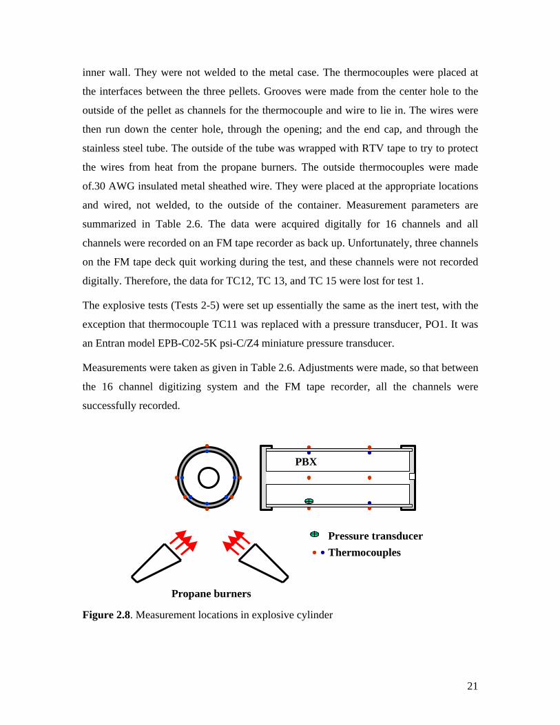
inner wall. They were not welded to the metal case. The thermocouples were placed at
the interfaces between the three pellets. Grooves were made from the center hole to the
outside of the pellet as channels for the thermocouple and wire to lie in. The wires were
then run down the center hole, through the opening; and the end cap, and through the
stainless steel tube. The outside of the tube was wrapped with RTV tape to try to protect
the wires from heat from the propane burners. The outside thermocouples were made
of.30 AWG insulated metal sheathed wire. They were placed at the appropriate locations
and wired, not welded, to the outside of the container. Measurement parameters are
summarized in Table 2.6. The data were acquired digitally for 16 channels and all
channels were recorded on an FM tape recorder as back up. Unfortunately, three channels
on the FM tape deck quit working during the test, and these channels were not recorded
digitally. Therefore, the data for TC12, TC 13, and TC 15 were lost for test 1.
The explosive tests (Tests 2-5) were set up essentially the same as the inert test, with the
exception that thermocouple TC11 was replaced with a pressure transducer, PO1. It was
an Entran model EPB-C02-5K psi-C/Z4 miniature pressure transducer.
Measurements were taken as given in Table 2.6. Adjustments were made, so that between
the 16 channel digitizing system and the FM tape recorder, all the channels were
successfully recorded.
Pressure transducer Thermocouples
Propane burners
PBX
Figure 2.8. Measurement locations in explosive cylinder
21
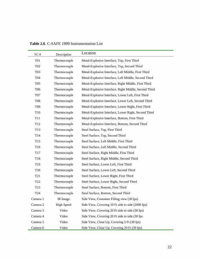
Table 2.6. C-SAFE 1999 Instrumentation List
TC # Description Location
T01 Thermocouple Metal-Explosive Interface, Top, First Third
T02 Thermocouple Metal-Explosive Interface, Top, Second Third
T03 Thermocouple Metal-Explosive Interface, Left Middle, First Third
T04 Thermocouple Metal-Explosive Interface, Left Middle, Second Third
T05 Thermocouple Metal-Explosive Interface, Right Middle, First Third
T06 Thermocouple Metal-Explosive Interface, Right Middle, Second Third
T07 Thermocouple Metal-Explosive Interface, Lower Left, First Third
T08 Thermocouple Metal-Explosive Interface, Lower Left, Second Third
T09 Thermocouple Metal-Explosive Interface, Lower Right, First Third
T10 Thermocouple Metal-Explosive Interface, Lower Right, Second Third
T11 Thermocouple Metal-Explosive Interface, Bottom, First Third
T12 Thermocouple Metal-Explosive Interface, Bottom, Second Third
T13 Thermocouple Steel Surface, Top, First Third
T14 Thermocouple Steel Surface, Top, Second Third
T15 Thermocouple Steel Surface, Left Middle, First Third
T16 Thermocouple Steel Surface, Left Middle, Second Third
T17 Thermocouple Steel Surface, Right Middle, First Third
T18 Thermocouple Steel Surface, Right Middle, Second Third
T19 Thermocouple Steel Surface, Lower Left, First Third
T20 Thermocouple Steel Surface, Lower Left, Second Third
T21 Thermocouple Steel Surface, Lower Right, First Third
T22 Thermocouple Steel Surface, Lower Right, Second Third
T23 Thermocouple Steel Surface, Bottom, First Third
T24 Thermocouple Steel Surface, Bottom, Second Third
Camera 1 IR Image Side View, Container Filling view (30 fps)
Camera 2 High Speed Side View, Covering 10 Ft side to side (2000 fps)
Camera 3 Video Side View, Covering 20 Ft side to side (30 fps)
Camera 4 Video Side View, Covering 20 Ft side to side (30 fps
Camera 5 Video Side View, Close Up, Covering 5 Ft (30 fps)
Camera 6 Video Side View, Close Up, Covering 20 Ft (30 fps)
22
For Tests 2 and 3 no attempt was made to seal the container. The end caps were just
screwed on, and the instrumentation leads exited the container as described above for the
first test. Grooves were cut in the end faces of two of the pellets to accommodate the
wires. The pellets were glued together using the Estane-BNDPA/F binder. The explosive
material was not bonded to the steel cylinder. Test 3 duplicated Test 2 to determine the
repeatability of the tests.
For Test 4, we tried to seal the cylindrical container to force the pressure inside to
increase. An O-ring was placed between each end of the cylinder and the end cap. In
addition, Dow Corning 90-006 aerospace sealant was used to coat the threads before the
end caps were screwed into place. Some of the sealant was also forced down the stainless
steel tubing around the instrumentation wires. The explosive pellets were prepared and
instrumented as before and were not bonded to the cylinder wall.
For Test 5, we again sealed the cylindrical container, as in Test 4, but put much more
aerospace sealant in the stainless steel tubing than before. The sealant was applied from
both ends of the tube. Also we bonded the explosive pellets to the inside of the cylinder
wall using the binder material.
The data acquisition system worked well for Tests 2-5, and all of the data were collected
without any problems. In addition to the thermocouples and pressure transducer, an IR
camera was used to monitor the infrared emission of all of the tests. Four standard-speed
video cameras recorded the test from different angles. A NAC Memrecam high-speed
color video camera was rented for this series of tests. The high-speed camera was run at
2000 fps at 1/4 frame and a shutter speed of 1/6000 second. The camera was able to
record and digitally store 4.2 s worth of data. The camera was set to run continuously and
to trigger on an end pulse, so that when the test exploded, the trigger was applied, and the
4 previous seconds were saved.
22..22..55.. EEXXPPEERRIIMMEENNTTAALL RREESSUULLTTSS
The weather conditions were not recorded for the first test but were recorded for
subsequent tests. The propane valve was opened and the propane was ignited using a
burn pit igniter that consists of a nichrome wire imbedded in a small piece of solid rocket
propellant. This was done remotely and was repeated for all the tests.
23
22..22..55..11.. TTEESSTT 11,, IINNEERRTT MMAATTEERRIIAALL,, OOCCTTOOBBEERR 44,, 11999999
The weather conditions for this test were not recorded, but it was cold, windy and
threatening rain. Wind was gusting to 25-30 mph. The test was nearly called off because
of the weather, but it was decided to proceed. The inert material, consisting of 6.3 pounds
of barium nitrate/Pentek was heated with the propane burners. The steel cylinder
containing the inert material did not explode but the material began to burn and emit
smoke. After about 10 minutes, the smoke diminished and the data acquisition was
terminated. Data from the thermocouples were collected at a rate of 50 Hz. A digital data
acquisition system was used for sixteen channels and an FM tape recorder was used to
record all the channels including those recorded digitally. During the test four channels in
the FM recorder stopped working but one of them was also recorded digitally. However,
data from T12, T13, and T15 were lost.
For the thermocouples on the inside top of the container (T01 and T02), there was a
temperature rise to around 402 K (265 °F), taking in excess of 100 seconds. The
temperatures remained in this range until about 400 s and then rose to 549 K (530 °F) for
TO1 and 444 K (340 °F) for T02.
The four inside-middle thermocouples went up to between 533 K (500 °F) and 588 K
(600 °F). T03 took over 400 s to reach 533 K (500 °F), T05 and T06 reached 533 K (500
°F) between 300 and 400 s, and T04 reached 533 K (500 °F) in 260 seconds. T05
experienced a couple of dips in the data that are not explainable.
All of the lower inside thermocouples were quite erratic with many hills and valleys,
although they show some similarities. T09 and T10 dropped at about 350 °F sand stayed
at about 449 K (350 °F) for the rest of the test. T07 also dropped at that time but then rose
again. T08 continued at a high temperature, between 533 K (500 °F) and 588 K (600 °F).
For the inside bottom thermocouples, T11 showed similar characteristics to T09 and T10.
T12 data was lost. T14 (outside, top) showed fluctuations from 577 K (580°F) to 766 K
(920°F), probably caused by wind gusts. T13 data was lost.
The outside middle thermocouples ranged from 644 K (700°F) to over 977 K (1300°F)
with many fluctuations. T16 and T18 were generally higher than T17. T15 data was lost.
24
For the outside lower thermocouples, T19 and T21 were high initially then dropped. T19
rose to 1310 K (1900°F) then dropped to around 922 K (1200°F) and T21 rose to almost
1033 K (1400°F) then dropped to between 755 K – 810 K (900 °F – 1000 °F). T20
averaged between 810 K (1000°F) and 922 K (1200°F). T22 averaged between 755 K
(900 °F) and 866 K (1100 °F).
For the outside bottom thermocouples, T23 was generally lower than T24. T23 ranged
between 700 K (800 °F) and 810 K (1000 °F). T24 rose to 1255 K (1800°F) initially and
then dropped to between 922 K (1200 °F) and 1144 K (1600 °F) for the majority of the
time.
The data for this test shows that the heating of the container was not very uniform or
stable, with the variability probably due to the wind.
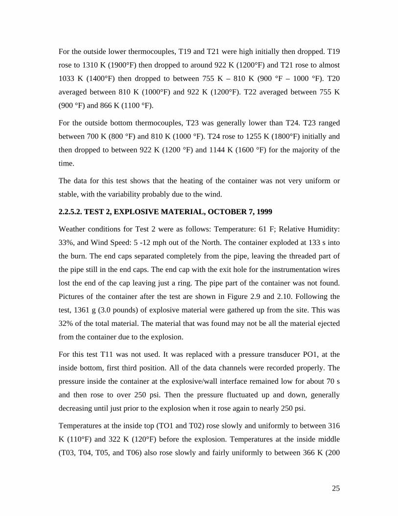
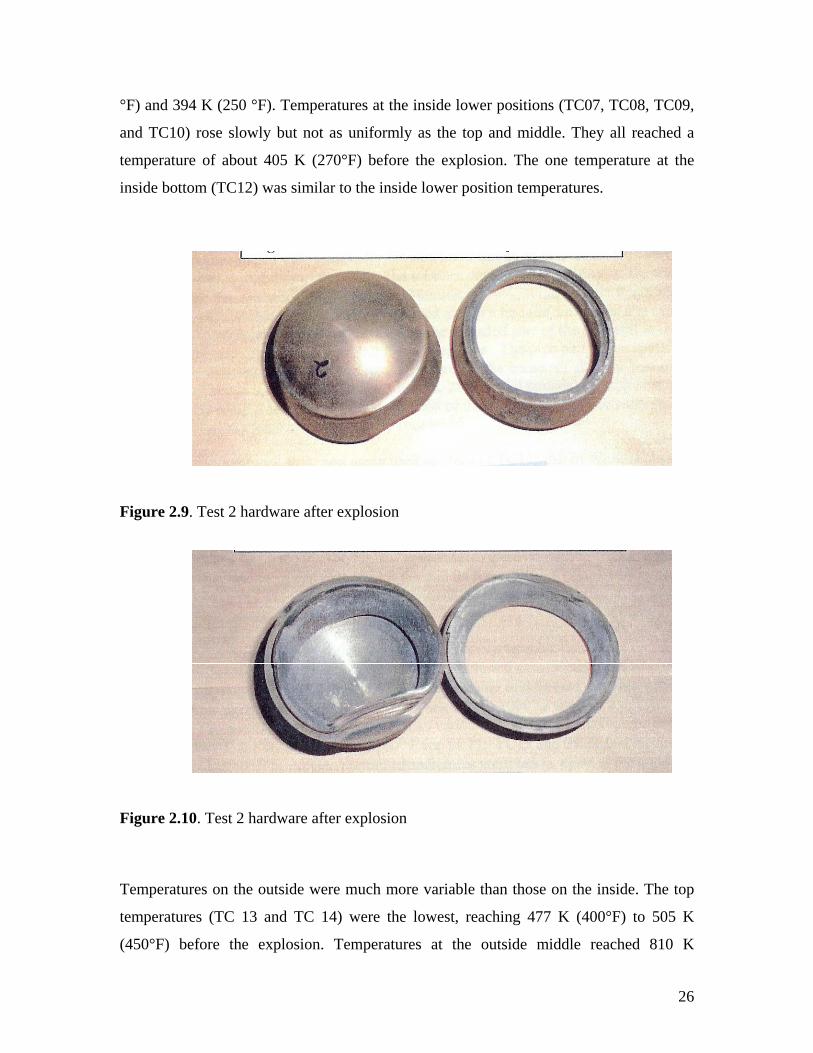
22..22..55..22.. TTEESSTT 22,, EEXXPPLLOOSSIIVVEE MMAATTEERRIIAALL,, OOCCTTOOBBEERR 77,, 11999999
Weather conditions for Test 2 were as follows: Temperature: 61 F; Relative Humidity:
33%, and Wind Speed: 5 -12 mph out of the North. The container exploded at 133 s into
the burn. The end caps separated completely from the pipe, leaving the threaded part of
the pipe still in the end caps. The end cap with the exit hole for the instrumentation wires
lost the end of the cap leaving just a ring. The pipe part of the container was not found.
Pictures of the container after the test are shown in Figure 2.9 and 2.10. Following the
test, 1361 g (3.0 pounds) of explosive material were gathered up from the site. This was
32% of the total material. The material that was found may not be all the material ejected
from the container due to the explosion.
For this test T11 was not used. It was replaced with a pressure transducer PO1, at the
inside bottom, first third position. All of the data channels were recorded properly. The
pressure inside the container at the explosive/wall interface remained low for about 70 s
and then rose to over 250 psi. Then the pressure fluctuated up and down, generally
decreasing until just prior to the explosion when it rose again to nearly 250 psi.
Temperatures at the inside top (TO1 and T02) rose slowly and uniformly to between 316
K (110°F) and 322 K (120°F) before the explosion. Temperatures at the inside middle
(T03, T04, T05, and T06) also rose slowly and fairly uniformly to between 366 K (200
25
°F) and 394 K (250 °F). Temperatures at the inside lower positions (TC07, TC08, TC09,
and TC10) rose slowly but not as uniformly as the top and middle. They all reached a
temperature of about 405 K (270°F) before the explosion. The one temperature at the
inside bottom (TC12) was similar to the inside lower position temperatures.
Figure 2.9. Test 2 hardware after explosion
Figure 2.10. Test 2 hardware after explosion
Temperatures on the outside were much more variable than those on the inside. The top
temperatures (TC 13 and TC 14) were the lowest, reaching 477 K (400°F) to 505 K
(450°F) before the explosion. Temperatures at the outside middle reached 810 K
26
(1000°F) to 866 K (1100°F). TC15 and TC 16 on the right side were more consistent and
than TC 17 and TC 18. The latter two had much wider fluctuations, perhaps because of
the wind. The outside lower temperatures varied widely and did not agree well with each
other. TC 19 barely reached 755 K (900° F), TC20 and TC22 reached 922 K (1200°F) to
1033 K (1400° F), while TC 21 reached 1255 K (1800° F). The outside bottom
temperatures were below those at the middle and lower positions. They reached around
810 K (1000°F) before the explosion.
From the data, the highest temperatures inside the container were at the lower positions,
reaching about 405 K (270°F) at the time of the explosion. It was also evident from the
video recordings that when the pressure began to rise, gases were expelled from the
container along the threads in the end caps. These gases ignited and burned and may be
the cause of the pressure rising and then falling inside the container.
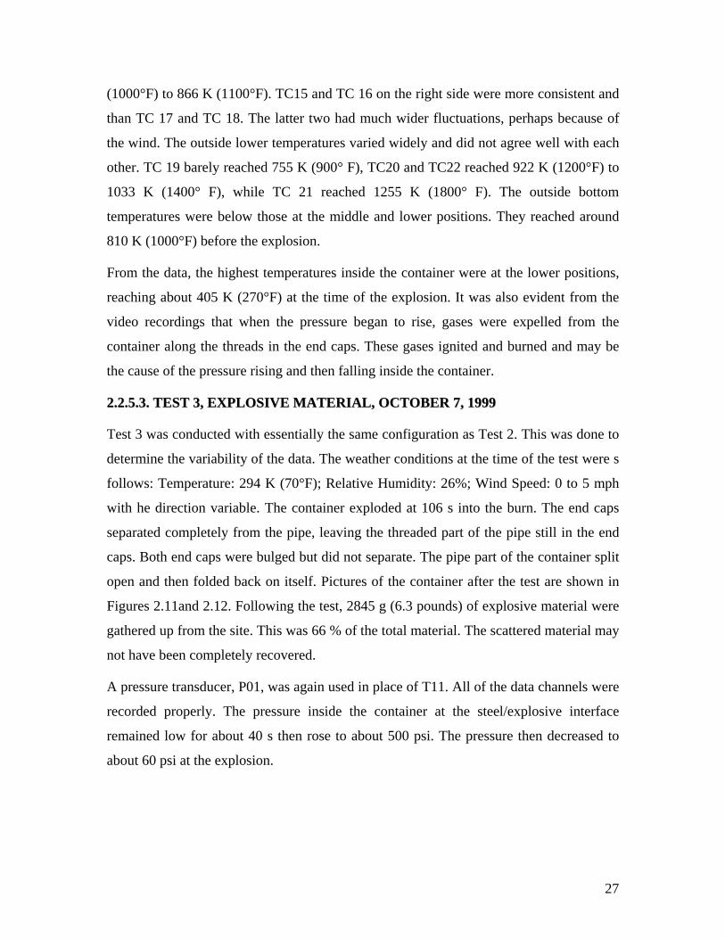
22..22..55..33.. TTEESSTT 33,, EEXXPPLLOOSSIIVVEE MMAATTEERRIIAALL,, OOCCTTOOBBEERR 77,, 11999999
Test 3 was conducted with essentially the same configuration as Test 2. This was done to
determine the variability of the data. The weather conditions at the time of the test were s
follows: Temperature: 294 K (70°F); Relative Humidity: 26%; Wind Speed: 0 to 5 mph
with he direction variable. The container exploded at 106 s into the burn. The end caps
separated completely from the pipe, leaving the threaded part of the pipe still in the end
caps. Both end caps were bulged but did not separate. The pipe part of the container split
open and then folded back on itself. Pictures of the container after the test are shown in
Figures 2.11and 2.12. Following the test, 2845 g (6.3 pounds) of explosive material were
gathered up from the site. This was 66 % of the total material. The scattered material may
not have been completely recovered.
A pressure transducer, P01, was again used in place of T11. All of the data channels were
recorded properly. The pressure inside the container at the steel/explosive interface
remained low for about 40 s then rose to about 500 psi. The pressure then decreased to
about 60 psi at the explosion.
27
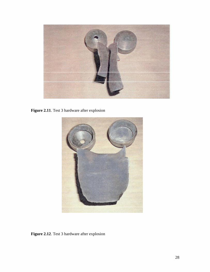
Figure 2.11. Test 3 hardware after explosion
Figure 2.12. Test 3 hardware after explosion
28
Temperatures at the inside top (TO1 and T02) rose slowly and uniformly to 349 K
temperatures for this test were much more variable than those on the inside.
r were at the lower positions, reaching 422 K
EERR 2255,, 11999999
o seal the end caps
Other than these changes, the other test parameters were the same as before.
(170°F) for T01 and 333 K (140°F) for T02 before the explosion. Temperatures at the
middle rose slowly and fairly uniformly but their maximums were not consistent. T03
and T05 rose to 283 K (50 °F) to 405 K (270 °F) while T04 and T05 rose to 349 K
(170°F) to 366 K (200°F). The higher temperatures were on opposite sides of the same
end of the container. Temperatures at the inside lower positions also rose slowly and
uniformly but were quite different in the maximums. T07 and T09 reached about 477 K
(400°F) while T08 reached just over 422 K (300 °F) and T10 reached 383 K (230 °F).
The higher temperatures were on opposite sides at the same end of the container in
agreement with the middle temperatures. The temperature at the inside bottom (T12)
agreed pretty well with T10, reaching a maximum of 383 K (230 °F) before the
explosion.
The outside
The outside top thermocouples (T13 and T14) varied considerably and reached a
maximum of between 588 K (600°F) and 644 K (700°F). The outside middle
temperatures varied widely and did not agree well at all. Maximums varied from 810 K
(1000°F) for T18 to 1310 K (1900°F) for T15. The outside lower temperatures also
varied considerably. Maximums ranged from 922 K (1200°F) for T20 to almost 1422 K
(2100°F) for T22. T19 and T21 had maximums around 1144 K (1600°F). The outside
bottom temperatures were below those at the middle and lower positions at about 755 K
(900°F). The data for T23 was very erratic.
The highest temperatures inside the containe
(300°F) and 477 K (400 °F) respectively, at the time of the explosion. The videos showed
that gases also escaped from the container and burned.
22..22..55..44.. TTEESSTT 44,, EEXXPPLLOOSSIIVVEE MMAATTEERRIIAALL,, OOCCTTOOBB
Because we had gases escaping from the container, we decided to try t
to the pipe. An O-ring was placed between the ends of the pipe and the end caps. The
threads were coated with Dow Corning 90-006 aerospace sealant. Some of the sealant
was also forced down the stainless steel tubing that housed the instrumentation wires.
29
Weather conditions for Test 4 were as follows: Temperature: 62 F, Relative humidity
19%, Wind Speed: 6 to 8 mph out of the East. The container exploded at 141 s into the
d a maximum of 400 psi at
burn. The end caps separated completely from the pipe, leaving the threaded part of the
pipe still in the end caps. Both end caps lost their ends but only one was recovered. The
pipe came apart into at least 3 pieces. Pictures of the container after the test are shown in
Figure 2.13 and 2.14. Following the test, 2655 g (5.9 pounds) of explosive material were
gathered up from the site. This was 62 % of the total material.
The pressure trace for this test was definitely different from previous tests. The pressure
started to rise uniformly almost front the beginning and reache
about 68 seconds. Then, it decreased with some variability, going negative at about 97 s
and remained negative until the explosion. The cause of the negative reading is not
known.
Figure 2.13. Test 4 hardware after explosion
30
Figure 2.14. Test 4 hardware after explosion
Temperatures at the inside top rose slowly and uniformly to a maximum of 383 K
(230˚F) for TO1 and 372 K (210˚F) for T02. Temperatures at the inside middle were well
behaved and rose to a maximum of 388 K (240˚F) to 400 K (260˚F) for T03, T05, and
T06. T04 was lower at a maximum temperature of 366 K (200˚F). Temperatures at the
inside lower positions were well behaved but differed in their maximums. T07 reached
about 416 K (290˚F), T08 and T09 both reached about 366 K (200˚F), and T10 reached
about 360 K (190˚F.) The inside bottom temperature, T12, reached about 372 K (210˚F).
The outside temperatures varied considerable and did not agree well with each other. At
the top, T13 fluctuated widely and reached a maximum of just rover 810 K (1000˚F). T14
behaved better but only reached a maximum of around 477 K (400˚F). The outside
middle temperatures were very different. T15 reach a maximum of 1422 K (2100˚F), T16
went to just over 810 K (1000˚F), T17 reached 1033 K (1400˚F), and T18 reached about
1200 K (1700˚F). The Outside lower temperature did not correlate well either. There
were great fluctuations in the data and the maximum ranged from 672 K (750˚F) to over
977 K (1300˚F). The outside bottom temperatures reached a maximum of nearly 1255 K
(1800˚F) for T23 and only 616 K (650˚F) for T24.
31
The highest temperature inside was at the lower position at 416 K (290˚F). The video
showed that we were successful in stopping the gases from escaping from around the
threads but not through the steel tubing.
22..22..55..55.. TTEESSTT 55,, EEXXPPLLOOSSIIVVEE MMAATTEERRIIAALL,, OOCCTTOOBBEERR 2288,, 11999999
Test 5 was similar to test 4 except that more aerospace sealant was used to try to seal the
stainless steel tubing housing the instrumentation wires. The sealant was forced into both
ends of the tubing. In addition, the explosive pellets were bonded to the cylinder wall
using the Estane/BNDPA/F binder. The weather conditions were as follows:
Temperature: 285 K (54˚F), Relative Humidity: 62 %, Wind Speed: 10 mph out of the
Northwest. The container exploded at 98 s into the burn. The end cap without the hole in
it, separated completely from the pipe, and the other end cap was minimally attached.
Both end caps were bulged but did not lose their ends. The threaded part of the pipe
remained in the end caps. The pipe split open along a line opposite the weld seam and
flattened out. Pictures of the container after the test are shown in Figure 2.15 and 2.16.
Following the test, 1773 g (3.9 pounds) of explosive material were gathered up from the
site. This was 41 % of the total material.
Figure 2.15. Test 5 hardware after the explosion
32
Figure 2.16. Test 5 hardware after the explosion
The pressure reading inside: the container remained low for about 30 s, then rose to a
maximum of nearly 1400 psi at 60 seconds. After reaching the maximum, the pressure
dropped off but stayed between 700 psi to 1100 psi until the explosion.
The temperatures at the inside top (T01 and T02) rose slowly and uniformly to almost
366 K (200˚F) for T01 and about 350 K (170˚F) for T02. Temperatures at the inside
middle were quite different from each other. T03 and T05 rose more slowly than the
other two and reached a maximum of 388 K (240˚F) to 405 K (270˚F). T04 and T06
started out slowly, and then at about 60 s, increased rapidly. T04 reached a maximum of
about 460 K (370˚F) and T06 reached a maximum of about 394 K (250˚F). The inside
lower position temperatures were also quite different from each other. T07 and T08 were
similar in their maximum temperatures, 366 K (200˚F) and 372 K (210˚F), respectively,
but their profiles were very different. T07 rose slowly and uniformly while T08 rose
slowly at first and then increased rapidly at about 80 seconds. T09 rose slowly until about
50 s and then increased rapidly to a maximum of almost 444 K (340˚F). T10 rose slowly
and uniformly to a maximum of about 394 K (250˚F). The inside bottom temperature
rose slowly at first and then at about 60 s increased rapidly to a maximum of 427 K
(310˚F).
33
The outside temperatures were not consistent with each other. T13 fluctuated
considerably but generally increased with time to a maximum of about 572 K (570˚F).
T14 reach a maximum of 866 K (1100˚F) in just over 20 s and then dropped to an
average level of 672 K (750˚F) until the explosion. The outside middle temperatures were
quite similar. They all rose quickly during the first 30 s and then fluctuated at levels
around 922 K (1200˚F) to 977 K (1300˚F). The outside lower position temperatures were
similar to the middle temperatures. They rose quickly and then leveled off. T19 and T20
reached highs of 977 K (1300˚F) and 1088 K (1500˚F) respectively. T21 and T22 only
went to 810 K (1000˚F) and 866 K (1100˚F) respectively. The outside bottom
temperatures also rose quickly at the beginning but then T23 dropped from a high of 950
K (1250˚F) to an average around 810 K (1000˚F). T24 quickly rose to 755 K (900˚F) and
then continued upward to nearly 922 K (1200˚F) at the end.
The highest temperature inside the container was at the middle position and was 275 K
(370˚F). However, one of the lower position temperatures reached 444 K (340˚F). The
videos did not reveal escaping gas and the pressure was considerably higher for this test
than the others. We do not know whether that was because the container was sealed
better, or whether it was because the explosive material was bonded to the cylinder wall.
The outside temperatures continue to be widely variable and difficult to analyze.
Sometimes the hot spots are on the same side of the cylinder at a location, and then at
another location, they are on the same end of the cylinder.
22..33 EELLEECCTTRRIICCAALL CCOOOOKKOOFFFF TTEESSTTSS
This report is based on the information provided by Thiokol Propulsion Company in
Report TR12646, C-SAFE TESTS, Phase III.
22..33..11 IINNTTRROODDUUCCTTIIOONN
A new container was designed to hold only one 4” diameter x 4” thick pellet of PBX9501
explosive. The previous design held three of the pellets. The container was changed
from schedule 80 pipe with Marman-type V-band clamps to a ¼” thick container with
thickened ends, and the end plugs were sealed with o-rings and snap rings. This
container was designed to withstand pressures up to about 7500 psi on the sidewall and
34
end plugs. A hydrostatic pressure test was conducted of the empty container to determine
the pressure at which it would burst.
22..33..22 DDIISSCCUUSSSSIIOONN
The tests specified for this contract were a hydrostatic pressure test of the container, a
pressure transducer characterization test, a burn rate test of the PBX-9501 material, and
up to six cook-off tests depending on the time and budget. The container must first be
assembled and the hydrostatic pressure test performed before the other tests could
proceed.
The original design for the container for the cook-off tests was to be a 4-inch inside
diameter schedule-80 pipe with a Marman-type V-band clamp on each end to hold the
end caps. Flanges with an o-ring groove were welded to each end of the pipe. The end
caps were machined so that their edges matched the flange design. The pipe was to be 12
inches long to hold three, 4-inch diameter x 4-inch thick explosive pellets. The container
was to be surrounded by an 11-inch wide band heater.
Because of the long lead-time to procure the Marman clamps and flanges, the tests were
delayed until after January 2001. At that time the University of Utah personnel decided
to change the design of the container to hold one pellet instead of three pellets. This
would make the computer modeling of the test much easier. Also at that time it was
decided to change the container design and use and engineered design with an o-ring and
snap ring instead of the schedule 80 pipe with end caps held in place by Marman-type V-
band clamps. The container was designed to be able to withstand about 7500 psi on the
sidewalls and end plugs. A picture of this container is shown in Figure 2.17.
35
Figure 2.17. Steel container used in the electrical cookoff tests
22..33..33 HHYYDDRROOSSTTAATTIICC PPRREESSSSUURREE TTEESSTT
After the design was completed, two containers were fabricated. The first container was
used for a hydrostatic pressure test. The objective of this test was to determine the
pressure at which the container would burst. A hole was drilled in one of the end caps
and a fitting was attached to connect to the pressurized water system. The end with the
pressure fitting was designated the top of the container. Strain gages were mounted on
the container, axially and circumferentially, at eight locations, making sixteen total.
Strain gages were mounted at the top and bottom at 0˚, 90˚, 180˚, and 270˚.
Pressure was applied in small increments starting about 20 seconds into the test. At about
110 seconds into the test and a pressure of 7541 psi, the container started to leak. The
snap-ring grooves gave way and the pressure forced the snap ring to deform allowing the
end plugs to move causing the leak. The container did not burst. However, the sidewalls
were bulged making the container look like a small potbelly stove.
22..33..44 PPRREESSSSUURREE TTRRAANNSSDDUUCCEERR CCHHAARRAACCTTEERRIIZZAATTIIOONN
Entran Model EPB-C02-5KP-/C/Z4 pressure transducers were purchased to use in this
year’s testing. These pressure transducers have a range of 5000 psi (not to exceed 10,000
psi) and have an operating temperature range of 233 to 394 K (-40 to 250˚F). They are
36
temperature compensated between 310 and 366 K (100 and 200˚F). Since the
temperature conditions of the tests were going to exceed these operating conditions, we
wanted to know the response of the pressure readings as a function of temperature.
One of the previously designed containers was used for this characterization test. The
Entran pressure transducer and a type K thermocouple were installed inside the container.
A pressure port was installed in one of the end caps to connect to the pressurized-air line.
A Conax connector was installed in the other end cap allowing the leads from the Entran
pressure transducer and thermocouple to exit the container without causing a pressure
leak. A Taber Model 207 pressure transducer was installed on the pressure supply line
just outside of the container. The Taber transducer was maintained at ambient
temperature and was used to record the pressure inside the container to compare with the
Entran transducer reading. An 11-inch wide band heater surrounded the container. The
pressure line was connected to a tank of compressed air. The pressure valves and voltage
to the band heater were operated remotely for personnel safety.
Several runs were made to determine how the setup operated and the response of the
pressurized system. For the actual test, the compressed air tank regulator was set to 350
psi. The data acquisition system recorded the temperature and both pressure readings at a
rate of 1 sample per second. The pressure valves were opened and the voltage was
applied to the band heater and data were recorded for 1 hour and 13 minutes. The
regulator on the pressure tank was not able to keep the pressure at 350 psi, allowing it to
drop to 310 psi over a period of time. The initial temperature inside the container was
287 K (57˚F).
The actual pressure measured by the Taber transducer went up and down as the regulator
tried to stabilize. The Entran transducer increased in pressure as the temperature
increased.
22..33..55 HHYYDDRROOBBUURRSSTT TTEESSTT ##11 –– 22000022
We have completed closed ballistic bomb testing of pelletized PBX-9501 explosive from
50 to 7,000 psi. This memo summarizes those findings.
37
22..33..55..11 IINNSSTTRRUUMMEENNTTAATTIIOONN BBAACCKKGGRROOUUNNDD
The closed ballistic bomb is a one-liter cylindrical high-pressure vessel instrumented with
a pressure transducer, thermocouple, nitrogen gas supply lines, a data acquisition system
and an ignition system. The bomb is jacketed in a liquid-filled conditioning collar for
temperature control. It is used to determine the burn rate and ignitability of propellants,
gas generants and other materials from sub-ambient to 14,000 psi over a broad range of
temperatures. The samples may be pressed pellets, extruded or cored slugs, or other
shapes as required.
22..33..55..22 EEXXPPEERRIIMMEENNTTAALL
The samples were weighed on an analytical balance reading to the tenth of a milligram.
The samples were measured dimensionally in inches using a dial caliper. This data was
entered into the data acquisition program prior to testing.
The pellets were adhered to the sticky side of masking tape that in turn was stuck onto
cardboard. The samples were then sprayed with 3 coats of Krylon Ignition sealer as an
inhibiter so only the top of the pellet would burn. A small amount of ignition powder
was placed on top of the pellet as an ignition aid. The ignition powder was kept in place
during bomb closure by means of a 3/8” strip of masking tape wrapped around the pellet
at the uninhibited (ignition) end.
The prepared samples were loaded into the M-9 1-liter closed bomb by placing them onto
the sample plate and a lift/sacrificial plate, with a short length of Parr bomb ignition wire
pulled taught over the ignition aid coated part of the pellet through slits in the tape and
secured to the electrical posts. The bomb closure (which carries the sample holder) was
loaded into the bomb, and the ignition circuit was then connected. The system was then
pressurized with nitrogen to the test pressure. The data acquisition system was used to
trigger ignition and record the resultant pressure rise as well as perform various other
calculations.
22..33..55..33 OOBBSSEERRVVAATTIIOONNSS
The pellets burned well with no problems or loss of inhibition (as would be shown by a
break to a steeper pressure rise trace). There was no combustion residue except with the
38
samples tested below about 500 psi when carbon dust was evident (which is typical of
similar materials). The sample tested at 20-psi did not ignite.
The raw data files were stored on a CD. Each trace consists of four segments of
information per burn. They are respectively the conditioning pressure, the ignition, the
pressure rise from burning and the cool down. Three additional pellets were burned with
a 60 second record time to show data for the cool down.
There is about 40 psi of generated gas independent of the test pressure. Also, there is a
pressure rise increase associated with higher starting pressures. Consequently 7000 psi
was the highest initial starting pressure used in order to keep from overshooting the gauge
maximum of 15,000 psi. Similarly, the psi/g data is used as a figure of merit in gas
generant data analysis and increases quite dramatically for PBX-9501. These values are
some of the largest ever seen in our lab.
22..33..55..44 RREESSUULLTTSS AANNDD CCOONNCCLLUUSSIIOONNSS
The burn rate exponent for PBX-9501 is 0.86 and is quite linear between the pressure
ranges of 50 to 7000 psi.
22..33..66 TTEESSTT 66,, EELLEECCTTRRIICCAALL,, JJUULLYY 22000011
The first cook-off test was conducted on July 3, 2001. The container used is shown in
Figure 2.17. The explosive material was PBX-9501, the same material that was used in
previous years. It is described in previous years’ reports. Conax connectors were
installed in each end cap of the container. They were used to seal the wires against a
pressure leak. The pressure transducer leads came out one of the ends, and the
thermocouple leads came out the other end. The band heater was 4.5-inches inside
diameter x 4-inches long with a mineral insulated construction. Its output was 35 W/sq in
and was supplied by Entherm. The band heater was split so that it could be placed
around the container.
Since only one pellet was used, it was cut in half to allow instruments to be placed in the
middle of the pellet. The cutting was done on a lathe using a 1/16-inch parting tool. The
outside thermocouples were placed between the container and the band heater. Their
locations are described in Table 2.7, along with the data acquisition setup parameters. A
39
2-inch layer of pipe insulation was wrapped around the outside of the band heater. A
voltage of 110 volts was applied to the band heater. The container was placed on the
ground with the 0˚ mark down and the split in the band heater was placed at about the 45˚
mark.
Our LeCroy data acquisition system was set up for 16 channels and recorded the inside
thermocouples, the pressure transducer channels, and 5 of the outside thermocouples.
Our Nicolet system recorded the rest of the outside thermocouple channels. One inside
thermocouple, TC07 was damaged in the assembly and did not respond in the final
checkout. Therefore, it was not connected to the data acquisition system.
Because the LeCroy system only has 512 K of memory and must be divided equally
among the 4 channels, the acquisition time was only 10.9 minutes. This was a concern
because we did not know how long the material would heat until it exploded. Personnel
at the University of Utah conducted some experiments with the band heater and
calculated that the time to explosion would be 2 to 3 minutes. In actuality, the time to
explosion was 31 minutes. This meant that the digitizers timed out and were re-armed
and triggered two more times. In the third segment of data collection we noticed that the
second and third LeCroy digitizers, which were recording thermocouples TC06 and TC08
– TC14 had stopped recording data. The dilemma we faced was whether to continue
recording, in which case we would lose those channels of data, or to stop the acquisition,
re-boot the system, and start over. If we chose the latter option, the explosion could
occur during the time for the restart and we would lose all of the data recorded by the
LeCroy system. The decision was made to restart the system. During the restart, the
explosion occurred and the pressure transducer data along with thermocouple data up
through TC14 were lost. The only data acquired were thermocouple channels
TC150TC20 and only for the last ten minutes of the test.
The explosion that took place was very complete. The container disintegrated and only
four small pieces of metal material were found. One of these looked like it came from
the band heater. No explosive material was found. The high-speed video of the event
showed the container exploding and quite small pieces of material flying away.
40
Table 2.7 C-SAFE 2001 Instrumentation List
Name Description Location
TC01 Thermocouple Inside Container, End #1, 0˚
TC02 Thermocouple Inside Container, End #1, 180˚
TC03 Thermocouple Inside Container, Middle of Pellet, 0˚
TC04 Thermocouple Inside Container, Middle of Pellet, 90˚
TC05 Thermocouple Inside Container, Middle of Pellet, 180˚
TC06 Thermocouple Inside Container, Middle of Pellet, 270˚
TC07 Thermocouple Inside Container, End #2, 0˚
TC08 Thermocouple Inside Container, End #2, 180˚
TC09 Thermocouple Outside Container, End #1, 0˚
TC10 Thermocouple Outside Container, End #1, 90˚
TC11 Thermocouple Outside Container, End #1, 180˚
TC12 Thermocouple Outside Container, End #1, 270˚
TC13 Thermocouple Outside Container, Middle, 0˚
TC14 Thermocouple Outside Container, Middle, 90˚
TC15 Thermocouple Outside Container, Middle, 180˚
TC16 Thermocouple Outside Container, Middle, 270˚
TC17 Thermocouple Outside Container, End #2, 0˚
TC18 Thermocouple Outside Container, End #2, 90˚
TC19 Thermocouple Outside Container, End #2, 180˚
TC20 Thermocouple Outside Container, End #2, 270˚
P001 Pressure Transducer Inside Container, End #1, 0˚, 1/16” from edge
P002 Pressure Transducer Inside Container, Middle, 0˚, 1/16” from edge
P003 Pressure Transducer Inside Container, In the bore of the pellet
Camera 1 High Speed Video Side View, Covering 5 feet to the side
Camera 2 Video Monitor Side View, Covering 20 feet to the side
Camera 3 Video Monitor End View, Covering 20 feet side to side
22..33..77 TTEESSTT 77,, EELLEECCTTRRIICCAALL,, AAUUGGUUSSTT 22000011
The second cook-off test was conducted on August 6, 2001. Because of the loss of data
in the first cook-off test, the decision was made to duplicate the first test with the
41
exception of the voltage applied to the band heater. In the first test we used 110 volts and
for the second test we used 220 volts. The pressure transducers and thermocouples were
placed the same as for the first test. However, the data acquisition systems were changed
from the first test. The pressure transducers were set up on channels 1-3 of the LeCroy
system at a sampling rate of 100 samples per second. This gave a recording time of
almost 22 minutes. The pressure transducers were also set up on channels 5-7 at a
sampling rate of 10,000 samples per second with a manual trigger. The data to be
recorded was all pre-trigger data for a period of time of about 13 seconds. The manual
trigger was applied when the explosion took place. This set up was designed so that we
could record data from the beginning at a slow rate and then record the explosion at a
much faster rate for the ten seconds or so, just before the explosion. The inside
thermocouples were recorded on channels 8-16 of the LeCroy system at a rate of 100
samples per second. The outside thermocouples were recorded on an Iotech LabBook 16
channel data acquisition system at a sampling rate of 200 samples per second. The
LabBook has enough memory that the recording time was 40 minutes at this sampling
rate.
The explosion occurred at 3 minutes and 12 seconds after the voltage was applied to the
band heaters. The explosion was not as violent as the first test. One side of the container
was blown out and peeled back leaving the rest of the container intact. A picture of the
container is shown in Figure 2.18. The explosive material was not all consumed and
about 2 pounds of the 3 pounds total was recovered from the site. A picture of some of
the material is shown in Figure 2.19.
All of the data were recovered from the first test. The data showed that the pressure near
the interface of the material and container reached about 50 psi (uncorrected) until just
prior to the event and then there was a sharp spike in the data up to about 130 psi and
then the explosion took place. The bore pressure remained near zero until just prior to
the test and then a spike in the data occurred up to 57 psi just before the explosion.
Transducer P002 went negative until just a few seconds before the explosion took place.
We can’t explain the reason for this negative excursion.
42
Figure 2.18. Container after test
igure 2.19. Fragments of explosive material after test
data just before the explosion.
F
The thermocouple data also showed the spike in the
Temperature inside the container ranged from 340 K (154˚F) to 443 K (338˚F). The ends
were lower as expected. The middle thermocouples ranged from 392 K (247˚F) to 443 K
(338˚F). The highest temperature was at the 90˚ position. The outside thermocouples
ranged from 490 K (423˚F) to 766 K (920˚F). Middle thermocouples TC14-TC16
exceeded their range and recorded only to 920˚F.
43
22..33..88 TTEESSTT 88,, EELLEECCTTRRIICCAALL,, SSEEPPTTEEMMBBEERR 22000022
The third electrical test was conducted on September 30, 2002. The voltage applied to
this test was 110 Volts. The experimental setup is similar to that described for tests 6 and
7 with the exception that some additional pressure transducers were placed around the
test site (i.e. the surrounding of the ordnance) to measure the overpressure. The
arrangement of the transducers is shown in Figure 2.20. This test was intended to
duplicate test 6 in which most data were lost. The explosion occurred after 1520 seconds
(25.3 minutes). Very few metallic pieces were gathered from the test site (see Figure
2.21).
The experimental results (Temperature and pressure) are plotted in Appendices A and B
and discussed in chapter 4.
Figure 2.20 Pressure transducers arrangement
44
Figure 2.21 Pressure transducers arrangement
22..33..99 TTEESSTT 99,, EELLEECCTTRRIICCAALL,, NNOOVVEEMMBBEERR 22000022
Test 9 consisted of two tests distinguished in this report as test 9A and test 9B. The main
goal for test 9 was to explore the cookoff behavior (i.e. reaction violence) of HMX-based
explosives in the low-heat flux regime (i.e. lower compared to test 6 and 8). The voltage
was reduced by half, that is. 55 Volts, and so the applied heat flux at the steel pipe was
reduced by a factor of 4 compared to test 8. No ignition resulted after 3 hours. The
heating was suspended and the ordnance was cooled down. This corresponds to test 9A in
this report. The same setup and instrumented container were used in test 9B. The voltage
was increased to 110 Volts and the ignition occurred at 1520 seconds (25 minutes).
Figure 2.22 shows some of the metallic pieces gathered from the test site.
The experimental temperatures and pressures are plotted in appendices A and B. Analysis
of these results is presented in chapter 4.
45
Figure 2.22. Metallic pieces found after test 9B.
22..33..1100 TTEESSTT 1100,, EELLEECCTTRRIICCAALL,, NNOOVVEEMMBBEERR 22000022
The main goal of test 10 was to explore the effects of no having an air core in the
explosive pellet. The voltage applied to this test was 110 Volts. The explosion occurred
after 1634 seconds (27.2 minutes), and was very comparable with test 6, 8, and 9B;
although, the explosion was not nearly as violent. Pictures of the container and explosive
material are shown in Figures 2.23 to 2.26.
The experimental temperatures and pressures are plotted in appendices A and B. Analysis
of these results is presented in chapter 4.
46
Figure 2.23. Container after test.
47
Figure 2.24. Container after test.
Figure 2.25. Heater pieces gathered from the test site.
Figure 2.26. Explosive material after test.
48
NNUUMMEERRIICCAALL AANNAALLYYSSIISS The heat transfer phenomena and the associated numerical methods are
specified in detail.
DDAATTAA AANNAALLYYSSIISS
Three different numerical methods were developed to study the thermal behavior of
confined PBX-9501 when heated by a fire and electricity. The experiments were
presented in detail in Chapter 2. For times to explosion up to 3 minutes in the present
studies, the thermal penetration depth is approximately 4.7 mm, much smaller than the
thickness of the explosive material. This implies that the system can be treated as a semi-
infinite and therefore, the temperature distribution within the solid can be accurately
described using a one-dimensional (1-D) heat flow equation.
perposition integral to the surface
temperature in order to get the surface heat flux. The second method used Inverse Heat
Conduction (IHC) equations and temperature measurement within the solid to calculate
third me
thermal-reaction model to investigate the boundaries of the overall system
33..11.. DDUUHHAAMMEELL SSUUPPEERRPPOOSSIITTIIOONN IINNTTEEGGRRAALL
The measured interface temperature and the Duhamel’s superp
used to obtain the heat flux at the explosive surface. Considering the explosive part of the
hysical properties, the formulation of the problem
The first method consisted of applying the Duhamel su
the thermal boundary at the surface. The thod used a finite difference based,
.
osition technique were
system and assuming constant thermop
for the unsteady temperature distribution T(r,t) is given by
rT
rrtrTtrT
t PBX ∂∂
+∂
∂⋅=
∂ ,(),( 2
α∂
1)2 (3.1)
An approximate solution for the surface heat flux is, (Buttsworth and Jones, 1997)
49
( )TotTRstt PBXPBX ⋅⎪⎭⎪⎩ −
⎥⎦
⎢⎣⋅ 2)(2 0
3απ
Equation (3.2) is accurate to better than 1 % for typical transient heat transfer
configurations in which
KdssTtTToq PBXt
PBX −−⎪⎬⎫
⎨ ⋅−
+⎤−
⋅= ∫ )()()(1) (3.2) tTK ⎪⎧⎡ (
06.02 ≤⋅
Rtα .
Equation (3.2) has a singularity when t = s. There are several numerical techniques that
can be used to get a reasonable solution [Diller, 1996]. One of the most widely used
consist of using a piecewise linear representation of the temperature trace [Cook and
Felderman, 1966].
( )∑=
lculate the temperature and the heat
ndary condition be known at
the interior of the cylinder or r=r1. The heat flux and the temperature at the surface of the
cylinder (r=rM) can be calculated ding the pro
would
provide the temperature and heat flux needed to solve the second part, that is, the inverse
region between r=rE and the surface r=rM.
The direct problem can be solved using a finite difference technique such as the Crank-
governing uation for the inverse problem is
−
− −⋅
+⎟⎟
⎠
⎞
⎜⎜
⎝
⎛
++−
−⋅
⋅⋅
=n
joj
PBX
PBX
jnjn
jj
PBX
PBXn TT
RK
ttttTTKtq
1 1
1
22)(
απ (3.3)
33..22.. IINNVVEERRSSEE HHEEAATT CCOONNDDUUCCTTIIOONN MMEETTHHOODD
Inverse heat conduction equations can be used to ca
flux on the surface of a solid from transient temperature measurements made within at
one or more locations [Hills and Hensel, 1986]. Consider the infinite long cylinder
illustrated in Figure 3.1. Initially, the cylinder is at uniform temperature. The temperature
measurement is taken at point r=rE. In addition, let the bou
by divi blem into two parts. The first part
consist of solving the direct problem, that is, the region between r=r1and r=rE. This
Nicholson method. The inverse heat conduction problem can be solved using a space-
marching technique. The eq
50
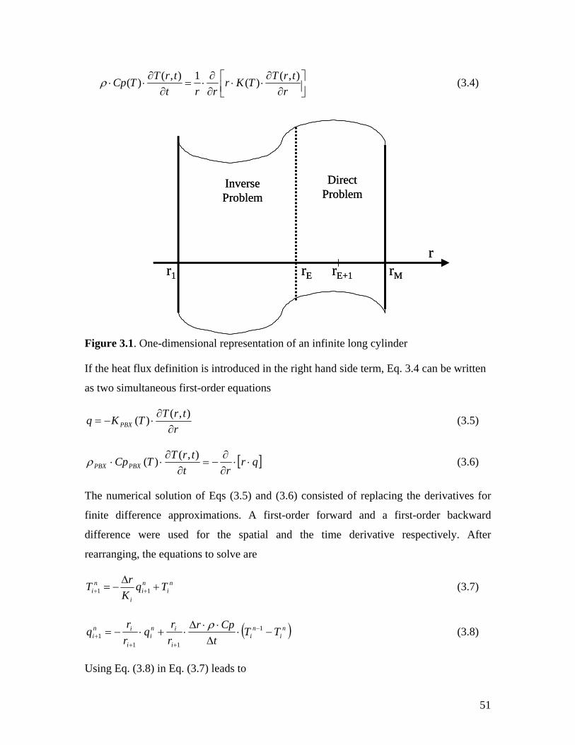
⎥⎦⎤⎡ ∂
⋅⋅∂
⋅=∂
∂⋅⋅
trTTKrt
trTTCp ),()(1),()(ρ (3.4) ⎢⎣ ∂∂ rrr
e right hand side term, Eq. 3.4 can be written
Figure 3.1. One-dimensional representation of an infinite long cylinder
If the heat flux definition is introduced in th
as two simultaneous first-order equations
rtrTTKq PBX ∂
∂⋅−=
),()( (3.5)
[ ]qrrt
trTTCpPBXPBX ⋅⋅∂∂
−=∂
∂⋅⋅
),()(ρ (
The numerical solution of Eqs (3.5) and (3.6) consisted of replacing the derivatives for
finite difference approxim
difference were used ter
rearranging, the equa
3.6)
ations. A first-order forward and a first-order backward
for the spatial and the time derivative respectively. Af
tions to solve are
ni
ni
i
ni Tq
KrT +
∆−= ++ 11 (3.7)
( )ni
ni
i
ini
i
ini TT
tCpr
rr
qrr
q −⋅∆⋅⋅∆
⋅+⋅−= −
+++
1
111
ρ (3.8)
Using Eq. (3.8) in Eq. (3.7) leads to
Inverse Problem Problem
rE
rr1 rE+1
Direct
rM
Inverse Problem Problem
rE
rr1 rE+1
Direct
rM
51
⎟⎟⎠⎝ ∆⋅⎠⎝ ∆⋅ +++ tKrtKrKr iiiiii 111
Equations (3.8) and (3.9) can be used to ca
⎞⎜ ⋅+⋅+⎟⎜ ⋅−⋅+⋅−=+ TTT iii 1 1 (3.9)
lculate the heat flux and the temperature in the
inverse region (rE < r < r
Analytical solutions for the inverse heat conduction problem in a semi-infinite solid are
well known [Burggraf, 1964 and Beck
heat flux at the surface of the explosive are given by
⎜⎛ ⋅⋅∆⎟
⎞⎜⎛ ⋅⋅∆⋅∆ − CprrCprrqrr inin
niin ρρ 22
1
M).
et al, 1985]. For a slab, the temperature and the
⎥⎦
⎤⎢⎣
⎡⋅
+++⋅⋅+= ∑∑
∞
=
∞
=n
En
n
nEt
EPBX
E
nnrE
n
n
nEt
rEt
rM dtqd
nr
qK
rdt
Tdn
rTT
1
2
1
2
)!12(1
)!2( α (3.10)
nrE
n
n
nE
nnrE
n
n
nE
PBXtE
trM
TdrKqq ⋅⋅⋅+= ∑∞ −12 1
dtqd
nr
dtn⋅+
− ∑∞
== 1
2
1 )!2()!12( α (3.11)
The results given b
implies that curvature effects were not important and so the 1-D planar solution can be
safely used to describe the thermal behavior o
33..33.. TTHHEERRMMAALL RREEAACCTTIIOONN MMOODDEELL
All energetic materials are, to some degree, sensitive to heat: They suffer degradation,
decomposition, and ultimately ignition. In general, mechanisms and kinetics are proposed
according to induction times that are obtained during slow thermal decomposition
een successfully obtained by using a reduced 3-step
(R-1)
(R-2)
y the numerical and the analytical solutions were very similar. This
f high-energy materials during fast cookoff.
experiments with different rates of heating. The prediction of the time to explosion for
HMX-based explosives has b
Arrhenius scheme [McGuire and Tarver, 1981]. The scheme is based on experimental
data and involves the following reactions:
)(22)( ss NONCHHMX −=⇒
)(2)(2)(22 ggs ONOCHNONCH +⇒−=
)(2)()(2)(2)(2)(2 gggggg COCONOHONOCH +++⇒+ (R-3)
The first reaction represents the endothermic breaking of C-
H2C=N-NO2. The second step is the exothermic rearrangement of H2C=N-NO2 into
N bonds in the ring forming
52
CH2O and N2O. The final reaction is the very exothermic gas phase decomposition of
CH2O and N2O into the stable gaseous products such as H2O, N2, CO and CO2. The heat
of reaction and kinetic parameters are listed in Table 3.1.
For modeling purposes, the reactions R-1 to R-3 can be conveniently represented as
)
uire
DCBA ⎯→⎯⎯→⎯⎯→⎯ 321 2 (R-4
Where A represents HMX, B represents H2C=N-NO2, C represents CH2O and N2O, and
D represents the final products such as H2O, N2, CO and CO2.
Table 3.1. Kinetic parameters for the thermal decomposition of HMX. (After McGand Tarver).
Reaction 1 Reaction 2 Reaction 3
Heat of reaction, kJ/kg -4.18 1.25 5.02
Activation energy, kJ/mole
Frequency factor, s-1 1.41*1021 1.58*1016 1.60*1012
220 185 143
Consider the sketch of the 1-D problem in Figure 3.2. When the thermal conductivity (K)
and specific heat (Cp) are temperature dependant, the radial temperature distribution
T(r,t) for t>0 can be obtained by solving the following
For PBXi RrR <<
Sr
trTr
TKtrTTKtrTTCp PBPBXPBXPBX +⎥
⎤⎢⎡ ∂
⋅⋅∂
=∂⋅⋅
),()(),()(ρrrt
X +∂
∂⋅
⎦⎣ ∂∂∂),()(
(3.12)
Where S represents the heat source due to the chemical decomposition of the explosive.
is given by Based on the simplified mechanism described by reaction R-4, S
⎟⎟⎠
⎞⎜⎜⎝
⎛
⋅−
⎟⎟⎠
⎞⎜⎜⎝
⎛
⋅−
⎟⎟⎠
⎞⎜⎜⎝
⎛
⋅−
⋅⋅⋅+⋅⋅⋅+⋅⋅⋅= TREa
TREa
TREa
AgggQmS
321
21 CB eZQmeZQmeZ 33221 (3.13)
53
ere, mA, mB, mC and mD are the mass fraction of A, B, C and D. As the decomposition
lowing rate
equations
Figure 3.2 One-dimensional representation of the system
H
proceeds, the concentration of each of the species is described by the fol
AkdtdA
A ⋅−= (3.14)
BkAkdtdB
BA ⋅−⋅= (3.15)
2CkBkdtdC
CB ⋅−⋅= (3.16)
2C (
stants ki for i=A, B, C and D and for j reactions (R1 to R4) are given by
kdtdD
C ⋅= 3.17)
The rate con
⎟⎟⎠
⎞⎜⎜⎝
⎛⋅
−
⋅= TRgEaj
jji eZk , (3.18)
For steelPBX RrR <<
rtrT
rTK
rrt SteelSteelSteel⎦⎣ ∂∂∂
trTTKtrTTCp Steel
∂∂⋅+⎥
⎤⎢⎡ ∂
⋅⋅∂
=∂⋅⋅
),()(),()(),()(ρ (3.19)
PBX Steel
r
Ri RPBX RSteel0
qHeater
PBX Steel
r
Ri RPBX RSteel0
qHeater
54
The initial condition is given by
TorT =)0,( (3.20)
The boundary conditions for the electrical test case are defined as
sH
steelSteel q
RAVtR ),(
rTTK =
⋅=
∂∂
− 2)( (3.21)
0),(=
∂∂
rtRT PBX (3.22)
At the interface betw
is,
een the two materials, the rate of heat flow must be continuous, that
rtRTK
rtRTK PBX
steelPBX
PBX ∂∂⋅−=
∂∂⋅−
− ),(),+( (3.23)
When two unpolished surfaces are brought into contact, they actually touch only at a
limited number o
apparent contact area. The remainder of the space between the surfaces may be filled
air or another uid. When heat flows from one solid to the other, heat flow paths
converge toward the actual contact spots, since the thermal conductivities of solids are
generally greater than those of fluids. This creates an additional resist e to t
flow at the interface [Kakac and Yener, 1993]. The gap may be filled with a gas and
the thermal expansion of the materials and the
generation o
es
f points, the total of which is usually only a small fraction of the
with fl
anc he heat
could increase even more due to
f gas from the exothermic combustion of the explosive. Assuming that this
gap is filled with air, the new energy balance at the interface becom
(),()( steelPBX
PBX Thr
tRTTK −⋅=∂
∂⋅−
−
And
)PBXT (3.24)
rSteelPBXsteel ∂
Wh
tRTTKTTh PBX∂⋅−=−⋅
+ ),()()( (3.25)
ere h is the total heat transfer coefficient at the interface. Although, h may include
conduction, convection and radiation through the gap, it has been reported that
55
conduction is the dominant mechanism
Therefore, h may be expressed as
for small gaps and not too high temperatures.
Air
Air
LKh = (3.26)
The length of the air gap for some preliminary experiments was found to be proportional
to the difference in the thermal expansion of the steel and the PBX.
][][ 12
21 PBXPBXsteelsteelSteelair TRTTRL ⋅∆+⋅+⋅∆= βαα (3.27)
It is important to mention that the calculated air gap width was in the range of the
measurement tolerance and therefore conclusions cannot be made yet based on Eq.
(3.27).
Equations (3.12) through (3.19) were solved numerically by using finite difference
approximations. The numerical solution of
the well-known Crank-Nicholson procedure, which is second order accurate in space and
Carnahan et al, 1969].
33..44.. TTHHEERRMMOOPPHHYYSSIICCAALL PPRROOPPEERRTTII
The thermal properties of steel, PBX-9501 and air are relatively strong function of
The the
(www.matweb.com
the discretized equations is performed using
time [
EESS
temperature. The accuracy of the data is a crucial factor in the analysis of experimental
heat transfer data. In the following sections, the material properties required in the heat
transfer models are presented.
33..44..11.. SSTTEEEELL
rmal properties of steel were obtained from an online database
).
37860mKg
⋅=ρ (3.28)
The measured heat capacity for steel 1025 at different temperatures is presented in Figure
3.3 In general, the heat capacity of steel increases in a nearly linear fashion until about
998 K. At this temperature, the heat capacity presents an endothermic peak due to a solid
56
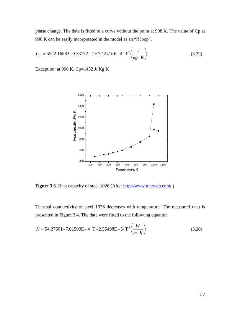
phase change. The data is fitted to a curve without the point at 998 K. The value of Cp at
998 K can be easily incorporated in the model as an “if loop”.
KkgJC p ⋅= 0.33772-522.168835⋅
⋅ 2T 4-7.12416E+T (3.29)
000
1200
1400
Exception: at 998 K, Cp=1432 J/ Kg K
1600
300 400 500 600 700 800 900 1000 1100400
600
800
1
Heat
kg K
cap
acity
, J/
Temperature, K
Figure 3.3. Heat capacity of steel 1026 (After http://www.matweb.com/ )
Thermal conductivity of steel 1026 decreases with temp
presented in Figure 3.4. The data were fitted to the following equation
erature. The measured data is
KmWK⋅
⋅⋅= 2T5-2.35498E-T 4-7.61593E-54.27601 (3.30)
57
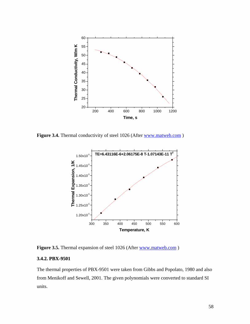
200 400 600 800 1000 120020
25
30
35
40
45
50
55
60
Ther
mal
Con
duct
ivity
, W/m
K
Time, s
Figure 3.4. Thermal conductivity of steel 1026 (After www.matweb.com )
300 350 400 450 500 550 600
1.20x10⁻⁵
1.25x10⁻⁵
1.30x10⁻⁵
1.35x10⁻⁵
1.40x10⁻⁵
1.45x10⁻⁵
1.50x10⁻⁵
Ther
mal
Exp
ansi
on,
Temperature, K
Figure 3.5. Thermal expansion of steel 1026 (After www.matweb.com
TE=6.43116E-6+2.06175E-8 T-1.07143E-11 T2
1/K
)
33..44..22.. PPBBXX--99550011
The thermal properties of PBX-9501 were taken from Gibbs and Popolato, 1980 and also
from Menikoff and Sewell, 2001. The given polynomials were converted to standard SI
units.
58
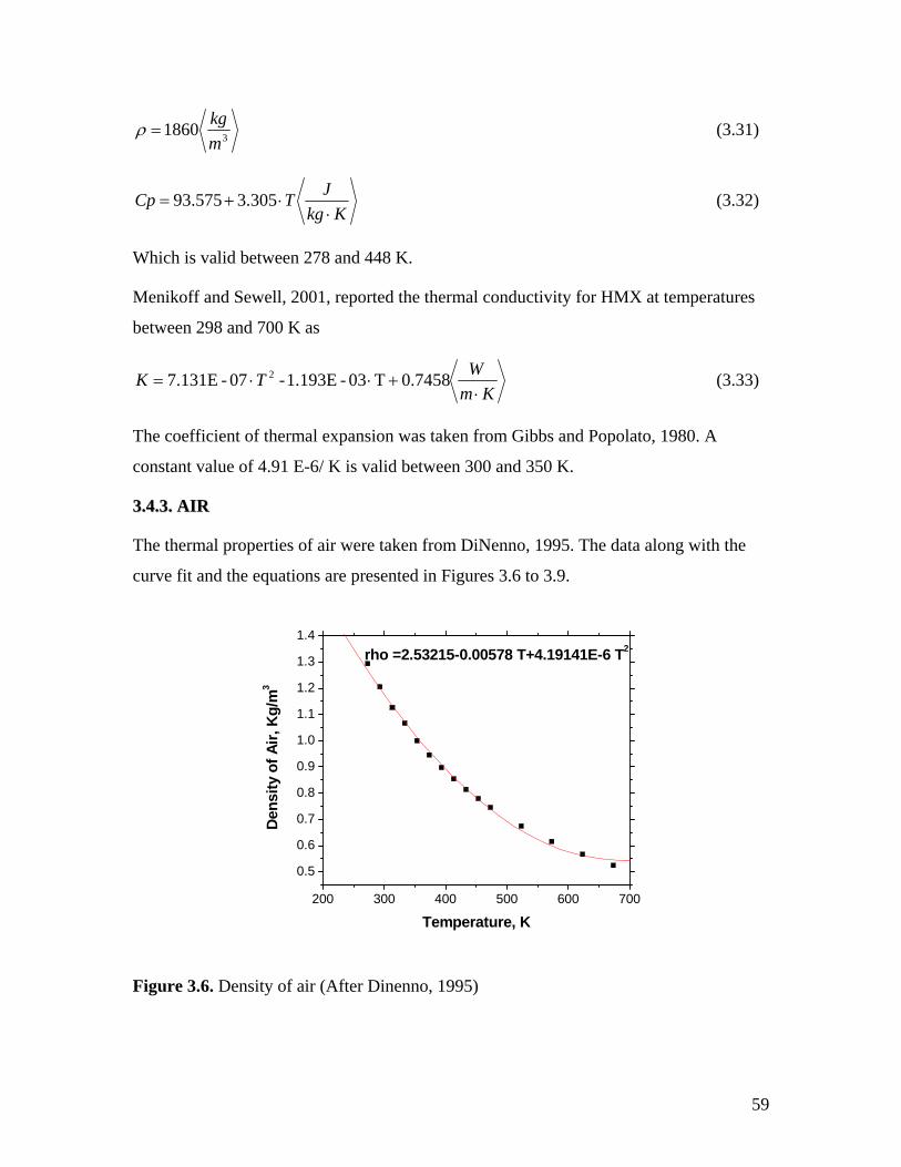
31860mkg
=ρ (3.31)
KkgJTCp⋅
⋅+= 305.3575.93 (3.32)
Which is valid between 278 and 448 K.
Menikoff and Sewell, 2001, reported the thermal conductivity for HMX at temperatures
between 298 and 700 K as
KmWTK⋅
+⋅⋅= 7458.0T03-1.193E - 07-7.131E 2 (3.33)
The coefficient of thermal expansion was taken from Gibbs and Popolato, 1980. A
constant value of 4.91 E-6/ K is valid between 300 and 350 K.
air were taken from DiNenno, 1995. The data along with the
curve fit and the equations are presented in Figures 3.6 to 3.9.
0.7
0.8
0.9
1.0
1.1
1.2
1.3
33..44..33.. AAIIRR
The thermal properties of
1.4
20
0.5
0 300 400 500 600 700
0.6
rho =2.53215-0.00578 T+4.19141E-6 T2
Dens
ity o
f Air,
3
Temperature, K
Figure 3.6. Density of air (After Dinenno, 1995)
Kg/
m
59
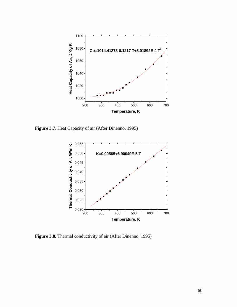
1080
200 300 400 500 600 700
1000
1020
1040
1060
1100
-4 T2
Heat
Cap
acity
of A
ir, J
/K
Temperature, K
Figure 3.7. Heat Capacity of air (After Dinenno, 1995)
Cp=1014.41273-0.1217 T+3.01892Eg K
200 300 400 500 600 7000.020
0.025
0.030
0.035
0.040
0.045
0.050
0.055
K=0.00565+6.9004
ir, W 9E-5 T
Ther
mal
Con
duct
ivity
of A
/m K
Temperature, K
Figure 3.8. Thermal conductivity of air (After Dinenno, 1995)
60
61
RREESSUULLTTSS AANNDD DDIISSCCUUSSSSIIOONN A more in-depth analysis of the experimental data is presented. A
comparison of the performance of the numerical methods is also included.
44..11.. FFIIRREE TTEESSTTSS
A complete list of temperature and pressure plots for all tests is included in the CD.
In this section, the thermal analysis of each test is described. In addition, separate
es with those given by
the ignition model for HMX-based explosives proposed by Beckstead in 1994.
4..11..11.. TTEESSTT 11,, EEXXPPLLOOSSIIVVEE MMAATTEERRIIAALL,, NNOOVVEEMMBBEERR 11999988
The correct measurement of steel temperature was one of the main difficulties found
hile carrying out the fire tests. The attached thermocouples are exposed to the fire and
they could not give the proper temperature rise of the steel pipe. Instead, the experimental
temperature profile seemed to correspond to that of a flame.
Assuming that the steel surface temperature is not too far from those represented in
Figure 4.1, and having into account that the steel wall is nearly isothermal, then the
temperature at the steel/PBX interface would be close to that represented by Tpbx, side in
the abovementioned Figure. This is in agreement with the fact that the thermocouples
were spot welded to the inner steel wall. Though, it is uncertain that this is the true
temperature of the PBX surface since some of the thermocouples may not have been
touching the PBX either because of an imperfect contact between the surfaces or a
displacement of the thermocouples when the PBX was placed in the pipe.
The measured interface temperature (T10 or Tpbx, side) and the Duhamel superposition
method were used to calculate the heat flux at the explosive surface as shown in Figure
4.2. The average heat flux was 19.8 kW/m^2 while Beckstead ignition model predicted
sections will be included to compare the experimental ignition tim
4
w
16.
goo
con
4 kW/m2. These values are presented in Figure 4.3. Even though, the values are in
d agreement (18 %), it is important to mention that the ignition model assumes
stant heat flux at the PBX surface and chemical reactions at atmospheric pressure.
550
600
0 20 40 60 80 100 120
300
350
400
450
500
650
700
750
800
er,
Tsteel, top Tsteel, bottom Tsteel, bottom Tpbx, bottom Tsteel, side Tpbx, side
Kat
ure
Tem
p
Time, s
odel include prediction of
Figure 4.1. Experimental temperatures for test 1, fire, 1998
The thermal behavior of the complete system was also studied using the thermal- reaction
model described in chapter 3. Some of the advantages of this m
ignition time, analysis of the temperature profile throughout the solid and also validation
of the assumptions (i.e. semi-infinite condition).
The boundary condition at the steel surface was adjusted to give the inner wall
temperature (T10 or Tpbx, side). This boundary consisted of radiative and convective
heat flux and the adjustment parameters were the flame temperature and the convective
heat transfer coefficient.
62
Figure 4.2 Heat flux at the PBX surface for test 1, fire, 1998
1
10
100
10 100 10001E-5
1E-4
1E-3
0.01
0.1
Igni
tion
Tim
, min
e
Heat flux, kW/m2
BYU Ignition Model,1994 Strakovski, 1989 Lengelle,1985 Atwood,1988 CSAFE Fire Test 1,1998
Figure 4.3. Ignition model for HMX-based explosives (After Beckstead, 1994)
63
All the calculations were based assuming that T10 was the true PBX temperature. The
argument emphasized isothermal conditions for the steel wall. Indeed, this was a valid
assumption as can be seen clearly in Figure 4.4.
Figure 4.4. Temperature profile for test 1, fire, 1998.
The thermal-reaction model assumed also semi-infinite conditions to reduce the problem
to a 1-D geometry. The penetration of heat was around 17 mm as can be seen in Figure
4.4, which is only 30 % of the explosive length. Therefore, for heat transfer calculations,
the system may be treated as a semi-infinite solid.
The heat flux profile at the surface of the explosive was similar to that obtained by
Duhamel and presented in Figure 4.2. An average of 19.5 kW/m2 was computed. The
model predicted an ignition time of 98 seconds, which is only 6 % sooner than the
experimental time. These results are also in good agreement with the ignition model
proposed by Beckstead in 1994.
44..11..22.. TTEESSTT 22,, EEXXPPLLOOSSIIVVEE MMAATTEERRIIAALL,, OOCCTTOOBBEERR 11999999
t for this
test mainly because the thermocouples were not spot welded to neither the outer nor the
The uncertainties in measuring the steel surface temperature are more significan
64
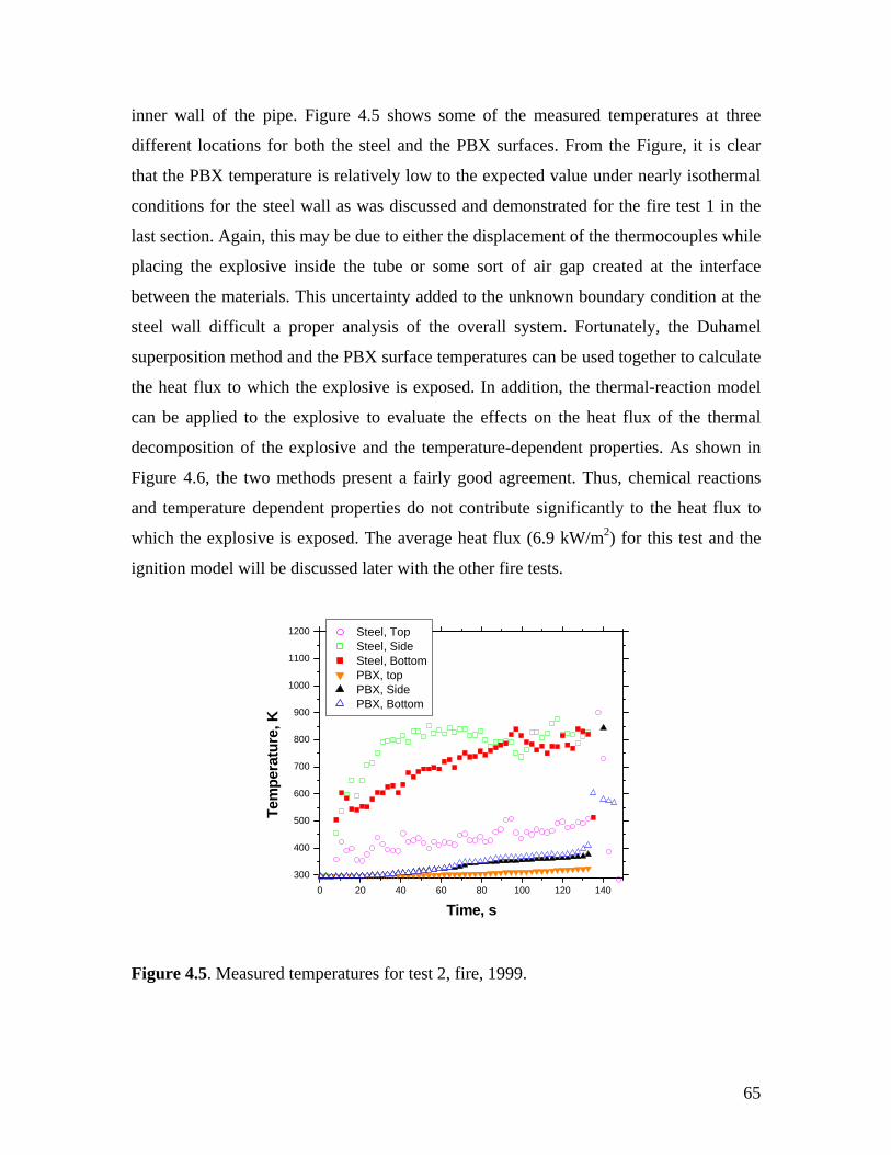
inner wall of the pipe. Figure 4.5 shows some of the measured temperatures at three
different locations for both the steel and the PBX surfaces. From the Figure, it is clear
that the PBX temperature is relatively low to the expected value under nearly isothermal
conditions for the steel wall as was discussed and demonstrated for the fire test 1 in the
last section. Again, this may be due to either the displacement of the thermocouples while
placing the explosive inside the tube or some sort of air gap created at the interface
between the materials. This uncertainty added to the unknown boundary condition at the
steel wall difficult a proper analysis of the overall system. Fortunately, the Duhamel
superposition method and the PBX surface temperatures can be used together to calculate
the heat flux to which the explosive is exposed. In addition, the thermal-reaction model
can be applied to the explosive to evaluate the effects on the heat flux of the thermal
decomposition of the explosive and the temperature-dependent properties. As shown in
Figure 4.6, the two methods present a fairly good agreement. Thus, chemical reactions
and temperature dependent properties do not contribute significantly to the heat flux to
which the explosive is exposed. The average heat flux (6.9 kW/m2) for this test and the
ignition model will be discussed later with the other fire tests.
0 20 40 60 80 100 120 140300
400
500
600
700
800
900
1000
1100
1200
T
Time, s
Steel, Top Steel, Side Steel, Bottom PBX, top PBX, Side PBX, Bottom
empe
ratu
re, K
Figure 4.5. Measured temperatures for test 2, fire, 1999.
65
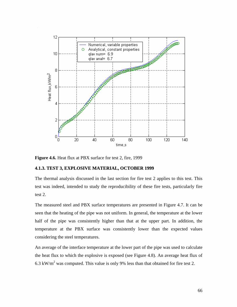
Figure 4.6. Heat flux at PBX surface for test 2, fire, 1999
44..11..33.. TTEESSTT 33,, EEXXPPLLOOSSIIVVEE MMAATTEERRIIAALL,, OOCCTTOOBBEERR 11999999
The thermal analysis discussed in the last section for fire test 2 applies to this test. This
test was indeed, intended to study the reproducibility of these fire tests, particularly fire
test 2.
The measured steel and PBX surface temperatures are presented in Figure 4.7. It can be
seen that the heating of the pipe was not uniform. In general, the temperature at the lower
half of the pipe was consistently higher than that at the upper part. In addition, the
temperature at the PBX surface was consistently lower than the expected values
considering the steel temperatures.
An average of the interface temperature at the lower part of the pipe was used to calculate
8). An average heat flux of
6.3 kW/m was computed. This value is only 9% less than that obtained for fire test 2.
the heat flux to which the explosive is exposed (see Figure 4.2
66
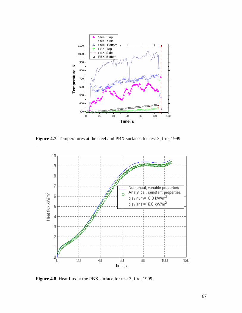
0 20 40 60 80 100 120300
400
500
600
700
800
900
1000
1100
Tem
pera
ture
, K
Time, s
Steel, Top Steel, Side Steel, Bottom PBX, Top PBX, Side PBX, Bottom
Figure 4.7. Temperatures at the steel and PBX surfaces for test 3, fire, 1999
Figure 4.8. Heat flux at the PBX surface for test 3, fire, 1999.
67
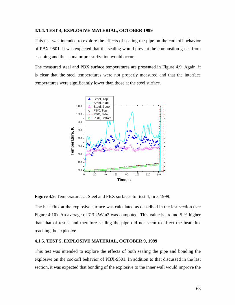
44..11..44.. TTEESSTT 44,, EEXXPPLLOOSSIIVVEE MMAATTEERRIIAALL,, OOCCTTOOBBEERR 11999999
This test was intended to explore the effects of sealing the pipe on the cookoff behavior
of PBX-9501. It was expected that the sealing would prevent the combustion gases from
escaping and thus a major pressurization would occur.
The measured steel and PBX surface temperatures are presented in Figure 4.9. Again, it
is clear that the steel temperatures were not properly measured and that the interface
temperatures were significantly lower than those at the steel surface.
800
900
1000
1100
0 20 40 60 80 100 120 140300
400
500
600
700
Tem
pera
t
Time, s
ure,
K
Steel, Top Steel, Side Steel, Bottom PBX, Top PBX, Side PBX, Bottom
Figure 4.9. Temperatures at Steel and PBX surfaces for test 4, fire, 1999.
The heat flux at the explosive surface was calculated as described in the last section (see
Figure 4.10). An average of 7.3 kW/m2 was computed. This value is around 5 % higher
than that of test 2 and therefore sealing the pipe did not seem to affect the heat flux
reaching the explosive.
44..11..55.. TTEESSTT 55,, EEXXPPLLOOSSIIVVEE MMAATTEERRIIAALL,, OOCCTTOOBBEERR 99,, 11999999
This test was intended to explore the effects of both sealing the pipe and bonding the
explosive on the cookoff behavior of PBX-9501. In addition to that discussed in the last
section, it was expected that bonding of the explosive to the inner wall would improve the
68
heat transfer at the interface. However, as can be seen in Figure 4.11 and 4.12, the
n that of test 4. This suggests that
sealing the steel pipe and bonding the explosive to the inner wall did not have a
thermal behavior of this test was similar to those discussed in the last three sections. For
instance, an average heat flux of 6.4 kW/m2 was computed, which of the same level of
those found for tests 2 and 3 and around 12% lower tha
significant impact on the amount of heat flux reaching the explosive.
Figure 4.10. Heat flux at the explosive surface for test 4, fire, 1999.
69
900
1000
1100
1200
0 20 40 60 80 100300
400
500
600
700
800
Tem
pera
Time, s
ture
, K
Steel, Top Steel, Side Steel, Bottom PBX, Top PBX, Side PBX, Bottom
Figure 4.11. Temperatures at the Steel and PBX surfaces for test 5, fire, 1999.
Figure 4.12. Heat flux at the explosive surface test 4, for fire, 1999.
70
44..11..66.. TTHHEE FFIIRREE TTEESSTTSS AANNDD TTHHEE IIGGNNIITTIIOONN MMOODDEELL
The experimental times to ignition are compared to those given by the ignition model for
HMX-based explosives (Beckstead, 1994). The model combines many of the physical
and chemical mechanisms needed to describe the ignition process of HMX and predicts
that the ignition time should decrease with increasing heat flux. It is important to mention
that the model assumes that the explosive is exposed to a constant heat flux and that the
reactions occur at atmospheric pressure. In this work it was shown that the heat flux
presents a transient behavior (i.e. Heat flux on Figures 4.2, 4.6, 4.8, 4.10 and 4.12) and
also that pressures are typical of highly confined systems (i.e., experimental pressures up
7500 psi, see for example Figures in Appendix B).
The average heat flux and the experimental ignition times for the fire tests are presented
in Table 4.1. For comparison purposes, the average heat flux values are used in the
es are also
included in Table 4.1.These values are also compared graphically in the ignition plot in
Figure 4.13. It can be seen that this work represents the only experimental data in the low
heat flux regime of the ignition model plot. The trend of the data is consistent with the
experimental work of Strakovski et al, 1989. Even though a direct comparison cannot be
made with the ignition model, it is clear that there is a lack of understanding and further
research is needed in the heating rate regime present in typical fire environments.
Table 4.1. Ignition times for the fire cookoff tests
Test # Container Characteristics
Heat Flux, KW/m2
Experimental Ignition Time
Ignition Time Beckstead Model
Error, %
ignition model to read the theoretical time from the ignition model and the valu
1* N/A 19.8 1.75 1.28 -26 2 Unbounded,
Unsealed 6.9 2.21 9.1 310
3 Unbounded, Unsealed
6.3 1.72 10.6 500
4 Unbounded, Sealed
7.3 2.35 8.0 240
5 Bonded, Sealed 6.4 1.63 10.3 530
*Test 1 used PBC-123 (85% HMX) while tests 2,3,4 and 5 used PBX-9501 (95% HMX)
71
10 100 10001E-5
1E-4
1E-3
0.01
0.1
1
10
100
Igni
tion
Tim
e, m
in
BYU Ignition Model,1994 Strakovski, 1989 Lengelle,1985 Atwood,1988 CSAFE Fire Tests,1998/99
Heat flux, kW/m2
Figure 4.13. Experimental and numerical ignition times (After Beckstead, 1994)
44..22.. EELLEECCTTRRIICCAALL TTEESSTTSS
It was concluded in the last section that a big gap exists in the understanding of the
thermal behavior of HMX-based explosives exposed to heating rates present in fires. The
main uncertainty found in the fire cookoff experiments was measuring the steel surface
dentified that electrical heaters could
provide a well-defined boundary condition at the steel surface.
44..22..11.. TTEE IICCAA Y 2200
Th igniti est too ace at approximately 31 minutes. Because of the
un tainty to expl , only som rmocouple data was recovered. The
temperature at the steel surface at the moment of the explosion was around 700 K. This
was a very violent explosion and almost all the container and the explosive material were
consume piec ere found. ents on the thermal analysis of
is test can be found in the appendices B and C included in the CD.
temperature. As discussed in chapter 2, it was i
SSTT 66,, EELLEECCTTRR LL,, JJUULLY 0011
e on for this t k pl
cer in the time osion e the
d, only four small es w Some comm
this test will be included in section 4.4. In addition, the data and some of the pictures for
th
72
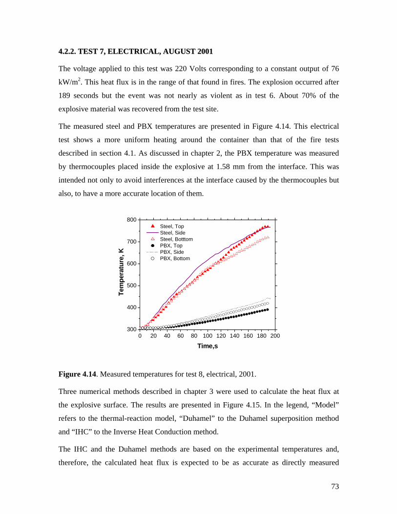
44..22..22.. TTEESSTT 77,, EELLEECCTTRRIICCAALL,, AAUUGGUUSSTT 22000011
The voltage applied to this test was 220 Volts corresponding to a constant output of 76
kW/m2. This heat flux is in the range of that found in fires. The explosion occurred after
189 seconds but the event was not nearly as violent as in test 6. About 70% of the
explosive material was recovered from the test site.
The measured steel and PBX temperatures are presented in Figure 4.14. This electrical
test shows a more uniform heating around the container than that of the fire tests
described in section 4.1. As discussed in chapter 2, the PBX temperature was measured
by thermocouples placed inside the explosive at 1.58 mm from the interface. This was
intended not only to avoid interferences at the interface caused by the thermocouples but
also, to have a more accurate location of them.
600
800
0 20 40 60 80 100 120 140 160 180 200
Steel, Top Steel, Side Steel, Botttom PBX, Top
700
300
400
500
PBX, Side PBX, Bottom
e,s
l temperatures and,
therefore, the calculated heat flux is expected to be as accurate as directly measured
ure,
K
Tem
pera
t
Tim
Figure 4.14. Measured temperatures for test 8, electrical, 2001.
Three numerical methods described in chapter 3 were used to calculate the heat flux at
the explosive surface. The results are presented in Figure 4.15. In the legend, “Model”
refers to the thermal-reaction model, “Duhamel” to the Duhamel superposition method
and “IHC” to the Inverse Heat Conduction method.
The IHC and the Duhamel methods are based on the experimenta
73
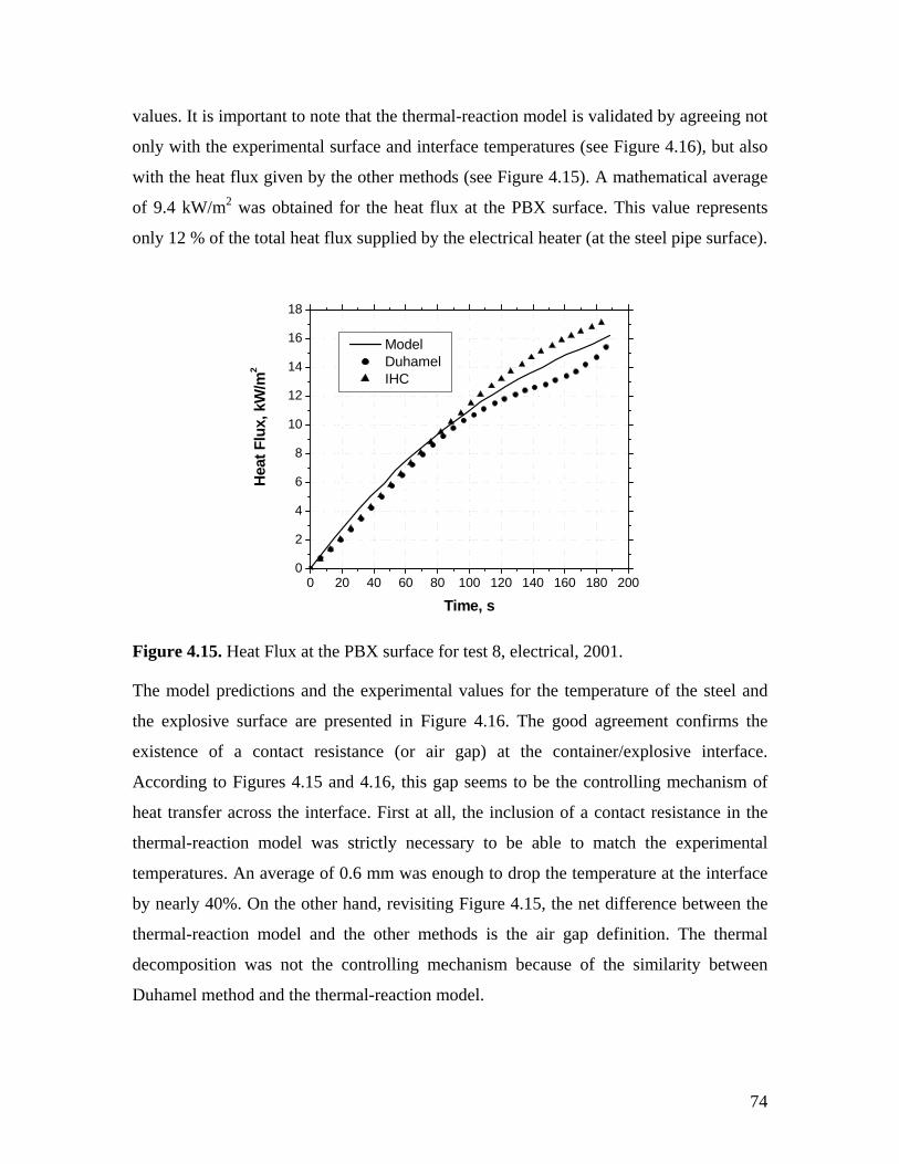
values. It is important to note that the thermal-reaction model is validated by agreeing not
ical heater (at the steel pipe surface).
Figure 4.15.
The m erature of the steel and
the explosiv
existence of a contact resistance (or air gap) at the container/explosive interface.
According to Figures 4.15 and 4.16, this gap seems to be the controlling mechanism of
heat transfer across the interface. First at all, the inclusion of a contact resistance in the
match the experimental
because of the similarity between
Duhamel method and the thermal-reaction model.
only with the experimental surface and interface temperatures (see Figure 4.16), but also
with the heat flux given by the other methods (see Figure 4.15). A mathematical average
of 9.4 kW/m2 was obtained for the heat flux at the PBX surface. This value represents
only 12 % of the total heat flux supplied by the electr
0 20 40 60 80 100 120 140 160 180 2000
2
4
6
8
10
12
14
16
18
Heat
Time, s
Flu
x, k
W/m
2
Model Duhamel IHC
Heat Flux at the PBX surface for test 8, electrical, 2001.
odel predictions and the experimental values for the temp
e surface are presented in Figure 4.16. The good agreement confirms the
thermal-reaction model was strictly necessary to be able to
temperatures. An average of 0.6 mm was enough to drop the temperature at the interface
by nearly 40%. On the other hand, revisiting Figure 4.15, the net difference between the
thermal-reaction model and the other methods is the air gap definition. The thermal
decomposition was not the controlling mechanism
74
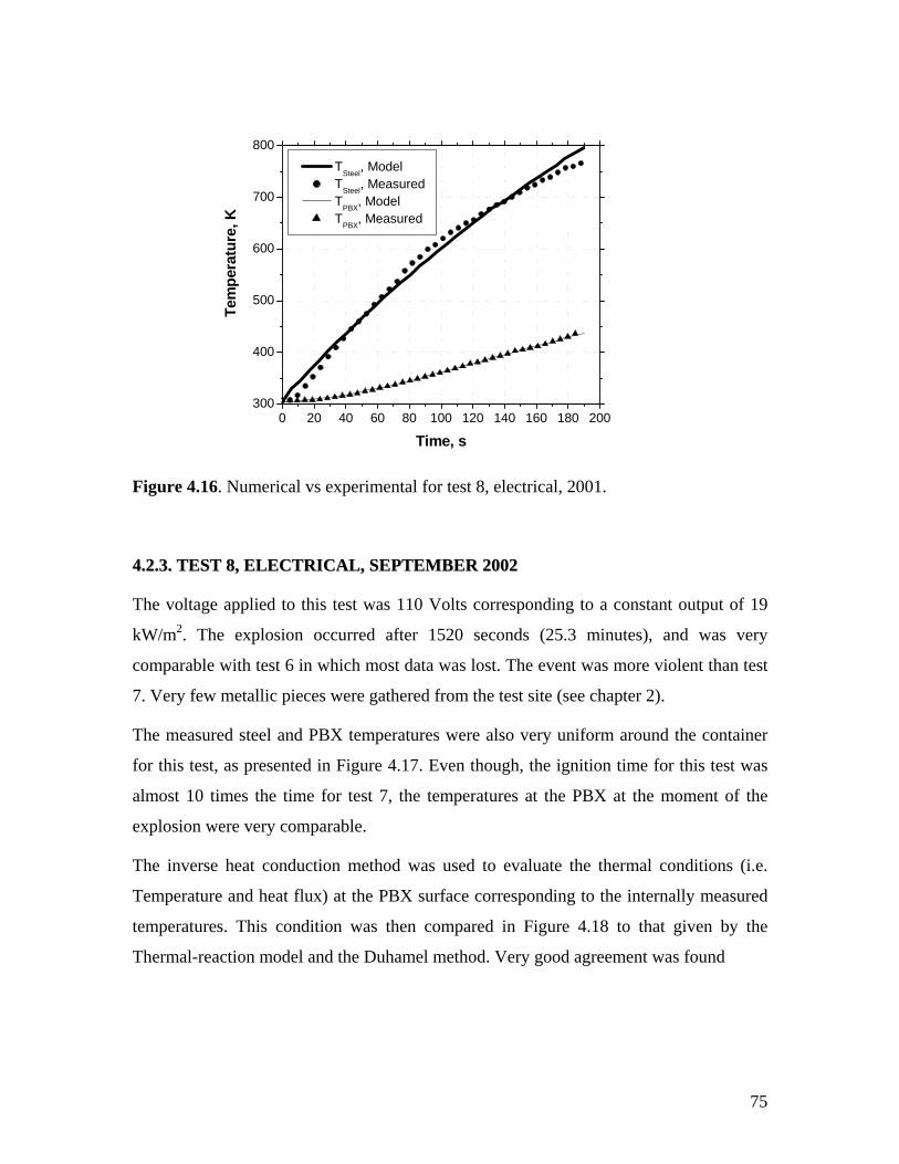
0 20 40 60 80 100 120 140 160 180 200300
400
500
600
700
800
Tem
pera
t
Time, s
ure,
K
TSteel, Model TSteel, Measured TPBX, Model TPBX, Measured
Figure 4.16
44..22..33.. TTEESSTT
constant output of 19
kW/m2. The explosion occurred after 1520 seconds (25.3 minutes), and was very
ore violent than test
. Numerical vs experimental for test 8, electrical, 2001.
88,, EELLEECCTTRRIICCAALL,, SSEEPPTTEEMMBBEERR 22000022
The voltage applied to this test was 110 Volts corresponding to a
comparable with test 6 in which most data was lost. The event was m
7. Very few metallic pieces were gathered from the test site (see chapter 2).
The measured steel and PBX temperatures were also very uniform around the container
for this test, as presented in Figure 4.17. Even though, the ignition time for this test was
almost 10 times the time for test 7, the temperatures at the PBX at the moment of the
explosion were very comparable.
The inverse heat conduction method was used to evaluate the thermal conditions (i.e.
Temperature and heat flux) at the PBX surface corresponding to the internally measured
temperatures. This condition was then compared in Figure 4.18 to that given by the
Thermal-reaction model and the Duhamel method. Very good agreement was found
75
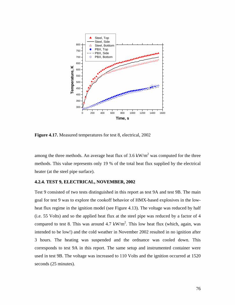
0 200 400 600 800 1000 1200 1400 1600
300
350
400
450
500
550
600
650
700
750
800
Steel, Top Steel, Side Steel, Botttom PBX, Top PBX, Side PBX, Bottom
Tem
pera
ture
, K
Time, s
Figure 4.17. Measured temperatures for test 8, electrical, 2002
2
heat flux at the steel pipe was reduced by a factor of 4 2
were
used in test 9B. The voltage was increased to 110 Volts and the ignition occurred at 1520
seconds (25 minutes).
among the three methods. An average heat flux of 3.6 kW/m was computed for the three
methods. This value represents only 19 % of the total heat flux supplied by the electrical
heater (at the steel pipe surface).
44..22..44.. TTEESSTT 99,, EELLEECCTTRRIICCAALL,, NNOOVVEEMMBBEERR,, 22000022
Test 9 consisted of two tests distinguished in this report as test 9A and test 9B. The main
goal for test 9 was to explore the cookoff behavior of HMX-based explosives in the low-
heat flux regime in the ignition model (see Figure 4.13). The voltage was reduced by half
(i.e. 55 Volts) and so the applied
compared to test 8. This was around 4.7 kW/m . This low heat flux (which, again, was
intended to be low!) and the cold weather in November 2002 resulted in no ignition after
3 hours. The heating was suspended and the ordnance was cooled down. This
corresponds to test 9A in this report. The same setup and instrumented container
76
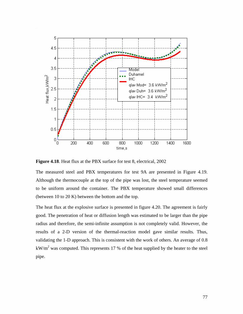
Figure 4.18. Heat flux at the PBX surface for test 8, electrical, 2002
The measured steel and PBX temperatures for test 9A are presented in Figure 4.19.
Although the thermocouple at the top of the pipe was lost, the steel temperature seemed
erature showed small differences to be uniform around the container. The PBX temp
(between 10 to 20 K) between the bottom and the top.
The heat flux at the explosive surface is presented in figure 4.20. The agreement is fairly
good. The penetration of heat or diffusion length was estimated to be larger than the pipe
radius and therefore, the semi-infinite assumption is not completely valid. However, the
results of a 2-D version of the thermal-reaction model gave similar results. Thus,
validating the 1-D approach. This is consistent with the work of others. An average of 0.8
kW/m2 was computed. This represents 17 % of the heat supplied by the heater to the steel
pipe.
77
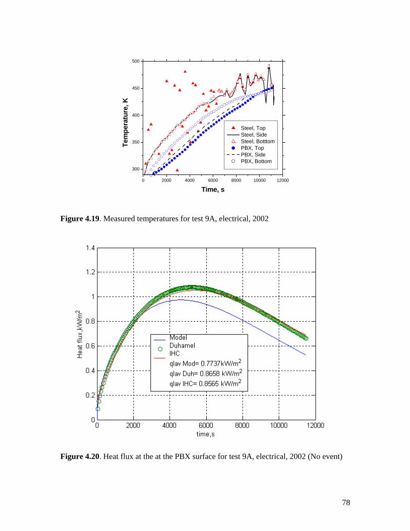
0 2000 4000 6000 8000 10000 12000
300
350
400
450
500
Steel, Top Steel, Side Steel, Botttom PBX, Top PBX, Side PBX, Bottom
Tem
pera
ture
, K
Time, s
Figure 4.19. Measured temperatures for test 9A, electrical, 2002
Figure 4.20. Heat flux at the at the PBX surface for test 9A, electrical, 2002 (No event)
78
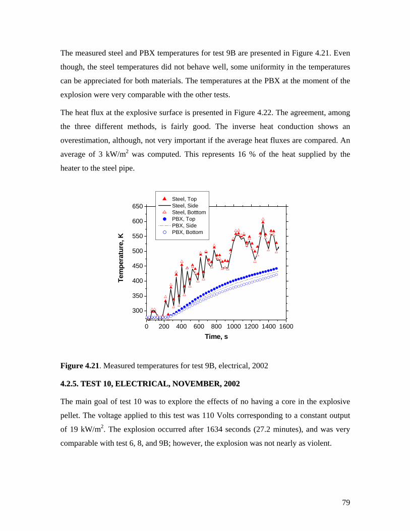
The measured steel and PBX temperatures for test 9B are presented in Figure 4.21. Even
though, the steel temperatures did not behave well, some uniformity in the temperatures
can be appreciated for both materials. The temperatures at the PBX at the moment of the
explosion were very comparable with the other tests.
The heat flux at the explosive surface is presented in Figure 4.22. The agreement, among
the three different methods, is fairly good. The inverse heat conduction shows an
overestimation, although, not very important if the average heat fluxes are compared. An
average of 3 kW/m2 was computed. This represents 16 % of the heat supplied by the
heater to the steel pipe.
650
0 200 400 600 800 1000 1200 1400 1600
300
350
400
450
500
550
Steel, Top Steel, Side Steel, Botttom PBX, Top600 PBX, Side PBX, Bottom
Tem
pera
ture
, K
Time, s
Figure 4.21. Measured temperatures for test 9B, electrical, 2002
44..22..55.. TTEESSTT 1100,, EELLEECCTTRRIICCAALL,, NNOOVVEEMMBBEERR,, 22000022
The main goal of test 10 was to explore the effects of no having a core in the explosive
pellet. The voltage applied to this test was 110 Volts corresponding to a constant output
of 19 kW/m2. The explosion occurred after 1634 seconds (27.2 minutes), and was very
comparable with test 6, 8, and 9B; however, the explosion was not nearly as violent.
79
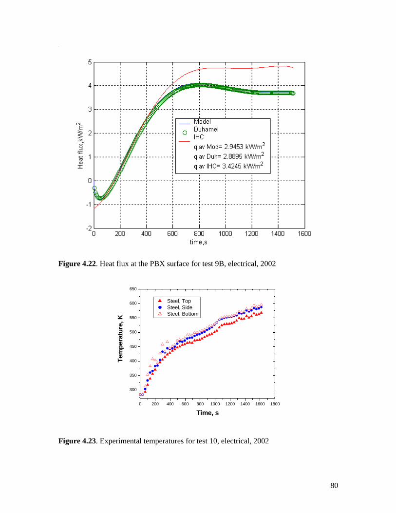
Figure 4.22. Heat flux at the PBX surface for test 9B, electrical, 2002
0 200 400 600 800 1000 1200 1400 1600 1800
300
350
400
450
500
550
600
650
Tem
pera
ture
, K
Time, s
Steel, Top Steel, Side Steel, Bottom
igure 4.23. Experimental temperatures for test 10, electrical, 2002
F
80
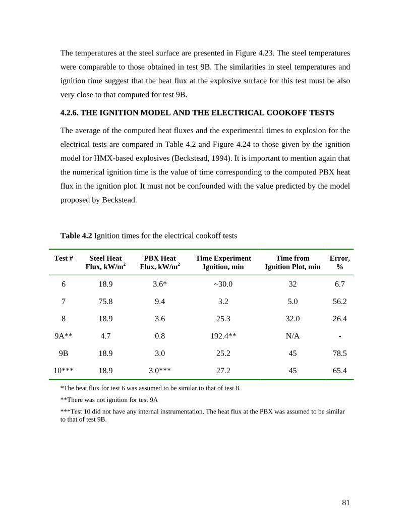
The temperatures at the steel surface are presented in Figure 4.23. The steel temperatures
were comparable to those obtained in test 9B. The similarities in steel temperatures and
ignition time suggest that the heat flux at the explosive surface for this test must be also
very close to that computed for test 9B.
44..22..66.. TTHHEE IIGGNNIITTIIOONN MMOODDEELL AANNDD TTHHEE EELLEECCTTRRIICCAALL CCOOOOKKOOFFFF TTEESSTTSS
The average of the computed heat fluxes and the experimental times to explosion for the
electrical tests are compared in Table 4.2 and Figure 4.24 to those given by the ignition
model for HMX-based explosives (Beckstead, 1994). It is important to mention again that
the numerical ignition time is the value of time corresponding to the computed PBX heat
flux in the ignition plot. It must not be confounded with the value predicted by the model
proposed by Beckstead.
Table 4.2 Ignition times for the electrical cookoff tests
Test # Steel Heat 2
PBX Heat 2
Time Experiment Time from , min
Error, % Flux, kW/m Flux, kW/m Ignition, min Ignition Plot
6 18.9 3.6* ~30.0 32 6.7
7 75.8 9.4 3.2 5.0 56.2
8 18.9 3.6 25.3 32.0 26.4
9A** 4.7 0.8 192.4** N/A -
9B 18.9 3.0 25.2 45 78.5
10*** 18.9 3.0*** 27.2 45 65.4
*The heat flux for test 6 was assumed to be similar to that of test 8.
**There was not ignition for test 9A
***Test 10 did not have any internal instrumentation. The heat flux at the PBX was assumed to be similar to that of test 9B.
81
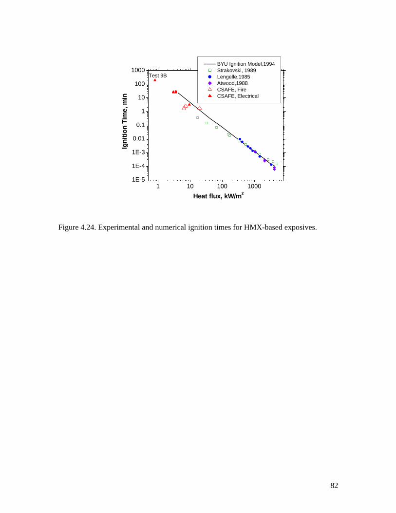
Figure 4.24. Experimental and numerical ignition times for HMX-based exposives.
1 10 100 10001E-5
1E-4
1E-3
0.01
0.1
1
10
100
1000Test 9B
n
BYU Ignition Model,1994 Strakovski, 1989 Lengelle,1985 Atwood,1988 CSAFE, Fire CSAFE, Electrical
me,
mi
Igni
tion
Ti
Heat flux, kW/m2
82
CCOONNCCLLUUDDIINNGG RREEMMAARRKKSS A series of fast cookoff tests were carried t an accident scenario where
high-energy materials are exposed to a rapidly generated fire. The experiments were
designed to develop a phenomenological understanding of the heat transfer in the overall
system. Thermal boundaries at the fire/container and container/explosive interfaces were
identified as critical for accomplishing the goals.
The initial experiments used propane burners but some uncertainties were found while
measuring the steel surface temperatures. Then, it was identified that electrical heaters
dvantage of a well-defined boundary at the steel surface. This helped to concentrate the
fforts on the steel/explosive interface.
hree methods for heat transfer analysis were developed to study the thermal behavior of
onfined HMX-based explosives when heated by a fire or electricity. The first method
sed the Duhamel superposition principles to convert the measured surface temperature
to heat flux. The second method used inverse heat equations to calculate the thermal
oundaries at the surface from temperature measurement made within the explosive. The
ird method used a finite difference technique to model the overall system and thus,
valuate the relative importance of the different mechanisms of heat transfer.
The heat transfer analysis has demonstrated that there was a significant thermal contact
resistance at the interface between the explosive material and the steel shell that resulted
in a significant delay in the time to explosion. It was shown that an air gap could have
been the responsible for this resistance.
The average heat flux at the explosive surface was between 12 and 20% of the heat flux
applied to the steel surface. This confirms the effectiveness of the air gap and also the
small diffusion length due to the insulating properties of the explosive
out to represen
could provide heat fluxes in the same range of those found in fires with the additional
a
e
T
c
u
in
b
th
e
83

A comparison of the three numerical methods has revealed that conduction through the
air gap may be the controlling mechanism of heat transfer across the steel/explosive
interface.
The accuracy in the heat flux calculations is crucial in predicting the time to explosion
, the numerical heat transfer results and the
greement was found for the electrical
with any suitable model. In this report
experimental times were compared with the ignition model proposed by Beckstead. An
average heat flux was used because the current version of the ignition model assumes that
the explosive is exposed to a constant heat flux.
A graphical comparison has shown that the data presented in this report follow the same
trend of the ignition model. In general, a better a
tests than for the fire tests. Many reasons can be inferred from the differences between
the tests. For instance, the fire tests used a cylindrical container that was 3 times longer or
had 3 times more explosive than the one used in the electrical tests. Also, fire
experiments are greatly influenced by weather conditions (i.e. wind influences non-
uniform heating around the container).
84
RREEFFEERREENNCCEESS 1. Beck, J. B. Blackwell and St. Clair, Ch. 1985. Inverse heat conduction: ill posed
problems, John Wiley Interscience publication, pp. 55.
2. Beckstead, M., 1994, “An Ignition Model for Modern Double Base Propellants,” 31st
., 101 (1005), pp. 209-212.
. Carnahan, B., Luther, H. A., and Wilkes, J. O., 1969, Applied Numerical Methods,
Krieger Publishing Company, pp. 429-530, Chap. 7.
6. Cook, W. and Felderman E., 1966, “Reduction of Data from Thin-Film Heat
Transfer: A Concise Numerical Technique,” AIAA Journal, 4 (3), pp.561-562.
Diller, T.E., 1996, “Methods of Determining Heat Flux from Temperature
Measurements,” Proceedings of the International Instrumentation Symposium,
Instrument Society of America, pp. 251-262.
. DiNenno, P., Appendix B, Property Data, in: The SFPE Handbook of Fire Protection
Engineering, second edition, 1995, pp. A-26.
. Gibbs, T. and Popolato, A., 1980, LASL Explosive Property Data, The University of
California Press, Berkeley, CA, pp. 109-119.
10. Hills, R. G., and Hensel, Jr. E. C., 1986, “One-Dimensional Nonlinear Inverse Heat
Conduction Technique,” Numerical Heat Transfer, 10, pp. 369-393.
JANNAF Combustion Meeting, Sunnyvale, CA, pp. 163-180.
3. Burggraf, O. R., 1964, “An Exact Solution of the Inverse Problem in Heat
Conduction. Theory and Applications,” ASME Journal of Heat Transfer, 86, pp.373-
382.
4. Buttsworth, D. R., and Jones, T. V., 1997, “Radial Conduction Effects in Transient
Heat Transfer Experiments,” AIAA J
5
7.
8
9
85
11. Kakac, S. and Yener, Y., 1993, Heat Conduction, Taylor & Francis, pp. 56-57, Chap.
3.
12. Online Material Property Data Sheet at www.matweb.com
13. McGuire, R. R., and Tarver, C. M., 1981, “Chemical Decomposition Models for the
of Confined HMX, TATB, RDX and TNT Explosives,” Seventh
14. Menikoff, R. and Sewell, T., 2001, “Constituen f HMX Needed for
Thermal Explosion
International Symposium on Detonation, Annapolis, MD, pp.56-64.
t Properties o
Meso-Scale Simulations,” Theoretical Division, Los Alamos National Laboratory,
Los Alamos, NM. Available online at:
http://t14web.lanl.gov/Staff/rsm/Preprints/HMXmeso.pdf
Murry, R. L., 1998, “CSAFE Cookoff test #1”, Report TR11566, Thiokol
Corpo
15.
ration, Brigham City, November.
line at
16. Murry, R. L., 1998, “CSAFE Cookoff Tests, Phase III,” Report TR12646, Thiokol
Corporation, Brigham City, September.
17. Murry, R. L., 1999, “CSAFE Cookoff Tests CY1999,” Report TR11996, Thiokol
Corporation, Brigham City, December.
18. Pershing, D., 2000, Center for the Simulation of Accidental Fires and Explosions,
Annual Report, 2000, University of Utah, Salt Lake City, Ut., Available on
http://www.csafe.utah.edu/documents/FY01annual.pdf
Eddings, E., and Sarofim, A., 1999, CSAFE Validation, Available online at 19.
ttp://www.combustion.utah.edu/prograhttp://www.combustion.utah.edu/main.html?h
ms.html
86
PPAAPP EENNDDIIXX AA AANNDD OOTTHHEERR FFIILLEESS IINNCCLLUUDDEEDD IINN TTHHEE CCDD
The
DA . There are two
. For
con
PICTURES: taken at the experimental site. They
are ordered by subfolders according to the test.
RE onic version of each chapter, the full report,
and the appendixes.
AP ll the plots from the cookoff tests. Due to its
form e is an explanation of them.
CD contains three major folders: Data, Pictures, Report.
TA: This folder contains all the data in Excel and Origin files
different origin files; one contains the original data and the other all the plots
venience, the plots are then collected in a single file (see Appendix A files)
This folder contains all the pictures
PORT: This folder contains the electr
PENDIX A: This appendix contains a
extension, only the electronic files have been included. For convenience, different
ats of the files are saved in the CD. Her
APPENDIXA.doc : Large file. Contains the plot pasted as Origin objects. Allows
dification of the plots.
PENDIXA.pdf
mo
AP : Small file, it corresponds to APPENDIXA.doc.
APPENDIXA_pict.doc: Small file. Contains the plots pasted as pictures.
APPENDIXA_pict.pdf: Small file, corresponding to APPENDIXA_pict.doc
APPENDIX B: This appendix was included in the report for the sake of the
discussion. It contains all the plots from the tests in a comparison form. That is, multiple
temperatures are included in the same plot in order to easily see or comment about the
particular behavior in one test.
87

88
AAPPPPEENNDDIIXX
BB

RREE,, NNOOVVEEMMBBEERR 11999988
PPLLOOTTSS,, TTEESSTT 11,, FFII
89
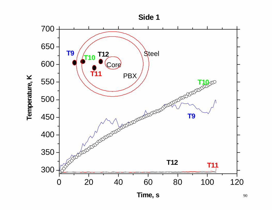
0 60 80 100 120300
350
400
450
550
600
500
650
700
T9 T12T10
Side 1
Steel
T11T10
T11
T9
T12
CorePBX
Tem
pera
te,
K
Time, s
ur
90
0 20 4
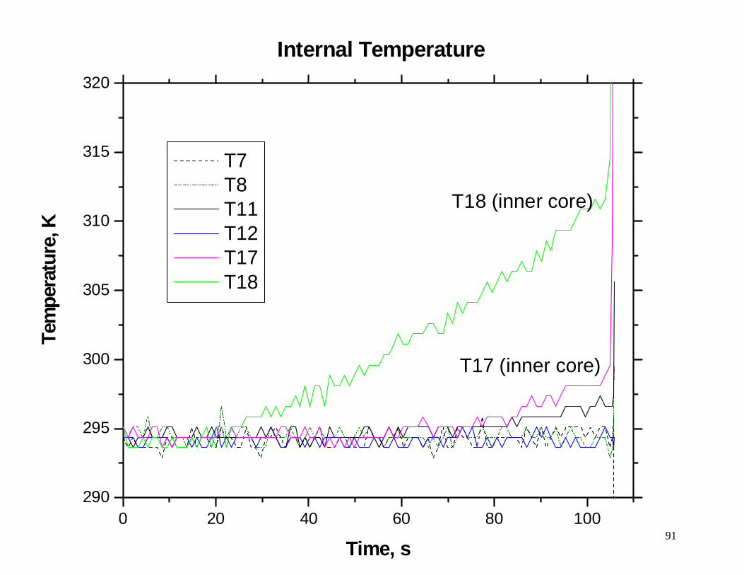
0 20 40 60 80 100290
295
300
305
310
315
320
T17 (inner core)
T18 (inner core)
Tem
pera
ture
, K
Time, s
Internal Temperature
T7 T8 T11 T12 T17 T18
91
92
0 20 40 60 80 100 120
300
350
400
450
500
550
600
650
700
T16
T13
T10
Interface Temperature
T10 T13 T16
Tem
pera
ture
, K
Time, s
93
0 20 40 60 80 100 120
300
350
400
450
500
550
600
650
700
750
800
Steel Suface TemperatureTe
mpe
ratu
re, K
Time, s
Tsteel, top Tsteel, side Tsteel, bottom Tpbx, top Tpbx, side Tpbx, bottom
94
0 20 40 60 80 100 120300
350
400
450
500
550
600
650
700T5
Bottom 1
T8 T7
T16
T5T16
T7T8
Core
Steel
PBX
Tem
pera
ture
, K
Time, s
95
0 20 40 60 80 100 120300
350
400
450
500
550
600
650
700
T18
T18T8 T7
T16
T15
Bottom 2
T15T16
T7T8
Core
Steel
PBX
Tem
pera
ture
, K
Time, s
0 20 40 60 80 100 120300
350
400
450
500
550
600
650
700
T
T16
96
17
T16
T18
T17, T18
T5 T15
Bottom 3
T5, T15
Core
Steel
PBX
Tem
pera
ture
, K
Time, s
97
0 20 40 60 80 100 120300
350
400
450
500
550
600
650
700
750
800 T13 T14
T14
T13
Top
Core
Steel
PBX
Tem
pera
ture
, K
Time, s

PPLLOOTTSS,, TTEESSTT 22,, FFIIRREE,, OOCCTTOOBBEERR 11999999
98
99
0 20 40 60 80 100 120 140250
300
350
450
500
550
600
400
Inside Container, 1/3, 0, 90,180,270
Teer
atur
e, K
Time, s
T12 T3 T5 T1
mp
100
0 20 40 60 80 100 120 140250
300
350
400
450
500
550
600
Inside Container, 1/3, 0, 90,180,270Te
mpe
ratu
re, K
me, s
T10 T4 T6 T2
Ti
101
0 20 40 60 80 100 120 140300350400450500550600650700750800850900950
1000105011001150120012501300
Tem
pera
ture
, K
Time, s
Outside Container, 1/3, 0, 90,180,270
T23 T15 T17 T13
102
0 20 40 60 80 100 120 140300350400450500550600650700750800850900950
1000105011001150120012501300
Outside Container, 1/3, 0, 90,180,270Te
mpe
ratu
re, K
Time, s
T24 T16 T18 T14

PPLLOOTTSS,, TTEESSTT 33,, FFIIRREE,, OOCCTTOOBBEERR 11999999
103
Inside Container, 1/3, 0, 90, 180, 270
104
0 20 40 60 80 100 120250
300
350
400
450
500
550
600
T12 T3 T5 T1
Tem
p
Time, s
erat
ure,
K
105
0 20 40 60 80 100 120250
300
350
400
450
500
550
600
Inside Container, 1/3, 0, 90, 180, 270Te
mpe
ratu
re, K
Time, s
T10 T4 T6 T2

PPLLOOTTSS,, TTEESSTT 44,, FFIIRREE,, OOCCTTOOBBEERR 11999999
106
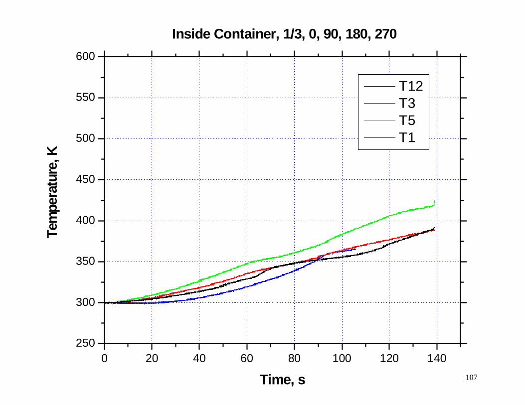
Inside Container, 1/3, 0, 90, 180, 270
107
0 20 40 60 80 100 120 140250
300
350
400
450
500
550
600
T12 T3 T5 T1
Tem
pera
re, K
Time, s
tu
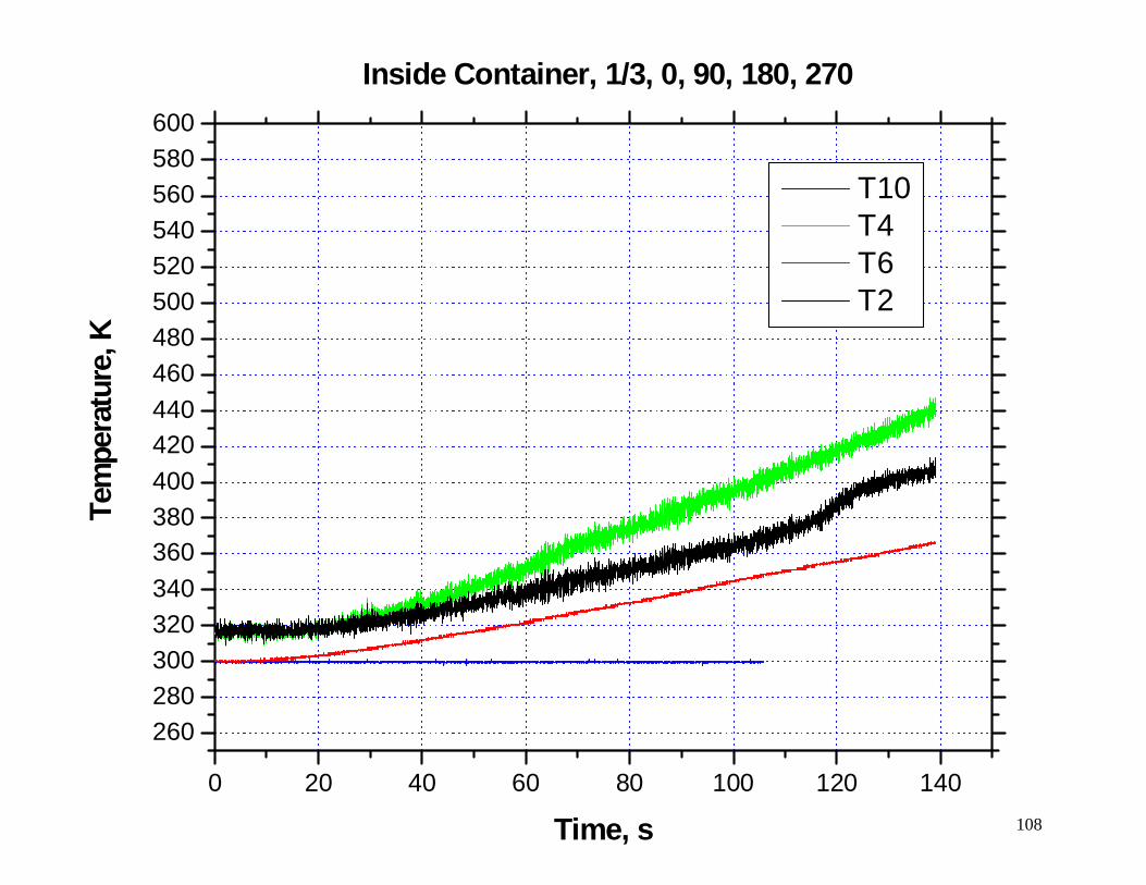
108
0 20 40 60 80 100 120 140
260280300320340360380400420440460480500520540560580600
Inside Container, 1/3, 0, 90, 180, 270Te
mpe
ratu
re, K
Time, s
T10 T4 T6 T2

PPLLOOTTSS,, TTEESSTT 55,, FFIIRREE,, OOCCTTOOBBEERR 11999999
109
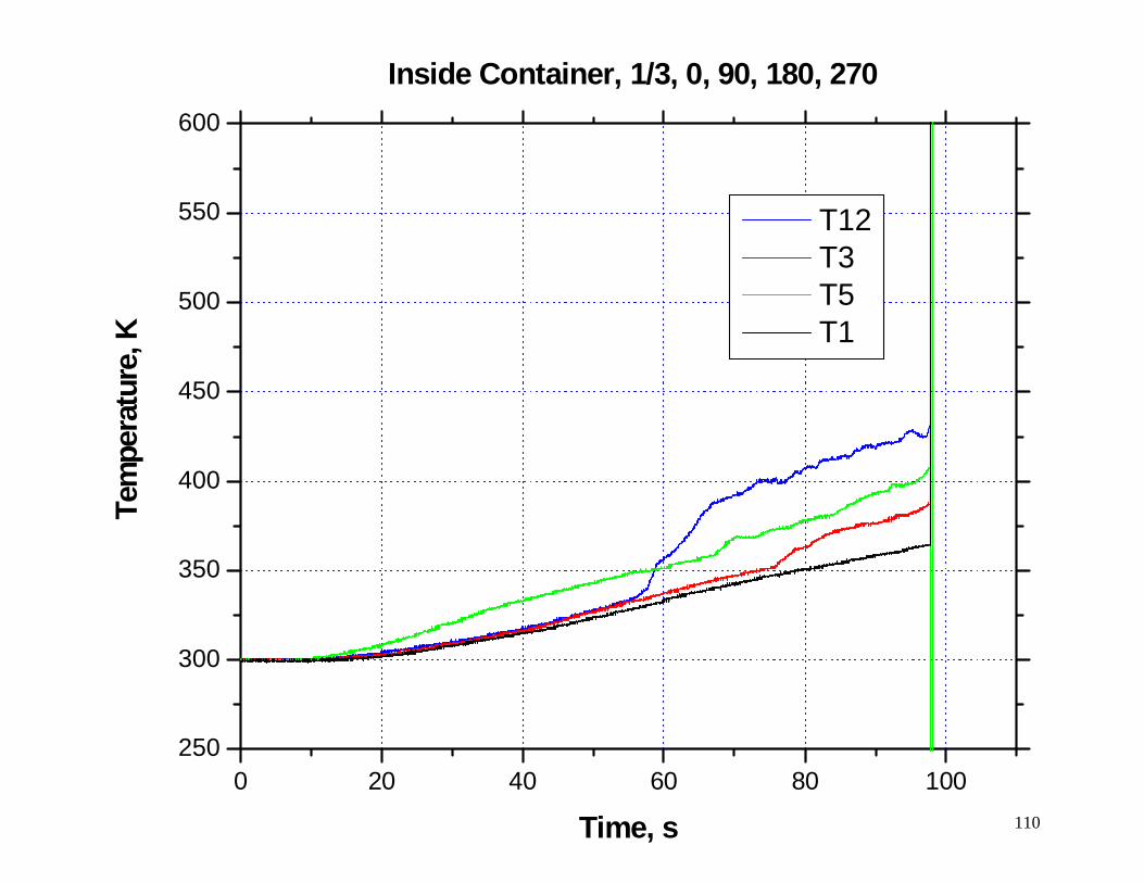
110
0 20 40 60 80 100250
300
350
400
450
500
550
600
Inside Container, 1/3, 0, 90, 180, 270
T12 T3 T5 T1
Tem
pera
re, K
Time, s
tu
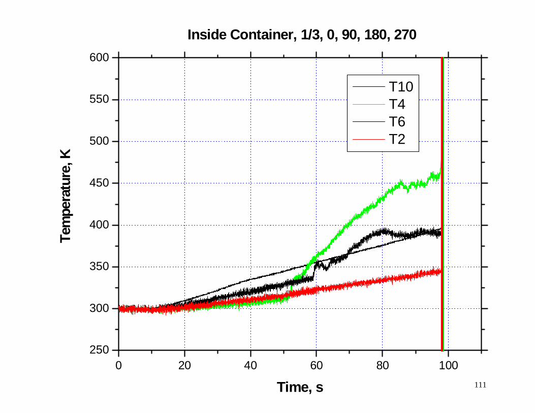
111
0 20 40 60 80 100250
300
350
400
450
500
550
600
Inside Container, 1/3, 0, 90, 180, 270
Tem
pera
ture
, K
Time, s
T10 T4 T6 T2
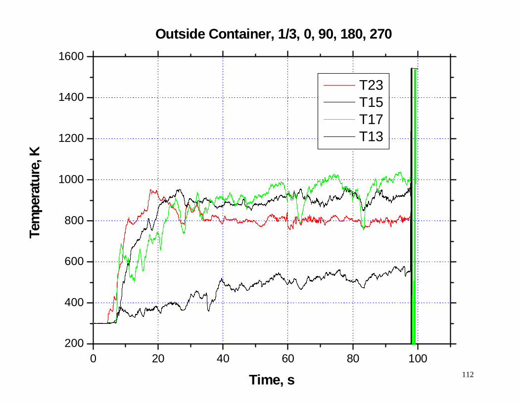
112
0 20 40 60 80 100200
400
600
800
1000
1200
1400
1600
Outside Container, 1/3, 0, 90, 180, 270
T23 T15 T17 T13
Tem
pera
ture
, K
Time, s
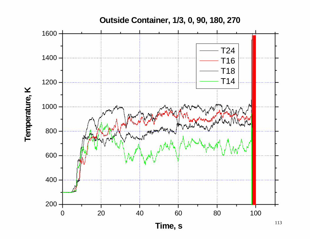
113
0 20 40 60 80 100200
400
600
800
1000
1200
1400
1600
Outside Container, 1/3, 0, 90, 180, 270Te
mpe
ratu
re, K
Time, s
T24 T16 T18 T14

PPLLOOTTSS,, TTEESSTT 66,, EELLEECCTTRRIICCAALL,, JJUULLYY 22000022
114
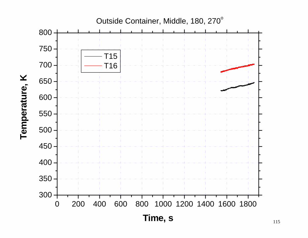
115
0 200 400 600 800 1000 1200 1400 1600 1800
300
350
400
450
550
600
650
700
750
800
500
Outside Container, Middle, 180, 270o
Te
mpe
ratu
re, K
Time, s
T15 T16
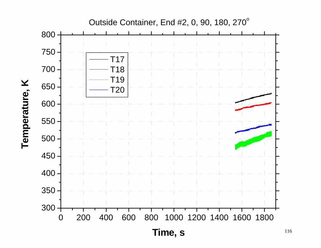
116
0 200 400 600 800 1000 1200 1400 1600 1800300
350
400
450
500
550
600
650
700
750
800Outside Container, End #2, 0, 90, 180, 270o
Te
mpe
ratu
re, K
Time, s
T17 T18 T19 T20

PPLLOOTTSS,, TTEESSTT 77,, EELLEECCTTRRIICCAALL,, AAUUGGUUSSTT 22000011
117
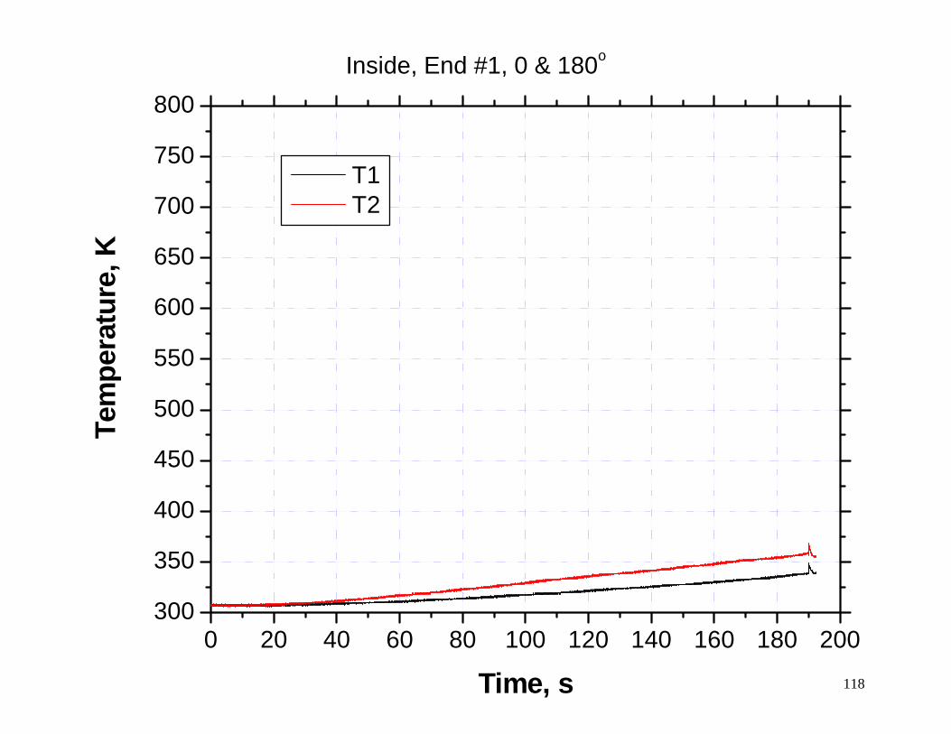
118
0 20 40 60 80 100 120 140 160 180 200300
350
400
450
500
600
650
700
750
800
550
Inside, End #1, 0 & 180o
Te
mpe
rur
e, K
Time, s
T1 T2
at
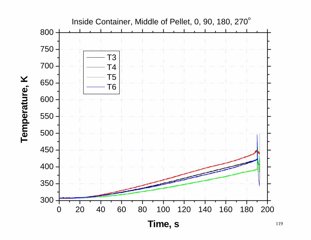
Inside Container, Middle of Pellet, 0, 90, 180, 270o
119
0 20 40 60 80 100 120 140 160 180 200300
350
400
450
500
550
600
650
700
750
800
Tem
pera
ture
, K
Time, s
T3 T4 T5 T6
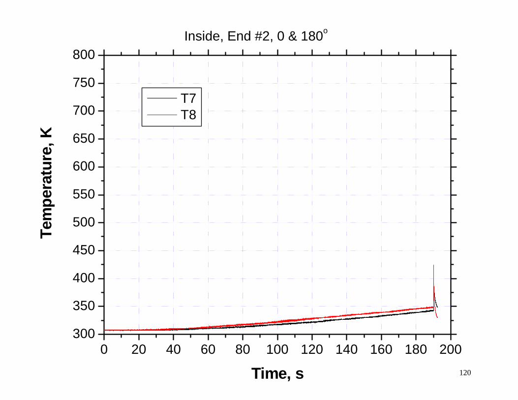
120
0 20 40 60 80 100 120 140 160 180 200300
350
400
450
500
550
600
650
700
750
800Inside, End #2, 0 & 180o
Te
mpe
ratu
re, K
Time, s
T7 T8
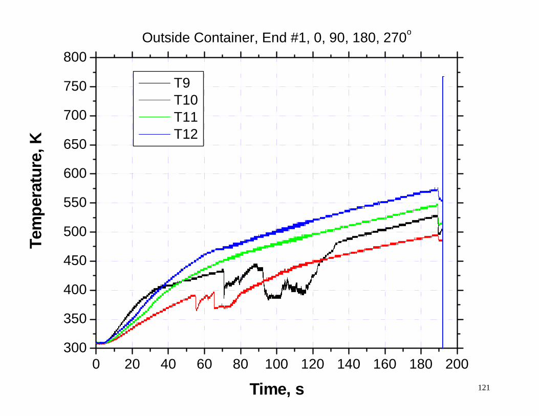
121
0 20 40 60 80 100 120 140 160 180 200300
350
400
450
500
550
600
650
700
750
800Outside Container, End #1, 0, 90, 180, 270o
Te
mpe
ratu
re, K
Time, s
T9 T10 T11 T12
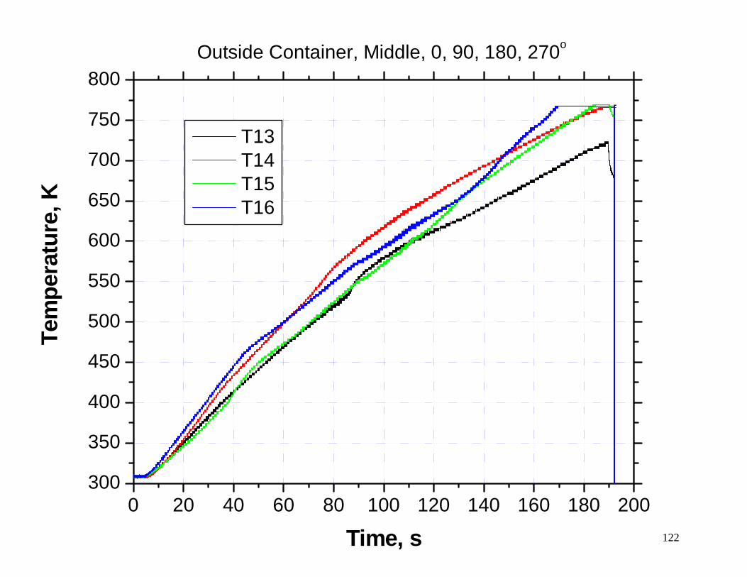
122
0 20 40 60 80 100 120 140 160 180 200300
350
400
450
500
550
600
650
700
750
800Outside Container, Middle, 0, 90, 180, 270o
Te
mpe
ratu
re, K
Time, s
T13 T14 T15 T16
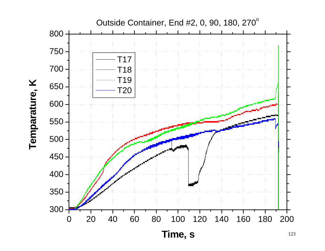
123
0 20 40 60 80 100 120 140 160 180 200300
350
400
450
500
550
600
650
700
750
800Outside Container, End #2, 0, 90, 180, 270o
Te
mpa
ratu
re, K
Time, s
T17 T18 T19 T20

PPLLOOTTSS,, TTEESSTT 88,, EELLEECCTTRRIICCAALL,, SSEEPPTTEEMMBBEERR 22000022
124
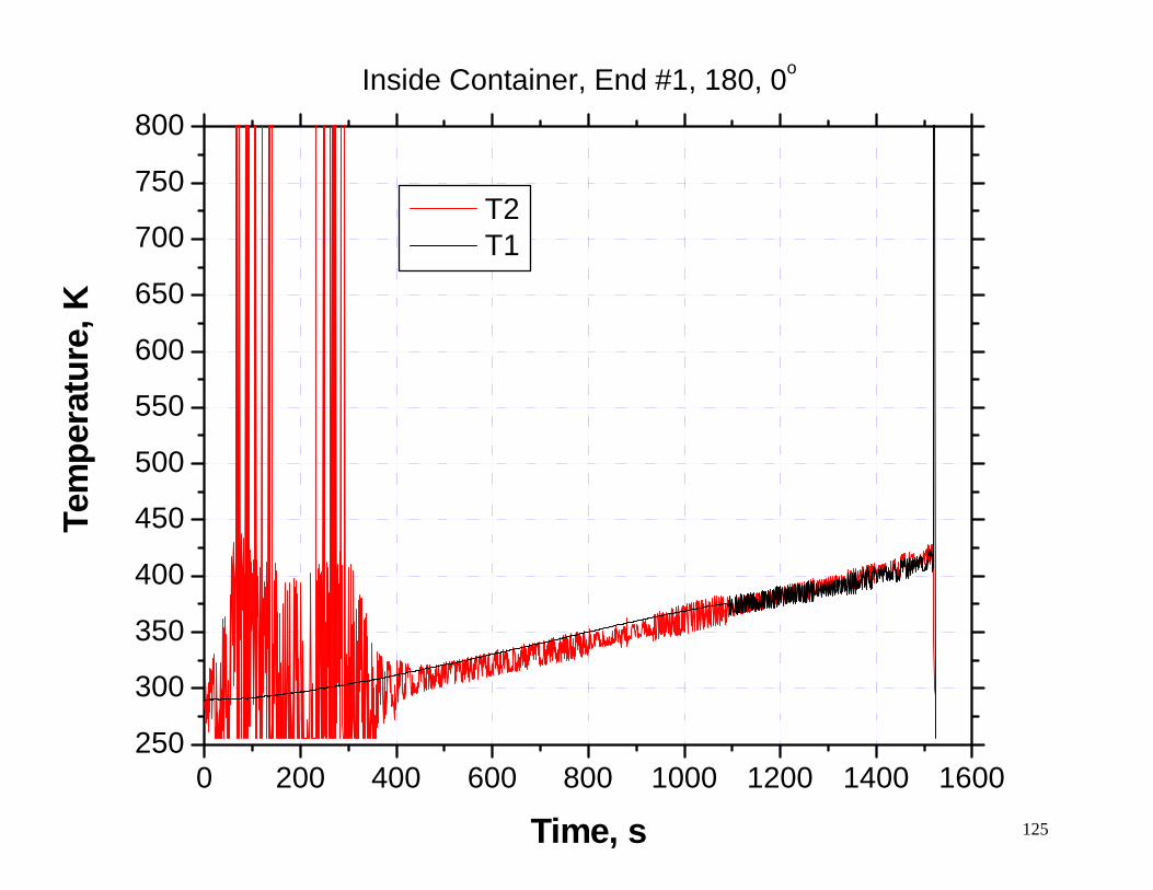
125
0 200 400 600 800 1000 1200 1400 1600250
300
350
400
450
550
600
650
700
750
800
500
Inside Container, End #1, 180, 0o
Te
mpe
ratu
re, K
Time, s
T2 T1
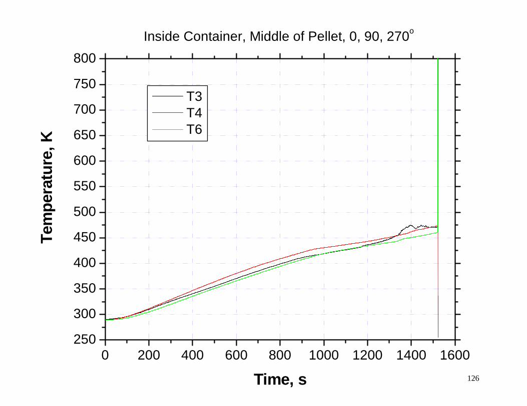
126
0 200 400 600 800 1000 1200 1400 1600250
300
350
400
450
500
550
600
650
700
750
800Inside Container, Middle of Pellet, 0, 90, 270o
Te
mpe
ratu
re, K
Time, s
T3 T4 T6
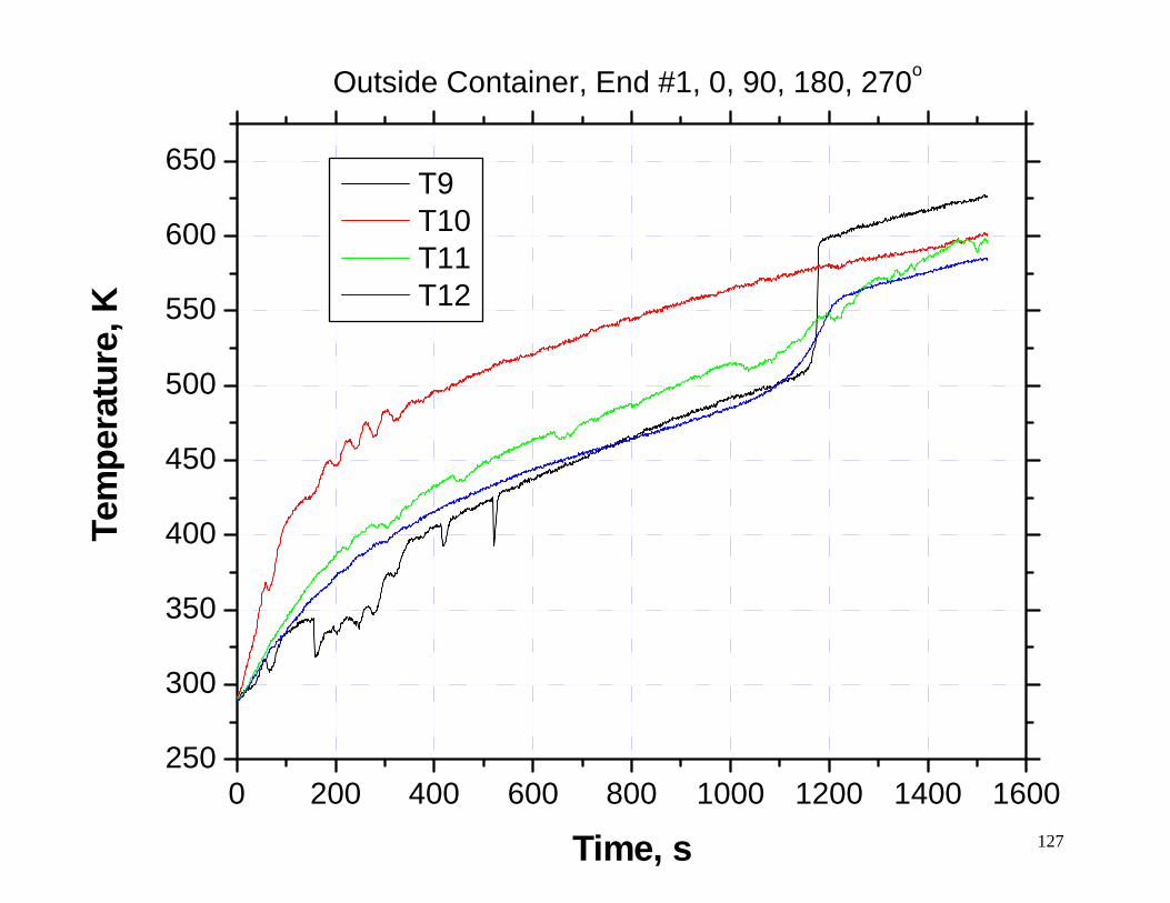
127
0 200 400 600 800 1000 1200 1400 1600250
300
350
400
450
500
550
600
650
Outside Container, End #1, 0, 90, 180, 270o
Tem
pera
ture
, K
Time, s
T9 T10 T11 T12
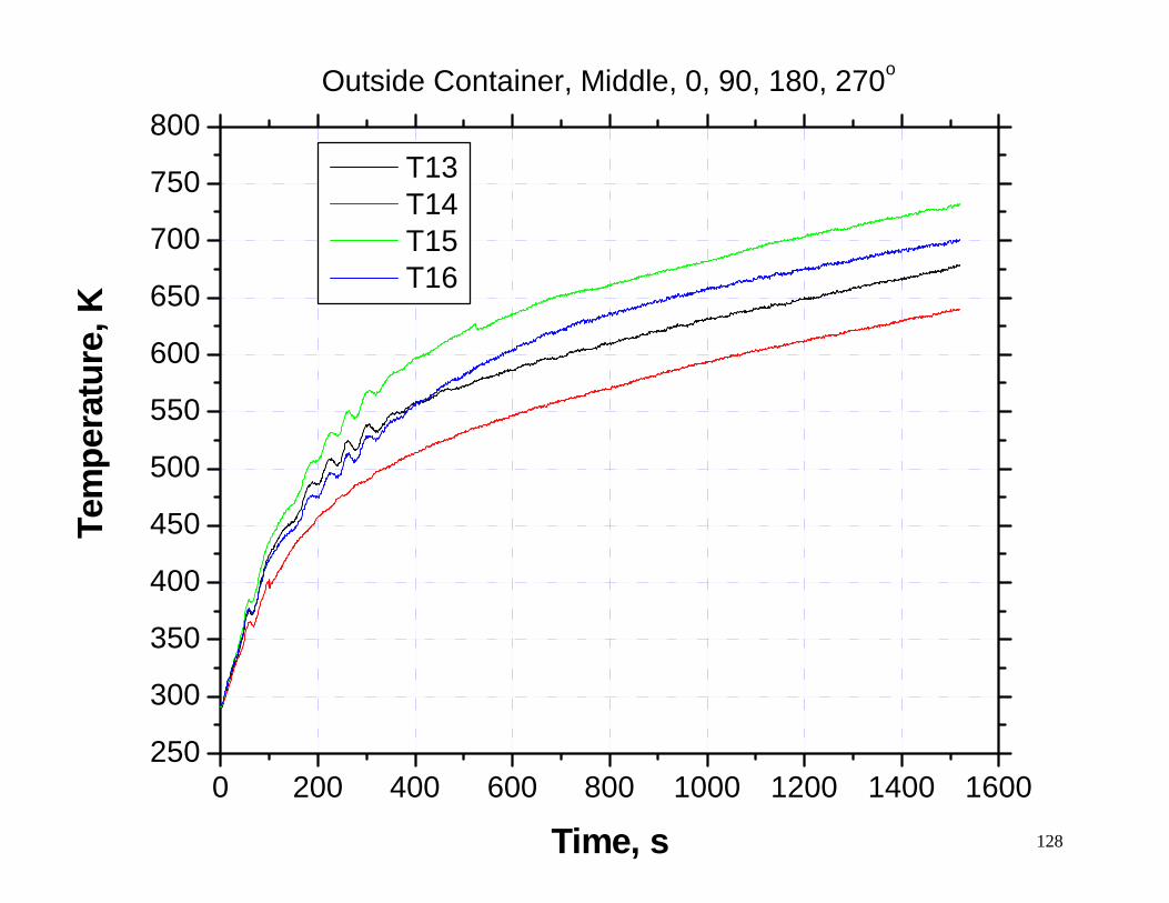
128
0 200 400 600 800 1000 1200 1400 1600250
300
350
400
450
500
550
600
650
700
750
800Outside Container, Middle, 0, 90, 180, 270o
Tem
pera
ture
, K
Time, s
T13 T14 T15 T16
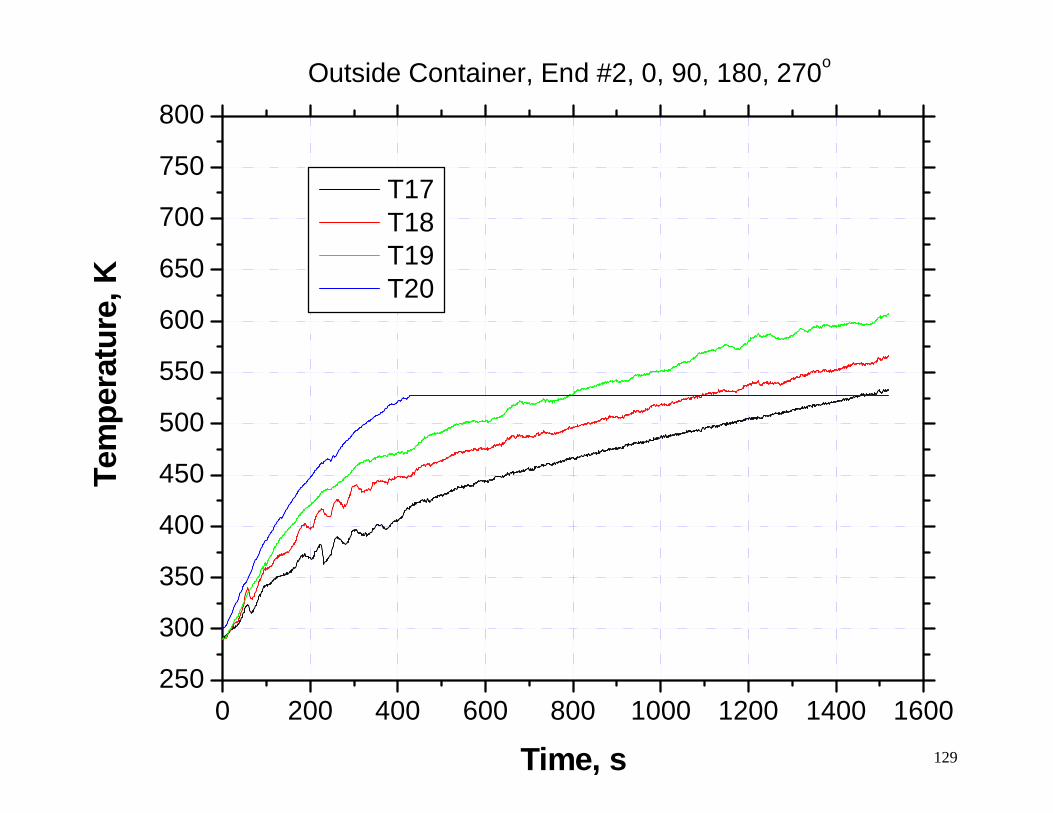
129
0 200 400 600 800 1000 1200 1400 1600250
300
350
400
450
500
550
600
650
700
750
800Outside Container, End #2, 0, 90, 180, 270o
Te
mpe
ratu
re, K
Time, s
T17 T18 T19 T20

PPLLOOTTSS,, TTEESSTT 99AA,, EELLEECCTTRRIICCAALL,, NNOOVVEEMMBBEERR 22000022
130
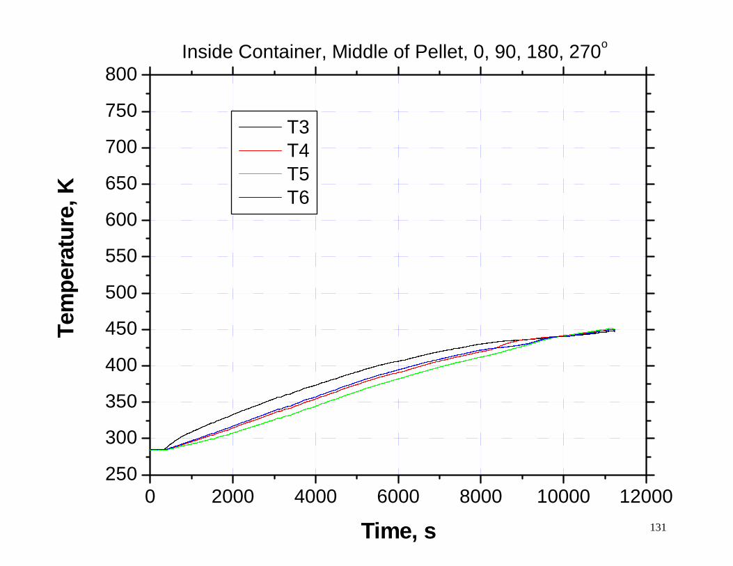
131
0 2000 4000 6000 8000 10000 12000250
300
350
400
450
550
600
650
700
750
800
500
Inside Container, Middle of Pellet, 0, 90, 180, 270o
Te
mp
ure,
K
Time, s
T3 T4 T5 T6
erat
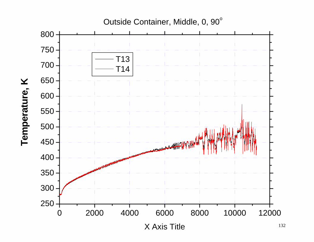
Outside Container, Middle, 0, 90o
132
0 2000 4000 6000 8000 10000 12000250
300
350
400
450
500
550
600
650
700
750
800
T13 T14
Tem
pera
ture
, K
X Axis Title
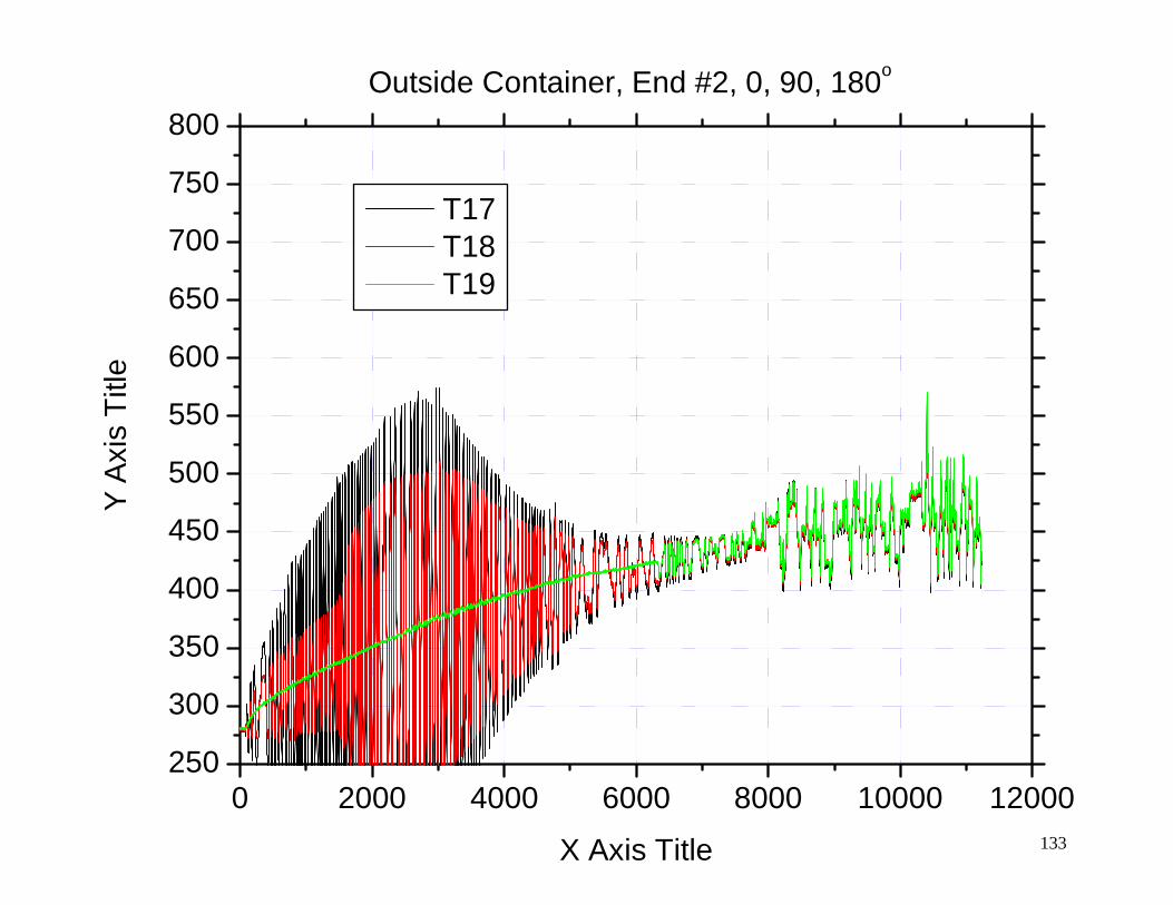
133
0 2000 4000 6000 8000 10000 12000250
300
350
400
450
500
550
600
650
700
750
800Outside Container, End #2, 0, 90, 180o
Y
Axis
Titl
e
X Axis Title
T17 T18 T19

PPLLOOTTSS,, TTEESSTT 99BB,, EELLEECCTTRRIICCAALL,, NNOOVVEEMMBBEERR 22000022
134
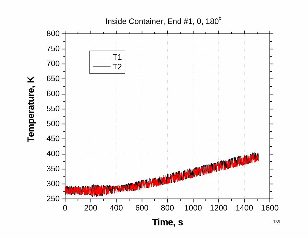
Inside Container, End #1, 0, 180o
135
0 200 400 600 800 1000 1200 1400 1600250
300
350
400
450
500
550
600
650
700
750
800
T1 T2
Tem
per
ure,
K
Time, s
at
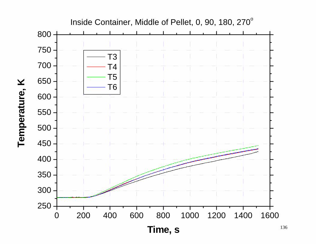
Inside Container, Middle of Pellet, 0, 90, 180, 270o
136
0 200 400 600 800 1000 1200 1400 1600250
300
350
400
450
500
550
600
650
700
750
800
Tem
pera
ture
, K
Time, s
T3 T4 T5 T6
137
0 200 400 600 800 1000 1200 1400 1600250
300
350
400
450
500
550
600
650
700
750
800Inside Container, End #2, 0, 180o
Te
mpe
ratu
re, K
Time, s
T7 T8
Outside Container, Middle, 0, 90, 180, 270o
138
0 200 400 600 800 1000 1200 1400 1600250
300
350
400
450
500
550
600
650
700
750
800
Tem
pera
ture
, K
Time, s
T13 T14 T15 T16
139
0 200 400 600 800 1000 1200 1400 1600250
300
350
400
450
500
550
600
650
700
750
800Outside Container, End #2, 0, 90, 180, 270o
Te
mpe
ratu
re, K
Ti , s
T17 T18 T19 T20
me

PPLLOOTTSS,, TTEESSTT 1100,, EELLEECCTTRRIICCAALL,, NNOOVVEEMMBBEERR 22000022
140
Outside Container, End #1, 0, 90, 180, 270o
141
0 200 400 600 800 1000 1200 1400 1600 1800250
300
350
400
450
500
550
600
650
700
750
800
Tem
per
ure,
K
Time, s
TC09 TC10 TC11 TC12
at
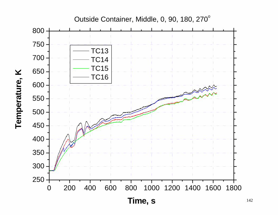
Outside Container, Middle, 0, 90, 180, 270o
142
0 200 400 600 800 1000 1200 1400 1600 1800250
300
350
400
450
500
550
600
650
700
750
800
Tem
pera
ture
, K
Ti , s
TC13 TC14 TC15 TC16
me
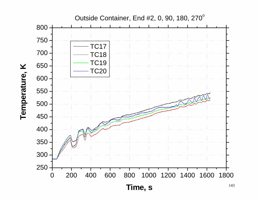
Outside Container, End #2, 0, 90, 180, 270o
143
0 200 400 600 800 1000 1200 1400 1600 1800250
300
350
400
450
500
550
600
650
700
750
800
Tem
pera
ture
, K
Time, s
TC17 TC18 TC19 TC20