Embed Size (px)
Citation preview
PIONEER PROJECTS
PIONEER PROJECTS
SOLAR IRRADIATION FROM THE ENERGY PRODUCTION OF RESIDENTIAL PV SYSTEM (SPIDER)
CONTRACT - BR/314/PI/SPIDER
FINAL REPORT
15/09/2017
Promotor
Dr. Cédric Bertrand
Royal Meteorological Institute of Belgium - 3 Avenue Circulaire - B-1180 Brussels
Authors
Cédric Bertrand (RMI)
Caroline Housmans (RMI)
Jonathan Leloux (Universidad Politécnica de Madrid, Spain)

Published in 2018 by the Belgian Science Policy
Avenue Louise 231
Louizalaan 231
B-1050 Brussels
Belgium
Tel: +32 (0)2 238 34 11 – Fax: +32 (0)2 230 59 12
http://www.belspo.be
Contact person: Georges JAMART
+32 (0)2 238 3 36 90
Neither the Belgian Science Policy nor any person acting on behalf of the Belgian Science Policy
is responsible for the use which might be made of the following information. The authors are
responsible for the content.
No part of this publication may be reproduced, stored in a retrieval system, or transmitted in any
form or by any means, electronic, mechanical, photocopying, recording, or otherwise, without
indicating the reference :
Bertrand, C. Housmans, C. and J. Leloux. Solar Irradiation From the Energy Production of
Residential PV Systems (SPIDER) . Final Report. Brussels : Belgian Science Policy 2017 – 45 p.
(BRAIN-be - Belgian Research Action through Interdisciplinary Networks)

Project BR/314/PI/SPIDER – Solar Irradiation From the Energy Production of Residential PV systems
BRAIN-be - (Belgian Research Action through Interdisciplinary Networks) 3
TABLE OF CONTENTS
SUMMARY 4 CONTEXT ..................................................................................................................................................................... 4 OBJECTIVES ................................................................................................................................................................. 4 CONCLUSIONS .............................................................................................................................................................. 4 KEYWORDS .................................................................................................................................................................. 4
SAMENVATTING 5 CONTEXT ..................................................................................................................................................................... 5 DOELSTELLINGEN ........................................................................................................................................................ 5 BESLUITEN ................................................................................................................................................................... 5 TREFWOORDEN ............................................................................................................................................................ 5
RESUME 6 CONTEXTE ................................................................................................................................................................... 6 OBJECTIFS .................................................................................................................................................................... 6 CONCLUSIONS .............................................................................................................................................................. 6 MOTS-CLÉS .................................................................................................................................................................. 6
1. INTRODUCTION 7 2. METHODOLOGY AND RESULTS 7
2.1 DATA ...................................................................................................................................................................... 7 2.1.1 Residential PV systems data ............................................................................................................................ 7 2.1.2 Ground stations measurements ........................................................................................................................ 9 2.1.3 July 15, 2015 to January 19, 2016 measurement campaign .......................................................................... 11
2.2 METHODOLOGY .................................................................................................................................................... 13 2.2.1 Conversion of PV system energy production to tilted global solar irradiation ............................................. 13 2.2.2 Tilt to horizontal global solar irradiance transposition ................................................................................ 17
2.3 RESULTS ............................................................................................................................................................... 20 2.3.1 Evaluation of the tilt to horizontal global solar irradiance transposition ..................................................... 20 2.3.2 Evaluation of the PV system energy production to global horizontal solar irradiation conversion.............. 25
3. PERSPECTIVES 36
4. PUBLICATIONS 37 4.1 INTERNATIONAL JOURNAL WITH READING COMMITTEE ........................................................................................ 37 4.2 CONFERENCE ABSTRACT ...................................................................................................................................... 37
5. ACKNOWLEDGEMENTS 37
6. REFERENCES 38 ANNEXES 41
A. DECOMPOSITION MODELS ...................................................................................................................................... 41 A.1 ERB model (Erbs et al., 1982): ........................................................................................................................ 41 A.2 OLS model (Skartveit and Olsethr, 1987): ....................................................................................................... 41
B TRANSPOSITION MODELS ........................................................................................................................................ 42 B.1 LIU model (Liu and Jordan, 1962): ................................................................................................................. 42 B.2 HAY model (Hay, 1979): .................................................................................................................................. 42 B.3 SKA model (Skartveit and Olseth, 1986):......................................................................................................... 42 B.4 PER model (Perez et al., 1987): ....................................................................................................................... 42
C. DESCRIPTION OF THE RMIS MAGIC/HELIOSAT-2 ALGORITHM ............................................................................ 43
Project BR/314/PI/SPIDER – Solar Irradiation From the Energy Production of Residential PV systems
BRAIN-be - (Belgian Research Action through Interdisciplinary Networks) 4
SUMMARY
Context
Knowledge of local solar irradiation is essential for many applications. Traditionally, solar
irradiation is observed by means of networks of radiometric stations. Cost for installation and
maintenance of such station are very high and national networks count only few stations.
Consequently the availability of observed solar irradiation measurements is spatially inadequate
for many applications. Mapping the solar radiation by interpolation of measurements is possible
but leads to large error. Accurately depicting the spatial extent and time-dependent
characteristics of the solar resource requires alternative methods.
Objectives
We propose to take advantage of the very dense network of residential photovoltaic (PV)
systems implemented in Belgium to use the energy production registered at PV systems as solar
irradiation sensors. This innovative approach requires (1) to derive solar irradiation from the
energy production of PV system and (2) to transpose solar irradiance on a tilted plan to that on
the horizontal plane.
Conclusions
One major problem that was encountered is that the information on the orientation and/or the
inclination of the PV installations provided by the PV systems installers or owners is not very
accurate. However tilt angle and surface’s orientation have been found to have a large impact
on the accuracy of the global horizontal solar irradiance calculation. Increasing the number of
PV installations involved in the computation process allows smoothing the estimation to some
extent. Validation results computed on an hourly basis provide a mean RMSE value of about
40% when considering a group of neighboring PV installations in the estimation process while
values as large as 60% are reported when using a single installation. By comparison satellite-
based global horizontal irradiance estimation exhibits a better performance with an associated
overall RMSE of about 20%. Another limitation of our approach is that there are certain sun
positions for which the tilt to horizontal transposition process fails to produce a valid estimation.
As an example unsuccessful tilt to horizontal conversions occurs at low solar elevation
irrespective of the number of PV systems involved in the conversion process.
Keywords
Photovoltaic system, solar radiation, decomposition model, transposition model, remote
sensing, ground measurements, crowdsourcing.
Project BR/314/PI/SPIDER – Solar Irradiation From the Energy Production of Residential PV systems
BRAIN-be - (Belgian Research Action through Interdisciplinary Networks) 5
SAMENVATTING
Context
Kennis van de plaatselijke zonnestraling is noodzakelijk voor een ruim aanbod aan
toepassingen. Normaal wordt de zonnestraling gemeten door netwerken van radiometrische
stations. Echter, gezien de hoge installatie- en onderhoudskosten van dergelijke stations,
beschikken de nationale stralingsnetwerken vaak slechts over een erg beperkt aantal stations.
Hierdoor is het dekkingsgebied van de stralingsgegevens niet toereikend voor heel wat
toepassingen. Het is wel mogelijk om de zonnestraling in kaart te brengen door middel van
interpolatie van de gegevens afkomstig van de stations, maar dit kan tot significante fouten
leiden. Een nauwkeurige ruimtelijke karakterisering van de beschikbare zonnestraling aan het
aardoppervlak vraagt om andere methodes.
Doelstellingen
Om een dergelijke beperking te omzeilen, stellen wij voor om gebruik te maken van het zeer
dichte netwerk van residentiële fotovoltaïsche (PV) systemen dat in België bestaat en de PV-
systemen te gebruiken als stralingsensoren. Deze innovatieve benadering vereist (1) het
ontlenen van de energieproductiegegevens van individuele PV-systemen, deze om te zetten
naar gegevens van invallende zonnestraling en vervolgens (2) de gegevens van zonnestraling op
een hellend vlak om te zetten naar deze op een horizontaal vlak.
Besluiten
Een groot probleem dat is vastgesteld, is dat de informatie over de oriëntatie en / of de neiging
van de PV-installaties die door de PV-installateurs of eigenaars wordt geleverd, niet erg
nauwkeurig is. De kantelhoek en de oriëntatie van het oppervlak hebben echter een grote
invloed op de nauwkeurigheid van de globale horizontale zonnestralingsberekening. Door het
aantal PV-installaties die bij het berekeningsproces betrokken zijn te verhogen, kan de schatting
tot op zekere hoogte worden vergemakkelijkt. Validatieresultaten die per uur worden berekend,
geven een gemiddelde RMSE-waarde van ongeveer 40% bij het overwegen van een groep
naburige PV-installaties in het schattingsproces, terwijl waarden zo groot als 60% worden
gerapporteerd bij gebruik van een enkele installatie. Ter vergelijking vertoont satellietgebaseerde
globale horizontale irradiantie schatting een betere prestatie met een bijbehorende totale RMSE
van ongeveer 20%. Een andere beperking van onze aanpak is dat er zekere zonneposities zijn
waarvoor het kantelen naar het horizontale omzettingsproces geen geldige schatting oplevert.
Bijvoorbeeld, de succesvolle kanteling naar horizontale conversies vindt plaats bij lage
zonnestraling, ongeacht het aantal PV-systemen dat bij het omzettingsproces betrokken is.
Trefwoorden
Residentiële fotovoltaïsche systemen , zonnestraling , ontbindingsmodel, omzettingsmodel,
remote sensing, grondmetingen, crowdsourcing
Project BR/314/PI/SPIDER – Solar Irradiation From the Energy Production of Residential PV systems
BRAIN-be - (Belgian Research Action through Interdisciplinary Networks) 6
RESUME
Contexte
Une connaissance localisée du rayonnement solaire incident en surface est essentielle pour un
grand nombre d’applications. Traditionnellement, le rayonnement solaire en surface est mesuré
au moyen d’un réseau de stations radiométriques. Cependant, vu les coûts élevés d’installation
et d’entretien de ces stations, les réseaux radiométriques nationaux ne comptent généralement
qu’un nombre limité de stations. Par conséquent, la couverture spatiale des données de
rayonnement est insuffisante pour de nombreuses applications. Une cartographie du
rayonnement solaire incident en surface par interpolation des mesures prises aux stations est
possible mais peut conduire à des erreurs non négligeables. La caractérisation spatiale à haute
résolution du rayonnement solaire disponible en surface nécessite l’utilisation d’autres
méthodes.
Objectifs
L’objectif principal de l’étude est de déterminer s’il est possible de tirer profit de la haute densité
du parc d’installations solaires photovoltaïques résidentielles belges pour arriver à une
cartographie fine du rayonnement solaire incident en surface sur la Belgique. Cette approche
innovante nécessite donc (1) de convertir la production d’électricité des différentes installations
photovoltaïques résidentielles en énergie solaire incidente reçue par les capteurs
photovoltaïques et (2) de transposer le rayonnement solaire reçu sur une surface inclinée à celui
reçu sur une surface horizontale.
Conclusions
Un problème majeur rencontré provient du fait que les informations sur l'orientation et / ou
l'inclinaison des installations photovoltaïques fournies par les installateurs ou les propriétaires
de systèmes photovoltaïques ne sont pas très précises. Or, l'angle d'inclinaison et l'orientation
des panneaux solaires ont un impact important sur la précision du calcul de l'irradiance solaire
horizontale. L'augmentation du nombre d'installations PV impliquées dans le processus de
calcul permet de lisser l'estimation dans une certaine mesure. Les résultats de validations
calculés sur base horaire donnent une valeur RMSE moyenne d'environ 40% lorsque
l’estimation est calculée pour un groupe d'installations photovoltaïques voisines, par contre
l’erreur quadratique moyenne peut atteindre des valeurs de l’ordre de 60 % pour une seule
installation. En comparaison, l'estimation de l'irradiance solaire horizontale à partir de
l’imagerie satellite offre une meilleure précision avec un RMSE moyen d'environ 20%. Une
autre limitation de notre approche est qu'il existe certaines positions solaires pour lesquelles la
conversion de l’irradiance inclinée à l’horizontale n’est pas possible. À titre d'exemple, la
procédure ne fonctionne pas aux faibles élévations solaire et ce quel que soit le nombre de
systèmes photovoltaïques impliqués dans le processus de conversion.
Mots-clés
Installations solaires photovoltaïques, rayonnement solaire, modèle de décomposition, modèle
de transposition, télédétection, mesures au sol, crowdsourcing.
Project BR/314/PI/SPIDER – Solar Irradiation From the Energy Production of Residential PV systems
BRAIN-be - (Belgian Research Action through Interdisciplinary Networks) 7
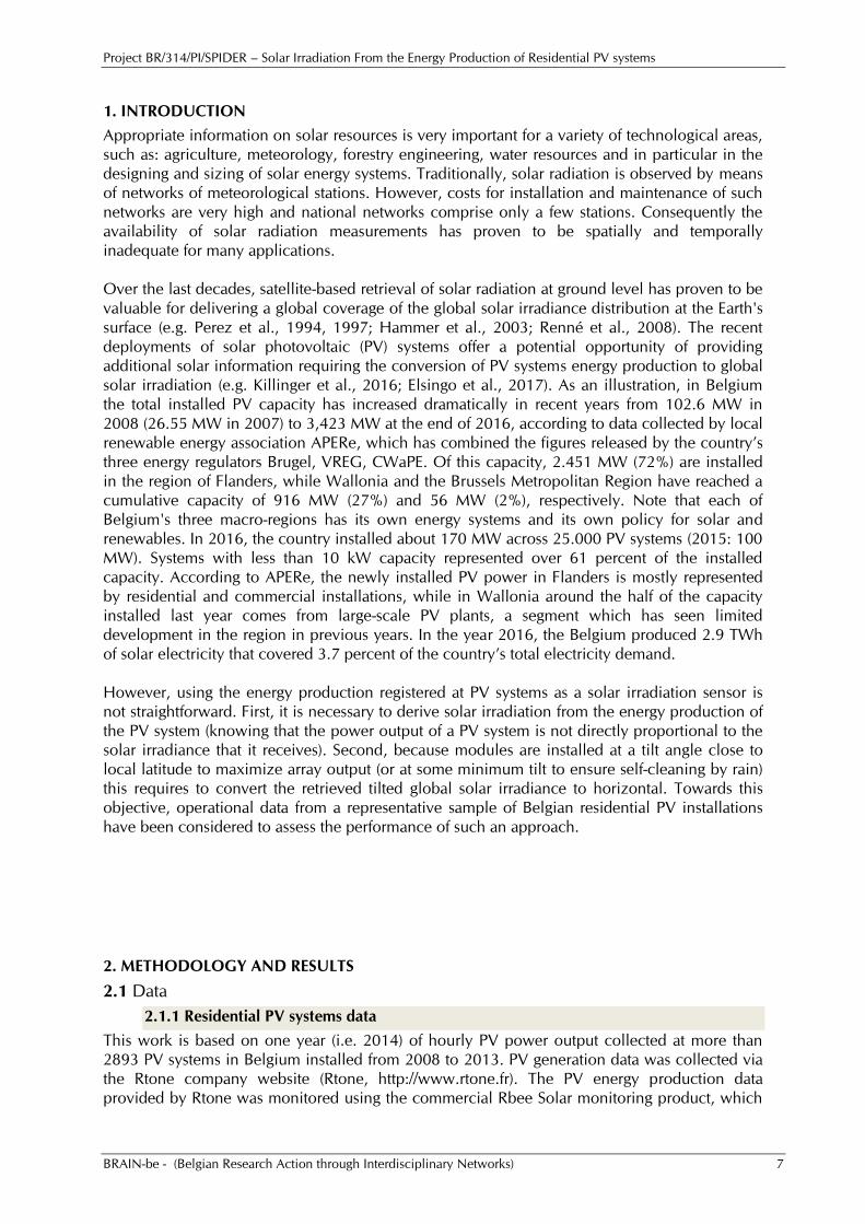
1. INTRODUCTION
Appropriate information on solar resources is very important for a variety of technological areas,
such as: agriculture, meteorology, forestry engineering, water resources and in particular in the
designing and sizing of solar energy systems. Traditionally, solar radiation is observed by means
of networks of meteorological stations. However, costs for installation and maintenance of such
networks are very high and national networks comprise only a few stations. Consequently the
availability of solar radiation measurements has proven to be spatially and temporally
inadequate for many applications.
Over the last decades, satellite-based retrieval of solar radiation at ground level has proven to be
valuable for delivering a global coverage of the global solar irradiance distribution at the Earth's
surface (e.g. Perez et al., 1994, 1997; Hammer et al., 2003; Renné et al., 2008). The recent
deployments of solar photovoltaic (PV) systems offer a potential opportunity of providing
additional solar information requiring the conversion of PV systems energy production to global
solar irradiation (e.g. Killinger et al., 2016; Elsingo et al., 2017). As an illustration, in Belgium
the total installed PV capacity has increased dramatically in recent years from 102.6 MW in
2008 (26.55 MW in 2007) to 3,423 MW at the end of 2016, according to data collected by local
renewable energy association APERe, which has combined the figures released by the country’s
three energy regulators Brugel, VREG, CWaPE. Of this capacity, 2.451 MW (72%) are installed
in the region of Flanders, while Wallonia and the Brussels Metropolitan Region have reached a
cumulative capacity of 916 MW (27%) and 56 MW (2%), respectively. Note that each of
Belgium's three macro-regions has its own energy systems and its own policy for solar and
renewables. In 2016, the country installed about 170 MW across 25.000 PV systems (2015: 100
MW). Systems with less than 10 kW capacity represented over 61 percent of the installed
capacity. According to APERe, the newly installed PV power in Flanders is mostly represented
by residential and commercial installations, while in Wallonia around the half of the capacity
installed last year comes from large-scale PV plants, a segment which has seen limited
development in the region in previous years. In the year 2016, the Belgium produced 2.9 TWh
of solar electricity that covered 3.7 percent of the country’s total electricity demand.
However, using the energy production registered at PV systems as a solar irradiation sensor is
not straightforward. First, it is necessary to derive solar irradiation from the energy production of
the PV system (knowing that the power output of a PV system is not directly proportional to the
solar irradiance that it receives). Second, because modules are installed at a tilt angle close to
local latitude to maximize array output (or at some minimum tilt to ensure self-cleaning by rain)
this requires to convert the retrieved tilted global solar irradiance to horizontal. Towards this
objective, operational data from a representative sample of Belgian residential PV installations
have been considered to assess the performance of such an approach.
2. METHODOLOGY AND RESULTS
2.1 Data
2.1.1 Residential PV systems data
This work is based on one year (i.e. 2014) of hourly PV power output collected at more than
2893 PV systems in Belgium installed from 2008 to 2013. PV generation data was collected via
the Rtone company website (Rtone, http://www.rtone.fr). The PV energy production data
provided by Rtone was monitored using the commercial Rbee Solar monitoring product, which
Project BR/314/PI/SPIDER – Solar Irradiation From the Energy Production of Residential PV systems
BRAIN-be - (Belgian Research Action through Interdisciplinary Networks) 8
measures the energy production with a smart energy meter at a 10-min time interval. The data
concerning the PV systems were supplied by their owners. Each PV system is localized by its
latitude and longitude, completed with the corresponding altitude. The PV generator is
characterized by its orientation and tilt angles, its total surface, and its total peak power. The
data also provides information about the manufacturers of the PV modules and inverters that
equip the systems, and the installers. Some of the PV system characteristics were available for
most of the installations: latitude, longitude, azimuth and tilt angles, surface and peak power.
Some other characteristics were available, depending on the PV system owner: PV module
manufacturer and model, inverter manufacturer and model, installer, year of installation, PV
cell/module technology.
The data has been subjected to several checks and validations in order to isolate and remove as
much erroneous data as possible. The standard set of filters employed prior to analyses is:
1. Use only single array systems since generation data cannot be decomposed into
constituent arrays
2. Use only system within the Belgium.
3. Use only systems with -90° orientation from south 90° and 0° < tilt from horizontal
60°
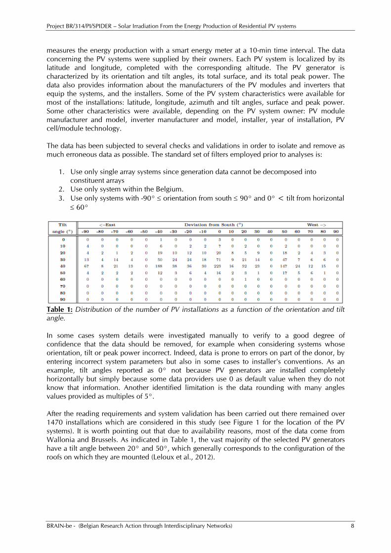
Table 1: Distribution of the number of PV installations as a function of the orientation and tilt angle.
In some cases system details were investigated manually to verify to a good degree of
confidence that the data should be removed, for example when considering systems whose
orientation, tilt or peak power incorrect. Indeed, data is prone to errors on part of the donor, by
entering incorrect system parameters but also in some cases to installer's conventions. As an
example, tilt angles reported as 0° not because PV generators are installed completely
horizontally but simply because some data providers use 0 as default value when they do not
know that information. Another identified limitation is the data rounding with many angles
values provided as multiples of 5°.
After the reading requirements and system validation has been carried out there remained over
1470 installations which are considered in this study (see Figure 1 for the location of the PV
systems). It is worth pointing out that due to availability reasons, most of the data come from
Wallonia and Brussels. As indicated in Table 1, the vast majority of the selected PV generators
have a tilt angle between 20° and 50°, which generally corresponds to the configuration of the
roofs on which they are mounted (Leloux et al., 2012).
Project BR/314/PI/SPIDER – Solar Irradiation From the Energy Production of Residential PV systems
BRAIN-be - (Belgian Research Action through Interdisciplinary Networks) 9
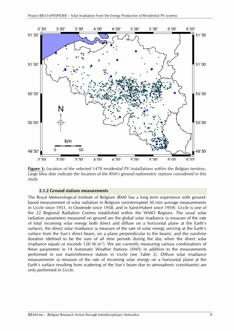
Figure 1: Location of the selected 1470 residential PV installations within the Belgian territory. Large bleu dots indicate the location of the RMI’s ground radiometric stations considered in this study
2.1.2 Ground stations measurements
The Royal Meteorological Institute of Belgium (RMI) has a long term experience with ground-
based measurement of solar radiation in Belgium (uninterrupted 30 min average measurements
in Uccle since 1951, in Oostende since 1958, and in Saint-Hubert since 1959). Uccle is one of
the 22 Regional Radiation Centres established within the WMO Regions. The usual solar
radiation parameters measured on ground are the global solar irradiance (a measure of the rate
of total incoming solar energy both direct and diffuse on a horizontal plane at the Earth's
surface), the direct solar irradiance (a measure of the rate of solar energy arriving at the Earth's
surface from the Sun's direct beam, on a plane perpendicular to the beam), and the sunshine
duration (defined to be the sum of all time periods during the day when the direct solar
irradiance equals or exceeds 120 W.m-2). We are currently measuring various combinations of
these parameters in 14 Automatic Weather Stations (AWS) in addition to the measurements
performed in our main/reference station in Uccle (see Table 2). Diffuse solar irradiance
measurements (a measure of the rate of incoming solar energy on a horizontal plane at the
Earth's surface resulting from scattering of the Sun's beam due to atmospheric constituents) are
only performed in Uccle.
Project BR/314/PI/SPIDER – Solar Irradiation From the Energy Production of Residential PV systems
BRAIN-be - (Belgian Research Action through Interdisciplinary Networks) 10
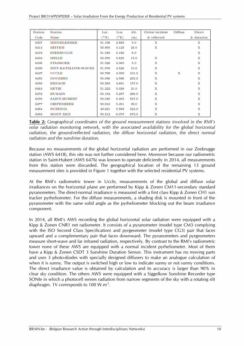
Table 2: Geographical coordinates of the ground measurement stations involved in the RMI’s solar radiation monitoring network, with the associated availability for the global horizontal radiation, the ground-reflected radiation, the diffuse horizontal radiation, the direct normal radiation and the sunshine duration.
Because no measurements of the global horizontal radiation are performed in our Zeebrugge
station (AWS 6418), this site was not further considered here. Moreover because our radiometric
station in Saint-Hubert (AWS 6476) was known to operate deficiently in 2014, all measurements
from this station were discarded. The geographical location of the remaining 13 ground
measurement sites is provided in Figure 1 together with the selected residential PV systems.
At the RMI's radiometric tower in Uccle, measurements of the global and diffuse solar
irradiances on the horizontal plane are performed by Kipp & Zonen CM11-secondary standard
pyranometers. The direct-normal irradiance is measured with a first class Kipp & Zonen CH1 sun
tracker pyrheliometer. For the diffuse measurements, a shading disk is mounted in front of the
pyranometer with the same solid angle as the pyrheliometer blocking out the beam irradiance
component.
In 2014, all RMI's AWS recording the global horizontal solar radiation were equipped with a
Kipp & Zonen CNR1 net radiometer. It consists of a pyranometer (model type CM3 complying
with the ISO Second Class Specification) and pyrgeometer (model type CG3) pair that faces
upward and a complementary pair that faces downward. The pyranometers and pyrgeometers
measure short-wave and far infrared radiation, respectively. By contrast to the RMI's radiometric
tower none of these AWS are equipped with a normal incident pyrheliometer. Most of them
have a Kipp & Zonen CSDT 3 Sunshine Duration Sensor. This instrument has no moving parts
and uses 3 photo-diodes with specially designed diffusers to make an analogue calculation of
when it is sunny. The output is switched high or low to indicate sunny or not sunny conditions.
The direct irradiance value is obtained by calculation and its accuracy is larger than 90% in
clear sky condition. The others AWS were equipped with a Siggelkow Sunshine Recorder type
SONIe in which a photocell senses radiation from narrow segments of the sky with a rotating slit
diaphragm. 1V corresponds to 100 W.m-2.
Project BR/314/PI/SPIDER – Solar Irradiation From the Energy Production of Residential PV systems
BRAIN-be - (Belgian Research Action through Interdisciplinary Networks) 11
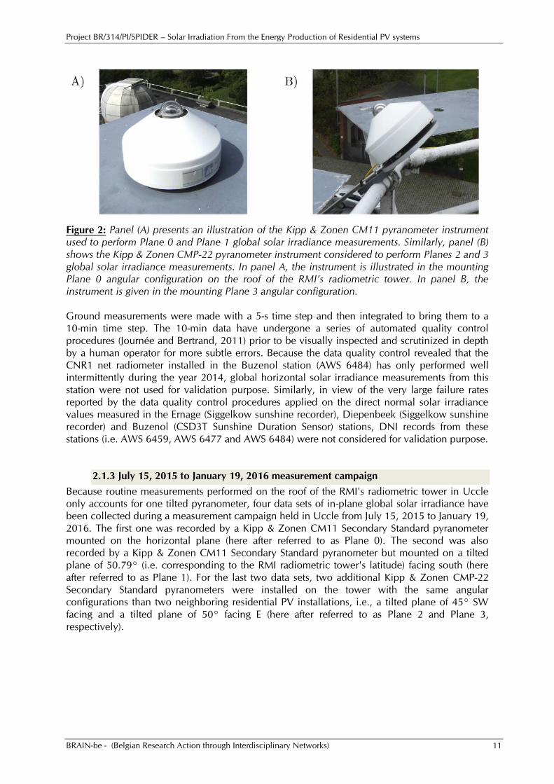
Figure 2: Panel (A) presents an illustration of the Kipp & Zonen CM11 pyranometer instrument used to perform Plane 0 and Plane 1 global solar irradiance measurements. Similarly, panel (B) shows the Kipp & Zonen CMP-22 pyranometer instrument considered to perform Planes 2 and 3
global solar irradiance measurements. In panel A, the instrument is illustrated in the mounting Plane 0 angular configuration on the roof of the RMI’s radiometric tower. In panel B, the instrument is given in the mounting Plane 3 angular configuration.
Ground measurements were made with a 5-s time step and then integrated to bring them to a
10-min time step. The 10-min data have undergone a series of automated quality control
procedures (Journée and Bertrand, 2011) prior to be visually inspected and scrutinized in depth
by a human operator for more subtle errors. Because the data quality control revealed that the
CNR1 net radiometer installed in the Buzenol station (AWS 6484) has only performed well
intermittently during the year 2014, global horizontal solar irradiance measurements from this
station were not used for validation purpose. Similarly, in view of the very large failure rates
reported by the data quality control procedures applied on the direct normal solar irradiance
values measured in the Ernage (Siggelkow sunshine recorder), Diepenbeek (Siggelkow sunshine
recorder) and Buzenol (CSD3T Sunshine Duration Sensor) stations, DNI records from these
stations (i.e. AWS 6459, AWS 6477 and AWS 6484) were not considered for validation purpose.
2.1.3 July 15, 2015 to January 19, 2016 measurement campaign
Because routine measurements performed on the roof of the RMI's radiometric tower in Uccle
only accounts for one tilted pyranometer, four data sets of in-plane global solar irradiance have
been collected during a measurement campaign held in Uccle from July 15, 2015 to January 19,
2016. The first one was recorded by a Kipp & Zonen CM11 Secondary Standard pyranometer
mounted on the horizontal plane (here after referred to as Plane 0). The second was also
recorded by a Kipp & Zonen CM11 Secondary Standard pyranometer but mounted on a tilted
plane of 50.79° (i.e. corresponding to the RMI radiometric tower's latitude) facing south (here
after referred to as Plane 1). For the last two data sets, two additional Kipp & Zonen CMP-22
Secondary Standard pyranometers were installed on the tower with the same angular
configurations than two neighboring residential PV installations, i.e., a tilted plane of 45° SW
facing and a tilted plane of 50° facing E (here after referred to as Plane 2 and Plane 3,
respectively).
Project BR/314/PI/SPIDER – Solar Irradiation From the Energy Production of Residential PV systems
BRAIN-be - (Belgian Research Action through Interdisciplinary Networks) 12
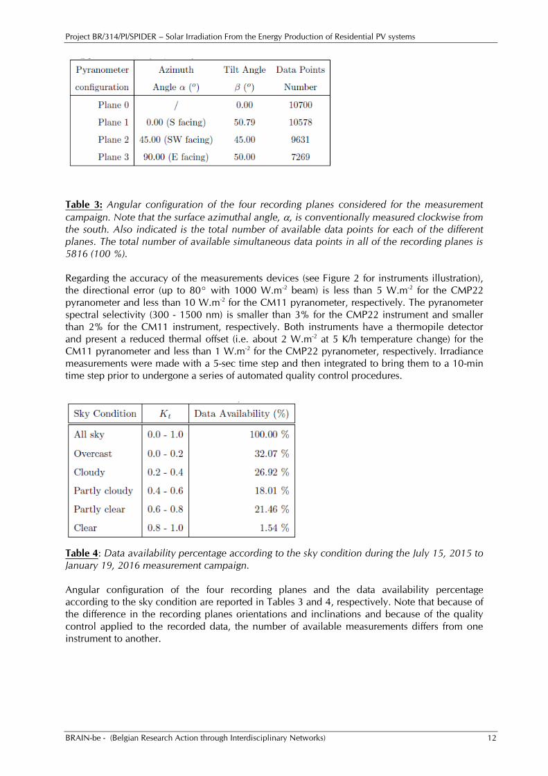
Table 3: Angular configuration of the four recording planes considered for the measurement
campaign. Note that the surface azimuthal angle, , is conventionally measured clockwise from the south. Also indicated is the total number of available data points for each of the different planes. The total number of available simultaneous data points in all of the recording planes is 5816 (100 %).
Regarding the accuracy of the measurements devices (see Figure 2 for instruments illustration),
the directional error (up to 80° with 1000 W.m-2 beam) is less than 5 W.m-2 for the CMP22
pyranometer and less than 10 W.m-2 for the CM11 pyranometer, respectively. The pyranometer
spectral selectivity (300 - 1500 nm) is smaller than 3% for the CMP22 instrument and smaller
than 2% for the CM11 instrument, respectively. Both instruments have a thermopile detector
and present a reduced thermal offset (i.e. about 2 W.m-2 at 5 K/h temperature change) for the
CM11 pyranometer and less than 1 W.m-2 for the CMP22 pyranometer, respectively. Irradiance
measurements were made with a 5-sec time step and then integrated to bring them to a 10-min
time step prior to undergone a series of automated quality control procedures.
Table 4: Data availability percentage according to the sky condition during the July 15, 2015 to January 19, 2016 measurement campaign.
Angular configuration of the four recording planes and the data availability percentage
according to the sky condition are reported in Tables 3 and 4, respectively. Note that because of
the difference in the recording planes orientations and inclinations and because of the quality
control applied to the recorded data, the number of available measurements differs from one
instrument to another.
Project BR/314/PI/SPIDER – Solar Irradiation From the Energy Production of Residential PV systems
BRAIN-be - (Belgian Research Action through Interdisciplinary Networks) 13
2.2 Methodology
2.2.1 Conversion of PV system energy production to tilted global solar irradiation
The initial step of the approach consists in the derivation of global irradiance in plane of array,
Gt from the specific power output, P, of a PV system. Numerous models to calculate P from Gt
exist in the literature (e.g. King et al., 2004; Lorenzo, 2011). However, it is well known that the
energy conversion efficiency of PV modules depends on a number of different influences. Losses
in PV systems can be separate in capture losses and system losses (e.g. Decker and Jahn, 1997;
Marion et al., 2005). Capture losses are caused, e.g., by attenuation of the incoming light,
temperature dependence, electrical mismatching, parasitic resistances in PV modules and
imperfect maximum power point tracking. System losses are caused, e.g., by wiring, inverter,
and transformer conversion losses. All these effects cause the module efficiency to deviate from
the efficiency measured under Standard Test Condition (STC), which defines the rated or
nominal power of a given module.
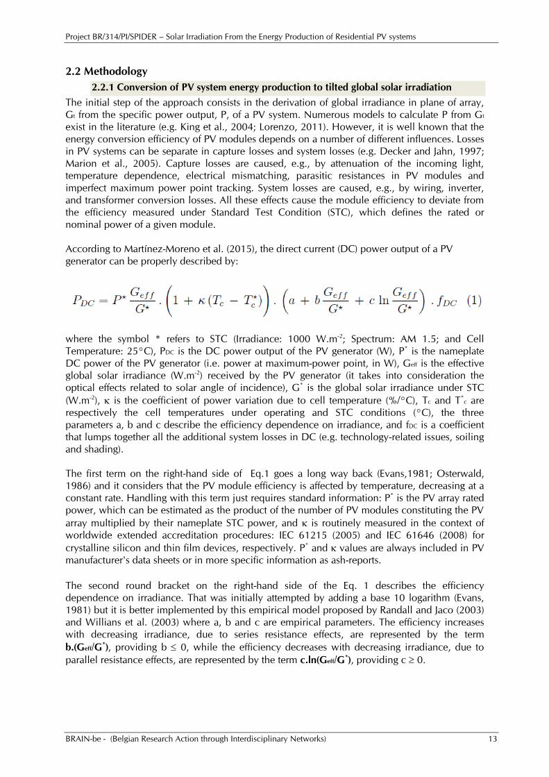
According to Martínez-Moreno et al. (2015), the direct current (DC) power output of a PV
generator can be properly described by:
where the symbol * refers to STC (Irradiance: 1000 W.m-2; Spectrum: AM 1.5; and Cell
Temperature: 25°C), PDC is the DC power output of the PV generator (W), P* is the nameplate
DC power of the PV generator (i.e. power at maximum-power point, in W), Geff is the effective
global solar irradiance (W.m-2) received by the PV generator (it takes into consideration the
optical effects related to solar angle of incidence), G* is the global solar irradiance under STC
(W.m-2), is the coefficient of power variation due to cell temperature (%/°C), Tc and T*c are
respectively the cell temperatures under operating and STC conditions (°C), the three
parameters a, b and c describe the efficiency dependence on irradiance, and fDC is a coefficient
that lumps together all the additional system losses in DC (e.g. technology-related issues, soiling
and shading).
The first term on the right-hand side of Eq.1 goes a long way back (Evans,1981; Osterwald,
1986) and it considers that the PV module efficiency is affected by temperature, decreasing at a
constant rate. Handling with this term just requires standard information: P* is the PV array rated
power, which can be estimated as the product of the number of PV modules constituting the PV
array multiplied by their nameplate STC power, and is routinely measured in the context of
worldwide extended accreditation procedures: IEC 61215 (2005) and IEC 61646 (2008) for
crystalline silicon and thin film devices, respectively. P* and values are always included in PV
manufacturer's data sheets or in more specific information as ash-reports.
The second round bracket on the right-hand side of the Eq. 1 describes the efficiency
dependence on irradiance. That was initially attempted by adding a base 10 logarithm (Evans,
1981) but it is better implemented by this empirical model proposed by Randall and Jaco (2003)
and Willians et al. (2003) where a, b and c are empirical parameters. The efficiency increases
with decreasing irradiance, due to series resistance effects, are represented by the term
b.(Geff/G*), providing b 0, while the efficiency decreases with decreasing irradiance, due to
parallel resistance effects, are represented by the term c.ln(Geff/G*), providing c 0.
Project BR/314/PI/SPIDER – Solar Irradiation From the Energy Production of Residential PV systems
BRAIN-be - (Belgian Research Action through Interdisciplinary Networks) 14
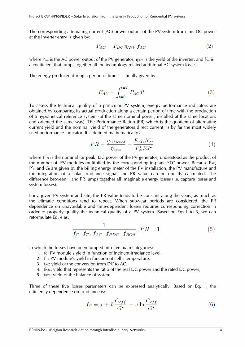
The corresponding alternating current (AC) power output of the PV system from this DC power
at the inverter entry is given by:
where PAC is the AC power output of the PV generator, INV is the yield of the inverter, and fAC is
a coefficient that lumps together all the technology related additional AC system losses.
The energy produced during a period of time T is finally given by:
To assess the technical quality of a particular PV system, energy performance indicators are
obtained by comparing its actual production along a certain period of time with the production
of a hypothetical reference system (of the same nominal power, installed at the same location,
and oriented the same way). The Performance Ration (PR) which is the quotient of alternating
current yield and the nominal yield of the generators direct current, is by far the most widely
used performance indicator. It is defined mathematically as:
where P*
N is the nominal (or peak) DC power of the PV generator, understood as the product of
the number of PV modules multiplied by the corresponding in-plane STC power. Because EAC,
P*N and Gt are given by the billing energy meter of the PV installation, the PV manufacture and
the integration of a solar irradiance signal, the PR value can be directly calculated. The
difference between 1 and PR lumps together all imaginable energy losses (i.e. capture losses and
system losses).
For a given PV system and site, the PR value tends to be constant along the years, as much as
the climatic conditions tend to repeat. When sub-year periods are considered, the PR
dependence on unavoidable and time-dependent losses requires corresponding correction in
order to properly qualify the technical quality of a PV system. Based on Eqs.1 to 3, we can
reformulate Eq. 4 as:
in which the losses have been lumped into five main categories:
1. fG: PV module's yield in function of incident irradiance level,
2. fT : PV module's yield in function of cell's temperature,
3. fAC: yield of the conversion from DC to AC.
4. fPDC: yield that represents the ratio of the real DC power and the rated DC power,
5. fBOS: yield of the balance of system.
Three of these five losses parameters can be expressed analytically. Based on Eq. 1, the
efficiency dependence on irradiance is:
Project BR/314/PI/SPIDER – Solar Irradiation From the Energy Production of Residential PV systems
BRAIN-be - (Belgian Research Action through Interdisciplinary Networks) 15
However, such a formulation of the fG parameter is useless here since the effective irradiance,
Geff , is by definition unknown in our case. To overcome such a limitation, fG is split into its two
main contributing factors:
where firr represents the variation in the PV module efficiency with the level of the solar
irradiance and finc the variation in the PV module efficiency as a function of the incidence angle
of the solar irradiance, respectively. Then, approximating the ratio Gt/G* by the Capacity
Utilization Factor (CUF) defined as:
with EAC the energy produced during a period of time T (see Eq. 3) and P*
N the nominal (or peak)
DC power of the PV system, firr can be estimated by:
In this equation, the three parameters a, b and c vary according to the considered PV module
technology. Values representative of crystalline silicon cells technology (i.e., a=1, b=-0.01 and
c=0.025) have been assumed for all the PV modules here. Finally, based on Martìn and Ruiz
(2005), the factor finc can be expressed as follows:
where i is the irradiance angle of incidence and r the angular loss coefficient, an empirical
dimensionless parameter dependent on the PV module technology and the dirtiness level of the
PV module. Typical r values range from 0.16 to 0.17 for commercial clean crystalline and
amorphous silicon modules. In this work a value of 0.20 has been assumed for r which is a
typical value for crystalline silicon PV modules presenting a moderate level of dirtiness.
The second factor, fT, is defined as:
where the operating temperature of the solar cell, Tc, is calculated from the ambient
temperature, Ta, using the following equation based on the Nominal Operation Cell
Temperature (NOCT) defined as the temperature reached by the cells when the PV module is
exposed to a solar irradiance of 800 W. m-2, an ambient temperature of 20°C, and a wind speed
of 1 m/s (it is obtained from the manufacturer datasheets):
Similarly to Eq. 6, the CUF approximation is used to estimate Tc reformulating Eq. 12 as follows:
Project BR/314/PI/SPIDER – Solar Irradiation From the Energy Production of Residential PV systems
BRAIN-be - (Belgian Research Action through Interdisciplinary Networks) 16
The third factor, fAC, is computed from:
where the so-called "European efficiency" of the inverter, EUR, is given by the formula:
with 5, 10, 20, 30, 50 and 100 the instantaneous power efficiency values at 5%,10%, 20%,
30%, 50% and 100% load.
The fourth factor, fPDC, as well as the fBOS factor cannot not be directly estimated because the real
energetic behavior of each PV system is unknown a priori. Lumping both factors together into a
new losses factor, fPERF , it follows from Eqs. 4 and 5 that:
where the fPERF factor sums up all the performance losses that, on the first hand could be avoided
and, on the other hand that cannot be modeled through a simple and general analytical
expression. This factor can be estimated for each PV system from historical data of EAC and Gt
using the EAC data took directly from the energy meters and Gt data obtained from the
combination of clear-sky radiative transfer model simulations and cloud cover information. It is
worth pointing out that to reduce the uncertainties in its estimation, the fPERF factor was
determined on a monthly basis from clear sky situations.
Similarly to Taylor et al. (2015) clear-sky situations were determined from the PV systems energy
production time series using a modified version of the algorithm developed by Reno et al.
(2012). For each PV system, fPERF, was calculated as being the ratio between the electrical energy
produced by the PV system corrected by the three others losses factors (i.e. fG, fT and fAC)
together with the quotient P*N /G* and the calculated in-plane clear-sky irradiation received by
the PV system during the considered month. Clear sky simulations were carried out by running
the Ineichen and Perez (2002) clear-sky radiative transfer model using monthly mean
climatological Linke turbidity values from PVGIS/CMSAF. Simulated clear sky global horizontal
irradiances were then transposed to tilted clear sky global irradiance using the ERB
decomposition model (Erbs et al., 1982; see Annexes A.1) and the HAY transposition model
(Hay, 1979; see Annexes B.2).
Finally, once all the losses factors are estimated, the derivation of the in-plane hourly global
solar irradiance from the hourly PV system energy production is given by:
Project BR/314/PI/SPIDER – Solar Irradiation From the Energy Production of Residential PV systems
BRAIN-be - (Belgian Research Action through Interdisciplinary Networks) 17
where all losses factors except fPERF were evaluated on an hourly basis using air temperature
measurements performed within the RMI's AWS interpolated at each of the PV system sites in
the computation of the operating solar cells temperature, Tc (see Eq. 13). fPERF is determined
monthly from the preceding month of EAC data.
2.2.2 Tilt to horizontal global solar irradiance transposition
The next step consists in the conversion of the retrieved in-plane global solar irradiance values
from the PV systems energy outputs to global horizontal solar irradiance at each of the PV
systems site location. If many transposition models have been proposed in the literature (see
Yang (2016) for a review) to convert solar irradiance on the horizontal plane, Gh, to that on a
tilted plane, Gt, the inverse process (i.e., converting from tilted to horizontal) is only poorly
discussed in literature (e.g. Faiman et al., 1987; Yang et al., 2013, 2014; Marion, 2015; Killinger
et al., 2016). The difficulty relies on the fact that the procedure is analytically not invertible.
Transposition models have the general form:
where the tilted global solar irradiance, Gt, is expressed as the sum of the in-plane direct
irradiance, Bt, in-plane diffuse irradiance, Dt, and the irradiance due to the ground reflection, Dg.
The direct component, Bt, is obtained from:
with Bn the direct normal irradiance and Bh the direct irradiance on a horizontal surface,
respectively. i is the incidence angle and, z, the solar zenith angle, respectively.
Parameter rb = cos i = cos z is a factor that accounts for the direction of the beam
radiation. The diffuse component, Dt, and the irradiance due to the ground reflection,
Dg, can be modeled as follows:
where Dh is the diffuse horizontal irradiance, Gh the global horizontal irradiance (i.e. Gh = Dh +
Bh), Rd the diffuse transposition factor and, the ground albedo. The transposition factor for
ground reflection, Rr, can be modeled under the isotropic assumption (e.g. Gueymard, 2009) as
follows:
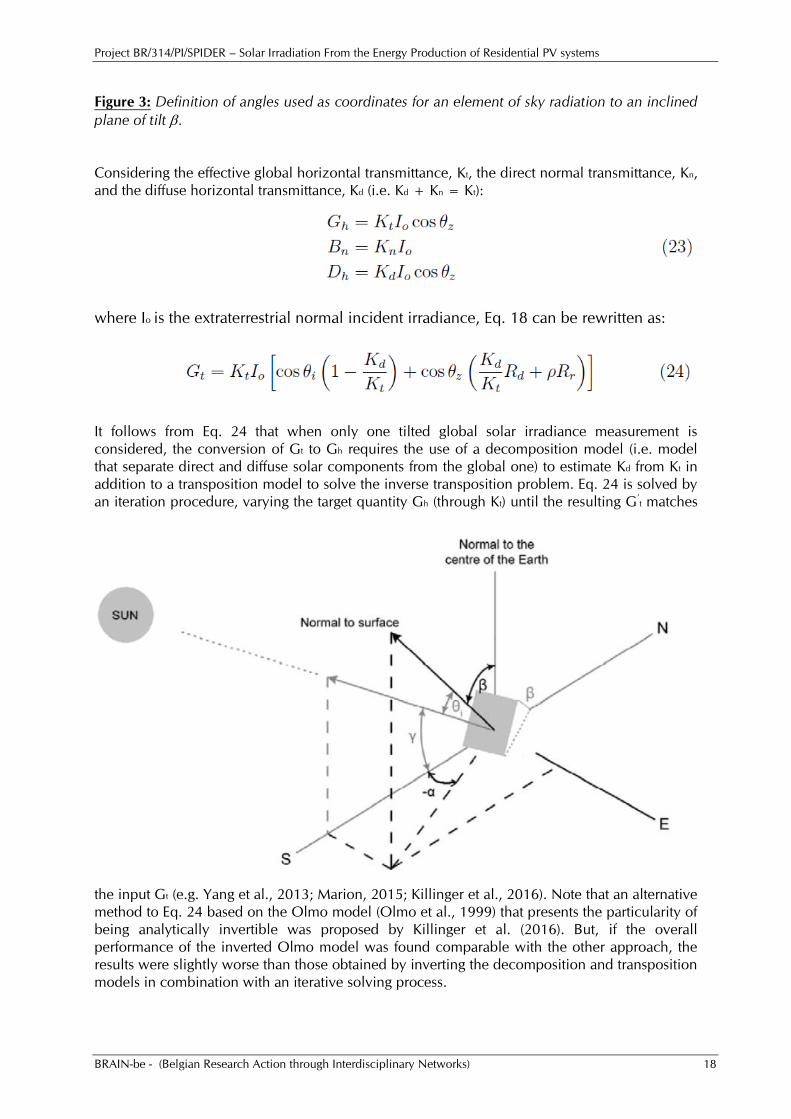
where is the tilt angle of the inclined surface (see Figure 3 for angles definition).
Project BR/314/PI/SPIDER – Solar Irradiation From the Energy Production of Residential PV systems
BRAIN-be - (Belgian Research Action through Interdisciplinary Networks) 18
Figure 3: Definition of angles used as coordinates for an element of sky radiation to an inclined
plane of tilt .
Considering the effective global horizontal transmittance, Kt, the direct normal transmittance, Kn,
and the diffuse horizontal transmittance, Kd (i.e. Kd + Kn = Kt):
where Io is the extraterrestrial normal incident irradiance, Eq. 18 can be rewritten as:
It follows from Eq. 24 that when only one tilted global solar irradiance measurement is
considered, the conversion of Gt to Gh requires the use of a decomposition model (i.e. model
that separate direct and diffuse solar components from the global one) to estimate Kd from Kt in
addition to a transposition model to solve the inverse transposition problem. Eq. 24 is solved by
an iteration procedure, varying the target quantity Gh (through Kt) until the resulting G’t matches
the input Gt (e.g. Yang et al., 2013; Marion, 2015; Killinger et al., 2016). Note that an alternative
method to Eq. 24 based on the Olmo model (Olmo et al., 1999) that presents the particularity of
being analytically invertible was proposed by Killinger et al. (2016). But, if the overall
performance of the inverted Olmo model was found comparable with the other approach, the
results were slightly worse than those obtained by inverting the decomposition and transposition
models in combination with an iterative solving process.
Project BR/314/PI/SPIDER – Solar Irradiation From the Energy Production of Residential PV systems
BRAIN-be - (Belgian Research Action through Interdisciplinary Networks) 19
.
When two (or more) tilted irradiances values (with different tilt angles and/or orientations) are
involved in the inverse transposition process, only a transposition model is required. The idea
that simultaneous readings of a multi-pyranometers system can be used to disangle the various
components of solar radiation on inclined surfaces was originally proposed by Faiman et al.
(1987) to solve in remote locations the periodic adjustment required by normal incidence and
shadow-band pyranometers to ensure that their readings remain accurate when long-term data
acquisition is in progress.
Given n tilted pyranometers (with different inclinations and/or orientations), the inverse
transposition problem can be represented in the matrix form (e.g. Yang et al., 2014):
where = {Ai} is a 2 x n x 2 third-order tensor, B = {Bi} is a n x 2 matrix, C is a column vector
with n given entries, and x is a column vector with 2 variables:
where the coefficients Ai, Bi and Ci depend on the considered transposition model.
The least square (hereafter referred to as LS) solution to Eq. 26 is given by:
with referring to the Euclidean norm. However, the LS is hard to solve and a standard
technique to resolve Eq. 27 is to use a Newton type iteration method (e.g., Grosan and
Abraham, 2008). As an alternative, Eq. 26 can also be solved by minimizing the errors (this
approach is hereafter denoted to as EM - Errors Minimization). In this case, the solution is to
minimize:
Project BR/314/PI/SPIDER – Solar Irradiation From the Energy Production of Residential PV systems
BRAIN-be - (Belgian Research Action through Interdisciplinary Networks) 20
where, ϵi(x) = (AiDhBh +BiBh +CiDh) - Gti , with i = 1, ..., n denoting the tilted pyranometer.
2.3 Results
2.3.1 Evaluation of the tilt to horizontal global solar irradiance transposition
Based on the four data sets of in-plane global solar irradiance collected at the RMI's radiometric
tower during the measurement campaign (see section 2.1.3), the relative ability of the single and
multi-pyranometers approaches to predict horizontal irradiance from tilted one(s) was estimated
by means of two statistical error indexes: Mean Bias Error (MBE) and Root Mean Square Error
(RMSE):
where ei = (Gi;e - Gi;o) is the residual value; Gi;e are the estimated values and Gi;o represent the
observed measurements. A positive MBE (resp. a negative MBE) means that the model tends to
overestimate (resp. underestimate) the observed measurements. To obtain dimensionless
statistical indicators we express MBE and RMSE as fractions of mean solar global irradiance
during the respective time interval,
where
n
ioiG
nM
1,
1 is the measurements mean. Note that for a proper estimation of the error
statistics, only radiation data recorded with a solar zenithal angle, z, smaller than 85° and an
incidence angle on the plane used, i, smaller than 90° were considered and tilted global solar
irradiance records were further restricted to non-zero values. Moreover when the retrieved
global horizontal solar irradiance was negative or larger than the corresponding extraterrestrial
irradiance the inverse transposition problem was considered unsuccessful. With these additional
conditions the total number of data points available simultaneously in all of the recording planes
(see Table 3) reduced to 5816 (i.e. 100%).
Project BR/314/PI/SPIDER – Solar Irradiation From the Energy Production of Residential PV systems
BRAIN-be - (Belgian Research Action through Interdisciplinary Networks) 21
Based on previous evaluation of popular decomposition and transposition models performance
in Uccle (i.e. Demain et al., 2013, 2017; Bertrand et al., 2015), the isotropic transposition model
proposed by Liu and Jordan (1962) (hereafter referred to as LIU model) and the anisotropic
models of Hay (1979) (hereafter referred to as HAY model), Skartveit and Olseth (1986)
(hereafter referred to as SKA model) and Perez et al. (1987) (hereafter referred to as PER model)
were considered together with the decomposition model of Skartveit and Olseth (1987)
(hereafter reffered to as OLS model). Formulation of the OLS decomposition model and the four
selected transposition models is provided in Annexes A.2 and B, respectively.
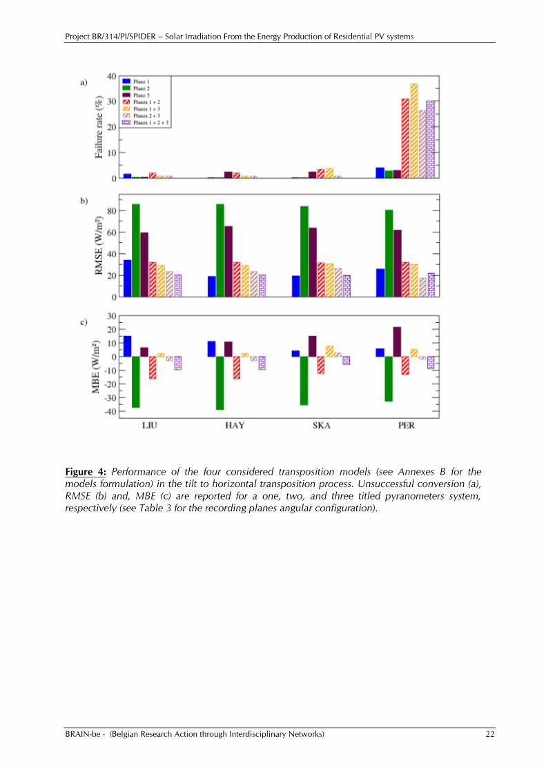
Figure 4 summarizes in terms of failure rate (panel a), RMSE (panel b) and, MBE (panel c) the
performance of the inverse transposition for each of the selected transposition models. Results
are reported for a single, two and three tilted pyranometers system, respectively. To evaluate the
transposition models on a same basis, only data points conversions that have succeeded for all
models are considered in the MBE and RMSE calculations. Note that while the LS and MS
approaches (i.e., Eqs. 27 and 28, respectively) have been considered to solve Eq. 25 (i.e. multi-
pyranometers system) only the MS results are displayed in Figure 4. Indeed, the minimization
carried out by using the Powell's quadratically convergent method (Powell, 1964) has been
found to systematically outperform the LS solution (Housmans et al., 2017). It is a generic
minimization method that allows to minimize a quadratic function of several variables without
calculating derivatives. The key advantage of not requiring explicit solution of derivatives is the
very fast execution time of the Powell method. In order to avoid the problem of linear
dependence in the Powell's algorithm, we adopted the modified Powell's method given in
Acton (1970) and implemented in Press et al. (1992).
Project BR/314/PI/SPIDER – Solar Irradiation From the Energy Production of Residential PV systems
BRAIN-be - (Belgian Research Action through Interdisciplinary Networks) 22
Figure 4: Performance of the four considered transposition models (see Annexes B for the models formulation) in the tilt to horizontal transposition process. Unsuccessful conversion (a), RMSE (b) and, MBE (c) are reported for a one, two, and three titled pyranometers system, respectively (see Table 3 for the recording planes angular configuration).
Project BR/314/PI/SPIDER – Solar Irradiation From the Energy Production of Residential PV systems
BRAIN-be - (Belgian Research Action through Interdisciplinary Networks) 23
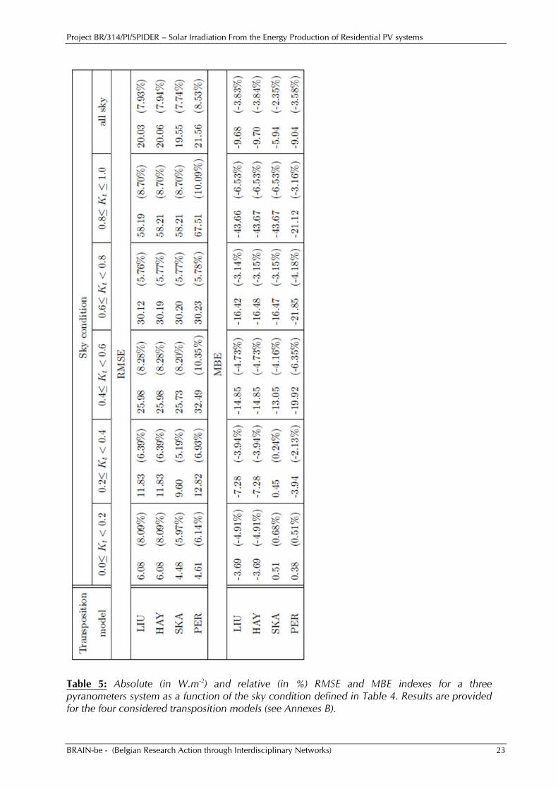
Table 5: Absolute (in W.m-2) and relative (in %) RMSE and MBE indexes for a three pyranometers system as a function of the sky condition defined in Table 4. Results are provided for the four considered transposition models (see Annexes B).
Project BR/314/PI/SPIDER – Solar Irradiation From the Energy Production of Residential PV systems
BRAIN-be - (Belgian Research Action through Interdisciplinary Networks) 24
It is apparent from panel (a) in Figure 4 that the PER model exhibits a significant percentage of
unsuccessful conversions. Because the PER model coefficients are binned according to the sky
clearness parameter, ϵ, (see Annexes B.4), the same strategy as in Yang et al. (2014) was adopted
here when running the PER model. Basically, K’t and K’d estimates are calculated for each ϵ bins
using the associated model coefficients Fij. In each ϵ bins G’h and D’h estimates are then
retrieved from the corresponding K’t and K’d estimates and used to determine the corresponding
ϵ’ value. If the assumed ϵ agrees with the calculated ϵ’, the corresponding G’h and D’h are
selected as the true estimated Gh and Dh. (Similarly, because the transposition factor defined by
the SKA model depends on the Skartveit-Olseth's correction factor Z (see Eq. 34), the conversion
process is performed for the two Rd model formulations before selecting the appropriate
solution. The global horizontal irradiance found has to satisfy the Z value definition assumed
during the conversion). Unfortunately, it may appear that none of the retrieved ϵ’ values agree
with its expected bin, or that more than one retrieved ϵ’ values agree with the expected bins,
increasing therefore the number of unsuccessful conversion associated to the PER model. This is
particularly well evident in Figure 4 when more than one tilted pyranometer is involved in the
inverse transposition problem. On the other hand, the failure rate reported for the three other
models reduces to nothing when three different Gt measurements are involved in the
calculations.
When only a single tilted sensor is used, the conversion can be carried out with a
decomposition model coupled with a transposition model to solve the inverse transposition
problem. In this case, there is an additional error (additional to the inverse transposition
problem) in the predicted horizontal irradiance. In addition with only one tilted irradiance
involved in the inverse modeling approach, the tilt angle and the surface's orientation have a
major impact on the Gh estimation's reliability irrespective of the considered transposition
model. None of the considered transposition models was found to perform the best over the 3
tilted pyranometers mounting plane configurations (see Table 3). The worst performance in
terms of RMSE and MBE are for Plane 2 measurements conversion (i.e. RMSE ranging from 80.2
W.m-2 or 28.7% to 85.8 W.m-2 or 30.8% vs. 19.0 W.m-2 or 6.8% to 33.9 W.m-2 or 12.2%
reported for Plane 1 conversions). Furthermore, Plane 2 conversions underestimate Gh (i.e. MBE
ranging from -39.2 W.m-2 or -14.1% to -32.7 W.m-2 or -11.7%) while a slight overestimation of
10.9 W.m-2 or 0.3% to 14.9 W.m-2 or 5.3% is reported for Plane 1 conversions and an
overestimation of 6.5 W.m-2 or 2.3% to 21.3 W.m-2 or 7.6% for Plane 3 conversions,
respectively.
Figure 4 indicates that the overall performance of the inverse transposition is improved when
using two different tilted global irradiance measurements as input to the Gh computation and
dependencies to tilt angles and surface orientations are reduced. For a given albedo, two tilted
pyranometers set at different orientations/inclinations suffice to determine the diffuse and beam
radiation components. In practice, there are certain sun positions for which this procedure fails
to produce a valid estimation of the global horizontal irradiance. Consequently, more
instruments should be used so as to overdetermine the system. Here it was found that three
tilted pyranometers set at different orientations is sufficient to guarantee a solution for three of
the four considered transposition models. Indeed, because of the non bijectivity of the PER
anisotropic model the conversion of a bit less than one third of the data points (i.e. 30.4 %) were
unsuccessful. Globally, all models behave quite similarly in term of RMSE (overall RMSE value
of 20.0 W.m-2 or 7.9%) and present a negative bias (i.e. MBE ranging from -9.7 W.m-2 or -3.8%
to -5.9 W.m-2 or -2.4%).
Table 5 shows that the models relative accuracy does not change noticeably as the sky condition
move from overcast to clear sky situations (i.e. a relative RMSE variation of about 4.6%, 3.5%
and 3% is reported for the PER, SKA and the LIU and HAY models, respectively). All models
show a negative bias in clear sky condition (i.e. 0.8 Kt 1.0) where the global radiation is
Project BR/314/PI/SPIDER – Solar Irradiation From the Energy Production of Residential PV systems
BRAIN-be - (Belgian Research Action through Interdisciplinary Networks) 25
mainly composed of direct radiation. As an illustration, an underestimation of about 43.7 W.m-2
or 6.5% is reported for the LIU, HAY, and SKA models and of 21.1 W.m-2 or 3.2% for the PER
model. In overcast condition (i.e. 0.0 Kt < 0.2) where the diffuse component largely domines,
while the global radiation is underestimated by about 3.7 W.m-2 or 4.9% by the LIU and HAY
models, it is in the opposite slightly overestimated by the SKA and PER models (i.e. MBE of 0.5
W.m-2 or 0.7% and 0.4 W.m-2 or 0.5%, respectively). If the SKA model is the best performing
model in overcast and cloudy conditions (i.e. Kt < 0.4) with reported RMSE values of 4.5 W.m-2
or 6% and 9.6 W.m-2 or 5.2%, respectively, its performances do not differ from those reported
for the LIU and HAY models in partly cloudy, partly clear and clear sky situations (i.e. Kt 0.4)
with RMSE values ranging from 30.2 W.m-2 or 5.8% in partly clear conditions to 58.2 W.m-2 or
8.7% in clear sky conditions. The PER model exhibits the lowest RMSE scores for the different
sky conditions excepted in overcast situation where its performance (i.e. RMSE of 4.6 W.m-2 or
6.1%) is closely similar to that reported for the SKA model.
Finally, comparing the performance between the isotropic and anisotropic approaches to the
inverse transposition problem in angular configurations similar to those encountered in Belgian
residential PV systems installations (e.g. with tilt angle as great as 50.79°) indicates that the
improvement from using the LIU isotropic model to using anisotropic models is not significant
(e.g. a RMSE of 20.0 W.m-2 or 7.9% and a MBE of -9.7 W.m-2 or -3.8% are reported for the LIU
model when considering a three tilted pyranometers system compared to a RMSE of 19.6 W.m-2
or 7.7% and a MBE of -5.9 W.m-2 or -2.35% for the best performing SKA anisotropic model) or
even inexistent regarding the percentage of unsuccessful conversion (e.g. a failure rate of 0% is
reported for the LIU model in the three tilted pyranometers system compared to a failure rate of
30.1% for the PER model) .
2.3.2 Evaluation of the PV system energy production to global horizontal solar
irradiation conversion
Similarly to the evaluation of the tilt to horizontal transposition process, the MBE and RMSE
statistical error indexes have been used to evaluate the prediction of the global horizontal solar
irradiance (GHI) from the energy production of residential PV systems. Statistical error indexes
were computed between in situ irradiance measurements and the estimations computed from
the hourly energy productions of residential PV systems surrounding the measurement stations.
An initial radius of 5 km centered on the station was considered to select the residential PV
systems for the validation purpose. When less than 4 PV installations were found within the
delimited area around the station, the radius was extended to 10 km. Table 6 indicates for each
of our measurements sites the number of neighboring PV installations used for validation. As we
can see none PV system was found in the vicinity of the Sint-Katelijn-Waver, Retie and Mont-
Rigi stations (i.e. AWS 6439, AWS 6464 and AWS 6494, respectively) and 3 others stations
only have one surrounding residential PV system. At the opposite, the maximum number of
installations surrounding a station is 37 and concerns the Ernage site (i.e. AWS 6457).
Based on our evaluation of the inverse transposition problem (see Section 2.3.1) two different
approaches have been considered to compute the global horizontal solar irradiance from the PV
systems energy production. In the first approach, the tilt to horizontal conversion is performed
independently at each PV installations surrounding the validation site using Eq. 24 with the OLS
decomposition model (see Annexes A.2) and the SKA transposition model (see Annexes B.3).
The resulting global horizontal solar irradiance for the group of PV systems is then taken as the
median value of the individual PV system estimates. This approach is referred to as 1_PV-M
hereafter. In the second approach all individual tilted global solar irradiance estimates are used
simultaneously and the tilt to horizontal conversion is solved by EM (see Eq. 28) using the
Project BR/314/PI/SPIDER – Solar Irradiation From the Energy Production of Residential PV systems
BRAIN-be - (Belgian Research Action through Interdisciplinary Networks) 26
Powell’s quadratically convergent method and the SKA transposition model. This approach is
hereafter denoted to as X_PV-EM. Performance of the two approaches in the GHI estimation
from PV systems AC power output have been evaluated and compared to GHI estimates
retrieved from Meteosat Second Generation (MSG; Schmetz, 2002) satellite images as
implement on an operational basis at RMI. Description of the RMI’s MAGIC/Heliosat-2
algorithm used to retrieve the solar surface irradiance at the SEVIRI imager spatial sampling
distance above Belgium (e.g. about 6 km in the north-south direction and 3.3 km in the east-
west direction) from MSG images is provided in Annexes C.
While the MSG based retrieval method always provides GHI estimates during day time, there
are certain sun positions for which the PV systems power output method fails to produce a valid
estimation. Unsuccessful tilt to horizontal conversions are found for both the 1_PV-M and the
X_PV-EM approaches at low solar elevation irrespective of the number of PV systems involved
in the conversion process. Failure rates reported for the 1_PV-M and the X_PV-EM approaches at
each validation sites are provided in Table 6 together with total number of available hourly data
points at each location for the year 2014. Unsurprisingly the largest failure rates (up to nearly
40% in the case of the Melle station -AWS 6434-) are found at validation sites where only one
PV installation is available. With more PV systems, the number of unsuccessful conversions after
sunrise and before sunset is decreased. Table 6 tends to indicate that 1_PV-M approach starts to
produce valid results at lower solar elevation conditions than the X_PV-EM approach (i.e. an
overall failure rate of about 12.4% is reported for the 1_PV-M approach and of 19.6% for the
X_PV-EM approach, respectively) but it is largely relying on the angular configurations (i.e. tilt
and azimuth angles) of the PV installations found within the group of PV systems.
Table 7 compares hourly GHI estimates as computed by the 1_PV-M and X_PV-EM approaches
and derived from MSG images with the corresponding ground measurements. To ensure that the
comparisons were made between comparable data, special attention was given to the coherence
of the data, the precision of the time acquisition, and the synchronization of the different data
sets with the ground measurements. Because of inaccuracies in the orientations and/or
inclinations of the PV installations provided by the PV systems installers or owners, GHI
computation from the energy production of only one installation can generate RMSE values as
large as 189.34 W.m-2 or 57.8% (i.e. at the Middelkerke validation site – AWS 6407-).
Increasing the number of PV installations involved in the estimation process allows smoothing
the GHI estimation to some extent. This is particularly apparent for the 1_PV-M approach which
globally presents lower RMSE values than found for the X_PV-EM approach (i.e. an overall
RMSE value of 113.5 W.m-2 or 41.4% is reported for the 1_PV-M approach and of 121.9 W.m-2
or 44.4% for the X_PV-EM approach, respectively). However, sensitivity experiments in which
the number of PV installations involved in the GHI determination was varying revealed a larger
variability in the resulting GHI estimations for the 1_PV-M approach than found for the X_PV-
EM approach which produces a more stable solution.
Project BR/314/PI/SPIDER – Solar Irradiation From the Energy Production of Residential PV systems
BRAIN-be - (Belgian Research Action through Interdisciplinary Networks) 27
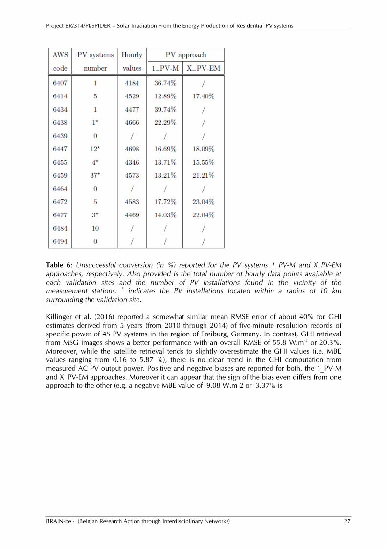
Table 6: Unsuccessful conversion (in %) reported for the PV systems 1_PV-M and X_PV-EM approaches, respectively. Also provided is the total number of hourly data points available at each validation sites and the number of PV installations found in the vicinity of the measurement stations. * indicates the PV installations located within a radius of 10 km surrounding the validation site.
Killinger et al. (2016) reported a somewhat similar mean RMSE error of about 40% for GHI
estimates derived from 5 years (from 2010 through 2014) of five-minute resolution records of
specific power of 45 PV systems in the region of Freiburg, Germany. In contrast, GHI retrieval
from MSG images shows a better performance with an overall RMSE of 55.8 W.m-2 or 20.3%.
Moreover, while the satellite retrieval tends to slightly overestimate the GHI values (i.e. MBE
values ranging from 0.16 to 5.87 %), there is no clear trend in the GHI computation from
measured AC PV output power. Positive and negative biases are reported for both, the 1_PV-M
and X_PV-EM approaches. Moreover it can appear that the sign of the bias even differs from one
approach to the other (e.g. a negative MBE value of -9.08 W.m-2 or -3.37% is
Project BR/314/PI/SPIDER – Solar Irradiation From the Energy Production of Residential PV systems
BRAIN-be - (Belgian Research Action through Interdisciplinary Networks) 28
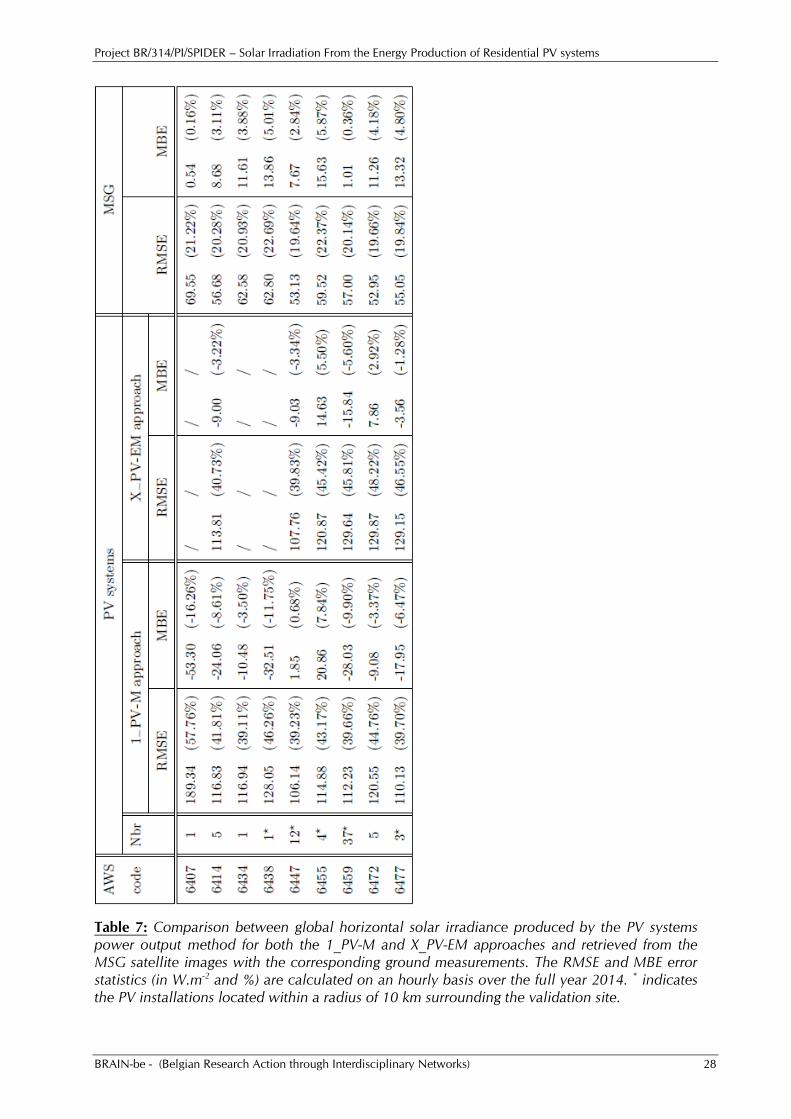
Table 7: Comparison between global horizontal solar irradiance produced by the PV systems power output method for both the 1_PV-M and X_PV-EM approaches and retrieved from the MSG satellite images with the corresponding ground measurements. The RMSE and MBE error statistics (in W.m-2 and %) are calculated on an hourly basis over the full year 2014. * indicates the PV installations located within a radius of 10 km surrounding the validation site.
Project BR/314/PI/SPIDER – Solar Irradiation From the Energy Production of Residential PV systems
BRAIN-be - (Belgian Research Action through Interdisciplinary Networks) 29
reported at the Humain validation site –AWS 6472 – for the 1_PV-M approach while an
overestimation of 7.86 W.m-2 or 2.92% is found for the X-PV-EM approach). In general, the
magnitude of the bias is lower with the X_PV-EM approach than with the 1_PV-M approach (i.e.
MBE values ranging from -5.6% to 5.5% and from -9.9% to 7.8%, respectively).
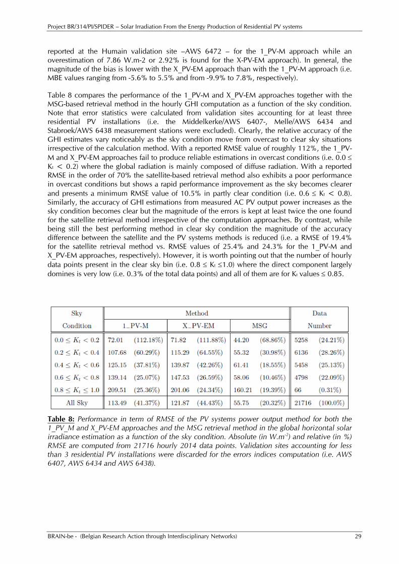
Table 8 compares the performance of the 1_PV-M and X_PV-EM approaches together with the
MSG-based retrieval method in the hourly GHI computation as a function of the sky condition.
Note that error statistics were calculated from validation sites accounting for at least three
residential PV installations (i.e. the Middelkerke/AWS 6407-, Melle/AWS 6434 and
Stabroek/AWS 6438 measurement stations were excluded). Clearly, the relative accuracy of the
GHI estimates vary noticeably as the sky condition move from overcast to clear sky situations
irrespective of the calculation method. With a reported RMSE value of roughly 112%, the 1_PV-
M and X_PV-EM approaches fail to produce reliable estimations in overcast conditions (i.e. 0.0
Kt < 0.2) where the global radiation is mainly composed of diffuse radiation. With a reported
RMSE in the order of 70% the satellite-based retrieval method also exhibits a poor performance
in overcast conditions but shows a rapid performance improvement as the sky becomes clearer
and presents a minimum RMSE value of 10.5% in partly clear condition (i.e. 0.6 Kt < 0.8).
Similarly, the accuracy of GHI estimations from measured AC PV output power increases as the
sky condition becomes clear but the magnitude of the errors is kept at least twice the one found
for the satellite retrieval method irrespective of the computation approaches. By contrast, while
being still the best performing method in clear sky condition the magnitude of the accuracy
difference between the satellite and the PV systems methods is reduced (i.e. a RMSE of 19.4%
for the satellite retrieval method vs. RMSE values of 25.4% and 24.3% for the 1_PV-M and
X_PV-EM approaches, respectively). However, it is worth pointing out that the number of hourly
data points present in the clear sky bin (i.e. 0.8 Kt 1.0) where the direct component largely
domines is very low (i.e. 0.3% of the total data points) and all of them are for Kt values 0.85.
Table 8: Performance in term of RMSE of the PV systems power output method for both the 1_PV_M and X_PV-EM approaches and the MSG retrieval method in the global horizontal solar irradiance estimation as a function of the sky condition. Absolute (in W.m-2) and relative (in %)
RMSE are computed from 21716 hourly 2014 data points. Validation sites accounting for less than 3 residential PV installations were discarded for the errors indices computation (i.e. AWS 6407, AWS 6434 and AWS 6438).
Project BR/314/PI/SPIDER – Solar Irradiation From the Energy Production of Residential PV systems
BRAIN-be - (Belgian Research Action through Interdisciplinary Networks) 30
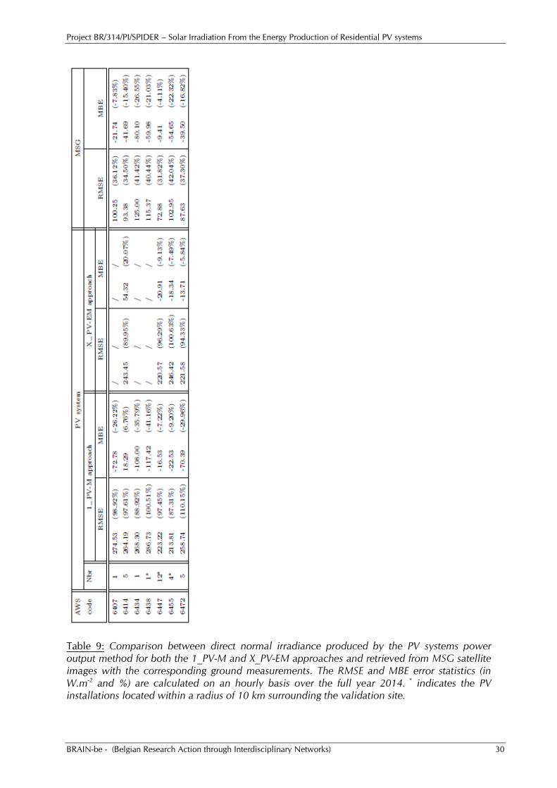
Table 9: Comparison between direct normal irradiance produced by the PV systems power output method for both the 1_PV-M and X_PV-EM approaches and retrieved from MSG satellite images with the corresponding ground measurements. The RMSE and MBE error statistics (in W.m-2 and %) are calculated on an hourly basis over the full year 2014. * indicates the PV installations located within a radius of 10 km surrounding the validation site.
Project BR/314/PI/SPIDER – Solar Irradiation From the Energy Production of Residential PV systems
BRAIN-be - (Belgian Research Action through Interdisciplinary Networks) 31
Performance of the different methods in the direct normal irradiance (DNI) determination
(hourly validation) is summarized in terms of RMSE and MBE in Table 9. To ensure comparisons
between comparable data, exactly the same data points as those used for the GHI statistical error
indexes calculations were used for the DNI validation at each selected validation sites. Globally,
the error associated to the DNI estimation is very large. As an example the overall magnitude of
the RMSE reported for the satellite retrieval method is nearly twice the one obtained for the GHI
estimation (i.e. 37.7% vs 21.0%, respectively). Accuracy of the DNI estimation from PV systems
AC output power is largely worst with reported RMSE values ranging from 87.31% to 110.15%
for the 1_PV-M approach and from 89.95% to 100.63% for the X_PV-EM approach,
respectively. As a comparison Killinger et al. (2016) reported mean RMSE error of about 80% for
DNI values derived from power records of 45 PV systems in the region of Freiburg, Germany.
In opposite to the GHI estimation, DNI estimates are systematically underestimated by the MSG-
based retrieval method with MBE values ranging from -26.6% to -4.1%. The 1_PV-M and X_PV-
EM approaches also have a negative bias (with reported underestimation up to 41.2% when the
estimation is computed from the power output of one individual PV installation) excepted in one
validation site (i.e. AWS 6414) where an overestimation of 6.8% is reported for the 1_PV-M
approach and up to 20.07% for the X_PV-EM approach, respectively.
Computation of the statistical errors indexes on a daily basis is not as straightforward as for an
hourly basis because as already mentioned both the 1_PV-M and X_PV-EM approaches fail to
produce valid GHI estimates at low solar elevation conditions. In Table 10 RMSE and MBE
indexes have been computed by assuming no incoming global horizontal solar irradiance in the
computation of the daily global horizontal solar irradiation for data points where no valid hourly
GHI estimates were obtained. By contrast Table 11 displays for each validation sites RMSE and
MBE values calculated when only considering hourly valid GHI estimates in the computation of
daily global horizontal solar irradiation. Note that because the failure rates differ for the 1_PV-M
and X_PV-EM approaches (see Table 6) the number of data points involved in the daily
validation at each measurement sites varies between the two approaches in Table 11.
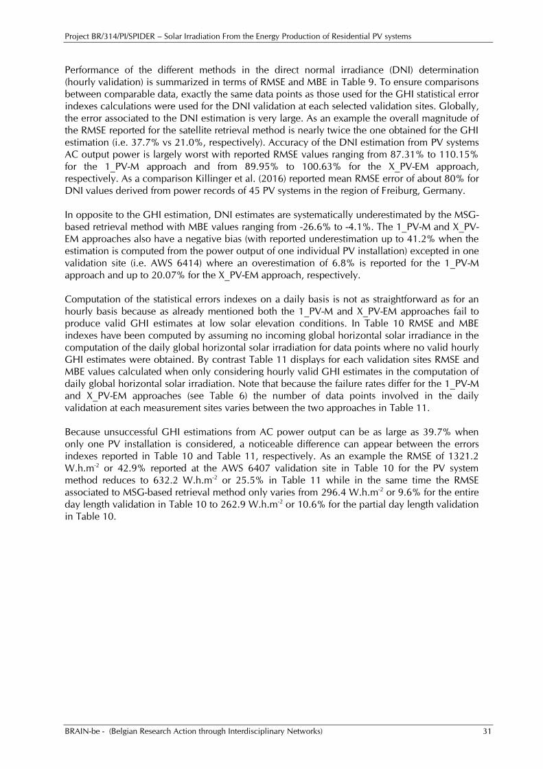
Because unsuccessful GHI estimations from AC power output can be as large as 39.7% when
only one PV installation is considered, a noticeable difference can appear between the errors
indexes reported in Table 10 and Table 11, respectively. As an example the RMSE of 1321.2
W.h.m-2 or 42.9% reported at the AWS 6407 validation site in Table 10 for the PV system
method reduces to 632.2 W.h.m-2 or 25.5% in Table 11 while in the same time the RMSE
associated to MSG-based retrieval method only varies from 296.4 W.h.m-2 or 9.6% for the entire
day length validation in Table 10 to 262.9 W.h.m-2 or 10.6% for the partial day length validation
in Table 10.
Project BR/314/PI/SPIDER – Solar Irradiation From the Energy Production of Residential PV systems
BRAIN-be - (Belgian Research Action through Interdisciplinary Networks) 32
Table 10: Comparison between daily cumulated surface solar irradiation produced by the PV system power output method for both the 1_PV-M and X_PV-EM approaches and retrieved from the MSG satellite images with the corresponding daily ground measurements. The RMSE and MBE error statistics (in W.h.m-2 and %) are calculated on a daily basis over the full year 2014. Hourly data points over the entire day length have been included in the daily surface solar
Project BR/314/PI/SPIDER – Solar Irradiation From the Energy Production of Residential PV systems
BRAIN-be - (Belgian Research Action through Interdisciplinary Networks) 33
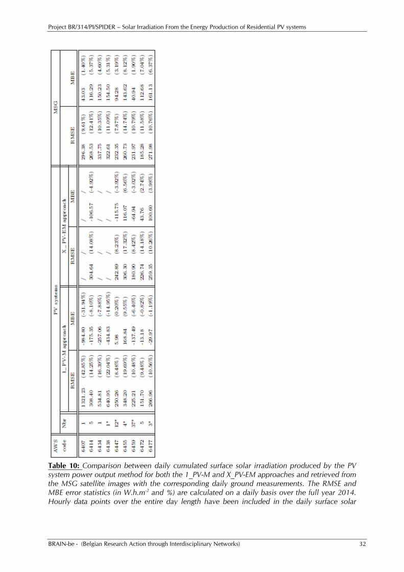
irradiation computation. * indicates the PV installations located within a radius of 10 km surrounding the validation site.
Table 11: Comparison between daily cumulated surface solar irradiation produced by the PV system power output method for both the 1_PV-M and X_PV-EM approaches and retrieved from the MSG satellite images with the corresponding daily ground measurements. The RMSE and
MBE error statistics (in W.h.m-2 and %) are calculated on a daily basis over the full year 2014. Only hourly data points for which the 1_PV-M approach in the first hand and the X_PV-EM approach in the second hand produced valid hourly GHI estimates have been included in the daily surface solar irradiation computation. Because the failure rate differs between the 1_PV-M and the X-PV-EM approaches (see Table 6) the number of considered data points varies between the AWS – 1_PV-M – MSG and AWS – X_PV-EM –MSG validations, respectively. * indicates the PV installations located within a radius of 10 km surrounding the validation site.
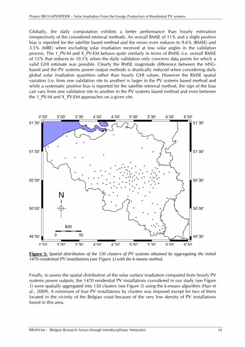
Project BR/314/PI/SPIDER – Solar Irradiation From the Energy Production of Residential PV systems
BRAIN-be - (Belgian Research Action through Interdisciplinary Networks) 34
Globally, the daily computation exhibits a better performance than hourly estimation
irrespectively of the considered retrieval methods. An overall RMSE of 11% and a slight positive
bias is reported for the satellite based method and the errors even reduces to 9.6% (RMSE) and
3.5% (MBE) when excluding solar irradiation received at low solar angles in the validation
process. The 1_PV-M and X_PV-EM behave quite similarly in terms of RMSE (i.e. overall RMSE
of 12% that reduces to 10.5% when the daily validation only concerns data points for which a
valid GHI estimate was possible. Clearly the RMSE magnitude difference between the MSG-
based and the PV systems power output methods is drastically reduced when considering daily
global solar irradiation quantities rather than hourly GHI values. However the RMSE spatial
variation (i.e. from one validation site to another) is larger in the PV systems based method and
while a systematic positive bias is reported for the satellite retrieval method, the sign of the bias
can vary from one validation site to another in the PV systems based method and even between
the 1_PV-M and X_PV-EM approaches on a given site.
Figure 5: Spatial distribution of the 150 clusters of PV systems obtained by aggregating the initial
1470 residential PV installations (see Figure 1) with the k-means method.
Finally, to assess the spatial distribution of the solar surface irradiation computed from hourly PV
systems power outputs, the 1470 residential PV installations considered in our study (see Figure
1) were spatially aggregated into 150 clusters (see Figure 5) using the k-means algorithm (Hair et
al., 2009). A minimum of four PV installations by clusters was imposed except for two of them
located in the vicinity of the Belgian coast because of the very low density of PV installations
found in this area.
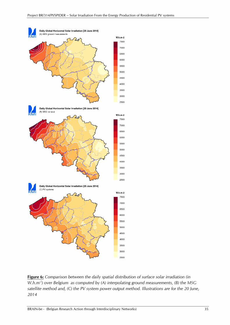
Project BR/314/PI/SPIDER – Solar Irradiation From the Energy Production of Residential PV systems
BRAIN-be - (Belgian Research Action through Interdisciplinary Networks) 35
Figure 6: Comparison between the daily spatial distribution of surface solar irradiation (in
W.h.m-2) over Belgium as computed by (A) interpolating ground measurements, (B) the MSG
satellite method and, (C) the PV system power output method. Illustrations are for the 20 June,
2014
Project BR/314/PI/SPIDER – Solar Irradiation From the Energy Production of Residential PV systems
BRAIN-be - (Belgian Research Action through Interdisciplinary Networks) 36
Figure 6 presents an example of daily solar surface irradiation over the Belgian territory as
computed from the interpolation of ground measurements using the ordinary kriging (OK)
method (e.g. Wackernagel, 1995), the MSG satellite derived estimation and the PV systems
method using the X_PV-EM. Clearly, due to the sparsity of the ground stations networks,
interpolating ground data generates only a coarse distribution of the solar surface irradiation:
large-scale variations of the solar irradiation (such as the south-east to north-west positive
gradient) are identified but local fluctuations remain unseen (Figure 6, panel A). Satellite-derived
estimates, on the other hand, provide a global coverage and are therefore able to account for
clouds induced small-scale variability in surface solar radiation (Figure 6, panel B). Regarding
the PV systems method, because it was not possible to obtain a spatially homogeneous
distribution of PV clusters from our residential PV installations dataset (most of them being
located in Wallonia and Brussels), the daily solar irradiation estimated obtained at the PV
clusters level were then interpolated by OK method to cover the entire Belgian territory (Figure
6, panel C). As we see, the south-east to north-west positive gradient is well apparent as well as
some of the regional specificities. For instance, the Gaume region (area in the south-east of
Belgium) located on the south side of the Ardenne (hilly mass) and that enjoys longer sunshine
time appears clearly on the mapping. In general the PV systems method provides small-scale
patterns partly supported by the MSG derived mapping. Some other appear as the signature of
an erroneous estimation at the cluster level. Such artefacts are well apparent along the Ourthe
valley in the Ardenne in Wallonia.
3. PERSPECTIVES
To maintain and improve Europe’s weather forecasting activities, EUMETSAT is currently
procuring a new, third generation of Meteosat weather satellites (MTG; Stuhlmann et al., 2005).
In total, six MTG satellites will be launched into space starting in 2019. Because our results
indicate that satellite-based surface solar irradiance estimates outperform estimations from the
power output of PV systems, it is essential to adapt our MSG retrieval algorithm to ensure the
operational continuity of the retrieval chain at RMI. Efforts will be made to take advantage of the
new capabilities offer by MTG in our retrieval process. The MTG series will comprise four
imaging and two sounding satellites. The MTG-I imaging satellites will carry the Flexible
Combined Imager (FCI) and the Lightning Imager. The MTG-S sounding satellites for will carry
an Infrared Sounder (IRS) and an Ultraviolet Visible Near-Infrared spectrometer. On the MTG-I
satellites, FCI will scan the full Earth disc every 10 minutes using 16 spectral channels at
very high spatial resolutions, from 2 km to 0.5 km. In a ‘fast imagery mode’ it will be
capable of a repeat cycle of 2.5 minutes over a quarter of the disc. FCI will offer better
capabilities for monitoring aerosols, making an important contribution to air-quality
monitoring. In addition, thanks to its higher-resolution capability in the thermal–infrared,
FCI will also provide improved fire detection.
Project BR/314/PI/SPIDER – Solar Irradiation From the Energy Production of Residential PV systems
BRAIN-be - (Belgian Research Action through Interdisciplinary Networks) 37
4. PUBLICATIONS
4.1 International journal with reading committee
Bertrand, C., Housmans, C., Leloux, J. and M. Journée, 2017: Solar irradiation from the energy
production of residential PV systems in Belgium. Manuscript in preparation
Housmans, C. and C. Bertrand, 2017: Evaluation of various procedures transposing global tilted
irradiance to horizontal surface irradiance. Adv. Sci. Res., 14:17-22.
Housmans, C., Ipe, A. and C. Bertrand, 2017: Tilt to horizontal global solar irradiance
conversion: an evaluation at high tilt angles and different orientations. Renew. Energy,
113:1529-1538.
4.2 Conference abstract
Housmans, C. and C. Bertrand, 2016: Evaluation of various procedure transposing global tilted
irradiance to horizontal surface irradiance. EMS Annual Meeting Abstracts, Vol. 13, EMS2016-
170, 2016, 16th EMS/11th ECAC
Housmans, C., Leloux, J. and C. Bertrand, 2017: Tilt to horizontal global solar irradiance
conversion: application to PV systems data. Geophysical Research Abstracts, Vol. 19, EGU2017-
14994, 2017, EGU General Assembly 2017.
5. ACKNOWLEDGEMENTS
The authors are grateful to the RMI’s AWS team for having kindly provided us with the two
CMP-22 pyranometer instruments used during the July 15, 2015 to January 19, 2016
measurements campaign. Thanks to Serge Ginion who has installed the instruments on the roof
of the RMI’s radiometric tower.
Project BR/314/PI/SPIDER – Solar Irradiation From the Energy Production of Residential PV systems
BRAIN-be - (Belgian Research Action through Interdisciplinary Networks) 38
6. REFERENCES
Acton, F.S., 1970: Numerical Methods That Work, 1990, corrected edition.
Mathematical Association of America, pp. 464-467.
Asner, G. P., 1998: Biophysical and Biochemical Sources of variability in Canopy
Reflectance, Remote Sens. Environ., 64:234–253.
Bertrand, C., Vanderveken, G. and M. Journée, 2015: Evaluation of decomposition
models of various complexity to estimate the direct solar irradiance over Belgium.
Renewable Energy, 74:618-626.
Cano, D., Monget, J. M., Albuisson, M., Guillar, H., Regas, N. and L. Wald, 1986: A
method for the determination of the global solar radiationfrom meteorological satellite
data. Solar Energy, 56:207–212.
Decker, B. and U. Jahn, 1997: Performance of 170 grid connected PV plants in northern
Germany - analysis of yields and optimization potentials. Solar Energy, 59(4):127-133.
Demain, C., Journée, M. and C. Bertrand, 2013: Evaluation of different models to
estimate the global solar radiation on inclined surfaces. Renewable Energy, 50:710-721.
Demain, C., Journée, M. and C. Bertrand, 2017: Corrigendum to "Evaluation of different
models to estimate the global solar radiation on inclined surfaces"[Renewable Energy 50
(2013) 710-721]. Renewable Energy, 101:1401-1403.
Derrien, M. and H. Le Gléau, 2005: MSG/SEVIRI cloud mask and type from SAFNWC.
Int. J. Remote Sens., 26:4707–4732.
Elsinga, B., van Sark, W. and L. Ramakers, 2017: Inverse photovoltaic yield model for
global horizontal irradiance reconstruction. Energy Science & Engineering,14pp, doi:
10.1002/ese3.162.
Evans, D.L., 1981: Simplified Method for Predicting Photovoltaic Array Output. Solar
Energy, 27:555-560.
Erbs, D.G., Klein, S.A. and J.A. Duffie, 1982: Estimation of the diffuse radiation fraction
for hourly, daily and monthly-average global radiation. Solar Energy 28:293-302.
Faiman, D., Zemel, A. and A. Zangvil, 1987: A method for monitoring insolation in
remote regions. Solar Energy, 38:327-333.
Grosan, C. and A. Abraham, 2008: A new approach for solving nonlinear equations
systems. IEEE Trans. Syst. Man. Cybern. Part A Syst. Humans, 38:698-714.
Hammer, A., Heinemann, D., Hoyer, C., Kuhlemann, R., Lorentz, E., Mueller, R. and
H.G. Beyer, 2003: Solar energy assessment using remote sensing technologies. Remote
Sensing of Environment, 86:423-432.
Hair, J.F., Black, W.C., Babin, B.J. and R.E. Anderson, 2009. Multivariate Data Analysis.
Seventh ed., Prentice Hall.
Hay, J.E., 1979: Study of shortwave radiation on non-horizontal surfaces. Rep. No. 79-
12, Atmospheric Environment Service, Downsview, Ontario.
Housmans, C., Ipe, A. and C. Bertrand, 2017: Tilt to horizontal global solar irradiance
conversion: An evaluation at high tilt angles and different orientations. Renewable
Energy, 113:1529-1538.
IEC Standard-61215, 2005: Crystalline silicon terrestrial photovoltaic (PV) modules
design qualification and type approval. International Electrotechnical Commission.
IEC Standard-61646, 2008: Thin-film terrestrial photovoltaic (PV) modules - Design
qualification and type approval. International Electrotechnical Commission.
Ineichen, P. and R. Perez, 2002: A new airmass independent formulation for the Linke
turbidity coefficient. Solar Energy, 73:151-157.
Ipe, A., Clerbaux, N., Bertrand, C., Dewitte, S. and L. Gonzalez, 2003: Pixel-scale
composite top-of-the-atmosphere clear-sky reflectances for Meteosat-7 visible data. J.
Geophys. Res., 108:148–227.
Project BR/314/PI/SPIDER – Solar Irradiation From the Energy Production of Residential PV systems
BRAIN-be - (Belgian Research Action through Interdisciplinary Networks) 39
Journée, M. and C. Bertrand, 2011: Quality control of solar radiation data within the
RMIB solar measurements network. Solar Energy, 85:72-76.
Journée, M., Stoeckli, R. and C. Bertrand, 2012: Sensitivity to spatiotemporal resolution
of satellite-derived daily surface solar irradiation. Remote Sens. Lett., 3:315–324, 2012.
King, D.L., Boyson, W.E. and J.A. Kratochvill, 2004: Photovoltaic Array Performance
Model. Sandia National Laboratories (SANDIA REPORT SAND2004 3535),
Albuquerque, New Mexico, 42pp.
Killinger, S., Braam, F.,Mueller, B., Wille-Haussmann, B. and R. McKenna, 2016:
Projection of power generation between differently-oriented PV systems. Solar Energy,
136:153-165.
Leloux, J., Narvarte, L. and D. Trebosc, 2012: Review of the performance of residential
PV systems in Belgium. Renewable and Sustainable Energy Reviews, 16:178-184.
Liu, B.Y.H. and R.C. Jordan, 1962: Daily insolation on surfaces tilted towards the
equator. Trans ASHRAE, 67:526-541.
Lorenzo, E., 2011: Energy Collected and Delivered by PV modules. In Handbook of
Photovoltaic Science and Engineering, edited by Antonio Luque and Steven Hegedus,
pp. 984-1042. John Wiley and Sons, Ltd.
Marion, B., 2015: A model for deriving the direct normal and diffuse horizontal
irradiance from the global tilted irradiance. Solar Energy, 122:1037-1046.
Marion, B., Adelstein, J., Boyle, K., Hayden, H., Hammond, B., Fletcher, T., Narang, D.,
Kimber, A., Mitchell, L. and G. Rich, 2005: Performance parameters for grid-connected
PV systems. In Conference record of the Thirty-first IEEE Photovoltaic Specialists
Conference, pp. 1601-1606.
Martín, N. and J.M. Ruiz, 2005: Annual angular reflection losses in PV modules. Prog.
Photovolt: Res. Appli., 13:75-84.
Martínez-Moreno, F., Lorenzo, E., Narvarte, L., Moret_on, R., Tyutyundzhiev, N. and I.
De La Parra, 2015: Technical specifications and quality control procedures for reducing
the uncertainty in PV installations: results of the FP7 project PVCROPS. In Proceedings
of the 31st European Photovoltaic Solar Energy Conference and Exhibition (EU PVSEC),
pp. 2217-2221.
Mayer, B. and A. Kylling, 2005: Technical note: The libRadtran software package for
radiative transfer calculations – description and examples of use, Atmos. Chem. Phys., 5,
1855–1877, doi:10.5194/acp-5-1855-2005, 2005.
Mueller, R., Dagestad, K-F., Ineichen, P., Schroedter Homscheidt, M., Cros, S.,
Dumortier, D., Kuhlemann, R., Olseth, J., Piernavieja, G., Reise, Ch., Wald, L. and D.
Heinnemann, 2004: Rethinking satellite based solar irradiance modelling – The SOLIS
clear sky module. Remote Sens. Environ., 91:160–174.
Mueller, R., Matsoukas, C., Gratzki, A., Behr, H. D. and R. Hollmann, 2009: The CM-
SAF operational scheme for the satellite based retrieval of solar surface irradiance – a
LUT based eigenvector hybrid approach, Remote Sens. Environ., 113:1012–1024.
Olmo, F., Vida, J., Foyo, I., Castro-Diez, Y. and L. Alados-Arboledas, 1999: Prediction of
global irradiance on inclined surfaces from horizontal global irradiance. Energy, 24:689-
704.
Osterwald, C.R., 1986: Translation of device performance measurements to reference
conditions, Solar Cells 18:269–279.
Perez, R., Seals, R., Ineichen, P., Stewart, R. and D. Menicucci, 1987: A new simplified
version of the Perez diffuse irradiance model for tilted surfaces. Solar Energy, 39:221-
231.
Perez, R., Seals, R., Stewart, R., Zelenka, A. and V. Estrada-Cajigal, 1994: Using satellite
derived insolation data for the site/time specific simulation of solar energy systems. Solar
Energy, 53:491-495.
Project BR/314/PI/SPIDER – Solar Irradiation From the Energy Production of Residential PV systems
BRAIN-be - (Belgian Research Action through Interdisciplinary Networks) 40
Perez, R., Seals, R. and A. Zelenka, 1997: Comparing satellite remote sensing and
ground network measurements for the production of site/time specific irradiance data.
Solar Energy, 60:89-96.
Powell, M.J.D., 1964: An efficient method for finding the minimum of a function of
several variables without calculating derivatives. Computer Journal, 7(2):155-162.
Press, W.H., Teukolsky, S.A., Vetterling, W.T. and B.P. Flannery, 1992: Numerical
recipes in C. The art of Scientific Computing. Second Edition (Reprinted with
corrections, 1997). Cambridge University Press, Cambridge, UK, 994 pp.
Randall, J.F. and J. Jacot, 2003: Is AM1.5 applicable in practice? Modelling eight
photovoltaic materials with respect to light intensity and two spectra. Renewable Energy,
28 (12): 1851–1864.
Rennée, D., George, R., Wilcox, S., Stoffel, T., Myers, D. and D. Heimiller, 2008. Solar
Resource Assessment. Technical Report NREL/TP-581-42301, February 2008. National
Renewable Energy Laboratory, 1617 Cole Boulevard, Golden, Colorado 80401-3393.
Reno, M.J., Hansen, C.W. and J.S. Stein, 2012: Global horizontal Irradiance Clear Sky
Models: Implementation and Analysis. Sandia National Laboratories (SANDIA REPORT
SAN2012-2389), Albuquerque, New Mexico, 68pp.
Raschke, E., Gratzki, A. and M. Rieland, 1987: Estimates of global radiation at the
ground from reduced data sets of International Satellite Cloud Climatology Project, J.
Climate, 7:205–213.
Rigollier, C., Lef`evre, M. and L. Wald, L., 2004: The method Heliosat-2 for deriving
shortwave solar radiation from satellite images. Solar Energy, 77:159–169.
Schmetz, J., Pili, P., Tjemkes, S., Just, D., Kerkmann, J., Rota, S. and A. Ratier, 2002: An
Introduction to Meteosat Second Generation (MSG). B. Am. Meteorol. Soc., 83:977–
992.
Skartveit, A and J.A. Olseth, 1986: Modelling slope irradiance at high latitudes. Solar
Energy, 36:333-344.
Skartveit, A and J.A. Olseth, 1987: A model for the diffuse fraction of hourly global
radiation. Solar Energy, 38:271-274.
Stuhlmann, R., Rodriguez, A., Tjemkes, S., Grandell, J., Arriaga, A., Bézy, J-L., Aminou,
D. and P. Bensi, 2005. Plans for EUMETSAT’s Third Generation Meteosat geostationary
satellite programme. Advances in Space Research, 36:975-981.
Taylor, J., Leloux, J., Everard, A.M., J. Briggs and A. Buckley, 2015: Monitoring
thousands of distributed systems in the UK: Energy production and performance. In 11th
Photovoltaic Science Application and Technology Conference: PVSAT-11: University of
Leeds, Leeds, UK, Wednesday 15th-Friday 17th April 2015: Conference Proceedings
C97.
Wackernagel, H., 1995: Multivariate Geostatistics: An Introduction with Applications.
Springer-Verlag, Berlin.
Williams, S.R., Betts, T.R., Helf, T., Gottschalg, R., Beyer, H.G. and D.G. Infield, 2003:
Long-term module performance based on realistic reporting conditions with
consideration to spectral effects. In 3rd World Conference on Photovoltaic Energy
Conversion, pp. 1908-1911. Osaka, Japan.
Yang, D., 2016: Solar radiation on inclined surfaces: corrections and benchmarks. Solar
Energy, 136:288-302.
Yang, D., Dong, Z., Nobre, A., Khoo, Y., Jirutitijaroen,P. and W. Walsh ,2013:
Evaluation of transposition and decomposition models for converting global solar
irradiance form tilted surface to horizontal in tropical regions. Solar Energy, 97:369-387.
Yang, D., Ye, Z., Nobre, A., Du, H.,Walsh, W. and L. Lim, 2014 : Bidirectional
irradiance transposition based on the Perez model. Solar Energy, 110:768-780.
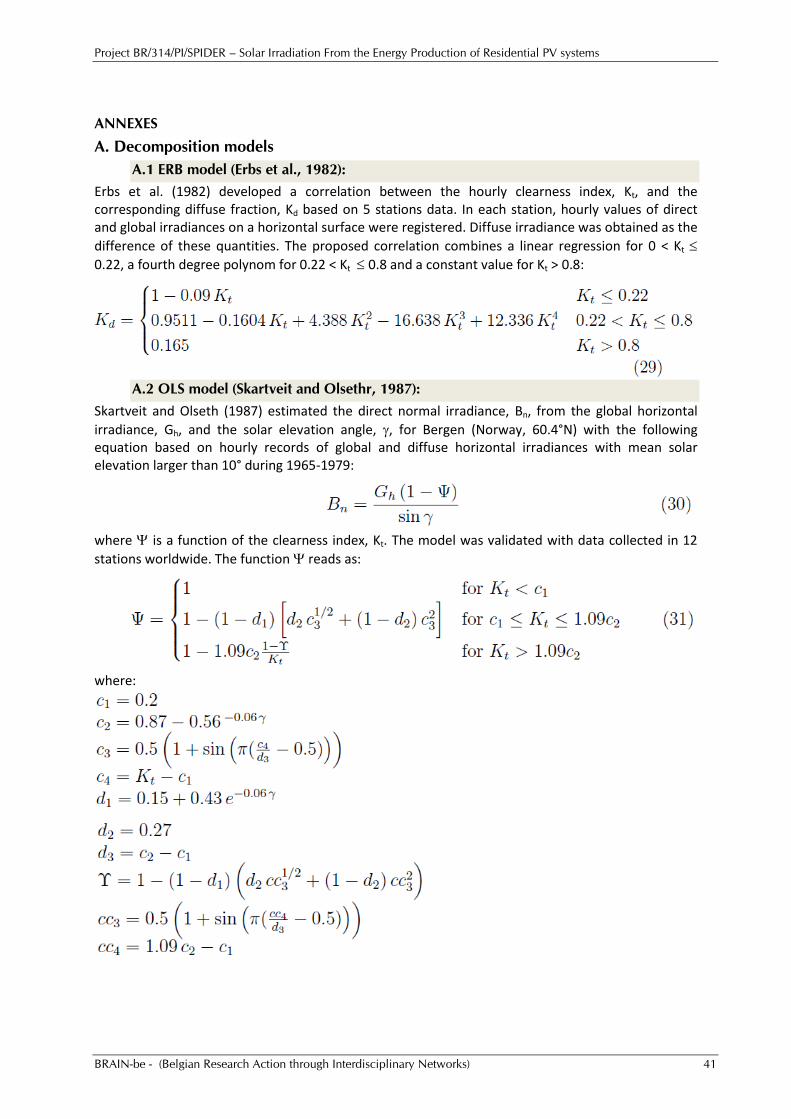
Project BR/314/PI/SPIDER – Solar Irradiation From the Energy Production of Residential PV systems
BRAIN-be - (Belgian Research Action through Interdisciplinary Networks) 41
ANNEXES
A. Decomposition models
A.1 ERB model (Erbs et al., 1982):
Erbs et al. (1982) developed a correlation between the hourly clearness index, Kt, and the corresponding diffuse fraction, Kd based on 5 stations data. In each station, hourly values of direct and global irradiances on a horizontal surface were registered. Diffuse irradiance was obtained as the
difference of these quantities. The proposed correlation combines a linear regression for 0 < Kt
0.22, a fourth degree polynom for 0.22 < Kt 0.8 and a constant value for Kt > 0.8:
A.2 OLS model (Skartveit and Olsethr, 1987):
Skartveit and Olseth (1987) estimated the direct normal irradiance, Bn, from the global horizontal
irradiance, Gh, and the solar elevation angle, , for Bergen (Norway, 60.4°N) with the following equation based on hourly records of global and diffuse horizontal irradiances with mean solar elevation larger than 10° during 1965-1979:
where is a function of the clearness index, Kt. The model was validated with data collected in 12
stations worldwide. The function reads as:
where:
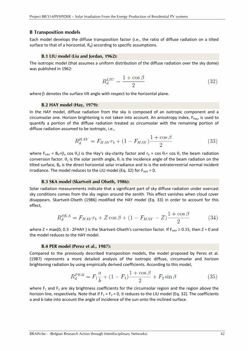
Project BR/314/PI/SPIDER – Solar Irradiation From the Energy Production of Residential PV systems
BRAIN-be - (Belgian Research Action through Interdisciplinary Networks) 42
B Transposition models
Each model develops the diffuse transposition factor (i.e., the ratio of diffuse radiation on a tilted surface to that of a horizontal, Rd) according to specific assumptions.
B.1 LIU model (Liu and Jordan, 1962):
The isotropic model (that assumes a uniform distribution of the diffuse radiation over the sky dome) was published in 1962:
where denotes the surface tilt angle with respect to the horizontal plane.
B.2 HAY model (Hay, 1979):
In the HAY model, diffuse radiation from the sky is composed of an isotropic component and a circumsolar one. Horizon brightening is not taken into account. An anisotropy index, FHay, is used to quantify a portion of the diffuse radiation treated as circumsolar with the remaining portion of diffuse radiation assumed to be isotropic, i.e.,
where FHAY = Bh=(Io cos z) is the Hay's sky-clarity factor and rb = cos i= cos z the beam radiation
conversion factor. z is the solar zenith angle, i is the incidence angle of the beam radiation on the tilted surface, Bh is the direct horizontal solar irradiance and Io is the extraterrestrial normal incident irradiance. The model reduces to the LIU model (Eq. 32) for FHAY = 0.
B.3 SKA model (Skartveit and Olseth, 1986):
Solar radiation measurements indicate that a significant part of sky diffuse radiation under overcast sky conditions comes from the sky region around the zenith. This effect vanishes when cloud cover disappears. Skartveit-Olseth (1986) modified the HAY model (Eq. 33) in order to account for this effect,
where Z = max(0; 0.3 - 2FHAY ) is the Skartveit-Olseth's correction factor. If FHAY 0.15, then Z = 0 and the model reduces to the HAY model.
B.4 PER model (Perez et al., 1987):
Compared to the previously described transposition models, the model proposed by Perez et al. (1987) represents a more detailed analysis of the isotropic diffuse, circumsolar and horizon brightening radiation by using empirically derived coefficients. According to this model,
where F1 and F2 are sky brightness coefficients for the circumsolar region and the region above the horizon line, respectively. Note that if F1 = F2 = 0, it reduces to the LIU model (Eq. 32). The coefficients a and b take into account the angle of incidence of the sun onto the inclined surface.
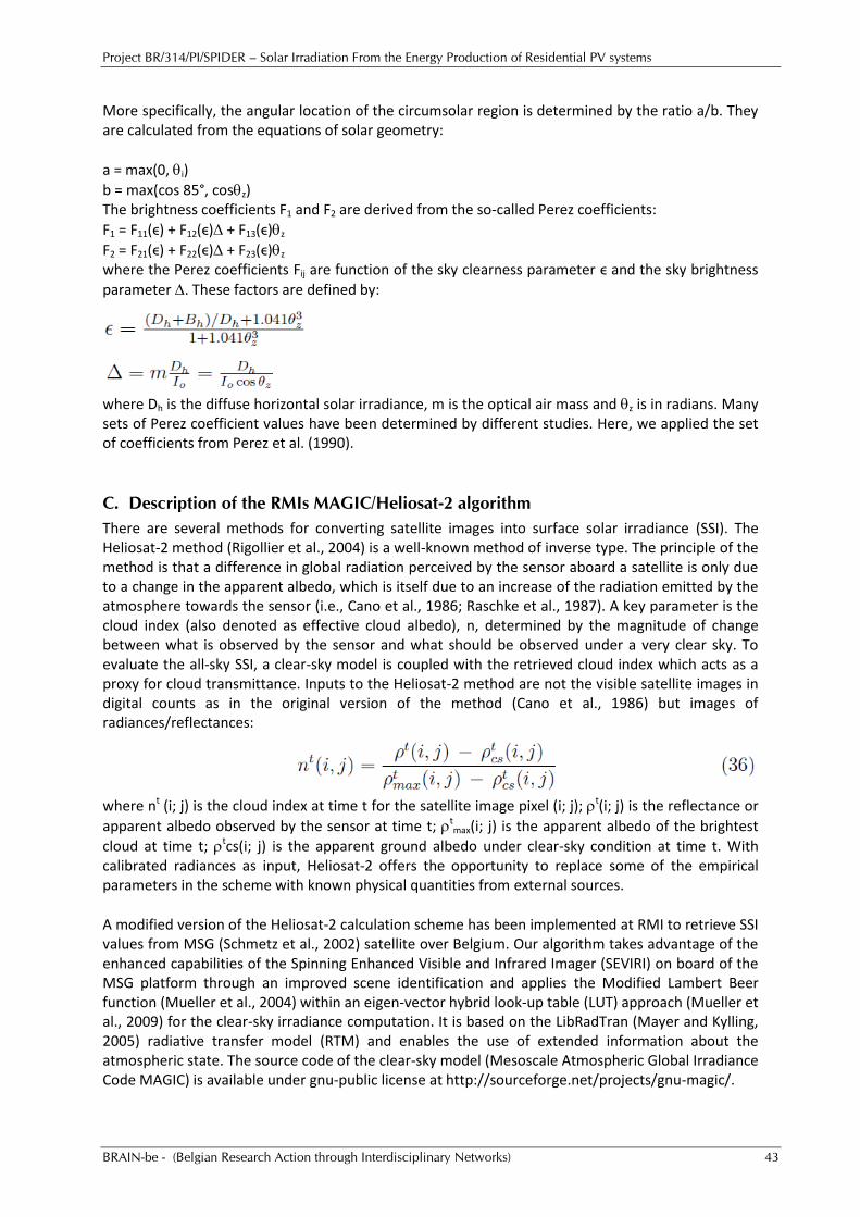
Project BR/314/PI/SPIDER – Solar Irradiation From the Energy Production of Residential PV systems
BRAIN-be - (Belgian Research Action through Interdisciplinary Networks) 43
More specifically, the angular location of the circumsolar region is determined by the ratio a/b. They are calculated from the equations of solar geometry:
a = max(0, i)
b = max(cos 85°, cosz) The brightness coefficients F1 and F2 are derived from the so-called Perez coefficients:
F1 = F11(ϵ) + F12(ϵ) + F13(ϵ)z
F2 = F21(ϵ) + F22(ϵ) + F23(ϵ)z
where the Perez coefficients Fij are function of the sky clearness parameter ϵ and the sky brightness
parameter . These factors are defined by:
where Dh is the diffuse horizontal solar irradiance, m is the optical air mass and z is in radians. Many sets of Perez coefficient values have been determined by different studies. Here, we applied the set of coefficients from Perez et al. (1990).
C. Description of the RMIs MAGIC/Heliosat-2 algorithm
There are several methods for converting satellite images into surface solar irradiance (SSI). The Heliosat-2 method (Rigollier et al., 2004) is a well-known method of inverse type. The principle of the method is that a difference in global radiation perceived by the sensor aboard a satellite is only due to a change in the apparent albedo, which is itself due to an increase of the radiation emitted by the atmosphere towards the sensor (i.e., Cano et al., 1986; Raschke et al., 1987). A key parameter is the cloud index (also denoted as effective cloud albedo), n, determined by the magnitude of change between what is observed by the sensor and what should be observed under a very clear sky. To evaluate the all-sky SSI, a clear-sky model is coupled with the retrieved cloud index which acts as a proxy for cloud transmittance. Inputs to the Heliosat-2 method are not the visible satellite images in digital counts as in the original version of the method (Cano et al., 1986) but images of radiances/reflectances:
where nt (i; j) is the cloud index at time t for the satellite image pixel (i; j); t(i; j) is the reflectance or
apparent albedo observed by the sensor at time t; tmax(i; j) is the apparent albedo of the brightest
cloud at time t; tcs(i; j) is the apparent ground albedo under clear-sky condition at time t. With calibrated radiances as input, Heliosat-2 offers the opportunity to replace some of the empirical parameters in the scheme with known physical quantities from external sources.
A modified version of the Heliosat-2 calculation scheme has been implemented at RMI to retrieve SSI values from MSG (Schmetz et al., 2002) satellite over Belgium. Our algorithm takes advantage of the enhanced capabilities of the Spinning Enhanced Visible and Infrared Imager (SEVIRI) on board of the MSG platform through an improved scene identification and applies the Modified Lambert Beer function (Mueller et al., 2004) within an eigen-vector hybrid look-up table (LUT) approach (Mueller et al., 2009) for the clear-sky irradiance computation. It is based on the LibRadTran (Mayer and Kylling, 2005) radiative transfer model (RTM) and enables the use of extended information about the atmospheric state. The source code of the clear-sky model (Mesoscale Atmospheric Global Irradiance Code MAGIC) is available under gnu-public license at http://sourceforge.net/projects/gnu-magic/.
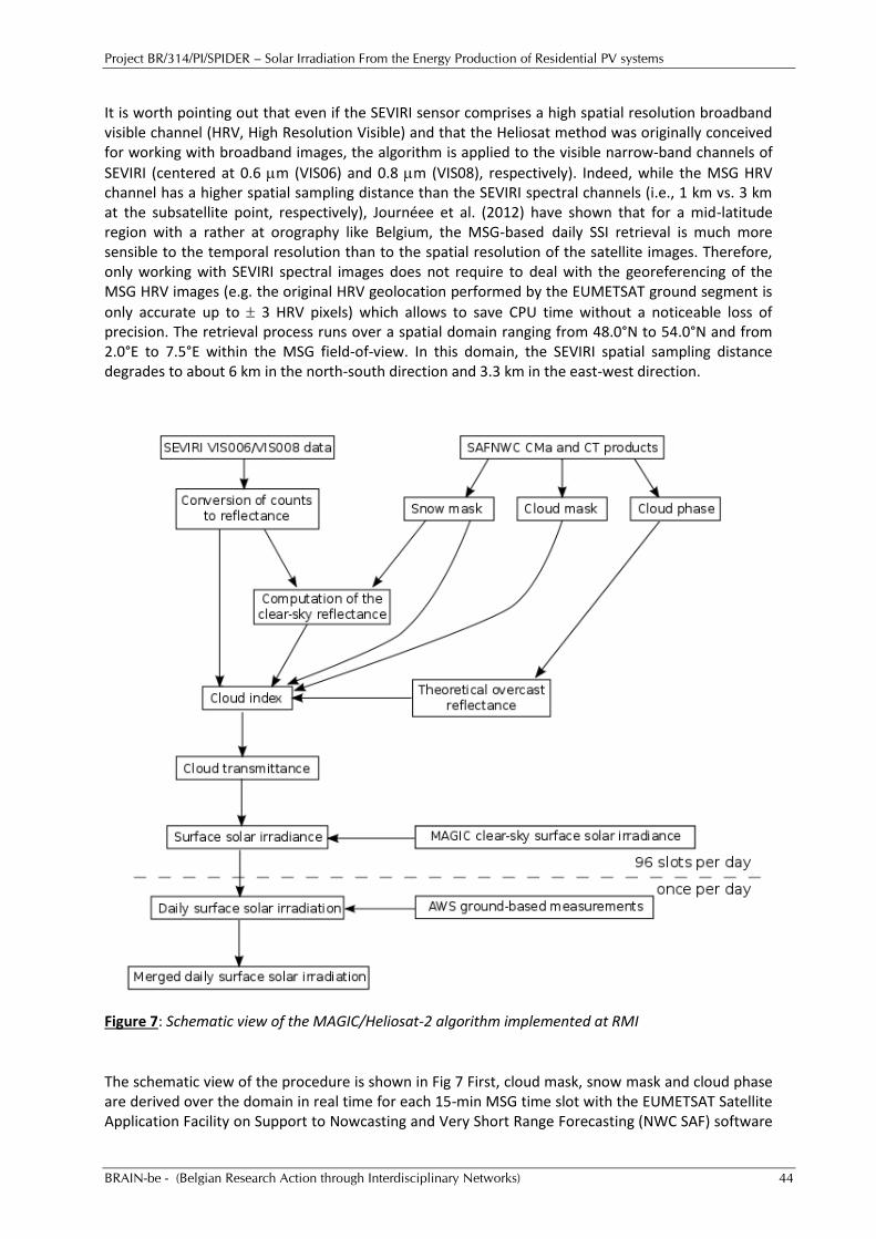
Project BR/314/PI/SPIDER – Solar Irradiation From the Energy Production of Residential PV systems
BRAIN-be - (Belgian Research Action through Interdisciplinary Networks) 44
It is worth pointing out that even if the SEVIRI sensor comprises a high spatial resolution broadband visible channel (HRV, High Resolution Visible) and that the Heliosat method was originally conceived for working with broadband images, the algorithm is applied to the visible narrow-band channels of
SEVIRI (centered at 0.6 m (VIS06) and 0.8 m (VIS08), respectively). Indeed, while the MSG HRV channel has a higher spatial sampling distance than the SEVIRI spectral channels (i.e., 1 km vs. 3 km at the subsatellite point, respectively), Journéee et al. (2012) have shown that for a mid-latitude region with a rather at orography like Belgium, the MSG-based daily SSI retrieval is much more sensible to the temporal resolution than to the spatial resolution of the satellite images. Therefore, only working with SEVIRI spectral images does not require to deal with the georeferencing of the MSG HRV images (e.g. the original HRV geolocation performed by the EUMETSAT ground segment is
only accurate up to 3 HRV pixels) which allows to save CPU time without a noticeable loss of precision. The retrieval process runs over a spatial domain ranging from 48.0°N to 54.0°N and from 2.0°E to 7.5°E within the MSG field-of-view. In this domain, the SEVIRI spatial sampling distance degrades to about 6 km in the north-south direction and 3.3 km in the east-west direction.
Figure 7: Schematic view of the MAGIC/Heliosat-2 algorithm implemented at RMI
The schematic view of the procedure is shown in Fig 7 First, cloud mask, snow mask and cloud phase are derived over the domain in real time for each 15-min MSG time slot with the EUMETSAT Satellite Application Facility on Support to Nowcasting and Very Short Range Forecasting (NWC SAF) software
Project BR/314/PI/SPIDER – Solar Irradiation From the Energy Production of Residential PV systems
BRAIN-be - (Belgian Research Action through Interdisciplinary Networks) 45
(Derrien and Le Gléeau, 2005) using the MSG SEVIRI spectral information and 24 h numerical weather forecasts from the European Centre for Medium- Range Weather Forecasts (ECMWF) two times a day. In parallel, the SEVIRI VIS06 and VIS08 data are converted from counts to reflectance.
Second, at the end of each day, the VIS06 and VIS08 reflectances and the NWC SAF algorithm products related to the 96 MSG time slots of the elapsed day are used to determine the effective cloud albedo (or cloud index), n. For each pixel in the image and each daytime MSG time slot, clear
sky reflectances in the VIS06 and VIS08 spectral bands, clr, are determined from a trailing window of
60 days MSG SEVIRI reflectances at 0.6 m and 0.8 m, respectively, according to Ipe et al. (2003).
Overcast visible reflectances, max, at 0.6 and 0.8 m are determined by a LUT approach using the cloud phase information provided by the NWC SAF software. It relies on the LibRadTran (Mayer and
Kylling, 2005) simulated outgoing radiances in the SEVIRI 0.6 and 0.8 m spectral bands. RTM computations were performed assuming a cloud optical depth of 128 and a pure cloud thermodynamic phase (i.e., water cloud or ice cloud). Because of the low reflectance of a majority of
natural land surfaces at 0.6 m and the reduced influence of the vegetation seasonal cycle on the reflectance signature at this wavelength (Asner, 1998), the algorithm is applied to the VIS06 channel over land surface and to the VIS08 channel over water surface. Based on the NWC SAF cloud and
snow masks the computed cloud index at 0.6 and 0.8 m are either corrected or not corrected for possible cloud shadow or snow contamination.
Third, SSI is derived for each pixel and MSG time slot by the combination of the satellite clearness index k(n) (a decreasing function of n, Hammer et al., 2003) and SSIclr, the corresponding clear-sky surface irradiance calculated by MAGIC: SSI = k(n) . SSIclr (37) Note that for effective cloud albedo values between 0 and 0.8, SSI is the clear-sky irradiance which is not reflected back to space by clouds: SSI = (1-n) . SSIclr (38) Based on Mueller et al. (2009) direct beam radiation on the horizontal plane at the Earth surface, Bh is retrieved from MSG satellite measurements using an adaptation of the OLS decomposition model (Skartveit and Olseth, 1987; Eq. 30). First, the direct beam radiation is derived for clear-sky conditions (Bh(clr; rtm)) by the way of the MAGIC clear-sky model. Then, the extension to the cloud-contaminated or cloudy conditions (all-sky) is performed using the following relation between the all sky direct radiation and Bh(clr; rtm):
Finally, the MSG retrieved all-sky SSI are integrated over the entire diurnal cycle and merged with the corresponding daily global solar irradiation recorded within the Belgian ground radiometric network operated by RMI. It is worth pointing out that in this study only unmerged MSG retrieved all-sky SSI were considered.