Forecasting Air Passenger Traffic Flows in Canada:An Evaluation of Time Series Models and

Combination Methods

Mémoire

Constantinos Bougas

Maîtrise en économiqueMaître ès arts (M.A.)

Québec, Canada

© Constantinos Bougas, 2013

Résumé

Ces quinze dernières années, le transport aérien a connu une expansion sans précédent au Canada.

Cette étude fournit des prévisions de court et moyen terme du nombre de passagers embarqués\débar-

qués au Canada en utilisant divers modèles de séries chronologiques : la régression harmonique, le

lissage exponentiel de Holt-Winters et les approches dynamiques ARIMA et SARIMA. De plus, elle

examine si la combinaison des prévisions issues de ces modèles permet d’obtenir une meilleure per-

formance prévisionnelle. Cette dernière partie de l’étude se fait à l’aide de deux techniques de com-

binaison : la moyenne simple et la méthode de variance-covariance. Nos résultats indiquent que les

modèles étudiés offrent tous une bonne performance prévisionnelle, avec des indicateurs MAPE et

RMSPE inférieurs à 10% en général. De plus, ils capturent adéquatement les principales caractéris-

tiques statistiques des séries de passagers. Les prévisions issues de la combinaison des prévisions des

modèles particuliers sont toujours plus précises que celles du modèle individuel le moins performant.

Les prévisions combinées se révèlent parfois plus précises que les meilleures prévisions obtenues à

partir d’un seul modèle. Ces résultats devraient inciter le gouvernement canadien, les autorités aéro-

portuaires et les compagnies aériennes opérant au Canada à utiliser des combinaisons de prévisions

pour mieux anticiper l’évolution du traffic de passager à court et moyen terme.

Mots-Clés : Passsagers aériens, Combinaisons de prévisions, Séries temporelles, ARIMA, SARIMA,

Canada.

iii

Abstract

This master’s thesis studies the Canadian air transportation sector, which has experienced significant

growth over the past fifteen years. It provides short and medium term forecasts of the number of en-

planed/deplaned air passengers in Canada for three geographical subdivisions of the market: domestic,

transborder (US) and international flights. It uses various time series forecasting models: harmonic re-

gression, Holt-Winters exponential smoothing, autoregressive-integrated-moving average (ARIMA)

and seasonal autoregressive-integrated-moving average (SARIMA) regressions. In addition, it exam-

ines whether or not combining forecasts from each single model helps to improve forecasting accu-

racy. This last part of the study is done by applying two forecasting combination techniques: simple

averaging and a variety of variance-covariance methods. Our results indicate that all models provide

accurate forecasts, with MAPE and RMSPE scores below 10% on average. All adequately capture

the main statistical characteristics of the Canadian air passenger series. Furthermore, combined fore-

casts from the single models always outperform those obtained from the single worst model. In some

instances, they even dominate the forecasts from the single best model. Finally, these results should

encourage the Canadian government, air transport authorities, and the airlines operating in Canada to

use combination techniques to improve their short and medium term forecasts of passenger flows.

Key Words: Air passengers, Forecast combinations, Time Series, ARIMA, SARIMA, Canada.

v

Contents

Résumé iii

Abstract v

Contents vii

List of Tables ix

List of Figures xi

Foreword xiii

Introduction 1

1 Review of literature 51.1 Univariate models . . . . . . . . . . . . . . . . . . . . . . . . . . . . . . . . . . . . 51.2 Forecast combinations . . . . . . . . . . . . . . . . . . . . . . . . . . . . . . . . . 71.3 Alternative forecasting methods . . . . . . . . . . . . . . . . . . . . . . . . . . . . 8

2 Econometric Methodology 112.1 Harmonic regression model . . . . . . . . . . . . . . . . . . . . . . . . . . . . . . . 112.2 Holt-Winters exponential smoothing model . . . . . . . . . . . . . . . . . . . . . . 122.3 Univariate time series models . . . . . . . . . . . . . . . . . . . . . . . . . . . . . . 142.4 Forecasting combination techniques . . . . . . . . . . . . . . . . . . . . . . . . . . 192.5 Forecasting performance criteria . . . . . . . . . . . . . . . . . . . . . . . . . . . . 21

3 Data 23

4 Results 274.1 Single model estimations . . . . . . . . . . . . . . . . . . . . . . . . . . . . . . . . 274.2 Combination forecasting techniques . . . . . . . . . . . . . . . . . . . . . . . . . . 32

Conclusion 37

Bibliography 39

vii

List of Tables

4.1 Harmonic regression model: estimation results . . . . . . . . . . . . . . . . . . . . . . 284.2 Holt-Winters exponential smoothing model results . . . . . . . . . . . . . . . . . . . . 294.3 ADF test results . . . . . . . . . . . . . . . . . . . . . . . . . . . . . . . . . . . . . . . 304.4 ARIMA and SARIMA model selection results . . . . . . . . . . . . . . . . . . . . . . . 314.5 MAPE and RMSPE for single models . . . . . . . . . . . . . . . . . . . . . . . . . . . 324.6 Comparison of the forecasting accuracy of single and combined forecasts for Harmonic

and SARIMA models (evaluation period: 2010(1)-2010(12)): MAPE and RMSPE . . . . 344.7 Comparison of the forecasting accuracy of single and combined forecasts for Holt-Winters

and SARIMA models (evaluation period: 2010(1)-2010(12)): MAPE and RMSPE . . . . 35

ix

List of Figures

3.1 Canadian E/D air passenger series in levels and first differences . . . . . . . . . . . . . . 243.2 Annual growth rates of air transport demand in Canada . . . . . . . . . . . . . . . . . . 25

4.1 Actual and forecasted Canadian E/D air passenger numbers for the domestic sector . . . 324.2 Actual and forecasted Canadian E/D air passenger numbers for the transborder sector . . 334.3 Actual and forecasted Canadian E/D air passenger numbers for the international sector . 33

xi

Foreword

This thesis would not have been produced without the assistance of my research supervisor, professor

Carlos Ordas Criado, who proposed the topic and provided focused and effective direction. He has

my sincere thanks for being always available and generous with his time and encouragement.

In addition, I would like to express my gratitude to the head of the airport research chair, professor

Denis Bolduc, for his generous financial help.

Furthermore, I would be remiss if I did not thank M. Raynald Ouellet of Transport Canada, who

provided the data for this thesis.

I would also like to thank the economics department of Laval university for its collegial and stimulat-

ing study and research environment.

Finally, I would like to thank my family and my friends for their support, patience and encouragement

throughout the course of this study.

xiii

Introduction

This thesis studies the forecasting of air passenger volumes in Canada. Its main objective is to evaluate

the accuracy of short and medium term monthly forecasts of enplaned/deplaned air passengers in

Canada for three different types of flights: domestic, transborder and international.

Transportation has long been recognized as being an important sector of the Canadian economy.

While it is true that air transportation greatly depends on the economic activity, the number of en-

planed/deplaned air passengers in Canada has displayed a remarkable growth between 2000 and 2010.

During this period, the number of enplaned/deplaned air passengers in Canada grew from 52 million

up to 66 million in the domestic sector (+26%), from 21 to 22 million in the transborder sector (+5%)

and from 13 to 21 million in the international sector (+62%)1. Total canadian GDP2 has roughly

grown from 11 to 13 thousand billion USD (+ 18%) over the same period. Predicting future air pas-

senger volumes is important, as it allows air transport authorities to adapt airport infrastructure to

future needs and offers airline companies the capacity to match the increasing passenger demand for

air transportation. Furthermore, the air transportation industry is an important employer in Canada,

and thus contributes both directly and indirectly to a prosperous Canadian economy. For example,

in 2009, there were 92 400 on site employees working in the air transportation sector, compared to

31 700 in the rail industry (Transport Canada, 2011).

This study provides forecasts of air passengers in Canada based on various time series forecasting

models. Given that air transportation demand is highly linked to the economy, which is typically

characterised by business cycles, or alternations between periods of economic growth and downturns,

our data series should exhibit cyclical patterns or seasonality. In addition, any economy is highly

susceptible to a variety of shocks of differing nature (political, economic, climatic, etc), which are

likely to modify the past trends and the volatility in the data. The majority of the time series models

used in this study take both of these characteristics into account. The models tested are: the harmonic

regression model, the Holt-Winters exponential smoothing model as well as two ARMA time series

models. From the latter class of models, we concentrate on the autoregressive-integrated-moving aver-

age model (ARIMA) and the seasonal autoregressive-integrated-moving average model (SARIMA).

Harmonic regression models are estimated by ordinary least squares and produce forecasts based on a

1These series have been kindly provided by Transport Canada.2Figures at constant US dollars of year 2000 are available from the Conference Board of Canada.

1

deterministic function which includes trigonometric terms (Cowpertwait and Metcalfe, 2009). Expo-

nential smoothing models produce forecasts by weighing current and past observations (Bourbonnais

and Terraza, 2004). Our ARMA specifications rely on dynamic equations based on the current and

past values of air passengers, as well as the current and past values of an error term. Most models take

into account the effects of past deterministic shocks. As noted by Emiray and Rodriguez (2003), all

these models assume that the future behavior of our air passenger series will be similar to their past be-

havior. In the short and medium run, this assumption seems appropriate, given that airports are heavy

structures characterised by inertia. In addition, we combine the forecasts obtained from the individual

models and examine, whether or not, the resulting forecasts are more accurate than their individ-

ual counterparts. Two combination techniques are used: simple averaging and variance-covariance

weighing schemes.

There are a great amount of studies, particularly since the 1990’s that use time series models to forecast

air passenger numbers. The forecasting performance of each model varies depending on the origin

country of the passengers, the type of flight considered (domestic, transborder, international), the

performance measure and the forecasting horizon (Emiray and Rodriguez, 2003; Oh and Morzuch,

2005; Chu, 2009). No methodological approach has been found to always dominate another in terms

of forecasting performance out-of-sample (Shen et al., 2011).

In recent years, combination forecasting techniques have become increasingly popular in the fore-

casting literature as a means to improve forecasting performance and to control for the uncertainty

of relying exclusively on a single model. In the tourism forecasting literature, single model com-

binations are generally found to outperform the specific models being combined, independently of

the time horizon considered (Shen et al., 2008; Coshall, 2009; Shen et al., 2011). However, these

results are sensitive to the combination technique (Wong et al., 2007; Coshall, 2009) as well as to

region/country-specific characteristics (Wong et al., 2007). Finally, the best performance is likely to

be achieved by combining two or three single forecasts at most (Wong et al., 2007).

This study complements the existing literature by providing the following contributions:

1. It deals with recent Canadian air passenger series and provides monthly forecasts over the 2009

to 2010 period.

2. It applies, for the very first time, a wide array of forecast combination techniques to Canadian

air passenger data and examines, whether or not, the conclusions of the other papers regarding

the performance of these techniques are still valid in this particular case.

3. Finally, this is the only study that uses a Holt-Winters exponential smoothing model in order to

forecast the number of monthly air passengers in Canada.

Our results indicate that all of the specific models offer adequate forecasts with MAPE and RMSPE

below 10% in most cases. Our forecasts capture the main characteristics of our air passenger series.

2

ARIMA and SARIMA models usually outperform the harmonic regression and Holt-Winters expo-

nential smoothing models. In addition, the performance of each model depends on the geographical

sector considered. Domestic series are better predicted with ARIMA regressions while transborder

series are better predicted with SARIMA specifications. On the other hand, international series are

better predicted with Holt-Winters. These results stress the fact that no single model dominates the

others for all market segments.

Regarding the forecast combinations, we notice that they are always more accurate than the predictions

obtained from the single worst model. Furthermore, forecast combinations sometimes dominate those

from the single best model. Finally, we note that the performance of combining forecasts is sensitive

to the models being combined, the flight sector considered as well as the combination method applied.

Simple average appears to provide the poorest performance.

The rest of this master’s thesis is structured as follows. The first section reviews the existing literature.

The second section describes the empirical time series models as well as the two forecast combination

techniques that we employ. The third section presents the data. Finally, the fourth section shows the

results of the study whereas the last section provides some conclusions.

3

Chapter 1

Review of literature

1.1 Univariate models

There is a large amount of literature regarding tourism and air passenger forecasting with univariate

time series and smoothing techniques. Most published studies tend to concentrate on three specific

regions: the United States, Europe and the Asia Pacific region (Oh and Morzuch, 2005; Lim and

McAleer, 2002; Andreoni and Postorino, 2006; Coshall, 2006; Chen et al., 2009). To our knowledge,

the lone study on Canada is the work of Emiray and Rodriguez (2003). These authors provide monthly

forecasts of enplaned/deplaned air passengers for three market segments (domestic, international and

transborder flights), based on data covering the period ranging from January 1984 to September 2002.

They consider six time series models (AR(p), AR(p) with seasonal unit roots, SARIMA, periodic au-

toregressive model (PAR), structural time series model (STSM) and the seasonal unit roots model)

as well as the simple average combination method. They conclude that forecasting performance de-

pends on two key elements: the market segment considered and the forecasting horizon. Emiray and

Rodriguez (2003) also show that short memory models are better for short term forecasting whereas

long memory models are better for long term forecasting. Their paper did not consider smoothing

forecasting techniques.

ARIMA and SARIMA models are among the most widely used in the air passenger forecasting litera-

ture. According to Zhang (2003), their popularity comes from the fact that they are based on very few

assumptions. Furthermore, they are easy to specify with the recursive Box-Jenkins methodology.

Many studies have examined the performance of ARIMA and SARIMA models for predicting air

traffic flows. For example, Coshall (2006) forecasts air travel from the United Kingdom to twenty

destinations using quarterly data of UK outbound air travelers with several models, which include:

the Naive 1 model, the Naive 2 model1, the Holt-Winters model and a variety of ARIMA models. The

Root Mean Squared Error (RMSE) suggests that the ARIMA model outperforms the other models

1The forecasts in the Naive 1 model for quarterly data are given by: yt=yt−4. In the Naive 2 model, they are given byyt=yt−4+[1+ yt−4+yt−8

yt−8]. For more details, see Coshall (2006).

5

for all destinations except one. This is true for both additive and multiplicative seasonality models.

Andreoni and Postorino (2006) use the yearly data of planed/enplaned passengers at Reggio Calabria

airport in the South of Italy to forecast air transport demand. Two univariate ARIMA models and

a multivariate ARIMAX model with two explanatory variables (mainly per capita income and the

number of movements both to and from Reggio Calabria airport) are used to generate forecasts. The

authors conclude that all three models offer accurate forecasts. Kulendran and Witt (2003) generate

one, four and six quarter ahead forecasts of international business passengers to Australia from the

following four countries: Japan, New Zealand, the United Kingdom and the United States. They

consider various forecasting models: the error correction model (ECM), the structural time series

model (STSM), the basic structural model (BSM), no change models as well as various ARIMA

models. They conclude that forecasting performance varies with the forecasting horizon and depends

on the adequate detection of seasonal unit roots. Consequently, ARIMA and BSM models are the

most accurate for short term forecasting (one-quarter ahead) whereas the seasonal no change model

outperforms the other models for medium term forecasting (four and six quarters ahead).

Chen et al. (2009) estimate monthly arrivals to Taiwan from Japan, Hong Kong and the United States

as well as the total amount of monthly inbound air travel arrivals. Interestingly, they divide air ar-

rivals in three categories according to travel purpose: tourism, non-tourism and any purpose. They

consider the following forecasting models: Holt-Winters, SARIMA and a Grey forecasting model.

The authors conclude that the SARIMA model outperforms all other models when it comes to es-

timating tourism related arrivals to Taiwan. For all purpose and non-tourism arrivals, the SARIMA

model outperforms the other two models for arrivals from Japan and the United States but not for

those from Hong Kong or for total arrivals (however, it remains very performant even in these cases).

Tsui et al. (2011) forecast air passenger traffic at Hong Kong International Airport using a univariate

seasonal ARIMA model and a multivariate ARIMAX model with exogenous explanatory variables.

Forecasts are obtained for the period ranging from March 2011 to December 2015. The authors show

that the ARIMA specification generates more accurate forecasts than the ARIMAX one over one to

three month horizons. In addition, one and two month ahead forecasts are more accurate than three

month ones.

Lim and McAleer (2001) predict monthly tourist arrivals to Australia from three destinations: Hong

Kong, Malaysia and Singapoure. They use the following forecasting models: the single exponen-

tial smoothing model, Brown’s double exponential smoothing model, the additive and multiplicative

seasonal Holt-Winters models as well as the non-seasonal exponential smoothing model. Their perfor-

mance is evaluated with the RMSE (Root Mean Squared Error) criterion. They find that for the series

in levels, the multiplicative Holt-Winters model offers the best performance for Hong Kong and Sin-

gapoure whereas in the case of Malaysia, the additive Holt-Winters model is the most accurate. Cho

(2003) forecasts tourist arrivals to Hong Kong from: the United Kingdom, Japan, Korea, Singapoure

and Taiwan. He uses three different forecasting models: multiplicative exponential smoothing model,

ARIMA and artificial neural network model (ANN). He finds, that according to both the MAPE (Mean

6

Absolute Percentage Error) and the RMSE (Root Mean Square Error), the ANN model outperforms

ARIMA and Holt-Winters for forecasting tourist arrivals to Hong Kong from all of the aformentioned

countries with the exception of the United Kingdom. For the latter, Holt-Winters offers the best perfor-

mance. However, the author also notes that ARIMA and Holt-Winters usually give a good forecasting

performance with a MAPE inferior or equal to 20%.

The preceding studies suggest that the forecasting performance of ARIMA and SARIMA models

varies with the market segment considered, the forecasting horizon as well as the origin and destination

countries of the passengers. In addition, these models are generally found to offer accurate forecasts

in the short and medium term.

1.2 Forecast combinations

Forecasting combination techniques offer an alternative approach to single models’ forecasts. Bates

and Granger (1969) were the first to propose such techniques to improve the forecasting accuracy

of individual models (Wong et al., 2007). Over the last three decades, these techiques have become

highly prevalent in the forecasting literature. They have been applied with success to numerous fields,

including: macroeconomics (Poncela and Senra, 2006; Bjørnland et al., 2011), meteorology (Brown

and Murphy, 1996), banking (Chan et al., 1999) and tourism (Shen et al., 2008, 2011; Coshall, 2009).

Many authors have outlined the reasons behind the prevalence of these techniques. For example,

Timmermann (2006) points out that combined forecasts allow to better aggregate all relevant informa-

tion captured in different single model forecasts and they are more robust against a misspecification

of the data generating process. Therefore, combined forecasts can improve the forecasting accuracy

and they are seen as being more comprehensive (see also Bunn, 1988). Brown and Murphy (1996)

note that combination forecasts are more likely to improve forecasting performance when each single

model forecast being combined is independant of the other (or uncorrelated). Timmermann (2006)

also stresses that combination forecasts are particularly useful when structural breaks are present in

the data series. Again, each individual model will process differently the structural breaks. The time

series used in this study are very likely to exhibit structural breaks, given the events that took place

during the time period under scrutiny (September 11th terrorist attacks, the Gulf war, the 2009 finan-

cial crash).

In this paper, we will apply two combination techniques that have been widely used in the forecasting

literature: simple averaging and variance covariance methodologies. Both techniques take a weighted

average of single model forecasts. However, they differ in how weights are computed. The simple

average method assigns equal weights to each predicted value from the single models that are being

combined. These weights are straightforward to compute : they are equal to the inverse of the number

of single model forecasts being combined. Various versions of the variance-covariance method exist

(see Bates and Granger (1969), Coshall (2009) and Chu (1998)). All of them assign unequal weights

to each single model forecast being combined and take into consideration the past performance of the

7

forecasting model.

The conclusions that have been reached regarding these combination techniques vary from one paper

to another. For example, Winkler and Makridakis (1983) generate forecasts for 1001 economic time

series with different types of data, and conclude that more complex combination methods slightly

outperform the simple average method for long term forecasting horizons. In the air transportation

forecasting literature, Chu (1998) provides monthly forecasts of tourist arrivals to Singapoure for year

1988 using a SARIMA and a sine wave regression model. He applies a version of the variance-

covariance method adapted for seasonal data. Forecasting performance is evaluated using the MAPE.

He finds that that the combined forecast is more accurate than the ones issued from ARIMA and sine

wave. Shen et al. (2011) use tourist flows from the United Kingdom to seven major touristic destina-

tions to point out that unequal weighing schemes outperform the simple average method. In contrast,

Coshall (2009) studies tourist departures from the United Kingdom to twelve destinations. He con-

cludes that the performance of different combination methods depends on the forecasting horizon. In

this particular case, the variance-covariance method outperforms simple averaging for one and two

years ahead forecasts while the reverse is true for three years ahead forecasts. Finally, Wong et al.

(2007) study tourist arrivals to Hong Kong. They find that forecasting performance depends on the

number of single model forecasts being combined. Thus, they mention that the best performance is

likely to be achieved by combining two or three single model forecasts at most.

In sum, most papers on combination forecasts highlight that forecasts based on some averaging of

individual models’ forecasts are more accurate than those based on a particular model. Moreover, un-

equal weighting schemes, which account for the past prediction performance of the individual models,

seem in general more appropriate than weighting equally the forecasts of the individual models.

1.3 Alternative forecasting methods

Univariate time series linear models are only one of the many methods used for forecasting air pas-

senger demand. Over the years, many other promising alternatives have been developed. A very brief

overview of some of these methods is presented in this section.

One of the major limitations of ARIMA models is their arbitrary parametric functional shape. A

priori specifications may fail to capture important non-linearities and interactions which have not been

explicitely modeled. These can be captured by artificial neural network models (ANN’s) but at the

expense of interpretability. The contribution of each regressor cannot be interpreted individually.

As an example, Chen et al. (2012) used back propagation neural networks to identify the factors that

influence air passenger and air cargo demand from Japan to Taiwan. They found that air transport and

air cargo demand are generally influenced by different factors but that there are some common factors

which influence both. This allowed them to construct models which possess very high forecasting

accuracy in the short and medium term. For example, their air passenger demand model had a MAPE

8

(Mean Absolute Percentage Error) of 0.34%. However, they noted that the performance of neural

network models heavily depends on choosing an appropriate training set.

Bao et al. (2012) compare the forecasting performance of a Holt-Winters exponential smoothing

model, a univariate time series model (ARIMA) and the following support vector machines basedmodels : single Support Vector Machines (SVM’s), Ensemble Empirical Mode Decomposition based

Support Vector Machines (EEMD-SVM’s) and Ensemble Empirical Mode Decomposition Slope based

method Support Vector Machines (EEMD-Slope-SVM’s). They do this using the monthly air passen-

ger data from six American and British airline companies and the following performance criteria:

Mean Absolute Percentage Error (MAPE), Root Mean Square Error (RMSE), Geometric Mean Rel-

ative Absolute Error (GMRAE) and the directional statistic (DS). They conclude the following: (i)

single SVM’s outperform ARIMA and Holt-Winters, (ii) EEMD-SVM’s outperform single SVM’s

and (iii) EEMD-Slope-SVM’s are more accurate than EEMD-SVM’s (and therefore also outperform

ARIMA, Holt-Winters and single SVM’s).

Fildes et al. (2011) make use of a wide variety of multivariate models to study air traffic flows be-

tween the United Kingdom and five other countries: Germany, Sweden, Italy, the USA and Canada.

They use the following econometric models: an autoregressive distributed lag model (ADL), a pooled

ADL model, a time-varying parameter model (TVP) as well as an automatic method for econometric

model specification. They also consider the previous four models augmented by a world trade ex-

planatory variable (which measures the total trade of all industrial countries). In addition, they apply

the following (mostly univariate) models: a vector autoregressive model (VAR), a vector autoregres-

sive model with the world trade variable, an exponential smoothing model, an autoregressive model

of order three (AR(3)) as well as Naive I and Naive II benchmark models. Forecasting performance is

evaluated according to the following four criteria: (i) Root Mean Square (Percentage) Error (RMSE),

(ii) Geometric Root Mean Square Error (GRMSE), (iii) Mean Absolute Scaled Error (MASE), and

(iv) Geometric Mean Relative Absolute Error (GRelAE). They find that ADL models with the inclu-

sion of a world trade variable outperform overall the univariate models (exponential smoothing and

AR(3) models) but that the difference in forecasting performance is usually small, although it varies

depending on the forecasting performance criterion used (usually larger when using RMSE).

Grosche et al. (2007) develop two gravity models in order to forecast air passengers between city

pairs. Both models include mostly geoeconomic variables. The first model excludes city-pairs which

involve multi-airport cities. Hence, it excludes competition. It uses such variables as: population,

distance between airports, average travel time and buying power index to predict travel demand. On

the other hand, the second model includes multi-airport cities as well as variables that take them into

account (such as the number of competing airports, the average distance to competing airports). Both

models are found to be statistically valid and fit the data well.

9

Chapter 2

Econometric Methodology

Our goal in this thesis is to use the most up-to-date monthly data available at Transport Canada in

order to evaluate the accuracy of both short run and medium run forecasts for the number of en-

planed/deplaned air passengers in Canada. We consider the most popular models for forecasting air

traffic flows: a harmonic regression, an exponential smoothing model as well as two standard ARMA-

based time series models. In addition, we examine whether or not combining the forecasts of the

above models helps to build more accurate forecasts. All our investigations are carried out using the

R statistical software1.

2.1 Harmonic regression model

Harmonic regression2 is a linear specification that accounts for seasonal patterns with the help of two

trigonometric functions: sine and cosine. Note that in this model both the linear time trend and the

seasonal pattern are considered as being fixed and stable over time (deterministic). The time series

can be represented as:

yt = α +β t +[s/2]

∑j=1

(γ jcosλ jt + γ∗j sinλ jt)+

k

∑j=1

Dt, j + εt (2.1a)

with:

λ j =2π j

sj = 1, . . . , [s/2]. (2.2a)

In the preceding equations, α is a constant, β is the linear time-trend coefficient, γ j and γ∗j are param-

eters linked to the seasonality components, λ j are the harmonics of order j, s represents the number

of seasons, [ ] is the integer function3 and Dt, j stands for exogenous variables which capture shocks

1For a complete description of this software see R Development Core Team (2012).2This section relies on Harvey (1993, p.138 and 186-187) and Cowpertwait and Metcalfe (2009, Ch. 5.6 to 5.10).3The nearest integer function [s/2] implies that s

2 = s if s is even and s2 = s−1

2 if s is odd.

11

to the series. In addition, εt is assumed to be a white noise error term, i.e, a normally, independantly

and identically distributed random variable such that 4:

E(εt) = 0 ∀t (2.3a)

E(ε2t ) = σ

2ε ∀t (2.3b)

Cov(εt ,εs) = 0 ∀t,∀s, t 6= s. (2.3c)

The model that best fits the data is selected through the backward selection procedure5. This pro-

cedure is implemented in the function step() of the stats package in R. It starts by considering

the model with all of the variables. From this model, the variables that lead to the biggest decrease

in Akaike’s information criterion (AIC) are eliminated one by one until the AIC cannot be further

lowered. Consequently, the best fitting model is the one that minimizes the AIC. The Breush-Pagan

and the Durbin-Watson tests6 are then applied to check whether the assumption of homoscedastic and

uncorrelated residuals holds.

The Breush-Pagan test is implemented with the bptest() function of the lmtest package7 in R. Note

that this function applies a version of the test which is robust to departures from normality. Regarding

the Durbin-Watson test, we use the dwtest() function of the aformentioned package. If the null

hypothesis of either or both of these tests is rejected, the ordinary least squares estimator will not be

efficient and the vcovHAC()8 function of the sandwich package in R is used to produce a covariance

matrix that is heteroscedasticity and autocorrelation consistent. Once this is achieved, forecasts are

generated using the predict() function of the stats package. Finally, it is important to note that the

harmonic regression model can also contain dummy variables that account for structural shocks that

occured during the period under investigation.

2.2 Holt-Winters exponential smoothing model

The Holt-Winters9 recursive procedure is an exponential smoothing technique that was developed as

a means of forecasting time series exhibiting both a trend and a seasonal pattern.

There exist two versions of this procedure: additive and multiplicative. In both versions, forecasts will

depend on the following three components of a seasonal time series: its level, its trend and its seasonal

coefficient. In addition, both are implemented in the HoltWinters() function of the forecast

package10 in R. The version to be used depends on the type of seasonality, additive or multiplicative,

4See Greene (2005, Ch.20.2).5Cornillon and Matzner-Løber (2007, p.167).6The description of these tests is inspired from Greene (2005, Ch.10 and 12).7For a complete description of this package, see Zeileis and Hothorn (2002).8For details, see Zeileis (2004).9This section follows Bourbonnais and Terraza (2004, Ch.2.II.C), Montgomery et al. (2008, p. 210-216) as well as

Chatfield (2003, p. 20, 78-79).10See Rob J Hyndman et al. (2013).

12

that we observe in the data by plotting the series with respect to time. Thus, the additive version

ought to be considered whenever the seasonal pattern of a series has a constant amplitude over time

(Kalekar, 2004). In such a case, the series can be written as:

yt = at + btt + St + εt witht=s

∑t=1

St = 0. (2.4)

In the preceding equation, at represents the level of the series at time t, bt the slope of the series at

time t, St the seasonal coefficient of the series at time t and s the periodicity of the series. Furthermore,

εt are error terms with mean 0 and constant variance.

Inversely, when a series displays a seasonal pattern characterised by an amplitude that varies with

the level of the series, the multiplicative version is a better choice (Kalekar, 2004; Lim and McAleer,

2001). In such a case, the series can be represented as follows:

yt = (at + btt)Stεt witht=s

∑t=1

St = s. (2.5)

In the preceding equation11, all the elements are defined as previously. In what follows, we will

concentrate on the multiplicative case. In the latter case, forecasts can be obtained using the following

equation:

yt+h = (at + hbt)St−12+1+(h−1)mod12 (2.6a)

where h represents the forecasting horizon and where at , bt and St need to be estimated using the

following three equations:

at = α(yt

st−12)+ (1−α)(at−1 + bt−1) (2.7a)

bt = β (at −at−1)+ (1−β )bt−1 (2.7b)

St = γ(yt

at)+ (1− γ)St−12. (2.7c)

In these equations, α , β and γ are smoothing parameters (or weights) for the level, the trend and the

seasonal component respectively. All three parameters lie between 0 and 1 and can be interpreted

as discounting factors: the closer to 1, the larger the weight of the recent past (Coshall, 2009). Cho

(2003) also mentions that the closer the parameter is to 0, the more the related component is constant

over time. Optimal values for the three parameters are obtained by minimizing the squared one-step

ahead forecast errors12 (Coshall, 2009).

Finally, it is important to note that the Holt-Winters procedure has been widely used in the forecasting

literature for over fifty years. Its popularity stems from the fact that it is simple to apply. Furthermore,

it does not entail fitting a parametric model (Gelper et al., 2010). However, it has the disadvantage of

being sensitive to structural breaks (Gelper et al., 2010), which are not accounted for.11The multiplicative seasonality model can also be expressed as: yt = (at + bt t)St + εt .12The forecast error is the difference between the forecasted and the observed value of a series.

13

2.3 Univariate time series models

2.3.1 Autoregressive-moving average model

The two univariate time series models used in this paper are based on the autoregressive-moving av-

erage or ARMA(p,q) model13. The idea behind this model is that the value taken by a time series at

a given time t, denoted yt , depends on two additive terms: (i) the past of the time series (an autore-

gressive component of order p) and (ii) the past of the disturbances of the data generation process (a

moving average component of order q). Hence, the general form of an ARMA model is:

yt =p

∑i=1

φiyt−i−q

∑i=1

θiεt−i + εt (2.8)

where the φi’s (i=1, . . . , p) are called autoregressive parameters, the θi’s (i=1, . . . , q) are called mov-

ing average parameters and the ε’s are white noise error terms. Note that ARMA models are often

expressed in a more elegant and compact form. Let’s first introduce the three following notations:

Bmyt = yt−m (2.9a)

φ (B) = 1−φ1B− . . .−φpBp (2.9b)

θ (B) = 1−θ1B− . . .−θqBq. (2.9c)

B represents the backward shift operaror, φ (B) is the autoregressive part polynomial of order p and

θ (B) is the moving average part polynomial of order q. Using equations (2.9a) to (2.9c), we rewrite

the ARMA model as follows:

φ (B)yt = θ (B)εt . (2.10)

An important assumption imposed on ARMA models is that of stationarity of the time series. A time

series yt is (weakly or covariance) stationary if the three following conditions are met14:

E(yt) = µ and E(y2t ) = µ

′2 ∀t (2.11a)

Var(yt) = µ′2−µ

2 = σ2y = γ(0) ∀t (2.11b)

Cov(yt ,ys) = E[ytys]−µ2 = γ(|t− s|) ∀t,∀s, t 6= s. (2.11c)

Equations (2.11a) and (2.11b) tell us that the mean and the variance of yt must be independant of time.

This implies that any shock on yt will be of temporary nature and will not permanently influence the

future values of the series (Rodrigues and Osborn, 1999). Equation (2.11c) states that the covariance

between any two observations yt and ys must be independant of origin times t and s. Indeed, it must

only be a function of the time difference (t− s) between the two observations.

Many economic time series display either deterministic or stochastic non-stationarity15. In addition,

some time series may exhibit both types. The first type of non-stationarity is due to the presence13The description of this model follows Harvey (1993, Ch.2.1) and Bourbonnais and Terraza (2004, p.82).14As given in Bresson and Pirotte (1995, p.19).15The following section is based on Bourbonnais and Terraza (2004, p.133-139), Harvey (1993, p.20) and Greene (2005,

p.597).

14

of a deterministic trend. Series exhibiting deterministic non-stationarity are said to follow a trend-

stationary process. To render them stationary, one can exploit the differences between the observations

and the deterministic trend. The general form of a purely trend-stationary series is:

yt = ft + εt (2.12)

where ft is a linear or non-linear function of time and εt is a stationnary process.

The second type of non-stationarity is called stochastic non-stationarity. Starting with the character-

istic equation of model (2.10):

φ (B) = 0 (2.13)

we say that equation (2.10) has a unit root if at least one of the roots of equation (2.13) is equal to one

(unit root). The presence of a unit root in process (2.10) generates stochastic non-stationarity. Such a

process can be rendered stationary through differencing. The same holds true whenever at least one

of the roots of the characteristic equation is inferior to one (lies inside the unit circle). Inversely, if all

the roots of the characteristic equation are superior to one (lie outside the unit root circle), then the

series is stationary.

It is important to determine the appropriate transformation required to render a time series stationary.

Indeed, applying the wrong transformation can significantly alter the statistical properties of the series,

thus producing biased forecasts. For example, using departures from a deterministic trend for a time

series exhibiting stochastic non-stationarity is likely to create spurious correlation in the residuals of

an ARMA model16.

There exist various procedures for determining the type of non-stationarity exhibited by a time series.

In this thesis, we will use an Augmented Dickey-Fuller test procedure, that is part of the Box-Jenkins

methodology described in section 2.3.4. This leads us to the ARIMA model.

2.3.2 Autoregressive-integrated-moving average model

The autoregressive-integrated-moving average17, or ARIMA(p,d,q) model differs from the ARMA

(p,q) model in one significant way: it contains a d parameter. This parameter states the level of

non-seasonal differencing that is required to render a non-stationary time series stationary (when dif-

ferencing is appropriate). Once stationarity is achieved, the series can be represented using an ARMA

(p,q) model. Note that if the series is already stationary and does not need to be differenced, then it

can directly be modeled through an ARMA(p,q). The general form of the ARIMA (p,d,q) model reads

φ (B)(1−B)dyt = θ (B)εt ⇔ φ (B)∆dyt = θ (B)εt , d ≥ 0 (2.14)

where ∆d = (1−B)d is the non-seasonal differencing operator. It is important to mention that the

ARIMA model is a short memory model (Bourbonnais and Terraza, 2004, p.265). Therefore, it is not16See Bourbonnais and Terraza (2004, p.137-139).17This section is based on Harvey (1993, Ch.5.2) and Greene (2005, Ch.20.3.1).

15

able to account for dependance between observations that are far apart over time. Another shortfall

of the ARIMA specification (2.14) is that it is unable to account for seasonality and shocks. Monthly

patterns can be captured by including dummy regressors of the form:18

D jt =

1 if t = j, j+ 12, j+ 24 . . .

0 if t 6= j, j+ 12, j+ 24 . . .

−1 if t = 12,24,36 . . .

Such seasonality is supposed to remain stable over time.

2.3.3 Seasonal autoregressive-integrated-moving average model

Like the ARIMA model, the seasonal autoregressive-integrated-moving average model19, or SARIMA

(p,d,q) x (P,D,Q)s, is a short memory model (Bourbonnais and Terraza, 2004, p.265). In addition, it

is a more flexible model, given that it accounts for stochastic seasonality. Such seasonality is present

when the seasonal pattern of a time series changes over time. In such a case, the time series will

contain a seasonal unit root and will need to be seasonally differenced. This will be done through the

seasonal difference parameter, "D". If this parameter equals zero, then the seasonal pattern exhibited

by the time series is relatively stable over time and can be modeled uniquely through the seasonal

autoregressive (Φ(Bs)) and moving average (Θ(Bs)) terms, of order P and Q respectively. These are

given by the following equations:

Φ(Bs) = 1−Φ1Bs− . . .−ΦPBPs (2.15a)

Θ(Bs) = 1−Θ1Bs− . . .−ΘQBQs. (2.15b)

These terms allow us to express the SARIMA model as follows:

φ (B)Φ(Bs)(1−B)d(1−Bs)Dyt = θ (B)Θ(Bs)εt , d,D≥ 0 (2.16)

where s denotes the periodicity of the time series (for example, s = 12 for monthly time series).

2.3.4 Box-Jenkins method

A common and effective method for specifying and estimating ARMA-based models is the iterative

Box-Jenkins method20. Its advantage is that it can be applied to many types of time series: seasonal,

non-seasonal, stationary... It proceeds in four steps: (i) identification, (ii) estimation (iii) diagnostic

testing and (iv) forecasting.

Identification

The first step of the Box-Jenkins method is to verify if the time series are stationary and if seasonal

patterns need to be modeled. Plotting the time series can provide useful information. In general, series18Based on Harvey (1993, p.137).19The following section relies on Harvey (1993, p.139-142) and Chen et al. (2009).20See Bresson and Pirotte (1995, Ch. 2.1 to 2.4).

16

that cover a large number of years and that exhibit a pronouced seasonal pattern will not have a stable

variance. The most common methods for stabilizing the variance are the logarithmic or the Box-Cox

transformations. Once the series are variance stationary, it is important to check that their mean is

constant through time. This can be done by applying the Augmented Dickey-Fuller or ADF test21.

This test requires estimating the two following equations:

∆yt = β1 +β2t +πyt−1 +k

∑j=1

γ j∆yt− j + εt (2.17a)

∆yt = β1 +πyt−1 +k

∑j=1

γ j∆yt− j + εt (2.17b)

where: yt is a time series, ∆ is the first difference operator, β1 is a constant, εt is a white noise error

term, β2 is the coefficient of the time trend and k is the lag order of the autoregressive process. The

two equations above allow us to determine whether or not a time series contains: (i) a stochastic trend

(π = 0) also called unit root, (ii) a deterministic trend (β2 6= 0) or (iii) both. We answer these questions

by applying the following strategy22.

First, equation (2.17a) is used to test the null hypothesis of the presence of a unit root (Hτ3 : π = 0) with

a non-standart t-test. If the null hypothesis is rejected, the data display no stochastic trend and they

need no differencing. If the null hypothesis cannot be rejected, the data does contain a unit root and we

proceed to testing the joint hypothesis of a unit root and a null deterministic trend (Hφ2 : β2 = π = 0)

with a non-standart F-test23. If Hφ2 is rejected, we need to check again that the data include a stochastic

trend under the null that the model includes a deterministic trend by comparing the empirical t-value

of the unit root coefficient π with standard normal cutoffs. If the stochastic trend is confirmed in the

latter test, differencing the residuals from a parametric fit to the time trend needs to be applied. We

then check that the latter transformed series is stationary by using equation (2.17b).

We now focus on equation (2.17b). If Hφ2 cannot be dismissed, the latter equation is used to test

the null hypothesis of a unit root (Hτ2 : π = 0) without trend (with a non-standart t-test). If the

null hypothesis cannot be rejected, the series exhibits stochastic non-stationarity and needs to be

differenced. In such a case, equation (2.17b) is applied to the series in first-differences to verify that

they are stationary and need no further differencing.

Once the ADF test has been applied and the series have been properly modified, we proceed by

modeling the seasonality both in a deterministic and a stochastic manner. The ARIMA model (2.14)

therefore includes dummies to capture the monthly effects, as outlined in section 2.3.2. Regarding

the SARIMA model, the Osborn, Chui, Smith and Birchenhall test (OSCB)24 is used to determine

whether the seasonal pattern changes sufficiently over time to warrant seasonal differencing. This test

21We follow Pfaff (2008, p.61-63).22This is a simplified version of the strategy recommended by Harris (1992) or Pfaff (2008, Ch. 3.2).23Note that this tests is based on a data generation process which assumes a unit root with no trend. However, the

equation includes the trend variable as a nuisance.24This section is based on Han and Thury (1997), Osborn et al. (1988) and Rodrigues and Osborn (1999).

17

is based on the following equation:

∆1∆12yt = µt +β1∆12yt−1 +β2∆1yt−12 +∑pj=1 γ j∆1∆12yt− j + εt (2.18)

where ∆1= (1-B) is the differencing operator and ∆12= (1−B12) is the seasonal differencing operator.

Equation (2.18) allows us to test the null hypothesis that both differencing operators need to be applied

to the time series, versus the alternative that only one of them is necessary. This hypothesis is primarily

verified with one sided t-tests on β1 and β2. Critical values are obtained through simulation. Whenever

the need for ∆1 differencing has already been established prior to applying the OSCB test, equation

(2.18) can be slightly modified in order to test for the presence of seasonal unit roots only :

∆12zt = µt +β1S(B)zt−1 +β2zt−12 +∑pj=1 γ j∆12zt− j + εt . (2.19)

Note that in the preceding equation, zt = ∆1yt and S(B) = ∑i=11i=0 Bi. The need for the ∆12 filter is

established using the overall Fβ1,β2 OSCB statistic.

Once the differencing parameters are estimated, one must select the model that best fits the data. This

is equivalent to determining the orders of the autoregressive and moving average terms. The selection

is based on some information criterion (Akaike’s or Schwarz’s). The preferred model is the one that

minimizes the chosen information criterion. In this thesis, we use Akaike’s information criterion25.

Estimation

Once the model has been specified, its autoregressive and moving average parameters need to be

estimated (as well as their seasonal equivalents in the case of a SARIMA model). The most commonly

used method are non-linear least squares. The estimation is carried out in R with the auto.arima()

function26 of the forecast package.

Diagnostic checking

The final step of the Box-Jenkins method consists of verifying the statistical validity of the estimated

model. The latter is valid if its disturbances are uncorrelated. In this thesis, this is verified through the

Ljung-Box portmanteau test27, whose null hypothesis is that there are no residual autocorrelations for

h lags. The test statistic is given by:

Q = n(n+ 2)∑hk=1

ρ2k

n−k (2.20)

where:

ρk = ∑nt=k+1 εt εt−k

∑nt=1 ε2

t. (2.21)

25For more details, see Harvey (1993, p.79).26For a description of this package, see Hyndman and Khandakar (2007).27As described in Ljung and Box (1978) or Bourbonnais and Terraza (2004, p.190).

18

Note that ρk is the autocorrelation at lag k; ε are the residuals of the fitted model; n is the total number

of observations and h is the total number of lags considered. The null hypothesis is rejected when Q

is superior to the 95th percentile of the χ2 distribution with h degrees of freedom. The Ljung-Box test

is implemented in the Box.test() function of the stats package in R.

Forecasting with autoregressive-moving average models

Forecasting28 a univariate time series consists of predicting its future values, which are denoted yt+s,

by using the estimated models. The goal in this thesis is to get the best forecasts with the help of the

models described in section 2.3. The expected value of yt at time t + s, given its past realizations, is:

E(yt+s|yt ,yt−1, . . .) = φ1E(yt+s−1|yt ,yt−1, . . .)+ . . .+φpE(yt+s−p|yt ,yt−1, . . .)

+E(εt+s|yt ,yt−1, . . .)− . . .−θqE(εt+s−q|yt ,yt−1, . . .), s = 1,2, . . . (2.22)

where the expected value of future error terms (εt+ j, j=1,2,. . . ), conditional on the information at

time t, is 0 and the expected value of future values of the series (yt+ j, j=1,2,. . . ), conditional on the

information at time t, is given by yt+ j.

This equation clearly shows that our forecasts s periods ahead will not only depend on the true obser-

vations but also on the forecasts from time t to time t + s− 1. In addition, after a certain lead time,

forecasts might be based only on previous forecasts and not on true observations. The latter are called

"bootstrap forecasts"(Bresson and Pirotte, 1995).

Finally, it is important to note that if the logarithmic transformation is applied to stabilize the variance

of the time series, then the forecast is in terms of logarithms. Given that our harmonic regression and

univariate time series models are based on the assumption that the error term is a white noise, the

logarithmic series will follow a lognormal distribution with mean e12 σ2

. Consequently, the anti-log

forecasts need to be corrected29.

2.4 Forecasting combination techniques

As our goal is to combine forecasts of selected models, this work applies two of the most popular

combination methods employed recently in the tourism literature: (i) the simple average method and

(ii) the variance-covariance method. Both if these methods produce a combined forecast for time t,

denoted fct , by taking a weighted average of the single model forecasts. More precisely30:

fct =J

∑j=1

w jt f jt = w1t f1t +w2t f2t + . . .+wJt fJt withJ

∑j=1

w jt = 1. (2.23)

In this equation, f jt represents the forecast for time t generated by the jth single time series model,

J represents the number of single model forecasts being combined and w jt represents the weight28This section is based on Harvey (1993, Ch.2.6) , Bourbonnais and Terraza (2004, p.244-247).29See Cowpertwait and Metcalfe (2009, Ch. 5.10.1).30See Wong et al. (2007).

19

assigned to the jth single model forecast (for time t). The key point when applying combination

techniques will be determining the weight that ought to be given to each single model forecast.

Simple average method

As outlined by Bates and Granger (1969), the most straightforward weighing scheme gives the same

weight to each single model forecast being combined: w1t = w2t = . . .= wJt =1J .

Variance-covariance method

The variance-covariance weighing method31 is among the first weighing schemes proposed in the

literature to optimally combine forecasts from different models. Let’s assume that we wish to combine

two single model forecasts of yearly frequency. In such a case, the combined forecast ( fct) is given

by:

fct = w1t f1t +(1−w1t) f2t with 0 < w1t < 1. (2.24)

If we let yt denote the current realization of a given time series at time t, the estimated prediction error

ect of the combined forecast is given by:

ect = yt − fct = w1te1t +(1−w1t)e2t (2.25)

where e jt , j=1,2, denotes the estimated prediction error of each individual model for time t. Denoting

the corresponding true error by ε jt and assuming no bias in the estimates, the errors’ variance σ2ct

would be given by:

σ2ct = E(ε2

ct) = w21tσ

21 +(1−w1t)

2σ

22 + 2w1t(1−w1t)ρσ1σ2 (2.26)

where σ2jt denotes the variance of the jth individual model’s prediction error - assumed to be constant

over time - and ρ is the related error’s correlation. To obtain optimal forecasts, Bates and Granger

(1969) propose to determine the weight w1t that minimizes σ2ct . They show that this weight is given

by :

wmin1t =

σ22 −ρσ1σ2

σ21 +σ2

2 −2ρσ1σ2. (2.27)

In practice, σ21 , σ2

2 and ρ are unknown. Assuming ρ = 0, equation (2.27) becomes :

wmin1t =

σ22

σ21 +σ2

2. (2.28)

Bates and Granger (1969) propose to render the optimal weighing feasable by computing the mag-

nitudes w1t and (1−w1t) with an approach called the variance-covariance method with shiftingwindow (SWVC). In this method, the weights associated with the combined forecast for a given

31As described in Chu (1998).

20

month take into consideration the forecasting performance of the individual models during the m pre-

ceding months. This is done through e jT , the sample’s forecast error of the jth individual model at

time T . In this thesis, we set m = 12. The resulting formula is therefore:

w1t =∑

t−1T=t−12 e2

2T

∑t−1T=t−12 e2

1T +∑t−1T=t−12 e2

2T. (2.29)

Note that the weights change through time.

Chu (1998) proposed to adapt equation (2.29) to seasonal monthly time series. This gave rise to

the seasonal variance-covariance method (SVC). In this technique, the weights that are needed to

obtain the combination forecast for a given month take into consideration the forecasting performance

of each single model forecast during the corresponding month of the previous year. For example, if we

want to determine the combined forecast for January 2010, the combination weights will reflect the

forecasting performance of the single model forecasts for January 2009. Consequently, the weights

can be determined according to the following equation:

w1t =e2

2,t−12

e21,t−12 + e2

2,t−12. (2.30)

Finally, the variance-covariance method with fixed window (FWVC)32 differs from the one with

shifting window in that the weights reflect the forecasting performance of the specific models for a

chosen year33. Hence, the same set of observations is used to calculate all the weights, resulting in the

formula:

w1t =∑

τ−1T=τ−12 e2

2T

∑τ−1T=τ−12 e2

1T +∑τ−1T=τ−12 e2

2T. (2.31)

In this thesis, we use τ= January 2010.

2.5 Forecasting performance criteria

In order to compare the predictive accuracy of the various combination methods, we use two forecast-

ing performance criteria: i) MAPE (Mean Absolute Percentage Error) and iii) RMPSE (Root Mean

Squared Percentage Error). These two criteria have widely been used in the air passenger and tourism

forecasting literatures (Emiray and Rodriguez, 2003; Coshall, 2006; Chen et al., 2009). Given that

they are expressed as a percentage of the actual realization, both criteria have the advantage of being

easy to interpret. Both are based on the forecast error, et . They are calculated using the following

formulas34:

MAPE =100

n

n

∑t=1

|et |yt

(2.32)

32This technique relies on Wong et al. (2007).33The forecasting performance can be calculated using any other arbitrary fixed period.34See Witt and Witt (1991).

21

RMSE =

√100n

n

∑t=1

(et

yt

)2

. (2.33)

According to Chen et al. (2009), percentages below 10% reflect high forecasting accuracy.

22

Chapter 3

Data

The data used in this paper are the monthly series of enplaned/deplaned air passengers for the domes-

tic, transborder and international sectors for the period ranging from January 1988 to December 2010.

These market segments are categories often employed and well identified in the air industry and they

also correspond to those investigated in Emiray and Rodriguez (2003). The domestic sector encom-

passes all travel between two airports in Canada; the transborder sector includes all travel between an

airport in the United States and an airport in Canada whereas the international sector considers the

flights from/to a foreign country other than the United States and an airport in Canada (Emiray and

Rodriguez, 2003). Our time series data are divided in two subsets, as done by Emiray and Rodriguez

(2003). The first sample includes data from January 1988 to December 2008. It corresponds to our

"training data", i.e the series used to fit our models. The second sample covers the period from

January 2009 to December 2010 and it’s used as "evaluation data" for measuring the forecasting

performance.

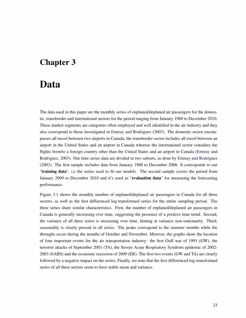
Figure 3.1 shows the monthly number of enplaned/deplaned air passengers in Canada for all three

sectors, as well as the first differenced log-transformed series for the entire sampling period. The

three series share similar characteristics. First, the number of enplaned/deplaned air passengers in

Canada is generally increasing over time, suggesting the presence of a positive time trend. Second,

the variance of all three series is increasing over time, hinting at variance non-stationarity. Third,

seasonality is clearly present in all series. The peaks correspond to the summer months while the

throughs occur during the months of October and November. Morever, the graphs show the location

of four important events for the air transportation industry: the first Gulf war of 1991 (GW), the

terrorist attacks of September 2001 (TA), the Severe Acute Respiratory Syndrom epidemic of 2002-

2003 (SARS) and the economic recession of 2009 (ER). The first two events (GW and TA) are clearly

followed by a negative impact on the series. Finally, we note that the first differenced log-transformed

series of all three sectors seem to have stable mean and variance.

23

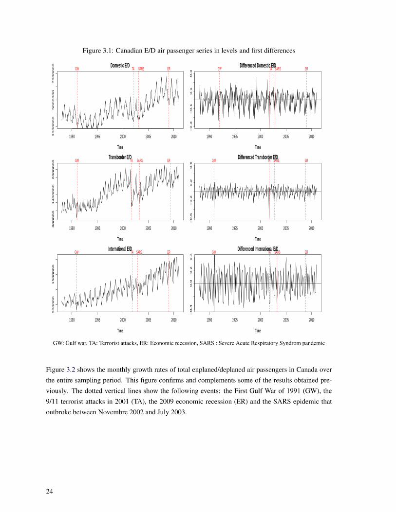
Figure 3.1: Canadian E/D air passenger series in levels and first differences

Time

1990 1995 2000 2005 201030

00

00

05

00

00

00

70

00

00

0

GW TA ERSARSDomestic E/D

Time

Diff

log

−se

rie

s

1990 1995 2000 2005 2010

−0

.3

−0

.1

0.1

0.3

GW TA SARS ERDifferenced Domestic E/D

Time

1990 1995 2000 2005 201080

00

00

14

00

00

02

00

00

00 GW TA ERSARS

Transborder E/D

Time

Diff

log

−se

rie

s

1990 1995 2000 2005 2010

−0

.6

−0

.2

0.2

0.6

GW TA SARS ERDifferenced Transborder E/D

Time

1990 1995 2000 2005 2010

50

00

00

15

00

00

0

GW TA ERSARSInternational E/D

Time

Diff

log

−se

rie

s

1990 1995 2000 2005 2010

−0

.4

0.0

0.2

0.4

GW TA SARS ERDifferenced International E/D

GW: Gulf war, TA: Terrorist attacks, ER: Economic recession, SARS : Severe Acute Respiratory Syndrom pandemic

Figure 3.2 shows the monthly growth rates of total enplaned/deplaned air passengers in Canada over

the entire sampling period. This figure confirms and complements some of the results obtained pre-

viously. The dotted vertical lines show the following events: the First Gulf War of 1991 (GW), the

9/11 terrorist attacks in 2001 (TA), the 2009 economic recession (ER) and the SARS epidemic that

outbroke between Novembre 2002 and July 2003.

24

Figu

re3.

2:A

nnua

lgro

wth

rate

sof

airt

rans

port

dem

and

inC

anad

a

1990

1995

2000

2005

2010

−0.20.00.2

Janu

ary

GW

TAE

RS

AR

S

1990

1995

2000

2005

2010

−0.20.00.2

Feb

ruar

yG

WTA

ER

SA

RS

1990

1995

2000

2005

2010

−0.20.00.2

Mar

chG

WTA

ER

SA

RS

1990

1995

2000

2005

2010

−0.20.00.2

Apr

ilG

WTA

ER

SA

RS

1990

1995

2000

2005

2010

−0.20.00.2

May

GW

TAE

RS

AR

S

1990

1995

2000

2005

2010

−0.20.00.2

June

GW

TAE

RS

AR

S

1990

1995

2000

2005

2010

−0.20.00.2

July

GW

TAE

RS

AR

S

1990

1995

2000

2005

2010

−0.20.00.2

Aug

ust

GW

TAE

RS

AR

S

1990

1995

2000

2005

2010

−0.20.00.2

Sep

tem

ber

GW

TAE

RS

AR

S

1990

1995

2000

2005

2010

−0.20.00.2

Oct

ober

GW

TAE

RS

AR

S

1990

1995

2000

2005

2010

−0.20.00.2

Nov

embe

rG

WTA

ER

SA

RS

1990

1995

2000

2005

2010

−0.20.00.2

Dec

embe

rG

WTA

ER

SA

RS

GW

:Gul

fwar

,TA

:Ter

rori

stat

tack

s,E

R:E

cono

mic

rece

ssio

n,SA

RS

:Sev

ere

Acu

teR

espi

rato

rySy

ndro

mpa

ndem

ic

25

Chapter 4

Results

4.1 Single model estimations

The following section presents the estimation results of the four models described in sections 2.1 to

2.3. In addition, it evaluates and compares their forecasting performance.

4.1.1 Harmonic regression model

We begin by presenting in table 4.1 the final harmonic regression model selected after applying a back-

ward selection procedure. The results of the Breush-Pagan and Durbin-Watson tests for heteroscedas-

ticity and autocorrelation are also shown. These tests indicate the presence of heteroscedasticity and

autocorrelation in the final models for all sectors (the lone exception is the international sector for

which the null hypothesis of homoscedasticity of the residuals cannot be rejected at the 5% signifi-

cance level). Therefore, the vcovHAC() function of the sandwich package in R was applied to get

heteroscedasticity and autocorrelation robust covariance matrices. Note that the harmonic regression

model includes dummy variables that account for several structural shocks that occured during the

sampling period : the first Gulf War (DGW), the terrorist attacks of September 2001 (D11S) and the

SARS epidemic (DSARS).

DGW =

{1 for t = 1990(11) to 1991(2)

0 otherwise

D11S =

{1 if t = 2001(09)

0 otherwise

DSARS =

{1 for t = 2002(11) to 2003(07)

0 otherwise

27

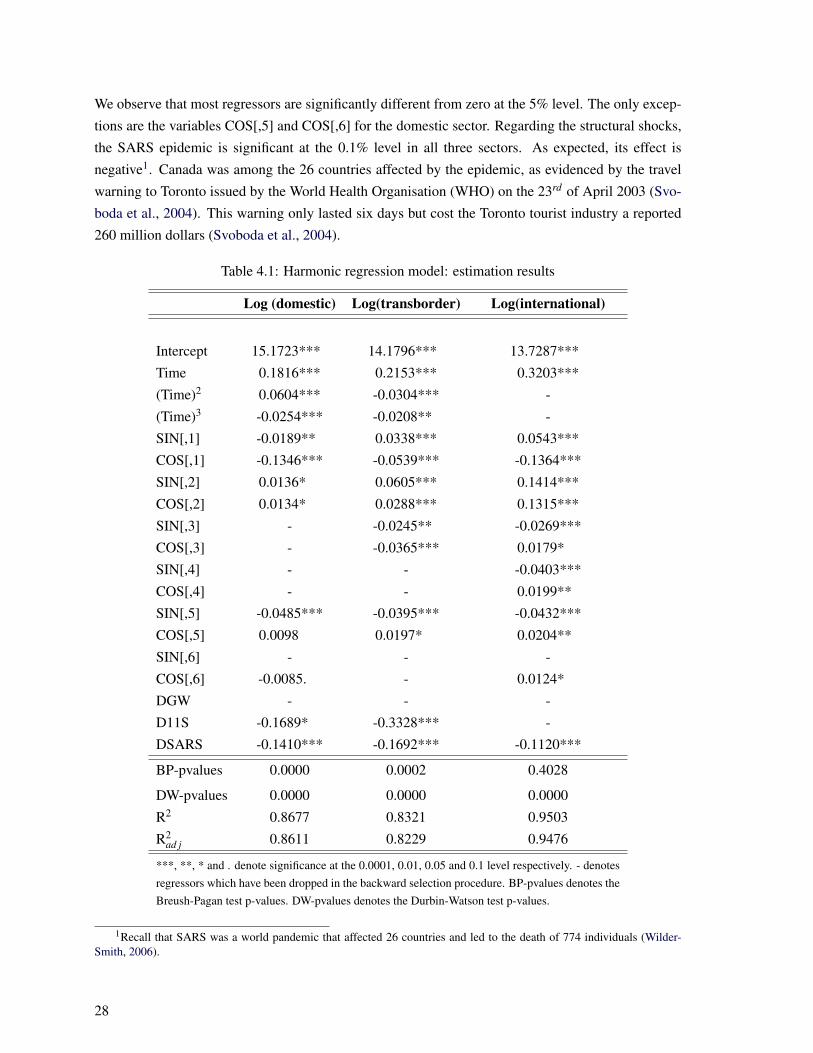
We observe that most regressors are significantly different from zero at the 5% level. The only excep-

tions are the variables COS[,5] and COS[,6] for the domestic sector. Regarding the structural shocks,

the SARS epidemic is significant at the 0.1% level in all three sectors. As expected, its effect is

negative1. Canada was among the 26 countries affected by the epidemic, as evidenced by the travel

warning to Toronto issued by the World Health Organisation (WHO) on the 23rd of April 2003 (Svo-

boda et al., 2004). This warning only lasted six days but cost the Toronto tourist industry a reported

260 million dollars (Svoboda et al., 2004).

Table 4.1: Harmonic regression model: estimation results

Log (domestic) Log(transborder) Log(international)

Intercept 15.1723*** 14.1796*** 13.7287***

Time 0.1816*** 0.2153*** 0.3203***

(Time)2 0.0604*** -0.0304*** -

(Time)3 -0.0254*** -0.0208** -

SIN[,1] -0.0189** 0.0338*** 0.0543***

COS[,1] -0.1346*** -0.0539*** -0.1364***

SIN[,2] 0.0136* 0.0605*** 0.1414***

COS[,2] 0.0134* 0.0288*** 0.1315***

SIN[,3] - -0.0245** -0.0269***

COS[,3] - -0.0365*** 0.0179*

SIN[,4] - - -0.0403***

COS[,4] - - 0.0199**

SIN[,5] -0.0485*** -0.0395*** -0.0432***

COS[,5] 0.0098 0.0197* 0.0204**

SIN[,6] - - -

COS[,6] -0.0085. - 0.0124*

DGW - - -

D11S -0.1689* -0.3328*** -

DSARS -0.1410*** -0.1692*** -0.1120***

BP-pvalues 0.0000 0.0002 0.4028

DW-pvalues 0.0000 0.0000 0.0000

R2 0.8677 0.8321 0.9503

R2ad j 0.8611 0.8229 0.9476

***, **, * and . denote significance at the 0.0001, 0.01, 0.05 and 0.1 level respectively. - denotesregressors which have been dropped in the backward selection procedure. BP-pvalues denotes theBreush-Pagan test p-values. DW-pvalues denotes the Durbin-Watson test p-values.

1Recall that SARS was a world pandemic that affected 26 countries and led to the death of 774 individuals (Wilder-Smith, 2006).

28

Turning our attention to the terrorist attacks of September 11th 2001, the results in table 4.1 indicate

that they had a significant and negative impact on air travel for the domestic and transborder sectors.

However, note that this variable was dropped in the international sector model. This is surprising con-

sidering that this event led to higher fares and made air travel more difficult throughout the world (for

example, through tighter security). Equally surprising is the fact that the dummy variable accounting

for the Gulf War was dropped in all three models.

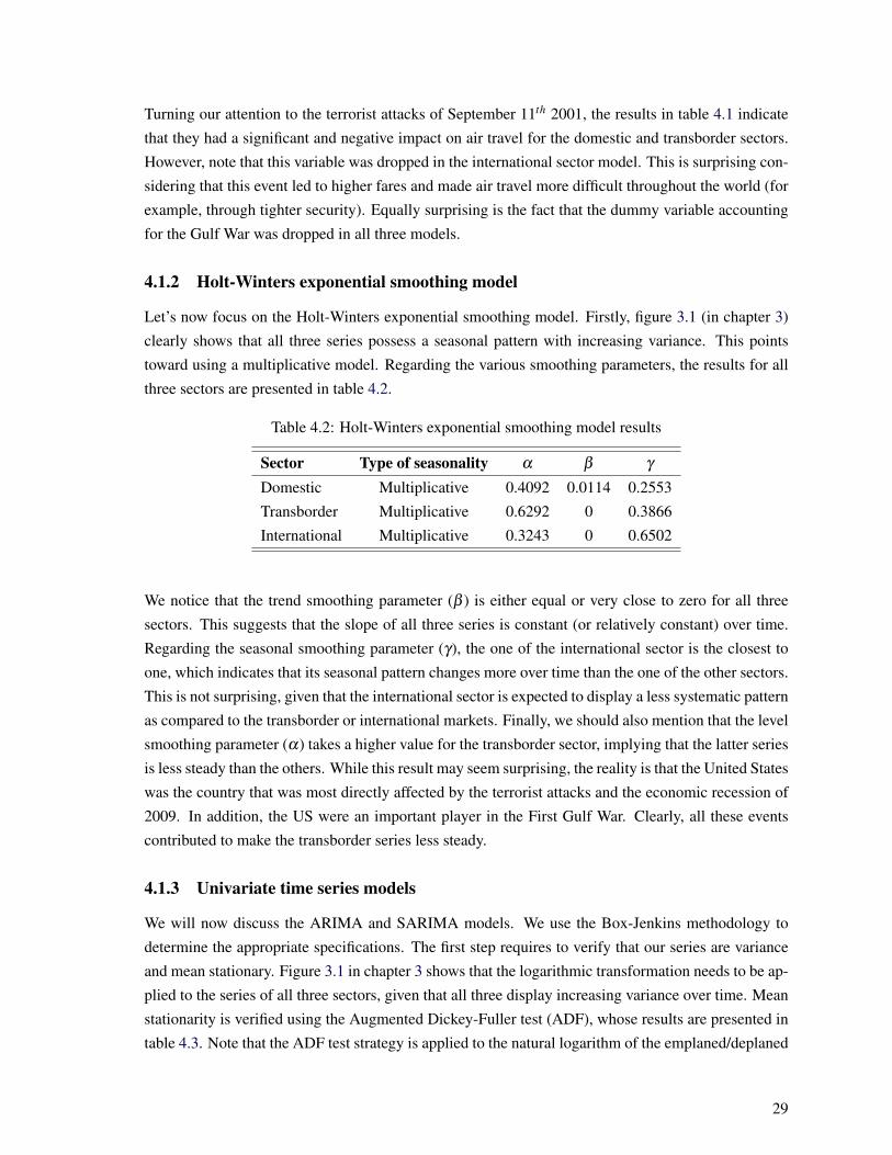
4.1.2 Holt-Winters exponential smoothing model

Let’s now focus on the Holt-Winters exponential smoothing model. Firstly, figure 3.1 (in chapter 3)

clearly shows that all three series possess a seasonal pattern with increasing variance. This points

toward using a multiplicative model. Regarding the various smoothing parameters, the results for all

three sectors are presented in table 4.2.

Table 4.2: Holt-Winters exponential smoothing model results

Sector Type of seasonality α β γ

Domestic Multiplicative 0.4092 0.0114 0.2553

Transborder Multiplicative 0.6292 0 0.3866

International Multiplicative 0.3243 0 0.6502

We notice that the trend smoothing parameter (β ) is either equal or very close to zero for all three

sectors. This suggests that the slope of all three series is constant (or relatively constant) over time.

Regarding the seasonal smoothing parameter (γ), the one of the international sector is the closest to

one, which indicates that its seasonal pattern changes more over time than the one of the other sectors.

This is not surprising, given that the international sector is expected to display a less systematic pattern

as compared to the transborder or international markets. Finally, we should also mention that the level

smoothing parameter (α) takes a higher value for the transborder sector, implying that the latter series

is less steady than the others. While this result may seem surprising, the reality is that the United States

was the country that was most directly affected by the terrorist attacks and the economic recession of

2009. In addition, the US were an important player in the First Gulf War. Clearly, all these events

contributed to make the transborder series less steady.

4.1.3 Univariate time series models

We will now discuss the ARIMA and SARIMA models. We use the Box-Jenkins methodology to

determine the appropriate specifications. The first step requires to verify that our series are variance

and mean stationary. Figure 3.1 in chapter 3 shows that the logarithmic transformation needs to be ap-

plied to the series of all three sectors, given that all three display increasing variance over time. Mean

stationarity is verified using the Augmented Dickey-Fuller test (ADF), whose results are presented in

table 4.3. Note that the ADF test strategy is applied to the natural logarithm of the emplaned/deplaned

29

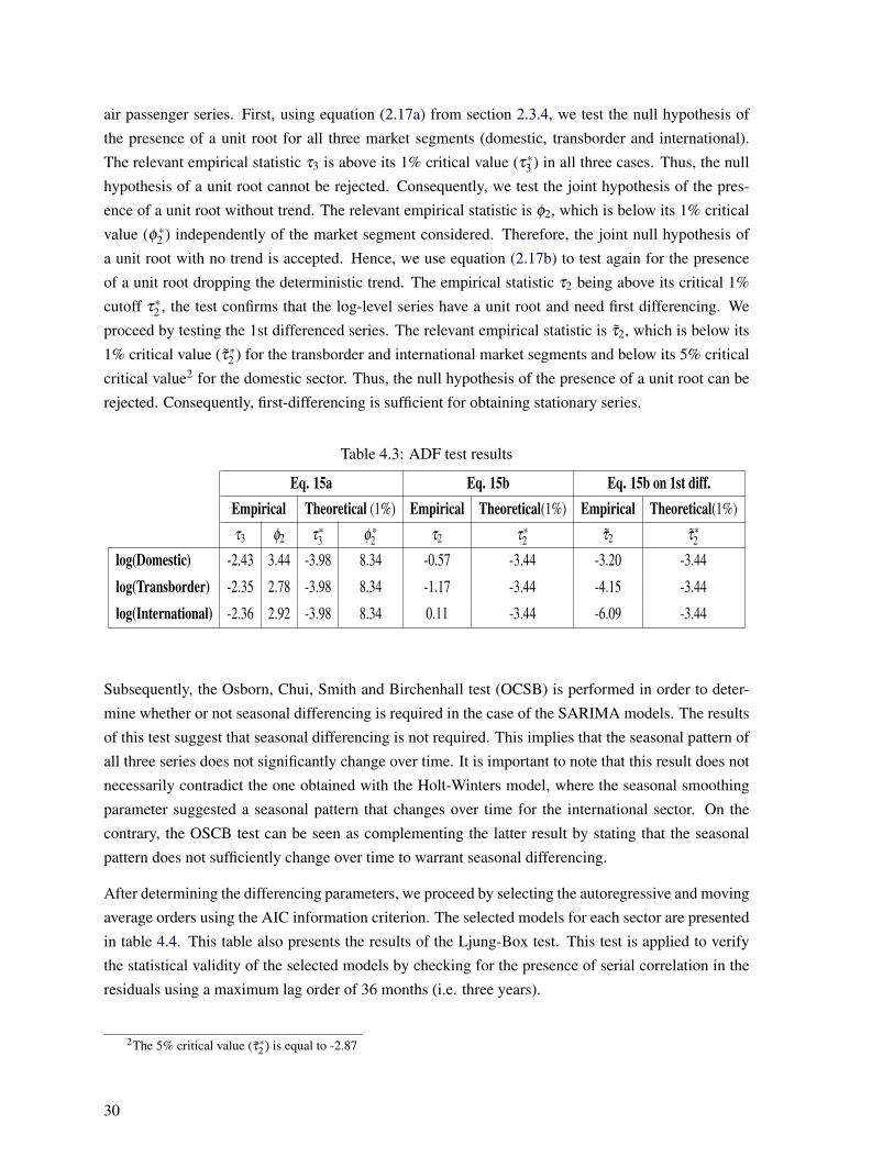
air passenger series. First, using equation (2.17a) from section 2.3.4, we test the null hypothesis of

the presence of a unit root for all three market segments (domestic, transborder and international).

The relevant empirical statistic τ3 is above its 1% critical value (τ∗3 ) in all three cases. Thus, the null

hypothesis of a unit root cannot be rejected. Consequently, we test the joint hypothesis of the pres-

ence of a unit root without trend. The relevant empirical statistic is φ2, which is below its 1% critical

value (φ ∗2 ) independently of the market segment considered. Therefore, the joint null hypothesis of

a unit root with no trend is accepted. Hence, we use equation (2.17b) to test again for the presence

of a unit root dropping the deterministic trend. The empirical statistic τ2 being above its critical 1%

cutoff τ∗2 , the test confirms that the log-level series have a unit root and need first differencing. We

proceed by testing the 1st differenced series. The relevant empirical statistic is τ2, which is below its

1% critical value (τ∗2 ) for the transborder and international market segments and below its 5% critical

critical value2 for the domestic sector. Thus, the null hypothesis of the presence of a unit root can be

rejected. Consequently, first-differencing is sufficient for obtaining stationary series.

Table 4.3: ADF test results

Eq. 15a Eq. 15b Eq. 15b on 1st diff.Empirical Theoretical (1%) Empirical Theoretical(1%) Empirical Theoretical(1%)

τ3 φ2 τ∗3 φ ∗2 τ2 τ∗2 τ2 τ∗2log(Domestic) -2.43 3.44 -3.98 8.34 -0.57 -3.44 -3.20 -3.44

log(Transborder) -2.35 2.78 -3.98 8.34 -1.17 -3.44 -4.15 -3.44

log(International) -2.36 2.92 -3.98 8.34 0.11 -3.44 -6.09 -3.44

Subsequently, the Osborn, Chui, Smith and Birchenhall test (OCSB) is performed in order to deter-

mine whether or not seasonal differencing is required in the case of the SARIMA models. The results

of this test suggest that seasonal differencing is not required. This implies that the seasonal pattern of

all three series does not significantly change over time. It is important to note that this result does not

necessarily contradict the one obtained with the Holt-Winters model, where the seasonal smoothing

parameter suggested a seasonal pattern that changes over time for the international sector. On the

contrary, the OSCB test can be seen as complementing the latter result by stating that the seasonal

pattern does not sufficiently change over time to warrant seasonal differencing.

After determining the differencing parameters, we proceed by selecting the autoregressive and moving

average orders using the AIC information criterion. The selected models for each sector are presented

in table 4.4. This table also presents the results of the Ljung-Box test. This test is applied to verify

the statistical validity of the selected models by checking for the presence of serial correlation in the

residuals using a maximum lag order of 36 months (i.e. three years).

2The 5% critical value (τ∗2 ) is equal to -2.87

30

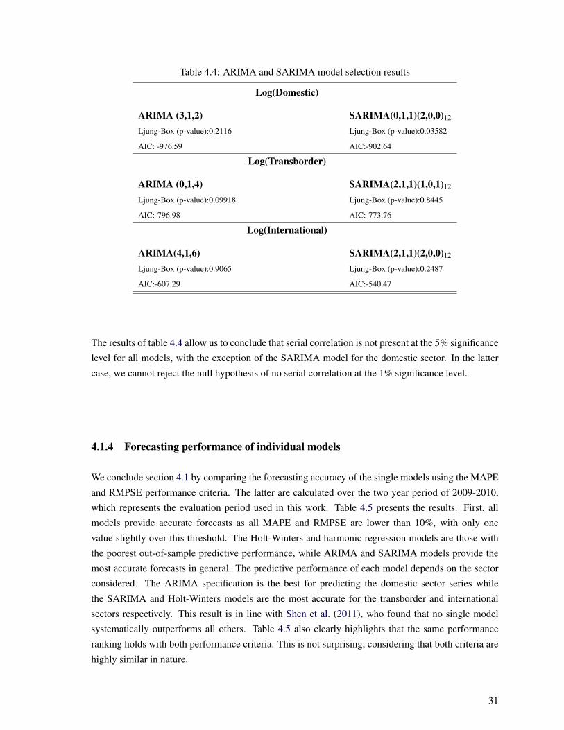
Table 4.4: ARIMA and SARIMA model selection results

Log(Domestic)

ARIMA (3,1,2) SARIMA(0,1,1)(2,0,0)12

Ljung-Box (p-value):0.2116 Ljung-Box (p-value):0.03582

AIC: -976.59 AIC:-902.64

Log(Transborder)

ARIMA (0,1,4) SARIMA(2,1,1)(1,0,1)12

Ljung-Box (p-value):0.09918 Ljung-Box (p-value):0.8445

AIC:-796.98 AIC:-773.76

Log(International)

ARIMA(4,1,6) SARIMA(2,1,1)(2,0,0)12

Ljung-Box (p-value):0.9065 Ljung-Box (p-value):0.2487

AIC:-607.29 AIC:-540.47

The results of table 4.4 allow us to conclude that serial correlation is not present at the 5% significance

level for all models, with the exception of the SARIMA model for the domestic sector. In the latter

case, we cannot reject the null hypothesis of no serial correlation at the 1% significance level.

4.1.4 Forecasting performance of individual models

We conclude section 4.1 by comparing the forecasting accuracy of the single models using the MAPE

and RMPSE performance criteria. The latter are calculated over the two year period of 2009-2010,

which represents the evaluation period used in this work. Table 4.5 presents the results. First, all

models provide accurate forecasts as all MAPE and RMPSE are lower than 10%, with only one

value slightly over this threshold. The Holt-Winters and harmonic regression models are those with

the poorest out-of-sample predictive performance, while ARIMA and SARIMA models provide the

most accurate forecasts in general. The predictive performance of each model depends on the sector

considered. The ARIMA specification is the best for predicting the domestic sector series while

the SARIMA and Holt-Winters models are the most accurate for the transborder and international

sectors respectively. This result is in line with Shen et al. (2011), who found that no single model

systematically outperforms all others. Table 4.5 also clearly highlights that the same performance

ranking holds with both performance criteria. This is not surprising, considering that both criteria are

highly similar in nature.

31

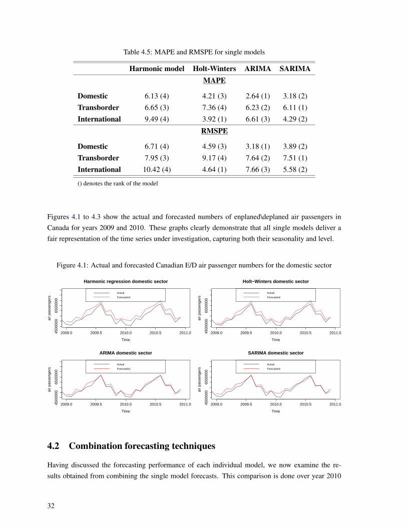
Table 4.5: MAPE and RMSPE for single models

Harmonic model Holt-Winters ARIMA SARIMAMAPE

Domestic 6.13 (4) 4.21 (3) 2.64 (1) 3.18 (2)

Transborder 6.65 (3) 7.36 (4) 6.23 (2) 6.11 (1)

International 9.49 (4) 3.92 (1) 6.61 (3) 4.29 (2)

RMSPE

Domestic 6.71 (4) 4.59 (3) 3.18 (1) 3.89 (2)

Transborder 7.95 (3) 9.17 (4) 7.64 (2) 7.51 (1)

International 10.42 (4) 4.64 (1) 7.66 (3) 5.58 (2)

() denotes the rank of the model

Figures 4.1 to 4.3 show the actual and forecasted numbers of enplaned\deplaned air passengers in

Canada for years 2009 and 2010. These graphs clearly demonstrate that all single models deliver a

fair representation of the time series under investigation, capturing both their seasonality and level.

Figure 4.1: Actual and forecasted Canadian E/D air passenger numbers for the domestic sector

Time

air

pass

enge

rs

2009.0 2009.5 2010.0 2010.5 2011.04500

000

6500

000

Actual

Forecasted

Harmonic regression domestic sector

Time

air

pass

enge

rs

2009.0 2009.5 2010.0 2010.5 2011.04500

000

6500

000

Actual

Forecasted

Holt−Winters domestic sector

Time

air

pass

enge

rs

2009.0 2009.5 2010.0 2010.5 2011.04500

000

6500

000

Actual

Forecasted

ARIMA domestic sector

Time

air

pass

enge

rs

2009.0 2009.5 2010.0 2010.5 2011.04500

000

6500

000

Actual

Forecasted

SARIMA domestic sector

4.2 Combination forecasting techniques

Having discussed the forecasting performance of each individual model, we now examine the re-

sults obtained from combining the single model forecasts. This comparison is done over year 2010

32

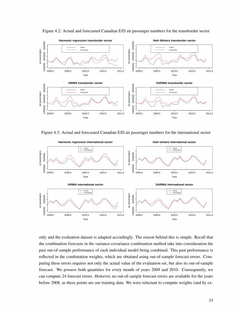
Figure 4.2: Actual and forecasted Canadian E/D air passenger numbers for the transborder sector

Time

air

pass

enge

rs

2009.0 2009.5 2010.0 2010.5 2011.01400

000

2000

000

2600

000

Actual

Forecasted

Harmonic regression transborder sector

Time

air

pass

enge

rs

2009.0 2009.5 2010.0 2010.5 2011.01400

000

2000

000

2600

000

Actual

Forecasted

Holt−Winters transborder sector

Time

air

pass

enge

rs

2009.0 2009.5 2010.0 2010.5 2011.01400

000

2000

000

2600

000

Actual

Forecasted

ARIMA transborder sector

Time

air

pass

enge

rs

2009.0 2009.5 2010.0 2010.5 2011.01400

000

2000

000

2600

000

Actual

Forecasted

SARIMA transborder sector

Figure 4.3: Actual and forecasted Canadian E/D air passenger numbers for the international sector

Time

air

pass

enge

rs

2009.0 2009.5 2010.0 2010.5 2011.01000

000

2000

000

ActualForecasted

Harmonic regression international sector

Time

air

pass

enge

rs

2009.0 2009.5 2010.0 2010.5 2011.01000

000

2000

000

ActualForecasted

Holt−winters international sector

Time

air

pass

enge

rs

2009.0 2009.5 2010.0 2010.5 2011.01000

000

2000

000

ActualForecasted

ARIMA international sector

Time

air

pass

enge

rs

2009.0 2009.5 2010.0 2010.5 2011.01000

000

2000

000

ActualForecasted

SARIMA international sector

only and the evaluation dataset is adapted accordingly. The reason behind this is simple. Recall that

the combination forecasts in the variance-covariance combination method take into consideration the

past out-of-sample performance of each individual model being combined. This past performance is

reflected in the combination weights, which are obtained using out-of-sample forecast errors. Com-

puting these errors requires not only the actual value of the evaluation set, but also its out-of-sample

forecast. We possess both quantities for every month of years 2009 and 2010. Consequently, we

can compute 24 forecast errors. However, no out-of-sample forecast errors are available for the years

before 2008, as these points are our training data. We were reluctant to compute weights (and by ex-

33

tension combination forecasts) for year 2009 based on in-sample predictions. This holds for all three

versions of the variance-covariance method. Note that the simple average combination method allows

us to compute combination forecasts for both 2009 and 2010. However, in order to keep identical

sample sizes across combination methods, the out-of-sample predictive performances for the simple

average method are based on projections made for year 2010 exclusively.

To keep our analysis tractable, we did not combine ARIMA and SARIMA forecasts since these are

highly similar models (both are ARMA-based models) whose forecasts are likely to be correlated.

Neither did we combine harmonic regression and Holt-Winters forecasts given that both are non-

autoregressive models. Finally, the SARIMA models dominating in general the ARIMA ones, we

restricted our analysis to combining SARIMA forecasts with those obtained from harmonic regres-

sions and Holt-Winters models, in tables 4.6 and 4.7 respectively.

We begin by comparing the forecasting accuracy of the harmonic regression and SARIMA models

as well as their combined version. Results are presented in table 4.6. We observe that whatever

the combination technique and forecasting performance metric, combined forecasts are always more

accurate then those obtained from the single worst model. This result holds across all market segments

considered. This result slightly differs from the one presented by Wong et al. (2007). These authors

find that there exist a few rare instances where the single worst model predictions are more accurate

than the combined forecasts.

Furthermore, we notice that the combined forecasts outperform their single best model counterpart 3

times (out of 16) with each performance criterion. Most of these cases apply to the transborder sector

and are displayed in bold characters in table 4.6. This suggests that the flight sector considered plays a

role in whether or not a combined forecast manages to surpass its single model counterparts. The latter

also likely depends on the combination technique used. Indeed, we observe that combined forecasts

obtained through the seasonal variance-covariance method never outperform their single best model

counterparts.

Table 4.6: Comparison of the forecasting accuracy of single and combined forecasts for Harmonicand SARIMA models (evaluation period: 2010(1)-2010(12)): MAPE and RMSPE

Single model forecasts Forecast combinationsHarmonic SARIMA SA SVC SWVC FWVC

Domestic 6.40 (6.99) 2.88 (3.69) 4.19 (4.86) 3.61 (4.39) 3.35 (4.14) 2.90 (3.70)Transborder 8.91 (10.0) 3.89 (4.55) 3.82 (4.94) 5.88 (6.72) 2.99 (3.77) 3.49 (3.85)International 8.04 (8.81) 2.50 (3.00) 4.52 (4.91) 2.61 (3.06) 2.99 (3.54) 2.50 (2.99)The RMSPE counterpart of the MAPE is in parenthesis. BOLD denotes that the combination forecast outperformsthe individual forecasts. SA: Simple average method. SVC: Seasonal variance-covariance method. SWVC: variance-covariance method with shifting window. FWVC: variance-covariance method with fixed window.

When comparing the forecasting performance of the various combination methods in table 4.6, we

34

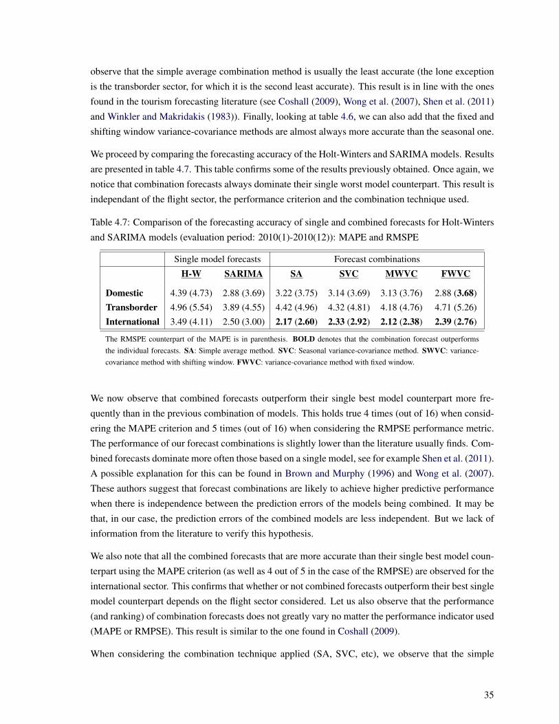
observe that the simple average combination method is usually the least accurate (the lone exception

is the transborder sector, for which it is the second least accurate). This result is in line with the ones

found in the tourism forecasting literature (see Coshall (2009), Wong et al. (2007), Shen et al. (2011)

and Winkler and Makridakis (1983)). Finally, looking at table 4.6, we can also add that the fixed and

shifting window variance-covariance methods are almost always more accurate than the seasonal one.

We proceed by comparing the forecasting accuracy of the Holt-Winters and SARIMA models. Results

are presented in table 4.7. This table confirms some of the results previously obtained. Once again, we

notice that combination forecasts always dominate their single worst model counterpart. This result is

independant of the flight sector, the performance criterion and the combination technique used.

Table 4.7: Comparison of the forecasting accuracy of single and combined forecasts for Holt-Winters

and SARIMA models (evaluation period: 2010(1)-2010(12)): MAPE and RMSPE

Single model forecasts Forecast combinations

H-W SARIMA SA SVC MWVC FWVC

Domestic 4.39 (4.73) 2.88 (3.69) 3.22 (3.75) 3.14 (3.69) 3.13 (3.76) 2.88 (3.68)

Transborder 4.96 (5.54) 3.89 (4.55) 4.42 (4.96) 4.32 (4.81) 4.18 (4.76) 4.71 (5.26)

International 3.49 (4.11) 2.50 (3.00) 2.17 (2.60) 2.33 (2.92) 2.12 (2.38) 2.39 (2.76)

The RMSPE counterpart of the MAPE is in parenthesis. BOLD denotes that the combination forecast outperformsthe individual forecasts. SA: Simple average method. SVC: Seasonal variance-covariance method. SWVC: variance-covariance method with shifting window. FWVC: variance-covariance method with fixed window.

We now observe that combined forecasts outperform their single best model counterpart more fre-

quently than in the previous combination of models. This holds true 4 times (out of 16) when consid-

ering the MAPE criterion and 5 times (out of 16) when considering the RMPSE performance metric.

The performance of our forecast combinations is slightly lower than the literature usually finds. Com-

bined forecasts dominate more often those based on a single model, see for example Shen et al. (2011).

A possible explanation for this can be found in Brown and Murphy (1996) and Wong et al. (2007).

These authors suggest that forecast combinations are likely to achieve higher predictive performance

when there is independence between the prediction errors of the models being combined. It may be

that, in our case, the prediction errors of the combined models are less independent. But we lack of

information from the literature to verify this hypothesis.

We also note that all the combined forecasts that are more accurate than their single best model coun-

terpart using the MAPE criterion (as well as 4 out of 5 in the case of the RMPSE) are observed for the

international sector. This confirms that whether or not combined forecasts outperform their best single

model counterpart depends on the flight sector considered. Let us also observe that the performance

(and ranking) of combination forecasts does not greatly vary no matter the performance indicator used

(MAPE or RMPSE). This result is similar to the one found in Coshall (2009).

When considering the combination technique applied (SA, SVC, etc), we observe that the simple

35

average method offers either the worst or second worst performance for two out of three sectors

considered.

36

Conclusion

This thesis tests the ability of several time-series models for predicting the monthly number of en-

planed/deplaned air passengers in Canada for three market segments : domestic, transborder and

international flights. Four standard models are explored: harmonic regresion, Holt-Winters expo-

nential smoothing, the autoregressive-integrated-moving average model (ARIMA) and the seasonal

autoregressive-integrated-moving average model (SARIMA). We further test the performance of com-

bining the single model predictions in different ways: by simply averaging the prediction of two

single models or by combining their forecasts based on their past predictive performance (variance-

covariance approach). Two global predictive accuracy metrics are used to carry out our analysis:

MAPE (mean absolute percentage error) and RMSE (root mean squared error).

We first estimate our models on training data covering the period from January 1998 to December

2008. We then offer monthly predictions over the months of January 2009 to Decembre 2010. Our

results show that all single models provide highly accurate forecasts, below the 10% threshold of the

pointwise realization on average. ARIMA and SARIMA model forecasts appear to always outper-

form harmonic regression and they are in general superior to Holt-Winters exponential smoothing in

terms of out-of-sample performance, whatever the accuracy measure used and the market segment.

Regarding the forecast combinations, we find that they are always more accurate than their single

worst model counterpart. In addition, in some instances, they outperform the best single model fore-

casts. This depends on: (i) the flight sector considered, (ii) the single models being combined and (iii)

the combination technique being applied. Indeed, we find that simple averaging is usually the least

accurate forecast combination technique, which is in accordance with what is found in the literature.

Combination methods seem therefore to achieve their goal of improving the forecasting accuracy when

applied to air passenger traffic series. This is of great interest for short and medium run planification in

the airport industry. As mentionned by Wong et al. (2007), day-to-day business may not always allow

the stylized exercice of finding the best model. However, relying on a combination of forecasts coming

from different models should clearly reduce the risk of using the worst model. In addition, combining

complementary models, capturing a variety of features of the data (such as non-autoregressive ones,

short and long run memory, non-linearities) as it has been done in other countries, could contribute to

better outline the specificities of the Canadian market.

37

Bibliography

Andreoni, A. and Postorino, M. (2006). A multivariate arima model to forecast air transport demand.

Proceedings of the Association for European Transport and Contributors, pages 1–14.

Bao, Y., Xiong, T., and Hu, Z. (2012). Forecasting air passenger traffic by support vector machines

with ensemble empirical mode decomposition and slope-based method. Discrete Dynamics in Na-

ture and Society, 2012.

Bates, J. and Granger, C. (1969). The combination of forecasts. Operational Research Quarterly,

20(4):451–468.

Bjørnland, H., Gerdrup, K., Jore, A., Smith, C., and Thorsrud, L. (2011). Does forecast combination

improve norges bank inflation forecasts? Oxford Bulletin of Economics and Statistics, 74(2):163–

179.

Bourbonnais, R. and Terraza, M. (2004). Analyse des séries temporelles: applications à l’économie

et à la gestion, volume 3. Dunod.

Bresson, G. and Pirotte, A. (1995). Économétrie des séries temporelles: Théorie et applications.

Presses Universitaires de France, first edition.

Brown, B. and Murphy, A. (1996). Improving forecasting performance by combining forecasts: The

example of road-surface temperature forecasts. Meteorological Applications, 3(3):257–265.

Bunn, D. (1988). Combining forecasts. European Journal of Operational Research, 33(3):223–229.

Chan, C., Kingsman, B., and Wong, H. (1999). The value of combining forecasts in inventory

management–a case study in banking. European Journal of Operational Research, 117(2):199–

210.

Chatfield, C. (2003). The analysis of time series: an introduction, volume 59. Chapman & Hall/CRC.

Chen, C., Chang, Y., and Chang, Y. (2009). Seasonal arima forecasting of inbound air travel arrivals

to taiwan. Transportmetrica, 5(2):125–140.

39

Chen, S.-C., Kuo, S.-Y., Chang, K.-W., and Wang, Y.-T. (2012). Improving the forecasting accu-

racy of air passenger and air cargo demand: the application of back-propagation neural networks.

Transportation Planning and Technology, 35(3):373–392.

Cho, V. (2003). A comparison of three different approaches to tourist arrival forecasting. Tourism

Management, 24(3):323–330.

Chu, F. (1998). Forecasting tourism: a combined approach. Tourism Management, 19(6):515–520.

Chu, F. (2009). Forecasting tourism demand with arma-based methods. Tourism Management,

30(5):740–751.

Cornillon, P.-A. and Matzner-Løber, E. (2007). Régression: Théorie et applications. Spinger.

Coshall, J. (2006). Time series analyses of UK outbound travel by air. Journal of Travel Research,

44(3):335–347.

Coshall, J. (2009). Combining volatility and smoothing forecasts of UK demand for international

tourism. Tourism Management, 30(4):495–511.

Cowpertwait, P. S. and Metcalfe, A. V. (2009). Introductory time series with R. Springer.

Emiray, E. and Rodriguez, G. (2003). Evaluating Time Series Models in Short and Long-Term Fore-

casting of Canadian Air Passenger Data. Department of Economics, University of Ottawa.

Fildes, R., Wei, Y., and Ismail, S. (2011). Evaluating the forecasting performance of econometric

models of air passenger traffic flows using multiple error measures. International Journal of Fore-

casting, 27(3):902–922.

Gelper, S., Fried, R., and Croux, C. (2010). Robust forecasting with exponential and holt–winters

smoothing. Journal of forecasting, 29(3):285–300.

Greene, R. (2005). Économétrie. Pearson Education, fifth edition.

Grosche, T., Rothlauf, F., and Heinzl, A. (2007). Gravity models for airline passenger volume estima-

tion. Journal of Air Transport Management, 13(4):175–183.

Han, L. and Thury, G. (1997). Testing for seasonal integration and cointegration: the austrian con-

sumption income relationship. Empirical Economics, 22(3):331–344.

Harris, R. I. (1992). Testing for unit roots using the augmented dickey-fuller test: Some issues relating

to the size, power and the lag structure of the test. Economics letters, 38(4):381–386.

Harvey, R. (1993). Time Series Models. MIT Press, second edition.

Hyndman, R. J. and Khandakar, Y. (2007). Automatic time series for forecasting: The forecast pack-

age for r. Technical report, Monash University, Department of Econometrics and Business Statistics.

40

Kalekar, P. S. (2004). Time series forecasting using holt-winters exponential smoothing. Kanwal

Rekhi School of Information Technology.

Kulendran, N. and Witt, S. (2003). Forecasting the demand for international business tourism. Journal

of Travel Research, 41(3):265–271.

Lim, C. and McAleer, M. (2001). Forecasting tourist arrivals. Annals of Tourism Research, 28(4):965–

977.

Lim, C. and McAleer, M. (2002). Time series forecasts of international travel demand for australia.

Tourism Management, 23(4):389–396.

Ljung, G. and Box, G. (1978). On a measure of lack of fit in time series models. Biometrika,

65(2):297–303.

Montgomery, D., C.L., J., and M., K. (2008). Introduction to Time Series Analysis and Forecasting.

John Wiley & Sons, Inc.

Oh, C. and Morzuch, B. (2005). Evaluating time-series models to forecast the demand for tourism in

singapore comparing within-sample and postsample results. Journal of Travel Research, 43(4):404–

413.

Osborn, D. R., Chui, A. P., Smith, J. P., and Birchenhall, C. R. (1988). Seasonality and the order of

integration for consumption*. Oxford Bulletin of Economics and Statistics, 50(4):361–377.

Pfaff, B. (2008). Analysis of integrated and cointegrated time series with R. Springer.

Poncela, P. and Senra, E. (2006). A two factor model to combine us inflation forecasts. Applied

Economics, 38(18):2191–2197.

R Development Core Team (2012). R: A Language and Environment for Statistical Computing. R

Foundation for Statistical Computing, Vienna, Austria. ISBN 3-900051-07-0.

Rob J Hyndman, w. c. f. G. A., Razbash, S., Schmidt, D., Zhou, Z., and Khan, Y. (2013). Forecast:

Forecasting functions for time series and linear models. R package version 4.02.

Rodrigues, P. M. and Osborn, D. R. (1999). Performance of seasonal unit root tests for monthly data.

Journal of Applied Statistics, 26(8):985–1004.

Shen, S., Li, G., and Song, H. (2008). An assessment of combining tourism demand forecasts over

different time horizons. Journal of Travel Research, 47(2):197–207.

Shen, S., Li, G., and Song, H. (2011). Combination forecasts of international tourism demand. Annals

of Tourism Research, 38(1):72–89.

41

Svoboda, T., Henry, B., Shulman, L., Kennedy, E., Rea, E., Ng, W., Wallington, T., Yaffe, B., Gour-

nis, E., Vicencio, E., et al. (2004). Public health measures to control the spread of the severe

acute respiratory syndrome during the outbreak in toronto. New England Journal of Medicine,

350(23):2352–2361.

Timmermann, A. (2006). Forecast combinations. Handbook of economic forecasting, 1:135–196.

Transport Canada (2011). Transportation in Canada: Addendum. Annual report. Retrieved February

20, 2012, from http://www.tc.gc.ca/media/documents/policy/addendum2010.pdf.

Tsui, W., Balli, H., and Gower, H. (2011). Forecasting airport passenger traffic: the case of hong kong

international airport. Aviation Education and Research Proceedings, 2011:54–62.

Wilder-Smith, A. (2006). The severe acute respiratory syndrome: impact on travel and tourism. Travel

medicine and infectious disease, 4(2):53–60.

Winkler, R. and Makridakis, S. (1983). The combination of forecasts. Journal of the Royal Statistical

Society. Series A (General), 146(20):150–157.

Witt, S. F. and Witt, C. A. (1991). Tourism forecasting: Error magnitude, direction of change error,

and trend change error. Journal of Travel Research, 30(2):26–33.

Wong, K., Song, H., Witt, S., and Wu, D. (2007). Tourism forecasting: to combine or not to combine?

Tourism Management, 28(4):1068–1078.

Zeileis, A. (2004). Econometric computing with hc and hac covariance matrix estimators. Journal of

Statistical Software, 11(10):1–17.

Zeileis, A. and Hothorn, T. (2002). Diagnostic checking in regression relationships. R News, 2(3):7–

10.

Zhang, G. (2003). Time series forecasting using a hybrid arima and neural network model. Neuro-

computing, 50:159–175.

42