Embed Size (px)
Citation preview
Résolution du problème d’allocation de culture par satisfaction decontraintes pondérées
Mahuna Akplogan1 Jérome Dury2 Simon de Givry1
Gauthier Quesnel1 Alexandre Joannon3 Frédérick Garcia1
1INRA: INRA, UR 875 Biométrie et Intelligence Artificielle, F-31326 Toulouse2INRA: INRA, UMR 1248 AGIR, F-31326 Toulouse
3INRA: INRA, UR 980 SAD-Paysage, F-35042 Rennes
JFPC 2012
BIA (INRA) Spatio-temporal farm planning May 2012 1 / 23
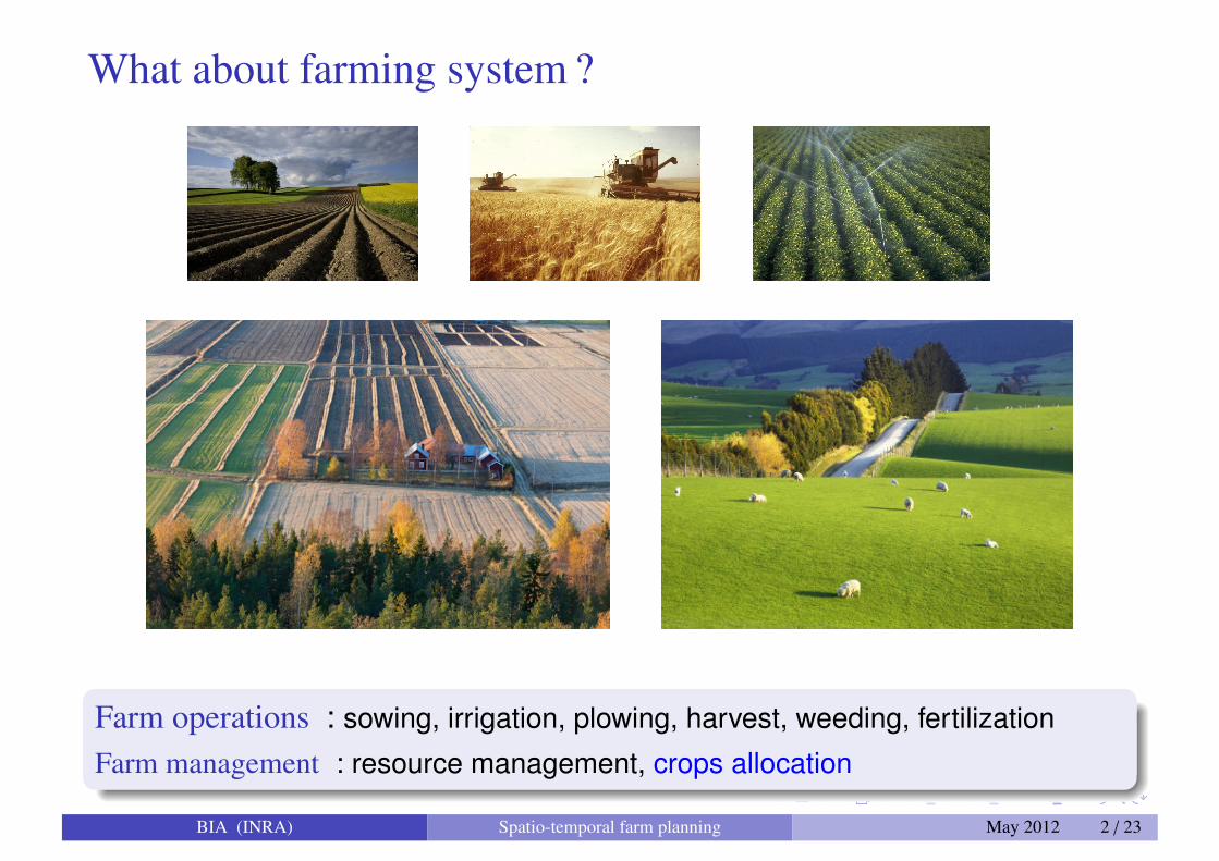
What about farming system ?
Farm operations : sowing, irrigation, plowing, harvest, weeding, fertilization
Farm management : resource management, crops allocation
BIA (INRA) Spatio-temporal farm planning May 2012 2 / 23
Summary
1 Crop allocation problem (CAP)
2 Methodological framework
3 CAP formulation
4 Experimentation
5 Conclusion
BIA (INRA) Spatio-temporal farm planning May 2012 3 / 23
Main concepts for crop allocation problem (CAP)
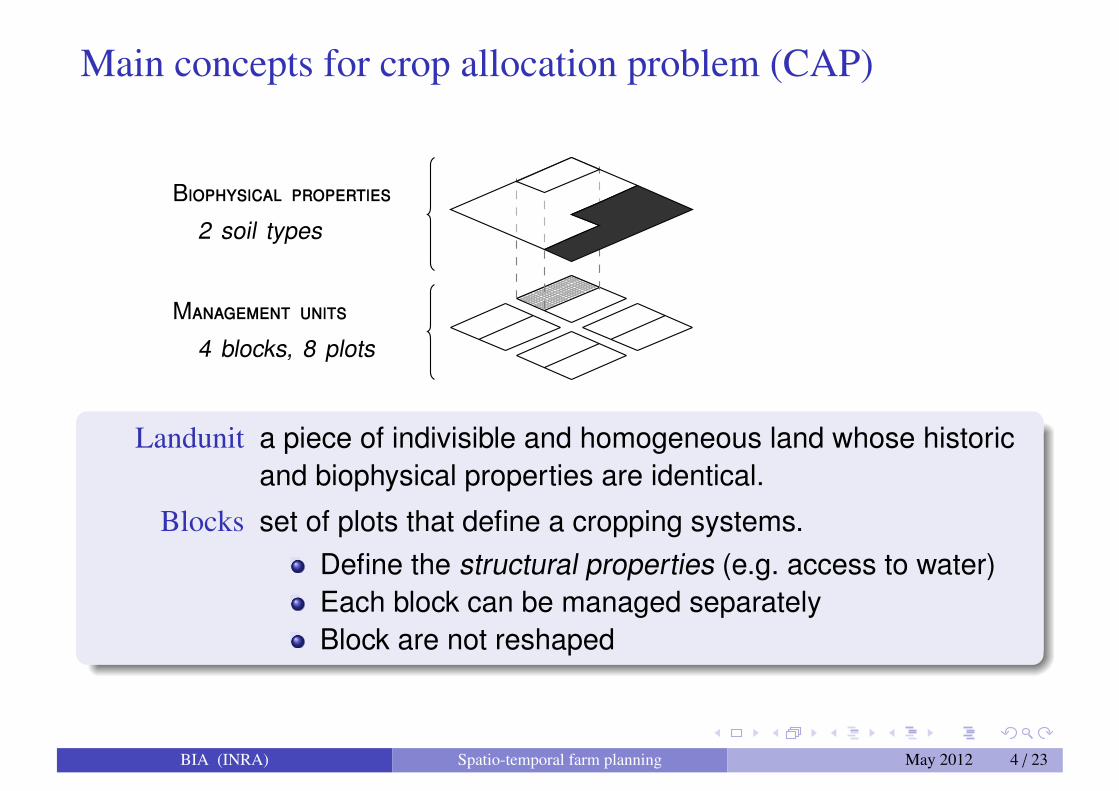
Biophysical properties
2 soil types
Management units
4 blocks, 8 plots
Landunit a piece of indivisible and homogeneous land whose historicand biophysical properties are identical.
Blocks set of plots that define a cropping systems.Define the structural properties (e.g. access to water)Each block can be managed separatelyBlock are not reshaped
BIA (INRA) Spatio-temporal farm planning May 2012 4 / 23
Main concepts for crop allocation problem (CAP)
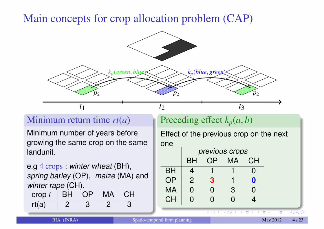
t1 t2 t3
kp(green, blue) kp(blue, green)
p2 p2 p2
Minimum return time rt(a)Minimum number of years beforegrowing the same crop on the samelandunit.
e.g 4 crops : winter wheat (BH),spring barley (OP), maize (MA) andwinter rape (CH).
crop i BH OP MA CHrt(a) 2 3 2 3
Preceding effect kp(a, b)Effect of the previous crop on the nextone
previous cropsBH OP MA CH
BH 4 1 1 0OP 2 3 1 0MA 0 0 3 0CH 0 0 0 4
BIA (INRA) Spatio-temporal farm planning May 2012 4 / 23
Aim of this work
water
water
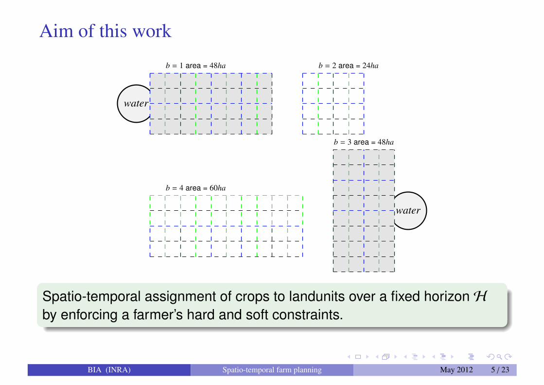
b = 1 area = 48ha b = 2 area = 24ha
b = 3 area = 48ha
b = 4 area = 60ha
Spatio-temporal assignment of crops to landunits over a fixed horizon Hby enforcing a farmer’s hard and soft constraints.
BIA (INRA) Spatio-temporal farm planning May 2012 5 / 23
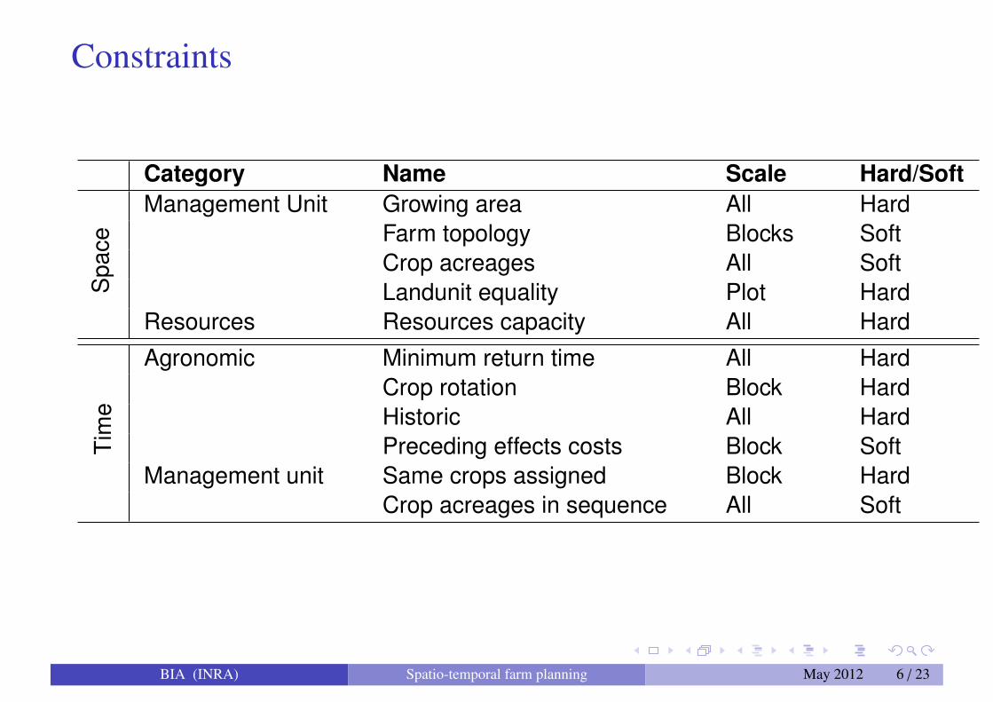
Constraints
Category Name Scale Hard/Soft
Spa
ce
Management Unit Growing area All HardFarm topology Blocks SoftCrop acreages All SoftLandunit equality Plot Hard
Resources Resources capacity All Hard
Tim
e
Agronomic Minimum return time All HardCrop rotation Block HardHistoric All HardPreceding effects costs Block Soft
Management unit Same crops assigned Block HardCrop acreages in sequence All Soft
BIA (INRA) Spatio-temporal farm planning May 2012 6 / 23
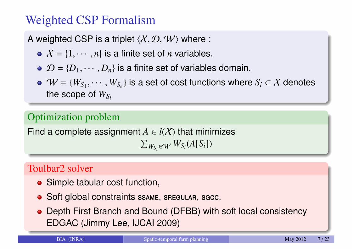
Weighted CSP FormalismA weighted CSP is a triplet 〈X,D,W〉 where :
X = {1, · · · , n} is a finite set of n variables.
D = {D1, · · · ,Dn} is a finite set of variables domain.
W = {WS1 , · · · ,WSe} is a set of cost functions where Si ⊂ X denotesthe scope of WSi
Optimization problemFind a complete assignment A ∈ l(X) that minimizes∑
WSi∈WWSi(A[Si])
Toulbar2 solverSimple tabular cost function,
Soft global constraints ssame, sregular, sgcc.
Depth First Branch and Bound (DFBB) with soft local consistencyEDGAC (Jimmy Lee, IJCAI 2009)
BIA (INRA) Spatio-temporal farm planning May 2012 7 / 23
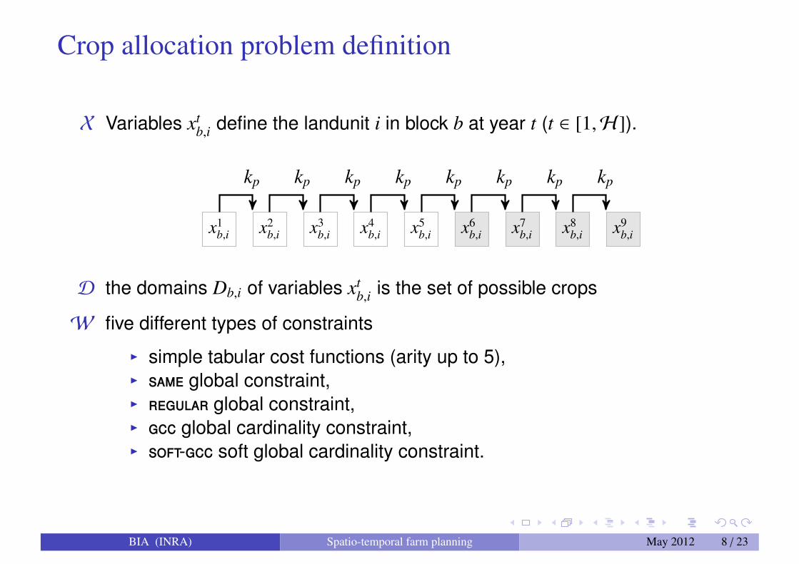
Crop allocation problem definition
X Variables xtb,i define the landunit i in block b at year t (t ∈ [1,H]).
x1b,i x2
b,i x3b,i x4
b,i x5b,i x6
b,i x7b,i x8
b,i x9b,i
kp kp kp kp kp kp kp kp
D the domains Db,i of variables xtb,i is the set of possible crops
W five different types of constraints
I simple tabular cost functions (arity up to 5),I same global constraint,I regular global constraint,I gcc global cardinality constraint,I soft-gcc soft global cardinality constraint.
BIA (INRA) Spatio-temporal farm planning May 2012 8 / 23
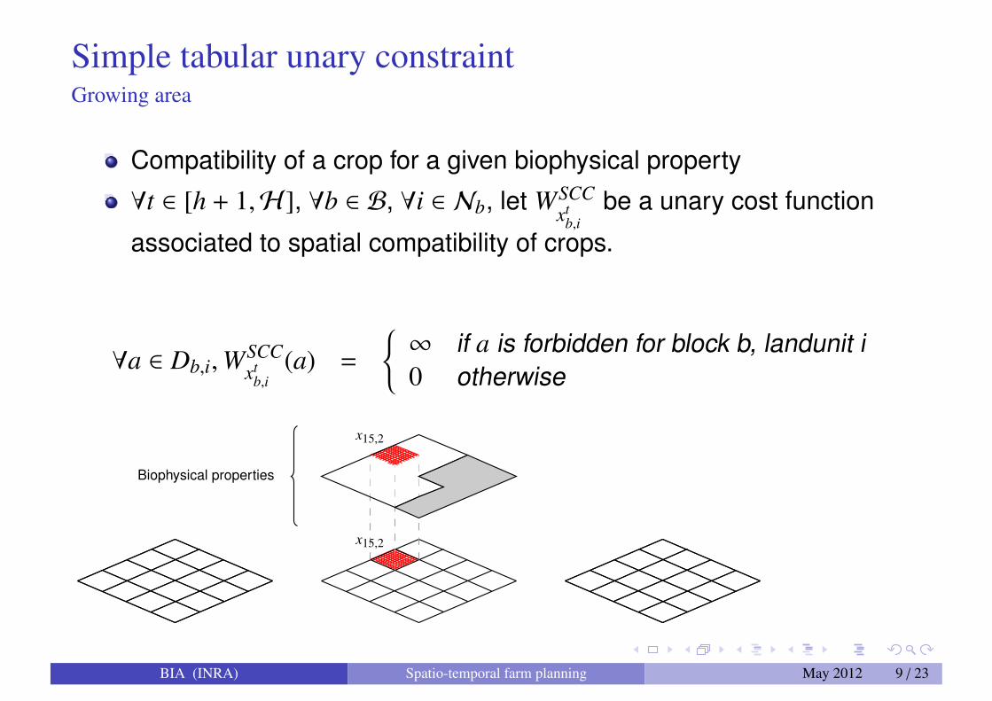
Simple tabular unary constraintGrowing area
Compatibility of a crop for a given biophysical property
∀t ∈ [h + 1,H], ∀b ∈ B, ∀i ∈ Nb, let WSCCxt
b,ibe a unary cost function
associated to spatial compatibility of crops.
∀a ∈ Db,i,WSCCxt
b,i(a) =
{∞ if a is forbidden for block b, landunit i0 otherwise
x15,2
x15,2
Biophysical properties
BIA (INRA) Spatio-temporal farm planning May 2012 9 / 23
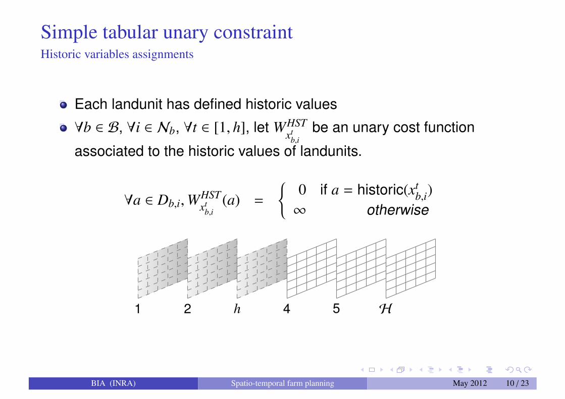
Simple tabular unary constraintHistoric variables assignments
Each landunit has defined historic values
∀b ∈ B, ∀i ∈ Nb, ∀t ∈ [1, h], let WHSTxt
b,ibe an unary cost function
associated to the historic values of landunits.
∀a ∈ Db,i,WHSTxt
b,i(a) =
{0 if a = historic(xt
b,i)∞ otherwise
1 2 h 4 5 H
BIA (INRA) Spatio-temporal farm planning May 2012 10 / 23
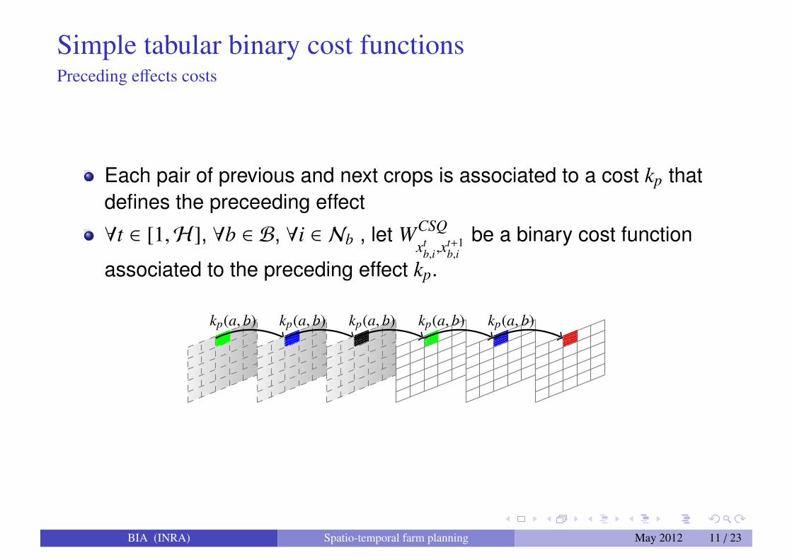
Simple tabular binary cost functionsPreceding effects costs
Each pair of previous and next crops is associated to a cost kp thatdefines the preceeding effect
∀t ∈ [1,H], ∀b ∈ B, ∀i ∈ Nb , let WCSQxt
b,i,xt+1b,i
be a binary cost function
associated to the preceding effect kp.
kp(a, b) kp(a, b) kp(a, b) kp(a, b) kp(a, b)
BIA (INRA) Spatio-temporal farm planning May 2012 11 / 23
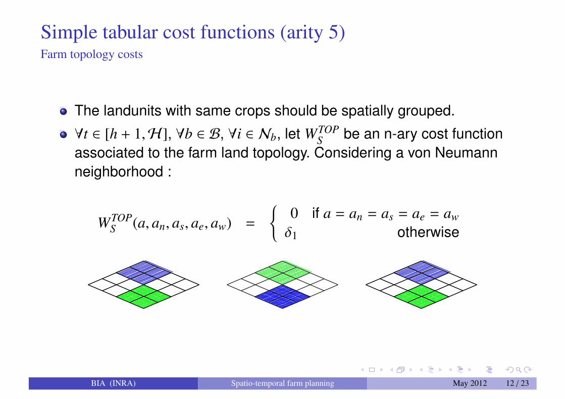
Simple tabular cost functions (arity 5)Farm topology costs
The landunits with same crops should be spatially grouped.
∀t ∈ [h + 1,H], ∀b ∈ B, ∀i ∈ Nb, let WTOPS be an n-ary cost function
associated to the farm land topology. Considering a von Neumannneighborhood :
WTOPS (a, an, as, ae, aw) =
{0 if a = an = as = ae = aw
δ1 otherwise
BIA (INRA) Spatio-temporal farm planning May 2012 12 / 23
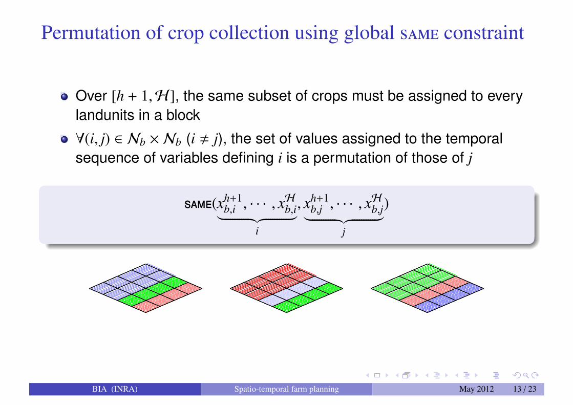
Permutation of crop collection using global same constraint
Over [h + 1,H], the same subset of crops must be assigned to everylandunits in a block
∀(i, j) ∈ Nb × Nb (i , j), the set of values assigned to the temporalsequence of variables defining i is a permutation of those of j
same(xh+1b,i , · · · , x
Hb,i︸ ︷︷ ︸
i
, xh+1b,j , · · · , x
Hb,j︸ ︷︷ ︸
j
)
BIA (INRA) Spatio-temporal farm planning May 2012 13 / 23
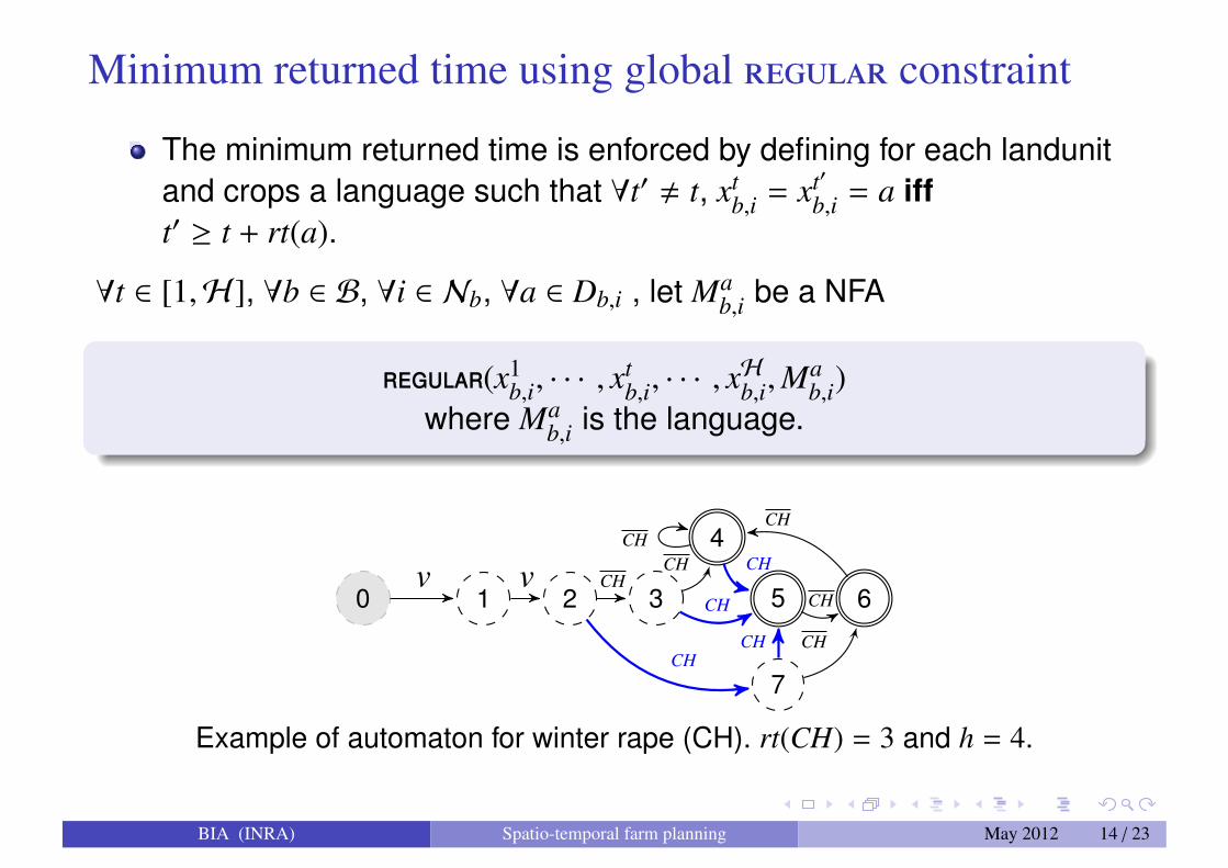
Minimum returned time using global regular constraint
The minimum returned time is enforced by defining for each landunitand crops a language such that ∀t′ , t, xt
b,i = xt′b,i = a iff
t′ ≥ t + rt(a).
∀t ∈ [1,H], ∀b ∈ B, ∀i ∈ Nb, ∀a ∈ Db,i , let Mab,i be a NFA
regular(x1b,i, · · · , x
tb,i, · · · , x
Hb,i,M
ab,i)
where Mab,i is the language.
4
5 6321
7
0CH
CH
CH
CH
CHCH
v CH
CHv CH
CH
Example of automaton for winter rape (CH). rt(CH) = 3 and h = 4.
BIA (INRA) Spatio-temporal farm planning May 2012 14 / 23
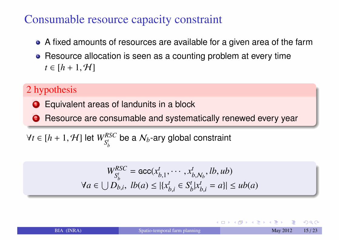
Consumable resource capacity constraint
A fixed amounts of resources are available for a given area of the farm
Resource allocation is seen as a counting problem at every timet ∈ [h + 1,H]
2 hypothesis1 Equivalent areas of landunits in a block2 Resource are consumable and systematically renewed every year
∀t ∈ [h + 1,H] let WRSCSt
bbe a Nb-ary global constraint
WRSCSt
b= gcc(xt
b,1, · · · , xtb,Nb
, lb, ub)
∀a ∈⋃
Db,i, lb(a) ≤ |{xtb,i ∈ St
b|xtb,i = a}| ≤ ub(a)
BIA (INRA) Spatio-temporal farm planning May 2012 15 / 23
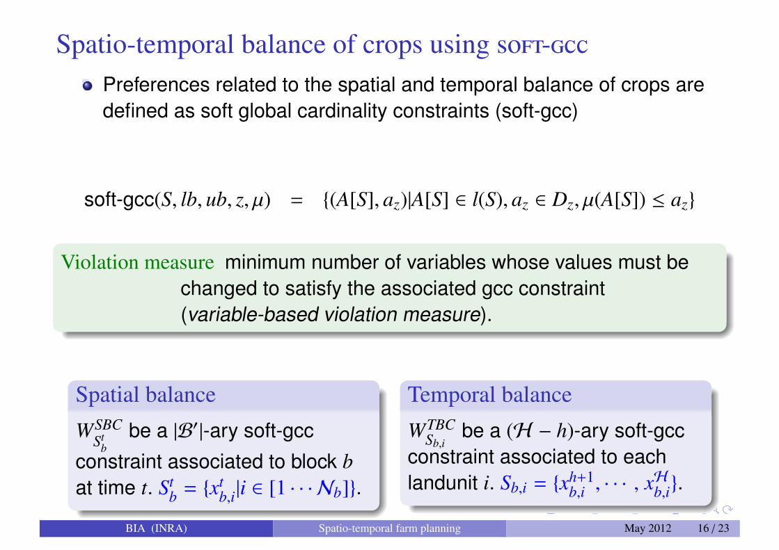
Spatio-temporal balance of crops using soft-gccPreferences related to the spatial and temporal balance of crops aredefined as soft global cardinality constraints (soft-gcc)
soft-gcc(S, lb, ub, z, µ) = {(A[S], az)|A[S] ∈ l(S), az ∈ Dz, µ(A[S]) ≤ az}
Violation measure minimum number of variables whose values must bechanged to satisfy the associated gcc constraint(variable-based violation measure).
Spatial balance
WSBCSt
bbe a |B′|-ary soft-gcc
constraint associated to block bat time t. St
b = {xtb,i|i ∈ [1 · · · Nb]}.
Temporal balance
WTBCSb,i
be a (H − h)-ary soft-gccconstraint associated to eachlandunit i. Sb,i = {xh+1
b,i , · · · , xHb,i}.
BIA (INRA) Spatio-temporal farm planning May 2012 16 / 23

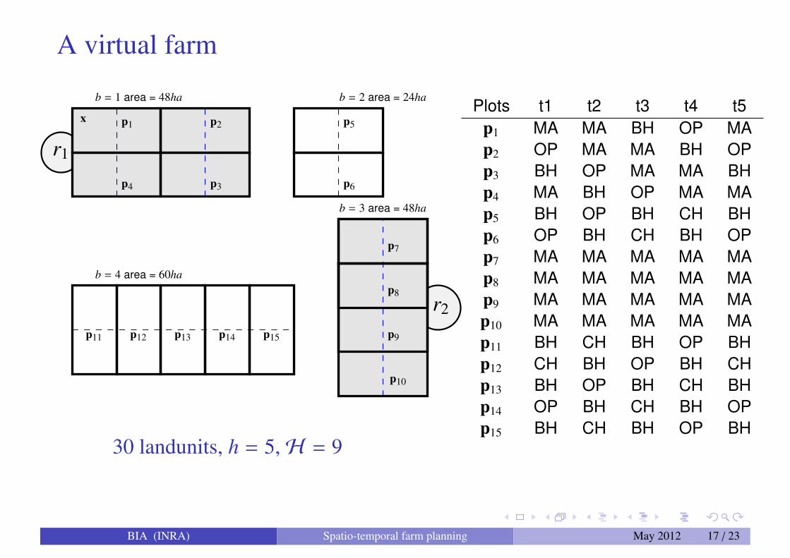
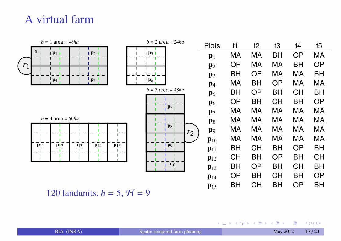
A virtual farm
r1
r2
b = 1 area = 48ha b = 2 area = 24ha
b = 3 area = 48ha
b = 4 area = 60ha
x p1 p2
p3p4
p5
p6
p7
p8
p9
p10
p11 p12 p13 p14 p15
15 landunits, h = 5,H = 9
Plots t1 t2 t3 t4 t5p1 MA MA BH OP MAp2 OP MA MA BH OPp3 BH OP MA MA BHp4 MA BH OP MA MAp5 BH OP BH CH BHp6 OP BH CH BH OPp7 MA MA MA MA MAp8 MA MA MA MA MAp9 MA MA MA MA MAp10 MA MA MA MA MAp11 BH CH BH OP BHp12 CH BH OP BH CHp13 BH OP BH CH BHp14 OP BH CH BH OPp15 BH CH BH OP BH
BIA (INRA) Spatio-temporal farm planning May 2012 17 / 23
A virtual farm
r1
r2
b = 1 area = 48ha b = 2 area = 24ha
b = 3 area = 48ha
b = 4 area = 60ha
x p1 p2
p3p4
p5
p6
p7
p8
p9
p10
p11 p12 p13 p14 p15
30 landunits, h = 5,H = 9
Plots t1 t2 t3 t4 t5p1 MA MA BH OP MAp2 OP MA MA BH OPp3 BH OP MA MA BHp4 MA BH OP MA MAp5 BH OP BH CH BHp6 OP BH CH BH OPp7 MA MA MA MA MAp8 MA MA MA MA MAp9 MA MA MA MA MAp10 MA MA MA MA MAp11 BH CH BH OP BHp12 CH BH OP BH CHp13 BH OP BH CH BHp14 OP BH CH BH OPp15 BH CH BH OP BH
BIA (INRA) Spatio-temporal farm planning May 2012 17 / 23

A virtual farm
r1
r2
b = 1 area = 48ha b = 2 area = 24ha
b = 3 area = 48ha
b = 4 area = 60ha
x p1 p2
p3p4
p5
p6
p7
p8
p9
p10
p11 p12 p13 p14 p15
60 landunits, h = 5,H = 9
Plots t1 t2 t3 t4 t5p1 MA MA BH OP MAp2 OP MA MA BH OPp3 BH OP MA MA BHp4 MA BH OP MA MAp5 BH OP BH CH BHp6 OP BH CH BH OPp7 MA MA MA MA MAp8 MA MA MA MA MAp9 MA MA MA MA MAp10 MA MA MA MA MAp11 BH CH BH OP BHp12 CH BH OP BH CHp13 BH OP BH CH BHp14 OP BH CH BH OPp15 BH CH BH OP BH
BIA (INRA) Spatio-temporal farm planning May 2012 17 / 23
A virtual farm
r1
r2
b = 1 area = 48ha b = 2 area = 24ha
b = 3 area = 48ha
b = 4 area = 60ha
x p1 p2
p3p4
p5
p6
p7
p8
p9
p10
p11 p12 p13 p14 p15
120 landunits, h = 5,H = 9
Plots t1 t2 t3 t4 t5p1 MA MA BH OP MAp2 OP MA MA BH OPp3 BH OP MA MA BHp4 MA BH OP MA MAp5 BH OP BH CH BHp6 OP BH CH BH OPp7 MA MA MA MA MAp8 MA MA MA MA MAp9 MA MA MA MA MAp10 MA MA MA MA MAp11 BH CH BH OP BHp12 CH BH OP BH CHp13 BH OP BH CH BHp14 OP BH CH BH OPp15 BH CH BH OP BH
BIA (INRA) Spatio-temporal farm planning May 2012 17 / 23
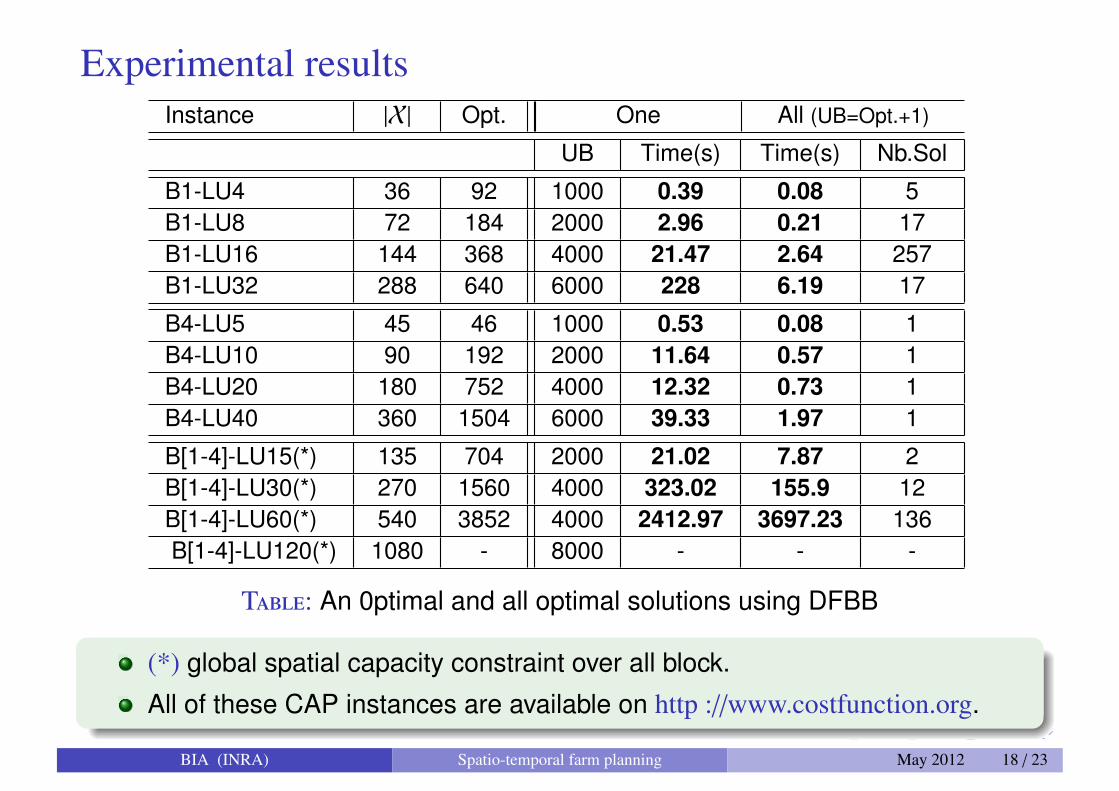
Experimental resultsInstance |X| Opt. One All (UB=Opt.+1)
UB Time(s) Time(s) Nb.Sol
B1-LU4 36 92 1000 0.39 0.08 5B1-LU8 72 184 2000 2.96 0.21 17B1-LU16 144 368 4000 21.47 2.64 257B1-LU32 288 640 6000 228 6.19 17
B4-LU5 45 46 1000 0.53 0.08 1B4-LU10 90 192 2000 11.64 0.57 1B4-LU20 180 752 4000 12.32 0.73 1B4-LU40 360 1504 6000 39.33 1.97 1
B[1-4]-LU15(*) 135 704 2000 21.02 7.87 2B[1-4]-LU30(*) 270 1560 4000 323.02 155.9 12B[1-4]-LU60(*) 540 3852 4000 2412.97 3697.23 136B[1-4]-LU120(*) 1080 - 8000 - - -
Table: An 0ptimal and all optimal solutions using DFBB
(*) global spatial capacity constraint over all block.
All of these CAP instances are available on http ://www.costfunction.org.
BIA (INRA) Spatio-temporal farm planning May 2012 18 / 23
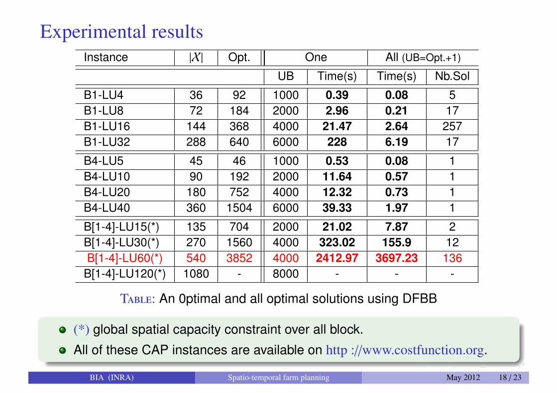
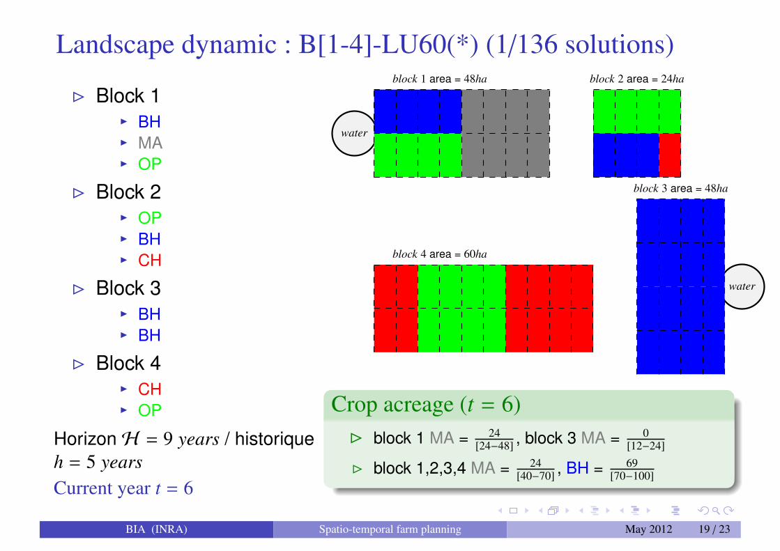
Landscape dynamic : B[1-4]-LU60(*) (1/136 solutions)
B Block 1I BHI MAI OP
B Block 2I OPI BHI CH
B Block 3I BHI BH
B Block 4I CHI OP
Horizon H = 9 years / historiqueh = 5 yearsCurrent year t = 6
water
water
block 1 area = 48ha block 2 area = 24ha
block 3 area = 48ha
block 4 area = 60ha
Crop acreage (t = 6)B block 1 MA = 24
[24−48] , block 3 MA = 0[12−24]
B block 1,2,3,4 MA = 24[40−70] , BH = 69
[70−100]
BIA (INRA) Spatio-temporal farm planning May 2012 19 / 23
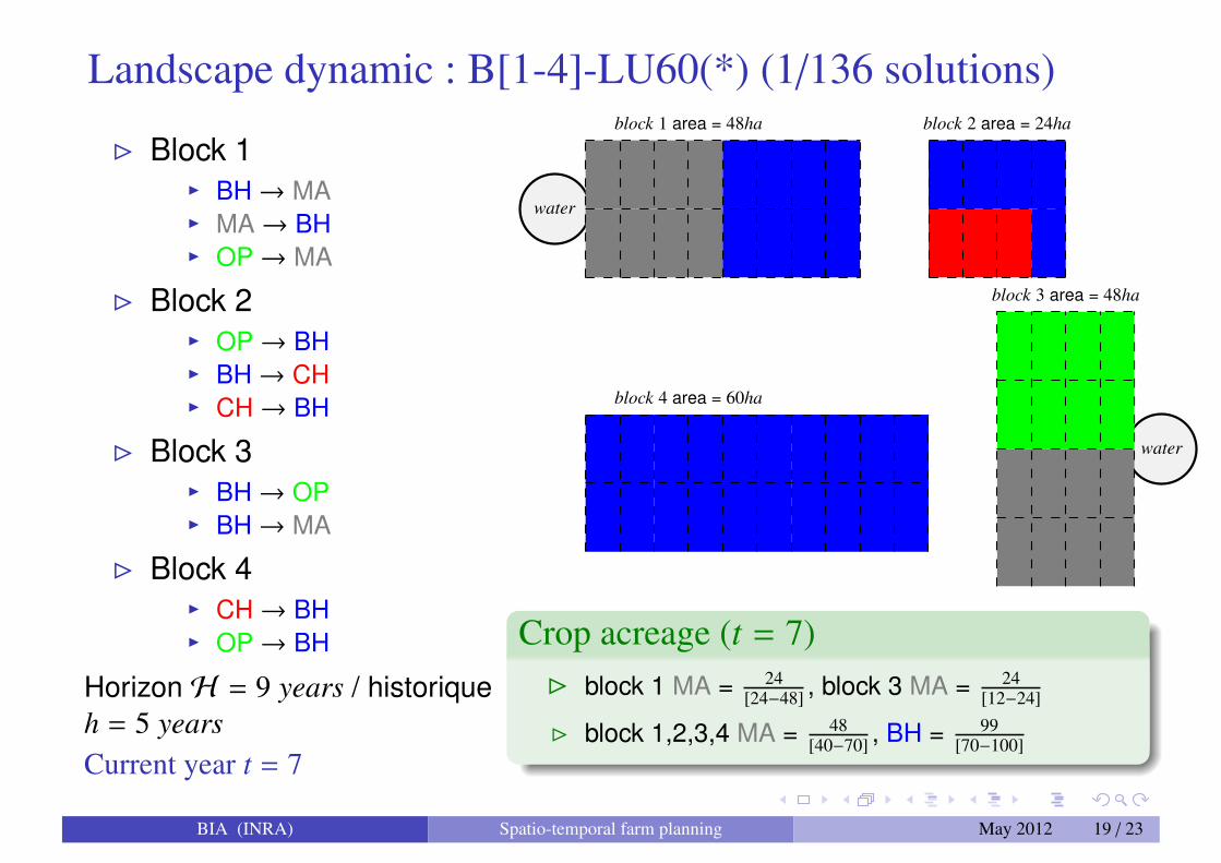
Landscape dynamic : B[1-4]-LU60(*) (1/136 solutions)
B Block 1I BH→ MAI MA→ BHI OP→ MA
B Block 2I OP→ BHI BH→ CHI CH→ BH
B Block 3I BH→ OPI BH→ MA
B Block 4I CH→ BHI OP→ BH
Horizon H = 9 years / historiqueh = 5 yearsCurrent year t = 7
water
water
block 1 area = 48ha block 2 area = 24ha
block 3 area = 48ha
block 4 area = 60ha
Crop acreage (t = 7)B block 1 MA = 24
[24−48] , block 3 MA = 24[12−24]
B block 1,2,3,4 MA = 48[40−70] , BH = 99
[70−100]
BIA (INRA) Spatio-temporal farm planning May 2012 19 / 23
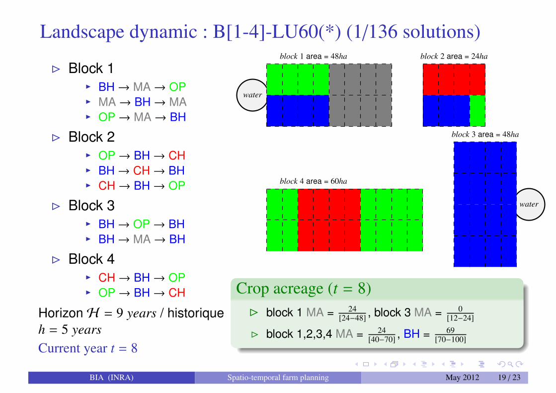
Landscape dynamic : B[1-4]-LU60(*) (1/136 solutions)
B Block 1I BH→ MA→ OPI MA→ BH→ MAI OP→ MA→ BH
B Block 2I OP→ BH→ CHI BH→ CH→ BHI CH→ BH→ OP
B Block 3I BH→ OP→ BHI BH→ MA→ BH
B Block 4I CH→ BH→ OPI OP→ BH→ CH
Horizon H = 9 years / historiqueh = 5 yearsCurrent year t = 8
water
water
block 1 area = 48ha block 2 area = 24ha
block 3 area = 48ha
block 4 area = 60ha
Crop acreage (t = 8)B block 1 MA = 24
[24−48] , block 3 MA = 0[12−24]
B block 1,2,3,4 MA = 24[40−70] , BH = 69
[70−100]
BIA (INRA) Spatio-temporal farm planning May 2012 19 / 23
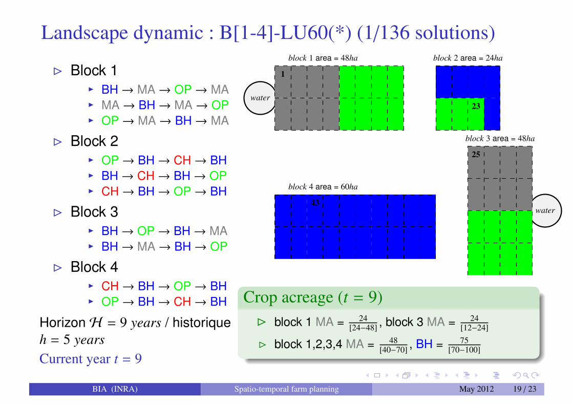
Landscape dynamic : B[1-4]-LU60(*) (1/136 solutions)
B Block 1I BH→ MA→ OP→ MAI MA→ BH→ MA→ OPI OP→ MA→ BH→ MA
B Block 2I OP→ BH→ CH→ BHI BH→ CH→ BH→ OPI CH→ BH→ OP→ BH
B Block 3I BH→ OP→ BH→ MAI BH→ MA→ BH→ OP
B Block 4I CH→ BH→ OP→ BHI OP→ BH→ CH→ BH
Horizon H = 9 years / historiqueh = 5 yearsCurrent year t = 9
water
water
block 1 area = 48ha block 2 area = 24ha
block 3 area = 48ha
block 4 area = 60ha
1
23
25
43
Crop acreage (t = 9)B block 1 MA = 24
[24−48] , block 3 MA = 24[12−24]
B block 1,2,3,4 MA = 48[40−70] , BH = 75
[70−100]
BIA (INRA) Spatio-temporal farm planning May 2012 19 / 23
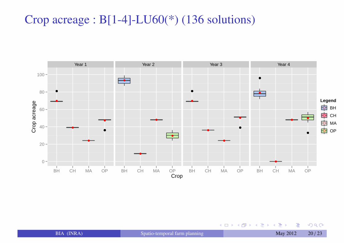
Crop acreage : B[1-4]-LU60(*) (136 solutions)
Crop
Cro
p ac
reag
e
0
20
40
60
80
100
Year 1
●●●●●●●●
●●●●●●●●
●
●
●
●
BH CH MA OP
Year 2
●
●
●
●
BH CH MA OP
Year 3
●●●●●●●●
●●●●●●●●
●
●
●
●
BH CH MA OP
Year 4
●●●●●●●●
●●●●●●●●
●
●
●●
BH CH MA OP
Legend
● BH
● CH
● MA
● OP
BIA (INRA) Spatio-temporal farm planning May 2012 20 / 23
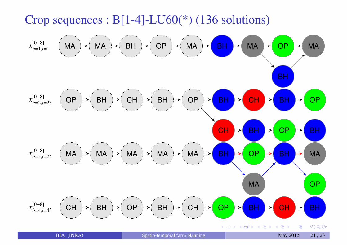
Crop sequences : B[1-4]-LU60(*) (136 solutions)
MA MA BH OP MA BH MA OP MA
BH
x[0−8]b=1,i=1
OP BH CH BH OP BH CH BH OP
CH BH OP BH
x[0−8]b=2,i=23
MA MA MA MA MA BH OP BH MA
MA OP
x[0−8]b=3,i=25
CH BH OP BH CH OP BH CH BHx[0−8]b=4,i=43
BIA (INRA) Spatio-temporal farm planning May 2012 21 / 23
Conclusion
Existing works are mainly focused on the spatial (crop acreage ) orthe temporal (crop sequence) aspects.
Our approach combines both the spatial and the temporal aspects ofCAP.
The results have shown that on small and middle CAP, relevantsolutions can be found in acceptable computational time.
Limitation due to the resource management seen as a countingproblem (cumulative).
costRegular constraint to mixe the return time and preceding effects.
Dealing with large CAP.
BIA (INRA) Spatio-temporal farm planning May 2012 22 / 23

Questions ?
BIA (INRA) Spatio-temporal farm planning May 2012 23 / 23