Embed Size (px)
Citation preview

UNIVERSITE DE MONTREAL
GESTION DE LA QUALITE DE SERVICE ET PLANIFICATION OPTIMALE DE
RESEAUX DE CAPTEURS MULTIMEDIA SANS FIL
LUIS COBO CAMPO
DEPARTEMENT DE GENIE INFORMATIQUE ET GENIE LOGICIEL
ECOLE POLYTECHNIQUE DE MONTREAL
THESE PRESENTEE EN VUE DE L’OBTENTION
DU DIPLOME DE PHILOSOPHIÆ DOCTOR
(GENIE INFORMATIQUE)
AOUT 2011
c© Luis Cobo Campo, 2011.

UNIVERSITE DE MONTREAL
ECOLE POLYTECHNIQUE DE MONTREAL
Cette these intitulee :
GESTION DE LA QUALITE DE SERVICE ET PLANIFICATION OPTIMALE DE
RESEAUX DE CAPTEURS MULTIMEDIA SANS FIL
presentee par : COBO CAMPO, Luis
en vue de l’obtention du diplome de : Philosophiæ Doctor
a ete dument acceptee par le jury d’examen constitue de :
Mme. BELLAICHE, Martine, Ph.D.,presidente.
M. QUINTERO, Alejandro, Doct., membre et directeur de recherche.
M. PIERRE, Samuel, Ph.D., membre et codirecteur de recherche.
M. CHAMBERLAND, Steven, Ph.D., membre.
M. AJIB, Wessam, Ph.D., membre externe.
iii
a dona Judith,
la autora de mis dıas. . .

iv
REMERCIEMENTS
Tout d’abord, j’aimerais remercier mon directeur de recherche, le professeur Alejandro
Quintero, pour son encadrement, ses conseils, ses commentaires et son encouragement. Je
lui exprime aussi ma reconnaissance pour m’avoir fourni le soutien financier necessaires a
l’accomplissement de mon travail de recherche et pour m’avoir accepte comme son etudiant
a nouveau apres plusieurs annees.
Je voudrais egalement remercier mon codirecteur, le professeur Samuel Pierre, pour ses
commentaires opportunes de mon travail doctoral et aussi, pour m’avoir donne l’opportunite
de faire partie de cette grande famille qui est LARIM.
Mes remerciements vont aussi aux membres de mon jury, les professeurs Martine Bellaıche,
Steven Chamberland et Wessam Ajib, qui, malgre leurs multiples occupations, m’ont accorde
leur temps pour evaluer cette these.
Finalement, j’aimerais exprimer ma profonde et sincere gratitude a ma mere, mes freres,
ma sœur, mes neveux et ma niece. Merci beaucoup de leur support, leur patience et leur
comprehension. Sans l’amour et l’encouragement que j’ai recu d’eux il aurait ete pratiquement
impossible finir ce projet de vie appele doctorat.
A vous tous, un GROS Merci !
v
RESUME
Un Reseau de capteurs sans fil (RCSF) est constitue d’un certain nombre d’entites (cap-
teurs) geographiquement dispersees, de taille reduite, avec une autonomie et une puissance
de traitement reduites. Ces dispositifs sont utilises pour realiser, de maniere independante,
des taches comme la surveillance, le controle de processus industriel, etc. Les avancees en
microelectronique ont conduit a l’emergence des petites cameras (type Complimentary Metal
Oxide Silicon (CMOS)) et microphones accessibles. Ces capteurs audio-visuels peuvent etre
integres dans un RCSF pour former des Reseau de capteurs multimedia sans fil (RCMSF).
Dans certains types d’applications, comme la surveillance des frontieres, un grand nombre de
ce type de capteurs est susceptible d’etre deployes, sur de vastes terrains. Un volume consi-
derable de flux audio-visuel (en plus des donnees) doit etre transmis au centre de controle
(le collecteur, ou SINK ) pour analyse et prise de decision. Il y a donc un besoin important
en termes de bande passante, avec surtout une forte contrainte en termes de delai de trans-
mission et d’autres parametres de RCSF. Des solutions pour le routage d’information ont ete
developpees pour des RCSF, mais ces protocoles n’ont pas pris en compte la generation a
grande echelle des donnees multimedia, elles sont par consequent inadaptees aux RCMSF.
Les capteurs typiquement sont omnidirectionnels, c’est-a-dire qu’ils sont capables de cap-
ter des signaux qui proviennent de toutes les directions autour d’eux. Les capteurs multime-
dia, en particulier les capteurs de video, sont de type directionnel. Pour ce type de capteurs,
l’aire de captage est limitee a un secteur donne d’un plan tridimensionnel. Malheureusement,
les modeles mathematiques developpes pour le placement des RCMSF conventionnels ne
peuvent pas etre appliques dans le cadre de la configuration et de la planification des reseaux
de capteurs directionnels. De nouveaux modeles d’optimisation sont donc necessaires pour la
capture des principaux parametres caracterisant les capteurs directionnels.
Dans cette these, nous abordons donc les problemes cles suivants : le routage des don-
nees heterogenes (scalaires et multimedia) pour les nœuds d’un RCMSF afin d’assurer une
meilleure Qualite de Service (QdS) aux usagers ; et le deploiement optimise de capteurs direc-
tionnels d’un RCMSF dans un espace tridimensionnel dont le but est couvrir un ensemble de
points d’interets definis dans tel espace. Notre these se compose de trois articles scientifiques,
chacun traitant d’une problematique bien specifique.
Le premier article traite du probleme du routage d’information pour les RCMSF base
sur la QdS. Nous proposons un nouveau protocole, AntSensNet, base sur l’heuristique de
la colonie de fourmis, qui utilise plusieurs metriques de QdS pour trouver de bonnes routes
pour les donnees multimedia et l’information scalaire. Dans la pratique, le protocole etablit

vi
d’abord une structure hierarchique sur le reseau avant de choisir les chemins appropries pour
repondre aux diverses exigences de QdS des differents types de trafic qui circulent dans le
reseau. Ceci permet de maximiser l’utilisation des ressources du reseau, tout en ameliorant la
performance de la transmission de l’information. En outre, AntSensNet est capable d’utiliser
un mecanisme efficace d’ordonnancement de paquets et de multiples chemins afin d’obtenir
la distorsion minimale au moment ou une application fait la transmission de la video dans le
reseau.
Dans le deuxieme article nous continuons avec le sujet de la QdS dans le RCMSFs et,
plus specifiquement, nous abordons la problematique du controle d’admission pour ce type de
reseau. Grace au controle d’admission, il est possible de determiner si un reseau est capable de
supporter un nouveau flot de donnees. S’il n’y a pas de controle d’admission dans un RCMSF,
le performance du reseau sera compromis car les ressources existantes dans le reseau ne seront
pas assez pour tous les flots acceptes et cela entraınera beaucoup de problemes comme la
perte de paquets des flots. Nous proposons un nouveau schema de controle d’admission de
nouveaux flots multimedia pour un RCMSF. Le systeme propose est en mesure de determiner
si un flot de donnees puisse etre admis dans le reseau, compte tenu de l’etat actuel des
liaisons de communications et l’energie des nœuds. La decision sur l’acceptation est prise
de maniere distribuee, sans utiliser une entite centrale. De plus, notre schema se presente
comme un plug-in, et est adaptable a d’eventuels protocoles de routage et MAC utilises pour
la transmission de donnees dans les RCMSF. Nos resultats de simulation montrent l’efficacite
de notre approche pour repondre aux exigences de QdS des nouveaux flots de donnees.
Finalement, notre troisieme article traite du probleme du deploiement optimal des cap-
teurs multimedia dans un espace 3D. Tel que mentionne ci-dessus, la plupart des capteurs
multimedia sont du type directionnel. De surcroıt, ces capteurs sont plus couteux et plus
specialises que les capteurs scalaires. En consequence, les deploiements aleatoires, qui sont
typiques pour les capteurs scalaires, ne sont ni souhaitables ni adequats pour les capteurs
multimedia. A cet effet, nous proposons un modele optimal de deploiement 3D de capteurs
directionnels. Ce modele vise a determiner le nombre minimum de capteurs directionnels
connectes, leur emplacement et leur configuration, qui sont necessaires pour couvrir un en-
semble de points de controle dans un espace 3D donne. La configuration de chaque capteur
deploye est determinee par trois parametres : la plage de detection, le champ de vision (Field
of View (FoV)) et l’orientation. Nous presentons une formulation “Integer Linear Program-
ming” (ILP) pour trouver la solution exacte du probleme et aussi, un algorithme glouton
capable de trouver une solution approximative (mais efficace) du probleme. Nous evaluons
egalement differentes proprietes des solutions proposees par le biais de nombreuses simula-
tions.

vii
Avec ces trois articles on a reussi a resoudre, d’une facon a la fois innovatrice et pratique,
les problemes de routage base sur la QdS pour les RCMSF et le deploiement de capteurs
directionnels, qui sont l’objectif principal de notre recherche.

viii
ABSTRACT
A Wireless Sensor Network (WSN) consists of a set of embedded processing units, called
sensors, communicating via wireless links, whose main function is the collection of parameters
related to the surrounding environment, such as temperature, pressure or the presence/motion
of objects. WSN are expected to have many applications in various fields, such as industrial
processes, military surveillance, observation and monitoring of habitat, etc. The availability
of inexpensive hardware such as CMOS cameras and microphones that are able to ubiqui-
tously capture multimedia content from the environment has fostered the development of
Wireless Multimedia Sensor Networks (WMSNs), i.e., networks of wirelessly interconnected
devices that allow retrieving video and audio streams, still images, and scalar sensor data. In
addition to the ability to retrieve multimedia data, WMSNs will be able to store, process in
real time, correlate and fuse multimedia data originated from heterogeneous sources, and per-
form actions on the environment based on the content gathered. Many applications require
the sensor network paradigm to be rethought in view of the need for mechanisms to deliver
multimedia content with a certain level of quality of service (QoS). Due to high bandwidth,
processing and stringent Qos requirements existing solutions are not feasible for WMSNs.
Since the need to minimize the energy consumption has driven most of the research in sensor
networks so far, there is a need to create mechanisms to efficiently deliver application-level
QoS, and to map these requirements to network-layer metrics such as latency or delay.
Additionally, in WSNs, an omnidirectional sensing model is often assumed where each
sensor can equally detect its environment in each direction. Instead, multimedia sensors,
specially video sensor, are directional sensors. A directional sensor is characterized by its
sensing region which can be viewed as a sector in a three-dimensional plane. Therefore, it
can only choose one active sector (or direction) at any time instant. Unfortunately, the many
methods developed for deploying traditional WSNs cannot directly be used for optimizing
and configuring directional WMSNs due to the different parameters involved. Therefore, new
optimization models which capture the primary parameters characterizing directional sensors
are necessary.
The issues aforementioned are crucial challenges for the development of WMSNs. In
this thesis, we are interested in the following aspects: routing of heterogeneous data (scalar
and multimedia) from the nodes of a WMSN to the sink in order to provide better QoS
experience to users; and an optimized deployment of directional sensors of a WMSN in a
three-dimensional surface with the objective to cover all the control points as defined in such
a space. Our thesis runs through three scientific papers, each addressing a specific problem.

ix
In our first paper, we address the problem of data routing based on different QoS metrics
in a WMSN. We propose a new protocol AntSensNet, based on the traditional ant-based
algorithm. The AntSensNet protocol builds a hierarchical structure on the network before
choosing suitable paths to meet various QoS requirements from different kinds of traffic, thus
maximizing network utilization, while improving its performance. In addition, AntSensNet
is able to use a efficient multipath video packet scheduling in order to get minimum video
distortion transmission.
In the second paper, we address the problem of connection admission control for WMSNs.
With admission control, it is possible to determine whether a network is capable of supporting
a new data stream. Without admission control in a WMSN, the network performance will
be compromised because the existing resources within the network cannot be enough for all
the flows accepted and this will cause many problems such as packet loss and congestion.
Taking multiple parameters into account, we propose a novel connection admission control
scheme for the multimedia traffic circulating in the network. The proposed scheme is able to
determine if a new flow can be admitted in the network considering the current link states
and the energy of the nodes. The decision about accepting is taken in a distributed way,
without trusting in a central entity to take this decision. In addition, our scheme works like
a plug-in, being easily adaptable to any routing and MAC protocols. Our simulation results
show the effectiveness of our approach to satisfy QoS requirements of flows and achieve fair
bandwidth utilization and low jitter.
Finally, in the third paper, we address the problem of optimal deployment of directional
sensors in a 3D space. We have already mentioned that conventional methods to deploy
omnidirectional sensors are not suitable to deploy directional sensors. To remedy this defi-
ciency, we propose a mathematical model which aims at to determine the minimum number
of connected directional multimedia sensor nodes and their configuration, needed to cover
a set of control points in a given 3D space. The configuration of each deployed sensor is
determined by three parameters: sensing range, field of view and orientation. We present the
exact ILP formulation for the problem and an approximate (but computationally efficient)
greedy algorithm solution. We also evaluate different properties of the proposed solutions
through extensive simulations.
Overall, the proposed solutions in this thesis are both innovative and practical. With
these three papers, we have been successfully resolved the problems of a QoS-based routing
protocol for WMSN and an optimal deployment of directional sensors in a 3D space, which
are the components of the main objective of this thesis.

x
TABLE DES MATIERES
DEDICACE . . . . . . . . . . . . . . . . . . . . . . . . . . . . . . . . . . . . . . . . . . iii
REMERCIEMENTS . . . . . . . . . . . . . . . . . . . . . . . . . . . . . . . . . . . . . iv
RESUME . . . . . . . . . . . . . . . . . . . . . . . . . . . . . . . . . . . . . . . . . . . v
ABSTRACT . . . . . . . . . . . . . . . . . . . . . . . . . . . . . . . . . . . . . . . . . viii
TABLE DES MATIERES . . . . . . . . . . . . . . . . . . . . . . . . . . . . . . . . . . x
LISTE DES TABLEAUX . . . . . . . . . . . . . . . . . . . . . . . . . . . . . . . . . . xiii
LISTE DES FIGURES . . . . . . . . . . . . . . . . . . . . . . . . . . . . . . . . . . . . xiv
LISTE DES SIGLES ET ABREVIATIONS . . . . . . . . . . . . . . . . . . . . . . . . xv
CHAPITRE 1 INTRODUCTION . . . . . . . . . . . . . . . . . . . . . . . . . . . . . 1
1.1 Definitions et concepts de base . . . . . . . . . . . . . . . . . . . . . . . . . . . 2
1.2 Elements de la problematique . . . . . . . . . . . . . . . . . . . . . . . . . . . 5
1.3 Objectifs de recherche . . . . . . . . . . . . . . . . . . . . . . . . . . . . . . . 9
1.4 Principales contributions de la these et leur originalite . . . . . . . . . . . . . . 9
1.5 Plan du memoire . . . . . . . . . . . . . . . . . . . . . . . . . . . . . . . . . . 10
CHAPITRE 2 REVUE DE LITTERATURE . . . . . . . . . . . . . . . . . . . . . . . 12
2.1 Qualite de service pour les RCMSF . . . . . . . . . . . . . . . . . . . . . . . . 12
2.1.1 La couche application . . . . . . . . . . . . . . . . . . . . . . . . . . . . 12
2.1.2 La couche reseau . . . . . . . . . . . . . . . . . . . . . . . . . . . . . . 13
2.2 Deploiement de capteurs directionnels . . . . . . . . . . . . . . . . . . . . . . . 19
CHAPITRE 3 ANT-BASED ROUTING FOR WIRELESS MULTIMEDIA SENSOR
NETWORKS USING MULTIPLE QOS METRICS . . . . . . . . . . . . . . . . . . 21
3.1 Introduction . . . . . . . . . . . . . . . . . . . . . . . . . . . . . . . . . . . . . 22
3.2 Related Work . . . . . . . . . . . . . . . . . . . . . . . . . . . . . . . . . . . . 23
3.3 The AntSensNet Protocol . . . . . . . . . . . . . . . . . . . . . . . . . . . . . 29
3.3.1 WMSNs QoS Routing Model . . . . . . . . . . . . . . . . . . . . . . . 30
3.3.2 Assumptions . . . . . . . . . . . . . . . . . . . . . . . . . . . . . . . . . 31

xi
3.3.3 Clustering Process . . . . . . . . . . . . . . . . . . . . . . . . . . . . . 32
3.3.4 AntSensNet Algorithm Description . . . . . . . . . . . . . . . . . . . . 38
3.4 Experimental Results . . . . . . . . . . . . . . . . . . . . . . . . . . . . . . . . 49
3.4.1 The Clustering Process . . . . . . . . . . . . . . . . . . . . . . . . . . . 49
3.4.2 The Routing Process . . . . . . . . . . . . . . . . . . . . . . . . . . . . 50
3.4.3 Influence of Network Loading . . . . . . . . . . . . . . . . . . . . . . . 53
3.4.4 Video Transmission . . . . . . . . . . . . . . . . . . . . . . . . . . . . . 54
3.5 Conclusion . . . . . . . . . . . . . . . . . . . . . . . . . . . . . . . . . . . . . . 55
CHAPITRE 4 A DISTRIBUTED CONNECTION ADMISSION CONTROL STRA-
TEGY FOR WIRELESS MULTIMEDIA SENSOR NETWORKS . . . . . . . . . . 58
4.1 Introduction . . . . . . . . . . . . . . . . . . . . . . . . . . . . . . . . . . . . . 58
4.2 Related Work . . . . . . . . . . . . . . . . . . . . . . . . . . . . . . . . . . . . 60
4.3 Our Proposed Algorithm . . . . . . . . . . . . . . . . . . . . . . . . . . . . . . 62
4.3.1 Network Model . . . . . . . . . . . . . . . . . . . . . . . . . . . . . . . 62
4.3.2 Operation of our CAC approach . . . . . . . . . . . . . . . . . . . . . . 62
4.3.3 Assumptions . . . . . . . . . . . . . . . . . . . . . . . . . . . . . . . . . 62
4.4 Experimental Results . . . . . . . . . . . . . . . . . . . . . . . . . . . . . . . . 66
4.5 Conclusions . . . . . . . . . . . . . . . . . . . . . . . . . . . . . . . . . . . . . 72
CHAPITRE 5 INTEGER PROGRAMMING FORMULATION AND GREEDY AL-
GORITHM FOR 3-D DIRECTIONAL SENSOR PLACEMENT IN WMSN . . . . 75
5.1 Introduction . . . . . . . . . . . . . . . . . . . . . . . . . . . . . . . . . . . . . 75
5.2 Related Work . . . . . . . . . . . . . . . . . . . . . . . . . . . . . . . . . . . . 77
5.3 Problem Formulation . . . . . . . . . . . . . . . . . . . . . . . . . . . . . . . . 79
5.3.1 Assumptions . . . . . . . . . . . . . . . . . . . . . . . . . . . . . . . . . 79
5.3.2 Sensing Model of 3D Directional Sensors . . . . . . . . . . . . . . . . . 80
5.3.3 Problem Statement . . . . . . . . . . . . . . . . . . . . . . . . . . . . . 81
5.3.4 Coverage by Directional Sensors . . . . . . . . . . . . . . . . . . . . . . 81
5.3.5 Problem Modeling . . . . . . . . . . . . . . . . . . . . . . . . . . . . . 83
5.4 Proposed Heuristic . . . . . . . . . . . . . . . . . . . . . . . . . . . . . . . . . 86
5.5 Computational Results . . . . . . . . . . . . . . . . . . . . . . . . . . . . . . . 87
5.5.1 Comparative Evaluation : Greedy vs CPLEX . . . . . . . . . . . . . . . 88
5.5.2 Impact of the Sensing Range . . . . . . . . . . . . . . . . . . . . . . . . 90
5.5.3 Impact of the FoV . . . . . . . . . . . . . . . . . . . . . . . . . . . . . 91
5.6 Conclusions . . . . . . . . . . . . . . . . . . . . . . . . . . . . . . . . . . . . . 91

xii
CHAPITRE 6 DISCUSSION GENERALE . . . . . . . . . . . . . . . . . . . . . . . . 93
6.1 Synthese des travaux . . . . . . . . . . . . . . . . . . . . . . . . . . . . . . . . 93
6.2 Methodologie . . . . . . . . . . . . . . . . . . . . . . . . . . . . . . . . . . . . 94
6.3 Analyse des resultats . . . . . . . . . . . . . . . . . . . . . . . . . . . . . . . . 94
CHAPITRE 7 CONCLUSION . . . . . . . . . . . . . . . . . . . . . . . . . . . . . . . 96
7.1 Sommaire des contributions de la these . . . . . . . . . . . . . . . . . . . . . . 96
7.2 Limitations de la solution proposee . . . . . . . . . . . . . . . . . . . . . . . . 97
7.3 Ameliorations futures . . . . . . . . . . . . . . . . . . . . . . . . . . . . . . . . 97
REFERENCES . . . . . . . . . . . . . . . . . . . . . . . . . . . . . . . . . . . . . . . . 99
xiii
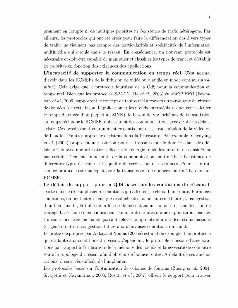
LISTE DES TABLEAUX
Tableau 3.1 Abilities Of Video And Standard Sensors . . . . . . . . . . . . . . . . . 34
Tableau 3.2 Pheromone table for Node i . . . . . . . . . . . . . . . . . . . . . . . . 40
Tableau 4.1 Comparison among admission control schemes . . . . . . . . . . . . . . 73
Tableau 5.1 Comparison between found solutions for CPLEX and Greedy algorithm 89
Tableau 5.2 CPLEX vs Greedy algorithm with large instances . . . . . . . . . . . . 90

xiv
LISTE DES FIGURES
Figure 1.1 Un exemple d’un RCSF . . . . . . . . . . . . . . . . . . . . . . . . . . 2
Figure 1.2 Un capteur de video Stargate . . . . . . . . . . . . . . . . . . . . . . . 4
Figure 1.3 Les parametres de la configuration d’un capteur directionnel : α = angle
avec la verticale, θ = ouverture de la camera, Rs = rayon de detection 5
Figure 2.1 Exemple de routes formes par RGD avec PathNum = 2 . . . . . . . . . 17
Figure 2.2 Schema de routage du protocole presente dans (Wu et Abouzeid, 2006) 19
Figure 3.1 WMSN clustering example. The backbone created by CHs is outlined
in black. . . . . . . . . . . . . . . . . . . . . . . . . . . . . . . . . . . . 37
Figure 3.2 Queuing model on a multimedia sensor node . . . . . . . . . . . . . . . 39
Figure 3.3 Route Discovery Process of AntSensNet . . . . . . . . . . . . . . . . . 41
Figure 3.4 The CH connectivity at various simulation time for AntSensNet and
T-ANT. . . . . . . . . . . . . . . . . . . . . . . . . . . . . . . . . . . . 50
Figure 3.5 Network lifetime vs simulation time for T-ANT and AntSensNet. . . . 51
Figure 3.6 Packet Delivery Ratio. . . . . . . . . . . . . . . . . . . . . . . . . . . . 52
Figure 3.7 End-to-end delay. . . . . . . . . . . . . . . . . . . . . . . . . . . . . . . 53
Figure 3.8 Routing overhead. . . . . . . . . . . . . . . . . . . . . . . . . . . . . . 54
Figure 3.9 Results of varying number of data connections on (a) PDR and (b)
average end-to-end delay . . . . . . . . . . . . . . . . . . . . . . . . . . 55
Figure 3.10 Received Video Quality of Foreman video . . . . . . . . . . . . . . . . 56
Figure 4.1 Connection Admission Control (CAC) Modelling . . . . . . . . . . . . 63
Figure 4.2 Throughput for flows with admission control . . . . . . . . . . . . . . . 69
Figure 4.3 Packet delay for flows with admission control . . . . . . . . . . . . . . . 70
Figure 4.4 Throughput of flows without admission control . . . . . . . . . . . . . 71
Figure 4.5 Throughput of flows with admission control . . . . . . . . . . . . . . . 72
Figure 4.6 Packet delay of flows without admission control . . . . . . . . . . . . . 73
Figure 4.7 Packet delay of flows admission control . . . . . . . . . . . . . . . . . . 74
Figure 5.1 FoV parameters . . . . . . . . . . . . . . . . . . . . . . . . . . . . . . . 81
Figure 5.2 Process to know if a point is covered in 2D . . . . . . . . . . . . . . . . 82
Figure 5.3 Performance Evaluation . . . . . . . . . . . . . . . . . . . . . . . . . . 91

xv
LISTE DES SIGLES ET ABREVIATIONS
WSN Wireless Sensor Network
WMSN Wireless Multimedia Sensor Network
CMOS Complimentary Metal Oxide Silicon
MEMS Micro-Electro-Mechanical System
QdS Qualite de Service
QoS Quality of Service
FoV Field of View
RCSF Reseau de capteurs sans fil
RCMSF Reseau de capteurs multimedia sans fil
ILP Integer Linear Programming
ACO Ant Colony Optimization
FEC Forward Error Correction
WFQ Weighted Fair Queuing
MANET Mobile Ad-hoc Networks
FANT Forward Ant
BANT Backward Ant
CH Cluster Head
M3DSP Minimum 3D Directional Sensor Placement
CAC Connection Admission Control

1
CHAPITRE 1
INTRODUCTION
Un RCSF est un systeme constitue de plusieurs dizaines a plusieurs centaines de nœuds
interconnectes, constitues chacun d’un capteur, d’une unite de traitement de l’information
et d’un bloc de communication (Akyildiz et al., 2002). Les nœuds disposent d’une zone de
couverture extremement reduite et sont deployes d’une maniere dense dans des environne-
ments heterogenes. Ils sont autonomes et disposent pour cela d’une reserve energetique, dont
le renouvellement peut s’averer impossible, ce qui limite leur duree de vie. Chacun des nœuds
doit etre en mesure de traiter les donnees recues, de prendre une decision locale et de la com-
muniquer de facon autonome aux nœuds voisins auxquels il est connecte. Cette cooperation
est destinee a assurer les meilleures prises de decision possibles malgre les limites en termes de
consommation energetique et de puissance de traitement. En effet, les RCSF sont assujettis a
des contraintes fortes et de natures multiples, energetique et calculatoire entre autres, ce qui
limite les capacites de traitement et de communication des nœuds du reseau. Etant donne la
rapide miniaturisation du materiel, un petit capteur peut etre equipe de modules de collecte
d’information visuelle et d’audio. Ces capteurs sont habilites a capturer du contenu multime-
dia (video, son, images) de l’environnement, ce qui a facilite le developpement des RCMSF.
Ce nouveau type de reseau ameliorera les applications deja existantes des reseaux de capteurs
(telles que la domotique ou la surveillance), mais aussi permettra la realisation d’applications
vraiment novatrices, comme des nouveaux services de localisation de personnes, le controle
environnemental ou l’assistance aux personnes agees.
Cette diversite d’applications amene ces reseaux a supporter differents types de trafics et
a fournir des services qui doivent etre a la fois generiques et adaptatifs aux applications car les
proprietes de la QdS different d’un type d’applications a un autre. Neanmoins, jusqu’a present,
le besoin de reduire au minimum la consommation d’energie a fait objet de la plupart des
recherches des RCSF. Peu d’etudes dans le domaine concernent les mecanismes pour delivrer
efficacement la QdS au niveau applicatif a partir de metriques de niveaux reseau et liaison
comme le delai ou la bande passante. Dans cet ordre d’idees, nous allons nous interesser dans
cette these aux mecanismes d’implantation de la QdS pour le RCMSF et comment deployer
ce type de reseau. Dans ce chapitre, nous commencerons par donner une breve description des
reseaux de capteurs multimedia, leurs applications et leurs principaux defis. Ensuite, nous
presenterons quelques elements de la problematique, lies principalement au routage base sur
la QdS. Puis, nous detaillerons nos objectifs de recherche et enfin, nous presenterons le plan
2
de cette these.
1.1 Definitions et concepts de base
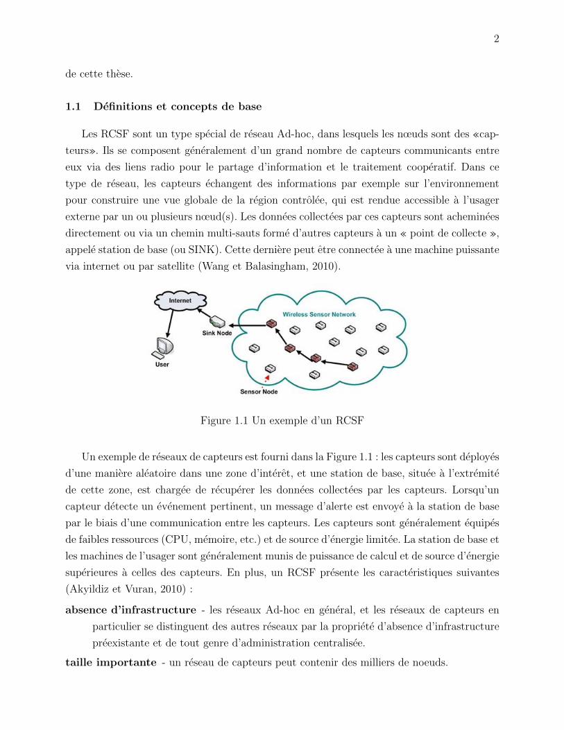
Les RCSF sont un type special de reseau Ad-hoc, dans lesquels les nœuds sont des «cap-
teurs». Ils se composent generalement d’un grand nombre de capteurs communicants entre
eux via des liens radio pour le partage d’information et le traitement cooperatif. Dans ce
type de reseau, les capteurs echangent des informations par exemple sur l’environnement
pour construire une vue globale de la region controlee, qui est rendue accessible a l’usager
externe par un ou plusieurs nœud(s). Les donnees collectees par ces capteurs sont acheminees
directement ou via un chemin multi-sauts forme d’autres capteurs a un « point de collecte »,
appele station de base (ou SINK). Cette derniere peut etre connectee a une machine puissante
via internet ou par satellite (Wang et Balasingham, 2010).
Figure 1.1 Un exemple d’un RCSF
Un exemple de reseaux de capteurs est fourni dans la Figure 1.1 : les capteurs sont deployes
d’une maniere aleatoire dans une zone d’interet, et une station de base, situee a l’extremite
de cette zone, est chargee de recuperer les donnees collectees par les capteurs. Lorsqu’un
capteur detecte un evenement pertinent, un message d’alerte est envoye a la station de base
par le biais d’une communication entre les capteurs. Les capteurs sont generalement equipes
de faibles ressources (CPU, memoire, etc.) et de source d’energie limitee. La station de base et
les machines de l’usager sont generalement munis de puissance de calcul et de source d’energie
superieures a celles des capteurs. En plus, un RCSF presente les caracteristiques suivantes
(Akyildiz et Vuran, 2010) :
absence d’infrastructure - les reseaux Ad-hoc en general, et les reseaux de capteurs en
particulier se distinguent des autres reseaux par la propriete d’absence d’infrastructure
preexistante et de tout genre d’administration centralisee.
taille importante - un reseau de capteurs peut contenir des milliers de noeuds.

3
topologie dynamique - les capteurs peuvent etre attaches a des objets mobiles qui se de-
placent d’une facon libre et arbitraire rendant ainsi la topologie du reseau frequemment
changeante.
bande passante limitee - une des caracteristiques primordiales des reseaux bases sur la
communication sans fil est l’utilisation d’un medium de communication partage. Ce
partage fait que la bande passante reservee a un noeud est limitee.
contrainte d’energie, de stockage et de calcul - la caracteristique la plus critique dans
les reseaux de capteurs est la limitation de ses ressources energetiques car chaque cap-
teur du reseau possede de faibles ressources en termes d’energie (batterie). Afin de
prolonger la duree de vie du reseau, une minimisation des depenses energetiques est
exigee chez chaque noeud. Ainsi, la capacite de stockage et la puissance de calcul sont
limitees dans un capteur.Pour cette raison, il est important de disposer de protocoles
de routage efficaces en termes de conservation d’energie.
Les RCSF sont generalement deployes en grand nombre dans une zone geographique ou ils
vont capter, mesurer et rapporter certains phenomenes physiques. Ils peuvent donc servir a la
surveillance de leur environnement physique ainsi qu’a la surveillance de zones, la detection
d’intrusion, la detection de feu, la surveillance d’infrastructures civiles ou encore a l’analyse
climatique. Ils peuvent egalement etre utilises pour surveiller des habitations et contribuer
au confort domestique, en transformant les logements en environnements intelligents dont les
parametres (temperature, pression, humidite, luminosite, etc.) s’adaptent automatiquement
au comportement des individus (Li et al., 2008).
L’evolution recente de la technologie a permis de passer d’un modele ou les capteurs
sans fil etaient principalement dedies a la mesure de parametres environnementaux simples
comme la temperature ou l’humidite a des capteurs equipes de capacites multimedia. En
effet, la disponibilite de materiel et dispositifs abordables tels que les cameras et microphones
CMOS permettent aujourd’hui d’embarquer dans un capteur des cameras et des microphones.
Cyclops (Rahimi et al., 2005) et Stargate (Figure 1.2) sont deux exemples concrets de ce type
de capteurs multimedias communicants.
Ces capteurs font partie d’un reseau de capteurs multimedia sans fil (RCMSF). Un
RCMSF est un reseau de dispositifs interconnectes d’une maniere sans fil qui permet d’obtenir
des flots d’audio et de video, meme d’images et de donnees scalaires (Akyildiz et al., 2007).
Comme consequence de cette definition, on peut donc conclure que les composantes d’un
RCMSF sont capables de capter des donnees scalaires de l’environnement (tels que la tempe-
rature, la pression ou le niveau de lumiere) mais aussi des videos ou des sons ou des images
autour de lui. En outre, les reseaux seront en mesure de stocker, de traiter en temps reel,
de correler et de fusionner des donnes multimedias provenant de sources heterogenes. Bien

4
Figure 1.2 Un capteur de video Stargate
que les RCMSFs heritent des memes problemes et limitations des RCSFs, ils permettront
d’ameliorer les applications deja existantes sur les RCSF telles que le suivi de personnes,
la domotique, et la surveillance de l’environnement, mais egalement le developpement de
nouvelles applications telles que :
– Surveillance multimedia : Les capteurs de video et d’audio completeront et amelioreront
les systemes actuels de surveillance contre le crime et le terrorisme. Les RCMSFs aussi
permettront de controler des frontieres, des evenements publics et des proprietes privees.
Ces capteurs peuvent inferer et enregistrer des activites potentiellement pertinentes
(telles que des vols, des accidents de voitures ou des violations de trafic) et produire
des flots d’audio-video pour de futures enquetes.
– Trafic : Il sera possible de surveiller le trafic dans les rues des grandes villes et d’offrir
des services qui aident les conducteurs a eviter des congestions.
– Services de localisation de personnes : Le contenu multimedia (tel que des videos ou
des images), accompagne avec des techniques avancees de traitement de signaux, sera
utilise pour localiser des personnes disparues ou meme pour identifier des criminels ou
des terroristes dans les aeroports ou les terminaux.
– Telemedicine : Les capteurs de telemedicine peuvent etre integres avec des reseaux
multimedia 3G ou 4G pour fournir des services ubiquitaire de sante. Les patients por-
teront des capteurs medicaux pour surveiller des parametres tels que la temperature
du corps, la pression arterielle, l’oxymetrie pulsee, l’ECG, et l’activite respiratoire. De
plus, les centres de sante pourront realiser des controles a distance de leur patients via
des capteurs d’audio ou de mouvement, qui se trouvent implantes dans leur corps.
Un autre element differenciateur entre un RCSF et un RCMSF est le modele de capta-
tion qui est utilise par les capteurs qui font partie de ces reseaux. Les capteurs scalaires,
c’est-a-dire, les capteurs de temperature ou de pression ou de lumiere, suivent le modele
5
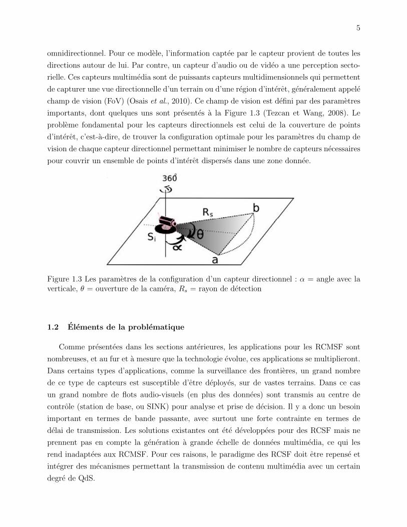
omnidirectionnel. Pour ce modele, l’information captee par le capteur provient de toutes les
directions autour de lui. Par contre, un capteur d’audio ou de video a une perception secto-
rielle. Ces capteurs multimedia sont de puissants capteurs multidimensionnels qui permettent
de capturer une vue directionnelle d’un terrain ou d’une region d’interet, generalement appele
champ de vision (FoV) (Osais et al., 2010). Ce champ de vision est defini par des parametres
importants, dont quelques uns sont presentes a la Figure 1.3 (Tezcan et Wang, 2008). Le
probleme fondamental pour les capteurs directionnels est celui de la couverture de points
d’interet, c’est-a-dire, de trouver la configuration optimale pour les parametres du champ de
vision de chaque capteur directionnel permettant minimiser le nombre de capteurs necessaires
pour couvrir un ensemble de points d’interet disperses dans une zone donnee.
Figure 1.3 Les parametres de la configuration d’un capteur directionnel : α = angle avec laverticale, θ = ouverture de la camera, Rs = rayon de detection
1.2 Elements de la problematique
Comme presentees dans les sections anterieures, les applications pour les RCMSF sont
nombreuses, et au fur et a mesure que la technologie evolue, ces applications se multiplieront.
Dans certains types d’applications, comme la surveillance des frontieres, un grand nombre
de ce type de capteurs est susceptible d’etre deployes, sur de vastes terrains. Dans ce cas
un grand nombre de flots audio-visuels (en plus des donnees) sont transmis au centre de
controle (station de base, ou SINK) pour analyse et prise de decision. Il y a donc un besoin
important en termes de bande passante, avec surtout une forte contrainte en termes de
delai de transmission. Les solutions existantes ont ete developpees pour des RCSF mais ne
prennent pas en compte la generation a grande echelle de donnees multimedia, ce qui les
rend inadaptees aux RCMSF. Pour ces raisons, le paradigme des RCSF doit etre repense et
integrer des mecanismes permettant la transmission de contenu multimedia avec un certain
degre de QdS.

6
La conservation de l’energie des capteurs et le maintien du reseau fonctionnel le plus long-
temps possible sont donc des defis importants qui sont poses par les RCSFs classiques. La
plupart d’algorithmes et protocoles valables pour les RCSFs utilisent cette contrainte ener-
getique comme l’element principal de leur conception et fonctionnement (Akkaya et Younis,
2005b). Malgre ces nombreuses approches recensees dans la litterature, force est de constater
que le probleme du support de la QdS pour les RCMSF est encore un probleme ouvert et
sans une solution satisfaisante.
Voici la liste des problemes que la QdS doit faire face dans les RCMSFs.
– Des mecanismes de controle d’admission inadequats. Quand un nœud a besoin
de generer un nouveau flot de donnees multimedia vers le SINK, des processus sont
necessaires pour savoir si le reseau a assez de ressources pour satisfaire les exigences de
ce flot, en termes de bande passante, de capacite des liens de communication ou de delai
de bout en bout par exemple. Les paradigmes de controle d’admission trouves dans la
litterature (notamment les articles (Perillo et Heinzelman, 2003) et (Yin et al., 2010))
sont inadequats pour les exigences des flots multimedia ou les schemas proposes par les
auteurs ne sont pas assez generaux pour prendre en compte des demandes de ressources
des nouvelles applications multimedia qui peuvent resider dans un RCMSF. Genera-
lement, ces solutions ne considerent que la consommation de l’energie pour admettre
un nouveau flot, tandis que d’autres importants aspects comme la bande passante, le
delai de bout en bout ou la gigue ne sont pas pris en compte. Il y a donc necessite de
concevoir des algorithmes pour le controle d’admission dans les RCMSF.
– L’absence d’un protocole de support de la QdS pour les reseaux de capteurs
multimedia. Comme nous l’avons deja mentionne, il y a beaucoup de protocoles de
routages pour les RCSFs. Et au fur et a mesure que les RCMSFs se rendent plus
populaires, il est tres probable que le nombre de ces protocoles augmente. Toutefois, a
notre connaissance, aucun de ces protocoles ne resout bel et bien les problemes courants
et futurs lies a la transmission de l’information multimedia dans un RCMSF.Parmi les
principaux defis, on trouve les suivants :
– Le support insuffisant pour le trafic heterogene. Le trafic multimedia requiert
un haut niveau d’heterogeneite car il est constitue de video, d’audio, et d’images.
De plus, il faut tenir compte du fait que le trafic dans un reseau de capteurs inclut
aussi des donnees scalaires (comme la temperature, la lumiere, etc.) qui sont captees
par les capteurs scalaires deployes dans le reseau. Autrement dit, dans le reseau,
circulent differents types de trafic que sont l’information multimedia et l’information
scalaire. Dans la litterature, on trouve que les protocoles concus pour la transmission
de la video (comme ceux proposes par Chen et al. (2007a) ou Politis et al. (2008)) ne
7
prennent en compte ni de multiples priorites ni l’existence de trafic heterogene. Par
ailleurs, les protocoles qui ont ete crees pour faire la differenciation des divers types
de trafic, ne tiennent pas compte des particularites et specificites de l’information
multimedia qui circule dans le reseau. En consequence, un nouveau protocole est
necessaire et doit etre capable de manipuler et classifier les types de trafic, et d’etablir
les priorites en fonction des exigences des applications.
– L’incapacite de supporter la communication en temps reel. C’est normal
d’avoir dans les RCMSFs de la diffusion de video ou d’audio en mode continu (strea-
ming). Cela exige que le protocole fournisse de la QdS pour la communication en
temps reel. Bien que les protocoles SPEED (He et al., 2003) et MMSPEED (Felem-
ban et al., 2006) supportent le concept de temps reel a travers du paradigme de vitesse
de donnees (de cette facon, l’application et les nœuds intermediaires peuvent calculer
le temps d’arrivee d’un paquet au SINK), le besoin de vrai schemas de transmission
en temps reel pour le RCMSF, qui assurent des communications avec de stricts delais,
existe. Ces besoins sont couramment ressentis lors de la transmission de la video ou
de l’audio. D’autres approches existent dans la litterature. Par exemple, Chenyang
et al. (2002) proposent une solution pour la transmission de donnees dans des de-
lais stricts avec une utilisation efficace de l’energie, mais les auteurs ne considerent
pas certains elements importants de la communication multimedia : l’existence de
differentes types de trafic et la qualite de service pour les donnees. Pour cette rai-
son, ce protocole est inadequat pour la transmission de donnees multimedia dans un
RCMSF.
– Le deficit de support pour la QdS basee sur les conditions du reseau. Il
existe dans le reseau plusieurs conditions qui affectent le choix d’une route. Parmi ces
conditions, on peut citer : l’energie residuelle des nœuds intermediaires, la congestion
d’un lien sans fil, la taille de la file de donnees dans un nœud, etc. Une decision de
routage basee sur ces metriques peut eliminer des routes qui ne supporteront pas des
transmissions avec une bande passante elevee ou qui introduiront des retransmissions
(et genereront des congestions) dues aux mauvaises conditions du canal.
Le protocole propose par Akkaya et Younis (2005a) est un bon exemple d’un protocole
qui s’adapte aux conditions du reseau. Cependant, le protocole a besoin d’ameliora-
tions par rapport a l’utilisation de la memoire des nœuds et la necessite de connaıtre
toute la topologie du reseau afin d’obtenir de bonnes routes. A defaut de ces amelio-
rations, il sera tres difficile de l’implanter.
Les protocoles bases sur l’optimisation de colonies de fourmis (Zheng et al., 2004;
Sivajothi et Naganathan, 2008; Rosati et al., 2007) offrent le support pour trouver

8
des routes en se basant sur de multiples metriques de qualite de service. Ces protocoles
tiennent compte de l’etat des nœuds du reseau et de ses liens pour transmettre les
paquets. En plus, cette adaptabilite aux conditions du reseau leur permet d’ameliorer
le « temps de vie » du reseau et de balancer la charge de routage sur un nombre plus
grand de nœuds. Toutefois, ces protocoles ne prennent pas en compte la diversite
du trafic dans les reseaux de capteurs multimedia et ne sont capables de gerer les
priorites de ce trafic. Enfin, il n’existe pas une facon de specifier le poids de chaque
metrique dans les decisions de routage, c’est-a-dire, ces protocoles n’ont pas l’habilite
de specifier l’importance de chaque metrique de QdS sur la route choisie.
Il y a donc un besoin de protocole qui prend en compte les conditions du reseau,
mais aussi, qui permet a la couche application de specifier quelques metriques ad-
ditionnelles (comme la bande passante, etc.) et leurs poids respectifs au moment de
trouver de bonnes routes. A notre connaissance, il n’existe pas encore de protocole
qui soit capable de trouver des routes a partir de plusieurs metriques en meme temps
et qui tienne compte des parametres stipules par les applications.
– Le deploiement de capteurs multimedia directionnels. La plupart des applica-
tions entrevues pour les RCMSF necessitent au prealable un placement optimal des
capteurs multimedia dans l’environnement. En effet, ces applications des reseaux de
capteurs tout comme certaines autres necessitent un placement des capteurs qui per-
met une couverture optimale de la zone a surveiller. Plusieurs techniques de placement
optimal de capteurs ont ete proposees dans la litterature (Younis et Akkaya, 2008).
Cependant celle-ci le sont pour des capteurs scalaires (i.e. capteurs avec des capacites
de capture omnidirectionnelles) et homogenes (i.e. etendu de la couverture du capteur).
Osais et al. (2010) propose un algorithme pour les capteurs directionnels, mais il consi-
dere seulement un deploiement homogene au niveau du sol, et cela n’est pas realiste
pour la plupart des capteurs de video ou d’audio. Par ailleurs, les reseaux de capteurs
multimedia sont par essence heterogenes (i.e. Puissance du microphone et zoom de la
camera) et directionnels (i.e. angle d’ouverture de la camera ou du microphone) ce qui
les rend completement differents des capteurs scalaires. Ces deux caracteristiques (he-
terogeneite et capture directionnelle) rendent le probleme de placement plus complexe
que ce que nous avions avec les capteurs scalaires. Les techniques de placement opti-
males proposees precedemment dans la litterature ne peuvent donc pas etre utilisees
directement. Un schema specifique pour le placement optimise de capteurs multimedia
directionnels en fonction de leurs capacites est donc necessaire. Celle-ci devra permettre
de placer les capteurs multimedia communicants dans le but de couvrir de facon opti-
male une zone visee.
9
1.3 Objectifs de recherche
L’objectif principal de cette these est de concevoir des mecanismes efficaces pour la ges-
tions et le support de la qualite de services (QdS) dans les reseaux de capteurs multimedia
sans fil (RCMSF) en mettant l’accent sur le processus de routage et de deploiement. De
maniere plus specifique, cette these vise a :
1. Analyser les solutions proposees dans la litterature pour le routage et la gestion de
la QdS, dans les RCSFs et les RCMSF, ainsi que les mecanismes proposes pour le
deploiement de capteurs. Le but est d’en ressortir les faiblesses et les limitations qui ne
sont pas encore resolues adequatement.
2. Proposer un nouveau protocole de routage adaptative pour les RCMSFs. Le protocole
garantira des metriques diverses de QdS, telles que : a) une bande passante, b) un faible
taux de pertes, c) un delai specifique et d) une gigue minimale, tout en minimisant la
consommation d’energie des nœuds capteurs qui font partie du reseau.
3. Evaluer la performance du protocole propose au point precedent en le comparant aux
principaux modeles recenses dans la litterature.
4. Proposer une strategie de controle d’admission pour les RCMSF. Cette strategie per-
mettra d’assurer que tout nouveau flot de donnees multimedia genere dans le reseau
aura toutes les ressources necessaires a son acheminement. Dans le cas contraire, il n’y
sera pas admis.
5. Concevoir un modele mathematique pour le probleme du deploiement de capteurs di-
rectionnels couvrant un ensemble de points d’interet dans un espace tri-dimensionnel.
6. Developper une solution heuristique pour le probleme pose au point precedent et me-
surer la qualite des solutions obtenues.
1.4 Principales contributions de la these et leur originalite
Les principales contributions de cette these s’articulent autour de deux grands axes qui
sont : la conception d’un protocole de routage et transmission de donnees pour les RCMSF
base sur la QdS et qui prend en compte les conditions du reseau, et la proposition d’un cadre
de resolution du probleme du placement optimal de capteurs multimedia directionnels. Ces
deux principales contributions aident a la resolution de deux problematiques qui constituent
des defis importants pour les systemes de reseaux de capteurs multimedia. Ces contributions
peuvent etre detaillees comme suit :
1. Nouveau protocole pour le routage et la transmission de donnees dans un
RCMSF : Nous avons concu un protocole pour les RCMSF, base sur la gestion de

10
la QdS et qui utilise l’heuristique de la colonie de fourmis pour trouver les meilleures
routes pour un flot d’information donne. Dans un premier temps, le protocole utilise un
mecanisme inspire du comportement des fourmis pour creer de grappes dans le reseau.
Notre algorithme de formation de grappes pour les RCMSF est original et il surpasse
en efficacite les autres schemas tres connus comme HEED (Younis et Fahmy, 2004) ou
LEACH (Xiangning et Yulin, 2007). En plus d’utiliser des fourmis pour trouver des
routes entre les tetes de grappe et le SINK en utilisant de multiples metriques de QdS,
le protocole considere des classes de trafic et est capable de prioriser un trafic a partir
des exigences de la couche application. Finalement, le protocole utilise des methodes
speciales pour diminuer la distorsion de la video transmise par les nœuds d’une route. A
notre connaissance, c’est la premiere fois qu’un protocole avec toutes ces caracteristiques
est propose pour les RCMSF, contrairement aux approches existantes qui ne considerent
pas tous ces elements en meme temps.
2. Nouveau algorithme reparti pour le controle d’admission : Nous avons pro-
pose un algorithme reparti qui permet de determiner si les ressources du reseau sont
suffisantes pour admettre un nouveau flot de donnees multimedia. Ce qui est original
dans notre approche est l’utilisation de multiples parametres de QdS afin que la couche
application specifie des exigences de QdS pour le nouveau flot a generer. La plupart des
approches de controle d’admission tient compte d’un ou maximum de deux elements de
la QdS pour savoir si le flot doit etre admis ou pas. De plus, notre approche est repartie
et independante de la couche reseau, ce qui permet une facilite d’adaptation de notre
algorithme a n’importe quel protocole de la couche reseau utilise par le RCMSF.
3. Solution au probleme de placement optimale des capteurs directionnels dans
un espace 3D sous contraintes de couverture et de connectivite : Nous avons
modelise le probleme de deploiement des capteurs directionnels dans un RCMSF dans
un espace 3D, dans le but de minimiser le nombre de capteurs deployes sous la double
contrainte de couverture et connectivite totale du reseau deploye. Notre modele peut
servir comme une borne superieure pour des solutions heuristiques. En plus, nous avons
propose une methode gloutonne pour trouver des bonnes solutions au probleme dans des
temps raisonnables. A notre connaissance, un modele pour ce probleme et un algorithme
glouton pour trouver de bonnes solutions n’ont jamais ete proposes auparavant.
1.5 Plan du memoire
Dans cette these, nous avons opte pour le format “par articles”. Certains chapitres sont
donc la transcription d’articles publies dans, ou soumis a, des revues scientifiques. Suite a ce
11
chapitre d’introduction, le Chapitre 2 presente une revue critique et selective de la litterature
sur les problemes cles du support de la QdS dans les RCMSF, et aussi, sur les mecanismes
de deploiement de capteurs. Les differents algorithmes et mecanismes rencontres dans la
litterature nous ont permis de faire ressortir des problemes et defis qui ont servi de base de
recherche a cette these. Ensuite, le Chapitre 3 presente le premier article Cobo et al. (2010)
intitule Ant-based routing for wireless multimedia sensor networks using multiple QoS metrics
et publie dans la revue Computer Networks. Dans cet article, nous proposons un protocole de
routage base sur la meta-heuristique de la colonie de fourmis qui permet trouver des routes
pour le flots de donnees a partir des exigences de QdS specifiees par la couche application et
qui est adaptatif aux conditions courantes du reseau. Le Chapitre 4 presente notre deuxieme
article intitule A Distributed Connection Admission Control Strategy for Wireless Multimedia
Sensor Networks, qui a ete soumis a la revue Journal Of Communications And Networks.
Dans cet article, un nouvel algorithme reparti pour l’admission de flots multimedia a un
RCMSF est propose. L’algorithme est compatible avec n’importe quel type de protocole de
la couche de reseau ou MAC et il est capable de reserver les ressources demandees par le flot
s’il est accepte dans le reseau. Le Chapitre 5 presente notre troisieme article intitule Integer
Programming Formulation And Greedy Algorithm for 3-D Directional Sensor Placement in
Wireless Multimedia Sensor Networks, qui a ete soumis a la revue ACM Transactions on
Sensor Networks (TOSN). Nous y abordons le probleme de deploiement optimal de capteurs
directionnels et nous y presentons un modele de planification ainsi qu’un algorithme glouton
afin de trouver de bons resultats en un temps raisonnable.
Au Chapitre 6, une discussion generale presente les differents resultats obtenus ainsi
qu’une synthese de nos contributions scientifiques et nous concluons la presente these au
Chapitre 7 en mettant l’accent sur les principales contributions apportees et en degageant les
principales limitations de nos travaux. Des recommandations pour des travaux futurs y sont
egalement apportees.

12
CHAPITRE 2
REVUE DE LITTERATURE
2.1 Qualite de service pour les RCMSF
La gestion de la QdS pour les RCMSF reste encore un defi pour les chercheurs. Selon
Almalkawi et al. (2010), il y a plusieurs problemes a resoudre pour ce type de reseaux qui
ne permettent leur vaste utilisation. Les problemes que l’on doit tenir compte se trouvent
dans les couches d’application, de transport, et de reseau (routage). On va presenter quelques
solutions qui se trouvent dans la litterature traitant de tels sujets.
2.1.1 La couche application
Pour les auteurs de (Akyildiz et al., 2007; Gurses et Akan, 2005), le controle d’admission
offert par la couche application est un des problemes a resoudre pour les RCMSF. Le controle
d’admission, c’est-a-dire, le fait d’eviter aux applications d’etablir des flots de donnees lorsque
les ressources necessitees du reseau ne sont pas disponibles, doit etre base sur les exigences
de qualite de service de l’application sous-jacente. Selon Akyildiz et al. (2007), les RCMSF
fourniront des services differencies pour les differents types de paquets qui y circuleront. En
particulier, ils devront fournir le service differencie entre les paquets de temps-reel et les
paquets qui tolerent des delais, ou entre les applications qui admettent les pertes de donnees
et celles qui ne les admettent pas. En plus, il y a des applications qui demandent un flot
continu de donnees multimedia par une periode prolongee de temps (multimedia streaming),
tandis qu’il y a d’autres applications qui peuvent demander des observations obtenues dans
une periode de temps plus courte (snapshot multimedia content).
Perillo et Heinzelman (2003) presentent un algorithme de controle d’admission de la
couche d’applications dont l’objectif est de maximiser le temps de vie du reseau soumis a
des demandes de l’application telles que la bande passante et la fiabilite. Dans (Boulis et
Srivastava, 2004), une methode de controle d’admission pour des applications est proposee.
Les auteurs proposent des manieres pour mesurer en temps reel la consommation d’energie
qu’une application utilise dans un nœud capteur. A partir de ces mesures, les auteurs pre-
sentent une politique de controle d’admission optimale qui tient compte de l’energie ajoutee
aux nœuds individuels par la nouvelle application. Bien que ces approches considerent des
elements de qualite de services dans la couche d’applications, elles ne considerent pas les
conditions multiples de qualite de service (comme le delai, la fiabilite ou la consommation de
13
l’energie) appliquees simultanement, tel qu’il est exige par les RCMSF. Par consequent, il y
a clairement une necessite a etablir des mecanismes et des criteres pour gerer l’admission des
flots multimedia conformement aux conditions de qualite de service souhaitees par la couche
d’application.
2.1.2 La couche reseau
La couche reseau d’un RCMSF est la responsable du transport de donnees entre un nœud
et le SINK, et constitue un element important pour fournir de la qualite de service grace aux
raisons suivantes :
a) Cette couche est responsable de l’obtention de routes efficaces qui tiennent compte de la
consommation de l’energie, qui sont stables et qui satisferont des parametres de qualite
de service demandes par l’application.
b) Cette couche sert d’intermediaire entre la couche MAC et la couche application pour
l’echange de parametres de performance entre elles.
En raison des exigences intensives de ressources qui ont les applications multimedia et de
la basse disponibilite de telles ressources dans un RCMSF, le travail du protocole de routage
est tres complique. Aussi, tel que nous l’avons mentionne au-dessus, la couche reseau sert
comme un intermediaire entre l’application et la couche MAC de chaque nœud du reseau.
En plus, la couche reseau a la connaissance des diverses caracteristiques des routes trouvees
entre chaque nœud du reseau et le SINK. La couche MAC ne connaıt que les caracteristiques
de point a point entre les differents liens du reseau. Finalement, la couche application n’a
pas d’information des conditions du reseau et n’a que de l’information de l’application. Cela
est la raison pour laquelle, pour repondre a des exigences de QdS de la couche application,
il faut que chacune des trois couches collaborent parmi elles. La couche reseau est l’unique
que peut faire correspondre les parametres de QdS que la couche application demande aux
parametres de performance de la couche MAC. De maniere semblable, grace a la retroaction
de la couche MAC a la couche application, cette derniere pourra realiser des ajustements aux
ses propres parametres.
La qualite de service est une exigence typique pour les protocoles de la couche reseau qui
transportent de l’information multimedia. Cependant, le support de la QdS dans les RCMSF
est une tache difficile. La raison est simple : les restrictions d’energie, la puissance de calcul
limitee et la basse capacite de la memoire des nœuds capteurs. Malgre cela, il y a aussi
plusieurs recherches dans la litterature de protocoles pour la couche reseau qui fournissent
de la QdS et qui permettent le transport d’information multimedia. Ces protocoles, on va les
diviser en trois categories : bases sur IntServ, bases sur DiffServ et routage a multiples routes

14
(Bhuyan et al., 2010).
Protocoles bases sur IntServ
Ces protocoles utilisent des reservations des ressources par flot de donnees. Dans (He
et al., 2003), les auteurs ont propose un protocole routage denomme SPEED qui supporte les
communications en temps reel dans un reseau de capteurs et fournit des garanties de temps
reel de facon soft. Le protocole SPEED utilise un schema d’acheminement geographique
non-deterministe et sans sauvegarder l’etat (Stateless Non-deterministic Geographic Forwar-
ding) comme le mecanisme primaire de routage. L’avantage du routage geographique est qu’il
n’existe pas la necessite d’etablir de routes entre l’origine et le destinataire des messages. Pour
SPEED, les nœuds du reseau doivent supporter une vitesse maximale de transmission pour
chaque paquet admis. Le terme “vitesse de transmission” est defini par les auteurs comme
le taux auquel le paquet avance le long de la ligne qui va de la source a la destination. De
cette definition de vitesse on peut deduire que le delai de bout-en-bout dans le reseau est
proportionnel a la distance entre la source et la destination. Si une application veut une
vitesse plus grande que la vitesse maximale de transmission, elle ne serait pas admise au
reseau. L’algorithme de routage calcule le delai de transmission pour un paquet en utilisant
la distance de entre le nœud actuel et la destination du paquet, et la vitesse maximale de
transmission. Ce schema est similaire en esprit au modele d’IntServ car la connexion n’est
admise que dans le cas que le reseau puisse garantir de la supporter. Dans les circonstances
ou quelques liens de la route deviennent congestionnes et ils ne sont plus capables de sup-
porter la vitesse maximale de transmission, le protocole a des mecanismes pour detourner le
trafic vers d’autres routes. SPEED utilise la technique nomme back-pressure re-routing pour
surmonter la degradation dans la transmission des paquets due a la congestion du reseau.
Cette technique evite que les paquets traversent des liens congestionnes, et de cette maniere,
la vitesse de transmission de paquets est maintenue. Un des inconvenients de SPEED est que
le protocole n’a pas de schema pour etablir les priorites des paquets. De plus, chaque nœud
ne peut que transmettre a une vitesse inferieure ou egale a la vitesse maximale pour laquelle
le protocole a ete configure. Neanmoins, si le paquet a besoin d’une transmission a plus haute
vitesse (par l’exemple, pour se recuperer des congestions dans les nœuds precedents), cela
n’est pas possible, meme si le reseau peut supporter telle vitesse.
Protocoles bases sur DiffServ
L’approche DiffServ est tres populaire dans les reseaux de capteurs sans fils etant donne
son extensibilite. Dans cette approche, les paquets qui vont etre transmis sont classifies par

15
des niveaux de priorite differents. Chacun de ces niveaux presente differents garanties de
temps, de bande passante, de gigue, etc. Chaque priorite represente une classe de trafic, et
aussi, chaque paquet appartient a une de ces classes de service en fonction de ses besoins.
Le protocole SAR presente par Sohrabi et al. (2000), appartient a cette categorie. Il utilise
le schema de priorites constantes pour chaque paquet. Pour ce protocole, chaque paquet qui
appartient a un flot donne, a une valeur constante de la priorite et cette valeur reste fixe tout
le temps que le paquet traverse la route vers sa destination. SAR utilise une approche multi-
route basee sur des tables de routage pour decouvrir de differentes routes qui repondent aux
exigences de QdS et de conservation de l’energie dans le reseau de capteurs. Le nœud source
selectionne une route particuliere parmi toutes les routes decouvertes pour l’utiliser dans la
transmission d’un flot donne. Cette selection est faite en tenant compte des exigences de
delai du flot et les intentions d’equilibrage de charge de la source. Les nœuds intermediaires
de la route choisie prennent en compte la priorite du paquet au moment de le transmettre.
L’avantage de cette approche est sa capacite pour supporter des classes diverses de trafic pour
les paquets. Toutefois, l’utilisation des tables dans la memoire des capteurs pour realiser le
routage est son majeur inconvenient. En effet, cette table requiert une quantite significative
de memoire dans chaque nœud capteur et, evidemment, cette methode n’est pas extensible
aux reseaux assez grands. De meme, le fait qu’un paquet ne peut jamais changer de priorite
empeche que les nœuds reagissent a des changements inattendus dans le reseau.
Akkaya et Younis (2005a) proposent un protocole base sur la QdS pour le trafic genere
par une reseau de capteurs sans fils consistant en des capteurs d’images. Ce protocole utilise
aussi un schema de priorites constantes ou tous les paquets qui vont etre transmis en temps
reel ont la meme priorite. Le protocole travail avec le concept de « le cout d’un lien ». Tel
cout est defini a partir de l’energie residuelle de chaque nœud, l’energie consomme pendant
la transmission, le taux d’erreurs et d’autres parametres de la communication. Tout le trafic
dans le systeme est divise en deux classes : best-effort et temps reel. Dans chaque nœud,
une file d’attente est utilisee pour stocker les paquets de chaque classe. Le protocole trouve
plusieurs routes de la source a la destination en utilisant une version etendue de l’algorithme
de Dijkstra. Ensuite, la source selectionne une route qui satisfait les exigences du delai de
bout-en-bout du paquet et apres envoie le susdit paquet au prochaine nœud de la route.
Chaque nœud intermediaire classifie le paquet recu dans les categories de temps-reel out de
best-effort. L’algorithme de repartition associe au protocole ne permet jamais le blocage des
paquets best-effort. Le merite de cet algorithme reside dans le fait qu’il garantit la transmission
des paquets best-effort tout en maximisant le debit du trafic en temps reel. Le principal
inconvenient de cette approche reside dans le manque de support pour multiples priorites du
trafic en temps-reel. Dans une application multimedia, des paquets differents pourraient avoir

16
des exigences de QdS differentes, et pour ces motifs, cette approche ne satisfait pas ce besoin.
D’autre part, l’algorithme pour calculer des routes multiples a besoin d’une connaissance
complete de la topologie du reseau dans chaque nœud, et pour cette raison, on peut affirmer
que cette approche n’est pas evolutive (scalable).
Felemban et al. (2006) presentent un mecanisme pour la transmission de paquets nomme
Multi-path Multi-speed Routing Protocol (MMSPEED). Ce protocole utilise des categories
differentes pour les paquets et ces categories peuvent changer dans chaque nœud du reseau.
MMSPEED fournit un schema de garantie de la QdS en deux domaines notamment : la
gestion du temps et la fiabilite. Par rapport a la fiabilite, elle est obtenue grace a un routage
multi-chemin avec un nombre de chemins dependant du degre de fiabilite requis pour un
paquet. Quant au temps, la transmission des paquets dans un delai specifique est obtenu
grace a la capacite du reseau d’offrir differents vitesses pour les paquets (un mecanisme
paraıt a celui du protocole SPEED (He et al., 2003)). Ce schema emploie aussi un routage
geo-localise, avec des procedures de compensation dynamique de position puisque les nœuds
intermediaires font des decisions bases seulement sur leur information locale. En plus, les
nœuds intermediaires ont la capacite d’augmenter la vitesse de transmission d’un paquet dans
le cas ou le paquet ne puisse pas atteindre la destination avec sa vitesse actuelle. MMSPEED
utilise toujours IEEE 802.11e comme sa couche MAC, et le protocole profite des mecanismes
d’affectation de priorites qui est offert par 802.11. De cette facon, chaque vitesse correspond
a une classe de priorite de la couche MAC.
Bien que MMSPED resout plusieurs aspects de la QdS pour le trafique multimedia dans
un reseau de capteurs, il y en a d’autres, tels que l’agregation des donnees ou la consideration
de l’energie au moment de transmettre des messages dont le protocole ne s’occupe pas et qui
sont relevant pour une architecture de communication multimedia.
D’autres approches
Il existe dans la litterature, d’autres schemas de routage qui ne peuvent pas etre classifies
comme bases sur l’IntServ ou sur le DiffServ. Ces protocoles sont speciaux et resolvent des
problemes tres specifiques de la communication multimedia dans les RCSF.
Chen et al. (2007a) presentent une solution interessante au probleme de la transmission
de video dans un reseau de capteurs. Les auteurs partent de l’hypothese que dans le reseau
il n’y a qu’un capteur de video (CV), et que tous les autres capteurs font seulement une
autre activite : celle de vehiculer le video du CV a la station base (le SINK). En plus, chaque
capteur connaıt parfaitement sa position geographique, de telle facon que le protocole propose
(nomme le “routage geographique directionnel” ou RGD) utilise les positions des nœuds pour
trouver la meilleure route vers la station base. Pour le protocole, la video est d’abord codee
17
en utilisant le standard H.26L, mais aucune raison n’est explicitee dans l’article sur les motifs
ou les avantages de l’utilisation de telle codification. Le protocole a deux caracteristiques
importantes qui font de lui une solution originale. La premiere caracteristique est l’utilisation
de plusieurs routes pour envoyer le flot de video. A partir d’un parametre connu comme le
PathNum (lequel indique le nombre de chemins qui seront formes pour envoyer les donnees),
le capteur de video determine les angles dans lesquels il trouvera les nœuds qui achemineront
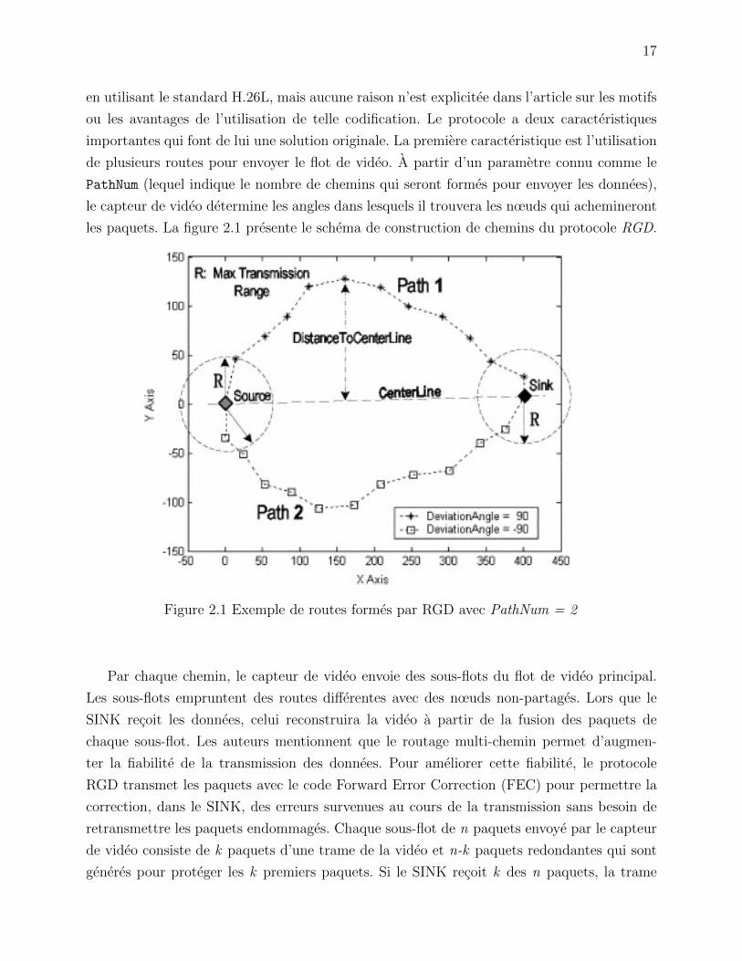
les paquets. La figure 2.1 presente le schema de construction de chemins du protocole RGD.
Figure 2.1 Exemple de routes formes par RGD avec PathNum = 2
Par chaque chemin, le capteur de video envoie des sous-flots du flot de video principal.
Les sous-flots empruntent des routes differentes avec des nœuds non-partages. Lors que le
SINK recoit les donnees, celui reconstruira la video a partir de la fusion des paquets de
chaque sous-flot. Les auteurs mentionnent que le routage multi-chemin permet d’augmen-
ter la fiabilite de la transmission des donnees. Pour ameliorer cette fiabilite, le protocole
RGD transmet les paquets avec le code Forward Error Correction (FEC) pour permettre la
correction, dans le SINK, des erreurs survenues au cours de la transmission sans besoin de
retransmettre les paquets endommages. Chaque sous-flot de n paquets envoye par le capteur
de video consiste de k paquets d’une trame de la video et n-k paquets redondantes qui sont
generes pour proteger les k premiers paquets. Si le SINK recoit k des n paquets, la trame

18
de video correspondante pourra etre restauree sans problemes. En definitive, RGD offre un
bon protocole pour la transmission de video dans un reseau de capteurs. La combinaison de
routage geographique, de multiples routes et du code FEC permet d’obtenir un protocole
fiable et rapide, et ce, on peut le constater dans les resultats presentes dans l’article. Mais,
les restrictions que ce protocole impose sont beaucoup : l’impossibilite d’avoir deux ou plus
sources de video, la specialisation du reseau pour la transmission de video (par exemple, les
capteurs ne peuvent pas capter de donnees scalaires comme la temperature ou la lumiere),
la manque de consideration de l’energie des nœuds intermediaires au moment de choisir les
routes, la necessite d’un grand nombre de capteurs intermediaires qui permettent la creation
de plusieurs routes disjointes (sans nœuds en commun). Ces inconvenients nous revelent que
ce protocole est a une etape preliminaire et qu’il y a de travaux a faire pour l’ameliorer.
Une autre approche, bien qu’il ne soit que pour le transport d’images, est presentee par
Wu et Abouzeid (2006). Le protocole presente dans cet article utilise un routage base sur
la formation des grappes dans le reseau de capteurs (clusters), et aussi sur l’utilisation de
multiples routes dans une grappe et sur le traitement d’images dans le reseau (in-network
processing). Quand la source souhaite transmettre une image vers le SINK, celle l’envoie
d’abord a plusieurs nœuds dans la meme grappe a laquelle appartient la source. Chaque
nœud achemine l’image vers la tete de la prochaine grappe du reseau. Partant du fait que
la source a envoye l’image par differents chemins, c’est sure que la tete de grappe recevra
plusieurs copies de la meme image. Cela est l’avantage du protocole, puisque a partir de ces
multiples images, la tete de grappe pourra choisir la meilleure ou simplement prendre de
donnees de diverses images pour creer une bonne image de l’information recue. Ce processus
est appele par les auteurs “ in-network diversity combining” ou combinaison en diversite dans
le reseau. En plus, les images sont envoyees en utilisant le schema de protection d’erreurs
FEC, que nous avons vu plus haut. En theorie, la combinaison de multiples routes avec le
traitement dans le reseau et la redondance des donnees rend presque impossible la perte de
l’information. Le routage continue a chaque tete de grappe. Celle fait le meme processus que la
source, c’est-a-dire, envoyer l’image a plusieurs nœuds dans la grappe, lesquels achemineront
l’information vers la prochaine tete de grappe, et ainsi de suite, jusqu’a arriver au SINK. La
figure 2.2 presenta un schema de ce type de routage.
Les inconvenients principaux de ce protocole resident dans la specialisation du reseau pour
ne transmettre que des images, l’utilisation tres grande de la memoire des tetes de grappe
pour recevoir et stocker tous les images qui proviennent des nœuds routeurs intermediaires,
l’impossibilite de que plusieurs sources d’images transmettent au meme temps et la manque
de criteres de QdS pour choisir les routes. Neanmoins, il y a des concepts et des idees de ce
protocole dont on peut profiter pour en construire un autre qui travaille d’une facon semblable

19
Figure 2.2 Schema de routage du protocole presente dans (Wu et Abouzeid, 2006)
mais pour la transmission de video.
Routage pour ACO
Plusieurs solutions de routage pour reseau de capteurs sans fils utilisent le paradigme
de colonies de fourmis presente par Dorigo et Blum (2005). Mais la plupart parmi eux (par
exemple (Camilo et al., 2006; Chen et al., 2007b; Sun et al., 2008)) n’utilisent que l’energie
comme le parametre de QdS pour trouver des routes. Dans les domaines des reseaux ad-hoc,
on peut faire saillie les solutions proposees par Jeon et Kesidis (2005) et par Zheng et al.
(2004). Les deux protocoles ont en commun l’utilisation de plusieurs metriques de QdS au
moment de trouver des routes. Le protocole ADRA de Zheng et al. (2004) utilise le delai et
la congestion des nœuds comme ses metriques, tandis que PPRA de Jeon et Kesidis (2005)
utilise le delai et l’energie des nœuds, mais pas ensemble, c’est-a-dire, l’application devra
choisir de travailler avec une metrique ou avec l’autre. Mais, aucunes de ces solution ne tient
compte les types de trafic diverses qui circulent dans le reseau.
2.2 Deploiement de capteurs directionnels
Les facons pour maintenir et optimiser la couverture d’une aire d’interet donnee ont ete
etudiees en profondeur dans les domaines du multimedia, la robotique et les reseaux de
capteurs sans fil. Du point de vue du reseau de capteurs, un travail considerable est presente
pour le probleme de couverture omnidirectionnelle (Cardei et al., 2005; Gupta et al., 2003;
Tian et Georganas, 2002) qui vise a couvrir un ensemble de points critiques ou d’interets sur
un plan en organisant des cercles avec chaque capteur deploye comme le centre du cercle.
Toutefois, les solutions proposees pour une couverture omnidirectionnelle ne peut pas etre

20
utilisees pour le probleme de la couverture avec des capteurs avec un champ de vision comme
les cameras video a basse resolution (capteurs de video). Une limitation commune de ces
solutions est que l’information collectee sur les phenomenes (par exemple, la temperature,
la concentration d’une substance, l’intensite lumineuse, la pression, la humidite, etc.) est
supposee provenant de n’importe quelle direction (detection omnidirectionnelle). Cependant,
les capteurs multimedia, (c’est-a-dire, les cameras a basse resolution, microphones, etc.) ont
la particularite de capter du contenu multimedia qui est sensibles a la direction. Surtout, les
capteurs de video seulement peuvent capturer des images utiles quand il y a une ligne de vue
entre l’evenement et le capteur (Akyildiz et al., 2007). Ainsi, les modeles qui ont ete elabores
pour la couverture traditionnelle dans les RCSF ne sont pas suffisants pour la planification
du deploiement de capteurs multimedias dans un RCMSF.
Soro et Heinzelman (2005) traitent le probleme de couverture pour les reseaux de capteurs
video. Le concept de la plage de detection des capteurs scalaires est remplace par le champ
de vue (FoV), qui est definie comme le volume maximum visible de la camera lorsque les
capteurs sont places sur le plancher. Tous les nœuds sont supposes etre situe sur un plan (le
plafond de la salle de surveillance), et ils prennent les images de la scene a partir d’un plan
parallele. Un tel placement sur un plafond 2D, cependant, ne peut s’adapter qu’a applications
specifique. Toutefois, la solution propose n’est pas optimal et elle est basee sur un schema
geometrique.
Une solution optimale au probleme de deploiement de capteurs directionnels est presentee
par Osais et al. (2010). L’article presente un modele optimal pour le probleme de minimiser le
nombre de capteurs deployes sur un terrain 2D qui couvrent un ensemble de points d’interet.
Mais, les auteurs se conforment avec le modele mathematique qui nous donne la solution
exacte au probleme et ne proposent jamais une solution heuristique. En plus, la recherche
est aussi limitee a capteurs deployes sur un plafond et cela le reste realisme a la solution
proposee.
Une solution pour le probleme de deploiement de capteurs directionnels est presentee par
Ma et al. (2009). Malheureusement, la solution n’est pas optimal et elle est aussi basee sur une
methode connue comme“les champs de potentielle virtuelle”. De cette facon, on peut conclure
qu’il est necessaire un methode pour faire le deploiement optimal de capteurs directionnels
dans un espace 3D.

21
CHAPITRE 3
ANT-BASED ROUTING FOR WIRELESS MULTIMEDIA SENSOR
NETWORKS USING MULTIPLE QOS METRICS
Luis Cobo, Alejandro Quintero and Samuel Pierre
Mobile Computing and Networking Research Laboratory (LARIM)
Department of Computer & Software Engineering,
Ecole Polytechnique de Montreal,
C.P 6079, succ. Centre-Ville, Montreal, H3C 3A7, Quebec, Canada.
E-mail : {luis.cobo, alejandro.quintero, samuel.pierre}@polymtl.ca
Abstract
In wireless sensor networks, most routing protocols consider energy savings as the main
objective and assume data traffic with unconstrained delivery requirements to be a given.
However, the introduction of video and imaging sensors unveils additional challenges. The
transmission of video and imaging data requires both energy efficiency and QoS assurance
(end-to-end delay and packet loss requirements), in order to ensure the efficient use of sen-
sor resources as well as the integrity of the information collected. This paper presents a
Quality of Service (QoS) routing model for Wireless Multimedia Sensor Network (WMSN).
Moreover, based on the traditional ant-based algorithm, an ant-based multi-QoS routing me-
tric (AntSensNet) is proposed. The AntSensNet protocol builds a hierarchical structure on
the network before choosing suitable paths to meet various QoS requirements from different
kinds of traffic, thus maximizing network utilization, while improving its performance. In
addition, AntSensNet is able to use a efficient multipath video packet scheduling in order to
get minimum video distortion transmission. Finally, extensive simulations are conducted to
assess the effectiveness of this novel solution and a detailed discussion regarding the effects
of different system parameters is provided. Compared to typical routing algorithms in sensor
networks and the traditional ant-based algorithm, this new algorithm has better convergence
and provides significantly better QoS for multiple types of services in WMSN.
Keywords : quality of service, routing protocols, wireless multimedia sensor networks, ant
routing algorithm, video distortion.
22
3.1 Introduction
Rapid advances in Micro-Electro-Mechanical System (MEMS) technology, proliferation of
wireless communication and digital electronics have set the stage for the deployment of low-
cost, low-power, multi-functional, autonomous sensor networks. The major objectives behind
the research and deployment of Wireless Sensor Network (WSN) (Akyildiz et al., 2002) lie
in the following two broad aspects : (i) Event detection (sensing) and data communication
through node coordination and (ii) Conservation of energy to maximize the post-deployment,
active lifetime of individual sensor nodes and the overall network. On the other hand, to-
day’s wireless communication is gradually changing the paradigms from the existing scalar
services (light, temperature, etc.) to a new world of real-time audio-visual applications. The
increasing popularity of multimedia applications has already given birth to the new term
WMSN (Akyildiz et al., 2007). Video surveillance, telemedicine, and traffic control will be
the high-impact applications of emerging WMSNs.
The additional challenges created by the intrinsic features of multimedia communication
must be addressed in order to deploy these multimedia applications within WMSNs. Unlike
conventional data communication, required for reliable transport of event features from the
field, multimedia traffic does not require 100% reliability, since it is endowed with most strict
requirements on bounded delay, packet loss, minimum bandwidth, and smooth change of the
transmission rate. These additional requirements inevitably amplify the challenges for mul-
timedia communication in sensor networks. Especially, high bandwidth demands and strict
multimedia communication time-constraints present significant challenges for sensor networks
when matching energy and processing capacities with the level at which application objec-
tives are met. While a significant amount of research has been conducted on WSN routing
problems (Akkaya et Younis, 2005b), WSN multimedia data routing remains vastly unexplo-
red. On the other hand, multimedia communication problems have been largely investigated
and numerous solutions exist for wireless environments and the Internet. However, such so-
lutions cannot be directly applied to WMSN scenarios due to their unique characteristics
and resource constraints. Consequently, there is an urgent need for research efforts to address
the challenges of WSN multimedia communications to help realize many currently envisioned
multimedia WSN applications.
When network size scales up, routing becomes more challenging and critical. Lately,
biologically-inspired intelligent algorithms have been deployed to tackle this problem (Chen
et al., 2007b; GhasemAghaei et al., 2007; Muraleedharan et Osadciw, 2004; Zhang et al., 2004;
Liu et al., 2007). Using ants, bees and other social swarms as models, software agents can be
created to solve complex problems, such as traffic rerouting in busy telecommunication net-

23
works. Swarm intelligence, which is revealed by such natural biological swarms, offers various
valuable properties renowned in many engineering systems, for instance in network routing.
Swarm intelligence systems refer to complex behaviors, typically invented from some simple
agents who cooperate with one another and their environment. One of the most successful
swarm intelligence techniques is called Ant Colony Optimization (ACO) (Dorigo et Stutzle,
2004), an optimization algorithm used to find approximate solutions for difficult combinato-
rial optimization problems. In ACO, artificial ants find solutions by moving on the problem
graph, mimicking real ants who previously left behind pheromones for the use of future ants
that can find better solutions. ACO was successfully applied to a remarkable number of op-
timization problems. Ants use reinforcement learning to discover the most efficient path. In
reinforcement learning, the intelligent system is simply given a goal that must be reached.
The system then adopts the goal using a trial and error interaction with the environment.
Interactions that take the system close to the target receive a reward, while punishment is
administered to those who stray away from the target. Computer scientists addressed rein-
forcement learning of artificial systems by introducing a concept called pheromone decay.
When this pheromone evaporates rapidly, longer paths have trouble maintaining pheromone
trails stable. This has also been used for telecommunication networks (Dorigo et Caro, 1998).
Artificial ants continuously explore different paths, and pheromone trails to provide backup
plans. Thus, if one link breaks down, a pool of alternatives already exists.
This paper proposes a QoS routing algorithm for WMSN based on an improved ant colony
algorithm. The AntSensNet protocol introduces routing modeling with four QoS metrics asso-
ciated with nodes or links. The algorithm can find a route in a WMSN that satisfies the QoS
requirements of an application, while simultaneously reducing the consumption of constrai-
ned resources as much as possible. Moreover, by using clustering, it can avoid congestion after
quickly judging the average queue length and solve convergence problems, which are typical
in ACO. Simulation results show that the proposed algorithm improves the performance of
other typical protocols such as Ad hoc On-Demand Distance Vector Routing (AODV).
The remainder of the paper is organized as follows : Section 3.2 provides a brief review
of some closely related works. The proposed protocol is described in Section 3.3. Then,
AntSensNet is tested through a series of computer simulations presented in Section 3.4.
Concluding remarks appear in Section 3.5.
3.2 Related Work
As previously mentioned, WMSNs not only enhance existing sensor network applications
such as tracking, home automation, and environmental monitoring, but they also enable se-

24
veral new applications such as multimedia surveillance sensor networks, automobile traffic
management (traffic congestion avoidance systems, speed control, car parking assistance),
storage of potentially relevant activities, advanced health care delivery, structural health mo-
nitoring, and industrial process control (visual inspection, automated actions). Many of these
applications require the sensor network paradigm to be re-thought in view of the fact that, in
these types of networks, the main concerns are not only energy constrains, limited computing
power, and memory availability of the Sensor Nodes, but also the need for mechanisms to
deliver multimedia content with a certain level of Quality of Service (QoS) : the transmission
of imaging and video data requires careful handling in order to ensure that end-to-end delay
remains within an acceptable range, while the delay variation is acceptable, the link band-
width pertains to the tolerable compression ratio, that jitter is satisfactory and that there is
a low packet loss rate (Akyildiz et al., 2007).
Providing QoS guarantees in wireless sensor networks consists of a very challenging pro-
blem, but several approaches have been proposed in the literature for QoS support in these
kinds of networks. For example, Sequential Assignment Routing (SAR) (Sohrabi et al., 2000),
one of the first approaches in the area of QoS for wireless sensor networks, builds multiple
paths from a source node to the sink node. Path selection considers both QoS metrics (the
flow delay requirements and the source load balancing intentions) and energy resources, to
avoid nodes with low QoS and energy reserves. Intermediate nodes forward packets according
to their level of priority. However, the algorithm does not consider reliability issues and it
cannot scale large networks due to the use of a routing table to calculate multiples paths.
An energy-aware QoS routing protocol for real-time traffic generated by a wireless sensor
network consisting of image sensors is proposed by Akkaya et Younis (2005a). This approach
finds multiple network routes by using a minimum path cost. Such cost is a function of
distance between nodes, node residual energy, energy transmission, and error rates which
meet the requested end-to-end delay constraints. All traffic is divided into best effort and real
time classes. A Weighted Fair Queuing (WFQ) approach is used at every node to provide
the required share of bandwidth for both traffic classes. Path generation is performed in a
centralized manner, at the base station using an extended version of Dijkstra’s Algorithm.
The advantage of this algorithm lies in the fact that it provides a guarantee for best-effort
transmission, while simultaneously trying to maximize real-time traffic throughput. The main
drawback is that the algorithm requires complete knowledge of the network topology at the
base station to calculate multiple routes, thereby limiting the scalability of this approach.
The Real-time communication Architecture Protocol (RAP) proposed by Chenyang et al.
(2002) uses a velocity monotonic scheduler to prioritize packets, and schedules them on
the basis of their required transmission speed. Geographic routing is used to forward traffic

25
towards its destination, while velocity-aware scheduling, either static (computed at the source,
based on both deadline and distance to destination) or dynamic (computed at every node,
based on the actual progress of the packet) ensures that packets meet their deadlines by
giving higher priority to packets with higher requested velocities. However, when calculating
routes, this protocol fails to consider energy issues and the number of hops executed by the
packets.
A QoS routing protocol, called SPEED, was proposed by He et al. (2003) to provide a
soft real-time end-to-end timeliness guarantee. The protocol requires that each node saves
information regarding its neighbors and exploits geographic forwarding to find paths. In
addition, SPEED strives to ensure a certain rapidity for each packet delivery so that each
application can estimate the end-to-end delay for the packets by considering the distance to
the sink and the speed of the packet delivery before making the admission decision. Using the
distance and delay, each node evaluates the packet progress speed of each neighbor node and
forwards a packet to a node whose progressive speed is higher than the pre-specified lower-
bound speed. In the event that some path links become congested and cannot support the
maximum delivery speed, the protocol includes mechanisms to divert traffic to other routes.
One of the drawbacks of SPEED is that it does not have a packet prioritization scheme. In
addition, the protocol does not provide any guarantee regarding packet reliability.
The QoS routing approach presented by Agrawal et al. (2006) utilizes the geographic
location of sensor nodes as well. This protocol assigns an urgency factor to every packet
depending on the remaining distance and the time left to deliver the packet. It determines
the distance required for the packet to be sent closer to the destination in order to meet its
deadline. Each node assigns a priority to all of its neighbors, according to their residual energy
and delay, as well as the priority of the packets, and packets are forwarded to the highest
priority nodes. Packets are sorted in two different queues, one for non-real-time traffic, and
another one for real-time traffic. Real-time traffic is prioritized based on its urgency factor,
scheduling those packets with more aggressive deadlines first for transmission. Reliability is
achieved by using duplication of information at the source node. However, the protocol does
not consider data aggregation and the network lacks a good decongestion scheme.
A multi-path and multi-speed routing protocol called “MMSPEED” is proposed by Fe-
lemban et al. (2006), which takes into account both timeliness and reliability as QoS requi-
rements. The goal is to provide QoS support that allows packets to choose the most proper
combination of service options depending on their timeliness and reliability requirements.
For timeliness, multiple QoS levels are supported by providing multiple packet delivery speed
guarantees. The scheme employs localized geographic forwarding with dynamic compensa-
tion to offset inaccuracies in decisions made with only local knowledge. Intermediate nodes

26
have the ability to boost a packet’s transmission speed to higher levels if they notice that
the packet may not meet its delay deadline at the current speed, although the deadline could
be met at a higher speed. MMSPEED assumes the use of IEEE 802.11e at the MAC layer
with its inherent prioritization mechanism based on the Differentiated Inter-Frame Spacing
(DIFS). Each speed value is mapped onto a MAC layer priority class. For reliability, multiple
reliability requirements are supported by probabilistic multi-path routing with the number of
paths being dependent upon the required degree of reliability. MMSPEED adapts to network
dynamics such as channel error conditions and speed changes to determine the number of
forwarding nodes (thus forming multiple paths) in each hop to satisfy the overall reliability
and timeliness of QoS requirements. However, MMSPEED fails to consider energy issues ;
hence, it is only applicable for short-term WSN applications whose mission lasts only a few
hours or at most one day. Moreover, it does not handle network layer aggregation and requires
substantial state information to be stored at intermediate sensor nodes.
Finally, ReInForM (Deb et al., 2003) was proposed to address end-to-end reliability issues.
ReInForM considers the importance of the data in the packet and it can adapt to channel
errors. The protocol sends multiple copies of a packet along multiple paths from the source
to the sink so that data can be delivered with the desired reliability. It uses the concept
of dynamic packet state in the context of sensor networks to control the number of paths
required for the desired reliability, based on local knowledge of the channel error rate and
topology. However, the protocol only addresses QoS in terms of reliability, disregarding energy
issues. In addition, the protocol does not consider route delays when selecting multiple paths.
The newly proposed solution to QoS routing in WMSNs is based on the ACO metaheuris-
tic, especially due to the fact that the ACO algorithm (Dorigo et Blum, 2005) was inspired by
the behavior of an authentic ant colony, more specifically real ants in a food search process.
When ants are out searching for food, they leave their nest and walk toward the food. When
an ant reaches a crossroad, it must decide which way to follow. While walking, ants deposit
pheromones, leaving behind tracks of the route taken. Ants can smell pheromone and they
are more likely to follow paths characterized by strong pheromone concentrations. The phe-
romone trails allow ants to find their way to the food source, or back to the nest. The same
pheromone can be used by other ants to find the location of the food sources discovered by
their mates. Based on this approach, there are many successful applications about the com-
binatorial optimization problems such as the Traveling Salesman Problem (TSP) (Dorigo et
Gambardella, 1997), Vehicle Routing Problem (VRP) (Bullnheimer et al., 1999) and routing
algorithms in mobile ad hoc networks (Dorigo et Caro, 1998).
According to Rosati et al. (2007), a distributed heuristic solution such as ant routing
displays several features making it particularly suitable in wireless sensor networks :

27
– the algorithm is fully distributed ; there is no single point of failure ;
– the operations to be performed in each node are very simple ;
– the algorithm is based on agents’ asynchronous and autonomous interactions ;
– it is self-organizing, thus robust and fault tolerant ; there is no need to define path
recovery algorithms ;
– it intrinsically adapts to traffic without requiring complex, and yet inflexible metrics ;
– it inherently adapts to all kinds of long-term variations in topology and traffic demand,
which are difficult to take into account by deterministic approaches.
Additionally, ant routing has shown excellent performance to solve routing problems in
WSNs and ad hoc networks. For instance, the Ant-Colony-Based Routing Algorithm (ARA)
(Gunes et al., 2002), suitable for MANETs, based both on swarm intelligence and ant-colony
meta-heuristics, consists of three phases : route discovery, route maintenance and route-failure
handling. In the route-discovery phase, new routes between nodes are discovered using forward
and backward ants (FAs and BAs), similar to AntNet (Dorigo et Caro, 1998). Routes are
maintained by subsequent data packets, i.e. as the data crosses the network, node pheromone
values are modified so that their paths are reinforced. Also, same as in nature, pheromone
values decay with time in the absence of such reinforcement. Routing or link failures, usually
caused by node mobility, are detected through missing acknowledgments.
In (Gerla et Xu, 2003), a mobile ant-based routing protocol for large scale WSNs is
proposed. Mobile ant nodes have greater capacity in terms of communication range length,
high quality multimedia sensory data processing capability, mobility management, and better
energy storage. The protocol defines three types of communication patterns : sensor to ant
nodes, ant to ant nodes and ant nodes to the sink. Regular sensor nodes detect the events and
report to the nearest ant node(s) and the mobile ant nodes relocate them nearest to the event
hotspot to capture detailed multi-modal information about the event for more accuracy. The
routing protocol maintains a hierarchy of clusters and uses two types of routing tables : for
intra-cluster and inter-cluster routing. The protocol is intended for upstream routing and uses
only a dedicated high bandwidth backbone channel to communicate with the sink and avoid
congestion. The protocol does not evaluate multimedia metrics such as bandwidth, packet
loss ratio, jitter, and end-to-end delay. Also, it does not actually employ ant-based routing
phenomena.
A multi-path routing protocol based on ACO intended for Mobile Ad-hoc Networks
(MANET) is proposed in (Ziane et Melou, 2005). The protocol specializes in carrying mul-
timedia real-time traffic over the MANET. To provide higher bandwidth and delivery gua-
rantees, it uses a multi-path solution. It also supports high mobility for nodes and certain
QoS parameters. However, the protocol uses the concept of IP-based routing and must be

28
modified in order to be suitable for WSN.
The M-IAR protocol proposed in (Rahman et al., 2008) is a flat multi-hop routing protocol
that exploits the geographic location of the sensor nodes in order to select the best route
possible. Basically, M-IAR finds the shortest route, the one that contains the fewest nodes
between the sending and receiving nodes. The authors believe that multimedia processing is
costly for resource constrained sensor nodes, in addition to the wireless communication costs.
Thus, finding the shortest path with the least number of forwarding nodes will help achieve
the least end-to end delay along with the best jitter conditions. However, this protocol does
not differentiate packets when selecting routes. Furthermore, it ignores the concept of packet
priority. Moreover, the basic assumption that shorter routes equal best routes is erroneous,
especially in WMSNs with heterogeneous nodes and different link bandwidths. Finally, this
protocol is unable to handle link or node failures.
Another interesting protocol is TPGF (Two-Phase geographic Greedy Forwarding) pro-
posed in (Shu et al., 2010). TPGF takes into account both the requirements of real time
multimedia transmission and the realistic characteristics of WMSNs. It finds one shortest
(near-shortest) path per execution and can be executed repeatedly to find more on-demand
shortest (near-shortest) node-disjoint routing paths. TPGF supports three features : (1) hole-
bypassing, (2) the shortest path transmission, and (3) multipath transmission, at the same
time. TPGF is a pure geographic greedy forwarding routing algorithm, which does not include
the face routing, e.g., right/left hand rules, and does not use planarization algorithms, e.g.,
GG or RNG. This point allows more links to be available for TPGF to explore more routing
paths, and enables TPGF to be different from many existing geographic routing algorithms.
But this protocol presents some inconvenience when an application wants to transmit video
between a source and the sink. TPGF only takes into account to create a route the “distance”
between the nodes and the sink, and other important characteristics such as link bandwidth
or node queue congestion, are not considered at the moment of route discovering. Besides
that, this protocol does not support heterogeneous traffic (video and scalar data at the same
time).
An ant-based protocol specifically designed for WMSN is ASAR (An ant-based service-
aware routing algorithm for multimedia sensor networks) presentd in (Sun et al., 2008). This
protocol define three different types of services found in a sensor networks, namely, event-
driven, data query and stream query services. The ASAR chooses suitable paths to meet
diverse QoS requirements from different kinds of services, thus maximizing network utilization
and improving network performance. Compared to the typical routing algorithm in sensor
networks and the traditional ant-based algorithm, ASAR algorithm has better convergence
and provides better QoS for multiple types of services in the multimedia sensor networks.

29
This protocol has important elements to take into account, but it lacks some others like
multipath data transmission, a very important requirement in order to increase transmission
performance in WMSNs.
As mentioned above, ant-based routing algorithms exhibit a number of interesting proper-
ties for WMSN routing. However, theses algorithms have a major drawback : scalability. This
problem arises since each node must send agents (ants) to all other network nodes in order to
discover a route to the sink, meaning that the total number of agents to be sent is N ·(N−1).
In large networks, the amount of traffic generated by the ants would be excessively high. Fur-
thermore, nodes located far from the sink increase the probability of the ants getting lost.
Moreover, the ants’ extensive travel times contribute to outdating the information they carry.
That is the main reason why it was decided to add a clustering mechanism to the algorithm,
to ensure that the protocol is more scalable and efficient. Simulation results corroborate this
decision. Therefore, WMSNs will henceforth be designed based on cluster-based architecture.
Nodes in the cluster are responsible for collecting scalar and multimedia data before sending
this information to the Cluster Head (CH). The CH fuses such data, and then transfers the
data results upstream to the sink. The sink node manages the status of CHs and broadcasts
signals to the WMSNs. CHs form an independent network. They connect the sink node via
multi-hop wireless links. Therefore, this paper addresses mainly the routing scheme between
the CHs and sink node.
None of the existing protocols can achieve all the following goals simultaneously :
– Traffic classification, in order to differentiate network data flows, and to treat each flow
with its proper QoS metrics,
– Clustering, in order to solve the scalability problems in large-scale sensor networks and
to facilitate in-network processing tasks (i.e. aggregation).
3.3 The AntSensNet Protocol
AntSensNet is a specially designed routing protocol for WMSNs. It combines a hierar-
chical structure of the network with the principles of ACO-based (Ant Colony Optimization)
routing, thus satisfying the QoS requirements requested by the applications. Besides that, our
protocol supports a power efficient multipath video packet scheduling scheme for minimum
video distortion transmission
AntSensNet comprises both reactive and proactive components :
1. It is reactive since routes are set up when needed, not before. Once routes are set up,
data packets are sent stochastically over the different paths using a pheromone table
placed in each router.

30
2. It is proactive due to the fact that, while a data session is in progress, paths are probed,
maintained, and improved proactively using a set of special agents designed for this task.
The algorithm comprises three parts. The first constituent clusters network nodes into
colonies. The second component finds network routes between clusters that meet the requi-
rements of each application in the network using ants. The third element forwards network
traffic using the routes previously discovered by the ants.
3.3.1 WMSNs QoS Routing Model
A WMSN can be presented as a connected, undirected and weighted graph G = (V,E)
where V = {v1, v2, . . . , vn} denotes the set of nodes (only CHs and sink node) in the network
and E = {e12, e13, . . . , exy} depicts the set of bi-directional links between CHs. For a pair
of nodes vi, vj ∈ V (i 6= j), if the link eij = (vi, vj) ∈ E then (vi, vj) consists of a pair of
adjacent nodes. Each node n ∈ V in the graph, includes a set of four QoS metrics elements :
{pl(n),ma(n), dl(n), re(n)}. Where pl(n) expresses the maximum packet loss rate of Node n,
ma(n) denotes the available memory in Node n, dl(n) shows the queuing delay in Node n
and re(n) reveals the normalized remaining energy in the node n with respect to the initial
energy, defined as : re(n) = Eresidual(n)Einitial(n)
, where Eresidual(n) unveils the remaining energy in the
battery of Node n and Einitial(n) indicates the initial energy in the battery of Node n. These
parameters, along with bandwidth, were chosen from those mentioned by (Akyildiz et al.,
2007), as important elements to find routes in a WMSN.
For a unicast path P = (va, vb, . . . , S) from a CH va to the sink node s, its QoS parameters
are computed as follows :
delay(P ) =∑n∈P
dl(n) (3.1)
packetloss(P ) = 1−∏n∈P
pl(n) (3.2)
energy(P ) = minn∈P{re(n)} (3.3)
memory(P ) = minn∈P{ma(n)} (3.4)
In a WMSN, various kinds of traffic are transported by nodes. For instance, real-time
audio/video data are delay-constrained with a certain bandwidth requirement. Packet losses
can be tolerated to a certain extent. In addition, environmental data from scalar sensors,
or non-time-critical snapshot multimedia content, are delay-tolerant and loss-tolerant kinds
of data with low or moderate bandwidth demands. Finally, each type or class of traffic

31
has its own requisites for QoS metrics. The goal of the AntSensNet algorithm is to find
accessible paths for each class of traffic from a source CH node to the sink that meet different
QoS requirements, thus minimizing interference among the types of traffic, balancing traffic
distribution and improving network performance.
Let vch denote a CH and s denote the network sink node. The issue of routing selection
from vch to s consists of finding different accessible paths PC , where C represents each traffic
class that the application being executed on the WMSN has defined. The objective function
of a path PC can be expressed as follows :
f(PC) = γdC · (Dmax − delay(PC))
+ γpC · (1− packetloss(PC))
+ γpC · (energy(PC)− Emin)
+ γmC · (memory(PC)−Mmin)
(3.5)
where delay(P ), packetloss(P ), energy(P ), and memory(P ) respectively denote delay, pa-
cket loss rate, residual energy ratio and available memory for the path as defined in Equations
(3.1) to (3.4). Dmax, Emin and Mmin indicate the path’s maximal tolerable delays, its minimal
residual energy ratio and normalized memory available, respectively. Variables γdC , γpC , γpCand γmC translate the delay weight factor, packet loss rate, residual energy ratio and available
memory for global QoS parameters, respectively.
The described QoS routing problem is similar to typical Path Constrained Path Optimi-
zation (PCPO) problems, which are proved to be NP-complete (Feng et al., 2002), and an
ant colony optimization based algorithm is used to solve this issue.
3.3.2 Assumptions
The following assumptions are made for this novel sensor network :
– Nodes are scattered randomly, in a uniform distribution, over a two-dimensional plane.
– The sink is not mobile and considered to be a powerful node endowed with enhanced
communication and computation capabilities and no energy constraints.
– Sensor nodes are not mobile.
– There are two types of sensors : multimedia sensors (resource-rich nodes, capable of
audio/video sensing of their environment) and scalar sensors that capture data such as
temperature, light or pressure. Both types are also distributed randomly over the area.
– Nodes are unaware of their location, i.e. they are not equipped with a GPS device.
– Communication from each node follows an isotropic propagation model.

32
– Radio transmitting power is controllable, i.e. nodes can adjust the transmitting power
according to the distance.
– Despite the fact that nodes are heterogeneous, it is assumed that radio transmissions
are identical for all nodes.
– Nodes can estimate the approximate distance by the received signal strength, given the
transmit power level is known, and the communication between nodes is not subject to
multi-path fading.
– We use the same radio model presented in (Heinzelman et al., 2002), and it is assumed
that the radio channel is symmetric so that the energy required to transmit a m-bit
message from Node i to Node j is identical to the energy required to transmit a m-bit
message from Node j to Node i, for a given signal to noise ratio.
3.3.3 Clustering Process
AntSensNet is a QoS routing protocol based on an ant colony algorithm. This algorithm
makes use of special agents (known as forward-ants or FANTs) to find a path between a
sensor node and the network base-station or sink. In the route discovery process, several ants
leave their node source, aiming for their neighbors, each one with the task of finding a route,
meaning that sensor nodes must communicate with one another and the routing table of
each node must contain the identification of all sensor nodes in the neighborhood as well as
their corresponding levels of pheromone left on the trail. As the number of nodes grows, the
number of agents required to establish the routing infrastructure may explode (Selvakennedy
et al., 2007). A way to overcome the overhead explosion and reach scalability consists of using
the hierarchical routing approach.
Nevertheless, scalability is not the only reason to cluster the network. This process also
allows for improving network data aggregation mechanisms, while concentrating this activity
in the CH, consequently reducing node workloads, saving energy and increasing the network
lifetime. Arboleda et Nasser (2006) presents other advantages of clustering that apply to
this novel protocol : the fact that only the CH transmits information out of the cluster
helps prevent collisions between the sensors inside the cluster, as they do not have to share
communication channels with nodes in other clusters. This also promotes energy savings and
avoids the black hole problem. Latency is also reduced. Although data must hop from one
CH to another, they cover larger distances than when sensors use a multi-hop communication
model (non-clustered) as the one used in other protocols.
Finally, clustering is applied in order to take advantage of the existence of nodes of different
abilities inside a WMSN. Table 3.1 (Misra et al., 2008) presents the processing performance
and memory capacities among standard (TelosB) and multimedia sensors. Table 3.1 shows

33
that the memory and processing capacities of multimedia sensors are superior to those of
conventional sensors. That is the reason for selecting multimedia sensors to become the
network CHs. This novel algorithm will be designed to favor the “selection” of these nodes as
CHs.
Our clustering algorithm aims at achieving the following goals :
– Saving network resources by encouraging the selection of resource-rich nodes (multime-
dia sensor nodes) as network CHs.
– Ensuring network connectivity by forming a virtual backbone among the different CHs.
Each CH is in the radio range transmission of at least one other CH. Communication
between two CHs is direct (there are no relay nodes between them).
– Maximizing network lifetime by implementing a mechanism of CH rotation.
With a virtual backbone in the network, only CHs are concerned with data transportation,
and other nodes are free to pursue their sensing tasks. Such task sharing improves network
performance with respect to routing overhead and, moreover, a smaller number of nodes
need to be alert for data transportation. This procedure reduces energy consumption, thus
simultaneously maximizing network lifetime.
Information Update Phase
This novel clustering algorithm is based on T-ANT (Selvakennedy et al., 2007) and the
clustering protocol uses a collection of agents to form clusters in a sensor network. It is com-
pletely distributed and completed in constant time. These are the reasons why this algorithm
was selected.
As in T-ANT, clustering operations are split into rounds. Each round comprises a cluster
setup phase and a steady phase. In the steady phase of the algorithm, data transmission
takes place between sensors and the sink. A number of timers are used to control the process
operations. During the cluster setup phase, CHs are elected and clusters are placed around
them. In order to avoid the maintenance of many state variables, as one finds in numerous
current clustering proposals, a series of agents (known as cluster-ants or CANTS) are used
to control CH elections. A node with a CANT becomes a CH, whereas others choose to join
the best cluster in range.
The cluster radius Rcluster is defined as a tunable parameter that determines the minimum
distance between any two CH nodes in the network. The value of this parameter always
remains inferior to the sensor communication radio range (called r). Before the cluster setup
phase, an information update phase is carried out by the sensors. Each sensor node broadcasts
a HELLO packet with information regarding its ID, its clustering pheromone value (Φc(n)) and
its state to its neighbors. When a HELLO packet arrives, the node stores such information in a

34
Tableau 3.1 Abilities Of Video And Standard Sensors
Stargate Samsung S3C44B0X TelosBClock Frequency 200/300/400 Mhz 66 Mhz 8 Mhz
Architecture 32 bit RISC 16/32 bit RISC 16 bit RISCMemory 64 MB SDRAM 256 MB 10 KB
32 MB Flash 1 MB FlashCache 32 KB data 8 KB Data not
32 KB instruction availableCost ($) 595 500 100
table, the neighborhood or the neighbor’s information table. This table is then used to select
clusters, to join a cluster and to route data packets.
The clustering pheromone value determines whether it is appropriate for this node to
become a CH. For each node, this value is calculated using the following formula :
Φc(n) = (ma(n))a · (re(n))b (3.6)
where ma(n) denotes the available memory in the node, re(n) is the residual ratio of the
node’s energy and a and b denote the importance of each component of the pheromone : a
for the memory capacity and b for the energy component. Thus, the application determines
which component is most important when selecting a CH, namely, memory or energy or both.
The state indicates if the node is a CH or a member of a cluster or neither. These HELLO
packets are constantly broadcast by the nodes throughout their lifetime.
Ant Release Phase
After the information update phase, the sink releases a fixed number of ants (i.e. control
messages) into the network. Assuming that the terrain is square, M × M , the number of
ants to be released is set at dM2
πd2e , where d depicts half of Rcluster. The latter formula also
represents the number of clusters that make up the network. Attempts are made to obtain
complete coverage of the area with this number of clusters, where every node belongs to a
cluster and the CHs are disseminated throughout the terrain. Ants move about the network
in a random fashion, as far as they can, respecting the limits imposed by their Time-To-Live
(TTL) values. The TTL value equals the number of ants. Hence, an ant can visit a large
number of candidate nodes to become a CH before they die. When the sink releases an ant,
it chooses one of its neighbors randomly according to the following probability distribution
function :

35
probc(j) =Φc(j)∑i∈Ns Φc(i)
(3.7)
where Φc(j) denotes the clustering pheromone value sent by Node j, as defined in Equa-
tion (3.6), and Ns represents the set of all of the sink neighbors located at a distance of
at least Rcluster. Before releasing the next cluster ant, the sink waits for a timer to expire
(CLUSTER_TIMER). Although the timer expiration is set at a random value, it always remains
proportional to the delay of sending an ant from a node to a neighbor. The objective of
this timer is to ensure that the ants’ subsequent transmissions do not self-interfere. Aside
from that, when the sink selects a neighbor, the pheromone value of that node is artificially
decreased, in order to avoid choosing the same set of nodes repeatedly.
Algorithm 1 presents the tasks performed by the sink in order to start the clustering
process.
ALGORITHM 1: Tasks developed by the sink
1 d← Rcluster2 ;
2 repeat3 Use probability distribution function (probc) to choose a neighbor (i) ;
4 Send a cluster ant to node i with a TTL = dM2
πd2e ;
5 Wait until a CLUSTER_TIMER expires ;
6 until all ants are released ;
When an ant arrives at a node, that node will execute the tasks depicted in Algorithm 2.
Algorithm 2 shows that, in order to become a CH, the selected node must have received
a cluster ant from another CH (or the sink) located at a distance Rcluster from it. Rcluster
was previously defined as the minimal distance between two CHs. Hence, at the moment of
selecting the following neighbor, the node reads its neighbors’ information table and selects,
with probability probc, a node whose distance is a minimum of Rcluster in a random manner.
The reason why a CH elects the next CH is to create a virtual backbone between the various
CHs, a direct communication strategy between them. This backbone will facilitate the task of
routing accomplished by the protocol AntSensNet. When a node becomes a CH, it broadcasts
an ADV_CLUSTER message to advise its neighborhood of its new condition. It also changes the
value of field state of a HELLO package subsequently sent by the node. Once a regular node
receives an ADV_CLUSTER message from a CH located at a distance below Rcluster, it stores the
corresponding information that pertains to that CH. This information is later used to join
a given cluster. Contrary to other proposals documented in the literature, this CH election
approach has a very small constant time and a low level of complexity. An ant’s TTL indicates
the maximum number of hops that it can perform. The CH pulverizes an ant once its TTL

36
ALGORITHM 2: Tasks developed by the other nodes
1 if an ant arrives at node i then2 if node i is not a CH then3 if there is a CH in the radius Rcluster then4 Pick a random CH neighbor ;5 Send the ant to it ;
6 end7 else8 Store the ant;
/* This node is a CH */
9 Broadcast a message ADV_CLUSTER to neighbors in range Rcluster ;
10 end
11 end12 else if node i is a CH then13 Decrement the TTL of the ant ;14 if TTL > 0 then15 Pick a random neighbor according to the probability function probc ;16 Send the cluster ant to it ;
17 end18 else19 Destroy the ant ;20 end
21 end
22 end
reaches the value zero. This situation shows the existence of a superfluous number of clusters
in the network, and the cluster ant is destroyed in order to avoid the creation of new clusters
that would hinder the network.
The actual clustering process happens once another timer expires. A regular node decides
to join a cluster when its JOIN_TIMER expires. This node chooses the nearest cluster to join
(from all of the ADV_CLUSTER packages it received) by sending a JOIN message with its ID.
When a CH receives JOIN messages, it stores such information in order to subsequently select
a cluster member as a new CH. If a regular node has never received an ADV_CLUSTER package
from a CH, it starts a JOIN_TIMER once again and repeats the latter process until this timer
expires. However, if in the process, it receives neither an ADV_CLUSTER message nor a HELLO
package from a CH, the node uses the nearest neighboring cluster member as a “bridge” to
reach its CH.
When a CH realizes that the node µ is three o more hops away from it, that CH selects the
neighbor in the path to µ as a new CH. This new CH broadcasts an ADV_CLUSTER message in
order to contact other CHs and initialize their pheromone tables. In that way, we can get a
better CH distribution to cover the whole network area. This new CH selection may be done

37
in any moment in the protocol execution.
The properties of the proposed clustering algorithm can be highlighted as follows :
1. The algorithm is completely distributed. A node locally decides to become a CH if an
ant reaches it or joins a cluster.
2. Given the absence of looping statements as a function of node quantity, it is clear that
the election process has an O(1) time complexity.
3. The algorithm ensures the creation of a backbone among the CHs. As all CHs are
connected, paths to a sink can be easily discovered.
Figure 3.1 shows an example of a sensor network clustering using our algorithm.
Figure 3.1 WMSN clustering example. The backbone created by CHs is outlined in black.

38
3.3.4 AntSensNet Algorithm Description
AntSensNet consists of a protocol based on ACO (Ant Colony Optimization) to discover
and maintain routes between CHs and the sink. The route discovery process starts as soon
as the cluster process finishes. Before presenting the algorithm, here are some definitions.
The Ant’s Structure
The data configuration of the ant’s structure used in its route discovery process is defined
below. It comprises the following fields :
1. ant.ID : the ant’s ID.
2. ant.type : the type of ant in the route discovery process. This field can be a Forward
Ant (FANT), a Backward Ant (BANT), a MANT (maintenance ant) or a DANT (data
ant).
3. ant.nodes : the nodes-visited-stack, contains the IDs of nodes by which the ant passes.
4. ant.hopcount : calculates the number of hops by which the ant passed from its CH
source. This field serves as the ant’s TTL.
5. ant.info : Each type of ant uses this field to store special information about the route
or the nodes, in order to evaluate how appropriate the route is. This field contains the
following subfields :
– The minimum residual energy of the nodes by which the ant passed ;
– The cumulative queue delay, packet loss, and available memory of each node visited
by the ant.
The Queuing Model
Sensor data may originate from various types of sources whose levels of importance vary.
Akyildiz et al. (2007) organizes the following examples of traffic into various WMSN classes :
– Real-time, Loss-tolerant, Multimedia Streams. This class includes video, audio or multi-
level streams composed of video/audio and other scalar data (e.g., temperature rea-
dings), as well as metadata associated with the stream that need to reach a human or
an automated operator in real-time, i.e., within strict time limits, although relatively
loss tolerant (e.g., video streams can tolerate a certain level of distortion). Traffic that
belongs to this class is usually associated with high bandwidth demands.
– Delay-tolerant, Loss-tolerant, Multimedia Streams. This class includes multimedia streams
intended for storage or subsequent offline processing, whose delivery is not bound by
strict delays. However, due to the typically high bandwidth demands of multimedia
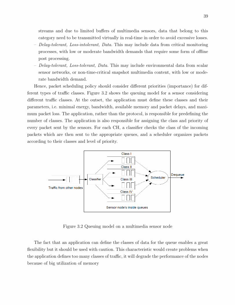
39
streams and due to limited buffers of multimedia sensors, data that belong to this
category need to be transmitted virtually in real-time in order to avoid excessive losses.
– Delay-tolerant, Loss-intolerant, Data. This may include data from critical monitoring
processes, with low or moderate bandwidth demands that require some form of offline
post processing.
– Delay-tolerant, Loss-tolerant, Data. This may include environmental data from scalar
sensor networks, or non-time-critical snapshot multimedia content, with low or mode-
rate bandwidth demand.
Hence, packet scheduling policy should consider different priorities (importance) for dif-
ferent types of traffic classes. Figure 3.2 shows the queuing model for a sensor considering
different traffic classes. At the outset, the application must define these classes and their
parameters, i.e. minimal energy, bandwidth, available memory and packet delays, and maxi-
mum packet loss. The application, rather than the protocol, is responsible for predefining the
number of classes. The application is also responsible for assigning the class and priority of
every packet sent by the sensors. For each CH, a classifier checks the class of the incoming
packets which are then sent to the appropriate queues, and a scheduler organizes packets
according to their classes and level of priority.
Figure 3.2 Queuing model on a multimedia sensor node
The fact that an application can define the classes of data for the queue enables a great
flexibility but it should be used with caution. This characteristic would create problems when
the application defines too many classes of traffic, it will degrade the performance of the nodes
because of big utilization of memory

40
Pheromone Table
An ant pheromone table is a data structure that stores pheromone trail information for
routing from Node i to the sink via a CH neighbor j. Saved into the node memory, this
structure is organized as shown in Table 3.2 below.
Tableau 3.2 Pheromone table for Node i
Neighbor Traffic Class k Class t Expiration TimeN1 eki (1) δki (1) εki (1) µki (1) · · · T1
N2 eki (2) δki (2) εki (2) µki (2) · · · T2
... · · · ......
Nj · · · ......
In the table 3.2, each column reflects the different traffic class, as defined by the appli-
cation. Each row corresponds to a neighbor. There are fivefour values for each traffic class
in the table. Each value is a pheromone trail concentration for each QoS metric used by the
protocol :
1. eki (j) : energy pheromone value from link between Nodes i and j for packets that belong
to traffic class k ;
2. δki (j) : delay pheromone value from link between Nodes i and j for packets that belong
to traffic class k ;
3. εki (j) : packet loss pheromone value ;
4. µki (j) : available memory pheromone value.
Every entry in the pheromone table has an expiration time and certain entries are disabled
as time goes on. When the current time exceeds the set expired time, a new route discovery
phase commences.
Route Discovery
When a regular node needs to send data to the sink, such information is immediately sent
to its CH. The working process of the AntSensNet algorithm is described as follows : when
a CH node is in possession of sensor data to be sent, it checks its routing table to find an
appropriate path for the traffic class of the packet. Before initiating a data transmission, the
CH source checks out its pheromone table in order to find any non-expired node information.
That information is expired if the value associated to the Expiration Time field is inferior
to the node clock. If all the information in the pheromone table is expired, a new route

41
probe phase is started. There are a number of forward ants needed to send for route probes.
After the routing discovery process, cached data are immediately sent to their destination. To
reduce delays associated with the first discovery phase, an AntSensNet algorithm launches a
full route probe phase for each traffic class after the clustering process was ended. A packet
flow that shows a CH receiving an ant is illustrated in Figure 3.3. There are three phases to
the AntSensNet : the forward ant phase, the backward ant phase and the route maintenance
phase.
Figure 3.3 Route Discovery Process of AntSensNet
Forward Ants Phase : If a CH finds that there is no satisfactory and unexpired path

42
to the sink in the packet’s traffic class in its routing table, it generates a certain number of
Forward Ants (FANTS) to search for paths leading to the sink. Forward ants are agents that
establish the pheromone track from the source CH to the sink node. The ants’ structure is
presented above. In their info field FANTs carry :
– The minimum residual energy (energy) of the nodes by which the ant passed ;
– The cumulative queue delay (delay), packet loss (packetloss) and available memory
(memory) of each node the ant visited.
These values are the QoS metrics used in order to discover routes. To find a route to
the sink, the CH source broadcasts a FANT. Each field of the ant packet must be set before
being sent, i.e., the type field ant.type ← FANT , ant.hopcount ← 0, and it pushes the CH
source into the ant.nodes stack. When an intermediate CH receives a FANT, it judges the
existence of loops on the ant.nodes field of the received FANT. Those ants resulting in route
loops are discarded. Before sending the FANT to the next CH, the field ant.info must be
updated with local information regarding the current CH. This update is carried out in the
following way :
ALGORITHM 3: Update process of a FANT
1 energy ← min(energy, re(CH)) ;2 delay ← delay + dl(CH) ;3 packetloss← packetloss× pl(CH) ;4 memory ← min(memory,ma(CH)) ;
When a CH receives a FANT, it updates the info field of the ant, increments the ant’s
hop count and push its identification (e.g. i) on the ant’s node stack. The next hop is selected
according a certain probability value. The probabilistic value P ki (j) determines the proba-
bility of moving from CH i to j for the traffic class k, which is computed as expressed by
Equation (3.8) :
P ki (j) =
Ψki (j)∑
s/∈Vpass Ψki (s)if j /∈ Vpass,
0 if j ∈ Vpass.(3.8)
where Vpass is the set of nodes that the FANT has passed. Ψki (j) is the normalized value of
pheromone from i to j for the traffic class k. This value combines all of the QoS parameters the
application has established for the traffic class. In order to compute this value, the following
probability value must be calculated :

43
1. The normalized energy probability :
pke,i(j) =eki (j)∑s∈Ni e
ki (s)
where Ni indicates the set of CH neighbors of CH i and eki (j) is the energy value for
Node j and traffic class k in the pheromone table of Node i.
2. The normalized delay probability :
pkδ,i(j) =δki (j)∑s∈Ni δ
ki (s)
where Ni denotes the set of CH neighbors of CH i and δki (j) depicts the delay value for
Node j and traffic class k in the pheromone table of Node i.
3. The normalized packet loss probability :
pkε,i(j) =εki (j)∑s∈Ni ε
ki (s)
where Ni identifies the set of CH neighbors of CH i and εki (j) is the packet loss value
for Node j and traffic class k in the pheromone table of Node i.
4. The normalized available memory probability :
pkµ,i(j) =µki (j)∑s∈Ni µ
ki (s)
where Ni translates the set of CH neighbors of CH i and µki (j) is the memory value for
Node j and traffic class k in the pheromone table of Node i.
Finally, the normalized pheromone value from i to j for the traffic class k, Ψki (j), is
calculated as :
Ψki (j) =
αepke,i(j) + αδp
kδ,i(j) + αεp
kε,i(j) + αµp
kµ,i(j)∑
s∈Ni [αepke,i(s) + αδpkδ,i(s) + αεpkε,i(s) + αµpkµ,i(s)]
(3.9)
Note that Ψ is calculated as the addition of all QoS parameters collected by the ants, that
is, the energy, delay, bandwidth, packet loss and available memory pheromones, normalized
into a single quantity with a comparable magnitude. Normalizing pheromones makes it pos-
sible to convert them into the same dimension. Note that alpha values are arbitrary, positive
constants, which represent the importance of each QoS components in the selection of the
next hop in the route.

44
Backward Ants Phase : When a forward ant reaches the sink, the evaluation of the
found route is carried out. The information collected by the FANT is compared with the
parameter values set by the application for each QoS metric. For instance, the application
can demand routes with a packet-loss value that is inferior to 1% and a residual energy ratio
superior to 80%. The sink evaluates the FANT’s info versus these parameters and determines
whether the route is adequate. If the route does not fulfill the application requirements, the
FANT is discarded. The application must tune these parameters in order to obtain efficient
routes. The sink may reject all of the paths found by the ants if parameters are unreal or
impossible to obtain under the current network conditions.
When an appropriate FANT is received that meets the application requirements, the sink
pulverizes the FANT and a BANT is generated. A BANT carries the collected information of
its corresponding FANT and the path’s intermediate node IDs and it is sent back using the
reverse path of its corresponding FANT. When a BANT is received at intermediate CH i,
the information stored inside such BANT is used to update the pheromone value and hence
the probability routing table entry corresponds to the FANT’s destination. The pheromone
values on the incoming link are increased and the values pertaining to the other links are
decreased using the pheromone update functions. These functions work as follows :
1. For the energy pheromone :
eki (j) =
ρe · energy + (1− ρe) · eki (j) incoming link
(1− ρe) · eki (j) other links(3.10)
where eki (j) depicts the pheromone value corresponding to residual energy for the traffic
class k and Neighbor j at Node i, energy is the collected value by the corresponding
FANT about the minimal path’s residual energy and ρe(0 < ρe < 1) is the pheromone
improvement parameter for the incoming link. Its purpose is to enforce efficient routes
while decreasing the appropriateness of the bad ones (pheromone evaporation). Other
pheromone update functions are similar.
2. For the delay pheromone :
δki (j) =
ρδ
delay+ (1− ρδ) · δki (j) incoming link
(1− ρδ) · δki (j) other links
where δki (j) denotes the delay pheromone value stored in the CH i for Class k and
Neighbor j, and delay represents the delay value collected by the corresponding FANT.
Likewise, in the energy pheromone formula, ρδ(0 < ρδ < 1) represents the pheromone

45
improvement factor for the incoming link of the BANT and (1 − ρδ) represents the
pheromone evaporation factor for the others links.
3. For the packet loss pheromone :
εki (j) =
ρε
packetloss+ (1− ρε) · εki (j) incoming link
(1− ρε) · εki (j) other links(3.11)
where εki (j) shows the packet loss pheromone value stored in the CH i for Class k
and Neighbor j, and packetloss represents the packet loss value collected by the cor-
responding FANT. Similar to the delay pheromone formula,ρε(0 < ρε < 1) represents
the pheromone improvement factor for the incoming link of the BANT and (1 − ρε)
represents the pheromone evaporation factor for the others links.
4. Finally, for the available memory pheromone :
µki (j) =
ρµ ·memory + (1− ρµ) · µki (j) incoming link
(1− ρµ) · µki (j) other links
where µki (j) indicates the memory pheromone value stored in the CH i for Class k
and Neighbor j, and memory represents the packet loss value collected by the corres-
ponding FANT. Similar to the delay pheromone formula, ρµ(0 < ρµ < 1) represents
the pheromone improvement factor for the incoming link of the BANT and (1 − ρµ)
expresses the pheromone evaporation factor for the others links.
The pheromone trails of the best route offer incentives, by providing a greater amount
of pheromone. Furthermore, in the current of history, the worst route offers a pheromone
punishment incite other ants to stay away from the worst solution.
The BANT is sent to the next CH in the reverse path of the corresponding FANT. When
the BANT reaches the FANT’s source CH, it is pulverized after updating the pheromone table
of the source table. Data can then be sent to the sink following the maximum probability
path.
Routing Maintenance Phase : While a node sends information that belongs to a given
traffic class, FANTs are generated periodically in order to find updated routes, i.e. topology
changes in the network that fulfill the QoS requirements specified by the application. The
process of routing maintenance also deals with congestion and lost link problems.
1. The Congestion Problem : When the load of a queue of a traffic class at an intermediate
CH surpasses a predefined threshold (called Γ), the CH sends a congestion-control
MANT to its upstream neighbor nodes to modify the pheromone tables for the given

46
traffic class. The TTL of this MANT is set according to the severity level of the traffic :
the heavier the traffic, the higher the TTL value. Upon receiving the MANT from
the CH j, Node i reduces the strength of pheromone on the corresponding route and
traffic class. Then, Node i uses other routes with a relatively high level of pheromone
to forward packets that are part of the congested traffic class.
2. The Lost Link Problem : AntSensNet also uses periodic HELLO messages to update
information about the connectivity of neighboring nodes. Once the next hop becomes
unreachable, the CH first deletes all the entries, in the pheromone table of Node i, which
correspond to the broken link, and then searches its pheromone table for an alternative
neighbor node for subsequent data transmissions. The CH then sends a MANT to all
neighbors in order to inform them that Node i is unreachable and that it must be
removed from their pheromone tables.
Data Transmission Phase : In AntSensNet, a CH forwards data following the maximum
pheromone value path. When a node has multiple next hops for a given traffic Class k, it
selects one with the maximum Ψ. This value is calculated in the same way as that of a FANT,
Equation (3.9). This strategy leads to data loading spreads according to the estimated path
quality. When estimates are kept up-to-date, which is done by using the FANT, as described
in the previous section, automatic load balancing ensues. When a path is clearly worse than
another, it is avoided, thus reducing its traffic load. Other paths thus obtain more traffic,
causing greater congestion, thus reducing their QoS parameters. Continuously adapting data
traffic incites nodes to spread data loads evenly over the network.
Data Ants or DANTs : In AntSensNet, ants are special agents that assist in route
discovery and maintenance. However, they are also high priority packets. They are sent,
processed, and received by the CH with a higher priority than any other traffic class. A
special ant, known as DANT (Data Ant), is assigned to transport urgent (or real-time) data
from a node to the sink. In this case, the information is encapsulated in this special type of
ant, and it is processed before all of the other traffic classes in every node. The behavior of
DANTs is similar to that of FANTs, yet the former do not collect information from each CH
they meet along their route, nor do they generate BANTs when they arrive at the sink. Also,
they choose their next hop according to the path that has the maximum level of pheromones.
Video Transmission
If an application needs more accuracy to transmit video, AntSensNet offers a mechanism
to transport a video stream between a source node and the sink. This mechanism use an
efficient multipath video packet scheduling scheme for minimum video distortion over the

47
wireless network. The mechanism is based on the “Baseline” algorithm proposed in (Poli-
tis et al., 2008). That scheme uses H.264/AVC codec as encoding technique because of its
compression efficiency, low complexity and error resiliency.
In that paper, the authors express that the high end-to-end bandwidth requirements of
video communication usually can not be met by the WMSNs, when the traditional single path
routing approach is used, leading to perceived video quality degradation. In order to meet
the QoS requirements, a multipath approach should be adopted, where the video source
delivers the data to its destinations via multiple paths, thereby supporting an aggregated
transfer rate higher than what is possible with any one path. Specifically, the encoded video
data are segmented and multiplexed in a specific way, based on their distortion importance,
over different paths so that the sink can assemble the video data and decode them with
the maximum perceived quality. AntSensNet, on an application demand, is able to create
multiple paths to transport video packages. In other words, the protocol has the possibility
to send the video packets using a single-path or a multi-path scheme, based on an application
decision.
Multiple paths to the sink Multipath video transmission has been studied extensively
(Golubchik et al., 2002). The benefits of selecting multiple paths among a video server and a
client instead of just the shortest path include among others :
– reduced correlation among packet losses
– increased channel resources that can support the application’s demands in QoS
– the power consumption is more evenly spread in the network nodes preventing node
failures
– ability to adjust to arbitrary congestion occurrences in different parts of the network
When a video source wants to initiate a video transmission and its CH does not have an ac-
tive route to the sink, that CH source initiates route discovery by broadcasting a special video
forward ant (VFANT) packet to the CH neighbors. The behavior in each intermediate node
is the same as when discovering a single-path. Unlike to the single-path routing algorithm,
in order to discover multiple paths, intermediate nodes do not discard duplicate VFANTs.
When a VFANT reaches the sink, it generates a video backward ant (VBANT) packet for
the CH source node. The VBANT returns to the source using the nodes that corresponding
VFANT visited. The routing table update methods are the same as single-path discovery.
Since duplicate VFANTs are not discarded, the sink node may send multiple VBANTs back
to the source. At the source, received VBANTs are examined and those that do not provide
link-disjointness with the routes discovered by other VBANTs are discarded. After that, the
CH source has a set of link-disjoint paths to use in a video transmission. When the video
packet sending starts, the next hop is determined by the discovered routes and these routes

48
are only modified when problems like congestion, like failures, etc., emerge.
Video Distortion Model We use the Baseline schedule algorithm proposed in (Politis
et al., 2008). This algorithm firstly identifies the possible paths from the CH sender to the
sink that can on aggregate satisfy the quality of services requirements of the video service.
Secondly, in case that the aggregate bandwidth of the multiple paths is limited, the algorithm
utilizes the following video distortion prediction model to determine the least important
packets that could be dropped prior to transmission.
In order to analytically express the distortion model, a list of previously encoded reference
frames with size MREF that is used during the encoding and decoding processes for motion-
compensated prediction, is defined. This parameter accounts for the impact of the number of
reference frames on the distortion propagation. Moreover, each frame is coded into a number
of video packets according to each size. Finally, a simple error concealment mechanism, which
replaces a lost frame with its previous at the decoder, is applied. The proposed model includes
analytical models for a single frame loss, a burst of losses with variable burst length B (where
B ≥ 2) and frame losses separated by a lag.
Baseline packet scheduling Politis et al. (2008) introduce the “Baseline” packet sche-
duling algorithm. In our implementation, this algorithm use AntSensNet in order to transport
the packages between a CH and the sink. Under these conditions the “Baseline” packet sche-
duling algorithm schedules the transmission of video packets via multi paths by dropping the
excess video traffic in order to prevent network congestion.
In more details, channel resources in a WMSN are scarce and there are cases when the
transmission requirements exceed the available aggregate transfer rate of the multiple paths.
If the required rate for error free transmission (RTR) is higher than the current available
aggregate transmission rate (ATR) then the sender decides which video packets will be op-
timally dropped in order to adapt its current rate to the allocated one. The packets to be
dropped are selected according to their impact to the overall video distortion. A combination
of one or more video packets may be omitted prior to the video transmission by the video
source. Dropping a packet imposes a distortion that affects not only the current video frame
but all the correlated video frames. The intelligence of the packet scheduling algorithm is that
utilizes the distortion prediction model presented previously, which considers the correlation
among the reference frames, thus it selects the optimum pattern of packets to drop in each
transmission window.
This process is neither time nor power consuming, as the transmission window is generally
small and the mathematical calculations are not of high complexity. The transmitted packets
are distributed among the available routes according to their impact in the video distortion ;
hence packets of high importance are transmitted through the higher capacity routes.

49
3.4 Experimental Results
Three main aspects of AntSensNet were evaluated : its clustering process, its routing
algorithm, and the video transmission mechanism, which were analyzed separately. In each
instance, an NS-2 (VINT, 2008) was used to implement and simulate the novel algorithms.
There are two types of nodes : scalars and multimedia (with more energy and memory than
scalar nodes). Half of the nodes are multimedia. The radio range of the nodes spans 100
meters and the data rate equals 2 Mbit/s. At the MAC layer, a modified version of 802.11b
DCF protocol was used. The modification was made in the queue politics of the MAC protocol
in order to accept multi-class and multi-priority traffic.
3.4.1 The Clustering Process
For these simulations, it was assumed that 100 sensor nodes were distributed randomly
over a square area of 100 m × 100 m. This scenario was executed during 600 seconds. In order
to benchmark this new protocol, it was decided to compare it to T-ANT (Selvakennedy et al.,
2007), as it was the base of our clustering protocol and also since it outperformed other well-
known clustering algorithms, such as LEACH (Heinzelman et al., 2002) and HEED (Younis et
Fahmy, 2004). For this experiment, an Rcluster = 20m is assumed, and the same CH rotation
scheme is used in AntSensNet as in T-ANT : there are multiple rounds in the network lifetime,
and in each round, a CH rotation is carried out. The CH finds its cluster member whose level
of pheromone, Equation (3.6), is the highest, before it becomes the CH for the next round.
Figure 3.4 depicts the CH connectivity of these protocols at different simulation time.
This property indicates if there is direct communication between the CHs of the network,
meaning that no CH isolated. This property is very important in this novel algorithm, as all
of the traffic between source nodes and the sink is transported by the CH. If CHs are isolated,
it is impossible to transmit information from that cluster to the sink. In this simulation, any
node can be a CH, in other words we set a = b = 0 in Equation (3.6). Observe that after only
20 rounds, (one round 20s each), the connectivity of T-ANT is acceptable. Meanwhile, the
connectivity of AntSensNet remains at a steady 100%. The main design goal of our clustering
algorithm is reached with the permanent connectivity of the CHs.
In Figure 3.5, the improvement gained through our AntSensNet clustering algorithm is
further exemplified by the network lifetime graph. The network lifetime is defined as the
time the first node in the network has a depleted battery. For this experiment, the memory
component in the clustering pheromone formula (parameter a in the Equation (3.6)) was set
to 0 (zero) and the energy component (parameter b in the Equation (3.6)) was set to 1. This
way, energy rich sensors have greater probabilities of becoming a CH. Moreover, a Constant

50
Figure 3.4 The CH connectivity at various simulation time for AntSensNet and T-ANT.
Bit Rate CBR traffic source was used to generate data traffic of 32-byte packets. All regular
nodes sent the sink a packet/second on average. Non sending nodes fall into a sleep mode. Five
simulations were carried out, where the value of the energy component varied. The initial
energy of the scalar nodes was 0.1J and for the multimedia nodes, this initial energy was
0.5J in order to let the nodes disappear sooner. However, this does not change the behavior
pattern of these protocols. It is clear that AntSensNet exhibits the longest lifetime with all
nodes remaining fully functional. Test results show that AntSensNet achieves more than twice
the cluster head lifetime of T-ANT. That can be explained by the fact that T-ANT selects
any node as a cluster head. That node can be a normal node or a resource-rich node. If a
normal node is selected as CH, it must carry out some important tasks in the routing process
and that implies a bigger consummation of energy. A normal node acting as CH will deplete
its battery first than a resource-rich node. AntSensNet, on the contrary, generally selects
resource-rich nodes as CH. In that way the network lifetime (the time that the first node
dies) is longer in AntSensNet than in T-ANT.
3.4.2 The Routing Process
This simulation was carried out after network clustering. The clustering parameters were
a = b = 0.5, that is, in order to select a CH, the memory and energy components are
equally important. The performance of this novel algorithm was compared with a well known

51
Figure 3.5 Network lifetime vs simulation time for T-ANT and AntSensNet.
protocol, AODV, supported in NS-2. AODV was modified in order to only consider the CHs
at the moment they search for network routes. This way, a version of AODV can be compared
with AntSensNet. In the base scenario, 400 nodes (200 scalars and 200 multimedia) are placed
in a square area of 400 m × 400 m, and Rcluster = 60m. Simulations run for a total of 600
seconds every time.
Three performance metrics were taken into consideration : the Packet Delivery Ratio
(PDR) involves the ratio of successfully delivered data packets to the total data packets sent
from the source to their destination. End-to-end delay shows the amount of time needed to
successfully deliver a packet from the source to the sink. Routing overhead indicates the ratio
of routing packets transmitted to the total data packets delivered. Routing packets include
control packets used for route discovery, route maintenance and pheromone updates.
To solely examine the effect of this novel routing algorithm, the network was moderately
loaded. A Constant Bit Rate (CBR) traffic source model was used to generate data traffic
between 32 and 1024-byte packets. Two traffic classes are produced by the nodes : multimedia
traffic (with a size of 1024-byte packet) and scalar traffic (32-byte packet). Two nodes (one
scalar and one multimedia) in the same cluster only send information to the sink. Obviously,
multimedia traffic has higher priority than scalar traffic. Using the CBR model, the source
nodes sent four data packets to the sink per second, on average.
Figure 3.6 shows the Packet Delivery Ratio (PDR) of AODV, AntSensNet Scalar traffic
(ASNS) and AntSensNet Multimedia traffic (ASNM). In this case, the application defined
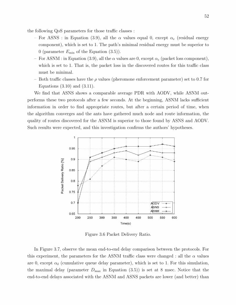
52
the following QoS parameters for those traffic classes :
– For ASNS : in Equation (3.9), all the α values equal 0, except αe (residual energy
component), which is set to 1. The path’s minimal residual energy must be superior to
0 (parameter Emin of the Equation (3.5)).
– For ASNM : in Equation (3.9), all the α values are 0, except αε (packet loss component),
which is set to 1. That is, the packet loss in the discovered routes for this traffic class
must be minimal.
– Both traffic classes have the ρ values (pheromone enforcement parameter) set to 0.7 for
Equations (3.10) and (3.11).
We find that ASNS shows a comparable average PDR with AODV, while ASNM out-
performs these two protocols after a few seconds. At the beginning, ASNM lacks sufficient
information in order to find appropriate routes, but after a certain period of time, when
the algorithm converges and the ants have gathered much node and route information, the
quality of routes discovered for the ASNM is superior to those found by ASNS and AODV.
Such results were expected, and this investigation confirms the authors’ hypotheses.
Figure 3.6 Packet Delivery Ratio.
In Figure 3.7, observe the mean end-to-end delay comparison between the protocols. For
this experiment, the parameters for the ASNM traffic class were changed : all the α values
are 0, except αδ (cumulative queue delay parameter), which is set to 1. For this simulation,
the maximal delay (parameter Dmax in Equation (3.5)) is set at 8 msec. Notice that the
end-to-end delays associated with the ASNM and ASNS packets are lower (and better) than
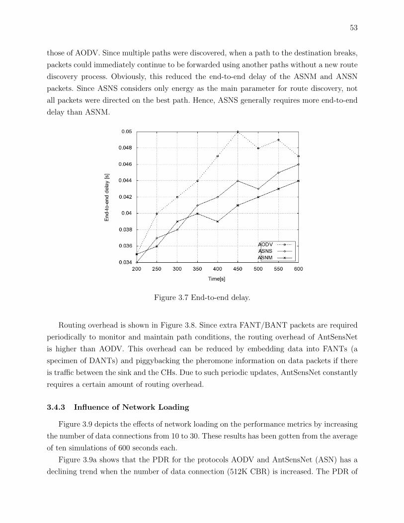
53
those of AODV. Since multiple paths were discovered, when a path to the destination breaks,
packets could immediately continue to be forwarded using another paths without a new route
discovery process. Obviously, this reduced the end-to-end delay of the ASNM and ANSN
packets. Since ASNS considers only energy as the main parameter for route discovery, not
all packets were directed on the best path. Hence, ASNS generally requires more end-to-end
delay than ASNM.
Figure 3.7 End-to-end delay.
Routing overhead is shown in Figure 3.8. Since extra FANT/BANT packets are required
periodically to monitor and maintain path conditions, the routing overhead of AntSensNet
is higher than AODV. This overhead can be reduced by embedding data into FANTs (a
specimen of DANTs) and piggybacking the pheromone information on data packets if there
is traffic between the sink and the CHs. Due to such periodic updates, AntSensNet constantly
requires a certain amount of routing overhead.
3.4.3 Influence of Network Loading
Figure 3.9 depicts the effects of network loading on the performance metrics by increasing
the number of data connections from 10 to 30. These results has been gotten from the average
of ten simulations of 600 seconds each.
Figure 3.9a shows that the PDR for the protocols AODV and AntSensNet (ASN) has a
declining trend when the number of data connection (512K CBR) is increased. The PDR of

54
Figure 3.8 Routing overhead.
AODV dropped from 76% to 51% while that of ASN dropped from 92% to 58%. Both AODV
and ASN are able to maintain >50% PDR in the latter case.
As Figure 3.9b shows, for a number of data connections of 10 nodes transmitting at
the same time, the protocols have relatively small latency of <20ms. The latency increases
gradually with the number of simultaneous data connections. It is worth to note that the
difference in latency between the load at 30 data connections is about twice, i.e., from 75ms
for ASN and 120ms for AODV, which is significant.
These results are explained by the AntSensNet’s capability to find adapt to the network
conditions, to find better routes and to use multiples routes.
3.4.4 Video Transmission
In this section we compare the capacity of protocols ASAR (Sun et al., 2008) and TPGF
(Shu et al., 2010) versus our protocol AntSensNet to transmit video packets.
The network topology used is the same used in the previous simulations. Only a video
sensor in all the network is capturing, encoding and sending a live video sequences to the sink.
We use only two paths to send the packets (in TPGF and AntSensNet, for ASAR we use only
a path). The video sequence is encoded according to H.264/AVC standard with a reference
frame list of size five frames for compensated prediction. The video testing sequence Foreman
(ASU, 2010) is used at QCIF resolution with 300 video frames at a frame rate of 30 fps with a

55
Figure 3.9 Results of varying number of data connections on (a) PDR and (b) average end-to-end delay
constant quantization step. In addition, the value of the parameter MREF was set to 5 frames.
The inter-frame period is 36 frames and is set to be equal with the transmission window. The
video frames are encapsulated into packets of size 1,024 bytes. A text trace of the video file
was created including the size of each frame and the time from the start of the video that
the frame occurred. This text information was included within the data field of the packets
in the simulation. As each packet was sent and received, a trace file was generated indicating
the time segment number of the video being sent. After the simulation, the video file was
reconstructed using the Evalvid software(Klaue et al., 2003), expanded into uncompressed
video using ffmpeg (Ke et al., 2008), and compared to the original uncompressed source file
again using the Evalvid software.
Figure 3.10 shows the average PSNR of the Foreman video. We can see that the video
quality was higher for the simulations using AntSensNet when compared to the other proto-
cols. This is because the protocols TPGF and ASAR are not able to handle correctly video
content. They do not implement any distortion minimization rate control and they are only
specialized in scalar data transmission. Conversely, AntSensNet is content-aware and and is
able to take actions in order to minimize the video distortion.
3.5 Conclusion
The promising pace of technological growth has led to the design of sensors capable of
sensing and producing multimedia data. However, as multimedia data contain images, video,

56
Figure 3.10 Received Video Quality of Foreman video
audio and scalar data, each deserves its own metrics. These characteristics of multimedia
sensor networks depend on efficient methods in order to satisfy QoS requirements. Given
such motivation, this paper proposes a QoS routing algorithm such as AntSensNet for WM-
SNs based on an Ant Colony optimization framework and a biologically inspired clustering
process. The routing algorithm also offers different classes of traffic, adapted to the needs of
applications. The clustering element uses special agents (ants) to guide the selection of CHs
in a totally distributed manner. In comparison with T-ANT, another ant-based clustering al-
gorithm, this novel clustering process achieves a permanent CH connection with lower energy
costs. Routing comprises both reactive and proactive components. In a reactive path setup ai-
med at the classes of traffic in the multimedia sensor networks, the algorithm can select paths
to meet the application QoS requirements, thus improving network performance. Multimedia
data are sent over the found paths. Over the course of the session, paths are continuously
monitored and improved in a proactive way. Simulation results show that the performance
of AntSensNet outperforms the standard AODV in terms of delivery ratio, end-to-end delay
and routing overhead.
Simulation results support that the proposed distortion reduction mechanism used to
transport video packets results in better quality video than using other protocols for multi-
media transport (TPGF and ASAR).
In future work, we intend to study the initialization method to populate routing tables
with initial pheromone levels. As shown in the literature (Ying et al., 2004), such mechanisms

57
can further increase network efficiency. Other approaches to be studied include the integration
of multiple sink-nodes as well as node mobility. Another improvement we plan to investigate
is to extend the proposed architecture to a t cross-layer architecture proposed in this work to
include a better interaction with a transport entity and the MAC sublayer. Similarly, Instead
of the 802.11 MAC layer, we will investigate the use of Sensor MAC (SMAC) which is a
MAC protocol designed for wireless sensor networks. SMAC has the potential to make the
cross-layer architecture more energy efficient.

58
CHAPITRE 4
A DISTRIBUTED CONNECTION ADMISSION CONTROL STRATEGY
FOR WIRELESS MULTIMEDIA SENSOR NETWORKS
Luis Cobo, Alejandro Quintero and Samuel Pierre
Mobile Computing and Networking Research Laboratory (LARIM)
Department of Computer & Software Engineering,
Ecole Polytechnique de Montreal,
C.P 6079, succ. Centre-Ville, Montreal, H3C 3A7, Quebec, Canada.
E-mail : {luis.cobo, alejandro.quintero, samuel.pierre}@polymtl.ca
Abstract
Wireless Multimedia Sensor Networks (WMSN) is an evolution of typical Wireless sensor
networks, where in addition to scalar data, devices in the network are able to retrieve vi-
deo and audio streams, still images, from the environment. Providing QoS guarantees for
the multimedia traffic in WMSNs requires sophisticated traffic management and admission
control procedures. In this paper, taking multiple parameters into account, we propose a
novel connection admission control scheme for this multimedia traffic. The proposed scheme
is able to determine if a new flow can be admitted in the network considering the current link
states and the energy of the nodes. The decision about accepting is taken in a distributed way,
without trusting in a central entity to take this decision. In addition, our scheme works like
a plug-in, being easily adaptable to any routing and MAC protocols. Our simulation results
show the effectiveness of our approach to satisfy QoS requirements of flows and achieve fair
bandwidth utilization and low jitter.
Keywords : quality of service, admission control, wireless multimedia sensor networks.
4.1 Introduction
Wireless Sensor Networks (WSN) have attracted attention from academia and industry
in recent years, mainly due to the various applications that can be built on them. A WSN
consists of spatially distributed sensor nodes. In a WSN, each sensor node is capable to in-
dependently perform some processing tasks and harvest information from the environment.
Most of this sensed information is scalar (like pressure, temperature, light or location of ob-
jects). Furthermore, sensor nodes communicate with each other via radio in order to forward

59
their sensed information to a central base station or perform some collaborative tasks such as
data fusion with others nodes in the network. In general, most of the applications currently
deployed on a WSN have low bandwidth demands in order to transmit their scalar data, and
are usually delay and packet-lost tolerant (Akyildiz et al., 2002).
More recently, the accelerated advance that has been experimented in the sensor hardware
field, MEMS and embedded computing, coupled with the availability of new and inexpensive
CMOS cameras and microphones that are capable to collect multimedia based data (image,
video or sound) from the environment, allowed the emergence of so called WMSN. A WMSN
is a network of wirelessly interconnected sensor nodes equipped with multimedia devices, such
as cameras and microphones, and these nodes are able to retrieve video and audio streams,
still images, as well as scalar sensor data (Akyildiz et al., 2007). By elapsing time, WMSNs
will become more and more popular and consequently these networks will allow the rise of a
wide range of applications in both civilian and military areas which require visual and audio
information such as multimedia surveillance sensor networks, traffic avoidance, enforcement
and control systems, advanced health care delivery, automated assistance to elderly and
family monitors, environmental monitoring and industrial process control.
The aforementioned applications require WMSNs provide mechanisms for delivering mul-
timedia content to a certain level of QoS. These requirements are a consequence of the nature
of the real time multimedia data such as high bandwidth demand, real-time delivery, tolerable
end-to-end delay, and proper jitter and frame loss rate. Moreover, there are many different
resource constraints in WMSNs involving energy, bandwidth, data rate, memory, buffer size
and processing capability because of the physically small size of the sensors and the nature
of the multimedia application that is typically producing a huge amount of data (Almalkawi
et al., 2010). Therefore, to meet the QoS requirements and to use the network scarce resource
in a fair and efficient manner is not an easy task. In addition, guaranteeing QoS in a WMSN
is a distributed task in nature, because of the use of error-prone wireless channels to com-
municate and its dynamic and infrastructure-less topology, ever changing. As a result, it is
very hard for a central entity to have an exact map of the network state and take decisions
about routing, for instance.
Much effort has been spent in protocols that provide QoS in WSN (Bhuyan et al., 2010),
but most of them do not take into accout an important factor when providing QoS to appli-
cations flows in the network : the dynamic CAC. CAC is an essential mechanism to accept
or reject a new flow based on determined constraints requested by the application and the
available resources in the network. Without an adequate admission control mechanism, the
network can admit traffic flows that will generate communication links saturates and overloa-
ded and the already admitted flows will experience unbearable performance degradation. In

60
this paper, we propose a framework an end-to-end connection admission control mechanism
that considers multiple QoS requirements simultaneously. Our framework :
– takes into account important QoS parameters, required by most application executing
on a WMSN. These parameters include bandwidth, packet-error rate, delay and jitter.
– is implemented as a separate scheme on top of routing protocols such as AODV. This
independence of the underlying routing protocol will allow our CAC to work as a plug-
in for any protocol that needs an admission control scheme. Nevertheless, In order to
reduce the overhead and improve the response time, our framework will use information
gathered by the routing and MAC protocols about link and node states.
– guarantees the global end-to-end QoS requirements by the joint local decisions of
the participating nodes. This operation is based on the concept of Hop-by-Hop QoS
contracts introduced by Melodia et Akyildiz (2010).
– additionally makes possible the reservation of the required resources by the new flow,
so that when the routing protocol begins to transmit packets, the network conditions
for the new flow are not different from those who our framework found.
The remainder of the paper is organized as follows. Section 4.2 addresses related work.
Section 4.3 presents our scheme for end-to-end call admission control. Section 4.4 describes
simulation and results. Finally, Section 4.5 draws the main conclusions.
4.2 Related Work
Solutions have been proposed in the literature providing QoS support in Wireless Ad-
Hoc Networks or Wireless Sensor Networks. Lee et al. (2000) propose INSIGNIA, a CAC
framework that is independent of the routing protocol and is implement on top of it. The
framework is based on an in-band signaling and soft-state resource management approach
that is well suited to supporting mobility and end-to-end quality of service in highly dynamic
environments where the network topology, node connectivity, and end-to-end quality of ser-
vice are time varying. However, this framework collects the bandwidth information by itself
(without taking into account the underlying routing and MAC information), generating high
overhead, slow response and inefficiency.
The Contention-aware Admission Control Protocol (CACP) presented by Yang et Kra-
vets (2005) aims to determine whether the available resources in the system can meet the
bandwidth requirements of a new flow, while bandwidth levels for existing flows are maintai-
ned. CACP is governed by three main characteristics : a) Prediction of available bandwidth ;
b) Contacting relevant neighborhoods and c) Prediction of bandwidth consumption by the
flow. However, CACP has significant overhead since packet transmission using high power

61
affects the ongoing transmission significantly and that makes unlikely the application of this
framework due the importance of the energy in this kind of networks. Perceptive Admission
Control (PAC), proposed by Chakeres et al. (2007) is another CAC protocols that enables
a high QoS by limiting the flows in the networks. PAC monitors the wireless channel and
dynamically adapts admission control decisions (increasing or decreasing the carrier sensing
range) to enable high network utilization while preventing congestion. That can be an ac-
ceptable action for a ad-hoc network, but in a WSN, the extension of the sensing range will
decrease the spatial reuse, and it will lead to some incorrect flow rejection decisions.
Zhu et Chlamtac (2006) introduce another framework which is compatible with existing
AODV routing protocol, and achieves bandwidth estimation, QoS routing and admission
decision by a cross layer cooperation between a IEEE 802.11 MAC and AODV-QoS routing
protocol. Unfortunately, that solution is closely tied to the MAC protocol, and that makes the
solution hard to implement if one wants to use other link protocols. Besides, this framework
does not consider important QoS measures as jitter or end-to-end delay when making the
flow admission decision.
With respect to WSN or WMSN, we cannot find many solutions to this problem in
the literature, but we can highlight the following two : Yin et al. (2010) model an admission
control algorithm for real-time traffic in a WSN, taking both delay and reliability into account.
Also, their algorithm also provides a fairness-aware rate control for non-real-time control
traffic. The scheme works in a cross-layer way, using information provided by the MAC layer.
Although the reliability and delay are important factors for the transmission of multimedia
data, this protocol forgets other important elements such as jitter or bandwidth used. Besides,
the flow admission decision is taken only with local information, and the neighbors are not
queried about their capacity when the new flow were admitted. Finally, Melodia et Akyildiz
(2010), presents an excellent mechanism for admission control in WMSN. Their algorithm is
based on the concept of Hop-by-Hop Qos contracts, where end-to-end QoS requirements for a
new flow, are guaranteed by establishing local contracts. Each single device that participates
in the communication is responsible for locally trying to guarantee the new flow performance
objectives. The global, end-to-end objective is thus achieved by the joint local decision of the
participating devices. Nevertheless, the scheme is strongly tied to UWB (Ultra Wide Band)
radio technology and geographic routing, and these technologies cannot be found in many
kinds of devices deployed in WMSN today.
Unlike our work, none of the previously proposed solutions consider the problem of satis-
fying multiple QoS constraints at the moment to make an admission control of a new flow
and, at the same time, create a CAC framework that can be plugged in to a routing protocol
to help it in the task to admit flows and which is capable to interact in a cross-layer way

62
with the MAC layer to get the necessary information to accomplish such task.
4.3 Our Proposed Algorithm
The aim of connection admission control (CAC) is to determine whether the available
resources in the network can meet the requirements of a new flow.
4.3.1 Network Model
In this work, a multimedia sensor network is represented as a graph G(V,E), where
V = {v1, v2, · · · , vN} is a finite set of nodes in a determined finite-dimension terrain, with
N = |V |, the number of nodes in the network, and E is the set of links between nodes, in
other words, eij ∈ E if and only if nodes vi and vj are within each other’s transmission range.
Node vN represents the sink of the network. Each link eij has a knowledge about its available
bandwidth βij and the energy spent in the transmission of a bit, which are dependent on the
distance dij between nodes vi and vj (also i and j in the following for simplicity).
4.3.2 Operation of our CAC approach
Our CAC mechanism works in the following way : given a requested new flow Φ(δ, β, χ, ρ)
, with maximum end-to-end delay δ, minimum guaranteed bandwidth β, maximum end-to-
end packet error rate χ and maximum end-to-end jitter ρ, generated at a node i that requires
a connection with the sink, our algorithm will return “ACCEPT”, if exists at lest a multi-hop
path from i to the sink that can provide and guarantee all the new flow requirements or
“REJECT”, otherwise.
4.3.3 Assumptions
Our CAC scheme will operate as a plug-in for the routing protocol of each network node.
The admission control mechanism is placed between the routing module and MAC layer (see
Figure 4.1), and operates in a cross-layer, obtaining information from both the MAC layer
and routing protocol, and accepting or rejecting a new connection for a flow of data the
application layer wants to establish with the sink. We suppose that both MAC and routing
layers are able to provide the required information to the CAC module. This information
includes :
– MAC Layer : link states and statistic data such as average sent packets, node’s neigh-
borhood, energy used to transmit a packet, packet error, etc.
– Routing Layer : paths to the sink from a determined node, packet error rate, queues
delay, etc.

63
This first assumption actually implicitly implies that MAC and routing protocols used by
our CAC mechanism are QoS-aware protocols. Typically, that kind of protocols maintains
and deals with this information, such as described by Bhuyan et al. (2010). It can also
deduced here is the routing protocol knows at least a route from node i to the sink before
performing admission control. Knowing the paths between any flow source node and the sink
is an important requirement for our CAC mechanism.
Routing Layer
CAC Mechanism
MAC Layer
Routes information
Link information: bandwidth, reliability, jitter
Are there resources for a new flow? Response: yes/no
Figure 4.1 CAC Modelling
We also suppose that a node can estimate their available link bandwidth in any moment
(for exemple, using the method presented by Alzate et al. (2008)) in a simple way. In the
same way, an application can provide information of bandwidth required by each data flow.
CAC Mechanism Description
As discussed before, the goal of a CAC scheme is to provide decisions on a new flow
admission with a certain QoS needs. If we are able to find a route providing the needed
end-to-end QoS requirements for the new flow, then we can admit it in the network and the
application can start transmit its packets.
Similarly to the solution presented by Melodia et Akyildiz (2010), we implement our
CAC mechanism using the concept of Hop-by-Hop QoS Contracts. In our case, in order to

64
determine if a route fulfills the end-to-end levels of quality of service required by a new data
flow, each node that is part of the route is responsible for locally trying to guarantee given
performance objectives, namely its contract. The global, end-to-end objective is thus achieved
by the joint local decisions of the participating nodes. In other words, each node in the route
has a QoS responsibility (a contract) derived from the end-to-end QoS requirements of the
new flow. If each node in the route has enough resources to accomplish its local contract,
the global needs of the new flow can be satisfied and as result of that, the new flow can be
admitted.
Let us assume that a new flow Φ(δ, β, χ, ρ) is generated at node i and requires service.
A multi-hop path from i to the sink needs to be established, with maximum end-to-end
delay δ, minimum guaranteed bandwidth β, maximum end-to-end packet error rate χ, and
maximum end-to-end jitter ρ. Now, by uniformly partitioning these end-to-end requirements
at all hops, we can get the hop requirements. As was previously pointed out, if the hop
requirement can achieved at each hop, the end-to-end QoS requirements can also be met. A
node can satisfy the hop requirement by selecting next hop nodes based on link conditions.
Clearly, the required bandwidth β needs to be provided at each hop. That is, for a given path
p,
β ≤ βij (4.1)
where βij represents the available bandwidth of link (i, j) on path p. Since the additive nature
of the delay, we can allow that the required end-to-end delay to be evenly divided at each
hop. For example, if the first hop in a 10 hops route towards the sink, then one tenth of the
total allowed end-to-end delay can be allowed to that hop. Then, the hop requirement for
maximum delay (δij) at each link (i, j) with route to the sink, can be expressed as :
δij =δ
Nij
(4.2)
where Nij denotes the maximum number of hops for all the routes from i to the sink when j
is next hop. This information must be provided by the routing layer. A similar concept can
be applied to the jitter ρij, that is :
ρij =ρ
Nij
. (4.3)
On the other hand, the packet error rate is multiplicative, and as result of that, the contract
is a little different, but we hold the same concept of proportionality. That is,
1− (1− χij)Nij ≤ χ, (4.4)

65
which leads to
χij ≤ 1− Nij
√(1− χ). (4.5)
In that way, we have the four contracts each hop must achieve to get a new flow admitted.
These values are computed by the source node i once, before the CAC operation begins, and
they are used by each node in deciding the next hop in the route towards the sink. As can
see, the contracts are based on information collected by the routing and MAC layer. Our
CAC mechanism only use such information in the task of deciding if a new flow should be
admitted or not.
Admission of new flows is regulated by an connection admission control protocol, which
works as follows. When receiving a new flow connection request form its application layer,
node i checks whether it has enough resource to accommodate this new flow while satisfy
its QoS requirements. If so, it broadcasts an CONTRACT_REQUEST packet, with the required
characteristics of the contract for the new flow being generated at i. If a node j, neighbor of
i, has a route to the sink and is able to provide the requested service with the necessary QoS
(that is, the node j has at least a link with another node in the route to the sink (different
to i) that satisfies all the contracts aforementioned), it replies with an CONTRACT_ ACCEPTED
control packet, which also includes the available level of batteries. Hence, node i receives an
CONTRACT_ ACCEPTED packet from all neighbors able to satisfy the contract for the new flow.
Among these, the best node j∗ (this one with the highest battery level) is selected. The node
source will then send ADMISSION_ REQUEST control packet to the selected node. This process
is depicted in the pseudo code presented in the algorithms 4 and 5.
When a node has not enough resources to satisfy the required contract, i.e., βij, δij, ρij, χij
for the new flow, it sends immediately to the previous node a CONTRACT_ REJECTED packet. If
no CONTRACT_ ACCEPTED packet is received, the CAC procedure is aborted for that node, and
an ADMISSION_ DENIED packet is sent to the upstream node, which will put the downstream
node in a blacklist in order to not contact it again, and the CAC procedure will continue
with the next best node. If there is no more neighbor nodes to continue, the node will also
send a ADMISSION_ DENIED control packet to the upstream node. When the flow originator
node receives ADMISSION_ DENIED packets from all its neighbors, it will notify to the routing
layer about the new flow cannot be admitted. The algorithms 6 and 7 present this process
at any node in the network.
When a ADMISSION_ REQUEST packet arrives at the sink, the sink will issue the CONNEC-
TION_ ADMITTED control packet to the corresponding source node, following the same route
but in inverse sense. After receiving the CONNECTION_ ADMITTED packet, the source node will
inform to the routing layer that the new flow has been admitted, that there is a route that
satisfy new flow requirements and that it can send packets stores in its buffer for the flow to

66
ALGORITHM 4: Beginning of CAC at source node i
Input: A connection admission request for flow Φ(δ, β, χ, ρ)
1 if not enough resources then2 Reject connection request for Φ ;3 return
4 end5 Calculate Contract δij , βij , χij , ρij ;6 Broadcast packet CONTRACT REQ with Contract ;7 while not TIMEOUT do8 Receive packet from a neighbor h;9 if received packet is CONTRACT ACCEPT then
10 Store h info ;11 end
12 end13 if a neighbor accepted Contract then
// Best node = max energy
14 j∗ ← Best neighbor among info received;// Initialize path to sink
15 Path ← [i] ;16 Send packet { ADMISSION REQ, Contract, Path } to node j∗ ;
17 else18 Reject connection request19 end
the sink. This process is shown by the algorithms 8 and 9.
4.4 Experimental Results
To assess the performance of our CAC mechanism, we conduct several simulations on the
ns2 network simulator version 2.34 (ns, 2010). Various tests were carried out with diverse
network topologies and conditions. For these experiences, we have modified AODV to use
the route found by the CAC algorithm after the flow is admitted to transmit the packets. In
addition, before the CAC started to work, we had found routes between each node and the
sink, using the normal AODV mechanism for finding routes.
In our first experience, we show that our CAC scheme is able to get routes that satisfy
the requirements of a new flow entering in the network. For this simulation, we considered a
scenario consisting of a 1000 m x 1000 m terrain with 49 nodes deployed in a grid structure.
The sink is located at the center of the terrain. Each node has a transmission range of 50 m.
We use IEEE 802.11 as our MAC protocol and AODV as the routing protocol. We assume
the channel capacity is 1 Mbps.
In this first scenario, we have three flows, each one generating traffic with bandwidth

67
ALGORITHM 5: Behavior of a intermediate node when it receives a CONTRACT REQUEST
Input: A packet CONTRACT REQ has arrived from node i
1 if Request has not been received before then2 if Contract can be satisfied and there is a route to sink then3 Reply with CONTRACT ACCEPT battery level to node i ;4 else5 Reply with CONTRACT REJECT to node i ;6 end
7 end
ALGORITHM 6: An intermediate node receives an ADMISSION REQ packet
Input: A packet { ADMISSION REQ, Contract, Path } has arrived from node i
1 Broadcast packet CONTRACT REQ with Contract ;2 while not TIMEOUT do3 Receive packet from a neighbor h;4 if received packet is CONTRACT ACCEPT then5 Store h info ;6 end
7 end8 if a neighbor accepted Contract then
// Best node = max energy
9 j∗ ← Best neighbor among info received;10 Add myself to Path ;11 Send packet { ADMISSION REQ, Contract, Path } to node j∗;
12 else13 Send packet ADMISSION DENIED to node i14 end
requirement of 320 kbps, maximum end-to-end packet delivery delay of 20ms, packet error
rate of 0% and maximum jitter of 10ms. Each flow generates a CBR traffic with a rate
of 80 packets per second with a packet size of 512 bytes. The second flow is started 10
seconds after the first flow, and the third flow, 10 seconds after the second flow. Figure 4.2
shows the throughput of each of the three flows, and Figure 4.3 shows the average end-
to-end packet delay for the three flows. The graphs confirms the advantages of our CAC
scheme. For instance, a stable throughput for each flow is guaranteed once it is accepted and
the requirements are obtained all the simulation time. Delays are also maintained all the
duration of the transmission and with a low fluctuation (low jitter). The found routes are
adequate for the flows and their requirements.
In a second scenario we compare flows with admission control versus flows without ad-
mission control in order to establish that the utilization of CAC is advantageous for the
transmission of multimedia information and overpasses AODV data transmission when it
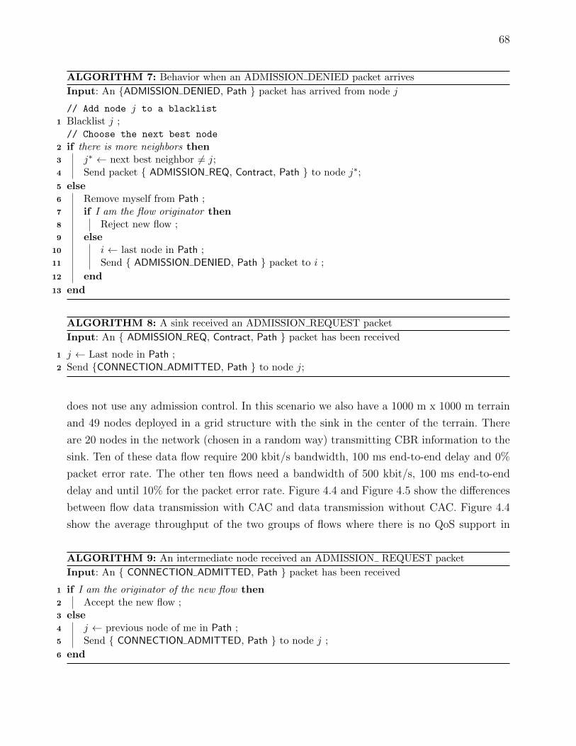
68
ALGORITHM 7: Behavior when an ADMISSION DENIED packet arrives
Input: An {ADMISSION DENIED, Path } packet has arrived from node j
// Add node j to a blacklist
1 Blacklist j ;// Choose the next best node
2 if there is more neighbors then3 j∗ ← next best neighbor 6= j;4 Send packet { ADMISSION REQ, Contract, Path } to node j∗;
5 else6 Remove myself from Path ;7 if I am the flow originator then8 Reject new flow ;9 else
10 i ← last node in Path ;11 Send { ADMISSION DENIED, Path } packet to i ;
12 end
13 end
ALGORITHM 8: A sink received an ADMISSION REQUEST packet
Input: An { ADMISSION REQ, Contract, Path } packet has been received
1 j ← Last node in Path ;2 Send {CONNECTION ADMITTED, Path } to node j;
does not use any admission control. In this scenario we also have a 1000 m x 1000 m terrain
and 49 nodes deployed in a grid structure with the sink in the center of the terrain. There
are 20 nodes in the network (chosen in a random way) transmitting CBR information to the
sink. Ten of these data flow require 200 kbit/s bandwidth, 100 ms end-to-end delay and 0%
packet error rate. The other ten flows need a bandwidth of 500 kbit/s, 100 ms end-to-end
delay and until 10% for the packet error rate. Figure 4.4 and Figure 4.5 show the differences
between flow data transmission with CAC and data transmission without CAC. Figure 4.4
show the average throughput of the two groups of flows where there is no QoS support in
ALGORITHM 9: An intermediate node received an ADMISSION REQUEST packet
Input: An { CONNECTION ADMITTED, Path } packet has been received
1 if I am the originator of the new flow then2 Accept the new flow ;3 else4 j ← previous node of me in Path ;5 Send { CONNECTION ADMITTED, Path } to node j ;
6 end
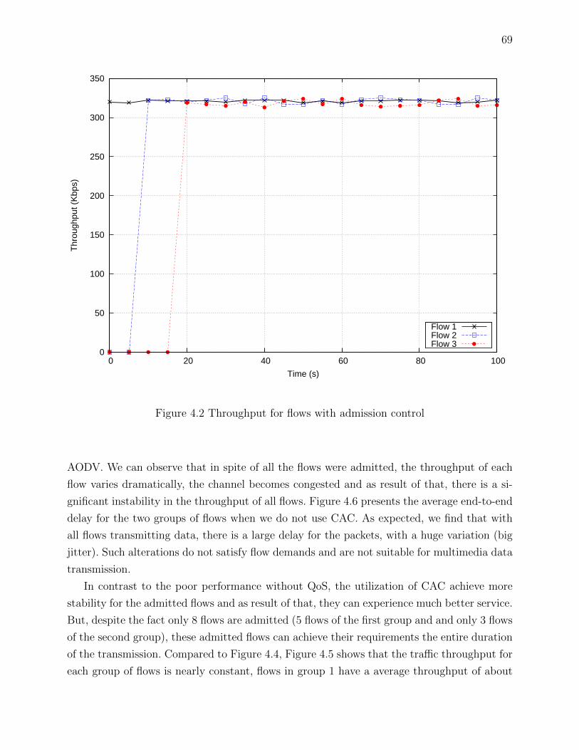
69
0
50
100
150
200
250
300
350
0 20 40 60 80 100
Thr
ough
put (
Kbp
s)
Time (s)
Flow 1Flow 2Flow 3
Figure 4.2 Throughput for flows with admission control
AODV. We can observe that in spite of all the flows were admitted, the throughput of each
flow varies dramatically, the channel becomes congested and as result of that, there is a si-
gnificant instability in the throughput of all flows. Figure 4.6 presents the average end-to-end
delay for the two groups of flows when we do not use CAC. As expected, we find that with
all flows transmitting data, there is a large delay for the packets, with a huge variation (big
jitter). Such alterations do not satisfy flow demands and are not suitable for multimedia data
transmission.
In contrast to the poor performance without QoS, the utilization of CAC achieve more
stability for the admitted flows and as result of that, they can experience much better service.
But, despite the fact only 8 flows are admitted (5 flows of the first group and and only 3 flows
of the second group), these admitted flows can achieve their requirements the entire duration
of the transmission. Compared to Figure 4.4, Figure 4.5 shows that the traffic throughput for
each group of flows is nearly constant, flows in group 1 have a average throughput of about

70
0
0.002
0.004
0.006
0.008
0.01
0.012
0.014
0.016
0.018
0.02
0 20 40 60 80 100
Ave
rage
Pac
ket D
elay
(s)
Time (s)
Flow 1Flow 2Flow 3
Figure 4.3 Packet delay for flows with admission control
200kbps, while flows in group 2 show a average throughput of about 490 kbps and match
their requirements. The delay, shown in Figure 4.7, is very small compared with the delay
obtained when we do not use CAC. The average end-to-end delays of the admitted flows
of the two groups are below the required admission values. These short delays, along with
a good obtained throughput demonstrate that our CAC mechanism can be used to sustain
multimedia traffic, such as audio or video.
Next, we conduct a simulation using the same characteristics of the second scenario.
In this case we will compare our CAC versus the admission control scheme implemented
by AODV-QoS (Perkins et Belding-Royer, 2003) and AntSensNet (Cobo et al., 2010) QoS
protocols. AODV-Qos is a modification of the popular protocol AODV, but it supports getting
routes considering bandwidth and time as QoS parameters. AntSensNet is based on ACO
(Ant Colony Optimization) paradigm and is able to find routes taking into account the same
parameters of our scheme (bandwidth, jitter, delay and packet lost), but also energy. In Table
4.1 we can observe the comparison among the three admission control schemes. There are 20
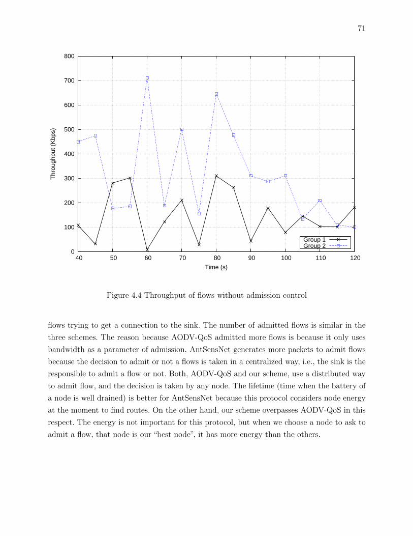
71
0
100
200
300
400
500
600
700
800
40 50 60 70 80 90 100 110 120
Thr
ough
put (
Kbp
s)
Time (s)
Group 1Group 2
Figure 4.4 Throughput of flows without admission control
flows trying to get a connection to the sink. The number of admitted flows is similar in the
three schemes. The reason because AODV-QoS admitted more flows is because it only uses
bandwidth as a parameter of admission. AntSensNet generates more packets to admit flows
because the decision to admit or not a flows is taken in a centralized way, i.e., the sink is the
responsible to admit a flow or not. Both, AODV-QoS and our scheme, use a distributed way
to admit flow, and the decision is taken by any node. The lifetime (time when the battery of
a node is well drained) is better for AntSensNet because this protocol considers node energy
at the moment to find routes. On the other hand, our scheme overpasses AODV-QoS in this
respect. The energy is not important for this protocol, but when we choose a node to ask to
admit a flow, that node is our “best node”, it has more energy than the others.

72
150
200
250
300
350
400
450
500
550
40 50 60 70 80 90 100 110 120
Thr
ough
put (
Kbp
s)
Time (s)
Group 1Group 2
Figure 4.5 Throughput of flows with admission control
4.5 Conclusions
In this paper, we have presented a framework for connection admission control (CAC) to
provide QoS in wireless multimedia sensor networks. Our CAC scheme is able to discover the
route satisfying the multiple requirements (bandwidth, delay, packet error rate and jitter)
and, on the basis of that, to determine whether a flow can be admitted. Our scheme is
distributed (there is no a central entity what takes the admission decision) and adaptive to
the link stated at the moment the new flow asks to be admitted. Performance evaluation shows
that the proposed scheme is effective in supporting multimedia data transmission with QoS
guarantees. In particular, delays are very low with low jitter, and throughput is maintained
pretty constant in time.

73
0.05
0.1
0.15
0.2
0.25
0.3
0.35
40 50 60 70 80 90 100 110 120
Ave
rage
Pac
ket D
elay
(s)
Time (s)
Group 1Group 2
Figure 4.6 Packet delay of flows without admission control
Tableau 4.1 Comparison among admission control schemes
Protocol Admitted flows Packets LifetimeOur CAC 8 12 411 secsAODV-QoS 11 10 304 secsAntSensNet 8 24 612 secs

74
0.005
0.01
0.015
0.02
0.025
0.03
0.035
0.04
0.045
40 50 60 70 80 90 100 110 120
Ave
rage
Pac
ket D
elay
(s)
Time (s)
Group 1Group 2
Figure 4.7 Packet delay of flows admission control

75
CHAPITRE 5
INTEGER PROGRAMMING FORMULATION AND GREEDY
ALGORITHM FOR 3-D DIRECTIONAL SENSOR PLACEMENT IN WMSN
Luis Cobo, Alejandro Quintero and Samuel Pierre
Mobile Computing and Networking Research Laboratory (LARIM)
Department of Computer & Software Engineering,
Ecole Polytechnique de Montreal,
C.P 6079, succ. Centre-Ville, Montreal, H3C 3A7, Quebec, Canada.
E-mail : {luis.cobo, alejandro.quintero, samuel.pierre}@polymtl.ca
Abstract
Conventional multimedia sensor deployment is generally based on a 2D directional sensing
model. However, this model cannot accurately characterize the actual behavior of real multi-
media (image/video) sensor networks. To remedy this deficiency, we propose a Minimum 3D
Directional Sensor Placement (M3DSP) which aim at to determine the minimum number of
connected directional multimedia sensor nodes and their configuration, needed to cover a set
of control points in a given 3D space. The configuration of each deployed sensor is determi-
ned by three parameters which are sensing range, FoV and orientation. We present the exact
ILP formulation for the problem and an approximate (but computationally efficient) greedy
algorithm solution. We also evaluate different properties of the proposed solutions through
extensive simulations.
Keywords : 3D, deployment, greedy algorithm, heuristics, linear programming, optimiza-
tion, Wireless Multimedia Sensor Networks.
5.1 Introduction
The rapid development and progress of sensors, MEMS, embedded computing, in addition
to the availability of inexpensive CMOS cameras and microphones coupled with the signi-
ficant advances in distributed signal processing and multimedia source coding techniques,
has allowed for the emergence of so called wireless multimedia sensor networks. As a result,
WMSN (Akyildiz et al., 2007) is a network of wirelessly interconnected smart nodes equipped
with multimedia devices, such as cameras and microphones, and capable to retrieve video
and audio streams, still images, as well as scalar sensor data. WMSNs promise a wide range

76
of potential applications in both civilian and military areas which require visual and audio
information such as video surveillance, traffic avoidance, law-enforcement reports, health care
delivery, automated assistance to elderly telemedicine, industrial process control and environ-
mental and structural monitoring. Besides, to successfully accomplish the assigned sensing
tasks, the deployed sensors must both cover certain specific point-locations or the entire tar-
get sensing area, and form a connected network through multi-hop wireless communications.
Therefore, an important issue in designing WMSNs is the appropriate placement of the sensor
such that they can provide a connected coverage of a given area (Han et al., 2008).
Sensors can be placed in an area of interest either deterministically or randomly. The
choice of the deployment scheme depends highly on the type of sensors, application and the
environment that the sensors will operate in. For some applications, random deployment of
nodes is the only feasible option. This is particularly true for harsh environments such as a
battle field or a disaster region. Depending on the node distribution and the level of redun-
dancy, random node deployment can achieve the required performance goals. Alternatively,
deterministic node deployment is viable and often necessary when sensors are expensive or
when their operation is significantly affected by their position. Such scenarios include popu-
lating an area with highly precise seismic nodes, underwater WSN applications, and placing
imaging and video sensors (Younis et Akkaya, 2008).
While conventional sensor networks often assume the omni-directional sensing model
where each sensor can equally detect its environment in each direction, image/video sen-
sors in a WMSN adopt the directional sensing model. In this model, the sensing region of
each directional sensor is a sector of the sensing disk centered at the sensor with a sensing
radius. In other words, directional sensors have the the notion of direction of measurement,
i.e., they are capable of taking measurement only in a specific direction. When a sensor is
facing to a direction and a target is in the sensing region of the sensor, we say that the
direction of the sensor covers the target.
In general, these sensors are involved in three-dimensional (3D) application scenarios,
which is much more difficult to analyze compared to two-dimensional deployment regions
(Younis et Akkaya, 2008). That is the reason most existing works focus on the simplified
2D sensing model. However, according to Poduri et al. (2006) who have investigated the
applicability of contemporary coverage analysis and placement strategies pursued for 2D
spaces to 3D setups, many of the popular formulations, such as art-gallery and sphere-packing
problems, which are optimally solvable in 2D, become NP-Hard in 3D. In addition to that,
most placement approaches for directional multimedia sensors strives to enhance the quality
of visual images and/or accuracy of the assessment of the detected objects. Other approaches
focus on optimizing the sensor network after the sensors are randomly deployed in a sensor

77
field. Therefore, there is a pressing need of efficient and effective 3D directional WMSN
planning techniques.
In this paper, we study the problem of the connected coverage deployment in the context
of directional multimedia sensor networks on a 3D sensing field. We provide an optimization
framework that minimizes the number of sensors installed, while considering both 3D direc-
tional point covering and network connectivity constraints. We propose an Integer Linear
Programming (ILP) formulation for the problem that allows to solve optimally in small size
networks and to evaluate the impact of system parameters. We also propose an heuristic
approach that allows to achieve good quality solution in short computing time, tackling also
the optimization of larger network deployments.
The rest of the paper is organized as follows : Section 5.2 presents background and related
work on this topic. Section 5.3 describes the 3D directional sensor network model and formally
defines the problem. In Section 5.4, we present our resolution method based on a Greedy
heuristic. In Section 5.5, we discuss our simulation results. Finally, Section 5.6 concludes the
paper and points out some future directions.
5.2 Related Work
Extensive research on deterministic connected coverage deployment has been done for
omni-directional sensor networks. Most work on this category of placement seeks to determine
the “optimal” placement pattern, that is, to find the minimum number of nodes deployed.
Minimizing the number of sensor can take the form of an“art gallery”problem (O’Rourke,
1987), which aims to find the minimum set of locations for security guards inside a polygonal
art gallery, such that the boundary of the entire gallery is visible by at least one of the security
guards. Gonzalez-Banos (2001) proposed a randomized algorithm to solve the art gallery
problem in order to find locations for sensor nodes. However, in the art gallery problem, all
security guards are assumed to have infinite vision if there is no obstacles. This assumption
does not hold for directional WMSNs in which sensor nodes have limited sensing ranges.
Besides, the problem does not require a connection between the guards, a very important
exigence for the deployment of the nodes.
There is also some published works discussing the node deployment scheme through the
maximization of coverage, using techniques as Virtual Force Algorithm (Wang et al., 2007)
or Tabu Search (Aitsaadi et al., 2009). However, these works only considered the coverage
constraint. They did not include the discussion about the connectivity, or they implicitly as-
sumed that the sensor network formed by the obtained pattern was connected, regardless the
transmission ranges of sensor nodes. Nevertheless, this assumption may not be true. To find

78
the optimal node placement pattern subject to both coverage and connectivity constraints,
Patel et al. (2005) have modeled the problem as an optimization problem that minimizes the
number of required sensors nodes, under the constraints that a set of control points must be
covered by at least a determined number of sensors and all the nodes are connected. However,
the paper did not find a general solution. Instead, it discussed different options of regular
sensor network deployment. These options include minimum cost placement or maximum
lifetime placement.
Recently, a few research efforts have been devoted to directional sensor networks deploy-
ment. Ai et Abouzeid (2006) presented some algorithms for randomly deployed directional
sensor networks to identify a minimal set of directions to cover the maximal number of point-
locations. Cai et al. (2009), several scheduling algorithms were presented to divide a randomly
deployed sensor network into subsets to alternatively cover a set of point-locations so as to
prolong lifetime. Han et al. (2008) also presented several algorithms to deploy directional
sensor networks. They were interested in the Connected Point-Coverage Deployment and the
Connected Region-Coverage Deployment problems, and they solved both problems in a geo-
metric way. They did not take into consideration important problems to any type of sensor
networks as the connection to the sink or the energy intake in their algorithms. Besides, the
authors only placement in a 2D space.
An interesting line of research is introduced by Osais et al. (2008, 2009, 2010), where
the authors formulated an ILP (defined as Minimum Sensor Placement problem) about the
placement of directional sensors, taking into account very important variables in this problem
like the field of view for the sensors, their sensing range and the base station position. The
model also considered point-coverage as well as connectivity among the deployed sensors.
However, a 3D space was not considered in these models.
There exist only few references on 3D directional sensor network deployment in the litera-
ture. Ma et al. (2009) proposed a 3D directional sensor coverage-control model with tunable
orientations. They used a virtual force analysis method to maximize the sensor area cove-
rage after an initial random deployment. But in this method the number of sensors is not
optimized and constraints like connectivity to the sink were not taken into account by the
authors.
The 3D directional sensor placement problem is similar to the camera placement problem.
Horster et Lienhart (2006) developed a binary integer programming model to post-optimize
the camera poses, after a random deployment, in order to increase coverage of the space
observed. The exact model determines jointly for each camera the pan and tilt angle that
maximizes the coverage of a 3D space. But this model is not directly applicable to a 3D
directional sensor network, because it did not consider either the connectivity among sensors
79
or between sensors and the sink.
Our work differs from prior work in a few aspects. First, the problem of covered-point
connected deployment for 3D directional sensor networks is formulated, which can be solved
exactly by the proposed ILP formulation in a small scale and approximately by the proposed
Greedy algorithm in a large scale. Second, in such formulation we took into consideration very
important elements in the WMSN design as the base station location. Finally, our proposed
solution to deal with coverage by directional sensor with tunable orientation can treat the
coverage by isotropic (omni-directional) sensors as a special case.
5.3 Problem Formulation
Controlled deployment is the ideal way pursued for the placement of multimedia sensor
networks. These sensors need to be installed at precise places in a room and not randomly
distributed on a outdoor field, mainly due in part to their cost and the importance to know
their exact position for the applications. Therefore, our work offer to WMSN designers an
efficient and effective model to help them make sure that their deterministically deployed
network will perform as best as possible in a 3D sensor field.
5.3.1 Assumptions
The following assumptions are made about the model we are formulating :
– A directional multimedia sensor network consists of directional multimedia sensors and
a base station, all of these are static.
– Directional sensors are responsible for sensing/monitoring environment as well as for-
warding data they receive from other sensors towards the base station. These sen-
sors have sectoral perception, that is, they capture information in a directional region,
usually called Field of View (FoV).
– A base station is responsible for collecting all the data generated by sensor. The base
station has sufficient hardware, sufficient software and constant power supply.
– The control points are locations in the sensor field which must be covered by a required
number of sensors.
– The feasible sites are a set of points where it is possible to deploy the sensors in the
sensor field.
– Either the control points or the feasible sites can regularly (i.e., a grid) or randomly be
distributed.
– The predominant traffic in the network is the data traffic from sensors to the base
station.

80
– We only consider convex 3D spaces without obstacles constricting the FoV of our mul-
timedia sensors.
– As a result of that, the area covered by a sensor will be a circle with center in the sensor
and radius equals to the sensing range of the sensor, and a control point will be covered
by a sensor if the control point is within the coverage area of the sensor.
5.3.2 Sensing Model of 3D Directional Sensors
For simplicity, we also assume a Boolean sensing model (Hossain et al., 2008). In this
model, an event will be detected by a sensor if the occurrence of such event is within the
sensing range of the sensor, otherwise not. Nevertheless, Different from the isotropic (omni-
directional) 2D sensing model which is viewed as a whole circular area in a two-dimension
plane, 3D sensing model focuses on two distinct features : 1) the sensor is located at a fixed
3D point, and its sensing direction is 3D rotatable around its location ; 2) the coverage area
of a sensor is constrained by its FoV. Please note that, through the rest of the paper, unless
otherwise mentioned, we use the terms “sensors” or “nodes” for simplicity to refer to wireless
multimedia sensor including video and audio sensors having a directional view. Thus, we
define a 3D directional sensing model as follows.
Our sensing model that defines the FoV of the sensors can be described by a pyramid.
This pyramid can be completely characterized by the following parameters (please refer to
Figure 5.1) :
1. P = (x, y, z) : the Cartesian coordinates which denote the location of the sensor in 3D
space.
2.−→D : the sensing direction (or orientation) of the directional sensor. This a vector that
connect the apex of the pyramide (the point P ) with the point located in the center of
the base of the pyramid. Besides its length, this direction is defined by its inclination
(θ) and its azimuth (ϕ). The inclination is the angle from the positive z-axis and the
azimuth is the angle measured from the Cartesian plane xy.
3. α and β : the horizontal and vertical offset angles of the FoV around−→D .
4. rs : the sensing range of the directional sensor, beyond which a control point will not
be covered. This value is the length of the vector−→D .
In the ideal case, sensor’ directions and offsets are continuous variables in the space. They
could take any value from 0◦ to 360◦. But, since our objective function, the (integer) number
of cameras, is not continuous and differentiable, and in order to make our problem tractable,
we approximate the continuous case by sampling poses, that is, we assume that directional
sensors can only adopt a discrete set of values for these angles.

81
x
y
z
~D
ϕ
θ
(a) Sensor direction (b) FoV amplitude
Figure 5.1 FoV parameters
5.3.3 Problem Statement
In this work, we aim at optimizing the overall network topology by properly selecting
location and FoV of directional sensors in such a way that the total number of deployed
sensors is minimized, under the constraints that each control point is covered by at least
a given number of sensors and the resulting network is connected. We call this problem
“Minimum 3D Directional Sensor Placement”or M3DSP. Unfortunately, M3DSP becomes the
set covering problem in its simplest form , which is known to be NP-hard in the strong sense
(Garey et Johnson, 1979). As a result, solving M3DSP becomes computationally prohibitive to
obtain an exact optimal sensor placement solution for networks of realistic size. We therefore
propose efficient and accurate approximation algorithms and heuristics.
5.3.4 Coverage by Directional Sensors
In the following, the term space denotes a convex physical three-dimensional room. We
define that a control point in that space is covered by a sensor if that point is inside the
sensor’s FoV. To determine whether a control point c located at C = (cx, cy, cz) is covered by
a sensor j with parameters (Pj = (xj, yj, zj),−→Dj, αj, βj, rs), firstly we transform the control
point’s coordinate from world coordinate system to the field of view coordinate system.
Figure 5.2 shows the process in 2D. To do this, we must follow the following two steps :
1. Translate the directional sensor’s FoV to the origin of the coordinate system. The
control point will be translated in the same way. As a consequence of that, the new
translated coordinates for the control point, that we called C ′, can be gotten in the
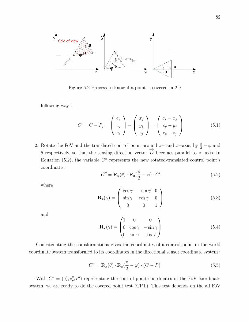
82
Figure 5.2 Process to know if a point is covered in 2D
following way :
C ′ = C − Pj =
cx
cy
cz
− xj
yj
zj
=
cx − xjcy − yjcz − zj
(5.1)
2. Rotate the FoV and the translated control point around z− and x−axis, by π2−ϕ and
θ respectively, so that the sensing direction vector−→D becomes parallel to z−axis. In
Equation (5.2), the variable C ′′ represents the new rotated-translated control point’s
coordinate :
C ′′ = Rx(θ) ·Rz(π
2− ϕ) · C ′ (5.2)
where
Rz(γ) =
cos γ − sin γ 0
sin γ cos γ 0
0 0 1
(5.3)
and
Rx(γ) =
1 0 0
0 cos γ − sin γ
0 sin γ cos γ
(5.4)
Concatenating the transformations gives the coordinates of a control point in the world
coordinate system transformed to its coordinates in the directional sensor coordinate system :
C ′′ = Rx(θ) ·Rz(π
2− ϕ) · (C − P ) (5.5)
With C ′′ = (c′′x, c′′y, c′′z) representing the control point coordinates in the FoV coordinate
system, we are ready to do the covered point test (CPT). This test depends on the all FoV

83
parameters and states that the control c is covered by a directional sensor j if all of the
following conditions are true :
a) c′′z ≤ rs (5.6)
b) − tanα
2≤ c′′y ≤ tan
α
2(5.7)
c) − tanβ
2≤ c′′x ≤ tan
β
2(5.8)
In other words, a 3D directional sensor at position Pj = (xj, yj, zj), orientation−→D (incli-
nation = θ, azimuth = ϕ), sensing range rs and offset angles α and β covers a control point
c located at C = (cx, cy, cz) if and only if 5.6–5.8 are satisfied.
5.3.5 Problem Modeling
In the following, we derive an ILP model to solve the M3DSP problem. We first define
the following sets :
– Let S = {1 . . . N} be the set feasible sites where the directional sensors can be installed.
deploying sensors in the sensor field.
– Let Φ = {1 . . .M} be the set of control points to monitor in the sensor field.
– Let Ψ be the set of all possible directions (or orientation) for a sensor.
– Let A be the set of all possible horizontal offset angles for a sensor. That is, the set of
values that we can assign to the parameter α in the sensor’s field of view.
– Let B be the set of all possible vertical offset angles for a sensor. That is, the set of
values that the we can assign to the parameter β in the sensor’s FoV.
Then, we define the following parameters
– Q, denote the minimum number of directional sensor that should cover every control
point.
– rs, the sensing range for all sensors.
– rc, the communication range for all sensors.
We also define our constants :
– D, Adjacency matrix that summarizes connectivity between two sensors installed at
two feasible sites. It is defined as
Dij =
1 if dist(i, j) ≤ rc with i ∈ S, j ∈ S, i 6= j,
0 otherwise(5.9)
where dist(·) is the Euclidean distance between the position of the two involved devices

84
.
– B, Adjacency matrix that summarizes connectivity between a sensor installed at a
feasible site and the WMSN base station. It is defined as
Bij =
1 if distb(i) ≤ rc with i ∈ S,
0 otherwise.(5.10)
where distb(·) represents the Euclidean distance between a sensor and the base station.
– C, Adjacency matrix that summarizes the control point coverage by the directional
sensors. This matrix is defined as
Crabij =
1, if a control point m ∈ Φ is within
the coverage area of a sensor placed at location
i ∈ S when its orientation is r ∈ Ψ,
its horizontal offset angle is a ∈ A
and its vertical offset angle is b ∈ B,
0, otherwise.
(5.11)
– Uij, Capacity of the wireless link between sensors (i, j), i, j ∈ S, i 6= j.
– U bi , Capacity of the wireless link between sensor i ∈ S and the network base station.
– Umax, Maximum amount of data a directional sensor can handle (transmit and/or re-
ceive) per unit time (called the node capacity).
– Ri, The rate at which the information is generated at a sensor located at i ∈ SFinally, we define the following decision variables :
– xrabi , a binary variable defined as
xrabi =
1, if a sensor is placed at location i ∈ S
with a orientation r ∈ Ψ, a horizontal offset angle a ∈ A
and a vertical offset angle b ∈ B,
0, otherwise.
(5.12)

85
– yij, a binary variable defined as
yij =
1, if there are is a sensor installed at site i ∈ S
that communicates with a sensor installed at site j ∈ S, i 6= j,
0, otherwise.
(5.13)
– ybi , a binary variable defined as
ybi =
1, if there are is a sensor installed at site i ∈ S
that communicates directly with the base station,
0, otherwise.
(5.14)
– fij, The data flow rate from sensor node i to sensor node j with i, j ∈ S and i 6= j.
– f bi , The data flow rate from sensor node i to the network base station, with i ∈ S.
Thus, we can model our problem by the following optimization system. The following
objective function aims at minimize the number of directional sensors that will be installed
over the network.
min∑i∈S
∑r∈Ψ
∑a∈A
∑b∈B
xrabi (5.15)
The optimization is subject to the following constraints :
The first constraint ensure that exactly one direction-offsets combination is assigned to
each sensor : ∑r∈Ψ
∑a∈A
∑b∈B
xrabi ≤ 1 ∀i ∈ S (5.16)
The coverage requirement is represented by the following constraint(∑i∈S
∑r∈Ψ
∑a∈A
∑b∈B
xrabi · Crabij
)≥ Q ∀j ∈ Φ (5.17)
which guarantees a full coverage of the monitored are such that every control point is covered
by at least Q sensors.
A wireless link is established between two placement sites if two sensors are installed at
those sites and they can communicate with each other. This is represented by the following
constraint
yij ≤Dij
2·
(∑r∈Ψ
∑a∈A
∑b∈B
xrabi +∑r∈Ψ
∑a∈A
∑b∈B
xrabj
)∀i, j ∈ S, i 6= j (5.18)

86
Similarly, a wireless link can be established between the base station and a placement site
only if there is a sensor installed at that site and it can communicate with the base station.
This is ensured by the following constraint :
ybi ≤ Bsi ·∑r∈Ψ
∑a∈A
∑b∈B
xrabi ∀i ∈ S (5.19)
The following constraint ensures that the resulting network is connected, that is, the base
station receives all the data generated by the installed sensor nodes.(Ri ·
∑r∈Ψ
∑a∈A
∑b∈B
xrabi
)+∑
j∈S,j 6=i
fij −∑
j∈S,j 6=i
fji ≤ f bi ∀i ∈ S (5.20)
The sum of incoming and outgoing flow through a sensor node should not exceed its
capacity and this is ensured by the following constraint :∑j∈S,j 6=i
fij +∑
j∈S,j 6=i
fji + f bi ≤ Umax ·∑r∈Ψ
∑a∈A
∑b∈B
xrabi ∀i ∈ S (5.21)
The remaining sets of constraints (5.22) and (5.23) ensure that the flow on a wireless link
does not exceed link’s capacity.
fij ≤ Uij · yij i, j ∈ S, i 6= j (5.22)
f bi ≤ U bi · ybi ∀i ∈ S (5.23)
Finally, constraints (5.24) and (5.25) define the domain of each variable
xrabi , yij, ybi ∈ {0, 1} ∀i, j ∈ S, i 6= j; r ∈ Ψ; a ∈ A, b ∈ B (5.24)
fij, fbi ∈ R+ ∀i ∈ S, i 6= j (5.25)
5.4 Proposed Heuristic
Though the solution of the ILP formulation provides the optimal solution for the M3DSP
problem, it is not scalable for large problems instances. That is the reason we present here a
greedy heuristic based polynomial-time algorithm for solving the problem in a approximate
way.
To find a good solution, our algorithm follows two steps. The first step is the selection of
a sensor set Γ ⊆ S with its respective FoV. We called this first step “The covering set finder”.

87
The sensors in this set cover all control points in the field (the set we previously defined as
Φ). The second step creates a connected network from Γ, adding nodes from S to achieve
this objective.
The pseudo-code for the first step is shown in Algorithm 10. The basic idea in this step
can be described as follow : starting with an empty set Γ, we add sensors one by one until
all control points are covered with Q sensors. Sensors that are not in Γ and cover at least
one control point in the field with any combination of directions (set Ψ) and offsets (sets Aand B) are eligible to be added to Γ. Among the eligible sensors, the one covering the biggest
number of control points will be selected.
A connected sensor network is the one in which all sensors can transmit the data they
collect to the sink either directly or through neighboring sensors. But the fact of covering
all control points does not assure a connected sensor network. Consequently, in the second
step of our algorithm we try to make sure that sensor set Γ is connected. This is achieved
by a procedure we called connected set finder which works on the set Γ∗ consisting of the
disconnected sensors in Γ which had been returned by the first step. This second step adds
sensors to Γ one by one until all disconnected sensors can transmit their data to the sink
through the newly added sensors. We also use the sensor set Π, which contains the sensors
not selected in the first step. Obviously, a sensor eligible for being added to Γ must be chosen
from Π. Among all eligible sensor, the one with the largest number of sensors in Γ∗ becoming
connected after adding it will be selected. The pseudo-code for the second step is shown in
Algorithm 11.
At the end of the second step, the set Γ does not only cover all control point of the sensor
field with the required quality, but also forms a connected network. We had deliberately
forgotten the capacity constraints in order to obtain a simpler solution to this problem.
5.5 Computational Results
In this section, we present the results to evaluate the performance of the ILP model and
we will also assess the quality of our greedy algorithm with respect to the exact (optimal)
solution obtained from the ILP formulation. To find the optimal solution, we implement
our model using IBM ILOG OPL CPLEX V6.3 (CPLEX, 2010). CPLEX is a mathematical
programming and optimization tool that solves linear problems with continuous, integer, or
mixed variables, using the branch-and-bound method.
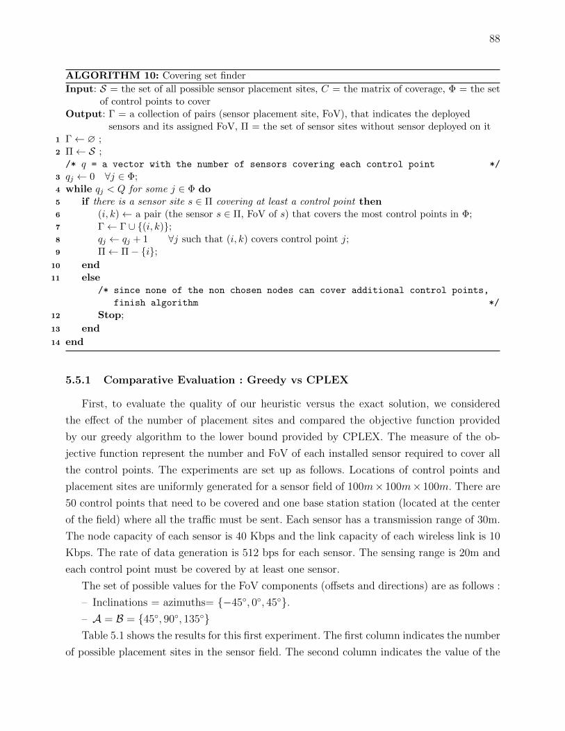
88
ALGORITHM 10: Covering set finder
Input: S = the set of all possible sensor placement sites, C = the matrix of coverage, Φ = the setof control points to cover
Output: Γ = a collection of pairs (sensor placement site, FoV), that indicates the deployedsensors and its assigned FoV, Π = the set of sensor sites without sensor deployed on it
1 Γ← ∅ ;2 Π← S ;/* q = a vector with the number of sensors covering each control point */
3 qj ← 0 ∀j ∈ Φ;4 while qj < Q for some j ∈ Φ do5 if there is a sensor site s ∈ Π covering at least a control point then6 (i, k)← a pair (the sensor s ∈ Π, FoV of s) that covers the most control points in Φ;7 Γ← Γ ∪ {(i, k)};8 qj ← qj + 1 ∀j such that (i, k) covers control point j;9 Π← Π− {i};
10 end11 else
/* since none of the non chosen nodes can cover additional control points,
finish algorithm */
12 Stop;
13 end
14 end
5.5.1 Comparative Evaluation : Greedy vs CPLEX
First, to evaluate the quality of our heuristic versus the exact solution, we considered
the effect of the number of placement sites and compared the objective function provided
by our greedy algorithm to the lower bound provided by CPLEX. The measure of the ob-
jective function represent the number and FoV of each installed sensor required to cover all
the control points. The experiments are set up as follows. Locations of control points and
placement sites are uniformly generated for a sensor field of 100m× 100m× 100m. There are
50 control points that need to be covered and one base station station (located at the center
of the field) where all the traffic must be sent. Each sensor has a transmission range of 30m.
The node capacity of each sensor is 40 Kbps and the link capacity of each wireless link is 10
Kbps. The rate of data generation is 512 bps for each sensor. The sensing range is 20m and
each control point must be covered by at least one sensor.
The set of possible values for the FoV components (offsets and directions) are as follows :
– Inclinations = azimuths= {−45◦, 0◦, 45◦}.– A = B = {45◦, 90◦, 135◦}Table 5.1 shows the results for this first experiment. The first column indicates the number
of possible placement sites in the sensor field. The second column indicates the value of the

89
ALGORITHM 11: Connected set finderInput: Γ = a collection of pairs (sensor placement site, FoV), that indicates the deployed sensors
and its assigned FoV, Π = the set of sensor sites without sensor deployed on itOutput: Γ
1 Γ∗ ← Γ;2 forall the (v, k) ∈ Γ do3 if there is a path between v and the sink then remove the connected node v4 Γ∗ ← Γ∗ − {(v, k)};5 end
6 end7 while Γ∗ 6= ∅ do8 if Π 6= ∅ then9 Determine sensor i ∈ Π that connect the highest number of sensors in Γ;
10 Γ← Γ ∪ {(i,∅)};/* i.e., ∅ = the FoV in this case is not important */
11 Π← Π− {i};12 Update Γ∗ by removing sensors that become connected due to addition of i to Γ;
13 end14 else
/* It’s impossible get a connected set Γ */
15 Stop;
16 end
17 end
objective function obtained by CPLEX and the third column is the time spent by CPLEX
to find this solution. The fourth column presents the value of the solution found by our
greedy algorithm and the fifth column is time took the algorithm to get this solution. For
each problem size, ten instances of the problem were randomly generated and the average
was calculated.
Tableau 5.1 Comparison between found solutions for CPLEX and Greedy algorithm
Placement CPLEX GreedySites Solution Time Solution Time
80 15 7.3609s 34 0.0883s100 14 43.504s 30 0.127s150 13 190.885s 26 0.2515s200 12 448.735s 22 0.3453s220 11 755.997s 20 0.5025s240 11 627.190s 21 0.61693s
As can be observed in the Table 5.1, we can infer that our greedy algorithm provides
good solutions, that can be used by another schemes (maybe a tabu search or a simulated

90
Tableau 5.2 CPLEX vs Greedy algorithm with large instances
Placement CPLEX GreedySites Solution Time Solution Time
500 21 11.721h 28 0.2002h1000 18 23.118h 24 0.2834h1500 23 32.417h 26 0.3141h2000 – – 22 0.3815h2500 – – 27 0.4144h
annealing algorithms) as a initial solution. With respect to the CPU times, it was predictable
that an exact ILP resolution would not be suitable for large-sized networks and the excellent
times obtained by the greedy algorithm demonstrate the this is a very efficient heuristic since
the required computation time is less than a second for all instances.
The Table 5.2 shows how the behavior of Greedy algorithm with large instances of the
problem. The time, in this case, is in hours. We can see the Greedy algorithm solution is
close to the CPLEX solution, but the time to get this solution is very higher for CPLEX.
Besides, when we work with a problem with a number of sites greater than to two thousand
sites, CPLEX aborts with a “out-of-memory” message, and we cannot get a solution for such
instances. Nevertheless, our Greedy algorithm has been able to get a good solution in a time
inferior to one hour of execution.
As far as the reduction in the number of installed sensors is concerned, we can see that as
the number of potential placement sites increases, the number of installed or deployed sensors
decreases. Since more placement sites are available, better locations can be selected and one
node can cover more control points, thus reducing the total number of installed sensors.
5.5.2 Impact of the Sensing Range
In practice, the value of the sensing range could vary depending on the physical properties
of the sensors and on the type of signal they are sensing. We measured the impact of the
sensing range in the found solution. To do that the number of placement sites was fixed to
200, the number of control points is 50 and the horizontal and vertical offsets of the possible
FoV was fixed to 90◦ as well. The sensing range took the values between 14m and 30m.
Figure 5.3a shows that for both the exact solution and the greedy heuristic as the sensing
range increase, less sensors are needed to cover the same number of control points. This
behavior is as expected since a given sensor node can cover more control points, but there
is always a 50% difference between the CPLEX result and the greedy algorithm result. The
figure also demonstrated that for this problem size, the tendence in the found solutions are

91
quite similar.
(a) Number of sensors required for different sensing ranges (b) Number of sensors required for different FoV
Figure 5.3 Performance Evaluation
5.5.3 Impact of the FoV
In practice, a directional sensor node must be able to adjust some parameters in order
to get a better or accurate capture of the objects in its FoV. To evaluate the impact of
the field of view on the solution found by CPLEX and by our greedy algorithm, we only
considered the horizontal and vertical offsets of the sensor (the angles α and β) around the
sensing direction (vector−→D). We fixed the number of placement sites at 200 and the number
of control points at 50. The sensing range is fixed at 20m and the communication radius is
fixed at 30m. We varied the angles α and β, but they are always equal, that is, the angles
took always the same value. Figure 5.3b shows the variation of the number of installed sensor
according to the selected FoV angles. Evidently, as the value of the angles decreases, more
sensors are needed to cover the same set of control points. That is the expected result since
with a smaller FoV, we covered less control points. We can also see that our greedy algorithm
produce good results close to the results produced by CPLEX.
5.6 Conclusions
In this work we developed an ILP formulation for the determination of optimal 3D direc-
tional sensor placement. We also proposed a greedy heuristic to solve large instances of the
model in a reasonable amount of CPU time. The main building block of this heuristic is to

92
find connected sensor sets that cover the control points with the required quality. Simulations
performed on a number of test instances indicate that the heuristic provides for acceptable
results with respect to the exact solution of the derived ILP model, within low computa-
tion times. Despite its centralized aspect, our greedy algorithm exhibits low complexity and
low computation times making its practical implementation adaptable for large-scale deploy-
ments.
As future research directions, we intend to develop a more sophisticated heuristic to
improve the found solutions. For example, we can use the greedy algorithm as the initial
solution for a tabu-search heuristic, because of good solution we found using that algorithm.
Besides, we will also include the notion of energy consumption and network lifetime to our
model, very important elements that all designers should take into account at the moment
to plan a wireless sensor network. Finally, we intend to work on a distributed version of our
approximative algorithms in order to obtain solutions in a shorter time.

93
CHAPITRE 6
DISCUSSION GENERALE
Dans ce chapitre, nous faisons une synthese de nos travaux et contributions en regard de
nos objectifs de recherche. Nous discutons egalement l’approche methodologique employee et
nous analysons les resultats obtenus.
6.1 Synthese des travaux
La recherche menee dans cette these a donne lieu a trois articles de revues. Chacun de
ces articles de revues traite d’un des points evoques dans nos objectifs de recherche que nous
allons recapitules dans les paragraphes ci-dessous. Un des articles de revues a deja ete publie
tandis que les deux autres sont actuellement en cours d’evaluation.
Notre premier objectif de recherche porte sur l’analyse des mecanismes pour le support de
la QdS dans les RCMSF et sur le deploiement de RCSF. Cet objectif a ete realise grace a une
revue de litterature exhaustive sur ces domaines. De plus, nous avons souligne des faiblesses
et des limitations des approches trouvees dans la litterature.
Partant de l’analyse, nos objectifs subsequents etaient de proposer un protocole qui sup-
porte la QdS dans les RCMSF et d’en evaluer sa performance. Ces objectifs ont ete realises
au moyen d’un nouveau protocole que nous avons propose et evalue. Ce protocole denomme
AntSensNet. Ce protocole est l’objet de l’article presente dans le Chapitre 3. AntSensNet est
specifiquement concu pour les RCMSF. Il est base sur l’heuristique des colonies de fourmis et
utilise un processus de creation de grappes dans le reseau inspire aussi par le comportement
des fourmis. Le protocole peut trouver des chemins dans le reseau qui repondent aux exi-
gences de qualite de service de l’application, et par consequent ameliore les performances du
reseau. Les resultats des simulations montrent que la performance de notre protocole surpasse
celle d’AODV en termes de delai de bout-en-bout, de taux de paquets perdus et de gigue. En
outre, AntSensNet realise un transport de paquets de video avec une distorsion inferieure a
celle des protocoles specialises comme TPGF ou ASAR.
Notre deuxieme article presente dans le Chapitre 4 nous permet de satisfaire l’objectif
de la proposition d’un nouveau mecanisme de controle d’admission pour les RCMSF. Notre
algorithme de controle d’admission applique une approche repartie pour repondre a la couche
d’application si un nouveau flot doit etre admis dans le reseau. La couche application specifie
les exigences du nouveau flot a partir de plusieurs metriques de QdS comme la gigue, la bande
94
passante, le delai et le taux d’erreur. L’algorithme essaie de trouver une route qui satisfait les
demandes du nouveau flot. Le flot n’est admis que si une route est trouvee. Notre algorithme
differe de la majorite des algorithmes proposes dans la litterature par son approche distribuee
et le fait qu’il considere divers parametres de QdS en meme temps.
Les deux derniers objectifs sont satisfaits grace au modele mathematique et l’algorithme
glouton presentes dans le troisieme article (Chapitre 5). Dans cet article nous avons propose
un modele mathematique pour minimiser le nombre de capteurs deployes dans une zone
specifique sous les contraintes de connectivite et de couverture. La solution du modele nous
fournit l’emplacement ou installer chaque capteur ainsi que sa configuration. Nous avons
aussi propose un algorithme glouton qui nous permet de trouver de bonnes solutions pour
des instances de grandes tailles, dans un temps raisonnable.
6.2 Methodologie
Dans cette these, nous avons propose de nouveaux algorithmes et des protocoles de com-
munications, ainsi que des modeles mathematiques de programmation linaire. Pour les al-
gorithmes et les protocoles, nous avons une validation par des simulations experimentales.
Deux outils ont ete utilises pour y arriver a savoir, le logiciel MATLAB (pour analyser les
resultats) et le simulateur de reseaux NS-2.
Pour le probleme de deploiement optimal, nous avons developpe nos modeles de program-
mation a l’aide d’equations mathematiques. Par la suite, en utilisant l’outil ILOG CPLEX,
nous avons obtenu des solutions optimales pour le modele. Ces solutions nous procurent ainsi
d’excellentes valeurs de reference.
Comme nous l’avons mentionne precedemment, puisque ces modeles sont tres complexes
a resoudre, nous avons egalement un algorithme glouton pour obtenir des solutions approxi-
matives. Ce dernier a ete implemente a l’aide du langage de programmation Python.
Par ailleurs, pour generer nos resultats, nous avons suivi un mode operatoire formel et pre-
cis base sur plusieurs batteries de tests qui ont permis de generer les valeurs moyennes ayant
servi a la validation des resultats generes par nos heuristiques et algorithmes de simulation
des protocoles.
6.3 Analyse des resultats
La validation numerique et par simulation de nos protocoles et algorithmes montrent
qu’on obtient des resultats tres satisfaisants.
Dans notre premier article, les resultats de la simulation en NS-2 ont montre que le
protocole que nous avons proposee produit de meilleurs resultats en termes de duree de vie

95
du reseau, de taux de perte de paquets et de surcharge du protocole que d’autres protocoles
proposes dans la litterature scientifique recente.
Dans notre deuxieme article, les resultats demontrent clairement et precisement que l’uti-
lisation d’un mecanisme de controle d’admission est benefique pour le bon fonctionnement du
reseau. On peut constater dans l’article la grande difference de performance d’un protocole
quand il utilise le controle d’admission et quand il ne l’utilise pas.
Dans notre troisieme article, les simulations demontrent que notre heuristique glouton
genere de bons resultats, comparee a la solution optimale generee par CPLEX. Les temps
pour trouver la solution sont aussi tres bons avec des instances de grande taille.

96
CHAPITRE 7
CONCLUSION
Dans ce chapitre de conclusion, nous mettrons en evidence les differentes contributions
de cette these. Par la suite, nous exposerons les limitations de nos travaux et, enfin, nous
terminerons avec nos recommandations pour des recherches futures.
7.1 Sommaire des contributions de la these
Cette these a donne lieu a plusieurs contributions au niveau de la gestion de la QdS pour
les RCMSF et la planification des reseaux de capteurs directionnels, qui etaient les elements
primordiaux de notre objectif principal. Voici un bref resume des contributions qui nous ont
permis d’atteindre notre objectif.
– Proposition d’un nouveau protocole pour la gestion de la QdS dans les RCMSF. Ce
protocole, appele AntSensNet, est base sur l’heuristique de la colonie de fourmis. A
partir des exigences demandees par la couche application, le protocole est capable de
determiner des routes qui satisfont de telles demandes. Le protocole est capable de
transporter des donnees heterogenes qui sont typiques dans les RCMSF. Ces donnees
incluent l’information scalaire (temperature, pression, lumiere, etc.) qui est produite
par les capteurs normaux ainsi que l’information multimedia (video, audio, images) qui
est produite par les capteurs multimedia. De plus, le protocole est capable d’etablir des
priorites pour les paquets a partir du type d’information qui se trouve dans les paquets.
Ce faisant, il est possible de transmettre en temps reel de la video ou l’audio dans le
reseau. Finalement, le protocole utilise un mecanisme de mise en grappe du reseau pour
faire de maniere plus efficace le transport de l’information et etendre la duree de vie du
reseau.
– Proposition d’un nouvel algorithme de controle d’admission pour les RCMSF. Cet al-
gorithme est capable de determiner si le reseau a assez de ressources pour satisfaire les
demandes d’un nouveau flot de donnees qui va etre genere par un nœud du reseau. L’al-
gorithme essaie de trouver une route dans le reseau avec les caracteristiques demandees
d’une facon repartie et, a partir de l’etat et l’information recueillie de chaque nœud,
repondre positivement ou negativement a la requete d’admission du nouveau flot.
– Modelisation et resolution du probleme de planification optimale du placement dans
un espace 3D des capteurs directionnels dans un RCMSF, dans le but de minimiser le

97
nombre de capteurs deployes sous les contraintes de couverture et connectivite. CPLEX
a ete utilise pour resoudre ce modele de facon exacte. Ces solutions nous offrent une
borne superieure, en termes de nombre de capteurs deployes ainsi que leur configura-
tion, pour les algorithmes qui essaient de trouver une solution non exacte au modele.
En outre, nous avons developpe une heuristique gloutonne pour trouver une solution
acceptable (par rapport a la solution exacte) aux instances de grandes tailles dans un
temps raisonnable.
7.2 Limitations de la solution proposee
Malgre les contributions enoncees ci-dessus, notre travail presente certaines limitations
dont nous pouvons citer :
– Une premiere limitation serait l’utilisation du protocole IEEE 802.11 comme le protocole
de la couche MAC pour les simulations de notre protocole AntSensNet. Il y a des
auteurs dans la litterature qui ne considerent pas ce protocole comme adequat ou realiste
pour les RCMSF. On peut voir aussi dans la litterature que les capteurs utilisent des
protocoles de la couche MAC qui sont plus economiseurs d’energie et, en consequence,
ideaux pour ce type de reseau.
– Une autre limitation concerne l’algorithme de controle d’admission et sa dependance de
l’information fournie par des entites externes comme les protocoles de la couche reseau
et MAC. Cela implique l’obligation d’adapter l’algorithme a chaque protocole de reseau
ou MAC qui l’utilisera. Par consequent, l’implantation, l’installation et l’utilisation
posterieure du mecanisme de controle d’admission deviennent une tache extenuante.
– Une derniere limitation concerne la resolution exacte des modeles mathematiques pre-
sentes dans le Chapitre 5. Ces modeles sont tres complexes a resoudre. De ce fait,
seulement des problemes de petite taille peuvent etre resolus en un temps raisonnable.
En plus, on n’a considere que des capteurs directionnels avec le meme rayon de detec-
tion pour simplifier le modele, mais cela est aussi une limitation importante de notre
travail de recherche.
7.3 Ameliorations futures
Il reste beaucoup de choses a faire pour la gestion et le support de la QdS dans lesRCMSF.
Nous presentons ci-apres quelques pistes.
Une premiere piste de recherche serait d’ameliorer la performance du protocole AntSens-
Net en trouvant des mecanismes qui permettront de remplir les tables de phenomenes des
tetes de grappes avant de commencer les taches de routage. Des articles recenses dans la

98
litterature montrent que ce mecanisme aide a augmenter l’efficacite du reseau. On peut aussi
faire de recherches sur la facon d’inclure des elements interessants au protocole comme la
mobilite des nœuds ou l’integration avec des reseaux a plusieurs SINKs.
En continuant avec notre protocole AntSensNet, une seconde piste de recherche serait
d’ameliorer le processus de mise en grappe utilise par le protocole. Notre mecanisme cree des
grappes autour des capteurs les plus puissants du reseau, mais au moment ou ces capteurs
tetes de grappe finissent de fonctionner, du par exemple a un epuisement de leur batterie, les
autres capteurs doivent se joindre aux grappes plus proches d’eux. Ce processus est simple
et rapide, mais il introduit un probleme de surcharge de trafic au niveau des grappes qui
recoivent les capteurs qui appartenaient aux grappes disparues. On pourrait rechercher des
methodes efficaces pour former de nouvelles grappes a la disparition d’une grappe donnee.
Une troisieme piste consisterait a etendre notre modele pour le placement de capteurs
directionnels dans un espace 3D en prenant en compte de possibles obstacles qui pourraient
se trouver sur le lieu de deploiement. Notre modele actuel ne considere pas le cas ou il y
a des obstacles entre le capteur et le point d’interet qu’il doit couvrir. La modelisation du
probleme avec des obstacles dans un espace 3D n’est pas simple et on a besoin de beaucoup de
recherche pour lui trouver une bonne solution. Finalement, une autre piste serait d’aborder
la solution computationnelle du modele en utilisant une heuristique differente de celle que
nous avons utilise. La solution avec un algorithme glouton produit de bons resultats dans
un temps excellent, mais si on a besoin de solutions plus proches de la solution exacte pour
des instances de grandes tailles, on pourrait developper une recherche Taboue et utiliser les
resultats de l’algorithme glouton comme la solution initiale a partir de laquelle l’algorithme
Tabou essaierait de decouvrir de meilleures solutions.

99
REFERENCES
AGRAWAL, D. P., MAHAPATRA, A. et ANAND, K. (2006). QoS and energy aware routing
for real-time traffic in wireless sensor networks. Computer Communications, 29, 437–445.
AI, J. et ABOUZEID, A. (2006). Coverage by directional sensors in randomly deployed
wireless sensor networks. Journal of Combinatorial Optimization, 11, 21 – 41.
AITSAADI, N., ACHIR, N., BOUSSETTA, K. et PUJOLLE, G. (2009). A Tabu Search
WSN Deployment Method for Monitoring Geographically Irregular Distributed Events. Sen-
sors, 9, 1625–1643.
AKKAYA, K. et YOUNIS, M. (2005a). Energy and QoS aware routing in wireless sensor
networks. Cluster Computing, 8, 179–88.
AKKAYA, K. et YOUNIS, M. (2005b). A survey on routing protocols for wireless sensor
networks. Ad Hoc Networks, 3, 325–349.
AKYILDIZ, I., MELODIA, T. et CHOWDHURY, K. (2007). A survey on wireless multi-
media sensor networks. Computer Networks, 51, 921 – 960.
AKYILDIZ, I. F., SU, W., SANKARASUBRAMANIAM, Y. et CAYIRCI, E. (2002). Wi-
reless sensor networks : a survey. Computer Networks, 38, 393–422.
AKYILDIZ, I. F. et VURAN, M. C. (2010). Wireless Sensor Networks. John Wiley & Sons
Ltd.
ALMALKAWI, I. T., GUERRERO ZAPATA, M., AL-KARAKI, J. N. et MORILLO-POZO,
J. (2010). Wireless Multimedia Sensor Networks : Current Trends and Future Directions.
Sensors, 10, 6662–6717.
ALZATE, M., PAGAN, J.-C., PENA, N. et LABRADOR, M. (2008). End-to-end bandwidth
and available bandwidth estimation in multi-hop IEEE 802.11b ad hoc networks. 42nd
Annual Conference on Information Sciences and Systems. IEEE, 659 –664.
ARBOLEDA, L. M. C. et NASSER, N. (2006). Comparison of clustering algorithms and
protocols for wireless sensor networks. Canadian Conference on Electrical and Computer
Engineering. 1787–1792.
ASU (2010). Arizona State University Video Traces Research Group.
Http ://traces.eas.asu.edu/yuv/index.html.
BHUYAN, B., SARMA, S. H. K. D., SARMA, N., KAR, A. et RALL, R. (2010). Quality
of Service (QoS) Provisions in Wireless Sensor Networks and Related Challenges. Wireless
Sensor Network, 2, 861–868.

100
BOULIS, A. et SRIVASTAVA, M. (2004). Node-level energy management for sensor net-
works in the presence of multiple applications. Wireless Networks, 10, 737–746.
BULLNHEIMER, B., HARTL, R. F. et STRAUSS, C. (1999). An improved ant system
algorithm for the vehicle routing problem. Annals of Operations Research, 89, 319–328.
CAI, Y., LOU, W., LI, M. et LI, X.-Y. (2009). Energy efficient target-oriented scheduling
in directional sensor networks. IEEE Transactions on Computers, 58, 1259 – 1274.
CAMILO, T., CARRETO, C., SILVA, J. et BOAVIDA, F. (2006). An energy-efficient
ant-based routing algorithm for wireless sensor networks. S. Berlin, editeur, Ant Colony
Optimization and Swarm Intelligence, vol. 4150/2006. 49–59.
CARDEI, M., THAI, M. et WU, W. (2005). Energy-efficient target coverage in wireless
sensor networks. Proc. IEEE Infocom. Miami, Florida, USA.
CHAKERES, I. D., BELDING-ROYER, E. M. et MACKERC, J. P. (2007). Perceptive
admission control for wireless network quality of service. Ad Hoc Networks, 5, 1129 – 1148.
CHEN, M., LEUNG, V. C. M., MAO, S. et YUAN, Y. (2007a). Directional geographical
routing for real-time video communications in wireless sensor networks. Computer Commu-
nications, 30, 3368–3383.
CHEN, W.-M., LI, C.-S., CHIANG, F.-Y. et CHAO, H.-C. (2007b). Jumping ant routing
algorithm for sensor networks. Computer Communications, 30, 2892–2903.
CHENYANG, L., BLUM, B. M., ABDELZAHER, T. F. et TIAN, J. A. S. H. (2002). RAP : a
real-time communication architecture for large-scale wireless sensor networks. Eighth IEEE
Real-Time and Embedded Technology and Applications Symposium. San Jose, CA, USA,
55–66.
COBO, L., QUINTERO, A. et PIERRE, S. (2010). Ant-based routing for wireless multi-
media sensor networks using multiple qos metrics. Computer Networks, 54, 2991 – 3010.
CPLEX (2010). IBM ILOG CPLEX Optimization Programming Language (OPL) V6.3.
Http ://www-01.ibm.com/software/websphere/products/optimization/.
DEB, B., BHATNAGAR, S. et NATH, B. (2003). Reinform : reliable information forwarding
using multiple paths in sensor networks. 28th Annual IEEE International Conference on
Local Computer Networks. Los Alamitos, CA, USA, 406–415.
DORIGO, M. et BLUM, C. (2005). Ant colony optimization theory : A survey. Theoretical
Computer Science, 344, 243–278.
DORIGO, M. et CARO, G. D. (1998). Antnet : Distributed stigmergetic control for com-
munications networks. Journal of Artificial Intelligence Research, 9, 317–365.

101
DORIGO, M. et GAMBARDELLA, L. M. (1997). Ant colony system : a cooperative lear-
ning approach to the traveling salesman problem. IEEE Transactions on Evolutionary
Computation, 1, 53–66.
DORIGO, M. et STUTZLE, T. (2004). Ant colony optimization. MIT Press, Cambridge,
Mass.
FELEMBAN, E., CHANG-GUN, L. et EKICI, E. (2006). MMSPEED : Multipath Multi-
SPEED protocol for QoS guarantee of reliabilityand timeliness in wireless sensor networks.
IEEE Transactions on Mobile Computing, 5, 738–754.
FENG, G., DOULIGERIS, C., MAKKI, K. et PISSINOU, N. (2002). Performance evalua-
tion of delay-constrained least-cost QoS routing algorithms based on linear and nonlinear
Lagrange relaxation. IEEE International Conference on Communications. ICC 2002. New
York, NY, USA, vol. 4, 2273–2278.
GAREY, M. R. et JOHNSON, D. S. (1979). Computers and Intractability : A Guide to the
Theory of NP-Completeness . W. H. Freeman, NY, first edition edition.
GERLA, M. et XU, K. (2003). Multimedia streaming in large-scale sensor networks with
mobile swarms. ACM SIGMOD Record, 32, 72–76.
GHASEMAGHAEI, R., RAHMAN, A., GUEAIEB, W. et SADDIK, A. E. (2007). Ant
colony-based reinforcement learning algorithm for routing in wireless sensor networks. IEEE
Instrumentation and Measurement Technology Conference Proceedings, 2007. IMTC 2007.
Warsaw, Poland, 1–6.
GOLUBCHIK, L., LUI, J., TUNG, T., CHOW, A., LEE, W.-J., FRANCESCHINIS, G. et
ANGLANO, C. (2002). Multi-path continuous media streaming : what are the benefits ? In-
ternational Symposium on Computer Performance Modeling, Measurement and Evaluation.
PERFORMANCE 2002. Elsevier, Netherlands, Rome, Italy, vol. 49, 429 – 49.
GONZALEZ-BANOS, H. (2001). A randomized art-gallery algorithm for sensor placement.
Proceedings of the seventeenth annual symposium on Computational geometry. SCG. ACM,
New York, NY, USA, 232–240.
GUNES, M., SORGES, U. et BOUAZIZI, I. (2002). ARA - the ant-colony based routing
algorithm for MANETs. Proceedings of International Conference on Parallel Processing
Workshops. IEEE, Vancouver, Canada, 79–85.
GUPTA, H., DAS, S. et GU, Q. (2003). Connected sensor cover : self-organization of sensor
networks for efficient query execution. Proc. ACM Mobihoc. Annapolis, Maryland, USA.
GURSES, E. et AKAN, O. B. (2005). Multimedia Communication in Wireless Sensor
Networks. Annals of Telecommunications, 60, 799–827.

102
HAN, X., CAO, X., LLOYD, E. L. et SHEN, C.-C. (2008). Deploying Directional Sensor
Networks with Guaranteed Connectivity and Coverage. Proc. 5th Annual IEEE Commu-
nications Society Conf. Sensor, Mesh and Ad Hoc Communications and Networks SECON
’08. 153–160.
HE, T., STANKOVIC, J. A., LU, C. et ABDELZAHER, T. (2003). SPEED : A stateless pro-
tocol for real-time communication in sensor networks. 23rd IEEE International Conference
on Distributed Computing Systems (ICDCS-03). Providence, RI, United States, 46–55.
HEINZELMAN, W. B., CHANDRAKASAN, A. P. et BALAKRISHNAN, H. (2002). An
application-specific protocol architecture for wireless microsensor networks. IEEE Transac-
tions on Wireless Communications, 1, 660–670.
HORSTER, E. et LIENHART, R. (2006). Calibrating and optimizing poses of visual sensors
in distributed platforms. Multimedia Systems, 12, 195 – 210.
HOSSAIN, A., BISWAS, P. et CHAKRABARTI, S. (2008). Sensing Models and Its Impact
on Network Coverage in Wireless Sensor Network. IEEE Region 10 and the Third inter-
national Conference on Industrial and Information Systems, ICIIS. IEEE, Piscataway, NJ,
USA, Kharagpur, 1 – 5.
JEON, P. B. et KESIDIS, G. (2005). Pheromone-aided robust multipath and multipriority
routing in wireless MANETs. Proceedings of the 2nd ACM international workshop on Per-
formance evaluation of wireless ad hoc, sensor, and ubiquitous networks. ACM, New York,
NY, USA, PE-WASUN ’05, 106–113.
KE, C.-H., SHIEH, C.-K., HWANG, W.-S. et ZIVIANI, A. (2008). An Evaluation Frame-
work for More Realistic Simulations of MPEG Video Transmission. Journal of Information
Science and Engineering, 24, 425–440.
KLAUE, J., RATHKE, B. et WOLISZ, A. (2003). EvalVid - A Framework for Video Trans-
mission and Quality Evaluation. P. Kemper et W. Sanders, editeurs, Computer Performance
Evaluation. Modelling Techniques and Tools, Springer Berlin / Heidelberg, vol. 2794 de Lec-
ture Notes in Computer Science. 255–272.
LEE, S.-B., AHN, G.-S., ZHANG, X. et CAMPBELL, A. T. (2000). INSIGNIA : An IP-
Based Quality of Service Framework for Mobile Ad Hoc Networks. Journal of Parallel and
Distributed Computing, 60, 374–406.
LI, Y., THAI, M. T. et WU, W. (2008). Wireless Sensor Networks and Applications. Sprin-
ger.
LIU, M., SUN, Y., LIU, R. et HUANG, X. (2007). An improved ant colony qos routing
algorithm applied to mobile ad hoc networks. International Conference on Wireless Com-
munications, Networking and Mobile Computing, WiCOM ’07. Shanghai, China, 1641–1644.
103
MA, H., ZHANG, X. et MING, A. (2009). A coverage-enhancing method for 3D directional
sensor networks. Proceedings 28th IEEE INFOCOM International Conference on Computer
Communications. 2791 – 2795.
MELODIA, T. et AKYILDIZ, I. (2010). Cross-Layer QoS-Aware Communication for Ultra
Wide Band Wireless Multimedia Sensor Networks. IEEE Journal on Selected Areas in
Communications, 28, 653 – 663.
MISRA, S., REISSLEIN, M. et GUOLIANG, X. (2008). A survey of multimedia streaming
in wireless sensor networks. IEEE Communications Surveys and Tutorials, 10, 18–39.
MURALEEDHARAN, R. et OSADCIW, L. A. (2004). A predictive sensor network using
ant system. SPIE Defense and Security Symposium. SPIE-Int. Soc. Opt. Eng, Orlando,
FL, USA, vol. 5440 de Proceedings of the SPIE - The International Society for Optical
Engineering, 181–192.
ns (2010). The Network Simulator NS-2. http ://www.isi.edu/nsnam/ns/.
O’ROURKE, J. (1987). Art gallery theorems and algorithms. Oxford University Press, Inc.,
New York, NY, USA.
OSAIS, Y., ST-HILAIRE, M. et YU, F. (2008). The minimum cost sensor placement problem
for directional wireless sensor networks. IEEE 68th Vehicular Technology Conference (VTC
2008-Fall). Calgary, BC, Canada, 1–5.
OSAIS, Y., ST-HILAIRE, M. et YU, F. (2009). On sensor placement for directional wireless
sensor networks. IEEE International Conference on Communications. IEEE, Piscaatway,
NJ, USA, Dresden, Germany.
OSAIS, Y. E., ST-HILAIRE, M. et YU, F. R. (2010). Directional Sensor Placement with
Optimal Sensing Range, Field of View and Orientation. Mobile Networks and Applications,
15, 216–225.
PATEL, M., CHANDRASEKARAN, R. et VENKATESAN, S. (2005). Energy efficient
sensor, relay and base station placements for coverage, connectivity and routing. Proceeding
of 24th IEEE International Performance, Computing, and Communications Conference.
IPCCC. 581 – 586.
PERILLO, M. A. et HEINZELMAN, W. B. (2003). Sensor management policies to provide
application QoS. Ad Hoc Networks, 1, 235–246.
PERKINS, C. E. et BELDING-ROYER, E. M. (2003). Quality of Service for Ad hoc On-
Demand Distance Vector Routing, Internet Draft, draft-perkins-manet-aodvqos-02.txt.
PODURI, S., PATTEM, S., KRISHNAMACHARI, B. et SUKHATME, G. S. (2006). Sensor
Network Configuration and the Curse of Dimensionality. The Third IEEE Workshop on
Embedded Networked Sensors.

104
POLITIS, I., TSAGKAROPOULOS, M., DAGIUKLAS, T. et KOTSOPOULOS, S. (2008).
Power efficient video multipath transmission over wireless multimedia sensor networks. Mo-
bile Networks and Applications, 13, 274 – 284.
RAHIMI, M., BAER, R., IROEZI, O. I., GARCIA, J. C., WARRIOR, J., ESTRIN, D. et
SRIVASTAVA, M. (2005). Cyclops : In situ image sensing and interpretation in wireless
sensor networks. Third ACM Conferences on Embedded Networked Sensor Systems (SenSys).
ACM Press, 192–204.
RAHMAN, M. A., GHASEMAGHAEI, R., SADDIK, A. E. et GUEAIEB, W. (2008). M-
IAR : Biologically Inspired Routing Protocol for Wireless Multimedia Sensor Networks.
IEEE Instrumentation and Measurement Technology Conference Proceedings. Victoria, BC,
1823–1827.
ROSATI, L., BERIOLI, M. et REALI, G. (2007). On ant routing algorithms in ad hoc
networks with critical connectivity. Ad Hoc Networks, 6, 827–859.
SELVAKENNEDY, S., SINNAPPAN, S. et SHANG, Y. (2007). A biologically-inspired
clustering protocol for wireless sensor networks. Computer Communications, 30, 2786–2801.
SHU, L., ZHANG, Y., YANG, L. T., WANG, Y., HAUSWIRTH, M. et XIONG, N. (2010).
TPGF : Geographic routing in wireless multimedia sensor networks. Telecommunication
Systems, 44, 79 – 95.
SIVAJOTHI, M. et NAGANATHAN, E. (2008). An ant colony based routing protocol to
support multimedia communication in ad hoc wireless networks. International Journal of
Computer Science and Network Security. IJCSNS., 8, 21–28.
SOHRABI, K., GAO, J., AILAWADHI, V. et POTTIE, G. J. (2000). Protocols for self-
organization of a wireless sensor network. IEEE Personal Communications, 7, 16–27.
SORO, S. et HEINZELMAN, W. (2005). On the coverage problem in video-based wireless
sensor networks. Proc. of the Second Workshop on Broadband Advanced Sensor Networks
(BaseNets 05). Boston, MA, USA, vol. 2, 932 – 939.
SUN, Y., MA, H., LIU, L. et ZHENG, Y. (2008). ASAR : an ant-based service-aware routing
algorithm for multimedia sensor networks. Frontiers of Electrical and Electronic Engineering
in China, 3, 25 – 33.
TEZCAN, N. et WANG, W. (2008). Self-orienting wireless multimedia sensor networks for
occlusion-free viewpoints. Computer Networks, 52, 2558 – 2567.
TIAN, D. et GEORGANAS, N. (2002). A coverage-preserving node scheduling scheme for
large wireless sensor networks. Proc. First ACM Int. Workshop on Wireless Sensor Networks
and Applications. Georgia, USA.

105
VINT (2008). The network simulator - ns-2. Http ://www.isi.edu/nsnam/ns/.
WANG, Q. et BALASINGHAM, I. (2010). Wireless sensor networks - an introduction.
D. G. V. Merret et D. Y. K. Tan, editeurs, Wireless Sensor Networks : Application-Centric
Design, InTech, chapitre 1. 3 – 16.
WANG, X., WANG, S. et BI, D. (2007). Virtual force-directed particle swarm optimization
for dynamic deployment in wireless sensor networks. ICIC’07 : Proceedings of the intelli-
gent computing 3rd international conference on Advanced intelligent computing theories and
applications. Springer-Verlag, Berlin, Heidelberg, 292–303.
WU, H. et ABOUZEID, A. A. (2006). Error resilient image transport in wireless sensor
networks. Computer Networks, 50, 2873–2887.
XIANGNING, F. et YULIN, S. (2007). Improvement on LEACH Protocol of Wireless Sensor
Network. International Conference on Sensor Technologies and Applications. SensorComm
2007. Valencia, Spain, 260–264.
YANG, Y. et KRAVETS, R. (2005). Contention-aware admission control for ad hoc net-
works. Mobile Computing, IEEE Transactions on, 4, 363 – 377.
YIN, X., ZHOU, X., PAN, M. et LI, S. (2010). Admission control with multi-constrained
QoS providing in Wireless Sensor Networks. Proc. Int Networking, Sensing and Control
(ICNSC) Conference. 524–529.
YING, Z., KUHN, L. D. et FROMHERZ, M. P. J. (2004). Improvements on ant routing
for sensor networks. 4th International Workshop Ant Colony Optimization and Swarm
Intelligence. Springer-Verlag, 154–165.
YOUNIS, M. et AKKAYA, K. (2008). Strategies and techniques for node placement in
wireless sensor networks : A survey. Ad Hoc Networks, 6, 621 – 655.
YOUNIS, O. et FAHMY, S. (2004). HEED : a hybrid, energy-efficient, distributed clustering
approach for ad hoc sensor networks. IEEE Transactions on Mobile Computing, 3, 366–379.
ZHANG, Y., KUHN, L. D. et FROMHERZ, M. P. J. (2004). Improvements on ant routing
for sensor networks. Ant Colony, Optimization and Swarm Intelligence, Springer, Berlin,
vol. 3172 de Lecture Notes in Computer Science. Premiere edition, 154–165.
ZHENG, X., GUO, W. et LIU, R. (2004). An ant-based distributed routing algorithm
for ad-hoc networks. International Conference on Communications, Circuits and Systems.
Chengdu, China, vol. 1, 412–417.
ZHU, H. et CHLAMTAC, I. (2006). Admission control and bandwidth reservation in multi-
hop ad hoc networks. Computer Networks, 50, 1653 – 1674.

106
ZIANE, S. et MELOU, A. (2005). A swarm intelligent multi-path routing for multimedia
traffic over mobile ad hoc networks. First ACM International Workshop on Quality of
Service and Security in Wireless and Mobile Networks. ACM, Montreal, QC, Canada, 55–
62.