Embed Size (px)
Citation preview
INSTITUT NATIONAL POLYTECHNIQUE DE GRENOBLE
THESE
pour obtenir le grade de
DOCTEUR DE L’INPG
Specialite : Sciences Cognitives
preparee au Laboratoire Leibniz-IMAGdans le cadre de l’Ecole Doctorale Ingenierie pour le Vivant : Sante,
Cognition, Environnement
presentee et soutenue publiquement
par
M. Remi Coulom
le 19 juin 2002
Titre :
Apprentissage par renforcement utilisant des reseaux deneurones, avec des applications au controle moteur
Directeur de These : M. Philippe Jorrand
JURY
M. Jean Della Dora PresidentM. Kenji Doya RapporteurM. Manuel Samuelides RapporteurM. Stephane Canu RapporteurM. Philippe Jorrand Directeur de theseMme. Mirta B. Gordon Examinateur

Remerciements
Je remercie Monsieur Philippe Jorrand pour avoir ete mon directeur dethese. Je remercie les membres du jury, Mme Mirta Gordon, Messieurs KenjiDoya, Manuel Samuelides, Stephane Canu et Jean Della Dora pour avoiraccepte d’evaluer mon travail, et pour leurs remarques pertinentes qui ontpermis d’ameliorer ce texte. Je remercie les chercheurs du laboratoire Leibnizpour leur accueil, en particulier son directeur, Monsieur Nicolas Balacheff, etles membres des equipes “Apprentissage et Cognition” et “Reseaux de Neuro-nes”, Messieurs Gilles Bisson, Daniel Memmi et Bernard Amy, ainsi que tousles etudiants avec lesquels j’ai travaille. Je remercie enfin le responsable de laFormation Doctorale en Sciences Cognitives, Monsieur Pierre Escudier, pourses conseils.

Table des matieres
Resume (Summary in French) 9Introduction . . . . . . . . . . . . . . . . . . . . . . . . . . . . . . . 9
Contexte . . . . . . . . . . . . . . . . . . . . . . . . . . . . . . 9Apprentissage par renforcement et reseaux de neurones . . . . 11Resume et contributions . . . . . . . . . . . . . . . . . . . . . 12Plan de la these . . . . . . . . . . . . . . . . . . . . . . . . . . 13
Theorie . . . . . . . . . . . . . . . . . . . . . . . . . . . . . . . . . 14Experiences . . . . . . . . . . . . . . . . . . . . . . . . . . . . . . . 15Conclusion . . . . . . . . . . . . . . . . . . . . . . . . . . . . . . . . 17
Introduction 27
Introduction 27Background . . . . . . . . . . . . . . . . . . . . . . . . . . . . . . . 27Reinforcement Learning using Neural Networks . . . . . . . . . . . 28Summary and Contributions . . . . . . . . . . . . . . . . . . . . . . 30Outline . . . . . . . . . . . . . . . . . . . . . . . . . . . . . . . . . 31
I Theory 33
1 Dynamic Programming 351.1 Discrete Problems . . . . . . . . . . . . . . . . . . . . . . . . . 35
1.1.1 Finite Discrete Deterministic Decision Processes . . . . 351.1.2 Example . . . . . . . . . . . . . . . . . . . . . . . . . . 371.1.3 Value Iteration . . . . . . . . . . . . . . . . . . . . . . 371.1.4 Policy Evaluation . . . . . . . . . . . . . . . . . . . . . 411.1.5 Policy Iteration . . . . . . . . . . . . . . . . . . . . . . 41
1.2 Continuous Problems . . . . . . . . . . . . . . . . . . . . . . . 421.2.1 Problem Definition . . . . . . . . . . . . . . . . . . . . 42
5
TABLE DES MATIERES
1.2.2 Example . . . . . . . . . . . . . . . . . . . . . . . . . . 431.2.3 Problem Discretization . . . . . . . . . . . . . . . . . . 451.2.4 Pendulum Swing-Up . . . . . . . . . . . . . . . . . . . 501.2.5 The Curse of Dimensionality . . . . . . . . . . . . . . . 51
2 Artificial Neural Networks 532.1 Function Approximators . . . . . . . . . . . . . . . . . . . . . 53
2.1.1 Definition . . . . . . . . . . . . . . . . . . . . . . . . . 532.1.2 Generalization . . . . . . . . . . . . . . . . . . . . . . . 542.1.3 Learning . . . . . . . . . . . . . . . . . . . . . . . . . . 55
2.2 Gradient Descent . . . . . . . . . . . . . . . . . . . . . . . . . 562.2.1 Steepest Descent . . . . . . . . . . . . . . . . . . . . . 562.2.2 Efficient Algorithms . . . . . . . . . . . . . . . . . . . 572.2.3 Batch vs. Incremental Learning . . . . . . . . . . . . . 59
2.3 Some Approximation Schemes . . . . . . . . . . . . . . . . . . 622.3.1 Linear Function Approximators . . . . . . . . . . . . . 622.3.2 Feedforward Neural Networks . . . . . . . . . . . . . . 64
3 Continuous Neuro-Dynamic Programming 673.1 Value Iteration . . . . . . . . . . . . . . . . . . . . . . . . . . 67
3.1.1 Value-Gradient Algorithms . . . . . . . . . . . . . . . . 673.1.2 Residual-Gradient Algorithms . . . . . . . . . . . . . . 693.1.3 Continuous Residual-Gradient Algorithms . . . . . . . 69
3.2 Temporal Difference Methods . . . . . . . . . . . . . . . . . . 723.2.1 Discrete TD(λ) . . . . . . . . . . . . . . . . . . . . . . 723.2.2 TD(λ) with Function Approximators . . . . . . . . . . 753.2.3 Continuous TD(λ) . . . . . . . . . . . . . . . . . . . . 763.2.4 Back to Grid-Based Estimators . . . . . . . . . . . . . 78
3.3 Summary . . . . . . . . . . . . . . . . . . . . . . . . . . . . . 81
4 Continuous TD(λ) in Practice 834.1 Finding the Greedy Control . . . . . . . . . . . . . . . . . . . 834.2 Numerical Integration Method . . . . . . . . . . . . . . . . . . 85
4.2.1 Dealing with Discontinuous Control . . . . . . . . . . . 854.2.2 Integrating Variables Separately . . . . . . . . . . . . . 884.2.3 State Discontinuities . . . . . . . . . . . . . . . . . . . 914.2.4 Summary . . . . . . . . . . . . . . . . . . . . . . . . . 92
4.3 Efficient Gradient Descent . . . . . . . . . . . . . . . . . . . . 934.3.1 Principle . . . . . . . . . . . . . . . . . . . . . . . . . . 944.3.2 Algorithm . . . . . . . . . . . . . . . . . . . . . . . . . 944.3.3 Results . . . . . . . . . . . . . . . . . . . . . . . . . . . 95
6
TABLE DES MATIERES
4.3.4 Comparison with Second-Order Methods . . . . . . . . 95
4.3.5 Summary . . . . . . . . . . . . . . . . . . . . . . . . . 96
II Experiments 97
5 Classical Problems 99
5.1 Pendulum Swing-up . . . . . . . . . . . . . . . . . . . . . . . 99
5.2 Cart-Pole Swing-up . . . . . . . . . . . . . . . . . . . . . . . . 102
5.3 Acrobot . . . . . . . . . . . . . . . . . . . . . . . . . . . . . . 105
5.4 Summary . . . . . . . . . . . . . . . . . . . . . . . . . . . . . 106
6 Robot Auto Racing Simulator 109
6.1 Problem Description . . . . . . . . . . . . . . . . . . . . . . . 109
6.1.1 Model . . . . . . . . . . . . . . . . . . . . . . . . . . . 109
6.1.2 Techniques Used by Existing Drivers . . . . . . . . . . 110
6.2 Direct Application of TD(λ) . . . . . . . . . . . . . . . . . . . 111
6.3 Using Features to Improve Learning . . . . . . . . . . . . . . . 114
6.4 Conclusion . . . . . . . . . . . . . . . . . . . . . . . . . . . . . 115
7 Swimmers 117
7.1 Problem Description . . . . . . . . . . . . . . . . . . . . . . . 117
7.2 Experiment Results . . . . . . . . . . . . . . . . . . . . . . . . 118
7.3 Summary . . . . . . . . . . . . . . . . . . . . . . . . . . . . . 118
Conclusion 127
Conclusion 127
Appendices 131
A Backpropagation 131
A.1 Notations . . . . . . . . . . . . . . . . . . . . . . . . . . . . . 131
A.1.1 Feedforward Neural Networks . . . . . . . . . . . . . . 131
A.1.2 The ∂∗ Notation . . . . . . . . . . . . . . . . . . . . . 132
A.2 Computing ∂E/∂∗ ~w . . . . . . . . . . . . . . . . . . . . . . . 133
A.3 Computing ∂~y/∂∗~x . . . . . . . . . . . . . . . . . . . . . . . . 133
A.4 Differential Backpropagation . . . . . . . . . . . . . . . . . . . 134
7
TABLE DES MATIERES
B Optimal-Control Problems 137B.1 Pendulum . . . . . . . . . . . . . . . . . . . . . . . . . . . . . 137
B.1.1 Variables and Parameters . . . . . . . . . . . . . . . . 137B.1.2 System Dynamics . . . . . . . . . . . . . . . . . . . . . 138B.1.3 Reward . . . . . . . . . . . . . . . . . . . . . . . . . . 138B.1.4 Numerical Values . . . . . . . . . . . . . . . . . . . . . 138
B.2 Acrobot . . . . . . . . . . . . . . . . . . . . . . . . . . . . . . 138B.2.1 Variables and Parameters . . . . . . . . . . . . . . . . 138B.2.2 System Dynamics . . . . . . . . . . . . . . . . . . . . . 139B.2.3 Reward . . . . . . . . . . . . . . . . . . . . . . . . . . 140B.2.4 Numerical Values . . . . . . . . . . . . . . . . . . . . . 140
B.3 Cart-Pole . . . . . . . . . . . . . . . . . . . . . . . . . . . . . 140B.3.1 Variables and Parameters . . . . . . . . . . . . . . . . 140B.3.2 System Dynamics . . . . . . . . . . . . . . . . . . . . . 141B.3.3 Reward . . . . . . . . . . . . . . . . . . . . . . . . . . 143B.3.4 Numerical Values . . . . . . . . . . . . . . . . . . . . . 143
B.4 Swimmer . . . . . . . . . . . . . . . . . . . . . . . . . . . . . . 143B.4.1 Variables and Parameters . . . . . . . . . . . . . . . . 143B.4.2 Model of Viscous Friction . . . . . . . . . . . . . . . . 144B.4.3 System Dynamics . . . . . . . . . . . . . . . . . . . . . 145B.4.4 Reward . . . . . . . . . . . . . . . . . . . . . . . . . . 145B.4.5 Numerical Values . . . . . . . . . . . . . . . . . . . . . 145
C The K1999 Path-Optimization Algorithm 147C.1 Basic Principle . . . . . . . . . . . . . . . . . . . . . . . . . . 147
C.1.1 Path . . . . . . . . . . . . . . . . . . . . . . . . . . . . 147C.1.2 Speed Profile . . . . . . . . . . . . . . . . . . . . . . . 148
C.2 Some Refinements . . . . . . . . . . . . . . . . . . . . . . . . . 149C.2.1 Converging Faster . . . . . . . . . . . . . . . . . . . . . 149C.2.2 Security Margins . . . . . . . . . . . . . . . . . . . . . 149C.2.3 Non-linear Variation of Curvature . . . . . . . . . . . . 150C.2.4 Inflections . . . . . . . . . . . . . . . . . . . . . . . . . 150C.2.5 Further Improvements by Gradient Descent . . . . . . 150
C.3 Improvements Made in the 2001 Season . . . . . . . . . . . . . 152C.3.1 Better Variation of Curvature . . . . . . . . . . . . . . 152C.3.2 Better Gradient Descent Algorithm . . . . . . . . . . . 155C.3.3 Other Improvements . . . . . . . . . . . . . . . . . . . 158
8
Resume (Summary in French)
Ce resume est compose d’une traduction de l’introduction et de la conclu-sion de la these, ainsi que d’une synthese des resultats presentes dans le de-veloppement. La traduction est assez grossiere, et les lecteurs anglophonessont vivement encourages a lire la version originale.
Introduction
Construire des controleurs automatiques pour des robots ou des meca-nismes de toutes sortes a toujours represente un grand defi pour les scienti-fiques et les ingenieurs. Les performances des animaux dans les taches mo-trices les plus simples, telles que la marche ou la natation, s’averent extre-ment difficiles a reproduire dans des systemes artificiels, qu’ils soient simulesou reels. Cette these explore comment des techniques inspirees par la Na-ture, les reseaux de neurones artificiels et l’apprentissage par renforcement,peuvent aider a resoudre de tels problemes.
Contexte
Trouver des actions optimales pour controler le comportement d’un sys-teme dynamique est crucial dans de nombreuses applications, telles que larobotique, les procedes industriels, ou le pilotage de vehicules spatiaux. Desefforts de recherche de grande ampleur ont ete produits pour traiter les ques-tions theoriques soulevees par ces problemes, et pour fournir des methodespratiques permettant de construire des controleurs efficaces.
L’approche classique de la commande optimale numerique consiste a cal-culer une trajectoire optimale en premier. Ensuite, un controleur peut etreconstruit pour suivre cette trajectoire. Ce type de methode est souvent uti-lise dans l’astronautique, ou pour l’animation de personnages artificiels dansdes films. Les algorithmes modernes peuvent resoudre des problemes trescomplexes, tels que la demarche simulee optimale de Hardt et al [30].
9
RESUME (SUMMARY IN FRENCH)
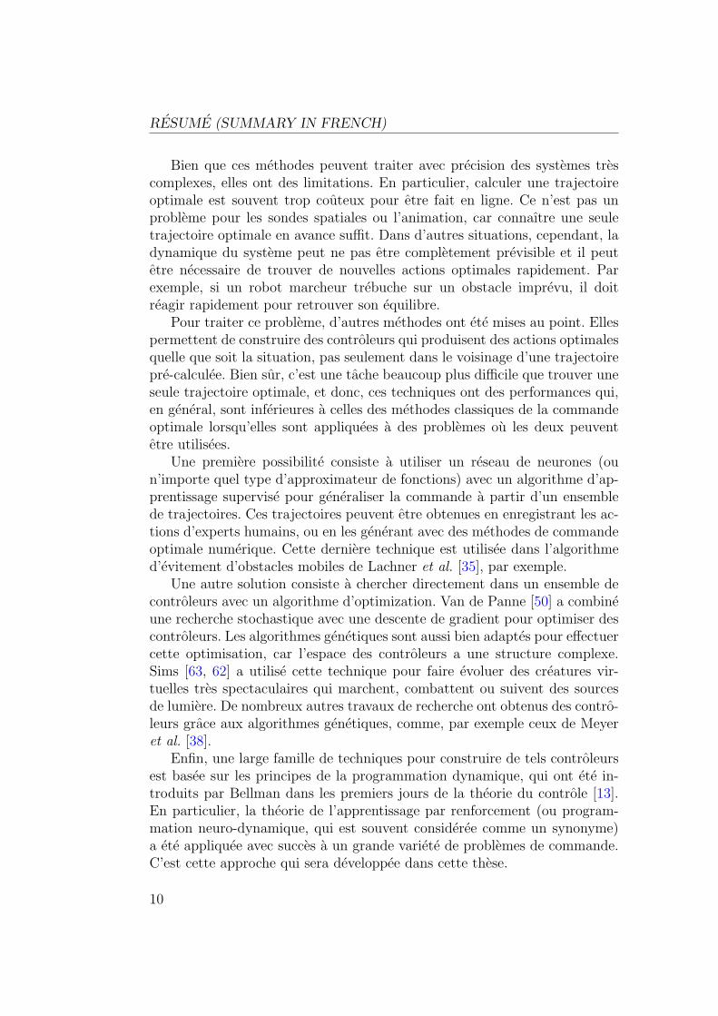
Bien que ces methodes peuvent traiter avec precision des systemes trescomplexes, elles ont des limitations. En particulier, calculer une trajectoireoptimale est souvent trop couteux pour etre fait en ligne. Ce n’est pas unprobleme pour les sondes spatiales ou l’animation, car connaıtre une seuletrajectoire optimale en avance suffit. Dans d’autres situations, cependant, ladynamique du systeme peut ne pas etre completement previsible et il peutetre necessaire de trouver de nouvelles actions optimales rapidement. Parexemple, si un robot marcheur trebuche sur un obstacle imprevu, il doitreagir rapidement pour retrouver son equilibre.
Pour traiter ce probleme, d’autres methodes ont ete mises au point. Ellespermettent de construire des controleurs qui produisent des actions optimalesquelle que soit la situation, pas seulement dans le voisinage d’une trajectoirepre-calculee. Bien sur, c’est une tache beaucoup plus difficile que trouver uneseule trajectoire optimale, et donc, ces techniques ont des performances qui,en general, sont inferieures a celles des methodes classiques de la commandeoptimale lorsqu’elles sont appliquees a des problemes ou les deux peuventetre utilisees.
Une premiere possibilite consiste a utiliser un reseau de neurones (oun’importe quel type d’approximateur de fonctions) avec un algorithme d’ap-prentissage supervise pour generaliser la commande a partir d’un ensemblede trajectoires. Ces trajectoires peuvent etre obtenues en enregistrant les ac-tions d’experts humains, ou en les generant avec des methodes de commandeoptimale numerique. Cette derniere technique est utilisee dans l’algorithmed’evitement d’obstacles mobiles de Lachner et al. [35], par exemple.
Une autre solution consiste a chercher directement dans un ensemble decontroleurs avec un algorithme d’optimization. Van de Panne [50] a combineune recherche stochastique avec une descente de gradient pour optimiser descontroleurs. Les algorithmes genetiques sont aussi bien adaptes pour effectuercette optimisation, car l’espace des controleurs a une structure complexe.Sims [63, 62] a utilise cette technique pour faire evoluer des creatures vir-tuelles tres spectaculaires qui marchent, combattent ou suivent des sourcesde lumiere. De nombreux autres travaux de recherche ont obtenus des contro-leurs grace aux algorithmes genetiques, comme, par exemple ceux de Meyeret al. [38].
Enfin, une large famille de techniques pour construire de tels controleursest basee sur les principes de la programmation dynamique, qui ont ete in-troduits par Bellman dans les premiers jours de la theorie du controle [13].En particulier, la theorie de l’apprentissage par renforcement (ou program-mation neuro-dynamique, qui est souvent consideree comme un synonyme)a ete appliquee avec succes a un grande variete de problemes de commande.C’est cette approche qui sera developpee dans cette these.
10
INTRODUCTION
Apprentissage par renforcement et reseaux de neurones
L’apprentissage par renforcement, c’est apprendre a agir par essai et er-reur. Dans ce paradigme, un agent peut percevoir sont etat et effectuer desactions. Apres chaque action, une recompense numerique est donnee. Le butde l’agent est de maximiser la recompense totale qu’il recoit au cours dutemps.
Une grande variete d’algorithmes ont ete proposes, qui selectionnent lesactions de facon a explorer l’environnement et a graduellement construireune strategie qui tend a obtenir une recompense cumulee maximale [68, 33].Ces algorithmes ont ete appliques avec succes a des problemes complexes,tels que les jeux de plateau [70], l’ordonnancement de taches [81], le controled’ascenceurs [20] et, bien sur, des taches de controle moteur, simulees [67, 24]ou reelles [41, 5].
Model-based et model-free
Ces algorithmes d’apprentissage par renforcement peuvent etre divisesen deux categories : les algorithmes dits model-based (ou indirects), qui uti-lisent une estimation de la dynamique du systeme, et les algorithmes ditsmodel-free (ou directs), qui n’en utilisent pas. La superiorite d’une approchesur l’autre n’est pas claire, et depend beaucoup du probleme particulier a re-soudre. Les avantages principaux apportes par un modele est que l’experiencereelle peut etre complementee par de l’experience simulee («imaginaire»), etque connaıtre la valeur des etats suffit pour trouver le controle optimal. Lesinconvenients les plus importants des algorithmes model-based est qu’ils sontplus complexes (car il faut mettre en œuvre un mecanisme pour estimer lemodele), et que l’experience simulee produite par le modele peut ne pas etrefidele a la realite (ce qui peut induire en erreur le processus d’apprentissage).
Bien que la superiorite d’une approche sur l’autre ne soit pas comple-tement evidente, certains resultats de la recherche tendent a indiquer quel’apprentissage par renforcement model-based peut resoudre des problemesde controle moteur de maniere plus efficace. Cela a ete montre dans des simu-lations [5, 24] et aussi dans des experiences avec des robots reels. Morimotoet Doya [42] ont combine l’experience simulee avec l’experience reelle pourapprendre a un robot a se mettre debout avec l’algorithme du Q-learning.Schaal et Atkeson ont aussi utilise avec succes l’apprentissage par renforce-ment model-base dans leurs experiences de robot jongleur [59].
11
RESUME (SUMMARY IN FRENCH)
Reseaux de neurones
Quasiment tous les algorithmes d’apprentissage par renforcement fontappel a l’estimation de «fonctions valeur» qui indiquent a quel point il estbon d’etre dans un etat donne (en termes de recompense totale attendue dansle long terme), ou a quel point il est bon d’effectuer une action donnee dansun etat donne. La facon la plus elementaire de construire cette fonction valeurconsiste a mettre a jour une table qui contient une valeur pour chaque etat(ou chaque paire etat-action), mais cette approche ne peut pas fonctionnerpour des problemes a grande echelle. Pour pouvoir traiter des taches qui ontun tres grand nombre d’etats, il est necessaire de faire appel aux capacitesde generalisation d’approximateurs de fonctions.
Les reseaux de neurones feedforward sont un cas particulier de tels ap-proximateurs de fonctions, qui peuvent etre utilises en combinaison avec l’ap-prentissage par renforcement. Le succes le plus spectaculaire de cette tech-nique est probablement le joueur de backgammon de Tesauro [70], qui a reussia atteindre le niveau des maıtres humains apres des mois de jeu contre lui-meme. Dans le jeu de backgammon, le nombre estime de positions possiblesest de l’ordre de 1020. Il est evident qu’il est impossible de stocker une tablede valeurs sur un tel nombre d’etats possibles.
Resume et contributions
Le probleme
L’objectif des travaux presentes dans cette these est de trouver des me-thodes efficaces pour construire des controleurs pour des taches de controlemoteur simulees. Le fait de travailler sur des simulations implique qu’un mo-dele exact du systeme a controler est connu. De facon a ne pas imposer descontraintes artificielles, on supposera que les algorithmes d’apprentissage ontacces a ce modele. Bien sur, cette supposition est une limitation importante,mais elle laisse malgre tout de nombreux problemes difficiles a resoudre, etles progres effectues dans ce cadre limite peuvent etre transposes dans le casgeneral ou un modele doit etre appris.
L’approche
La technique employee pour aborder ce probleme est l’algorithme TD(λ)continu de Doya [23]. Il s’agit d’une formulation continue du TD(λ) classiquede Sutton [66] qui est bien adaptee aux problemes de controle moteur. Sonefficacite a ete demontree par l’apprentissage du balancement d’une tige enrotation montee sur un chariot mobile [24].
12
INTRODUCTION
Dans de nombreux travaux d’apprentissage par renforcement applique aucontrole moteur, c’est un approximateur de fonctions lineaire qui est uti-lise pour approximer la fonction valeur. Cette technique d’approximation ade nombreuses proprietes interessantes, mais sa capacite a traiter un grandnombre de variables d’etat independantes est assez limitee.
L’originalite principale de l’approche suivie dans cette these est que lafonction valeur est estimee avec des reseaux de neurones feedforward au lieud’approximateurs de fonction lineaires. La non-linearite de ces reseaux deneurones les rend difficiles a maıtriser, mais leurs excellentes capacites degeneralisation dans des espaces d’entree en dimension elevee leur permet deresoudre des problemes dont la complexite est superieure de plusieurs ordresde grandeur a ce que peut traiter un approximateur de fonctions lineaire.
Contributions
Ce travail explore les problemes numeriques qui doivent etre resolus defacon a ameliorer l’efficacite de l’algorithme TD(λ) continu lorsqu’il est utiliseen association avec des reseaux de neurones feedforward. Les contributionsprincipales qu’il apporte sont :
– Une methode pour traiter les discontinuites de la commande. Dans denombreux problemes, la commande est discontinue, ce qui rend diffi-cile l’application de methodes efficaces d’integration numerique. Nousmontrons que la commande de Filippov peut etre obtenue en utilisantdes informations de second ordre sur la fonction valeur.
– Une methode pour traiter les discontinuites de l’etat. Elle est necessairepour pouvoir appliquer l’algorithme TD(λ) continu a des problemesavec des chocs ou des capteurs discontinus.
– L’algorithme Vario-η [47] est propose comme une methode efficace poureffectuer la descente de gradient dans l’apprentissage par renforcement.
– De nombreux resultats experimentaux indiquent clairement le poten-tiel enorme de l’utilisation de reseaux de neurones feedforward dansles algorithmes d’apprentissage par renforcement appliques au controlemoteur. En particulier, un nageur articule complexe, possedant 12 va-riables d’etat independantes et 4 variables de controle a appris a nagergrace aux reseaux de neurones feedforward.
Plan de la these
– Partie I : Theorie– Chapitre 1 : La Programmation dynamique– Chapitre 2 : Les reseaux de neurones
13
RESUME (SUMMARY IN FRENCH)
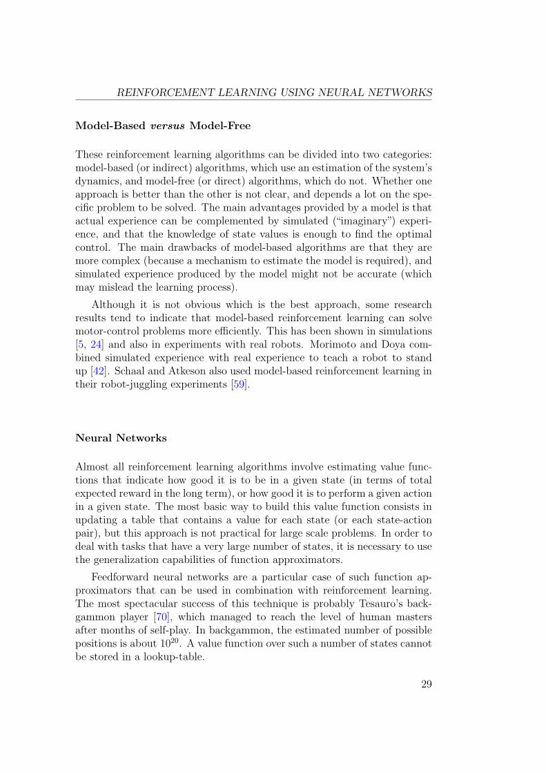
V
+1
−1
θ
−π
+π
θ
+10
−10
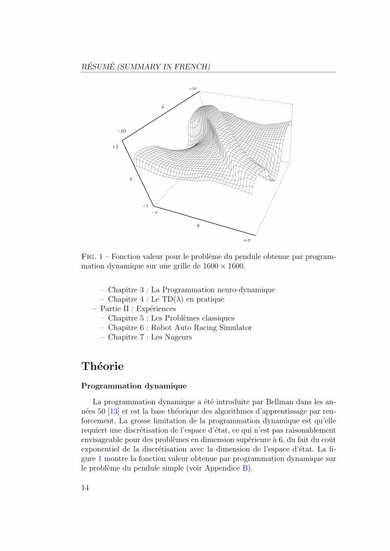
Fig. 1 – Fonction valeur pour le probleme du pendule obtenue par program-mation dynamique sur une grille de 1600× 1600.
– Chapitre 3 : La Programmation neuro-dynamique– Chapitre 4 : Le TD(λ) en pratique
– Partie II : Experiences– Chapitre 5 : Les Problemes classiques– Chapitre 6 : Robot Auto Racing Simulator– Chapitre 7 : Les Nageurs
Theorie
Programmation dynamique
La programmation dynamique a ete introduite par Bellman dans les an-nees 50 [13] et est la base theorique des algorithmes d’apprentissage par ren-forcement. La grosse limitation de la programmation dynamique est qu’ellerequiert une discretisation de l’espace d’etat, ce qui n’est pas raisonablementenvisageable pour des problemes en dimension superieure a 6, du fait du coutexponentiel de la discretisation avec la dimension de l’espace d’etat. La fi-gure 1 montre la fonction valeur obtenue par programmation dynamique surle probleme du pendule simple (voir Appendice B).
14
EXPERIENCES
Reseaux de neurones
Les reseaux de neurones sont des approximateurs de fonctions dont lescapacites de generalisation vont permettre de resoudre les problemes d’ex-plosion combinatoire.
Programmation neuro-dynamique
La programmation neuro-dynamique consiste a combiner les techniquesde reseaux de neurones avec la programmation dynamique. Les algorithmesde differences temporelles, et en particulier, le TD(λ) continu invente parDoya [24] sont particulierement bien adaptes a la resolution de problemes decontrole moteur.
Le TD(λ) dans la pratique
Dans ce chapitre sont presentees des techniques pour permettre une uti-lisation efficace de l’algorithme TD(λ) avec des reseaux de neurones. Il s’agitdes contributions theoriques les plus importantes de ce travail.
Experiences
Problemes classiques
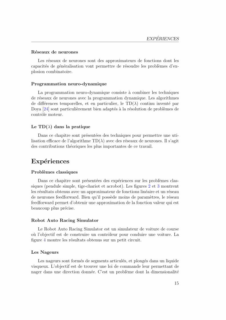
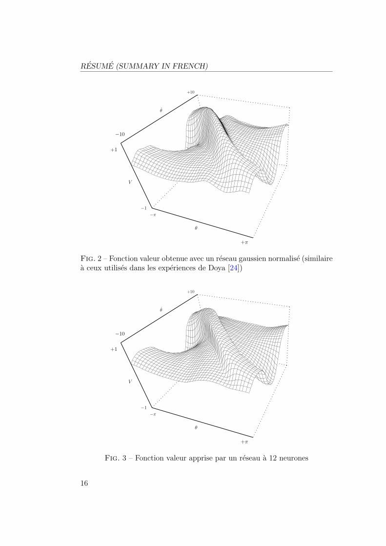
Dans ce chapitre sont presentees des experiences sur les problemes clas-siques (pendule simple, tige-chariot et acrobot). Les figures 2 et 3 montrentles resultats obtenus avec un approximateur de fonctions lineaire et un reseaude neurones feedforward. Bien qu’il possede moins de parametres, le reseaufeedforward permet d’obtenir une approximation de la fonction valeur qui estbeaucoup plus precise.
Robot Auto Racing Simulator
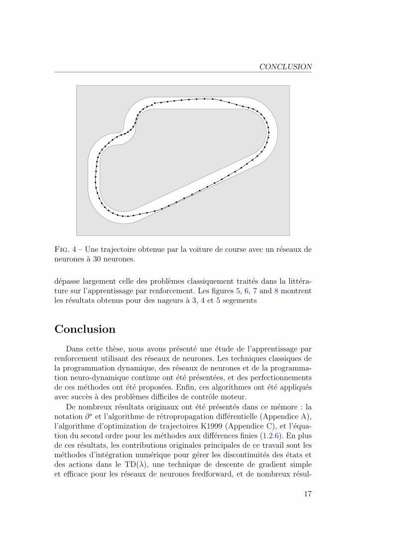
Le Robot Auto Racing Simulator est un simulateur de voiture de courseou l’objectif est de construire un controleur pour conduire une voiture. Lafigure 4 montre les resultats obtenus sur un petit circuit.
Les Nageurs
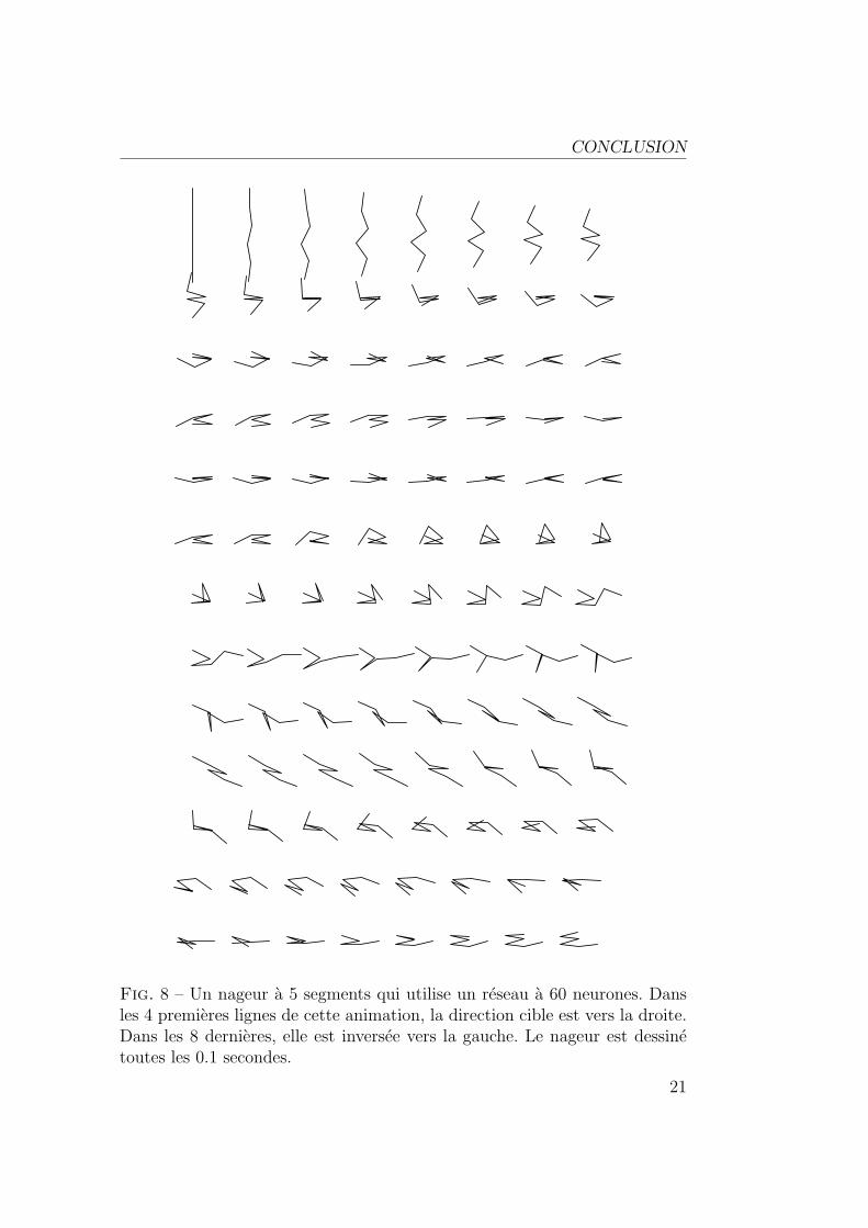
Les nageurs sont formes de segments articules, et plonges dans un liquidevisqueux. L’objectif est de trouver une loi de commande leur permettant denager dans une direction donnee. C’est un probleme dont la dimensionalite
15
RESUME (SUMMARY IN FRENCH)
V
+1
−1
θ
−π
+π
θ
+10
−10
Fig. 2 – Fonction valeur obtenue avec un reseau gaussien normalise (similairea ceux utilises dans les experiences de Doya [24])
V
+1
−1
θ
−π
+π
θ
+10
−10
Fig. 3 – Fonction valeur apprise par un reseau a 12 neurones
16
CONCLUSION
b b b b b b b b bb
bb
bb
bb
b
b
b
b
b
b
b
b
b
b
b
b
b
b
b
b
b
b
b
b
b
b
b
bb
bb
bbbbb
b
b
b
b
b
b
b
b
b
b
b
b
b
b
b
b
bb
bbbb
b
b
b
b
bb
bb
Fig. 4 – Une trajectoire obtenue par la voiture de course avec un reseaux deneurones a 30 neurones.
depasse largement celle des problemes classiquement traites dans la littera-ture sur l’apprentissage par renforcement. Les figures 5, 6, 7 and 8 montrentles resultats obtenus pour des nageurs a 3, 4 et 5 segements
Conclusion
Dans cette these, nous avons presente une etude de l’apprentissage parrenforcement utilisant des reseaux de neurones. Les techniques classiques dela programmation dynamique, des reseaux de neurones et de la programma-tion neuro-dynamique continue ont ete presentees, et des perfectionnementsde ces methodes ont ete proposees. Enfin, ces algorithmes ont ete appliquesavec succes a des problemes difficiles de controle moteur.
De nombreux resultats originaux ont ete presentes dans ce memore : lanotation ∂∗ et l’algorithme de retropropagation differentielle (Appendice A),l’algorithme d’optimization de trajectoires K1999 (Appendice C), et l’equa-tion du second ordre pour les methodes aux differences finies (1.2.6). En plusde ces resultats, les contributions originales principales de ce travail sont lesmethodes d’integration numerique pour gerer les discontinuites des etats etdes actions dans le TD(λ), une technique de descente de gradient simpleet efficace pour les reseaux de neurones feedforward, et de nombreux resul-
17

RESUME (SUMMARY IN FRENCH)
Fig. 5 – Un nageur a 3 segments qui utilise un reseau a 30 neurones. Dansles 4 premieres lignes de cette animation, la direction cible est vers la droite.Dans les 8 dernieres, elle est inversee vers la gauche. Le nageur est dessinetoutes les 0.1 secondes.
18

CONCLUSION
Fig. 6 – Un nageur a 4 segments qui utilise un reseau a 30 neurones. Dansles 7 premieres lignes de cette animation, la direction cible est vers la droite.Dans les 3 dernieres, elle est inversee vers la gauche. Le nageur est dessinetoutes les 0.2 secondes.
19

RESUME (SUMMARY IN FRENCH)
Fig. 7 – Un nageur a 4 segments qui utilise un reseau a 60 neurones. Dansles 4 premieres lignes de cette animation, la direction cible est vers la droite.Dans les 4 dernieres, elle est inversee vers la gauche. Le nageur est dessinetoutes les 0.1 secondes.
20
CONCLUSION
Fig. 8 – Un nageur a 5 segments qui utilise un reseau a 60 neurones. Dansles 4 premieres lignes de cette animation, la direction cible est vers la droite.Dans les 8 dernieres, elle est inversee vers la gauche. Le nageur est dessinetoutes les 0.1 secondes.
21
RESUME (SUMMARY IN FRENCH)
tats experimentaux originaux sur une grand variete de taches motrices. Lacontribution la plus significative est probablement le succes des experiencesavec les nageurs (Chapitre 7), qui montre que combiner l’apprentissage parrenforcement continu base sur un modele avec des reseaux de neurones feed-forward peut traiter des problemes de controle moteur qui sont beaucoup pluscomplexes que ceux habituellement resolus avec des methodes similaires.
Chacune de ces contributions ouvre aussi des questions et des directionspour des travaux futurs :
– La methode d’integration numerique pourrait certainement etre ame-lioree de maniere significative. En particulier, l’idee d’utiliser l’infor-mation du second ordre sur la fonction valeur pour estimer le controlede Filippov pourrait etre etendue aux espaces de controle a plus d’unedimension.
– Il faudrait comparer la methode de descente de gradient efficace utiliseedans cette these aux methodes classiques du second ordre dans destaches d’apprentissage supervise ou par renforcement.
– De nombreuses experiences nouvelles pourraient etre realisees avec lesnageurs. En particulier, il faudrait etudier les raisons des instabilitesobservees, et des nageurs plus gros pourraient apprendre a nager. Au-dela des nageurs, la methode utilisee pourrait aussi servir a construiredes controleurs pour des problemes beaucoup plus complexes.
En plus de ces extensions directes, une autres question tres importante aexplorer est la possibilite d’appliquer les reseaux de neurones feedforward horsdu cadre restreint du controle moteur simule base sur la connaissance d’unmodele. En particulier, les experiences indiquent que les reseaux de neuronesfeedforward demandent beaucoup plus d’episodes que les approximateurs defonction lineaires. Cette demande pourrait etre un obstacle majeur dans dessituations ou les donnees d’apprentissage sont couteuses a obtenir, ce qui estle cas quand les experiences ont lieu en temps reel (comme dans les expe-riences de robotique), ou quand la selection des actions implique beaucoupde calculs (comme dans le jeu d’echecs [12]). Ce n’etait pas le cas dans lesexperiences des nageurs, ou avec le joueur de Backgammon de Tesauro, car iletait possible de produire, sans cout, autant de donnees d’apprentissage quenecessaire.
Le probleme cle, ici, est la localite. Tres souvent, les approximateurs defonction lineaires sont preferes, parce que leur bonne localite leur permetde faire de l’apprentissage incremental efficacement, alors que les reseauxde neurones feedforward ont tendance a desapprendre l’experience passeequand de nouvelles donnees d’apprentissage sont traitees. Cependant, Lesperformances des nageurs obtenues dans cette these indiquent clairement queles reseaux de neurones feedforward peuvent resoudre des problemes qui sont
22
CONCLUSION
plus complexes que ce que les approximateurs de fonctions lineaires peuventtraiter. Il serait donc naturel d’essayer de combiner les qualites de ces deuxschemas d’approximation.
Creer un approximateur de fonction qui aurait a la fois la localite desapproximateurs de fonctions lineaires, et les capacites de generalisation desreseaux de neurones feedforward semble tres difficile. Weaver et al. [78] ontpropose un algorithme d’apprentissage special qui permet d’eviter le desap-prentissage. Son efficacite dans l’apprentissage par renforcement en dimensionelevee reste a demontrer, mais cela pourrait etre une direction de rechercheinteressante.
Une autre possibilite pour faire un meilleur usage de donnees d’appren-tissage peu abondantes consisterait a utiliser, en complement de l’algorithmed’apprentissage par renforcement, une forme de memoire a long terme quistocke ces donnees. Apres un certain temps, l’algorithme d’apprentissagepourrait rappeler ces donnees stockees pour verifier qu’elles n’ont pas eteoubliees par le reseau de neurones feedforward. Une difficulte majeure decette approche est qu’elle demanderait un sorte de TD(λ) hors-strategie, carl’algorithme d’apprentissage observerait des trajectoires qui ont ete genereesavec une fonction valeur differente.
23


Introduction
25

Introduction
Building automatic controllers for robots or mechanisms of all kinds has beena great challenge for scientists and engineers, ever since the early days of thecomputer era. The performance of animals in the simplest motor tasks, suchas walking or swimming, turns out to be extremely difficult to reproduce inartificial mechanical devices, simulated or real. This thesis is an investigationof how some techniques inspired by Nature—artificial neural networks andreinforcement learning—can help to solve such problems.
Background
Finding optimal actions to control the behavior of a dynamical system is cru-cial in many important applications, such as robotics, industrial processes,or spacecraft flying. Some major research efforts have been conducted to ad-dress the theoretical issues raised by these problems, and to provide practicalmethods to build efficient controllers.
The classical approach of numerical optimal control consists in comput-ing an optimal trajectory first. Then, a controller can be built to track thistrajectory. This kind of method is often used in astronautics, or for theanimation of artificial movie characters. Modern algorithms can solve com-plex problems such as, for instance, Hardt et al.’s optimal simulated humangait [30].
Although these methods can deal accurately with very complex systems,they have some limitations. In particular, computing an optimal trajectory isoften too costly to be performed online. This is not a problem for space probesor animation, because knowing one single optimal trajectory in advance isenough. In some other situations, however, the dynamics of the system mightnot be completely predictable, and it might be necessary to find new optimalactions quickly. For instance, if a walking robot stumbles over an unforeseenobstacle, it must react rapidly to recover its balance.
In order to deal with this problem, some other methods have been de-signed. They allow to build controllers that produce optimal actions in any
27
INTRODUCTION
situation, not only in the neighborhood of a pre-computed optimal trajectory.This is a much more difficult task than finding one single path, so these tech-niques usually do not perform as well as classical numerical optimal controlon applications where both can be used.
A first possibility consists in using a neural network (or any kind offunction approximator) with a supervised learning algorithm to generalizecontrols from a set of trajectories. These trajectories can be obtained byrecording actions of human “experts” or by generating them with methods ofnumerical optimal control. The latter technique is used by Lachner et al.’scollision-avoidance algorithm [35], for instance.
Another solution consists in directly searching a set of controllers withan optimization algorithm. Van de Panne [50] combined stochastic searchand gradient descent to optimize controllers. Genetic algorithms are alsowell suited to perform this optimization, because the space that is searchedoften has a complex structure. Sims [63, 62] used this technique to evolvevery spectacular virtual creatures that can walk, swim, fight or follow a lightsource. Many other research works produced controllers thanks to geneticalgorithms, such as, for instance Meyer et al ’s [38].
Lastly, a wide family of techniques to build such controllers is based on theprinciples of dynamic programming, which were introduced by Bellman in theearly days of control theory [13]. In particular, the theory of reinforcementlearning (or neuro-dynamic programming, which is often considered as asynonym) has been successfully applied to a large variety of control problems.It is this approach that will be developed in this thesis.
Reinforcement Learning using Neural Networks
Reinforcement learning is learning to act by trial and error. In this paradigm,an agent can perceive its state and perform actions. After each action, anumerical reward is given. The goal of the agent is to maximize the totalreward it receives over time.
A large variety of algorithms have been proposed that select actions inorder to explore the environment, and gradually build a strategy that tends toobtain a maximum reward [68, 33]. These algorithms have been successfullyapplied to complex problems such as board games [70], job-shop scheduling[81], elevator dispatching [20], and motor control tasks, either simulated [67,24], or real [41, 59].
28
REINFORCEMENT LEARNING USING NEURAL NETWORKS
Model-Based versus Model-Free
These reinforcement learning algorithms can be divided into two categories:model-based (or indirect) algorithms, which use an estimation of the system’sdynamics, and model-free (or direct) algorithms, which do not. Whether oneapproach is better than the other is not clear, and depends a lot on the spe-cific problem to be solved. The main advantages provided by a model is thatactual experience can be complemented by simulated (“imaginary”) experi-ence, and that the knowledge of state values is enough to find the optimalcontrol. The main drawbacks of model-based algorithms are that they aremore complex (because a mechanism to estimate the model is required), andsimulated experience produced by the model might not be accurate (whichmay mislead the learning process).
Although it is not obvious which is the best approach, some researchresults tend to indicate that model-based reinforcement learning can solvemotor-control problems more efficiently. This has been shown in simulations[5, 24] and also in experiments with real robots. Morimoto and Doya com-bined simulated experience with real experience to teach a robot to standup [42]. Schaal and Atkeson also used model-based reinforcement learning intheir robot-juggling experiments [59].
Neural Networks
Almost all reinforcement learning algorithms involve estimating value func-tions that indicate how good it is to be in a given state (in terms of totalexpected reward in the long term), or how good it is to perform a given actionin a given state. The most basic way to build this value function consists inupdating a table that contains a value for each state (or each state-actionpair), but this approach is not practical for large scale problems. In order todeal with tasks that have a very large number of states, it is necessary to usethe generalization capabilities of function approximators.
Feedforward neural networks are a particular case of such function ap-proximators that can be used in combination with reinforcement learning.The most spectacular success of this technique is probably Tesauro’s back-gammon player [70], which managed to reach the level of human mastersafter months of self-play. In backgammon, the estimated number of possiblepositions is about 1020. A value function over such a number of states cannotbe stored in a lookup-table.
29
INTRODUCTION
Summary and Contributions
Problem
The aim of the research reported in this dissertation is to find efficient meth-ods to build controllers for simulated motor control tasks. Simulation meansthat an exact model of the system to be controlled is available. In order toavoid imposing artificial constraints, learning algorithms will be supposed tohave access to this model. This assumption is an important limitation, butit still provides a lot of challenges, and progress made within this limitedframework can be transposed to the more general case where a model has tobe learnt.
Approach
The technique used to tackle this problem is Doya’s continuous TD(λ) rein-forcement learning algorithm [23]. It is a continuous formulation of Sutton’sclassical discrete TD(λ) [66] that is well adapted to motor control problems.Its efficiency was demonstrated by successfully learning to swing up a rotatingpole mounted on a moving cart [24].
In many of the reinforcement learning experiments in the domain of motorcontrol, a linear function approximator has been used to approximate thevalue function. This approximation scheme has many interesting properties,but its ability to deal with a large number of independent state variables isnot very good.
The main originality of the approach followed in this thesis is that thevalue function is estimated with feedforward neural networks instead of linearfunction approximators. The nonlinearity of these neural networks makesthem difficult to harness, but their excellent ability to generalize in high-dimensional input spaces might allow them to solve problems that are ordersof magnitude more complex than what linear function approximators canhandle.
Contributions
This work explores the numerical issues that have to be solved in order toimprove the efficiency of the continuous TD(λ) algorithm with feedforwardneural networks. Some of its main contributions are:
• A method to deal with discontinuous control. In many problems, theoptimal control is discontinuous, which makes it difficult to apply effi-cient numerical integration algorithms. We show how Filippov control
30
OUTLINE
can be obtained by using second order information about the valuefunction.
• A method to deal with discontinuous states, that is to say hybrid controlproblems. This is necessary to apply continuous TD(λ) to problemswith shocks or discontinuous inputs.
• The Vario-η algorithm [47] is proposed as practical method to performgradient descent in reinforcement learning.
• Many experimental results that clearly indicate the huge potential offeedforward neural networks in reinforcement learning applied to motorcontrol. In particular, a complex articulated swimmer with 12 indepen-dent state variables and 4 control variables learnt to swim thanks tofeedforward neural networks.
Outline
• Part I: Theory
– Chapter 1: Dynamic Programming
– Chapter 2: Neural Networks
– Chapter 3: Neuro-Dynamic Programming
– Chapter 4: TD(λ) in Practice
• Part II: Experiments
– Chapter 5: Classical Problems
– Chapter 6: Robot Auto Racing Simulator
– Chapter 7: Swimmers
31


Part I
Theory
33

Chapter 1
Dynamic Programming
Dynamic programming is a fundamental tool in the theory of optimal control,which was developed by Bellman in the fifties [13, 14]. The basic principlesof this method are presented in this chapter, in both the discrete and thecontinuous case.
1.1 Discrete Problems
The most basic category of problems that dynamic programming can solveare problems where the system to be controlled can only be in a finite numberof states. Motor control problems do not belong to this category, becausea mechanical system can be in a continuous infinity of states. Still, it isinteresting to study discrete problems, since they are much simpler to ana-lyze, and some concepts introduced in this analysis can be extended to thecontinuous case.
1.1.1 Finite Discrete Deterministic Decision Processes
A finite discrete deterministic decision process (or control problem) is for-mally defined by
• a finite set of states S.
• for each state x, a finite set of actions U(x).
• a transition function ν that maps state-action pairs to states. ν(x, u)is the state into which the system jumps when action u is performed instate x.
35
CHAPTER 1. DYNAMIC PROGRAMMING
• a reward function r that maps state-action pairs to real numbers.r(x, u) is the reward obtained for performing action u in state x. Thegoal of the control problem is to maximize the total reward obtainedover a sequence of actions.
A strategy or policy is a function π : S 7→ U that maps states to actions.Applying a policy from a starting state x0 produces a sequence of statesx0, x1, x2, . . . that is called a trajectory and is defined by
∀i ∈ N xi+1 = ν(xi, π(xi)
).
Cumulative reward obtained over such a trajectory depends only on π and x0.The function of x0 that returns this total reward is called the value functionof π. It is denoted V π and is defined by
V π(x0) =∞∑
i=0
r(xi, π(xi)
).
A problem with this sum is that it may diverge. V π(x0) converges onlywhen a limit cycle with zero reward is reached. In order to get rid of theseconvergence issues, a discounted reward is generally introduced, where eachterm of the sum is weighted by an exponentially decaying coefficient:
V π(x0) =∞∑
i=0
γir(xi, π(xi)
).
γ is a constant (γ ∈ [0, 1[) called the discount factor. The effect of γ isto introduce a time horizon to the value function: the smaller γ, the moreshort-sighted V π.
The goal is to find a policy that maximizes the total amount of rewardover time, whatever the starting state x0. More formally, the optimal controlproblem consists in finding π∗ so that
∀x0 ∈ S V π∗(x0) = maxπ:S 7→U
V π(x0).
It is easy to prove that such a policy exists. It might not be unique, however,since it is possible that two different policies lead to the same cumulativereward from a given state. V π∗ does not depend on π∗ and is denoted V ∗. Itis called the optimal value function.
36
1.1. DISCRETE PROBLEMS
x1 x2 x3 x4 x5
G x7 x8 x9 x10
x11 x12 x13 x14 x15
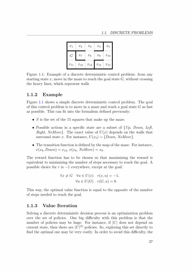
Figure 1.1: Example of a discrete deterministic control problem: from anystarting state x, move in the maze to reach the goal state G, without crossingthe heavy lines, which represent walls
1.1.2 Example
Figure 1.1 shows a simple discrete deterministic control problem. The goalof this control problem is to move in a maze and reach a goal state G as fastas possible. This can fit into the formalism defined previously:
• S is the set of the 15 squares that make up the maze.
• Possible actions in a specific state are a subset of {Up, Down, Left,Right, NoMove}. The exact value of U(x) depends on the walls thatsurround state x. For instance, U(x5) = {Down, NoMove}.
• The transition function is defined by the map of the maze. For instance,ν(x8, Down) = x13, ν(x9, NoMove) = x9.
The reward function has to be chosen so that maximizing the reward isequivalent to minimizing the number of steps necessary to reach the goal. Apossible choice for r is −1 everywhere, except at the goal:
∀x 6= G ∀u ∈ U(x) r(x, u) = −1,
∀u ∈ U(G) r(G, u) = 0.
This way, the optimal value function is equal to the opposite of the numberof steps needed to reach the goal.
1.1.3 Value Iteration
Solving a discrete deterministic decision process is an optimization problemover the set of policies. One big difficulty with this problem is that thenumber of policies may be huge. For instance, if |U | does not depend oncurrent state, then there are |U ||S| policies. So, exploring this set directly tofind the optimal one may be very costly. In order to avoid this difficulty, the
37
CHAPTER 1. DYNAMIC PROGRAMMING
x
ν(x, u1)
ν(x, u2)
ν(x, u3)
u1
u2
u3
V ∗(x) = maxu∈{u1,u2,u3}
(
r(x, u) + V ∗(ν(x, u)
))
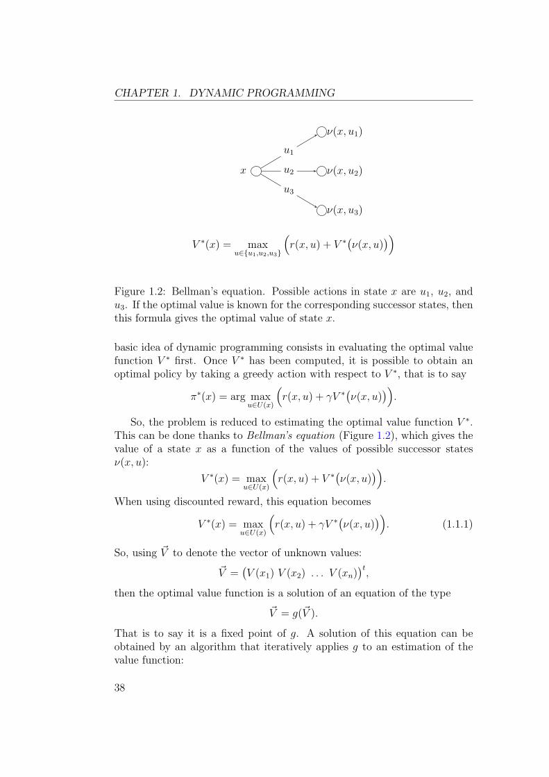
Figure 1.2: Bellman’s equation. Possible actions in state x are u1, u2, andu3. If the optimal value is known for the corresponding successor states, thenthis formula gives the optimal value of state x.
basic idea of dynamic programming consists in evaluating the optimal valuefunction V ∗ first. Once V ∗ has been computed, it is possible to obtain anoptimal policy by taking a greedy action with respect to V ∗, that is to say
π∗(x) = arg maxu∈U(x)
(
r(x, u) + γV ∗(ν(x, u)
))
.
So, the problem is reduced to estimating the optimal value function V ∗.This can be done thanks to Bellman’s equation (Figure 1.2), which gives thevalue of a state x as a function of the values of possible successor statesν(x, u):
V ∗(x) = maxu∈U(x)
(
r(x, u) + V ∗(ν(x, u)
))
.
When using discounted reward, this equation becomes
V ∗(x) = maxu∈U(x)
(
r(x, u) + γV ∗(ν(x, u)
))
. (1.1.1)
So, using ~V to denote the vector of unknown values:
~V =(V (x1) V (x2) . . . V (xn)
)t,
then the optimal value function is a solution of an equation of the type
~V = g(~V ).
That is to say it is a fixed point of g. A solution of this equation can beobtained by an algorithm that iteratively applies g to an estimation of thevalue function:
38
1.1. DISCRETE PROBLEMS
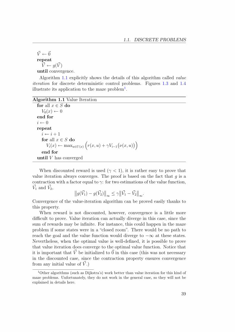
~V ← ~0repeat
~V ← g(~V )until convergence.
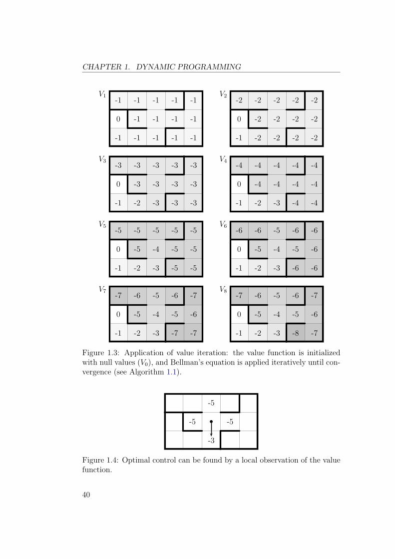
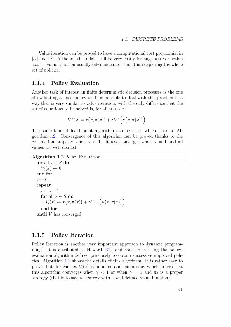
Algorithm 1.1 explicitly shows the details of this algorithm called valueiteration for discrete deterministic control problems. Figures 1.3 and 1.4illustrate its application to the maze problem1.
Algorithm 1.1 Value Iterationfor all x ∈ S do
V0(x)← 0end fori← 0repeat
i← i + 1for all x ∈ S do
Vi(x)← maxu∈U(x)
(
r(x, u) + γVi−1
(ν(x, u)
))
end foruntil V has converged
When discounted reward is used (γ < 1), it is rather easy to prove thatvalue iteration always converges. The proof is based on the fact that g is acontraction with a factor equal to γ: for two estimations of the value function,~V1 and ~V2, ∥
∥g(~V1)− g(~V2)∥∥∞≤ γ
∥∥~V1 − ~V2
∥∥∞
.
Convergence of the value-iteration algorithm can be proved easily thanks tothis property.
When reward is not discounted, however, convergence is a little moredifficult to prove. Value iteration can actually diverge in this case, since thesum of rewards may be infinite. For instance, this could happen in the mazeproblem if some states were in a “closed room”. There would be no path toreach the goal and the value function would diverge to −∞ at these states.Nevertheless, when the optimal value is well-defined, it is possible to provethat value iteration does converge to the optimal value function. Notice thatit is important that ~V be initialized to ~0 in this case (this was not necessaryin the discounted case, since the contraction property ensures convergencefrom any initial value of ~V .)
1Other algorithms (such as Dijkstra’s) work better than value iteration for this kind ofmaze problems. Unfortunately, they do not work in the general case, so they will not beexplained in details here.
39
CHAPTER 1. DYNAMIC PROGRAMMING
V1-1 -1 -1 -1 -1
0 -1 -1 -1 -1
-1 -1 -1 -1 -1
V2-2 -2 -2 -2 -2
0 -2 -2 -2 -2
-1 -2 -2 -2 -2
V3-3 -3 -3 -3 -3
0 -3 -3 -3 -3
-1 -2 -3 -3 -3
V4-4 -4 -4 -4 -4
0 -4 -4 -4 -4
-1 -2 -3 -4 -4
V5-5 -5 -5 -5 -5
0 -5 -4 -5 -5
-1 -2 -3 -5 -5
V6-6 -6 -5 -6 -6
0 -5 -4 -5 -6
-1 -2 -3 -6 -6
V7-7 -6 -5 -6 -7
0 -5 -4 -5 -6
-1 -2 -3 -7 -7
V8-7 -6 -5 -6 -7
0 -5 -4 -5 -6
-1 -2 -3 -8 -7
Figure 1.3: Application of value iteration: the value function is initializedwith null values (V0), and Bellman’s equation is applied iteratively until con-vergence (see Algorithm 1.1).
-3
-5
-5
-5
Figure 1.4: Optimal control can be found by a local observation of the valuefunction.
40
1.1. DISCRETE PROBLEMS
Value iteration can be proved to have a computational cost polynomial in|U | and |S|. Although this might still be very costly for huge state or actionspaces, value iteration usually takes much less time than exploring the wholeset of policies.
1.1.4 Policy Evaluation
Another task of interest in finite deterministic decision processes is the oneof evaluating a fixed policy π. It is possible to deal with this problem in away that is very similar to value iteration, with the only difference that theset of equations to be solved is, for all states x,
V π(x) = r(x, π(x)
)+ γV π
(
ν(x, π(x)
))
.
The same kind of fixed point algorithm can be used, which leads to Al-gorithm 1.2. Convergence of this algorithm can be proved thanks to thecontraction property when γ < 1. It also converges when γ = 1 and allvalues are well-defined.
Algorithm 1.2 Policy Evaluationfor all x ∈ S do
V0(x)← 0end fori← 0repeat
i← i + 1for all x ∈ S do
Vi(x)← r(x, π(x)
)+ γVi−1
(
ν(x, π(x)
))
end foruntil V has converged
1.1.5 Policy Iteration
Policy Iteration is another very important approach to dynamic program-ming. It is attributed to Howard [31], and consists in using the policy-evaluation algorithm defined previously to obtain successive improved poli-cies. Algorithm 1.3 shows the details of this algorithm. It is rather easy toprove that, for each x, Vi(x) is bounded and monotonic, which proves thatthis algorithm converges when γ < 1 or when γ = 1 and π0 is a properstrategy (that is to say, a strategy with a well-defined value function).
41
CHAPTER 1. DYNAMIC PROGRAMMING
Algorithm 1.3 Policy Iterationπ0 ← an arbitrary policyi← 0repeat
Vi ← evaluation of policy πi
πi+1 ← a greedy policy on Vi
i← i + 1until V has converged or π has converged
1.2 Continuous Problems
The formalism defined previously in the discrete case can be extended to con-tinuous problems. This extension is not straightforward because the numberof states is infinite (so, the value function can not be stored as a table ofnumerical values), and time is continuous (so, there is no such thing as a“next state” or a “previous state”). As a consequence, discrete algorithmscannot be applied directly and have to be adapted.
1.2.1 Problem Definition
The first element that has to be adapted to the continuous case is the defi-nition of the problem. A continuous deterministic decision process is definedby:
• A state space S ⊂ Rp. This means that the state of the system is
defined by a vector ~x of p real valued variables. In the case of mechanicalsystems, these will typically be angles, velocities or positions.
• A control space U ⊂ Rq. The controller can influence the behavior of
the system via a vector ~u of q real valued variables. These will typicallybe torques, forces or engine throttle. U may depend on the state ~x. ~uis also called the action.
• System dynamics f : S × U 7→ Rp. This function maps states and
actions to derivatives of the state with respect to time. That is to say~x = f(~x, ~u). This is analogous to the ν(x, u) function, except that aderivative is used in order to deal with time continuity.
• A reward function r : S×U 7→ R. The problem consists in maximizingthe cumulative reward as detailed below.
42
1.2. CONTINUOUS PROBLEMS
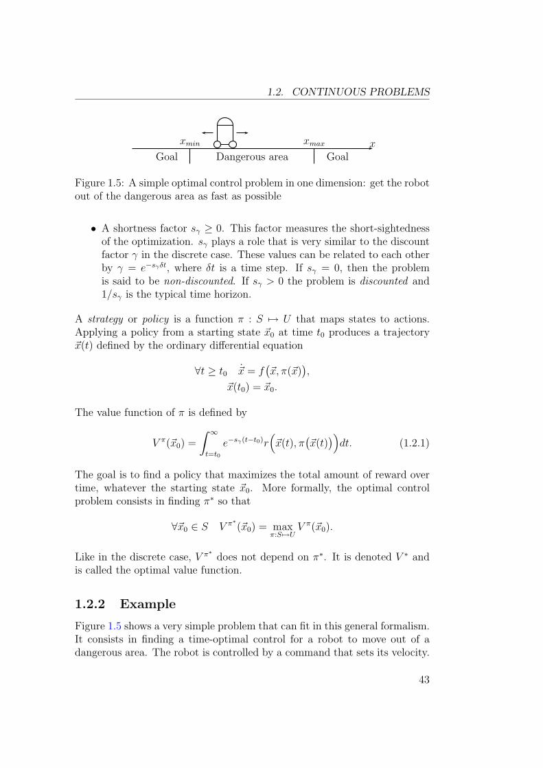
Dangerous areaGoal Goal
xmin xmax x
Figure 1.5: A simple optimal control problem in one dimension: get the robotout of the dangerous area as fast as possible
• A shortness factor sγ ≥ 0. This factor measures the short-sightednessof the optimization. sγ plays a role that is very similar to the discountfactor γ in the discrete case. These values can be related to each otherby γ = e−sγδt, where δt is a time step. If sγ = 0, then the problemis said to be non-discounted. If sγ > 0 the problem is discounted and1/sγ is the typical time horizon.
A strategy or policy is a function π : S 7→ U that maps states to actions.Applying a policy from a starting state ~x0 at time t0 produces a trajectory~x(t) defined by the ordinary differential equation
∀t ≥ t0 ~x = f(~x, π(~x)
),
~x(t0) = ~x0.
The value function of π is defined by
V π(~x0) =
∫ ∞
t=t0
e−sγ(t−t0)r(
~x(t), π(~x(t)
))
dt. (1.2.1)
The goal is to find a policy that maximizes the total amount of reward overtime, whatever the starting state ~x0. More formally, the optimal controlproblem consists in finding π∗ so that
∀~x0 ∈ S V π∗(~x0) = maxπ:S 7→U
V π(~x0).
Like in the discrete case, V π∗ does not depend on π∗. It is denoted V ∗ andis called the optimal value function.
1.2.2 Example
Figure 1.5 shows a very simple problem that can fit in this general formalism.It consists in finding a time-optimal control for a robot to move out of adangerous area. The robot is controlled by a command that sets its velocity.
43
CHAPTER 1. DYNAMIC PROGRAMMING
• The state space is the set of positions the robot can take. It is equalto the S = [xmin; xmax] segment. The robot may have a position thatis outside this interval, but this case is of little interest, as the problemof finding an optimal control only makes sense in the dangerous area.Any control is acceptable outside of it. The dimensionality of the statespace is 1 (p = 1).
• The control space is the set of possible velocity commands. We willsuppose it is the interval U = [vmin; vmax]. This means that the dimen-sionality of the control space is also 1 (q = 1).
• The time derivative of the robot’s position is the velocity command. So,the dynamics is defined by f(x, u) = u. In order to prevent the robotfrom getting out of its state space, boundary states are absorbing, thatis to say f(xmin, u) = 0 and f(xmax, u) = 0.
The previous elements of the optimal control problem have been taken di-rectly from the mechanical specifications of the system to be controlled, butwe are left with the choice of the shortness factor and the reward function.There is actually an infinite number of possible values of these parametersthat can be used to find the time-optimal path for the robot. It is oftenimportant to make the choice that will be easiest to handle by the methodused to solve the control problem. Here, they are chosen to be similar to themaze problem described in section 1.1.2:
• The goal of the present optimal control problem is to reach the bound-ary of the state space as fast as possible. To achieve this, a constantnegative reward r(x, u) = −1 can be used inside the state space, anda null reward at boundary states (r(xmin, u) = 0) and r(xmax, u) = 0).Thus, maximizing the total reward is equivalent to minimizing the timespent in the state space.
• sγ = 0. This choice will make calculations easier. Any other value ofsγ would have worked too.
If t0 is the starting time of a trial, and tb the time when the robot reachesthe boundary, then
V π(~x(t0)
)=
∫ tb
t=t0
(−1)dt +
∫ ∞
t=tb
0dt = t0 − tb.
This means that the value function is equal to the opposite of the timespent in the dangerous area. Figure 1.6 shows some value functions for three
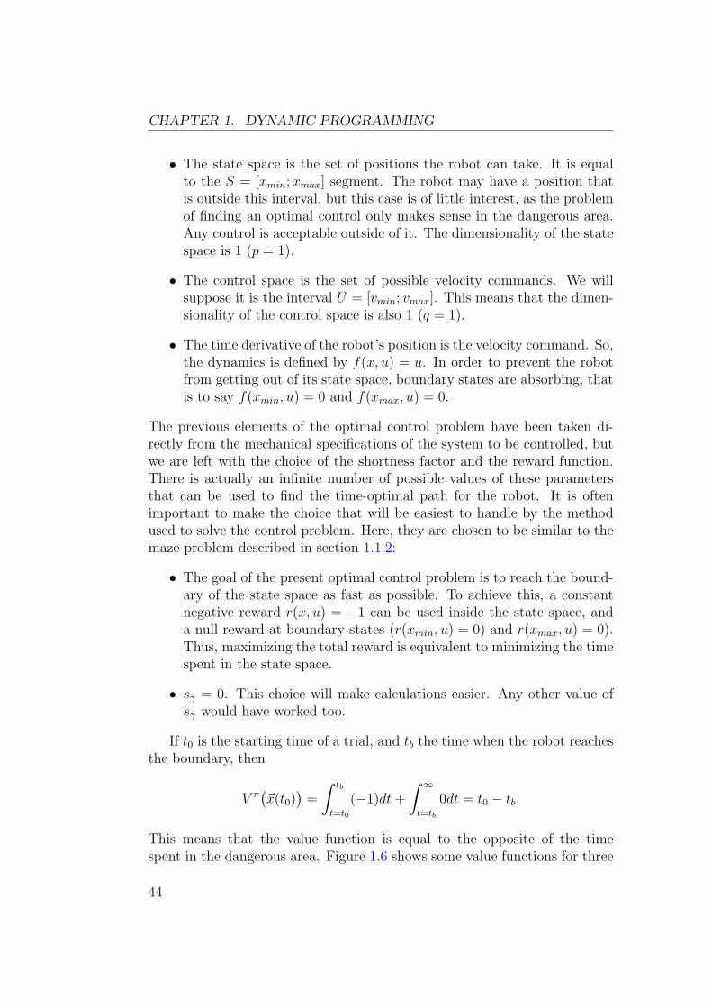
44
1.2. CONTINUOUS PROBLEMS
π(x) = 1x
V π
−1 1
−2
π(x) =
{
+12
if x ≥ 0
−12
if x < 0
x
V π
−1 1
−2
π(x) =
{
+1 if x ≥ 0
−1 if x < 0
x
V π
−1 1
−1
Figure 1.6: Examples of value functions for different policies π
different policies (numerical values are2 xmin = −1, xmax = +1, vmin = −1,and vmax = +1.) It is intuitively obvious that the third policy is optimal. Itconsists in going at maximum speed to the right if the robot is on the rightside of the dangerous area and at maximum speed to the left if the robot ison its left side.
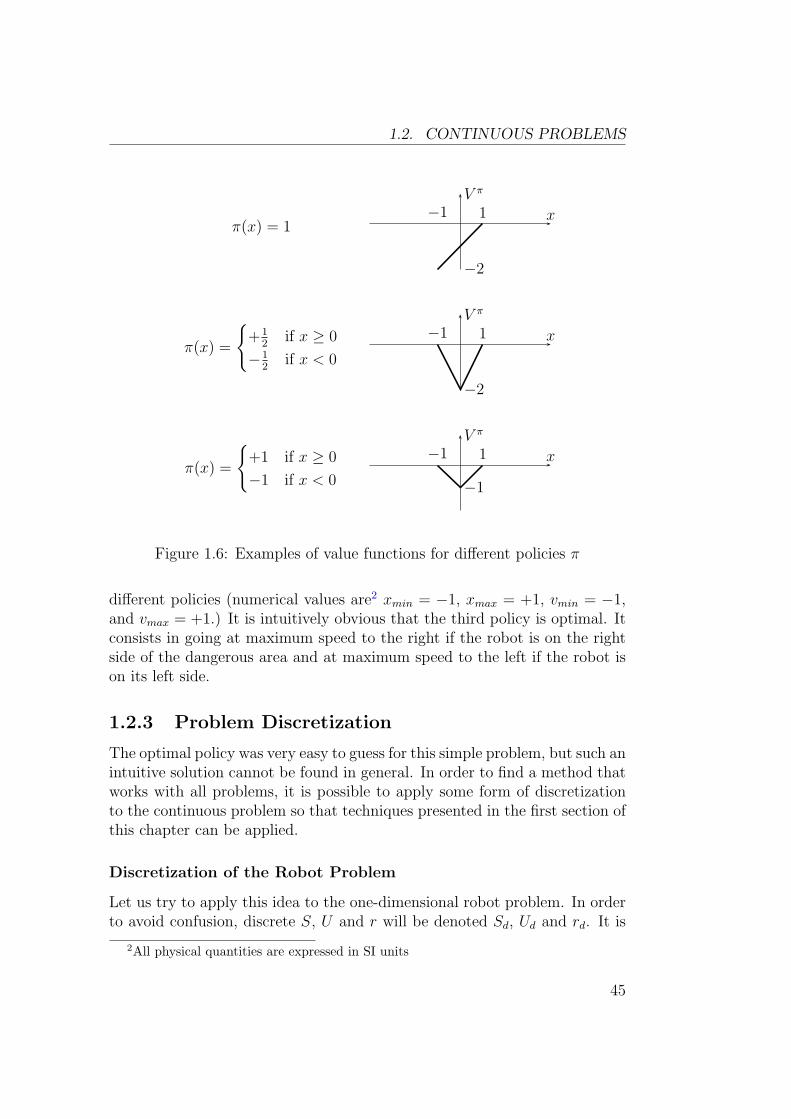
1.2.3 Problem Discretization
The optimal policy was very easy to guess for this simple problem, but such anintuitive solution cannot be found in general. In order to find a method thatworks with all problems, it is possible to apply some form of discretizationto the continuous problem so that techniques presented in the first section ofthis chapter can be applied.
Discretization of the Robot Problem
Let us try to apply this idea to the one-dimensional robot problem. In orderto avoid confusion, discrete S, U and r will be denoted Sd, Ud and rd. It is
2All physical quantities are expressed in SI units
45
CHAPTER 1. DYNAMIC PROGRAMMING
possible to define an “equivalent” discrete problem this way:
• Sd = {−98
, −78
, −58
, −38
, −18
, +18
, +38
, +58
, +78
, +98}, as shown on Figure 1.7.
• Ud = {−1, 0, +1}
• In order to define the ν function, a fixed time step δt = 14
can be used.This way, ν(1
8, +1) = 3
8. More generally, ν(x, u) = x + uδt, except at
boundaries ( ν(−98
,−1) = −98
and ν(98, +1) = 9
8).
• rd(x, u) = −δt except at boundaries, where rd(x, u) = 0. This way, thetotal reward is still equal to the opposite of the total time spent in thedangerous area.
• γ = 1
Figure 1.8 shows the approximate value function obtained by value iterationfor such a discretization. It is very close to the V shape of the optimal valuefunction.
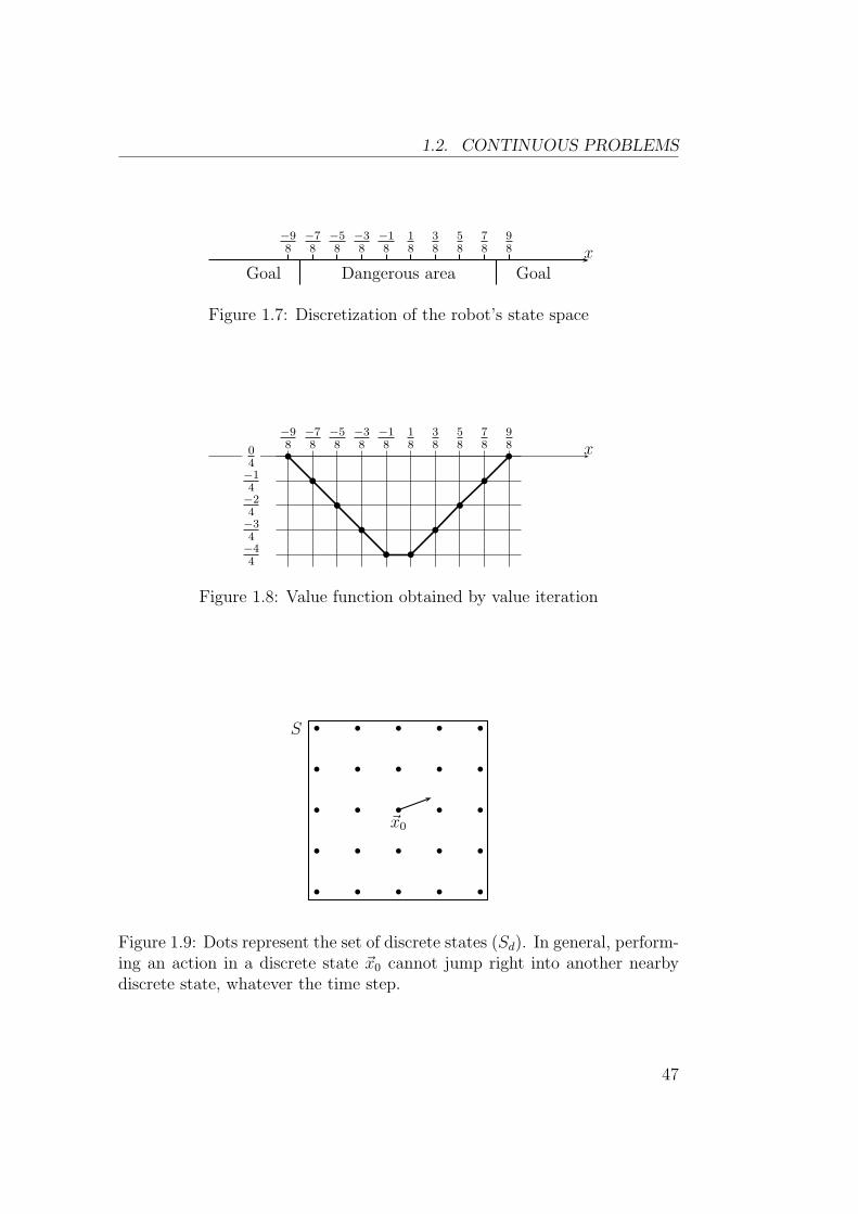
General Case
In the general case, a finite number of sample states and actions have to bechosen to make up the state and action sets: Sd ⊂ S and Ud ⊂ U . Thesesample elements should be chosen to be representative of the infinite set theyare taken from.
Once this has been done, it is necessary to define state transitions. Itwas rather easy with the robot problem because it was possible to choose aconstant time step so that performing an action during this time step lets thesystem jump from one discrete state right into another one. Unfortunately,this can not be done in the general case (see Figure 1.9), so it is not alwayspossible to transform a continuous problem to make it fit into the discretedeterministic formalism.
Although there is no hope to define discrete deterministic state transitionsfor a continuous problem, it is still possible to apply dynamic programmingalgorithms to a state discretization. The key issue is to find an equivalent tothe discrete Bellman equation. So, let us consider a time step of length δt.It is possible to split the sum that defines the value function (1.2.1) into twoparts:
V π(~x0) =
∫ t0+δt
t=t0
e−s(t−t0)r(
~x(t), π(~x(t)
))
dt + e−sδtV π(~x(t0 + δt)
). (1.2.2)
46
1.2. CONTINUOUS PROBLEMS
Dangerous areaGoal Goalx
−98
−78
−58
−38
−18
18
38
58
78
98
Figure 1.7: Discretization of the robot’s state space
x−98
−78
−58
−38
−18
18
38
58
78
980
4−14−24−34−44
b
b
b
b
b b
b
b
b
b
Figure 1.8: Value function obtained by value iteration
b b b b b
b b b b b
b b b b b
b b b b b
b b b b bS
~x0
Figure 1.9: Dots represent the set of discrete states (Sd). In general, perform-ing an action in a discrete state ~x0 cannot jump right into another nearbydiscrete state, whatever the time step.
47
CHAPTER 1. DYNAMIC PROGRAMMING
When δt is small, this can be approximated by
V π(~x0) ≈ r(~x0, π(~x0)
)δt + e−sδtV π(~x0 + δ~x), (1.2.3)
with
δ~x = f(~x0, π(~x0)
)δt.
Thanks to this discretization of time, it is possible to obtain a semi-continuousBellman equation that is very similar to the discrete one (1.1.1):
V ∗(~x) ≈ max~u∈Ud
(r(~x, ~u)δt + e−sδtV ∗(~x + δ~x)
). (1.2.4)
In order to solve equation (1.2.4), one might like to try to replace it byan assignment. This would allow to iteratively update V (~x) for states ~x inSd, similarly to the discrete value iteration algorithm. One major obstacle tothis approach, however, is that ~x + δ~x is not likely to be in Sd. In order toovercome this difficulty, it is necessary to use some form of interpolation toestimate V (~x+ δ~x) from the values of discrete states that are close to ~x+ δ~x.Algorithm 1.4 shows this general algorithm for value iteration.
Algorithm 1.4 Semi-Continuous Value Iteration
for all ~x ∈ Sd doV0(~x)← 0
end fori← 0repeat
i← i + 1for all ~x ∈ Sd do
Vi(~x)← max~u∈Ud
(
r(~x, ~u)δt + e−sγδt Vi−1
(~x + f(~x, ~u)δt
)
︸ ︷︷ ︸
estimated by interpolation
)
end foruntil V has converged
Finite Difference Method
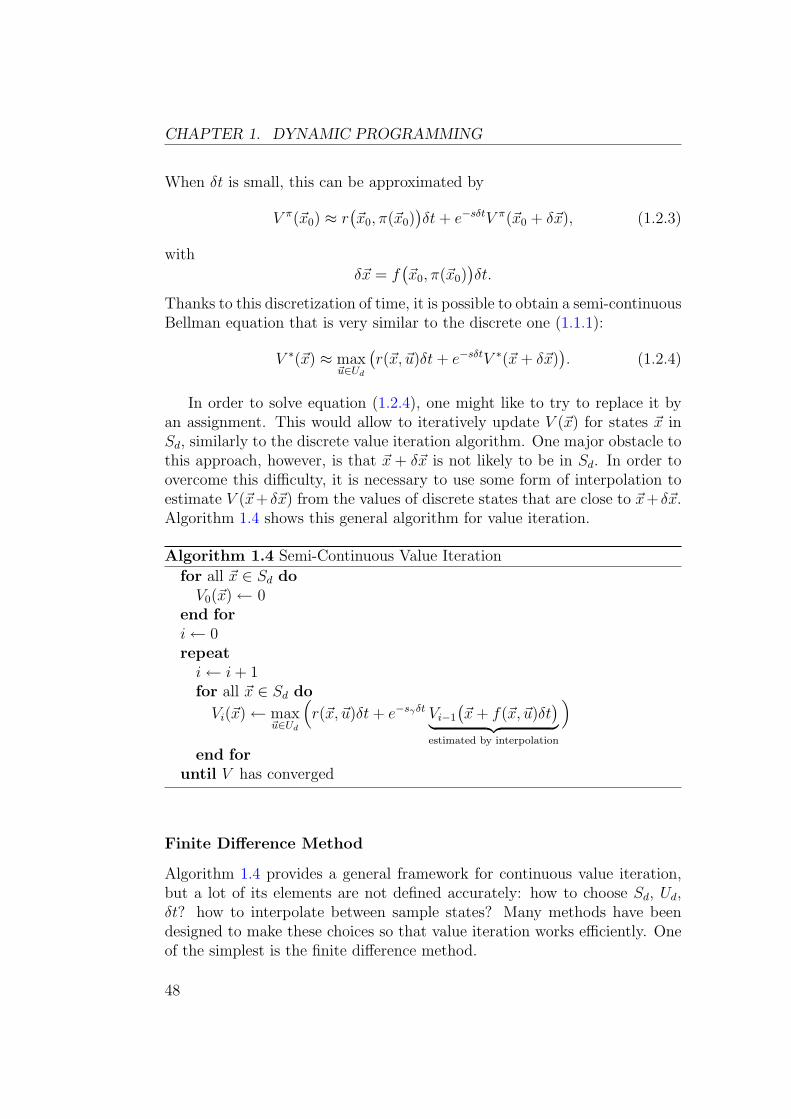
Algorithm 1.4 provides a general framework for continuous value iteration,but a lot of its elements are not defined accurately: how to choose Sd, Ud,δt? how to interpolate between sample states? Many methods have beendesigned to make these choices so that value iteration works efficiently. Oneof the simplest is the finite difference method.
48
1.2. CONTINUOUS PROBLEMS
b b b
b b b
b b b
~x0 ~x1
~x2
0.7
0.3
V (~x0 + δ~x) ≈ 0.7V (~x1) + 0.3V (~x2)
Figure 1.10: Finite Difference Method
This method consists in using a rectangular grid for Sd. The time step δtis chosen so that applying action ~u during a time interval of length δt movesthe state to an hyperplane that contains nearby states (Figure 1.10). Thevalue function is estimated at ~x + δ~x by linear interpolation between thesenearby states.
A problem with this method is that the time it takes to move to nearbystates may be very long when ‖f(~x, ~u)‖ is small. In this case, the finitedifference method does not converge to the right value function because thesmall-time-step approximation (1.2.3) is not valid anymore. Fortunately,when δ~x is small and δt is not, it is possible to obtain a more accurateBellman equation. It simply consists in approximating (1.2.2) by supposingthat r is almost constant in the integral sum:
V π(~x) ≈ r(~x, π(~x)
)1− e−sγδt
sγ
+ e−sγδtV π(~x + δ~x), (1.2.5)
which is a good approximation, even if δt is large. This equation can besimplified into
V π(~x) ≈ r(~x, π(~x)
)δt + (1− sγδt/2)V π(~x + δ~x)
1 + sγδt/2, (1.2.6)
which keeps a second order accuracy in δt. Thanks to this equation, finitedifference methods converge even for problems that have stationary states.Besides, (1.2.6) is not only more accurate than (1.2.3), but it is also morecomputationally efficient since there is no costly exponential to evaluate.
49
CHAPTER 1. DYNAMIC PROGRAMMING
bc
θ
mg
Figure 1.11: The pendulum swing-up problem
Convergence
When an averaging interpolation is used, it is easy to prove that this al-gorithm converges. Similarly to the discrete case, this result is based on acontraction property, with a factor equal to e−sγδt (or
∣∣1−sγδt/2
1+sγδt/2
∣∣ when (1.2.6)
is used).This convergence result, however, does not give any indication about how
close to the exact value function it converges (that is to say, how close tothe value of the continuous problem). In particular, (1.2.3) can give a signif-icantly different result from what (1.2.6) gives. Although this discretizationtechnique has been known since the early days of dynamic programming, it isonly very recently that Munos [43][44] proved that finite difference methodsconverge to the value function of the continuous problem, when the step sizeof the discretization goes to zero.
1.2.4 Pendulum Swing-Up
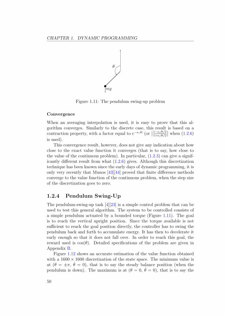
The pendulum-swing-up task [4][23] is a simple control problem that can beused to test this general algorithm. The system to be controlled consists ofa simple pendulum actuated by a bounded torque (Figure 1.11). The goalis to reach the vertical upright position. Since the torque available is notsufficient to reach the goal position directly, the controller has to swing thependulum back and forth to accumulate energy. It has then to decelerate itearly enough so that it does not fall over. In order to reach this goal, thereward used is cos(θ). Detailed specifications of the problem are given inAppendix B.
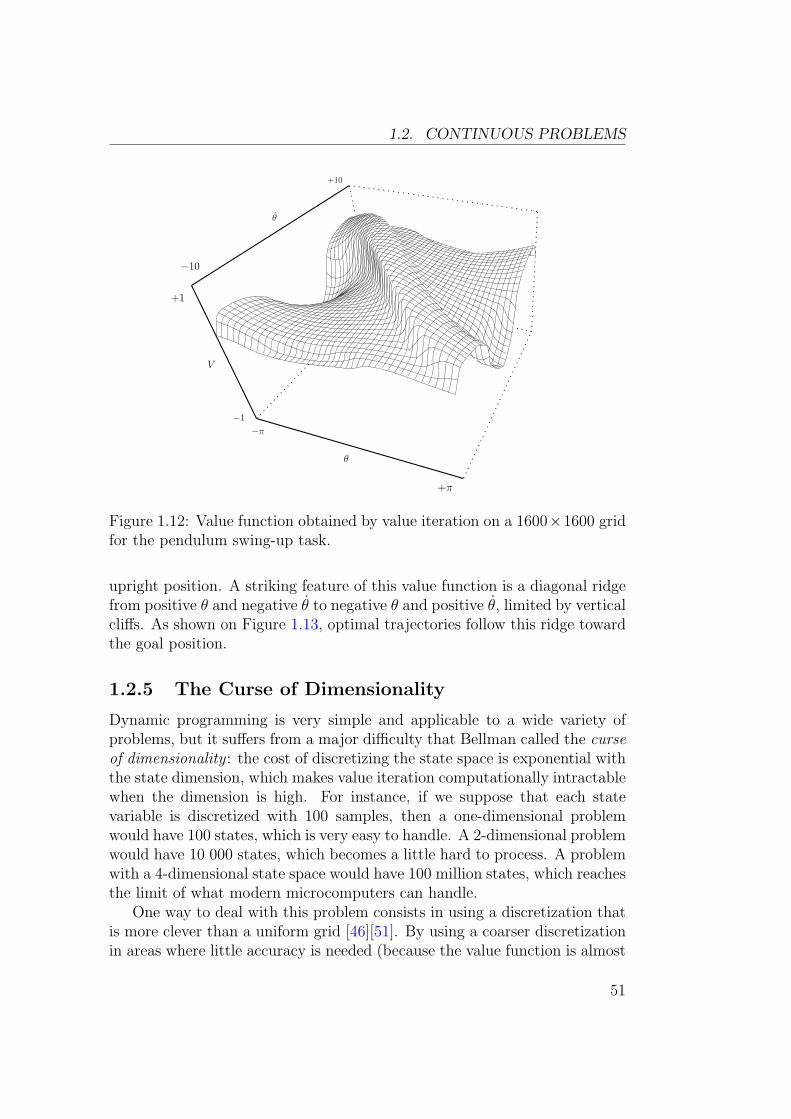
Figure 1.12 shows an accurate estimation of the value function obtainedwith a 1600× 1600 discretization of the state space. The minimum value isat (θ = ±π, θ = 0), that is to say the steady balance position (when thependulum is down). The maximum is at (θ = 0, θ = 0), that is to say the
50
1.2. CONTINUOUS PROBLEMS
V
+1
−1
θ
−π
+π
θ
+10
−10
Figure 1.12: Value function obtained by value iteration on a 1600×1600 gridfor the pendulum swing-up task.
upright position. A striking feature of this value function is a diagonal ridgefrom positive θ and negative θ to negative θ and positive θ, limited by verticalcliffs. As shown on Figure 1.13, optimal trajectories follow this ridge towardthe goal position.
1.2.5 The Curse of Dimensionality
Dynamic programming is very simple and applicable to a wide variety ofproblems, but it suffers from a major difficulty that Bellman called the curseof dimensionality : the cost of discretizing the state space is exponential withthe state dimension, which makes value iteration computationally intractablewhen the dimension is high. For instance, if we suppose that each statevariable is discretized with 100 samples, then a one-dimensional problemwould have 100 states, which is very easy to handle. A 2-dimensional problemwould have 10 000 states, which becomes a little hard to process. A problemwith a 4-dimensional state space would have 100 million states, which reachesthe limit of what modern microcomputers can handle.
One way to deal with this problem consists in using a discretization thatis more clever than a uniform grid [46][51]. By using a coarser discretizationin areas where little accuracy is needed (because the value function is almost
51
CHAPTER 1. DYNAMIC PROGRAMMING
θ
−10
10
θ−π 2π
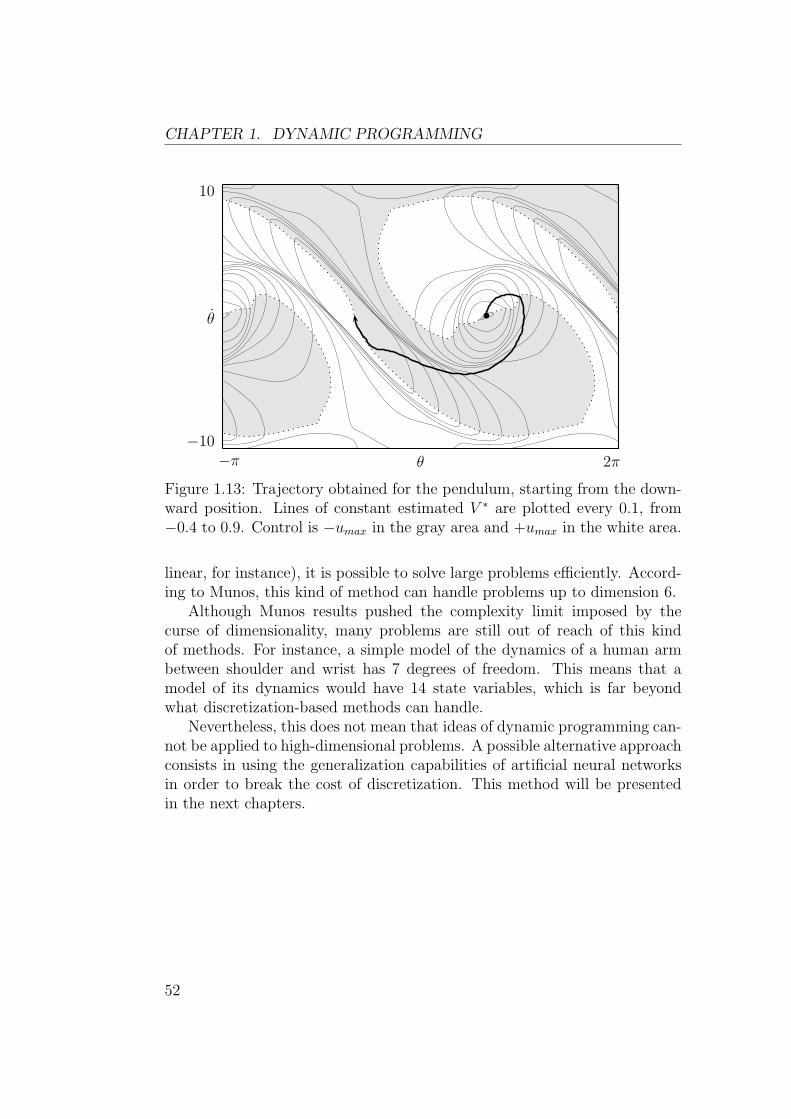
Figure 1.13: Trajectory obtained for the pendulum, starting from the down-ward position. Lines of constant estimated V ∗ are plotted every 0.1, from−0.4 to 0.9. Control is −umax in the gray area and +umax in the white area.
linear, for instance), it is possible to solve large problems efficiently. Accord-ing to Munos, this kind of method can handle problems up to dimension 6.
Although Munos results pushed the complexity limit imposed by thecurse of dimensionality, many problems are still out of reach of this kindof methods. For instance, a simple model of the dynamics of a human armbetween shoulder and wrist has 7 degrees of freedom. This means that amodel of its dynamics would have 14 state variables, which is far beyondwhat discretization-based methods can handle.
Nevertheless, this does not mean that ideas of dynamic programming can-not be applied to high-dimensional problems. A possible alternative approachconsists in using the generalization capabilities of artificial neural networksin order to break the cost of discretization. This method will be presentedin the next chapters.
52
Chapter 2
Artificial Neural Networks
The grid-based approximation of the value function that was used in theprevious chapter is only a particular case of a function approximator. Grid-based approximation suffers from the curse of dimensionality, which is amajor obstacle to its application to difficult motor control tasks. Some otherfunction approximators, however, can help to solve this problem thanks totheir ability to generalize. This chapter presents artificial neural networks,which are a particular kind of such approximators.
2.1 Function Approximators
2.1.1 Definition
A parametric function approximator (or estimator) can be formally definedas a set of functions indexed by a vector ~w of scalar values called weights. Atypical example is the set of linear functions f~w defined by
f~w(x) = w1x + w0
where
~w =
(w0
w1
)
∈ R2
is the vector of weights. Polynomials of any degree can be used too. Otherarchitectures will be described in Section 2.3.
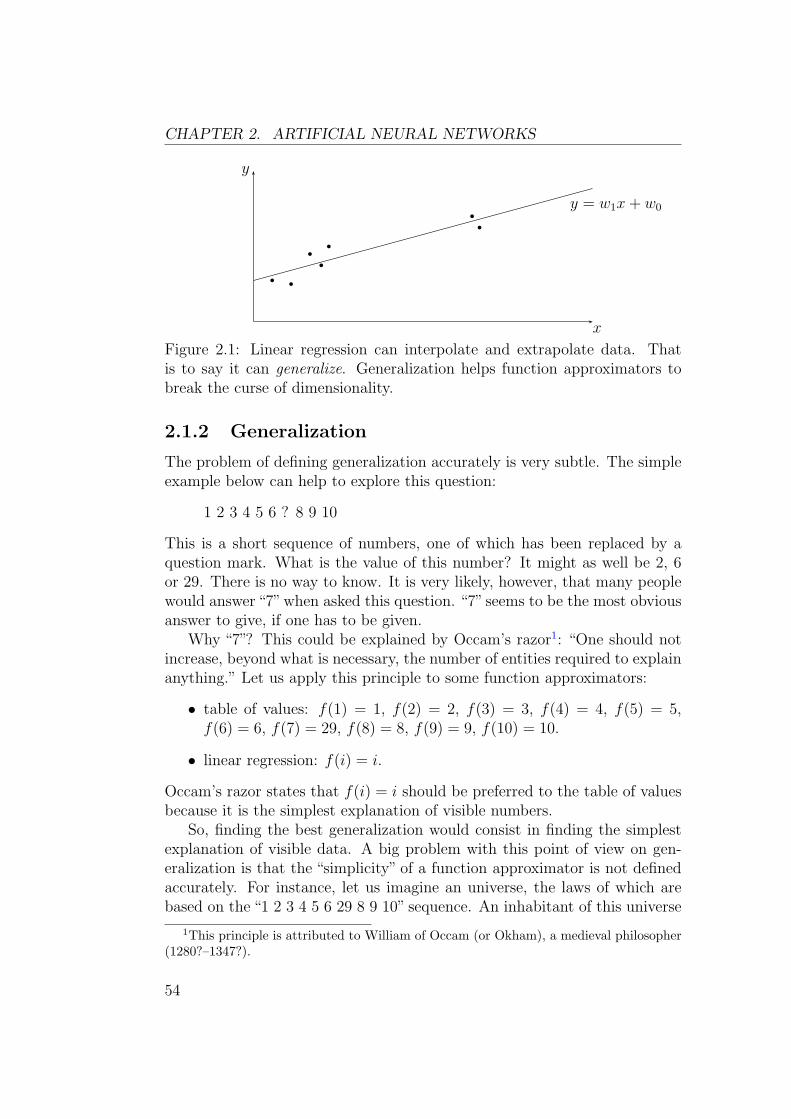
As its name says, a function approximator is used to approximate data.One of the main reason to do this is to get some form of generalization. A typ-ical case of such a generalization is the use of linear regression to interpolateor extrapolate some experimental data (see Figure 2.1).
53
CHAPTER 2. ARTIFICIAL NEURAL NETWORKS
x
y
bb
b
b
b
b
b
y = w1x + w0
Figure 2.1: Linear regression can interpolate and extrapolate data. Thatis to say it can generalize. Generalization helps function approximators tobreak the curse of dimensionality.
2.1.2 Generalization
The problem of defining generalization accurately is very subtle. The simpleexample below can help to explore this question:
1 2 3 4 5 6 ? 8 9 10
This is a short sequence of numbers, one of which has been replaced by aquestion mark. What is the value of this number? It might as well be 2, 6or 29. There is no way to know. It is very likely, however, that many peoplewould answer “7”when asked this question. “7” seems to be the most obviousanswer to give, if one has to be given.
Why “7”? This could be explained by Occam’s razor1: “One should notincrease, beyond what is necessary, the number of entities required to explainanything.” Let us apply this principle to some function approximators:
• table of values: f(1) = 1, f(2) = 2, f(3) = 3, f(4) = 4, f(5) = 5,f(6) = 6, f(7) = 29, f(8) = 8, f(9) = 9, f(10) = 10.
• linear regression: f(i) = i.
Occam’s razor states that f(i) = i should be preferred to the table of valuesbecause it is the simplest explanation of visible numbers.
So, finding the best generalization would consist in finding the simplestexplanation of visible data. A big problem with this point of view on gen-eralization is that the “simplicity” of a function approximator is not definedaccurately. For instance, let us imagine an universe, the laws of which arebased on the “1 2 3 4 5 6 29 8 9 10” sequence. An inhabitant of this universe
1This principle is attributed to William of Occam (or Okham), a medieval philosopher(1280?–1347?).
54
2.1. FUNCTION APPROXIMATORS
might find that 29 is the most natural guess for the missing number! Another(less weird) possibility would be that, independently of this sequence, othernumbers had been presented to this person the day before:
1 2 3 4 5 6 29 8 9 101 2 3 4 5 6 29 8 9 101 2 3 4 5 6 29 8 9 10. . .
This means that deciding whether a generalization is good depends on priorknowledge. This prior knowledge may be any kind of information. It may beother data or simply an intuition about what sort of function approximatorwould be well suited for this specific problem.
Some theories have been developed to formalize this notion of general-ization, and to build efficient algorithms. Their complexity is way beyondthe scope of this chapter, but further developments of this discussion canbe found in the machine-learning literature. In particular, Vapnik’s theoryof structural risk minimization is a major result of this field [75]. Manyother important ideas, such as Bayesian techniques, are clearly explained inBishop’s book [16].
Without going into these theories, it is possible to estimate the gener-alization capabilities of a parametric function approximator intuitively: itshould be as “simple” as possible, and yet be able to approximate as many“usual” functions as possible.
2.1.3 Learning
In order to approximate a given target function, it is necessary to find a goodset of weights. The problem is that changing one weight is likely to alter theoutput of the function on the whole input space, so it is not as easy as usinga grid-based approximation. One possible solution consists in minimizing anerror function that measures how bad an approximation is.
Usually, there is a finite number of sample input/output pairs and thegoal is to find a function that approximates them well. Let us call thesesamples (xi, yi) with i ∈ {1, . . . , p}. In this situation, a quadratic error canbe used:
E(~w) =1
2
p∑
i=1
(f~w(xi)− yi
)2.
The process of finding weights that minimize the error function E is calledtraining or learning by artificial intelligence researchers. It is also calledcurve-fitting or regression in the field of data analysis. In the particular caseof linear functions (Figure 2.1), the linear regression method directly provides
55
CHAPTER 2. ARTIFICIAL NEURAL NETWORKS
w
Ebc bc
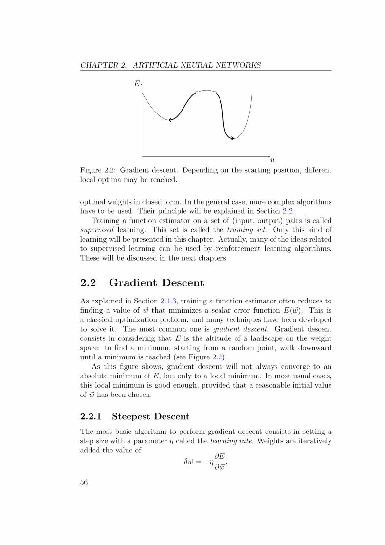
Figure 2.2: Gradient descent. Depending on the starting position, differentlocal optima may be reached.
optimal weights in closed form. In the general case, more complex algorithmshave to be used. Their principle will be explained in Section 2.2.
Training a function estimator on a set of (input, output) pairs is calledsupervised learning. This set is called the training set. Only this kind oflearning will be presented in this chapter. Actually, many of the ideas relatedto supervised learning can be used by reinforcement learning algorithms.These will be discussed in the next chapters.
2.2 Gradient Descent
As explained in Section 2.1.3, training a function estimator often reduces tofinding a value of ~w that minimizes a scalar error function E(~w). This isa classical optimization problem, and many techniques have been developedto solve it. The most common one is gradient descent. Gradient descentconsists in considering that E is the altitude of a landscape on the weightspace: to find a minimum, starting from a random point, walk downwarduntil a minimum is reached (see Figure 2.2).
As this figure shows, gradient descent will not always converge to anabsolute minimum of E, but only to a local minimum. In most usual cases,this local minimum is good enough, provided that a reasonable initial valueof ~w has been chosen.
2.2.1 Steepest Descent
The most basic algorithm to perform gradient descent consists in setting astep size with a parameter η called the learning rate. Weights are iterativelyadded the value of
δ ~w = −η∂E
∂ ~w.
56
2.2. GRADIENT DESCENT
This is repeated until some termination criterion is met. This algorithm iscalled steepest descent2.
2.2.2 Efficient Algorithms
Choosing the right value for the learning rate η is a difficult problem. If ηis too small, then learning will be too slow. If η is too large, then learningmay diverge. A good value of η can be found by trial and error, but it isa rather tedious and inefficient method. In order to address this problem, avery large variety of efficient learning techniques has been developed. Thissection presents the most important theoretical ideas underlying them.
One of the most fundamental ideas to accelerate learning consists in usingsecond order information about the error function. As Figure 2.3 shows, fora quadratic error in one dimension, the best learning rate is the inverse of thesecond order derivative. This can help to design efficient learning techniques;if it is possible to evaluate this second order derivative, then it is possible toautomatically find a good learning rate.
Unfortunately, the error function might not be quadratic at all. So, settingthe learning coefficient to the reverse of the second order derivative only worksnear the optimum, in areas where the quadratic approximation is valid. Butwhen, for instance, the second order derivative is negative, this does not workat all (that is the case at the starting positions in Figure 2.2.) Special caremust be taken to handle these situations.
Some other problems arise when the dimension of the weight space islarger than one, which is always the case in practice. The second orderderivative is not a single number anymore, but a matrix called the Hessianand defined by
H =∂2E
∂ ~w2=
∂2E∂w2
1
∂2E∂w1∂w2
. . . ∂2E∂w1∂wn
∂2E∂w2∂w1
∂2E∂w2
2. . . ∂2E
∂w2∂wn
......
. . ....
∂2E∂wn∂w1
∂2E∂wn∂w2
. . . ∂2E∂w2
n
.
As Figure 2.4 shows, it is possible to have different curvatures in differentdirections. It can create a lot of trouble if there is, say, a second derivativeof 100 in one direction, and a second derivative of 1 in another. In this case,
2This algorithm is sometimes also called standard backprop, which is short for back-
propagation of error. This vocabulary is very confusing. In this document, the “backprop-agation” term will only refer to the algorithm used to compute the gradient of the errorfunction in feedforward neural networks.
57
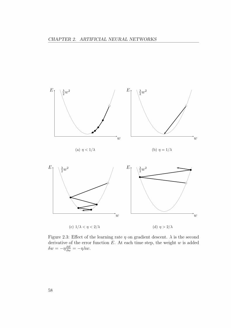
CHAPTER 2. ARTIFICIAL NEURAL NETWORKS
E
w
λ2w2
b
b
b
bb
bc
(a) η < 1/λ
E
w
λ2w2
bbc
(b) η = 1/λ
E
w
λ2w2
b
b
bb
bbbb
bc
(c) 1/λ < η < 2/λ
E
w
λ2w2
b
bb
b b
bc
(d) η > 2/λ
Figure 2.3: Effect of the learning rate η on gradient descent. λ is the secondderivative of the error function E. At each time step, the weight w is addedδw = −η ∂E
∂w= −ηλw.
58
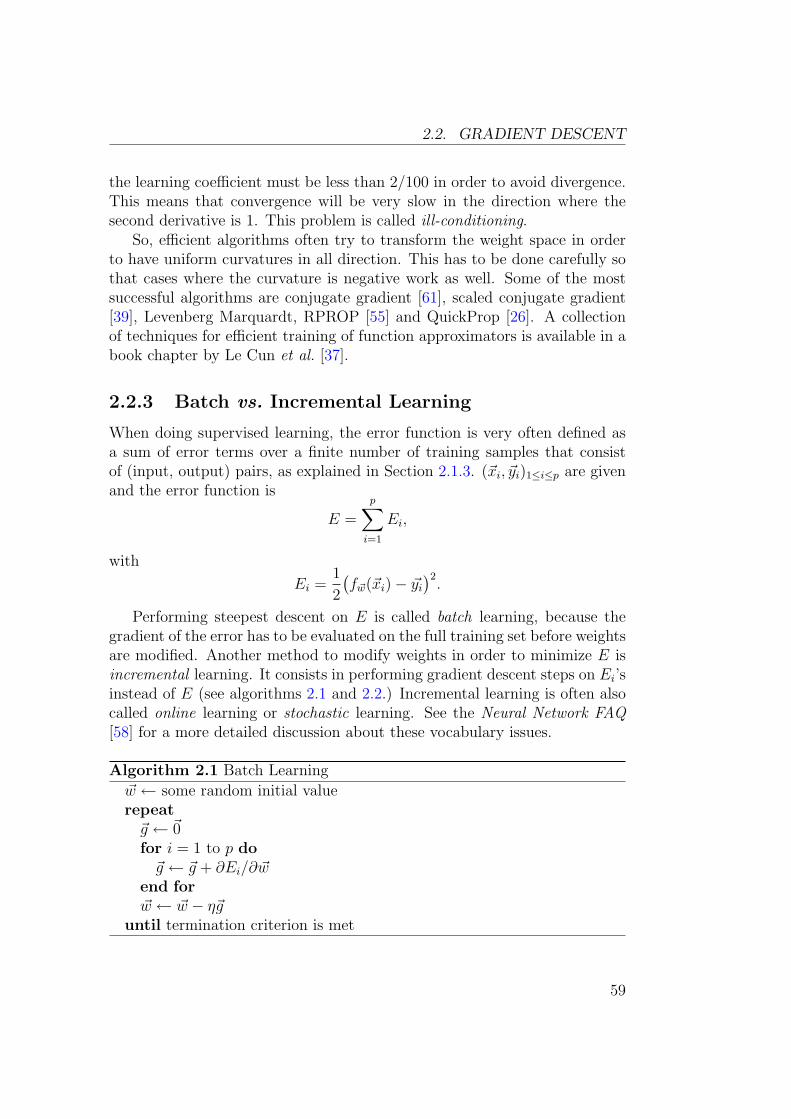
2.2. GRADIENT DESCENT
the learning coefficient must be less than 2/100 in order to avoid divergence.This means that convergence will be very slow in the direction where thesecond derivative is 1. This problem is called ill-conditioning.
So, efficient algorithms often try to transform the weight space in orderto have uniform curvatures in all direction. This has to be done carefully sothat cases where the curvature is negative work as well. Some of the mostsuccessful algorithms are conjugate gradient [61], scaled conjugate gradient[39], Levenberg Marquardt, RPROP [55] and QuickProp [26]. A collectionof techniques for efficient training of function approximators is available in abook chapter by Le Cun et al. [37].
2.2.3 Batch vs. Incremental Learning
When doing supervised learning, the error function is very often defined asa sum of error terms over a finite number of training samples that consistof (input, output) pairs, as explained in Section 2.1.3. (~xi, ~yi)1≤i≤p are givenand the error function is
E =
p∑
i=1
Ei,
with
Ei =1
2
(f~w(~xi)− ~yi
)2.
Performing steepest descent on E is called batch learning, because thegradient of the error has to be evaluated on the full training set before weightsare modified. Another method to modify weights in order to minimize E isincremental learning. It consists in performing gradient descent steps on Ei’sinstead of E (see algorithms 2.1 and 2.2.) Incremental learning is often alsocalled online learning or stochastic learning. See the Neural Network FAQ[58] for a more detailed discussion about these vocabulary issues.
Algorithm 2.1 Batch Learning
~w ← some random initial valuerepeat
~g ← ~0for i = 1 to p do
~g ← ~g + ∂Ei/∂ ~wend for~w ← ~w − η~g
until termination criterion is met
59
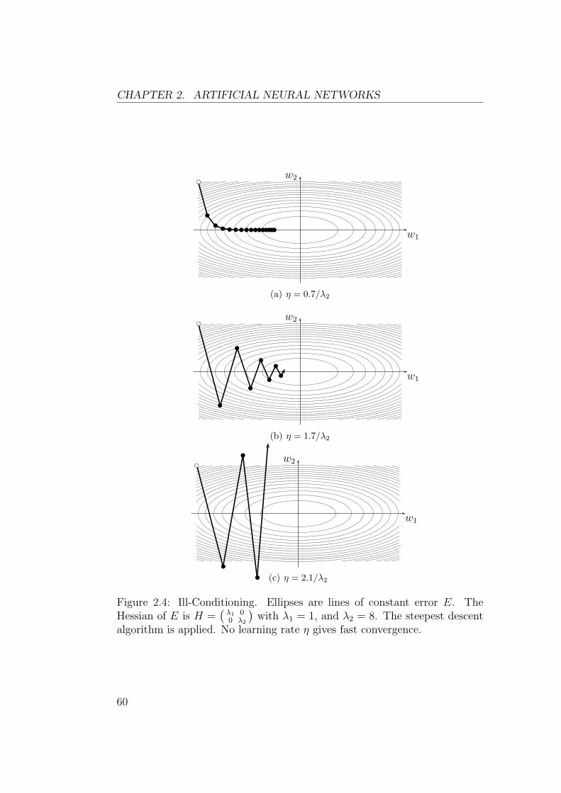
CHAPTER 2. ARTIFICIAL NEURAL NETWORKS
w1
w2b
bb
bb bb bb bb bb bb bb bb bb bb bb bb bb bb
bc
(a) η = 0.7/λ2
w1
w2b
bb
bb
bb
bb
bb
bb
b b
bc
(b) η = 1.7/λ2
w1
w2b
bb
bb
b b
bc
(c) η = 2.1/λ2
Figure 2.4: Ill-Conditioning. Ellipses are lines of constant error E. TheHessian of E is H =
(λ1 00 λ2
)with λ1 = 1, and λ2 = 8. The steepest descent
algorithm is applied. No learning rate η gives fast convergence.
60
2.2. GRADIENT DESCENT
Algorithm 2.2 Incremental Learning
~w ← some random initial valuerepeat
i← random value between 1 and p~w ← ~w − η∂Ei/∂ ~w
until termination criterion is met
Which of these techniques is the best? This is a difficult question, theanswer of which depends on the specific problem to be solved. Here are someof the points to consider: (This discussion is very deeply inspired by a bookchapter by Le Cun et al. [37].)
Advantages of Incremental Learning
1. Incremental learning is usually faster than batch learning, especiallywhen the training set is redundant. In the case when the training sethas input/output patterns that are similar, batch learning wastes timecomputing and adding similar gradients before performing one weightupdate.
2. Incremental learning often results in better solutions. The reasons isthat the randomness of incremental learning creates noise in the weightupdates. This noise helps weights to jump out of bad local optima [48].
3. Incremental learning can track changes. A typical example is whenlearning a model of the dynamics of a mechanical system. As thissystem gets older, its properties might slowly evolve (due to wear ofsome parts, for instance). Incremental learning can track this kind ofdrift.
Advantages of Batch Learning
1. Conditions of convergence are well understood. Noise in incrementallearning causes weights to constantly fluctuate around a local optimum,and they never converge to a constant stable value. This does nothappen in batch learning, which makes it easier to analyze.
2. Many acceleration techniques only operate in batch learning. In par-ticular, algorithms listed in the previous subsection can be applied tobatch learning only (Conjugate gradient, RPROP, QuickProp, . . . ).
61
CHAPTER 2. ARTIFICIAL NEURAL NETWORKS
3. Theoretical analysis of the weight dynamics and convergence rates aresimpler. This is also related to the lack of noise in batch learning.
2.3 Some Approximation Schemes
2.3.1 Linear Function Approximators
The general form of linear function approximators is
V~w(~x) =∑
i
wiφi(~x).
This kind of function approximator has many nice characteristics that havemade it particularly successful in reinforcement learning.
Unlike some more complex function approximation schemes, like feedfor-ward neural networks, it is rather easy to train a linear function approxima-tor. In particular, there is no poor local optimum and the Hessian of theerror function is diagonal (and easy to evaluate).
Another nice quality of such a function approximator is locality [77]. Bychoosing φi’s such that φi(~x) has a non-zero value in a small area of the inputspace only, it is possible to make sure that a change in wi will have significantconsequences in a small area only. This is often considered a good propertyfor reinforcement learning. The reason is that reinforcement learning is oftenperformed incrementally, and the value-function approximator should notforget what it has learnt in other areas of the state space when trained on anew single input ~x.
Some of the most usual linear function approximators are described inthe sections below. Many variations on these ideas exist.
Grid-Based Approximation
The grid-based approximation of the value function used in the previouschapter is a particular case of a linear function approximator. As explainedpreviously, this kind of function approximation suffers from the curse of di-mensionality, because it takes a huge number of weights to sample a high-dimensional state space with enough accuracy (even with clever discretizationmethods). In terms of neural-network learning, this means that this kind offunction approximation scheme has very poor generalization capabilities.
Tile Coding (or CMAC[1])
Instead of using one single grid to approximate the value function, tile codingconsists in adding multiple overlapping tilings (cf. Figure 2.5). This is a way
62
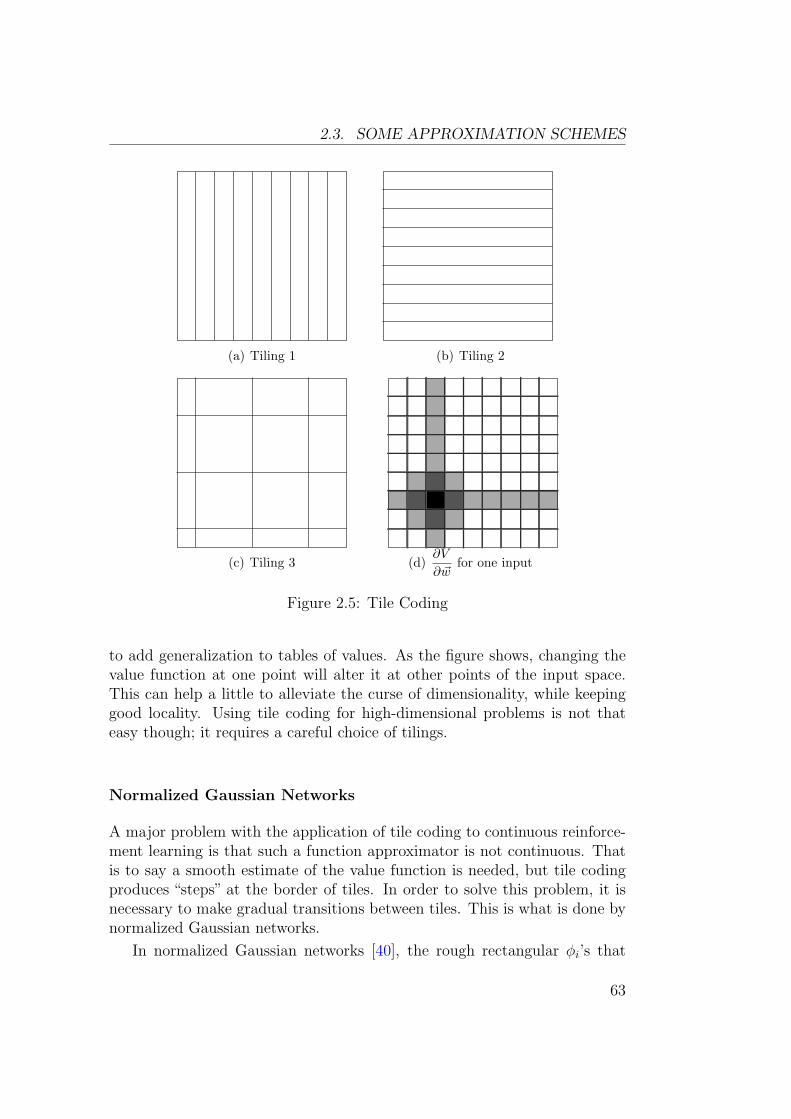
2.3. SOME APPROXIMATION SCHEMES
(a) Tiling 1 (b) Tiling 2
(c) Tiling 3 (d)∂V
∂ ~wfor one input
Figure 2.5: Tile Coding
to add generalization to tables of values. As the figure shows, changing thevalue function at one point will alter it at other points of the input space.This can help a little to alleviate the curse of dimensionality, while keepinggood locality. Using tile coding for high-dimensional problems is not thateasy though; it requires a careful choice of tilings.
Normalized Gaussian Networks
A major problem with the application of tile coding to continuous reinforce-ment learning is that such a function approximator is not continuous. Thatis to say a smooth estimate of the value function is needed, but tile codingproduces “steps” at the border of tiles. In order to solve this problem, it isnecessary to make gradual transitions between tiles. This is what is done bynormalized Gaussian networks.
In normalized Gaussian networks [40], the rough rectangular φi’s that
63
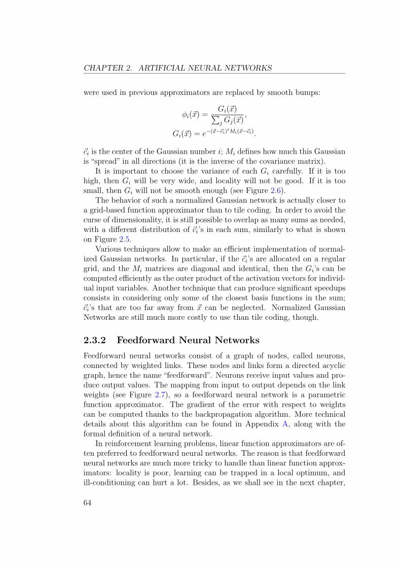
CHAPTER 2. ARTIFICIAL NEURAL NETWORKS
were used in previous approximators are replaced by smooth bumps:
φi(~x) =Gi(~x)
∑
j Gj(~x),
Gi(~x) = e−(~x−~ci)tMi(~x−~ci).
~ci is the center of the Gaussian number i; Mi defines how much this Gaussianis “spread” in all directions (it is the inverse of the covariance matrix).
It is important to choose the variance of each Gi carefully. If it is toohigh, then Gi will be very wide, and locality will not be good. If it is toosmall, then Gi will not be smooth enough (see Figure 2.6).
The behavior of such a normalized Gaussian network is actually closer toa grid-based function approximator than to tile coding. In order to avoid thecurse of dimensionality, it is still possible to overlap as many sums as needed,with a different distribution of ~ci’s in each sum, similarly to what is shownon Figure 2.5.
Various techniques allow to make an efficient implementation of normal-ized Gaussian networks. In particular, if the ~ci’s are allocated on a regulargrid, and the Mi matrices are diagonal and identical, then the Gi’s can becomputed efficiently as the outer product of the activation vectors for individ-ual input variables. Another technique that can produce significant speedupsconsists in considering only some of the closest basis functions in the sum;~ci’s that are too far away from ~x can be neglected. Normalized GaussianNetworks are still much more costly to use than tile coding, though.
2.3.2 Feedforward Neural Networks
Feedforward neural networks consist of a graph of nodes, called neurons,connected by weighted links. These nodes and links form a directed acyclicgraph, hence the name “feedforward”. Neurons receive input values and pro-duce output values. The mapping from input to output depends on the linkweights (see Figure 2.7), so a feedforward neural network is a parametricfunction approximator. The gradient of the error with respect to weightscan be computed thanks to the backpropagation algorithm. More technicaldetails about this algorithm can be found in Appendix A, along with theformal definition of a neural network.
In reinforcement learning problems, linear function approximators are of-ten preferred to feedforward neural networks. The reason is that feedforwardneural networks are much more tricky to handle than linear function approx-imators: locality is poor, learning can be trapped in a local optimum, andill-conditioning can hurt a lot. Besides, as we shall see in the next chapter,
64
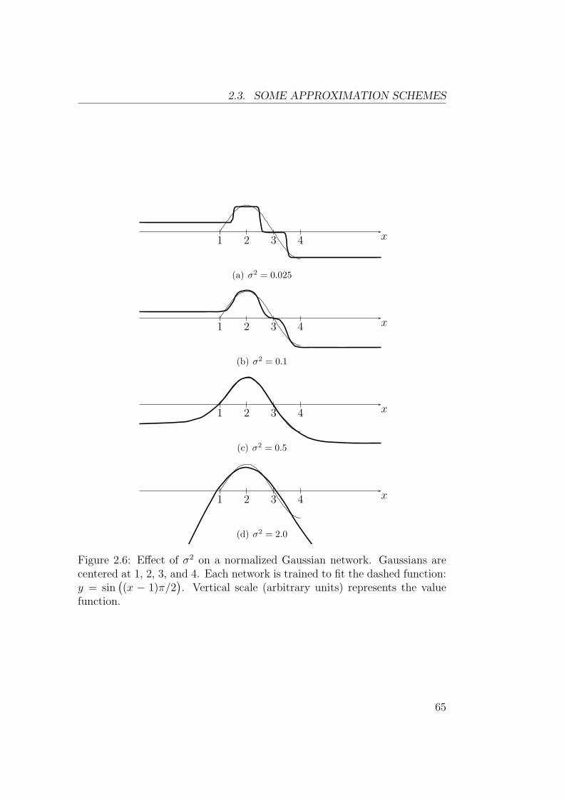
2.3. SOME APPROXIMATION SCHEMES
1 2 3 4 x
(a) σ2 = 0.025
1 2 3 4 x
(b) σ2 = 0.1
1 2 3 4 x
(c) σ2 = 0.5
1 2 3 4 x
(d) σ2 = 2.0
Figure 2.6: Effect of σ2 on a normalized Gaussian network. Gaussians arecentered at 1, 2, 3, and 4. Each network is trained to fit the dashed function:y = sin
((x − 1)π/2
). Vertical scale (arbitrary units) represents the value
function.
65
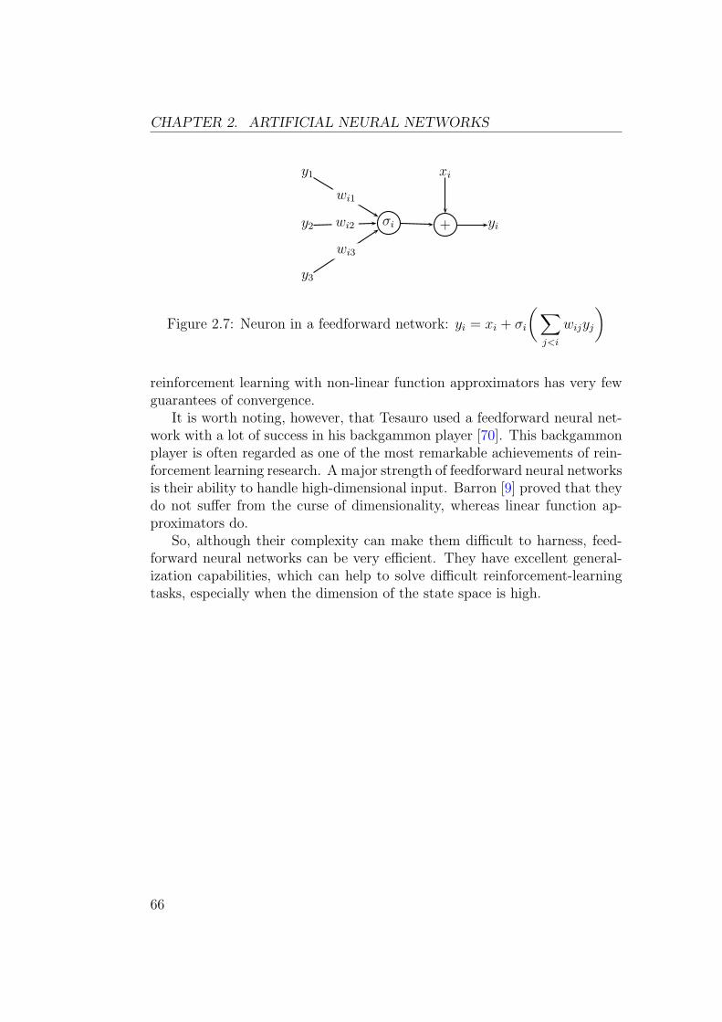
CHAPTER 2. ARTIFICIAL NEURAL NETWORKS
σi yi
y1
y2
y3
+
xi
wi1
wi2
wi3
Figure 2.7: Neuron in a feedforward network: yi = xi + σi
(∑
j<i
wijyj
)
reinforcement learning with non-linear function approximators has very fewguarantees of convergence.
It is worth noting, however, that Tesauro used a feedforward neural net-work with a lot of success in his backgammon player [70]. This backgammonplayer is often regarded as one of the most remarkable achievements of rein-forcement learning research. A major strength of feedforward neural networksis their ability to handle high-dimensional input. Barron [9] proved that theydo not suffer from the curse of dimensionality, whereas linear function ap-proximators do.
So, although their complexity can make them difficult to harness, feed-forward neural networks can be very efficient. They have excellent general-ization capabilities, which can help to solve difficult reinforcement-learningtasks, especially when the dimension of the state space is high.
66
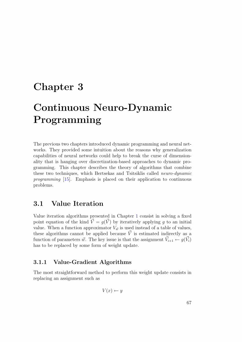
Chapter 3
Continuous Neuro-DynamicProgramming
The previous two chapters introduced dynamic programming and neural net-works. They provided some intuition about the reasons why generalizationcapabilities of neural networks could help to break the curse of dimension-ality that is hanging over discretization-based approaches to dynamic pro-gramming. This chapter describes the theory of algorithms that combinethese two techniques, which Bertsekas and Tsitsiklis called neuro-dynamicprogramming [15]. Emphasis is placed on their application to continuousproblems.
3.1 Value Iteration
Value iteration algorithms presented in Chapter 1 consist in solving a fixedpoint equation of the kind ~V = g(~V ) by iteratively applying g to an initialvalue. When a function approximator V~w is used instead of a table of values,these algorithms cannot be applied because ~V is estimated indirectly as afunction of parameters ~w. The key issue is that the assignment ~Vi+1 ← g(~Vi)has to be replaced by some form of weight update.
3.1.1 Value-Gradient Algorithms
The most straightforward method to perform this weight update consists inreplacing an assignment such as
V (x)← y
67
CHAPTER 3. CONTINUOUS NEURO-DYNAMIC PROGRAMMING
by one step of gradient descent on the error
E(~w) =1
2
(V~w(x)− y
)2.
This leads to a weight update
~w ← ~w + η(y − V~w(x)
)∂V~w(x)
∂ ~w,
where η is the learning rate.Although this might look like a natural way to generalize value iteration
to function approximators, this method does not work well. Baird showedthat this approach to value iteration may diverge for a very small decisionprocess [7]. Tsitsiklis and Van Roy gave another very simple two-state coun-terexample [73]:
V (0) =w0
V (1) =2w0
In this process, each state has only one possible action and all transitionsgive a reward of zero. Thus, when a discount factor γ < 1 is used, the valuefunction is equal to zero everywhere. A linear function approximator is usedto approximate this value function. The value-gradient approach to valueiteration leads to a weight update of
w0 ← w0 + η
((γV (1)− V (0)
)∂V (0)
∂w0
+(γV (1)− V (1)
)∂V (1)
∂w0
)
,
that is to say
w0 ← w0 + η((2γ − 1)w0 + (2γ − 2)2w0
),
which can be simplified into
w0 ← w0
(1 + η(6γ − 5)
).
So, when γ > 56, this algorithm diverges.
A reason why this method does not work is that the contraction propertythat proved convergence of lookup-table approaches can not be establishedanymore. Gordon [29] studied characteristics that a function approximatorshould have so that the process of updating weights still is a contraction.Unfortunately, the conditions imposed to keep this property are extremelyrestrictive, and dismiss most of the function approximators with good gen-eralization abilities, such as tile coding or feedforward neural networks.
68
3.1. VALUE ITERATION
3.1.2 Residual-Gradient Algorithms
Divergence of value-gradient algorithms is related to interference: whenweights are updated to change the value of one state, it is very likely that thevalue of other states will change as well. As a consequence, the target valuey in the V (x) ← y assignment might change as ~w is modified, which mayactually let y move away from V (x) and cause divergence of the algorithm.
In order to solve this problem, Baird proposed residual-gradient algo-rithms [7]. They consist in using an error function that takes into accountthe dependency of y on ~w:
E(~w) =1
2
(~V~w − g(~V~w)
)2
Since E is a function of ~w that does not change as learning progresses, thereis no moving-target problem anymore, which lets the gradient-descent algo-rithm converge1.
One major limit to this approach, however, is that there is no guaranteethat the estimated value function obtained is close to the solution of thedynamic programming problem. In fact, it is possible to get a value of ~wso that ~V~w is extremely close to g(~V~w), but very far from the single solution
of the ~V = g(~V ) equation. This phenomenon is particularly striking in thecontinuous case, which is presented in the next section.
3.1.3 Continuous Residual-Gradient Algorithms
The semi-continuous Bellman equation derived in Chapter 1 is based on theapproximation
V π(~x) ≈ r(~x, π(~x)
)δt + e−sγδtV π(~x + δ~x).
When using a discretization of the state space, a value of δt is used so that itlets the system move from one discrete state to nearby discrete states. In thegeneral case of function approximation, however, there is no such thing as“nearby states”. δt could be chosen to be any arbitrarily small time interval.This leads to completely continuous formulations of dynamic programmingalgorithms.
1Note that, in general, E is not differentiable because of the max operator in g. Since Eis continuous and differentiable almost everywhere, gradient descent should work, anyway.
69
CHAPTER 3. CONTINUOUS NEURO-DYNAMIC PROGRAMMING
The Hamilton-Jacobi-Bellman Equation
Let us suppose that δt is replaced by an infinitely small step dt. The policy-evaluation equation becomes
V π(~x) ≈ r(~x, π(~x)
)dt + e−sγdtV π(~x + d~x)
≈ r(~x, π(~x)
)dt + (1− sγdt)V π(~x + d~x).
By subtracting V π(~x) to each term and dividing by dt we get:
0 = r(~x, π(~x)
)− sγV
π(~x) + V π(~x). (3.1.1)
If we note that
V π(~x) =∂V π
∂~x· d~x
dt=
∂V π
∂~x· f(~x, ~u),
then (3.1.1) becomes
0 = r(~x, π(~x)
)− sγV
π(~x) +∂V π
∂~x· f(~x, π(~x)
). (3.1.2)
A similar equation can be obtained for the optimal value function:
0 = max~u∈U
(
r(~x, ~u)− sγV∗(~x) +
∂V ∗
∂~x· f(~x, ~u)
)
. (3.1.3)
(3.1.3) is the Hamilton-Jacobi-Bellman equation. It is the continuous equiv-alent to the discrete Bellman equation. Besides, for any value function V ,the Hamiltonian H is defined as
H = max~u∈U
(
r(~x, ~u)− sγV (~x) +∂V
∂~x· f(~x, ~u)
)
,
which is analogous to the discrete Bellman residual.
Continuous Value Iteration
So, continuous residual-gradient algorithms would consist in performing gra-dient decent2 on E = 1
2
∫
x∈SH2dx. Munos, Baird and Moore [45] studied this
algorithm and showed that, although it does converge, it does not convergeto the right value function. The one-dimensional robot problem presented
2Performing gradient descent on this kind of error function is a little bit more com-plex than usual supervised learning, because the error depends on the gradient of thevalue function with respect to its input. This problem can be solved by the differentialbackpropagation algorithm presented in Appendix A.
70
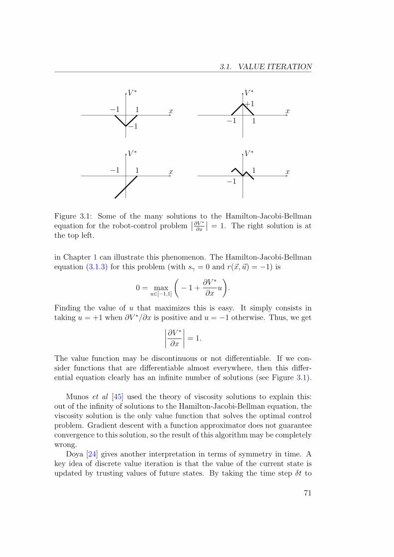
3.1. VALUE ITERATION
x
V ∗
−1
−1 1 x
V ∗
+1
−1 1
x
V ∗
−1 1 x
V ∗
−1
1
Figure 3.1: Some of the many solutions to the Hamilton-Jacobi-Bellmanequation for the robot-control problem
∣∣∂V ∗
∂x
∣∣ = 1. The right solution is at
the top left.
in Chapter 1 can illustrate this phenomenon. The Hamilton-Jacobi-Bellmanequation (3.1.3) for this problem (with sγ = 0 and r(~x, ~u) = −1) is
0 = maxu∈[−1,1]
(
− 1 +∂V ∗
∂xu
)
.
Finding the value of u that maximizes this is easy. It simply consists intaking u = +1 when ∂V ∗/∂x is positive and u = −1 otherwise. Thus, we get
∣∣∣∣
∂V ∗
∂x
∣∣∣∣= 1.
The value function may be discontinuous or not differentiable. If we con-sider functions that are differentiable almost everywhere, then this differ-ential equation clearly has an infinite number of solutions (see Figure 3.1).
Munos et al [45] used the theory of viscosity solutions to explain this:out of the infinity of solutions to the Hamilton-Jacobi-Bellman equation, theviscosity solution is the only value function that solves the optimal controlproblem. Gradient descent with a function approximator does not guaranteeconvergence to this solution, so the result of this algorithm may be completelywrong.
Doya [24] gives another interpretation in terms of symmetry in time. Akey idea of discrete value iteration is that the value of the current state isupdated by trusting values of future states. By taking the time step δt to
71
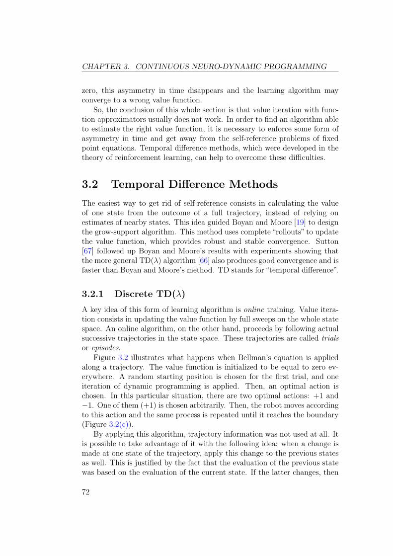
CHAPTER 3. CONTINUOUS NEURO-DYNAMIC PROGRAMMING
zero, this asymmetry in time disappears and the learning algorithm mayconverge to a wrong value function.
So, the conclusion of this whole section is that value iteration with func-tion approximators usually does not work. In order to find an algorithm ableto estimate the right value function, it is necessary to enforce some form ofasymmetry in time and get away from the self-reference problems of fixedpoint equations. Temporal difference methods, which were developed in thetheory of reinforcement learning, can help to overcome these difficulties.
3.2 Temporal Difference Methods
The easiest way to get rid of self-reference consists in calculating the valueof one state from the outcome of a full trajectory, instead of relying onestimates of nearby states. This idea guided Boyan and Moore [19] to designthe grow-support algorithm. This method uses complete “rollouts” to updatethe value function, which provides robust and stable convergence. Sutton[67] followed up Boyan and Moore’s results with experiments showing thatthe more general TD(λ) algorithm [66] also produces good convergence and isfaster than Boyan and Moore’s method. TD stands for “temporal difference”.
3.2.1 Discrete TD(λ)
A key idea of this form of learning algorithm is online training. Value itera-tion consists in updating the value function by full sweeps on the whole statespace. An online algorithm, on the other hand, proceeds by following actualsuccessive trajectories in the state space. These trajectories are called trialsor episodes.
Figure 3.2 illustrates what happens when Bellman’s equation is appliedalong a trajectory. The value function is initialized to be equal to zero ev-erywhere. A random starting position is chosen for the first trial, and oneiteration of dynamic programming is applied. Then, an optimal action ischosen. In this particular situation, there are two optimal actions: +1 and−1. One of them (+1) is chosen arbitrarily. Then, the robot moves accordingto this action and the same process is repeated until it reaches the boundary(Figure 3.2(c)).
By applying this algorithm, trajectory information was not used at all. Itis possible to take advantage of it with the following idea: when a change ismade at one state of the trajectory, apply this change to the previous statesas well. This is justified by the fact that the evaluation of the previous statewas based on the evaluation of the current state. If the latter changes, then
72
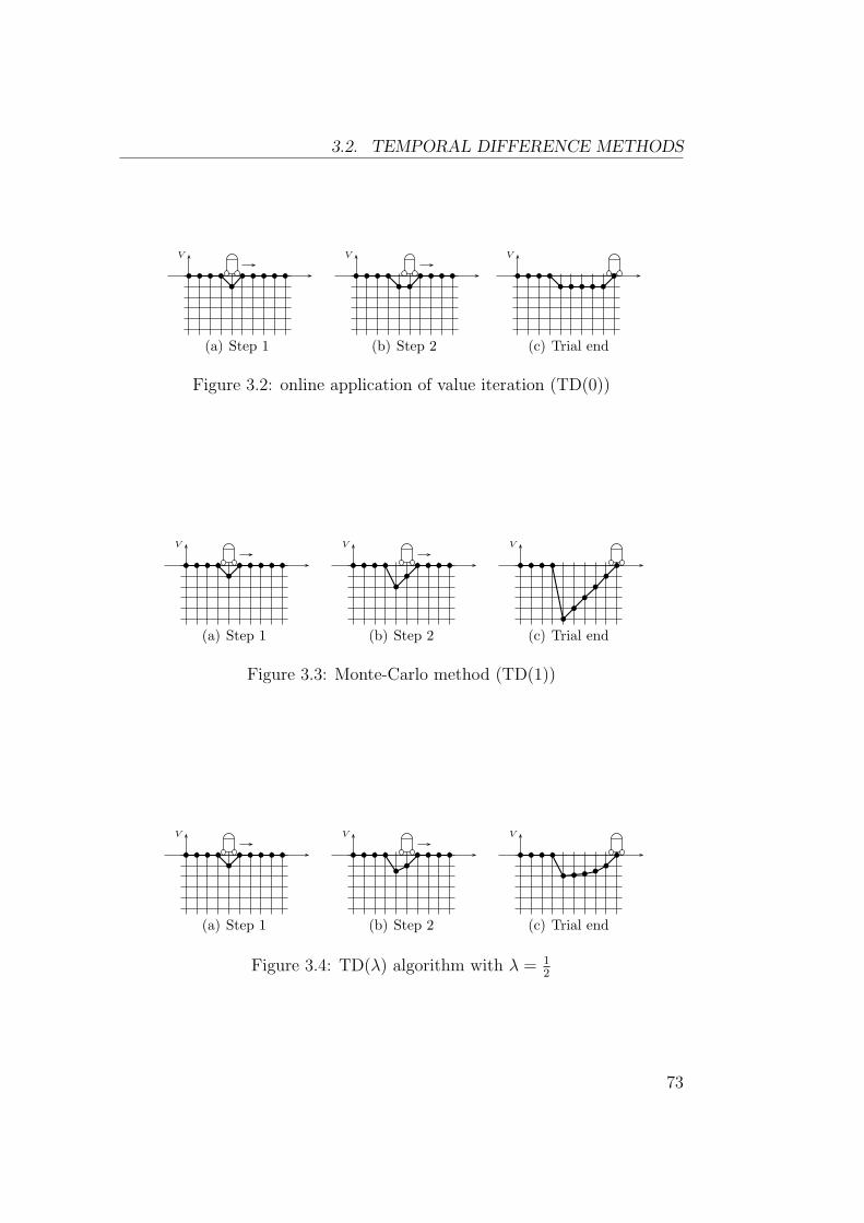
3.2. TEMPORAL DIFFERENCE METHODS
V
b b b b
b
b b b b b
(a) Step 1
V
b b b b
b b
b b b b
(b) Step 2
V
b b b b
b b b b b
b
(c) Trial end
Figure 3.2: online application of value iteration (TD(0))
V
b b b b
b
b b b b b
(a) Step 1
V
b b b b
b
b
b b b b
(b) Step 2
V
b b b b
b
b
b
b
b
b
(c) Trial end
Figure 3.3: Monte-Carlo method (TD(1))
V
b b b b
b
b b b b b
(a) Step 1
V
b b b b
bb
b b b b
(b) Step 2
V
b b b b
b b b bb
b
(c) Trial end
Figure 3.4: TD(λ) algorithm with λ = 12
73
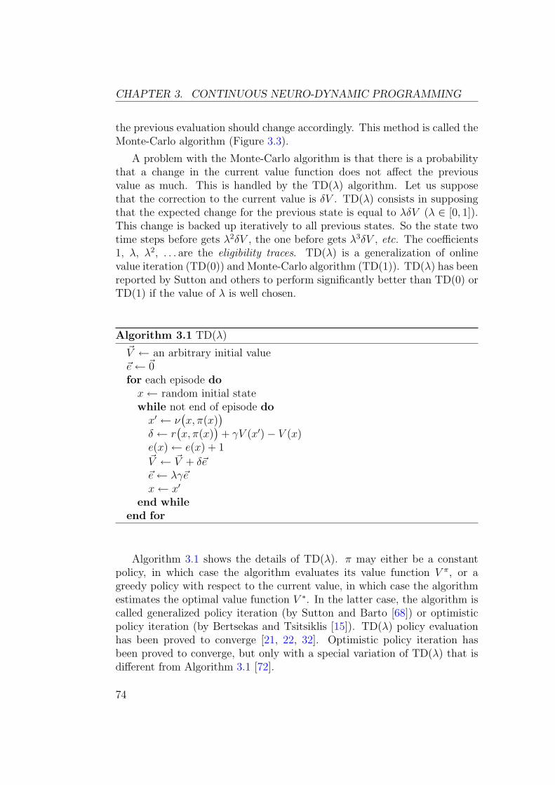
CHAPTER 3. CONTINUOUS NEURO-DYNAMIC PROGRAMMING
the previous evaluation should change accordingly. This method is called theMonte-Carlo algorithm (Figure 3.3).
A problem with the Monte-Carlo algorithm is that there is a probabilitythat a change in the current value function does not affect the previousvalue as much. This is handled by the TD(λ) algorithm. Let us supposethat the correction to the current value is δV . TD(λ) consists in supposingthat the expected change for the previous state is equal to λδV (λ ∈ [0, 1]).This change is backed up iteratively to all previous states. So the state twotime steps before gets λ2δV , the one before gets λ3δV , etc. The coefficients1, λ, λ2, . . . are the eligibility traces. TD(λ) is a generalization of onlinevalue iteration (TD(0)) and Monte-Carlo algorithm (TD(1)). TD(λ) has beenreported by Sutton and others to perform significantly better than TD(0) orTD(1) if the value of λ is well chosen.
Algorithm 3.1 TD(λ)
~V ← an arbitrary initial value~e← ~0for each episode do
x← random initial statewhile not end of episode do
x′ ← ν(x, π(x)
)
δ ← r(x, π(x)
)+ γV (x′)− V (x)
e(x)← e(x) + 1~V ← ~V + δ~e~e← λγ~ex← x′
end whileend for
Algorithm 3.1 shows the details of TD(λ). π may either be a constantpolicy, in which case the algorithm evaluates its value function V π, or agreedy policy with respect to the current value, in which case the algorithmestimates the optimal value function V ∗. In the latter case, the algorithm iscalled generalized policy iteration (by Sutton and Barto [68]) or optimisticpolicy iteration (by Bertsekas and Tsitsiklis [15]). TD(λ) policy evaluationhas been proved to converge [21, 22, 32]. Optimistic policy iteration hasbeen proved to converge, but only with a special variation of TD(λ) that isdifferent from Algorithm 3.1 [72].
74
3.2. TEMPORAL DIFFERENCE METHODS
3.2.2 TD(λ) with Function Approximators
In order to use function approximators, value updates can be replaced byweight updates in the direction of the value gradient. This is similar to whathas been presented in Section 3.1.1. Algorithm 3.2 shows the details of thisalgorithm. Notice that, if a table-lookup approximation is used with η = 1,it is identical to Algorithm 3.1
Convergence properties of this algorithm are not very well known. Thestrongest theoretical result, obtained by Tsitsiklis and Van Roy [74], provesthat discrete policy evaluation with linear function approximators convergeswhen learning is performed along trajectories with TD(λ). They also provedthat the error on the value function is bounded by
E ≤ 1− λγ
1− γE∗,
where E∗ is the optimal quadratic error that could be obtained with thesame function approximator. This indicates that, the more λ is close to 1,the more accurate the approximation.
Convergence of algorithms that compute the optimal value function hasnot been established. Tsitsiklis and Van Roy also gave an example wherepolicy evaluation with a non-linear function approximator diverges. Nev-ertheless, although it has little theoretical guarantees, this technique oftenworks well in practice.
Algorithm 3.2 Discrete-time TD(λ) with function approximation
~w ← an arbitrary initial value~e← ~0 {dimension of ~e = dimension of ~w}for each episode do
x← random initial statewhile not end of episode do
x′ ← ν(x, π(x)
)
δ ← r(x, π(x)
)+ γV~w(x′)− V~w(x)
~e← λγ~e + ∂V~w(x)/∂ ~w~w ← ~w + ηδ~ex← x′
end whileend for
75
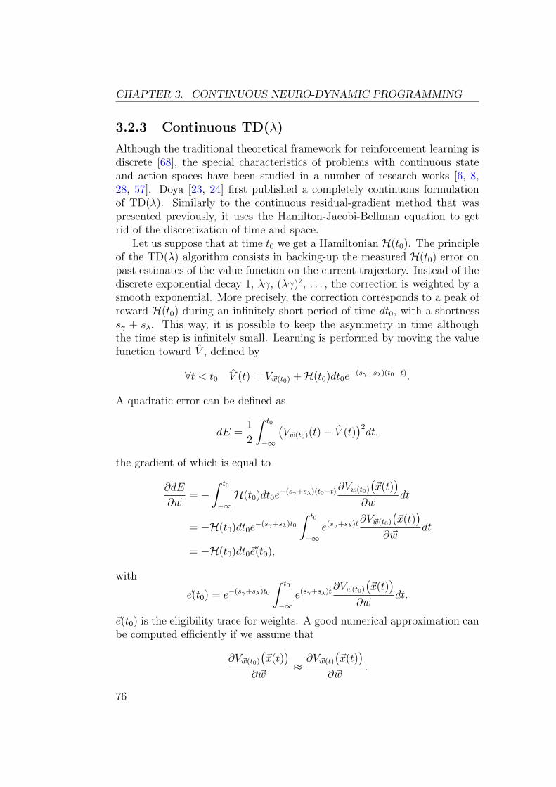
CHAPTER 3. CONTINUOUS NEURO-DYNAMIC PROGRAMMING
3.2.3 Continuous TD(λ)
Although the traditional theoretical framework for reinforcement learning isdiscrete [68], the special characteristics of problems with continuous stateand action spaces have been studied in a number of research works [6, 8,28, 57]. Doya [23, 24] first published a completely continuous formulationof TD(λ). Similarly to the continuous residual-gradient method that waspresented previously, it uses the Hamilton-Jacobi-Bellman equation to getrid of the discretization of time and space.
Let us suppose that at time t0 we get a Hamiltonian H(t0). The principleof the TD(λ) algorithm consists in backing-up the measured H(t0) error onpast estimates of the value function on the current trajectory. Instead of thediscrete exponential decay 1, λγ, (λγ)2, . . . , the correction is weighted by asmooth exponential. More precisely, the correction corresponds to a peak ofreward H(t0) during an infinitely short period of time dt0, with a shortnesssγ + sλ. This way, it is possible to keep the asymmetry in time althoughthe time step is infinitely small. Learning is performed by moving the valuefunction toward V , defined by
∀t < t0 V (t) = V~w(t0) +H(t0)dt0e−(sγ+sλ)(t0−t).
A quadratic error can be defined as
dE =1
2
∫ t0
−∞
(V~w(t0)(t)− V (t)
)2dt,
the gradient of which is equal to
∂dE
∂ ~w= −
∫ t0
−∞
H(t0)dt0e−(sγ+sλ)(t0−t)∂V~w(t0)
(~x(t)
)
∂ ~wdt
= −H(t0)dt0e−(sγ+sλ)t0
∫ t0
−∞
e(sγ+sλ)t ∂V~w(t0)
(~x(t)
)
∂ ~wdt
= −H(t0)dt0~e(t0),
with
~e(t0) = e−(sγ+sλ)t0
∫ t0
−∞
e(sγ+sλ)t ∂V~w(t0)
(~x(t)
)
∂ ~wdt.
~e(t0) is the eligibility trace for weights. A good numerical approximation canbe computed efficiently if we assume that
∂V~w(t0)
(~x(t)
)
∂ ~w≈ ∂V~w(t)
(~x(t)
)
∂ ~w.
76
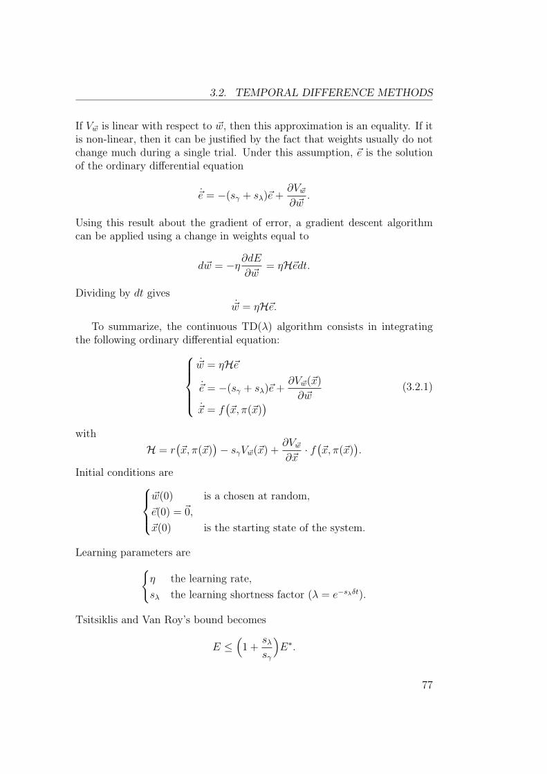
3.2. TEMPORAL DIFFERENCE METHODS
If V~w is linear with respect to ~w, then this approximation is an equality. If itis non-linear, then it can be justified by the fact that weights usually do notchange much during a single trial. Under this assumption, ~e is the solutionof the ordinary differential equation
~e = −(sγ + sλ)~e +∂V~w
∂ ~w.
Using this result about the gradient of error, a gradient descent algorithmcan be applied using a change in weights equal to
d~w = −η∂dE
∂ ~w= ηH~edt.
Dividing by dt gives~w = ηH~e.
To summarize, the continuous TD(λ) algorithm consists in integratingthe following ordinary differential equation:
~w = ηH~e
~e = −(sγ + sλ)~e +∂V~w(~x)
∂ ~w
~x = f(~x, π(~x)
)
(3.2.1)
with
H = r(~x, π(~x)
)− sγV~w(~x) +
∂V~w
∂~x· f(~x, π(~x)
).
Initial conditions are
~w(0) is a chosen at random,
~e(0) = ~0,
~x(0) is the starting state of the system.
Learning parameters are
{
η the learning rate,
sλ the learning shortness factor (λ = e−sλδt).
Tsitsiklis and Van Roy’s bound becomes
E ≤(
1 +sλ
sγ
)
E∗.
77
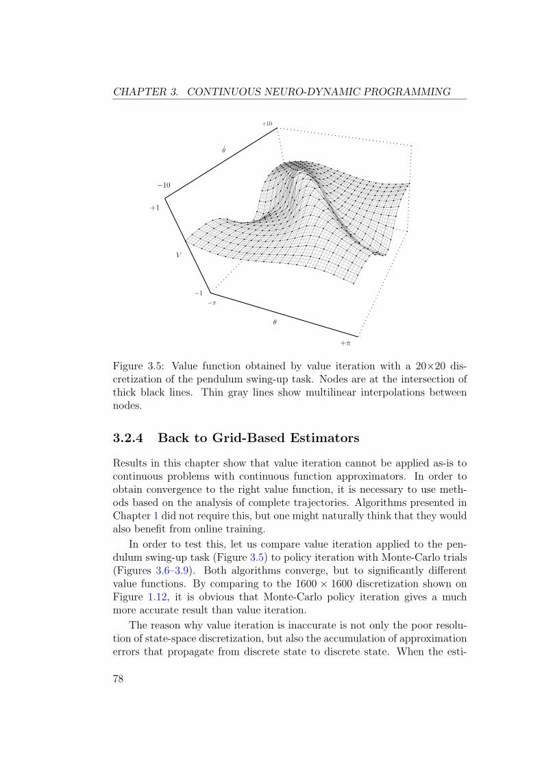
CHAPTER 3. CONTINUOUS NEURO-DYNAMIC PROGRAMMING
V
+1
−1
θ
−π
+π
θ
+10
−10
b
b
b
b
bb
bb b b b b b b
bb
b
b
b
b
b
b
b
b
b
bb
bb b b b b b b b
bb
b
b
b
b
b
b
b
b
bb
b b b b b b b b b b
b
b
b
b
b
b
b
b
b
bb
b b b b b bb
b bb
b
b
b
b
b
b
b
b
bb
b b b b bb
b
b
b b
b
b
b
b
b
b
b
b
bb
bb b b b
b
b
b
bb
b
b
b
b
b
b
b
bb
bb b b b b
b
b
b
b
b b
b
b
b
b
b
b
b
b b b b bb
b
b
b
bb
b
b
b
b
bb
bb
b
b
b
b
bb
b
b
b
b
b
b b
bb
b
b
b
b
b
b b
b
b
b
b
b
b
b
b
b
b
b
b
b
b
b
bb
b
b
b
b
b
b
b
b
bb
b
b
b
b
b
b
b b
b
b
b
b
b
b
b
b
b
b
bb
b
b
b
b
b
bb
b
b
b
b
b
b
b
b
b
b
b
b
b bb
b
b
b
bb
b
b
b
b
b
b
b
b
bb
bb b
bb
b
b
b
bb
b
b
b
b
b
b
b
b
bb
b b b b
bb
bb
bb b
b
b
b
b
b
b
b
bb
b b b bb
bb
bb
b bb
b
b
b
b
b
b
bb
bb b b b
b
bb
bb b b
b
b
b
b
b
b
b
bb
bb b b b
b
bb
b b bb
b
b
b
b
b
b
bb
bb b b b b b
b b b b bb
bb
bb
bb
bb
bb b b b b b
Figure 3.5: Value function obtained by value iteration with a 20×20 dis-cretization of the pendulum swing-up task. Nodes are at the intersection ofthick black lines. Thin gray lines show multilinear interpolations betweennodes.
3.2.4 Back to Grid-Based Estimators
Results in this chapter show that value iteration cannot be applied as-is tocontinuous problems with continuous function approximators. In order toobtain convergence to the right value function, it is necessary to use meth-ods based on the analysis of complete trajectories. Algorithms presented inChapter 1 did not require this, but one might naturally think that they wouldalso benefit from online training.
In order to test this, let us compare value iteration applied to the pen-dulum swing-up task (Figure 3.5) to policy iteration with Monte-Carlo trials(Figures 3.6–3.9). Both algorithms converge, but to significantly differentvalue functions. By comparing to the 1600 × 1600 discretization shown onFigure 1.12, it is obvious that Monte-Carlo policy iteration gives a muchmore accurate result than value iteration.
The reason why value iteration is inaccurate is not only the poor resolu-tion of state-space discretization, but also the accumulation of approximationerrors that propagate from discrete state to discrete state. When the esti-
78
3.2. TEMPORAL DIFFERENCE METHODS
V
+1
−1
θ
−π
+π
θ
+10
−10
b
b
b
b
bb
bb b b b b b
bb
b
b
b
b
b
b
b
b
b
b
bb
bb b b b b b b
bb
b
b
b
b
b
b
b
b
b
bb
b b b b b b b bb
b
b
b
b
b
b
b
b
b
bb
bb b b b b b b b
bb
b
b
b
b
b
b
b
b
bb
b b b b b b b b b bb
b
b
b
b
b
b
b
b
bb
b b b b b b b b b b bb
b
b
b
b
b
b
b
bb b b b b
bb
bb
b b b b
b
b b
bb b b b
bb
bb
b
bb
b b
b
bb b b
bb
b
b
b
b
b
b b
b
b b bb
b
b
b
b
b
b
b
b bb
b
b
b
b
b
b
b b
b bb
b
b
b
b
b
b
b
b
b
bb
bb
bb
b
b
b
b
b
b
b
b
b
b
b
b
b bb
b bb
b
b
b
b
b
b
b
b
b
b
b
b
bb
b b
b
bb
b
b
b
b
b
b
b
b
b
b
b
b
b
bb
b b b
bb
b
b
b
b
b
b
b
b
b
b
b
b
b
bb
b b b
b
b
b
b
b
b
b
b
b
b
b
b
b
b
bb
b bb
b
b
b
b
bb
bb
b
b
b
b
b
bb b b
b
b
bb
b b b bb
b
b
b b
b
b
b
bb b
b
bb
b
b
b
b b b
Figure 3.6: Value function obtained after the first step of policy iteration.The initial policy was π0(~x) = −umax.
V
+1
−1
θ
−π
+π
θ
+10
−10
b
b
b
b
b
bb
bb
b b b bb
bb
b
b
b
b
b
b
b
b
b
b
bb
b bb b b b b b
b
b
bb
b
b
b
b
bb
b
bb b b b b b b b
b
bb
b
b
b
b
b
b
b b
b
b b b b b
b
b
b
b
b
b
b
b
b
b
b
b b b
b
b
b b b
b
b
b
b
b
b
b
b
b
bb
b b
b bb
b
b
b
b
b
b
b
b
b
b
bb b
bb b b
bb
bb
b
b
b
b b b b bb
bb
b
b
bb
b b bb
b
b
b b
b
b
b b
b bb
b
b
b
b
b
b b
bb
b
b b
b
b
b
b
b
b
bb
b
b
bb
b
b
b
b
b
b
b
b
b
b
b
b
b
b
b
b
b
bb b
b
b
b
b
b
bb
b
b
b
b
b
b
bb
bb
b b bb b
b b
b
b
b
bb b
b
b
b
b
bb
bb
b b b
b
bb
b
b
b b
b
b
b
b
bb
bb b
b bb
b
bb
b
b
b
b
b
b
bb
b b b b
bb
b
b
bb
bb
bb b b
bb
b bb
b
bb
bb
b b b bb b b
b bb
bb
bb
bb
b bb b b b b b
Figure 3.7: Second step of policy iteration
79
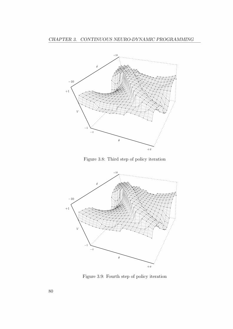
CHAPTER 3. CONTINUOUS NEURO-DYNAMIC PROGRAMMING
V
+1
−1
θ
−π
+π
θ
+10
−10
b
b
b
b
b
bb
bb
b b b b
b
bb
b
b
b
b
b
b
b
b
b
b
b
bb
b b
bb
bb
b
bb b
b
b
b
b
b
b
b
bb
bb b b b b b
b
bb
b
b
b
b
b
b
b
b
b
bb
b b b b b bb
b
b
b
b
b
b
b
b
b
bb
bb
b b b b b b
b
b
b
b
b
b
b
b
b
bb
bb b b b b b
b
b
b
b
b
b
b
b
b
bb
b b b b b b bb
b
b
b
b
b
b
b
b b b b bb
b
bb
b
b
b
b
b
bb
bb
b
bb
b
b
bb
bb
b bb
b
b
b
b
b
b
b b b
b
b
bb
b
b
b
b
bb b b
b
b
b
b b
b
b
b
b
b bb
b
b
bb
bb
b
b
b
b
bb
b
b
b
b
b
bb
b
b
b
bb
b
b
b
b
b
b
b b bb
b b
bb
b
b
b
b
bb
b
b
b
b
bb
bb b
b b b
b
b
b
b
b
bb
b
b
bb
bb
b b
b bb
bb
bb
b
b
bb
b
b bb
bb
bb
b b b bb
b
b
b
b
b
b bb
bb
bb
bb
b bb b b
b
b
b
bb
bb b b b
bb
b b b
b
bb
bb
Figure 3.8: Third step of policy iteration
V
+1
−1
θ
−π
+π
θ
+10
−10
b
b
b
b
b
bb
bb
b bb b
b
b
b
b
b
b
b
b
b
b
b
b
b
b
b
bb b
b
bb
bb
b
b
b b
b
b
b
b
b
b
b
bb
bb b b b b b
bb b
b
b
b
b
b
b
b
b
b
bb
bb b b b b b
b
b
b
b
b
b
b
b
b
b
bb
bb b b b b b
b
b
b
b
b
b
b
b
b
bb
bb b b b b b
b
b
b
b
b
b
b
b
b
bb
b b b b b b bb
b
b
b
b
b
b
b
b b b b bb
b
bb
b
b
b
b
b
bb
bb
b
bb
b
b
bb
bb
b bb
b
b
b
b
b
b
b
bb
b
b
b
b
b
b
b
b
b
b
b
b
b
b bb
b
b
b
b
b
b
b
b
b
b b
b
b
b
b
b b b
b
b
b
b
b
b
b
b
b
b
b
bb
b
b
b
bb b
b
b
b
b
b
b
bb
bb
b
bb
b
b
b
bb b
b
b
b
b
bb
bb
b b b b
bb
b
b
bb
b
b
b
b
b
bb
bb
b b b bb
bb
b
bb
b
b
bb
b
bb
bb
b b b bb
b
bb
bb
bb
bb
bb
bb
b b b b bb
b
bb
b bb
bb
b
bb b b b
bb
b b b b
bb
Figure 3.9: Fourth step of policy iteration
80
3.3. SUMMARY
mation of the value function is based on the outcome of long trajectories, amuch more accurate result is obtained.
3.3 Summary
This chapter shows that combining function approximators with dynamicprogramming produces a lot of complexity, notably in the analysis of con-vergence properties of learning algorithms. Among all the possible learningmethods, those that have the best stability and accuracy are algorithms thatlearn over trajectories. Training along trajectories is necessary to keep asym-metry in time and get a more accurate estimation of the value function.
Another important result presented in this chapter is Doya’s continuousTD(λ). Thanks to a completely continuous formulation of this reinforcementlearning algorithm, it is possible to get rid of time and space discretizations,and of inaccuracies related to this approximation. The next chapter presentssome optimizations and refinements of the basic algorithm offered by thislate discretization.
81

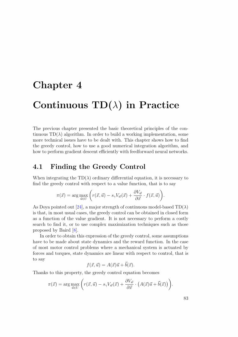
Chapter 4
Continuous TD(λ) in Practice
The previous chapter presented the basic theoretical principles of the con-tinuous TD(λ) algorithm. In order to build a working implementation, somemore technical issues have to be dealt with. This chapter shows how to findthe greedy control, how to use a good numerical integration algorithm, andhow to perform gradient descent efficiently with feedforward neural networks.
4.1 Finding the Greedy Control
When integrating the TD(λ) ordinary differential equation, it is necessary tofind the greedy control with respect to a value function, that is to say
π(~x) = arg max~u∈U
(
r(~x, ~u)− sγV~w(~x) +∂V~w
∂~x· f(~x, ~u)
)
.
As Doya pointed out [24], a major strength of continuous model-based TD(λ)is that, in most usual cases, the greedy control can be obtained in closed formas a function of the value gradient. It is not necessary to perform a costlysearch to find it, or to use complex maximization techniques such as thoseproposed by Baird [8].
In order to obtain this expression of the greedy control, some assumptionshave to be made about state dynamics and the reward function. In the caseof most motor control problems where a mechanical system is actuated byforces and torques, state dynamics are linear with respect to control, that isto say
f(~x, ~u) = A(~x)~u +~b(~x).
Thanks to this property, the greedy control equation becomes
π(~x) = arg max~u∈U
(
r(~x, ~u)− sγV~w(~x) +∂V~w
∂~x·(A(~x)~u +~b(~x)
))
.
83
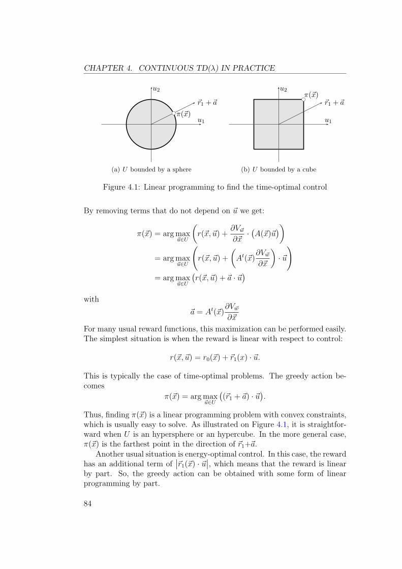
CHAPTER 4. CONTINUOUS TD(λ) IN PRACTICE
u1
u2
~r1 + ~abc π(~x)
(a) U bounded by a sphere
u1
u2
~r1 + ~abcπ(~x)
(b) U bounded by a cube
Figure 4.1: Linear programming to find the time-optimal control
By removing terms that do not depend on ~u we get:
π(~x) = arg max~u∈U
(
r(~x, ~u) +∂V~w
∂~x·(A(~x)~u
))
= arg max~u∈U
(
r(~x, ~u) +
(
At(~x)∂V~w
∂~x
)
· ~u)
= arg max~u∈U
(r(~x, ~u) + ~a · ~u
)
with
~a = At(~x)∂V~w
∂~x
For many usual reward functions, this maximization can be performed easily.The simplest situation is when the reward is linear with respect to control:
r(~x, ~u) = r0(~x) + ~r1(x) · ~u.
This is typically the case of time-optimal problems. The greedy action be-comes
π(~x) = arg max~u∈U
((~r1 + ~a) · ~u
).
Thus, finding π(~x) is a linear programming problem with convex constraints,which is usually easy to solve. As illustrated on Figure 4.1, it is straightfor-ward when U is an hypersphere or an hypercube. In the more general case,π(~x) is the farthest point in the direction of ~r1+~a.
Another usual situation is energy-optimal control. In this case, the rewardhas an additional term of
∣∣~r1(~x) · ~u
∣∣, which means that the reward is linear
by part. So, the greedy action can be obtained with some form of linearprogramming by part.
84
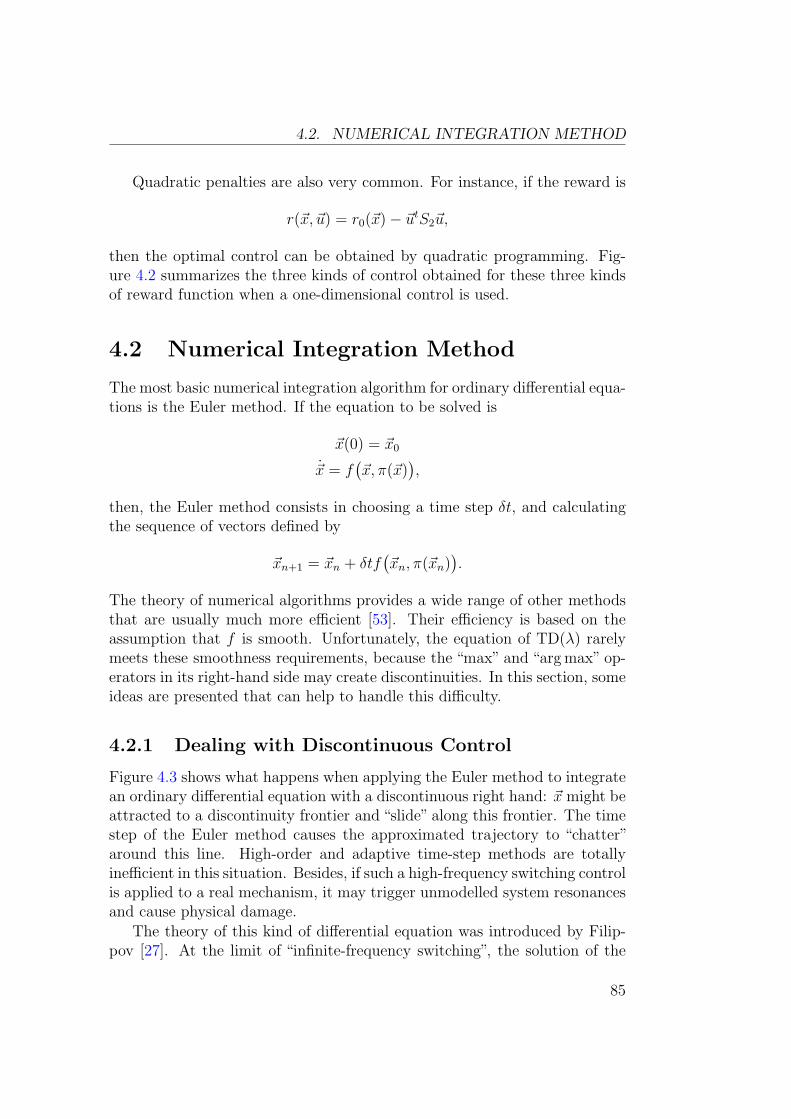
4.2. NUMERICAL INTEGRATION METHOD
Quadratic penalties are also very common. For instance, if the reward is
r(~x, ~u) = r0(~x)− ~utS2~u,
then the optimal control can be obtained by quadratic programming. Fig-ure 4.2 summarizes the three kinds of control obtained for these three kindsof reward function when a one-dimensional control is used.
4.2 Numerical Integration Method
The most basic numerical integration algorithm for ordinary differential equa-tions is the Euler method. If the equation to be solved is
~x(0) = ~x0
~x = f(~x, π(~x)
),
then, the Euler method consists in choosing a time step δt, and calculatingthe sequence of vectors defined by
~xn+1 = ~xn + δtf(~xn, π(~xn)
).
The theory of numerical algorithms provides a wide range of other methodsthat are usually much more efficient [53]. Their efficiency is based on theassumption that f is smooth. Unfortunately, the equation of TD(λ) rarelymeets these smoothness requirements, because the “max” and “arg max” op-erators in its right-hand side may create discontinuities. In this section, someideas are presented that can help to handle this difficulty.
4.2.1 Dealing with Discontinuous Control
Figure 4.3 shows what happens when applying the Euler method to integratean ordinary differential equation with a discontinuous right hand: ~x might beattracted to a discontinuity frontier and “slide” along this frontier. The timestep of the Euler method causes the approximated trajectory to “chatter”around this line. High-order and adaptive time-step methods are totallyinefficient in this situation. Besides, if such a high-frequency switching controlis applied to a real mechanism, it may trigger unmodelled system resonancesand cause physical damage.
The theory of this kind of differential equation was introduced by Filip-pov [27]. At the limit of “infinite-frequency switching”, the solution of the
85
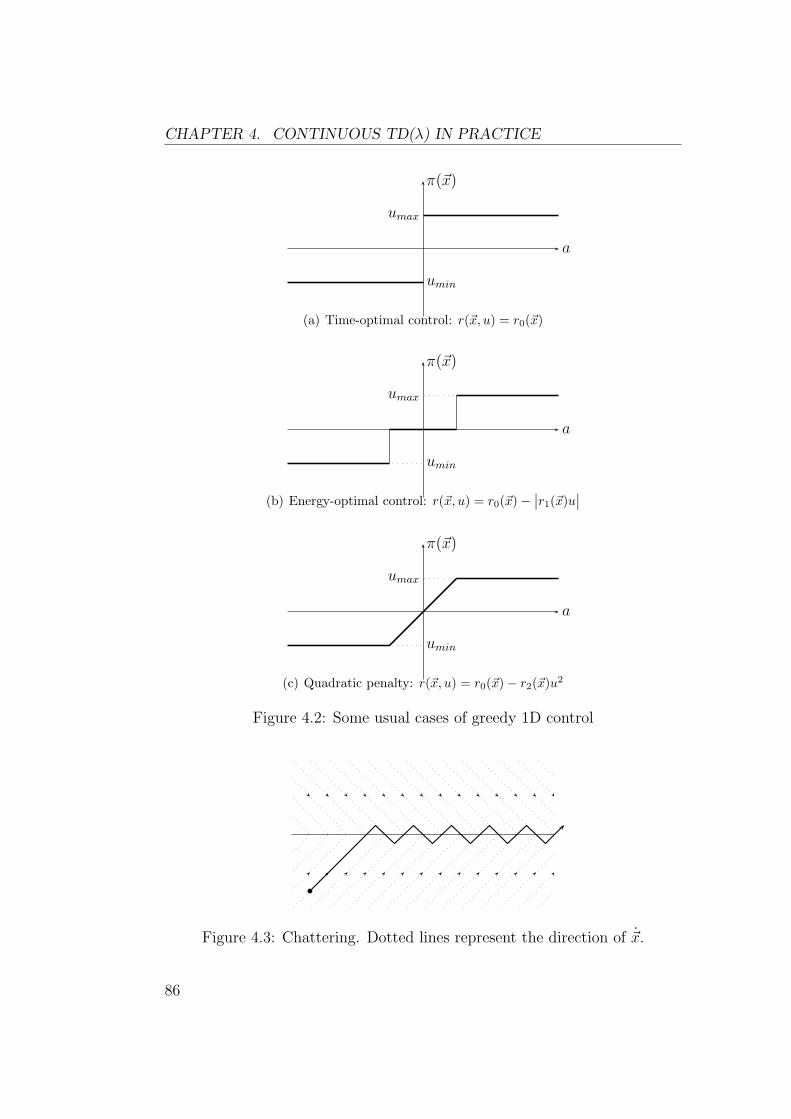
CHAPTER 4. CONTINUOUS TD(λ) IN PRACTICE
π(~x)
a
umax
umin
(a) Time-optimal control: r(~x, u) = r0(~x)
π(~x)
a
umax
umin
(b) Energy-optimal control: r(~x, u) = r0(~x)−∣∣r1(~x)u
∣∣
π(~x)
a
umax
umin
(c) Quadratic penalty: r(~x, u) = r0(~x)− r2(~x)u2
Figure 4.2: Some usual cases of greedy 1D control
Figure 4.3: Chattering. Dotted lines represent the direction of ~x.
86
4.2. NUMERICAL INTEGRATION METHOD
differential equation is defined as smoothly following the frontier, at a veloc-ity that is a weighted average of velocities on both sides. This velocity iscalled the Filippov velocity.
A usual method to integrate such a differential equation consists in re-placing the discontinuous step in the control by a stiff (but continuous) ap-proximation [76]. Doya used this method in his continuous TD(λ) exper-iments [24], replacing steps by sigmoids, thus allowing more advanced nu-merical integration methods to be applied. More precisely, he replaced theoptimal “bang-bang” control law
u = umax sign(∂f
∂u· ∂V
∂~x
)
by
u = umax tanh(
10× ∂f
∂u· ∂V
∂~x
)
in the pendulum swing-up task. The smooth control obtained is plotted onFigure 4.5(b).
The control law obtained by this smoothing clearly removes all chattering,but it is also less efficient than the bang-bang control. In particular, it is muchslower to get out of the bottom position. This is because this position is aminimum of the value function, so it is close to a switching boundary ofthe discontinuous optimal control and the sigmoid gives a low value to thecontrol, whereas it should be constant and maximal. Smoothing the controlworks very well near the upright balance position, because the system isreally in sliding mode there, but it works very poorly in the bottom position,because it is a discontinuity that does not attract the system.
Instead of performing such a spatial low-pass filter on the control law,it would make more sense to apply a temporal low-pass filter. Actually,the Filippov velocity can be obtained by using a temporal low-pass filter onthe velocity. So, since the system dynamics are linear with respect to thecontrol, the Filippov velocity corresponds to applying an equivalent Filippovcontrol ~uF , obtained by low-pass filtering the bang-bang control in time. Forinstance, this could be done by integrating
~uF =1
τ(~u∗ − ~uF ).
Unfortunately, this kind of filtering technique does not help the numericalintegration process at all, since it does not eliminate discontinuous variables.Applying a temporal low-pass filter on the bang-bang control only helps whena real device has to be controlled (this is the principle of Emelyanov et al.’s[25] “higher-order sliding modes”).
87
CHAPTER 4. CONTINUOUS TD(λ) IN PRACTICE
Temporal low-pass filtering does not help to perform the numerical inte-gration, but there is yet another possible approach. It consists in finding thecontrol that is optimal for the whole interval of length δt. Instead of
~u∗ = arg max~u∈U
(
r(~x, ~u)− sγV~w(~x) +∂V~w
∂~x· f(~x, ~u)
)
,
which is optimal when infinitely small time steps are taken, the Filippovcontrol can be estimated by
~uF = arg max~u∈U
V(~x(t + δt)
).
~uF cannot be obtained in closed form as a function of the value gradient,so it is usually more difficult to evaluate than ~u∗. Nevertheless, when thedimension of the control space is 1, it can be estimated at virtually no costby combining the value-gradient information obtained at ~xn with the valueobtained at ~xn+1 to build a second-order approximation of the value function.Figure 4.4 and Algorithm 4.1 illustrate this technique. Figure 4.5(c) showsthe result obtained on the pendulum task. It still has a few discontinuitiesat switching points, but not in sliding mode.
Unfortunately, it is hard to generalize this approach to control spaces thathave more than one dimension. It is all the more unfortunate as the system ismuch more likely to be in sliding mode when the dimension of the control ishigh (experiments with swimmers in Chapter 7 show that they are in slidingmode almost all the time.) It might be worth trying to estimate ~uF , anyway,but we did not explore this idea further. The key problem is that buildingand using a second order approximation of the value function is much moredifficult when the dimension is higher. So we are still stuck with the Eulermethod in this case.
4.2.2 Integrating Variables Separately
The TD(λ) differential equation defines the variations of different kinds ofvariables: the state ~x, eligibility traces ~e and weights ~w. All these vari-ables have different kinds of dynamics, and different kinds of accuracy re-quirements, so it might be a good idea to use different kinds of integrationalgorithms for each of them.
A first possibility is to split the state into position ~p and velocity ~v.Mechanical systems are usually under a “cascade” form because they areactually second order differential equations:
{
~p = ~v
~v = fv(~x,~v, ~u).
88
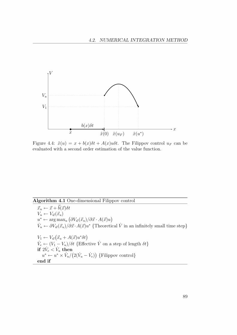
4.2. NUMERICAL INTEGRATION METHOD
x
V
b(x)δt
x x(0)
Vu
V1
x(u∗)x(uF )
b
b
Figure 4.4: x(u) = x + b(x)δt + A(x)uδt. The Filippov control uF can beevaluated with a second order estimation of the value function.
Algorithm 4.1 One-dimensional Filippov control
~xu ← ~x +~b(~x)δtVu ← V~w(~xu)u∗ ← arg maxu
(∂V~w(~xu)/∂~x · A(~x)u
)
Vu ← ∂V~w(~xu)/∂~x ·A(~x)u∗ {Theoretical V in an infinitely small time step}
V1 ← V~w
(~xu + A(~x)u∗δt
)
Ve ← (V1 − Vu)/δt {Effective V on a step of length δt}if 2Ve < Vu then
u∗ ← u∗ × Vu/(2(Vu − Ve)
){Filippov control}
end if
89
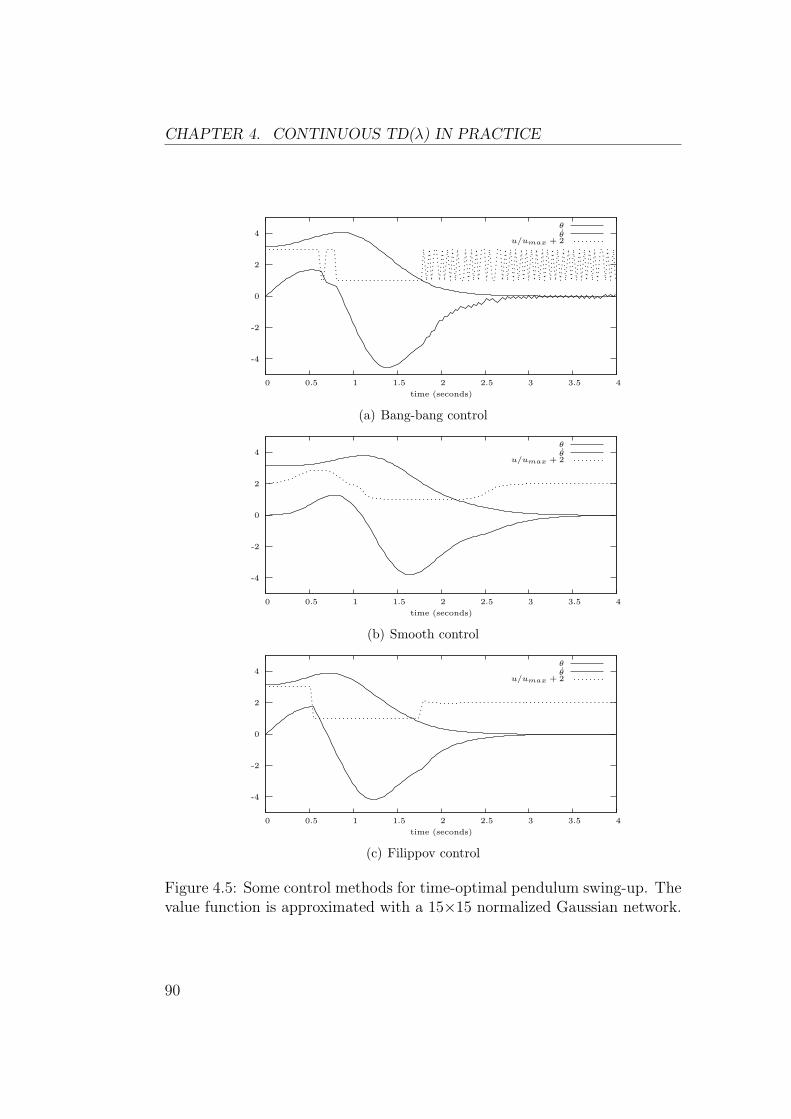
CHAPTER 4. CONTINUOUS TD(λ) IN PRACTICE
-4
-2
0
2
4
0 0.5 1 1.5 2 2.5 3 3.5 4
time (seconds)
θθ
u/umax + 2
(a) Bang-bang control
-4
-2
0
2
4
0 0.5 1 1.5 2 2.5 3 3.5 4
time (seconds)
θθ
u/umax + 2
(b) Smooth control
-4
-2
0
2
4
0 0.5 1 1.5 2 2.5 3 3.5 4
time (seconds)
θθ
u/umax + 2
(c) Filippov control
Figure 4.5: Some control methods for time-optimal pendulum swing-up. Thevalue function is approximated with a 15×15 normalized Gaussian network.
90
4.2. NUMERICAL INTEGRATION METHOD
It is possible to take advantage of this in the numerical integration algorithm,by cascading it too. For instance, this can be done by using a first orderintegration for ~v and a second order integration for ~p (algorithm 4.2).
Algorithm 4.2 Integration with Split Position and Velocity
while End of trial not reached do
~vi+1 ← ~vi + ~viδt
~pi+1 ← ~pi + 12(~vi + ~vi+1)δt {Second order integration}
~ei+1 ← ~ei + ~eiδt
~wi+1 ← ~wi + ηHi~eiδt
i← i + 1
end while
When system dynamics are stiff, that is to say there can be very short andvery high accelerations (this is typically the case of swimmers of Chapter 7),the Euler method can be unstable and requires short time steps. In this case,it might be a good idea to separate the integration of eligibility traces andweights from the integration of state dynamics, using a shorter time step forthe latter.
4.2.3 State Discontinuities
We have considered continuous and differentiable state dynamics so far.Many interesting real problems, however, have discrete deterministic discon-tinuities. A typical example is the case of a mechanical shock that causes adiscontinuity in the velocity. Another typical case will be met in Section 6.3:the distance to the obstacle ahead for a robot in a complex environment mayhave discontinuities when the heading direction varies continuously.
In these discontinuous cases, the main problem is that the Hamiltoniancannot be computed with the gradient of the value function. It can be eval-uated using an approximation over a complete interval:
H = r − sγV + V
≈ r − sγV (t + δt) + V (t)
2+
V (t + δt)− V (t)
δt.
This incurs some cost, mainly because the value function needs to becomputed at each value of ~x for two values of ~w. But this cost is usually morethan compensated by the fact that it might not be necessary to compute the
91
CHAPTER 4. CONTINUOUS TD(λ) IN PRACTICE
full gradient ∂V/∂~x in order to get the optimal control1. Changes to thenumerical method are given in algorithm 4.3.
Algorithm 4.3 Integration with accurate Hamiltonian
while End of trial not reached do
~vi+1 ← ~vi + ~viδt {or a discontinuous jump}~pi+1 ← ~pi + 1
2(~vi + ~vi+1)δt {or a discontinuous jump}
~ei+1 ← ~ei + ~eiδt
V1 ← V~wi(~xi+1)
V0 ← V~wi(~xi)
H ← r(~xi)− sγ(V1 + V0)/2 + (V1 − V0)/δt
~wi+1 ← ~wi + ηH~eiδt
i← i + 1
end while
Practice demonstrated that algorithm 4.3 is better than algorithm 4.2 notonly because it runs trials in less CPU time and can handle state disconti-nuities, but also because it is much more stable and accurate. Experimentsshowed that with a feedforward neural network as function approximator,algorithm 4.2 completely blows up on the cart-pole task (cf. Appendix B)as soon as it starts to be able to maintain the pole in an upright position,whereas algorithm 4.3 works nicely. Figure 4.6 shows what happens at sta-tionary points and why the discrete estimation of the Hamiltonian is better.
4.2.4 Summary
Integrating the continuous TD(λ) algorithm efficiently is very tricky, in par-ticular because the right-hand side of the equation is discontinuous, and thesystem is often in sliding mode. A few ideas to deal with this have beenpresented in this section, but we are still not very far from the lowly Eu-ler method. Using second order information about the value function worksvery well with a one-dimensional control, and generalizing this idea to higherdimensions seems a promising research direction.
1In fact, it is possible to completely remove this cost by not updating weights duringan episode. Weight changes can be accumulated in a separate variable, and incorporatedat the end of the episode.
92
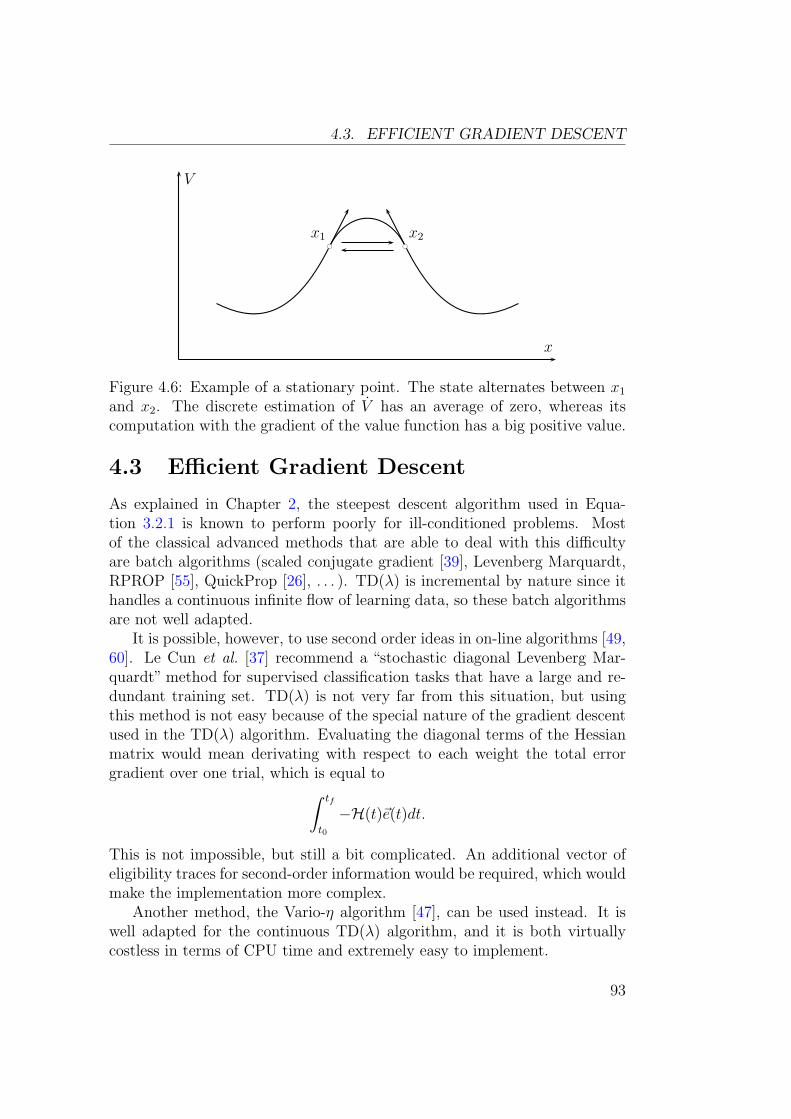
4.3. EFFICIENT GRADIENT DESCENT
V
x
bc bc
x1 x2
Figure 4.6: Example of a stationary point. The state alternates between x1
and x2. The discrete estimation of V has an average of zero, whereas itscomputation with the gradient of the value function has a big positive value.
4.3 Efficient Gradient Descent
As explained in Chapter 2, the steepest descent algorithm used in Equa-tion 3.2.1 is known to perform poorly for ill-conditioned problems. Mostof the classical advanced methods that are able to deal with this difficultyare batch algorithms (scaled conjugate gradient [39], Levenberg Marquardt,RPROP [55], QuickProp [26], . . . ). TD(λ) is incremental by nature since ithandles a continuous infinite flow of learning data, so these batch algorithmsare not well adapted.
It is possible, however, to use second order ideas in on-line algorithms [49,60]. Le Cun et al. [37] recommend a “stochastic diagonal Levenberg Mar-quardt” method for supervised classification tasks that have a large and re-dundant training set. TD(λ) is not very far from this situation, but usingthis method is not easy because of the special nature of the gradient descentused in the TD(λ) algorithm. Evaluating the diagonal terms of the Hessianmatrix would mean derivating with respect to each weight the total errorgradient over one trial, which is equal to
∫ tf
t0
−H(t)~e(t)dt.
This is not impossible, but still a bit complicated. An additional vector ofeligibility traces for second-order information would be required, which wouldmake the implementation more complex.
Another method, the Vario-η algorithm [47], can be used instead. It iswell adapted for the continuous TD(λ) algorithm, and it is both virtuallycostless in terms of CPU time and extremely easy to implement.
93
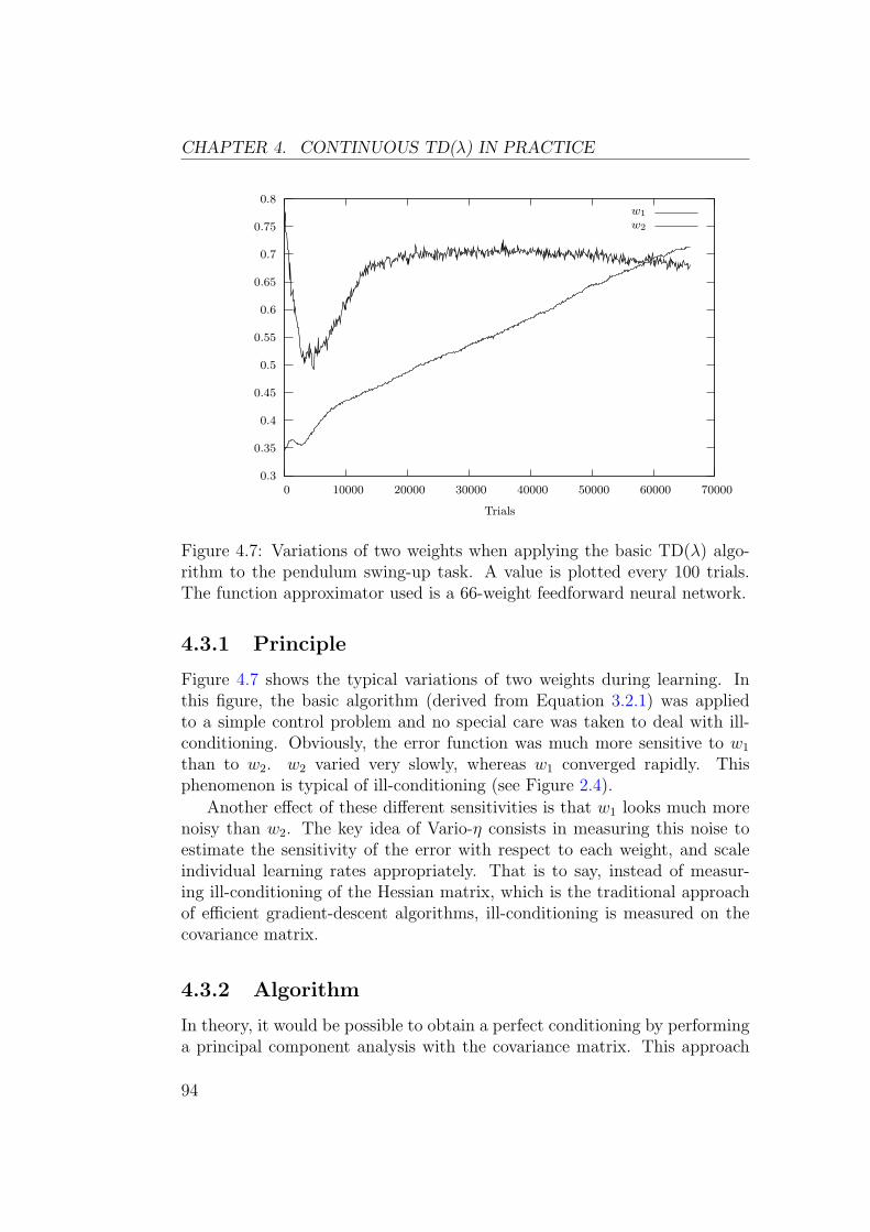
CHAPTER 4. CONTINUOUS TD(λ) IN PRACTICE
0.3
0.35
0.4
0.45
0.5
0.55
0.6
0.65
0.7
0.75
0.8
0 10000 20000 30000 40000 50000 60000 70000
Trials
w1
w2
Figure 4.7: Variations of two weights when applying the basic TD(λ) algo-rithm to the pendulum swing-up task. A value is plotted every 100 trials.The function approximator used is a 66-weight feedforward neural network.
4.3.1 Principle
Figure 4.7 shows the typical variations of two weights during learning. Inthis figure, the basic algorithm (derived from Equation 3.2.1) was appliedto a simple control problem and no special care was taken to deal with ill-conditioning. Obviously, the error function was much more sensitive to w1
than to w2. w2 varied very slowly, whereas w1 converged rapidly. Thisphenomenon is typical of ill-conditioning (see Figure 2.4).
Another effect of these different sensitivities is that w1 looks much morenoisy than w2. The key idea of Vario-η consists in measuring this noise toestimate the sensitivity of the error with respect to each weight, and scaleindividual learning rates appropriately. That is to say, instead of measur-ing ill-conditioning of the Hessian matrix, which is the traditional approachof efficient gradient-descent algorithms, ill-conditioning is measured on thecovariance matrix.
4.3.2 Algorithm
In theory, it would be possible to obtain a perfect conditioning by performinga principal component analysis with the covariance matrix. This approach
94
4.3. EFFICIENT GRADIENT DESCENT
is not practical because of its computational cost, so a simple analysis of thediagonal is performed:
vi(k + 1) = (1− β)vi(k) + β
(wi(k + 1)− wi(k)
ηi(k)
)2
,
ηi(k) =η
√
vi(k) + ε.
k is the trial number. vi(0) is a large enough value. β is the variance decaycoefficient. A typical choice is 1/100. ε is a small constant to prevent divisionby zero. ηi(k) is the learning rate for weight wi. This formula assumes thatthe standard deviation of the gradient is large in comparison to its mean,which was shown to be true empirically in experiments.
4.3.3 Results
Experiments were run with fully-connected feedforward networks, with a lin-ear output unit, and sigmoid internal units. Observations during reinforce-ment learning indicated that the variances of weights on connections to thelinear output unit were usually n times larger than those on internal con-nections, n being the total number of neurons. The variances of internalconnections are all of the same order of magnitude. This means that goodconditioning can be simply obtained by scaling the learning rate of the out-put unit by 1/
√n. This allows to use a global learning rate that is
√n times
larger and provides a speed-up of about√
n. The biggest networks used inexperiments had 60 neurons, so this is a very significant acceleration.
4.3.4 Comparison with Second-Order Methods
An advantage of this method is that it does not rely on the assumptionthat the error surface can be approximated by a positive quadratic form. Inparticular, dealing with negative curvatures is a problem for many second-order methods. There is no such problem when measuring the variance.
It is worth noting, however, that the Gauss-Newton approximation ofthe Hessian suggested by Le Cun et al. is always positive. Besides, thisapproximation is formally very close to the variance of the gradient (I thankYann Le Cun for pointing this out to me): the Gauss-Newton approximationof the second order derivative of the error with respect to one weight is
∂2E
∂w2ij
≈ ∂2E
∂a2i
y2j
95
CHAPTER 4. CONTINUOUS TD(λ) IN PRACTICE
(with notations of Appendix A). This is very close to
( ∂E
∂wij
)2
=(∂E
∂ai
)2
y2j .
A major difference between the two approaches is that there is a risk thatthe variance goes to zero as weights approach their optimal value, whereas theestimate of the second order derivative of the error would stay positive. Thatis to say, the learning rate increases as the gradient of the error decreases,which may be a cause of instability, especially if the error becomes zero.This was not a problem at all in the reinforcement learning experiments thatwere run, because the variance actually increased during learning, and neverbecame close to zero.
4.3.5 Summary
The main advantage of using gradient variance is that, in the case of rein-forcement learning problems, it is simpler to implement than an estimationof second order information and still provides very significant speedups. Inorder to find out whether it is more efficient, it would be necessary to runmore experimental comparisons.
96

Part II
Experiments
97

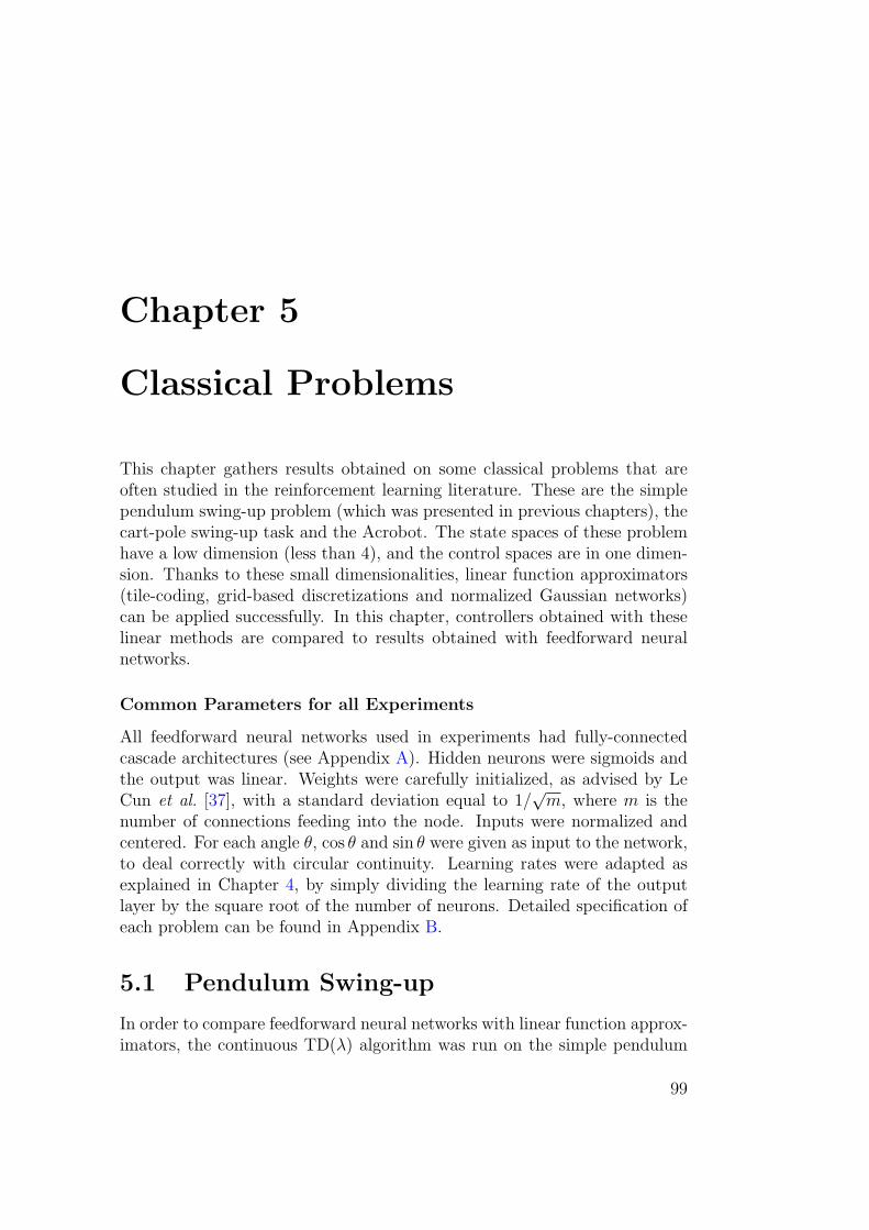
Chapter 5
Classical Problems
This chapter gathers results obtained on some classical problems that areoften studied in the reinforcement learning literature. These are the simplependulum swing-up problem (which was presented in previous chapters), thecart-pole swing-up task and the Acrobot. The state spaces of these problemhave a low dimension (less than 4), and the control spaces are in one dimen-sion. Thanks to these small dimensionalities, linear function approximators(tile-coding, grid-based discretizations and normalized Gaussian networks)can be applied successfully. In this chapter, controllers obtained with theselinear methods are compared to results obtained with feedforward neuralnetworks.
Common Parameters for all Experiments
All feedforward neural networks used in experiments had fully-connectedcascade architectures (see Appendix A). Hidden neurons were sigmoids andthe output was linear. Weights were carefully initialized, as advised by LeCun et al. [37], with a standard deviation equal to 1/
√m, where m is the
number of connections feeding into the node. Inputs were normalized andcentered. For each angle θ, cos θ and sin θ were given as input to the network,to deal correctly with circular continuity. Learning rates were adapted asexplained in Chapter 4, by simply dividing the learning rate of the outputlayer by the square root of the number of neurons. Detailed specification ofeach problem can be found in Appendix B.
5.1 Pendulum Swing-up
In order to compare feedforward neural networks with linear function approx-imators, the continuous TD(λ) algorithm was run on the simple pendulum
99
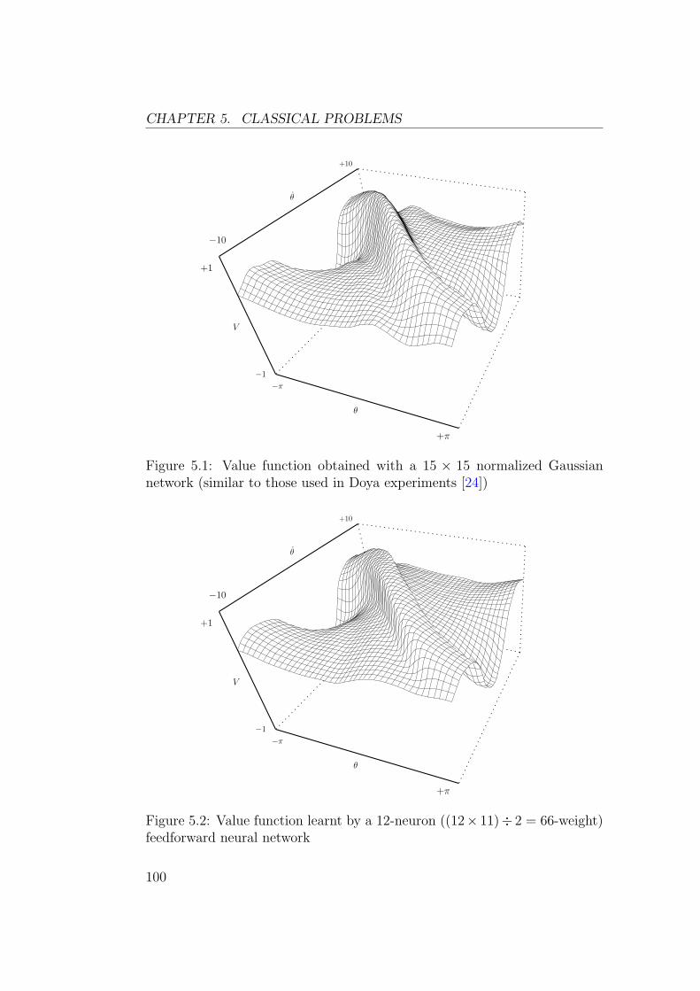
CHAPTER 5. CLASSICAL PROBLEMS
V
+1
−1
θ
−π
+π
θ
+10
−10
Figure 5.1: Value function obtained with a 15 × 15 normalized Gaussiannetwork (similar to those used in Doya experiments [24])
V
+1
−1
θ
−π
+π
θ
+10
−10
Figure 5.2: Value function learnt by a 12-neuron ((12× 11)÷ 2 = 66-weight)feedforward neural network
100
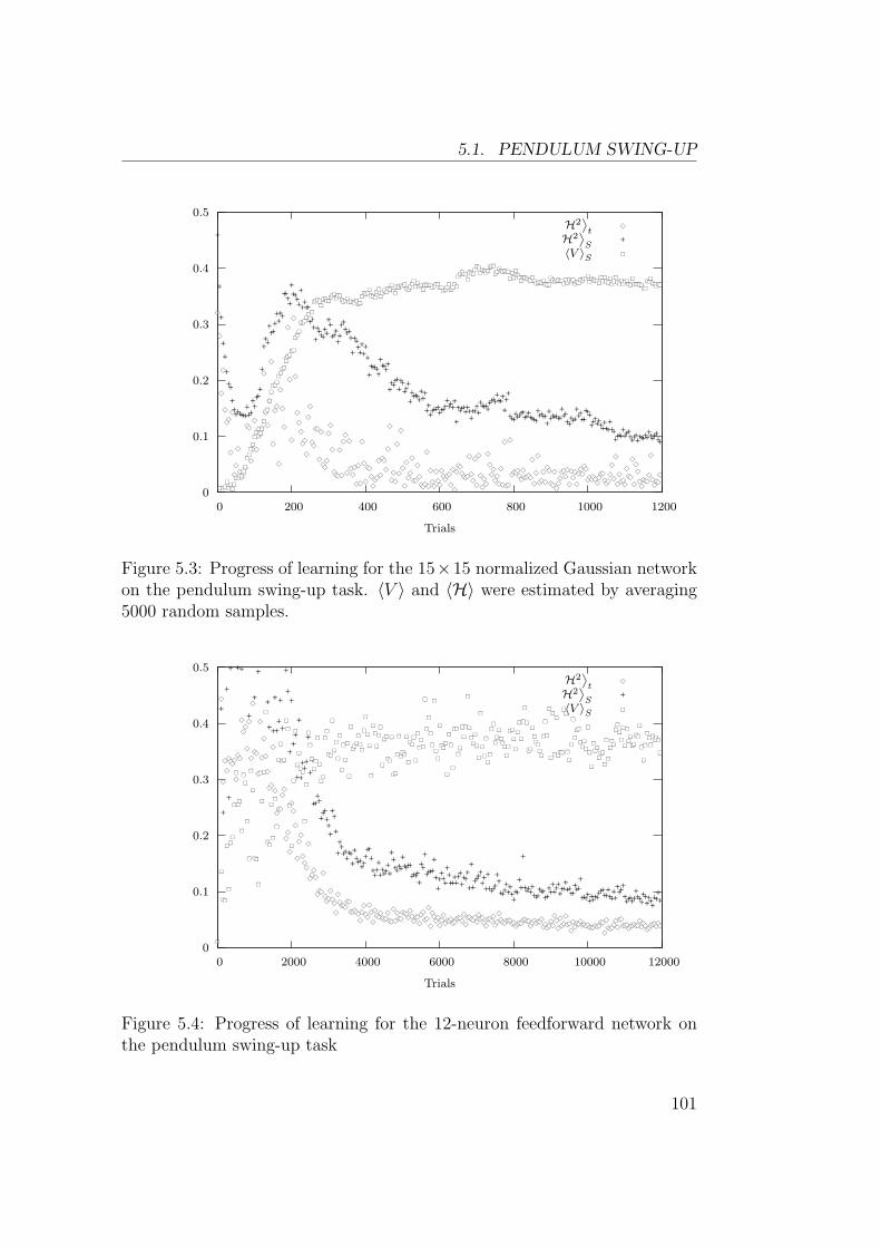
5.1. PENDULUM SWING-UP
0
0.1
0.2
0.3
0.4
0.5
0 200 400 600 800 1000 1200
Trials
˙
H2¸
t
rs
rs
rs
rs
rs
rs rs
rs
rs
rs
rs
rs
rsrsrsrs
rs rs
rs
rs
rs
rs
rsrsrs
rs
rs
rs
rs
rs
rs
rsrs
rs
rs
rs
rs
rs
rs
rs
rs
rs
rs
rs
rs
rs
rs rs
rs
rs
rs
rsrs
rs rs
rs
rs
rs rsrs
rs
rs
rs
rs rs rs
rs
rs
rsrs
rs
rs
rsrsrs
rs
rs
rs
rs
rs
rs
rs rs
rs
rsrs rs
rs
rs
rs rs
rs
rs
rs
rsrs
rs
rs
rs
rs
rs
rs
rs
rsrs
rs
rs rs
rs
rs
rs rs rs
rs
rs
rs
rsrs
rs
rsrs
rsrs rsrs rs
rs
rs
rs
rsrs rsrs rs rs rs
rs
rsrs
rs
rs
rs
rs
rs
rsrs
rs
rs
rsrs
rsrsrs
rs
rs
rs
rs rs
rs
rs rs rsrsrsrs
rsrs rs rs rs
rs
rs
rs
rs
rs rs
rs
rs
rsrs
rs rs
rs
rsrsrsrs rsrsrs
rs
rsrsrs
rs
rsrsrsrs rs
rs rs rs rs rs rsrsrs rsrsrs rsrs
rs
rs
rs
rs
rsrs rs rs
rsrs rs
rs
rs
rsrs
rsrsrs rs rsrs
rs
rsrsrs rsrs
rs˙
H2¸
S+
+
+
++
+++
++++++++
++++++++
+
+++
++++++++
++++
+++++
+
++++
++++++++
++
+++++++++++++
+
++++++++
++++++
++++
+
++++
+++++++
++++++
+++
++++++++++
+++++
+
+
++++++++++++
+++++++++
++++
+++
+++++++++++++++
+++++++++++++
++++++++
+++++
++++++++++
++++++++++
++++++++++++
+++++++++
+
〈V 〉S
rs rs rsrsrsrsrsrsrs rs rs rsrsrs
rs rsrsrsrsrsrs rsrsrs
rs rs
rs
rsrs rsrsrs rsrs rsrsrs rsrs rs
rs rsrs
rs rs rsrs rs rsrs
rs rs rs rsrsrs rs rs rsrs rs rs rs rs rs rs rs rs rs rs rs rs rs rs rs rs
rs rs rsrs rs rs rs rs
rs rsrsrs rs rsrs rsrsrs rsrs rs rs rs rs rs rs rs
rs rs rsrs rs rsrsrs rs rs rs rs rs rs
rsrs rsrs rsrsrsrs rsrs rs
rs rsrs rs rsrsrs rs rsrsrs rsrsrs rs rs rsrs rs rsrs rsrs rs rs rs rs rs
rsrsrsrsrs rs rsrs rs rs rs rs
rsrs rs rs rs rs rs rs rs rs
rs rs rs rs rs rs rs rsrs rs rs rs rs rs rs rs
rs rs rs rsrsrsrs rs rs rs rs
rsrsrsrs rsrsrs rsrsrs rs rs rs rs rs rs rs
rsrs rs rs rs rs rs rs
rs rsrsrs rs rs rs rs
rs
Figure 5.3: Progress of learning for the 15×15 normalized Gaussian networkon the pendulum swing-up task. 〈V 〉 and 〈H〉 were estimated by averaging5000 random samples.
0
0.1
0.2
0.3
0.4
0.5
0 2000 4000 6000 8000 10000 12000
Trials
˙
H2¸
trs
rs
rs
rs
rs rs rsrs
rs
rs rs
rs
rsrs
rs
rs
rs
rs
rs rs
rs
rs
rs
rs
rs
rs
rs rs
rs
rs
rsrs rs
rsrs
rsrs
rs
rs
rs
rs
rs
rsrs
rsrsrs
rs
rsrsrsrs
rsrs rs
rs
rsrs rs
rs
rsrs
rs
rs
rsrs rs rsrs rs
rs rs rs rs rsrs
rsrs
rs rs
rsrs
rs
rsrs rsrsrs rs rsrs
rs rs
rs
rs
rsrs rsrs rs rsrsrsrsrsrs rsrs
rs rs
rs rs
rs
rs
rsrsrs rsrsrsrs
rs rs rsrsrs rsrs rs rs rsrs
rsrs rs rs rs rs rs
rsrs rsrs rsrs rs rsrs
rs rs
rsrs rs rs rs rs rs rs rs rs rs rs rs
rs rs rs rsrs rsrs rs rs rsrs
rs rs rs rsrsrs
rsrsrs
rsrs rs
rs
rs rsrs
rsrsrs rs rs rs rs rs rs rs rs rs rs rs rs
rs rs
rs
rs
rs rs rsrsrsrsrs rsrs rs rs rs rs rs
rs rs rsrsrsrs rsrs rsrs rs rs rsrs rs
rs˙
H2¸
S+
+
+
+
+ ++
+
+
+
+
++
+
++
+
+
+
+
+
+
++
+
+
+
+++
+
++
++++
++++++
++
+
++++++
+++++++++
+++++++
+++++
++
++++++
+++++
+++++
+++
+++++
++++++
++++++++++++
+
+
++++
++++
+
+++++++++
+++++
++++
+
++++++++
++++++++++++++
+++++
++++
++++++++++++++
+++++++++++++++
++++
++++++
++++
+
〈V 〉S
rs
rs
rs rs
rs
rs
rsrs
rs
rs
rsrs
rs
rs
rs
rs
rs
rs
rs
rs rs
rs
rs
rs
rs
rs
rs rs
rs
rs
rs
rs
rs
rs
rs rs
rs
rs
rs
rs
rs
rs
rs
rs
rs rs
rs
rs
rs
rs
rs
rs
rs
rs
rs
rsrs
rsrs
rs rs
rs
rs
rs
rs
rs
rs
rs
rs
rs
rs
rs
rs rsrsrs
rsrs
rs
rs
rs
rs
rs
rs
rs
rs
rs
rs
rs
rs rs
rs rs
rs
rs rs
rs
rs
rsrs rs
rs
rs
rs rsrs
rs
rs
rs
rsrs
rs
rs
rs
rs
rs
rs
rsrs
rs
rs rsrs
rs
rs
rs
rs
rs rs
rsrs
rs
rs
rs
rs
rs
rsrs
rs
rs
rs
rs
rs
rs
rs
rs
rs
rsrs
rsrsrs
rsrsrs
rs
rs
rs rs
rs
rs
rs
rs
rs
rs
rs
rs
rs rs
rs
rsrs rsrsrs
rs
rs
rs
rs
rs
rs
rs
rs
rsrs rs
rsrs
rs
rs
rs
rs
rs
rs rs
rsrsrsrs
rs
rs
rs
rsrs rs
rsrs rs
rs
rs
rs
rsrsrs
rsrs
rsrs
rs
rs
rs
rsrs
rs rs
rs rs
rs
rs
rs
rs
rsrsrs
rsrs rs rs
rs
rs
Figure 5.4: Progress of learning for the 12-neuron feedforward network onthe pendulum swing-up task
101
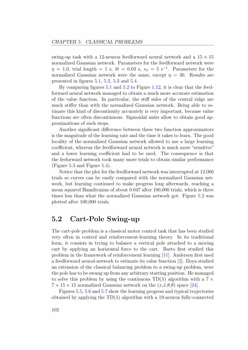
CHAPTER 5. CLASSICAL PROBLEMS
swing-up task with a 12-neuron feedforward neural network and a 15 × 15normalized Gaussian network. Parameters for the feedforward network wereη = 1.0, trial length = 1 s, δt = 0.03 s, sλ = 5 s−1. Parameters for thenormalized Gaussian network were the same, except η = 30. Results arepresented in figures 5.1, 5.2, 5.3 and 5.4.
By comparing figures 5.1 and 5.2 to Figure 1.12, it is clear that the feed-forward neural network managed to obtain a much more accurate estimationof the value function. In particular, the stiff sides of the central ridge aremuch stiffer than with the normalized Gaussian network. Being able to es-timate this kind of discontinuity accurately is very important, because valuefunctions are often discontinuous. Sigmoidal units allow to obtain good ap-proximations of such steps.
Another significant difference between these two function approximatorsis the magnitude of the learning rate and the time it takes to learn. The goodlocality of the normalized Gaussian network allowed to use a large learningcoefficient, whereas the feedforward neural network is much more “sensitive”and a lower learning coefficient had to be used. The consequence is thatthe feeforward network took many more trials to obtain similar performance(Figure 5.3 and Figure 5.4).
Notice that the plot for the feedforward network was interrupted at 12,000trials so curves can be easily compared with the normalized Gaussian net-work, but learning continued to make progress long afterwards, reaching amean squared Hamiltonian of about 0.047 after 100,000 trials, which is threetimes less than what the normalized Gaussian network got. Figure 5.2 wasplotted after 100,000 trials.
5.2 Cart-Pole Swing-up
The cart-pole problem is a classical motor control task that has been studiedvery often in control and reinforcement-learning theory. In its traditionalform, it consists in trying to balance a vertical pole attached to a movingcart by applying an horizontal force to the cart. Barto first studied thisproblem in the framework of reinforcement learning [11]. Anderson first useda feedforward neural-network to estimate its value function [2]. Doya studiedan extension of the classical balancing problem to a swing-up problem, werethe pole has to be swung up from any arbitrary starting position. He managedto solve this problem by using the continuous TD(λ) algorithm with a 7 ×7× 15× 15 normalized Gaussian network on the (x,x,θ,θ) space [24].
Figures 5.5, 5.6 and 5.7 show the learning progress and typical trajectoriesobtained by applying the TD(λ) algorithm with a 19-neuron fully-connected
102
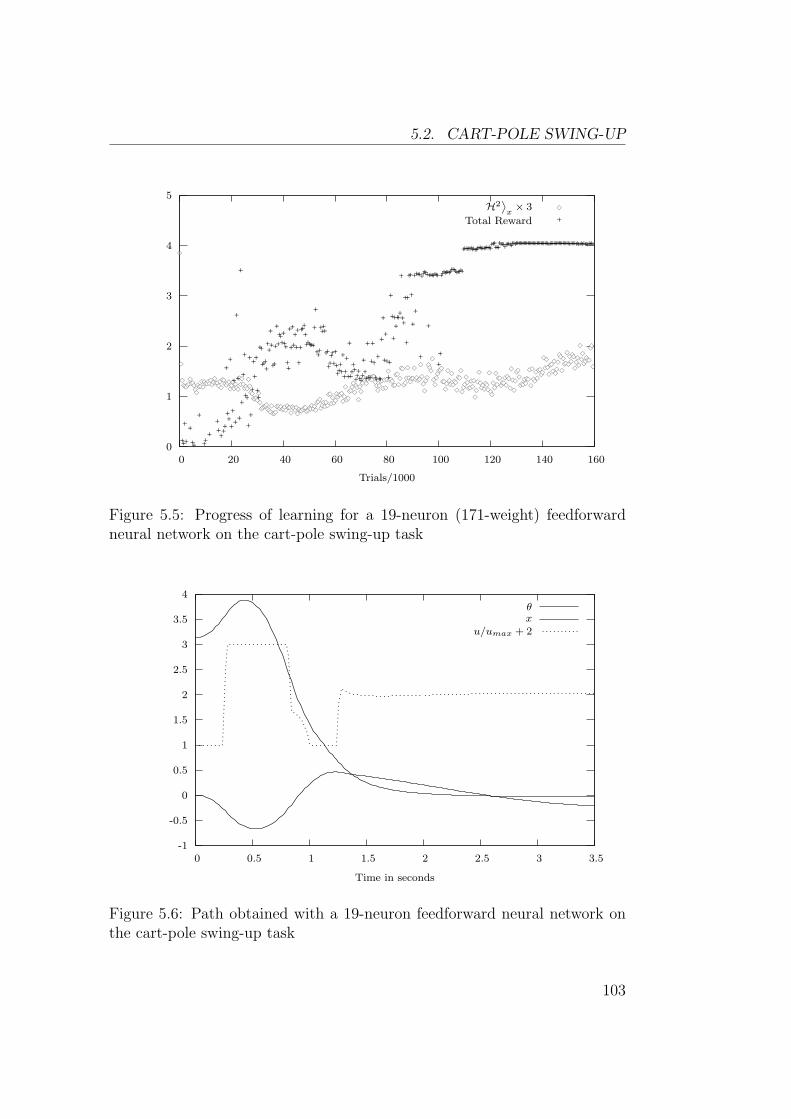
5.2. CART-POLE SWING-UP
0
1
2
3
4
5
0 20 40 60 80 100 120 140 160
Trials/1000
˙
H2¸
x× 3
rs
rs
rsrs rs rs rsrsrsrs rs rsrsrs
rs rs rsrsrsrs rs rs rs rsrsrs rsrsrs rsrsrsrs
rs rsrs rs rsrs
rsrsrsrsrsrs rs
rsrsrsrsrs rs rs
rsrsrs rsrs rs rs rsrs
rsrs rs rsrs rsrs rs rsrs
rs rs rsrs rs rs rs rs rs rs rs
rs rs rsrsrs rs rs rsrsrs rs rs rsrs rsrs rsrs rsrsrs rs rs
rs rsrs
rs rsrsrsrsrs
rs rs
rsrsrs rsrsrs rs rsrs
rsrs
rs
rs rsrs rsrsrs
rsrs rs
rs
rsrs
rsrs rsrsrs rs rs rsrs rsrsrsrsrsrs rs
rs
rs
rs
rs
rs
rs rs rsrs rs
rs rs
rsrs
rs rs
rs rsrs
rs
rsrsrs rs
rs
rs rs rs rs
rs
rs
rs
rs
rsrs
rsrsrs
rs
rsrsrsrsrs rs rs
rs rs
rsrs
rs
rsrs
rs
rsrs rs
rs
rs rs
rs
rsrsrs
rsrsrs rsrsrsrs
rsrs
rs
rs
rsrs rs rsrs rsrs
rs
rsrs
rsrs
rs
rsrs rs
rs rs rsrs
rs
rs rs
rs
rs
rs
rs
rs
rs rsrs
rs rs rsrsrsrs rs
rs
rs
rs
rs rs
rsrs
rs rsrs rs
rs
rs
rs
rsrs
rs rsrs
rs
rsrs
rs
rs rs
rs
rsrs rs
rs
rs
rsrsrs rs
rsrsrs
rs
rs
rsrs
rs rsrs rs rs
rs rs
rs
rs
Total Reward
++
+
+
+
++
+
+++
+++++
+
++
+
+
+
+
+
+
+
+
+
+
+
+
++
+
+
+
+
+
+
+
++
++
++++
++
+
+
++
+
+
+++++++
++
+
+
+
++
+
+
+
+
++++++++++
+
+
+++
++++
++
++++++
+++++
+
++
+
+
+
++++++++++
+++
+
++
+
+
+
++
+
++
+
+
+
+
+
+
+
+
+
+
+++++
+
++
+
+
+
++
+
+
+
+
+++
+
+++++
+
+++++++
++
+++++++++++++++++
+++++++++++++++++++++++++++++++++++++++++++++++++++++++++++++++++++++++++++++++++++++++++++++++++++++
+
Figure 5.5: Progress of learning for a 19-neuron (171-weight) feedforwardneural network on the cart-pole swing-up task
-1
-0.5
0
0.5
1
1.5
2
2.5
3
3.5
4
0 0.5 1 1.5 2 2.5 3 3.5
Time in seconds
θx
u/umax + 2
Figure 5.6: Path obtained with a 19-neuron feedforward neural network onthe cart-pole swing-up task
103
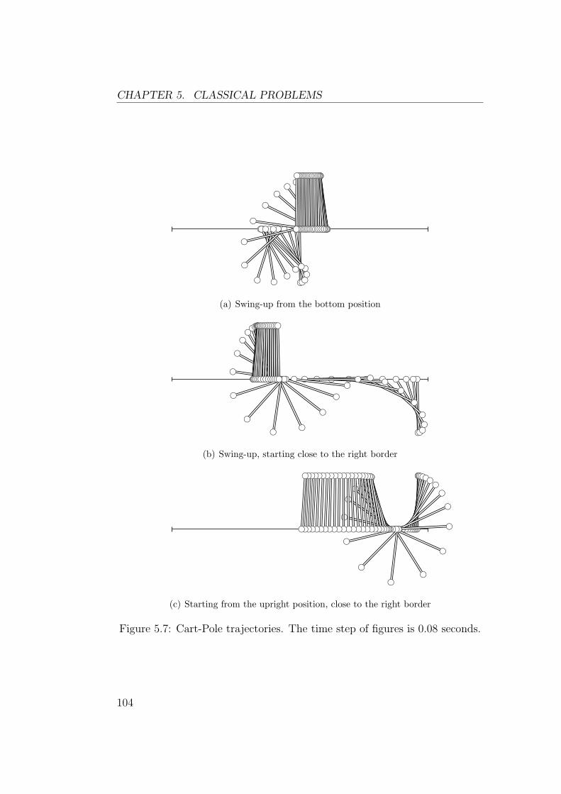
CHAPTER 5. CLASSICAL PROBLEMS
bc
bc
bc
bc
bc
bc
bc
bc
bc
bc
bc
bc
bc
bc
bc
bc
bc
bc
bc
bc
bc
bc
bc
bc
bcbc
bc
bc
bc
bc
bc
bc
bc
bc
bc
bc
bc
bc
bc
bc
bc
bc
bc
bc
bc
bc
bc
bc
bc
bc
bc
bc
bc
bc
bc
bc
bc
bc
bc
bc
bc
bc
bc
bc
bc
bc
bc
bc
bc
bc
bc
bc
bc
bc
bc
bc
bc
bc
bc
bc
bc
bc
bc
bc
bc
bc
bc
bc
(a) Swing-up from the bottom position
bc
bc
bc
bc
bc
bc
bc
bc
bc
bc
bc
bc
bcbc
bc bcbc bcbc bcbcbc
bc
bc
bc
bc
bc
bc
bc
bc
bc
bc
bc
bc
bcbc
bc
bc
bc
bc
bc
bc
bc
bc
bc
bc
bc
bc
bc
bc
bc
bc
bc
bc
bc
bc
bc
bc
bc
bc
bc
bc
bc
bc
bc
bc
bc
bc
bc
bc
bc
bc
bc
bc
bc
bc
bc
bc
bc
bc
bc
bc
bc
bc
bc
bc
bc
bc
(b) Swing-up, starting close to the right border
bc
bc
bc
bc
bc
bc
bc
bc
bc
bc
bc
bc
bc
bc
bc
bc
bc
bc
bc
bc
bc bcbc
bc
bc
bc
bc
bc
bc
bc
bc
bc
bc
bc
bc
bc
bc
bc
bc
bc
bc
bc
bc
bc
bc
bc
bc
bc
bc
bc
bc
bc
bc
bc
bc
bc
bc
bc
bc
bc
bc
bc
bc
bc
bc
bc
bc
bc
bc
bc
bc
bc
bc
bc
bc
bc
bc
bc
bc
bc
bc
bc
bc
bc
bc
bc
bc
bc
(c) Starting from the upright position, close to the right border
Figure 5.7: Cart-Pole trajectories. The time step of figures is 0.08 seconds.
104
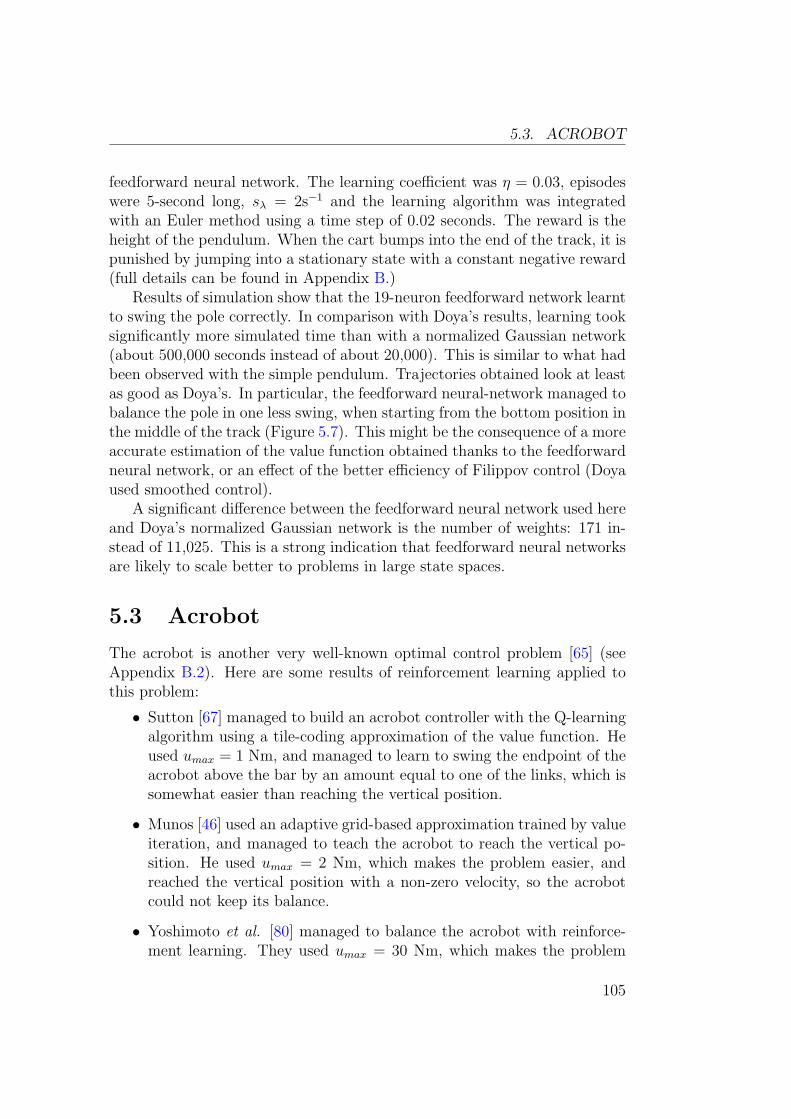
5.3. ACROBOT
feedforward neural network. The learning coefficient was η = 0.03, episodeswere 5-second long, sλ = 2s−1 and the learning algorithm was integratedwith an Euler method using a time step of 0.02 seconds. The reward is theheight of the pendulum. When the cart bumps into the end of the track, it ispunished by jumping into a stationary state with a constant negative reward(full details can be found in Appendix B.)
Results of simulation show that the 19-neuron feedforward network learntto swing the pole correctly. In comparison with Doya’s results, learning tooksignificantly more simulated time than with a normalized Gaussian network(about 500,000 seconds instead of about 20,000). This is similar to what hadbeen observed with the simple pendulum. Trajectories obtained look at leastas good as Doya’s. In particular, the feedforward neural-network managed tobalance the pole in one less swing, when starting from the bottom position inthe middle of the track (Figure 5.7). This might be the consequence of a moreaccurate estimation of the value function obtained thanks to the feedforwardneural network, or an effect of the better efficiency of Filippov control (Doyaused smoothed control).
A significant difference between the feedforward neural network used hereand Doya’s normalized Gaussian network is the number of weights: 171 in-stead of 11,025. This is a strong indication that feedforward neural networksare likely to scale better to problems in large state spaces.
5.3 Acrobot
The acrobot is another very well-known optimal control problem [65] (seeAppendix B.2). Here are some results of reinforcement learning applied tothis problem:
• Sutton [67] managed to build an acrobot controller with the Q-learningalgorithm using a tile-coding approximation of the value function. Heused umax = 1 Nm, and managed to learn to swing the endpoint of theacrobot above the bar by an amount equal to one of the links, which issomewhat easier than reaching the vertical position.
• Munos [46] used an adaptive grid-based approximation trained by valueiteration, and managed to teach the acrobot to reach the vertical po-sition. He used umax = 2 Nm, which makes the problem easier, andreached the vertical position with a non-zero velocity, so the acrobotcould not keep its balance.
• Yoshimoto et al. [80] managed to balance the acrobot with reinforce-ment learning. They used umax = 30 Nm, which makes the problem
105
CHAPTER 5. CLASSICAL PROBLEMS
much easier than with 1 Nm.
Boone [18, 17] probably obtained the best controllers, but the techniques heused are not really reinforcement learning (he did not build a value function)and are very specific to this kind of problem.
In our experiments, physical parameters were the same as those used byMunos (umax = 2 Nm). The value function was estimated with a 30-neuron(378-weight) feed-forward network. η = 0.01, trial length = 5s, δt = 0.02s,sλ = 2. Figure 5.8 shows the trajectory of the acrobot after training. Itmanaged to reach the vertical position at a very low velocity, but it couldnot keep its balance.
Figure 5.9 shows a slice of the value function obtained. It is not likelythat a linear function approximator of any reasonable size would be able toapproximate such a narrow ridge, unless some extremely clever choices ofbasis functions were made.
5.4 Summary
These experiments show that a feedforward neural network can approximatea value function with more accuracy than a normalized Gaussian network,and with many less weights. This is all the more true as the dimension ofthe state space is high, which gives and indication that feedforward neuralnetworks might be able to deal with some significantly more complex prob-lems. This superior accuracy is obtained at the expense of requiring manymore trials, though.
106
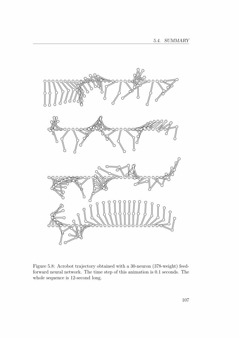
5.4. SUMMARY
Figure 5.8: Acrobot trajectory obtained with a 30-neuron (378-weight) feed-forward neural network. The time step of this animation is 0.1 seconds. Thewhole sequence is 12-second long.
107
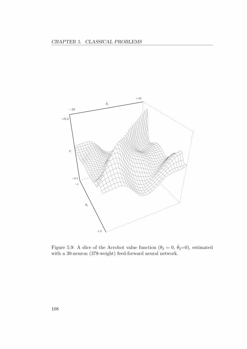
CHAPTER 5. CLASSICAL PROBLEMS
V
+0.4
−0.4
θ1
−π
+π
θ1
+10
−10
Figure 5.9: A slice of the Acrobot value function (θ2 = 0, θ2=0), estimatedwith a 30-neuron (378-weight) feed-forward neural network.
108
Chapter 6
Robot Auto Racing Simulator
This chapter contains a description of attempts at applying reinforcementlearning to a car driver in the Robot Auto Racing Simulator. This is aproblem with 4 state variables and 2 control variables that requires a lot ofaccuracy.
6.1 Problem Description
The Robot Auto Racing Simulator was originally designed and written byMitchell E. Timin in 1995 [71]. This is the description he gave in his originalannouncement:
The Robot Auto Racing Simulation (RARS) is a simulation ofauto racing in which the cars are driven by robots. Its purpose istwo-fold: to serve as a vehicle for Artificial Intelligence develop-ment and as a recreational competition among software authors.The host software, including source, is available at no charge.
The simulator has undergone continuous development since then and is stillactively used in a yearly official Formula One season.
6.1.1 Model
The Robot Auto Racing Simulator uses a very simple two-dimensional modelof car dynamics. Let ~p and ~v be the two-dimensional vector indicating theposition and velocity of the car. Let ~x = (~p,~v)t be the state variable of thesystem. Let ~u be the command. A simplified model of the simulation is
109
CHAPTER 6. ROBOT AUTO RACING SIMULATOR
described by the differential equations:{
~p = ~v
~v = ~u− k‖~v‖~v(6.1.1)
The command ~u is restricted by the following constraints (Figure 6.1):
‖~u‖ ≤ at
~u · ~v ≤ P
m
(6.1.2)
k, at, P and m are numerical constants that define some mechanical charac-teristics of the car:
• k = air-friction coefficient (aerodynamics of the car)
• P = maximum engine power
• at = maximum acceleration (tires)
• m = mass of the car
Numerical values used in official races are k = 2.843 × 10⁻⁴ kg · m−1, at =10.30 m · s−2 and P/m = 123.9 m2 · s−3.
In fact, the physical model is a little more complex and takes into consid-eration a friction model of tires on the track that makes the friction coefficientdepend on slip speed. The mass of the car also varies depending on the quan-tity of fuel, and damage due to collisions can alter the car dynamics. Thesimplification proposed above does not significantly change the problem andwill make further calculations much easier.
6.1.2 Techniques Used by Existing Drivers
RARS has a long history of racing, and dozens of drivers have been pro-grammed. They can be roughly split into two categories:
• Cars that compute an optimal path first. This method allows to usevery costly optimization algorithms. For instance, Jussi Pajala opti-mized trajectories with A∗, Doug Eleveld used a genetic algorithm inDougE1 (and won the 1999 F1 season), and K1999 used gradient de-scent (and won the 2000 and 2001 F1 seasons)(see Appendix C). Aservo-control is used to follow the target trajectory. Drivers based onthis kind of methods are usually rather poor at passing (K1999 alwaysstick to its pre-computed trajectory), but often achieve excellent laptime on empty tracks.
110
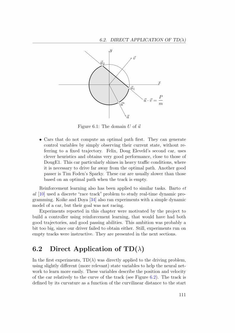
6.2. DIRECT APPLICATION OF TD(λ)
~u · ~v =P
m
x
y
~a
~v
bc ~u1
bc~u2
bc
~u∗
Figure 6.1: The domain U of ~u
• Cars that do not compute an optimal path first. They can generatecontrol variables by simply observing their current state, without re-ferring to a fixed trajectory. Felix, Doug Eleveld’s second car, usesclever heuristics and obtains very good performance, close to those ofDougE1. This car particularly shines in heavy traffic conditions, whereit is necessary to drive far away from the optimal path. Another goodpasser is Tim Foden’s Sparky. These car are usually slower than thosebased on an optimal path when the track is empty.
Reinforcement learning also has been applied to similar tasks. Barto etal [10] used a discrete “race track” problem to study real-time dynamic pro-gramming. Koike and Doya [34] also ran experiments with a simple dynamicmodel of a car, but their goal was not racing.
Experiments reported in this chapter were motivated by the project tobuild a controller using reinforcement learning, that would have had bothgood trajectories, and good passing abilities. This ambition was probably abit too big, since our driver failed to obtain either. Still, experiments run onempty tracks were instructive. They are presented in the next sections.
6.2 Direct Application of TD(λ)
In the first experiments, TD(λ) was directly applied to the driving problem,using slightly different (more relevant) state variables to help the neural net-work to learn more easily. These variables describe the position and velocityof the car relatively to the curve of the track (see Figure 6.2). The track isdefined by its curvature as a function of the curvilinear distance to the start
111
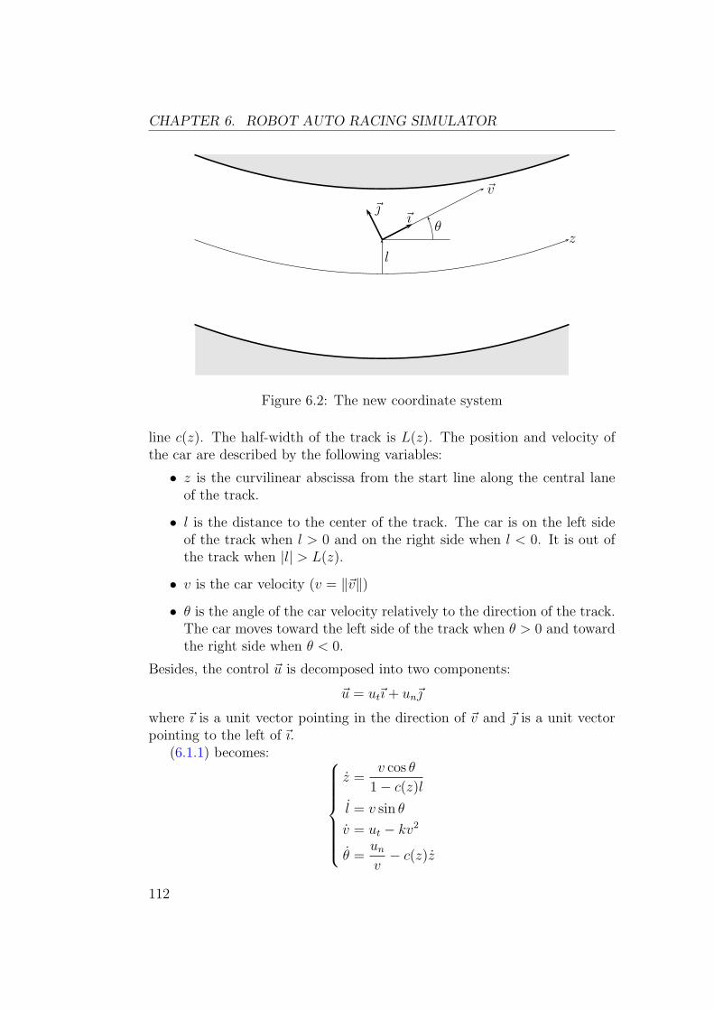
CHAPTER 6. ROBOT AUTO RACING SIMULATOR
z
l
θ~ı
~
~v
Figure 6.2: The new coordinate system
line c(z). The half-width of the track is L(z). The position and velocity ofthe car are described by the following variables:
• z is the curvilinear abscissa from the start line along the central laneof the track.
• l is the distance to the center of the track. The car is on the left sideof the track when l > 0 and on the right side when l < 0. It is out ofthe track when |l| > L(z).
• v is the car velocity (v = ‖~v‖)
• θ is the angle of the car velocity relatively to the direction of the track.The car moves toward the left side of the track when θ > 0 and towardthe right side when θ < 0.
Besides, the control ~u is decomposed into two components:
~u = ut~ı + un~
where ~ı is a unit vector pointing in the direction of ~v and ~ is a unit vectorpointing to the left of ~ı.
(6.1.1) becomes:
z =v cos θ
1− c(z)l
l = v sin θ
v = ut − kv2
θ =un
v− c(z)z
112
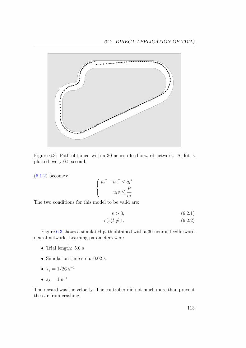
6.2. DIRECT APPLICATION OF TD(λ)
b b b b b b b b b b b b b b b b b b b b b b b b bbbbbb
b
b
b
b
b
b
b
b
bb
bb
bb
bb
bb
bb
bb
bb
bb
bb
bb
bb
bb
bb
bb
bb
bb
bb
bb
bb
bb
bbbbb
b
b
b
b
b
b
b
b
b
b
b
b
b
b
b
bb
b b bbb
b
b
b
b
bbbbbbbb b b b
Figure 6.3: Path obtained with a 30-neuron feedforward network. A dot isplotted every 0.5 second.
(6.1.2) becomes:
ut2 + un
2 ≤ at2
utv ≤P
m
The two conditions for this model to be valid are:
v > 0, (6.2.1)
c(z)l 6= 1. (6.2.2)
Figure 6.3 shows a simulated path obtained with a 30-neuron feedforwardneural network. Learning parameters were
• Trial length: 5.0 s
• Simulation time step: 0.02 s
• sγ = 1/26 s−1
• sλ = 1 s−1
The reward was the velocity. The controller did not much more than preventthe car from crashing.
113
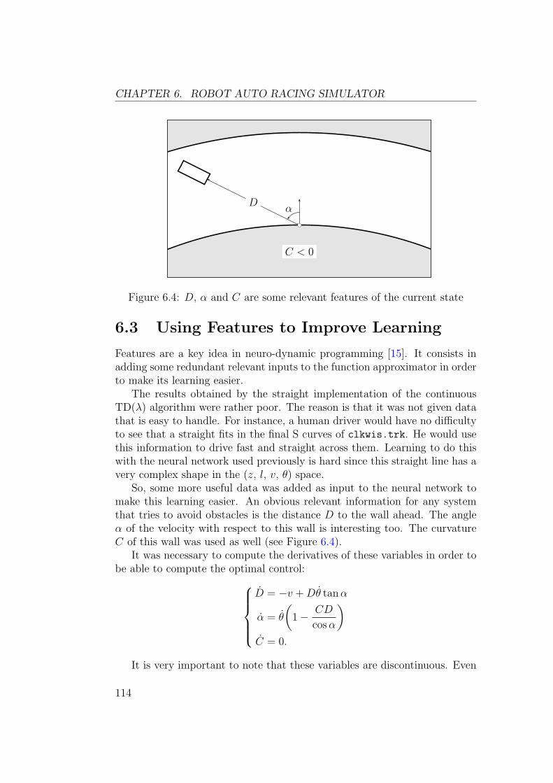
CHAPTER 6. ROBOT AUTO RACING SIMULATOR
D
bc
C < 0
α
Figure 6.4: D, α and C are some relevant features of the current state
6.3 Using Features to Improve Learning
Features are a key idea in neuro-dynamic programming [15]. It consists inadding some redundant relevant inputs to the function approximator in orderto make its learning easier.
The results obtained by the straight implementation of the continuousTD(λ) algorithm were rather poor. The reason is that it was not given datathat is easy to handle. For instance, a human driver would have no difficultyto see that a straight fits in the final S curves of clkwis.trk. He would usethis information to drive fast and straight across them. Learning to do thiswith the neural network used previously is hard since this straight line has avery complex shape in the (z, l, v, θ) space.
So, some more useful data was added as input to the neural network tomake this learning easier. An obvious relevant information for any systemthat tries to avoid obstacles is the distance D to the wall ahead. The angleα of the velocity with respect to this wall is interesting too. The curvatureC of this wall was used as well (see Figure 6.4).
It was necessary to compute the derivatives of these variables in order tobe able to compute the optimal control:
D = −v + Dθ tan α
α = θ
(
1− CD
cos α
)
C = 0.
It is very important to note that these variables are discontinuous. Even
114
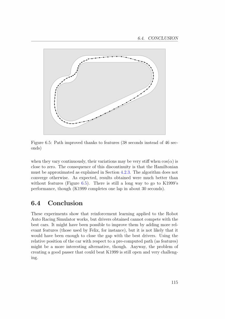
6.4. CONCLUSION
b b b b b b b b bb
bb
bb
bb
b
b
b
b
b
b
b
b
b
b
b
b
b
b
b
b
b
b
b
b
b
b
b
bb
bb
bbbbb
b
b
b
b
b
b
b
b
b
b
b
b
b
b
b
b
bb
bbbb
b
b
b
b
bb
bb
Figure 6.5: Path improved thanks to features (38 seconds instead of 46 sec-onds)
when they vary continuously, their variations may be very stiff when cos(α) isclose to zero. The consequence of this discontinuity is that the Hamiltonianmust be approximated as explained in Section 4.2.3. The algorithm does notconverge otherwise. As expected, results obtained were much better thanwithout features (Figure 6.5). There is still a long way to go to K1999’sperformance, though (K1999 completes one lap in about 30 seconds).
6.4 Conclusion
These experiments show that reinforcement learning applied to the RobotAuto Racing Simulator works, but drivers obtained cannot compete with thebest cars. It might have been possible to improve them by adding more rel-evant features (those used by Felix, for instance), but it is not likely that itwould have been enough to close the gap with the best drivers. Using therelative position of the car with respect to a pre-computed path (as features)might be a more interesting alternative, though. Anyway, the problem ofcreating a good passer that could beat K1999 is still open and very challeng-ing.
115

Chapter 7
Swimmers
Control problems that have been tested in previous chapters have a rathersmall dimensionality (≤ 4). Experiment results with these problems tend toindicate that feedforward neural networks could deal accurately with systemswith many more independent state variables. In this chapter, this intuition isconfirmed by successfully applying feedforward neural networks trained withcontinuous TD(λ) to complex swimmers. The most complex of them has 12state variables and 4 control variables, which is significantly beyond the com-plexity of some of the most difficult dynamical motor control problems thathave been solved by reinforcement learning, such as Randløv and Alstrøm’sbicycle [54] or Morimoto and Doya’s robot [42] (both have 6 state variables).
7.1 Problem Description
The swimmers to be controlled are made of three or more segments (thusproviding a large scale of problems, from the simplest to any arbitrarilycomplex swimmer), connected by joints, and moving in a two-dimensionalpool. Control variables are torques applied at these joints. The goal is toswim as fast as possible to the right, by using the friction of water.
The state of a n-segment swimmer is defined by the n angles of its seg-ments, the two Euclidian coordinates Gx and Gy of its center of mass, andthe n + 2 derivatives of these variables. That makes a total of 2n + 4 statevariables. The control variables are the n − 1 torques applied at segmentjoints. The complete model of this system can be found in Appendix B.
In fact, since the goal is to swim in a given direction (r(~x, ~u) = Gx), thevalue function and the optimal control do not depend on Gx and Gy. Thismeans that actually, there are only 2n + 2 significant state variables.
117
CHAPTER 7. SWIMMERS
7.2 Experiment Results
Figures 7.1, 7.2, 7.3, 7.4 show swimming styles obtained with a variety ofswimmers and function approximators. Since the state space is isotropic(all directions are identical), it is possible to tell a swimmer to swim in anydirection by rotating its state variables. On these figures, swimmers weretold to perform a U-turn after a few seconds.
Unlike the simpler problems that were presented in the previous chapters,many unstabilities were observed during learning. Most of them are not wellunderstood yet, and would require more investigations.
Figure 7.5 shows instabilities recorded when using a 30-neuron neural net-work to train a 3-segment swimmer. The reason for these instabilities are notclear, but the shape of the performance curve is strikingly similar to resultsobtained by Anderson [3] on a simple Q-learning experiment with feedfor-ward neural networks. In the case of Anderson’s experiments, instabilitieswere related to an insufficient number of neurons. In order to test if moreneurons would help, the learning experiment was run again with 60 neuronsinstead of 30. Results are plotted on Figure 7.6. Training was much morestable. After these 2,500,000 trials, performance kept a high level duringmore than 10,000,000 trials, after which learning was stopped. This does notprove that there would not have been instabilities, but, at least, it is muchbetter than with 30 neurons.
Figure 7.7 shows the learning of a 5-segment swimmer with 60 neurons.Learning made steady progress during the first 2,500,000 trials, but then,performance suddenly collapsed. Unlike the 3-segment instabilities of Fig-ure 7.5, the 5-segment swimmer did not manage to recover from this crisis,and its neural network blew up completely. What happened exactly is still amystery.
7.3 Summary
These experiment results clearly demonstrate the superior generalization ca-pabilities of feedforward neural networks. In fact, it is extremely unlikelythat such a high-dimensional problem could be solved with a linear func-tion approximator. Besides, some instabilities were observed. They mightbe caused by the insufficient size of the networks used, but this hypothesiswould require more investigation. These swimmers clearly show the strengthof the dynamic programming approach: with very little computing power,the controller can handle instantaneously any unexpected direction change.
118
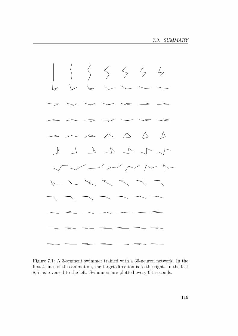
7.3. SUMMARY
Figure 7.1: A 3-segment swimmer trained with a 30-neuron network. In thefirst 4 lines of this animation, the target direction is to the right. In the last8, it is reversed to the left. Swimmers are plotted every 0.1 seconds.
119
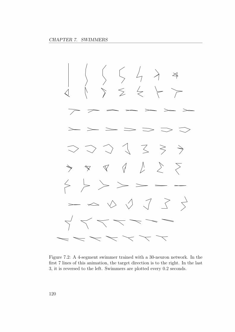
CHAPTER 7. SWIMMERS
Figure 7.2: A 4-segment swimmer trained with a 30-neuron network. In thefirst 7 lines of this animation, the target direction is to the right. In the last3, it is reversed to the left. Swimmers are plotted every 0.2 seconds.
120
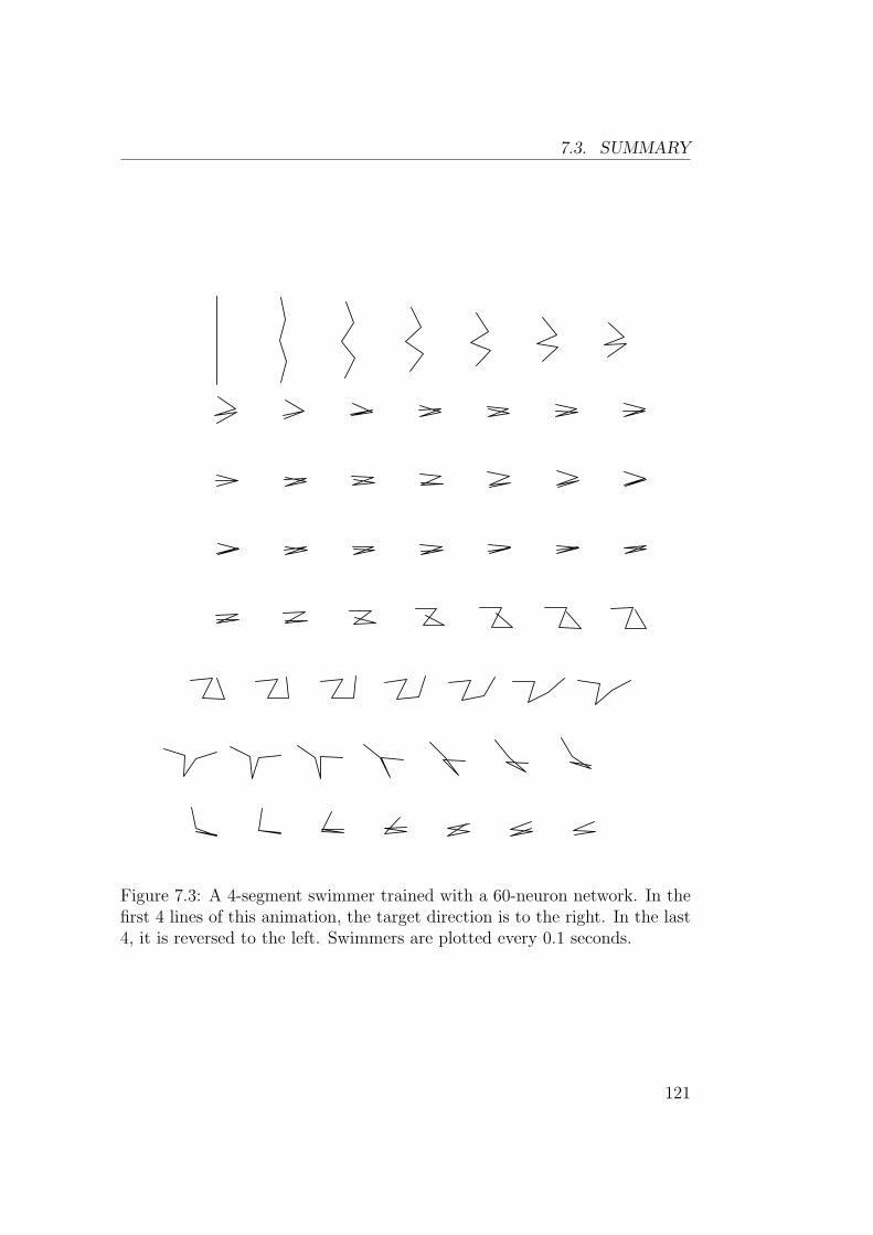
7.3. SUMMARY
Figure 7.3: A 4-segment swimmer trained with a 60-neuron network. In thefirst 4 lines of this animation, the target direction is to the right. In the last4, it is reversed to the left. Swimmers are plotted every 0.1 seconds.
121
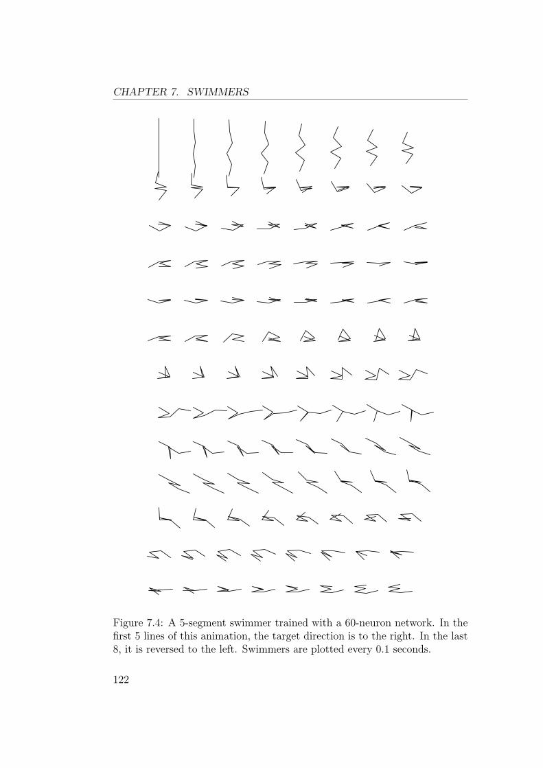
CHAPTER 7. SWIMMERS
Figure 7.4: A 5-segment swimmer trained with a 60-neuron network. In thefirst 5 lines of this animation, the target direction is to the right. In the last8, it is reversed to the left. Swimmers are plotted every 0.1 seconds.
122
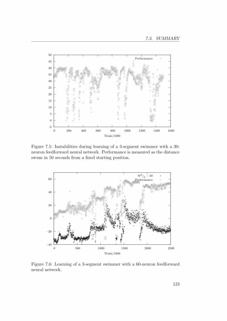
7.3. SUMMARY
-5
0
5
10
15
20
25
30
35
40
45
50
0 200 400 600 800 1000 1200 1400 1600
Trials/1000
Performance
rs rs rs rs rs rsrs rs rsrs rs rs rs rs rsrs rs rsrsrs rs rs rsrsrsrsrs
rs rs
rsrs rs rsrs rs
rs
rs rs rs rs rsrs rsrs
rs
rs
rs rs
rs
rsrs rsrsrs rs
rs
rs rsrsrs rsrs rs rsrs rsrs rs
rs rs rsrs
rs rsrsrs rsrs rs rs rsrsrs rsrsrs
rs
rs rs rs rsrsrsrsrsrs rs rsrs
rsrs rs rs rsrsrs rs rsrs rsrs rs rs rs rs rsrs rs rsrs rs rsrs rsrs rs rs rs
rs rsrs rs rs rs rs rs rs rs rs
rsrs rs
rs
rsrs rs rsrs rs rsrsrsrsrsrsrsrsrs rs
rsrs rsrs rsrs rsrs rs
rs
rs
rs
rs rs
rs
rs
rs
rs rs
rs
rs
rs
rs
rs
rs
rs
rs
rs
rs
rs
rs
rsrs
rs
rs
rs
rs
rs
rs
rs
rs
rs
rsrs
rs
rs
rs
rs
rs
rs
rs
rs
rs
rs rsrs rs rs
rs
rsrs rs
rs
rs
rs rs rsrs
rs
rsrs
rs rs
rs
rsrs
rs
rs
rsrsrs
rs
rs
rs
rs rs
rs
rs
rsrs
rs
rs rs
rsrs rs
rs
rs rs
rsrsrs
rs
rs
rs
rs rs
rs
rs
rs
rsrs rs
rs
rs
rs
rs
rs
rs
rs
rs
rs
rs
rs
rs
rs
rs
rs
rs
rs
rs rs
rs
rsrs
rs rs rs rs rs rs rs rs rs
rs
rs
rs
rs rsrs
rsrsrsrs rs rs rs rsrs
rs rs
rs rs
rs rsrsrs
rsrs rs
rs
rs
rs rs
rsrsrs rs
rs rs
rs
rsrs
rs
rs
rs
rsrs
rs
rs
rs
rs
rs rs
rs
rs
rsrsrs
rsrs
rs
rs
rs rs rsrs rs rs rs
rsrs rs rs
rsrs rs rsrs rs rs rs rs rs
rs
rs
rsrs rs rsrs rsrsrsrs rs
rsrs
rsrs rs
rs
rs
rs
rs
rs
rsrs
rs
rs
rs
rs
rsrsrs
rs
rs rs rs
rs rs rs rsrs rs rs rs rs rs rsrsrs
rs
rs rs
rs
rs rsrs rs rsrsrs rs rs rsrs rsrs rs rsrs rs rs
rs rs
rs rs rs rs
rs
rs
rs rs rs rsrs
rs rs rsrs
rs
rs
rs
rs
rs rs
rsrsrsrs rs rs
rs rs rs
rsrs rs
rsrs rs
rsrsrs
rs
rs
rs
rs
rs
rs rsrsrs
rs
rs
rs
rs
rs
rs
rs
rs
rs
rs
rs
rs
rs
rs
rs
rs
rs
rs
rs
rs
rsrs rs
rs rsrs rs rs
rs rs rs
rs rsrs
rsrs
rs
rsrs rs
rsrsrsrs rs
rs
rsrs
rs
rs
rs
rsrsrs
rs
rs rs
rs
rs rs
rs rsrs rs rsrs
rs rs rs
rs
rs
rs
rs
rsrs
rsrs rs rs
rs
rs rsrs
rs rs
rsrs rs
rs rsrsrs
rs
rs
rs
rsrs
rs
rsrs
rs
rs
rs
rs
rs
rs rs
rs
rs
rs
rs
rs
rs rsrs rs
rs rs
rs
rs
rsrs rs
rs rs rsrs rsrsrsrs
rs
rs rs rs
rs rs
rs
rs
rs
rs rsrs rsrs
rs
rsrs rsrs rs rs
rs
rs
rs
rs
rs
rs
rs rsrsrs rs rs
rs
rs rs rsrs rs rsrsrs rs
rs
rs
rs
rs rs
rsrsrs
rs
rs rsrs
rs rs rs
rs
rs rs rs rs rs
rs
rsrs rs rs rsrsrsrsrs
rs
rs
rs
rs
rs
rsrsrs
rs
rs
rs rsrs
rs rs
rs
rs
rsrs rs rs rsrs rsrs rs
rs
rs rsrs
rs rs rsrsrsrsrs
rsrs rsrs rs
rsrs
rs
rsrs
rs
rs
rsrsrsrs
rs
rs
rs
rsrs
rs
rsrs rs rsrs rs
rs
rs
rs
rs
rs rsrsrs rs
rs rsrs
rs
rs rs
rs
rs
rsrsrs rs rsrs rs
rs
rs
rs
rs
rs rsrs rs rs rsrs rs rs rs rs
rs
rs
rs
rs rs rsrs rsrs
rs rsrs rs rsrs rsrsrs rsrs
rs rsrs rs rs rs rsrs rs rs
rs
rsrs rs
rs
rs
rsrs rs rs
rsrs
rsrs
rs rs rsrsrsrs
rs rs
rsrsrsrs
rs rsrs
rs
rs
rs rs
rs
rsrs
rs
rs
rs
rs
rs
rs
rs rs
rs
rs
rs
rsrs rs
rs
rs
rs
rs rs
rs
rs rs rsrs rs rsrs rs
rsrsrsrs rs rsrsrsrs rs rsrsrs rs rsrs rs rs rsrsrs rsrs rs rsrs rsrsrs rs rs rs rs rs rsrsrsrs rs rsrsrsrs rsrsrs rs rs rs rs rsrs rs rsrs
rs
rs
rs rsrs
rs
rs
rs
rs
rs
rs
rs
rs
rs
rsrs
rs
rs
rs
rsrs
rs
rsrs
rs
rsrs rs
rs
rs
rs
rs
rs
rs
rs
rs
rs
rs
rs
rs
rsrs rs
rs
rs rs
rsrs rs rsrsrs rs rs rs rs rsrs rsrs rs rs rs rsrs rs rsrs rs rsrsrs rs rsrsrs rsrs
rs
rs
rs rsrsrsrs rs rs rs rs rsrsrs rs rsrs rs rs rs rs rsrs rs rs rs rs rs rsrs
rs
rs
rsrsrs rs rs rs rsrs rs rs
rs rs rs
rs
rs
rsrs
rs
rs
rs
rs
rs
rs
rs rsrsrs rsrsrsrs
rs
rsrsrs rs rs rsrs rs rsrsrsrs
rs
rs
rs rs rs rsrs rs rs
rs
rs rs rs rsrs rs rs
rsrs
rs rs
rs
rsrsrs
rsrsrs rs
rs
rs
rs rsrs
rs
rs rsrs
rs
rsrs rs
rs rs rsrs
rsrsrsrs
rsrsrs
rs
rs rsrs rs
rs
rsrs
rs
rs rsrs rsrs rs rs rs
rs
rs rs
rs
rs rs
rs
rs
rs
rs rs
rsrs rs
rs
rs
rs
rsrs
rs rs
rs
rs rs
rs
rsrs rs
rsrs
rs
rsrsrs
rs
rs
rs rsrs
rs
rs
rs
rs
rs rs
rs
rsrs
rs rsrs rsrs
rs
rs
rs
rs
rsrs
rs
rs rsrsrs
rs
rs
rs
rsrs rs
rsrs
rs
rsrsrsrs rs
rs rs
rsrs
rs rsrs rs
rs rs
rs
rs
rs rs
rs
rsrs
rs
rs
rs rs
rsrs rs rsrs
rs
rs
rs
rs
rs
rs rs rs rs
rs
rs
rs rsrs
rsrs rs
rs
rs rsrs rs
rs
rs
rs rs
rs rs
rs
rs
rs
rs
rs rs
rs
rs
rsrs
rs
rs
rs
rs rs
rsrs
rs rs
rs rs
rs rsrs rs
rs
rs rs
rsrs
rs
rs
rs
rs
rs
rs
rs
rs
rs
rsrs
rs
rs
rs
rs
rsrs
rs
rs
rs
rs rs rs
rs
rs
rs
rs
rs
rs
rs
rs
rs rs
rs
rs
rsrsrs
rs
rs
rs
rs
rs
rs
rs
rs
rs
rs
rs rs
rs
rsrs
rs
rs
rs rs
rs
rs rs
rs
rsrs rsrs
rsrs
rs
rs
rs rs
rsrsrs
rs
rs
rs
rsrs
rsrs
rs
rs
rs
rs
rs
rs
rs
rs rs rs
rsrs
rs rs rs rsrsrsrs rs rs
rs
rs
rs
rs
rs
rs
rs
rs
rs
rsrs rs
rsrs
rs
rs
rsrsrs
rs
rs
rsrs
rs
rsrsrsrs
rs rs rsrs
rsrsrs rsrsrs rs
rsrs
rs
rs rsrsrs rsrs
rs
rs rs
rs
Figure 7.5: Instabilities during learning of a 3-segment swimmer with a 30-neuron feedforward neural network. Performance is measured as the distanceswum in 50 seconds from a fixed starting position.
-40
-20
0
20
40
60
0 500 1000 1500 2000 2500
Trials/1000
˙
H2¸
S− 50
+
++++++++++++++++++++++++++++++++++++++++++++++++++++++++++++++++++++
+++++++++++++++++++++++++++++++++++++++++++++++++++++++++++++++++++++++++++++
+
++++++++++++++++++++++++++++++++++++++++++++++++
+++++++++++++
+++++++++++
+
+++++++
+
+
++++++
++++++++++++++++++++++++++
++
+++++++++++
+
++++++++++++++
++++++++++++++++++++++++++++++++++++++
+++++++++++++++++++++++++++++++++++++++++++++++++++++++++++++++++++++++++++++++++++++++++++++++++++++++++++++++++++++++++++++
+++++++++++++++++++++++++++++++++++++++++++++++++++++++++++++++++++++++++
+++++++
+
++++++++++
+
+
+++
+++
+
++
+++++
+++
+++
+
+++
+++++
+
+++++++
+++
+
++++++++
+++++++++++++++++
++++++++++
++++++++++++++++++
+++++
+++++++
++
+++++++++++++++++++
++++++++++++++++++++++++++
+++++++
++++
+
+++++++++++++
+
+++++++
+
+
+
+
++
+++
+
++
++
++
+
+
+
+++
+++
+
+
+
+++
++++++
+
++
+
+++++
++
+
+
+
+
++
+
++++
++++
++++
+
++
+
+
+++++++
++
++++
+
+++++
+++++++
+
++
+++++
+
+
++++
+++++++
+++
++
+++
+++++
+
+
+
+++++++++++
+
+
+
++
++
++
+++++++++++++++++++
+
+
+++
++++++++
+
+++++++++
++++
+
+
+
+++
++
+++++++
++
++++
++++++++++
++++++
+++++++
+
+
+
+
+
+++
+++++++++
+++++
++
+
+
+
+
+
+++
+
+
+
+
++
+++++++
+++
+
+
+
+
+
+
+
+
+
+
+++++++
++
++++
++
+
+
+
+
+
+
+++++++++
++
++
+
++++++++
+
+
++++
+
+++
+
+
++
+
+
+
+
+
+
+++++++
++++
++++
++
+
+
+
+
++++++++
+++
+
+
++
+++
++
+
+
+++
+
+
+
+
+++
++
++
+
++
++
+
++
+++++++
+
++
+++++
+
+
+
++
+
++++++
+++
+
+
+
++
+++
+
+
+++++++
+
+
++++
+++
+
++
+
+
+
+++++++++++++
++
++++++++++
+
+
+
+++++++
+
++++
+
+
+
+
+
+
+
+
+
+++
+
+++
+
+
++
+
++++++
+++
+
+++
+++
+++
++
+
++
+
+++++++
+
+++
+++
+
++++
++
+
+
++++++
+++
+
++++
+
++++++++++++++++
++++
+++++
++++
+
++++++++++++
++++++++
++++++++
+++++++
++
+
+
+
+
++++
++++
++++++++++
+
++++++++++++++
++++++
++
+++++++++++++++++++++++++++++++++++++++++++++++++++++++++
+++++++++++++++
+
+++++++++
+++++++++++++
+++++++++++++++++++++++++++++++
++++
++
++++++++++++++++++++
+
+++++
+
+++++++++++++++
+++++
++++++
+
+
+++++++++
+
++++++++++
+
Performance
rs
rsrs rs rs rs rs rs rs rs rs
rs
rs
rs rs rsrsrsrsrs rs rs rsrs rs rs rsrsrs rs
rs
rs rsrsrs
rs rs rs rs rs rs rs rs rs rs rs rsrs rsrs rs rs rs rs rsrsrs rs rs rsrsrs rsrsrs rs rsrs rsrs rs rs rsrs rsrsrs rsrs rs rs rs rsrs rsrsrs rs rs rsrs rs rs rs rs rs rs rsrs
rsrsrs rs rs rs rs rs rs rs rs rs rsrsrs rsrs rsrs rsrs rsrs rs rs rs rs rs rs rs rsrs rs rs rs rs
rs
rs rs rs rs rsrsrs rsrs rs rs rsrs rs rs rs rs rsrs rs rs rs rs rs rs rsrs rsrs rs rsrs rs rsrs rs rs rsrs rs rs rs rsrs rs rs rsrs rs rsrs rsrsrs
rs
rs rsrs rsrs
rs rs
rs
rsrs
rs
rs
rsrsrs
rs
rsrs rs
rs
rs
rsrs
rs rs
rs
rs rs
rs
rs rsrsrsrsrs
rs rs
rsrs
rs
rsrs
rs
rsrs rs rs
rs
rs
rsrsrs
rs
rs
rs rs
rs
rs
rs rsrsrs
rs
rsrs rs
rs
rs
rs
rsrsrsrsrs rs rs rs rs
rs
rs
rs
rsrs
rs rs rs rs rs rs rs rs rs rs rs
rs rs
rs
rsrs
rs
rs rs
rs
rsrsrs rs
rs
rs
rs
rs
rsrs
rs
rs rs rs rs rs
rsrs rs rsrs
rs
rs
rs
rsrs
rs rsrs rsrs rs
rs rs rsrs rs rsrs
rs
rsrsrs
rs
rs
rsrs
rs
rs
rsrsrs
rs
rsrs
rs
rsrsrs
rsrs
rs
rs
rs
rs
rs
rs rsrs
rs rsrs
rs rs
rs
rs
rs rs
rs rs
rs rsrsrs
rsrsrsrs rs
rs
rsrs
rsrs
rs rs
rs
rsrsrs rs rsrsrs rs
rs
rs
rsrs rs rsrsrs rs rs rs
rs
rs rs
rs rsrs
rsrs
rs rs
rsrs
rsrsrsrs rs rsrsrsrs rsrs
rs rs rs rs
rs
rs
rsrs
rs
rs
rs rs rsrs
rs
rs
rs
rs rs
rs
rs
rs rs
rs rs rs rs
rs
rs rs
rs
rs rs rs rs rsrs
rs rsrs
rs
rs rsrsrs
rsrs rs rsrs rs rs rs
rs
rs rsrs rs
rsrsrsrsrs rsrs rsrs
rs
rs rs rsrsrsrsrs
rs
rs
rs
rs
rs
rs rs rsrs rs rsrs rsrsrs rsrs rs rsrsrsrsrs rsrsrs rsrs rsrs
rs
rs rsrs rs
rs
rs
rs
rs
rs
rs
rsrs
rs
rs
rs
rs
rsrs rs
rs
rs
rs
rsrs
rsrs
rs
rs rs
rs rs rs rs
rs
rs
rs
rs rs
rs rsrsrs rs rsrs rs
rs rsrs rsrsrsrs rs
rs rs
rs
rs
rs rs
rs rsrs rs rsrs rs rs rs rsrs rs rsrsrsrsrs rsrsrsrs rs rs rs rs rs rs rs rs rs rs rsrs
rs
rsrsrs rs rs rs rs rs rsrs rs rs rs rs rs rsrsrs rs rs rs rs rs rsrs rs rsrs rs rs rs rs rs rs rs rs rs rs rs rsrsrs
rs
rs rs rs rsrs rsrs rs rs rs rsrs rsrs rsrs rs rs rsrs rsrs rs rsrs rsrsrs
rs
rsrs
rs
rs
rs
rs rsrs
rsrsrsrs
rs
rs
rs rsrs rs
rs
rsrs rsrsrs rs rsrs rs rs rs
rs
rs
rs
rs
rs rs
rsrs
rs rs
rs
rs
rsrsrs
rs
rsrs rs rsrs rs
rs rs rsrs rs rsrs rs rs rs rs rs rs rsrs rs rs rs rs rs rs rs rs rs rsrsrs rs rs rs rs rs rs rs rs rsrs rsrs
rsrs rsrsrs rsrs rs rs rs rs rsrs rsrsrsrs rs rsrs rs rsrs
rsrs
rsrs
rs rsrs rsrs rs rsrs
rs
rs
rsrs
rsrsrs
rsrs
rs rsrs rsrsrsrs
rs
rs
rs rsrs
rsrs rs rs rs rs rs rs rs
rs
rsrsrsrsrs rs rs rsrs rs rsrs rs rs rs rs rs rs rs rs rs rsrsrs
rs rs
rs
rs
rs
rsrs rs
rs
rs rs
rs
rs rsrs rs
rsrsrs
rs rs
rsrs
rsrs
rs
rs rs rs rsrs
rs
rs
rs
rs rs rsrs
rs
rs rs rsrsrsrs
rsrsrs
rs
rsrs rsrs rs
rs rsrsrsrs
rs rs
rs
rs
rs
rs rsrs
rs rs
rsrsrs rs rs
rs
rsrs
rs
rs
rs
rsrs
rsrsrs
rsrs
rsrs
rs
rs
rs
rs rs
rs
rs rsrs rsrs rsrs rsrs rs rs rs rs rs rs rs
rsrs rs rsrsrs
rs rs
rs
rs
rs rs
rsrsrsrsrsrs rsrs rsrs rs rs rs rs rs rs rsrsrsrs rs rs rs rs rs rs rs rs rsrsrs rs rs rs rsrs
rsrs rsrsrs rs rs rs rsrsrs rs rs rs rs rs rs rsrs rsrs rs rs rs rs rs rs rsrs rs rsrs rs rs rsrsrs rs rs rs rs rs rs rs rs rs rs rs rs rs rs rs rsrs
rsrs rs rs rs rs rsrs
rsrsrs rs
rs rsrs
rsrsrsrs rs rsrs
rsrs rs
rs
rsrs
rs rs rsrsrs rs rs rs rs rs rs rsrs rs rs rs rsrs rsrs rsrsrsrsrs rs rsrs rsrs rs rs rs rsrs rs rs rs rsrs rs rs rs rs rs rs rsrs rs rsrsrs rsrsrs rs rs rs rsrsrs rs rs rs rsrs rs rs rs rsrsrs rs rs rs rs rs rsrsrsrs rs rs rs rs rsrsrs rs rs rsrs rs rs
rsrs rsrs
rs
rs
rsrs
rs
rs rsrs
rs
rs rs
rsrsrs rsrs
rs
rs rs
rs
rs
rsrsrs rs rsrs rsrsrs
rs
rs rs
rs
rs
rs
rs
rs
rs rs rs rs rs rsrsrsrsrs
rs rs
rs
rs
rs
rs rs rs rs
rs
rs
rs
rs rs
rs rs rs rsrs rs rsrs rs rs rs rsrs rs rs rs rs rs rsrsrsrsrsrs rs rsrsrsrs rsrsrsrs rs rs rs rsrs rs rs rs rs rs rs rs rs rs rs rs rsrs rsrs rs rsrs rs rs rs rs rs rs rs rsrsrs rs rs rs rs rs rs rsrsrs rsrsrs rs rs rsrs rs rs rs rs rs rsrsrsrsrsrsrs rs rs rs rsrs rs
rs rs rs
rs
rs rs
rs
rs rs rs rs rs rs rs rs rs rs rsrs rs rsrs rsrs
rs
rs rsrsrsrsrsrsrs rs rs
rsrs rs rs rs rsrsrs rsrsrs rs rsrsrs rs rs rs rs rs rs rs
rs
rsrs rsrs rs
rs rs rs rs
rs rs
rs
rs
rs rs rs
rsrs
rsrs rsrs
rs rs
rs rsrs
rs
rs
rsrs
rs rsrsrs rs rs
rsrsrs rs rs rs rs rsrsrsrs rs rsrs rs rsrs rs rs
rs
rs rsrsrs
rs
rsrs rs rsrsrs rs rsrs rs rs rs rs rsrsrsrs rs rs rs rs rs
rs
rs rs
rsrs rs rs rs
rs
rsrs
rs
rs
rs rs
rs rs
rs
rs
rsrs rs
rs
rs rs rs rsrsrs rsrs rsrs rsrs rsrs rs rs rsrs rs rs rs
rs
rs rsrs
rs
rs
rs rs
rs
rs rsrsrsrsrs
rs rs rs rs
rs
rs
rs rs
rsrsrsrs rs rs rsrs rs rs rs rsrs rs rs rsrsrs rsrs rs rs rs rs rs rs rs rsrsrs rs rs rs rs rsrsrsrs rs rs rsrs rs rs rs rs rsrs rs rs rs rs rs rs rs rsrs rs
rs
rs rs rs rs rsrs rs rs rs
rs
Figure 7.6: Learning of a 3-segment swimmer with a 60-neuron feedforwardneural network.
123
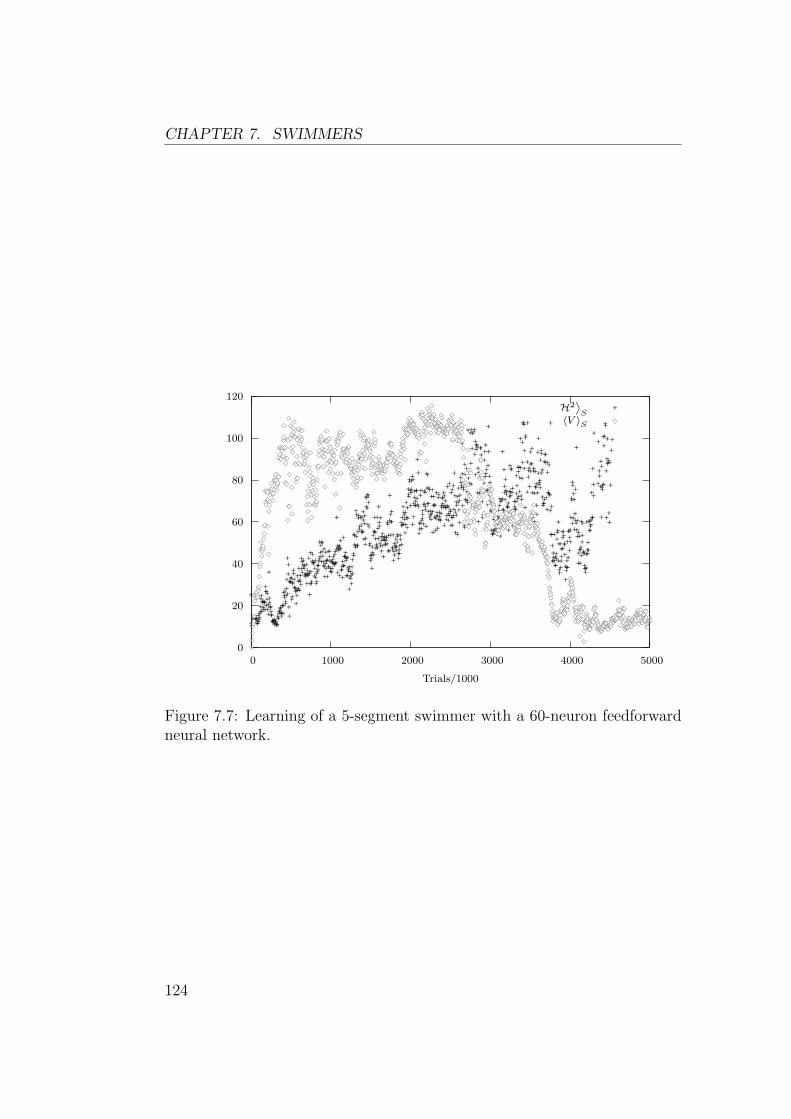
CHAPTER 7. SWIMMERS
0
20
40
60
80
100
120
0 1000 2000 3000 4000 5000
Trials/1000
˙
H2¸
S
+
+++++++++++++++++
+++++++++
+++++++++
++
+
+++
+++
+
++++++++++++++++++++++++++++++++++++
+++++++++
+
+
++
++
+++++
++
++
+++++++
+
++
+
+++
++++++
++++++++++++++
+++++
+
+
++
+
+++
++++++
+++
++++++++++
+
+++
+
+++
+++
+
++
++
+++
+
++
++++++++++++++++++++
+
+
+
+
++++
+
+++
++++
+
+
+++++++
+
++
++++
+
++++++
++
+
++
+++++
+
+
+
++
+
++
++
++
+++
+
++
++
+
++
++
++++
+
+
++
+
++
++++
+
++
+
+
+
+
++++++
+
+
++
+
++
++
+
+
+++++
+
+++++++++
+++
++
+
+
+
++++
++
+
++++++++++++
+++++++
+
+
+++
+
++++
+
+
+
+
++
++
+++
+++
+
++++
+
+
+
+
+++++
+++
+
+
+
+
++++
++
++++++
+
+
++
++
+
+
+
+
+
++
++
+++++
++
+
+
+++
++
+
+
+
+
++
++
++
+++++++++++
+
+
+++++++
+
++
++
+
+++
+
+
+
+
++
+
++
+
+
+
+
+
++
+
++
+
+
+
++
++++
+
+
+
++
++
+
+
+
+
+
+++
+
+
+
+++
+
+
+
+
+
+++
+
+
+
++++
+
+
+
+
+
++
+++
++
+
++
++
++
+
+
++
++
+
+
+
+
+
+
+
+++
+
+
++++++
+
++++++++++
+
++
+
+
+
+
+
+
+
++
+
++
+
++++
++++
+
++
+
++
++
++
++++
++++++
++
+
++
+
+
+
+
+
+
++
+
+
+
+++
+
+
+
++
+
+
+
+++
+
+
+
++
+
+
+
++
+
+
+
+++
++
+
+
+
+++++
+++
++
+++++
++++
++
++
++
+
++
+
+
+
+
++
++++
+
++++++
++++
+
+
++
+
++++
+
++++++++
++++
+
++
++
+
+++
+
++
+
++
+
++
+
++
+
+
+
++
+
+
+
+
+
+
+
++
+
+
++
+
+++
+++++
+
+
++++
+++++++
+
++
+
++
+
+
+
+++
+
+
+
+++
+
+
++
++
+
+
+
+
+++
++
+
+
++
+
〈V 〉S
rsrs
rsrs rs rsrsrs
rsrs rs rsrs rsrs rs rs
rs rsrs
rs
rsrs
rs
rsrs
rsrs rs rsrs
rsrs
rs rs
rs
rs rs
rs
rs
rs
rs
rs
rs
rsrsrsrsrs rs rsrs
rs
rsrs rsrs
rs rs rsrs rs
rsrs
rsrs rs
rs rs
rs
rsrs
rs
rs rs
rs rs rsrs
rs
rsrs
rs
rs rs
rs
rsrs
rs
rs
rs
rs
rs
rs
rs rs
rs
rs
rs
rs
rs
rs
rs
rsrs
rsrs
rs
rs rs
rs rs
rsrs
rs
rs
rs
rs
rs
rs
rs
rs
rs
rsrs
rs
rs
rs
rsrs rsrs
rs rsrs
rs
rsrsrs
rs
rs
rs
rs
rs
rs
rs
rs
rs
rs
rs
rs
rs
rs
rs
rsrs rs
rs
rs
rs
rs
rs rs rsrs
rs
rs rs rs
rsrs
rs rsrs rsrsrs rs
rs
rs
rs
rs rsrs
rs
rs
rs rs
rs
rs
rs
rs
rs
rs
rs
rs
rs
rs
rs
rsrs
rsrsrs
rs
rsrs rs
rs
rs
rs
rs
rs
rs rsrs
rs
rs rsrs rs
rs
rs rs rs
rs
rs rsrsrs
rs
rs
rsrs
rsrsrs rs
rsrs
rs rsrs rs rs
rs rsrs
rs rs rsrs
rs
rs
rs
rs
rs
rs rs rs
rsrs rs
rsrs rsrs
rs
rsrs
rs rs
rsrs
rs
rs
rsrs
rs
rs
rsrs
rs
rs
rs
rs
rs
rs rsrsrs rs rsrs rsrs
rs
rsrsrs
rsrs
rs
rs rsrs
rs
rs
rsrsrs
rsrs
rs
rsrs rsrsrsrs rs
rsrs rs rsrs rs rs rsrs rs rsrs
rs
rs rs rs
rs rs rsrsrs rs rs rsrs
rs
rs
rs rs rs rs
rs rs rs
rs
rsrs rsrs
rs rs
rs rs rsrsrs
rsrsrsrs
rs rs
rs
rs
rsrsrs rsrs
rsrs
rs
rs
rs
rs
rs rs rs rsrsrs rs
rsrsrsrsrsrsrs rsrsrsrs rsrs rs rsrsrs rs rsrsrsrsrsrsrs rs rs rs
rs rs
rs
rs rs
rs
rs rs rsrs
rsrs
rs
rs
rsrs rs
rs
rs
rs
rsrs
rs rsrs
rs
rsrs rs
rs
rs
rs
rs rs
rs
rs rs
rs rsrs rsrs rs rsrsrsrs
rs rs
rs
rsrsrs rs rs
rs rs
rsrs rs rs rsrsrs rsrs rs rs rs rs
rs rsrs rs
rs rs rs rs rs
rsrsrsrs
rs rs
rs
rs rsrsrsrsrsrs rsrs
rsrs rs
rs
rsrs
rsrs
rsrs
rsrsrs
rs
rs
rs
rs
rs
rs rs
rs rs rs
rs
rsrs
rs
rs
rs
rs
rs rs
rs rs
rs
rs
rsrsrsrs rsrs
rs rs
rs
rs
rs
rsrs rsrsrs rsrsrs
rs
rs
rs
rs rs
rs
rs rs
rs
rs rsrs
rsrs
rs
rsrs rs
rsrs rsrsrs
rs
rs
rsrsrsrsrs rs
rs
rs
rsrs rs rs rsrsrs rs rsrs rs rs
rs
rs
rsrsrsrs
rsrs rs rs rs rs rsrsrs
rsrsrsrsrs rs rsrs rsrs rsrsrsrs rs rs rs
rsrsrs
rsrsrs rs rs rs rsrsrs rs
rs rsrsrs
rsrsrsrs
rsrs rs
rs
rs rs
rs
rs rsrsrsrs rs rs
rs
rs rs
rs
rsrsrs
rs
rs rsrs rs
rs
rs rsrs rsrs rsrsrs
rs
rs
rs rs
rs
rs
rs rs rs rs rsrs
rs
rsrsrsrs rs rs rs rsrsrsrs rsrsrsrs rs rsrs rs
rs rs rs rsrs rsrsrs
rsrs rs
rs rsrs rsrsrs rsrsrsrsrs rs rsrsrs rs rsrsrsrs
rsrsrs rs rs rs rsrsrsrs rs rsrs rsrs rsrsrsrs rsrs rs rs rs rsrs
rs rs rsrsrs rs
rsrs rs rsrsrs rsrsrsrs rs
rs
rsrs
rs
rs rs rsrs rs rs rsrsrsrs
rs
rsrsrs rsrs
rs
rs rs
rs
rsrs rs rsrs rs
rsrs rs rs
rsrsrs rs rs rs
rs rs rsrsrsrs rs rs
rs
rs
rs rsrs rs rsrs
rsrsrsrs rsrs rs rs rsrs rsrs rs rs rsrs rs rs rsrs rs rs rs rsrs rs rs rs rsrs rs rs rs rs rs rsrsrsrsrs rsrs rsrs rs rs rs rsrsrs rsrs rs rsrs
rs
rs rsrsrs
rsrsrsrsrsrs
rsrs
rs rs
rsrs rs rsrsrs rs rs
rs rs rsrs
rsrs rs rs rsrsrsrs rs rs rsrsrs rsrs rs rsrs rs rs rsrsrs
rs
rs rs rsrsrs
rs rs rs rsrs rsrs rsrs rs rs
rs rsrs
rsrs rsrsrs rsrsrs rs
rs
Figure 7.7: Learning of a 5-segment swimmer with a 60-neuron feedforwardneural network.
124

Conclusion
125

Conclusion
In this thesis, we have presented a study of reinforcement learning using neu-ral networks. Classical techniques of dynamic programming, neural networksand continuous neuro-dynamic programming have been reviewed, and somerefinements of these methods have been proposed. Finally, these algorithmshave been applied successfully to difficult motor-control problems.
Many original results have been presented in this dissertation: the ∂∗ no-tation and the differential back-propagation algorithm (Appendix A), theK1999 path-optimization algorithm (Appendix C), and the second orderequation (1.2.6) for finite difference methods. Besides these, the main orig-inal contributions of this work are numerical integration methods to dealwith state and action discontinuities in TD(λ), and many original experimen-tal results on a large variety of motor tasks. The most significant of thesecontributions is probably the success of the swimmer experiments (Chap-ter 7), which demonstrates that the combination of continuous model-basedreinforcement learning with feedforward neural networks can handle motor-control problems that are much more complex than those usually solved withsimilar methods.
Each of these contributions also opens questions and directions for futureresearch:
• The numerical integration method could certainly be improved signifi-cantly. In particular, the idea of using second order information aboutthe value function to estimate the Filippov control might be extendedto control spaces with more than one dimension.
• The vario-η algorithm should be compared empirically to other classicalsecond-order methods.
• Many new interesting experiments could be run with swimmers. Inparticular, the reasons for the observed instabilities should be investi-gated. Methods based on the actor-critic approach seem to have betterconvergence properties [69], and should be tried on this problem. Also,bigger swimmers could learn to swim. Beyond swimmers, the method
127
CONCLUSION
used might as well be able to build controllers for much more complexproblems.
Besides these direct extensions, another very important question to ex-plore is the possibility to apply feedforward neural networks outside therestricted framework of simulated model-based motor-control. In partic-ular, experiments indicate that feedforward neural networks require manymore learning episodes than linear function approximators. This require-ment might be a major obstacle in situations where learning data is costlyto obtain, which is the case when it is collected in real time (like in roboticsexperiments), or when selecting actions entails a lot of computation (like incomputer chess [12]). It was not the case in swimmer experiments, or withTesauro’s backgammon player, because it was possible to produce, at no cost,as much training data as needed.
The key problem here is locality. Very often, linear function approxima-tors are preferred, because their good locality allows them to perform in-cremental learning efficiently, whereas feedforward networks tend to unlearnpast experience as new training data is processed. The performance of theswimmers obtained in this thesis, however, clearly indicates that feedforwardnetworks can solve problems that are orders of magnitude more complex thanwhat linear function approximators can handle. So, it would be natural totry to combine the qualities of these two approximation schemes.
Creating a function approximator that would have both the locality of lin-ear function approximators, and the generalization capabilities of feedforwardneural networks seems very difficult. Weaver et al. [78] proposed a speciallearning algorithm to prevent unlearning. Its efficiency on high-dimensionalreinforcement learning tasks remains to be demonstrated, but it might be aninteresting research direction.
Another possibility to make a better use of scarce learning data wouldconsist in complementing the reinforcement learning algorithm by some formof long term memory that stores it. After some time, the reinforcementlearning algorithm could recall this stored data to check that it has not been“unlearnt” by the feedforward neural network. A major difficulty of thisapproach is that it would require some kind of off-policy TD(λ) learning, be-cause the learning algorithm would observe trajectories that were generatedwith a different value function.
128

Appendices
129

Appendix A
Backpropagation
This appendix gathers results related to backpropagation.
A.1 Notations
A.1.1 Feedforward Neural Networks
Let us consider a n-neuron feedforward neural network defined by its con-nection matrix W = (wij) and its output functions σi. We will supposeneurons are ordered so that W is strictly triangular, that is ∀j ≥ i wij = 0,and that output functions are differentiable twice. Let ~x, ~a and ~y be respec-tively the input, the activation and the output vectors, each of them havingn components. The dynamics of the neural network is described by:
~a = W~y (A.1.1)
yi = xi + σi(ai). (A.1.2)
Since W is triangular, the output of the network can be simply obtained bycomputing a1, y1, a2, y2, . . . an, yn in sequence.
Having n inputs and n outputs for a n-neuron neural network might looka little strange. Usually, only a few of the first neurons are said to be “input”neurons, a few of the last neurons are “output” neurons, and the others are“hidden” neurons. Here, we will consider that all neurons can play all theseroles at the same time. This formalism has the advantage of being both moresimple and more general than the traditional input-hidden-output layeredarchitecture1.
1This kind of formalism is attributed to Fernando Pineda by Pearlmutter [52].
131
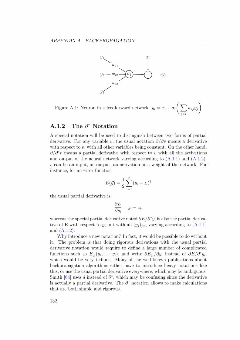
APPENDIX A. BACKPROPAGATION
σi yi
y1
y2
y3
+
xi
wi1
wi2
wi3
Figure A.1: Neuron in a feedforward network: yi = xi + σi
(∑
j<i
wijyj
)
A.1.2 The ∂∗ Notation
A special notation will be used to distinguish between two forms of partialderivative. For any variable v, the usual notation ∂/∂v means a derivativewith respect to v, with all other variables being constant. On the other hand,∂/∂∗v means a partial derivative with respect to v with all the activationsand output of the neural network varying according to (A.1.1) and (A.1.2).v can be an input, an output, an activation or a weight of the network. Forinstance, for an error function
E(~y) =1
2
n∑
i=1
(yi − zi)2
the usual partial derivative is
∂E
∂yi
= yi − zi,
whereas the special partial derivative noted ∂E/∂∗yi is also the partial deriva-tive of E with respect to yi but with all (yj)j>i varying according to (A.1.1)and (A.1.2).
Why introduce a new notation? In fact, it would be possible to do withoutit. The problem is that doing rigorous derivations with the usual partialderivative notation would require to define a large number of complicatedfunctions such as Eyi
(y1, . . . , yi), and write ∂Eyi/∂yi instead of ∂E/∂∗yi,
which would be very tedious. Many of the well-known publications aboutbackpropagation algorithms either have to introduce heavy notations likethis, or use the usual partial derivative everywhere, which may be ambiguous.Smith [64] uses d instead of ∂∗, which may be confusing since the derivativeis actually a partial derivative. The ∂∗ notation allows to make calculationsthat are both simple and rigorous.
132
A.2. COMPUTING ∂E/∂∗ ~W
A.2 Computing ∂E/∂∗ ~w
This section describes the backpropagation algorithm [36] [56] that computes,for a given input ~x, the gradient with respect to weights of an error functionE(~y).
∂E
∂∗wij
=∂E
∂∗ai
∂ai
∂wij
. (A.2.1)
Let us define
δi =∂E
∂∗ai
,
and
αi =∂E
∂∗yi
.
(A.2.1) becomes∂E
∂∗wij
= δiyj. (A.2.2)
δi can be evaluated with
δi =∂E
∂∗yi
∂yi
∂ai
= αiσ′i(ai),
and
αi =∂E
∂∗yi
=∂E
∂yi
+n∑
j=i+1
∂E
∂∗aj
∂aj
∂yi
=∂E
∂yi
+n∑
j=i+1
wjiδj.
These equations allow to compute αn, δn, αn−1, δn−1, . . . , α1, δ1 in sequence.Then, equation (A.2.2) gives the gradient of the error with respect to weights.
A.3 Computing ∂~y/∂∗~x
By derivating (A.1.2) and using (A.1.1) we get:
∂yi
∂∗xk
=∂xi
∂xk
+ σ′i(ai)
i−1∑
j=k
wij∂yj
∂∗xk
.
This is formally equivalent to the output of a “derivative network” that hasthe same connection weights W , the input of which is ∂~x/∂xk and the output
133
APPENDIX A. BACKPROPAGATION
functions of which are multiplications by σ′i(ai). Let us call its activation
vector ~a′k. (A.1.1) and (A.1.2) for this network are
~a′k = W
∂~y
∂∗xk
(A.3.1)
∂yi
∂∗xk
=∂xi
∂xk
+ σ′i(ai)a
′ki. (A.3.2)
Strangely, this algorithm is sometimes called “computing the Jacobian of theoutput by backpropagation”. In fact, propagation is forward, not backward.
A.4 Differential Backpropagation
This section describes an algorithm to compute, for a feedforward neural-network, the gradient with respect to weights of an error function that de-pends not only on the output of the network, like in the classical backpropa-gation, but also on its derivative with respect to inputs. This algorithm canbe used to solve partial differential equations with a neural network. Somesimilar algorithms have been published [45], but, as far as I know, this generalformulation for feedforward neural networks is an original result.
Let us suppose that for a given input ~x we want the network to mini-mize an error function E that depends on the output of the network and itsderivatives with respect to inputs:
E
(
~y,∂~y
∂∗~x
)
.
Let us calculate its gradient with respect to weights:
∂E
∂∗wij
=∂E
∂∗ai
∂ai
∂wij
+n∑
k=1
∂E
∂∗(
∂ai
∂∗xk
)∂(
∂ai
∂∗xk
)
∂wij
. (A.4.1)
If we define
δi =∂E
∂∗ai
and
δ′ki =∂E
∂∗(
∂ai
∂∗xk
) ,
then (A.4.1) becomes
∂E
∂∗wij
= δiyj +n∑
k=1
δ′ki
∂yj
∂∗xk
. (A.4.2)
134
A.4. DIFFERENTIAL BACKPROPAGATION
Let us now find recurrence relations to compute δi and δ′ki by backpropaga-tion:
δi =∂E
∂∗yi
∂yi
∂ai
+n∑
k=1
∂E
∂∗(
∂yi
∂∗xk
)∂(
∂yi
∂∗xk
)
∂ai
. (A.4.3)
Decomposing the first part of the first term gives
∂E
∂∗yi
=∂E
∂yi
+n∑
j=i+1
∂E
∂∗aj
∂aj
∂yj
(A.4.4)
=∂E
∂yi
+n∑
j=i+1
wjiδj. (A.4.5)
Decomposing the second term (let us call it α′ki):
α′ki =
∂E
∂∗(
∂yi
∂∗xk
) =∂E
∂(
∂yi
∂∗xk
) +n∑
j=i+1
∂E
∂∗( ∂aj
∂∗xk
)
∂( ∂aj
∂∗xk
)
∂(
∂yi
∂∗xk
) (A.4.6)
=∂E
∂(
∂yi
∂∗xk
) +n∑
j=i+1
wjiδ′kj. (A.4.7)
By substituting (A.4.5) and (A.4.7) into (A.4.3) we get
δi = σ′i(ai)
(∂E
∂yi
+n∑
j=i+1
wjiδj
)
+ σ′′i (ai)
n∑
k=1
a′kiα
′ki. (A.4.8)
The recurrence relation for δ′ki can be obtained by applying a similar chainrule:
δ′ki =∂E
∂∗(
∂yi
∂∗xk
)∂(
∂yi
∂∗xk
)
∂(
∂ai
∂∗xk
) (A.4.9)
= σ′i(ai)
(∂E
∂(
∂yi
∂∗xk
) +n∑
j=i+1
wjiδ′kj
)
(A.4.10)
= σ′i(ai)α
′ki. (A.4.11)
To summarize, backpropagation to evaluate the gradient of an error func-tion that depends on the derivative of outputs with respect to inputs can beperformed in 5 steps:
1. Compute the output of the neural network using usual forward propa-gation (equations (A.1.1) and (A.1.2)).
135

APPENDIX A. BACKPROPAGATION
2. Compute the output and activation of the derivative neural networksby forward propagation (equations (A.3.1) and (A.3.2)).
3. Compute the δ′ki’s and α′ki’s using (A.4.11) and (A.4.7), which is usual
backpropagation on the derivative networks.
4. Compute the δi’s using (A.4.8) which is a special form of backpropaga-tion on the main network.
5. Get the gradient of the error with (A.4.2)
136
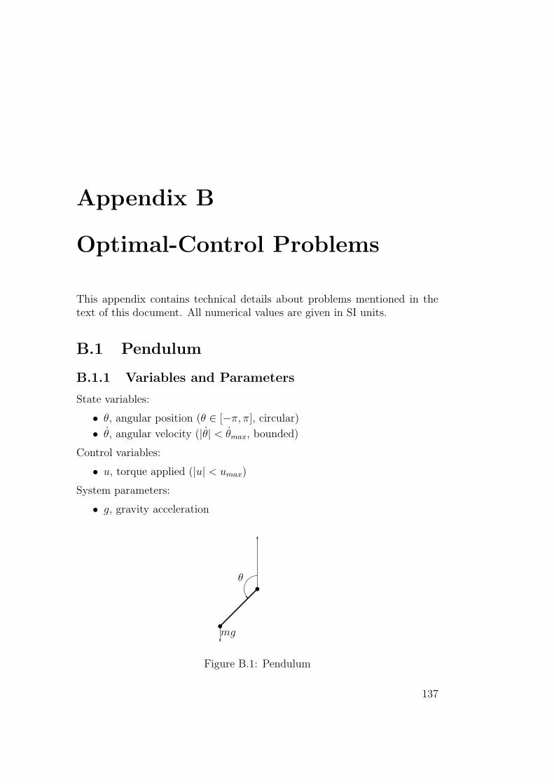
Appendix B
Optimal-Control Problems
This appendix contains technical details about problems mentioned in thetext of this document. All numerical values are given in SI units.
B.1 Pendulum
B.1.1 Variables and Parameters
State variables:
• θ, angular position (θ ∈ [−π, π], circular)
• θ, angular velocity (|θ| < θmax, bounded)
Control variables:
• u, torque applied (|u| < umax)
System parameters:
• g, gravity acceleration
θ
mg
b
b
Figure B.1: Pendulum
137
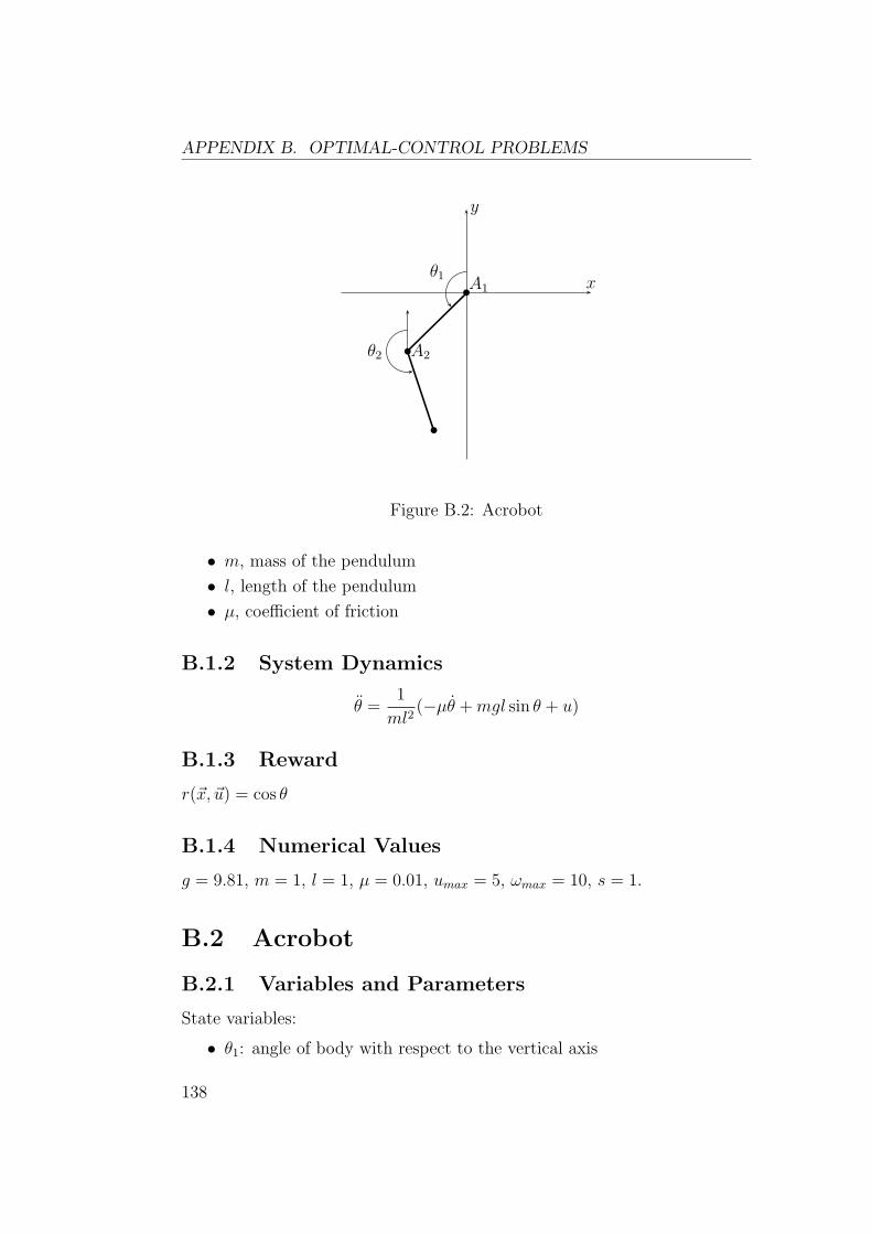
APPENDIX B. OPTIMAL-CONTROL PROBLEMS
x
y
θ1
θ2
A1
A2
b
b
b
Figure B.2: Acrobot
• m, mass of the pendulum
• l, length of the pendulum
• µ, coefficient of friction
B.1.2 System Dynamics
θ =1
ml2(−µθ + mgl sin θ + u)
B.1.3 Reward
r(~x, ~u) = cos θ
B.1.4 Numerical Values
g = 9.81, m = 1, l = 1, µ = 0.01, umax = 5, ωmax = 10, s = 1.
B.2 Acrobot
B.2.1 Variables and Parameters
State variables:
• θ1: angle of body with respect to the vertical axis
138
B.2. ACROBOT
• θ2: angle of legs with respect to the vertical axis
• θ1, θ2: their derivatives with respect to time
Control variable:
• u, torque applied to legs (|u| < umax)
Problem parameters:
• g: gravity acceleration
• m1: mass of acrobot body
• m2: mass of acrobot legs
• l1: half-length of body
• l2: half-length of legs
• µ1: friction coefficient of body
• µ2: friction coefficient of legs
B.2.2 System Dynamics
Let ~pi, ~vi and ~ai be the vectors defined for i in {1, 2} by
~pi =
(− sin θi
cos θi
)
,
~vi = ~pi =
(−θi cos θi
−θi sin θi
)
,
~ai = ~vi =
(θ2
i sin θi − θi cos θi
θ2i cos θi + θi sin θi
)
.
Let ~f1 be the force applied to hands and ~f2 the force applied by the body tolegs. Let G1 and G2 be the centers of mass of the two body parts. The lawsof mechanics can be written as
~f1 − ~f2 + m1~g = m1l1~a1,
~f2 −m2~g = m2(2l1~a1 + l2~a2),
l213
m1θ1 = det(−−−→G1A1, ~f1 + ~f2)− u− µ1θ1,
l223
m2θ2 = det(−−−→G2A2, ~f2) + u− µ2θ2.
139
APPENDIX B. OPTIMAL-CONTROL PROBLEMS
Since
det(−−−→G1A1,~a1) = −l1θ1
det(−−−→G2A2,~a2) = −l2θ2
det(−−−→G1A1,~a2) = l1
(θ22 sin(θ2 − θ1)− θ2 cos(θ1 − θ2)
)
det(−−−→G2A2,~a1) = l2
(θ21 sin(θ1 − θ2)− θ1 cos(θ2 − θ1)
)
these equations can be simplified into
(a11 a12
a21 a22
)(θ1
θ2
)
=
(b1
b2
)
,
with
a11 = (4
3m1 + 4m2)l
21,
a22 =4
3m2l
22,
a12 = a21 = 2m2l1l2 cos(θ1 − θ2),
b1 = 2m2l2l1θ22 sin(θ2 − θ1) + (m1 + 2m2)l1g sin θ1 − µ1θ1 − u,
b2 = 2m2l1l2θ21 sin(θ1 − θ2) + m2l2g sin θ2 − µ2θ2 + u.
B.2.3 Reward
r(~x, ~u) = l1 cos θ1 + l2 cos θ2
B.2.4 Numerical Values
m1 = m2 = 1, l1 = l2 = 0.5, µ1 = µ2 = 0.05, umax = 2
B.3 Cart-Pole
B.3.1 Variables and Parameters
State variables:
• x: cart position (|x| < L),
• θ: pole angle with respect to a vertical axis,
• x, θ: their derivatives with respect to time.
Control variable:
140
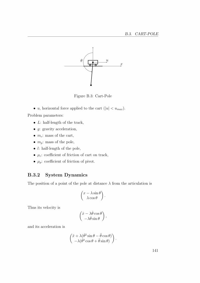
B.3. CART-POLE
ux
θ b
b
Figure B.3: Cart-Pole
• u, horizontal force applied to the cart (|u| < umax).
Problem parameters:
• L: half-length of the track,
• g: gravity acceleration,
• mc: mass of the cart,
• mp: mass of the pole,
• l: half-length of the pole,
• µc: coefficient of friction of cart on track,
• µp: coefficient of friction of pivot.
B.3.2 System Dynamics
The position of a point of the pole at distance λ from the articulation is
(x− λ sin θ
λ cos θ
)
.
Thus its velocity is(
x− λθ cos θ
−λθ sin θ
)
,
and its acceleration is
(x + λ(θ2 sin θ − θ cos θ)
−λ(θ2 cos θ + θ sin θ)
)
.
141
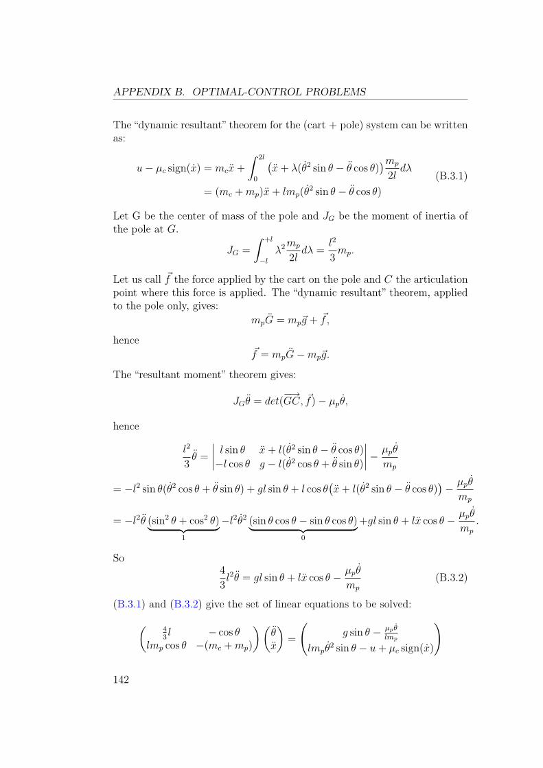
APPENDIX B. OPTIMAL-CONTROL PROBLEMS
The“dynamic resultant” theorem for the (cart + pole) system can be writtenas:
u− µc sign(x) = mcx +
∫ 2l
0
(x + λ(θ2 sin θ − θ cos θ)
)mp
2ldλ
= (mc + mp)x + lmp(θ2 sin θ − θ cos θ)
(B.3.1)
Let G be the center of mass of the pole and JG be the moment of inertia ofthe pole at G.
JG =
∫ +l
−l
λ2mp
2ldλ =
l2
3mp.
Let us call ~f the force applied by the cart on the pole and C the articulationpoint where this force is applied. The “dynamic resultant” theorem, appliedto the pole only, gives:
mpG = mp~g + ~f,
hence~f = mpG−mp~g.
The “resultant moment” theorem gives:
JGθ = det(−→GC, ~f)− µpθ,
hence
l2
3θ =
∣∣∣∣
l sin θ x + l(θ2 sin θ − θ cos θ)
−l cos θ g − l(θ2 cos θ + θ sin θ)
∣∣∣∣− µpθ
mp
= −l2 sin θ(θ2 cos θ + θ sin θ) + gl sin θ + l cos θ(x + l(θ2 sin θ − θ cos θ)
)− µpθ
mp
= −l2θ (sin2 θ + cos2 θ)︸ ︷︷ ︸
1
−l2θ2 (sin θ cos θ − sin θ cos θ)︸ ︷︷ ︸
0
+gl sin θ + lx cos θ − µpθ
mp
.
So4
3l2θ = gl sin θ + lx cos θ − µpθ
mp
(B.3.2)
(B.3.1) and (B.3.2) give the set of linear equations to be solved:
(43l − cos θ
lmp cos θ −(mc + mp)
)(
θx
)
=
(
g sin θ − µpθ
lmp
lmpθ2 sin θ − u + µc sign(x)
)
142
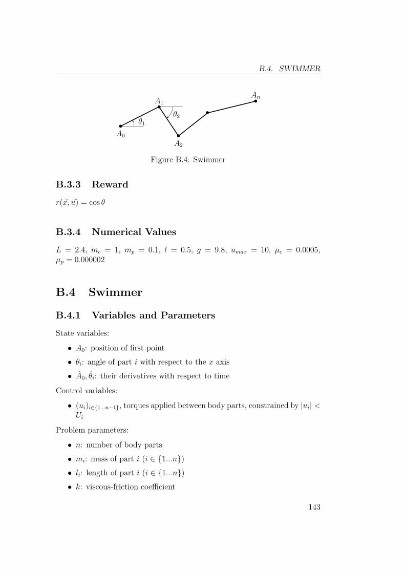
B.4. SWIMMER
A0
A1
A2
An
θ1
θ2
b
b
b
b
b
Figure B.4: Swimmer
B.3.3 Reward
r(~x, ~u) = cos θ
B.3.4 Numerical Values
L = 2.4, mc = 1, mp = 0.1, l = 0.5, g = 9.8, umax = 10, µc = 0.0005,µp = 0.000002
B.4 Swimmer
B.4.1 Variables and Parameters
State variables:
• A0: position of first point
• θi: angle of part i with respect to the x axis
• A0, θi: their derivatives with respect to time
Control variables:
• (ui)i∈{1...n−1}, torques applied between body parts, constrained by |ui| <Ui
Problem parameters:
• n: number of body parts
• mi: mass of part i (i ∈ {1...n})• li: length of part i (i ∈ {1...n})• k: viscous-friction coefficient
143
APPENDIX B. OPTIMAL-CONTROL PROBLEMS
B.4.2 Model of Viscous Friction
The model of viscous friction used consists in supposing that a small line oflength dλ with a normal vector ~n and moving at velocity ~v receives a smallforce of value d~F = −k(~v · ~n)~ndλ. Let us use this law of friction to calculatethe total force and moment applied to a moving part of the swimmer’s body.Let us call M a point of this body part at distance λ from the center of massGi = (Ai−1 + Ai)/2. M = Gi + λ~pi with
~pi =
(cos θi
sin θi
)
.
Besides, the normal vector is
~ni =
(− sin θi
cos θi
)
and ~pi = θi~ni, so M = Gi + λθi~ni. The total force is equal to
~Fi =
∫ li2
−li2
−k(M · ~ni)~nidλ
=
∫ li2
−li2
−k(Gi · ~ni)~nidλ +
∫ li2
−li2
−k(λθi~ni · ~ni)~nidλ
︸ ︷︷ ︸
0
= −kli(Gi · ~ni)~ni.
Let us now calculate the total moment at Gi:
Mi =
∫ li2
−li2
det(λ~pi,−k(M · ~ni)~nidλ
)
=
∫ li2
−li2
−k(M · ~ni)λdλ
=
∫ li2
−li2
−k(Gi · ~ni)λdλ
︸ ︷︷ ︸
0
+
∫ li2
−li2
−k(λθi~ni · ~ni)λdλ
= −kθil3i12
144
B.4. SWIMMER
B.4.3 System Dynamics
Let ~fi be the force applied by part i + 1 to part i.
∀i ∈ {1, . . . , n} − ~fi+1 + ~fi + ~Fi = miGi
These equations allow to express the ~fi’s as a function of state variables:
~f0 = ~0
∀i ∈ {1, . . . , n} ~fi = ~fi−1 − ~Fi + miGi
We end up with a set of n + 2 linear equations with n + 2 unknowns:
~fn = ~0,
mili12
θi = det(−−→GiAi, ~fi + ~fi−1) +Mi − ui + ui−1.
Unknowns are G0 (or any Gi) and all the θi’s. Solving this set of equationsgives state dynamics.
B.4.4 Reward
r(~x, ~u) = Gx (Gx is the abscissa of the center of mass)
B.4.5 Numerical Values
mi = 1, li = 1, k = 10, Ui = 5
145

Appendix C
The K1999 Path-OptimizationAlgorithm
This appendix is a description of the path-optimization algorithm that is usedin the K1999 car driver of the Robot Auto-Racing Simulator [71]. I wrote thisvery informal document to explain to other competitors how my car works,so it is probably not as formal as a serious research paper should be. Inparticular, no comparison is made with classical methods. This appendix issimply meant as an illustration of a method that is much more efficient thanreinforcement learning. K1999 won the 2000 and 2001 formula one seasons.
C.1 Basic Principle
C.1.1 Path
The path is approximated by a sequence of points (~xi)1≤i≤n. The curvatureci of the track at each point ~xi is computed as the inverse of the radius ofthe circumscribed circle for points ~xi−1, ~xi and ~xi+1. The formula is:
ci =2 det(~xi+1 − ~xi, ~xi−1 − ~xi)
‖~xi+1 − ~xi‖‖~xi−1 − ~xi‖‖~xi+1 − ~xi−1‖(C.1.1)
This curvature is positive for curves to the left and negative for curves tothe right. The (~xi)1≤i≤n points are initially set to be right in the middle ofthe track. The method consists in slowly modifying this path by repeatingalgorithm C.1 several times.
When (If ?) this algorithm has converged then the curvature of the pathvaries linearly except at points where it touches one side of the track. Notethat on the actual implementation, each ~xi is constrained to stay on a given
147

APPENDIX C. THE K1999 PATH-OPTIMIZATION ALGORITHM
Algorithm C.1 Basic algorithmfor i = 1 to n do
c1 ← ci−1
c2 ← ci+1
set ~xi at equal distance to ~xi+1 and ~xi−1 so that ci = 12(c1 + c2)
if ~xi is out of the track thenMove ~xi back onto the track
end ifend for
line that crosses the track. As a consequence, ~xi can not be set “at equaldistance to ~xi+1 and ~xi−1”. ci = 1
2(c1 + c2) is replaced by a sum weighted by
distance.
C.1.2 Speed Profile
Once the path has been computed, the target speed vi all along this path canbe obtained by supposing that acceleration is limited by tyre grip to havinga norm inferior to a0. This is done in two passes. First, si is initialized withan “instantaneous” maximum speed with algorithm C.2 (ε is a small enoughpositive constant). Then, algorithm C.3 consists in anticipating braking.This second pass is iterated a dozen times so that it reaches convergence. Iam not particularaly happy by this technique, but it works. A more cleversolution could be found that does not need iteration at all. But it does notmatter much since it is very fast and gives good results.
Algorithm C.2 Pass 1for i = 1 to n do
if |ci| > ε thensi ←
√
a0/|ci|else
si ←√
a0/εend if
end for
148
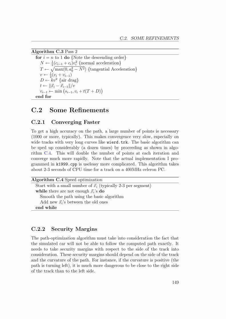
C.2. SOME REFINEMENTS
Algorithm C.3 Pass 2
for i = n to 1 do {Note the descending order}N ← 1
2(ci−1 + ci)v
2i {normal acceleration}
T ←√
max(0, a20 −N2) {tangential Acceleration}
v ← 12(vi + vi−1)
D ← kv2 {air drag}t← ‖~xi − ~xi−1‖/vvi−1 ← min
(si−1, vi + t(T + D)
)
end for
C.2 Some Refinements
C.2.1 Converging Faster
To get a high accuracy on the path, a large number of points is necessary(1000 or more, typically). This makes convergence very slow, especially onwide tracks with very long curves like wierd.trk. The basic algorithm canbe sped up considerably (a dozen times) by proceeding as shown in algo-rithm C.4. This will double the number of points at each iteration andconverge much more rapidly. Note that the actual implementation I pro-grammed in k1999.cpp is uselessy more complicated. This algorithm takesabout 2-3 seconds of CPU time for a track on a 400MHz celeron PC.
Algorithm C.4 Speed optimization
Start with a small number of ~xi (typically 2-3 per segment)while there are not enough ~xi’s do
Smooth the path using the basic algorithmAdd new ~xi’s between the old ones
end while
C.2.2 Security Margins
The path-optimization algorithm must take into consideration the fact thatthe simulated car will not be able to follow the computed path exactly. Itneeds to take security margins with respect to the side of the track intoconsideration. These security margins should depend on the side of the trackand the curvature of the path. For instance, if the curvature is positive (thepath is turning left), it is much more dangerous to be close to the right sideof the track than to the left side.
149
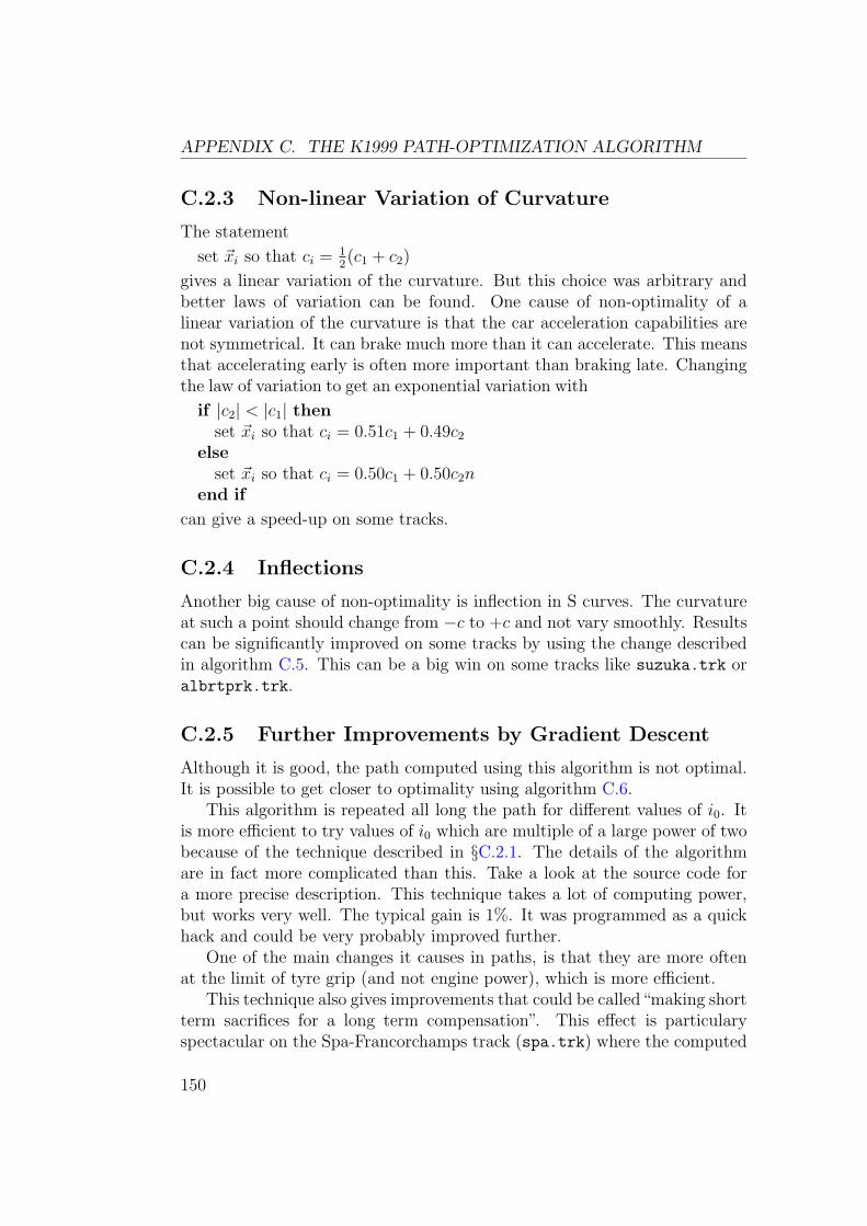
APPENDIX C. THE K1999 PATH-OPTIMIZATION ALGORITHM
C.2.3 Non-linear Variation of Curvature
The statement
set ~xi so that ci = 12(c1 + c2)
gives a linear variation of the curvature. But this choice was arbitrary andbetter laws of variation can be found. One cause of non-optimality of alinear variation of the curvature is that the car acceleration capabilities arenot symmetrical. It can brake much more than it can accelerate. This meansthat accelerating early is often more important than braking late. Changingthe law of variation to get an exponential variation with
if |c2| < |c1| thenset ~xi so that ci = 0.51c1 + 0.49c2
elseset ~xi so that ci = 0.50c1 + 0.50c2n
end if
can give a speed-up on some tracks.
C.2.4 Inflections
Another big cause of non-optimality is inflection in S curves. The curvatureat such a point should change from −c to +c and not vary smoothly. Resultscan be significantly improved on some tracks by using the change describedin algorithm C.5. This can be a big win on some tracks like suzuka.trk oralbrtprk.trk.
C.2.5 Further Improvements by Gradient Descent
Although it is good, the path computed using this algorithm is not optimal.It is possible to get closer to optimality using algorithm C.6.
This algorithm is repeated all long the path for different values of i0. Itis more efficient to try values of i0 which are multiple of a large power of twobecause of the technique described in §C.2.1. The details of the algorithmare in fact more complicated than this. Take a look at the source code fora more precise description. This technique takes a lot of computing power,but works very well. The typical gain is 1%. It was programmed as a quickhack and could be very probably improved further.
One of the main changes it causes in paths, is that they are more oftenat the limit of tyre grip (and not engine power), which is more efficient.
This technique also gives improvements that could be called“making shortterm sacrifices for a long term compensation”. This effect is particularyspectacular on the Spa-Francorchamps track (spa.trk) where the computed
150

C.2. SOME REFINEMENTS
Algorithm C.5 Inflectionsfor i = 1 to n do
c1 ← ci−1
c2 ← ci+1
if c1c2 < 0 thenc0 ← ci−2
c3 ← ci+2
if c0c1 > 0 and c2c3 > 0 thenif |c1| < |c2| and |c1| < |c3| then
c1 ← −c1
elseif |c2| < |c1| and |c2| < |c0| then
c2 ← −c2
end ifend if
end ifend ifset ~xi at equal distance to ~xi+1 and ~xi−1 so that ci = 1
2(c1 + c2)
if ~xi is out of the track thenMove ~xi back onto the track
end ifend for
Algorithm C.6 Rough and Badly Written Principle of Gradient Descent
Choose an index i0 and a fixed value for ~xi0
Run the standard algorithm without changing ~xi0
Estimate the lap time for this pathChange ~xi0 a littleRun the standard algorithm again and estimate the new lap timewhile It is an improvement do
Continue moving ~xi0 in the same directionend while
151
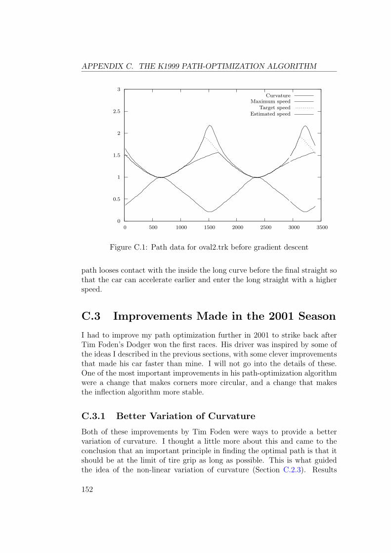
APPENDIX C. THE K1999 PATH-OPTIMIZATION ALGORITHM
0
0.5
1
1.5
2
2.5
3
0 500 1000 1500 2000 2500 3000 3500
CurvatureMaximum speed
Target speedEstimated speed
Figure C.1: Path data for oval2.trk before gradient descent
path looses contact with the inside the long curve before the final straight sothat the car can accelerate earlier and enter the long straight with a higherspeed.
C.3 Improvements Made in the 2001 Season
I had to improve my path optimization further in 2001 to strike back afterTim Foden’s Dodger won the first races. His driver was inspired by some ofthe ideas I described in the previous sections, with some clever improvementsthat made his car faster than mine. I will not go into the details of these.One of the most important improvements in his path-optimization algorithmwere a change that makes corners more circular, and a change that makesthe inflection algorithm more stable.
C.3.1 Better Variation of Curvature
Both of these improvements by Tim Foden were ways to provide a bettervariation of curvature. I thought a little more about this and came to theconclusion that an important principle in finding the optimal path is that itshould be at the limit of tire grip as long as possible. This is what guidedthe idea of the non-linear variation of curvature (Section C.2.3). Results
152
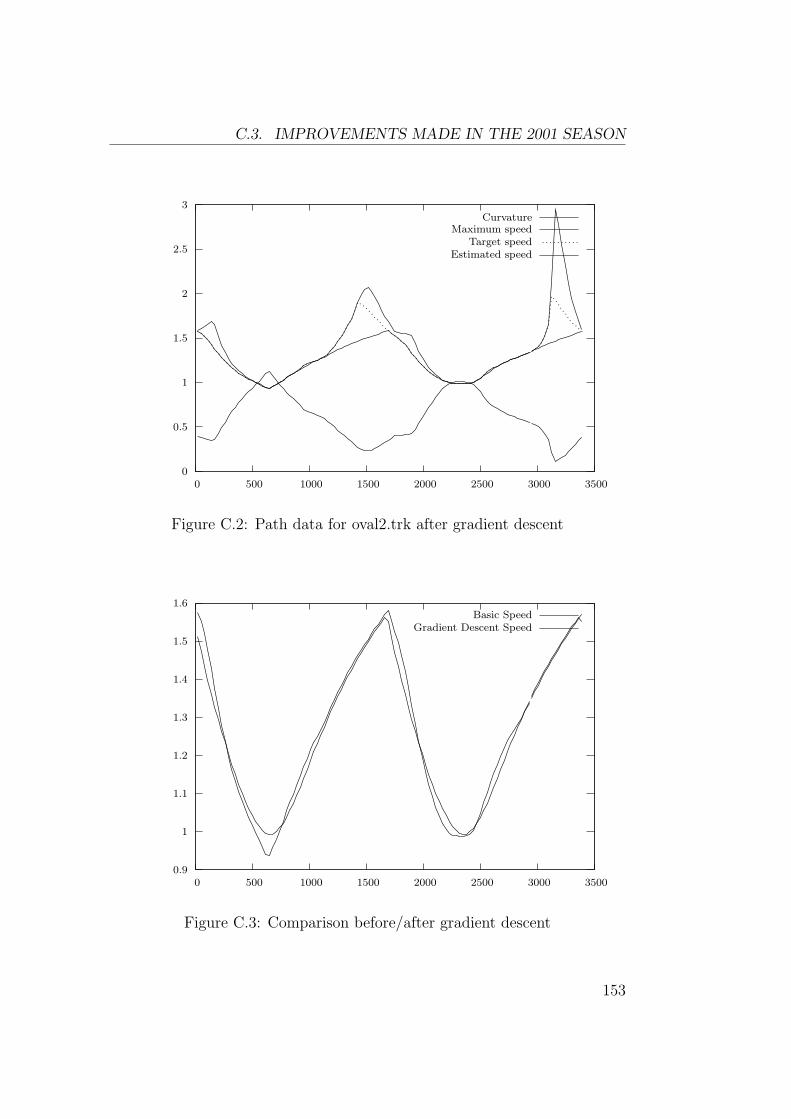
C.3. IMPROVEMENTS MADE IN THE 2001 SEASON
0
0.5
1
1.5
2
2.5
3
0 500 1000 1500 2000 2500 3000 3500
CurvatureMaximum speed
Target speedEstimated speed
Figure C.2: Path data for oval2.trk after gradient descent
0.9
1
1.1
1.2
1.3
1.4
1.5
1.6
0 500 1000 1500 2000 2500 3000 3500
Basic SpeedGradient Descent Speed
Figure C.3: Comparison before/after gradient descent
153
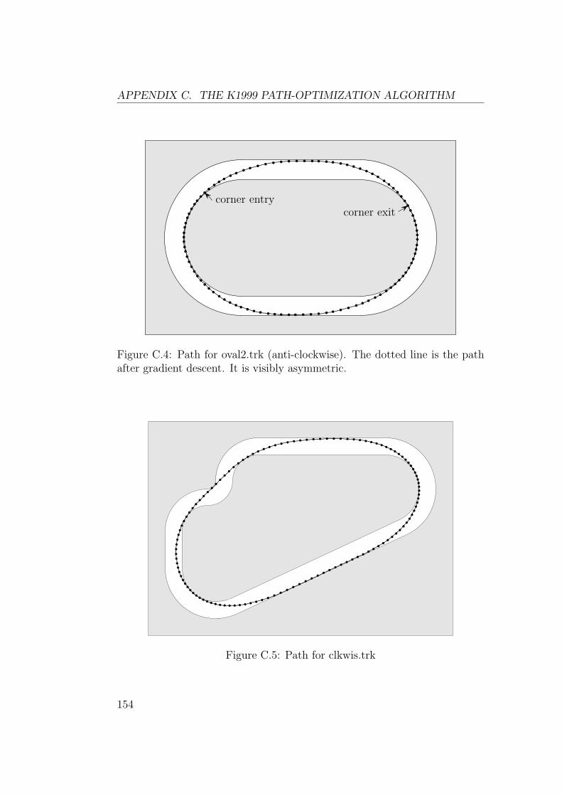
APPENDIX C. THE K1999 PATH-OPTIMIZATION ALGORITHM
b b b b b b b b b b b b b bb
bb
bb
bbbbbbbb
bb
bbb
bbb
bb
b
b
bb
bb
bb
bb
bb
bbbbbbbbbbbbbbb
bb
bb
bb
bb
bb
bb
b
bb
bb
bbb
bb
b
b
b
bbbbbb
bb
bbb
corner exitcorner entry
Figure C.4: Path for oval2.trk (anti-clockwise). The dotted line is the pathafter gradient descent. It is visibly asymmetric.
bb
b b b b b b b b b b b b b b b b b bbbbbbbbbbbbbbbbbbbbbb
bb
bb
bb
bb
bb
bb
bb
bb
bb
bb
bb
bb
bb
bb
bbbbbbbbbbbb
bb
bb
bb
bbbb
b
b
b
b
b
b
b
b
b
b
b
b
b
bbbbbbbb
b
bb
bb
bb
b
Figure C.5: Path for clkwis.trk
154
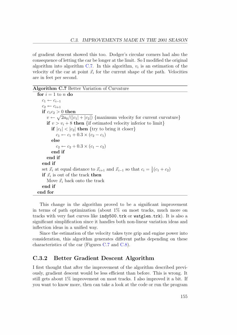
C.3. IMPROVEMENTS MADE IN THE 2001 SEASON
of gradient descent showed this too. Dodger’s circular corners had also theconsequence of letting the car be longer at the limit. So I modified the originalalgorithm into algorithm C.7. In this algorithm, vi is an estimation of thevelocity of the car at point ~xi for the current shape of the path. Velocitiesare in feet per second.
Algorithm C.7 Better Variation of Curvaturefor i = 1 to n do
c1 ← ci−1
c2 ← ci+1
if c1c2 > 0 thenv ←
√
2a0/(|c1|+ |c2|) {maximum velocity for current curvature}if v > vi + 8 then {if estimated velocity inferior to limit}
if |c1| < |c2| then {try to bring it closer}c1 ← c1 + 0.3× (c2 − c1)
elsec2 ← c2 + 0.3× (c1 − c2)
end ifend if
end ifset ~xi at equal distance to ~xi+1 and ~xi−1 so that ci = 1
2(c1 + c2)
if ~xi is out of the track thenMove ~xi back onto the track
end ifend for
This change in the algorithm proved to be a significant improvementin terms of path optimization (about 1% on most tracks, much more ontracks with very fast curves like indy500.trk or watglen.trk). It is also asignificant simplification since it handles both non-linear variation ideas andinflection ideas in a unified way.
Since the estimation of the velocity takes tyre grip and engine power intoconsideration, this algorithm generates different paths depending on thesecharacteristics of the car (Figures C.7 and C.8).
C.3.2 Better Gradient Descent Algorithm
I first thought that after the improvement of the algorithm described previ-ously, gradient descent would be less efficient than before. This is wrong. Itstill gets about 1% improvement on most tracks. I also improved it a bit. Ifyou want to know more, then can take a look at the code or run the program
155
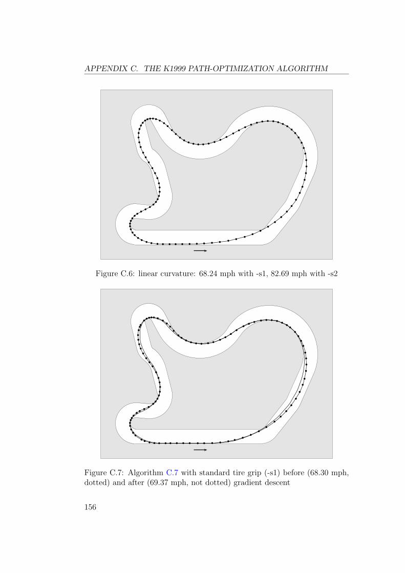
APPENDIX C. THE K1999 PATH-OPTIMIZATION ALGORITHM
bb
b b b b b b b b b b b b bb
bb
b
b
b
b
b
b
b
b
b
b
b
b
b
b
b
b
b
b
bb
bbbbbb
bb
bb
bb
bbbbb
bb
b
b
b
bb
bbbbbb
bb
b
b
b
b
b
b
b
b
b
b
b
b
b
b
bbb
bb
bb
bb
bbbbbbb
Figure C.6: linear curvature: 68.24 mph with -s1, 82.69 mph with -s2
bb b b b b b b b b b b b b b b
bb
b
b
b
b
b
b
b
b
b
b
b
b
b
b
b
b
b
b
bb
bbbbb
bb
b
b
bb
bbbbbb
bb
b
b
bb
bbbbbb
b
bb
b
b
b
b
b
b
b
b
b
b
b
b
b
b
bb
bb
bb
bb
bbbbb
bbb
Figure C.7: Algorithm C.7 with standard tire grip (-s1) before (68.30 mph,dotted) and after (69.37 mph, not dotted) gradient descent
156
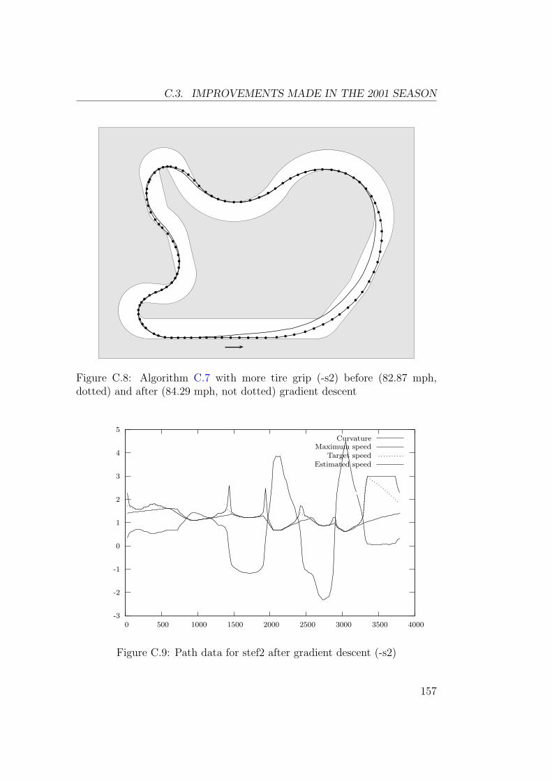
C.3. IMPROVEMENTS MADE IN THE 2001 SEASON
b b b b b b b b b b b b b b b b b b bb
bb
b
b
b
b
b
b
b
b
b
b
b
b
b
b
b
b
bb
bbbbb
bb
b
b
bb
bbbbb
bb
b
b
b
bb
bbbbb
b
bb
bb
b
b
b
bbb
b
b
b
b
b
b
bb
bb
bb
bb
bb
bb
b
bb
Figure C.8: Algorithm C.7 with more tire grip (-s2) before (82.87 mph,dotted) and after (84.29 mph, not dotted) gradient descent
-3
-2
-1
0
1
2
3
4
5
0 500 1000 1500 2000 2500 3000 3500 4000
CurvatureMaximum speed
Target speedEstimated speed
Figure C.9: Path data for stef2 after gradient descent (-s2)
157
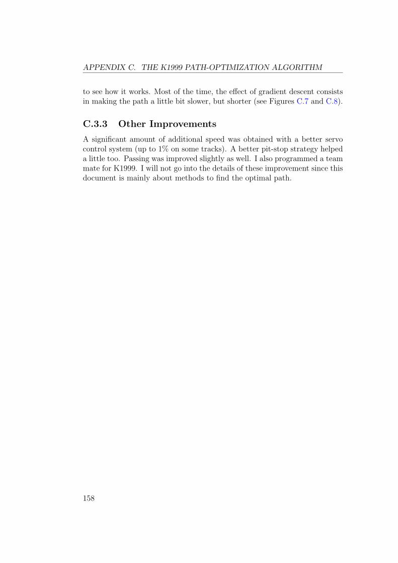
APPENDIX C. THE K1999 PATH-OPTIMIZATION ALGORITHM
to see how it works. Most of the time, the effect of gradient descent consistsin making the path a little bit slower, but shorter (see Figures C.7 and C.8).
C.3.3 Other Improvements
A significant amount of additional speed was obtained with a better servocontrol system (up to 1% on some tracks). A better pit-stop strategy helpeda little too. Passing was improved slightly as well. I also programmed a teammate for K1999. I will not go into the details of these improvement since thisdocument is mainly about methods to find the optimal path.
158
Bibliography
[1] James S. Albus. A new approach to manipulator control: The cere-bellar model articulation controller (CMAC). In Journal of DynamicSystems, Measurement and Control, pages 220–227. American Societyof Mechanical Engineers, September 1975.
[2] Charles W. Anderson. Strategy learning with multilayer connectionistrepresentations. In Proceedings of the Fourth International Workshop onMachine Learning, pages 103–114, Irvine, CA, 1987. Morgan Kaufmann.
[3] Charles W. Anderson. Approximating a policy can be easier than ap-proximating a value function. Technical Report CS-00-101, ColoradoState University, 2000.
[4] Christopher G. Atkeson. Using local trajectory optimizers to speedup global optimization in dynamic programming. In J. D. Cowan,G. Tesauro, and J. Alspector, editors, Advances in Neural InformationProcessing Systems 6. Morgan Kaufmann, 1994.
[5] Christopher G. Atkeson and Juan Carlos Santamarıa. A comparison ofdirect and model-based reinforcement learning. In International Con-ference on Robotics and Automation, 1997.
[6] Leemon C. Baird. Advantage updating. Technical Report WL-TR-93-1146, Wright-Patterson Air Force Base Ohio: Wright Laboratory, 1993.Available from the Defense Technical Information Center, Cameron Sta-tion, Alexandria, VA 22304-6145.
[7] Leemon C. Baird. Residual algorithms: Reinforcement learning withfunction approximation. In Machine Learning: Proceedings of theTwelfth International Conference. Morgan Kaufman, 1995.
[8] Leemon C. Baird and A. Harry Klopf. Reinforcement learning with high-dimensional, continuous actions. Technical Report WL-TR-93-1147,
159
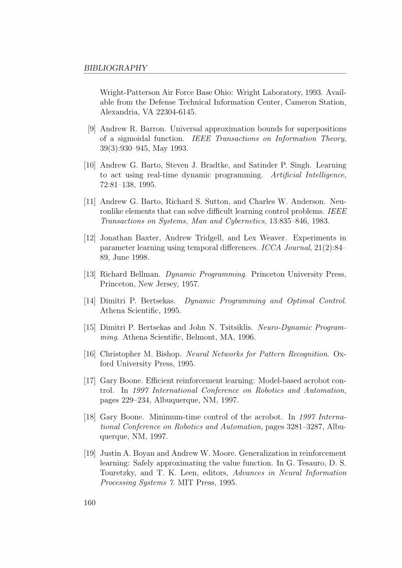
BIBLIOGRAPHY
Wright-Patterson Air Force Base Ohio: Wright Laboratory, 1993. Avail-able from the Defense Technical Information Center, Cameron Station,Alexandria, VA 22304-6145.
[9] Andrew R. Barron. Universal approximation bounds for superpositionsof a sigmoidal function. IEEE Transactions on Information Theory,39(3):930–945, May 1993.
[10] Andrew G. Barto, Steven J. Bradtke, and Satinder P. Singh. Learningto act using real-time dynamic programming. Artificial Intelligence,72:81–138, 1995.
[11] Andrew G. Barto, Richard S. Sutton, and Charles W. Anderson. Neu-ronlike elements that can solve difficult learning control problems. IEEETransactions on Systems, Man and Cybernetics, 13:835–846, 1983.
[12] Jonathan Baxter, Andrew Tridgell, and Lex Weaver. Experiments inparameter learning using temporal differences. ICCA Journal, 21(2):84–89, June 1998.
[13] Richard Bellman. Dynamic Programming. Princeton University Press,Princeton, New Jersey, 1957.
[14] Dimitri P. Bertsekas. Dynamic Programming and Optimal Control.Athena Scientific, 1995.
[15] Dimitri P. Bertsekas and John N. Tsitsiklis. Neuro-Dynamic Program-ming. Athena Scientific, Belmont, MA, 1996.
[16] Christopher M. Bishop. Neural Networks for Pattern Recognition. Ox-ford University Press, 1995.
[17] Gary Boone. Efficient reinforcement learning: Model-based acrobot con-trol. In 1997 International Conference on Robotics and Automation,pages 229–234, Albuquerque, NM, 1997.
[18] Gary Boone. Minimum-time control of the acrobot. In 1997 Interna-tional Conference on Robotics and Automation, pages 3281–3287, Albu-querque, NM, 1997.
[19] Justin A. Boyan and Andrew W. Moore. Generalization in reinforcementlearning: Safely approximating the value function. In G. Tesauro, D. S.Touretzky, and T. K. Leen, editors, Advances in Neural InformationProcessing Systems 7. MIT Press, 1995.
160
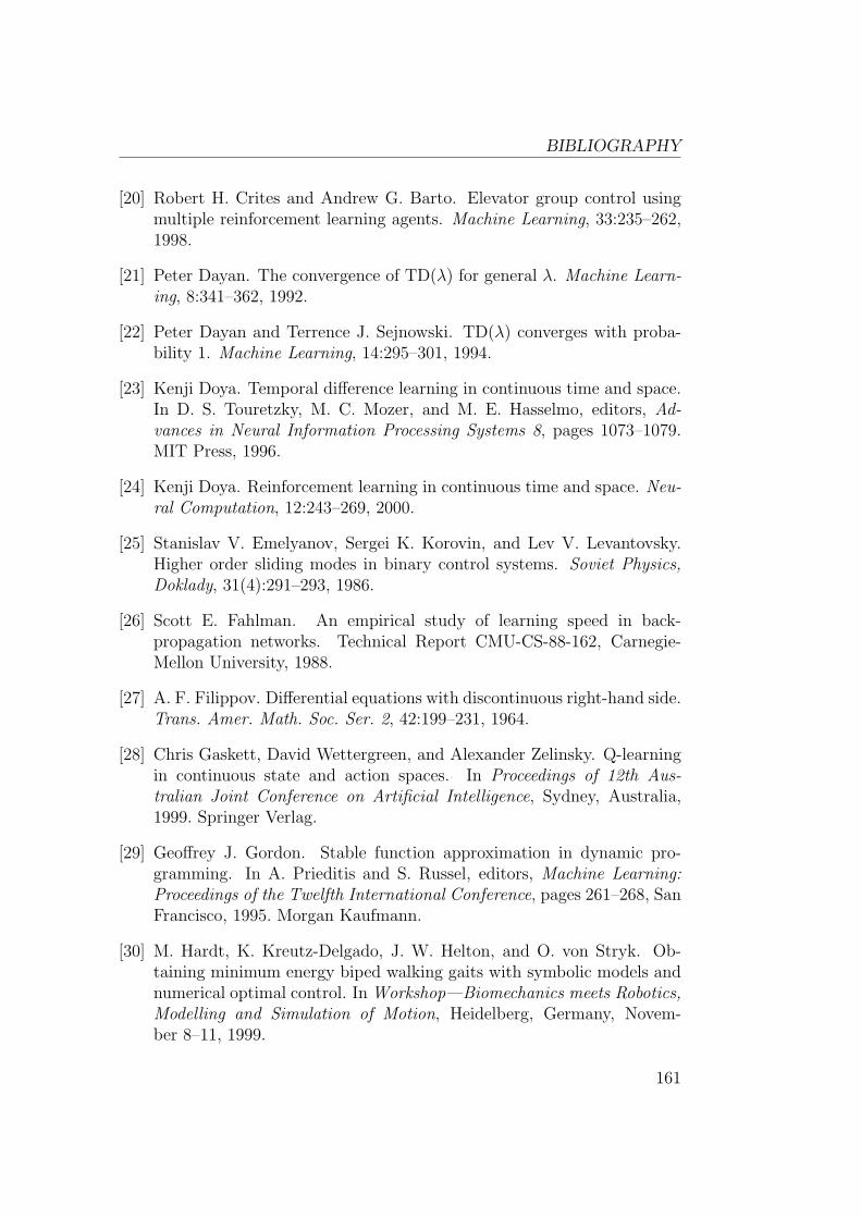
BIBLIOGRAPHY
[20] Robert H. Crites and Andrew G. Barto. Elevator group control usingmultiple reinforcement learning agents. Machine Learning, 33:235–262,1998.
[21] Peter Dayan. The convergence of TD(λ) for general λ. Machine Learn-ing, 8:341–362, 1992.
[22] Peter Dayan and Terrence J. Sejnowski. TD(λ) converges with proba-bility 1. Machine Learning, 14:295–301, 1994.
[23] Kenji Doya. Temporal difference learning in continuous time and space.In D. S. Touretzky, M. C. Mozer, and M. E. Hasselmo, editors, Ad-vances in Neural Information Processing Systems 8, pages 1073–1079.MIT Press, 1996.
[24] Kenji Doya. Reinforcement learning in continuous time and space. Neu-ral Computation, 12:243–269, 2000.
[25] Stanislav V. Emelyanov, Sergei K. Korovin, and Lev V. Levantovsky.Higher order sliding modes in binary control systems. Soviet Physics,Doklady, 31(4):291–293, 1986.
[26] Scott E. Fahlman. An empirical study of learning speed in back-propagation networks. Technical Report CMU-CS-88-162, Carnegie-Mellon University, 1988.
[27] A. F. Filippov. Differential equations with discontinuous right-hand side.Trans. Amer. Math. Soc. Ser. 2, 42:199–231, 1964.
[28] Chris Gaskett, David Wettergreen, and Alexander Zelinsky. Q-learningin continuous state and action spaces. In Proceedings of 12th Aus-tralian Joint Conference on Artificial Intelligence, Sydney, Australia,1999. Springer Verlag.
[29] Geoffrey J. Gordon. Stable function approximation in dynamic pro-gramming. In A. Prieditis and S. Russel, editors, Machine Learning:Proceedings of the Twelfth International Conference, pages 261–268, SanFrancisco, 1995. Morgan Kaufmann.
[30] M. Hardt, K. Kreutz-Delgado, J. W. Helton, and O. von Stryk. Ob-taining minimum energy biped walking gaits with symbolic models andnumerical optimal control. In Workshop—Biomechanics meets Robotics,Modelling and Simulation of Motion, Heidelberg, Germany, Novem-ber 8–11, 1999.
161
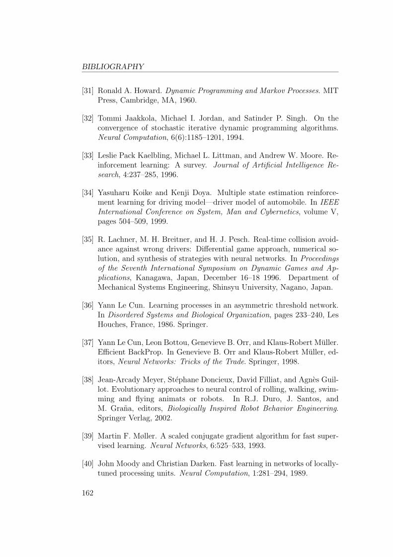
BIBLIOGRAPHY
[31] Ronald A. Howard. Dynamic Programming and Markov Processes. MITPress, Cambridge, MA, 1960.
[32] Tommi Jaakkola, Michael I. Jordan, and Satinder P. Singh. On theconvergence of stochastic iterative dynamic programming algorithms.Neural Computation, 6(6):1185–1201, 1994.
[33] Leslie Pack Kaelbling, Michael L. Littman, and Andrew W. Moore. Re-inforcement learning: A survey. Journal of Artificial Intelligence Re-search, 4:237–285, 1996.
[34] Yasuharu Koike and Kenji Doya. Multiple state estimation reinforce-ment learning for driving model—driver model of automobile. In IEEEInternational Conference on System, Man and Cybernetics, volume V,pages 504–509, 1999.
[35] R. Lachner, M. H. Breitner, and H. J. Pesch. Real-time collision avoid-ance against wrong drivers: Differential game approach, numerical so-lution, and synthesis of strategies with neural networks. In Proceedingsof the Seventh International Symposium on Dynamic Games and Ap-plications, Kanagawa, Japan, December 16–18 1996. Department ofMechanical Systems Engineering, Shinsyu University, Nagano, Japan.
[36] Yann Le Cun. Learning processes in an asymmetric threshold network.In Disordered Systems and Biological Organization, pages 233–240, LesHouches, France, 1986. Springer.
[37] Yann Le Cun, Leon Bottou, Genevieve B. Orr, and Klaus-Robert Muller.Efficient BackProp. In Genevieve B. Orr and Klaus-Robert Muller, ed-itors, Neural Networks: Tricks of the Trade. Springer, 1998.
[38] Jean-Arcady Meyer, Stephane Doncieux, David Filliat, and Agnes Guil-lot. Evolutionary approaches to neural control of rolling, walking, swim-ming and flying animats or robots. In R.J. Duro, J. Santos, andM. Grana, editors, Biologically Inspired Robot Behavior Engineering.Springer Verlag, 2002.
[39] Martin F. Møller. A scaled conjugate gradient algorithm for fast super-vised learning. Neural Networks, 6:525–533, 1993.
[40] John Moody and Christian Darken. Fast learning in networks of locally-tuned processing units. Neural Computation, 1:281–294, 1989.
162
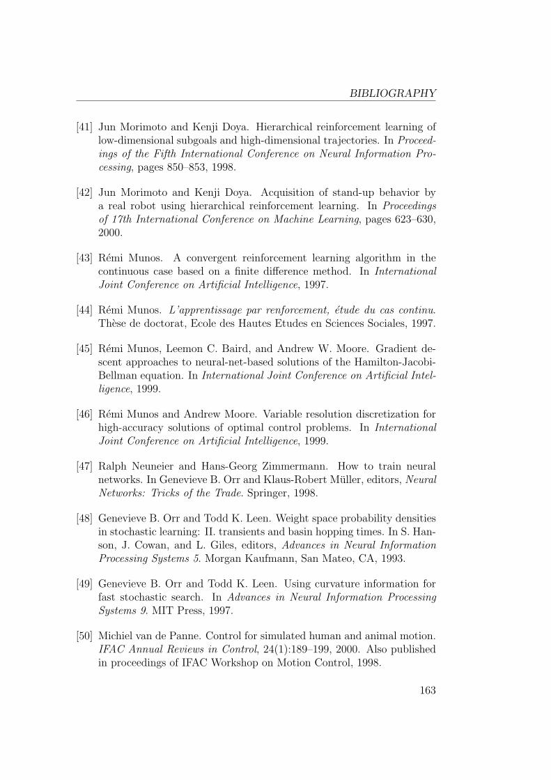
BIBLIOGRAPHY
[41] Jun Morimoto and Kenji Doya. Hierarchical reinforcement learning oflow-dimensional subgoals and high-dimensional trajectories. In Proceed-ings of the Fifth International Conference on Neural Information Pro-cessing, pages 850–853, 1998.
[42] Jun Morimoto and Kenji Doya. Acquisition of stand-up behavior bya real robot using hierarchical reinforcement learning. In Proceedingsof 17th International Conference on Machine Learning, pages 623–630,2000.
[43] Remi Munos. A convergent reinforcement learning algorithm in thecontinuous case based on a finite difference method. In InternationalJoint Conference on Artificial Intelligence, 1997.
[44] Remi Munos. L’apprentissage par renforcement, etude du cas continu.These de doctorat, Ecole des Hautes Etudes en Sciences Sociales, 1997.
[45] Remi Munos, Leemon C. Baird, and Andrew W. Moore. Gradient de-scent approaches to neural-net-based solutions of the Hamilton-Jacobi-Bellman equation. In International Joint Conference on Artificial Intel-ligence, 1999.
[46] Remi Munos and Andrew Moore. Variable resolution discretization forhigh-accuracy solutions of optimal control problems. In InternationalJoint Conference on Artificial Intelligence, 1999.
[47] Ralph Neuneier and Hans-Georg Zimmermann. How to train neuralnetworks. In Genevieve B. Orr and Klaus-Robert Muller, editors, NeuralNetworks: Tricks of the Trade. Springer, 1998.
[48] Genevieve B. Orr and Todd K. Leen. Weight space probability densitiesin stochastic learning: II. transients and basin hopping times. In S. Han-son, J. Cowan, and L. Giles, editors, Advances in Neural InformationProcessing Systems 5. Morgan Kaufmann, San Mateo, CA, 1993.
[49] Genevieve B. Orr and Todd K. Leen. Using curvature information forfast stochastic search. In Advances in Neural Information ProcessingSystems 9. MIT Press, 1997.
[50] Michiel van de Panne. Control for simulated human and animal motion.IFAC Annual Reviews in Control, 24(1):189–199, 2000. Also publishedin proceedings of IFAC Workshop on Motion Control, 1998.
163
BIBLIOGRAPHY
[51] Stefan Pareigis. Adaptive choice of grid and time in reinforcement learn-ing. In M. I. Jordan, M. J. Kearns, and S. A. Solla, editors, Advancesin Neural Information Processing Systems 10, pages 1036–1042. MITPress, Cambrdige, MA, 1998.
[52] Barak A. Pearlmutter. Fast exact multiplication by the Hessian. NeuralComputation, 6:147–160, 1994.
[53] William H. Press, Saul A. Teukolsky, William T. Vetterling, and Brian P.Flannery. Numerical Recipes in C—The Art of Scientific Computing.Cambridge University Press, 1992.
[54] Jette Randløv and Preben Alstrøm. Learning to drive a bicycle usingreinforcement learning and shaping. In Machine Learning: Proceedingsof the Fifteenth International Conference (ICML’98). MIT Press, 1998.
[55] Martin Riedmiller and Heinrich Braun. A direct adaptive method forfaster backpropagation learning: The RPROP algorithm. In Proceedingsof the IEEE International Conference on Neural Networks, 1993.
[56] D. E. Rumelhart, G. E. Hinton, and R. J. Williams. Learning inter-nal representations by error propagation. In D. E. Rumelhart and J. L.McClelland, editors, Parallel Distributed Processing: Explorations in theMicrostructure of Cognition, volume 1, pages 318–362. MIT Press, Cam-bridge, MA, 1986.
[57] Juan Carlos Santamarıa, Richard S. Sutton, and Ashwin Ram. Exper-iments with reinforcement learning in problems with continuous stateand action spaces. Adaptive Behavior, 6(2):163–218, 1998.
[58] Warren S. Sarle, editor. Neural Network FAQ. Available via anonymousftp from ftp://ftp.sas.com/pub/neural/FAQ.html, 1997. Periodicposting to the usenet newsgroup comp.ai.neural-nets.
[59] Stefan Schaal and Christopher G. Atkeson. Robot juggling: An imple-mentation of memory-based learning. Control Systems Magazine, 14:57–71, 1994.
[60] Nicol N. Schraudolph. Local gain adaptation in stochastic gradient de-scent. In Proceedings of the 9th International Conference on ArtificialNeural Networks, London, 1999. IEE.
[61] Jonathan Richard Shewchuk. An introduction to the conjugate gradientmethod without the agonizing pain, August 1994. Available on theWorld Wide Web at http://www.cs.cmu.edu/~jrs/jrspapers.html.
164
BIBLIOGRAPHY
[62] Karl Sims. Evolving 3D morphology and behavior by competition. InR. Brooks and P. Maes, editors, Artificial Life IV Proceedings, pages28–39. MIT Press, 1994.
[63] Karl Sims. Evolving virtual creatures. In Computer Graphics, AnnualConference Series, (SIGGRAPH ’94 Proceedings), pages 15–22, July1994.
[64] Russel L. Smith. Intelligent Motion Control with an Artificial Cerebel-lum. PhD thesis, University of Auckland, New Zealand, July 1998.
[65] Mark Spong. The swingup control problem for the acrobot. IEEE Con-trol Systems Magazine, 15(1):49–55, February 1995.
[66] Richard S. Sutton. Learning to predict by the methods of temporaldifferences. Machine Learning, 3:9–44, 1988.
[67] Richard S. Sutton. Generalization in reinforcement learning: Successfulexamples using sparse coarse coding. In Advances in Neural InformationProcessing Systems 8, pages 1038–1044. MIT Press, 1996.
[68] Richard S. Sutton and Andrew G. Barto. Reinforcement Learning: AnIntroduction. MIT Press, Cambridge, MA, 1998.
[69] Richard S. Sutton, David McAllester, Satinder Singh, and Yishay Man-sour. Policy gradient methods for reinforcement learning with functionapproximation. In Advances in Neural Information Processing Systems12. MIT Press, 1999.
[70] Gerald Tesauro. Temporal difference learning and TD-Gammon. Com-munications of the ACM, 38(3):58–68, March 1995.
[71] Mitchell E. Timin. The robot auto racing simulator, 1995.http://rars.sourceforge.net/.
[72] John N. Tsitsiklis. On the convergence of optimistic policy iteration.Journal of Machine Learning Research, 3:59–72, July 2002.
[73] John N. Tsitsiklis and Benjamin Van Roy. Feature-based methods forlarge scale dynamic programming. Machine Learning, 22:59–94, 1996.
[74] John N. Tsitsiklis and Benjamin Van Roy. An analysis of temporal-difference learning with function approximation. IEEE Transactions onAutomatic Control, 42(5):674–690, May 1997.
165
BIBLIOGRAPHY
[75] Vladimir N. Vapnik. The Nature of Statistical Learning Theory.Springer, 1995.
[76] Thomas L. Vincent and Walter J. Grantham. Nonlinear and OptimalControl Systems. Wiley, 1997.
[77] Scott E. Weaver, Leemon C. Baird, and Marios M. Polycarpou. Ananalytical framework for local feedforward networks. IEEE Transactionson Neural Networks, 9(3):473–482, 1998. Also published as Univeristyof Cincinnati Technical Report TR 195/07/96/ECECS.
[78] Scott E. Weaver, Leemon C. Baird, and Marios M. Polycarpou. Pre-venting unlearning during on-line training of feedforward networks. InProceedings of the International Symposium of Intelligent Control, 1998.
[79] Norbert Wiener. Cybernetics or Control and Communication in theAnimal and the Machine. Hermann, 1948.
[80] Junichiro Yoshimoto, Shin Ishii, and Masa-aki Sato. Application of rein-forcement learning to balancing of acrobot. In 1999 IEEE InternationalConference on Systems, Man and Cybernetics, volume V, pages 516–521,1999.
[81] Wei Zhang and Thomas G. Dietterich. High-performance job-shopscheduling with a time-delay TD(λ) network. In D. S. Touretzky, M. C.Mozer, and M. E. Hasselmo, editors, Advances in Neural InformationProcessing Systems 8, pages 1024–1030. MIT Press, 1996.
166

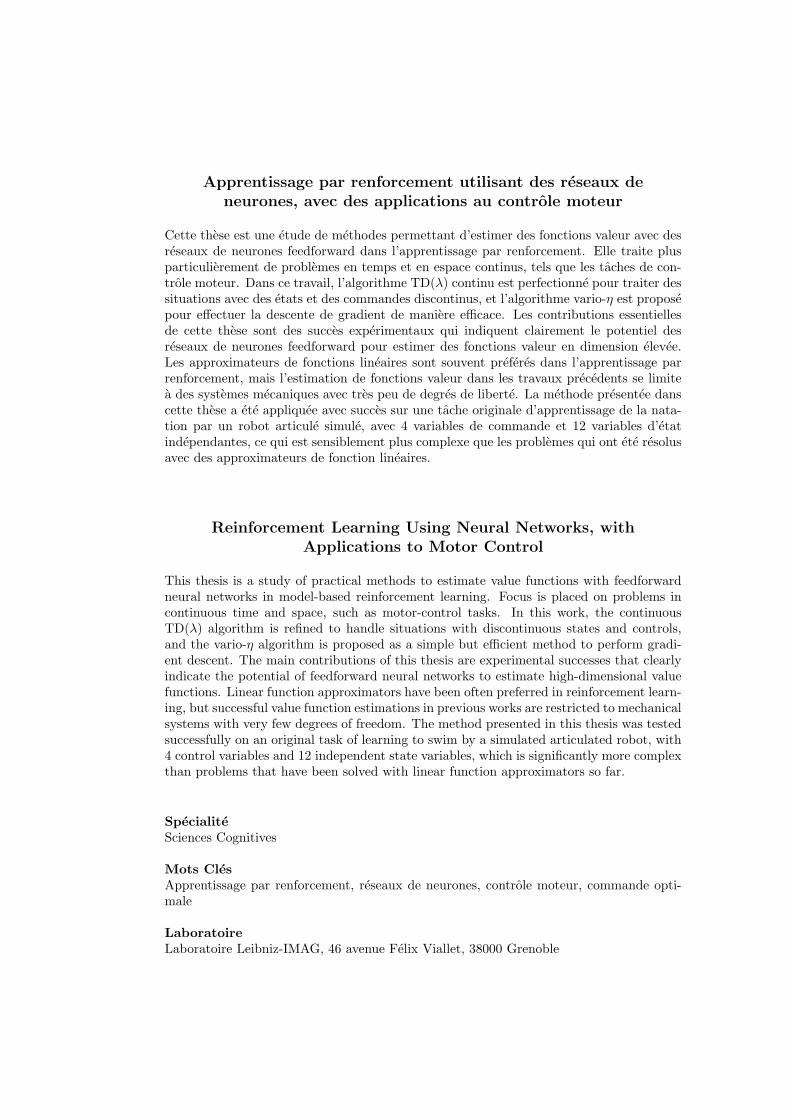
Apprentissage par renforcement utilisant des reseaux deneurones, avec des applications au controle moteur
Cette these est une etude de methodes permettant d’estimer des fonctions valeur avec desreseaux de neurones feedforward dans l’apprentissage par renforcement. Elle traite plusparticulierement de problemes en temps et en espace continus, tels que les taches de con-trole moteur. Dans ce travail, l’algorithme TD(λ) continu est perfectionne pour traiter dessituations avec des etats et des commandes discontinus, et l’algorithme vario-η est proposepour effectuer la descente de gradient de maniere efficace. Les contributions essentiellesde cette these sont des succes experimentaux qui indiquent clairement le potentiel desreseaux de neurones feedforward pour estimer des fonctions valeur en dimension elevee.Les approximateurs de fonctions lineaires sont souvent preferes dans l’apprentissage parrenforcement, mais l’estimation de fonctions valeur dans les travaux precedents se limitea des systemes mecaniques avec tres peu de degres de liberte. La methode presentee danscette these a ete appliquee avec succes sur une tache originale d’apprentissage de la nata-tion par un robot articule simule, avec 4 variables de commande et 12 variables d’etatindependantes, ce qui est sensiblement plus complexe que les problemes qui ont ete resolusavec des approximateurs de fonction lineaires.
Reinforcement Learning Using Neural Networks, withApplications to Motor Control
This thesis is a study of practical methods to estimate value functions with feedforwardneural networks in model-based reinforcement learning. Focus is placed on problems incontinuous time and space, such as motor-control tasks. In this work, the continuousTD(λ) algorithm is refined to handle situations with discontinuous states and controls,and the vario-η algorithm is proposed as a simple but efficient method to perform gradi-ent descent. The main contributions of this thesis are experimental successes that clearlyindicate the potential of feedforward neural networks to estimate high-dimensional valuefunctions. Linear function approximators have been often preferred in reinforcement learn-ing, but successful value function estimations in previous works are restricted to mechanicalsystems with very few degrees of freedom. The method presented in this thesis was testedsuccessfully on an original task of learning to swim by a simulated articulated robot, with4 control variables and 12 independent state variables, which is significantly more complexthan problems that have been solved with linear function approximators so far.
Specialite
Sciences Cognitives
Mots Cles
Apprentissage par renforcement, reseaux de neurones, controle moteur, commande opti-male
Laboratoire
Laboratoire Leibniz-IMAG, 46 avenue Felix Viallet, 38000 Grenoble


![Institut National Polytechnique de Grenoble U.F.R ...iihm.imag.fr/publs/2002/rapport-dea-barralon.pdf · lité, sont dites plastiques [Thevenin et Coutaz 1999]. Prenons deux exemples](https://img.pdfslide.fr/doc/110x75/5c7fb8f309d3f26a7f8bd6a1/institut-national-polytechnique-de-grenoble-ufr-iihmimagfrpubls2002rapport-dea-.jpg)