INTERNATIONAL ISO STANDARD 22007-2 · International Standard requires approval by at least 75 % of the member bodies casting a vote. Attention is drawn to the possibility that some

Reference numberISO 22007-2:2008(E)

© ISO 2008

INTERNATIONAL STANDARD

ISO22007-2

First edition2008-12-15

Plastics — Determination of thermal conductivity and thermal diffusivity — Part 2: Transient plane heat source (hot disc) method

Plastiques — Détermination de la conductivité thermique et de la diffusivité thermique —

Partie 2: Méthode de la source plane transitoire (disque chaud)

ISO 22007-2:2008(E)

PDF disclaimer This PDF file may contain embedded typefaces. In accordance with Adobe's licensing policy, this file may be printed or viewed but shall not be edited unless the typefaces which are embedded are licensed to and installed on the computer performing the editing. In downloading this file, parties accept therein the responsibility of not infringing Adobe's licensing policy. The ISO Central Secretariat accepts no liability in this area.

Adobe is a trademark of Adobe Systems Incorporated.

Details of the software products used to create this PDF file can be found in the General Info relative to the file; the PDF-creation parameters were optimized for printing. Every care has been taken to ensure that the file is suitable for use by ISO member bodies. In the unlikely event that a problem relating to it is found, please inform the Central Secretariat at the address given below.

COPYRIGHT PROTECTED DOCUMENT © ISO 2008 All rights reserved. Unless otherwise specified, no part of this publication may be reproduced or utilized in any form or by any means, electronic or mechanical, including photocopying and microfilm, without permission in writing from either ISO at the address below or ISO's member body in the country of the requester.

ISO copyright office Case postale 56 • CH-1211 Geneva 20 Tel. + 41 22 749 01 11 Fax + 41 22 749 09 47 E-mail [email protected] Web www.iso.org

Published in Switzerland

ii © ISO 2008 – All rights reserved

ISO 22007-2:2008(E)

© ISO 2008 – All rights reserved iii

Contents Page

Foreword............................................................................................................................................................ iv Introduction ........................................................................................................................................................ v 1 Scope ......................................................................................................................................................1 2 Normative references ............................................................................................................................1 3 Terms and definitions ...........................................................................................................................2 4 Principle..................................................................................................................................................3 5 Apparatus ...............................................................................................................................................3 6 Test specimens ......................................................................................................................................5 6.1 Bulk specimens......................................................................................................................................5 6.2 Anisotropic bulk specimens.................................................................................................................6 6.3 Slab specimens......................................................................................................................................6 6.4 Thin-film specimens ..............................................................................................................................6 7 Procedure ...............................................................................................................................................7 8 Calculation of thermal properties ........................................................................................................9 8.1 Bulk specimens......................................................................................................................................9 8.2 Anisotropic bulk specimens...............................................................................................................12 8.3 Slab specimens....................................................................................................................................13 8.4 Thin-film specimens ............................................................................................................................14 9 Calibration and verification ................................................................................................................14 9.1 Calibration of apparatus .....................................................................................................................14 9.2 Verification of apparatus.....................................................................................................................14 10 Precision and bias ...............................................................................................................................15 11 Test report ............................................................................................................................................16 Bibliography ......................................................................................................................................................17

ISO 22007-2:2008(E)

iv © ISO 2008 – All rights reserved

Foreword

ISO (the International Organization for Standardization) is a worldwide federation of national standards bodies (ISO member bodies). The work of preparing International Standards is normally carried out through ISO technical committees. Each member body interested in a subject for which a technical committee has been established has the right to be represented on that committee. International organizations, governmental and non-governmental, in liaison with ISO, also take part in the work. ISO collaborates closely with the International Electrotechnical Commission (IEC) on all matters of electrotechnical standardization.

International Standards are drafted in accordance with the rules given in the ISO/IEC Directives, Part 2.

The main task of technical committees is to prepare International Standards. Draft International Standards adopted by the technical committees are circulated to the member bodies for voting. Publication as an International Standard requires approval by at least 75 % of the member bodies casting a vote.

Attention is drawn to the possibility that some of the elements of this document may be the subject of patent rights. ISO shall not be held responsible for identifying any or all such patent rights.

ISO 22007-2 was prepared by Technical Committee ISO/TC 61, Plastics, Subcommittee SC 5, Physical-chemical properties.

ISO 22007 consists of the following parts, under the general title Plastics — Determination of thermal conductivity and thermal diffusivity:

⎯ Part 1: General principles

⎯ Part 2: Transient plane heat source (hot disc) method

⎯ Part 3: Temperature wave analysis method

⎯ Part 4: Laser flash method

ISO 22007-2:2008(E)

© ISO 2008 – All rights reserved v

Introduction

A significant increase in the development and application of new and improved materials for broad ranges of physical, chemical, biological and medical applications has necessitated better performance data from methods of measurement of thermal-transport properties. The introduction of alternative methods that are relatively simple, fast and of good precision would be of great benefit to the scientific and engineering communities [1].

A number of measurement techniques described as contact transient methods have been developed and several have been commercialized. These are being widely used and are suitable for testing many types of material. In some cases, they can be used to measure several properties separately or simultaneously [2],[3].

A further advantage of some of these methods is that it has become possible to measure the true bulk properties of a material. This feature stems from the possibility of eliminating the influence of the thermal contact resistance (see 8.1.1) that is present at the interface between the probe and the specimen surfaces [1],[3],[4],[5],[6].

INTERNATIONAL STANDARD ISO 22007-2:2008(E)

© ISO 2008 – All rights reserved 1

Plastics — Determination of thermal conductivity and thermal diffusivity —

Part 2: Transient plane heat source (hot disc) method

1 Scope

1.1 This part of ISO 22007 specifies a method for the determination of the thermal conductivity and thermal diffusivity, and hence the specific heat capacity per unit volume, of plastics. The experimental arrangement can be designed to match different specimen sizes. Measurements can be made in gaseous and vacuum environments at a range of temperatures and pressures.

1.2 This method is suitable for testing homogeneous and isotropic materials, as well as anisotropic materials with a uniaxial structure. In general, the method is suitable for materials having values of thermal conductivity, λ, in the approximate range 0,01 W⋅m−1⋅K−1 < λ < 500 W⋅m−1⋅K−1 and values of thermal diffusivity, α, in the range 5 × 10−8 m2⋅s−1 u α u 10−4 m2⋅s−1, and for temperatures, T, in the approximate range 50 K < T < 1 000 K.

NOTE The specific heat capacity per unit volume, C, can be obtained by dividing the thermal conductivity, λ, by the thermal diffusivity, α, i.e. C = λ/α, and is in the approximate range 0,2 MJ⋅m−3⋅K−1< C < 5 MJ⋅m−3⋅K−1. It is also referred to as the volumetric heat capacity.

1.3 The thermal-transport properties of liquids can also be determined, provided care is taken to minimize thermal convection.

2 Normative references

The following referenced documents are indispensable for the application of this document. For dated references, only the edition cited applies. For undated references, the latest edition of the referenced document (including any amendments) applies.

ISO 472, Plastics — Vocabulary

ISO 22007-1, Plastics — Determination of thermal conductivity and thermal diffusivity — Part 1: General principles

ISO 22007-2:2008(E)

2 © ISO 2008 – All rights reserved

3 Terms and definitions

For the purposes of this document, the terms and definitions given in ISO 472 and ISO 22007-1 and the following apply.

3.1 penetration depth ∆ppen measure of how far into the specimen, in the direction of heat flow, a heat wave has travelled

NOTE 1 For this method, the penetration depth is given by

pen totp tκ α∆ = ⋅

where

ttot is the total measurement time for the transient recording;

α is the thermal diffusivity of the specimen material;

κ is a constant dependent on the sensitivity of the temperature recordings.

NOTE 2 It is expressed in metres (m).

3.2 probing depth ∆pprob measure of how far into the specimen, in the direction of heat flow, a heat wave has travelled during the time window used for calculation

NOTE 1 The probing depth is given by

prob maxp tκ α∆ = ⋅

where tmax is the maximum time of the time window used for calculating the thermal-transport properties.

NOTE 2 It is expressed in metres (m).

NOTE 3 A typical value in hot-disc measurements is κ = 2, which is assumed throughout this document.

3.3 sensitivity coefficient βq coefficient defined by the equation

( )q

T tq

qβ

⎡ ⎤∂ ∆⎣ ⎦=∂

where

q is the thermal conductivity, λ, the thermal diffusivity, α, or the volumetric specific heat capacity, C;

∆T(t) is the mean temperature increase of the probe

NOTE 1 Different sensitivity coefficients are defined for thermal conductivity, thermal diffusivity and specific heat per unit volume [8].

ISO 22007-2:2008(E)


NOTE 2 To define the time window that is used to determine both the thermal conductivity and diffusivity from one single experiment, the theory of sensitivity coefficients is used. Through this theory, which deals with a large number of experiments and considers the constants, q, as variables, it has been established that

0,30 u tmax⋅α /r2 u 1,0

where r is the mean radius of the outermost spiral of the probe.

Assuming κ = 2, this expression can be rewritten as

1,1r u ∆pprob u 2,0r

4 Principle

A specimen containing an embedded hot-disc probe of negligible heat capacity is allowed to equilibrate at a given temperature. A heat pulse in the form of a stepwise function is produced by an electrical current through the probe to generate a dynamic temperature field within the specimen. The increase in the temperature of the probe is measured as a function of time. The probe operates as a temperature sensor unified with a heat source (i.e. a self-heated sensor). The response is then analysed in accordance with the model developed for the specific probe and the assumed boundary conditions.

5 Apparatus

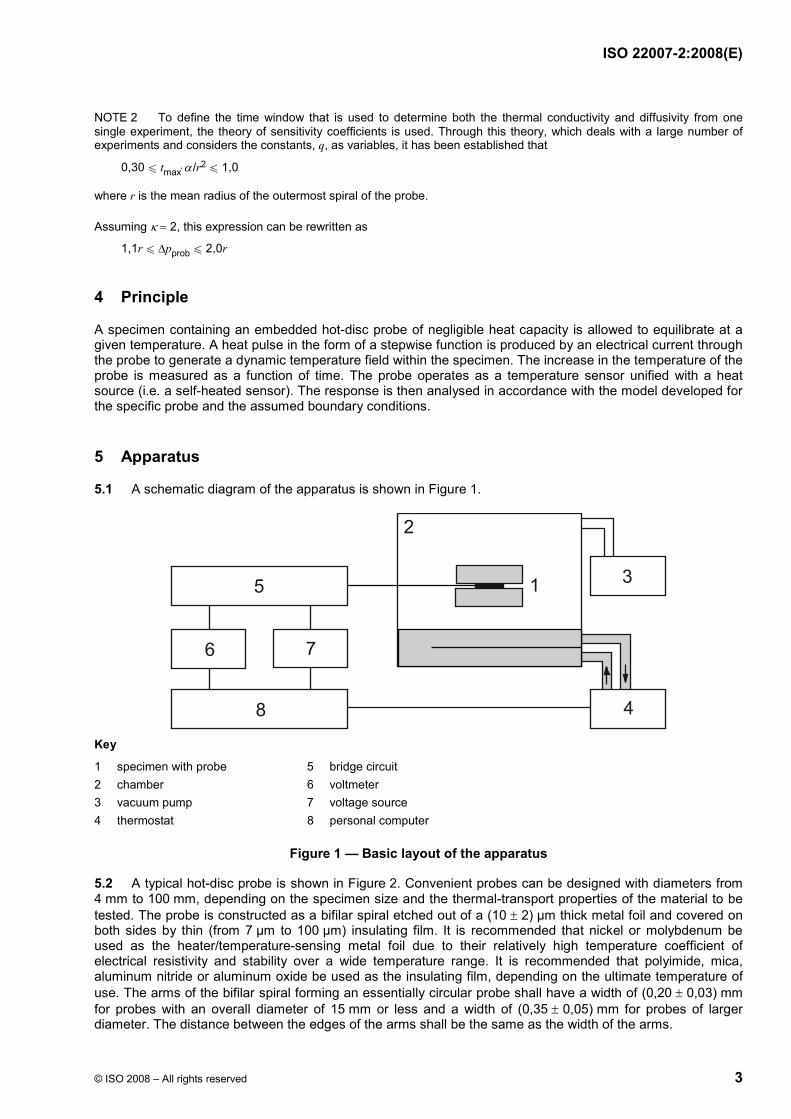
5.1 A schematic diagram of the apparatus is shown in Figure 1.

5

6 7

8

1

2

3

4

Key

1 specimen with probe 5 bridge circuit 2 chamber 6 voltmeter 3 vacuum pump 7 voltage source 4 thermostat 8 personal computer

Figure 1 — Basic layout of the apparatus

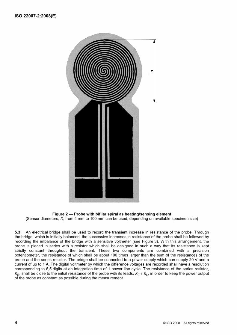
5.2 A typical hot-disc probe is shown in Figure 2. Convenient probes can be designed with diameters from 4 mm to 100 mm, depending on the specimen size and the thermal-transport properties of the material to be tested. The probe is constructed as a bifilar spiral etched out of a (10 ± 2) µm thick metal foil and covered on both sides by thin (from 7 µm to 100 µm) insulating film. It is recommended that nickel or molybdenum be used as the heater/temperature-sensing metal foil due to their relatively high temperature coefficient of electrical resistivity and stability over a wide temperature range. It is recommended that polyimide, mica, aluminum nitride or aluminum oxide be used as the insulating film, depending on the ultimate temperature of use. The arms of the bifilar spiral forming an essentially circular probe shall have a width of (0,20 ± 0,03) mm for probes with an overall diameter of 15 mm or less and a width of (0,35 ± 0,05) mm for probes of larger diameter. The distance between the edges of the arms shall be the same as the width of the arms.

ISO 22007-2:2008(E)


Figure 2 — Probe with bifilar spiral as heating/sensing element (Sensor diameters, D, from 4 mm to 100 mm can be used, depending on available specimen size)

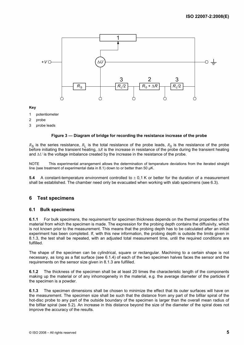
5.3 An electrical bridge shall be used to record the transient increase in resistance of the probe. Through the bridge, which is initially balanced, the successive increases in resistance of the probe shall be followed by recording the imbalance of the bridge with a sensitive voltmeter (see Figure 3). With this arrangement, the probe is placed in series with a resistor which shall be designed in such a way that its resistance is kept strictly constant throughout the transient. These two components are combined with a precision potentiometer, the resistance of which shall be about 100 times larger than the sum of the resistances of the probe and the series resistor. The bridge shall be connected to a power supply which can supply 20 V and a current of up to 1 A. The digital voltmeter by which the difference voltages are recorded shall have a resolution corresponding to 6,5 digits at an integration time of 1 power line cycle. The resistance of the series resistor, RS, shall be close to the initial resistance of the probe with its leads, R0 + RL, in order to keep the power output of the probe as constant as possible during the measurement.

ISO 22007-2:2008(E)


Key

1 potentiometer 2 probe 3 probe leads

Figure 3 — Diagram of bridge for recording the resistance increase of the probe

RS is the series resistance, RL is the total resistance of the probe leads, R0 is the resistance of the probe before initiating the transient heating, ∆R is the increase in resistance of the probe during the transient heating and ∆U is the voltage imbalance created by the increase in the resistance of the probe.

NOTE This experimental arrangement allows the determination of temperature deviations from the iterated straight line (see treatment of experimental data in 8.1) down to or better than 50 µK.

5.4 A constant-temperature environment controlled to ± 0,1 K or better for the duration of a measurement shall be established. The chamber need only be evacuated when working with slab specimens (see 6.3).

6 Test specimens

6.1 Bulk specimens

6.1.1 For bulk specimens, the requirement for specimen thickness depends on the thermal properties of the material from which the specimen is made. The expression for the probing depth contains the diffusivity, which is not known prior to the measurement. This means that the probing depth has to be calculated after an initial experiment has been completed. If, with this new information, the probing depth is outside the limits given in 8.1.3, the test shall be repeated, with an adjusted total measurement time, until the required conditions are fulfilled.

The shape of the specimen can be cylindrical, square or rectangular. Machining to a certain shape is not necessary, as long as a flat surface (see 6.1.4) of each of the two specimen halves faces the sensor and the requirements on the sensor size given in 8.1.3 are fulfilled.

6.1.2 The thickness of the specimen shall be at least 20 times the characteristic length of the components making up the material or of any inhomogeneity in the material, e.g. the average diameter of the particles if the specimen is a powder.

6.1.3 The specimen dimensions shall be chosen to minimize the effect that its outer surfaces will have on the measurement. The specimen size shall be such that the distance from any part of the bifilar spiral of the hot-disc probe to any part of the outside boundary of the specimen is larger than the overall mean radius of the bifilar spiral (see 5.2). An increase in this distance beyond the size of the diameter of the spiral does not improve the accuracy of the results.

ISO 22007-2:2008(E)


6.1.4 Specimen surfaces which are in contact with the sensor shall be plane and smooth. The specimen halves shall be clamped on to both sides of the hot-disc probe.

NOTE Heat sink contact paste is not recommended since:

a) it is difficult to obtain a sufficiently thin layer of paste which will actually improve the thermal contact;

b) the paste obviously increases the heat capacity of the insulating layer and delays the development of the constant temperature difference between the sensing material and the specimen surface;

c) it is difficult to obtain exactly the same thickness of paste on both sides of the probe and achieve a strictly symmetrical flow of heat from the heating/sensing material through the insulation into the two specimen halves.

6.1.5 For liquids, suitable containment vessels with adequate seals are necessary and air bubbles and evaporation shall be avoided.

Storage and conditioning of the liquid may affect its properties, e.g. by absorbtion of water or gas. It may be necessary to pretreat the specimen prior to testing, e.g. by degassing. However, pretreatment procedures shall not be used when they could detrimentally affect the material to be tested, e.g. through degradation.

6.1.6 For materials with which significant dimensional changes may occur, e.g. when making measurements over large temperature ranges, due to thermal expansion, a change of state, a phase transition or other causes, care shall be taken to ensure that, when placing the hot-disc probe in contact with the specimen, the applied load does not affect the properties of the specimen.

With soft materials, the clamping pressure shall not compress the specimen and thus change its thermal-transport properties.

6.1.7 The specimen shall be conditioned in accordance with the standard specification which applies to the type of material and its particular use.

6.2 Anisotropic bulk specimens

6.2.1 If a material is anisotropic, specimens shall be cut (or otherwise prepared) so that the probe can be oriented in the main directions (e.g. the fibre directions in reinforced plastics, the main directions in layered structures or the principal axes in crystals) [4],[7]. The hot-disc method is limited to materials in which the thermal properties along two of the orthogonal and principal axes are the same, but are different from those along the third axis.

6.2.2 The size of anisotropic specimens shall be chosen so that the requirements of 8.1.3 are fulfilled along the principal axes.

6.3 Slab specimens

The so-called slab method is used with sheet-formed specimens extending in two dimensions, but with a limited and well-defined thickness in the range from 1 mm to 10 mm [9]. The slab specimen thickness shall be known to an accuracy of 0,01 mm. When two equally thick slabs of a material are clamped around a probe and thermally insulated on the outer sides, it is possible to measure the thermal conductivity and diffusivity of such specimens. The condition related to the probing depth (see 3.2) has to be fulfilled in the plane of the probe but not in the through-thickness direction. This method is particularly suited to studies of materials having thermal conductivities higher than 10 W⋅m−1⋅K−1 but can also be used for materials with thermal conductivities as low as 1 W⋅m−1⋅K−1, provided good thermal insulation of the slabs can be arranged (for instance by performing the measurements in a vacuum).

6.4 Thin-film specimens

The so-called thin-film method is used with specimens such as paper, textiles, polymer films or deposited thin-film layers (such as ceramic coatings) with thicknesses ranging from 0,01 mm to 1,0 mm [10]. The thickness of thin-film specimens (placed on both sides of the probe) shall be known to an accuracy of ± 1 µm.

ISO 22007-2:2008(E)


NOTE 1 When making a measurement on a material with a high thermal conductivity, the temperature undergoes a rapid increase at the very beginning of the transient followed by a much more gradual increase. The insulating layer, between which the sensing spiral is sandwiched, causes this rapid increase. It has been shown both experimentally and in computer simulations that the temperature difference across the insulating layer becomes constant within a very short time and remains constant throughout the measurement. The reason is that the total power output, the area of the sensing material and the thickness of the insulating layer are constant in the test.

If thin films of a material are placed between the probe and a high-conductivity background material (in the form of an “infinite” solid), it is possible to measure the thermal conductivity of the film material, provided that the thermal conductivity of the insulating layer with which the probe is covered has been determined in a separate experiment [10].

NOTE 2 It might be necessary to make measurements on films of different thicknesses or with different clamping pressures to eliminate mathematically the influence of thermal contact resistances.

The thermal conductivity of the background material shall be at least 10 times greater than that of the thin-film material.

In order to simulate better a plane heat source when testing thin films, a probe similar to the one depicted in Figure 2 shall be used. However, the circular strips should preferably have a width of 0,8 mm and the openings between the strips should only be 0,2 mm. When using a probe with thermal insulation on both sides of the bifilar spiral, an initial test to determine the effective thermal conductivity of the insulation and the adhesive holding the probe together shall be carried out.

7 Procedure

7.1 Place the probe between the plane surfaces of two specimen halves of the material whose thermal properties are to be determined.

Clamp or assemble the specimen/probe assembly securely in the test rig.

NOTE 1 When studying liquids, the probe is simply dipped into the liquid, often with an arrangement to keep the probe flat.

NOTE 2 The total temperature increase in the specimen is normally less than 2 K. This means that the thermodynamic state of the material under test hardly changes during the measurement process and the thermal properties can thus be ascribed to the equilibrium temperature attained prior to the test.

7.2 Assemble the complete system in a constant-temperature chamber and allow it to attain temperature stability as defined in 5.4.

7.3 Balance the electrical bridge prior to the test. For a sensor with an initial resistance between 1 Ω and 50 Ω, the voltage for balancing the bridge shall be selected such that the current does not exceed 1 mA.

7.4 Apply the heat pulse and record the temperature during a predetermined measuring time. Use values provided in Table 1 as an initial guide for the power output and the measurement time.

NOTE In general, a lower power output is preferred in order to minimize the perturbation of the system. However, it should be noted that the sensitivity of the temperature recording increases when the power output (and consequently the current) is higher, which is the case when studying materials with high thermal conductivity. For this reason, it is possible to obtain good precision in measurements on such materials even with temperature increases of only a fraction of a degree.

7.5 The voltage imbalance is determined and recorded at appropriate time intervals over the duration of the measurement time. It is recommended that the frequency of data acquisition be such that at least 100 data points are collected during the measurement time. If the method is used to measure the thermal-transport properties of liquids, the measurement time shall be limited to 1 s so that thermal convection in the liquid does not perturb the measurement.

ISO 22007-2:2008(E)


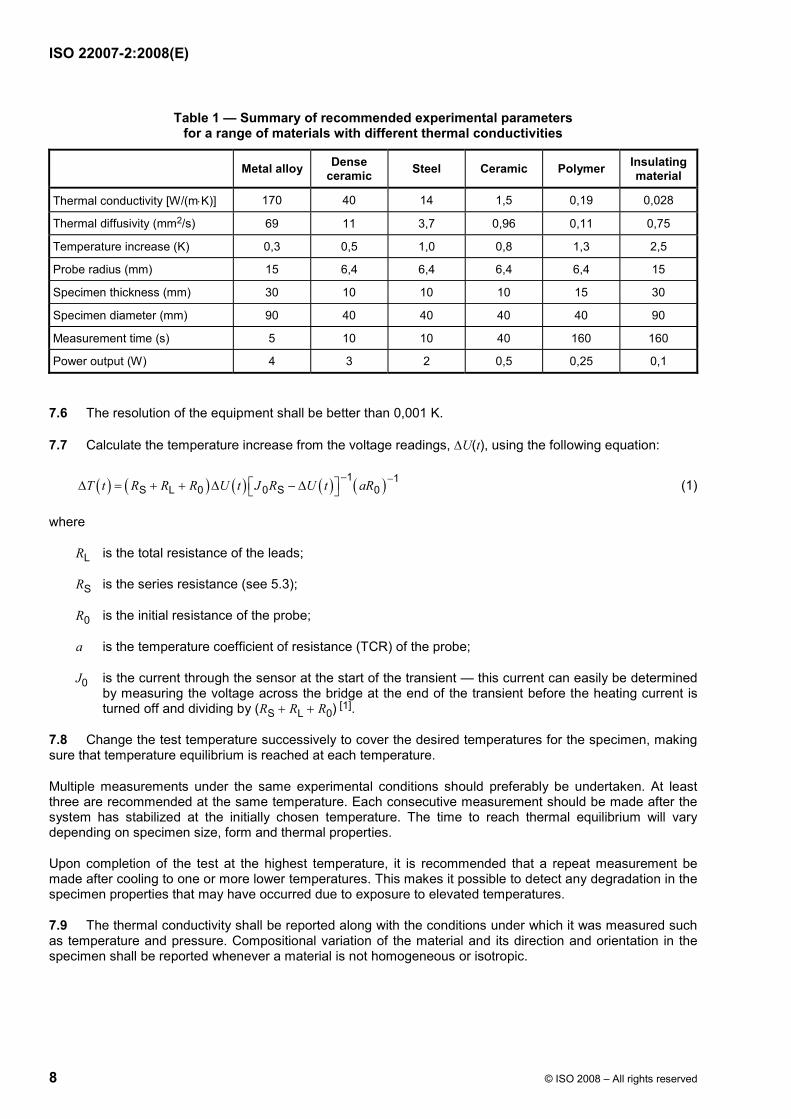
Table 1 — Summary of recommended experimental parameters for a range of materials with different thermal conductivities

Metal alloy Dense ceramic Steel Ceramic Polymer Insulating

material

Thermal conductivity [W/(m⋅K)] 170 40 14 1,5 0,19 0,028

Thermal diffusivity (mm2/s) 69 11 3,7 0,96 0,11 0,75

Temperature increase (K) 0,3 0,5 1,0 0,8 1,3 2,5

Probe radius (mm) 15 6,4 6,4 6,4 6,4 15

Specimen thickness (mm) 30 10 10 10 15 30

Specimen diameter (mm) 90 40 40 40 40 90

Measurement time (s) 5 10 10 40 160 160

Power output (W) 4 3 2 0,5 0,25 0,1

7.6 The resolution of the equipment shall be better than 0,001 K.

7.7 Calculate the temperature increase from the voltage readings, ∆U(t), using the following equation:

( ) ( ) ( ) ( ) ( )1 1S L 0 0 S 0T t R R R U t J R U t aR

− −⎡ ⎤∆ = + + ∆ − ∆⎣ ⎦ (1)

where

RL is the total resistance of the leads;

RS is the series resistance (see 5.3);

R0 is the initial resistance of the probe;

a is the temperature coefficient of resistance (TCR) of the probe;

J0 is the current through the sensor at the start of the transient — this current can easily be determined by measuring the voltage across the bridge at the end of the transient before the heating current is turned off and dividing by (RS + RL + R0) [1].

7.8 Change the test temperature successively to cover the desired temperatures for the specimen, making sure that temperature equilibrium is reached at each temperature.

Multiple measurements under the same experimental conditions should preferably be undertaken. At least three are recommended at the same temperature. Each consecutive measurement should be made after the system has stabilized at the initially chosen temperature. The time to reach thermal equilibrium will vary depending on specimen size, form and thermal properties.

Upon completion of the test at the highest temperature, it is recommended that a repeat measurement be made after cooling to one or more lower temperatures. This makes it possible to detect any degradation in the specimen properties that may have occurred due to exposure to elevated temperatures.

7.9 The thermal conductivity shall be reported along with the conditions under which it was measured such as temperature and pressure. Compositional variation of the material and its direction and orientation in the specimen shall be reported whenever a material is not homogeneous or isotropic.

ISO 22007-2:2008(E)


8 Calculation of thermal properties

8.1 Bulk specimens

8.1.1 For small increases in the temperature of the probe, we have

( ) ( )0 1R t R a T t⎡ ⎤= + ⋅ ∆⎣ ⎦ (2)

where

∆T(t) (= T(t) − T0) is the mean temperature increase of the probe;

R0 is the initial resistance of the probe at temperature T0;

a is the temperature coefficient of resistance (TCR) of the probe.

The temperature increase can be seen as consisting of two parts. One part represents the temperature difference across the intercalated insulating layer and the other part the temperature increase of the specimen surface during the transient measurement. This can be expressed as

( ) ( ) ( )i sT t T t T t∆ = ∆ + ∆ (3)

where

∆Ti(t) is the increase in temperature over the insulating layers of the probe;

∆Ts(t) is the increase in the temperature of the specimen surface.

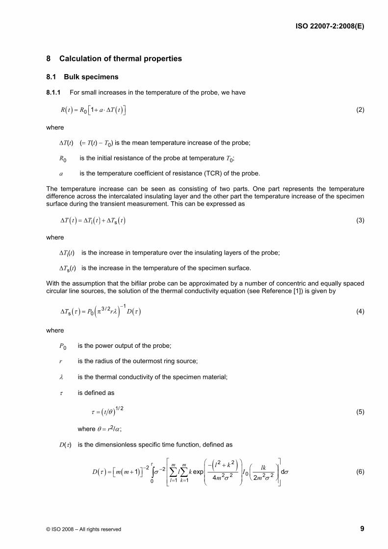
With the assumption that the bifilar probe can be approximated by a number of concentric and equally spaced circular line sources, the solution of the thermal conductivity equation (see Reference [1]) is given by

( ) ( ) ( )13 / 2

s 0T P r Dτ λ τ−

∆ = π (4)

where

P0 is the power output of the probe;

r is the radius of the outermost ring source;

λ is the thermal conductivity of the specimen material;

τ is defined as

( )1/ 2tτ θ= (5)

where θ = r2/α ;

D(τ) is the dimensionless specific time function, defined as

( ) ( )( )2 2

2 202 2 2 2

1 10

1 exp d4 2

m m

l k

l k lkD m m l k Im m

τ

τ σ σσ σ

− −

= =

⎡ ⎤⎛ ⎞− + ⎛ ⎞⎢ ⎥⎜ ⎟⎡ ⎤= + ⎜ ⎟⎣ ⎦ ⎢ ⎥⎜ ⎟ ⎝ ⎠⎜ ⎟⎢ ⎥⎝ ⎠⎣ ⎦

∑ ∑∫ (6)

ISO 22007-2:2008(E)


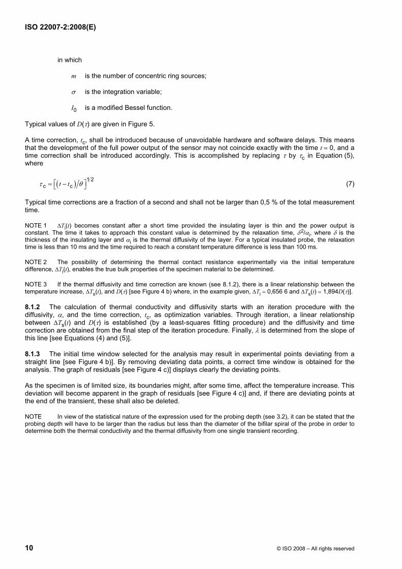
in which

m is the number of concentric ring sources;

σ is the integration variable;

I0 is a modified Bessel function.

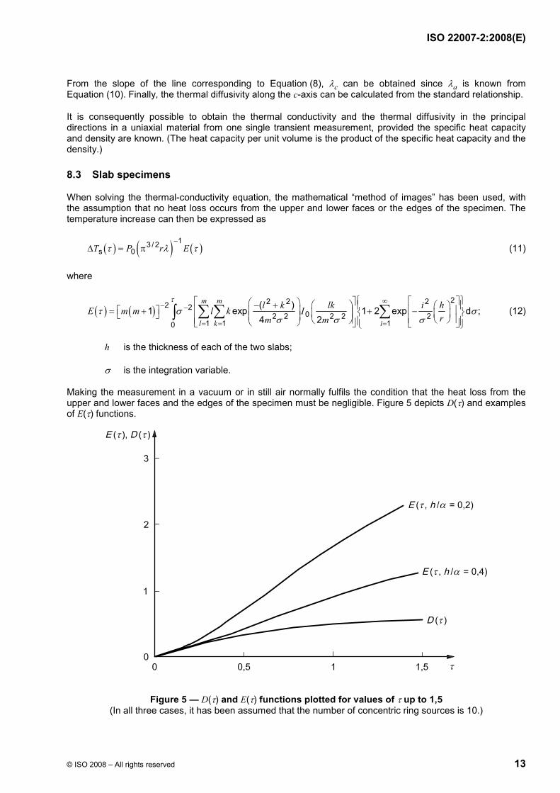
Typical values of D(τ) are given in Figure 5.

A time correction, tc, shall be introduced because of unavoidable hardware and software delays. This means that the development of the full power output of the sensor may not coincide exactly with the time t = 0, and a time correction shall be introduced accordingly. This is accomplished by replacing τ by τc in Equation (5), where

( ) 1 2c ct tτ θ⎡ ⎤= −⎣ ⎦ (7)

Typical time corrections are a fraction of a second and shall not be larger than 0,5 % of the total measurement time.

NOTE 1 ∆Ti(t) becomes constant after a short time provided the insulating layer is thin and the power output is constant. The time it takes to approach this constant value is determined by the relaxation time, δ2/αi, where δ is the thickness of the insulating layer and αi is the thermal diffusivity of the layer. For a typical insulated probe, the relaxation time is less than 10 ms and the time required to reach a constant temperature difference is less than 100 ms.

NOTE 2 The possibility of determining the thermal contact resistance experimentally via the initial temperature difference, ∆Ti(t), enables the true bulk properties of the specimen material to be determined.

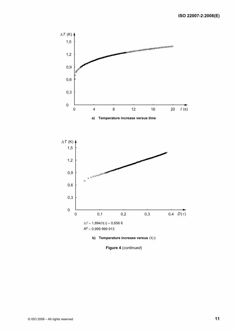
NOTE 3 If the thermal diffusivity and time correction are known (see 8.1.2), there is a linear relationship between the temperature increase, ∆Ts(t), and D(τ) [see Figure 4 b) where, in the example given, ∆Ti = 0,656 6 and ∆Ts(t) = 1,894D(τ)].

8.1.2 The calculation of thermal conductivity and diffusivity starts with an iteration procedure with the diffusivity, α, and the time correction, tc, as optimization variables. Through iteration, a linear relationship between ∆Ts(t) and D(τ) is established (by a least-squares fitting procedure) and the diffusivity and time correction are obtained from the final step of the iteration procedure. Finally, λ is determined from the slope of this line [see Equations (4) and (5)].

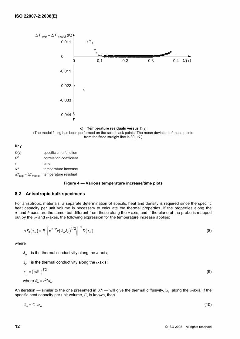
8.1.3 The initial time window selected for the analysis may result in experimental points deviating from a straight line [see Figure 4 b)]. By removing deviating data points, a correct time window is obtained for the analysis. The graph of residuals [see Figure 4 c)] displays clearly the deviating points.

As the specimen is of limited size, its boundaries might, after some time, affect the temperature increase. This deviation will become apparent in the graph of residuals [see Figure 4 c)] and, if there are deviating points at the end of the transient, these shall also be deleted.

NOTE In view of the statistical nature of the expression used for the probing depth (see 3.2), it can be stated that the probing depth will have to be larger than the radius but less than the diameter of the bifilar spiral of the probe in order to determine both the thermal conductivity and the thermal diffusivity from one single transient recording.

ISO 22007-2:2008(E)


a) Temperature increase versus time

∆T = 1,894D(τ) + 0,656 6 R2 = 0,999 999 913

b) Temperature increase versus D(τ)

Figure 4 (continued)

ISO 22007-2:2008(E)


c) Temperature residuals versus D(τ) (The model fitting has been performed on the solid black points. The mean deviation of these points

from the fitted straight line is 30 µK.)

Key

D(τ) specific time function R2 correlation coefficient t time ∆T temperature increase ∆Texp − ∆Tmodel temperature residual

Figure 4 — Various temperature increase/time plots

8.2 Anisotropic bulk specimens

For anisotropic materials, a separate determination of specific heat and density is required since the specific heat capacity per unit volume is necessary to calculate the thermal properties. If the properties along the a- and b-axes are the same, but different from those along the c-axis, and if the plane of the probe is mapped out by the a- and b-axes, the following expression for the temperature increase applies:

( ) ( ) ( )11/ 23 / 2

s 0a a c aT P r Dτ λ λ τ−

⎡ ⎤∆ = π⎢ ⎥⎣ ⎦ (8)

where

λa is the thermal conductivity along the a-axis;

λc is the thermal conductivity along the c-axis;

( )1 2a atτ θ= (9)

where θa = r2/αa.

An iteration — similar to the one presented in 8.1 — will give the thermal diffusivity, αa, along the a-axis. If the specific heat capacity per unit volume, C, is known, then

a aCλ α= ⋅ (10)

ISO 22007-2:2008(E)


From the slope of the line corresponding to Equation (8), λc can be obtained since λa is known from Equation (10). Finally, the thermal diffusivity along the c-axis can be calculated from the standard relationship.

It is consequently possible to obtain the thermal conductivity and the thermal diffusivity in the principal directions in a uniaxial material from one single transient measurement, provided the specific heat capacity and density are known. (The heat capacity per unit volume is the product of the specific heat capacity and the density.)

8.3 Slab specimens

When solving the thermal-conductivity equation, the mathematical “method of images” has been used, with the assumption that no heat loss occurs from the upper and lower faces or the edges of the specimen. The temperature increase can then be expressed as

( ) ( ) ( )13 / 2

s 0T P r Eτ λ τ−

∆ = π (11)

where

( ) ( )22 2 22 2

02 2 2 2 21 1 10

( )1 exp 1 2 exp d ;4 2

m m

l k i

l k lk i hE m m l k Irm m

τ

τ σ σσ σ σ

∞− −

= = =

⎧ ⎫⎡ ⎤⎡ ⎤⎛ ⎞ ⎛ ⎞− + ⎛ ⎞⎪ ⎪⎡ ⎤ ⎢ ⎥⎢ ⎥= + + −⎜ ⎟ ⎨ ⎬⎜ ⎟ ⎜ ⎟⎣ ⎦ ⎜ ⎟ ⎢ ⎥⎢ ⎥ ⎝ ⎠⎝ ⎠ ⎪ ⎪⎝ ⎠⎣ ⎦ ⎣ ⎦⎩ ⎭∑ ∑ ∑∫ (12)

h is the thickness of each of the two slabs;

σ is the integration variable.

Making the measurement in a vacuum or in still air normally fulfils the condition that the heat loss from the upper and lower faces and the edges of the specimen must be negligible. Figure 5 depicts D(τ) and examples of E(τ) functions.

Figure 5 — D(τ) and E(τ) functions plotted for values of τ up to 1,5 (In all three cases, it has been assumed that the number of concentric ring sources is 10.)

ISO 22007-2:2008(E)


8.4 Thin-film specimens

The theory for thin-film specimens follows directly from Equations (2) and (3) and the measurement of the temperature increase, ∆Ti(t), over the insulating layer. By extrapolating the iterated straight line to zero time, the constant temperature increase, ∆Ti, is obtained. From the equation

( )0 i i2P A Tλ δ= ∆ (13)

the thermal conductivity of the insulating layer, λi, can be calculated, where A is the area of the probe and δ the thickness of the insulating layers.

When a probe with insulation outside the bifilar spiral of the sensing material is used (see 6.4), it is necessary to make two transient recordings to determine the thermal conductivity of the thin-film material. The first test is made with the probe itself between the plane surfaces of the high-conducting material and the second is made with the two thin-film specimens placed between the probe and the surfaces of the high-conducting material. From these tests, two thermal conductivities are determined, viz. λprobe, which is the thermal conductivity of the insulating layer of the probe together with the adhesive used to attach the insulating layers to the bifilar spiral, and λtotal, which is the thermal conductivity of the combination of the probe insulation and the thin-film specimens. To calculate the thermal conductivity of the thin-film specimen, λspecimen, the following equation shall be used:

probe specimen probe specimen

total probe specimen

δ δ δ δλ λ λ+

= + (14)

where

δprobe is the thickness of the probe insulation on one of the sides, together with its adhesive;

δspecimen is the thickness of one of the specimens.

9 Calibration and verification

9.1 Calibration of apparatus

The hot-disc method is an absolute method which allows the user to perform measurements that are directly traceable to primary SI units (such as temperature, time, length and voltage) without calibration against reference materials. Thus the following aspects of the hot-disc set-up shall be calibrated separately:

⎯ the travelling microscope used to measure the mean diameter of the outermost line source of the sensor;

⎯ the micrometer used to measure the thickness of specimens used in thin-film and slab experiments;

⎯ the time base and the voltages of the data-acquisition system used to record the electrical signals from the bridge circuit;

⎯ the TCR of the material used as the sensing material in the probe;

⎯ the series resistor in the electrical bridge.

In addition, make sure that the volumetric heat capacity used when calculating the transport properties from tests performed on an anisotropic material has been determined with an accuracy better than 1 %.

9.2 Verification of apparatus

Verification of the apparatus shall be performed periodically, preferably by measuring the thermal conductivity and the thermal diffusivity of one or more reference materials giving values within the range covered by the materials to be tested. If the measured values differ from the reference values by more than the limits

ISO 22007-2:2008(E)


specified in Clause 10, recalibration in accordance with 9.1 shall be performed. If no appropriate certified reference materials are available for thermal conductivity and thermal diffusivity, verification can be performed by measurements on materials which have isotropic, well-known and reproducible thermal-transport properties, such as stainless steels, Pyroceram 96061) and perspex.

10 Precision and bias

10.1 In routine measurements at or around room temperature, the accuracy for thermal conductivity is estimated at 2 % to 5 % and for diffusivity at 5 % to 10 %. The accuracy of slab measurements and measurements at higher temperatures is estimated at 5 % to 7 % for thermal conductivity and at 7 % to 11 % for thermal diffusivity. The ranges in uncertainty indicated here relate to probes with polyimide insulations (thickness of insulation between 7 µm and 40 µm), different radii (from 2 mm to 30 mm) and transient recordings of different durations (from 1 s to 1 000 s).

NOTE A covering factor of 2 has been used when estimating the uncertainties from a large number of tests.

10.2 If tests are repeated at the same temperature using the same sensor and test equipment, the deviation from the first measurement is indeed very small, since the same TCR, the same probe radius, the same power output and preferably also the same time window for the transient are being used to evaluate the data. In such experiments, the repeatability of both the thermal conductivity and the thermal diffusivity is between 1 % and 2 %.

NOTE 1 For estimating the accuracy of the hot-disc method, Equations (4), (8) and (11) are taken as starting points. The accuracy of the thermal conductivity is directly dependent on the accuracy of measurement or determination of the power output, the radius of the hot-disc probe, the thickness of slab and thin-film specimens, and the slope of the straight line of temperature increase plotted against D(τ) or E(τ) functions determined after an iterative fitting process.

NOTE 2 The model used to describe the thermal-conductivity process in the specimen does not incorporate all the initial and boundary conditions that are present in actual experiments. These include the following:

a) The approximation of the bifilar spiral with a number of concentric line sources requires that the number of equivalent line sources be not less than 10 unless calibration of the spiral with respect to the radius of the outer line source is performed.

b) The specific heat of the probe can be estimated from the size and thickness of the sensing material (10 µm) and the two insulating sheets (between 7 µm and 100 µm). For a probe with a radius of 6 mm, the loss in power is estimated at 1 mW in a test of 10 s duration with a mean temperature increase of 2 K.

c) The heat loss through conduction along the leads to the bifilar spiral is estimated to be less than 1 mW for typical probe designs.

d) Measurements on slabs call for an estimation of the loss in heat from the thermally insulated outer surfaces of the two slab specimens. In a test using a probe with a radius of 10 mm between 1 mm thick slabs and insulated by polystyrene, the loss in power to the surroundings can be estimated at 2 % for a slab with a thermal conductivity of 10 W⋅m−1⋅K−1. By performing measurements in a vacuum, it is possible to make measurements on materials with appreciably lower thermal conductivities and also to reduce the power loss still further.

NOTE 3 Typically, a minimum of 100 data points (times and voltages) are recorded and the temperature increases calculated. To carry out these calculations, it is necessary to supply information on three resistances and the TCR, a, separately. The resistance of the series resistor, Rs, is determined by direct electrical comparison with a standard resistor. The other resistances are measured by direct comparison with the series resistor. All these measurements are performed by digital voltmeter, and the uncertainty should normally be negligible (i.e. below 0,1 %). In contrast, the uncertainty in the TCR is estimated to be about 2 % since the measurement of this quantity entails measurements of both resistance and temperature [see Equation (2)]. This means that the precision of the temperature recordings in a single measurement is about 2 %. However, when repeating a test at the same temperature and using the same TCR for the calculations, the differences in the temperature increase from one test to another are negligible.

1) Pyroceram® 9606 is an example of a suitable product available commercially. This information is given for the convenience of users of this part of ISO 22007 and does not constitute an endorsement by ISO of this product.

ISO 22007-2:2008(E)


11 Test report

In addition to the information required in ISO 22007-1, the following information specific to the hot-disc method shall be supplied:

⎯ a description of the test apparatus, including details of the power supply and digital voltmeter in the bridge circuit;

⎯ relevant details of the hot-disc probe, the measurement time, the power output, the scanning rate and the time windows used in the analysis of the test data.

ISO 22007-2:2008(E)


Bibliography

[1] GUSTAFSSON, S.E.: Transient plane source techniques for thermal conductivity and thermal diffusivity measurements of solid materials, Rev. Sci. Instrum., 62 (3), p. 797 (1991)

[2] SULEIMAN, M., UL-HAQ, I., KARAWACKI, E., MAQSOOD, A. and GUSTAFSSON, S.E.: Thermal conductivity and electrical resistivity of the Y- and Er-substituted 1:2:3 superconducting compounds in the vicinity of the transition temperature, Physical Review B, 48 (6), p. 4095 (1993)

[3] LOG, T. and GUSTAFSSON, S.E.: Transient Plane Source (TPS) Technique for Measuring Thermal Transport Properties of Building Materials, Fire and Materials, 19, p. 43 (1995)

[4] LUNDSTRÖM, D., KARLSSON, B. and GUSTAVSSON, M.: Anisotropy in Thermal Transport Properties of Cast γ-TiAl Alloys, Z. Metallkd., 92 (11), p. 1203 (2001)

[5] ERICSON, T., HÄLLDAHL, L. and SANDÉN, R.: A Facile Method for Study of Thermal Transport Properties of Explosives, Eleventh symposium on chemical problems connected with the stability of explosives, Båstad, Sweden (1998)

[6] NAGAI, H., NAKATA, Y., TSURUE, T., MINAGAWA, H., KAMADA, K., GUSTAFSSON, S.E. and OKUTANI, T.: Thermal Conductivity Measurement of Molten Silicon by a Hot-Disk Method in Short-Duration Microgravity Environments, Jpn. J. Appl. Phys., 39 (3A), p. 1405 (2000)

[7] GUSTAVSSON, M. and GUSTAFSSON, S.E.: On the Use of Transient Plane Source Sensors for Studying Materials with Direction Dependent Properties, Thermal Conductivity 26, DEStech Publications (2004)

[8] BOHAC, V., GUSTAVSSON, M.K., KUBICAR, L. and GUSTAFSSON, S.E.: Parameter estimations for measurements of thermal transport properties with the hot disk thermal constants analyzer, Rev. Sci. Instrum., 71 (6), p. 2452 (2000)

[9] GUSTAVSSON, M., KARAWACKI, E. and GUSTAFSSON, S.E.: Thermal conductivity, thermal diffusivity and specific heat of thin samples from transient measurements with hot disk sensors, Rev. Sci. Instrum., 65 (12), p. 3856 (1994)

[10] GUSTAVSSON, J.S., GUSTAVSSON, M. and GUSTAFSSON, S.E.: On the Use of the Hot Disk Thermal Constants Analyser for Measuring the Thermal Conductivity of Thin Samples of Electrically Insulating Materials, Thermal Conductivity 24, Technomic Publ. Co. (1998)

ISO 22007-2:2008(E)

ICS 83.080.01 Price based on 17 pages

© ISO 2008 – All rights reserved

Documents

INTERNATIONAL ISO STANDARD 22007-2 · International Standard requires approval by at least 75 % of the member bodies casting a vote. Attention is drawn to the possibility that some