AN

NALESDE

L’INSTIT

UTFOUR

IER

ANNALESDE

L’INSTITUT FOURIER

Charles L. EPSTEIN

Introduction to Magnetic Resonance Imaging for mathematiciansTome 54, no 5 (2004), p. 1697-1716.

<http://aif.cedram.org/item?id=AIF_2004__54_5_1697_0>

© Association des Annales de l’institut Fourier, 2004, tous droitsréservés.

L’accès aux articles de la revue « Annales de l’institut Fourier »(http://aif.cedram.org/), implique l’accord avec les conditionsgénérales d’utilisation (http://aif.cedram.org/legal/). Toute re-production en tout ou partie cet article sous quelque forme que cesoit pour tout usage autre que l’utilisation à fin strictement per-sonnelle du copiste est constitutive d’une infraction pénale. Toutecopie ou impression de ce fichier doit contenir la présente mentionde copyright.

cedramArticle mis en ligne dans le cadre du

Centre de diffusion des revues académiques de mathématiqueshttp://www.cedram.org/

1697-1

INTRODUCTION TO MAGNETIC RESONANCE

IMAGING FOR MATHEMATICIANS

by Charles L. EPSTEIN (*)

1. Introduction.

Nuclear magnetic resonance (NMR) is a subtle quantum mechanicalphenomenon that has played a major role in the revolution in medicalimaging over the last 30 years. Before being used in imaging, NMR wasemployed by chemists to do spectroscopy, and remains a very importanttechnique for determining the structure of complex chemical compoundslike proteins. There are many points of contact between these technologies,and problems of interest to mathematicians. Spectroscopy is an appliedform of spectral theory. NMR imaging is connected to Fourier analysis, andmore general Fourier integral operators. The problem of selective excitationin NMR is easily translated into a classical inverse scattering problem, andin this formulation, is easily solved. On the other hand, practical problemsin NMR suggest interesting mathematical questions in Fourier theory andinverse scattering theory.

In this note, which is adapted from my lecture, presented in Parison June 27th, 2003 at the conference in honor of Professor Louis Boutetde Monvel, I give a rapid introduction to nuclear magnetic resonanceimaging. Special emphasis is placed on the more mathematical aspectsof the problem. After presenting an empirical semiclassical description ofthe basic NMR phenomenon, and the elementary techniques used in NMR

(*) Research partially supported by NSF grants DMS02-03795 and DMS02-07123, andthe Francis J. Carey term chair.Keywords: Nuclear magnetic resonance - Imaging - Selective excitation - Inverse

scattering.Math. classification: 78A46 - 81 V35 - 65R10 - 65R32.

1698

imaging, I describe the application of inverse scattering to the problem ofselective excitation.

Scant attention is paid to both the NMR spectroscopy, and thequantum description of NMR. Those seeking a more complete introductionto these subjects should consult the monographs of Abragam, [Ab], orErnst, Bodenhausen and Wokaun, [EBW], for spectroscopy, and thatof Callaghan, [Cal], for imaging. All three books consider the quantummechanical description of the these phenomena.

AcknovcTledgements. - I would like to thank the referee for usefulcomments and Valerio Toledano for his help with the French translations.

2. Nuclear magnetic resonance.

A proton is a spin-.i particle. In NMR, the spin state of a proton isdescribed by a C2-valued function, Y. The intrinsic angular momentum, Jpand magnetic moment, Mp are R3-valued quantum mechanical observables,which transform, under the action of SO(3), by the standard 3-dimensionalrepresentation. As there is a unique such representation, there is a

constant, 7p, such that

This constant is called the gyromagnetic ratio, see [Me]. In the physicsliterature this relation is a special case of the Wigner-Eckart theorem.

As quantum mechanical observables, Jp and are operators whichact on y. In this context they are represented in terms of the Pauli spinmatrices,

with

Recall that Plank’s constant h = 1.0545 x 10-27 erg sec. If B is a magneticfield, then the Schrodinger equation, describing the time evolution of thespin of a proton in this field, is given by

1699

The expectations of an observable is a quantum mechanical model for ameasurement. The expectations of Jp and tip are defined by the innerproducts:

These expectations are Revalued functions.

The Schrodinger equation implies that Jp&#x3E; satisfies the ordinarydifferential equation:

In light of equation (1), this implies that the expectation of pp satisfies

If B is a static field of the form (0, 0, bo), then equation (5) impliesthat precesses about the z-axis with a characteristic angularfrequency, uo = rypbo. This is the resonance phenomenon which charac-terizes NMR. The frequency uo is called the Larmor frequency; it is

proportional to the strength of the magnetic field. Note that there areno spatial variables in this model, i.e. the Schrodinger equation does notinvolve spatial derivatives. This is a low temperature approximation that issuitable for most medical applications of NMR.

In a classical NMR experiment, the proton would be placed in astatic magnetic field of the form Bo = (o, 0, bo). The proton wouldthen be irradiated by a time varying magnetic field of the form

(b1 cos wt, b1 0). The angular frequency would then be slowlyvaried through a range of values. By observing the power absorbed bythis system at different frequencies, one could determine the resonantfrequency, and thereby measure ryp, see [Ab]. This is the "old" approach toNMR spectroscopy, called continuous wave, or CW spectroscopy.

Of course one cannot obtain an isolated proton, so the constant -yphas never been measured directly. What can actually be measured areresonances for protons contained in nuclei of molecules. The electron cloudin a molecule affects the magnetic field at the nuclei, leading to small shiftsin the observed resonances. This phenomenon is one of the basic ingredientsneeded to use NMR spectroscopy to determine molecular structure. For

hydrogen protons in water molecules

1700

For hydrogen protons in other molecules, the gyromagnetic ratio is

expressed in the form ( 1 - a)q. The coefficient a is called the chemicalIt is typically between 10-6 and 10-4. In the sequel we use q to

denote a gyromagnetic ratio, which can safely be thought of as that of ahydrogen proton in a water molecule.

For purposes of comparison, the strength of the earth’s magnetic fieldis about 5 x 10-5 Tesla. The strength of a standard magnet used in ahospital MR imaging device is in the 1-3 Tesla range, and spectrometerstypically use magnets in the 5-15 Tesla range. For imaging magnets, theresonance frequencies are in the 40-120 MHz range. That this is the

standard radio frequency (RF) band turns out to be a great piece ofluck for medical applications. The quantum mechanical energy (E = huo)at these frequencies is too small to break chemical bonds, and so theradiation used in MR is fundamentally "safe" in ways that X-rays are not.Technologically, it is also a relatively simple frequency band to work in.

In most NMR imaging applications one is attempting to determinethe distribution of water molecules in an extended object. Let (x, y, z)denote orthogonal coordinates in the region occupied by the sample,and p(x, y, z) denote the density of water molecules at (x, y, z). Thenuclear spins in a complex, extended object interact with one another.If the object is placed within a static magnetic field Bo (no longer assumedto be homogeneous) then the spins become polarized leading to a netbulk equilibrium magnetization Mo. The strength of Mo is determined bythermodynamic considerations: there is a universal constant C so that

Here T is the absolute temperature. At room temperature, in a 1 Tesla

field, roughly 1 in 106 moments are aligned with Bo. Thus Mo is a tinyperturbation of Bo, which would be very difficult to directly detect.

Felix Bloch introduced a phenomenological equation, which describesthe interactions of the bulk magnetization, resulting from the nuclear spins,with one another, and with an applied field. If B is a magnetic field of theform Bo (x, y, z) + f3(x, y, z ; t), with the time dependent parts much smallerthan Bo, then the bulk magnetization, M, satisfies the equation

1701

Here is the component of M, perpendicular to Bo, (called thetransverse component), and Mll is the component of M, parallel to Bo,(called the longitudinal component). Much of the analysis in NMR amountsto understanding the behavior of solutions to equation (8) with differentchoices of B. We now consider some important special cases.

If B has no time dependent component, then this equation predictsthat the sample becomes polarized with the transverse part of M decayingas e-t~T2 , , and the longitudinal component approaching the equilibriumfield, Mo as 1 - e-’ITI. In Bloch’s model, the spins at different pointsdo not directly interact. Instead, the relaxation terms describe averagedinteractions with "spin baths." This simple model is adequate for most

imaging applications. Indeed, for many purposes, it is sufficient to use theBloch equation without the relaxation terms. See [Bl] and [To].

Typically, Bo, the background field, is assumed to be a strong uniformfield, Bo = (0, 0, bo), and B takes the form

where G is a gradient field. Usually the gradient fields are "piecewise timeindependent" fields, small relative to Bo. By piecewise time independentfield we mean a collection of static fields that, in the course of the

experiment, are turned on and off. The B1 component is a time dependentradio frequency field, nominally at right angles to Bo. It is usually taken tobe spatially homogeneous, with time dependence of the form:

as before uo = 1bo.

~

If G = 0 and 0 - 0, then the solution operator for Bloch’s equation,without relaxation terms, is

where

1702

Up to the "resonance rotation" about the z-axis, at time t (the first factoron the r.h.s. of (11)) this is simply a rotation about the x-axis through theangle 0(t). If, on the other hand, B1 = 0 and Gt - (o, 0, £(x, y, z)), wheref (.) is a linear function, then U depends on (x, y, z), and is given by

The field Gt, defined above, is not divergence free, and thereforecannot be a solution to Maxwell’s equations. For any linear function I thereis a solution to Maxwell’s equations of the form GE (~1~2~)? where .~1and .~2 are also linear functions, with coefficients bounded by those of .~.So long as .~, and therefore also £i and .~2 are small, relative to IIBoll, it issafe to simply ignore the components of Gg orthogonal to Bo. Over theduration of a realistic MR experiment, they have a negligible effect. In mostof the MR-literature, when one speaks of "field gradients" one is referringonly to the component in the direction of Bo of a relatively small, piecewisetime independent magnetic field.

3. A basic imaging experiment.

With these preliminaries we can describe the basic measurements in

magnetic resonance imaging. The sample is polarized, and then an RF-field,of the form given in (10), (with /3 = 0) is turned on for a finite time T. Thisis called an RF-excitation. For the purposes of this discussion we supposethat the time is chosen so that ~(T) = 90°, see equation (12). As Boand B1 are spatially homogeneous, the magnetization vectors within thesample remain parallel throughout the RF-excitation. At the conclusion ofthe RF-excitation, orthogonal to Bo.

After time T, the RF is turned off, and the vector field M(x, y, z; t)precesses about Bo, in phase, with angular velocity wo. The transversecomponent of M decays exponentially. If we normalize the time so thatt = 0 corresponds to the conclusion of the RF-pulse, then

Here 0 is a fixed real phase. In this formula and in the sequel we followthe standard practice in MR, expressing the magnetization in the form

[Mx + iMy, Mz].

1703

Recall Faraday’s Law: A changing magnetic field induces an electro-motive force (EMF) in a loop of wire according to the relation

Here Qloop denotes the flux of the field through the loop of wire. A loop is anoriented, simple closed curve, c; if E is an oriented surface with boundaryequal to c, then 4l~, the flux of M through c, is given by

here v is the outward pointing unit normal to E.

The transverse components of M are a rapidly varying magnetic field,which, according to Faraday’s law, induce a current in a loop of wire. Infact, by placing several such loops near to the sample we can measure asignal of the form:

Here quantifies the sensitivity of the detector to the

precessing magnetization located at (x, y, z). From ,5‘(t) we easily obtaina measurement of the integral of the function pblrc. By using a carefullydesigned detector, birec can be taken to be a constant, and therefore wecan determine the total spin density within the object of interest. For therest of this section we assume that b1rec is a constant. Note that the size ofthe measured signal is proportional to w5, which is, in turn, proportionalto This explains, in part, why it is so useful to have a very strongbackground field. Though even with a 1.5 T magnet, the measured signal isonly in the micro-watt range, see [Hol], [Ho2].

for a constant vector

1~ _ ky, Suppose that at the end of the RF-excitation, we turnon Gp. As the magnetic field B = Bo + Gp now has a nontrivial spatialdependence, the precessional frequency of the spins, which equals also has a spatial dependence. In fact, it follows from (13) that the measuredsignal would now be given by

1704

Up to a constant, simply the Fourier transform of pat By sampling in time and using a variety of different linearfunctions .~, we can sample the Fourier transform of p in neighborhood of 0.This suffices to reconstruct an approximation to p.

This is an idealized model for the measurement process. The factthat the objects being studied are often electrically conductive, leads tonoise in the measurements. The amplitude of the noise is proportionalto the bandwidth of the measured data and the volume of the sample.The measurement apparatus itself also produces noise. From the RiemannLebesgue lemma, it follows that let/T2SR(t)I is decaying as tincreases. As the noise has a constant mean amplitude, there is a practicallimit on how long the signal can be sampled. This translates into a maximumabsolute frequency in Fourier space that can reasonably be measured. Thismaximum absolute frequency in turn limits the resolution attainable in thereconstructed image.

The foregoing remarks indicate that the measurements made in anMR experiment should be regarded as samples of a random variable.Real MR experiments are often repeated many times. As these constituteessentially independent measurements, the noise is uncorrelated from trialto trial. By repeating the same measurement N times, and averaging theresults, the variance is reduced by a factor of m.

The approach to imaging described above captures the spirit of themethods used in real applications. It is however, not representative in severalparticulars. It is unusual to sample the 3-dimensional Fourier transform of p.Rather, a specially shaped RF-pulse is used in the presence of nontrivialfield gradients, to excite the spins in a thin, essentially 2-dimensional, sliceof the sample. The spins slightly outside this slice remain in the equilibriumstate. This means that any measured signal comes predominately from theexcited slice. This process is called selective excitation. In the next section

we explain a technique used to design RF-pulses to produce such a selectiveexcitation. It is also much more common to sample the Fourier domainin a rectilinear fashion, rather than in the radial fashion described above.This makes it possible to use the "fast Fourier transform" algorithm toreconstruct the image, vastly reducing the computational requirements ofthe reconstruction step. We do not consider this aspect of the problem inany detail, the interested reader is referred to [Cal] or [Ha].

1705

4. Selective excitation.

As noted above, it is unusual to excite the entire sample at once.By using carefully designed RF-pulses, applied in the presence of gradientfields, we can excite the spins in a thin slice of the sample while leavingthose outside a slightly larger slice in the equilibrium state. In this sectionwe show how the design of such a pulse is actually an inverse scatteringproblem for the classical Zakharov-Shabat 2 x 2-system. This fact wasfirst recognized in the early 1980s and appears in papers of, inter alia,Alberto Griinbaum, M. Shinnar, and John Leigh, see [GH], [SL1], [SL2].The approach we describe can be found in the work of Carlson, and Morrisand Rourke, see [Cal], [Ca2], [MR], and [Ep]

The Bloch equation is usually analyzed in a rotating referenceframe, related to the laboratory frame by a time dependent orthogonaltransformation of the form

We set

so that m denotes the bulk magnetization in the rotating reference frame.Larmor’s theorem implies that if M satisfies = "’(1M x B, then msatisfies

where

In this section we assume that Bo = (o, 0, bo ) and G = (o, 0, gz). Inthis case, settingd(t) = gives

The constant value v = gz is called the offset frequency or resonance offset.In the laboratory frame, the radio frequency magnetic field takes the form

1706

A magnetization profile is a unit vector valued function defined

for v e R,

In essentially all MR applications, (0,0,1)~, for v outside ofa bounded interval. The problem of RF-pulse synthesis is to find a timedependent complex pulse envelope, (t) -I- icv2 (t), so that, if Beff(V) is givenby (23), then the solution of

with

(27)

satisfies

We have used the standard complex notation, m1 + im2, for the transversecomponents of the magnetization. If wi (t) + is supported in theinterval [to , ti ] , then these asymptotic conditions are replaced by

With the offset frequency, v, interpreted as a spectral parameter, it is clearthat this is an inverse scattering problem.

In the rotating reference frame, the Bloch equation without relaxationcan be rewritten in the form

where XB is the skew symmetric matrix

1707

By appending two additional orthogonal columns to M this equation canbe extended to the canonical equation on SO(3) : XB. This

equation can in turn be lifted to the double cover, SU(2). The lifted

equation is known, in MR, as the spin domain Bloch equation. It is given by

with m

A simple recipe takes a solution of (32) and produces a solutionof (26). If 1jJ(ç;t) == [~i(~)~2(~)F satisfies (32), then the 3-vector valuedfunction

satisfies (26). If in addition

then m satisfies (27). Thus the RF-pulse synthesis problem is easilytranslated into a inverse scattering problem for equation (32).

Scattering theory, for an equation like (32), relates the behavior

of 1f;(ç;t), as t ~ -oo to that of as t -~ +oo. If q has boundedsupport, then, outside the support of q, the functions

are a basis of solutions for (32). If the L1-norm of q is finite, then, it is

shown in [AKNS], that (32) has solutions that are asymptotic to thesesolutions as t

THEOREM 1. finite, then, for every ~ E R, there areunique solutions

to equation (32), urhich satisfy

The extend as analytic functions of ~ to the upperhalf plane, ~~ : Im ~ &#x3E; 0~ , and 1P2-(Ç),1P1+(Ç) extend as analytic functionsof ~ to the lower half plane, ~~ : 1m ç 01.

1708

The proof of this theorem can be found in [AKNS].For real values of ~, the solutions normalized at -oo can be expressed

in terms of the solutions normalized at +oo by linear relations:

The functions a, b are called the scattering coefficients for the potential q.The 2 x 2-matrices

The scattering matrix for the potential q is defined to be

It is well known that a extends to the upper half plane as an analyticfunction. On the real axis we have

These results are proved in [AKNS].

Assuming that is integrable for all j, it is shown in [AKNS]that a has finitely many zeros in Im ~ &#x3E; 0. The function a vanishes at ~if and only if the functions 1P1-(Ç) and ~b2+(~) are linearly dependent.Let {Ç1,’.’, be a list of the zeros of a. For each j there is a nonzerocomplex number Cil so that

If Imgj &#x3E; 0, then is not hard to show that, in this case, the functions

~~1 _ (~~ ) ~ belong to L2 (R), and therefore define bound states. We generallyassume that the zeros of a are simple and that their imaginary parts arepositive. This is mostly to simplify the exposition, there is no difhculty, inprinciple, if a has real zeros or higher order zeros.

DEFINITION 1. - The pair of functions (a(~),~(~)), for ~ E R, andthe collection of Cj): j = 1, ..., N~ define the scattering data forequation (32).

1709

The scattering data are not independent. If = 1,..., N~ are thezeros of a(~) in the upper half plane, then

is an analytic function without zeros in the upper half plane. Moreover~a(~) ~ _ ~ I on the real axis. The function log a is also analytic inthe upper half plane, and is O(lçl-1) tends to infinity.The Cauchy integral formula therefore applies to give a representation oflog a in 1m ç &#x3E; 0 :

Exponentiating, and putting the zeros of a back in gives

see [FT]. The reflection coefficient is defined by

A priori the reflection coefficient is only defined on the real axis. Using (42)we rewrite (46) in terms of r:

Both (46) and (48) have well defined limits as ~ approaches the real axis.

If a has simple zeros at the points {Ç1,... gN ) (so that a’(gj ) 7~ 0),then we define the norming constants by setting

where the are defined in (43). The definition needs to be modifiedif a has nonsimple zeros. The are often referred to as the

discrete data. A complete discussion of inverse scattering for the ZS-systemcan be found in [Ma].

1710

DEFINITION 2. The function r(~) , for ~ E R, and the collectionof - 1, ... , N~ define the reduced scattering data forequation (32).

Evidently the reduced scattering data is a function of the potential q.In inverse scattering theory, the data (r (g) for ~ C (Ç1, C1),..., (~N, are specified, and we seek a potential q that has this reduced scatteringdata. The map from the reduced scattering data to q is often called theInverse Scattering Transform or IST.

We now rephrase the RF-pulse synthesis problem as an inversescattering problem. Recall that the data for the pulse synthesis problemis the magnetization profile m°°, which we now think of as a function

Using (33), the solution to the ZS-system defines a solutionm1- to (26), satisfying (27). It follows from (38) and (39) that

Therefore

As before, we use the complex notation for the transverse componentsof If also satisfies (28), then it follows from (51) and (42) that

As is a unit vector valued function, we see that the reflectioncoefficient r(~) uniquely determines and vice-versa. Thus the RF-

pulse synthesis problem can be rephrased as the following inverse scatteringproblem: Find a potentzal q(t) for the ZS-system so that the reflectioncoefficient r(E) satisfies (52) for all real E. Note that the pulse synthesisproblem makes no reference to the data connected to the bound states,i.e. {(~?Cj)}. Indeed these are free parameters in the RF-pulse synthesisproblem, making the problem highly underdetermined.

Remark 1. - Our discussion of inverse scattering and its applicationsto RF-pulse design is largely adapted from [AKNS], [MR], [PRNM] and [Ep].

1711

Remark 2. - In the mid 1980s Patrick Le Roux, and Jack Leigh andMeir Shinnar introduced a method for RF-pulse synthesis now known asthe SLR method. In this approach, one looks for a potential of the specialform

The scattering data for such a potential are periodic functions. For

scattering data of this type, the inverse problem can be solved using asimple, and efficient recursive algorithm. The potential qo is not physicallyrealizable, instead one uses a smoothed version, for example,

If At is sufficiently small then qo and q1 have very similar reflection

coefficients for frequencies in the interval . See [SL1],

We conclude our discussion with a formula for the energy of the pulseenvelope in terms of the reduced scattering data. The underlying resultsfrom inverse scattering theory are due to Zakharov, Faddeev, and Manakov.

THEOREM 2. - Suppose that q(t) is a sufficiently rapidly decayingpotential for the ZS-system, with reflection coefficient r(ç), I and discretedata l, ... ,N~, then

The proof of this result can be found in [AKNS] or [FT]. Note thatthe norming constants play no role in this formula.

Combining (52) with (53) we obtain the following simple corollary.

COROLLARY 1. - If m°° is a sufficiently smooth magnetizationprolile, such that mer -I- im2° decays to zero as lçl - oo, and is absolutely

1712

integrable, then the total energy of any RF-envelope, (t) + ic,v2 (t), whichproduces this magnetization profile, satisfies the estimate

Equality holds in this estimate if and only if the ZS-system with thecorresponding potential has no bound states.

From the corollary it is evident that the lowest energy RF-envelope isobtained by solving the inverse scattering problem with no bound states.

5. Some examples and questions.

The inverse scattering problem stated in the previous section can besolved numerically in a variety of different ways. In [Ep] we present analgorithm using the left and right Marchenko equations. This improvesan earlier approach given in [MR] in that it allows for an essentiallyarbitrary specification of bound states. Without bound states the problemis numerically well behaved; if there are bound states one is faced with

solving highly ill conditioned linear systems. A very effective approachto this has been found, in collaboration with Jeremy Magland, and is

described in his PhD thesis, see [Ma]. In this section we present solutionsto some typical selective excitation problems, and then consider some openquestions.

As described in Section 3, a fundamental problem is to flip themagnetization 90° for offset frequencies in a certain interval, [ço, ~1], whileleaving those outside a slightly larger interval fixed. The "ideal" reflectioncoefficient is given by ri (~) = (~). The mapping properties of the ISTare quite similar to those of the Fourier transform. In particular, thequantitative smoothness of the reflection coefficient determines the rate of

decay of the potential and vice versa, see [BC]. In real applications it is

important to have a potential with small effective support; this translatesinto a requirement to smooth ri.

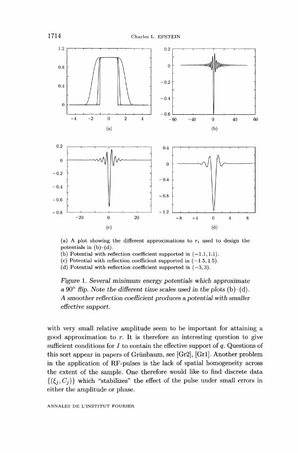
Example 1. - For our first example we use piecewise polynomialfunctions, with three continuous derivatives, to design pulses. Figure 1 (a)shows several such approximations to r- and Figure 1 (b)-(d) shows

1713

the corresponding minimum energy (no bound states) potentials. Therelationship between the quantitative smoothness of r and the effectivesupport of q is quite apparent in these examples.

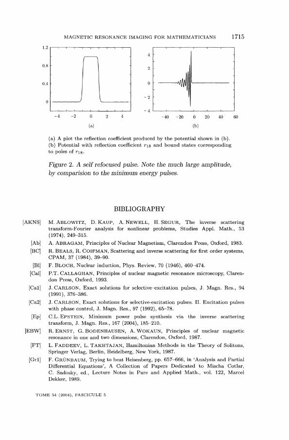
Example 2. - For our next example we consider the effects of addingbound states. We use the rational function (1 + ç18)-1 as an

approximation to rz. We use 9 bound states with ~9 I given bythe poles of r18 in the upper half. For the norming constants, we use theresidues of r18 at the corresponding points. As is well known, this producesa potential supported in (0,00]. In the MR-literature this is called a selfrefocused pulse. The pulse and its corresponding reflection coefficient areshown in Figure 2.

The physical problem of selective excitation fixes only the reflectioncoefficient. The discrete data for the inverse scattering problem are freeparameters. In medical applications it is usually important to keep thetotal energy and maximum amplitude of the pulse small; this makes

the minimum energy pulse an attractive choice. There are however otherconsiderations which might make a pulse with higher energy more useful.The main desideratum is to reduce the "effective" support of the potential.In real applications one might truncate the potential produced by the ISTto obtain a function of the form w(t)q(t), with support in a finite interval.This leads one to ask the following questions:

1) For a given reflection coefficient r, is it possible to choose discreteCj)1, so that the potential with this reduced scattering data has

arbitrarily small effective support?

2) For a given reflection coeffcient r, is it possible to choose discreteso that the effective support of the potential with this

reduced scattering data is reduced by a definite factor over that of theminimum energy potential, e.g., cut in half?

3) Is there a nonlinear Heisenberg uncertainty principle for the 1ST?

These problems beg the question of what is meant by effective support.The main goal is to attain a good approximation to the given reflectioncoefficient, r. Hence, we say that an interval I contains the effective supportof q if there is a window function w supported in I so that rw is a goodapproximation to r. From experiments we have done, it is fairly clear that,for minimum energy pulses, the effective support can be described as aninterval where the potential assumes at least some fraction of its maximumvalue. On the other hand, for pulses with bound states, parts of the pulse

1714

(a) A plot showing the different approximations to ri used to design thepotentials in (b)-(d).(b) Potential with reflection coefficient supported in (-1.1, 1.1).(c) Potential with reflection coefficient supported in (-1.5, 1.5).(d) Potential with reflection coefficient supported in (-3, 3).

Figure 1. Several minimum energy potentials which approximatea 90° flip. Note the different time scales used in the plots (b)-(d).A smoother reflection coefficient produces a potential with smallereffective support.

with very small relative amplitude seem to be important for attaining agood approximation to r. It is therefore an interesting question to givesufficient conditions for I to contain the effective support of q. Questions ofthis sort appear in papers of Grfnbaum, see [Gr2], [Grl]. Another problemin the application of RF-pulses is the lack of spatial homogeneity acrossthe extent of the sample. One therefore would like to find discrete data

which "stabilizes" the effect of the pulse under small errors ineither the amplitude or phase.

1715

’B / , /

(a) A plot the reflection coefficient produced by the potential shown in (b).(b) Potential with reflection coefficient r18 and bound states correspondingto poles of r18.

Figure 2. A self refocused pulse. Note the much large amplitude,by comparision to the minimum energy pulses.

BIBLIOGRAPHY

[AKNS] M. ABLOWITZ, D. KAUP, A. NEWELL, H. SEGUR, The inverse scatteringtransform-Fourier analysis for nonlinear problems, Studies Appl. Math., 53

(1974), 249-315.[Ab] A. ABRAGAM, Principles of Nuclear Magnetism, Clarendon Press, Oxford, 1983.

[BC] R. BEALS, R. COIFMAN, Scattering and inverse scattering for first order systems,CPAM, 37 (1984), 39-90.

[Bl] F. BLOCH, Nuclear induction, Phys. Review, 70 (1946), 460-474.

[Cal] P.T. CALLAGHAN, Principles of nuclear magnetic resonance microscopy, Claren-don Press, Oxford, 1993.

[Ca1] J. CARLSON, Exact solutions for selective-excitation pulses, J. Magn. Res., 94(1991), 376-386.

[Ca2] J. CARLSON, Exact solutions for selective-excitation pulses. II. Excitation pulseswith phase control, J. Magn. Res., 97 (1992), 65-78.

[Ep] C.L. EPSTEIN, Minimum power pulse synthesis via the inverse scatteringtransform, J. Magn. Res., 167 (2004), 185-210.

[EBW] R. ERNST, G. BODENHAUSEN, A. WOKAUN, Principles of nuclear magneticresonance in one and two dimensions, Clarendon, Oxford, 1987.

[FT] L. FADDEEV, L. TAKHTAJAN, Hamiltonian Methods in the Theory of Solitons,Springer Verlag, Berlin, Heidelberg, New York, 1987.

[Gr1] F. GRÜNBAUM, Trying to beat Heisenberg, pp. 657-666, in ’Analysis and PartialDifferential Equations’, A Collection of Papers Dedicated to Mischa Cotlar,C. Sadosky, ed., Lecture Notes in Pure and Applied Math., vol. 122, Marcel

Dekker, 1989.

1716

[Gr2] F. GRÜNBAUM, Concentrating a potential and its scattering transform for adiscrete version of the Schrodinger and Zakharov-Shabat operators, Physica D, 44(1990), 92-98.

[GH] F. GRÜNBAUM, A. HASENFELD, An exploration of the invertibility of the Blochtransform, Inverse Problems, 2 (1986), 75-81.

[Ha] E.M. HAACKE, R.W. BROWN, M.R. THOMPSON, R. VENKATESAN, MagneticResonance Imaging, Wiley-Liss, New York, 1999..

[Ho1] D. HOULT, The principle of reciprocity in signal strength calculations - A mathe-matical guide, Concepts Magn. Res., 12 (2000), 173-187.

[Ho2] D. HOULT, Sensitivity and power deposition in a high field imaging experiment,JMRI, 12 (2000), 46-67.

[Ma] J. MAGLAND, Discrete Inverse Scattering Theory and NMR pulse design, PhD.Thesis, University of Pennsylvania, 2004.

[Me] E. MERZBACHER, Quantum Mechanics, 2nd ed., John Wiler &#x26; Sons, New York,1970.

[PRNM] J. PAULY, P. LE ROUX, D. NISHIMURA, A. MACOVSKI, Parameter relations forthe Shinnar-Le Roux selective excitation pulse design algorithm, IEEE Trans.Med. Imaging, 10 (1991), 53-65.

[MR] D.E. ROURKE, P.G. MORRIS, The inverse scattering transform and its use in theexact inversion of the Bloch equation for noninteracting spins, J. Magn. Res., 99(1992), 118-138.

[SL1] M. SHINNAR, J. LEIGH, The application of spinors to pulse synthesis and analysis,Magn. Res. in Med., 12 (1989), 93-98.

[SL2] M. SHINNAR, J. LEIGH, Inversion of the Bloch equation, J. Chem. Phys., 98(1993), 6121-6128.

[To] H.C. TORREY, Bloch equations with diffusion terms, Phys. Review, 104 (1956),563-565.

Charles L. EPSTEIN,University of PennsylvaniaDepartment of Mathematicsand

LSNI, Hospital of the University of PennsylvaniaPhiladelphia, PA (USA).cle@math.upenn.edu