Jean-Philippe Colombier · [email protected]. ... 3D evaluation of EM fields below a rough surface ... ion el el e i i i i el e

Modélisation de l’interaction laser-matière

Jean-Philippe Colombier

[email protected]

Multiscale modelling

2

➢ General models & methods

➢ Some specific metallic cases

➢ Discussion on simulation results

Laser material modelling

Aspects fondamentauxde l’interaction

laser-matière

Excitation électronique&

Relaxation du matériau

3

Modélisation des effets d’irradiation

Impulsion ultracourte Energie concentrée sur 100 fs

[ Désordre et déséquilibre]

Interaction laser-matière

4

Modélisation des effets d’irradiation

Laserfs

Plasma

Substrat

Surface / Bulk structuring

Interaction laser-matière


5

MODÉLISATION

MULTI-ÉCHELLE

de l’atomeà la 100aine

10-15 s à 1 s

Physique atomique

Dynamique Moléculaire

Thermodynamique

Hydrodynamique

Chimie

& transfert de charge

Photonique

& Plasmonique

Multiphysics modelling


6

MODÉLISATION

MULTI-ÉCHELLE

de l’atomeà la 100aine

10-15 s à 1 s

Physique atomique


Thermodynamique

Hydrodynamique

Chimie

& transfert de charge

Photonique

& Plasmonique



7

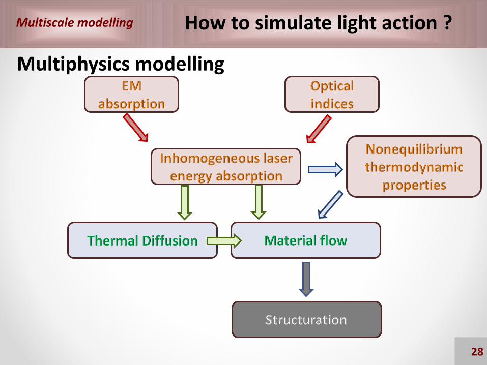
How to simulate light action ?


EM Modelling Electromagnetic calculations

8

Laser source (ultrashort)

Boundary conditions

Index change

Scattered waves& plasmons?

Reflexion/refraction

Absorbed energy ?

Transientmaterial change?

EM Modelling

9

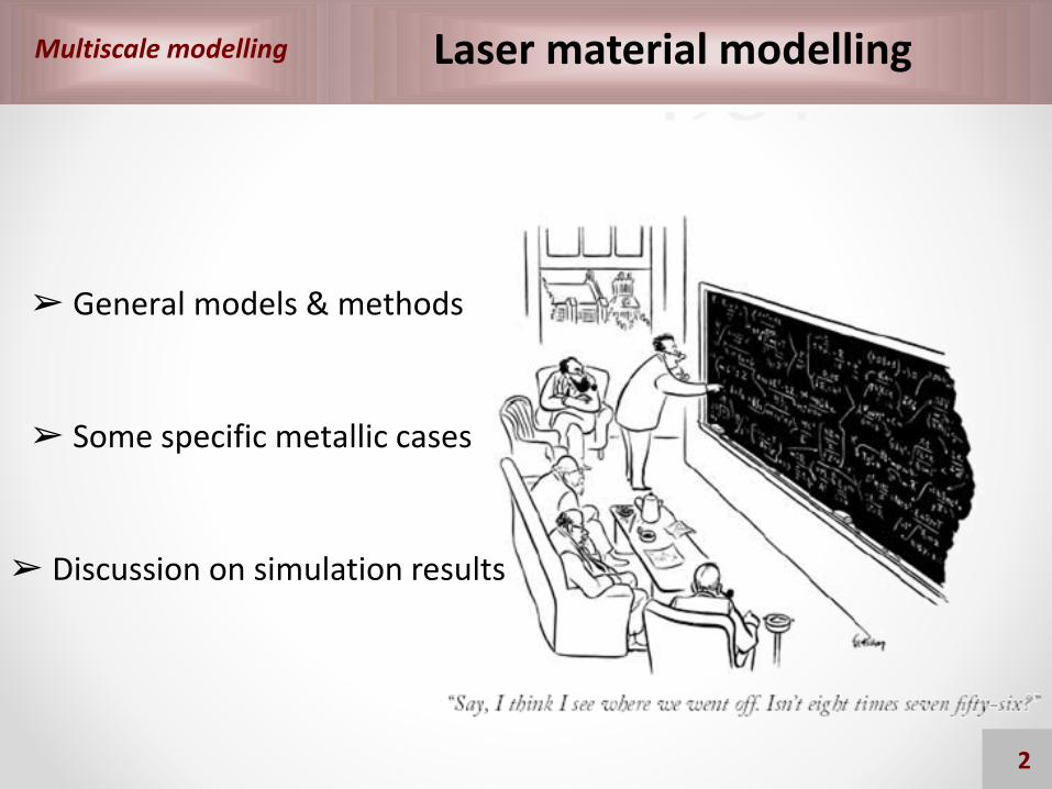
Engraved in stone…

Maxwell equations

A function value isassigned to a specificpoint within the grid

unit cell

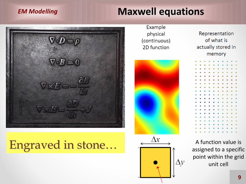
EM Modelling Flow of Maxwell’s equations

10

+ t in on the attosecond timescale

+ The discretization scheme must resolve the minimum structural dimension and sample the wavelength /10 50 nm to be correctly resolved

+ For a laser spot of 50 µm 1000 cells required / dimension

+ 3D 109 cells where E, H, J, … has to be stored for double precision (8 bytes) Needs of tens of GB of memory !

EM Modelling

11

Commercial code example

FDTD solution - LumericalLaser source

Perfectly Matched Layerssurrounding the box

Intensity distribution

Black box calculation

Field patterns=

Energy distribution

EM Modelling

12

Rouhness layer (flat)

Hole or bump

Linear Polarization

Gaussian laser field

Concept: EM response: A sharp single roughness generates scattered fields.

The superposition (interference) with incident one would produce stationary waves and local field enhancement.

A single roughness center

3D evaluation of EM fieldsbelow a rough surface

3D-FDTD Calculations[Maxwell equations]

Zhang et al.,

PRB 92,

174109

(2015)

EM Modelling

13

Bump Hole

Near Field enhancement

Intensity very close to a single roughness center in the plane transverse to the propagation

Laser action not necessarily erases the bump, but mainly

contributes to the development of roughness

plane perpendicular to k

Energy deposited inside the nanohole

Similar to Rayleigh Scattering theory

Bump/hole - Different feedback expected

EM Modelling

14

Far Field contribution

Bump Hole

Intensity around a single roughness center in the plane transverse to the propagation

Far-field contributions of bump/hole are complementary

Non evanescent – reinforced by multiple scattering

H. Zhang et al, PRB 92, 174109 (2015)

EM Modelling

15

EM Calculations on metal surfaces

Coupling

Collective response

Random roughness

Feedback

Coherent scattering

LSFL + HSFL

Mie scatteringIndividualresponse

E

Polarization

Roughness inducedinhomogeneous

absorption

Sipe modelH. Zhang et al, PRB 92, 174109 (2015)

Random roughness is a superposition of bump and hole responses

LIPSS formation !

EM Modelling

16

Nonlinear 3D-FDTD calculations[Maxwell Equations]

High Frequency LIPSS

= Local field enhancement on inhomogeneities

Low Frequency LIPSS

= Coherent superposition betweenscattering waves and incident/refracted waves

LIPSS on Cr

NG in SiO2

0

E

t

H

JJHt

DNLLin

τ=100 fs

I=1013 W/cm2

Λ≈ /2n

≈ 250 nm

SiO2

τ=20 fs

Electromagnetic calculations

A. Rudenko et al, Scientific reports 7: 12306 (2017)

EM Modelling

17

Ripples formation

Modulated patterns result from the coherent superposition of incident and scattered waves for LSFL, HSFL, Grooves…

EM interpretation of LIPSS kind based on the evolving surface topology

EM interference theory

explains the profusion of LIPSS

The initial and transient topologies as well as optical indices are crucial

Zhang et al., PRB 92, 174109 (2015)Li et al. OE 24, 11558 (2016)

Initial random roughness

TF

E LSFL Λ≃

LSFL – Type s

Grooves


18



Optical properties

19

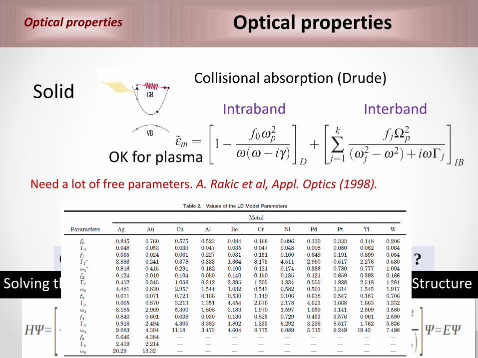
Solid

OK for plasma

Collisional absorption (Drude)

DL model

Band theory required…fsE

k

F

k

k

XG

X

Change of the electronic structure with excitation ?

core

Solving the Schrödinger equation by DFT to evaluate Electronic Structure

Optical properties

Need a lot of free parameters. A. Rakic et al, Appl. Optics (1998).

Intraband Interband

Ab initio

20

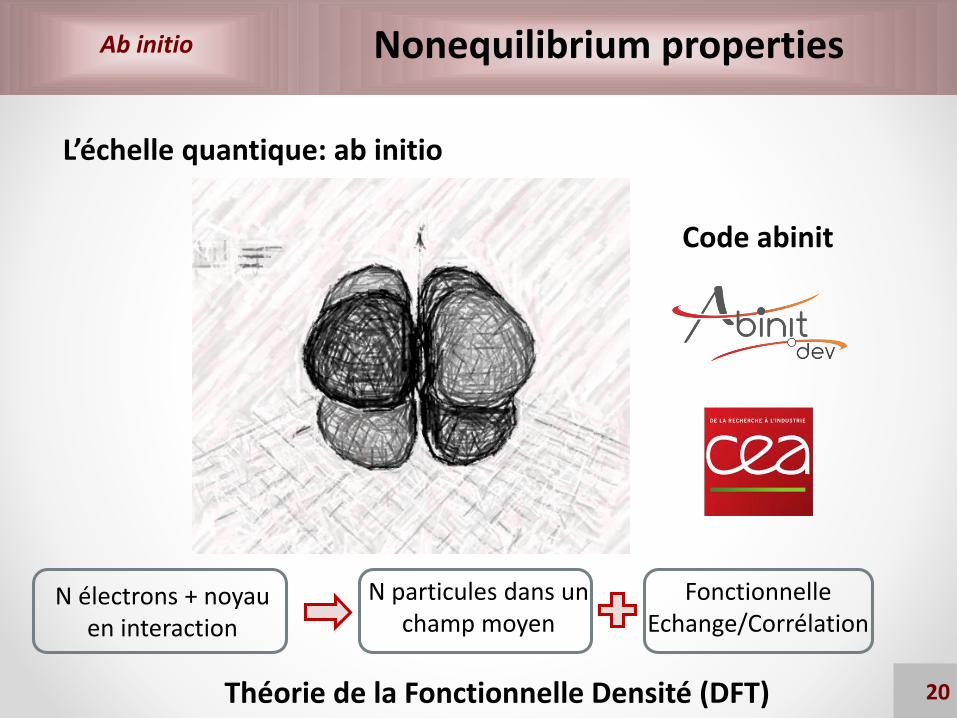
Nonequilibrium properties

L’échelle quantique: ab initio

Théorie de la Fonctionnelle Densité (DFT)

N électrons + noyauen interaction

N particules dans un champ moyen

FonctionnelleEchange/Corrélation

Code abinit

Ab initio

21

Interaction laser-solide

0/)(

02

22

1

1),(),(

)],([),(2

)(

),(),(),(

kTii

N

i

ii

elelion

e

iii

i

el

effwithtrftr

trVtrVm

rH

trtrtrH

][2

2

E

dt

RdM R

Théorie Fonctionnelle de la Densité


Codes: ABINIT [DFT] - Octopus [TD-DFT]

Ab initio approach

Ab initio

22

ne evolution with Te

Partially filled d-band

Semi-conductor

Loss of delocalized e-

Loss of non-bondeninglocalized d-electrons

Siprimitive diamond cell

Electronic Density differences

between hot and cold e- population

Ground-state Density Functional

Theory [ABINIT Code]

Niprimitive FCC cell

Wprimitive BCC cell

Nearly filled d-band

Softening of e- bondening Gain of delocalized e-

ne +-

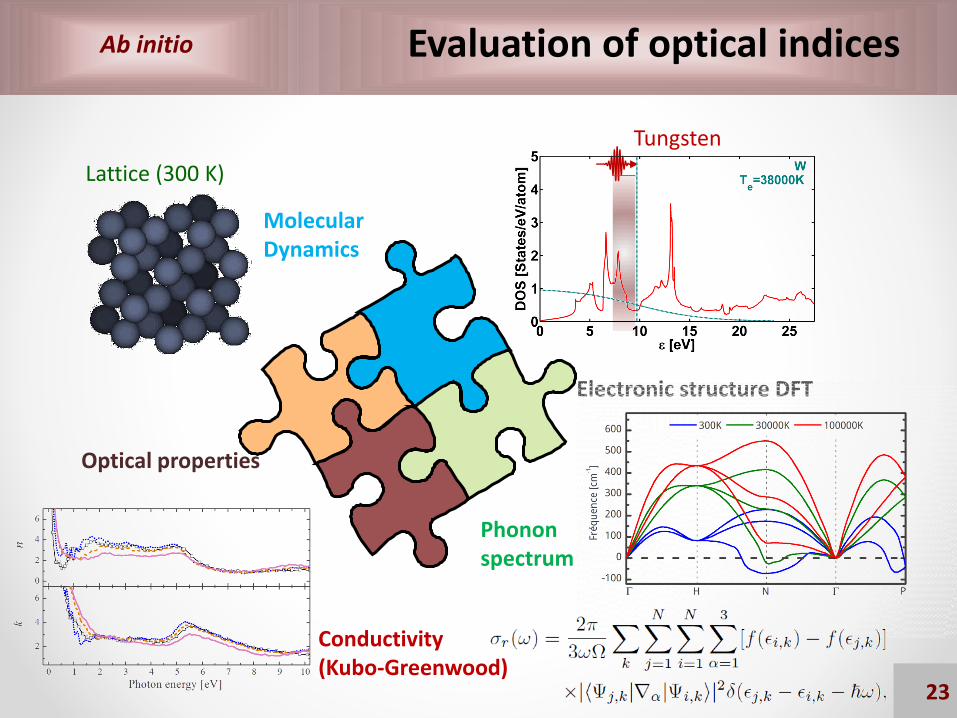
Ab initio Evaluation of optical indices

MolecularDynamics

Lattice (300 K)

Optical properties

Conductivity(Kubo-Greenwood)

23

Electronic structure DFT

Tungsten

Phonon spectrum

Ab initio Optical properties

24

DO

S

Potential electronic transitions at

W electronic structure: Increase of the phase space

available for e- transition with Te

Strongly impact optical properties

λ=800 nm

Low Te (<105 K) Decrease of e- in sp bands Gain of e- localization (d-band)

W, primitive BCC cell Ground-state Density Functional

Theory [ABINIT Code]

e- density differences between

hot and cold e- population

MD + DFT Calculations

Optical properties Optical properties

25

DO

S

Energy [eV]

Potential electronic transitions at

W electronic structure: Increase of the phase space

available for e- transition with Te

Strongly impact optical properties

λ=800 nm

n decreasek increase

W [10000K] ≈ Ti [300K] W [25000K] ≈ Ni [300K] !

λ = 800 nm

E. Bévillon et al, Phys. Rev. B 93, 165416 (2016)

Optical properties Optical properties

26

n decreasek increase

W [10000K] ≈ Ti [300K] W [25000K] ≈ Ni [300K] !

λ = 800 nm

E. Bévillon et al, Phys. Rev. B 93, 165416 (2016)

2 angles time-resolved one colorEllipsometry measurement

n800=2.1+i3.8

n800=3.6+i2.7

Plasmon switch

Optical properties

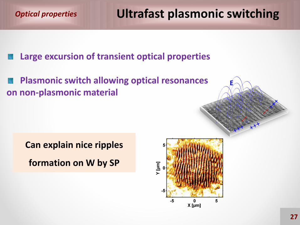
27

Ultrafast plasmonic switching

Large excursion of transient optical properties

Plasmonic switch allowing optical resonanceson non-plasmonic material

E

Can explain nice ripples

formation on W by SP


28



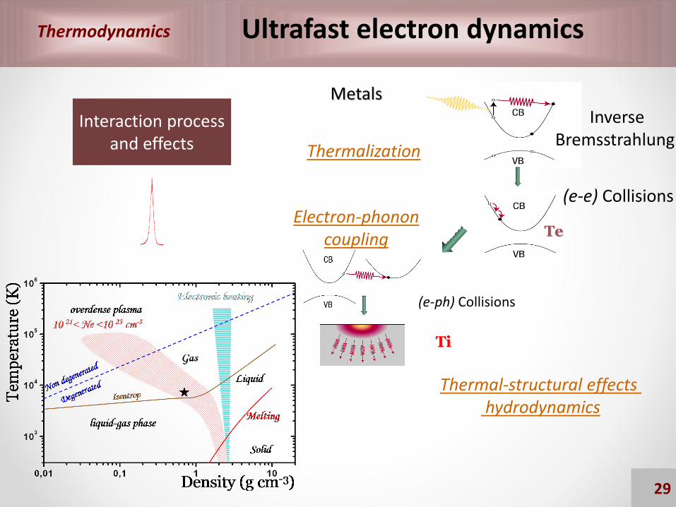
Thermodynamics

29

Thermalization

Electron-phononcoupling

Thermal-structural effectshydrodynamics

MetalsInverse

Bremsstrahlung

(e-e) Collisions

(e-ph) Collisions

Te

Ti

Interaction processand effects

Ultrafast electron dynamics

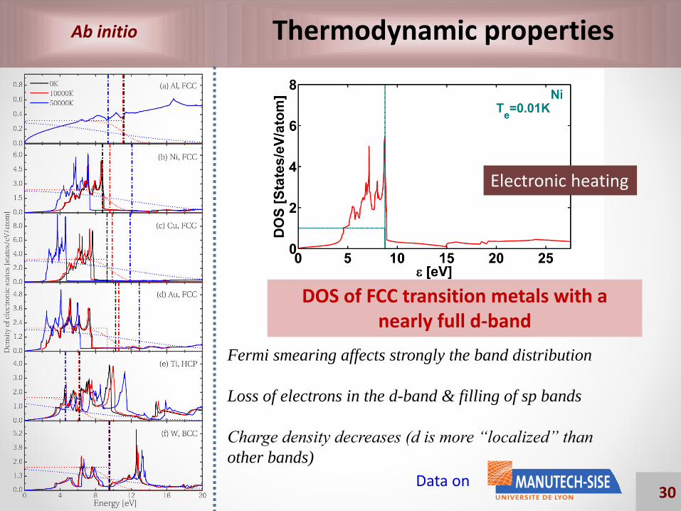
Ab initio Thermodynamic properties

Fermi smearing affects strongly the band distribution

Loss of electrons in the d-band & filling of sp bands

Charge density decreases (d is more “localized” than

other bands)

DOS of FCC transition metals with a nearly full d-band

Electronic heating

30Data on


Electronic capacity

The electronic

structure is required

for transition metals

Make the connection

between energy and

temperature

31

Data on


Electronic Pressure

Te increase: Band stucture has strong effect for low Te

Follows ideal electron gas law for high Te

Pe reach several tens of GPa in LIPSS range32


33




34

p

s

Cib

le

√ Diffusion 2 températures

√ Hydrodynamique

√ Equation d’état

√ Physico-Chimie

• Diffusion thermique système hors d’équilibre [Modèle 2T]

• Hydrodynamique [Navier-Stokes]

( ) ( )

( ) ( )

ee e e ei e i abs

ii i i ei e i

TC k T T T I

t

TC k T T T

t

uµ

Fpuut

u

uput

ut

21)(

0,0)(

Time [ps]z

[nm

]

• Physico-Chimie

• Distribution de l’énergie électromagnétique [Maxwell non-linéaires]

0

E

t

H

JJHt

DNLLin

• Equation d’état avec données électroniques/transport ab initio

Material dynamics

N. Destouches et al. E. Bévillon et al., JPCC (2015)

Thermodynamics

1D Modelling: Dynamics of the excited material

Two temperature model

Thermodynamic states

Couplage e-ph

Equation of states For electrons & transport

Ce, Ke, Ne, Pe…Equation of statesfor each material

E, ρ, TP, cs, Z*

35

Thermodynamics

36

Two temperature model

Dynamics of the excited material in 1 cell

Thermodynamics

37

Transient modification

Solidification[1 ns]

Capillarity

10 ps – 1 ns

10-100 nmLiquid layer

DENSITY [Kg/m3]

Liquid

Ni

Meltinge-ph

Diffusion

1-10 ps

Solid

Surface

e-ph

Diffusion

Dynamics of the excited material in multi-cells

Thermodynamics

38

Thermal Diffusion [In depth]

3D problem…BUT:

Longitudinal gradients [104 K on 10-100nm]

vsRadial gradients [104 K on 50µm]

COMSOL example

Thermodynamics

39

Modulation disappears ≈ 5 ns

Surface temperature

evolution in time

Initial surface temperature

Thermal Diffusion [Radial]

For periodic features on surface, radial gradients can play a role as well…

Fluid dynamics

Chauffage du solide

1014 K/s

Chauffage électronique

1017 K/s

Vitesse expansion104 m/s

Vitesse de refroidissement

(quenching)

1012 K/s

Fluide supercritiqueForte température

Forte densitéMatière Dense et

chaude

« Fortement corrélée »

100 µm

N. Zhang et al., Phys. Rev. Lett. 99, 167602 (2007).

Transient properties

40

Fluid dynamics

p

s

Cib

le

√ Absorption Helmholtz

√ 2T model

√ Ionization

√ Hydrodynamics

e-ph coupling

Absorption

Hydro

Recombination

Code ESTHER

Thermal conduction

core

Hydrodynamic simulation

41Colombier et al., PRB 2005 – PRB 2006 – PRB 2007 – PRE 2008 – NJP 2012

Fluid dynamics

Solid

Shock

Rarefactionwave

Liquid Pe

Pi

AirAir

Sub ablation threshold: thermo-mechanical stress close to 15 GPa (F=0.25 J/cm2)

Evaluating the laser effect

Esther code

42

Fluid dynamics

S

G

S+G

Phases thermodynamiques

L+GL

Pc

Processus d’ablation

43

Fluid dynamics

G

S+G

√ Chauffage laser isochore

√ Expansion de fluidesupercritique


FragmentationCluster+gaz

√ Formation de plasma

DM – T. Itina

S

L+GL

Pc


44

Fluid dynamics

G

S+G

√ Chauffage laser isochore

√ Transformation liquide-gaz


Nucléationhomogène

S

L+G

LPc


45

Fluid dynamics

104

107

106

105

1010

109

108

1011

TEM

PER

ATU

RE

[K]

DENSITY [Kg m-3]

PRESSURE [Pa]

20 ps

OP10 nm

20 nm

30 nm

40 nm

50 nm

2 nm

BINODAL10 ps

30 ps

40 ps

101

102

10310

3

104

(not-so) isochorictransition

mixed region: nucleation

Plasma

supercritical

CP

OP

Thermodynamic pathways

[80%]

F5 J/cm2

Colombier et al., New Journal of Physics (2012)46

Fluid dynamics

G

S+G

√ Chauffage par choc

√ Cavitation en phaseliquide


Ejection d’une goutte

S

L+GL

Pc


47

Fluid dynamics

SP

5 µm

SP

Picosecond pulse(10 ps)

Liquid phase ejection

Ion emission

OP

150 fsNanoparticles

Droplet

Plasma

Pulse Laser deposition

[Experiments]

Guillermin et al., Phys. Rev. B 82, 035430 (2010).

48

Fluid dynamics

G

√ Compression par choc

√ Cavitation en phasesolide


Ecaillage en phase solide


Laser

S

L+GL

Pc

S+G

49


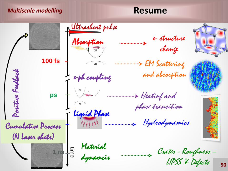
50

Resume

0

100 fs

Metal

Absorption

ps

Liquid Phase100 ps

Ultrashort pulse

e-ph coupling

1 ns

Posi

tive

Feedb

ack

Cumulative Process

(N Laser shots)Material

dynamcisCrater - Roughness –

LIPSS & Defects

Heatinf and

phase transition

Hydrodynamics

EM Scattering

and absorption

e- structure

change

Thanks for your attention !Collaborators

Anton RudenkoEmile Bévillon

Andrei VoloshkoHao Zhang

Chen LiAnthony Abou SalehMatthieu Guillermin

Florent PigeonFlorence Garrelie

Tatiana ItinaRazvan Stoian

Documents

Jean-Philippe Colombier · [email protected]. ... 3D evaluation of EM fields below a rough surface ... ion el el e i i i i el e