Embed Size (px)
Citation preview
N° d’ordre : 2007telb0055
THÈSE
Présentée à
l’ÉCOLE NATIONALE SUPERIEURE DES TELECOMMUNICATION S DE BRETAGNE
en habilitation conjointe avec l’Université de Bretagne Sud
pour obtenir le grade de
DOCTEUR de l’ENST Bretagne
Mention « Sciences pour l’ingénieur »
par
Mickaël DE MEULENEIRE
« CODAGE IMBRIQUÉ POUR LA PAROLE À 8-32 KBIT/S COMBINANT
TECHNIQUES CELP, ONDELETTES ET EXTENSION DE BANDE »
Soutenue le 21 novembre 2007 devant la Commission d’Examen :
Composition du Jury
- Rapporteurs : Régine LE BOUQUIN JEANNÈS, Professeur, Université de Rennes I
Pascal SCALART, Professeur, ENSSAT
- Examinateurs : Samir SAOUDI, Professeur, ENST Bretagne
Dominique PASTOR, Maître de conférences, ENST Bretagne
Hervé TADDEI, Ingénieur de recherche, Nokia Siemens Networks
Emmanuel BOUTILLON, Professeur, Université de Bretagne Sud
- Invitée : Claude Lamblin, Ingénieur de recherche, France Télécom


Acknowledgements
First of all, I would like to thank my supervisor Hervé Taddei for o�ering me the chanceto work on this thesis, for always ensuring good working conditions, and for proofreading somany times my dissertation. His advice has always been valuable to me. He often encouragedme to pursue directions that I wanted to give up. I particularly appreciated his everyday goodmood.
I am thankful to sponsors from Siemens Mobile, BenQ Siemens, Siemens Corporate Tech-nology, Siemens Networks and Nokia Siemens Networks for �nancing my study.
I want also to express my gratitude to Pr. Samir Saoudi and my advisor Dr. DominiquePastor from ENST Bretagne for their many suggestions and for taking care of the administra-tive tasks during this thesis.
I am grateful to Pr. Régine Le Bouquin Jeannes and Pr. Pascal Scalart for accepting tobe rapporteurs of my work. Moreover, I would like to thank Dr. Claude Lamblin for proof-reading my dissertation and Pr. Emmanuel Boutillon for being president of the examinationcommission.
I am also indebted to the students I supervised during this thesis, Emmanuel Thepie Fapi,Olivier de Zélicourt, and Clément Marechalle, for their contribution to my work.
Many thanks go to the collegues, Imre, Christophe and Martin, students that I have metover these four years at Siemens Mobile, Siemens Corporate Technology and Nokia SiemensNetworks, especially Panji, Suhadi, Antoine, Kai, Virginia, Stéphanie, and all the others Icould not mention, with whom I had a really good time, for their help and participation tolistening tests.
Finally, I would like to deeply thank my familly and my friends, as well as my wife Ailsa,for their support and their love throughout all these years.

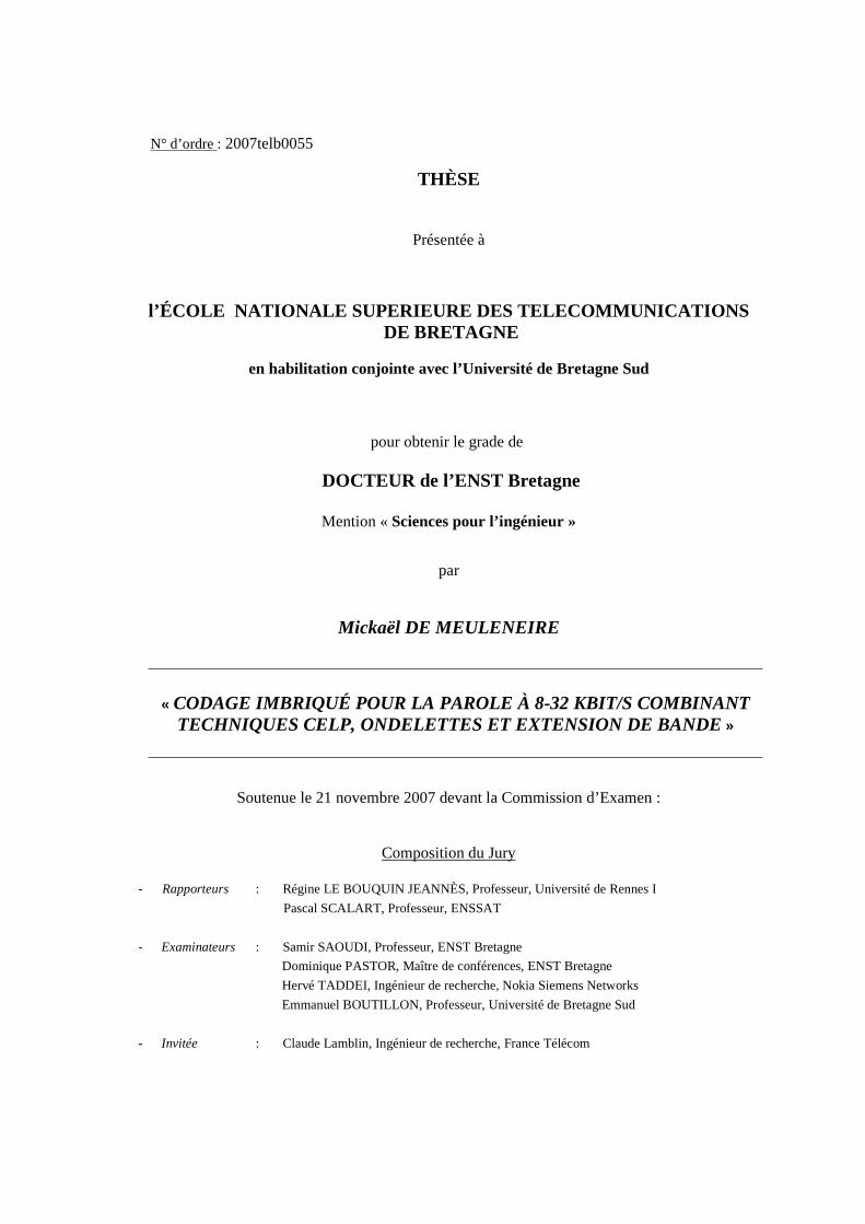
List of Abbreviations
AbS Analysis-by-Synthesis.ACELP Algebraic Code-Excited Linear Prediction.ACR Absolute Category Rating.ADC Analog-to-Digital Converter.ADPCM Adaptive Di�erential Pulse Code Modulation.AMR Adaptive Multi-Rate.AMR-WB Adaptive Multi-Rate Wide-Band.ATH Absolute Threshold of Hearing.BWE Band-Width Extension.CD Compact Disc.CELP Code-Excited Linear Prediction.CNG Comfort Noise Generator.CODEC COder/DECoder.CQF Conjugate Mirror Filter.DAC Digital-to-Analog Converter.DCT Discrete Cosine Transform.DFT Discrete Fourier Transform.DSL Digital Subscriber Line.DTX Discontinuous Transmission.ECG Encephalo-Cardio-Gram.EL Enhancement Layer.EZW Embedded Zerotree Wavelet.FFT Fast Fourier Transform.FIR Finite Impulse Response.GSM Global System for Mobile communications.IP Internet Protocol.ISO International Organization for Standardization.ITU-T International Telecommunication Union, Telecommunication standardiza-
tion sector.IWPD Inverse Wavelet Packet Decomposition.JPEG Joint Photographic Experts Group.LAN Local Area Network.LIP List of Insigni�cant Points.

LIS List of Insigni�cant Sets.LP Linear Prediction.LPC Linear Predictive Coding.LSA Log Spectral Amplitude.LSF Line Spectral Frenquencies.LSP Line Spectral Pair,List of Signi�cant Points.LTP Long-Term Prediction.MA Moving Average.MDCT Modi�ed Discrete Cosine Transform.MNRU Modulated Noise Reference Unit.MOS Mean Opinion Score.MP3 MPEG 1/2 Audio Layer 3.MPE Multi-Pulse Excitation.MPEG Moving Picture Experts Group.MPEG-ALS MPEG Audio Lossless Coding.MSE Mean Square Error.NBSP Nested-Binary Set Partitioning.PC Personal Computer.PCM Pulse Code Modulation.PDA Personal Digital Assistant.PESQ Perceptual Evaluation of Speech Quality.PLC Packet Loss Concealment.PSTN Public Switch Telephone Network.PZW Perceptual Zerotree Wavelet.QMF Quadrature Mirror Filter.QoS Quality of Service.RD Rate-Distortion.RPE Regular-Pulse Excitation.SMR Signal-to-Mask Ratio.SNR Signal-to-Noise Ratio.SPIHT Set Partitioning In Hierarchical Trees.SSNR Segmental Signal-to-Noise Ratio.STP Short-Term Prediction.SUPER SUbband PERceptual measure.TDBWE Time-Domain Band Width Extension.UDP User Datagram Protocol.UMTS Universal Mobile Telecommunications System.VAD Voice Activity Detection.VoIP Voice over Internet Protocol.

VQ Vector Quantization.VSELP Vector-Sum Excited Linear Prediction.WP Wavelet Packet.WPD Wavelet Packet Decomposition.WT Wavelet Transform.

Résumé des chapitres
Chapitre 1 : Le codage scalable
Le premier chapitre introduit le concept de codage audio imbriqué. La première sectiondécrit le codage audio en général, qui consiste en la réduction des données produites par unesource audio. Elle introduit également la notion de largeur de bande. Le codage audio estpartagé en deux catégories : codage avec perte et codage sans perte. Alors que le codage sansperte garantit un signal reconstruit identique au signal original, le codage avec perte permetd'écarter les parties non signi�catives ou non pertinentes du signal à reconstruire. Le signalreconstruit est alors di�érent du signal original. Néanmoins, il est possible de reconstruireun signal perceptuellement identique au signal original, c'est-à-dire extrêmement di�cile àdistinguer du signal original. Ceci est possible en exploitant les propriétés de masquage del'oreille humaine par l'utilisation d'un modèle dit psychoacoustique ou perceptuel. Cette sectionse termine par un aperçu du codage de la parole.
La deuxième section établit les principes du codage imbriqué et en donne quelques exemplesd'utilisation. Le codage imbriqué construit un train binaire qui est organisé en couches. Chaquecouche peut être décodée indépendamment des couches supérieures. La première couche estappelée couche c÷ur et est indispensable au décodeur pour reconstruire un signal avec unequalité et une largeur de bande minimales. Les couches suivantes sont appelées couches d'amé-lioration car elles permettent d'améliorer la qualité du signal décodé par la couche c÷ur et/oud'augmenter sa largeur de bande.
Chapitre 2 : Codage par prédiction linéaire
Le deuxième chapitre est consacré au codage de la parole par prédiction linéaire, notammentà la prédiction linéaire avec excitation par séquences codées, plus connu sous l'abréviationanglaise CELP. Les codeurs CELP travaillent sur des morceaux consécutifs d'égale longueurdu signal d'entrée, appelés trames. Suivant le codeur, la longueur d'une trame varie entre 10ms et 30 ms pour rester dans l'hypothèse de stationnarité du signal de parole.
Tout d'abord, la corrélation à court terme sur une trame du signal est réduite par prédictionlinéaire, c'est-à-dire qu'un échantillon de la trame est estimé par combinaison linéaire deséchantillons précédents, ceci pour un nombre �ni d'échantillons. L'ensemble des coe�cientsde prédiction forme le �ltre de synthèse. Ce �ltre modélise le conduit vocal. Un résidu deprédiction est obtenu par di�érence entre le signal d'entrée et son estimée par prédictionlinéaire. Ce résidu est quanti�é par une combinaison linéaire de deux mots de code, provenantde deux dictionnaires. Le résidu quanti�é joue le rôle d'excitation du �ltre de synthèse.
Le premier dictionnaire, dit adaptatif, modélise la corrélation à long terme présente dans lerésidu, résultant de la vibration des cordes vocales. Ce dictionnaire contient un ensemble d'ex-citations quanti�ées des dernières trames codées. Les mots de code sont indicés par une valeurappelée pitch, qui caractérise la périodicité du signal à la trame courante. Une fois le mot decode optimal trouvé, son gain associé est également calculé. Le deuxième dictionnaire, quali�éde �xe, contient un ensemble de séquences prédé�nies et code l'information non prédictible,appelé innovation. Le codeur détermine le mot de code optimal ainsi que son gain associé. Dansles deux cas, le mot de code ainsi que son gain sont obtenus en minimisant l'erreur quadratiquemoyenne entre le signal original et le signal reconstruit. Cette méthode est appelée analyse parsynthèse.
L'excitation consiste en la somme des deux mots de code, pondérés par leur gain quan-ti�é respectif. Le dictionnaire adaptatif est mis à jour en concatenant cette excitation auxexcitations des trames précédentes. Les propriétés de masquages du système auditif peuventêtre prises en compte en pondérant l'erreur par une fonction dépendant des coe�cients deprédiction à court terme.
Chapitre 3 : La norme G.729
Le codeur G.729 standardisé à l'UIT-T ainsi que les modi�cations apportées dans l'annexeA pour réduire la complexité de l'ensemble codeur/décodeur sont présentés dans ce troisièmechapitre. Le G.729 encode des signaux échantillonnés à 8 kHz à un débit de 8 kbit/s.
Le signal d'entrée est segmenté en trames de 10 ms, soit 80 échantillons. Chaque trame estde nouveau divisée en 2 sous-trames de longueur égale. Une analyse par prédiction linéaire este�ectuée une fois par trame, en considérant, en plus des échantillons de la trame courante, les140 échantillons du passé et les 40 premiers échantillons de la trame suivante. L'ensemble descoe�cients est pondéré par une fenêtre asymétrique. Les coe�cients de la prédiction linéaireforment le �ltre de synthèse pour la seconde sous-trame. Les coe�cients correspondant à lapremière sous-trame sont obtenus par interpolation avec la seconde sous-trame de la trameprécédente. Les coe�cients de prédiction linéaire ne sont pas quanti�és directement, mais sousforme de paire de lignes spectales (Line Spectral Pairs). Leur quanti�cation requiert 18 bitspar trame. Le �ltre de pondération perceptuelle pour la recherche des autres paramètres est
calculé à partir du �ltre de synthèse non quanti�é.
Ensuite, une première estimation du pitch est réalisée sur l'ensemble de la trame. Unevaleur plus �ne, qui peut comporter une partie fractionnaire en plus de sa partie entière, estcalculée pour chaque sous-trame. Les deux valeurs sont quanti�ées par un total de 14 bits.Chacune des deux valeurs code un mot de code dans le dictionnaire adaptatif. Un gain estcalculé pour chaque mot de code.
En�n, un mot de code �xe est déterminé pour chaque sous-trame. Il est composé de 40échantillons, dont 4 impulsions non-nulles qui peuvent prendre les valeurs ±1. De plus, cedictionnaire dispose d'une structure algébrique. La quanti�cation des deux mots de codesnécessite 17 bit par sous-trame. Pour chaque sous-trame, le gain du mot de code �xe et celuidu mot de code adaptatif sont conjointement quanti�és. Cette quanti�cation utilise 7 bits parsous-trame. Ce codeur sera choisi comme codeur c÷ur de la structure proposée dans cettethèse.
Chapitre 4 : Codage CELP imbriqué
Le chapitre 4 est dédié aux techniques d'imbrication relatives aux codeurs par prédictionlinéaire. La première section donne une vue d'ensemble des di�érentes techniques abordées dansla littérature. La deuxième section s'intéresse plus précisément aux techniques d'enrichissementdu mot de code �xe. Après avoir montré l'importance de telles techniques, des expérimentationssur un dictionnaire �xe imbriqué sont présentées. Cette section se conclut par la présentationd'une technique développée au cours de la thèse qui repose sur une modi�cation de l'amplitudede chacune des impulsions du mot de code �xe. Cette technique utilise 8 bits par sous-trame.Un deuxième dictionnaire de mots de code avec 2 impulsions non nulle d'amplitude ±1 estajouté. La transmission du mot de code et du gain associé nécéssite 12 bits par sous-trame.L'association de la modi�cation des amplitudes du mot de code �xe et de l'addition d'undictionnaire supplémentaire est comparée avec un deuxième dictionnaire seul, identique à celuidu G.729, et utilisant un total de 20 bits par sous-trames (17 bits pour le mot de code et 3bits pour la quanti�cation du gain). Cette association présente certes l'avantage d'introduireun débit intermédiaire, mais n'est pas aussi performante qu'un dictionnaire additionnel seul.
Chapitre 5 : Les ondelettes d'un point de vue "banc de �ltre"
Le chapitre 5 présente le concept de transformée discrète en ondelettes d'un point de vuebanc de �ltres, dont la réalisation pratique se résume à l'application récursive d'un banc de�ltres à deux canaux. La transformée en ondelettes, et plus généralement la décomposition enpaquets d'ondelettes, permet d'obtenir une représentation temps-fréquence d'un signal, c'est-
à-dire de connaître les composantes fréquentielles présentes dans un intervalle de temps donné.La première section de ce chapitre rappelle les conditions de reconstruction parfaite que doiventsatisfaire les �ltres d'analyse et de synthèse. Puis, les propriétés de la transformée discrète enondelettes sont décrites dans la deuxième section : décomposition en approximations et détails,résolution temporelle et résolution fréquentielle, propriété d'autosimilarité. Ensuite, une troi-sième section dé�nit la décomposition en paquets d'ondelettes en décomposant non seulementles approximations mais aussi les détails résultant du banc de �ltres à deux canaux. Cettedécomposition peut être �xe, quel que soit le signal à analyser, ou adaptative, ce qui signi�eque la profondeur de décomposition ainsi que le nombre de paquets à décomposer dépendentdu signal à décomposer. En�n, la dernière section traite des di�érentes implémentations pourgérer les problèmes aux bords de la convolution, liés à la transformée discrète en ondelettes.
Chapitre 6 : Quanti�cation imbriquée
Le chapitre 6 est consacré à la description de la quanti�cation imbriquée de coe�cientsd'ondelettes. Pour une transformation temps-fréquence qui conserve la norme, et en dehors detoute considération perceptuelle, la distorsion entre le signal original et le signal reconstruit estd'autant plus faible que les coe�cients les plus grands en valeur absolue sont bien reconstruits.Il est alors important de transmettre ces coe�cients pour que, à un débit donné, la distorsionsoit la plus faible possible. Une des solutions existantes est le codage par plan binaire. Les coef-�cients sont transmis bit par bit, du bit de poids le plus fort au bit de poids le plus faible, touten transmettant en priorité les coe�cients les plus importants. Ce type de codage est illustrépar deux algorithmes, à savoir EZW et SPIHT, dont l'application première est la quanti�cationde coe�cients d'ondelettes. Les deux algorithmes exploitent la propriété d'autosimilarité descoe�cients d'ondelettes. Les principes de chacun des algorithmes sont présentés. SPIHT estplus e�cace qu'EZW car il est plus rapide, et produit un train binaire plus court. C'est donccet algorithme qui a été retenu pour la quanti�cation des coe�cients d'ondelettes.
Chapitre 7 : Codeurs à base d'ondelettes
Ce septième chapitre présente un ensemble d'exemples de codeurs de parole et audioconstruits autour d'une transformée en ondelettes ou d'une décomposition en paquets d'onde-lettes. Ces codeurs sont en majorité scalables, c'est-à-dire qu'ils permettent une reconstructiond'un signal à partir d'une partie du train binaire. Ces codeurs sont regroupés en deux sections.La première section traite des codeurs considérés comme perceptuels, car les signaux recons-truits sont indiscernables des signaux originaux. Quant aux autres codeurs, ils sont présentésdans une deuxième section. Une troisième et dernière section fait le point sur les di�érentescaractéristiques des codeurs, comme le type de décomposition, uniforme ou non uniforme, àstructure �xe ou adaptative, les méthodes employées pour quanti�er les coe�cients d'onde-
lettes, utilisation ou non d'un modèle perceptuel. Le chapitre est conclu par le choix de ladécomposition en paquets d'ondelettes utilisé dans le codeur proposé, à savoir une décomposi-tion uniforme sans utilisation de modèle perceptuel.
Chapitre 8 : Extension de bande
Le chapitre 8 est dédié à la présentation de l'extension de bande. Dans une version précé-dente du codeur, la décomposition en paquets d'ondelettes était calculée sur la di�érence entrele signal original et le signal décodé par le G.729 suréchantillonné à 16 kHz puis �ltré. À débitconstant, dépendant du type du signal et donc de son spectre, les coe�cients transmis ainsique leur nombre varient d'une trame à l'autre. Par conséquent, le signal reconstruit présenteun spectre à trous, et les zones fréquentielles non codées sont di�érentes d'une trame à l'autre.Les artéfacts produits sont similaires au bruit musical créé par certains algorithmes de réduc-tion de bruit. Pour pallier ce problème, un module d'extension de bande, appelé TDBWE,avec transmission d'information additionnelle a été intercalé entre le G.729 et la quanti�cationdes coe�cients d'ondelettes. Ce module est similaire à celui présent dans le codeur G.729.1de l'UIT-T. Des résultats de test ont montré que l'ajout de l'extension de bande améliore laqualité d'écoute.
Ce module a été ensuite remplacé par une extension de bande qui s'appuie sur le bancde �ltres de la décomposition en paquets d'ondelettes. Parmi plusieurs méthodes testées, uneméthode semblable au TDBWE a été retenue. À l'encodeur, l'enveloppe temporelle de la bandehaute à la sortie du premier niveau de décomposition est calculée, puis quanti�ée vectorielle-ment. Après le dernier niveau de décomposition, l'énergie des di�érents paquets d'ondelettesdans la bande haute est également calculée et quanti�ée vectoriellement. Au décodeur, unsignal dit d'excitation est généré dans la bande haute. L'enveloppe temporelle de ce signalest mise en forme par l'enveloppe temporelle déquanti�ée du signal original. Ce signal estensuite décomposé en paquets d'ondelettes. L'énergie de chaque paquet est corrigée par l'éner-gie quanti�ée correspondante calculée sur le signal original. Le débit alloué à la transmissionde l'enveloppe temporelle et de l'enveloppe fréquentielle est de 2 kbit/s. Par conséquent, ledécodeur reconstruit un signal bande élargie avec un spectre complet à partir de 10 kbit/s.
Chapitre 9 : Codeur proposé
Ce dernier chapitre détaille la structure du codec proposé ainsi que les améliorations ap-portées sur certains modules. Tout d'abord, la structure du codeur et celle du décodeur sontsuccinctement présentées. La couche c÷ur est assurée par le G.729, qui synthétise un signal enbande étroite à un débit de 8 kbit/s. Une première couche d'amélioration reconstruit le signalen bande élargie avec un débit additionnel de 2 kbit/s, soit un débit total de 10 kbit/s. En-
�n, la seconde et dernière couche d'amélioration enrichit progressivement le signal reconstruitjusqu'à un débit de 32 kbit/s, en transmettant les coe�cients de décomposition en paquetsd'ondelettes. Cette décomposition porte sur la di�érence entre le signal original et le signalsynthétisé par le G.729 dans la portion bande étroite (fréquences inférieures à 4 kHz), et surle signal original dans la portion bande élargie (fréquences supérieures à 4 kHz).
Les �ltres ondelettes de Vaidyanathan à 24 coe�cients ont été choisis parce qu'ils assurentune bonne décomposition fréquentielle avec un nombre faible de coe�cients, entraînant unretard faible. Il s'avère que l'utilisation de ce �ltre assure de bonnes performances de SPIHTen termes de débit. Le nombre de décompositions est limité à 4, bien qu'un cinquième niveau dedécomposition soit possible. Ce cinquième niveau n'a aucune in�uence sur le débit de SPIHT,et multiplie par deux le retard du banc de �ltres. Le retard de cette structure est de 23,125ms. De plus, le premier niveau de décomposition a été remplacé par un banc de �ltres à deuxcanaux utilisant un �ltre QMF de Johnston à 64 coe�cients pour réduire le bruit dû à laréplication spectrale présent à la reconstruction à 10 kbit/s. Toutefois, le retard du nouveaubanc de �ltres est accru de 2,5 ms.
Les coe�cients d'ondelettes ont été d'abord quanti�és et compressés par SPIHT. Les para-mètres de cet algorithme qui dé�nissent les relations parents-enfants ont été choisis de manièreà minimiser le débit. Les performances obtenues n'étant pas satisfaisantes, des mécanismes ontété introduits pour contrôler les coe�cients à transmettre, ainsi que leur nombre, dans le butd'allouer en moyenne plus de bits par coe�cient transmis. Cependant, ces mesures ne sont passu�samment e�caces.


CONTENTS i
Contents
Contents i
List of �gures vii
List of tables ix
Introduction 1
I About Scalable Coding 5
1 Introduction to embedded/scalable coding 7
1.1 Short introduction to speech and audio coding . . . . . . . . . . . . . . . . . . . 71.1.1 Audio signal bandwidth . . . . . . . . . . . . . . . . . . . . . . . . . . . 81.1.2 Lossless or lossy . . . . . . . . . . . . . . . . . . . . . . . . . . . . . . . 9
1.1.2.1 Lossless . . . . . . . . . . . . . . . . . . . . . . . . . . . . . . . 91.1.2.2 Lossy . . . . . . . . . . . . . . . . . . . . . . . . . . . . . . . . 9
1.1.3 Speech coding . . . . . . . . . . . . . . . . . . . . . . . . . . . . . . . . . 101.2 Embedded and scalable . . . . . . . . . . . . . . . . . . . . . . . . . . . . . . . 11
1.2.1 Principles . . . . . . . . . . . . . . . . . . . . . . . . . . . . . . . . . . . 121.2.2 Foreseen applications . . . . . . . . . . . . . . . . . . . . . . . . . . . . . 12
Summary . . . . . . . . . . . . . . . . . . . . . . . . . . . . . . . . . . . . . . . . . . 13
II Linear Predictive Coding 15
2 CELP coding 17
2.1 Principles . . . . . . . . . . . . . . . . . . . . . . . . . . . . . . . . . . . . . . . 172.2 Linear prediction . . . . . . . . . . . . . . . . . . . . . . . . . . . . . . . . . . . 182.3 Perceptual weighting �lter . . . . . . . . . . . . . . . . . . . . . . . . . . . . . . 202.4 Long term prediction . . . . . . . . . . . . . . . . . . . . . . . . . . . . . . . . . 20
2.4.1 Open-loop pitch search . . . . . . . . . . . . . . . . . . . . . . . . . . . . 212.4.2 Closed-loop pitch estimation (adaptive codebook search) . . . . . . . . . 22
2.5 Fixed codebook search . . . . . . . . . . . . . . . . . . . . . . . . . . . . . . . . 24
ii CONTENTS
2.6 Fixed Codebook Structure . . . . . . . . . . . . . . . . . . . . . . . . . . . . . . 26Summary . . . . . . . . . . . . . . . . . . . . . . . . . . . . . . . . . . . . . . . . . . 27
3 The G.729 standard 29
Introduction . . . . . . . . . . . . . . . . . . . . . . . . . . . . . . . . . . . . . . . . . 293.1 Encoder . . . . . . . . . . . . . . . . . . . . . . . . . . . . . . . . . . . . . . . . 29
3.1.1 Linear prediction . . . . . . . . . . . . . . . . . . . . . . . . . . . . . . . 303.1.2 Long-term prediction . . . . . . . . . . . . . . . . . . . . . . . . . . . . . 33
3.1.2.1 Open-loop pitch analysis . . . . . . . . . . . . . . . . . . . . . 333.1.2.2 Adaptive codebook search . . . . . . . . . . . . . . . . . . . . . 33
3.1.3 Algebraic codebook search . . . . . . . . . . . . . . . . . . . . . . . . . . 353.1.4 Gain quantization . . . . . . . . . . . . . . . . . . . . . . . . . . . . . . 39
3.1.4.1 Gain prediction . . . . . . . . . . . . . . . . . . . . . . . . . . . 393.1.4.2 Conjugate-structure quantization of the gains . . . . . . . . . . 40
3.2 Decoder . . . . . . . . . . . . . . . . . . . . . . . . . . . . . . . . . . . . . . . . 41Summary . . . . . . . . . . . . . . . . . . . . . . . . . . . . . . . . . . . . . . . . . . 43
4 Embedded CELP 45
Introduction . . . . . . . . . . . . . . . . . . . . . . . . . . . . . . . . . . . . . . . . . 454.1 CELP-based coders overview . . . . . . . . . . . . . . . . . . . . . . . . . . . . 45
4.1.1 Pulse-Excited LPC in subband coding . . . . . . . . . . . . . . . . . . . 464.1.2 A 2-stage narrowband-wideband embedded coder . . . . . . . . . . . . . 484.1.3 Pyramid CELP . . . . . . . . . . . . . . . . . . . . . . . . . . . . . . . . 494.1.4 Embedded algebraic CELP/VSELP coders . . . . . . . . . . . . . . . . 504.1.5 Embedded algebraic codebook . . . . . . . . . . . . . . . . . . . . . . . . 52
4.2 Second-stage CELP . . . . . . . . . . . . . . . . . . . . . . . . . . . . . . . . . . 534.2.1 On the importance of �xed codeword improvement . . . . . . . . . . . . 544.2.2 Embedded �xed codebook search . . . . . . . . . . . . . . . . . . . . . . 554.2.3 A two-stage enhancement layer . . . . . . . . . . . . . . . . . . . . . . . 57
4.2.3.1 Pulse gain optimization . . . . . . . . . . . . . . . . . . . . . . 574.2.3.2 Second �xed codebook search . . . . . . . . . . . . . . . . . . . 594.2.3.3 Experimental results and discussion . . . . . . . . . . . . . . . 61
Conclusion . . . . . . . . . . . . . . . . . . . . . . . . . . . . . . . . . . . . . . . . . 62
III Wavelets 63
5 Wavelets from a �lter bank perspective 65
Introduction . . . . . . . . . . . . . . . . . . . . . . . . . . . . . . . . . . . . . . . . . 655.1 The 2-channel analysis/synthesis �lter bank . . . . . . . . . . . . . . . . . . . . 66
5.1.1 Downsampling and upsampling . . . . . . . . . . . . . . . . . . . . . . . 665.1.2 Polyphase decomposition . . . . . . . . . . . . . . . . . . . . . . . . . . 695.1.3 Conditions of perfect reconstruction . . . . . . . . . . . . . . . . . . . . 695.1.4 Groups of admissible �lters . . . . . . . . . . . . . . . . . . . . . . . . . 71
CONTENTS iii
5.2 Wavelet transform . . . . . . . . . . . . . . . . . . . . . . . . . . . . . . . . . . 725.2.1 Approximation and detail . . . . . . . . . . . . . . . . . . . . . . . . . . 735.2.2 Approximation at di�erent scales . . . . . . . . . . . . . . . . . . . . . . 745.2.3 Time and frequency localization . . . . . . . . . . . . . . . . . . . . . . . 775.2.4 Self similarity . . . . . . . . . . . . . . . . . . . . . . . . . . . . . . . . . 80
5.3 Wavelet packet decomposition . . . . . . . . . . . . . . . . . . . . . . . . . . . . 815.3.1 Spectral folding . . . . . . . . . . . . . . . . . . . . . . . . . . . . . . . . 835.3.2 Natural and frequency ordering . . . . . . . . . . . . . . . . . . . . . . . 835.3.3 Adaptive wavelet packet decomposition . . . . . . . . . . . . . . . . . . 85
5.4 Implementation . . . . . . . . . . . . . . . . . . . . . . . . . . . . . . . . . . . . 865.4.1 Zero padding . . . . . . . . . . . . . . . . . . . . . . . . . . . . . . . . . 875.4.2 Periodization . . . . . . . . . . . . . . . . . . . . . . . . . . . . . . . . . 875.4.3 Symmetrization . . . . . . . . . . . . . . . . . . . . . . . . . . . . . . . . 875.4.4 Boundary wavelets . . . . . . . . . . . . . . . . . . . . . . . . . . . . . . 885.4.5 Full convolution . . . . . . . . . . . . . . . . . . . . . . . . . . . . . . . . 88
Summary . . . . . . . . . . . . . . . . . . . . . . . . . . . . . . . . . . . . . . . . . . 88
6 Embedded Quantizer 91
Introduction . . . . . . . . . . . . . . . . . . . . . . . . . . . . . . . . . . . . . . . . . 916.1 Principles . . . . . . . . . . . . . . . . . . . . . . . . . . . . . . . . . . . . . . . 916.2 EZW . . . . . . . . . . . . . . . . . . . . . . . . . . . . . . . . . . . . . . . . . . 93
6.2.1 Zero-tree of wavelet coe�cients . . . . . . . . . . . . . . . . . . . . . . . 936.2.2 The EZW algorithm . . . . . . . . . . . . . . . . . . . . . . . . . . . . . 94
6.2.2.1 Dominant-pass . . . . . . . . . . . . . . . . . . . . . . . . . . . 966.2.2.2 Subordinate-pass . . . . . . . . . . . . . . . . . . . . . . . . . . 96
6.3 SPIHT . . . . . . . . . . . . . . . . . . . . . . . . . . . . . . . . . . . . . . . . . 986.3.1 Temporal orientation tree . . . . . . . . . . . . . . . . . . . . . . . . . . 986.3.2 Set partitioning sorting algorithm . . . . . . . . . . . . . . . . . . . . . . 996.3.3 Coding process . . . . . . . . . . . . . . . . . . . . . . . . . . . . . . . . 99
6.4 Discussion . . . . . . . . . . . . . . . . . . . . . . . . . . . . . . . . . . . . . . . 100
7 Wavelet-Based Coders 103
Introduction . . . . . . . . . . . . . . . . . . . . . . . . . . . . . . . . . . . . . . . . . 1037.1 Near Transparency . . . . . . . . . . . . . . . . . . . . . . . . . . . . . . . . . . 104
7.1.1 Audio compression using adapted wavelets . . . . . . . . . . . . . . . . . 1047.1.2 Complexity scalable audio coding . . . . . . . . . . . . . . . . . . . . . . 1057.1.3 Audio compression using an adaptive wavelet packet decomposition . . . 1067.1.4 SPIHT in perceptual wavelet coder . . . . . . . . . . . . . . . . . . . . . 107
7.2 Non-transparency . . . . . . . . . . . . . . . . . . . . . . . . . . . . . . . . . . . 1097.2.1 A 2-Stage Wavelet Packet Based Scalable Codec . . . . . . . . . . . . . 1097.2.2 Scalable embedded zerotree wavelet packet audio coding . . . . . . . . . 1107.2.3 Adaptive �lter banks and EZW . . . . . . . . . . . . . . . . . . . . . . . 1107.2.4 Perceptual Zerotrees . . . . . . . . . . . . . . . . . . . . . . . . . . . . . 111
7.3 Discussion . . . . . . . . . . . . . . . . . . . . . . . . . . . . . . . . . . . . . . . 112
iv CONTENTS
Summary . . . . . . . . . . . . . . . . . . . . . . . . . . . . . . . . . . . . . . . . . . 114
IV Bandwidth Extension 115
8 Bandwidth Extension 117
Introduction . . . . . . . . . . . . . . . . . . . . . . . . . . . . . . . . . . . . . . . . . 1178.1 The bandwidth extension concept . . . . . . . . . . . . . . . . . . . . . . . . . . 1178.2 Presentation of a scalable coder . . . . . . . . . . . . . . . . . . . . . . . . . . . 1188.3 On the need of a bandwidth extension . . . . . . . . . . . . . . . . . . . . . . . 1198.4 Bandwidth extension in time-frequency domain . . . . . . . . . . . . . . . . . . 121
8.4.1 Excitation signal (�ne structure) . . . . . . . . . . . . . . . . . . . . . . 1218.4.1.1 Spectral mirroring . . . . . . . . . . . . . . . . . . . . . . . . . 1228.4.1.2 Waveform matching . . . . . . . . . . . . . . . . . . . . . . . . 1228.4.1.3 Spectral translation . . . . . . . . . . . . . . . . . . . . . . . . 125
8.4.2 Spectral envelope . . . . . . . . . . . . . . . . . . . . . . . . . . . . . . . 1268.4.3 Time envelope . . . . . . . . . . . . . . . . . . . . . . . . . . . . . . . . 127
8.5 Discussion . . . . . . . . . . . . . . . . . . . . . . . . . . . . . . . . . . . . . . . 129Conclusion . . . . . . . . . . . . . . . . . . . . . . . . . . . . . . . . . . . . . . . . . 130
V Proposed Coder 131
9 Proposed Coder 133
Introduction . . . . . . . . . . . . . . . . . . . . . . . . . . . . . . . . . . . . . . . . . 1339.1 Codec structure . . . . . . . . . . . . . . . . . . . . . . . . . . . . . . . . . . . . 133
9.1.1 Encoder overview . . . . . . . . . . . . . . . . . . . . . . . . . . . . . . . 1349.1.2 Decoder overview . . . . . . . . . . . . . . . . . . . . . . . . . . . . . . . 135
9.2 Choice of the wavelet �lter . . . . . . . . . . . . . . . . . . . . . . . . . . . . . . 1359.3 The split band structure . . . . . . . . . . . . . . . . . . . . . . . . . . . . . . . 1379.4 CELP codec . . . . . . . . . . . . . . . . . . . . . . . . . . . . . . . . . . . . . . 1389.5 Bandwidth extension . . . . . . . . . . . . . . . . . . . . . . . . . . . . . . . . . 1399.6 Embedded quantization of the wavelet coe�cients . . . . . . . . . . . . . . . . . 140
9.6.1 Optimization of embedded quantizer parameters . . . . . . . . . . . . . 1419.6.2 SPIHT limitations . . . . . . . . . . . . . . . . . . . . . . . . . . . . . . 1439.6.3 Pseudo bit allocation . . . . . . . . . . . . . . . . . . . . . . . . . . . . . 143
9.7 Algebraic quantization . . . . . . . . . . . . . . . . . . . . . . . . . . . . . . . . 1449.7.1 Principles . . . . . . . . . . . . . . . . . . . . . . . . . . . . . . . . . . . 1459.7.2 Comparison with a threshold . . . . . . . . . . . . . . . . . . . . . . . . 1459.7.3 Minimization of an error criterion . . . . . . . . . . . . . . . . . . . . . . 1469.7.4 Band ordering principles . . . . . . . . . . . . . . . . . . . . . . . . . . . 1489.7.5 Proposed band ordering . . . . . . . . . . . . . . . . . . . . . . . . . . . 149
9.8 Listening tests . . . . . . . . . . . . . . . . . . . . . . . . . . . . . . . . . . . . 1529.8.1 Performance on speech signal . . . . . . . . . . . . . . . . . . . . . . . . 154
CONTENTS v
9.8.2 Performance on music signal . . . . . . . . . . . . . . . . . . . . . . . . . 156Conclusion . . . . . . . . . . . . . . . . . . . . . . . . . . . . . . . . . . . . . . . . . 159
Conclusion 161
VI Appendix 165
A QMF and wavelet �lters 167A.1 Johnston 64-tap QMF �lter [Johnston 1980] . . . . . . . . . . . . . . . . . . . . 167A.2 Vaidyanathan 24-tap wavelet �lter . . . . . . . . . . . . . . . . . . . . . . . . . 167
B Delay of a wavelet packet decomposition 171B.1 Delay of a two-channel analysis/synthesis �lter bank . . . . . . . . . . . . . . . 171B.2 Delay of 2-level wavelet packet decomposition . . . . . . . . . . . . . . . . . . . 173B.3 Generalization . . . . . . . . . . . . . . . . . . . . . . . . . . . . . . . . . . . . . 175
C SPIHT pseudo-code 177
Bibliography 181

vi CONTENTS
LIST OF FIGURES vii
List of Figures
1.1 Audio encoding/decoding chain. . . . . . . . . . . . . . . . . . . . . . . . . . . . 81.2 Bitstream organized into layers. . . . . . . . . . . . . . . . . . . . . . . . . . . . 12
2.1 Analysis-by-Synthesis coder scheme. . . . . . . . . . . . . . . . . . . . . . . . . 182.2 Example of analysis window. . . . . . . . . . . . . . . . . . . . . . . . . . . . . 192.3 Closed-loop procedure scheme. . . . . . . . . . . . . . . . . . . . . . . . . . . . 232.4 LTP analysis-synthesis scheme (LTP �lter). . . . . . . . . . . . . . . . . . . . . 242.5 CELP coder scheme with adaptive and �xed codebooks. . . . . . . . . . . . . . 26
3.1 Encoding principle of the G.729 encoder. . . . . . . . . . . . . . . . . . . . . . . 313.2 One possible combination in G.729 �xed codebook search. . . . . . . . . . . . . 383.3 One possible combination in G.729 Annex A �xed codebook search. . . . . . . . 393.4 Decoding principle of the G.729 decoder. . . . . . . . . . . . . . . . . . . . . . . 41
4.1 The 4 di�erent enhancement structures. . . . . . . . . . . . . . . . . . . . . . . 494.2 Statistics of the coe�cients αi . . . . . . . . . . . . . . . . . . . . . . . . . . . . 594.3 Correlation between both gains . . . . . . . . . . . . . . . . . . . . . . . . . . . 604.4 Segmental SNR comparisons . . . . . . . . . . . . . . . . . . . . . . . . . . . . . 62
5.1 A 2-channel �lter bank. . . . . . . . . . . . . . . . . . . . . . . . . . . . . . . . 665.2 Downsampling (a) and upsampling (b). . . . . . . . . . . . . . . . . . . . . . . . 665.3 Original spectrum (a), downsampled spectrum (b), upsampled spectrum (c) and
low-pass �ltered upsampled spectrum (d). . . . . . . . . . . . . . . . . . . . . . 685.4 Noble identities. . . . . . . . . . . . . . . . . . . . . . . . . . . . . . . . . . . . . 685.5 Polyphase decomposition of a �lter into M components. . . . . . . . . . . . . . 695.6 Analysis and synthesis of a signal with the Haar �lters. . . . . . . . . . . . . . . 735.7 Example of decomposition for N = 32 and j = 4. . . . . . . . . . . . . . . . . . 755.8 Time-frequency representation of Fig. 5.7. . . . . . . . . . . . . . . . . . . . . . 765.9 Example of approximation at di�erent scales with the Haar �lters. . . . . . . . 775.10 Example of approximation at di�erent scales with the D20 �lters. . . . . . . . . 785.11 Comparison of frequency localization for di�erent �lters. . . . . . . . . . . . . . 795.12 Comparison of time localization for di�erent �lters. . . . . . . . . . . . . . . . . 805.13 Time dependency across the bands of wavelet coe�cients. . . . . . . . . . . . . 805.14 Example of wavelet packet decomposition for N = 32 and j = 4. . . . . . . . . 81
viii LIST OF FIGURES
5.15 Time dependency across the bands of wavelet packet coe�cients. . . . . . . . . 825.16 Time-frequency representation of Fig. 5.14. . . . . . . . . . . . . . . . . . . . . 825.17 Natural ordering of the wavelet packets. . . . . . . . . . . . . . . . . . . . . . . 845.18 Example of decomposition for N = 16 and j = 3. . . . . . . . . . . . . . . . . . 865.19 Example of padding in wavelet transform . . . . . . . . . . . . . . . . . . . . . 865.20 Di�erent kinds of extension: zero padding (a), periodization (b), symmetrization
(c). . . . . . . . . . . . . . . . . . . . . . . . . . . . . . . . . . . . . . . . . . . . 875.21 Utilization of boundary �lters . . . . . . . . . . . . . . . . . . . . . . . . . . . . 88
6.1 A typical zero-tree. . . . . . . . . . . . . . . . . . . . . . . . . . . . . . . . . . . 946.2 EZW algorithm block diagram. . . . . . . . . . . . . . . . . . . . . . . . . . . . 956.3 Symbol allocation in the dominant-pass . . . . . . . . . . . . . . . . . . . . . . 976.4 Symbol allocation of the subordinate-pass. . . . . . . . . . . . . . . . . . . . . . 986.5 Comparison of the number of bits necessary to encode a signal. The number is
given for each frame of the signal. . . . . . . . . . . . . . . . . . . . . . . . . . . 996.6 Examples of temporal orientation trees. . . . . . . . . . . . . . . . . . . . . . . 100
7.1 Proposed scheme in [Kudumakis, Sandler 1996]. . . . . . . . . . . . . . . . . . . 110
8.1 Embedded wideband coder in [De Meuleneire et al. 2006b]. . . . . . . . . . . . 1198.2 Frequency tiling by the wavelet packet decomposition. . . . . . . . . . . . . . . 1198.3 The decoder part. . . . . . . . . . . . . . . . . . . . . . . . . . . . . . . . . . . . 1208.4 Waveform matching for bandwitdh extension with N = 160, L1 = 4 and L2 = 4. 1248.5 Regeneration of the �ne structure . . . . . . . . . . . . . . . . . . . . . . . . . . 1268.6 Example of bandwitdh extension with N = 160, L1 = 1 and L2 = 4. . . . . . . 1288.7 Smoothing of the time envelope. . . . . . . . . . . . . . . . . . . . . . . . . . . 129
9.1 High level scheme of the proposed encoder. . . . . . . . . . . . . . . . . . . . . 1349.2 High level scheme of the proposed decoder. . . . . . . . . . . . . . . . . . . . . 1359.3 Average bitrate against the number of decompositions for di�erent wavelets. . . 1369.4 In�uence of the QMF on the bitrate. . . . . . . . . . . . . . . . . . . . . . . . . 1389.5 Average bitrate against the number of roots and children for L = 4. . . . . . . . 1429.6 Average bitrate against the number of roots and children for L = 5. . . . . . . . 1429.7 Comparison between the di�erent orderings for speech signal. . . . . . . . . . . 1519.8 Comparison between the di�erent orderings for music signal. . . . . . . . . . . . 1519.9 MOS for the tested conditions on speech material. . . . . . . . . . . . . . . . . 1559.10 MOS for the tested conditions on music material. . . . . . . . . . . . . . . . . . 158
A.1 Frequency response of the Johnston-64D QMF analysis �lters. . . . . . . . . . . 167A.2 Frequency response of the Vaidyanathan-24 CQF analysis �lters. . . . . . . . . 170
B.1 2-level wavelet packet decomposition. . . . . . . . . . . . . . . . . . . . . . . . . 174B.2 n-level wavelet packet decomposition. . . . . . . . . . . . . . . . . . . . . . . . . 175
C.1 The di�erents sets O(i), D(i) and L(i) of descendants. . . . . . . . . . . . . . . 178
LIST OF TABLES ix
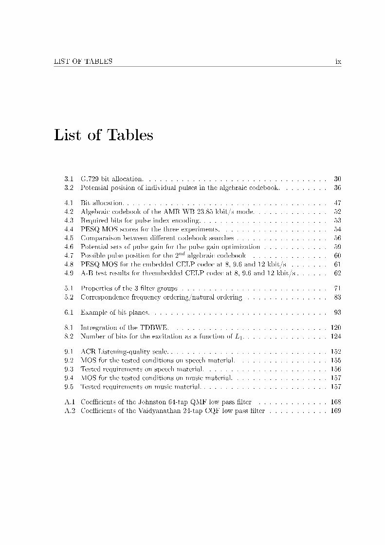
List of Tables
3.1 G.729 bit allocation. . . . . . . . . . . . . . . . . . . . . . . . . . . . . . . . . . 303.2 Potential position of individual pulses in the algebraic codebook. . . . . . . . . 36
4.1 Bit allocation. . . . . . . . . . . . . . . . . . . . . . . . . . . . . . . . . . . . . . 474.2 Algebraic codebook of the AMR-WB 23.85 kbit/s mode. . . . . . . . . . . . . . 524.3 Required bits for pulse index encoding. . . . . . . . . . . . . . . . . . . . . . . . 534.4 PESQ MOS scores for the three experiments. . . . . . . . . . . . . . . . . . . . 544.5 Comparaison between di�erent codebook searches . . . . . . . . . . . . . . . . . 564.6 Potential sets of pulse gain for the pulse gain optimization . . . . . . . . . . . . 594.7 Possible pulse position for the 2nd algebraic codebook . . . . . . . . . . . . . . 604.8 PESQ MOS for the embedded CELP codec at 8, 9.6 and 12 kbit/s . . . . . . . 614.9 A-B test results for theembedded CELP codec at 8, 9.6 and 12 kbit/s . . . . . . 62
5.1 Properties of the 3 �lter groups . . . . . . . . . . . . . . . . . . . . . . . . . . . 715.2 Correspondence frequency ordering/natural ordering . . . . . . . . . . . . . . . 83
6.1 Example of bit planes. . . . . . . . . . . . . . . . . . . . . . . . . . . . . . . . . 93
8.1 Intregration of the TDBWE. . . . . . . . . . . . . . . . . . . . . . . . . . . . . 1208.2 Number of bits for the excitation as a function of L1. . . . . . . . . . . . . . . . 124
9.1 ACR Listening-quality scale. . . . . . . . . . . . . . . . . . . . . . . . . . . . . . 1529.2 MOS for the tested conditions on speech material. . . . . . . . . . . . . . . . . 1559.3 Tested requirements on speech material. . . . . . . . . . . . . . . . . . . . . . . 1569.4 MOS for the tested conditions on music material. . . . . . . . . . . . . . . . . . 1579.5 Tested requirements on music material. . . . . . . . . . . . . . . . . . . . . . . . 157
A.1 Coe�cients of the Johnston 64-tap QMF low pass �lter . . . . . . . . . . . . . 168A.2 Coe�cients of the Vaidyanathan 24-tap CQF low pass �lter . . . . . . . . . . . 169

x LIST OF TABLES
INTRODUCTION 1
Introduction
Due to the development of broadband Internet connection like Digital Subscriber Line (DSL)or cable, VoIP (Voice over Internet Protocol) has encountered for the last years a dramaticsuccess. VoIP, also called Internet telephony, makes reference to techniques able to routevoice conversations over the Internet or any IP-based networks. Existing hardware and soft-ware solutions make it possible to give a call from PC (Personal Computer) to PC, from PCto landline/mobile phone, and even from landline/mobile phone to PC. Indeed, some VoIPproviders permit users to subscribe to numbers in several countries. For instance, someoneliving in Australia can subscribe to a German landline phone number. Anyone in Germanywho calls this number will be billed for a national phone call. The subscriber is reachablewherever he is connected to a broadband access.
When using VoIP, the speech signal is encoded, packetized and sent using UDP (UniversalDatagram Protocol) through the IP network. Unfortunately, since VoIP uses the UDP, it alsosu�ers from its drawbacks. Among others, UDP does not guarantee any reliability. The packetsmay arrive out of order (i.e. not in the same order as they have been sent), duplicated, or maynot arrive at all. The main source of packet loss is the network congestion. When a packetis missing, the corresponding speech frame(s) can not be synthesized, impacting considerablythe listening experience. In such a case, PLC (Packet Loss Cancelation) procedures may beapplied to recover the missing packets at the expense of quality degradation.
The solution investigated in this thesis to deal with network congestion issues, amongother possibilities, is the use of embedded, or scalable, coding. A scalable codec organizes thebitstream in layers, where each layer is independent from the upper layers. The �rst layer,called core layer, contains the necessary data to synthesize a signal with a minimal qualityand bandwidth. Upper layers called enhancement layers are meant to improve the qualityand/or increase the bandwidth of the reconstructed signal. According to the network tra�c,the bitrate can be adapted on the �y at any point of the transmission chain by dropping packetscontaining data from the upper layers, favoring the delivery of core layer packets. Moreover,the bitrate can also �t the terminal capacity. For example, mobile phone on a wireless LAN willdecode at a lower bitrate than a PC connected to the same network. Besides, scalable codingeasily enables premium access, where the user can access the highest quality of a multimediacontent after payment.
2 INTRODUCTION
Embedded speech coding is an active topic at the ITU-T (International TelecommunicationUnion, Telecommunication standardization sector) Study Group 16 Working Party 3. Forexample, the scalable extension of G.729, called G.729.1 [ITU-T 2006a] was standardized inMay 2006. A super wideband extension and a DTX (Discontinuous Transmission) mode isunder study in Study Group 16 Working Party 3, Question 23, "Media coding", and 10,"Software tools for signal processing standardization activities and maintenance and extensionof existing voice coding standards", respectively. In the same time, a new embedded coderG.EV-VBR is in optimization phase in Question 9, "Variable Bit Rate Coding of SpeechSignals" (Standardization work is carried out by the technical Study Groups. The StudyGroups drive their work primarily in the form of study Questions. Each of these addressestechnical studies in a particular area of telecommunication standardization).
The objective of this thesis is the study of an hybrid structure CELP/wavelet (Code-ExcitedLinear Prediction). The structure CELP/frequency transform is already present in scalablecoders. The G.729.1 combines the G.729 [ITU-T 1996d] with an enhancement layer based ona MDCT (Modi�ed Discrete Cosine Transform). The ISO MPEG-4 CELP scalable [MPEG1998] builds a MPEG-2 AAC (Advanced Audio Coding) [MPEG 1997] based enhancementlayer on top of a CELP coder. Whereas transforms like MDCT give a spectral representationof a signal for �nite time duration, discrete wavelet transform and packet decomposition canprovide a time-frequency representation.
Discrete wavelet transform has been successfully applied to image coding. The main ideaof wavelet transform is to decompose a signal into approximation and details. It is a invertibletransform. The reconstruction from the approximation only gives a coarse representationof the original signal. The more details added, the better this representation, until perfectreconstruction. Progressive image transmission is enabled by coding �rst the approximationcoe�cients, then the details from the coarsest to the �nest. Lately, discrete wavelet transformhas been integrated as part of the JPEG2000 standard [ITU-T 2002]. The success of wavelettransform in image coding has encouraged people to transpose the technology to 1-dimensionalsignal like audio.
This thesis took place in audio coding departments of Siemens Mobile, Siemens CorporateTechnology, and Nokia Siemens Networks, successively. Those departments have been involvedin the ITU-T study group activities related to embedded speech and audio coding. As theG.729.1 standardization process took place in the same period, it has been decided that theproposed structure would be inspired by the G.729.1 terms of reference. The core layer shouldbe G.729 bitstream compliant. One or more enhancement layers would improve the qualityprogressively, wideband being enabled for low bitrate. The targeted bitrate range spans 24kbit/s, from 8 kbit/s to 32 kbit/s, with a large number of intermediate bitrates.
The �rst investigated structure is similar to the one presented in [De Meuleneire et al.2006b]. The input signal at 16 kHz sampling frequency is lowpass �ltered and downsampled to8 kHz sampling frequency in order to be encoded by the G.729. The local G.729 decoder outputis upsampled to 16 kHz sampling frequency and low pass �ltered before being subtracted from
INTRODUCTION 3
the delayed original signal. A wavelet packet decomposition is applied to this di�erence signal.The wavelet coe�cients are quantized with an embedded quantizer called Embedded ZerotreeWavelet (EZW) algorithm [Shapiro 1993]. The structure has opened several issues:
• How many bits should be allocated to CELP coding? CELP coding, dedicated to speechcompression, performs better for speech than transform coding at low bitrate. Theoverall performance of the coder might bene�t from an enhancement layer based onCELP technology.
• How to implement the wavelet transform? The convolution of a �nite length segmentand the �lter poses the problem of the boundary handling. Circular convolution solvesthe problem by considering the segment to be �ltered as periodic. Albeit without delay,it causes discontinuities between frames at the reconstruction (so-called block e�ect orartifact).
• How to ensure full wideband rendering? The decoder reconstructs progressively thecoe�cients as the bitrate increases. For low bitrate, some coe�cients are missing at thedecoder, yielding a spectrum with holes.
• How to quantize the wavelet coe�cients? Make a coder scalable usually penalizes theperformance of the coder. Moreover, the granularity of the coder, i.e. the minimalamount of bits necessary to improve the synthesized signal, has an impact on the maximalbitrate quality.
Modi�cations made to the initial structure attempt to address these issues. Investigationshave been conducted to build an enhancement layer on top of the G.729. Wavelet decompo-sition is implemented through a �lter bank structure ensuring the absence of block artifacts.Moreover, an enhancement layer has been designed to always enable wideband rendering evenat low bitrate. Lastly, the structure has been optimized in order to increase the performanceof the wavelet coe�cient quantization.
This thesis is organized in �ve parts. The �rst part comprising one chapter deals withgeneral points on audio and speech coding. It will point out the di�erence between losslessand lossy codings. Afterwards, the concept of embedded bitstream and scalable algorithm, aswell as core and enhancement layers, will be introduced. To conclude, some examples will begiven to illustrate those concepts.
The second part is divided into three chapters. Linear speech coding will be described in a�rst chapter, illustrated in a second chapter by the G.729 used as a core layer of the proposedcoder. Finally, in a third chapter, after examples of embedded linear predictive coders fromthe literature, investigated methods will be presented.
The third part is dedicated to wavelet in audio scalable coding. Its �rst chapter givesan introduction to wavelet transform, an important tool to give a compact time-frequency
4 INTRODUCTION
representation of any digital audio signal. A parallel between wavelet transform and perfectreconstruction �lter bank will be drawn. In a second chapter, the concept of embedded quan-tizer will be instanced by two examples designed for embedded coding of wavelet coe�cients.Finally, the last chapter will make a survey of wavelet-based audio scalable codecs.
The concept of bandwidth extension will be the topic of the fourth part. It mainly explainswhat bandwidth extension is all about. It is an important feature in the codec as it extendsthe bandwidth of the core layer output with a small amount of side information compared tothe total bitrate of the proposed coder. The investigated approaches for the proposed codecwill be described.
In the last part, on the basis of the foregoing chapters, the structure of the proposed coderwill be presented. This structure comprises the encoder and the decoder, with its core layerand its enhancement layers. Moreover, this part will give the di�erent optimizations broughtto the codec in order to increase its performance.

5
Part I
About Scalable Coding

7
Chapter 1
Introduction to embedded/scalablecoding
This chapter introduces the concept of embedded audio coding. The �rst section describesthe audio coding in general, and in particular the di�erence between lossless coding and lossycoding. It is concluded by an overview of speech coding, a special case of lossy coding. Thesecond part gives the principles of embedded coding, as well as examples of applications.
1.1 Short introduction to speech and audio coding
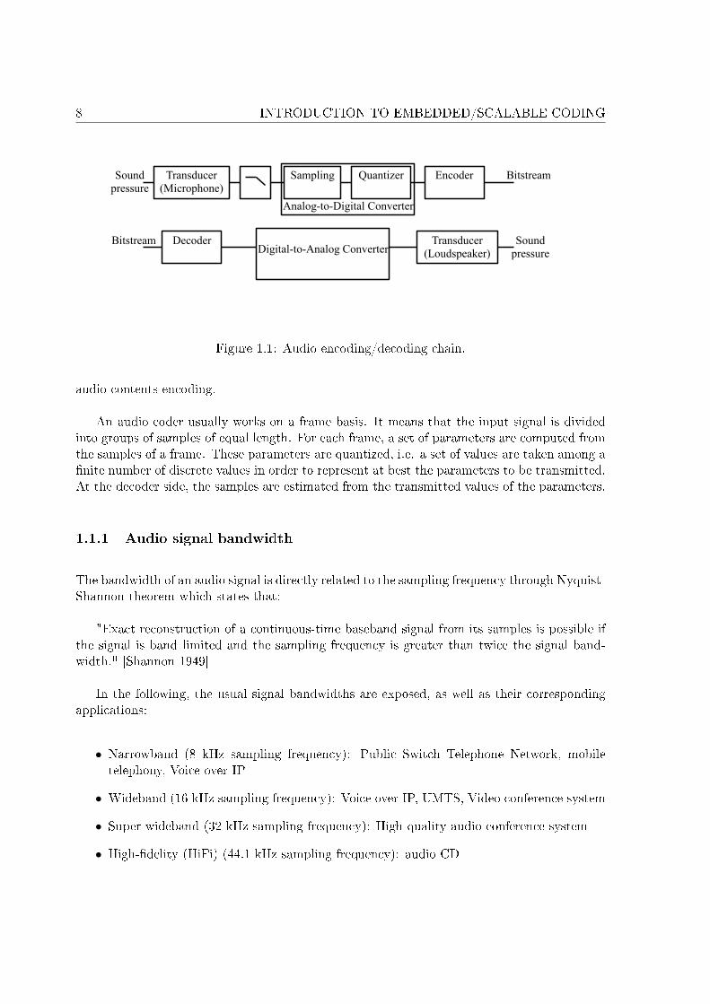
The goal of speech and audio coding algorithms is to reduce the amount of data to be trans-mitted over a channel (e.g. a GSM channel) or stored (e.g. a memory card of an MP3 player).As such, it can be seen as a particular kind of data compression. Fig. 1.1 depicts a typicalaudio coding chain.
First, the sound pressure level is converted to an analog signal by a transducer, typically amicrophone. After low-pass �ltering, the analog signal is converted to a digital signal, thanksto an Analog-to-Digital Converter (ADC), comprising a sampling unit and a quantizer. Then,the resulting digital signal is encoded into a bitstream. At this point, the number of bits torepresent the signal is smaller than the one of the original digital signal. The bitstream canbe later decoded (after storage or transmission) to produce a digital signal, and can be �nallyplayed through a loudspeaker, after a Digital-to-Analog Converter (DAC).
Depending on the application trade-o�, issues like �delity, bitrate, complexity, delay, orbandwidth have to be addressed. For instance, a codec designed for telephony (8-16 kHz)must have a smaller delay and a lower complexity than a high �delity coder (44.1-48 kHz) for
8 INTRODUCTION TO EMBEDDED/SCALABLE CODING
Figure 1.1: Audio encoding/decoding chain.
audio contents encoding.
An audio coder usually works on a frame basis. It means that the input signal is dividedinto groups of samples of equal length. For each frame, a set of parameters are computed fromthe samples of a frame. These parameters are quantized, i.e. a set of values are taken among a�nite number of discrete values in order to represent at best the parameters to be transmitted.At the decoder side, the samples are estimated from the transmitted values of the parameters.
1.1.1 Audio signal bandwidth
The bandwidth of an audio signal is directly related to the sampling frequency through Nyquist-Shannon theorem which states that:
"Exact reconstruction of a continuous-time baseband signal from its samples is possible ifthe signal is band limited and the sampling frequency is greater than twice the signal band-width." [Shannon 1949]
In the following, the usual signal bandwidths are exposed, as well as their correspondingapplications:
• Narrowband (8 kHz sampling frequency): Public Switch Telephone Network, mobiletelephony, Voice over IP
• Wideband (16 kHz sampling frequency): Voice over IP, UMTS, Video conference system
• Super wideband (32 kHz sampling frequency): High quality audio conference system
• High-�delity (HiFi) (44.1 kHz sampling frequency): audio CD
1.1. SHORT INTRODUCTION TO SPEECH AND AUDIO CODING 9
• Full Band Audio (48 kHz sampling frequency): High quality audio conference system
Sampling frequencies of 88.2, 96, 192 kHz are also supported in the area of professional studiorecording.
1.1.2 Lossless or lossy
Depending on the target application, the compression applied to the signal can be lossless orlossy. Lossless coding is described in a �rst section. The second section deals with lossy coding.As this thesis focuses on embedded speech coding, a third section addresses this topic, that isa particular case of lossy coding.
1.1.2.1 Lossless
The compression is carried out without loss of information, i.e. the reconstructed signals areexactly the same as the original ones. Generally, lossless coding involves computationallycomplex algorithms and is not intended for real time encoding. Nevertheless, the decoder isusually much less complex than the encoder. Hence, it allows real time decoding to producea continuous play back of the decoded signal. Usually, the most e�cient lossless codecs makeuse of linear prediction, e.g. the MPEG-ALS [Liebchen 2004]. By predicting samples fromthe previous ones, it is possible to remove the short-term correlation between samples. Thedi�erence between the original and the predicted signals is then entropy coded. Lossless codingis for instance used by professional recording studios.
1.1.2.2 Lossy
The compression allows for some loss of insigni�cant or non pertinent information. As aresult, the reconstructed signal will be di�erent from the original one. A bit allocation moduleis commonly used and is in charge of allocating bits to quantize groups of coe�cients. Themore bits allocated, the better the quantization of the coe�cients.
Mostly, the bit allocation is driven by a psychoacoustic model. The psychoacoustic modelrelies on the properties of the human ear. Mainly two components are of interest:
• The Absolute Threshold of Hearing (ATH): It is the minimum threshold at which afrequency is audible. For example, the ear is most sensitive to frequencies between 1 kHzand 5 kHz [Moore 2003].
10 INTRODUCTION TO EMBEDDED/SCALABLE CODING
• The Masking Threshold: A strong frequency component can mask weaker components(noise or tone) in its frequency vicinity, so that they are not audible.
By taking into account these properties, it is possible to determine for each group of coe�cientsthe maximum level of inaudible quantization noise. Inaudible components, because they arebeing masked by stronger components or are below the ATH, are not alloted bits. Accordingto these values, the bit allocation tries to distribute the available bits in order to minimizethe level of the audible quantization noise. Coders using psychoacoustic model are calledperceptual. Some perceptual coders can achieve transparency, i.e. the decoded signal is notdistinguishable from the original one. One of the most famous lossy codec is the ISO-MPEG1 Layer III, nicknamed MP3. This codec is present in so-called MP3-Player, portable devicescapable of decoding MP3 bitstream. It reduces dramatically the size of music �les whileensuring quality close to the original.
1.1.3 Speech coding
Speech is surely the easiest way for human beings to communicate with each other. Transmis-sion of speech signals has a privileged place in communication systems, like land and mobiletelephony, or VoIP. Although 8 kHz sampling frequency might be su�cient for the compre-hensibility of words and sentences, the intelligibility may su�er from the inaccuracy of somesounds whose energy is concentrated above 4 kHz, like fricatives. 16 kHz sampling frequencyovercomes this problem. Speech codecs must produce a high quality synthesized speech at lowcomplexity, low bitrates and with low delay. These requirements constraint the choice towardslossy coding. The coders applicable to speech signals are traditionally categorized in threeclasses [Vary, Martin 2006]:
• Waveform-approximating codersThe speech signal is digitized and each sample is coded by a constant number of bits(G.711 or PCM [ITU-T 1988a], Pulse Code Modulation). As a result, the reconstructedsignal converges towards the original signal with decreasing quantization error with anincreasing bitrate. Thus, they work as well with non-speech signals. The number of bitsneeded for the quantization can be reduced when the di�erence between the sample andits linear prediction from a few previous samples is coded (G.721 or ADPCM, AdaptiveDi�erential Pulse Code Modulation [Daumer et al. 1984], also described in [ITU-T 1990]).They provide high speech quality at bit rate greater than 32 kbit/s. Below this limit,the quality degrades rapidly.
• Parametric codersAfter sampling the speech signal, the digital signal is divided into blocks. From each blockof samples, parameters corresponding to a speech synthesis model are computed and thenquantized. The vocal tract is represented as a time-varying �lter and is excited with either
1.2. EMBEDDED AND SCALABLE 11
a white noise source, for unvoiced speech segments, or a train of pulses separated by thepitch period for voiced speech. For instance in Linear Predictive Coding (LPC) vocoders(e.g. [Federal Standard 1015, Telecommunications: Analog to Digital Conversion of RadioVoice By 2400 Bit/Second Linear Predictive Coding 1984]), the �lter is derived from alinear prediction. Therefore information which must be sent to the decoder, are the �ltercoe�cients, a voiced/unvoiced �ag, the necessary energy of the excitation signal, and thepitch period for voiced speech. The block size is 10-30 ms, corresponding approximatelyto the length of the speech stationarity. Although the decoded speech signal is stillintelligible, the quality is far from that obtained with waveform-approximating coders,the voice sounds unnatural. Such codecs are used in military applications where verylow bit-rates (usually lower than 4 kbit/s) are preferred to naturalness, permitting heavydata protection and encryption.
• Hybrid codersThese codecs are a trade-o� between the two previous categories. They provide a goodspeech quality while decreasing the bit-rate below 16 kbit/s. Among the hybrid codecs,the most commonly used are Analysis-by-Synthesis coders using the same linear predic-tion as LPC vocoders. Quantizing the excitation with Analysis-by-Synthesis schemesimproves the quality. Instead of using a two-state model (voiced-unvoiced) like in para-metric coding, the residual excitation is computed independently on the type of thespeech segment. The bit-rate of such coders is between 4 kbit/s and 16 kbit/s. Cel-lular telephony, motivated by saving spectral resources, or packet transmission over aX-network, are common applications of hybrids codecs. They provide indeed a goodspeech quality while keeping the necessary bit-rate below 16 kbit/s (in order, for exam-ple, to allocate more bits to channel coding).
While initially intended for speech signal, the aforementioned coders might also be used toencode music. For example, the coder described in the Annex E of the ITU-T G.729 [ITU-T1998d] is suited for both speech and music. It is also usual to distinguish between time-domaincodecs using for instance linear prediction and frequency-domain codecs based on short-termspectral analysis. Time-domain codec based on linear prediction is suitable for speech withbitrates less than 2 bits/sample. Conversely, frequency-domain codecs gives good results formusic with bitrates from 2 bits/sample [Vary, Martin 2006].
1.2 Embedded and scalable
A codec usually works at a constant bitrate. The same number of bits is transmitted foreach frame. Nevertheless, codecs might also be designed to work at several bit rates. Thenumber of transmitted parameters and their quantization di�er from one bitrate to an other.For example, the Adaptive Multi-Rate (AMR) [3GPP 1999] for coding narrowband speech canwork at 8 di�erent bitrates from 4.75 kbit/s to 12.2 kbit/s. Designed for GSM and UMTS,
12 INTRODUCTION TO EMBEDDED/SCALABLE CODING
the objective of the AMR is to increase error for better speech quality in adverse channelconditions. In a similar way, the Adaptive Multi-Rate WideBand (AMR-WB) for widebandspeech, also standardized at the ITU-T [ITU-T 2003], operates at 9 di�erence bitrates from6.6 kbit/s to 23.85 kbit/s. In such cases, the encoder and decoder must negotiate the bitrateto use during the communication. For some reason, if the bitrate has to be increased ordecreased, the encoder and decoder must re-negotiate a new bitrate. Furthermore, due to badnetwork conditions, a few bits in a frame might be corrupted. The decoder is thus not able toreconstruct the frame samples, yielding impairments in the synthesized signal. The concept ofembedded (or sometimes called scalable) coding is meant to be a solution to such problems.
1.2.1 Principles
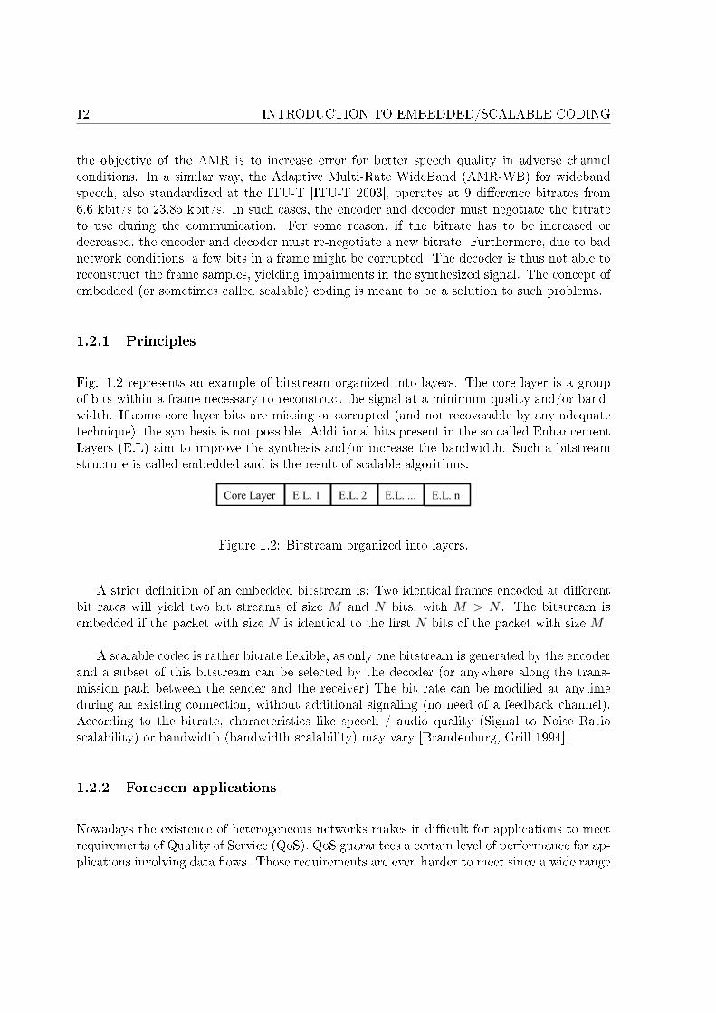
Fig. 1.2 represents an example of bitstream organized into layers. The core layer is a groupof bits within a frame necessary to reconstruct the signal at a minimum quality and/or band-width. If some core layer bits are missing or corrupted (and not recoverable by any adequatetechnique), the synthesis is not possible. Additional bits present in the so-called EnhancementLayers (E.L) aim to improve the synthesis and/or increase the bandwidth. Such a bitstreamstructure is called embedded and is the result of scalable algorithms.
Figure 1.2: Bitstream organized into layers.
A strict de�nition of an embedded bitstream is: Two identical frames encoded at di�erentbit rates will yield two bit streams of size M and N bits, with M > N . The bitstream isembedded if the packet with size N is identical to the �rst N bits of the packet with size M .
A scalable codec is rather bitrate �exible, as only one bitstream is generated by the encoderand a subset of this bitstream can be selected by the decoder (or anywhere along the trans-mission path between the sender and the receiver) The bit rate can be modi�ed at anytimeduring an existing connection, without additional signaling (no need of a feedback channel).According to the bitrate, characteristics like speech / audio quality (Signal to Noise Ratioscalability) or bandwidth (bandwidth scalability) may vary [Brandenburg, Grill 1994].
1.2.2 Foreseen applications
Nowadays the existence of heterogeneous networks makes it di�cult for applications to meetrequirements of Quality of Service (QoS). QoS guarantees a certain level of performance for ap-plications involving data �ows. Those requirements are even harder to meet since a wide range
1.2. EMBEDDED AND SCALABLE 13
of terminals such as personal computers, narrowband or wideband capable phones, mobilephones or PDAs are exchanging data through di�erent types of network accesses like dial-upconnection, xDSL, LAN, wireless connection, GSM link, etc.
Applications such as audio conferencing may bene�t from embedded coding. With currentcodecs, before establishing a connection, the terminals need to agree on the codec and thebitrate to use. Whenever the network conditions change, the connection might be reinitializedwith a new bitrate and/or another codec. If the involved terminals do not use the samecodec, the bitstreams must be transcoded either by smart transcoding (without decoding andre-encoding) or by tandeming (decoding and re-encoding with the other codec). Tandemingusually has an impact on the quality of the reconstructed signal. Embedded coding can simplifythe process. Participants can communicate by using a unique codec, each terminal being ableto adapt the bitrate according to its capacity and to the network tra�c. To cope with networkcongestion, EL packets can be dropped on the �y, ensuring an uninterrupted conversation ata cost of a quality degradation.
Scalable coding is particularly suitable for delivering contents. To reduce network conges-tion or to increase the number of users over a backbone, some entities in the network maydiscard the higher layers. Unequal error protection can be very easily implemented with asimple scheme where, for example, the core layer is better protected than the other layers.Enhancement layers can also be encrypted. Only premium user will have access to the highestquality. Also, with lossy-to -lossless scalable coder, the core layer may provide a preview ofaudio contents.
Summary
Transmission of speech and audio contents may bene�t from scalability. Embedded codecprovides a unique bitstream that can be decoded at di�erent bitrates according to the networkconditions or the terminal capabilities, avoiding quality degradation due to tandeming. Forspeech coding, it is suitable to use a speech coder as a core layer of an embedded audio coder.Throughout this thesis, embedding coding concept will be used in domain like linear predictivecoding and time-frequency transform coding. Bandwidth extension will be also considered asan enhancement layer. This overview in the next chapters will give the di�erent componentsof the proposed embedded codec.

14 INTRODUCTION TO EMBEDDED/SCALABLE CODING
15
Part II
Linear Predictive Coding

17
Chapter 2
CELP coding
Originally proposed by M.R Schroeder and B.S. Atal [Schroeder, Atal 1985a], Code-ExcitedLinear Prediction (CELP) coding is present in many coding standards like the ITU-T G.729[ITU-T 1996d], the Adaptive Multi-Rate (AMR) [3GPP 1999], the ITU-T G.722.2 [ITU-T2003], the ITU-T G.723.1 [ITU-T 1996a] or the ITU-T G.728 [ITU-T 1992]. CELP codinguses a speech production model. First the vocal tract is modeled by the linear predictioncoe�cients. Then, the vibrations of the vocal chords are detected by the analysis of thelong term correlation of the speech signal and represented by the pitch lag. Finally, the nonpredictable excitation from the lung is coded by an entry in a �xed codebook.
2.1 Principles
CELP coding is based on an Analysis-by-Synthesis (AbS) scheme (cf Fig. 2.1). An AbS coderworks on a block-by-block basis. The longest block is called a frame. The duration of a frameis typically 10-30 ms to stay in the hypothesis of speech signal stationarity. A frame is furtherdivided into blocks of same length called subframes.
This type of coder is based on a source-�lter model. The excitation to the synthesis �lteris chosen by attempting to match the reconstructed speech waveform as closely as possibleto the original speech waveform. The synthesis �lter is composed of two �lters, namely aShort-Term Prediction (STP) �lter and a Long-Term Prediction (LTP) �lter. The �rst onemodels the envelope of the speech spectrum produced by the vocal tract. The coe�cientsare computed by Linear Prediction (LP) of the input signal. This �lter is usually called thesynthesis �lter or the Linear Prediction Coding �lter. The second �lter reproduces the longterm-correlation present especially in voiced sounds due to the vocal chords vibrations. Theoptimal excitation is chosen by minimizing a criterion that is a function of the di�erence
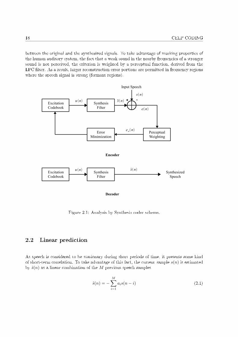
18 CELP CODING
between the original and the synthesized signals. To take advantage of masking properties ofthe human auditory system, the fact that a weak sound in the nearby frequencies of a strongersound is not perceived, the criterion is weighted by a perceptual function, derived from theLPC �lter. As a result, larger reconstruction error portions are permitted in frequency regionswhere the speech signal is strong (formant regions).
Figure 2.1: Analysis-by-Synthesis coder scheme.
2.2 Linear prediction
As speech is considered to be stationary during short periods of time, it presents some kindof short-term correlation. To take advantage of this fact, the current sample s(n) is estimatedby s(n) as a linear combination of the M previous speech samples
s(n) = −M∑i=1
ais(n− i) (2.1)
2.2. LINEAR PREDICTION 19
s(n) represents the digitalized speech signal at time n, s(n) for n = 0 is the �rst sample of thecurrent frame, and samples s(n) for n < 0 come from the previous frame(s). The predictionerror, also called LP or LPC residual, is de�ned by:
e(n) = s(n)− s(n) =M∑i=0
ais(n− i), a0 = 1 (2.2)
The coe�cients ai are calculated by minimizing the mean square error E[e2(n)
]:
∂E[e2(n)
]∂ak
= 0 ⇒M∑i=1
aiΓs(k − i) = −Γs(k), ∀k ∈ {1, . . . ,M} (2.3)
with E [.] the expected value operator and Γs(k) = E [s(n)s(n− k)] the autocorrelation of thespeech signal. This system of linear equations, called the Yule-Walker equations, can be solvedby the Levinson-Durbin recursion [Trench 1964] or the Schur decomposition [Strobach 1990].The short-term synthesis �lter which derives from a M th order Linear Prediction (LP) is thengiven by:
1
A(z)=
1
1 +M∑i=1
aiz−i
(2.4)
where ai, i = 1, . . . ,M, are the quantized LP parameters.
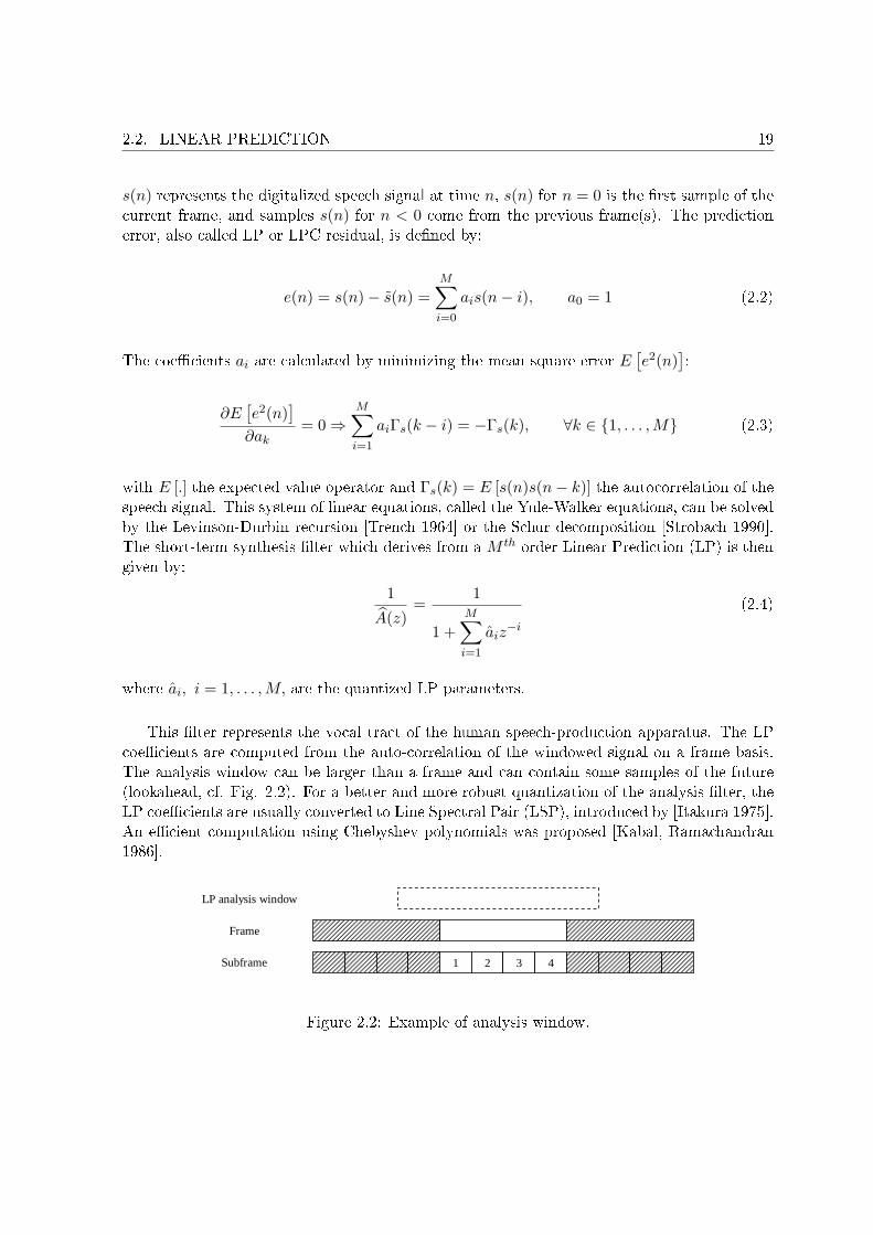
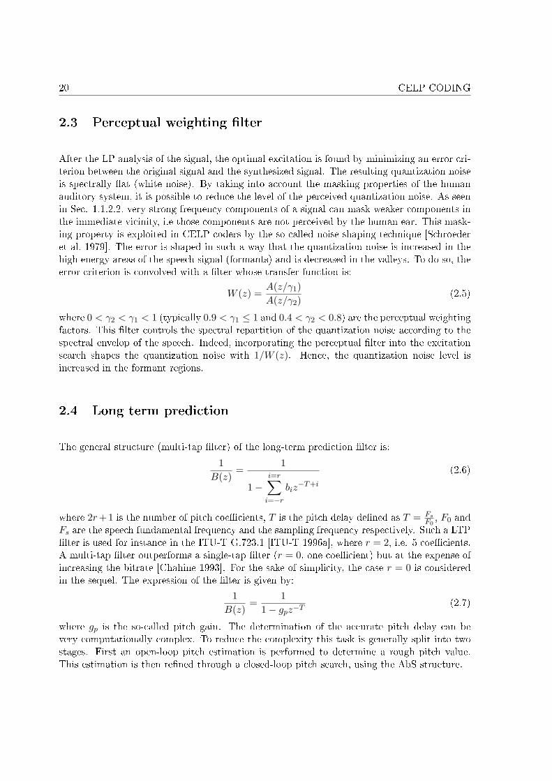
This �lter represents the vocal tract of the human speech-production apparatus. The LPcoe�cients are computed from the auto-correlation of the windowed signal on a frame basis.The analysis window can be larger than a frame and can contain some samples of the future(lookahead, cf. Fig. 2.2). For a better and more robust quantization of the analysis �lter, theLP coe�cients are usually converted to Line Spectral Pair (LSP), introduced by [Itakura 1975].An e�cient computation using Chebyshev polynomials was proposed [Kabal, Ramachandran1986].
1 2 3 4
LP analysis window
Frame
Subframe
Figure 2.2: Example of analysis window.
20 CELP CODING
2.3 Perceptual weighting �lter
After the LP analysis of the signal, the optimal excitation is found by minimizing an error cri-terion between the original signal and the synthesized signal. The resulting quantization noiseis spectrally �at (white noise). By taking into account the masking properties of the humanauditory system, it is possible to reduce the level of the perceived quantization noise. As seenin Sec. 1.1.2.2, very strong frequency components of a signal can mask weaker components inthe immediate vicinity, i.e those components are not perceived by the human ear. This mask-ing property is exploited in CELP coders by the so-called noise shaping technique [Schroederet al. 1979]. The error is shaped in such a way that the quantization noise is increased in thehigh energy areas of the speech signal (formants) and is decreased in the valleys. To do so, theerror criterion is convolved with a �lter whose transfer function is:
W (z) =A(z/γ1)A(z/γ2)
(2.5)
where 0 < γ2 < γ1 < 1 (typically 0.9 < γ1 ≤ 1 and 0.4 < γ2 < 0.8) are the perceptual weightingfactors. This �lter controls the spectral repartition of the quantization noise according to thespectral envelop of the speech. Indeed, incorporating the perceptual �lter into the excitationsearch shapes the quantization noise with 1/W (z). Hence, the quantization noise level isincreased in the formant regions.
2.4 Long term prediction
The general structure (multi-tap �lter) of the long-term prediction �lter is:
1B(z)
=1
1−i=r∑
i=−r
biz−T+i
(2.6)
where 2r +1 is the number of pitch coe�cients, T is the pitch delay de�ned as T = FsF0, F0 and
Fs are the speech fundamental frequency and the sampling frequency respectively. Such a LTP�lter is used for instance in the ITU-T G.723.1 [ITU-T 1996a], where r = 2, i.e. 5 coe�cients.A multi-tap �lter outperforms a single-tap �lter (r = 0, one coe�cient) but at the expense ofincreasing the bitrate [Chahine 1993]. For the sake of simplicity, the case r = 0 is consideredin the sequel. The expression of the �lter is given by:
1B(z)
=1
1− gpz−T(2.7)
where gp is the so-called pitch gain. The determination of the accurate pitch delay can bevery computationally complex. To reduce the complexity this task is generally split into twostages. First an open-loop pitch estimation is performed to determine a rough pitch value.This estimation is then re�ned through a closed-loop pitch search, using the AbS structure.
2.4. LONG TERM PREDICTION 21
2.4.1 Open-loop pitch search
A �rst estimation of the pitch is obtained by minimizing the mean square error of the LTPresidual de�ned as:
ε(n) = e(n)− gpe(n− T ) (2.8)
ELTP =L−1∑n=0
ε2(n) =L−1∑n=0
[e(n)− gpe(n− T )]2 (2.9)
The optimal gain gp is obtained when ∂ELTP∂gp
= 0
∂ELTP
∂gp= 0 ⇒ gp =
L−1∑n=0
e(n)e(n− T )
L−1∑n=0
e(n− T )2(2.10)
Substituting the expression of gp given by Eq. (2.10) in (2.9) yields
ELTP =L−1∑n=0
e2(n)−
[L−1∑n=0
e(n)e(n− T )
]2
L−1∑n=0
e(n− T )2(2.11)
Minimizing E is equivalent to maximizing the second term in the right-hand side of the aboveequation, which represents the normalized correlation between the LPC residual e(n) and itsdelayed version. All the pitch values within a range [Tmin, Tmax] are tested, and the value of Twhich maximizes this term is chosen. Those values depend on the frame size and the samplingfrequency, and may also depend on the computed value of the previous frame. This coarsepitch estimation is usually performed on a frame basis. T is the optimal value in the sense ofthis criterion.
A less complex alternative method [Rabiner 1977] consists in maximizing the autocorre-lation function of the perceptual weighted signal sw(n) (Sw(z) = S(z)W (z), with W (z) theperceptual weighting �lter) and choosing the delay T which maximizes the following term
C(T ) =L−1∑n=0
sw(n)sw(n− T ) (2.12)
The main problem with this technique is the possibility to choose a sub-multiple of the pitch(given by the minimization Eq. (2.11)). This may occur if the pitch period is small. The �rstpeak of the autocorrelation function is then missed. In this case, the pitch range is dividedinto several ranges, the autocorrelation is maximized in each range with a proper weightingaimed at favoring the smaller values.
22 CELP CODING
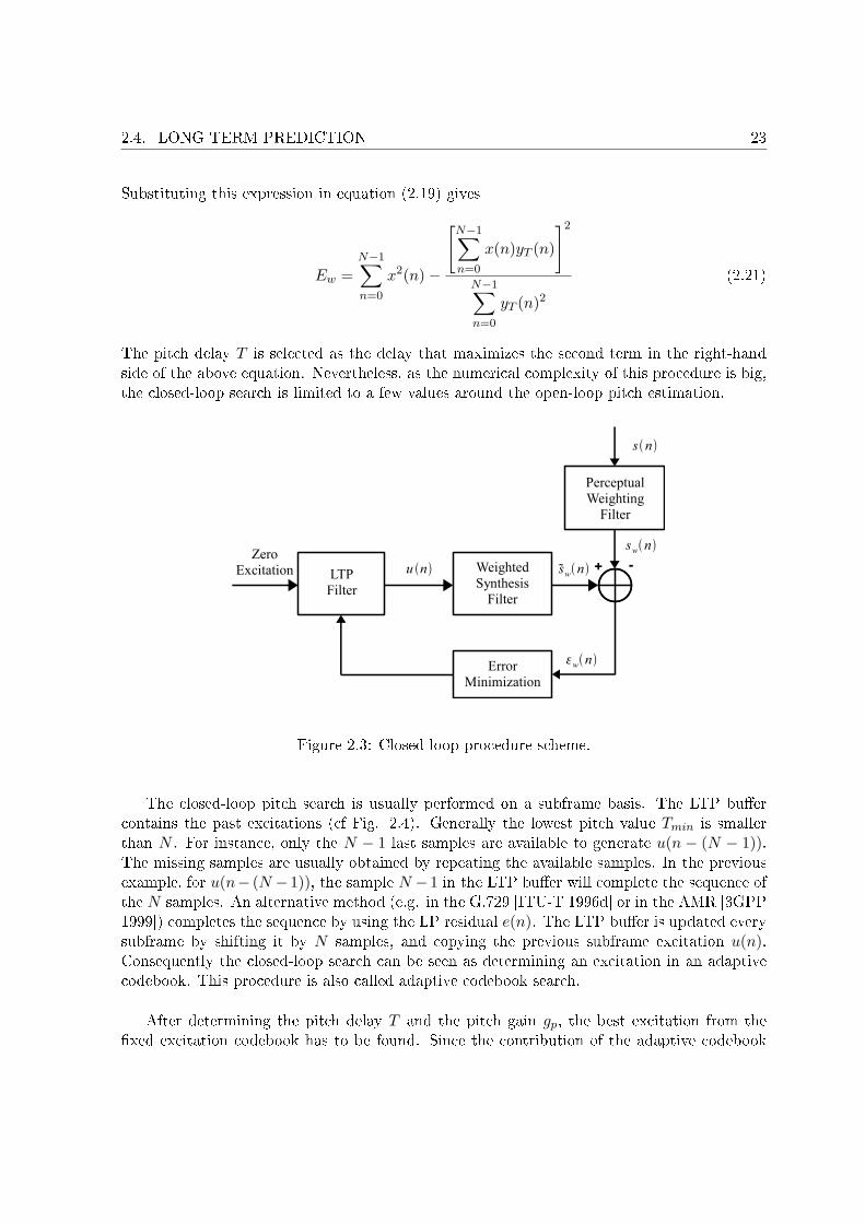
2.4.2 Closed-loop pitch estimation (adaptive codebook search)
The closed-loop pitch estimation procedure exploits the structure of the AbS scheme to estimatethe pitch accurately (cf. Fig. 2.3). This method minimizes the squared error between theweighted speech sw(n) and the estimated weighted speech sw(n) on a subframe basis (of sizeN)
Ew =N−1∑n=0
ε2w(n) (2.13)
εw(n) = sw(n)− sw(n) (2.14)
with
sw(n) = sw0(n) +n∑
k=0
u(k)h(n− k) (2.15)
where sw0(n) is the zero-input response of the perceptual weighted synthesis �lter. This �lteris de�ned as:
H(z) =1
A(z)W (z) (2.16)
The weighted speech is the convolution of the sampled speech signal with the perceptualweighting �lter:
sw(n) = (s ∗ w)(n) ⇔ Sw(z) = S(z)W (z) (2.17)
Supposing the LTP �lter is self excited, i.e. u(n) = gpu(n− T ), it comes:
εw(n) = sw(n)− sw0(n)− gp
n∑k=0
u(n− T )h(n− k) = x(n)− gpyT (n)︸ ︷︷ ︸LTP residual
(2.18)
x(n) = sw(n)− sw0(n) and yT (n) are respectively the target signal and the �ltered past excita-tion at delay T , and h(n) is the impulse response of the weighted synthesis �lter. Consequently,the new expression of the squared error is
Ew =N−1∑n=0
[x(n)− gpyT (n)]2 (2.19)
Like for Eq. (2.10), the expression of gp is obtained by:
∂Ew
∂gp= 0 ⇒ gp =
N−1∑n=0
x(n)yT (n)
N−1∑n=0
yT (n)2. (2.20)
2.4. LONG TERM PREDICTION 23
Substituting this expression in equation (2.19) gives
Ew =N−1∑n=0
x2(n)−
[N−1∑n=0
x(n)yT (n)
]2
N−1∑n=0
yT (n)2(2.21)
The pitch delay T is selected as the delay that maximizes the second term in the right-handside of the above equation. Nevertheless, as the numerical complexity of this procedure is big,the closed-loop search is limited to a few values around the open-loop pitch estimation.
Figure 2.3: Closed-loop procedure scheme.
The closed-loop pitch search is usually performed on a subframe basis. The LTP bu�ercontains the past excitations (cf Fig. 2.4). Generally the lowest pitch value Tmin is smallerthan N . For instance, only the N − 1 last samples are available to generate u(n − (N − 1)).The missing samples are usually obtained by repeating the available samples. In the previousexample, for u(n− (N − 1)), the sample N − 1 in the LTP bu�er will complete the sequence ofthe N samples. An alternative method (e.g. in the G.729 [ITU-T 1996d] or in the AMR [3GPP1999]) completes the sequence by using the LP residual e(n). The LTP bu�er is updated everysubframe by shifting it by N samples, and copying the previous subframe excitation u(n).Consequently the closed-loop search can be seen as determining an excitation in an adaptivecodebook. This procedure is also called adaptive codebook search.
After determining the pitch delay T and the pitch gain gp, the best excitation from the�xed excitation codebook has to be found. Since the contribution of the adaptive codebook
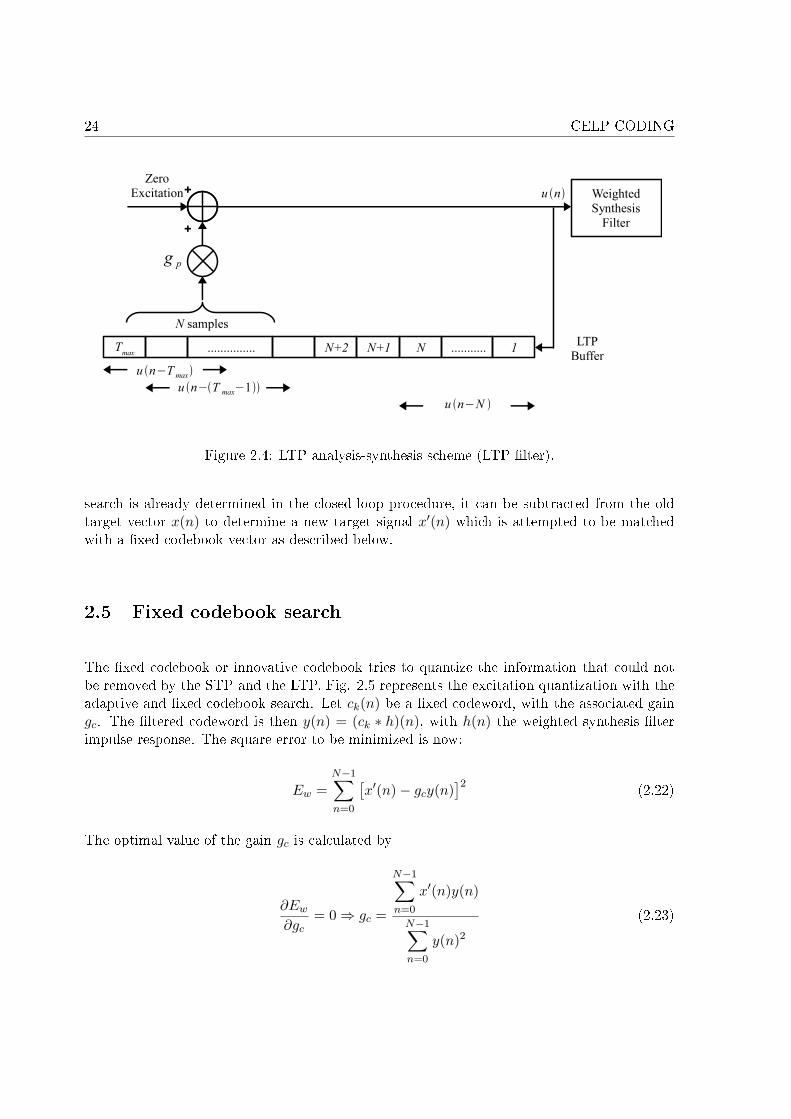
24 CELP CODING
Figure 2.4: LTP analysis-synthesis scheme (LTP �lter).
search is already determined in the closed-loop procedure, it can be subtracted from the oldtarget vector x(n) to determine a new target signal x′(n) which is attempted to be matchedwith a �xed codebook vector as described below.
2.5 Fixed codebook search
The �xed codebook or innovative codebook tries to quantize the information that could notbe removed by the STP and the LTP. Fig. 2.5 represents the excitation quantization with theadaptive and �xed codebook search. Let ck(n) be a �xed codeword, with the associated gaingc. The �ltered codeword is then y(n) = (ck ∗ h)(n), with h(n) the weighted synthesis �lterimpulse response. The square error to be minimized is now:
Ew =N−1∑n=0
[x′(n)− gcy(n)
]2(2.22)
The optimal value of the gain gc is calculated by
∂Ew
∂gc= 0 ⇒ gc =
N−1∑n=0
x′(n)y(n)
N−1∑n=0
y(n)2(2.23)
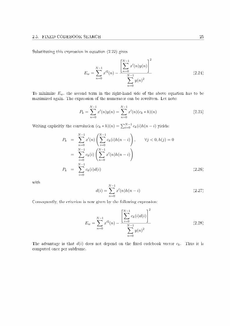
2.5. FIXED CODEBOOK SEARCH 25
Substituting this expression in equation (2.22) gives
Ew =N−1∑n=0
x′2(n)−
[N−1∑n=0
x′(n)y(n)
]2
N−1∑n=0
y(n)2(2.24)
To minimize Ew, the second term in the right-hand side of the above equation has to bemaximized again. The expression of the numerator can be rewritten. Let note:
Pk =N−1∑n=0
x′(n)y(n) =N−1∑n=0
x′(n)(ck ∗ h)(n) (2.25)
Writing explicitly the convolution (ck ∗ h)(n) =∑N−1
i=0 ck(i)h(n− i) yields:
Pk =N−1∑n=0
x′(n)
(N−1∑i=0
ck(i)h(n− i)
), ∀j < 0, h(j) = 0
=N−1∑i=0
ck(i)
(N−1∑n=0
x′(n)h(n− i)
)
Pk =N−1∑i=0
ck(i)d(i) (2.26)
with
d(i) =N−1∑n=0
x′(n)h(n− i) (2.27)
Consequently, the criterion is now given by the following expression:
Ew =N−1∑n=0
x′2(n)−
[N−1∑i=0
ck(i)d(i)
]2
N−1∑n=0
y(n)2(2.28)
The advantage is that d(i) does not depend on the �xed codebook vector ck. Thus it iscomputed once per subframe.
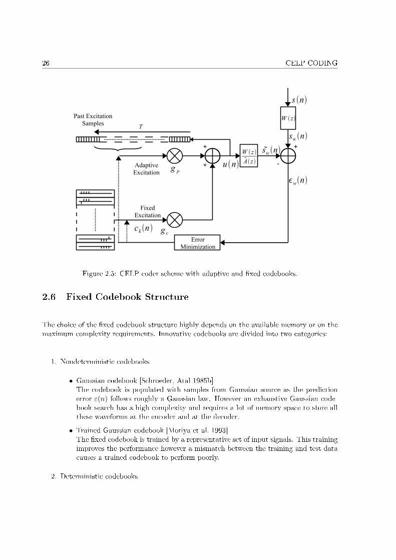
26 CELP CODING
Figure 2.5: CELP coder scheme with adaptive and �xed codebooks.
2.6 Fixed Codebook Structure
The choice of the �xed codebook structure highly depends on the available memory or on themaximum complexity requirements. Innovative codebooks are divided into two categories:
1. Nondeterministic codebooks
• Gaussian codebook [Schroeder, Atal 1985b]The codebook is populated with samples from Gaussian source as the predictionerror ε(n) follows roughly a Gaussian law. However an exhaustive Gaussian code-book search has a high complexity and requires a lot of memory space to store allthese waveforms at the encoder and at the decoder.
• Trained Gaussian codebook [Moriya et al. 1993]The �xed codebook is trained by a representative set of input signals. This trainingimproves the performance however a mismatch between the training and test datacauses a trained codebook to perform poorly.
2. Deterministic codebooks
2.6. FIXED CODEBOOK STRUCTURE 27
The general expression of the excitation vector [Atal, Remde 1982] is
c(n) =M−1∑i=0
βiδ(n−mi) (2.29)
The excitation is composed of M non-zero pulses with their amplitudes βi
• Regular pulse excitation [Kroon et al. 1986]The di�erence between two consecutive pulses is constant.
• Algebraic codebook (βi = ±1,∀i ∈ {0, . . . ,M − 1}) [Adoul et al. 1987]The structure of the excitation vector decreases the computation costs. The excita-tion comprises M non-zero values, called pulses. There is also a constraint on thepositions of the pulses. The complexity may be again decreased when only a subsetof the codebook is examined for �nding the best candidate. Although such algo-rithms are suboptimal, they cause only small degradations in terms of performanceand have great interest in terms of complexity reduction and memory requirements.
Codebooks with white Gaussian sequences were originally used in CELP codecs, as both pre-dictions were supposed to remove the correlation completely. They have been progressivelysupplanted by codebooks containing a few pulses. The simpli�cations to the computationof Eq. (2.28) reduces dramatically the complexity. Most recent CELP codecs make use ofalgebraic codebooks.
Summary
CELP coding is often used in speech coding standards. This success relies on the fact thanthis model accounts well for the speech production apparatus. A �rst prediction removesthe short-term correlation present in speech. The synthesis �lter associated to the predictioncoe�cients models the short-term spectrum of the input signal. Then, a second predictionoften implemented as an adaptive codebook removes the long-term correlation. This codebookrepresents the �ne structure of the input signal spectrum. Finally, the so-called �xed codebookcodes the information that can not be predicted. The codebook entries are chosen to minimizethe error between the original signal and the synthesized signal. The error is weighted by afunction of the LP coe�cients, in order to take the masking properties into account. CELPcoding allows good quality for speech with bitrate ranging from 4 to 16 kbit/s. Ch. 3 describesthe ITU-T G.729 [ITU-T 1996d], the chosen core layer for the proposed embedded codec.

28 CELP CODING
29
Chapter 3
The G.729 standard
Introduction
The G.729 standard comprises several recommendations, called "Annex", describing the stan-dard, the bitrate extensions and the additional modules, and giving the �xed- and �oating-pointimplementations. The G.729 Recommendation [ITU-T 1996d] comprises the "Main Body", alow level description of a codec encoding a narrowband signal sampled at 8 kHz with a bi-trate of 8 kbit/s, and di�erent annexes. The annex A [ITU-T 1996b] is a low complexityimplementation of the G.729 "Main Body" and is bitstream compliant with it. The lowercomplexity has an impact on the quality. A �oating-point implementation can be found in[ITU-T 1998b]. The annex B [ITU-T 1996c] describes a discontinuous transmission (DTX)mode coupled with a Voice Activity Detection (VAD) and Comfort Noise Generator (CNG).The annexes D [ITU-T 1998c] and E [ITU-T 1998d] are extensions of the G.729 at bitrateof 6.4 kbit/s and 11.8 kbit/s respectively. This chapter will describe the G.729 encoder anddecoder, with the simpli�cations related to Annex A if appropriate.
3.1 Encoder
The G.729 encoder is depicted in Fig. 3.1. It works on a 10 ms frame basis corresponding to80 samples for a sampling frequency of 8 kHz. Before any operation, the samples are high-pass�ltered, to get rid of possible low frequency components, and down-scaled by a factor of 2 toreduce the possibility of over�ows. A frame is composed of 2 subframes of 5 ms (40 samples).The CELP parameters, i.e the 10 LP coe�cients, two sets of adaptive and �xed codewords (oneset per subframe), two sets of �xed and the adaptive codebook gains (one set per subframe),(cf Sec. 2.1) are computed on 80 samples. A linear prediction analysis �rst gives the LP �lter
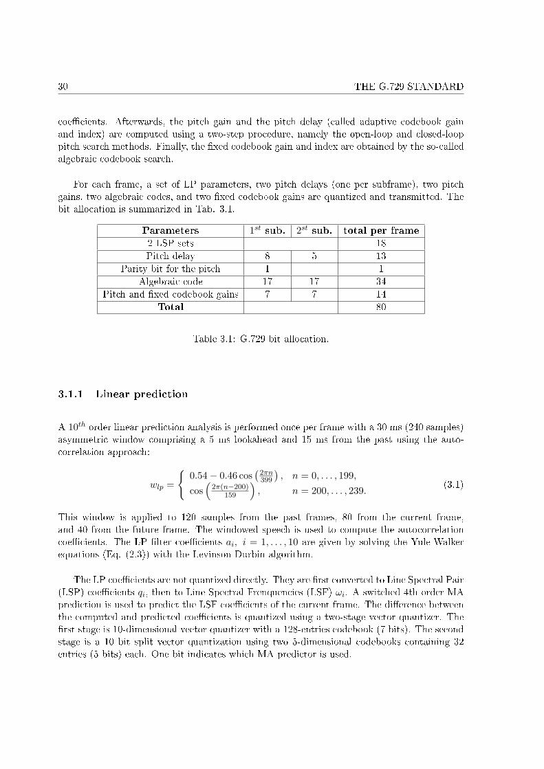
30 THE G.729 STANDARD
coe�cients. Afterwards, the pitch gain and the pitch delay (called adaptive codebook gainand index) are computed using a two-step procedure, namely the open-loop and closed-looppitch search methods. Finally, the �xed codebook gain and index are obtained by the so-calledalgebraic codebook search.
For each frame, a set of LP parameters, two pitch delays (one per subframe), two pitchgains, two algebraic codes, and two �xed codebook gains are quantized and transmitted. Thebit allocation is summarized in Tab. 3.1.
Parameters 1st sub. 2st sub. total per frame
2 LSP sets 18Pitch delay 8 5 13
Parity bit for the pitch 1 1Algebraic code 17 17 34
Pitch and �xed codebook gains 7 7 14Total 80
Table 3.1: G.729 bit allocation.
3.1.1 Linear prediction
A 10th order linear prediction analysis is performed once per frame with a 30 ms (240 samples)asymmetric window comprising a 5 ms lookahead and 15 ms from the past using the auto-correlation approach:
wlp =
{0.54− 0.46 cos
(2πn399
), n = 0, . . . , 199,
cos(
2π(n−200)159
), n = 200, . . . , 239.
(3.1)
This window is applied to 120 samples from the past frames, 80 from the current frame,and 40 from the future frame. The windowed speech is used to compute the autocorrelationcoe�cients. The LP �lter coe�cients ai, i = 1, . . . , 10 are given by solving the Yule-Walkerequations (Eq. (2.3)) with the Levinson-Durbin algorithm.
The LP coe�cients are not quantized directly. They are �rst converted to Line Spectral Pair(LSP) coe�cients qi, then to Line Spectral Frenquencies (LSF) ωi. A switched 4th order MAprediction is used to predict the LSF coe�cients of the current frame. The di�erence betweenthe computed and predicted coe�cients is quantized using a two-stage vector quantizer. The�rst stage is 10-dimensional vector quantizer with a 128-entries codebook (7 bits). The secondstage is a 10 bit split vector quantization using two 5-dimensional codebooks containing 32entries (5 bits) each. One bit indicates which MA predictor is used.
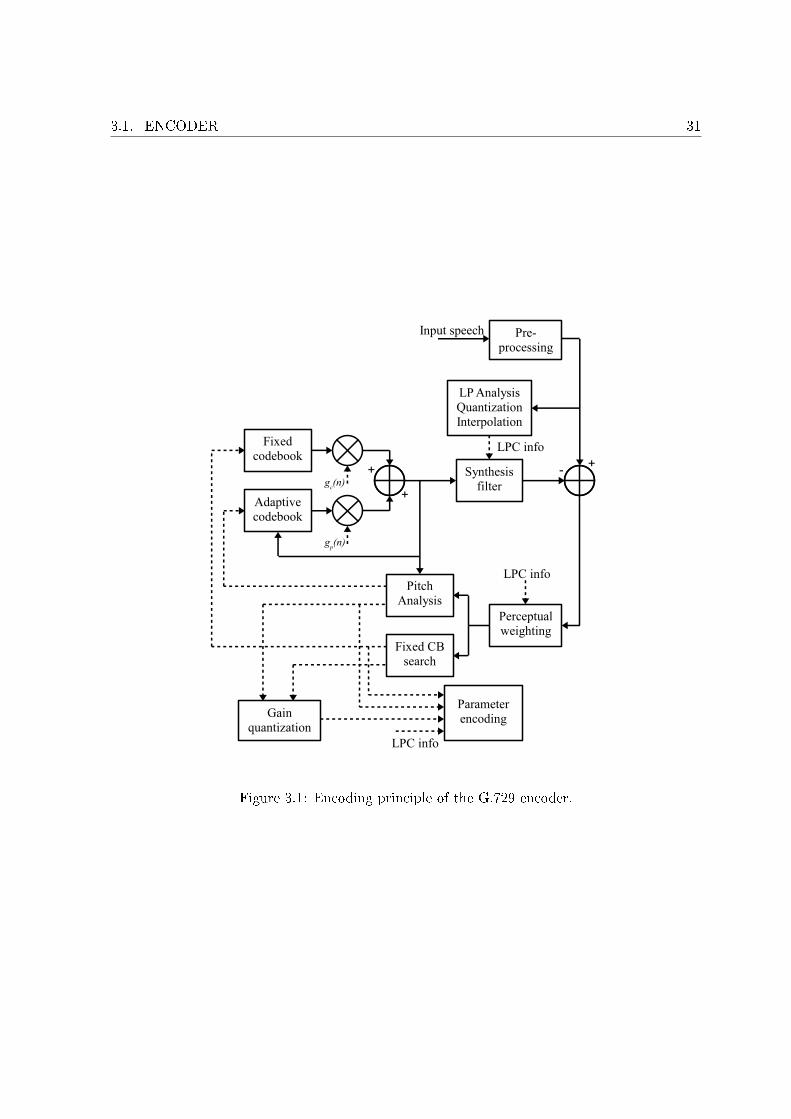
3.1. ENCODER 31
Figure 3.1: Encoding principle of the G.729 encoder.
32 THE G.729 STANDARD
The quantized and unquantized LP coe�cients are used as such for the second subframe.For the �rst subframe, a linear interpolation with the coe�cients from the previous subframeis done. This interpolation is done in the LSP coe�cients domain. Let q
(current)i be the LSP
coe�cients computed for the current 10 ms frame, and q(previous)i the LSP coe�cients computed
in the previous 10 ms frame. The unquantized interpolated LSP coe�cients in each of the 2subframes are given by:
Subframe 1 : q(1)i = 0.5q
(previous)i + 0.5q
(current)i , i = 1, . . . , 10,
Subframe 2 : q(2)i = q
(current)i , i = 1, . . . , 10, (3.2)
The same interpolation procedure is used for the interpolation of the quantized LSP coe�cientsby substituting qi by qi in Eq. (3.2).
The perceptual weighting �lter is computed from the unquantized LP coe�cients (Eq.(2.5)) with γ1 and γ2 as a function of the spectral shape of the input signal:
W (z) =A(z/γ1)A(z/γ2)
=1 +
∑10i=1 γi
1aiz−i
1 +∑10
i=1 γi2aiz−i
. (3.3)
The factors γ1 and γ2 depend of the spectral shape of the input signal. They are updated onceevery 10 ms frame, an interpolation procedure is used to smooth this adaptation process. Theweighting �lter is then applied to the speech signal to obtain the weighted speech signal:
sw(n) = s(n) +10∑i=1
aiγi1s(n− i)−
10∑i=1
aiγi2sw(n− i), n = 0, . . . 39. (3.4)
In Annex A, the complexity of the LP to LSP conversion is simpli�ed when compared to G.729.Since the weighting �lter uses the quantized LP coe�cients, the unquantized LP coe�cientsare not interpolated. The perceptual �lter is based on the quantized LP �lter coe�cients ai
and is given by:
W (z) =A(z)
A(z/γ)(3.5)
with γ = 0.75. There is no adaptive procedure. The weighting speech is only used to computethe open loop pitch estimate. The low-pass �ltered weighted speech is found by �ltering thespeech signal s(n) through the �lter A(z)/[A(z/γ)(1 − 0.7z−1)]. First the coe�cients of the�lter A′(z) = A(z/γ)(1− 0.7z−1) are computed, then the low-pass �ltered weighted speech ina subframe is computed by:
sw(n) = s(n) +10∑i=1
ais(n− i)−10∑i=1
a′isw(n− i), n = 0, . . . , 39 (3.6)
3.1. ENCODER 33
3.1.2 Long-term prediction
The long-term prediction is performed by searching the pitch value with a �rst analysis, calledopen-loop pitch analysis, then re�ning the rough value with an adaptive codebook search.
3.1.2.1 Open-loop pitch analysis
The open-loop pitch analysis is performed once by frame and consists in determining themaximum of the weighted speech auto-correlation :
R(k) =79∑
n=0
sw(n)sw(n− k), (3.7)
in three ranges [20, 39],[40, 79] and [80, 143]. The maximum R(ti) in each interval is normalizedthrough:
R′(ti) =R(ti)√∑
n s2w(n− ti)
, with i = 1, 2, 3 (3.8)
Starting from the highest range, the normalized correlation is compared with that computedfor the lower range, weighted by the factor 0.85, in order to favor the lower delay, as explainedin Sec. 2.4.1. Top is the selected delay. To reduce the complexity in Annex A, the correlationis computed with the even samples only:
R(k) =39∑
n=0
sw(2n)sw(2n− k), (3.9)
in three ranges [20, 39],[40, 79] and [80, 143]. In the third region [80, 143] only the correlationsat the even delays are computed in the �rst pass, then the delays at ±1 of the selected evendelay are tested. The retained maxima R(ti), i = 1, . . . , 3 are normalized by dividing by√∑
n s2w(2n− ti) and ti the corresponding delay:
R′(ti) =R(ti)√∑39
n=0 s2w(2n− ti)
, i = 1, . . . , 3. (3.10)
The selected value among the three normalized correlations is again selected by favouring thedelays with the values in the lower range.
3.1.2.2 Adaptive codebook search
The adaptive codebook search is performed on a subframe basis. In the �rst subframe, thefractional pitch T1 is determined with a resolution: 1
3 in the range[19 + 1
3 , 84 + 23
]and integer
34 THE G.729 STANDARD
resolution in the range [85, 143]. For the second subframe, the pitch T2 is found in the range[int(T1)− 5 + 2
3 , int(T1) + 4 + 23
]with a pitch resolution of 1
3 where int(T1) is the nearestinteger to the fractional pitch delay T1. For the �rst subframe, the search boundaries tmin andtmax are de�ned by:
20 ≤ tmin = Top − 3 < tmax = Top + 6 ≤ 143
In the second subframe, the search boundaries are between tmin − 23 and tmax + 2
3 where tmin
and tmax are de�ned by:
20 ≤ tmin = int(T1)− 5 < tmax = int(T1) + 4 ≤ 143
In the range speci�ed above, the pitch lag is obtained by maximizing the second term in theright-hand side of Eq. (2.21), namely
R(k) =
39∑n=0
x(n)yk(n)√√√√ 39∑n=0
[yk(n)]2
. (3.11)
where x(n) is the target signal (i.e. the di�erence between the weighted speech signal andthe zero-input response of the weighted synthesis �lter, cf. Sec. 2.4.2) and yk(n) is thepast excitation at the delay k (past excitation convolved with h(n)). For the range k =tmin + 1, . . . , tmax, the �ltered past excitation is updated by using the recursive relation:
yk(n) = yk−1(n− 1) + u(−k)h(n), n = 39, . . . , 0 (3.12)
where u(n), n = −143, . . . , 39 is the excitation bu�er and yk−1(−1) = 0. For n = 0, . . . , 39,the samples are actually not known (they form the searched adaptive excitation for the currentsubframe), the LP residual s(n) +
∑10i=1 ais(n− i) is thus copied to the excitation bu�er u(n)
in order to simplify the search procedure. After determining the optimum integer delay, thefractions from −2
3 to 23 are tested. Since the R(k) values are not available for non-integer
values of k, they are interpolated by:
R(k)t =3∑
i=0
R(k − i)b12(t + 3i) +3∑
i=0
R(k + 1 + i)b12(3− t + 3i) (3.13)
where t = 0, 1, 2 corresponds to the fractions 0,13 ,23 , respectively. The �lter b12 is based on
a Hamming windowed sin(x)/x function truncated at ±11 and padded with zeros at ±12.Finally the adaptive codebook vector v(n) is computed by interpolating the past excitationsignal u(n) at the integer part k of the pitch lag and at its fraction t:
v(n) =9∑
i=0
u(n−k− i)b30(t+3i)+9∑
i=0
u(n−k+1+ i)b30(3− t+3i), n = 0, . . . , 39 (3.14)
3.1. ENCODER 35
b30 is also based on a Hamming windowed sin(x)/x function. The adaptive codebook gain isthen found and bounded by:
gp =
39∑n=0
x(n)y(n)
39∑n=0
[yk(n)]2, 0 ≤ gp ≤ 1.2 and y(n) =
n∑i=0
v(i)h(n− i) (3.15)
This gain and the �xed codebook gain (presented in the next section) are jointly quantizedwith 7 bits per subframe. The pitch delay is encoded with 8 bits for the �rst subframe andthe relative delay of the other subframe is encoded with 5 bits (cf. Tab. 3.1).
To simplify the closed-loop pitch search in Annex A, only the numerator RN (k) of Eq.(3.11) is maximized:
RN (k) =39∑
n=0
x(n)yk(n) =39∑
n=0
xb(n)uk(n) (3.16)
where xb(n) is the backward �ltered target signal (correlation between x(n) and the impulseresponse h(n)) and uk(n) is the past excitation at delay k (u(n − k)). The search range islimited around a preselected value, which is the open-loop pitch Top for the �rst subframe, andT1 for the second subframe. In case of fractional pitch, when the optimum integer pitch is lessthat 85, the past excitation at a given delay k and fraction t is interpolated with the �lter b30:
uk,t(n) =9∑
i=0
u(n−k−i)b30(t+3i)+9∑
i=0
u(n−k+1+i)b30(3−t+3i), n = 0, . . . , 39, t = 0, 1, 2
(3.17)
3.1.3 Algebraic codebook search
The �xed codebook structure is algebraic. The �xed excitation, called innovation, contains 4non-zero pulses. The 40 positions in a subframe are divided into 4 tracks, where each trackcontains one pulse, as shown in Tab. 3.2.
The position of the �rst three pulses are encoded with 3 bits, the last one with 4 bits. Eachpulse sign is encoded with 1 bit. The algebraic codeword is then encoded with 17 bits (cf.Tab. 3.1) and can be written as:
c(n) = s0δ(n−m0) + s1δ(n−m1) + s2δ(n−m2) + s3δ(n−m3), n = 0, . . . , 39 (3.18)
where δ(0) is a unit pulse. The harmonic components of the reconstructed signal can beenhanced by �ltering the selected algebraic codeword through an adaptive pre-�lter P (z):
P (z) =1
1− βz−T(3.19)
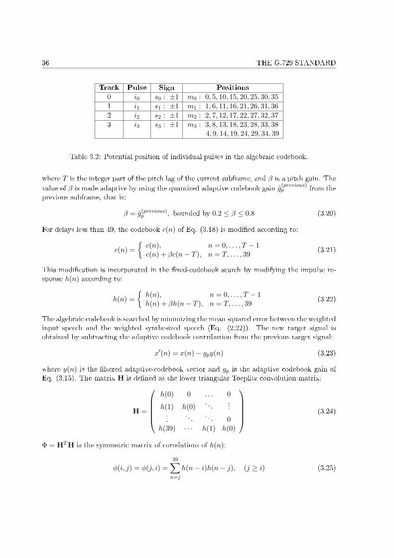
36 THE G.729 STANDARD
Track Pulse Sign Positions
0 i0 s0 : ±1 m0 : 0, 5, 10, 15, 20, 25, 30, 351 i1 s1 : ±1 m1 : 1, 6, 11, 16, 21, 26, 31, 362 i2 s2 : ±1 m2 : 2, 7, 12, 17, 22, 27, 32, 373 i3 s3 : ±1 m3 : 3, 8, 13, 18, 23, 28, 33, 38
4, 9, 14, 19, 24, 29, 34, 39
Table 3.2: Potential position of individual pulses in the algebraic codebook.
where T is the integer part of the pitch lag of the current subframe, and β is a pitch gain. Thevalue of β is made adaptive by using the quantized adaptive-codebook gain g
(previous)p from the
previous subframe, that is:
β = g(previous)p , bounded by 0.2 ≤ β ≤ 0.8 (3.20)
For delays less than 40, the codebook c(n) of Eq. (3.18) is modi�ed according to:
c(n) ={
c(n), n = 0, . . . , T − 1c(n) + βc(n− T ), n = T, . . . , 39
(3.21)
This modi�cation is incorporated in the �xed-codebook search by modifying the impulse re-sponse h(n) according to:
h(n) ={
h(n), n = 0, . . . , T − 1h(n) + βh(n− T ), n = T, . . . , 39
(3.22)
The algebraic codebook is searched by minimizing the mean squared error between the weightedinput speech and the weighted synthesized speech (Eq. (2.22)). The new target signal isobtained by subtracting the adaptive codebook contribution from the previous target signal:
x′(n) = x(n)− gpy(n) (3.23)
where y(n) is the �ltered adaptive-codebook vector and gp is the adaptive codebook gain ofEq. (3.15). The matrix H is de�ned as the lower triangular Toeplitz convolution matrix:
H =
h(0) 0 . . . 0
h(1) h(0). . .
......
. . . . . . 0h(39) · · · h(1) h(0)
(3.24)
Φ = HTH is the symmetric matrix of correlations of h(n):
φ(i, j) = φ(j, i) =39∑
n=j
h(n− i)h(n− j), (j ≥ i) (3.25)
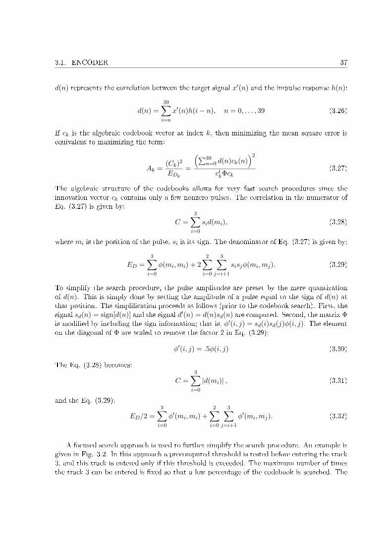
3.1. ENCODER 37
d(n) represents the correlation between the target signal x′(n) and the impulse response h(n):
d(n) =39∑
i=n
x′(n)h(i− n), n = 0, . . . , 39 (3.26)
If ck is the algebraic codebook vector at index k, then minimizing the mean square error isequivalent to maximizing the term:
Ak =(Ck)2
EDk
=
(∑39n=0 d(n)ck(n)
)2
ctkΦck
(3.27)
The algebraic structure of the codebooks allows for very fast search procedures since theinnovation vector ck contains only a few nonzero pulses. The correlation in the numerator ofEq. (3.27) is given by:
C =3∑
i=0
sid(mi), (3.28)
where mi is the position of the pulse, si is its sign. The denominator of Eq. (3.27) is given by:
ED =3∑
i=0
φ(mi,mi) + 22∑
i=0
3∑j=i+1
sisjφ(mi,mj). (3.29)
To simplify the search procedure, the pulse amplitudes are preset by the mere quantizationof d(n). This is simply done by setting the amplitude of a pulse equal to the sign of d(n) atthat position. The simpli�cation proceeds as follows (prior to the codebook search). First, thesignal sd(n) = sign[d(n)] and the signal d′(n) = d(n)sd(n) are computed. Second, the matrix Φis modi�ed by including the sign information; that is, φ′(i, j) = sd(i)sd(j)φ(i, j). The elementon the diagonal of Φ are scaled to remove the factor 2 in Eq. (3.29):
φ′(i, j) = .5φ(i, j) (3.30)
The Eq. (3.28) becomes:
C =3∑
i=0
|d(mi)| , (3.31)
and the Eq. (3.29):
ED/2 =3∑
i=0
φ′(mi,mi) +2∑
i=0
3∑j=i+1
φ′(mi,mj). (3.32)
A focused search approach is used to further simplify the search procedure. An example isgiven in Fig. 3.2. In this approach a precomputed threshold is tested before entering the track3, and this track is entered only if this threshold is exceeded. The maximum number of timesthe track 3 can be entered is �xed so that a low percentage of the codebook is searched. The
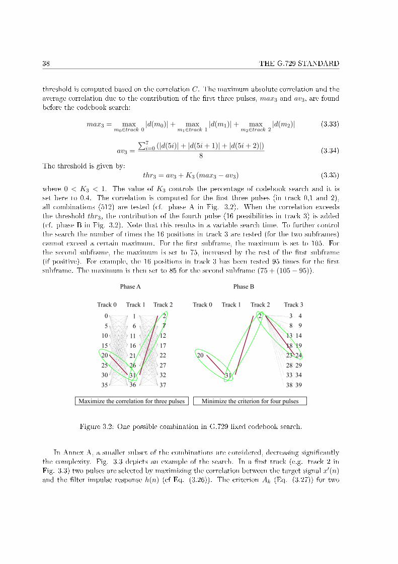
38 THE G.729 STANDARD
threshold is computed based on the correlation C. The maximum absolute correlation and theaverage correlation due to the contribution of the �rst three pulses, max3 and av3, are foundbefore the codebook search:
max3 = maxm0∈track 0
|d(m0)|+ maxm1∈track 1
|d(m1)|+ maxm2∈track 2
|d(m2)| (3.33)
av3 =∑7
i=0 (|d(5i)|+ |d(5i + 1)|+ |d(5i + 2)|)8
(3.34)
The threshold is given by:thr3 = av3 + K3 (max3 − av3) (3.35)
where 0 < K3 < 1. The value of K3 controls the percentage of codebook search and it isset here to 0.4. The correlation is computed for the �rst three pulses (in track 0,1 and 2),all combinations (512) are tested (cf. phase A in Fig. 3.2). When the correlation exceedsthe threshold thr3, the contribution of the fourth pulse (16 possibilities in track 3) is added(cf. phase B in Fig. 3.2). Note that this results in a variable search time. To further controlthe search the number of times the 16 positions in track 3 are tested (for the two subframes)cannot exceed a certain maximum. For the �rst subframe, the maximum is set to 105. Forthe second subframe, the maximum is set to 75, increased by the rest of the �rst subframe(if positive). For example, the 16 positions in track 3 has been tested 95 times for the �rstsubframe. The maximum is then set to 85 for the second subframe (75 + (105− 95)).
Figure 3.2: One possible combination in G.729 �xed codebook search.
In Annex A, a smaller subset of the combinations are considered, decreasing signi�cantlythe complexity. Fig. 3.3 depicts an example of the search. In a �rst track (e.g. track 2 inFig. 3.3) two pulses are selected by maximizing the correlation between the target signal x′(n)and the �lter impulse response h(n) (cf Eq. (3.26)). The criterion Ak (Eq. (3.27)) for two
3.1. ENCODER 39
Figure 3.3: One possible combination in G.729 Annex A �xed codebook search.
pulses only is tested with all the 16 combinations formed by these two pulses and 8 pulses fromanother track (e.g. track 3). After this �rst phase, called phase A, the criterion is tested for4 pulses with the two pulses selected in two other tracks (e.g. track 0 and 1). In this phasecalled phase B, 64 combinations are tested. Consequently, 80 pulses are tested. This procedureis repeated for three other choices of tracks {3, 0, 1, 2} {2, 4, 0, 1} {4, 0, 1, 2}. Altogether, 320combinations are tested.
3.1.4 Gain quantization
The gain codebook search is done by minimizing the mean-squared weighted error betweenoriginal and reconstructed speech which is given by:
E = ‖x− gpy − gcz‖2 (3.36)
where x is the target vector, y is the �ltered adaptive-codebook vector and z is the �xed-codebook vector convolved with h(n)
z(n) =n∑
i=0
c(i)h(n− i) n = 0, . . . , 39 (3.37)
3.1.4.1 Gain prediction
The �xed-codebook gain gc can be expressed as:
gc = γg′c (3.38)
40 THE G.729 STANDARD
where g′c is a predicted gain based on previous �xed-codebook energies, and γ is a correctionfactor. The �xed codebook gain quantization is indeed performed using MA prediction with�xed coe�cients. The 4th order MA prediction is performed on the innovation energy asfollows. Let E(m) be the mean-removed innovation energy (in dB) at subframe m, and givenby:
E(m) = 10 log
(140
g2c
39∑n=0
c2(n)
)− E (3.39)
where c(i) is the �xed codebook excitation, and E = 30 dB is the mean enery of the �xedcodebook excitation. The predicted energy is given by:
E(m) =4∑
i=1
biU(m−i) (3.40)
where [b1 b2 b3 b4] = [0.68 0.58 0.34 0.19] are the MA prediction coe�cients, and U (m) is thequantized prediction error at subframe m. The predicted energy is used to compute a predicted�xed-codebook gain g′c as in Eq. (3.39) (by substituting E(m) by E(m) and gc by g′c). This isdone as follows. First the mean innovation energy is found by:
E = 10 log
(140
39∑j=0
c2(j)
)(3.41)
and then the predicted gain g′c is found by:
g′c = 100.05( eE(m)+E−E) (3.42)
A correction factor between the gain gc and the estimated one g′c is given by:
γ = gc/g′c. (3.43)
The correlation factor γ is related to the gain-prediction error by:
U (m) = E(m) − E(m) = 20 log(γ). (3.44)
3.1.4.2 Conjugate-structure quantization of the gains
The adaptive-codebook gain, gp, and the factor γ are vector quantized using a two-stageconjugate structured codebook. The �rst stage consists of a 3 bit two-dimensional codebookGA, and the second stage consists of a 4 bit two-dimensional codebook GB. The �rst elementin each codebook represents the quantized adaptive-codebook gain gp, and the second elementrepresents the quantized �xed-codebook gain correction factor γ. Given codebook indices GAand GB for GA and GB, respectively, the quantized adaptive-codebook gain is given by:
gp = GA1(GA) + GB1(GB) (3.45)
and the quantized �xed-codebook gain by:
gc = g′cγ = g′c(GA1(GA) + GB2(GB)) (3.46)
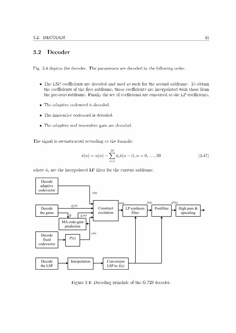
3.2. DECODER 41
3.2 Decoder
Fig. 3.4 depicts the decoder. The parameters are decoded in the following order:
• The LSP coe�cients are decoded and used as such for the second subframe. To obtainthe coe�cients of the �rst subframe, these coe�cients are interpolated with those fromthe previous subframe. Finally the set of coe�cients are converted to the LP coe�cients.
• The adaptive codeword is decoded.
• The innovative codeword is decoded.
• The adaptive and innovative gain are decoded.
The signal is reconstructed according to the formula:
s(n) = u(n)−10∑i=1
ais(n− i), n = 0, . . . , 39 (3.47)
where ai are the interpolated LP �lter for the current subframe.
Figure 3.4: Decoding principle of the G.729 decoder.
42 THE G.729 STANDARD
The reconstructed speech is �nally post-�ltered to enhance the perceptual quality, thenpost-processed. The post�lter comprises a long-term post�lter, a short-term post�lter and atilt compensation. The long-term post�lter is given by:
Hp(z) =1
1 + γpgl(1 + γpglz
−T ) (3.48)
where T is the pitch delay, and gl is the gain coe�cient. Note that 0 ≤ gl ≤ 1 , gl is adaptedon a subframe basis, and it is set to zero if the long-term prediction gain is less than 3 dB. Thefactor γp controls the amount of long-term post�ltering and has the value of γp = 0.5. Thelong-term delay and gain are computed from the residual signal r(n) obtained by �ltering thespeech s(n) through A(z/γn), which is the numerator of the short-term post�lter
r(n) = s(n) +10∑i=1
γinais(n− i) (3.49)
The pitch T is searched within the range [int(T1)− 1, int(T1) + 1] with a fractional resolutionof 1
8 , where int(T1) is the integer part of the (transmitted) pitch delay T1 in the �rst subframe.This is done by maximizing the autocorrelation of the residual signal r(n). In Annex A, Tis always an integer delay and it is computed by searching the range [Tcl − 3, Tcl + 3], whereTcl is the integer part of the (transmitted) pitch delay in the current subframe bounded byTcl ≤ 140.
The short-term post�lter is given by:
Hf (z) =1gf
A(z/γn)A(z/γd)
=1gf
1 +∑10
i=1 γinaiz
−i
1 +∑10
i=1 γidaiz−i
(3.50)
where A(z) is the received quantized LP inverse �lter and the factors γn and γd control theamount of short-term post�ltering, and are set to γn = 0.55, and γd = 0.7. The gain termgf is calculated on the truncated impulse response hf (n) of the �lter A(z/γn)/A(z/γd) and isgiven by:
gf =19∑
n=0
|hf (n)| (3.51)
In Annex A gf = 1 to reduce the complexity.
The �lter Ht(z) compensates for the tilt in the short-term post�lter Hf (z) and is given by:
Ht(z) =1gt
(1 + γtk′1z−1) (3.52)
where γtk′1 is a tilt factor k′1 being the �rst re�ection coe�cient calculated from hf (n) with
k′1 = −rh(1)rh(0)
rh(i) =19−i∑j=0
hf (j)hf (j + i) (3.53)
3.2. DECODER 43
The gain term gt = 1−|γtk′1| compensates for the decreasing e�ect of gf in Hf (z). Furthermore,
it has been shown that the product �lter Hf (z)Ht(z) has generally no gain. Two values for γt
are used depending on the sign of k′1. If k′1 is negative, γt = 0.9, and if k′1 is positive, γt = 0.2.In the Annex A, for simpli�cation sake, gt = 1. Furthermore, if k′1 is negative, γt = 0.8, and ifk′1 is positive, γt = 0.
Adaptive gain control is used to compensate for gain di�erences between the reconstructedspeech signal s(n) and the post�ltered signal sf(n). The gain scaling factor G for the presentsubframe is computed by:
G =∑39
n=0 |s(n)|∑39n=0 |sf(n)|
(3.54)
In Annex A, The gain scaling factor G for the present subframe is computed by:
G =
√ ∑39n=0 s2(n)∑39
n=0 sf2(n)(3.55)
The post-�ltered signal is �nally high-�ltered and upscaled by a factor 2, in order to getthe input level before the encoding.
Summary
In this chapter, the G.729 encoder has been presented, as well as the algorithmic simpli�cationsbrought by its Annex A. G.729 is based on CELP technology, with an algebraic �xed codebook,that allows a lower search complexity than original Gaussian waveform codebooks. It producesgood quality narrowband speech at a bitrate of 8 kbit/s. For these reasons, the G.729 has beenchosen as core layer of the proposed codec.
The next chapter will describe di�erent possibilities to enable scalability in LPC-basedcodecs, and propose a solution for an enhancement layer on top of ACELP coders, in particularthe G.729.

44 THE G.729 STANDARD
45
Chapter 4
Embedded CELP
Introduction
Di�erent approaches of scalable CELP-based coders are already available in the literature. Forexample, some solutions adopt the subband coding. The signal is split into 2 or more subbands.In each subband, a linear prediction removes the short term correlation between the samples.Consequently, the signal in each subband is encoded independently of the other subbands.Another approach is to improve the quantization of the LP residual by adding codebookcontributions to the initial quantized excitation. This chapter comprises two sections. First, afew examples of existing solutions are presented. For each solution, the embedded procedure ishighlighted, with its advantages and its drawbacks. Then some investigations about a secondstage in a CELP coder are described. Finally, conclusion is drawn.
4.1 CELP-based coders overview
This section presents a few examples of scalable coders that make use of linear prediction only.In 4.1.1, the subband approach is investigated. The input signal is divided into subbandsof 4kHz bandwidth, and each subband, CELP coding is applied. The proposed solution in4.1.2 is a two-layer codec for wideband signal. The core layer encodes the downsampled inputsignal with a CELP codec, and the second layer encodes with a CELP structure the di�erencebetween the original signal and the upsampled output of the core layer. Finally, the embeddedquantization of the LTP residual is experimented in 4.1.3, 4.1.4 and 4.1.5.
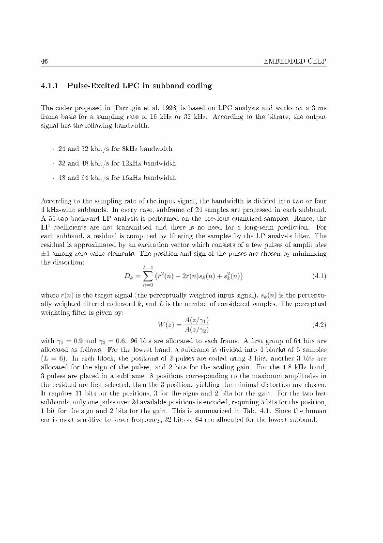
46 EMBEDDED CELP
4.1.1 Pulse-Excited LPC in subband coding
The coder proposed in [Farrugia et al. 1998] is based on LPC analysis and works on a 3 msframe basis for a sampling rate of 16 kHz or 32 kHz. According to the bitrate, the outputsignal has the following bandwidth:
- 24 and 32 kbit/s for 8kHz bandwidth
- 32 and 48 kbit/s for 12kHz bandwidth
- 48 and 64 kbit/s for 16kHz bandwidth
According to the sampling rate of the input signal, the bandwidth is divided into two or four4 kHz-wide subbands. In every case, subframe of 24 samples are processed in each subband.A 50-tap backward LP analysis is performed on the previous quantized samples. Hence, theLP coe�cients are not transmitted and there is no need for a long-term prediction. Foreach subband, a residual is computed by �ltering the samples by the LP analysis �lter. Theresidual is approximated by an excitation vector which consists of a few pulses of amplitudes±1 among zero-value elements. The position and sign of the pulses are chosen by minimizingthe distortion:
Dk =L−1∑n=0
(r2(n)− 2r(n)sk(n) + s2
k(n))
(4.1)
where r(n) is the target signal (the perceptually weighted input signal), sk(n) is the perceptu-ally weighted �ltered codeword k, and L is the number of considered samples. The perceptualweighting �lter is given by:
W (z) =A(z/γ1)A(z/γ2)
(4.2)
with γ1 = 0.9 and γ2 = 0.6. 96 bits are allocated to each frame. A �rst group of 64 bits areallocated as follows. For the lowest band, a subframe is divided into 4 blocks of 6 samples(L = 6). In each block, the positions of 3 pulses are coded using 3 bits, another 3 bits areallocated for the sign of the pulses, and 2 bits for the scaling gain. For the 4-8 kHz band,3 pulses are placed in a subframe. 8 positions corresponding to the maximum amplitudes inthe residual are �rst selected, then the 3 positions yielding the minimal distortion are chosen.It requires 11 bits for the positions, 3 for the signs and 2 bits for the gain. For the two lastsubbands, only one pulse over 24 available positions is encoded, requiring 5 bits for the position,1 bit for the sign and 2 bits for the gain. This is summarized in Tab. 4.1. Since the humanear is most sensitive to lower frequency, 32 bits of 64 are allocated for the lowest subband.
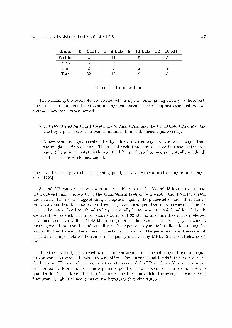
4.1. CELP-BASED CODERS OVERVIEW 47
Band 0 - 4 kHz 4 - 8 kHz 8 - 12 kHz 12 - 16 kHz
Position 3 11 5 5Sign 3 3 1 1Gain 2 2 2 2Total 32 16 8 8
Table 4.1: Bit allocation.
The remaining bits available are distributed among the bands, giving priority to the lowest.The utilization of a second quantization stage (enhancement layer) improves the quality. Twomethods have been experimented:
- The reconstruction error between the original signal and the synthesized signal is quan-tized by a pulse excitation search (minimization of the mean square error).
- A new reference signal is calculated by subtracting the weighted synthesized signal fromthe weighted original signal. The second excitation is searched so that the synthesizedsignal (the second excitation through the LPC synthesis �lter and perceptually weighted)matches the new reference signal.
The second method gives a better listening quality, according to various listening tests [Farrugiaet al. 1998].
Several AB comparison tests were made at bit rates of 24, 32 and 48 kbit/s to evaluatethe perceived quality provided by the enhancement layer or by a wider band, both for speechand music. The results suggest that, for speech signals, the perceived quality at 24 kbit/simproves when the �rst and second frequency bands are quantized more accurately. For 48kbit/s, the output has been found to be perceptually better when the third and fourth bandsare quantized as well. For music signals at 24 and 32 kbit/s, �ner quantization is preferredthan increased bandwidth. At 48 kbit/s no preference is given. In this case, psychoacousticmasking would improve the audio quality at the expense of dynamic bit allocation among thebands. Further listening tests were conducted at 64 kbit/s. The performance of the coder atthis rate is comparable to the compressed quality achieved by MPEG-2 Layer II also at 64kbits.
Here the scalability is achieved by mean of two techniques. The splitting of the input signalinto subbands ensures a bandwidth scalability. The output signal bandwidth increases withthe bitrates. The second technique is the re�nement of the LP synthesis �lter excitation ineach subband. From the listening experience point of view, it sounds better to increase thequantization in the lowest band before increasing the bandwidth. However, this coder lacks�ner grain scalability since it has only 4 bitrates with 8 kbit/s step.
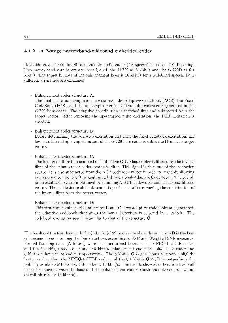
48 EMBEDDED CELP
4.1.2 A 2-stage narrowband-wideband embedded coder
[Koishida et al. 2000] describes a scalable audio coder (for speech) based on CELP coding.Two narrowband core layers are investigated, the G.729 at 8 kbit/s and the G.729D at 6.4kbit/s. The target bit rate of the enhancement layer is 16 kbit/s for a wideband speech. Fourdi�erent structures are examined:
- Enhancement coder structure A:The �nal excitation comprises three sources: the Adaptive CodeBook (ACB), the FixedCodeBook (FCB), and the up-sampled version of the pulse codevector generated in theG.729 base coder. The adaptive contribution is searched �rst and subtracted from thetarget vector. After removing the up-sampled pulse excitation, the FCB excitation isselected.
- Enhancement coder structure B:Before determining the adaptive excitation and then the �xed codebook excitation, thelow-pass �ltered up-sampled output of the G.729 base coder is subtracted from the targetvector.
- Enhancement coder structure C:The low-pass �ltered up-sampled output of the G.729 base coder is �ltered by the inverse�lter of the enhancement coder synthesis �lter. This signal is then one of the excitationsource. It is also subtracted from the ACB codebook vector in order to avoid duplicatingpitch period component (the result is called Additional-Adaptive CodeBook). The overallpitch excitation vector is obtained by summing A-ACB codevector and the inverse �lteredvector. The excitation codebook search is performed after removing the contribution ofthe inverse �lter from the target vector.
- Enhancement coder structure D:This structure combines the structures B and C. Two adaptive codebooks are generated,the adaptive codebook that gives the lower distortion is selected by a switch. Thecodebook excitation search is similar to that of the structure C.
The results of the test done with the 8 kbit/s G.729 base coder show the structure D is the bestenhancement coder among the four structures according to SNR and Weighted SNR measures.Formal listening tests (A-B test) were then performed between the MPEG-4 CELP coder,and the 6.4 kbit/s base coder and 9.6 kbit/s enhancement coder (8 kbit/s base coder and8 kbit/s enhancement coder, respectively). The 8 kbit/s G.729 is shown to provide slightlybetter quality than the MPEG-4 CELP coder and the 6.4 kbit/s G.729D to outperform thepublicly available MPEG-4 CELP coder at 16 kbit/s. The results show also there is a trade-o�in performance between the base and the enhancement coders (both scalable coders have anoverall bit rate of 16 kbit/s).
4.1. CELP-BASED CODERS OVERVIEW 49
Figure 4.1: The 4 di�erent enhancement structures.
At a constant global bitrate of 16 kbit/s, giving more bits to the enhancement layer hasmore impact on the quality. Both bandwidth and SNR scalability are achieved by subtractingthe contribution of the G.729 to the target signal. Also, the best enhancement layer looks themore complex as well since there is possibility to switch between two adaptive codebooks, theone giving the less distortion is selected. Moreover, the presence of two adaptive codebooksincrease the risk of desynchronization if packet loss occurs.
4.1.3 Pyramid CELP
[Erdmann et al. 2002] proposes a transposition of the pyramid encoding from the area of thestill image compression to the domain of speech coding. A so-called image pyramid means therepresentation of an image with multiple resolutions. This kind of encoding is based on thestructure of a so-called Gauss pyramid. A gray-scale image can be represented by a m × mmatrix where each coe�cient represents the luminosity of a pixel. A layer gi of the Gausspyramid is a sub-sampled version of the original image. By de�ning a set of reduce operatorsRi and applying Ri sequentially to the input signal (the image), one obtains the di�erent layersgi of the Gauss pyramid g, given recursively by the equation:
gi = Ri−1(gi−1), i = 1, . . . , L (4.3)
R0 representing actually the identity operator. The application of the pyramid encoding toscalable encoding is straightforward when the Gauss pyramid is transformed into Laplace pyra-
50 EMBEDDED CELP
mid. The base layer of the Gauss pyramid is unchanged and the enhanced layer li of the Laplacepyramid l represents the reconstruction error between the Gauss layer gi and its reconstructedversion from the layer gi+1:
lL = gL (4.4)
li = gi − Ei(gi+1), i = 1, . . . , L− 1 (4.5)
Ei represents the reconstruction operator, typically a up-sampling and a low-pass �ltering(interpolation). The reconstruction formulas are immediate:
gL = lL (4.6)
gi = Ei(gi+1) + li, i = 1, . . . , L− 1. (4.7)
In the case of linear operator, for each layer in the reconstruction processing, the operators Ei
can be concatenated:Ei = E0 ◦ · · · ◦ Ei, i = 1, . . . , L− 1. (4.8)
The equivalent layer l′i = Ei−1(li) has the same size as the original input signal, and leads toa simple reconstruction rule:
s =L∑
i=1
Ei−1(li) =L∑
i=1
l′i. (4.9)
This scheme has been applied to the LP residual of a CELP coder. For each layer, thequantization of the LP residual is obtained by a closed-loop search in a �xed codebook search.The adaptive contribution to the excitation is performed in the coarsest approximation of theexcitation signal, i.e. the layer l′L. The LPC coe�cients are transmitted as side informationin order to reconstruct properly the speech signal over the whole frequency range. Besidesin the reconstruction process, the low-pass �ltering after up-sampling is omitted, the missingpart of the spectrum is thus reconstructed by mirroring the low-frequency (aliasing). Theso-modi�ed CELP coder is shown to signi�cantly improve error robustness and speech qualitywhen transmitting over lossy packet networks.
The scalability is achieved by quantizing the di�erence between two levels of resolution onthe LP synthesis �lter excitation. In the worst case, the excitation covers only a portion of theresidual signal. The rest of the residual spectrum is obtained by spectral mirroring. In theory,after the short-and long-term prediction, the residual spectrum is �at. In practice, it is by farto be the case. The decoded signal sounds distorted compared to a conventional CELP coderat a similar bitrate.
4.1.4 Embedded algebraic CELP/VSELP coders
[LeGuyader et al. 1995] deals with a embedded CELP codec. The residual excitation is re�nedsuccessively by adding excitation vectors from di�erent codebooks that can be algebraic and/orstochastic codebooks, Vector Sum Excited Linear Prediction (VSELP) codebook or multi-pulse
4.1. CELP-BASED CODERS OVERVIEW 51
codebook, therefore increasing the bitrate. The residual excitation is given by the generalexpression:
excK =K∑
j=1
gK(j)F jCjIj
, 1 ≤ Ij ≤ N j (4.10)
where CjIj
is the Ij-th codevector in the j-th codebook whose size is N j , F j is a transform
matrix and gK(j) is the gain of the j-th waveform (modeled by the j-th codebook). The typicaltarget signal t for the excitation search is obtained by subtracting the adaptive contributionand the ringing from the weighted speech signal.
The determination of the gains and the excitation vectors from the di�erent codebooksis performed successively through K steps for each codebook while minimizing the followingcriterion:
Eki =
∥∥∥∥∥∥t−k−1∑j=1
gki (j)HF jCj
Ij− gk
i (k)HF kCki
∥∥∥∥∥∥2
, i = 1, . . . , Nk (4.11)
where H is the impulse response matrix, Cji is the ith vector in the jth codebook and gk
i (j)is the j-th component of the gain vector gk
i . The adaptive codebook can be included inthis equation. In this case, the �rst codebook C1 is composed of shifted versions of the pastreconstructed residual. At the step k, the optimum index is searched through the k-th codebookCk, together with a set of optimized gains gk
i (j), j = 1, . . . , k by minimizing the CELP/VSELPerror criterion. When a new contribution is added, the gains of the previous codewords arereoptimized. The recomputation of the gains and the search of the new contribution at thestage k is equivalent to orthogonalizing the new contribution to the previous ones (1, . . . , k−1).This is done by using a Gram-Schmidt procedure.
This method is illustrated with an VSELP embedded coder working at 24 kbit/s and 32kbit/s on wideband signal. The codebooks comprise one adaptive codebook and two VSELPcodebooks. The lower bitrate excitation is given by a combination of an adaptive codewordand the �xed codeword. The additional �xed codeword yields the higher bitrate excitation. Inboth modes, the adaptive codebook contains the past lower bitrate excitation. The referencecoder (non-embedded) consists of the 32 kbit/s whose adaptive codebook is updated by thehigh bit rate �xed excitation. The embedded constraint does not a�ect signi�cantly the speechquality, compared to the reference coder. Furthermore, formal listening tests have shown tobe as good as the ITU-T G.722 at 56 kbit/s.
Although this method is less complex than the optimal case (i.e. �nd the k codewordsand gains at the same time), it becomes rapidly complex with many codebooks. Moreover thequality saturates after adding a few contributions.
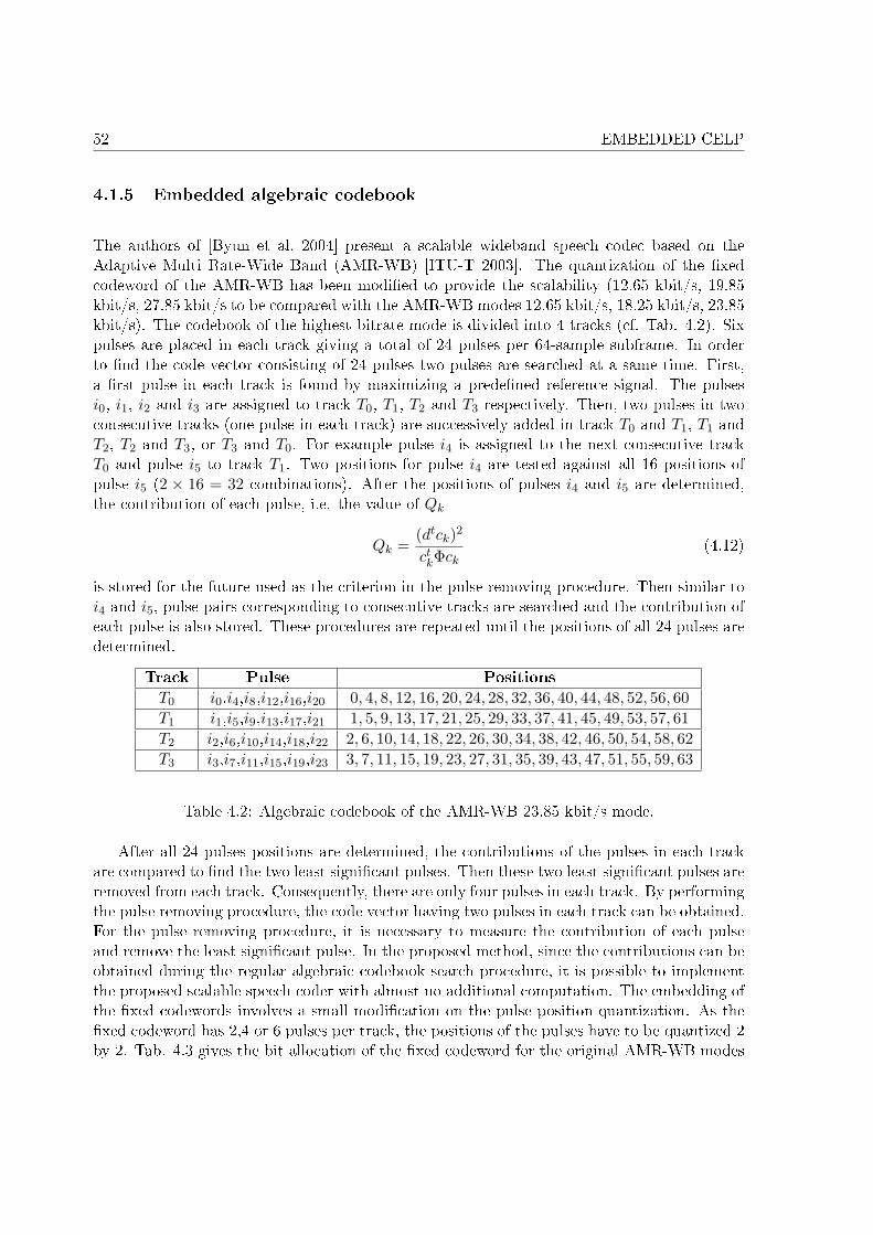
52 EMBEDDED CELP
4.1.5 Embedded algebraic codebook
The authors of [Byun et al. 2004] present a scalable wideband speech codec based on theAdaptive Multi Rate-Wide Band (AMR-WB) [ITU-T 2003]. The quantization of the �xedcodeword of the AMR-WB has been modi�ed to provide the scalability (12.65 kbit/s, 19.85kbit/s, 27.85 kbit/s to be compared with the AMR-WB modes 12.65 kbit/s, 18.25 kbit/s, 23.85kbit/s). The codebook of the highest bitrate mode is divided into 4 tracks (cf. Tab. 4.2). Sixpulses are placed in each track giving a total of 24 pulses per 64-sample subframe. In orderto �nd the code vector consisting of 24 pulses two pulses are searched at a same time. First,a �rst pulse in each track is found by maximizing a prede�ned reference signal. The pulsesi0, i1, i2 and i3 are assigned to track T0, T1, T2 and T3 respectively. Then, two pulses in twoconsecutive tracks (one pulse in each track) are successively added in track T0 and T1, T1 andT2, T2 and T3, or T3 and T0. For example pulse i4 is assigned to the next consecutive trackT0 and pulse i5 to track T1. Two positions for pulse i4 are tested against all 16 positions ofpulse i5 (2 × 16 = 32 combinations). After the positions of pulses i4 and i5 are determined,the contribution of each pulse, i.e. the value of Qk
Qk =(dtck)2
ctkΦck
(4.12)
is stored for the future used as the criterion in the pulse removing procedure. Then similar toi4 and i5, pulse pairs corresponding to consecutive tracks are searched and the contribution ofeach pulse is also stored. These procedures are repeated until the positions of all 24 pulses aredetermined.
Track Pulse Positions
T0 i0,i4,i8,i12,i16,i20 0, 4, 8, 12, 16, 20, 24, 28, 32, 36, 40, 44, 48, 52, 56, 60T1 i1,i5,i9,i13,i17,i21 1, 5, 9, 13, 17, 21, 25, 29, 33, 37, 41, 45, 49, 53, 57, 61T2 i2,i6,i10,i14,i18,i22 2, 6, 10, 14, 18, 22, 26, 30, 34, 38, 42, 46, 50, 54, 58, 62T3 i3,i7,i11,i15,i19,i23 3, 7, 11, 15, 19, 23, 27, 31, 35, 39, 43, 47, 51, 55, 59, 63
Table 4.2: Algebraic codebook of the AMR-WB 23.85 kbit/s mode.
After all 24 pulses positions are determined, the contributions of the pulses in each trackare compared to �nd the two least signi�cant pulses. Then these two least signi�cant pulses areremoved from each track. Consequently, there are only four pulses in each track. By performingthe pulse removing procedure, the code vector having two pulses in each track can be obtained.For the pulse removing procedure, it is necessary to measure the contribution of each pulseand remove the least signi�cant pulse. In the proposed method, since the contributions can beobtained during the regular algebraic codebook search procedure, it is possible to implementthe proposed scalable speech coder with almost no additional computation. The embedding ofthe �xed codewords involves a small modi�cation on the pulse position quantization. As the�xed codeword has 2,4 or 6 pulses per track, the positions of the pulses have to be quantized 2by 2. Tab. 4.3 gives the bit allocation of the �xed codeword for the original AMR-WB modes
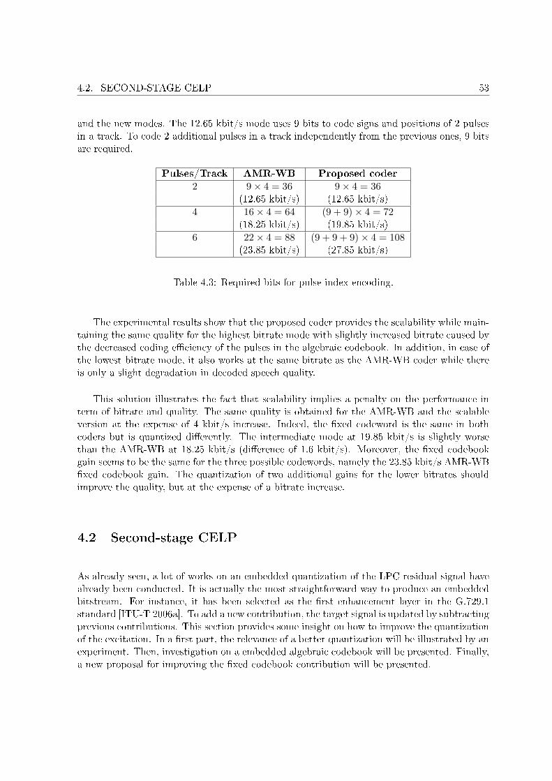
4.2. SECOND-STAGE CELP 53
and the new modes. The 12.65 kbit/s mode uses 9 bits to code signs and positions of 2 pulsesin a track. To code 2 additional pulses in a track independently from the previous ones, 9 bitsare required.
Pulses/Track AMR-WB Proposed coder
2 9× 4 = 36 9× 4 = 36(12.65 kbit/s) (12.65 kbit/s)
4 16× 4 = 64 (9 + 9)× 4 = 72(18.25 kbit/s) (19.85 kbit/s)
6 22× 4 = 88 (9 + 9 + 9)× 4 = 108(23.85 kbit/s) (27.85 kbit/s)
Table 4.3: Required bits for pulse index encoding.
The experimental results show that the proposed coder provides the scalability while main-taining the same quality for the highest bitrate mode with slightly increased bitrate caused bythe decreased coding e�ciency of the pulses in the algebraic codebook. In addition, in case ofthe lowest bitrate mode, it also works at the same bitrate as the AMR-WB coder while thereis only a slight degradation in decoded speech quality.
This solution illustrates the fact that scalability implies a penalty on the performance interm of bitrate and quality. The same quality is obtained for the AMR-WB and the scalableversion at the expense of 4 kbit/s increase. Indeed, the �xed codeword is the same in bothcoders but is quantized di�erently. The intermediate mode at 19.85 kbit/s is slightly worsethan the AMR-WB at 18.25 kbit/s (di�erence of 1.6 kbit/s). Moreover, the �xed codebookgain seems to be the same for the three possible codewords, namely the 23.85 kbit/s AMR-WB�xed codebook gain. The quantization of two additional gains for the lower bitrates shouldimprove the quality, but at the expense of a bitrate increase.
4.2 Second-stage CELP
As already seen, a lot of works on an embedded quantization of the LPC residual signal havealready been conducted. It is actually the most straightforward way to produce an embeddedbitstream. For instance, it has been selected as the �rst enhancement layer in the G.729.1standard [ITU-T 2006a]. To add a new contribution, the target signal is updated by subtractingprevious contributions. This section provides some insight on how to improve the quantizationof the excitation. In a �rst part, the relevance of a better quantization will be illustrated by anexperiment. Then, investigation on a embedded algebraic codebook will be presented. Finally,a new proposal for improving the �xed codebook contribution will be presented.
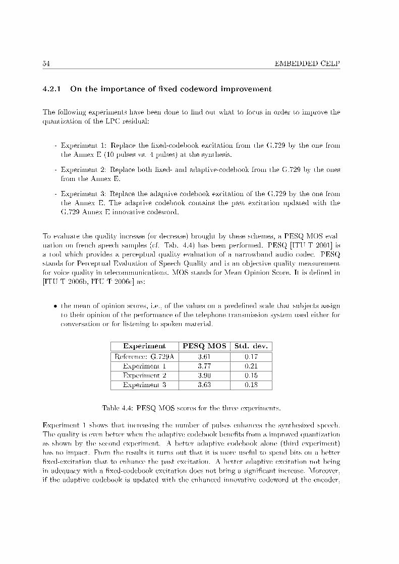
54 EMBEDDED CELP
4.2.1 On the importance of �xed codeword improvement
The following experiments have been done to �nd out what to focus in order to improve thequantization of the LPC residual:
- Experiment 1: Replace the �xed-codebook excitation from the G.729 by the one fromthe Annex E (10 pulses vs. 4 pulses) at the synthesis.
- Experiment 2: Replace both �xed- and adaptive-codebook from the G.729 by the onesfrom the Annex E.
- Experiment 3: Replace the adaptive codebook excitation of the G.729 by the one fromthe Annex E. The adaptive codebook contains the past excitation updated with theG.729 Annex E innovative codeword.
To evaluate the quality increase (or decrease) brought by these schemes, a PESQ MOS eval-uation on french speech samples (cf. Tab. 4.4) has been performed. PESQ [ITU-T 2001] isa tool which provides a perceptual quality evaluation of a narrowband audio codec. PESQstands for Perceptual Evaluation of Speech Quality and is an objective quality measurementfor voice quality in telecommunications. MOS stands for Mean Opinion Score. It is de�ned in[ITU-T 2006b, ITU-T 2006c] as:
• the mean of opinion scores, i.e., of the values on a prede�ned scale that subjects assignto their opinion of the performance of the telephone transmission system used either forconversation or for listening to spoken material.
Experiment PESQ MOS Std. dev.
Reference: G.729A 3.61 0.17Experiment 1 3.77 0.21Experiment 2 3.90 0.15Experiment 3 3.63 0.18
Table 4.4: PESQ MOS scores for the three experiments.
Experiment 1 shows that increasing the number of pulses enhances the synthesized speech.The quality is even better when the adaptive codebook bene�ts from a improved quantizationas shown by the second experiment. A better adaptive codebook alone (third experiment)has no impact. From the results it turns out that it is more useful to spend bits on a better�xed-excitation that to enhance the past excitation. A better adaptive excitation not beingin adequacy with a �xed-codebook excitation does not bring a signi�cant increase. Moreover,if the adaptive codebook is updated with the enhanced innovative codeword at the encoder,
4.2. SECOND-STAGE CELP 55
the decoder might update its adaptive codebook with a lower quality innovative codeword, asthe decoder may work at a lower bitrate. In such a case, both adaptive codebooks are notsynchronized anymore. Thereafter e�orts have been spent on providing a better innovativeexcitation.
4.2.2 Embedded �xed codebook search
The previous section has shown that improving the quantization of the innovation has animpact on the quality. E�ort has been put on investigating an embedded quantization of theinnovation. A method to produce an embedded �xed-codebook has been investigated, i.e. thepulses of the low bit rate (e.g. G.729A) are among the pulses of the enhanced layer. In otherwords, the G.729A innovative codeword is a subset of the enhanced layer innovative codeword.For a 8-pulses innovative codeword, Eq. (3.28) and (3.29) become:
C =7∑
i=0
sid(mi)
C =3∑
i=0
sid(mi) +7∑
i=4
sid(mi) (4.13)
and
E =7∑
i=0
φ(mi,mi) + 26∑
i=0
7∑j=i+1
sisjφ(mi,mj)
E =3∑
i=0
φ(mi,mi) + 22∑
i=0
3∑j=i+1
sisjφ(mi,mj)
+7∑
i=4
φ(mi,mi) + 26∑
i=4
7∑j=i+1
sisjφ(mi,mj)
+ 23∑
i=0
7∑j=4
sisjφ(mi,mj). (4.14)
The �rst term of Eq. (4.13) represents the correlation between the target signal and the�ltered codeword from the G.729, while the second term deals with the correlation betweenthis target signal and the �ltered innovative contribution from the second stage. The energyof the global �ltered codeword is given by the Eq. (4.14). The two �rst terms are the energyof the �ltered G.729 innovative codeword. The two next terms represent the energy of the�ltered second stage contribution. The last term corresponds to the correlations between theG.729 �xed-codeword and the innovative codeword from the second stage.
The �xed codebook search has to �nd 8 pulses. The �rst 4 pulses will give the �xedcodeword of the G.729. Then, the next 4 pulses will form with the former ones the 8-pulses
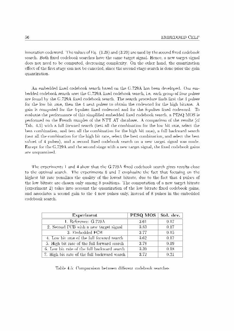
56 EMBEDDED CELP
innovation codeword. The values of Eq. (3.28) and (3.29) are used by the second �xed codebooksearch. Both �xed codebook searches have the same target signal. Hence, a new target signaldoes not need to be computed, decreasing complexity. On the other hand, the quantizatione�ect of the �rst stage can not be canceled, since the second stage search is done prior the gainquantization.
An embedded �xed codebook search based on the G.729A has been developed. Our em-bedded codebook search uses the G.729A �xed codebook search, i.e. each group of four pulsesare found by the G.729A �xed codebook search. The search procedure �nds �rst the 4 pulsesfor the low bit rate, then the 4 next pulses to obtain the codeword for the high bitrate. Again is computed for the 4-pulses �xed codeword and for the 8-pulses �xed codeword. Toevaluate the performance of this simpli�ed embedded �xed codebook search, a PESQ MOS isperformed on the French samples of the NTT-AT database. A comparison of the results (cfTab. 4.5) with a full forward search (test all the combination for the low bit rate, select thebest combination, and test all the combination for the high bit rate), a full backward search(test all the combination for the high bit rate, select the best combination, and select the bestsubset of 4 pulses), and a second �xed codebook search on a new target signal was made.Except for the G.729A and the second stage with a new target signal, the �xed codebook gainsare unquantized.
The experiments 1 and 4 show that the G.729A �xed codebook search gives results closeto the optimal search. The experiments 6 and 7 emphasize the fact that focusing on thehighest bit rate penalizes the quality of the lowest bitrate, due to the fact that 4 pulses ofthe low bitrate are chosen only among 8 positions. The computation of a new target bitrate(experiment 2) takes into account the quantization of the low bitrate �xed codebook gains,and associates a second gain to the 4 new pulses only, instead of 8 pulses in the embeddedcodebook search.
Experiment PESQ MOS Std. dev.
1. Reference: G.729A 3.61 0.172. Second FCB with a new target signal 3.83 0.17
3. Embedded FCB 3.77 0.154. Low bit rate of the full forward search 3.62 0.175. High bit rate of the full forward search 3.78 0.196. Low bit rate of the full backward search 3.39 0.187. High bit rate of the full backward search 3.72 0.21
Table 4.5: Comparaison between di�erent codebook searches
4.2. SECOND-STAGE CELP 57
4.2.3 A two-stage enhancement layer
Algebraic codebooks make the �xed codebook search more e�cient. Nevertheless, the con-straint on the pulse amplitude limits the performance. Giving more �exibility on the choice ofthe amplitudes by modulating each pulse amplitude with a gain might produce an LP synthesis�lter excitation closer to the true residual. Pulse gain optimization has been introduced in[De Meuleneire et al. 2006a]. It is a new way to improve the quantization of the LPC residual.The rest is organized as follows. First, a low level description of the method is given. After-wards, a second algebraic innovative codebook is introduced. Eventually, the concatenation ofthe two stages is compared with a unique second innovative codebook.
4.2.3.1 Pulse gain optimization
Unlike conventional methods in CELP-based scalable coding which consist in adding furthercodebook contributions to decrease the quantization error, the proposed approach will directlymodify the innovative codeword that has been chosen during the �rst stage. The �xed codebooksearch of G.729 only uses pulses of amplitude ±1 that are later multiplied by a �xed gain gc.As it is mandatory to select one pulse per track with the same amplitude for each of them,it can happen that a pulse is selected so that it would have been better either to have noneor to have one with a higher / lower amplitude than the already selected ones. In the past,codebooks with a few pulses of di�erent amplitudes have been investigated. The Multi-PulseExcitation (MPE) for example [Atal, Remde 1982] minimizes the perceptually weighted errorcriterion by �nding the optimal positions and amplitudes of M pulses, M smaller than thesubframe length. This solution requires to transmit the position and amplitude of each pulse,thus is bitrate consuming with M increasing. In the Regular-Pulse Excitation (RPE) method[Kroon et al. 1986], the pulses are regularly spaced of K positions. Hence, only the index ofthe �rst pulses and the amplitudes must be quantized.
The proposed solution in this section attempts to improve the innovative codeword andmodifying the amplitude of each pulse in order to get di�erent amplitudes for each pulse. Themodi�ed codeword is similar to the MPE method, with the di�erence that the pulse positionsare already given by the �xed codebook search. The modi�cation of the algebraic codewordyields a new codeword which can be written as:
z′(n) = gc
3∑i=0
siαiδ(n−mi) (4.15)
This is equivalent to the multiplication of each pulse by a factor 1 +αi. The coe�cients orso called pulse gain αi are determined with the minimization of the square error between theperceptual weighted signal and the synthesized signal. Let h(n) be the perceptual weighted
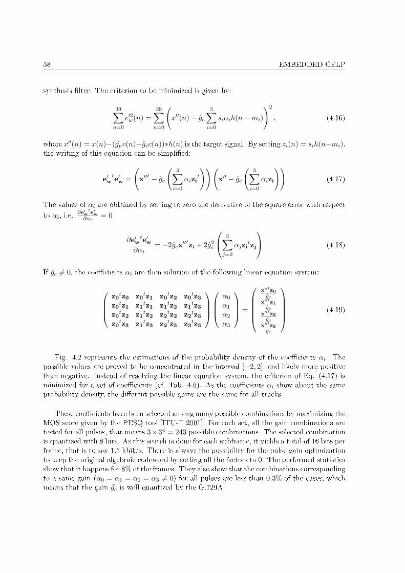
58 EMBEDDED CELP
synthesis �lter. The criterion to be minimized is given by:
39∑n=0
e′2w(n) =39∑
n=0
(x′′(n)− gc
3∑i=0
siαih(n−mi)
)2
, (4.16)
where x′′(n) = x(n)−(gpv(n)−gcc(n))∗h(n) is the target signal. By setting zi(n) = sih(n−mi),the writing of this equation can be simpli�ed:
e′wte′w =
(x′′t − gc
(3∑
i=0
αizit
))(x′′ − gc
(3∑
i=0
αizi
))(4.17)
The values of αi are obtained by setting to zero the derivative of the square error with respect
to αi, i.e.∂e′w
te′w∂αi
= 0
∂e′wte′w
∂αi= −2gcx′′
tzi + 2g2c
3∑j=0
αjzitzj
(4.18)
If gc 6= 0, the coe�cients αi are then solution of the following linear equation system:
z0
tz0 z0tz1 z0
tz2 z0tz3
z0tz1 z1
tz1 z1tz2 z1
tz3
z0tz2 z1
tz2 z2tz2 z2
tz3
z0tz3 z1
tz3 z2tz3 z3
tz3
α0
α1
α2
α3
=
x′′tz0
gc
x′′tz1gc
x′′tz2gc
x′′tz3gc
(4.19)
Fig. 4.2 represents the estimations of the probability density of the coe�cients αi. Thepossible values are proved to be concentrated in the interval [−2, 2], and likely more positivethan negative. Instead of resolving the linear equation system, the criterion of Eq. (4.17) isminimized for a set of coe�cients (cf. Tab. 4.6). As the coe�cients αi show about the sameprobability density, the di�erent possible gains are the same for all tracks.
These coe�cients have been selected among many possible combinations by maximizing theMOS score given by the PESQ tool [ITU-T 2001]. For each set, all the gain combinations aretested for all pulses, that means 3×34 = 243 possible combinations. The selected combinationis quantized with 8 bits. As this search is done for each subframe, it yields a total of 16 bits perframe, that is to say 1.6 kbit/s. There is always the possibility for the pulse gain optimizationto keep the original algebraic codeword by setting all the factors to 0. The performed statisticsshow that it happens for 8% of the frames. They also show that the combinations correspondingto a same gain (α0 = α1 = α2 = α3 6= 0) for all pulses are less than 0.3% of the cases, whichmeans that the gain gc is well quantized by the G.729A.
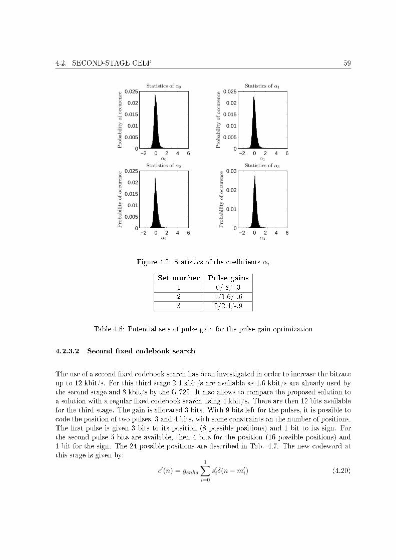
4.2. SECOND-STAGE CELP 59
−2 0 2 4 60
0.005
0.01
0.015
0.02
0.025Statistics of α0
α0
Pro
bability
ofocc
ure
nce
−2 0 2 4 60
0.005
0.01
0.015
0.02
0.025Statistics of α1
α1
Pro
bability
ofocc
ure
nce
−2 0 2 4 60
0.005
0.01
0.015
0.02
0.025Statistics of α2
α2
Pro
bability
ofocc
ure
nce
−2 0 2 4 60
0.01
0.02
0.03Statistics of α3
α3
Pro
bability
ofocc
ure
nce
Figure 4.2: Statistics of the coe�cients αi
Set number Pulse gains
1 0/.8/-.32 0/1.6/-.63 0/2.4/-.9
Table 4.6: Potential sets of pulse gain for the pulse gain optimization
4.2.3.2 Second �xed codebook search
The use of a second �xed codebook search has been investigated in order to increase the bitrateup to 12 kbit/s. For this third stage 2.4 kbit/s are available as 1.6 kbit/s are already used bythe second stage and 8 kbit/s by the G.729. It also allows to compare the proposed solution toa solution with a regular �xed codebook search using 4 kbit/s. There are then 12 bits availablefor the third stage. The gain is allocated 3 bits. With 9 bits left for the pulses, it is possible tocode the position of two pulses, 3 and 4 bits, with some constraints on the number of positions.The �rst pulse is given 3 bits to its position (8 possible positions) and 1 bit to its sign. Forthe second pulse 5 bits are available, then 4 bits for the position (16 possible positions) and1 bit for the sign. The 24 possible positions are described in Tab. 4.7. The new codeword atthis stage is given by:
c′(n) = genha
1∑i=0
s′iδ(n−m′i) (4.20)
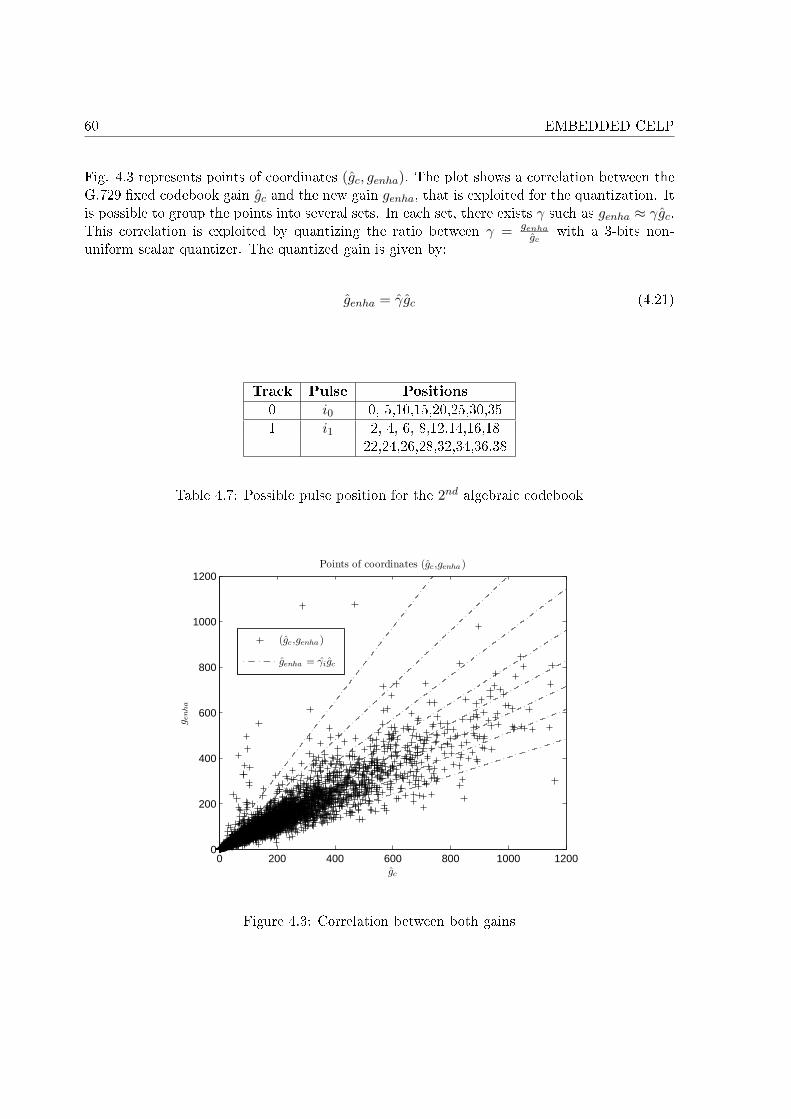
60 EMBEDDED CELP
Fig. 4.3 represents points of coordinates (gc, genha). The plot shows a correlation between theG.729 �xed codebook gain gc and the new gain genha, that is exploited for the quantization. Itis possible to group the points into several sets. In each set, there exists γ such as genha ≈ γgc.This correlation is exploited by quantizing the ratio between γ = genha
gcwith a 3-bits non-
uniform scalar quantizer. The quantized gain is given by:
genha = γgc (4.21)
Track Pulse Positions
0 i0 0, 5,10,15,20,25,30,351 i1 2, 4, 6, 8,12,14,16,18
22,24,26,28,32,34,36,38
Table 4.7: Possible pulse position for the 2nd algebraic codebook
0 200 400 600 800 1000 12000
200
400
600
800
1000
1200Points of coordinates (gc,genha)
gc
genha
(gc ,genha)
genha = γigc
Figure 4.3: Correlation between both gains
4.2. SECOND-STAGE CELP 61
4.2.3.3 Experimental results and discussion
Another scalable codec was built in order to evaluate the performance of the proposed scheme.It comprises G.729A as core and a second stage that simply consists of a �xed codebook searchsimilar to the one of G.729A. This �xed codebook needs 4 kbit/s, hence this scalable requiresthe same bitrate as the proposed method. Nevertheless, it does not comprise the 9.6 kbit/sintermediate bitrate. As objective measures, the MOS score was computed with the PESQtool and segmental SNR. The segmental SNR is computed by:
1M
M∑m=1
10 log10
∑80m−1n=80(m−1) s2(n)∑80m−1
n=80(m−1) (s(n)− s(n))2(4.22)
where M is the number of frames. It gives a measure of the distortion between the originaland the reconstructed signal. Tab. 4.8 regroups the means of PESQ MOS for English, German
Coders
Language G.729A 9.6kbit/s 12kbit/s Reference
English 3.731 3.783 3.855 3.918German 3.687 3.763 3.834 3.897French 3.703 3.756 3.830 3.892
Table 4.8: PESQ MOS for the embedded CELP codec at 8, 9.6 and 12 kbit/s
and French samples of the NTT-AT database, performed on the decoded samples at 8, 9.6 and12 kbit/s. The G.729A with the second �xed codebook stage similar to the G.729A one asenhancement layer is called reference. It turns out that the quality increases with the bitrate.Still the proposed 12 kbit/s is slightly worse than the reference. Also, this trend is to benoticed on Fig. 4.4 that depicts the segmental SNR for each English sample of the NTT-ATspeech database, decoded at 8, 9.6 and 12 kbit/s.
Several A-B listening tests between the di�erent bitrates as well have been conducted. Thespeech material comprises 8 English samples of the NTT-AT speech database (4 male and 4female voices). A panel of 8 listeners participated to the test and had to grade each versionagainst the other. They could listen to the test �les on their computer with a headset. Tab.4.9 gives the results of the listening tests. It turns out that unlike the objective test, it is quitedi�cult to distinguish between the G.729A and the 9.6 kbit/s. In order to better discriminateperhaps it would have been better to use an Absolute Category Rating listening test and morelisteners (e.g 32) such that the con�dence interval stays low. As for the proposed 12 kbit/s,it is shown to improve the reconstructed signal. Nevertheless, it did not reach the quality ofthe reference. This penalty is caused by including an intermediate bitrate between 8 and 12kbit/s. It can be the case that in order to suppress one or two non optimal pulses selected bythe core codec, it is sometimes better to add a completely new 4 pulse codeword.
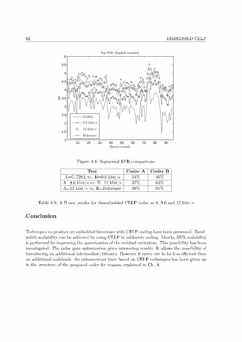
62 EMBEDDED CELP
10 20 30 40 50 60 70 80 901
1.5
2
2.5
3
3.5
4
4.5
5
5.5
6Seg SNR (English samples)
Speech sample
dB
G729A
9.6 kbit/s
12 kbit/s
Reference
Figure 4.4: Segmental SNR comparisons
Test Coder A Coder B
A=G.729A vs. B=9.6 kbit/s 54% 46%A=9.6 kbit/s vs. B=12 kbit/s 37% 63%A=12 kbit/s vs. B=Reference 39% 61%
Table 4.9: A-B test results for theembedded CELP codec at 8, 9.6 and 12 kbit/s
Conclusion
Techniques to produce an embedded bitstream with CELP coding have been presented. Band-width scalability can be achieved by using CELP in subbands coding. Mostly, SNR scalabilityis performed by improving the quantization of the residual excitation. This possibility has beeninvestigated. The pulse gain optimization gives interesting results. It allows the possibility ofintroducing an additional intermediate bitrates. However it turns out to be less e�cient thanan additional codebook. An enhancement layer based on CELP techniques has been given upin the structure of the proposed coder for reasons explained in Ch. 9.
63
Part III
Wavelets

65
Chapter 5
Wavelets from a �lter bank perspective
Introduction
When reaching a given bitrate (e.g. 2 bits/samples) linear predictive coding is not anymorethe preferred method. Transform coding yields better performance with equivalent or even lesscomplexity. The input frame samples are transformed into a set of coe�cients. The transformis chosen in such a manner that it produces a maximum number of coe�cients with smallamplitude (this property is called energy compaction). Transform in the frequency domain suchas Fourier Transform, Discrete Cosine Transform (DCT), or MDCT gives a representation of asignal closely related to the spectral distribution of energy across frequencies. The coe�cientsare quantized and transmitted. The decoder reconstructs the coe�cients, then transformsthem back to time samples. A drawback of frequency transform coding is the lack of timeresolution. As an example, during onsets (transition from low to high energy region), theintroduced quantization noise in frequency domain is equally spread across the time domain,leading to the so called pre-echo e�ect. This artifact might be reduced by choosing shorterframe size, i.e. increasing the time resolution.
Wavelet transform has been originally introduced to provide a multiresolution analysisof real life signal. This tool gives resolutions at di�erent precision levels of a signal, fromthe original signal to its coarsest version, dropping more and more details as the resolutiondecreases. It has been shown [Mallat 1998] that going from one resolution to a coarser or�ner resolution is equivalent to a discrete analysis or synthesis 2-channel �lter bank. Thus,the discrete wavelet transform is equivalent to a �lter bank structure, respecting the perfectreconstruction conditions. It gives a time-frequency representation of signal. Taking intoaccount the time dimension in the quantization process may reduce among others the pre-echoe�ect.
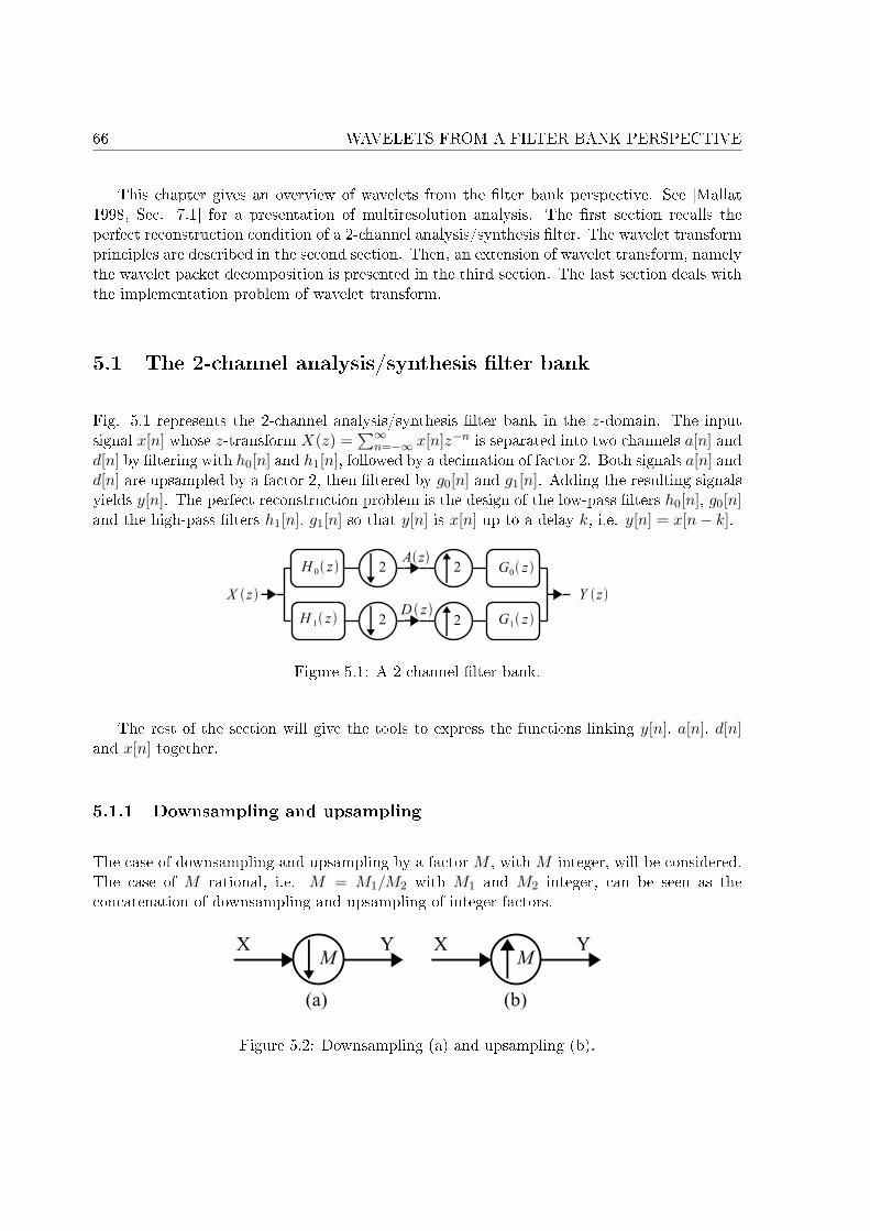
66 WAVELETS FROM A FILTER BANK PERSPECTIVE
This chapter gives an overview of wavelets from the �lter bank perspective. See [Mallat1998, Sec. 7.1] for a presentation of multiresolution analysis. The �rst section recalls theperfect reconstruction condition of a 2-channel analysis/synthesis �lter. The wavelet transformprinciples are described in the second section. Then, an extension of wavelet transform, namelythe wavelet packet decomposition is presented in the third section. The last section deals withthe implementation problem of wavelet transform.
5.1 The 2-channel analysis/synthesis �lter bank
Fig. 5.1 represents the 2-channel analysis/synthesis �lter bank in the z-domain. The inputsignal x[n] whose z-transform X(z) =
∑∞n=−∞ x[n]z−n is separated into two channels a[n] and
d[n] by �ltering with h0[n] and h1[n], followed by a decimation of factor 2. Both signals a[n] andd[n] are upsampled by a factor 2, then �ltered by g0[n] and g1[n]. Adding the resulting signalsyields y[n]. The perfect reconstruction problem is the design of the low-pass �lters h0[n], g0[n]and the high-pass �lters h1[n], g1[n] so that y[n] is x[n] up to a delay k, i.e. y[n] = x[n− k].
Figure 5.1: A 2-channel �lter bank.
The rest of the section will give the tools to express the functions linking y[n], a[n], d[n]and x[n] together.
5.1.1 Downsampling and upsampling
The case of downsampling and upsampling by a factor M , with M integer, will be considered.The case of M rational, i.e. M = M1/M2 with M1 and M2 integer, can be seen as theconcatenation of downsampling and upsampling of integer factors.
Figure 5.2: Downsampling (a) and upsampling (b).
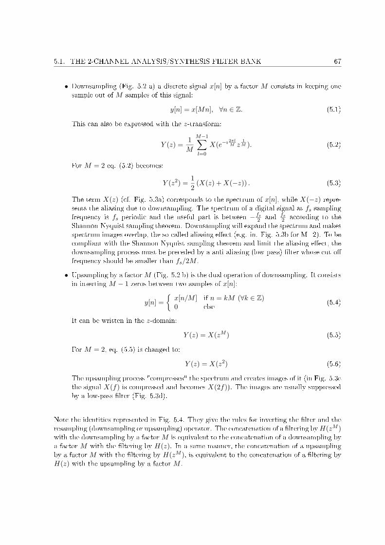
5.1. THE 2-CHANNEL ANALYSIS/SYNTHESIS FILTER BANK 67
• Downsampling (Fig. 5.2 a) a discrete signal x[n] by a factor M consists in keeping onesample out of M samples of this signal:
y[n] = x[Mn], ∀n ∈ Z. (5.1)
This can also be expressed with the z-transform:
Y (z) =1M
M−1∑l=0
X(e−ı 2πlM z
1M ). (5.2)
For M = 2 eq. (5.2) becomes:
Y (z2) =12
(X(z) + X(−z)) . (5.3)
The term X(z) (cf. Fig. 5.3a) corresponds to the spectrum of x[n], while X(−z) repre-sents the aliasing due to downsampling. The spectrum of a digital signal at fs samplingfrequency is fs periodic and the useful part is between −fs
2 and fs
2 according to theShannon-Nyquist sampling theorem. Downsampling will expand the spectrum and makesspectrum images overlap, the so-called aliasing e�ect (e.g. in. Fig. 5.3b for M=2). To becompliant with the Shannon-Nyquist sampling theorem and limit the aliasing e�ect, thedownsampling process must be preceded by a anti-aliasing (low-pass) �lter whose cut-o�frequency should be smaller than fs/2M .
• Upsampling by a factor M (Fig. 5.2 b) is the dual operation of downsampling. It consistsin inserting M − 1 zeros between two samples of x[n]:
y[n] ={
x[n/M ] if n = kM (∀k ∈ Z)0 else
(5.4)
It can be written in the z-domain:
Y (z) = X(zM ) (5.5)
For M = 2, eq. (5.5) is changed to:
Y (z) = X(z2) (5.6)
The upsampling process "compresses" the spectrum and creates images of it (in Fig. 5.3cthe signal X(f) is compressed and becomes X(2f)). The images are usually suppressedby a low-pass �lter (Fig. 5.3d).
Note the identities represented in Fig. 5.4. They give the rules for inverting the �lter and theresampling (downsampling or upsampling) operator. The concatenation of a �ltering by H(zM )with the downsampling by a factor M is equivalent to the concatenation of a downsampling bya factor M with the �ltering by H(z). In a same manner, the concatenation of a upsamplingby a factor M with the �ltering by H(zM ), is equivalent to the concatenation of a �ltering byH(z) with the upsampling by a factor M .
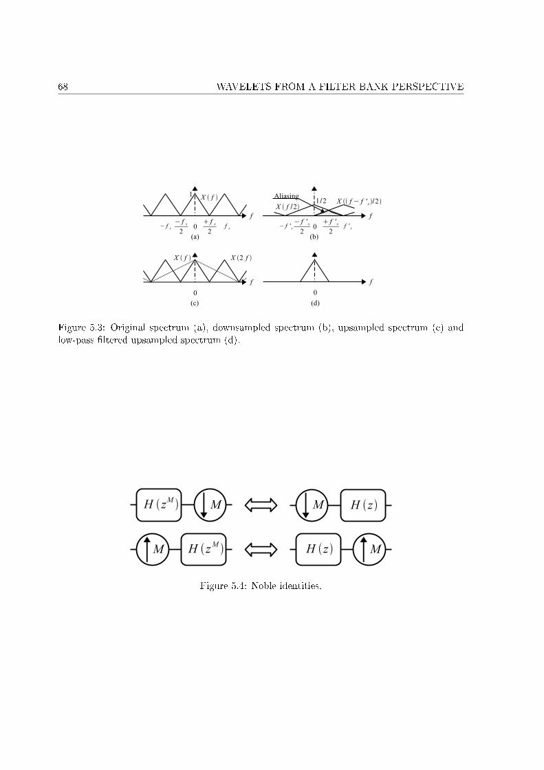
68 WAVELETS FROM A FILTER BANK PERSPECTIVE
Figure 5.3: Original spectrum (a), downsampled spectrum (b), upsampled spectrum (c) andlow-pass �ltered upsampled spectrum (d).
Figure 5.4: Noble identities.
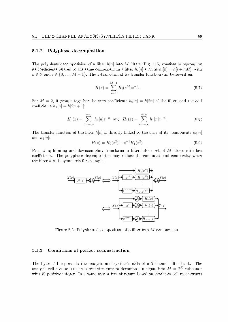
5.1. THE 2-CHANNEL ANALYSIS/SYNTHESIS FILTER BANK 69
5.1.2 Polyphase decomposition
The polyphase decomposition of a �lter h[n] into M �lters (Fig. 5.5) consists in regroupingits coe�cients related to the same component in a �lter hi[n] such as hi[n] = h[i + nM ], withn ∈ N and i ∈ {0, . . . ,M − 1}. The z-transform of its transfer function can be rewritten:
H(z) =M−1∑i=0
Hi(zM )z−i. (5.7)
For M = 2, it groups together the even coe�cients h0[n] = h[2n] of the �lter, and the oddcoe�cients h1[n] = h[2n + 1]:
H0(z) =+∞∑
n=−∞h0[n]z−n and H1(z) =
+∞∑n=−∞
h1[n]z−n. (5.8)
The transfer function of the �lter h[n] is directly linked to the ones of its components h0[n]and h1[n]:
H(z) = H0(z2) + z−1H1(z2) (5.9)
Permuting �ltering and downsampling transforms a �lter into a set of M �lters with lesscoe�cients. The polyphase decomposition may reduce the computational complexity whenthe �lter h[n] is symmetric for example.
Figure 5.5: Polyphase decomposition of a �lter into M components.
5.1.3 Conditions of perfect reconstruction
The �gure 5.1 represents the analysis and synthesis cells of a 2-channel �lter bank. Theanalysis cell can be used in a tree structure to decompose a signal into M = 2K subbandswith K positive integer. In a same way, a tree structure based on synthesis cell reconstructs
70 WAVELETS FROM A FILTER BANK PERSPECTIVE
the signal from the subband samples. Wavelet discrete transform, and more generally, waveletpacket decomposition, rely on the 2-channel �lter bank structure with perfect reconstruction.
The input signal x[n] is decomposed into two signals a[n] and d[n]. They are then recom-bined to give the output signal y[n]. According to Eq. (5.3), the z-transform of the analysisoutput is given by: {
A(z2) = 12 (H0(z)X(z) + H0(−z)X(−z))
D(z2) = 12 (H1(z)X(z) + H1(−z)X(−z))
(5.10)
Eq. (5.6) gives the relation between a[n], d[n] and the output y[n]:
Y (z) = G0(z)A(z2) + G1(z)D(z2) (5.11)
The z-transform of the reconstructed signal after the synthesis cell is:
Y (z) = 12 [(G0(z)H0(z) + G1(z)H1(z))X(z)+
(G0(z)H0(−z) + G1(z)H1(−z))X(−z)].(5.12)
The perfect reconstruction is ensured if the aliasing term X(−z) is canceled, G0(z)H0(−z) +G1(z)H1(−z) = 0, and if the output signal is a delayed version of the original signal y[n] =x[n− k], i.e. G0(z)H0(z) + G1(z)H1(z) = 2z−k, with k ≥ 0. Both conditions are expressed bythe following linear equation system:[
H0(z) H1(z)H0(−z) H1(−z)
] [G0(z)G1(z)
]= 2
[z−k
0
]. (5.13)
If the determinant of the system ∆(z) = H0(z)H1(−z)−H0(−z)H1(z) is non zero, the solutionof this system is: {
G0(z) = 2z−k
H0(z)H1(−z)−H0(−z)H1(z)H1(−z)
G1(z) = −2z−k
H0(z)H1(−z)−H0(−z)H1(z)H0(−z)(5.14)
For stability reason [Vetterli 1986], the �lters are chosen to be FIR with the constraint:
H0(z)H1(−z)−H0(−z)H1(z) = z−k (5.15)
Under this constraint, one solution of the system (5.13) is:{G0(z) = 2H1(−z)G1(z) = −2H0(−z)
(5.16)
These equations give the dependence of the synthesis �lters on the analysis �lters. The outputof the synthesis �lter bank becomes Y (z) = X(z)z−k. Some extra conditions are necessary onthe analysis �lter in order to �nd solutions.
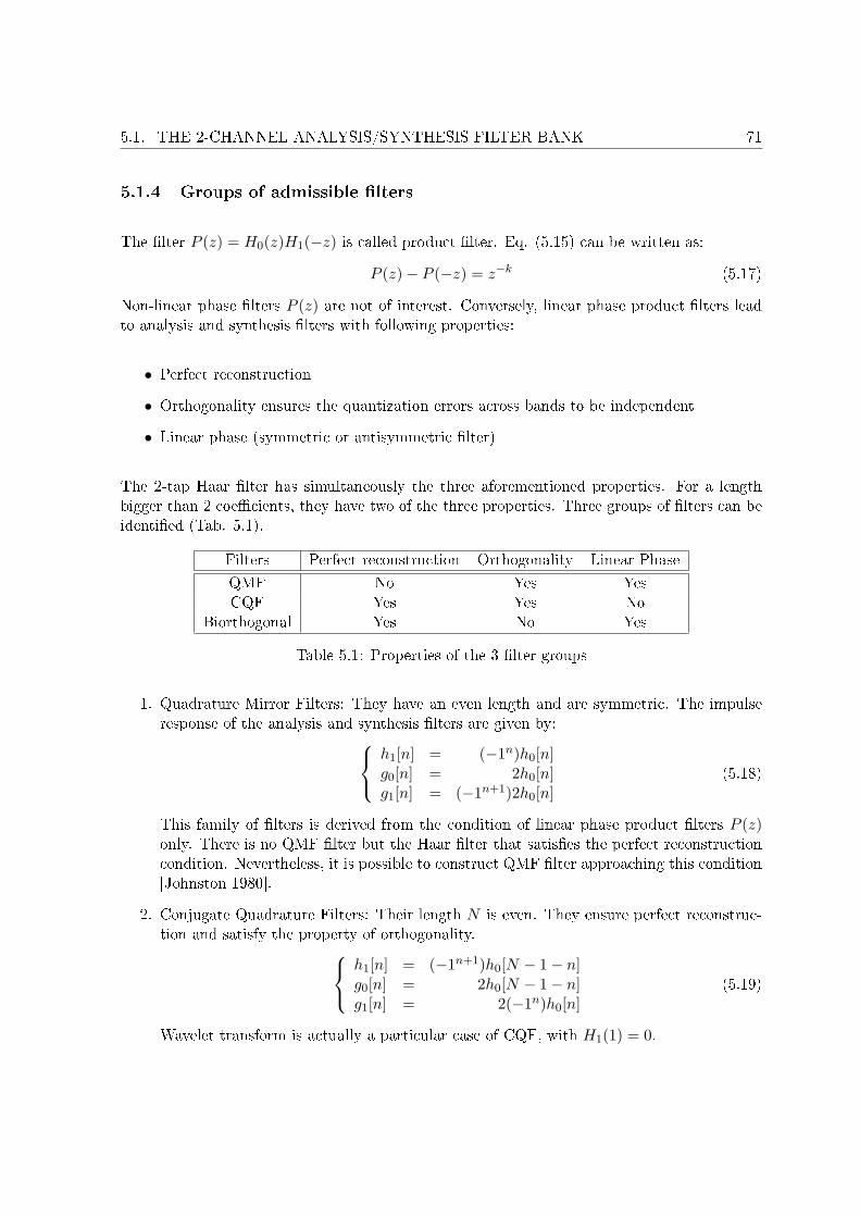
5.1. THE 2-CHANNEL ANALYSIS/SYNTHESIS FILTER BANK 71
5.1.4 Groups of admissible �lters
The �lter P (z) = H0(z)H1(−z) is called product �lter. Eq. (5.15) can be written as:
P (z)− P (−z) = z−k (5.17)
Non-linear phase �lters P (z) are not of interest. Conversely, linear phase product �lters leadto analysis and synthesis �lters with following properties:
• Perfect reconstruction
• Orthogonality ensures the quantization errors across bands to be independent
• Linear phase (symmetric or antisymmetric �lter)
The 2-tap Haar �lter has simultaneously the three aforementioned properties. For a lengthbigger than 2 coe�cients, they have two of the three properties. Three groups of �lters can beidenti�ed (Tab. 5.1).
Filters Perfect reconstruction Orthogonality Linear Phase
QMF No Yes YesCQF Yes Yes No
Biorthogonal Yes No Yes
Table 5.1: Properties of the 3 �lter groups
1. Quadrature Mirror Filters: They have an even length and are symmetric. The impulseresponse of the analysis and synthesis �lters are given by:
h1[n] = (−1n)h0[n]g0[n] = 2h0[n]g1[n] = (−1n+1)2h0[n]
(5.18)
This family of �lters is derived from the condition of linear phase product �lters P (z)only. There is no QMF �lter but the Haar �lter that satis�es the perfect reconstructioncondition. Nevertheless, it is possible to construct QMF �lter approaching this condition[Johnston 1980].
2. Conjugate Quadrature Filters: Their length N is even. They ensure perfect reconstruc-tion and satisfy the property of orthogonality.
h1[n] = (−1n+1)h0[N − 1− n]g0[n] = 2h0[N − 1− n]g1[n] = 2(−1n)h0[n]
(5.19)
Wavelet transform is actually a particular case of CQF, with H1(1) = 0.
72 WAVELETS FROM A FILTER BANK PERSPECTIVE
3. Biorthogonal �lters: In that case, both �lters have linear phase. The impulse responsesh0 and h1 can have di�erent lengths.
5.2 Wavelet transform
Two families of �lters, namely the biorthogonal �lters and the conjugate quadratic �lters, ful�llthe conditions of perfect reconstruction. The signal x[n] can be then split into two channelsa1[n] and d1[n]:
a1[n] =∞∑
l=−∞x[l]h0[2n− l] and d1[n] =
∞∑l=−∞
x[l]h1[2n− l] (5.20)
From the signals a1[n] and d1[n], it is possible to reconstruct the original signal with a delayk:
y[n] = x[n− k] =∞∑
l=−∞a1[l]g0[n− 2l] + d1[l]g1[n− 2l] (5.21)
Discrete wavelet transform is always associated to a pair of �lters [Mallat 1998]. Nonethe-less, some extra conditions [Mallat 1998] are needed for a pair of CQF to be associated toa wavelet transform. Let H0(w) be the Fourier transform of the �lter h0[n]. If H0 (w) is2π-periodic and continuously di�erentiable in a neighborhood of w = 0, if H0(0) =
√(2) and
if
infw∈[−π/2,π/2]
|H0 (w)| > 0 (5.22)
then
Φ (w) =+∞∏p=1
H0 (2−pw)√2
(5.23)
is the Fourier transform of a scaling function [Mallat 1998]. A scaling function φ satis�es thedilatation equation:
φ(z)√(2)
=p−1∑k=0
h0[k]φ(2t− k), ∀t ∈ [0, p− 1] (5.24)
Under these conditions only a pair of �lters ensuring perfect reconstruction is related to awavelet scaling function. Note that the �lter h0[n] with the length p is the same for each stage.Although it is possible to use a di�erent �lter pair for each stage, there is no guarantee that thein�nite product in Eq. (5.23) converges to a scaling function. The equivalent time-frequencytransform is not a wavelet transform anymore.
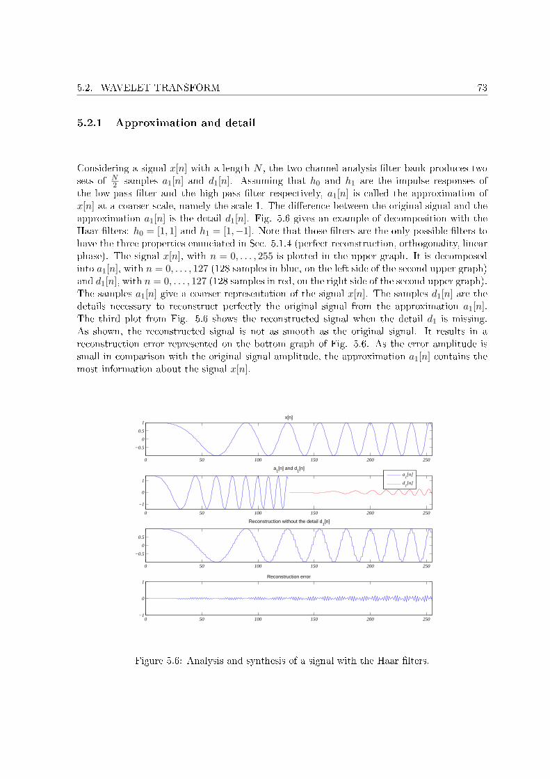
5.2. WAVELET TRANSFORM 73
5.2.1 Approximation and detail
Considering a signal x[n] with a length N , the two-channel analysis �lter bank produces twosets of N
2 samples a1[n] and d1[n]. Assuming that h0 and h1 are the impulse responses ofthe low-pass �lter and the high-pass �lter respectively, a1[n] is called the approximation ofx[n] at a coarser scale, namely the scale 1. The di�erence between the original signal and theapproximation a1[n] is the detail d1[n]. Fig. 5.6 gives an example of decomposition with theHaar �lters: h0 = [1, 1] and h1 = [1,−1]. Note that those �lters are the only possible �lters tohave the three properties enunciated in Sec. 5.1.4 (perfect reconstruction, orthogonality, linearphase). The signal x[n], with n = 0, . . . , 255 is plotted in the upper graph. It is decomposedinto a1[n], with n = 0, . . . , 127 (128 samples in blue, on the left side of the second upper graph)and d1[n], with n = 0, . . . , 127 (128 samples in red, on the right side of the second upper graph).The samples a1[n] give a coarser representation of the signal x[n]. The samples d1[n] are thedetails necessary to reconstruct perfectly the original signal from the approximation a1[n].The third plot from Fig. 5.6 shows the reconstructed signal when the detail d1 is missing.As shown, the reconstructed signal is not as smooth as the original signal. It results in areconstruction error represented on the bottom graph of Fig. 5.6. As the error amplitude issmall in comparison with the original signal amplitude, the approximation a1[n] contains themost information about the signal x[n].
0 50 100 150 200 250
−0.5
0
0.5
1x[n]
0 50 100 150 200 250
−1
0
1
a1[n] and d
1[n]
0 50 100 150 200 250
−0.5
0
0.5
Reconstruction without the detail d1[n]
0 50 100 150 200 250−1
0
1Reconstruction error
a1[n]
d1[n]
Figure 5.6: Analysis and synthesis of a signal with the Haar �lters.
74 WAVELETS FROM A FILTER BANK PERSPECTIVE
For a sampling frequency fs, the signal bandwidth is [0, 0.5fs]. The �lter bank splitsthe signal in two subbands whose bandwidth is half of the original signal bandwidth. a1[n]and d1[n] are roughly the frequency band [0, 0.25fs] and [0.25fs, 0.5fs] respectively. Thus, thefrequency resolution has been increased. The counterpart is the decrease of the time resolution.If N samples represent a time duration ∆t, the time di�erence between two samples is about∆tN . At the output of the �lter bank, since there are N
2 samples in each subband due to thedownsampling, the time di�erence becomes roughly 2∆t
N . Splitting a band into two subbandswith such a �lter bank allows to better localize an event in the frequency plane by increasingthe frequency resolution, at the expense of a worse time localization.
5.2.2 Approximation at di�erent scales
Since the perfect reconstruction condition permits to split a channel into two channels withoutany loss of information, it is possible to further split both channels. In the sequel, the analysis ofthe approximation only (lower frequency channel) is considered. The analysis (resp. synthesis)�lter bank applied to an approximation of scale j (resp. j + 1) gives an approximation at acoarser (resp. �ner) scale j + 1 (resp. j):
aj+1[n] =∞∑
l=−∞aj [l]h0[2n− l] and dj+1[n] =
∞∑l=−∞
aj [l]h1[2n− l] (5.25)
aj [n] =∞∑
l=−∞aj+1[l]g0[n− 2l] + dj+1[l]g1[n− 2l] (5.26)
The analysis of the approximation aj [n] at the scale j provides an approximation aj+1[n]and the detail dj+1[n] at the scale j + 1. Conversely, with both approximation aj+1[n] anddetail dj+1[n], it is possible to reconstruct the approximation aj [n]. Applying recursively theanalysis �lter bank j times on the input signal x[n] of length N yields an approximation aj [n]comprising N
2j samples and a set of details di[n] comprising N2i samples, with 1 ≤ i ≤ j. Fig.
5.7 is an illustration for N = 32 and j = 4. To reconstruct x[n] perfectly, the approximationa4[n] is required as well as the details d1[n],d2[n],d3[n],d4[n].
The �nest approximation is a1[n] since applying the synthesis �lter bank to a1[n] and d1[n]reconstructs the original signal x[n]. The bigger j, the coarser the approximation. Fig. 5.9 givesan example. The original signal x[n] is decomposed into approximation and details with theHaar �lters. The signal is reconstructed from the approximations a1[n], a2[n] and a3[n] withoutthe corresponding details (they are set to zero). The reconstructed signal is getting coarser asthe number of decomposition increases. For a very coarse approximation, the reconstructedsignal is far from the original. However it is still possible to guess the time evolution of thesignal. Fig. 5.10 is the result of a similar experiment where the Haar �lters have been replacedby the D20 (20 taps) �lters [Daubechies 1988]. They produce smoother approximations thanthe Haar �lters. Indeed, Haar �lter belongs to the same family as Daubechies �lters, and for
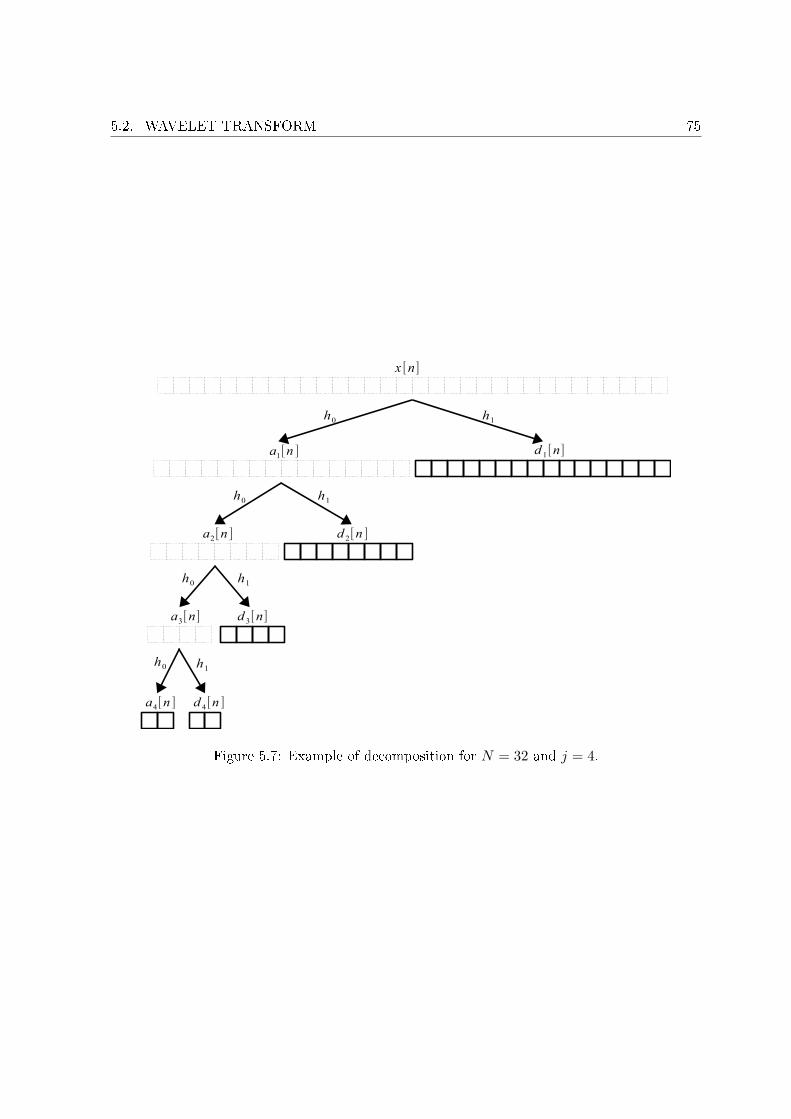
5.2. WAVELET TRANSFORM 75
Figure 5.7: Example of decomposition for N = 32 and j = 4.
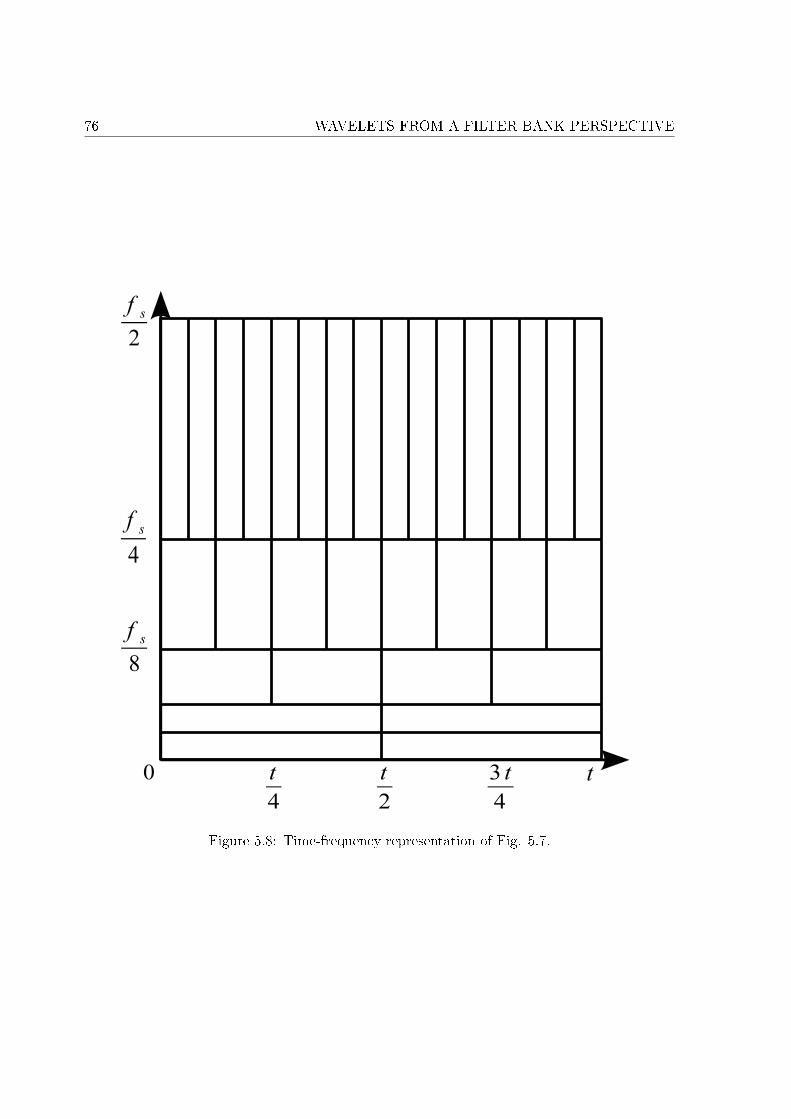
76 WAVELETS FROM A FILTER BANK PERSPECTIVE
Figure 5.8: Time-frequency representation of Fig. 5.7.
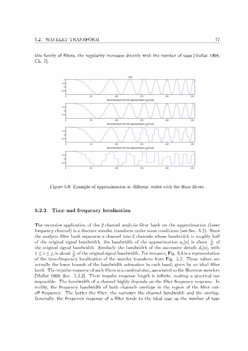
5.2. WAVELET TRANSFORM 77
this family of �lters, the regularity increases directly with the number of taps [Mallat 1998,Ch. 7].
0 50 100 150 200 250
−0.5
0
0.5
1x[n]
0 50 100 150 200 250
−0.5
0
0.5
Reconstruction from the approximation a1[n] only
0 50 100 150 200 250
−0.5
0
0.5
Reconstruction from the approximation a2[n] only
0 50 100 150 200 250
−0.5
0
0.5
Reconstruction from the approximation a3[n] only
Figure 5.9: Example of approximation at di�erent scales with the Haar �lters.
5.2.3 Time and frequency localization
The recursive application of the 2-channel analysis �lter bank on the approximation (lowerfrequency channel) is a discrete wavelet transform under some conditions (see Sec. 5.2). Sincethe analysis �lter bank separates a channel into 2 channels whose bandwidth is roughly halfof the original signal bandwidth, the bandwidth of the approximation aj [n] is about 1
2j ofthe original signal bandwidth. Similarly the bandwidth of the successive details di[n], with1 ≤ i ≤ j, is about 1
2i of the original signal bandwidth. For instance, Fig. 5.8 is a representationof the time-frequency localization of the wavelet transform from Fig. 5.7. Those values areactually the lower bounds of the bandwidth estimation in each band, given by an ideal �lterbank. The impulse response of such �lters is a cardinal sine, associated to the Shannon wavelets[Mallat 1998, Sec. 7.2.2]. Their impulse response length is in�nite, making a practical useimpossible. The bandwidth of a channel highly depends on the �lter frequency response. Inreality, the frequency bandwidth of both channels overlaps in the region of the �lter cut-o� frequency. The better the �lter, the narrower the channel bandwidth and the overlap.Generally, the frequency response of a �lter tends to the ideal case as the number of taps
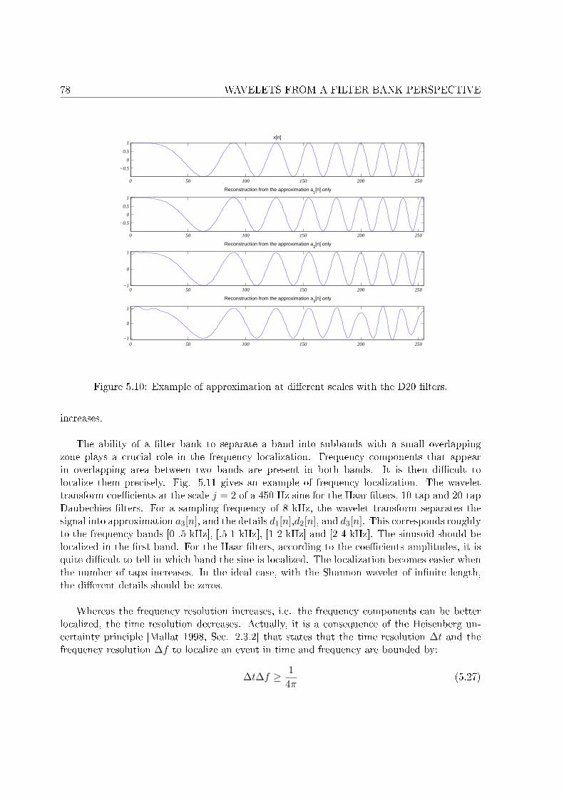
78 WAVELETS FROM A FILTER BANK PERSPECTIVE
0 50 100 150 200 250
−0.5
0
0.5
1x[n]
0 50 100 150 200 250
−0.5
0
0.5
1
Reconstruction from the approximation a1[n] only
0 50 100 150 200 250−1
0
1
Reconstruction from the approximation a2[n] only
0 50 100 150 200 250−1
0
1
Reconstruction from the approximation a3[n] only
Figure 5.10: Example of approximation at di�erent scales with the D20 �lters.
increases.
The ability of a �lter bank to separate a band into subbands with a small overlappingzone plays a crucial role in the frequency localization. Frequency components that appearin overlapping area between two bands are present in both bands. It is then di�cult tolocalize them precisely. Fig. 5.11 gives an example of frequency localization. The wavelettransform coe�cients at the scale j = 2 of a 450 Hz sine for the Haar �lters, 10-tap and 20-tapDaubechies �lters. For a sampling frequency of 8 kHz, the wavelet transform separates thesignal into approximation a3[n], and the details d1[n],d2[n], and d3[n]. This corresponds roughlyto the frequency bands [0-.5 kHz], [.5-1 kHz], [1-2 kHz] and [2-4 kHz]. The sinusoid should belocalized in the �rst band. For the Haar �lters, according to the coe�cients amplitudes, it isquite di�cult to tell in which band the sine is localized. The localization becomes easier whenthe number of taps increases. In the ideal case, with the Shannon wavelet of in�nite length,the di�erent details should be zeros.
Whereas the frequency resolution increases, i.e. the frequency components can be betterlocalized, the time resolution decreases. Actually, it is a consequence of the Heisenberg un-certainty principle [Mallat 1998, Sec. 2.3.2] that states that the time resolution ∆t and thefrequency resolution ∆f to localize an event in time and frequency are bounded by:
∆t∆f ≥ 14π
(5.27)
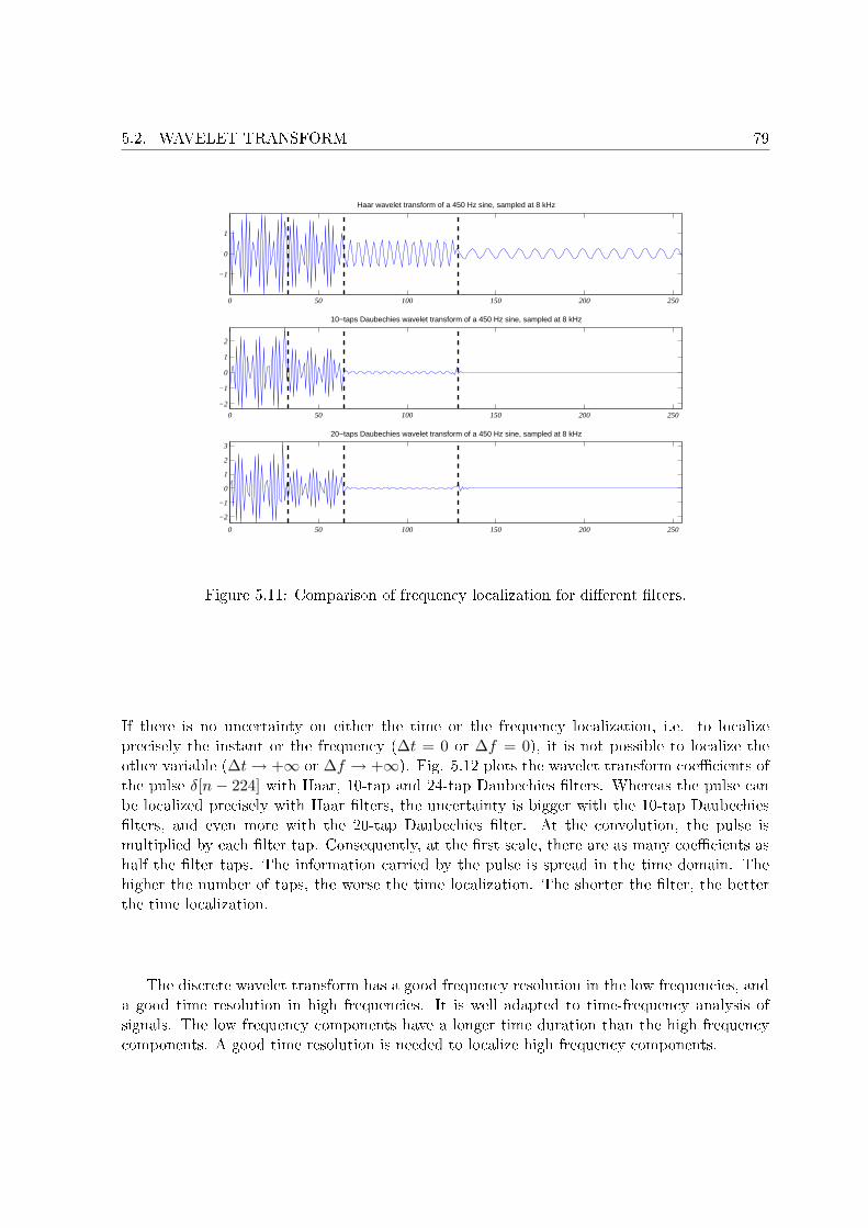
5.2. WAVELET TRANSFORM 79
0 50 100 150 200 250
−1
0
1
Haar wavelet transform of a 450 Hz sine, sampled at 8 kHz
0 50 100 150 200 250
−2
−1
0
1
2
10−taps Daubechies wavelet transform of a 450 Hz sine, sampled at 8 kHz
0 50 100 150 200 250
−2
−1
0
1
2
3
20−taps Daubechies wavelet transform of a 450 Hz sine, sampled at 8 kHz
Figure 5.11: Comparison of frequency localization for di�erent �lters.
If there is no uncertainty on either the time or the frequency localization, i.e. to localizeprecisely the instant or the frequency (∆t = 0 or ∆f = 0), it is not possible to localize theother variable (∆t → +∞ or ∆f → +∞). Fig. 5.12 plots the wavelet transform coe�cients ofthe pulse δ[n − 224] with Haar, 10-tap and 24-tap Daubechies �lters. Whereas the pulse canbe localized precisely with Haar �lters, the uncertainty is bigger with the 10-tap Daubechies�lters, and even more with the 20-tap Daubechies �lter. At the convolution, the pulse ismultiplied by each �lter tap. Consequently, at the �rst scale, there are as many coe�cients ashalf the �lter taps. The information carried by the pulse is spread in the time domain. Thehigher the number of taps, the worse the time localization. The shorter the �lter, the betterthe time localization.
The discrete wavelet transform has a good frequency resolution in the low frequencies, anda good time resolution in high frequencies. It is well adapted to time-frequency analysis ofsignals. The low frequency components have a longer time duration than the high frequencycomponents. A good time resolution is needed to localize high frequency components.
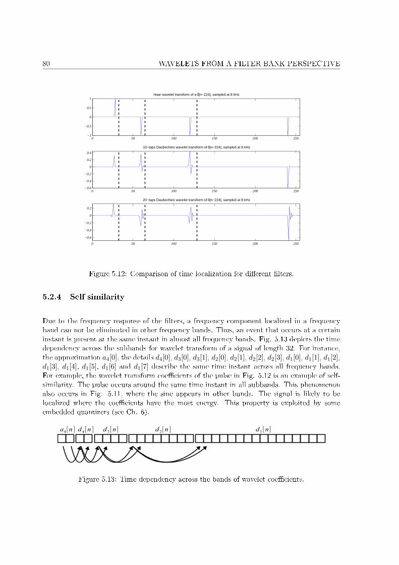
80 WAVELETS FROM A FILTER BANK PERSPECTIVE
0 50 100 150 200 250−1
−0.5
0
0.5
1Haar wavelet transform of a δ[n−224], sampled at 8 kHz
0 50 100 150 200 250−0.6
−0.4
−0.2
0
0.2
0.4
10−taps Daubechies wavelet transform of δ[n−224], sampled at 8 kHz
0 50 100 150 200 250
−0.6
−0.4
−0.2
0
0.2
20−taps Daubechies wavelet transform of δ[n−224], sampled at 8 kHz
Figure 5.12: Comparison of time localization for di�erent �lters.
5.2.4 Self similarity
Due to the frequency response of the �lters, a frequency component localized in a frequencyband can not be eliminated in other frequency bands. Thus, an event that occurs at a certaininstant is present at the same instant in almost all frequency bands. Fig. 5.13 depicts the timedependency across the subbands for wavelet transform of a signal of length 32. For instance,the approximation a4[0], the details d4[0], d3[0], d3[1], d2[0], d2[1], d2[2], d2[3], d1[0], d1[1], d1[2],d1[3], d1[4], d1[5], d1[6] and d1[7] describe the same time instant across all frequency bands.For example, the wavelet transform coe�cients of the pulse in Fig. 5.12 is an example of self-similarity. The pulse occurs around the same time instant in all subbands. This phenomenonalso occurs in Fig. 5.11, where the sine appears in other bands. The signal is likely to belocalized where the coe�cients have the most energy. This property is exploited by someembedded quantizers (see Ch. 6).
Figure 5.13: Time dependency across the bands of wavelet coe�cients.
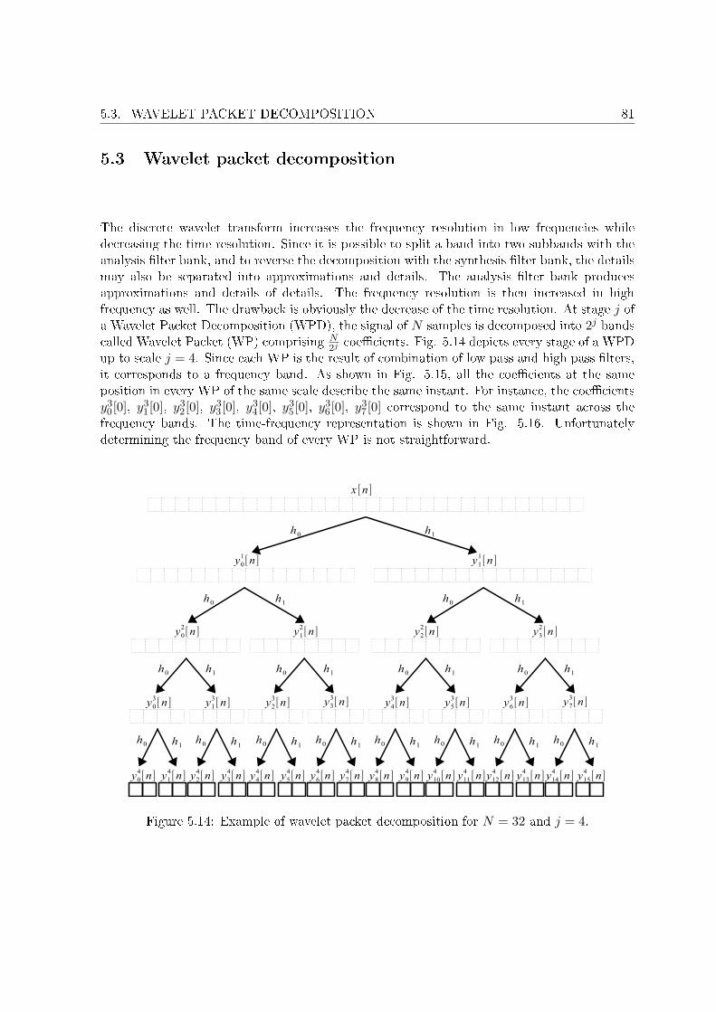
5.3. WAVELET PACKET DECOMPOSITION 81
5.3 Wavelet packet decomposition
The discrete wavelet transform increases the frequency resolution in low frequencies whiledecreasing the time resolution. Since it is possible to split a band into two subbands with theanalysis �lter bank, and to reverse the decomposition with the synthesis �lter bank, the detailsmay also be separated into approximations and details. The analysis �lter bank producesapproximations and details of details. The frequency resolution is then increased in highfrequency as well. The drawback is obviously the decrease of the time resolution. At stage j ofa Wavelet Packet Decomposition (WPD), the signal of N samples is decomposed into 2j bandscalled Wavelet Packet (WP) comprising N
2j coe�cients. Fig. 5.14 depicts every stage of a WPDup to scale j = 4. Since each WP is the result of combination of low pass and high pass �lters,it corresponds to a frequency band. As shown in Fig. 5.15, all the coe�cients at the sameposition in every WP of the same scale describe the same instant. For instance, the coe�cientsy30[0], y3
1[0], y32[0], y3
3[0], y34[0], y3
5[0], y36[0], y3
7[0] correspond to the same instant across thefrequency bands. The time-frequency representation is shown in Fig. 5.16. Unfortunatelydetermining the frequency band of every WP is not straightforward.
Figure 5.14: Example of wavelet packet decomposition for N = 32 and j = 4.
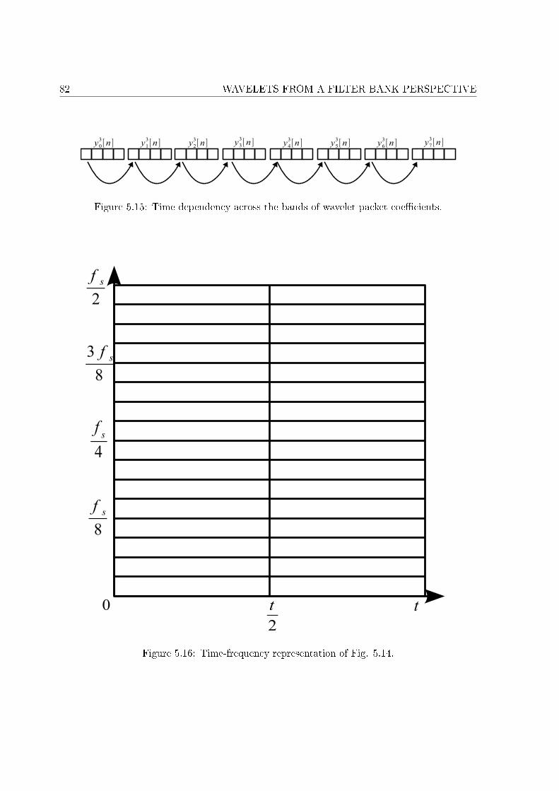
82 WAVELETS FROM A FILTER BANK PERSPECTIVE
Figure 5.15: Time dependency across the bands of wavelet packet coe�cients.
Figure 5.16: Time-frequency representation of Fig. 5.14.
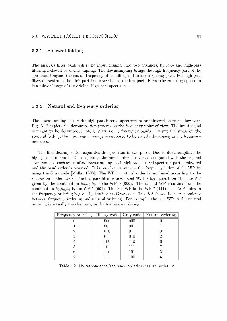
5.3. WAVELET PACKET DECOMPOSITION 83
5.3.1 Spectral folding
The analysis �lter bank splits the input channel into two channels, by low- and high-pass�ltering followed by downsampling. The downsampling brings the high frequency part of thespectrum (beyond the cut-o� frequency of the �lter) in the low frequency part. For high pass�ltered spectrum, the high part is mirrored onto the low part. Hence the resulting spectrumis a mirror image of the original high part spectrum.
5.3.2 Natural and frequency ordering
The downsampling causes the high-pass �ltered spectrum to be mirrored on to the low part.Fig. 5.17 depicts the decomposition process on the frequency point of view. The input signalis meant to be decomposed into 8 WPs, i.e. 8 frequency bands. To put the stress on thespectral folding, the input signal energy is supposed to be strictly decreasing as the frequencyincreases.
The �rst decomposition separates the spectrum in two parts. Due to downsampling, thehigh part is mirrored. Consequently, the band order is reversed compared with the originalspectrum. At each scale, after downsampling, each high pass �ltered spectrum part is mirroredand the band order is reversed. It is possible to retrieve the frequency index of the WP byusing the Gray code [Mallat 1998]. The WP in natural order is numbered according to thesuccession of the �lters. The low pass �lter is associated '0', the high pass �lter '1'. The WPgiven by the combination h0,h0,h0 is the WP 0 (000). The second WP resulting from thecombination h0,h0,h1 is the WP 1 (001). The last WP is the WP 7 (111). The WP index inthe frequency ordering is given by the inverse Gray code. Tab. 5.2 shows the correspondencebetween frequency ordering and natural ordering. For example, the last WP in the naturalordering is actually the channel 5 in the frequency ordering.
Frequency ordering Binary code Gray code Natural ordering
0 000 000 01 001 001 12 010 011 33 011 010 24 100 110 65 101 111 76 110 101 57 111 100 4
Table 5.2: Correspondence frequency ordering/natural ordering
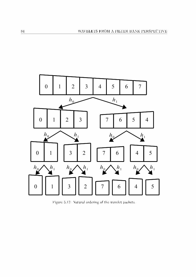
84 WAVELETS FROM A FILTER BANK PERSPECTIVE
Figure 5.17: Natural ordering of the wavelet packets.
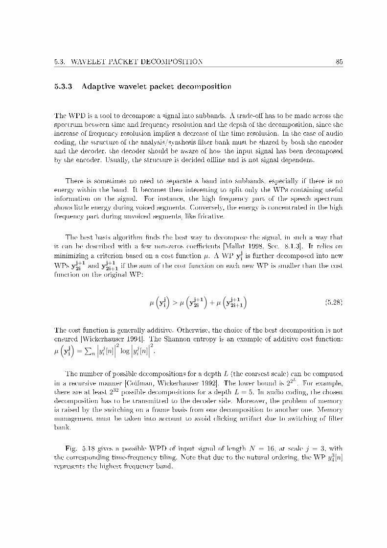
5.3. WAVELET PACKET DECOMPOSITION 85
5.3.3 Adaptive wavelet packet decomposition
The WPD is a tool to decompose a signal into subbands. A trade-o� has to be made across thespectrum between time and frequency resolution and the depth of the decomposition, since theincrease of frequency resolution implies a decrease of the time resolution. In the case of audiocoding, the structure of the analysis/synthesis �lter bank must be shared by both the encoderand the decoder, the decoder should be aware of how the input signal has been decomposedby the encoder. Usually, the structure is decided o�ine and is not signal dependent.
There is sometimes no need to separate a band into subbands, especially if there is noenergy within the band. It becomes then interesting to split only the WPs containing usefulinformation on the signal. For instance, the high frequency part of the speech spectrumshows little energy during voiced segments. Conversely, the energy is concentrated in the highfrequency part during unvoiced segments, like fricative.
The best basis algorithm �nds the best way to decompose the signal, in such a way thatit can be described with a few non-zeros coe�cients [Mallat 1998, Sec. 8.1.3]. It relies onminimizing a criterion based on a cost function µ. A WP yj
i is further decomposed into new
WPs yj+12i and yj+1
2i+1 if the sum of the cost function on each new WP is smaller than the costfunction on the original WP:
µ(yj
i
)> µ
(yj+1
2i
)+ µ
(yj+1
2i+1
)(5.28)
The cost function is generally additive. Otherwise, the choice of the best decomposition is notensured [Wickerhauser 1994]. The Shannon entropy is an example of additive cost function:
µ(yj
i
)=∑
n
∣∣∣yji [n]
∣∣∣2 log∣∣∣yj
i [n]∣∣∣2.
The number of possible decompositions for a depth L (the coarsest scale) can be computedin a recursive manner [Coifman, Wickerhauser 1992]. The lower bound is 22L
. For example,there are at least 232 possible decompositions for a depth L = 5. In audio coding, the chosendecomposition has to be transmitted to the decoder side. Moreover, the problem of memoryis raised by the switching on a frame basis from one decomposition to another one. Memorymanagement must be taken into account to avoid clicking artifact due to switching of �lterbank.
Fig. 5.18 gives a possible WPD of input signal of length N = 16, at scale j = 3, withthe corresponding time-frequency tiling. Note that due to the natural ordering, the WP y3
4[n]represents the highest frequency band.
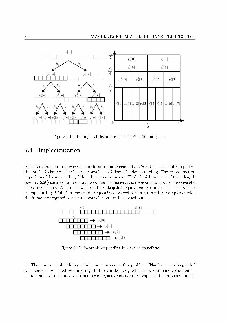
86 WAVELETS FROM A FILTER BANK PERSPECTIVE
Figure 5.18: Example of decomposition for N = 16 and j = 3.
5.4 Implementation
As already exposed, the wavelet transform or, more generally, a WPD, is the iterative applica-tion of the 2-channel �lter bank, a convolution followed by downsampling. The reconstructionis performed by upsampling followed by a convolution. To deal with interval of �nite length(see �g. 5.20) such as frames in audio coding, or images, it is necessary to modify the wavelets.The convolution of N samples with a �lter of length l requires more samples as it is shown forexample in Fig. 5.19. A frame of 16 samples is convolved with a 8-tap �lter. Samples outsidethe frame are required so that the convolution can be carried out.
Figure 5.19: Example of padding in wavelet transform
There are several padding techniques to overcome this problem. The frame can be paddedwith zeros or extended by mirroring. Filters can be designed especially to handle the bound-aries. The most natural way for audio coding is to consider the samples of the previous frames.
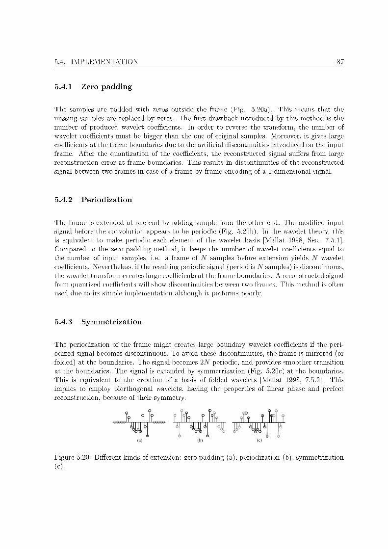
5.4. IMPLEMENTATION 87
5.4.1 Zero padding
The samples are padded with zeros outside the frame (Fig. 5.20a). This means that themissing samples are replaced by zeros. The �rst drawback introduced by this method is thenumber of produced wavelet coe�cients. In order to reverse the transform, the number ofwavelet coe�cients must be bigger than the one of original samples. Moreover, it gives largecoe�cients at the frame boundaries due to the arti�cial discontinuities introduced on the inputframe. After the quantization of the coe�cients, the reconstructed signal su�ers from largereconstruction error at frame boundaries. This results in discontinuities of the reconstructedsignal between two frames in case of a frame by frame encoding of a 1-dimensional signal.
5.4.2 Periodization
The frame is extended at one end by adding sample from the other end. The modi�ed inputsignal before the convolution appears to be periodic (Fig. 5.20b). In the wavelet theory, thisis equivalent to make periodic each element of the wavelet basis [Mallat 1998, Sec. 7.5.1].Compared to the zero-padding method, it keeps the number of wavelet coe�cients equal tothe number of input samples, i.e. a frame of N samples before extension yields N waveletcoe�cients. Nevertheless, if the resulting periodic signal (period is N samples) is discontinuous,the wavelet transform creates large coe�cients at the frame boundaries. A reconstructed signalfrom quantized coe�cients will show discontinuities between two frames. This method is oftenused due to its simple implementation although it performs poorly.
5.4.3 Symmetrization
The periodization of the frame might creates large boundary wavelet coe�cients if the peri-odized signal becomes discontinuous. To avoid these discontinuities, the frame is mirrored (orfolded) at the boundaries. The signal becomes 2N periodic, and provides smoother transitionat the boundaries. The signal is extended by symmetrization (Fig. 5.20c) at the boundaries.This is equivalent to the creation of a basis of folded wavelets [Mallat 1998, 7.5.2]. Thisimplies to employ biorthogonal wavelets, having the properties of linear phase and perfectreconstruction, because of their symmetry.
Figure 5.20: Di�erent kinds of extension: zero padding (a), periodization (b), symmetrization(c).
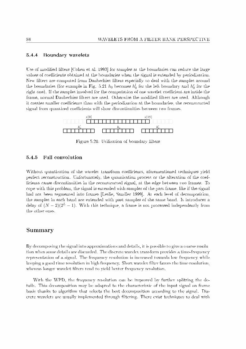
88 WAVELETS FROM A FILTER BANK PERSPECTIVE
5.4.4 Boundary wavelets
Use of modi�ed �lters [Cohen et al. 1993] for samples at the boundaries can reduce the largevalues of coe�cients obtained at the boundaries when the signal is extended by periodization.New �lters are computed from Daubechies �lters especially to deal with the samples aroundthe boundaries (for example in Fig. 5.21 h0 becomes hl
0 for the left boundary and hr0 for the
right one). If the samples involved for the computation of one wavelet coe�cient are inside theframe, normal Daubechies �lters are used. Otherwise the modi�ed �lters are used. Althoughit creates smaller coe�cients than with the periodization at the boundaries, the reconstructedsignal from quantized coe�cients will show discontinuities between two frames.
Figure 5.21: Utilization of boundary �lters
5.4.5 Full convolution
Without quantization of the wavelet transform coe�cients, aforementioned techniques yieldperfect reconstruction. Unfortunately, the quantization process or the alteration of the coef-�cients cause discontinuities in the reconstructed signal, at the edge between two frames. Tocope with this problem, the signal is extended with samples of the past frame, like if the signalhad not been segmented into frames [Leslie, Sandler 1999]. At each level of decomposition,the samples in each band are extended with past samples of the same band. It introduces adelay of (N − 2)(2L − 1). With this technique, a frame is not processed independently fromthe other ones.
Summary
By decomposing the signal into approximations and details, it is possible to give a coarse resolu-tion when some details are discarded. The discrete wavelet transform provides a time-frequencyrepresentation of a signal. The frequency resolution is increased towards low frequency whilekeeping a good time resolution in high frequency. Short wavelet �lter favors the time resolution,whereas longer wavelet �lters tend to yield better frequency resolution.
With the WPD, the frequency resolution can be improved by further splitting the de-tails. This decomposition may be adapted to the characteristic of the input signal on framebasis thanks to algorithm that selects the best decomposition according to the signal. Dis-crete wavelets are usually implemented through �ltering. There exist techniques to deal with

5.4. IMPLEMENTATION 89
boundaries in case of frame by frame processing. The full convolution is well adapted to au-dio coding, since the quantization of wavelet coe�cients does not cause any blocking artifact(discontinuities at frame boundaries). The WPD has been implemented as �lter bank in theproposed coder. Quantization methods of the coe�cients are described in Ch. 6.

90 WAVELETS FROM A FILTER BANK PERSPECTIVE
91
Chapter 6
Embedded Quantizer
Introduction
Using transform coding in a scalable coder implies a smart way to quantize the coe�cients.The quantizer should be able to produce an embedded bitstream in order to provide a repre-sentation of the coe�cients closer to their original values as the bit rate increases. Moreover,the bitstream should be organized in such a way that the perceptually most important coef-�cients, often the largest ones, are transmitted �rst. It is for example the case in the ITU-TG.729.1 [ITU-T 2006a]. The energy of each band is transmitted to the decoder. From thesevalues, the encoder and decoder can compute the bit allocation and the band ordering, fromthe most signi�cant band to the less one. The more important the band, the more the numberof alloted bits. However, all the bits of a codeword corresponding to a band are required toreconstruct coe�cients. Incomplete codewords are simply discarded since they can not helpto reconstruct coe�cients. To take every single bit into account, bit-plane coding may beapplied. This chapter gives the principles of embedded quantization by bit-plane coding forwavelet coe�cients. They will be illustrated by two examples of algorithm from the literaturedeveloped in order to produce an embedded bitstream.
6.1 Principles
The purpose of an embedded quantizer is to produce an embedded bitstream where the �rstbits represent the most important bits of the most important coe�cients, the next bits encodesmaller coe�cients while re�ning the quantization of the former quantized ones, and the lastbits correspond to the less important coe�cients. This can be achieved by performing bit planecoding. Let ci with i ∈ [0, . . . , N − 1] be a set of N coe�cients to be quantized. The binary
92 EMBEDDED QUANTIZER
representation of the coe�cients is given by:
ci =M−1∑k=0
bk2k, ∀i ∈ [0, . . . , N − 1] (6.1)
where M is the required number of bits to binary represent the largest of the coe�cients. Abit-plane is the set of bits having the same position in the binary representation. The �rst bitplane is the set of the most signi�cant bits, the last bit plane the set of the less signi�cant bits.The table 6.1 is an illustration of binary representation of set of integers. In this example, thebinary representation spans six bit-planes. For instance, the second bit-plane is b4 with thevalues {1 0 1 1 0 0 0 0}. The concept of bit-plane coding is to transmit the bit-planes fromthe �rst one to the last one. To justify bit-plane coding, a coder comprising a transformationand a quantizer will be considered. Let T be the transformation that maps the input samplesof a frame x to coe�cients c.
c = T (x) (6.2)
The Mean Square Error gives a measure of the distortion introduced by a coder. For each frame,the input samples x are transformed into coe�cients c. The quantizer outputs a bitstream.This decoder extracts the quantized values c, then inverse transforms those coe�cients tosynthesize the output sample x.
x = T −1 (c) (6.3)
The MSE can be written as:
MSE (x, x) =1N
N−1∑i=0
(xi − xi)2 (6.4)
If the transformation preserves the Euclidean norm, i.e. ‖T (x)‖ = ‖x‖, the equation can berewritten by introduction of the coe�cient values:
MSE (x, x) = MSE (c, c) =1N
N−1∑i=0
(ci − ci)2 (6.5)
Before the decoding, the reconstructed coe�cients are set to zero, ci = 0, i = 0, . . . , N − 1.
The MSE is then equal toPN−1
i=0 c2iN . If a coe�cient ci is perfectly decoded (i.e. ci = ci), the
MSE decreases by c2iN . It results that the transmission of the largest coe�cients contributes to
reduce the distortion the most signi�cantly. In a same manner, the transmission of the mostsigni�cant bit for a single coe�cient will reduce the MSE at most.
This embedded coding is similar in spirit to binary �nite precision representation of realnumbers. Each real number can be represented by a string of binary digits. For each digitadded to the end of the bitstream, more precision is added. Yet the encoding can cease atany moment and provide the best approximation of the real number achievable within theframework of the binary digit representation. Similarly, the embedded coder can cease at anytime and provide the best representation of a signal achievable within its framework.
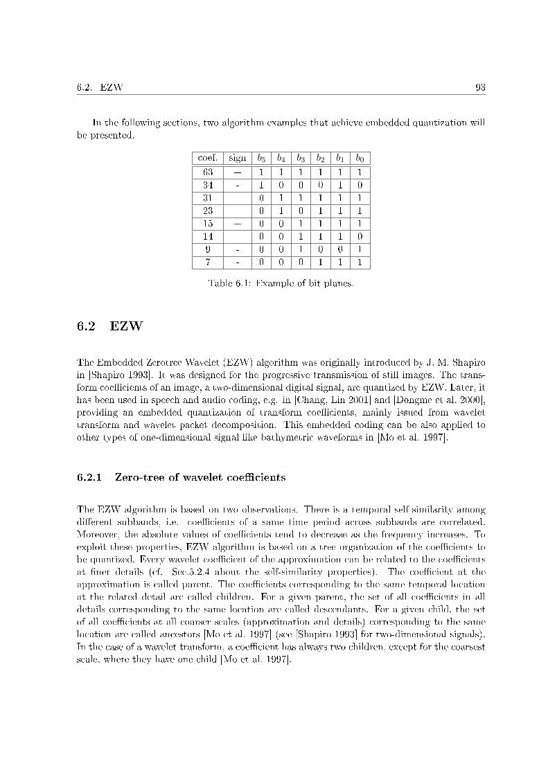
6.2. EZW 93
In the following sections, two algorithm examples that achieve embedded quantization willbe presented.
coef. sign b5 b4 b3 b2 b1 b0
63 + 1 1 1 1 1 134 - 1 0 0 0 1 031 - 0 1 1 1 1 123 + 0 1 0 1 1 115 + 0 0 1 1 1 114 + 0 0 1 1 1 09 - 0 0 1 0 0 17 - 0 0 0 1 1 1
Table 6.1: Example of bit planes.
6.2 EZW
The Embedded Zerotree Wavelet (EZW) algorithm was originally introduced by J. M. Shapiroin [Shapiro 1993]. It was designed for the progressive transmission of still images. The trans-form coe�cients of an image, a two-dimensional digital signal, are quantized by EZW. Later, ithas been used in speech and audio coding, e.g. in [Chang, Lin 2001] and [Dongme et al. 2000],providing an embedded quantization of transform coe�cients, mainly issued from wavelettransform and wavelet packet decomposition. This embedded coding can be also applied toother types of one-dimensional signal like bathymetric waveforms in [Mo et al. 1997].
6.2.1 Zero-tree of wavelet coe�cients
The EZW algorithm is based on two observations. There is a temporal self-similarity amongdi�erent subbands, i.e. coe�cients of a same time period across subbands are correlated.Moreover, the absolute values of coe�cients tend to decrease as the frequency increases. Toexploit these properties, EZW algorithm is based on a tree organization of the coe�cients tobe quantized. Every wavelet coe�cient of the approximation can be related to the coe�cientsat �ner details (cf. Sec.5.2.4 about the self-similarity properties). The coe�cient at theapproximation is called parent. The coe�cients corresponding to the same temporal locationat the related detail are called children. For a given parent, the set of all coe�cients in alldetails corresponding to the same location are called descendants. For a given child, the setof all coe�cients at all coarser scales (approximation and details) corresponding to the samelocation are called ancestors [Mo et al. 1997] (see [Shapiro 1993] for two-dimensional signals).In the case of a wavelet transform, a coe�cient has always two children, except for the coarsestscale, where they have one child [Mo et al. 1997].
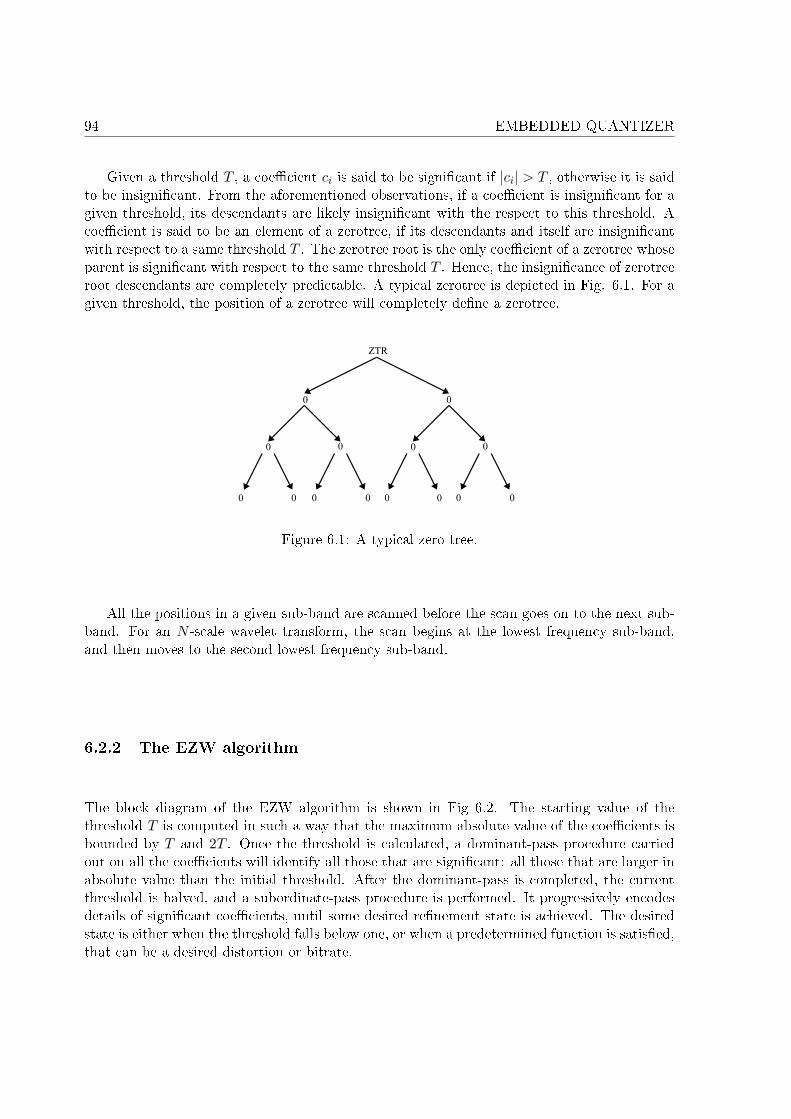
94 EMBEDDED QUANTIZER
Given a threshold T , a coe�cient ci is said to be signi�cant if |ci| > T , otherwise it is saidto be insigni�cant. From the aforementioned observations, if a coe�cient is insigni�cant for agiven threshold, its descendants are likely insigni�cant with the respect to this threshold. Acoe�cient is said to be an element of a zerotree, if its descendants and itself are insigni�cantwith respect to a same threshold T . The zerotree root is the only coe�cient of a zerotree whoseparent is signi�cant with respect to the same threshold T . Hence, the insigni�cance of zerotreeroot descendants are completely predictable. A typical zerotree is depicted in Fig. 6.1. For agiven threshold, the position of a zerotree will completely de�ne a zerotree.
Figure 6.1: A typical zero-tree.
All the positions in a given sub-band are scanned before the scan goes on to the next sub-band. For an N -scale wavelet transform, the scan begins at the lowest frequency sub-band,and then moves to the second lowest frequency sub-band.
6.2.2 The EZW algorithm
The block diagram of the EZW algorithm is shown in Fig 6.2. The starting value of thethreshold T is computed in such a way that the maximum absolute value of the coe�cients isbounded by T and 2T . Once the threshold is calculated, a dominant-pass procedure carriedout on all the coe�cients will identify all those that are signi�cant: all those that are larger inabsolute value than the initial threshold. After the dominant-pass is completed, the currentthreshold is halved, and a subordinate-pass procedure is performed. It progressively encodesdetails of signi�cant coe�cients, until some desired re�nement state is achieved. The desiredstate is either when the threshold falls below one, or when a predetermined function is satis�ed,that can be a desired distortion or bitrate.
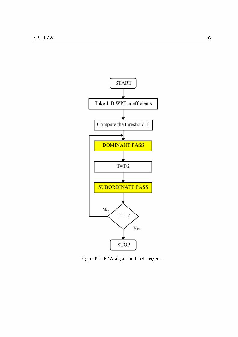
6.2. EZW 95
Figure 6.2: EZW algorithm block diagram.
96 EMBEDDED QUANTIZER
6.2.2.1 Dominant-pass
The Dominant Pass scans the coe�cients at the current level to identify signi�cant coe�cientsand zero-trees. The dominant-pass divides wavelet coe�cients into four classes:
1. POS. Coe�cients are signi�cant and positive.
2. NEG. Coe�cients are signi�cant and negative.
3. ZTR. Coe�cients are zero-tree roots. When a coe�cient and all its descendants areinsigni�cant.
4. IZ. Coe�cients are insigni�cant but have some signi�cant descendants (at least one).
The dominant-pass selects which symbol to generate according to Fig. 6.3. The �rst step isto check whether the current coe�cient was previously found signi�cant. In which case thecoe�cient is skipped and nothing is outputted. If the coe�cient has become signi�cant atthe current threshold, the absolute value is appended to the Subordinate-List and either thepositive signi�cant (P) or negative signi�cant (N) symbol is outputted. The Subordinate-Listrecords each signi�cant coe�cient. If the coe�cient is not signi�cant, the next step is to checkif the insigni�cant coe�cient is a child of an already discovered zero-tree. In which case nosymbol is outputted. If the coe�cient is not part of an already discovered zero-tree, it musteither be a root of a new zero-tree or an isolated zero and the appropriate symbol is outputted.The signi�cant components found in the �rst scan are treated as zero in the second scan. Theorder in which the coe�cients are scanned is very important. Any scan order can be used,on condition that no child is scanned before his parents. The scanning order is shared by theencoder and the decoder.
6.2.2.2 Subordinate-pass
The Subordinate-Pass, Fig. 6.4, (sometimes called the re�nement Pass) re�nes the value ofeach signi�cant coe�cient. For each coe�cient in the Subordinate-List, the Subordinate-Passchecks if their current value is larger or smaller than the current threshold value. If it islarger, the coder outputs '1'. Otherwise it outputs '0'. The magnitude of the Subordinate-Listmight be rearranged in a decreasing order (this should be done at the encoder and decoder)for two reasons. The largest coe�cients carry the most information will be transmitted �rst,thus will be decoded in priority during successive subordinate pass. Furthermore, the use ofan optional entropy coder will compress more e�ciently a burst of '1'-symbols followed by agroup of '0'-symbols as opposed to randomly generated symbols '0' and '1'.
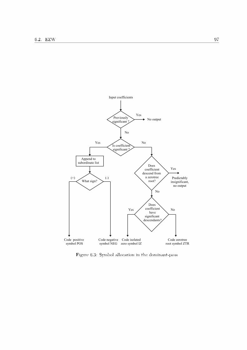
6.2. EZW 97
Figure 6.3: Symbol allocation in the dominant-pass
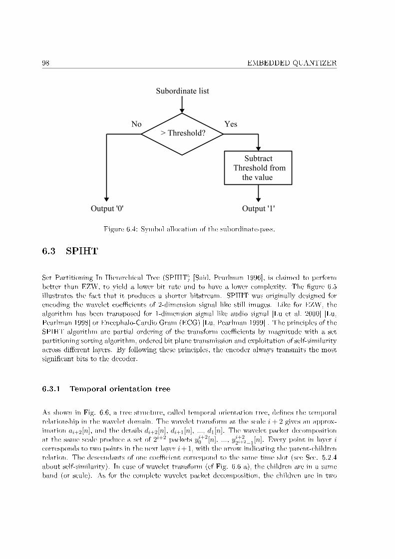
98 EMBEDDED QUANTIZER
Figure 6.4: Symbol allocation of the subordinate-pass.
6.3 SPIHT
Set Partitioning In Hierarchical Tree (SPIHT) [Said, Pearlman 1996], is claimed to performbetter than EZW, to yield a lower bit rate and to have a lower complexity. The �gure 6.5illustrates the fact that it produces a shorter bitstream. SPIHT was originally designed forencoding the wavelet coe�cients of 2-dimension signal like still images. Like for EZW, thealgorithm has been transposed for 1-dimension signal like audio signal [Lu et al. 2000] [Lu,Pearlman 1998] or Encephalo-Cardio Gram (ECG) [Lu, Pearlman 1999] . The principles of theSPIHT algorithm are partial ordering of the transform coe�cients by magnitude with a setpartitioning sorting algorithm, ordered bit plane transmission and exploitation of self-similarityacross di�erent layers. By following these principles, the encoder always transmits the mostsigni�cant bits to the decoder.
6.3.1 Temporal orientation tree
As shown in Fig. 6.6, a tree structure, called temporal orientation tree, de�nes the temporalrelationship in the wavelet domain. The wavelet transform at the scale i + 2 gives an approx-imation ai+2[n], and the details di+2[n], di+1[n], ..., d1[n]. The wavelet packet decompositionat the same scale produce a set of 2i+2 packets yi+2
0 [n], ..., yi+22i+2−1
[n]. Every point in layer icorresponds to two points in the next layer i+1, with the arrow indicating the parent-childrenrelation. The descendants of one coe�cient correspond to the same time slot (see Sec. 5.2.4about self-similarity). In case of wavelet transform (cf Fig. 6.6 a), the children are in a sameband (or scale). As for the complete wavelet packet decomposition, the children are in two
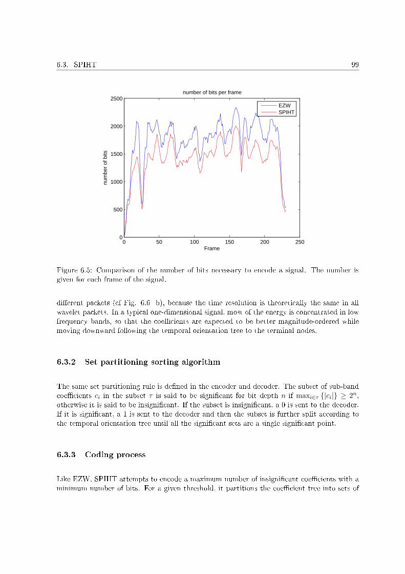
6.3. SPIHT 99
0 50 100 150 200 2500
500
1000
1500
2000
2500
Frame
num
ber
of b
its
number of bits per frame
EZWSPIHT
Figure 6.5: Comparison of the number of bits necessary to encode a signal. The number isgiven for each frame of the signal.
di�erent packets (cf Fig. 6.6 b), because the time resolution is theoretically the same in allwavelet packets. In a typical one-dimensional signal, most of the energy is concentrated in lowfrequency bands, so that the coe�cients are expected to be better magnitude-ordered whilemoving downward following the temporal orientation tree to the terminal nodes.
6.3.2 Set partitioning sorting algorithm
The same set partitioning rule is de�ned in the encoder and decoder. The subset of sub-bandcoe�cients ci in the subset τ is said to be signi�cant for bit depth n if maxi∈τ {|ci|} ≥ 2n,otherwise it is said to be insigni�cant. If the subset is insigni�cant, a 0 is sent to the decoder.If it is signi�cant, a 1 is sent to the decoder and then the subset is further split according tothe temporal orientation tree until all the signi�cant sets are a single signi�cant point.
6.3.3 Coding process
Like EZW, SPIHT attempts to encode a maximum number of insigni�cant coe�cients with aminimum number of bits. For a given threshold, it partitions the coe�cient tree into sets of
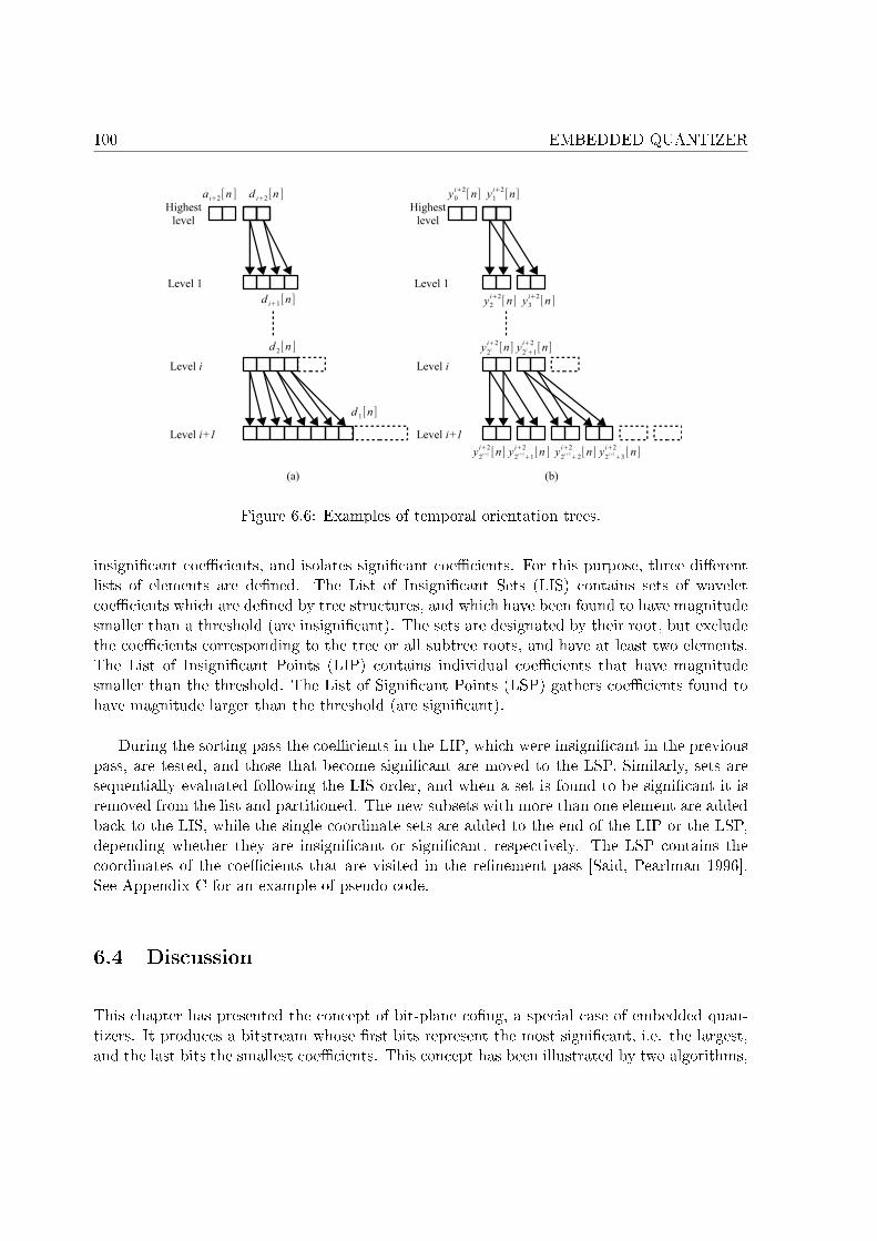
100 EMBEDDED QUANTIZER
Figure 6.6: Examples of temporal orientation trees.
insigni�cant coe�cients, and isolates signi�cant coe�cients. For this purpose, three di�erentlists of elements are de�ned. The List of Insigni�cant Sets (LIS) contains sets of waveletcoe�cients which are de�ned by tree structures, and which have been found to have magnitudesmaller than a threshold (are insigni�cant). The sets are designated by their root, but excludethe coe�cients corresponding to the tree or all subtree roots, and have at least two elements.The List of Insigni�cant Points (LIP) contains individual coe�cients that have magnitudesmaller than the threshold. The List of Signi�cant Points (LSP) gathers coe�cients found tohave magnitude larger than the threshold (are signi�cant).
During the sorting pass the coe�cients in the LIP, which were insigni�cant in the previouspass, are tested, and those that become signi�cant are moved to the LSP. Similarly, sets aresequentially evaluated following the LIS order, and when a set is found to be signi�cant it isremoved from the list and partitioned. The new subsets with more than one element are addedback to the LIS, while the single coordinate sets are added to the end of the LIP or the LSP,depending whether they are insigni�cant or signi�cant, respectively. The LSP contains thecoordinates of the coe�cients that are visited in the re�nement pass [Said, Pearlman 1996].See Appendix C for an example of pseudo-code.
6.4 Discussion
This chapter has presented the concept of bit-plane co�ng, a special case of embedded quan-tizers. It produces a bitstream whose �rst bits represent the most signi�cant, i.e. the largest,and the last bits the smallest coe�cients. This concept has been illustrated by two algorithms,
6.4. DISCUSSION 101
EZW and SPIHT.
SPIHT has clearly some advantages over EZW. First, it requires less bits. The dominantpass (for EZW) and the sorting pass (for SPIHT) have the same aim, i.e. to determine for agiven threshold, if the coe�cients are signi�cant or not. While EZW always outputs 2 bits,even for signalizing a zero-tree (a subset of coe�cients considered as insigni�cant), SPIHT willalways output one bit to signalize a subset as signi�cant or not. Furthermore, SPIHT turnsout to be less complex, due to a more e�cient partitioning of the coe�cients into subsets.Consequently, the choice of the embedded quantizer has been made towards SPIHT.
Variants of SPIHT have been developed over the past few years [Raad et al. 2003] [Wanget al. 2003] [Su et al. 2005]. They will not be detailed in this thesis. They are mostly used forencoding audio content with high �delity quality like music with a bit rate above 64 kbit/s.There are very few examples of its utilization for wideband coding. That brings into questionthe use of SPIHT for wideband speech. In [De Meuleneire et al. 2006b], SPIHT has beenapplied in the context of wideband speech coding. Whereas it enables �ne grain scalability, itscompression performance in comparison with the G.722 at 56 kbit/s is not as good as expected.The chapter 9 explores some possibilities to increase its performance.
As already seen, SPIHT has a clear advantage over EZW because of its e�ciency, therapidity, and its compression performance. Hence, SPIHT has been chosen as embeddedquantizer in the proposed solution.

102 EMBEDDED QUANTIZER
103
Chapter 7
Wavelet-Based Coders
Introduction
Ch. 5 presented the wavelet transform by introducing the perfect reconstruction conditionof a 2-channel �lter bank. With such a �lter bank, it is possible to decompose a signal intotwo bands of equal bandwidth, of low and high frequencies, respectively. Wavelet transform isachieved by successively decompose the lowest frequency band with the �lter bank (the �ltershould ful�ll the conditions in Sec. 5.2). As a result, the frequency resolution increases towardslow frequencies at the expense of a worse time resolution. Hence, it provides a good frequencyresolution in low frequencies, and a good time resolution in high frequencies.
Utilization of wavelet packet transform increases the frequency resolution in high frequen-cies. The decomposition tree can be chosen to closely mimic the critical bands, in order toapply a perceptual model, or to be adapted to the signal to yield a maximum number of coe�-cients with small amplitudes. At any rate, the coe�cients within a band have a time-frequencysigni�cation. They are somehow related to the importance of the band within a time duration,smaller than the frame length. These properties have been investigated in audio codecs inorder to replace frequency transforms like FFT of MDCT.
This chapter presents an overview of wavelet based coders. Most of them are scalable, andrely on the embedded quantizers presented in Ch. 6. In a �rst section, codecs that achievenear transparency are described. Decoded audio samples can not be distinguished from theiroriginal versions. They necessarily rely on perceptual model. Conversely, codecs that do notachieve near transparency are gathered in the second section. A discussion on the advantagesand the drawbacks of the di�erent methods will follow the overview.
104 WAVELET-BASED CODERS
7.1 Near Transparency
An audio coder compresses a digital audio signal for the purpose of transmitting over a com-munication channel, or storing. Depending on the target application, a tradeo� has to beachieved between the complexity, the quality, the delay and the bitrate of the coder. For ex-ample lossless coding guarantees that the decoded samples are perfect copies of their respectiveoriginal samples, but at the expense of a higher complexity and bitrate. However it is possibleto encode audio samples in such a way that a naive listener does not perceive the di�erence be-tween the original and the decoded samples. Such codecs achieve the same perceptual qualityat lower bitrates by making use of a psychoacoustic model (cf. Sec. 1.1.2.2).
The codec in Sec. 7.1.1 selects on the frame basis the best wavelet in the sense of minimumbitrate. Then a complexity scalable coder is presented in Sec. 7.1.2. Afterwards, a waveletcoder based on adaptive wavelet packet is reviewed in Sec. 7.1.3. Finally Sec. 7.1.4 presentsa wavelet coder based on SPIHT.
7.1.1 Audio compression using adapted wavelets
[Sinha, Tew�k 1993] propose an audio codec based on wavelet packet decomposition that workson 44.1 kHz sampling rate input signal on a 1024/2048 samples frame basis (about 23/46 ms).The two ends of each frame are weighted by the square root of a Hanning window of size 128 (i.eeach two consecutive frames overlap by this amount). Wavelet packet coe�cients are quantizedby scalar adaptive quantizer. The coder uses a psychoacoustic model is order to reduce theperceived quantization noise. According to the model, the masking threshold is computedfrom the power spectrum of the input signal by using a FFT. The quantization error in theFourier domain is made inaudible if this energy is smaller than the masking threshold acrossthe frequencies. This condition is transposed to the wavelet domain. By using approximateexpressions of the quantization errors for the scalar quantizers, the minimal number of bitsallocated to each coe�cient required for transparent coding can be calculated as the functionof the wavelet �lter coe�cients. This function is optimized for wavelet �lters of a given lengthK, whose coe�cients ck satisfy:
K−1∑k=0
(−1)kkmck = 0, m = 0, 1, . . . ,K
2− 1 (7.1)
The magnitude responses of such �lters are nearly constant over the passband, their transitionband is very narrow, and their phase are nearly linear. Among all the possible �lters at the givenlength K, the �lter that minimizes the bitrate is selected as the �lter of the wavelet packetdecomposition. The wavelet packet tree is �xed and is chosen to closely mimic the criticalband divisions. The wavelet packet decomposition is implemented with a circular convolution,ensuring a without-delay �lter bank. Wavelet �lters with K = 10, 20, 30, 40 and 60 taps havebeen investigated.
7.1. NEAR TRANSPARENCY 105
The coder exploits the redundancies of the signal by using a dynamic waveform dictionary.Each frame of length N = 2048 samples is divided into two subframes of length N
2 = 1024samples. A pre-echo control mechanism based on an energy-entropy criterion is used to reducethe frame length to 1024 samples if a sudden energy transition is detected (propitious for pre-echo e�ect). In this case, the frame is not further segmented, so the segment to be encodedalways has the same length (1024 samples). For each audio subframe x, the best matchingentry xD in the dictionary is selected. The residual r = x − xD is computed. Both x andr are encoded with the wavelet packet algorithm. The encoder transmits either x or r plusxD according to the required number of bits for each vector. If r is transmitted, the indexof xD is transmitted as well. One extra bit is required to tell whether x or r is transmitted.To take the time scaling variation of the input signal into account, a time scale factor is alsocomputed and transmitted. The dictionary is updated by comparing the minimum distancebetween the decoded frame x corresponding to frame x and the perceptually closest entry intothe dictionary. Then, this distance is compared against a threshold. If the distance is abovethe threshold, the last-used entry of the dictionary is replaced by x.
The coder transmits the wavelet domain masking threshold, that drives the bit allocation.The signal energy is also transmitted of each frame, because each frame is normalized by itsenergy before analysis. The dynamic ranges of the quantizers are quantized in the logarithmfor a group of 8 coe�cients. This quantization depends also on the pre-echo control. The totaloverhead for the side information is approximatively 0.4 bit/sample.
The transparency of the coding at 64 kbit/s has been assessed on audio source materialcomprising solo modern drum, female vocal pop song, violin with orchestra, solo castanets,solo clarinet and solo piano. Formal A-B tests showed that the coder provided a transparentcoding quality for all but two audio sources. Due to negligible pre-echo artifacts in a codedcastanets piece, the quality is nearly transparent. Also, the wavelet based coder does not seemto handle steady sinusoids of the piano piece. The coder performs better than the MPEGLayer-II at 64 kbit/s for the castanet piece, and the same for the piano piece.
7.1.2 Complexity scalable audio coding
[Dongme et al. 2000] provide a complexity scalable codec based on wavelet packet transforma-tion. The codec works on a 1024-sample frame basis for 44.1 kHz audio signal (23 ms). 64samples weighted with a Hanning window are overlapped between two adjacent frames. Thesignal is decomposed into subbands with an incomplete wavelet packet decomposition in orderto closely mimic the critical bands. 20-tap Daubechies wavelet �lters are used. This coderis also scalable in complexity, as the decomposition level depends on the amount of availablecomputing resources to perform the wavelet packet decomposition. The higher the resources,the deeper the decomposition.
A psychoacoustic model similar to MPEG model 1 [MPEG 1992] but less computationally
106 WAVELET-BASED CODERS
complex takes into account the masking properties of the human ear. The masking thresholdsare directly computed from the wavelet coe�cient in each subband. The dominant pass of theEZW is modi�ed to include the masking thresholds. If the absolute value of the wavelet coe�-cient is larger than the given threshold T and the error introduced by quantizing according toT is larger than the masking threshold within the subband, the coe�cient is called signi�cantwith respect to T . Otherwise it is insigni�cant. Accordingly, the subordinate pass is modi�edin such a way, that a coe�cient is not re�ned, when its quantization error is below the maskingthreshold. The resulting bitstream is then entropy coded by arithmetic coding. At the de-coder, according to the available computational complexity, the wavelet packet reconstructionalgorithm may discard the highest bands in order to meet the maximal allowed computationalcomplexity and reconstruct an output frame at 44.1 kHz.
Experiments showed that the higher the complexity of the algorithm, the better the qualityof the reconstructed signal. Besides, the coder is claimed to achieve transparent quality at 64kbit/s.
7.1.3 Audio compression using an adaptive wavelet packet decomposition
This coder proposed in [Srinivasan, Jamieson 1998] encodes a 44.1 kHz mono audio signalon 512 sample frame basis (about 12 ms). The signal is decomposed by an adaptive wavelet�lter bank, based on the spline-based biorthogonal wavelet �lter. The psychoacoustic modelis based on the Model 2 of the ISO-MPEG speci�cation [MPEG 1992]. It gives the maskingthreshold in each critical band, computed on a 1024-point FFT. However, the main output ofthe model is a measure called subband perceptual rate (SUPER), which is a measure that triesto adapt the subband structure to approach the perceptual entropy [Johnston 1988] as closelyas possible.
The SUPER is the iteratively determined number of bits so that the error quantization ineach subband is lower than the masking threshold at the current subband decomposition. Foreach frame, an algorithm tries to adaptively determine the optimal subband structure thatachieves the minimum SUPER, given the maximal computational limit and the best temporalresolution possible. The last point is important since the bit allocation scheme is based on sometemporal correlations. At a given decomposition structure, the overall SUPER is computed.If the decomposition of a subband reduces the overall SUPER, it is carried out. The subbandwith the maximal SUPER is always examined �rst.
The bit allocation and coe�cient quantization is performed by the EZW algorithm. Aftereach subordinate pass, the perceptual evaluation step checks if the bitrate is satis�ed. If it isthe case, the algorithm terminates. The structure decomposition and the number of iterationsof EZW (number of subordinate passes) are sent as side information. For each frame, thewhole bitstream is lossless coded in order to reduce the bitstream.
7.1. NEAR TRANSPARENCY 107
This coder is claimed to be suitable for high quality audio transfers over the Internetor storage at about 45 kbit/s, and is amenable to progressive transmission, thanks EZW.Nevertheless, it exhibits di�culties to encode wind instruments, as �ute and saxophone.
7.1.4 SPIHT in perceptual wavelet coder
The codec proposed in [Lu, Pearlman 1998] works with 44.1 kHz audio samples on a 1024-sample frame basis (about 23 ms). The input frame is decomposed into 29 subbands thatclosely mimic the critical bands by a wavelet packet decomposition using the 20-tap Daubechies�lters. The �rst 17 subbands corresponding to the frequency band [0 - 3.4 kHz] are encodedby SPIHT. The other subbands are quantized with uniform scalar quantizers, whose stepzisesare determined by a rate allocation procedure. A psychoacoustic model, which is based on theMPEG model 1, computes the Signal to Mask Ratio (SMR) SMRm in each subband. In eachsubband, SMRm is combined with the coe�cients to drive the bit allocation constrained bythe following Rate-Distortion (RD) relation:
dm(rm) = wmg2−2rm (7.2)
where dm is the distortion in each subband, rm is the bitrate in each subband, wm is thesubband weight calculated by SMRm and g a constant. Eq. (7.2) expresses the distortion ofa memoryless gaussian source. At a constant bitrate rm, a bigger value of wm allows moredistortion. The parameter g controls the distortion of the uniform quantizers. Transparentquality is achieved when the SNR is larger than the SMR in each subband (i.e. the quantizationis smaller than the masking threshold within the subband). The bitrate is computed iterativelyby:
rm =
{12 log2
⌊wmσ2
mθnm
⌋, wmσ2
m/nm > θ
0 , wmσ2m/nm ≤ θ
(7.3)
where nm is the number of coe�cients in the mth subband and σ2m their variance. The param-
eter θ is continually adjusted until the overall target bitrate is met with non-negative rm. Thequantizer step-sizes are computed according to the allocated bitrate.
The quantization step-sizes of the low frequency coe�cients determine the target bitrateof SPIHT. Whereas the low frequency coe�cients are encoded using the embedded quantizerSPIHT, the high frequency coe�cients are encoded after quantization with a reverse sort-ing process followed by arithmetic coding. In the high frequency bands, the coe�cients aremostly small. In the proposed algorithm the coe�cients whose magnitude are greater than thethreshold is in the signi�cant list. The sorting process is as follows:
1. In the initialization phase, all the coe�cients are put into the signi�cant lists, and thethreshold is set to 1.
2. The maximum value of the coe�cients is transmitted.
108 WAVELET-BASED CODERS
3. Afterwards, for all the coe�cients in the signi�cant list, if the coe�cient is greater thanthe threshold, 1 is sent, otherwise, 0 is sent and the coe�cient is removed from thesigni�cant list.
4. For all the coe�cients in the signi�cant list, if the coe�cient is positive, 1 is sent, other-wise 0 is sent.
5. The threshold is increased by 1, and for all the coe�cients in the signi�cant list, if thecoe�cient is greater than the threshold, 1 is sent, otherwise, 0 is sent and the coe�cientis removed from the list of signi�cant coe�cients.
6. The last step is repeated until the list of coe�cients is empty.
The decoder is able to reconstruct the coe�cients from the maximum value and the decisionand signs bits without extra information. The step-sizes are also sent as side information.
Several music pieces have been encoded to assess the performance of the proposed coder.It has been shown that nearly transparent quality is achieved at bitrates between 55 and 66kbit/s.
In [Lu, Pearlman 1999], another method is applied to encode the high frequency coe�cients,the Nested Binary Set Partitioning (NBSP). The set of coe�cients within each high-passsubband is recursively partitioned into two equal subsets. The whole set is tested. If the set isfound signi�cant (compared to the threshold), it is further partitioned into two equal subsets.Both of them are tested and the signi�cant subset is split again. This process is repeated untilall the signi�cant points are found and put into the LSP (see Ch. 6). The insigni�cant subsetsdiscovered in the recursive binary splitting process are put into the LIS and are tested againat lower thresholds. As in SPIHT, a signi�cant subset or point is never tested again at a lowerthreshold. Also, SPIHT and NBSP in [Lu, Pearlman 1999] stop transmitting bits concerningsubbands whose step-sizes becomes larger than the threshold. Integration of the quantizationin the coding procedure was shown to be more e�cient than explicit quantization.
This new codec has been tested against the MPEG Layer II [MPEG 1992] at 48 kbit/sand 64 kbit/s on various audio samples, like opera, songs and instrumental music. Generally,the new scheme SPIHT-NBSP is comparable or better than MPEG Layer II at 64 kbps andcomparable at 48 kbps. SPIHT-NBSP has better �delity to the original than MPEG LayerII, but at the lower bit rate exhibits some low level aliasing noise absent in MPEG Layer II.The aliasing noise has been eliminated by use of biorthogonal (10, 18) �lters with symmetricextension.
7.2. NON-TRANSPARENCY 109
7.2 Non-transparency
The codecs presented in this section are not claimed to achieve near-transparency. Neverthelessall but one rely on a perceptual model to bene�t from the masking properties of the humanear. A simple 2-stage structure is presented in Sec. 7.2.1. Sec. 7.2.2 describes a codec thatcombines peak picking and EZW to encode wavelet packet coe�cients. Di�erent structures ofwavelet decomposition associated with EZW are outlined in Sec. 7.2.3. A presentation of aperceptual EZW algorithm in Sec. 7.2.4 closes this section.
7.2.1 A 2-Stage Wavelet Packet Based Scalable Codec
[Kudumakis, Sandler 1996] provides a two-stage wavelet packet scalable audio coder. The baselayer encodes the signal with a wavelet packet algorithm. The second stage encodes the waveletpacket coe�cients of the di�erence between the original and the reconstructed signal (cf. Fig.7.1). The coe�cients are then quantized and compressed.
The codec works at a sampling rate of 48 kHz. The wavelet packet decomposition comprises5 levels, and divides the 1024-sample input frames (21 ms) into 32 uniform subbands. TheDynamic Bit Allocation based on Psychoacoustic Model-1 as adapted for use with MPEGLayer-II [MPEG 1992] allocates bits for the di�erent subbands according to the input powerspectrum (given by a FFT). The quantization of coe�cients in a subband is based on theBlock Companding as in MPEG Layer-I [MPEG 1992]. Finally, redundancy is removed by aHu�man noiseless coding as in MPEG Layer-III.
This structure with di�erent wavelet �lters is compared with a 2-stage MPEG-based scal-able codec. Firstly, using Daubechies 4-tap �lters halves the delay in comparison to the MPEGscheme. Moreover, increasing the length of the wavelet �lter improves the performance of thecodec in term of Segmental Signal to Noise Ratio (SSNR), but not signi�cantly. Secondly,this codec outperforms the MPEG scheme for bitrates up to 64 kbit/s. Even if the �rst stageof the scalable MPEG at 64 kbit/s is equivalent to the 32+32 kbit/s 2-stage wavelet codec,Above 64 kbit/s, the scalable MPEG becomes superior. Finally, the penalty introduced by thescalability is less important for the wavelet scheme than for the MPEG one.
A study on wavelet 6-tap �lter coe�cients combined with this structure has been conductedin [Kudumakis, Sandler 1997]. Wavelet �lters satisfying of length K that satisfy Eq. (7.1) maybe parametrized by K
2 − 1 free parameters, each taking values in the interval [0;2π[. Hence theconsidered �lters depend on 2 parameters a and b, respectively. The SSNR of coded samplesat di�erent bitrates were computed for several values of the parameters. Maximal values ofSSNR are always obtained at the same values of a and b. Also, the peaks of SSNR correspondto the most regular wavelet �lters.
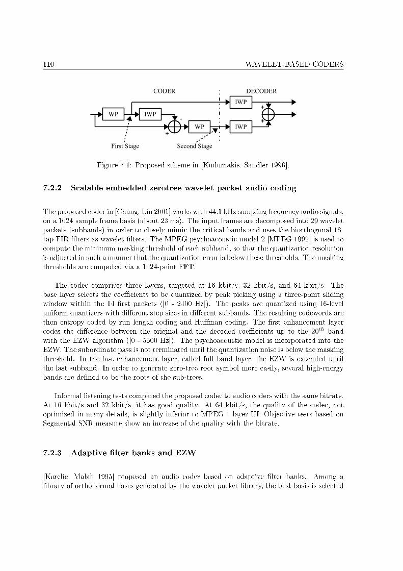
110 WAVELET-BASED CODERS
Figure 7.1: Proposed scheme in [Kudumakis, Sandler 1996].
7.2.2 Scalable embedded zerotree wavelet packet audio coding
The proposed coder in [Chang, Lin 2001] works with 44.1 kHz sampling frequency audio signals,on a 1024-sample frame basis (about 23 ms). The input frames are decomposed into 29 waveletpackets (subbands) in order to closely mimic the critical bands and uses the biorthogonal 18-tap FIR �lters as wavelet �lters. The MPEG psychoacoustic model 2 [MPEG 1992] is used tocompute the minimum masking threshold of each subband, so that the quantization resolutionis adjusted in such a manner that the quantization error is below these thresholds. The maskingthresholds are computed via a 1024-point FFT.
The codec comprises three layers, targeted at 16 kbit/s, 32 kbit/s, and 64 kbit/s. Thebase layer selects the coe�cients to be quantized by peak picking using a three-point slidingwindow within the 14 �rst packets ([0 - 2400 Hz]). The peaks are quantized using 16-leveluniform quantizers with di�erent step sizes in di�erent subbands. The resulting codewords arethen entropy coded by run length coding and Hu�man coding. The �rst enhancement layercodes the di�erence between the original and the decoded coe�cients up to the 20th bandwith the EZW algorithm ([0 - 5500 Hz]). The psychoacoustic model is incorporated into theEZW. The subordinate pass is not terminated until the quantization noise is below the maskingthreshold. In the last enhancement layer, called full band layer, the EZW is extended untilthe last subband. In order to generate zero-tree root symbol more easily, several high-energybands are de�ned to be the roots of the sub-trees.
Informal listening tests compared the proposed codec to audio coders with the same bitrate.At 16 kbit/s and 32 kbit/s, it has good quality. At 64 kbit/s, the quality of the codec, notoptimized in many details, is slightly inferior to MPEG-1 layer III. Objective tests based onSegmental SNR measure show an increase of the quality with the bitrate.
7.2.3 Adaptive �lter banks and EZW
[Karelic, Malah 1995] proposed an audio coder based on adaptive �lter banks. Among alibrary of orthonormal bases generated by the wavelet packet library, the best basis is selected
7.2. NON-TRANSPARENCY 111
by minimizing a cost function. It is usually an additive function because it enables a fastersearch for the best basis. In [Coifman, Wickerhauser 1992], the entropy was used as a costfunction:
M({xi}) = −∑
i
pi ln pi, pi =|xi|2∑j |xj |2
(7.4)
where xi are the coe�cients to be quantized within the same subband. Instead, the au-thors suggested to use a log2 cost function that gives better results, de�ned as M({xi}) =∑
i:xi 6=0 dlog2 xie (round-up operation to the next integer), i.e the number of bits needed torepresent each coe�cient as an integer. The coe�cients are encoded with the EZW algorithm.
The best basis algorithm needs all the coe�cients at all scales in order to select the bestbasis. At the synthesis part, when new branches are created, the �lters in these branches donot have the correct initial state inputs needed to produce valid output values, and thereforethey produce errors for a certain period after the switching between di�erent structures. Apost �lter is used to remove the transients that occur after switching. This method is called'prolonged' decomposition.
The wavelet decomposition can also be performed on each segment separately. There is aneed for information outside the relevant interval. Consequently, the expansion of the segmentis necessary. It can be done either by mirroring (symmetric expansion) or periodically (cyclicexpansion). The �rst method avoids undesired edge e�ects in the low frequency band. Howeverthe segmental decomposition causes some ine�ciency in coding the signal because edge e�ectsare present in the high frequency band and therefore many bits may be needed for coding thecoe�cients at the segment boundaries. Energy leakage to higher frequency can also occur forshort length of the segment. This method is called 'segmental' decomposition.
Objective measurements (Segmental SNR) showed that 'prolonged' adaptive wavelet de-composition plus the EZW and arithmetic coding outperforms the MPEG scheme (without thepsychoacoustic model) at both 64 kbit/s and 128 kbit/s. Nevertheless it requires more com-putations than using a uniform �lter bank due to the memory management and post�ltering.
7.2.4 Perceptual Zerotrees
The proposed coder in [Aggarwal et al. 1999] works on wideband signal (16 kHz samplingrate) on a 512 sample frames basis (32 ms). The input frame is decomposed by an adaptivewavelet packet structure based on the biorthogonal 9-7 tap Daubechies �lters. The �lter bankis without delay since the symmetric extension is implemented.
A Rate-Distortion (RD) module controls the depth of the wavelet decomposition, the binarysplit decision during wavelet decomposition, and the iteration of the zerotree coder (basedon EZW). The adaptation of these parameters is based on an operational RD tradeo�, thedistortion criterion being the Segmental SNR.
112 WAVELET-BASED CODERS
At the �rst stage of the wavelet decomposition, the input frame is split into two subbands.The binary split decision decides which subband is further decomposed. At each stage, onlyone packet is decomposed. After the decomposition, the coe�cients are organized in a binarytree in such a way that it becomes a time-orientation tree (as described in Ch. 6).
A modi�ed EZW algorithm, called Perceptual Zerotree Wavelet (PZW), scans the coe�-cients in the binary tree but only transmits the most signi�cant bit of each coe�cient. Then,the algorithm uses this information to generate an initial estimate of the coe�cients and quan-tize them using perceptual considerations. The initial estimate ei of the coe�cient pi is setequal to the threshold value, given by:
ei = 2ni , where ni = blog2 |pi|c ∀i (7.5)
where the operator b.c takes the integer part. A bit allocation bi required to scalar quantize acoe�cient according to a simple perceptual model is given by:
ei =⌈log2
∣∣∣∣Kei
El
∣∣∣∣⌉ , where l = blog2 ic (7.6)
with El =P2l+1
i=2l p2i
2l the average energy of level l. The operator d.e rounds up to the nextinteger. The model controls the amount of noise introduced in di�erent frequency bands byquantizing each coe�cient to a �xed average SNR, given by the constant K.
The quality of the proposed codec was assessed by an A-B listening test with 8 naivelisteners on speech and music samples. First PZW at an average bitrate of 30 kbit/s wascompared to the EZW without perceptual considerations at an average bitrate of 35 kbit/s(on a wavelet transform of depth 9). The listening test results show that PZW outperformsEZW for both speech and music. The second test compared PZW at 30 kbit/s with the ITU-TG.722 [ITU-T 1988b] at 48 kbit/s. The PZW was preferred 70% to 30% despite the loweraverage bit rate.
7.3 Discussion
This overview addresses several problems encountered when designing a wavelet �lter bank.The choice of the wavelet �lter length and coe�cients is a crucial point in [Sinha, Tew�k1993]. The wavelet �lter that gives the minimum bitrate is chosen to perform the waveletpacket decomposition. Particularly, it is shown that this optimization yields the minimumbitrate gain for a given length, and the longer the wavelet, the higher the probability to reducethe bitrate. Hence, longer wavelet should be preferred. This is not the chosen strategy in[Kudumakis, Sandler 1996] and [Kudumakis, Sandler 1997] where short wavelets are preferablyused. This choice is motivated by reducing the delay of the wavelet decomposition. This pointleads to another problem that is the implementation of the wavelet transform.
7.3. DISCUSSION 113
As explained in Sec. 5.4 and Sec. 7.2.3, there are two ways to deal with the boundaries, ei-ther in a 'segmental manner' or in a 'prolonged manner'. The �rst method can be implementedwith a circular convolution for orthogonal wavelet �lters, or with a symmetric extension forbiorthogonal wavelet �lters. One of the advantages is the implementation of a without-delay�lter bank, since no samples from the past (or the future) are required for the convolution.This strategy has been adopted for instance by [Aggarwal et al. 1999], [Lu, Pearlman 1999] and7.1.1. The main drawback is the discontinuity introduced at frame boundaries (see Sec. 5.4).It has not been addressed in any of the concerned papers. This problem has been probablycircumvented by the coe�cient quantization since those papers claimed near-transparent audiocoding. The prolonged manner avoids this artifact by considering samples from the past atthe convolution. Even at low bit rate with a coarse quantization, no discontinuity appears atthe frame boundary at the expense of a bigger delay [Leslie, Sandler 1999].
In case of the prolonged manner, the choice of an adaptive �lter bank becomes problematic,as explained in [Karelic, Malah 1995]. As the �lter bank structure changes from one frame tothe other, �lter memory problem occurs and causes transient at frame boundaries. To copewith this undesirable e�ect, adaptive post�ltering is carried out. An adaptive structure issuitable to �nd the best basis of a wavelet packet decomposition in order to minimize thenumber of non-zero coe�cients (see Sec. 5.3.3). In [Srinivasan, Jamieson 1998], the bestdecomposition is chosen by minimizing the bitrate under the constraint of a maximal givencomplexity and subbands with the best time resolution. Another strategy in [Aggarwal et al.1999] is to only decompose one band at each decomposition level in order to get a temporal-oriented binary tree. Moreover, an adapted decomposition seems to yield better results thanan uniform decomposition according to [Karelic, Malah 1995].
Rather than a �xed uniform �lter bank, a �xed structure bank that mimics closely thecritical bands is usually preferred (e.g. [Aggarwal et al. 1999][Sinha, Tew�k 1993]). The com-putation of the masking thresholds from a FFT [Chang, Lin 2001] or directly from the waveletcoe�cients [Dongme et al. 2000] makes possible to adapt the quantization of coe�cients. In-deed the masking thresholds drive the bit allocation by giving more bits to the bands with alow masking threshold so that the quantization noise in those bands is inaudible. Nevertheless,when using a FFT, it is also possible to use a uniform �lter bank [Kudumakis, Sandler 1996].
The main issue of interest is the scalability. This overview gives a large range of possibilities.Scalability can be achieved by 2-stage structure as in [Kudumakis, Sandler 1996], where thedi�erence of the original signal and a low bitrate version is coded as an enhancement layer.The utilization of embedded quantizer as EZW in [Karelic, Malah 1995] or SPIHT in [Lu,Pearlman 1998][Lu, Pearlman 1999] is specially developed for progressive transmission. Thosequantizers can be modi�ed to account for a perceptual model as in [Chang, Lin 2001] or in[Srinivasan, Jamieson 1998].
For the targeted bitrate, i.e. 32 kbit/s, the transparency was not a priority. Thus, thestructure of the �lter bank has been designed without any perceptual consideration. A �xedstructure that mimics the critical band has however been investigated. This idea has been
114 WAVELET-BASED CODERS
abandoned for two reasons. First, it is di�cult to be close enough to the critical bands withshort wideband frames since it limits the wavelet packet decomposition level. Second, theabsence of frequency resolution in high frequencies is the cause of annoying artifacts when afew coe�cients among the subband are reconstructed. Moreover, the choice of the wavelet�lters has been guided by the magnitude response of the �lter. Orthogonal wavelets havebeen preferred to biorthogonal wavelet, since they have a better magnitude response (narrowtransition band) and then limits the imaging e�ect (folding) at the reconstruction. Finally,wavelet packet decomposition is performed as in [Leslie, Sandler 1999].
Summary
Wavelet decomposition can easily replace frequency transform in audio coding. To take intoaccount the masking properties of the human ear, a perceptual model can be integrated. Themasking threshold might be calculated either via a FFT or directly on the wavelet coe�cients.For this purpose, it is possible to adapt the wavelet packet decomposition so that the subbandsclosely mimic the critical bands. The decomposition can also be adapted on a frame basis inorder to give the most compact representation of the input signal. Near transparent qualitycan be achieved. Wavelet packet o�ers also a framework for scalable coding via algorithmssuch as EZW or SPIHT.
Uniform wavelet packet decomposition has been chosen to provide the same time andfrequency resolution in all subbands. Since transparency is not a �rst priority, no perceptualmodel is applied. Scalability is achieved by using SPIHT algorithm. Optimization of thewavelet �lter length and decomposition level, as well as SPIHT parameters is investigated inCh. 9.
115
Part IV
Bandwidth Extension

117
Chapter 8
Bandwidth Extension
Introduction
This chapter presents investigation on the BandWidth Extension (BWE) module. The purposeof this chapter is to give the key points of bandwidth extension rather than an exhaustivesurvey of the literature. For further and more detailed bibliography see [Jax 2002] [Collen2002] [Larsen, Aarts 2004]. After a brief review of the bandwidth extension concept in the�rst section, the second section will expose the reasons for integrating a BWE module intothe proposed codec. In the third section, the di�erent BWE approaches with side informationinvestigated will be described. The last section will discuss the advantages and drawbacks ofthe experimented bandwidth extension.
8.1 The bandwidth extension concept
Nowadays most of the speech communication systems (�xed and mobile telephony) makesuse of narrowband speech codecs working for signals whose bandwidth spanning less than 4kHz, from 300 Hz to 3.4 kHz [ITU-T 1998a]. Though, it is broadly accepted that increas-ing the acoustic bandwidth of transmitted speech signals improves both speech intelligibility[Terhardt 1998] and subjective speech quality [Voran 1997]. To meet a strong demand ofindustrials (equipment providers, operators), wideband speech codecs, eg the ITU-T G.722[ITU-T 1988b], the ITU-T G.722.1 [ITU-T 2005], the ITU-T G.722.2 [ITU-T 2003] and latelythe ITU-T G.729.1 [ITU-T 2006a], have been already standardized for the last twenty years.However their implementation implies to modify both transmitter and receiver sides at expen-sive costs. Narrowband and wideband technologies might coexist in speech communicationnetworks for a long time. Arti�cial BWE provides a solution to make bandwidth of speech
118 BANDWIDTH EXTENSION
signals uniform, i.e. enable wideband signal synthesis according to the terminal capabilities(loudspeaker, complexity). The integration of BWE can be present in scenarios such as com-munication between a narrowband terminal like analog �xed phone and wideband terminallike PC. For compatibility reasons, a narrowband codec is used during the communication. Tobene�t from wideband and computational capability of the PC, BWE may be integrated afterthe decoding in order to enable wideband rendering.
Arti�cial BWE of speech signal consists in estimating from the narrowband synthesizedsignal its wideband components. The bandwidth of a wideband signal being usually limitedbetween 50 Hz and 7 kHz [ITU-T 1988b], a narrowband signal between 300 Hz and 3.4 kHz,the components between 50 Hz and 300 Hz, and from 3.4 kHz to 7 kHz are to be estimated.By exploiting the narrowband components and the a priori knowledge on the signal (statisticalmodel) the BWE generates the aforementioned components. Assuming a source-�lter model,this process can be separated into two sub-systems:
- the estimation of the spectral envelope.
- the generation of the �ne structure corresponding to the harmonic structure of the signal.
Additional information like the temporal envelope (evolution of the signal energy over the timewithin a frame) may be transmitted in order to improve the synthesis of the wideband part.
This technology is interesting for a embedded coder. For example, it has already beensuccessfully integrated to the G.729 in [ITU-T 2006a] and to the AMR 12.2 kbit/s in [Jax etal. 2006]. It turns out that a coder may bene�t wideband capability at low bit rate from aBWE module. The motivation of using a BWE as a part of the embedded codec is argued inthe following.
8.2 Presentation of a scalable coder
Fig. 8.1 depicts the scalable wideband speech coder proposed in [De Meuleneire et al. 2006b].The wideband input signal s16kHz(n) is low pass �ltered und downsampled by a factor 2. Theresulting narrowband signal s8kHz(n) is encoded then locally decoded by the ITU-T G.729codec. Its output s8kHz(n) is upsampled by a factor 2 and low pass �ltered. The synthesizedsignal s16kHz(n) is subtracted from the original signal s16kHz(n). The di�erence signal r(n) istransformed by a Wavelet Packet Decomposition (WPD) into a time-frequency domain. TheWavelet Packet (WP) coe�cients are quantized into an embedded bitstream by SPIHT. Foreach frame, the bitstream comprises the G.729 bitstream and the SPIHT bitstream correspond-ing to the wavelet coe�cients of the di�erence signal in a narrowband part (< 4kHz) and ofthe original signal in the wideband part (> 4kHz).
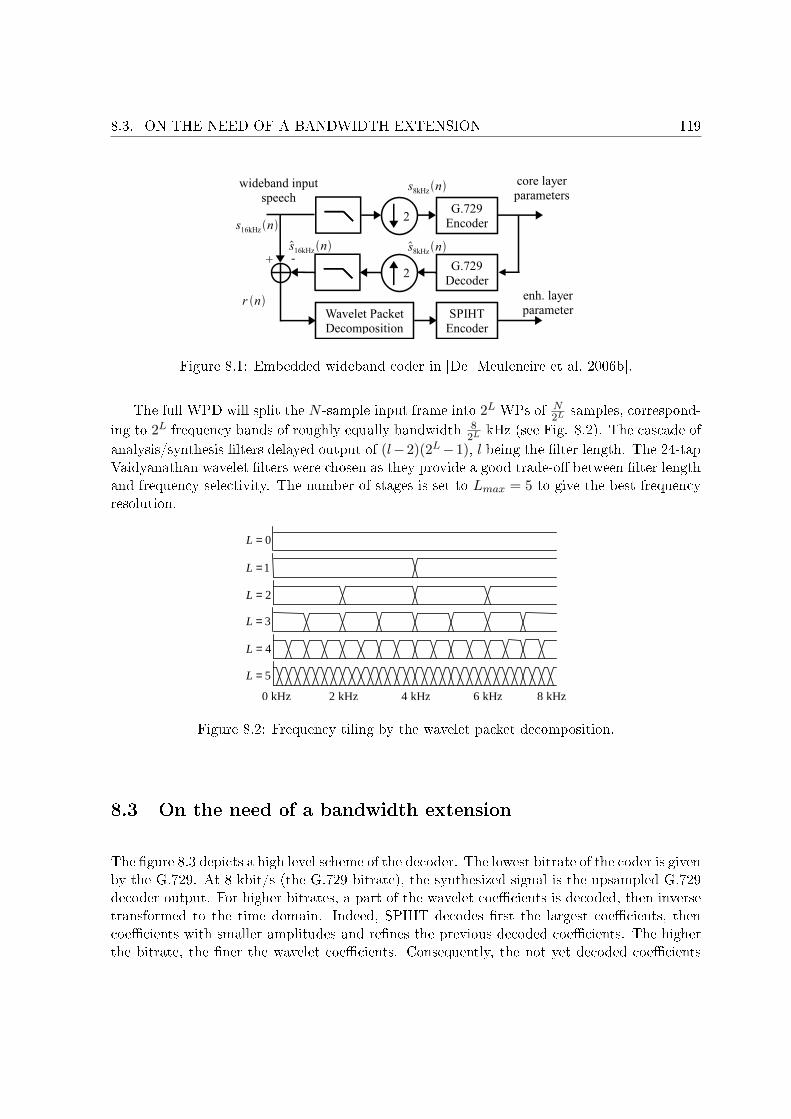
8.3. ON THE NEED OF A BANDWIDTH EXTENSION 119
Figure 8.1: Embedded wideband coder in [De Meuleneire et al. 2006b].
The full WPD will split the N -sample input frame into 2L WPs of N2L samples, correspond-
ing to 2L frequency bands of roughly equally bandwidth 82L kHz (see Fig. 8.2). The cascade of
analysis/synthesis �lters delayed output of (l−2)(2L−1), l being the �lter length. The 24-tapVaidyanathan wavelet �lters were chosen as they provide a good trade-o� between �lter lengthand frequency selectivity. The number of stages is set to Lmax = 5 to give the best frequencyresolution.
0=L
1=L
2=L
3=L
5=L
4=L
4 kHz 8 kHz 2 kHz 6 kHz 0 kHz
Figure 8.2: Frequency tiling by the wavelet packet decomposition.
8.3 On the need of a bandwidth extension
The �gure 8.3 depicts a high level scheme of the decoder. The lowest bitrate of the coder is givenby the G.729. At 8 kbit/s (the G.729 bitrate), the synthesized signal is the upsampled G.729decoder output. For higher bitrates, a part of the wavelet coe�cients is decoded, then inversetransformed to the time domain. Indeed, SPIHT decodes �rst the largest coe�cients, thencoe�cients with smaller amplitudes and re�nes the previous decoded coe�cients. The higherthe bitrate, the �ner the wavelet coe�cients. Consequently, the not yet decoded coe�cients
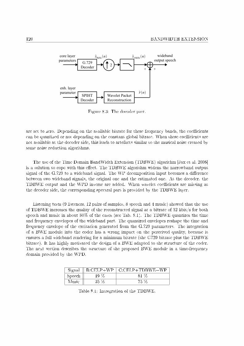
120 BANDWIDTH EXTENSION
Figure 8.3: The decoder part.
are set to zero. Depending on the available bitrate for these frequency bands, the coe�cientscan be quantized or not depending on the constant global bitrate. When these coe�cients arenot available at the decoder side, this leads to artefacts similar to the musical noise created bysome noise reduction algorithms.
The use of the Time Domain BandWidth Extension (TDBWE) algorithm [Jax et al. 2006]is a solution to cope with this e�ect. The TDBWE algorithm widens the narrowband outputsignal of the G.729 to a wideband signal. The WP decomposition input becomes a di�erencebetween two wideband signals, the original one and the estimated one. At the decoder, theTDBWE output and the WPD inverse are added. When wavelet coe�cients are missing atthe decoder side, the corresponding spectral part is provided by the TDBWE layer.
Listening tests (9 listeners, 12 pairs of samples, 8 speech and 4 music) showed that the useof TDBWE increases the quality of the reconstructed signal at a bitrate of 32 kbit/s for bothspeech and music in about 80% of the cases (see Tab. 8.1). The TDBWE quantizes the timeand frequency envelopes of the wideband part. The quantized envelopes reshape the time andfrequency envelope of the excitation generated from the G.729 parameters. The integrationof a BWE module into the coder has a strong impact on the perceived quality, because itensures a full wideband rendering for a minimum bitrate (the G729 bitrate plus the TDBWEbitrate). It has highly motivated the design of a BWE adapted to the structure of the coder.The next section describes the structure of the proposed BWE module in a time-frequencydomain provided by the WPD.
Signal B:CELP+WP C:CELP+TDBWE+WPSpeech 19 % 81 %Music 25 % 75 %
Table 8.1: Intregration of the TDBWE.
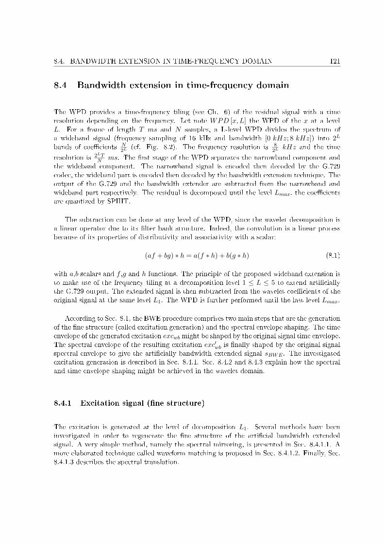
8.4. BANDWIDTH EXTENSION IN TIME-FREQUENCY DOMAIN 121
8.4 Bandwidth extension in time-frequency domain
The WPD provides a time-frequency tiling (see Ch. 6) of the residual signal with a timeresolution depending on the frequency. Let note WPD [x, L] the WPD of the x at a levelL. For a frame of length T ms and N samples, a L-level WPD divides the spectrum ofa wideband signal (frequency sampling of 16 kHz and bandwidth [0 kHz; 8 kHz]) into 2L
bands of coe�cients N2L (cf. Fig. 8.2). The frequency resolution is 8
2L kHz and the time
resolution is 2LTN ms. The �rst stage of the WPD separates the narrowband component and
the wideband component. The narrowband signal is encoded then decoded by the G.729codec, the wideband part is encoded then decoded by the bandwidth extension technique. Theoutput of the G.729 and the bandwidth extender are subtracted from the narrowband andwideband part respectively. The residual is decomposed until the level Lmax, the coe�cientsare quantized by SPIHT.
The subtraction can be done at any level of the WPD, since the wavelet decomposition isa linear operator due to its �lter bank structure. Indeed, the convolution is a linear processbecause of its properties of distributivity and associativity with a scalar:
(af + bg) ∗ h = a(f ∗ h) + b(g ∗ h) (8.1)
with a,b scalars and f ,g and h functions. The principle of the proposed wideband extension isto make use of the frequency tiling at a decomposition level 1 ≤ L ≤ 5 to extend arti�ciallythe G.729 output. The extended signal is then subtracted from the wavelet coe�cients of theoriginal signal at the same level L1. The WPD is further performed until the last level Lmax.
According to Sec. 8.1, the BWE procedure comprises two main steps that are the generationof the �ne structure (called excitation generation) and the spectral envelope shaping. The timeenvelope of the generated excitation excwb might be shaped by the original signal time envelope.The spectral envelope of the resulting excitation exc′wb is �nally shaped by the original signalspectral envelope to give the arti�cially bandwidth extended signal sBWE . The investigatedexcitation generation is described in Sec. 8.4.1. Sec. 8.4.2 and 8.4.3 explain how the spectraland time envelope shaping might be achieved in the wavelet domain.
8.4.1 Excitation signal (�ne structure)
The excitation is generated at the level of decomposition L1. Several methods have beeninvestigated in order to regenerate the �ne structure of the arti�cial bandwidth extendedsignal. A very simple method, namely the spectral mirroring, is presented in Sec. 8.4.1.1. Amore elaborated technique called waveform matching is proposed in Sec. 8.4.1.2. Finally, Sec.8.4.1.3 describes the spectral translation.
122 BANDWIDTH EXTENSION
8.4.1.1 Spectral mirroring
At the �rst level of decomposition, the N2 samples corresponding to the narrowband part is
encoded by the G.729. The output samples are copied to the wideband part
WPD [excwb, 1](
N
2+ n
)= WPD [s16kHz, 1] (n), ∀n ∈
{0, . . . ,
N
2− 1}
(8.2)
where WPD[s, L](n) is the nth WPD coe�cient of a signal s at the decomposition level L.The WPD always reverses the frequency order of downsampled high-pass �ltered WPs. Theinverse transform at the reconstruction produces the opposite e�ect, i.e. will reverse theimpacted bands. Consequently, if the coe�cients are simply copied to the wideband part,the corresponding spectrum will be reversed at the reconstruction. This operation is thusequivalent to mirroring (or folding) the narrowband part of the spectrum to the wideband part.It creates arti�cially the wideband part of the signal. Two problems may arise. First, in caseof strong voiced frames, the frequency above 6 kHz will show the same formantic structure asthe low frequency part (the problem is not annoying above 7 kHz since the arti�cially extendedsignal spectrum will be forced to zero). The second problem may happen in case of unvoicedframe. The G.729 output spectrum is poor in frequency components. For this reason, themirror spectrum may su�er from inconsistency. Even though the energy of the synthesizedsignal in a band is close to original after the spectral shaping, the bandwidth extended signaldoes not sound natural. Thereafter the focus has been put on a better way to reproduce thecoe�cients of the wideband part.
8.4.1.2 Waveform matching
Instead of copying the G.729 output samples into the wideband part like in Eq. 8.2, the signalis further decomposed until the level L1 > 1, with
WPD [s16kHz, 1](
N
2+ n
)= 0, ∀n ∈
{0, . . . ,
N
2− 1}
(8.3)
Let M1 = 2L1−1 be the number of WPs in the narrowband part and M2 = 2L1−1 − 2L1−3 thenumber of WPs to be quantized (e.g. for L1 = 4, M1 = 8 and M2 = 6). The expression ofM2 is only valid for L1 ≥ 3. The term 2L1−3 is the number of WPs describing the band [7 - 8kHz]. For L1 < 3, this term is zero. This band can be �ltered out at the spectral shaping bysetting the corresponding WP(s) to zero or by a �lter after the synthesis.
To determine the waveform of the coe�cients in each WP belonging to the widebandpart, the wideband part WPs are chosen among WPs of the reconstructed narrowband partto 'match' as much as possible the original WPs. The maximum of correlation determineswhich WPs of the narrowband part are the closest to the WPs of the wideband part. The
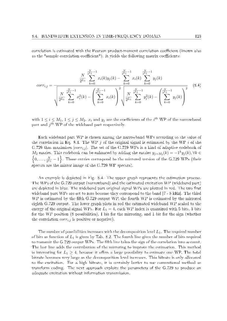
8.4. BANDWIDTH EXTENSION IN TIME-FREQUENCY DOMAIN 123
correlation is estimated with the Pearson product-moment correlation coe�cient (known alsoas the "sample correlation coe�cient"). It yields the following matrix coe�cients:
corri,j =
N
2L1
N
2L1−1∑
k=0
xi(k)yj(k)−
N
2L1−1∑
k=0
xi(k)
N
2L1−1∑
k=0
yj(k)√√√√√√ N
2L1
N
2L1−1∑
k=0
x2i (k)−
N
2L1−1∑
k=0
xi(k)
2√√√√√√ N
2L1
N
2L1−1∑
k=0
y2j (k)−
N
2L1−1∑
k=0
yj(k)
2
(8.4)
with 1 ≤ i ≤ M1, 1 ≤ j ≤ M2. xi and yj are the coe�cients of the ith WP of the narrowbandpart and jth WP of the wideband part respectively.
Each wideband part WP is chosen among the narrowband WPs according to the value ofthe correlation in Eq. 8.4. The WP j of the original signal is estimated by the WP i of theG.729 that maximizes |corri,j |. The set of the G.729 WPs is a kind of adaptive codebook ofM2 entries. This codebook can be enhanced by adding the entries yj+M2(k) = −1kyj(k),∀k ∈{
0, . . . , N2L1
− 1}. Those entries correspond to the mirrored version of the G.729 WPs (their
spectra are the mirror image of the G.729 WP spectra).
An example is depicted in Fig. 8.4. The upper graph represents the estimation process.The WPs of the G.729 output (narrowband) and the estimated excitation WP (wideband part)are depicted in blue. The wideband part original signal WPs are plotted in red. The two �rstwideband part WPs are set to zero because they correspond to the band [7 - 8 kHz]. The thirdWP is estimated by the �fth G.729 output WP, the fourth WP is estimated by the mirroredeighth G.729 output. The lower graph plots in red the estimated wideband WP scaled to theenergy of the original signal WPs. For L1 = 4, each WP index is quantized with 5 bits, 3 bitsfor the WP position (8 possibilities), 1 bit for the mirroring, and 1 bit for the sign (whetherthe correlation corri,j is positive or negative).
The number of possibilities increases with the decomposition level L1. The required numberof bits as function of L1 is given by Tab. 8.2. The fourth line gives the number of bits requiredto transmit the G.729 output WPs. The �fth line takes the sign of the correlation into account.The last line adds the contribution of the mirroring to improve the estimation. This methodis interesting for L1 ≥ 4, because it o�ers a large possibility to estimate one WP. The totalbitrate becomes very large as the decomposition level increases. This bitrate is only allocatedto the excitation. For a high bitrate, it is certainly better to use conventional method astransform coding. The next approach exploits the parameters of the G.729 to produce anadequate excitation without information transmission.
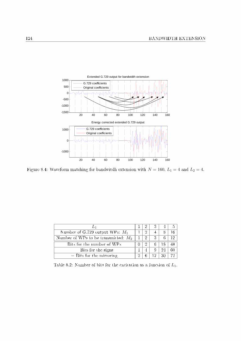
124 BANDWIDTH EXTENSION
20 40 60 80 100 120 140 160-1500
-1000
-500
0
500
1000Extended G.729 output for bandwidth extension
20 40 60 80 100 120 140 160
-1000
0
1000
Energy corrected extended G.729 output
G.729 coefficients
Original coefficients
G.729 coefficients
Original coefficients
Figure 8.4: Waveform matching for bandwitdh extension with N = 160, L1 = 4 and L2 = 4.
L1 1 2 3 4 5Number of G.729 output WPs: M1 1 2 4 8 16
Number of WPs to be transmitted: M2 1 2 3 6 12
Bits for the number of WPs 0 2 6 18 48+ Bits for the signs 1 4 9 24 60
+ Bits for the mirroring 2 6 12 30 72
Table 8.2: Number of bits for the excitation as a function of L1.
8.4. BANDWIDTH EXTENSION IN TIME-FREQUENCY DOMAIN 125
8.4.1.3 Spectral translation
Another approach was to consider the excitation as the combination of a voiced contribution(tonal excitation) excv and an unvoiced contribution excuv, like it is done in CELP coder forinstance with an adaptive and innovation codevector. The global excitation is given by:
WPD [s16kHz, 1](
N
2+ n
)= gvexcv(n) + guvexcuv(n), ∀n ∈
{0, . . . ,
N
2− 1}
(8.5)
with the relation g2v + g2
uv = 1. The gain gv is computed as in [ITU-T 2006a].
ξ =
E2p
E2c
1 + Ep
Ec
(8.6)
g′v =
√ξ
1 + ξ(8.7)
gv =
√12(g′2v + g′2v,old) (8.8)
where g′v,old is the value of g′v at the previous frame. Ec and Ep represent the energy of
the �xed codevector and the adaptive codevector from the G.729, Ec = g2c
∑39i=0 c2(i) and
Ep = g2p
∑39i=0 v2(i). ξ represents the voicing degree of the current speech subframe. The
higher this factor, the more voiced the frame. The equation (8.7) converts this voicing factorto a gain between 0 and 1. This approach has the advantage of avoiding a hard decisionbetween voiced segment and unvoiced segment. The �nal gain is given by the equation (8.8)that ensures smooth transition between subframes. Afterwards, the �nal excitation is obtainedby linear combination of an unvoiced excitation and a voiced excitation weighted by the gainsguv and gv respectively. The unvoiced contribution is generated by a pseudo noise generatorwith a Gaussian distribution.
The crucial point here is to regenerate the harmonic structure present in strong voicedsegments. A straightforward method is the utilization of G.729 the adaptive codeword v(n)as voiced contribution. This ensures the reproduction of the harmonics in the band 4 kHz - 8kHz.
Fig. 8.5 represents the harmonic structure of the original signal, f0 is the fundamentaland n0f0 the �rst harmonic beyond 4 kHz. The dashed lines depict the harmonic structureestimated by the adaptive codeword only. It is equivalent to translate the harmonic structureof the G.729 output above 4 kHz. As shown in Fig. 8.5, it often happens that regeneratedharmonics do not coincide with the original ones. In this case, the regenerated harmonics canbe shifted by multiplying the excitation with a modulation function. The analytic signal xa ofa real-valued signal is given by:
xa(n) = x(n) + ıH (x) (n) (8.9)
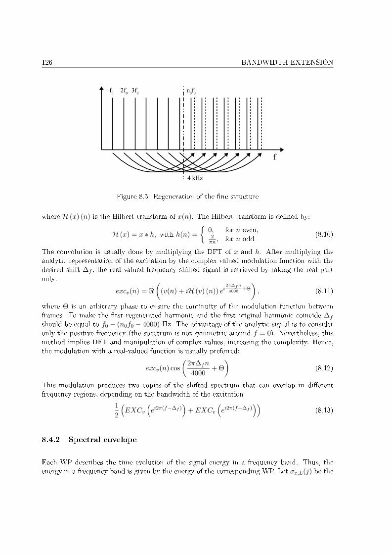
126 BANDWIDTH EXTENSION
Figure 8.5: Regeneration of the �ne structure
where H (x) (n) is the Hilbert transform of x(n). The Hilbert transform is de�ned by:
H (x) = x ∗ h, with h(n) ={
0, for n even,2
πn , for n odd(8.10)
The convolution is usually done by multiplying the DFT of x and h. After multiplying theanalytic representation of the excitation by the complex valued modulation function with thedesired shift ∆f , the real valued frequency shifted signal is retrieved by taking the real partonly:
excv(n) = <(
(v(n) + ıH (v) (n)) eı2π∆f n
4000+Θ
), (8.11)
where Θ is an arbitrary phase to ensure the continuity of the modulation function betweenframes. To make the �rst regenerated harmonic and the �rst original harmonic coincide ∆f
should be equal to f0 − (n0f0 − 4000) Hz. The advantage of the analytic signal is to consideronly the positive frequency (the spectrum is not symmetric around f = 0). Nevertheless, thismethod implies DFT and manipulation of complex values, increasing the complexity. Hence,the modulation with a real-valued function is usually preferred:
excv(n) cos(
2π∆fn
4000+ Θ
)(8.12)
This modulation produces two copies of the shifted spectrum that can overlap in di�erentfrequency regions, depending on the bandwidth of the excitation
12
(EXCv
(eı2π(f−∆f )
)+ EXCv
(eı2π(f+∆f )
))(8.13)
8.4.2 Spectral envelope
Each WP describes the time evolution of the signal energy in a frequency band. Thus, theenergy in a frequency band is given by the energy of the corresponding WP. Let σx,L(j) be the
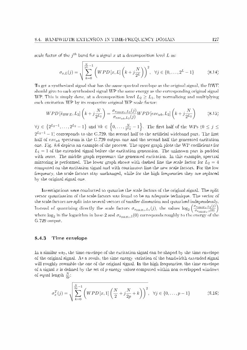
8.4. BANDWIDTH EXTENSION IN TIME-FREQUENCY DOMAIN 127
scale factor of the jth band for a signal x at a decomposition level L as:
σx,L(j) =
√√√√√ N
2L−1∑k=0
(WPD [x, L]
(k + j
N
2L
))2
, ∀j ∈ {0, . . . , 2L − 1} (8.14)
To get a synthesized signal that has the same spectral envelope as the original signal, the BWEshould give to each synthesized signal WP the same energy as the corresponding original signalWP. This is simply done, at a decomposition level L2 ≥ L1, by normalizing and multiplyingeach excitation WP by its respective original WP scale factor:
WPD [sBWE , L2](
k + jN
2L2
)=
σs16kHz ,L2(j)σexcwb,L2(j)
WPD [excwb, L2](
k + jN
2L2
)(8.15)
∀j ∈{2L2−1, . . . , 2L2 − 1
}and ∀k ∈
{0, . . . , N
2L2− 1}. The �rst half of the WPs (0 ≤ j ≤
2L2−1 − 1) corresponds to the G.729, the second half to the arti�cial wideband part. The �rsthalf of excwb spectrum is the G.729 output one and the second half the generated excitationone. Fig. 8.6 depicts an example of the process. The upper graph plots the WP coe�cients forL1 = 1 of the extended signal before the excitation generation. The unknown part is paddedwith zeros. The middle graph represents the generated excitation. In this example, spectralmirroring is performed. The lower graph shows with dashed line the scale factor for L2 = 4computed on the excitation signal and with continuous line the new scale factors. For the lowfrequency, the scale factors stay unchanged, while for the high frequencies they are replacedby the original signal one.
Investigations were conducted to quantize the scale factors of the original signal. The splitvector quantization of the scale factors was found to be an adequate technique. The vector ofthe scale factors are split into several vectors of smaller dimension and quantized independently.
Instead of quantizing directly the scale factors σs16kHz ,L1(j), the values log2
(σs16kHz,L2
(j)
σs16kHz,1(0)
)where log2 in the logarithm in base 2 and σs16kHz ,1(0) corresponds roughly to the energy of theG.729 output.
8.4.3 Time envelope
In a similar way, the time envelope of the excitation signal can be shaped by the time envelopeof the original signal. As a result, the time energy variation of the bandwidth extended signalwill roughly resemble the one of the original signal. In the high frequencies, the time envelopeof a signal x is de�ned by the set of p energy values computed within non overlapped windowsof equal length N
2p :
σTx (j) =
√√√√√N2p−1∑
k=0
(WPD [x, 1]
(N
2+ j
N
2p+ k
))2
, ∀j ∈ {0, . . . , p− 1} (8.16)
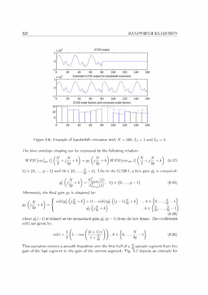
128 BANDWIDTH EXTENSION
0 20 40 60 80 100 120 140 160−1
0
1x 10
4 G729 output
0 20 40 60 80 100 120 140 160−1
0
1x 10
4 Extended G729 output for bandwitdh extension
0 20 40 60 80 100 120 140 160
5
10
15G729 scale factors and corrected scale factors
Figure 8.6: Example of bandwitdh extension with N = 160, L1 = 1 and L2 = 4.
The time envelope shaping can be expressed by the following relation:
WPD[exc′wb, 1
](N
2+ j
N
2p+ k
)= gT
(jN
2p+ k
)WPD [excwb, 1]
(N
2+ j
N
2p+ k
)(8.17)
∀j ∈ {0, . . . , p− 1} and ∀k ∈ {0, . . . , N2p − 1}. Like in the G.729.1, a �rst gain g′T is computed:
g′T
(jN
2p+ k
)=
σTs16kHz
(j)σT
excwb(j)
, ∀j ∈ {0, . . . , p− 1} (8.18)
Afterwards, the �nal gain gT is obtained by:
gT
(jN
2p+ k
)=
α(k)g′T(j N
2p + k)
+ (1− α(k))g′T((j − 1) N
2p + k)
, k ∈{
0, . . . , N4p − 1
}g′T
(j N
2p + k)
, k ∈{
N4p , . . . , N
2p − 1}
(8.19)where g′T (−1) is de�ned as the memorized gain g′T (p− 1) from the last frame. The coe�cientsα(k) are given by:
α(k) =12
(1− cos
((k + 1) π
1 + N4p
)), k ∈
{0, . . . ,
N
4p− 1}
(8.20)
This operation ensures a smooth transition over the �rst half of a N2p -sample segment from the
gain of the last segment to the gain of the current segment. Fig. 8.7 depicts an example for
8.5. DISCUSSION 129
N = 160 and p = 8. The high frequency channel is divided into 8 segments of 10 samples. The�rst two segments are represented. The gain increases progressively from zero to the value inthe �rst segment. Then it increases to the value in the second segment. The transition areacomprises 5 samples, i.e. half a segment.
1st segment 2nd segment
Figure 8.7: Smoothing of the time envelope.
Like for the spectral envelope, split vector quantization of the values log2
(σT
s16kHz(j)
σs16kHz,1(0)
)has been investigated.
8.5 Discussion
Spectral mirroring is the simplest way to perform an extension of the excitation in BWE.It preserves the harmonic structure of the high frequency bands. A common encounteredproblem is a strong voicing in the highest frequencies towards 8 kHz due to the mirroringof the synthesized low frequencies. As the wavelet coe�cients corresponding to the band 7kHz - 8 kHz are zeroed, this phenomenon is very limited. Another inconvenience can be therupture of the harmonic structure around 4 kHz as the distance between the last harmonic inthe narrowband part and the �rst arti�cial harmonic in the extended part. Conversely, thespectral translation enables to respect the harmonic structure around 4 kHz.
The waveform matching is an interesting idea. For each wavelet, the algorithm tries tomatch the narrowband G.729 WP with the high band original signal ones. The G.729 WPsact as an adaptive codebook. The advantage of this method is to produce a more natural
130 BANDWIDTH EXTENSION
sounding of the synthesized speech at the price of high bitrate. For instance, 30 bits i.e. 3kbit/s are required to transmit the codebook indices for L1 = 4.
The last proposed method is actually inspired from the TDBWE of the G.729.1 [ITU-T2006a]. The excitation is separated in a tonal component and a non tonal component, analo-gously to a CELP coder. The mixture of both components depends highly on the parametersrepresenting the same components in the core coder. Consequently, the wideband excitationis always in adequacy with the quantized narrowband one. In comparison with the two previ-ous methods, this proposal provides the best sounding extended wideband part. The spectraltranslation is done by using the analytic representation, via the Hilbert transform.
The time envelope shaping gives the excitation the time energy variation of the originalsignal. The envelope extraction can be done at the decomposition level L1, on the WP cor-responding to the band [4 - 8 kHz]. The energies are computed on p = 8 non-overlappingwindows. Investigations showed that a split vector quantizer of dimension 4 with two 5 bits-codebooks are e�cient to quantize the time envelope.
In the G.729.1, the frequency envelope extraction is done in the Fourier domain, while theshaping is performed by linear �ltering with a FIR �lter bank in the time domain. Unlikethe TDBWE in the G.729.1, the proposed method has the advantage of using the same �lterbank (i.e. WPD) for the analysis and synthesis. The bandwidth of the signal to be encoded islimited to [.05 kHz-7 kHz]. Consequently, the 8
2L1scale factors corresponding to the frequency
bandwidth [7 kHz-8 kHz] are irrelevant. In the end, the number of scale factor to be quantizedis 2L1−1−2L1−3 (for L1 ≥ 3). Experiments showed that for L1 = 4 and N = 160 (10 ms frame),a split vector quantizer of dimension 3 with two 5 bits-codebooks are e�cient to quantize theneeded scale factors.
Conclusion
The concept of arti�cial bandwidth extension have been introduced. It has been shown that awideband embedded codec takes advantage of such a layer. Throughout this chapter, investi-gated bandwidth extension techniques on top of a CELP codec has been presented. Unlike theTDBWE, representing the state of the art of the bandwidth extension with side information,the encoder and decoder share the same �lter bank (WPD). Indeed, the analysis �lter bankthat extracts the scale factors is also the synthesis �lter bank that shapes the excitation withthe scale factors. No extra bits are required for the excitation, 1 kbit/s is allocated to the timeenvelope, and 1 kbit/s to the spectral envelope. A total of 2 kbit/s is required to transmit therelevant information of the bandwidth extension.
131
Part V
Proposed Coder

133
Chapter 9
Proposed Coder
Introduction
The previous chapters have given the framework for the proposed codec. This chapter presentsthe codec developed during this thesis. The encoder and decoder are described in Sec. 9.1. Thecodec works on a 10 ms frame basis for speech and audio wideband signals at bitrates rangingfrom 8 kbit/s to 32 kbit/s. The structure involves a combination of CELP coding, wavelettransform and bandwidth extension. Sec. 9.2 explains the choice of the wavelet �lter. The split-band structure in Sec. 9.3 provides the input of the core layer, a CELP codec (Sec. 9.4), andof the �rst enhancement layer, a bandwidth extension (Sec. 9.5), providing a wideband outputat 10 kbit/s. The second enhancement layer consists of the wavelet coe�cient quantization.It improves gracefully the synthesized signal as the bitrate increases. Sec. 9.6 investigatesthe embedded quantization with SPIHT. Because of performance, SPIHT was replaced by thealgebraic quantization, described in Sec. 9.7. The last section presents listening tests thatassess the quality of the proposed codec.
9.1 Codec structure
The coder comprises an encoder and a decoder, presented in Sec. 9.1.1 and 9.1.2.
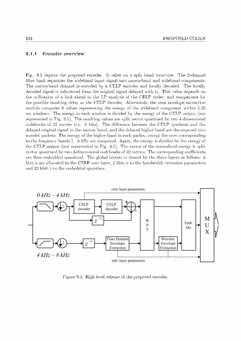
134 PROPOSED CODER
9.1.1 Encoder overview
Fig. 9.1 depicts the proposed encoder. It relies on a split band structure. The 2-channel�lter bank separates the wideband input signal into narrowband and wideband components.The narrowband channel is encoded by a CELP encoder and locally decoded. The locallydecoded signal is subtracted from the original signal delayed with t1. This value depends onthe utilization of a look-ahead in the LP analysis of the CELP codec, and compensate forthe possible resulting delay at the CELP decoder. Afterwards, the time envelope extractionmodule computes 8 values representing the energy of the wideband component within 1.25ms windows. The energy in each window is divided by the energy of the CELP output (notrepresented in Fig. 9.1). The resulting values are split vector quantized by two 4-dimensionalcodebooks of 32 entries (i.e. 5 bits). The di�erence between the CELP synthesis and thedelayed original signal in the narrow band, and the delayed higher band are decomposed intowavelet packets. The energy of the higher band in each packet, except the ones correspondingto the frequency bands 7 - 8 kHz are computed. Again, the energy is divided by the energy ofthe CELP output (not represented in Fig. 9.1). The vector of the normalized energy is splitvector quantized by two 3-dimensional codebooks of 32 entries. The corresponding coe�cientsare then embedded quantized. The global bitrate is shared by the three layers as follows: 8kbit/s are allocated to the CELP core layer, 2 kbit/s to the bandwidth extension parametersand 22 kbit/s to the embedded quantizer.
Figure 9.1: High level scheme of the proposed encoder.
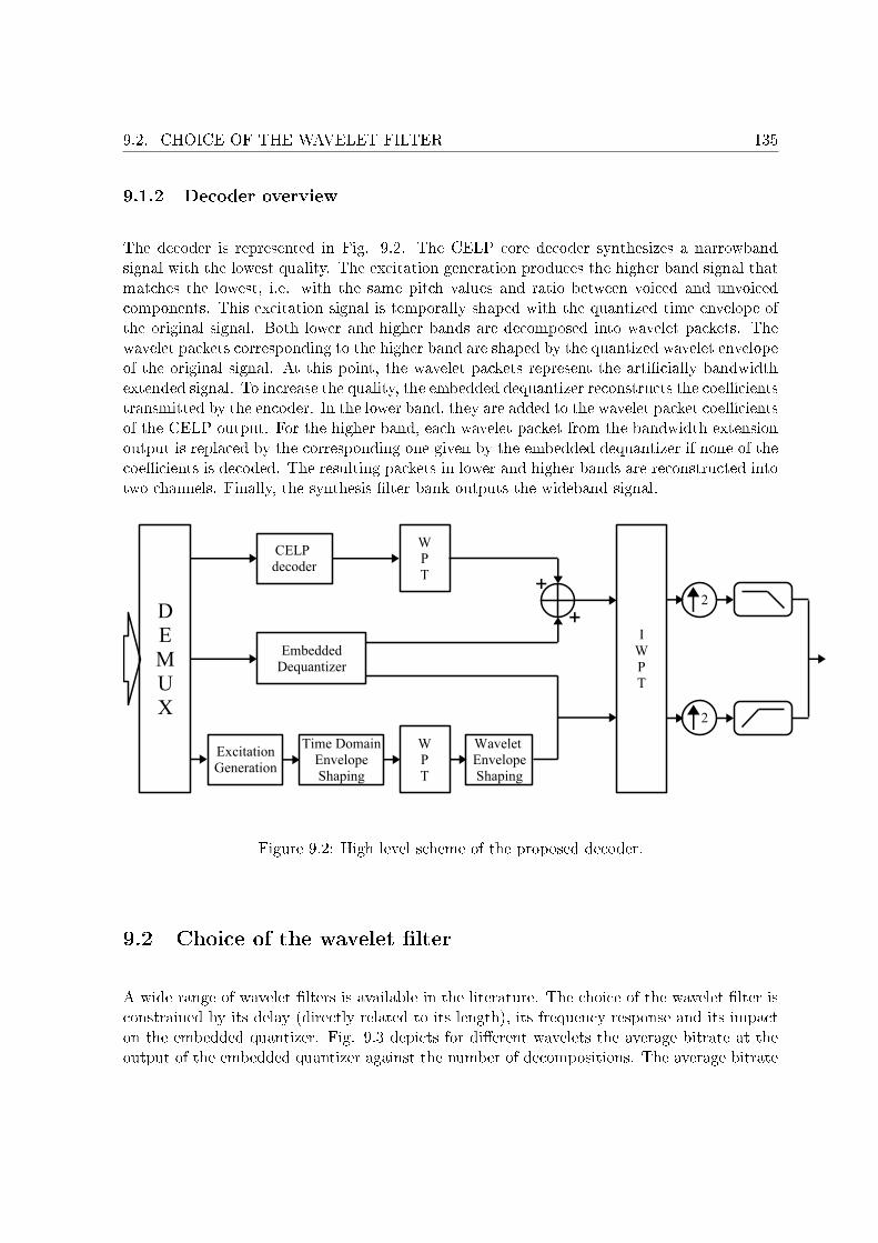
9.2. CHOICE OF THE WAVELET FILTER 135
9.1.2 Decoder overview
The decoder is represented in Fig. 9.2. The CELP core decoder synthesizes a narrowbandsignal with the lowest quality. The excitation generation produces the higher band signal thatmatches the lowest, i.e. with the same pitch values and ratio between voiced and unvoicedcomponents. This excitation signal is temporally shaped with the quantized time envelope ofthe original signal. Both lower and higher bands are decomposed into wavelet packets. Thewavelet packets corresponding to the higher band are shaped by the quantized wavelet envelopeof the original signal. At this point, the wavelet packets represent the arti�cially bandwidthextended signal. To increase the quality, the embedded dequantizer reconstructs the coe�cientstransmitted by the encoder. In the lower band, they are added to the wavelet packet coe�cientsof the CELP output. For the higher band, each wavelet packet from the bandwidth extensionoutput is replaced by the corresponding one given by the embedded dequantizer if none of thecoe�cients is decoded. The resulting packets in lower and higher bands are reconstructed intotwo channels. Finally, the synthesis �lter bank outputs the wideband signal.
Figure 9.2: High level scheme of the proposed decoder.
9.2 Choice of the wavelet �lter
A wide range of wavelet �lters is available in the literature. The choice of the wavelet �lter isconstrained by its delay (directly related to its length), its frequency response and its impacton the embedded quantizer. Fig. 9.3 depicts for di�erent wavelets the average bitrate at theoutput of the embedded quantizer against the number of decompositions. The average bitrate
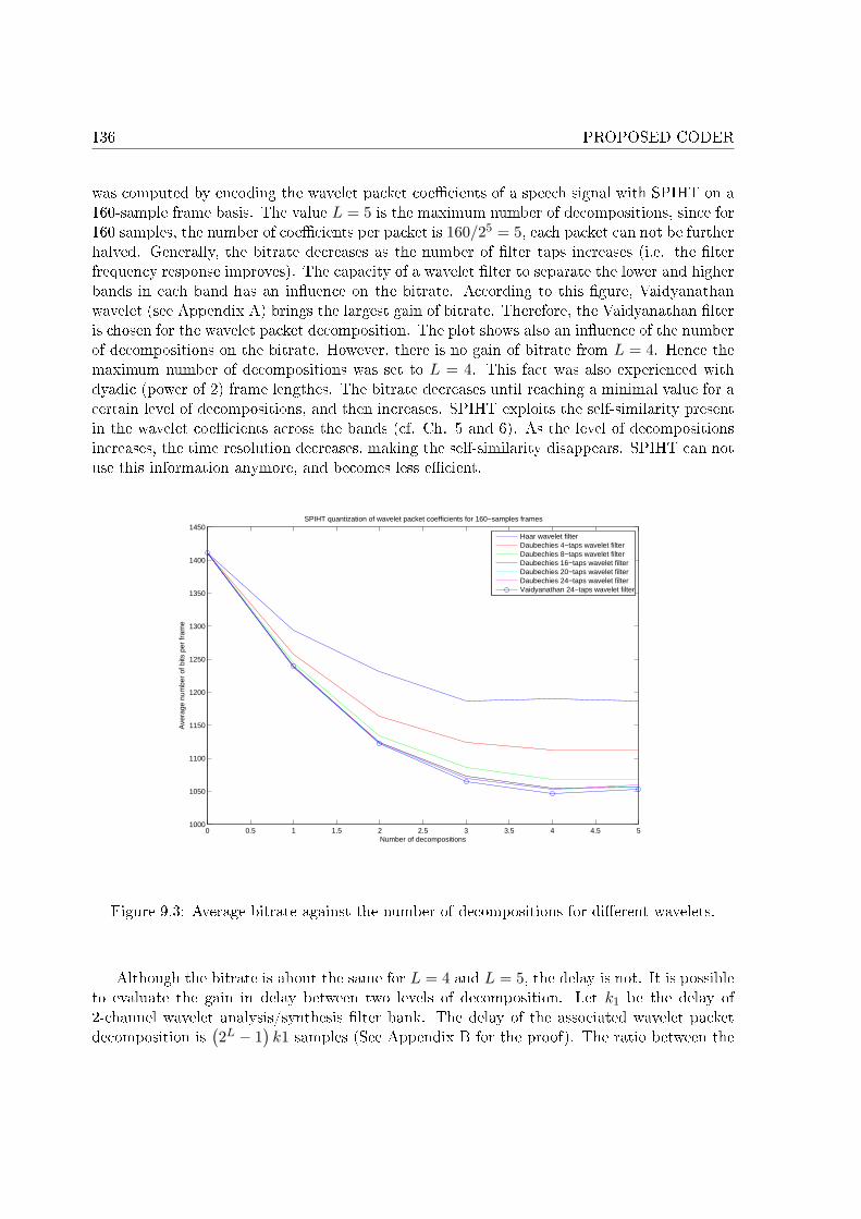
136 PROPOSED CODER
was computed by encoding the wavelet packet coe�cients of a speech signal with SPIHT on a160-sample frame basis. The value L = 5 is the maximum number of decompositions, since for160 samples, the number of coe�cients per packet is 160/25 = 5, each packet can not be furtherhalved. Generally, the bitrate decreases as the number of �lter taps increases (i.e. the �lterfrequency response improves). The capacity of a wavelet �lter to separate the lower and higherbands in each band has an in�uence on the bitrate. According to this �gure, Vaidyanathanwavelet (see Appendix A) brings the largest gain of bitrate. Therefore, the Vaidyanathan �lteris chosen for the wavelet packet decomposition. The plot shows also an in�uence of the numberof decompositions on the bitrate. However, there is no gain of bitrate from L = 4. Hence themaximum number of decompositions was set to L = 4. This fact was also experienced withdyadic (power of 2) frame lengthes. The bitrate decreases until reaching a minimal value for acertain level of decompositions, and then increases. SPIHT exploits the self-similarity presentin the wavelet coe�cients across the bands (cf. Ch. 5 and 6). As the level of decompositionsincreases, the time resolution decreases, making the self-similarity disappears. SPIHT can notuse this information anymore, and becomes less e�cient.
0 0.5 1 1.5 2 2.5 3 3.5 4 4.5 51000
1050
1100
1150
1200
1250
1300
1350
1400
1450
Number of decompositions
Ave
rage
num
ber
of b
its p
er fr
ame
SPIHT quantization of wavelet packet coefficients for 160−samples frames
Haar wavelet filterDaubechies 4−taps wavelet filterDaubechies 8−taps wavelet filterDaubechies 16−taps wavelet filterDaubechies 20−taps wavelet filterDaubechies 24−taps wavelet filterVaidyanathan 24−taps wavelet filter
Figure 9.3: Average bitrate against the number of decompositions for di�erent wavelets.
Although the bitrate is about the same for L = 4 and L = 5, the delay is not. It is possibleto evaluate the gain in delay between two levels of decomposition. Let k1 be the delay of2-channel wavelet analysis/synthesis �lter bank. The delay of the associated wavelet packetdecomposition is
(2L − 1
)k1 samples (See Appendix B for the proof). The ratio between the
9.3. THE SPLIT BAND STRUCTURE 137
delay for L + 1 and L is given by:2L+1 − 12L − 1
(9.1)
The numerator can be bounded by 2L+1 − 2. The ratio is then bounded by:
2L+1 − 12L − 1
>2(2L − 1
)2L − 1
2L+1 − 12L − 1
> 2 (9.2)
(9.3)
The ratio between the delay for L + 1 and L is greater than 2. Consequently, the delay isroughly halved between L + 1 and L. The delay introduced by the decomposition with theVaidyanathan (k1 = 24− 2) wavelet �lters for L = 4, is 330 samples, that is 20.625 ms.
9.3 The split band structure
The split band structure separates the narrowband and wideband components. The nar-rowband component is encoded by the core layer and the wideband component is analyzedto extract the bandwidth extension parameter. Both components are then decomposed intowavelet packet. A 2-channel �lter bank implements the split band structure. This role was�rst played by the wavelet packet decomposition. Indeed, the �rst stage split the input signalinto two components. Parameters of the core and �rst enhancement layers are computed, thenthe wavelet packet decomposition is further performed. The �lter characteristics do not havea real in�uence on the quality of the lower band reconstruction. However, informal listen-ing tests showed that the frequency response of the 2-channel �lter bank has an impact onthe subjective quality of the bandwidth extension. The wavelet packet decomposition ensuresperfect reconstruction as long as the coe�cients are not modi�ed (by quantization or otherdistortions). In fact, the aliasing e�ect is canceled at the reconstruction. Unfortunately, whenthe coe�cients are poorly quantized or highly distorted, the aliasing is far to be canceled.This actually happens with the bandwidth extension, as the higher band �ne structure is esti-mated from the quantized lower band and the original time and frequency envelope are vectorquantized.
In order to minimize the aliasing e�ect, the split band structure is performed by the John-ston 64-tap QMF �lter bank [Johnston 1980] (cf. Appendix A). In Fig. 9.4 the �rst stage of thewavelet packet decomposition has been replaced by a 2-channel QMF �lter bank. The QMFhas a strong impact on the average bitrate when used with a short wavelet. Conversely, theimpact is little when combined with longer wavelet �lters. If the delay of the 2-channel QMF�lter bank is k2, then the delay of the new structure for L decompositions is 2
(2L−1 − 1
)k1+k2
samples (c.f. Appendix B). Hence the delay is increased by k2− k1 samples. For the Johnston
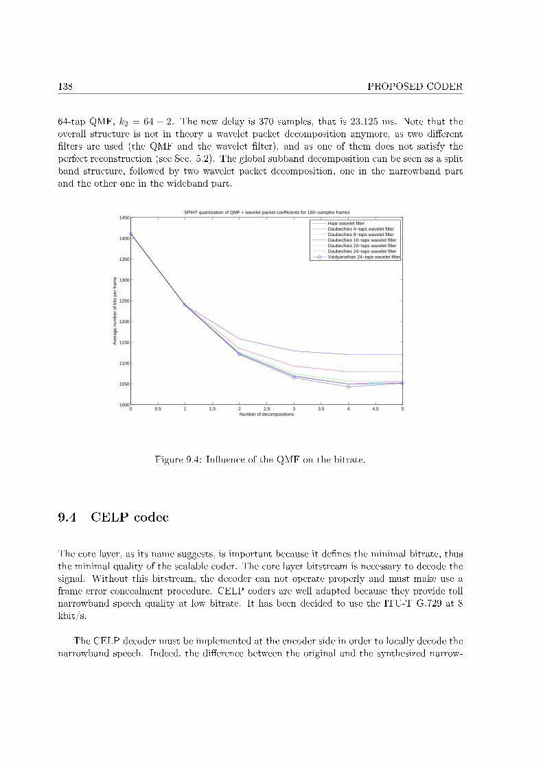
138 PROPOSED CODER
64-tap QMF, k2 = 64 − 2. The new delay is 370 samples, that is 23.125 ms. Note that theoverall structure is not in theory a wavelet packet decomposition anymore, as two di�erent�lters are used (the QMF and the wavelet �lter), and as one of them does not satisfy theperfect reconstruction (see Sec. 5.2). The global subband decomposition can be seen as a splitband structure, followed by two wavelet packet decomposition, one in the narrowband partand the other one in the wideband part.
0 0.5 1 1.5 2 2.5 3 3.5 4 4.5 51000
1050
1100
1150
1200
1250
1300
1350
1400
1450
Number of decompositions
Ave
rage
num
ber
of b
its p
er fr
ame
SPIHT quantization of QMF + wavelet packet coefficients for 160−samples frames
Haar wavelet filterDaubechies 4−taps wavelet filterDaubechies 8−taps wavelet filterDaubechies 16−taps wavelet filterDaubechies 20−taps wavelet filterDaubechies 24−taps wavelet filterVaidyanathan 24−taps wavelet filter
Figure 9.4: In�uence of the QMF on the bitrate.
9.4 CELP codec
The core layer, as its name suggests, is important because it de�nes the minimal bitrate, thusthe minimal quality of the scalable coder. The core layer bitstream is necessary to decode thesignal. Without this bitstream, the decoder can not operate properly and must make use aframe error concealment procedure. CELP coders are well adapted because they provide tollnarrowband speech quality at low bitrate. It has been decided to use the ITU-T G.729 at 8kbit/s.
The CELP decoder must be implemented at the encoder side in order to locally decode thenarrowband speech. Indeed, the di�erence between the original and the synthesized narrow-
9.5. BANDWIDTH EXTENSION 139
band component is decomposed into wavelet packets, encoded and transmitted as enhancementlayer. For some CELP codecs, due to LPC look-ahead, the output might be delayed by t1. Ifnecessary, the original signal must be delayed in order to time-aligned with the CELP output.The look-ahead used in the G.729 cause a delay t1 = 5 ms.
Utilization of a CELP based enhancement layer like in the G.729.1, on top of the G.729A,has been investigated (cf. Ch. 4). In a �rst step, the innovation codeword is modi�ed insuch a way that each pulse is multiplied by an individual gain. The quantization of the gainsrequires 1.6 kbit/s. Then, a second �xed codeword at 2.4 kbit/s is added. The resultingstructure 8/9.6/12 kbit/s was compared to a reference structure 8/12 kbit/s, achieved by asecond �xed codebook. The reference structure performed slightly better than the proposedstructure. Nonetheless, this kind of structure was not integrated to the proposed coder for tworeasons. Informal listening tests showed that the bitrate allocated to a CELP enhancementlayer does not work better as when allocated to the wavelet coe�cient quantizer. Moreover, bykeeping the bitrate of the CELP codec low, wideband rendering is enabled as soon as possible.The core coder is �nally chosen as the G.729 main body, more complex than the G.729A butwith better quality.
To enhance the quality of the synthesized signal in the narrowband part (CELP output plusthe decoded wavelet packet coe�cients), the adaptive post�ltering of the G.729 is also used(cf. Ch. 3). However, it is necessary to modify the original implementation. Indeed, due to the�lter bank, the synthesis signal after the wavelet packet reconstruction is delayed comparedto the CELP output. The adaptive post�lter needs the pitch lag and the LP synthesis �lterthat have contributed to the CELP synthesis before the wavelet packet decomposition. Theseparameters have to be stored in bu�ers at the CELP synthesis and will be used by the adaptivepost�lter after the wavelet packet reconstruction a few subframes later. This delay expressed
in number of subframes is 2 +⌊
12 + 2L−1k1
40
⌋, where the operator b.c takes the integer part.
9.5 Bandwidth extension
The bandwidth extension is the �rst enhancement layer. With additional 2 kbit/s, it producesarti�cially the wideband component at a bitrate of 10 kbit/s. To do so, the time envelopeand frequency envelope are extracted from the delayed original signal. The high frequencypart at the output of the split band structure is divided into 8 non-overlapped windows. Theenergy within each window is normalized by the energy of the CELP coder output. The set ofnormalized energies are split vector quantized with two 32-entry 4-dimensional codebooks. Itrequires 10 bits per frame, that is 1 kbit/s. After the wavelet packet transform, the energy ofeach high frequency wavelet packet is also normalized by the energy of the CELP coder output.The set of normalized energies are split vector quantized with two 32-entry 3-dimensionalcodebooks. The vector quantizers are allocated 10 bits per frame, i.e. 1 kbit/s. The excitationgeneration mimics the �ne structure of the higher frequency part. The adaptive excitation
140 PROPOSED CODER
from the CELP coder reproduces this �ne structure. Its analytic representation (via an Hilberttransform) is modulated in order to mimic the harmonic structure. This excitation is �nallylinearly combined with a pseudo-random noise. Both the adaptive excitation and the pseudonoise are multiplied by their corresponding gains. The gains depend on the ratio between theCELP adaptive excitation energy and algebraic codebook energy, and on one another (cf. Ch.8). In the case of voiced frames, the adaptive excitation is clearly favored because its gainis closed to 1. Conversely, the pseudo-noise is favored for unvoiced frames. Afterwards, theexcitation is shaped by the quantized time envelope of the original signal. After the waveletpacket decomposition, the wideband part wavelet packets from the excitation generation areshaped by the quantized frequency envelope of the original signal. At bitrates above 10 kbit/s,the non-decoded packets are replaced by the corresponding arti�cially generated packet.
9.6 Embedded quantization of the wavelet coe�cients
The second and last enhancement layer relies on the progressive transmission of the waveletcoe�cients. It should enhance the synthesized signal as the bitrate increases. The �rst inves-tigated strategy was bit-plane coding (see Ch. 6). Bit-plane coding algorithms like EZW andSPIHT are widely used in image coding to ensure a progressive transmission of the waveletcoe�cients. It is naturally that both algorithms have been considered. It turned out thatSPIHT outperforms EZW in term of compression e�ciency and complexity.
The strength of SPIHT is to be found in the way it partitions the coe�cients in set ofsigni�cant and insigni�cant coe�cients with the respect to a threshold. The partitions arefurther re�ned as the threshold decreases. To do so, the coe�cients are organized in treeswherein the coe�cients depend on one another through the so-called parent-child relation.The tree structure is de�ned by two parameters:
• the number of roots: the number of coe�cients that do not depend on other coe�cients(they do not have ascendant)
• the number of children: the number of children per coe�cient.
The term root does not take into account the coe�cients that do not have either parent orchild. Those coe�cients come from the lowest frequency band. It is assumed that there are asmany roots as coe�cients without child. Sec. 9.6 describes how the values of the parametersare chosen in order to optimize SPIHT performance.
Yet, SPIHT has shown limits. Albeit the high scalability of its bitstream, the codingperformances are not as good as expected. Too few coe�cients are encoded. Also, except thefact that the most signi�cant bits of the most signi�cant coe�cients are transmitted �rst, it is
9.6. EMBEDDED QUANTIZATION OF THE WAVELET COEFFICIENTS 141
not possible to know explicitely where the bits are allocated. These problems are described inSec. 9.6.2.
Since SPIHT does not achieve the transmission of all coe�cients, solutions to reduce thenumber of coe�cients to be transmitted were investigated. They consist in selecting the waveletpackets according to a distortion criterion. In a �rst approach, the number of wavelet packetsto be transmitted was constant. The second approach computes the number of packets frameby frame. Both approaches are presented in Sec. 9.6.3.
9.6.1 Optimization of embedded quantizer parameters
There is no single tree structure for organizing the coe�cients. For example, the number ofchildren per coe�cient is set to 2 in [Lu et al. 2000] and [Lu, Pearlman 1999] with a wavelettransform or to 4 in [Raad et al. 2002] with a MDCT. Like the choice of the wavelet �lter hasan in�uence on SPIHT performance (cf. Sec. 9.2), the number of roots and the number ofcoe�cients may also a�ect the bitrate. To obtain the best possible bitrate, it is important tochoose carefully these parameters.
Statistical analysis has been conducted in order to determine the optimal value of theparameters. Fig. 9.5 and 9.6 plot the average bitrate per frame against the number n ofchildren per coe�cients and the number of roots r. The average bitrate was computed byencoding the wavelet packet coe�cients of the whole french part of the NTT-AT database ona 160-samples frame basis with SPIHT. Roots refer only to coe�cients without parents andwith children. Note there are always as many roots as coe�cients without parent and child.It is interesting to remark that the graphs for L = 4 and L = 5 are similar, the average bitrateis about the same for the same con�gurations. This con�rms the choice of L = 4.
The worst results are obtained with only one child. It is very unlikely that there areinsigni�cant sets comprising a lot of coe�cients. SPIHT spends most of the bits where thesigni�cant coe�cients are among the insigni�cant ones. The average bitrate decreases by 200bits when the number of children increases by one. It is more likely to get sets of insigni�cantcoe�cients. The average bitrate decreases a bit until n = 5 and then increases. In the area1 ≤ r ≤ 10, 1 ≤ c ≤ 10, the di�erence between the highest lowest value is about 50 bits.
The minimum is reached at r = 5 and n = 5. Those numbers are to be put in relation withthe number of coe�cients in a wavelet packet. There are 10 coe�cients (resp. 5) per packetfor L = 4 (resp. L = 5). In average, the coe�cients in a packet are of about the same energy.If a coe�cient in a packet is insigni�cant, it is very likely that all the coe�cients in the packetare insigni�cant. One bit can represent more insigni�cant coe�cients in the sorting pass andconsequently reduces the bitrate.
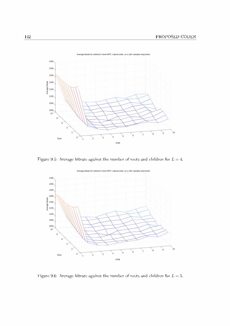
142 PROPOSED CODER
1 2 3 4 5 6 7 8 9 10
0
2
4
6
8
10
1000
1050
1100
1150
1200
1250
1300
1350
Child
Average bitrate for ordered 4−level WPT, natural order, on a 160−samples long frame
Root
Ave
rage
bitr
ate
Figure 9.5: Average bitrate against the number of roots and children for L = 4.
1 2 3 4 5 6 7 8 9 10
0
2
4
6
8
10
1000
1050
1100
1150
1200
1250
1300
1350
1400
Child
Average bitrate for ordered 5−level WPT, natural order, on a 160−samples long frame
Root
Ave
rage
bitr
ate
Figure 9.6: Average bitrate against the number of roots and children for L = 5.
9.6. EMBEDDED QUANTIZATION OF THE WAVELET COEFFICIENTS 143
9.6.2 SPIHT limitations
A bit allocation module is commonly used in speech and audio coders. It is in charge ofallocating bits to quantize a group of coe�cients. The more bits allocated, the better thequantization of the coe�cients. Mostly, the bit allocation is driven by a psychoacoustic model.By taking into account the masking properties of the human ear, it is possible to determinefor each group of coe�cients the maximum level of inaudible quantization noise. According tothese values, the bit allocation tries to distribute the available bits in order to minimize thelevel of the audible quantization noise. SPIHT does not make use of any explicit bit allocation,it is rather implicit. It is impossible to know a priori the amount of bits allocated to a groupof coe�cients.
SPIHT was designed to quantize integers in a lossless way. However for the target bitrate(i.e. 32 kbit/s), the values of the decoded coe�cients are far from the original values. Also, thepart of the non-encoded coe�cients is important. SPIHT focuses on reducing the distortionbetween the original and the encoded values by quantizing the most signi�cant coe�cients �rst(i.e. the biggest absolute values). Then, with the bitrate of 32 kbit/s, it often occurs that somebands are not encoded at all. In the low band, the corresponding wavelet packets are given bythe G.729 output only, since the re�nement contribution is zero. In the high band, since theoriginal signal is directly quantized (via the wavelet packets), the spectrum of the synthesizedsignal might show gaps. To �ll up those gaps, the missing wavelet packets are replaced by thecorresponding wavelet packets from the bandwidth extension.
9.6.3 Pseudo bit allocation
As it is not possible to retrieve information from the bitstream about all the coe�cients at32 kbit/s, a way to transmit only a part of the coe�cients has been investigated. First, thenumber of bands to be transmitted should be estimated. Then, the packets to be transmittedare selected according to a criterion. Let w(i) and wBWE(i), with i ∈ {0, . . . , 139} be thecoe�cients of the original signal and the 10 kbit/s output. The energy of their di�erence ineach packet is computed:
eq(k) =9∑
j=0
(w(10k + j)− wBWE(10k + j))2 , with k ∈ {0, . . . , 13} (9.4)
The values are normalized by the sum of the energy to get values ranging from 0 to 1:
eqN (k) =eq(k)∑13
k′=0 eq(k′), with k ∈ {0, . . . , 13} (9.5)
The value eqN (k) indicates how good the band k is quantized by the bandwidth extensionrelatively to the other bands. A value close to 1 means that the coe�cients decoded at 10
144 PROPOSED CODER
kbit/s are far from the original ones, i.e. the packet is badly quantized (either by the G.729 orby the bandwidth extension) compared to the other wavelet packets. Conversely, values closeto 0 imply a good quantization of the corresponding packets. If all the value are roughly equalto 1
14 , the distortion is the same across the wavelet packets.
The �rst approach attempts to go beyond SPIHT limitations as follows. In order to reducethe overall distortion as much as possible, the wavelet packets that are the worst rendered(with high "quantization coe�cients" eq(k)) at 10 kbit/s are transmitted in priority. It wasalso decided to always transmit the packets corresponding to the bands 0− .5 kHz and 3.5− 4kHz since the G.729 performs slightly worse in those areas. To some extent, the bits are onlyallocated to the packets of interest. The number of transmitted wavelet packets is 8. Informallistening tests showed that the high bands are globally better quantized and sounds less noisy.However, the quality in the low frequencies is sometimes degraded.
In a second approach, the number of bands are dynamically computed on a frame basis.To do so, the spectral �atness of the "quantization coe�cients", i.e. the ratio between theirgeometric mean and their arithmetic mean, is computed:
sf =14 14
√∏13k=0 eqN (k)∑13
k=0 eqN (k)(9.6)
The spectral �atness is bounded between 0 and 1. High values mean that the "quantizationcoe�cients" are about the same across the packets, they are of equal importance. On thecontrary, values close to 0 indicate that a few packets needs to be improved. The number ofbands depends linearly on the spectral �atness measure. Informal listening tests does not showany signi�cant improvements with the respect to the �rst approach.
Both approaches select a few packets to be transmitted, based on a distortion measure.The �rst one always transmits a constant number of bands, the second one computes thenumber of bands on a frame basis. However none of them brings signi�cant improvement tothe quality. It seems di�cult to increase noticeably the performance of SPIHT. Consequently,another form of quantization of the coe�cients has been investigated. Although less scalable,it improves the listening experience.
9.7 Algebraic quantization
SPIHT enables very �ne scalability in the decoding of the coe�cients. However this highscalability appears to become a drawback for the targeted bitrates. Progressive quantizationis achieved by coding successively the bit-planes from the most signi�cant one to the lesssigni�cant one. It ensures the perfect reconstruction of integer coe�cients. However, perfectreconstruction is hardly feasible for the targeted bit rate. In order to transmit more coe�cients,SPIHT should be replaced by a coarser quantization.
9.7. ALGEBRAIC QUANTIZATION 145
The proposed quantization is inspired by the algebraic codebook search in ACELP coding.In ACELP coding, the innovation is only quantized with a few pulses, multiplied by a gain. Thepulse positions are determined with a AbS scheme by minimizing an error criterion. Similarly,the wavelet coe�cients worth to be transmitted are selected and coded by an amplitude andtheir sign. Only one amplitude is transmitted per packet. The coe�cients within a waveletpacket are transmitted progressively, so that only a part of the coe�cients can be decoded.Sec. 9.7.1 presents the principles of the method, illustrated by two examples in Sec. 9.7.2 andSec. 9.7.3. The sending order of the wavelet packets is discussed in Sec. 9.7.4 and Sec. 9.7.5.
9.7.1 Principles
Let x(i), i ∈ {0, . . . , N − 1} be the coe�cients to be quantized, N is the number of coe�cientsper frame. In the general case, the input coe�cients are divided into M subbands. A subbandk comprises Nk coe�cients, such that
∑M−1k=0 Nk = N . The �rst coe�cient of the subband k
is noted b(k). For example, b(0) = 0, b(1) = N0, b(2) = N0 + N1, b(M − 1) =∑M−2
k=0 Nk, andby default, b(M) = N . The coe�cient within a band k is indexed by j. The coe�cient at theposition j in the band k has the position b(k) + j in the frame.
It has been seen in Ch. 6 that the transmission of the biggest coe�cients reduces at mostthe mean square error between the original and the reconstructed coe�cients. In this sense,the most signi�cant coe�cients are the biggest ones. It is surely important to quantize thosecoe�cients, but not as precisely as with SPIHT, in order to allocate bits to more coe�cients.The following model has been investigated to quantize the coe�cients. In a band k, thecoe�cients are estimated by:
x(b(k) + j) = mkc(b(k) + j), j ∈ {0, . . . , Nk − 1}, (9.7)
where c(b(k) + j) = ±1 or 0, and mk > 0. If c(b(k) + j) 6= 0, it is called a pulse. The valuemk is the pulses amplitude. The coe�cients are estimated by multiplying the pulses with theamplitude. In the band k, the encoder has to determine how many pulses must be sent, theirposition, their sign, and which value mk is given. Since the estimated coe�cients are meant tobe as close as possible to the original values, their signs should be at least given by the signs oftheir respective original coe�cients, i.e. c(b(k) + j)x(b(k) + j) ≥ 0, with ∀k ∈ {0, . . . ,M − 1}and ∀j ∈ {0, . . . , Nk − 1}.
9.7.2 Comparison with a threshold
The �rst attempt has been to compute the amplitude �rst, and to select the coe�cients to betransmitted accordingly. The amplitude is given by:
mk =
∑Nk−1j=0 |x(b(k) + j)|
Nk(9.8)
146 PROPOSED CODER
i.e. the mean of the coe�cient absolute values. Afterwards, the following rule is applied todetermine how many pulses should be transmitted:
c(b(k) + j) =
1, if x(b(k) + j) ≥ mk
−1, if x(b(k) + j) < −mk
0, else(9.9)
As a result, the most important coe�cients in a band are selected by comparing with a thresh-old. The number of pulses is controlled by the value of mk. An increase of mk would decreasethe number of pulses. Conversely, a decrease would increase the number of pulses. The maindrawback of this method is the computation of the amplitude prior to the pulse selection pro-cedure. The absolute value of the selected coe�cients is always bigger than mk. Consequently,the energy of the estimated coe�cients is lower than the one of the original coe�cients. To takethis bias into account, the coe�cients are multiplied by
√2. This value has been determined
empirically.
9.7.3 Minimization of an error criterion
In the previous approach, the most signi�cant coe�cients are selected without any measureof their in�uence on the distortion. Moreover, the amplitude mk does not re�ect directly theenergy of the original coe�cients. A new attempt tried to unify the determination of the pulsesand of mk. This is done by minimizing the mean square error between the original and theestimated coe�cients:
ek =Nk−1∑j=0
(x(b(k) + j)−mkc(b(k) + j))2 (9.10)
The optimal value of mk is given by the solution of ∂ek∂mk
= 0, i.e.
mk =
∑Nk−1j=0 (x(b(k) + j)c(b(k) + j))∑Nk−1
j=0 c2(b(k) + j)(9.11)
Replacing mk by this expression in Eq. (9.10) yields:
ek =Nk−1∑j=0
x2(b(k) + j)−
(∑Nk−1j=0 x(b(k) + j)c(b(k) + j)
)2
∑Nk−1j=0 c2(b(k) + j)
(9.12)
Whatever the number of pulses and their position are, the �rst term∑Nk−1
j=0 x2(b(k) + j) isalways constant. Thus the minimization of ek is strictly equivalent to the maximization of theterm dk de�ned by:
dk =
(∑Nk−1j=0 x(b(k) + j)c(b(k) + j)
)2
∑Nk−1j=0 c2(b(k) + j)
(9.13)
9.7. ALGEBRAIC QUANTIZATION 147
At each position, there is either a pulse or no pulse, i.e. two possibilities (the sign is alwaysset as explained previously). The number of possible combinations is then 2Nk . Afterwards,the amplitude mk is computed by Eq. (9.11). The pulse combination that maximizes dk andthe corresponding amplitude mk are sent to the decoder.
For Nk large, the search can become very complex. It is actually not necessary to test allthe combinations. If the search is restricted to �nding the best combination of l pulses amongNk pulses, l < Nk, the number of combinations to be tested is C l
Nk= Nk!
l!(Nk−l)! . The criteriondk becomes:
dlk =
(∑Nk−1j=0 x(b(k) + j)c(b(k) + j)
)2
l(9.14)
For l constant, maximizing the criterion Eq. (9.14) is equivalent to maximizing the numeratorof dl
k. As x(b(k)+j)c(b(k)+j) > 0, with k = 0 . . .M−1 and j = 0, . . . , Nk−1, maximizing the
criterion dlk is equivalent to maximizing
(∑Nk−1j=0 x(b(k) + j)c(b(k) + j)
). A sum of positive
values is maximal when every term of the sum is maximal. Consequently, the criterion dlk is
maximal when the l pulses correspond to the l biggest coe�cient absolute values. The criterionmay only be tested for Nk + 1 combinations (i.e. l = 0, . . . , Nk).
The optimal pulse combination is selected as follows. For l = 0, . . . , Nk, the criterion dlk
is computed according to Eq. (9.14) with the l biggest absolute values (with d0k = 0). The
optimal number lopt is found by maximizing dlk
dlopt
k = arg maxl∈0...Nk
dlk (9.15)
The optimal combination is given by the lopt pulses at the position of the lopt biggest absolutevalues.
This search might be slightly sped up by taking into account the following assumption.The value of the criterion dl
k increases with l until the maximal value dlopt
k is reached, then dlk
decreases. lopt is the �rst value of l such as dlopt
k > dlopt+1k . There exists a recursive relation
between dlk and dl+1
k :
dl+1k =
[√ldl
k + |x(b(k) + jl+1)|]2
l + 1(9.16)
where jl is the index within the band k of the coe�cient with lth biggest absolute value. Anew pulse is added if its contribution increases the criterion. Otherwise dl
k > dl+1k , the search
is stopped, lopt = l. The amplitude mk is computed and sent together with the selected pulsecombination. This assumption proves to be true in about 95% of the cases. The 5% leftcorresponds generally to periods of weak energy like speech pauses.
For each band, the encoding procedure comprises two parts. The �rst one is the selectionof the optimal set of pulses in the sense of the mean square error. Once the pulses position
148 PROPOSED CODER
has been found, their signs being set to the one of their respective coe�cients, the amplitudemk is computed and quantized. A 16-step non-uniform scalar quantizer is used to quantizethe amplitude. Each amplitude is transmitted with 4 bits. After transmitting the amplitude,the pulse positions and signs are transmitted with 2 bits, the absence of a pulse at a positionwith 1 bit. For a band k, for each coe�cient c(10k + j), the encoder outputs:
• 0 (1 bit) if c(10k + j) = 0
• 11 (2 bits) if c(10k + j) = 1
• 10 (2 bits) if c(10k + j) = −1
The pulses are quantized with 10 +∑9
k=0 |c(10k + j)| bits.
9.7.4 Band ordering principles
At a given target bitrate, the transmitted coe�cients should reduce at most the distortionbetween the original signal and the decoded signal. In other words, among all the coe�cients,the ones that contribute at most to the distortion reduction should already be transmitted atthe target bitrate. According to Ch. 6, in absence of perceptual model and in the sense ofMSE, the largest coe�cients should be transmitted �rst. Ideally, the wavelet packets must betransmitted following a decreasing energy order. This order has to be shared by the encoderand the decoder. Note that this order does not take into account the masking properties ofthe human ear.
The G.729.1 [ITU-T 2006a] utilizes the following strategy to transmit the MDCT coe�-cients. First, it computes the scale factors of the coe�cients in each band. They are relatedto the energy per coe�cient in each band. Those factors are quantized, Hu�man coded andtransmitted. Afterwards, the bit allocation determines from the quantized scale factors thenumber of bits to be allocated to the vector quantizer in each band. Finally, the VQ codewordindices are transmitted in the decreasing order of quantized energy (quantized scale factormultiplied by number of coe�cients). The VQ index of the band with the biggest scale factoris transmitted �rst, then the VQ index of the band with the second largest scale factor, andso on. Since the quantized scale factors are transmitted, the decoder is able to �nd out whichband is being sent, to compute the bit allocation and to reconstruct the MDCT coe�cients.
A similar strategy could be applied in the proposed codec. The input frame is divided into16 wavelet packets. Half of the coe�cients are related to the di�erence between the originalsignal and the G.729 output and the other half comes directly from the original signal. Eachpacket comprises 10 coe�cients. The two packets corresponding to the frequency band [7-8kHz] (20 coe�cients) are set to zero. Consequently, 14 packets have to be transmitted. Thescale factors may be replaced by the amplitudes mk. However, their transmission requires
9.7. ALGEBRAIC QUANTIZATION 149
56 bits, or 5.6 kbit/s. The amplitudes themselves do not contribute directly to enhance thereconstructed signal. Hence, between 10 kbit/s and 15.6 kbit/s, nothing would happen.
9.7.5 Proposed band ordering
To avoid the transmission of all the amplitudes before the pulses, another method has beeninvestigated. The packets are transmitted in the decreasing order of the 10 kbit/s outputenergy. The arti�cially bandwidth extended signal is present at both encoder and decoder inform of wavelet coe�cients. In the narrowband part, the energy of each band is computed onthe wavelet coe�cients of the G.729 output. In the wideband part, the energy in each bandis given by the bandwidth extension. Let xBWE be the wavelet packet coe�cients of the 10kbit/s output. The energy of a wavelet packet k is de�ned by:
en(k) =9∑
j=0
x2BWE (10k + j) , (9.17)
Let k0, . . . , k13 be indices verifying the ordering relation:
en(k0) ≥ en(k1) ≥ · · · ≥ en(k12) ≥ en(k13) (9.18)
The encoder transmits �rst the packet k0 by sending the amplitude mk0 and bits concerningthe pulses. Afterwards, the packets k1, k2, . . . , k12, k13 are successively transmitted. For eachpacket, between 14 and 24 bits are needed. Consequently, a band requires in average 20 bits,that is to say the number of decoded bands increases by 1 with step of 2 kbit/s.
To compare the proposed ordering with the ideal ordering (given by the decreasing orderof the residual signal energy), the following experiment has been conducted. The ideal orderand the computed order are compared on a frame basis for a long speech signal comprisingsentences uttered by 2 male and 2 female speakers, where most of the speech pauses has beenremoved. At a given bitrate, for each frame, the encoder transmits J1 complete bands withthe proposed ordering and J2 complete bands with the ideal ordering. The J �rst transmittedbands for both orderings are compared, where J is the minimum of J1 and J2. The numberof bands transmitted by the proposed ordering that are also transmitted by the ideal orderingis computed (bands in common). The rate of bands in common is obtained by dividing thisnumber by J .
Fig. 9.7 depicts the rate of common bands between the ideal ordering and di�erent orderingssuch as the proposed ordering (in blue), the normal (frequency) ordering (in black), the randomordering (in red). The green line depicts the lower bound, i.e. the minimum number of bandsin common between two orderings. Considering only the complete transmitted bands, theaverage number of transmitted bands m is given by the relation m = bitrate
2 − 6. Indeed,increasing the bitrate of 2 kbit/s will increment approximatively the number of transmittedband by 1. For instance, one band is transmitted at 14 kbit/s, ten bands are transmitted at
150 PROPOSED CODER
32 kbit/s. Thus, at 14 kbit/s, the minimum number of bands in common is zero. At 28 kbit/s,eight bands are transmitted, there are at least two bands in common, then the rate is 2
8 = .25.If the transmission of one band is an equiprobable event, the probability that k bands out ofm transmitted are in common is:
Pm [X = k] =Ck
mCm−k14−m
Cm14
, with Cij =
j!i!(j − i)!
(9.19)
Note that this probability is only de�ned if k ≥ 2m − 14. For m = 8, it comes k ≥ 2. Thatmeans there are at least two bands in common between the ideal ordering and the randomordering. Hence, it is not possible to have less than 2m− 14 bands in common
P [X ≤ 2m− 14] = 0 (9.20)
The average number of bands in common for a transmission of m bands is given by theexpectation:
E [X] =∑
k≥2m−14
kPm [X = k] (9.21)
The rate depicted in red is given by E[X]m .
Fig. 9.7 shows that the proposed ordering (in blue) has an advantage over the normal(frequency) ordering (in black). At a given bitrate, the proposed ordering shares more bandswith the ideal ordering than the normal ordering. It is more likely that the proposed orderingyields less distortion than the normal ordering. Obviously this advantage tends to be less asthe bitrate increases, since the number of transmitted bands comes close to the maximum, i.e.14 bands. Fig. 9.8 depicts values computed from four music samples. The normal orderingand frequency order yield same results. This is for two reasons. Speech signal often exhibitshigh frequency components like in case of fricative phonemes, rarely present in music signal.The corresponding bands must be sent with higher priority. Also, the CELP coder performspoorly for music. As a consequence, the di�erence signal in the narrowband part shows higherenergy than the wideband part. Those bands are sent �rst. Note that the only value of interestis at 32 kbit/s, as the codec is not likely to operate at lower bitrate for music contents due topoor performances.
The algebraic quantization represents the wavelet packet coe�cient with pulses multipliedby an amplitude. The sign and position of the pulses are computed by minimizing an errorcriterion in a AbS scheme. The amplitude is the average of selected coe�cient absolute values.The bands are transmitted according to the ordering of the bandwidth extension energy. Theproposed ordering is a good estimate of the ideal ordering, that reduces at most the distortionbetween the original and the reconstructed signal. It allows to transmit successively the am-plitude and the pulses for each band, and does not send any side information before sendingthe bands.
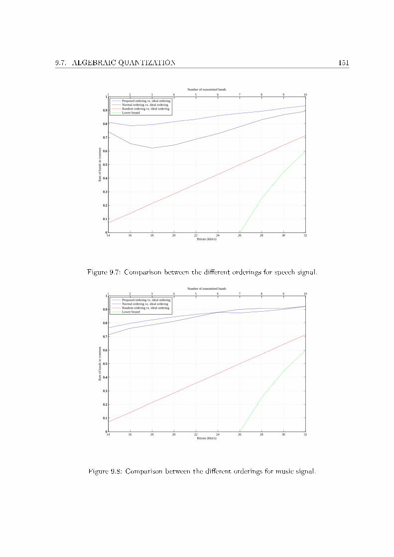
9.7. ALGEBRAIC QUANTIZATION 151
14 16 18 20 22 24 26 28 30 320
0.1
0.2
0.3
0.4
0.5
0.6
0.7
0.8
0.9
1
Bitrate (kbit/s)
Rat
e of
ban
ds in
com
mon
Proposed ordering vs. ideal orderingNormal ordering vs. ideal orderingRandom ordering vs. ideal orderingLower bound
1 2 3 4 5 6 7 8 9 10
0
0.1
0.2
0.3
0.4
0.5
0.6
0.7
0.8
0.9
1
Number of transmitted bands
Figure 9.7: Comparison between the di�erent orderings for speech signal.
14 16 18 20 22 24 26 28 30 320
0.1
0.2
0.3
0.4
0.5
0.6
0.7
0.8
0.9
1
Bitrate (kbit/s)
Rat
e of
ban
ds in
com
mon
Proposed ordering vs. ideal orderingNormal ordering vs. ideal orderingRandom ordering vs. ideal orderingLower bound
1 2 3 4 5 6 7 8 9 10
0
0.1
0.2
0.3
0.4
0.5
0.6
0.7
0.8
0.9
1
Number of transmitted bands
Figure 9.8: Comparison between the di�erent orderings for music signal.
152 PROPOSED CODER
9.8 Listening tests
To assess the coding performance of the proposed structure, two listening tests have beenconducted. The chosen protocol is the Absolute Category Rating described in the ITU-TRecommendation P.800 [ITU-T 1996e]. For each test, the same panel of 8 listeners rated speechor music samples, that might be degraded by a processing, according to the scale presented inTab. 9.1. The samples were presented to the listeners over headphones for two-ears listening.This is somehow more discriminative than tests conducted with one-ear listening. For eachtest, the proposed codec was tested against other codecs and reference signals, such the non-processed samples, called 'direct', and Modulated Noise Reference Unit (MNRU) generated byadding noise to the test signals [ITU-T 1996f]. Note that none of the test participants is anative English speaker, but all of them speak and understand English.
Quality of the sample ScoreExcellent 5Good 4Fair 3Poor 2Bad 1
Table 9.1: ACR Listening-quality scale.
The Mean Opinion Score (MOS) Yk for the condition k is estimated by averaging the scoresXk,i given by the listeners on the corresponding samples:
Yk =∑n
i=1 Xk,i
n(9.22)
where n is the number of observations, i.e. the number of samples multiplied by the numberof listeners. The MOS measure provides a numerical indication of the perceived quality. Thevalue Yk is an estimation of the true expected value µk. To take the measure uncertainty intoaccount, it is recommended [ITU-T 1996e] to calculate con�dence intervals instead of simplyusing standard deviation. The con�dence interval at the con�dence level (1− α) is given by:
CIk = ±t(1−α/2),n−1Sk√n
(9.23)
where ν = n−1 is the number of degrees of freedom, and t(1−α),ν follows a Student-t distributionfor a (1− α) con�dence interval. The standard deviation Sk of the MOS is estimated by:
Sk =
√√√√ 1n− 1
n∑i=1
(Xk,i − Yk)2 (9.24)
9.8. LISTENING TESTS 153
The probability that the value
∣∣∣∣ Yk−µk
Sk/√
(n)
∣∣∣∣ is greater or equal than t(1−α/2),ν is α:
P
(Yk − µk
Sk/√
(n)≥ t(1−α/2),n−1
)=
α
2and P
(Yk − µk
Sk/√
(n)≤ −t(1−α/2),n−1
)=
α
2(9.25)
It indicates that the expected MOS µk is contained with a probability of (1−α) in the interval:
Yk − t(1−α/2),n−1Sk√n≤ µk ≤ Yk + t(1−α/2),n−1
Sk√n
(9.26)
The quality assessment consists of simple pair wise MOS comparisons obtained for theproposed codec (test) and a reference codec (ref). To allow for experimental uncertainty, asimple paired t-test at the 1 − α = 95% signi�cance level is used to accept or reject thehypothesis. The comparisons are made between pairs of MOS Yref and Ytest, having standarddeviations sref and stest. The expected mean values are µref and µtest, and it is assumed thatthe two means have the same variance s2.
The comparisons between the proposed codec, denoted Codec under Test (CuT), and thereference codecs are expressed in requirements "the proposed codec at x kbit/s is not worsethan the reference codec lambda at y kbit/s". A one-sided t-test is used to verify the nullhypothesis.
• The null hypothesis is: H0 µtest ≥ µref
• which is tested against the alternative: H1 µtest < µref
The null hypothesis is accepted if:
Yref − Ytest ≤ t(1−α),νs0
√1n
(9.27)
where s20 is the pooled estimator of the common variance given by:
s20 =
∑i
(di −
Pi di
n
)2
n− 1(9.28)
where di is the pair di�erence for the observation i:
di = Xtest,i −Xref,i (9.29)
In order to compare the proposed codec with reference codecs, such statistical tests areperformed on results obtained for speech signal in Sec. 9.8.1 and music signal in Sec. 9.8.2.
154 PROPOSED CODER
9.8.1 Performance on speech signal
The test material comprises six 8-second long wideband speech samples, uttered by 3 male and3 female English speakers. The following conditions were tested:
1. MNRU at 5 dB
2. MNRU at 15 dB
3. MNRU at 25 dB
4. MNRU at 35 dB
5. MNRU at 45 dB
6. Direct
7. G.722.2 [ITU-T 2003] at 12.65 kbit/s
8. G.729.1 [ITU-T 2006a] at 24 kbit/s
9. G.729.1 at 32 kbit/s
10. G.722 [ITU-T 1988b] at 56 kbit/s
11. G.722 at 64 kbit/s
12. CuT at 10 kbit/s
13. CuT at 24 kbit/s
14. CuT at 32 kbit/s
The codec was not tested at 8 kHz since the G729 used as core codec has not been modi�edcompared to its standardized version. Hence, the core coder is expected to provide the samequality. The MOS for each condition, as well as the standard deviation and the 95% con�denceinterval are gathered in Tab. 9.2 and represented in Fig. 9.2. The scores obtained by theproposed codec show that the quality increases gracefully with the bitrate.
The proposed codec has been tested at 10, 24 and 32 kibt/s against speech codec at equiv-alent or higher bitrates. The di�erent requirements are gathered in Tab. 9.3. A requirementis veri�ed with a con�dence level of (1 − α) = 95% if the MOS di�erence is smaller than thethreshold (cf (Eq. 9.27)). If a requirement is veri�ed, i.e. the proposed codec (CuT) is notworse (n.w.t.) than the reference codec, it is likely that the proposed codec is equivalent orbetter than the reference codec.
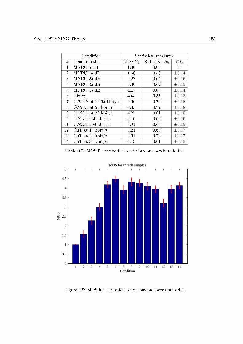
9.8. LISTENING TESTS 155
Condition Statistical measuresk Denomination MOS Yk Std. dev. Sk CIk
1 MNRU 5 dB 1.00 0.00 02 MNRU 15 dB 1.56 0.58 ±0.143 MNRU 25 dB 2.27 0.64 ±0.164 MNRU 35 dB 3.00 0.62 ±0.155 MNRU 45 dB 4.17 0.60 ±0.146 Direct 4.48 0.55 ±0.137 G.722.2 at 12.65 kbit/s 3.90 0.72 ±0.188 G.729.1 at 24 kbit/s 4.33 0.72 ±0.189 G.729.1 at 32 kbit/s 4.27 0.61 ±0.1510 G.722 at 56 kbit/s 4.10 0.66 ±0.1611 G.722 at 64 kbit/s 3.94 0.63 ±0.1512 CuT at 10 kbit/s 3.21 0.68 ±0.1713 CuT at 24 kbit/s 3.94 0.70 ±0.1714 CuT at 32 kbit/s 4.13 0.61 ±0.15
Table 9.2: MOS for the tested conditions on speech material.
1 2 3 4 5 6 7 8 9 10 11 12 13 140
0.5
1
1.5
2
2.5
3
3.5
4
4.5
5MOS for speech samples
Condition
MO
S
Figure 9.9: MOS for the tested conditions on speech material.
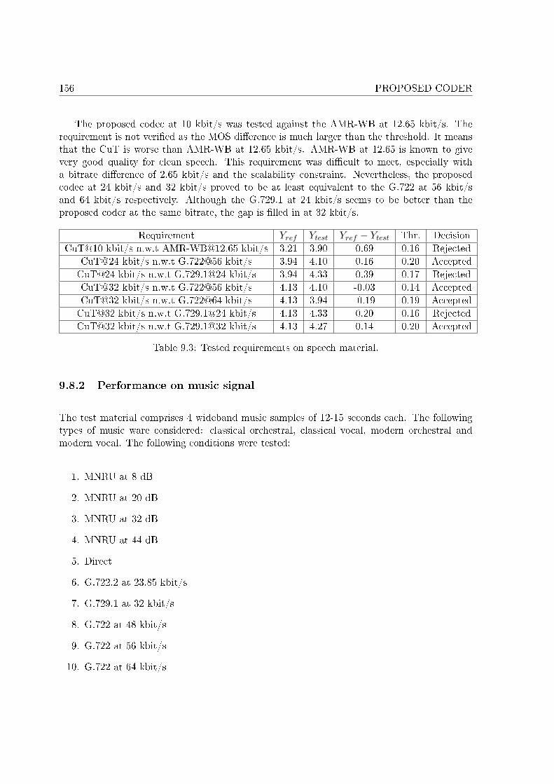
156 PROPOSED CODER
The proposed codec at 10 kbit/s was tested against the AMR-WB at 12.65 kbit/s. Therequirement is not veri�ed as the MOS di�erence is much larger than the threshold. It meansthat the CuT is worse than AMR-WB at 12.65 kbit/s. AMR-WB at 12.65 is known to givevery good quality for clean speech. This requirement was di�cult to meet, especially witha bitrate di�erence of 2.65 kbit/s and the scalability constraint. Nevertheless, the proposedcodec at 24 kbit/s and 32 kbit/s proved to be at least equivalent to the G.722 at 56 kbit/sand 64 kbit/s respectively. Although the G.729.1 at 24 kbit/s seems to be better than theproposed coder at the same bitrate, the gap is �lled in at 32 kbit/s.
Requirement Yref Ytest Yref − Ytest Thr. DecisionCuT@10 kbit/s n.w.t [email protected] kbit/s 3.21 3.90 0.69 0.16 Rejected
CuT@24 kbit/s n.w.t G.722@56 kbit/s 3.94 4.10 0.16 0.20 AcceptedCuT@24 kbit/s n.w.t G.729.1@24 kbit/s 3.94 4.33 0.39 0.17 RejectedCuT@32 kbit/s n.w.t G.722@56 kbit/s 4.13 4.10 -0.03 0.14 AcceptedCuT@32 kbit/s n.w.t G.722@64 kbit/s 4.13 3.94 -0.19 0.19 AcceptedCuT@32 kbit/s n.w.t G.729.1@24 kbit/s 4.13 4.33 0.20 0.16 RejectedCuT@32 kbit/s n.w.t G.729.1@32 kbit/s 4.13 4.27 0.14 0.20 Accepted
Table 9.3: Tested requirements on speech material.
9.8.2 Performance on music signal
The test material comprises 4 wideband music samples of 12-15 seconds each. The followingtypes of music ware considered: classical orchestral, classical vocal, modern orchestral andmodern vocal. The following conditions were tested:
1. MNRU at 8 dB
2. MNRU at 20 dB
3. MNRU at 32 dB
4. MNRU at 44 dB
5. Direct
6. G.722.2 at 23.85 kbit/s
7. G.729.1 at 32 kbit/s
8. G.722 at 48 kbit/s
9. G.722 at 56 kbit/s
10. G.722 at 64 kbit/s
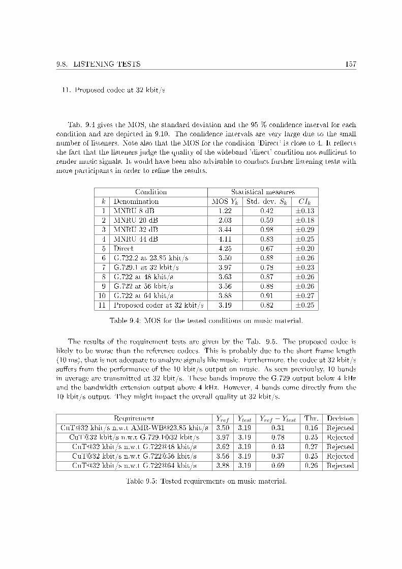
9.8. LISTENING TESTS 157
11. Proposed codec at 32 kbit/s
Tab. 9.4 gives the MOS, the standard deviation and the 95 % con�dence interval for eachcondition and are depicted in 9.10. The con�dence intervals are very large due to the smallnumber of listeners. Note also that the MOS for the condition 'Direct' is close to 4. It re�ectsthe fact that the listeners judge the quality of the wideband 'direct' condition not su�cient torender music signals. It would have been also advisable to conduct further listening tests withmore participants in order to re�ne the results.
Condition Statistical measuresk Denomination MOS Yk Std. dev. Sk CIk
1 MNRU 8 dB 1.22 0.42 ±0.132 MNRU 20 dB 2.03 0.59 ±0.183 MNRU 32 dB 3.44 0.98 ±0.294 MNRU 44 dB 4.11 0.83 ±0.255 Direct 4.25 0.67 ±0.206 G.722.2 at 23.85 kbit/s 3.50 0.88 ±0.267 G.729.1 at 32 kbit/s 3.97 0.78 ±0.238 G.722 at 48 kbit/s 3.63 0.87 ±0.269 G.722 at 56 kbit/s 3.56 0.88 ±0.2610 G.722 at 64 kbit/s 3.88 0.91 ±0.2711 Proposed coder at 32 kbit/s 3.19 0.82 ±0.25
Table 9.4: MOS for the tested conditions on music material.
The results of the requirement tests are given by the Tab. 9.5. The proposed codec islikely to be worse than the reference codecs. This is probably due to the short frame length(10 ms), that is not adequate to analyze signals like music. Furthermore, the codec at 32 kbit/ssu�ers from the performance of the 10 kbit/s output on music. As seen previoulsy, 10 bandsin average are transmitted at 32 kbit/s. These bands improve the G.729 output below 4 kHzand the bandwidth extension output above 4 kHz. However, 4 bands come directly from the10 kbit/s output. They might impact the overall quality at 32 kbit/s.
Requirement Yref Ytest Yref − Ytest Thr. DecisionCuT@32 kbit/s n.w.t [email protected] kbit/s 3.50 3.19 0.31 0.16 Rejected
CuT@32 kbit/s n.w.t G.729.1@32 kbit/s 3.97 3.19 0.78 0.25 RejectedCuT@32 kbit/s n.w.t G.722@48 kbit/s 3.62 3.19 0.43 0.27 RejectedCuT@32 kbit/s n.w.t G.722@56 kbit/s 3.56 3.19 0.37 0.25 RejectedCuT@32 kbit/s n.w.t G.722@64 kbit/s 3.88 3.19 0.69 0.26 Rejected
Table 9.5: Tested requirements on music material.
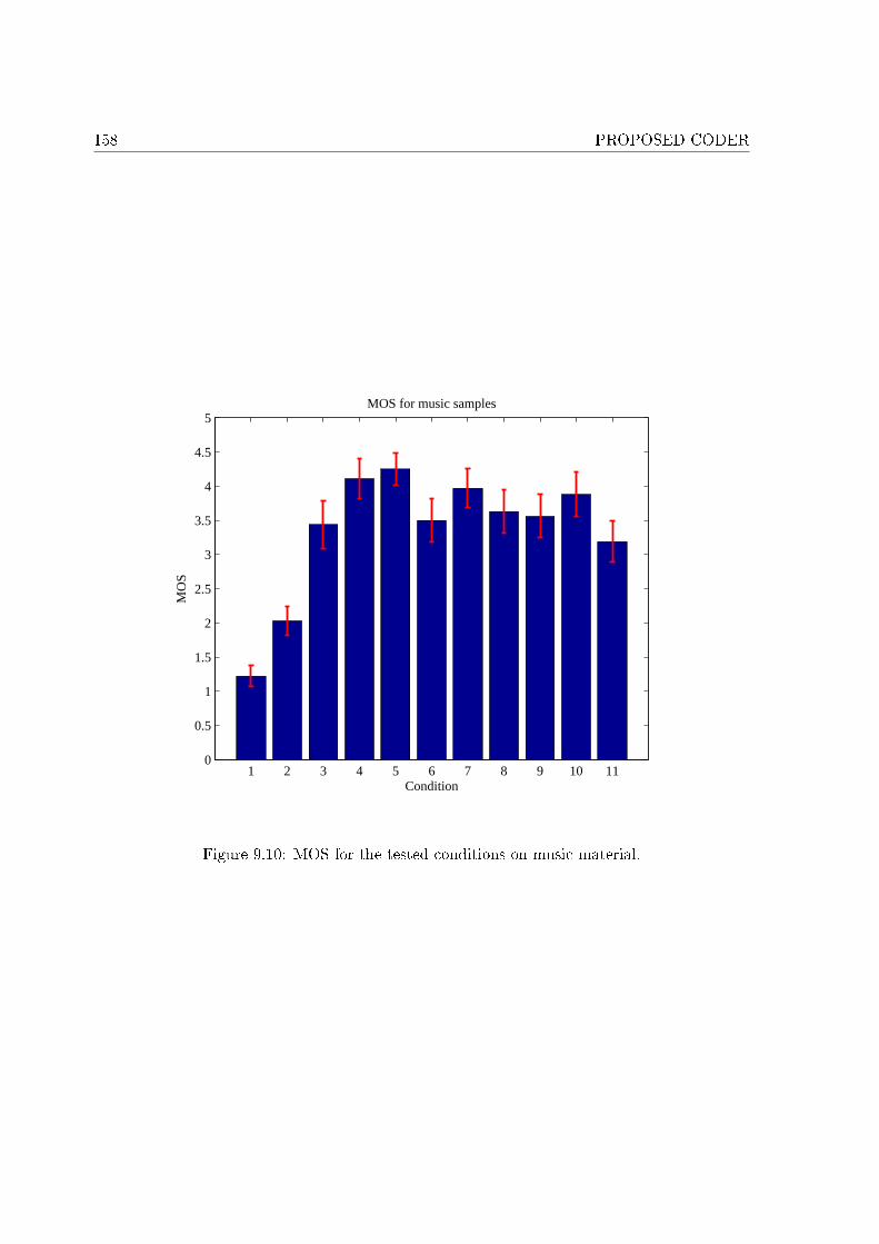
158 PROPOSED CODER
1 2 3 4 5 6 7 8 9 10 110
0.5
1
1.5
2
2.5
3
3.5
4
4.5
5MOS for music samples
Condition
MO
S
Figure 9.10: MOS for the tested conditions on music material.
9.8. LISTENING TESTS 159
Conclusion
This chapter presents in details the proposed coder while justifying the choices made for theimportant modules. The 10 ms wideband input frame is split into two components. Thenarrowband part is encoded with the G.729 that produces the core layer. The wideband partis analyzed to extract the parameters that constitute the �rst enhancement layer necessaryto the bandwidth extension. The error signal between delayed low band input and the G.729output, and the delayed original high band input are decomposed into wavelet packet. Thequantized coe�cients provide the second and last enhancement layer.
This chapter also described investigations conducted to solve the problems encountered andhow to optimize the overall performance of the coder. The split band structure was shown tohave an in�uence on the quality at 10 kbit/s. Firstly performed by the �rst stage of the waveletpacket decomposition, the split band structure was then implemented by a 2-channel QMF�lter. Indeed, the wavelet �lters are not able to cancel the aliasing at the reconstruction becausethe wavelet coe�cients are roughly quantized. The utilization of a longer �lter reduces theresidual aliasing noise. The absence of a CELP-based enhancement, like the one investigatedin Ch. 4, enables wideband rendering at 10 kbit/s. Because of its high scalability potential, alot of e�orts were put on improving the wavelet coding stage, by choosing the optimal wavelet,designing the tree structure of SPIHT, and selecting the coe�cients to be sent. Finally, SPIHThas to be replaced by a new coding structure, based on algebraic quantization of the waveletcoe�cients. The new structure improves the performance of the codec at the expense of lessscalability.
The quality of the proposed codec was assessed for wideband speech and music. The testshowed that the quality improves gracefully with the bitrate in case of speech signal. Thebandwidth extension provides fair quality at 10 kbit/s. The results at 24 kbit/s and 32 kbit/sare encouraging. However the results for music show that further investigations are required.The frame length is certainly too short for music signal. Moreover the wavelet coding layer(last layer) does not transmit enough bands even at 32 kbit/s. The bands that have not beenenhanced by the last layer are left untouched and use the information coming from the coreG.729 module and the bandwidth extension module. As these modules are rather adapted tospeech signals, it results in a signal that is not optimally encoded for music.
Most certainly, the quality of the proposed scheme can be further enhanced. As showedby the results, in clean speech conditions, the quality is close to the one of the G.729.1 (20 msframe length, 48.9375 ms algorithmic delay) that is a state of the art codec (standardized inMay 2006) to which many companies contributed. It was achieved with a shorter frame length(10 ms) and a shorter algorithmic delay (38.125 ms). The goal of this work was to evaluatewhether wavelet coding can be applied to scalable speech coding at low bitrates (8-32 kbit/s).According to the results, it seems to be the case.

160 PROPOSED CODER
CONCLUSION 161
Conclusion
Scalable coding is one possible solution to the problem of network congestion, particularlypenalizing for interactive applications such as VoIP. The bitstream structure, quali�ed as em-bedded or scalable, allows its partial decoding. It can be truncated at several points overthe transmission chain and still can be decoded. The core layer sets the minimal quality andthe bandwidth of the decoded signal. Bandwidth/quality is increased/improved by furtherenhancement layers until reaching its maximal quality. The activities of standardization orga-nizations and also the number of publications show the growing interest for this research area.Scalable coding can also have applications in multimedia content broadcast. The bitrate canbe adapted to the terminal capacity, or to the user preferences, like for instance an access tothe highest quality for premium users.
This thesis attempts to contribute to scalable coding. The proposed codec is intended tocoding wideband speech signals. It works on a 10 ms frame basis at bitrates from 8 kbit/sto 32 kbit/s. It relies on a unusual structure combining CELP and wavelet. CELP coding isunquestionable in speech coding at low bitrates. As core layer, it provides a good narrowbandspeech quality at low bit rates. At higher bitrates, transform coding performs better. Anenhancement layer based on wavelet packet decomposition encodes the di�erence betweenthe original signal and the CELP decoder output. Wavelet introduces a more �exible time-frequency resolution tradeo� than conventional frequency transforms like MDCT. The 24-taps Vaidyanathan wavelet �lter was �rst chosen for its in�uence on the embedded quantizerbitrate. This �lter provides also a good tradeo� between delay and its frequency response.The transition narrowband/wideband is made by a 2-kbit/s bandwidth extension.
During this thesis, investigations have been conducted on an enhancement layer based onACELP coding. Usually, scalability in CELP coding is obtained by improving the quantizationof the LP excitation, and more precisely the non-predictable part, called innovation. Ch. 4 haspresented a di�erent way to enhance the innovation. The innovative codeword is modi�ed bymultiplying each pulse by an individual gain. This method has been combined with a second�xed codebook on top of the G.729A in order to provide a 3-bitrate scalable structure 8/9.6/12kbit/s. Compared to a single enhancement layer like the one used in the G.729.1, the proposedstructure does not perform as well, due to the intermediate bitrate at 9.6 kbit/s. The proposedcodec does not comprise a CELP-based enhancement layer for two reasons. The improvement
162 CONCLUSION
brought by this layer can also be achieved by the upper layer at an equivalent bitrate. Thewideband rendering can be enabled at low bitrate.
The bandwidth extension is an essential module of the codec structure. Progressive trans-mission of the wavelet coe�cients implies progressive decoding. As a consequence, the decoderreconstructs only the corresponding parts of the spectrum. The number and the position ofthe decoded bands in the spectrum change from frame to frame. Decoded bands in a framemay disappear in the next frame. Conversely, missing bands in a frame might appear in thenext frame. The resulting artifacts sound like musical noise, similar to the one caused by noisereduction algorithms. Bandwidth extension provides a constant wideband spectrum, whateverthe number of transmitted coe�cients. Hence, a constant wideband synthesis is guaranteedat 10 kbit/s. Beyond this bitrate, the wavelet packets of the arti�cially bandwidth extendedsignal replace the missing wavelet packets.
The proposed bandwidth extension is well integrated into the structure as it exploits thesubband decomposition inherent to the wavelet packet decomposition. Indeed, after the splitband structure that separates the lower and upper components, the time and frequency en-velopes of the excitation signal are shaped by the quantized time and frequency envelopes ofthe original signal. This excitation signal is a linear combination of pseudo-random noise andof the adaptive codeword of the CELP codec. The weighting factors are computed from theenergy of the innovative and adaptive contributions on a subframe basis (5 ms). As a result, theadaptive contribution is favored in case of voiced frames, and conversely, the pseudo-randomnoise is emphasized in case of unvoiced frames. In the �rst place, the �rst level of the WPDplayed the role of the split band structure. However, due to a rough estimation of the waveletcoe�cient by the bandwidth extension, aliasing present at the reconstruction impacted thequality at 10 kbit/s. The wavelet �lter has then been substituted by a QMF �lter in the �rststage of the decomposition. The utilization of the QMF reduces this aliasing. However, theQMF increases slightly the arithmetic delay by 2.5 ms.
Scalability might also be enabled at the wavelet coe�cient level by using progressive trans-mission, which is achieved with EZW and SPIHT, presented in Ch. 6. Both algorithms areimplementations of bit-plane coding which consists in transmitting �rst the most signi�cantbits of the most signi�cant coe�cients. They rely on a tree structure of the wavelet coe�cientsand exploit the self-similarity of the coe�cients across the bands. Due to its superiority overEZW, SPIHT was �rst chosen as embedded quantizer. However, SPIHT does not seem toperform well enough for wideband signal at the targeted bitrates. It is mainly due to the factthat too many bits are spent on the most signi�cant coe�cients, neglecting the less signi�cantones. Methods to better control the number of coe�cients to be transmitted have been investi-gated, without any sensible improvement. This impassable limit led to rethink the coe�cientsquantization.
In the proposed scheme, SPIHT has been then replaced by an algebraic quantization ofthe coe�cients. The term algebraic reminds the algebraic codebook present in AMR or G.729.The coe�cients within a band are quantized by a few non-zero pulses along with their sign,
CONCLUSION 163
multiplied by an amplitude. The number of pulses, their positions and their amplitude areoptimally determined by minimizing a mean square error criterion between the original coe�-cients and the estimated ones. It turns out that the selected coe�cients are the most importantones, and the amplitude is the average of their absolute values. The most important bandsare transmitted in priority. The most important coe�cients are not quantized as precisely aswith SPIHT and more bits are allocated to other coe�cients. More bands above 4 kHz aretransmitted, reducing the artifacts of the bandwidth extension.
The speech quality of the proposed codec was shown to improve gracefully with the bitrate.The bandwidth quality extension at 10 kbit/s does not perform as good as the AMR-WB at12.65 kbit/s. Nevertheless, the proposed codec is penalized by its scalability and the bitratedi�erence. At 24 kbit/s and 32 kbit/s, it is equivalent to the G.722 at 56 and 64 kbit/srespectively. Moreover, the proposed codec at 32 kbit/s with a 38.125 ms algorithmic delayworking on a 10 ms frame basis performs as well as the G.729.1 at the same bitrate with alonger delay (48.9375 ms) and working on a 20 ms frame basis. However, the performance formusic is not as good as expected. A short frame length and a poor bandwidth extension formusic might impact the music quality. Due to lack of time, it was not possible to work onother ideas that could improve the performance of the proposed codec.
The proposed coe�cient quantization does not take any perceptual consideration into ac-count. Integration of a psychoacoustic model might enhance the quality. It can happen thatsome transmitted pulses are actually not perceived. In other words, whether those pulses aretransmitted or not, the listener does not notice any di�erence. Saved bits could be used totransmit perceptually important pulses that could not have been transmitted otherwise. Thiscould be implemented by a mechanism similar to the perceptual weighting �lter in CELPcoding. In each wavelet packet, the di�erence between the original and estimated coe�cientscould be multiplied by a weighting function, based on masking model, that favors perceptuallyimportant coe�cients. That would lead to the minimization of a perceptually mean squareerror. This would be equivalent to spectrally shaping the quantization noise according to theoriginal signal spectrum.
Adaptive post�ltering above 4 kHz could also exploit the human auditory system in orderto minimize the perceptual e�ects of the quantization noise after the synthesis. By puttinga slight emphasis on spectral envelope peaks and the pitch periodicity, it could enhance theperceptual quality of the reconstructed speech. The WPD could make easier the modi�cationof the spectral envelope on a subband basis. Likewise, the time-frequency characteristics of theWPD would facilitate the modi�cation of the �ne structure. Also, like in the G.729.1, adaptivepost�ltering could depend on the bitrate. The lower the bitrate, the stronger the post�lter.
With the proposed quantization, like in SPIHT, there is also no explicit bit allocation. Nomodule controls the number of bits allocated in each subband to the coe�cients quantization.The criterion minimization in each subband gives the number of coe�cients to be transmitted,thus the number of bits. A module could control the number of bits allocated to each band tobe transmitted, in order to reallocate bits to other bands. For instance, at 32 kbit/s, removing
164 CONCLUSION
one pulse in each transmitted band, i.e. reallocating 2 bits to other bands, can save 20 bits forthe transmission of an additional band.
No optimization has been done on the amplitude quantization and the transmission of thepulses. In their current form they are bit consuming. For example, at 32 kbit/s, 40 bits inaverage are allocated to the amplitude quantization of 10 bands. Investigations could be con-ducted on reducing the bit rate allocated to the amplitudes. Their current scalar quantizationcould be replaced by a split vector quantization. For instance, one 4-dimensional and two3-dimensional codebook with 5 bits each, would require a total of 15 bits. This implies togroup a few amplitudes into vectors before encoding the pulse positions and signs. In order toreduce the dynamic of the amplitudes, a di�erential coding can be implemented. For example,the di�erence between the �rst band and the other bands can be transmitted. A Hu�mancoding could also be considered, as it is done for instance in the G.729.1.
The codec structure can easily be extended for bitrates above 32 kbit/s. With 32 kbit/s,10 bands are in average transmitted. In order to transmit the rest of the bands, 8 to 10 kbit/sare required. Afterwards, two possibilities are conceivable. Either the di�erence between theoriginal and the reconstructed wavelet packet decomposition are algebraically quantized, or thenon-transmitted coe�cients during the �rst pass are algebraically quantized. For instance, if 6coe�cients in one wavelet packet of 10 coe�cients have been transmitted during the �rst pass,the 4 left are the only candidates for the second pass. Among the 4 coe�cients, those thatminimize the error criterion will be transmitted. Super wideband coding could be enabledby adding an additional split band structure. It would separate the input signal into thecomponent 0 kHz - 8 kHz and the component 8 kHz - 14 kHz. The band 0 kHz - 7 kHz wouldbe encoded by the proposed codec. Note that in this case the band 7 kHz - 8 kHz should betransmitted in an additional layer, as it is not encoded by the proposed codec.

165
Part VI
Appendix

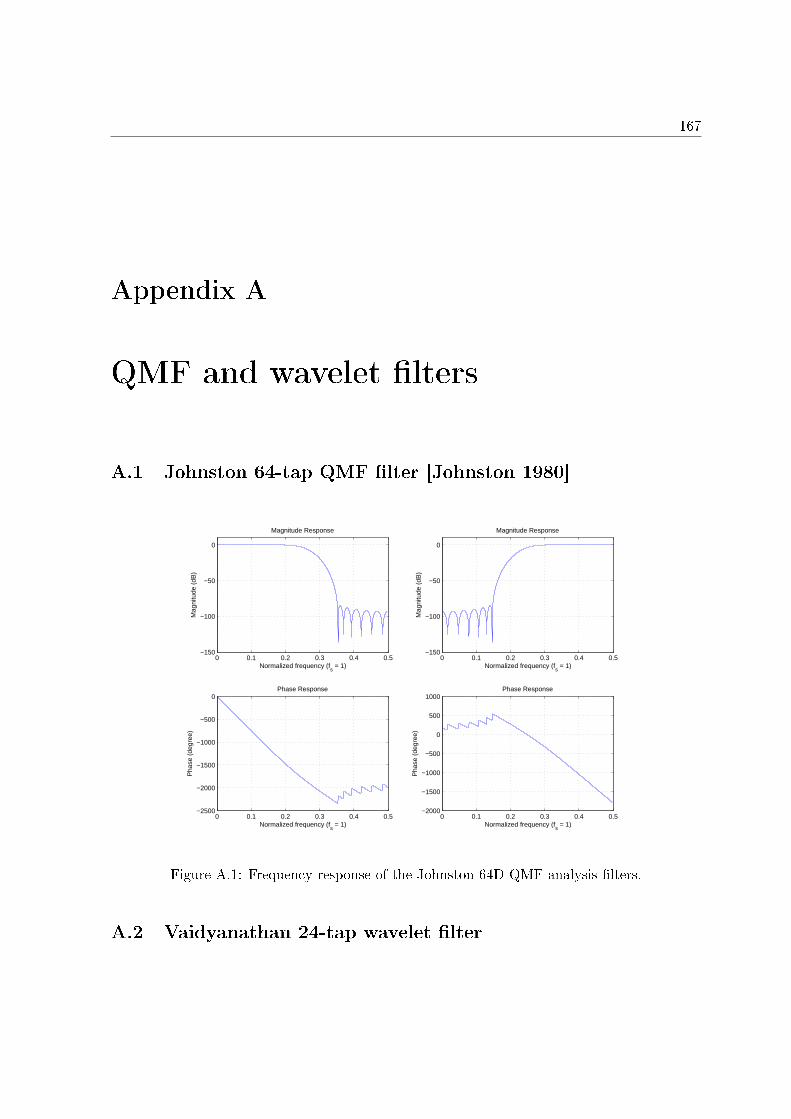
167
Appendix A
QMF and wavelet �lters
A.1 Johnston 64-tap QMF �lter [Johnston 1980]
0 0.1 0.2 0.3 0.4 0.5−150
−100
−50
0
Magnitude Response
Normalized frequency (fs = 1)
Mag
nitu
de (
dB)
0 0.1 0.2 0.3 0.4 0.5−150
−100
−50
0
Magnitude Response
Normalized frequency (fs = 1)
Mag
nitu
de (
dB)
0 0.1 0.2 0.3 0.4 0.5−2500
−2000
−1500
−1000
−500
0Phase Response
Normalized frequency (fs = 1)
Pha
se (
degr
ee)
0 0.1 0.2 0.3 0.4 0.5−2000
−1500
−1000
−500
0
500
1000Phase Response
Normalized frequency (fs = 1)
Pha
se (
degr
ee)
Figure A.1: Frequency response of the Johnston-64D QMF analysis �lters.
A.2 Vaidyanathan 24-tap wavelet �lter
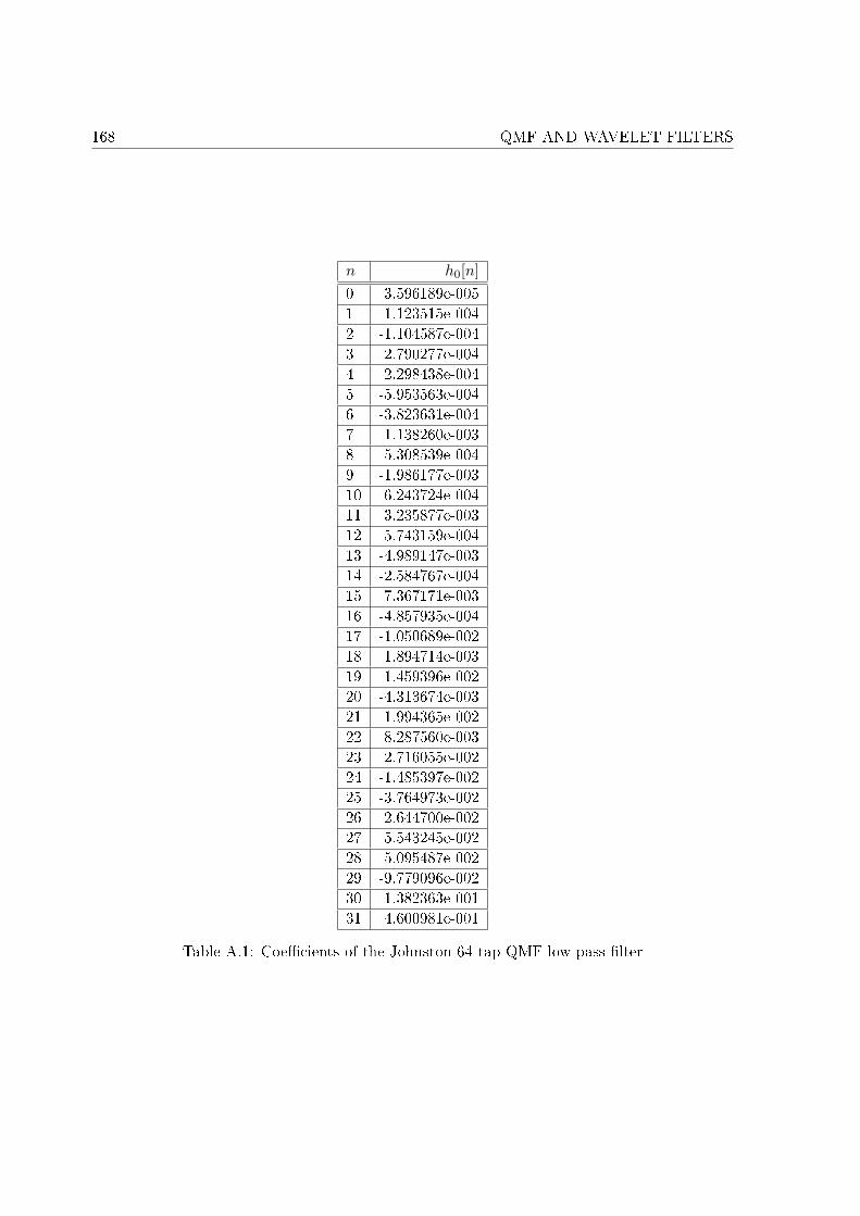
168 QMF AND WAVELET FILTERS
n h0[n]0 3.596189e-0051 -1.123515e-0042 -1.104587e-0043 2.790277e-0044 2.298438e-0045 -5.953563e-0046 -3.823631e-0047 1.138260e-0038 5.308539e-0049 -1.986177e-00310 -6.243724e-00411 3.235877e-00312 5.743159e-00413 -4.989147e-00314 -2.584767e-00415 7.367171e-00316 -4.857935e-00417 -1.050689e-00218 1.894714e-00319 1.459396e-00220 -4.313674e-00321 -1.994365e-00222 8.287560e-00323 2.716055e-00224 -1.485397e-00225 -3.764973e-00226 2.644700e-00227 5.543245e-00228 -5.095487e-00229 -9.779096e-00230 1.382363e-00131 4.600981e-001
Table A.1: Coe�cients of the Johnston 64-tap QMF low pass �lter
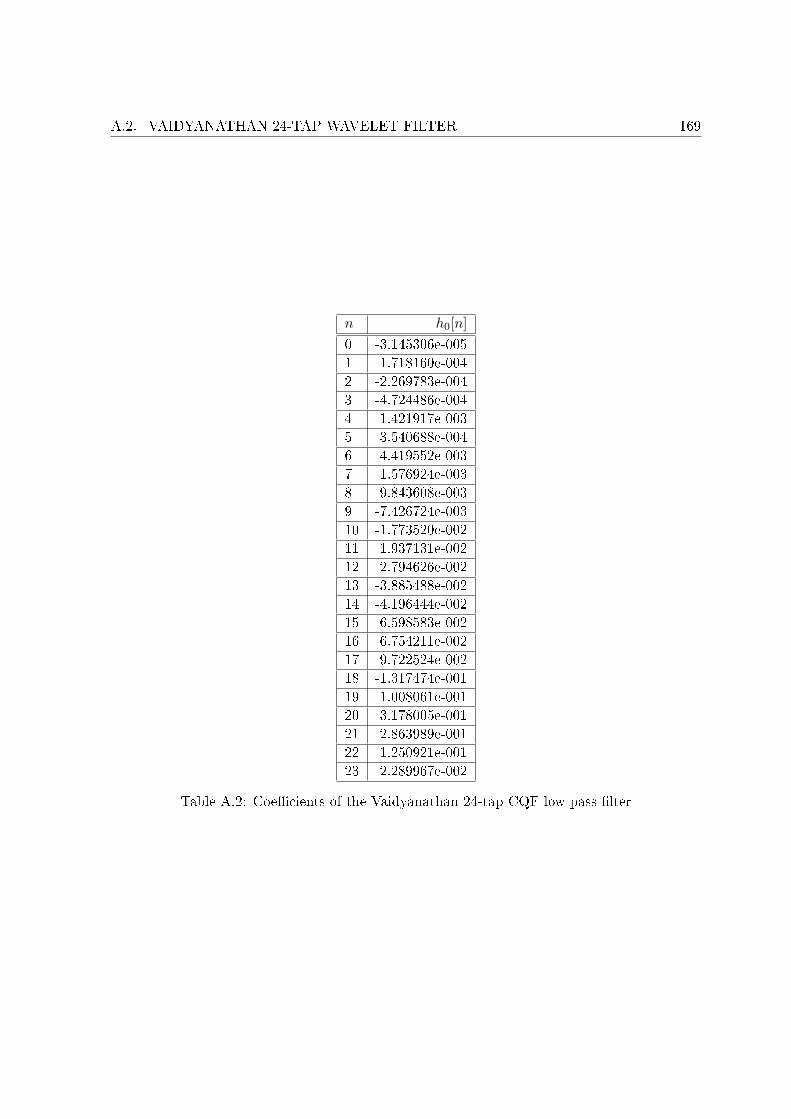
A.2. VAIDYANATHAN 24-TAP WAVELET FILTER 169
n h0[n]0 -3.145306e-0051 1.718160e-0042 -2.269783e-0043 -4.724486e-0044 1.421917e-0035 3.540688e-0046 -4.419552e-0037 1.576924e-0038 9.843608e-0039 -7.426724e-00310 -1.773520e-00211 1.937131e-00212 2.794626e-00213 -3.885488e-00214 -4.196444e-00215 6.598583e-00216 6.754211e-00217 -9.722524e-00218 -1.317474e-00119 1.008061e-00120 3.178005e-00121 2.863989e-00122 1.250921e-00123 2.289967e-002
Table A.2: Coe�cients of the Vaidyanathan 24-tap CQF low pass �lter
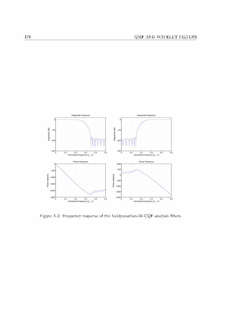
170 QMF AND WAVELET FILTERS
0 0.1 0.2 0.3 0.4 0.5−150
−100
−50
0
Magnitude Response
Normalized frequency (fs = 1)
Mag
nitu
de (
dB)
0 0.1 0.2 0.3 0.4 0.5−150
−100
−50
0
Magnitude Response
Normalized frequency (fs = 1)
Mag
nitu
de (
dB)
0 0.1 0.2 0.3 0.4 0.5−2500
−2000
−1500
−1000
−500
0Phase Response
Normalized frequency (fs = 1)
Pha
se (
degr
ee)
0 0.1 0.2 0.3 0.4 0.5−2000
−1500
−1000
−500
0
500
1000Phase Response
Normalized frequency (fs = 1)
Pha
se (
degr
ee)
Figure A.2: Frequency response of the Vaidyanathan-24 CQF analysis �lters.
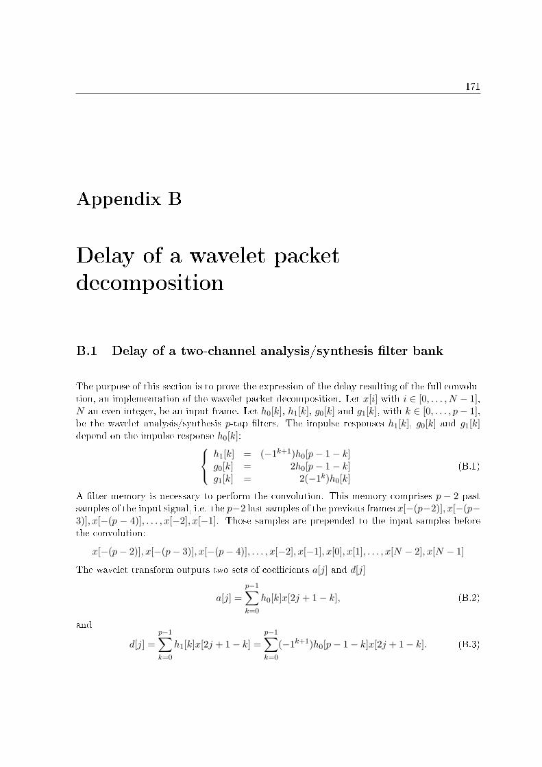
171
Appendix B
Delay of a wavelet packetdecomposition
B.1 Delay of a two-channel analysis/synthesis �lter bank
The purpose of this section is to prove the expression of the delay resulting of the full convolu-tion, an implementation of the wavelet packet decomposition. Let x[i] with i ∈ [0, . . . , N − 1],N an even integer, be an input frame. Let h0[k], h1[k], g0[k] and g1[k], with k ∈ [0, . . . , p− 1],be the wavelet analysis/synthesis p-tap �lters. The impulse responses h1[k], g0[k] and g1[k]depend on the impulse response h0[k]:
h1[k] = (−1k+1)h0[p− 1− k]g0[k] = 2h0[p− 1− k]g1[k] = 2(−1k)h0[k]
(B.1)
A �lter memory is necessary to perform the convolution. This memory comprises p − 2 pastsamples of the input signal, i.e. the p−2 last samples of the previous frames x[−(p−2)], x[−(p−3)], x[−(p − 4)], . . . , x[−2], x[−1]. Those samples are prepended to the input samples beforethe convolution:
x[−(p− 2)], x[−(p− 3)], x[−(p− 4)], . . . , x[−2], x[−1], x[0], x[1], . . . , x[N − 2], x[N − 1]
The wavelet transform outputs two sets of coe�cients a[j] and d[j]
a[j] =p−1∑k=0
h0[k]x[2j + 1− k], (B.2)
and
d[j] =p−1∑k=0
h1[k]x[2j + 1− k] =p−1∑k=0
(−1k+1)h0[p− 1− k]x[2j + 1− k]. (B.3)
172 DELAY OF A WAVELET PACKET DECOMPOSITION
with j ∈[0, . . . , N
2 − 1]. In a same manner, �lter memories are necessary to perform the
inverse wavelet transform. These memories are the p2 coe�cients of the previous frames:
a[−(p2)], a[−(p
2 − 1)], a[−(p2 − 2)], . . . , a[−2], a[−1] and d[−(p
2)], d[−(p2 − 1)], d[−(p
2 − 2)], . . . ,d[−2], d[−1]. These samples are prepended to the coe�cients of the current frame before theupsampling
a[−(p
2)], a[−(
p
2− 1)], a[−(
p
2− 2)], . . . , a[−2], a[−1], a[0], a[1], . . . , a[
N
2− 2], a[
N
2− 1]
d[−(p
2)], d[−(
p
2− 1)], d[−(
p
2− 2)], . . . , d[−2], d[−1], d[0], d[1], . . . , d[
N
2− 2], d[
N
2− 1].
The upsampled coe�cients
a[−(p
2)], 0, a[−(
p
2− 1)], 0, . . . , a[−1], 0, a[0], 0, a[1], 0, . . . , a[
N
2− 2], 0, a[
N
2− 1], 0
d[−(p
2)], 0, d[−(
p
2− 1)], 0, . . . , d[−1], 0, d[0], 0, d[1], 0, . . . , d[
N
2− 2], 0, d[
N
2− 1], 0
are noted
a′[j] ={
a[j/2] if j is even0 else
and d′[j] ={
d[j/2] if j is even0 else
. (B.4)
The frame samples are reconstructed by:
y[i] =∑p−1
l=0 g0[l]a′[i− l] +∑p−1
l=0 g1[l]d′[i− l]=
∑p−1l=0 h0[p− 1− l]a′[i− l] +
∑p−1l=0 (−1l)h0[l]d′[i− l]
(B.5)
Considering i odd, the equation (B.5) can be expanded as follows:
y[i] =∑p/2−1
l=0 h0[p− 1− (2l + 1)]a′[i− (2l + 1)] +∑p/2−1
l=0 (−12l+1)h0[2l + 1]d′[i− (2l + 1)]=
∑p/2−1l=0 h0[p− 1− (2l + 1)]a[ i−(2l+1)
2 ] +∑p/2−1
l=0 (−12l+1)h0[2l + 1]d[ i−(2l+1)2 ]
y[i] = h0[p− 2] (h0[0]x[i] + h0[1]x[i− 1] + · · ·+ h0[p− 1]x[i− (p− 1)])+h0[p− 4] (h0[0]x[i− 2] + h0[1]x[i− 3] + · · ·+ h0[p− 1]x[i− (p + 1)])+h0[p− 6] (h0[0]x[i− 4] + h0[1]x[i− 5] + · · ·+ h0[p− 1]x[i− (p + 3)])
...+h0[0] (−h0[p− 1]x[i− (p− 2)] + h0[p− 2]x[i− (p− 1)] + · · ·+ h0[0]x[i− (2p + 1)])
−h0[1] (−h0[p− 1]x[i] + h0[p− 2]x[i− 1] + · · ·+ h0[0]x[i− (p− 1)])−h0[3] (−h0[p− 1]x[i− 2] + h0[p− 2]x[i− 3] + · · ·+ h0[0]x[i− (p + 1)])−h0[5] (−h0[p− 1]x[i− 4] + h0[p− 2]x[i− 5] + · · ·+ h0[0]x[i− (p + 3)])
...−h0[p− 1] (−h0[p− 1]x[i− (p− 2)] + h0[p− 2]x[i− (p− 1)] + · · ·+ h0[0]x[i− (2p + 3)])
B.2. DELAY OF 2-LEVEL WAVELET PACKET DECOMPOSITION 173
y[i] = (h0[p− 2]h0[0] + h0[1]h0[p− 1])x[i]+ (h0[p− 2]h0[1]− h0[1]h0[p− 2])x[i− 1]+ (h0[p− 4]h0[0] + h0[p− 2]h0[2] + h0[3]h0[p− 1] + h0[1]h0[p− 3])x[i− 2]+ (h0[p− 4]h0[1] + h0[p− 2]h0[3] + h0[3]h0[p− 2] + h0[1]h0[p− 4])x[i− 3]...
+(∑p−1
k=0 h0[k]2 +∑p−1
k=0 h0[k]2)
x[i− (p− 2)]
+(∑p−2
k=0 h0[k]h0[k + 1]−∑p−2
k=0 h0[k]h0[k + 1])
x[i− (p− 1)]...+(h0[0]h0[p− 4] + h0[2]h0[p− 2] + h0[p− 1]h0[3] + h0[p− 3]h0[1])x[i− (2p− 1)]+ (h0[0]h0[p− 3] + h0[2]h0[p− 1]− h0[p− 1]h0[2]− h0[p− 3]h0[0])x[i− (2p)]+ (h0[0]h0[p− 2] + h0[p− 1]h0[1])x[i− (2p + 2)]+ (h0[0]h0[p− 1]− h0[p− 1]h0[0])x[i− (2p + 3)]
Half of the coe�cients vanishes. To calculate the values of the other coe�cients, the perfectreconstruction condition is used:
H0(z)H0(z−1) + H0(−z)H0(−z−1) = 2 (B.6)
The product �lter H0(z)H0(z−1) can be expanded as follows:
H0(z)H0(z−1) =(∑p−1
k=0 h0[k]z−k)(∑p−1
k=0 h0[k]zk)
= (h0[p− 1]h0[0]) z−(p−1)
+(h0[p− 1]h0[1] + h0[p− 2]h0[0]) z−(p−2)
+(h0[p− 1]h0[2] + h0[p− 2]h0[1] + h0[p− 3]h0[0]) z−(p−3)
+(h0[p− 1]h0[3] + h0[p− 2]h0[2] + h0[p− 3]h0[1] + h0[p− 4]h0[0]) z−(p−4)
...
+(∑p−1
k=0 h0[k]2)
...+(h0[3]h0[p− 1] + h0[2]h0[p− 2] + h0[1]h0[p− 3] + h0[0]h0[p− 4]) z(p−4)
+(h0[2]h0[p− 1] + h0[1]h0[p− 2] + h0[0]h0[p− 3]) z(p−3)
+(h0[1]h0[p− 1] + h0[0]h0[p− 2]) z(p−2)
+(h0[0]h0[p− 1]) z(p−1)
(B.7)According to the equation (B.6), it turns out that all the coe�cients but one are zero, and∑p−1
k=0 h0[k]2 = 1. Consequently, y[i] = 2x[i− (p− 2)], the delay is p− 2. For i even, the proofcan be done in the same way.
B.2 Delay of 2-level wavelet packet decomposition
The �gure B.1 a depicts a 2-level wavelet packet decomposition as a �lter bank. The 2-channel
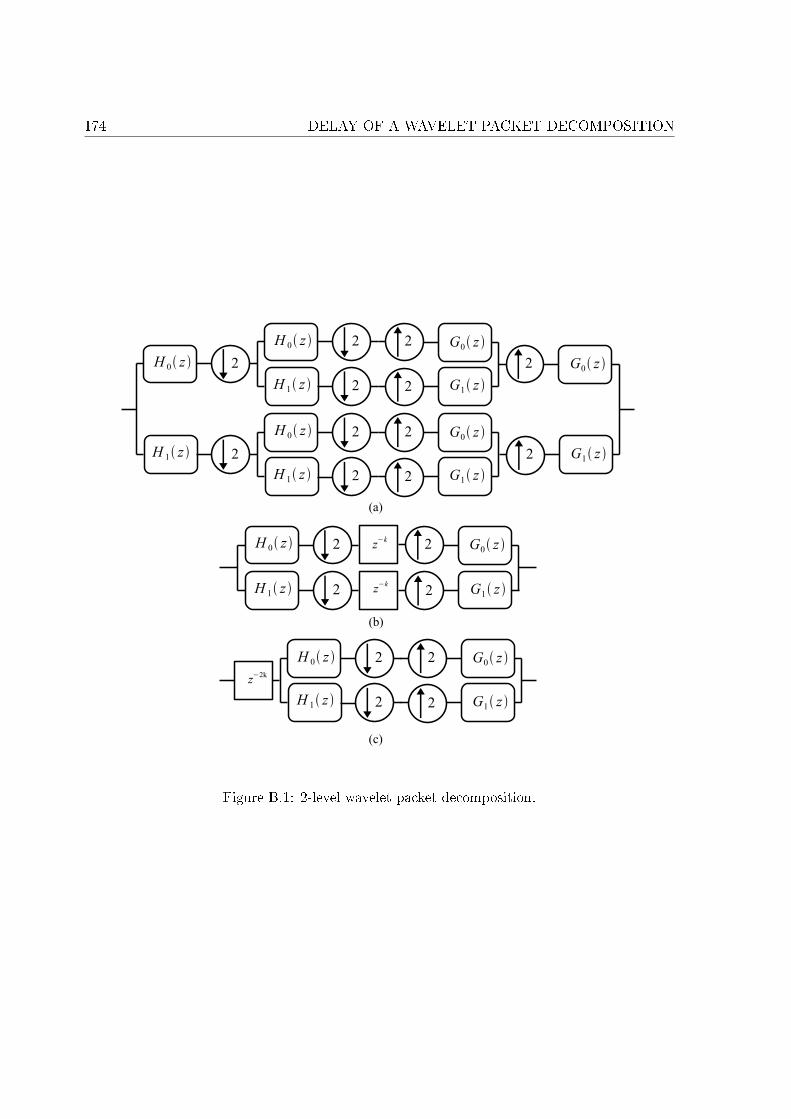
174 DELAY OF A WAVELET PACKET DECOMPOSITION
Figure B.1: 2-level wavelet packet decomposition.
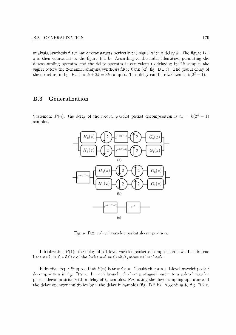
B.3. GENERALIZATION 175
analysis/synthesis �lter bank reconstructs perfectly the signal with a delay k. The �gure B.1a is then equivalent to the �gure B.1 b. According to the noble identities, permuting thedownsampling operator and the delay operator is equivalent to delaying by 2k samples thesignal before the 2-channel analysis/synthesis �lter bank (cf. �g. B.1 c). The global delay ofthe structure in �g. B.1 a is k + 2k = 3k samples. This delay can be rewritten as k(22 − 1).
B.3 Generalization
Statement P (n): the delay of the n-level wavelet packet decomposition is tn = k(2n − 1)samples.
Figure B.2: n-level wavelet packet decomposition.
Initialization P (1): the delay of a 1-level wavelet packet decomposition is k. This is truebecause it is the delay of the 2-channel analysis/synthesis �lter bank.
Inductive step : Suppose that P (n) is true for n. Considering a n + 1-level wavelet packetdecomposition in �g. B.2 a. In each branch, the last n stages constitute a n-level waveletpacket decomposition with a delay of tn samples. Permuting the downsampling operator andthe delay operator multiplies by 2 the delay in samples (�g. B.2 b). According to �g. B.2 c,
176 DELAY OF A WAVELET PACKET DECOMPOSITION
the equivalent delay of the n + 1-level wavelet packet decomposition is then:
tn+1 = k(2n+1 − 2) + k= k2n+1 − 2k + k= k2n+1 − k
tn+1 = k(2n+1 − 1)
(B.8)
P (n + 1) is also true. Consequently, for all n ∈ N, n ≥ 1 the delay of a n-level wavelet packetdecomposition is k(2n − 1). This result is true only if the wavelet �lter used in each stage ofthe decomposition has the same length.
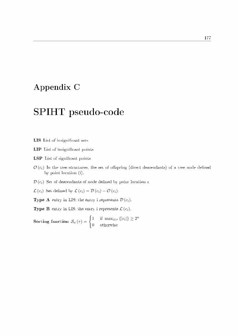
177
Appendix C
SPIHT pseudo-code
LIS List of insigni�cant sets
LIP List of insigni�cant points
LSP List of signi�cant points
O (ci) In the tree structures, the set of o�spring (direct descendants) of a tree node de�nedby point location (i).
D (ci) Set of descendants of node de�ned by point location i.
L (ci) Set de�ned by L (ci) = D (ci)−O (ci).
Type A entry in LIS: the entry i represents D (ci).
Type B entry in LIS: the entry i represents L (ci).
Sorting function Sn (τ) =
{1 if maxi∈τ {|ci|} ≥ 2n
0 otherwise
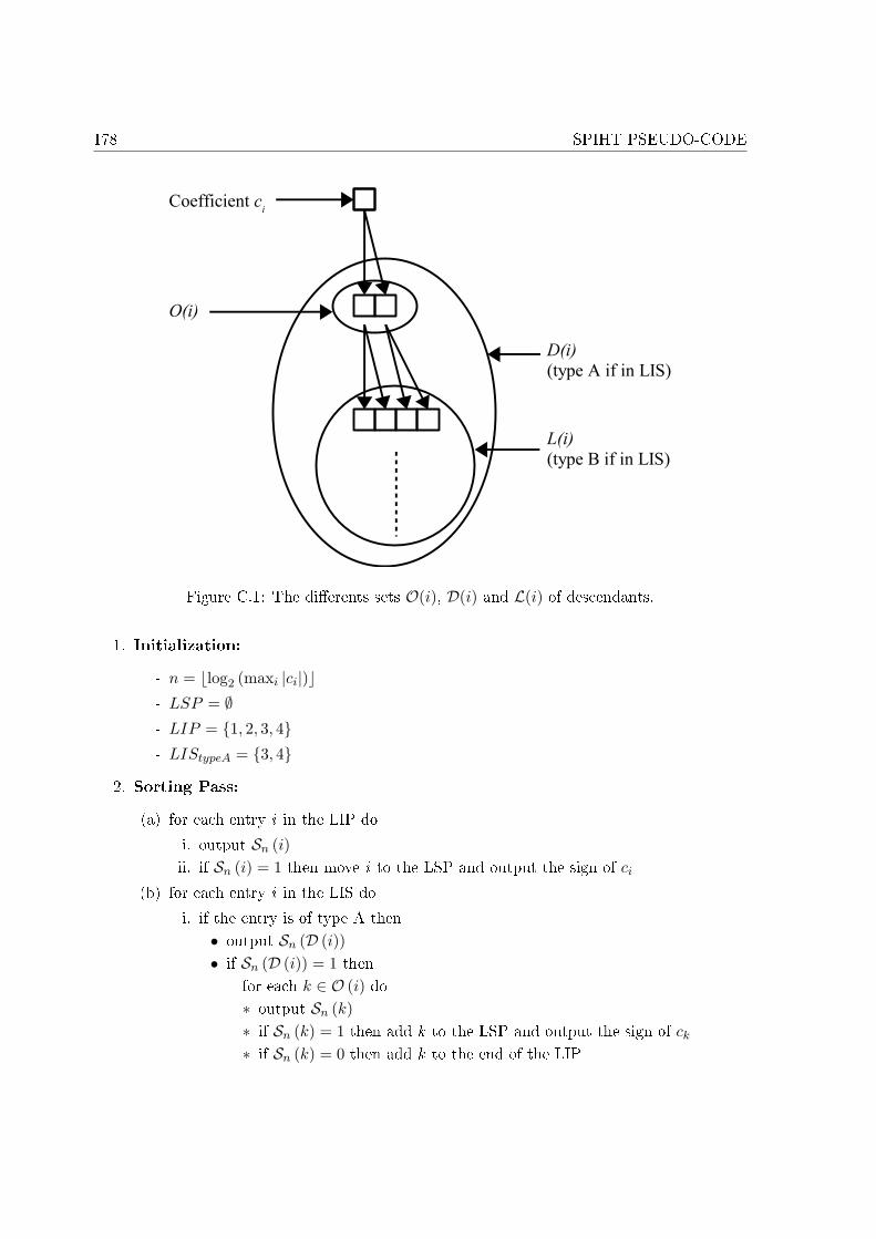
178 SPIHT PSEUDO-CODE
Figure C.1: The di�erents sets O(i), D(i) and L(i) of descendants.
1. Initialization:
- n = blog2 (maxi |ci|)c- LSP = ∅- LIP = {1, 2, 3, 4}- LIStypeA = {3, 4}
2. Sorting Pass:
(a) for each entry i in the LIP do
i. output Sn (i)ii. if Sn (i) = 1 then move i to the LSP and output the sign of ci
(b) for each entry i in the LIS do
i. if the entry is of type A then
• output Sn (D (i))• if Sn (D (i)) = 1 then
� for each k ∈ O (i) do∗ output Sn (k)∗ if Sn (k) = 1 then add k to the LSP and output the sign of ck
∗ if Sn (k) = 0 then add k to the end of the LIP
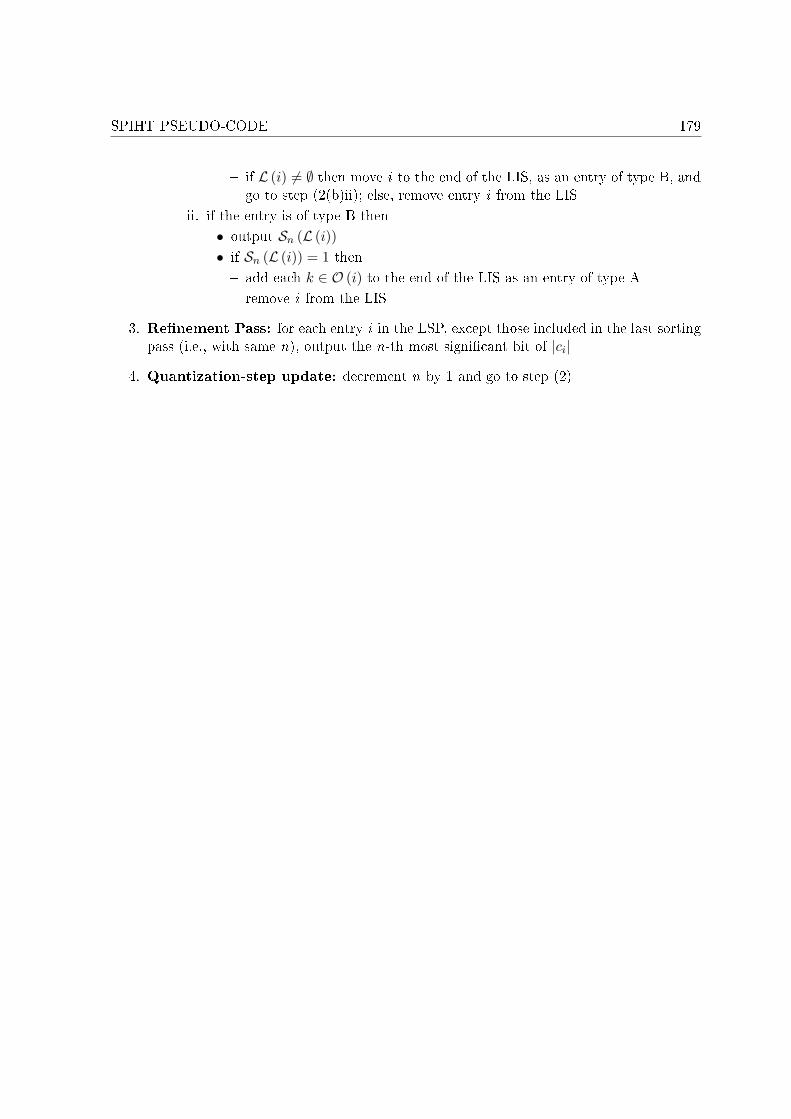
SPIHT PSEUDO-CODE 179
� if L (i) 6= ∅ then move i to the end of the LIS, as an entry of type B, andgo to step (2(b)ii); else, remove entry i from the LIS
ii. if the entry is of type B then
• output Sn (L (i))• if Sn (L (i)) = 1 then
� add each k ∈ O (i) to the end of the LIS as an entry of type A
� remove i from the LIS
3. Re�nement Pass: for each entry i in the LSP, except those included in the last sortingpass (i.e., with same n), output the n-th most signi�cant bit of |ci|
4. Quantization-step update: decrement n by 1 and go to step (2)

180 SPIHT PSEUDO-CODE
BIBLIOGRAPHY 181
Bibliography
3GPP (1999). TS 26.090: Mandatory Speech Codec speech processing functions; AMR Speechcodec; General Description, Technical report, 3GPP.
Adoul, J. P.; Mabilleau, P.; Delprat, M.; Morissette, S. (1987). Fast CELP Coding Based onAlgebraic Codes, Proceedings of ICASSP '87, IEEE, pp. 1957�1960.
Aggarwal, A.; Cuperman, V.; Rose, K.; Gersho, A. (1999). Perceptual Zerotrees for ScalableWavelet Coding of Wideband Audio, Proc. of IEEE Workshop on Speech Coding, IEEE,pp. 16�18.
Atal, B. S.; Remde, J. R. (1982). A New Model of Excitation for Producing Natural-SoundingSpeech at Low Bit Rates, Proceedings of ICASSP '82, vol. 1, pp. 614�617.
Brandenburg, K.; Grill, B. (1994). First Ideas on Scalable Audio Coding, Proceedings of the97th AES Convention, AES.
Byun, K. J.; Jung, H. B.; Kim, K. S.; Hahn, M. (2004). A New Bitrate Scalable WidebandSpeech Coder Based On The Standard AMR-WB Codec, 6th IASTED International Con-ference SIGNAL AND IMAGE PROCESSING, IASTED, Honolulu, Hawaii, USA.
Chahine, G. (1993). Pitch Modelling for Speech Coding at 4.8 kbit/s, Master's thesis, McGillUniversity.
Chang, P.-C.; Lin, J.-H. (2001). Scalable Embedded Zero Tree Wavelet Packet Audio Cod-ing, IEEE Third Workshop on Signal Processing Advances in Wireless Communications(SPAWC'01), IEEE, Taiwan, pp. 384�387.
Cohen, A.; Daubechies, I.; Vial, P. (1993). Wavelets on the interval and fast wavelet transforms,Appl. Comput. Harmon. Anal., vol. 1, no. 1, pp. 54�81.
Coifman, R. R.; Wickerhauser, M. V. (1992). Entropy-Based Algorithms for Best Basis Selec-tion, IEEE Transactions on Information Theory, vol. 38, pp. 713�718.
Collen, P. (2002). Techniques d'Enrichissement de Spectre des Signaux Audionumériques, PhDthesis, Ecole Nationale Supérieure des Télécommunications.

182 BIBLIOGRAPHY
Daubechies, I. (1988). Orthonormal Bases of Compactly Supported Wavelets, Commun. Pureand Appl. Math., vol. 41, pp. 909�996.
Daumer, W. R.; Mermelstein, P.; Maitre, X.; Tokizawa, I. (1984). Overview of the ADPCMCoding Algorithm, Proc. of GLOBECOM 1984, pp. 23.1.�23.1.4.
De Meuleneire, M.; Gartner, M.; Schandl, S.; Taddei, H. (2006a). An Enhancement Layer forACELP Coder, Proc. of MMSP 2006, IEEE, Victoria, BC, Canada.
De Meuleneire, M.; Taddei, H.; de Zelicourt, O.; Pastor, D.; Jax, P. (2006b). A CELP-WaveletScalable Wideband Speech Coder, Proc. of ICASSP 2006, IEEE, Toulouse, France, vol. 1,pp. 697�700.
Dongme, H.; Wen, G.; Jiangqin, W. (2000). Complexity Scalable Audio Coding AlgorithmBased on Wavelet Packet Decomposition, ICSP 2000, IEEE, vol. 2, pp. 659�665.
Erdmann, C. .; Bauer, D.; Vary, P. (2002). Pyramid CELP: Embedded Speech Coding forPacket Communications, ICASSP 2002, IEEE, Orlando, USA, vol. 1, pp. 181�184.
Farrugia, M.; Jbira, A.; Kondoz, A. (1998). Pulse-excited LPC for wideband speech and audiocoding, IEEE Colloquium on Audio and Music Technology: The Challenge of CreativeDSP, IEEE, London, UK, pp. 1/1�1/6.
Federal Standard 1015, Telecommunications: Analog to Digital Conversion of Radio Voice By2400 Bit/Second Linear Predictive Coding (1984). Technical report, National Communi-cation System - O�ce Technology and Standards.
Itakura, F. (1975). Line Spectrum Representation of Linear predictive Coe�cients of SpeechSignals, J. Acoust. Soc. Am., vol. 57, pp. S35.
ITU-T (1988a). Recommendation G.711: Pulse Code Modulation (PCM) of voice frequencies.
ITU-T (1988b). Recommendation G.722: 7 kHz Audio - Coding within 64 kbit/s.
ITU-T (1990). Recommendation G.726: 40,32,24,16 kbit/s Adaptive Di�erential Pulse CodeModulation (ADPCM).
ITU-T (1992). Recommendation G.728: Coding of Speech at 16 kbit/s Using Low-Delay CodeExcited Linear Prediction.
ITU-T (1996a). Recommendation G.723.1: Dual Rate Speech Coder for Multimedia Commu-nications Transmitting at 5.3 and 6.3 kbit/s.
ITU-T (1996b). Recommendation G.729 Annex A: Reduced complexity 8 kbit/s CS-ACELPspeech codec.
ITU-T (1996c). Recommendation G.729 Annex B: A silence compression scheme for G.729optimized for terminals conforming to Recommendation V.70.
BIBLIOGRAPHY 183
ITU-T (1996d). Recommendation G.729: Coding of Speech at 8 kbit/s using Conjugate-Structure Algebraic-Code-Excited Linear Prediction (CS-ACELP).
ITU-T (1996e). Recommendation P.800: Methods for Subjective Determination of Transmis-sion Quality.
ITU-T (1996f). Recommendation P.810: Modulated Noise Rerence Unit (MNRU).
ITU-T (1998a). Recommendation G.120: Transmission characteristics of national networks.
ITU-T (1998b). Recommendation G.729 Annex C: Reference �oating-point implementationfor G.729 CS-ACELP 8 kbit/s speech coding.
ITU-T (1998c). Recommendation G.729 Annex D: 6.4 kbit/s CS-ACELP speech coding algo-rithm.
ITU-T (1998d). Recommendation G.729 Annex E: 11.8 kbit/s CS-ACELP speech codingalgorithm.
ITU-T (2001). P862 Perceptual Evaluation of Speech Quality (PESQ): An Objective Methodfor End-to-End Speech Quality Assessment of Narrow-Band Telephone Networks andSpeech Codecs.
ITU-T (2002). Recommendation T.800: Information Technology - JPEG 2000 Image CodingSystem: Core Coding System.
ITU-T (2003). Recommendation G.722.2: Wideband coding of speech at around 16 kbit/susing Adaptive Multi-Rate Wideband (AMR-WB).
ITU-T (2005). Recommendation G.722.1: Low-complexity coding at 24 and 32 kbit/s forhands-free operation in systems with low frame loss.
ITU-T (2006a). Recommendation G.729.1: G.729 based Embedded Variable bit-rate coder:An 8-32 kbit/s scalable wideband coder bitstream interoperable with G.729.
ITU-T (2006b). Recommendation P.10: Vocabulary for Performance and Quality of Service.
ITU-T (2006c). Recommendation P.800.1: Mean Opinion Score (MOS) Terminology.
Jax, P. (2002). Enhancement of Bandlimited Speech Signals: Algorithms and TheoriticalBounds, PhD thesis, IND Aachen.
Jax, P.; Geiser, B.; Schandl, S.; Taddei, H.; Vary, P. (2006). An Embedded Scalable WidebandCodec based on the GSM EFR Codec, Proc. of ICASSP 2006, IEEE, Toulouse, France,vol. 1, pp. 5�8.
Johnston, J. D. (1980). A Filter Family Designed for Use in Quadrature Mirror Filter Banks,Proc. of ICASSP 80, IEEE, vol. 5, pp. 291�294.
184 BIBLIOGRAPHY
Johnston, J. D. (1988). Estimation of Perceptual Entropy Using Noise Masking Criteria, Proc.of ICASSP 1988, pp. 2524�2527.
Kabal, P.; Ramachandran, R. P. (1986). The Computation of Line Spectral Frequencies UsingChebyshev Polynomials, IEEE Transactions on Acoustics, Speech and Signal Processing,vol. 6, December, pp. 1419�1425.
Karelic, Y.; Malah, D. (1995). Compression of High-Quality Audio Signals Using AdaptiveFilterbanks and A Zero-Tree Coder, Eighteenth Convention of Electrical and ElectronicsEngineers in Israel, 1995, IEEE, Tel Aviv, Israel.
Koishida, K.; Cuperman, V.; Gersho, A. (2000). A 16 kbit/s Bandwidth Scalable Audio CoderBased on the G.729 Standard, ICASSP 00, IEEE, Istanbil, Turkey, vol. 2, pp. 1149�1152.
Kroon, P.; Deprettere, E.; Sluyter, R. (1986). Regular-Pulse Excitation - A Novel Approachto E�ective and E�cient Multipulse Coding of Speech, IEEE Transactions on Acoustics,Speech, and Signal Processing, vol. 34, no. 5, pp. 1054�1063.
Kudumakis, P.; Sandler, M. (1996). Wavelet Packet Based Scalable Audio Coding, ISCAS 96,IEEE, Atlanta, USA, vol. 2, pp. 41�44.
Kudumakis, P.; Sandler, M. (1997). Usage of Short Wavelets for Scalable Audio Coding, SPIE,vol. 3169, pp. 171�178.
Larsen, E.; Aarts, R. M. (2004). Audio Bandwidth Extension: Application of Psychoacoustics,Signal Processing and Loudspeaker Design.
LeGuyader, A.; Lamblin, C.; Boursicaut, E. (1995). Embedded algebraic CELP/VSELP codersfor wideband speech coding, Speech Communication, vol. 16, no. 4, pp. 319�328.
Leslie, B.; Sandler, M. (1999). A Wavelet Packet Algorithm for 1-D Data With No Block EndE�ects, 1999 IEEE International Symposium on Circuits and Systems ISCAS '99, IEEE,Orlando, USA, vol. 3, pp. 423�426.
Liebchen, T. (2004). An Introduction to MPEG-4 Audio Lossless Coding, Proc. of ICASSP'04,IEEE, Montreal, Quebec, Canada, vol. 3, pp. 1012�1015.
Lu, Z.; Kim, D. Y.; Pearlman, W. A. (2000). Wavelet Compression of ECG Signals by the SetPartitioning in Hierarchical Trees (SPIHT) Algorithm, IEEE Transactions on BiomedicalEngineering, vol. 47, July, pp. 849�856.
Lu, Z.; Pearlman, W. A. (1998). An E�cient, Low-Complexity Audio Coder Delivering Mul-tiple Levels of Quality for Interactive Applications, Proc. IEEE Signal Processing Society1998 Workshop on Multimedia Signal Processing, pp. 529�534.
Lu, Z.; Pearlman, W. A. (1999). High Quality Scalable Stereo Audio Coding, Technical report,Rensselaer Polytechnic Institute.
Mallat, S. (1998). A Wavelet Tour of Signal Processing, Second edn, Academic Press.
BIBLIOGRAPHY 185
Mo, Y.; Lu, W.-S.; Antoniou, A. (1997). Embedded coding for 1-D signals using zerotrees ofwavelet coe�cients, 1997 IEEE Paci�c Rim Conference on Communications, Computersand Signal Processing, IEEE, Victoria, Canada, vol. 1, pp. 306�309.
Moore, B. C. J. (2003). An Introduction to the Psychology of Hearing, Academic Press.
Moriya, T.; Miki, S.; Mano, K.; Ohmuro, H. (1993). Training Method of the ExcitationCodebook for CELP, Proceedings of Eurospeech 93, pp. 1155�1158.
MPEG (1992). ISO/IEC JTC1/SC29/WG11 MPEG, IS 11172-3, "Information Technology- Coding of Moving Pictures and Associated Audio for Digital Storage Media at up toAbout 1.5 Mbit/s, Part 3: Audio".
MPEG (1997). ISO/IEC JTC1/SC29/WG11 MPEG, IS 13818-7, "Information technology -Generic coding of moving pictures and associated audio information, Part 7: AdvancedAudio Coding".
MPEG (1998). ISO/IEC JTC1/SC29/WG11 MPEG, IS 14496-3, "Information Technology -Generic Coding of Audio Vidual Objects, Part 3: Audio".
Raad, M.; Burnett, I.; Mertins, A. (2003). Multi-rate and Multi-resolution Scalable to LosslessAudio Compression Using PSPIHT, Proceedings of the Seventh International Symposiumon Signal Processing and Its Applications, vol. 2, pp. 121�124.
Raad, M.; Mertins, A.; Burnett, I. (2002). Audio Compression using the MLT and SPIHT, theSixth International Symposium on Digital Signal Processing for Communication SystemsDSPCS'02, Telecommunications & Information Technology Research Institute, Wollon-gong, Australia, pp. 128�131.
Rabiner, L. R. (1977). On the Use of the Autocorellation Analysis for Pitch Detection, IEEETrans. Acoust., Speech, Signal Processing, vol. ASSP-25, February, pp. 24�33.
Said, A.; Pearlman, W. A. (1996). A New Fast and E�cient Image Codec Based on SetPartitioning in Hierarchical Trees, IEEE Transactions on Circuits and Systems for VideoTechnology, vol. 6, June, pp. 243�250.
Schroeder, M. R.; Atal, B. S. (1985a). Code-Excited Linear Prediction (CELP): High-QualitySpeech at Very Low Bit Rates, Proceedings of ICASSP' 85, IEEE, vol. 10, pp. 937�940.
Schroeder, M. R.; Atal, B. S. (1985b). Stochastic Coding of Speech at Very Low Bit Rates:the importance of Speech Perception, Speech Communication 1985, vol. 4, pp. 155�162.
Schroeder, M. R.; Atal, B. S.; Hall, J. L. (1979). Optimizing Digital Speech Coders by Ex-ploiting Masking Properties of the Human Ear, The Journal of the Acoustical Society ofAmerica, vol. 66, no. 6, December, pp. 1647�1652.
Shannon, C. E. (1949). Communication in the Presence of Noise, Proc. Institute of RadioEngineers, vol. 37, pp. 10�21. Reprint as classic paper in: Proc. IEEE, Vol. 86, No. 2,(Feb 1998).
186 BIBLIOGRAPHY
Shapiro, J. (1993). Embedded Image Coding Using Zerotrees of Wavelet Coe�cients, IEEETransactions on Signal Processing, vol. 41, December, pp. 3445�3462.
Sinha, D.; Tew�k, A. H. (1993). Low Bit Rate Transparent Audio Compression using AdaptedWavelets, IEEE Transactions on Signal Processing, vol. 41, no. 12, December, pp. 3463�3479.
Srinivasan, P.; Jamieson, L. H. (1998). High-Quality Audio Compression using an AdaptiveWavelet Packet Decomposition and Psychoacoustic Modeling, IEEE Transactions on Sig-nal Processing, vol. 46, pp. 1085�1093.
Strobach, P. (1990). Linear Prediction Theory, Springer Verlag.
Su, A.; Chang, W.-C.; Wang, J.-X. (2005). A New Audio Compression Method Based onSpectral Oriented Trees, Proceedings of the 118th AES Convention, AES.
Terhardt, E. (1998). Akustische Kommunikation: Grundlagen mit Hörbeispielen, Springer.
Trench, W. F. (1964). An Algorithm for the Inversion of Finite Toeplitz Matrices, J. Soc.Indust. Appl. Math., vol. 12, pp. 515�522.
Vary, P.; Martin, R. (2006). Digital Speech Transmission: Enhancement, Coding and ErrorConcealment, Wiley.
Vetterli, M. (1986). Filter Banks Allowing Perfect Reconstruction, Signal Processing, vol. 10,no. 3, April, pp. 219�244.
Voran, S. (1997). Listener Ratings of Speech Passbands, Proceedings of IEEE Workshop onSpeech Coding, IEEE, Pocono Manor, PA, USA, pp. 81�82.
Wang, J.-X.; Cheng, F.; Su, A. (2003). Concurrent encoding in hierarchical trees for waveletbased image compression, Proceedings of the 2004 International Conference on ImageProcessing, IEEE, vol. 5, pp. 3173�3176.
Wickerhauser, M. V. (1994). Adapted Wavelet Analysis from Theory to Software , AK Peters,Ltd.

Résumé
Les contraintes de qualité de service liées aux applications de voix sur IP ont rendu néces-saire le développement d'une nouvelle classe de codecs, quali�és d'imbriqués, ou scalables, quisont capables de décoder tout ou partie du train binaire.
Le codec de parole en bande élargie développé au cours de cette thèse produit un trainbinaire qui peut être décodé à des débits variant de 8 à 32 kbit/s. Dans ce but, la structure ducodeur comprend trois couches. Tout d'abord, un premier banc de �ltre isole la composantebande étroite de la composante bande élargie du signal d'entrée. Puis, la première couche,appelée couche coeur, encode la composante bande étroite du signal d'entrée. Cette coucheutilise le codeur G.729 de l'UIT-T. Ensuite, la deuxième couche, encore appelée première couched'amélioration, emploie des techniques d'extension de bandes qui reposent sur l'utilisation d'unbanc de �ltre en ondelettes pour reproduire arti�ciellement la composante bande élargie, avecun débit additionnel de 2 kbit/s. En�n, la seconde et dernière couche d'amélioration, encodede manière progressive les coe�cients d'ondelettes de la di�érence entre le signal original et lasortie du G.729 dans la partie bande étroite, et encode les coe�cients d'ondelettes du signaloriginal dans la partie bande élargie. Par conséquent, le décodeur assure un signal reconstruità bande étroite à un débit de 8 kbit/s, produit un signal bande élargie à 10 kbit/s, et améliorela qualité jusqu'à un débit de 32 kbit/s.
Des tests d'écoute ont montré que la qualité du codec s'améliore avec une augmentation dudébit. Pour des signaux de parole, le codec à 24 et 32 kbit/s est équivalent au codeur G.722de l'UIT-T à 56 et 64 kbit/s. De plus, le codec à 32 kbit/s est équivalent au codeur imbriquéG.729.1 au même débit, récemment standardisé à l'UIT-T.
Mots clés :ondelettes, codage imbriqué, CELP, extension de bande, EZW, SPIHT, quanti�-cation algébrique.
Abstract
The constraints of quality of service related to Voice over IP applications have made nec-essary the development of a new class of codecs, called embedded, or scalable, codecs, able todecode a part of the generated bitstream.
The wideband speech codec developed during this thesis provides an embedded bitstreamthat can be decoded at bitrates ranging from 8 to 32 kbit/s. To do so, the codec structurecomprises three layers. First, a split band structure separates the narrowband component andwideband component of the input signal. Then, the �rst layer, called core layer, encodes thenarrow band component of the input signal. This layer makes use of the ITU-T G.729 coder.Afterwards, the second layer, called �rst enhancement layer, utilizes bandwidth extension tech-niques relying on a wavelet �lter bank to reproduce arti�cially the wideband component, withan additional bitrate of 2 kbit/s. Finally, the second and last enhancement layer, progressivelyencodes the wavelet coe�cients of the di�erence between the original signal and the G.729 out-put in the narrowband part, and encodes the wavelet coe�cients of the original signal in thewideband part. Hence, the decoder ensures a narrowband signal at 8 kbit/s, enables widebandrendering at 10 kbit/s and improves the quality up to 32 kbit/s.
Listening tests have shown that the quality of the codec improves gracefully as the bitrateincreases. For speech signals the codec at 24 kbit/s and 32 kbit/s is shown to be equivalent tothe ITU-T G.722 codec at 56 and 64 kbit/s, respectively. Moreover, the codec at 32 kbit/s isassessed to be equivalent to the recently standardized embedded codec ITU-T G.729.1 at thesame bitrate.
Keywords: wavelets, embedded coding, CELP, bandwidth extension, EZW, SPIHT, algebraicquantization.