Lec3 Soil Mechanics Lec 2015-2016 2

8/20/2019 Lec3 Soil Mechanics Lec 2015-2016 2

http://slidepdf.com/reader/full/lec3-soil-mechanics-lec-2015-2016-2 1/4

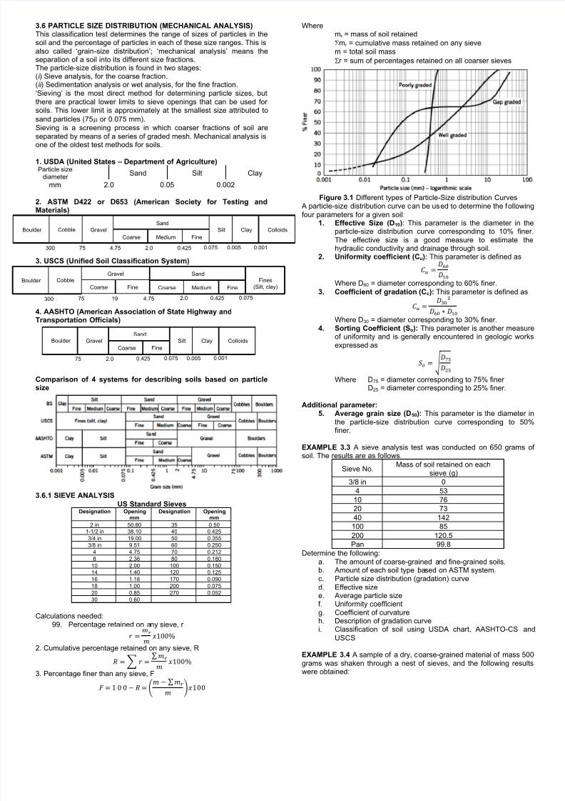
3.6 PARTICLE SIZE DISTRIBUTION (MECHANICAL ANALYSIS)This classification test determines the range of sizes of particles in thesoil and the percentage of particles in each of these size ranges. This is

also called ‘grain-size distribution’; ‘mechanical analysis’ means theseparation of a soil into its different size fractions.The particle-size distribution is found in two stages:(i ) Sieve analysis, for the coarse fraction.(ii ) Sedimentation analysis or wet analysis, for the fine fraction.

‘Sieving’ is the most direct method for determining particle sizes, but

there are practical lower limits to sieve openings that can be used forsoils. This lower limit is approximately at the smallest size attributed to

sand particles (75 or 0.075 mm).

Sieving is a screening process in which coarser fractions of soil are

separated by means of a series of graded mesh. Mechanical analysis isone of the oldest test methods for soils.

1. USDA (United States – Department of Agriculture)Particle size

diameterSand Silt Clay

mm 2.0 0.05 0.002

2. ASTM D422 or D653 (American Society for Testing andMaterials)

3. USCS (Unified Soil Classification System)

4. AASHTO (American Association of State Highway andTransportation Officials)

Comparison of 4 systems for describing soils based on particlesize

3.6.1 SIEVE ANALYSIS

US Standard SievesDesignation Opening

mmDesignation Opening

mm

2 in 50.80 35 0.50

1-1/2 in 38.10 40 0.425

3/4 in 19.00 50 0.355

3/8 in 9.51 60 0.250

4 4.75 70 0.212

8 2.36 80 0.180

10 2.00 100 0.150

14 1.40 120 0.125

16 1.18 170 0.090

18 1.00 200 0.075

20 0.85 270 0.052

30 0.60

Calculations needed:99. Percentage retained on any sieve, r

2. Cumulative percentage retained on any sieve, R

∑

3. Percentage finer than any sieve, F

∑

Wheremr = mass of soil retained

mr = cumulative mass retained on any sieve

m = total soil mass

r = sum of percentages retained on all coarser sieves

Figure 3.1 Different types of Particle-Size distribution Curves A particle-size distribution curve can be used to determine the followin

four parameters for a given soil:1. Effective Size (D10): This parameter is the diameter in th

particle-size distribution curve corresponding to 10% fine

The effective size is a good measure to estimate thhydraulic conductivity and drainage through soil.

2. Uniformity coefficient (Cu): This parameter is defined as

Where D60 = diameter corresponding to 60% finer.3. Coefficient of gradation (Cc): This parameter is defined as

Where D30 = diameter corresponding to 30% finer.

4. Sorting Coefficient (So): This parameter is another measuof uniformity and is generally encountered in geologic wor

expressed as

√ Where D75 = diameter corresponding to 75% finer

D25 = diameter corresponding to 25% finer.

Additional parameter:5. Average grain size (D50): This parameter is the diameter

the particle-size distribution curve corresponding to 50finer.

EXAMPLE 3.3 A sieve analysis test was conducted on 650 grams soil. The results are as follows.

Sieve No.Mass of soil retained on each

sieve (g)

3/8 in 0

4 53

10 76

20 73

40 142

100 85

200 120.5

Pan 99.8

Determine the following:

a. The amount of coarse-grained and fine-grained soils.b. Amount of each soil type based on ASTM system.c. Particle size distribution (gradation) curve

d. Effective sizee. Average particle sizef. Uniformity coefficient

g. Coefficient of curvatureh. Description of gradation curvei. Classification of soil using USDA chart, AASHTO-CS an

USCS

EXAMPLE 3.4 A sample of a dry, coarse-grained material of mass 50

grams was shaken through a nest of sieves, and the following resulwere obtained:

Boulder Cobble Gravel

Sand

Coarse Medium Fine

Silt Clay Colloids

300 75 4.75 2.0 0.425 0.075 0.005 0.001

Boulder Cobble

Sand

Coarse Medium FineFines

(Silt, clay)

300 75 19 4.75 2.0 0.425 0.075

Gravel

Coarse Fine

Boulder Gravel

Sand

Coarse Fine

Silt Clay Colloids

75 2.0 0.425 0.075 0.005 0.001



a. Plot the particle size distribution (gradation) curve

b. Determine (1) the effective size, (2) the average particle size,

(3) the uniformity coefficient, and (4) the coefficient ofcurvature

c. Determine the textural composition of the soil (i.e., theamount of gravel, sand, etc.).

,EXAMPLE 3.5 Classify the soil using AASHTO-CS and USCS.

EXAMPLE 3.6 Classify the soil using AASHTO-CS and USCS.

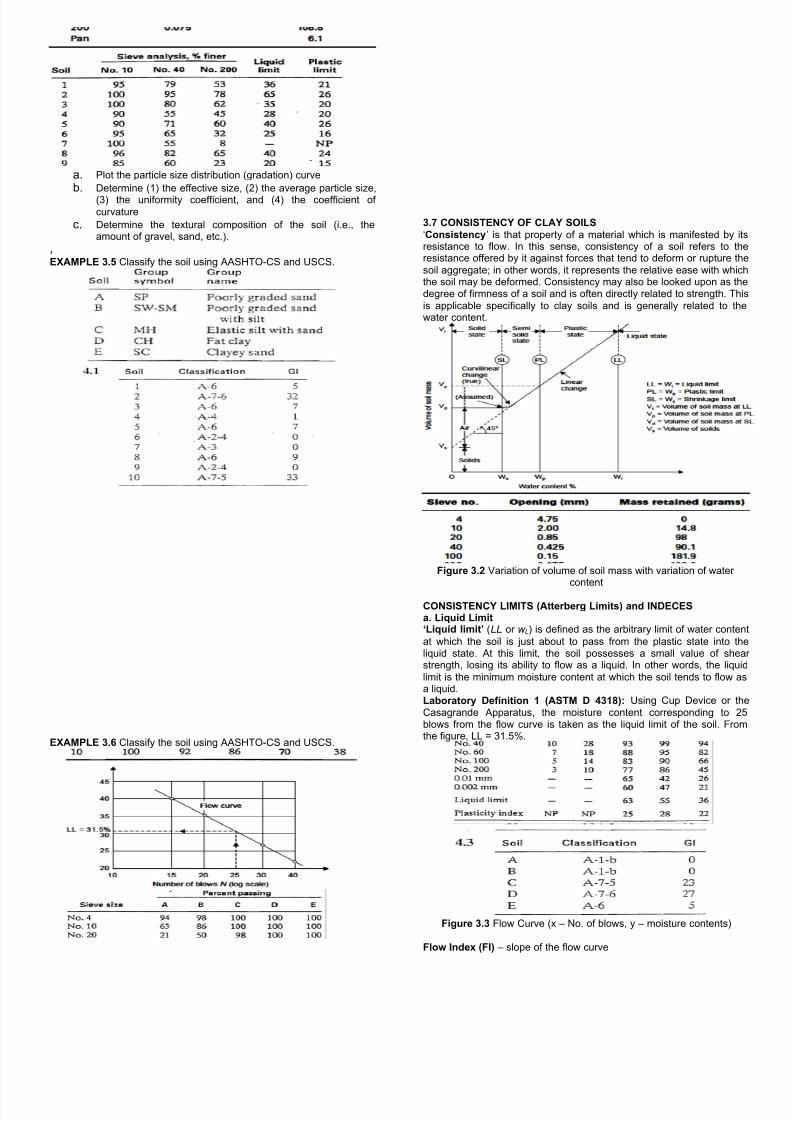
3.7 CONSISTENCY OF CLAY SOILS

‘Consistency’ is that property of a material which is manifested by iresistance to flow. In this sense, consistency of a soil refers to thresistance offered by it against forces that tend to deform or rupture th

soil aggregate; in other words, it represents the relative ease with whicthe soil may be deformed. Consistency may also be looked upon as thdegree of firmness of a soil and is often directly related to strength. Th

is applicable specifically to clay soils and is generally related to thwater content.

Figure 3.2 Variation of volume of soil mass with variation of watercontent

CONSISTENCY LIMITS (Atterberg Limits) and INDECESa. Liquid Limit‘Liquid limit’ (LL or w L) is defined as the arbitrary limit of water conte

at which the soil is just about to pass from the plastic state into thliquid state. At this limit, the soil possesses a small value of shestrength, losing its ability to flow as a liquid. In other words, the liqu

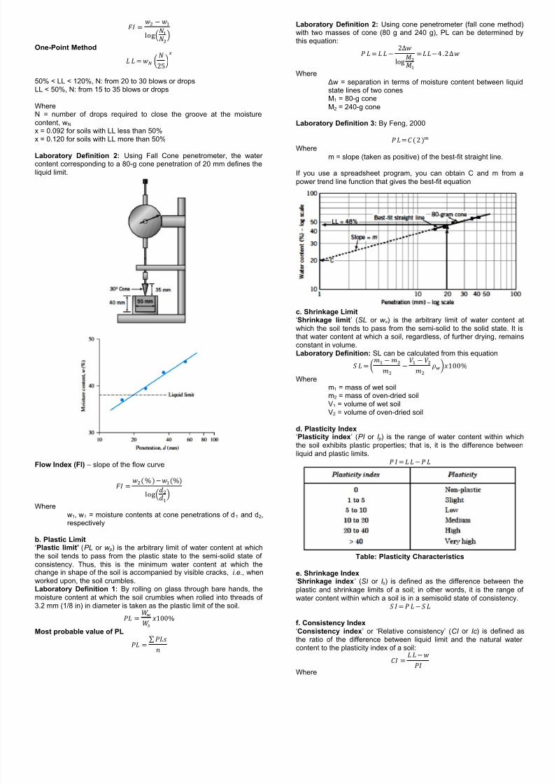
limit is the minimum moisture content at which the soil tends to flow aa liquid.Laboratory Definition 1 (ASTM D 4318): Using Cup Device or th

Casagrande Apparatus, the moisture content corresponding to 2blows from the flow curve is taken as the liquid limit of the soil. Frothe figure, LL = 31.5%.

Figure 3.3 Flow Curve (x – No. of blows, y – moisture contents)

Flow Index (FI) – slope of the flow curve



One-Point Method

()

50% < LL < 120%, N: from 20 to 30 blows or dropsLL < 50%, N: from 15 to 35 blows or drops

WhereN = number of drops required to close the groove at the moisture

content, wN x = 0.092 for soils with LL less than 50%

x = 0.120 for soils with LL more than 50%

Laboratory Definition 2: Using Fall Cone penetrometer, the watercontent corresponding to a 80-g cone penetration of 20 mm defines the

liquid limit.

Flow Index (FI) – slope of the flow curve

Where

w1, w2 = moisture contents at cone penetrations of d1 and d2,respectively

b. Plastic Limit

‘Plastic limit’ (PL or w p) is the arbitrary limit of water content at whichthe soil tends to pass from the plastic state to the semi-solid state of

consistency. Thus, this is the minimum water content at which thechange in shape of the soil is accompanied by visible cracks, i.e., when

worked upon, the soil crumbles.Laboratory Definition 1: By rolling on glass through bare hands, the

moisture content at which the soil crumbles when rolled into threads of3.2 mm (1/8 in) in diameter is taken as the plastic limit of the soil.

Most probable value of PL

∑

Laboratory Definition 2: Using cone penetrometer (fall cone methowith two masses of cone (80 g and 240 g), PL can be determined bthis equation:

Where

Δw = separation in terms of moisture content between liqustate lines of two conesM1 = 80-g cone

M2 = 240-g cone

Laboratory Definition 3: By Feng, 2000

Where

m = slope (taken as positive) of the best-fit straight line.

If you use a spreadsheet program, you can obtain C and m from

power trend line function that gives the best-fit equation

c. Shrinkage Limit‘Shrinkage limit’ (SL or w s) is the arbitrary limit of water content

which the soil tends to pass from the semi-solid to the solid state. It that water content at which a soil, regardless, of further drying, remai

constant in volume. Laboratory Definition: SL can be calculated from this equation

( )

Wherem1 = mass of wet soilm2 = mass of oven-dried soil

V1 = volume of wet soil

V2 = volume of oven-dried soil

d. Plasticity Index‘Plasticity index’ (PI or I p) is the range of water content within whic

the soil exhibits plastic properties; that is, it is the difference betwee

liquid and plastic limits.

Table: Plasticity Characteristics

e. Shrinkage Index‘Shrinkage index’ (SI or I s) is defined as the difference between th

plastic and shrinkage limits of a soil; in other words, it is the range

water content within which a soil is in a semisolid state of consistency.

f. Consistency Index‘Consistency index’ or ‘Relative consistency’ (CI or Ic ) is defined a

the ratio of the difference between liquid limit and the natural watecontent to the plasticity index of a soil:

Where



w = natural moisture content of the soil (water content of asoil in the undisturbed condition in the ground

If CI = 0, w = LLCI = 1, w = PLCI > 1, the soil is in semi-solid state and is stiff

CI < 0, the natural water content is greater than LL, and the soilbehaves like liquid

g. Liquidity Index‘Liquidity index (LI or I L)’ or ‘Water -plasticity ratio’ is the ratio of the

difference between the natural water content and the plastic limit to the

plasticity index:

If LI = 0, w = PLLI = 1, w = LLLI > 1, the soil is in liquid state

LI < 0, the soil is in the semi-solid state and is stiff

Table: Consistency Classification

h. Toughness Index‘Toughness Index’ (TI) is defined as the ratio of the plasticity index to

the flow index:

EXAMPLE 3.7 A liquid limit test, conducted on a soil sample in the cupdevice, gave the following results:

Number of blows 10 19 23 27 40

Water Content (%) 60.0 45.2 39.8 36.5 25.2

Four determinations for the plastic limit gave water contents of 20.3%20.55%, 20.8% and 11.26%.

Determine the following:a. LL and PL (in %)

b. Plasticity Indexc. Liquidity index and Consistency Index, if the natural water

content is 27.4%. Describe the consistency.

d. Void ratio at the LL if Gs = 2.7e. Shrinkage limit of the soil if the void ratio of this soil is at the

minimum volume reached on shrinkage is 0.405

If the soil were to be loaded to failure, would you expect a brittle failure?

EXAMPLE 3.8 A fall cone test was carried out on a soil to determineliquid limit and plastic limit using cones of masses 80 g and 240 g. Thefollowing results were obtained.

80-g cone 240-g cone

Penetration(mm)

8 15 19 28 9 18 22 30

MoistureContent %

43.1 52 56.1 62.9 37 47.5 51 55.1

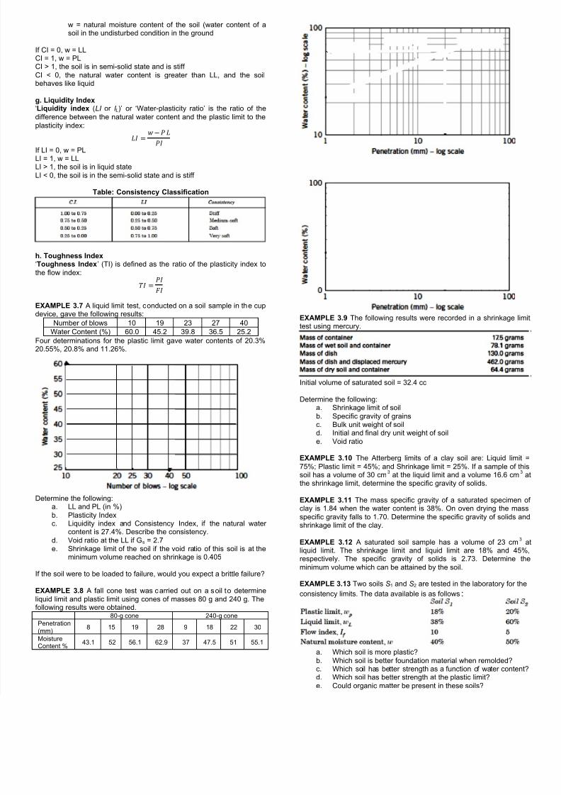
EXAMPLE 3.9 The following results were recorded in a shrinkage limtest using mercury.

Initial volume of saturated soil = 32.4 cc

Determine the following:a. Shrinkage limit of soil

b. Specific gravity of grainsc. Bulk unit weight of soild. Initial and final dry unit weight of soil

e. Void ratio

EXAMPLE 3.10 The Atterberg limits of a clay soil are: Liquid limit

75%; Plastic limit = 45%; and Shrinkage limit = 25%. If a sample of thsoil has a volume of 30 cm

3 at the liquid limit and a volume 16.6 cm

3

the shrinkage limit, determine the specific gravity of solids.

EXAMPLE 3.11 The mass specific gravity of a saturated specimen clay is 1.84 when the water content is 38%. On oven drying the mas

specific gravity falls to 1.70. Determine the specific gravity of solids anshrinkage limit of the clay.

EXAMPLE 3.12 A saturated soil sample has a volume of 23 cm3

liquid limit. The shrinkage limit and liquid limit are 18% and 45%

respectively. The specific gravity of solids is 2.73. Determine thminimum volume which can be attained by the soil.

EXAMPLE 3.13 Two soils S1 and S2 are tested in the laboratory for the

consistency limits. The data available is as follows:

a. Which soil is more plastic?

b. Which soil is better foundation material when remolded?c. Which soil has better strength as a function of water contentd. Which soil has better strength at the plastic limit?

e. Could organic matter be present in these soils?

Documents

Lec3 Soil Mechanics Lec 2015-2016 2