Embed Size (px)
Citation preview

AVERTISSEMENT
Ce document est le fruit d'un long travail approuvé par le jury de soutenance et mis à disposition de l'ensemble de la communauté universitaire élargie. Il est soumis à la propriété intellectuelle de l'auteur. Ceci implique une obligation de citation et de référencement lors de l’utilisation de ce document. D'autre part, toute contrefaçon, plagiat, reproduction illicite encourt une poursuite pénale. Contact : [email protected]
LIENS Code de la Propriété Intellectuelle. articles L 122. 4 Code de la Propriété Intellectuelle. articles L 335.2- L 335.10 http://www.cfcopies.com/V2/leg/leg_droi.php http://www.culture.gouv.fr/culture/infos-pratiques/droits/protection.htm
Ecole doctorale IAEM Lorraine
Parallel Scheduling in the Cloud
Systems : Approximate and Exact
Methods
THESIS
Submitted to the IAEM Lorraine Doctoral School In 15 December 2016
In Partial Fulfillment of the Requirements for the Degree of
Doctor of the Universite de Lorraine
(Computer Sciences )
by
Mohammed Albarra HASSAN ABDELJABBAR HASSAN
Dissertation Committee
President : Prof. Ridha MAHJOUB Universite de Paris-Dauphine, France
Reporters : Prof. Feng CHU Universite d’Evry, France
Dr. Fatiha BENDALI Universite de ClermontFerrand, France
Examiners : Dr. Marie-Ange MANIER Universite de Technologie de Belfort-Montbeliard, France
Dr. Murtada ELBASHIR University of Gezira, Sudan
Supervisors : Prof. Imed KACEM Universite de Lorraine, France
Prof. Izzeldin OSMAN University of Gezira, Sudan
Co-Supervisors : Dr. Sebastien MARTIN Universite de Lorraine, France
Laboratoire de Conception, Optimisation, et Modelisation des Systemes – EA 7306

Mis en page avec la classe thesul.

Acknowledgments
First and foremost, sincere gratitude is due to my Supervisors. Firstly, I would like to
thank my Supervisor in université de Lorraine Prof. Imed KACEM, your encouragement,
guidance and intellectual support from the initial to the �nal level of my PhD degree
enabled me to expand my knowledge by guiding me to develop new methods, and to
practice a lot of research skills, and to know new research directions. Your constant pursuit
for perfection, and valuable suggestions have guided me at every step of my research. It
was a great pleasure and honor to work with you. Particularly, I value your respect towards
professionalism and the desire to excel higher and higher. I owe you lots of gratitude for
having shown me how to be an ideal researcher, a good reviewer and a hard worker.
I'm profoundly indebted to my Co-Supervisor Dr. Sebastién MARTIN who was very
generous with his time and knowledge and assisted me in each step to complete this thesis.
I deeply appreciate your work attitude and your work e�ciency. It was a great pleasure and
honor to work with you too. Your perpetual energy and enthusiasm in research extremely
motivated me in my studies. I shall be missing our regular meetings at 7 :30 AM.
It gives me great pleasure to acknowledge my Supervisor at University of Gezira Prof.
Izzeldin M.OSMAN, his advises, constant support, availability and bright inputs helped
me a lot to accomplish this work. He was always accessible and willing to help every young
scientist with their research every where, and every time.
I have been extremely lucky to have a supervisors like you all, you granted me much
of your time and you cared so much about my work, and responded to my queries and
questions so promptly. This thesis would not have been possible without your extraordi-
nary support. I learned a lot from you, but in fact this clearly shows that there is still a
lot to learn from you.
I also must thank again Prof. Imed KACEM he accepted me as a Ph.D fellow and
giving me an opportunity to pursue a doctorate degree in LCOMS. As well as funding all
costs of all international conferences, publications, and the traveling costs.
I also thank the thesis reporters and all jury members for the thorough and critical
judgment and evaluation of this thesis.
I would also like to thank all members, and Phd colleagues at LCOMS.
I acknowledge the University of Gezira for providing me with this scholarship to pursue
my doctorate studies especially Prof. Mohammed WARRAQ OMER, Prof. Abdelelah M.
ALHASSAN and Prof. Osman ELAMIN. I greatly appreciate all kinds of help received
from the sta� members of the French embassy in Khartoum, espicially Pierre MULLER,
i

Jean-Noel BALEO, Geneviève ICHARD, Abusu�an ALI and Salma YAGI.
I also extend my gratitude to the sta� members and friends from the IUT-Metz for
their help and support, especially Pierre, Frank, Zsuszana, Natali, Crystle and Nicolas,
Je vais manquer le dîner annuel de Noël avec vous.
I deeply thank my wife Ebtihal MUSTAFA, who accepted my long hours at research,
and endured with open heart and mind and encouraged me at every step of my career
and life.
A special thanks goes to my brother Alfrazdaq and his family for living every moment
of this work with me, and for his warmest welcoming in Cork, and Dublin during holidays.
Finally and forever, I acknowledge moral and emotional support I received from my
mother, father, brothers during this challenging period and my life in general.
However, I'm the only person responsible for errors in this thesis.
ii

Dedication
To my parents for their love, prays, and support. You put me through the best education
possible. I appreciate your sacri�ces and I wouldn't have been able to get to this stage
without you.
To my wife Ebtihal and my sons Mohammed, Alaa, you have persevered and endured a lot
during this period.
To my brothers and my sister for unending love and support.
iii

iv

Table of contents
General Introduction 1
Chapitre 1
State-of-the-Art
1.1 Cloud Computing . . . . . . . . . . . . . . . . . . . . . . . . . . . . . . . . 5
1.2 Scheduling problems . . . . . . . . . . . . . . . . . . . . . . . . . . . . . . 6
1.3 Computational complexity . . . . . . . . . . . . . . . . . . . . . . . . . . . 8
1.4 Heuristics and meta-heuristics . . . . . . . . . . . . . . . . . . . . . . . . . 9
1.4.1 Heuristics . . . . . . . . . . . . . . . . . . . . . . . . . . . . . . . . 9
1.4.2 Metaheuristics . . . . . . . . . . . . . . . . . . . . . . . . . . . . . . 9
Genetic algorithm . . . . . . . . . . . . . . . . . . . . . . . . . . . . 10
1.5 Graph theory . . . . . . . . . . . . . . . . . . . . . . . . . . . . . . . . . . 12
1.6 Optimization problems . . . . . . . . . . . . . . . . . . . . . . . . . . . . . 12
1.6.1 Combinatorial optimization . . . . . . . . . . . . . . . . . . . . . . 13
1.6.2 Linear programming . . . . . . . . . . . . . . . . . . . . . . . . . . 14
1.6.3 Integer programming . . . . . . . . . . . . . . . . . . . . . . . . . . 14
1.7 Polyhedral approach . . . . . . . . . . . . . . . . . . . . . . . . . . . . . . 15
1.7.1 Elements of polyhedral theory . . . . . . . . . . . . . . . . . . . . . 16
1.7.2 Cutting plane methods . . . . . . . . . . . . . . . . . . . . . . . . . 17
1.8 Branch and cut algorithm . . . . . . . . . . . . . . . . . . . . . . . . . . . 19
Chapitre 2
Heuristics and Meta-heuristics Solutions 23
2.1 Introduction . . . . . . . . . . . . . . . . . . . . . . . . . . . . . . . . . . . 24
2.1.1 Literature Review . . . . . . . . . . . . . . . . . . . . . . . . . . . . 25
2.2 Problem formulation . . . . . . . . . . . . . . . . . . . . . . . . . . . . . . 27
v
Table of contents
2.3 An existing algorithm . . . . . . . . . . . . . . . . . . . . . . . . . . . . . . 29
2.4 Genetic algorithm (GA) . . . . . . . . . . . . . . . . . . . . . . . . . . . . 29
2.4.1 Modeling the problem using Genetic Algorithm . . . . . . . . . . . 31
Task Scheduling Genetic Algorithm (GATS) . . . . . . . . . . . . . 31
Genetic Algorithm Based on Cut-point (GACP) . . . . . . . . . . 32
Genetic Algorithm Based on The List of Available Jobs (GAAV) . . 32
Genetic Algorithm (GAAV +) . . . . . . . . . . . . . . . . . . . . . 36
Experimental Results . . . . . . . . . . . . . . . . . . . . . . . . . . 37
Integral Linear Programming Solution (ILP) . . . . . . . . . . . . . 39
Transformations Between Genetic Algorithms . . . . . . . . . . . . 40
Conclusion . . . . . . . . . . . . . . . . . . . . . . . . . . . . . . . . 44
Chapitre 3
Mathematical Formulations 47
3.1 Introduction . . . . . . . . . . . . . . . . . . . . . . . . . . . . . . . . . . . 48
3.2 Problem Description . . . . . . . . . . . . . . . . . . . . . . . . . . . . . . 49
3.3 Mathematical Formulations . . . . . . . . . . . . . . . . . . . . . . . . . . 50
3.3.1 Classical Formulation . . . . . . . . . . . . . . . . . . . . . . . . . . 50
3.3.2 Flow Formulation . . . . . . . . . . . . . . . . . . . . . . . . . . . . 52
3.3.3 Order Formulation . . . . . . . . . . . . . . . . . . . . . . . . . . . 54
3.3.4 Interval Graph Formulation . . . . . . . . . . . . . . . . . . . . . . 55
3.4 Valid Inequalities . . . . . . . . . . . . . . . . . . . . . . . . . . . . . . . . 58
3.4.1 Separation Algorithm for SPT Inequality . . . . . . . . . . . . . . . 62
3.4.2 Reformulation of Interval Graph Formulation . . . . . . . . . . . . 62
3.5 Experimental Results . . . . . . . . . . . . . . . . . . . . . . . . . . . . . . 63
3.5.1 Conclusion . . . . . . . . . . . . . . . . . . . . . . . . . . . . . . . . 67
Chapitre 4
Polyedral study on interval graphs under m-clique free constraints 71
4.1 Introduction . . . . . . . . . . . . . . . . . . . . . . . . . . . . . . . . . . . 72
4.2 The polytopes of interval sub-graphs . . . . . . . . . . . . . . . . . . . . . 74
4.2.1 Forbidden subgraphs inequalities . . . . . . . . . . . . . . . . . . . 74
Bipartite Claw . . . . . . . . . . . . . . . . . . . . . . . . . . . . . 75
Umbrella Inequalities . . . . . . . . . . . . . . . . . . . . . . . . . . 79
n-net Inequalities . . . . . . . . . . . . . . . . . . . . . . . . . . . . 82
vi
n-tent Inequalities . . . . . . . . . . . . . . . . . . . . . . . . . . . 84
Hole inequalities . . . . . . . . . . . . . . . . . . . . . . . . . . . . 85
Clique inequalities . . . . . . . . . . . . . . . . . . . . . . . . . . . 87
Clique-Hole inequalities . . . . . . . . . . . . . . . . . . . . . . . . 89
4.3 Cutting plane algorithms . . . . . . . . . . . . . . . . . . . . . . . . . . . . 90
4.3.1 Bipartite claw separation . . . . . . . . . . . . . . . . . . . . . . . . 90
Exact Separation (ExBC-Sep) . . . . . . . . . . . . . . . . . . . . . 91
Heuristic1 : Separation (H1BC-Sep) . . . . . . . . . . . . . . . . . . 92
Heuristic 2 : Separation (H2BC-Sep) . . . . . . . . . . . . . . . . . 92
4.3.2 Umbrella separation . . . . . . . . . . . . . . . . . . . . . . . . . . 92
Exact separation algorithm . . . . . . . . . . . . . . . . . . . . . . 93
H1U-Sep separation . . . . . . . . . . . . . . . . . . . . . . . . . . . 93
H2U-Sep Separation . . . . . . . . . . . . . . . . . . . . . . . . . . 93
n-net separation . . . . . . . . . . . . . . . . . . . . . . . . . . . . . 95
n-tent separation . . . . . . . . . . . . . . . . . . . . . . . . . . . . 96
4.3.3 Hole separation . . . . . . . . . . . . . . . . . . . . . . . . . . . . . 97
4.3.4 Clique separation . . . . . . . . . . . . . . . . . . . . . . . . . . . . 97
4.3.5 Lazy constraint approach . . . . . . . . . . . . . . . . . . . . . . . . 98
4.4 Application to URPMDC problem. . . . . . . . . . . . . . . . . . . . . . . 99
4.4.1 Mathematical formulation . . . . . . . . . . . . . . . . . . . . . . . 99
4.4.2 Computational Results . . . . . . . . . . . . . . . . . . . . . . . . . 102
4.5 Conclusion . . . . . . . . . . . . . . . . . . . . . . . . . . . . . . . . . . . . 103
Chapitre 5
Generalized Open Shop, and Open Shop Problems 107
5.1 Introduction . . . . . . . . . . . . . . . . . . . . . . . . . . . . . . . . . . . 108
5.2 Generalized open shop problem with jobs disjunctive constraints . . . . . . 109
5.2.1 Integer linear programming formulation . . . . . . . . . . . . . . . . 109
5.2.2 Valid inequalities . . . . . . . . . . . . . . . . . . . . . . . . . . . . 110
Sequence inequalities . . . . . . . . . . . . . . . . . . . . . . . . . . 110
Previous job inequalities . . . . . . . . . . . . . . . . . . . . . . . . 111
Line job inequalities . . . . . . . . . . . . . . . . . . . . . . . . . . 112
Logical implication inequalities . . . . . . . . . . . . . . . . . . . . 113
5.2.3 Experimental results . . . . . . . . . . . . . . . . . . . . . . . . . . 113
5.3 Open shop problem . . . . . . . . . . . . . . . . . . . . . . . . . . . . . . . 115
vii
Table of contents
5.3.1 Integer linear programming formulation . . . . . . . . . . . . . . . . 116
5.3.2 Valid inequalities . . . . . . . . . . . . . . . . . . . . . . . . . . . . 118
Sequence inequalities . . . . . . . . . . . . . . . . . . . . . . . . . . 118
Previous operations inequalities . . . . . . . . . . . . . . . . . . . . 119
Logical implication inequalities . . . . . . . . . . . . . . . . . . . . 120
5.3.3 Experimental results . . . . . . . . . . . . . . . . . . . . . . . . . . 121
5.4 Conclusion . . . . . . . . . . . . . . . . . . . . . . . . . . . . . . . . . . . . 122
Chapitre 6
General Conclusion and Perspectives 127
Bibliographie 131
viii
Résumé
Cette thèse porte sur la résolution exacte et heuristique de plusieurs problèmes ayant
des applications dans le domaine de l'Informatique dématérialisé (cloud computing). L'In-
formatique dématérialisée est un domaine en plein extension qui consiste à mutualiser les
machines/serveurs en dé�nissant des machines virtuelles représentant des fractions des
machines/serveurs. Il est nécessaire d'apporter des solutions algorithmiques performantes
en termes de temps de calcul et de qualité des solutions. Dans cette thèse, nous nous
sommes intéressés dans un premier temps au problème d'ordonnancement sur plusieurs
machines (les machines virtuelles) avec contraintes de précédence, c-à-d., que certaines
tâches ne peuvent s'exécuter que si d'autres sont déjà �nies. Ces contraintes représentent
une subdivision des tâches en sous tâchespouvant s'exécuter sur plusieurs machines vir-
tuelles. Nous avons proposé plusieurs algorithmes génétiques permettant de trouver rapi-
dement une bonne solution réalisable. Nous les avons comparés avec les meilleurs algo-
rithmes génétiques de la littérature et avons dé�ni les types d'instances où les solutions
trouvées sont meilleures avec notre algorithme. Dans un deuxième temps, nous avons
modélisé ce problème à l'aide de la programmation linéaire en nombres entiers permet-
tant de résoudre à l'optimum les plus petites instances. Nous avons proposé de nouvelles
inégalités valides permettant d'améliorer les performances de notre modèle. Nous avons
aussi comparé cette modélisation avec plusieurs formulations trouvées dans la littérature.
Dans un troisième temps, nous avons analysé de manière approfondie la sous-structure du
sous-graphe d'intervalle ne possédant pas de clique de taille donnée. Nous avons étudié
le polytope associé à cette sous-structure et nous avons montré que les facettes que nous
avons trouvées sont valides pour le problème d'ordonnancement sur plusieurs machines
avec contraintes de précédence mais elles le sont aussi pour tout problème d'ordonnance-
ment sur plusieurs machines. Nous avons étendu la modélisation permettant de résoudre
le précédent problème a�n de résoudre le problème d'ordonnancement sur plusieurs ma-
chines avec des contraintes disjonctives entre les tâches, c-à-d., que certaines tâches ne
peuvent s'exécuter en même temps que d'autres. Ces contraintes représentent le partage
de ressources critiques ne pouvant pas être utilisées par plusieurs tâches. Nous avons pro-
posé des algorithmes de séparation a�n d'insérer de manière dynamique nos facettes dans
la résolution du problème puis avons développé un algorithme de type Branch-and-Cut.
ix
Nous avons analysé les résultats obtenus a�n de déterminer les inégalités les plus inté-
ressantes a�n de résoudre ce problème.En�n dans le dernier chapitre, nous nous sommes
intéressés au problème d'ordonnancement d'atelier généralisé ainsi que la version plus
classique d'ordonnancement d'atelier (open shop). En e�et, le problème d'ordonnance-
ment d'atelier généralisé est aussi un cas particulier du problème d'ordonnancement sur
plusieurs machines avec des contraintes disjonctives entre les tâches. Nous avons proposé
une formulation à l'aide de la programmation mathématique pour résoudre ces deux pro-
blèmes et nous avons proposé plusieurs familles d'inégalités valides permettant d'améliorer
les performances de notre algorithme. Nous avons aussi pu utiliser les contraintes dé�-
nies précédemment a�n d'améliorer les performances pour le problème d'ordonnancement
d'atelier généralisé. Nous avons �ni par tester notre modèle amélioré sur les instances
classiques de la littérature pour le problème d'ordonnancement d'atelier. Nous obtenons
de bons résultats permettant d'être plus rapide sur certaines instances.
Résumé du chapitre 1 :
Dans ce chapitre, nous avons proposé un état de l'art portant dans un premier temps
sur les problématiques de recherche opérationnelle que l'on peut trouver dans l'Infor-
matique dématérialisée. Ensuite, nous avons rappelé quelques problématiques d'ordon-
nancement s'insérant dans le cadre de l'Informatique dématérialisée. Après cet état de
l'art thématique, nous nous sommes intéressés aux méthodes permettant de résoudre ces
problèmes. En introduction aux méthodologies, nous avons décrit ce qu'est un problème
d'optimisation combinatoire, la modélisation par les graphes et expliqué la di�culté de
résolution de certains problèmes en dé�nissant la complexité. Ensuite, nous avons com-
mencé par décrire les heuristiques et méta-heuristiques que sont les algorithmes gloutons,
les méthodes de recherches locales et les algorithmes génétiques. Puis, nous avons rappelé
les concepts de la programmation en nombres entiers. Ces concepts regroupent, la mo-
délisation, l'approche polyédrale, les algorithmes de type Branch-and-Bound et ceux de
type Branch-and-Cut.
Résumé du chapitre 2 :
Dans le chapitre 2 nous décrivons le problème d'ordonnancement sur plusieurs ma-
chines avec contraintes de précédence et nous donnons une formulation à l'aide de la
programmation mathématique a�n de comparer les heuristiques sur de petites instances.
Nous discutons ensuite des algorithmes heuristiques et méta-heuristiques proposés dans la
littérature et permettant de résoudre ce problème. Nous proposons un nouvel algorithme
génétique basé sur l'a�ectation des jobs aux machines. Nous développons plusieurs va-
x
riantes basées sur cette idée, puis nous combinons plusieurs algorithmes génétiques dif-
férents a�n d'améliorer la meilleure solution trouvée sur les instances de grandes tailles.
Nous �nissons par comparer les di�érents algorithmes sur un ensemble d'instances générées
aléatoirement. Nous montrons que notre algorithme génétique obtient de bien meilleures
performances sur de nombreuses instances.
Résumé du chapitre 3 :
Dans ce chapitre, nous décrivons plusieurs formulations mathématiques données dans
la littérature. Nous proposons une nouvelle modélisation basée sur les graphes d'inter-
valles. Cette formulation possède un nombre exponentiel de contraintes. Nous proposons
des séparations polynomiales pour ces inégalités nous permettant de résoudre e�cacement
les instances testées. Cette modélisation obtient de très bons résultats et outrepasse en
termes de performance toutes les modélisations proposées dans la littérature à l'excep-
tion de la formulation basée sur les ordres linéaires. Nous avons proposé de nombreuses
inégalités valides pour notre modèle basé sur les graphes d'intervalles nous permettant
d'obtenir de meilleurs résultats et des résultats compétitifs sur de nombreuses instances
en comparaison avec la formulation basée sur les ordres linéaires.
Résumé du chapitre 4 :
Dans le chapitre 4, nous avons analysé le problème du sous-graphe d'intervalle sans
clique de taille supérieure à m. Ce sous-problème se retrouve dans de nombreux pro-
blèmes d'ordonnancement. Nous avons proposé des inégalités permettant de supprimer
les sous-graphes interdits dé�nis dans la littérature. Pour chacune de ces inégalités nous
analysons leur aspect facial. Ces contraintes sont en nombres exponentiels et nous propo-
sons plusieurs séparations, exactes et heuristiques pour chacune d'entre elle. Nous �nissons
par comparer les performances de chaque contrainte sur le problème d'ordonnancement
sur plusieurs machines avec contraintes disjonctives. Cette comparaison nous permet de
dé�nir les contraintes les plus intéressantes et la force des séparations proposées.
Résumé du chapitre 5 :
Dans ce chapitre, nous étudions deux problématiques qui sont des cas particuliers du
problème d'ordonnancement sur plusieurs machines avec contraintes disjonctives. Le pre-
mier problème consiste à dé�nir le meilleur ordre des tâches sur plusieurs machines tout en
respectant les contraintes disjonctives. Nous proposons une formulation par la program-
mation linéaire en nombres entiers pour résoudre ce problème ainsi que des contraintes
spéci�ques. Nous avons testé ce modèle en ajoutant les contraintes basées sur le sous-
graphe d'intervalle sans clique de taille m et nous comparons les résultats sur des ins-
xi

tances aléatoires. Le second problème est celui de l'ordonnancement d'atelier (open shop)
largement étudié dans la littérature. Nous étendons le modèle précédent ainsi que les
contraintes proposées précédemment. Ce modèle se base sur l'ordre linéaire des tâches
sur une machine et appartenant à la même tâche. Nous testons la performance de notre
modèle sur les instances utilisées dans la littérature.
Mots-clés: Ordonancement, programmation mathématique, heuristiques, Approche po-
lyèdrale, Branch-and-cut.
xii
Abstract
The Cloud Computing appears as a strong concept to share costs and resources
related to the use of end-users. As a consequence, several related models exist and are
widely used (IaaS, PaaS, SaaS. . . ). In this context, our research focused on the design
of new methodologies and algorithms to optimize performances using the scheduling and
combinatorial theories. We were interested in the performance optimization of a Cloud
Computing environment where the resources are heterogeneous (operators, machines, pro-
cessors...) but limited. Several scheduling problems have been addressed in this thesis.
Our objective was to build advanced algorithms by taking into account all these addi-
tional speci�cities of such an environment and by ensuring the performance of solutions.
Generally, the scheduling function consists in organizing activities in a speci�c system
imposing some rules to respect. The scheduling problems are essential in the management
of projects, but also for a wide set of real systems (telecommunication, computer science,
transportation, production...). More generally, solving a scheduling problem can be re-
duced to the organization and the synchronization of a set of activities (jobs or tasks)
by exploiting the available capacities (resources). This execution has to respect di�erent
technical rules (constraints) and to provide the maximum of e�ectiveness (according to a
set of criteria). Most of these problems belong to the NP-Hard problems class for which
the majority of computer scientists do not expect the existence of a polynomial exact
algorithm unless P=NP. Thus, the study of these problems is particularly interesting at
the scienti�c level in addition to their high practical relevance. In particular, we aimed to
build new e�cient combinatorial methods for solving parallel-machine scheduling prob-
lems where resources have di�erent speeds and tasks are linked by precedence constraints.
In our work we studied two methodological approaches to solve the problem under the
consideration : exact and meta-heuristic methods.We studied three scheduling problems,
where the problem of task scheduling in cloud environment can be generalized as unrelated
parallel machines, and open shop scheduling problem with di�erent constraints. For solv-
ing the problem of unrelated parallel machines with precedence constraints, we proposed a
novel genetic-based task scheduling algorithms in order to minimize maximum completion
time (makespan). These algorithms combined the genetic algorithm approach with di�er-
ent techniques and batching rules such as list scheduling (LS) and earliest completion time
(ECT ). We reviewed, evaluated and compared the proposed algorithms against one of the
well-known genetic algorithms available in the literature, which has been proposed for the
task scheduling problem on heterogeneous computing systems. Moreover, this compari-
xiii
son has been extended to an existing greedy search method, and to an exact formulation
based on basic integer linear programming. The proposed genetic algorithms show a good
performance dominating the evaluated methods in terms of problems' sizes and time
complexity for large benchmark sets of instances. We also extended three existing math-
ematical formulations to derive an exact solution for this problem. These mathematical
formulations were validated and compared to each other by extensive computational ex-
periments. Moreover, we proposed an integer linear programming formulations for solving
unrelated parallel machine scheduling with precedence/disjunctive constraints, this model
based on the intervalandm−clique free graphs with an exponential number of constraints.We developed a Branch-and-Cut algorithm, where the separation problems are based on
graph algorithms. We also worked to hybridize the meta-heuristic with the mathematical
program and improved our mathematical program by adding di�erent classes and fami-
lies of valid inequalities to strengthen the model. We also studied the polytope associated
with our mathematical formulation. We discussed the separation algorithms associated
with the valid inequalities and used them within branch-and-cut algorithm to solve the
problem. Finally, we proposed a novel model for solving a generalized open shop task
scheduling problem, and then, we adapted the model to solve the task scheduling prob-
lem in an open shop environment. We also identi�ed some classes of valid inequalities to
improve these models.
Keywords: scheduling, mathematical programming, heuristics, polyhedral study, Branch-
and-cut
xiv
Table des �gures
1.1 Task scheduling in cloud computing model. . . . . . . . . . . . . . . . . . . 7
1.2 A convex hull . . . . . . . . . . . . . . . . . . . . . . . . . . . . . . . . . . 16
1.3 Valid inequality, facet . . . . . . . . . . . . . . . . . . . . . . . . . . . . . . 17
2.1 Precedence Constraints . . . . . . . . . . . . . . . . . . . . . . . . . . . . . 30
2.2 Example of the GATS and GAAV encoding. . . . . . . . . . . . . . . . . . 36
2.3 Counts of best results . . . . . . . . . . . . . . . . . . . . . . . . . . . . . . 38
2.4 Genetic algorithms convergence. . . . . . . . . . . . . . . . . . . . . . . . . 39
2.5 Average Relatives Percentage Gap. . . . . . . . . . . . . . . . . . . . . . . 45
3.1 Classical Formulation Illustration. . . . . . . . . . . . . . . . . . . . . . . . 50
3.2 Job in position r must start its processing after job in position r − 1. . . . 51
3.3 Flow Formulation Illustration. . . . . . . . . . . . . . . . . . . . . . . . . . 52
3.4 Finding Path between sequences. . . . . . . . . . . . . . . . . . . . . . . . 53
3.5 Illustration for the Status of Inequalities (3.34) . . . . . . . . . . . . . . . . 57
3.6 An induced sub graph with it's valid schedule . . . . . . . . . . . . . . . . 58
3.7 Schedule of three jobs. . . . . . . . . . . . . . . . . . . . . . . . . . . . . . 61
4.1 Cliques with 3, 4, 5 and 6 vertices. . . . . . . . . . . . . . . . . . . . . . . 73
4.2 Forbidden Subgraphs Characterization . . . . . . . . . . . . . . . . . . . . 75
4.3 Subsets of the complementary Bipartite Claw . . . . . . . . . . . . . . . . 76
4.4 Subsets of umbrella and its complementary . . . . . . . . . . . . . . . . . . 79
4.5 Hole free subgraphs . . . . . . . . . . . . . . . . . . . . . . . . . . . . . . . 86
4.6 Coe�cient of umbrella and its complementary edges . . . . . . . . . . . . . 93
4.7 Basic edges for Bipartite Claw and Umbrella . . . . . . . . . . . . . . . . . 94
4.8 Adding one vertex to 2-net to �nd 3-net . . . . . . . . . . . . . . . . . . . 95
4.9 Adding one vertex to 3-tent to �nd 4-tent. . . . . . . . . . . . . . . . . . . 96
xv
Table des �gures
4.10 Hole . . . . . . . . . . . . . . . . . . . . . . . . . . . . . . . . . . . . . . . 97
4.11 Clique of size 4. . . . . . . . . . . . . . . . . . . . . . . . . . . . . . . . . . 98
4.12 Schedule of 4 jobs on 3 machines . . . . . . . . . . . . . . . . . . . . . . . 99
5.1 Di�erent sequences of jobs on a machine . . . . . . . . . . . . . . . . . . . 111
5.2 Sequence inequalities. . . . . . . . . . . . . . . . . . . . . . . . . . . . . . . 111
5.3 Previous job inequalities. . . . . . . . . . . . . . . . . . . . . . . . . . . . . 112
5.4 Line job inequalities . . . . . . . . . . . . . . . . . . . . . . . . . . . . . . 112
5.5 Open shop for three jobs . . . . . . . . . . . . . . . . . . . . . . . . . . . . 116
5.6 Example : previous job inequalities between operations . . . . . . . . . . . 119
5.7 Logical implication on one machine. . . . . . . . . . . . . . . . . . . . . . . 120
5.8 Logical implication between operations. . . . . . . . . . . . . . . . . . . . . 120
xvi
Liste des tableaux
2.1 Processing Time . . . . . . . . . . . . . . . . . . . . . . . . . . . . . . . . . 30
2.2 Average and Standard deviation for Instances Processing time . . . . . . . 31
2.3 GATS vs GATS+, Cmax Comparison . . . . . . . . . . . . . . . . . . . . . 33
2.4 Chromosome representation for GAAV . . . . . . . . . . . . . . . . . . . . 34
2.5 GAAV :Crossover Operator . . . . . . . . . . . . . . . . . . . . . . . . . . 35
2.6 GAAV :Mutation Operator . . . . . . . . . . . . . . . . . . . . . . . . . . . 35
2.7 Results Obtained by the ILP . . . . . . . . . . . . . . . . . . . . . . . . . . 40
2.8 Makespan(Cmax)for the proposed algorithms and GATS, (Low& Medium
Density) . . . . . . . . . . . . . . . . . . . . . . . . . . . . . . . . . . . . . 41
2.9 The Average Relative Percentage Gap(ARPG) for the transformation pro-
cess between Genetic Algorithms . . . . . . . . . . . . . . . . . . . . . . . 42
2.10 Best Makespan/ Cmax obtained among All GAs Comparing to AVtoTS and
AV+toTS . . . . . . . . . . . . . . . . . . . . . . . . . . . . . . . . . . . . 43
3.1 Results . . . . . . . . . . . . . . . . . . . . . . . . . . . . . . . . . . . . . . 66
3.2 Results . . . . . . . . . . . . . . . . . . . . . . . . . . . . . . . . . . . . . . 68
3.3 Average Relative Percentage Gap between Optimal Solution and Obtained
Solution. . . . . . . . . . . . . . . . . . . . . . . . . . . . . . . . . . . . . . 69
4.1 Results for 10 jobs with di�erent methods . . . . . . . . . . . . . . . . . . 105
4.2 Results for 15 jobs with di�erent methods . . . . . . . . . . . . . . . . . . 106
4.3 Results for hard instances with 15 jobs and di�erent methods . . . . . . . 106
5.1 Results of the generalized open shop model . . . . . . . . . . . . . . . . . 114
5.2 Number of optimal solutions obtained. . . . . . . . . . . . . . . . . . . . . 123
5.3 Number of optimal solutions obtained. . . . . . . . . . . . . . . . . . . . . 124
5.4 Number of optimal solutions obtained. . . . . . . . . . . . . . . . . . . . . 125
xvii
Liste des tableaux
5.5 Number of optimal solutions obtained. . . . . . . . . . . . . . . . . . . . . 126
xviii
General Introduction
Cloud computing is a natural development of the previous models of distributed and
grid computing, beyond the technical innovations related to the idea of virtualization.
Cloud providers provide the computing as a services, it is called infrastructure as a service
(IaaS). Amazon Elastic Compute Cloud [13] is an example of IaaS. In cloud the providers
deliver physical resources as virtual machines with di�erent capacities to remote users as
a service on pay-as-you-go basis. Remote users send their data (applications, programs,
etc) to the cloud, the scheduler needs to place these data to its proper virtual machines. In
scheduling theory, this problem belongs to the class of parallel machines and open shop.
When the capacity of machines is di�erent, then it becomes more precisely an unrelated
parallel machines and a generalized case of open shop. In cloud computing most applica-
tions can be represented in a form of a directed cyclic graph (DAG). Therefore, precedence
constraints and disjunctive constraints are found. Cloud management is responsible for
resources allocation. When users send their applications (set of jobs with dependencies)
to the cloud the scheduler aims to assign each dependent job to its virtual machines ef-
�ciently. The allocation of jobs to virtual machines is a complicated process in the cloud
computing environment. Optimizing the maximum completion time normally a�ects the
performance of the whole system. The main advantage of job scheduling algorithms in
cloud environment is to achieve an excellent system throughput and high performance
computing.
Scheduling is the allocation of resources over time to perform a collection of tasks,
in which one or several objectives have to be optimized. From this general de�nition of
the term, we could deduce that, scheduling is an important decision making function.
We can say also, scheduling is a theory when it has a collection of principles, models
and techniques. Scheduling plays a crucial role in manufacturing, as well as in services
industries [113]. E�ective scheduling becomes a necessity for survival in marketplace.
For example, services companies have to schedule activities in such a way as to use the
available resources in an e�cient manner. Referring to Conway et al [4], scheduling is
1
General Introduction
classi�ed according to four types of information : the operations to be processed, the
number and types of machines, the constraints that restrict the assignment of jobs and
the criteria by which the schedule can be evaluated. In the real life, there are tremendous
number of scheduling applications in manufacturing [6], production systems [7] and in
services industries [3], as well as in most information processing environment [1, 5]. The
journey of scheduling theory starts by Henry Gantt and other pioneers. Di�erent directions
were pursued in academia and industry with an increasing amount of attention paid
to scheduling problems. As a consequence, di�erent approaches have been developed to
solve the scheduling problems [8, 10, 11, 12]. These approaches, generally based on the
optimization techniques including heuristics, meta-heuristics (approximate methods) and
exact techniques, aim to design e�ective algorithms for attacking the considered scheduling
problems.
Most of scheduling problems belong to the NP-Hard problems class for which the
majority of computer scientists do not expect the existence of a polynomial exact algo-
rithm. Thus, the study of these problems is particularly interesting at the scienti�c level
in addition to their high industrial relevance.
Motivated by the optimization of the performances in cloud computing environment.
The scheduling problem in cloud is generalized as an unrelated parallel machine and open
shop scheduling problems according to the cloud environment. In this thesis, we propo-
sed di�erent optimization methods (approximate, and exact ) to handle such scheduling
problems. Our contribution is as follows :
- Several genetic algorithms have been proposed based on local search, list scheduling and
some batching rules.
- Several mathematical formulations are developed to solve the parallel-machine and open
shop scheduling problems.
- The proposed interval subgraph mathematical model have been investigated with the
associated polytope and some facets are de�ned for this polytope.
- Several classes of valid inequalities have been derived.
- Several separation procedures are proposed to strengthen the model.
Many experimental computations have been applied for some generated benchmarks as
well as for some known benchmarks.
2
Outlines of the thesis
This thesis consists of �ve chapters where each one could be a self-contained chapter
based on the problem under the consideration and the combinatorial optimization methods
used. The reader can access the chapter with the corresponding method of his interest
directly. The manuscript is organized as follows :
Chapter 1 presents the preliminary and preparatory de�nitions and notations as a
conceptual framework. This chapter includes also some state of the art on cloud compu-
ting, scheduling problem and some de�nitions about complexity theory, polyhedral and
graph theory.
Chapter 2 focus on the approximate solutions of combinatorial problems. Greedy and
genetic algorithms for solving the task scheduling problems in cloud computing are pro-
posed in this chapter. Here, the problem is formulated as an unrelated parallel-machine
with precedences and disjunctive constraints. Moreover, some related work on this area
of research are presented and our results are compared with the existing works.
Chapter 3 presents the mathematical formulation of the studied problem. Our novel
mathematical model, which is based on interval andm-clique free subgraphs for solving the
unrelated parallel machines scheduling problem with precedence constraints is proposed.
We also compared the proposed model against di�erent other mathematical formulations
found in the literature. At the end of this chapter computational experiments are presented
and analysed.
Chapter 4 investigates our mathematical model and studies its associated polytope.
We explore the subproblem of �nding an interval graph and m-clique free subgraphs.
Moreover, we present some facet de�nitions and we also describe the exact and heuristic
separation algorithms to separate some forbidden subgraphs and we propose a branch-
and-cut algorithm based on families of strong valid inequalities presented in this chapter.
Chapter 5 discusses two problems. The �rst one is the Generalized Open Shop problem
and the second is the Open Shop scheduling problem. The structure of our model helps on
solving such problems. By applying the idea of interval graph to propose other mathema-
tical formulations for solving the considered problems, some classes of valid inequalities
are presented. Some separation algorithms are proposed as well.
Most of the results of these chapters have been published in journals, and international
conferences listed below :
Two articles in international journals :
� M-A. Hassan, I. Kacem, S. Martin, I.M. Osman, Genetic Algorithms for Job sche-
3
General Introduction
duling in cloud computing. Studies in Informatics and Control, 2015, Vol. 24, No.
4, December 2015. PP. 387-399.
� Mohammed-Albarra Hassan, ImedKacem, Sébastien Martin, Izzeldin M. Osman : m-
clique free Interval sub-graph : Polyhedral analysis and Branch and Cut. (submitted
to the Journal of Combinatoric Optinization (JOCO) in November 2016).
Four articles in international conferences :
� Mohammed-Albarra Hassan, ImedKacem, Sébastien Martin, Izzeldin M. Osman :
Unrelated Parallel Machine Scheduling Problem with Precedence Constraints : Po-
lyhedral Analysis and Branch-and-Cut. ISCO 2016 : Lecture Notes of Computer
Science (SPRINGER) PP. 308-319 (DOI :10.1007/978-3-319-45587-727).
� M-A. Hassan, I. Kacem, S. Martin, I.M.Osman. Valid Inequalities for Unrelated
Parallel Machines Scheduling with Precedence Constraints. Proceedings of IEEE
CODIT'16, 6-8 April 2016, Saint Julian's � Malta : pp.677 - 682 (DOI : 10.1109/Co-
DIT.2016.7593644).
� M-A. Hassan, I. Kacem, S. Martin and I. M. Osman. Mathematical Formulations for
the Unrelated Parallel Machines with Precedence Constraints. Proceedings of 45th
International Conference on Computers & Industrial Engineering (CIE45), 28-30
October 2015, FRANCE.
� Mohammed-Albarra Hassan Abdel-Jabbar, ImedKacem, Sébastien Martin : Unre-
lated parallel machines with precedence constraints : application to cloud compu-
ting. IEEE CLOUDNET 2014 Luxembourg : pp.438-442 (DOI : 10.1109/Cloud-
Net.2014.6969034).
One poster in poster session :
� Poster session presented at � IAEM Journée d'automne �, 15 Octobre 2014 - Faculté
des Sciences & Technologies, Université de Lorraine, Nancy.
4
1
State-of-the-Art
Contents
1.1 Cloud Computing . . . . . . . . . . . . . . . . . . . . . . . . . . 5
1.2 Scheduling problems . . . . . . . . . . . . . . . . . . . . . . . . . 6
1.3 Computational complexity . . . . . . . . . . . . . . . . . . . . . 8
1.4 Heuristics and meta-heuristics . . . . . . . . . . . . . . . . . . . 9
1.4.1 Heuristics . . . . . . . . . . . . . . . . . . . . . . . . . . . . . . 9
1.4.2 Metaheuristics . . . . . . . . . . . . . . . . . . . . . . . . . . . 9
1.5 Graph theory . . . . . . . . . . . . . . . . . . . . . . . . . . . . . 12
1.6 Optimization problems . . . . . . . . . . . . . . . . . . . . . . . 12
1.6.1 Combinatorial optimization . . . . . . . . . . . . . . . . . . . . 13
1.6.2 Linear programming . . . . . . . . . . . . . . . . . . . . . . . . 14
1.6.3 Integer programming . . . . . . . . . . . . . . . . . . . . . . . . 14
1.7 Polyhedral approach . . . . . . . . . . . . . . . . . . . . . . . . . 15
1.7.1 Elements of polyhedral theory . . . . . . . . . . . . . . . . . . . 16
1.7.2 Cutting plane methods . . . . . . . . . . . . . . . . . . . . . . . 17
1.8 Branch and cut algorithm . . . . . . . . . . . . . . . . . . . . . 19
1.1 Cloud Computing
Cloud computing is a type of distributed and parallel system, which consists of physi-
cal and virtual resources. The physical resources in cloud shared virtually across a limited
number of virtual machines to the end users according to their demand [18]. These vir-
tual machines are dynamically presented as computing resources to the end user based on
5
Chapitre 1. State-of-the-Art
what is called a service level agreements (SLA), which is a determined contract between
end-user and service provider that de�nes the computing service expected from the ser-
vice provider. When the computing resources are allocated to the users, they access the
services such as applications and stored data from anywhere at any time. The request for
virtualized resources is described through a list of parameters describing the processing,
the memory and the disk needs. The hardware and software resources are allocated to
the cloud applications on-demand basis. Execution of a task has a cost and this may vary
depending on the resources allocated. Therefore, when the maximum completion time
is minimized, that means the performance of the whole system will be improved. Cloud
computing services are o�ered based on three-tier architecture. The challenge is that, for
the cloud service providers it is di�cult to allocate the virtual machines dynamically and
e�ciently [17, 18].
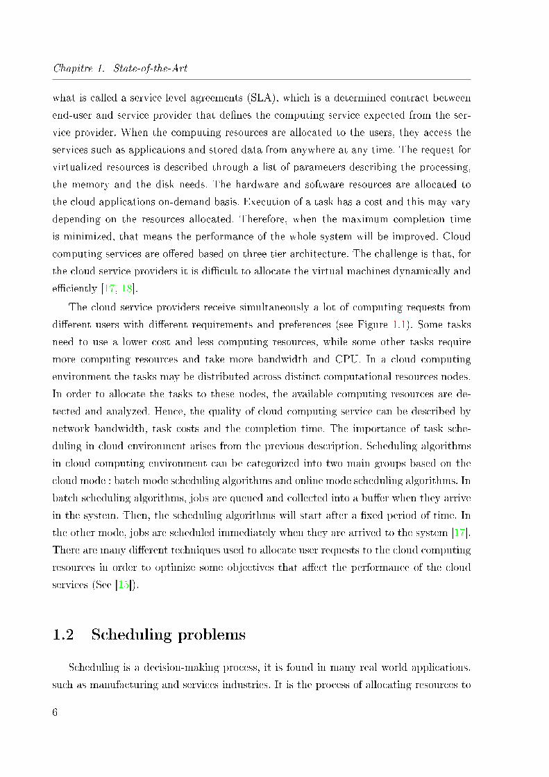
The cloud service providers receive simultaneously a lot of computing requests from
di�erent users with di�erent requirements and preferences (see Figure 1.1). Some tasks
need to use a lower cost and less computing resources, while some other tasks require
more computing resources and take more bandwidth and CPU. In a cloud computing
environment the tasks may be distributed across distinct computational resources nodes.
In order to allocate the tasks to these nodes, the available computing resources are de-
tected and analyzed. Hence, the quality of cloud computing service can be described by
network bandwidth, task costs and the completion time. The importance of task sche-
duling in cloud environment arises from the previous description. Scheduling algorithms
in cloud computing environment can be categorized into two main groups based on the
cloud mode : batch mode scheduling algorithms and online mode scheduling algorithms. In
batch scheduling algorithms, jobs are queued and collected into a bu�er when they arrive
in the system. Then, the scheduling algorithms will start after a �xed period of time. In
the other mode, jobs are scheduled immediately when they are arrived to the system [17].
There are many di�erent techniques used to allocate user requests to the cloud computing
resources in order to optimize some objectives that a�ect the performance of the cloud
services (See [15]).
1.2 Scheduling problems
Scheduling is a decision-making process, it is found in many real world applications.
such as manufacturing and services industries. It is the process of allocating resources to
6
1.2. Scheduling problems
Figure 1.1 � Task scheduling in cloud computing model.
tasks over a given time period aiming to optimize one, two, or multiple objectives. The
resources and tasks can take many di�erent forms in services and in manufacturing. The
resources may be machines in a factory, processing units in a computing environment, etc.
The tasks may be operations in a production line, processing of a computer programs,
etc. In machine environment each task may have some constraints such as a precedence
constraints, a possible starting time and a due date. The objectives can also take many
di�erent forms. One objective may be a single objective such as the minimization of the
completion time of the last task, and another may be bi-objective or multi-objectives.
Scheduling, as a decision-making process, plays an important role in computing environ-
ments, especially in cloud computing. Suppose that m machines Mi(i = 1, ...,m) have to
process n jobs Jj(j = 1, ..., n). A schedule is for each job an allocation of one or more
time intervals to one or more machines.
The classes of scheduling problems are speci�ed in terms of a three-�eld classi�cation
α|β|γ where α speci�es the machine environment, β speci�es the job characteristics and γ
denotes the optimality criterion. Such a classi�cation scheme was introduced by Graham
et al [66].
7

Chapitre 1. State-of-the-Art
1.3 Computational complexity
In this section, we present some de�nitions and principles about the computational
complexity. Complexity theory provides a mathematical framework in which computa-
tional problems are studied so that they can be classi�ed as "easy" or "hard". A more
detailed presentation can be found in the book of Garey & Johnson [61]. The main issue
of the theory of complexity is to determine the required resources needed (time, storage
space) and to measure the performance of algorithms with respect to computational time.
The notations P, NP and co-NP are collections of decision problems : problems that can
be answered by 'yes' or 'no', like whether a given graph has a perfect matching or a Ha-
miltonian circuit. The optimization problem is not a decision problem, but often can be
reduced to it in a certain sense [19]. An easy way to characterize the class NP is : NP is
the collection of decision problems that can be reduced in polynomial time to the satis�a-
bility problem. However, Cook in [16] de�ned NP as the collection of all decision problems
for which each input with positive answer, has a polynomial-time checkable of correctness
of the answer (NP stands for nondeterministically polynomial-time). The NP-complete
problems are the problems that are the hardest in NP : every problem in NP can be
reduced to them. Next description clarify. Problem∏⊂ Sigma∗ is said to be reducible
to problem ∧ ⊂ Sigma∗ if there exists a polynomial-time algorithm that returns, for any
input w ∈ Σ∗ an output x ∈ Σ∗ with the property : w ∈∏⇔ x ∈ ∧. This implies that
if∏
is reducible to ∧ and ∧ belongs to P, then also∏
belongs to P. Similarly, if∏
is
reducible to ∧ and ∧ belongs to NP, then also∏
belongs to NP. A problem∏
is said
to be NP-complete if each problem in NP is reducible to∏. An optimization problem is
NP-hard if the corresponding decision problem is NP-complete.
One of the most successful methods of attacking hard combinatorial optimization
problems is the genetic algorithm, which will be discussed in this chapter. Genetic algo-
rithm generally generates feasible solutions that are not guaranteed to be optimal. Any
approach without formal guarantee of performance can be considered as a "heuristic".
Such approaches are useful in practical situations if there is no better methods available.
Important classes of problems which are polynomially solvable are linear programming
problems [25] and integer linear programming problems with �xed number of variables
[27].
8
1.4. Heuristics and meta-heuristics
1.4 Heuristics and meta-heuristics
In this section, we present some de�nitions for heuristics and metaheuristics widely
used in combinatorial optimization.
1.4.1 Heuristics
Optimization techniques can be classi�ed, in a heuristic, exact and approximation me-
thods. The heuristic methods try to �nd optimal solutions or near-optimal solutions in a
signi�cantly reduced amount of time. The heuristic methods categorized into constructive
methods and local search methods. Constructive algorithms obtain solutions from scratch
by adding solution components to an initially empty list, until reaching the �nal solution.
Local search algorithms start from an initial solution and iteratively replace the current
solution by a better candidate from the neighbors of the current solution [22]. As de�ned
in [18], a heuristic technique is a method, which tries to �nd good solutions at a reaso-
nable computation cost without being able to guarantee optimality. Unfortunately, it may
not even be possible to determine how close to the optimal solution a particular heuristic
solution is.
1.4.2 Metaheuristics
The term meta-heuristic refers to a certain class of heuristic methods. As Fred Glover
in [21], �rst used this term and de�ned it as follows : A meta-heuristic refers to a master
strategy that guides and modi�es other heuristics to produce solutions beyond those that are
normally generated in a quest for local optimality. In another de�nition, "meta-heuristics
are solution methods that orchestrate an interaction between local improvement procedures
and higher level strategies to create a process capable of escaping from local optima and
performing a robust search of a solution space" [23]. The heuristics guided by such a meta-
strategy may be high level procedures or may include nothing more than a description
of the strategies of moving from one solution to another with an associated evaluation
rule (called �tness). To distinguish between heuristics and metaheuristic concepts, we
can mention that heuristics are often problem dependent, heuristics normally de�ned
for a given problem to �nd optimal or near to the optimal solutions for the problem
under consideration, whereas the metaheuristics are problem independent techniques that
can be applied for a wide range of problems. As an example, when we use simulated
9
Chapitre 1. State-of-the-Art
annealing metaheuristic in scheduling, the decision of moving from current solution to
another candidate one will be done by metaheuristic procedure whereas this method does
not know nothing about scheduling. In the literature there is a vast amount of research
that used a heuristic and metaheuristics to attack scheduling problems.
Genetic algorithm
Holland in 1975 developed the idea of applying the principles of natural evolution to
optimization problems. This idea has been published in his book "Adaptation in natural
and arti�cial systems". He built the �rst genetic algorithm. Holland's theory has been
further developed. Now, genetic algorithms (GAs) considered as a powerful tool for sol-
ving optimization problems. Genetic algorithms are based on the principle of genetics
and evolution. Todays, GAs are used to resolve complicated optimization problems, like
timetabling, job shop scheduling, games playing and others [49].
Now, we give a brief introduction to simple genetic algorithms and associated termi-
nology. GAs encode the decision variables of a search problem into �nite length strings of
alphabets or digits of a certain cardinality. The strings which are candidate solutions to
the search problem are referred to as chromosomes. The chromosome represent a single
solution, the alphabets or digits are referred to as genes and the values of genes are called
alleles. For example, in scheduling problems, a chromosome represents a sequence and a
gene may represent a job, and an allele is a value of processing time taken by a speci�c
job.
In contrast to traditional optimization techniques, GAs work with coding of parame-
ters, rather than the parameters themselves. The general procedures of the GA are as
follows :
1. Initialization. The initial population of candidate solutions is usually generated ran-
domly across the search space. It can be binary or non-binary chromosomes.
2. Evaluation. Once the population is initialized or an o�spring population is created,
the algorithm uses a �tness function to evaluate each chromosome in the population.
3. Selection. In the selection step, the algorithm works to prefer better solutions to worse
ones. The algorithm selects a chromosome to mate the reproduction.
4. Recombination. Recombination combines parts of two or more parental solutions to
create new ones. Here, the algorithm applies a genetic operator (crossover) on the selected
chromosomes.
5. Mutation. Select one solution and apply a small random change to this solution.
10
1.4. Heuristics and meta-heuristics
6. Replacement. Replace the current population with the temporary population.
If stopping condition is met, then STOP with the best chromosome as the �nal solution
for the problem. Otherwise, GOTO 2.
The determination of a population size is a crucial element in the GAs. In most of
GA applications, the population size can be considered as a constant. The initialization of
population performed by using some suitable heuristics that are relevant to the considered
problem or can be created randomly. Selecting a very small size of population increases
the risk of not converging to a global optimal solution. Large size of population increases
the chance to converge to obtain a good solution. The second operator of GAs is the
�tness function, GA uses this function to evaluate the solution for each chromosome,
then GA can determine if the chromosome can be kept or not. If the chromosome kept
then it produces a new o�spring or will be eliminated.The most important operator is
the selection of chromosomes, which is ensure the convergence of the GA. When the
genetic algorithm capable to select the best chromosome, then it will have a population of
similar chromosomes, that led the GA to converge to a local optimum. Now, we give some
selection methods : roulette wheel selection, deterministic selection, ranking selection,
tournament selection and etc. In step four, the combination of two parents which combines
the features of two �ttest chromosomes and carries these features to the next generation
by forming o�springs. Many well known crossover methods have been developed and
applied. One of them is the two-position crossover method, which consists in selecting two
crossover positions in two chromosomes and then making swapping segments between the
chromosomes. Also, there is another crossover method, which is multi-position crossover
method. This method changes the number of segments during the execution of GA. Shu�e
crossover method �rst shu�es the crossover positions in the two selected chromosomes.
Then, it exchanges the segments between the crossover positions and �nally un-shu�es
the chromosomes. The uniform crossover method is a mix between one position and multi-
positions crossover methods. It produces two new children by exchanging genes in two
chromosomes randomly. The �fth operator in GA steps is the mutation, which exchange
one or more of the chromosome genes randomly to ensure search changement, which may
lead to the global optimum.
Finally, the last GA step is the stopping criterion. There are many methods, which
can be used for the stopping criteria. One of them is the maximum number of generations.
The method based on the convergence is also used : the algorithm stops when the GA
11
Chapitre 1. State-of-the-Art
converges after all chromosomes have reached a certain degree of homogeneity or, by
another stopping criterion, after a chromosome with a certain level of �tness value is
found.
1.5 Graph theory
In this section, we will introduce some basic de�nitions and notations of graph theory
that will be used throughout the chapters of this dissertation. For more details, we refer
the reader to [19].
A graph is denoted G = (V,E) where V is the set of vertices or nodes and E is the
set of edges. If e ∈ E is an edge with initial node u and terminal node v, we may also use
both notations uv or (u, v) to denote e.
The graphs considered here are directed, �nite, loopless and may include multiple arcs.
A directed graph or digraph is denoted G = (V,A) where V is the set of vertices or
nodes and A is the set of arcs. If a ∈ A is an arc with origin node u and destination node
v, we may also use both notations uv or (u, v) to denote a. The graph G is said to be
complete if there exists an arc between each pair of nodes (u, v).
A graph or undirected graph is a pair G = (V,E), where V is a �nite set and E is a
family of unordered pairs from V . The elements of V are called the vertices, sometimes
the nodes or the points. The elements of E are called the edges, sometimes the lines.
A graph G′ = (V ′, E ′) is called a subgraph of a graph G = (V,E) if V ′ ⊂ V and
E ′ ⊂ E. If E ′ consists of all edges of G spanned by V ′, then G′ is called an induced
subgraph, or the subgraph induced by V ′. In notation,
G[V ′] := subgraph of G induced by V ′,
E[V ′] := family of edges spanned by V ′
The complementary graph or complement of a graph G = (V,E) is the simple graph
with vertex set V and edges all pairs of distinct vertices that are nonadjacent in G. In
notation, G := the complementary graph of G.
1.6 Optimization problems
In mathematics, optimization is a branch of applied mathematics. It derives its im-
portance from the wide variety of its applications and from the availability of e�cient
algorithms that have been used to solve such problems. Mathematically, it refers to the
12

1.6. Optimization problems
minimization (or maximization) of a given objective function of several decision variables
that satisfy functional constraints [113]. For example, let us consider the optimization mo-
del, which addresses the allocation of limited resources among possible alternative uses in
order to maximize the total pro�t. Objective function, decision variables, and constraints
are three essential elements of any optimization problem. If the decision variables in an
optimization problem are restricted to integers, or to a discrete set of possibilities, there
is an integer or discrete optimization problems. The problem is a continuous optimization
problem, if there are no such restrictions on the variables. Some problems may have a
mixture of discrete and continuous variables, that depends on the nature of the problem.
We give the generic description of an optimization problem.
Given a function f (x) : Rn → R and a set S ⊂ Rn, the problem of �nding an x∗ ∈ R that
solves
minxf (x) (1.1)
s.t. x ∈ S
is called an optimization problem (OP). We denote by f the objective function and by S
the feasible region. If S is empty, the problem is called infeasible. If it is possible to �nd a
sequence xk ∈ S such that f (xk)→ −∞ as k → +∞, then the problem is unbounded. If
the problem is neither infeasible nor unbounded, then it is often possible to �nd a solution
x∗ ∈ S.
1.6.1 Combinatorial optimization
Combinatorial Optimization is a subset of mathematical optimization that is related to
operations research, algorithm theory, and computational complexity theory. Its purpose
is to study the optimization problems where the set of feasible solutions can be represented
as a discrete one.
The combinatorial optimization problems are the problems, which are formulated as
follows. Let E = {e1, ..., en} be a �nite set where each element ei is associated with a
weight w(ei). Let F be a family of subsets of E. If F ∈ F , then w(F ) =∑
ei∈F w(ei)
denotes the weight of F. The problem consists in identifying an element F ∗ of F whose
weight is minimum or maximum. The set F represents the set of feasible solutions of the
problem. Such a problem is called combinatorial optimization problem.
The term combinatorial refers to the discrete structure of the representation of the
feasible solution set F . Generally, this structure is represented by a graph. The term
13
Chapitre 1. State-of-the-Art
optimization tells that we are looking for the best element in the set of feasible solutions.
This set may contain an exponential number of solutions. Thus, we cannot expect to solve
a combinatorial optimization problem by checking or enumerating all its solutions one by
one, which is not a reasonable option. Such a problem is then considered as a hard problem.
Many e�ective techniques and approaches have been developed to attack combinatorial
optimization problems. Some of these approaches use linear, integer programming, and
polyhedral approach and others based on graph theory. combinatorial optimization is
closely related to algorithm and computational complexity theory.
1.6.2 Linear programming
Linear programming deals with the OP with a linear function in the presence of li-
near inequalities. One of the most common optimization problems is linear optimization
or linear programming (LP). It is the problem of optimizing a linear objective function
subject to linear inequalities and equality constraints. Indeed, any combinatorial optimi-
zation problem can be reduced to solving a linear program. The standard form of the LP
is given below :
minx CTx
Ax = b (1.2)
x ≥ 0,
where A ∈ Rm×n, b ∈ Rm, c ∈ Rn are given and x ∈ Rn is the variable vector to be deter-mined. A wide variety of real life problems can be formulated as linear integer optimization
problems. The combinatorial problems, such as the knapsack problem, resources alloca-
tion problem, TSP, network �ow and graph problems, and many scheduling problems can
also be solved as a linear integer optimization problems [24].
1.6.3 Integer programming
When the variables are integer, we call the formulation of the problem as integer
programming. Integer programs are optimization problems that require some or all of
the variables to take integer values. This restriction on the variables usually makes the
14
1.7. Polyhedral approach
problems very hard to solve. A pure integer linear program is given by :
minx CTx
Ax ≥ b (1.3)
x ≥ 0 and integral,
where A ∈ Rm×n, b ∈ Rm, c ∈ Rn are given, and x ∈ Nn is the variable vector to be
determined.
A very common case occurs when the variables xj represent binary decision variables,
that is x ∈ {0, 1}n. The problem is then called a 0 − 1 linear program (or discrete).
When there are both integer constrained variables and continuous variables, the problem
is called a Mixed Integer Linear Program (MILP) :
minx CTx
Ax ≥ b (1.4)
x ≥ 0
xj ∈ N, for j = 1, ..., p
where A, b, c are given data and the integer p (with 1 ≤ p < n) is also part of the input.
1.7 Polyhedral approach
The development of polyhedral theory and the consequent introduction of strong va-
lid inequalities led to a resurgence of cutting plane methods. The polyhedral method was
initiated by Edmonds in 1965 for a matching problem. It consists in describing the convex
hull of problem solutions by a system of linear inequalities. The problem reduces then to
the resolution of a linear program. Normally, in most of the cases, it is not straightforward
to obtain a complete characterization of the convex hull of the solutions for a combinato-
rial optimization problem. However, having a system of linear inequalities that partially
describes the solutions polyhedron may often lead to solve the problem in polynomial
time. This approach has been successfully applied to several combinatorial optimization
problems. In this section, we present the basic notions of polyhedral theory. For detail,
the reader is invited to consult [19, 20, 22].
First, we will recall some de�nitions, propositions, and properties related to polyhedral
theory.
15
Chapitre 1. State-of-the-Art
Elements of (S)
Conv(S)
Figure 1.2 � A convex hull
1.7.1 Elements of polyhedral theory
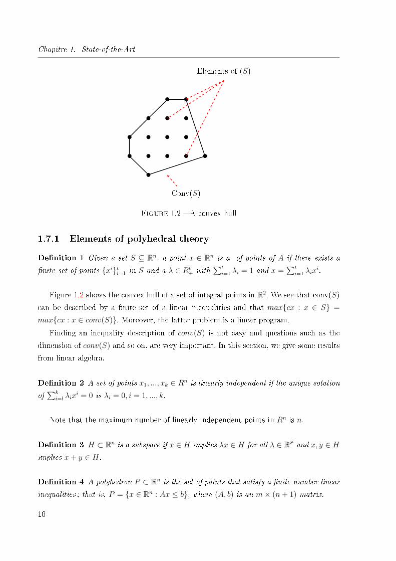
De�nition 1 Given a set S ⊆ Rn, a point x ∈ Rn is a of points of A if there exists a
�nite set of points {xi}ti=1 in S and a λ ∈ Rt+ with
∑ti=1 λi = 1 and x =
∑ti=1 λix
i.
Figure 1.2 shows the convex hull of a set of integral points in R2. We see that conv(S)
can be described by a �nite set of a linear inequalities and that max{cx : x ∈ S} =
max{cx : x ∈ conv(S)}. Moreover, the latter problem is a linear program.
Finding an inequality description of conv(S) is not easy and questions such as the
dimension of conv(S) and so on, are very important. In this section, we give some results
from linear algebra.
De�nition 2 A set of points x1, ..., xk ∈ Rn is linearly independent if the unique solution
of∑k
i=l λixi = 0 is λi = 0, i = 1, ..., k.
Note that the maximum number of linearly independent points in Rn is n.
De�nition 3 H ⊂ Rn is a subspace if x ∈ H implies λx ∈ H for all λ ∈ R1 and x, y ∈ Himplies x+ y ∈ H.
De�nition 4 A polyhedron P ⊂ Rn is the set of points that satisfy a �nite number linearinequalities ; that is, P = {x ∈ Rn : Ax ≤ b}, where (A, b) is an m× (n+ 1) matrix.
16
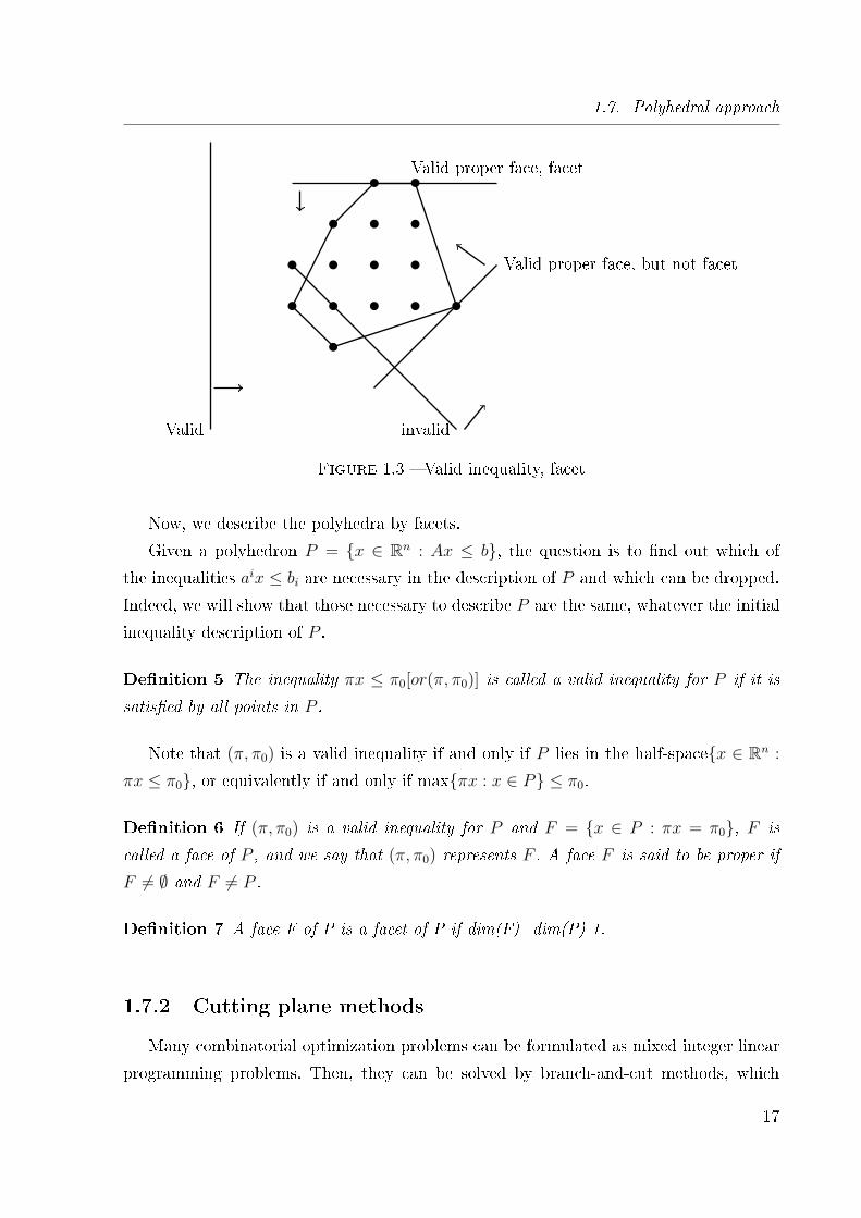
1.7. Polyhedral approach
Valid proper face, facet
Valid invalid
Valid proper face, but not facet
Figure 1.3 � Valid inequality, facet
Now, we describe the polyhedra by facets.
Given a polyhedron P = {x ∈ Rn : Ax ≤ b}, the question is to �nd out which of
the inequalities aix ≤ bi are necessary in the description of P and which can be dropped.
Indeed, we will show that those necessary to describe P are the same, whatever the initial
inequality description of P .
De�nition 5 The inequality πx ≤ π0[or(π, π0)] is called a valid inequality for P if it is
satis�ed by all points in P .
Note that (π, π0) is a valid inequality if and only if P lies in the half-space{x ∈ Rn :
πx ≤ π0}, or equivalently if and only if max{πx : x ∈ P} ≤ π0.
De�nition 6 If (π, π0) is a valid inequality for P and F = {x ∈ P : πx = π0}, F is
called a face of P , and we say that (π, π0) represents F . A face F is said to be proper if
F 6= ∅ and F 6= P .
De�nition 7 A face F of P is a facet of P if dim(F)=dim(P)-1.
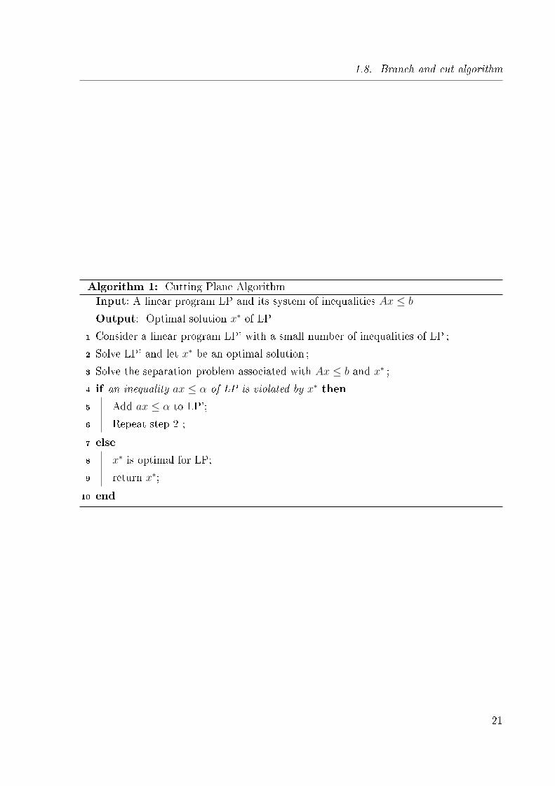
1.7.2 Cutting plane methods
Many combinatorial optimization problems can be formulated as mixed integer linear
programming problems. Then, they can be solved by branch-and-cut methods, which
17
Chapitre 1. State-of-the-Art
are exact algorithms consisting of a combination of branch-and-bound algorithm with
a cutting plane method. These methods work by solving a sequence of linear program-
ming relaxations of the integer programming problem. Cutting plane methods improve
the relaxation of the problem to more closely integer programming problem and branch-
and-bound algorithms carry out by a sophisticated divide and conquer approach to solve
problems. Cutting plane algorithms for general integer programming problems were �rst
proposed by Gomory [27]. Thus, this method sometimes called "Gomory Cut", who pro-
ved that these algorithms terminate after a �nite number of iterations with an optimum
solution.
Now, let P be a combinatorial optimization problem, E its basic set, w(.) the weight
function, and S the set of feasible solutions. The problem P consists in �nding an element
of S whose weight is maximum/minimum. If F ⊆ E, then the 0− 1 vector xF ∈ RE suchthat xF (e) = 1 if e ∈ F and xF (e) = 0 otherwise, is called the incidence vector of F . The
polyhedron P (S) = convxS|S ∈ S is the polyhedron of the solutions of P or polyhedron
associated with P . P is thus equivalent to the linear program max{cx|x ∈ P (S)}. Noticethat the polyhedron P (S) can be described by a set of a facet de�ning inequalities. And,
when all the inequalities of this set are known, then solving P is equivalent to solve a
linear program.
The objective of the polyhedral approach for combinatorial optimization problems
is to reduce the resolution of P to that of a linear program. In order to reduce P we
need a deep investigation of the polyhedron associated with P . It is generally not easy
to characterize the polyhedron of a combinatorial optimization problem by a system of
linear inequalities. In particular, when the problem is NP-hard it is di�cult to �nd such
a characterization. Moreover, the number of inequalities describing this polyhedron is
exponential in most of time. Therefore, even if we know the complete description of that
polyhedron, its resolution remains in practice a hard task because of the large number of
inequalities.
Cutting plane method is based on the so-called separation problem. This consists, given
a polyhedron P of Rn and a point x∗ ∈ Rn, in verifying whether if x∗ belongs to P , and
if this is not the case, to identify an inequality aTx ≤ b, valid for P and violated by x∗.
In the later case, we say that the hyperplane aTx = b separates P and x∗. More precisely,
the cutting plane method consists in solving successive linear programs, with possibly a
large number of inequalities, by using the following steps. Let LP = max{cx,Ax ≤ b} bea linear program and LP ′ a linear program obtained by considering a small number of
18
1.8. Branch and cut algorithm
inequalities among Ax ≤ b. Let x∗ be the optimal solution of the latter system. We solve
the separation problem associated with Ax ≤ b and x∗. This phase is called the separation
phase. If every inequality of Ax ≤ b is satis�ed by x∗, then x∗ is also optimal for LP. If
not, let ax ≤ α be an inequality violated by x∗. Then, we add ax ≤ α to LP ′ and repeat
this process until an optimal solution is found.
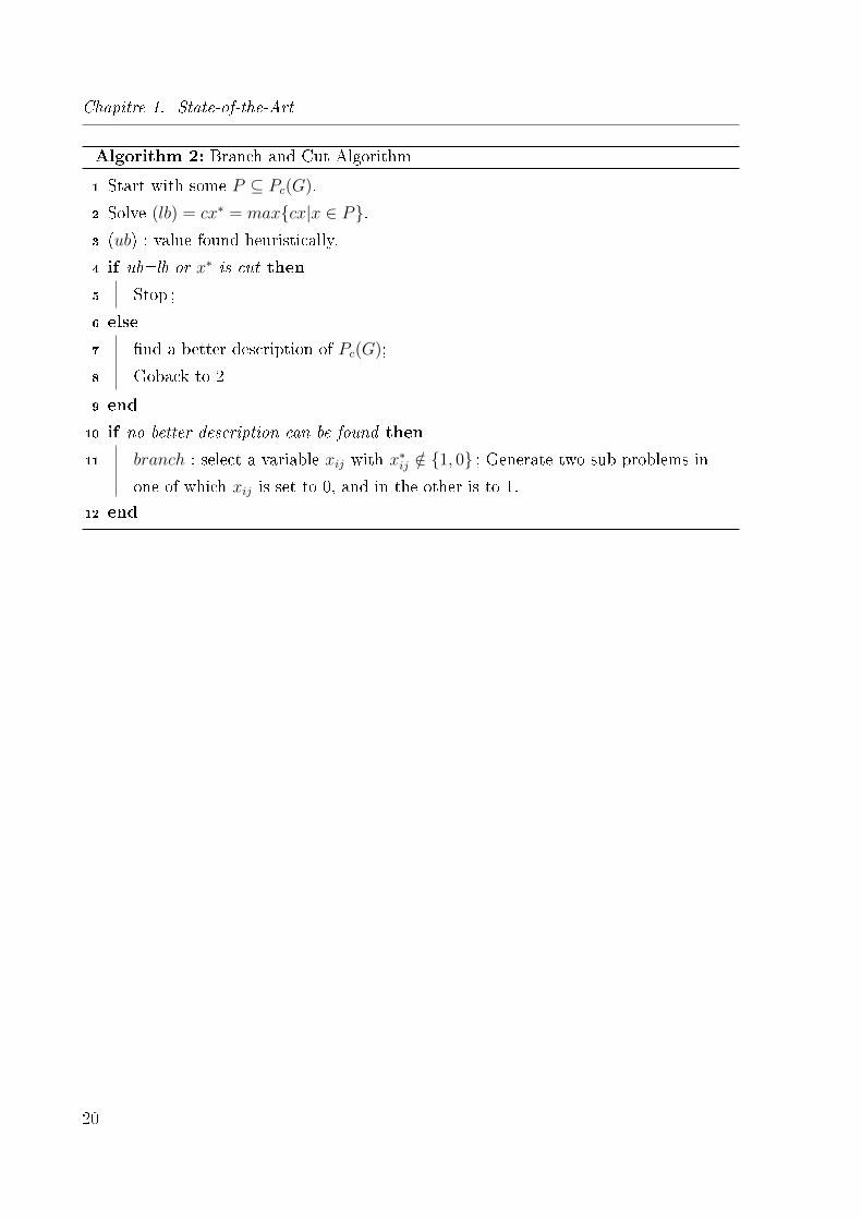
1.8 Branch and cut algorithm
Branch and cut methods are often successful for �nding an exact solution of hard
optimization problems. For each instance, the method always maintains an upper bound
(ub) and a lower bound (lb) for the optimum solution value. Iteratively, the value of the
upper and lower bounds are improved, until they get the optimal solution, or a solution
that is tight enough. It is known that, branch and cut is a special case of branch and
bound method, where in branch and cut method the bounds are determined through LP
and polyhedral theory. Informally, we summarize the basic concepts of branch and cut. We
need a partial description Q of Qc(G) with the properties that the latter is contained in Q.
We call such a polytope a relaxation polytope. The inequality system Apx ≥ bp describing
Q is known and can be generated in polynomial time. We optimize over Q to solve the
linear program, which is found in the form of the LP mentioned in this chapter. Fast
algorithms for solving linear programs exist, for example the well known one is Simplex
method. Within the branch and cut approach we start by some relaxation Q of Qc(G).
Iteratively, we generate tighter description of the cut polytope. The upper bound (ub) on
the optimum value of the maximum cut can be obtained by any heuristic. In the case
where upper and lower bounds are the same we can stop and return an optimum solution,
we can also stop where lower bound solution vector becomes integer. In branch and cut a
sub problem is a node of the tree. The branch and cut algorithm is described as follows.
19
Chapitre 1. State-of-the-Art
Algorithm 2: Branch and Cut Algorithm
1 Start with some P ⊆ Pc(G).
2 Solve (lb) = cx∗ = max{cx|x ∈ P}.3 (ub) : value found heuristically.
4 if ub=lb or x∗ is cut then
5 Stop ;
6 else
7 �nd a better description of Pc(G);
8 Goback to 2
9 end
10 if no better description can be found then
11 branch : select a variable xij with x∗ij /∈ {1, 0} ; Generate two sub problems in
one of which xij is set to 0, and in the other is to 1.
12 end
20
1.8. Branch and cut algorithm
Algorithm 1: Cutting Plane AlgorithmInput: A linear program LP and its system of inequalities Ax ≤ b
Output: Optimal solution x∗ of LP
1 Consider a linear program LP' with a small number of inequalities of LP ;
2 Solve LP' and let x∗ be an optimal solution ;
3 Solve the separation problem associated with Ax ≤ b and x∗ ;
4 if an inequality ax ≤ α of LP is violated by x∗ then
5 Add ax ≤ α to LP';
6 Repeat step 2 ;
7 else
8 x∗ is optimal for LP;
9 return x∗;
10 end
21

Chapitre 1. State-of-the-Art
22
2
Heuristics and Meta-heuristics
Solutions
Contents
2.1 Introduction . . . . . . . . . . . . . . . . . . . . . . . . . . . . . 24
2.1.1 Literature Review . . . . . . . . . . . . . . . . . . . . . . . . . 25
2.2 Problem formulation . . . . . . . . . . . . . . . . . . . . . . . . 27
2.3 An existing algorithm . . . . . . . . . . . . . . . . . . . . . . . . 29
2.4 Genetic algorithm (GA) . . . . . . . . . . . . . . . . . . . . . . 29
2.4.1 Modeling the problem using Genetic Algorithm . . . . . . . . . 31
E�cient job scheduling algorithms are addressed in this chapter to improve the resource
utilization in cloud computing where the aim is to minimize the total completion time
(Makespan). We present a genetic-based task scheduling algorithms in order to minimize
Maximum Completion Time Makespan. These algorithms combines di�erent techniques
such as list scheduling and earliest completion time(ECT) with genetic algorithm. We re-
viewed, evaluated and compared the proposed algorithms against one of the well known
GAs available in the literature, which has been proposed for optimizing the task schedu-
ling on heterogeneous systems. After an exhaustive computational experiments the results
identify that our proposed Genetic algorithms show a good performance dominating the
evaluated algorithms in di�erent problem sizes and complexity for a large benchmark set
of instances. Moreover, greedy algorithm and ILP have been applied to attack the problem.
23
Chapitre 2. Heuristics and Meta-heuristics Solutions
2.1 Introduction
This chapter discusses di�erent solutions for the problem of unrelated parallel machine
scheduling with precedence constraints based on heuristic and metaheuristic approaches.
In Cloud environments a task scheduling is a process that maps and assign the inter-
dependent tasks on the data centers (resources) [15]. It allocates the tasks its appropriate
virtual resources which is virtual machines (VMs) inorder to satisfy objective functions
imposed by end-users. The idea of virtualizing a computer system resources(processors,
memory, input/output devices), aiming to improve the sharing of computer resources[29].
Generally,an e�cient task scheduling algorithm will have an important impact to the per-
formance of the system throughput [40, 36]. The scheduling problem in cloud computing
can be generalized as an unrelated parallel machine with di�erent speeds and precedence
constraints. We consider VMs as an unrelated parallel machine because the cloud com-
puting providers o�er their services virtually by sharing their physical resources through
a large number of virtual machines in parallel. These virtual machines, allocated with
di�erent CPU capacities, so it can be considered as an unrelated parallel machines. In
cloud computing users may face hundreds of thousands of virtualized resources to utilize.
It is hard to allocate user± tasks on the available resources. Due to the virtualization pro-
perties, cloud computing leaves task scheduling complexity to the virtual machine layer
through resource virtualization.
Hence, to allocate the resources to each task e�ciently, scheduling plays more im-
portant role in cloud computing [28]. It is di�cult to obtain an optimal solution with
traditional optimization methods. Mathematical optimization techniques can solve the
problems optimally for a reasonable size of instances, however, in the case of a large scale
problems, their application is limited [65]. Dispatching rules (EDD, SPT, LPT,...) are
suitable only for small sized problems. It is also known that, no single dispatching rule
guarantees optimal or near to the optimal solution in various problems [45]. Research ef-
forts in scheduling are concentrated on heuristic approaches as well. Many heuristics and
meta-heuristics have been proposed such as simulated annealing (SA), branch and bound
(Branch and Bound), tabu search, and genetic algorithm (GA) [28]. Among these various
approaches to di�erent scheduling problems, there is an increasing interest in applying
GAs, this interest comes from its characteristic, the ease of implementation, and the high
adaptability. The important di�erence between GA and other heuristics is that GA ge-
nerate a set of solutions (populations) rather than a unique solution, which can lead to
a better diversity. In scheduling problems, Cmax is equivalent to the completion time of
24
2.1. Introduction
the last task leaving the system. The small makespan usually means a high utilization.
Therefore, reducing the makespan should also lead to a higher throughput rate in the
overall system [45]. Three genetic algorithms have been applied to solve this problem.
2.1.1 Literature Review
The problem of task scheduling in distributed systems is known as an NP-hard [46].
To allocate n jobs to m virtual machines (VMs), the number of allocation is |n||m| andthe number of states will be n!. One of the objectives of scheduling in cloud computing is
to determine the assignment of jobs to VMs in order to optimize the completion time of
the last task in the system. The job scheduling problem in distributed, and heterogeneous
systems such as cloud computing [15], has been studied widely in the last few years. Ge-
nerally, job scheduling problem can be found in two forms : dynamic and static. When all
information needed for scheduling, such as data dependencies between jobs, and execution
times of jobs are known by the scheduler, then the scheduling problem known as static
scheduling problem. In static scheduling, jobs placed during the compile time. On the
other hand, in the dynamic model, jobs are allocated to the processors upon their arrival
to the scheduler, and scheduling decisions must be made immediately at run time [48, 49].
In this section we focus our attention on the available algorithms for static scheduling in
cloud environment, as well the algorithms that haves been used to solve the unrelated
parallel machine with precedence constraints scheduling problem. A survey on scheduling
in cloud computing can be found in [15],[28],and [43]. Di�erent methods for optimizing
di�erent objectives in cloud computing exist (See[32, 33, 34, 48, 35]). Some researchers
proposed e�cient meta-heuristics based on genetic algorithm : Zhou et al in [50] proposed
a genetic algorithm based on earliest completion time (ECT) to minimize completion time
(we represent this GA in the next sections. Arash and Yalda also developed hybrid genetic
algorithm for work �ow scheduling in cloud system (HSGA). It merges best-�t and Round
Robin methods to obtain a good solution quickly by making an optimal initial population.
It makes a job prioritization in complex graph. A particle swarm optimization (PSO) used
in [51] for work�ow scheduling in cloud environment, which considers not only execution
cost but also the cost for transmitting dependent data. In [52] a PSO is also formulated
as a model for the multi-objective task assignment to optimize the time and cost. To the
best of our knowledge, none of the existing Genetic algorithms have considered the idea
of scheduling jobs with a high number of successors in order to optimize the makespan.
Shamsollah et al in [40] presented a novel approach for job scheduling in cloud computing
25
Chapitre 2. Heuristics and Meta-heuristics Solutions
which was called priority based job scheduling algorithm. Their solution method based on
multi-criteria decision-making model and multi-attribute decision-making model which
was �rst developed by T.Saaty in 1980 and called the theory of Analytical Hierarchy
Process. The proposed algorithm mainly focused on priority of job. The experimental
results indicated that the algorithm has reasonable complexity, however the authors did
not expect that this algorithm provides an optimal makespan. Xiaofeng Wang et al in [42]
proposed a new max-min strategy speci�cally for GAs, which use a novel task critical-
ness. They modeled a work�ow job as a Directed Acyclic Graph (DAG). The reliability
driven scheduling of a work�ow application applied to maximize the reliability and to
minimize the makespan of the application. The literature on parallel machine scheduling
is fairly large, we focus mainly on the non-preemptive unrelated parallel machine problem
with precedence constraints to minimize makespan criterion. There are many applications
for this scheduling problem specially in distributed computing systems [52],[50]. Several
heuristics and meta-heuristics have been proposed to solve this problem for optimizing
di�erent objectives. In [38] Vallada and Ruiz proposed a genetic algorithm to minimize
the makespan. Their GA includes a fast local search and a local search enhanced cros-
sover operator. In [65] Balin proposed a new crossover operator for genetic algorithm to
minimize makespan, his algorithm achieved a high computational speed for large-scale
problems. In [53] Tavakkoli-Moghaddam et al proposed a genetic algorithm to solve bi-
objective unrelated parallel machine scheduling problem. Je�rey et al [44] considered the
case where a task has at most one predecessor and at most one successor. They propo-
sed a greedy search, which we use in this chapter for a comparison purpose, and they
proposed also a heuristic based on a branch-and-bound procedure. They also applied a
simulated annealing algorithm to solve the problem. Liu and Yang in [71] considered the
case where the machines do not have speci�c speeds but every job has a processing time
depending on the used machine, which is an extension of the constraint we used in our
problem. They proposed an integer linear programming model and they provided a po-
lynomial time algorithm that can schedule the prior job on the prior machine as early
as possible for minimizing makespan. A hybrid genetic algorithm has been proposed in
[71] for minimizing the total tardiness for the problem of unrelated parallel machines
with precedence constraints. For other proposed approaches the reader could refer to see
[37, 63, 30, 31, 39, 41].
In this chapter, we deal with the problem of job scheduling in cloud environment and
we generalized this problem as an unrelated parallel machines scheduling with precedence
26
2.2. Problem formulation
constraints for optimizing the makespan. We proposed three genetic algorithms, they show
a very good performance for small and medium benchmarks.
In the next section we will present the problem formulation and a mathematical formula-
tion associated to solve unrelated parallel machine with precedence constraints scheduling
problem.
2.2 Problem formulation
The problem under consideration is to schedule n jobs on m machines which are
arranged in parallel with the aim of minimizing the total completion time. Let J be the
set of the jobs andM be the set of the parallel machines. A precedence constraint between
two jobs j1 and j2 is denoted by (j1 ≺ j2) and it requires that job j2 cannot start to be
processed until job j1 will �nish its processing. The type of the precedence constraint is
a graph type, which is denoted by D = (V,A), where V is the set of vertices associated
at each job ϑ and V denotes the set of edges associated with each precedence constraint.
We called this graph the precedence graph. We take also the case where {v, w, w} ⊆ V
such that v before w and w before w then v before w. We consider also the speeds for
all machines denoted by si, where i ∈ M . Every job j ∈ J has a processing time pj and
its e�ective processing time depends on the selected machine i, where pij = πj × si. Eachmachine i ∈M cannot process more than one job at a given time. Furthermore, machines
have di�erent speeds and preemption of jobs is not allowed. According to the well-known
α|β|γ scheduling problem classi�cation scheme proposed initially by Graham et al [66],
scheduling problem classi�cation scheme this problem can be denoted as P |prec|Cmax We
denote by Ci the completion time of machine i, where i ∈ M , and denote by Cϑ the
completion time of job j, where j ∈ J , in the rest of this chapter. Thus, the problem can
be reduced to the following mathematical formulation proposed in [71]
xjir =
1 if job j is processed in position r on machine i
0 otherwise ∀j ∈ J, i ∈M, r ∈ J
Cj ∈ N+ the completion time of job j.
Cmax ∈ N+ is the total length of the schedule. That is, when all the jobs have �nished
processing.
The model can be stated as :
27
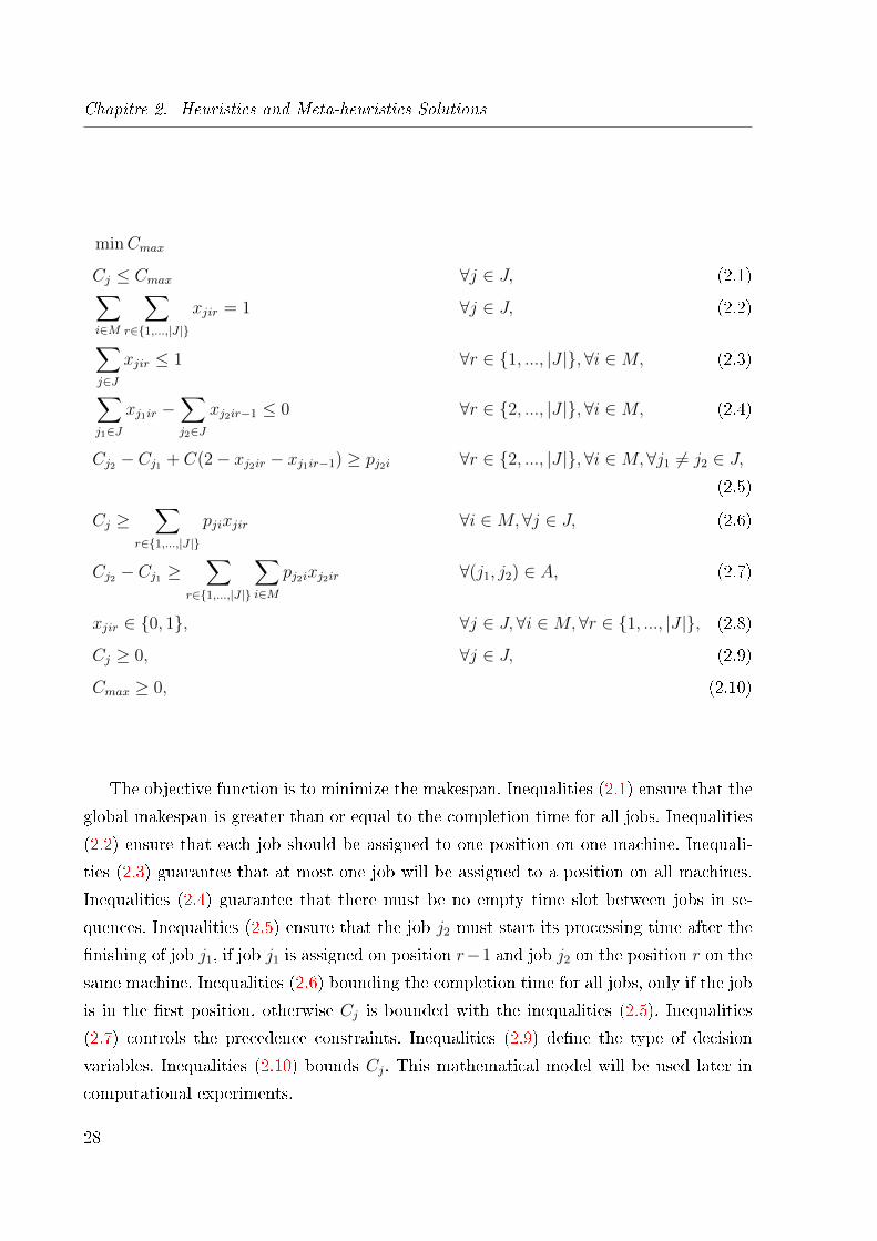
Chapitre 2. Heuristics and Meta-heuristics Solutions
minCmax
Cj ≤ Cmax ∀j ∈ J, (2.1)∑i∈M
∑r∈{1,...,|J |}
xjir = 1 ∀j ∈ J, (2.2)
∑j∈J
xjir ≤ 1 ∀r ∈ {1, ..., |J |},∀i ∈M, (2.3)
∑j1∈J
xj1ir −∑j2∈J
xj2ir−1 ≤ 0 ∀r ∈ {2, ..., |J |},∀i ∈M, (2.4)
Cj2 − Cj1 + C(2− xj2ir − xj1ir−1) ≥ pj2i ∀r ∈ {2, ..., |J |},∀i ∈M, ∀j1 6= j2 ∈ J,(2.5)
Cj ≥∑
r∈{1,...,|J |}
pjixjir ∀i ∈M,∀j ∈ J, (2.6)
Cj2 − Cj1 ≥∑
r∈{1,...,|J |}
∑i∈M
pj2ixj2ir ∀(j1, j2) ∈ A, (2.7)
xjir ∈ {0, 1}, ∀j ∈ J,∀i ∈M,∀r ∈ {1, ..., |J |}, (2.8)
Cj ≥ 0, ∀j ∈ J, (2.9)
Cmax ≥ 0, (2.10)
The objective function is to minimize the makespan. Inequalities (2.1) ensure that the
global makespan is greater than or equal to the completion time for all jobs. Inequalities
(2.2) ensure that each job should be assigned to one position on one machine. Inequali-
ties (2.3) guarantee that at most one job will be assigned to a position on all machines.
Inequalities (2.4) guarantee that there must be no empty time slot between jobs in se-
quences. Inequalities (2.5) ensure that the job j2 must start its processing time after the
�nishing of job j1, if job j1 is assigned on position r−1 and job j2 on the position r on the
same machine. Inequalities (2.6) bounding the completion time for all jobs, only if the job
is in the �rst position, otherwise Cj is bounded with the inequalities (2.5). Inequalities
(2.7) controls the precedence constraints. Inequalities (2.9) de�ne the type of decision
variables. Inequalities (2.10) bounds Cj. This mathematical model will be used later in
computational experiments.
28
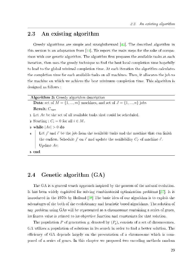
2.3. An existing algorithm
2.3 An existing algorithm
Greedy algorithms are simple and straightforward [42]. The described algorithm in
this section is an adaptation from [44]. We report the main steps for the sake of compa-
rison with our genetic algorithm. The algorithm �rst prepares the available tasks at each
iteration, then uses the greedy technique to �nd the best local completion time hopefully
to lead to the global minimal completion time. At each iteration the algorithm calculates
the completion time for each available tasks on all machines. Then, it allocates the job to
the machine on which we achieve the best minimum completion time. This algorithm is
designed as follows :
Algorithm 3: Greedy algorithm descriptionData: set of M = {1, ...,m} machines, and set of J = {1, ..., n} jobsResult: Cmax
1 Let Av be the set of all available tasks that could be scheduled.
2 Starting : Ci = 0 for all i ∈M .
3 while |Av| > 0 do
4 Let j′ and i′ be the job from the available tasks and the machine that can �nish
the earliest. Schedule j′ on i′ and update the availability Ci′ of machine i′.
Update Av;
5 end
2.4 Genetic algorithm (GA)
The GA is a general search approach inspired by the process of the natural evolution.
It has been widely exploited for solving combinatorial optimization problems [37]. It is
introduced in the 1970s by Holland [38] The basic idea of our algorithm is to exploit the
advantages of the both of the evolutionary and heuristic based algorithms. The solution of
any problem using GAs will be represented as a chromosome containing a series of genes,
its �tness value is related to its objective function and constraints for that solution.
The population P of generation g, denoted by (Pg), consists of a set of chromosomes.
GA utilizes a population of solutions in its search in order to �nd a better solution. The
e�ciency of GA depends largely on the presentation of a chromosome which is com-
posed of a series of genes. In this chapter we proposed two encoding methods random
29
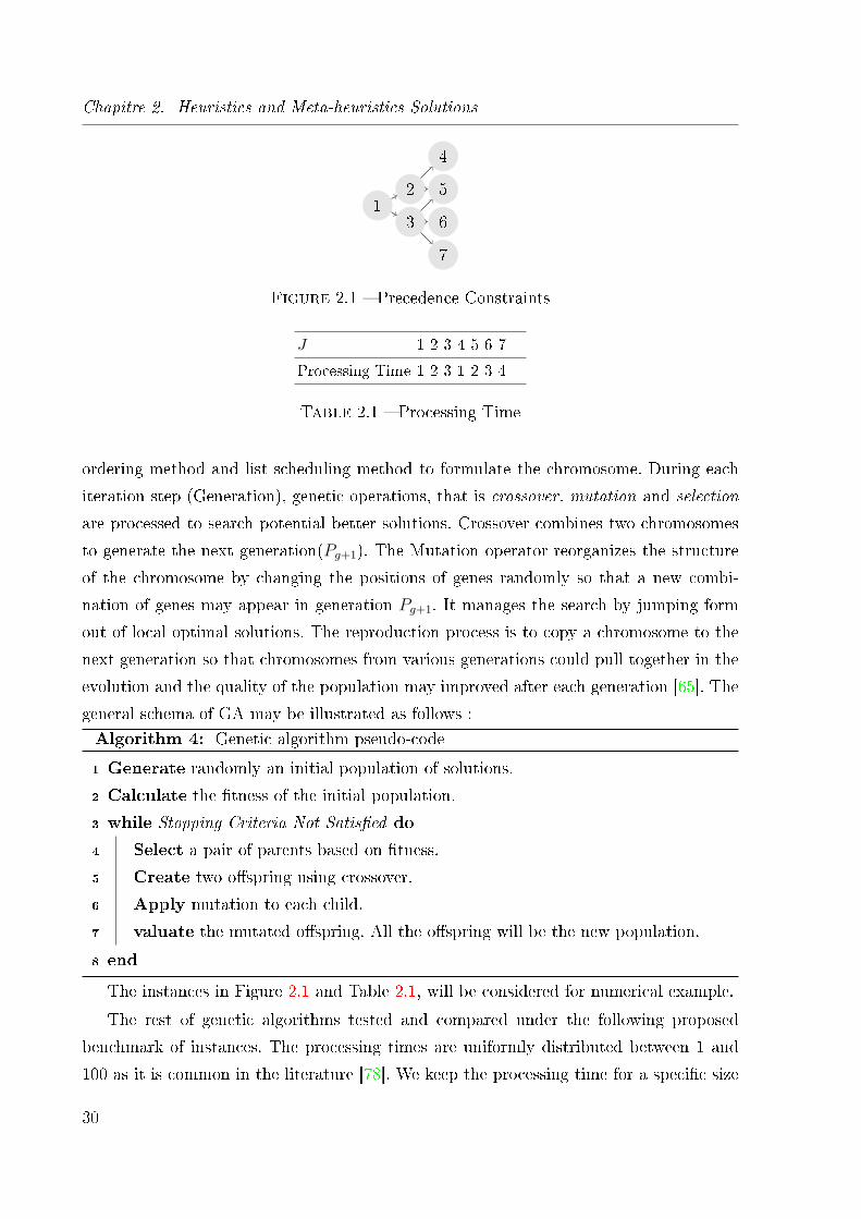
Chapitre 2. Heuristics and Meta-heuristics Solutions
4
51
2
3
7
6
Figure 2.1 � Precedence Constraints
J 1 2 3 4 5 6 7
Processing Time 1 2 3 1 2 3 4
Table 2.1 � Processing Time
ordering method and list scheduling method to formulate the chromosome. During each
iteration step (Generation), genetic operations, that is crossover, mutation and selection
are processed to search potential better solutions. Crossover combines two chromosomes
to generate the next generation(Pg+1). The Mutation operator reorganizes the structure
of the chromosome by changing the positions of genes randomly so that a new combi-
nation of genes may appear in generation Pg+1. It manages the search by jumping form
out of local optimal solutions. The reproduction process is to copy a chromosome to the
next generation so that chromosomes from various generations could pull together in the
evolution and the quality of the population may improved after each generation [65]. The
general schema of GA may be illustrated as follows :Algorithm 4: Genetic algorithm pseudo-code
1 Generate randomly an initial population of solutions.
2 Calculate the �tness of the initial population.
3 while Stopping Criteria Not Satis�ed do
4 Select a pair of parents based on �tness.
5 Create two o�spring using crossover.
6 Apply mutation to each child.
7 valuate the mutated o�spring. All the o�spring will be the new population.
8 end
The instances in Figure 2.1 and Table 2.1, will be considered for numerical example.
The rest of genetic algorithms tested and compared under the following proposed
benchmark of instances. The processing times are uniformly distributed between 1 and
100 as it is common in the literature [78]. We keep the processing time for a speci�c size
30
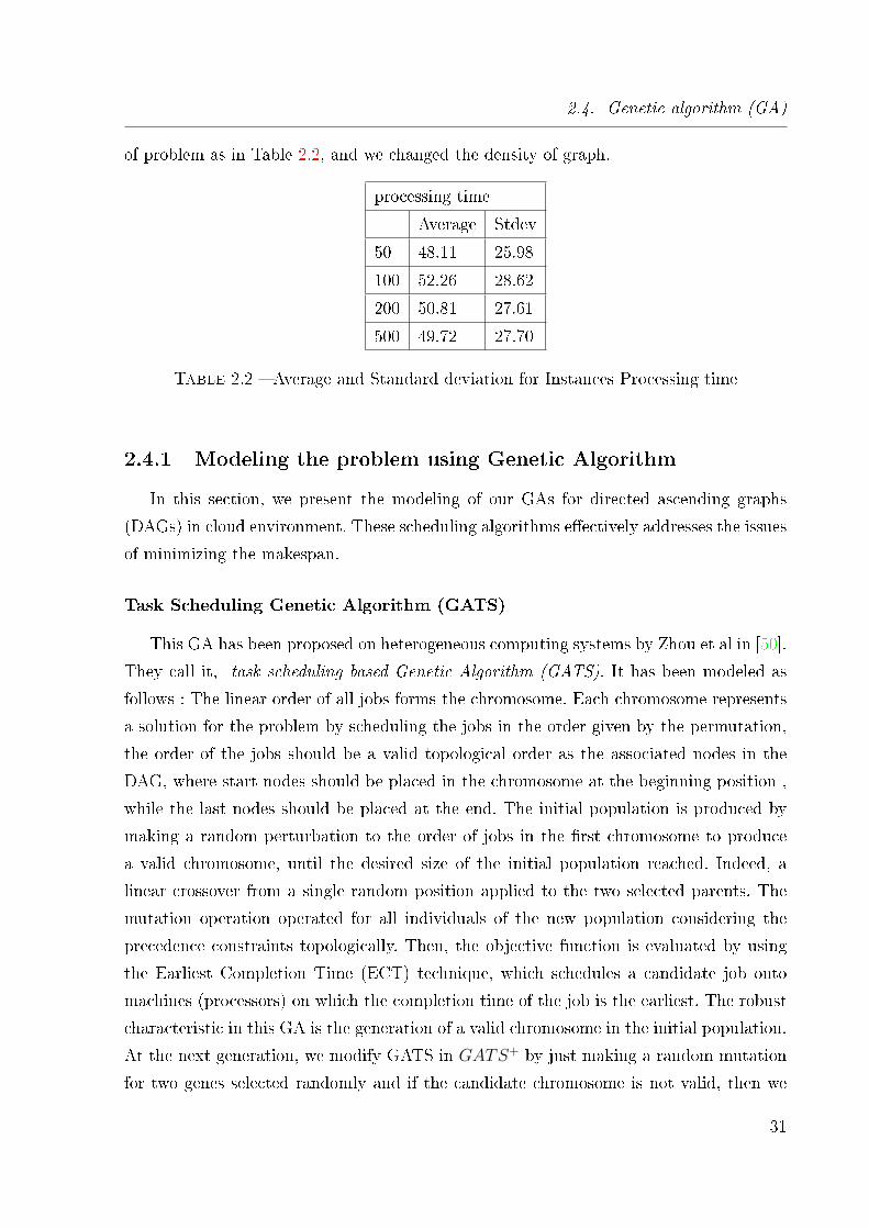
2.4. Genetic algorithm (GA)
of problem as in Table 2.2, and we changed the density of graph.
processing time
Average Stdev
50 48.11 25.98
100 52.26 28.62
200 50.81 27.61
500 49.72 27.70
Table 2.2 � Average and Standard deviation for Instances Processing time
2.4.1 Modeling the problem using Genetic Algorithm
In this section, we present the modeling of our GAs for directed ascending graphs
(DAGs) in cloud environment. These scheduling algorithms e�ectively addresses the issues
of minimizing the makespan.
Task Scheduling Genetic Algorithm (GATS)
This GA has been proposed on heterogeneous computing systems by Zhou et al in [50].
They call it, task scheduling based Genetic Algorithm (GATS). It has been modeled as
follows : The linear order of all jobs forms the chromosome. Each chromosome represents
a solution for the problem by scheduling the jobs in the order given by the permutation,
the order of the jobs should be a valid topological order as the associated nodes in the
DAG, where start nodes should be placed in the chromosome at the beginning position ,
while the last nodes should be placed at the end. The initial population is produced by
making a random perturbation to the order of jobs in the �rst chromosome to produce
a valid chromosome, until the desired size of the initial population reached. Indeed, a
linear crossover from a single random position applied to the two selected parents. The
mutation operation operated for all individuals of the new population considering the
precedence constraints topologically. Then, the objective function is evaluated by using
the Earliest Completion Time (ECT) technique, which schedules a candidate job onto
machines (processors) on which the completion time of the job is the earliest. The robust
characteristic in this GA is the generation of a valid chromosome in the initial population.
At the next generation, we modify GATS in GATS+ by just making a random mutation
for two genes selected randomly and if the candidate chromosome is not valid, then we
31
Chapitre 2. Heuristics and Meta-heuristics Solutions
throw it out by assigning a big value as Cmax to this candidate. Since we have valid
chromosomes in the initial population, the robust characteristics of the GATS can still be
maintained and we will not spend a lot of computation time in the mutation operator. This
small change increases the chance to �nd a best result, especially when the computation
time is less than one minute, because GATS spends a lot of time in mutation procedure
if the candidate is not valid. Table 2.3 shows the results obtained by GATS and GATS+
in one second with Psize = 100, Pc = 1.0 and Pm = 0.5. The dashed results means that
GATS does not �nd a solution during one second and also when we run the instances for
10 seconds GATS cannot �nd a solution with the problems of large number of instances
in all of the three density sets.
Genetic Algorithm Based on Cut-point (GACP)
For this genetic algorithm (GACP), the chromosome coding composed of two rows :
the �rst represents a valid order of jobs according to the precedence constraints, and
the second row gives an information on job positioning according to the cut-point. We
generate m− 1 random cut-points (cp) = {cp1, cp2, ..., cpm−1, } to assign jobs to its VMs.
The solution provided as follows : The sequence of jobs from j0 to jcp1 will be assigned
on VM1 and the sequence of jobs from jcp1 + 1 to jcp2 will be assigned on VM2 and the
sequence of jobs from to on VM3 and so on. In other words, we assign a valid sub-sequence
of a random length of jobs on a speci�c VM. In this genetic algorithm we carried out one
point crossover between two parents and an exchange between two random points carried
as mutation operator. However, this genetic algorithm gave bad results. The best result
obtained by GACP is at least two times the Cmax obtained by GATS.
Genetic Algorithm Based on The List of Available Jobs (GAAV)
In this section we will propose a simple idea to generate the population with lowest
computational cost, where the chromosome coding depends on VMs and places the job in
its associated VM, and the computational e�orts will be taken in the evaluation function.
In this section we will describe our second genetic algorithm, based on the list of available
jobs (GAAV), which is depends mainly on the available-list scheduling heuristic.
Coding an initial population : The assignment of VMs to the list of jobs is a candidate
solution to the problem. Therefore, the chromosome can be represented by a linear list of
integers, each integer representing a VM, here mi considered as gene. The series of genes
with the length of n are generated randomly by assigning each job of J to a random mi
32
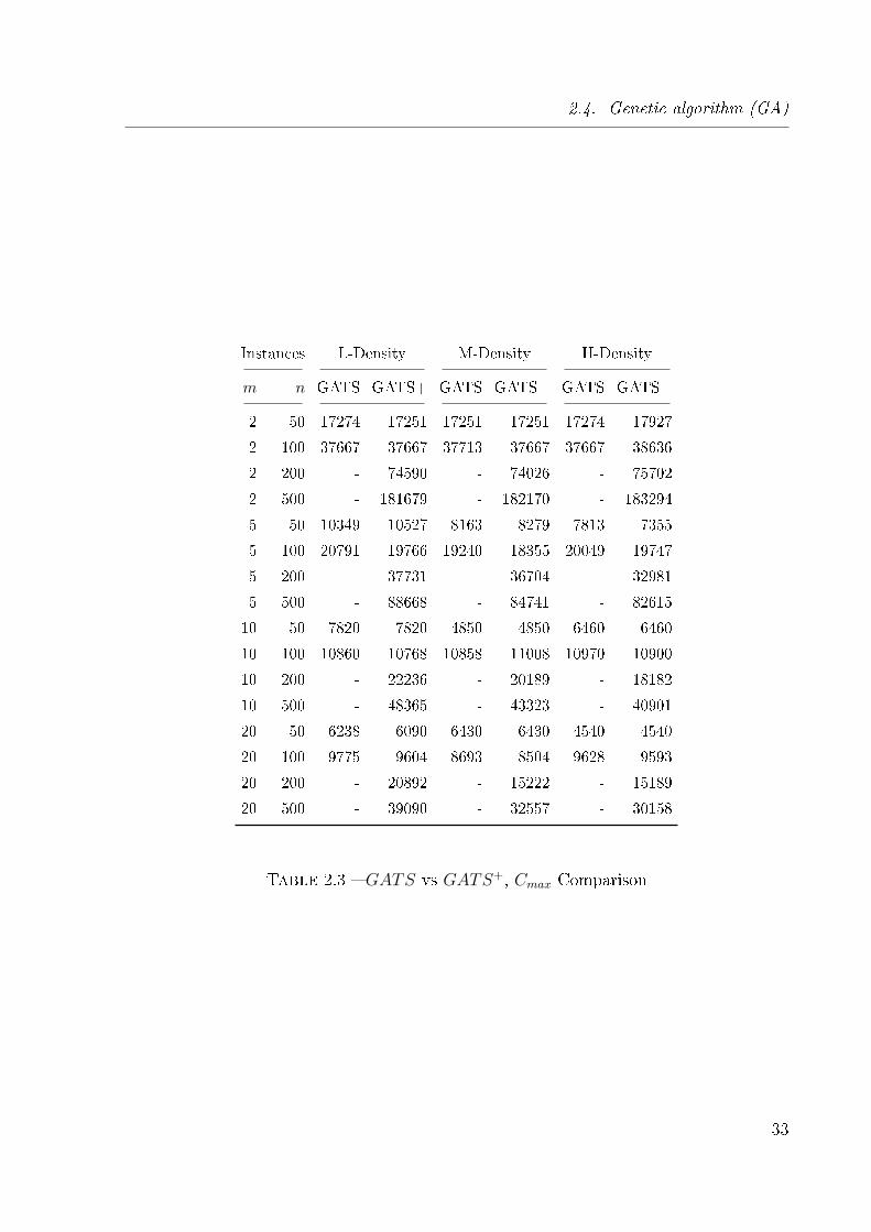
2.4. Genetic algorithm (GA)
Instances L-Density M-Density H-Density
m n GATS GATS+ GATS GATS+ GATS GATS+
2 50 17274 17251 17251 17251 17274 17927
2 100 37667 37667 37713 37667 37667 38636
2 200 - 74590 - 74026 - 75702
2 500 - 181679 - 182170 - 183294
5 50 10349 10527 8163 8279 7813 7355
5 100 20791 19766 19240 18355 20049 19747
5 200 - 37731 - 36704 - 32981
5 500 - 88668 - 84741 - 82615
10 50 7820 7820 4850 4850 6460 6460
10 100 10860 10768 10858 11008 10970 10900
10 200 - 22236 - 20189 - 18182
10 500 - 48365 - 43323 - 40901
20 50 6238 6090 6430 6430 4540 4540
20 100 9775 9604 8693 8504 9628 9593
20 200 - 20892 - 15222 - 15189
20 500 - 39090 - 32557 - 30158
Table 2.3 � GATS vs GATS+, Cmax Comparison
33
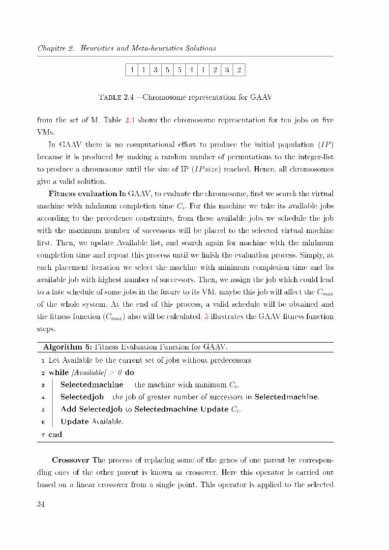
Chapitre 2. Heuristics and Meta-heuristics Solutions
4 1 3 5 5 4 1 2 3 2
Table 2.4 � Chromosome representation for GAAV
from the set of M. Table 2.4 shows the chromosome representation for ten jobs on �ve
VMs.
In GAAV there is no computational e�ort to produce the initial population (IP )
because it is produced by making a random number of permutations to the integer-list
to produce a chromosome until the size of IP (IPsize) reached. Hence, all chromosomes
give a valid solution.
Fitness evaluation In GAAV, to evaluate the chromosome, �rst we search the virtual
machine with minimum completion time Ci. For this machine we take its available jobs
according to the precedence constraints, from these available jobs we schedule the job
with the maximum number of successors will be placed to the selected virtual machine
�rst. Then, we update Available list, and search again for machine with the minimum
completion time and repeat this process until we �nish the evaluation process. Simply, at
each placement iteration we select the machine with minimum completion time and its
available job with highest number of successors. Then, we assign the job which could lead
to a late schedule of some jobs in the future to its VM, maybe this job will a�ect the Cmaxof the whole system. At the end of this process, a valid schedule will be obtained and
the �tness function (Cmax) also will be calculated. 5 illustrates the GAAV �tness function
steps.
Algorithm 5: Fitness Evaluation Function for GAAV.
1 Let Available be the current set of jobs without predecessors
2 while |Available| > 0 do
3 Selectedmachine = the machine with minimum Ci.
4 Selectedjob= the job of greater number of successors in Selectedmachine.
5 Add Selectedjob to Selectedmachine Update Ci.
6 Update Available.
7 end
Crossover The process of replacing some of the genes of one parent by correspon-
ding ones of the other parent is known as crossover. Here this operator is carried out
based on a linear crossover from a single point. This operator is applied to the selected
34

2.4. Genetic algorithm (GA)
parents (parent1, parent2), then a new two o�springs are obtained as offspring1, and
offspring2, the crossover operated between two chromosomes one with higher �tness
value and the other with the Pc ratio. Table 2.5 illustrates the crossover operator.
↓Parent 1 1 4 2 1 3 3 5 2 1 3
↓Parent 2 2 1 1 4 5 2 3 3 1 5
Child 1 1 4 2 1 3 2 3 3 1 5
Child 2 2 1 1 4 5 3 5 2 1 3
Table 2.5 � GAAV :Crossover Operator
Mutation Mutation can be thought as an e�ectively escape method for premature
convergence by randomly change the value of an individual. For maintaining the feasibility
of the new generated individual. During the mutation process, one gene selected randomly
and we put it on a di�erent random mi from the set ofM to obtain a new o�spring, Table
2.6 represents the mutation operator.
O�spring 1 1 4 2 1 3 2 3 3 1 5
O�spring 2 1 4 2 1 3 4 3 3 1 5
Table 2.6 � GAAV :Mutation Operator
Selection Finally, the best chromosome of the �rst population is stored as in a linear
ranking.
35

Chapitre 2. Heuristics and Meta-heuristics Solutions
0 1 2 3 4 5 6 7 8 9 10 11 12 13 14
j1 j2 j6 j7
Cmax↓
m1
j3 j4 j5m2
(a) GAAV solution
0 1 2 3 4 5 6 7 8 9 10 11 12 13 14
Cmax↓
j1 j2 j6 j7m1
j3j4 j5m2
(b) GATS solution
Figure 2.2 � Example of the GATS and GAAV encoding.
Stopping rule The GA is stopped when the execution time is greater than the
maximum execution time allowed.
Figure 2.2, represents an example of chromosome encoding solution for GATS, which
is (1-3-2-6-7-4-5), and a chromosome encoding solution for GAAV, which is (2-1-1-2-2-1-
1), for the instances in Table 2.1 according to the precedence constraints in Figure2.1,
run on two VMs of di�erent speeds which are : s1 = 1, s2 = 2.
Genetic Algorithm (GAAV +)
When GATS depends mainly on ECT technique and GAAV based on the local density
of the DAG, according to the e�ectiveness of these two techniques in the optimization of
scheduling unrelated parallel machine problem with precedence constraints, we combined
these two techniques in GAAV +.
In this genetic algorithmGAAV +, the modi�cation occurred in the Fitness Evaluation.
Therefore, the chromosome representation as in Table 2.4, according to this coding we
know the VM for each job, this �tness evaluation will select the job in machine that will
give the minimum Cj from the available jobs j AV, where AV is the current set of jobs
without predecessors, this is ECT technique. From the other hand, at the same time we
considered the number of successors of this job, and this is the local density of the DAG
technique. Thus, the evaluation can be taken by selecting job j from AV with the minimum
36
2.4. Genetic algorithm (GA)
value produced by the following function : α(Cj) − (1 − α)|Succj| where α ∈ [1, 0] and
|Succj| is the number of successors of job j. We schedule the job with the minimum value
of this function �rst to generate a valid schedule for calculating Cmax.
Experimental Results
This section presents the experimental results ofGATS,GATS+,GAAV andGAAV +.
A set of simulations have been performed on Dell Intel, core i5 running at 3.4 GHz, and
8 GB of RAM. The GAs have been coded in C++, compiled with g++ compiler, and
tested under Ubuntu 14.02 64-OS. The entries in the Table 2.8 are :
m : number of machines,
n : number of jobs,
GATS : Cmax value for GATS,
GATS+ : Cmax value for GATS+,
GAAV : Cmax value for GAAV,
GAAV+ : Cmax value for GAAV+,
Genetic search is implemented through genetic operators. 2.8 show the results given by our
proposed GAs (GATS+, GAAV, and GAAV +) compared to GATS. From this simulation
study we �xed the parameters with the combination of (100, 1.0, 0.5, 600), Population
size, Crossover ratio, mutation ratio and the computation time respectively. We have tes-
ted out di�erent values of α in GAAV + to �nd the best value. Therefore, we took α = 0.5.
From the results we have noticed that when population size in GAAV is larger than 100,
any increase of it has no signi�cant in�uence on the performance of the genetic algorithm.
In Table 2.8 we can see the genetic algorithm GAAV can improve 31% of the solutions
obtained by GATS in low density problems, 43% in medium density problems and 43% in
high density problems. One other interesting outcome is that GAAV can be considered as
an e�cient algorithm with the problems of small and medium number of VMs. GAAV +
mostly outperforms GATS when the number of jobs 100 and 200 in high density. This
may improve 50% of solutions obtained by GATS. It can also improve 50% of medium
density problems and 31 of low density problems. If we focused our attention to genetic
algorithm GATS+, we can see that for low density showed a good performance and for
medium and high density problems is really far from the best solutions, because when
we thrown out the invalid candidates we lost some information about some generations.
According to the GATS operators behaviors, it always needs more time than the speci�ed
stop criterion, with the problems of large numbers of machines and jobs.
37
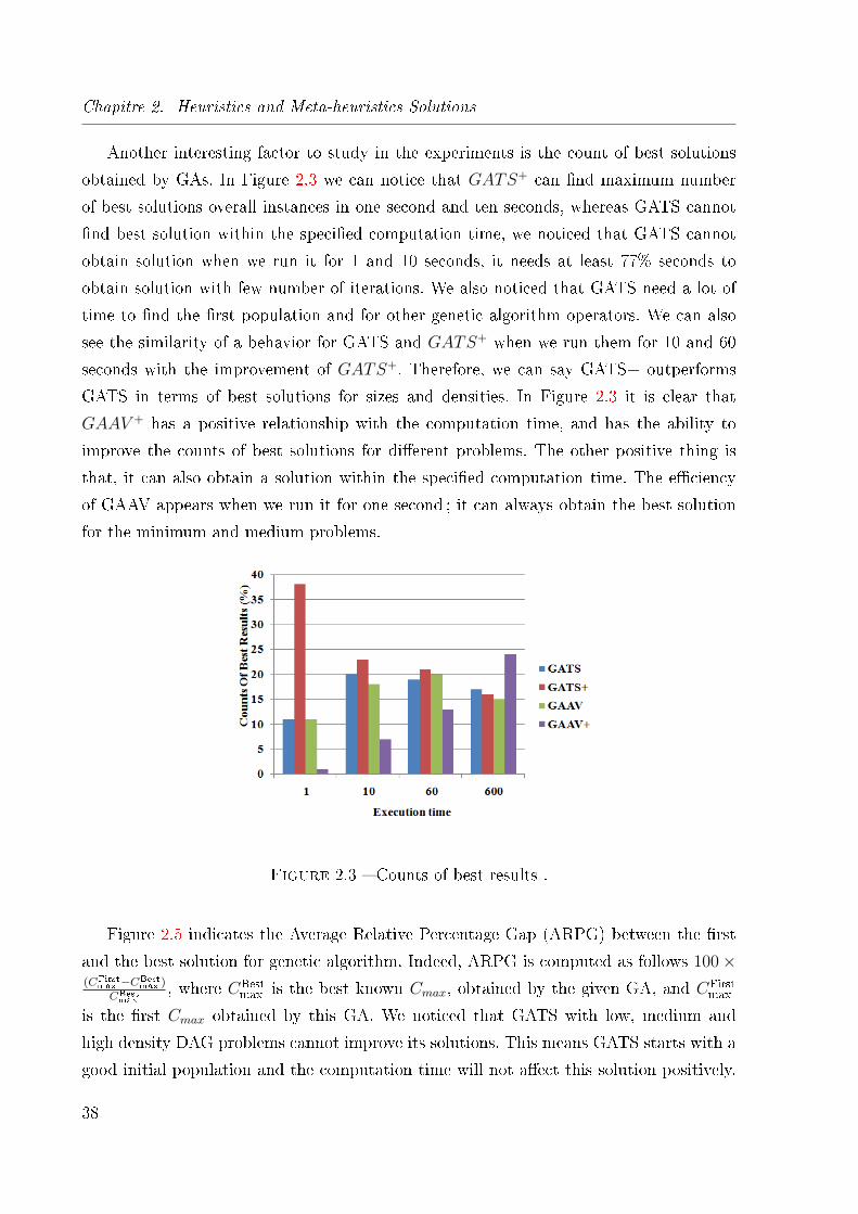
Chapitre 2. Heuristics and Meta-heuristics Solutions
Another interesting factor to study in the experiments is the count of best solutions
obtained by GAs. In Figure 2.3 we can notice that GATS+ can �nd maximum number
of best solutions overall instances in one second and ten seconds, whereas GATS cannot
�nd best solution within the speci�ed computation time, we noticed that GATS cannot
obtain solution when we run it for 1 and 10 seconds, it needs at least 77% seconds to
obtain solution with few number of iterations. We also noticed that GATS need a lot of
time to �nd the �rst population and for other genetic algorithm operators. We can also
see the similarity of a behavior for GATS and GATS+ when we run them for 10 and 60
seconds with the improvement of GATS+. Therefore, we can say GATS+ outperforms
GATS in terms of best solutions for sizes and densities. In Figure 2.3 it is clear that
GAAV + has a positive relationship with the computation time, and has the ability to
improve the counts of best solutions for di�erent problems. The other positive thing is
that, it can also obtain a solution within the speci�ed computation time. The e�ciency
of GAAV appears when we run it for one second ; it can always obtain the best solution
for the minimum and medium problems.
Figure 2.3 � Counts of best results .
Figure 2.5 indicates the Average Relative Percentage Gap (ARPG) between the �rst
and the best solution for genetic algorithm. Indeed, ARPG is computed as follows 100×(CFirst
max −CBestmax )
CBestmax
, where CBestmax is the best known Cmax, obtained by the given GA, and CFirst
max
is the �rst Cmax obtained by this GA. We noticed that GATS with low, medium and
high density DAG problems cannot improve its solutions. This means GATS starts with a
good initial population and the computation time will not a�ect this solution positively.
38
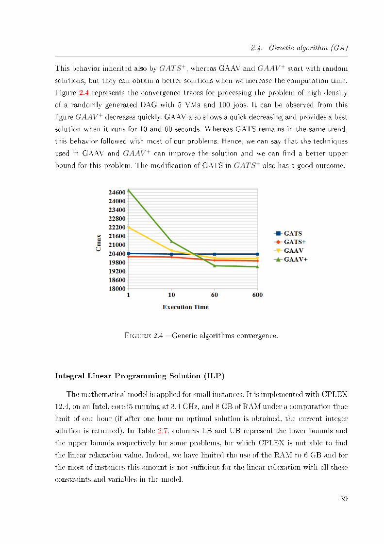
2.4. Genetic algorithm (GA)
This behavior inherited also by GATS+, whereas GAAV and GAAV + start with random
solutions, but they can obtain a better solutions when we increase the computation time.
Figure 2.4 represents the convergence traces for processing the problem of high density
of a randomly generated DAG with 5 VMs and 100 jobs. It can be observed from this
�gure GAAV + decreases quickly. GAAV also shows a quick decreasing and provides a best
solution when it runs for 10 and 60 seconds. Whereas GATS remains in the same trend,
this behavior followed with most of our problems. Hence, we can say that the techniques
used in GAAV and GAAV + can improve the solution and we can �nd a better upper
bound for this problem. The modi�cation of GATS in GATS+ also has a good outcome.
Figure 2.4 � Genetic algorithms convergence.
Integral Linear Programming Solution (ILP)
The mathematical model is applied for small instances. It is implemented with CPLEX
12.4, on an Intel, core i5 running at 3.4 GHz, and 8 GB of RAM under a computation time
limit of one hour (if after one hour no optimal solution is obtained, the current integer
solution is returned). In Table 2.7, columns LB and UB represent the lower bounds and
the upper bounds respectively for some problems, for which CPLEX is not able to �nd
the linear relaxation value. Indeed, we have limited the use of the RAM to 6 GB and for
the most of instances this amount is not su�cient for the linear relaxation with all these
constraints and variables in the model.
39
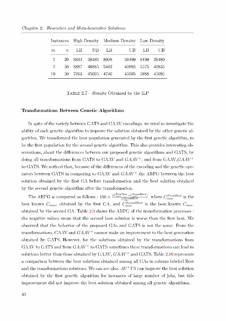
Chapitre 2. Heuristics and Meta-heuristics Solutions
Instances High Density Medium Density Low Density
m n LB UB LB UB LB UB
2 20 8892 38480 8008 38480 8190 38480
2 50 8887 40885 5482 40885 5575 40835
10 50 7263 45695 4746 45695 5888 45695
Table 2.7 � Results Obtained by the ILP
Transformations Between Genetic Algorithms
In spite of the variety between GATS and GAAV encodings, we tried to investigate the
ability of each genetic algorithm to improve the solution obtained by the other genetic al-
gorithm. We transformed the best population generated by the �rst genetic algorithm, to
be the �rst population for the second genetic algorithm. This also provides interesting ob-
servations, about the di�erences between our proposed genetic algorithms and GATS, by
doing all transformations from GATS to GAAV and GAAV +, and from GAAV,GAAV +
to GATS. We noticed that, because of the di�erences of the encoding and the genetic ope-
rators between GATS in comparing to GAAV and GAAV + the ARPG between the best
solution obtained by the �rst GA before transformation and the best solution obtained
by the second genetic algorithm after the transformation.
The ARPG is computed as follows : 100× (CFirstBestmax −CSecondBest
max )CSecondBestmax
, where CFirstBestmax is the
best known Cmax, obtained by the �rst GA, and CSecondBestmax is the best known Cmax,
obtained by the second GA. Table 2.9 shows the ARPG of the transformation processes :
the negative values mean that the second best solution is worse than the �rst best. We
observed that the behavior of the proposed GAs and GATS is not the same. From the
transformations, GAAV and GAAV + cannot make an improvement to the best generation
obtained by GATS. However, for the solutions obtained by the transformations from
GAAV to GATS and from GAAV + to GATS sometimes these transformations can lead to
solutions better than those obtained by GAAV, GAAV + and GATS. Table 2.10 represents
a comparison between the best solutions obtained among all GAs in column labeled Best
and the transformations solutions. We can see also, AV +TS can improve the best solution
obtained by the �rst genetic algorithm for instances of large number of jobs, but this
improvement did not improve the best solution obtained among all genetic algorithms.
40
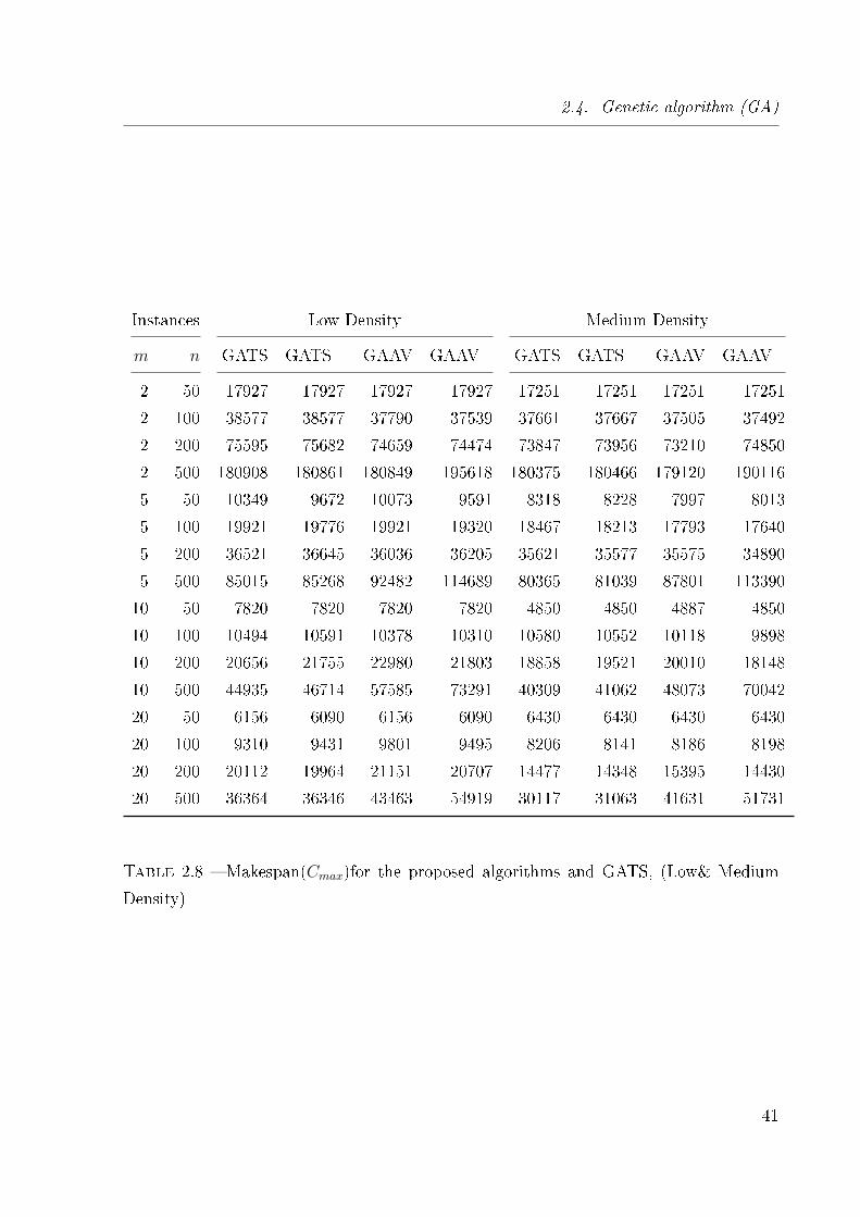
2.4. Genetic algorithm (GA)
Instances Low Density Medium Density
m n GATS GATS+ GAAV GAAV+ GATS GATS+ GAAV GAAV+
2 50 17927 17927 17927 17927 17251 17251 17251 17251
2 100 38577 38577 37790 37539 37661 37667 37505 37492
2 200 75595 75682 74659 74474 73847 73956 73210 74850
2 500 180908 180861 180849 195618 180375 180466 179120 190116
5 50 10349 9672 10073 9591 8318 8228 7997 8013
5 100 19921 19776 19921 19320 18467 18213 17793 17640
5 200 36521 36645 36036 36205 35621 35577 35575 34890
5 500 85015 85268 92482 114689 80365 81039 87801 113390
10 50 7820 7820 7820 7820 4850 4850 4887 4850
10 100 10494 10591 10378 10310 10580 10552 10118 9898
10 200 20656 21755 22980 21803 18858 19521 20010 18148
10 500 44935 46714 57585 73291 40309 41062 48073 70042
20 50 6156 6090 6156 6090 6430 6430 6430 6430
20 100 9310 9431 9801 9495 8206 8141 8186 8198
20 200 20112 19964 21151 20707 14477 14348 15395 14430
20 500 36364 36346 43463 54919 30117 31063 41631 51731
Table 2.8 � Makespan(Cmax)for the proposed algorithms and GATS, (Low& Medium
Density)
41
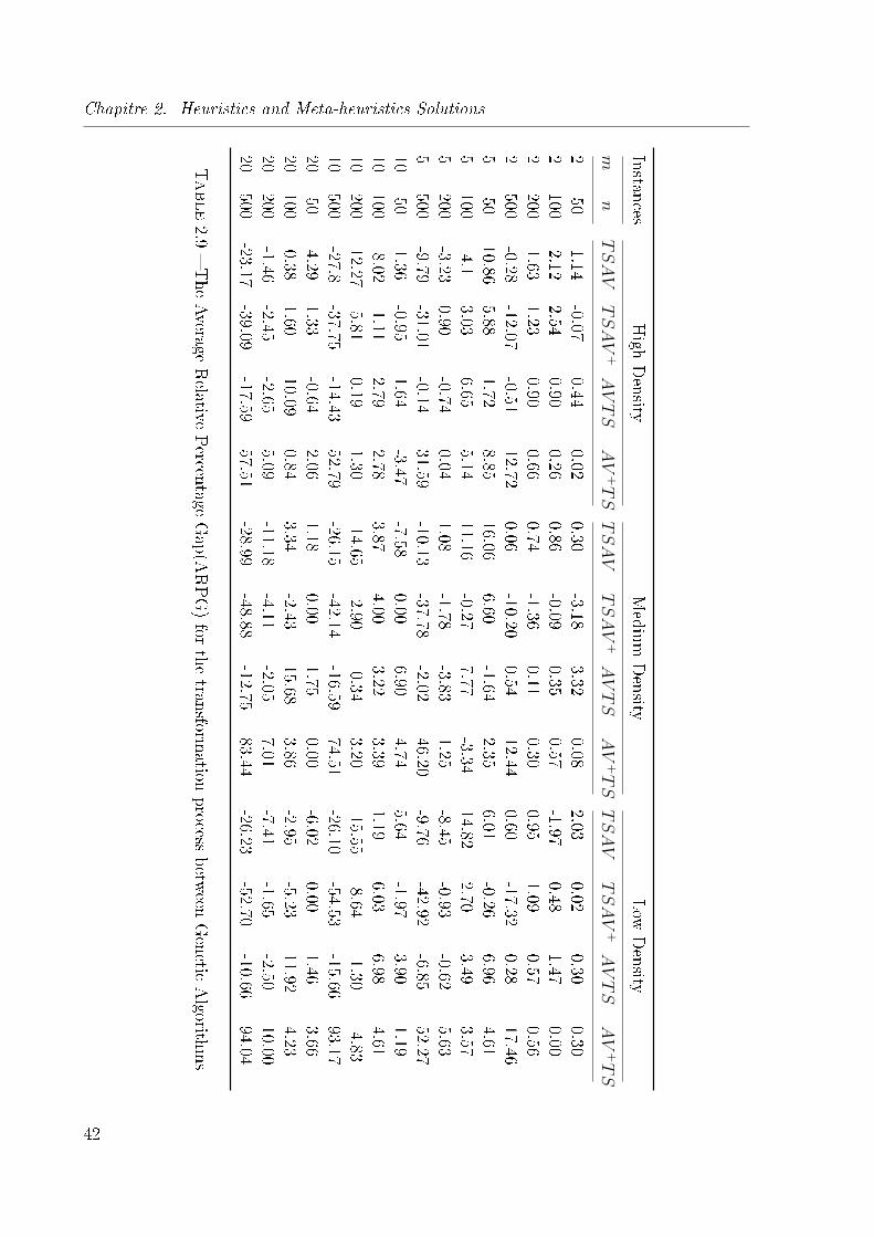
Chapitre 2. Heuristics and Meta-heuristics Solutions
InstancesHigh
Density
Medium
Density
Low
Density
mn
TSAV
TSAV
+AVTS
AV
+TS
TSAV
TSAV
+AVTS
AV
+TS
TSAV
TSAV
+AVTS
AV
+TS
250
1.14-0.07
0.440.02
0.30-3.18
3.320.08
2.030.02
0.300.30
2100
2.122.54
0.900.26
0.86-0.09
0.350.57
-1.970.48
1.470.00
2200
1.631.23
0.900.66
0.74-1.36
0.110.30
0.951.09
0.570.56
2500
-0.28-12.07
-0.5112.72
0.06-10.20
0.5412.44
0.60-17.32
0.2817.46
550
10.865.88
1.728.85
16.066.60
-1.642.35
6.01-0.26
6.964.61
5100
4.13.03
6.655.14
11.16-0.27
7.77-3.34
14.822.70
3.493.57
5200
-3.230.90
-0.740.04
1.08-1.78
-3.831.25
-8.45-0.93
-0.625.63
5500
-9.79-31.01
-0.1431.59
-10.13-37.78
-2.0246.20
-9.76-42.92
-6.8552.27
1050
1.36-0.95
1.64-3.47
-7.580.00
6.904.74
5.64-1.97
3.901.19
10100
-8.02-1.11
2.792.78
3.874.00
3.223.39
1.196.03
6.984.61
10200
-12.27-5.81
0.191.30
-14.65-2.90
-0.343.20
-15.55-8.64
-1.30-4.83
10500
-27.8-37.75
-14.4352.79
-26.15-42.14
-16.5974.51
-26.10-54.53
-15.6693.17
2050
4.291.33
-0.642.06
1.180.00
1.750.00
-6.020.00
1.463.66
20100
0.381.60
10.090.84
3.34-2.43
15.683.86
-2.95-5.23
11.924.23
20200
-1.46-2.45
-2.655.09
-11.18-4.11
-2.057.01
-7.41-1.65
-2.5010.00
20500
-23.17-39.09
-17.5957.51
-28.99-48.88
-12.7583.44
-26.23-52.70
-10.6694.04
Table2.9
�The
Average
Relative
Percentage
Gap(A
RPG)for
thetransform
ationprocess
between
Genetic
Algorithm
s
42
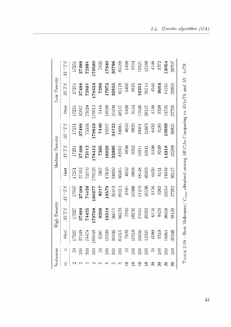
2.4. Genetic algorithm (GA)
Instances
HighDensity
Medium
Density
Low
Density
mn
Best
AVTS
AV
+TS
Best
AVTS
AV
+TS
Best
AVTS
AV
+TS
250
17927
17927
17937
17251
17251
17251
17251
17251
17251
2100
37539
37488
37488
37492
37488
37488
37667
37488
37488
2200
74474
74425
74438
73210
73112
73358
73024
72891
72891
2500
180849
179768
180377
179120
178412
178919
179612
178334
179580
550
9591
9308
9217
7997
7365
7440
7416
7280
7435
5100
19320
19318
18579
17640
16929
18597
18020
17973
17830
5200
36036
36011
36418
34890
33995
34122
31600
30835
30796
5500
85015
86133
89414
80365
82007
84885
38147
81178
85589
1050
7820
7820
8101
4850
4850
4850
6460
6460
6460
10100
10310
10736
10306
9898
9952
9920
9544
9570
9704
10200
20656
21045
21218
18148
18951
19301
17030
16251
19321
10500
44935
45262
46536
40309
40841
41663
38147
38744
42580
2050
6090
6156
6156
6430
6430
6430
4540
4540
4540
20100
9310
9428
9262
8141
8249
8189
9320
9054
9372
20200
19964
20208
20054
14348
14318
13880
13735
14235
13054
20500
36346
38198
37252
30117
32289
30835
27765
28950
28707
Table2.10
�BestMakespan/
Cmaxobtained
amongAllGAsCom
paring
toAVtoTSandAV+toTS
43
Chapitre 2. Heuristics and Meta-heuristics Solutions
Conclusion
In this chapter we have proposed genetic algorithms for job scheduling problem in
cloud computing with the objective of minimizing the makespan (Cmax), which is consi-
dered as an unrelated parallel-machine scheduling problem under precedence constraints.
GAAV includes a new local search procedure for local graph density to evaluate the chro-
mosome. GATS+ which is based on a permutation coding and ECT, and GAAV + which
is combined the innovative characteristics of GAAV with the (ECT) technique. The per-
formances of our proposed genetic algorithms have been compared against one of the best
existing genetic algorithm for the same problem. After extensive comparisons, we can
conclude that the proposed algorithms can improve the solutions obtained by GATS for
small and medium problems. Moreover, they can get better results than GATS within
the speci�c running time (stop criterion) for a high and medium DAG density problem.
In the future work, we will enhance the mathematical model by adding new constraints
for further improvement. Another interesting topic regarding scheduling problem in cloud
computing is to consider the multiobjective optimization context.
In the next chapter we will compare the available mathematical models with our
proposed model, and will present some valid inequalities to our model.
44
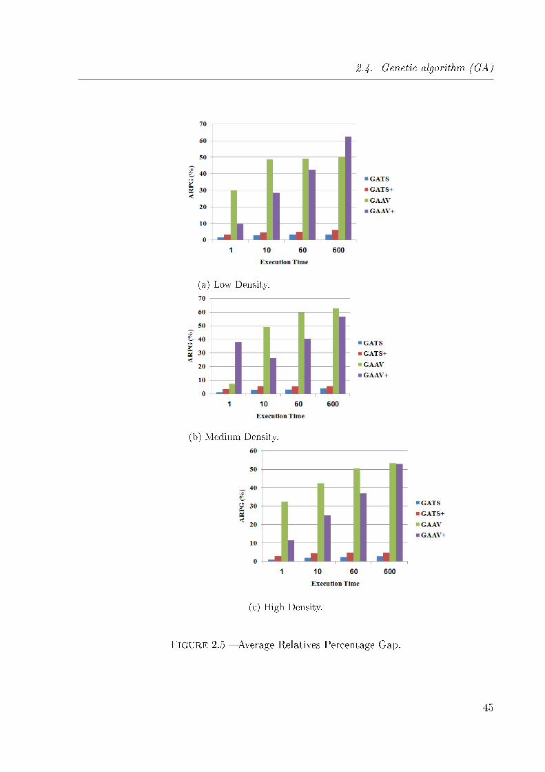
2.4. Genetic algorithm (GA)
(a) Low Density.
(b) Medium Density.
(c) High Density.
Figure 2.5 � Average Relatives Percentage Gap.
45

Chapitre 2. Heuristics and Meta-heuristics Solutions
46
3
Mathematical Formulations
Contents
3.1 Introduction . . . . . . . . . . . . . . . . . . . . . . . . . . . . . 48
3.2 Problem Description . . . . . . . . . . . . . . . . . . . . . . . . . 49
3.3 Mathematical Formulations . . . . . . . . . . . . . . . . . . . . 50
3.3.1 Classical Formulation . . . . . . . . . . . . . . . . . . . . . . . 50
3.3.2 Flow Formulation . . . . . . . . . . . . . . . . . . . . . . . . . . 52
3.3.3 Order Formulation . . . . . . . . . . . . . . . . . . . . . . . . . 54
3.3.4 Interval Graph Formulation . . . . . . . . . . . . . . . . . . . . 55
3.4 Valid Inequalities . . . . . . . . . . . . . . . . . . . . . . . . . . . 58
3.4.1 Separation Algorithm for SPT Inequality . . . . . . . . . . . . 62
3.4.2 Reformulation of Interval Graph Formulation . . . . . . . . . . 62
3.5 Experimental Results . . . . . . . . . . . . . . . . . . . . . . . . 63
3.5.1 Conclusion . . . . . . . . . . . . . . . . . . . . . . . . . . . . . 67
In this chapter we studied an unrelated parallel machine scheduling problem of mi-
nimizing makespan subject to precedence constraints Rm|prec|Cmax. In this chapter we
compared our proposed mathematical model with other mathematical formulations found
in the literature. The main di�erence between these formulations is the way the makespan
has been linearized. We generate sets of benchmark instances and compare the perfor-
mance of the mathematical formulations with extensive computational testing. Moreover,
three families of valid inequalities are proposed. The �rst two inequalities based on the
idea of the precedence jobs and the third based on the shortest processing time(SPT). We
studied the validity of the new inequalities and strength them by checking the linear com-
bination. After an exhaustive computational and statistical analysis we can conclude that
47
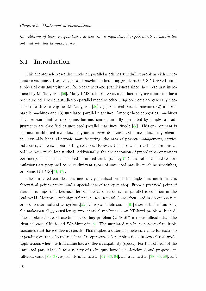
Chapitre 3. Mathematical Formulations
the addition of these inequalities decreases the computational requirements to obtain the
optimal solution in many cases.
3.1 Introduction
This chapter addresses the unrelated parallel machines scheduling problem with prece-
dence constraints. However, parallel machine scheduling problems (PMSPs) have been a
subject of continuing interest for researchers and practitioners since they were �rst intro-
duced by McNaughton [56]. Many PMSPs for di�erent manufacturing environments have
been studied. Previous studies on parallel machine scheduling problems are generally clas-
si�ed into three categories McNaughton [56] : (1) identical parallelmachines (2) uniform
parallelmachines and (3) unrelated parallel machines. Among these categories, machines
that are non-identical to one another and cannot be fully correlated by simple rate ad-
justments are classi�ed as unrelated parallel machines Pinedo [55]. This environment is
common in di�erent manufacturing and services domains, textile manufacturing, chemi-
cal, assembly lines, electronic manufacturing, the area of project management, service
industries, and also in computing services. However, the case when machines are unrela-
ted has been much less studied. Additionally, the consideration of precedence constraints
between jobs has been considered in limited works (see e.g[74]). Several mathematical for-
mulations are proposed to solve di�erent types of unrelated parallel machine scheduling
problems (UPMS)[74, 75].
The unrelated parallel machines is a generalization of the single machine from it is
theoretical point of view, and a special case of the open shop. From a practical point of
view, it is important because the occurrence of resources in parallel is common in the
real world. Moreover, techniques for machines in parallel are often used in decomposition
procedures for multi-stage systems[55]. Garey and Johnson in [61] showed that minimizing
the makespan Cmax considering two identical machines is an NP-hard problem. Indeed,
The unrelated parallel machine scheduling problem (UPMSP) is more di�cult than the
identical case, Chiuh and Wei-Shung in [9]. The unrelated machines consist of multiple
machines that have di�erent speeds. This implies a di�erent processing time for each job
depending on the selected machine. It represents a lot of situations in several real world
applications where each machine has a di�erent capability (speed). For the solution of the
unrelated parallel machine a variety of techniques have been developed and proposed in
di�erent cases [70, 69], especially in heuristics [62, 63, 64], meta-heuristics [38, 65, 59], and
48
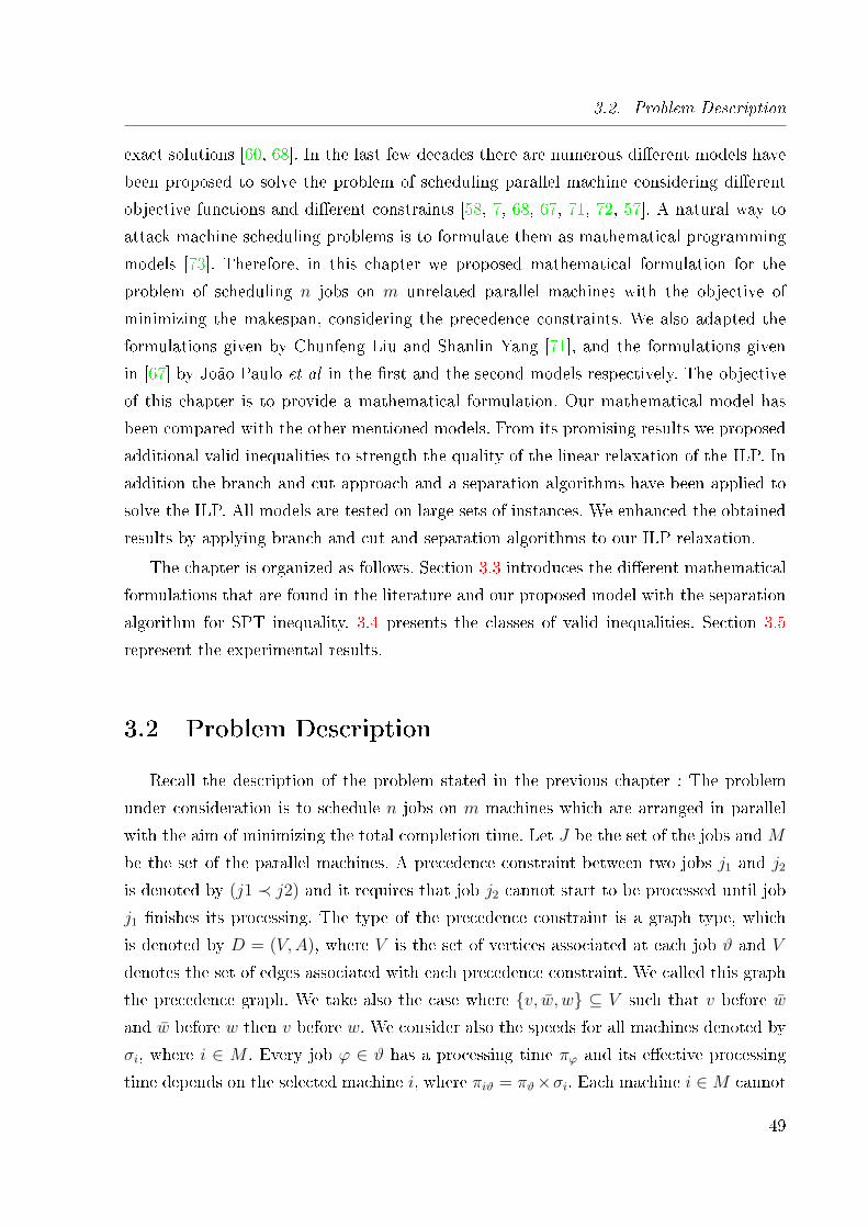
3.2. Problem Description
exact solutions [60, 68]. In the last few decades there are numerous di�erent models have
been proposed to solve the problem of scheduling parallel machine considering di�erent
objective functions and di�erent constraints [58, 7, 68, 67, 71, 72, 57]. A natural way to
attack machine scheduling problems is to formulate them as mathematical programming
models [73]. Therefore, in this chapter we proposed mathematical formulation for the
problem of scheduling n jobs on m unrelated parallel machines with the objective of
minimizing the makespan, considering the precedence constraints. We also adapted the
formulations given by Chunfeng Liu and Shanlin Yang [71], and the formulations given
in [67] by João Paulo et al in the �rst and the second models respectively. The objective
of this chapter is to provide a mathematical formulation. Our mathematical model has
been compared with the other mentioned models. From its promising results we proposed
additional valid inequalities to strength the quality of the linear relaxation of the ILP. In
addition the branch and cut approach and a separation algorithms have been applied to
solve the ILP. All models are tested on large sets of instances. We enhanced the obtained
results by applying branch and cut and separation algorithms to our ILP relaxation.
The chapter is organized as follows. Section 3.3 introduces the di�erent mathematical
formulations that are found in the literature and our proposed model with the separation
algorithm for SPT inequality. 3.4 presents the classes of valid inequalities. Section 3.5
represent the experimental results.
3.2 Problem Description
Recall the description of the problem stated in the previous chapter : The problem
under consideration is to schedule n jobs on m machines which are arranged in parallel
with the aim of minimizing the total completion time. Let J be the set of the jobs and M
be the set of the parallel machines. A precedence constraint between two jobs j1 and j2
is denoted by (j1 ≺ j2) and it requires that job j2 cannot start to be processed until job
j1 �nishes its processing. The type of the precedence constraint is a graph type, which
is denoted by D = (V,A), where V is the set of vertices associated at each job ϑ and V
denotes the set of edges associated with each precedence constraint. We called this graph
the precedence graph. We take also the case where {v, w, w} ⊆ V such that v before w
and w before w then v before w. We consider also the speeds for all machines denoted by
σi, where i ∈ M . Every job ϕ ∈ ϑ has a processing time πϕ and its e�ective processing
time depends on the selected machine i, where πiϑ = πϑ×σi. Each machine i ∈M cannot
49
Chapitre 3. Mathematical Formulations
m11 6 4
x4,1,3 = 1
2 3 5m2
Figure 3.1 � Classical Formulation Illustration.
process more than one job at a given time. Furthermore, machines have di�erent speeds
and preemption of jobs is not allowed. According to the well-known α|β|γ scheduling
problem classi�cation scheme proposed initially by Graham et al [66], scheduling problem
classi�cation scheme this problem can be denoted as P |prec|Cmax We denote by Ci the
completion time of machine i, where i ∈M , and denote by Cϑ the completion time of job
ϑ, where ϑ ∈ ϕ.
3.3 Mathematical Formulations
In this section we present di�erent mathematical models for the UPMSP with prece-
dence constraints, with the objective of minimizing the makespan Cmax. The �rst model
based on the position of job on the machine and the job completion time. The second
model use idea of the �ow formulation which is focus on the sequence of jobs on machines.
The third model is based on the partition in linear orderings. Our proposed models are
based on the interval and m-clique free graphs.
In the next sections we present these mathematical formulations.
3.3.1 Classical Formulation
The idea of this ILP given in [71] is based on the position of job on the machine and
the completion time of each job. Figure 3.1, and Figure 3.2 illustrate the idea of this
formulation.
In this Formulation we will denote by C a large positive number. For describing this
model, let us introduce the following variables :
50
3.3. Mathematical Formulations
mi j j′ .. j2 j1
Cj1Cj2
positions 1 2 ... r-1 r
pij1
Figure 3.2 � Job in position r must start its processing after job in position r − 1.
xjir =
{1 if job j is processed in the position r on machine i0 otherwise
∀j ∈ J, i ∈M, r ∈
J
Cj ∈ N+ is the completion time of job j.
Cmax ∈ N+ is the total length of the schedule. That is, when all the jobs have �nished
processing.
The model can be stated as :
minCmax
Cj ≤ Cmax ∀j ∈ J, (3.1)∑i∈M
∑r∈{1,...,|J |}
xjir = 1 ∀j ∈ J, (3.2)
∑j∈J
xjir ≤ 1 ∀r ∈ {1, ..., |J |},∀i ∈M, (3.3)
∑j1∈J
xj1ir −∑j2∈J
xj2ir−1 ≤ 0 ∀r ∈ {2, ..., |J |},∀i ∈M, (3.4)
Cj2 − Cj1 + C(2− xj2ir − xj1ir−1) ≥ pj2i ∀r ∈ {2, ..., |J |},∀i ∈M,∀j1 6= j2 ∈ J,(3.5)
Cj ≥∑
r∈{1,...,|J |}
pjixjir ∀i ∈M, ∀j ∈ J, (3.6)
Cj2 − Cj1 ≥∑
r∈{1,...,|J |}
∑i∈M
pj2ixj2ir ∀(j1, j2) ∈ A, (3.7)
xjir ∈ {0, 1}, ∀j ∈ J,∀i ∈M,∀r ∈ {1, ..., |J |}, (3.8)
Cj ≥ 0, ∀j ∈ J, (3.9)
Cmax ≥ 0, (3.10)
The objective function is to minimize the makespan. Inequalities (3.1) ensure that the
51
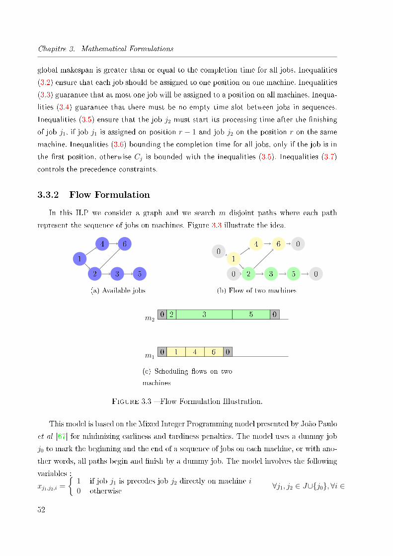
Chapitre 3. Mathematical Formulations
global makespan is greater than or equal to the completion time for all jobs. Inequalities
(3.2) ensure that each job should be assigned to one position on one machine. Inequalities
(3.3) guarantee that at most one job will be assigned to a position on all machines. Inequa-
lities (3.4) guarantee that there must be no empty time slot between jobs in sequences.
Inequalities (3.5) ensure that the job j2 must start its processing time after the �nishing
of job j1, if job j1 is assigned on position r − 1 and job j2 on the position r on the same
machine. Inequalities (3.6) bounding the completion time for all jobs, only if the job is in
the �rst position, otherwise Cj is bounded with the inequalities (3.5). Inequalities (3.7)
controls the precedence constraints.
3.3.2 Flow Formulation
In this ILP we consider a graph and we search m disjoint paths where each path
represent the sequence of jobs on machines. Figure 3.3 illustrate the idea.
4
5
1
2 3
6
(a) Available jobs
4
5
1
2 3
0
0
0
0
6
(b) Flow of two machines
m10 1 4 6 0
0 2 3 5 0m2
(c) Scheduling �ows on two
machines
Figure 3.3 � Flow Formulation Illustration.
This model is based on the Mixed Integer Programming model presented by João Paulo
et al [67] for minimizing earliness and tardiness penalties. The model uses a dummy job
j0 to mark the beginning and the end of a sequence of jobs on each machine, or with ano-
ther words, all paths begin and �nish by a dummy job. The model involves the following
variables :
xj1,j2,i =
{1 if job j1 is precedes job j2 directly on machine i0 otherwise
∀j1, j2 ∈ J∪{j0}, ∀i ∈
52
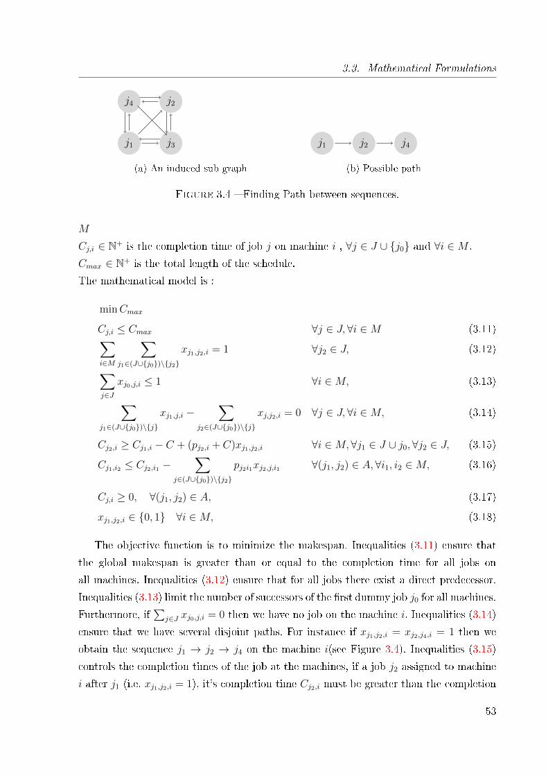
3.3. Mathematical Formulations
j4
j1
j2
j3
(a) An induced sub graph
j1 j2 j4
(b) Possible path
Figure 3.4 � Finding Path between sequences.
M
Cj,i ∈ N+ is the completion time of job j on machine i , ∀j ∈ J ∪ {j0} and ∀i ∈M .
Cmax ∈ N+ is the total length of the schedule.
The mathematical model is :
minCmax
Cj,i ≤ Cmax ∀j ∈ J,∀i ∈M (3.11)∑i∈M
∑j1∈(J∪{j0})\{j2}
xj1,j2,i = 1 ∀j2 ∈ J, (3.12)
∑j∈J
xj0,j,i ≤ 1 ∀i ∈M, (3.13)
∑j1∈(J∪{j0})\{j}
xj1,j,i −∑
j2∈(J∪{j0})\{j}
xj,j2,i = 0 ∀j ∈ J,∀i ∈M, (3.14)
Cj2,i ≥ Cj1,i − C + (pj2,i + C)xj1,j2,i ∀i ∈M, ∀j1 ∈ J ∪ j0,∀j2 ∈ J, (3.15)
Cj1,i2 ≤ Cj2,i1 −∑
j∈(J∪{j0})\{j2}
pj2i1xj2,j,i1 ∀(j1, j2) ∈ A,∀i1, i2 ∈M, (3.16)
Cj,i ≥ 0, ∀(j1, j2) ∈ A, (3.17)
xj1,j2,i ∈ {0, 1} ∀i ∈M, (3.18)
The objective function is to minimize the makespan. Inequalities (3.11) ensure that
the global makespan is greater than or equal to the completion time for all jobs on
all machines. Inequalities (3.12) ensure that for all jobs there exist a direct predecessor.
Inequalities (3.13) limit the number of successors of the �rst dummy job j0 for all machines.
Furthermore, if∑
j∈J xj0,j,i = 0 then we have no job on the machine i. Inequalities (3.14)
ensure that we have several disjoint paths. For instance if xj1,j2,i = xj2,j4,i = 1 then we
obtain the sequence j1 → j2 → j4 on the machine i(see Figure 3.4). Inequalities (3.15)
controls the completion times of the job at the machines, if a job j2 assigned to machine
i after j1 (i.e. xj1,j2,i = 1), it's completion time Cj2,i must be greater than the completion
53
Chapitre 3. Mathematical Formulations
time of j1, Cj1,i plus the processing time of j2. If (xj1,j2,i=0), then the big constant C
render the constrain redundant. Inequalities (3.16) ensure that in di�erent machines the
completion time of precedent job in an arc is less than or equal to the starting time of
successor job in the same arc. Inequalities (3.17) and (3.18) bound the decision variables.
3.3.3 Order Formulation
This formulation proposed by Coll et al [76], this formulation reveals as a part of it a
polytope of partition in linear orderings for solving the problem of multiprocessors sche-
duling with precedence constraints. The following variables used to describe the model :
xji =
{1 if job j processed on machine i0 otherwise
∀j ∈ J,∀i ∈M
zj1j2 =
{1 if job j1 scheduled before j2 on the same machine0 otherwise
∀j1, j2 ∈ J
- yj the starting time of the execution of each job j ∈ J .
- Pj = {j1 ∈ J : there exists a path in G from j1 to j2}, i.e., Pj is the set of predecessorsof job j1 ;
- Γj = {j1 ∈ J : (j1, j2) ∈ A}, i.e.,Γj is the set of immediate predecessors of job j2 ;
- Qj = {j1 ∈ J : there exists a path in G from j2 to j1}, i.e.,- Qj is the set of successors of job j2 ;
- Rj = {j1 ∈ J : there is no path in G from j2 to j1 or from j1 to j2}. The model formulated
54
3.3. Mathematical Formulations
as follows :
minCmax∑i∈M
xij = 1 ∀j ∈ J, (3.19)
yj1 − yj2 +∑i∈M
dj1i.xj1i ≤ µj1j2(1− zj1j2) ∀j2 ∈ J,∀j1 ∈ Rj, (3.20)
yj1 − yj2 +∑i∈M
dj1i.xj1i ≤ 0, ∀j2 ∈ J,∀j1 ∈ Γj, (3.21)
yj − Cmax +∑i∈M
dji.xji ≤ 0, ∀j ∈ J, (3.22)
zj1j2 + zj2j1 + xj1i − xj2i ≤ 1 ∀j1 ∈ J,∀j2 ∈ Rj,∀i ∈M, (3.23)
zj1j2 + xj1i − xj2i ≤ 1 ∀j1 ∈ Pj,∀j2 ∈ J,∀i ∈M, (3.24)
xj1i + xj2i − zj1j2 ≤ 1 ∀j1 ∈ Rj, ∀j2 ∈ J,∀i ∈M, (3.25)
yj ≤ δj ∀j ∈ J, (3.26)
yji ∈ {0, 1} ∀(j, i) ∈ J ×M, (3.27)
zj1j2 ∈ {0, 1} ∀j2 ∈ J,∀j1 ∈ Rj2 ∪ pj2 , (3.28)
Eq. (3.19) ensure that each job is processed and assigned to exactly one processor.
Inequalities (3.21) express the precedence constraints. Inequalities (3.22) de�ne the ma-
kespan. Inequalities (3.20) de�ne the sequence of starting times of the jobs assigned to
the same processor, ensuring that no overlap occurs. The constant µj1j2 is such that if job
j1 and j2 are not executed in the same processor in that order, then inequality (3.20) is
always satis�ed. Inequality (3.26) δj is a lower bound to the earliest starting time of job
j.
3.3.4 Interval Graph Formulation
The third Integer Linear Programming considers the beginning of the job and the
relation between jobs if they run on the same machine, also verify if one job j1 run before
another job j2 or they run the same time on di�erent machines.
The graph induced by the relation where two jobs run in the same time must be an in-
terval graph and check if all jobs can be schedule on this number of machines.
This model consists of the following decision variables :
yi ∈ N+ the starting time of job j.
55
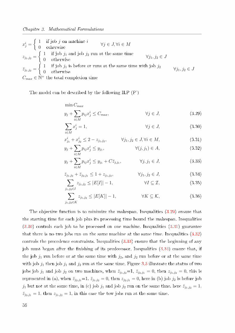
Chapitre 3. Mathematical Formulations
xij =
{1 if job j on machine i0 otherwise
∀j ∈ J,∀i ∈M
zj1,j2 =
{1 if job j1 and job j2 run at the same time0 otherwise
∀j1, j2 ∈ J
zj1,j2 =
{1 if job j1 is before or runs at the same time with job j2
0 otherwise∀j1, j2 ∈ J
Cmax ∈ N+ the total completion time
The model can be described by the following ILP (P')
minCmax
yj +∑i∈M
pijxij ≤ Cmax, ∀j ∈ J, (3.29)∑
i∈M
xij = 1, ∀j ∈ J, (3.30)
xij1 + xij2 ≤ 2− zj1,j2 , ∀j1, j2 ∈ J,∀i ∈M, (3.31)
yj +∑i∈M
pijxij ≤ yj1 , ∀(j, j1) ∈ A, (3.32)
yj +∑i∈M
pijxij ≤ yj1 + Czj,j1 , ∀j, j1 ∈ J, (3.33)
zj1,j2 + zj2,j1 ≤ 1 + zj1,j2 , ∀j1, j2 ∈ J, (3.34)∑j1,j2∈I
zj1,j2 ≤ |E[I]| − 1, ∀I ⊆ I, (3.35)
∑j1,j2∈K
zj1,j2 ≤ |E[K]| − 1, ∀K ⊆ K, (3.36)
The objective function is to minimize the makespan. Inequalities (3.29) ensure that
the starting time for each job plus its processing time bound the makespan. Inequalities
(3.30) controls each job to be processed on one machine. Inequalities (3.31) guarantee
that there is no two jobs run on the same machine at the same time. Inequalities (3.32)
controls the precedence constraints. Inequalities (3.33) ensure that the beginning of any
job must began after the �nishing of its predecessor. Inequalities (3.34) ensure that, if
the job j1 run before or at the same time with j2, and j2 run before or at the same time
with job j1 then job j1 and j2 run at the same time. Figure 3.5 illustrate the status of two
jobs job j1 and job j2 on two machines, when zj1,j2=1, zj2,j1 = 0, then zj1,j2 = 0, this is
represented in (a), when zj2,j1=1, zj1,j2 = 0, then zj2,j1 = 0, here in (b) job j2 is before job
j1 but not at the same time, in (c) job j1 and job j2 run on the same time, here zj1,j2 = 1,
zj2,j1 = 1, then zj1,j2 = 1, in this case the tow jobs run at the same time.
56
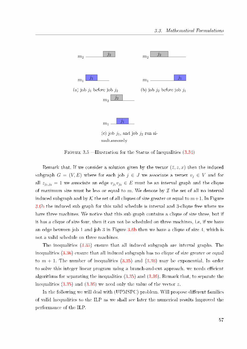
3.3. Mathematical Formulations
m1
m2
j1
j2
(a) job j1 before job j2
m1
m2
j1
j2
(b) job j2 before job j1
m1
m2
j1
j2
(c) job j1, and job j2 run si-
multaneously
Figure 3.5 � Illustration for the Status of Inequalities (3.34)
Remark that, If we consider a solution given by the vector (z, z, x) then the induced
subgraph G = (V,E) where for each job j ∈ J we associate a vertex vj ∈ V and for
all zj1,j2 = 1 we associate an edge vj1vj2 ∈ E must be an interval graph and the clique
of maximum size must be less or equal to m. We denote by I the set of all no interval
induced subgraph and by K the set of all cliques of size greater or equal tom+1. In Figure
3.6b the induced sub graph for this valid schedule is interval and 3-clique free where we
have three machines. We notice that this sub graph contains a clique of size three, but if
it has a clique of size four, then it can not be scheduled on three machines, i.e, if we have
an edge between job 1 and job 3 in Figure 3.6b then we have a clique of size 4, which is
not a valid schedule on three machines.
The inequalities (3.35) ensure that all induced subgraph are interval graphs. The
inequalities (3.36) ensure that all induced subgraph has no clique of size greater or equal
to m + 1. The number of inequalities (3.35) and (3.36) may be exponential. In order
to solve this integer linear program using a branch-and-cut approach, we needs e�cient
algorithms for separating the inequalities (3.35) and (3.36). Remark that, to separate the
inequalities (3.35) and (3.36) we need only the value of the vector z.
In the following we will deal with (UPMSPC) problem. Will propose di�erent families
of valid inequalities to the ILP as we shall see later the numerical results improved the
performance of the ILP.
57
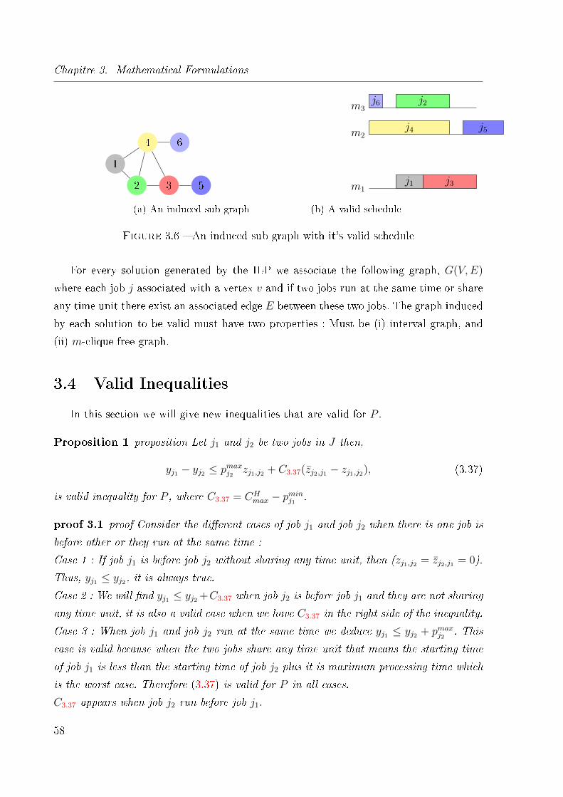
Chapitre 3. Mathematical Formulations
4
5
1
2 3
6
(a) An induced sub graph
m1j1 j3
m2j4 j5
m3j2j6
(b) A valid schedule
Figure 3.6 � An induced sub graph with it's valid schedule
For every solution generated by the ILP we associate the following graph, G(V,E)
where each job j associated with a vertex v and if two jobs run at the same time or share
any time unit there exist an associated edge E between these two jobs. The graph induced
by each solution to be valid must have two properties : Must be (i) interval graph, and
(ii) m-clique free graph.
3.4 Valid Inequalities
In this section we will give new inequalities that are valid for P .
Proposition 1 proposition Let j1 and j2 be two jobs in J then,
yj1 − yj2 ≤ pmaxj2zj1,j2 + C3.37(zj2,j1 − zj1,j2), (3.37)
is valid inequality for P , where C3.37 = CHmax − pminj1
.
proof 3.1 proof Consider the di�erent cases of job j1 and job j2 when there is one job is
before other or they run at the same time :
Case 1 : If job j1 is before job j2 without sharing any time unit, then (zj1,j2 = zj2,j1 = 0).
Thus, yj1 ≤ yj2, it is always true.
Case 2 : We will �nd yj1 ≤ yj2 +C3.37 when job j2 is before job j1 and they are not sharing
any time unit, it is also a valid case when we have C3.37 in the right side of the inequality.
Case 3 : When job j1 and job j2 run at the same time we deduce yj1 ≤ yj2 + pmaxj2. This
case is valid because when the two jobs share any time unit that means the starting time
of job j1 is less than the starting time of job j2 plus it is maximum processing time which
is the worst case. Therefore (3.37) is valid for P in all cases.
C3.37 appears when job j2 run before job j1.
58
3.4. Valid Inequalities
Proposition 2 Let j1 and j2 be two jobs in J then,
yj1 − yj2 ≤ C3.38zj2,j1 − pminj1zj1,j2 , (3.38)
is valid inequality for P where C3.38 = CHmax − pminj1 .
proof 3.2 proof Case 1 : Job j1 is before job j2 and they do not share any time unit.
Then, zj2,j1 = 0, and zj1,j2 = 1. Thus, yj1 ≤ yj2 - pminj1, this case is valid because the
starting of job j1 plus the smallest processing time is less than the starting of job j2.
Case 2 : Job j2 is before job j1 and they do not share any time unit. Then we deduce
yj1 ≤ yj2 +C3.38, this case is also valid when we have C3.38 in the right part of the inequa-
lity.
Case 3 : Job j1 and job j2 run at the same time, or share any time unit, then we deduce
yj1 ≤ yj2 + C3.38 − pminj1, and it is true. Therefore (3.38) is valid for P .
We improved this inequality by adding (pminj1+ pmaxj2
− C3.38)zj1j2 to the right side of the
inequality is important to notice that, this part will not appear in case 1 and case 2 but
will appear when job j1 and job j2 share any time unit. In case 3 when job j1 and job
j2 run at the same time then we deduce that yj1 ≤ yj2 + pmaxj2as we can see in Figure
3.38(3-a and 3-b) this inequality can be valid. Thus, we will get the following inequality :
Corollary 1 corollary Let j1 and j2 be two jobs in J then,
yj1 − yj2 ≤ C3.38zj2,j1 − pminj1zj1,j2 + (pminj1
+ pmaxj2− C3.38)zj1j2 , (3.39)
This inequality is valid for P in all cases.
Remark that if we add the following valid inequality 0 ≤ pminj1zj1j2 − pminj1
zj1j2 to (3.39)
then we obtain (3.37), we deduce that inequality (3.37) is dominated by (3.39). Then it
is not necessary to add the inequalities (3.37) in the model.
Proposition 3 Let j1 and j2 be two jobs in J then,
yj2 − yj1 ≤ C3.40zj1,j2 −∑i∈M
pij2xij2
+ pmaxj2zj1,j2 , (3.40)
is valid inequality for P where C3.40 = CHmax.
59

Chapitre 3. Mathematical Formulations
proof 3.3 proof Case 1 : If job j1 is before job j2 and they do not share any time unit,
then yj2 ≤ yj1 −∑
i∈M pij2xij2
+ C3.40, which is valid.
Case 2 : If job j2 is before job j1 and they do not share any time unit, then yj2 ≤ yj1 −∑i∈M pij2x
ij2, which is also valid when job j1 starts after job j2.
Case 3 : When job j1 and job j2 run at the same time we deduce yj2 ≤ yj1−∑
i∈M pij2xij2
+
pmaxj1+C3.40, which is valid when we have a positive C3.40 in the right side of the equality.
Therefore (3.40) is valid for P in all cases.
Here, C3.40 can be bounded by CHmax where job j1 runs before job j2. In the worst case we
have yj2 + pminj2≤ yj1 + C3.40.
Remark that in case 3 we can reduce the value of C3.40 by this value (pmaxj1+pmaxj2
−CHmax)
when job j1 and job j2 run at the same time, this value can be a coe�cient for the variable
zj1j2 . Thus, we can improve (3.40) by inequality (3.41)
Corollary 2 Let j1 and j2 be two jobs in J then,
yj2 − yj1 ≤ C3.40zj1,j2 −∑i∈M
pij2xij2
+(pmaxj1+ pmaxj2
− C3.40)zj1,j2 , (3.41)
The coe�cient of zj1j2 in (3.41) will not appear in case 1 and case 2 in (3.40). In case
(3-a) when job j1 and job j2 share any time unit and job j1 starts before job j2 we obtain
yj2 ≤ yj1 + pmaxj2, this inequality is valid where job j2 starts before the completion of the
processing time for job j1. In case (3-b) it is clear yj2 ≤ yj1 + pmaxj2is valid where job j2
begin before job j1. Thus, it will improve the inequality when we reduce the right side of
the inequality.
There is no linear combination between inequalities (3.39) and (3.41), because when
we subtract inequality (3.41) from inequality(3.39), we �nd inequality (3.42) which is
invalid when job j1 run before job j2 and do not share any time unit
0 ≤ Czj2,j1 +∑i∈M
pixij2
+
pminj1zj1,j2 − pmaxj1
zj1,j2 − C3.41zj1,j2 − pminj1zj1,j2 , (3.42)
60
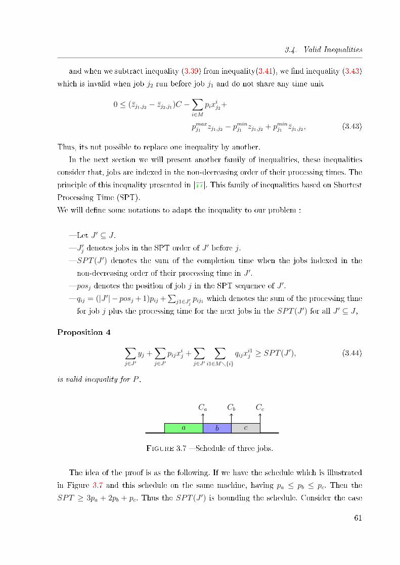
3.4. Valid Inequalities
and when we subtract inequality (3.39) from inequality(3.41), we �nd inequality (3.43)
which is invalid when job j2 run before job j1 and do not share any time unit
0 ≤ (zj1,j2 − zj2,j1)C −∑i∈M
pixij2
+
pmaxj1zj1,j2 − pminj1
zj1,j2 + pminj1zj1,j2 , (3.43)
Thus, its not possible to replace one inequality by another.
In the next section we will present another family of inequalities, these inequalities
consider that, jobs are indexed in the non-decreasing order of their processing times. The
principle of this inequality presented in [77]. This family of inequalities based on Shortest
Processing Time (SPT).
We will de�ne some notations to adapt the inequality to our problem :
� Let J ′ ⊆ J .
� J ′j denotes jobs in the SPT order of J ′ before j.
� SPT (J ′) denotes the sum of the completion time when the jobs indexed in the
non-decreasing order of their processing time in J ′.
� posj denotes the position of job j in the SPT sequence of J ′.
� qij = (|J ′| − posj + 1)pij +∑
j1∈J ′jpij1 which denotes the sum of the processing time
for job j plus the processing time for the next jobs in the SPT (J ′) for all J ′ ⊆ J ,
Proposition 4 ∑j∈J ′
yj +∑j∈J ′
pijxij +
∑j∈J ′
∑i1∈M�{i}
qijxi1j ≥ SPT (J ′), (3.44)
is valid inequality for P ,
a b c
Ca Cb Cc
Figure 3.7 � Schedule of three jobs.
The idea of the proof is as the following. If we have the schedule which is illustrated
in Figure 3.7 and this schedule on the same machine, having pa ≤ pb ≤ pc. Then the
SPT ≥ 3pa + 2pb + pc. Thus the SPT (J ′) is bounding the schedule. Consider the case
61
Chapitre 3. Mathematical Formulations
where job b is runs on another machine, then the SPT (J ′) ≥ 2pa + pc, and still bounding
the schedule. Thus, in this case we must remove the value of qij from the SPT (J ′). Thus,
for all j ∈ J ′, if we remove job j from this machine then SPT (J ′) become : SPT (J ′)−qij.Remark that, if we remove more than one job(i.e.) two jobs (job j1 and job j2), then the
value of SPT will be :
SPT (J ′�{j1, j2}) ≥ SPT (J ′)− qij1 − qij2.
3.4.1 Separation Algorithm for SPT Inequality
In this section we give the idea of the heuristic used to separate inequality (3.44). Given
a fractional solution (x, y∗, z∗, z∗), the separation problem for inequalities (3.44) consists
in determining whether (x, y∗, z∗, z∗) satis�es inequalities (3.44). We run this algorithm
for each machine. For all machine i ∈M we sort the jobs according to the SPT order for
y∗, for each job j in the order if xij ≥ 0.99 we take this job, and continue until the SPT
inequality is violated.
The performance of the valid inequalities is evaluated in the experimental results section.
In the following we will propose an updated formulation invented based on Interval graph
formulation.
3.4.2 Reformulation of Interval Graph Formulation
In the following we will present another version of Interval Graph formulation, in this
formulation we made some changes on the variable zj1j2 , by considering the case if one
job processed before the other job by using the variable zj1j2 it is more nature for the
precedence constraints, and this change enhanced the previous model by reducing the
number of variables. We use the same variables in P with this change
zj1,j2 =
{1 if job j1processed before job j2
0 otherwise∀j1, j2 ∈ J.
62
3.5. Experimental Results
The model can be described as follow :
minCmax
yj +∑i
xijpij ≤ Cmax, ∀j ∈ J, (3.45)∑i∈M
xij = 1, ∀j ∈ J (3.46)
xij1 + xij2 ≤ 2− zj1j2 , ∀j1, j2 ∈ J, i ∈M, (3.47)
yj1 +∑i∈M
pij1xij1≤ yj2 , ∀(j1, j2) ∈ A, (3.48)
yj1 − yj2 +∑i∈M
pij1xij1≤ C(1− zj1j2), ∀j1, j2 ∈ J (3.49)
zj1j2 + zj2j1 + zj1j2 = 1, ∀j1, j2 ∈ J, (3.50)
yj2 ≤ yj1 +∑i∈M
pij1xij1
+ (C − pminj1)zj1j2 ∀j1, j2 ∈ J, (3.51)∑
(j1,j2)∈E(I)
zj1,j2 −∑
(j1,j2)∈E(I)
zj1,j2 ≤ |E(I)| − 1, ∀I ⊆ I, (3.52)
∑(j1,j2)∈E(K)
zj1,j2 −∑
(j1,j2)∈E(K)
zj1,j2 ≤ |E(K)| − 1, ∀K ⊆ K (3.53)
The objective function is to minimize the makespan. Inequalities (3.45) ensure that the
beginning time for each job plus its processing time is less than or equal to the total
completion time. Inequalities (3.46) controls each job to be processed on one machine.
Inequalities (3.47) guarantee that there is no two jobs run on the same machine at the same
time. Inequalities (3.48) controls the precedence constraints. Inequalities (3.49) ensure
that the beginning of any job must began after the �nishing of its predecessor. Inequalities
(3.50) ensure that, if the job j1 run before job j2, and j2 run before job j1 then job j1 and
j2 run at the same time, this inequality made the major modi�cation. Inequalities (3.51)
ensure that the beginning of any job must began after the �nishing of its predecessor.
3.5 Experimental Results
The mathematical formulations tested and compared under the following proposed
benchmark of instances.
The processing times are uniformly, distributed between 1 and 100 as it is common in the
literature [78]. We generated �ve di�erent sets of three subsets of DAG where the graph
density is high, medium and low respectively, with the following combinations of number
63
Chapitre 3. Mathematical Formulations
of jobs n = {10, 12, 14, 16, 18, 20, 25} and 2 machines . The speed of machines generated
randomly between 10 and 20. In total 5× 7× 3 instances are generated.
Regarding to the graph density(GD), is calculated as follow GD = |E||V |(|V |−1)
where E is
the set of edges associated with precedence constraints between jobs, and V is the set
of vertices associated with jobs, we generated the instances of three density sets (low,
medium and high) density with the values (0.1, 0.15 and 0.25) respectively.
The Mathematical model implemented with CPLEX 12.4, on an Intel, core i5 running at
3.4 GHz, and 8 GB of RAM. The obtained results in this experiment are reported in table
3.1. Each line gives the average results obtained by solving 5 instances for each problem
size. The entries in these tables are :
� n : the number of jobs,
� ILP : the Integer Linear Program used to solve :
� 1=classical formulation,
� 2=�ow formulation,
� 3=order formulation,
� 4=interval graph formulation,
� CPU : the total CPU time in seconds,
� Gap : the Gap between the lower bounds and the upper bounds (100× UB−LBLB
),
� GapH : the Gap between the best solution given by the heuristic and the integer
linear program (100× Heuristique−UBUB
),
� o/p : the number of problems solved to optimality over the number of instances
tested.
Remark that, all instances are carried out for two machines and n jobs. We remark that
the classical formulation give bad results and can solved only the smallest instances. We
can observe that the interval graph formulation found 62%, 28% and 22% of optimal
solutions in high density, medium and low density respectively. Whereas, the optimal so-
lutions obtained by classical formulation is 17%, 11% and 11% in high density, medium
and low density respectively, and �ow formulation obtained 45%, 20%, and 20% in high
density, medium and low density respectively, and order formulation obtained 68%, 57%,
45% in high density, medium, and low density. The dashed results means that, the model
did not success to run the integer linear program due to the number of inequalities, we
�xed the processing time to one hour.
64
3.5. Experimental Results
Also we remark the Gap between the lower bounds and the upper bounds is sometimes
better for the interval graph formulation. For the high density instances the Gap is always
less than 40% and is acceptable for the instances with less than 20 jobs. Furthermore the
interval graph formulation improve the value given by the heuristic on 11 instances and
only 6 instances for the �ow formulation where the classical formulation improve the value
on 4 instances, and order improved 12 instances.
The ILP with the valid inequalities is tested under the following proposed benchmark
of instances.
The processing times are uniformly, distributed between 1 and 100 as it is common in
the literature [78]. We generated �ve di�erent sets of instances where the graph density is
equal to 0.15 which is calculated as follows GD = |E||V |(|V |−1)
where E is the set of edges as-
sociated with precedence constraints between jobs, and V is the set of vertices associated
with jobs, with the following combinations of numbers of jobs n ∈ {10, 12, 14, 16, 18, 20}and the number of machines m ∈ 2, 3 . The speed of machines is generated randomly
between 10 and 20. In total 5 × 6 × 2 instances are generated. CPU time required is in
seconds.
The ILP is implemented with CPLEX 12.4, on an Intel, core i5 running at 3.4 GHz, and
8 GB of RAM.
We �rst present an overview of the results of computational tests for the ILP when we
add the inequalities. We limit the resolution time of each instance to 3600 seconds.
The number of obtained optimal solutions from the computational experiments are
presented in Table 3.2 with the average of the CPU time required by the model when we
add the inequality for the �ve sets of instances for each problem. We can observe that
Cplex, within the established time, was not able to obtain the optimal solution for all
instances. We can see that the solver founds the optimal solution for all �ve instances
just for the problem of 2×10. We can notice that when we add the inequalities (3.39)
the model found 53% optimal solutions, whereas, the optimal solutions obtained when we
add the inequalities (3.41) is 43%, and when we add the two inequalities (3.39) and (3.41)
the model found 53% optimal solutions with less CPU time. The inequalities (3.44) give
46% optimal solutions, however when we add all inequalities the model found 50% optimal
solution. The results of Table 3.2 also indicate that when we add the two inequalities (3.39)
and (3.41) the model needs less CPU time to �nd optimal solutions. We can notice also
when we increase the number of machines the model is always able to �nd more optimal
65
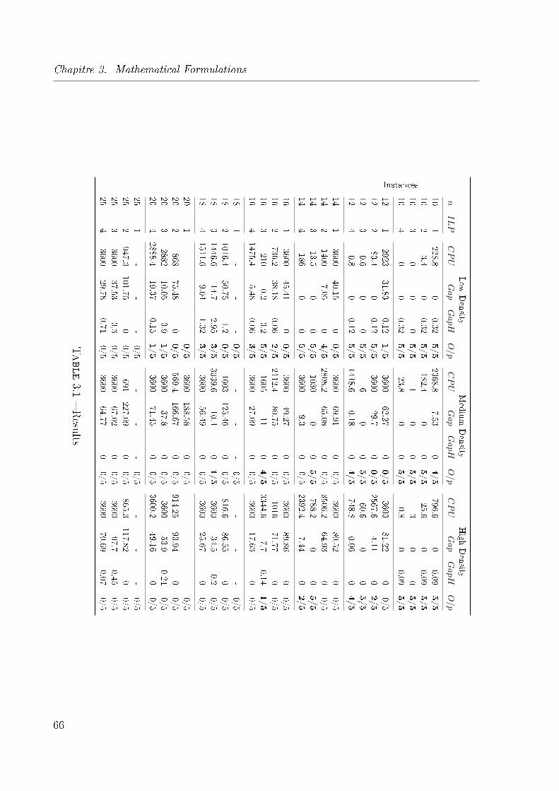
Chapitre 3. Mathematical Formulations
Low
Density
Medium
Density
High
Density
nILP
CPU
Gap
GapH
O/p
CPU
Gap
GapH
O/p
CPU
Gap
GapH
O/p
Instances
101
228.80
0.325/5
2368.87.53
04/5
796.60
0.095/5
102
3.40
0.325/5
182.40
05/5
25.60
0.095/5
103
00
05/5
10
05/5
30
05/5
104
00
0.325/5
23.80
05/5
0.80
0.095/5
121
292331.83
0.121/5
360062.27
00/5
360081.22
00/5
122
83.40
0.125/5
360029.7
00/5
2567.64.11
02/5
123
0.60
05/5
60
05/5
60.60
05/5
124
0.80
0.125/5
1418.60.18
04/5
748.80.06
04/5
141
360040.15
00/5
360069.91
00/5
360080.52
00/5
142
14007.05
04/5
2808.265.08
00/5
3506.264.93
00/5
143
13.50
05/5
10300
05/5
788.20
05/5
144
1860
05/5
36009.3
00/5
2392.47.44
02/5
161
360045.41
00/5
360049.27
00/5
360089.86
00/5
162
736.238.18
0.062/5
2112.480.75
00/5
101671.77
00/5
163
2100.2
0.25/5
160511
04/5
3344.67.7
0.141/5
164
1475.45.48
0.063/5
360027.09
00/5
360017.63
00/5
181
--
-0/5
--
-0/5
--
-0/5
182
1016.450.75
1.20/5
1603125.46
00/5
816.686.55
00/5
183
1446.614.7
2.953/5
3039.610.4
01/5
360034.5
0.20/5
184
1511.69.04
1.323/5
360056.49
00/5
360025.67
00/5
201
--
-0/5
3600188.58
00/5
--
-0/5
202
86875.48
00/5
569.4166.67
00/5
914.2593.94
00/5
203
288210.05
0.91/5
360037.8
00/5
360053.9
0.240/5
204
2888.419.37
0.151/5
360071.45
00/5
3600.249.16
00/5
251
--
-0/5
--
-0/5
--
-0/5
252
947.3101.75
00/5
691227.09
00/5
865.3117.82
00/5
253
360037.53
0.30/5
360067.02
00/5
360097.7
0.450/5
254
360029.78
0.710/5
360064.77
00/5
360070.69
0.070/5
Table3.1
�Results
66
3.5. Experimental Results
solutions within the time limit for all families of inequalities, with the best results obtained
when we add the family of inequalities(3.39).
In Table 3.3 we can see the results for the average relative percentage gap between
the lower bound and the upper bound when we add the inequalities. Indeed, Gap is com-
puted as follows 100 × Upper bound−Lower boundUpper bound
. The average relative percentage gap is no
more than 31% for all problems when we add the inequalities (3.39) and (3.41). However,
the dashes in Cplex column indicates that the Cplex is not able to �nd a valid solution
within the time limit and the limited use of the RAM. Furthermore, we remark that,
when the number of tasks increases with 3 machines, the gap still reduces when we use
the inequalities (3.39) and (3.41).
Other analysis can be displayed in Table 3.2. We can notice that when we add inequa-
lities (3.39) and (3.41) together, the model gives the maximum counts of best obtained
results for all problems, and its also interesting to notice the ability of inequalities (3.39)
for obtaining the same number in comparing with other families of inequalities when they
added individually.
Generally, we can notice the improvement of the model in terms of obtained results
and CPU time occurred when we add the two families (3.39) and (3.41) together to
the ILP. When we add the family of inequalities (3.39) alone to the ILP the improvement
happen with the obtained optimal solutions but with more CPU time. We notice a limited
improvement when we add inequalities (3.41) alone to the ILP . The family of inequalities
(3.44) (the separation algorithm) may need more improvements to obtain better results.
We can say there is no remarkable improvements when we add all families of inequalities
to the model.
3.5.1 Conclusion
In this chapter we considered the problem of unrelated parallel machine scheduling,
minimizing makespan subject to precedence constraints. The main di�erence between
these formulations is the way the makespan has been linearized. To study and evaluate
the e�ectiveness and e�ciency of these models, 105 instances of numerical experiments are
conducted. The obtained results show the e�ectiveness of the interval graph formulation
in comparing with the available formulations except the order formulation, but the facial
structure of the polytope generated by interval graph model can be investigated to de�ne
some facet de�ning inequalities, where there is an important piece of information from
67
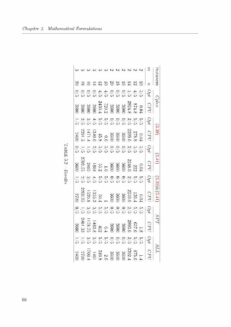
Chapitre 3. Mathematical Formulations
InstancesCplex
(3.39)(3.41)
(3.39)&(3.41)
SPT
ALL
mn
Opt
CPU
Opt
CPU
Opt
CPU
Opt
CPU
Opt
CPU
Opt
CPU
210
5/50.04
5/50.04
5/50.04
5/50.04
5/51.8
5/51.4
212
4/5874.8
5/5278.8
5/5222
5/5136.4
5/5657.6
5/5875.6
214
1/52924.8
2/52299.6
2/52248.6
2/52259.6
2/52993.6
2/53392.4
216
0/53600
0/53600
0/53600
0/53600
0/53600
0/53600
218
0/53600
0/53600
0/53600
0/53600
0/53600
0/53600
220
0/53600
0/53600
0/53600
0/53600
0/53600
0/53600
310
4/5720.2
5/50.6
5/51.6
5/51
5/56.4
5/52.6
312
4/52430.4
5/545.8
5/555.2
5/550.4
5/5412
5/5310.8
314
0/53600
4/51340.6
2/51804
4/51355.2
3/51483.8
3/51461
316
0/53600
3/51471.4
1/52405
3/51520.8
3/51178.75
3/51760.4
318
0/53600
2/52291.5
1/52702.75
2/52269.25
1/52401.33
1/52700
320
0/53600
1/52400
0/53600
1/52700
0/53600
1/52400
Table3.2
�Results
68
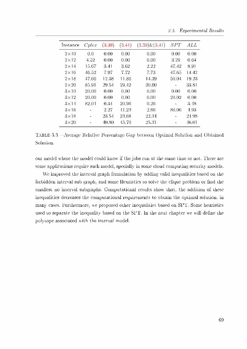
3.5. Experimental Results
Instance Cplex (3.39) (3.41) (3.39)&(3.41) SPT ALL
2×10 0.0 0.00 0.00 0.00 0.00 0.002×12 4.52 0.00 0.00 0.00 3.29 0.642×14 15.67 3.41 3.62 2.22 47.42 8.912×16 46.52 7.97 7.72 7.73 47.65 14.422×18 47.60 12.38 11.80 14.39 50.04 19.232×20 85.91 29.54 29.42 30.60 - 33.813×10 20.00 0.00 0.00 0.00 0.00 0.003×12 20.00 0.00 0.00 0.00 20.02 0.003×14 82.04 0.34 20.96 0.26 - 3.483×16 - 2.27 41.23 2.66 80.06 4.933×18 - 23.54 23.68 22.34 - 24.983×20 - 40.80 45.70 25.31 - 46.01
Table 3.3 � Average Relative Percentage Gap between Optimal Solution and Obtained
Solution.
our model where the model could know if the jobs run at the same time or not. There are
some applications require such model, specially in some cloud computing security models.
We improved the interval graph formulation by adding valid inequalities based on the
forbidden interval sub graph, and some Heuristics to solve the clique problem or �nd the
smallest no interval subgraphs. Computational results show that, the addition of these
inequalities decreases the computational requirements to obtain the optimal solution, in
many cases. Furthermore, we proposed other inequalities based on SPT. Some heuristics
used to separate the inequality based on the SPT. In the next chapter we will de�ne the
polytope associated with the interval model.
69

Chapitre 3. Mathematical Formulations
70
4
Polyedral study on interval graphs
under m-clique free constraints
Contents
4.1 Introduction . . . . . . . . . . . . . . . . . . . . . . . . . . . . . 72
4.2 The polytopes of interval sub-graphs . . . . . . . . . . . . . . . 74
4.2.1 Forbidden subgraphs inequalities . . . . . . . . . . . . . . . . . 74
4.3 Cutting plane algorithms . . . . . . . . . . . . . . . . . . . . . . 90
4.3.1 Bipartite claw separation . . . . . . . . . . . . . . . . . . . . . 90
4.3.2 Umbrella separation . . . . . . . . . . . . . . . . . . . . . . . . 92
4.3.3 Hole separation . . . . . . . . . . . . . . . . . . . . . . . . . . . 97
4.3.4 Clique separation . . . . . . . . . . . . . . . . . . . . . . . . . . 97
4.3.5 Lazy constraint approach . . . . . . . . . . . . . . . . . . . . . 98
4.4 Application to URPMDC problem. . . . . . . . . . . . . . . . . 99
4.4.1 Mathematical formulation . . . . . . . . . . . . . . . . . . . . . 99
4.4.2 Computational Results . . . . . . . . . . . . . . . . . . . . . . . 102
4.5 Conclusion . . . . . . . . . . . . . . . . . . . . . . . . . . . . . . . 103
71
Chapitre 4. Polyedral study on interval graphs under m-clique free constraints
In this chapter we consider the problem of interval and m-clique free subgraphs and
we show the relation between the graph problem and the unrelated parallel machines with
disjunctives constraints (UPMSDC) problem. We study the facial structure of their poly-
tope and we present some inequalities de�ning facets to bound the associated integer linear
programming formulation. Moreover, we present exact and heuristic separation algorithms
associated with a cutting-plane algorithm for solving the problem. Finally, we present some
experimental results as well as their analysis.
4.1 Introduction
Interval, m-clique graphs have attracted the interest of researchers for many decades.
The scope of current research in this area extends now to the mathematical and algorith-
mic properties of interval and m-clique graphs, their generalizations and the related graph
parameters. One main reason for this increasing interest is that many real-world applica-
tions involve solving problems on graphs, which are either interval graphs themselves or
are related to interval graphs or a clique in a natural way. Algorithmic aspects of interval
graphs have been the subject of ongoing research for several decades, stimulated by their
numerous applications ; see e.g. [97]. In some applications, interval representations with
special properties are required.
Numerous applications of interval graphs have appeared in the literature including applica-
tions to genetic structure, sequential storage and scheduling (see [97, 58]). An application
of the interval graphs arises on the context of scheduling jobs in cloud computing. In cloud
computing, we not only have to determine how many, but also which jobs should be alloca-
ted to a virtual machine. In scheduling, for example, jobs can have certain durations that
should be refected by the lengths of their intervals and two consecutive jobs can require
a certain handover period that is determined by how much their intervals should intersect.
All graphs in this chapter are simple and have no self-loops. Let G = (V,E) be a
graph. An undirected graph G is called an interval graph if its vertices can be put into a
one-to-one correspondence with a set of intervals I of a linearly ordered set (like the real
line) such that two vertices are connected by an edge of G if their corresponding intervals
have nonempty intersection.
An interval graph is the graph showing intersecting intervals on a line. Thus, we associate
a set of intervals I = {I1, ..., In} on a line with the interval graph G = (V,E), where
72
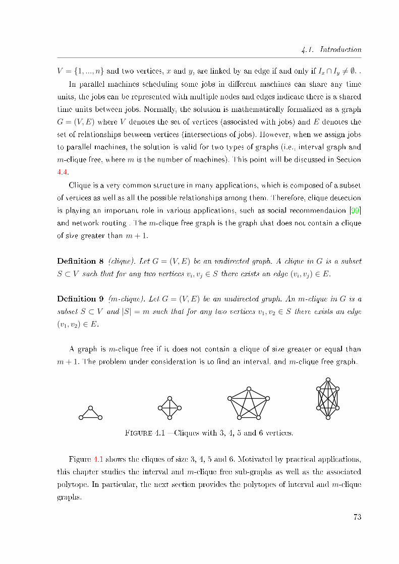
4.1. Introduction
V = {1, ..., n} and two vertices, x and y, are linked by an edge if and only if Ix ∩ Iy 6= ∅. .In parallel machines scheduling some jobs in di�erent machines can share any time
units, the jobs can be represented with multiple nodes and edges indicate there is a shared
time units between jobs. Normally, the solution is mathematically formalized as a graph
G = (V,E) where V denotes the set of vertices (associated with jobs) and E denotes the
set of relationships between vertices (intersections of jobs). However, when we assign jobs
to parallel machines, the solution is valid for two types of graphs (i.e., interval graph and
m-clique free, where m is the number of machines). This point will be discussed in Section
4.4.
Clique is a very common structure in many applications, which is composed of a subset
of vertices as well as all the possible relationships among them. Therefore, clique detection
is playing an important role in various applications, such as social recommendation [99]
and network routing . The m-clique free graph is the graph that does not contain a clique
of size greater than m+ 1.
De�nition 8 (clique). Let G = (V,E) be an undirected graph. A clique in G is a subset
S ⊂ V such that for any two vertices vi, vj ∈ S there exists an edge (vi, vj) ∈ E.
De�nition 9 (m-clique). Let G = (V,E) be an undirected graph. An m-clique in G is a
subset S ⊂ V and |S| = m such that for any two vertices v1, v2 ∈ S there exists an edge
(v1, v2) ∈ E.
A graph is m-clique free if it does not contain a clique of size greater or equal than
m+ 1. The problem under consideration is to �nd an interval, and m-clique free graph.
Figure 4.1 � Cliques with 3, 4, 5 and 6 vertices.
Figure 4.1 shows the cliques of size 3, 4, 5 and 6. Motivated by practical applications,
this chapter studies the interval and m-clique free sub-graphs as well as the associated
polytope. In particular, the next section provides the polytopes of interval and m-clique
graphs.
73
Chapitre 4. Polyedral study on interval graphs under m-clique free constraints
4.2 The polytopes of interval sub-graphs
In this section, we consider the problem of characterizing an interval graph m-clique
free.
Let I := {I ⊆ E |G[I] induces an interval m-clique free subgraph}. The vector zI is calledthe incidence vector associated with I. We de�ne the Interval m-Clique Free Subgraph
Problem (IMCFSP) polytope as follows :
PI(G,m) := conv{zI ∈ {0, 1}|E||I ∈ I} ,
Now, we analyze the dimension of this polytope.
Proposition 5 Polytope PI(G,m) has a full dimension.
proof 4.1 We need to show the existence of |E| + 1 feasible solutions such that their
incidence vectors are a�nely independent.
Let I0 = ∅ be a valid solution, because it has no edge. We also de�ne solutions Ie = {e}for all e ∈ E. The incidence vectors of these solutions are clearly a�nely independents.
Thus, we have |E|+1 vectors of PI(G,m) a�nely independent and the proof is completed.
�
In the following proposition, we will prove that the trivial inequality is a facet.
Proposition 6 Let e ∈ E. The trivial inequality ze ≥ 0 de�nes a facet of PI(G,m).
proof 4.2 Let us denote by az ≤ α inequality −ze ≤ 0 associated with e ∈ E. Let bz ≤ β
be a facet de�ning an equality of PI(G,m), such that {z ∈ PI(G,m) : az = α} ⊆ {z ∈PI(G,m) : bz = β}. We show that b = ρa for some ρ ∈ R.Let I0 = ∅ be a valid solution, and the associated incidence vector zI0 verify −ze = 0.
Let e′ ∈ E \ {e}. The solution Ie′ = {e′} is valid and the incidence vector zIe′ associated
with Ie′ veri�es −ze = 0.
Since, azI0=azIe′ , then we deduce that bzI0=bzIe′ and this implies that b(e′) = 0 for all
e′ ∈ E. Therefore, we set b(e) = ρ, and then b = ρa. �
4.2.1 Forbidden subgraphs inequalities
In this section we analyze the graph properties in order to propose valid inequalities.
Properties on interval graphs have been studied in [80]. The authors give all forbidden
74
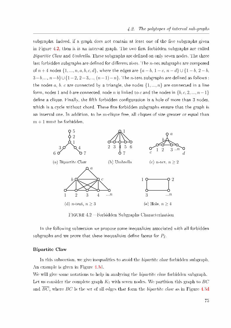
4.2. The polytopes of interval sub-graphs
subgraphs. Indeed, if a graph does not contain at least one of the �ve subgraphs given
in Figure 4.2, then it is an interval graph. The two �rst forbidden subgraphs are called
Bipartite Claw and Umbrella. These subgraphs are de�ned on only seven nodes. The three
last forbidden subgraphs are de�ned for di�erent sizes. The n-net subgraphs are composed
of n+ 4 nodes {1, ..., n, a, b, c, d}, where the edges are {a− b, 1− c, n− d} ∪ {1− b, 2− b,3−b,..., n−b}∪{1−2, 2−3,..., (n−1)−n}. The n-tent subgraphs are de�ned as follows :
the nodes a, b, c are connected by a triangle, the nodes {1, ..., n} are connected in a line
form, nodes 1 and b are connected, node n is linked to c and the nodes in {b, c, 2, ..., n−1}de�ne a clique. Finally, the �fth forbidden con�guration is a hole of more than 3 nodes,
which is a cycle without chord. These �ve forbidden subgraphs ensure that the graph is
an interval one. In addition, to be m-clique free, all cliques of size greater or equal than
m+ 1 must be forbidden.
21
3 4
5
6 7
(a) Bipartite Claw
2
1
3 4 5 6
7
(b) Umbrella
b
a
1 2 3 ..nc d
(c) n-net, n ≥ 2
a
b c
1 2 3 4 ...n
(d) n-tent, n ≥ 3
1 2
3 ...n
(e) Hole, n ≥ 4
Figure 4.2 � Forbidden Subgraphs Characterization
In the following subsection we propose some inequalities associated with all forbidden
subgraphs and we prove that these inequalities de�ne facets for PI .
Bipartite Claw
In this subsection, we give inequalities to avoid the bipartite claw forbidden subgraph.
An example is given in Figure 4.3d.
We will give some notations to help in analyzing the bipartite claw forbidden subgraph.
Let us consider the complete graph K7 with seven nodes. We partition this graph to BC
and BC, where BC is the set of all edges that form the bipartite claw as in Figure 4.3d
75

Chapitre 4. Polyedral study on interval graphs under m-clique free constraints
and BC is the set of edges in the associated complementary graph of BC. Moreover, BC
is partitioned as follows :
◦ Subset BC4
h contains all the edges such that each of them enables to form a hole of
size 4 in a bipartite claw.
◦ Subset BC4 contains three edges such that when we add one of them to BC, then
we obtain a central triangle.
◦ Subset BCi contains the edges that are able to form a triangle with the inner vertex.
◦ Subset BC5
h is composed of all edges such that each of them enables to form a hole
of size 5 in the bipartite claw.
Figure 4.3 shows these subsets.
21
3 4
5
6 7
(a) Sub set BCi
2
13 4
5
6 7
(b) Sub Set BC4h
2
13 4
5
6 7
(c) Sub Set BC5h
2
13 4
5
6 7
(d) Sub Set BC4
Figure 4.3 � Subsets of the complementary Bipartite Claw
As a consequence, the previous de�nitions lead explicitely to the following subsets :
� BC = {(1, 2), (1, 3), (1, 4), (2, 5), (4, 7), (3, 6)}.� BC = { (7, 1), (7, 2), (7, 3), (7, 5), (7, 6), (6, 1), (6, 2), (6, 4), (6, 5), (5, 1), (5, 3),
(5, 4), (4, 2), (4, 3), (3, 2) }.� BC
4
h = {(3, 5),(2, 6),(5, 4),(2, 7),(3, 7),(4, 6)}.� BC4 = {(2, 3),(2, 4),(3, 4)},� BCi = {(1, 5), (1, 6), (1, 7)}.� BC
5
h = {(5, 6), (5, 7), (6, 7)}.
76
4.2. The polytopes of interval sub-graphs
We consider two cases, when m = 2, and when m ≥ 3.
If m = 2 then the following inequality is valid :∑e∈BC
ze ≤ 5. (4.1)
Indeed, when we add an edge from BC4 in Figure 4.3d, by de�nition, the resulting sub-
graph will contain a clique of size 3, which is not m-clique free in this case, as well it
is 2 − net. Moreover, when we add an edge e ∈ BCh then we obtain a hole. If we add
another edge to break this hole then we obtain a clique of size 3.
Proposition 7 The inequality (4.1) de�nes a facet, when m = 2.
proof 4.3 Let us denote by az ≤ α the inequality (4.1). Let bz ≤ β be an inequality that
de�nes a facet of PI(G,m), such that {z ∈ PI(G,m) : az = α} ⊆ {z ∈ PI(G,m) : bz =
β}. Since PI(G,m) is of a full dimension, we need to prove that there exists ρ such that
b = ρa for some ρ ∈ R.
Let e1, e2 ∈ BC be two edges. The solutions I1 = BC \ {e1}, and I2 = BC \ {e2} arevalid. Their incidence vectors satisfy the inequality (4.1) to the equality. Since, azI1=azI2,
therefore bzI1=bzI2 implying that b(e1) = b(e2). We set b(e1) = ρ. As e1 and e2 are arbi-
trary in BC, then b(e) = b(e′) ∀e, e′ ∈ BC.
The solutions I3 = BC \ {(1, 4)}, and I4 = I3 ∪ {(2, 4)}, I5 = I3 ∪ {(5, 4)}, andI6 = I3 ∪ {(5, 7)} are valid. Their incidence vectors satisfy the inequality (4.1) to the
equality. Since, azI3=azI4=azI4=azI5=azI6, therefore bzI3=bzI4=bzI4=bzI5=bzI6 implying
that b((2, 4)) = b((5, 4)) = b((5, 7)) = 0. By symmetry, b(e) = 0, ∀e ∈ BC4
h∪BC5
h∪BC4.
The solutions I7 = BC\{(4, 7)} and I8 = I7∪{(1, 7)} are valid and verify the inequality(4.1) to the equality. Since, azI7 =azI8, therefore bzI7 = bzI8, implying that b((1, 7)) = 0.
By symmetry, we have b((1, 5)) = b((1, 6)) = 0.
Let e3 ∈ E \ (BC ∪ BC). The solutions I3 and I9 = I3 ∪ {e3} are valid and verify
the inequality (4.1) to the equality. Since, azI3 =azI9, therefore bzI3 = bzI9, which implies
that b(e3) = 0. By symmetry, we have b(e) = 0 for all e ∈ E \ (BC ∪BC). �
77
Chapitre 4. Polyedral study on interval graphs under m-clique free constraints
Now, if m ≥ 3 then the following inequality is valid.∑e∈BC
2ze −∑
e∈BC4h∪BC4
ze − 2∑e∈BCi
ze ≤ 10 (4.2)
This inequality is valid, if we add one edge of BC4 to the bipartite claw, then the resul-
ting subgraph contains 2−net. If we add one edge of BC5
h or BC4
h, then we obtain a hole
of size 5 respectively 4. It is clear that when we add one, two or three edges of BCi, then
the resulting graph becomes interval and m-clique free.
Proposition 8 Inequality (4.2) de�nes a facet, when m ≥ 3.
proof 4.4 Let us denote by az ≤ α the inequality (4.2). Let bz ≤ β be an equality that de-
�nes a facet of PI(G,m), such that {z ∈ PI(G,m) : az = α} ⊆ {z ∈ PI(G,m) : bz = β}.Since PI(G,m) is of a full dimension, we need to prove that there exists ρ such that b = ρa
for some ρ ∈ R.
Let e1, e2 ∈ BC be two edges. The solution I1 = BC \ {e1} and I2 = BC \ {e2} arevalid. Their incidence vectors satisfy the inequality (4.2) to the equality. Since azI1=azI2,
therefore bzI1=bzI2 implying that b(e1) = b(e2). We set b(e1) = 2ρ. As e1 and e2 are arbi-
trary in BC, then b(e) = b(e′) = 2ρ ∀e, e′ ∈ BC.
Let e3 ∈ BCi be one edge. The solutions I3 = BC ∪ {e3} and I1 are valid. Their
incidence vectors satisfy the inequality (4.2) to the equality. As azI3=azI1, then bzI3=bzI1
implying that b(e3) = −b(e1). As e3 is arbitrary in BCi and e1 ∈ BC, then b(e) = −b(e′′).We deduce that b(e′′) = −2ρ, e′′ ∈ BCi.
The solutions I4 = BC ∪ {(2, 4), (3, 4)} and I5 = BC ∪ {(2, 4), (2, 3)} are valid and
verify the inequality (4.2) to equality. As azI4 = azI5 then bzI4 = bzI5, implying that
b((3, 4)) = b((2, 3)). By symmetry, we have b((3, 4)) = b((2, 4)) = b((2, 3)).
The two solutions I6 = BC ∪ {(2, 4), (5, 4)} and I7 = BC ∪ {(2, 4), (2, 7)} are valid and
verify the inequality (4.2) to equality. Since azI6 = azI7, then bzI6 = bzI7, implying that
b((5, 4)) = b((2, 7)). By symmetry, we have b((2, 6)) = b((3, 5)) and b((4, 6)) = b((3, 7)).
By considering the solutions I4 and I6 we can observe that azI4 = azI6. For this reason
bzI4 = bzI6, which implies that b((3, 4)) = b((5, 4)). By symmetry we have b(e) = b(e′) for
78
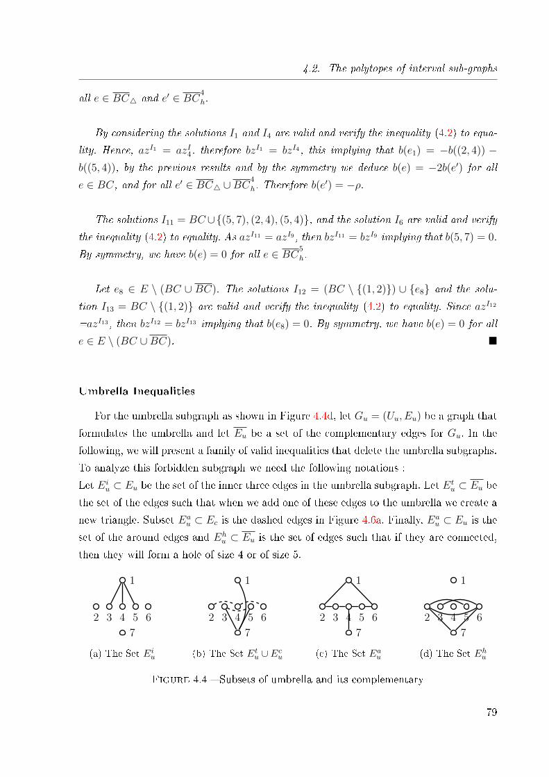
4.2. The polytopes of interval sub-graphs
all e ∈ BC4 and e′ ∈ BC4
h.
By considering the solutions I1 and I4 are valid and verify the inequality (4.2) to equa-
lity. Hence, azI1 = azI4, therefore bzI1 = bzI4, this implying that b(e1) = −b((2, 4)) −
b((5, 4)), by the previous results and by the symmetry we deduce b(e) = −2b(e′) for all
e ∈ BC, and for all e′ ∈ BC4 ∪BC4
h. Therefore b(e′) = −ρ.
The solutions I11 = BC ∪{(5, 7), (2, 4), (5, 4)}, and the solution I6 are valid and verify
the inequality (4.2) to equality. As azI11 = azI9, then bzI11 = bzI9 implying that b(5, 7) = 0.
By symmetry, we have b(e) = 0 for all e ∈ BC5
h.
Let e8 ∈ E \ (BC ∪ BC). The solutions I12 = (BC \ {(1, 2)}) ∪ {e8} and the solu-
tion I13 = BC \ {(1, 2)} are valid and verify the inequality (4.2) to equality. Since azI12
=azI13, then bzI12 = bzI13 implying that b(e8) = 0. By symmetry, we have b(e) = 0 for all
e ∈ E \ (BC ∪BC). �
Umbrella Inequalities
For the umbrella subgraph as shown in Figure 4.4d, let Gu = (Uu, Eu) be a graph that
formulates the umbrella and let Eu be a set of the complementary edges for Gu. In the
following, we will present a family of valid inequalities that delete the umbrella subgraphs.
To analyze this forbidden subgraph we need the following notations :
Let Eiu ⊂ Eu be the set of the inner three edges in the umbrella subgraph. Let Et
u ⊂ Eu be
the set of the edges such that when we add one of these edges to the umbrella we create a
new triangle. Subset Eau ⊂ Ec is the dashed edges in Figure 4.6a. Finally, Ea
u ⊂ Eu is the
set of the around edges and Ehu ⊂ Eu is the set of edges such that if they are connected,
then they will form a hole of size 4 or of size 5.
2
1
3 4 5 6
7
(a) The Set Eiu
2
1
3 4 5 6
7
(b) The Set Etu ∪ Ec
u
2
1
3 4 5 6
7
(c) The Set Eau
2
1
3 4 5 6
7
(d) The Set Ehu
Figure 4.4 � Subsets of umbrella and its complementary
79
Chapitre 4. Polyedral study on interval graphs under m-clique free constraints
� Eiu = { (1, 3), (1, 4), (1, 5) }.
� Etu = { (1, 7), (3, 7), (5, 7) }.
� Ecu = {(2, 4), (3, 5), (4, 6)}.
� Eau = {(1, 2), (2, 3), (3, 4), (4, 5), (5, 6), (1, 6), (4, 7) }.
� Ehu = { (2, 7), (6, 7), (2, 5), (2, 6), (3, 6) }.
Remark that the graph induced by Hu = {Eiu ∪ Et
u ∪ Ecu ∪ Ea
u ∪ Ehu} is a complete
graph.
When m = 2, the triangle becomes a forbidden subgraph (and then it is not possible to
�nd an umbrella). For this forbidden subgraph we focus on instance where m ≥ 3.
When m = 3, in order to keep all edges of Eu it is necessary to add at least one edge of
Etu. Moreover, when we add an edge from Ec
u in this case the subgraph contains a clique
of size 4. If we add an edge from Ehu , then the induced subgraph will contain a hole.
Thus, the valid inequalities when m = 3 will be :∑e∈Eau\{(4,7)}
ze + z(2,6) + z(2,5) + z(3,6) ≤ 5. (4.3)
Proposition 9 Inequality (4.3) de�nes a facet if m = 3.
proof 4.5 Let us denote by az ≤ α the inequality (4.3) associated with e. Let bz ≤ β be
a facet de�ning an equality (4.3) such that {z ∈ PI(G,m) : az = α} ⊆ {z ∈ PI(G,m) :
bz = β}. We show that b = ρa for some ρ ∈ R.
Let e1, e2 ∈ Eau \ {(4, 7)}. The solutions I1 = Eu \ {e1} and I2 = Eu \ {e2} are valid
and the incidence vectors zI1 and zI2 verify the inequality (4.3) to equality. Moreover, we
have azI1=azI2. Hence, bzI1=bzI2. This implies that b(e1) = b(e2). We set b(e1) = ρ. As
e1 and e2 are arbitrary in Eau \ {(4, 7)}, thus by symmetry, we have b(e′) = b(e) = ρ for
all e ∈ Eau \ {(4, 7)}.
The solution I3 = Eau \ {(4, 7), (1, 6)} and I4 = (I3 ∪ {(2, 5)}) \ {(4, 5)} are valid and
the incidence vectors zI3 and zI4 verify the inequality (4.3) to equality. Moreover, we have
azI3=azI4. Hence, bzI3=bzI4. This implies that b((4, 5)) = b((2, 5)). Thus, from the pre-
vious results we deduce that b((2, 5)) = b(e) for all e ∈ Eau \ {(4, 7)}.
The solutions I3 and I5 = (I3 ∪ {(2, 6)}) \ {(5, 6)} are valid, such that the incidence
vectors zI5 and zI3 verify the inequality (4.3) to equality. Moreover, we have azI5=azI3.
80
4.2. The polytopes of interval sub-graphs
Hence, bzI5=bzI6. This implies that b((2, 6)) = b((5, 6)). Indeed, from the previous results
we have b((2, 6)) = b(e) for all e ∈ Eau \ {(4, 7)}.
The solution I3 and I6 = (I3 ∪ {(3, 6)}) \ {(5, 6)} are valid and the incidence vectors
zI3 and zI6 verify the inequality (4.3) to equality. Moreover, we have azI3=azI6. Hence,
bzI3=bzI6. This implies that b((3, 6)) = b((5, 6)). Indeed, from the previous results we can
deduce that b((3, 6)) = b(e) for all e ∈ Eau \ {(4, 7)}.
The solutions I7 = Eau \ {(4, 7)∪ (1, 6)} and I8 = (I7 ∪ {(4, 7)} ∪Ei
u) are valid and the
incidence vectors zI7, and zI8 verify the inequality (4.3) to equality. Moreover, we have
azI7=azI8. Hence bzI7=bzI8. This implies that b(e) = 0 ∀e ∈ Eiu.
Let e ∈ {(2, 7), (3, 7), (1, 7), (5, 7), (6, 7)}. The solutions I1 and I9 = I1 ∪ {e} are validand the incidence vectors zI1, zI9 verify the inequality (4.3) to equality. Moreover, we
have azI1 = azI9. Hence, bzI1 = bzI9. This implies that b((2, 7)) = b((3, 7)) = b((1, 7)) =
b((5, 7)) = b((6, 7)) = 0. �
When m ≥ 4, to �nd a valid solution we can add also the edges from Ecu. Then, the
valid inequalities when m ≥ 4 will be :∑e∈Eau
ze −∑
e∈Etu∪Ecu
ze ≤ 6. (4.4)
Proposition 10 Inequality (4.4) de�nes a facet if m ≥ 4.
proof 4.6 Let us denote by az ≤ α inequality (4.4) associated with e. Let bz ≤ β be a facet
de�ning an equality (4.4) such that {z ∈ PI(G,m) : az = α} ⊆ {z ∈ PI(G,m) : bz = β}.We show that b = ρa for some ρ ∈ R.
Let e1, e2 ∈ Etu ∪ Ec
u be two edges, where e1 6= e2. We consider the edge sets I1 =
Eu ∪ {e1} and I2 = Eu ∪ {e2} where the incidence vectors zI1 and zI2 are solutions of
PI(G,m) and satisfy the inequality (4.4) to equality. Moreover, we have azI1=azI2. Thus,
bzI1=bzI2. This implies that b(e1) = b(e2). As e1, e2 are arbitrary, then b(e) = b(e′) for all
e, e′ ∈ Etu ∪ Ec
u.
81
Chapitre 4. Polyedral study on interval graphs under m-clique free constraints
Let e3 ∈ Eau. The solution I3 = Eu\{e3} is valid and the incidence vectors zI3 verify the
inequality (4.4) to equality. Moreover, we have azI1=azI3. Hence, bzI1=bzI3. This implies
that b(e3) = −b(e1). Thus, by symmetry we have b(e′) = −b(e) for all e ∈ Etu∪Ec
u, e′ ∈ Ea
u .
The solutions I4 = Eu \ {(1, 6)}, I5 = (Eu \ {(1, 6)}) ∪ Eiu, I6 = I5 \ {(1, 5)},
I7 = I6 \ {(1, 4)} and I8 = I7 \ {(1, 3)} are valid. The incidence vectors zI4, zI5, zI6,
zI7 and zI8 verify the inequality (4.3) to the equality. Since azI4=azI5=azI6=azI7=azI8,
therefore bzI4=bzI5=bzI6=bzI7=bzI8, implying that b(e) = 0 ∀e ∈ Eiu.
The solutions I9 = Eu ∪ {(2, 7), (2, 4)}, I10 = Eu ∪ {(2, 5), (2, 4)}, I11 = Eu ∪ {(2, 4)},I12 = Eu \ {(2, 3)}, I13 = I12 ∪ {(2, 6)}, I14 = I12 ∪ {(2, 5)}, I15 = Eu \ {(5, 6)} and I16 =
I15 ∪ {(3, 6)} are valid and verify the inequality (4.4) to the equality. Since azI9=azI10=
azI11=azI12=azI13=azI14=azI15 =azI16, therefore bzI9=bzI10= bzI11= bzI12 =bzI13=bzI14=
bzI15 = bzI16, implying that b((2, 6)) = b((2, 5)) = b((2, 7)) = b((6, 7)) = b((3, 6)) = 0.
Let e ∈ E \ (Eu ∪ Eu). The solutions I17 = Eu \ {(4, 7)} and I18 = I17 ∪ {e} are validand verify the inequality (4.4) to the equality. Since azI17=azI18, therefore bzI17=bzI18. By
symmetry, we have b(e) = 0.
We set b(e) = ρ for e ∈ Eu and the proof is ended. �
n-net Inequalities
The n− net forbidden subgraph is shown in Figure 4.2c. We will give some notations
to help in analyzing the n− net forbidden subgraph.
Let Gnet = (Unet, Enet) be the graph that forms a net of size n (i.e., n − net) and Enetbe a set of complementary edges of Gnet. To avoid to have a subgraph that represents an
n−net, where n ≥ 2 we need either to eliminate an edge from the n−net without havinga hole denoted by Eh
net, or to add an edge that does not construct a hole denoted by Ehnet.
To analyze this forbidden subgraph we will use the following notations. From Figure 4.2c
let us consider :
- Ehnet = {(a, c), (a, d)}∪{(c, 3), (c, 4), ..., (c, n)}∪{(d, 1), (d, 2), ..., (d, n−2)}∪{(c, d)}.
- Ehnet = {(b, 2), ..., (b, n− 1)}.
82
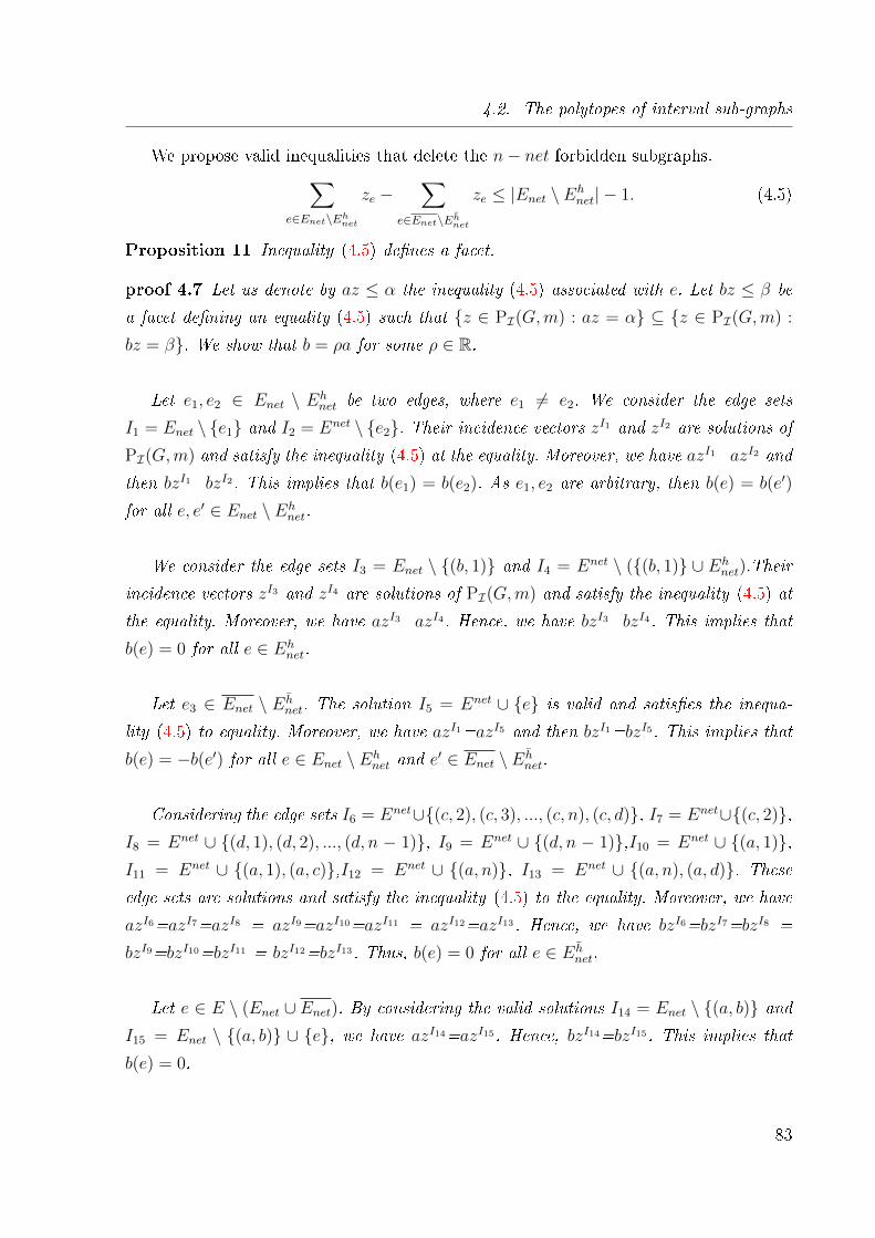
4.2. The polytopes of interval sub-graphs
We propose valid inequalities that delete the n− net forbidden subgraphs.∑e∈Enet\Ehnet
ze −∑
e∈Enet\Ehnet
ze ≤ |Enet \ Ehnet| − 1. (4.5)
Proposition 11 Inequality (4.5) de�nes a facet.
proof 4.7 Let us denote by az ≤ α the inequality (4.5) associated with e. Let bz ≤ β be
a facet de�ning an equality (4.5) such that {z ∈ PI(G,m) : az = α} ⊆ {z ∈ PI(G,m) :
bz = β}. We show that b = ρa for some ρ ∈ R.
Let e1, e2 ∈ Enet \ Ehnet be two edges, where e1 6= e2. We consider the edge sets
I1 = Enet \ {e1} and I2 = Enet \ {e2}. Their incidence vectors zI1 and zI2 are solutions of
PI(G,m) and satisfy the inequality (4.5) at the equality. Moreover, we have azI1=azI2 and
then bzI1=bzI2. This implies that b(e1) = b(e2). As e1, e2 are arbitrary, then b(e) = b(e′)
for all e, e′ ∈ Enet \ Ehnet.
We consider the edge sets I3 = Enet \ {(b, 1)} and I4 = Enet \ ({(b, 1)} ∪ Ehnet).Their
incidence vectors zI3 and zI4 are solutions of PI(G,m) and satisfy the inequality (4.5) at
the equality. Moreover, we have azI3=azI4. Hence, we have bzI3=bzI4. This implies that
b(e) = 0 for all e ∈ Ehnet.
Let e3 ∈ Enet \ Ehnet. The solution I5 = Enet ∪ {e} is valid and satis�es the inequa-
lity (4.5) to equality. Moreover, we have azI1=azI5 and then bzI1=bzI5. This implies that
b(e) = −b(e′) for all e ∈ Enet \ Ehnet and e
′ ∈ Enet \ Ehnet.
Considering the edge sets I6 = Enet∪{(c, 2), (c, 3), ..., (c, n), (c, d)}, I7 = Enet∪{(c, 2)},I8 = Enet ∪ {(d, 1), (d, 2), ..., (d, n − 1)}, I9 = Enet ∪ {(d, n − 1)},I10 = Enet ∪ {(a, 1)},I11 = Enet ∪ {(a, 1), (a, c)},I12 = Enet ∪ {(a, n)}, I13 = Enet ∪ {(a, n), (a, d)}. Theseedge sets are solutions and satisfy the inequality (4.5) to the equality. Moreover, we have
azI6=azI7=azI8 = azI9=azI10=azI11 = azI12=azI13. Hence, we have bzI6=bzI7=bzI8 =
bzI9=bzI10=bzI11 = bzI12=bzI13. Thus, b(e) = 0 for all e ∈ Ehnet.
Let e ∈ E \ (Enet ∪ Enet). By considering the valid solutions I14 = Enet \ {(a, b)} andI15 = Enet \ {(a, b)} ∪ {e}, we have azI14=azI15. Hence, bzI14=bzI15. This implies that
b(e) = 0.
83
Chapitre 4. Polyedral study on interval graphs under m-clique free constraints
We set b(e) = ρ for e ∈ Enet \ Ehnet and the proof is completed. �
n-tent Inequalities
Figure 4.2d shows the n − tent forbidden subgraph, the graph is non-interval if it
contains an n − tent forbidden subgraph Gtent. The induced subgraph Gtent to be valid
we need to add or remove one or more edges considering to not have a hole when we add
or remove any edge.
Let the graph Gtent = (Utent, Etent) be a graph that formulate n− tent for all n ≥ 3, and
Etent be the set of complementary edges.
From Figure 4.2c
- Ehtent = {(b, c), (c, 4), (b, 2)},
- Ehtent = {(1, 4), (2, 5), ..., (n, n+ 3)}.
Remark that, all n-tent where n ≥ 5 contain a clique of size 5 then the clique inequality
cut these n-tent sub graph if m ≤ 4. It is the same idea for all n-tent where n = 4 (resp.
n = 3) then the clique inequality cut these n-tent sub graph if m = 3(resp. m = 2).
In the following we will propose valid inequalities that delete the n-tent forbidden
subgraphs. ∑e∈Etent\Ehtent
ze −∑
e∈Etent\Ehtent
ze ≤ |Etent \ Ehtent| − 1. (4.6)
Proposition 12 Inequality (4.6) de�nes a facet, when m ≥ 5 or (n = 4 and m = 3) or
(n = 3 and m = 2).
proof 4.8 Let us denote by az ≤ α the inequality (4.6) associated with e. Let bz ≤ β be
a facet de�ning an equality (4.6) such that {z ∈ PI(G,m) : az = α} ⊆ {z ∈ PI(G,m) :
bz = β}. We show that b = ρa for some ρ ∈ R.
Let e1, e2 ∈ Etent \ Ehtent be two edges, where e1 6= e2. We consider the edge sets
I1 = Etent \ {e1} and I2 = Etent \ {e2}. Their incidence vectors zI1 and zI2 are solutions
of PI(G,m) and satisfy the inequality (4.6) to equality. Moreover, we have azI1=azI2 and
then bzI1=bzI2. This implies that b(e1) = b(e2). As e1, e2 are arbitrary, then b(e) = b(e′)
for all e, e′ ∈ Etent \ Ehtent.
84
4.2. The polytopes of interval sub-graphs
We consider the edge sets I3 = Etent\{(a, c)}, and I4 = Etent\({(a, c)}∪{(b, c)}) thereincidence vectors zI3, and zI4 are solutions of PI(G,m) and satisfy the inequality (4.6)
to equality. Moreover, we have azI3=azI4 and then bzI3=bzI4. This implies by symmetry
that b((b, c)) = b((b, 2)) = b((c, 4)) = 0.
Let e3 ∈ Etent \ Ehtent. The solution I5 = Etent ∪ {e} is valid and satis�es the inequa-
lity (4.6) to equality. Moreover, we have azI1=azI5. Hence, bzI1=bzI5. This implies that
b(e) = −b(e′) for all e ∈ Etent \ Ehtent and e
′ ∈ Etent \ Ehtent.
Let (i, i + 3) ∈ Ehtent. The solutions I6 = Etent ∪ {(i, i + 3), (i, i + 2)} and I7 =
Etent∪{(i, i+ 2)} are valid and satisfy the inequality (4.6) to equality. Moreover, we have
azI6=azI7 and then bzI6=bzI7. Thus, b(e) = 0 for all e ∈ Ehtent.
Let e ∈ E \ (Etent ∪Etent). By considering the valid solutions I8 = Etent \ {(a, c)} andI9 = Etent\{(a, c)}∪{e}, we have azI8=azI9 and then bzI8=bzI9. This implies that b(e) = 0.
We set b(e) = ρ for e ∈ Etent \ Ehtent and the proof is completed. �
Hole inequalities
Here, it is convenient to de�ne a hole as an induced subgraph of G isomorphic to Ck for
some k ≥ 4, [19]. The hole C is a forbidden subgraph as depicted in Figure 4.2e. Let C de-
note the set of edges that construct the hole, i.e., C = { (u1, u2),(u2, u3),...,(u|C|−1, u|C|),(u|C|, u1)
}. If (i + k) > |C|, then ui+k = ui′ , i′ = (i + k) − |C|. Let C denote the set of all chords
of hole C.
Suppose we have a hole of size 4 this graph is non-interval graph. The induced subgraph
by a hole is valid only if we add to it at least one chord.
Proposition 13 For a hole C, the minimum number of necessary chords that should be
added to the hole to be an interval graph is |C| − 3, when |C| ≥ 4.
proof 4.9 We prove this proposition by induction. When |C| = 4, then we need one chord
kc = 1, and then the proposition is true.
Let assume that the property is true until |C| = l and kc = l−3. We need to prove it for a
cycle C ′ where |C ′| = |C|+1 and that kc′ = |C ′|−3. Let consider C = {u1, u2, u3, ..., u|C|}be the hole graph given by C where we add kc edges in order to make it hole free and
85
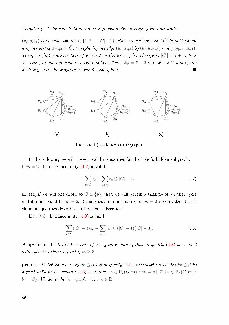
Chapitre 4. Polyedral study on interval graphs under m-clique free constraints
(ui, ui+1) is an edge, where i ∈ {1, 2, ..., |C|−1}. Now, we will construct C ′ from C by ad-
ding the vertex u|C|+1 in C, by replacing the edge (ui, ui+1) by (ui, u|C|+1) and (u|C|+1, ui+1).
Then, we �nd a unique hole of a size 4 in the new cycle. Therefore, |C ′| = l + 1. It is
necessary to add one edge to break this hole. Thus, kc′ = l′ − 3 is true. As C and kc are
arbitrary, then the property is true for every hole. �
u1u2
u3
u4
u5u6
unun−2un−1
(a)
u1u2
u3
u4
u5u6
unun−2un−1
(b)
u1u2
u3
u4
u5u6
unun−2un−1
(c)
Figure 4.5 � Hole free subgraphs
In the following we will present valid inequalities for the hole forbidden subgraph.
If m = 2, then the inequality (4.7) is valid.∑e∈C
ze +∑e∈C
ze ≤ |C| − 1. (4.7)
Indeed, if we add one chord to C ⊂ {e}, then we will obtain a triangle or another cycle
and it is not valid for m = 2. Remark that this inequality for m = 2 is equivalent to the
clique inequalities described in the next subsection.
If m ≥ 3, then inequality (4.8) is valid.∑e∈C
(|C| − 3)ze −∑e∈C
ze ≤ (|C| − 1)(|C| − 3). (4.8)
Proposition 14 Let C be a hole of size greater than 3, then inequality (4.8) associated
with cycle C de�nes a facet if m ≥ 3.
proof 4.10 Let us denote by az ≤ α the inequality (4.8) associated with e. Let bz ≤ β be
a facet de�ning an equality (4.8) such that {z ∈ PI(G,m) : az = α} ⊆ {z ∈ PI(G,m) :
bz = β}. We show that b = ρa for some e ∈ R.
86
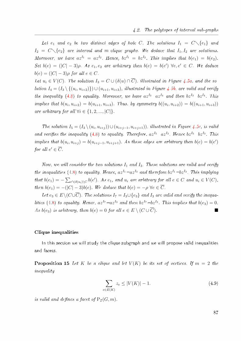
4.2. The polytopes of interval sub-graphs
Let e1 and e2 be two distinct edges of hole C. The solutions I1 = C�{e1} and
I2 = C�{e2} are interval and m-clique graphs. We deduce that I1, I2 are solutions.
Moreover, we have azI1 = azI2. Hence, bzI1 = bzI2. This implies that b(e1) = b(e2).
Set b(e) = (|C| − 3)ρ. As e1, e2 are arbitrary then b(e) = b(e′) ∀e, e′ ∈ C. We deduce
b(e) = (|C| − 3)ρ for all e ∈ C.Let ui ∈ V (C). The solution I3 = C ∪ (δ(u) ∩ C), illustrated in Figure 4.5a, and the so-
lution I4 = (I3 \ {(ui, ui+2)})∪ (ui+1, ui+3), illustrated in Figure 4.5b, are valid and verify
the inequality (4.8) to equality. Moreover, we have azI3=azI4 and then bzI3=bzI4. This
implies that b(ui, ui+2) = b(ui+1, ui+3). Thus, by symmetry b((ui, ui+2)) = b((ui+1, ui+3))
are arbitrary for all ∀i ∈ {1, 2, ..., |C|}.
The solution I5 = (I3 \ (ui, ui+j))∪ (ui+j−1, ui+j+1)), illustrated in Figure 4.5c, is valid
and veri�es the inequality (4.8) to equality. Therefore, azI5=azI3. Hence bzI5=bzI3. This
implies that b(ui, ui+j) = b(ui+j−1, ui+j+1). As these edges are arbitrary then b(e) = b(e′)
for all e′ ∈ C.
Now, we will consider the two solutions I1 and I3. These solutions are valid and verify
the inequalities (4.8) to equality. Hence, azI1=azI3 and therefore bzI1=bzI3. This implying
that b(e1) = −∑
e′∈δ(ui)\C b(e′). As e1, and ui are arbitrary for all e ∈ C and ui ∈ V (C),
then b(e1) = −(|C| − 3)b(e). We deduce that b(e) = −ρ ∀e ∈ C.Let e3 ∈ E\(C∪C). The solutions I7 = I3∪{e3} and I3 are valid and verify the inequa-
lities (4.8) to equality. Hence, azI7=azI3 and then bzI7=bzI3. This implies that b(e3) = 0.
As b(e3) is arbitrary, then b(e) = 0 for all e ∈ E \ (C ∪ C). �
Clique inequalities
In this section we will study the clique subgraph and we will propose valid inequalities
and facets.
Proposition 15 Let K be a clique and let V (K) be its set of vertices. If m = 2 the
inequality ∑e∈E(K)
ze ≤ |V (K)| − 1. (4.9)
is valid and de�nes a facet of PI(G,m).
87

Chapitre 4. Polyedral study on interval graphs under m-clique free constraints
proof 4.11 Remark that if m = 2, then a solution can be given only by a forest in the
subgraph G(K). We deduce that the maximum number of edges in this subgraph is equal
to |V (K)| − 1.
Let us denote by az ≤ α the inequality (4.9) associated with e. Let bz ≤ β be a facet
de�ning an equality (4.9) such that {z ∈ PI(G,m) : az = α} ⊆ {z ∈ PI(G,m) : bz = β}.We show that b = ρa for some ρ ∈ R.
Let (u, v), (u,w) ∈ E(K), be two connected edges. Considering a line Tuv beginning by
(u, v) and �nishing by the vertex w and the line Tuw = Tuv \ {(u, v)} ∪ {(u,w)}. Thesetwo solutions are valid and satisfy the inequality (4.9) to equality. Moreover, we have
azTuv=azTuw . Hence, bzTuv=bzTuw . This implies that b((u, v)) = b((u,w)). By symmetry,
we deduce then that b(e) = b(e′) for all e, e′ ∈ E(K).
Let e ∈ E \ E(K). By considering the valid solution T ′uv = Tuv ∪ {e}, we have
azTuv=azT′uv . Hence, bzTuv=bzT
′uv . This implies that b(e) = 0. �
Proposition 16 Let K be a clique of size m+ 1. The inequality∑e∈E(K)
ze ≤ |E(K)| − 1 (4.10)
de�nes a facet of PI(G,m).
proof 4.12 Let us denote by az ≤ α the inequality (4.10) associated with e. Let bz ≤ β be
a facet de�ning an equality (4.10) such that {z ∈ PI(G,m) : az = α} ⊆ {z ∈ PI(G,m) :
bz = β}. We show that b = ρa for some ρ ∈ R.Let e, e′ be two edges in E(K). The solution I1 = E(K)\{e} and I2 = E(K)\{e′} are
valid and verify the inequality (4.10) to equality. Hence, azI1=azI2. Therefore, bzI1=bzI2.
This implies that b(e) = b(e′). We set b(e) = ρ. As b(e) and b(e′) are arbitrary, then
b(e) = b(e′) for all e, e′ ∈ E(K).
Let e1 be an edge in E \E(K). The solution I3 = I1 ∪{e1} and I1 are valid and verify
the inequality (4.10) to equality. Hence, azI1=azI3. Therefore bzI1=bzI3. This implies that
b(e1) = 0. As b(e1) is arbitrary we deduce that b(e) = 0, ∀e ∈ E \ E(K). �
Let f(K,m) be a function giving the minimum number of edges necessary to be
removed from E(K) such that the resulting graph G′(K) ism-clique free. Let α = d |V (K)|me,
nα−1 = mα− |V (K)| and nα = |V (K)|−(nα−1)(α−1)α
88
4.2. The polytopes of interval sub-graphs
Proposition 17 f(K,m) = nα−1(α−1)(α−2)
2+ nα
(α)(α−1)2
proof 4.13 Let E ′ be a set of f(K,m) edges such that E(K)\E ′ is m-clique free. Remark
that in the complementary graph G(K) we have a stable set of size |K|. If we add E ′, thenthere does not exist a stable of size m+ 1 (m-stable free). Let consider a minimum set of
edges E ′′ ∈ E(K) such that |E ′′| < |E ′| and G(K)\E ′′ is m-clique free and thus G(K)∪E ′′
is m-stable free. Clearly E ′′ is a set of m disjoint cliques K = {K1, ..., Km}, otherwise E ′′
is not minimal or contain a stable set of size m + 1. To have the minimum set of edges,
it is important to balance the size of cliques. Indeed, if we have two cliques Ki and Kj
where |Ki| ≥ |Kj|+ 2, then for u ∈ Ki we obtain the following result |E(Ki)|+ |E(Kj)| >|E(Ki\{u})|+ |E(Kj∪{u})|. We deduce that the maximum di�erence between two cliques
of K is less or equal to 1. �
Proposition 18 Let K be a clique. The inequality∑e∈E(K)
ze ≤ |E(K)| − f(K,m) (4.11)
is valid.
proof 4.14 By de�nition f(K,m) is the minimum number of edges necessary to be remo-
ved from E(K) such that the resulting graph G′(K) is m-clique free. Thus, the inequality
(4.11) is valid. �
In the next subsection, we will improve this family of inequalities.
Clique-Hole inequalities
Remark that if we remove m disjoint cliques in G(K), then we obtain a complete
bipartite subgraph between all pairs of two cliques. Let Hij = (Ki, Kj, Eij) be a complete
bipartite graph. Remark that H contains a hole if |Ki| ≥ 2 and |Kj| ≥ 2. To remove every
hole inHij, the minimum number of edges E ′ necessary to be removed to obtain a hole free
graph is equal to max(|Ki|, |Kj|)−1, otherwise we can always take 2 nodes inKi orKj such
that these two nodes are not covered by E ′. Note that E ′, with size max(|Ki|, |Kj|)− 1,
covers the maximum nodes of Ki and Kj. We can strength the inequality (4.11) by the
following inequality. Let β =∑
i∈m(max{|Ki| − 1, 0})−maxi∈m |Ki| − 1.
Proposition 19 Let K be a clique. The inequality∑e∈E(K)
ze ≤ |E(K)| − (f(K,m) + β) (4.12)
is valid and de�nes a facet.
89
Chapitre 4. Polyedral study on interval graphs under m-clique free constraints
proof 4.15 Remark that if we unbalance two cliques Ki and Kj to reduce the value
max(|Ki|, |Kj|) − 1 of 1, then the number of edges necessary to be removed increases
by max(|Ki|, |Kj|) −min(|Ki|, |Kj|). Let us denote by az ≤ α the inequality (4.12) asso-
ciated with e. Let bz ≤ β be a facet de�ning an equality (4.12) such that {z ∈ PI(G,m) :
az = α} ⊆ {z ∈ PI(G,m) : bz = β}. We show that b = ρa for some ρ ∈ R.
Let (u, v), (u,w) ∈ E(K) be two connected edges. Let consider a set of stable set where
u is in the stable set i and v, w in the stable set j. We can easily �nd a solution where
(u, v) is an edge and (u,w) is not an edge. These two solutions are valid and satisfy the
inequality (4.12) to equality. This implies by symmetry that b((u, v)) = b((u,w)). We de-
duce then that b(e) = b(e′) for all e, e′ ∈ E(K).
Let e ∈ E \E(K). By considering a valid solution where e is not an edge and a second
solution with the same edges plus e, we can deduce that b(e) = 0. �
4.3 Cutting plane algorithms
Cutting plane method allows us to strengthen the linear relaxation by adding inequa-
lities. Cutting plane algorithms mainly consist in generating constraints by means of a
separation procedure (see, for example, [84], [81],[96], [19] and [67]). Let z∗ be the incidence
vector associated with the value of the variable z in the linear relaxation. The separation
problem consists in �nding if there exists a valid inequality az ≤ b0 that cuts o� the so-
lution z∗,i.e., az ∗ > b0. The separation algorithm associated with a family of inequalities
aE′x ≤ bE
′for all E ′ ∈ E ′ consists in �nding a set E ′ ∈ E ′ such that aE ′z ∗ > bE
′.
The results of the previous sections have allowed us to derive some exact separation
algorithms and some heuristics separation algorithms. Furthermore, at the end of this
section we propose "lazy separation procedure" to ensure that the integer solutions are
interval and m-clique free subgraph. In the next paragraphs, we will describe these sepa-
ration algorithms for all inequalities described in the previous section.
4.3.1 Bipartite claw separation
In this section we describe the BC separation algorithms. We propose three algorithms
to separate the bipartite claw inequalities. One is an exact algorithm and two others are
90
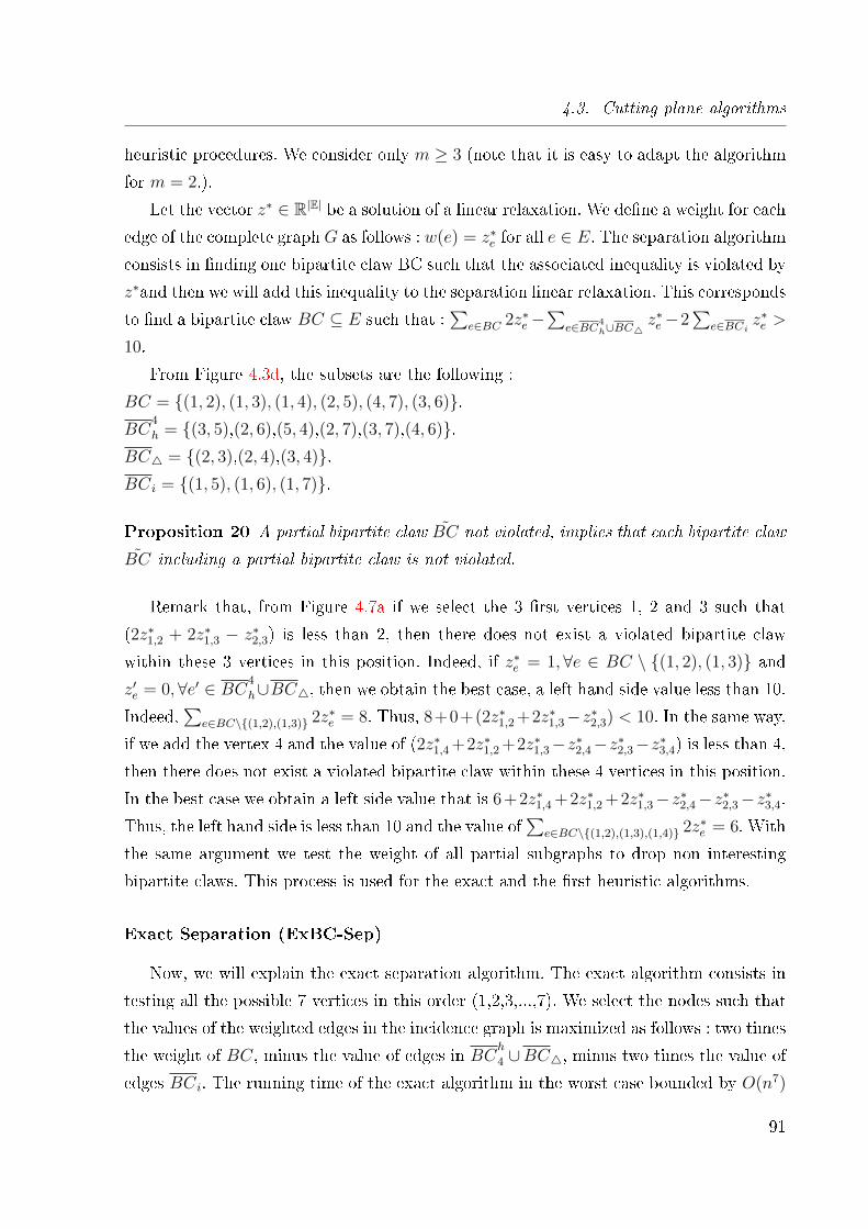
4.3. Cutting plane algorithms
heuristic procedures. We consider only m ≥ 3 (note that it is easy to adapt the algorithm
for m = 2.).
Let the vector z∗ ∈ R|E| be a solution of a linear relaxation. We de�ne a weight for each
edge of the complete graph G as follows : w(e) = z∗e for all e ∈ E. The separation algorithmconsists in �nding one bipartite claw BC such that the associated inequality is violated by
z∗and then we will add this inequality to the separation linear relaxation. This corresponds
to �nd a bipartite claw BC ⊆ E such that :∑
e∈BC 2z∗e−∑
e∈BC4h∪BC4
z∗e−2∑
e∈BCi z∗e >
10.
From Figure 4.3d, the subsets are the following :
BC = {(1, 2), (1, 3), (1, 4), (2, 5), (4, 7), (3, 6)}.BC
4
h = {(3, 5),(2, 6),(5, 4),(2, 7),(3, 7),(4, 6)}.BC4 = {(2, 3),(2, 4),(3, 4)}.BCi = {(1, 5), (1, 6), (1, 7)}.
Proposition 20 A partial bipartite claw BC not violated, implies that each bipartite claw
BC including a partial bipartite claw is not violated.
Remark that, from Figure 4.7a if we select the 3 �rst vertices 1, 2 and 3 such that
(2z∗1,2 + 2z∗1,3 − z∗2,3) is less than 2, then there does not exist a violated bipartite claw
within these 3 vertices in this position. Indeed, if z∗e = 1,∀e ∈ BC \ {(1, 2), (1, 3)} andz′e = 0,∀e′ ∈ BC4
h∪BC4, then we obtain the best case, a left hand side value less than 10.Indeed,
∑e∈BC\{(1,2),(1,3)} 2z∗e = 8. Thus, 8+0+(2z∗1,2 +2z∗1,3−z∗2,3) < 10. In the same way,
if we add the vertex 4 and the value of (2z∗1,4 +2z∗1,2 +2z∗1,3−z∗2,4−z∗2,3−z∗3,4) is less than 4,
then there does not exist a violated bipartite claw within these 4 vertices in this position.
In the best case we obtain a left side value that is 6+2z∗1,4 +2z∗1,2 +2z∗1,3−z∗2,4−z∗2,3−z∗3,4.Thus, the left hand side is less than 10 and the value of
∑e∈BC\{(1,2),(1,3),(1,4)} 2z∗e = 6. With
the same argument we test the weight of all partial subgraphs to drop non interesting
bipartite claws. This process is used for the exact and the �rst heuristic algorithms.
Exact Separation (ExBC-Sep)
Now, we will explain the exact separation algorithm. The exact algorithm consists in
testing all the possible 7 vertices in this order (1,2,3,...,7). We select the nodes such that
the values of the weighted edges in the incidence graph is maximized as follows : two times
the weight of BC, minus the value of edges in BCh
4 ∪BC4, minus two times the value of
edges BCi. The running time of the exact algorithm in the worst case bounded by O(n7)
91
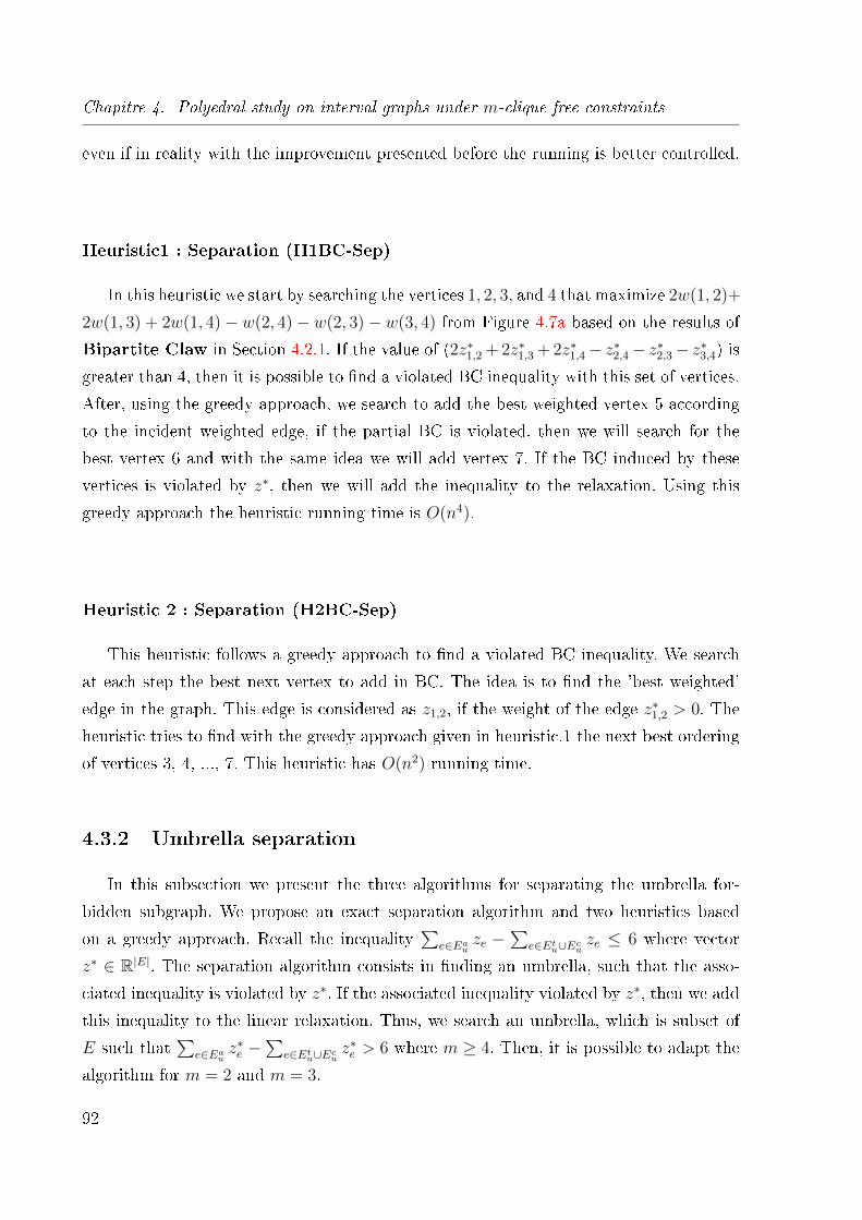
Chapitre 4. Polyedral study on interval graphs under m-clique free constraints
even if in reality with the improvement presented before the running is better controlled.
Heuristic1 : Separation (H1BC-Sep)
In this heuristic we start by searching the vertices 1, 2, 3, and 4 that maximize 2w(1, 2)+
2w(1, 3) + 2w(1, 4)− w(2, 4)− w(2, 3)− w(3, 4) from Figure 4.7a based on the results of
Bipartite Claw in Section 4.2.1. If the value of (2z∗1,2 + 2z∗1,3 + 2z∗1,4− z∗2,4− z∗2,3− z∗3,4) isgreater than 4, then it is possible to �nd a violated BC inequality with this set of vertices.
After, using the greedy approach, we search to add the best weighted vertex 5 according
to the incident weighted edge, if the partial BC is violated, then we will search for the
best vertex 6 and with the same idea we will add vertex 7. If the BC induced by these
vertices is violated by z∗, then we will add the inequality to the relaxation. Using this
greedy approach the heuristic running time is O(n4).
Heuristic 2 : Separation (H2BC-Sep)
This heuristic follows a greedy approach to �nd a violated BC inequality. We search
at each step the best next vertex to add in BC. The idea is to �nd the 'best weighted'
edge in the graph. This edge is considered as z1,2, if the weight of the edge z∗1,2 > 0. The
heuristic tries to �nd with the greedy approach given in heuristic.1 the next best ordering
of vertices 3, 4, ..., 7. This heuristic has O(n2) running time.
4.3.2 Umbrella separation
In this subsection we present the three algorithms for separating the umbrella for-
bidden subgraph. We propose an exact separation algorithm and two heuristics based
on a greedy approach. Recall the inequality∑
e∈Eauze −
∑e∈Etu∪Ecu
ze ≤ 6 where vector
z∗ ∈ R|E|. The separation algorithm consists in �nding an umbrella, such that the asso-
ciated inequality is violated by z∗. If the associated inequality violated by z∗, then we add
this inequality to the linear relaxation. Thus, we search an umbrella, which is subset of
E such that∑
e∈Eauz∗e −
∑e∈Etu∪Ecu
z∗e > 6 where m ≥ 4. Then, it is possible to adapt the
algorithm for m = 2 and m = 3.
92
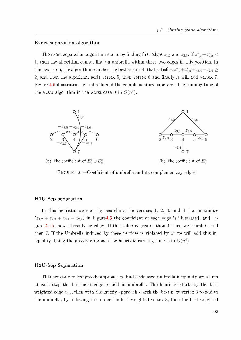
4.3. Cutting plane algorithms
Exact separation algorithm
The exact separation algorithm starts by �nding �rst edges z1,2 and z2,3. If z∗1,2 +z∗2,3 <
1, then the algorithm cannot �nd an umbrella within these two edges in this position. In
the next step, the algorithm searches the best vertex 4, that satis�es z∗1,2+z∗2,3+z3,4−z2,4 ≥
2, and then the algorithm adds vertex 5, then vertex 6 and �nally it will add vertex 7.
Figure 4.6 illustrates the umbrella and the complementary subgraps. The running time of
the exact algorithm in the worst case is in O(n7).
2
1
3 4 5 6
7
−z1,7
−z3,7 −z5,7
−z3,5−z2,4−z4,6
(a) The coe�cient of Etu ∪ Ec
u
2
1
3 4 5 6
7
z1,2
z2,3
z3,4 z4,5
z5,6
z1,6
z7,4
(b) The coe�cient of Eau
Figure 4.6 � Coe�cient of umbrella and its complementary edges
H1U-Sep separation
In this heuristic we start by searching the vertices 1, 2, 3, and 4 that maximize
(z1,2 + z2,3 + z3,4 − z2,4) in Figure4.6 the coe�cient of each edge is illustrated, and Fi-
gure 4.7b shows these basic edges. If this value is greater than 4, then we search 6, and
then 7. If the Umbrella induced by these vertices is violated by z∗ we will add this in-
equality. Using the greedy approach the heuristic running time is in O(n4).
H2U-Sep Separation
This heuristic follow greedy approach to �nd a violated umbrella inequality we search
at each step the best next edge to add in umbrella. The heuristic starts by the best
weighted edge z1,2, then with the greedy approach search the best next vertex 3 to add to
the umbrella, by following this order the best weighted vertex 3, then the best weighted
93
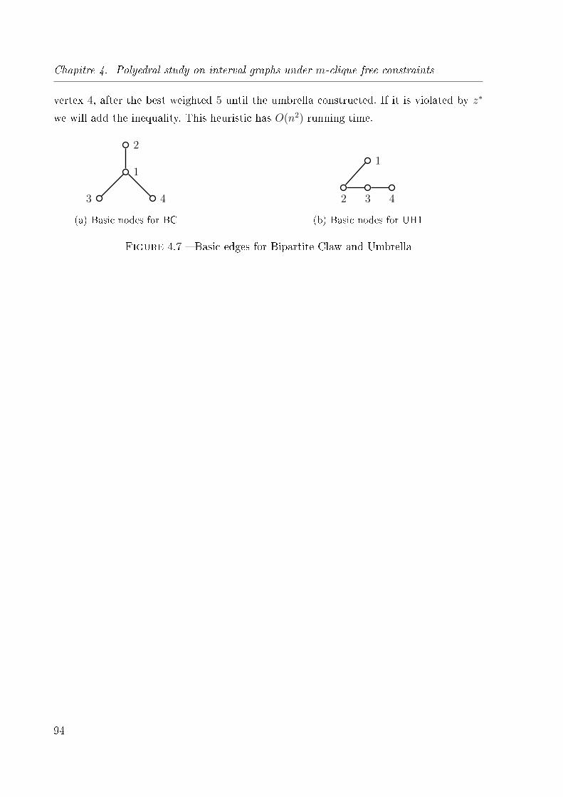
Chapitre 4. Polyedral study on interval graphs under m-clique free constraints
vertex 4, after the best weighted 5 until the umbrella constructed. If it is violated by z∗
we will add the inequality. This heuristic has O(n2) running time.
2
1
3 4
(a) Basic nodes for BC
1
2 3 4
(b) Basic nodes for UH1
Figure 4.7 � Basic edges for Bipartite Claw and Umbrella
94
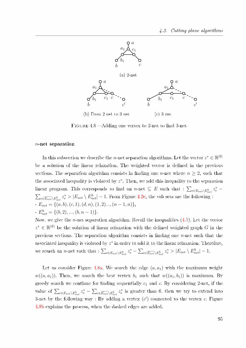
4.3. Cutting plane algorithms
a1
a
b1
c1
b c
(a) 2-net
a1
a
b1c1
b
c
c′
(b) From 2-net to 3-net
a1
a
b1c1
b
c
c′
(c) 3-net
Figure 4.8 � Adding one vertex to 2-net to �nd 3-net
n-net separation
In this subsection we describe the n-net separation algorithms. Let the vector z∗ ∈ R|E|
be a solution of the linear relaxation. The weighted vector is de�ned in the previous
sections. The separation algorithm consists in �nding one n-net where n ≥ 2, such that
the associated inequality is violated by z∗. Then, we add this inequality to the separation
linear program. This corresponds to �nd an n-net ⊆ E such that :∑
e∈Enet\Ehnetz∗e −∑
e∈Enet\Ehnetz∗e > |Enet \ Eh
net| − 1. From Figure 4.2c, the sub sets are the following :
- Enet = {(a, b), (c, 1), (d, n), (1, 2)..., (n− 1, n)},- Eh
net = {(b, 2), ..., (b, n− 1)}.Now, we give the n-net separation algorithm. Recall the inequalities (4.5). Let the vector
z∗ ∈ R|E| be the solution of linear relaxation with the de�ned weighted graph G in the
previous sections. The separation algorithm consists in �nding one n-net such that the
associated inequality is violated by z∗ in order to add it to the linear relaxation. Therefore,
we search an n-net such that :∑
e∈Enet\Ehnetz∗e −
∑e∈Enet\Ehnet
z∗e > |Enet \ Ehnet| − 1.
Let us consider Figure 4.8a. We search the edge (a, a1) with the maximum weight
w((a, a1)). Then, we search the best vertex b1 such that w((a1, b1)) is maximum. By
greedy search we continue for �nding sequentially c1 and c. By considering 2-net, if the
value of∑
e∈Enet\Ehnetz∗e −
∑e∈Enet\Ehnet
z∗e is greater than 6, then we try to extend into
3-net by the following way : By adding a vertex (c′) connected to the vertex c. Figure
4.8b explains the process, when the dashed edges are added.
95
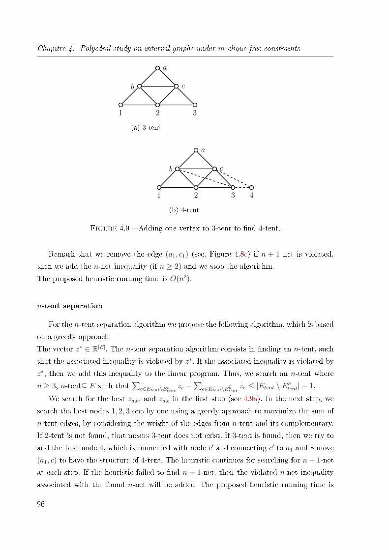
Chapitre 4. Polyedral study on interval graphs under m-clique free constraints
a
b c
1 2 3
(a) 3-tent
a
b c
1 2 3 4
(b) 4-tent
Figure 4.9 � Adding one vertex to 3-tent to �nd 4-tent.
Remark that we remove the edge (a1, c1) (see. Figure 4.8c) if n + 1 net is violated,
then we add the n-net inequality (if n ≥ 2) and we stop the algorithm.
The proposed heuristic running time is O(n2).
n-tent separation
For the n-tent separation algorithm we propose the following algorithm, which is based
on a greedy approach.
The vector z∗ ∈ R|E|. The n-tent separation algorithm consists in �nding an n-tent, such
that the associated inequality is violated by z∗. If the associated inequality is violated by
z∗, then we add this inequality to the linear program. Thus, we search an n-tent where
n ≥ 3, n-tent⊆ E such that∑
e∈Etent\Ehtentze −
∑e∈Etent\Ehtent
ze ≤ |Etent \ Ehtent| − 1.
We search for the best za,b, and za,c in the �rst step (see 4.9a). In the next step, we
search the best nodes 1, 2, 3 one by one using a greedy approach to maximize the sum of
n-tent edges, by considering the weight of the edges from n-tent and its complementary.
If 2-tent is not found, that means 3-tent does not exist. If 3-tent is found, then we try to
add the best node 4, which is connected with node c′ and connecting c′ to a1 and remove
(a1, c) to have the structure of 4-tent. The heuristic continues for searching for n+ 1-net
at each step. If the heuristic failed to �nd n + 1-net, then the violated n-net inequality
associated with the found n-net will be added. The proposed heuristic running time is
96
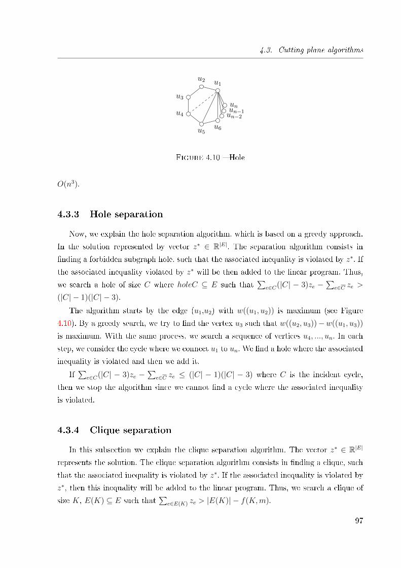
4.3. Cutting plane algorithms
u1u2
u3
u4
u5u6
unun−2un−1
Figure 4.10 � Hole
O(n3).
4.3.3 Hole separation
Now, we explain the hole separation algorithm, which is based on a greedy approach.
In the solution represented by vector z∗ ∈ R|E|. The separation algorithm consists in
�nding a forbidden subgraph hole, such that the associated inequality is violated by z∗. If
the associated inequality violated by z∗ will be then added to the linear program. Thus,
we search a hole of size C where holeC ⊆ E such that∑
e∈C(|C| − 3)ze −∑
e∈C ze >
(|C| − 1)(|C| − 3).
The algorithm starts by the edge (u1,u2) with w((u1, u2)) is maximum (see Figure
4.10). By a greedy search, we try to �nd the vertex u3 such that w((u2, u3))−w((u1, u3))
is maximum. With the same process, we search a sequence of vertices u4, ..., un. In each
step, we consider the cycle where we connect u1 to un. We �nd a hole where the associated
inequality is violated and then we add it.
If∑
e∈C(|C| − 3)ze −∑
e∈C ze ≤ (|C| − 1)(|C| − 3) where C is the incident cycle,
then we stop the algorithm since we cannot �nd a cycle where the associated inequality
is violated.
4.3.4 Clique separation
In this subsection we explain the clique separation algorithm. The vector z∗ ∈ R|E|
represents the solution. The clique separation algorithm consists in �nding a clique, such
that the associated inequality is violated by z∗. If the associated inequality is violated by
z∗, then this inequality will be added to the linear program. Thus, we search a clique of
size K, E(K) ⊆ E such that∑
e∈E(K) ze > |E(K)| − f(K,m).
97
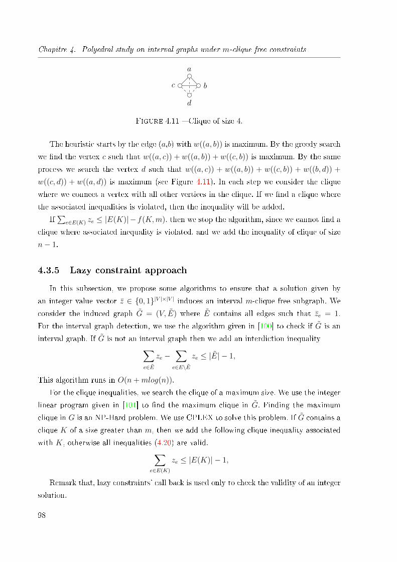
Chapitre 4. Polyedral study on interval graphs under m-clique free constraints
b
a
c
d
Figure 4.11 � Clique of size 4.
The heuristic starts by the edge (a,b) with w((a, b)) is maximum. By the greedy search
we �nd the vertex c such that w((a, c)) + w((a, b)) + w((c, b)) is maximum. By the same
process we search the vertex d such that w((a, c)) + w((a, b)) + w((c, b)) + w((b, d)) +
w((c, d)) + w((a, d)) is maximum (see Figure 4.11). In each step we consider the clique
where we connect a vertex with all other vertices in the clique. If we �nd a clique where
the associated inequalities is violated, then the inequality will be added.
If∑
e∈E(K) ze ≤ |E(K)|− f(K,m), then we stop the algorithm, since we cannot �nd a
clique where associated inequality is violated, and we add the inequality of clique of size
n− 1.
4.3.5 Lazy constraint approach
In this subsection, we propose some algorithms to ensure that a solution given by
an integer value vector z ∈ {0, 1}|V |×|V | induces an interval m-clique free subgraph. We
consider the induced graph G = (V, E) where E contains all edges such that ze = 1.
For the interval graph detection, we use the algorithm given in [100] to check if G is an
interval graph. If G is not an interval graph then we add an interdiction inequality∑e∈E
ze −∑e∈E\E
ze ≤ |E| − 1,
This algorithm runs in O(n+mlog(n)).
For the clique inequalities, we search the clique of a maximum size. We use the integer
linear program given in [101] to �nd the maximum clique in G. Finding the maximum
clique in G is an NP-Hard problem. We use CPLEX to solve this problem. If G contains a
clique K of a size greater than m, then we add the following clique inequality associated
with K, otherwise all inequalities (4.20) are valid.∑e∈E(K)
ze ≤ |E(K)| − 1,
Remark that, lazy constraints' call back is used only to check the validity of an integer
solution.
98
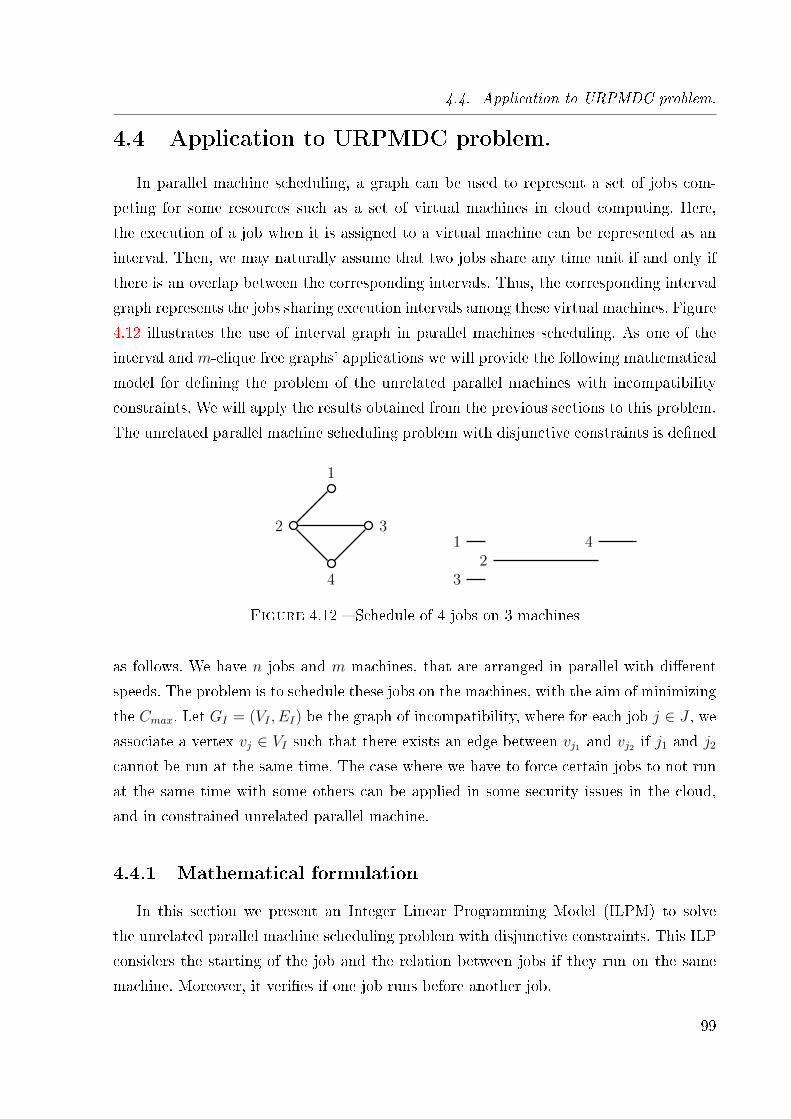
4.4. Application to URPMDC problem.
4.4 Application to URPMDC problem.
In parallel machine scheduling, a graph can be used to represent a set of jobs com-
peting for some resources such as a set of virtual machines in cloud computing. Here,
the execution of a job when it is assigned to a virtual machine can be represented as an
interval. Then, we may naturally assume that two jobs share any time unit if and only if
there is an overlap between the corresponding intervals. Thus, the corresponding interval
graph represents the jobs sharing execution intervals among these virtual machines. Figure
4.12 illustrates the use of interval graph in parallel machines scheduling. As one of the
interval and m-clique free graphs' applications we will provide the following mathematical
model for de�ning the problem of the unrelated parallel machines with incompatibility
constraints. We will apply the results obtained from the previous sections to this problem.
The unrelated parallel machine scheduling problem with disjunctive constraints is de�ned
2
1
3
4
4
32
1
Figure 4.12 � Schedule of 4 jobs on 3 machines
as follows. We have n jobs and m machines, that are arranged in parallel with di�erent
speeds. The problem is to schedule these jobs on the machines, with the aim of minimizing
the Cmax. Let GI = (VI , EI) be the graph of incompatibility, where for each job j ∈ J , weassociate a vertex vj ∈ VI such that there exists an edge between vj1 and vj2 if j1 and j2
cannot be run at the same time. The case where we have to force certain jobs to not run
at the same time with some others can be applied in some security issues in the cloud,
and in constrained unrelated parallel machine.
4.4.1 Mathematical formulation
In this section we present an Integer Linear Programming Model (ILPM) to solve
the unrelated parallel machine scheduling problem with disjunctive constraints. This ILP
considers the starting of the job and the relation between jobs if they run on the same
machine. Moreover, it veri�es if one job runs before another job.
99
Chapitre 4. Polyedral study on interval graphs under m-clique free constraints
This model is based on interval graph and an m-clique free graph, because the graph
induced by each solution must be interval graph, and m-clique free graph in order to be
valid. A graph G(V,E) is called interval graph if its vertices V can be represented by
interval Iv of the real line such that two vertices are adjacent if and only if the correspon-
ding intervals intersect [19]. Let K be a clique in G (K ⊆ V such that every two distinct
vertices of K are adjacent). This is equivalent to the condition that the subgraph of G
induced by K is complete. Let I ⊆ E be a subset of edges, the graph G[I] is an m-clique
free if and only if G[I] does not contain a clique of size strictly greater than m.
Now, we introduce the ILPM :
For each job we consider a variable yj ∈ N+ de�ning the starting of job j in J .
We consider binary variables for assigning the jobs on machines.
xij =
{1 if job j is performed on machine i,0 otherwise
∀i ∈M,∀j ∈ J.
For every two jobs sharing a time unit the associated subgraph must be interval and m-
clique free. For this reason we consider the following binary variables to know if two jobs
share a time unit or if they are performed on disjonctive intervals :
zj1,j2 =
{1 if job j1 and job j2 run at the same time,0 otherwise
∀j1, j2 ∈ J.
zj1,j2 =
{1 if job j1 runs before j2,
0 otherwise∀j1, j2 ∈ J.
For all j ∈ J , we denote by Cj ∈ N+ the completion time of job j.
Cmax ∈ N+ is the maximum of Cj.
100
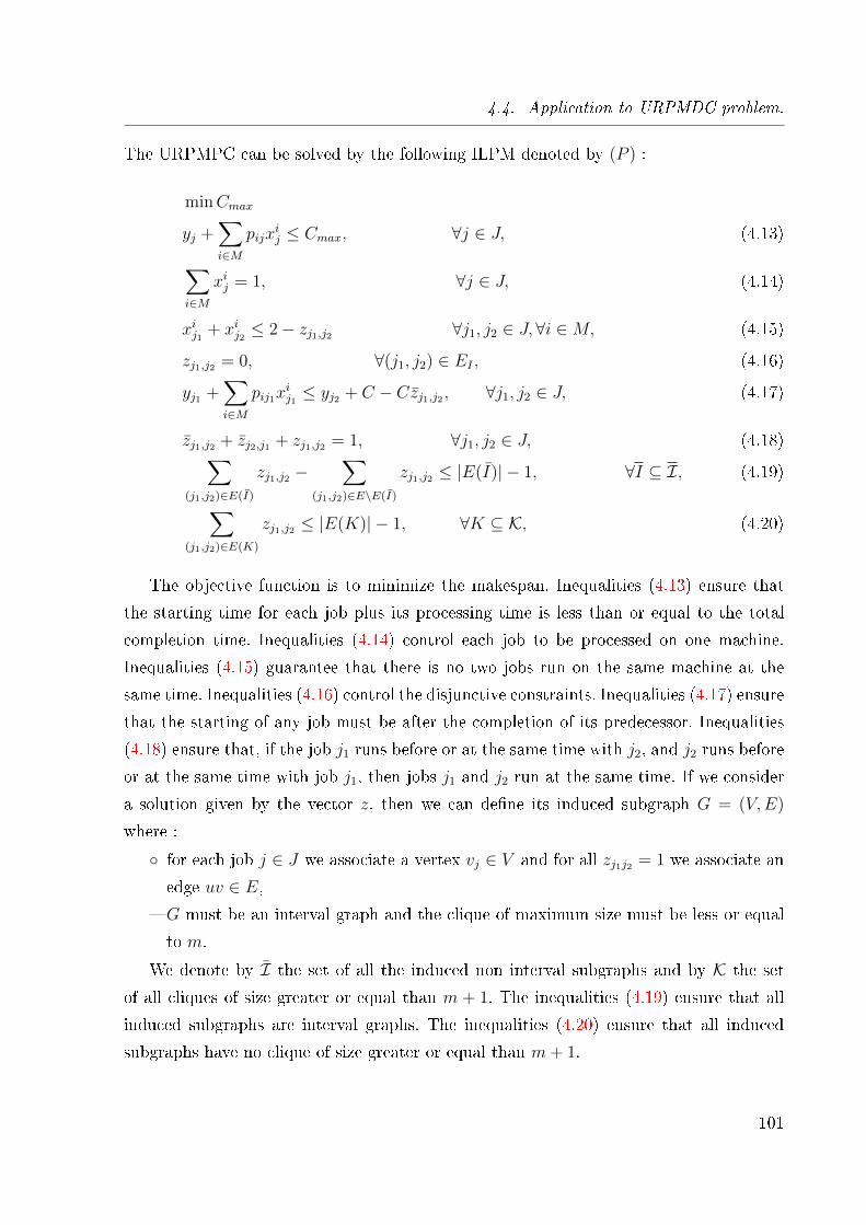
4.4. Application to URPMDC problem.
The URPMPC can be solved by the following ILPM denoted by (P ) :
minCmax
yj +∑i∈M
pijxij ≤ Cmax, ∀j ∈ J, (4.13)∑
i∈M
xij = 1, ∀j ∈ J, (4.14)
xij1 + xij2 ≤ 2− zj1,j2 ∀j1, j2 ∈ J,∀i ∈M, (4.15)
zj1,j2 = 0, ∀(j1, j2) ∈ EI , (4.16)
yj1 +∑i∈M
pij1xij1≤ yj2 + C − Czj1,j2 , ∀j1, j2 ∈ J, (4.17)
zj1,j2 + zj2,j1 + zj1,j2 = 1, ∀j1, j2 ∈ J, (4.18)∑(j1,j2)∈E(I)
zj1,j2 −∑
(j1,j2)∈E\E(I)
zj1,j2 ≤ |E(I)| − 1, ∀I ⊆ I, (4.19)
∑(j1,j2)∈E(K)
zj1,j2 ≤ |E(K)| − 1, ∀K ⊆ K, (4.20)
The objective function is to minimize the makespan. Inequalities (4.13) ensure that
the starting time for each job plus its processing time is less than or equal to the total
completion time. Inequalities (4.14) control each job to be processed on one machine.
Inequalities (4.15) guarantee that there is no two jobs run on the same machine at the
same time. Inequalities (4.16) control the disjunctive constraints. Inequalities (4.17) ensure
that the starting of any job must be after the completion of its predecessor. Inequalities
(4.18) ensure that, if the job j1 runs before or at the same time with j2, and j2 runs before
or at the same time with job j1, then jobs j1 and j2 run at the same time. If we consider
a solution given by the vector z, then we can de�ne its induced subgraph G = (V,E)
where :
◦ for each job j ∈ J we associate a vertex vj ∈ V and for all zj1j2 = 1 we associate an
edge uv ∈ E,� G must be an interval graph and the clique of maximum size must be less or equal
to m.
We denote by I the set of all the induced non interval subgraphs and by K the set
of all cliques of size greater or equal than m + 1. The inequalities (4.19) ensure that all
induced subgraphs are interval graphs. The inequalities (4.20) ensure that all induced
subgraphs have no clique of size greater or equal than m+ 1.
101
Chapitre 4. Polyedral study on interval graphs under m-clique free constraints
4.4.2 Computational Results
To test the e�ciency of the inequalities mentioned in Section 4.2.1 we developed the
mentioned exact and heuristic separations. All computational results are obtained by
using Cplex 12.6 and Java for implementing exact and heuristic algorithms. The ILPM
with the valid inequalities is tested on the following proposed benchmark of instances.
The processing times are uniformly distributed between 50 and 150 as it is common
in the literature [78]. We generated �ve di�erent sets of DAG where the graph density
(GD) is equal to 0.5 and calculated as follows : GD = |E||V |(|V |−1)
where E is the set of
edges associated with precedence constraints between jobs, and V is the set of vertices
associated with jobs. The speeds of machines were generated randomly between 10 and
15.
The required CPU time is measured in seconds. We limit to 3600 seconds the algo-
rithm running time for each instance, by using 4.0 GB of RAM.
The next tables provide the following information :
� |J | : number of jobs� m : number of machines
� Method : 0 cplex only ; 1 bipartite claw inequalities with heuristic separation 1 ;
2 umbrella inequalities with heuristic separation 1 ; 3 hole inequalities ; 4 clique
inequalities with heuristic separation ; 5 n-net inequalities ; 6 n-tent inequalities ; 7
all inequalities.
� CPU : cpu time (limited to 1 hour)
� Nb Nodes : number of nodes in the branching tree
� ct BC : number of bipartite claw inequalities added in the B&C
� ct UMB : number of umbrella inequalities added in the B&C
� ct H : number of hole inequalities added in the B&C
� ct Q : number of clique inequalities added in the B&C
� ct NN : number of n-net inequalities added in the B&C
� ct NT : number of n-tent inequalities added in the B&C
� o/p : number of instances solved (5 instances over 5 or 0 over 5)
In Table 4.1 we can see the that all the instances are solved in less than 20 seconds.
These instances contain 10 jobs with 2 to 8 machines. Remark that the number of the
generated inequalities is less than 200 for the bipartite claw inequalities and less than
70 for all the others. These values are relatively small. Moreover, we generate very small
102
4.5. Conclusion
number of clique inequalities, which is due to a small number of jobs. We did not generate
n-net inequalities, which is due to the small average number of jobs per machine. Finally,
we reduce in average the size of the search tree by adding these new valid inequalities.
Table 4.2 gives the results for 15 jobs with 4 to 8 machines. We easily solve the set of
instances within less than 10 minutes. Adding the valid contraints reduces signi�catively
the number of nodes in the tree search. The computation time is variable and adding the
valid contraints does not reduce it systematically. This is due to the reduced size of the
instances. Moreover, it can happen to generate a lot of contraints, as in the instances of 15
jobs on 6 machines, which explains the reduced performance. We observe that the method
3 allows us to reduce the computation times in average on the instances of 15 jobs and
6 machines. Finally, we remark that we generate few clique and n-net constraints for the
same reasons previously mentioned.
Table 4.3 shows the results for 15 jobs and 2 machines. We did not solve the instances
of this size, which demonstrates the hardness of the studied problem. Wa can notice that
we improved the gap of the standard formulation by using the method 4 (exploiting the
clique contraints).
For solving this problem the new valid inequalities dod not allow to signi�cantly im-
prove the computation time. Nevertheless, we will demonstrate in the next chapter the
positive impact of these contraints. Indeed, the instances we try to solve are too small
so that the valid inequalities will be able to improve the CPLEX routines. Moreover, our
separation algorithms need certainly to be improved in order to quickly generate valid
contraints.
4.5 Conclusion
In this chapter we presented a polyhedral study for the problem of interval under
m-clique free subgraphs. A polyhedral investigation of the convex hull of these vectors
yielded several results on facet de�ning inequalities for the de�ned polytope. We designed
and implemented a branch-and-cut algorithms based on families of strong valid inequali-
ties presented in this chapter. We separate some forbidden subgraphs, and we have also
applied the obtained results to the problem of unrelated parallel machines with disjunc-
tives/precedence constraints. The computational experiments on set of instances have
shown that the algorithms are capable to solve all instances more less to the optimality
within less CPU time when we add these separation algorithms. Further research in this
103
Chapitre 4. Polyedral study on interval graphs under m-clique free constraints
direction will be helpful to strengthen the integer programming formulations of a large
variety of unrelated parallel machines problems as an application to the interval under m-
clique free subgraphs. In the next chapter the properties of interval graph will be applied
for solving generalized Open Shop.
104
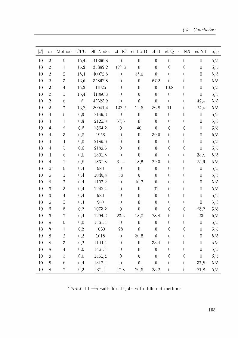
4.5. Conclusion
|J | m Method CPU Nb Nodes ct BC ct UMB ct H ct Q ct NN ct NT o/p
10 2 0 15,4 41866,8 0 0 0 0 0 0 5/5
10 2 1 15,2 35862,2 177,6 0 0 0 0 0 5/5
10 2 2 15,4 40972,6 0 35,6 0 0 0 0 5/5
10 2 3 13,6 35867,8 0 0 67,2 0 0 0 5/5
10 2 4 15,2 41925 0 0 0 10,8 0 0 5/5
10 2 5 15,4 41866,8 0 0 0 0 0 0 5/5
10 2 6 18 45625,2 0 0 0 0 0 42,4 5/5
10 2 7 13,8 30941,4 138,2 12,6 56,8 11 0 24,4 5/5
10 4 0 0,6 2189,6 0 0 0 0 0 0 5/5
10 4 1 0,8 2125,8 57,6 0 0 0 0 0 5/5
10 4 2 0,6 1864,2 0 40 0 0 0 0 5/5
10 4 3 0,8 1958 0 0 39,6 0 0 0 5/5
10 4 4 0,6 2189,6 0 0 0 0 0 0 5/5
10 4 5 0,6 2189,6 0 0 0 0 0 0 5/5
10 4 6 0,6 1801,8 0 0 0 0 0 38,4 5/5
10 4 7 0,8 1837,8 31,4 18,6 29,6 0 0 25,6 5/5
10 6 0 0,4 980 0 0 0 0 0 0 5/5
10 6 1 0,4 1046,8 38 0 0 0 0 0 5/5
10 6 2 0,4 1107,2 0 40,2 0 0 0 0 5/5
10 6 3 0,4 1245,4 0 0 31 0 0 0 5/5
10 6 4 0,4 980 0 0 0 0 0 0 5/5
10 6 5 0,4 980 0 0 0 0 0 0 5/5
10 6 6 0,2 1075,2 0 0 0 0 0 23,2 5/5
10 6 7 0,4 1294,2 23,2 18,8 28,4 0 0 23 5/5
10 8 0 0,6 1461,4 0 0 0 0 0 0 5/5
10 8 1 0,2 1060 28 0 0 0 0 0 5/5
10 8 2 0,2 1018 0 30,8 0 0 0 0 5/5
10 8 3 0,2 1104,4 0 0 33,4 0 0 0 5/5
10 8 4 0,6 1461,4 0 0 0 0 0 0 5/5
10 8 5 0,6 1461,4 0 0 0 0 0 0 5/5
10 8 6 0,4 1312,4 0 0 0 0 0 37,8 5/5
10 8 7 0,2 971,4 17,8 20,6 23,2 0 0 21,8 5/5
Table 4.1 � Results for 10 jobs with di�erent methods
105
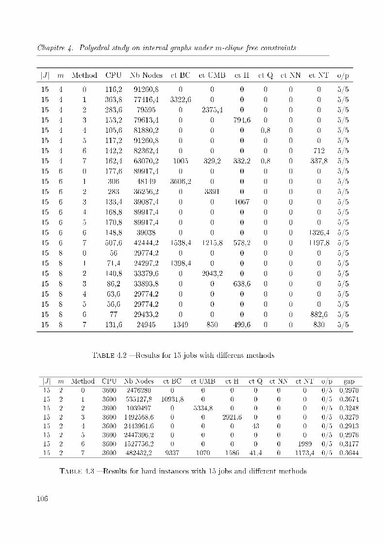
Chapitre 4. Polyedral study on interval graphs under m-clique free constraints
|J | m Method CPU Nb Nodes ct BC ct UMB ct H ct Q ct NN ct NT o/p
15 4 0 116,2 91260,8 0 0 0 0 0 0 5/515 4 1 363,8 77416,4 3322,6 0 0 0 0 0 5/515 4 2 283,6 79595 0 2375,4 0 0 0 0 5/515 4 3 153,2 79613,4 0 0 794,6 0 0 0 5/515 4 4 105,6 81880,2 0 0 0 0,8 0 0 5/515 4 5 117,2 91260,8 0 0 0 0 0 0 5/515 4 6 142,2 82362,4 0 0 0 0 0 712 5/515 4 7 162,4 63070,2 1005 329,2 332,2 0,8 0 337,8 5/515 6 0 177,6 89917,4 0 0 0 0 0 0 5/515 6 1 306 48149 3606,2 0 0 0 0 0 5/515 6 2 283 36256,2 0 3391 0 0 0 0 5/515 6 3 133,4 39087,4 0 0 1067 0 0 0 5/515 6 4 168,8 89917,4 0 0 0 0 0 0 5/515 6 5 170,8 89917,4 0 0 0 0 0 0 5/515 6 6 148,8 39038 0 0 0 0 0 1326,4 5/515 6 7 507,6 42444,2 1538,4 1215,8 578,2 0 0 1197,8 5/515 8 0 56 29774,2 0 0 0 0 0 0 5/515 8 1 71,4 24297,2 1398,4 0 0 0 0 0 5/515 8 2 140,8 33379,6 0 2043,2 0 0 0 0 5/515 8 3 86,2 33893,8 0 0 638,6 0 0 0 5/515 8 4 63,6 29774,2 0 0 0 0 0 0 5/515 8 5 56,6 29774,2 0 0 0 0 0 0 5/515 8 6 77 29433,2 0 0 0 0 0 882,6 5/515 8 7 131,6 24945 1349 850 499,6 0 0 830 5/5
Table 4.2 � Results for 15 jobs with di�erent methods
|J | m Method CPU Nb Nodes ct BC ct UMB ct H ct Q ct NN ct NT o/p gap15 2 0 3600 2476280 0 0 0 0 0 0 0/5 0,297015 2 1 3600 535127,8 10931,8 0 0 0 0 0 0/5 0,367415 2 2 3600 1039497 0 5334,8 0 0 0 0 0/5 0,324815 2 3 3600 1492568,6 0 0 2921,6 0 0 0 0/5 0,327915 2 4 3600 2443961,6 0 0 0 43 0 0 0/5 0,291315 2 5 3600 2447396,2 0 0 0 0 0 0 0/5 0,297615 2 6 3600 1527756,2 0 0 0 0 0 1989 0/5 0,317715 2 7 3600 482432,2 9337 1070 1586 41,4 0 1173,4 0/5 0,3644
Table 4.3 � Results for hard instances with 15 jobs and di�erent methods
106
5
Generalized Open Shop, and Open
Shop Problems
Contents
5.1 Introduction . . . . . . . . . . . . . . . . . . . . . . . . . . . . . 108
5.2 Generalized open shop problem with jobs disjunctive constraints109
5.2.1 Integer linear programming formulation . . . . . . . . . . . . . 109
5.2.2 Valid inequalities . . . . . . . . . . . . . . . . . . . . . . . . . . 110
5.2.3 Experimental results . . . . . . . . . . . . . . . . . . . . . . . . 113
5.3 Open shop problem . . . . . . . . . . . . . . . . . . . . . . . . . 115
5.3.1 Integer linear programming formulation . . . . . . . . . . . . . 116
5.3.2 Valid inequalities . . . . . . . . . . . . . . . . . . . . . . . . . . 118
5.3.3 Experimental results . . . . . . . . . . . . . . . . . . . . . . . . 121
5.4 Conclusion . . . . . . . . . . . . . . . . . . . . . . . . . . . . . . . 122
In this chapter we continued the study of our mathematical formulation, which is ba-
sed on the interval subgraph. The strong structure of its polytope encourage us to adapt
this model to solve other scheduling problems. We addressed two open shop scheduling
problems : the generalized version with disjunctive constraints and the standard one. We
present two mathematical formulations for solving these problems. We derived di�erent
classes of valid inequalities to strength our models. We also add separation algorithms to
the relaxed model of the generalized open shop problem. Exhaustive computational experi-
ments on the well known sets of Taillard's benchmarks are presented. The derived valid
inequalities show a good improvement to the computational time for the two models. Mo-
107
Chapitre 5. Generalized Open Shop, and Open Shop Problems
reover, the generalized open shop model shows the e�ciency of adding the cutting plane
inequalities.
5.1 Introduction
In this chapter, we consider a particular case related to the model of the previous
chapter. This problem is called generalized open shop with disjunctive constraints. In
the �rst part of this chapter, we propose a model for this problem and give some valid
inequalities to improve the associated linear relaxation. Furthermore, we test experimen-
tally the di�erent inequalities. In the second part of this chapter we propose an integer
linear programming model for the standard open shop problem. Indeed, the open shop
is a restricted case of the generalized open shop with jobs disjunctive constraints. The
Open-Shop problem is an important research branch of scheduling problems and it re-
ceives an important amount of attention because of their wide range of applications, such
as modern transport and logistics, modern service industry, large-scale systematic main-
tenance, clothing industry, health care, and so on [102, 103, 104]. In cloud computing,
there is a special case where the job can be divided into m sub tasks. Therefore, each sub
task can be processed on a virtual machine. In general, this problem can be described
by a set of n jobs to be processed by a set of m machines and there is no predetermined
processing route for the jobs. Therefore in the open shop, there are two decisions to make :
the determination of the processing route of each job as well as the job sequence at each
stage [105]. The general O||Cmax problem is strongly NP-hard [66].
Among the many techniques proposed in the literature the problem has not been
attacked a lot by the mathematical models. Masuda and Ishii [107] studied the open shop
scheduling problem for two-machines and they proposed a bi-criteria linear program. Kis
et al [108] described an integer program in two dimension.
We also propose new valid inequalities and we test our model on a well known Taillard's
[109] instances. The experimental results show the e�ciency of our model by solving all
Taillard's instances of size 4 × 4, 5 × 5, 7 × 7 and 10 × 10. Furthermore, we solve all
instances of size 15× 15 and reduce all upper and lower bounds for all other instances.
108
5.2. Generalized open shop problem with jobs disjunctive constraints
5.2 Generalized open shop problem with jobs disjunc-
tive constraints
The Generalized Open Shop with Disjunctive Constraints (GOSDC) can be formulated
as follows. Let M be the set of machines. For all i ∈ M we consider the set of jobs Jimust be running of the machine i and we denote by J = {J1, ..., Jm} the set of all thesesets and by J =
⋃i∈M Ji the union of these sets. We denote by pij the processing time of
job j on its machine i. We consider an incompatibility graph GI = (VI , EI), in this graph,
for each job j ∈ J we associate a vertex vj ∈ VI and there exist an edge between vj1 and
vj2 if j1 and j2 cannot run at the same time. Remark that, it is necessary to considering
a linear ordering on each machine. To the best of our knowledge this special problem has
not been studied before.
5.2.1 Integer linear programming formulation
In this section, we present the integer linear programming for solving the problem. We
need a family of binary variables. In the following, we describe the variables used in the
model :
zj1,j2 =
{1 if the job j1 runs before the job j20 otherwise
∀j1, j2 ∈ J.
zj1,j2 =
{1 if j1 and j2 run at the same time0 otherwise
∀j1 ∈ Ji, j2 ∈ Ji′ |i 6= i′ ∈M.
For all j ∈ J , we consider the variable yj ∈ N+ representing the starting time of job
j.
Cmax ∈ N+ is the maximum completion time.
The GOSDC can be solved by the following ILP, denoted by (PGOS) :
109
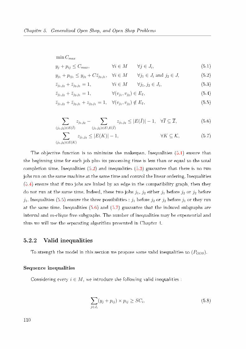
Chapitre 5. Generalized Open Shop, and Open Shop Problems
minCmax
yj + pij ≤ Cmax, ∀i ∈M ∀j ∈ Ji, (5.1)
yj1 + pij1 ≤ yj2 + Czj2,j1 , ∀i ∈M ∀j1 ∈ Ji and j2 ∈ J, (5.2)
zj1,j2 + zj2,j1 = 1, ∀i ∈M ∀j1, j2 ∈ Ji, (5.3)
zj1,j2 + zj2,j1 = 1, ∀(vj1 , vj2) ∈ EI , (5.4)
zj1,j2 + zj2,j1 + zj2,j1 = 1, ∀(vj1 , vj2) /∈ EI , (5.5)
∑(j1,j2)∈E(I)
zj1,j2 −∑
(j1,j2)∈E\E(I)
zj1,j2 ≤ |E(I)| − 1, ∀I ⊆ I, (5.6)
∑(j1,j2)∈E(K)
zj1,j2 ≤ |E(K)| − 1, ∀K ⊆ K, (5.7)
The objective function is to minimize the makespan. Inequalities (5.1) ensure that
the beginning time for each job plus its processing time is less than or equal to the total
completion time. Inequalities (5.2) and inequalities (5.3) guarantee that there is no two
jobs run on the same machine at the same time and control the linear ordering. Inequalities
(5.4) ensure that if two jobs are linked by an edge in the compatibility graph, then they
do not run at the same time. Indeed, these two jobs j1, j2 either j1 before j2 or j2 before
j1. Inequalities (5.5) ensure the three possibilities : j1 before j2 or j2 before j1 or they run
at the same time. Inequalities (5.6) and (5.7) guarantee that the induced subgraphs are
interval and m-clique free subgraphs. The number of inequalities may be exponential and
thus we will use the separating algorithm presented in Chapter 4.
5.2.2 Valid inequalities
To strength the model in this section we propose some valid inequalities to (PGOS).
Sequence inequalities
Considering every i ∈M , we introduce the following valid inequalities :
∑j∈Ji
(yj + pij)× pij ≥ SCi, (5.8)
110
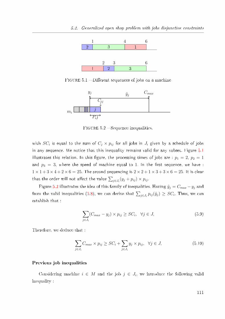
5.2. Generalized open shop problem with jobs disjunctive constraints
12
23
36
21
34
16
Figure 5.1 � Di�erent sequences of jobs on a machine
mij
yj
Cij↓
Pij
yj Cmax
Figure 5.2 � Sequence inequalities.
with SCi is equal to the sum of Cj × pij for all jobs in Ji given by a schedule of jobs
in any sequence. We notice that this inequality remains valid for any subset. Figure 5.1
illustrates this relation. In this �gure, the processing times of jobs are : p1 = 2, p2 = 1
and p3 = 3, where the speed of machine equal to 1. In the �rst sequence, we have :
1× 1 + 3× 4 + 2× 6 = 25. The second sequencing is 2× 2 + 1× 3 + 3× 6 = 25. It is clear
that the order will not a�ect the value∑
j∈Ji(yj + pij)× pij.Figure 5.2 illustrates the idea of this family of inequalities. Having yj = Cmax−yj and
from the valid inequalities (5.8), we can derive that∑
j∈Ji pij(yj) ≥ SCi. Thus, we can
establish that :
∑j∈Ji
(Cmax − yj)× pij ≥ SCi, ∀j ∈ J, (5.9)
Therefore, we deduce that :
∑j∈Ji
Cmax × pij ≥ SCi +∑j∈Ji
yj × pij, ∀j ∈ J, (5.10)
Previous job inequalities
Considering machine i ∈ M and the job j ∈ Ji, we introduce the following valid
inequality :
111
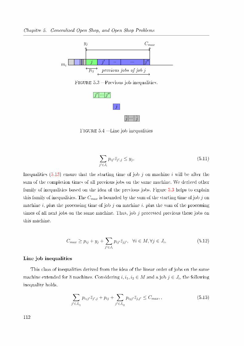
Chapitre 5. Generalized Open Shop, and Open Shop Problems
mij j′ .. ... j′′
previous jobs of job j
yj
pij
Cmax
Figure 5.3 � Previous job inequalities.
j ... j
j
j′ ... j′′
Figure 5.4 � Line job inequalities
∑j′∈Ji
pij′ zj′,j ≤ yj, (5.11)
Inequalities (5.13) ensure that the starting time of job j on machine i will be after the
sum of the completion times of all previous jobs on the same machine. We derived other
family of inequalities based on the idea of the previous jobs. Figure 5.3 helps to explain
this family of inequalities. The Cmax is bounded by the sum of the starting time of job j on
machine i, plus the processing time of job j on machine i, plus the sum of the processing
times of all next jobs on the same machine. Thus, job j processed previous these jobs on
this machine.
Cmax ≥ pij + yj +∑j′∈Ji
pij′ zjj′ , ∀i ∈M,∀j ∈ Ji, (5.12)
Line job inequalities
This class of inequalities derived from the idea of the linear order of jobs on the same
machine extended for 3 machines. Considering i, i1, i2 ∈M and a job j ∈ Ji, the followinginequality holds. ∑
j′∈Ji1
pi1j′ zj′,j + pij +∑j′∈Ji2
pi2j′ zj,j′ ≤ Cmax, , (5.13)
112
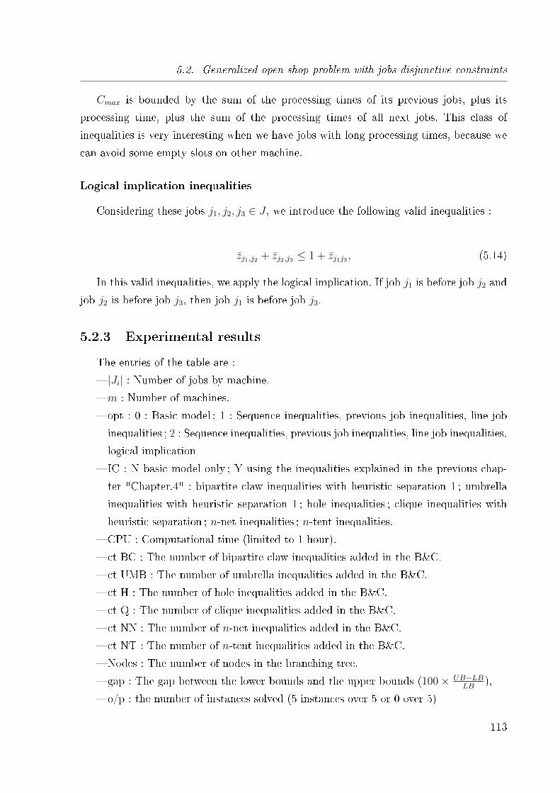
5.2. Generalized open shop problem with jobs disjunctive constraints
Cmax is bounded by the sum of the processing times of its previous jobs, plus its
processing time, plus the sum of the processing times of all next jobs. This class of
inequalities is very interesting when we have jobs with long processing times, because we
can avoid some empty slots on other machine.
Logical implication inequalities
Considering these jobs j1, j2, j3 ∈ J , we introduce the following valid inequalities :
zj1,j2 + zj2,j3 ≤ 1 + zj1j3 , (5.14)
In this valid inequalities, we apply the logical implication. If job j1 is before job j2 and
job j2 is before job j3, then job j1 is before job j3.
5.2.3 Experimental results
The entries of the table are :
� |Ji| : Number of jobs by machine.
� m : Number of machines.
� opt : 0 : Basic model ; 1 : Sequence inequalities, previous job inequalities, line job
inequalities ; 2 : Sequence inequalities, previous job inequalities, line job inequalities,
logical implication
� IC : N basic model only ; Y using the inequalities explained in the previous chap-
ter "Chapter.4" : bipartite claw inequalities with heuristic separation 1 ; umbrella
inequalities with heuristic separation 1 ; hole inequalities ; clique inequalities with
heuristic separation ; n-net inequalities ; n-tent inequalities.
� CPU : Computational time (limited to 1 hour).
� ct BC : The number of bipartite claw inequalities added in the B&C.
� ct UMB : The number of umbrella inequalities added in the B&C.
� ct H : The number of hole inequalities added in the B&C.
� ct Q : The number of clique inequalities added in the B&C.
� ct NN : The number of n-net inequalities added in the B&C.
� ct NT : The number of n-tent inequalities added in the B&C.
� Nodes : The number of nodes in the branching tree.
� gap : The gap between the lower bounds and the upper bounds (100× UB−LBLB
),
� o/p : the number of instances solved (5 instances over 5 or 0 over 5)
113
Chapitre 5. Generalized Open Shop, and Open Shop Problems
|Ji |
mopt
ICCPU
ctBC
ctUMB
ctH
ctQ
ctNN
ctNT
Nodes
gapo/p
52
0N
0,50
00
00
02550,75
05/5
52
0Y
0,7511,25
1,755,5
00
32773
05/5
52
1N
00
00
00
0106,75
05/5
52
1Y
00,75
0,51
00
0,2545
05/5
52
2N
00
00
00
015
05/5
52
2Y
00
00,5
00
017,5
05/5
54
0N
36000
00
00
081065,75
0,69560/5
54
0Y
3249,756489
2674,751785,25
0599,5
1778,5102119
0,28811/5
54
1N
36000
00
00
0224810
0,57560/5
54
1Y
36007450,25
3656,751974,25
0710,5
2187,2590313,75
0,11690/5
54
2N
32200
00
00
0111017,25
0,06901/5
54
2Y
3597,5227,25
84,5257,75
0103,5
134,587498,5
0,03821/5
102
0N
36000
00
00
0986257,25
0,38800/5
102
0Y
36003580
453,75757,75
00
496,5714914,5
0,40760/5
102
1N
158,50
00
00
052605,75
05/5
102
1Y
864,75470
59,25124,25
00
41,25320811
05/5
102
2N
40
00
00
0339
05/5
102
2Y
32
15,5
00
0218
05/5
Table5.1
�Results
ofthe
generalizedopen
shopmodel
114
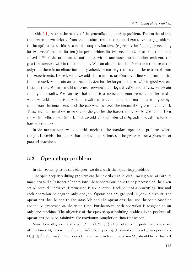
5.3. Open shop problem
Table 5.1 presents the results of the generalized open shop problem. The entries of this
table were shown before. From the obtained results, the model can solve many problems
to the optimality within reasonable computation time (especially for 5 jobs per machine,
for two machines, and for ten jobs per machine, for two machines). In overall, the model
solved 61% of the problems to optimality within one hour. For the other problems the
gap is reasonable within this time limit. We can also notice that from the structure of the
polytope there is no clique inequality added. Interesting results could be extracted from
this experiments. Indeed, when we add the sequence, previous, and line valid inequalities
to our model, we obtain an optimal solution for the larger instances within good compu-
tational time. When we add sequence, previous, and logical valid inequalities, we obtain
some good results. We can say that there is a noticeable improvement for the results
when we add our derived valid inequalities to our model. The most interesting things
come from the improvement of the gap when we add the inequalities given in chapter 4.
These inequalities allow us to divide the gap for the harder instances by 2 to 5 and then
show their e�ciency. Remark that we add a lot of interval subgraph inequalities for the
harder instances.
In the next section, we adapt this model to the standard open shop problem, where
the job is divided into operations and the operations will be processed on a given set of
parallel machines.
5.3 Open shop problem
In the second part of this chapter, we deal with the open shop problem.
The open shop scheduling problem can be described as follows. Having a set of parallel
machines and a �nite set of operations, these operations have to be processed on the given
set of parallel machines. Preemption is not allowed. Each job has a processing time and
each operation belongs to only one job. Operations are grouped in jobs. Moreover, the
operations that belong to the same job and the operations that use the same machine
cannot be processed at the same time. Furthermore, each operation is assigned to an
only one machine. The objective of the open shop scheduling problem is to perform all
operations, so as to minimize the maximum completion time (makespan).
More formally, we have a set J = {1, 2, .., n} of n jobs to be performed on a set
of machines Mi where i = {1, 2, ...,m}. Each job j ∈ J consists of exactly m operations
Oi,j(i ∈ {1, 2, ...,m}). For every job j and every index i, operationOi,j should be performed
115
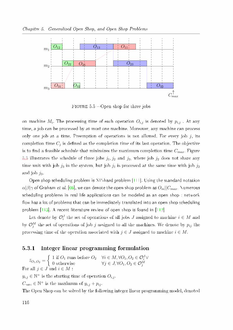
Chapitre 5. Generalized Open Shop, and Open Shop Problems
O31 O32 O33
Cmax↑
m3
O22 O21 O23m2
O12 O13 O11m1
Figure 5.5 � Open shop for three jobs
on machine Mi. The processing time of each operation Oi,j is denoted by pi,j . At any
time, a job can be processed by at most one machine. Moreover, any machine can process
only one job at a time. Preemption of operations is not allowed. For every job j, its
completion time Cj is de�ned as the completion time of its last operation. The objective
is to �nd a feasible schedule that minimizes the maximum completion time Cmax. Figure
5.5 illustrates the schedule of three jobs j1, j2 and j3, where job j2 does not share any
time unit with job j3 in the system, but job j1 is processed at the same time with job j2
and job j3.
Open shop scheduling problem is NP-hard problem [111]. Using the standard notation
α|β|γ of Graham et al. [66], we can denote the open shop problem as Om||Cmax. Numerous
scheduling problems in real life applications can be modeled as an open shop : network
�ow has a lot of problems that can be immediately translated into an open shop scheduling
problem [113]. A recent literature review of open shop is found in [112]
Let denote by OJi the set of operations of all jobs J assigned to machine i ∈ M and
by OMj the set of operations of job j assigned to all the machines. We denote by pij the
processing time of the operation associated with j ∈ J assigned to machine i ∈M .
5.3.1 Integer linear programming formulation
zO1,O2 =
{1 if O1 runs before O2
0 otherwise∀i ∈M,∀O1, O2 ∈ OJi ∨∀j ∈ J,∀O1, O2 ∈ OMj
For all j ∈ J and i ∈M :
yi,j ∈ N+ is the starting time of operation Oi,j.
Cmax ∈ N+ is the maximum of yi,j + pij.
The Open Shop can be solved by the following integer linear programming model, denoted
116
5.3. Open shop problem
by (POS) :
minCmax
yi,j + pij ≤ Cmax, ∀i ∈M ∀j ∈ J, (5.15)
yi,j1 + pij1 ≤ yi,j2 + CzOi,j2 ,Oi,j1 , ∀i ∈M ∀j1, j2 ∈ J, (5.16)
yi1,j + pi1j ≤ yi2,j + CzOi2,j ,Oi1,j , ∀j ∈ J ∀i1, i2 ∈M, (5.17)
zOi,j1 ,Oi,j2 + zOi,j2 ,Oi,j1 = 1, ∀i ∈M ∀j1, j2 ∈ J, (5.18)
zOi1,j ,Oi2,j + zOi2,j ,Oi1,j = 1, ∀j ∈ J ∀i1, i2 ∈M, (5.19)
The objective function is to minimize the makespan.
Inequalities (5.15) ensure that the starting time for each operation plus its processing
time is less than or equal to the total completion time. Inequalities (5.16) control that if
operation Oij1 is before operation Oij2 , then operation Oij2 must start after the completion
of operation Oij1 on the same machine. Inequalities (5.17) guarantee that if operation of
job j runs on machine i1 before its operation on machine i2, then the starting time of Oi2,j
must be after the completion of operation Oi1,j. Inequalities (5.18) and (5.19) guarantee
the linear ordering of the operations on the same machine and the linear ordering of the
operations of the same job.
We also use the conditional constraints for inequalities (5.2) and (5.3). We can write
these two constraints as follows :
if(zOi,j1 ,Oi,j2 = 1), then yi,j1 + pij1 ≤ yi,j2 , ∀i ∈M ∀j1, j2 ∈ J, (5.20)
(5.21)
if(zOi1,j ,Oi2,j = 1), then yi1,j + pi1j ≤ yi2,j, ∀j ∈ J ∀i1, i2 ∈M, (5.22)
Inequalities (5.20) imply that if job j1 is before job j2, then it implies that, the starting
time of job j2 must be after the completion time of job j1. The conditional inequalities
5.21 test if the operation of job j on machine i1 is before the operation of the same job on
machine i2, then the starting time of the operation of job j on machine i2 must be after
the completion of the operation of job j on machine i1. Adding the conditional inequalities
will remove the bigM(C), but the solver must branch on these conditions. We will explain
the results of using conditional inequalities in the section dedicated to the experimental
results.
117
Chapitre 5. Generalized Open Shop, and Open Shop Problems
5.3.2 Valid inequalities
In this section, we derive various classes of valid inequalities for the integer linear
programming model. In these derived inequalities, we consider the sequence of jobs on
the machines, the relation between a job and its previous ones as in [110] and we consider
a logical implication. We adapted the classes of valid inequalities introduced in Section
5.2.2.
Sequence inequalities
Considering job j ∈ J , we introduce the following valid inequalities :∑i∈M
(yi,j + pij)× pij ≥ SCj, (5.23)
where SCj is equal to the sum of Ci,j×pij where Ci,j is the completion time of operation
Oi,j in any sequence. With the same idea, we can dervie similar valid inequalities for every
subset of operations of job j.
By symmetry, let i ∈M . The following valid inequalities hold :∑j∈J
(yi,j + pij)× pij ≥ SCi, (5.24)
where SCi is equal to the sum of Ci,j × pij by varying j, and Ci,j is the completion time
of Oi,j in any sequence.
Having yi,j = Cmax − yi,j, and form the valid inequalities (5.24), we can derive that∑j∈J pij(yi,j) ≥ SCi. Thus, we deduce that :
∑j∈J
pij(Cmax − yi,j) ≥ SCi, ∀i ∈M, (5.25)
Therefore, the following relation holds :
∑j∈J
pijCmax ≥∑j∈J
pijyi,j + SCi, ∀i ∈M, (5.26)
These valid inequalities can lead to similar inequalities (5.23) for all jobs j ∈ J :
∑i∈M
pijCmax ≥∑i∈M
pijyi,j + SCj, (5.27)
118
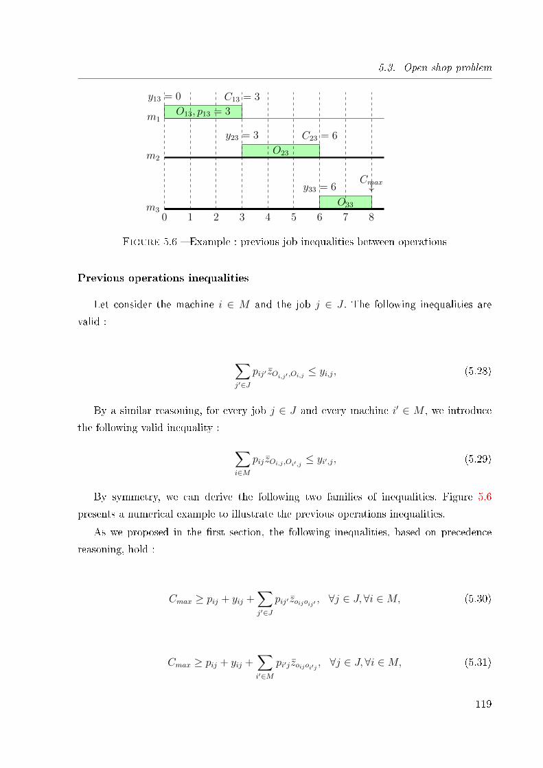
5.3. Open shop problem
0 1 2 3 4 5 6 7 8
O33
y33 = 6Cmax↓
m3
O23
C23 = 6y23 = 3
m2
O13, p13 = 3
C13 = 3y13 = 0
m1
Figure 5.6 � Example : previous job inequalities between operations
Previous operations inequalities
Let consider the machine i ∈ M and the job j ∈ J . The following inequalities are
valid :
∑j′∈J
pij′ zOi,j′ ,Oi,j ≤ yi,j, (5.28)
By a similar reasoning, for every job j ∈ J and every machine i′ ∈ M , we introduce
the following valid inequality :
∑i∈M
pij zOi,j ,Oi′,j ≤ yi′,j, (5.29)
By symmetry, we can derive the following two families of inequalities. Figure 5.6
presents a numerical example to illustrate the previous operations inequalities.
As we proposed in the �rst section, the following inequalities, based on precedence
reasoning, hold :
Cmax ≥ pij + yij +∑j′∈J
pij′ zoijoij′ , ∀j ∈ J,∀i ∈M, (5.30)
Cmax ≥ pij + yij +∑i′∈M
pi′j zoijoi′j , ∀j ∈ J,∀i ∈M, (5.31)
119
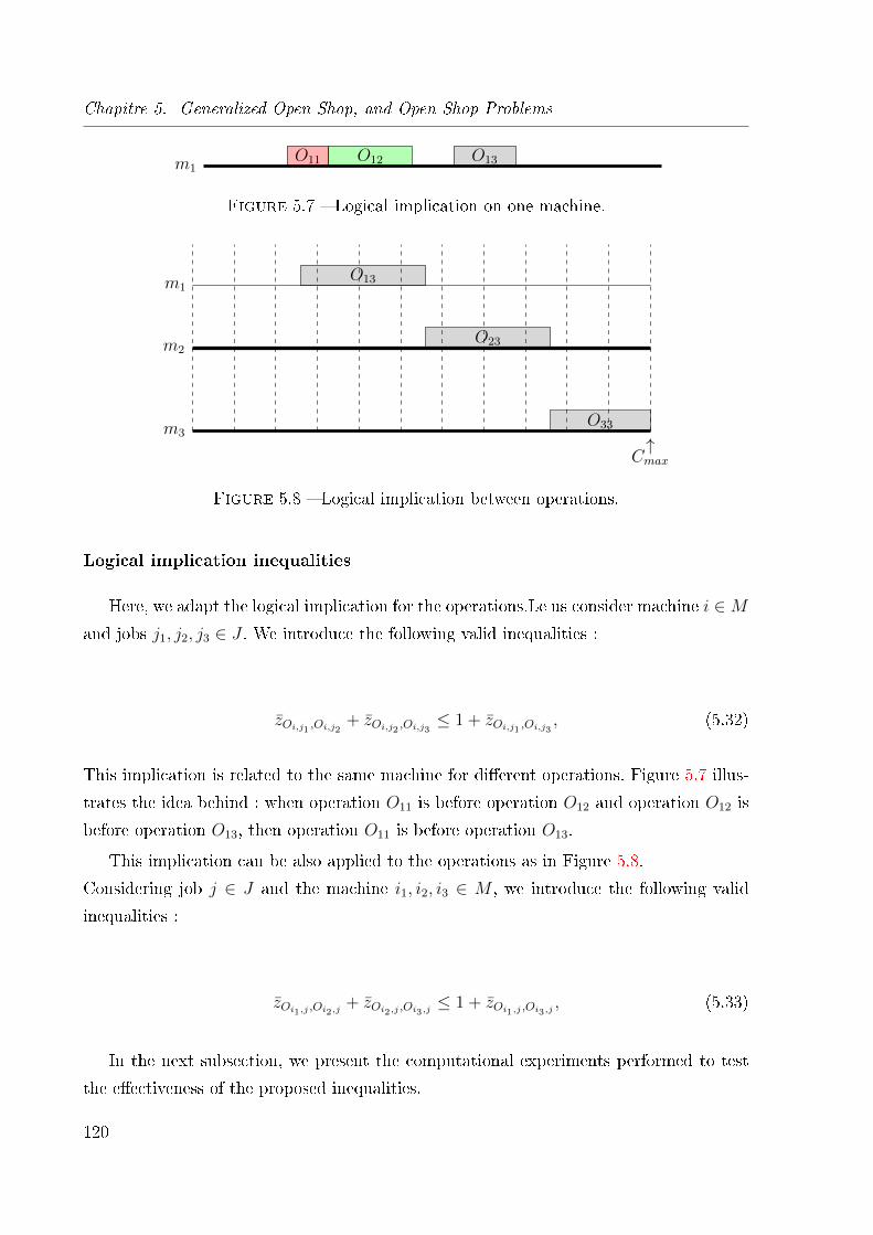
Chapitre 5. Generalized Open Shop, and Open Shop Problems
O11 O12 O13m1
Figure 5.7 � Logical implication on one machine.
O33
Cmax↑
m3
O23m2
O13m1
Figure 5.8 � Logical implication between operations.
Logical implication inequalities
Here, we adapt the logical implication for the operations.Le us consider machine i ∈Mand jobs j1, j2, j3 ∈ J . We introduce the following valid inequalities :
zOi,j1 ,Oi,j2 + zOi,j2 ,Oi,j3 ≤ 1 + zOi,j1 ,Oi,j3 , (5.32)
This implication is related to the same machine for di�erent operations. Figure 5.7 illus-
trates the idea behind : when operation O11 is before operation O12 and operation O12 is
before operation O13, then operation O11 is before operation O13.
This implication can be also applied to the operations as in Figure 5.8.
Considering job j ∈ J and the machine i1, i2, i3 ∈ M , we introduce the following valid
inequalities :
zOi1,j ,Oi2,j + zOi2,j ,Oi3,j ≤ 1 + zOi1,j ,Oi3,j , (5.33)
In the next subsection, we present the computational experiments performed to test
the e�ectiveness of the proposed inequalities.
120
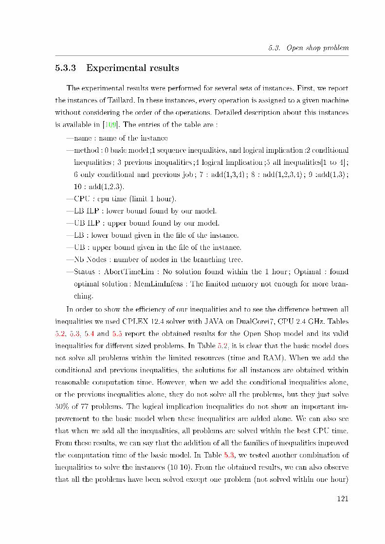
5.3. Open shop problem
5.3.3 Experimental results
The experimental results were performed for several sets of instances. First, we report
the instances of Taillard. In these instances, every operation is assigned to a given machine
without considering the order of the operations. Detailed description about this instances
is available in [109]. The entries of the table are :
� name : name of the instance
� method : 0 basic model ;1 sequence inequalities, and logical implication ;2 conditional
inequalities ; 3 previous inequalities ;4 logical implication ;5 all inequalities[1 to 4] ;
6 only conditional and previous job ; 7 : add(1,3,4) ; 8 : add(1,2,3,4) ; 9 :add(1,3) ;
10 : add(1,2,3).
� CPU : cpu time (limit 1 hour).
� LB ILP : lower bound found by our model.
� UB ILP : upper bound found by our model.
� LB : lower bound given in the �le of the instance.
� UB : upper bound given in the �le of the instance.
� Nb Nodes : number of nodes in the branching tree.
� Status : AbortTimeLim : No solution found within the 1 hour ; Optimal : found
optimal solution ; MemLimInfeas : The limited memory not enough for more bran-
ching.
In order to show the e�ciency of our inequalities and to see the di�erence between all
inequalities we used CPLEX 12.4 solver with JAVA on DualCorei7, CPU 2.4 GHz. Tables
5.2, 5.3, 5.4 and 5.5 report the obtained results for the Open Shop model and its valid
inequalities for di�erent sized problems. In Table 5.2, it is clear that the basic model does
not solve all problems within the limited resources (time and RAM). When we add the
conditional and previous inequalities, the solutions for all instances are obtained within
reasonable computation time. However, when we add the conditional inequalities alone,
or the previous inequalities alone, they do not solve all the problems, but they just solve
50% of 77 problems. The logical implication inequalities do not show an important im-
provement to the basic model when these inequalities are added alone. We can also see
that when we add all the inequalities, all problems are solved within the best CPU time.
From these results, we can say that the addition of all the families of inequalities improved
the computation time of the basic model. In Table 5.3, we tested another combination of
inequalities to solve the instances (10 10). From the obtained results, we can also observe
that all the problems have been solved except one problem (not solved within one hour)
121
Chapitre 5. Generalized Open Shop, and Open Shop Problems
when we add the combination of inequalities (sequence, previous and logical implication).
It is also worthy to notice that the best CPU time obtained by the combination of the
sequence and previous inequalities. Table 5.4 reports the results for instances (15 15). Ac-
cording to these results, the related problems are not easy to solve within the limited time
and the memory space. Thus, few number of problems have been solved. The combination
of the sequence and previous inequalities allows us to obtain some optimal solutions. It is
also the same case, when we add to this combination the conditional inequalities (i.e., we
obtained the same number of the optimal solutions). The gap between the obtained UB
ILP and LB ILP does not exceed 5%.
Table 5.5 reports the results for instances of (20 20). Within the adjusted time to one
hour, no problem has been solved for this size. But, we can see the small gaps between
the UB and LB obtained by the ILP. All of them appear when we add the combination
of sequence and previous inequalities.
5.4 Conclusion
In this chapter, we considered two parallel-machine scheduling problems. The �rst
problem is the generalized open shop with disjunctive constraints. To the best of our
knowledge there is no mathematical model for this problem. The second problem is the
standard open shop problem. The aim is to minimize the maximum completion time.
To deal with these problems, two mathematical models were proposed. We derived some
classes of valid inequalities. We also added the interval subgraph separation algorithms
for the generalized open shop problem. We adapted the derived valid inequalities to the
open shop mathematical formulation. The results on some instances show that the basic
models can solve the small size instances to optimality, and the generalized model shows
the e�ciency of adding the cutting plane inequalities proposed in Chapter 4, which can
divide the gaps by 2 to 5. The derived valid inequalities show an important improvement
of the computation time for the two models. We believe that the design of new classes
of valid inequalities and the incorporation of further separation algorithms will improve
the computation times of our models and it will lead to optimal solutions for some of the
unsolved instances.
122
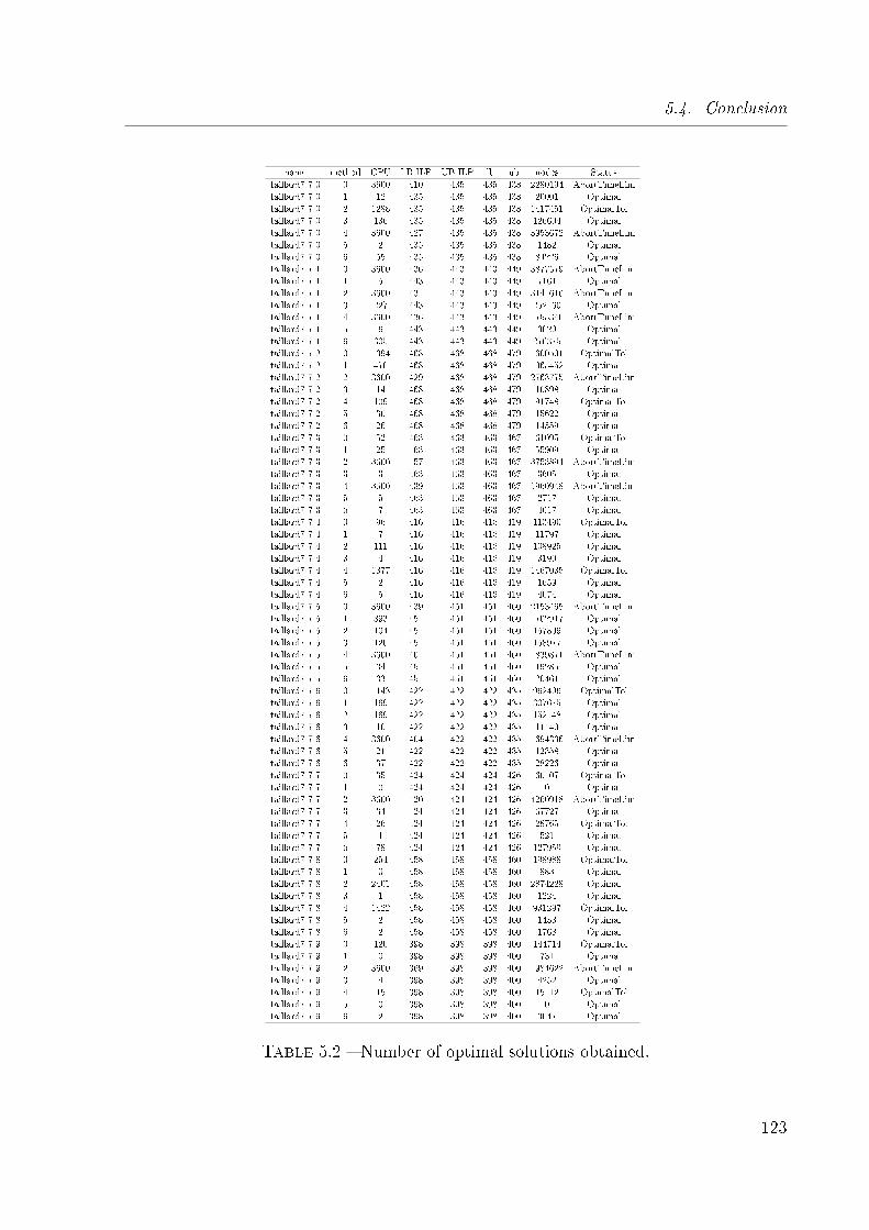
5.4. Conclusion
name method CPU LB ILP UB ILP lb ub nodes Statustaillard7 7 0 0 3600 410 435 435 438 2280194 AbortTimeLimtaillard7 7 0 1 12 435 435 435 438 20001 Optimaltaillard7 7 0 2 1288 435 435 435 438 1417451 OptimalToltaillard7 7 0 3 136 435 435 435 438 126604 Optimaltaillard7 7 0 4 3600 427 435 435 438 3953672 AbortTimeLimtaillard7 7 0 5 2 435 435 435 438 1482 Optimaltaillard7 7 0 6 55 435 435 435 438 84226 Optimaltaillard7 7 1 0 3600 436 443 443 449 3877579 AbortTimeLimtaillard7 7 1 1 5 443 443 443 449 7161 Optimaltaillard7 7 1 2 3600 431 443 443 449 3141616 AbortTimeLimtaillard7 7 1 3 227 443 443 443 449 252160 Optimaltaillard7 7 1 4 3600 436 443 443 449 1755340 AbortTimeLimtaillard7 7 1 5 6 443 443 443 449 3029 Optimaltaillard7 7 1 6 305 443 443 443 449 276375 Optimaltaillard7 7 2 0 1394 468 468 468 479 1600501 OptimalToltaillard7 7 2 1 470 468 468 468 479 1065452 Optimaltaillard7 7 2 2 3600 429 468 468 479 2763775 AbortTimeLimtaillard7 7 2 3 14 468 468 468 479 10898 Optimaltaillard7 7 2 4 109 468 468 468 479 91748 OptimalToltaillard7 7 2 5 30 468 468 468 479 15622 Optimaltaillard7 7 2 6 26 468 468 468 479 14559 Optimaltaillard7 7 3 0 52 463 463 463 467 61095 OptimalToltaillard7 7 3 1 25 463 463 463 467 55909 Optimaltaillard7 7 3 2 3600 457 463 463 467 3753894 AbortTimeLimtaillard7 7 3 3 3 463 463 463 467 3605 Optimaltaillard7 7 3 4 3600 439 463 463 467 1960948 AbortTimeLimtaillard7 7 3 5 5 463 463 463 467 2717 Optimaltaillard7 7 3 6 7 463 463 463 467 4017 Optimaltaillard7 7 4 0 96 416 416 416 419 113490 OptimalToltaillard7 7 4 1 7 416 416 416 419 11797 Optimaltaillard7 7 4 2 111 416 416 416 419 108925 Optimaltaillard7 7 4 3 4 416 416 416 419 3190 Optimaltaillard7 7 4 4 1377 416 416 416 419 1467035 OptimalToltaillard7 7 4 5 2 416 416 416 419 1659 Optimaltaillard7 7 4 6 5 416 416 416 419 4074 Optimaltaillard7 7 5 0 3600 439 451 451 460 2153465 AbortTimeLimtaillard7 7 5 1 893 451 451 451 460 1702917 Optimaltaillard7 7 5 2 104 451 451 451 460 157809 Optimaltaillard7 7 5 3 120 451 451 451 460 158977 Optimaltaillard7 7 5 4 3600 401 451 451 460 1839871 AbortTimeLimtaillard7 7 5 5 34 451 451 451 460 19285 Optimaltaillard7 7 5 6 33 451 451 451 460 20461 Optimaltaillard7 7 6 0 1143 422 422 422 435 962496 OptimalToltaillard7 7 6 1 169 422 422 422 435 307675 Optimaltaillard7 7 6 2 169 422 422 422 435 152148 Optimaltaillard7 7 6 3 10 422 422 422 435 11140 Optimaltaillard7 7 6 4 3600 404 422 422 435 1694336 AbortTimeLimtaillard7 7 6 5 21 422 422 422 435 12358 Optimaltaillard7 7 6 6 37 422 422 422 435 28226 Optimaltaillard7 7 7 0 35 424 424 424 426 60107 OptimalToltaillard7 7 7 1 0 424 424 424 426 0 Optimaltaillard7 7 7 2 3600 420 424 424 426 4260918 AbortTimeLimtaillard7 7 7 3 34 424 424 424 426 67727 Optimaltaillard7 7 7 4 26 424 424 424 426 28765 OptimalToltaillard7 7 7 5 1 424 424 424 426 521 Optimaltaillard7 7 7 6 78 424 424 424 426 127959 Optimaltaillard7 7 8 0 254 458 458 458 460 198988 OptimalToltaillard7 7 8 1 0 458 458 458 460 883 Optimaltaillard7 7 8 2 2401 458 458 458 460 2874228 Optimaltaillard7 7 8 3 1 458 458 458 460 1224 Optimaltaillard7 7 8 4 1422 458 458 458 460 931297 OptimalToltaillard7 7 8 5 2 458 458 458 460 1433 Optimaltaillard7 7 8 6 2 458 458 458 460 1768 Optimaltaillard7 7 9 0 120 398 398 398 400 144714 OptimalToltaillard7 7 9 1 0 398 398 398 400 731 Optimaltaillard7 7 9 2 3600 369 398 398 400 1984622 AbortTimeLimtaillard7 7 9 3 4 398 398 398 400 4252 Optimaltaillard7 7 9 4 15 398 398 398 400 15112 OptimalToltaillard7 7 9 5 0 398 398 398 400 0 Optimaltaillard7 7 9 6 2 398 398 398 400 3047 Optimal
Table 5.2 � Number of optimal solutions obtained.
123
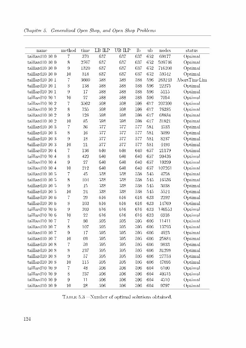
Chapitre 5. Generalized Open Shop, and Open Shop Problems
name method time LB ILP UB ILP lb ub nodes statustaillard10 10 0 7 370 637 637 637 652 60177 Optimaltaillard10 10 0 8 2767 637 637 637 652 509746 Optimaltaillard10 10 0 9 1320 637 637 637 652 716200 Optimaltaillard10 10 0 10 318 637 637 637 652 59542 Optimaltaillard10 10 1 7 3600 588 589 588 596 263243 AbortTimeLimtaillard10 10 1 8 138 588 588 588 596 22275 Optimaltaillard10 10 1 9 17 588 588 588 596 5115 Optimaltaillard10 10 1 10 27 588 588 588 596 7054 Optimaltaillard10 10 2 7 3502 598 598 598 617 207390 Optimaltaillard10 10 2 8 735 598 598 598 617 76285 Optimaltaillard10 10 2 9 128 598 598 598 617 68884 Optimaltaillard10 10 2 10 85 598 598 598 617 31821 Optimaltaillard10 10 3 7 36 577 577 577 581 4533 Optimaltaillard10 10 3 8 16 577 577 577 581 3099 Optimaltaillard10 10 3 9 18 577 577 577 581 8237 Optimaltaillard10 10 3 10 21 577 577 577 581 4493 Optimaltaillard10 10 4 7 136 640 640 640 657 21179 Optimaltaillard10 10 4 8 429 640 640 640 657 90436 Optimaltaillard10 10 4 9 27 640 640 640 657 10299 Optimaltaillard10 10 4 10 212 640 640 640 657 107261 Optimaltaillard10 10 5 7 45 538 538 538 545 4758 Optimaltaillard10 10 5 8 104 538 538 538 545 16536 Optimaltaillard10 10 5 9 15 538 538 538 545 3038 Optimaltaillard10 10 5 10 24 538 538 538 545 5524 Optimaltaillard10 10 6 7 29 616 616 616 623 2292 Optimaltaillard10 10 6 8 103 616 616 616 623 14769 Optimaltaillard10 10 6 9 269 616 616 616 623 146553 Optimaltaillard10 10 6 10 22 616 616 616 623 6938 Optimaltaillard10 10 7 7 80 595 595 595 606 11411 Optimaltaillard10 10 7 8 107 595 595 595 606 13793 Optimaltaillard10 10 7 9 17 595 595 595 606 4923 Optimaltaillard10 10 7 10 69 595 595 595 606 25884 Optimaltaillard10 10 8 7 59 595 595 595 606 9833 Optimaltaillard10 10 8 8 237 595 595 595 606 31298 Optimaltaillard10 10 8 9 57 595 595 595 606 27753 Optimaltaillard10 10 8 10 115 595 595 595 606 47695 Optimaltaillard10 10 9 7 48 596 596 596 604 6100 Optimaltaillard10 10 9 8 237 596 596 596 604 40515 Optimaltaillard10 10 9 9 11 596 596 596 604 4510 Optimaltaillard10 10 9 10 28 596 596 596 604 9797 Optimal
Table 5.3 � Number of optimal solutions obtained.
124
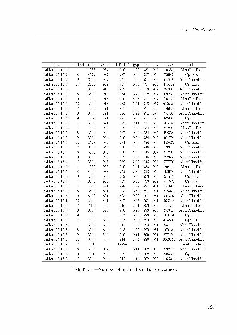
5.4. Conclusion
name method time LB ILP UB ILP gap lb ub nodes statustaillard15 15 0 7 1233 937 956 1.99 937 956 16338 MemLimFeastaillard15 15 0 8 3572 937 937 0.00 937 956 72686 Optimaltaillard15 15 0 9 3600 937 947 1.06 937 956 517809 AbortTimeLimtaillard15 15 0 10 2638 937 937 0.00 937 956 475219 Optimaltaillard15 15 1 7 3600 918 939 2.24 918 957 34301 AbortTimeLimtaillard15 15 1 8 3600 918 954 3.77 918 957 59266 AbortTimeLimtaillard15 15 1 9 1550 918 949 3.27 918 957 76726 MemLimFeastaillard15 15 1 10 3600 918 933 1.61 918 957 610624 AbortTimeLimtaillard15 15 2 7 952 871 897 2.90 871 899 16983 MemLimFeastaillard15 15 2 8 3600 871 896 2.79 871 899 54762 AbortTimeLimtaillard15 15 2 9 462 871 871 0.00 871 899 82995 Optimaltaillard15 15 2 10 3600 871 872 0.11 871 899 505148 AbortTimeLimtaillard15 15 3 7 1450 934 942 0.85 934 946 27800 MemLimFeastaillard15 15 3 8 3600 934 937 0.32 934 946 52356 AbortTimeLimtaillard15 15 3 9 3600 934 940 0.64 934 946 364704 AbortTimeLimtaillard15 15 3 10 1518 934 934 0.00 934 946 255462 Optimaltaillard15 15 4 7 3600 946 990 4.44 946 992 19375 AbortTimeLimtaillard15 15 4 8 3600 946 990 4.44 946 992 54201 AbortTimeLimtaillard15 15 4 9 3600 946 949 0.32 946 992 222656 AbortTimeLimtaillard15 15 4 10 3600 946 969 2.37 946 992 577703 AbortTimeLimtaillard15 15 5 7 1336 933 956 2.41 933 959 20458 MemLimFeastaillard15 15 5 8 3600 933 955 2.30 933 959 48663 AbortTimeLimtaillard15 15 5 9 299 933 933 0.00 933 959 54583 Optimaltaillard15 15 5 10 3525 933 933 0.00 933 959 557028 Optimaltaillard15 15 6 7 793 891 928 3.99 891 931 14393 MemLimFeastaillard15 15 6 8 3600 891 925 3.68 891 931 92441 AbortTimeLimtaillard15 15 6 9 3600 891 893 0.22 891 931 948307 AbortTimeLimtaillard15 15 6 10 3600 891 897 0.67 891 931 993133 AbortTimeLimtaillard15 15 7 7 619 893 916 2.51 893 916 14173 MemLimFeastaillard15 15 7 8 3600 893 900 0.78 893 916 94041 AbortTimeLimtaillard15 15 7 9 455 893 893 0.00 893 916 108151 Optimaltaillard15 15 7 10 1613 893 893 0.00 893 916 414890 Optimaltaillard15 15 8 7 3600 899 911 1.32 899 951 95415 AbortTimeLimtaillard15 15 8 8 3600 899 943 4.67 899 951 109120 AbortTimeLimtaillard15 15 8 9 3600 899 900 0.11 899 951 877150 AbortTimeLimtaillard15 15 8 10 3600 899 914 1.64 899 951 1046262 AbortTimeLimtaillard15 15 9 7 631 12226 MemLimInfeastaillard15 15 9 8 3600 902 931 3.11 902 935 99270 AbortTimeLimtaillard15 15 9 9 431 902 902 0.00 902 935 98569 Optimaltaillard15 15 9 10 3600 902 912 1.10 902 935 1166219 AbortTimeLim
Table 5.4 � Number of optimal solutions obtained.
125
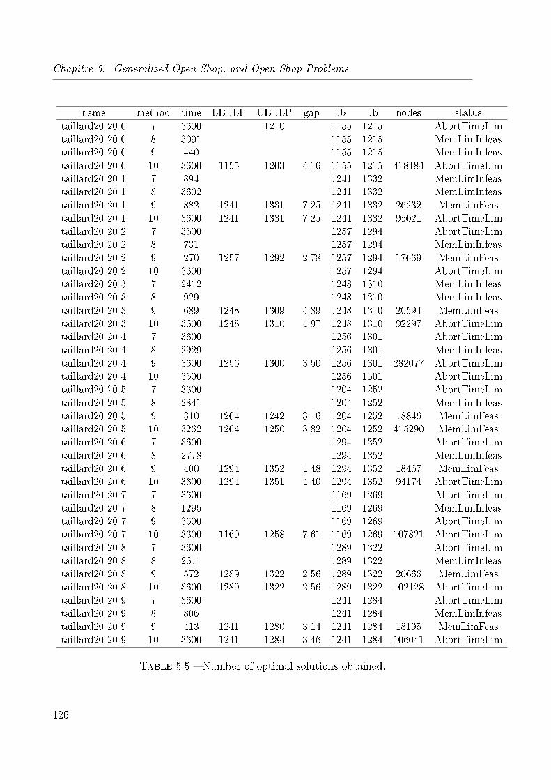
Chapitre 5. Generalized Open Shop, and Open Shop Problems
name method time LB ILP UB ILP gap lb ub nodes statustaillard20 20 0 7 3600 1210 1155 1215 AbortTimeLimtaillard20 20 0 8 3091 1155 1215 MemLimInfeastaillard20 20 0 9 440 1155 1215 MemLimInfeastaillard20 20 0 10 3600 1155 1203 4.16 1155 1215 418184 AbortTimeLimtaillard20 20 1 7 894 1241 1332 MemLimInfeastaillard20 20 1 8 3602 1241 1332 MemLimInfeastaillard20 20 1 9 882 1241 1331 7.25 1241 1332 26232 MemLimFeastaillard20 20 1 10 3600 1241 1331 7.25 1241 1332 95021 AbortTimeLimtaillard20 20 2 7 3600 1257 1294 AbortTimeLimtaillard20 20 2 8 731 1257 1294 MemLimInfeastaillard20 20 2 9 270 1257 1292 2.78 1257 1294 17669 MemLimFeastaillard20 20 2 10 3600 1257 1294 AbortTimeLimtaillard20 20 3 7 2412 1248 1310 MemLimInfeastaillard20 20 3 8 929 1248 1310 MemLimInfeastaillard20 20 3 9 689 1248 1309 4.89 1248 1310 20594 MemLimFeastaillard20 20 3 10 3600 1248 1310 4.97 1248 1310 92297 AbortTimeLimtaillard20 20 4 7 3600 1256 1301 AbortTimeLimtaillard20 20 4 8 2929 1256 1301 MemLimInfeastaillard20 20 4 9 3600 1256 1300 3.50 1256 1301 282077 AbortTimeLimtaillard20 20 4 10 3600 1256 1301 AbortTimeLimtaillard20 20 5 7 3600 1204 1252 AbortTimeLimtaillard20 20 5 8 2841 1204 1252 MemLimInfeastaillard20 20 5 9 310 1204 1242 3.16 1204 1252 18846 MemLimFeastaillard20 20 5 10 3262 1204 1250 3.82 1204 1252 415290 MemLimFeastaillard20 20 6 7 3600 1294 1352 AbortTimeLimtaillard20 20 6 8 2778 1294 1352 MemLimInfeastaillard20 20 6 9 400 1294 1352 4.48 1294 1352 18467 MemLimFeastaillard20 20 6 10 3600 1294 1351 4.40 1294 1352 94174 AbortTimeLimtaillard20 20 7 7 3600 1169 1269 AbortTimeLimtaillard20 20 7 8 1295 1169 1269 MemLimInfeastaillard20 20 7 9 3600 1169 1269 AbortTimeLimtaillard20 20 7 10 3600 1169 1258 7.61 1169 1269 107821 AbortTimeLimtaillard20 20 8 7 3600 1289 1322 AbortTimeLimtaillard20 20 8 8 2611 1289 1322 MemLimInfeastaillard20 20 8 9 572 1289 1322 2.56 1289 1322 20666 MemLimFeastaillard20 20 8 10 3600 1289 1322 2.56 1289 1322 102128 AbortTimeLimtaillard20 20 9 7 3600 1241 1284 AbortTimeLimtaillard20 20 9 8 806 1241 1284 MemLimInfeastaillard20 20 9 9 413 1241 1280 3.14 1241 1284 18195 MemLimFeastaillard20 20 9 10 3600 1241 1284 3.46 1241 1284 106041 AbortTimeLim
Table 5.5 � Number of optimal solutions obtained.
126
6
General Conclusion and Perspectives
Due to increasing demand, scheduling in cloud environment attracted much attention
in recent years. Several scheduling problems have been recently addressed in cloud com-
puting research �eld. Nonetheless, scheduling in cloud computing still lacks some research
e�orts, because of the everyday growing of this recent technology.
In this thesis, we consider the scheduling problem in cloud computing, which is formu-
lated as an unrelated parallel-machine scheduling problem under precedence constraints
(URPMPC) and as a generalized case of open shop problem under disjonctive constraints.
For solving these problems we applied di�erent combinatorial optimization techniques.
To attack URPMPC, we proposed several genetic algorithms for job scheduling problem
in cloud computing with the objective of minimizing the makespan (Cmax). We also wor-
ked on di�erent exact approaches. We studied the mathematical formulations that are
found in literature. Moreover, we proposed a novel mathematical formulations based on
interval graph. The main di�erence between these formulations is the way the makes-
pan has been linearized. The facial structure of the polytope generated by interval graph
model is investigated to de�ne some facets. There is an important piece of information
contained in this model but it cannot know if the jobs run at the same time or not.
There are some applications that require such an information, especially in some cloud
computing security based models. We improved the interval graph formulation by adding
valid inequalities based on the forbidden interval subgraph and some heuristics to solve
the clique problem or �nd the smallest non interval subgraphs. Furthermore, we proposed
other inequalities based on SPT (Shortest Processing Time). Some heuristics are used to
separate the inequality based on the SPT. We also present a polyhedral study for the pro-
blem of interval and m-clique free graphs. A polyhedral investigation of the convex hull of
127
Chapitre 6. General Conclusion and Perspectives
these vectors yielded several results on inequalities de�ning facets for this new polytope.
We have also applied the obtained results to the problem of unrelated parallel-machine
with disjunctive constraints. We designed and implemented a branch-and-cut algorithms
based on families of strong valid inequalities presented in this chapter. We separate some
forbidden subgraphs. The results in heuristics and metaheuristic show that the perfor-
mances of our proposed genetic algorithms have been compared against one of the best
existing genetic algorithm for the same problem. After extensive comparisons, we can
conclude that the proposed algorithms can improve the solutions obtained. In the exact
solutions, we studied and evaluated the e�ectiveness and e�ciency of our model and the
other models. Intensive numerical experiments are conducted. The obtained results show
the e�ectiveness of the interval graph formulation compared to the available formulations
except the order formulation. Computational results show that the addition of the valid
inequalities decreases the computational requirements to obtain the optimal solution in
many cases.
Finally, we considered the generalized open shop with disjunctive constraints and the
open shop scheduling problem. To the best of our knowledge there is no mathematical mo-
del for this problem. To tackle these problems, two mathematical models are constructed.
We derived some classes of valid inequalities. We also add the interval subgraph sepa-
ration algorithms for the generalized open shop problem. We adapted the derived valid
inequalities to the open shop mathematical formulation. The results on some instances
show that the basic models can solve the small size instances to optimality. The generali-
zed model shows the e�ciency of adding the cutting plane inequalities and the reduction
of the gap between upper and lower bounds. The derived valid inequalities show a good
improvement of the computational time for the two models.
We can conclude that, in this thesis we developed di�erent approaches to tackle the
scheduling problem in cloud computing. Three novel genetic algorithms based and three
novel mathematical models with interesting theoretical results in polyhedral analysis were
proposed. The class of scheduling problems in cloud computing has di�erent perspectives
in terms of optimization criteria (minimization of total completion time and other objec-
tives). Moreover, we need to develop other heuristics for the branch and cut, to derive
new classes of valid inequalities and to incorporate further separation algorithms, in order
to improve the computation time of our models. Furthermore, for the theoretical point of
view, the identi�cation of further relaxations to de�ne more facets will be interesting in
such problems. It will be also interesting to work on branch and price methods. Finally,
128

another interesting topic regarding scheduling problem in cloud computing is to consider
the multiobjective optimization context.
129

Chapitre 6. General Conclusion and Perspectives
130
Bibliographie
[1] Dogan, Atakan, and Fusun Ozguner. "Genetic algorithm based scheduling of
meta-tasks with stochastic execution times in heterogeneous computing sys-
temst1." Cluster Computing 7.2 (2004) : 177-190.
[2] Izakian, Hesam, Ajith Abraham, and . "Metaheuristic based scheduling meta-
tasks in distributed heterogeneous computing systems." Sensors 9.7 (2009) :
5339-5350.
[3] Hart, Emma, Peter Ross, and David Corne. "Evolutionary scheduling : A re-
view." Genetic Programming and Evolvable Machines 6.2 (2005) : 191-220.
[4] Conway, Richard W and Maxwell, William L and Miller, Louis W. Theory of
scheduling,2012, Courier Corporation.
[5] Falzon, Geo�rey, and Maozhen Li. "Enhancing list scheduling heuristics for
dependent job scheduling in grid computing environments." The Journal of
Supercomputing 59.1 (2012) : 104-130.
[6] Wang, I-Lin, Yi-Chi Wang, and Chih-Wei Chen. "Scheduling unrelated paral-
lel machines in semiconductor manufacturing by problem reduction and local
search heuristics." Flexible Services and Manufacturing Journal 25.3 (2013) :
343-366.
[7] Hsu, Chou-Jung, TC Edwin Cheng, and Dar-Li Yang. "Unrelated parallel-
machine scheduling with rate-modifying activities to minimize the total com-
pletion time." Information Sciences 181.20 (2011) : 4799-4803.
[8] Unlu, Yasin, and Scott J. Mason. "Evaluation of mixed integer programming
formulations for non-preemptive parallel machine scheduling problems." Com-
puters & Industrial Engineering 58.4 (2010) : 785-800.
[9] Chyu, Chiuh-Cheng, and Wei-Shung Chang. "A Pareto evolutionary algorithm
approach to bi-objective unrelated parallel machine scheduling problems." The
131
Bibliographie
International Journal of Advanced Manufacturing Technology 49.5-8 (2010) :
697-708.
[10] Van den Akker, J. M., C. P. M. Van Hoesel, and Mathieu Willem Paul Savels-
bergh. "A polyhedral approach to single-machine scheduling problems." Ma-
thematical Programming 85.3 (1999) : 541-572.
[11] Kacem, Imed. "Approximation algorithm for the weighted �ow-time minimiza-
tion on a single machine with a �xed non-availability interval." Computers &
Industrial Engineering 54.3 (2008) : 401-410.
[12] Hardin, Jill R., George L. Nemhauser, and Martin WP Savelsbergh. "Strong
valid inequalities for the resource-constrained scheduling problem with uniform
resource requirements." Discrete Optimization 5.1 (2008) : 19-35.
[13] "Amazon Web Services (AWS) - Cloud Computing Services." Amazon Web
Services, Inc. N.p., n.d. Web. 26 Dec. 2015.
[14] Pinedo, Michael. Planning and scheduling in manufacturing and services. 2005,
Springer.
[15] BALA, A., CHANA, I., "A survey of various task scheduling algorithms in
cloud environment", IJCA, 2011,PP. 26-30.
[16] S.A. Cook. The complexity of theorem-proving procedures. In Proceedings of
the 3rd Annual ACM Symposium on Theory of Computing, 151-158. ACM-
Press, 1971.
[17] Vignesh V, Sendhil Kumar KS, Jaisankar N," Resource Management and Sche-
duling in Cloud Environment ", International Journal of Scienti�c and Research
Publications, Volume 3, Issue 6, June 2013.
[18] V.Vinothina, Sr., Dr.R.Sridaran, Dr.PadmavathiGanapathi, "A Survey on Re-
source Allocation Strategies in Cloud Computing", (IJACSA) International
Journal of Advanced Computer Science and Applications, Vol. 3, No.6, 2012
pages 97-104.
[19] A. Schrijver. Combinatorial Optimization : Polyhedra and E�ciency. Algo-
rithms and Combinatorics, volume 24. Springer, 2003.
[20] A. R.Mahjoub . Polyhedral Approaches, pages 261-324. Wiley Online Li-
brary,2013.
[21] Zbigniew Michalewicz , David B. Fogel "How to Solve It : Modern Heuristics",
Springer,2000.
132
[22] Francisco LUNA, Enrique ALBA, Antonio J. NEBRO "Parallel Meta-heuristic :
A New Class of Algorithms ", John Wiley & Sons, Inc,2005.
[23] Darrall Henderson, Sheldon H. Jacobson , Alan W. Johnson "Metaheuristic
Handbook The Theory and Practice of Simulated Annealing ",Kluwer Academic
Publishers,2003.
[24] Genova, Krasimira, and Vassil Guliashki. "Linear integer programming me-
thods and approaches :a survey." Journal of Cybernetics and Information Tech-
nologies 11.1 (2011).
[25] L.G. Khachiyan. A polynomial algorithm in linear programming. Doklasy Aka-
demii Nauk SSSR, 244 :1093-1096,1979.
[26] Peter Brucker, Sigrid Knust. Complex Scheduling, Springer 2012.
[27] H.W. Lenstra, Jr. Integer programming with a �xed number of variables. Ma-
thematics of Operations Research, 8 :538-548, 1983.
[28] SHENAI, S., Survey on scheduling issues in cloud computing, Procedia Engi-
neering, vol. 38, 2012, PP. 2881-2888.
[29] Jinn-Tsong Tsai, Jia-Cen Fang, Jyh-Horng Chou, Optimized task scheduling and
resource allocation on cloud computing environment using improved di�erential
evolution algorithm, Computers & Operations Research. 2013 ;40 :3045-3033.
[30] Hariri, A. M. A., and Chris N. Potts. "Heuristics for scheduling unrelated pa-
rallel machines." Computers & operations research 18.3 (1991) : 323-331.
[31] Glass, C. A., C. N. Potts, and P. Shade. "Unrelated parallel machine scheduling
using local search." Mathematical and Computer Modelling 20.2 (1994) : 41-52.
[32] Ge, Jun Wei, and Yong Sheng Yuan. "Research of cloud computing task schedu-
ling algorithm based on improved genetic algorithm." Applied Mechanics and
Materials. Vol. 347. Trans Tech Publications, 2013.
[33] Jang, Sung Ho, et al. "The study of genetic algorithm-based task scheduling
for cloud computing." International Journal of Control and Automation 5.4
(2012) : 157-162.
[34] Dao, Son, and Romeo Marian. Optimisation of precedence-constrained pro-
duction sequencing and scheduling using genetic algorithms. Diss. Newswood
Limited, 2011.
133
Bibliographie
[35] Falzon, Geo�rey, and Maozhen Li. "Enhancing genetic algorithms for dependent
job scheduling in grid computing environments." The Journal of Supercompu-
ting 62.1 (2012) : 290-314.
[36] Jiayin Li, Meikang Qiu, Zhong Ming, Gang Quan, Xiao Qin, Zonghua Gu,
"Online optimization for scheduling preemptable tasks on IaaS cloud systems",
J.ParallelDistrib.Comput, 2012 ;72 :666-677.
[37] Pfund, Michele, John W. Fowler, and Jatinder ND Gupta. "A survey of algo-
rithms for single and multi-objective unrelated parallel-machine deterministic
scheduling problems." Journal of the Chinese Institute of Industrial Engineers
21.3, 2004 : 230-241.
[38] Vallada, E., RUIZ, R., A genetic algorithm for the unrelated parallel machine
scheduling problem with sequence dependent setup times, European Journal of
Operational Research, vol.211, no.3, 2011, PP. 612-622.
[39] Luis Fanjul-peyro, Ruben Ruiz, "Iterated greedy local search methods for
unrelated parallel machine scheduling", European Journal of Operational Re-
search,2010 ;207 :55-69.
[40] Shamsollah Ghanbari, Mohamed Othman, "A Priority based Job Scheduling
Algorithm in Cloud Computing", Procedia Engineering2012 ;50 :778-785.
[41] Xiaonian Wu ,Mengqing Deng, Runlian Zhang, Bing Zeng, Shengyuan Zhou,
"A Task Scheduling Algorithm based on QoS-driven in Cloud Computing",
Procedia Computer Science2013 ;17 :1162-1169.
[42] Xiaofeng Wang, Chee Shin Yeo, Rajkumar Buyya, and Jinshu Su, "Optimi-
zing Makespan and Reliability for Work�ow Applications with Reputation
and Look-ahead Genetic Algorithm", Future Generation Computer Systems
2011 ;27 :1124-1134.
[43] Jing, Si-Yuan, et al. "State-of-the-art research study for green cloud compu-
ting." The Journal of Supercomputing 65.1 (2013) : 445-468.
[44] Je�rey Herrmann, Jean-Marie proth, Nathalie Sauer, "Heuristics for unrelated
machines scheduling with precedence constraints", European Journal of Opera-
tional Research, 1997 ;102 :528-537.
[45] Min, L., Cheng, W, A genetic algorithm for minimizing the makespan in the case
of scheduling identical parallel machines, Arti�cial Intelligence in Engineering,
vol. 13, no. 4, 1999, PP. 399-403.
134
[46] Rahmani, A. M., Rezvani, M, A Novel Genetic Algorithm for Static Task Sche-
duling in Distributed Systems, International Journal of Computer Theory and
Engineering, vol 1, no.1, 2009, PP. 1793-8201.
[47] BENZIANI, Y., KACEM, I., LAROCHE, P., NAGIH, A., Exact and Heuristic
Methods for Minimizing the Total Completion Time in Job-shops, Studies in
Informatics and Control, ISSN 1220-1766, vol. 23 (1), pp. 31-40, 2014.
[48] KWOK, Y. K., & AHMAD, I., Static Scheduling Algorithms for Allocating
Directed Task Graphs to Multiprocessors ,ACM Computing Surveys, vol. 31,
no. 4, 1999, PP. 406-471.
[49] SIVANANDAM S. N., DEEPA S. N., Introduction to Genetic Algorithm, Sprin-
ger Berlin Heidelberg, 2008.
[50] ZHOU, G., XU, Y., TIAN, S., ZHAO, H., A Genetic-based Task scheduling Al-
gorithms on Heterogeneous Computing Systems to Minimize Makespan, Jour-
nal of Convergence Information Technology( JCIT), vol. 8, no. 5, 2013, PP.
547-555.
[51] Wu, Zhangjun, et al. "A revised discrete particle swarm optimization for cloud
work�ow scheduling." Computational Intelligence and Security (CIS), 2010 In-
ternational Conference on. IEEE, 2010.
[52] KANG, Y., LU, H., HE, J., A PSO-based Genetic Algorithm for Scheduling of
Tasks in a Heterogeneous Distributed System, Journal of software, vol. 8, no.
6, 2013, PP. 1443-1450.
[53] TAVAKKOLI-MOGHADDAM, R., TAHERI, F., BAZZAZI, M., IZADI, M.,
SASSANI, F. , Design of a genetic algorithm for bi-objective unrelated paral-
lel machines scheduling with sequence-dependent setup times and precedence
constraints, Computers & Operations Research, vol. 36, no. 12 , 2009, PP. 3224-
3230.
[54] H. Kopka and P. W. Daly, A Guide to LATEX, 3rd ed. Harlow, England :
Addison-Wesley, 1999.
[55] Pinedo, Michael L. "Scheduling : theory, algorithms, and systems", Springer
Science and Business Media, 2012.
[56] McNaughton, R. Scheduling with deadlines and loss functions, Management
135
Bibliographie
Science, 6, pp 1-12, 1959.
[57] Blazewicz, J., Dror, M., Weglarz, J. "Mathematical programming formulations
for machine scheduling : A survey", European Journal of Operational Research,
51, 283-300, 1991.
[58] Gacias, Bernat, Christian Artigues, and Pierre Lopez. "Parallel machine sche-
duling with precedence constraints and setup times." Computers & Operations
Research 37.12 (2010) : 2141-2151.
[59] Ying, Kuo-Ching, Zne-Jung Lee, and Shih-Wei Lin. "Makespan minimization
for scheduling unrelated parallel machines with setup times." Journal of Intel-
ligent Manufacturing 23.5 (2012) : 1795-1803.
[60] Liaw, Ching-Fang, et al. "Scheduling unrelated parallel machines to minimize
total weighted tardiness." Computers & Operations Research 30.12 (2003) :
1777-1789.
[61] Garey, R. and Johnson, D. Computers and Intractability : A Guide to the
Theory of NP-Completeness. Series of Books in the Mathematical Sciences,
W. H. Freeman, 1979.
[62] Aho, Isto, and Erkki Makinen. "On a parallel machine scheduling problem
with precedence constraints." Journal of Scheduling 9.5 (2006) : 493-495.
[63] Ghirardi, Marco, and Chris N. Potts. "Makespan minimization for scheduling
unrelated parallel machines : A recovering beam search approach." European
Journal of Operational Research 165.2 (2005) : 457-467.
[64] Wang, I-Lin, Yi-Chi Wang, and Chih-Wei Chen. "Scheduling unrelated parallel
machines in semiconductor manufacturing by problem reduction and local
search heuristics." Flexible Services and Manufacturing Journal 25.3 (2013) :
343-366.
[65] Balin, Savas. "Non-identical parallel machine scheduling using genetic algo-
rithm." Expert Systems with Applications 38.6 (2011) : 6814-6821.
136
[66] Graham,R.L.,Lawler,E.L.,Lenstra,J.K.,RinnooyKan,A.H.G. "Optimization
and approximation in deterministic sequencing and scheduling : A survey",
Annals of Discrete Mathematics,5 , 287�326, 1979
[67] João Paulo de C. M. Nogueira, José Elias C. Arroyo,Harlem Mauricio M.
Villadiego, Luciana B. Gonçalves. "Hybrid GRASP Heuristics to Solve an
Unrelated Parallel Machine Scheduling Problem with Earliness and Tardiness
Penalties", Electronic Notes in Theoretical Computer Science. 302, 53-72, 2012.
[68] Mingozzi, A., Maniezzo, V., Ricciardelli, S., and Bianco, L. "An Exact
Algorithm for the Resources Constrained Project Scheduling Problem Based
on a New Mathematical Formulation", Management Science, 44(5), 714-729,
1998
[69] Mohammed-Albarra H., Imed Kacem, Sébastien Martin, and I. M. Osman.
"Genetic Algorithm for Job Scheduling in Cloud Computing", Studies in In-
formatics and Control.24(3), 387-399, 2015.
[70] Keqin Li. "Scheduling Precedence Constrained Parallel Tasks on Multiproces-
sors Using the Harmonic System Partitioning Scheme", Journal of Information
Science and Engineering 21, 309-326, 2012.
[71] Chunfeng Liu and Shanlin Yang. "A heuristic serial schedule algorithm for
unrelated parallel machine scheduling with precedence constraints", Journal
of Software. 6 ,1146-1153, 2011.
[72] Blazewicz, J., Dror, M., and Weglarz, J. "Mathematical programming formu-
lations for machine scheduling : a survey", European Journal of Operational
Research, 51(3), 283-300, 1991.
[73] A. Rinnooy Kan. "Machine scheduling problems", Martinus Nijho�,The
Hauge, 1976.
[74] Kumar, VS Anil, et al. "Scheduling on unrelated machines under tree-like pre-
cedence constraints." Approximation, Randomization and Combinatorial Op-
137
Bibliographie
timization. Algorithms and Techniques. Springer Berlin Heidelberg, 146-157,
2005.
[75] Edis, Emrah B., Ceyda Oguz, and Irem Ozkarahan. "Parallel machine sche-
duling with additional resources : Notation, classi�cation, models and solution
methods." European Journal of Operational Research 230(3), 449-463, 2013.
[76] Coll, P. E., Ribeiro, C. C., & de Souza, C. C. : Multiprocessor scheduling un-
der precedence constraints : Polyhedral results. Discrete Applied Mathematics,
154(5), 770�801 (2006).
[77] I. Kacem. "Lower bounds for tardiness minimization on a single machine with
family setup times". International Journal of Operations Research, 4(1), 18-31,
2007.
[78] Nicholas G. Hall and Marc E. Posner. "Generating Experimental Data for
Computational Testing with Machine Scheduling Applications", Operations Re-
search ,49(7), 854-865, 2011.
[79] Agnetis, A., Kellerer, H., Nicosia, G., & Paci�ci, A. : Parallel dedicated ma-
chines scheduling with chain precedence constraints. European Journal of Ope-
rational Research, 221(2), 296�305 (2012).
[80] Lekkeikerker, C., & Boland, J. : Representation of a �nite graph by a set of
intervals on the real line. Fundamenta Mathematicae, 51(1), 45-64 (1962).
[81] Aardal, K., & Van Hoesel, C. P. M. : Polyhedral techniques in combinatorial
optimization II : Applications and computations. Statistica Neerlandica, 53(2),
131�177 (1999).
[82] Hassan, M-A., Kacem, I., Martin, S., & Osman, I. M. : Mathematical Formu-
lations for the Unrelated Parallel Machines with Precedence Constraints. In-
ternational Conference on Computers & Industrial Engineering (45th Edition)
proceeding, (2015).
[83] Martello, S., Soumis, F., & Toth, P. : Exact and approximation algorithms
for makespan minimization on unrelated parallel machines. Discrete applied
mathematics, 75(2),169�188 (1997).
[84] Jiinger, M., Reinelt, G., & Thienel, S. : Practical problem solving with cutting
plane algorithms in combinatorial optimization. Combinatorial Optimization,
Dimacs, 20, 111�152 (1995).
138
[85] Damodaran, P., Sharma, H. V., & Moraga, R. : Scheduling Unrelated Parallel
Machines with Sequence Dependent Setup Times to Minimize Makespan. In
IIE Annual Conference. Proceedings (p. 1). Institute of Industrial Engineers-
Publisher (2012).
[86] McNaughton, R. : Scheduling with deadlines and loss functions, Management
Science, 6, 1�12 (1959).
[87] Pinedo, M. : Scheduling theory, algorithm, and systems, New Jersey : Prentice
Hall, (1995).
[88] Eduardo, L., and Stefan, V. :Modelling the Parallel Machine Scheduling Pro-
blem with Step Deteriorating Jobs, , European Journal of Operational Research
(2016).
[89] Bianco L, Caramia M. : A new formulation for the project scheduling problem
under limited resources. Flexible Services and Manufacturing Journal. 1(25),
6�24 (2013).
[90] Naber A, Kolisch R. MIP models for resource-constrained project scheduling
with �exible resource pro�les. European Journal of Operational Research. 2014
Dec 1 ;239(2) :335-48.
[91] Herroelen W, De Reyck B, Demeulemeester E. Resource-constrained project
scheduling : a survey of recent developments. Computers & Operations Re-
search. 1998 Apr 30 ;25(4) :279-302.
[92] Kim ES. Scheduling of uniform parallel machines with s-precedence constraints.
Mathematical and Computer Modelling. 2011 Jul 31 ;54(1) :576-83.
[93] Kim ES, Sung CS, Lee IS. Scheduling of parallel machines to minimize total
completion time subject to s-precedence constraints. Computers & Operations
Research. 2009 Mar 31 ;36(3) :698-710.
[94] Ramachandra G, Elmaghraby SE. Sequencing precedence-related jobs on two
machines to minimize the weighted completion time. International Journal of
Production Economics. 2006 Mar 31 ;100(1) :44-58.
[95] El Cadi AA, Souissi O, Atitallah RB, Belanger N, Artiba A. Mathematical
programming models for scheduling in a CPU/FPGA architecture with hetero-
139
Bibliographie
geneous communication delays. Journal of Intelligent Manufacturing. 2015 Apr
7 :1-2.
[96] Vallada E, Ruiz R. Scheduling unrelated parallel machines with sequence de-
pendent setup times and weighted earliness tardiness minimization. InJust-in-
Time Systems 2012 (pp. 67-90). Springer New York.
[97] Golumbic, Martin Charles. Algorithmic graph theory and perfect graphs. Vol.
57. Elsevier, 2004.
[98] Hao, Fei, Doo-Soon Park, Geyong Min, Young-Sik Jeong, and Jong-Hyuk Park.
k-Cliques Mining in Dynamic Social Networks based on Triadic Formal Concept
Analysis. Neurocomputing 2016.
[99] Mokoto�, E. and Chretienne, P. A cutting plane algorithm for the unrelated pa-
rallel machine scheduling problem, European Journal of Operational Research,
141, pp 515-525, 2002.
[100] Habib M., McConnell R., Paul C. and Viennot L. : Lex-BFS and partition
re�nement, with applications to transitive orientation, interval graph recogni-
tion, and consecutive ones testing, Theor. Comput. Sci., vol. 234, pp 59-84, 2000
[101] Pardalos P. M. and Xue J. The maximum clique problem, Journal of Global
Optimization, Volume 4, Issue 3, pp 301-328, 1994
[102] Ma, Y., & Jin, D. (2013). Concurrent Open-shop Scheduling Model Research.
[103] Bai, D., & Tang, L. (2013). Open shop scheduling problem to minimize makes-
pan with release dates. Applied Mathematical Modelling, 37(4), 2008-2015.
[104] Kyparisis, G. J., & Koulamas, C. (1997). Open shop scheduling with maximal
machines. Discrete applied mathematics, 78(1), 175-187.
[105] Naderi, B., Ghomi, S. F., Aminnayeri, M., & Zandieh, M. Scheduling open
shops with parallel machines to minimize total completion time. Journal of
Computational and Applied Mathematics, 235(5), 1275-1287, (2011).
[106] Sakellari, Georgia, and George Loukas. "A survey of mathematical models,
simulation approaches and testbeds used for research in cloud computing."
Simulation Modelling Practice and Theory 39 (2013) : 92-103.
[107] Masuda, Teruo, and Hiroaki Ishii. "Two machine open shop scheduling problem
with bi-criteria." Discrete Applied Mathematics 52.3 (1994) : 253-259.
140
[108] Kis, Tamás, Dominique De Werra, and Wieslaw Kubiak. "A projective algo-
rithm for preemptive open shop scheduling with two multiprocessor groups."
Operations Research Letters 38.2 (2010) : 129-132.
[109] Taillard, Eric. "Benchmarks for basic scheduling problems." european journal
of operational research 64.2 (1993) : 278-285.
[110] Bekrar, Abdelghani, et al. "An improved heuristic and an exact algorithm for
the 2D strip and bin packing problem." International Journal of Product De-
velopment 10.1-3 (2009) : 217-240.
[111] BÅ,azewicz, J., Ecker, K. H., Pesch, E., Schmidt, G., & Weglarz, J. (2013).
Scheduling computer and manufacturing processes. Springer Science & Business
Media.
[112] Anand, E., & Panneerselvam, R. (2015). Literature review of open shop sche-
duling problems. Intelligent Information Management, 7(01), 33.
[113] Pinedo, M. (2005). Planning and scheduling in manufacturing and services (Vol.
24). New York : Springer.
141


![Algorithmes génétiques - old.i2m.univ-amu.frpreaux/PDF/pdf_proteges/Optimisation... · Algorithmes génétiques ! Inventés par Holland dans les années 70 [Holland, 75] pour imiter](https://img.pdfslide.fr/doc/110x75/5b98fbf809d3f22f0a8cf311/algorithmes-genetiques-oldi2muniv-amufr-preauxpdfpdfprotegesoptimisation.jpg)