Logic and Rational Languages of Words Indexed

by Linear Orderings

Nicolas Bedon1, Alexis Bes2, Olivier Carton3, and Chloe Rispal1

1 Universite Paris-Est and CNRSLaboratoire d’informatique de l’Institut Gaspard Monge, CNRS UMR 8049

Email: Nicolas.Bedon@univ-mlv.fr, Chloe.Rispal@univ-mlv.fr2 Universite Paris-Est, LACLEmail: bes@univ-paris12.fr,

3 Universite Paris 7 and CNRSLIAFA, CNRS UMR 7089

Email: Olivier.Carton@liafa.jussieu.fr

Abstract. We prove that every rational language of words indexed bylinear orderings is definable in monadic second-order logic. We also showthat the converse is true for the class of languages indexed by countablescattered linear orderings, but false in the general case. As a corollary weprove that the inclusion problem for rational languages of words indexedby countable linear orderings is decidable.

1 Introduction

In [4, 6], Bruyere and Carton introduce automata and rational expressions forwords on linear orderings. These notions unify naturally previously defined no-tions for finite words, left- and right-infinite words, bi-infinite words, and ordinalwords. They also prove that a Kleene-like theorem holds when the orderings arerestricted to countable scattered linear orderings; recall that a linear ordering isscattered if it does not contain any dense sub-ordering. Since [4], the study ofautomata on linear orderings was carried on in several papers. The emptinessproblem and the inclusion problem for rational languages is addressed in [7, 11].The papers [5, 2] provide a classification of rational languages with respect tothe rational operations needed to describe them. Algebraic characterizations ofrational languages are presented in [2, 21, 20]. The paper [3] introduces a newrational operation of shuffle of languages which allows to deal with dense order-ings, and extends the Kleene-like theorem proved in [4] to languages of wordsindexed by all linear orderings.

In this paper we are interested in connections between rational languagesand languages definable in a logical formalism. The main motivations are, onone hand, to extend the classical results to the case of linear orderings, and onthe other hand to get a better understanding of monadic second order (shortly:MSO) theories of linear orderings. Let us recall the state-of-the-art. In his semi-nal paper [8], Buchi proved that rational languages of finite words coincide withlanguages definable in the weak MSO theory of (ω,<), which allowed him to

prove decidability of this theory. In [9] he proved that a similar equivalenceholds between rational languages of infinite words of length ω and languages de-finable in the MSO theory of (ω,<). The result was then extended to languagesof words indexed by a countable ordinal [10]. What can be said about MSO the-ories for linear orderings beyond ordinals ? Using the automata technique, Rabinproved decidability of the MSO theory of the binary tree [19], from which he de-duces decidability of the MSO theory of Q, which in turn implies decidability ofthe MSO theory of countable linear orderings. Shelah [24] (see also [12, 27]) im-proved model-theoretical techniques that allow him to reprove almost all knowndecidability results about MSO theories, as well as new decidability results forthe case of linear orderings. He proved in particular that the MSO theory of R isundecidable. Shelah’s decidability method is model-theoretical, and up to nowno corresponding automata techniques are known. This led Thomas to ask [27]whether there is an appropriate notion of automata for words indexed by linearorderings beyond the ordinals. As mentioned in [4], this question was an impor-tant motivation for the introduction of automata over words indexed by linearorderings.

In this paper we study rational languages in terms of definability in MSOlogic. Our main result is that every rational language of words indexed by linearorderings is definable in MSO logic. The proof does not rely on the classicalencoding of an accepting run of an automaton recognizing the language, but onan induction on the rational expression denoting the language. As a corollarywe prove that the inclusion problem for rational languages of countable linearorderings is decidable, which extends [7] where the result was proven for count-able scattered linear orderings. We also study the converse problem, i.e. whetherevery MSO-definable language of words indexed by linear orderings is rational.A key argument in order to prove this kind of results is the closure of the classof rational languages under complementation. Carton and Rispal [21] proved(using semigroup theory) that the class of rational languages of words indexedby countable scattered orderings is closed under complementation; building onthis, we prove that every MSO-definable language of words indexed by count-able scattered linear orderings is rational, giving thus the equivalence betweenrational expressions and MSO logic in this case. On the other hand we show thatfor every finite alphabet A the language of words over A indexed by scatteredorderings is not rational, while its complement is. This proves that the class ofrational languages of words over linear orderings is not closed under comple-mentation, and as a corollary of the previous results that this class is strictlycontained in the class of MSO-definable languages.

The paper is organized as follows: we recall in Section 2 some useful def-initions related to linear orderings, rational expressions for words over linearorderings, automata and MSO. In Section 3 we show that rational languagesare MSO-definable. Section 4 deals with the converse problem. We conclude thepaper with some open questions.

2 Preliminaries

2.1 Linear Orderings

We recall useful definitions and results about linear orderings. A good referenceon the subject is Rosenstein’s book [22].

A linear ordering J is an ordering < which is total, that is, for any j 6= kin J , either j < k or k < j holds. Given a linear ordering J , we denote by −Jthe backwards linear ordering obtained by reversing the ordering relation. Forinstance, −ω is the backwards linear ordering of ω which is used to index theso-called left-infinite words.

The sum of orderings is concatenation. Let J and Kj for j ∈ J , be linearorderings. The linear ordering

∑

j∈J Kj is obtained by concatenation of theorderings Kj with respect to J . More formally, the sum

∑

j∈J Kj is the set Lof all pairs (k, j) such that k ∈ Kj . The relation (k1, j1) < (k2, j2) holds if andonly if j1 < j2 or (j1 = j2 and k1 < k2 in Kj1). The sum of two orderings K1

and K2 is denoted K1 +K2.Given two elements j, k of a linear ordering J , we denote by [j; k] the interval

[min (j, k),max (j, k)]. The elements j and k are called consecutive if j < k and ifthere is no element i ∈ J such that j < i < k. An ordering is dense if it containsno pair of consecutive elements. More generally, a subset K ⊂ J is dense in Jif for any j, j′ ∈ J such that j < j′, there is k ∈ K such that j < k < j′. Anordering is scattered if it contains no dense sub-ordering.

A cut of a linear ordering J is a pair (K,L) of intervals such that J = K ∪Land such that for any k ∈ K and l ∈ L, k < l. The set of all cuts of the ordering Jis denoted by J . This set J can be linearly ordered by the relation defined byc1 < c2 if and only if K1 ( K2 for any cuts c1 = (K1, L1) and c2 = (K2, L2).This linear ordering can be extended to J ∪ J by setting j < c1 whenever j ∈ K1

for any j ∈ J . For an ordering J , we denote by J∗ the set J \ {(∅, J), (J,∅)}where (∅, J) and (J,∅) are the first and last cut. The consecutive elements ofJ deserve some attention. For any element j of J , define two cuts c−j and c+jby c−j = (K, {j} ∪ L) and c+j = (K ∪ {j}, L) where K = {k | k < j} andL = {k | j < k}. It can be easily checked that the pairs of consecutive elementsof J are the pairs of the form (c−j , c

+j ).

A gap of an ordering J is a cut (K,L) such that K 6= ∅, L 6= ∅, K has no lastelement and L has no first element. An ordering J is complete if it has no gap.For example, the linear ordering of the real numbers R is complete,

whereas the linear ordering of the rational numbers Q is not.

We respectively denote by N , O and L the class of finite orderings, the classof all ordinals and the class of all linear orderings.

2.2 Words and rational expressions

Given a finite alphabet A and a linear ordering J , a word (aj)j∈J is a functionfrom J to A which maps any element j of J to a letter aj of A. We say thatJ is the length |x| of the word x. For instance, the empty word ε is indexed by

the empty linear ordering J = ∅. Usual finite words are the words indexed byfinite orderings J = {1, 2, . . . , n}, n ≥ 0. A word of length J = ω is usuallycalled an ω-word or an infinite word. A word of length ζ = −ω+ω is a sequence. . . a−2a−1a0a1a2 . . . of letters which is usually called a bi-infinite word.

The sum operation on linear orderings leads to a notion of product of wordsas follows. Let J and Kj for j ∈ J , be linear orderings. Let xj = (ak,j)k∈Kj

be a word of length Kj , for any j ∈ J . The product∏

j∈J xj is the word z of

length L =∑

j∈J Kj equal to (ak,j)(k,j)∈L. For instance, the word aζ = a−ωaω

of length ζ is the product of the two words a−ω and aω of length −ω and ωrespectively.

We now recall the notion of rational languages of words indexed by linearorderings as defined in [4, 3]. The rational operations include of course the usualKleene operations for finite words which are the union +, the concatenation ·and the star operation ∗. They also include the omega iteration ω usually used toconstruct ω-words and the ordinal iteration ♯ introduced by Wojciechowski [29]for ordinal words. Four new operations are also needed: the backwards omegaiteration −ω, the backwards ordinal iteration −♯, a binary operation denoted ⋄which is a kind of iteration for all orderings, and finally a shuffle operation whichallows to deal with dense linear orderings. Given two classes X and Y of words,define

X + Y = {z | z ∈ X ∪ Y },X · Y = {x · y | x ∈ X, y ∈ Y },X∗ = {

∏

j∈{1,...,n} xj | n ∈ N , xj ∈ X},

Xω = {∏

j∈ω xj | xj ∈ X},X−ω = {

∏

j∈−ω xj | xj ∈ X},

X♯ = {∏

j∈α xj | α ∈ O, xj ∈ X},

X−♯ = {∏

j∈−α xj | α ∈ O, xj ∈ X},

X ⋄ Y = {∏

j∈J∪J∗ zj | J ∈ L, zj ∈ X if j ∈ J and zj ∈ Y if j ∈ J∗}.

We denote by A⋄ the class of words over A indexed by linear orderings. Notethat we have A⋄ = (A ⋄ ε) + ε.

For every finite alphabet A, every n ≥ 1, and all languages L1, . . . , Ln ⊆ A⋄,we define

sh(L1, . . . , Ln)

as the class of words w ∈ A⋄ that can be written as w =∏

j∈J wj , where Jis a complete linear ordering without first and last element, and there exists apartition (J1, . . . , Jn) of J such that all Ji’s are dense in J , and for every j ∈ J ,if j ∈ Jk then wj ∈ Lk.

An abstract rational expression is a well-formed term of the free algebraover {∅} ∪ A with the symbols denoting the rational operations as functionsymbols. Each rational expression denotes a class of words which is inductivelydefined by the above definitions of the rational operations. A class of words isrational if it can be denoted by a rational expression. As usual, the dot denotingconcatenation is omitted in rational expressions.

Example 1. Consider the word w = (wr)r∈R of length R over the alphabet A ={a, b}, defined by wr = a if r ∈ Q, and wr = b otherwise. Then it is not difficultto check that w ∈ sh(a, b). Consider now the word w′ = (w′

q)q∈Q of length Q

over the alphabet A, defined by w′q = a if q ∈ {m/2n | m ∈ Z, n ∈ N}, and

w′q = b otherwise. Here w′ /∈ sh(a, b) because Q is not complete, but it can be

checked that w′ ∈ sh(a, b, ε) (the use of ε in sh(a, b, ε) allows to complete Q).

Example 2. The rational expression a∗(ε+sh(a∗, ε))a∗ denotes the class of words(over the unary alphabet {a}) whose length is an ordering containing no infinitesequence of consecutive elements. It is clear that the length of any word denotedby this expression cannot contain an infinite sequence of consecutive elements.Conversely, let J be such an ordering. Define the equivalence relation ∼ on Jby x ∼ y if and only if there are finitely many elements between x and y. Theclasses of ∼ are then finite intervals. Furthermore the ordering of these intervalsmust be a dense ordering with possibly a first and a last element. This completesthe converse.

Example 3. The rational expression (ε + sh(a)) ⋄ a denotes the class of words(over the unary alphabet {a}) whose length is a complete ordering. The shuffleoperator is defined using complete orderings J , and the ordering J is alwayscomplete. It follows from these two facts that the length of any word denotedby this expression is complete. Conversely, let J be a complete ordering, and letJ ′ = 1 + J + 1. Define the equivalence relation ∼ on J ′ by x ∼ y if and only ifthere is an open dense interval containing both x and y. Each class of ∼ is eithera singleton or an open dense interval. Let K be the ordering of the singletonclasses and let L0 be the ordering of the dense classes. Let L1 be the ordering ofpairs of consecutive elements of K in K ∪L0 equipped with the natural orderingand let L be L0 ∪ L1 equipped with the natural ordering. It can be shown thatK = L. This gives the expression (ε+sh(a))⋄a where ε is due to L1, sh(a) to L0

and a to K. This completes the converse.

2.3 Automata

We recall the definition given in [4] for automata accepting words on linearorderings. As already noted in [4], this definition is actually suitable for alllinear orderings.

Automata accepting words on linear orderings are classical finite automataequipped with limit transitions. They are defined as A = (Q,A,E, I, F ), whereQ denotes the finite set of states, A is a finite alphabet, and I, F denote theset of initial and final states, respectively. The set E consists in three types oftransitions: the usual successor transitions in Q×A×Q, the left limit transitionswhich belong to 2Q ×Q and the right limit transitions which belong to Q× 2Q.A left (respectively right) limit transition (P, q) ∈ 2Q ×Q (respectively, (q, P ) ∈Q× 2Q) will usually be denoted by P → q (respectively q → P ).

We sometimes write that an automaton A has transitions P1, . . . , Pm →q1, . . . , qn when A has all left limit transitions Pi → qj for 1 ≤ i ≤ m and

1 ≤ j ≤ n. Analogously we shall use the notation q1, . . . , qn → P1, . . . , Pm forright limit transitions.

We now turn to the definition of a path in an automaton. Let J be a linearordering. Observe that the ordering J always has a first element and a lastelement, namely the cuts cmin = (∅, J) and cmax = (J,∅). For any cut c ∈ J ,define the sets limc− γ and limc+ γ as follows:

limc−

γ = {q ∈ Q | ∀c′ < c ∃k c′ < k < c and q = qk},

limc+

γ = {q ∈ Q | ∀c < c′ ∃k c < k < c′ and q = qk}.

A sequence γ = (qc)c∈J of states is a path for (or labeled by) the word x = (aj)j∈J

if the following conditions are fulfilled. For any pair (c−j , c+j ) of consecutive cuts

of J , the automaton must have the successor transition qc−j

aj−→ qc+

j. For any

cut c 6= cmin which has no predecessor in J , limc− γ → qc must be a left limittransition. For any cut c 6= cmax in J which has no successor, qc → limc+ γ mustbe a right limit transition.

The content of a path γ is the set of states which occur inside γ. It does nottake account the first and the last state of the path. We denote by q w−→ q′ anypath labeled by w and whose first (resp. last) element is q (resp. q′).

A path is successful if its first state qcminis initial and its last state qcmax

isfinal. A word is accepted by A if it is the label of a successful path. The languageL(A) of the automaton A is the class of the words it accepts. A class of wordsis regular if it is the language of some automaton.

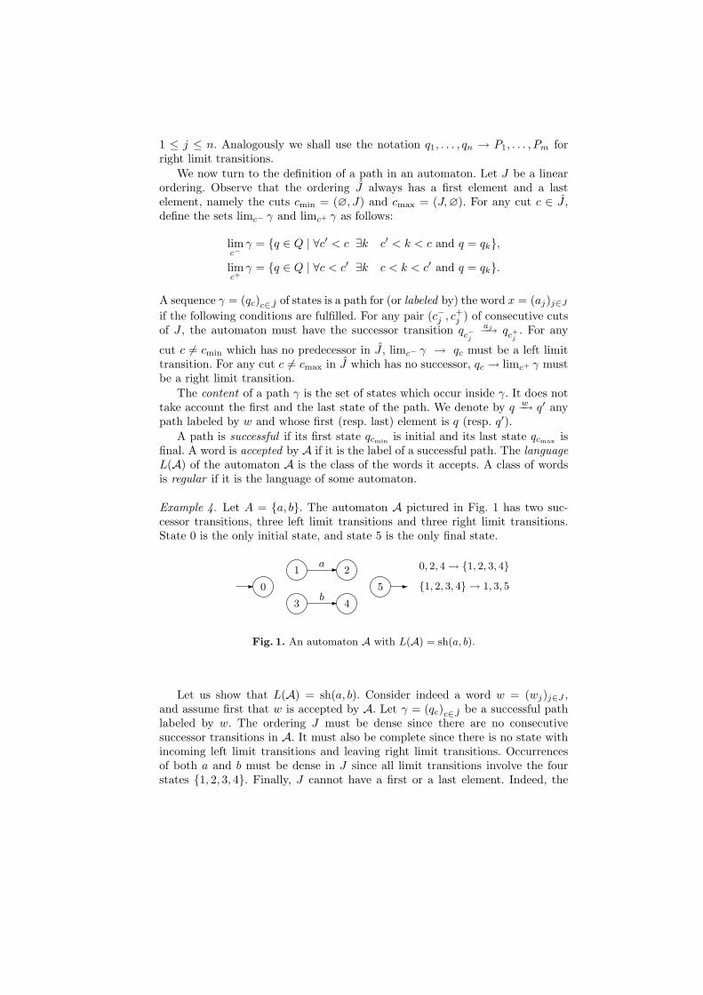
Example 4. Let A = {a, b}. The automaton A pictured in Fig. 1 has two suc-cessor transitions, three left limit transitions and three right limit transitions.State 0 is the only initial state, and state 5 is the only final state.

0

1 2

3 4

5

a

b

0, 2, 4 → {1, 2, 3, 4}

{1, 2, 3, 4} → 1, 3, 5

Fig. 1. An automaton A with L(A) = sh(a, b).

Let us show that L(A) = sh(a, b). Consider indeed a word w = (wj)j∈J ,and assume first that w is accepted by A. Let γ = (qc)c∈J be a successful pathlabeled by w. The ordering J must be dense since there are no consecutivesuccessor transitions in A. It must also be complete since there is no state withincoming left limit transitions and leaving right limit transitions. Occurrencesof both a and b must be dense in J since all limit transitions involve the fourstates {1, 2, 3, 4}. Finally, J cannot have a first or a last element. Indeed, the

only transition leaving state 0 is a limit one, and similarly for the only transitionentering state 5.

Conversely, let w = (wj)j∈J be a word indexed by a complete ordering Jwithout first and last element, and such that occurrences of both a and b aredense in J . Since J is complete, any cut of J (apart from cmin and cmax) iseither preceded or followed by a letter. Then the sequence γ = (qc)c∈J definedas follows is a successful path labeled by w.

– qcmin= 0,

– qcmax= 5,

– qc = 1 if c is followed by an a and qc = 2 if c is preceded by an a,

– qc = 3 if c is followed by a b and qc = 4 if c is preceded by a b.

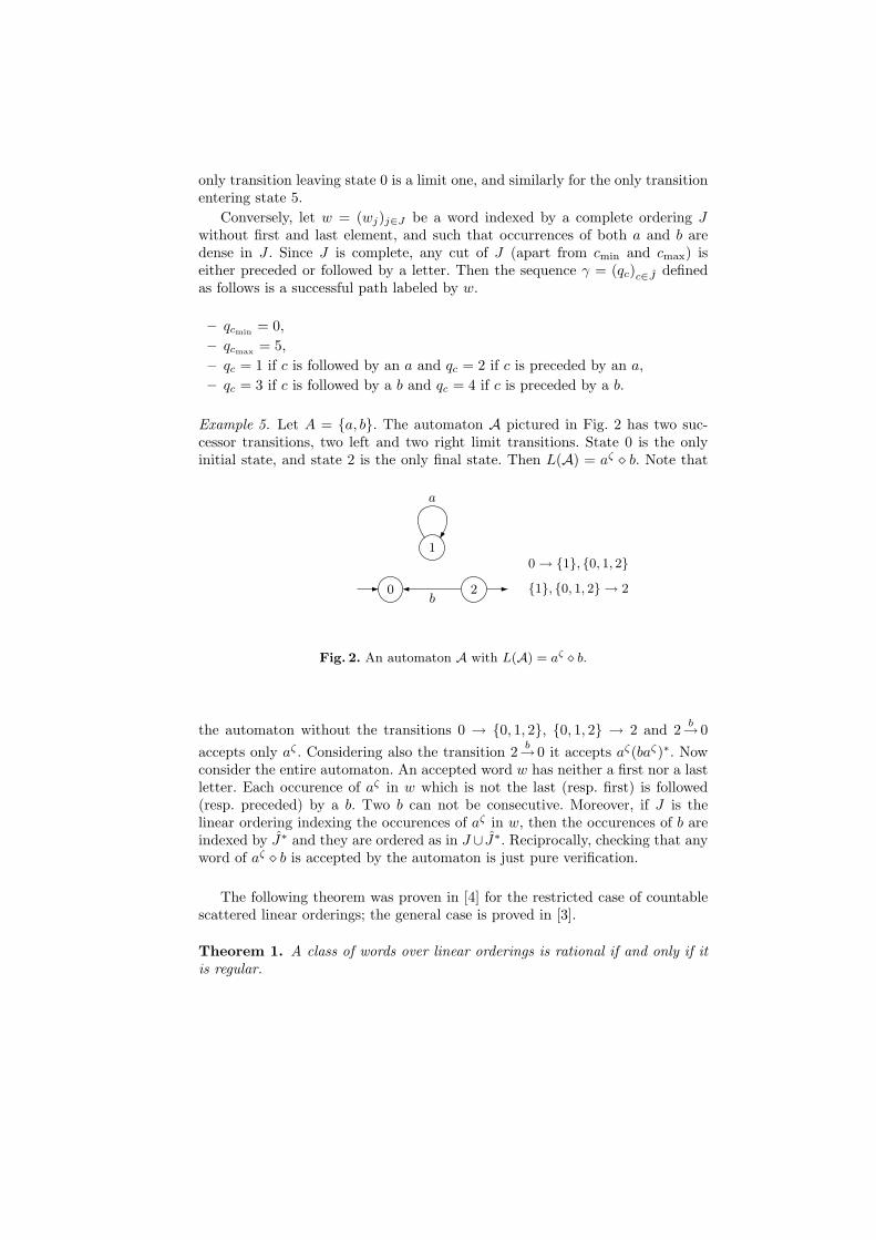
Example 5. Let A = {a, b}. The automaton A pictured in Fig. 2 has two suc-cessor transitions, two left and two right limit transitions. State 0 is the onlyinitial state, and state 2 is the only final state. Then L(A) = aζ ⋄ b. Note that

0

1

2b

a

0 → {1}, {0, 1, 2}

{1}, {0, 1, 2} → 2

Fig. 2. An automaton A with L(A) = aζ ⋄ b.

the automaton without the transitions 0 → {0, 1, 2}, {0, 1, 2} → 2 and 2b→ 0

accepts only aζ . Considering also the transition 2b→ 0 it accepts aζ(baζ)∗. Now

consider the entire automaton. An accepted word w has neither a first nor a lastletter. Each occurence of aζ in w which is not the last (resp. first) is followed(resp. preceded) by a b. Two b can not be consecutive. Moreover, if J is thelinear ordering indexing the occurences of aζ in w, then the occurences of b areindexed by J∗ and they are ordered as in J ∪ J∗. Reciprocally, checking that anyword of aζ ⋄ b is accepted by the automaton is just pure verification.

The following theorem was proven in [4] for the restricted case of countablescattered linear orderings; the general case is proved in [3].

Theorem 1. A class of words over linear orderings is rational if and only if itis regular.

2.4 Monadic Second-Order Logic

Let us recall useful elements of monadic second-order logic, and settle somenotations. For more details about MSO logic we refer e.g. to Thomas’ surveypaper [28].

Monadic second-order logic is an extension of first-order logic that allows toquantify over elements as well as subsets of the domain of the structure. Givena signature L, one can define the set of MSO-formulas over L as well-formedformulas that can use first-order variable symbols x, y, . . . interpreted as elementsof the domain of the structure, monadic second-order variable symbols X,Y, . . .interpreted as subsets of the domain, symbols from L, and a new binary predicatex ∈ X interpreted as “x belongs to X”. We call MSO sentence any MSO formulawithout free variable. As usual, we will often confuse logical symbols with theirinterpretation. Moreover we will use freely abbreviations such as ∃x ∈ X ϕ,∀X ⊆ Y ϕ, ∃!tϕ, and so on.

Given a signature L and an L−structure M with domain D, we say that arelation R ⊆ Dm × (2D)n is MSO-definable in M if and only if there exists anMSO-formula over L, say ϕ(x1, . . . , xm,X1, . . . ,Xn), which is true in M if andonly if (x1, . . . , xm,X1, . . . ,Xn) is interpreted by an (m+ n)−tuple of R.

Given a finite alphabet A, let us consider the signature LA = {<, (Pa)a∈A}where < is a binary relation symbol and the Pa’s are unary predicates (over first-order variables). One can associate to every word w = (aj)j∈J over A (where aj ∈A for every j) the LA−structure Mw = (J ;<; (Pa)a∈A) where < is interpretedas the ordering over J , and Pa(x) holds if and only if ax = a. In order to takeinto account the case w = ε, which leads to the structure Mε which has anempty domain, we will allow structures to be empty. Given an MSO sentence ϕover the signature LA, we define the language Lϕ as the class of words w overA such that Mw |= ϕ. We will say that a language L over A is definable in MSOlogic (or MSO-definable) if and only if there exists an MSO-sentence ϕ over thesignature LA such that L = Lϕ.

Example 6. In this example we assume the axiom of choice. Let A = {a, b} and Lbe the class of words w over A such that w contains a sub-sequence of a indexedby ω. Then L is the language of the following MSO-sentence ϕ:

ϕ ≡∃X((∃x x ∈ X) ∧ ∀x(x ∈ X ⇒ (Pa(x) ∧ ∃y (y ∈ X ∧ x < y))))

If w ∈ L then choose X to be the positions of the letters of the sub-sequence.Then X is not empty, each element of X is the index of a letter a and as Xis isomorphic to ω it has no last element. Thus Mw |= ϕ. Conversely assumethat w is such that Mw |= ϕ. Then w contains a non-empty ordered set X ofelements all labeled by a and that contains no last element. As a consequence ofthe axiom of choice, an ordered sub-sequence of type ω can be extracted fromX.

3 Rational languages are MSO-definable

3.1 Introduction and examples

Buchi’s proof [8] that every rational language L of finite words is definable inMSO logic relies on the encoding of an accepting run of an automaton A rec-ognizing L. Given a word w, one expresses the existence of a successful path inA labeled by w, by encoding each state of the path on a position of w, which ispossible because - up to a finite number of elements - the underlying ordering ofthe path is the same as the one of the word. This property still holds when oneconsiders infinite words of length ω, and more generally of any ordinal length.However it does not hold anymore for words indexed by all linear orderings,since for a word of length J , the path of the automaton is defined on the set J ofcuts of J , and in general J can be quite different from J - consider e.g. the caseJ = Q for which J is countable while J is not. Thus in our situation there seemsto be no natural extension of the classical Buchi’s encoding technique. In orderto overcome this issue, we use a proof by induction over rational expressions.

Proposition 1. (Assuming the Axiom of Choice) For every finite alphabet Aand every language L ⊆ A⋄, if L is rational then it is definable in monadicsecond-order logic.

Let us give a quick outline of the proof. One proves that for every rationallanguage L there exists an MSO formula ϕ(X) over the signature LA such thatfor every word w over A indexed by some linear ordering J , we have w ∈ L ifand only if Mw satisfies ϕ when X is interpreted as an interval of J . This yieldsProposition 1 since every rational language L can then be defined by the MSOsentence

∃X(ϕ(X) ∧ ∀x x ∈ X).

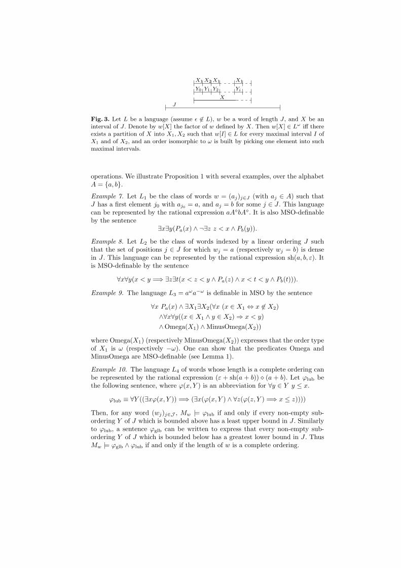
The proof proceeds by induction on a rational expression denoting L; this ap-proach is not new, see e.g. [15] where it is used in the case of finite words. Thecase of the empty word, as well as the one of singletons, union and productoperations, are easy. For the other rational operations one has to find a way toexpress that the interval X can be partitioned in some way in intervals. Considerfor instance the case of the ω-power operation. Assume that L is definable bythe MSO formula ϕ(X). Then Lω could be defined by an MSO formula whichexpresses the existence of a partition of X in a sequence (Yi)i∈ω of intervals Yi

such that ϕ(Yi) holds for every i. Since the existence of such a partition cannotbe expressed directly in MSO, one reformulates this property as the existenceof a partition of X in two subsets X1,X2 such that every Yi corresponds to aninterval, maximal for inclusion, which consists in elements of X1 only, or ele-ments of X2 only (see Figure 3). These maximal intervals are definable in MSOin terms of X,X1 and X2, and moreover one can express that the order type ofthe sequence of these maximal intervals is ω. This allows to find an MSO for-mula which defines Lω. The idea of interleaving finitely many subsets in orderto encode some partition of X in intervals is also used for the other rational

J

X

Y0

X1

Y1

X2 X1

Y2 Yi

X1

Fig. 3. Let L be a language (assume ǫ 6∈ L), w be a word of length J , and X be aninterval of J . Denote by w[X] the factor of w defined by X. Then w[X] ∈ Lω iff thereexists a partition of X into X1, X2 such that w[I] ∈ L for every maximal interval I ofX1 and of X2, and an order isomorphic to ω is built by picking one element into suchmaximal intervals.

operations. We illustrate Proposition 1 with several examples, over the alphabetA = {a, b}.

Example 7. Let L1 be the class of words w = (aj)j∈J (with aj ∈ A) such thatJ has a first element j0 with aj0 = a, and aj = b for some j ∈ J . This languagecan be represented by the rational expression aA⋄bA⋄. It is also MSO-definableby the sentence

∃x∃y(Pa(x) ∧ ¬∃z z < x ∧ Pb(y)).

Example 8. Let L2 be the class of words indexed by a linear ordering J suchthat the set of positions j ∈ J for which wj = a (respectively wj = b) is densein J . This language can be represented by the rational expression sh(a, b, ε). Itis MSO-definable by the sentence

∀x∀y(x < y =⇒ ∃z∃t(x < z < y ∧ Pa(z) ∧ x < t < y ∧ Pb(t))).

Example 9. The language L3 = aωa−ω is definable in MSO by the sentence

∀x Pa(x) ∧ ∃X1∃X2(∀x (x ∈ X1 ⇔ x 6∈ X2)

∧∀x∀y((x ∈ X1 ∧ y ∈ X2) ⇒ x < y)

∧Omega(X1) ∧ MinusOmega(X2))

where Omega(X1) (respectively MinusOmega(X2)) expresses that the order typeof X1 is ω (respectively −ω). One can show that the predicates Omega andMinusOmega are MSO-definable (see Lemma 1).

Example 10. The language L4 of words whose length is a complete ordering canbe represented by the rational expression (ε + sh(a + b)) ⋄ (a + b). Let ϕlub bethe following sentence, where ϕ(x, Y ) is an abbreviation for ∀y ∈ Y y ≤ x.

ϕlub ≡ ∀Y ((∃xϕ(x, Y )) =⇒ (∃x(ϕ(x, Y ) ∧ ∀z(ϕ(z, Y ) =⇒ x ≤ z))))

Then, for any word (wj)j∈J , Mw |= ϕlub if and only if every non-empty sub-ordering Y of J which is bounded above has a least upper bound in J . Similarlyto ϕlub, a sentence ϕglb can be written to express that every non-empty sub-ordering Y of J which is bounded below has a greatest lower bound in J . ThusMw |= ϕglb ∧ ϕlub if and only if the length of w is a complete ordering.

Example 11. Consider the language L5 of words over A whose length is a non-scattered ordering. It follows from [22, chap. 4] that L5 consists in words w whichcan be written as w =

∏

k∈K wk where K is a dense ordering, and wk 6= ε forevery k ∈ K. From this decomposition one can deduce that a convenient rationalexpression for L5 is sh(A⋄(a+ b)A⋄, ε). The language L5 can also be defined bythe following MSO formula

∃X(∃x1 ∈ X ∃x2 ∈ X x1 < x2

∧∀y1 ∈ X ∀y2 ∈ X(y1 < y2 =⇒ ∃z z ∈ X ∧ (y1 < z ∧ z < y2))).

3.2 Proof of Proposition 1

We shall prove that for every rational language L there exists an MSO formulaϕ(X) in the language LA such that for every word w = (wj)j∈J where wj ∈ A,then w ∈ L if and only if Mw satisfies ϕ when X is interpreted by J .

This will yield Proposition 1 since every rational language L can then bedefined by the MSO sentence ∃X(ϕ(X) ∧ ∀x x ∈ X).

The proof proceeds by induction on a rational expression denoting L.The following lemma provides auxiliary predicates which will be useful later.

Lemma 1. Let L = {<} be a language where < is interpreted as a linear order-ing over the domain of the structure. The following relations are MSO-definablein the language LA.

– The relations x = y, x ≤ y, x ∈ [y; z], X = ∅, X ⊆ Y , x ∈ Y ∩Z, x ∈ Y \Z;– “x, y are consecutive elements of Z”, denoted by Consec(x, y, Z)– “X is an interval”, denoted by Interval(X)– “X is maximal among the intervals contained in Y ”, denoted byX ⊆max Y

– “X is an ordinal”, denoted by Ord(X)– “X is an ordinal less than or equal to ω“, denoted by Ord≤ω(X)– “X is a finite ordinal”, denoted by Ordfin(X)– “X equals ω”, denoted by Omega(X)– “T is contained in X, and every maximal interval of X contains exactly one

element of T”, denoted by Trace(X,T )– “X is complete”, denoted by Complete(X)– Given n ≥ 1, the relation “X1, . . . ,Xn form a partition of X”, denoted by

Partition(X,X1, . . . ,Xn). We shall “overload” the predicate symbol Partitionand use it with several values of n.

– “X is the sum of Y and Z” denoted by X = Y + Z.

Proof. We give below the formal definitions for each relation, except for therelations of the first item.

– x ∈ [y; z] : y ≤ x ≤ z ∨ z ≤ x ≤ y– Consec(x, y, Z) : x ∈ Z ∧ y ∈ Z ∧ x < y ∧ ¬∃z ∈ Z(x < z ∧ z < y)– Interval(X) : ∀x, x′ ∈ X(∀y x ≤ y ≤ x′ =⇒ y ∈ X)

– X ⊆max Y :

Interval(X) ∧X ⊆ Y ∧X 6= ∅ ∧ ∀y ∈ (Y \X) ∀x ∈ X ∃z 6∈ Y z ∈ [x; y]

– Ord(X) : ∀Y ⊆ X (Y 6= ∅ =⇒ ∃y ∈ Y ∀y′ ∈ Y y ≤ y′)– Ord≤ω(X) :

Ord(X)∧∀x ∈ X((∀y ∈ X x ≤ y)∨∃z ∈ X (z < x∧∀y ∈ X (y < x =⇒ y ≤ z))

(i.e., every x ∈ X is either the first element of X or has a predecessor in X)– Ordfin(X) : Ord≤ω(X) ∧ ∃y ∈ X∀z ∈ X(z ≤ y)– Omega(X) : Ord≤ω(X) ∧ ¬Ordfin(X)– Trace(X,T ) : T ⊆ X ∧ (∀x ∈ X ∃!t ∈ T ∀x′ ∈ [x; t] x′ ∈ X)– Complete(X) :

∀Y ⊆ X((∃x ∈ X ϕ(x, Y )) =⇒ (∃x ∈ X(ϕ(x, Y )∧∀z ∈ X(ϕ(z, Y ) =⇒ x ≤ z))))

where ϕ(x, Y ) is an abbreviation for ∀y ∈ Y y ≤ x– Partition(X,X1, . . . ,Xn) :

∧

1≤i≤n

Xi ⊆ X ∧∧

1≤i<j≤n

Xi ∩Xj = ∅ ∧ ∀x ∈ X∨

1≤i≤n

x ∈ Xi

– X = Y + Z : Partition(X,Y,Z) ∧ ∀y∀z((y ∈ Y ∧ z ∈ Z) ⇒ y < z).

We now start the proof of Proposition 1, by induction on a rational expressiondenoting L. Note that L = ∅ is obviously MSO-definable.

Empty word. The language L = {ε} is defined by the formula

ϕ(X) : ¬∃x ∈ X

Singletons. For every a ∈ A, the language {a} is defined by the formula

ϕ(X) : ∃x ∈ X(Pa(x) ∧ ∀x′ ∈ X x′ = x)

Product operation. Assume that L1, L2 are languages defined by the MSOformulas ϕ1(X), ϕ2(X), respectively. Then the language L1 ·L2 is defined by theformula

ϕ(X) : ∃X1∃X2(X = X1 +X2 ∧ ϕ1(X1) ∧ ϕ2(X2)).

Star operation. Assume that L1 is defined by the MSO formula ψ(X). Let usfind an MSO formula which defines the language L = L∗

1.Consider first the case where ε 6∈ L1 and L1 6= ∅. Then by definition a

word w belongs to L if and only if it can be written as w =∏

i∈I wi where I isfinite and all wi’s are non-empty words which belong to L1. The MSO-formulawhich defines L expresses this property as the existence a partition of X intotwo subsets X1,X2 such that each interval I of X which is maximal among

subsets of X1 (resp. X2) corresponds to one of the subwords wi of w. Moreover,in order to express that there are finitely many such maximal intervals, theformula states the existence of two subsets T1, T2 of X such that every maximalinterval I ⊆ X1 (resp. I ⊆ X2) contains exactly one element of T1 (resp. T2), andsuch that T1∪T2 is finite. It is easy to check that these properties are equivalentto w ∈ L∗

1.This leads to define the language L by the formula

ϕ(X) : ∃X1∃X2∃T1∃T2

(Partition(X,X1,X2) ∧ Trace(X1, T1) ∧ Trace(X2, T2) ∧ Ordfin(T1 ∪ T2)

∧∀U((U ⊆max X1 ∨ U ⊆max X2) ⇒ ψ(U)).

The case L = ∅ is trivial, and the case where ε ∈ L can be handled byconsidering the formula ϕ′(X) : ϕ(X) ∨ ¬∃x ∈ X.

Power operations. The language Lω (respectively L♯) is defined using thesame ideas as above, except that the formula Ordfin(T1 ∪T2) has to be replacedby Omega(T1 ∪ T2) (respectively Ord(T1 ∪ T2)). The cases of L−ω and L−♯ aresimilar.

Diamond operation. Assume that L1, L2 are languages defined by the MSOformulas ϕ1(X), ϕ2(X), respectively. We shall find a formula that defines thelanguage L = L1 ⋄ L2. We have to consider several cases depending on whetherε belongs to L1 and L2.

First case: ε 6∈ L1 ∪ L2. In this case we use the following lemma from [3],which gives necessary and sufficient conditions which ensure that a partition(J, J ′) of an ordering K satisfies J ′ = J∗. We recall the proof for the convenienceof the reader.

Lemma 2. Let K be a complete linear ordering, and let (J, J ′) be a partition ofK. Assume that

– if K has a first (resp. last) element then it belongs to J ;– any non-first and non-last element of J has a predecessor and successor

in J ′;– the first (resp. last) element of J , if it exists, has a successor (resp. prede-

cessor) in J ′;– there is at least one element of J between two elements of J ′.

Then J ′ equals J∗, that is K = J ∪ J∗.

Note that one checks easily that the converse of Lemma 2 holds.

Proof. We define a function f from K into J ∪ J∗ as follows. For any k ∈ K,define

f(k) =

{

k if k ∈ J(

{j ∈ J | j < k}, {j ∈ J | k < j})

if k ∈ J ′.

Since J ∩ J ′ = ∅ and K = J ∪ J ′, the function f is well defined. The restrictionof f to J is the identity. The image of an element of J ′ is a cut of J . Thereforef is a function from K into J ∪ J∗.

We claim that the function f is one-to-one. We first show that k 6= k′ impliesf(k) 6= f(k′). If k ∈ J or k′ ∈ J , the result is trivial. Suppose then that k, k′ ∈ J ′

and that k < k′. By our second hypothesis there exists j′ ∈ J such that k <j′ < k′, which implies {j ∈ J | j < k} 6= ({j ∈ J | j < k′}, thus f(k) 6= f(k′).

We now prove that the function f is onto. It is clear that J ⊆ f(K). Let(L,M) ∈ J∗. We claim that there is k ∈ J ′ such that (L,M) = f(k). Define thetwo elements l and m of K by l = sup(L) and m = inf(M). If l belongs to L, ithas a successor k in J ′ and one has (L,M) = f(k). If m belongs to M , it hasa predecessor k in J ′ and one has (L,M) = f(k). If l and m do not belong toL and M , they belong to J ′ and their image by f is the cut (L,M). Since f isone-to-one, l and m are equal.

Lemma 2 allows to define the language L1 ⋄ L2 in MSO logic, by expressingthat there exists a partition of X into two subsets X1,X2 such that the set ofmaximal intervals of X1 or X2 has an underlying ordering of the form J ∪ J∗,where J (resp. J∗) is the ordering of maximal intervals of X1 (resp. X2), andeach maximal interval of X1 (resp. X2) corresponds to a subword of w whichbelongs to L1 (resp. L2).

Let us give a formal definition:

ϕ(X) : ∃X1∃X2∃T1∃T2 (Complete(T1 ∪ T2) (1)

∧Partition(X,X1,X2) ∧ Trace(X1, T1) ∧ Trace(X2, T2) (2)

∧∀U ⊆max X1 ϕ1(U) (3)

∧∀U ⊆max X2 ϕ2(U) (4)

∧∀t ∈ T1 (∃u ∈ T1 ∪ T2 u < t) ⇒ (∃u ∈ T2 Consec(u, t, T1 ∪ T2)) (5)

∧∀t ∈ T1 (∃u ∈ T1 ∪ T2 t < u) ⇒ (∃u ∈ T2 Consec(t, u, T1 ∪ T2)) (6)

∧∀u1 ∈ T2 ∀u2 ∈ T2 (u1 < u2 ⇒ ∃t ∈ T1 (u1 < t < u2))) (7)

∧∀t ∈ (T1 ∪ T2)((∀u ∈ (T1 ∪ T2) t ≤ u) ⇒ t ∈ T1) (8)

∧∀t ∈ (T1 ∪ T2)((∀u ∈ (T1 ∪ T2) u ≤ t) ⇒ t ∈ T1)) (9)

Lines (5), (6) and (7) express the conditions of Lemma 2 for the orderings T1

and T2, while line (8) (respectively (9)) expresses that if T1∪T2 has a first (resp.last) element then it belongs to T1; this allows to take into account the fact thatwe deal with an ordering of the form J ∪ J∗ and not J ∪ J .

Second case: ε ∈ L1 and ε 6∈ L2. This case can be handled by proving a vari-ant of Lemma 2. Indeed we have w ∈ L1⋄L2 if and only if w satisfies the followingcondition, which we denote by (C1): w can be written as w =

∏

k∈K wk whereK is a complete ordering and there exists a partition of K in two subsets J1, J2

such that

– wk 6= ε for every k ∈ K;

– wk ∈ L1 if k ∈ J1, and wk ∈ L2 if k ∈ J2;– every element of J1 which is not the first (resp. last) element of K admits a

predecessor (resp. successor) which belongs to J2;– K does not contain any dense interval consisting only in elements of J2.

Indeed assume first that w ∈ L1 ⋄ L2. By definition w can be written asw =

∏

j∈J∪J∗ wj ; where wj ∈ L1 if j ∈ J and wj ∈ L2 if j ∈ J∗. If one

removes from J ∪ J∗ all elements j ∈ J such that wj = ε, one can re-write w as

w =∏

j∈J1∪J2wj where J2 = J∗, and J1 corresponds to the remaining elements

of J . Let us prove that the set K = J1 ∪ J2 and the partition (J1, J2) satisfy(C1). It is easy to check that K is complete, and that every element of K whichbelongs to J1 has a predecessor and a successor which belong to J2. Moreover letus show that every dense interval I of K contains at least an element of J1. Letx, y be two elements of I such that x < y. If x or y belong to J1 then the resultfollows. Now if both x, y belong to J2 = J∗, then x and y correspond to differentcuts of J , which implies that there exists in J ∪ J∗ an element z ∈ J between xand y. Let us prove that z ∈ J1, which will yield the result since z ∈ I. Assumefor a contradiction that z 6∈ J1. The element z admits in J ∪ J∗ a predecessor x′

and a successor y′ which both belong to J∗, that is to J2. In this case x′ and y′,seen as elements of K = J1 ∪J2, become consecutive elements, which contradictthe fact that I is a dense interval of K.

Conversely assume that w =∏

k∈K wk, where K is a complete ordering andthere exists a partition of K in two subsets J1, J2 satisfying condition (C1). Letus add to K a new element of J1 between every pair of elements of J2 which areconsecutive in K, and also (if necessary) elements of J1 at both extremities of K.This gives rise to a set K ′ and a partition (J ′

1, J′2) of K ′ such that J ′

1 correspondsto the union of J1 and the new elements, and J ′

2 = J2. If we associate to everynew element the empty word, we can re-write w as w =

∏

k∈K′ wk where K ′

is complete, wk ∈ L1 if k ∈ J ′1, and wk ∈ L2 if k ∈ J ′

2. Let us prove that

J ′2 = J ′

∗

1. By Lemma 2 it suffices to prove, on one hand, that every element ofJ ′

1, apart from the first (resp. last) element of K if it exists, admits a predecessor(resp. successor) in J ′

2, and on the other hand that between two elements of J ′2

there exists at least an element of J ′1. The first fact follows easily from the

construction of J ′1. For the second fact, assume for a contradiction that there

exist two elements x, y ∈ J ′2 with x < y such that the interval [x, y] does not

contain any element of J ′1. By our hypothesis on J2 = J ′

2, the interval [x, y], seenas an interval of K, cannot be dense, thus it contains two consecutive elementsx′ < y′ which both belong to J2. This implies by definition of J ′

1 that there exists(in K ′) an element of J ′

1 between x′ and y′, that is between x and y, which leadsto a contradiction.

We proved that w ∈ L1 ⋄ L2 if and only if w satisfies (C1). It remains toprove that (C1) can be expressed with a MSO-formula, which can be done easilyusing ideas similar to the first case.

Third case: ε 6∈ L1 and ε ∈ L2. This case is similar to the previous one. Inthis case we have w ∈ L1 ⋄ L2 if and only if w satisfies the following conditions,

which we denote by (C2): w can be written as w =∏

k∈K wk where K is anyordering and there exists a partition of K in two subsets J1, J2 such that

– wk 6= ε for every k ∈ K;– wk ∈ L1 if k ∈ J1, and wk ∈ L2 if k ∈ J2;– between two elements of J2 there exists at least an element of J1;– if K has a first (resp. last) element then it belongs to J1.

Indeed assume first that w ∈ L1 ⋄ L2. By definition w can be written asw =

∏

j∈J∪J∗ wj where wj ∈ L1 if j ∈ J and wj ∈ L2 if j ∈ J∗. If one

removes from J ∪ J∗ all elements j ∈ J∗ such that wj = ε, one can re-write w asw =

∏

j∈J1∪J2wj where J1 = J and J2 corresponds to the remaining elements

of J∗. It is easy to check that J1 and J2 satisfy the properties required in (C2).Conversely assume that w =

∏

k∈K wk, where K is a complete ordering andthere exists a partition of K into two subsets J1, J2 satisfying condition (C2).We shall add elements to J2 in order to fill gaps in J1∪J2. For each cut (K1,K2)of J1 ∪ J2 such that K1 does not admit a last element in J2 and K2 does notadmit a first element in J2, we add to K a new element of J2 between K1 andK2. This gives rise to a set K ′ and a partition (J ′

1, J′2) of K ′ such that J ′

1 = J1,and J ′

2 corresponds to the union of J2 and the new elements. If we associate toevery new element the empty word, we can re-write w as w =

∏

k∈K′ wk whereK ′ is complete, wk ∈ L1 if k ∈ J ′

1, and wk ∈ L2 if k ∈ J ′2. It follows from the

construction of J ′2 that J ′

2 = J ′∗

1. This proves that w ∈ L1 ⋄ L2.We proved that w ∈ L1 ⋄ L2 if and only if w satisfies (C2). It remains to

prove that (C2) can be expressed with a MSO-formula, which again can be doneeasily using ideas similar to the first case.

Fourth case: ε ∈ L1 ∩ L2. In this case we have w ∈ L1 ⋄ L2 if and only ifw satisfies the following conditions, which we denote by (C3): w can be writtenas w =

∏

k∈K wk where K is any ordering and wk is a non empty word whichbelongs to L1 ∪ L2 for every k ∈ K.

As in the previous cases, it is easy to check that if w ∈ L1⋄L2 then w satisfies(C3). Conversely assume that w =

∏

k∈K wk for some ordering K. Let (J1, J2)be the partition of K such that wk ∈ J1 if and only if k ∈ L1. We proceed ina similar way as in the two previous cases. First, as in the second case, we adda new element of J1 between every pair of elements of J2 which are consecutivein K, and also (if necessary) elements of J1 at both extremities of K. Then, asin the third case, for each cut (K1,K2) of J1 ∪ J2 such that K1 does not admita last element in J2 and K2 does not admit a first element in J2, we add a newelement of J2 between K1 and K2. These two steps give rise to a set K ′ anda partition (J ′

1, J′2) of K ′ such that J ′

1 corresponds to the union of J1 and thenew elements added during the first step, and J ′

2 corresponds to the union ofJ2 and the new elements added during the second step. If we associate to allnew elements the empty word, we can re-write w as w =

∏

k∈K′ wk where K ′

is complete, wk ∈ L1 if k ∈ J ′1, and wk ∈ L2 if k ∈ J ′

2. Using ideas from the

previous cases one can check that J ′2 = J ′

∗

1. This proves that w ∈ L1 ⋄ L2.It is easy to express condition (C3) in MSO.

This completes the proof that L1 ⋄ L2 is definable in MSO.

Shuffle operation. Let n ≥ 1, and assume that L1, . . . , Ln are languages de-fined by the MSO formulas ϕ1(X), . . . , ϕn(X), respectively. We shall find a for-mula that defines the language L = sh(L1, . . . , Ln). We have to consider againseveral cases depending on whether ε belongs to some of the Li’s.

First case: ε 6∈⋃

i Li. In this case the language L can be defined by a formulawhich expresses in a direct way the definition of the shuffle operation. Here issuch a formula:

ϕ(X) : ∃X1 . . . ∃Xn∃T1 . . . ∃Tn∃T

(Partition(X,X1, . . . ,Xn) ∧∧

1≤i≤n

Trace(Xi, Ti) ∧ T =⋃

1≤i≤n

Ti ∧ Complete(T )

∧ ∀x ∈ T (∃y1 ∈ T y1 < x ∧ ∃y2 ∈ T x < y2)

∧ ∀x, y ∈ T (x < y =⇒∧

1≤i≤n

(∃z ∈ Ti x < z < y))

∧∧

1≤i≤n

(∀U ⊆max Xi ϕi(U)) )

Second case: there exists i such that ε ∈ Li. In the sequel assume withoutloss of generality that there exists k such that for every i we have ε ∈ Li if andonly if i ≤ k.

We need the following lemma (see e.g. [24]). We denote by |Z| the cardinalityof Z.

Lemma 3. (Assuming the Axiom of Choice) Let X be a non-empty dense setand let n ≥ 1 be a natural number. There exists a partition of X into n subsetsX1, . . . ,Xn which are dense in X.

Proof. It suffices to prove the case n = 2.Consider the binary relation ≡ defined on X as follows: given x, y ∈ X, x ≡ y

if and only if

– x = y, or– x 6= y and there exist x′, y′ ∈ X such that x′ < [x; y] < y′ and for everya, b ∈]x′; y′[ with a < b we have |[a; b]| = |[x; y]|.

It is easy to check that ≡ is a condensation, i.e. an equivalence relation whoseequivalence classes are intervals of X. We shall choose, in each equivalence classof ≡, which elements belong to X1 (respectively X2).

Given an equivalence class x/≡ which contains more than one element, allintervals [a, b] such that a < b and a, b belong to x/≡ have (by definition of ≡)the same cardinality, say λ. The cardinal λ is infinite since X is dense; moreoverwe have λ ≤ |x/≡ |.

Assume first that λ = |x/≡ |. Consider an enumeration {(ai, bi) : i < λ}of pairs of elements of x/≡ such that ai < bi. We define by induction on i

two sequences (x1i )i<λ and (x2

i )i<λ as follows: set x10 = a0 and x2

0 = b0. Thenassuming that x1

i and x2i are defined for every i < j, choose for x1

j any element

of the set [aj , bj ] \ ({x1i : i < j}∪ {x2

i : i < j}), and for x2j any element of the set

[aj , bj ]\({x1i : i ≤ j}∪{x2

i : i < j}). This is always possible since |[aj , bj ]| = λ bythe very definition of ≡, and λ is infinite. Finally we add elements of the sequence(x1

i )i<λ (resp. (x2i )i<λ) to the set X1 (resp. X2). It is clear that X1 ∩ x/≡ and

X2 ∩ x/≡ are dense in x/≡.Consider now the case λ < |x/≡ |. Then it is not difficult to prove that there

exists a partition of |x/ ≡ | into (λ+) intervals of cardinal λ, and we can applyagain the above construction to each such interval.

Finally we add to X1 all elements of X which were not included into X1∪X2

up to now (in particular, all x ∈ X such that |x/≡ | = 1).Let us show that X1 and X2 are dense in X. Consider a, b ∈ X such that

a < b. Let γ be the least cardinal of an interval [a′, b′] ⊆ [a, b] with a′ < b′. Thefact that X is dense ensures that such an interval exists and that γ is infinite.Any non-singleton interval included in [a′, b′] has cardinality γ, which impliesthat a′ ≡ b′, and the previous construction ensures that [a′, b′] has a non-emptyintersection with X1 and X2.

The following lemma gives a necessary and sufficient condition which ensuresthat w ∈ sh(L1, . . . , Ln) in case at least one of the Li’s contain the emptyword. We define the completion of an ordering Z, and denote by Z, the minimalcomplete ordering which contains Z.

Lemma 4. For every word w ∈ A⋄, we have w ∈ sh(L1, . . . , Ln) if and only ifthere exists an ordering J and a partition J1, . . . , Jn of J such that w can bewritten as w =

∏

j∈J wj where

– J has neither first nor last element;– for every j ∈ J , j ∈ Ji if and only if wj ∈ Li;– for every i > k, the set Ji is dense in J ;– for every interval I of J such that I ∩Ji = ∅ for some i ≤ k, the set of gaps

of I is dense in the completion of I.

Proof. Assume first that w satisfies the hypotheses of Lemma 4. We add elementsto J in such a way that the resulting ordering satisfies the conditions given inthe definition of the shuffle. More precisely consider the completion J ′ = J . Weprove that there exist a partition J ′

1, . . . , J′n of J such that

– w =∏

j∈J ′ w′j where w′

j = wj for every j ∈ J , and w′j = ε for every j ∈ J ′\J ;

– Ji ⊆ J ′i for every i ≤ k, and J ′

i = Ji for every i > k;– J ′

i is dense in J ′ for every i;– w′

j ∈ Li if and only if j ∈ J ′i .

We start by setting J ′i = Ji for every i. We shall add each element of J ′ \ J

to one of the sets J ′1, . . . , J

′k. Consider the binary relation ∼ defined on J as

follows: given x, y ∈ J , x ∼ y if and only if

– x = y, or– x 6= y and

1. either every Ji is dense in the interval [x; y]2. or for every interval I ⊆ [x; y] there exists i such that Ji ∩ I is not dense

in I

One checks easily that ∼ is a condensation. Let I ⊆ J be an equivalence class of∼ with more than one element. If I arises from case (1) above, then we chooseto add every gap x of I to the subset J ′

1, and set w′x = ε. If I arises from case (2)

above, then by definition of ∼ and the hypotheses of Lemma 4, the set of gaps ofI is dense in its completion. Thus by Lemma 3 there exists a partition of (I \ I)into n dense subsets X1, . . . ,Xn. We choose to add every gap x of I to the subsetJ ′

i such that x ∈ Xi, and we set w′x = ε. One checks that the sets J ′

1, . . . , J′n

satisfy the required properties, which ensures that w ∈ sh(L1, . . . , Ln).Conversely if w ∈ sh(L1, . . . , Ln) then w can be written as w =

∏

j∈J wj

where J satisfies the conditions required in the definition of the shuffle operation.By removing from J all elements j such that wj = ε, one can re-write w asw =

∏

j∈J ′ wj where J ′ ⊆ J and wj 6= ε. Now if we set J ′i = Ji ∩ J

′ for everyi, then one can check that the set J ′ and the partition (J ′

1, . . . , J′n) of J ′ satisfy

the hypotheses of the lemma.

In order to complete the proof that sh(L1, . . . , Ln) is MSO-definable, it suf-fices to prove that there exists a MSO-formula which expresses the propertiesrequired in the statement of the above lemma. Since this formula is a variant ofthe one given in the first case, we leave this task to the reader.

This concludes the proof of Proposition 1.Combining Proposition 1 and Rabin’s result [19] about the decidability of

the MSO theory of countable linear orderings yields the following result.

Corollary 1. The inclusion problem for rational languages of words over count-able linear orderings is decidable.

Proof. Assume that A = {a1, . . . , an}, and let L1, L2 be two rational languagesof words over A indexed by countable orderings. By Proposition 1, one canconstruct effectively from L1 and L2 two MSO-formulas ϕ1(X) and ϕ2(X) whichrespectively define L1 and L2.

Consider the MSO-sentence ψ defined as

∀X∀X1 . . . ∀Xn((Partition(X,X1, . . . ,Xn) ∧ ϕ′1(X)) ⇒ ϕ′

2(X))

where ϕ′1(X) (resp. ϕ′

2(X)) is obtained from ϕ1(X) (resp. ϕ2(X)) by replacingall atomic formulas of the form Pai

(x) by x ∈ Xi.It is easy to check that L1 ⊆ L2 if and only if ψ is true in the monadic

second order theory of countable linear orderings. Now by Rabin [19] this theoryis decidable, from which the result follows.

This improves [7] where the authors prove the result for languages of wordsover scattered countable linear orderings.

4 MSO-definable languages vs rational languages

In this section we consider the problem whether MSO-definable languages arerational. The answer is positive if we consider words indexed by countable scat-tered linear orderings. Indeed we can prove the following result.

Proposition 2. For every finite alphabet A and every language L of words overA indexed by countable scattered linear orderings, L is rational if and only if itis MSO-definable.

Proof. We give a sketch of the proof. The “only if” part comes from Proposi-tion 1, and the “if” part is a direct adaptation of Buchi’s proof [8], which goesby induction on a MSO-formula (in prenex form) defining L. The crucial argu-ment here is that by [21] the class of rational languages of words on countablescattered linear orderings is closed under complementation. Let us recall quicklythe main arguments of the proof. We refer e.g. to [25] for more explanation.

First of all, we have to extend our notion of definable language to the case ofMSO formulas with free variables. Assume that ϕ(X1, . . . ,Xm, x1, . . . , xn) is anMSO formula whose free variables are X1, . . . ,Xm, x1, . . . , xn (the case wherethe free variables are only first-order variables, or only second-order variables,are handled similarly).

Then we associate with ϕ the language Lϕ defined as the class of words wover the alphabet {0, 1}m+n ×A such that:

– for every j ∈ [m + 1, n], there is exactly one symbol from w such that itsj−th component equals 1;

– Mw |= ϕ(X1, . . . ,Xm, x1, . . . , xn) where

• every Xi is interpreted as the set of positions in w carrying a lettera ∈ {0, 1}m+n ×A whose i−th component equals 1.

• every xj is interpreted as the only position in w carrying a letter whosej−th component equals 1.

• Pa(x) is interpreted as “the position x carries a symbol whose last com-ponent equals a”

With this definition, we can prove that every MSO formula ϕ defines a ra-tional language by induction on the construction of ϕ, which we can assume tobe in prenex form. It is easy to check that atomic formulas Pa(x), x < y, x ∈ Xdefine rational languages. The case ϕ = ϕ1 ∨ ϕ2 can be solved using the factthat the class of rational languages is closed under union and cylindrification.The case ϕ = ¬ϕ′ is handled thanks to the fact that by [21] the class of ratio-nal languages of words on countable scattered linear orderings is closed undercomplementation. Finally the closure of rational languages under projection (re-spectively projection and intersection) allows to deal with the case ϕ = ∃X ϕ′

(resp. ϕ = ∃x ϕ′).

The effectiveness of the previous construction, together with the decidabilityof the emptiness problem for automata on words indexed by countable scatteredlinear orderings [11], yield the following corollary.

Corollary 2. The monadic second order theory of countable scattered linearorderings is decidable.

Note that the latter result is also a direct consequence of Rabin’s result [19]about the decidability of the MSO theory of countable linear orderings (theproperty “to be scattered” is expressible in the latter theory).

Proposition 2 does not hold anymore if we consider languages of words in-dexed by all linear orderings. Indeed consider, for every finite alphabet A, thelanguage SA of words over A indexed by scattered linear orderings, i.e. the com-plement of the language L5 of Example 11. Since L5 is definable in MSO, thesame holds for SA. However the following holds.

Proposition 3. For every finite alphabet A, the language SA of words over Aindexed by scattered linear orderings is not rational.

Proof. By Theorem 1 it suffices to prove that SA is not regular.Let us introduce some useful vocabulary. An automaton A is said to be trim if

and only if every state and every transition of A appears in at least one successfulpath. If an automaton is not trim, it can easily be trimmed by removing anystate and any transition which does not appear in a successful path. The class ofwords recognized by the automaton is of course not changed by this operation.

By a slight abuse of language, a word is called scattered if its length is ascattered ordering.

The proof follows directly from the following two lemmas.

Lemma 5. Let A be a trim automaton such that there exist a left limit transitionP → p and a right limit transition q → P with p, q ∈ P . Then the automatonaccepts a non scattered word.

Proof. Since the automaton is trim, there is a path i u−→ q from an initial state ito q. There is also a path p w−→ f from p to a final state. There is also a pathp v−→ q whose content is exactly P . Then it is clear that the word x = uvRw isaccepted by the automaton.

Example 12. The automaton of Example 5 is trim. It accepts (aζb)R, which isnot scattered.

Let (xn)n≥0 be the sequence of words defined by induction by x0 = a andxn+1 = xζ

n. The length of the word xn is the ordering ζn. Note that each word xn

is scattered.

Lemma 6. If an automaton with m states accepts x2m+3, then it also acceptsa non scattered word.

Proof. By the previous lemma, it suffices to prove that there are two limit tran-sitions P → p and q → P with p, q ∈ P .

The ordering ζn is the ordering Jn = Zn of all the n-tuples (i1, . . . , in) ofrelative integers with the lexicographic ordering. This means that (i1, . . . , in) <

(j1, . . . , jn) if ik < jk where k is the least integer such that ik 6= jk. We say thatan r-tuple (i1, . . . , ir) is a prefix of a s-tuple (j1, . . . , js) if r ≤ s and ik = jk forany 1 ≤ k ≤ r.

We first give an explicit description of the ordering J∗n of non-trivial cuts of

the ordering J . Let us denote by Z + 12 the set {n + 1

2 | n ∈ Z} and let Kn bedefined by

Kn = {(i1, . . . , ir) | 1 ≤ r ≤ n, i1, . . . , ir−1 ∈ Z and ir ∈ Z +1

2}.

The fact that the last element of a tuple in Kn is in Z + 12 makes Kn disjoint

from Jn and prevents two tuples of Kn from being prefix of each other. Theset Kn is endowed with the lexicographic ordering. The relation (i1, . . . , ir) <(j1, . . . , js) holds if ik < jk where k is the least integer such that ik 6= jk. Notethat this integer k always exists since ir, js ∈ Z + 1

2 . The orderings of Jn andKn can be extended to an ordering of Jn ∪Kn.

We claim that Kn with this ordering is isomorphic to the ordering J∗n. It is

clear that each element k of Kn defines the cut (K,L) of Jn where K = {j ∈Jn | j < k} and L = {j ∈ Jn | k < j}. It is easy to see that any cut of Jn is ofthis form.

Let A be an automaton with m states which accepts the word x2m+3. We setn = 2m+3. Let γ be an accepting path labeled by xn. This path γ is a functionfrom Kn to the state set Q of A. Let Ln be the set

Ln = {(i1, . . . , ir) | 1 ≤ r ≤ n, and i1, . . . , ir ∈ Z}.

We define a function Γ from Ln to the power set 2Q of Q as follows.

Γ (i1, . . . , ir) = {γ(j1, . . . , js) | (i1, . . . , ir) is a prefix of (j1, . . . , js)}.

It follows from the definition that if (i1, . . . , ir) is a prefix of (j1, . . . , js), thenΓ (i1, . . . , ir) ⊇ Γ (j1, . . . , js). Since n = 2m + 3, there is an element (i1, . . . , ir)of Ln such that for any j, j′ ∈ Z

Γ (i1, . . . , ir, j, j′) = Γ (i1, . . . , ir).

Otherwise, we may find a strictly decreasing sequence of subsets of Q of lengthm+ 2 which is impossible. Let P be the set Γ (i1, . . . , ir) and let p and q be thestates γ(i1, . . . , ir,−

12 ) and γ(i1, . . . , ir,

12 ). By definition of Γ , both states q and p

belong to P . Furthermore, since Γ (i1, . . . , ir, 0, j) is equal to P for each j ∈ Z,p → P and P → q are two limit transitions of A. By the previous lemma, thiscompletes the proof of the lemma.

This concludes the proof of Proposition 3.

Since the language L5 was shown to be rational (see Example 11), we candeduce the following result from Propositions 1 and 3.

Corollary 3. For every finite alphabet A, the class of rational languages overA is not closed under complementation, and is strictly contained in the class ofMSO-definable languages.

5 Open questions

Let us mention some related problems. It would be interesting to determinewhich syntactic fragment of the monadic second-order theory captures rationallanguages. The proof of Proposition 1, which uses an induction on the rational ex-pression, gives rise to defining formulas where the alternation of (second-order)quantifiers is unbounded. However if we consider the special form of formu-las used in the proof, together with classical techniques of re-using variableswe can show that every rational language can be defined by MSO formulas ofthe form ∀X1 . . . ∀Xm∃Y1 . . . ∃Yn∀Z1 . . . ∀Zp ϕ, where ϕ has no monadic second-order quantifier. We already know that the ∀∃∀-fragment of MSO contains non-rational languages, since by Proposition 3 the language of words indexed byscattered orderings, which can be defined by a ∀-formula, is not rational. Thus itwould be interesting to know the expressive power of smaller syntactic fragmentswith respect to rational languages, and in particular the existential fragment.Recall that for the MSO theory of ω (and more generally any countable ordinal)the existential fragment is equivalent in terms of expressive power to the fulltheory. This comes from the fact that the formula encoding a successful run ofan automaton is existential (for second-order variables). In our context the ex-istential fragment does not capture all rational languages, as one can prove e.g.that the language aω is not existentially definable. We conjecture that the classof languages definable by existential formulas is strictly included in the class ofrational languages.

Another related problem is the expressive power of first-order logic. For finitewords the McNaughton-Papert Theorem [14] shows that sets of finite words de-fined by first-order sentences coincide with star-free languages. Schutzenbergergave another characterization of star-free sets, based on the equivalence of au-tomata and an algebraic formalism, the finite monoids, for the definition of setsof finite words. He proved that the star-free sets are exactly those definable bya finite group-free monoid [23]. This double equivalence of Schutzenberger, Mc-Naughton and Papert was already extended to the infinite words by Ladner [13],Thomas [26] and Perrin [17], to words whose letters are indexed by all the rel-ative integers by Perrin and Pin [17, 16, 18], and to the countable ordinals caseby Bedon [1]. We already know [2] that a language of countable scattered linearorderings is star-free if and only if its syntactic ⋄-semigroup is finite and ape-riodic. However, one can show that first-order definable languages of countablescattered linear orderings do not coincide any more with star-free and aperiodicones [2, 22]. It would be interesting to characterize languages which are first-orderdefinable.

Acknowledgements

The authors wish to thank the anonymous referees for useful suggestions.

References

1. N. Bedon. Logic over words on denumerable ordinals. J. Comput. System Sci.,63(3):394–431, 2001.

2. N. Bedon and C. Rispal. Schutzenberger and Eilenberg theorems for words onlinear orderings. In C. De Felice and A. Restivo, editors, DLT’2005, volume 3572of Lect. Notes in Comput. Sci., pages 134–145. Springer-Verlag, 2005.

3. A. Bes and O. Carton. A Kleene theorem for languages of words indexed by linearorderings. Int. J. Found. Comput. Sci., 17(3):519–542, 2006.

4. V. Bruyere and O. Carton. Automata on linear orderings. In J. Sgall, A. Pultr,and P. Kolman, editors, MFCS’2001, volume 2136 of Lect. Notes in Comput. Sci.,pages 236–247, 2001.

5. V. Bruyere and O. Carton. Hierarchy among automata on linear orderings. InR. Baeza-Yate, U. Montanari, and N. Santoro, editors, Foundation of Information

technology in the era of network and mobile computing, pages 107–118. KluwerAcademic Publishers, 2002.

6. V. Bruyere and O. Carton. Automata on linear orderings. J. Comput. System Sci.,73(1):1–24, 2007.

7. V. Bruyere, O. Carton, and G. Senizergues. Tree automata and automata on linearorderings. In T. Harju and J. Karhumaki, editors, WORDS’2003, pages 222–231.Turku Center for Computer Science, 2003.

8. J. R. Buchi. Weak second-order arithmetic and finite automata. Z. Math. Logik

und grundl. Math., 6:66–92, 1960.9. J. R. Buchi. On a decision method in the restricted second-order arithmetic. In

Proc. Int. Congress Logic, Methodology and Philosophy of science, Berkeley 1960,pages 1–11. Stanford University Press, 1962.

10. J. R. Buchi. Transfinite automata recursions and weak second order theory ofordinals. In Proc. Int. Congress Logic, Methodology, and Philosophy of Science,

Jerusalem 1964, pages 2–23. North Holland, 1965.11. O. Carton. Accessibility in automata on scattered linear orderings. In K.Diks and

W.Rytter, editors, MFCS’2002, volume 2420 of Lect. Notes in Comput. Sci., pages155–164, 2002.

12. Y. Gurevich. Monadic second-order theories. In J. Barwise and S. Feferman,editors, Model-Theoretic Logics, pages 479–506. Springer-Verlag, Perspectives inMathematical Logic, 1985.

13. R. E. Ladner. Application of model theoretic games to discrete linear orders andfinite automata. Inform. Control, 33, 1977.

14. R. McNaughton and S. Papert. Counter free automata. MIT Press, Cambridge,MA, 1971.

15. C. Michaux and F. Point. Les ensembles k-reconnaissables sont definissables dans< N, +, Vk >. (the k-recognizable sets are definable in < N, +, Vk >). C. R. Acad.

Sci. Paris, Ser. I(303):939–942, 1986.16. D. Perrin. An introduction to automata on infinite words. In M. Nivat, editor,

Automata on infinite words, volume 192 of Lect. Notes in Comput. Sci., pages 2–17.Springer, 1984.

17. D. Perrin. Recent results on automata and infinite words. In M. P. Chytil andV. Koubek, editors, Mathematical foundations of computer science, volume 176 ofLect. Notes in Comput. Sci., pages 134–148, Berlin, 1984. Springer.

18. D. Perrin and J. E. Pin. First order logic and star-free sets. J. Comput. System

Sci., 32:393–406, 1986.

19. M.O. Rabin. Decidability of second-order theories and automata on infinite trees.Transactions of the American Mathematical Society, 141:1–35, 1969.

20. C. Rispal. Automates sur les ordres lineaires: complementation. PhD thesis, Uni-versity of Marne-la-Vallee, France, 2004.

21. C. Rispal and O. Carton. Complementation of rational sets on countable scatteredlinear orderings. In C. S. Calude, E. Calude, and M. J. Dinneen, editors, DLT’2004,volume 3340 of Lect. Notes in Comput. Sci., pages 381–392, 2004.

22. J. G. Rosenstein. Linear orderings. Academic Press, New York, 1982.23. M. P. Schutzenberger. On finite monoids having only trivial subgroups. Inform.

Control, 8:190–194, 1965.24. S. Shelah. The monadic theory of order. Annals of Mathematics, 102:379–419,

1975.25. H. Straubing. Finite automata, formal logic and circuit complexity. Birkhauser,

1994.26. W. Thomas. Star free regular sets of ω-sequences. Inform. Control, 42:148–156,

1979.27. W. Thomas. Ehrenfeucht games, the composition method, and the monadic theory

of ordinal words. In Structures in Logic and Computer Science, A Selection of

Essays in Honor of A. Ehrenfeucht, number 1261 in Lect. Notes in Comput. Sci.,pages 118–143. Springer-Verlag, 1997.

28. W. Thomas. Languages, automata, and logic. In G. Rozenberg and A. Salomaa, ed-itors, Handbook of Formal Languages, volume III, pages 389–455. Springer-Verlag,1997.

29. J. Wojciechowski. Finite automata on transfinite sequences and regular expres-sions. Fundamenta informaticæ, 8(3-4):379–396, 1985.