Embed Size (px)
Citation preview

http://lib.ulg.ac.be http://matheo.ulg.ac.be
Master thesis : Electrical Design for an Electrical System of the Future
Auteur : Marulli, Daniele
Promoteur(s) : Ernst, Damien
Faculté : Faculté des Sciences appliquées
Diplôme : Cours supplémentaires destinés aux étudiants d'échange (Erasmus, ...)
Année académique : 2016-2017
URI/URL : http://hdl.handle.net/2268.2/3128
Avertissement à l'attention des usagers :
Tous les documents placés en accès ouvert sur le site le site MatheO sont protégés par le droit d'auteur. Conformément
aux principes énoncés par la "Budapest Open Access Initiative"(BOAI, 2002), l'utilisateur du site peut lire, télécharger,
copier, transmettre, imprimer, chercher ou faire un lien vers le texte intégral de ces documents, les disséquer pour les
indexer, s'en servir de données pour un logiciel, ou s'en servir à toute autre fin légale (ou prévue par la réglementation
relative au droit d'auteur). Toute utilisation du document à des fins commerciales est strictement interdite.
Par ailleurs, l'utilisateur s'engage à respecter les droits moraux de l'auteur, principalement le droit à l'intégrité de l'oeuvre
et le droit de paternité et ce dans toute utilisation que l'utilisateur entreprend. Ainsi, à titre d'exemple, lorsqu'il reproduira
un document par extrait ou dans son intégralité, l'utilisateur citera de manière complète les sources telles que
mentionnées ci-dessus. Toute utilisation non explicitement autorisée ci-avant (telle que par exemple, la modification du
document ou son résumé) nécessite l'autorisation préalable et expresse des auteurs ou de leurs ayants droit.
UNIVERSITY OF LIÈGEFaculty of Applied Sciences
Implementing supervised learning techniquesto design a decentralized control strategy for
Electric Prosumer Communities
Graduation Studies conducted for obtainingthe Master’s degree in Energy and Nuclear Engineering
(Erasmus+ Programme)
by
Daniele Marulli
Supervisors: Damien Ernst
Raphael Fonteneau
Frédéric Olivier
September 2017
Abstract
This work is dedicated to electricity prosumer communities and their challenges. Thefirst pages of the work introduce briefly the reasons that are leading the shape of the tra-ditional grid to change. A description of the concepts and of the technologies associatedwith the figure of the prosumer is provided, in order to better understand its role. Afterthis introductory part, we formalized a mathematical model to describe the dynamics ofthe community, such as power production, energy storage and power exchanges betweenthe prosumers. The challenge involved in the control of the EPC is then contextualized,discussing the differences between centralized and decentralized schemes. The designof a distributed control mechanism has been then investigated, focusing the attention onthe possibility to resort on machine learning approaches in order to try to follow an op-timal behavior. An alternative decentralized strategy, easier to implement, has been alsoformulated. We presented a case study in order to analyze the characteristics and thelimits of the control strategies developed. The results are finally discussed drawing someconclusions.

Contents
Abstract 2
1 Introduction 51.1 Outline . . . . . . . . . . . . . . . . . . . . . . . . . . . . . . . . . . . 7
2 The electric prosumer community 92.1 Generation . . . . . . . . . . . . . . . . . . . . . . . . . . . . . . . . . . 10
2.1.1 Solar photovoltaic . . . . . . . . . . . . . . . . . . . . . . . . . 102.1.2 Small wind Turbines . . . . . . . . . . . . . . . . . . . . . . . . 112.1.3 Micro-CHP . . . . . . . . . . . . . . . . . . . . . . . . . . . . . 12
Microturbines . . . . . . . . . . . . . . . . . . . . . . . . . . . . 12Fuel cells . . . . . . . . . . . . . . . . . . . . . . . . . . . . . . 12
2.1.4 Other technologies . . . . . . . . . . . . . . . . . . . . . . . . . 132.2 Storage . . . . . . . . . . . . . . . . . . . . . . . . . . . . . . . . . . . 13
2.2.1 Electric Vehicles . . . . . . . . . . . . . . . . . . . . . . . . . . 142.3 Demand . . . . . . . . . . . . . . . . . . . . . . . . . . . . . . . . . . . 142.4 A goal-oriented community . . . . . . . . . . . . . . . . . . . . . . . . . 15
3 A control scheme for the community 173.1 Formalising the prosumer community . . . . . . . . . . . . . . . . . . . 173.2 Decentralized control scheme . . . . . . . . . . . . . . . . . . . . . . . . 193.3 Supervised learning algorithm . . . . . . . . . . . . . . . . . . . . . . . 20
3.3.1 Estimators . . . . . . . . . . . . . . . . . . . . . . . . . . . . . 21Training . . . . . . . . . . . . . . . . . . . . . . . . . . . . . . . 21
3.3.2 Post-processing the prediction . . . . . . . . . . . . . . . . . . . 23
4 The Power flow analysis 274.1 AC Power flow equations . . . . . . . . . . . . . . . . . . . . . . . . . . 27
3
4 CONTENTS
4.2 Optimal Power Flow in an EPC . . . . . . . . . . . . . . . . . . . . . . . 284.2.1 The FBS-OPF algorithm . . . . . . . . . . . . . . . . . . . . . . 29
Approximating the voltages . . . . . . . . . . . . . . . . . . . . 30Approximating the currents in the branches . . . . . . . . . . . . 31Approximating the losses . . . . . . . . . . . . . . . . . . . . . . 31Battery dynamics . . . . . . . . . . . . . . . . . . . . . . . . . . 32Power balance . . . . . . . . . . . . . . . . . . . . . . . . . . . 33Network physical limits . . . . . . . . . . . . . . . . . . . . . . 33The feeder . . . . . . . . . . . . . . . . . . . . . . . . . . . . . 34Objective Function . . . . . . . . . . . . . . . . . . . . . . . . . 34LP-OPF . . . . . . . . . . . . . . . . . . . . . . . . . . . . . . . 34FBS algorithm . . . . . . . . . . . . . . . . . . . . . . . . . . . 36
5 Case study 375.1 Test network . . . . . . . . . . . . . . . . . . . . . . . . . . . . . . . . . 375.2 Test scenarios . . . . . . . . . . . . . . . . . . . . . . . . . . . . . . . . 38
5.2.1 Load profiles . . . . . . . . . . . . . . . . . . . . . . . . . . . . 395.2.2 Sun radiation profiles . . . . . . . . . . . . . . . . . . . . . . . . 395.2.3 Electricity prices . . . . . . . . . . . . . . . . . . . . . . . . . . 40
5.3 Learning set . . . . . . . . . . . . . . . . . . . . . . . . . . . . . . . . . 405.4 "Rule of thumb" algorithm . . . . . . . . . . . . . . . . . . . . . . . . . 415.5 Results . . . . . . . . . . . . . . . . . . . . . . . . . . . . . . . . . . . . 43
Discussing the results . . . . . . . . . . . . . . . . . . . . . . . . 46
6 Conclusion 47

Chapter 1
Introduction
We live in a world that seems to go, now more than ever, towards an energy crisis. Thetraditional power grids have been used in conditions that are a lot different from the onesthat were originally designed, causing great stress and deterioration to the system. In theircurrent state, they are not adequate to fit the future needs of the society [1]. This is notthe only the reason of why it is needed to change the way we conceive the electricitysector. Relying only on large power stations, far from the place where the electricity isconsumed, brings to a huge waste of energy due to transmission losses (only in the UnitedStates, losses cost $70 to $120 billion a year [2]). Besides transmission losses, wide-scalepower outages leave million of peoples and services without electricity every year (seeTable 1). Improving the traditional grid can help to reduce them but it is not enough.
Largest power outagesLocation Date People affected Duration
India 30-31 July 2012 620 millions From 1 to 2 daysIndia 2 January 2001 230 millions 3 hours
Bangladesh 1 November 2014 150 millions 10-12 hoursPakistan 26 January 2015 140 millions 10 hoursJava-Bali 18 August 2005 100 millions 7 hours
Brazil 11 March 1999 97 millions 4 hoursBrazil and Paraguay 10-11 November 2009 87 millions 5 hours
Turkey 31 March 2015 70 millions 8 hoursNortheast America 14-15 August 2003 55 millions From 1 to 2 days
Italy 28 September 2003 230 millions 12 hours
Table 1.1: 10 biggest black-outs in history1(8 are in the last 15 years).
5
6 CHAPTER 1. INTRODUCTION
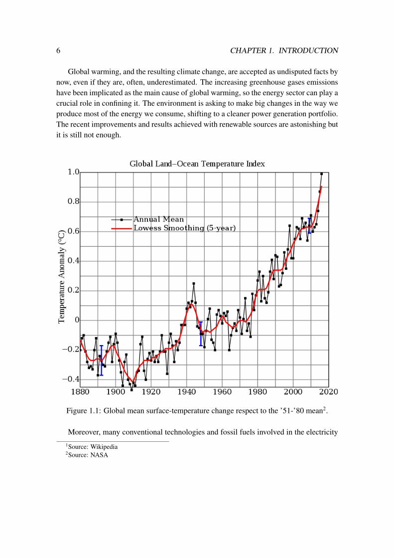
Global warming, and the resulting climate change, are accepted as undisputed facts bynow, even if they are, often, underestimated. The increasing greenhouse gases emissionshave been implicated as the main cause of global warming, so the energy sector can play acrucial role in confining it. The environment is asking to make big changes in the way weproduce most of the energy we consume, shifting to a cleaner power generation portfolio.The recent improvements and results achieved with renewable sources are astonishing butit is still not enough.
Figure 1.1: Global mean surface-temperature change respect to the ’51-’80 mean2.
Moreover, many conventional technologies and fossil fuels involved in the electricity1Source: Wikipedia2Source: NASA

1.1. OUTLINE 7
production are no more so much affordable.These and other relevant problems requires drastic changes in the electric power industry.A better integration of renewables along the grid, smarter ways of managing it, reducingthe energy consumption: many solution have been suggested in the last years. Some ofthem are very promising, some are more difficult to put in place. Most of them, however,cannot be implemented continuing to use the current traditional power grids: a re-designis needed. A re-design of the electrical grid that has more and more been proposed, usu-ally involves the introduction of a smaller, and smarter, type of network inside the grid,the so-called "microgrid".The U.S. department of energy defines the microgrid as "a group of interconnected loadsand distributed energy resources within clearly defined electrical boundaries that acts asa single controllable entity with respect to the grid. A microgrid can connect and dis-connect from the grid to enable it to operate in both grid-connected or island-mode" [4].Creating a microgrid offers many key advantages: the generating units are usually locatednear the place where the energy will be consumed, reducing the losses due to transmis-sion; small, renewable energy generators, can be more easily integrated in a microgrid,making it an eco-friendly concept; a smaller grid is easier to be monitored and managedthan the traditional ones; their architecture allows in some cases to serve the loads evenwhen the transmission grid is down (island mode). However, they presents shortcomingstoo, and developing a stable and reliable microgrid is not easy.Something that shares many similarities to the concept of the microgrid is the ElectricProsumer Community, a group of people (the prosumers) that consumes and produce elec-tricity at the same time, willing to achieve some common goals. The Electric ProsumerCommunity is the main argument of this work and some of the challenges associated withits development will be investigated.
1.1 Outline
This thesis is structured as follows: Chapter 2 gives a quick insight into the concept ofthe EPC, presenting some of the technologies available to produce and store the energy,describing their advantages and their drawbacks. Chapter 3 provides a simplified mathe-matical formalization of the community, exploiting it to focus on the design of a controlscheme that uses a decentralized approach that relies on imitative learning techniques.Chapter 4 describes a method to solve the optimal power flow in a low-voltage distribu-tion network, in order to obtaining a learning set to train the supervised learning algorithm.Chapter 5 presents a case study that compares the performance of the supervised learn-

8 CHAPTER 1. INTRODUCTION
ing algorithm with those of another, simpler, decentralized control scheme and with theoptimal strategy. Chapter 6 concludes and analyzes what could be future research in thecontext of control schemes for EPCs.
Chapter 2
The electric prosumer community
A prosumer is somebody that is, at the same time, both a consumer and a producer ofa certain good. In the energy sector, it is often used to indicate consumers (households,businesses, communities, organizations, etc.) that rely on microgeneration systems to pro-duce electricity and/or combine these with energy management systems, energy storageand electric vehicles [3]. The technologies that revolve around the idea of the electric-ity prosumer have seen, in the last decades, an outstanding process of improvements andgrowth. The recent large availability of generating units that offer different sizes at everlower prices, the increasing potential of storage devices and the proliferation of smart me-ters devices are helping the figure of the prosumer to spread around the globe.Single renewable generators managed by prosumers that act individually are too small tocompete on the market and their supply is unpredictable or inappropriate to satisfy effi-ciently the demand profile. [9] However, better results can be achieved when prosumersthat have the same goals and motivations, located in the same area, are connected togetheras a community. This group of people is what is called an Electric Prosumer Community(EPC).Many drawbacks and challenges are encountered at various levels when thinking aboutthe concept, from the development of solid regulations to the expedients to make it aneconomically advantageous alternative to traditional strategies. Co-ordinating efficientlythe interests of every member of the community can be difficult and disagreements amongmembers are very likely to occur [5]. The following sections present some popular tech-nologies to produce and store energy, along with some possible goals to be pursued bythe community.
9
10 CHAPTER 2. THE ELECTRIC PROSUMER COMMUNITY
2.1 Generation
The revolution brought by renewable energies has already passed its early stage and it hasstarted to be taken seriously by almost everyone. Even though most of the estabilishedgoals are not yet reached, the transition to a low-carbon economy seems, now, less distantthan before. The total installed power capacity associated to renewable sources reached2 millions of MW at the end of 2016 [6] providing, in the same year, the 24.5 % of theglobal electricity production [7]. Renewables are breaking records after records. In Marchand April 2017, renewable generation surpasses nuclear in the U.S. for the first time since1984 [10]. One month later, in Italy, renewable sources produced more than the 87% ofthe total demand of one day [11]. And these are just some of the many recent milestoneshit by renewable power.Even if they are not the only option, renewables and eco-friendly generators have becomeone of the first things that comes to mind when people talk about small, distributed gen-erating units, and thus, microgrids and electric prosumer communities.The most promising and widespread technologies for current microgeneration systemsare:
• Solar PV panels;
• Micro-wind turbines;
• Micro Combined Heat and Power (micro-CHP);
• Fuel cells;
• Microturbines;
They and some of their characteristics will be now introduced.
2.1.1 Solar photovoltaic
Solar photovoltaic (PV) panels are usually considered as the face of the "renewable revo-lution". The electric capacity of solar PV installed has been, in 2016, bigger than any othergeneration technology [15] (the total capacity has crossed the 300 GW [12]). Residentialsolar PV systems are now as much as 70% cheaper than in 2008 [14]. In Germany, pricesfor a typical 10 to 100 kWp PV residential rooftop-system were around 14,000 e/kW p in1990. At the end of 2016, such systems cost about 1,270 e/kW p. As regards the EnergyPayback Time of a solar photovoltaic system, it is strongly dependent from the location:in the Northern Europe it is less than 3 years, while in the South it is around 1.5 years (in
2.1. GENERATION 11
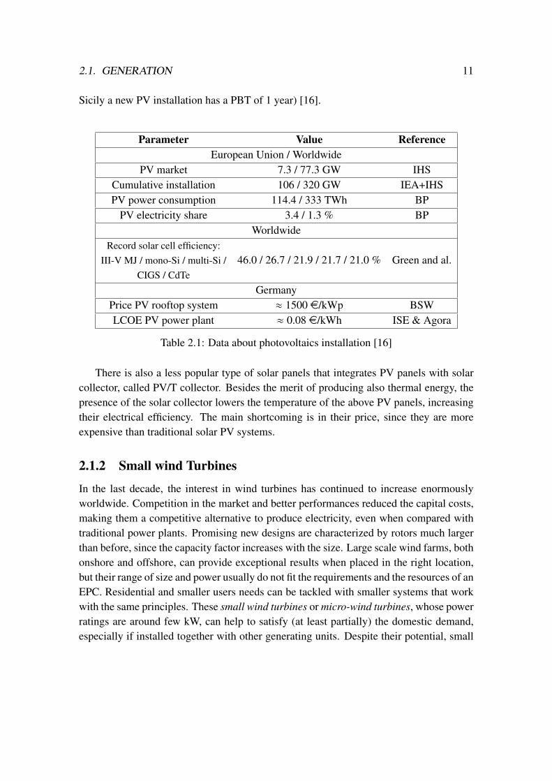
Sicily a new PV installation has a PBT of 1 year) [16].
Parameter Value ReferenceEuropean Union / Worldwide
PV market 7.3 / 77.3 GW IHSCumulative installation 106 / 320 GW IEA+IHSPV power consumption 114.4 / 333 TWh BP
PV electricity share 3.4 / 1.3 % BPWorldwide
Record solar cell efficiency:III-V MJ / mono-Si / multi-Si /
CIGS / CdTe46.0 / 26.7 / 21.9 / 21.7 / 21.0 % Green and al.
GermanyPrice PV rooftop system ≈ 1500 e/kWp BSWLCOE PV power plant ≈ 0.08 e/kWh ISE & Agora
Table 2.1: Data about photovoltaics installation [16]
There is also a less popular type of solar panels that integrates PV panels with solarcollector, called PV/T collector. Besides the merit of producing also thermal energy, thepresence of the solar collector lowers the temperature of the above PV panels, increasingtheir electrical efficiency. The main shortcoming is in their price, since they are moreexpensive than traditional solar PV systems.
2.1.2 Small wind Turbines
In the last decade, the interest in wind turbines has continued to increase enormouslyworldwide. Competition in the market and better performances reduced the capital costs,making them a competitive alternative to produce electricity, even when compared withtraditional power plants. Promising new designs are characterized by rotors much largerthan before, since the capacity factor increases with the size. Large scale wind farms, bothonshore and offshore, can provide exceptional results when placed in the right location,but their range of size and power usually do not fit the requirements and the resources of anEPC. Residential and smaller users needs can be tackled with smaller systems that workwith the same principles. These small wind turbines or micro-wind turbines, whose powerratings are around few kW, can help to satisfy (at least partially) the domestic demand,especially if installed together with other generating units. Despite their potential, small

12 CHAPTER 2. THE ELECTRIC PROSUMER COMMUNITY
wind turbines present many shortcomings: the efficiency of these devices is smaller thenthe one of common wind turbines, the problem of noise production becomes very relevantinside a neighborhood and suburban locations offer, in most of the cases, only low windspeed with high turbulence. These characteristics make small wind turbines difficult toget accepted by the public opinion [17].
2.1.3 Micro-CHP
Cogeneration is the production, at the same time, of two forms of energy, usually electric-ity and heat. It is an old concept and it can be found applied even in early power plants.The recent growing interest by consumers (and investors) in sustainability and, gave anadditional boost to cogeneration because, even when it does not involve renewable energysources, it represents a very efficient way to reduce carbon emissions. Moreover, it allowsto save an incredible amount of money. Combined heat and power system can be alsodesigned at smaller scales (Micro-CHP), making it an attractive option to implement inEPCs. Another advantage of cogeneration is that it can be applied with a large range of(renewables and non-renewables) generation systems.
Microturbines
Among the distributed generation technologies that do not rely on renewable sources,there is one that fits very well the characteristics of the EPCs: microturbines. Microtur-bines are basically small versions of the combustion turbines that can be found in powerplants. Their output can go from 10 kW to a few hundred of kW [18]. The main advan-tages are the tolerable costs, the good efficiency, the easy installation and a high reliability.A wide range of models with different features are available on the market. Most of themare powered by fuels like natural gas or diesel and, unlike PV panels or wind turbine, canbe started whenever it is needed.The use of fuel in microturbines becomes more efficient when the device is integrated ina co-generation (CHP) system, achieving efficiency up to 80%. In this case, the thermalenergy produced by the turbine is no more wasted, but it can be used for heating.
Fuel cells
Another option to generate power inside an EPC is represented by fuel cells. Fuel cellsare devices that convert the chemical energy of a fuel into electrical energy [29] and canbe easily integrated into CHP systems. They are usually compared to batteries since theconversion is performed by electrochemical processes, but they differ in the fact that fuel
2.2. STORAGE 13
cells require a fuel to flow through them. There are a lot of different fuel cells and most ofthem represents an eco-friendly option to generate energy with a good efficiency. Theirmarket is growing rapidly, researchers are developing more and more technolgies. Amongthe current available fuel cells, phosphoric acid fuel cells (PAFC), molten carbonate fuelcells (MCFC), and solid oxide fuel cells (SOFC) are the ones most recommended for anEPC [1].
2.1.4 Other technologies
What has been presented in this section is only a small part of the available technologiesfor distributed generation (DG). Many other techniques used to produce electric energy inlarge power plants can be applied also at smaller scales. Sustainable alternatives such assmall hydroelectric plants, geothermal energy or biomass resources can be feasible optionin some cases. Every one of them is characterized by advantages and disadvantages andit is not possible to affirm which one the best since it depends on countless parameters. Agood suggestion on how to produce energy in the community is to rely on more than justone technology: hybrid systems are a good method to compensate for the shortcomings ofone technology with the advantages of another one, increasing the production reliability.
2.2 Storage
Renewable distributed generators are not perfect. Many flaws that are often ascribed tothese technologies are, for example, the lack of high reliability, the limited power qualityand the difficulties to predict and organize the production. An expedient that helps to mit-igate these problems is the integration in the network of efficient energy storage systems(ESS). Besides the benefits that they offer to renewable generators, they are however apowerful tool to manage energy in a clever way. EES can be classified according to theform of energy they involve: we can have electrochemical, thermal, chemical, electricalor mechanical devices.Electrochemical batteries are what is popularly associated to the concept of energy stor-age, due to their presence in many common applications. Batteries store energy under theelectrochemical form and saw their origin at the beginning of the 19th century. Since then,countless technologies appeared, increasing the capacity, the power density, the lifetime,etc. The last decades saw new remarkable improvements, making batteries less expensiveand more suitable for residential usage [19] [29].Even though batteries are very popular, the 96% of the electrical storage capacity installedin the world is represented by another kind of system: the pumped hydroelectric energy

14 CHAPTER 2. THE ELECTRIC PROSUMER COMMUNITY
storage (PHES) [29]. PHES uses the gravitational energy of a reservoir of water locatedat a certain elevation. When an electrical demand is required, the water is sent to a lowerreservoir, flowing through a turbine that produce electricity. Depending on the case, somecommunities could implement smaller PHES system for seasonal storage.
Many other technologies are available for EES, such as compressed air energy stor-ages (CAES), flywheels and supercapacitors, but they still present major shortcoming andare suited only for particular applications. A summary of the characteristics of some ofthe energy storage technologies is presented in Fig. 2.2.
Type Energy Density Power Density Response Time Cycling TimesWh/kg W/kg
Flywheel 5-30 400-1500 1 s Above 20,000Compressed air 30-60 - 1-10 min Above 100,000
Lead-acid 30-50 75-300 10 s 2000Lithium-ion 75-200 150-300 10 s 10,000
Sodium-sulfur 100-250 100-230 10 s 2500-6000Supercapacitor 5-10 5-10 1 s 100,000
Table 2.2: Energy storage technologies [19]
2.2.1 Electric Vehicles
There is another element, besides renewables, that promises to help the shift to a cleanerenvironment and the building of a more sustainable future: Electric Vehicles (EVs). Be-sides the effects that they can have on the automotive industry, EVs can be a powerful toolinto the pocket of the electric grid, providing or storing power upon request when pluggedin: this concept is called Vehicle-to-Grid power (V2G) [20]. Utility fleets seem to have agood economic potential as ancillary service for the power grid [21], but also individualvehicles could be exploited if used as storage devices in an EPC. Their implementationin a microgrid is more difficult than the common battery’s one, but they still can provideinteresting features and additional capacity [22].
2.3 Demand
The cleanest energy is the one that you do not use, we all know it. Reducing the energyconsumption would be probably the most efficient way to contrast pollution and global

2.4. A GOAL-ORIENTED COMMUNITY 15
warming, but it is not always feasible in practice. One of the key points of an EPC istrying to satisfy the internal demand of the prosumers in an efficient way. Not an easytask, since forecasting future demand and production is extremely difficult, and in somecases, impossible. When more consumers join together in the same community, however,it would be possible to coordinate and to organize some of the energy consuming tasksin order to reduce total consumption, peak demand and costs. This approach is called"demand management" (from the demand-side).
2.4 A goal-oriented community
The concept itself of a community of multiple electric prosumers implies that they intendto pursue a set of mutual goals. Since EPCs are still in their early state and since thereis a lack of regulations, it is not perfectly clear what the policy of a community couldbe. The objective of the community can be, for example, to maximize the consumption of"green" power produced by the distributed generators, to minimize the exchanges with thefeeder or to optimize the overall costs of the entire community [24]. Whatever the goalis, however, there are very few studies that analyze the energy sharing between prosumersand there seems to exists no techniques yet to identify prosumers that do not act as agreed[25]. Investigating further on these aspects is crucial for the development of new EPCs.


Chapter 3
A control scheme for the community
Since their conception, microgrids have been deeply examined in literature (see for exam-ple [26] - [28]) and many challenges and shortcomings have been detected. Monitoringand controlling the network can be extremely difficult, representing an interesting argu-ment for research. The dynamics of electric power system are complex even at smallerscales, due to the many parameters that have effect on the system. The safety of the net-work is not the only thing that matters, the economic side of the problem is very relevanttoo. Therefore, this work will focus on how to control the prosumers’ operation inside thecommunity, trying to ensure the safety of the grid while pursuing a common objective.
3.1 Formalising the prosumer community
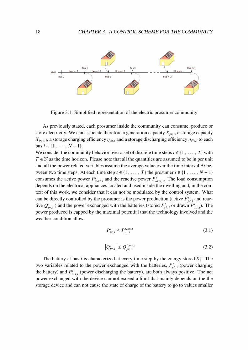
Before looking further in the control challenges, it is better to try to formalize a simplifiedmodel of the prosumer community dynamics to use in the design of a decentralized controlscheme. We consider a low-voltage distribution network composed by N ∈ N buses,where one bus is the root connection, the point of connection between the communityand the power system, while the remaining N − 1 buses are the Npro ∈ N prosumers’dwellings inside the EPC. The number of branches in the network is L ∈ N, with Rl andXl as, respectively, the resistance and the reactance of the l − th branch (l ∈ 1 . . . L ).For simplicity we will consider a linear network like the one in Fig.3.1, with batteries andsolar photovoltaic panels installed at each prosumer bus.
17
18 CHAPTER 3. A CONTROL SCHEME FOR THE COMMUNITY
Figure 3.1: Simplified representation of the electric prosumer community
As previously stated, each prosumer inside the community can consume, produce orstore electricity. We can associate therefore a generation capacity Xpr, i, a storage capacityX batt, i, a storage charging efficiency ηch, i and a storage discharging efficiency ηdis, i to eachbus i ∈ 1 , . . . , N − 1.We consider the community behavior over a set of discrete time steps t ∈ 1 , . . . , T withT ∈ N as the time horizon. Please note that all the quantities are assumed to be in per unitand all the power related variables assume the average value over the time interval ∆t be-tween two time steps. At each time step t ∈ 1 , . . . , T the prosumer i ∈ 1 , . . . , N − 1consumes the active power P t
load, i and the reactive power P tload, i. The load consumption
depends on the electrical appliances located and used inside the dwelling and, in the con-text of this work, we consider that it can not be modulated by the control system. Whatcan be directly controlled by the prosumer is the power production (active P t
pr, i and reac-tive Q t
pr, i ) and the power exchanged with the batteries (stored P tch, i or drawn P t
dis, i). Thepower produced is capped by the maximal potential that the technology involved and theweather condition allow:
P tpr, i ≤ P t,max
pr, i (3.1)
∣∣∣Q tpr, i
∣∣∣ ≤ Q t,maxpr, i (3.2)
The battery at bus i is characterized at every time step by the energy stored S ti . The
two variables related to the power exchanged with the batteries, P tch, i (power charging
the battery) and P tdis, i (power discharging the battery), are both always positive. The net
power exchanged with the device can not exceed a limit that mainly depends on the thestorage device and can not cause the state of charge of the battery to go to values smaller
3.2. DECENTRALIZED CONTROL SCHEME 19
than 0 or higher than 1. The battery dynamics is described in the following equations:
P tch, i − P t
dis, i ≤ P t,maxbatt, i (3.3)
0 ≤ S tbatt, i + ηch, i P t
ch, i∆t −P t
dis, i
ηdis, i∆t ≤ Xbatt, i (3.4)
We denote with P tδ, i and Q t
δ, i the power injected in the distribution network from prosumeri at time t.
P tδ, i = P t
pr, i + P tdis, i − P t
ch, i − P tload, i (3.5)
Q tδ, i = Q t
pr, i − Q tload, i (3.6)
When these variables are different from zero it means that the prosumer i has a surplus (ifP tδ, i > 0) or a deficit of power (if P t
δ, i < 0). In these cases, it need to be balanced by thesurplus/deficit of another prosumer inside the community or by the feeder. The control ofthe power production and the usage of the batteries is a crucial element to reduce over-voltages, line overloadings, network losses and costs.Speaking about costs and revenues, we assume that the power exchanges between pro-sumers are not associated to any expense (their price is zero) while the energy exchangedby a prosumer with the retailer at time t is characterized by a price ct
el.
3.2 Decentralized control scheme
Like other system composed by multiple agents, there are two main control strategies foran EPC, a centralized and hierarchical mechanism or a distributed scheme. A centralizedcontrol scheme indicates that all the data possessed are gathered together and sent to acentral entity that computes the orders and coordinates the prosumers’ actions. In orderto achieve good results, this entity should have a detailed model of the network, effi-cient communication devices and the equipment required to receive, store and process theinformation. The latter is called "Microgrid Central Controller" (MGCC) and plays a fun-damental role in the control structur. The main shortcoming of building and maintainingall the machinery involved in the centralized strategy is that it can be very expensive. Mo-rover, since current smart meters technologies appeared on the market, privacy concernsfor the single prosumer are rised due to the sharing of personal consumption informationwith other people [8]. We still do not know how a future regulation will treat this matter

20 CHAPTER 3. A CONTROL SCHEME FOR THE COMMUNITY
once the figure of prosumers will spread, therefore it could be interesting to investigatepossible designs for decentralized control schemes that do not require the individual toshare too much information.With "decentralized control scheme" we imply that each single prosumer in an EPC takesautonomous decisions on how to interact with the rest of the network. We want to in-vestigate how to design distributed control schemes that may contribute to reach (at leastpartially) the objectives of the community. In order to avoid that prosumers share privacy-related information, we suppose that they compute their decisions only relying on localmeasurements. This is not an easy task, since a partial knowledge of the state of the net-work makes difficult for to compute cost-effective decisions. Not only, the revenues aredifficult to maximize, but unappropriate actions can cause overvoltages, undervoltages oroverloadings inside the network, undermining the safety of the microgrid. Our strategyis to resort to supervised learning techniques that may extract, from centralized, optimalsolutions, decision making patterns to be applied at the level of the single prosumer.
3.3 Supervised learning algorithm
Supervised learning (SL) methods have their roots in statistics world. Their main goalis to predict what the output Ψ of a set of inputs ψ is, analyzing the characterstics of thetraining data [36]. SL techniques are used in many areas and problems. If the outputs aresome sorts of labels, we call it a classification problem, otherwise, if the outputs consistof continuous variables, it is a regression problem. Each problem involving SupervisedLearning includes, indeed, a training process, that is performed using a data-set of samplesthat contains a set of inputs and their corresponding outputs. The SL algorithm examinesthese data, tries to learn from them and produce an estimation function to find the outputassociated to new inputs.Literature is full of SL methods and algorithm to apply to several problems. One popularfamily of SL techniques is the one of the tree-based methods, simple to apply and suitablefor both classification and regression problems [36]. Some common tree-based methodsare CART (Classification and Regression Trees) [30], Tree Bagging and Random Forest[38]. The accuracy of these models depend on the particular problems on which theyare applied, but in several cases the results are slightly the same. The model used inthe development of the decentralized control strategy is another tree-based method calledExtremely Randomized Trees.
3.3. SUPERVISED LEARNING ALGORITHM 21
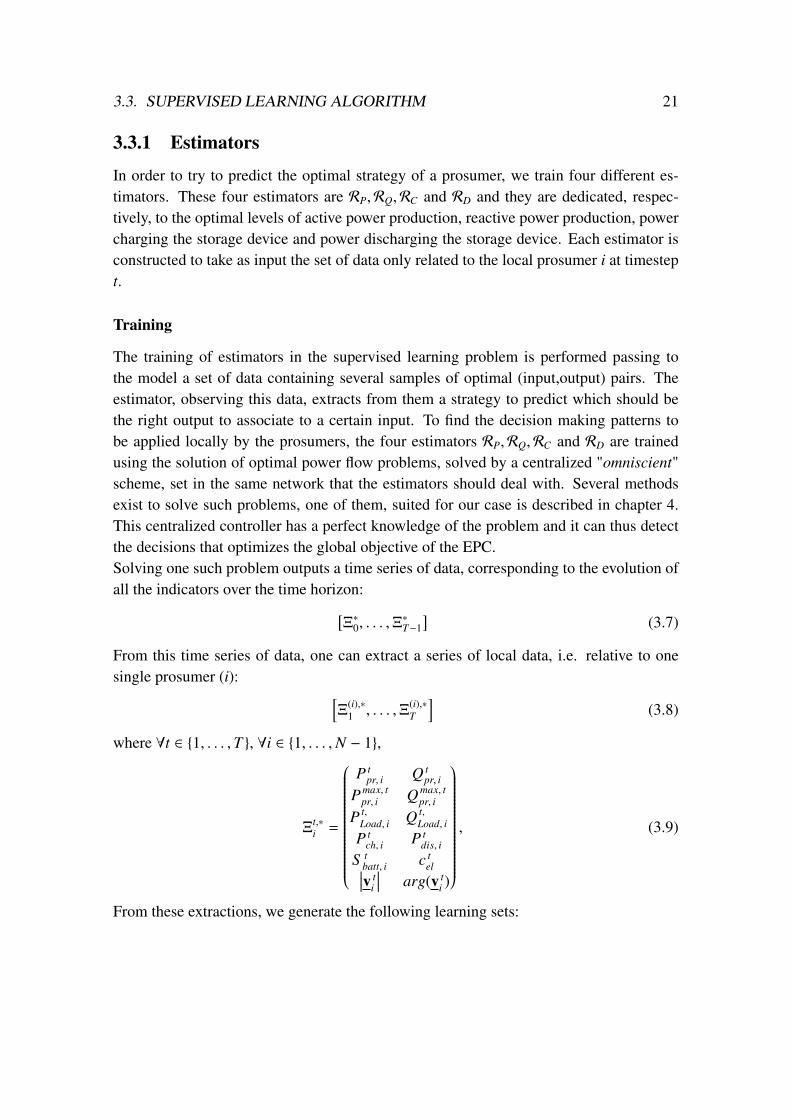
3.3.1 Estimators
In order to try to predict the optimal strategy of a prosumer, we train four different es-timators. These four estimators are RP,RQ,RC and RD and they are dedicated, respec-tively, to the optimal levels of active power production, reactive power production, powercharging the storage device and power discharging the storage device. Each estimator isconstructed to take as input the set of data only related to the local prosumer i at timestept.
Training
The training of estimators in the supervised learning problem is performed passing tothe model a set of data containing several samples of optimal (input,output) pairs. Theestimator, observing this data, extracts from them a strategy to predict which should bethe right output to associate to a certain input. To find the decision making patterns tobe applied locally by the prosumers, the four estimators RP,RQ,RC and RD are trainedusing the solution of optimal power flow problems, solved by a centralized "omniscient"scheme, set in the same network that the estimators should deal with. Several methodsexist to solve such problems, one of them, suited for our case is described in chapter 4.This centralized controller has a perfect knowledge of the problem and it can thus detectthe decisions that optimizes the global objective of the EPC.Solving one such problem outputs a time series of data, corresponding to the evolution ofall the indicators over the time horizon:[
Ξ∗0, . . . ,Ξ∗T−1
](3.7)
From this time series of data, one can extract a series of local data, i.e. relative to onesingle prosumer (i): [
Ξ(i),∗1 , . . . ,Ξ(i),∗
T
](3.8)
where ∀t ∈ 1, . . . ,T , ∀i ∈ 1, . . . ,N − 1,
Ξt,∗i =
P tpr, i Q t
pr, i
P max, tpr, i Q max, t
pr, i
P t,Load, i Q t,
Load, i
P tch, i P t
dis, i
S tbatt, i c t
el∣∣∣v ti
∣∣∣ arg(v ti )
, (3.9)
From these extractions, we generate the following learning sets:

22 CHAPTER 3. A CONTROL SCHEME FOR THE COMMUNITY
• To generate a learning set dedicated to learning how to optimize the level of activepower production, we process the whole variables Ξ t,∗
i into the following set of(input, output) pairs:
LP =(ψ t
P, i,ΨtP, i
)i=N−1,t=T
i=1,t=1(3.10)
where, ∀t ∈ 0, . . . ,T − 1, ∀i ∈ 1, . . . ,N,
ψ tP, i =
(i, t, c t
el,∣∣∣v t
i
∣∣∣ , arg(v ti ), P t
Load, i, Q tLoad, i, P max, t
pr, i ,Q max, tpr, i , S t
batt, i
)(3.11)
Ψ tP, i = P t
pr, i (3.12)
Where:
– i : id number of the bus considered;
– t : time-step considered;
–∣∣∣v t
i
∣∣∣ : magnitude of the voltage at bus i at time step t;
– arg(v t) : phase of the voltage at bus i at time step t;
– c tel : electricity price at time step t;
– S tbatt, i : level of charge of the storage of bus i at time step t;
– P tLoad, i, Q t
Load, i : active and reactive power consumption at bus i at time step t;
– P max, tpr, i ,Q max, t
pr, i : maximal active and reactive production potential at bus i attime step t;
• To generate a learning set dedicated to learning how to optimize the level of reactivepower production, we process the whole variables Ξ t,∗
i into the following set of(input, output) pairs:
LQ =(ψ t
Q, i,ΨtQ, i
)i=N−1,t=T
i=1,t=1(3.13)
where, ∀t ∈ 0, . . . ,T − 1, ∀i ∈ 1, . . . ,N − 1:
ψ tQ, i = = ψ t
P, i
Ψ tQ, i = = Q t
pr, i
3.3. SUPERVISED LEARNING ALGORITHM 23
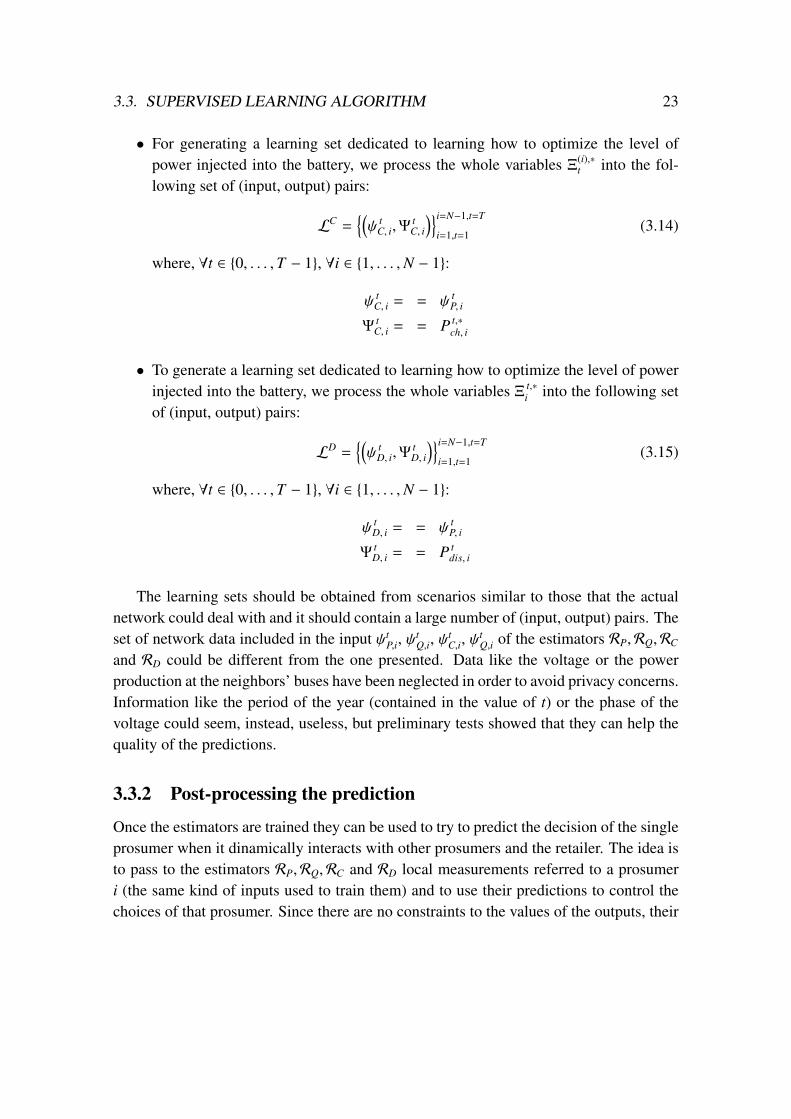
• For generating a learning set dedicated to learning how to optimize the level ofpower injected into the battery, we process the whole variables Ξ
(i),∗t into the fol-
lowing set of (input, output) pairs:
LC =(ψ t
C, i,ΨtC, i
)i=N−1,t=T
i=1,t=1(3.14)
where, ∀t ∈ 0, . . . ,T − 1, ∀i ∈ 1, . . . ,N − 1:
ψ tC, i = = ψ t
P, i
Ψ tC, i = = P t,∗
ch, i
• To generate a learning set dedicated to learning how to optimize the level of powerinjected into the battery, we process the whole variables Ξ t,∗
i into the following setof (input, output) pairs:
LD =(ψ t
D, i,ΨtD, i
)i=N−1,t=T
i=1,t=1(3.15)
where, ∀t ∈ 0, . . . ,T − 1, ∀i ∈ 1, . . . ,N − 1:
ψ tD, i = = ψ t
P, i
Ψ tD, i = = P t
dis, i
The learning sets should be obtained from scenarios similar to those that the actualnetwork could deal with and it should contain a large number of (input, output) pairs. Theset of network data included in the input ψt
P,i, ψtQ,i, ψ
tC,i, ψ
tQ,i of the estimators RP,RQ,RC
and RD could be different from the one presented. Data like the voltage or the powerproduction at the neighbors’ buses have been neglected in order to avoid privacy concerns.Information like the period of the year (contained in the value of t) or the phase of thevoltage could seem, instead, useless, but preliminary tests showed that they can help thequality of the predictions.
3.3.2 Post-processing the prediction
Once the estimators are trained they can be used to try to predict the decision of the singleprosumer when it dinamically interacts with other prosumers and the retailer. The idea isto pass to the estimators RP,RQ,RC and RD local measurements referred to a prosumeri (the same kind of inputs used to train them) and to use their predictions to control thechoices of that prosumer. Since there are no constraints to the values of the outputs, their

24 CHAPTER 3. A CONTROL SCHEME FOR THE COMMUNITY
prediction could lead to impracticable or dangerous actions, (i.e. the estimator suggesta power production greater then the potential one or a power injected in the storage thatwould bring the charge of the battery beyond the maximum value that it allows). There-fore a partial post-processing of the outputs is needed to change the value. We denote withRP∗
i,t , RQ∗i,t , RC∗
i,t and RD∗i,t the preliminary predictions made by the estimators associated to
the input of bus i and time step t.The actual actions at the same bus and time step are corrected to P t
pr, i, Q tpr, i, P t
ch, i andP t
dis, i as follows:
• For the active power production level:
if RP∗i,t ≥ P max, t
pr, i
P tpr, i = P max, t
pr, i
else if LP(ini,t
)≤ P min, t
pr, i
P tpr, i = P min, t
pr, i
else P tpr, i = RP∗
i,t
• For the reactive power production level:
if RQ∗i,t ≥ Q max, t
pr, i
Q tpr, i = Q max, t
pr, i
else if LQ(ini,t
)≤ Q min, t
pr, i
Q tpr, i = Q min, t
pr, i
else Q tpr, i = R
Q∗i,t
• For the power injected in the battery:
if RC∗i,t ≥ P max
batt, i
P tc, i = P max, t
pr, i
else if RC∗i,t ≤ 0
P tch, i = 0
else P tch, i = RC∗
i,t
if S ti + Pt
ch, iηch,i ≥ Xbatt, i
Ptch, i =
Xbatt, i−S ti
ηch, i

3.3. SUPERVISED LEARNING ALGORITHM 25
• For the power drawn from the battery:
if RD∗i,t ≥ P max
batt, i
P tdis, i = P max, t
pr, i
else if RD∗i,t ≤ 0
P tdis, i = 0
else P tdis, i = RD∗
i,t
if S ti −
Ptdis, i
ηdis,i< 0
Ptdis, i = S t
iηdis, i
It is important to notice that, even after post-processing the output values, there is still riskof incurring in under-voltages/over-voltages.


Chapter 4
The Power flow analysis
The study and operation of any interconnected electric power system require to performa numerical analysis to determine the electrical state of the network starting from param-eters that are known: this computation is called power flow analysis or load-flow study.Power flow analysis allows to compute currents, real and reactive power flowing in thebranches, losses, voltages at the buses. It is used not only to analyze the operation ofnetworks that already exist, but is a powerful method also to find what configurations leadto critical conditions or to design new power systems. Moreover it can be included inother methods to perform unit commitment, economic dispatch or to determine the opti-mal power flow, the most efficient configuration of the system. This chapter presents abasic formulation of the problem and a method to solve it when applied to an EPC.
4.1 AC Power flow equations
Defining and solving the power flow equations of the power system are the main tasks inthe load flow study. One of the data required to perform it is the nodal admittance matrixYBUS . In a system of N buses, YBUS is a N × N matrix such that:
VYBUS = I (4.1)
Eq. (4.1) is the matrix form of the well-known Ohm’s Law.There are four different variables associated to each bus i ∈ 0, . . . ,N − 1 : the activepower injection Pi, the reactive power injection Qi, the voltage magnitude Vi and thevoltage phase θi. Depending on the type of the bus i, the variables that are assumed to beknown are:
• if the bus i is the slack bus, the voltage magnitude Vi and phase θi;
27
28 CHAPTER 4. THE POWER FLOW ANALYSIS
• if the bus i is a P-V bus, the voltage magnitude Vi and the active power injection Pi;
• if the bus i is a P-Q bus, the active power Pi and reactive power Qi injections;
The purpose of the analysis is to evaluate the remaining:
• NP−V + NP−Q voltage phases;
• NP−Q voltage magnitudes;
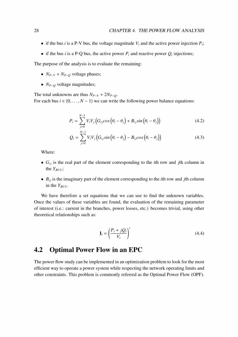
The total unknowns are thus NP−V + 2NP−Q.For each bus i ∈ 0, . . . ,N − 1 we can write the following power balance equations:
Pi =
N−1∑j=0
ViV j
(Gi jcos
(θi − θ j
)+ Bi jsin
(θi − θ j
))(4.2)
Qi =
N−1∑j=0
ViV j
(Gi jsin
(θi − θ j
)− Bi jcos
(θi − θ j
))(4.3)
Where:
• Gi j is the real part of the element corresponding to the ith row and jth column inthe YBUS ;
• Bi j is the imaginary part of the element corresponding to the ith row and jth columnin the YBUS .
We have therefore a set equations that we can use to find the unknown variables.Once the values of these variables are found, the evaluation of the remaining parameterof interest (i.e.: current in the branches, power losses, etc.) becomes trivial, using othertheoretical relationships such as:
Ii =
(Pi + jQi
Vi
)∗(4.4)
4.2 Optimal Power Flow in an EPC
The power flow study can be implemented in an optimization problem to look for the mostefficient way to operate a power system while respecting the network operating limits andother constraints. This problem is commonly referred as the Optimal Power Flow (OPF).
4.2. OPTIMAL POWER FLOW IN AN EPC 29
The set of equations described in Section 4.1 involves non-linear relationships. The re-sulting optimizational problem is non-linear and non-convex, increasing exponentially thecomputational cost required to solve the OPF, especially with large interconnected powersystems. There are many methods to solve it and multiple approaches have been devel-oped to decrease the complexity of the problem (i.e. "Direct Current Power Flow" [31]and "Fast Decoupled Load Flow" [32]). The assumptions that most of these models re-quire, however, do not always fit with low-voltage (LV) distribution networks.An interesting method with good convergence properties that well matches with LV net-works is the one developed by Fortenbacher and al. [33]. In this paper, the authors recastthe non-linear power flow equations into a linear problem, relying on assumptions thatare common to most LV networks. This linear problem is iteratively solved, updatingeach time the voltages at the buses with a combined forward backward sweep technique(FBS) [34]. This method is called Forward-Backward Sweep Optimal Power Flow (FBS-OPF) and it will be used, in the context of this work, to represent a centralized "omini-scient" control strategy and to create the learning sets used by SL model presented inSection 3.3. Its formulation will now be resumed and explained.
4.2.1 The FBS-OPF algorithm
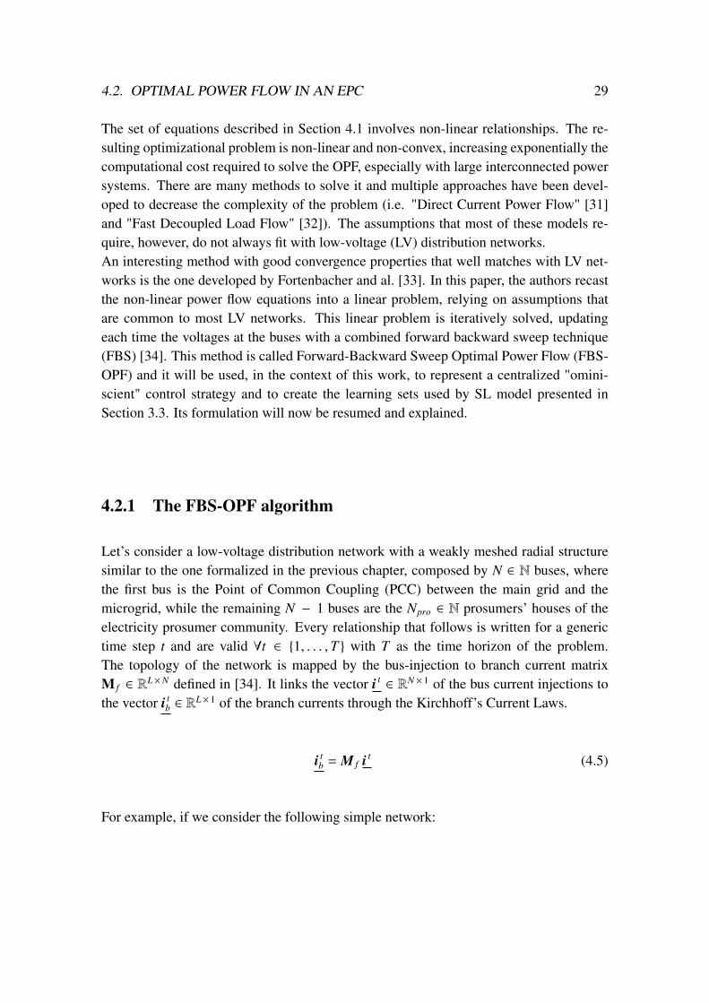
Let’s consider a low-voltage distribution network with a weakly meshed radial structuresimilar to the one formalized in the previous chapter, composed by N ∈ N buses, wherethe first bus is the Point of Common Coupling (PCC) between the main grid and themicrogrid, while the remaining N − 1 buses are the Npro ∈ N prosumers’ houses of theelectricity prosumer community. Every relationship that follows is written for a generictime step t and are valid ∀t ∈ 1, . . . ,T with T as the time horizon of the problem.The topology of the network is mapped by the bus-injection to branch current matrixM f ∈ R
L×N defined in [34]. It links the vector i t∈ RN × 1 of the bus current injections to
the vector i tb ∈ R
L× 1 of the branch currents through the Kirchhoff’s Current Laws.
i tb = M f i t (4.5)
For example, if we consider the following simple network:
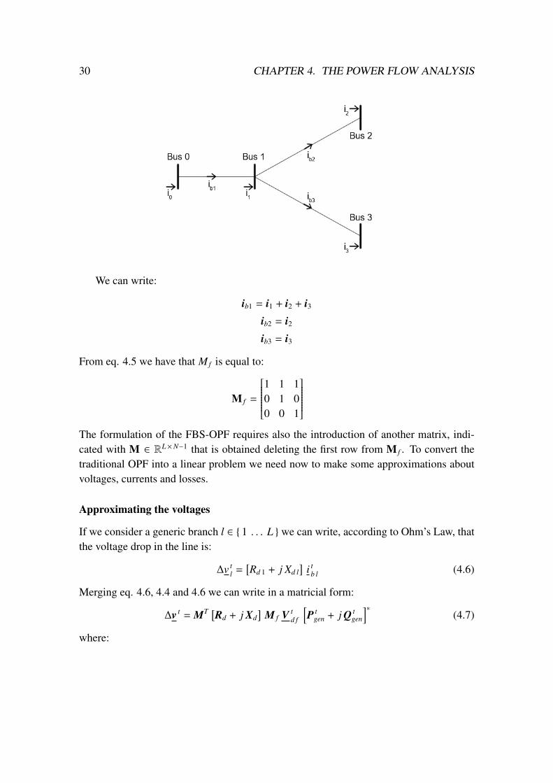
30 CHAPTER 4. THE POWER FLOW ANALYSIS
We can write:
ib1 = i1 + i2 + i3
ib2 = i2
ib3 = i3
From eq. 4.5 we have that M f is equal to:
M f =
1 1 10 1 00 0 1
The formulation of the FBS-OPF requires also the introduction of another matrix, indi-cated with M ∈ RL×N−1 that is obtained deleting the first row from M f . To convert thetraditional OPF into a linear problem we need now to make some approximations aboutvoltages, currents and losses.
Approximating the voltages
If we consider a generic branch l ∈ 1 . . . L we can write, according to Ohm’s Law, thatthe voltage drop in the line is:
∆v tl =
[Rd 1 + j Xd l
]i t
b l (4.6)
Merging eq. 4.6, 4.4 and 4.6 we can write in a matricial form:
∆v t = MT [Rd + j Xd
]M f V t
d f
[P t
gen + j Q tgen
]∗(4.7)
where:
4.2. OPTIMAL POWER FLOW IN AN EPC 31
• Rd = diag Rd 1 . . . Rd L ∈ RL×L is the resistance matrix;
• Xd = diag Xd 1 . . . Xd L ∈ RL×L is the reactance matrix;
• V td f = diag
1
v t0. . . 1
v tN
∈ RN×N is nodal line to neutral voltages matrix.
Eq.(4.7) presents a complex relationship. To linearize it, the authors of the paper [33],decide to assume that nodal voltage angles are small and resistances in the network areway bigger than its reactances. This assumptions is usually true for LV networks. We canapproximate then Eq.(4.7) as:
v t ≈ vs +
[MT RdM f
∣∣∣∣V td f
∣∣∣∣ MT XdM f
∣∣∣∣V td f
∣∣∣∣] [P t
gen
Q tgen
]
The matrix[MT RdM f
∣∣∣∣V td f
∣∣∣∣ MT XdM f
∣∣∣∣V td f
∣∣∣∣] is called B tv and vs ∈ R
L×1 is the slack busvoltage vector.
Approximating the currents in the branches
Another assumption that we can make for LV networks is that reactive power injectionsare usually small if compared with active power injections. Assuming that, we expresscurrent in the branches as:
i tb ≈ M f
∣∣∣∣V td f
∣∣∣∣ P t
The product M f
∣∣∣∣V td f
∣∣∣∣ is denoted as B tr .
Approximating the losses
The power losses are approximated as linear piecewise function:
PLoss ≈ maxL t0P t,−L t
0P t,L t1P t + b t,−L t
1P t + b t
QLoss ≈ maxL t0Q t,−L t
0Q t,L t1Q t + b t,−L t
1Q t + b t
Where:
• L t0 = diagi 0, t
0 , . . . , 1 0, tl RdM f
∣∣∣∣V td f
∣∣∣∣• L t
1 = diagi 0, t0 + i 1, t
0 , . . . , i 0, tl + 1 1, t
l RdM f
∣∣∣∣V td f
∣∣∣∣
32 CHAPTER 4. THE POWER FLOW ANALYSIS
• b t = −[rd1i 0, t
0 i 1, t0 , . . . , rdli 0, t
l 1 1, tl
]• i 0, t = 0.25M f Pmax, t
• i 1, t = 0.75M f Pmax, t
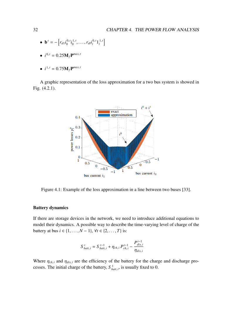
A graphic representation of the loss approximation for a two bus system is showed inFig. (4.2.1).
Figure 4.1: Example of the loss approximation in a line between two buses [33].
Battery dynamics
If there are storage devices in the network, we need to introduce additional equations tomodel their dynamics. A possible way to describe the time-varying level of charge of thebattery at bus i ∈ 1, . . . ,N − 1, ∀t ∈ 2, . . . ,T is:
S tbatt, i = S t−1
batt, i + ηch, i P t−1ch, i −
P t−1dis, i
ηdis, i
Where ηch, i and ηdis, i are the efficiency of the battery for the charge and discharge pro-cesses. The initial charge of the battery, S 1
batt, i, is usually fixed to 0.
4.2. OPTIMAL POWER FLOW IN AN EPC 33
Power balance
The most important constraint of the OPF problem is to satisfy the power balance insidethe network, expressed as:
N−1∑i=0
P tgen, i −
L∑j=1
P tlos, j −
L∑j=1
Q tlos, j −
N−1∑i=0
P tload, i = 0
Network physical limits
Any solution proposed by the optimization problem must respect the physical limits re-lated to power production and consumption, avoiding overvoltages, undervoltages, over-loadings and that the state of charge of the batteries remains between a minimum and amaximum value. These constraints can be written as:
−i maxb + Bt
rP tload ≤ Bt
rP tgen ≤ i max
b + BtrP t
load
v min ≤ v t ≤ v max
P min, tpr ≤ P t
pr ≤ P max, tpr
Q min, tpr ≤ Q t
pr ≤ Q max, tpr
0 ≤ P tch ≤ P max
batt, ch
0 ≤ P tdis ≤ P max
batt, dis
S t = 1batt, i = S in
batt, i
S minbatt, i ≤ S t
batt, i ≤ xbatt, i
ηch, i P Tch, i ≤ xbatt, i − S T
batt, i
P Tdis, i
ηdis, i≤ S T
batt, i
Where:
• i maxb is the vector of the maximal admissible currents in the branches;
• v min and v max are the vectors of the minimal and maximal admissible voltages atthe buses;
• P min, tpr and P max, t
pr are the vectors of the minimal and maximal level of active powerproduction at the buses;
• Q min, tpr and Q max, t
pr are the vectors of the minimal and maximal level of reactive powerproduction at the buses;
• P maxbatt, dis is the vector of the maximal admissible power exchanged with the batteries;
34 CHAPTER 4. THE POWER FLOW ANALYSIS
The feeder
Since we are using the same variables both for the prosumer and the feeder, we needto fix to zero the values related to batteries and consumption of the first bus (the rootconnection).
P tLoad, 0 = 0
Q tLoad, 0 = 0
P tch, 0 = 0
P tdis, 0 = 0
Objective Function
The objective of the optimization problem is to minimize the costs (or maximize therevenues) encountered, over the entire time period, exchanging power with the main grid.If c t
el is the price of the electricity and P t0 is the power exchanged with the grid at time
t ∈ 1, . . . ,T (positive if sold to the feeder, negative if bought from it), the objectivefunction of the optimization problem can be written as:
minT∑
t=1
c telP
t0
LP-OPF
The assumptions and approximations introduced until now define the formulation of aLinear Programming of the Optimal Power Flow (LF-OPF) problem:
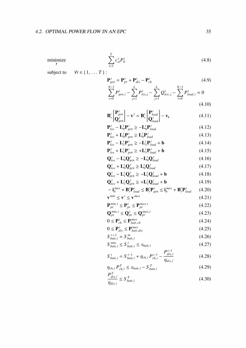
4.2. OPTIMAL POWER FLOW IN AN EPC 35
minimizey
T∑t=1
c telP
t0 (4.8)
subject to ∀t ∈ 1, . . . T :
P tgen = P t
pr + P tdis − P t
ch (4.9)N−1∑i=0
P tgen, i −
L∑j=1
P tlos, j −
L∑j=1
Q tlos, j −
N−1∑i=0
P tload, i = 0
(4.10)
Btv
[P t
gen
Q tgen
]− v t = Bt
v
[P t
load
Q tload
]− vs (4.11)
P tlos − Lt
0P tgen ≥ −Lt
0P tload (4.12)
P tlos + Lt
0P tgen ≥ Lt
0P tload (4.13)
P tlos − Lt
1P tgen ≥ −Lt
1P tload + b (4.14)
P tlos + Lt
1P tgen ≥ +Lt
1P tload + b (4.15)
Q tlos − Lt
0Q tgen ≥ −Lt
0Q tload (4.16)
Q tlos + Lt
0Q tgen ≥ Lt
0Q tload (4.17)
Q tlos − Lt
1Q tgen ≥ −Lt
1Q tload + b (4.18)
Q tlos + Lt
1Q tgen ≥ +Lt
1Q tload + b (4.19)
− i maxb + Bt
rPtload ≤ Bt
rPtgen ≤ i max
b + BtrP
tload (4.20)
v min ≤ v t ≤ v max (4.21)
P min, tpr ≤ P t
pr ≤ P max, tpr (4.22)
Q min, tpr ≤ Q t
pr ≤ Q max, tpr (4.23)
0 ≤ P tch ≤ P max
batt, ch (4.24)
0 ≤ P tdis ≤ P max
batt, dis (4.25)
S t = 1batt, i = S in
batt, i (4.26)
S minbatt, i ≤ S t
batt, i ≤ xbatt, i (4.27)
S tbatt, i = S t−1
batt, i + ηch, i P t−1ch, i −
P t−1dis, i
ηdis, i(4.28)
ηch, i P Tch, i ≤ xbatt, i − S T
batt, i (4.29)
P Tdis, i
ηdis, i≤ S T
batt, i (4.30)
36 CHAPTER 4. THE POWER FLOW ANALYSIS
Where y is the set of variables of the optimization problem:
y = y1, . . . , yT (4.31)
∀t ∈ 1, . . . ,T :
yt = vt,Ptpr,Q
tpr,P
tch,P
tdis,P
tlos,Q
tlos,S
tbatt, (4.32)
FBS algorithm
The matrices Lt0,L
t1,B
tr and Bt
v depend on the bus voltages v t, that are initially unknown.The way to get around it, as presented in [33] is to set first the voltages to 1 pu and then tosolve iteratively the LP-OPF. After each iteration h, the currents are calculated in the for-ward stage and the voltages updated in the backward stage. The new voltages are used toevaluate the matrices Lt
0,Lt1,B
tr and Bt
v for the next iteration, until the difference betweenthe values of v of two consecutive iterations is below a certain threshold of tolerance.The FBS-OPF problem presented, optimize the control strategy over all the simulatedperiod, knowing at each step the future prices of electricity, the future load consumptionand the future potential power production. Thanks to this information, it is able to de-cide how to produce, store, buy and sell the electricity in the most efficient way. This isobviously an idealistic situation, since in real world, future is extremely difficult to pre-dict. However, the results obtained simulating realistic scenarios and solving them withthis centralized "omniscient" controller, can be useful to produce a learning set for a SLmodel as the one presented in the chapter 3.
Chapter 5
Case study
In this chapter we check how the SL algorithm formulated in Section 3.3 performs on asimulated test network with different scenarios of load consumption, potential productionand electricity prices. We tackle the scenarios also with: (a) a another decentralizedcontrol strategy (described in Section 5.4) (b) the centralized optimized strategy definedin Section 4.2, in order to have a better idea on the quality of the performance.
5.1 Test network
The control schemes are simulated on a linear network composed by the root connectionand Npro prosumers similar to Fig.3.1. Each branch linking two buses has the same length,the same resistance and the same reactance. The simulations are performed over a periodrepresenting an entire year, with one time-step per hour. In summary:
• The number of buses N is 15;
• The number of prosumers Npro is 14;
• The number of branches L is 14;
• ∆t is 1h;
• The time horizon T is 8760;
• The line resistance Rd1 = Rd2 = . . . = RdL is 0.025 Ω;
• The line reactance Xd1 = Xd2 = . . . = XdL is 0.005 Ω;
• The nominal voltage of the network is 400 V;
37

38 CHAPTER 5. CASE STUDY
• The maximum admissible voltage v max is 1.10 pu;
• The minimum admissible voltage v min is 0.90 pu;
• For the feeder, P max, tpr,0 = 1 MW, P min, t
pot,0 = -1 MW, Q max, tpr,0 = 1 MW, Q min, t
pr,0 = -1 MW∀t ∈ 1, . . . ,T ;
Each prosumer inside the community is defined by an identification number (its posi-tion along the network), the number of occupants of the associated dwelling, the PV andstorage installed capacity. These information are resumed in Table 5.1.
Id Number of occupants PV installed capacity Storage installed capacitykWp kWh
1 1 2 22 1 2 23 2 3 24 2 3 25 2 3 26 3 3.5 57 3 3.5 58 3 3.5 59 4 5 610 4 5 611 4 5 612 4 5 613 5 7 814 5 7 8
Table 5.1: Dwellings characteristic inside the community
All the values are then converted in the per unit system.
5.2 Test scenarios
To create a complete scenario that can be used to test the control schemes, we need,after defining the characteristic of the test network, to specify the load profiles, maximalproduction potentials and electricity prices over the entire period of time. Three differentscenarios, named S1, S2 and S3, are generated as follows.
5.2. TEST SCENARIOS 39
5.2.1 Load profiles
The generation of the load profiles of each prosumer are obtained using the model pre-sented in [41]. The model allows to produce the load profile of a customized dwelling in aday, setting the number of residents of the house, specifying the type of day (weekday orweekend), the month and what are the appliances inside. To obtain the set of P t
Load, i andQ t
Load i ∀t ∈ 1, . . . 8760 , ∀i ∈ 1, . . . N − 1 the model was run several time, obtainingweekdays and weekend days for every month of the year. The appliances associated to adwelling have been selected randomly. The model also provides a mean power factor forthe appliances, in order to obtain the reactive power starting from the active power values.
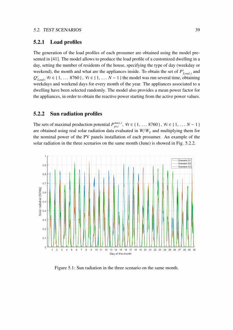
5.2.2 Sun radiation profiles
The sets of maximal production potential P max, tpr,i , ∀t ∈ 1, . . . 8760 , ∀i ∈ 1, . . . N − 1
are obtained using real solar radiation data evaluated in W/Wp and multiplying them forthe nominal power of the PV panels installation of each prosumer. An example of thesolar radiation in the three scenarios on the same month (June) is showed in Fig. 5.2.2.
Figure 5.1: Sun radiation in the three scenario on the same month.
40 CHAPTER 5. CASE STUDY
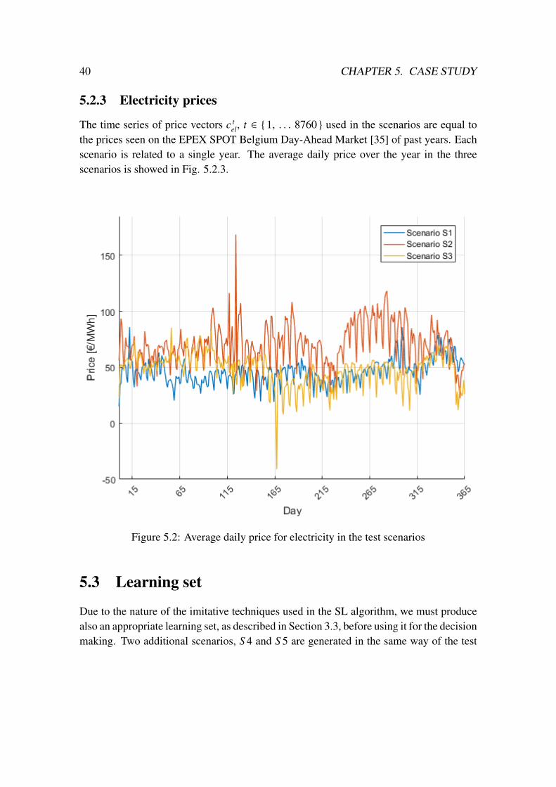
5.2.3 Electricity prices
The time series of price vectors c tel, t ∈ 1, . . . 8760 used in the scenarios are equal to
the prices seen on the EPEX SPOT Belgium Day-Ahead Market [35] of past years. Eachscenario is related to a single year. The average daily price over the year in the threescenarios is showed in Fig. 5.2.3.
Figure 5.2: Average daily price for electricity in the test scenarios
5.3 Learning set
Due to the nature of the imitative techniques used in the SL algorithm, we must producealso an appropriate learning set, as described in Section 3.3, before using it for the decisionmaking. Two additional scenarios, S 4 and S 5 are generated in the same way of the test
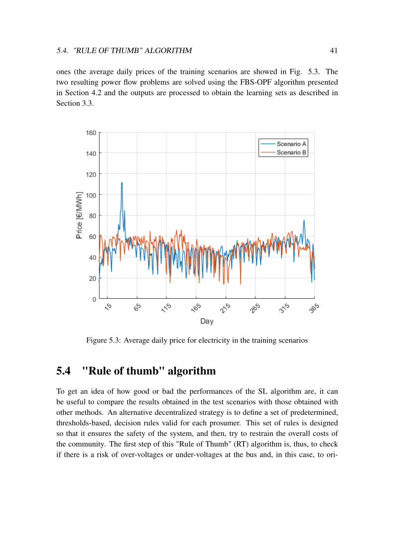
5.4. "RULE OF THUMB" ALGORITHM 41
ones (the average daily prices of the training scenarios are showed in Fig. 5.3. Thetwo resulting power flow problems are solved using the FBS-OPF algorithm presentedin Section 4.2 and the outputs are processed to obtain the learning sets as described inSection 3.3.
Figure 5.3: Average daily price for electricity in the training scenarios
5.4 "Rule of thumb" algorithm
To get an idea of how good or bad the performances of the SL algorithm are, it canbe useful to compare the results obtained in the test scenarios with those obtained withother methods. An alternative decentralized strategy is to define a set of predetermined,thresholds-based, decision rules valid for each prosumer. This set of rules is designedso that it ensures the safety of the system, and then, try to restrain the overall costs ofthe community. The first step of this "Rule of Thumb" (RT) algorithm is, thus, to checkif there is a risk of over-voltages or under-voltages at the bus and, in this case, to ori-
42 CHAPTER 5. CASE STUDY
ent the actions of that prosumer to avoid it (fully charging/discharging the storage andmaximising/minimising the power production). In the case where the safety of the gridseems ensured, the decisions are imposed looking at the price of the electricity at thattime step (when it is above/under a predetermined price, impose a predetermined pro-sumer’s action). The algorithm is used by each prosumer i at each time step t and it canbe expressed, for example, in the following form:
if |v ti | 6 0.91pu
P tpr, i = Pmax, t
pr, i
Q tpr, i = Qmax, t
pr, i
P tdis,i = S t
i ηd, i
P tch,i = 0
else if |v ti | > 1.09pu
P tpr, i = 0
Q tpr, i = −Qmax, t
pr, i
P tch,i =
Xbatt, i−S ti
ηc, i
P tdis,i = 0
else
P tpr, i = P t,max
pr, i
Q tpr, i = 0
if ctel > c+
el
P tch,i = 0
if P tpr, i > P t
Load, i
if S ti > 0.3 Xbatt, i
P tdis,i =
(S t
i − 0.3 Xbatt, i
)η(i)
d
elseP t
dis,i = 0
elseP t
dis,i = S ti η
(i)d
5.5. RESULTS 43
else if ctel 6 c−el
if P tpr, i > P t
Load, i
if P tpr, i − P t
Load, i 6(Xbatt, i − S t
i
)η(i)
c
P tch,i =
P tpr, i−P t
Load, i
η(i)c
elseP t
ch,i =Xbatt, i−S i
t
η(i)c
elseif S t
i > 0.3 Xbatt, i
P tdis,i =
(S t
i − 0.3 Xbatt, i
)η(i)
d
elseP t
ch,i =0.3 Xbatt, i−S t
i
η(i)c
if P tch,i > Pmax
batt, i
P tch,i = Pmax
batt, i
if P tdis,i < Pmax
batt, i
P tdis,i = Pmax
batt, i
The thresholds c+el and c−el are predetermined values that defines, respectively, when
the electricity price is high or is low (in this cases study they are set to 2 and 0.5 timesthe average price of the training scenarios). The algorithm is designed to keep the batteryalways with a minimum SoC of 30% and to discharge the battery totally only when thereis a deficit of power production and the electricity price is very high. When the prosumerhas a production surplus, it inject it into the network or into the battery depending on theprice. Using this kind of algorithm is certainly a rough method to take decisions and it isoriented to favor the single prosumer more than the community, but it is still a reasonableway to control the action of the prosumer when there are not other strategies and it hasthe advantage of being very easy to implement in a controller.
5.5 Results
Before dealing with the test scenarios, the training scenarios are optimized using the FBS-OPF algorithm and a learning set for the SL algorithm is extrapolated. All the problems
44 CHAPTER 5. CASE STUDY
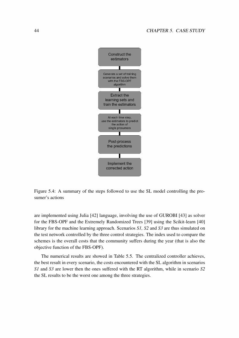
Figure 5.4: A summary of the steps followed to use the SL model controlling the pro-sumer’s actions
are implemented using Julia [42] language, involving the use of GUROBI [43] as solverfor the FBS-OPF and the Extremely Randomized Trees [39] using the Scikit-learn [40]library for the machine learning approach. Scenarios S1, S2 and S3 are thus simulated onthe test network controlled by the three control strategies. The index used to compare theschemes is the overall costs that the community suffers during the year (that is also theobjective function of the FBS-OPF).
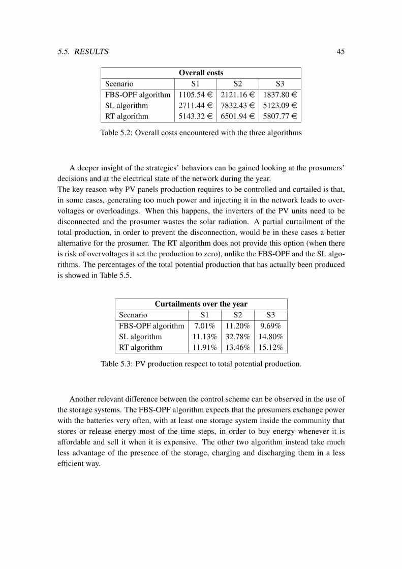
The numerical results are showed in Table 5.5. The centralized controller achieves,the best result in every scenario, the costs encountered with the SL algorithm in scenariosS1 and S3 are lower then the ones suffered with the RT algorithm, while in scenario S2the SL results to be the worst one among the three strategies.
5.5. RESULTS 45
Overall costsScenario S1 S2 S3FBS-OPF algorithm 1105.54 e 2121.16 e 1837.80 eSL algorithm 2711.44 e 7832.43 e 5123.09 eRT algorithm 5143.32 e 6501.94 e 5807.77 e
Table 5.2: Overall costs encountered with the three algorithms
A deeper insight of the strategies’ behaviors can be gained looking at the prosumers’decisions and at the electrical state of the network during the year.The key reason why PV panels production requires to be controlled and curtailed is that,in some cases, generating too much power and injecting it in the network leads to over-voltages or overloadings. When this happens, the inverters of the PV units need to bedisconnected and the prosumer wastes the solar radiation. A partial curtailment of thetotal production, in order to prevent the disconnection, would be in these cases a betteralternative for the prosumer. The RT algorithm does not provide this option (when thereis risk of overvoltages it set the production to zero), unlike the FBS-OPF and the SL algo-rithms. The percentages of the total potential production that has actually been producedis showed in Table 5.5.
Curtailments over the yearScenario S1 S2 S3FBS-OPF algorithm 7.01% 11.20% 9.69%SL algorithm 11.13% 32.78% 14.80%RT algorithm 11.91% 13.46% 15.12%
Table 5.3: PV production respect to total potential production.
Another relevant difference between the control scheme can be observed in the use ofthe storage systems. The FBS-OPF algorithm expects that the prosumers exchange powerwith the batteries very often, with at least one storage system inside the community thatstores or release energy most of the time steps, in order to buy energy whenever it isaffordable and sell it when it is expensive. The other two algorithm instead take muchless advantage of the presence of the storage, charging and discharging them in a lessefficient way.
46 CHAPTER 5. CASE STUDY
Discussing the results
Huge differences between the FBS-OPF algorithm and the two decentralized controlschemes were expected, since it has much more data about the problem and each pro-sumer action is oriented to optimize the global objective. Batteries play a crucial role inthe centralized strategy: they can be used the knowledge of future prices can be used tomanage perfectly well the energy stored, optimizing the purchases and avoiding to wastepotential production when possible. The optimal behavior is very difficult to formalize orto mimic.The results obtained by the SL algorithm in the scenario S1 can be considered, thus, morethan acceptable, especially if compared with the RT algorithm. In the other two scenarios,the decisions taken by the algorithm based on machine brought to worse results: it hassuggested to curtail the production even when it was not needed (one third of the totalpotential production is not exploited in the second scenario) and to use the batteries in aninappropriate way. The set of inputs of the estimators contains many variables, it is possi-ble that unexpected values of some of the variables inside the input misled the predictionsof the estimators about the optimal actions to suggest. RT algorithm was able to performbetter than SL in the case of scenario S 2.The contrasting performances in the three cases are probably linked to the fact that sce-nario S1, in terms of prices and solar radiation profiles, is similar to the two trainingscenarios, while scenarios S2 and S3 present many differences in potential production,load profiles and electricity prices from the data used in the learning set. The "quality" ofthe learning set has, indeed, critical effects on methods based on imitative learning.A better post-processing of the predictions made by the estimator could be implemented,maybe adding some extra check, similar to those of the RT algorithm to verify that theactions are not obviously illogical, in order to avoid results like the one seen in scenarioS 2. Testing other SL method for the SL control strategy can be interesting too. However,imitative learning models have their limits and are not suited to manage unexpected in-puts.The simulations performed demonstrate, however, that a decentralized control scheme,that uses only local measurements, designed relying on supervised learning techniques,could produce, in standard cases, better results than predetermined strategies.
Chapter 6
Conclusion
This work presented some of the main aspects that revolve around the concept, quite re-cent, of the Electric Prosumer Communities. It pointed out several times what are thereason for them to spread worldwide and what could be the challenges that they offer.A snapshot of the technologies associated to distributed generation and energy storagehas been provided, demonstrating that many solutions are available to shift from beinga consumer to a prosumer. The attention was then moved on the control strategies ofa community, in particular on decentralized schemes. A simplified mathematical frame-work has been presented in order to better contextualize the problem. Power flow analysisand optimal power flow problems have been briefly introduced. We described one possi-ble method to find what are the optimal actions of each prosumer when all the externalvariables, like potential production, consumption and electricity price are known at everyinstant. We tried to design a decentralized control scheme using a machine learning ap-proach (more specifically, regression trees) to mimic, at an individual level (using localmeasurements only), the optimal behavior observed in the centralized solution. Anotherdecentralized control strategy that follows predetermined procedures has been developedto make comparisons. The control schemes were then tested on a case study in three dif-ferent scenarios.As expected, decentralized control schemes are penalized respect to centralized strategy,when it comes to efficiency. A deeper and wider knowledge of the network is essentialto manage adequately the community and to understand what would be the appropriatebehavior of single prosumers. Finally, knowing about the simultaneous actions of everyprosumers, gives the central entity a better insight of the situation, making possible toput in place cost-effective strategies. Hierarchical control mechanism requires howeverexpensive machinery and sharing personal information such as consumption habits, andit is not that easy to find the optimal strategy with so many unpredictable parameters. The
47

48 CHAPTER 6. CONCLUSION
results suggest that a decentralized control scheme relying supervised learning can pro-vide interesting results, but revealed some of its limits. Some expedient that can improvethis SL control strategy have been proposed.This thesis work was however performed using several simplification. The mathematicalmodel for the community and for the power flow analysis involved many assumptions inorder to reduce the computational cost of the problems, and discrete event simulation canrarely model adequately the dynamics of electric power system, therefore the results ofthe case study need to be seen in the right perspective.What is for sure is that developing more and more sophisticated methods to tackle the con-trol challenge of microgrids and EPCs is an essential step to make them spread. Designingnew decentralized schemes relying on more advanced machine learning techniques, suchas Reinforcement Learning (RL), could lead to interesting results, due the ability of thosemethod to self-improve, even when addressing unexpected scenarios [44].
Bibliography
[1] A. Kwasinski, W. Weaver, R. S. Balog, Microgrids and other Local Area Power andEnergy Systems, 2016.
[2] M. Amin and P. Schewe, Preventing Blackouts: Building a Smarter Power Grid,Scientific American, 2008.
[3] Yael Parag1 and Benjamin K. Sovacool, Electricity market design for the prosumerera, 2016.
[4] Dan T. Ton and Merrill A. Smith, The U.S. Department of Energy’s Microgrid Ini-tiative, 2016.
[5] Rathnayaka, Potdar, Dillon, Hussain and Kuruppu, Goal-Oriented Prosumer Com-munity Groups for the smart grids, IEEE Technology and Society Magazine, March2014.
[6] RENEWABLE CAPACITY STATISTICS 2017, Available online: http://www.irena.org/DocumentDownloads/Publications/IRENA_RE_Capacity_Statistics_2017.pdfIRENA, 2017.
[7] Renewables 2017 - Global status report, REN21, 2017
[8] Klaus Kursawe, George Danezis and Markulf Kohlweiss, Privacy-Friendly Aggre-gation for the Smart-Grid, S. Fischer-Hubner and N. Hopper (Eds.): PETS 2011,2011.
[9] A.J. Dinusha Rathnayaka, Vidyasagar M. Potdar, Tharam Dillon, Omar Hussain,and Elizabeth Chang, A Methodology to find Influential Prosumers in ProsumerCommunity Groups, 2009.
[10] https://www.eia.gov/todayinenergy/detail.php?id=31932, Monthly renewable elec-tricity generation surpasses nuclear, July 2017.
49
50 BIBLIOGRAPHY
[11] Rapporto Mensile sul Sistema Elettrico - Maggio 2017 Terna, May 2017.
[12] Snapshot of Global Photovoltaic Markets, IEA, 2016.
[13] Nicolae Badea, Design for Micro-Combined Cooling, Heating and Power Systems,Springer, 2015.
[14] Renewable Power Costs Plummet: Many Sources Now Cheaper than Fossil FuelsWorldwide, IRENA, 2015.
[15] Renewables 2017 Global Status Report, REN21, 2017.
[16] Photovoltaics report 2017, Fraunhofer Institute for Solar Energy Systems, ISE, July2017.
[17] Makkawi A, Celik AN, Muneer T., Evaluation of micro-wind turbine aerodynam-ics, wind speed sampling interval and its spatial variation, Services EngineeringResearch and Technology, 2009.
[18] Claire Soares, Microturbines: Applications for Distributed Energy Systems,Butterworth-Heinemann, 2007.
[19] David Gao, Energy Storage for Sustainable Microgrid, Academic Press, 2015
[20] Steven E. Letendre, Willett Kempton, The V2G Concept: A new model for power?,Public Utilities Fortnightly, February 15, 2002
[21] Jasna Tomic, Willett Kempton, Using fleets of electric-drive vehicles for grid sup-port, 2007.
[22] J. A. Pecas Lopesa, Silvan A. Polenzb, C. L. Moreiraa, R. Cherkaouib, Identificationof control and management strategies for LV unbalanced microgrids with plugged-inelectric vehicles, Electric Power Systems Research, 2010.
[23] Zhang, Shah, Papageorgiou, Efficient energy consumption and operation manage-ment in a smart building with microgrid, Energy Conversion and Management, Vol-ume 74, October 2013.
[24] F. Olivier, D. Ernst, R. Fonteneau, D. Marulli, Foreseeing New Control Challengesin Electricity Prosumer Communities, 2017.
BIBLIOGRAPHY 51
[25] A. J. Dinusha Rathnayaka, Vidyasagar M. Potdar, Samitha J. Kuruppu, Design ofSmart Grid Prosumer Communities via Online Social Networking Communities,2012.
[26] Marnay, Rubio, Siddiqui, Shape of the microgrid, 2000.
[27] TE Hoff, HJ Wenger, C. Herig, RW Shawn, A MICRO-GRID WITH PV, FUELCELLS, AND ENERGY EFFICIENCY, 1998.
[28] H.J. Song ; X. Liu ; D. Jakobsen ; R. Bhagwan ; X. Zhang ; K. Taura ; A. Chien,The MicroGrid: a Scientific Tool for Modeling Computational Grids 2000.
[29] Mahmoud, AL-Sunni, Control and optimization of Distributed Generation System,Springer International Publishing Switzerland, 2015.
[30] L. Breiman, J. H. Friedman, R. A. Olshen, and C. J. Stone, Classification and Re-gression Trees, Chapman & Hall, 1984.
[31] B. Stott, Review of load-flow calculation methods , Proceedings of the IEEE (Vol-ume: 62, Issue: 7), July 1974.
[32] B. Stott, O. Alsac, Fast Decoupled Load Flow, IEEE, May 1974.
[33] Fortenbacher, Philipp and Zellner, Martin and Andersson, Goran, Optimal sizingand placement of distributed storage in low voltage networks, 2016.
[34] Jen-Hao Teng, A Direct Approach for Distribution System Load Flow Solutions,IEEE, 2002.
[35] EPEX Spot DAM [Online], https://www.belpex.be/wp-content/uploads/marketdata/,EPEX (previously Belpex).
[36] C. Crisci, B. Ghattas, G. Perera, A review of supervised machine learning algorithmsand their applications to ecological data, 2012.
[37] Breiman, Bagging predictors, Machine Learning 24, 123–140, 1996.
[38] Breiman, Random forests, Machine Learning 45 (1), 5–32, 2001.
[39] P. Geurts, D. Ernst, and L. Wehenkel, Extremely randomized trees, Machine learn-ing, vol. 63, no. 1, pp. 3–42, 2006.
52 BIBLIOGRAPHY
[40] F. Pedregosa, G. Varoquaux, A. Gramfort, V. Michel, B. Thirion, O. Grisel, M.Blondel, P. Prettenhofer, R. Weiss, V. Dubourg et al., Scikit-learn: Machine learningin python, Journal of Machine Learning Research, vol. 12, no. Oct, pp. 2825–2830,2011.
[41] Ian Richardson, Murray Thomson, David Infield, Conor Clifford, Domestic electric-ity use: A high-resolution energy demand model 2010.
[42] The Julia Language, Available: https://julialang.org/
[43] Gurobi optimizer reference manual, Available: http://www.gurobi.com.
[44] Mevludin Glavic, Raphael Fonteneau, Damien Ernst, Reinforcement Learning forElectric Power System Decision and Control: Past Considerations and Perspectives,2017.