Mathematical modeling of textures : application to color image

decomposition with a projected gradient algorithm

Vincent Duval 1 & Jean-Francois Aujol 2 & Luminita A. Vese 3

1 Institut Telecom, Telecom ParisTech, CNRS UMR 5141vduval@enst.fr

2 CMLA, ENS Cachan, CNRS, UniverSudJean-Francois.Aujol@cmla.ens-cachan.fr

3 UCLA, Mathematics Departmentlvese@ucla.math.edu

Abstract: In this paper, we are interested in texture modeling with functional analysis spaces.We focus on the case of color image processing, and in particular color image decomposition. Theproblem of image decomposition consists in splitting an original image f into two components u andv. u should contain the geometric information of the original image, while v should be made of theoscillating patterns of f , such as textures. We propose here a scheme based on a projected gradientalgorithm to compute the solution of various decomposition models for color images or vector-valuedimages. We provide a direct convergence proof of the scheme, and we give some analysis on colortexture modeling.

Key-words: Texture modeling, color image decomposition, projected gradient algorithm, color tex-ture modeling.

1 Introduction

Since the seminal work by Rudin et al [59], total variation based image restoration and decompositionhas drawn a lot of attention (see [26, 7, 57, 5] and references therein for instance). We are interestedin minimizing energies of the following type where f is the original image:

∫

|Du| + µ‖f − u‖kT . (1)

∫|Du| stands for the total variation; in the case when u is smooth, then

∫|Du| =

∫|∇u| dx. ‖.‖T

stands for a norm which captures the noise and/or the textures of the original image f (in the sensethat it is not too large for such features) and k is a positive exponent.

The most basic choice for ‖.‖T is the L2 norm, and k = 2. From a Bayesian point of view, this isalso the norm which appears naturally when assuming that the image f has been corrupted by someadditive Gaussian white noise (see e.g. [26]). However, since the book by Y. Meyer [53], other spaceshave been considered for modeling oscillating patterns such as textures or noise. The problem of imagedecomposition has been a very active field of research during the last past five years. [53], was the

1

inspiration source of many works, e.g. [65, 58, 9, 6, 64, 10, 15, 24, 35, 69, 70, 71, 44, 11, 43, 48, 50].Image decomposition consists in splitting an original image f into two components, u and v = f − u.u is supposed to contain the geometrical component of the original image (it can be seen as some kindof sketch of the original image), while v is made of the oscillatory component (the texture componentin the case when the original image f is noise free).

In this paper, we focus on color image processing. While some authors deal with color imagesusing a Riemannian framework, like G. Sapiro and D. L. Ringach [60] or N. Sochen, R. Kimmel andR. Malladi [62], others combine a functional analysis viewpoint with the Chromaticity-Brightnessrepresentation [14]. The model we use is more basic: it is the same as the one used in [19] (andrelated with [18]). Its advantage is to have a rich functional analysis interpretation. Note that in [66],the authors also propose a cartoon + texture color decomposition and denoising model inspired fromY. Meyer, using the vectorial versions of total variation and approximations of the space G(Ω) fortextures (to be defined later); unlike the work presented here, they use Euler-Lagrange equations andgradient descent scheme for the minimization, which should be slower than by projection methods.

Here, we give some insight into the definition of a texture space for color images. In [12], aTV-Hilbert model was proposed for image restoration and/ or decomposition:

∫

|Du| + µ‖f − u‖2H (2)

where ‖.‖H stands for the norm of some Hilbert space H. This is a particular case of problem (1). Dueto the Hilbert structure of H, there exist many different methods to minimize (2), such as a projectionalgorithm [12]. We extend (2) to the case of color images.

From a numerical point of view, (1) is not straightforward to minimize. Depending on thechoice for ‖.‖T , the minimization of (1) can be quite challenging. Nevertheless, even in the simplestcase when ‖.‖T is the L2 norm, handling the total variation term

∫|Du| needs to be done with care.

The most classical approach consists in writing the associated Euler-Lagrange equation for problem(1). In [59], a fixed step gradient descent scheme is used to compute the solution. This methodhas on the one hand the advantage of being very easy to implement, and on the other hand thedisadvantage of being quite slow. To improve the convergence speed, quasi-Newton methods havebeen proposed [23, 67, 36, 1, 28, 55, 56]. Iterative methods have proved successful [17, 34, 15]. Aprojected-subgradient method can be found in [30].

Duality based schemes have also drawn a lot of attention to solve (1): first by Chan and Golub in[25], later by A. Chambolle in [20] with a projection algorithm. A multiscale version of this algorithmhas just been introduced in [22]. This projection algorithm has recently been extended to the caseof color images in [19]. Chambolle’s projection algorithm [20] has grown very popular, since it is thefirst algorithm solving exactly the total variation regularization problem and not an approximation,with a complete proof of convergence. In [73], a very interesting combination of the primal and dualproblems has been introduced. Second order cone programming ideas and interior point methods haveproved interesting approaches [45, 42]. Recently, it has been shown that graph cuts based algorithmscould also be used [21, 33]. Finally, let us notice that it is shown in [68, 8] that Nesterov’s scheme [54]provides fast algorithms for minimizing (1).

Another variant of Chambolle’s projection algorithm [20] is to use a projected gradient algorithm[21, 8, 72]. Here we have decided to use this approach which has both advantages of being easy toimplement and of being quite efficient.

Notice that all the schemes based on duality proposed in the literature can be seen as particular

2

instance of proximal algorithms [31, 51, 37, 41, 61].

The plan of the paper is the following. In Section 2, we define and provide some analysis aboutthe spaces we consider in the paper. In Section 3, we extend the TV-Hilbert model originally intro-duced in [12] to the case of color images. In Section 4, we present a projected gradient algorithm tocompute a minimizer of problem (2). This projected gradient algorithm has first been proposed by A.Chambolle in [21] for total variation regularization. A proof of convergence was given in [8] relying onoptimization results by Bermudez and Moreno [16]. A proof based on results for proximal algorithmswas proposed in [72]. We derive here a simple and direct proof of convergence. In Section 5, weapply this scheme to solve various classical denoising and decomposition problems. We illustrate ourapproach with many numerical examples. We discuss qualitative properties of image decompositionmodels in Section 6.

2 Definitions and properties of the considered color spaces

In this section, we introduce several notations and we provide some analysis of the functional spaceswe consider to model color textures.

2.1 Introduction

Let Ω be a Lipschitz convex bounded open set in R2. We model color images as R

M -valued functionsdefined on Ω. The inner product in L2(Ω, RM ) is denoted as:

〈u,v〉L2(Ω,RM ) =

∫

Ω

M∑

i=1

uivi.

For a vector ξ ∈ RM , we define the norms:

|ξ|1 =

M∑

i=1

|ξi|, |ξ|2 =√

∑Mi=1 ξ2

i , |ξ|∞ = maxi=1...M

|ξi|. (3)

We will sometimes refer to the space of zero-mean functions in L2(Ω, RM ) by V0:

V0 = f ∈ L2(Ω, RM ),

∫

Ωf = 0.

We say that a function f ∈ L1(Ω, RM ) has bounded variation if the following quantity is finite:

|f |TV = sup

∫

Ω

M∑

i=1

fidiv ~ϕi, ~ϕ ∈ C1c (Ω,B)

= sup~ϕ∈C1

c (Ω,B)〈f ,div ~ϕ〉L2(Ω,RM )

where B is a centrally symmetric convex body of R2×M . This quantity is called the total variation.

For more information on its properties, we refer the reader to [4]. The set of functions with boundedvariation is a vector space classically denoted by BV

(Ω, RM

).

3

In this paper, we will consider the following set of test-functions, which is the classical choice([4], [7]) :

B = ~w ∈ R2×M/| ~w|2 ≤ 1.

Then, for f smooth enough, the total variation of f is:

|f |TV =

∫

Ω

√√√√

M∑

i=1

|∇fi|2dx.

As X. Bresson and T. Chan notice in [19], the choice of the set B is crucial. If one chooses:

B = ~w ∈ R2×M/| ~w|∞ ≤ 1,

then one has:

|f |TV =

M∑

i=1

∫

Ω|∇fi|dx =

M∑

i=1

|fi|TV .

These two choices are mathematically equivalent and define the same BV space, but in practicethe latter induces no coupling between the channels. As a consequence, if the data fidelity term doesnot introduce a coupling either, the minimization of an energy of type (1) amounts to a series ofindependent scalar TV minimization problems, which gives visual artifacts in image processing (see[18, 27]).

2.2 The color G(Ω) space

The G(R2) space was introduced by Y. Meyer in [53] to model textures in grayscale images. It wasdefined as div

(L∞(R2)

), but one could show that this space was equal to W−1,∞(R2) (the dual of

W 1,1(R2)). For the generalization to color images, we will adopt the framework of [6] (the color spaceG(Ω) is also used in [66], as a generalization of [65] to color image decomposition and color imagedenoising). Let us insist on the fact that the results of this section (notably Proposition 2.1) arespecific to the case of 2-dimensional images (i.e. Ω ⊂ R

2).

Definition 2.1. The space G(Ω) is defined by:

G(Ω) = v ∈ L2(Ω, RM )/∃~ξ ∈ L∞(Ω, (R2)M ),∀i = 1, . . . ,M, vi = div ~ξi and ~ξi · ~N = 0 on ∂Ω

(where ~ξi · ~N refers to the normal trace of ~ξi over ∂Ω). One can endow it with the norm:

‖v‖G = inf‖~ξ‖∞, ∀i = 1, . . . ,M, vi = div ξi, ~ξi · ~N = 0 on ∂Ω

with ‖~ξ‖∞ = sup ess

√∑M

i=1 |~ξi|2.

The following result, proved in [6] for grayscale images, can be easily extended working compo-nent by component: it characterizes G(Ω).

Proposition 2.1.

G(Ω) =

v ∈ L2(Ω, RM )/

∫

Ωv = 0

.

4

Following the framework of [49], we define ‖ ·‖∗ below. Since the total variation does not changeby the addition of constants, we also have:

Lemma 2.1. For f ∈ L2(Ω, RM ), let us consider the semi-norm:

‖f‖∗ = supu∈BV (Ω,RM ),|u|TV 6=0

〈f ,u〉L2(Ω,RM )

|u|TV= sup

u∈BV (Ω,RM ),|u|TV 6=0

∑Mi=1

∫

Ω fiui

|u|TV.

If ‖f‖∗ < +∞, then∫

Ω f = 0.

Comparing this property to Proposition 2.1, we can deduce that any function f such that‖f‖∗ < ∞ belongs to G(Ω). The converse is also true:

Lemma 2.2. Let f ∈ G(Ω). Then ‖f‖∗ < ∞.

Proof: Let f ∈ G(Ω). Since∫

Ω f = 0, the quantity〈f ,u〉

L2(Ω,RM )

|u|TVdoes not change with the addition

of constants to u. Thus

supu∈BV,|u|TV 6=0

〈f ,u〉L2(Ω,RM )

|u|TV= sup

u∈BV,R

u=0

〈f ,u〉L2(Ω,RM )

|u|TV

≤ supu∈BV,

R

u=0

‖f‖L2(Ω,RM )‖u‖L2(Ω,RM )

|u|TV

≤ C‖f‖L2(Ω) < ∞,

where we used Poincare inequality : ‖u − uΩ‖L2(Ω,RM ) ≤ C|u|TV .

The following theorem completes the above two lemmas:

Theorem 2.2. The following equality holds :

G(Ω) = f ∈ L2(Ω)/ supu∈BV (Ω,RM ),|u|BV 6=0

〈f ,u〉L2(Ω,RM )

|u|TV< +∞

and for all function f ∈ L2(Ω, RM ), ‖f‖∗ = ‖f‖G.

Moreover, the infimum in the definition of ‖ · ‖G is reached.

Proof:

(i) Let f be a function in the set on the right hand-side. Thanks to Lemma 2.1, we know that∀i ∈ 1, . . . ,M,

∫

Ω fi = 0. By Proposition 2.1, f ∈ G(Ω).

Now let u ∈ BV(Ω, RM

)such that |u|TV 6= 0. By Meyers-Serrin’s theorem, one can find a

sequence un ∈ C∞(Ω, RM ) ∩ W 1,1(Ω; RM ) such that ‖u − un‖2 → 0 and |un|TV → |u|TV .

5

Then, for all ~g such that f = div ~g and ~g · ~N = 0 on ∂Ω:

〈f ,un〉L2(Ω,RM ) =

M∑

i=1

∫

Ωdiv ~g un

= −

∫

Ω(

M∑

i=1

~gi · ∇ui,n)

≤

∫

Ω|~g||∇un|

≤ ‖~g‖∞|un|TV .

Since f ∈ L2(Ω), we can pass to the limit in both sides of the inequality, and by construction ofun, we get:

‖f‖∗ ≤ ‖f‖G.

(ii) For the converse inequality, the proof is standard (see e.g. [46], [2]).

Let f ∈ L2(Ω, RM ) such that supu∈BV (Ω,RM ),|u|TV 6=0

〈f ,u〉L2(Ω,RM )

|u|TV< +∞. Let us define :

T :

D(Ω, RM ) → L1(Ω, R2M )

ϕ 7→(

∂ϕ1

∂x1, ∂ϕ1

∂x2, . . . , ∂ϕM

∂x1, ∂ϕM

∂x2

)

To each vector(

∂ϕ1

∂x1, ∂ϕ1

∂x2, . . . , ∂ϕM

∂x1, ∂ϕM

∂x2

)

∈ T (D(Ω, RM )), we can associate∫

Ω

∑Mi=1 f iϕidx

(without ambiguity since fi has zero-mean, and if two functions have the same gradient over Ωthey only differ by a constant on the convex domain Ω). We have

∫

Ω

∑Mi=1 f iϕidx ≤ ‖f‖∗|ϕ|BV =

‖f‖∗‖(∂ϕ1

∂x1, . . . , ∂ϕM

∂x2)‖1 thus we have defined a bounded linear form on T (D(Ω, RM )). Using

Hahn-Banach’s theorem, we can extend it to L1(Ω, R2M ) with the same norm ‖f‖∗. SinceL∞(Ω, R2M ) is identifiable with the dual of L1(Ω, R2M ), there exists g ∈ L∞(Ω, R2M ) with‖g‖L∞(Ω,RM ) = ‖f‖∗, such that:

∀ϕ ∈ D(Ω, RM ),

∫

Ω

M∑

i=1

fiϕi = −

∫

Ω

M∑

i=1

2∑

j=1

∂ϕi

∂xjgi,j = −

M∑

i=1

∫

Ω~gi · ∇ϕi. (4)

This is true in particular for ϕ ∈ D(Ω, RM ), thus f = div ~g in the distributional sense, andsince the functions are in L2(Ω, RM ) there is equality in L2(Ω, RM ). Since div ~g ∈ L2(Ω, RM ),we can then consider the normal trace of ~g.

If ϕ ∈ D(Ω, RM ), we have by (4):

M∑

i=1

∫

Ωfiϕi = −

M∑

i=1

∫

Ωgi · ∇ϕi.

But on the other hand, using integration by parts:

M∑

i=1

∫

Ωdiv ~giϕi = −

M∑

i=1

∫

Ω~gi · ∇ϕi +

M∑

i=1

∫

∂Ωϕi~gi · ~N.

6

The equality f = div ~g in L2(Ω, RM ) shows that the boundary contribution vanishes for ϕ ∈D(Ω, RM ). Thus ~gi · ~N = 0 over ∂Ω.

Incidentally, we notice that the infimum in the G-norm is reached.

Remark 2.3. From the proof of Lemma 2.2, we can deduce that the topology induced by the G-normon G(Ω) is coarser than the one induced by the L2 norm. More generally, there exists a constantC > 0 (depending only on Ω), such that for all f ∈ G(Ω), ‖f‖∗ ≤ C‖f‖L2(Ω,RM ).

In fact the G norm is strictly coarser than the L2 norm. Here is an example for M =2 color channels. Let us consider the family of functions

(f (m1,m2)

)

m1,m2∈N∗defined on (−π, π)2

by f(m1,m2)1 (x, y) = cos m1x + cos m1y and f

(m1,m2)2 (x, y) = cos m2x + cos m2y. The vector field

~ξ(m1,m2) defined by ~ξ(m1,m2)k =

(1

mksin(mkx), 1

mksin(mky)

)

for k ∈ 1, 2 satisfies the boundary con-

dition, and its divergence is equal to f (m1,m2). As a consequence ‖f (m1,m2)‖G ≤

√

2(

1m2

1+ 1

m22

)

and

limm1,m2→+∞ ‖f (m1,m2)‖G = 0.

Yet,

‖f (m1,m2)‖2L2(Ω,RM ) =

∫ π

−π

∫ π

−π

(cos m1x + cos m1y)2 + (cos m2x + cos m2y)2dxdy = 8π2.

The sequence fm converges to 0 for the topology induced by the G-norm, but not for the oneinduced by the L2 norm .

The following result proposed by Y. Meyer in [53] specifies this idea.

Proposition 2.2. Let fn, n ≥ 1 be a sequence of functions of Lq(Ω, RM ) ∩ G(Ω) with the followingproperties :

1. There exists q > 2 and C > 0 such that ‖fn‖Lq(Ω,RM ) ≤ C.

2. The sequence fn converges to 0 in the distributional sense.

Then ‖fn‖G converges to 0 when n goes to infinity.

It means that oscillating patterns with zero mean have a small G-norm. Incidentally, noticethat in the above example, the frequencies of all color channels had to go to infinity in order to haveconvergence to zero for the G-norm. Otherwise, assumption 2) in the above proposition fails.

3 Color TV-Hilbert model: presentation and mathematical analysis

The G-norm detailed in Section 2 is the main tool to study the TV-Hilbert problem on which all thealgorithms described in this paper rely.

7

3.1 Presentation

The TV-Hilbert framework was introduced for grayscale images by J.-F. Aujol and G. Gilboa in [12]as a way to approximate the BV-G model. They prove that one can extend Chambolle’s algorithm tothis model. In this section we show that this is still true for color images. We are interested in solvingthe following problem:

infu

|u|TV +1

2λ‖f − u‖2

H (5)

where H = V0 (the space of zero-mean functions of L2(Ω, RM )) is a Hilbert space endowed with thefollowing norm:

‖v‖2H = 〈v,Kv〉L2(Ω,RM )

and where K : H → L2(Ω, RM )

• is a bounded linear operator (for the topology induced by the L2(Ω, RM ) norm on H)

• is symmetric positive definite

and K−1 is bounded on Im(K).

Examples:

• The Rudin-Osher Fatemi modelIt was proposed in [59] by L. Rudin, S. Osher, and E. Fatemi for grayscale images. It was thenextended to color images using different methods, for instance by G. Sapiro and D.L. Ringach[60], or Blomgren and T. Chan [18] . In [19], X. Bresson and T. Chan use another kind of colortotal variation, which is the one we use in this paper. The idea is to minimize the functional:

|u|TV +1

2λ‖f − u‖2

L2(Ω,RM ). (6)

It is clear that the problem commutes with the addition of constants. If the (unique) solutionassociated to f is u, then the solution associated to f + C is (u + C). As a consequence wecan always assume that f has zero mean. Then this model becomes a particular case of theTV-Hilbert model with K = Id.

• The OSV modelIn [58], S. Osher, A. Sole and L. Vese propose to model textures by the H−1 space. In order togeneralize this model, we must be cautious about the meaning of our notations but it is naturalto introduce the following functional :

infu

|u|TV +1

2λ

∫

Ω|∇∆−1(f − u)|2 (7)

where ∆−1v =

∆−1v1...

∆−1vM

, ∇ρ =

∇ρ1...

∇ρM

, |∇ρ|2 = |∇ρ1|

2 + |∇ρ2|2 + . . . + |∇ρM |2 and

8

∫

Ω|∇∆−1(f − u)|2 =

∫

Ω

∑Mi=1 |∇∆−1(f i − ui)|2 = −

∫

Ω

M∑

i=1

(f i − ui)∆−1(f i − ui)

= 〈f − u,−∆−1(f − u)〉L2(Ω,RM ).

The inversion of the Laplacian is defined component by component. For one component, it isdefined by the following consequence of the Lax-Milgram theorem:

Proposition 3.1. Let X0 = P ∈ H1(Ω, R) :∫

Ω P = 0. If v ∈ L2(Ω), with∫

Ω v = 0, then theproblem:

−∆P = v,∂P

∂n|∂Ω = 0

admits a unique solution in X0.

For K = −∆−1, the Osher-Sole-Vese problem is a particular case of the TV-Hilbert framework.

3.2 Mathematical study

In this subsection, we study the existence and uniqueness of minimizers of Problem (5). A characteri-zation of these minimizers is then given in Theorem 3.1. Notice that this theorem and its reformulationcould be easily obtained using convex analysis results ([40]), but for a pedagogical purpose, we givean elementary proof inspired from [53].

Proposition 3.2 (Existence and Uniqueness). Let f ∈ L2(Ω, RM ). The minimization problem:

inf

|u|TV +1

2λ〈f − u,K(f − u)〉L2(Ω,RM ), u ∈ BV

(Ω, RM

), (f − u) ∈ V0

has a unique solution u ∈ BV(Ω, RM

).

Proof: Let E(u) denote the functional defined on L2(Ω, RM ) (with E(u) = +∞ if u /∈ BV(Ω, RM

)

or (f − u) /∈ V0).

Let us notice that E 6= +∞ since fΩ = 1|Ω|

∫

Ω f belongs to BV(Ω, RM

)and (f − fΩ) ∈ V0.

The functional E is convex. Since K is bounded, we deduce that E is lower semi-continuous forthe weak L2(Ω) topology. E is coercive: by Poincare inequality,

∃C > 0, ‖u − uΩ‖2 ≤ C|u|TV

with uΩ = 1|Ω|

∫

Ω u = 1|Ω|

∫

Ω f for E(u) < +∞. Thus E has a minimizer. Since the functional isstrictly convex, this minimizer is unique.

We introduce the notation v = f − u, when u is the unique minimizer of the TV-Hilbertproblem.

9

Theorem 3.1 (Characterization of minimizers). Let f ∈ L2(Ω, RM ).

(i) If ‖Kf‖∗ ≤ λ then the solution of the TV-Hilbert problem is given by (u,v) = (0,f).

(ii) If ‖Kf‖∗ > λ then the solution (u,v) is characterized by:

‖Kv‖∗ = λ and 〈u,Kv〉L2(Ω,RM ) = λ|u|TV .

Proof:

(i) (0,f) is a minimizer iff

∀h ∈ BV(Ω, RM

),∀ǫ ∈ R, |ǫh|TV +

1

2λ‖f − ǫh‖2

H ≥1

2λ‖f‖2

H,

which is equivalent to |ǫ||h|TV +1

2λǫ2‖h‖2

H −1

λǫ〈f ,h〉H ≥ 0.

We can divide by |ǫ| → 0, and depending on the sign of ǫ we get :

±〈f ,h〉H ≤ λ|h|TV .

If (0,f) is a minimizer, we can take the supremum for h ∈ BV(Ω, RM

). By definition of the

*-norm, we have : ‖Kf‖∗ ≤ λ.

Conversely, if f ∈ L2(Ω, RM ) is such that ‖Kf‖∗ ≤ λ, the second inequality is true , thus (0,f)is a minimizer.

(ii) As before, let us characterize the extremum: (u,v) is a minimizer iff

∀h ∈ BV(Ω, RM

),∀ǫ ∈ R, |u + ǫh|TV +

1

2λ‖v − ǫh‖2

H ≥ |u|TV +1

2λ‖v‖2

H,

or |u + ǫh|TV +1

2λǫ2‖h‖2

H −1

λǫ〈v,h〉H ≥ |u|TV .

By triangle inequality, we have:

|u|TV + |ǫ||h|TV +1

2λǫ2‖h‖2

H −1

λǫ〈v,h〉H ≥ |u|TV

|h|BV ≥1

λ〈v,h〉H

Taking the supremum, we obtain ‖Kv‖∗ ≤ λ.

Moreover, choosing h = u, ǫ ∈] − 1, 1[:

(1 + ǫ)|u|BV ≥1

λǫ〈v,u〉H + |u|TV

For ǫ > 0 : |u|TV ≥1

λ〈v,u〉H

For ǫ < 0 : |u|TV ≤1

λ〈v,u〉H

10

We deduce that ‖Kv‖∗|u|TV ≥ 〈v,u〉H = λ|u|TV , and by the first upper-bound inequality, wehave ‖Kv‖∗ = λ.

Conversely, let us assume these equalities hold. Then:

|u + ǫh|TV +1

2λ‖v − ǫh‖2

H ≥1

λ〈(u + ǫh),Kv〉L2(Ω,RM ) +

1

2λ‖v‖2

H +1

2λ‖h‖2

Hǫ2 −1

λǫ〈h, v〉H

≥ |u|TV +1

2λ‖v‖2

H.

The mapping v 7→ sup|u|TV 6=0〈u,Kv〉2L(Ω,RM )

|u|TVis convex, lower semi-continuous for the H strong

topology as a supremum of convex lower semi-continuous functions. As a consequence, for λ > 0 theset

Gλ = v ∈ L2(Ω, RM ), ‖v‖∗ ≤ λ

is a closed convex set, as well as K−1Gλ. The orthogonal projection of this set is well-defined and wecan notice that Theorem 3.1 reformulates :

v = PH

K−1Gλ(f)

u = f − v.

Indeed, if (u,v) is a minimizer of the TV-Hilbert problem, with f = u + v, we have v ∈ K−1Gλ andfor any v ∈ K−1Gλ,

〈f − v, v − v〉H = 〈u,Kv〉L2(Ω,RM ) − 〈u,Kv〉L2(Ω,RM ) ≤ ‖Kv‖∗|u|TV − λ|u|TV ≤ 0,

thus by the equivalent definition of the projection on a closed convex set (see Ekeland-Temam [40]),we obtain the desired result.

Consequently, v is the orthogonal projection of f on the set K−1Gλ where Gλ = λdiv ~p, |~p| ≤1 (see Theorem 2.2), and the problem is equivalent to its dual formulation:

inf|~p|≤1

‖λK−1 div ~p − f‖2H. (8)

4 Projected gradient algorithm

In the present section, we are interested in solving the dual formulation (8), which can be done usingfast algorithms. For grayscale images, the famous projection algorithm by A. Chambolle [20] wasthe inspiration for all the following algorithms. We present here a projection algorithm, and weprovide a complete proof of convergence of this scheme. We note that an independent work has justbeen reported in [52], where the authors M. Zhu, S.J. Wright, and T.F. Chan have also applied theprojected gradient method for solving the dual formulation of total variation minimization for imagedenoising. They have a general framework also, although applied only to scalar image denoising andnot related to image decompositions.

As explained in the introduction, the scheme we propose here can be seen as a proximal pointalgorithm [31]. The proof of convergence could then be derived from results in [51] (the Lions-Mercieralgorithm being itself a particular instance of proximal algorithms [39]). However, we have decided topresent here an elementary proof of the convergence for didactic reasons.

11

4.1 Discrete setting

From now on, we will work in the discrete case, using the following conventions. A grayscale image isa matrix of size N × N . We write X = R

N×N the space of grayscale images. Their gradients belongto the space Y = X × X. The discrete L2 inner product is 〈u, v〉X =

∑

1≤i,j≤N ui,jvi,j.

The gradient operator is defined by (∇u)i,j = ((∇u)xi,j , (∇u)yi,j) with:

(∇u)xi,j =

ui+1,j − ui,j if i < N

0 if i = Nand (∇u)yi,j =

ui,j+1 − ui,j if j < N

0 if j = N.

The divergence operator is defined as the opposite of the adjoint operator of ∇:

∀~p ∈ Y, 〈−div ~p, u〉X = 〈~p,∇u〉Y

(div ~p)i,j =

pxi+1,j − px

i,j if 1 < i < N

pxi,j if i = 1

−pxi−1,j if i = N

+

pxi,j+1 − py

i,j if 1 < j < N

pyi,j if j = 1

−pyi,j−1 if j = N.

A color image is an element of XM . The gradient and the divergence are defined component bycomponent, and the discrete L2 inner product is given by :

∀u,v ∈ XM , 〈u,v〉XM =M∑

k=1

〈u(k), v(k)〉X

∀~p, ~q ∈ Y M , 〈~p, ~q〉Y M =

M∑

k=1

〈p(k), q(k)〉Y

so that the color divergence is still the opposite of the adjoint of the color gradient.

4.2 Bresson-Chan algorithm

Problem (8) for grayscale images was tackled in [20] in the case K = Id, then in [12] for a general K.For color images, X. Bresson and T. Chan [19] showed that Chambolle’s projection algorithm couldstill be used when K = Id. It is actually easy to check that it can be used with a general K for colorimages as well.

Following the steps of [12], one can notice that, provided τ ≤ 18‖K−1‖

L2, the fixed point iteration:

~p n+1 =~p n + τ(∇(K−1div ~p n − f/λ)

1 + τ |∇(K−1div ~p n − f/λ)|(9)

gives a sequence (~p n)n∈N such that λK−1div ~p n+1 → vλ, and f − λK−1div ~p n+1 → uλ whenn → +∞.

Notice that the upper bound on τ is the same as for grayscale images.

12

4.3 Projected gradient

It was recently noticed ([21], [8]) that problem (8) for grayscale images could be solved using a projectedgradient descent. This is the algorithm we decided to extend to the case of color images.

Let B be the discrete version of our set of test-functions :

B = v ∈ Y M ,∀ 1 ≤ i, j ≤ N, |vi,j |2 ≤ 1.

The orthogonal projection on B is easily computed:

PB(x) =

(x1

max1, |x|2,

x2

max1, |x|2

)

.

The projected gradient descent scheme is defined by :

~pm+1 = PB

(~pm+1 + τ∇(K−1div ~pm − f/λ

)(10)

which amounts to:

pm+1i,j =

pmi,j + τ∇(K−1div pm − f

λ )i,j

max(

1, |pmi,j + τ∇(K−1div pm − f

λ )i,j |2

) (11)

where τ = λµ.

The convergence result for the projected gradient descent in the case of elliptic functions isstandard (see [29], Theorem 8.6-2). Yet in our case the functional is not elliptic, and the proof needsa little more work.

Proposition 4.1. If 0 < τ < 14‖K−1‖

, then algorithm (11) converges. More precisely, there exists

~p ∈ B such that :lim

m→∞(K−1 div ~pm) = K−1 div ~p

and‖λK−1 div ~p − f‖2

H = inf~p∈B

‖λK−1 div ~p − f‖2H

Proof: Writing

‖K−1 div ~q−f/λ‖2H = ‖K−1 div ~p−f/λ‖2

H+〈KK−1 div (~q− ~p),K−1 div ~p−f/λ〉L2 +O(‖~q− ~p‖2),

we begin by noticing that ~p is a minimizer if and only if,

~p ∈ B and ∀~q ∈ B,∀τ > 0, 〈~q − ~p, ~p − (~p + τ∇(K−1 div ~p − f/λ))〉L2 ≥ 0.

Or equivalently:~p = PB

(~p + τ(∇(K−1 div ~p − f/λ)

)

where PB is the orthogonal projection on B with respect to the L2 inner product.

We know that such a minimizer exists. Let us denote it by ~p.

13

• Now let us consider a sequence defined by (10), and write A = −∇K−1 div . We have:

‖~pk+1 − ~p‖2 = ‖PB(~pk + τ∇(K−1 div ~pk − f/λ)) − PB(~p + τ∇(K−1 div ~p − f/λ))‖2

≤ ‖~p − ~pk + τ∇K−1 div (~p − ~pk)‖2 since PB is 1-Lipschitz [29]

≤ ‖(I − τA)(~p − ~pk)‖2

Provided ‖I − τA‖ ≤ 1, we can deduce:

‖~pk+1 − ~p‖ ≤ ‖~pk − ~p‖ (12)

and the sequence (‖~pk − ~p‖) is convergent.

• A is a symmetric positive semi-definite operator. By writing E = ker A and F = ImA, we have:

Y M = E⊥⊕ F

and we can decompose any ~q ∈ Y M as the sum of two orthogonal components ~qE ∈ E and~qF ∈ F . Notice that by injectivity of K−1, E is actually equal to the kernel of the divergenceoperator.

Let µ1 = 0 < µ2 ≤ . . . ≤ µa be the ordered eigenvalues of A.

‖I − τA‖ = max(|1 − τµ1|, |1 − τµa|)

= max(1, |1 − τµa|)

= 1 for 0 ≤ τ ≤2

µa

We can restrict I − τA to F and then define:

g(τ) = ‖(I − τA)|F‖ = max(|1 − τµ2|, |1 − τµa|)

< 1 for 0 < τ <2

µa

• Now we assume that 0 < τ < 2µa

. Therefore, inequality (12) is true and the sequence (~pk)

is bounded, and so is the sequence (K−1 div ~pk). We are going to prove that the sequence(K−1 div ~pk) has a unique cluster point. Let (K−1 div ~pϕ(k)) be a convergent subsequence. Byextraction, one can assume that ~pϕ(k) is convergent too, and denote by ~p its limit.

Passing to the limit in (10), the sequence (~pϕ(k)+1) is convergent towards:

~p = PB

(

~p + τ∇(K−1div ~p − f/λ))

Using (12), we also notice that:

‖~p − ~p‖ = ‖~p − ~p‖

As a consequence:

‖~p − ~p‖2 = ‖~p − ~p‖2

= ‖PB

(

~p + τ∇(K−1div ~p − f/λ))

− PB

(~p + τ∇(K−1div ~p − f/λ)

)‖2

≤ ‖(I − τA)(~p − ~p)‖2

≤ ‖(~p − ~p)E‖2 + g(τ)2‖(~p − ~p)F ‖

2

< ‖~p − ~p‖2 if (~p − ~p)F 6= 0

14

Of course, this last inequality cannot hold, which means that ‖(~p − ~p)F ‖ = 0. Hence (~p − ~p) ∈E = ker A and K−1 div ~p = K−1 div ~p: the sequence (K−1 div ~pk) is convergent.

• The last remark consists in evaluating µa. We have:

µa = ‖∇K−1 div ‖ ≤ ‖∇‖‖K−1‖‖ div ‖

Since ‖ div ‖2 = ‖∇‖2 = 8 (see [20], the result is still true for color images), we deduce that

µa ≤ 8‖K−1‖.

Since we are only interested in v = λK−1div ~p, Proposition (4.1) justifies the validity of algo-rithm (10). Yet it is possible to prove that ~p itself converges.

Lemma 4.1. Let P be the orthogonal projection on a nonempty closed convex set K. Let Q = Id−P .Then we have:

‖Q(v1) − Q(v2)‖2 + ‖P (v1) − P (v2)‖

2 ≤ ‖v1 − v2‖2. (13)

Proof:

‖Q(v1) − Q(v2)‖2 + ‖P (v1) − P (v2)‖

2

= ‖v1 − v2 + P (v1) − P (v2)‖2 + ‖P (v1) − P (v2)‖

2

= ‖v1 − v2‖2 + 2‖P (v1) − P (v2)‖

2 − 2〈P (v1) − P (v2), v1 − v2〉

= ‖v1 − v2‖2 + 2〈P (v1) − P (v2), P (v1) − P (v2) − v1 + v2〉

= ‖v1 − v2‖2 + 2 〈P (v1) − P (v2), P (v1) − v1〉

︸ ︷︷ ︸

≤0

+2 〈P (v2) − P (v1), P (v2) − v2〉︸ ︷︷ ︸

≤0

(using the characterization of the projection on a nonempty closed convex set [29]).

Remark: We have:

~p = PB(~p − τ(A~p + ∇f/λ)) = ~p − τ(A~p + ∇f/λ)) − QB(~p − τ(A~p + ∇f/λ)),

thus−τ(A~p + ∇f/λ)) = QB(~p − τ(A~p + ∇f/λ)). (14)

Corollary 4.1. The sequence ~pk defined by (10) converges to ~p unique solution of problem (8).

15

Proof: Using the above lemma, we have:

‖QB(~p − τ(A~p + ∇f/λ)) − QB(~pk − τ(A~pk + ∇f/λ))‖2

+‖PB(~p − τ(A~p + ∇f/λ)) − PB(~pk − τ(A~pk + ∇f/λ))‖2

≤ ‖~p − τ(A~p + ∇f/λ) − ~pk + τ(A~pk + ∇f/λ)‖2

≤ ‖~p − ~pk‖2 + τ2‖A(~p − ~pk))‖2 − 2τ〈~p − ~pk, A(~p − ~pk)〉

Hence:

‖QB(~p − τ(A~p + ∇f/λ)) − QB(~pk − τ(A~pk + ∇f/λ))‖2 + ‖~p − ~pk+1‖2

≤ ‖~p − ~pk‖2 + τ2‖A(~p − ~pk))‖2 − 2τ〈~p − ~pk, A(~p − ~pk)〉.

But we have already shown that ‖~p − ~pk‖ converges, and that K−1div (~p − ~pk) → 0 (thereforeA(~p − ~pk) → 0). Hence, passing to the limit in the above equation, we get:

Q(~pk − τ(A~pk + ∇f/λ)) → QB(~p − τ(A~p + ∇f/λ)).

We thus deduce from (14) that

QB(~pk − τ(A~pk + ∇f/λ)) → −τ(A~p + ∇f/λ).

Remembering that PB + QB = Id, we get:

~pk+1 = PB(~pk − τ(A~pk + ∇f/λ)) = (Id − QB)(~pk − τ(A~pk + ∇f/λ)).

Hence,~pk+1 − ~pk = −τ(A~pk + ∇f/λ)) − QB(~pk − τ(A~pk + ∇f/λ)).

Passing to the limit, we obtain~pk+1 − ~pk → 0.

We can now pass to the limit in (10) and get that ~pk → ~p.

5 Applications to color image denoising and decomposition

The projected gradient algorithm may now be applied to solve various color image problems.

5.1 TV-Hilbert model

The color ROF model

As an application of (11) with K = Id, we use the following scheme for the ROF model (6):

pm+1i,j =

pmi,j + τ∇(div pm − f

λ)i,j

max(

1, |pmi,j + τ∇(div pm − f

λ )i,j |2

) . (15)

16

The color OSV model

As for the OSV model (7), K = −∆−1, we use:

pm+1i,j =

pmi,j − τ∇(∆div pm + f

λ )i,j

max(

1, |pmi,j − τ∇(∆div pm + f

λ)i,j |2

) . (16)

5.2 The color A2BC algorithm

Following Y. Meyer [53], one can use the G(Ω) space to model textures, and try to solve the problem:

infu

|u|TV + α‖f − u‖G (17)

In [9], J.-F. Aujol, G. Aubert, L. Blanc-Feraud and A. Chambolle approximate this problem byminimizing the following functional:

Fµ,λ(u,v) =

|u|TV + 1

2λ‖f − u − v‖2

L2(Ω) if (u,v) ∈ BV (Ω, R) × Gµ

+∞ otherwise(18)

or equivalently,

Fµ,λ(u,v) = |u|TV +1

2λ‖f − u − v‖2

L2(Ω) + χGµ(vn)

with χGµ(v) =

0 if v ∈ Gµ

+∞ otherwise.

The generalization to color images was done by J.-F. Aujol and S. H. Kang in [14] using achromaticity-brightness model. The authors used gradient descent in order to compute the projections,which is rather slow, and requires to regularize the total variation.

In [19], X. Bresson and T. Chan used the following scheme (but relying on Chambolle’s algo-rithm) for color images in order to compute the projections. As in the grayscale case, the minimizationis done using an alternate scheme (but in the present paper we use the projected gradient descentscheme described before to compute the projections):

• Initialization:u0 = v0 = 0

• Iterations:

vn+1 = PGµ(f − un) (19)

un+1 = f − vn+1 − PGλ(f − vn+1) (20)

• Stop if the following condition is true:

max(|un+1 − un|, |vn+1 − vn|) ≤ ǫ

In [6], it is shown that under reasonable assumptions, the solutions of problem (18) convergewhen λ → 0 to a solution of problem (17) for some α.

17

5.3 The color TV-L1 model

The TV-L1 model is very popular for grayscale images. It benefits from having both good theoreticalproperties (it is a morphological filter) and fast algorithms (see [32]). In order to extend it to colorimages, we consider the following problem:

infu

|u|TV + λ‖f − u‖1 (21)

with the notation

‖u‖1 =

∫

Ω

√√√√

M∑

l=1

|ul|2

(as for the total variation, we have decided to have a coupling between channels).

Our approach is different from the one used by J. Darbon in [32], since it was using a channel bychannel decomposition with the additional constraint that no new color is created. As for the A2BCalgorithm, we are led to consider the approximation:

infu,v

|u|TV +1

2α‖f − u − v‖2

2 + λ‖v‖1.

Once again, having a projection algorithm for color images allows us to generalize easily thisproblem. In order to generalize the TV-L1 algorithm proposed by J.-F. Aujol, G. Gilboa, T. Chanand S. Osher ([13]), we aim at solving the alternate minimization problem:

(i)

infu

|u|TV +1

2α‖f − u − v‖2

2

(ii)

infv

1

2α‖f − u − v‖2

2 + λ‖v‖1

The first problem is a Rudin-Osher-Fatemi problem. Scheme (11) with K = Id is well adaptedfor solving it. For the second one, the following property shows that a ”vectorial soft thresholding”gives the solution:

Proposition 5.1. The solution of problem (ii) is given by:

v(x) = V Tαλ(f(x) − u(x)) =f(x) − u(x)

|f(x) − u(x)|2max (|f(x) − u(x)|2 − αλ, 0) almost everywhere.

The proof of this last result is a straightforward extension of Proposition 4 in [13].

Henceforth, we propose the following generalization of the TV-L1 algorithm:

• Initialization:u0 = v0 = 0

• Iterations:

vn+1 = V Tαλ(f − un) (22)

un+1 = f − vn+1 − PGα(f − vn+1) (23)

18

• Stop if the following condition is satisfied:

max(|un+1 − un|, |vn+1 − vn|) ≤ ǫ

0 50 100 150 200 250

106.1

106.2

106.3

Energy vs iterations

OSV 1/64

OSV 1/32

Projected OSV 1/32

0 50 100 150 200 250 300 350 40010

4

105

106

107

108

Square distance to the limit vs iterations

Chambolle

Projected

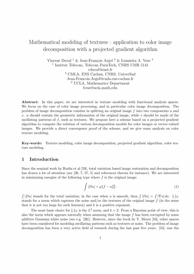
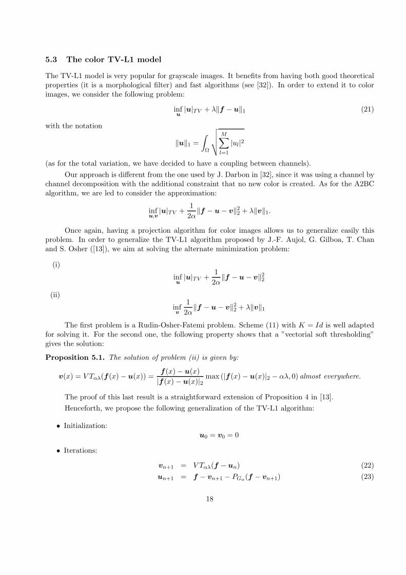
Figure 1: Left: Energy vs iterations of the Osher-Sole-Vese model with Chambolle’s projection algo-rithm (in green and blue - stepsize 1/64 and 0.031) and with the Projected gradient algorithm (in red- stepsize 0.031). Right: L2 square distance (on a logarithmic scale) between the limit value (2000iterations) vs the number of iterations, for OSV using 1/64 stepsize.

5.4 Numerical experiments

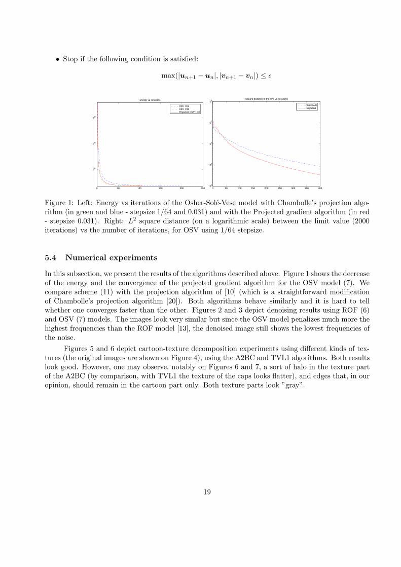
In this subsection, we present the results of the algorithms described above. Figure 1 shows the decreaseof the energy and the convergence of the projected gradient algorithm for the OSV model (7). Wecompare scheme (11) with the projection algorithm of [10] (which is a straightforward modificationof Chambolle’s projection algorithm [20]). Both algorithms behave similarly and it is hard to tellwhether one converges faster than the other. Figures 2 and 3 depict denoising results using ROF (6)and OSV (7) models. The images look very similar but since the OSV model penalizes much more thehighest frequencies than the ROF model [13], the denoised image still shows the lowest frequencies ofthe noise.

Figures 5 and 6 depict cartoon-texture decomposition experiments using different kinds of tex-tures (the original images are shown on Figure 4), using the A2BC and TVL1 algorithms. Both resultslook good. However, one may observe, notably on Figures 6 and 7, a sort of halo in the texture partof the A2BC (by comparison, with TVL1 the texture of the caps looks flatter), and edges that, in ouropinion, should remain in the cartoon part only. Both texture parts look ”gray”.

19

Figure 2: First row: original and noisy images (PSNR = 56.9 dB). Second row: denoised with colorROF (λ = 15, PSNR= 73.8 dB) and with color OSV (λ = 15, PSNR= 73.4 dB).

20

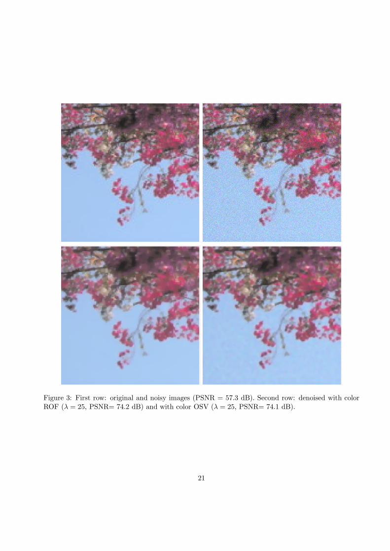
Figure 3: First row: original and noisy images (PSNR = 57.3 dB). Second row: denoised with colorROF (λ = 25, PSNR= 74.2 dB) and with color OSV (λ = 25, PSNR= 74.1 dB).

21

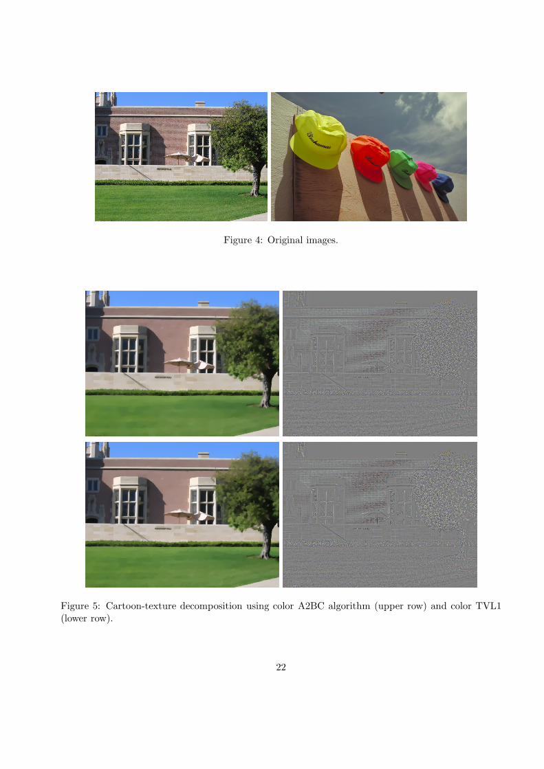
Figure 4: Original images.

Figure 5: Cartoon-texture decomposition using color A2BC algorithm (upper row) and color TVL1(lower row).

22

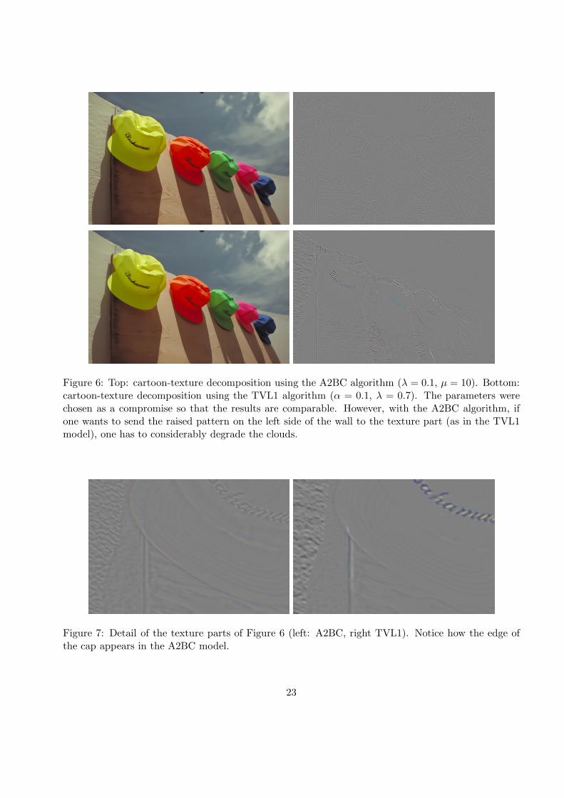
Figure 6: Top: cartoon-texture decomposition using the A2BC algorithm (λ = 0.1, µ = 10). Bottom:cartoon-texture decomposition using the TVL1 algorithm (α = 0.1, λ = 0.7). The parameters werechosen as a compromise so that the results are comparable. However, with the A2BC algorithm, ifone wants to send the raised pattern on the left side of the wall to the texture part (as in the TVL1model), one has to considerably degrade the clouds.

Figure 7: Detail of the texture parts of Figure 6 (left: A2BC, right TVL1). Notice how the edge ofthe cap appears in the A2BC model.

23

6 Qualitative analysis of decomposition models

In this section, we try to explain some of the visual results obtained in the last section.

6.1 Edges and halo

More precisely, we first focus on Figures 6 and 7 (cartoon-texture decomposition), where it seems that,with the A2BC algorithm, a sort of halo and edges appear in the texture part (at least more visiblythan with the TVL1 algorithm). We believe that this phenomenon is not related to a wrong choiceof parameters, but rather to an inherent limit of models that rely on the total variation plus a normthat favors oscillations for the texture part (like the BV-G model).

For the sake of simplicity, we will restrict our discussion to the simple case of one-dimensionalsingle channel signals, but the core idea still applies to the case of color images. Suppose for instance,that one wants to decompose a signal f using the BV-G model, i.e. find a decomposition (u, v) thatsolves :

minu+v=f

|u|TV + ‖v‖G (24)

where the functions are defined on Ω = (−1, 1). In dimension 1, the divergence operator reduces tothe derivation, and the boundary condition on ξ implies that ξ is the antiderivative of v that cancelsat −1:

‖v‖G = supt∈(−1,1)

∣∣∣∣

∫ t

−1v(t)dt

∣∣∣∣

(25)

Now, consider a step edge, perturbed with some textures as in Figure 8 (a), for instance :

f(x) = 1(0,1)(x) + β sin(8pπx)1 14≤|x|≤ 3

4(26)

where β > 0, p ∈ N∗. The ideal decomposition would be a perfect step u(x) = 1(0,1)(x) on the one

hand, and the pure oscillation v(x) = β sin(8pπx)1 14≤|x|≤ 3

4on the other hand (see Figure 8 (b) and

(c)). The energy of the cartoon part is simply |u|TV = lim1 u − lim−1 u = 1, whereas the energy of

the texture part is given by ‖v‖G = β∫ 1

4+ 1

8p

14

sin(8pπt)dt = β4pπ

. Yet, replacing u on [−14 , 1

4 ] with any

non-decreasing function u with the same limits at the boundary, say, a ramp x 7→ (12 + 1

2ηx)1[−η,η](x)as in Figure 8 (d)), one still gets the same cartoon energy |u|TV = 1. As for the texture part, weshould notice that one extra oscillation is added near the discontinuity of the original function f . But,precisely, the G-norm favors oscillations, so that this change in the texture part will not be penalized.Indeed:

‖v‖G = max

(β

4pπ,

∫ 0

−η

(1

2+

1

2ηt)dt

)

=1

4pπ(27)

for η small enough (0 ≤ η ≤ min(14 , β

pπ )).

To sum up, given any decomposition with sharp edges, there exists a decomposition with thesame energy where shadows of edges appear in the texture part. So it is not surprising to see edgesappear in the texture part of our experiments. This phenomenon is also a possible explanation of the

24

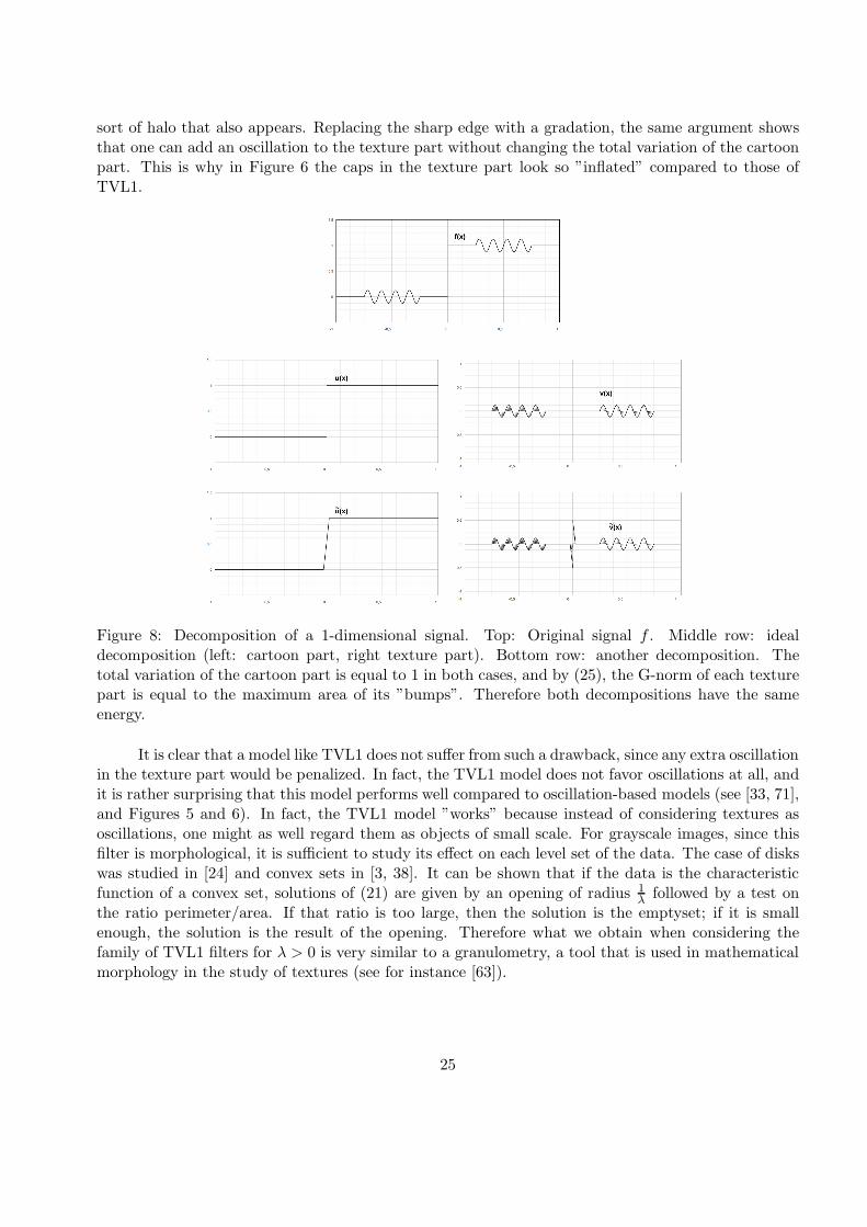
sort of halo that also appears. Replacing the sharp edge with a gradation, the same argument showsthat one can add an oscillation to the texture part without changing the total variation of the cartoonpart. This is why in Figure 6 the caps in the texture part look so ”inflated” compared to those ofTVL1.

Figure 8: Decomposition of a 1-dimensional signal. Top: Original signal f . Middle row: idealdecomposition (left: cartoon part, right texture part). Bottom row: another decomposition. Thetotal variation of the cartoon part is equal to 1 in both cases, and by (25), the G-norm of each texturepart is equal to the maximum area of its ”bumps”. Therefore both decompositions have the sameenergy.

It is clear that a model like TVL1 does not suffer from such a drawback, since any extra oscillationin the texture part would be penalized. In fact, the TVL1 model does not favor oscillations at all, andit is rather surprising that this model performs well compared to oscillation-based models (see [33, 71],and Figures 5 and 6). In fact, the TVL1 model ”works” because instead of considering textures asoscillations, one might as well regard them as objects of small scale. For grayscale images, since thisfilter is morphological, it is sufficient to study its effect on each level set of the data. The case of diskswas studied in [24] and convex sets in [3, 38]. It can be shown that if the data is the characteristicfunction of a convex set, solutions of (21) are given by an opening of radius 1

λ followed by a test onthe ratio perimeter/area. If that ratio is too large, then the solution is the emptyset; if it is smallenough, the solution is the result of the opening. Therefore what we obtain when considering thefamily of TVL1 filters for λ > 0 is very similar to a granulometry, a tool that is used in mathematicalmorphology in the study of textures (see for instance [63]).

25

6.2 Color of textures

The second remark is that the extracted texture parts look like gray-level images. If one looks atthem closely, one can see that there are colors, but they are spread on very small areas. In view ofthe definition of the G-norm and the example of Remark 2.3, it is clear that, on each channel andon every local neighboorhood, the average value of the texture part should vanish (otherwise, the”antiderivative” ξ would take large values, so that the G-norm would be large). Therefore the overallimpression is gray. The TVL1 model does not impose such a condition on the average value, as it canbe seen on Figure 6. Notice the stripes of the wood and the holes inside the letters that are colored,contrary to the A2BC model. These were sent to the texture part because of their small scale, notbecause they were oscillations. However the overall impression is still gray too, since the colors oflarge areas, which matter for an impression of color, are kept in the cartoon part.

6.3 Comments

The conclusion is that although the different algorithms studied in this paper produce apparentlysimilar results, they actually have very different qualitative properties, and they rely on differentdefinitions of textures. This is another illustration of the difficulty to define precisely the notion oftexture. Even though we pointed out some qualitative differences in the visual results, the choice ofthe best decomposition is arguable. While it is clear that some textures should be dealt with workingon their frequential content, some others require to work geometrically on their elementary patterns,in a way that is reminiscent of the texton theory [47].

References

[1] R. Acar and C. Vogel. Analysis of total variation penalty methods for ill-posed problems. InverseProblems, 10:1217–1229, 1994.

[2] R.A. Adams. Sobolev Spaces, volume 65 of Mathematics. Academic Press, 1975.

[3] W.K. Allard. Total variation regularization for image denoising II: Examples. SIAM Journal onImaging Sciences, 2008. Accepted.

[4] L. Ambrosio, N. Fusco, and D. Pallara. Functions of Bounded Variation and Free DiscontinuityProblems. Oxford mathematical monographs. Oxford University Press, 2000.

[5] F. Andreu-Vaillo, V. Caselles, and J. M. Mazon. Parabolic quasilinear equations minimizing lineargrowth functionals, volume 223 of Progress in Mathematics. Birkhauser, 2002.

[6] G. Aubert and J.-F. Aujol. Modeling very oscillating signals. application to image processing.Applied Mathematics and Optimization, 51(2):163–182, mars 2005.

[7] G. Aubert and P. Kornprobst. Mathematical Problems in Image Processing: Partial DifferentialEquations and the Calculus of Variations, volume 147. Springer Verlag, Applied MathematicalSciences, 2001.

[8] J.-F. Aujol. Some first-order algorithms for total variation based image restoration. J. Math.Imaging Vis., 34(3):307–327, 2009.

26

[9] J-F. Aujol, G. Aubert, L. Blanc-Feraud, and A. Chambolle. Image decomposition into a boundedvariation component and an oscillating component. Journal of Mathematical Imaging and Vision,22(1):71–88, January 2005.

[10] J.-F. Aujol and A. Chambolle. Dual norms and image decomposition models. InternationalJournal on Computer Vision, 63(1):85–104, June 2005.

[11] J.-F. Aujol and T. F. Chan. Combining geometrical and textured information to perform imageclassification. Journal of Visual Communication and Image representation, 17(5):1004–1023,October 2006.

[12] J.-F. Aujol and G. Gilboa. Constrained and SNR-based solutions for TV-Hilbert space imagedenoising. Journal of Mathematical Imaging and Vision, 26(1-2):217–237, 2006.

[13] J.-F. Aujol, G. Gilboa, T. Chan, and S. Osher. Structure-texture image decomposition - modeling,algorithms, and parameter selection. International Journal of Computer Vision, 67(1):111–136,April 2006.

[14] J.-F. Aujol and S. H. Kang. Color image decomposition and restoration. Journal of VisualCommunication and Image Representation, 17(4):916–928, August 2006.

[15] J. Bect, L. Blanc-Feraud, G. Aubert, and A. Chambolle. A l1-unified variational framework forimage restoration. In ECCV 04, volume 3024 of Lecture Notes in Computer Sciences, pages 1–13,2004.

[16] A. Bermudez and C. Moreno. Duality methods for solving variational inequalities. Comp. andMaths. with Appls., 7(1):43–58, July 1981.

[17] J. Bioucas-Dias and M. Figueiredo. Thresholding algorithms for image restoration. IEEE Trans-actions on Image processing, 16(12):2980–2991, 2007.

[18] P. Blomgren and T. Chan. Color TV: Total variation methods for restoration of vector valuedimages. IEEE Transactions on Image Processing, 7(3):304–309, 1998.

[19] X. Bresson and T. Chan. Fast minimization of the vectorial total variation norm and applicationsto color image processing. SIAM Journal on Imaging Sciences (SIIMS), Submitted, 2007.

[20] A. Chambolle. An algorithm for total variation minimization and its applications. Journal ofMathematical Imaging and Vision, 20:89–97, 2004.

[21] A. Chambolle. Total variation minimization and a class of binary MRF models. EMMCVPR inVol. 3757 of Lecture Notes in Computer Sciences, pages 136–152, June 2005.

[22] A. Chambolle, S.E. Levine, and B.J. Lucier. Some variations on total variation-based imagesmoothing. 2009.

[23] A. Chambolle and P.L. Lions. Image recovery via total variation minimization and related prob-lems. Numerische Mathematik, 76(3):167–188, 1997.

[24] T. Chan and S. Esedoglu. Aspects of total variation regularized L1 function approximation. SIAMJournal of Applied Mathematics, 65(5):1817–1837, 2005.

27

[25] T. Chan, G. Golub, and P. Mulet. A nonlinear primal-dual method for total variation-basedimage restoration. SIAM Journal on Scientific Computing, 20(6):1964–1977, 1999.

[26] T. Chan and J. Shen. Image processing and analysis - Variational, PDE, wavelet, and stochasticmethods. SIAM Publisher, 2005.

[27] Tony F. Chan, Sung Ha Kang, and Jianhong Shen. Total variation denoising and enhancement ofcolor images based on the cb and hsv color models. J. Visual Comm. Image Rep, 12:2001, 2000.

[28] P. Charbonnier, L. Blanc-Feraud, G. Aubert, and M. Barlaud. Deterministic edge-preservingregularization in computed imaging. IEEE Transactions on Image Processing, 6(2), 2007.

[29] P. G Ciarlet. Introduction a l’Analyse Numerique Matricielle et a l’Optimisation. Dunod, 1998.

[30] P.L. Combettes and J. Pesquet. Image restoration subject to a total variation constraint. IEEETransactions on Image Processing, 13(9):1213–1222, 2004.

[31] P.L. Combettes and V. Wajs. Signal recovery by proximal forward-backward splitting. SIAMJournal on Multiscale Modeling and Simulation, 4(4):1168–1200, 2005.

[32] J. Darbon. Total variation minimization with l1 data fidelity as a contrast invariant filter. 4thInternational Symposium on Image and Signal Processing and Analysis (ISPA 2005), pages 221–226, September 2005.

[33] J. Darbon and M. Sigelle. Image restoration with discrete constrained total variation part I: Fastand exact optimization. Journal of Mathematical Imaging and Vision, 26(3):261–276, December2006.

[34] I. Daubechies, M. Defrise, and C. De Mol. An iterative thresholding algorithm for linear inverseproblems with a sparsity constraint. Communications on Pure and Applied Mathematics, 57:1413–1457, 2004.

[35] I. Daubechies and G. Teschke. Variational image restoration by means of wavelets: simultaneousdecomposition, deblurring and denoising. Applied and Computational Harmonic Analysis, 19:1–16, 2005.

[36] D. Dobson and C. Vogel. Convergence of an iterative method for total variation denoising. SIAMJournal on Numerical Analysis, 34:1779–1791, 1997.

[37] S. Durand, J. Fadili, and M. Nikolova. Multiplicative noise removal using L1 fidelity on framecoefficients. CMLA Report, 08-40, 2008.

[38] V. Duval and Y. Gousseau J.-F. Aujol. The TVL1 model: a geometric point of view. SIAMjournal on Multiscale Modeling and Simulation, April 2009. (submitted).

[39] J. Eckstein. The Lions-Mercier algorithm and the alternating direction method are instances ofthe proximal point algorithm. 1988.

[40] I. Ekeland and R. Temam. Convex Analysis and Variational Problems, volume 28 of Classics inApplied Mathematics. SIAM, 1999.

28

[41] J. Fadili and J.-L. Starck. Monotone operator splitting for fast sparse solutions of inverse prob-lems., 2009. submitted.

[42] H. Fu, M. Ng, M. Nikolova, and J. Barlow. Efficient minimization methods of mixed l1-l1 andl2-l1 norms for image restoration. SIAM Journal on Scientific computing, 27(6):1881–1902, 2006.

[43] J. Garnett, P. Jones, T. Le, and L. Vese. Modeling oscillatory components with the homogeneousspaces BMO−α and W−α,p. UCLA CAM Report, 07-21, July 2007.

[44] J. Gilles. Noisy image decomposition: a new structure, textures and noise model based on localadaptivity. Journal of Mathematical Imaging and Vision, 28(3), July 2007.

[45] D. Goldfarb and W. Yin. Second-order cone programming methods for total variation basedimage restoration. SIAM Journal on Scientific Computing, 27(2):622–645, 2005.

[46] A. Haddad. Methodes variationnelles en traitement d’images. PhD thesis, ENS Cachan, June2005.

[47] B. Julesz. Texton gradients: The texton theory revisited. Biological Cybernetics, 54:245–251,1986.

[48] T. Le and L. Vese. Image decomposition using total variation and div(BMO). Multiscale Modelingand Simulation, SIAM Interdisciplinary Journal, 4(2):390–423, June 2005.

[49] L. Lieu. Contribution to Problems in Image Restoration, Decomposition, and Segmentation byVariational Methods and Partial Differential Equations,. PhD thesis, UCLA, June 2006.

[50] L.H. Lieu and L.A. Vese. Image restoration and decomposition via bounded total variation andnegative Hilbert-Sobolev spaces. Applied Mathematics & Optimization, 58:167–193, 2009.

[51] P.L. Lions and B. Mercier. Algorithms for the sum of two nonlinear operators. SIAM Journal onNumerical Analysis, 16(6):964–979, 1979.

[52] S.J. Wright M. Zhu and T.F. Chan. Duality-based algorithms for total variation image restoration.Technical report, UCLA CAM Report 08-33, 2008.

[53] Y. Meyer. Oscillating patterns in image processing and nonlinear evolution equations, volume 22of University Lecture Series. American Mathematical Society, Providence, RI, 2001. The fifteenthDean Jacqueline B. Lewis memorial lectures.

[54] Y. Nesterov. Smooth minimization of non-smooth functions. Mathematical Programming (A),103(1):127–152, 2005.

[55] M.K. Ng, L. Qi, Y.F. Yang, and Y. Huang. On semismooth Newton methods for total variationminimization. Journal of Mathematical Imaging and Vision, 27:265–276, 2007.

[56] M. Nikolova and R. Chan. The equivalence of half-quadratic minimization and the gradientlinearization iteration. IEEE Transactions on Image Processing, 16(6):1623–1627, 2007.

[57] S. Osher and N. Paragios. Geometric Level Set Methods in Imaging, Vision, and Graphic.Springer, 2003.

29

[58] S. Osher, A. Sole, and L. Vese. Image decomposition and restoration using total variation mini-mization and the H−1 norm. SIAM journal on Multiscale Modeling and Simulation, 1(3):349–370,2003.

[59] L. Rudin, S. Osher, and E. Fatemi. Non linear total variation based noise removal algorithms.Physica D, 60:259–268, 2003.

[60] G. Sapiro and D. L. Ringach. Anisotropic diffusion of multivalued images with applications tocolor filtering. IEEE Transactions on Image Processing, 5(11):1582–1586, 1996.

[61] S. Setzer. Split Bregman Algorithm, Douglas-Rachford Splitting and frame shrinkage. Preprint,University of Mannheim, 2008.

[62] N. Sochen, R. Kimmel, and R. Malladi. A general framework for low level vision. IEEE Trans-actions on Image Processing, 7(3):310–318, 1998.

[63] P. Soille. Morphological Image Analysis: Principles and Applications. Springer-Verlag New York,Inc., Secaucus, NJ, USA, 2003.

[64] J.L. Starck, M. ELad, and D.L. Donoho. Image decomposition via the combination of sparserepresentations and a variational approach, 2005.

[65] L.A. Vese and S. J. Osher. Modeling textures with total variation minimization and oscillatingpatterns in image processing. Journal of Scientific Computing, 19(1-3):553–572, December 2003.

[66] L.A. Vese and S.J. Osher. Color texture modeling and color image decomposition in a variational-PDE approach ,. In Proceedings of the Eighth International Symposium on Symbolic and NumericAlgorithms for Scientific Computing (SYNASC ’06), pages 103 – 110. IEEE, 2006.

[67] C.R. Vogel. Computational Methods for Inverse Problems, volume 23 of Frontiers in AppliedMathematics. SIAM, 2002.

[68] P. Weiss, L. Blanc-Feraud, and G. Aubert. Efficient schemes for total variation minimizationunder constraints in image processing. SIAM journal on Scientific Computing, 31(3):2047–2080,2009.

[69] W. Yin and D. Goldfarb. Second-order cone programming methods for total variation basedimage restoration. SIAM J. Scientific Computing, 27(2):622–645, 2005.

[70] W. Yin, D. Goldfarb, and S. Osher. Image cartoon-texture decomposition and feature selectionusing the total variation regularized l1. In Variational, Geometric, and Level Set Methods inComputer Vision, volume 3752 of Lecture Notes in Computer Science, pages 73–84. Springer,2005.

[71] W. Yin, D. Goldfarb, and S. Osher. A comparison of three total variation based texture extractionmodels. Journal of Visual Communication and Image Representation, 18(3):240–252, June 2007.

[72] J. Yuan, C. Schnorr, and G. Steidl. Convex Hodge decomposition and regularization of imageflows. Journal of Mathematical Imaging and Vision, 2009. in press.

[73] M. Zhu and T.F. Chan. An efficient primal-dual hybrid gradient algorithm for total variationimage restoration, May 2008. UCLA CAM Report 08-34.

30