Embed Size (px)
Citation preview
Septembre 2013
Mémoire de soutenance pour le Diplôme d’Ingénieur INSA de
Strasbourg
- Spécialité Mécatronique -
Et le Master des sciences de l’université de Strasbourg
- Mention Imagerie, Robotique et Ingénierie pour le Vivant -
Parcours Automatique et Robotique
Onboard Vision based SLAM on a Quadruped Robot
(SLAM Visuel Embarqué sur un Robot Quadrupède)
Présenté par Anis MEGUENANI
Réalisé au sein de l’Istituto Italiano di Tecnologia
Genova – ITALY

1
Thesis supervisors:
Dr. Stephane Bazeille
Senior Post-doc within the HyQ team
Department of Advanced Robotics
Istituto Italiano di Tecnologia (IIT)
Dr. Renaud KIEFER
Professor
INSA de Strasbourg
Dr. Jacques Gangloff
Professor
Université de Strasbourg
Dr. Claudio Semini
HyQ Group Leader
Department of Advanced Robotics
Istituto Italiano di Tecnologia (IIT)
2
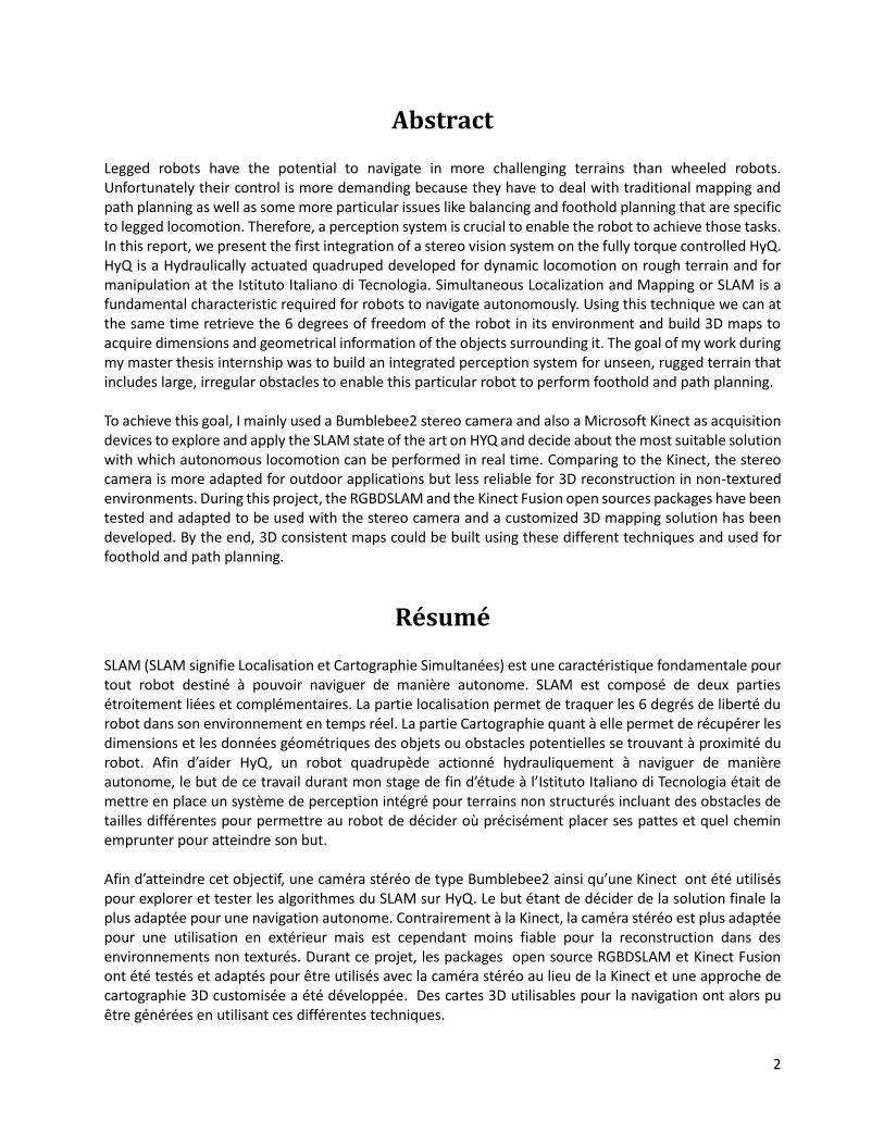
Abstract Legged robots have the potential to navigate in more challenging terrains than wheeled robots. Unfortunately their control is more demanding because they have to deal with traditional mapping and path planning as well as some more particular issues like balancing and foothold planning that are specific to legged locomotion. Therefore, a perception system is crucial to enable the robot to achieve those tasks. In this report, we present the first integration of a stereo vision system on the fully torque controlled HyQ. HyQ is a Hydraulically actuated quadruped developed for dynamic locomotion on rough terrain and for manipulation at the Istituto Italiano di Tecnologia. Simultaneous Localization and Mapping or SLAM is a fundamental characteristic required for robots to navigate autonomously. Using this technique we can at the same time retrieve the 6 degrees of freedom of the robot in its environment and build 3D maps to acquire dimensions and geometrical information of the objects surrounding it. The goal of my work during my master thesis internship was to build an integrated perception system for unseen, rugged terrain that includes large, irregular obstacles to enable this particular robot to perform foothold and path planning. To achieve this goal, I mainly used a Bumblebee2 stereo camera and also a Microsoft Kinect as acquisition devices to explore and apply the SLAM state of the art on HYQ and decide about the most suitable solution with which autonomous locomotion can be performed in real time. Comparing to the Kinect, the stereo camera is more adapted for outdoor applications but less reliable for 3D reconstruction in non-textured environments. During this project, the RGBDSLAM and the Kinect Fusion open sources packages have been tested and adapted to be used with the stereo camera and a customized 3D mapping solution has been developed. By the end, 3D consistent maps could be built using these different techniques and used for foothold and path planning.
Résumé SLAM (SLAM signifie Localisation et Cartographie Simultanées) est une caractéristique fondamentale pour tout robot destiné à pouvoir naviguer de manière autonome. SLAM est composé de deux parties étroitement liées et complémentaires. La partie localisation permet de traquer les 6 degrés de liberté du robot dans son environnement en temps réel. La partie Cartographie quant à elle permet de récupérer les dimensions et les données géométriques des objets ou obstacles potentielles se trouvant à proximité du robot. Afin d’aider HyQ, un robot quadrupède actionné hydrauliquement à naviguer de manière autonome, le but de ce travail durant mon stage de fin d’étude à l’Istituto Italiano di Tecnologia était de mettre en place un système de perception intégré pour terrains non structurés incluant des obstacles de tailles différentes pour permettre au robot de décider où précisément placer ses pattes et quel chemin emprunter pour atteindre son but. Afin d’atteindre cet objectif, une caméra stéréo de type Bumblebee2 ainsi qu’une Kinect ont été utilisés pour explorer et tester les algorithmes du SLAM sur HyQ. Le but étant de décider de la solution finale la plus adaptée pour une navigation autonome. Contrairement à la Kinect, la caméra stéréo est plus adaptée pour une utilisation en extérieur mais est cependant moins fiable pour la reconstruction dans des environnements non texturés. Durant ce projet, les packages open source RGBDSLAM et Kinect Fusion ont été testés et adaptés pour être utilisés avec la caméra stéréo au lieu de la Kinect et une approche de cartographie 3D customisée a été développée. Des cartes 3D utilisables pour la navigation ont alors pu être générées en utilisant ces différentes techniques.

3
Acknowledgments
Firstly, I would like to express my gratitude, love and appreciation to my parents. Their unwavering
support and guidance throughout my life has enabled me to finish my MSc thesis in robotics.
I would like also sincerely to thank my supervisors Prof. Renaud Kieffer, Dr. Stéphane Bazeille and Prof.
Jacques Gangloff for all the support, time, patience and teaching that I received from them. I appreciate
a lot their effort and contributions for helping me to defend this MSc thesis.
I would like also to express my gratitude to Dr. Claudio Semini and Prof. Ryad Chellali for giving this
opportunity to be part of the Istituto Italiano di Tecnologia and the HyQ team during 6 months
Finally I would like to thank all the members of the HyQ team for their kindness, help, and encouragement
and for treating me as a full member during the time that I spent with them. A special thanks to Ioannis
Havoutis for all his advices, help and support.

4
Contents Abstract ......................................................................................................................................................... 2
Résumé ......................................................................................................................................................... 2
Acknowledgments ......................................................................................................................................... 3
List of Figures ................................................................................................................................................ 7
Chapter I: Introduction ............................................................................................................................... 10
1. Context and motivation ...................................................................................................................... 10
2. HYQ robot project ............................................................................................................................... 10
3. Contributions ...................................................................................................................................... 12
4. Thesis Plan ........................................................................................................................................... 13
Chapter II: Acquisition devices and 3D data ............................................................................................. 14
1. Devices ................................................................................................................................................ 14
a. The Kinect characteristics and limitations ...................................................................................... 14
b. The Bumblebee2 stereo camera: Characteristics and limitations .................................................. 15
2. 3D data extraction .............................................................................................................................. 15
a. The disparity map ........................................................................................................................... 15
a.1. Sum of Absolute Differences (SAD) ......................................................................................... 16
a.2. Block Matching algorithm (BM) .............................................................................................. 16
b. Point clouds from the disparity map............................................................................................... 17
c. The depth map ................................................................................................................................ 18
d. The height map ............................................................................................................................... 19
Chapter III: The SLAM state of the art ...................................................................................................... 20
1. Visual SLAM on LittleDog .................................................................................................................... 20
2. Visual SLAM on FROG-1 ...................................................................................................................... 20
3. SLAM based on Edge-Point ICP algorithm .......................................................................................... 21
4. Visual odometry and FOVIS ................................................................................................................ 21
5. The RGBDSLAM open source package ................................................................................................ 22
6. Kinect Fusion ....................................................................................................................................... 22
Chapter IV: Methods, theory and tools .................................................................................................... 24
1. The stereo camera calibration ............................................................................................................ 24
a. The distortion model....................................................................................................................... 24
b. The projection matrix ...................................................................................................................... 25

5
b.1. From 3D to 2D ......................................................................................................................... 25
b.2. From 2D to 3D ......................................................................................................................... 26
2. The SLAM general pipeline ................................................................................................................. 28
a. Definition of the problem ............................................................................................................... 28
b. Workflow of a standard registration process ................................................................................. 28
b.1. Keypoints ................................................................................................................................. 29
b.2. Features .................................................................................................................................. 30
b.3. Correspondences .................................................................................................................... 32
b.4. Correspondences filtering ....................................................................................................... 32
b.5. Estimation of the 3D transformation ...................................................................................... 33
b.6. Pose Graph .............................................................................................................................. 34
3. The Kinect Fusion algorithm steps ...................................................................................................... 35
a. Surface extraction ........................................................................................................................... 35
b. Alignment ........................................................................................................................................ 36
c. Surface reconstruction .................................................................................................................... 37
4. ROS ...................................................................................................................................................... 39
5. Shared memory ................................................................................................................................... 40
6. The used libraries ................................................................................................................................ 40
d. The Point Cloud Library (PCL) .......................................................................................................... 40
b. OpenCV ........................................................................................................................................... 41
7. CloudCompare .................................................................................................................................... 41
Chapter V: Implementation, description of the work and results ........................................................... 44
1. The experimental environment .......................................................................................................... 44
2. Camera Calibration and 3D data computation ................................................................................... 45
a. Camera calibration .......................................................................................................................... 45
b. 3D data computation using ROS code ............................................................................................ 46
c. 3D data computation using Triclops ............................................................................................... 49
3. Test of the RGBDSLAM package to build 3D maps ............................................................................. 53
a. 3D maps with 3D data acquired with a Microsoft Kinect device .................................................... 53
b. 3D maps with point clouds from the “stereo_image_proc” ROS node .......................................... 54
c. 3D maps with point clouds computed using the Triclops library ................................................... 56
4. Customized registration pipelines ...................................................................................................... 59

6
a. Visual odometry registration approach .......................................................................................... 59
b. The point clouds registration helped with visual odometry approach ........................................... 62
5. Test of the Kinect Fusion package to build 3D maps .......................................................................... 68
a. Results of the Kinect Fusion package with the Microsoft Kinect .................................................... 68
b. Results of the Kinect Fusion package with the Bumblebee2 stereo camera .................................. 70
b.1. Results of the Kinect Fusion algorithm with ROS point clouds from the stereo camera........ 72
b.2. Results of the Kinect Fusion algorithm with Triclops point clouds from the stereo camera .. 73
Chapter VI: Results Discussion .................................................................................................................. 77
Chapter VII: Conclusion and futur work ................................................................................................... 79
Appendix .................................................................................................................................................... 80
A. The pinhole camera model ................................................................................................................. 79
B. Epipolar geometry ............................................................................................................................... 80
C. NARF Keypoints ................................................................................................................................... 82
D. PFH (Point Feature Histogram) descriptors ........................................................................................ 83
E. Other registration algorithms ............................................................................................................. 85
F. Loop closure ........................................................................................................................................ 86
G. Graph optimization ............................................................................................................................. 86
7
List of Figures Figure 1 HyQ robot ...................................................................................................................................... 11
Figure 2 HyQ path planning over a rough terrain simulation ..................................................................... 12
Figure 3 The Microsoft Kinect ..................................................................................................................... 14
Figure 4 Infrared pattern emitted by Kinect ............................................................................................... 14
Figure 5 The Bumblebee BB2-08S2C and its dimensions............................................................................ 15
Figure 6 Left: Left rectified image from the Bumblebee2 stereo camera. Right: Noisy disparity map. ..... 16
Figure 7 Image and world coordinate systems for the Bumblebee2 stereo camera ................................. 17
Figure 8 Left: The extracted pointcloud seen from above. Right: The same pointcloud rotated so we can
perceive the 3rd dimension ........................................................................................................................ 18
Figure 9 Original image of the scene Figure 10 Corresponding depth map ......... 18
Figure 11 Right: 3D map generated using the Kinect Fusion algorithm with the Kinect device. Left: Its
corresponding height map .......................................................................................................................... 19
Figure 12 Part of the HYQ lab scanned with Kinect Fusion using the Kinect .............................................. 23
Figure 13 Representation of the radial distortion ...................................................................................... 24
Figure 14 Representation of the tangential distortions ............................................................................. 25
Figure 15 Reconstruction: The 2D point (shown as a cross) corresponds to a line of points (dashed line) in
3D; any point along this line would project to the same point. Thus, the 3D position of a point cannot be
determined in general from one camera .................................................................................................... 26
Figure 16 Reconstruction 2: The same point observed in two cameras result in two different lines which
intersect at the 3D object. Hence, 3D reconstruction from stereo cameras is possible ............................ 26
Figure 17 Top: A set of six individual point clouds taken from different point of views. Bottom: The
registration result to obtain a merged point cloud model ......................................................................... 28
Figure 18 Workflow of a general registration problem .............................................................................. 29
Figure 19 For the point Pq only the edge between itself and the k-neighbors are computed .................. 31
Figure 20 Correspondences between two overlapping point clouds ......................................................... 32
Figure 21 A bilateral filter applied to a 2D image. The left picture is the original image. The right picture
has the filter applied to it, resulting in noise removal ................................................................................ 35
Figure 22 A 3-level multi resolution pyramid ............................................................................................. 36
Figure 23 Normal estimation at a vertex of the extracted point cloud ...................................................... 36
Figure 24 Point to plane ICP. Example of two iterations ............................................................................ 37
Figure 25 The cube containing the model is subdivided into a set of voxels that are equal in size. The
default size for the cube is 3meters per axis. The default voxel size is 512 per axis .................................. 38
Figure 26 A representation of the TSDF volume grid in the GPU. Each element in the grid represents a
voxel and the value inside represents the TSDF value. .............................................................................. 38
Figure 27 Surface reconstruction using TSDF: (a) Unweighted signed distance function in 3D. (b)
Weighted and averaged signed distance function ..................................................................................... 39
Figure 28 Graph representing interaction between ROS running nodes ................................................... 40
Figure 29 Outdoor space exposed to sunlight (Kinect image) .................................................................... 42
Figure 30 3D data extracted from the Bumblebee. Left: depth map. Right: Point cloud ........................... 42
Figure 31 3D data extracted from the Kinect. Left: depth map. Right: Point cloud ................................... 43
8
Figure 32 Map used for experiments .......................................................................................................... 44
Figure 33 The check board calibration pattern ........................................................................................... 45
Figure 34 Raw right image from the Bumblebee2 Figure 35 Rectified right black & white image from
the Bumblebee2 .......................................................................................................................................... 45
Figure 36 Inputs and outputs of the stereo_image_proc ROS node .......................................................... 46
Figure 37 A ROS point cloud seen from the top ......................................................................................... 47
Figure 38 The ROS point cloud seen from the side ..................................................................................... 47
Figure 39 The ROS point cloud seen in perspective with the measure of the width of the box ................ 48
Figure 40 The ROS point cloud seen in perspective with the measure of the length of the box ............... 48
Figure 41 The ROS point cloud seen in perspective with the measure of the height of the box ............... 49
Figure 42 Code structure to extract 3D data from the Bumblebee2 using shared memory ...................... 50
Figure 43 A Triclops point cloud seen from the top ................................................................................... 51
Figure 44 The Triclops point cloud seen from the side ............................................................................... 51
Figure 45 The Triclops point cloud seen in perspective with the measure of the width of the box .......... 52
Figure 46 The Triclops point cloud seen in perspective with the measure of the length of the box ......... 52
Figure 47 The Triclops point cloud seen in perspective with the measure of the height of the box ......... 53
Figure 48 3D map generated by the RGBDSLAM package with a Microsoft Kinect device – perspective
view ............................................................................................................................................................. 54
Figure 49 3D map generated by the RGBDSLAM package with a Microsoft Kinect device – side view ..... 54
Figure 50 3D maps building using the RGBDSLAM open source package with ROS point clouds code
structure ...................................................................................................................................................... 55
Figure 51 3D map generated by the RGBDSLAM package with ROS point clouds – perspective view ...... 56
Figure 52 3D map generated by the RGBDSLAM package with ROS point clouds – side view .................. 56
Figure 53 3D maps building using the RGBDSLAM open source package with Triclops extracted point
clouds code structure ................................................................................................................................. 57
Figure 54 3D map generated by the RGBDSLAM package with Triclops extracted point clouds –
perspective view ......................................................................................................................................... 58
Figure 55 3D map generated by the RGBDSLAM package with Triclops extracted point clouds – side view
.................................................................................................................................................................... 58
Figure 56 The stereo camera frame moving away from the fixed world frame ......................................... 59
Figure 57 Translational movement of the stereo camera for the FOVIS mapping experiment ................. 60
Figure 58 Code structure for the visual odometry mapping approach ...................................................... 60
Figure 59 3D map generated by the visual odometry approach using ROS point clouds – Top view ........ 61
Figure 60 3D map generated by the visual odometry approach using ROS point clouds – Side view ....... 61
Figure 61 Adding of the acquired point clouds without transforming them .............................................. 62
Figure 62 Code structure for two consecutive point clouds registration ................................................... 63
Figure 63 Two consecutive point clouds FOVIS transformed and added together. Notice the translational
and rotational drift in the map ................................................................................................................... 64
Figure 64 Normals computed at some key points of point cloud 2 ............................................................ 65
Figure 65 Correspondences between two point clouds. The clouds are distant from each other for a
representation purposes. (in reality the clouds are overlapping) .............................................................. 65
Figure 66 The matched clouds. Top: only with FOVIS transformation. Down: with FOVIS and ICP ........... 66
9
Figure 67 Results of the point clouds registration helped with visual odometry method applied for a
bigger map. Top: map built using FOVIS transformation alone. Middle: map built using FOVIS + ICP but
without initial guess. Bottom: map built with FOVIS and ICP with initial transformation estimation ....... 67
Figure 68 3D Mesh model build with the Kinect Fusion algorithm using the Kinect – Top view ............... 68
Figure 69 Truncated point cloud 3D model of the map with the height of the box – Perspective view .... 69
Figure 70 Truncated point cloud 3D model of the map – Side view........................................................... 69
Figure 71 Truncated point cloud 3D model of the map with the length of the box – Perspective view .... 70
Figure 72 Code structure for the Kinect Fusion algorithm adapted to work with the Bumblebee2 stereo
camera ........................................................................................................................................................ 71
Figure 73 A point cloud and its computed depth map used as input to the Kinect Fusion algorithm ....... 71
Figure 74 3D map generated by the Kinect Fusion algorithm using ROS point clouds from the stereo
camera – Top view ...................................................................................................................................... 72
Figure 75 3D map generated by the Kinect Fusion algorithm using ROS point clouds from the stereo
camera – Side view ..................................................................................................................................... 72
Figure 76 3D map generated by the Kinect Fusion algorithm using ROS point clouds from the stereo
camera – Perspective view ......................................................................................................................... 73
Figure 77 3D map generated by the Kinect Fusion algorithm using Triclops point clouds from the stereo
camera – Top view ...................................................................................................................................... 74
Figure 78 3D map generated by the Kinect Fusion algorithm using Triclops point clouds from the stereo
camera – Side view ..................................................................................................................................... 74
Figure 79 3D map generated by the Kinect Fusion algorithm using ROS point clouds from the stereo
camera – Perspective view ......................................................................................................................... 74
Figure 80 A Kinect RGBDSLAM generated 3D map matched with the ground truth.................................. 76
Figure 81 Projection of 1D object X onto the Image plane ......................................................................... 79
Figure 82 Projection of 3D point Q onto the image plane .......................................................................... 80
Figure 83 Epipolar Geometry: the epipolar line ......................................................................................... 81
Figure 84 The check board calibration pattern ........................................................................................... 82
Figure 85 Influence region diagram of the PFH computation for a query point Pq placed in the middle of
a sphere (in 3D) with radius r, and all its k neighbors are fully interconnected in a mesh ........................ 83
Figure 86 Normals computed on some key points of the point cloud ....................................................... 84
Figure 87 Loop closure detection representation. (Left) The poses are linked together by edges without
loop closure. (Right) The observation of a region already seen in the past triggers the creation of a new
link between two poses that were previously completely unrelated ........................................................ 86
Figure 88 Process of the graph optimization process ................................................................................. 87
10
Chapter I Introduction
1. Context and motivation
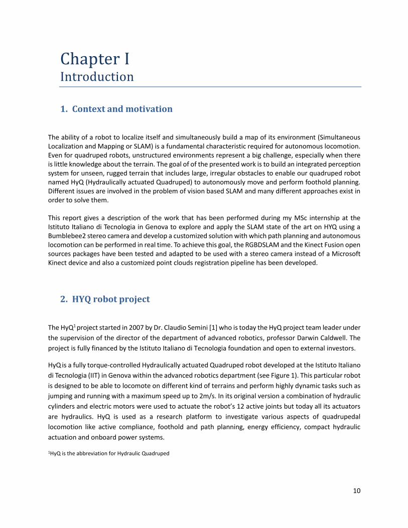
The ability of a robot to localize itself and simultaneously build a map of its environment (Simultaneous Localization and Mapping or SLAM) is a fundamental characteristic required for autonomous locomotion. Even for quadruped robots, unstructured environments represent a big challenge, especially when there is little knowledge about the terrain. The goal of of the presented work is to build an integrated perception system for unseen, rugged terrain that includes large, irregular obstacles to enable our quadruped robot named HyQ (Hydraulically actuated Quadruped) to autonomously move and perform foothold planning. Different issues are involved in the problem of vision based SLAM and many different approaches exist in order to solve them. This report gives a description of the work that has been performed during my MSc internship at the Istituto Italiano di Tecnologia in Genova to explore and apply the SLAM state of the art on HYQ using a Bumblebee2 stereo camera and develop a customized solution with which path planning and autonomous locomotion can be performed in real time. To achieve this goal, the RGBDSLAM and the Kinect Fusion open sources packages have been tested and adapted to be used with a stereo camera instead of a Microsoft Kinect device and also a customized point clouds registration pipeline has been developed.
2. HYQ robot project
The HyQ1 project started in 2007 by Dr. Claudio Semini [1] who is today the HyQ project team leader under
the supervision of the director of the department of advanced robotics, professor Darwin Caldwell. The
project is fully financed by the Istituto Italiano di Tecnologia foundation and open to external investors.
HyQ is a fully torque-controlled Hydraulically actuated Quadruped robot developed at the Istituto Italiano
di Tecnologia (IIT) in Genova within the advanced robotics department (see Figure 1). This particular robot
is designed to be able to locomote on different kind of terrains and perform highly dynamic tasks such as
jumping and running with a maximum speed up to 2m/s. In its original version a combination of hydraulic
cylinders and electric motors were used to actuate the robot’s 12 active joints but today all its actuators
are hydraulics. HyQ is used as a research platform to investigate various aspects of quadrupedal
locomotion like active compliance, foothold and path planning, energy efficiency, compact hydraulic
actuation and onboard power systems.
1HyQ is the abbreviation for Hydraulic Quadruped
11
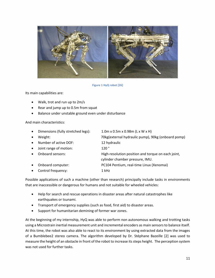
Figure 1 HyQ robot [26]
Its main capabilities are:
Walk, trot and run up to 2m/s
Rear and jump up to 0.5m from squat
Balance under unstable ground even under disturbance
And main characteristics:
Dimensions (fully stretched legs): 1.0m x 0.5m x 0.98m (L x W x H)
Weight: 70kg(external hydraulic pump), 90kg (onboard pomp)
Number of active DOF: 12 hydraulic
Joint range of motion: 120 °
Onboard sensors: High-resolution position and torque on each joint,
cylinder chamber pressure, IMU.
Onboard computer: PC104 Pentium, real-time Linux (Xenomai)
Control frequency: 1 kHz
Possible applications of such a machine (other than research) principally include tasks in environments
that are inaccessible or dangerous for humans and not suitable for wheeled vehicles:
Help for search and rescue operations in disaster areas after natural catastrophes like
earthquakes or tsunami.
Transport of emergency supplies (such as food, first aid) to disaster areas.
Support for humanitarian demining of former war zones.
At the beginning of my internship, HyQ was able to perform non autonomous walking and trotting tasks
using a Microstrain inertial measurement unit and incremental encoders as main sensors to balance itself.
At this time, the robot was also able to react to its environment by using extracted data from the images
of a Bumblebee2 stereo camera. The algorithm developed by Dr. Stéphane Bazeille [2] was used to
measure the height of an obstacle in front of the robot to increase its steps height. The perception system
was not used for further tasks.
12
3. Contributions
For a robot that will be used into areas that are completely inaccessible to human beings, the full
autonomy walking and behaving is essential for accomplishing the needed tasks. To be able to perform
that, a Microsoft Kinect and a Bumblebee2 stereo camera have been used to perform SLAM and 3D
mapping using open source packages and Libraries.
By the end of the 6 months internship, the following tasks were achieved:
Calibration of the Bumblebee2 stereo camera using OpenCV/ROS open-source code and 3D point
clouds and disparity map computation using the Bloc Matching algorithm.
Resolving the Triclops library/ROS compatibility problem using a shared memory communication
protocol. The 3D point clouds and disparity map computation were obtained using the SAD (Sum of
Absolute Differences)salgorithm.
Using the RGBDSLAM open-source package to build consistent 3D maps with the Microsoft Kinect
device and the stereo camera using 3D data (point clouds) computed with the two precedent methods
(SAD and Bloc Matching).
Developing a customized registration pipeline with PCL (the Point Cloud Library) to match point clouds
using the FOVIS (visual odometry) and ICP (Iterative Closest Point) algorithms and testing it with point
clouds computed with the two precedent methods. The use of the visual odometry to help the
mapping process is a new approach that has been developed during my internship.
Testing the Kinect Fusion algorithm with the Microsoft Kinect and adapting it to be used with the
Bumblebee2 stereo camera by using a shared memory communication protocol. Both 3D data
computed with ROS and Triclops were used.
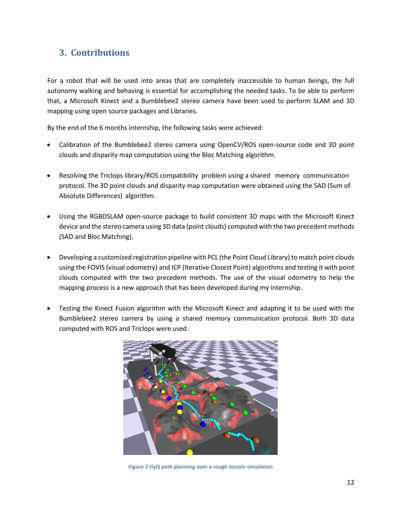
Figure 2 HyQ path planning over a rough terrain simulation

13
4. Thesis Plan
Chapter I: Introduction
Chapter II: Acquisition devices and 3D data In this chapter, we present the Microsoft Kinect and the Bumblebee2 stereo camera devices used during
the project with the different 3D data that they can generate.
Chapter III: The SLAM state of the art In this chapter we have a description of two SLAM techniques that have recently been applied on
quadruped robots and also details about the most promising open source packages and algorithms.
Chapter IV: Methods, theory and tools In this chapter we discuss the theory behind every open source SLAM package, technique and algorithm
that has been used to perform 3D mapping. In sub-chapters 1 we expose the mathematical basics behind
the calibration process then in sub-chapters 2 and 3 details about SLAM related techniques are given and
finally in sub-chapters 4, 5, 6 and 7 the used platform, softwares, libraries and tools are presented.
Chapter V: Implementation, description of the work and results In this chapter we present the experimental environment, the code structure and the results of the
different methods and techniques used to generate 3D consistent maps. A visual comparison between
the results of the RGBDSLAM package, the visual odometry based SLAM developed technique and the
Kinect Fusion algorithm is also performed.
Chapter V: Results discussion In this chapter we have a mathematical comparison between the different results and also a dipper
discussion about the different approaches.
Chapter VI: Conclusion and future work
14
Chapter II Acquisition devices and 3D data
1. Devices
a. The Kinect characteristics and limitations
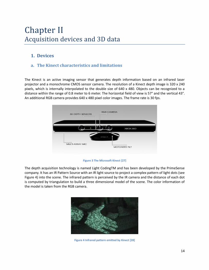
The Kinect is an active imaging sensor that generates depth information based on an infrared laser projector and a monochrome CMOS sensor camera. The resolution of a Kinect depth image is 320 x 240 pixels, which is internally interpolated to the double size of 640 x 480. Objects can be recognized to a distance within the range of 0.8 meter to 6 meter. The horizontal field of view is 57° and the vertical 43°. An additional RGB camera provides 640 x 480 pixel color images. The frame rate is 30 fps.
Figure 3 The Microsoft Kinect [27]
The depth acquisition technology is named Light CodingTM and has been developed by the PrimeSense company. It has an IR Pattern Source with an IR light source to project a complex pattern of light dots (see Figure 4) into the scene. The infrared pattern is perceived by the IR camera and the distance of each dot is computed by triangulation to build a three dimensional model of the scene. The color information of the model is taken from the RGB camera.
Figure 4 Infrared pattern emitted by Kinect [28]
15
This sort of sensor is precisely what is needed to overcome the limitations of stereo systems regarding the non-textured environments. However it is impossible for the infrared sensor of the Kinect to perform outside when the environment is in sunlight where the IR structured lighting pattern gets completely lost in ambient IR. This is why stereo cameras are better for outdoor applications.
b. The Bumblebee2 stereo camera: Characteristics and limitations
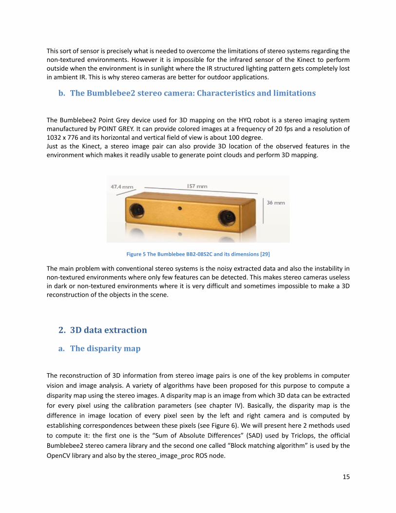
The Bumblebee2 Point Grey device used for 3D mapping on the HYQ robot is a stereo imaging system manufactured by POINT GREY. It can provide colored images at a frequency of 20 fps and a resolution of 1032 x 776 and its horizontal and vertical field of view is about 100 degree. Just as the Kinect, a stereo image pair can also provide 3D location of the observed features in the environment which makes it readily usable to generate point clouds and perform 3D mapping.
Figure 5 The Bumblebee BB2-08S2C and its dimensions [29]
The main problem with conventional stereo systems is the noisy extracted data and also the instability in non-textured environments where only few features can be detected. This makes stereo cameras useless in dark or non-textured environments where it is very difficult and sometimes impossible to make a 3D reconstruction of the objects in the scene.
2. 3D data extraction
a. The disparity map
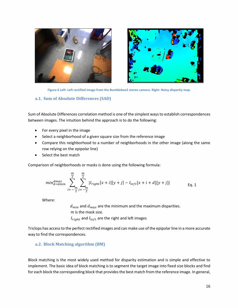
The reconstruction of 3D information from stereo image pairs is one of the key problems in computer
vision and image analysis. A variety of algorithms have been proposed for this purpose to compute a
disparity map using the stereo images. A disparity map is an image from which 3D data can be extracted
for every pixel using the calibration parameters (see chapter IV). Basically, the disparity map is the
difference in image location of every pixel seen by the left and right camera and is computed by
establishing correspondences between these pixels (see Figure 6). We will present here 2 methods used
to compute it: the first one is the “Sum of Absolute Differences” (SAD) used by Triclops, the official
Bumblebee2 stereo camera library and the second one called “Block matching algorithm” is used by the
OpenCV library and also by the stereo_image_proc ROS node.
16
Figure 6 Left: Left rectified image from the Bumblebee2 stereo camera. Right: Noisy disparity map.
a.1. Sum of Absolute Differences (SAD)
Sum of Absolute Differences correlation method is one of the simplest ways to establish correspondences
between images. The intuition behind the approach is to do the following:
For every pixel in the image
Select a neighborhood of a given square size from the reference image
Compare this neighborhood to a number of neighborhoods in the other image (along the same
row relying on the epipolar line)
Select the best match
Comparison of neighborhoods or masks is done using the following formula:
𝑚𝑖𝑛𝑑=𝑑𝑚𝑖𝑛𝑑𝑚𝑎𝑥 ∑ ∑ |𝐼𝑟𝑖𝑔ℎ𝑡[𝑥 + 𝑖][𝑦 + 𝑗] − 𝐼𝑙𝑒𝑓𝑡[𝑥 + 𝑖 + 𝑑][𝑦 + 𝑗]|
𝑚2
𝑗= −𝑚2
𝑚2
𝑖= − 𝑚2
Eq. 1
Where:
𝑑𝑚𝑖𝑛 and 𝑑𝑚𝑎𝑥 are the minimum and the maximum disparities.
m is the mask size.
𝐼𝑟𝑖𝑔ℎ𝑡 and 𝐼𝑙𝑒𝑓𝑡 are the right and left images
Triclops has access to the perfect rectified images and can make use of the epipolar line in a more accurate
way to find the correspondences.
a.2. Block Matching algorithm (BM)
Block matching is the most widely used method for disparity estimation and is simple and effective to
implement. The basic idea of block matching is to segment the target image into fixed size blocks and find
for each block the corresponding block that provides the best match from the reference image. In general,
17
the block minimizing the estimation error is usually selected as the matching block. However, block
matching with a simple error measure may not give smooth disparity fields, and thus may result in
increased entropy in the disparity map. Block matching is less precise than the SAD algorithm but is more
suitable to be used when the stereo images are not perfectly rectified and free from distortions. Other
methods that are more reliable and produce denser disparity maps like the Semi Global Matching (SGM)
method and the Graph-Cut-Based exist but need more processing power to be used in real time.
b. Point clouds from the disparity map
To project the pixels of the disparity map in 3D space, we use the calibration parameters of the stereo
camera. Usually for cameras, the following co-ordinates system convention is used:
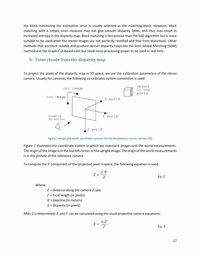
Figure 7 Image and world coordinate systems for the Bumblebee2 stereo camera [30]
Figure 7 illustrates the coordinate system in which we represent images and the world measurements.
The origin of the image is in the top left corner of the upright image. The origin of the world measurements
is in the pinhole of the reference camera.
To compute the 𝑍 component of the projected pixel in space, the following equation is used:
𝑍 = 𝑓. 𝐵
𝑑
Eq. 2
Where:
𝑍 = distance along the camera 𝑍 axis
𝑓 = focal length (in pixels)
𝐵 = baseline (in meters)
𝑑 = disparity (in pixels)
After Z is determined, 𝑋 and 𝑌 can be calculated using the usual projective camera equations:
𝑋 =
𝑢. 𝑍
𝑓
Eq. 3
18
𝑌 =
𝑣. 𝑍
𝑓
Eq. 4
Where:
𝑢 and 𝑣 are the pixel location in the 2D image
𝑋, 𝑌, 𝑍 is the real 3d position
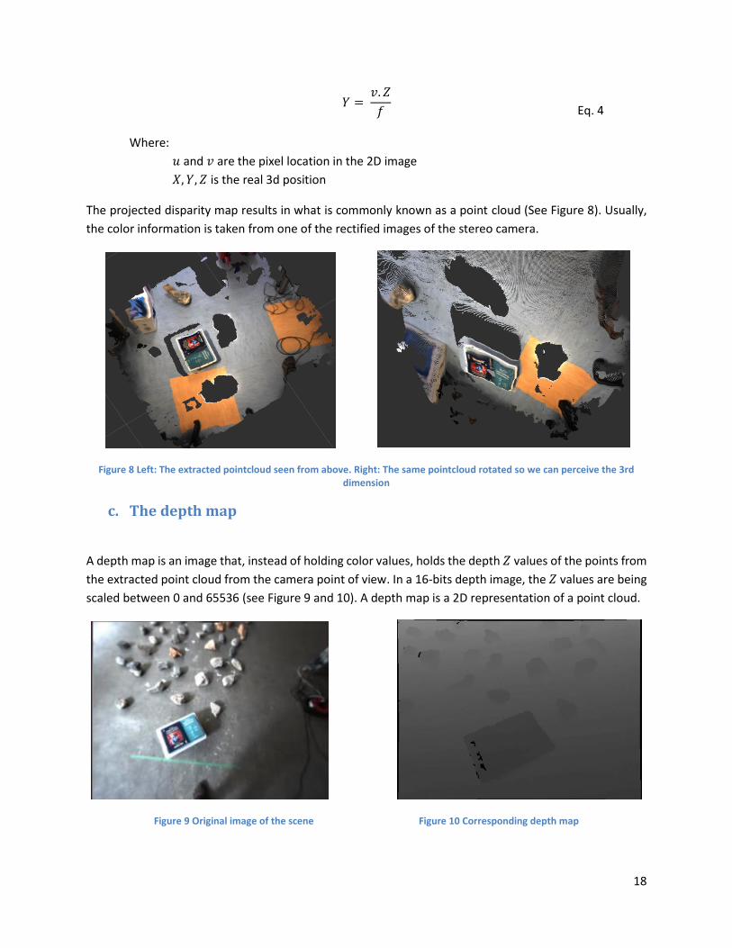
The projected disparity map results in what is commonly known as a point cloud (See Figure 8). Usually,
the color information is taken from one of the rectified images of the stereo camera.
Figure 8 Left: The extracted pointcloud seen from above. Right: The same pointcloud rotated so we can perceive the 3rd dimension
c. The depth map
A depth map is an image that, instead of holding color values, holds the depth 𝑍 values of the points from
the extracted point cloud from the camera point of view. In a 16-bits depth image, the 𝑍 values are being
scaled between 0 and 65536 (see Figure 9 and 10). A depth map is a 2D representation of a point cloud.
Figure 9 Original image of the scene Figure 10 Corresponding depth map
19
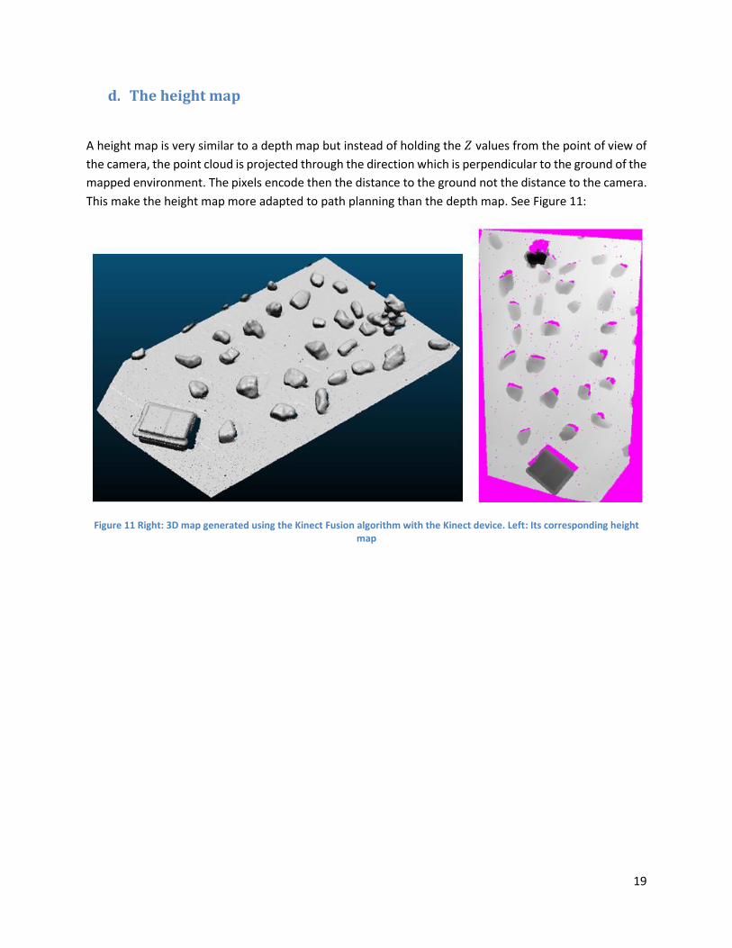
d. The height map
A height map is very similar to a depth map but instead of holding the 𝑍 values from the point of view of
the camera, the point cloud is projected through the direction which is perpendicular to the ground of the
mapped environment. The pixels encode then the distance to the ground not the distance to the camera.
This make the height map more adapted to path planning than the depth map. See Figure 11:
Figure 11 Right: 3D map generated using the Kinect Fusion algorithm with the Kinect device. Left: Its corresponding height map
20
Chapter III The SLAM state of the art
In this chapter we present some interesting SLAM techniques applied on quadruped robots and also the
tools and methods that will be the most suitable to be used on the HyQ robot to perform 3D mapping.
1. Visual SLAM on LittleDog
The Stanford university team led by Dr. J.Zico Kolter who is working on terrain modeling for a quadruped
robot named LittleDog (designed and built by Boston Dynamics)[3] pushed the visual SLAM technique to
its limits by implementing a real time reconstruction algorithm that fills in the missing portions of the
height map. These missing parts in the 3D map are caused by an inevitable effect of occlusions in the
camera’s line of sight. The method presented in the paper is inspired by texture synthesis approaches
from the computer graphics community. The algorithm looks in a “library” of known height map images
of terrain to find a patch that closely resembles the visible areas nearby the missing value; it then uses
the corresponding pixel from the patch to fill in the missing value. By employing this non-parametric
modeling algorithm they succeeded in improving the cost map which indicates the desirability of
different points on the terrain to perform a better path planning and control.
2. Visual SLAM on FROG-1
Xuesong Shao team from the Chinese Academy of Sciences who is also working on terrain modeling using
a stereo vision system for a quadruped robot called FROG-1 (Four legged Robot for Optimal Gaits)
[4] focuses on the post processing of the disparity map to enhance the result of the 3D reconstructed
map.
The disparity map is the most important part to obtain terrain's depth and height in terrain modeling. This
map always contains some noise and due to poor light, low texture, and surface reflection conditions,
more outliers would appear. Some pixels would be mismatched and others might not be able to find their
corresponding points. Blanks would appear in the disparity map. The post-processing algorithm proposed
by the team is designed with two steps:
a) Outlier detection: For each row in the disparity image, there are several different disparity values
and some mismatched points. Numbers of different disparity values are counted and put in
sequence. A threshold is set to divide the sequence into two parts. The numbers below the
threshold value are sorted out and the corresponding pixels are marked as mismatched disparity
values. Then, the positions of the labeled pixels are reset to blank areas.
21
b) Area filling: After the first step, the disparity map contains two kinds of areas, effective disparity
areas and blank areas. The pixels in blank areas are assigned with the same invalidated value, for
example, 255. The invalidated pixels are classified into different types according their positions
and replaced by their proximate elements. An effective dense disparity map can then be
generated even under sever conditions with low texture, poor light, and surface reflection.
By employing this approach, Xuesong Shao team succeeded in performing autonomous locomotion in
ground plane clattered with many obstacles based on stereo vision.
3. SLAM based on Edge-Point ICP algorithm
Most of the conventional vision-based SLAM systems use corner points features detected by the Harris
detector. The main reason is that data association is relatively easy for corner points due to their
distinguishability. However, corner points cannot be detected sufficiently in non-textured environments
and vision-based SLAM could be unstable due to lack of these features. Masahiro Tomono [5] proposes a
3D SLAM scheme using edge points.
An edge point is a point on an edge segment detected in the image. These edge points are detected using
a Canny Deriche detector and can be obtained from not only long segments but also fine textures. The
presented method computes 3D points from the edge points detected in a stereo image pair, and then
estimates the camera motion by matching the next stereo image with the 3D points. The ICP (Iterative
Closest Points) algorithm is applied for the registration process. By repeating these steps, the camera
trajectory and the 3D map are created. The camera motion estimation is equivalent with visual odometry,
and the estimation errors are accumulated. To reduce the accumulated errors, keyframe adjustment is
used, in which the camera motion is re-estimated using keyframes selected with an appropriate interval.
A major advantage of the method proposed by Masahiro Tomono is that the estimation process is
extremely robust due to plenty of edge points, which can be detected from a few edge lines in non-
textured environments.
4. Visual odometry and FOVIS
Visual odometry refers to the process of estimating a robot’s 3D motion from visual imagery alone. The
basic algorithm idea is to identify features of interest in each stereo camera frame, estimate the depth of
each feature, match features across time, and then estimate the rigid body transformation that best aligns
the features over time. The process is very similar to a standard SLAM registration pipeline but instead of
computing the features on point clouds, the points of interest here are extracted directly from the left
and right images of the stereo camera and no loop closure is performed.
22
FOVIS [6] [7] is an open source visual odometry implementation that uses FAST features detector [8] which
are relatively quick to compute and robust to small viewpoint changes. Methods for robustly matching
features across frames include RANSAC-based methods and graph-based consistency algorithms.
FOVIS can be integrated with SLAM algorithms which make use of loop closing techniques to help in the
robot 6Dof estimation process. Data extracted from visual odometry can be used as initial guess with for
matching algorithms like ICP or NDT (Normal Distribution Transform). Visual odometry estimates local
motion and generally has unbounded global drift that can be limited by these matching algorithms.
5. The RGBDSLAM open source package
The RGBD SLAM package [9] [10] is an open source code developed at the University of Freiburg that
makes use of four processing steps to build a consistent 3D model of the perceived environment and can
be used either with a Microsoft Kinect or a stereo vision system. When a stereo camera is used, the
algorithm takes as input a 640x480 colored image and a point cloud. Its registration pipeline can be
described as following: First, SURF features are extracted from the incoming color images and matched
against features from the previous image. By evaluating the point clouds at the location of these feature
points, a set of point-wise 3D correspondences between any two frames can be obtained. Based on these
correspondences, the estimation of the relative transformation between the frames is computed using a
“RANdom Sample Consensus” algorithm that can reduce/remove the effect of noisy data and outliers. To
perform that, after matching the feature descriptors of two frames, RANSAC randomly select three
matched feature pairs, which is the minimal number from which a rigid transformation can be computed.
Sample sets for which the pairwise Euclidean distances do no match, are refused. If the samples pass this
test, they are used to compute an estimate of the rigid transformation that is applied to all the features.
In this case, a feature point is considered as inlier when its mutual distance after the transformation is
smaller than 3cm. The third step is to improve this initial estimate using a variant of the ICP algorithm [11].
The registered point clouds are organized by a Graph-Based [12] structure which is an intuitive way to
formulate the SLAM problem by using a graph whose nodes correspond to the poses of the camera at
different points in time and whose edges represent constraints (the rigid transformations) between the
poses. As the pairwise pose estimates between frames are not necessarily globally consistent, the
resulting pose graph is optimized in the fourth step using the g2o solver, which is a general open-source
framework for optimizing graph-based nonlinear error functions [13] and detecting loop closures.
6. Kinect Fusion
Kinect Fusion is an algorithm developed by Microsoft Research in 2011 [14] that allows a 3D robust
reconstruction of the environment of the robot in real-time by moving the Microsoft Kinect sensor around
the real scene. Where SLAM techniques provide rudimentary camera tracking and mapping, Kinect
23
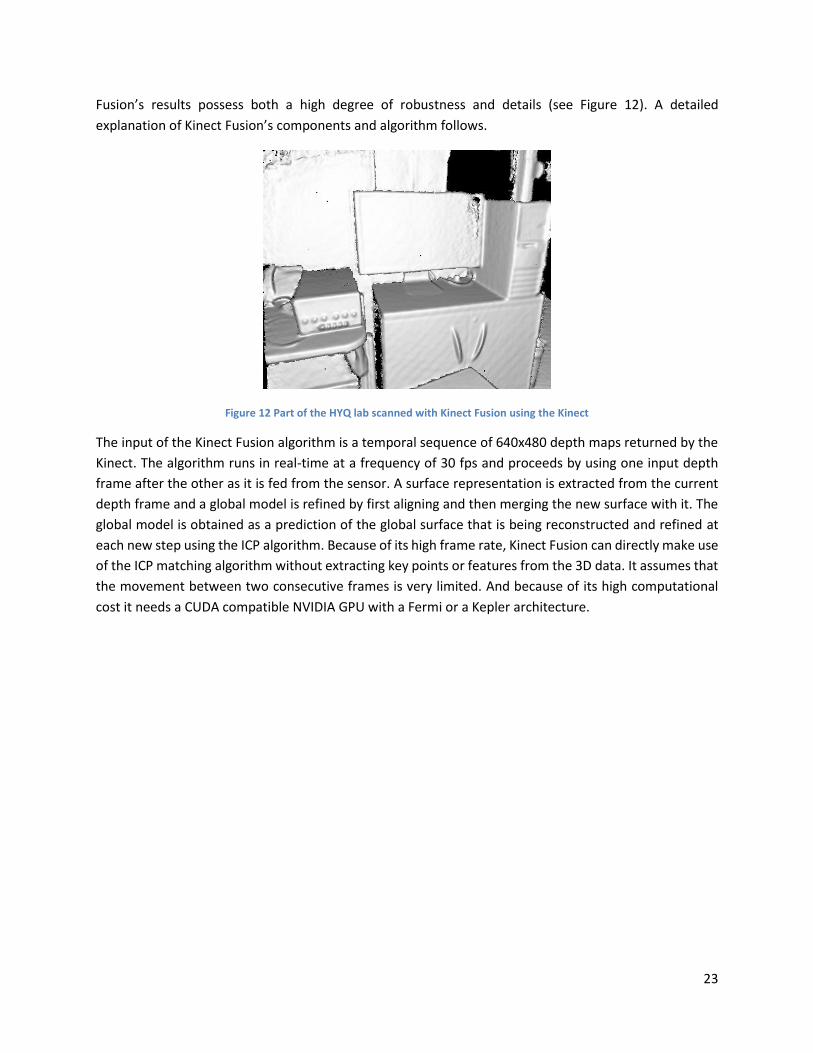
Fusion’s results possess both a high degree of robustness and details (see Figure 12). A detailed
explanation of Kinect Fusion’s components and algorithm follows.
Figure 12 Part of the HYQ lab scanned with Kinect Fusion using the Kinect
The input of the Kinect Fusion algorithm is a temporal sequence of 640x480 depth maps returned by the
Kinect. The algorithm runs in real-time at a frequency of 30 fps and proceeds by using one input depth
frame after the other as it is fed from the sensor. A surface representation is extracted from the current
depth frame and a global model is refined by first aligning and then merging the new surface with it. The
global model is obtained as a prediction of the global surface that is being reconstructed and refined at
each new step using the ICP algorithm. Because of its high frame rate, Kinect Fusion can directly make use
of the ICP matching algorithm without extracting key points or features from the 3D data. It assumes that
the movement between two consecutive frames is very limited. And because of its high computational
cost it needs a CUDA compatible NVIDIA GPU with a Fermi or a Kepler architecture.
24
Chapter IV Methods, theory and tools
In this chapter we discuss the theory behind every open source SLAM package, technique and algorithm
that has been used to perform 3D mapping. In sub-chapters 1 we expose the mathematical basics behind
the calibration process then in sub-chapters 2 and 3 details about SLAM related techniques are given and
finally in sub-chapters 4, 5, 6 and 7 the used platform, softwares, libraries and tools are presented.
1. The stereo camera calibration
The calibration performed on stereo cameras (see the pinhole model in annexes 1) does not concern only
the intrinsic and distortion parameters of every camera but also finding the projection matrix with which
the 3D position of the features that are visualized on the left and right images can be retrieved.
a. The distortion model
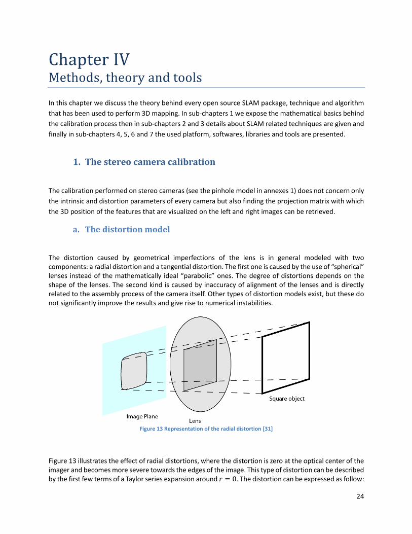
The distortion caused by geometrical imperfections of the lens is in general modeled with two components: a radial distortion and a tangential distortion. The first one is caused by the use of “spherical” lenses instead of the mathematically ideal “parabolic” ones. The degree of distortions depends on the shape of the lenses. The second kind is caused by inaccuracy of alignment of the lenses and is directly related to the assembly process of the camera itself. Other types of distortion models exist, but these do not significantly improve the results and give rise to numerical instabilities.
Figure 13 Representation of the radial distortion [31]
Figure 13 illustrates the effect of radial distortions, where the distortion is zero at the optical center of the imager and becomes more severe towards the edges of the image. This type of distortion can be described by the first few terms of a Taylor series expansion around 𝑟 = 0. The distortion can be expressed as follow:
25
𝑥𝑐𝑜𝑟𝑟𝑒𝑐𝑡𝑒𝑑 = 𝑥 (1 + 𝑘1𝑟
2 + 𝑘2𝑟4 + 𝑘3𝑟
6 )
Eq. 1
𝑦𝑐𝑜𝑟𝑟𝑒𝑐𝑡𝑒𝑑 = 𝑦 (1 + 𝑘1𝑟
2 + 𝑘2𝑟4 + 𝑘3𝑟
6 )
Eq. 2
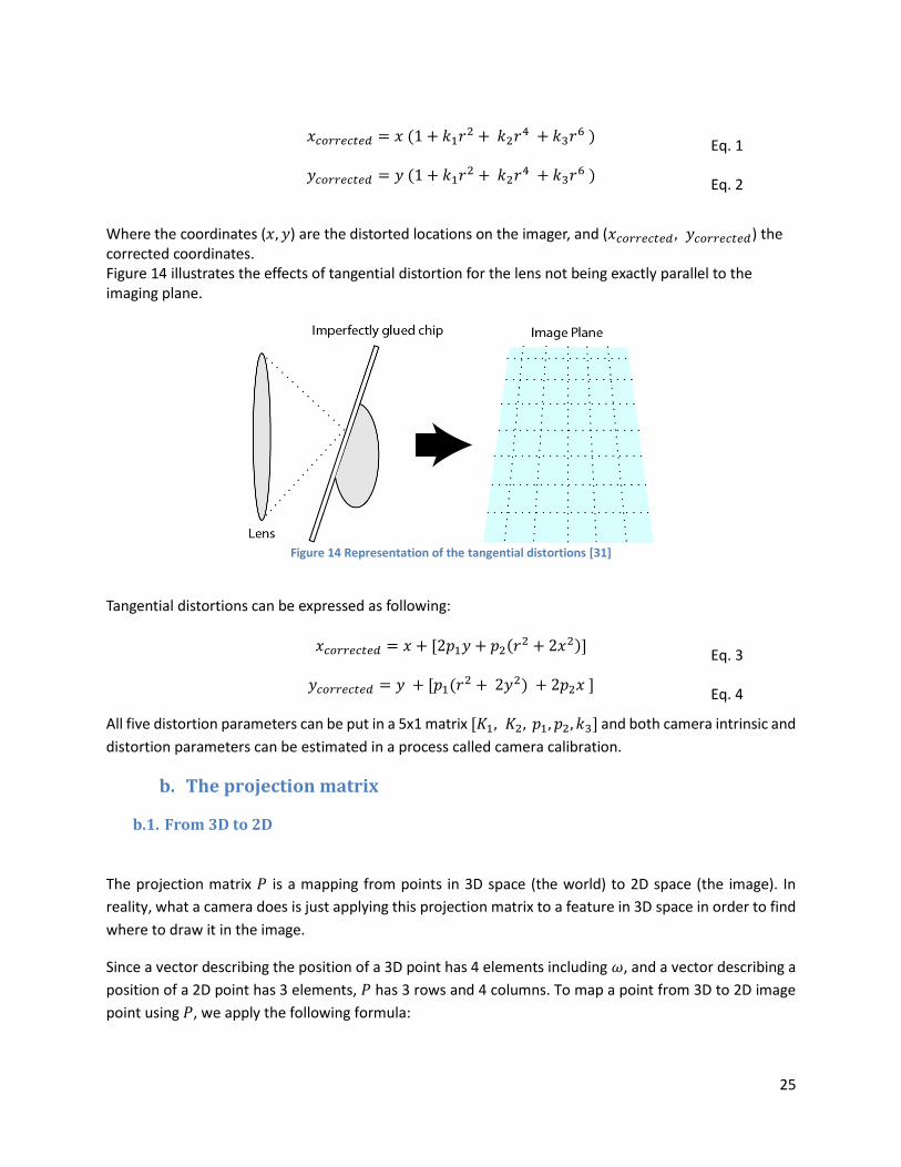
Where the coordinates (𝑥, 𝑦) are the distorted locations on the imager, and (𝑥𝑐𝑜𝑟𝑟𝑒𝑐𝑡𝑒𝑑 , 𝑦𝑐𝑜𝑟𝑟𝑒𝑐𝑡𝑒𝑑) the corrected coordinates. Figure 14 illustrates the effects of tangential distortion for the lens not being exactly parallel to the imaging plane.
Figure 14 Representation of the tangential distortions [31]
Tangential distortions can be expressed as following:
𝑥𝑐𝑜𝑟𝑟𝑒𝑐𝑡𝑒𝑑 = 𝑥 + [2𝑝1𝑦 + 𝑝2(𝑟
2 + 2𝑥2)]
Eq. 3
𝑦𝑐𝑜𝑟𝑟𝑒𝑐𝑡𝑒𝑑 = 𝑦 + [𝑝1(𝑟
2 + 2𝑦2) + 2𝑝2𝑥 ]
Eq. 4
All five distortion parameters can be put in a 5x1 matrix [𝐾1, 𝐾2, 𝑝1, 𝑝2, 𝑘3] and both camera intrinsic and
distortion parameters can be estimated in a process called camera calibration.
b. The projection matrix
b.1. From 3D to 2D
The projection matrix 𝑃 is a mapping from points in 3D space (the world) to 2D space (the image). In
reality, what a camera does is just applying this projection matrix to a feature in 3D space in order to find
where to draw it in the image.
Since a vector describing the position of a 3D point has 4 elements including 𝜔, and a vector describing a
position of a 2D point has 3 elements, 𝑃 has 3 rows and 4 columns. To map a point from 3D to 2D image
point using 𝑃, we apply the following formula:
26
[𝑎′
𝑏′
ω′] = 𝑝 [
𝑎𝑏𝑐ω
] Eq. 5
With 𝑝 = [
𝑝11 𝑝12 𝑝13 𝑝14
𝑝21 𝑝22 𝑝23 𝑝24
𝑝31 𝑝32 𝑝33 𝑝34
]
b.2. From 2D to 3D
We have just seen how to compute the 2D position of a point in an image given its 3D co-ordinates in
space using the projection matrix P. A question automatically pops up: Is it possible to go the other way
and work out where a point must be in real 3D space given its position in an image? The simple answer to
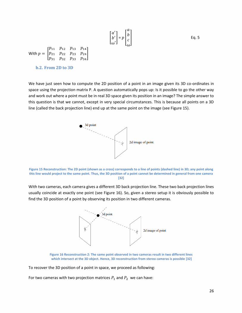
this question is that we cannot, except in very special circumstances. This is because all points on a 3D
line (called the back projection line) end up at the same point on the image (see Figure 15).
Figure 15 Reconstruction: The 2D point (shown as a cross) corresponds to a line of points (dashed line) in 3D; any point along this line would project to the same point. Thus, the 3D position of a point cannot be determined in general from one camera
[32]
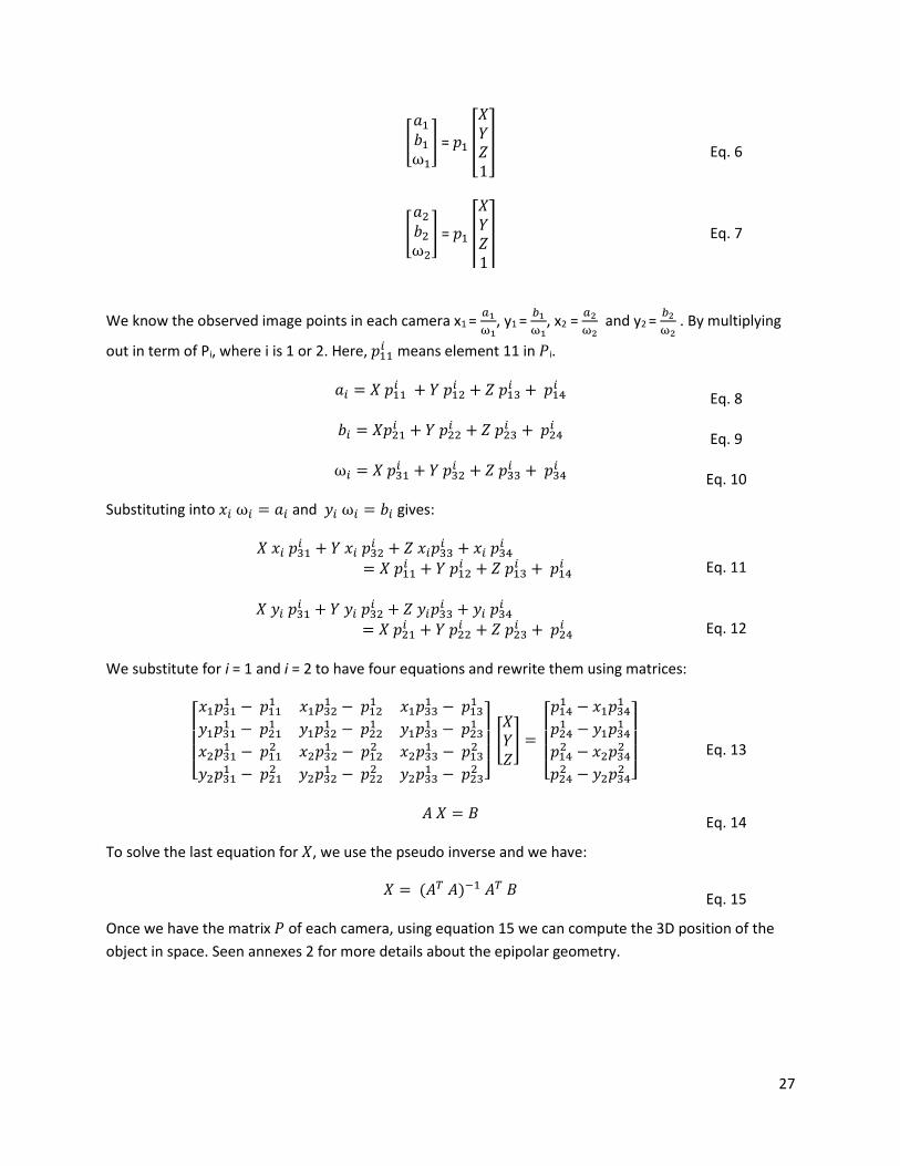
With two cameras, each camera gives a different 3D back projection line. These two back projection lines
usually coincide at exactly one point (see Figure 16). So, given a stereo setup it is obviously possible to
find the 3D position of a point by observing its position in two different cameras.
Figure 16 Reconstruction 2: The same point observed in two cameras result in two different lines which intersect at the 3D object. Hence, 3D reconstruction from stereo cameras is possible [32]
To recover the 3D position of a point in space, we proceed as following:
For two cameras with two projection matrices 𝑃1 and 𝑃2 we can have:
27
[
𝑎1
𝑏1
ω1
] = 𝑝1 [
𝑋𝑌𝑍1
]
Eq. 6
[
𝑎2
𝑏2
ω2
] = 𝑝1 [
𝑋𝑌𝑍1
] Eq. 7
We know the observed image points in each camera x1 = 𝑎1
ω1, y1 =
𝑏1
ω1, x2 =
𝑎2
ω2 and y2 =
𝑏2
ω2 . By multiplying
out in term of Pi, where i is 1 or 2. Here, 𝑝11𝑖 means element 11 in 𝑃i.
𝑎𝑖 = 𝑋 𝑝11
𝑖 + 𝑌 𝑝12
𝑖 + 𝑍 𝑝13𝑖 + 𝑝14
𝑖
Eq. 8
𝑏𝑖 = 𝑋𝑝21
𝑖 + 𝑌 𝑝22𝑖 + 𝑍 𝑝23
𝑖 + 𝑝24𝑖
Eq. 9
ω𝑖 = 𝑋 𝑝31
𝑖 + 𝑌 𝑝32𝑖 + 𝑍 𝑝33
𝑖 + 𝑝34𝑖
Eq. 10
Substituting into 𝑥𝑖 ω𝑖 = 𝑎𝑖 and 𝑦𝑖 ω𝑖 = 𝑏𝑖 gives:
𝑋 𝑥𝑖 𝑝31
𝑖 + 𝑌 𝑥𝑖 𝑝32𝑖 + 𝑍 𝑥𝑖𝑝33
𝑖 + 𝑥𝑖 𝑝34𝑖
= 𝑋 𝑝11𝑖 + 𝑌 𝑝12
𝑖 + 𝑍 𝑝13𝑖 + 𝑝14
𝑖
Eq. 11
𝑋 𝑦𝑖 𝑝31
𝑖 + 𝑌 𝑦𝑖 𝑝32𝑖 + 𝑍 𝑦𝑖𝑝33
𝑖 + 𝑦𝑖 𝑝34𝑖
= 𝑋 𝑝21𝑖 + 𝑌 𝑝22
𝑖 + 𝑍 𝑝23𝑖 + 𝑝24
𝑖
Eq. 12
We substitute for i = 1 and i = 2 to have four equations and rewrite them using matrices:
[ 𝑥1𝑝31
1 − 𝑝111 𝑥1𝑝32
1 − 𝑝121 𝑥1𝑝33
1 − 𝑝131
𝑦1𝑝311 − 𝑝21
1 𝑦1𝑝321 − 𝑝22
1 𝑦1𝑝331 − 𝑝23
1
𝑥2𝑝311 − 𝑝11
2 𝑥2𝑝321 − 𝑝12
2 𝑥2𝑝331 − 𝑝13
2
𝑦2𝑝311 − 𝑝21
2 𝑦2𝑝321 − 𝑝22
2 𝑦2𝑝331 − 𝑝23
2 ]
[𝑋𝑌𝑍] =
[ 𝑝14
1 − 𝑥1𝑝341
𝑝241 − 𝑦1𝑝34
1
𝑝142 − 𝑥2𝑝34
2
𝑝242 − 𝑦2𝑝34
2 ]
Eq. 13
𝐴 𝑋 = 𝐵
Eq. 14
To solve the last equation for 𝑋, we use the pseudo inverse and we have:
𝑋 = (𝐴𝑇 𝐴)−1 𝐴𝑇 𝐵
Eq. 15
Once we have the matrix 𝑃 of each camera, using equation 15 we can compute the 3D position of the
object in space. Seen annexes 2 for more details about the epipolar geometry.
28
2. The SLAM general pipeline
a. Definition of the problem
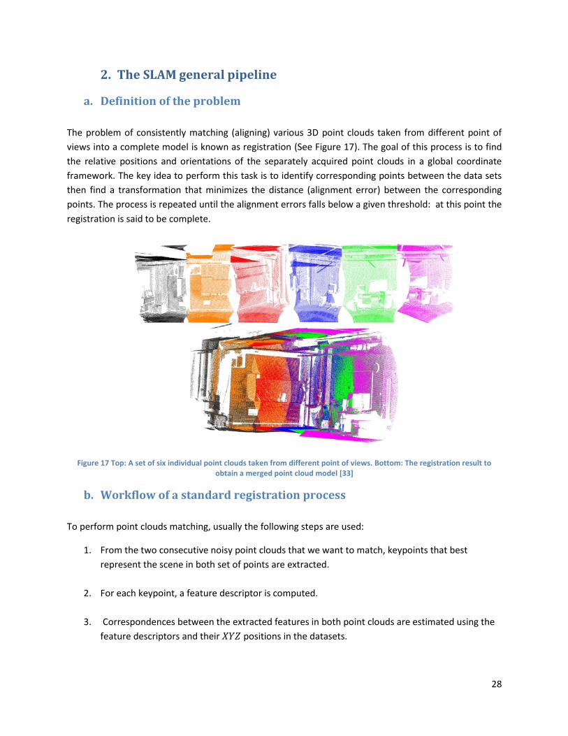
The problem of consistently matching (aligning) various 3D point clouds taken from different point of
views into a complete model is known as registration (See Figure 17). The goal of this process is to find
the relative positions and orientations of the separately acquired point clouds in a global coordinate
framework. The key idea to perform this task is to identify corresponding points between the data sets
then find a transformation that minimizes the distance (alignment error) between the corresponding
points. The process is repeated until the alignment errors falls below a given threshold: at this point the
registration is said to be complete.
Figure 17 Top: A set of six individual point clouds taken from different point of views. Bottom: The registration result to obtain a merged point cloud model [33]
b. Workflow of a standard registration process
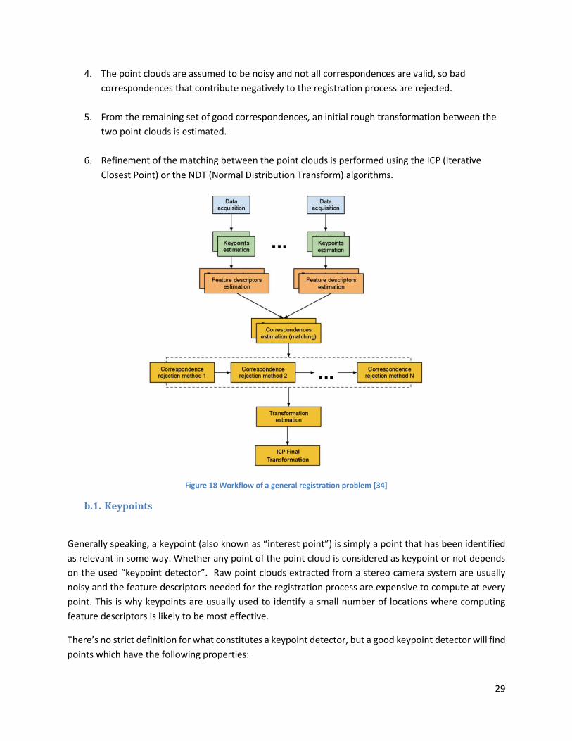
To perform point clouds matching, usually the following steps are used:
1. From the two consecutive noisy point clouds that we want to match, keypoints that best
represent the scene in both set of points are extracted.
2. For each keypoint, a feature descriptor is computed.
3. Correspondences between the extracted features in both point clouds are estimated using the
feature descriptors and their 𝑋𝑌𝑍 positions in the datasets.
29
4. The point clouds are assumed to be noisy and not all correspondences are valid, so bad
correspondences that contribute negatively to the registration process are rejected.
5. From the remaining set of good correspondences, an initial rough transformation between the
two point clouds is estimated.
6. Refinement of the matching between the point clouds is performed using the ICP (Iterative
Closest Point) or the NDT (Normal Distribution Transform) algorithms.
Figure 18 Workflow of a general registration problem [34]
b.1. Keypoints
Generally speaking, a keypoint (also known as “interest point”) is simply a point that has been identified
as relevant in some way. Whether any point of the point cloud is considered as keypoint or not depends
on the used “keypoint detector”. Raw point clouds extracted from a stereo camera system are usually
noisy and the feature descriptors needed for the registration process are expensive to compute at every
point. This is why keypoints are usually used to identify a small number of locations where computing
feature descriptors is likely to be most effective.
There’s no strict definition for what constitutes a keypoint detector, but a good keypoint detector will find
points which have the following properties:
30
Sparseness: Typically, only a small subset of points in the scene are keypoints
Repeatability: If a point is determined to be a keypoint in one point cloud, a keypoint should also
be found in a second point cloud taken from a different view point. Such keypoint will be called
“Stable”.
Distinctiveness: The area surrounding each keypoint should have a unique shape or appearance
that can be captured by some feature descriptor.
Interest points are usually placed at corners of shapes and where the color/brightness gradient is the
highest. There are various methods to find keypoints, and each technique has its specific output:
b.1.1. Uniform sampling
The uniform keypoints extraction method is the fastest method to estimate “interest points” in a point
cloud. It works somehow similarly to the voxel grid filter where:
A grid of cubes (with edges = keypoint leafSize) is built on the point cloud.
For each cube the centroid of the present points is computed and it is set as the voxel for that
cube.
For the uniform sampling keypoints method another step is added to the algorithm.
The point of the source cloud nearest to the computed centroid voxel is set as the keypoint for
that cube.
Hence, the difference between voxel points and uniform keypoints is: the uniform sampling keypoints
belong to the source cloud when the voxel points don’t. The keypoints are a subset of the input cloud.
The uniform keypoints have been chosen because voxels introduce new points and then noise affecting
the registration process.
Other keypoints detectors like NARF (Normal Aligned Radial Feature) exist. This one is detailed in annexes
1
b.2. Features
In their basic representation, points as defined in the concept of 3D mapping systems are simply
represented using their Cartesian coordinates 𝑥, 𝑦 and 𝑧 with respect to a given origin. When the origin
of the coordinate system does not change over time, there could be two different points 𝑝1 and 𝑝2, from
two different point clouds of the same scene acquired at 𝑡1and 𝑡2, having the same coordinates.
Comparing only the Cartesian coordinates of the two points to verify that they correspond to each other
is not a robust approach in the sense that if the second point cloud is taken from a different point view,
we will not be able to find the corresponding point just by comparing the Cartesian coordinates. The two
points could be sampled on completely different surfaces and thus represent totally different information
when taken together with the other surrounding points in their neighborhood.
31
Applications which need to compare points for various reasons require better characteristics and metrics
to be able to distinguish between geometric surfaces. The concept of a 3D point as a singular entity with
Cartesian coordinates therefore disappears and a new concept of local descriptors takes its place.
Features (or descriptors), generally speaking, are structures containing data that describe in a better way
the key points of the dataset. There are two main kinds of features:
i. Local features
For every key point, a local feature is computed based on its neighbors, so the description includes a set
of adjacent points. If we take a 2D image for example, a local feature for a point could be the gradient of
brightness with neighbors.
ii. Global features
There is just one descriptor for the entire dataset. For a 2D image for example, a global feature could be
the average brightness or the average color, or a data structure containing many of these global
characteristics.
b.2.1. FPFH (Fast Point Feature Histogram) descriptor
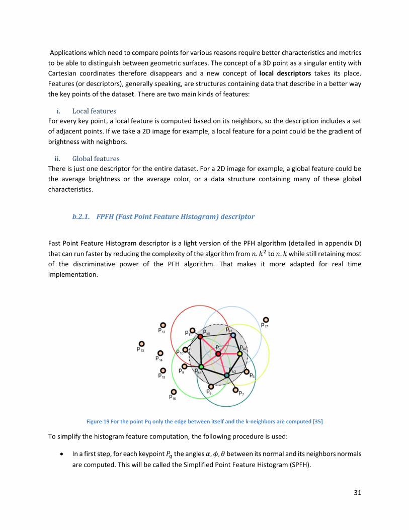
Fast Point Feature Histogram descriptor is a light version of the PFH algorithm (detailed in appendix D)
that can run faster by reducing the complexity of the algorithm from 𝑛. 𝑘2 to 𝑛. 𝑘 while still retaining most
of the discriminative power of the PFH algorithm. That makes it more adapted for real time
implementation.
Figure 19 For the point Pq only the edge between itself and the k-neighbors are computed [35]
To simplify the histogram feature computation, the following procedure is used:
In a first step, for each keypoint 𝑃𝑞 the angles 𝛼, 𝜙, 𝜃 between its normal and its neighbors normals
are computed. This will be called the Simplified Point Feature Histogram (SPFH).
32
In a second step, for each point its 𝑘 neighbors are re-determined and the neighboring SPFH
values are used to weight the final histogram of 𝑃𝑞 (called FPFH) as follows:
𝐹𝑃𝐹𝐻(𝑃𝑞) = 𝑆𝑃𝐹𝐻(𝑃𝑞) +
1
𝑘 ∑
1
𝜔𝑘
𝑘
𝑖=1
𝑆𝑃𝐹𝐻(𝑃𝑘)
Eq. 20
Where the weight 𝜔𝑘represents the distance between the query point 𝑃𝑞and a neighbor point 𝑃𝑘.
More details about the FPFH descriptor can be found in Appendix D.
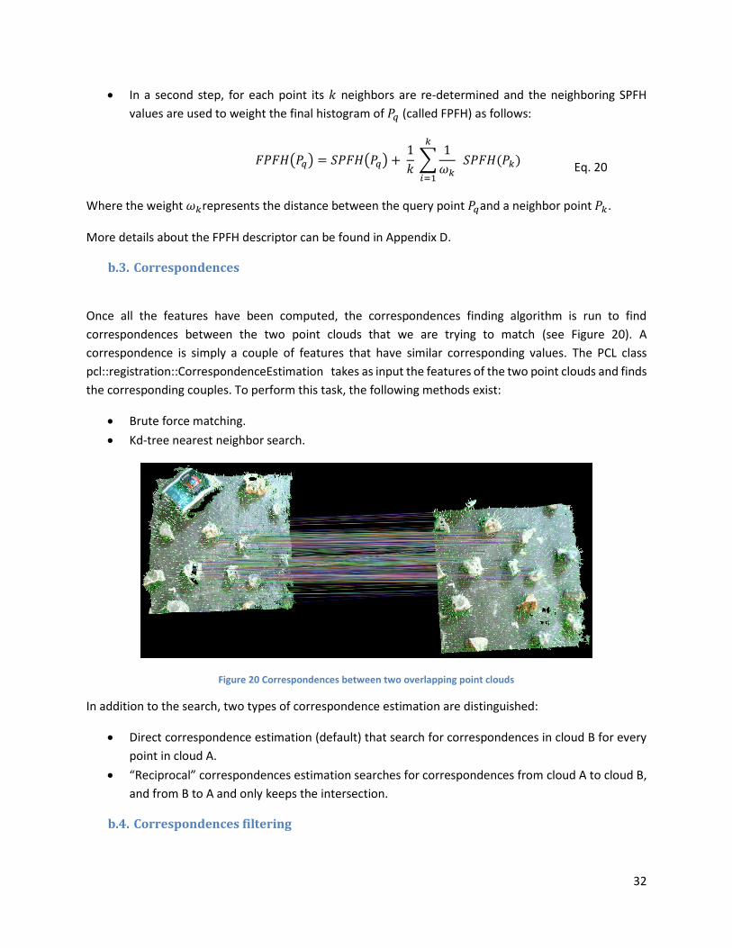
b.3. Correspondences
Once all the features have been computed, the correspondences finding algorithm is run to find
correspondences between the two point clouds that we are trying to match (see Figure 20). A
correspondence is simply a couple of features that have similar corresponding values. The PCL class
pcl::registration::CorrespondenceEstimation takes as input the features of the two point clouds and finds
the corresponding couples. To perform this task, the following methods exist:
Brute force matching.
Kd-tree nearest neighbor search.
Figure 20 Correspondences between two overlapping point clouds
In addition to the search, two types of correspondence estimation are distinguished:
Direct correspondence estimation (default) that search for correspondences in cloud B for every
point in cloud A.
“Reciprocal” correspondences estimation searches for correspondences from cloud A to cloud B,
and from B to A and only keeps the intersection.
b.4. Correspondences filtering
33
Once the correspondences have been computed, using pcl::resgistration::CorrespondenceRejector, it is
possible to reject some of them to improve the matching results. Different rejection methods exist:
b.4.1. Rejection by distance
All correspondences that exceed a distance threshold are rejected. The distance is a measure between
the corresponding keypoints of the point clouds considered in the registration process and depends on
how far these point clouds stand from each other. The bigger is the frame rate of the point clouds
acquisition the smaller will be this distance.
b.4.2. Rejection using the Median distance
The median distance between all the keypoints correspondences is computed, and then all the
correspondences that exceed a deviation threshold from that mean are being rejected.
b.5. Estimation of the 3D transformation
To perfectly match two consecutive point clouds and be able to build a consistent map, the 3D
transformation between them is computed in two steps. First the initial alignment which is a rough
alignment that brings the two point clouds closers to each other. Then the final alignment that allows to
perfectly match the point clouds.
b.5.1. Initial alignment using the RANSAC algorithm
The RANdom SAmple Consensus (RANSAC) presented in [15] is an iterative method widely known in computer vision that works on the assumption that data has inliers and outliers, meaning points that fit some kind of model or not. Within the registration pipeline, the RANSAC algorithm is used to generate a set of correspondences (Valuable important data) from a superset of correspondences (Valuable data + noise) that provides the best rigid body transform estimation for most of the points from the two matched point clouds.
Once the correspondences filtering has been performed, the initial alignment between the two point
clouds which is represented by a 4x4 matrix (rotation + translation) can be computed using only the good
correspondences. There are two classes in the PCL library that can estimate this transformation using only
the good corresponding points as input:
pcl::registration::TransformationEstimationLM – (Levenberg-Marquardt): which is an iterative
least-squares based algorithm. The result of this transformation does not bring always the best
score.
pcl::registration::TransformationEstimationSVD – (Singular Value Decomposition): The constrain
between a point 𝑃𝐴 from the source point cloud 𝐴 and its correspondence 𝑃𝐵 from the target
point cloud 𝐵 can be written as following :
𝑃𝐵 = 𝑇 𝑃𝐴
Eq. 21
Where 𝑇 is a 4x4 transformation matrix
34
The transformation matrix 𝑇 can be computed by solving the previous equation through a Singular
Value Decomposition (SVD) of the covariance data. To do this, a minimal number of points 𝑘 = 3
is needed and the more points, the better defined the system would be. However, because of
the uncertainty due to sensory noise, a single point which location is incorrectly estimated could
lead to a significant error in the final transformation. Therefore, a better transformation can be
found iteratively using the RANSAC algorithm.
To evaluate the initial alignment, at every iteration of the RANSAC process, 3 correspondences
are picked from the two point clouds and the transformation matrix 𝑇 is computed then all the
other points from the source cloud are projected according to this transformation. A 3D vector is
computed from the difference between the projected points and the points in the target point
cloud. The error is the norm of this vector. RANSAC performs a certain number of iterations to
minimize this error and a threshold is defined to stop the iterations.
b.5.2. Fine Alignment (ICP)
The Iterative Closest Point (ICP) presented by Zhang in [16] is an iterative algorithm that can retrieve the
final rigid transformation needed to minimize the distance between two sets of points (key points)
extracted from two consecutive point clouds. Considering the two sets of points (𝑝𝑖 , 𝑞𝑖), the scope is to
find the optimal transformation, composed by a translation 𝑡 and a rotation 𝑅, to align the source set (𝑝𝑖)
to the target (𝑞𝑖). The problem can be formulated as minimizing the squared distance between each
neighboring pairs:
𝑚𝑖𝑛 ∑||(𝑅 𝑝𝑖 + 𝑡) − 𝑞𝑖||
2
𝑖
Eq. 22
As any gradient descent method, the ICP is applicable when we have in advance a relatively good initial
guess. Otherwise, it is likely to be trapped into a local minimum. This is why the initial transformation
RANSAC algorithm is used to determine a good approximation of the rigid transformation, and use it as
the first guess for the ICP procedure.
Other registration algorithms like ICP non-linear and NDT (Normal Distribution Transform) exist. Details
about them can be found in annexes 1 and 2.
b.6. Pose Graph
The SLAM problem can be defined as a least square optimization of an error function and can be described
by a graph model, combining graph theory and probabilistic theory. Such a graph is called a pose graph,
where the nodes represent a state describing the poses of the imaging system, and the edges represent
the related constrains (rigid transformations) between a pair of nodes. Not only the graph representation
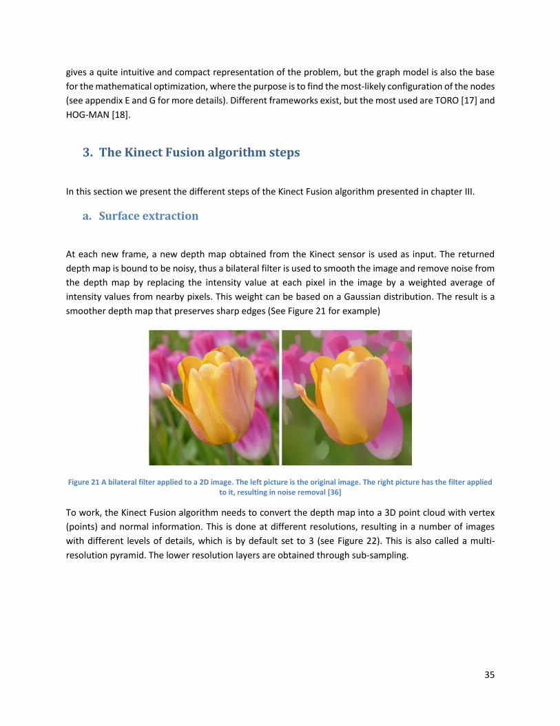
35
gives a quite intuitive and compact representation of the problem, but the graph model is also the base
for the mathematical optimization, where the purpose is to find the most-likely configuration of the nodes
(see appendix E and G for more details). Different frameworks exist, but the most used are TORO [17] and
HOG-MAN [18].
3. The Kinect Fusion algorithm steps
In this section we present the different steps of the Kinect Fusion algorithm presented in chapter III.
a. Surface extraction
At each new frame, a new depth map obtained from the Kinect sensor is used as input. The returned
depth map is bound to be noisy, thus a bilateral filter is used to smooth the image and remove noise from
the depth map by replacing the intensity value at each pixel in the image by a weighted average of
intensity values from nearby pixels. This weight can be based on a Gaussian distribution. The result is a
smoother depth map that preserves sharp edges (See Figure 21 for example)
Figure 21 A bilateral filter applied to a 2D image. The left picture is the original image. The right picture has the filter applied to it, resulting in noise removal [36]
To work, the Kinect Fusion algorithm needs to convert the depth map into a 3D point cloud with vertex
(points) and normal information. This is done at different resolutions, resulting in a number of images
with different levels of details, which is by default set to 3 (see Figure 22). This is also called a multi-
resolution pyramid. The lower resolution layers are obtained through sub-sampling.
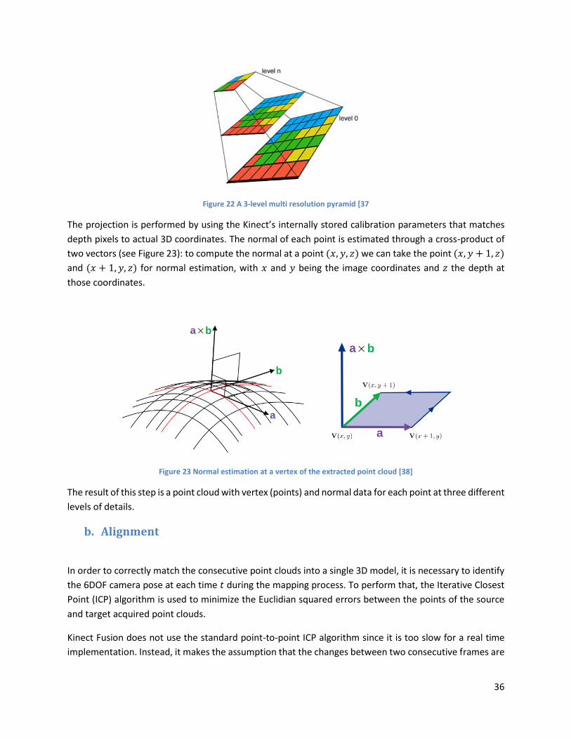
36
Figure 22 A 3-level multi resolution pyramid [37
The projection is performed by using the Kinect’s internally stored calibration parameters that matches
depth pixels to actual 3D coordinates. The normal of each point is estimated through a cross-product of
two vectors (see Figure 23): to compute the normal at a point (𝑥, 𝑦, 𝑧) we can take the point (𝑥, 𝑦 + 1, 𝑧)
and (𝑥 + 1, 𝑦, 𝑧) for normal estimation, with 𝑥 and 𝑦 being the image coordinates and 𝑧 the depth at
those coordinates.
Figure 23 Normal estimation at a vertex of the extracted point cloud [38]
The result of this step is a point cloud with vertex (points) and normal data for each point at three different
levels of details.
b. Alignment
In order to correctly match the consecutive point clouds into a single 3D model, it is necessary to identify
the 6DOF camera pose at each time 𝑡 during the mapping process. To perform that, the Iterative Closest
Point (ICP) algorithm is used to minimize the Euclidian squared errors between the points of the source
and target acquired point clouds.
Kinect Fusion does not use the standard point-to-point ICP algorithm since it is too slow for a real time
implementation. Instead, it makes the assumption that the changes between two consecutive frames are
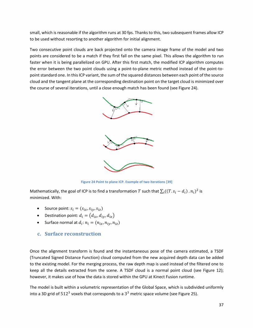
37
small, which is reasonable if the algorithm runs at 30 fps. Thanks to this, two subsequent frames allow ICP
to be used without resorting to another algorithm for initial alignment.
Two consecutive point clouds are back projected onto the camera image frame of the model and two
points are considered to be a match if they first fall on the same pixel. This allows the algorithm to run
faster when it is being parallelized on GPU. After this first match, the modified ICP algorithm computes
the error between the two point clouds using a point-to-plane metric method instead of the point-to-
point standard one. In this ICP variant, the sum of the squared distances between each point of the source
cloud and the tangent plane at the corresponding destination point on the target cloud is minimized over
the course of several iterations, until a close enough match has been found (see Figure 24).
Figure 24 Point to plane ICP. Example of two iterations [39]
Mathematically, the goal of ICP is to find a transformation 𝑇 such that ∑ ((𝑇. 𝑠𝑖 − 𝑑𝑖) . 𝑛𝑖)2
𝑖 is
minimized. With:
Source point: 𝑠𝑖 = (𝑠𝑖𝑥 , 𝑠𝑖𝑦, 𝑠𝑖𝑧)
Destination point: 𝑑𝑖 = (𝑑𝑖𝑥 , 𝑑𝑖𝑦, 𝑑𝑖𝑧)
Surface normal at 𝑑𝑖: 𝑛𝑖 = (𝑛𝑖𝑥 , 𝑛𝑖𝑦, 𝑛𝑖𝑧)
c. Surface reconstruction
Once the alignment transform is found and the instantaneous pose of the camera estimated, a TSDF
(Truncated Signed Distance Function) cloud computed from the new acquired depth data can be added
to the existing model. For the merging process, the raw depth map is used instead of the filtered one to
keep all the details extracted from the scene. A TSDF cloud is a normal point cloud (see Figure 12);
however, it makes use of how the data is stored within the GPU at Kinect Fusion runtime.
The model is built within a volumetric representation of the Global Space, which is subdivided uniformly
into a 3D grid of 5123 voxels that corresponds to a 33 metric space volume (see Figure 25).
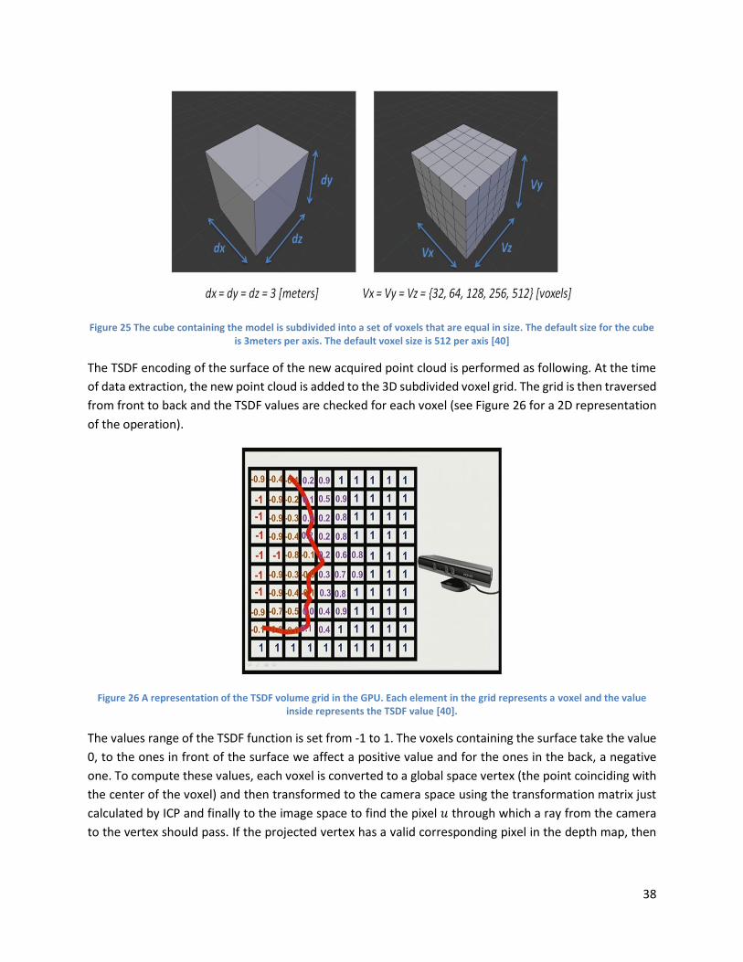
38
Figure 25 The cube containing the model is subdivided into a set of voxels that are equal in size. The default size for the cube is 3meters per axis. The default voxel size is 512 per axis [40]
The TSDF encoding of the surface of the new acquired point cloud is performed as following. At the time
of data extraction, the new point cloud is added to the 3D subdivided voxel grid. The grid is then traversed
from front to back and the TSDF values are checked for each voxel (see Figure 26 for a 2D representation
of the operation).
Figure 26 A representation of the TSDF volume grid in the GPU. Each element in the grid represents a voxel and the value inside represents the TSDF value [40].
The values range of the TSDF function is set from -1 to 1. The voxels containing the surface take the value
0, to the ones in front of the surface we affect a positive value and for the ones in the back, a negative
one. To compute these values, each voxel is converted to a global space vertex (the point coinciding with
the center of the voxel) and then transformed to the camera space using the transformation matrix just
calculated by ICP and finally to the image space to find the pixel 𝑢 through which a ray from the camera
to the vertex should pass. If the projected vertex has a valid corresponding pixel in the depth map, then
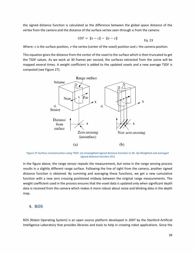
39
the signed distance function is calculated as the difference between the global space distance of the
vertex from the camera and the distance of the surface vertex seen through 𝑢 from the camera:
𝑆𝐷𝐹 = ‖𝑠 − 𝑐‖ − ‖𝑣 − 𝑐‖
Eq. 23
Where: 𝑠 is the surface position, 𝑣 the vertex (center of the voxel) position and 𝑐 the camera position.
This equation gives the distance from the center of the voxel to the surface which is then truncated to get
the TSDF values. As we work at 30 frames per second, the surfaces extracted from the scene will be
mapped several times. A weight coefficient is added to the updated voxels and a new average TSDF is
computed (see Figure 27).
Figure 27 Surface reconstruction using TSDF: (a) Unweighted signed distance function in 3D. (b) Weighted and averaged signed distance function [41]
In the figure above, the range sensor repeats the measurement, but noise in the range sensing process
results in a slightly different range surface. Following the line of sight from the camera, another signed
distance function is obtained. By summing and averaging these functions, we get a new cumulative
function with a new zero crossing positioned midway between the original range measurements. The
weight coefficient used in the process ensures that the voxel data is updated only when significant depth
data is received from the camera which makes it more robust about noise and blinking data in the depth
map.
4. ROS
ROS (Robot Operating System) is an open source platform developed in 2007 by the Stanford Artificial
Intelligence Laboratory that provides libraries and tools to help in creating robot applications. Since the
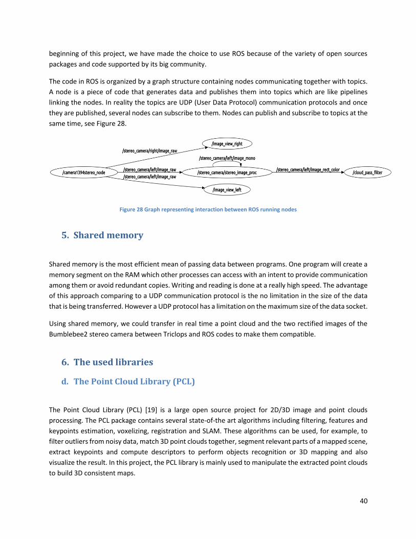
40
beginning of this project, we have made the choice to use ROS because of the variety of open sources
packages and code supported by its big community.
The code in ROS is organized by a graph structure containing nodes communicating together with topics.
A node is a piece of code that generates data and publishes them into topics which are like pipelines
linking the nodes. In reality the topics are UDP (User Data Protocol) communication protocols and once
they are published, several nodes can subscribe to them. Nodes can publish and subscribe to topics at the
same time, see Figure 28.
Figure 28 Graph representing interaction between ROS running nodes
5. Shared memory
Shared memory is the most efficient mean of passing data between programs. One program will create a
memory segment on the RAM which other processes can access with an intent to provide communication
among them or avoid redundant copies. Writing and reading is done at a really high speed. The advantage
of this approach comparing to a UDP communication protocol is the no limitation in the size of the data
that is being transferred. However a UDP protocol has a limitation on the maximum size of the data socket.
Using shared memory, we could transfer in real time a point cloud and the two rectified images of the
Bumblebee2 stereo camera between Triclops and ROS codes to make them compatible.
6. The used libraries
d. The Point Cloud Library (PCL)
The Point Cloud Library (PCL) [19] is a large open source project for 2D/3D image and point clouds
processing. The PCL package contains several state-of-the art algorithms including filtering, features and
keypoints estimation, voxelizing, registration and SLAM. These algorithms can be used, for example, to
filter outliers from noisy data, match 3D point clouds together, segment relevant parts of a mapped scene,
extract keypoints and compute descriptors to perform objects recognition or 3D mapping and also
visualize the result. In this project, the PCL library is mainly used to manipulate the extracted point clouds
to build 3D consistent maps.

41
PCL is released under the terms of the BSD license and is free to be used for commercial and research use.
b. OpenCV
OpenCV (Open Source Computer Vision Library) [20] is an open source C++ library for image processing
and computer vision that has originally been developed by Intel and is today supported by Willow Garage.
The library contains many functions and algorithms mainly aimed at real time image processing.
In this project, OpenCV has been mainly used to manipulate, filter or truncate the images extracted from
the Bumblebee2 stereo camera.
7. CloudCompare
CloudCompare is a free licenced software used for managing and comparing 3D point clouds. The
development of the application started in 2004 as part of a CIFRE thesis, funded by EDF R&D and housed
at the École Nationale Supérieure des Télécommunications (ENST – Telecom Paris, TSI Laboratory, TII team
- France).
During this project, CloudCompare has been used to:
Calculate local distances between two points in point clouds.
Match 3D maps and compute the mean squared error distance between them.
Project the 3D maps to generate height maps that are more adapted for path planning.
All of this without using code.
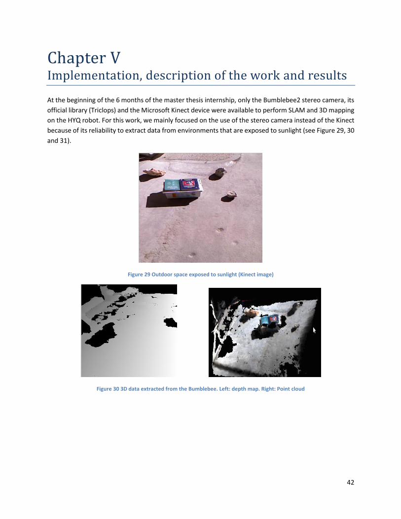
42
Chapter V Implementation, description of the work and results
At the beginning of the 6 months of the master thesis internship, only the Bumblebee2 stereo camera, its
official library (Triclops) and the Microsoft Kinect device were available to perform SLAM and 3D mapping
on the HYQ robot. For this work, we mainly focused on the use of the stereo camera instead of the Kinect
because of its reliability to extract data from environments that are exposed to sunlight (see Figure 29, 30
and 31).
Figure 29 Outdoor space exposed to sunlight (Kinect image)
Figure 30 3D data extracted from the Bumblebee. Left: depth map. Right: Point cloud
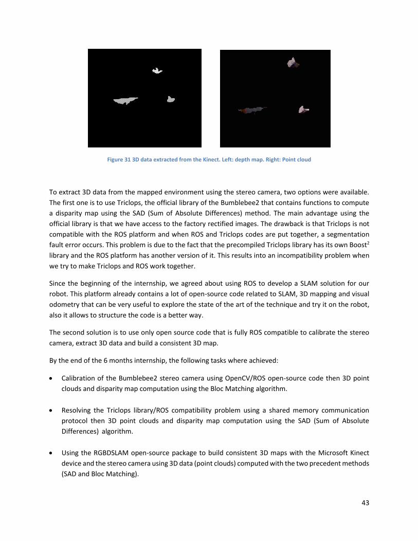
43
Figure 31 3D data extracted from the Kinect. Left: depth map. Right: Point cloud
To extract 3D data from the mapped environment using the stereo camera, two options were available.
The first one is to use Triclops, the official library of the Bumblebee2 that contains functions to compute
a disparity map using the SAD (Sum of Absolute Differences) method. The main advantage using the
official library is that we have access to the factory rectified images. The drawback is that Triclops is not
compatible with the ROS platform and when ROS and Triclops codes are put together, a segmentation
fault error occurs. This problem is due to the fact that the precompiled Triclops library has its own Boost2
library and the ROS platform has another version of it. This results into an incompatibility problem when
we try to make Triclops and ROS work together.
Since the beginning of the internship, we agreed about using ROS to develop a SLAM solution for our
robot. This platform already contains a lot of open-source code related to SLAM, 3D mapping and visual
odometry that can be very useful to explore the state of the art of the technique and try it on the robot,
also it allows to structure the code is a better way.
The second solution is to use only open source code that is fully ROS compatible to calibrate the stereo
camera, extract 3D data and build a consistent 3D map.
By the end of the 6 months internship, the following tasks where achieved:
Calibration of the Bumblebee2 stereo camera using OpenCV/ROS open-source code then 3D point
clouds and disparity map computation using the Bloc Matching algorithm.
Resolving the Triclops library/ROS compatibility problem using a shared memory communication
protocol then 3D point clouds and disparity map computation using the SAD (Sum of Absolute
Differences)salgorithm.
Using the RGBDSLAM open-source package to build consistent 3D maps with the Microsoft Kinect
device and the stereo camera using 3D data (point clouds) computed with the two precedent methods
(SAD and Bloc Matching).
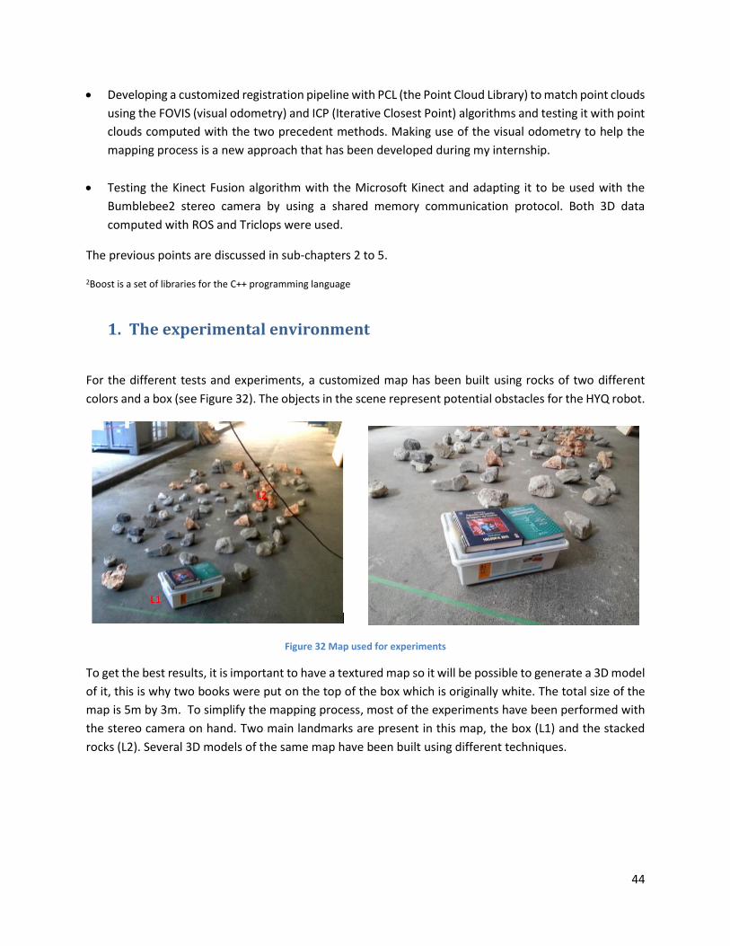
44
Developing a customized registration pipeline with PCL (the Point Cloud Library) to match point clouds
using the FOVIS (visual odometry) and ICP (Iterative Closest Point) algorithms and testing it with point
clouds computed with the two precedent methods. Making use of the visual odometry to help the
mapping process is a new approach that has been developed during my internship.
Testing the Kinect Fusion algorithm with the Microsoft Kinect and adapting it to be used with the
Bumblebee2 stereo camera by using a shared memory communication protocol. Both 3D data
computed with ROS and Triclops were used.
The previous points are discussed in sub-chapters 2 to 5.
2Boost is a set of libraries for the C++ programming language
1. The experimental environment
For the different tests and experiments, a customized map has been built using rocks of two different
colors and a box (see Figure 32). The objects in the scene represent potential obstacles for the HYQ robot.
Figure 32 Map used for experiments
To get the best results, it is important to have a textured map so it will be possible to generate a 3D model
of it, this is why two books were put on the top of the box which is originally white. The total size of the
map is 5m by 3m. To simplify the mapping process, most of the experiments have been performed with
the stereo camera on hand. Two main landmarks are present in this map, the box (L1) and the stacked
rocks (L2). Several 3D models of the same map have been built using different techniques.
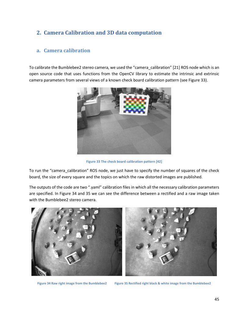
45
2. Camera Calibration and 3D data computation
a. Camera calibration
To calibrate the Bumblebee2 stereo camera, we used the “camera_calibration” [21] ROS node which is an
open source code that uses functions from the OpenCV library to estimate the intrinsic and extrinsic
camera parameters from several views of a known check board calibration pattern (see Figure 33).
Figure 33 The check board calibration pattern [42]
To run the “camera_calibration” ROS node, we just have to specify the number of squares of the check
board, the size of every square and the topics on which the raw distorted images are published.
The outputs of the code are two “.yaml” calibration files in which all the necessary calibration parameters
are specified. In Figure 34 and 35 we can see the difference between a rectified and a raw image taken
with the Bumblebee2 stereo camera.
Figure 34 Raw right image from the Bumblebee2 Figure 35 Rectified right black & white image from the Bumblebee2
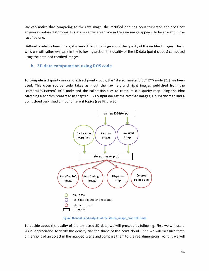
46
We can notice that comparing to the raw image, the rectified one has been truncated and does not
anymore contain distortions. For example the green line in the raw image appears to be straight in the
rectified one.
Without a reliable benchmark, it is very difficult to judge about the quality of the rectified images. This is
why, we will rather evaluate in the following section the quality of the 3D data (point clouds) computed
using the obtained rectified images.
b. 3D data computation using ROS code
To compute a disparity map and extract point clouds, the “stereo_image_proc” ROS node [22] has been
used. This open source code takes as input the raw left and right images published from the
“camera1394stereo” ROS node and the calibration files to compute a disparity map using the Bloc
Matching algorithm presented in chapter II. As output we get the rectified images, a disparity map and a
point cloud published on four different topics (see Figure 36).
Figure 36 Inputs and outputs of the stereo_image_proc ROS node
To decide about the quality of the extracted 3D data, we will proceed as following. First we will use a
visual appreciation to verify the density and the shape of the point cloud. Then we will measure three
dimensions of an object in the mapped scene and compare them to the real dimensions. For this we will
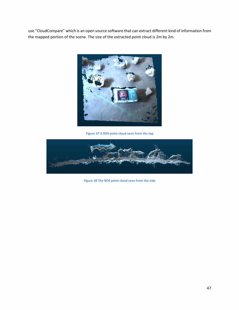
47
use “CloudCompare” which is an open source software that can extract different kind of information from
the mapped portion of the scene. The size of the extracted point cloud is 2m by 2m.
Figure 37 A ROS point cloud seen from the top
Figure 38 The ROS point cloud seen from the side
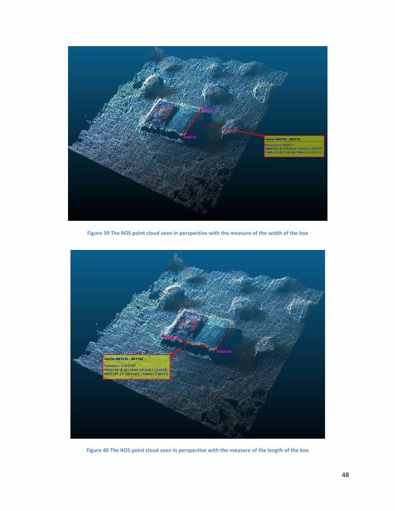
48
Figure 39 The ROS point cloud seen in perspective with the measure of the width of the box
Figure 40 The ROS point cloud seen in perspective with the measure of the length of the box
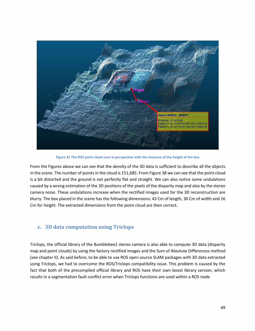
49
Figure 41 The ROS point cloud seen in perspective with the measure of the height of the box
From the Figures above we can see that the density of the 3D data is sufficient to describe all the objects
in the scene. The number of points in the cloud is 151,685. From Figure 38 we can see that the point cloud
is a bit distorted and the ground is not perfectly flat and straight. We can also notice some undulations
caused by a wrong estimation of the 3D positions of the pixels of the disparity map and also by the stereo
camera noise. These undulations increase when the rectified images used for the 3D reconstruction are
blurry. The box placed in the scene has the following dimensions: 43 Cm of length, 30 Cm of width and 16
Cm for height. The extracted dimensions from the point cloud are then correct.
c. 3D data computation using Triclops
Triclops, the official library of the Bumblebee2 stereo camera is also able to compute 3D data (disparity
map and point clouds) by using the factory rectified images and the Sum of Absolute Differences method
(see chapter II). As said before, to be able to use ROS open source SLAM packages with 3D data extracted
using Triclops, we had to overcome the ROS/Triclops compatibility issue. This problem is caused by the
fact that both of the precompiled official library and ROS have their own boost library version, which
results in a segmentation fault conflict error when Triclops functions are used within a ROS node.
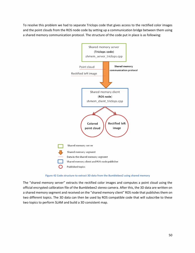
50
To resolve this problem we had to separate Triclops code that gives access to the rectified color images
and the point clouds from the ROS node code by setting up a communication bridge between them using
a shared memory communication protocol. The structure of the code put in place is as following:
Figure 42 Code structure to extract 3D data from the Bumblebee2 using shared memory
The “shared memory server” extracts the rectified color images and computes a point cloud using the
official encrypted calibration file of the Bumblebee2 stereo camera. After this, the 3D data are written on
a shared memory segment and received on the “shared memory client” ROS node that publishes them on
two different topics. The 3D data can then be used by ROS compatible code that will subscribe to these
two topics to perform SLAM and build a 3D consistent map.
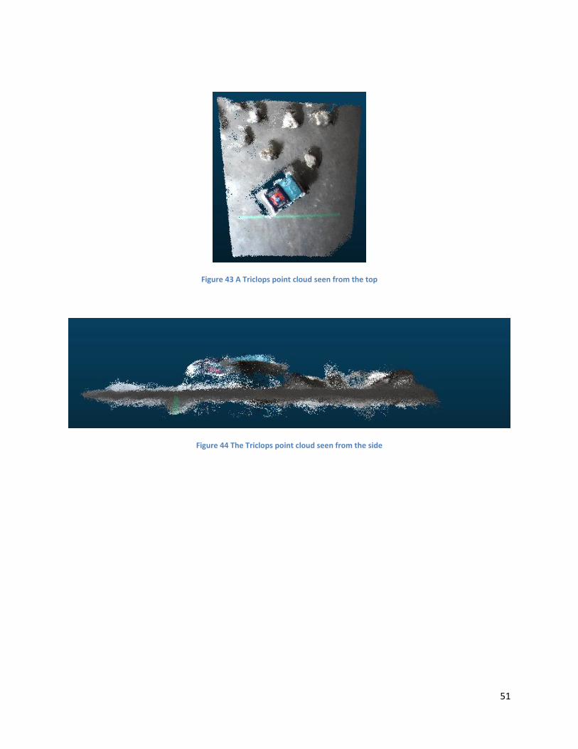
51
Figure 43 A Triclops point cloud seen from the top
Figure 44 The Triclops point cloud seen from the side
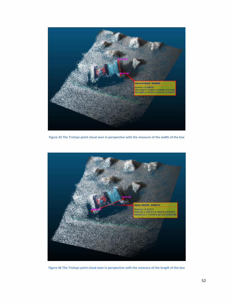
52
Figure 45 The Triclops point cloud seen in perspective with the measure of the width of the box
Figure 46 The Triclops point cloud seen in perspective with the measure of the length of the box
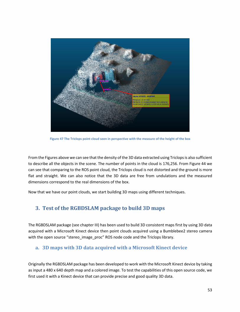
53
Figure 47 The Triclops point cloud seen in perspective with the measure of the height of the box
From the Figures above we can see that the density of the 3D data extracted using Triclops is also sufficient
to describe all the objects in the scene. The number of points in the cloud is 176,256. From Figure 44 we
can see that comparing to the ROS point cloud, the Triclops cloud is not distorted and the ground is more
flat and straight. We can also notice that the 3D data are free from undulations and the measured
dimensions correspond to the real dimensions of the box.
Now that we have our point clouds, we start building 3D maps using different techniques.
3. Test of the RGBDSLAM package to build 3D maps
The RGBDSLAM package (see chapter III) has been used to build 3D consistent maps first by using 3D data
acquired with a Microsoft Kinect device then point clouds acquired using a Bumblebee2 stereo camera
with the open source “stereo_image_proc” ROS node code and the Triclops library.
a. 3D maps with 3D data acquired with a Microsoft Kinect device
Originally the RGBDSLAM package has been developed to work with the Microsoft Kinect device by taking
as input a 480 x 640 depth map and a colored image. To test the capabilities of this open source code, we
first used it with a Kinect device that can provide precise and good quality 3D data.
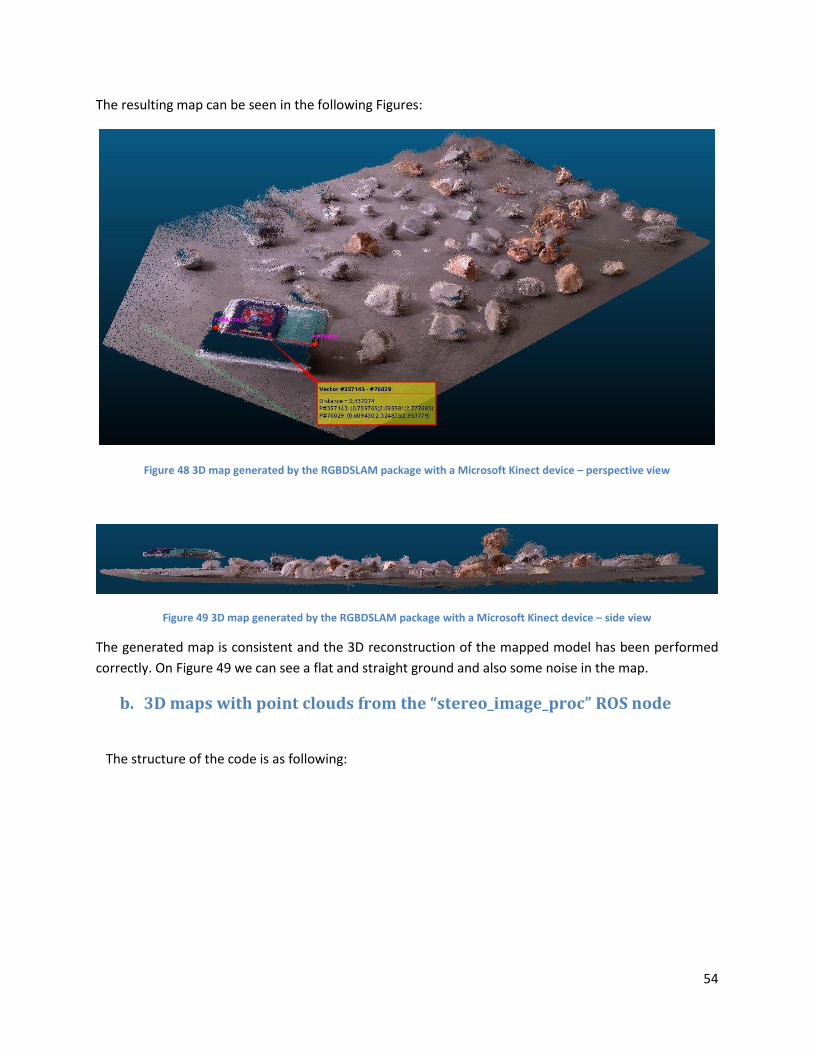
54
The resulting map can be seen in the following Figures:
Figure 48 3D map generated by the RGBDSLAM package with a Microsoft Kinect device – perspective view
Figure 49 3D map generated by the RGBDSLAM package with a Microsoft Kinect device – side view
The generated map is consistent and the 3D reconstruction of the mapped model has been performed
correctly. On Figure 49 we can see a flat and straight ground and also some noise in the map.
b. 3D maps with point clouds from the “stereo_image_proc” ROS node
The structure of the code is as following:
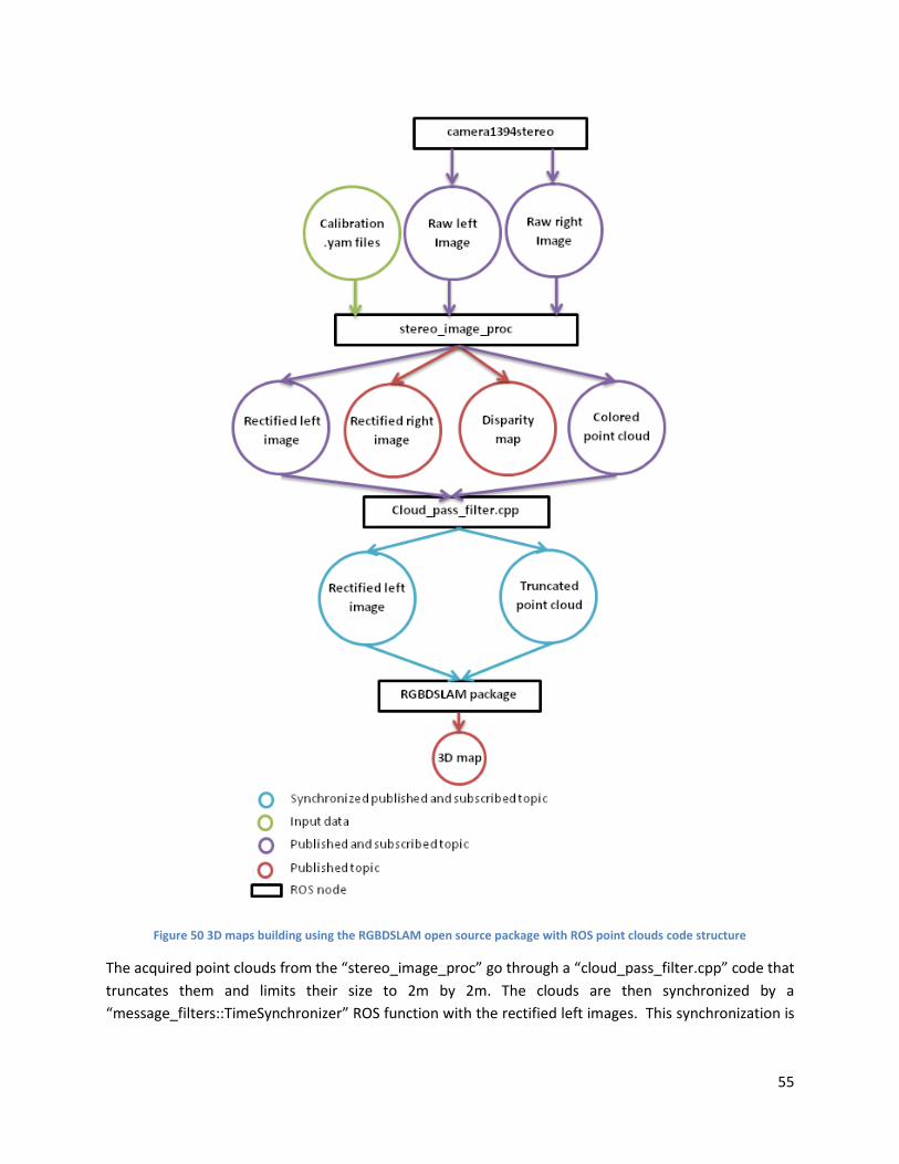
55
Figure 50 3D maps building using the RGBDSLAM open source package with ROS point clouds code structure
The acquired point clouds from the “stereo_image_proc” go through a “cloud_pass_filter.cpp” code that
truncates them and limits their size to 2m by 2m. The clouds are then synchronized by a
“message_filters::TimeSynchronizer” ROS function with the rectified left images. This synchronization is
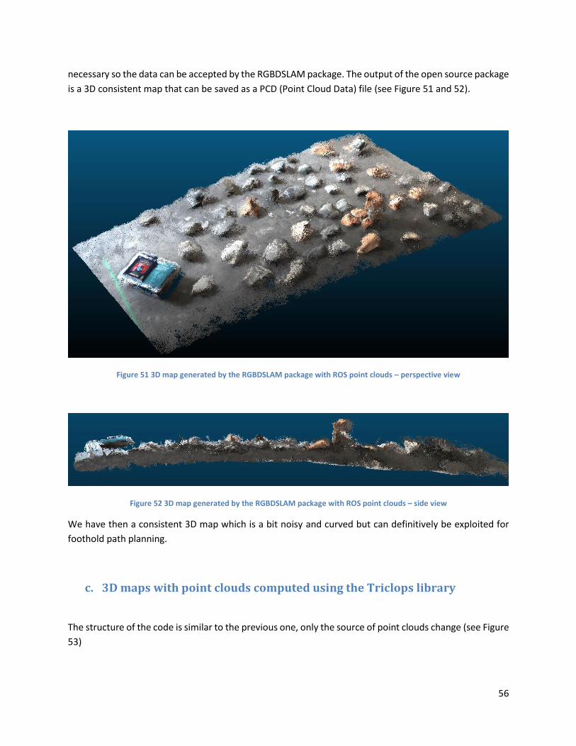
56
necessary so the data can be accepted by the RGBDSLAM package. The output of the open source package
is a 3D consistent map that can be saved as a PCD (Point Cloud Data) file (see Figure 51 and 52).
Figure 51 3D map generated by the RGBDSLAM package with ROS point clouds – perspective view
Figure 52 3D map generated by the RGBDSLAM package with ROS point clouds – side view
We have then a consistent 3D map which is a bit noisy and curved but can definitively be exploited for
foothold path planning.
c. 3D maps with point clouds computed using the Triclops library
The structure of the code is similar to the previous one, only the source of point clouds change (see Figure
53)
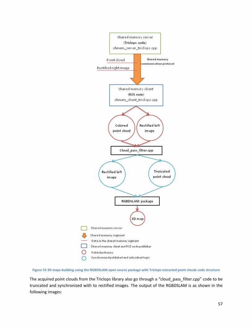
57
Figure 53 3D maps building using the RGBDSLAM open source package with Triclops extracted point clouds code structure
The acquired point clouds from the Triclops library also go through a “cloud_pass_filter.cpp” code to be
truncated and synchronized with to rectified images. The output of the RGBDSLAM is as shown in the
following images:
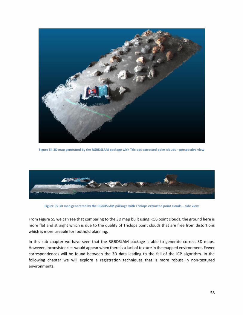
58
Figure 54 3D map generated by the RGBDSLAM package with Triclops extracted point clouds – perspective view
Figure 55 3D map generated by the RGBDSLAM package with Triclops extracted point clouds – side view
From Figure 55 we can see that comparing to the 3D map built using ROS point clouds, the ground here is
more flat and straight which is due to the quality of Triclops point clouds that are free from distortions
which is more useable for foothold planning.
In this sub chapter we have seen that the RGBDSLAM package is able to generate correct 3D maps.
However, inconsistencies would appear when there is a lack of texture in the mapped environment. Fewer
correspondences will be found between the 3D data leading to the fail of the ICP algorithm. In the
following chapter we will explore a registration techniques that is more robust in non-textured
environments.
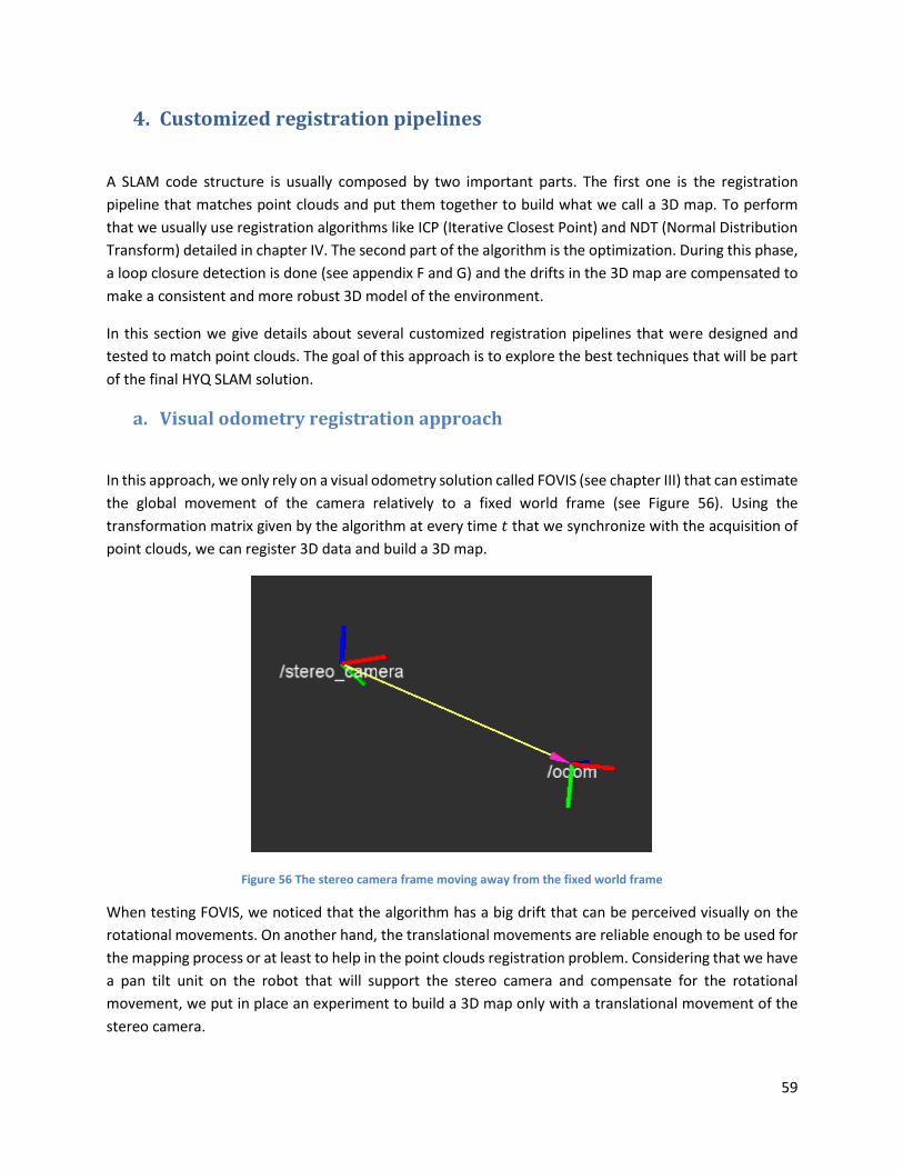
59
4. Customized registration pipelines
A SLAM code structure is usually composed by two important parts. The first one is the registration
pipeline that matches point clouds and put them together to build what we call a 3D map. To perform
that we usually use registration algorithms like ICP (Iterative Closest Point) and NDT (Normal Distribution
Transform) detailed in chapter IV. The second part of the algorithm is the optimization. During this phase,
a loop closure detection is done (see appendix F and G) and the drifts in the 3D map are compensated to
make a consistent and more robust 3D model of the environment.
In this section we give details about several customized registration pipelines that were designed and
tested to match point clouds. The goal of this approach is to explore the best techniques that will be part
of the final HYQ SLAM solution.
a. Visual odometry registration approach
In this approach, we only rely on a visual odometry solution called FOVIS (see chapter III) that can estimate
the global movement of the camera relatively to a fixed world frame (see Figure 56). Using the
transformation matrix given by the algorithm at every time 𝑡 that we synchronize with the acquisition of
point clouds, we can register 3D data and build a 3D map.
Figure 56 The stereo camera frame moving away from the fixed world frame
When testing FOVIS, we noticed that the algorithm has a big drift that can be perceived visually on the
rotational movements. On another hand, the translational movements are reliable enough to be used for
the mapping process or at least to help in the point clouds registration problem. Considering that we have
a pan tilt unit on the robot that will support the stereo camera and compensate for the rotational
movement, we put in place an experiment to build a 3D map only with a translational movement of the
stereo camera.
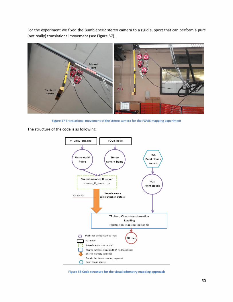
60
For the experiment we fixed the Bumblebee2 stereo camera to a rigid support that can perform a pure
(not really) translational movement (see Figure 57).
Figure 57 Translational movement of the stereo camera for the FOVIS mapping experiment
The structure of the code is as following:
Figure 58 Code structure for the visual odometry mapping approach
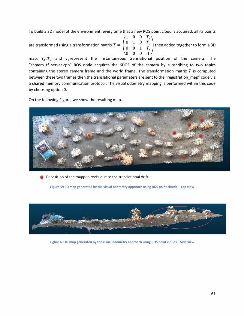
61
To build a 3D model of the environment, every time that a new ROS point cloud is acquired, all its points
are transformed using a transformation matrix 𝑇 = (
1 0 0 𝑇𝑥
0 1 0 𝑇𝑦
0 0 1 𝑇𝑧
0 0 0 1
) then added together to form a 3D
map. 𝑇𝑥 , 𝑇𝑦 and 𝑇𝑧represent the instantaneous translational position of the camera. The
“shmem_tf_server.cpp” ROS node acquires the 6DOF of the camera by subscribing to two topics
containing the stereo camera frame and the world frame. The transformation matrix 𝑇 is computed
between these two frames then the translational parameters are sent to the “registration_map” code via
a shared memory communication protocol. The visual odometry mapping is performed within this code
by choosing option 0.
On the following Figure, we show the resulting map.
Figure 59 3D map generated by the visual odometry approach using ROS point clouds – Top view
Figure 60 3D map generated by the visual odometry approach using ROS point clouds – Side view
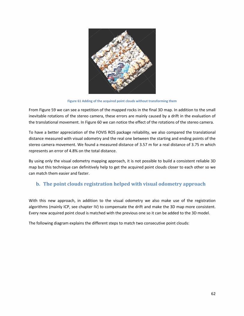
62
Figure 61 Adding of the acquired point clouds without transforming them
From Figure 59 we can see a repetition of the mapped rocks in the final 3D map. In addition to the small
inevitable rotations of the stereo camera, these errors are mainly caused by a drift in the evaluation of
the translational movement. In Figure 60 we can notice the effect of the rotations of the stereo camera.
To have a better appreciation of the FOVIS ROS package reliability, we also compared the translational
distance measured with visual odometry and the real one between the starting and ending points of the
stereo camera movement. We found a measured distance of 3.57 m for a real distance of 3.75 m which
represents an error of 4.8% on the total distance.
By using only the visual odometry mapping approach, it is not possible to build a consistent reliable 3D
map but this technique can definitively help to get the acquired point clouds closer to each other so we
can match them easier and faster.
b. The point clouds registration helped with visual odometry approach
With this new approach, in addition to the visual odometry we also make use of the registration
algorithms (mainly ICP, see chapter IV) to compensate the drift and make the 3D map more consistent.
Every new acquired point cloud is matched with the previous one so it can be added to the 3D model.
The following diagram explains the different steps to match two consecutive point clouds:
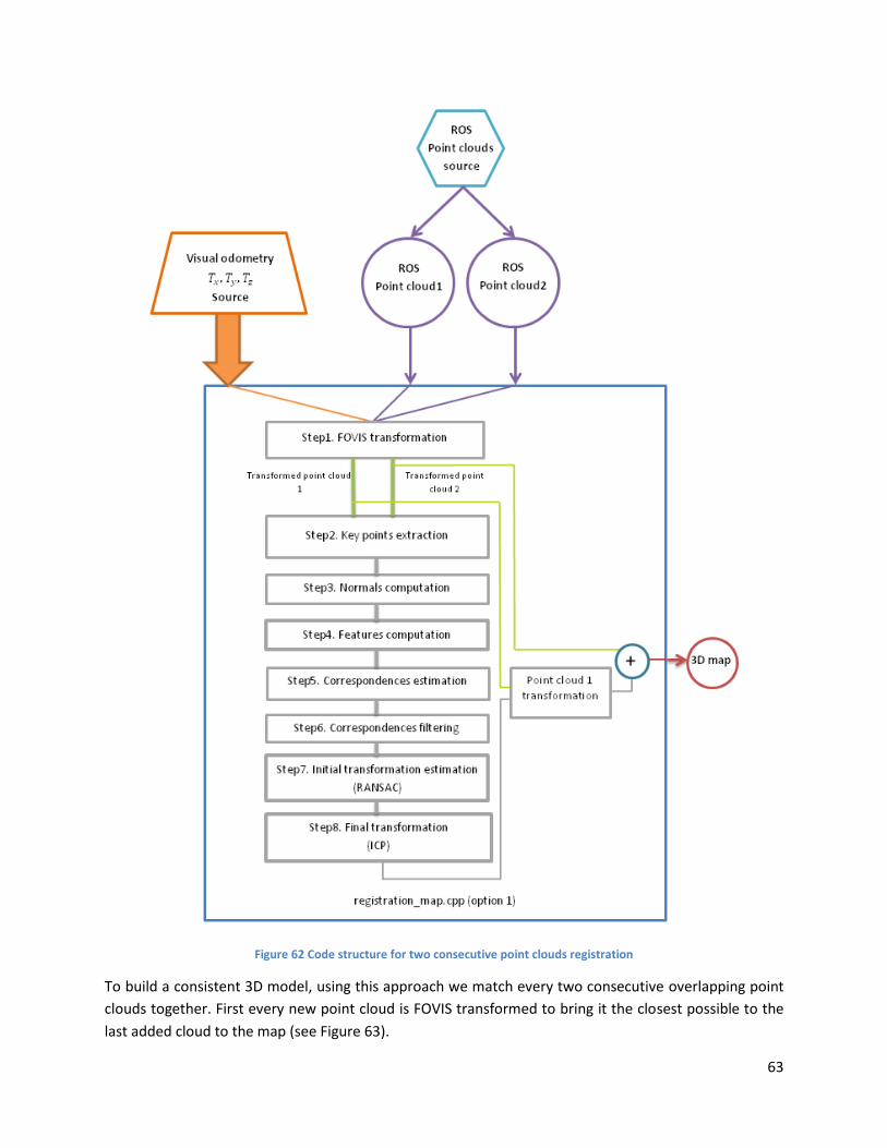
63
Figure 62 Code structure for two consecutive point clouds registration
To build a consistent 3D model, using this approach we match every two consecutive overlapping point
clouds together. First every new point cloud is FOVIS transformed to bring it the closest possible to the
last added cloud to the map (see Figure 63).
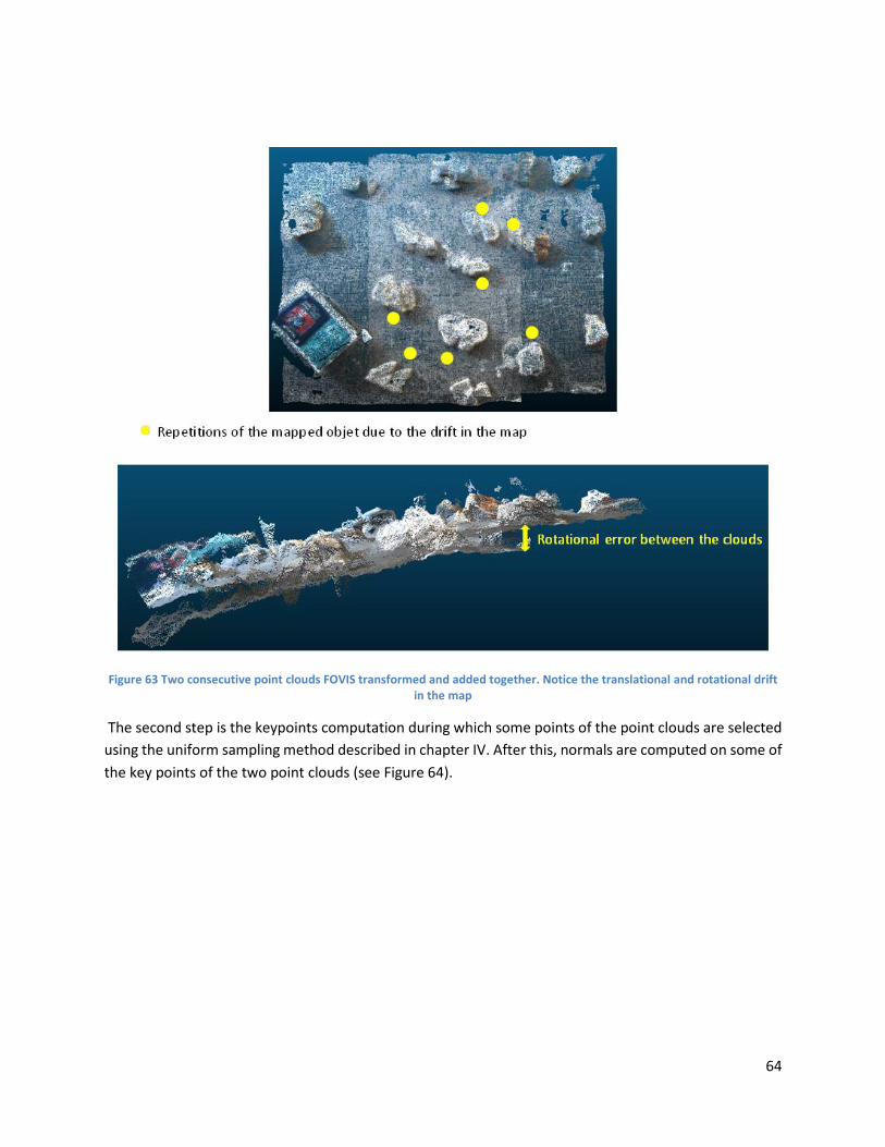
64
Figure 63 Two consecutive point clouds FOVIS transformed and added together. Notice the translational and rotational drift in the map
The second step is the keypoints computation during which some points of the point clouds are selected
using the uniform sampling method described in chapter IV. After this, normals are computed on some of
the key points of the two point clouds (see Figure 64).
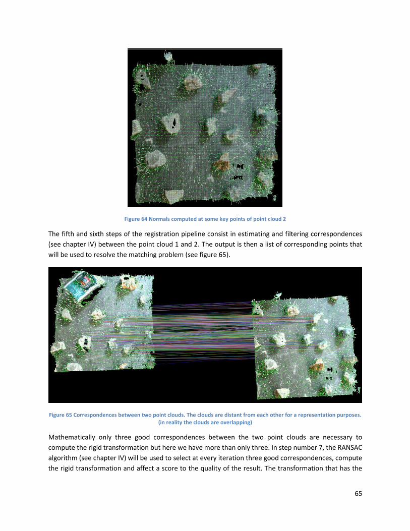
65
Figure 64 Normals computed at some key points of point cloud 2
The fifth and sixth steps of the registration pipeline consist in estimating and filtering correspondences
(see chapter IV) between the point cloud 1 and 2. The output is then a list of corresponding points that
will be used to resolve the matching problem (see figure 65).
Figure 65 Correspondences between two point clouds. The clouds are distant from each other for a representation purposes. (in reality the clouds are overlapping)
Mathematically only three good correspondences between the two point clouds are necessary to
compute the rigid transformation but here we have more than only three. In step number 7, the RANSAC
algorithm (see chapter IV) will be used to select at every iteration three good correspondences, compute
the rigid transformation and affect a score to the quality of the result. The transformation that has the
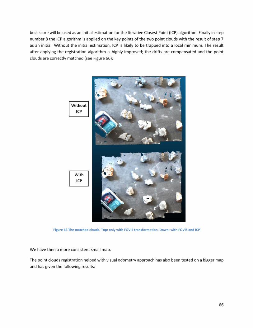
66
best score will be used as an initial estimation for the Iterative Closest Point (ICP) algorithm. Finally in step
number 8 the ICP algorithm is applied on the key points of the two point clouds with the result of step 7
as an initial. Without the initial estimation, ICP is likely to be trapped into a local minimum. The result
after applying the registration algorithm is highly improved; the drifts are compensated and the point
clouds are correctly matched (see Figure 66).
Figure 66 The matched clouds. Top: only with FOVIS transformation. Down: with FOVIS and ICP
We have then a more consistent small map.
The point clouds registration helped with visual odometry approach has also been tested on a bigger map
and has given the following results:
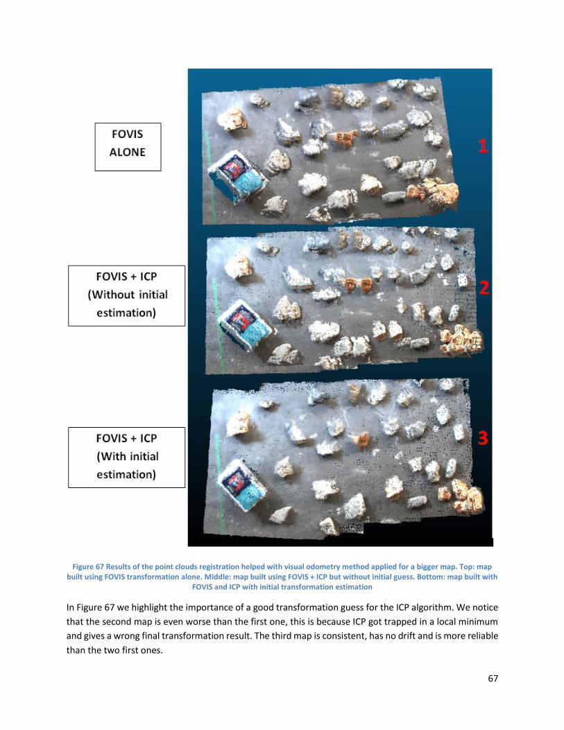
67
Figure 67 Results of the point clouds registration helped with visual odometry method applied for a bigger map. Top: map built using FOVIS transformation alone. Middle: map built using FOVIS + ICP but without initial guess. Bottom: map built with
FOVIS and ICP with initial transformation estimation
In Figure 67 we highlight the importance of a good transformation guess for the ICP algorithm. We notice
that the second map is even worse than the first one, this is because ICP got trapped in a local minimum
and gives a wrong final transformation result. The third map is consistent, has no drift and is more reliable
than the two first ones.
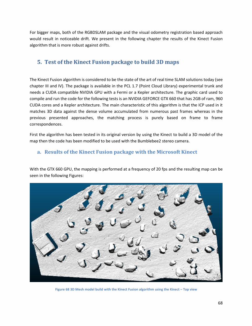
68
For bigger maps, both of the RGBDSLAM package and the visual odometry registration based approach
would result in noticeable drift. We present in the following chapter the results of the Kinect Fusion
algorithm that is more robust against drifts.
5. Test of the Kinect Fusion package to build 3D maps
The Kinect Fusion algorithm is considered to be the state of the art of real time SLAM solutions today (see
chapter III and IV). The package is available in the PCL 1.7 (Point Cloud Library) experimental trunk and
needs a CUDA compatible NVIDIA GPU with a Fermi or a Kepler architecture. The graphic card used to
compile and run the code for the following tests is an NVIDIA GEFORCE GTX 660 that has 2GB of ram, 960
CUDA cores and a Kepler architecture. The main characteristic of this algorithm is that the ICP used in it
matches 3D data against the dense volume accumulated from numerous past frames whereas in the
previous presented approaches, the matching process is purely based on frame to frame
correspondences.
First the algorithm has been tested in its original version by using the Kinect to build a 3D model of the
map then the code has been modified to be used with the Bumblebee2 stereo camera.
a. Results of the Kinect Fusion package with the Microsoft Kinect
With the GTX 660 GPU, the mapping is performed at a frequency of 20 fps and the resulting map can be
seen in the following Figures:
Figure 68 3D Mesh model build with the Kinect Fusion algorithm using the Kinect – Top view
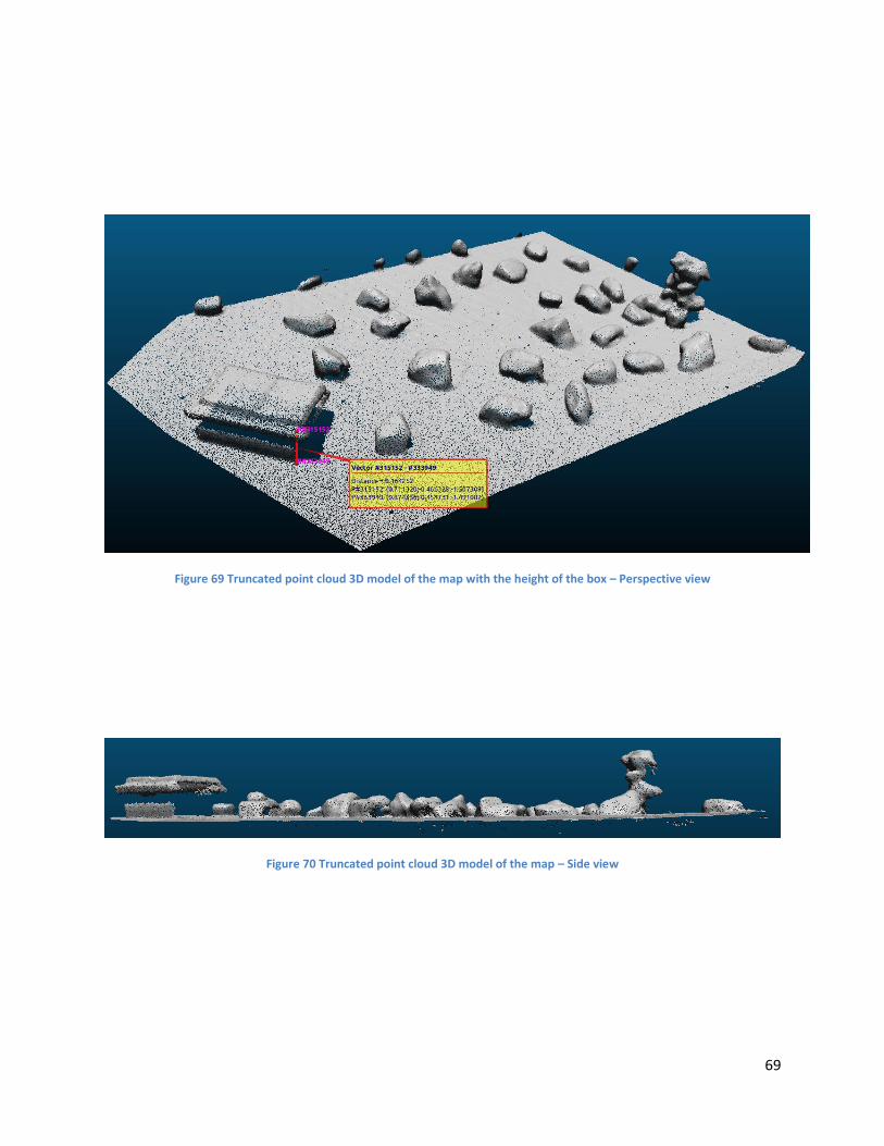
69
Figure 69 Truncated point cloud 3D model of the map with the height of the box – Perspective view
Figure 70 Truncated point cloud 3D model of the map – Side view
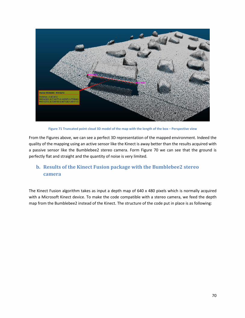
70
Figure 71 Truncated point cloud 3D model of the map with the length of the box – Perspective view
From the Figures above, we can see a perfect 3D representation of the mapped environment. Indeed the
quality of the mapping using an active sensor like the Kinect is away better than the results acquired with
a passive sensor like the Bumblebee2 stereo camera. Form Figure 70 we can see that the ground is
perfectly flat and straight and the quantity of noise is very limited.
b. Results of the Kinect Fusion package with the Bumblebee2 stereo
camera
The Kinect Fusion algorithm takes as input a depth map of 640 x 480 pixels which is normally acquired
with a Microsoft Kinect device. To make the code compatible with a stereo camera, we feed the depth
map from the Bumblebee2 instead of the Kinect. The structure of the code put in place is as following:
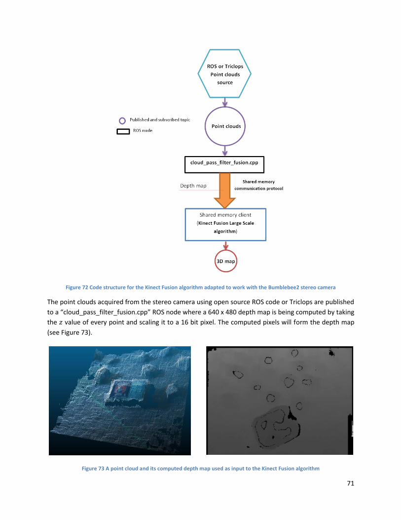
71
Figure 72 Code structure for the Kinect Fusion algorithm adapted to work with the Bumblebee2 stereo camera
The point clouds acquired from the stereo camera using open source ROS code or Triclops are published
to a “cloud_pass_filter_fusion.cpp” ROS node where a 640 x 480 depth map is being computed by taking
the 𝑧 value of every point and scaling it to a 16 bit pixel. The computed pixels will form the depth map
(see Figure 73).
Figure 73 A point cloud and its computed depth map used as input to the Kinect Fusion algorithm
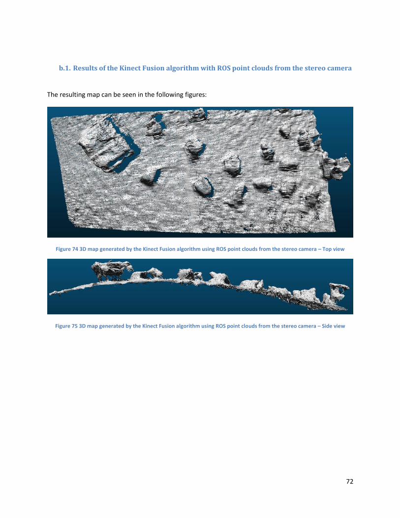
72
b.1. Results of the Kinect Fusion algorithm with ROS point clouds from the stereo camera
The resulting map can be seen in the following figures:
Figure 74 3D map generated by the Kinect Fusion algorithm using ROS point clouds from the stereo camera – Top view
Figure 75 3D map generated by the Kinect Fusion algorithm using ROS point clouds from the stereo camera – Side view
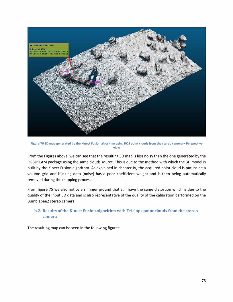
73
Figure 76 3D map generated by the Kinect Fusion algorithm using ROS point clouds from the stereo camera – Perspective view
From the Figures above, we can see that the resulting 3D map is less noisy than the one generated by the
RGBDSLAM package using the same clouds source. This is due to the method with which the 3D model is
built by the Kinect Fusion algorithm. As explained in chapter IV, the acquired point cloud is put inside a
volume grid and blinking data (noise) has a poor coefficient weight and is then being automatically
removed during the mapping process.
From figure 75 we also notice a slimmer ground that still have the same distortion which is due to the
quality of the input 3D data and is also representative of the quality of the calibration performed on the
Bumblebee2 stereo camera.
b.2. Results of the Kinect Fusion algorithm with Triclops point clouds from the stereo
camera
The resulting map can be seen in the following figures:
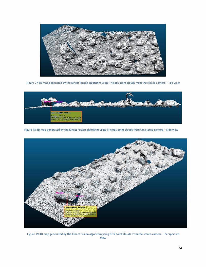
74
Figure 77 3D map generated by the Kinect Fusion algorithm using Triclops point clouds from the stereo camera – Top view
Figure 78 3D map generated by the Kinect Fusion algorithm using Triclops point clouds from the stereo camera – Side view
Figure 79 3D map generated by the Kinect Fusion algorithm using ROS point clouds from the stereo camera – Perspective view

75
Comparing to the map generated by ROS point clouds, from the figures above we can see that the ground
of the generated map is not curved but straight. However from the top view of the map we can also see
that the reconstruction of the 3D model is not as good as the one built using ROS point clouds. The
dimensions of the mapped objects in the scene are less respected than before.
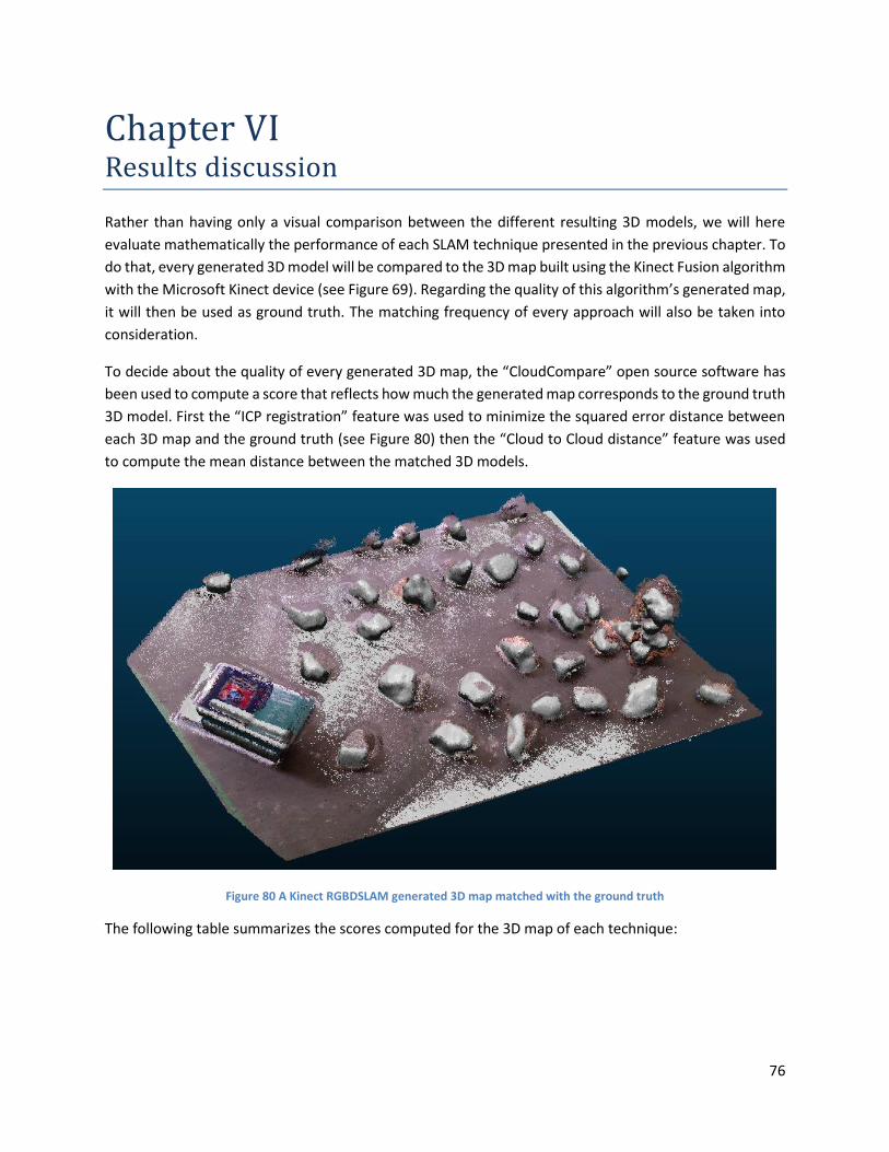
76
Chapter VI Results discussion
Rather than having only a visual comparison between the different resulting 3D models, we will here
evaluate mathematically the performance of each SLAM technique presented in the previous chapter. To
do that, every generated 3D model will be compared to the 3D map built using the Kinect Fusion algorithm
with the Microsoft Kinect device (see Figure 69). Regarding the quality of this algorithm’s generated map,
it will then be used as ground truth. The matching frequency of every approach will also be taken into
consideration.
To decide about the quality of every generated 3D map, the “CloudCompare” open source software has
been used to compute a score that reflects how much the generated map corresponds to the ground truth
3D model. First the “ICP registration” feature was used to minimize the squared error distance between
each 3D map and the ground truth (see Figure 80) then the “Cloud to Cloud distance” feature was used
to compute the mean distance between the matched 3D models.
Figure 80 A Kinect RGBDSLAM generated 3D map matched with the ground truth
The following table summarizes the scores computed for the 3D map of each technique:

77
Technique Mean distance (m)
RGBDSLAM with Kinect device 0.0102
Kinect Fusion with stereo camera
(Triclops 3D data) 0.014
RGBDSLAM with stereo camera (Triclops point clouds)
0.024
Kinect Fusion with stereo camera
(ROS 3D data) 0.040
FOVIS registration Pipeline (ROS point clouds)
0.066
RGBDSLAM with stereo camera (ROS point clouds)
0.093
Table 1 Mean distance between the 3D map of each approach and the ground truth 3D model
As we can see in the table above, the best result after the ground truth generated using the Microsoft
Kinect device and the Kinect Fusion algorithm is the 3D map built using this same device and the
RGBDSLAM package. This proves again the superiority of an active sensor over a passive one like the
Bumblebee2 stereo camera. Once we go into the results of the stereo camera, the best one is using the
Kinect Fusion algorithm with point clouds from the Triclops library. Using this approach, the model
updating frequency is around 10 fps; the ground is completely flat and straight but because of the method
(SAD algorithm) used to compute the 3D data, the shape of the mapped objects is not perfectly respected
(see Figure 77 and 79).
The second best approach using the stereo camera is the RGBDSLAM package with point clouds from the
Triclops library. This is not really a surprise when we know that the quality of the final map depends on
the quality of the 3D data and Triclops point clouds are not distorted comparing to the clouds extracted
using ROS open source code. In fourth position we have the 3D model generated using the Kinect Fusion
algorithm and a depth map computed from ROS point clouds. The 3D map shown in Figure 74, 75 and 76
is curved but the mapped objects are better defined than in Triclops maps. The updating model frequency
is about 3 fps.
In last position we have the map built using the visual odometry registration pipeline and then the
RGBDSLAM package both using ROS 3D data. The bad matching results with the ground truth are related
to the quality of the input point clouds and not to the used approaches. With a better quality point clouds,
the visual odometry based approach will perform better than the RGBDSLAM package.
78
Chapter VI Conclusion and future work
This dissertation provides an experimental analysis of different SLAM approaches to enable HyQ, a hydraulically actuated quadruped robot developed at the Istituto Italiano di Tecnologia in Genova (Italy) to be able to perform foothold and path planning. By using a Bumblebee2 stereo camera and a Microsoft Kinect as acquiring devices, we could during this project explore the limits of these two sensors for 3D mapping tasks. First, we started by testing the most promising SLAM state of the art algorithms; The RGBDSLAM and the Kinect Fusion open source packages were used to build 3D consistent maps with both of the available sensing devices then, a customized visual odometry based approach was designed and used for the same purpose. Foothold and path planning could be achieved using the generated maps. By evaluating the quality of the 3D map generated using each of these techniques, we have now a better appreciation about the most appropriate SLAM device and techniques suitable to be used on HyQ. Both of the stereo camera and the Kinect have their advantages and drawbacks. When the Kinect is more precise to evaluate 3D dimensions and more robust in non-textured environments, the stereo camera can extract 3D data from scenes that are exposed to sunlight which makes it more adapted for outdoor applications. A combination of these two devices would make the perfect 3D sensor. Today, the foothold and path planning strategy of HyQ relies on the precision of the extracted 3D data from the environment of the robot. Even With an active device like the Microsoft Kinect, the best precision for the evaluation of distances and dimensions is about +/- 2cm; with a passive sensor like a stereo camera, this precision is even worse. The approach consisting in computing the best position in which a foot of the robot can be placed then achieving it may not be the best solution when the precision of the sensing device is taken into consideration. This is why the foothold planning strategy should be changed to deal with this incertitude in the evaluation of the best foot position by using force sensors for example to be able not only to see the ground but also to feel it. Between all the SLAM algorithms tested during this project, the Kinect Fusion is today the most reliable and promising one. By running on GPUs, it can achieve real time localization and mapping at a maximum frequency of 30 fps and also produce high quality consistent maps. The quality of the depth map extracted from the stereo camera is less than the 3D data generated with the Kinect but other methods than SAD and Bloc matching like SGM (Semi-Global Matching [25]) should be tested to compute the disparity map. To increase the frequency with which 3D data are computed, a stereo camera of a higher frequency should be used and the computation process should be performed on an FPGA ship.
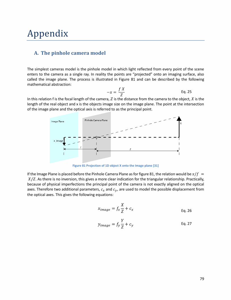
79
Appendix
A. The pinhole camera model
The simplest cameras model is the pinhole model in which light reflected from every point of the scene enters to the camera as a single ray. In reality the points are “projected” onto an imaging surface, also called the image plane. The process is illustrated in Figure 81 and can be described by the following mathematical abstraction:
−𝑥 = 𝑓 𝑋
𝑍 Eq. 25
In this relation f is the focal length of the camera, 𝑍 is the distance from the camera to the object, 𝑋 is the length of the real object and x is the objects image size on the image plane. The point at the intersection of the image plane and the optical axis is referred to as the principal point.
Figure 81 Projection of 1D object X onto the Image plane [31]
If the Image Plane is placed before the Pinhole Camera Plane as for figure 81, the relation would be 𝑥/𝑓 = 𝑋/𝑍. As there is no inversion, this gives a more clear indication for the triangular relationship. Practically, because of physical imperfections the principal point of the camera is not exactly aligned on the optical axes. Therefore two additional parameters, 𝑐𝑥 and 𝑐𝑦, are used to model the possible displacement from
the optical axes. This gives the following equations:
𝑥𝑖𝑚𝑎𝑔𝑒 = 𝑓𝑥
𝑋
𝑍+ 𝑐𝑥
Eq. 26
𝑦𝑖𝑚𝑎𝑔𝑒 = 𝑓𝑦𝑌
𝑍+ 𝑐𝑦 Eq. 27
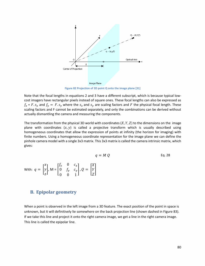
80
Figure 82 Projection of 3D point Q onto the image plane [31]
Note that the focal lengths in equations 2 and 3 have a different subscript, which is because typical low-cost imagers have rectangular pixels instead of square ones. These focal lengths can also be expressed as 𝑓𝑥 = 𝐹. 𝑠𝑥 and 𝑓𝑦 = 𝐹. 𝑠𝑦 where the 𝑠𝑥 and 𝑠𝑦 are scaling factors and 𝐹 the physical focal length. These
scaling factors and F cannot be estimated separately, and only the combinations can be derived without actually dismantling the camera and measuring the components. The transformation from the physical 3D world with coordinates (𝑋, 𝑌, 𝑍) to the dimensions on the image plane with coordinates (𝑥, 𝑦) is called a projective transform which is usually described using homogeneous coordinates that allow the expression of points at infinity (the horizon for imaging) with finite numbers. Using a homogeneous coordinate representation for the image plane we can define the pinhole camera model with a single 3x3 matrix. This 3x3 matrix is called the camera intrinsic matrix, which gives:
𝑞 = 𝑀 𝑄 Eq. 28
With: 𝑞 = [𝑥𝑦𝑧], M = [
𝑓𝑥 0 𝑐𝑥
0 𝑓𝑦 𝑐𝑦
0 0 1
] , 𝑄 = [𝑋𝑌𝑍]
B. Epipolar geometry
When a point is observed in the left image from a 3D feature. The exact position of the point in space is
unknown, but it will definitively lie somewhere on the back projection line (shown dashed in Figure 83).
If we take this line and project it onto the right camera image, we get a line in the right camera image.
This line is called the epipolar line.
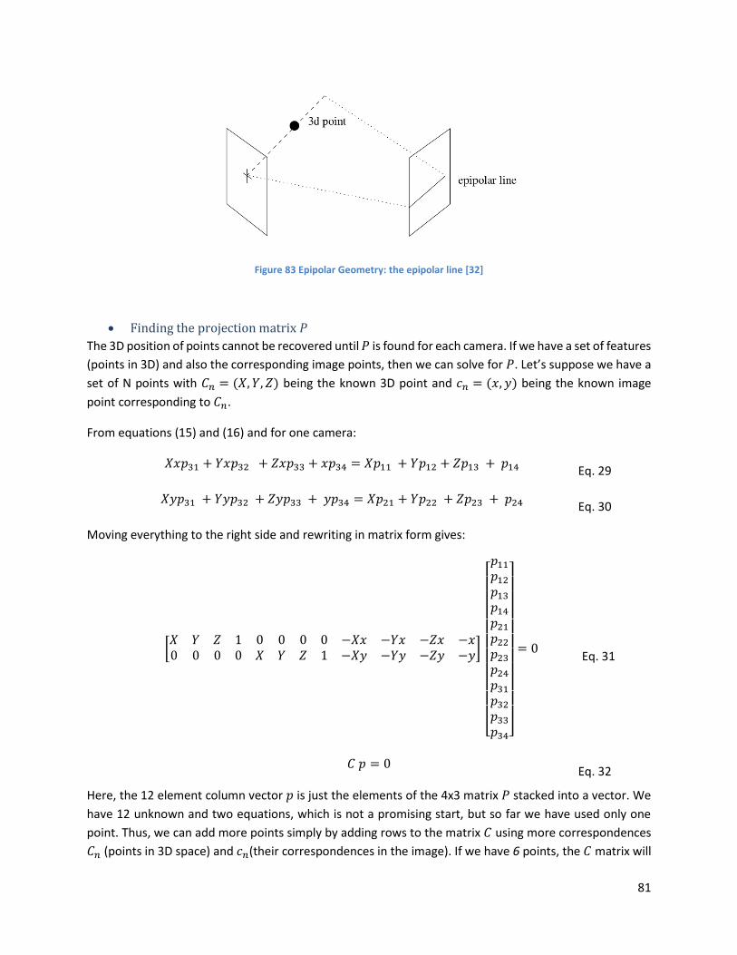
81
Figure 83 Epipolar Geometry: the epipolar line [32]
Finding the projection matrix 𝑃
The 3D position of points cannot be recovered until 𝑃 is found for each camera. If we have a set of features
(points in 3D) and also the corresponding image points, then we can solve for 𝑃. Let’s suppose we have a
set of N points with 𝐶𝑛 = (𝑋, 𝑌, 𝑍) being the known 3D point and 𝑐𝑛 = (𝑥, 𝑦) being the known image
point corresponding to 𝐶𝑛.
From equations (15) and (16) and for one camera:
𝑋𝑥𝑝31 + 𝑌𝑥𝑝32 + 𝑍𝑥𝑝33 + 𝑥𝑝34 = 𝑋𝑝11 + 𝑌𝑝12 + 𝑍𝑝13 + 𝑝14
Eq. 29
𝑋𝑦𝑝31 + 𝑌𝑦𝑝32 + 𝑍𝑦𝑝33 + 𝑦𝑝34 = 𝑋𝑝21 + 𝑌𝑝22 + 𝑍𝑝23 + 𝑝24
Eq. 30
Moving everything to the right side and rewriting in matrix form gives:
[𝑋 𝑌 𝑍 1 0 0 0 0 −𝑋𝑥 −𝑌𝑥 −𝑍𝑥 −𝑥0 0 0 0 𝑋 𝑌 𝑍 1 −𝑋𝑦 −𝑌𝑦 −𝑍𝑦 −𝑦
]
[ 𝑝11
𝑝12
𝑝13
𝑝14
𝑝21
𝑝22
𝑝23
𝑝24
𝑝31
𝑝32
𝑝33
𝑝34]
= 0
Eq. 31
𝐶 𝑝 = 0
Eq. 32
Here, the 12 element column vector 𝑝 is just the elements of the 4x3 matrix 𝑃 stacked into a vector. We
have 12 unknown and two equations, which is not a promising start, but so far we have used only one
point. Thus, we can add more points simply by adding rows to the matrix 𝐶 using more correspondences
𝐶𝑛 (points in 3D space) and 𝑐𝑛(their correspondences in the image). If we have 6 points, the 𝐶 matrix will
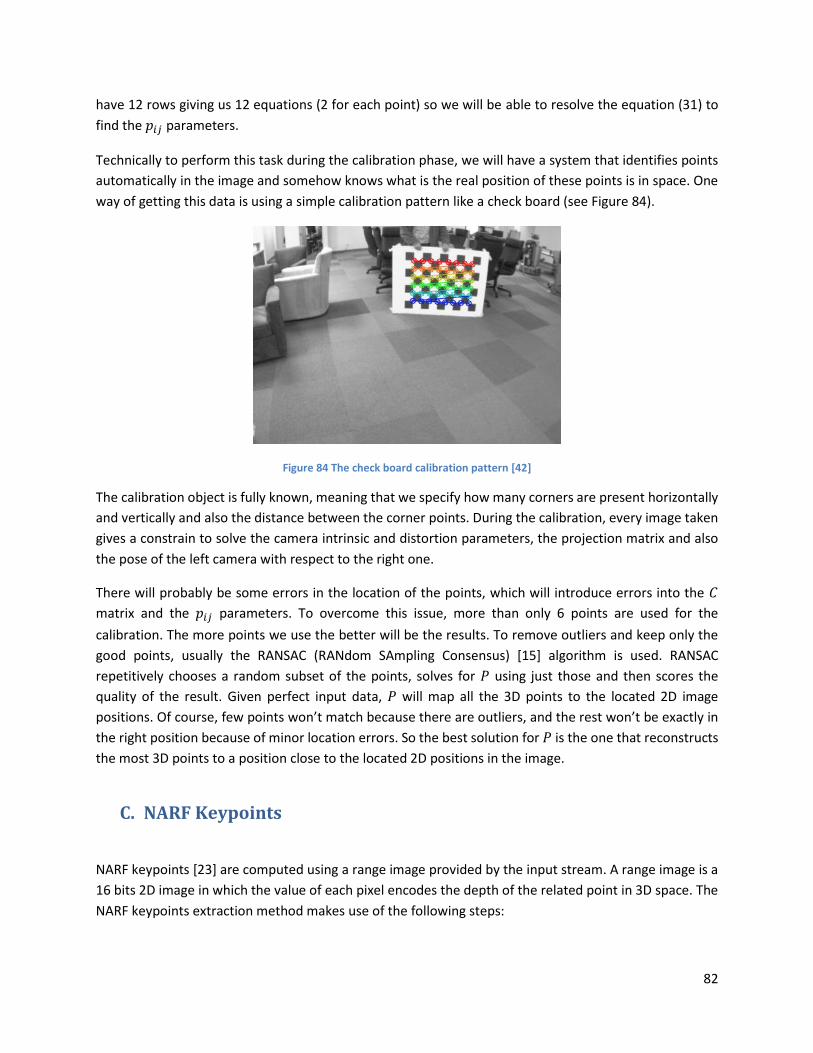
82
have 12 rows giving us 12 equations (2 for each point) so we will be able to resolve the equation (31) to
find the 𝑝𝑖𝑗 parameters.
Technically to perform this task during the calibration phase, we will have a system that identifies points
automatically in the image and somehow knows what is the real position of these points is in space. One
way of getting this data is using a simple calibration pattern like a check board (see Figure 84).
Figure 84 The check board calibration pattern [42]
The calibration object is fully known, meaning that we specify how many corners are present horizontally
and vertically and also the distance between the corner points. During the calibration, every image taken
gives a constrain to solve the camera intrinsic and distortion parameters, the projection matrix and also
the pose of the left camera with respect to the right one.
There will probably be some errors in the location of the points, which will introduce errors into the 𝐶
matrix and the 𝑝𝑖𝑗 parameters. To overcome this issue, more than only 6 points are used for the
calibration. The more points we use the better will be the results. To remove outliers and keep only the
good points, usually the RANSAC (RANdom SAmpling Consensus) [15] algorithm is used. RANSAC
repetitively chooses a random subset of the points, solves for 𝑃 using just those and then scores the
quality of the result. Given perfect input data, 𝑃 will map all the 3D points to the located 2D image
positions. Of course, few points won’t match because there are outliers, and the rest won’t be exactly in
the right position because of minor location errors. So the best solution for 𝑃 is the one that reconstructs
the most 3D points to a position close to the located 2D positions in the image.
C. NARF Keypoints
NARF keypoints [23] are computed using a range image provided by the input stream. A range image is a
16 bits 2D image in which the value of each pixel encodes the depth of the related point in 3D space. The
NARF keypoints extraction method makes use of the following steps:
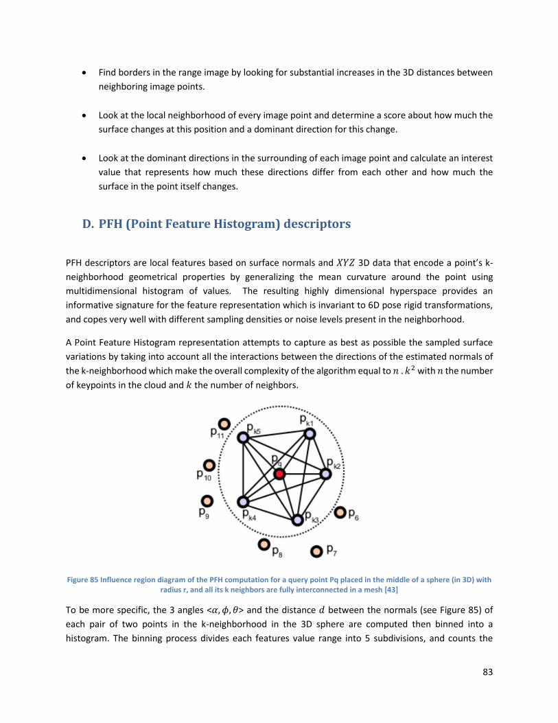
83
Find borders in the range image by looking for substantial increases in the 3D distances between
neighboring image points.
Look at the local neighborhood of every image point and determine a score about how much the
surface changes at this position and a dominant direction for this change.
Look at the dominant directions in the surrounding of each image point and calculate an interest
value that represents how much these directions differ from each other and how much the
surface in the point itself changes.
D. PFH (Point Feature Histogram) descriptors
PFH descriptors are local features based on surface normals and 𝑋𝑌𝑍 3D data that encode a point’s k-
neighborhood geometrical properties by generalizing the mean curvature around the point using
multidimensional histogram of values. The resulting highly dimensional hyperspace provides an
informative signature for the feature representation which is invariant to 6D pose rigid transformations,
and copes very well with different sampling densities or noise levels present in the neighborhood.
A Point Feature Histogram representation attempts to capture as best as possible the sampled surface
variations by taking into account all the interactions between the directions of the estimated normals of
the k-neighborhood which make the overall complexity of the algorithm equal to 𝑛 . 𝑘2 with 𝑛 the number
of keypoints in the cloud and 𝑘 the number of neighbors.
Figure 85 Influence region diagram of the PFH computation for a query point Pq placed in the middle of a sphere (in 3D) with radius r, and all its k neighbors are fully interconnected in a mesh [43]
To be more specific, the 3 angles <𝛼, 𝜙, 𝜃> and the distance 𝑑 between the normals (see Figure 85) of
each pair of two points in the k-neighborhood in the 3D sphere are computed then binned into a
histogram. The binning process divides each features value range into 5 subdivisions, and counts the
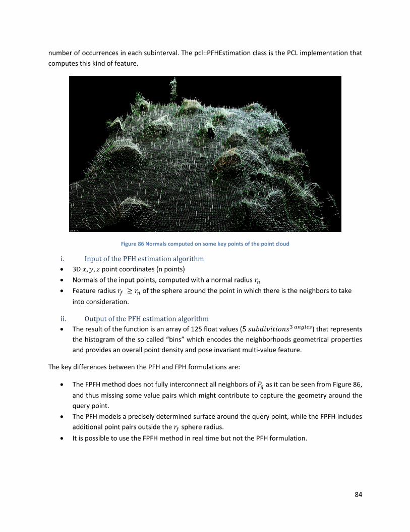
84
number of occurrences in each subinterval. The pcl::PFHEstimation class is the PCL implementation that
computes this kind of feature.
Figure 86 Normals computed on some key points of the point cloud
i. Input of the PFH estimation algorithm
3D 𝑥, 𝑦, 𝑧 point coordinates (n points)
Normals of the input points, computed with a normal radius 𝑟𝑛
Feature radius 𝑟𝑓 ≥ 𝑟𝑛 of the sphere around the point in which there is the neighbors to take
into consideration.
ii. Output of the PFH estimation algorithm
The result of the function is an array of 125 float values (5 𝑠𝑢𝑏𝑑𝑖𝑣𝑖𝑡𝑖𝑜𝑛𝑠3 𝑎𝑛𝑔𝑙𝑒𝑠) that represents
the histogram of the so called “bins” which encodes the neighborhoods geometrical properties
and provides an overall point density and pose invariant multi-value feature.
The key differences between the PFH and FPH formulations are:
The FPFH method does not fully interconnect all neighbors of 𝑃𝑞 as it can be seen from Figure 86,
and thus missing some value pairs which might contribute to capture the geometry around the
query point.
The PFH models a precisely determined surface around the query point, while the FPFH includes
additional point pairs outside the 𝑟𝑓 sphere radius.
It is possible to use the FPFH method in real time but not the PFH formulation.
85
iii. Input of the FPFH estimation algorithm
The input of this function is the same as the input of PFH features and the effectiveness of the
algorithm heavily depends on the chosen radius.
Usually we choose: 𝑟𝑛 = 0.8 𝑟𝑓 with 𝑟𝑛the radius used to compute the normals and 𝑟𝑓 the radius
of the 3D features sphere.
iv. Output of the FPFH estimation algorithm
The result of the function is an array of 33 float values that represents the FPFH histogram and
which is stored in the pcl::PFHSignature33 type.
E. Other registration algorithms
i. ICP Non Linear
This is an ICP variant that uses nonlinear Levenberg-Marquardt optimization backend. And can apply non
rigid transformation on the source point cloud to match it with the target.
ii. Normal Distribution Transform (NDT)
The NDT algorithm [24] is one of the final transformation estimation methods. It has become very popular
recently due to its faster convergence time and compact map representation. In this algorithm:
The target cloud space in discretized into 3D cells and a Gaussian probability density function for
each cell is computed.
For each point 𝑥𝑖 (20-30% are usually sufficient) of the source cloud, the initial transformation
𝑇 = [𝑅 𝑡0 1
] is applied (We can use RANSAC initial transformation or visual odometry).
We determine the corresponding normal distribution for each point of the target cloud that has
been transformed 𝑥𝑖′ into the frame of the source cloud.
The mapping according to 𝑇 could be considered optimal, if the sum evaluating the normal
distributions of all points 𝑥𝑖′ with parameters ∑ ,𝑖 𝑞𝑖 is a maximum. This sum is called the score of
𝑇. ∑ ,𝑖 𝑞𝑖 are the covariance matrix and the mean of the corresponding normal distribution to
point 𝑥𝑖′, looked up in the NDT of the source cloud.
Better values of the transformation matrix 𝑇 are computed by trying to optimize the score using
a Newton optimization method.
Another important advantage of NDT is that the memory storage is very less than ICP because NDT only
stores mean and covariance information while ICP has to store all the points for mapping. As a
consequence, NDT based methods are more beneficial for large scale and outdoor environments.
However, convergence time and the accuracy of the NDT based point clouds registration are highly
correlated with the cell size and there is no way to choose the optimal value for this parameter.
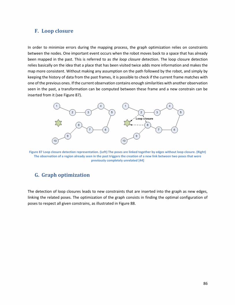
86
F. Loop closure
In order to minimize errors during the mapping process, the graph optimization relies on constraints
between the nodes. One important event occurs when the robot moves back to a space that has already
been mapped in the past. This is referred to as the loop closure detection. The loop closure detection
relies basically on the idea that a place that has been visited twice adds more information and makes the
map more consistent. Without making any assumption on the path followed by the robot, and simply by
keeping the history of data from the past frames, it is possible to check if the current frame matches with
one of the previous ones. If the current observation contains enough similarities with another observation
seen in the past, a transformation can be computed between these frame and a new constrain can be
inserted from it (see Figure 87).
Figure 87 Loop closure detection representation. (Left) The poses are linked together by edges without loop closure. (Right) The observation of a region already seen in the past triggers the creation of a new link between two poses that were
previously completely unrelated [44]
G. Graph optimization
The detection of loop closures leads to new constraints that are inserted into the graph as new edges,
linking the related poses. The optimization of the graph consists in finding the optimal configuration of
poses to respect all given constrains, as illustrated in Figure 88.
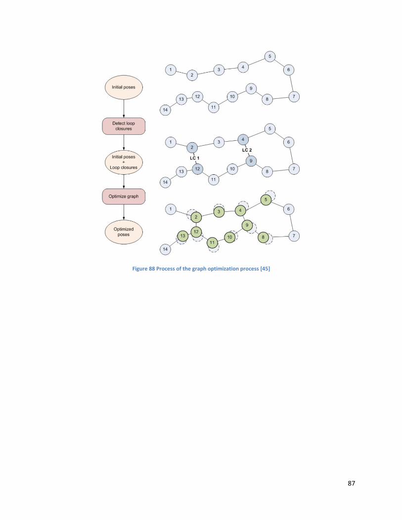
87
Figure 88 Process of the graph optimization process [45]
88
References
[1]: C. Semini, N. G. Tasagaraki, E. Guglielmino, M. Focchi, F. Canella and D. G. Caldwell, "Design of HyQ –
a hydraulically and electrically actuated quadruped robot". Journal of Systems and Control
Engineering, vol. 255, no. 6, pp. 831-849, 2011.
[2]: S. Bazeille, V. Barasuol, M. Focchi, I. Havoutis, M. Frigerio, J. Buchli, C. Semini, D. G. Caldwell, Vision
Enhanced Reactive Locomotion Control for Trotting on Rough Terrain. Proceedings of the 3rd
International Conference on Technologies for Practical Robot Applications (TePRA). Boston, 2013.
[3]: J. Zico Kolter, Youngjun Kim, Andrew Y. Ng, "Stereo vision and terrain modeling for quadruped
robots".
[4]: X. Shao, Y. Yang, Y. Zhang, and W. Wang,"Trajectory planning and posture adjustment of a
quadruped robot for obstacle striding", in Proc. ROBIO, 2011, pp.1924-1929.
[5]: Masahiro Tomono, "Robust 3D SLAM with a Stereo Camera Based on an Edge-Point ICP Algorithm".
[6]: http://wiki.ros.osuosl.org/fovis_ros
[7]:;Albert S. Huang, Abraham Bachrach, Peter Henry, Michael Krainin, Daniel
Maturana, Dieter Fox, Nicholas Roy, "Visual Odometry and Mapping for Autonomous
Flight Using an RGB-D Camera".
[8]: E. Rosten and T. Drummond, "Machine learning for high-speed corner detection". In European
Conference on Computer Vision, 2006.
[9]: Nikolas Engelhard and Felix Endres and Juergen Hess and Juergen Sturm and Wolfram Burgard,
"Real-time 3D visual SLAM with a hand-held RGB-D camera", Proc. of the RGB-D Workshop on 3D
Perception in Robotics at the European Robotics Forum, Vasteras, Sweden, 2011.
[10]: Felix Endres, Jürgen Sturm, Jürgen Hess, Daniel Cremers, Nikolas Engelhard, Wolfram Burgard, "An
Evaluation of the RGB-D SLAM System".
[11]: A. Segal D. Haehnel, S. Thrun, " Generalized ICP". In Proc. of Robotics: Science and Systems (RSS),
2009.
[12]: Giorgio Grisetti, Rainer Kuemmerle, Cyrill Stachniss, and Wolfram Burgard, "A Tutorial on Graph-
based SLAM". IEEE - Transactions on Intelligent Transportation Systems Magazine.
[13]: Rainer Kummerle, Giorgio Grisetti, Hauke Strasdat, Kurt Konolige, Wolfram Burgard, "g2o: A
General Framework for Graph Optimization".
89
[14]: Richard A. Newcombe, Shahram Izadi, Otmar Hilliges, David Molyneaux, David Kim, Andrew J.
Davison, Pushmeet Kohli, Jamie Shotton, Steve Hodges, and Andrew Fitzgibbon, "KinectFusion:
Real-Time Dense Surface Mapping and Tracking". October 2011 - IEEE ISMAR.
[15]: M. A. Fischler, R.C. Bolles,"Random Sample Consensus: A Paradigm for Model Fitting with
Applications to Image Analysis and Automated Cartography". ACM, June 1981, Communications of
the ACM, Vol. 24, pp. 381-395. ISSN 0001-0782.
[16]: Zhengyou ZHANG, "Iterative Point Matching for Registration of Free-form Curves" 1992.
[17]: G. Grisetti, R. Kümmerle, C. Stachniss, U. Frese, and C. Hertzberg, "Hierarchical optimization on
manifolds for online 2D and 3D mapping". In Proc. of the IEEE Intl. Conf. on Robotics and
Automation (ICRA), Anchorage, AK, USA, 2010.
[18]: G. Grisetti, C. Stachniss, S. Grzonka, and W. Burgard, "A Tree Parameterization for Efficiently
Computing Maximum Likelihood Maps using Gradient Descent". Atlanta, GA (USA), 2007.
[19]: http://pointclouds.org/
[20]: http://opencv.org/
[21]: www.ros.org/wiki/camera_calibration
[22]: http://wiki.ros.osuosl.org/camera_calibration
[23]: Bastian Steder, Radu Bogdan Rusu, Kurt Konolige, Wolfram Burgard, "NARF: 3D Range Image
Features for Object Recognition".
[24]: Cihan Ulaş, Hakan Temeltaş, "A 3D Scan Matching Method Based On Multi-Layered Normal
Distribution Transform".
[25]: Christian Banz, Sebastian Hesselbarth, Holger Flatt, Holger Blume, and Peter Pirsch, "Real-Time Stereo Vision System using Semi-Global Matching Disparity Estimation: Architecture and FPGA Implementation". [26]: http://www.iit.it/en/advr-labs/dynamic-legged-systems/hydraulically-actuated-quadruped- hyq.html [27]: http://gmv.cast.uark.edu/uncategorized/working-with-data-from-the-kinect/ [28]: http://gmv.cast.uark.edu/uncategorized/working-with-data-from-the-kinect/ [29]: http://www.ptgrey.com/products/triclopsSDK/ [30]: http://www.ptgrey.com/products/triclopsSDK/ [31]: Bas des Bouvie, "Master thesis".

90
[32]: Peter Hillman, "White Paperl : Camera Calibration and Stereo Vision". [33]: http://pointclouds.org/documentation/tutorials/registration_api.php#registration-api [34]: http://pointclouds.org/documentation/tutorials/registration_api.php#registration-api [35]: http://pointclouds.org/documentation/tutorials/fpfh_estimation.php [36]: http://vcg.isti.cnr.it/~corsini/publications.html [37]: Michele Pirovano, "Kinfu – an open source implementation of Kinect Fusion + case study: implementing a 3D scanner with PCL". [38]: Michele Pirovano, "Kinfu – an open source implementation of Kinect Fusion + case study: implementing a 3D scanner with PCL". [39]: Michele Pirovano, "Kinfu – an open source implementation of Kinect Fusion + case study: implementing a 3D scanner with PCL". [40]: http://pointclouds.org/documentation/tutorials/using_kinfu_large_scale.php [41]: Brian Curless, Marc Levoy, "A Volumetric Method for Building Complex Models from Range Images". [42]: http://wiki.ros.org/camera_calibration/Tutorials/StereoCalibration [43]: http://pointclouds.org/documentation/tutorials/pfh_estimation.php [44]: Virgile Hogman, "Building a 3D map from RGB-D sensors". [45]: Virgile Hogman, "Building a 3D map from RGB-D sensors".