CER

N-T

HES

IS-2

011-

097

03/0

6/20

11

THESEPour obtenir le grade de

DOCTEUR DE L’UNIVERSITE DE GRENOBLESpecialite : Physique/Physique subatomique & Astroparticules

Arrete ministerial :

Presentee par

Yaxian Mao

These dirigee par Pr. Christophe Furgetet codirigee par Pr. Daicui Zhou

preparee au sein du Laboratoire de Physique Subatomique et deCosmologie

Mesures des correlations γ-hadrondans les collisions p-p avecl’experience ALICE au LHC

These soutenue publiquement le 3 juin 2011,devant le jury compose de :.Pr Yugang Ma, president du jury, SINAP Shanghai (China)

Pr. Nu Xu, rapporteur, LBNL Berkeley (USA)

Pr. Xu Cai, examinateur, CCNU Wuhan (China)

Pr. Daicui Zhou, co-directeur de these, CCNU Wuhan (China)

Dr. Christelle Roy, rapporteur, IPHC Strasbourg (France)

Dr. Yves Schutz, examinateur, CERN Geneva (Suisse)

Dr. Serge Kox, examinateur, LPSC Grenoble (France)

Pr. Christophe Furget, directeur de these, LPSC Grenoble (France)

博士学位论文

LHC/ALICE中的双粒子关联测量

及介质效应的研究

论文作者: 毛 亚 显

指导教师: 周代翠 , Christophe Furget 教授

学科专业: 粒子物理与原子核物理

研究方向: 高能重离子碰撞实验

华中师范大学物理科学与技术学院

&

法国格勒诺布尔理工大学物理学院

2011年5月

Two Particle Correlations with Photon Triggers to Study

Hot QCD Medium in ALICE at LHC

A Dissertation Presented

BY

Yaxian Mao

to

The Doctoral School in partial fulfillment of the requirements

For the Degree of Doctor of Philosophy in Physics

of

Huazhong Normal University

and

Universite de Grenoble

Supervisors: Daicui Zhou, Christophe Furget, Yves Schutz

Academic Titles: Professor, Professor, Directeur de Recherches

May 2011

华中师范大学学位论文原创性声明和使用授权说明

原创性声明 本人郑重声明：所呈交的学位论文，是本人在导师指导下，独立进行研究工

作所取得的研究成果。除文中已经标明引用的内容外，本论文不包含任何其他个

人或集体已经发表或撰写过的研究成果。对本文的研究做出贡献的个人和集体，

均已在文中以明确方式标明。本声明的法律结果由本人承担。

作者签名： 日期： 年 月 日

学位论文版权使用授权书 本学位论文作者完全了解学校有关保留、使用学位论文的规定，即：学校有

权保留并向国家有关部门或机构送交论文的复印件和电子版，允许论文被查阅和

借阅。本人授权华中师范大学可以将本学位论文的全部或部分内容编入有关数据

库进行检索，可以采用影印、缩印或扫描等复制手段保存和汇编本学位论文。同

时授权中国科学技术信息研究所将本学位论文收录到《中国学位论文全文数据

库》，并通过网络向社会公众提供信息服务。

作者签名： 导师签名：

日期： 年 月 日 日期： 年 月 日

本人已经认真阅读“CALIS高校学位论文全文数据库发布章程”,同意将本人

的学位论文提交“CALIS高校学位论文全文数据库”中全文发布,并可按“章程”

中的规定享受相关权益。同意论文提交后滞后：□半年；□一年；□二年发布。

作者签名： 导师签名：

日期： 年 月 日 日期： 年 月 日

Resume

Depuis le demarrage du LHC (the Large Hadron Collider), le complexe accelerateurs du CERN

(Organisation Europeenne pour la Recherche Nucleaire) realise des collisions entre protons et entre

ions lourds a des energies jamais atteintes auparavant. ALICE (A Large Ion Collider Experiment),

l’une des experiences principales installees aupres du LHC, est dediee a l’etude de la matiere

nucleaire soumise a des conditions extremes de temperature et d’energie. L’objectif de l’experience

est de verifier l’existence d’un nouvel etat de la matiere, le QGP (Quark Gluon Plasma) et d’en

etudier les proprietes. Cette etude permettra d’explorer les aspects fondamentaux de l’interaction

forte, l’une de 4 interactions fondamentales de l’univers responsable de la cohesion de la matiere

ainsi que du vide qui lui est associe.

Pour mener a bien cet ambitieux programme scientifique, il est essentiel de choisir des observ-

ables pertinentes porteuses d’informations utiles pour la comprehension de la nature de la matiere

creee dans les collisions d’ions lourds aux energies ultra relativistes. Les informations extraites de

nombreuses observables permettront, a partir de modelisations des principes fondamentaux mis

en jeu, de concevoir une interpretation coherente des phenomenes observes. Apres une mise en

contexte de ce programme de recherche, les principaux aspects des collisions entre ions-lourds et

un bref etat des lieux des resultats obtenus a ce jour dans ce domaine sont presentes dans une

premiere partie de ce document.

Parmi les observables, la production de jets de hadrons est particulierement interessante. Les

jets resultent du processus de hadronisation de partons de grande impulsion transverse et apparais-

sent dans les detecteurs comme un faisceau collimate de hadrons. Les partons de grande impulsion

transverse quant a eux sont crees dans les interactions dures entre partons (de type 2 → 2) consti-

tuant les projectiles en collision. La mesure de la structure des jets, telle la distribution des hadrons

en fonction de la fraction d’energie du parton initial emporte par chacun d’eux, est l’observable

de predilection. En effet, dans les collisions entre ions lourds les partons de grande impulsion

transverse sont crees simultanement avec le milieu chaud et dense, objet de notre etude, et voient

leurs proprietes cinematiques modifiees lorsqu’ils traversent ce meme milieu. Lors du processus

de hadronisation, les hadrons gardent la memoire des modifications subies par le parton de facon

a modifier la structure du jet. Ces modifications sont revelees en comparant la structure du jet

lorsque le parton de grande impulsion transverse est produit dans des collisions proton–proton (on

parle de structure du jet dans le vide) avec la structure du jet lorsque le parton est produit dans

i

des collisions noyaux-noyaux (on parle de structure du jet dans le milieu). Reste un probleme

technique: alors que les jets sont aisement identifies et mesures dans les collisions proton–proton,

dans les collisions entre ions lourds, le fond sous jacent de hadrons dans l’etat final rend la mesure

des jets particulierement ardue. De plus il est impossible de connaıtre quelle etait l’impulsion du

parton lors de sa creation, seule l’impulsion finale apres interaction avec le milieu est mesurable,

ce qui complique l’interpretation de la mesure.

Pour pallier a ces problemes techniques, j’ai choisi d’etudier un type de processus dur particulier,

celui qui met un en jeu dans l’etat final un photon (il s’agit des photons directs par opposition

aux photons de decroissance des mesons neutres). L’impulsion (pγ) du photon, qui n’interagit

pas fortement avec le milieu, permet de calibrer l’impulsion du parton (pp = −pγ) tel qu’il a ete

cree dans le processus dur. Ainsi l’impulsion du photon nous donne l’impulsion du parton avant

interaction avec le milieu et la mesure de l’impulsion du jet nous donne l’impulsion du parton apres

interaction avec le milieu. De plus la mesure du photon permet de s’affranchir de l’identification

des jets, puisqu’il suffira de mesurer la correlation azimutale entre le photon et l’ensemble des

hadrons generes dans la collision. Cependant, les faibles section efficace du processus photon–jet

rend cette mesure relativement difficile. Les elements necessaires a l’etude des correlations et les

equipements experimentaux sont decrits dans la deuxieme partie de ce document.

La strategie d’un telle etude commence par la validation de la mesure, qui consiste a etudier a

l’aide de simulations Monte Carlo d’une part quelle est la sensisibilite de l’observable choisie pour

reveler le phenomene recherche et d’en quantifier les effets et d’autre part si le signal est mesurable

avec les systemes de detection de l’experience. Cette etude est decrite dans la troisieme partie

de ce document. Je decris les performances attendues pour l’etude des correlations azimutales

entre photons et hadrons charges mesures avec l’experience ALICE. Deux quantite sont extraites

de cette etude a partir des simulations de collisions proton–proton: la valeur moyenne du moment

transverse total au niveau partonique (< kT >) et la distribution de la fraction (xE) d’energie du

jet emportee par les hadrons produits en coincidence avec un photon (fonction de correlation). Les

memes quantites sont extraites a partir de simulations de collisions d’ions lourds et les modifications

subies par le mileu sont analysees: la distribution des valeurs de kT est elargie d’une quantite qui

peut etre directement reliee au coefficient de transport du milieu et la fonction de correlation est

modifiee de facon a supprimer les hadrons de grande valeur de xE (jet quenching) et a augmenter

le nombre de hadrons a petites valeurs de xE (production radiative de gluons). L’amplitude de

cette derniere modification est proportionnelle au coefficient de transport et a la distance parcourue

ii

dans le milieu. Je termine cette partie consacree aux simulations (et a laquelle j’ai consacre la plus

grande partie de mon temps) par une etude detaillee qui devrait permettre, theoriquement, de

realiser une etude tomographique du milieu forme dans les collisions d’ions lourds. La procedure

repose sur une idee suggeree par X.N Wang et consiste a localiser le processus dur dans le milieu

(grande valeur de xE pour une production du photon et du jet en surface et petite valeur de xE

pour une production profondeur) et ainsi sonder le milieu de la partie la plus dense jusqu’a la

partie la moins dense en surface. Je conclus que la mesure releve du defi experimental !

La quatrieme partie de ce document est consacree a l’analyse des donnees collectees en 2010

pour des collisions proton–proton a une energie dans le centre de masse de√s = 7 TeV. Pour

cette premiere longue campagne de mesure au LHC, l’experience ALICE n’etait pas encore dans

les conditions optimales pour la mesure des correlations photon–jet. En effet, les calorimetres

electromagnetiques n’offraient qu’une acceptance reduite et l’experience ne disposait pas encore

d’un declenchement selectif pour enrichir les donnees enregistrees en evenements photon – jet. Il

en a resulte un nombre d’evenements insuffisant pour une etude concluante. En particulier la statis-

tique disponible a limite l’etude au domaine d’energie inferieur a 10 GeV, domaine tres defavorable

pour l’identification des photons directs du fait de leur rarete dans le bruit de fond predominant des

photons de decroissance. S’est ajoute a ce handicap, le peu de temps disponible pour completer

une analyse tres delicate. Des resultats preliminaires sont presentes pour les correlations entre

photons inclusifs et hadrons charges et photons isoles et hadrons charges: les structures 2 jets et

mono jet sont bien identifiees, une valeur de ⟨kT ⟩ a ete determinee et les distributions en xE ont

ete construites.

Cette premiere analyse est un premier pas vers une analyse complete de l’observable photon

– jet a partir des donnees plus riches (calorimetre complet, et declenchement selectif) qui seront

collectees en 2011 pour les collisions proton–proton et Pb–Pb.

Dans la derniere partie de ce document, je decris ma contribution au controle qualite des

calorimetres electromagnetiques pendant la prise de donnees.

iii

摘摘摘 要要要

在现代自然科学研究中，一项极具挑战性的研究目标是在最小尺度上探索物质的构成。 一种

描述基本粒子与作用力的理论–标准模型，假定物质的基本结构是由夸克和轻子通过规范粒子的相

互作用而组成的，认为组成物质结构的最小单元是夸克（u, d；c, s; t, b)、轻子(e, νe; µ, νµ; τ ,

ντ )，以及传递相互作用力的媒介子，即玻色子(W±和Z0)、胶子(g)和光子(γ)。基本作用力根据

规范粒子的不同划分为电磁相互作用，弱相互作用和强相互作用。 正是这些基本粒子和相互作用

力构建了亚原子世界。然而，这个理论并不十分完备，因为它依然无法解释某些基本的问题，比

如：基本粒子质量的起源、宇宙的真实真空、以及宇宙中物质远比反物质多的问题...。

人们普遍认为，强相互作用由量子色动力学(Quantum Chromodynamics, QCD)描述。量子

色动力学的重要特性是渐近自由性质，即随着相互作用的动量标度的变大，强相互作用的耦合

常数(αs)趋于零。 在渐近自由状态下，部分子间的相互作用是微扰的。 QCD预言，在相对论

重离子碰撞下，部分子可以达到这种状态，形成夸克胶子等离子体(QGP)。 美国布鲁海文国家

实验室(BNL)利用相对论重离子对撞机(RHIC)来寻找这种新的物质形态。 位于欧洲核子研究中

心(CERN)的大型强子对撞机(LHC)于2009年正式启动运行，实现了前所未有的TeV能区的高能重

离子碰撞，LHC上的大型重离子对撞机实验(ALICE)合作组专门致力于高温高能量密度的极端条

件下强相互作用的基本性质及其物理真空的研究。

基于量子色动力学(QCD)，利用格点计算方法，人们成功地预言了夸克从禁闭的普通强子

物质中退禁闭到QGP相的临界温度。 实验上，该临界温度首先在CERN√sNN = 17.2 GeV下

的SPS重离子碰撞实验中达到。进而在美国布鲁海文国家实验室(BNL)运行的质心能量√sNN =

60 − 200 GeV下的相对论重离子对撞机(RHIC)实验中，证实了从强子物质到夸克物质的相变能

在高温高密条件下发生。 位于欧洲核子研究中心(CERN)的大型强子对撞机LHC实现了质心能

量√sNN = 2.76 TeV下的铅-铅碰撞，该能量高于RHIC碰撞能量的∼14倍，使其在更高温度下形

成的热密QCD物质持续更长时间。 另外，LHC能区的重离子碰撞诱导产生的硬散射过程更加丰

富，这些敏锐的硬探针将提供TeV能区下细致研究QGP性质的机会。比如，在核–核中心碰撞中高

横动量强子产额的压低和背对背喷注之间的关联消失。 ALICE探测器就是为了更加系统的测量

核–核碰撞中产生的末态粒子，由此反映碰撞初期出现的热密物质相的性质。特别是，通过测量

相空间中强子谱的改变，可以研究硬散射部分子在穿越密度物质时的能量损失效应及碎裂函数性

质。 在重离子碰撞中，由于喷注淬火效应，硬散射过程产生的大横动量部分子穿越密度物质时会

因为多重散射而损失能量，导致高横动量的强子产额减少，低动量强子数目会增多，引起强子谱

在相空间中的重新分布。 因此，通过测量核环境下部分子的碎裂函数(FF)，即测量部分子喷注

v

产生的强子携带喷注动量份额z = pTh/Ejet

T 的分布函数，将真空中的碎裂函数(质子–质子碰撞或

核–核边沿碰撞中的碎裂函数)与被介质修正后的碎裂函数(核–核中心碰撞下的碎裂函数)分布进行

比较，就可以推断核–核碰撞中的密度物质及其性质。

本论文主要目的是利用光子–强子的关联测量来研究部分子的碎裂函数，即通过测量高能直接

光子与散射到光子背面强子之间的关联来研究喷注的碎裂函数。 高能直接光子在碰撞初期的硬

散射过程中直接产生，主要来自康普顿散射(qg → γq)和湮灭过程(qq → γg)。 由于光子的平均自

由程很大，在碰撞区域内与其他粒子只有电磁相互作用，因此光子携带了它们初始产生时刻的信

息。 而与该光子产生于同一硬散射过程的部分子会碎裂为末态强子，通过对强子的测量，就能获

得部分子在穿越密度物质后的信息。 将产生于同一事件中的光子和强子关联，我们就能得到密度

物质作用于部分子喷注上的效应。 我选择了高横动量的喷注作为对介质作断层扫描的探针：观测

量是高动量直接光子与在其相反方向上的强子的关联。在这一测量中，直接光子标记了同样作为

在初始碰撞中硬过程产生的部分子的初始能量，而强子，作为该部分子碎裂出的末态粒子，描述

了穿越介质的部分子的属性。 通过比较这两种碰撞系统下的光子–强子关联测量，我们可以得到

介质效应对末态运动学和喷注碎裂的修正。 然而，在碰撞中来自强子和中性介子(主要是π0和η)的

衰变光子是直接光子信号提取过程中的主要背景，因此光子信号的提取在本工作中显得至关重

要。

本论文着重开展如下两方面的工作。第一部分是关于光子测量，鉴别效率以及直接光子的提取

研究，估计来自衰变光子误判引起的系统误差， 并研究利用光子－强子关联及强子－强子关联方

法在ALICE实验中测量的可行性。 利用Monte-Carlo模拟数据，我们研究了ALICE实验中电磁量

能器(PHOS和EMCAL)在探测和鉴别光子时的性能表现。 由于有限的接受度，在碰撞过程中产生

的某些光子落在探测器边缘使得沉积在晶体上的能量不能获得完整的重建，这些光子将不能被正

确探测到。同时，光子在穿越位于量能器之前的其它探测器时与探测器物质发生相互作用而使光

子转换成正负电子对(γ → e+e−)。 模拟结果表明，不同探测器对光子探测效率的影响程度不一

样。例如，光子在时间投影室(TPC)和内部径迹系统(ITS)的转换几率约为10%，而在跃迁辐射探

测器(TRD)和时间飞行探测器(TOF)中的转换几率接近20%。 本文首先报告了在LHC能区中的质

子–质子和铅–铅碰撞过程中利用ALICE实验探测器通过直接光子–强子关联测量的方法研究喷注碎

裂函数和介质效应的可行性。 光子–强子关联测量在质子–质子碰撞中是必须的，因为该测量能够

为我们提供有关重离子碰撞下的关联测量的基线参考。 我研究了介质可能引起的一系列效应。对

于第一个相关的参数就是kT，即部分子层次上的有效横动量。 基于国际上已有的实验数据测量

值，我们将其延伸外推到LHC能区，从而预测LHC能区上的kT值。 本文估计了光子-强子关联测

量对于高温热密物质的敏感度及光子–强子关联函数的重新分布，从而提取热密物质的性质。 另

外，我还通过光子-喷注产生机制研究了喷注在穿越热密物质里产生的过程进行层析结构分析。

vi

该工作的第二部分，主要聚焦在LHC于2010年首次运行的质子-质子碰撞下质心能量√s = 7

TeV下的ALICE数据分析工作。 该工作从真实数据入手，采用我们在前面已经建立的可行性研

究方法，旨在测量质子-质子碰撞下的喷注碎裂函数，为铅-铅数据分析提供基线测量。 鉴于当

前ALICE有限的统计量和不完整的电磁量能器接收度，本工作的测量集中在小于20GeV/c的横动

量区域进行，由于在该横动量范围内大量来自衰变光子的背景贡献使得该测量在此区间特别具有

难度和挑战性。 由于当前探测器的校准工作依然在进行之中，我无法利用粒子鉴别的方法来区

分光子和π0作为触发粒子，而是直接利用在量能器上形成的电磁簇射团簇和利用不变质量方法重

建出的π0作为触发粒子进行两粒子关联。而后对触发粒子进行孤立截断的判选，从而提高直接瞬

时光子数据样本的机率。 双喷注结构与单光子/π0–喷注的运动学结构通过以上研究观测到。同

时，利用孤立光子–强子的方位角关联我们提取了部分子层次上的横动量kT值，该测量值与我之

前利用蒙特卡罗数据预言的kT结果一致，更进一步，我尝试了构建 20GeV以下的喷注在质子-质

子√s = 7TeV下的碎裂函数。 但展开实际数据分析的时间之短让我无法对该项研究进入到更深的

地步。

对于在2010年底LHC首次运行铅-铅碰撞下的质心能量√sNN = 2.76 TeV下的数据，我做了同

样的数据分析，但时间之仓促不允许我将该数据分析部分纳入该论文之中。 鉴于电磁量能器覆盖

范围的增加以及高横动量光子触发判选能力的实现，2011，2012年LHC运行获取的数据无疑会提

供更大的统计量，让该项研究的有效测量范围达到更高，从而获得更多有趣的物理现象和物理结

果。

最后， 为了论文的完整性，对于我在博士期间对于整个ALICE实验合作组中的主要贡献简要

概括如下：

• 利用光子–强子关联测量的可行性研究。该项可行性研究是本人硕士论文的延续，我在硕士

论文研究出的测量和分析方法基础之上，发展和延伸了该观测量对于核核碰撞下形成的热密

物质的敏感度。通过各项细致研究，总结出利用光子–强子关联方法测量介质效应是敏感而

且有效的，我们甚至可以通过该关联测量提取部分子层次上的运动学量kT， 并对形成的热

密物质介质本身进行层析扫描。 这些研究结果均在ALICE国际合作组中广泛讨论并得到认

同，并在大型国际学术会议上报告。

• EMCal探测器校准工作。为了获得一个较好的能量和位置分辨率，我参加了在格勒诺布尔利

用宇宙射线和在CERN利用高能电子束流对EMCal探测器进行校准的工作。

• EMCal在线数据质量监控(DQM)。 为了检测在数据获取过程中的探测器质量，自LHC准

备运行以来，我担任了EMCal探测器数据质量检测的任务，并开发和提供了数据检测的软

件工具并且保持维护和更新。还开发了数据监控的算法和质量检测的标准，并将其补充

vii

到ALICE数据获取系统的在线数据监测框架之下。

• 电磁量能器EMCal和PHOS的离线数据监测和质量认证(QA)。我负责运行每周从LHC上取

得的ALICE数据，对量能器的离线数据质量检验，并将质量检验结果在每周ALICE数据质

量检验和数据分析会议上报告，为实验合作组的量能器数据物理分析提供有效数据库。

• 中性介子和光子–强子关联的数据分析工作。自2009年LHC开始采集数据以来，我一直致力

于探测器的校准和实验数据的分析工作(数据分析现在依然进行之中)。其中包括π0的重建，

以及光子–强子的关联测量。我被相应的ALICE物理工作组推选为光子/π0-强子关联测量的

数据分析协调人，每周召集两次课题讨论会，并定期在ALICE合作组内报告工作进展。

关关关键键键词词词：：： 大型重离子对撞实验(ALICE)，夸克胶子等离子体(QGP)，喷注，瞬时光子，孤立

截断，关联测量，碎裂函数，部分子kT , 层析结构

viii

Abstract

With the advent of the Large Hadron Collider (LHC)at the end of 2009, the new accelerator

at CERN collides protons and heavy-ions at unprecedented high energies. ALICE , one of the

major experiment installed at LHC, is dedicated to the study of nuclear matter under extreme

conditions of energy density with the opportunity of creating a partonic medium called the Quark-

Gluon-Plasma (QGP). This new experimental facility opens new avenues for the understanding of

fundamental properties of the strong interaction and its vacuum.

To reach the objectives of this scientific program, it is required to select a set of appropriate

probes carrying relevant information on the properties of the medium created in ultra-relativistic

heavy-ion collisions. Based on the information delivered by all the observables and guided by

modelization of the fundamental principles in action, a coherent picture will emerge to interpret

the observed phenomena. In the first part of the present document I describe the context of the

scientific program, the general concepts involved in heavy-ion collisions at ultra relativistic energies,

and the main results obtained so far in the field.

Among the observables of interest, the production of hadrons jets is particularly attractive. Jets

are the result of the hadronisation process of high transverse momentum partons and are observed

in the detectors as a beam of collimated hadrons. High transverse momentum partons are created

by hard scattering of partons (2 → 2 type of processes) constituting the colliding projectiles.

The jet structure measured, for example as the distribution of the factional jet energy carried by

the individual hadrons inside the jet, is the observable of choice. In heavy ion collisions, high

transverse momentum partons are created concurrently with the hot and dense medium of interest

and their kinematical properties are modified as they traverse the medium. This modification,

imprinted in the jet structure, is observed by comparing the jet structure measured in heavy-ion

collisions (in medium jet structure) with the jet structure measured in proton-proton collisions

(vacuum jet structure). Such a measurement faces however a technical difficulty: whereas jets

can be easily identified and measured in proton-proton collisions, in heavy-ion collisions the large

hadronic background from the underlying event (the underlying event is everything except the

two hard scattered jets and is generated by the beams particle break up and by initial and final

state radiation) makes the jet identification measurement quite challenging. In addition the initial

momentum of the hard scattered parton is unknown since only the final jet momentum can be

measured i.e. the momentum of the parton as it emerges from the medium. This complicates the

ix

interpretation of the measurement.

To overcome these difficulties, I have selected a particular 2 → 2 process which creates a

direct photon (direct photon at variance with decay photon) in the final state together with a

high transverse momentum parton. The momentum of the photon (pγ), since it does not interact

strongly with the medium, calibrates the momentum of the parton (pp = −pγ). Therefore the

photon momentum is a measure of the parton momentum when created and the jet momentum

the momentum of the parton after it has traversed the medium. In addition since the photon

momentum (energy and direction) defines also the jet momentum, jet reconstruction algorithms

are not required anymore. Instead of studying photon – jet correlations (where the jet is fully

reconstructed), it is sufficient to study photon – hadron correlations from all the hadrons in the

event. However, the relatively small cross section for the production of these particular hard

scattering processes makes the measurement quite challenging. An introduction to 2 particle

correlations is given in the second part of this document followed by a description of the ALICE

detection systems used for this measurement.

The strategy I have followed for this study starts with a validation of the measurement. It

consists first in studying with the help of Monte Carlo simulations the accuracy of the selected ob-

servable in revealing and quantifying the phenomenon under study. Second, it consists in verifying

the ability to measure the observable and its robustness with the detectors setup of the ALICE

experiment. The validation procedure and results are discussed in the third part of this document.

I have particularly studied the possibility to extract two quantities from the 2 particle azimuthal

correlation measured in proton-proton collisions: (i) the average total transverse momentum (⟨kT ⟩)

generated at the partonic level by the Fermi motion and initial and final state radiation, and (ii)

the per trigger yield of jet hadrons as a function of the fractional jet energy (xE) they each carry

(correlation function). The same quantities have been studied from simulated heavy-ion collisions

with the objective to analyze the effects due to the presence of highly dense color medium. The

distribution of kT values becomes broader in a way that can be directly related to the transport

properties of the medium and the correlation function is modified so that the number of high xE

hadrons are suppressed (jet quenching) and the number of low xE hadrons is increased (radiative

gluon production) with an amplitude proportional to the transport coefficient and to distance tra-

versed inside the medium. To finish this part of the document dedicated to Monte Carlo studies

(on which I have spent most of my time as a PhD student) with another detailed study the possi-

bility to exploit the photon – jet observable as a tomographic tool (following a suggestion by X.N.

x

Wang). The idea is to localize the hard scattering well inside the medium (by selecting hadrons

with low xE values) or at the surface of the medium (by selecting hadrons with large xE values).

One would therefore choose the distance in the medium through which the hard scattered parton

travels and probe the medium from its densest part (center) to its less dense part (surface). I

found that such a measurement will be quite challenging.

In the fourth part of the present document, I address the analysis of the data collected in 2010

for proton-proton collisions at√s = 7 TeV. During this first long data taking period at LHC,

the ALICE detection system was not yet complete. In particular, the incomplete coverage of the

electromagnetic calorimeters and the absence of a selective photon trigger was a severe handicap

for the photon – jet measurement. The resulting event statistics available for the measurement of

this observable was limited to the photon energy range below 10 GeV. This low energy domain is

not well suited for the identification of direct photons because of their scarcity in the overwhelming

background generated by decay photons. On top of that, the time between the availability of the

data and the scheduled time for my defense was too short to perform an in-depth analysis. Most

of the results presented from this analysis in the present document must therefore be considered

as very preliminary, but the key features are there. The results concern the 2 jet and mono jet

structure observed in the photon – jet azimuthal correlation, the measured value of ⟨kT ⟩ and the

xE distributions.

This very preliminary analysis of the first data collected at LHC and presented in this document

is the first only toward a comprehensive study of the photon – jet observable. Since the writing of

the document, the analysis has progressed and provided a few results which were considered ripe

by the collaboration to be presented at the Quark Matter conference in May 2011. The data which

will be collected in 2011 in proton-proton and Pb-Pb collisions will be much richer in photon – jet

events thanks to the complete coverage of the ALICE electromagnetic calorimeter and thanks to

a very high energy photon trigger provided by the calorimeter as well.

For completeness, I finish the present document with the description of my contribution, as

being the main person in charge, to the quality assurance and monitoring tasks for the two ALICE

electromagnetic calorimeters during data taking.

Keywords: ALICE, Quark-Gluon Plasma (QGP), jet, prompt photon, isolation cut, kT ,

fragmentation function, tomorgraphy

xi

Acknowledgements

The writing of this thesis would not have been possible without the help and encouragement

of many professors and teachers, friends and relatives. It is my great pleasure to thank all these

people, though it is difficult to express my gratitude to all of them individually.

First of all, I am deeply indebted to my advisors Prof. SCHUTZ Yves, Prof. ZHOU Daicui and

Prof. FURGET Christophe, who led me to the fascinating world of high energy particle physics. I

feel fortunate to work under their kind guidances and supports and I will never forget the exciting

moments we have enjoyed in our discussions. All of my supervisors have spent a significant effort

and time in teaching me how to be a good scientist. The remarkable scope of insight with clarity,

profound knowledge with breadth, together with the careful judgement, vitality, precision and

enthusiasm of Prof. SCHUTZ, inspire me to work harder to live up to their expectation.

I would like to thank Andreas Morsch, Terry Awes, Gustavo Conesa Balbastre, David Silvermyr,

Yuri. V. Kharlov, and Hisayuki Torii for their advices and all their work that made possible I could

advance and obtain my results. Also I would like to thank Prof. WANG Xin-Nian and Francois

Arleo for their bright theoretical ideas and useful discussions.

I would like also to thank Prof. XU Nu, Prof. CAI Xu, Prof. YANG Yadong, Prof. WANG

Enke, Prof. LIU Feng, Prof. YANG Chunbin, Prof. LIU Fuming, Prof. HOU Defu, Prof. WU

Yuanfang, Prof. ZHANG Beiwei and associate Prof. ZHOU Daimei for their teaching and helps

during my studies. In particular, I would like to thank associate Prof. YIN Zhongbao and associate

Prof. WANG Yaping for their discussions in our work group.

I am grateful to all colleagues of ALICE collaboration especially for Physics Work Group 4

(PWG4), PHOS and EMCal group collaboration like Jan Rak, Peter Jacobs, Mateusz Andrzej

Ploskon, Christian Klei-Boesing and Francesco Blanco for their instructive suggestions and enthu-

siastic discussions.

For sure I would never forget the great supports from China Scholarship Council (CSC), French

Embassy in Beijing (CNOUS) and French-China Particle Physics Laboratory (FCPPL), without

their continous final support, I would have no chance to stay abroad for my PhD. Thanks to all

the people that I have known or shared my time at CERN and in Grenoble, specially Ulla Tihinen,

Canita Hervet, Rucy Renshall, Luciano Musa and Paolo Giubellino for their patient assistance and

supports when I was in trouble. I appreciate the help of Prof. KOX Serge, Prof.ROY Christelle,

Julien Faivre, Rachid Guernane, Nicolas Arbor and Renaud Vernet to make my life in France more

xiii

smoothly.

It is my pleasure to thank all members from the Institute of Particle Physics (IOPP) and

Laboratoire de Physique Subatomique & Cosmologie (LPSC) for their effort to make our institute

and laboratory warm and enjoyable, just like a big family. I appreciate the help of Teacher Gao

Yanmin, Teacher Wang Jianping, my colleagues like Zhu Xiangrong, Wang Mengliang, Zhu Hong-

sheng, Huang Meidana, Yuan Xianbao, Zhang Xiaoming, Wan Renzhuo and Yin Xuan, specially

the friendship of Wu Pingping, Li Nana, Jin Dan, Xiong Juan, Zhu Lilin, Chen Jiayun and Zhang

Fan.

And of course to all people that I have met, appreciates and know me and who have accompanied

me physically and psychologically. Finally, last but least in my thoughts, I want to express my

heartfelt gratitude to my parents and my elder sisters for their love. And I am always inspired by

their belief that I can succeed in doing anything which I want to do.

To all of you,

THANK YOU !

谢谢 !

Merci Beaucoup !

xiv

Contents

1 Introduction 1

2 Heavy Ion Physics Program 11

2.1 Relativistic Heavy Ion Collisions . . . . . . . . . . . . . . . . . . . . . . . . . . . . 11

2.1.1 Centrality . . . . . . . . . . . . . . . . . . . . . . . . . . . . . . . . . . . . 16

2.2 Particle Production . . . . . . . . . . . . . . . . . . . . . . . . . . . . . . . . . . . 17

2.2.1 Soft Particles Production . . . . . . . . . . . . . . . . . . . . . . . . . . . . 17

2.2.2 Hard Particles Production . . . . . . . . . . . . . . . . . . . . . . . . . . . . 19

2.2.3 Nuclear Effects Modifying Particles Production . . . . . . . . . . . . . . . 22

2.3 Probes of the QGP . . . . . . . . . . . . . . . . . . . . . . . . . . . . . . . . . . . 25

2.3.1 Global observables characterizing the collision . . . . . . . . . . . . . . . . . 25

2.3.2 Observables characterizing the medium . . . . . . . . . . . . . . . . . . . . 27

3 Jet and Particle Correlations 35

3.1 Two-Particle Correlation . . . . . . . . . . . . . . . . . . . . . . . . . . . . . . . . 36

3.2 Jet Properties . . . . . . . . . . . . . . . . . . . . . . . . . . . . . . . . . . . . . . 40

3.3 γ+ Jet . . . . . . . . . . . . . . . . . . . . . . . . . . . . . . . . . . . . . . . . . . 43

4 Experimental Facility 55

4.1 The Large hadron Collider: LHC . . . . . . . . . . . . . . . . . . . . . . . . . . . . 55

4.2 ALICE: A Large Ion Collider Experiment . . . . . . . . . . . . . . . . . . . . . . . 57

4.2.1 Central Tracking System . . . . . . . . . . . . . . . . . . . . . . . . . . . . 60

4.2.2 Electromagnetic Calorimeters . . . . . . . . . . . . . . . . . . . . . . . . . 65

4.3 ALICE Offline Computing . . . . . . . . . . . . . . . . . . . . . . . . . . . . . . . 69

i

5 Validation of γ -hadron observable: A Monte-Carlo Study 73

5.1 Monte Carlo Event Generator . . . . . . . . . . . . . . . . . . . . . . . . . . . . . 73

5.2 Direct photon identification . . . . . . . . . . . . . . . . . . . . . . . . . . . . . . . 76

5.2.1 Invariant Mass Analysis: IMA . . . . . . . . . . . . . . . . . . . . . . . . . 77

5.2.2 Shower Shape Analysis: SSA . . . . . . . . . . . . . . . . . . . . . . . . . . 79

5.2.3 Isolation Cut: IC . . . . . . . . . . . . . . . . . . . . . . . . . . . . . . . . . 80

5.3 Correlation distributions in pp collisions . . . . . . . . . . . . . . . . . . . . . . . . 83

5.4 kT smearing . . . . . . . . . . . . . . . . . . . . . . . . . . . . . . . . . . . . . . . 88

5.5 Measurements of Nuclear Effect via Photon-Hadron Correlations . . . . . . . . . . 89

5.5.1 Energy Loss via γ+ Jets . . . . . . . . . . . . . . . . . . . . . . . . . . . . 91

5.5.2 Tomography with γ+ Jet events . . . . . . . . . . . . . . . . . . . . . . . . 96

6 Analysis of ALICE Data 103

6.1 Data Sample . . . . . . . . . . . . . . . . . . . . . . . . . . . . . . . . . . . . . . . 103

6.2 Calorimeter Calibration . . . . . . . . . . . . . . . . . . . . . . . . . . . . . . . . . 106

6.2.1 Cosmic muons calibration . . . . . . . . . . . . . . . . . . . . . . . . . . . . 111

6.2.2 π0 mass calibration . . . . . . . . . . . . . . . . . . . . . . . . . . . . . . . 111

6.3 Photon and π0 measurements . . . . . . . . . . . . . . . . . . . . . . . . . . . . . 113

6.4 Two particle correlations with photon and π0 triggers . . . . . . . . . . . . . . . . 118

6.4.1 Azimuthal Correlation . . . . . . . . . . . . . . . . . . . . . . . . . . . . . . 119

6.4.2 kT extraction . . . . . . . . . . . . . . . . . . . . . . . . . . . . . . . . . . . 125

6.4.3 Per-trigger conditional yield . . . . . . . . . . . . . . . . . . . . . . . . . . . 131

7 Summary and Outlook 141

Bibliography 147

Publications 155

Appendix 158

Appendix A: 2-Dimension kinematical quantities . . . . . . . . . . . . . . . . . . . . . . 158

Appendix B: kT dependence on transverse momentum study . . . . . . . . . . . . . . . 159

Appendix C: EMCal Data Quality Monitoring (DQM) . . . . . . . . . . . . . . . . . . . 164

ii

List of Figures

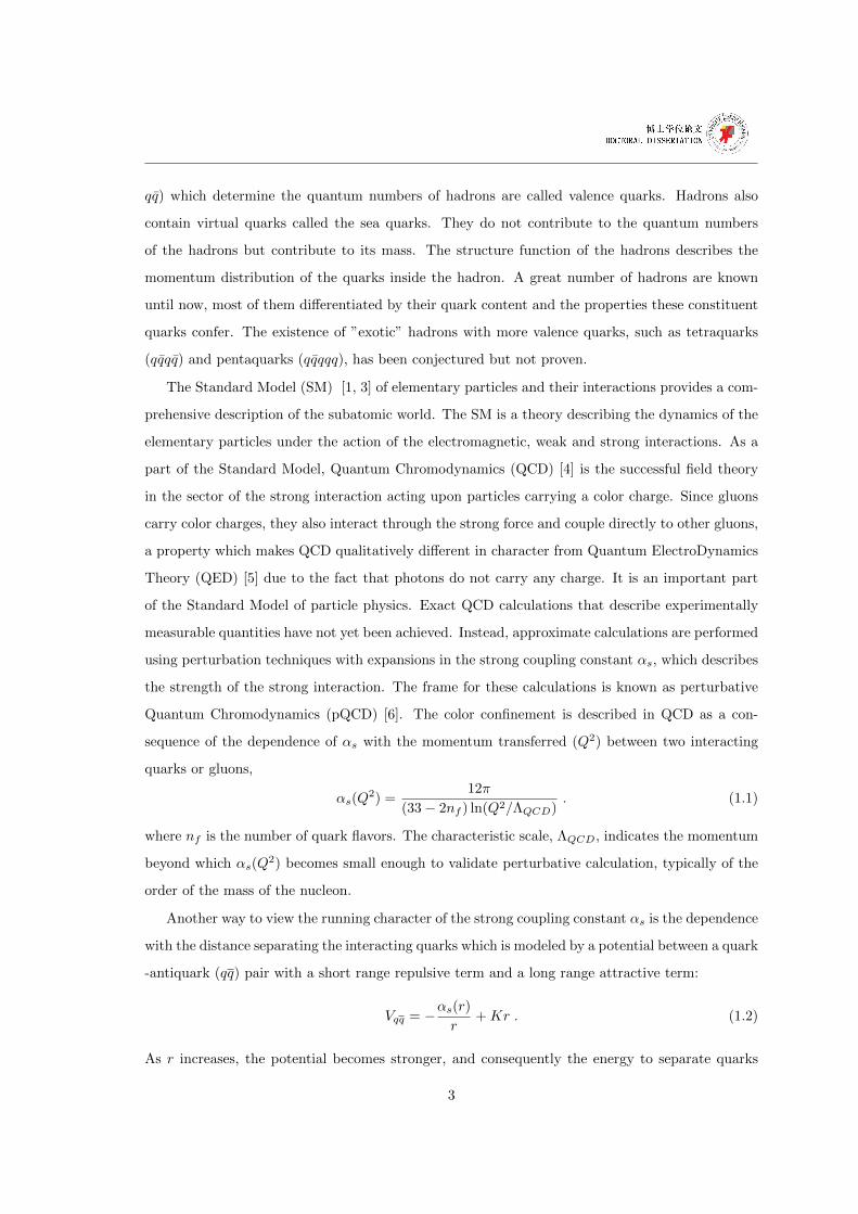
1.1 The evolution of the energy density/T 4 as a function of temperature scaled by the

critical temperature TC resulting from Lattice QCD calculation [9]. The arrows on

the right side indicating the values for the Stefan-Boltzmann limit. . . . . . . . . . 5

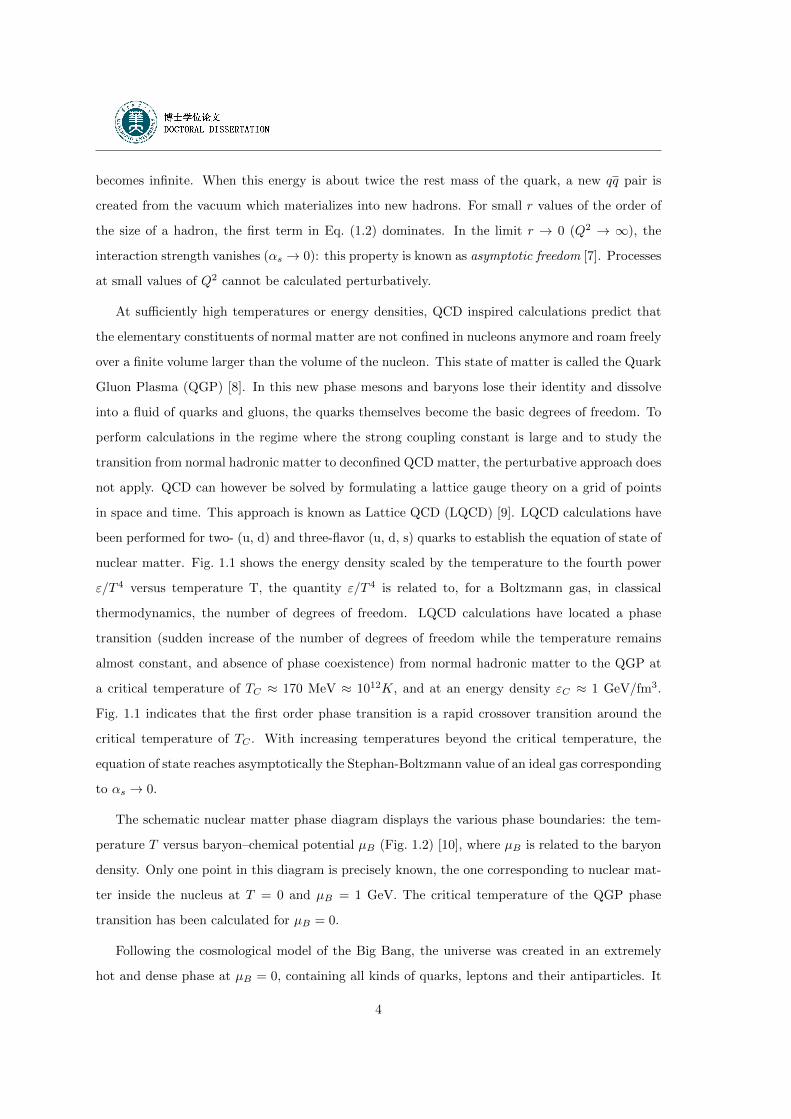
1.2 The phase diagram of QCD [10]. . . . . . . . . . . . . . . . . . . . . . . . . . . . . 6

1.3 The hard scattering of γ-jet process. . . . . . . . . . . . . . . . . . . . . . . . . . . 8

2.1 Schematic view of two colliding nuclei in the geometrical participant-spectator model.

The distance between the centers of the two Lorentz contracted nuclei is the impact

parameter b. . . . . . . . . . . . . . . . . . . . . . . . . . . . . . . . . . . . . . . . 12

2.2 Nuclear stopping scenarios. Th particle rapidity are given before the collision and

after the collision in the case of a full stopping (Landau) and complete transparency

(Bjorken). . . . . . . . . . . . . . . . . . . . . . . . . . . . . . . . . . . . . . . . . 13

2.3 The space-time evolution of the system in center-of momentum frame in relativistic

heavy ion collisions according to Bjorken [21]. . . . . . . . . . . . . . . . . . . . . . 14

2.4 Particle ratios [25] in central collisions at√sNN = 200 GeV at mid-rapidity with

thermal model prediction [26] compared with PHENIX, PHOBOS, BRAHMS, and

STAR. . . . . . . . . . . . . . . . . . . . . . . . . . . . . . . . . . . . . . . . . . . 18

2.5 The diagram of calculation for hard scattering. . . . . . . . . . . . . . . . . . . . . 20

2.6 Parton distribution function by the CTEQ group as a function of x at Q = 2 GeV

(left) and 100 GeV (right) [30]. . . . . . . . . . . . . . . . . . . . . . . . . . . . . 21

2.7 Probability that a given parton will fragment into a π0 as a function of the mo-

mentum fraction z of the π0. These fragmentation functions were evaluated at

Q2 = 10 GeV2 [31]. . . . . . . . . . . . . . . . . . . . . . . . . . . . . . . . . . . 21

iii

2.8 The invariant differential cross section for inclusive π0 production (points) and the

results from NLO pQCD calculations in√s = 7 TeV pp collisions. The relative

difference between the data and the theory using KKP [33] and CTEQ5M [29] sets

of fragmentation functions with scales of pT /2, pT and 2pT respectively. . . . . . . 22

2.9 A phenomenological curve and some experimental data for nuclear effect on structure

function, FA2 /FD2 , from [36]. . . . . . . . . . . . . . . . . . . . . . . . . . . . . . . 24

2.10 Charged particle pseudorapidity density per participant pair for central nucleus-

nucleus [43]-[47] and non-single diffractive pp (pp) collisions [48]-[49], as a function

of√sNN . The solid lines ∝ s0.15NN and ∝ s0.11NN are superimposed on the heavy-ion

and pp (pp) data, respectively [42] . . . . . . . . . . . . . . . . . . . . . . . . . . . 26

2.11 The decoupling time extracted from Rlong [52]. The ALICE result is compared to

those obtained for central gold and lead collisions at lower energy at the AGS [53],

SPS [54]-[55] and RHIC [56]-[57]. . . . . . . . . . . . . . . . . . . . . . . . . . . . 27

2.12 The ellipsoidal shape of participant in non-central high energy nucleus-nucleus col-

lisions. . . . . . . . . . . . . . . . . . . . . . . . . . . . . . . . . . . . . . . . . . . 28

2.13 Measured charged particle ν2 as a function of pT in Pb+Pb collisions at√sNN =

2.76 TeV [59]. a) ν2{2} for the centrality bin 40–50% from the 2- and 4-particle cu-

mulant methods for ALICE measurement and for Au–Au collisions at√sNN = 200 GeV

in RHIC measurements. b) ν2{4} for various centralities compared to STAR mea-

surements. The data points in the 20–30% centrality bin are shifted in pT for visibility. 29

2.14 ν2 as a function of pT (left) and K ET (right) scaled by the number of constituent

quarks in minimum bias Au+Au collisions at√sNN = 200 GeV [62]. . . . . . . . 30

2.15 The energy dependence of K+/π+ and K−/π− ratio at mid-rapidity [63]. . . . . . 31

2.16 Comparison of RAA in central (0–5%) Pb+Pb collisions at√sNN = 2.76 TeV at

LHC to measurements at√sNN = 200 GeV by the PHENIX [65] and STAR [66]

experiments at RHIC. The vertical bars around RAA = 1 show the pT independent

scaling uncertainty with 〈Ncoll〉 [64]. . . . . . . . . . . . . . . . . . . . . . . . . . . 32

2.17 The RAA of direct photon, π0 and η meson as a function of pT in central Au + Au

collisions at√sNN = 200GeV [65]. . . . . . . . . . . . . . . . . . . . . . . . . . . . 33

3.1 Cartoon illustrating a measurement of two-particle correlations from jet. . . . . . 37

3.2 Two particle azimuthal correlation distributions for minimum bias in proton-proton

collision at√s = 7 TeV. . . . . . . . . . . . . . . . . . . . . . . . . . . . . . . . . 37

iv

3.3 (a) Two particle azimuthal correlation distributions for minimum bias and central

d + Au collisions. (b) Comparison of two particle correlations for central Au + Au

collisions to those seen in pp and central d + Au collisions [67]. . . . . . . . . . . 38

3.4 The scheme of jet quenching in heavy-ion collisions. . . . . . . . . . . . . . . . . . 39

3.5 Azimuthal correlations of high-pT charged hadron pairs in central Au + Au collisions

for various ptrigT and passocT ranges. All pT values in this figure have GeV/c unit [68]. 39

3.6 Schematic view of a hard scattering event in the plane perpendicular to the beam. . 41

3.7 ppairT as a function of collision energy√s from various particle correlation measure-

ments [72]. . . . . . . . . . . . . . . . . . . . . . . . . . . . . . . . . . . . . . . . . 42

3.8 Feynman diagrams of the main production processes for direct photons in initial hard

scatterings as well as in a thermalized quark-gluon plasma phase: (a) quark-gluon

Compton scattering of order αs; (b) quark-antiquark annihilation of order αs; (c)

fragmentation photons of order α2s. . . . . . . . . . . . . . . . . . . . . . . . . . . 44

3.9 Error band, including systematic uncertainties, for the ratio of all photons to decay

photons as a function of pT [77]. . . . . . . . . . . . . . . . . . . . . . . . . . . . . 45

3.10 The photon spectrum for central Pb + Pb collisions at the SPS including recent

interferometry results from WA98 [78]. For comparison, results from theoretical

calculation are included [79]. . . . . . . . . . . . . . . . . . . . . . . . . . . . . . . 46

3.11 Direct photon spectra for different centralities in Au+Au collisions at RHIC [80]. 47

3.12 xE distributions for several ranges of ptrigT compared to calculations using quark

(solid) and gluon (dashed) fragmentation functions as parameterized by the LEP

data [71]. . . . . . . . . . . . . . . . . . . . . . . . . . . . . . . . . . . . . . . . . . 49

3.13 Azimuthal correlation distribution of charged hadrons with various trigger particle

types with 7 GeV/c < ptrigT < 9 GeV/c and 3 GeV/c < passocT < 5 GeV/c for pp and

central Au + Au (0-20%) collisions. Top: Inclusive, decay and direct jet function

in pp collisions. Middle: Inclusive, decay and direct jet function is central Au + Au

collisions. Bottom: π0, η, γ(π0) and γ(η) associated yields in pp. [85]. . . . . . . 50

3.14 The direct γ− h correlation distribution for pp collisions multiplied by a factor of

10 and Au + Au [86]. . . . . . . . . . . . . . . . . . . . . . . . . . . . . . . . . . . 51

3.15 R(+/−) for isolated photons (blue) and π0 (red) triggers as a function of associated

particles passocT for several selections of ptrigT . The lines are calculated using DSS

fragmentation functions [85]. . . . . . . . . . . . . . . . . . . . . . . . . . . . . . . 52

v

3.16 Transverse distributions of the initial γ− jet production vertices that contribute to

the final observed γ− hadron pairs along a given direction (arrows) with xE ≈ 0.9

(left plot) and xE ≈ 0.3 (right plot) [87]. . . . . . . . . . . . . . . . . . . . . . . . . 53

4.1 The LHC injector complex [88]. . . . . . . . . . . . . . . . . . . . . . . . . . . . . 56

4.2 Longitudinal view of the ALICE detector [89]. . . . . . . . . . . . . . . . . . . . . 58

4.3 Physical track-finding efficiency for different combinations of the tracking detectors

in central Pb+Pb collisions (dNch/dη = 6000) (left) and proton–proton collisions

(right) [77]. . . . . . . . . . . . . . . . . . . . . . . . . . . . . . . . . . . . . . . . 62

4.4 Transverse-momentum resolution for different combinations of the tracking detectors

in central Pb+Pb collisions (dNch/dη = 6000) (left) and proton–proton collisions

(right) [77]. . . . . . . . . . . . . . . . . . . . . . . . . . . . . . . . . . . . . . . . 62

4.5 dE/dx measurements performed by TPC and ITS with ALICE in proton-proton

collisions at√s = 7 TeV. . . . . . . . . . . . . . . . . . . . . . . . . . . . . . . . . 63

4.6 Identified particle transverse momentum distribution measured by ALICE detectors

in proton-proton collisions at√s = 7 TeV. . . . . . . . . . . . . . . . . . . . . . . 64

4.7 Energy resolution in EMCal (left) and PHOS (right) for electrons as a function of

incident beam momentum. The continuous line represents the result of the fit of

Eq. (4.1) to the experimental data [77]. . . . . . . . . . . . . . . . . . . . . . . . . 68

4.8 Schematic view of the AliRoot framework [97]. . . . . . . . . . . . . . . . . . . . 69

5.1 The ratio of NLO contribution to LO contribution for direct photon production. . . 75

5.2 Monte Carlo (PYTHIA) γ–jet photon spectrum (left) and jet–jet photon spectrum

(right) pT spectra in proton–proton collisions at√s = 14 TeV. γ–jet photons are

produced in qg → γq and qq → γg hard processes and jet–jet photons in final state

radiation during the parton shower evolution or in the decay of neutral pions frag-

menting jets from 2→ 2 hard processes. Simulation bins in phardT normalized to the

cross section are also displayed. . . . . . . . . . . . . . . . . . . . . . . . . . . . . . 76

5.3 Example of the two decay photon clusters from π0. . . . . . . . . . . . . . . . . . . 78

5.4 Example of a shower profile and its principal axes e1 and e2 [93]. . . . . . . . . . . 79

5.5 The scheme of isolation criteria. . . . . . . . . . . . . . . . . . . . . . . . . . . . . 81

vi

5.6 Number of photons from PYTHIA generated (left) γ-jet and jet-jet events with jet

energy Ejet > 5 GeV and the isolated photons after applying the isolation cut pa-

rameters of R = 0.4, ε = 0.1 and pthresT = 1 GeV/c on the photon clusters from

generated ones (right). . . . . . . . . . . . . . . . . . . . . . . . . . . . . . . . . . . 82

5.7 Relative azimuthal angle distribution ∆φ = φγ −φhadron in proton–proton collisions

at√s = 14 TeV for isolated photons with pTγ > 20 GeV/c: from Monte Carlo events

(dashed line) and from events reconstructed by ALICE (solid line) for γ–jet events

(left) and jet–jet events (right). In jet–jet events the π0 trigger is not necessarily

the leading particle. . . . . . . . . . . . . . . . . . . . . . . . . . . . . . . . . . . . . 84

5.8 The ratio of reconstructed signal hadrons from jet fragmentation to background

hadrons from underlying events in γ–jet events. The solid line is a fit to the data

points. . . . . . . . . . . . . . . . . . . . . . . . . . . . . . . . . . . . . . . . . . . . 85

5.9 Photon-charged hadron correlation spectrum and the contribution from underlying

event using photons identified by EMCal in pp collisions at√s = 5.5 TeV [111]. 86

5.10 Photon–charged hadrons correlation distribution with pTγ > 20 GeV/c, pTh>

2 GeV/c calculated in proton–proton collisions at√s = 14 TeV from PYTHIA

generated Monte-Carlo data. The data points with error bars represents the total

spectrum (γ–jet plus jet–jet events) as it will be measured, the errors bars repre-

sent the statistical errors of the measurement and the area around the data points

represents the systematic errors due to the jet–jet photons not properly identified.

The contribution from jet–jet photons (closed circles) and from the underlying event

(downwards triangles) are displayed as well. The ideal jet fragmentation function

are calculated from the PYTHIA generated Monte-Carlo γ–jet events is also shown

(green line) [17]. . . . . . . . . . . . . . . . . . . . . . . . . . . . . . . . . . . . . . 87

5.11 kT reproduced by PYTHIA generated γ-jet events and extrapolated to LHC energies. 89

5.12 Comparison of fragmentation function with imbalance distribution from Monte Carlo

generated γ-jet events with jet energy larger than 20GeV in pp@10TeV by tuned

parameters in PYTHIA, the uncertainty of kT from the estimation are shown as well. 90

5.13 Ratio of fragmentation function (left) and correlation function (right) distribution

when ISR/FSR radiation on and off from Monte Carlo generated γ-jet events with

jet energy larger than 20GeV in pp@10TeV by PYTHIA. . . . . . . . . . . . . . . . 90

vii

5.14 Comparison of hadrons transverse momentum spectrum with and without quench-

ing in jet fragmentation function and correlation distribution from Monte Carlo

generated γ-jet events with jet energy larger than 20GeV in pp@5.5TeV by tuned

parameters in PYTHIA. . . . . . . . . . . . . . . . . . . . . . . . . . . . . . . . . . 92

5.15 γ-hadrons correlation distribution in heavy ion collisions, the underlying events dis-

tribution is correlated photons with the hadrons at the same side of photons. On the

right is the γ-hadrons correlation distribution after the underlying subtraction. . . . 93

5.16 The nuclear modification factor IAA for γ-hadrons correlation distribution in central

and perpgeral Pb+Pb collisions at LHC energy. . . . . . . . . . . . . . . . . . . . . 93

5.17 The nuclear modification factor RAA for charged hadrons in γ-jet events at LHC

energy, different transport coefficient q are used for different production. . . . . . . 94

5.18 The nuclear modification factor IAA for γ-hadrons correlation distribution at LHC

energy, different transport coefficient q are used for different γ-jet production. . . . 94

5.19 Relative azimuthal angle distribution ∆φ = φγ − φhadron for γ-jet events in pp

collisions at√s = 5.5 TeV. Photons with pT,γ > 30 GeV/c are measured and

isolated in EMCAL. Associated hadrons have pT,hadron > 2 GeV/c. Full circles

indicate quenched events and empty circles indicate unquenched events by PYTHIA

generator. Distributions are normalized to the total number of isolated photons. . 95

5.20 Left: γ-hadron correlation distributions in quenched and unquenched PYTHIA

events as a function of ξ. Right: The ratio of the photon-triggered conditional

hadron yields RCY for PYTHIA and qPYTHIA events. . . . . . . . . . . . . . . . 96

5.21 The ratio of the leading particles pT over the photons pT with and without quenching

effect is taken into account. . . . . . . . . . . . . . . . . . . . . . . . . . . . . . . . 97

5.22 The correlation between the leading particle ratio and the ∆φ distribution of leading

particles and photons, with (low) and without (up) quenching effect is taken into

account respectively. The left panel is selecting leading particles inside all the gen-

erated particles (ideal case), the right one just took final state particles which could

be measured in the experiment. . . . . . . . . . . . . . . . . . . . . . . . . . . . . . 98

viii

5.23 The correlation between the leading particle ratio and the medium length distribu-

tion of leading particles, with (low) and without quenching effect (up) is taken into

account respectively. The left panel is selecting leading particles inside all the gen-

erated particles (ideal case), the right one just took final state particles which could

be measured in the experiment. . . . . . . . . . . . . . . . . . . . . . . . . . . . . . 99

5.24 The probability of the leading particles production as a function of medium length L,

with (right) and without (left) quenching effect is taken into account. . . . . . . . . 100

5.25 The ratio of the probability for leading particles with large x over small x as a

function of medium length L. . . . . . . . . . . . . . . . . . . . . . . . . . . . . . . 101

5.26 The ratio with quenching over without quenching for leading particles with large x

and small x as a function of medium length L. . . . . . . . . . . . . . . . . . . . . 101

5.27 The nuclear modification factor IAA distribution as a function of medium length L

by selecting different regions of xE correlation distribution. . . . . . . . . . . . . . 102

6.1 Longitudinal vertex distribution from hit correlations in the two pixel layers of the

ALICE inner tracking system. A Gauss fit with an estimated r.m.s of about 6 cm

to the central part is also shown. . . . . . . . . . . . . . . . . . . . . . . . . . . . . 104

6.2 Arrival time of particles in the V0 detectors relative to the beam crossing time (time

zero). A number of beam-halo or beam-gas events are visibles as secondary peaks

in V0A (left panel) and V0C (right panel) [116]. This is because particles produced

in background interactions arrive at earlier times in one or the other of the two

counters. The majority of the signals have the correct arrival time expected for

collisions around the nominal vertex. . . . . . . . . . . . . . . . . . . . . . . . . . 105

6.3 Run quality criteria for pp data at√s = 7 TeV: the mean cluster multiplicity dis-

tribution for EMCAL (left) and PHOS (right) as a function of run numbers. The

run index and run number correspondence is in Appendix. . . . . . . . . . . . . . 106

6.4 Run quality criteria for pp data at√s = 7 TeV: the mean total energy (< E >=∑

E∗Ncluster(E)∑Ncluster(E) ) deposited on EMCAL (left) and PHOS (right) with cluster energy

larger than 0.5 GeV per event. The different colors on the same canvas represent

single (Super) Modules check from each run. . . . . . . . . . . . . . . . . . . . . . . 107

6.5 Run quality criteria for pp data at√s = 7 TeV: the slope of the cluster energy

spectrum from power law function fitting (f(E) = (a+ b ∗E)−n) for EMCAL (left)

and PHOS (right). . . . . . . . . . . . . . . . . . . . . . . . . . . . . . . . . . . . . 107

ix

6.6 Invariant mass analysis for pp data at√s = 7 TeV for EMCAL (left) and PHOS

(right). A Gauss + Polynoimal function (A ∗ e−(x−m0)2

2∗σ2 + a0 + a1 ∗ x + a2 ∗ x2) is

fitted on the invariant mass spectrum at the mass range 110 < Mγγ < 160 MeV/c2

as the black solid curve. . . . . . . . . . . . . . . . . . . . . . . . . . . . . . . . . . 108

6.7 Run quality criteria for π0 analysis in pp collisions at√s = 7 TeV: the mean position

of the π0 peak (upper panel) and width (bottom panel) obtained from the fitting on

Fig. 6.14 for EMCAL (left) and PHOS (right). . . . . . . . . . . . . . . . . . . . . 109

6.8 Run quality criteria for π0 analysis in pp collisions at√s = 7 TeV: the mean number

of reconstructed π0 (upper panel) and the significance ( SS+B =

Npi0

Nγγ) of the signal

over the signal plus background (bottom panel) obtained from the fitting on Fig. 6.14

for EMCAL (left) and PHOS (right). . . . . . . . . . . . . . . . . . . . . . . . . . . 110

6.9 Mean value of MIP position in ADC counts from all the towers calibration. . . . . 112

6.10 Response of 384 towers of the EMCAL to cosmic muons before (dashed histogram)

and after (full histogram) individual gain calibration. The curve represents a fit of

a Gaussian to the full histogram with fit results as given together [120]. . . . . . . . 112

6.11 The π0 mass position and width from decalibrate Monte-Carlo (MC) and real data

in PHOS (upper) and EMCal (bottom). . . . . . . . . . . . . . . . . . . . . . . . . 114

6.12 The EMCal time vs. cell energy distribution. . . . . . . . . . . . . . . . . . . . . . 115

6.13 The raw inclusive cluster energy spectrum (left) and the normalized spectrum from

different calorimeters. . . . . . . . . . . . . . . . . . . . . . . . . . . . . . . . . . . 115

6.14 The invariant mass spectrum of cluster pairs in pp@7TeV from EMCal (top) and

PHOS (bottom) detector. . . . . . . . . . . . . . . . . . . . . . . . . . . . . . . . . . 116

6.15 Dependence of the π0 peak position (upper) and width (bottom) on pT for EMCal

(left) and PHOS (right) in pp collisions at√s = 7 TeV. . . . . . . . . . . . . . . . 117

6.16 Raw spectra of π0 vs pT measured by EMCal (left) and PHOS (right) detector in pp

collisions at√s = 7 TeV. . . . . . . . . . . . . . . . . . . . . . . . . . . . . . . . . 118

6.17 Different trigger transverse momentum distribution from different detector measure-

ments. . . . . . . . . . . . . . . . . . . . . . . . . . . . . . . . . . . . . . . . . . . . 120

6.18 Relative azimuthal angle distribution ∆φ = φtrig − φh± for different pT cluster

triggers in EMCal and charged tracks with ph±

T > 1 GeV/c in central tracking system

in pp collisions at√s = 7 TeV. . . . . . . . . . . . . . . . . . . . . . . . . . . . . . 121

x

6.19 Relative azimuthal angle distribution ∆φ = φtrig − φh± for charged track triggers

and cluster triggers with ph±

T > 1 GeV/c in pp collisions at√s = 7 TeV. . . . . . 122

6.20 Relative azimuthal angle distribution ∆φ = φtrig −φh± for inclusive cluster triggers

and π0 triggers in EMCal with ptrigT > 5 GeV/c and ph±

T > 1 GeV/c in pp collisions

at√s = 7 TeV. . . . . . . . . . . . . . . . . . . . . . . . . . . . . . . . . . . . . . . 123

6.21 Energy distribution of cluster triggers (left) from EMCAL before and after the iso-

lation selection (R = 0.4, ε = 0.1) in pp collisisons at√s = 7 TeV. The right hand

figure shows the isolation efficiency on the inclusive cluster triggers. . . . . . . . . 124

6.22 Relative azimuthal angle distribution ∆φ = φtrig−φh± for inclusive charged and clus-

ter triggers with different pT bins and ph±

T > 1 GeV/c in pp collisions at√s = 7 TeV

before and after isolation cut (IC) selection: R = 0.4, ε = 0.1. . . . . . . . . . . . . 125

6.23 Two-particle correlation distribution as a function of the relative azimuthal angle

between trigger particles and associate particles ∆φ= φt − φa. Trigger particles

are selected as the isolated trigger (R = 0.4, ε = 0.1 red triangle symbols) with

pT> 5 GeV/c or non-isolated trigger (black dot symbols) with pT> 5 × 0.50.8 GeV/c

detected in EMCAL. Associated particles are selected as tracks detected by the central

tracking system with pT> 1 GeV/c. The data have been obtained in proton-proton

collisions at√s= 7 TeV. . . . . . . . . . . . . . . . . . . . . . . . . . . . . . . . . . 126

6.24 pout distributions for inclusive cluster triggers from EMCal with ph±

T > 1 GeV/c in

pp collisions at√s = 7 TeV for different pTtrig ranges. The distributions have been

fitted with both Gaussian (solid lines) and Kaplan (dashed lines) functions. . . . . 127

6.25 Yield per trigger of charged tracks associated with cluster triggers in EMCal (left)

and charged track triggers in CTS (right) as a function of ∆φ in pp collisisons at√s = 7 TeV. The lines correspond to fits which are described in the text. . . . . . . 128

6.26√< p2out > values obtained from the fits for different triggers with ptrigT > 5 GeV/c

and ph±

T > 1 GeV/c in pp collisions at√s = 7 TeV. . . . . . . . . . . . . . . . . . 129

6.27 zt and xh calculated by a Monte-Carlo model using the Born level pQCD cross

sections plus a Gaussian kT smearing in pp collisions at√s = 7 TeV. . . . . . . . 130

6.28√< p2out > values obtained from the fits for inclusive and isolated cluster triggers

from EMCal with ptrigT > 5 GeV/c and ph±

T > 1 GeV/c in pp collisions at√s = 7 TeV.131

xi

6.29√< k2T > values euvalated from Eq. 6.6 by obtaining the

√< p2out > values from

the fits for isolated cluster triggers from EMCal with ptrigT > 5 GeV/c and ph±

T >

1 GeV/c in pp collisions at√s = 7 TeV. . . . . . . . . . . . . . . . . . . . . . . . 132

6.30 Associate particles spectra selected in the transverse azimuthal regions with respect

to the trigger particle: π/2 < ∆φ < 2π/3 and 4π/3 < ∆φ < 3π/2 (away-side

hemisphere) and π/3 < ∆φ < π/2 (near-side hemisphere) for non-isolated (top left)

and isolated (top right) cluster triggers detected in EMCal. Ratio of the the spectra

from the two different away-side transverse regions for non-isolated and isolated

triggers detected in EMCAL (bottom). Data have been taken in pp collisions at√s = 7 TeV. . . . . . . . . . . . . . . . . . . . . . . . . . . . . . . . . . . . . . . . 134

6.31 Associate particle spectra selected in various azimuthal regions with respect to non-

isolated (top let) or isolated (top right) cluster triggers detected in EMCAL: −π/3 <

∆φ < π/3 (toward region), 2π/3 < ∆φ < 4π/3 (away region) and π/2 < ∆φ < 2π/3

(away-side transverse region, same as Fig. 6.30). Toward-associate particle spec-

trum including the trigger particle compared to the away-associate particle spectrum

(bottom). Data have been taken in proton-proton collisions at√s= 7 TeV. . . . . . 135

6.32 Associate away-side charged hadrons (paT > 1 GeV/c) per trigger (ptT > 5 GeV/c)

yield as a function of xE for isolated cluster triggers detected in EMCal (left) and

charged particle triggers (right ) detected in the central tracking system. Data have

been taken in pp collisions at√s= 7 TeV. . . . . . . . . . . . . . . . . . . . . . . . 136

6.33 Away-side associate charged hadron (paT > 1 GeV/c) yield per trigger (ptT > 5 GeV/c)

as a function of xE for non-isolated (dot symbols) and isolated (triangle symbols) trig-

gers detected in EMCal (left) and central tracking system (right). Data have been

taken in pp collisions at√s= 7 TeV. . . . . . . . . . . . . . . . . . . . . . . . . . . 137

6.34 Extracted inverse xE slope as a function of the mean trigger pTt for charged (red)

and neutral triggers (blue) in pp collisions at√s = 7 TeV. The contribution of the

underlying event has been subtracted. . . . . . . . . . . . . . . . . . . . . . . . . . 138

6.35 Extracted inverse xE slope as a function of the mean trigger pTt for non-isolated

and isolated triggers in pp collisions at√s = 7 TeV. . . . . . . . . . . . . . . . . 139

xii

6.36 Associate away-side charged hadron (paT > 1 GeV/c) yield per trigger (ptT > 14 GeV/c)

(triangle symbols) as a function of xE for isolated cluster triggers detected in central

tracking system in pp collisions at√s= 7 TeV compared to the same distribution cal-

culated from PYTHIA generated γ+jet events (initial state and final state radiation

switched on and PYTHIA kT value set equal to 5.5 GeV/c. . . . . . . . . . . . . . . 140

7.1 ppairT distribution (left) and the averaged value < pT >pair from each pT bin (right).

The pT dependence is interpreted by a linear function (lines). . . . . . . . . . . . . 159

7.2 The averaged < pT >pair as a function of jet pT from jet-jet events. The pT depen-

dence is interpreted by a linear function (lines) . . . . . . . . . . . . . . . . . . . . 160

7.3 The averaged < pT >pair as a function of photon pT from γ-jet events. The pT

dependence is interpreted by a linear function (lines) . . . . . . . . . . . . . . . . . 161

7.4 The averaged < pT >pair as a function of jet pT from jet-jet events. The pT depen-

dence is interpreted by a linear function (lines) . . . . . . . . . . . . . . . . . . . . 162

7.5 The averaged < pT >pair as a function of jet pT from jet-jet events. The pT depen-

dence is interpreted by a linear function (lines) . . . . . . . . . . . . . . . . . . . . 163

7.6 The ratio of the tower amplitude over Reference data as a function of cell eta and

phi for different SMs (x-column(eta direction); y-row(phi direction)) from one run

during the data taking. . . . . . . . . . . . . . . . . . . . . . . . . . . . . . . . . . . 165

7.7 The projection of the 2D figure 7.6, for data Quality Assurance (QA) checker usage. 166

7.8 the AMORE canvas for EMCAL at P2 DQM station during the data taking from

different running period with good data quality (left) and problemable data (right). 167

xiii

List of Tables

1.1 Matter and interactions in the Standard Model of particles and forces [1]. . . . . . 2

4.1 Technical data of the PHOS electromagnetic calorimeter [93]. . . . . . . . . . . . 66

4.2 The EMCAL physical parameters [94]. . . . . . . . . . . . . . . . . . . . . . . . . 67

6.1 Track quality cuts used in the analysis. . . . . . . . . . . . . . . . . . . . . . . . . . 108

7.1 Parameters fitted on averaged parton-parton pT pair and photon-parton pT pair by

a linear function respectively. . . . . . . . . . . . . . . . . . . . . . . . . . . . . . . 159

7.2 Parameters fitted on averaged jet-jet pT pair by the linear function. . . . . . . . . . 160

7.3 Parameters fitted on averaged γ-jet pT pair by the linear function. . . . . . . . . . 162

7.4 Parameters fitted on averaged jet-jet pT pair by the linear function. . . . . . . . . . 162

7.5 Parameters fitted on averaged leading-leading pT pair by the linear function. . . . . 163

7.6 Run Number and Run Index: LHC10e period . . . . . . . . . . . . . . . . . . . . . 168

xiv

Chapter 1

Introduction

During the last century, understanding the nature of matter became a long way. Atoms, thought

to be indivisible at the end of 19th century, have shown a complex structure, containing a shell of

electrons and a nucleus of protons and neutrons also called nucleons. These particles were soon

considered as the elementary blocks of matter: the fundamental role of atoms had been taken over

by electrons and nucleons.

Series of discoveries, starting with the muon in 1937 followed by pion and kaon in 1947, led

to a classification of the constituents of matter in three categories: leptons, that only interact

through the electromagnetic and weak forces; hadrons, that interact through the strong force,

and the mediators of these three fundamental forces called gauge bosons: the photon for the

electromagnetic force, the Z0 and W± bosons for the weak force, and the gluons for the strong

force. The group of leptons consists in the electron, the muon and the tau, the associate neutrinos

and their anti-particles for a total of twelve particles, grouped into three generations (Tab. 1.1) [1].

These particles are elementary particles as they have revealed, up to now, no substructure. The

large variety of hadrons, and the way they interact, has been explained by the existence of smaller

constituent particles, the quarks, where no substructure has been discovered so far down to the

scale of 10−19 m.

There are six types or flavors of quarks: up (u), down (d), charm (c), strange (s), bottom (b)

and top (t), grouped into three generations, each with two quarks (Tab. 1.1). For every quark flavor

there is a corresponding antiparticle, named antiquark. It differs from the quark only in that some

of its properties have equal magnitude but opposite sign. Quarks have various intrinsic properties:

they carry half integer spin and obey Fermi-Dirac statistics, they carry a fraction of the electron

1

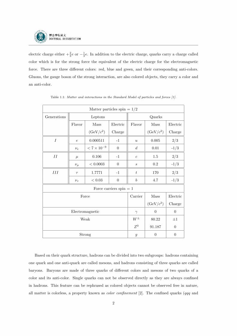
electric charge either + 23e or − 1

3e. In addition to the electric charge, quarks carry a charge called

color which is for the strong force the equivalent of the electric charge for the electromagnetic

force. There are three different colors: red, blue and green, and their corresponding anti-colors.

Gluons, the gauge boson of the strong interaction, are also colored objects, they carry a color and

an anti-color.

Table 1.1: Matter and interactions in the Standard Model of particles and forces [1].

Matter particles spin = 1/2

Generations Leptons Quarks

Flavor Mass Electric Flavor Mass Electric

(GeV/c2) Charge (GeV/c2) Charge

I e 0.000511 -1 u 0.005 2/3

νe < 7× 10−9 0 d 0.01 -1/3

II µ 0.106 -1 c 1.5 2/3

νµ < 0.0003 0 s 0.2 -1/3

III τ 1.7771 -1 t 170 2/3

ντ < 0.03 0 b 4.7 -1/3

Force carriers spin = 1

Force Carrier Mass Electric

(GeV/c2) Charge

Electromagnetic γ 0 0

Weak W± 80.22 ±1

Z0 91.187 0

Strong g 0 0

Based on their quark structure, hadrons can be divided into two subgroups: hadrons containing

one quark and one anti-quark are called mesons, and hadrons consisting of three quarks are called

baryons. Baryons are made of three quarks of different colors and mesons of two quarks of a

color and its anti-color. Single quarks can not be observed directly as they are always confined

in hadrons. This feature can be rephrased as colored objects cannot be observed free in nature,

all matter is colorless, a property known as color confinement [2]. The confined quarks (qqq and

2

qq) which determine the quantum numbers of hadrons are called valence quarks. Hadrons also

contain virtual quarks called the sea quarks. They do not contribute to the quantum numbers

of the hadrons but contribute to its mass. The structure function of the hadrons describes the

momentum distribution of the quarks inside the hadron. A great number of hadrons are known

until now, most of them differentiated by their quark content and the properties these constituent

quarks confer. The existence of ”exotic” hadrons with more valence quarks, such as tetraquarks

(qqqq) and pentaquarks (qqqqq), has been conjectured but not proven.

The Standard Model (SM) [1, 3] of elementary particles and their interactions provides a com-

prehensive description of the subatomic world. The SM is a theory describing the dynamics of the

elementary particles under the action of the electromagnetic, weak and strong interactions. As a

part of the Standard Model, Quantum Chromodynamics (QCD) [4] is the successful field theory

in the sector of the strong interaction acting upon particles carrying a color charge. Since gluons

carry color charges, they also interact through the strong force and couple directly to other gluons,

a property which makes QCD qualitatively different in character from Quantum ElectroDynamics

Theory (QED) [5] due to the fact that photons do not carry any charge. It is an important part

of the Standard Model of particle physics. Exact QCD calculations that describe experimentally

measurable quantities have not yet been achieved. Instead, approximate calculations are performed

using perturbation techniques with expansions in the strong coupling constant αs, which describes

the strength of the strong interaction. The frame for these calculations is known as perturbative

Quantum Chromodynamics (pQCD) [6]. The color confinement is described in QCD as a con-

sequence of the dependence of αs with the momentum transferred (Q2) between two interacting

quarks or gluons,

αs(Q2) =

12π

(33− 2nf ) ln(Q2/ΛQCD). (1.1)

where nf is the number of quark flavors. The characteristic scale, ΛQCD, indicates the momentum

beyond which αs(Q2) becomes small enough to validate perturbative calculation, typically of the

order of the mass of the nucleon.

Another way to view the running character of the strong coupling constant αs is the dependence

with the distance separating the interacting quarks which is modeled by a potential between a quark

-antiquark (qq) pair with a short range repulsive term and a long range attractive term:

Vqq = −αs(r)r

+Kr . (1.2)

As r increases, the potential becomes stronger, and consequently the energy to separate quarks

3

becomes infinite. When this energy is about twice the rest mass of the quark, a new qq pair is

created from the vacuum which materializes into new hadrons. For small r values of the order of

the size of a hadron, the first term in Eq. (1.2) dominates. In the limit r → 0 (Q2 → ∞), the

interaction strength vanishes (αs → 0): this property is known as asymptotic freedom [7]. Processes

at small values of Q2 cannot be calculated perturbatively.

At sufficiently high temperatures or energy densities, QCD inspired calculations predict that

the elementary constituents of normal matter are not confined in nucleons anymore and roam freely

over a finite volume larger than the volume of the nucleon. This state of matter is called the Quark

Gluon Plasma (QGP) [8]. In this new phase mesons and baryons lose their identity and dissolve

into a fluid of quarks and gluons, the quarks themselves become the basic degrees of freedom. To

perform calculations in the regime where the strong coupling constant is large and to study the

transition from normal hadronic matter to deconfined QCD matter, the perturbative approach does

not apply. QCD can however be solved by formulating a lattice gauge theory on a grid of points

in space and time. This approach is known as Lattice QCD (LQCD) [9]. LQCD calculations have

been performed for two- (u, d) and three-flavor (u, d, s) quarks to establish the equation of state of

nuclear matter. Fig. 1.1 shows the energy density scaled by the temperature to the fourth power

ε/T 4 versus temperature T, the quantity ε/T 4 is related to, for a Boltzmann gas, in classical

thermodynamics, the number of degrees of freedom. LQCD calculations have located a phase

transition (sudden increase of the number of degrees of freedom while the temperature remains

almost constant, and absence of phase coexistence) from normal hadronic matter to the QGP at

a critical temperature of TC ≈ 170 MeV ≈ 1012K, and at an energy density εC ≈ 1 GeV/fm3.

Fig. 1.1 indicates that the first order phase transition is a rapid crossover transition around the

critical temperature of TC . With increasing temperatures beyond the critical temperature, the

equation of state reaches asymptotically the Stephan-Boltzmann value of an ideal gas corresponding

to αs → 0.

The schematic nuclear matter phase diagram displays the various phase boundaries: the tem-

perature T versus baryon–chemical potential µB (Fig. 1.2) [10], where µB is related to the baryon

density. Only one point in this diagram is precisely known, the one corresponding to nuclear mat-

ter inside the nucleus at T = 0 and µB = 1 GeV. The critical temperature of the QGP phase

transition has been calculated for µB = 0.

Following the cosmological model of the Big Bang, the universe was created in an extremely

hot and dense phase at µB = 0, containing all kinds of quarks, leptons and their antiparticles. It

4

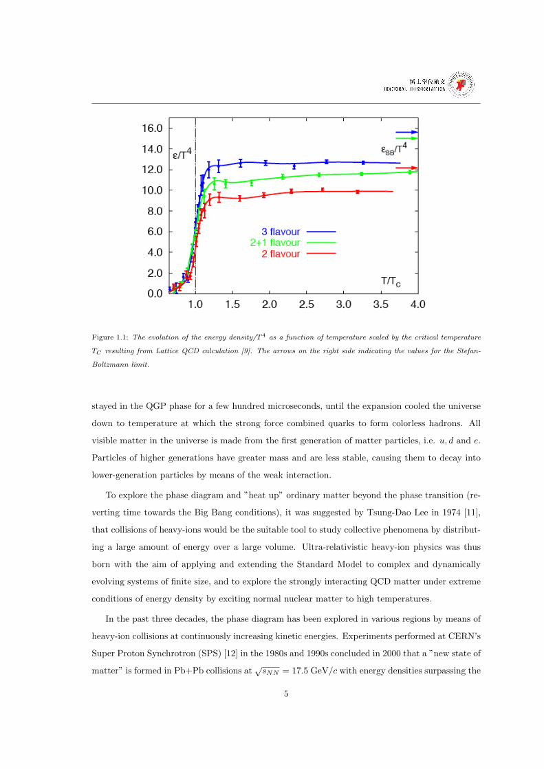
Figure 1.1: The evolution of the energy density/T 4 as a function of temperature scaled by the critical temperature

TC resulting from Lattice QCD calculation [9]. The arrows on the right side indicating the values for the Stefan-

Boltzmann limit.

stayed in the QGP phase for a few hundred microseconds, until the expansion cooled the universe

down to temperature at which the strong force combined quarks to form colorless hadrons. All

visible matter in the universe is made from the first generation of matter particles, i.e. u, d and e.

Particles of higher generations have greater mass and are less stable, causing them to decay into

lower-generation particles by means of the weak interaction.

To explore the phase diagram and ”heat up” ordinary matter beyond the phase transition (re-

verting time towards the Big Bang conditions), it was suggested by Tsung-Dao Lee in 1974 [11],

that collisions of heavy-ions would be the suitable tool to study collective phenomena by distribut-

ing a large amount of energy over a large volume. Ultra-relativistic heavy-ion physics was thus

born with the aim of applying and extending the Standard Model to complex and dynamically

evolving systems of finite size, and to explore the strongly interacting QCD matter under extreme

conditions of energy density by exciting normal nuclear matter to high temperatures.

In the past three decades, the phase diagram has been explored in various regions by means of

heavy-ion collisions at continuously increasing kinetic energies. Experiments performed at CERN’s

Super Proton Synchrotron (SPS) [12] in the 1980s and 1990s concluded in 2000 that a ”new state of

matter” is formed in Pb+Pb collisions at√sNN = 17.5 GeV/c with energy densities surpassing the

5

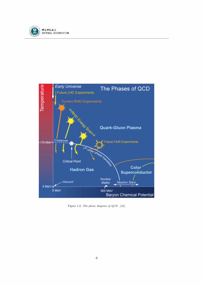
Figure 1.2: The phase diagram of QCD [10].

6

critical value. Current experiments at Brookhaven National Laboratory’s Relativistic Heavy Ion

Collider (RHIC) are continuing this effort. With center of mass energies up to√sNN = 200 GeV/c,

the deconfined phase of matter was evidenced and some of its properties have been explored

quantitatively [13]. The outcome of these studies is so far quite surprising. Although RHIC has

formed matter well beyond the critical temperature predicted by LQCD, measurements indicate

that matter does no behave as a quasi-ideal state of free quarks and gluons, but, rather, as an

almost perfect strongly interacting fluid [14]!

The new experiments, ALICE, ATLAS and CMS, operating at the CERN’s Large Hadron

Collider (LHC) [88], have now taken the lead in studying the properties of QGP. Thanks to the

huge step in collision energy, entering the TeV scale, the largest ever in the history of heavy-

ion physics, LHC opens new avenues for the exploration of matter under extreme conditions of

temperature. Hot QCD matter is formed at much higher temperatures than RHIC and matter

stays in the deconfined phase for a much longer duration strengthening thus the signature emerging

from the collision. In addition, deeply penetrating probes or hard probes are abundantly produced

in the initial stage of the collision offering the unique opportunity to scrutinize the properties of

hot QCD matter.

Among the hard probes, hard scattered quarks or gluons, which materialize in the detector as a

jet of hadrons and are dubbed as jets [16], provide a promising probe to investigate the properties

of the hot and dense matter. They are produced in the early phase of the collision through hard

scattering of the incoming quarks and gluons, and traverse the hot medium which is concurrently

produced in heavy-ion collisions. As these auto generated probes are produced with energies signif-

icantly larger than the typical temperature of the medium, they decouple from the medium acting

similarly to an external probe. Before reaching the detector, the hard scattered quarks or gluons

(q, g) fragment into a jet of hadrons (h) with a momentum distribution defined by the jet frag-

mentation function (f(z) = dNdz with z =

phTEq,g

). The comparison of this jet fragmentation measured

in proton-proton collisions with the one measured in heavy-ion collisions provides a remarkable

observable revealing the modifications inferred on the hard scattered partons by the medium and

hence give access to the properties of the medium itself. Ideally, for such a measurement, one

needs to know the 4-momentum of the parton as it has been produced in the hard scattering and

the 4-momentum after the parton has been modified by the medium. This can be achieved by

selecting particular hard processes with a photon in the final state. Since photons do not interact

strongly with the medium, its 4-momentum is not modified and thus provides a measure of the

7

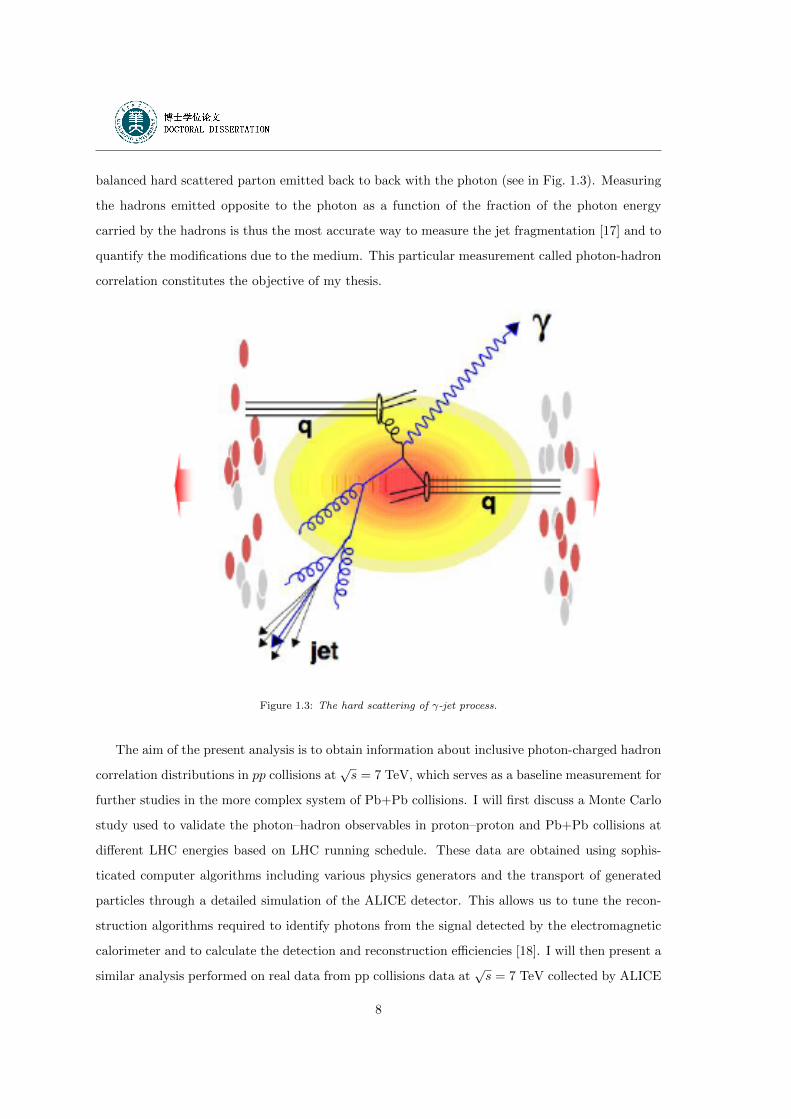
balanced hard scattered parton emitted back to back with the photon (see in Fig. 1.3). Measuring

the hadrons emitted opposite to the photon as a function of the fraction of the photon energy

carried by the hadrons is thus the most accurate way to measure the jet fragmentation [17] and to

quantify the modifications due to the medium. This particular measurement called photon-hadron

correlation constitutes the objective of my thesis.

Figure 1.3: The hard scattering of γ-jet process.

The aim of the present analysis is to obtain information about inclusive photon-charged hadron

correlation distributions in pp collisions at√s = 7 TeV, which serves as a baseline measurement for

further studies in the more complex system of Pb+Pb collisions. I will first discuss a Monte Carlo

study used to validate the photon–hadron observables in proton–proton and Pb+Pb collisions at

different LHC energies based on LHC running schedule. These data are obtained using sophis-

ticated computer algorithms including various physics generators and the transport of generated

particles through a detailed simulation of the ALICE detector. This allows us to tune the recon-

struction algorithms required to identify photons from the signal detected by the electromagnetic

calorimeter and to calculate the detection and reconstruction efficiencies [18]. I will then present a

similar analysis performed on real data from pp collisions data at√s = 7 TeV collected by ALICE

8

detectors with the first LHC run in 2010.

The layout of my thesis is as follows. In Chapter 2, I review the scientific background of heavy

ion physics, where the experimental observables exploited so far in different experiments will be

listed; Jets and two particle correlations are described in Chapter 3; the experimental apparatus

especially ALICE experiment at LHC is introduced in Chap. 4; in Chap. 5, the approach for a

feasibility study with ALICE detectors from Monte Carlo data is fully validated; then the two

particle correlations with γ/π0 triggers measured by ALICE within the data collected in 2010 at

the first year LHC run is presented in Chap. 6; at the end, a brief summary and outlook for my

PhD study is given in Chap. 7.

9

10

Chapter 2

Heavy Ion Physics Program

In this chapter, I will briefly discuss aspects of Heavy-Ion Collisions (HIC). Before introducing

the anticipated properties of the QGP, I will end up by discussing the main experimental observ-

ables allowing the comprehensive study of the new state of matter and the main results obtained

by experiments at SPS, RHIC and LHC.

2.1 Relativistic Heavy Ion Collisions

The study of nuclear collisions is not a new endeavor and, in fact, predates the quark model.

The history of the field can be traced back to the HILAC (Heavy Ion Linear Accelerator) at

Berkeley, the first dedicated heavy-ion accelerator, which entered into operation in 1957. The

objectives of the field at the time were the creation of new elements by nuclear transmutation and

the investigation of radiation damage to human tissue for space travel [19]. During the 1970’s a

new paradigm began to emerge in which heavy-ion collisions were viewed as a tool to study the

equation of state of matter at high temperature and density, conditions thought to govern the

behavior of matter inside neutron stars. Following the suggestion of T. D. Lee [11], the creation of

the Quark Gluon Plasma (QGP), a fundamentally new state of matter, is expected to be realized

in the laboratory by colliding high energy heavy-ions. However, a heavy-ion collision is a complex

system with a fast thermodynamic evolution during which the system passes a fleetingly short

time through the QGP phase of interest. Therefore, understanding the thermodynamic evolution

of the heavy-ion colliding system is a pre-requisite before one can reliably extract from various

observables effects revealing the existence and properties of QGP.

11

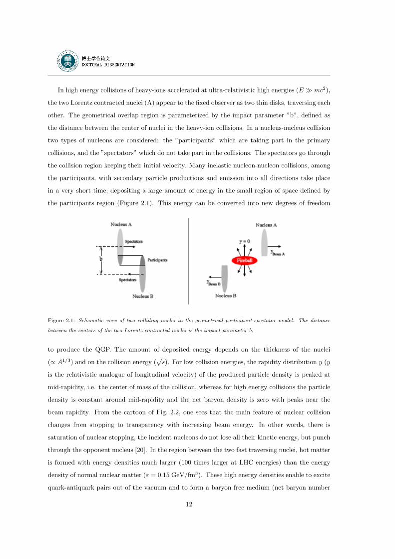
In high energy collisions of heavy-ions accelerated at ultra-relativistic high energies (E � mc2),

the two Lorentz contracted nuclei (A) appear to the fixed observer as two thin disks, traversing each

other. The geometrical overlap region is parameterized by the impact parameter ”b”, defined as

the distance between the center of nuclei in the heavy-ion collisions. In a nucleus-nucleus collision

two types of nucleons are considered: the ”participants” which are taking part in the primary

collisions, and the ”spectators” which do not take part in the collisions. The spectators go through

the collision region keeping their initial velocity. Many inelastic nucleon-nucleon collisions, among

the participants, with secondary particle productions and emission into all directions take place

in a very short time, depositing a large amount of energy in the small region of space defined by

the participants region (Figure 2.1). This energy can be converted into new degrees of freedom

Figure 2.1: Schematic view of two colliding nuclei in the geometrical participant-spectator model. The distance

between the centers of the two Lorentz contracted nuclei is the impact parameter b.

to produce the QGP. The amount of deposited energy depends on the thickness of the nuclei

(∝ A1/3) and on the collision energy (√s). For low collision energies, the rapidity distribution y (y

is the relativistic analogue of longitudinal velocity) of the produced particle density is peaked at

mid-rapidity, i.e. the center of mass of the collision, whereas for high energy collisions the particle

density is constant around mid-rapidity and the net baryon density is zero with peaks near the

beam rapidity. From the cartoon of Fig. 2.2, one sees that the main feature of nuclear collision

changes from stopping to transparency with increasing beam energy. In other words, there is

saturation of nuclear stopping, the incident nucleons do not lose all their kinetic energy, but punch

through the opponent nucleus [20]. In the region between the two fast traversing nuclei, hot matter

is formed with energy densities much larger (100 times larger at LHC energies) than the energy

density of normal nuclear matter (ε = 0.15 GeV/fm3). These high energy densities enable to excite

quark-antiquark pairs out of the vacuum and to form a baryon free medium (net baryon number

12

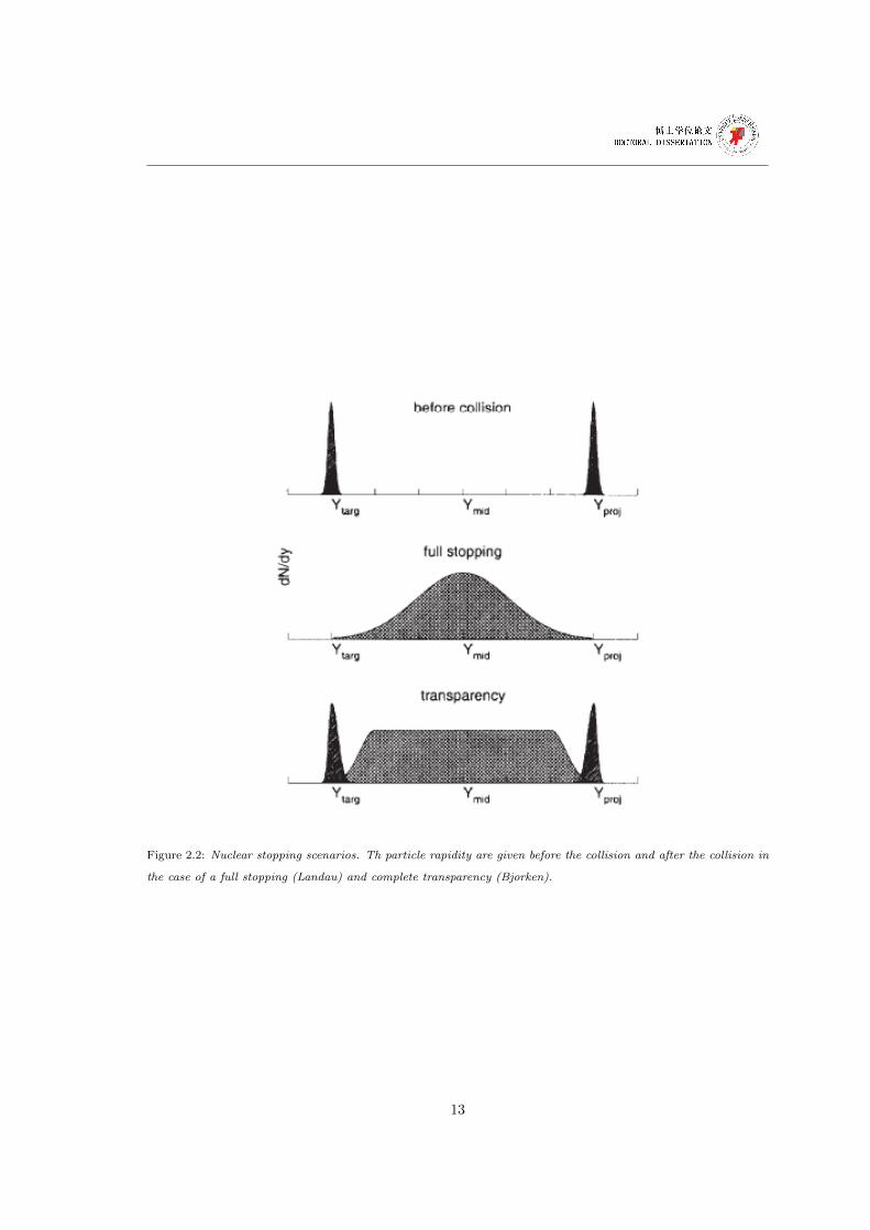
Figure 2.2: Nuclear stopping scenarios. Th particle rapidity are given before the collision and after the collision in

the case of a full stopping (Landau) and complete transparency (Bjorken).

13

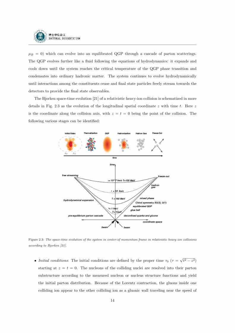
µB = 0) which can evolve into an equilibrated QGP through a cascade of parton scatterings.

The QGP evolves further like a fluid following the equations of hydrodynamics: it expands and

cools down until the system reaches the critical temperature of the QGP phase transition and

condensates into ordinary hadronic matter. The system continues to evolve hydrodynamically

until interactions among the constituents cease and final state particles freely stream towards the

detectors to provide the final state observables.

The Bjorken space-time evolution [21] of a relativistic heavy-ion collision is schematized in more

details in Fig. 2.3 as the evolution of the longitudinal spatial coordinate z with time t. Here z

is the coordinate along the collision axis, with z = t = 0 being the point of the collision. The

following various stages can be identified:

Figure 2.3: The space-time evolution of the system in center-of momentum frame in relativistic heavy ion collisions

according to Bjorken [21].

• Initial conditions: The initial conditions are defined by the proper time τ0 (τ =√t2 − z2)

starting at z = t = 0. The nucleons of the colliding nuclei are resolved into their parton

substructure according to the measured nucleon or nucleus structure functions and yield

the initial parton distribution. Because of the Lorentz contraction, the gluons inside one

colliding ion appear to the other colliding ion as a gluonic wall traveling near the speed of

14

light and with densities increasing strongly with the collision energy or equivalently at very

small values of x = 2pT√s� 0.1 (x is the fraction of the longitudinal momentum carried by

the parton).

• Pre-equilibrium: In the pre-equilibrium phase the dynamic of partons is described as a cascade

of freely colliding partons. The space-time evolution of the partons distribution is described

by a transport equation where the collision term is described by QCD processes calculated

within the pertubative approximation. The main hypothesis (factorization theorem) is that

the collisions during the cascade are independent of each other and that the pertubative

aspects (the scattering) and the non-pertubative aspects (the structure function) can be

factorized. This stage features the creation of high transverse momentum (pT ) partons,

which can be used to probe the subsequent stages of the collision through their interaction

with the nuclear medium.

• Chemical and thermal equilibrium: The subsequent multiple parton scattering brings the

matter to local equilibrium. Chemical equilibrium is driven by the two-body reactions and

gluon multiplication and its inverse process, gluon fusion. After the time τ0 where the system

is at thermal equilibrium, the system evolves to the law of hydrodynamics. Relativistic

hydrodynamics is then used to describe the expansion of the hot and compressed central

region. Until the interacting medium is thermalized, the hot and dense matter, consisting of

quarks, anti-quarks and gluons (the QGP) will be formed. The average energy deposited by

unit of rapidity d < E > /dy reached at thermal equilibrium (t = τ0) is estimated using the

rapidity y definition:

y =1

2lnE + pzE − pz

,

=1

2lnt+ z

t− z(vz =

z

t=pzE

), (2.1)

as well as the longitudinal thickness, 2d, of the expanding medium and the overlap area S

(S = π(r0A1/3)2, r0 is the nucleon radius and A is the nucleus number) as:

E =d < E >

dy∆y,

=d < E >

dy

2d

τ0, (2.2)

15

The energy density can be deduced from the measured particle density, dN/dy ,

ε0 =E

2dS,

=1

S

1

τ0

d < E >

dy,

=1

τ0πr20A2/3

d < E >

dy,

=< ET >

τ0πr20A2/3

dN

dy, (2.3)

where, < ET > is the mean transverse energy of the produced particles. In this equation,

d<E>dy |y=0 =< ET > ·dN/dy is assumed at y = 0 [22].

• Hadronization and freeze-out: The system continues to expand and cool down fast through

strong interactions and reaches quickly the critical temperature Tc ' 170 MeV, where the

hadronization takes place and a hadron gas is formed. The created hadron gas expands

and cools till the distance between hadrons is large enough so that they stop interacting

(freeze-out temperature, Tf ∼ 100 MeV) and stream out of the collision region.

2.1.1 Centrality

To characterize the relativistic heavy-ion collisions and to study the nuclear phenomena in the

collisions systematically, the centrality parameter is used. The degree of centrality C of a given

subset of collisions is expressed at a given impact parameter bC as:

C =

∫ bC0

2πσAAbdb∫ bmax0

σAA. (2.4)

It represents the probability that the collision occurs for impact parameter b < bC [23]. Since

the impact parameter is not directly measurable, experimentally one can measure C through the

number of participants Npart or the number of spectators Nspec. The number of participants Npart

is the number of nucleons contributing to the collision in the participant overlap region. The

number of spectators can be deduced from measurement at zero degree with respect to the beam

axis by calorimetry techniques and the number of participants through the measurement of the

number of low pT charged particles emitted in the transverse direction. It refers collectively to

the soft processes producing these particles. Hard processes scale with the number of collisions

Ncoll, i.e. the number of participants which have experienced at least one scattering. In a central

collision, b is equal to zero and the number of participants Npart is equal to the total number of

nucleons in both nuclei. The term central collisions refers to collisions with 0 < C < 0.1 and

16

peripheral collisions are defined with 0.9 < C < 1. Collisions without any selection in C are called

minimum-bias collisions. The average number of nucleon-nucleon collisions < Ncoll > at an impact

parameter b is given by < Ncoll(b) >= TAA(b)σpp, where σpp is the total proton-proton inelastic

cross section.

For each centrality, the geometric parameters of nucleus-nucleus collisions (Npart, Ncoll, TAA(b),

and b) are estimated with the Glauber model [24]. TAA(b) is the nuclear overlapping function

defined as:

TAA(b) =

∫dr2TA(r)TA(|r− b|), (2.5)

where

TA(r) =

∫dzρA(r, z). (2.6)

The nucleon distribution inside the nucleus is assumed to follow a Woods-Saxon density profile:

ρA(r) =ρ0

1 + exp ( r−r0a ), (2.7)

where r is the distance from a given point of the nucleus to the center of the nucleus. The

parameters a and r0 are obtained empirically from electron scattering experiments. The model

provides a quantitative consideration of the geometrical configuration of the nuclei when they

collide, and basically describe the nucleus-nucleus interaction in terms of the elementary nucleon-

nucleon cross section measured in proton–proton collisions.

2.2 Particle Production

Properties, such as phase space distribution and relative abundance of particle species, of the

final state hadrons provide significant information of the heavy ion collision dynamics and reflect

the properties of the colliding system at the time of freeze-out. We will discuss separately soft

probes reflecting the collective dynamics of the collision at equilibrium and hard probes reflecting

the dynamics at the partonic level during the pre-equilibrium phase of the collision.

2.2.1 Soft Particles Production

In high energy heavy-ion collisions, local equilibrium and collective behavior are established

following multiple scatterings. The final state particle species ratio can be interpreted in terms

of chemical equilibrium of the system at chemical freeze-out. These ratios can be described by

thermodynamical statistical models, based for example on the grand canonical ensemble describing

17

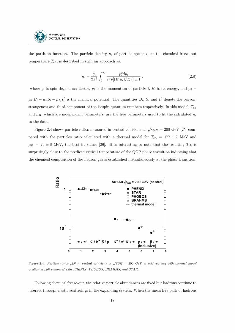
the partition function. The particle density ni of particle specie i, at the chemical freeze-out

temperature Tch, is described in such an approach as:

ni =gi

2π2

∫ ∞0

p2i dpiexp[(Eiµi)/Tch]± 1

. (2.8)

where gi is spin degeneracy factor, pi is the momentum of particle i, Ei is its energy, and µi =

µBBi − µSSi − µI3I3i is the chemical potential. The quantities Bi, Si and I3i denote the baryon,

strangeness and third-component of the isospin quantum numbers respectively. In this model, Tch

and µB , which are independent parameters, are the free parameters used to fit the calculated ni

to the data.

Figure 2.4 shows particle ratios measured in central collisions at√sNN = 200 GeV [25] com-

pared with the particles ratio calculated with a thermal model for Tch = 177 ± 7 MeV and

µB = 29 ± 8 MeV, the best fit values [26]. It is interesting to note that the resulting Tch is

surprisingly close to the prediced critical temperature of the QGP phase transition indicating that

the chemical composition of the hadron gas is established instantaneously at the phase transition.

Figure 2.4: Particle ratios [25] in central collisions at√sNN = 200 GeV at mid-rapidity with thermal model

prediction [26] compared with PHENIX, PHOBOS, BRAHMS, and STAR.

Following chemical freeze-out, the relative particle abundances are fixed but hadrons continue to

interact through elastic scatterings in the expanding system. When the mean free path of hadrons

18

becomes comparable to the size of the system, kinetic freeze-out is reached and the momentum of

hadrons is frozen. Kinetic equilibration is visible predominantly in the transverse degrees of freedom

and temperatures can be measured from the spectral slope of the low energy part of the transverse

momentum (pT =√p2x + p2y, z being the beam axis) or transverse mass (mT =

√m2

0 + p2T , where

m0 is the rest mass) distributions. The equation of state, the energy density ε versus temperature

T, can be probed experimentally by the correlation of the mean transverse momentum < pT >

of hadrons and the rapidity particle density dN/dy or the transverse energy density dN/dET

generated in the collision. If a phase transition occurs, one expects to observe a rupture in the

monotonously rise of pT and a saturation of < pT > when the number of degrees of freedom

changes.

The invariant cross section for particles with four-momentum, (E, px, py, pz), is given by,

Ed3σ

dp3= E

d3σ

dpxdpydpz,

=d3σ

pT dpT dydφ,

=1

2πpT

d2σ

dpT dy, (2.9)

where φ is the azimuthal angle of the observed particles.

2.2.2 Hard Particles Production

High pT hadrons, remnants of high pT partons produced in the early phase of the collision

through hard scattering are particularly interesting probes of the medium created concurrently in

heavy-ion collisions.

The cross section for the production of these high-pT hadrons is calculated within the factoriza-

tion theorem separating pQCD calculable parton cross section (σ) and non-perturbative processes

such as the parton distribution function (f) and the fragmentation function (D) (see Fig. 2.5). The

production cross section of a hadron h in a nucleus-nucleus collision A + B is, in this formalism,

written as:

σAB→hX =∑abcd

∫dxadxbdzc · fa/A(xa, Q

2) · fb/B(xb, Q2) · σ(ab → cd) · D0

h/cd(zcd, Q2), (2.10)

where fa/A(xa, Q2) (fb/B(xb, Q

2)) is the Parton Distribution Function (PDF) of the initial parton

”a” (”b”) in the initial nucleus ”A” (”B”), Dh/cd(zcd, Q2) is the Fragmentation Function (FF)

19

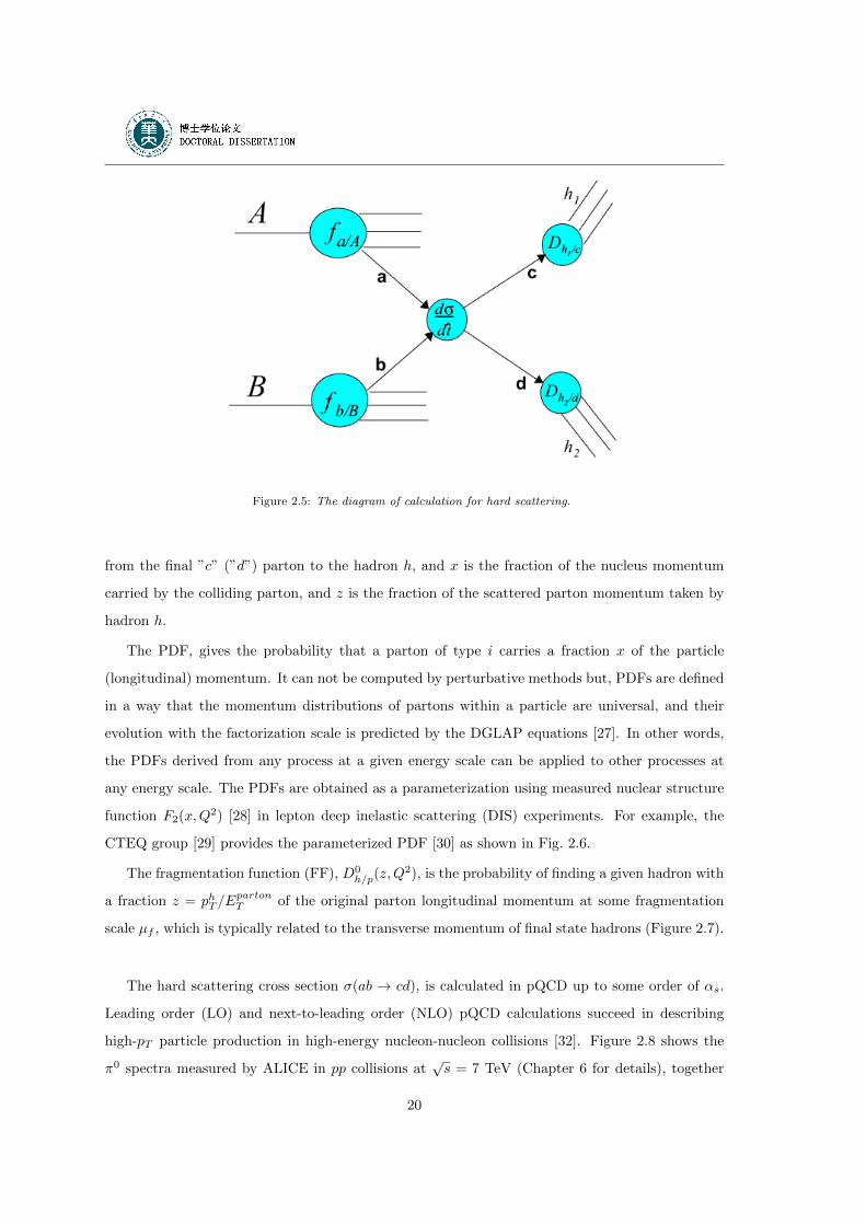
Figure 2.5: The diagram of calculation for hard scattering.

from the final ”c” (”d”) parton to the hadron h, and x is the fraction of the nucleus momentum

carried by the colliding parton, and z is the fraction of the scattered parton momentum taken by

hadron h.

The PDF, gives the probability that a parton of type i carries a fraction x of the particle

(longitudinal) momentum. It can not be computed by perturbative methods but, PDFs are defined

in a way that the momentum distributions of partons within a particle are universal, and their

evolution with the factorization scale is predicted by the DGLAP equations [27]. In other words,

the PDFs derived from any process at a given energy scale can be applied to other processes at

any energy scale. The PDFs are obtained as a parameterization using measured nuclear structure

function F2(x,Q2) [28] in lepton deep inelastic scattering (DIS) experiments. For example, the

CTEQ group [29] provides the parameterized PDF [30] as shown in Fig. 2.6.

The fragmentation function (FF), D0h/p(z,Q

2), is the probability of finding a given hadron with

a fraction z = phT /EpartonT of the original parton longitudinal momentum at some fragmentation

scale µf , which is typically related to the transverse momentum of final state hadrons (Figure 2.7).

The hard scattering cross section σ(ab → cd), is calculated in pQCD up to some order of αs.

Leading order (LO) and next-to-leading order (NLO) pQCD calculations succeed in describing

high-pT particle production in high-energy nucleon-nucleon collisions [32]. Figure 2.8 shows the

π0 spectra measured by ALICE in pp collisions at√s = 7 TeV (Chapter 6 for details), together

20

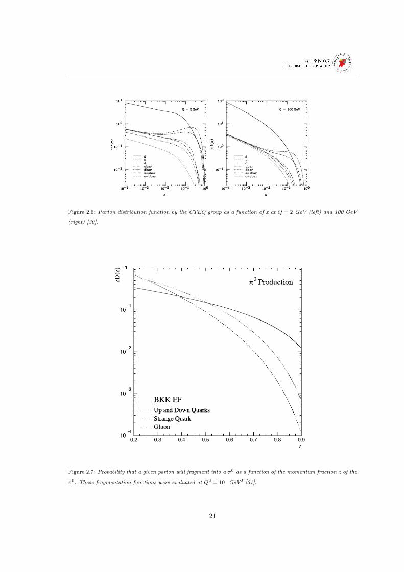
Figure 2.6: Parton distribution function by the CTEQ group as a function of x at Q = 2 GeV (left) and 100 GeV

(right) [30].

Figure 2.7: Probability that a given parton will fragment into a π0 as a function of the momentum fraction z of the

π0. These fragmentation functions were evaluated at Q2 = 10 GeV2 [31].

21

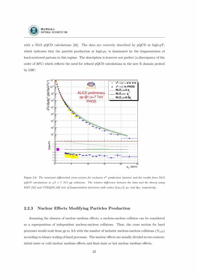
with a NLO pQCD calculations [32]. The data are correctly described by pQCD at high-pT,

which indicates that the particle production at high-pT is dominated by the fragmentation of

hard-scattered partons in this regime. The description is however not perfect (a discrepancy of the

order of 20%) which reflects the need for refined pQCD calculations in the new E domain probed

by LHC.

)­2

c2

(p

b/G

eV

2 t/d

yd

pσ

3d

310

410

510

610

710

810

910

1010

1110

­e+ e­e+ e→γγ→0π

in PHOSγγ→0π

t=2 pµNLO,

t= pµNLO,

t

=0.5pµNLO,

ALICE preliminary

=7 TeVspp @

PHOS

, GeV/cT

p0 5 10 15 20 25

Da

ta/F

it

0

0.2

0.4

0.6

0.8

1

1.2

1.4

Figure 2.8: The invariant differential cross section for inclusive π0 production (points) and the results from NLO

pQCD calculations in√s = 7 TeV pp collisions. The relative difference between the data and the theory using

KKP [33] and CTEQ5M [29] sets of fragmentation functions with scales of pT /2, pT and 2pT respectively.

2.2.3 Nuclear Effects Modifying Particles Production

Assuming the absence of nuclear medium effects, a nucleus-nucleus collision can be considered

as a superposition of independent nucleon-nucleon collisions. Thus, the cross section for hard

processes would scale from pp to AA with the number of inelastic nucleon-nucleon collisions (Ncoll)

according to binary scaling of hard processes. The nuclear effects are usually divided in two sources:

initial state or cold nuclear medium effects and final state or hot nuclear medium effects.

22

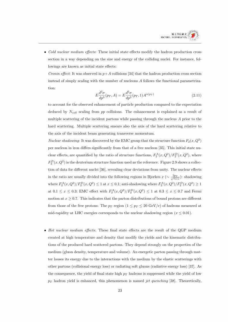
• Cold nuclear medium effects: These initial state effects modify the hadron production cross

section in a way depending on the size and energy of the colliding nuclei. For instance, fol-

lowings are known as initial state effects:

Cronin effect: It was observed in p+A collisions [34] that the hadron production cross section

instead of simply scaling with the number of nucleons A follows the functional parametriza-

tion:

Ed3σ

dp3(pT , A) = E

d3σ

dp3(pT , 1)Aα(pT ) (2.11)

to account for the observed enhancement of particle production compared to the expectation

deduced by Ncoll scaling from pp collisions. The enhancement is explained as a result of

multiple scattering of the incident partons while passing through the nucleus A prior to the

hard scattering. Multiple scattering smears also the axis of the hard scattering relative to

the axis of the incident beam generating transverse momentum.

Nuclear shadowing: It was discovered by the EMC group that the structure function F2(x,Q2)

per nucleon in iron differs significantly from that of a free nucleon [35]. This initial state nu-

clear effects, are quantified by the ratio of structure functions, FA2 (x,Q2)/FD2 (x,Q2), where

FD2 (x,Q2) is the deuterium structure function used as the reference. Figure 2.9 shows a collec-

tion of data for different nuclei [36], revealing clear deviations from unity. The nuclear effects

in the ratio are usually divided into the following regions in Bjorken x (∼ 2pT√sNN

): shadowing

where FA2 (x,Q2)/FD2 (x,Q2) ≤ 1 at x ≤ 0.1; anti-shadowing where FA2 (x,Q2)/FD2 (x,Q2) ≥ 1

at 0.1 ≤ x ≤ 0.3; EMC effect with FA2 (x,Q2)/FD2 (x,Q2) ≤ 1 at 0.3 ≤ x ≤ 0.7 and Fermi

motion at x ≥ 0.7. This indicates that the parton distributions of bound protons are different

from those of the free protons. The pT region (1 ≤ pT ≤ 20 GeV/c) of hadrons measured at

mid-rapidity at LHC energies corresponds to the nuclear shadowing region (x ≤ 0.01).

• Hot nuclear medium effects: These final state effects are the result of the QGP medium

created at high temperature and density that modify the yields and the kinematic distribu-

tions of the produced hard scattered partons. They depend strongly on the properties of the

medium (gluon density, temperature and volume). An energetic parton passing through mat-

ter looses its energy due to the interactions with the medium by the elastic scatterings with

other partons (collisional energy loss) or radiating soft gluons (radiative energy loss) [37]. As

the consequence, the yield of final state high pT hadrons is suppressed while the yield of low

pT hadron yield is enhanced, this phenomenon is named jet quenching [38]. Theoretically,

23

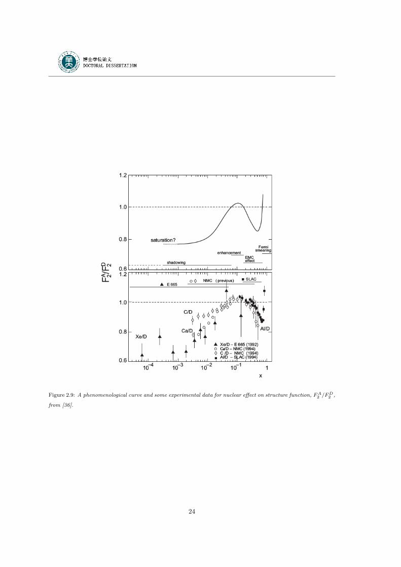
Figure 2.9: A phenomenological curve and some experimental data for nuclear effect on structure function, FA2 /FD2 ,

from [36].

24

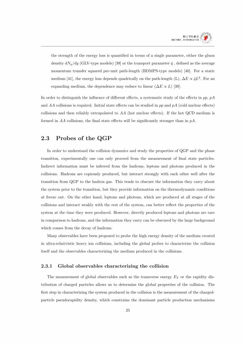
the strength of the energy loss is quantified in terms of a single parameter, either the gluon

density dNg/dy (GLV-type models) [39] or the transport parameter q , defined as the average

momentum transfer squared per-unit path-length (BDMPS-type models) [40]. For a static

medium [41], the energy loss depends quadrically on the path-length (L), ∆E ∝ qL2. For an

expanding medium, the dependence may reduce to linear (∆E ∝ L) [39].

In order to distinguish the influence of different effects, a systematic study of the effects in pp, pA

and AA collisions is required. Initial state effects can be studied in pp and pA (cold nuclear effects)

collisions and then reliably extrapolated to AA (hot nuclear effects). If the hot QCD medium is

formed in AA collisions, the final state effects will be significantly stronger than in pA.

2.3 Probes of the QGP

In order to understand the collision dynamics and study the properties of QGP and the phase

transition, experimentally one can only proceed from the measurement of final state particles.

Indirect information must be inferred from the hadrons, leptons and photons produced in the

collisions. Hadrons are copiously produced, but interact strongly with each other well after the

transition from QGP to the hadron gas. This tends to obscure the information they carry about

the system prior to the transition, but they provide information on the thermodynamic conditions

at freeze out. On the other hand, leptons and photons, which are produced at all stages of the

collisions and interact weakly with the rest of the system, can better reflect the properties of the

system at the time they were produced. However, directly produced leptons and photons are rare

in comparison to hadrons, and the information they carry can be obscured by the large background

which comes from the decay of hadrons.

Many observables have been proposed to probe the high energy density of the medium created

in ultra-relativistic heavy ion collisions, including the global probes to characterize the collision

itself and the observables characterizing the medium produced in the collisions.

2.3.1 Global observables characterizing the collision

The measurement of global observables such as the transverse energy ET or the rapidity dis-

tribution of charged particles allows us to determine the global properties of the collision. The

first step in characterizing the system produced in the collision is the measurement of the charged-

particle pseudorapidity density, which constrains the dominant particle production mechanisms

25

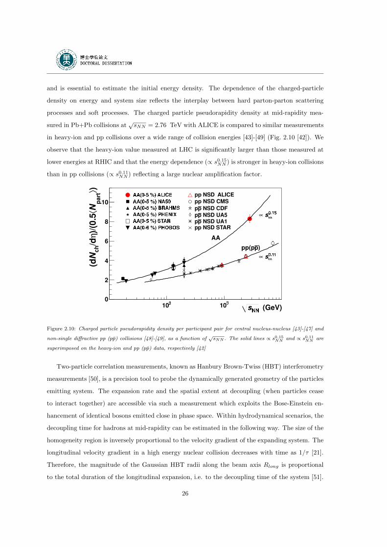
and is essential to estimate the initial energy density. The dependence of the charged-particle

density on energy and system size reflects the interplay between hard parton-parton scattering

processes and soft processes. The charged particle pseudorapidity density at mid-rapidity mea-

sured in Pb+Pb collisions at√sNN = 2.76 TeV with ALICE is compared to similar measurements

in heavy-ion and pp collisions over a wide range of collision energies [43]-[49] (Fig. 2.10 [42]). We

observe that the heavy-ion value measured at LHC is significantly larger than those measured at

lower energies at RHIC and that the energy dependence (∝ s0.15NN ) is stronger in heayy-ion collisions

than in pp collisions (∝ s0.11NN ) reflecting a large nuclear amplification factor.

Figure 2.10: Charged particle pseudorapidity density per participant pair for central nucleus-nucleus [43]-[47] and

non-single diffractive pp (pp) collisions [48]-[49], as a function of√sNN . The solid lines ∝ s0.15NN and ∝ s0.11NN are

superimposed on the heavy-ion and pp (pp) data, respectively [42]

Two-particle correlation measurements, known as Hanbury Brown-Twiss (HBT) interferometry

measurements [50], is a precision tool to probe the dynamically generated geometry of the particles

emitting system. The expansion rate and the spatial extent at decoupling (when particles cease

to interact together) are accessible via such a measurement which exploits the Bose-Einstein en-

hancement of identical bosons emitted close in phase space. Within hydrodynamical scenarios, the

decoupling time for hadrons at mid-rapidity can be estimated in the following way. The size of the

homogeneity region is inversely proportional to the velocity gradient of the expanding system. The

longitudinal velocity gradient in a high energy nuclear collision decreases with time as 1/τ [21].

Therefore, the magnitude of the Gaussian HBT radii along the beam axis Rlong is proportional

to the total duration of the longitudinal expansion, i.e. to the decoupling time of the system [51].

26

The decoupling time extracted from ALICE HBT measurement in central Pb+Pb collisions at

√sNN = 2.76 TeV is shown in Fig. 2.11 [52], together with the results at lower energies [53]-[57].

It is found that the decoupling time τf scales with the cube root of the charged particle pseudora-

pidity density and reaches 10-11 fm/c in central Pb+Pb collisions at√sNN = 2.76 TeV, which is

40% larger than at RHIC. Similarely the homogeneity volume is found to be larger by a factor of

two at the LHC energy than at the RHIC highest energy. We conclude that the fireball formed in

nuclear collisions at the LHC is hotter, lives longer, and expands to a larger size at freeze-out as

compared to lower energies [52].

1/3 >/dch< dN0 2 4 6 8 10 12 14

(fm

/c)

f

0

2

4

6

8

10

12 E895NA49CERESPHENIXPHOBOSSTARALICE

E895NA49CERESPHENIXPHOBOSSTARALICE

Figure 2.11: The decoupling time extracted from Rlong [52]. The ALICE result is compared to those obtained for

central gold and lead collisions at lower energy at the AGS [53], SPS [54]-[55] and RHIC [56]-[57].

2.3.2 Observables characterizing the medium

• Flow Measurements of the collective motion, or flow, of final state particles produced in heay-

ion collisions provide a probe of collective properties of the colliding system. It results from

interactions among the soft particles in the dense medium, and thus provides information on

the equation of state and the transport properties of the matter created in heavy ion collisions.

If particles have a common expanding velocity β, their purely thermal transverse momentum

spectrum is modified by the so called radial flow by a change of the slope parameter T so

that:

T ≈ Tf +1

2mβ2, (2.12)

27

where Tf is a measure of the freeze-out temperature and m is the mass of particles. Other

components of the flow are measured through the azimuthal distribution of particles with

respect to the reaction plane (φ− φ0, the reaction plane is defined by the impact parameter

vector b and the direction of the colliding beams z) . The flow components are deduced by

describing this distribution as a Fourier expansion [58]:

dN

dφ=

1

2π{1 + 2

∑n

νn cos[n(φ− φ0)]} . (2.13)

Figure 2.12: The ellipsoidal shape of participant in non-central high energy nucleus-nucleus collisions.

The second harmonic coefficient ν2 of Eq. 2.13 is called elliptic flow and is sensitive to the

geometry of the collision region in the early stage of the collisions (Fig. 2.12). The larger

pressure gradient in the small axis direction of the almond shape results in a larger boost

of the particles towards this direction. This causes an increase of the particle emission

in the reaction plane with respect to those emitted perpendicularly to the reaction plane.

Elliptic flow is a fundamental observable since it directly reflects the initial spatial anisotropy,

of the nuclear overlap region in the transverse plane, directly translated into the observed

momentum distribution of identified particles. Since the spatial anisotropy is largest at

the beginning of the evolution, elliptic flow is especially sensitive to the early stages of

system evolution. A measurement of elliptic flow thus provides access to the fundamental

thermalization time scale and thermodynamics properties of the medium in the early stages

of a relativistic heavy-ion collision.

28

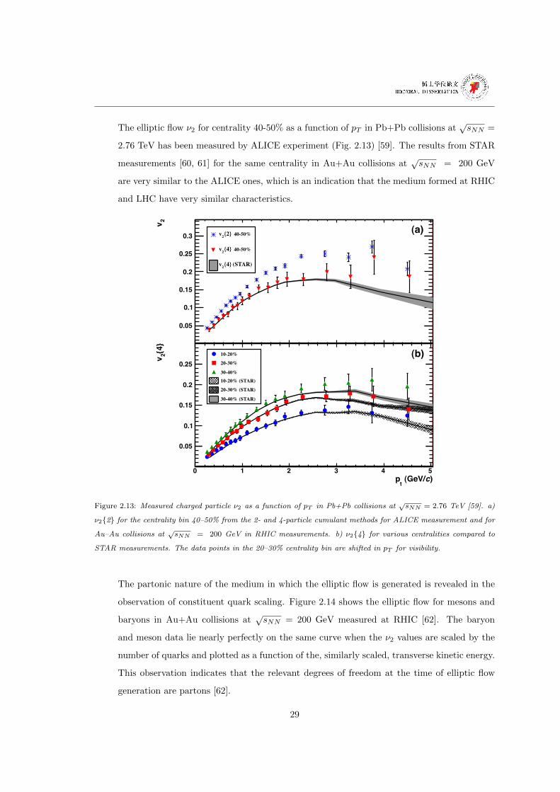
The elliptic flow ν2 for centrality 40-50% as a function of pT in Pb+Pb collisions at√sNN =

2.76 TeV has been measured by ALICE experiment (Fig. 2.13) [59]. The results from STAR

measurements [60, 61] for the same centrality in Au+Au collisions at√sNN = 200 GeV

are very similar to the ALICE ones, which is an indication that the medium formed at RHIC

and LHC have very similar characteristics.

)c (GeV/t

p0 1 2 3 4 5

2v

0.05

0.1

0.15

0.2

0.25

0.3 {2}2v

{4}2v

(STAR){4}2v

)c (GeV/t

p0 1 2 3 4 5

{4}

2v

0.05

0.1

0.15

0.2

0.2510-20%

20-30%

30-40%10-20% (STAR)

20-30% (STAR)

30-40% (STAR)

(a)

(b)

40-50%

40-50%

Figure 2.13: Measured charged particle ν2 as a function of pT in Pb+Pb collisions at√sNN = 2.76 TeV [59]. a)

ν2{2} for the centrality bin 40–50% from the 2- and 4-particle cumulant methods for ALICE measurement and for

Au–Au collisions at√sNN = 200 GeV in RHIC measurements. b) ν2{4} for various centralities compared to

STAR measurements. The data points in the 20–30% centrality bin are shifted in pT for visibility.

The partonic nature of the medium in which the elliptic flow is generated is revealed in the

observation of constituent quark scaling. Figure 2.14 shows the elliptic flow for mesons and

baryons in Au+Au collisions at√sNN = 200 GeV measured at RHIC [62]. The baryon

and meson data lie nearly perfectly on the same curve when the ν2 values are scaled by the

number of quarks and plotted as a function of the, similarly scaled, transverse kinetic energy.

This observation indicates that the relevant degrees of freedom at the time of elliptic flow

generation are partons [62].

29

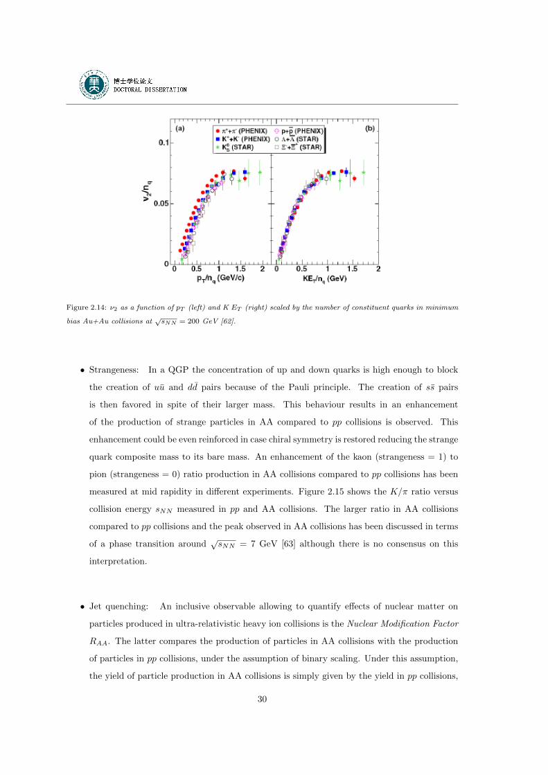
Figure 2.14: ν2 as a function of pT (left) and K ET (right) scaled by the number of constituent quarks in minimum

bias Au+Au collisions at√sNN = 200 GeV [62].

• Strangeness: In a QGP the concentration of up and down quarks is high enough to block

the creation of uu and dd pairs because of the Pauli principle. The creation of ss pairs

is then favored in spite of their larger mass. This behaviour results in an enhancement

of the production of strange particles in AA compared to pp collisions is observed. This

enhancement could be even reinforced in case chiral symmetry is restored reducing the strange

quark composite mass to its bare mass. An enhancement of the kaon (strangeness = 1) to

pion (strangeness = 0) ratio production in AA collisions compared to pp collisions has been

measured at mid rapidity in different experiments. Figure 2.15 shows the K/π ratio versus

collision energy sNN measured in pp and AA collisions. The larger ratio in AA collisions

compared to pp collisions and the peak observed in AA collisions has been discussed in terms

of a phase transition around√sNN = 7 GeV [63] although there is no consensus on this

interpretation.

• Jet quenching: An inclusive observable allowing to quantify effects of nuclear matter on

particles produced in ultra-relativistic heavy ion collisions is the Nuclear Modification Factor

RAA. The latter compares the production of particles in AA collisions with the production

of particles in pp collisions, under the assumption of binary scaling. Under this assumption,

the yield of particle production in AA collisions is simply given by the yield in pp collisions,

30

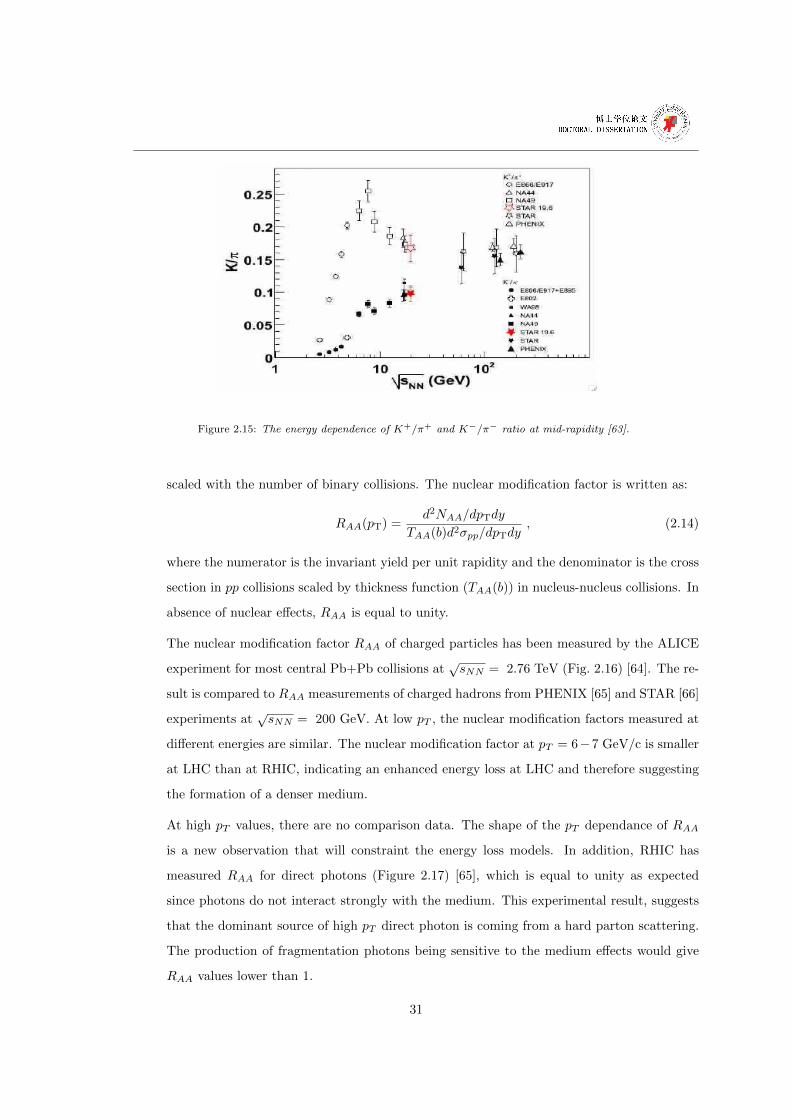
Figure 2.15: The energy dependence of K+/π+ and K−/π− ratio at mid-rapidity [63].

scaled with the number of binary collisions. The nuclear modification factor is written as:

RAA(pT) =d2NAA/dpTdy

TAA(b)d2σpp/dpTdy, (2.14)

where the numerator is the invariant yield per unit rapidity and the denominator is the cross

section in pp collisions scaled by thickness function (TAA(b)) in nucleus-nucleus collisions. In

absence of nuclear effects, RAA is equal to unity.

The nuclear modification factor RAA of charged particles has been measured by the ALICE

experiment for most central Pb+Pb collisions at√sNN = 2.76 TeV (Fig. 2.16) [64]. The re-

sult is compared to RAA measurements of charged hadrons from PHENIX [65] and STAR [66]

experiments at√sNN = 200 GeV. At low pT , the nuclear modification factors measured at

different energies are similar. The nuclear modification factor at pT = 6−7 GeV/c is smaller

at LHC than at RHIC, indicating an enhanced energy loss at LHC and therefore suggesting

the formation of a denser medium.

At high pT values, there are no comparison data. The shape of the pT dependance of RAA

is a new observation that will constraint the energy loss models. In addition, RHIC has

measured RAA for direct photons (Figure 2.17) [65], which is equal to unity as expected

since photons do not interact strongly with the medium. This experimental result, suggests

that the dominant source of high pT direct photon is coming from a hard parton scattering.

The production of fragmentation photons being sensitive to the medium effects would give

RAA values lower than 1.

31

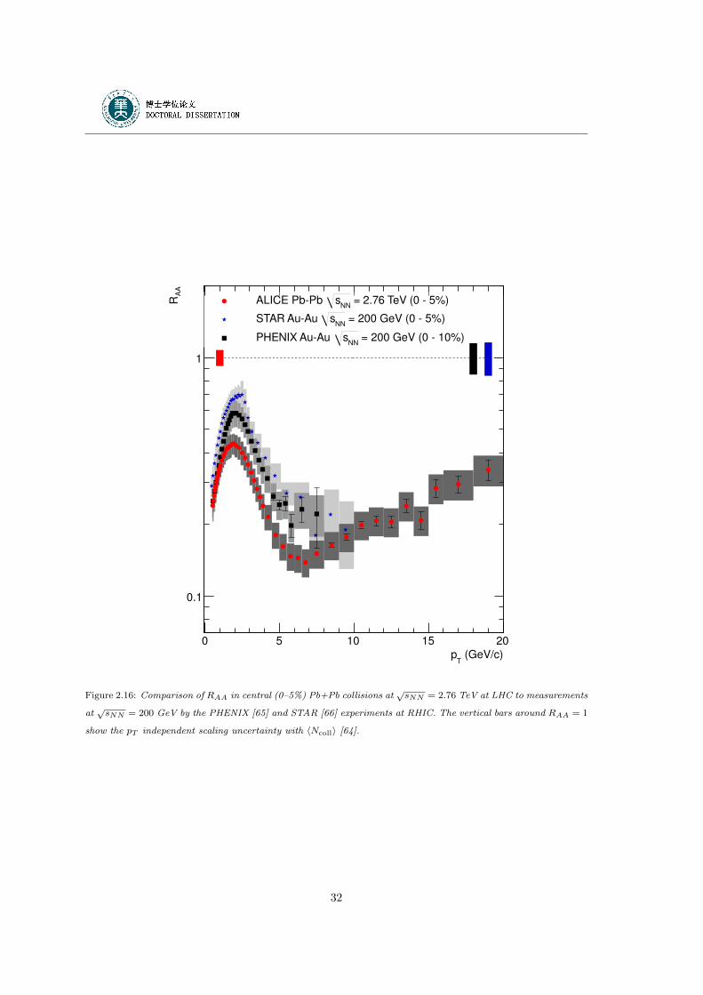
(GeV/c)T

p

0 5 10 15 20

AA

R

0.1

1

= 2.76 TeV (0 ­ 5%)NN

sALICE Pb­Pb

= 200 GeV (0 ­ 5%)NN

sSTAR Au­Au

= 200 GeV (0 ­ 10%)NN

sPHENIX Au­Au

Figure 2.16: Comparison of RAA in central (0–5%) Pb+Pb collisions at√sNN = 2.76 TeV at LHC to measurements

at√sNN = 200 GeV by the PHENIX [65] and STAR [66] experiments at RHIC. The vertical bars around RAA = 1

show the pT independent scaling uncertainty with 〈Ncoll〉 [64].

32

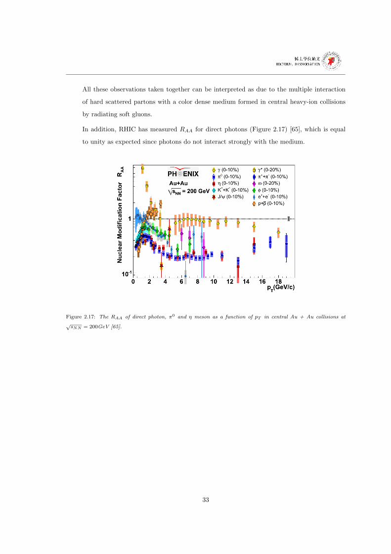
All these observations taken together can be interpreted as due to the multiple interaction

of hard scattered partons with a color dense medium formed in central heavy-ion collisions

by radiating soft gluons.

In addition, RHIC has measured RAA for direct photons (Figure 2.17) [65], which is equal

to unity as expected since photons do not interact strongly with the medium.

Figure 2.17: The RAA of direct photon, π0 and η meson as a function of pT in central Au + Au collisions at√sNN = 200GeV [65].

33

34

Chapter 3

Jet and Particle Correlations

The production of hadrons in heavy-ion collisions is described in QCD by the interaction

of quarks and gluons. The hard QCD scattering of quarks and gluons (distance scale of

1/pT ≤ 0.1 fm) leads to the production of jets in the final state. Jets are defined by the

hadrons originating from the fragmentation of the hard scattered parton and observed in a

localized spatial area. The propagation of the hard scattered parton through the hot and

dense QCD medium produced in heavy-ion collisions modifies the parton transverse momen-

tum, and generates acoplanarity and energy imbalance of the two back-to-back scattered

partons due to multiple scattering and soft gluon radiation. The modifications experienced

by the hard scattered partons traversing the medium is imprinted in the fragmentation of the

final state high transverse momentum hadrons and can be revealed by comparing the same

observables measured in proton-proton collisions and in heavy-ion collisions. Contemporary

jet measurements imply jet reconstruction algorithms to determine the full energy of the jet

on an event-by-event basis. However, such a reconstruction is quite challenging in heavy-ion

events due to the copious production of final state particles in soft multi-scattering processes

which constitute the underlying events. Particle correlations are considered as an alternative

approach to study jets.

In this chapter, the two-particle correlation technique will be first discussed, then jet kine-

matics will be explained, and finally, the golden channel ”γ+Jet” will be emphasized.

35

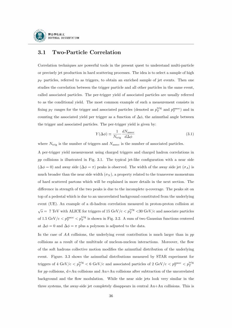
3.1 Two-Particle Correlation

Correlation techniques are powerful tools in the present quest to understand multi-particle

or precisely jet production in hard scattering processes. The idea is to select a sample of high

pT particles, referred to as triggers, to obtain an enriched sample of jet events. Then one

studies the correlation between the trigger particle and all other particles in the same event,

called associated particles. The per-trigger yield of associated particles are usually referred

to as the conditional yield. The most common example of such a measurement consists in

fixing pT ranges for the trigger and associated particles (denoted as ptrigT and passocT ) and in

counting the associated yield per trigger as a function of ∆φ, the azimuthal angle between

the trigger and associated particles. The per-trigger yield is given by:

Y (∆φ) ≡ 1

Ntrig

dNassoc

d∆φ(3.1)

where Ntrig is the number of triggers and Nassoc is the number of associated particles.

A per-trigger yield measurement using charged triggers and charged hadron correlations in

pp collisions is illustrated in Fig. 3.1. The typical jet-like configuration with a near side

(∆φ = 0) and away side (∆φ = π) peaks is observed. The width of the away side jet (σA) is

much broader than the near side width (σN ), a property related to the transverse momentum

of hard scattered partons which will be explained in more details in the next section. The

difference in strength of the two peaks is due to the incomplete η-coverage. The peaks sit on

top of a pedestal which is due to an uncorrelated background constituted from the underlying

event (UE). An example of a di-hadron correlation measured in proton-proton collision at√s = 7 TeV with ALICE for triggers of 15 GeV/c < ptrigT <30 GeV/c and associate particles

of 1.5 GeV/c < passocT < ptrigT is shown in Fig. 3.2. A sum of two Gaussian functions centered

at ∆φ = 0 and ∆φ = π plus a polynom is adjusted to the data.

In the case of AA collisions, the underlying event contribution is much larger than in pp

collisions as a result of the multitude of nucleon-nucleon interactions. Moreover, the flow

of the soft hadrons collective motion modifies the azimuthal distribution of the underlying

event. Figure. 3.3 shows the azimuthal distributions measured by STAR experiment for

triggers of 4 GeV/c < ptrigT < 6 GeV/c and associated particles of 2 GeV/c < passocT < ptrigT

for pp collisions, d+Au collisions and Au+Au collisions after subtraction of the uncorrelated

background and the flow modulation. While the near side jets look very similar in the

three systems, the away-side jet completely disappears in central Au+Au collisions. This is

36

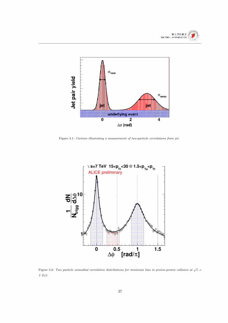
Figure 3.1: Cartoon illustrating a measurement of two-particle correlations from jet.

]π [rad/φ∆0 0.5 1 1.5

φ∆

ddN

tr

igg

N1

1

10

Tt<p

Ta 1.5<p⊗<30

Tt=7 TeV 15<ps

ALICE preliminary

Figure 3.2: Two particle azimuthal correlation distributions for minimum bias in proton-proton collision at√s =

7 TeV.

37

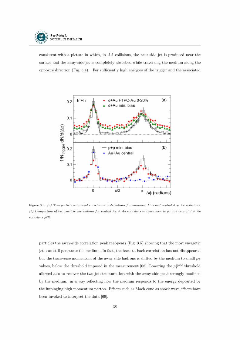
consistent with a picture in which, in AA collisions, the near-side jet is produced near the

surface and the away-side jet is completely absorbed while traversing the medium along the

opposite direction (Fig. 3.4). For sufficiently high energies of the trigger and the associated

Figure 3.3: (a) Two particle azimuthal correlation distributions for minimum bias and central d + Au collisions.

(b) Comparison of two particle correlations for central Au + Au collisions to those seen in pp and central d + Au

collisions [67].

particles the away-side correlation peak reappears (Fig. 3.5) showing that the most energetic

jets can still penetrate the medium. In fact, the back-to-back correlation has not disappeared

but the transverse momentum of the away side hadrons is shifted by the medium to small pT

values, below the threshold imposed in the measurement [68]. Lowering the passocT threshold

allowed also to recover the two-jet structure, but with the away side peak strongly modified

by the medium. in a way reflecting how the medium responds to the energy deposited by

the impinging high momentum parton. Effects such as Mach cone as shock wave effects have

been invoked to interpret the data [69].

38

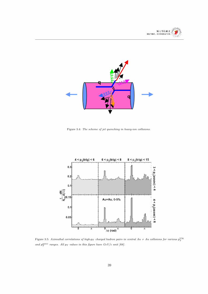
q

q

Figure 3.4: The scheme of jet quenching in heavy-ion collisions.

Figure 3.5: Azimuthal correlations of high-pT charged hadron pairs in central Au + Au collisions for various ptrigT

and passocT ranges. All pT values in this figure have GeV/c unit [68].

39

3.2 Jet Properties

Knowledge of the jet fragmentation process in the vacuum (measured in pp or e+e− collision)

is useful not only as a reference measurement for a similar analysis in heavy-ion collisions, but

also to constrain pQCD calculations (the fragmentation distribution involves soft processes

that cannot be calculated by pQCD and is parametrized instead). The hard scattering is

treated as a 2→ 2 process (1 + 2→ 3 + 4) where the two incoming partons collide at center-

of-mass energy s and the two outgoing partons (jets) are emitted back-to-back with equal

magnitude of transverse momentum pT = s/2 sin θ∗, where θ∗ is the center of mass scattering

angle. s is related to the total pp collision center-of-mass energy√s as s = x1x2s, where

x1,2 is the relative fraction of the proton momentum carried by the scattering partons. The

distribution of the x1 - x2 value is quite broad, hence the proton-proton and parton-parton

center-of-mass frame do not coincide.

The parameters describing the 2→ 2 hard scattering kinematics (Fig. 3.6) are the following:

– ~ptrigT is the trigger particle momentum;

– ~pnearT is the jet (parton) momentum which fragments into the the trigger particle;

– ~passocT is the associated particle with momentum which results either from the fragmen-

tation of the trigger jet (near-side correlation), or from the away-side jet (parton);

– ~pawayT is the momentum of the away side parton;

– jT = jTy +jTz is the momentum of the trigger particle with respect to the trigger parton

direction, y denotes the transverse component and z the longitudinal component; pout

is the transverse component of the the associated particle with respect to the trigger

particle momentum;

– ∆φ is the azimuthal angle between the trigger and the associated particle: pout =

|passocT |sin(∆φ)

At the partonic level, the back-to-back partons produced in a 2→ 2 hard process are balanced

in momentum (pnearT = pawayT ). However this ideal back-to-back azimuthal kinematics is mod-

ified in pp collisions by the finite transverse momentum (kT ) which results in an acoplanarity

and momentum imbalance between the outgoing jets. This acoplanarity is quantified by the

momentum of the jet pair < p2T >pair= 2 < k2T > (see Fig. 3.6) [70]. The net transverse

40

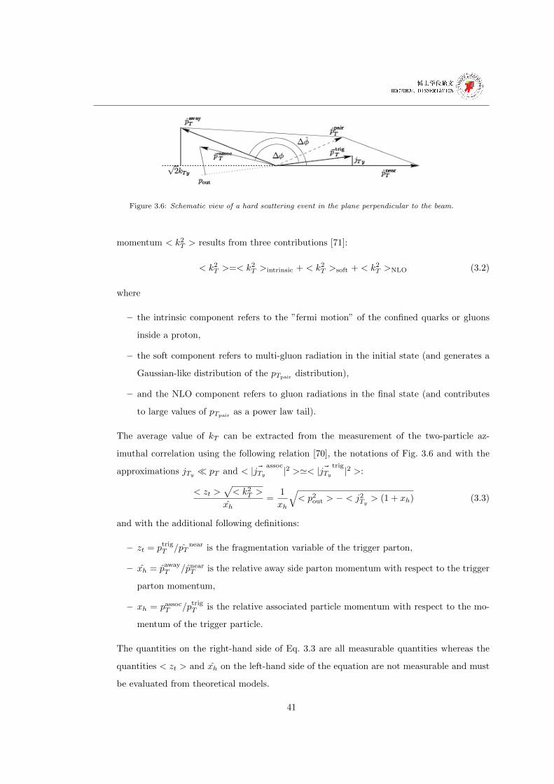
Figure 3.6: Schematic view of a hard scattering event in the plane perpendicular to the beam.

momentum < k2T > results from three contributions [71]:

< k2T >=< k2T >intrinsic + < k2T >soft + < k2T >NLO (3.2)

where

– the intrinsic component refers to the ”fermi motion” of the confined quarks or gluons

inside a proton,

– the soft component refers to multi-gluon radiation in the initial state (and generates a

Gaussian-like distribution of the pTpairdistribution),

– and the NLO component refers to gluon radiations in the final state (and contributes

to large values of pTpairas a power law tail).

The average value of kT can be extracted from the measurement of the two-particle az-

imuthal correlation using the following relation [70], the notations of Fig. 3.6 and with the

approximations jTy � pT and < | ~jTyassoc|2 >'< | ~jTy

trig|2 >:

< zt >√< k2T >

xh=

1

xh

√< p2out > − < j2Ty > (1 + xh) (3.3)

and with the additional following definitions:

– zt = ptrigT /pTnear is the fragmentation variable of the trigger parton,

– xh = pawayT /pnearT is the relative away side parton momentum with respect to the trigger

parton momentum,

– xh = passocT /ptrigT is the relative associated particle momentum with respect to the mo-

mentum of the trigger particle.

The quantities on the right-hand side of Eq. 3.3 are all measurable quantities whereas the

quantities < zt > and xh on the left-hand side of the equation are not measurable and must

be evaluated from theoretical models.

41

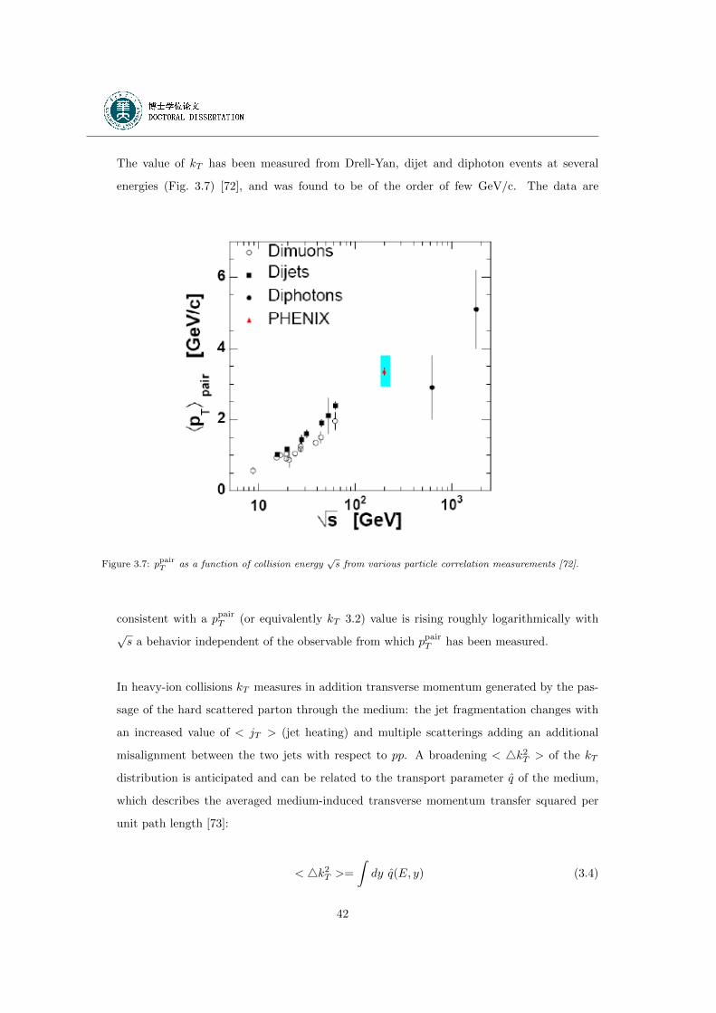
The value of kT has been measured from Drell-Yan, dijet and diphoton events at several

energies (Fig. 3.7) [72], and was found to be of the order of few GeV/c. The data are

Figure 3.7: ppairT as a function of collision energy√s from various particle correlation measurements [72].

consistent with a ppairT (or equivalently kT 3.2) value is rising roughly logarithmically with√s a behavior independent of the observable from which ppairT has been measured.

In heavy-ion collisions kT measures in addition transverse momentum generated by the pas-

sage of the hard scattered parton through the medium: the jet fragmentation changes with

an increased value of < jT > (jet heating) and multiple scatterings adding an additional

misalignment between the two jets with respect to pp. A broadening < 4k2T > of the kT

distribution is anticipated and can be related to the transport parameter q of the medium,

which describes the averaged medium-induced transverse momentum transfer squared per

unit path length [73]:

< 4k2T >=

∫dy q(E, y) (3.4)

42

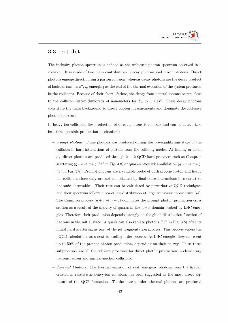
3.3 γ+ Jet

The inclusive photon spectrum is defined as the unbiased photon spectrum observed in a

collision. It is made of two main contributions: decay photons and direct photons. Direct

photons emerge directly from a parton collision, whereas decay photons are the decay product

of hadrons such as π0, η, emerging at the end of the thermal evolution of the system produced

in the collisions. Because of their short lifetime, the decay from neutral mesons occurs close

to the collision vertex (hundreds of nanometers for Eπ > 1 GeV). These decay photons

constitute the main background to direct photon measurements and dominate the inclusive

photon spectrum.

In heavy-ion collisions, the production of direct photons is complex and can be categorized

into three possible production mechanisms:

– prompt photons: These photons are produced during the pre-equilibrium stage of the

collision in hard interactions of partons from the colliding nuclei. At leading order in

αs, direct photons are produced through 2→ 2 QCD hard processes such as Compton

scattering (g+q → γ+q, ”a” in Fig. 3.8) or quark-antiquark annihilation (q+ q → γ+g,

”b” in Fig. 3.8). Prompt photons are a valuable probe of both proton-proton and heavy

ion collisions since they are not complicated by final state interactions in contrast to

hadronic observables. Their rate can be calculated by perturbative QCD techniques

and their spectrum follows a power law distribution at large transverse momentum [74].

The Compton process (g + q → γ + q) dominates the prompt photon production cross

section as a result of the scarcity of quarks in the low x domain probed by LHC ener-

gies. Therefore their production depends strongly on the gluon distribution function of

hadrons in the initial state. A quark can also radiate photons (”c” in Fig. 3.8) after its

initial hard scattering as part of the jet fragmentation process. This process enters the

pQCD calculations as a next-to-leading order process. At LHC energies they represent

up to 50% of the prompt photon production, depending on their energy. These three

subprocesses are all the relevant processes for direct photon production in elementary

hadron-hadron and nuclear-nuclear collisions.

– Thermal Photons: The thermal emission of real, energetic photons from the fireball

created in relativistic heavy-ion collisions has been suggested as the most direct sig-

nature of the QGP formation. To the lowest order, thermal photons are produced

43

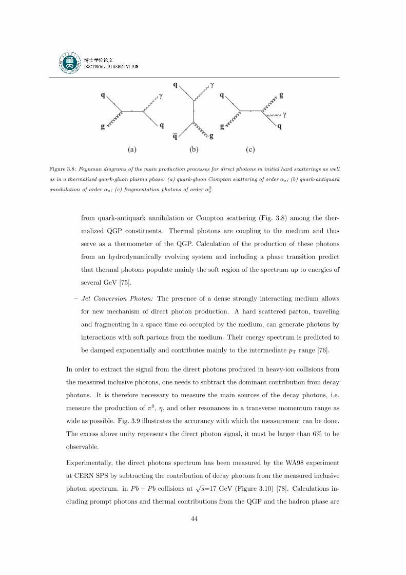
Figure 3.8: Feynman diagrams of the main production processes for direct photons in initial hard scatterings as well

as in a thermalized quark-gluon plasma phase: (a) quark-gluon Compton scattering of order αs; (b) quark-antiquark

annihilation of order αs; (c) fragmentation photons of order α2s.

from quark-antiquark annihilation or Compton scattering (Fig. 3.8) among the ther-

malized QGP constituents. Thermal photons are coupling to the medium and thus

serve as a thermometer of the QGP. Calculation of the production of these photons

from an hydrodynamically evolving system and including a phase transition predict

that thermal photons populate mainly the soft region of the spectrum up to energies of

several GeV [75].

– Jet Conversion Photon: The presence of a dense strongly interacting medium allows

for new mechanism of direct photon production. A hard scattered parton, traveling

and fragmenting in a space-time co-occupied by the medium, can generate photons by

interactions with soft partons from the medium. Their energy spectrum is predicted to

be damped exponentially and contributes mainly to the intermediate pT range [76].

In order to extract the signal from the direct photons produced in heavy-ion collisions from

the measured inclusive photons, one needs to subtract the dominant contribution from decay

photons. It is therefore necessary to measure the main sources of the decay photons, i.e.

measure the production of π0, η, and other resonances in a transverse momentum range as

wide as possible. Fig. 3.9 illustrates the accurancy with which the measurement can be done.

The excess above unity represents the direct photon signal, it must be larger than 6% to be

observable.

Experimentally, the direct photons spectrum has been measured by the WA98 experiment

at CERN SPS by subtracting the contribution of decay photons from the measured inclusive

photon spectrum. in Pb + Pb collisions at√s=17 GeV (Figure 3.10) [78]. Calculations in-

cluding prompt photons and thermal contributions from the QGP and the hadron phase are

44

Figure 3.9: Error band, including systematic uncertainties, for the ratio of all photons to decay photons as a

function of pT [77].

also shown [79]. While they yield a reasonable description of direct photon spectrum at high

pT , the calculations can not account for the yield at low pT . The direct photon spectra mea-

sured by the PHENIX experiment [80] at RHIC (Fig. 3.11) shows a good agreement at high

pT with predictions of pQCD calculations [81]. The contribution from low energy thermal

photons could only be measured at RHIC through the γ− > e+e− conversion pairs [82].

γ+jet events are often referred to as the ”golden channel” for jet studies. The point-like

nature of the photon coupling turns out to be an extremely useful property of the γ+jet

channel if one wants to measure the fragmentation function, or effective modifications to the

fragmentation function in nuclear collisions. The dominant processes are g+q → γ+q (Comp-

ton) and q + q → γ + g (Annihilation) (Fig. 3.8), where photons emerge almost unaltered

from the dense strongly-interaction medium. In contrast to dihadron measurements, where

the initial parton energy cannot be known, γ + jet measurements provide thus a calibrated

measurement since jets recoiling from direct photon exactly balance the photon momentum

at Leading Order and in absence of kT .

Then γ− h correlations provide the momentum and angular distribution of hadrons emitted

by the known recoil parton without the need to reconstruct the jet. The reconstruction of

jets at moderate pT (< 50 GeV) being quite challenging in heavy-ion collisions because of

45

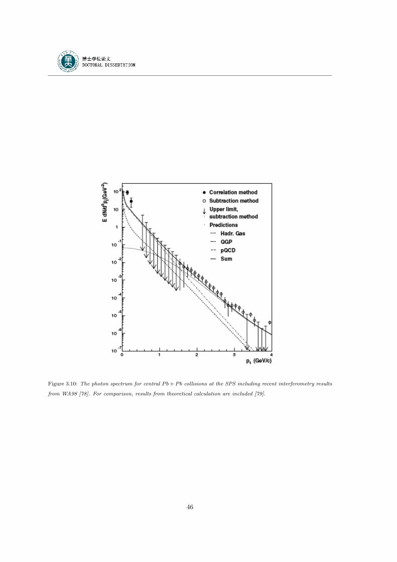
Figure 3.10: The photon spectrum for central Pb+ Pb collisions at the SPS including recent interferometry results

from WA98 [78]. For comparison, results from theoretical calculation are included [79].

46

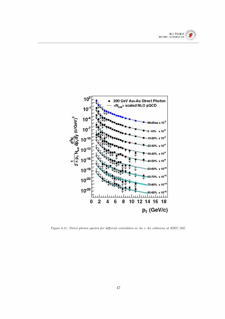
Figure 3.11: Direct photon spectra for different centralities in Au+Au collisions at RHIC [80].

47

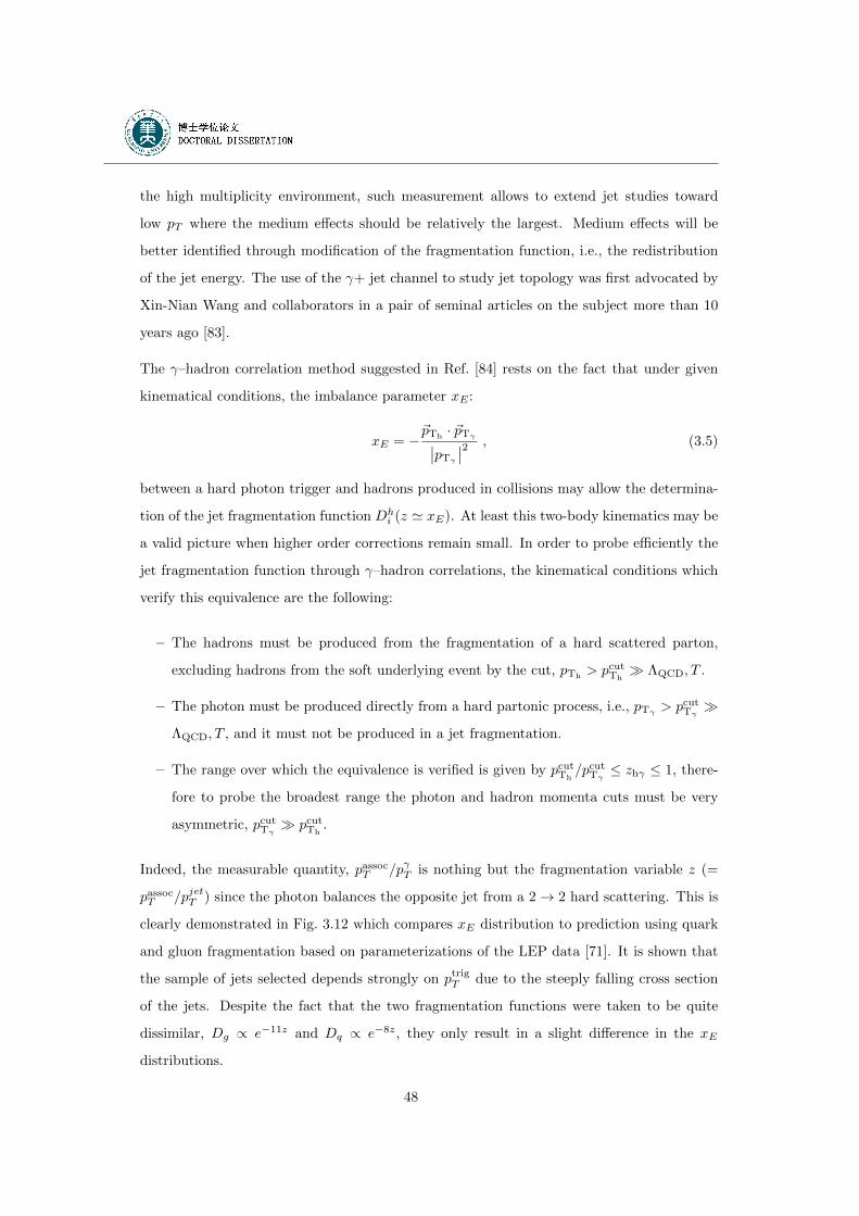
the high multiplicity environment, such measurement allows to extend jet studies toward

low pT where the medium effects should be relatively the largest. Medium effects will be

better identified through modification of the fragmentation function, i.e., the redistribution

of the jet energy. The use of the γ+ jet channel to study jet topology was first advocated by

Xin-Nian Wang and collaborators in a pair of seminal articles on the subject more than 10

years ago [83].

The γ–hadron correlation method suggested in Ref. [84] rests on the fact that under given

kinematical conditions, the imbalance parameter xE :

xE = −~pTh· ~pTγ∣∣pTγ ∣∣2 , (3.5)

between a hard photon trigger and hadrons produced in collisions may allow the determina-

tion of the jet fragmentation function Dhi (z ' xE). At least this two-body kinematics may be

a valid picture when higher order corrections remain small. In order to probe efficiently the

jet fragmentation function through γ–hadron correlations, the kinematical conditions which

verify this equivalence are the following:

– The hadrons must be produced from the fragmentation of a hard scattered parton,

excluding hadrons from the soft underlying event by the cut, pTh> pcutTh

� ΛQCD, T .

– The photon must be produced directly from a hard partonic process, i.e., pTγ > pcutTγ�

ΛQCD, T , and it must not be produced in a jet fragmentation.

– The range over which the equivalence is verified is given by pcutTh/pcutTγ

≤ zhγ ≤ 1, there-

fore to probe the broadest range the photon and hadron momenta cuts must be very

asymmetric, pcutTγ� pcutTh

.

Indeed, the measurable quantity, passocT /pγT is nothing but the fragmentation variable z (=

passocT /pjetT ) since the photon balances the opposite jet from a 2→ 2 hard scattering. This is

clearly demonstrated in Fig. 3.12 which compares xE distribution to prediction using quark

and gluon fragmentation based on parameterizations of the LEP data [71]. It is shown that

the sample of jets selected depends strongly on ptrigT due to the steeply falling cross section

of the jets. Despite the fact that the two fragmentation functions were taken to be quite

dissimilar, Dg ∝ e−11z and Dq ∝ e−8z, they only result in a slight difference in the xE

distributions.

48

Figure 3.12: xE distributions for several ranges of ptrigT compared to calculations using quark (solid) and gluon

(dashed) fragmentation functions as parameterized by the LEP data [71].

The PHENIX experiment has measured photon triggered jets correlation measurements to

study the jet fragmentation in both pp and central Au + Au collisions at√s = 200 GeV.

Fig. 3.13 shows the per-trigger yields of associated charged hadrons after the flow and com-

binatorial background subtraction as a function of ∆φ. The triggers were either an inclusive

photon, a decay photon or a direct photon with 7 < ptrigT < 9 GeV/c and the condition on

the associated particles was 3 < passocT < 5 GeV/c, where the decay photon trigger is iden-

tified by ’tagging’ from the reconstructed π0 and η, and the direct photons are sampled by

applying an isolation criterion (more details see Sec. 5.2). The strong near-side correlation

for inclusive and decay photons is largely absent for direct photon triggers as expected from

a sample dominated by photons produced directly in the hard scattering. Comparing the

inclusive and decay photon near side correlations for pp (top) and Au + Au (middle) the

larger direct photon signal-to-background in Au + Au is evident. The absence of the direct

photon triggered near-side correlation is apparent in the Au + Au data, as well as in pp.

The disappearance of the away-side correlation in Au + Au can be seen by comparing to the

pp correlations [85].

The modification of jet fragmentation function is evidenced by comparing the direct pho-

ton triggered away-side yields as a function of zT = passocT /pγT in pp and AA collisions. A

suppression has been observed in central Au + Au collisions with respect to pp (Fig. 3.14):

the slope of the correlation distribution in Au + Au collision is steeper than the one in pp

49

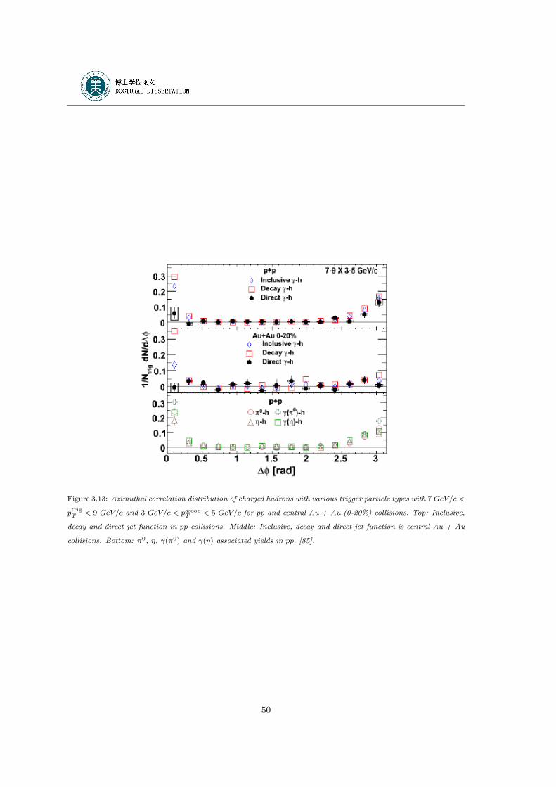
Figure 3.13: Azimuthal correlation distribution of charged hadrons with various trigger particle types with 7 GeV/c <

ptrigT < 9 GeV/c and 3 GeV/c < passocT < 5 GeV/c for pp and central Au + Au (0-20%) collisions. Top: Inclusive,

decay and direct jet function in pp collisions. Middle: Inclusive, decay and direct jet function is central Au + Au

collisions. Bottom: π0, η, γ(π0) and γ(η) associated yields in pp. [85].

50

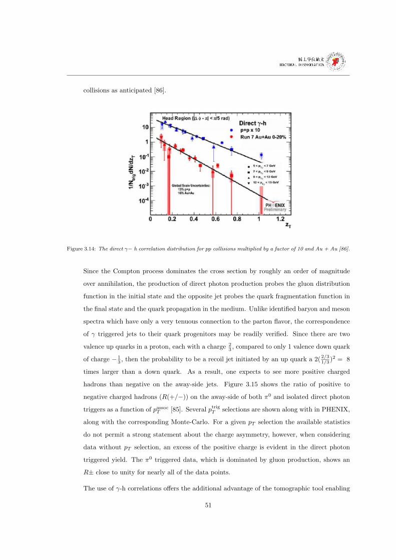
collisions as anticipated [86].

Figure 3.14: The direct γ− h correlation distribution for pp collisions multiplied by a factor of 10 and Au + Au [86].

Since the Compton process dominates the cross section by roughly an order of magnitude

over annihilation, the production of direct photon production probes the gluon distribution

function in the initial state and the opposite jet probes the quark fragmentation function in

the final state and the quark propagation in the medium. Unlike identified baryon and meson

spectra which have only a very tenuous connection to the parton flavor, the correspondence

of γ triggered jets to their quark progenitors may be readily verified. Since there are two

valence up quarks in a proton, each with a charge 23 , compared to only 1 valence down quark

of charge − 13 , then the probability to be a recoil jet initiated by an up quark a 2( 2/3

1/3 )2 = 8

times larger than a down quark. As a result, one expects to see more positive charged

hadrons than negative on the away-side jets. Figure 3.15 shows the ratio of positive to

negative charged hadrons (R(+/−)) on the away-side of both π0 and isolated direct photon

triggers as a function of passocT [85]. Several ptrigT selections are shown along with in PHENIX,

along with the corresponding Monte-Carlo. For a given pT selection the available statistics

do not permit a strong statement about the charge asymmetry, however, when considering

data without pT selection, an excess of the positive charge is evident in the direct photon

triggered yield. The π0 triggered data, which is dominated by gluon production, shows an

R± close to unity for nearly all of the data points.

The use of γ-h correlations offers the additional advantage of the tomographic tool enabling

51

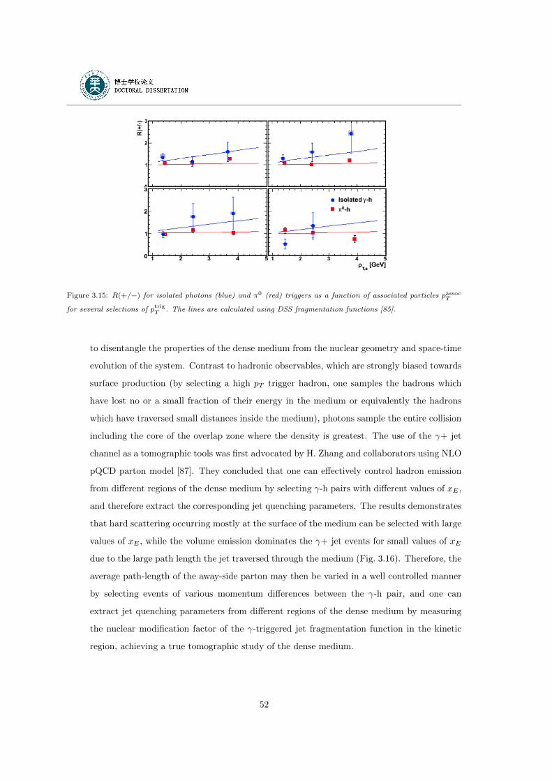
Figure 3.15: R(+/−) for isolated photons (blue) and π0 (red) triggers as a function of associated particles passocT

for several selections of ptrigT . The lines are calculated using DSS fragmentation functions [85].

to disentangle the properties of the dense medium from the nuclear geometry and space-time

evolution of the system. Contrast to hadronic observables, which are strongly biased towards

surface production (by selecting a high pT trigger hadron, one samples the hadrons which

have lost no or a small fraction of their energy in the medium or equivalently the hadrons

which have traversed small distances inside the medium), photons sample the entire collision

including the core of the overlap zone where the density is greatest. The use of the γ+ jet

channel as a tomographic tools was first advocated by H. Zhang and collaborators using NLO

pQCD parton model [87]. They concluded that one can effectively control hadron emission

from different regions of the dense medium by selecting γ-h pairs with different values of xE ,

and therefore extract the corresponding jet quenching parameters. The results demonstrates

that hard scattering occurring mostly at the surface of the medium can be selected with large

values of xE , while the volume emission dominates the γ+ jet events for small values of xE

due to the large path length the jet traversed through the medium (Fig. 3.16). Therefore, the

average path-length of the away-side parton may then be varied in a well controlled manner

by selecting events of various momentum differences between the γ-h pair, and one can

extract jet quenching parameters from different regions of the dense medium by measuring

the nuclear modification factor of the γ-triggered jet fragmentation function in the kinetic

region, achieving a true tomographic study of the dense medium.

52

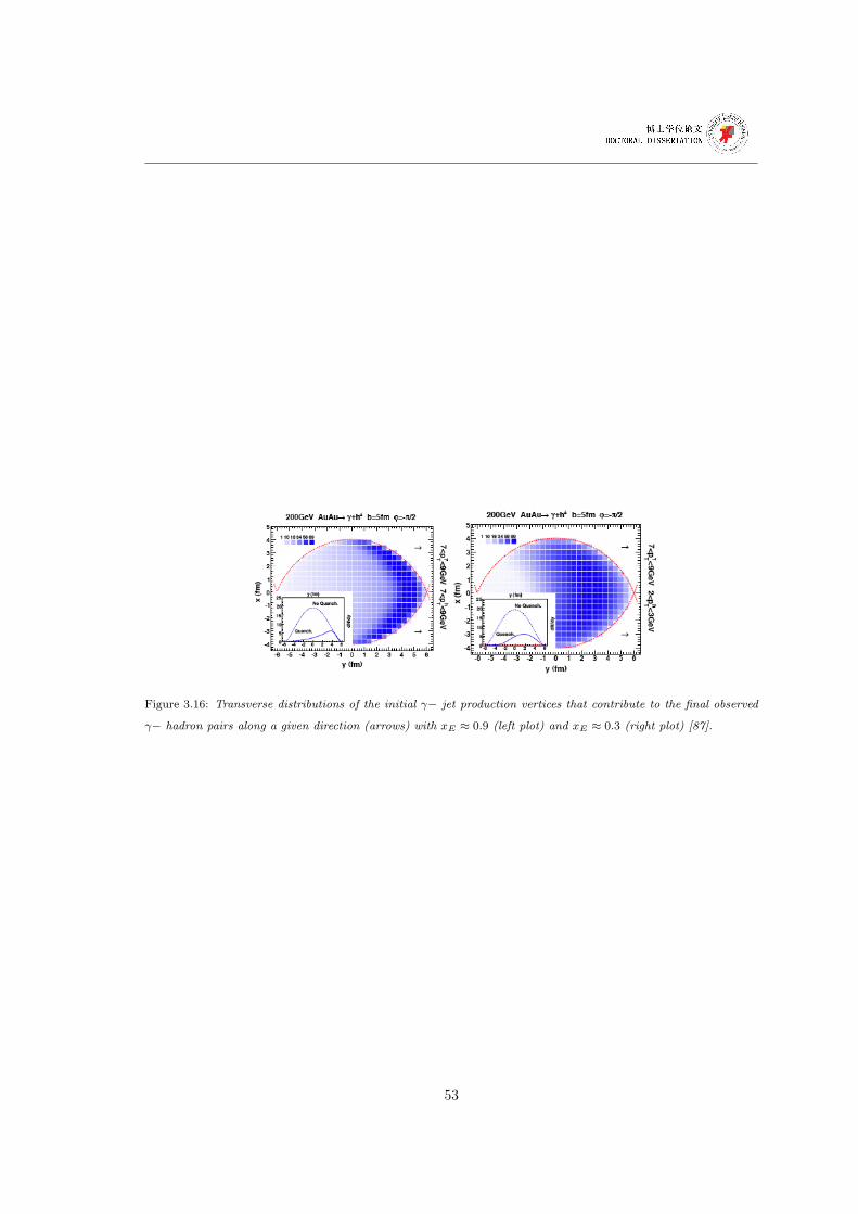
Figure 3.16: Transverse distributions of the initial γ− jet production vertices that contribute to the final observed

γ− hadron pairs along a given direction (arrows) with xE ≈ 0.9 (left plot) and xE ≈ 0.3 (right plot) [87].

53

54

Chapter 4

Experimental Facility

The Large Hadron Collider (LHC) at CERN near Geneva is the world newest and most

powerful tool for Particle Physics research. This chapter is devoted to the description of

the ALICE experiment at LHC. First, a brief description of the LHC and some relevant

parameters are given. Then, the ALICE detector layout is described, and finally, the soft-

ware currently being developed to simulate, reconstruct and analyze ALICE data is briefly

discussed.

4.1 The Large hadron Collider: LHC

The Large Hadron Collider is a two-ring-superconducting-hadron accelerator and collider

installed in the existing 26.7 km tunnel that was constructed between 1984 and 1989 for the

CERN LEP (Large Electron-Positron Collider) machine [88]. There are two transfer tunnels,

each approximately 2.5 km in length, linking the LHC to the CERN accelerator complex

that acts as injector. The chain of accelerators, sketched in Fig. 4.1, includes the Linac2

injector for proton beams (until 50 MeV) or the Linac4 injector for heavy-ion beams (up to

160 MeV/c), Proton Synchrotron (PS) and the Super Proton Synchrotron (SPS) (up to 450

GeV/v) and finally the LHC rings.

The LHC will ultimately deliver proton–proton collisions at center of mass energy√s =

14 TeV and Pb–Pb collisions at√sNN = 5.5 TeV with maximum luminosities of L =

1034 cm−2s−1 and L = 1027 cm−2s−1 respectively.

55

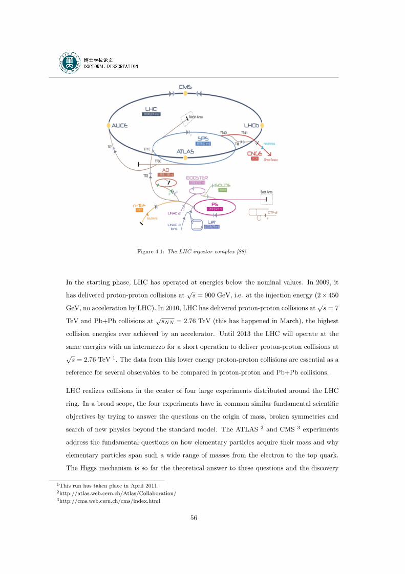
Figure 4.1: The LHC injector complex [88].

In the starting phase, LHC has operated at energies below the nominal values. In 2009, it

has delivered proton-proton collisions at√s = 900 GeV, i.e. at the injection energy (2× 450

GeV, no acceleration by LHC). In 2010, LHC has delivered proton-proton collisions at√s = 7

TeV and Pb+Pb collisions at√sNN = 2.76 TeV (this has happened in March), the highest

collision energies ever achieved by an accelerator. Until 2013 the LHC will operate at the

same energies with an intermezzo for a short operation to deliver proton-proton collisions at√s = 2.76 TeV 1. The data from this lower energy proton-proton collisions are essential as a

reference for several observables to be compared in proton-proton and Pb+Pb collisions.

LHC realizes collisions in the center of four large experiments distributed around the LHC

ring. In a broad scope, the four experiments have in common similar fundamental scientific

objectives by trying to answer the questions on the origin of mass, broken symmetries and

search of new physics beyond the standard model. The ATLAS 2 and CMS 3 experiments

address the fundamental questions on how elementary particles acquire their mass and why

elementary particles span such a wide range of masses from the electron to the top quark.

The Higgs mechanism is so far the theoretical answer to these questions and the discovery

1This run has taken place in April 2011.2http://atlas.web.cern.ch/Atlas/Collaboration/3http://cms.web.cern.ch/cms/index.html

56

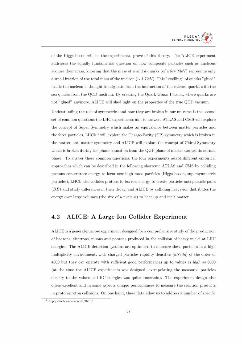
of the Higgs boson will be the experimental prove of this theory. The ALICE experiment

addresses the equally fundamental question on how composite particles such as nucleons

acquire their mass, knowing that the mass of u and d quarks (of a few MeV) represents only

a small fraction of the total mass of the nucleon (∼ 1 GeV). This ”swelling” of quarks ”glued”

inside the nucleon is thought to originate from the interaction of the valence quarks with the

sea quarks from the QCD medium. By creating the Quark Gluon Plasma, where quarks are

not ”glued” anymore, ALICE will shed light on the properties of the true QCD vacuum.

Understanding the role of symmetries and how they are broken in our universe is the second

set of common questions the LHC experiments aim to answer. ATLAS and CMS will explore

the concept of Super Symmetry which makes an equivalence between matter particles and

the force particles, LHCb 4 will explore the Charge-Parity (CP) symmetry which is broken in

the matter–anti-matter symmetry and ALICE will explore the concept of Chiral Symmetry

which is broken during the phase transition from the QGP phase of matter toward its normal

phase. To answer these common questions, the four experiments adapt different empirical

approaches which can be described in the following shortcut: ATLAS and CMS by colliding

protons concentrate energy to form new high mass particles (Higgs boson, supersymmetric

particles), LHCb also collides protons to borrow energy to create particle–anti-particle pairs

(BB) and study differences in their decay, and ALICE by colliding heavy-ion distributes the

energy over large volumes (the size of a nucleus) to heat up and melt matter.

4.2 ALICE: A Large Ion Collider Experiment

ALICE is a general-purpose experiment designed for a comprehensive study of the production

of hadrons, electrons, muons and photons produced in the collision of heavy nuclei at LHC

energies. The ALICE detection systems are optimized to measure these particles in a high

multiplicity environment, with charged particles rapidity densities (dN/dη) of the order of

4000 but they can operate with sufficient good performances up to values as high as 8000

(at the time the ALICE experiments was designed, extrapolating the measured particles

density to the values at LHC energies was quite uncertain). The experiment design also

offers excellent and in some aspects unique performances to measure the reaction products

in proton-proton collisions. On one hand, these data allow us to address a number of specific

4http://lhcb.web.cern.ch/lhcb/

57

strong interaction topics for which ALICE is complementary to the other LHC experiments.

On the other hand, these data provide the necessary reference data to which heavy-ion data

are compared to in order to reveal effects related to the formation of a hot and dense nuclear

medium.

The ALICE detector has been designed, built and is now operated by a collaboration includ-

ing currently over 1000 physicists and engineers from 105 institutes in 30 countries. Its overall

dimensions are 16 × 16 × 26 m3 for a total weight of approximately 10000 t. The ALICE

experiment (Fig. 4.2) consists of a central barrel detection system, covering the mid-rapidity

region (η ≤ 0.9; polar angles from 45◦ to 135◦) over the full azimuth, to measure and iden-

tify charged hadrons and electrons, and several detectors at forward/backward rapidity [89].

The central barrel is installed inside the large L3 [90] 5 solenoid magnet which generates an

Figure 4.2: Longitudinal view of the ALICE detector [89].

uniform magnetic field of up to 0.5 T and oriented along the beam axis. It is composed, from

the interaction vertex outwards, of the following detectors:

5L3 [90] is the former experiment operated at the LEP accelerator which infrastructure has been reused by

ALICE

58

– six cylindrical layers of high-resolution silicon pixel (SPD), drift (SDD) and strip (SSD)

detectors, forming the Inner Tracking System (ITS), for secondary vertex identification

of short lived particles and the tracking and identification of low transverse momentum

charged particles down to 100 MeV/c;

– a cylindrical Time Projection Chamber (TPC) for the high resolution tracking and

particle identification;

– a Time of Flight (TOF) detector to optimize charged hadrons identification;

– and a Transition Radiation Detector (TRD) for electron identification.

A ring imaging Cerenkov detector (HMPID) extending the useful range for the identification

of p/K and K/p, on a track-by-track basis, up to 3 GeV/c and 5 GeV/c respectively, covers

a limited acceptance (η < 0.6, ∆φ = 58◦). Two electomagnetic calorimeters (EMCAL and

PHOS), covering also a limited acceptance (|η| < 0.7 for EMCAL and |η| < 0.12 for PHOS,

and for both ∆φ = 100◦), for the detection and identification of photons and neutral mesons

and for providing a trigger on high-pT photons and jets, complete the central barrel systems.

Outside the central magnetic field and at very forward rapidity (−4.0 < η < 2.5), the forward

muon arm consists of a complex arrangement including hadron absorbers, a large dipole

magnet, and fourteen planes of tracking and triggering chambers, to detect and identify with

high momentum-resolution and low background muons from heavy quarks and quarkonia

decay. Opposite to the muon spectrometer (2.3 ≤ η ≤ 3.7), a Photon Multiplicity Detector

(PMD) measures the inclusive-photon multiplicity.

Additional detectors located at large rapidity complete the ALICE setup to characterize the

global event and to provide the interaction trigger:

– an ensemble of Si strip detectors, the Forward Multiplicity Detectors (FMD), covering

acceptance at large rapidities (−3.4 ≤ η ≤ −1.7, 1.7 ≤ η ≤ 5.0) to measure the charge

particles multiplicity in very forward directions;

– a Zero Degree Calorimeter (ZDC), consisting of two sets of neutron and hadron calorime-

ters located at 90 m from the interaction vertex, to measure the impact parameter of

the collision;

– a system of scintillation and quartz counters, V0 and T0, to provide fast trigger signals.

59

The detectors used for my study and their performance will be described in more details

next.

4.2.1 Central Tracking System

Tracking in the central barrel is performed by the ITS and the TPC. The need for efficient and

robust tracking has led to the choice of a TPC as the main tracking detector. Together with

the other central barrel detectors, TPC provides charged-particle momentum measurements

with excellent two-track separation, particle identification and vertex determination. The

main tasks of the ITS are to localize the primary vertex with a resolution better than 100

µm (longitudinal spatial precision is 100 µm and the radial spatial precision is 12 µm), to

reconstruct the secondary vertices from the decays of strange baryons and D and B mesons,

to track and identify particles with momentum below 200 MeV/c which can not reach the

TPC, and to improve the momentum and angle resolution for particles reconstructed by the

TPC.

4.2.1.1 Layout

The ITS surrounds the beam pipe, a 800 µm-thick beryllium cylinder of 6 cm outer diameter,

coaxial with the ITS detector layers. The layers are located at radii ranging between 4 and

43 cm and cover the rapidity range of η ≤ 0.9 for all vertices located within the length of

the interaction diamond (±1σ, i.e. ±5.3 cm along the beam direction). Because of the high

particle density expected in heavy-ion collisions, and in order to achieve the required impact

parameter resolution, the innermost four layers (SPD and SDD) are truly two-dimensional

devices. The two outer layers (SSD) are equipped with double-sided silicon micro-strip

detectors. The four outer layers have analog readout for independent particle identification

via dE/dx in the non-relativistic (1/β2) region, which provides the ITS with stand-alone

capability as a low-pT particle spectrometer [91]. The number, position and segmentation

of the layers are optimized for efficient track finding and high impact-parameter resolution.

In particular, the outer radius of ITS, rmax = 43 cm, is determined by the track matching

with the TPC and the inner radius (rmin = 4 cm) is the minimum allowed by the size of the

beam pipe (3 cm). The first layer has a more extended coverage (|η| < 1.98), in order to

provide, together with the FMD, a continuous coverage in rapidity for the measurement of

60

the charged particle multiplicity.

The TPC design is optimized to provide the largest possible acceptance for full-length, high-

pT tracks, in order to ensure significant statistics and good momentum resolution for high-

mass and high-pT electron pairs, high tracking efficiency and good performance even at as

high multiplicities as dN/dη ∼ 8000.

The TPC has an inner radius of rmin = 80 cm, an outer radius of rmax = 250 cm, and

an overall length along the beam direction of l = 500 cm. The inner radius of the TPC is

determined by the maximum acceptable hit density, the outer radius by the length required

for achieving dE/dx resolution of better than 5-7 %. Particle identification is performed for

low momentum particles with dE/dx measurement in the 1/β2 region (below the particle

mass). For high momentum particle, up to momenta of the order of several tens of GeV/c,

accurate particle identification can be performed thanks to the relativistic rise of the dE/dx.

The TPC is filled with a gas mixture of 90% of Ne and 10% of CO2. Ionisation electrons drift

in a longitudinal electric field toward the end-plate of the cylinders where they are detected

by multi-wire proportional chambers [92].

4.2.1.2 Performances

One of the most challenging tasks for ALICE is that of track finding in an unprecedented high

particle multiplicity density environment. Track finding begins with the reconstruction of the

primary vertex using the correlation of the hits position in the innermost detector (SPD).

Pairs of reconstructed points close in azimuthal angle in the transverse plane are selected in

the two layers. The z position of the primary vertex is estimated from their z-coordinates

using a linear extrapolation. The same procedure is repeated in the transverse plane. The

resulting position of the primary vertex position is used as an input for the tracking.

The basic method for track finding depends critically on the determination, for each track, of

a set of initial seed values for the track parameters and their covariance matrix. This seeding

is done using the space points reconstructed in the TPC. To start, a few outermost space

points from pad rows are used to build track seeds and the track is propagated inwards. The

procedure is repeated several times, choosing a set of space points closer and closer to the

centre of the TPC. After this step, the tracks are propagated to the outer layers of the ITS.

The combined track reconstruction accumulates the information from the different detectors

61

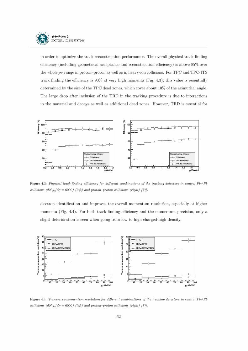
in order to optimize the track reconstruction performance. The overall physical track-finding

efficiency (including geometrical acceptance and reconstruction efficiency) is above 85% over

the whole pT range in proton–proton as well as in heavy-ion collisions. For TPC and TPC-ITS

track finding the efficiency is 90% at very high momenta (Fig. 4.3); this value is essentially

determined by the size of the TPC dead zones, which cover about 10% of the azimuthal angle.

The large drop after inclusion of the TRD in the tracking procedure is due to interactions

in the material and decays as well as additional dead zones. However, TRD is essential for

Figure 4.3: Physical track-finding efficiency for different combinations of the tracking detectors in central Pb+Pb

collisions (dNch/dη = 6000) (left) and proton–proton collisions (right) [77].

electron identification and improves the overall momentum resolution, especially at higher

momenta (Fig. 4.4). For both track-finding efficiency and the momentum precision, only a

slight deterioration is seen when going from low to high charged-high density.

Figure 4.4: Transverse-momentum resolution for different combinations of the tracking detectors in central Pb+Pb

collisions (dNch/dη = 6000) (left) and proton–proton collisions (right) [77].

62

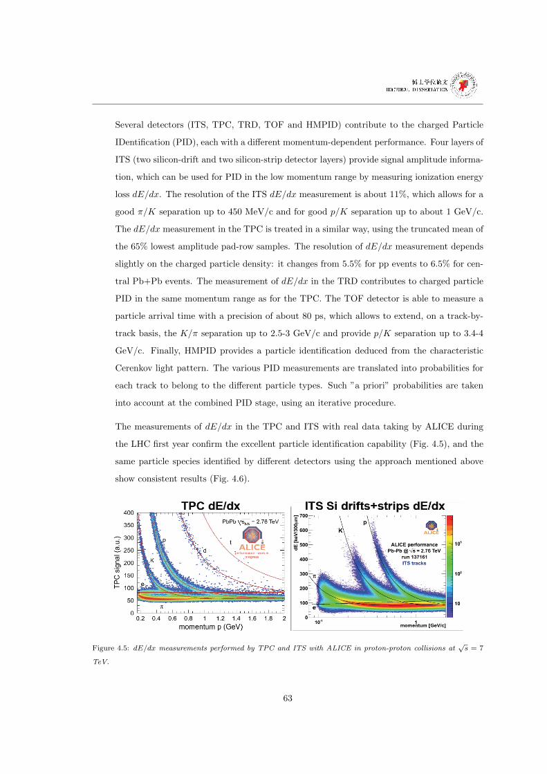
Several detectors (ITS, TPC, TRD, TOF and HMPID) contribute to the charged Particle

IDentification (PID), each with a different momentum-dependent performance. Four layers of

ITS (two silicon-drift and two silicon-strip detector layers) provide signal amplitude informa-

tion, which can be used for PID in the low momentum range by measuring ionization energy

loss dE/dx. The resolution of the ITS dE/dx measurement is about 11%, which allows for a

good π/K separation up to 450 MeV/c and for good p/K separation up to about 1 GeV/c.

The dE/dx measurement in the TPC is treated in a similar way, using the truncated mean of

the 65% lowest amplitude pad-row samples. The resolution of dE/dx measurement depends

slightly on the charged particle density: it changes from 5.5% for pp events to 6.5% for cen-

tral Pb+Pb events. The measurement of dE/dx in the TRD contributes to charged particle

PID in the same momentum range as for the TPC. The TOF detector is able to measure a

particle arrival time with a precision of about 80 ps, which allows to extend, on a track-by-

track basis, the K/π separation up to 2.5-3 GeV/c and provide p/K separation up to 3.4-4

GeV/c. Finally, HMPID provides a particle identification deduced from the characteristic

Cerenkov light pattern. The various PID measurements are translated into probabilities for

each track to belong to the different particle types. Such ”a priori” probabilities are taken

into account at the combined PID stage, using an iterative procedure.

The measurements of dE/dx in the TPC and ITS with real data taking by ALICE during

the LHC first year confirm the excellent particle identification capability (Fig. 4.5), and the

same particle species identified by different detectors using the approach mentioned above

show consistent results (Fig. 4.6).

Figure 4.5: dE/dx measurements performed by TPC and ITS with ALICE in proton-proton collisions at√s = 7

TeV.

63

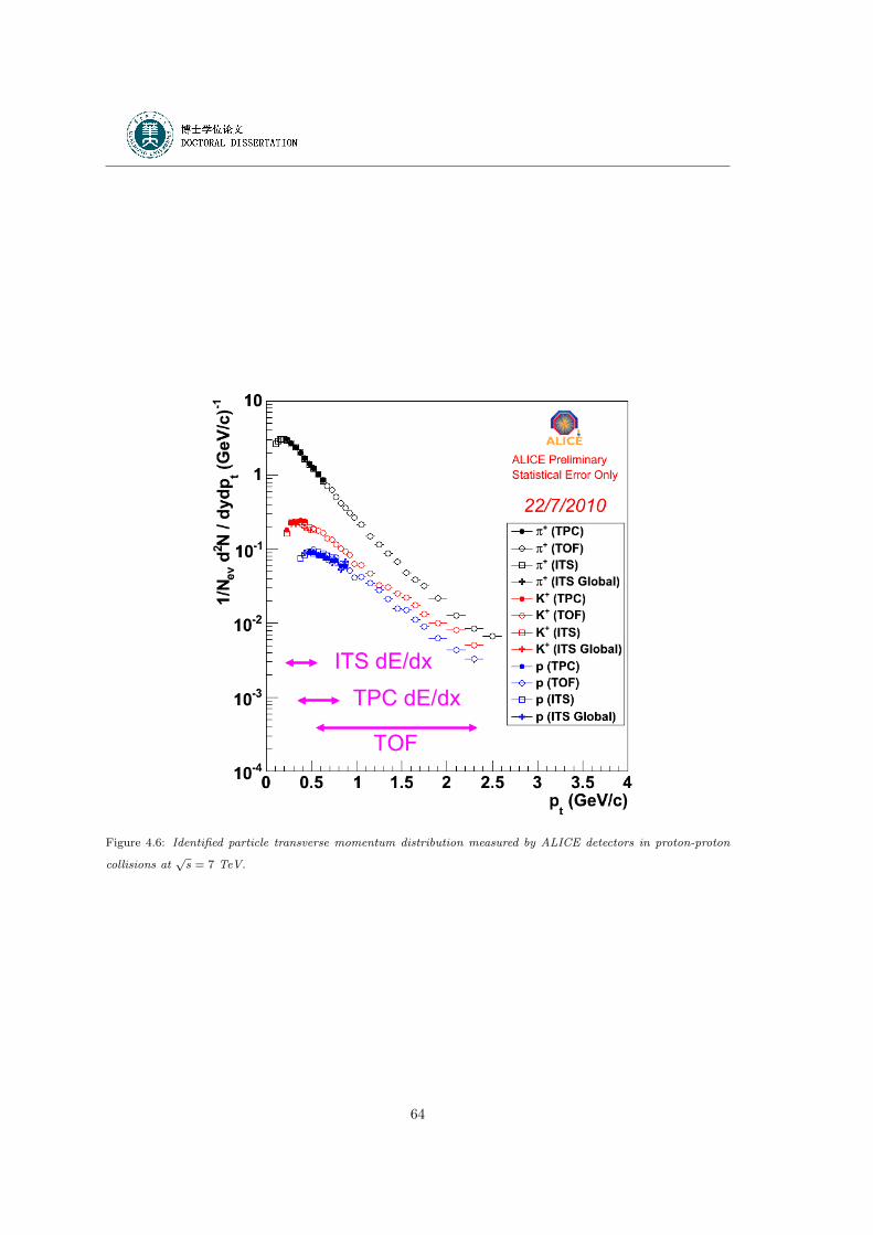
ITS dE/dx

TOF

TPC dE/dx

Figure 4.6: Identified particle transverse momentum distribution measured by ALICE detectors in proton-proton

collisions at√s = 7 TeV.

64

4.2.2 Electromagnetic Calorimeters

Photons, spanning the energy range from thermal photons (a few hundred MeV to a few

GeV) to hard QCD photons (up to hundred GeV), as well as decay photons from neutral

mesons are detected and identified in a small single-arm, high-resolution and high-granularity

(PHOS) and in a large acceptance (EMCal) electromagnetic calorimeter.

4.2.2.1 Layout

The high photon multiplicity generated by nuclear collisions requires a dense and highly

segmented calorimeter with small Molire radius at a large distance from the interaction

point in order to keep the cell occupancy at a manageable level of about 10-20%. Therefore,

PHOS or EMCAL, are located far away from the interaction vertex (∼ 4.6 m).

– PHOS, thanks to its high granularity and high energy resolution, is optimized for high

resolution measurement of the low energy thermal part of the photon spectrum and of

π0 and η and other electromagnetically decaying mesons in the energy range up to ∼ 50

GeV. It is made of dense scintillating crystals (PbWO4), subdivided into five indepen-

dent calorimeter units, named modules. Each module consists of 64 × 56 (across and

along the beam direction, respectively) PbWO4 scintillator crystals. Each crystal is a 18

cm long parallelepiped, equivalent to 20 radiation length units (X0[PbWO4]=0.89 cm).

A module covers approximately a quarter of a unit in pseudo-rapidity, −0.12 ≤ η ≤ 0.12,

and 100◦ in azimuthal angle, and its total area is 8 m2. Only 3 modules have been

installed at P2 for the first operational period at LHC, the remaining 2 will be sampled

and installed in the next 2 years. The technical data of the PHOS electromagnetic

calorimeter are listed in Tab. 4.1 [93].

– EMCAL, the second calorimeter has been designed to enhance the ALICE capabilities

for measuring jet properties over a large kinematic range. It is less segmented and

provides a worse energy resolution than PHOS. It is a large-acceptance, moderate-

resolution electromagnetic calorimeter providing a fast and efficient trigger for hard

jets, photons and electrons. The scope and basic design parameters of the calorimeter

are chosen to match the physics performance requirements of the high-pT physics goals.

The EMCAL is integrated within a cylindrical volume approximately 110 cm deep in the

radial direction sandwiched between the frame which supports the entire ALICE central

65

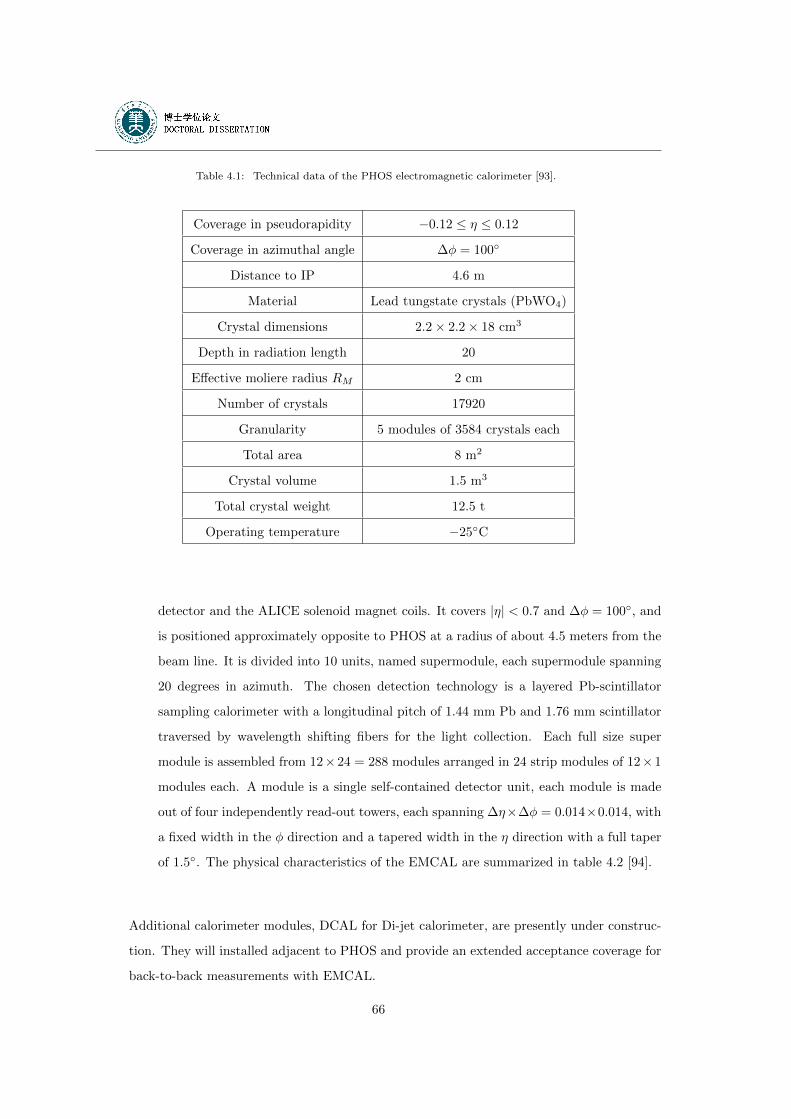
Table 4.1: Technical data of the PHOS electromagnetic calorimeter [93].

Coverage in pseudorapidity −0.12 ≤ η ≤ 0.12

Coverage in azimuthal angle ∆φ = 100◦

Distance to IP 4.6 m

Material Lead tungstate crystals (PbWO4)

Crystal dimensions 2.2× 2.2× 18 cm3

Depth in radiation length 20

Effective moliere radius RM 2 cm

Number of crystals 17920

Granularity 5 modules of 3584 crystals each

Total area 8 m2

Crystal volume 1.5 m3

Total crystal weight 12.5 t

Operating temperature −25◦C

detector and the ALICE solenoid magnet coils. It covers |η| < 0.7 and ∆φ = 100◦, and

is positioned approximately opposite to PHOS at a radius of about 4.5 meters from the

beam line. It is divided into 10 units, named supermodule, each supermodule spanning

20 degrees in azimuth. The chosen detection technology is a layered Pb-scintillator

sampling calorimeter with a longitudinal pitch of 1.44 mm Pb and 1.76 mm scintillator

traversed by wavelength shifting fibers for the light collection. Each full size super

module is assembled from 12×24 = 288 modules arranged in 24 strip modules of 12×1

modules each. A module is a single self-contained detector unit, each module is made

out of four independently read-out towers, each spanning ∆η×∆φ = 0.014×0.014, with

a fixed width in the φ direction and a tapered width in the η direction with a full taper

of 1.5◦. The physical characteristics of the EMCAL are summarized in table 4.2 [94].

Additional calorimeter modules, DCAL for Di-jet calorimeter, are presently under construc-

tion. They will installed adjacent to PHOS and provide an extended acceptance coverage for

back-to-back measurements with EMCAL.

66

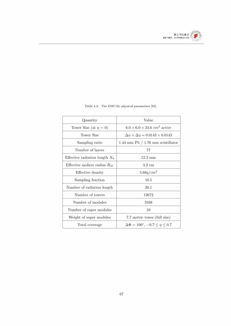
Table 4.2: The EMCAL physical parameters [94].

Quantity Value

Tower Size (at η = 0) 6.0× 6.0× 24.6 cm3 active

Tower Size ∆φ×∆η = 0.0143× 0.0143

Sampling ratio 1.44 mm Pb / 1.76 mm scintillator

Number of layers 77

Effective radiation length X0 12.3 mm

Effective moliere radius RM 3.2 cm

Effective density 5.68g/cm3

Sampling fraction 10.5

Number of radiation length 20.1

Number of towers 12672

Number of modules 3168

Number of super modules 10

Weight of super modules 7.7 metric tones (full size)

Total coverage ∆Φ = 100◦, −0.7 ≤ η ≤ 0.7

67

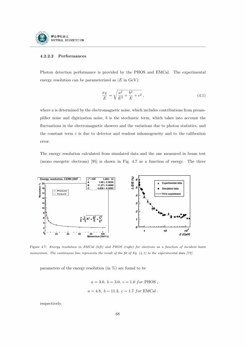
4.2.2.2 Performances

Photon detection performance is provided by the PHOS and EMCal. The experimental

energy resolution can be parameterized as (E in GeV):

σEE

=

√a2

E2+b2

E+ c2 , (4.1)

where a is determined by the electromagnetic noise, which includes contributions from pream-

plifier noise and digitization noise, b is the stochastic term, which takes into account the

fluctuations in the electromagnetic showers and the variations due to photon statistics, and

the constant term c is due to detector and readout inhomogeneity and to the calibration

error.

The energy resolution calculated from simulated data and the one measured in beam test

(mono energetic electrons) [95] is shown in Fig. 4.7 as a function of energy. The three

Figure 4.7: Energy resolution in EMCal (left) and PHOS (right) for electrons as a function of incident beam

momentum. The continuous line represents the result of the fit of Eq. (4.1) to the experimental data [77].

parameters of the energy resolution (in %) are found to be

a = 3.0, b = 3.0, c = 1.0 for PHOS ,

a = 4.8, b = 11.3, c = 1.7 for EMCal .

respectively.

68

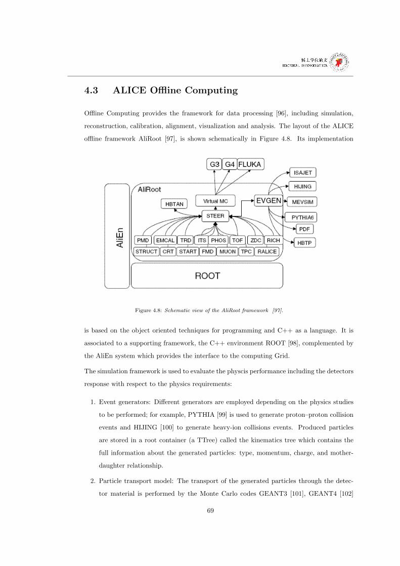
4.3 ALICE Offline Computing

Offline Computing provides the framework for data processing [96], including simulation,

reconstruction, calibration, alignment, visualization and analysis. The layout of the ALICE

offline framework AliRoot [97], is shown schematically in Figure 4.8. Its implementation

Figure 4.8: Schematic view of the AliRoot framework [97].

is based on the object oriented techniques for programming and C++ as a language. It is

associated to a supporting framework, the C++ environment ROOT [98], complemented by

the AliEn system which provides the interface to the computing Grid.

The simulation framework is used to evaluate the physcis performance including the detectors

response with respect to the physics requirements:

1. Event generators: Different generators are employed depending on the physics studies

to be performed; for example, PYTHIA [99] is used to generate proton–proton collision

events and HIJING [100] to generate heavy-ion collisions events. Produced particles

are stored in a root container (a TTree) called the kinematics tree which contains the

full information about the generated particles: type, momentum, charge, and mother-

daughter relationship.

2. Particle transport model: The transport of the generated particles through the detec-

tor material is performed by the Monte Carlo codes GEANT3 [101], GEANT4 [102]

69

or FLUKA [103]. The energy deposited by the generated particles in the detector is

stored in the form of hits. It consists of a deposited energy per tracking step (the mini-

mum propagation distance for which the deposited energy is calculated by the transport

model), the volume in which the energy is deposited, the time at which the energy is

deposited and the identification of the primary particle. A primary particle can generate

several hits in different volumes and there can be several hits in a single volume origi-

nating from different primary particles. The hits are stored separately for each detector.

The information is complemented by the so called ”track references” corresponding to

the location where the particles are crossing user defined reference planes.

3. Digitalization: The deposited energy, stored in the hits, is then modified for various

effects (adding the response of the front-end electronics, noise, digitization) to yield

the amplitude of the signal simulating the one delivered delivered by the detectors

electronics. It is stored as digits. Finally, pseudo raw data are produced from these

simulated digits in a format identical to the one used for real data.

The next steps are common to the processing of simulated data and real raw data.

4. Reconstruction: As an input, the reconstruction uses the digits together with some

additional information like the detector geometry. The reconstruction can use both

digits stored in the ROOT format and digits extracted from real raw data acquired

by the detectors. At this point, the reconstruction algorithms [96] reconstruct the full

information about the particles trajectory and mass. For digits found in the central

tracking detectors, reconstruction produces first clusters, a set of adjacent (in space

and/or in time) digits that were presumably generated by the same particle crossing

the sensitive element of a detector. It then calculates space points which provides an

estimation of the position where a particle crossed the sensitive element of a detector

(often, this is done by calculating the center of gravity of the cluster). After that,

tracks are reconstructed by combining clusters and consist of five parameters (such

as the curvature and the angles with respect to the coordinate axes) of the particle’s

trajectory together with the corresponding covariance matrix (used to calculate the

probability that the reconstructed track represents a real track) the estimated at a

given space point. Finally, with the reconstructed vertices and tracks, particles types

are identified.

For the calorimeters, the reconstruction algorithm produces clusters of hit cells and

70

calculates various parameters such as, the position in the reference frame local to the

calorimeter (super)module, the local deposited energy, shape parameters of the cluster,

and store them into a RecPoint in which the list of digits at the origin of the cluster

is stored as well. This list is important to recalibrate the calorimeter without need to

repeat the entire reconstruction process. The output of the reconstruction is stored as

the Event Summary Data (ESD).

71

72

Chapter 5

Validation of γ -hadron

observable: A Monte-Carlo

Study

In this chapter, I will present my work while ALICE was waiting for the start of the LHC

operation. I describe first the generators for the Monte-Carlo studies. The methods to

identify direct photons among inclusive photons and to identify π0 will be explained next.

Finally, the results from a feasibility study demonstrating that the ALICE experiment is well

suited for photon-hadron correlation measurements in proton–proton and heavy-ion collisions

at LHC energies are discussed.

5.1 Monte Carlo Event Generator

As discussed earlier, two processes are involved for the prompt photon production at leading-

order (LO). The elementary 2→ 2 hard processes contributing at the parton-level are gluon

Compton scattering and quark annihilation (Fig. 3.8),

g + q → γ + q ,

q + q → γ + g .(5.1)

These two processes generate prompt direct photons in what we will call γ–jet events.

73

As main background, we considered the following 2→ 2 hard QCD processes at LO:

q + q → g + g ,

q + q′→ q + q

′,

q + q → q + q ,

q + g → q + g ,

g + g → g + g ,

g + g → q + q′.

(5.2)

These processes contribute to the photon production through the decay photons from neutral

mesons, originating from the fragmentation of the hard scattered partons. These processes

generate what we will call the jet–jet events.

We have used the event generator of leading order processes of the Standard Model PYTHIA

6.214 [99] to simulate proton–proton collisions. This event generator is a Monte Carlo type

of generator and can be used to generate high-energy-physics ”events”, i.e., sets of outgoing

particles produced in the interactions between two incoming particles. The PYTHIA event

generator provides an accurate (provided adequate tuning) representation of the event prop-

erties in a wide range of reactions, within and beyond the Standard Model, with emphasis

on those where strong interaction plays a role, directly or indirectly, including multiple soft

scattering that constitutes the underlying event of the multi-hadronic final state. Due to

the Fermi motion of partons inside the colliding hadrons, the initial state partons have an

intrinsic transverse momentum motion, kTintric . Soft gluons radiation occurring in the initial

and final state of the hard scattering contribute also to the overall transverse momentum

< kT > observed in the final state measurable particles (see Sec. 3.2). PYTHIA provides

switches for these initial- and final-state radiation (ISR/FSR) processes. The processes of

interest for the present study are those leading to the production of prompt photons, they

are treated as the signal while those leading to the production of neutral pions are treated

as the background.

Proton–proton events triggered either by the γ–jet (from Eq. 5.1) or jet–jet (from Eq. 5.2)

processes were generated with the default parton distribution function CTEQ4L [104]. Initial

and final state radiation were switched on and the intrinsic transverse momentum of the

colliding partons was set to the default value kTintric = 1 GeV/c. Fragmentation photons

74

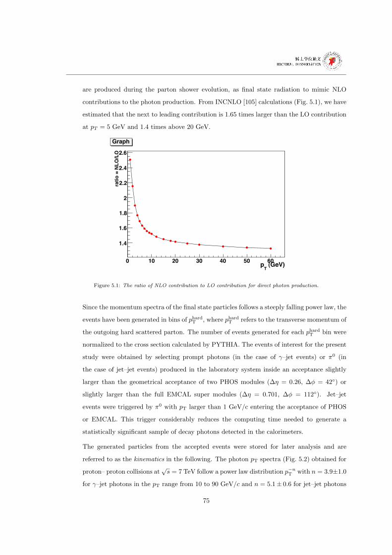
are produced during the parton shower evolution, as final state radiation to mimic NLO

contributions to the photon production. From INCNLO [105] calculations (Fig. 5.1), we have

estimated that the next to leading contribution is 1.65 times larger than the LO contribution

at pT = 5 GeV and 1.4 times above 20 GeV.

(GeV)T

p0 10 20 30 40 50 60

ratio

= N

LO/L

O

1.4

1.6

1.8

2

2.2

2.4

2.6

Graph

Figure 5.1: The ratio of NLO contribution to LO contribution for direct photon production.

Since the momentum spectra of the final state particles follows a steeply falling power law, the

events have been generated in bins of phardT , where phardT refers to the transverse momentum of

the outgoing hard scattered parton. The number of events generated for each phardT bin were

normalized to the cross section calculated by PYTHIA. The events of interest for the present

study were obtained by selecting prompt photons (in the case of γ–jet events) or π0 (in

the case of jet–jet events) produced in the laboratory system inside an acceptance slightly

larger than the geometrical acceptance of two PHOS modules (∆η = 0.26, ∆φ = 42◦) or

slightly larger than the full EMCAL super modules (∆η = 0.701, ∆φ = 112◦). Jet–jet

events were triggered by π0 with pT larger than 1 GeV/c entering the acceptance of PHOS

or EMCAL. This trigger considerably reduces the computing time needed to generate a

statistically significant sample of decay photons detected in the calorimeters.

The generated particles from the accepted events were stored for later analysis and are

referred to as the kinematics in the following. The photon pT spectra (Fig. 5.2) obtained for

proton– proton collisions at√s = 7 TeV follow a power law distribution p−nT with n = 3.9±1.0

for γ–jet photons in the pT range from 10 to 90 GeV/c and n = 5.1± 0.6 for jet–jet photons

75

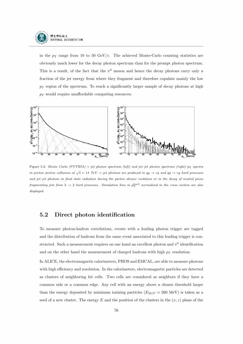
in the pT range from 10 to 50 GeV/c. The achieved Monte-Carlo counting statistics are

obviously much lower for the decay photon spectrum than for the prompt photon spectrum.

This is a result, of the fact that the π0 meson and hence the decay photons carry only a

fraction of the jet energy from where they fragment and therefore copulate mainly the low

pT region of the spectrum. To reach a significantly larger sample of decay photons at high

pT would require unaffordable computing resources.

(GeV/c)γT

p10 20 30 40 50 60 70 80 90 100

) (m

b/(

GeV

/c))

φ d

η d

T/(

dp

σ3d

-1210

-1110

-1010

-910

-810

-710

-610

(GeV/c)γT

p10 20 30 40 50 60 70 80 90 100

) (m

b/(

GeV

/c))

φ d

η d

T/(

dp

σ3d

-1110

-1010

-910

-810

-710

-610

-510

-410

-310

Figure 5.2: Monte Carlo (PYTHIA) γ–jet photon spectrum (left) and jet–jet photon spectrum (right) pT spectra

in proton–proton collisions at√s = 14 TeV. γ–jet photons are produced in qg → γq and qq → γg hard processes

and jet–jet photons in final state radiation during the parton shower evolution or in the decay of neutral pions

fragmenting jets from 2 → 2 hard processes. Simulation bins in phardT normalized to the cross section are also

displayed.

5.2 Direct photon identification

To measure photon-hadron correlations, events with a leading photon trigger are tagged

and the distribution of hadrons from the same event associated to this leading trigger is con-

structed. Such a measurement requires on one hand an excellent photon and π0 identification

and on the other hand the measurement of charged hadrons with high pT resolution.

In ALICE, the electromagnetic calorimeters, PHOS and EMCAL, are able to measure photons

with high efficiency and resolution. In the calorimeters, electromagnetic particles are detected

as clusters of neighboring hit cells. Two cells are considered as neighbors if they have a

common side or a common edge. Any cell with an energy above a chosen threshold larger

than the energy deposited by minimum ionizing particles (EMIP ' 260 MeV) is taken as a

seed of a new cluster. The energy E and the position of the clusters in the (x, z) plane of the

76

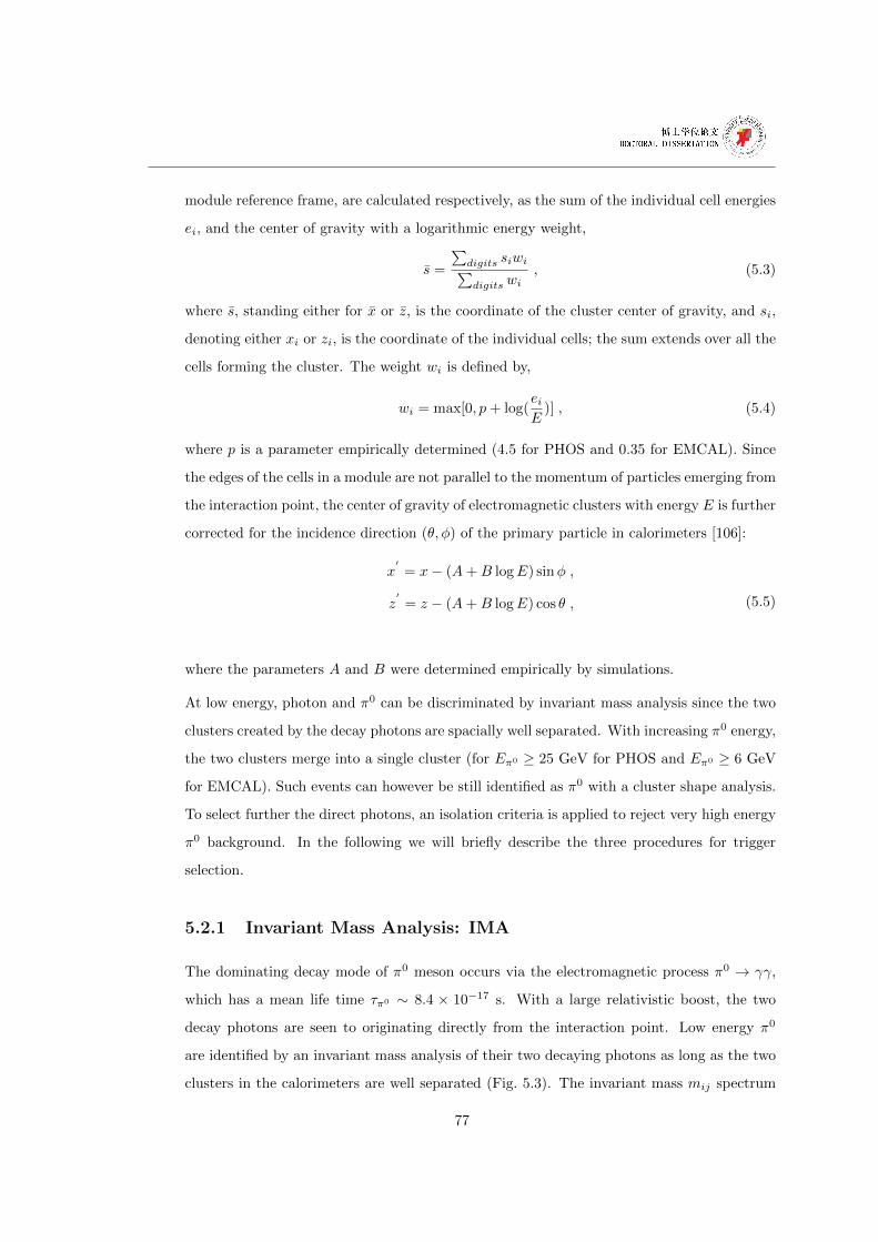
module reference frame, are calculated respectively, as the sum of the individual cell energies

ei, and the center of gravity with a logarithmic energy weight,

s =

∑digits siwi∑digits wi

, (5.3)

where s, standing either for x or z, is the coordinate of the cluster center of gravity, and si,

denoting either xi or zi, is the coordinate of the individual cells; the sum extends over all the

cells forming the cluster. The weight wi is defined by,

wi = max[0, p+ log(eiE

)] , (5.4)

where p is a parameter empirically determined (4.5 for PHOS and 0.35 for EMCAL). Since

the edges of the cells in a module are not parallel to the momentum of particles emerging from

the interaction point, the center of gravity of electromagnetic clusters with energy E is further

corrected for the incidence direction (θ, φ) of the primary particle in calorimeters [106]:

x′

= x− (A+B logE) sinφ ,

z′

= z − (A+B logE) cos θ , (5.5)

where the parameters A and B were determined empirically by simulations.

At low energy, photon and π0 can be discriminated by invariant mass analysis since the two

clusters created by the decay photons are spacially well separated. With increasing π0 energy,

the two clusters merge into a single cluster (for Eπ0 ≥ 25 GeV for PHOS and Eπ0 ≥ 6 GeV

for EMCAL). Such events can however be still identified as π0 with a cluster shape analysis.

To select further the direct photons, an isolation criteria is applied to reject very high energy

π0 background. In the following we will briefly describe the three procedures for trigger

selection.

5.2.1 Invariant Mass Analysis: IMA

The dominating decay mode of π0 meson occurs via the electromagnetic process π0 → γγ,

which has a mean life time τπ0 ∼ 8.4 × 10−17 s. With a large relativistic boost, the two

decay photons are seen to originating directly from the interaction point. Low energy π0

are identified by an invariant mass analysis of their two decaying photons as long as the two

clusters in the calorimeters are well separated (Fig. 5.3). The invariant mass mij spectrum

77

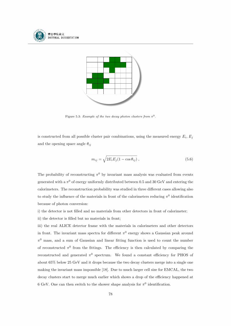
Figure 5.3: Example of the two decay photon clusters from π0.

is constructed from all possible cluster pair combinations, using the measured energy Ei, Ej

and the opening space angle θij

mij =√

2EiEj(1− cos θij) , (5.6)

The probability of reconstructing π0 by invariant mass analysis was evaluated from events

generated with a π0 of energy uniformly distributed between 0.5 and 30 GeV and entering the

calorimeters. The reconstruction probability was studied in three different cases allowing also

to study the influence of the materials in front of the calorimeters reducing π0 identification

because of photon conversion:

i) the detector is not filled and no materials from other detectors in front of calorimeter;

ii) the detector is filled but no materials in front;

iii) the real ALICE detector frame with the materials in calorimeters and other detectors

in front. The invariant mass spectra for different π0 energy shows a Gaussian peak around

π0 mass, and a sum of Gaussian and linear fitting function is used to count the number

of reconstructed π0 from the fittings. The efficiency is then calculated by comparing the

reconstructed and generated π0 spectrum. We found a constant efficiency for PHOS of

about 65% below 25 GeV and it drops because the two decay clusters merge into a single one

making the invariant mass impossible [18]. Due to much larger cell size for EMCAL, the two

decay clusters start to merge much earlier which shows a drop of the efficiency happened at

6 GeV. One can then switch to the shower shape analysis for π0 identification.

78

5.2.2 Shower Shape Analysis: SSA

The shape of the clusters is defined by the intersection of the cone containing the shower

with the front plane of the calorimeter (Fig. 5.4). This surface can be expressed in terms of

the covariance matrix,

S =

sxx szx

sxz szz

, (5.7)

where,

sxx =< (x− x)2 >=

∑digits wix

2i∑

digits wi−

(∑digits wixi∑digits wi

)2

, (5.8)

with similar definitions for szz and szx. Here <> denotes averaging with the logarithmic

weights wi defined by Eq. (5.4), x and z are the coordinates of the center of gravity of the

cluster [Eq. (5.3)],(xi, zi) are the coordinate positions of crystal i. The core energy is the

sum of the energies of the crystal with the largest energy and the neighbor crystals. The

principal axes of the shower surface are the eigenvectors (e1, e2) of the covariance matrix,

with eigenvalues λ0 and λ1. The geometrical meaning of the principal axes is illustrated in

Fig. 5.4. The lateral dispersion d of the clusters in the (x, z) plane, measured on the surface

!0!!1!

Figure 5.4: Example of a shower profile and its principal axes e1 and e2 [93].

of electromagnetic calorimeters,

d =

∑digits wi[(xi − x)2 + (zi − z)2]∑

digits wi. (5.9)

Using shower shape analysis, the particles detected with calorimeters relies on three inde-

pendent identification parameters derived from the data collected by the detector. For high

79

energy π0 (pT > 25 GeV/c for PHOS, and pT > 6 GeV/c for EMCAL), the Lorentz boost

contracts the relative angle between π0 decay photons to small values (∆γ1γ2 < 0.8◦ for

a symmetric decay) and the two showers developing in calorimeters overlap and are recon-

structed as one single photon. This configuration provides, however, the opportunity to

discriminate photons from overlapped decay photons based on an analysis of the cluster

shape: a cluster with axial symmetry in (x,z) signs a photon, whereas an asymmetric cluster

signs overlapped decay photons [107]. Particle identification weights, which represent the

probability that the detected particle is of a given type, among photon (γ), electron (e±),

charged hadron (h±), neutral hadron (h0) and high–pT π0, are assigned to each reconstructed

particle following a Bayesian approach [108]. For the Monte-Carlo study, we considered a

particle to be a photon when the probability weight is larger than 0.5. With this selection

criteria, we find an efficiency to reconstruct and identify direct photons, calculated as the

ratio of reconstructed and identified photons to γ–jet generated photons, equal to 70% at

10 GeV and about 55% at 80 GeV. This efficiency includes a 10% loss due to γ-conversion in

the material in front of PHOS and an additional loss of 10% due to border effects. In jet-jet

events, we observe a decrease in the ratio identified to generated photons from the same

value as the one obtained for γ–jet events, below 20 GeV/c, to a value of 0.2 at 45 GeV/c,

demonstrating the excellent rejection provided by the shower shape analysis [109].

We therefore conclude that the shower shape analysis, for distinguishing direct photons and

decay photons merging into a single cluster, allows us to enrich substantially the data sample

with direct photons. However the ratio of direct photon to decay photon, of about 0.2

at pT of 20 GeV/c [109], remains too low. The method is not selective enough to reduce

the contribution of decay photons to a negligible low level. We then consider the isolation

techniques to enhance the significance of signal to background level.

5.2.3 Isolation Cut: IC

Prompt photons are produced from Compton Scattering and Annihilation (Eq. 5.1) in which

the final state photon and parton are emitted back-to-back. As there is no hadron from the

parton jet flying in the same direction as the photon, the latter should appear as isolated

photons. One can take benefit of this kinematics and apply isolation selection to identify

prompt photons and obtain a sufficiently clean sample of prompt photons [107]. The isolation

80

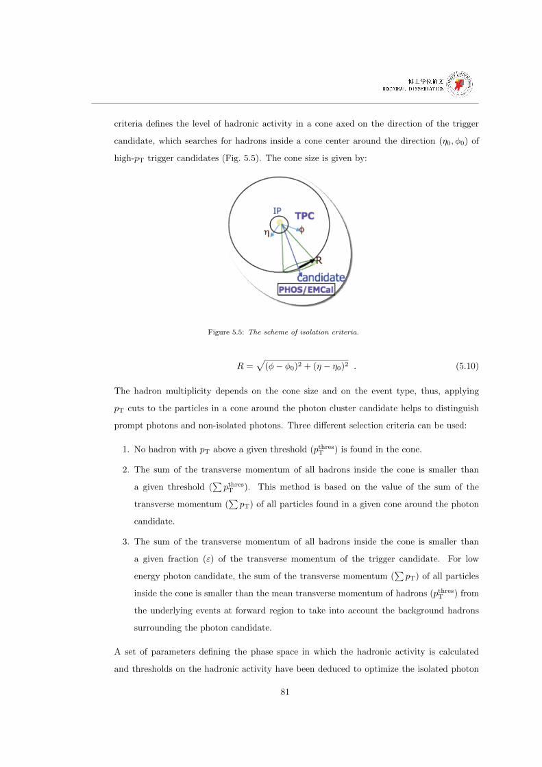
criteria defines the level of hadronic activity in a cone axed on the direction of the trigger

candidate, which searches for hadrons inside a cone center around the direction (η0, φ0) of

high-pT trigger candidates (Fig. 5.5). The cone size is given by:

Figure 5.5: The scheme of isolation criteria.

R =√

(φ− φ0)2 + (η − η0)2 . (5.10)

The hadron multiplicity depends on the cone size and on the event type, thus, applying

pT cuts to the particles in a cone around the photon cluster candidate helps to distinguish

prompt photons and non-isolated photons. Three different selection criteria can be used:

1. No hadron with pT above a given threshold (pthresT ) is found in the cone.

2. The sum of the transverse momentum of all hadrons inside the cone is smaller than

a given threshold (∑pthresT ). This method is based on the value of the sum of the

transverse momentum (∑pT) of all particles found in a given cone around the photon

candidate.

3. The sum of the transverse momentum of all hadrons inside the cone is smaller than

a given fraction (ε) of the transverse momentum of the trigger candidate. For low

energy photon candidate, the sum of the transverse momentum (∑pT) of all particles

inside the cone is smaller than the mean transverse momentum of hadrons (pthresT ) from

the underlying events at forward region to take into account the background hadrons

surrounding the photon candidate.

A set of parameters defining the phase space in which the hadronic activity is calculated

and thresholds on the hadronic activity have been deduced to optimize the isolated photon

81

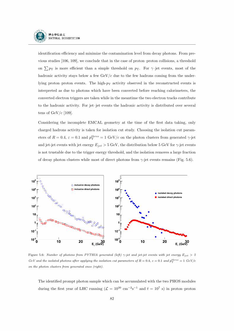
identification efficiency and minimize the contamination level from decay photons. From pre-

vious studies [106, 109], we conclude that in the case of proton–proton collisions, a threshold

on∑pT is more efficient than a simple threshold on pT. For γ–jet events, most of the

hadronic activity stays below a few GeV/c due to the few hadrons coming from the under-

lying proton–proton events. The high-pT activity observed in the reconstructed events is

interpreted as due to photons which have been converted before reaching calorimeters, the

converted electron triggers are taken while in the meantime the two electron tracks contribute

to the hadronic activity. For jet–jet events the hadronic activity is distributed over several

tens of GeV/c [109].

Considering the incomplete EMCAL geometry at the time of the first data taking, only

charged hadrons activity is taken for isolation cut study. Choosing the isolation cut param-

eters of R = 0.4, ε = 0.1 and pthresT = 1 GeV/c on the photon clusters from generated γ-jet

and jet-jet events with jet energy Ejet > 5 GeV, the distribution below 5 GeV for γ-jet events

is not trustable due to the trigger energy threshold, and the isolation removes a large fraction

of decay photon clusters while most of direct photons from γ-jet events remains (Fig. 5.6).

Figure 5.6: Number of photons from PYTHIA generated (left) γ-jet and jet-jet events with jet energy Ejet > 5

GeV and the isolated photons after applying the isolation cut parameters of R = 0.4, ε = 0.1 and pthresT = 1 GeV/c

on the photon clusters from generated ones (right).

The identified prompt photon sample which can be accumulated with the two PHOS modules

during the first year of LHC running (L = 1030 cm−2s−1 and t = 107 s) in proton–proton

82

collisions at√s = 14 TeV will be sufficient to measure the prompt photon spectrum over a

large pT range between 20 and 80 GeV/c. Counting rates will limit the measurement, but

not systematic errors which are dominated by the remaining decay photon and fragmentation

photon background (the systematic errors have been arbitrarily multiplied by two to take

into account additional source of photons in jet–jet events not considered in our simulation).

The larger acceptance calorimeter EMCal allows to improve the quality of the measurements,

where the direct prompt photon pT range could reach up to 120 GeV/c with the full EMCAL

super modules during the LHC running (Lint= 0.5 × 106 mb−1) in proton–proton collisions

at√s = 5.5 TeV.

5.3 Correlation distributions in pp collisions

Jets are usually produced in pairs, that are back-to-back in the transverse plane, and are

separated by an azimuthal distance ∆φ ≈ π. They can be revealed by studying azimuthal

correlations as a function of ∆φ (= φtrig−φh) between a trigger particle with high transverse

momentum in calorimeters, i.e. prompt photon clusters from γ–jets events or decay clusters

from jet–jet events, and associated particles from the same event. For jet–jet events, the

correlation shows a near (∆φ = 0) and an away side (∆φ = π) peak, and in γ−jet events

there are no hadrons surrounding the prompt photons as selected trigger therefore no near side

correlations is observed (Fig. 5.7, left). The difference between the generated MC distribution

and reconstructed ESD distribution results from the detector response loss. In jet-jet events

the away side peak is shifted with respect to π and is broader than the far side peak in γ–jet

events, because the tagged decay cluster from π0 in jet–jet events carries only a fraction of

the jet and is not necessarily the leading particle of the jet fragments hadrons. (Fig. 5.7,

right).

To construct the photon-hadrons correlation distribution, events where photons and charged

hadron are emitted in different hemispheres (π/2 < ∆φ < 3π/2) are selected. The contri-

bution from the underlying proton–proton events was estimated by correlating the trigger

photon with the charged hadrons emitted on the same side (−π/2 < ∆φ < π/2). We

define our signal (S) as the opposite side correlated charged hadrons minus the same side

correlated charged hadrons (B) and compare their pT spectra (Fig. 5.8) to the one of the

opposite side correlated charged hadrons (S+B). At pT larger than 5 GeV/c, the contri-

83

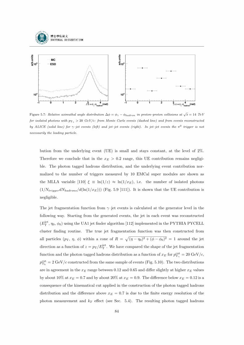
(rad)hadron

φ-γ

φ = φ ∆-1 0 1 2 3 4

arb

.un

its

410

510

MC

ESD

(rad)hadron

φ-γ

φ = φ ∆-1 0 1 2 3 4

arb

.un

its

410

510

Figure 5.7: Relative azimuthal angle distribution ∆φ = φγ − φhadron in proton–proton collisions at√s = 14 TeV

for isolated photons with pTγ > 20 GeV/c: from Monte Carlo events (dashed line) and from events reconstructed

by ALICE (solid line) for γ–jet events (left) and jet–jet events (right). In jet–jet events the π0 trigger is not

necessarily the leading particle.

bution from the underlying event (UE) is small and stays constant, at the level of 2%.

Therefore we conclude that in the xE > 0.2 range, this UE contribution remains negligi-

ble. The photon tagged hadrons distribution, and the underlying event contribution nor-

malized to the number of triggers measured by 10 EMCal super modules are shown as

the MLLA variable [110] ξ ≡ ln(1/z) ≈ ln(1/xE), i.e. the number of isolated photons

(1/NtriggerdNhadrons/d(ln(1/xE))) (Fig. 5.9 [111]). It is shown that the UE contribution is

negligible.

The jet fragmentation function from γ–jet events is calculated at the generator level in the

following way. Starting from the generated events, the jet in each event was reconstructed

(EjetT , η0, φ0) using the UA1 jet finder algorithm [112] implemented in the PYTHIA PYCELL

cluster finding routine. The true jet fragmentation function was then constructed from

all particles (pT, η, φ) within a cone of R =√

(η − η0)2 + (φ− φ0)2 = 1 around the jet

direction as a function of z = pT/EjetT . We have compared the shape of the jet fragmentation

function and the photon tagged hadrons distribution as a function of xE for pcutTγ= 20 GeV/c,

pcutTh= 2 GeV/c constructed from the same sample of events (Fig. 5.10). The two distributions

are in agreement in the xE range between 0.12 and 0.65 and differ slightly at higher xE values

by about 10% at xE = 0.7 and by about 20% at xE = 0.9. The difference below xE = 0.12 is a

consequence of the kinematical cut applied in the construction of the photon tagged hadrons

distribution and the difference above xE = 0.7 is due to the finite energy resolution of the

photon measurement and kT effect (see Sec. 5.4). The resulting photon tagged hadrons

84

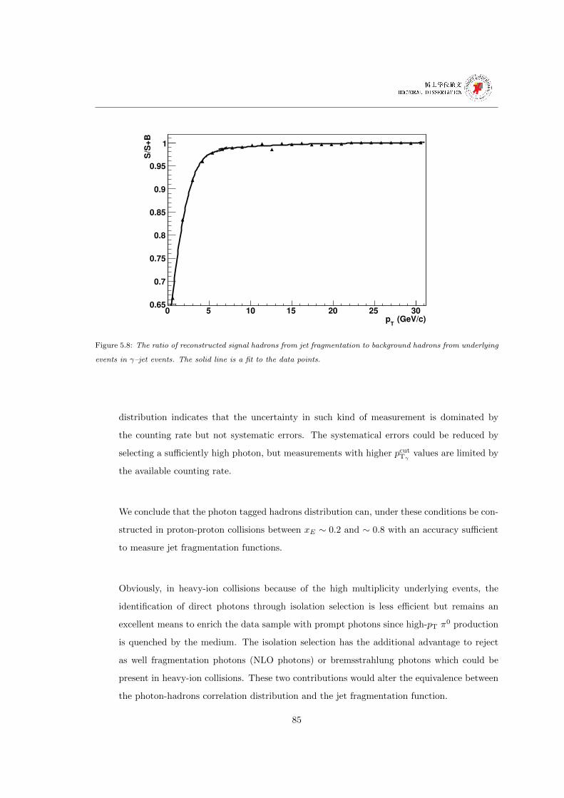
(GeV/c)T

p0 5 10 15 20 25 30

S/S

+B

0.65

0.7

0.75

0.8

0.85

0.9

0.95

1

Figure 5.8: The ratio of reconstructed signal hadrons from jet fragmentation to background hadrons from underlying

events in γ–jet events. The solid line is a fit to the data points.

distribution indicates that the uncertainty in such kind of measurement is dominated by

the counting rate but not systematic errors. The systematical errors could be reduced by

selecting a sufficiently high photon, but measurements with higher pcutTγvalues are limited by

the available counting rate.

We conclude that the photon tagged hadrons distribution can, under these conditions be con-

structed in proton-proton collisions between xE ∼ 0.2 and ∼ 0.8 with an accuracy sufficient

to measure jet fragmentation functions.

Obviously, in heavy-ion collisions because of the high multiplicity underlying events, the

identification of direct photons through isolation selection is less efficient but remains an

excellent means to enrich the data sample with prompt photons since high-pT π0 production

is quenched by the medium. The isolation selection has the additional advantage to reject

as well fragmentation photons (NLO photons) or bremsstrahlung photons which could be

present in heavy-ion collisions. These two contributions would alter the equivalence between

the photon-hadrons correlation distribution and the jet fragmentation function.

85

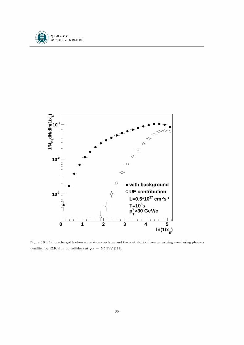
)E

ln(1/x0 1 2 3 4 5

)E

dN/d

ln(1

/xtr

ig1/

N

-310

-210

-110

with backgroundUE contribution

-1s-2 cm27L=0.5*10s6T=10

>30 GeV/cγ

Tp

Figure 5.9: Photon-charged hadron correlation spectrum and the contribution from underlying event using photons

identified by EMCal in pp collisions at√s = 5.5 TeV [111].

86

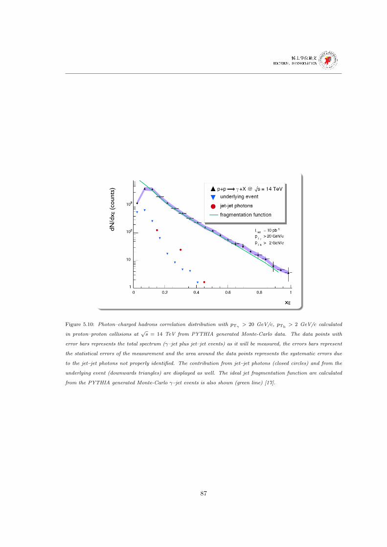
xE

dN/d

x E (

coun

ts)

Figure 5.10: Photon–charged hadrons correlation distribution with pTγ > 20 GeV/c, pTh> 2 GeV/c calculated

in proton–proton collisions at√s = 14 TeV from PYTHIA generated Monte-Carlo data. The data points with

error bars represents the total spectrum (γ–jet plus jet–jet events) as it will be measured, the errors bars represent

the statistical errors of the measurement and the area around the data points represents the systematic errors due

to the jet–jet photons not properly identified. The contribution from jet–jet photons (closed circles) and from the

underlying event (downwards triangles) are displayed as well. The ideal jet fragmentation function are calculated

from the PYTHIA generated Monte-Carlo γ–jet events is also shown (green line) [17].

87

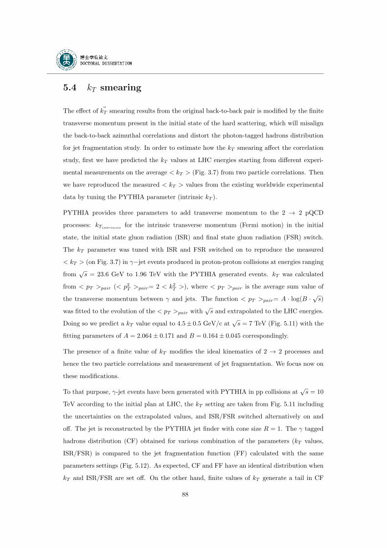
5.4 kT smearing

The effect of ~kT smearing results from the original back-to-back pair is modified by the finite

transverse momentum present in the initial state of the hard scattering, which will misalign

the back-to-back azimuthal correlations and distort the photon-tagged hadrons distribution

for jet fragmentation study. In order to estimate how the kT smearing affect the correlation

study, first we have predicted the kT values at LHC energies starting from different experi-

mental measurements on the average < kT > (Fig. 3.7) from two particle correlations. Then

we have reproduced the measured < kT > values from the existing worldwide experimental

data by tuning the PYTHIA parameter (intrinsic kT ).

PYTHIA provides three parameters to add transverse momentum to the 2 → 2 pQCD

processes: kTintrinsic for the intrinsic transverse momentum (Fermi motion) in the initial

state, the initial state gluon radiation (ISR) and final state gluon radiation (FSR) switch.

The kT parameter was tuned with ISR and FSR switched on to reproduce the measured

< kT > (on Fig. 3.7) in γ−jet events produced in proton-proton collisions at energies ranging

from√s = 23.6 GeV to 1.96 TeV with the PYTHIA generated events. kT was calculated

from < pT >pair (< p2T >pair= 2 < k2T >), where < pT >pair is the average sum value of

the transverse momentum between γ and jets. The function < pT >pair= A · log(B ·√s)

was fitted to the evolution of the < pT >pair with√s and extrapolated to the LHC energies.

Doing so we predict a kT value equal to 4.5± 0.5 GeV/c at√s = 7 TeV (Fig. 5.11) with the

fitting parameters of A = 2.064± 0.171 and B = 0.164± 0.045 correspondingly.

The presence of a finite value of kT modifies the ideal kinematics of 2 → 2 processes and

hence the two particle correlations and measurement of jet fragmentation. We focus now on

these modifications.

To that purpose, γ-jet events have been generated with PYTHIA in pp collisions at√s = 10

TeV according to the initial plan at LHC, the kT setting are taken from Fig. 5.11 including

the uncertainties on the extrapolated values, and ISR/FSR switched alternatively on and

off. The jet is reconstructed by the PYTHIA jet finder with cone size R = 1. The γ tagged

hadrons distribution (CF) obtained for various combination of the parameters (kT values,

ISR/FSR) is compared to the jet fragmentation function (FF) calculated with the same

parameters settings (Fig. 5.12). As expected, CF and FF have an identical distribution when

kT and ISR/FSR are set off. On the other hand, finite values of kT generate a tail in CF

88

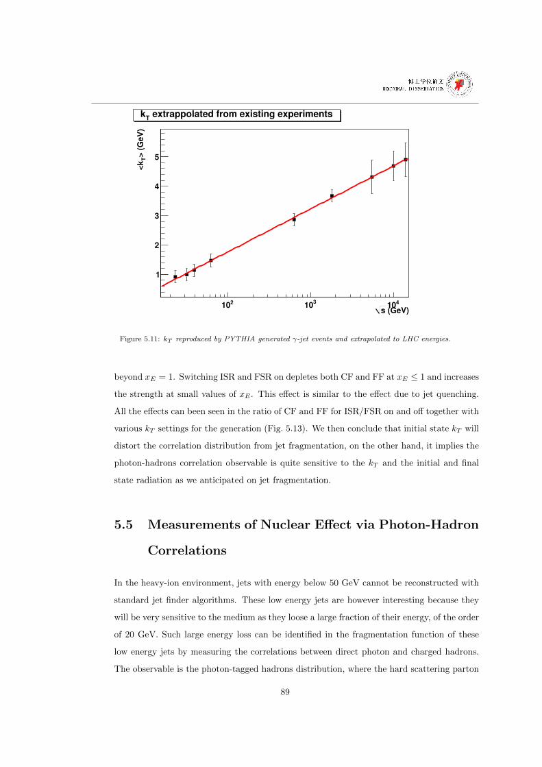
(GeV)s210

310 410

> (

GeV

)T

<k

1

2

3

4

5

extrappolated from existing experimentsT

k

Figure 5.11: kT reproduced by PYTHIA generated γ-jet events and extrapolated to LHC energies.

beyond xE = 1. Switching ISR and FSR on depletes both CF and FF at xE ≤ 1 and increases

the strength at small values of xE . This effect is similar to the effect due to jet quenching.

All the effects can been seen in the ratio of CF and FF for ISR/FSR on and off together with

various kT settings for the generation (Fig. 5.13). We then conclude that initial state kT will

distort the correlation distribution from jet fragmentation, on the other hand, it implies the

photon-hadrons correlation observable is quite sensitive to the kT and the initial and final

state radiation as we anticipated on jet fragmentation.

5.5 Measurements of Nuclear Effect via Photon-Hadron

Correlations

In the heavy-ion environment, jets with energy below 50 GeV cannot be reconstructed with

standard jet finder algorithms. These low energy jets are however interesting because they

will be very sensitive to the medium as they loose a large fraction of their energy, of the order

of 20 GeV. Such large energy loss can be identified in the fragmentation function of these

low energy jets by measuring the correlations between direct photon and charged hadrons.

The observable is the photon-tagged hadrons distribution, where the hard scattering parton

89

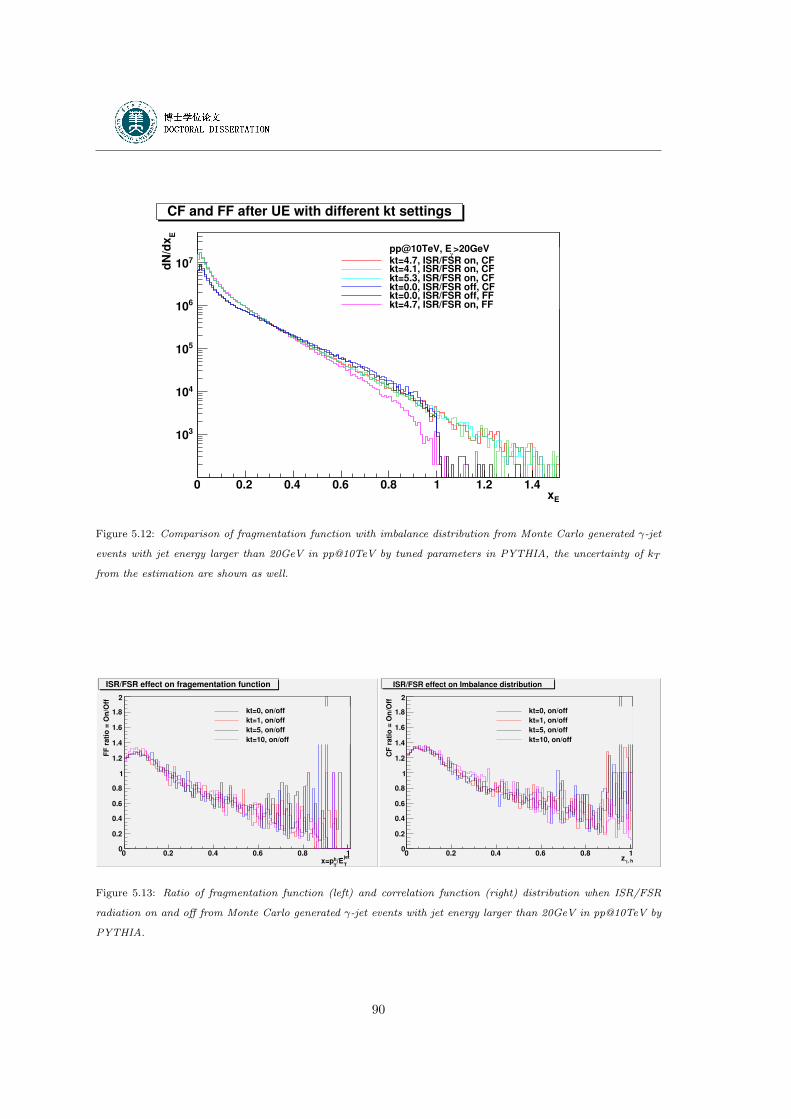
Ex0 0.2 0.4 0.6 0.8 1 1.2 1.4

Ed

N/d

x

310

410

510

610

710

>20GeVγ

pp@10TeV, E

kt=4.7, ISR/FSR on, CFkt=4.1, ISR/FSR on, CFkt=5.3, ISR/FSR on, CFkt=0.0, ISR/FSR off, CFkt=0.0, ISR/FSR off, FFkt=4.7, ISR/FSR on, FF

CF and FF after UE with different kt settings

Figure 5.12: Comparison of fragmentation function with imbalance distribution from Monte Carlo generated γ-jet

events with jet energy larger than 20GeV in pp@10TeV by tuned parameters in PYTHIA, the uncertainty of kT

from the estimation are shown as well.

jet

T/Eh

Tx=p

0 0.2 0.4 0.6 0.8 1

FF

ra

tio

= O

n/O

ff

0

0.2

0.4

0.6

0.8

1

1.2

1.4

1.6

1.8

2

kt=0, on/off

kt=1, on/off

kt=5, on/off

kt=10, on/off

ISR/FSR effect on fragementation function

, hγz

0 0.2 0.4 0.6 0.8 1

CF

ra

tio

= O

n/O

ff

0

0.2

0.4

0.6

0.8

1

1.2

1.4

1.6

1.8

2

kt=0, on/off

kt=1, on/off

kt=5, on/off

kt=10, on/off

ISR/FSR effect on Imbalance distribution

Figure 5.13: Ratio of fragmentation function (left) and correlation function (right) distribution when ISR/FSR

radiation on and off from Monte Carlo generated γ-jet events with jet energy larger than 20GeV in pp@10TeV by

PYTHIA.

90

opposite to photon will experience medium induced energy loss in AA collision compared to

pp collision.

To quantify this medium modification of γ-hadrons correlation distribution in heavy ion

collisions relative to pp collisions, one defines the medium modification factor IAA,

IAA(xE) =CFAACFpp

, (5.11)

for γ-hadrons correlation distribution.

5.5.1 Energy Loss via γ+ Jets

To study this medium induced energy loss, we have used a simple quenching model (QPYTHIA) [113]

implemented into PYTHIA. Such a quenching model combines the calculation of energy

loss [114] and a realistic description of the collision geometry [24], which plays an important

role for studying medium induced energy loss and the possibility for a tomographic study in

heavy-ion collisions, where a HIJING [100] event generator is taken for heavy-ion collisions.

Within these generators, three samples of γ-jet events with energy larger than 20 GeV have

been generated:

– The first sample is composed of γ-jet events generated in pp collisions at 5.5 TeV, using

PYTHIA under the AliRoot framework. No quenching is considered. This sample is

representative of a baseline of quenching study.

– The second sample, consists in merging quenched γ-jet events from QPYTHIA, and the

underlying events of central heavy-ion collisions from the HIJING generator.

– The last sample, is similar to the previous one but without quenching and the underlying

events of peripheral heavy ion collisions.

In the Figure 5.14, which shows the pT spectrum of hadrons with and without quenching

effect, the suppression at high pT can be clearly observed, as well as an enhancement at low

pT .

In the γ-hadrons correlation distribution (Fig. 5.15), the large contribution from the UE of

heavy-ion collisions is clearly visible. It can be subtracted by evaluating its contribution

from emitted hadrons in the same azimuthal directions as the photon trigger. After UE

subtraction, the modification when going from peripheral to central collisions become visible.

91

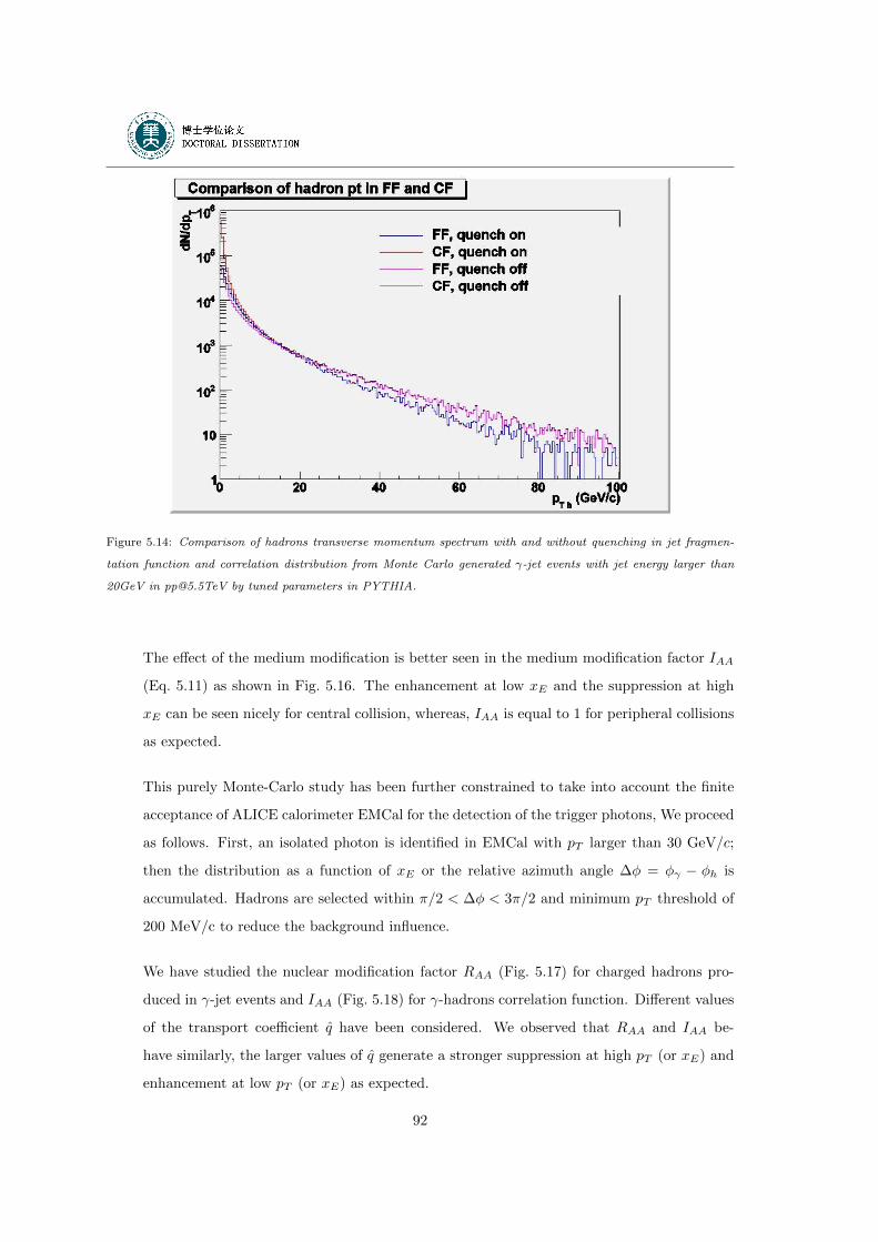
Figure 5.14: Comparison of hadrons transverse momentum spectrum with and without quenching in jet fragmen-

tation function and correlation distribution from Monte Carlo generated γ-jet events with jet energy larger than

20GeV in pp@5.5TeV by tuned parameters in PYTHIA.

The effect of the medium modification is better seen in the medium modification factor IAA

(Eq. 5.11) as shown in Fig. 5.16. The enhancement at low xE and the suppression at high

xE can be seen nicely for central collision, whereas, IAA is equal to 1 for peripheral collisions

as expected.

This purely Monte-Carlo study has been further constrained to take into account the finite

acceptance of ALICE calorimeter EMCal for the detection of the trigger photons, We proceed

as follows. First, an isolated photon is identified in EMCal with pT larger than 30 GeV/c;

then the distribution as a function of xE or the relative azimuth angle ∆φ = φγ − φh is

accumulated. Hadrons are selected within π/2 < ∆φ < 3π/2 and minimum pT threshold of

200 MeV/c to reduce the background influence.

We have studied the nuclear modification factor RAA (Fig. 5.17) for charged hadrons pro-

duced in γ-jet events and IAA (Fig. 5.18) for γ-hadrons correlation function. Different values

of the transport coefficient q have been considered. We observed that RAA and IAA be-

have similarly, the larger values of q generate a stronger suppression at high pT (or xE) and

enhancement at low pT (or xE) as expected.

92

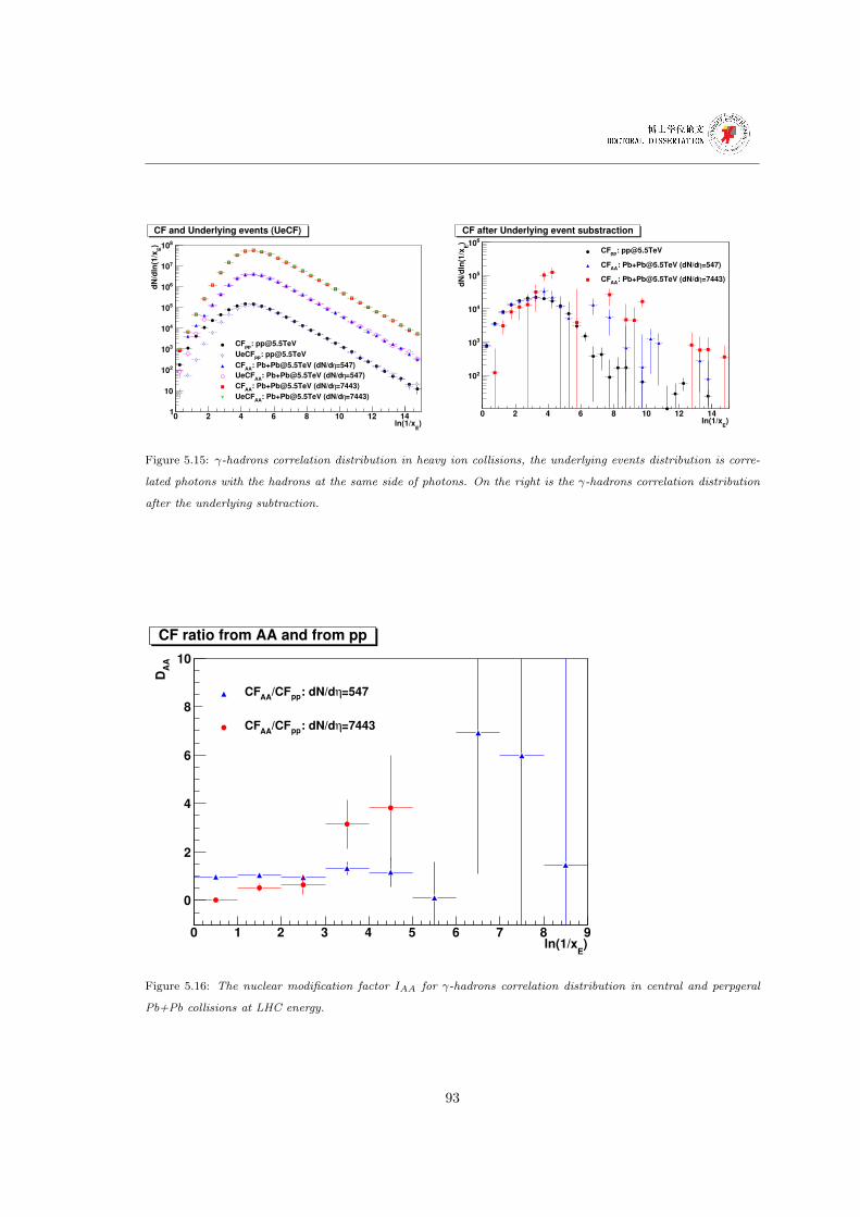
)E

ln(1/x0 2 4 6 8 10 12 14

)E

dN

/dln

(1/x

1

10

210

310

410

510

610

710

810

: pp@5.5TeVppCF

: pp@5.5TeVppUeCF

=547)η: Pb+Pb@5.5TeV (dN/dAA

CF

=547)η: Pb+Pb@5.5TeV (dN/dAA

UeCF

=7443)η: Pb+Pb@5.5TeV (dN/dAA

CF

=7443)η: Pb+Pb@5.5TeV (dN/dAA

UeCF

CF and Underlying events (UeCF)

)E

ln(1/x0 2 4 6 8 10 12 14

)E

dN

/dln

(1/x

210

310

410

510

610: pp@5.5TeVppCF

=547)η: Pb+Pb@5.5TeV (dN/dAA

CF

=7443)η: Pb+Pb@5.5TeV (dN/dAA

CF

CF after Underlying event substraction

Figure 5.15: γ-hadrons correlation distribution in heavy ion collisions, the underlying events distribution is corre-

lated photons with the hadrons at the same side of photons. On the right is the γ-hadrons correlation distribution

after the underlying subtraction.

)E

ln(1/x0 1 2 3 4 5 6 7 8 9

AA

D

0

2

4

6

8

10

=547η: dN/dpp/CFAA

CF

=7443η: dN/dpp/CFAA

CF

CF ratio from AA and from pp

Figure 5.16: The nuclear modification factor IAA for γ-hadrons correlation distribution in central and perpgeral

Pb+Pb collisions at LHC energy.

93

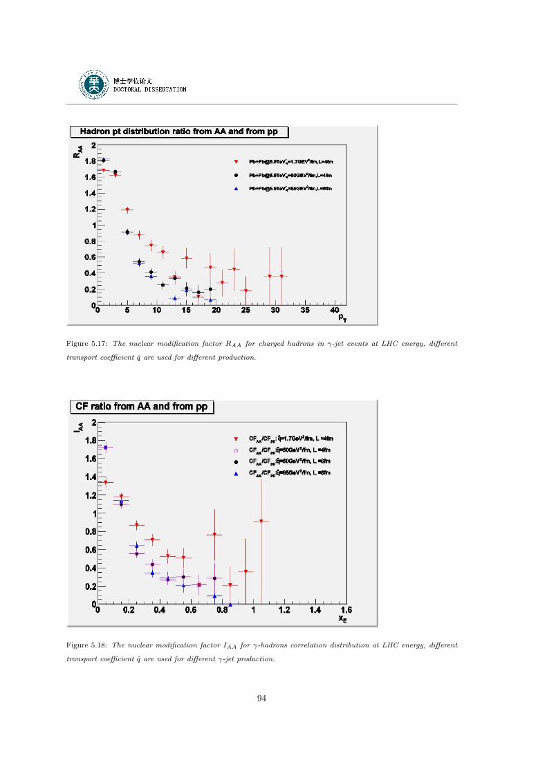
Figure 5.17: The nuclear modification factor RAA for charged hadrons in γ-jet events at LHC energy, different

transport coefficient q are used for different production.

Figure 5.18: The nuclear modification factor IAA for γ-hadrons correlation distribution at LHC energy, different

transport coefficient q are used for different γ-jet production.

94

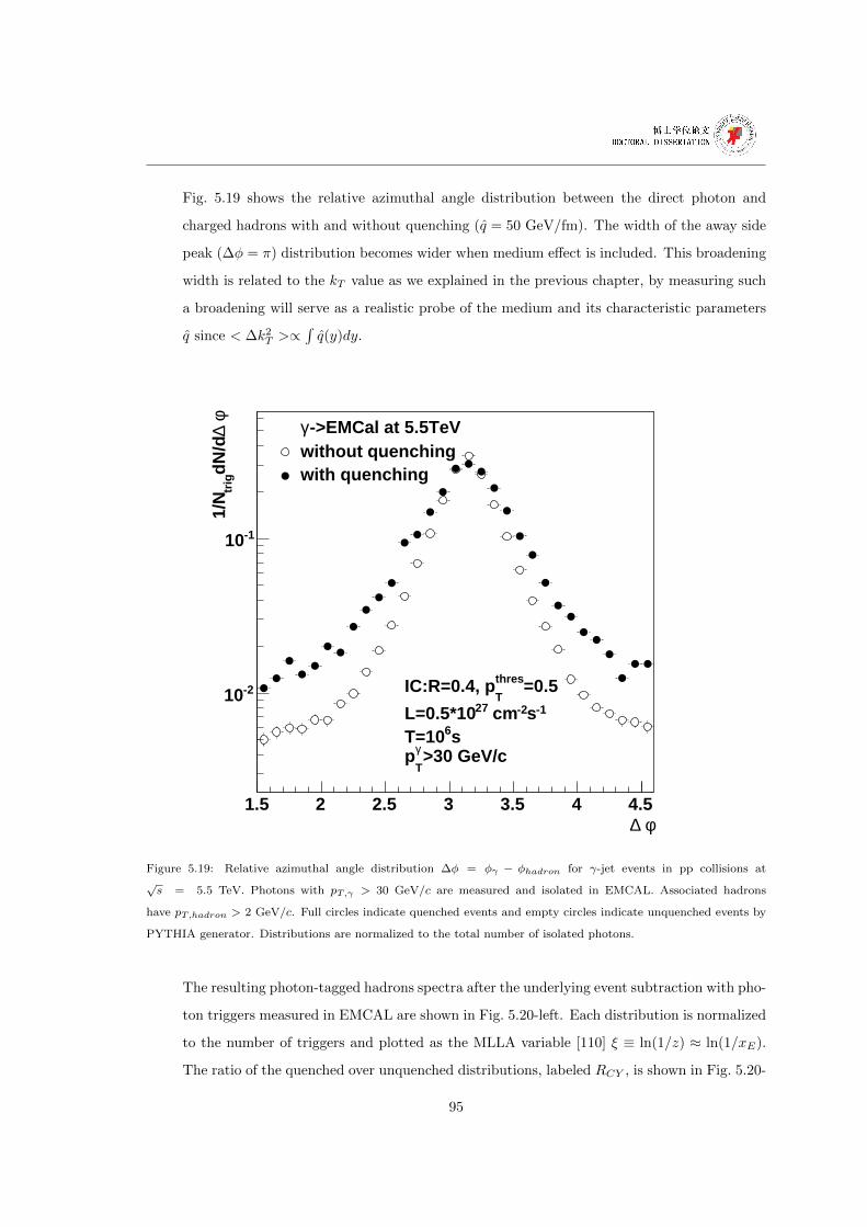
Fig. 5.19 shows the relative azimuthal angle distribution between the direct photon and

charged hadrons with and without quenching (q = 50 GeV/fm). The width of the away side

peak (∆φ = π) distribution becomes wider when medium effect is included. This broadening

width is related to the kT value as we explained in the previous chapter, by measuring such

a broadening will serve as a realistic probe of the medium and its characteristic parameters

q since < ∆k2T >∝∫q(y)dy.

φ ∆1.5 2 2.5 3 3.5 4 4.5

φ ∆dN

/dtr

ig1/

N

-210

-110

->EMCal at 5.5TeVγwithout quenchingwith quenching

=0.5thres

TIC:R=0.4, p

-1s-2 cm27L=0.5*10s6T=10

>30 GeV/cγ

Tp

Figure 5.19: Relative azimuthal angle distribution ∆φ = φγ − φhadron for γ-jet events in pp collisions at√s = 5.5 TeV. Photons with pT,γ > 30 GeV/c are measured and isolated in EMCAL. Associated hadrons

have pT,hadron > 2 GeV/c. Full circles indicate quenched events and empty circles indicate unquenched events by

PYTHIA generator. Distributions are normalized to the total number of isolated photons.

The resulting photon-tagged hadrons spectra after the underlying event subtraction with pho-

ton triggers measured in EMCAL are shown in Fig. 5.20-left. Each distribution is normalized

to the number of triggers and plotted as the MLLA variable [110] ξ ≡ ln(1/z) ≈ ln(1/xE).

The ratio of the quenched over unquenched distributions, labeled RCY , is shown in Fig. 5.20-

95

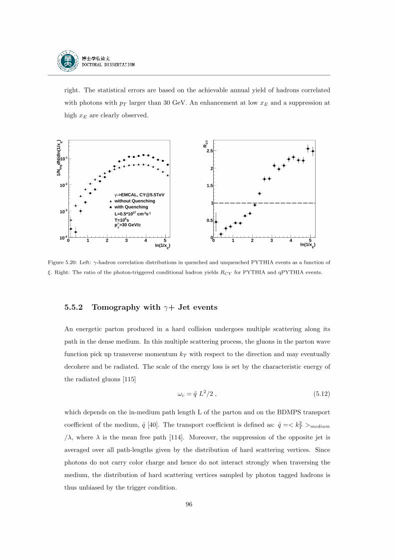
right. The statistical errors are based on the achievable annual yield of hadrons correlated

with photons with pT larger than 30 GeV. An enhancement at low xE and a suppression at

high xE are clearly observed.

)E

ln(1/x0 1 2 3 4 5

)E

dN/d

ln(1

/xtr

ig1/

N

-410

-310

-210

-110

->EMCAL, CY@5.5TeVγwithout Quenchingwith Quenching

-1s-2 cm27L=0.5*10s6T=10

>30 GeV/cγ

Tp

)E

ln(1/x0 1 2 3 4 5

CY

R

0

0.5

1

1.5

2

2.5

Figure 5.20: Left: γ-hadron correlation distributions in quenched and unquenched PYTHIA events as a function of

ξ. Right: The ratio of the photon-triggered conditional hadron yields RCY for PYTHIA and qPYTHIA events.

5.5.2 Tomography with γ+ Jet events

An energetic parton produced in a hard collision undergoes multiple scattering along its

path in the dense medium. In this multiple scattering process, the gluons in the parton wave

function pick up transverse momentum kT with respect to the direction and may eventually

decohere and be radiated. The scale of the energy loss is set by the characteristic energy of

the radiated gluons [115]

ωc = q L2/2 , (5.12)

which depends on the in-medium path length L of the parton and on the BDMPS transport

coefficient of the medium, q [40]. The transport coefficient is defined as: q =< k2T >medium

/λ, where λ is the mean free path [114]. Moreover, the suppression of the opposite jet is

averaged over all path-lengths given by the distribution of hard scattering vertices. Since

photons do not carry color charge and hence do not interact strongly when traversing the

medium, the distribution of hard scattering vertices sampled by photon tagged hadrons is

thus unbiased by the trigger condition.

96

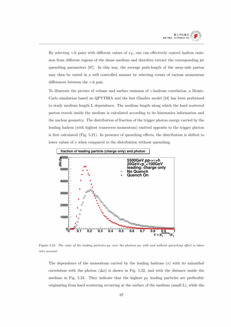
By selecting γ-h pairs with different values of xE , one can effectively control hadron emis-

sion from different regions of the dense medium and therefore extract the corresponding jet

quenching parameters [87]. In this way, the average path-length of the away-side parton

may then be varied in a well controlled manner by selecting events of various momentum

differences between the γ-h pair.

To illustrate the picture of volume and surface emission of γ-hadrons correlation, a Monte-

Carlo simulation based on QPYTHIA and the fast Glauber model [24] has been performed

to study medium length L dependence. The medium length along which the hard scattered

parton travels inside the medium is calculated according to its kinematics information and

the nuclear geometry. The distribution of fraction of the trigger photon energy carried by the

leading hadron (with highest transverse momentum) emitted opposite to the trigger photon

is first calculated (Fig. 5.21). In presence of quenching effects, the distribution is shifted to

lower values of x when compared to the distribution without quenching.

γ

T/p

leading

Tx = p

0 0.1 0.2 0.3 0.4 0.5 0.6 0.7 0.8 0.9 1

dN

/dx

0

1000

2000

3000

4000

5000

6000+hγ5500GeV pp­>

<100GeVγ

T20GeV<pleading: charge onlyNo QuenchQuench On

fraction of leading particle (charge only) and photon

Figure 5.21: The ratio of the leading particles pT over the photons pT with and without quenching effect is taken

into account.

The dependence of the momentum carried by the leading hadrons (x) with its azimuthal

correlation with the photon (∆φ) is shown in Fig. 5.22, and with the distance inside the

medium in Fig. 5.23. They indicate that the highest pT leading particles are preferably

originating from hard scattering occurring at the surface of the medium (small L), while the

97

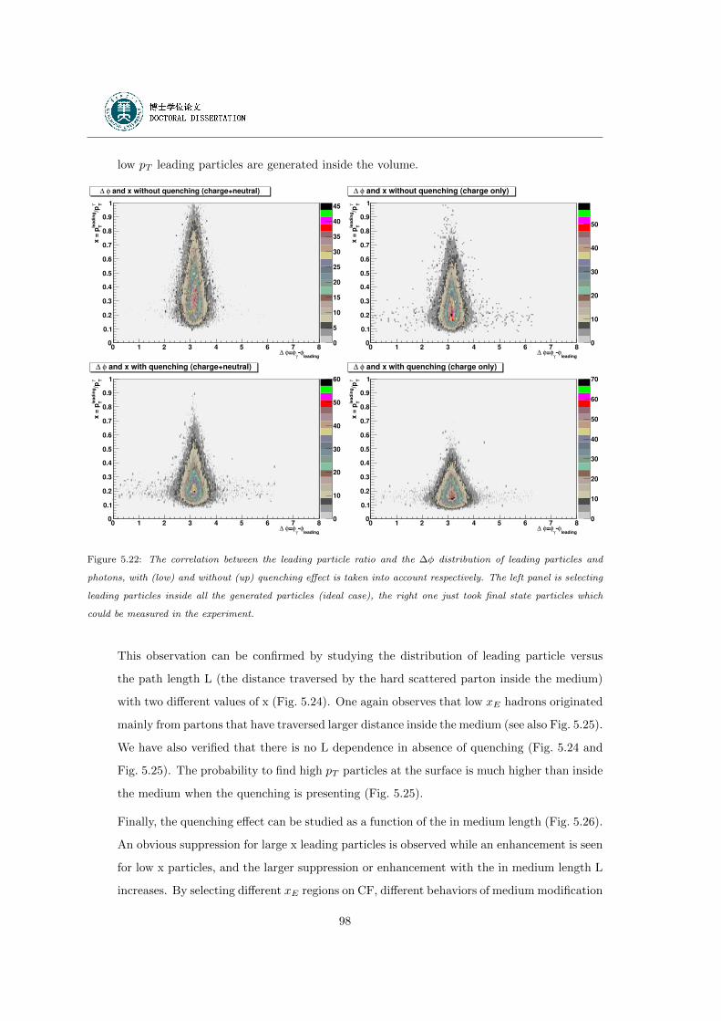
low pT leading particles are generated inside the volume.

leadingφ­

γφ=φ ∆

0 1 2 3 4 5 6 7 8

γ T/p

lead

ing

Tx =

p

0

0.1

0.2

0.3

0.4

0.5

0.6

0.7

0.8

0.9

1

0

5

10

15

20

25

30

35

40

45

and x without quenching (charge+neutral)φ ∆

leadingφ­

γφ=φ ∆

0 1 2 3 4 5 6 7 8γ T

/ple

ad

ing

Tx =

p

0

0.1

0.2

0.3

0.4

0.5

0.6

0.7

0.8

0.9

1

0

10

20

30

40

50

and x without quenching (charge only)φ ∆

leadingφ­

γφ=φ ∆

0 1 2 3 4 5 6 7 8

γ T/p

lead

ing

Tx =

p

0

0.1

0.2

0.3

0.4

0.5

0.6

0.7

0.8

0.9

1

0

10

20

30

40

50

60

and x with quenching (charge+neutral)φ ∆

leadingφ­

γφ=φ ∆

0 1 2 3 4 5 6 7 8

γ T/p

lead

ing

Tx =

p

0

0.1

0.2

0.3

0.4

0.5

0.6

0.7

0.8

0.9

1

0

10

20

30

40

50

60

70

and x with quenching (charge only)φ ∆

Figure 5.22: The correlation between the leading particle ratio and the ∆φ distribution of leading particles and

photons, with (low) and without (up) quenching effect is taken into account respectively. The left panel is selecting

leading particles inside all the generated particles (ideal case), the right one just took final state particles which

could be measured in the experiment.

This observation can be confirmed by studying the distribution of leading particle versus

the path length L (the distance traversed by the hard scattered parton inside the medium)

with two different values of x (Fig. 5.24). One again observes that low xE hadrons originated

mainly from partons that have traversed larger distance inside the medium (see also Fig. 5.25).

We have also verified that there is no L dependence in absence of quenching (Fig. 5.24 and

Fig. 5.25). The probability to find high pT particles at the surface is much higher than inside

the medium when the quenching is presenting (Fig. 5.25).

Finally, the quenching effect can be studied as a function of the in medium length (Fig. 5.26).

An obvious suppression for large x leading particles is observed while an enhancement is seen

for low x particles, and the larger suppression or enhancement with the in medium length L

increases. By selecting different xE regions on CF, different behaviors of medium modification

98

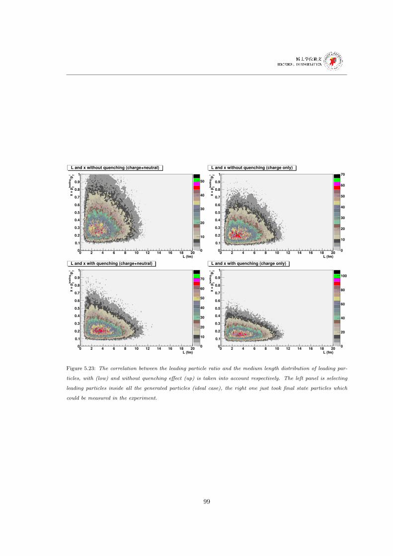
L (fm)0 2 4 6 8 10 12 14 16 18 20

γ T/p

lead

ing

Tx =

p

0

0.1

0.2

0.3

0.4

0.5

0.6

0.7

0.8

0.9

1

0

10

20

30

40

50

L and x without quenching (charge+neutral)

L (fm)0 2 4 6 8 10 12 14 16 18 20

γ T/p

lead

ing

Tx =

p

0

0.1

0.2

0.3

0.4

0.5

0.6

0.7

0.8

0.9

1

0

10

20

30

40

50

60

70

L and x without quenching (charge only)

L (fm)0 2 4 6 8 10 12 14 16 18 20

γ T/p

lead

ing

Tx =

p

0

0.1

0.2

0.3

0.4

0.5

0.6

0.7

0.8

0.9

1

0

10

20

30

40

50

60

70

L and x with quenching (charge+neutral)

L (fm)0 2 4 6 8 10 12 14 16 18 20

γ T/p

lead

ing

Tx =

p

0

0.1

0.2

0.3

0.4

0.5

0.6

0.7

0.8

0.9

1

0

20

40

60

80

100

L and x with quenching (charge only)

Figure 5.23: The correlation between the leading particle ratio and the medium length distribution of leading par-

ticles, with (low) and without quenching effect (up) is taken into account respectively. The left panel is selecting

leading particles inside all the generated particles (ideal case), the right one just took final state particles which

could be measured in the experiment.

99

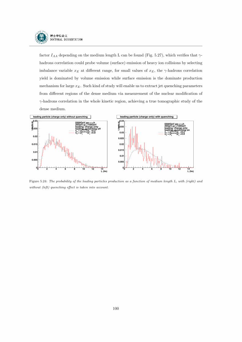
factor IAA depending on the medium length L can be found (Fig. 5.27), which verifies that γ-

hadrons correlation could probe volume (surface) emission of heavy ion collisions by selecting

imbalance variable xE at different range, for small values of xE , the γ-hadrons correlation

yield is dominated by volume emission while surface emission is the dominate production

mechanism for large xE . Such kind of study will enable us to extract jet quenching parameters

from different regions of the dense medium via measurement of the nuclear modification of

γ-hadrons correlation in the whole kinetic region, achieving a true tomographic study of the

dense medium.

L (fm)0 2 4 6 8 10 12 14

1/N

dN

/dL

0

0.005

0.01

0.015

0.02

0.025

0.03+hγ5500GeV pp­>

<100GeVγ

T20GeV<pleading: charge onlyleading: quenching off

<0.2γ

T/pleading

T = p

Ex

>0.8γ

T/p

leading

T = p

Ex

leading particle (charge only) without quenching

L (fm)0 2 4 6 8 10 12 14

1/N

dN

/dL

0

0.005

0.01

0.015

0.02

0.025

0.03

0.035

0.04

+hγ5500GeV pp­><100GeV

γ

T20GeV<pleading: charge onlyleading: quenching on

<0.2γ

T/pleading

T = p

Ex

>0.8γ

T/pleading

T = p

Ex

leading particle (charge only) with quenching

Figure 5.24: The probability of the leading particles production as a function of medium length L, with (right) and

without (left) quenching effect is taken into account.

100

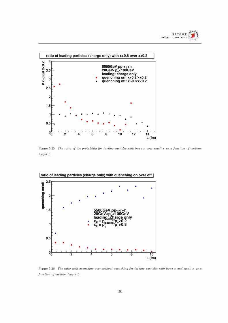
L (fm)0 2 4 6 8 10 12 14

# x

>0.8

/# x

<0.2

0

0.5

1

1.5

2

2.5

3

3.5

4

+hγ5500GeV pp­><100GeV

γ

T20GeV<pleading: charge onlyquenching on: x>0.8/x<0.2quenching off: x>0.8/x<0.2

ratio of leading particles (charge only) with x>0.8 over x<0.2

Figure 5.25: The ratio of the probability for leading particles with large x over small x as a function of medium

length L.

L (fm)0 2 4 6 8 10

qu

en

ch

ing

on

/off

0

0.5

1

1.5

2

2.5

+hγ5500GeV pp­><100GeV

γ

T20GeV<pleading: charge only

<0.2γ

T/p

leading

T = pEx

>0.8γ

T/p

leading

T = pEx

ratio of leading particles (charge only) with quenching on over off

Figure 5.26: The ratio with quenching over without quenching for leading particles with large x and small x as a

function of medium length L.

101

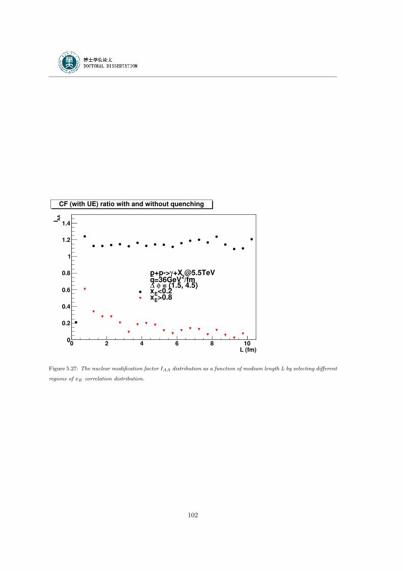
L (fm)0 2 4 6 8 10

AA

I

0

0.2

0.4

0.6

0.8

1

1.2

1.4

+X @5.5TeVγp+p­>/fm

2=36GeVq

= (1.5, 4.5)φ ∆<0.2Ex>0.8Ex

CF (with UE) ratio with and without quenching

Figure 5.27: The nuclear modification factor IAA distribution as a function of medium length L by selecting different

regions of xE correlation distribution.

102

Chapter 6

Analysis of ALICE Data

In this chapter I present the status (March 2011) of my analysis of the data collected for

proton-proton collisions at√s = 7 TeV during the first LHC run in 2010. The goal of this

analysis is to construct the direct photon-charged hadron correlations. This analysis will

provide a reference for a data analysis of heavy-ion data. The results to be shown here

are obtained by analyzing about 160 million minimum bias events. The preliminary result

include inclusive photon-charged hadrons and π0-charged hadrons correlation all showing the

characteristic di-jet pattern from where the momentum imbalance kT is extracted. Results

on direct photons are not convincing because of the limited statistics accumulated during

this time.

6.1 Data Sample

The definition of an interaction, the basis of the minimum bias trigger, is based on a logical

mix of different detector inputs, two detectors have been used for triggering [116]:

– The Silicon Pixel Detector (SPD) provides trigger signals, which can be set up in a

programmable way to run with the main multiplicity-based trigger selections.

– The scintillator hodoscopes V0 provide four basic signals, corresponding to hits on either

side of the interaction region in the time windows for incoming beam-gas and outgoing

colliding-beam interactions, the latter classified according to multiplicity.

103

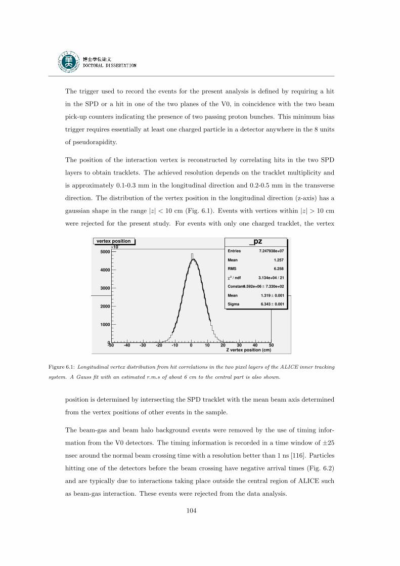
The trigger used to record the events for the present analysis is defined by requiring a hit

in the SPD or a hit in one of the two planes of the V0, in coincidence with the two beam

pick-up counters indicating the presence of two passing proton bunches. This minimum bias

trigger requires essentially at least one charged particle in a detector anywhere in the 8 units

of pseudorapidity.

The position of the interaction vertex is reconstructed by correlating hits in the two SPD

layers to obtain tracklets. The achieved resolution depends on the tracklet multiplicity and

is approximately 0.1-0.3 mm in the longitudinal direction and 0.2-0.5 mm in the transverse

direction. The distribution of the vertex position in the longitudinal direction (z-axis) has a

gaussian shape in the range |z| < 10 cm (Fig. 6.1). Events with vertices within |z| > 10 cm

were rejected for the present study. For events with only one charged tracklet, the vertex

_pzEntries 7.247938e+07

Mean 1.257

RMS 6.258

/ ndf 2χ 3.134e+04 / 21

Constant 7.330e+02± 4.592e+06

Mean 0.001± 1.319

Sigma 0.001± 6.343

Z vertex position (cm)­50 ­40 ­30 ­20 ­10 0 10 20 30 40 500

1000

2000

3000

4000

5000

310×

_pzEntries 7.247938e+07

Mean 1.257

RMS 6.258

/ ndf 2χ 3.134e+04 / 21

Constant 7.330e+02± 4.592e+06

Mean 0.001± 1.319

Sigma 0.001± 6.343

vertex position

Figure 6.1: Longitudinal vertex distribution from hit correlations in the two pixel layers of the ALICE inner tracking

system. A Gauss fit with an estimated r.m.s of about 6 cm to the central part is also shown.

position is determined by intersecting the SPD tracklet with the mean beam axis determined

from the vertex positions of other events in the sample.

The beam-gas and beam halo background events were removed by the use of timing infor-

mation from the V0 detectors. The timing information is recorded in a time window of ±25

nsec around the normal beam crossing time with a resolution better than 1 ns [116]. Particles

hitting one of the detectors before the beam crossing have negative arrival times (Fig. 6.2)

and are typically due to interactions taking place outside the central region of ALICE such

as beam-gas interaction. These events were rejected from the data analysis.

104

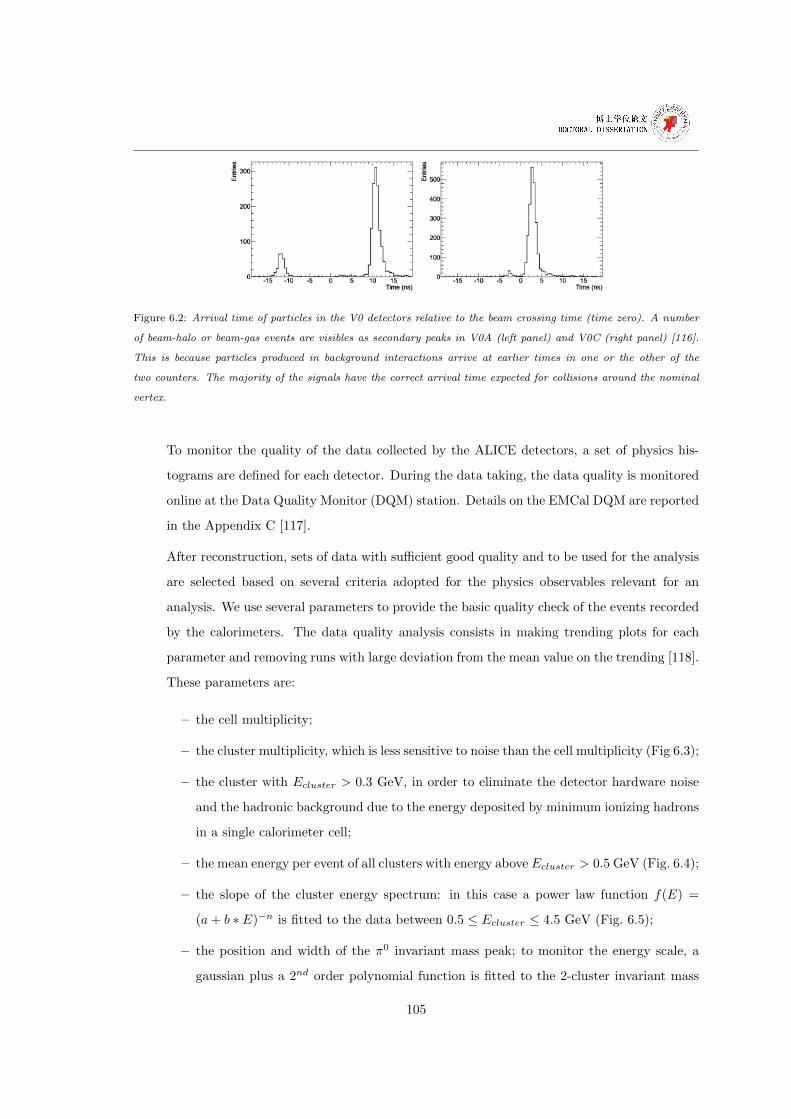
Figure 6.2: Arrival time of particles in the V0 detectors relative to the beam crossing time (time zero). A number

of beam-halo or beam-gas events are visibles as secondary peaks in V0A (left panel) and V0C (right panel) [116].

This is because particles produced in background interactions arrive at earlier times in one or the other of the

two counters. The majority of the signals have the correct arrival time expected for collisions around the nominal

vertex.

To monitor the quality of the data collected by the ALICE detectors, a set of physics his-

tograms are defined for each detector. During the data taking, the data quality is monitored

online at the Data Quality Monitor (DQM) station. Details on the EMCal DQM are reported

in the Appendix C [117].

After reconstruction, sets of data with sufficient good quality and to be used for the analysis

are selected based on several criteria adopted for the physics observables relevant for an

analysis. We use several parameters to provide the basic quality check of the events recorded

by the calorimeters. The data quality analysis consists in making trending plots for each

parameter and removing runs with large deviation from the mean value on the trending [118].

These parameters are:

– the cell multiplicity;

– the cluster multiplicity, which is less sensitive to noise than the cell multiplicity (Fig 6.3);

– the cluster with Ecluster > 0.3 GeV, in order to eliminate the detector hardware noise

and the hadronic background due to the energy deposited by minimum ionizing hadrons

in a single calorimeter cell;

– the mean energy per event of all clusters with energy above Ecluster > 0.5 GeV (Fig. 6.4);

– the slope of the cluster energy spectrum: in this case a power law function f(E) =

(a+ b ∗ E)−n is fitted to the data between 0.5 ≤ Ecluster ≤ 4.5 GeV (Fig. 6.5);

– the position and width of the π0 invariant mass peak; to monitor the energy scale, a

gaussian plus a 2nd order polynomial function is fitted to the 2-cluster invariant mass

105

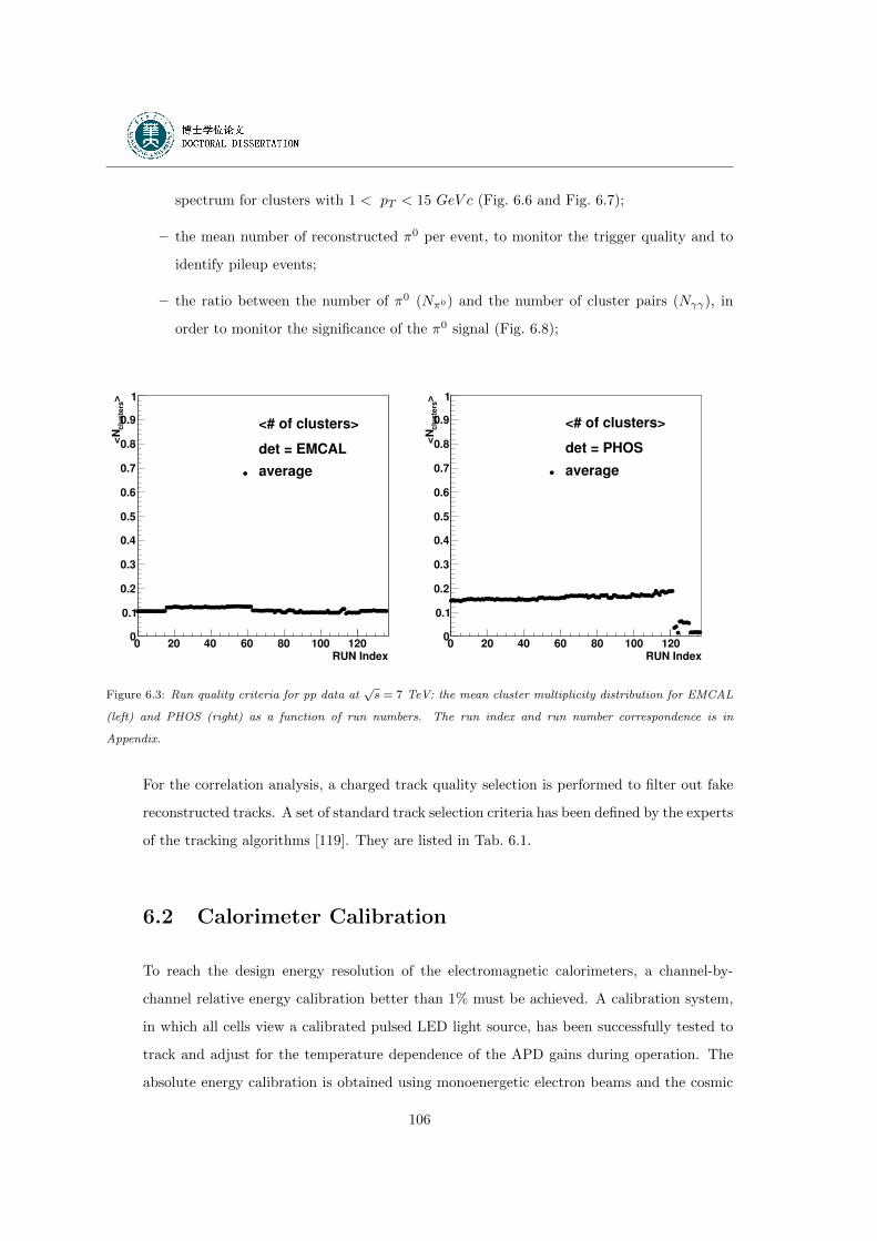
spectrum for clusters with 1 < pT < 15 GeV c (Fig. 6.6 and Fig. 6.7);

– the mean number of reconstructed π0 per event, to monitor the trigger quality and to

identify pileup events;

– the ratio between the number of π0 (Nπ0) and the number of cluster pairs (Nγγ), in

order to monitor the significance of the π0 signal (Fig. 6.8);

RUN Index0 20 40 60 80 100 120

>c

lus

ters

<N

0

0.1

0.2

0.3

0.4

0.5

0.6

0.7

0.8

0.9

1

<# of clusters>

det = EMCAL

average

RUN Index0 20 40 60 80 100 120

>c

lus

ters

<N

0

0.1

0.2

0.3

0.4

0.5

0.6

0.7

0.8

0.9

1

<# of clusters>

det = PHOS

average

Figure 6.3: Run quality criteria for pp data at√s = 7 TeV: the mean cluster multiplicity distribution for EMCAL

(left) and PHOS (right) as a function of run numbers. The run index and run number correspondence is in

Appendix.

For the correlation analysis, a charged track quality selection is performed to filter out fake

reconstructed tracks. A set of standard track selection criteria has been defined by the experts

of the tracking algorithms [119]. They are listed in Tab. 6.1.

6.2 Calorimeter Calibration

To reach the design energy resolution of the electromagnetic calorimeters, a channel-by-

channel relative energy calibration better than 1% must be achieved. A calibration system,

in which all cells view a calibrated pulsed LED light source, has been successfully tested to

track and adjust for the temperature dependence of the APD gains during operation. The

absolute energy calibration is obtained using monoenergetic electron beams and the cosmic

106

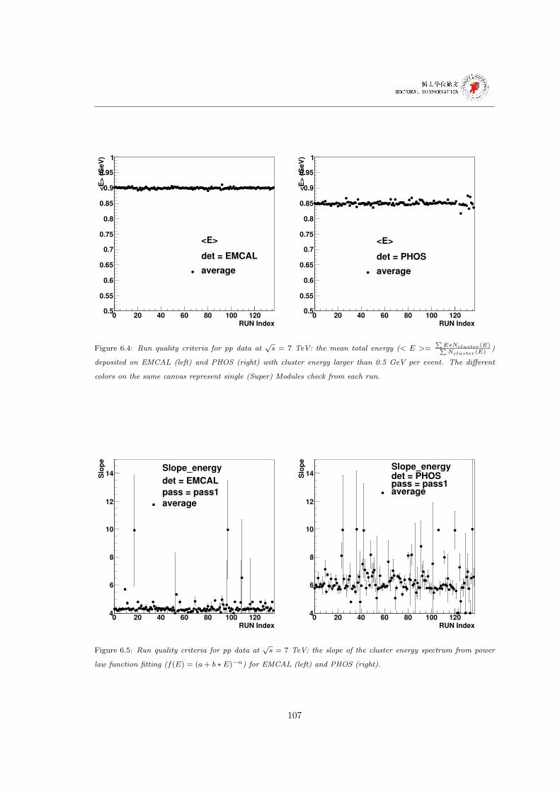
RUN Index0 20 40 60 80 100 120

<E

> (

Ge

V)

0.5

0.55

0.6

0.65

0.7

0.75

0.8

0.85

0.9

0.95

1

<E>

det = EMCAL

average

RUN Index0 20 40 60 80 100 120

<E

> (

Ge

V)

0.5

0.55

0.6

0.65

0.7

0.75

0.8

0.85

0.9

0.95

1

<E>

det = PHOS

average

Figure 6.4: Run quality criteria for pp data at√s = 7 TeV: the mean total energy (< E >=

∑E∗Ncluster(E)∑Ncluster(E)

)

deposited on EMCAL (left) and PHOS (right) with cluster energy larger than 0.5 GeV per event. The different

colors on the same canvas represent single (Super) Modules check from each run.

RUN Index0 20 40 60 80 100 120

Slo

pe

4

6

8

10

12

14Slope_energy

det = EMCAL

pass = pass1

average

RUN Index0 20 40 60 80 100 120

Slo

pe

4

6

8

10

12

14Slope_energydet = PHOSpass = pass1average

Figure 6.5: Run quality criteria for pp data at√s = 7 TeV: the slope of the cluster energy spectrum from power

law function fitting (f(E) = (a+ b ∗ E)−n) for EMCAL (left) and PHOS (right).

107

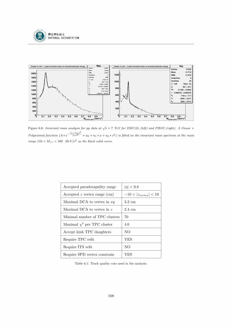
MggEntries 142547

Mean 0.3248

RMS 0.2077

Underflow 0

Overflow 2998

/ ndf 2χ 75.09 / 44

A 24.6± 793.1

0

m 0.0005± 0.1397

σ 0.00067± 0.01577

0

a 30.2± 546.7

1

a 452.5± 7117

2

a 1.35e+03± ­1.56e+04

)2 (GeV/ccluster pairsM0 0.1 0.2 0.3 0.4 0.5 0.6 0.7 0.8 0.9 1

0

200

400

600

800

1000

1200

1400

1600

1800

2000

MggEntries 142547

Mean 0.3248

RMS 0.2077

Underflow 0

Overflow 2998

/ ndf 2χ 75.09 / 44

A 24.6± 793.1

0

m 0.0005± 0.1397

σ 0.00067± 0.01577

0

a 30.2± 546.7

1

a 452.5± 7117

2

a 1.35e+03± ­1.56e+04

Cluster (n cell > 1) pairs Invariant mass vs reconstructed pair energy Mgg

Entries 31323

Mean 0.1716

RMS 0.1374

Underflow 0

Overflow 20

/ ndf 2χ 165.6 / 44

A 22.7± 561

0m 0.0003± 0.1362

σ 0.000378± 0.008318

0

a 17.7± 718.3

1

a 210.7± ­2544

2

a 573.4± 2565

)2 (GeV/ccluster pairsM0 0.1 0.2 0.3 0.4 0.5 0.6 0.7 0.8 0.9 1

0

200

400

600

800

1000

1200

Mgg

Entries 31323

Mean 0.1716

RMS 0.1374

Underflow 0

Overflow 20

/ ndf 2χ 165.6 / 44

A 22.7± 561

0m 0.0003± 0.1362

σ 0.000378± 0.008318

0

a 17.7± 718.3

1

a 210.7± ­2544

2

a 573.4± 2565

Cluster (n cell > 1) pairs Invariant mass vs reconstructed pair energy

Figure 6.6: Invariant mass analysis for pp data at√s = 7 TeV for EMCAL (left) and PHOS (right). A Gauss +

Polynoimal function (A ∗ e−(x−m0)2

2∗σ2 + a0 + a1 ∗ x+ a2 ∗ x2) is fitted on the invariant mass spectrum at the mass

range 110 < Mγγ < 160 MeV/c2 as the black solid curve.

Accepted pseudorapidity range |η| < 0.8

Accepted z vertex range (cm) −10 < |zvertex| < 10

Maximal DCA to vertex in xy 3.2 cm

Maximal DCA to vertex in z 2.4 cm

Minimal number of TPC clusters 70

Maximal χ2 per TPC cluster 4.0

Accept kink TPC daughters NO

Require TPC refit YES

Require ITS refit NO

Require SPD vertex constrain YES

Table 6.1: Track quality cuts used in the analysis.

108

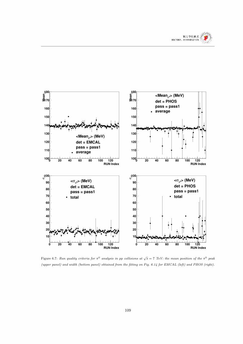
RUN Index0 20 40 60 80 100 120

0π

Me

an

100

110

120

130

140

150

160

170

180

> (MeV)0π

<Mean

det = EMCAL

pass = pass1

average

RUN Index0 20 40 60 80 100 120

0π

Me

an

100

110

120

130

140

150

160

170

180

> (MeV)0π

<Mean

det = PHOS

pass = pass1

average

RUN Index0 20 40 60 80 100 120

0π

σ

10

20

30

40

50

60

70

80

90

100

> (MeV)0π

σ<

det = EMCAL

pass = pass1

total

RUN Index0 20 40 60 80 100 120

0π

σ

10

20

30

40

50

60

70

80

90

100

> (MeV)0π

σ<

det = PHOS

pass = pass1

total

Figure 6.7: Run quality criteria for π0 analysis in pp collisions at√s = 7 TeV: the mean position of the π0 peak

(upper panel) and width (bottom panel) obtained from the fitting on Fig. 6.14 for EMCAL (left) and PHOS (right).

109

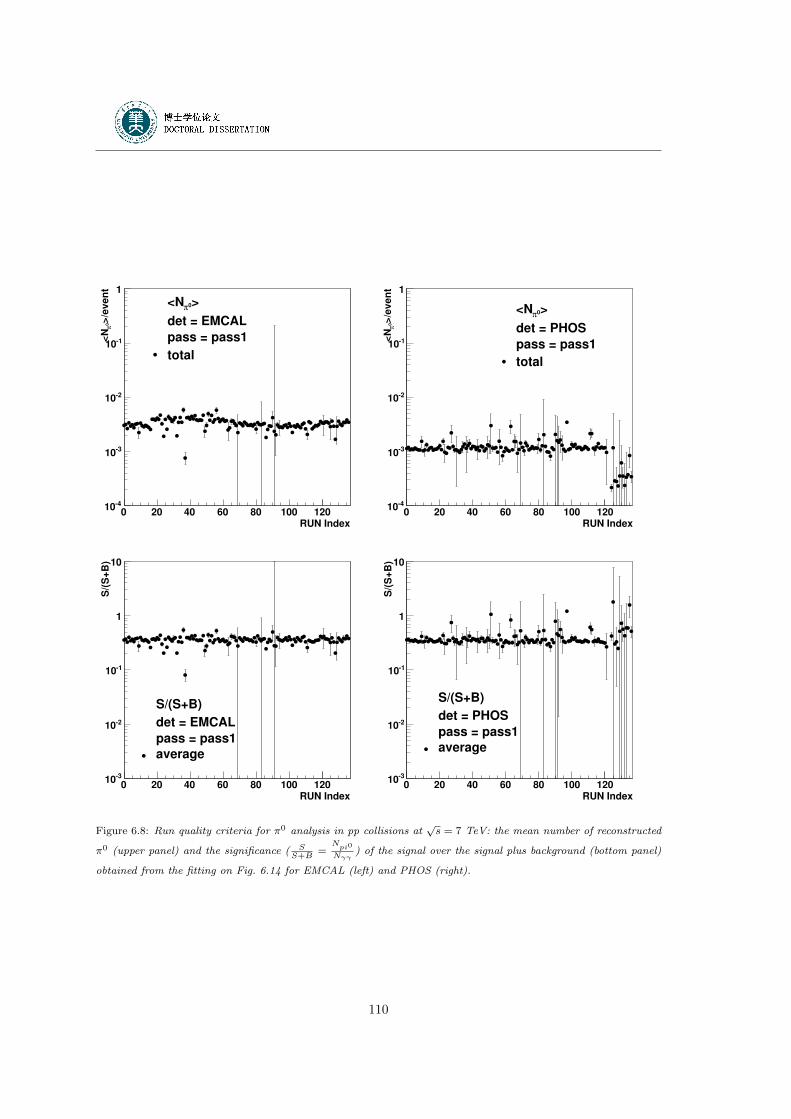
RUN Index0 20 40 60 80 100 120

>/e

ve

nt

0π

<N

­410

­310

­210

­110

1

>0π<N

det = EMCAL

pass = pass1

total

RUN Index0 20 40 60 80 100 120

>/e

ve

nt

0π

<N

­410

­310

­210

­110

1

>0π<N

det = PHOS

pass = pass1

total

RUN Index0 20 40 60 80 100 120

S/(

S+

B)

­310

­210

­110

1

10

S/(S+B)

det = EMCAL

pass = pass1

average

RUN Index0 20 40 60 80 100 120

S/(

S+

B)

­310

­210

­110

1

10

S/(S+B)

det = PHOS

pass = pass1

average

Figure 6.8: Run quality criteria for π0 analysis in pp collisions at√s = 7 TeV: the mean number of reconstructed

π0 (upper panel) and the significance ( SS+B

=Npi0

Nγγ) of the signal over the signal plus background (bottom panel)

obtained from the fitting on Fig. 6.14 for EMCAL (left) and PHOS (right).

110

muons. Final tuning of the calibration is achieved with the collision data by adjusting the

position of the π0 peak in the 2-clusters invariant mass distribution.

6.2.1 Cosmic muons calibration

High statistics MIP data enable us to adjust the relative gain factors between EMCAL towers.

The muon signal measured in each tower is obtained by the use of an isolation procedure

applied offline. For each event, the maximum amplitude is chosen and for all neighboring

towers a signal smaller than a threshold value is required. This threshold is limited by the

electronic noise (set to 3 ADC counts for the present study). The muons, passing the towers

along their length, are selected using scintillator paddles. Each paddle covers 12 modules

grouped into a ”strip module”, and is read out at both extremities by photomultiplier tubes

(PMT). The time of flight between both PMTs allows one to select vertical muons with a

spatial accuracy of a few centimeters. The isolation procedure then ensures that no energy

was deposited in the neighboring towers. The amplitude of the signal is extracted by fitting

a Gamma-2 function (F = A ∗ tN ∗ eN∗(1−t), where A is the amplitude value, N is the order

of Gamma function) to the time dependent electronic signal delivered by a tower.

A 24-h run allows the accumulation of about 500 muons per towers, which is sufficient to

exact the MIP peak with an accuracy of about 1% (Fig. 6.9). An individual gain calibration

is performed for each tower by aligning the MIP peak for all towers. The tower gains,

which are controlled through the tower high voltage power, are tuned iteratively. The mean

amplitude signal from all towers are clearly peaked around 16 ADC counts after the isolation

selection, and other additional cuts only change slightly the mean and the width of the

relative calibration (see Fig 6.9). Fig. 6.10 shows the dispersion of the MIP peak position

for 384 towers before and after several iterations done (thin and bold lines, respectively), A

final relative dispersion < 3% is reached [120].

6.2.2 π0 mass calibration

With high statistics pp collision data, two photon invariant mass spectra are accumulated for

each tower. The position of the observed π0 peak is used to improve the channel by channel

absolute energy calibration. In the ideal case, the reconstructed two photon invariant mass

shows a sharp peak at the π0 mass with a width corresponding to the intrinsic resolution of

111

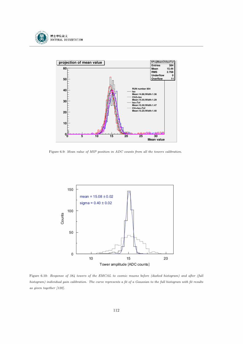
Mean value0 5 10 15 20 25 30

0

10

20

30

40

50

60

hProjMeanChiIsol

Entries 384

Mean 14.96

RMS 3.247

Underflow 0

Overflow 5

hProjMeanChiIsol

Entries 384

Mean 14.96

RMS 3.247

Underflow 0

Overflow 5

hProjMeanIsolTof

Entries 384

Mean 15.61

RMS 2.706

Underflow 0

Overflow 14

hProjMeanIsolTof

Entries 384

Mean 15.61

RMS 2.706

Underflow 0

Overflow 14

hProjMeanChiIsolTof

Entries 384

Mean 15.44

RMS 2.768

Underflow 0

Overflow 11

hProjMeanChiIsolTof

Entries 384

Mean 15.44

RMS 2.768

Underflow 0

Overflow 11

RUN number 854

IsoMean:14.86;Width:1.36

Chi2+IsoMean:14.55;Width:1.29

Iso+TofMean:15.50;Width:1.47

Chi+Iso+TofMean:15.25;Width:1.40

projection of mean value

Figure 6.9: Mean value of MIP position in ADC counts from all the towers calibration.

Figure 6.10: Response of 384 towers of the EMCAL to cosmic muons before (dashed histogram) and after (full

histogram) individual gain calibration. The curve represents a fit of a Gaussian to the full histogram with fit results

as given together [120].

112

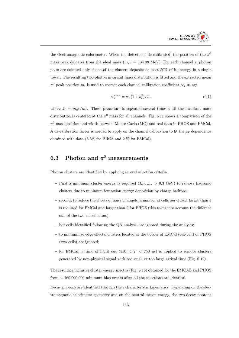
the electromagnetic calorimeter. When the detector is de-calibrated, the position of the π0

mass peak deviates from the ideal mass (mπ0 = 134.98 MeV). For each channel i, photon

pairs are selected only if one of the clusters deposits at least 50% of its energy in a single

tower. The resulting two-photon invariant mass distribution is fitted and the extracted mean

π0 peak position mi is used to correct each channel calibration coefficient cci using:

cccorri = cci(1 + k2i )/2 . (6.1)

where ki = mπ0/mi. These procedure is repeated several times until the invariant mass

distribution is centered at the π0 mass for all channels. Fig. 6.11 shows a comparison of the

π0 mass position and width between Monte-Carlo (MC) and real data in PHOS and EMCal.

A de-calibration factor is needed to apply on the channel calibration to fit the pT dependence

obtained with data (6.5% for PHOS and 2 % for EMCal).

6.3 Photon and π0 measurements

Photon clusters are identified by applying several selection criteria.

– First a minimum cluster energy is required (Ecluster > 0.3 GeV) to remove hadronic

clusters due to minimum ionization energy deposition by charge hadrons;

– second, to reduce the effects of noisy channels, a number of cells per cluster larger than 1

is required for EMCal and larger than 2 for PHOS (this takes into account the different

size of the two calorimeters);

– hot cells identified following the QA analysis are ignored during the analysis;

– to minimimize edge effects, clusters located at the border of EMCal (one cell) or PHOS

(two cells) are ignored;

– for EMCal, a time of flight cut (550 < T < 750 ns) is applied to remove clusters

generated by non-physical signal with too small or too large arrival time (Fig. 6.12).

The resulting inclusive cluster energy spectra (Fig. 6.13) obtained for the EMCAL and PHOS

from ∼ 160,000,000 minimum bias events after all the selections are identical.

Decay photons are identified through their characteristic kinematics. Depending on the elec-

tromagnetic calorimeter geometry and on the neutral meson energy, the two decay photons

113

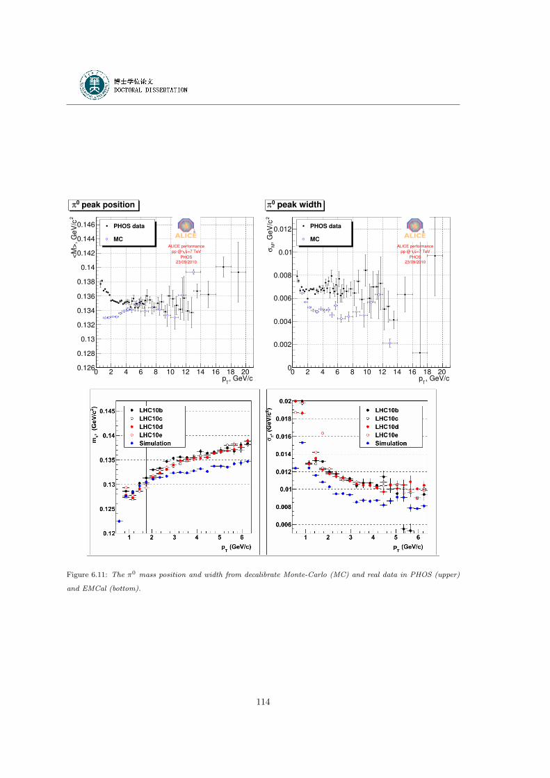
, GeV/cT

p0 2 4 6 8 10 12 14 16 18 20

2<

M>

, G

eV

/c

0.126

0.128

0.13

0.132

0.134

0.136

0.138

0.14

0.142

0.144

0.146

peak position0π

PHOS data

MCALICE performance

=7 TeVspp @

PHOS23/09/2010

peak position0π

, GeV/cT

p0 2 4 6 8 10 12 14 16 18 20

2, G

eV

/cM

σ

0

0.002

0.004

0.006

0.008

0.01

0.012

peak width0π

PHOS data

MCALICE performance

=7 TeVspp @

PHOS23/09/2010

peak width0π

Figure 6.11: The π0 mass position and width from decalibrate Monte-Carlo (MC) and real data in PHOS (upper)

and EMCal (bottom).

114

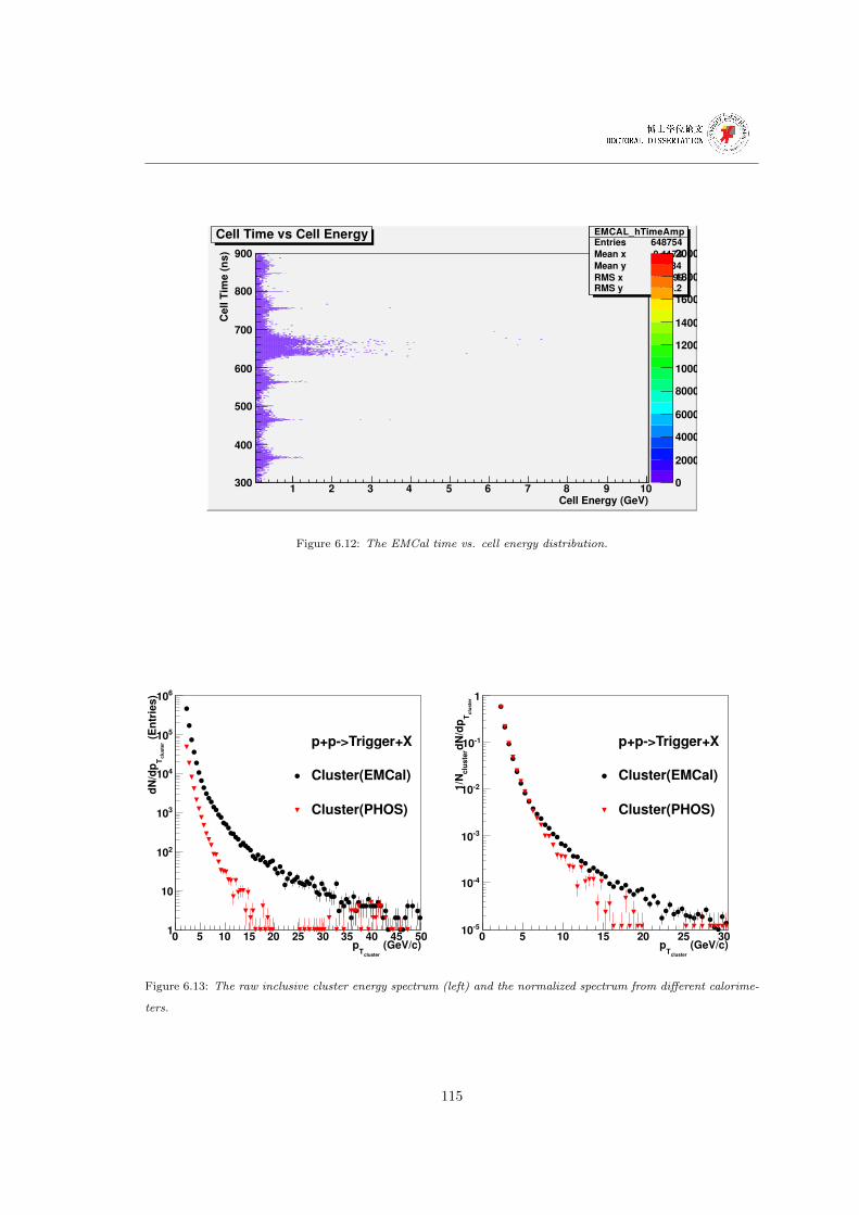
Cell Energy (GeV)1 2 3 4 5 6 7 8 9 10

Cell

Tim

e (

ns)

300

400

500

600

700

800

900

EMCAL_hTimeAmpEntries 648754

Mean x 0.1174

Mean y 634

RMS x 0.1199RMS y 135.2

EMCAL_hTimeAmpEntries 648754

Mean x 0.1174

Mean y 634

RMS x 0.1199RMS y 135.2

0

2000

4000

6000

8000

10000

12000

14000

16000

18000

20000

Cell Time vs Cell Energy

Figure 6.12: The EMCal time vs. cell energy distribution.

(GeV/c)cluster

Tp

0 5 10 15 20 25 30 35 40 45 50

(E

ntr

ies)

clu

ste

rT

dN

/dp

1

10

210

310

410

510

610

p+p­>Trigger+X

Cluster(EMCal)

Cluster(PHOS)

(GeV/c)cluster

Tp

0 5 10 15 20 25 30

clu

ste

rT

dN

/dp

clu

ste

r1/N

­510

­410

­310

­210

­110

1

p+p­>Trigger+X

Cluster(EMCal)

Cluster(PHOS)

Figure 6.13: The raw inclusive cluster energy spectrum (left) and the normalized spectrum from different calorime-

ters.

115

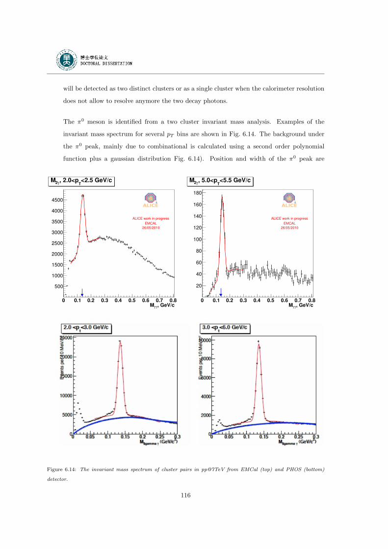
will be detected as two distinct clusters or as a single cluster when the calorimeter resolution

does not allow to resolve anymore the two decay photons.

The π0 meson is identified from a two cluster invariant mass analysis. Examples of the

invariant mass spectrum for several pT bins are shown in Fig. 6.14. The background under

the π0 peak, mainly due to combinational is calculated using a second order polynomial

function plus a gaussian distribution Fig. 6.14). Position and width of the π0 peak are

, GeV/cγγM0 0.1 0.2 0.3 0.4 0.5 0.6 0.7 0.8

500

1000

1500

2000

2500

3000

3500

4000

4500

<2.5 GeV/cT

, 2.0<pγ2M

ALICE work in progress

EMCAL

26/05/2010

<2.5 GeV/cT

, 2.0<pγ2M

, GeV/cγγM0 0.1 0.2 0.3 0.4 0.5 0.6 0.7 0.8

20

40

60

80

100

120

140

160

180

<5.5 GeV/cT

, 5.0<pγ2M

ALICE work in progress

EMCAL

26/05/2010

<5.5 GeV/cT

, 5.0<pγ2M

Figure 6.14: The invariant mass spectrum of cluster pairs in pp@7TeV from EMCal (top) and PHOS (bottom)

detector.

116

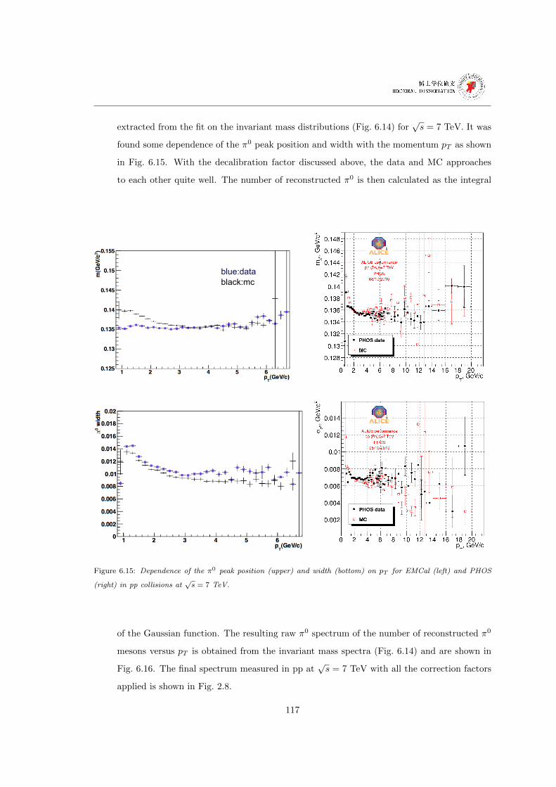
extracted from the fit on the invariant mass distributions (Fig. 6.14) for√s = 7 TeV. It was

found some dependence of the π0 peak position and width with the momentum pT as shown

in Fig. 6.15. With the decalibration factor discussed above, the data and MC approaches

to each other quite well. The number of reconstructed π0 is then calculated as the integral

blue:data black:mc

blue:data black:mc

Figure 6.15: Dependence of the π0 peak position (upper) and width (bottom) on pT for EMCal (left) and PHOS

(right) in pp collisions at√s = 7 TeV.

of the Gaussian function. The resulting raw π0 spectrum of the number of reconstructed π0

mesons versus pT is obtained from the invariant mass spectra (Fig. 6.14) and are shown in

Fig. 6.16. The final spectrum measured in pp at√s = 7 TeV with all the correction factors

applied is shown in Fig. 2.8.

117

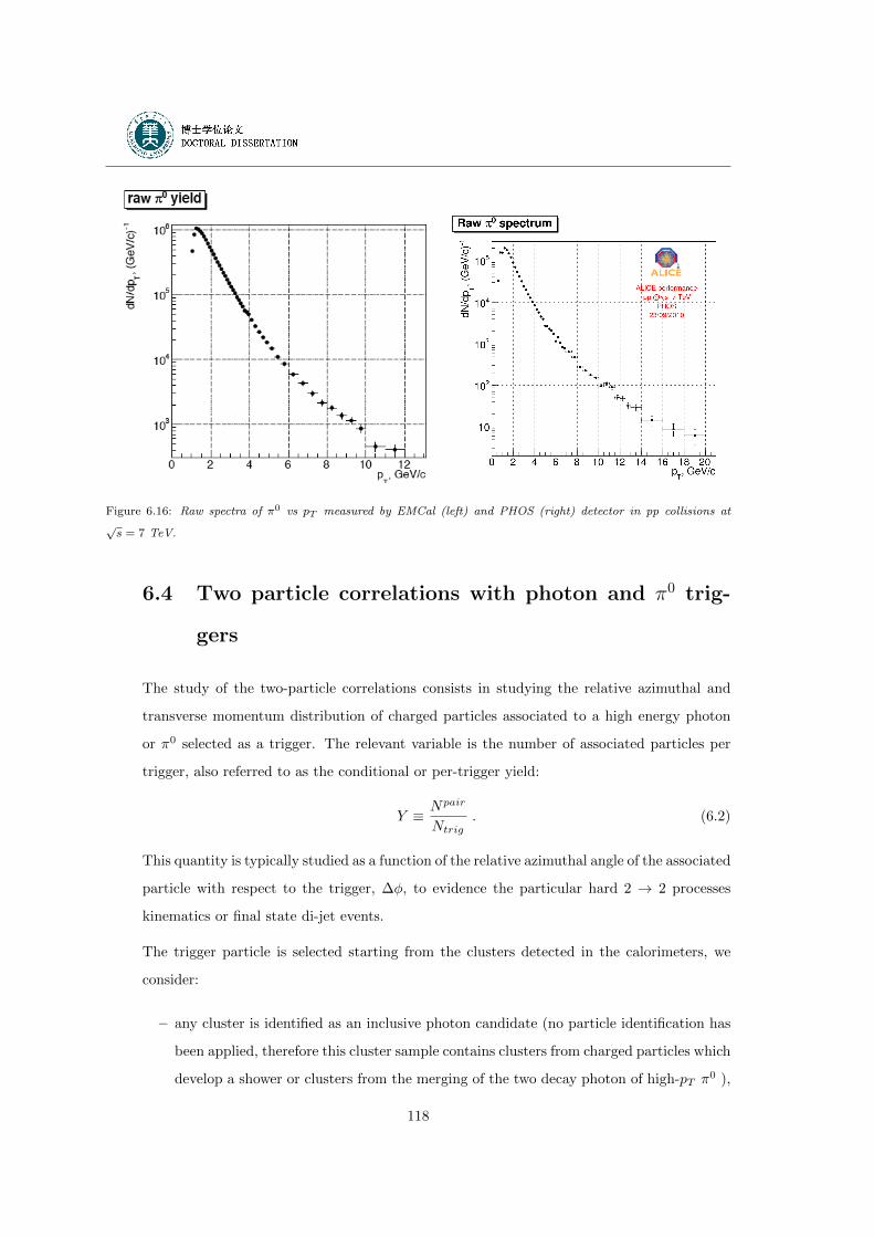
Figure 6.16: Raw spectra of π0 vs pT measured by EMCal (left) and PHOS (right) detector in pp collisions at√s = 7 TeV.

6.4 Two particle correlations with photon and π0 trig-

gers

The study of the two-particle correlations consists in studying the relative azimuthal and

transverse momentum distribution of charged particles associated to a high energy photon

or π0 selected as a trigger. The relevant variable is the number of associated particles per

trigger, also referred to as the conditional or per-trigger yield:

Y ≡ Npair

Ntrig. (6.2)

This quantity is typically studied as a function of the relative azimuthal angle of the associated

particle with respect to the trigger, ∆φ, to evidence the particular hard 2 → 2 processes

kinematics or final state di-jet events.

The trigger particle is selected starting from the clusters detected in the calorimeters, we

consider:

– any cluster is identified as an inclusive photon candidate (no particle identification has

been applied, therefore this cluster sample contains clusters from charged particles which

develop a shower or clusters from the merging of the two decay photon of high-pT π0 ),

118

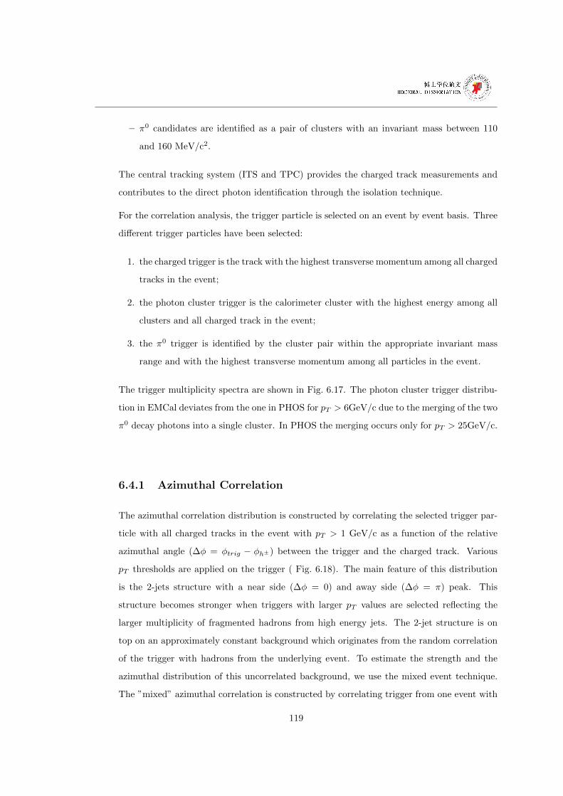
– π0 candidates are identified as a pair of clusters with an invariant mass between 110

and 160 MeV/c2.

The central tracking system (ITS and TPC) provides the charged track measurements and

contributes to the direct photon identification through the isolation technique.

For the correlation analysis, the trigger particle is selected on an event by event basis. Three

different trigger particles have been selected:

1. the charged trigger is the track with the highest transverse momentum among all charged

tracks in the event;

2. the photon cluster trigger is the calorimeter cluster with the highest energy among all

clusters and all charged track in the event;

3. the π0 trigger is identified by the cluster pair within the appropriate invariant mass

range and with the highest transverse momentum among all particles in the event.

The trigger multiplicity spectra are shown in Fig. 6.17. The photon cluster trigger distribu-

tion in EMCal deviates from the one in PHOS for pT > 6GeV/c due to the merging of the two

π0 decay photons into a single cluster. In PHOS the merging occurs only for pT > 25GeV/c.

6.4.1 Azimuthal Correlation

The azimuthal correlation distribution is constructed by correlating the selected trigger par-

ticle with all charged tracks in the event with pT > 1 GeV/c as a function of the relative

azimuthal angle (∆φ = φtrig − φh±) between the trigger and the charged track. Various

pT thresholds are applied on the trigger ( Fig. 6.18). The main feature of this distribution

is the 2-jets structure with a near side (∆φ = 0) and away side (∆φ = π) peak. This

structure becomes stronger when triggers with larger pT values are selected reflecting the

larger multiplicity of fragmented hadrons from high energy jets. The 2-jet structure is on

top on an approximately constant background which originates from the random correlation

of the trigger with hadrons from the underlying event. To estimate the strength and the

azimuthal distribution of this uncorrelated background, we use the mixed event technique.

The ”mixed” azimuthal correlation is constructed by correlating trigger from one event with

119

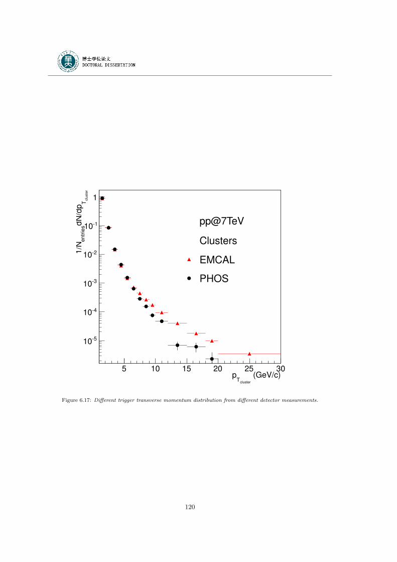
(GeV/c)cluster

Tp

5 10 15 20 25 30

clu

ste

rT

dN

/dp

entr

ies

1/N

­510

­410

­310

­210

­110

1

pp@7TeV

Clusters

EMCAL

PHOS

Figure 6.17: Different trigger transverse momentum distribution from different detector measurements.

120

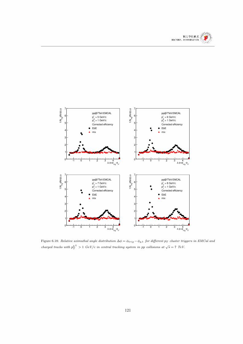
±h

φ­trig

φ=φ ∆­1 0 1 2 3 4

φ ∆

dN

/dtr

ig1

/N

0

1

2

3

4

5

6

7

pp@7TeV:EMCAL

> 5 GeV/ct

Tp

> 1 GeV/ca

Tp

Corrected efficiency

EbE

mix

±h

φ­trig

φ=φ ∆­1 0 1 2 3 4

φ ∆

dN

/dtr

ig1

/N

0

1

2

3

4

5

6

7

pp@7TeV:EMCAL

> 6 GeV/ct

Tp

> 1 GeV/ca

Tp

Corrected efficiency

EbE

mix

±h

φ­trig

φ=φ ∆­1 0 1 2 3 4

φ ∆

dN

/dtr

ig1

/N

0

1

2

3

4

5

6

7

pp@7TeV:EMCAL

> 7 GeV/ct

Tp

> 1 GeV/ca

Tp

Corrected efficiency

EbE

mix

±h

φ­trig

φ=φ ∆­1 0 1 2 3 4

φ ∆

dN

/dtr

ig1

/N

0

1

2

3

4

5

6

7

pp@7TeV:EMCAL

> 8 GeV/ct

Tp

> 1 GeV/ca

Tp

Corrected efficiency

EbE

mix

Figure 6.18: Relative azimuthal angle distribution ∆φ = φtrig−φh± for different pT cluster triggers in EMCal and

charged tracks with ph±T > 1 GeV/c in central tracking system in pp collisions at

√s = 7 TeV.

121

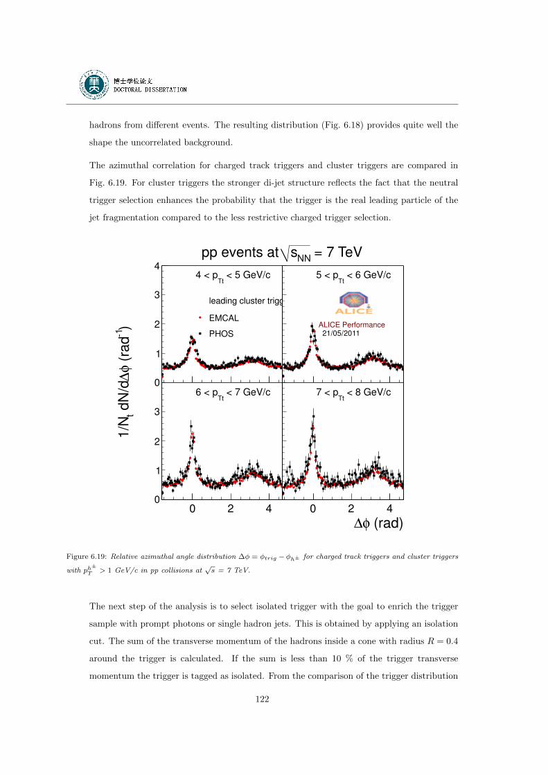
hadrons from different events. The resulting distribution (Fig. 6.18) provides quite well the

shape the uncorrelated background.

The azimuthal correlation for charged track triggers and cluster triggers are compared in

Fig. 6.19. For cluster triggers the stronger di-jet structure reflects the fact that the neutral

trigger selection enhances the probability that the trigger is the real leading particle of the

jet fragmentation compared to the less restrictive charged trigger selection.

0

1

2

3

4

< 5 GeV/cTt

4 < p

leading cluster trigger

EMCAL

PHOS

0

1

2

3

4

< 7 GeV/cTt

6 < p0

1

2

3

4

< 6 GeV/cTt

5 < p

ALICE Performance21/05/2011

0

1

2

3

4

< 8 GeV/cTt

7 < p

0

1

2

3

40

1

2

3

4

0 2 4 0 2 4

= 7 TeVNN

spp events at

(rad)φ∆

)­1

(ra

dφ

∆ d

N/d

t1/N

Figure 6.19: Relative azimuthal angle distribution ∆φ = φtrig − φh± for charged track triggers and cluster triggers

with ph±T > 1 GeV/c in pp collisions at

√s = 7 TeV.

The next step of the analysis is to select isolated trigger with the goal to enrich the trigger

sample with prompt photons or single hadron jets. This is obtained by applying an isolation

cut. The sum of the transverse momentum of the hadrons inside a cone with radius R = 0.4

around the trigger is calculated. If the sum is less than 10 % of the trigger transverse

momentum the trigger is tagged as isolated. From the comparison of the trigger distribution

122

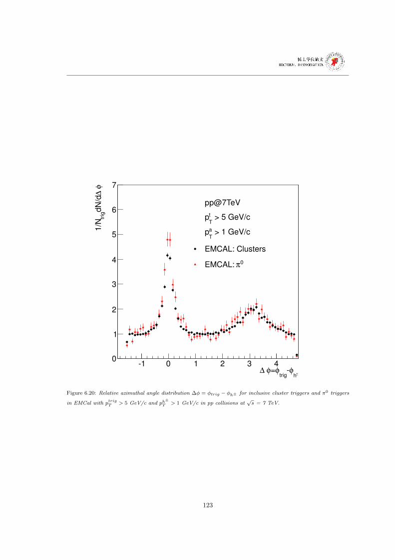
±hφ­

trigφ=φ ∆

­1 0 1 2 3 4

φ ∆

dN

/dtr

ig1

/N

0

1

2

3

4

5

6

7

pp@7TeV

> 5 GeV/ct

Tp

> 1 GeV/ca

Tp

EMCAL: Clusters

0πEMCAL:

Figure 6.20: Relative azimuthal angle distribution ∆φ = φtrig − φh± for inclusive cluster triggers and π0 triggers

in EMCal with ptrigT > 5 GeV/c and ph±T > 1 GeV/c in pp collisions at

√s = 7 TeV.

123

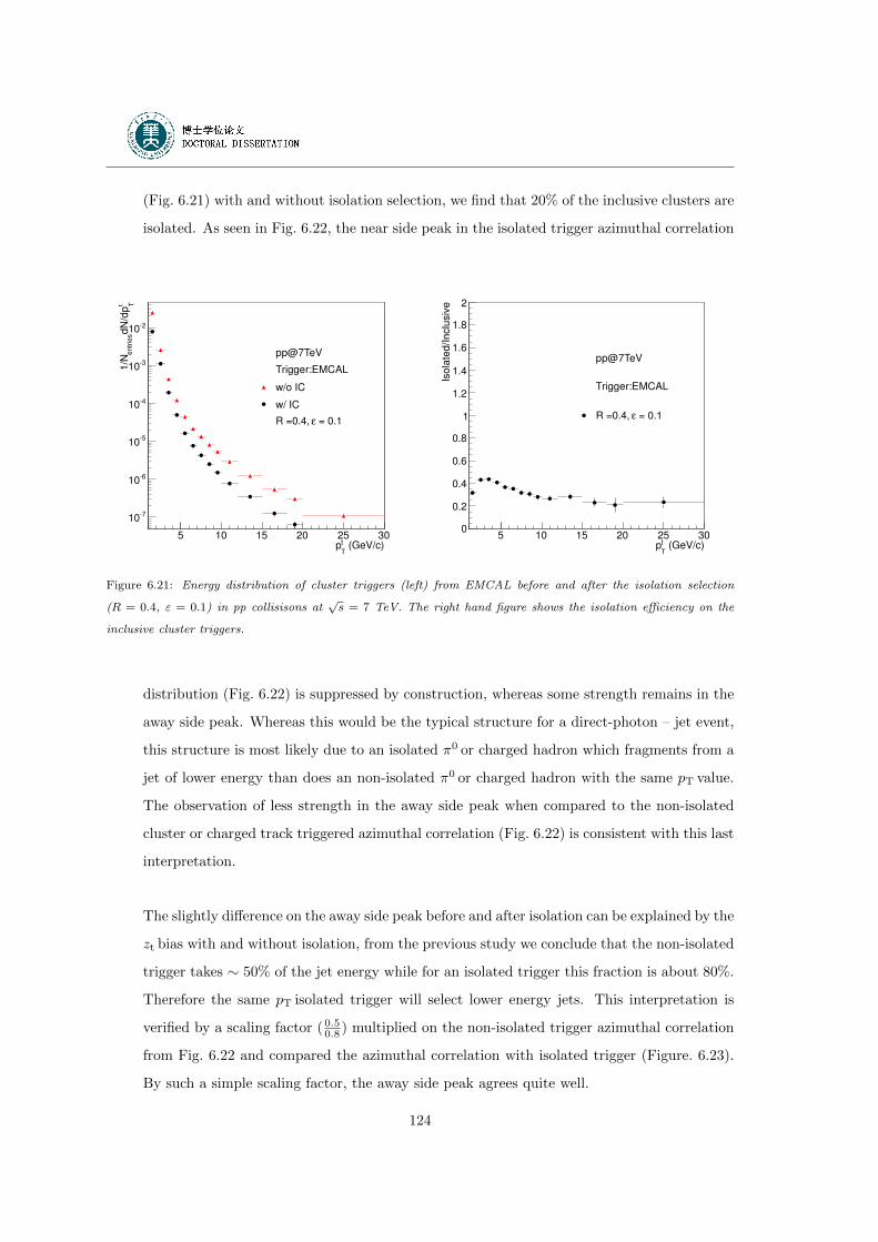
(Fig. 6.21) with and without isolation selection, we find that 20% of the inclusive clusters are

isolated. As seen in Fig. 6.22, the near side peak in the isolated trigger azimuthal correlation

(GeV/c)t

Tp

5 10 15 20 25 30

t TdN

/dp

entr

ies

1/N

­710

­610

­510

­410

­310

­210

pp@7TeV

Trigger:EMCAL

w/o IC

w/ IC

= 0.1εR =0.4,

(GeV/c)t

Tp

5 10 15 20 25 30

Isola

ted/Inclu

siv

e

0

0.2

0.4

0.6

0.8

1

1.2

1.4

1.6

1.8

2

pp@7TeV

Trigger:EMCAL

= 0.1εR =0.4,

Figure 6.21: Energy distribution of cluster triggers (left) from EMCAL before and after the isolation selection

(R = 0.4, ε = 0.1) in pp collisisons at√s = 7 TeV. The right hand figure shows the isolation efficiency on the

inclusive cluster triggers.

distribution (Fig. 6.22) is suppressed by construction, whereas some strength remains in the

away side peak. Whereas this would be the typical structure for a direct-photon – jet event,

this structure is most likely due to an isolated π0 or charged hadron which fragments from a

jet of lower energy than does an non-isolated π0 or charged hadron with the same pT value.

The observation of less strength in the away side peak when compared to the non-isolated

cluster or charged track triggered azimuthal correlation (Fig. 6.22) is consistent with this last

interpretation.

The slightly difference on the away side peak before and after isolation can be explained by the

zt bias with and without isolation, from the previous study we conclude that the non-isolated

trigger takes ∼ 50% of the jet energy while for an isolated trigger this fraction is about 80%.

Therefore the same pT isolated trigger will select lower energy jets. This interpretation is

verified by a scaling factor ( 0.50.8 ) multiplied on the non-isolated trigger azimuthal correlation

from Fig. 6.22 and compared the azimuthal correlation with isolated trigger (Figure. 6.23).

By such a simple scaling factor, the away side peak agrees quite well.

124

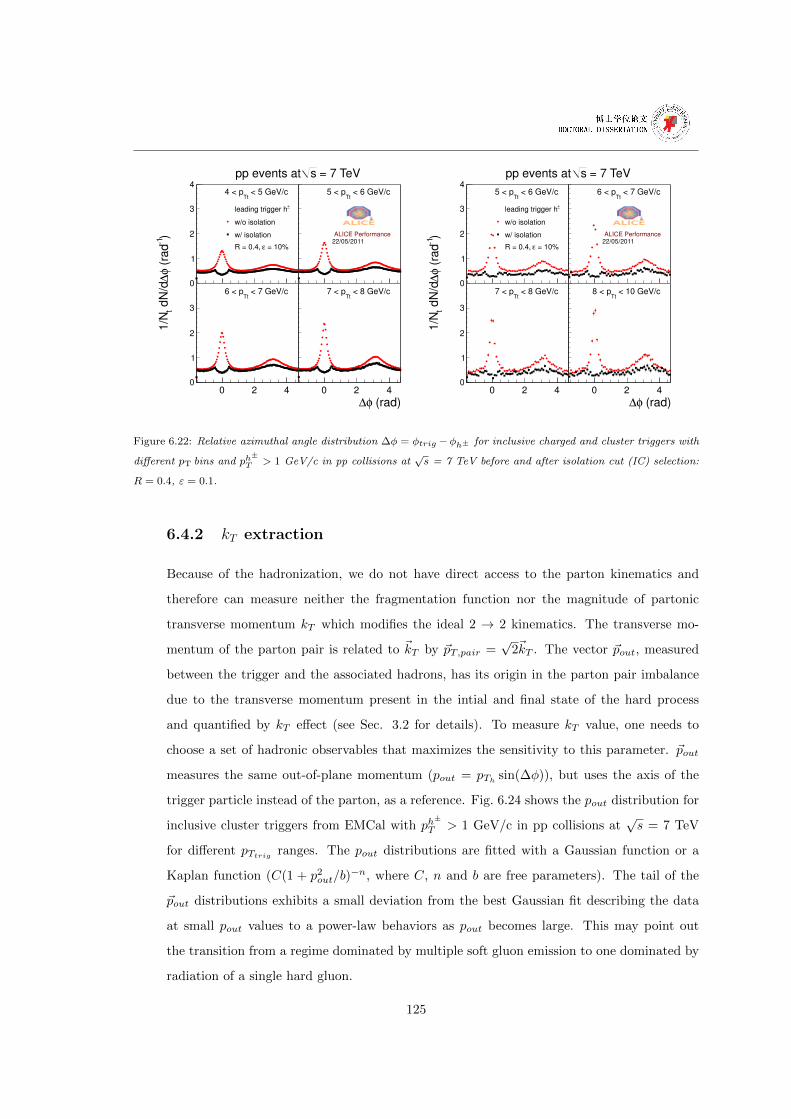
0

1

2

3

4

< 5 GeV/cTt

4 < p

±leading trigger h

w/o isolation

w/ isolation

= 10%εR = 0.4,

0

1

2

3

4

< 7 GeV/cTt

6 < p0

1

2

3

4

< 6 GeV/cTt

5 < p

ALICE Performance22/05/2011

0

1

2

3

4

< 8 GeV/cTt

7 < p

0

1

2

3

40

1

2

3

4

0 2 4 0 2 4

= 7 TeVspp events at

(rad)φ∆

)­1

(ra

dφ

∆ d

N/d

t1/N

0

1

2

3

4

< 6 GeV/cTt

5 < p

±leading trigger h

w/o isolation

w/ isolation

= 10%εR = 0.4,

0

1

2

3

4

< 8 GeV/cTt

7 < p0

1

2

3

4

< 7 GeV/cTt

6 < p

ALICE Performance22/05/2011

0

1

2

3

4

< 10 GeV/cTt

8 < p

0

1

2

3

40

1

2

3

4

0 2 4 0 2 4

= 7 TeVspp events at

(rad)φ∆

)­1

(ra

dφ

∆ d

N/d

t1/N

Figure 6.22: Relative azimuthal angle distribution ∆φ = φtrig −φh± for inclusive charged and cluster triggers with

different pT bins and ph±T > 1 GeV/c in pp collisions at

√s = 7 TeV before and after isolation cut (IC) selection:

R = 0.4, ε = 0.1.

6.4.2 kT extraction

Because of the hadronization, we do not have direct access to the parton kinematics and

therefore can measure neither the fragmentation function nor the magnitude of partonic

transverse momentum kT which modifies the ideal 2 → 2 kinematics. The transverse mo-

mentum of the parton pair is related to ~kT by ~pT,pair =√

2~kT . The vector ~pout, measured

between the trigger and the associated hadrons, has its origin in the parton pair imbalance

due to the transverse momentum present in the intial and final state of the hard process

and quantified by kT effect (see Sec. 3.2 for details). To measure kT value, one needs to

choose a set of hadronic observables that maximizes the sensitivity to this parameter. ~pout

measures the same out-of-plane momentum (pout = pTh sin(∆φ)), but uses the axis of the

trigger particle instead of the parton, as a reference. Fig. 6.24 shows the pout distribution for

inclusive cluster triggers from EMCal with ph±

T > 1 GeV/c in pp collisions at√s = 7 TeV

for different pTtrig ranges. The pout distributions are fitted with a Gaussian function or a

Kaplan function (C(1 + p2out/b)−n, where C, n and b are free parameters). The tail of the

~pout distributions exhibits a small deviation from the best Gaussian fit describing the data

at small pout values to a power-law behaviors as pout becomes large. This may point out

the transition from a regime dominated by multiple soft gluon emission to one dominated by

radiation of a single hard gluon.

125

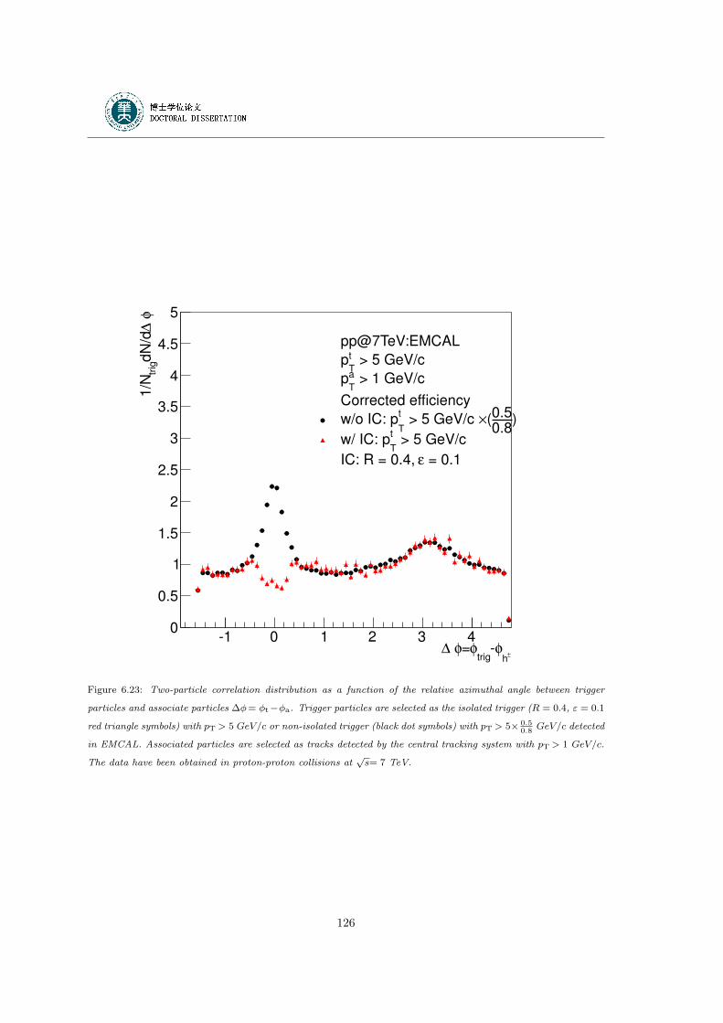
±h

φ­trig

φ=φ ∆­1 0 1 2 3 4

φ ∆

dN

/dtr

ig1/N

0

0.5

1

1.5

2

2.5

3

3.5

4

4.5

5

pp@7TeV:EMCAL

> 5 GeV/ct

Tp

> 1 GeV/ca

Tp

Corrected efficiency

)0.80.5(× > 5 GeV/c

t

Tw/o IC: p

> 5 GeV/ct

Tw/ IC: p

= 0.1εIC: R = 0.4,

Figure 6.23: Two-particle correlation distribution as a function of the relative azimuthal angle between trigger

particles and associate particles ∆φ= φt−φa. Trigger particles are selected as the isolated trigger (R = 0.4, ε = 0.1

red triangle symbols) with pT> 5 GeV/c or non-isolated trigger (black dot symbols) with pT> 5× 0.50.8

GeV/c detected

in EMCAL. Associated particles are selected as tracks detected by the central tracking system with pT> 1 GeV/c.

The data have been obtained in proton-proton collisions at√s= 7 TeV.

126

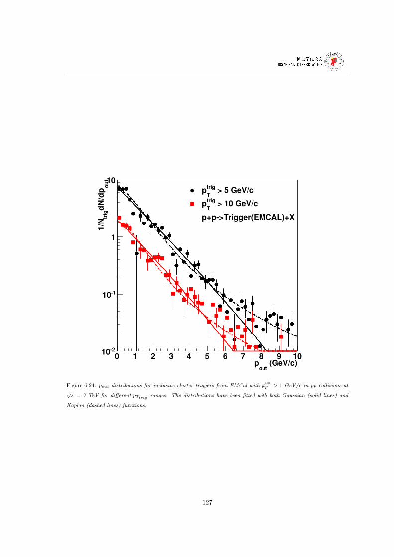
(GeV/c)out

p0 1 2 3 4 5 6 7 8 9 10

ou

td

N/d

ptr

ig1/N

­210

­110

1

10

> 5 GeV/ctrig

Tp

> 10 GeV/ctrig

Tp

p+p­>Trigger(EMCAL)+X

Figure 6.24: pout distributions for inclusive cluster triggers from EMCal with ph±T > 1 GeV/c in pp collisions at

√s = 7 TeV for different pTtrig ranges. The distributions have been fitted with both Gaussian (solid lines) and

Kaplan (dashed lines) functions.

127

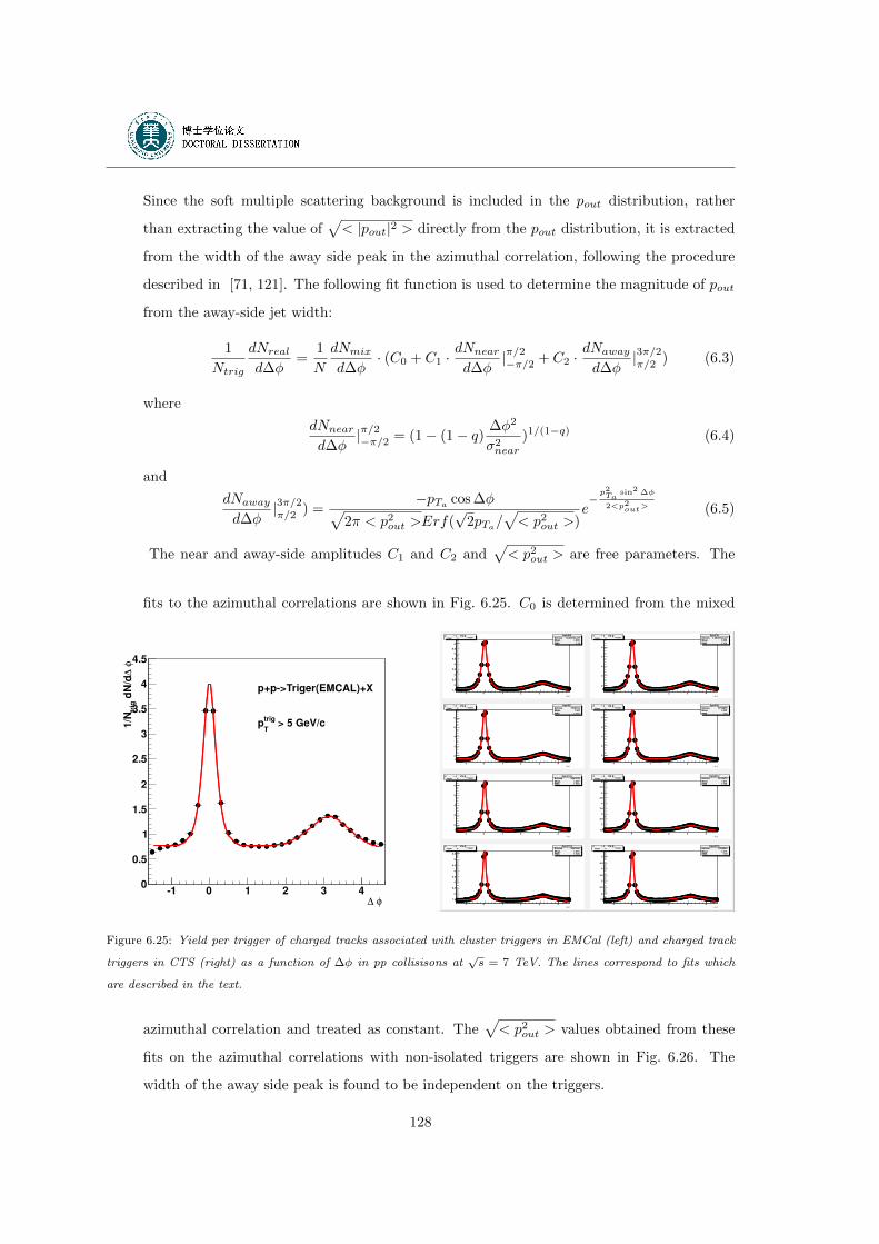
Since the soft multiple scattering background is included in the pout distribution, rather

than extracting the value of√< |pout|2 > directly from the pout distribution, it is extracted

from the width of the away side peak in the azimuthal correlation, following the procedure

described in [71, 121]. The following fit function is used to determine the magnitude of pout

from the away-side jet width:

1

Ntrig

dNreald∆φ

=1

N

dNmixd∆φ

· (C0 + C1 ·dNneard∆φ

|π/2−π/2 + C2 ·dNawayd∆φ

|3π/2π/2 ) (6.3)

where

dNneard∆φ

|π/2−π/2 = (1− (1− q) ∆φ2

σ2near

)1/(1−q) (6.4)

and

dNawayd∆φ

|3π/2π/2 ) =−pTa cos ∆φ√

2π < p2out >Erf(√

2pTa/√< p2out >)

e−p2Ta

sin2 ∆φ

2<p2out> (6.5)

The near and away-side amplitudes C1 and C2 and√< p2out > are free parameters. The

fits to the azimuthal correlations are shown in Fig. 6.25. C0 is determined from the mixed

φ ∆

­1 0 1 2 3 4

φ

∆ d

N/d

trig

1/N

0

0.5

1

1.5

2

2.5

3

3.5

4

4.5

p+p­>Triger(EMCAL)+X

> 5 GeV/ctrig

Tp

DphiPt5

Entries 1.646016e+07Mean 1.408

RMS 1.72

φ ∆

­1 0 1 2 3 4

1.5

2

2.5

3

3.5

4

4.5

5

5.5

6

T trigger vs p

±h

φ ­ trigger

φ DphiPt6

Entries 1.054931e+07Mean 1.403

RMS 1.719

φ ∆

­1 0 1 2 3 4

2

3

4

5

6

T trigger vs p

±h

φ ­ trigger

φ

DphiPt7

Entries 7518018Mean 1.401

RMS 1.719

φ ∆

­1 0 1 2 3 4

2

3

4

5

6

T trigger vs p

±h

φ ­ trigger

φ DphiPt8

Entries 5778875Mean 1.403

RMS 1.72

φ ∆

­1 0 1 2 3 4

2

3

4

5

6

T trigger vs p

±h

φ ­ trigger

φ

DphiPt10Entries 3941845

Mean 1.407RMS 1.723

φ ∆

­1 0 1 2 3 4

2

3

4

5

6

T trigger vs p

±h

φ ­ trigger

φ DphiPt12Entries 3014474

Mean 1.411RMS 1.725

φ ∆

­1 0 1 2 3 4

1.5

2

2.5

3

3.5

4

4.5

5

5.5

6

T trigger vs p

±h

φ ­ trigger

φ

DphiPt15Entries 2257950

Mean 1.415RMS 1.728

φ ∆

­1 0 1 2 3 4

1.5

2

2.5

3

3.5

4

4.5

5

5.5

T trigger vs p

±h

φ ­ trigger

φ DphiPt18Entries 1824043

Mean 1.417RMS 1.73

φ ∆

­1 0 1 2 3 4

1.5

2

2.5

3

3.5

4

4.5

5

T trigger vs p

±h

φ ­ trigger

φ

Figure 6.25: Yield per trigger of charged tracks associated with cluster triggers in EMCal (left) and charged track

triggers in CTS (right) as a function of ∆φ in pp collisisons at√s = 7 TeV. The lines correspond to fits which

are described in the text.

azimuthal correlation and treated as constant. The√< p2out > values obtained from these

fits on the azimuthal correlations with non-isolated triggers are shown in Fig. 6.26. The

width of the away side peak is found to be independent on the triggers.

128

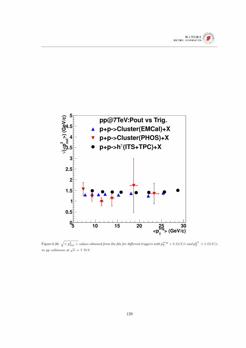
> (GeV/c)trig

T<p

5 10 15 20 25 30

>)

(GeV

/c)

2 ou

t(<

p√

0

0.5

1

1.5

2

2.5

3

3.5

4

4.5

5pp@7TeV:Pout vs Trig.

p+p­>Cluster(EMCal)+X

p+p­>Cluster(PHOS)+X

(ITS+TPC)+X±p+p­>h

Figure 6.26:√< p2out > values obtained from the fits for different triggers with ptrigT > 5 GeV/c and ph

±T > 1 GeV/c

in pp collisions at√s = 7 TeV.

129

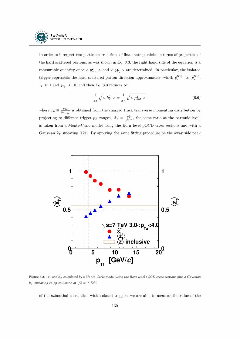
In order to interpret two particle correlations of final state particles in terms of properties of

the hard scattered partons, as was shown in Eq. 3.3, the right hand side of the equation is a

measurable quantity once < p2out > and < j2Ty > are determined. In particular, the isolated

trigger represents the hard scattered parton direction approximately, which ptrigT ' ptrigT ,

zt ≈ 1 and jTy ≈ 0, and then Eq. 3.3 reduces to:

1

xh

√< k2T > =

1

xh

√< p2out > (6.6)

where xh ≡ pTapTtrig

is obtained from the charged track transverse momentum distribution by

projecting to different trigger pT ranges. xh =paTptrigT

, the same ratio at the partonic level,

is taken from a Monte-Carlo model using the Born level pQCD cross sections and with a

Gaussian kT smearing [121]. By applying the same fitting procedure on the away side peak

]c [GeV/Tt

p0 5 10 15 20

!h

x"

0

0.5

1

<4.0Ta

=7 TeV 3.0<ps

hx!tz" inclusive!z"

! tz"

0

0.5

1

Figure 6.27: zt and xh calculated by a Monte-Carlo model using the Born level pQCD cross sections plus a Gaussian

kT smearing in pp collisions at√s = 7 TeV.

of the azimuthal correlation with isolated triggers, we are able to measure the value of the

130

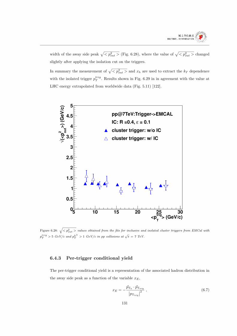
width of the away side peak√< p2out > (Fig. 6.28), where the value of

√< p2out > changed

slightly after applying the isolation cut on the triggers.

In summary the measurement of√< p2out > and xh are used to extract the kT dependence

with the isolated trigger ptrigT . Results shown in Fig. 6.29 in in agreement with the value at

LHC energy extrapolated from worldwide data (Fig. 5.11) [122].

> (GeV/c)trig

T<p

5 10 15 20 25 30

>)

(GeV

/c)

2 ou

t(<

p√

0

0.5

1

1.5

2

2.5

3

3.5

4

4.5

5

pp@7TeV:Trigger­>EMCAL

= 0.1εIC: R =0.4,

cluster trigger: w/o IC

cluster trigger: w/ IC

Figure 6.28:√< p2out > values obtained from the fits for inclusive and isolated cluster triggers from EMCal with

ptrigT > 5 GeV/c and ph±T > 1 GeV/c in pp collisions at

√s = 7 TeV.

6.4.3 Per-trigger conditional yield

The per-trigger conditional yield is a representation of the associated hadron distribution in

the away side peak as a function of the variable xE ,

xE = −~pTh· ~pTtrig∣∣pTtrig

∣∣2 , (6.7)

131

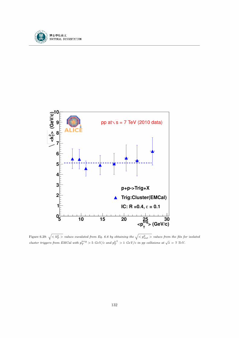
> (GeV/c)trig

T<p

5 10 15 20 25 30

(G

eV

/c)

>

2 T <

k

0

1

2

3

4

5

6

7

8

9

10

p+p­>Trig+X

Trig:Cluster(EMCal)

= 0.1εIC: R =0.4,

= 7 TeV (2010 data)spp at

Figure 6.29:√< k2T > values euvalated from Eq. 6.6 by obtaining the

√< p2out > values from the fits for isolated

cluster triggers from EMCal with ptrigT > 5 GeV/c and ph±T > 1 GeV/c in pp collisions at

√s = 7 TeV.

132

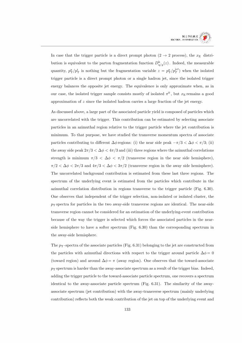
In case that the trigger particle is a direct prompt photon (2 → 2 process), the xE distri-

bution is equivalent to the parton fragmentation function Dhq/g(z) . Indeed, the measurable

quantity, paT/ptT is nothing but the fragmentation variable z = paT/p

jetT ) when the isolated

trigger particle is a direct prompt photon or a single hadron jet, since the isolated trigger

energy balances the opposite jet energy. The equivalence is only approximate when, as in

our case, the isolated trigger sample consists mostly of isolated π0 , but xE remains a good

approximation of z since the isolated hadron carries a large fraction of the jet energy.

As discussed above, a large part of the associated particle yield is composed of particles which

are uncorrelated with the trigger. This contribution can be estimated by selecting associate

particles in an azimuthal region relative to the trigger particle where the jet contribution is

minimum. To that purpose, we have studied the transverse momentum spectra of associate

particles contributing to different ∆φ regions: (i) the near side peak −π/3 < ∆φ < π/3; (ii)

the away side peak 2π/3 < ∆φ < 4π/3 and (iii) three regions where the azimuthal correlations

strength is minimum π/3 < ∆φ < π/2 (transverse region in the near side hemisphere),

π/2 < ∆φ < 2π/3 and 4π/3 < ∆φ < 3π/2 (transverse region in the away side hemisphere).

The uncorrelated background contribution is estimated from these last three regions. The

spectrum of the underlying event is estimated from the particles which contribute in the

azimuthal correlation distribution in regions transverse to the trigger particle (Fig. 6.30).

One observes that independent of the trigger selection, non-isolated or isolated cluster, the

pT spectra for particles in the two away-side transverse regions are identical. The near-side

transverse region cannot be considered for an estimation of the underlying-event contribution

because of the way the trigger is selected which forces the associated particles in the near-

side hemisphere to have a softer spectrum (Fig. 6.30) than the corresponding spectrum in

the away-side hemisphere.

The pT -spectra of the associate particles (Fig. 6.31) belonging to the jet are constructed from

the particles with azimuthal directions with respect to the trigger around particle ∆φ= 0

(toward region) and around ∆φ= π (away region). One observes that the toward-associate

pT spectrum is harder than the away-associate spectrum as a result of the trigger bias. Indeed,

adding the trigger particle to the toward-associate particle spectrum, one recovers a spectrum

identical to the away-associate particle spectrum (Fig. 6.31). The similarity of the away-

associate spectrum (jet contribution) with the away-transverse spectrum (mainly underlying

contribution) reflects both the weak contribution of the jet on top of the underlying event and

133

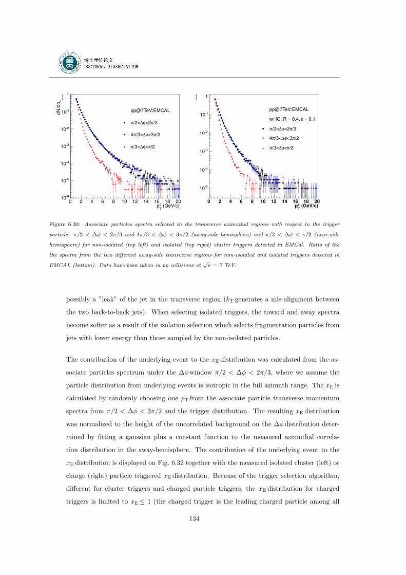
(GeV/c)a

Tp

0 2 4 6 8 10 12 14 16 18 20

asso

cT

dN

/dp

­610

­510

­410

­310

­210

­110

1

pp@7TeV:EMCAL

/3π<2φ∆/2<π

/2π<3φ∆/3<π4

/2π<φ∆/3<π

(GeV/c)a

Tp

0 2 4 6 8 10 12 14 16 18 20

asso

cT

dN

/dp

­510

­410

­310

­210

­110

1

pp@7TeV:EMCAL

= 0.1εw/ IC: R = 0.4,

/3π<2φ∆/2<π

/2π<3φ∆/3<π4

/2π<φ∆/3<π

Figure 6.30: Associate particles spectra selected in the transverse azimuthal regions with respect to the trigger

particle: π/2 < ∆φ < 2π/3 and 4π/3 < ∆φ < 3π/2 (away-side hemisphere) and π/3 < ∆φ < π/2 (near-side

hemisphere) for non-isolated (top left) and isolated (top right) cluster triggers detected in EMCal. Ratio of the

the spectra from the two different away-side transverse regions for non-isolated and isolated triggers detected in

EMCAL (bottom). Data have been taken in pp collisions at√s = 7 TeV.

possibly a ”leak” of the jet in the transverse region (kT generates a mis-alignment between

the two back-to-back jets). When selecting isolated triggers, the toward and away spectra

become softer as a result of the isolation selection which selects fragmentation particles from

jets with lower energy than those sampled by the non-isolated particles.

The contribution of the underlying event to the xE distribution was calculated from the as-

sociate particles spectrum under the ∆φwindow π/2 < ∆φ < 2π/3, where we assume the

particle distribution from underlying events is isotropic in the full azimuth range. The xE is

calculated by randomly choosing one pT from the associate particle transverse momentum

spectra from π/2 < ∆φ < 3π/2 and the trigger distribution. The resulting xE distribution

was normalized to the height of the uncorrelated background on the ∆φdistribution deter-

mined by fitting a gaussian plus a constant function to the measured azimuthal correla-

tion distribution in the away-hemisphere. The contribution of the underlying event to the

xE distribution is displayed on Fig. 6.32 together with the measured isolated cluster (left) or

charge (right) particle triggered xE distribution. Because of the trigger selection algorithm,

different for cluster triggers and charged particle triggers, the xE distribution for charged

triggers is limited to xE≤ 1 (the charged trigger is the leading charged particle among all

134

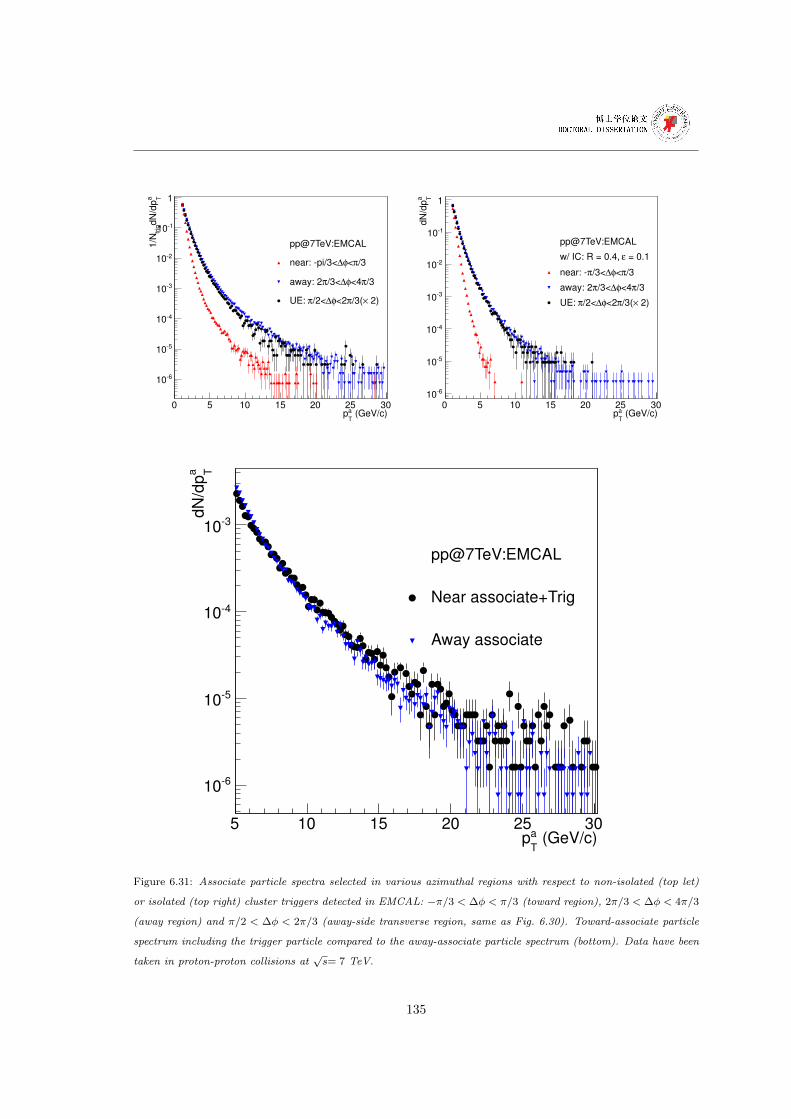
(GeV/c)a

Tp

0 5 10 15 20 25 30

a TdN

/dp

trig

1/N

­610

­510

­410

­310

­210

­110

1

pp@7TeV:EMCAL

/3π<φ∆near: ­pi/3<

/3π<4φ∆/3<πaway: 2

2)×/3(π<2φ∆/2<πUE:

(GeV/c)a

Tp

0 5 10 15 20 25 30

a TdN

/dp

­610

­510

­410

­310

­210

­110

1

pp@7TeV:EMCAL

= 0.1εw/ IC: R = 0.4,

/3π<φ∆/3<πnear: ­

/3π<4φ∆/3<πaway: 2

2)×/3(π<2φ∆/2<πUE:

(GeV/c)a

Tp

5 10 15 20 25 30

a TdN

/dp

­610

­510

­410

­310

pp@7TeV:EMCAL

Near associate+Trig

Away associate

Figure 6.31: Associate particle spectra selected in various azimuthal regions with respect to non-isolated (top let)

or isolated (top right) cluster triggers detected in EMCAL: −π/3 < ∆φ < π/3 (toward region), 2π/3 < ∆φ < 4π/3

(away region) and π/2 < ∆φ < 2π/3 (away-side transverse region, same as Fig. 6.30). Toward-associate particle

spectrum including the trigger particle compared to the away-associate particle spectrum (bottom). Data have been

taken in proton-proton collisions at√s= 7 TeV.

135

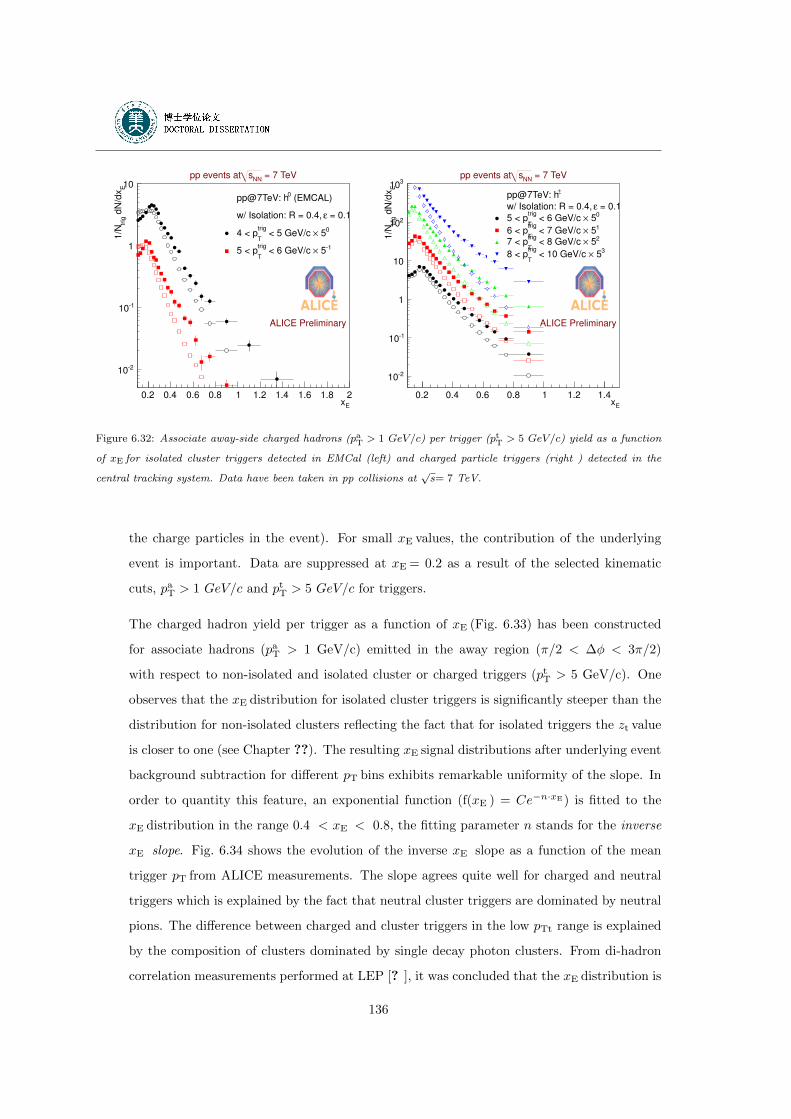
Ex0.2 0.4 0.6 0.8 1 1.2 1.4 1.6 1.8 2

E

dN

/dx

trig

1/N

­210

­110

1

10

(EMCAL)0pp@7TeV: h

= 0.1εw/ Isolation: R = 0.4,

0 5× < 5 GeV/c trig

T4 < p

­1 5× < 6 GeV/c trig

T5 < p

= 7 TeVNN

spp events at

ALICE Preliminary

Ex0.2 0.4 0.6 0.8 1 1.2 1.4

E

dN

/dx

trig

1/N

­210

­110

1

10

210

310±pp@7TeV: h

= 0.1εw/ Isolation: R = 0.4, 0 5× < 6 GeV/c

trig

T5 < p

1 5× < 7 GeV/c trig

T6 < p

2 5× < 8 GeV/c trig

T7 < p

3 5× < 10 GeV/c trig

T8 < p

= 7 TeVNN

spp events at

ALICE Preliminary

Figure 6.32: Associate away-side charged hadrons (paT > 1 GeV/c) per trigger (ptT > 5 GeV/c) yield as a function

of xE for isolated cluster triggers detected in EMCal (left) and charged particle triggers (right ) detected in the

central tracking system. Data have been taken in pp collisions at√s= 7 TeV.

the charge particles in the event). For small xE values, the contribution of the underlying

event is important. Data are suppressed at xE = 0.2 as a result of the selected kinematic

cuts, paT > 1 GeV/c and ptT > 5 GeV/c for triggers.

The charged hadron yield per trigger as a function of xE (Fig. 6.33) has been constructed

for associate hadrons (paT > 1 GeV/c) emitted in the away region (π/2 < ∆φ < 3π/2)

with respect to non-isolated and isolated cluster or charged triggers (ptT > 5 GeV/c). One

observes that the xE distribution for isolated cluster triggers is significantly steeper than the

distribution for non-isolated clusters reflecting the fact that for isolated triggers the zt value

is closer to one (see Chapter ??). The resulting xE signal distributions after underlying event

background subtraction for different pT bins exhibits remarkable uniformity of the slope. In

order to quantity this feature, an exponential function (f(xE ) = Ce−n·xE) is fitted to the

xE distribution in the range 0.4 < xE < 0.8, the fitting parameter n stands for the inverse

xE slope. Fig. 6.34 shows the evolution of the inverse xE slope as a function of the mean

trigger pT from ALICE measurements. The slope agrees quite well for charged and neutral

triggers which is explained by the fact that neutral cluster triggers are dominated by neutral

pions. The difference between charged and cluster triggers in the low pTt range is explained

by the composition of clusters dominated by single decay photon clusters. From di-hadron

correlation measurements performed at LEP [? ], it was concluded that the xE distribution is

136

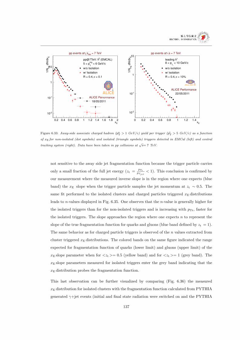
Ex0.2 0.4 0.6 0.8 1 1.2 1.4 1.6 1.8 2

E

dN

/dx

trig

1/N

­210

­110

1

10

(EMCAL)0pp@7TeV: h

< 6 GeV/ctrig

T5 < p

w/o Isolation

w/ Isolation

= 0.1εR = 0.4,

= 7 TeVNN

spp events at

ALICE Performance

18/05/2011

Ex0 0.2 0.4 0.6 0.8 1 1.2 1.4

E

dN

/dx

trig

1/N

­210

­110

1

10±leading h

< 10 GeV/ctT

8 < p

w/o isolation

w/ isolation

= 10%εR = 0.4,

= 7 TeVspp events at

ALICE Performance

22/05/2011

Figure 6.33: Away-side associate charged hadron (paT > 1 GeV/c) yield per trigger (ptT > 5 GeV/c) as a function

of xE for non-isolated (dot symbols) and isolated (triangle symbols) triggers detected in EMCal (left) and central

tracking system (right). Data have been taken in pp collisions at√s= 7 TeV.

not sensitive to the away side jet fragmentation function because the trigger particle carries

only a small fraction of the full jet energy (zt =pTtpTjet

< 1). This conclusion is confirmed by

our measurement where the measured inverse slope is in the region where one expects (blue

band) the xE slope when the trigger particle samples the jet momentum at zt ∼ 0.5. The

same fit performed to the isolated clusters and charged particles triggered xE distributions

leads to n-values displayed in Fig. 6.35. One observes that the n-value is generally higher for

the isolated triggers than for the non-isolated triggers and is increasing with pTt, faster for

the isolated triggers. The slope approaches the region where one expects n to represent the

slope of the true fragmentation function for quarks and gluons (blue band defined by zt = 1).

The same behavior as for charged particle triggers is observed of the n values extracted from

cluster triggered xE distributions. The colored bands on the same figure indicated the range

expected for fragmentation function of quarks (lower limit) and gluons (upper limit) of the

xE slope parameter when for <zt>= 0.5 (yellow band) and for <zt>= 1 (grey band). The

xE slope parameters measured for isolated triggers enter the grey band indicating that the

xE distribution probes the fragmentation function.

This last observation can be further visualized by comparing (Fig. 6.36) the measured

xE distribution for isolated clusters with the fragmentation function calculated from PYTHIA

generated γ+jet events (initial and final state radiation were switched on and the PYTHIA

137

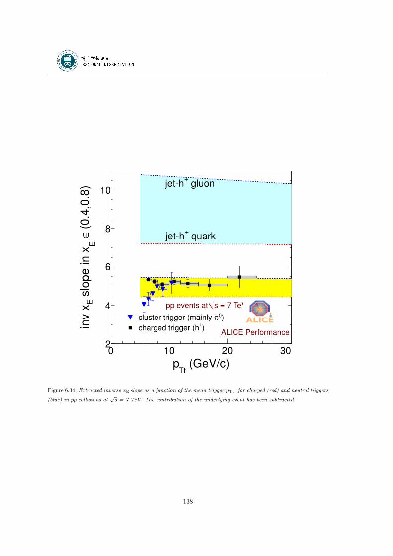
(GeV/c)Tt

p0 10 20 30

(0.4

,0.8

)∈

E s

lope in x

Ein

v x

2

4

6

8

10

)0πcluster trigger (mainly

)±charged trigger (h

gluon±jet­h

quark±jet­h

= 7 TeVspp events at

ALICE Performance

Figure 6.34: Extracted inverse xE slope as a function of the mean trigger pTt for charged (red) and neutral triggers

(blue) in pp collisions at√s = 7 TeV. The contribution of the underlying event has been subtracted.

138

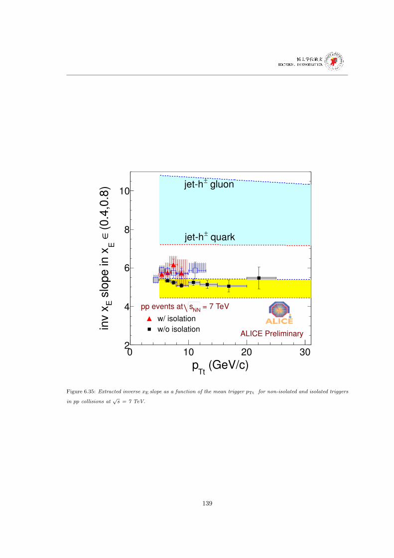
(GeV/c)Tt

p0 10 20 30

(0.4

,0.8

)∈

E s

lope in x

Ein

v x

2

4

6

8

10

w/ isolation

w/o isolation

gluon±jet­h

quark±jet­h

= 7 TeVNN

spp events at

ALICE Preliminary

Figure 6.35: Extracted inverse xE slope as a function of the mean trigger pTt for non-isolated and isolated triggers

in pp collisions at√s = 7 TeV.

139

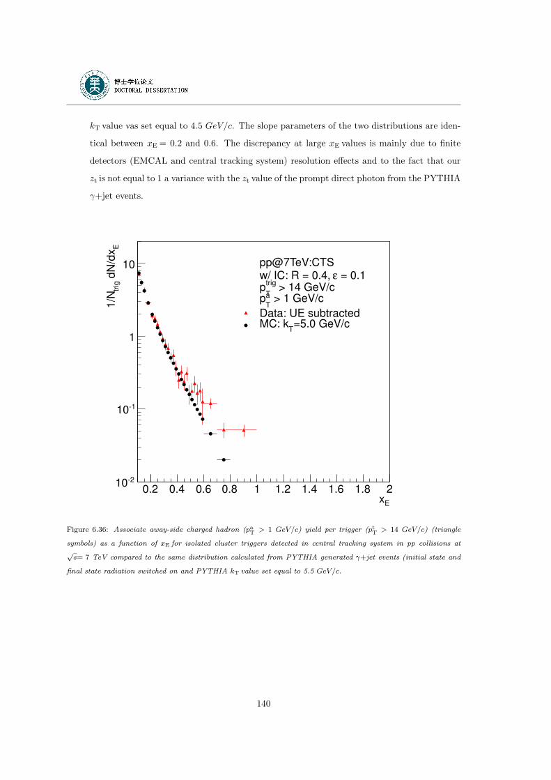
kT value vas set equal to 4.5 GeV/c. The slope parameters of the two distributions are iden-

tical between xE = 0.2 and 0.6. The discrepancy at large xE values is mainly due to finite

detectors (EMCAL and central tracking system) resolution effects and to the fact that our

zt is not equal to 1 a variance with the zt value of the prompt direct photon from the PYTHIA

γ+jet events.

Ex0.2 0.4 0.6 0.8 1 1.2 1.4 1.6 1.8 2

E

dN

/dx

trig

1/N

­210

­110

1

10 pp@7TeV:CTS = 0.1εw/ IC: R = 0.4,

> 14 GeV/ctrig

Tp

> 1 GeV/ca

Tp

Data: UE subtracted=5.0 GeV/c

TMC: k

Figure 6.36: Associate away-side charged hadron (paT > 1 GeV/c) yield per trigger (ptT > 14 GeV/c) (triangle

symbols) as a function of xE for isolated cluster triggers detected in central tracking system in pp collisions at√s= 7 TeV compared to the same distribution calculated from PYTHIA generated γ+jet events (initial state and

final state radiation switched on and PYTHIA kT value set equal to 5.5 GeV/c.

140

Chapter 7

Summary and Outlook

The ultimate objective of the work partly presented in this thesis is to study the properties of

the hot and dense QCD (Quantum Chromo Dynamics) matter in the deconfined QGP (Quark

Gluon Plasma) phase through the measurement of direct photon tagged charged hadrons

correlations. This study is part of the scientific program of the ALICE experiment designed

and optimized for the detection and identification of a complete set of probes generated in

heavy-ion collisions at LHC energies. The QGP is the fundamental state of QCD matter

and is, according to the Big Bang cosmological model, the primordial state of matter that

prevailed during the first hundreds of micro seconds of existence of the Universe. Recreating

this state of matter and studying its properties will shed light on fundamental still unanswered

questions, such as the origin of the constituent mass of matter (the constituent mass of quarks

contributes to 99% of the mass of the nucleon whereas the bare mass, supposedly generated

through the Higgs mechanism, contributes to the remaining 1%) and the Chiral symmetry

breaking (which could be at the origin of the difference in quark masses). LHC has already

provided heavy-ion collisions at the unprecedented high energies of√sNN = 2.76 TeV and

ALICE was quickly able to establish the global properties of the collision and to have a

glimpse on the properties of the created medium. So, from the measurement of charged

particle densities, we deduced that the energy density of the medium is 15 GeV/fm3 (three

times larger that the density reached at RHIC) and the temperature is 30% larger than the

one reached at RHIC. The volume and lifetime of the collisions was deduced, from identical

particles interferometry measurement, to be two times larger and 40% longer, respectively,

141

than the ones at RHIC. Collective flow measurements indicate that the medium produced at

LHC has the properties of an ideal liquid (almost zero viscosity) and has a very high color

density able to absorb completely high energy partons (jet quenching measurement). It is

precisely this last effect which drives my study.

Partons with high pT (transverse momentum) are produced in hard pQCD (perturbative

QCD) scattering between constituent partons inside the colliding nuclei and are observed in

the detectors as a collimated jet of hadrons. The 4-momentum of the hard scattered parton

is modified through soft gluons radiation while traversing the color dense and deconfined

medium created concurrently in the collision. The modification, which depends on the color

density of the medium and on the distance traversed inside the medium, is imprinted in the

fragmenting hadrons in a way that modifies dynamically the fragmentation function of the jet

(he fragmentation function measures the hadrons distribution inside a jet as a function of the

jet fractional momentum carried by each hadron). The medium modification is evidenced in

the jet fragmentation function by a suppression of high pT hadrons (jet quenching effect) and

a simultaneous enhancement of low pT hadrons originating from the fragmentation of the soft

radiated gluons. The suppression and enhancement in heavy ion collisions are defined with

respect to the fragmentation function measured under similar conditions in proton-proton

collisions. Hence the importance of the proton-proton measurements to provide the reference

data. For the measurement itself one needs to measure, on one hand, the total energy of

the jet (i.e., the energy of the primary hard scattered parton), and on the other hand, the

momentum of the hadrons which make up the jet. Whereas measuring with high resolution

the momentum of charged partons (the central tracking system of ALICE was designed with

this objective) is relatively straightforward, identifying jets is challenging because of the high

particle density from the underlying heavy-ion event that limits these measurements. Jets

with energies below 50 GeV cannot be reconstructed with standard jet algorithms (the jet

particles do not stand out sufficiently on top of the background). These low jet energies are

however particularly interesting since energy loss models predict that the medium effect will

be the most dramatic, they will loose a large fraction of their energy. One can advocate

however an alternative approach by selecting the often considered as the golden channel,

i.e., the particular hard scattering QCD processes which produce in the final state a direct

photon (direct characterizes photons not coming from the decay of hadrons such as π0) and

a parton, the so called γ - jet events. Since photons do not interact through the strong

142

interaction with the color charges of the medium, they traverse the medium unscathed and

can therefore be detected with the energy with which they emerged from the hard scattering

process. By momentum balance in a 2 → 2 process, the photon provides therefore also the

direction (opposite in azimuth, the correlation in polar angle or rapidity is smeared out by

the Fermi motion of partons inside nucleons) and the energy of the parton/jet emerging from

the same process: we say that we tag the jet with a direct photon. We therefore have at

hand the measure of the parton energy as it has been produced (measure the photon energy)

and the the parton energy after it has traversed the medium (measure the final state jet

energy). The measurement can still be simplified. Following a suggestion by X. N. Wang,

F. Arleo et al., I have demonstrated in this thesis, though a detailed Monte-Carlo study,

that instead of identifying a jet detected opposite in azimuth to a direct photon, measuring

the correlation of all the hadrons emitted opposite to a direct photon provides a sufficiently

good approximation and enables to construct a quasi fragmentation function (we call it per-

trigger conditional yield) in which the medium effects can be identified and quantified. The

measurement can be perfected further making the γ - jet observable a real tomographic tool.

Following an idea by H. Zhang, X.N. Wang et al., I have demonstrated that by selecting

adequately the fraction z of the photon energy carried by the hadrons emitted opposite to

the photon, one can select the distance the hard scattered parton travels through the medium

(z values close to 1 select hard processes at the surface of the medium and z values much

smaller than one select hard processes in the interior of the medium) and hence the location

of the hard scattering inside the medium. One can thus probe the medium throughout its

volume, however, with less sensitivity as anticipated by a pure theoretical model.

A key requirement for this study is the proper identification of direct photons among the very

larger amount of decay photons and fragmentation photons (photons radiated from a quark

in the final state of a hard scattering or Next to Leading Order 2 → 3 process). The method

retained presently (the shower shape analysis is an additional possibility) is the isolation

selection which requires the absence of hadronic activity around the photon candidate. I

have discussed the efficiency and remaining contamination of this selection and applied in

the Monte-Carlo study and real data analysis.

In ALICE the measurement of γ-jet events is achieved by combining the ALICE calorimeters,

for the detection and the identification of photons, with the ALICE central tracking detectors

for the detection of charged particles. My feasibility study has been performed for both

143

proton–proton and Leas–Lead collisions simulated by Monte-Carlo techniques. Anticipated

effects due to the formation of a quark gluon plasma can indeed be observed by comparing

the same measurement performed in proton–proton collisions and in heavy-ion collisions.

I have shown that the measurement is feasible, based on statistical and systematic errors

arguments, the correlation distribution can be measured with sufficient counting rate, the

systematic errors, due to improperly identified π0 decay photons and fragmentation photons

and, at small values of z, to the underlying event contribution, remaining low enough for a

meaningful measurement.

The analysis of data acquired in real proton–proton collisions during 2010 constitutes the

last part of my doctoral study. This study must be considered as preliminary: the statistics

was limited during this first year of LHC operation, the calorimeters coverage was incomplete

(less than 50% of the final coverage), absence of photon triggers and at last but not at least

the time left (a few months) for the final analysis was to short because of the quite long time

needed a priori to understand the various detectors. Consequently, the results are limited

to a quite low pT range, the most unfavorable for the identification of direct photons and

jets. It was however a very useful exercise with some valid results for the preparation of the

analysis of the data to be collected under much more favorable conditions.

After the raw data have been properly corrected for detector calibrations and reconstructed,

I have performed the final analysis. Photons are detected in the calorimeters as clusters of hit

elementary detection cells. I have considered three cases to trigger the analysis: single clusters

(mainly decay photons), identified π0 and charged tracks (for a control measurement). The

azimuthal correlation of these three type of trigger ”particles” with the remainder charged

hadrons in the event shows the expected 2 jets structure and the structure is similar with the

three kind of triggers again as anticipated. This comparison validates the use of calorimeter

clusters as a trigger of jet events (such a trigger has now been implemented in the hardware

of the calorimeters). I have also demonstrated that calorimeters allow us a much sharper

selection of the jet trigger selection enhancing the 2 jet structure in the azimuthal correlation.

I have also constructed the correlation starting from isolated clusters where the structure due

to jet emitted in the direction opposite to the isolated cluster remains present. Such events

are presently interpreted as hard fragmenting partons into a single π0 or direct photons.

The production of these events is now being quantified to confirm the interpretation of their

origin.

144

A detailed analysis of the opposite jet structure has been performed to estimate the total

transverse momentum kT involved in the hard process. This transverse momentum is gener-

ated by the convolution of the Fermi motion of partons in nuclei, the multi-gluon radiation

of the quarks in the initial state (before the hard scattering) and the single gluon radiation

of the quarks in the final state (after the hard scattering). Prior to this analysis, I have

performed a Monte-Carlo study to extrapolate from the world wide data the value of kT at

LHC energies. The value obtained from my real data analysis, equal to 5 GeV/c, reproduces

well my prediction.

Finally, I have constructed the per-trigger conditional yield of charged hadrons as a function

of xE = − ~passocT ~ptrigT

|ptrigT |2. When isolated cluster are selected as photon candidate, the condi-

tional yield comes very close to the fragmentation function. Detectors effect have still to be

understood before final conclusions can be drawn.

To conclude, I can say that I had a very long training with Monte-Carlo studies (thanks or

because of the delayed start of LHC). When data became available I was confronted with

”real life” and with the hard work until the detector was sufficiently understood to proceed

with the data analysis. I have learned in all aspects of the experiment and feel confident

enough to reach the original objectives of my study with the new data to be collected soon.

145

146

Bibliography

[1] M. J. Herrero, The standard model (1998). hep-ph/9812242. Lectures presented at the

NATO ASI 98 School, Techniques and Concepts of High Energy Physics; St. Croix,

Virgin Islands, USA, June 18-29.

[2] V. Barger, R. Phillips Collider Physics (1997) ISBN 0201149451.

[3] S. F. Novaes, standard model: An introduction (2000). hep-ph/0001283. Published in

”Particle and Fields”.

[4] G. Dissertori, I. Knowles, and M. Schmelling, Quantum Chromodynamics - High Energy

Experiments and Theory. Oxford University Press, 2003.

[5] R. P. Feynman (1998). Quantum Electrodynamics. Westview Press; New Ed edition.

ISBN 978-0201360752.

[6] B. Jager, A. Schafer et al., Phys. Rev. D67 (2003) 054005.

[7] D. J. Gross and F. Wilczek, Phys. Rev. Lett. 30 (1973) 1343.

[8] E. V. Shuryak, Phys. Rep. 61 (1980) 71.

[9] S. Hands, Contemp. Phys. 42 (2001) 209.

[10] R. J. Fries and B. Muller, Eur. Phys. J. C34 (2004) S279.

[11] T. D. Lee, in Proceedings of the XV II International Conference on High Energy Physics,

1974.

[12] U. W. Heinz and M. Jacob, arXiv:nucl-th/0002042.

[13] RHIC, URL http://www.bnl.gov/rhic.

BNL, URL http://www.bnl.gov/.

147

[14] http://www.bnl.gov/rhic/news2/news.asp?a=05-38&t=pr.

[15] L. Evans and P. Bryant, JINST 3 (2008) S08001.

[16] S. Grinstein, PhD thesis: The Inclusive Jet Cross Section using the kT Algorithm (2003).

[17] Y. X. Mao et al., ALICE-INT-2007-021, Euro. Phys. J. C 57 (2008) 613.

[18] Y. X. Mao et al., ALICE-INT-2007-017, Chinese Physics C 32(07) (2008).

[19] Time Magazine (1957), http://www.lbl.gov/Science-Articles/Research-

Review/Magazine/1997-fall/contents.html.

[20] U. Yves, http://www-subatech.in2p3.fr/ photons/subatech/physics/potpourri/physics.html.

[21] J. D. Bjorken, Phys. Rev. D27 (1983) 140.

[22] K. Miki, PhD thesis: Azimuthal Anisotropy Measurement of Neutral Pion and Direct

Photon in√sNN = 200 GeV Au+Au collisions at RHIC-PHENIX (2009).

[23] Z. Yin, Ph. D. Thesis: High pT physics in heavy ion collisions at√sNN = 200 GeV

(2004).

[24] R. Glauber and G. Matthias, Nucl. Phys. B21 (1970) 135.

T. Wibig and D. Sobezynska, J. Phys. G: Nucl. Part. Phys. 24 (1998) 2037.

[25] A. Kiyomichi, PhD thesis: Study of identified hadron spectra and yields at mid-rapidity

in Au+Au collisions at√s = 200 GeV (2005).

[26] P. Braun-Munzinger, D. Magestro, K. Redlich and J. Stahel, Phys. Lett. B 518 (2001)

41.

[27] Yu. L. Dokshitzer, Sov. Phys. JETP 46 (1977) 416;

V. N. Gribov and L. P. Lipatov, Sov. J. Nucl. Phys. 15 (1972) 438;

G. Altarelli and G. Parisi, Nucl. Phys. B 126 (1977) 298.

[28] M. Gluck, E. Reya and A. Vogt, Z. Phys. C 67 (1995) 433.

[29] G. Sterman et al., CTEQ Collaboration, Rev. Mod. Phys. 67 (1995) 157.

[30] J. Pumplin et al., JHEP, 07 (2002) 012.

[31] J. Binnewies, B. A. Kniehl and G. Kramer, Phys. Rev. D 52 (1995) 4947.

148

[32] P. Aurenche et al., Euro. Phys. J. C 13 (2000) 347.

[33] B. A. Knirhl, G. Kramer and B. Potter, Nucl. Phys. B 597 (2001) 337.

[34] J. W. Cronin et al., Phys. Rev. D11 (1975) 3105.

[35] J. J. Aubert et al., Phys. Lett. B123 (1983) 275.

[36] M. Arneodo et al., Nucl. Phys. B441 (1995) 12-30.

[37] Y. X. Mao, W. C. Xiang and D. C. Zhou, International Journal Modern Physics E,

Vol.16, Nos. 7-8 (2007) 2130.

J. Liu, Y. X. Mao, W. C. Xiang and D. C. Zhou, Chinese Science Bulletin Vol.51,No.2

(2006) 139.

D. C. Zhou, W. C. Xiang and Y. X. Mao, Journal of Central China Normal University

(Natural Sciences) 39 (2005) 482.

[38] X. N. Wang and M. Gyulassy, Phys. Rev. Lett 68 (1992) 1480.

M. Gyulassy and X. N. Wang, Nucl. Phys. B420 (1994) 583.

X. N. Wang, Phys. Lett. B579 (2004) 299 nucl-th/0307036.

[39] M. Gyulassy, P. Levai and I. Vitev, Phys. Lett. B 538 (2002) 282.

[40] R. Baier, Y. L. Dokshitzer, S. Peigne and D. Schiff, Phys. Lett. B 345 (1995) 277.

[41] R. Baier, D. Schiff and B. G. Zakharov, Ann. Rev. Nucl. Part. Sci 50 (2000) 37.

[42] K. Aamodt et al., ALICE Collaboration, Phys. Rev. Lett. 105 (2010) 252301.

[43] M. C. Abreu et al., NA50 Collaboration, Phys. Lett. B 530 (2002) 43.

[44] C. Adler et al., STAR Collaboration, Phys. Rev. Lett 87 (2001) 112303.

[45] I. G. Bearden et al., BRAHMS Collaboration, Phys. Rev. Lett. 88 (2002) 202301.

[46] K. Adcox et al., PHENIX Collaboration, Phys. Rev. Lett. 88 (2001) 3500.

[47] B.B.Back et al., PHOBOS Collaboration, Phys. Rev. Lett. 87 (2001) 102303.

[48] K. Aamodt et al., ALICE Collaboration, Euro. Phys. J. C 68 (2010) 89.

[49] V. Khachatryan et al., CMS Collaboration, JHEP 02 (2010) 041.

149

[50] R. Hanbury Brown and R. Q. Twiss, Nature (London) 178 (1956) 1046.

[51] A.N. Makhlin, Y. M. Sinyukov, Z. Phys. C 39 (1988) 69.

[52] K. Aamodt et al., ALICE Collaboration, Phys. Lett. B 696 (2011) 328.

[53] M. A. Lisa, et. al., E895 Collaboration, Phys. Rev. Lett. 84 (2000) 2798.

[54] C. Alt, et. al., NA49 Collaboration, Phys. Rev. C 66 (2008) 064908.

[55] D. Adamova, et .al., CERES Collaboration, Nucl. Phys. A 714 (2003) 124.

[56] B.I. Abelev et al., STAR Collaboration, Phys. Rev. C 80 (2009) 024905.

[57] B.B.Back et al., PHOBOS Collaboration, Phys. Rev. C. 73 (2006) 031901.

[58] H. Sorge, Phys. Rev. Lett. 82 (1999) 2048.

[59] K. Aamodt et al., ALICE Collaboration, Phys. Rev. Lett. 105 (2010) 252302.

[60] Y. Bai, PhD thesis, Nikhef and Utrecht University (2007).

[61] B. I. Abelev et al., STAR Collaboration, Phys. Rev. C 77 (2008) 054901.

[62] A. Adare et al., PHENIX Collaboration, Phys. Rev. Lett. 98 (2007) 162301.

[63] S. M. Dogra, PhD thesis: Particle Production and Correlations in Ultrarrelativeistic

Nucleus-Nucleus Collisions (2008).

[64] K. Aamodt et al., ALICE Collaboration, Phys. Lett. B 696 (2011) 30.

[65] S.S. Adler et al., PHENIX Collaboration, Phys. Rev. C. 69 (2004) 034910.

[66] J. Adams et al., STAR Collaboration, Phys. Rev. Lett. 91 (2003) 172302.

[67] J. Adams et al., STAR Collaboration, Phys. Rev. Lett. 91 (2003) 072302.

[68] D. Magestro, Nucl. Phys. A 774 (2006) 573.

[69] http://xxx.lanl.gov/pdf/nucl-th/0610051.

[70] R. Feynman, R. Field and G. Fox, Nucl. Phys. B128 (1977) 1.

[71] S. S. Adler et al., PHENIX Collaboration, Phys. Rev. D74 (2006) 072002.

150

[72] L. Apanasevich, et. al., Phys. Rev. D 59 (1999) 074007.

[73] R. Baier, Y. L. Dokshitzer, S. Peigne and D. Schiff, Phys. Lett. B 345 (1995) 277.

[74] T. Horaguchi, Ph. D. Thesis: Prompt Photon Production in Proton–Proton Collisions

at√s = 200 GeV (2005).

[75] E. V. Shuryak, Sov. J. Nucl. Phys. 28 (1978) 408.

[76] R. J. Fries, B. Muller and D. K. Srivastava, Phys. Rev. Lett. 90 (2003) 132301.

[77] ALICE Collaboration, J. Phys. G: Nucl. Part. Phys., 32 (2006) 1295.

[78] M. M. Aggarwal et al., (WA98 Collaboration), Phys. Rev. Lett. 85 (2000) 3595.

[79] S. Turbide, R. Rapp and C. Gale, Phys. Rev. D56 (2004) 014903.

[80] S. S. Adler et al., (PHENIX Collaboration), Phys. Rev. Lett. 94 (2005) 232301.

[81] L. E. Gordon and W. Vogelsang, Phys. Rev. D (1993) 3136.

[82] A. Adare et al., PHENIX Collaboration, Phys. Rev. Lett. 104 (2010) 132301.

[83] X. N. Wang, Z. Huang and I. Sarcevic, Phys. Rev. Lett. 77 (1996) 231.

[84] F. Arleo, J. Phys. G: Nuclear and Particle Physics, 34, 8 (2007) S1037.

F. Arleo, P. Aurenche, Z, Belghobsi, J.-P. Guillet, JHEP 11 (2004) 009.

F. Arleo, JHEP 09 (2006) 015.

[85] M. Nguyen, PhD thesis: Two particle correlations with direct photon and π0 triggers in

200 GeV p+p and Au+Au collisions (2009).

[86] M. Connors, PHENIX Collaboration, nucl-ex/0907.4571v2 (2009).

[87] H. Zhang, J. F. Owens, E. Wang and X. N. Wang, hep-ph/0907.4816v2 (2009).

[88] L. Evans and P. Bryant, JINST 3 (2008) S08001.

[89] K. Aamodt et al., ALICE Collaboration, JINST 3 (2008) S08002.

ALICE, URL http://aliceinfo.cern.ch/.

[90] http://l3.web.cern.ch/l3/.

[91] ALICE Collaboration, ALICE TDR 4 (1999).

151

[92] ALICE Collaboration, ALICE TDR 7 (2000).

[93] ALICE Collaboration, CERN/LHCC 99-4, http://alice.web.cern.ch/Alice/TDR/.

[94] T. M. Cormier, Eur. Phys. J C34 (2004) s333.

[95] Test Beam, URL http://aliceinfo.cern.ch/Collaboration.

[96] offline, URL http://aliceinfo.cern.ch/Offline/.

[97] AliRoot, URL http://pcaliweb02.cern.ch/Offline/AliRoot/.

[98] Root, URL http://root.cern.ch.

[99] T. Sjostrand, L. Loonnblad and S. Mrenna, hep-ph/0108264 (2001).

T. Sjostrand et al., Comput. Phys. Commun. 135 (2001) 238.

[100] M. Gyulassy and X. N. Wang, Comput. Phys. Commun. 83 (1994) 307.

[101] R. Brun et al., GEANT3 User Guide, (1985) CERN Data Handling Division

DD/EE/84-1. GEANT3, URL http://wwwasd.web.cern.ch/wwasd/geant/.

[102] GEANT4, URL http://wwasd.web.cern.ch/wwasd/geant4/geant4.html.

[103] A. Fasso et al., FLUKA: Status and Prospective for Hadronic Applications (Springer-

Verlag Berlin, 2001)955.

[104] H. L. Lai et al., Phys. Rev. D55 (1997) 1280-1296. e-Print Archive: hep-ph/9606399.

[105] P. Aurenche et al., arXiv: hep-ph/9811382 (1998).

[106] G. Conesa, Ph. D. Thesis: Identification of particles and hard processes with the spec-

trometer PHOS of the ALICE experiment (2005).

[107] G. Conesa et al., Nucl. Instr. and Meth. Nucl. Res. A580 (2007) 1446.

[108] G. Conesa et al., ALICE-INT-2005-16.

[109] Y. Mao, Master thesis: Study of jet fragmentation with ALICE at LHC through

γ−hadron correlation measurement.

[110] Y. L. Dokshitzer, V. A. Khoze and S. I. Troian, Z. Phys. C55 (1992) 107.

152

[111] U. Abeysekara et al., ALICE/EMCAL Collaboration, arXiv: hep-ph/10080413v1

(2010).

[112] C. Albajar et al., UA1 Collaboration, Nucl. Phys. B309 (1988) 405.

[113] N. Armesto, L. Cunqueiro and C. A. Salgado, arXiv:hep-ph/0907.1014.

[114] C. A. Salgado and U. A. Wiedemann, Phys. Rev. D68 (2003) 014008, hep -ph/0302184.

[115] A. Dainese, C. Loizides and G. Paic, hep-ph/0406201v3 (2004).

[116] K. Aamodt et al., ALICE Collaboration, Euro. Phys. J. C 65 (2010) 111.

[117] https://twiki.cern.ch/twiki/bin/viewauth/AliceEVE/EVEEMC.

[118] https://twiki.cern.ch/twiki/bin/viewauth/ALICE/CaloQA.

[119] K. Aamodt et al., ALICE Collaboration, Phys. Lett. B 693 (2011) 53.

[120] J. Allen et al., ALICE/EMCAL Collaboration, Nucl. Instr. and Meth. Nucl. Res. A615

(2010) 6.

[121] S. S. Adler et al., PHENIX Collaboration, Phys. Rev. D81 (2010) 072001.

[122] http://qm09.phys.utk.edu/indico/getFile.py/

access?contribId=745&amp;sessionId=44&amp;resId=0&amp;materialId=poster&amp;confId=1

[123] F. Poukoutakis et al., Proceedings of the Computing in High Energy Physics (CHEP

2007), http://cdsweb.cern.ch/record/1066450.

153

154

Publications

– Y. Mao, for the ALICE Collaboration, Two Particle Correlations with Photon and π0

triggers in ALICE, arXiv:hep-ex/1102.2116v1, will be published on Nuclear Physics A.

– Y. Mao, G. C. Balbastre, Y. Schutz, D. Zhou, Direct isolated photons and jets to probe

the LHC medium: A feasibility Study, will be published on India Journal of Physics.

– Y. Mao, for the ALICE Collaboration, Two Particle Correlations: a probe of the LHC

QCD medium, arXiv:hep-ex/1102.2119v1, Journal of Physics: Conference Series 270

(2011) 012032.

– Y. Mao, Yves Schutz, Daicui Zhou, Christophe Furget, Gustavo Conesa Balbastre, QG-

P tomography with photon tagged jets in ALICE, arXiv:hep-ex/1102.2123v1, Chinese

Physics C 34 (2010) 9.

– D. C. Zhou, Y. Mao et al., Potential physics measurement with ALICE electromagnetic

calorimeters, Nuclear Physics A 834 (2010) 291c-294c.

– D. C. Zhou, R. Wan, Y. Mao et al., High Pt and photon physics with ALICE at LHC,

Chinese Physics C Vol 34, No.9 (2010) 1383.

– Y. Mao, G. C. Balbastre, M. Sano, Y. Schutz, D. C. Zhou, γ–hadron correlation

measurements to study jets fragmentation with ALICE at LHC, ALICE-INT-2007-021,

Eur. Phys. J. C 57 (2008) 613.

– Y. Mao, Zhou Daicui, Xu Chuncheng, Yin Zhongbao, Study of Photon Identification

Efficiency with ALICE Photon Spectrum, ALICE-INT-2007-017, Chinese Physics C,

32(07) (2008).

– 周代翠，万仁卓，毛毛毛亚亚亚显显显等，“LHC/ALICE及其光子探测”，原子能科学技术，

第42卷第7期(2008)655.

– Y. Mao, W. C. Xiang, D. C. Zhou, Charm Quark Energy Loss in Dense Matter within

the Light–Cone Path Integral Approach, International Journal Modern Physics E, Vol.

16, No. 7-8 (2007) 2130.

– J. Liu, Y. Mao, W. C. Xiang, D. C. Zhou, Parton energy loss in hot and dense QCD

matter, Chinese Science Bulletin Vol. 51, No. 2 (2006) 139.

– 刘杰，毛毛毛亚亚亚显显显等，”热密QCD介质中部分子能量损失”, 科学通报，51(2006)13.

155

– D. C. Zhou, W. C. Xiang, Y. Mao, Heavy quark energy loss in dense medium, Journal

of Central China Normal University (Natural Sciences) 39 (2005) 482.

ALICE Collaboration Publications

– ALICE Collaboration, Two-pion Bose-Einstein correlations in central PbPb collisions

at√sNN = 2.76 TeV, Phys. Lett. B 696 (2011) 328.

– ALICE Collaboration, Centrality dependence of the charged-particle multiplicity density

at mid-rapidity in Pb-Pb collisions at√sNN = 2.76 TeV, Phys. Rev. Lett. 106 (2011)

032301.

– ALICE Collaboration, Suppression of Charged Particle Production at Large Transverse

Momentum in Central Pb-Pb Collisions at√sNN = 2.76 TeV, Phys. Lett. B 696 (2011)

30.

– ALICE Collaboration, Elliptic flow of charged particles in Pb-Pb collisions at√sNN =

2.76 TeV, Phys. Rev. Lett. 105 (2010) 252302.

– ALICE Collaboration, Charged-particle multiplicity density at mid-rapidity in central

Pb-Pb collisions at√sNN = 2.76 TeV, Phys. Rev. Lett. 105 (2010) 252301.

– ALICE Collaboration, Transverse momentum spectra of charged particles in proton-

proton collisions at√s = 900 GeV with ALICE at the LHC, Phys. Lett. B 693(2010)53.

– ALICE Collaboration, Two-pion Bose-Einstein correlations in pp collisions at√s =

900 GeV, Phys. Rev. D 82 (2010) 052001.

– ALICE Collaboration, Midrapidity Antiproton-to-Proton Ratio in pp Collisons at√s=

0.9 and 7 TeV Measured by the ALICE Experiment, Phys. Rev. Lett. Vol 105 No. 7

(2010).

– ALICE Collaboration, Charged-particle multiplicity measurement in proton-proton col-

lisions at√s = 7 TeV with ALICE at LHC, Eur. Phys. J. C 68 (2010) 345.

– ALICE Collaboration, Charged-particle multiplicity measurement in proton-proton col-

lisions at√s = 0.9 and 2.36 TeV with ALICE at LHC, Eur. Phys. J. C 68 (2010)

89.

– ALICE Collaboration, Alignment of the ALICE Inner Tracking System with cosmic-ray

tracks, JINST 5 (2010) P03003.

156

– ALICE Collaboration, First proton-proton collisions at the LHC as observed with the

ALICE detector: measurement of charged-particle pseudorapidity density at√s =

900 GeV, Eur. Phys. J. C 65 (2010) 111.

– ALICE Collaboration, The ALICE experiment at CERN LHC, JINST 3 (2008) S08002.

– ALICE/PHOS Collaboration, Solving a Deconvolution Problem in Photon Spectrome-

try, NIMA 620 (2010) 526.

157

Appendix A: 2-Dimension kinematical quantities

Let x be a 1-dimensional variable with normal (Gaussian) distribution and r =√x2 + y2 is

a 2-dimensional variable with x and y of normal distribution. Then the following relations

can be easily be derived

< x >= 0 < r > =

√π

2σ

< |x| >=

√2

πσ < |r| > = < r >

< x2 >= σ2 < r2 > = 2 σ2 (7.1)

Both ~jT and ~kT are 2-dimensional vectors. If x and y components are Gaussian distributed,

the mean value < kTx > and < kTy > is equal to zero. The non-zero components of the

two-dimensional Gaussian distribution are the root mean squares√< j2T > and

√< k2T >

or the mean absolute values of the ~jT , ~kT projections into the perpendicular plane to the jet

axes < jTy > and < kTy >. There is a trivial correspondence√< k2T > =

2√π

< kT >=√π < kTy > . (7.2)

158

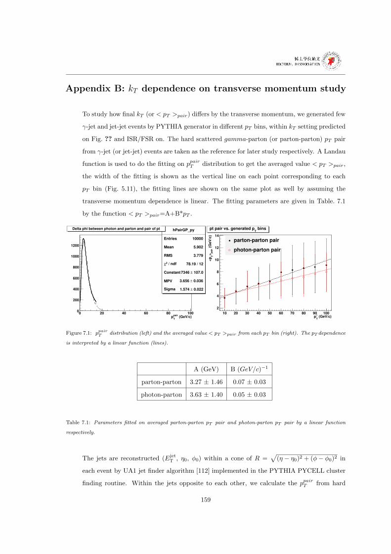
Appendix B: kT dependence on transverse momentum study

To study how final kT (or < pT >pair) differs by the transverse momentum, we generated few

γ-jet and jet-jet events by PYTHIA generator in different pT bins, within kT setting predicted

on Fig. ?? and ISR/FSR on. The hard scattered gamma-parton (or parton-parton) pT pair

from γ-jet (or jet-jet) events are taken as the reference for later study respectively. A Landau

function is used to do the fitting on ppairT distribution to get the averaged value < pT >pair,

the width of the fitting is shown as the vertical line on each point corresponding to each

pT bin (Fig. 5.11), the fitting lines are shown on the same plot as well by assuming the

transverse momentum dependence is linear. The fitting parameters are given in Table. 7.1

by the function < pT >pair=A+B*pT .

hPairGP_py

Entries 10000

Mean 5.902

RMS 3.779

/ ndf 2χ 78.19 / 12

Constant 107.0± 7346

MPV 0.036± 3.656

Sigma 0.022± 1.574

(GeV/c)pair

Tp

0 20 40 60 80 1000

200

400

600

800

1000

1200

hPairGP_py

Entries 10000

Mean 5.902

RMS 3.779

/ ndf 2χ 78.19 / 12

Constant 107.0± 7346

MPV 0.036± 3.656

Sigma 0.022± 1.574

Delta phi between photon and parton and pair of pt

(GeV/c)γ

Tp

10 20 30 40 50 60 70 80 90 100

(G

eV

/c)

pair

>T

<p

2

4

6

8

10

12

14

parton­parton pair

photon­parton pair

binsT

pt pair vs. generated p

Figure 7.1: ppairT distribution (left) and the averaged value < pT >pair from each pT bin (right). The pT dependence

is interpreted by a linear function (lines).

A (GeV) B (GeV/c)−1

parton-parton 3.27 ± 1.46 0.07 ± 0.03

photon-parton 3.63 ± 1.40 0.05 ± 0.03

Table 7.1: Parameters fitted on averaged parton-parton pT pair and photon-parton pT pair by a linear function

respectively.

The jets are reconstructed (EjetT , η0, φ0) within a cone of R =

√(η − η0)2 + (φ− φ0)2 in

each event by UA1 jet finder algorithm [112] implemented in the PYTHIA PYCELL cluster

finding routine. Within the jets opposite to each other, we calculate the ppairT from hard

159

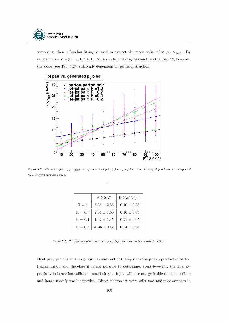
scattering, then a Landau fitting is used to extract the mean value of < pT >pair. By

different cone size (R =1, 0.7, 0.4, 0.2), a similar linear pT is seen from the Fig. 7.2, however,

the slope (see Tab. 7.2) is strongly dependent on jet reconstruction.

(GeV/c)jet

Tp

10 20 30 40 50 60 70 80 90 100

(G

eV

/c)

pair

>T

<p

0

5

10

15

20

25

30 parton­parton pairjet­jet pair: R =1.0jet­jet pair: R =0.7jet­jet pair: R =0.4jet­jet pair: R =0.2

binsT

pt pair vs. generated p

Figure 7.2: The averaged < pT >pair as a function of jet pT from jet-jet events. The pT dependence is interpreted

by a linear function (lines)

.

A (GeV) B (GeV/c)−1

R = 1 6.25 ± 2.56 0.10 ± 0.05

R = 0.7 2.84 ± 1.56 0.16 ± 0.05

R = 0.4 1.42 ± 1.45 0.21 ± 0.05

R = 0.2 -0.36 ± 1.08 0.24 ± 0.05

Table 7.2: Parameters fitted on averaged jet-jet pT pair by the linear function.

Dijet pairs provide an ambiguous measurement of the kT since the jet is a product of parton

fragmentation and therefore it is not possible to determine, event-by-event, the final kT

precisely in heavy ion collisions considering both jets will lose energy inside the hot medium

and hence modify the kinematics. Direct photon-jet pairs offer two major advantages in

160

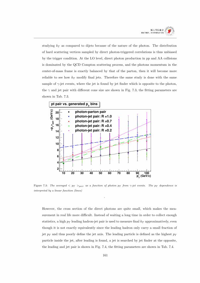
studying kT as compared to dijets because of the nature of the photon. The distribution

of hard scattering vertices sampled by direct photon-triggered correlations is thus unbiased

by the trigger condition. At the LO level, direct photon production in pp and AA collisions

is dominated by the QCD Compton scattering process, and the photons momentum in the

center-of-mass frame is exactly balanced by that of the parton, then it will become more

reliable to see how kT modify final jets. Therefore the same study is done with the same

sample of γ-jet events, where the jet is found by jet finder which is opposite to the photon,

the γ and jet pair with different cone size are shown in Fig. 7.3, the fitting parameters are

shown in Tab. 7.3.

(GeV/c)γ

Tp

10 20 30 40 50 60 70 80 90 100

(G

eV

/c)

pair

>T

<p

2

4

6

8

10

12

14

16

18

20 photon­parton pair

photon­jet pair: R =1.0

photon­jet pair: R =0.7

photon­jet pair: R =0.4

photon­jet pair: R =0.2

binsT

pt pair vs. generated p

Figure 7.3: The averaged < pT >pair as a function of photon pT from γ-jet events. The pT dependence is

interpreted by a linear function (lines)

.

However, the cross section of the direct photons are quite small, which makes the mea-

surement in real life more difficult. Instead of waiting a long time in order to collect enough

statistics, a high pT leading hadron-jet pair is used to measure final kT approximatively, even

though it is not exactly equivalently since the leading hadron only carry a small fraction of

jet pT and thus poorly define the jet axis. The leading particle is defined as the highest pT

particle inside the jet, after leading is found, a jet is searched by jet finder at the opposite,

the leading and jet pair is shown in Fig. 7.4, the fitting parameters are shown in Tab. 7.4.

161

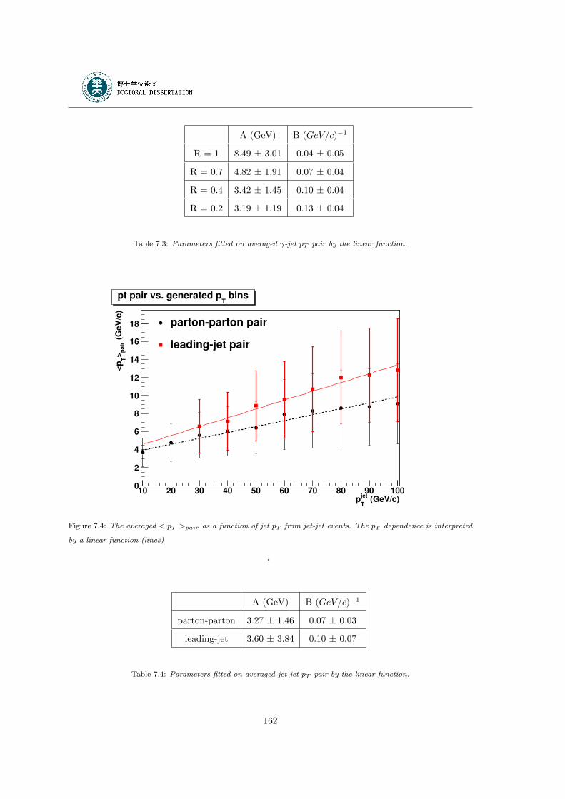
A (GeV) B (GeV/c)−1

R = 1 8.49 ± 3.01 0.04 ± 0.05

R = 0.7 4.82 ± 1.91 0.07 ± 0.04

R = 0.4 3.42 ± 1.45 0.10 ± 0.04

R = 0.2 3.19 ± 1.19 0.13 ± 0.04

Table 7.3: Parameters fitted on averaged γ-jet pT pair by the linear function.

(GeV/c)jet

Tp

10 20 30 40 50 60 70 80 90 100

(G

eV

/c)

pair

>T

<p

0

2

4

6

8

10

12

14

16

18 parton­parton pair

leading­jet pair

binsT

pt pair vs. generated p

Figure 7.4: The averaged < pT >pair as a function of jet pT from jet-jet events. The pT dependence is interpreted

by a linear function (lines)

.

A (GeV) B (GeV/c)−1

parton-parton 3.27 ± 1.46 0.07 ± 0.03

leading-jet 3.60 ± 3.84 0.10 ± 0.07

Table 7.4: Parameters fitted on averaged jet-jet pT pair by the linear function.

162

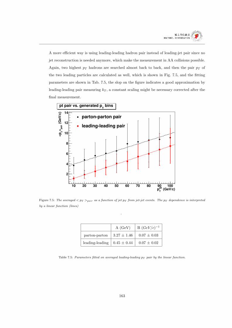
A more efficient way is using leading-leading hadron pair instead of leading-jet pair since no

jet reconstruction is needed anymore, which make the measurement in AA collisions possible.

Again, two highest pT hadrons are searched almost back to back, and then the pair pT of

the two leading particles are calculated as well, which is shown in Fig. 7.5, and the fitting

parameters are shown in Tab. 7.5, the slop on the figure indicates a good approximation by

leading-leading pair measuring kT , a constant scaling might be necessary corrected after the

final measurement.

(GeV/c)jet

Tp

10 20 30 40 50 60 70 80 90 100

(G

eV

/c)

pair

>T

<p

2

4

6

8

10

12

14

parton­parton pair

leading­leading pair

binsT

pt pair vs. generated p

Figure 7.5: The averaged < pT >pair as a function of jet pT from jet-jet events. The pT dependence is interpreted

by a linear function (lines)

.

A (GeV) B (GeV/c)−1

parton-parton 3.27 ± 1.46 0.07 ± 0.03

leading-leading 0.45 ± 0.44 0.07 ± 0.02

Table 7.5: Parameters fitted on averaged leading-leading pT pair by the linear function.

163

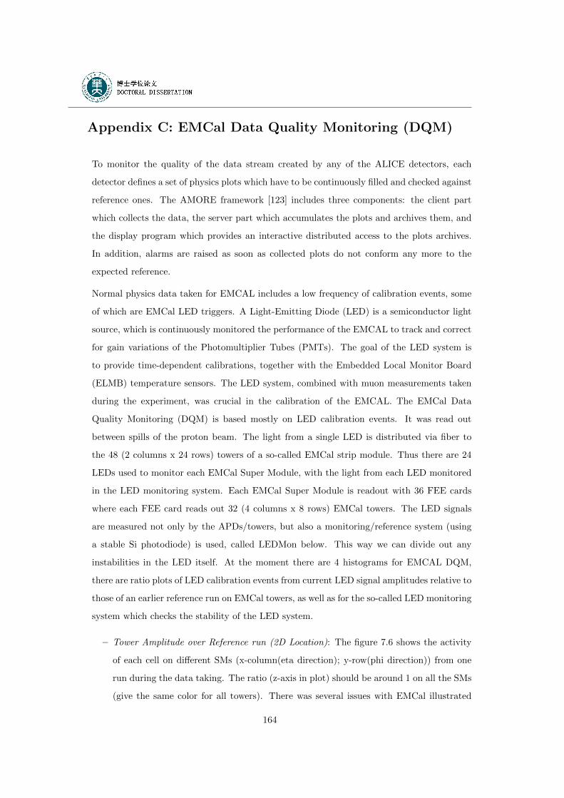
Appendix C: EMCal Data Quality Monitoring (DQM)

To monitor the quality of the data stream created by any of the ALICE detectors, each

detector defines a set of physics plots which have to be continuously filled and checked against

reference ones. The AMORE framework [123] includes three components: the client part

which collects the data, the server part which accumulates the plots and archives them, and

the display program which provides an interactive distributed access to the plots archives.

In addition, alarms are raised as soon as collected plots do not conform any more to the

expected reference.

Normal physics data taken for EMCAL includes a low frequency of calibration events, some

of which are EMCal LED triggers. A Light-Emitting Diode (LED) is a semiconductor light

source, which is continuously monitored the performance of the EMCAL to track and correct

for gain variations of the Photomultiplier Tubes (PMTs). The goal of the LED system is

to provide time-dependent calibrations, together with the Embedded Local Monitor Board

(ELMB) temperature sensors. The LED system, combined with muon measurements taken

during the experiment, was crucial in the calibration of the EMCAL. The EMCal Data

Quality Monitoring (DQM) is based mostly on LED calibration events. It was read out

between spills of the proton beam. The light from a single LED is distributed via fiber to

the 48 (2 columns x 24 rows) towers of a so-called EMCal strip module. Thus there are 24

LEDs used to monitor each EMCal Super Module, with the light from each LED monitored

in the LED monitoring system. Each EMCal Super Module is readout with 36 FEE cards

where each FEE card reads out 32 (4 columns x 8 rows) EMCal towers. The LED signals

are measured not only by the APDs/towers, but also a monitoring/reference system (using

a stable Si photodiode) is used, called LEDMon below. This way we can divide out any

instabilities in the LED itself. At the moment there are 4 histograms for EMCAL DQM,

there are ratio plots of LED calibration events from current LED signal amplitudes relative to

those of an earlier reference run on EMCal towers, as well as for the so-called LED monitoring

system which checks the stability of the LED system.

– Tower Amplitude over Reference run (2D Location): The figure 7.6 shows the activity

of each cell on different SMs (x-column(eta direction); y-row(phi direction)) from one

run during the data taking. The ratio (z-axis in plot) should be around 1 on all the SMs

(give the same color for all towers). There was several issues with EMCal illustrated

164

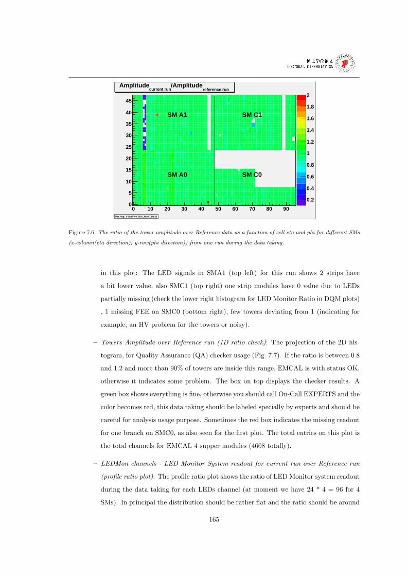
0 10 20 30 40 50 60 70 80 900

5

10

15

20

25

30

35

40

45

SM A0

SM A1

SM C0

SM C1

0.2

0.4

0.6

0.8

1

1.2

1.4

1.6

1.8

2

Tue Aug 3 09:55:04 2010, Run 127822

reference run/Amplitude

current runAmplitude

Figure 7.6: The ratio of the tower amplitude over Reference data as a function of cell eta and phi for different SMs

(x-column(eta direction); y-row(phi direction)) from one run during the data taking.

in this plot: The LED signals in SMA1 (top left) for this run shows 2 strips have

a bit lower value, also SMC1 (top right) one strip modules have 0 value due to LEDs

partially missing (check the lower right histogram for LED Monitor Ratio in DQM plots)

, 1 missing FEE on SMC0 (bottom right), few towers deviating from 1 (indicating for

example, an HV problem for the towers or noisy).

– Towers Amplitude over Reference run (1D ratio check): The projection of the 2D his-

togram, for Quality Assurance (QA) checker usage (Fig. 7.7). If the ratio is between 0.8

and 1.2 and more than 90% of towers are inside this range, EMCAL is with status OK,

otherwise it indicates some problem. The box on top displays the checker results. A

green box shows everything is fine, otherwise you should call On-Call EXPERTS and the

color becomes red, this data taking should be labeled specially by experts and should be

careful for analysis usage purpose. Sometimes the red box indicates the missing readout

for one branch on SMC0, as also seen for the first plot. The total entries on this plot is

the total channels for EMCAL 4 supper modules (4608 totally).

– LEDMon channels - LED Monitor System readout for current run over Reference run

(profile ratio plot): The profile ratio plot shows the ratio of LED Monitor system readout

during the data taking for each LEDs channel (at moment we have 24 * 4 = 96 for 4

SMs). In principal the distribution should be rather flat and the ratio should be around

165

Figure 7.7: The projection of the 2D figure 7.6, for data Quality Assurance (QA) checker usage.

1 since we expect LED system is rather stable. However, with the time going on, the

environment change (for example temperature) may result the light signal changes then

it is not flatted at 1 as it should. For that the best way is to update our QA reference

data since our checker rely on the LED system.

– LEDMon channels - LED Monitor Amplitude over Reference run (1D ratio plot): The

projection of third histogram (lower left in DQM). As explained on that plot, we should

see the distribution peaked at 1 with 96 entries. This two plots (lower part) are for LED

monitor system check.

Finally, the AMORE canvas for EMCAL at P2 DQM station during the data taking is shown

on Fig. 7.8, where all the 4 plots explained above are shown together from different running

period with good data quality (left) and problemable data (right). Since the EMCal data

quality is checked within LED calibration events, the different collision system (no matter

pp or PbPb ) has no impact on EMCal DQM display since they look the same during the

proton-proton and Pb+Pb data taking in 2010.

166

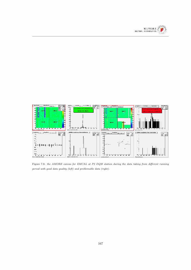
Figure 7.8: the AMORE canvas for EMCAL at P2 DQM station during the data taking from different running

period with good data quality (left) and problemable data (right).

167

Table 7.6: Run Number and Run Index: LHC10e period

0 127719 1 127724 2 127729 3 127730 4 127814

5 127815 6 127817 7 127822 8 127931 9 127932

10 127933 11 127935 12 127936 13 127937 14 127941

15 127942 16 128175 17 128180 18 128182 19 128185

20 128186 21 128189 22 128191 23 128192 24 128257

25 128260 26 128452 27 128483 28 128486 29 128494

30 128495 31 128498 32 128503 33 128504 34 128505

35 128506 36 128507 37 128581 38 128582 39 128590

40 128592 41 128594 42 128596 43 128605 44 128609

45 128611 46 128615 47 128621 48 128678 49 128777

50 128813 51 128819 52 128820 53 128823 54 128824

55 128833 56 128835 57 128836 58 128843 59 128850

60 128853 61 128855 62 128913 63 129513 64 129514

65 129515 66 129516 67 129519 68 129520 69 129521

70 129523 71 129524 72 129525 73 129527 74 129528

75 129536 76 129540 77 129586 78 129587 79 129599

80 129639 81 129641 82 129647 83 129650 84 129652

85 129653 86 129654 87 129659 88 129666 89 129667

90 129723 91 129725 92 129726 93 129729 94 129735

95 129736 96 129738 97 129742 98 129744 99 129959

100 129960 101 129961 102 129962 103 129966 104 129983

105 130149 106 130151 107 130157 108 130158 109 130172

110 130178 111 130179 112 130342 113 130343 114 130479

115 130480 116 130481 117 130517 118 130519 119 130520

120 130524 121 130526 122 130601 123 130608 124 130628

125 130696 126 130704 127 130793 128 130795 129 130798

130 130799 131 130834 132 130840 133 130842 134 130844

135 130847 136 130848

168