Embed Size (px)
Citation preview
Methode multipole rapide pour les calculstridimensionnels de propagation des ondes
(visco)elastodynamiques
Marc Bonnet1
1UMA (Dept. of Appl. Math.), POems, UMR 7231 CNRS-INRIA-ENSTAENSTA, PARIS, France
collaborateurs: Stephanie Chaillat (these 2005-08), Eva Grasso (these 2008-11),Jean-Francois Semblat (IFSTTAR)
Seminaire LAMSID, 18 octobre 2011
Marc Bonnet (POems, ENSTA) Methode multipole rapide pour ondes (visco)elastiques 1 / 71
Plan
1. Principes
2. FMM elastodynamiqueFormulation multi-niveau mono-domaineFormulation multi-niveau multi-domaineExemples: effets de site simplifiesExemple: modelisation simplifiee de la vallee de Grenoble
3. FMM viscoelastodynamiqueEvaluation de la fonction de transfert pour k complexeValidation (exemple mono-domaine)Formulation multi-niveau multi-domaineExemple: effet de site simplifie
4. Couplage FMM-FEM
5. Conclusions
Marc Bonnet (POems, ENSTA) Methode multipole rapide pour ondes (visco)elastiques 2 / 71
Principes
1. Principes
2. FMM elastodynamiqueFormulation multi-niveau mono-domaineFormulation multi-niveau multi-domaineExemples: effets de site simplifiesExemple: modelisation simplifiee de la vallee de Grenoble
3. FMM viscoelastodynamiqueEvaluation de la fonction de transfert pour k complexeValidation (exemple mono-domaine)Formulation multi-niveau multi-domaineExemple: effet de site simplifie
4. Couplage FMM-FEM
5. Conclusions
Marc Bonnet (POems, ENSTA) Methode multipole rapide pour ondes (visco)elastiques 3 / 71
Principes
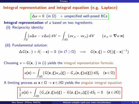
Integral representation and integral equation (e.g. Laplace)
∆u = 0 (in Ω) + unspecified well-posed BCs
Integral representation of u based on two ingredients:(i) Reciprocity identity:∫
Ω
(u∆v − v∆u) dV =
∫∂Ω
(uv,n − vu,n) dV (u,n ≡∇u ·n)
(ii) Fundamental solution:
∆G (x, ·) + δ(·−x) = 0 (in O⊃Ω) =⇒ G (x, ξ) = O(‖ξ−x‖−1)
Choosing v =G (x, ·) in (i) yields the integral representation formula:
u(x) =
∫∂Ω
(G (x, ξ)u,n(ξ)− G,n(x, ξ)u(ξ)
)dSξ (x∈Ω)
A limiting process as x∈Ω→ z∈ ∂Ω yields the singular integral equation:
1
2u(z) +
∫∂Ω
(G,n(z, ξ)u(ξ)− G (z, ξ)u,n(ξ)
)dSξ = 0 (z∈ ∂Ω)
Marc Bonnet (POems, ENSTA) Methode multipole rapide pour ondes (visco)elastiques 4 / 71
Principes
Integral representation and integral equation
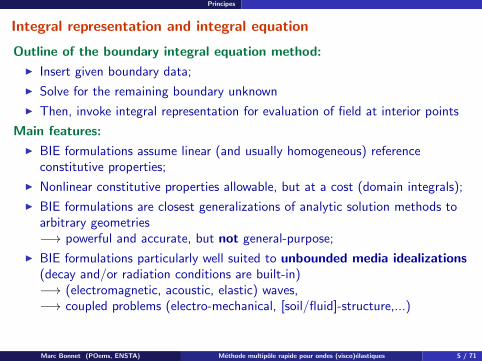
Outline of the boundary integral equation method:
I Insert given boundary data;
I Solve for the remaining boundary unknown
I Then, invoke integral representation for evaluation of field at interior points
Main features:
I BIE formulations assume linear (and usually homogeneous) referenceconstitutive properties;
I Nonlinear constitutive properties allowable, but at a cost (domain integrals);
I BIE formulations are closest generalizations of analytic solution methods toarbitrary geometries−→ powerful and accurate, but not general-purpose;
I BIE formulations particularly well suited to unbounded media idealizations(decay and/or radiation conditions are built-in)−→ (electromagnetic, acoustic, elastic) waves,−→ coupled problems (electro-mechanical, [soil/fluid]-structure,...)
Marc Bonnet (POems, ENSTA) Methode multipole rapide pour ondes (visco)elastiques 5 / 71
Principes
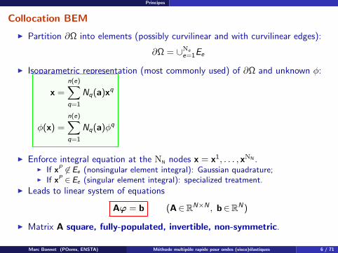
Collocation BEM
I Partition ∂Ω into elements (possibly curvilinear and with curvilinear edges):
∂Ω = ∪Nee=1Ee
I Isoparametric representation (most commonly used) of ∂Ω and unknown φ:
x =
n(e)∑q=1
Nq(a)xq
φ(x) =
n(e)∑q=1
Nq(a)φq
I Enforce integral equation at the NN nodes x = x1, . . . , xNN .I If xP 6∈Ee (nonsingular element integral): Gaussian quadrature;I If xP ∈Ee (singular element integral): specialized treatment.
I Leads to linear system of equations
Aϕ = b (A∈RN×N , b∈RN)
I Matrix A square, fully-populated, invertible, non-symmetric.
Marc Bonnet (POems, ENSTA) Methode multipole rapide pour ondes (visco)elastiques 6 / 71
Principes
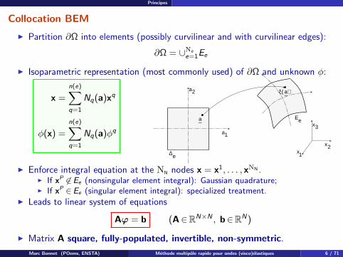
Collocation BEM
I Partition ∂Ω into elements (possibly curvilinear and with curvilinear edges):
∂Ω = ∪Nee=1Ee
I Isoparametric representation (most commonly used) of ∂Ω and unknown φ:
x =
n(e)∑q=1
Nq(a)xq
φ(x) =
n(e)∑q=1
Nq(a)φq
ξ( )
a
∆
1
2
3
12
a
e
E
_
a
_
a
ex
xx
I Enforce integral equation at the NN nodes x = x1, . . . , xNN .I If xP 6∈Ee (nonsingular element integral): Gaussian quadrature;I If xP ∈Ee (singular element integral): specialized treatment.
I Leads to linear system of equations
Aϕ = b (A∈RN×N , b∈RN)
I Matrix A square, fully-populated, invertible, non-symmetric.
Marc Bonnet (POems, ENSTA) Methode multipole rapide pour ondes (visco)elastiques 6 / 71
Principes
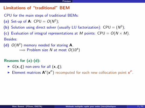
Limitations of “traditional” BEM
CPU for the main steps of traditional BEMs:
(a) Set-up of A: CPU = O(N2);
(b) Solution using direct solver (usually LU factorization): CPU = (N3);
(c) Evaluation of integral representations at M points: CPU = O(N ×M).
Besides:
(d) O(N2) memory needed for storing A.=⇒ Problem size N at most O(104)
Reasons for (a)-(d):
I G (x, ξ) non-zero for all (x, ξ);
I Element matrices Ae(xP) recomputed for each new collocation point xP .
Marc Bonnet (POems, ENSTA) Methode multipole rapide pour ondes (visco)elastiques 7 / 71
Principes
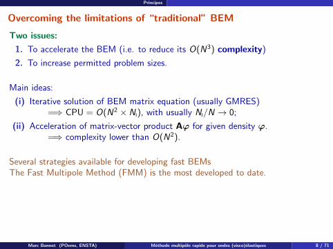
Overcoming the limitations of “traditional” BEM
Two issues:
1. To accelerate the BEM (i.e. to reduce its O(N3) complexity)
2. To increase permitted problem sizes.
Main ideas:
(i) Iterative solution of BEM matrix equation (usually GMRES)=⇒ CPU = O(N2 × NI), with usually NI/N → 0;
(ii) Acceleration of matrix-vector product Aϕ for given density ϕ.=⇒ complexity lower than O(N2).
Several strategies available for developing fast BEMsThe Fast Multipole Method (FMM) is the most developed to date.
Marc Bonnet (POems, ENSTA) Methode multipole rapide pour ondes (visco)elastiques 8 / 71
Principes
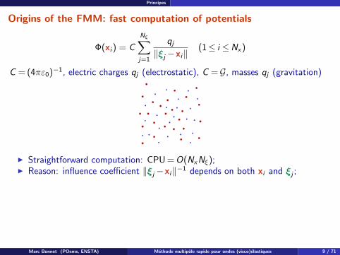
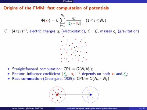
Origins of the FMM: fast computation of potentials
Φ(xi ) = C
Nξ∑j=1
qj‖ξj −xi‖
(1≤ i ≤Nx)
C = (4πε0)−1, electric charges qj (electrostatic), C =G, masses qj (gravitation)
I Straightforward computation: CPU =O(NxNξ);I Reason: influence coefficient ‖ξj −xi‖−1 depends on both xi and ξj ;
I Fast summation (Greengard, 1985): CPU =O(Nx +Nξ)
Marc Bonnet (POems, ENSTA) Methode multipole rapide pour ondes (visco)elastiques 9 / 71
Principes
Origins of the FMM: fast computation of potentials
Φ(xi ) = C
Nξ∑j=1
qj‖ξj −xi‖
(1≤ i ≤Nx)
C = (4πε0)−1, electric charges qj (electrostatic), C =G, masses qj (gravitation)
I Straightforward computation: CPU =O(NxNξ);I Reason: influence coefficient ‖ξj −xi‖−1 depends on both xi and ξj ;I Fast summation (Greengard, 1985): CPU =O(Nx +Nξ)
Marc Bonnet (POems, ENSTA) Methode multipole rapide pour ondes (visco)elastiques 9 / 71
Principes
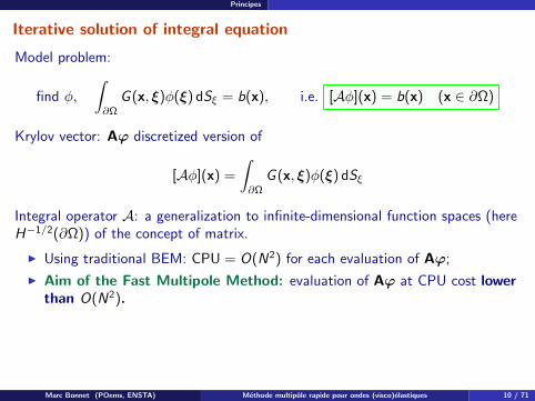
Iterative solution of integral equation
Model problem:
find φ,
∫∂Ω
G (x, ξ)φ(ξ) dSξ = b(x), i.e. [Aφ](x) = b(x) (x ∈ ∂Ω)
Krylov vector: Aϕ discretized version of
[Aφ](x) =
∫∂Ω
G (x, ξ)φ(ξ) dSξ
Integral operator A: a generalization to infinite-dimensional function spaces (hereH−1/2(∂Ω)) of the concept of matrix.
I Using traditional BEM: CPU = O(N2) for each evaluation of Aϕ;
I Aim of the Fast Multipole Method: evaluation of Aϕ at CPU cost lowerthan O(N2).
Marc Bonnet (POems, ENSTA) Methode multipole rapide pour ondes (visco)elastiques 10 / 71

Principes
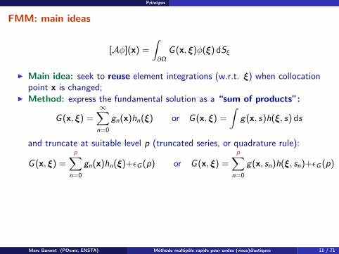
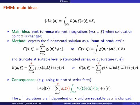
FMM: main ideas
[Aφ](x) =
∫∂Ω
G (x, ξ)φ(ξ) dSξ
I Main idea: seek to reuse element integrations (w.r.t. ξ) when collocationpoint x is changed;
I Method: express the fundamental solution as a “sum of products”:
G (x, ξ) =∞∑n=0
gn(x)hn(ξ) or G (x, ξ) =
∫g(x, s)h(ξ, s) ds
and truncate at suitable level p (truncated series, or quadrature rule):
G (x, ξ) =
p∑n=0
gn(x)hn(ξ)+εG (p) or G (x, ξ) =
p∑n=0
g(x, sn)h(ξ, sn)+εG (p)
I Consequence: (e.g. using truncated-series form)
[Aφ](x) =
p∑n=0
gn(x)
∫∂Ω
hn(ξ)φ(ξ) dSξ + ε(p)
The p integrations are independent on x and are reusable as x is changed.
Marc Bonnet (POems, ENSTA) Methode multipole rapide pour ondes (visco)elastiques 11 / 71
Principes
FMM: main ideas
[Aφ](x) =
∫∂Ω
G (x, ξ)φ(ξ) dSξ
I Main idea: seek to reuse element integrations (w.r.t. ξ) when collocationpoint x is changed;
I Method: express the fundamental solution as a “sum of products”:
G (x, ξ) =∞∑n=0
gn(x)hn(ξ) or G (x, ξ) =
∫g(x, s)h(ξ, s) ds
and truncate at suitable level p (truncated series, or quadrature rule):
G (x, ξ) =
p∑n=0
gn(x)hn(ξ)+εG (p) or G (x, ξ) =
p∑n=0
g(x, sn)h(ξ, sn)+εG (p)
I Consequence: (e.g. using truncated-series form)
[Aφ](x) =
p∑n=0
gn(x)
∫∂Ω
hn(ξ)φ(ξ) dSξ + ε(p)
The p integrations are independent on x and are reusable as x is changed.Marc Bonnet (POems, ENSTA) Methode multipole rapide pour ondes (visco)elastiques 11 / 71
Principes
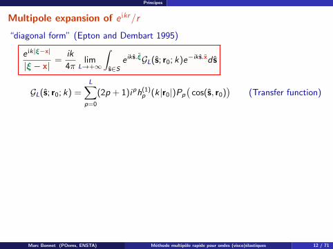
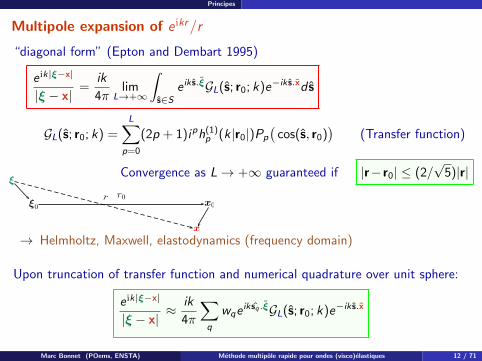
Multipole expansion of e ikr/r
“diagonal form” (Epton and Dembart 1995)
eik|ξ−x|
|ξ − x| =ik
4πlim
L→+∞
∫s∈S
e ik s.ξGL(s; r0; k)e−ik s.xd s
GL(s; r0; k) =L∑
p=0
(2p + 1)iph(1)p (k |r0|)Pp
(cos(s, r0)
)(Transfer function)
ξ
ξ0 x0
x
r r0
Convergence as L→ +∞ guaranteed if |r− r0| ≤ (2/√
5)|r|
→ Helmholtz, Maxwell, elastodynamics (frequency domain)
Upon truncation of transfer function and numerical quadrature over unit sphere:
eik|ξ−x|
|ξ − x| ≈ik
4π
∑q
wqeik sq.ξGL(s; r0; k)e−ik s.x
Marc Bonnet (POems, ENSTA) Methode multipole rapide pour ondes (visco)elastiques 12 / 71
Principes
Multipole expansion of e ikr/r
“diagonal form” (Epton and Dembart 1995)
eik|ξ−x|
|ξ − x| =ik
4πlim
L→+∞
∫s∈S
e ik s.ξGL(s; r0; k)e−ik s.xd s
GL(s; r0; k) =L∑
p=0
(2p + 1)iph(1)p (k |r0|)Pp
(cos(s, r0)
)(Transfer function)
ξ
ξ0 x0
x
r r0
Convergence as L→ +∞ guaranteed if |r− r0| ≤ (2/√
5)|r|
→ Helmholtz, Maxwell, elastodynamics (frequency domain)
Upon truncation of transfer function and numerical quadrature over unit sphere:
eik|ξ−x|
|ξ − x| ≈ik
4π
∑q
wqeik sq.ξGL(s; r0; k)e−ik s.x
Marc Bonnet (POems, ENSTA) Methode multipole rapide pour ondes (visco)elastiques 12 / 71
FMM elastodynamique
1. Principes
2. FMM elastodynamiqueFormulation multi-niveau mono-domaineFormulation multi-niveau multi-domaineExemples: effets de site simplifiesExemple: modelisation simplifiee de la vallee de Grenoble
3. FMM viscoelastodynamiqueEvaluation de la fonction de transfert pour k complexeValidation (exemple mono-domaine)Formulation multi-niveau multi-domaineExemple: effet de site simplifie
4. Couplage FMM-FEM
5. Conclusions
Marc Bonnet (POems, ENSTA) Methode multipole rapide pour ondes (visco)elastiques 13 / 71
FMM elastodynamique
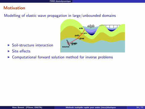
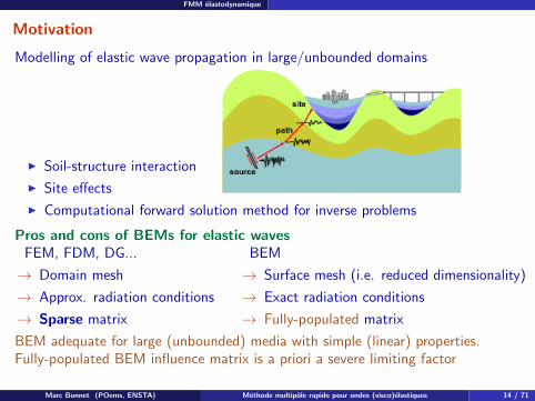
Motivation
Modelling of elastic wave propagation in large/unbounded domains
I Soil-structure interaction
I Site effects
I Computational forward solution method for inverse problems
Pros and cons of BEMs for elastic wavesFEM, FDM, DG...
→ Domain mesh
→ Approx. radiation conditions
→ Sparse matrix
BEM
→ Surface mesh (i.e. reduced dimensionality)
→ Exact radiation conditions
→ Fully-populated matrix
BEM adequate for large (unbounded) media with simple (linear) properties.Fully-populated BEM influence matrix is a priori a severe limiting factor
Marc Bonnet (POems, ENSTA) Methode multipole rapide pour ondes (visco)elastiques 14 / 71
FMM elastodynamique
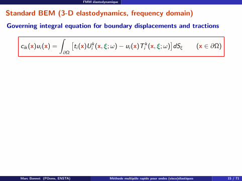
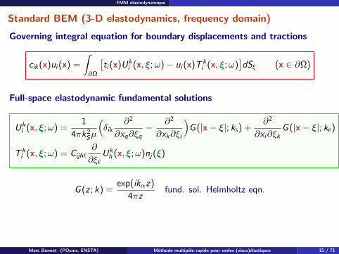
Standard BEM (3-D elastodynamics, frequency domain)
Governing integral equation for boundary displacements and tractions
cik(x)ui (x) =
∫∂Ω
[ti (x)Uk
i (x, ξ;ω)− ui (x)T ki (x, ξ;ω)
]dSξ (x ∈ ∂Ω)
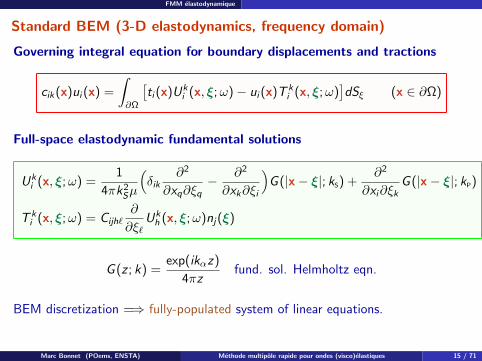
Full-space elastodynamic fundamental solutions
Uki (x, ξ;ω) =
1
4πk2Sµ
(δik
∂2
∂xq∂ξq− ∂2
∂xk∂ξi
)G (|x− ξ|; kS) +
∂2
∂xi∂ξkG (|x− ξ|; kP)
T ki (x, ξ;ω) = Cijh`
∂
∂ξ`Ukh (x, ξ;ω)nj(ξ)
G (z ; k) =exp(ikαz)
4πzfund. sol. Helmholtz eqn.
BEM discretization =⇒ fully-populated system of linear equations.
Marc Bonnet (POems, ENSTA) Methode multipole rapide pour ondes (visco)elastiques 15 / 71
FMM elastodynamique
Standard BEM (3-D elastodynamics, frequency domain)
Governing integral equation for boundary displacements and tractions
cik(x)ui (x) =
∫∂Ω
[ti (x)Uk
i (x, ξ;ω)− ui (x)T ki (x, ξ;ω)
]dSξ (x ∈ ∂Ω)
Full-space elastodynamic fundamental solutions
Uki (x, ξ;ω) =
1
4πk2Sµ
(δik
∂2
∂xq∂ξq− ∂2
∂xk∂ξi
)G (|x− ξ|; kS) +
∂2
∂xi∂ξkG (|x− ξ|; kP)
T ki (x, ξ;ω) = Cijh`
∂
∂ξ`Ukh (x, ξ;ω)nj(ξ)
G (z ; k) =exp(ikαz)
4πzfund. sol. Helmholtz eqn.
BEM discretization =⇒ fully-populated system of linear equations.
Marc Bonnet (POems, ENSTA) Methode multipole rapide pour ondes (visco)elastiques 15 / 71
FMM elastodynamique Formulation multi-niveau mono-domaine
1. Principes
2. FMM elastodynamiqueFormulation multi-niveau mono-domaineFormulation multi-niveau multi-domaineExemples: effets de site simplifiesExemple: modelisation simplifiee de la vallee de Grenoble
3. FMM viscoelastodynamique
4. Couplage FMM-FEM
5. Conclusions
Marc Bonnet (POems, ENSTA) Methode multipole rapide pour ondes (visco)elastiques 16 / 71
FMM elastodynamique Formulation multi-niveau mono-domaine
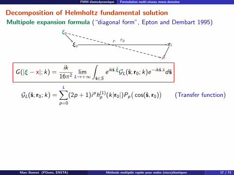
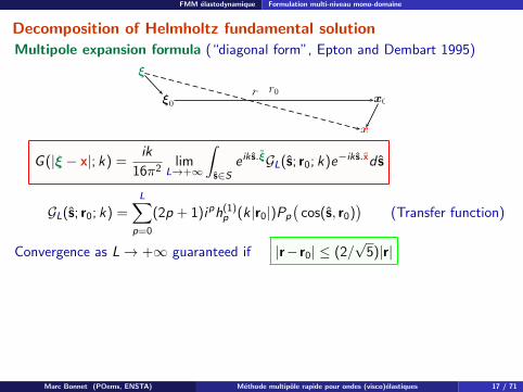
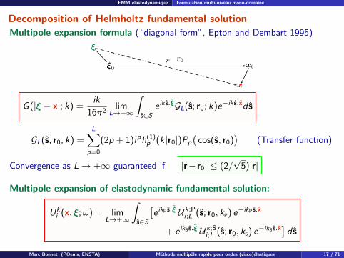
Decomposition of Helmholtz fundamental solution
Multipole expansion formula (“diagonal form”, Epton and Dembart 1995)
ξ
ξ0 x0
x
r r0
G (|ξ − x|; k) =ik
16π2lim
L→+∞
∫s∈S
e ik s.ξGL(s; r0; k)e−ik s.xd s
GL(s; r0; k) =L∑
p=0
(2p + 1)iph(1)p (k |r0|)Pp
(cos(s, r0)
)(Transfer function)
Convergence as L→ +∞ guaranteed if |r− r0| ≤ (2/√
5)|r|
Multipole expansion of elastodynamic fundamental solution:
Uki (x, ξ;ω) = lim
L→+∞
∫s∈S
[e ikP s.ξ Uk;P
i ;L (s; r0, kP) e−ikP s.x
+ e ikS s.ξ Uk;Si ;L (s; r0, kS) e−ikS s.x
]d s
Marc Bonnet (POems, ENSTA) Methode multipole rapide pour ondes (visco)elastiques 17 / 71
FMM elastodynamique Formulation multi-niveau mono-domaine
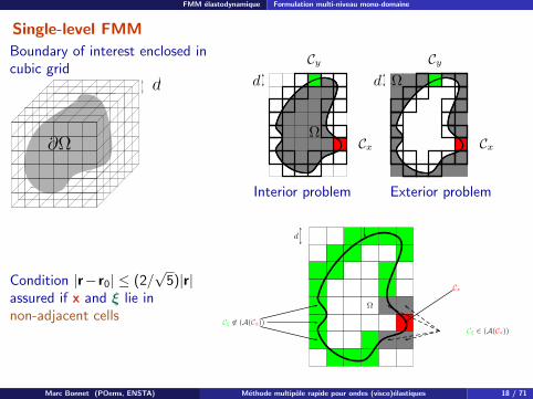
Single-level FMM
Boundary of interest enclosed incubic grid
d
∂Ω
Cy
Cx
Ω
d
Cy
Cx
Ωd
Interior problem Exterior problem
Condition |r− r0| ≤ (2/√
5)|r|assured if x and ξ lie innon-adjacent cells
Cx
Cξ ∈ (A(Cx))Cξ 6∈ (A(Cx))
Ω
d
Marc Bonnet (POems, ENSTA) Methode multipole rapide pour ondes (visco)elastiques 18 / 71
FMM elastodynamique Formulation multi-niveau mono-domaine
Single-level FMM
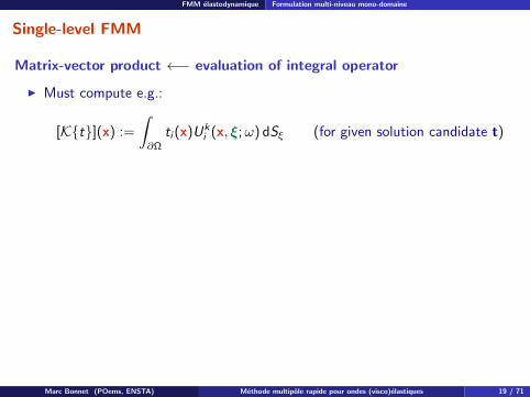
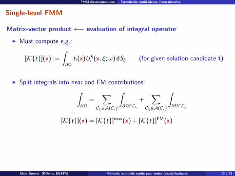
Matrix-vector product ←− evaluation of integral operator
I Must compute e.g.:
[Kt](x) :=
∫∂Ω
ti (x)Uki (x, ξ;ω) dSξ (for given solution candidate t)
I Split integrals into near and FM contributions:∫∂Ω
=∑
Cξ∈A(Cx )
∫∂Ω∩Cξ
+∑
Cξ /∈A(Cx )
∫∂Ω∩Cξ
[Kt](x) = [Kt]near(x) + [Kt]FM(x)
Marc Bonnet (POems, ENSTA) Methode multipole rapide pour ondes (visco)elastiques 19 / 71
FMM elastodynamique Formulation multi-niveau mono-domaine
Single-level FMM
Matrix-vector product ←− evaluation of integral operator
I Must compute e.g.:
[Kt](x) :=
∫∂Ω
ti (x)Uki (x, ξ;ω) dSξ (for given solution candidate t)
I Split integrals into near and FM contributions:∫∂Ω
=∑
Cξ∈A(Cx )
∫∂Ω∩Cξ
+∑
Cξ /∈A(Cx )
∫∂Ω∩Cξ
[Kt](x) = [Kt]near(x) + [Kt]FM(x)
Marc Bonnet (POems, ENSTA) Methode multipole rapide pour ondes (visco)elastiques 19 / 71
FMM elastodynamique Formulation multi-niveau mono-domaine
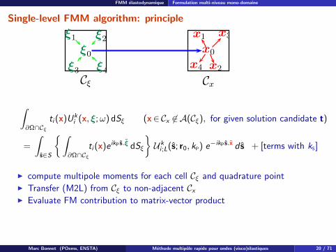
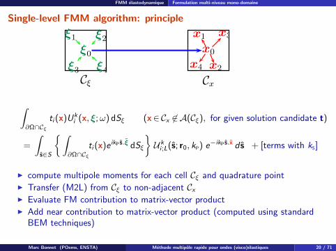
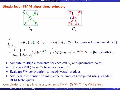
Single-level FMM algorithm: principle
Cξ
ξ0
ξ1 ξ2
ξ3 ξ4
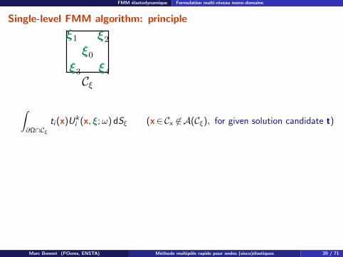
∫∂Ω∩Cξ
ti (x)Uki (x, ξ;ω) dSξ (x∈Cx 6∈ A(Cξ), for given solution candidate t)
=
∫s∈S
∫∂Ω∩Cξ
ti (x)e ikP s.ξ dSξ
Uki ;L(s; r0, kP) e−ikP s.x d s + [terms with kS]
I compute multipole moments for each cell Cξ and quadrature pointI Transfer (M2L) from Cξ to non-adjacent CxI Evaluate FM contribution to matrix-vector productI Add near contribution to matrix-vector product (computed using standard
BEM techniques)
Complexity of single-level elastodynamic FMM: O(N3/2) / GMRES iter.
Marc Bonnet (POems, ENSTA) Methode multipole rapide pour ondes (visco)elastiques 20 / 71

FMM elastodynamique Formulation multi-niveau mono-domaine
Single-level FMM algorithm: principle
Cξ
ξ0
ξ1 ξ2
ξ3 ξ4
∫∂Ω∩Cξ
ti (x)Uki (x, ξ;ω) dSξ (x∈Cx 6∈ A(Cξ), for given solution candidate t)
=
∫s∈S
∫∂Ω∩Cξ
ti (x)e ikP s.ξ dSξ
Uki ;L(s; r0, kP) e−ikP s.x d s
+ [terms with kS]
I compute multipole moments for each cell Cξ and quadrature point
I Transfer (M2L) from Cξ to non-adjacent CxI Evaluate FM contribution to matrix-vector productI Add near contribution to matrix-vector product (computed using standard
BEM techniques)
Complexity of single-level elastodynamic FMM: O(N3/2) / GMRES iter.
Marc Bonnet (POems, ENSTA) Methode multipole rapide pour ondes (visco)elastiques 20 / 71
FMM elastodynamique Formulation multi-niveau mono-domaine
Single-level FMM algorithm: principle
Cξ
ξ0
ξ1 ξ2
ξ3 ξ4
Cx
x0
x1
x2
x3
x4
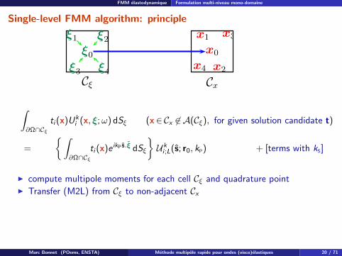
∫∂Ω∩Cξ
ti (x)Uki (x, ξ;ω) dSξ (x∈Cx 6∈ A(Cξ), for given solution candidate t)
=
∫s∈S
∫∂Ω∩Cξ
ti (x)e ikP s.ξ dSξ
Uki ;L(s; r0, kP)
e−ikP s.x d s
+ [terms with kS]
I compute multipole moments for each cell Cξ and quadrature pointI Transfer (M2L) from Cξ to non-adjacent Cx
I Evaluate FM contribution to matrix-vector productI Add near contribution to matrix-vector product (computed using standard
BEM techniques)
Complexity of single-level elastodynamic FMM: O(N3/2) / GMRES iter.
Marc Bonnet (POems, ENSTA) Methode multipole rapide pour ondes (visco)elastiques 20 / 71
FMM elastodynamique Formulation multi-niveau mono-domaine
Single-level FMM algorithm: principle
Cξ
ξ0
ξ1 ξ2
ξ3 ξ4
Cx
x0
x1
x2
x3
x4
∫∂Ω∩Cξ
ti (x)Uki (x, ξ;ω) dSξ (x∈Cx 6∈ A(Cξ), for given solution candidate t)
=
∫s∈S
∫∂Ω∩Cξ
ti (x)e ikP s.ξ dSξ
Uki ;L(s; r0, kP) e−ikP s.x d s + [terms with kS]
I compute multipole moments for each cell Cξ and quadrature pointI Transfer (M2L) from Cξ to non-adjacent CxI Evaluate FM contribution to matrix-vector product
I Add near contribution to matrix-vector product (computed using standardBEM techniques)
Complexity of single-level elastodynamic FMM: O(N3/2) / GMRES iter.
Marc Bonnet (POems, ENSTA) Methode multipole rapide pour ondes (visco)elastiques 20 / 71
FMM elastodynamique Formulation multi-niveau mono-domaine
Single-level FMM algorithm: principle
Cξ
ξ0
ξ1 ξ2
ξ3 ξ4
Cx
x0
x1
x2
x3
x4
∫∂Ω∩Cξ
ti (x)Uki (x, ξ;ω) dSξ (x∈Cx 6∈ A(Cξ), for given solution candidate t)
=
∫s∈S
∫∂Ω∩Cξ
ti (x)e ikP s.ξ dSξ
Uki ;L(s; r0, kP) e−ikP s.x d s + [terms with kS]
I compute multipole moments for each cell Cξ and quadrature pointI Transfer (M2L) from Cξ to non-adjacent CxI Evaluate FM contribution to matrix-vector productI Add near contribution to matrix-vector product (computed using standard
BEM techniques)
Complexity of single-level elastodynamic FMM: O(N3/2) / GMRES iter.
Marc Bonnet (POems, ENSTA) Methode multipole rapide pour ondes (visco)elastiques 20 / 71
FMM elastodynamique Formulation multi-niveau mono-domaine
Single-level FMM algorithm: principle
Cξ
ξ0
ξ1 ξ2
ξ3 ξ4
Cx
x0
x1
x2
x3
x4
∫∂Ω∩Cξ
ti (x)Uki (x, ξ;ω) dSξ (x∈Cx 6∈ A(Cξ), for given solution candidate t)
=
∫s∈S
∫∂Ω∩Cξ
ti (x)e ikP s.ξ dSξ
Uki ;L(s; r0, kP) e−ikP s.x d s + [terms with kS]
I compute multipole moments for each cell Cξ and quadrature pointI Transfer (M2L) from Cξ to non-adjacent CxI Evaluate FM contribution to matrix-vector productI Add near contribution to matrix-vector product (computed using standard
BEM techniques)
Complexity of single-level elastodynamic FMM: O(N3/2) / GMRES iter.Marc Bonnet (POems, ENSTA) Methode multipole rapide pour ondes (visco)elastiques 20 / 71
FMM elastodynamique Formulation multi-niveau mono-domaine
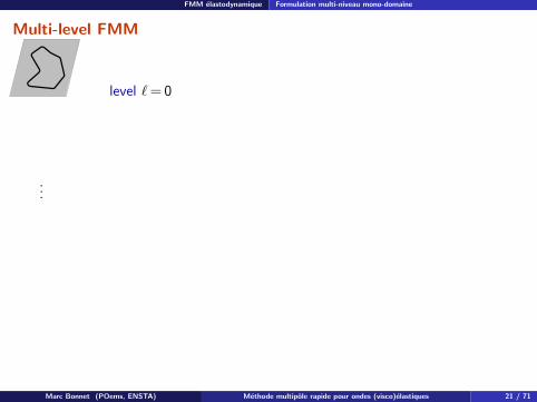
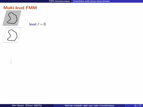
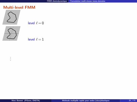
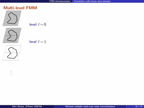
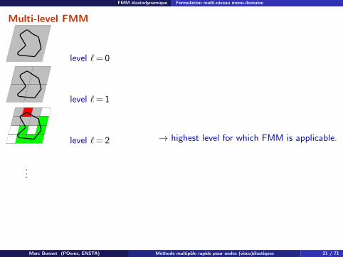
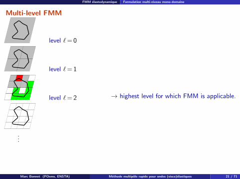
Multi-level FMM
level `= 0
level `= 1
level `= 2
level `= 3
...
level `= ¯ (leaf)
→ highest level for which FMM is applicable.
computation organization based onrecursive subdivision (oc-tree)
Complexity of multi-level elastodynamic FMM: O(N logN)
S. Chaillat, MB, J.F. Semblat, Comp. Meth. Appl. Mech. Engng., 197 (2008)
Marc Bonnet (POems, ENSTA) Methode multipole rapide pour ondes (visco)elastiques 21 / 71
FMM elastodynamique Formulation multi-niveau mono-domaine
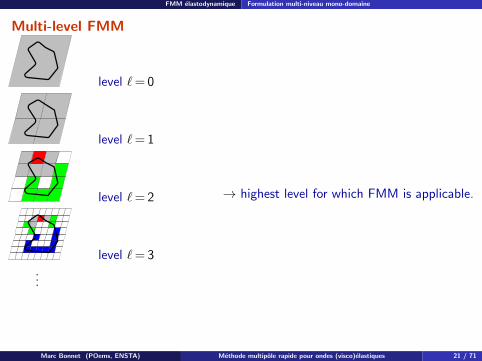
Multi-level FMM
level `= 0
level `= 1
level `= 2
level `= 3
...
level `= ¯ (leaf)→ highest level for which FMM is applicable.
computation organization based onrecursive subdivision (oc-tree)
Complexity of multi-level elastodynamic FMM: O(N logN)
S. Chaillat, MB, J.F. Semblat, Comp. Meth. Appl. Mech. Engng., 197 (2008)
Marc Bonnet (POems, ENSTA) Methode multipole rapide pour ondes (visco)elastiques 21 / 71
FMM elastodynamique Formulation multi-niveau mono-domaine
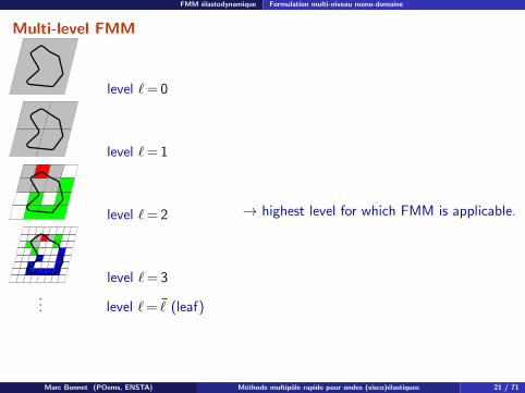
Multi-level FMM
level `= 0
level `= 1
level `= 2
level `= 3
...
level `= ¯ (leaf)→ highest level for which FMM is applicable.
computation organization based onrecursive subdivision (oc-tree)
Complexity of multi-level elastodynamic FMM: O(N logN)
S. Chaillat, MB, J.F. Semblat, Comp. Meth. Appl. Mech. Engng., 197 (2008)
Marc Bonnet (POems, ENSTA) Methode multipole rapide pour ondes (visco)elastiques 21 / 71
FMM elastodynamique Formulation multi-niveau mono-domaine
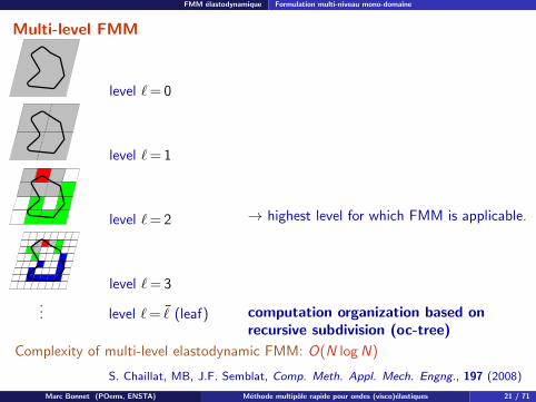
Multi-level FMM
level `= 0
level `= 1
level `= 2
level `= 3
...
level `= ¯ (leaf)
→ highest level for which FMM is applicable.
computation organization based onrecursive subdivision (oc-tree)
Complexity of multi-level elastodynamic FMM: O(N logN)
S. Chaillat, MB, J.F. Semblat, Comp. Meth. Appl. Mech. Engng., 197 (2008)
Marc Bonnet (POems, ENSTA) Methode multipole rapide pour ondes (visco)elastiques 21 / 71
FMM elastodynamique Formulation multi-niveau mono-domaine
Multi-level FMM
level `= 0
level `= 1
level `= 2
level `= 3...
level `= ¯ (leaf)
→ highest level for which FMM is applicable.
computation organization based onrecursive subdivision (oc-tree)
Complexity of multi-level elastodynamic FMM: O(N logN)
S. Chaillat, MB, J.F. Semblat, Comp. Meth. Appl. Mech. Engng., 197 (2008)
Marc Bonnet (POems, ENSTA) Methode multipole rapide pour ondes (visco)elastiques 21 / 71
FMM elastodynamique Formulation multi-niveau mono-domaine
Multi-level FMM
level `= 0
level `= 1
level `= 2
level `= 3... level `= ¯ (leaf)
→ highest level for which FMM is applicable.
computation organization based onrecursive subdivision (oc-tree)
Complexity of multi-level elastodynamic FMM: O(N logN)
S. Chaillat, MB, J.F. Semblat, Comp. Meth. Appl. Mech. Engng., 197 (2008)
Marc Bonnet (POems, ENSTA) Methode multipole rapide pour ondes (visco)elastiques 21 / 71
FMM elastodynamique Formulation multi-niveau mono-domaine
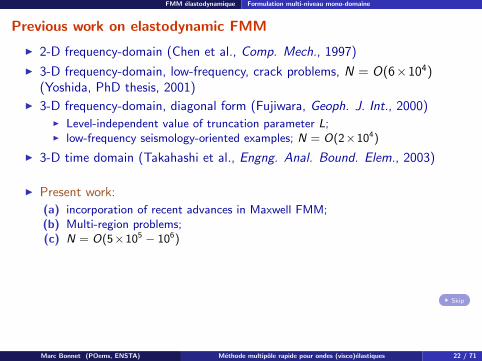
Previous work on elastodynamic FMM
I 2-D frequency-domain (Chen et al., Comp. Mech., 1997)
I 3-D frequency-domain, low-frequency, crack problems, N = O(6×10⁴)(Yoshida, PhD thesis, 2001)
I 3-D frequency-domain, diagonal form (Fujiwara, Geoph. J. Int., 2000)I Level-independent value of truncation parameter L;I low-frequency seismology-oriented examples; N = O(2×10⁴)
I 3-D time domain (Takahashi et al., Engng. Anal. Bound. Elem., 2003)
I Present work:
(a) incorporation of recent advances in Maxwell FMM;(b) Multi-region problems;(c) N = O(5×10⁵ − 106)
Skip
Marc Bonnet (POems, ENSTA) Methode multipole rapide pour ondes (visco)elastiques 22 / 71
FMM elastodynamique Formulation multi-niveau mono-domaine
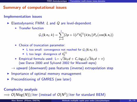
Summary of computational issues
Implementation issues
I Elastodynamic FMM: L and Q are level-dependentI Transfer function
GL(s; r0; k) =L∑
p=0
(2p + 1)iph(1)p (k|r0|)Pp
(cos (s, r0)
)I Choice of truncation parameter:
I L too small: convergence not reached for GL (s; r0; k);
I L too large: divergence of h(1)p
I Empirical formula used: L=√
3kSd + Cεlog10(√
3kSd + π)(see Darve 2000 and Sylvand 2002 for Maxwell eqns)
→ upward (downward) pass features (inverse) extrapolation step
I Importance of optimal memory management
I Preconditioning of GMRES (see later)
Complexity analysis
=⇒ O(Nlog(N))/iter (instead of O(N2)/iter for standard BEM)
Marc Bonnet (POems, ENSTA) Methode multipole rapide pour ondes (visco)elastiques 23 / 71
FMM elastodynamique Formulation multi-niveau mono-domaine
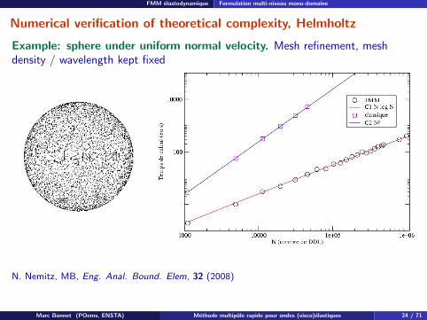
Numerical verification of theoretical complexity, Helmholtz
Example: sphere under uniform normal velocity. Mesh refinement, meshdensity / wavelength kept fixed
N. Nemitz, MB, Eng. Anal. Bound. Elem, 32 (2008)
Marc Bonnet (POems, ENSTA) Methode multipole rapide pour ondes (visco)elastiques 24 / 71
FMM elastodynamique Formulation multi-niveau mono-domaine
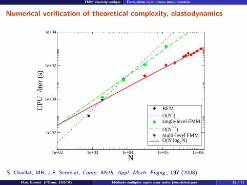
Numerical verification of theoretical complexity, elastodynamics
1e+02 1e+03 1e+04 1e+05 1e+06
N
1e-02
1e+00
1e+02
1e+04
CPU
/ite
r (s
)
BEMO(N
2)
single-level FMM
O(N3/2
)multi-level FMMO(N log
2N)
S. Chaillat, MB, J.F. Semblat, Comp. Meth. Appl. Mech. Engng., 197 (2008)
Marc Bonnet (POems, ENSTA) Methode multipole rapide pour ondes (visco)elastiques 25 / 71
FMM elastodynamique Formulation multi-niveau multi-domaine
1. Principes
2. FMM elastodynamiqueFormulation multi-niveau mono-domaineFormulation multi-niveau multi-domaineExemples: effets de site simplifiesExemple: modelisation simplifiee de la vallee de Grenoble
3. FMM viscoelastodynamique
4. Couplage FMM-FEM
5. Conclusions
Marc Bonnet (POems, ENSTA) Methode multipole rapide pour ondes (visco)elastiques 26 / 71
FMM elastodynamique Formulation multi-niveau multi-domaine
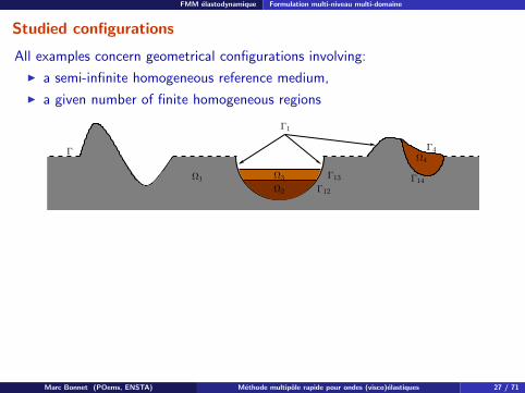
Studied configurations
All examples concern geometrical configurations involving:
I a semi-infinite homogeneous reference medium,
I a given number of finite homogeneous regions
Ω1
Ω2
Ω3
Ω4Γ
Γ12
Γ13
Γ1
Γ4
Γ14
Marc Bonnet (POems, ENSTA) Methode multipole rapide pour ondes (visco)elastiques 27 / 71
FMM elastodynamique Formulation multi-niveau multi-domaine
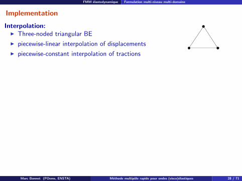
Implementation
Interpolation:I Three-noded triangular BE
I piecewise-linear interpolation of displacements
I piecewise-constant interpolation of tractions
Single region FMM applied independently in each subdomain
I definition of an octree in each sub-domain
Marc Bonnet (POems, ENSTA) Methode multipole rapide pour ondes (visco)elastiques 28 / 71
FMM elastodynamique Formulation multi-niveau multi-domaine
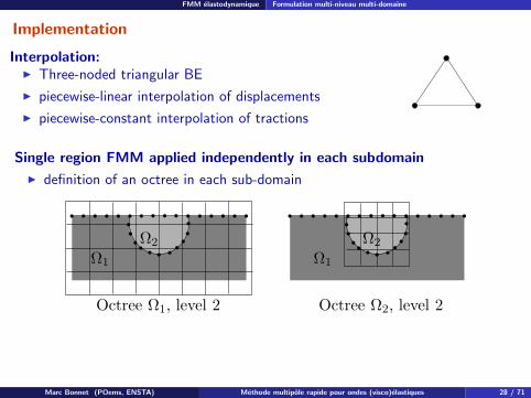
Implementation
Interpolation:I Three-noded triangular BE
I piecewise-linear interpolation of displacements
I piecewise-constant interpolation of tractions
Single region FMM applied independently in each subdomain
I definition of an octree in each sub-domain
Ω2
Ω1
Ω2
Ω1
Octree Ω1, level 2 Octree Ω2, level 2
Marc Bonnet (POems, ENSTA) Methode multipole rapide pour ondes (visco)elastiques 28 / 71
FMM elastodynamique Formulation multi-niveau multi-domaine
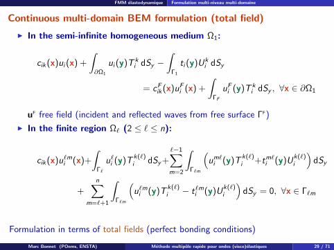
Continuous multi-domain BEM formulation (total field)
I In the semi-infinite homogeneous medium Ω1:
cik(x)ui (x) +
∫∂Ω1
ui (y)T ki dSy −
∫Γ1
ti (y)Uki dSy
= cFik(x)uFi (x) +
∫ΓF
uFi (y)T ki dSy , ∀x ∈ ∂Ω1
uF free field (incident and reflected waves from free surface ΓF)
I In the finite region Ω` (2 ≤ ` ≤ n):
cik(x)u`mi (x)+
∫Γ`
u`i (y)Tk(`)i dSy+
`−1∑m=2
∫Γ`m
(um`i (y)T
k(`)i +tm`i (y)U
k(`)i
)dSy
+n∑
m=`+1
∫Γ`m
(u`mi (y)T
k(`)i − t`mi (y)U
k(`)i
)dSy = 0, ∀x ∈ Γ`m
Formulation in terms of total fields (perfect bonding conditions)
Marc Bonnet (POems, ENSTA) Methode multipole rapide pour ondes (visco)elastiques 29 / 71
FMM elastodynamique Formulation multi-niveau multi-domaine
Linear combinations of collocations on interfaces
Single region FMM applied independently in each sub-domain (collocation:red nodes + blue element centers)
I Over-determined system;
I Contribution of Ωi and of Ωj to collocation on interface Γij are linearlycombined (optimal coefficients chosen using numerical experiments)
Marc Bonnet (POems, ENSTA) Methode multipole rapide pour ondes (visco)elastiques 30 / 71
FMM elastodynamique Exemples: effets de site simplifies
1. Principes
2. FMM elastodynamiqueFormulation multi-niveau mono-domaineFormulation multi-niveau multi-domaineExemples: effets de site simplifiesExemple: modelisation simplifiee de la vallee de Grenoble
3. FMM viscoelastodynamique
4. Couplage FMM-FEM
5. Conclusions
Marc Bonnet (POems, ENSTA) Methode multipole rapide pour ondes (visco)elastiques 31 / 71
FMM elastodynamique Exemples: effets de site simplifies
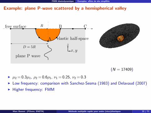
Example: plane P-wave scattered by a hemispherical valley
x, y
z
plane P wave
R
D = 5R
free surface
elastic half-spaceA
B C
(N = 17409)
I µ2 = 0.3µ1, ρ2 = 0.6ρ1, ν1 = 0.25, ν2 = 0.3
I Low frequency: comparison with Sanchez-Sesma (1983) and Delavaud (2007)
I Higher frequency: FMM
Marc Bonnet (POems, ENSTA) Methode multipole rapide pour ondes (visco)elastiques 32 / 71
FMM elastodynamique Exemples: effets de site simplifies
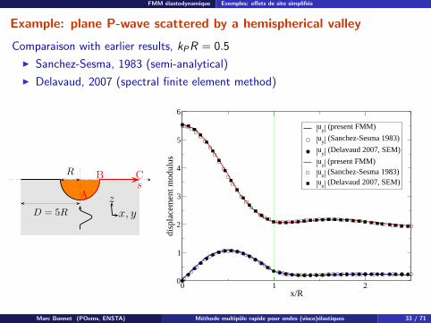
Example: plane P-wave scattered by a hemispherical valley
Comparaison with earlier results, kPR = 0.5
I Sanchez-Sesma, 1983 (semi-analytical)
I Delavaud, 2007 (spectral finite element method)
x, yz
R
D = 5R
A
B Cs
0 1 2x/R
0
1
2
3
4
5
6
disp
lace
men
t mod
ulus
|uy| (present FMM)
|uy| (Sanchez-Sesma 1983)
|uy| (Delavaud 2007, SEM)
|uz| (present FMM)
|uz| (Sanchez-Sesma 1983)
|uz| (Delavaud 2007, SEM)
Marc Bonnet (POems, ENSTA) Methode multipole rapide pour ondes (visco)elastiques 33 / 71
FMM elastodynamique Exemples: effets de site simplifies
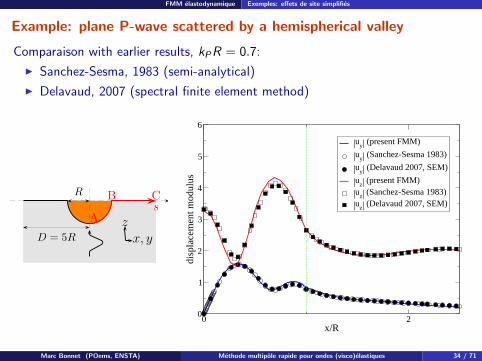
Example: plane P-wave scattered by a hemispherical valley
Comparaison with earlier results, kPR = 0.7:
I Sanchez-Sesma, 1983 (semi-analytical)
I Delavaud, 2007 (spectral finite element method)
x, yz
R
D = 5R
A
B Cs
0 2x/R
0
1
2
3
4
5
6
disp
lace
men
t mod
ulus
|uy| (present FMM)
|uy| (Sanchez-Sesma 1983)
|uy| (Delavaud 2007, SEM)
|uz| (present FMM)
|uz| (Sanchez-Sesma 1983)
|uz| (Delavaud 2007, SEM)
Marc Bonnet (POems, ENSTA) Methode multipole rapide pour ondes (visco)elastiques 34 / 71
FMM elastodynamique Exemples: effets de site simplifies
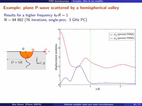
Example: plane P-wave scattered by a hemispherical valley
Results for a higher frequency kPR = 1N = 84 882 (76 iterations, single-proc. 3 GHz PC)
x, yz
R
D = 5R
A
B Cs
0 1 2x/R
0
1
2
3
4
5
6
disp
lace
men
t mod
ulus
|uy| (present FMM)
|uz| (present FMM)
Marc Bonnet (POems, ENSTA) Methode multipole rapide pour ondes (visco)elastiques 35 / 71
FMM elastodynamique Exemples: effets de site simplifies
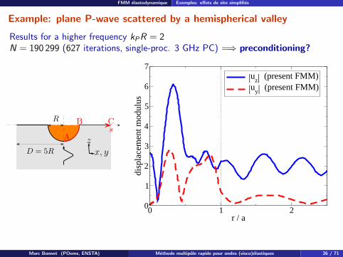
Example: plane P-wave scattered by a hemispherical valley
Results for a higher frequency kPR = 2N = 190 299 (627 iterations, single-proc. 3 GHz PC) =⇒ preconditioning?
x, yz
R
D = 5R
A
B Cs
0 1 2r / a
0
1
2
3
4
5
6
7
disp
lace
men
t mod
ulus
|uz| (present FMM)
|uy| (present FMM)
Marc Bonnet (POems, ENSTA) Methode multipole rapide pour ondes (visco)elastiques 36 / 71
FMM elastodynamique Exemples: effets de site simplifies
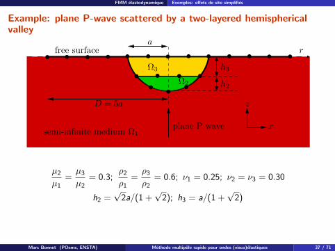
Example: plane P-wave scattered by a two-layered hemisphericalvalley
free surfacea
Ω3
Ω2
r
D = 5a
plane P wave
z
x
h3
h2
semi-infinite medium Ω1
µ2
µ1=µ3
µ2= 0.3;
ρ2
ρ1=ρ3
ρ2= 0.6; ν1 = 0.25; ν2 = ν3 = 0.30
h2 =√
2a/(1 +√
2); h3 = a/(1 +√
2)
Marc Bonnet (POems, ENSTA) Methode multipole rapide pour ondes (visco)elastiques 37 / 71
FMM elastodynamique Exemples: effets de site simplifies
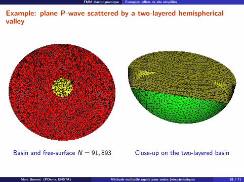
Example: plane P-wave scattered by a two-layered hemisphericalvalley
Basin and free-surface N = 91, 893 Close-up on the two-layered basin
Marc Bonnet (POems, ENSTA) Methode multipole rapide pour ondes (visco)elastiques 38 / 71
FMM elastodynamique Exemples: effets de site simplifies
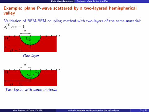
Example: plane P-wave scattered by a two-layered hemisphericalvalley
Validation of BEM-BEM coupling method with two-layers of the same material:
k(1)P a/π = 1
a
Ω2r
D = 5a
Ω1
One layer
a
Ω2
r
D = 5a
Ω1 Ω3
Two layers with same material
0 1 2r /a
0
1
2
3
4
5
6
disp
lace
men
t mod
ulus
|uz|, two layers same material
" , one layer|uy|, two layers same material
" , one layer
N = 91, 893 (240 iter., 48s / iter, single-proc. 3 GHz PC)
Marc Bonnet (POems, ENSTA) Methode multipole rapide pour ondes (visco)elastiques 39 / 71
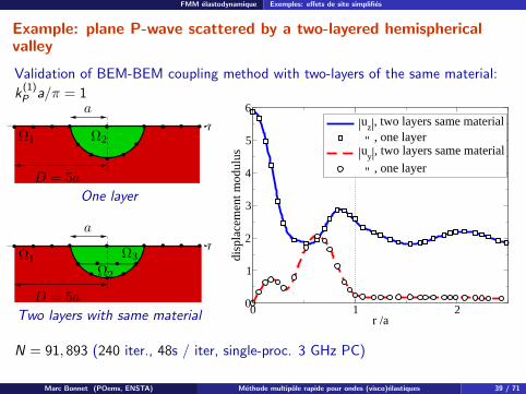
FMM elastodynamique Exemples: effets de site simplifies
Example: plane P-wave scattered by a two-layered hemisphericalvalley
Validation of BEM-BEM coupling method with two-layers of the same material:
k(1)P a/π = 1
a
Ω2r
D = 5a
Ω1
One layer
a
Ω2
r
D = 5a
Ω1 Ω3
Two layers with same material 0 1 2r /a
0
1
2
3
4
5
6
disp
lace
men
t mod
ulus
|uz|, two layers same material
" , one layer|uy|, two layers same material
" , one layer
N = 91, 893 (240 iter., 48s / iter, single-proc. 3 GHz PC)
Marc Bonnet (POems, ENSTA) Methode multipole rapide pour ondes (visco)elastiques 39 / 71
FMM elastodynamique Exemples: effets de site simplifies
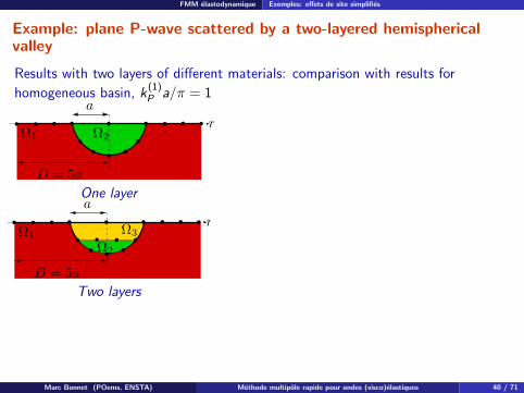
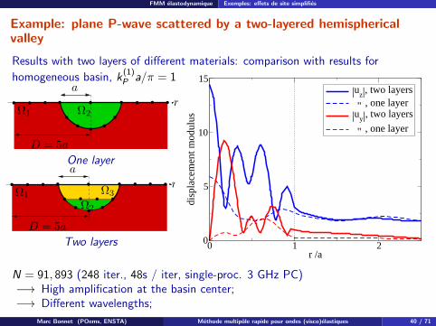
Example: plane P-wave scattered by a two-layered hemisphericalvalley
Results with two layers of different materials: comparison with results for
homogeneous basin, k(1)P a/π = 1
a
Ω2r
D = 5a
Ω1
One layera
Ω2
r
D = 5a
Ω1 Ω3
Two layers
0 1 2r /a
0
5
10
15
disp
lace
men
t mod
ulus
|uz|, two layers
" , one layer|uy|, two layers
" , one layer
N = 91, 893 (248 iter., 48s / iter, single-proc. 3 GHz PC)−→ High amplification at the basin center;−→ Different wavelengths;
Marc Bonnet (POems, ENSTA) Methode multipole rapide pour ondes (visco)elastiques 40 / 71
FMM elastodynamique Exemples: effets de site simplifies
Example: plane P-wave scattered by a two-layered hemisphericalvalley
Results with two layers of different materials: comparison with results for
homogeneous basin, k(1)P a/π = 1
a
Ω2r
D = 5a
Ω1
One layera
Ω2
r
D = 5a
Ω1 Ω3
Two layers 0 1 2r /a
0
5
10
15
disp
lace
men
t mod
ulus
|uz|, two layers
" , one layer|uy|, two layers
" , one layer
N = 91, 893 (248 iter., 48s / iter, single-proc. 3 GHz PC)−→ High amplification at the basin center;−→ Different wavelengths;
Marc Bonnet (POems, ENSTA) Methode multipole rapide pour ondes (visco)elastiques 40 / 71

FMM elastodynamique Exemples: effets de site simplifies
Time-domain results
Time-domain surface response: [ux ] [ux (truncated)]
Chaillat S., Bonnet M., Semblat J.F., Geophys. J. Int., 2009Marc Bonnet (POems, ENSTA) Methode multipole rapide pour ondes (visco)elastiques 41 / 71
FMM elastodynamique Exemples: effets de site simplifies
Preconditioning
A simple strategy implemented, based on flexible GMRES (preconditioner:low-accuracy GMRES for near-interaction matrix).
Example: Diffraction of plane P- or SV-wave by a semi-ellipsoidal basin (b = 2a)
Ω2
D = 8a
Dfree surface A B
C
a E
z
yθplane P– or SV–wave
infinite elastic half space Ω1
ν(1) = ν(2) = 1/3, µ(2) = 1/4µ(1), ρ(2) = ρ(1), θ = 0, 30
Computational data:
k(1)P a/π N ¯
1; ¯2 CPU time (s)
per iter.
1 278, 304 4; 3 111
1.5 685, 830 6; 5 199
Marc Bonnet (POems, ENSTA) Methode multipole rapide pour ondes (visco)elastiques 42 / 71
FMM elastodynamique Exemples: effets de site simplifies
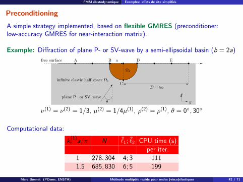
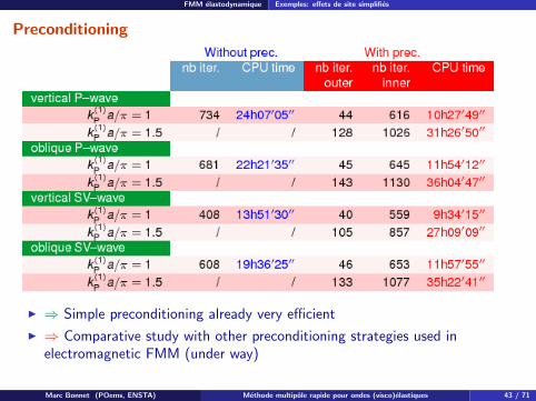
Preconditioning
I ⇒ Simple preconditioning already very efficient
I ⇒ Comparative study with other preconditioning strategies used inelectromagnetic FMM (under way)
Marc Bonnet (POems, ENSTA) Methode multipole rapide pour ondes (visco)elastiques 43 / 71
FMM elastodynamique Exemple: modelisation simplifiee de la vallee de Grenoble
1. Principes
2. FMM elastodynamiqueFormulation multi-niveau mono-domaineFormulation multi-niveau multi-domaineExemples: effets de site simplifiesExemple: modelisation simplifiee de la vallee de Grenoble
3. FMM viscoelastodynamique
4. Couplage FMM-FEM
5. Conclusions
Marc Bonnet (POems, ENSTA) Methode multipole rapide pour ondes (visco)elastiques 44 / 71
FMM elastodynamique Exemple: modelisation simplifiee de la vallee de Grenoble
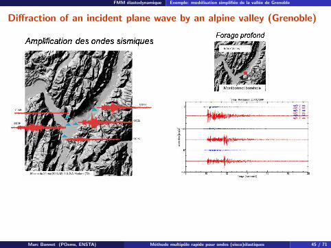
Diffraction of an incident plane wave by an alpine valley (Grenoble)
Marc Bonnet (POems, ENSTA) Methode multipole rapide pour ondes (visco)elastiques 45 / 71
FMM elastodynamique Exemple: modelisation simplifiee de la vallee de Grenoble
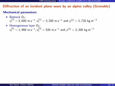
Diffraction of an incident plane wave by an alpine valley (Grenoble)
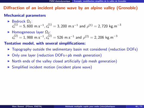
Mechanical parameters
I Bedrock Ω1:c
(1)P = 5, 600 m.s−1, c
(1)s = 3, 200 m.s−1 and ρ(1) = 2, 720 kg.m−3
I Homogeneous layer Ω2:
c(2)P = 1, 988 m.s−1, c
(2)s = 526 m.s−1 and ρ(2) = 2, 206 kg.m−3
Tentative model, with several simplifications:
I Topography outside the sedimentary basin not considered (reduction DOFs)
I Only one layer (reduction DOFs+pb mesh generation)
I North ends of the valley closed artificially (pb mesh generation)
I Simplified incident motion (incident plane wave)
Marc Bonnet (POems, ENSTA) Methode multipole rapide pour ondes (visco)elastiques 46 / 71
FMM elastodynamique Exemple: modelisation simplifiee de la vallee de Grenoble
Diffraction of an incident plane wave by an alpine valley (Grenoble)
λ(1)S
Marc Bonnet (POems, ENSTA) Methode multipole rapide pour ondes (visco)elastiques 47 / 71
FMM elastodynamique Exemple: modelisation simplifiee de la vallee de Grenoble
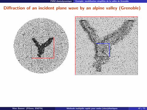
Diffraction of an incident plane wave by an alpine valley (Grenoble)
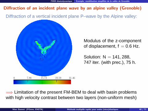
Diffraction of a vertical incident plane P–wave by the Alpine valley:
0 7.86 15.73 23.59 31.46
Modulus of the z-componentof displacement, f = 0.6 Hz.
Solution: N = 141, 288,747 iter. (with prec.), 75 h.
=⇒ Limitation of the present FM-BEM to deal with basin problemswith high velocity contrast between two layers (non-uniform mesh)
Marc Bonnet (POems, ENSTA) Methode multipole rapide pour ondes (visco)elastiques 48 / 71
FMM viscoelastodynamique
1. Principes
2. FMM elastodynamiqueFormulation multi-niveau mono-domaineFormulation multi-niveau multi-domaineExemples: effets de site simplifiesExemple: modelisation simplifiee de la vallee de Grenoble
3. FMM viscoelastodynamiqueEvaluation de la fonction de transfert pour k complexeValidation (exemple mono-domaine)Formulation multi-niveau multi-domaineExemple: effet de site simplifie
4. Couplage FMM-FEM
5. Conclusions
Marc Bonnet (POems, ENSTA) Methode multipole rapide pour ondes (visco)elastiques 49 / 71
FMM viscoelastodynamique
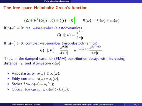
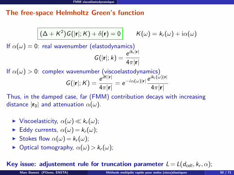
The free-space Helmholtz Green’s function
(∆ + K 2)G (|r|;K ) + δ(r) = 0 K (ω) = kr (ω) + iα(ω)
If α(ω) = 0: real wavenumber (elastodynamics)
G (|r|; k) =e ikr |r|
4π|r|If α(ω) > 0: complex wavenumber (viscoelastodynamics)
G (|r|;K ) =e iK |r|
4π|r| = e−iα(ω)|r| eikr (ω)|r|
4π|r|Thus, in the damped case, far (FMM) contribution decays with increasingdistance |r0| and attenuation α(ω).
I Viscoelasticity, α(ω) kr (ω);I Eddy currents, α(ω) = kr (ω);I Stokes flow α(ω) = kr (ω);I Optical tomography, α(ω)> kr (ω);
Key issue: adjustement rule for truncation parameter L= L(dcell, kr , α);
Marc Bonnet (POems, ENSTA) Methode multipole rapide pour ondes (visco)elastiques 50 / 71
FMM viscoelastodynamique
The free-space Helmholtz Green’s function
(∆ + K 2)G (|r|;K ) + δ(r) = 0 K (ω) = kr (ω) + iα(ω)
If α(ω) = 0: real wavenumber (elastodynamics)
G (|r|; k) =e ikr |r|
4π|r|If α(ω) > 0: complex wavenumber (viscoelastodynamics)
G (|r|;K ) =e iK |r|
4π|r| = e−iα(ω)|r| eikr (ω)|r|
4π|r|Thus, in the damped case, far (FMM) contribution decays with increasingdistance |r0| and attenuation α(ω).
I Viscoelasticity, α(ω) kr (ω);I Eddy currents, α(ω) = kr (ω);I Stokes flow α(ω) = kr (ω);I Optical tomography, α(ω)> kr (ω);
Key issue: adjustement rule for truncation parameter L= L(dcell, kr , α);Marc Bonnet (POems, ENSTA) Methode multipole rapide pour ondes (visco)elastiques 50 / 71
FMM viscoelastodynamique
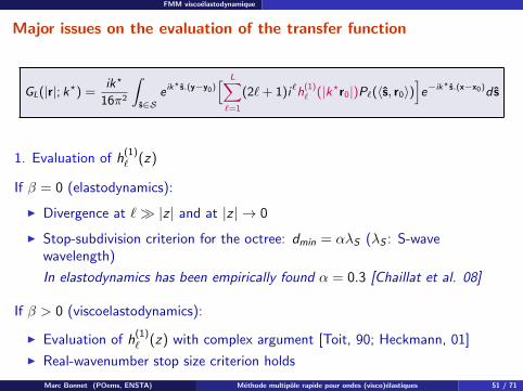
Major issues on the evaluation of the transfer function
GL(|r|; k?) =ik?
16π2
∫s∈S
e ik? s.(y−y0)
[ L∑`=1
(2`+ 1)i`h(1)` (|k?r0|)P`(〈s, r0〉)
]e−ik? s.(x−x0)d s
1. Evaluation of h(1)` (z)
If β = 0 (elastodynamics):
I Divergence at ` |z | and at |z | → 0
I Stop-subdivision criterion for the octree: dmin = αλS (λS : S-wavewavelength)
In elastodynamics has been empirically found α = 0.3 [Chaillat et al. 08]
If β > 0 (viscoelastodynamics):
I Evaluation of h(1)` (z) with complex argument [Toit, 90; Heckmann, 01]
I Real-wavenumber stop size criterion holds
Marc Bonnet (POems, ENSTA) Methode multipole rapide pour ondes (visco)elastiques 51 / 71
FMM viscoelastodynamique
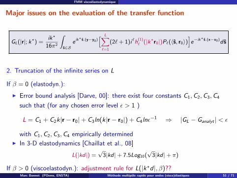
Major issues on the evaluation of the transfer function
GL(|r|; k?) =ik?
16π2
∫s∈S
e ik? s.(y−y0)
[ L∑`=1
(2`+ 1)i`h(1)` (|k?r0|)P`(〈s, r0〉)
]e−ik? s.(x−x0)d s
2. Truncation of the infinite series on L
If β = 0 (elastodyn.):
I Error bound analysis [Darve, 00]: there exist four constants C1,C2,C3,C4
such that (for any chosen error level ε > 1 )
L = C1 + C2k |r − r0|+ C3ln(k |r − r0|) + C4lnε−1 ⇒ |GL − Ganalyt | < ε
with C1,C2,C3,C4 empirically determined
I In 3-D elastodynamics [Chaillat et al., 08]
L(|kd |) =√
3|kd |+ 7.5Log10(√
3|kd |+ π)
If β > 0 (viscoelastodyn.): adjustment rule for L(|k?d |, β)??Marc Bonnet (POems, ENSTA) Methode multipole rapide pour ondes (visco)elastiques 51 / 71
FMM viscoelastodynamique Evaluation de la fonction de transfert pour k complexe
1. Principes
2. FMM elastodynamique
3. FMM viscoelastodynamiqueEvaluation de la fonction de transfert pour k complexeValidation (exemple mono-domaine)Formulation multi-niveau multi-domaineExemple: effet de site simplifie
4. Couplage FMM-FEM
5. Conclusions
Marc Bonnet (POems, ENSTA) Methode multipole rapide pour ondes (visco)elastiques 52 / 71
FMM viscoelastodynamique Evaluation de la fonction de transfert pour k complexe
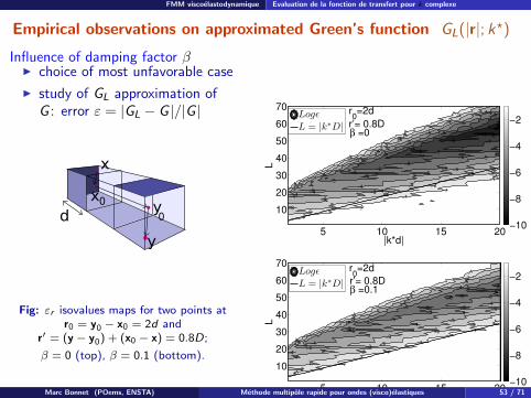
Empirical observations on approximated Green’s function GL(|r|; k?)
Influence of damping factor βI choice of most unfavorable case
I study of GL approximation ofG : error ε = |GL − G |/|G |
d
x
xy
y
0
0
Fig: εr isovalues maps for two points atr0 = y0 − x0 = 2d and
r′ = (y − y0) + (x0 − x) = 0.8D;
β = 0 (top), β = 0.1 (bottom).
−9−8
−8−8
−7
−7
−7−7
−7
−7
−6
−6
−6
−6−6
−6
−5
−5
−5
−5−5
−5−5
−5
−4
−4
−4
−4
−4 −4−4
−4
−4
−4−4
−3
−3
−3
−3
−3
−3−3
−3
−3
−2
−2
−2
−2
−1
−1
−1
−1
−2
−2
−2
−2
−2
−1
−1
−1
−1
−1−6−6 −2
−8 −6
−5
−1
−5
|k*d|
L
r0=2d
r’= 0.8Dβ =0
5 10 15 20
10
20
30
40
50
60
70
−10
−8
−6
−4
−2LogǫL = |k∗D|
−6−6
−5
−5
−5
−5−5
−5
−4
−4
−4
−4
−4−4
−4
−4
−4−3
−3−3
−3
−3
−3
−3
−3
−3
−3
−3
−2
−2
−2
−2
−2
−2
−2
−2
−2
−2
−1
−1
−1
−1
−1
−1
−1
−1
−1
−1
−4−4
−5
−4
−5−5
−5−6 −6
−6
−7
|k*d|
L
r0=2d
r’= 0.8Dβ =0.1
5 10 15 20
10
20
30
40
50
60
70
−10
−8
−6
−4
−2LogǫL = |k∗D|
Marc Bonnet (POems, ENSTA) Methode multipole rapide pour ondes (visco)elastiques 53 / 71
FMM viscoelastodynamique Evaluation de la fonction de transfert pour k complexe
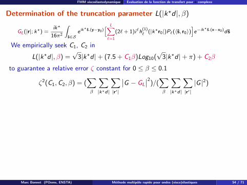
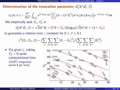
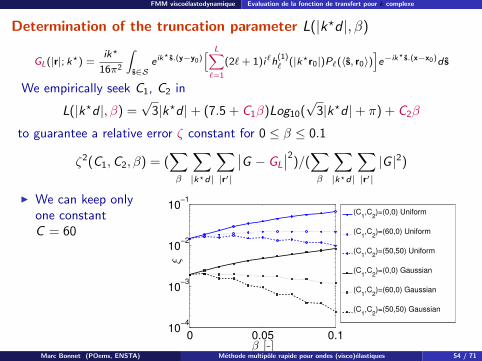
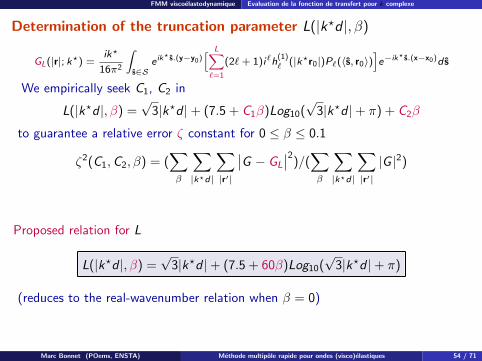
Determination of the truncation parameter L(|k?d |, β)
GL(|r|; k?) =ik?
16π2
∫s∈S
e ik? s.(y−y0)
[ L∑`=1
(2`+ 1)i`h(1)` (|k?r0|)P`(〈s, r0〉)
]e−ik? s.(x−x0)d s
We empirically seek C1, C2 in
L(|k?d |, β) =√
3|k?d |+ (7.5 + C1β)Log10(√
3|k?d |+ π) + C2β
to guarantee a relative error ζ constant for 0 ≤ β ≤ 0.1
ζ2(C1,C2, β) = (∑β
∑|k?d|
∑|r′|
∣∣G − GL
∣∣2)/(∑β
∑|k?d|
∑|r′||G |2)
Marc Bonnet (POems, ENSTA) Methode multipole rapide pour ondes (visco)elastiques 54 / 71
FMM viscoelastodynamique Evaluation de la fonction de transfert pour k complexe
Determination of the truncation parameter L(|k?d |, β)
GL(|r|; k?) =ik?
16π2
∫s∈S
e ik? s.(y−y0)
[ L∑`=1
(2`+ 1)i`h(1)` (|k?r0|)P`(〈s, r0〉)
]e−ik? s.(x−x0)d s
We empirically seek C1, C2 in
L(|k?d |, β) =√
3|k?d |+ (7.5 + C1β)Log10(√
3|k?d |+ π) + C2β
to guarantee a relative error ζ constant for 0 ≤ β ≤ 0.1
ζ2(C1,C2, β) = (∑β
∑|k?d|
∑|r′|
∣∣G − GL
∣∣2)/(∑β
∑|k?d|
∑|r′||G |2)
I For given ζ, takingC2 = 0 savescomputational time(O(N2) integrationpoints s per level)
0.00180.002
0.0
02
0.0
02
0.0
022
0.0022
0.0022
0.0
022
0.0022
0.0
024
0.0
024
0.0024
0.0024
0.0
026
0.0026
0.0026
0.0028
0.0028
0.0
03
0.0030.00320.00340.003620
21
21
21
22
22
22
22
23
23
23
24
24
C1
C2
10 20 30 40 50
10
20
30
40
50 ζ
L
Marc Bonnet (POems, ENSTA) Methode multipole rapide pour ondes (visco)elastiques 54 / 71
FMM viscoelastodynamique Evaluation de la fonction de transfert pour k complexe
Determination of the truncation parameter L(|k?d |, β)
GL(|r|; k?) =ik?
16π2
∫s∈S
e ik? s.(y−y0)
[ L∑`=1
(2`+ 1)i`h(1)` (|k?r0|)P`(〈s, r0〉)
]e−ik? s.(x−x0)d s
We empirically seek C1, C2 in
L(|k?d |, β) =√
3|k?d |+ (7.5 + C1β)Log10(√
3|k?d |+ π) + C2β
to guarantee a relative error ζ constant for 0 ≤ β ≤ 0.1
ζ2(C1,C2, β) = (∑β
∑|k?d|
∑|r′|
∣∣G − GL
∣∣2)/(∑β
∑|k?d|
∑|r′||G |2)
I We can keep onlyone constantC = 60
0 0.05 0.110
−4
10−3
10−2
10−1
β [-]
ξ
(C1,C
2)=(0,0) Uniform
(C1,C
2)=(60,0) Uniform
(C1,C
2)=(50,50) Uniform
(C1,C
2)=(0,0) Gaussian
(C1,C
2)=(60,0) Gaussian
(C1,C
2)=(50,50) Gaussian
Marc Bonnet (POems, ENSTA) Methode multipole rapide pour ondes (visco)elastiques 54 / 71
FMM viscoelastodynamique Evaluation de la fonction de transfert pour k complexe
Determination of the truncation parameter L(|k?d |, β)
GL(|r|; k?) =ik?
16π2
∫s∈S
e ik? s.(y−y0)
[ L∑`=1
(2`+ 1)i`h(1)` (|k?r0|)P`(〈s, r0〉)
]e−ik? s.(x−x0)d s
We empirically seek C1, C2 in
L(|k?d |, β) =√
3|k?d |+ (7.5 + C1β)Log10(√
3|k?d |+ π) + C2β
to guarantee a relative error ζ constant for 0 ≤ β ≤ 0.1
ζ2(C1,C2, β) = (∑β
∑|k?d|
∑|r′|
∣∣G − GL
∣∣2)/(∑β
∑|k?d|
∑|r′||G |2)
Proposed relation for L
L(|k?d |, β) =√
3|k?d |+ (7.5 + 60β)Log10(√
3|k?d |+ π)
(reduces to the real-wavenumber relation when β = 0)
Marc Bonnet (POems, ENSTA) Methode multipole rapide pour ondes (visco)elastiques 54 / 71
FMM viscoelastodynamique Validation (exemple mono-domaine)
1. Principes
2. FMM elastodynamique
3. FMM viscoelastodynamiqueEvaluation de la fonction de transfert pour k complexeValidation (exemple mono-domaine)Formulation multi-niveau multi-domaineExemple: effet de site simplifie
4. Couplage FMM-FEM
5. Conclusions
Marc Bonnet (POems, ENSTA) Methode multipole rapide pour ondes (visco)elastiques 55 / 71
FMM viscoelastodynamique Validation (exemple mono-domaine)
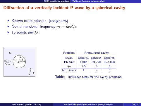
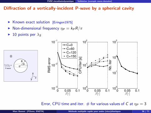
Diffraction of a vertically-incident P-wave by a spherical cavity
I Known exact solution [Eringen1975]
I Non-dimensional frequency ηP = kPR/π
I 10 points per λS
R
Ω
P-wave
x
zy
oθ
Problem Pressurized cavity
Mesh sphere3 sphere4 sphere5
Pb size 7 686 30 726 122 886
ηP 1.5 3 6
Nb. levels 4 5 6
Table: Reference tests for the cavity problems.
Marc Bonnet (POems, ENSTA) Methode multipole rapide pour ondes (visco)elastiques 56 / 71
FMM viscoelastodynamique Validation (exemple mono-domaine)
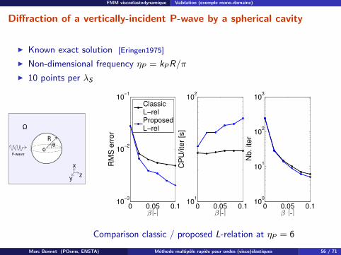
Diffraction of a vertically-incident P-wave by a spherical cavity
I Known exact solution [Eringen1975]
I Non-dimensional frequency ηP = kPR/π
I 10 points per λS
R
Ω
P-wave
x
zy
oθ
0 0.05 0.110
−3
10−2
10−1
β[-]
RM
S e
rror
C=0C=60C=120C=150
0 0.05 0.110
0
101
102
β[-]
CP
U/ite
r [s
]
0 0.05 0.110
0
101
102
103
β[-]
Nb. iter
Error, CPU time and iter. # for various values of C at ηP = 3
Marc Bonnet (POems, ENSTA) Methode multipole rapide pour ondes (visco)elastiques 56 / 71
FMM viscoelastodynamique Validation (exemple mono-domaine)
Diffraction of a vertically-incident P-wave by a spherical cavity
I Known exact solution [Eringen1975]
I Non-dimensional frequency ηP = kPR/π
I 10 points per λS
R
Ω
P-wave
x
zy
oθ
0 0.05 0.110
−3
10−2
10−1
β[-]
RM
S e
rror
ClassicL−relProposedL−rel
0 0.05 0.110
1
102
β[-]
CP
U/ite
r [s
]
0 0.05 0.110
0
101
102
103
β [-]
Nb. iter
Comparison classic / proposed L-relation at ηP = 6
Marc Bonnet (POems, ENSTA) Methode multipole rapide pour ondes (visco)elastiques 56 / 71
FMM viscoelastodynamique Validation (exemple mono-domaine)
Diffraction of a vertically-incident P-wave by a spherical cavity
1 1.5 2 2.5 3−1.5
−1
−0.5
0
0.5
1
r/R
rad
ial d
isp
l.
θ = 0
1 1.5 2 2.5 3
−0.5
0
0.5
r/R
rad
ial d
isp
l.
θ = π/4
R
Ω
P-wave
oθ
(a)(b)
(c)
(d)(e)
x
zy
1 1.5 2 2.5 3−0.4
−0.3
−0.2
−0.1
0
0.1
0.2
r/R
rad
ial d
isp
l.
θ = π/2
1 1.5 2 2.5 3−8
−6
−4
−2
0
2
4
6
r/R
rad
ial d
isp
l.
θ = π
1 1.5 2 2.5 3−2
−1
0
1
2
r/R
rad
ial d
isp
l.θ = 3/4π
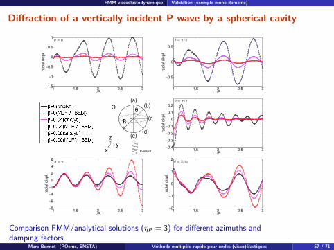
Comparison FMM/analytical solutions (ηP = 3) for different azimuths anddamping factors
Marc Bonnet (POems, ENSTA) Methode multipole rapide pour ondes (visco)elastiques 57 / 71
FMM viscoelastodynamique Formulation multi-niveau multi-domaine
1. Principes
2. FMM elastodynamique
3. FMM viscoelastodynamiqueEvaluation de la fonction de transfert pour k complexeValidation (exemple mono-domaine)Formulation multi-niveau multi-domaineExemple: effet de site simplifie
4. Couplage FMM-FEM
5. Conclusions
Marc Bonnet (POems, ENSTA) Methode multipole rapide pour ondes (visco)elastiques 58 / 71

FMM viscoelastodynamique Formulation multi-niveau multi-domaine
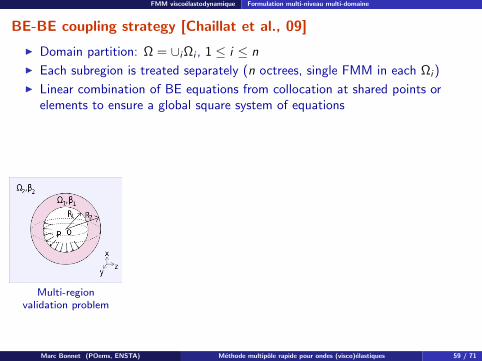
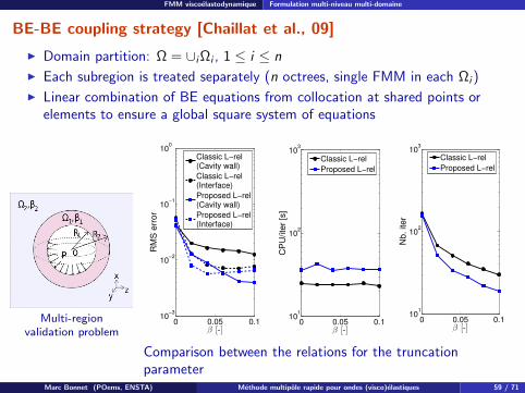
BE-BE coupling strategy [Chaillat et al., 09]
I Domain partition: Ω = ∪iΩi , 1 ≤ i ≤ n
I Each subregion is treated separately (n octrees, single FMM in each Ωi )
I Linear combination of BE equations from collocation at shared points orelements to ensure a global square system of equations
Multi-regionvalidation problem
0 0.05 0.110
−3
10−2
10−1
100
β [-]
RM
S e
rro
r
Classic L−rel(Cavity wall)
Classic L−rel(Interface)
Proposed L−rel(Cavity wall)
Proposed L−rel(Interface)
0 0.05 0.110
1
102
103
β [-]
CP
U/ite
r [s
]
Classic L−rel
Proposed L−rel
0 0.05 0.110
1
102
103
β [-]
Nb
. ite
r
Classic L−rel
Proposed L−rel
Comparison between the relations for the truncationparameter
Marc Bonnet (POems, ENSTA) Methode multipole rapide pour ondes (visco)elastiques 59 / 71
FMM viscoelastodynamique Formulation multi-niveau multi-domaine
BE-BE coupling strategy [Chaillat et al., 09]
I Domain partition: Ω = ∪iΩi , 1 ≤ i ≤ n
I Each subregion is treated separately (n octrees, single FMM in each Ωi )
I Linear combination of BE equations from collocation at shared points orelements to ensure a global square system of equations
Multi-regionvalidation problem
0 0.05 0.110
−3
10−2
10−1
100
β [-]
RM
S e
rro
r
Classic L−rel(Cavity wall)
Classic L−rel(Interface)
Proposed L−rel(Cavity wall)
Proposed L−rel(Interface)
0 0.05 0.110
1
102
103
β [-]
CP
U/ite
r [s
]
Classic L−rel
Proposed L−rel
0 0.05 0.110
1
102
103
β [-]
Nb
. ite
r
Classic L−rel
Proposed L−rel
Comparison between the relations for the truncationparameter
Marc Bonnet (POems, ENSTA) Methode multipole rapide pour ondes (visco)elastiques 59 / 71
FMM viscoelastodynamique Exemple: effet de site simplifie
1. Principes
2. FMM elastodynamique
3. FMM viscoelastodynamiqueEvaluation de la fonction de transfert pour k complexeValidation (exemple mono-domaine)Formulation multi-niveau multi-domaineExemple: effet de site simplifie
4. Couplage FMM-FEM
5. Conclusions
Marc Bonnet (POems, ENSTA) Methode multipole rapide pour ondes (visco)elastiques 60 / 71
FMM viscoelastodynamique Exemple: effet de site simplifie
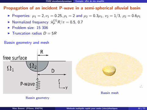
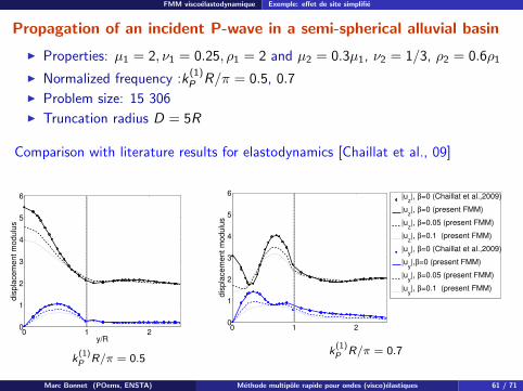
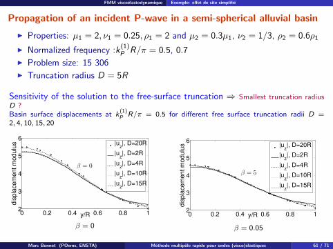
Propagation of an incident P-wave in a semi-spherical alluvial basin
I Properties: µ1 = 2, ν1 = 0.25, ρ1 = 2 and µ2 = 0.3µ1, ν2 = 1/3, ρ2 = 0.6ρ1
I Normalized frequency :k(1)P R/π = 0.5, 0.7
I Problem size: 15 306
I Truncation radius D = 5R
Bassin geometry and mesh
P-wavez
y
o
Bassin geometry
X Y
Z
Bassin mesh
Marc Bonnet (POems, ENSTA) Methode multipole rapide pour ondes (visco)elastiques 61 / 71
FMM viscoelastodynamique Exemple: effet de site simplifie
Propagation of an incident P-wave in a semi-spherical alluvial basin
I Properties: µ1 = 2, ν1 = 0.25, ρ1 = 2 and µ2 = 0.3µ1, ν2 = 1/3, ρ2 = 0.6ρ1
I Normalized frequency :k(1)P R/π = 0.5, 0.7
I Problem size: 15 306
I Truncation radius D = 5R
Comparison with literature results for elastodynamics [Chaillat et al., 09]
0 1 20
1
2
3
4
5
6
y/R
dis
pla
ce
me
nt
mo
du
lus
k(1)P R/π = 0.5
0 1 20
1
2
3
4
5
6
dis
pla
cem
ent m
odulu
s
|uz|, β=0 (Chaillat et al.,2009)
|uz|, β=0 (present FMM)
|uz|, β=0.05 (present FMM)
|uz|, β=0.1 (present FMM)
|uy|, β=0 (Chaillat et al.,2009)
|uy|,β=0 (present FMM)
|uy|, β=0.05 (present FMM)
|uy|, β=0.1 (present FMM)
k(1)P R/π = 0.7
Marc Bonnet (POems, ENSTA) Methode multipole rapide pour ondes (visco)elastiques 61 / 71
FMM viscoelastodynamique Exemple: effet de site simplifie
Propagation of an incident P-wave in a semi-spherical alluvial basin
I Properties: µ1 = 2, ν1 = 0.25, ρ1 = 2 and µ2 = 0.3µ1, ν2 = 1/3, ρ2 = 0.6ρ1
I Normalized frequency :k(1)P R/π = 0.5, 0.7
I Problem size: 15 306
I Truncation radius D = 5R
Sensitivity of the solution to the free-surface truncation ⇒ Smallest truncation radiusD ?Basin surface displacements at k
(1)P R/π = 0.5 for different free surface truncation radii D =
2, 4, 10, 15, 20
0 0.2 0.4 0.6 0.8 12
3
4
5
6
y/R
dis
pla
cem
ent m
odulu
s
β = 0
|uz|, D=20R
|uz|, D=2R
|uz|, D=4R
|uz|, D=10R
|uz|, D=15R
β = 0
0 0.2 0.4 0.6 0.8 12
3
4
5
6
y/R
dis
pla
cem
ent m
odulu
s
β = 5
|uz|, D=20R
|uz|, D=2R
|uz|, D=4R
|uz|, D=10R
|uz|, D=15R
β = 0.05
The sensitivity to the surface truncation is reduced by increasing dampingMarc Bonnet (POems, ENSTA) Methode multipole rapide pour ondes (visco)elastiques 61 / 71
Couplage FMM-FEM
1. Principes
2. FMM elastodynamiqueFormulation multi-niveau mono-domaineFormulation multi-niveau multi-domaineExemples: effets de site simplifiesExemple: modelisation simplifiee de la vallee de Grenoble
3. FMM viscoelastodynamiqueEvaluation de la fonction de transfert pour k complexeValidation (exemple mono-domaine)Formulation multi-niveau multi-domaineExemple: effet de site simplifie
4. Couplage FMM-FEM
5. Conclusions
Marc Bonnet (POems, ENSTA) Methode multipole rapide pour ondes (visco)elastiques 62 / 71
Couplage FMM-FEM
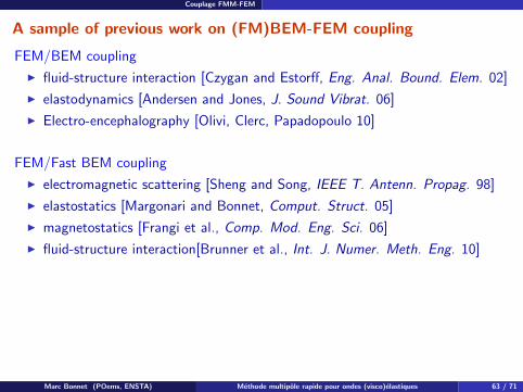
A sample of previous work on (FM)BEM-FEM coupling
FEM/BEM coupling
I fluid-structure interaction [Czygan and Estorff, Eng. Anal. Bound. Elem. 02]
I elastodynamics [Andersen and Jones, J. Sound Vibrat. 06]
I Electro-encephalography [Olivi, Clerc, Papadopoulo 10]
FEM/Fast BEM coupling
I electromagnetic scattering [Sheng and Song, IEEE T. Antenn. Propag. 98]
I elastostatics [Margonari and Bonnet, Comput. Struct. 05]
I magnetostatics [Frangi et al., Comp. Mod. Eng. Sci. 06]
I fluid-structure interaction[Brunner et al., Int. J. Numer. Meth. Eng. 10]
Marc Bonnet (POems, ENSTA) Methode multipole rapide pour ondes (visco)elastiques 63 / 71
Couplage FMM-FEM
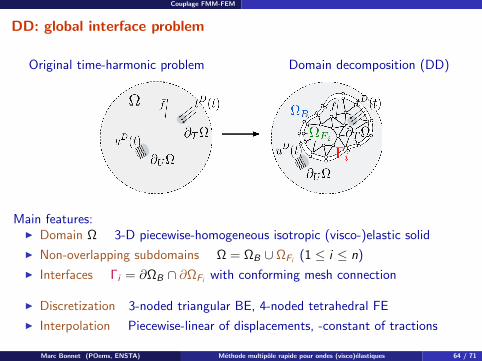
DD: global interface problem
Original time-harmonic problem Domain decomposition (DD)
Main features:I Domain Ω 3-D piecewise-homogeneous isotropic (visco-)elastic solid
I Non-overlapping subdomains Ω = ΩB ∪ ΩFi (1 ≤ i ≤ n)
I Interfaces Γi = ∂ΩB ∩ ∂ΩFi with conforming mesh connection
I Discretization 3-noded triangular BE, 4-noded tetrahedral FE
I Interpolation Piecewise-linear of displacements, -constant of tractions
Marc Bonnet (POems, ENSTA) Methode multipole rapide pour ondes (visco)elastiques 64 / 71
Couplage FMM-FEM
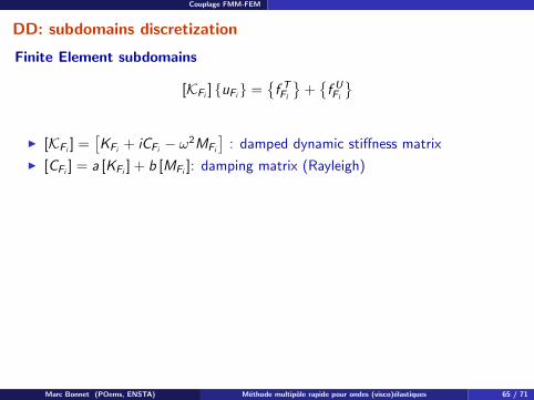
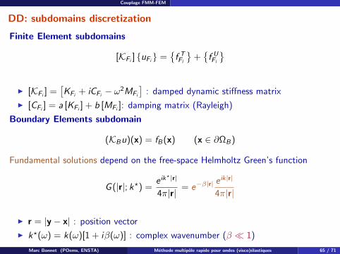
DD: subdomains discretization
Finite Element subdomains
[KFi ] uFi =f TFi
+f UFi
I [KFi ] =
[KFi + iCFi − ω2MFi
]: damped dynamic stiffness matrix
I [CFi ] = a [KFi ] + b [MFi ]: damping matrix (Rayleigh)
Boundary Elements subdomain
(KBu)(x) = fB(x) (x ∈ ∂ΩB)
Fundamental solutions depend on the free-space Helmholtz Green’s function
G (|r|; k?) =e ik
?|r|
4π|r| = e−β|r|e ik|r|
4π|r|
I r = |y − x| : position vector
I k?(ω) = k(ω)[1 + iβ(ω)] : complex wavenumber (β 1)
Marc Bonnet (POems, ENSTA) Methode multipole rapide pour ondes (visco)elastiques 65 / 71
Couplage FMM-FEM
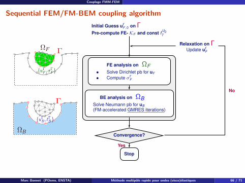
Sequential FEM/FM-BEM coupling algorithm
Initial Guess uΓF,0 on Γ
Pre-compute FE- KF and const fU0T
Relaxation on ΓUpdate uΓ
F
FE analysis on ΩF
• Solve Dirichlet pb for uF
• Compute σΓF
BE analysis on ΩB
Solve Neumann pb for uB
(FM-accelerated GMRES iterations)
Convergence?
Stop
Yes
No
Marc Bonnet (POems, ENSTA) Methode multipole rapide pour ondes (visco)elastiques 66 / 71
Couplage FMM-FEM
Interface Relaxation
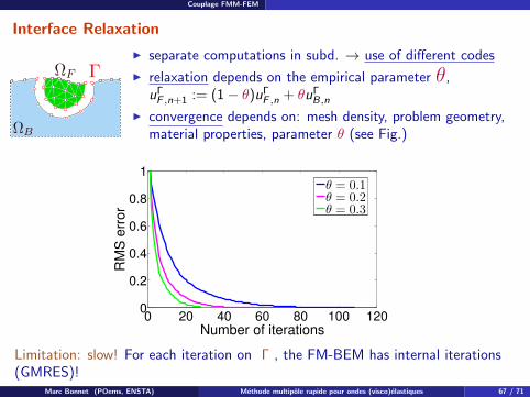
I separate computations in subd. → use of different codes
I relaxation depends on the empirical parameter θ,uΓF ,n+1 := (1− θ)uΓ
F ,n + θuΓB,n
I convergence depends on: mesh density, problem geometry,material properties, parameter θ (see Fig.)
0 20 40 60 80 100 1200
0.2
0.4
0.6
0.8
1
Number of iterations
RM
S e
rro
r
θ = 0.1θ = 0.2θ = 0.3
Limitation: slow! For each iteration on Γ , the FM-BEM has internal iterations(GMRES)!
Marc Bonnet (POems, ENSTA) Methode multipole rapide pour ondes (visco)elastiques 67 / 71
Couplage FMM-FEM
Vibration isolation using trenches
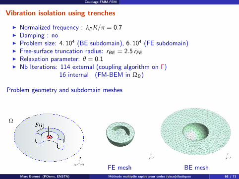
I Normalized frequency : kPR/π = 0.7I Damping : noI Problem size: 4. 104 (BE subdomain), 6. 104 (FE subdomain)I Free-surface truncation radius: rBE = 2.5 rFEI Relaxation parameter: θ = 0.1I Nb Iterations: 114 external (coupling algorithm on Γ)
16 internal (FM-BEM in ΩB)
Problem geometry and subdomain meshes
x
z
y
XY
Z
FE mesh
XY
Z
BE meshMarc Bonnet (POems, ENSTA) Methode multipole rapide pour ondes (visco)elastiques 68 / 71
Couplage FMM-FEM
Vibration isolation using trenches
I Normalized frequency : kPR/π = 0.7I Damping : noI Problem size: 4. 104 (BE subdomain), 6. 104 (FE subdomain)I Free-surface truncation radius: rBE = 2.5 rFEI Relaxation parameter: θ = 0.1I Nb Iterations: 114 external (coupling algorithm on Γ)
16 internal (FM-BEM in ΩB)
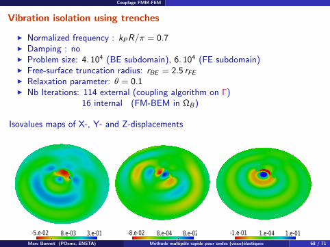
Isovalues maps of X-, Y- and Z-displacements
-5.e-02
-9.e-03
8.e-03
4.e-02
3.e-01 -8.e-02
-2.e-02
8.e-04
2.e-02
8.e-02 -1.e-01
-4.e-02
1.e-04
4.e-02
1.e-01
Marc Bonnet (POems, ENSTA) Methode multipole rapide pour ondes (visco)elastiques 68 / 71
Couplage FMM-FEM
Vibration isolation using trenches
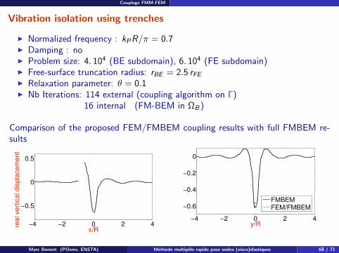
I Normalized frequency : kPR/π = 0.7I Damping : noI Problem size: 4. 104 (BE subdomain), 6. 104 (FE subdomain)I Free-surface truncation radius: rBE = 2.5 rFEI Relaxation parameter: θ = 0.1I Nb Iterations: 114 external (coupling algorithm on Γ)
16 internal (FM-BEM in ΩB)
Comparison of the proposed FEM/FMBEM coupling results with full FMBEM re-sults
−4 −2 0 2 4
−0.5
0
0.5
x/R
rea
l ve
rtic
al d
isp
lace
me
nt
−4 −2 0 2 4
−0.6
−0.4
−0.2
0
y/R
FMBEMFEM/FMBEM
Marc Bonnet (POems, ENSTA) Methode multipole rapide pour ondes (visco)elastiques 68 / 71
Conclusions
1. Principes
2. FMM elastodynamiqueFormulation multi-niveau mono-domaineFormulation multi-niveau multi-domaineExemples: effets de site simplifiesExemple: modelisation simplifiee de la vallee de Grenoble
3. FMM viscoelastodynamiqueEvaluation de la fonction de transfert pour k complexeValidation (exemple mono-domaine)Formulation multi-niveau multi-domaineExemple: effet de site simplifie
4. Couplage FMM-FEM
5. Conclusions
Marc Bonnet (POems, ENSTA) Methode multipole rapide pour ondes (visco)elastiques 69 / 71
Conclusions
Conclusions
I FMM successfully extended to 3-D frequency-domain elastodynamics
I Implementation tested on exact and published solutions
I Implementation consistent with theoretical complexity
I BE models of size N = O(106) on a single-processor PC
I Simplified topographical site effect studied
I Multi-region formulation implemented, tested against published results, andrun for higher frequencies.
I Preconditioning: simple strategy successfully implemented, others understudy (e.g. SPAI)
I Multipole expansions for homogeneous and layered elastodynamic half-spaceGreen’s tensors (under progress)
I Preliminary seismological applications (framework of QSHA French project)
I Damping (complex-valued wavenumbers): thesis E. Grasso (2008-2012)
I FMBEM-FEM coupling: under progress, thesis E. Grasso (2008-2012)
Marc Bonnet (POems, ENSTA) Methode multipole rapide pour ondes (visco)elastiques 70 / 71

Conclusions
Outlook
I Complex wavenumbers:I Investigate preconditioningI Empirical rules for low-frequency multipole expansion (Frangi, Bonnet 2010)I Extend theoretical error analysis (of. e.g. Darve) to k ∈C
I Multipole formulation for half-space Green’s tensorI Separation of variables permitted by Fourier transform in planes parallel to free
surface (Chaillat 2008)I Requires quadrature rule suitable for fast evaluation (e.g. SVD-based, Rokhlin,
Yarvin 1997); under progress
I FEM-BEM couplingI Symmetric Galerkin FM-BEM ?I Non-conforming interfacesI Reduce computational effort through geometrically-symmetric FEM-BEM
interfaces
I FMM as auxiliary for enhancing FEM:I Enrichment bases associated with small defects (see Brancherie, Dambrine
2009) or 3-D interaction integral of LEFMI Evaluate pointwise residual for (nonlinear) FEM analysis in O(N) CPU time
Marc Bonnet (POems, ENSTA) Methode multipole rapide pour ondes (visco)elastiques 71 / 71