Embed Size (px)
Citation preview
MGM657 Outils Numériques pour l’IngénieurTraitement de signal
www.polytech.univ-savoie.fr
1 Introduction
2 Notations
3 Échantillonnage
4 Analyse fréquentielle
MGM657 Outils Numériques pour l’IngénieurIntroduction
Plan
1 Introduction
2 Notations
3 Échantillonnage
4 Analyse fréquentielle
Outils numériques pour l’ingénieur 2/71
MGM657 Outils Numériques pour l’IngénieurIntroduction
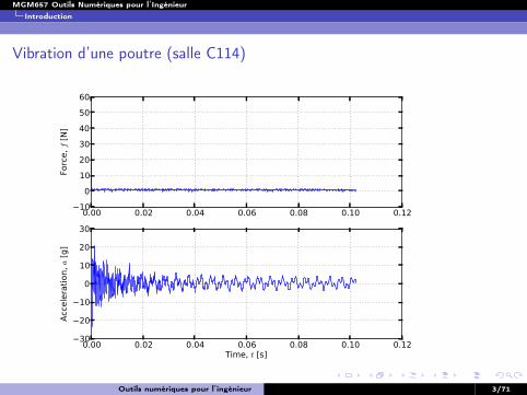
Vibration d’une poutre (salle C114)
0.00 0.02 0.04 0.06 0.08 0.10 0.12100
102030405060
Forc
e, f
[N]
0.00 0.02 0.04 0.06 0.08 0.10 0.12Time, t [s]
30
20
10
0
10
20
30
Acce
lera
tion,
a [g
]
Outils numériques pour l’ingénieur 3/71
MGM657 Outils Numériques pour l’IngénieurIntroduction
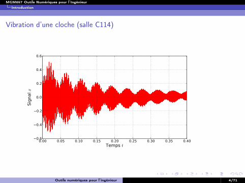
Vibration d’une cloche (salle C114)
0.00 0.05 0.10 0.15 0.20 0.25 0.30 0.35 0.40Temps t
0.6
0.4
0.2
0.0
0.2
0.4
0.6
Sign
al x
Outils numériques pour l’ingénieur 4/71
MGM657 Outils Numériques pour l’IngénieurNotations
Plan
1 Introduction
2 Notations
3 Échantillonnage
4 Analyse fréquentielle
Outils numériques pour l’ingénieur 5/71
MGM657 Outils Numériques pour l’IngénieurNotations
Notations
Un signal ?
Dans ce cours on étudie le comportement d’un signal x issu de la mesure d’unegrandeur physique (vitesse, température, . . . ). Le signal dépend d’une variable uniquet qui peut représenter le temps, une position . . .
Signal quelconque
D’un point de vue mathématique, le signal x(t) défini par :
x : t 7−→ x(t), ∀x ∈ [0, tmax ]
Signal périodique
Si x est périodique, on note T sa période et f sa fréquence avec :
f =1T
Outils numériques pour l’ingénieur 6/71
MGM657 Outils Numériques pour l’IngénieurÉchantillonnage
Plan
1 Introduction
2 Notations
3 Échantillonnage
4 Analyse fréquentielle
Outils numériques pour l’ingénieur 7/71
MGM657 Outils Numériques pour l’IngénieurÉchantillonnage
Les bases
Les bases
Principe
Échantilloner un signal x consiste à l’évaluer sur une grille comportant N pointsdéfinie par :
tn = tmin +n
fe, n ∈ [0,N[
La fréquence fe est la fréquence échantillonnage. La durée d’observation du signalnotée D est donc obtenue par :
D = N/fe
Le signal échantillonné est alors obtenu par :
xn = x(tn)
On note [tn] et [xn] les vecteurs ainsi obtenus.
Paramètres importants
DT
: ajustable en modifiant la durée d’observation D
fef: ajustable en modifiant la fréquence d’échantillonnage fe .
Outils numériques pour l’ingénieur 8/71
MGM657 Outils Numériques pour l’IngénieurÉchantillonnage
Choix de la durée d’observation
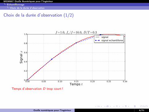
Choix de la durée d’observation (1/2)
0.00 0.05 0.10 0.15 0.20 0.25 0.30Temps t
0.0
0.2
0.4
0.6
0.8
1.0
Sign
al x
f=1.0, fe/f=16.0, D/T=0.3
signalsignal echantillone
Temps d’observation D trop court !
Outils numériques pour l’ingénieur 9/71
MGM657 Outils Numériques pour l’IngénieurÉchantillonnage
Choix de la durée d’observation
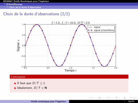
Choix de la durée d’observations (2/2)
0.0 0.5 1.0 1.5 2.0Temps t
1.0
0.5
0.0
0.5
1.0
Sign
al x
f=1.0, fe/f=16.0, D/T=2.0
signalsignal echantillone
Conclusion
Il faut que D/T ≥ 1
Idéalement, D/T ∈ N
Outils numériques pour l’ingénieur 10/71
MGM657 Outils Numériques pour l’IngénieurÉchantillonnage
Une borne basse de la fréquence d’échantillonage ?
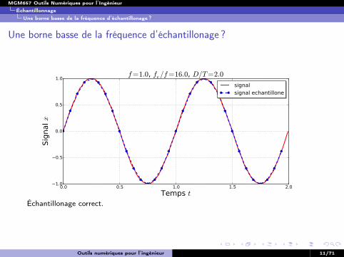
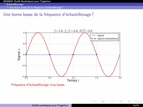
Une borne basse de la fréquence d’échantillonage ?
0.0 0.5 1.0 1.5 2.0Temps t
1.0
0.5
0.0
0.5
1.0
Sign
al x
f=1.0, fe/f=16.0, D/T=2.0
signalsignal echantillone
Échantillonage correct.
Outils numériques pour l’ingénieur 11/71
MGM657 Outils Numériques pour l’IngénieurÉchantillonnage
Une borne basse de la fréquence d’échantillonage ?
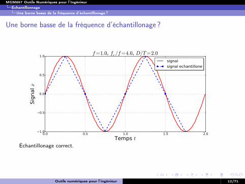
Une borne basse de la fréquence d’échantillonage ?
0.0 0.5 1.0 1.5 2.0Temps t
1.0
0.5
0.0
0.5
1.0
Sign
al x
f=1.0, fe/f=4.0, D/T=2.0
signalsignal echantillone
Échantillonage correct.
Outils numériques pour l’ingénieur 12/71
MGM657 Outils Numériques pour l’IngénieurÉchantillonnage
Une borne basse de la fréquence d’échantillonage ?
Une borne basse de la fréquence d’échantillonage ?
0.0 0.5 1.0 1.5 2.0Temps t
1.0
0.5
0.0
0.5
1.0
Sign
al x
f=1.0, fe/f=2.0, D/T=2.0
signalsignal echantillone
Fréquence d’échantillonage trop basse.
Outils numériques pour l’ingénieur 13/71
MGM657 Outils Numériques pour l’IngénieurÉchantillonnage
Une borne basse de la fréquence d’échantillonage ?
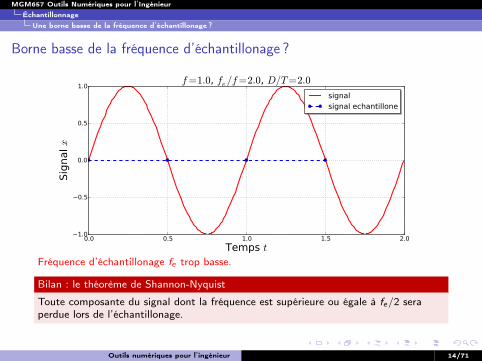
Borne basse de la fréquence d’échantillonage ?
0.0 0.5 1.0 1.5 2.0Temps t
1.0
0.5
0.0
0.5
1.0
Sign
al x
f=1.0, fe/f=2.0, D/T=2.0
signalsignal echantillone
Fréquence d’échantillonage fe trop basse.
Bilan : le théorème de Shannon-Nyquist
Toute composante du signal dont la fréquence est supérieure ou égale à fe/2 seraperdue lors de l’échantillonage.
Outils numériques pour l’ingénieur 14/71
MGM657 Outils Numériques pour l’IngénieurÉchantillonnage
Hautes fréquences et aliasing
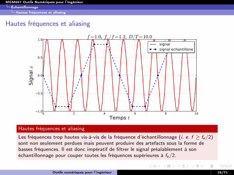
Hautes fréquences et aliasing
0 2 4 6 8 10Temps t
1.0
0.5
0.0
0.5
1.0
Sign
al x
f=1.0, fe/f=1.2, D/T=10.0
signalsignal echantillone
Hautes fréquences et aliasing
Les fréquences trop hautes vis-à-vis de la fréquence d’échantillonnage (i. e. f ≥ fe/2)sont non seulement perdues mais peuvent produire des artefacts sous la forme debasses fréquences. Il est donc impératif de filtrer le signal préalablement à sonéchantillonnage pour couper toutes les fréquences supérieures à fe/2.
Outils numériques pour l’ingénieur 15/71
MGM657 Outils Numériques pour l’IngénieurÉchantillonnage
Hautes fréquences et aliasing
Hautes fréquences et aliasing
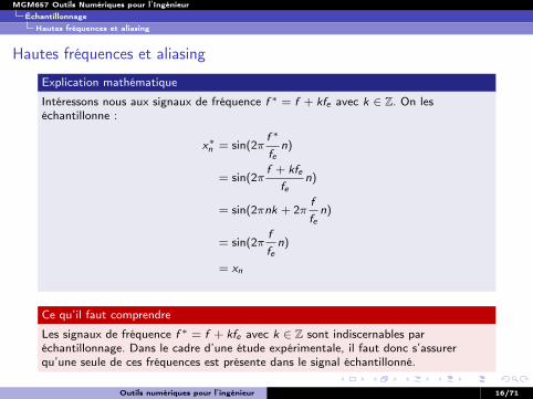
Explication mathématique
Intéressons nous aux signaux de fréquence f ∗ = f + kfe avec k ∈ Z. On leséchantillonne :
x∗n = sin(2πf ∗
fen)
= sin(2πf + kfe
fen)
= sin(2πnk + 2πf
fen)
= sin(2πf
fen)
= xn
Ce qu’il faut comprendre
Les signaux de fréquence f ∗ = f + kfe avec k ∈ Z sont indiscernables paréchantillonnage. Dans le cadre d’une étude expérimentale, il faut donc s’assurerqu’une seule de ces fréquences est présente dans le signal échantillonné.
Outils numériques pour l’ingénieur 16/71
MGM657 Outils Numériques pour l’IngénieurÉchantillonnage
Hautes fréquences et aliasing
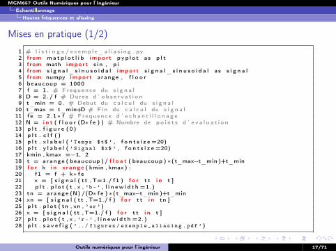
Mises en pratique (1/2)
1 # l i s t i n g s / e x emp l e_a l i a s i n g . py2 f rom ma t p l o t l i b impo r t pyp l o t as p l t3 f rom math impo r t s i n , p i4 f rom s i g n a l _ s i n u s o i d a l impo r t s i g n a l _ s i n u s o i d a l as s i g n a l5 f rom numpy impo r t arange , f l o o r6 beaucoup = 10007 f = 1 . # Frequence du s i g n a l8 D = 2 ./ f # Duree d ’ o b s e r v a t i o n9 t_min = 0 . # Debut du c a l c u l du s i g n a l
10 t_max = t_min+D # Fin du c a l c u l du s i g n a l11 f e = 2.1∗ f # Frequence d ’ e c h a n t i l l o n a g e12 N = i n t ( f l o o r (D∗ f e ) ) # Nombre de p o i n t s d ’ e v a l u a t i o n13 p l t . f i g u r e (0 )14 p l t . c l f ( )15 p l t . x l a b e l ( ’ Temps $t$ ’ , f o n t s i z e =20)16 p l t . y l a b e l ( ’ Signal $x$ ’ , f o n t s i z e =20)17 kmin , kmax =−1, 218 t = arange ( beaucoup ) / f l o a t ( beaucoup ) ∗(t_max−t_min )+t_min19 f o r k i n x r ange ( kmin , kmax ) :20 f1 = f + k∗ f e21 x = [ s i g n a l ( t t ,T=1./ f1 ) f o r t t i n t ]22 p l t . p l o t ( t , x , ’b - ’ , l i n e w i d t h =1.)23 tn = arange (N) /(D∗ f e ) ∗(t_max−t_min )+t_min24 xn = [ s i g n a l ( t t ,T=1./ f ) f o r t t i n tn ]25 p l t . p l o t ( tn , xn , ’ or ’ )26 x = [ s i g n a l ( t t ,T=1./ f ) f o r t t i n t ]27 p l t . p l o t ( t , x , ’r - ’ , l i n e w i d t h =2.)28 p l t . s a v e f i g ( ’ ../ figures / e x e m p l e _ a l i a s i n g . pdf ’ )
Outils numériques pour l’ingénieur 17/71
MGM657 Outils Numériques pour l’IngénieurÉchantillonnage
Hautes fréquences et aliasing
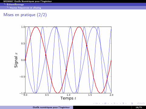
Mises en pratique (2/2)
0.0 0.5 1.0 1.5 2.0Temps t
1.0
0.5
0.0
0.5
1.0
Sign
al x
Outils numériques pour l’ingénieur 18/71
MGM657 Outils Numériques pour l’IngénieurAnalyse fréquentielle
Plan
1 Introduction
2 Notations
3 Échantillonnage
4 Analyse fréquentielle
Outils numériques pour l’ingénieur 19/71
MGM657 Outils Numériques pour l’IngénieurAnalyse fréquentielle
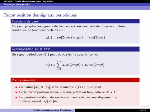
Décomposition des signaux périodiquesFonctions de baseOn peut projeter les signaux de fréquence f sur une base de dimension infinieconstituée de fonctions de la forme :
fn(t) = sin(2πnft) et gn(t) = cos(2πnft)
Décomposition sur la base
Un signal périodique x(t) peut donc s’écrire sous la forme :
x(t) =+∞∑n=0
ansin(2πnft) + bn cos(2πnft)
Points essentiels
Connaître [an] et [bn], c’est connaître x(t) en tout point.
Cette décomposition donne une interprétation fréquentielle de x(t).
La question est donc de savoir comment calculer analytiquement etnumériquement [an] et [bn].
Outils numériques pour l’ingénieur 20/71
MGM657 Outils Numériques pour l’IngénieurAnalyse fréquentielle
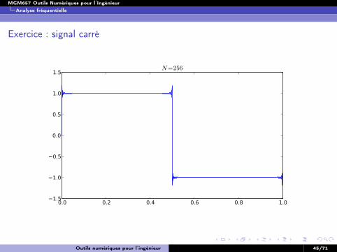
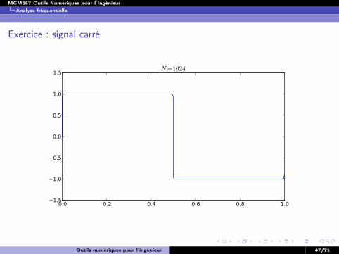
Développement en séries de Fourier
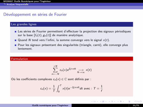
Les grandes lignes
Les séries de Fourier permettent d’effectuer la projection des signaux périodiquessur la base [fn(t), gn(t)] de manière analytique.
Quand N tend vers l’infini, la somme converge vers le signal x(t).
Pour les signaux présentant des singularités (triangle, carré), elle converge pluslentement.
Formulation
+N∑n=−N
cn(x)e2jπnft −→
N→∞x(t)
Où les coefficients complexes cn(x) ∈ C sont définis par :
cn(x) =1T
∫ T
0x(t)e−2jπnftdt avec : T =
1f
Outils numériques pour l’ingénieur 21/71
MGM657 Outils Numériques pour l’IngénieurAnalyse fréquentielle
Exercices
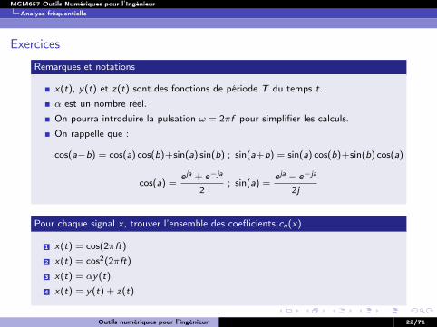
Remarques et notations
x(t), y(t) et z(t) sont des fonctions de période T du temps t.
α est un nombre réel.
On pourra introduire la pulsation ω = 2πf pour simplifier les calculs.
On rappelle que :
cos(a−b) = cos(a) cos(b)+sin(a) sin(b) ; sin(a+b) = sin(a) cos(b)+sin(b) cos(a)
cos(a) =e ja + e−ja
2; sin(a) =
e ja − e−ja
2j
Pour chaque signal x , trouver l’ensemble des coefficients cn(x)
1 x(t) = cos(2πft)
2 x(t) = cos2(2πft)
3 x(t) = αy(t)
4 x(t) = y(t) + z(t)
Outils numériques pour l’ingénieur 22/71
MGM657 Outils Numériques pour l’IngénieurAnalyse fréquentielle
Exercice : signal sinusoïdal
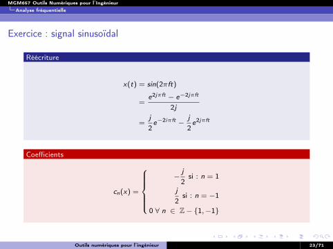
Réécriture
x(t) = sin(2πft)
=e2jπft − e−2jπft
2j
=j
2e−2iπft −
j
2e2jπft
Coefficients
cn(x) =
−
j
2si : n = 1
j
2si : n = −1
0 ∀ n ∈ Z− {1,−1}
Outils numériques pour l’ingénieur 23/71
MGM657 Outils Numériques pour l’IngénieurAnalyse fréquentielle
Interprétation des coefficients cn
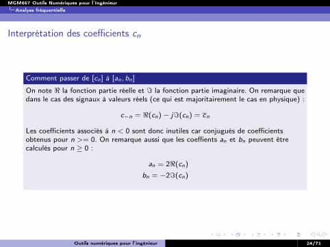
Comment passer de [cn] à [an, bn]
On note < la fonction partie réelle et = la fonction partie imaginaire. On remarque quedans le cas des signaux à valeurs réels (ce qui est majoritairement le cas en physique) :
c−n = <(cn)− j=(cn) = cn
Les coefficients associés à n < 0 sont donc inutiles car conjugués de coefficientsobtenus pour n >= 0. On remarque aussi que les coeffients an et bn peuvent êtrecalculés pour n ≥ 0 :
an = 2<(cn)bn = −2=(cn)
Outils numériques pour l’ingénieur 24/71
MGM657 Outils Numériques pour l’IngénieurAnalyse fréquentielle
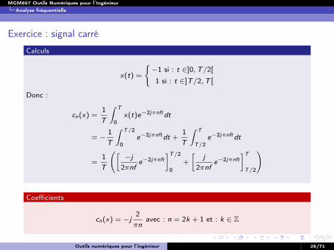
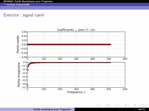
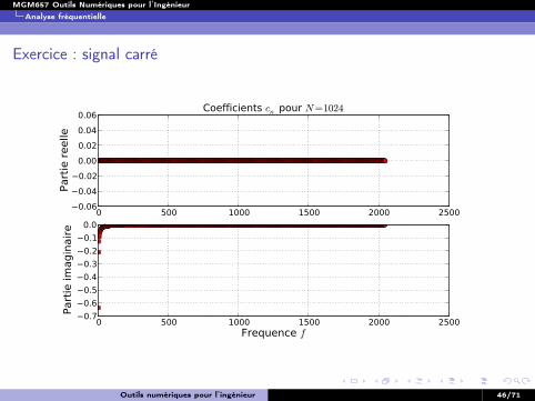
Exercice : signal carré
Calculs
x(t) =
{−1 si : t ∈]0,T/2[1 si : t ∈]T/2,T [
Donc :
cn(x) =1T
∫ T
0x(t)e−2jπnftdt
= −1T
∫ T/2
0e−2jπnftdt +
1T
∫ T
T/2e−2jπnftdt
=1T
([−j
2πnfe−2jπnft
]T/20
+
[j
2πnfe−2jπnft
]TT/2
)
Coefficients
cn(x) = −j2πn
avec : n = 2k + 1 et : k ∈ Z
Outils numériques pour l’ingénieur 25/71
MGM657 Outils Numériques pour l’IngénieurAnalyse fréquentielle
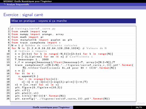
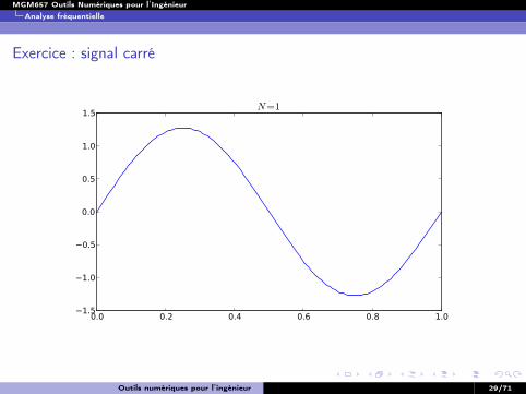
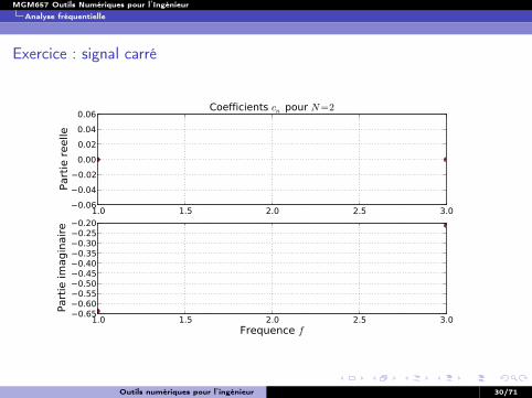
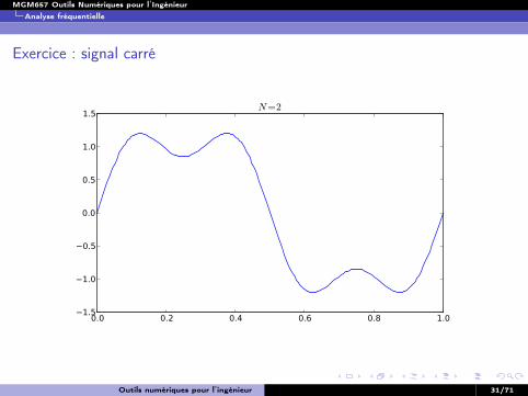
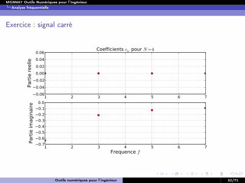
Exercice : signal carréMise en pratique : voyons si ça marche
1 # l i s t i n g s / s e r i e F_ca r r e . py2 f rom cmath impo r t exp3 f rom numpy impo r t arange , a r r a y4 f rom math impo r t p i5 f rom ma t p l o t l i b impo r t pyp l o t as p l t6 f rom t race_complexes impo r t ∗7 N = 1 # Nombre de c o e f f i c i e n t s c a l c u l e s8 f o r N i n [ 1 , 2 , 4 , 8 , 16 , 32 , 64 , 128 , 256 , 1024 ] : # Va l e u r s de N9 # I n d i c e s n impa i r s
10 n = [2∗ k+1 f o r k i n r ange (−N, 0 ) ]+[2∗ k+1 f o r k i n r ange (N) ]11 c = [−2 j /( p i ∗nn ) f o r nn i n n ] # C o e f f i c i e n t s c12 T, beaucoup= 1 . , 200013 t , f = arange ( beaucoup ) / f l o a t ( beaucoup )∗T, a r r a y ( n [N:2∗N] ) /T14 t race_complexes ( f , c [N:2∗N] , ’ ../ figures / s e r i e F _ c a r r e _ c _ {0}. pdf ’ . f o rmat (
N) , t i t l e=’ C o e f f i c i e n t s $c_n$ pour $N = {0} $ ’ . f o rmat (N) )15 x = [ ]16 f o r t t i n t :17 x . append ( 0 . )18 f o r i i n x r ange ( l e n ( n ) ) :19 x [−1] = x[−1]+c [ i ]∗ exp (2 j ∗ p i ∗n [ i ]∗ t t /T)20 x1 = [ xx . r e a l f o r xx i n x ]21 p l t . f i g u r e (0 , f i g s i z e =(10 ,2) )22 p l t . c l f ( )23 p l t . p l o t ( t , x1 )24 p l t . t i t l e ( ’ $N ={0} $ ’ . f o rmat (N) )25 p l t . s a v e f i g ( ’ ../ figures / s e r i e F _ c a r r e _ {0}. pdf ’ . f o rmat (N) )
Outils numériques pour l’ingénieur 26/71
MGM657 Outils Numériques pour l’IngénieurAnalyse fréquentielle
Exercice : signal carré
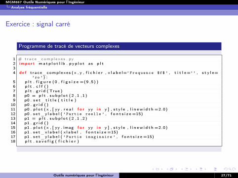
Programme de tracé de vecteurs complexes
1 # trace_complexes . py2 impo r t ma t p l o t l i b . p y p l o t as p l t34 de f t race_complexes ( x , y , f i c h i e r , x l a b e l=’ Frequence $f$ ’ , t i t l e=’ ’ , s t y l e=
’ ro ’ ) :5 p l t . f i g u r e (0 , f i g s i z e =(9 ,5) )6 p l t . c l f ( )7 p l t . g r i d ( True )8 p0 = p l t . s u bp l o t ( 2 , 1 , 1 )9 p0 . s e t _ t i t l e ( t i t l e )
10 p0 . g r i d ( )11 p0 . p l o t ( x , [ yy . r e a l f o r yy i n y ] , s t y l e , l i n e w i d t h =2.0)12 p0 . s e t_y l a b e l ( ’ Partie reelle ’ , f o n t s i z e =15)13 p1 = p l t . s u bp l o t ( 2 , 1 , 2 )14 p1 . g r i d ( )15 p1 . p l o t ( x , [ yy . imag f o r yy i n y ] , s t y l e , l i n e w i d t h =2.0)16 p1 . s e t_x l a b e l ( x l a b e l , f o n t s i z e =15)17 p1 . s e t_y l a b e l ( ’ Partie imaginaire ’ , f o n t s i z e =15)18 p l t . s a v e f i g ( f i c h i e r )
Outils numériques pour l’ingénieur 27/71
MGM657 Outils Numériques pour l’IngénieurAnalyse fréquentielle
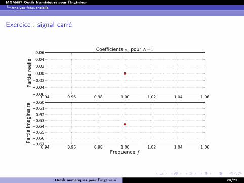
Exercice : signal carré
0.94 0.96 0.98 1.00 1.02 1.04 1.060.060.040.020.000.020.040.06
Part
ie re
elle
Coefficients cn pour N=1
0.94 0.96 0.98 1.00 1.02 1.04 1.06Frequence f
0.670.660.650.640.630.620.610.60
Part
ie im
agin
aire
Outils numériques pour l’ingénieur 28/71
MGM657 Outils Numériques pour l’IngénieurAnalyse fréquentielle
Exercice : signal carré
0.0 0.2 0.4 0.6 0.8 1.01.5
1.0
0.5
0.0
0.5
1.0
1.5 N=1
Outils numériques pour l’ingénieur 29/71
MGM657 Outils Numériques pour l’IngénieurAnalyse fréquentielle
Exercice : signal carré
1.0 1.5 2.0 2.5 3.00.060.040.020.000.020.040.06
Part
ie re
elle
Coefficients cn pour N=2
1.0 1.5 2.0 2.5 3.0Frequence f
0.650.600.550.500.450.400.350.300.250.20
Part
ie im
agin
aire
Outils numériques pour l’ingénieur 30/71
MGM657 Outils Numériques pour l’IngénieurAnalyse fréquentielle
Exercice : signal carré
0.0 0.2 0.4 0.6 0.8 1.01.5
1.0
0.5
0.0
0.5
1.0
1.5 N=2
Outils numériques pour l’ingénieur 31/71
MGM657 Outils Numériques pour l’IngénieurAnalyse fréquentielle
Exercice : signal carré
1 2 3 4 5 6 70.060.040.020.000.020.040.06
Part
ie re
elle
Coefficients cn pour N=4
1 2 3 4 5 6 7Frequence f
0.70.60.50.40.30.20.10.0
Part
ie im
agin
aire
Outils numériques pour l’ingénieur 32/71
MGM657 Outils Numériques pour l’IngénieurAnalyse fréquentielle
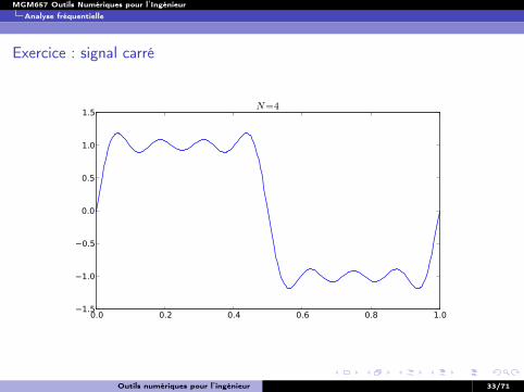
Exercice : signal carré
0.0 0.2 0.4 0.6 0.8 1.01.5
1.0
0.5
0.0
0.5
1.0
1.5 N=4
Outils numériques pour l’ingénieur 33/71
MGM657 Outils Numériques pour l’IngénieurAnalyse fréquentielle
Exercice : signal carré
0 2 4 6 8 10 12 14 160.060.040.020.000.020.040.06
Part
ie re
elle
Coefficients cn pour N=8
0 2 4 6 8 10 12 14 16Frequence f
0.70.60.50.40.30.20.10.0
Part
ie im
agin
aire
Outils numériques pour l’ingénieur 34/71
MGM657 Outils Numériques pour l’IngénieurAnalyse fréquentielle
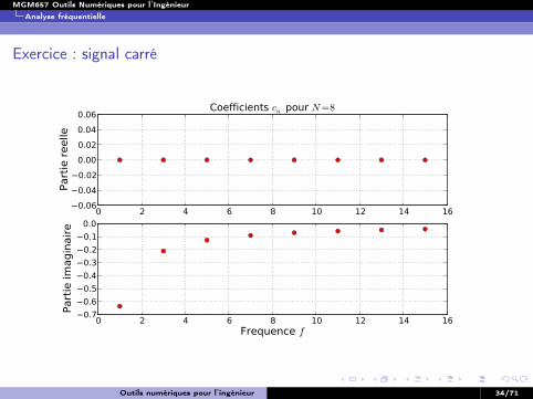
Exercice : signal carré
0.0 0.2 0.4 0.6 0.8 1.01.5
1.0
0.5
0.0
0.5
1.0
1.5 N=8
Outils numériques pour l’ingénieur 35/71
MGM657 Outils Numériques pour l’IngénieurAnalyse fréquentielle
Exercice : signal carré
0 5 10 15 20 25 30 350.060.040.020.000.020.040.06
Part
ie re
elle
Coefficients cn pour N=16
0 5 10 15 20 25 30 35Frequence f
0.70.60.50.40.30.20.10.0
Part
ie im
agin
aire
Outils numériques pour l’ingénieur 36/71

MGM657 Outils Numériques pour l’IngénieurAnalyse fréquentielle
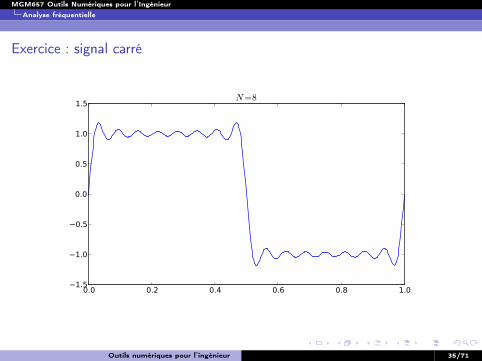
Exercice : signal carré
0.0 0.2 0.4 0.6 0.8 1.01.5
1.0
0.5
0.0
0.5
1.0
1.5 N=16
Outils numériques pour l’ingénieur 37/71
MGM657 Outils Numériques pour l’IngénieurAnalyse fréquentielle
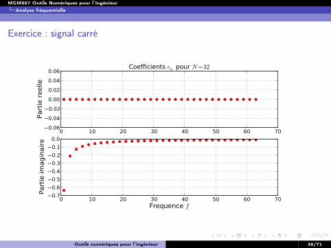
Exercice : signal carré
0 10 20 30 40 50 60 700.060.040.020.000.020.040.06
Part
ie re
elle
Coefficients cn pour N=32
0 10 20 30 40 50 60 70Frequence f
0.70.60.50.40.30.20.10.0
Part
ie im
agin
aire
Outils numériques pour l’ingénieur 38/71
MGM657 Outils Numériques pour l’IngénieurAnalyse fréquentielle
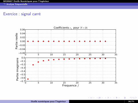
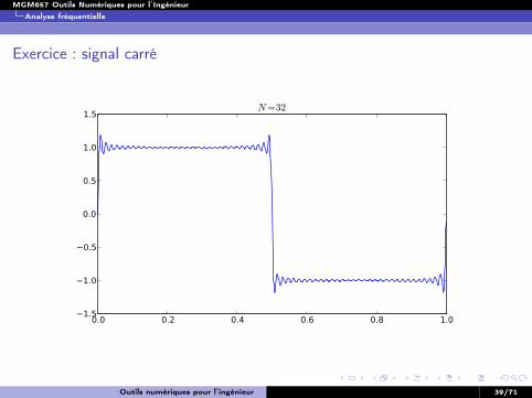
Exercice : signal carré
0.0 0.2 0.4 0.6 0.8 1.01.5
1.0
0.5
0.0
0.5
1.0
1.5 N=32
Outils numériques pour l’ingénieur 39/71
MGM657 Outils Numériques pour l’IngénieurAnalyse fréquentielle
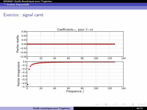
Exercice : signal carré
0 20 40 60 80 100 120 1400.060.040.020.000.020.040.06
Part
ie re
elle
Coefficients cn pour N=64
0 20 40 60 80 100 120 140Frequence f
0.70.60.50.40.30.20.10.0
Part
ie im
agin
aire
Outils numériques pour l’ingénieur 40/71
MGM657 Outils Numériques pour l’IngénieurAnalyse fréquentielle
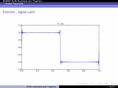
Exercice : signal carré
0.0 0.2 0.4 0.6 0.8 1.01.5
1.0
0.5
0.0
0.5
1.0
1.5 N=64
Outils numériques pour l’ingénieur 41/71

MGM657 Outils Numériques pour l’IngénieurAnalyse fréquentielle
Exercice : signal carré
0 50 100 150 200 250 3000.060.040.020.000.020.040.06
Part
ie re
elle
Coefficients cn pour N=128
0 50 100 150 200 250 300Frequence f
0.70.60.50.40.30.20.10.0
Part
ie im
agin
aire
Outils numériques pour l’ingénieur 42/71

MGM657 Outils Numériques pour l’IngénieurAnalyse fréquentielle
Exercice : signal carré
0.0 0.2 0.4 0.6 0.8 1.01.5
1.0
0.5
0.0
0.5
1.0
1.5 N=128
Outils numériques pour l’ingénieur 43/71
MGM657 Outils Numériques pour l’IngénieurAnalyse fréquentielle
Exercice : signal carré
0 100 200 300 400 500 6000.060.040.020.000.020.040.06
Part
ie re
elle
Coefficients cn pour N=256
0 100 200 300 400 500 600Frequence f
0.70.60.50.40.30.20.10.0
Part
ie im
agin
aire
Outils numériques pour l’ingénieur 44/71
MGM657 Outils Numériques pour l’IngénieurAnalyse fréquentielle
Exercice : signal carré
0.0 0.2 0.4 0.6 0.8 1.01.5
1.0
0.5
0.0
0.5
1.0
1.5 N=256
Outils numériques pour l’ingénieur 45/71
MGM657 Outils Numériques pour l’IngénieurAnalyse fréquentielle
Exercice : signal carré
0 500 1000 1500 2000 25000.060.040.020.000.020.040.06
Part
ie re
elle
Coefficients cn pour N=1024
0 500 1000 1500 2000 2500Frequence f
0.70.60.50.40.30.20.10.0
Part
ie im
agin
aire
Outils numériques pour l’ingénieur 46/71
MGM657 Outils Numériques pour l’IngénieurAnalyse fréquentielle
Exercice : signal carré
0.0 0.2 0.4 0.6 0.8 1.01.5
1.0
0.5
0.0
0.5
1.0
1.5 N=1024
Outils numériques pour l’ingénieur 47/71
MGM657 Outils Numériques pour l’IngénieurAnalyse fréquentielle
Extention aux signaux apériodiques
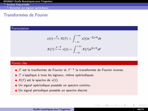
Transformées de Fourier
Formulation
x(t)F7−→ X (f ) =
∫ +∞
−∞x(t)e−2jπftdt
X (f )F−17−→ x(t) =
∫ +∞
−∞X (f )e2jπftdf
Points clés
F est la tranformée de Fourier et F−1 la transformée de Fourier inverse.
F s’applique à tous les signaux, même apériodiques.
X (f ) est le spectre de x(t).
Un signal apériodique possède un spectre continu.
Un signal périodique possède un spectre discret.
Outils numériques pour l’ingénieur 48/71
MGM657 Outils Numériques pour l’IngénieurAnalyse fréquentielle
La Transformée de Fourier Discrète (DFT)
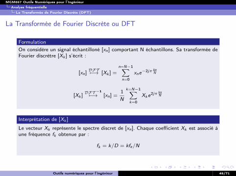
La Transformée de Fourier Discrète ou DFT
FormulationOn considère un signal échantilloné [xn] comportant N échantillons. Sa transformée deFourier discrètre [Xk ] s’écrit :
[xn]DFT7−→ [Xk ] =
n=N−1∑n=0
xne−2jπ kn
N
[Xk ]DFT−17−→ [xn] =
1N
k=N−1∑k=0
Xke2jπ kn
N
Interprétation de [Xk ]
Le vecteur Xk représente le spectre discret de [xn]. Chaque coefficient Xk est associé àune fréquence fk obtenue par :
fk = k/D = kfe/N
Outils numériques pour l’ingénieur 49/71
MGM657 Outils Numériques pour l’IngénieurAnalyse fréquentielle
La Transformée de Fourier Rapide (FFT)
La Transformée de Fourier Discrète ou DFT
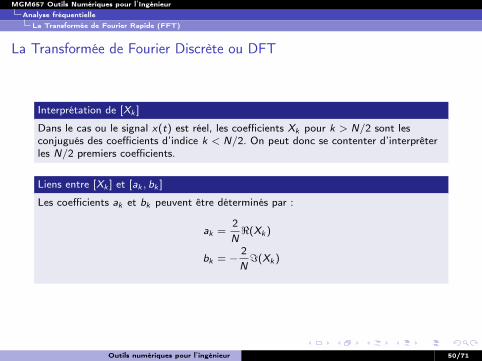
Interprétation de [Xk ]
Dans le cas ou le signal x(t) est réel, les coefficients Xk pour k > N/2 sont lesconjugués des coefficients d’indice k < N/2. On peut donc se contenter d’interprêterles N/2 premiers coefficients.
Liens entre [Xk ] et [ak , bk ]
Les coefficients ak et bk peuvent être déterminés par :
ak =2N<(Xk )
bk = −2N=(Xk )
Outils numériques pour l’ingénieur 50/71
MGM657 Outils Numériques pour l’IngénieurAnalyse fréquentielle
La Transformée de Fourier Rapide (FFT)
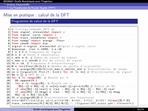
Mise en pratique : calcul de la DFTProgramme de calcul de la DFT
1 # l i s t i n g s /exemple_DFT . py2 f rom s i g n a l _ s i n u s o i d a l impo r t ∗3 f rom s i g n a l_ c a r r e impo r t ∗4 f rom t race_complexes impo r t ∗5 f rom numpy impo r t arange , f l o o r6 f rom cmath impo r t exp7 s i g n a l = s i g n a l _ s i n u s o i d a l #s i g n a l = s i g n a l_ c a r r e8 beaucoup , r i e n = 1000 , 1 . e−109 f = 3 .3 # Frequence du s i g n a l
10 D = 4 . # Duree d ’ o b s e r v a t i o n11 t_min = 0 . # Debut du c a l c u l du s i g n a l12 t_max = t_min+D # Fin du c a l c u l du s i g n a l13 f e = 16 . # Frequence d ’ e c h a n t i l l o n a g e14 N = i n t ( f l o o r (D∗ f e ) ) # Nombre de p o i n t s d ’ e v a l u a t i o n15 tn = arange (N) /(D∗ f e ) ∗(t_max−t_min )+t_min # D i s c r e t i s a t i o n du temps16 xn = [ s i g n a l ( t t ,T=1./ f , k=4.) f o r t t i n tn ] # D i s c r e t i s a t i o n du s i g n a l17 Xk = [ ] # DFT de xn18 f o r k i n r ange (N) : # Bouc le s u r k19 Xk . append ( 0 . )20 f o r n i n r ange (N) : # Bouc le s u r n21 Xk[−1] = Xk[−1] + xn [ n ]∗ exp(−2 j ∗ p i ∗n∗k/N) # Ca l c u l de Xk22 i f abs (Xk [−1] . r e a l ) < r i e n : Xk[−1] = Xk[−1] − Xk[−1] . r e a l23 i f abs (Xk [−1] . imag ) < r i e n : Xk[−1] = Xk[−1] − 1 j ∗Xk[−1] . imag24 Xk[−1] = Xk[−1]∗2/N25 f k = arange (N) /D # D i s c r e t i s a t i o n des f r e q u e n c e s26 t i t=’ $DFT (\ sin (2\ pi nf / f_e ) ) *2/ N$ : N ={0} , f ={1} , D ={2} ’ . f o rmat (N, f ,D)27 t race_complexes ( f k [ : N/2 ] , Xk [ : N/2 ] , ’ ../ figures / DFT_sinus . pdf ’ , t i t l e=t i t )
Outils numériques pour l’ingénieur 51/71
MGM657 Outils Numériques pour l’IngénieurAnalyse fréquentielle
La Transformée de Fourier Rapide (FFT)
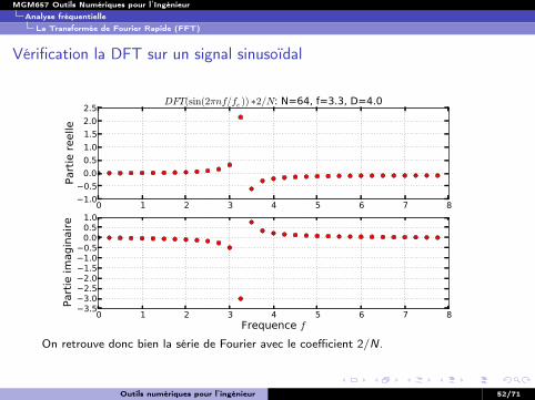
Vérification la DFT sur un signal sinusoïdal
0 1 2 3 4 5 6 7 81.00.50.00.51.01.52.02.5
Part
ie re
elle
DFT(sin(2πnf/fe )) ∗2/N: N=64, f=3.3, D=4.0
0 1 2 3 4 5 6 7 8Frequence f
3.53.02.52.01.51.00.50.00.51.0
Part
ie im
agin
aire
On retrouve donc bien la série de Fourier avec le coefficient 2/N.
Outils numériques pour l’ingénieur 52/71
MGM657 Outils Numériques pour l’IngénieurAnalyse fréquentielle
Optimisation de la DFT : la Transformée de Fourier Rapide (FFT)
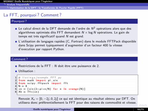
La FFT, pourquoi ? Comment ?Pourquoi ?
Le calcul direct de la DFT demande de l’ordre de N2 opérations alors que desalgorithmes optimisés dits FFT demandent N × logN opérations. Le gain detemps est très significatif quand N est grand.
L’utilisation de langages rapides (C, Fortran) dans le module FFTPack disponibledans Scipy permet typiquement d’augmenter d’un facteur 400 la vitessed’execution par rapport Python.
Comment ?
Restrictions de la FFT : N doit être une puissance de 2.
Utilisation :
1 # l i s t i n g s /exemple_FFT . py2 f rom math impo r t pi , s i n3 f rom s c i p y . f f t p a c k impo r t f f t4 N = 85 xn = [ s i n (2∗ p i ∗n/N) f o r n i n x r ange (N) ]6 Xk = f f t ( xn )
Renvoie Xn = [0,−2j , 0, 2j] ce qui est identique au résultat obtenu par DFT. Onutilisera donc préférentiellement la FFT pour des raisons de commodité et vitesse.
Outils numériques pour l’ingénieur 53/71
MGM657 Outils Numériques pour l’IngénieurAnalyse fréquentielle
Optimisation de la DFT : la Transformée de Fourier Rapide (FFT)
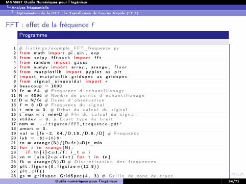
FFT : effet de la fréquence f
Programme
1 # l i s t i n g s /exemple_FFT_frequence . py2 f rom math impo r t pi , s i n , exp3 f rom s c i p y . f f t p a c k impo r t f f t4 f rom random impo r t gauss5 f rom numpy impo r t a r r ay , arange , f l o o r6 f rom ma t p l o t l i b impo r t pyp l o t as p l t7 impo r t ma t p l o t l i b . g r i d s p e c as g r i d s p e c8 f rom s i g n a l _ s i n u s o i d a l impo r t ∗9 beaucoup = 1000
10 f e = 64 . # Frequence d ’ e c h a n t i l l o n a g e11 N = 4096 # Nombre de p o i n t s d ’ e c h a n t i l l o n a g e12 D = N/ f e # Duree d ’ o b s e r v a t i o n13 f = 8 ./D # Frequence du s i g n a l14 t_min = 0 . # Debut du c a l c u l du s i g n a l15 t_max = t_min+D # Fin du c a l c u l du s i g n a l16 s tddev = 0 . # Eca r t type du b r u i t17 nom = ’ ../ figures / F F T _ f r e q u e n c e . pdf ’18 amort = 0 .19 v a l = [ fe −2, 64 ./D, 1 6 . /D, 8 . /D] # Frequence20 l a b = ’ $f ={0} $ ’21 tn = arange (N) /(D∗ f e )∗D+t_min22 f o r i i n x r ange (N) :23 i f tn [ i ]<=1./ f : i_t = i24 xn = [ s i n (2∗ p i ∗ f ∗ t ) f o r t i n tn ]25 f k = arange (N) /D # D i s c r e t i s a t i o n des f r e q u e n c e s26 p l t . f i g u r e (0 , f i g s i z e =(12 ,8) )27 p l t . c l f ( )28 gs = g r i d s p e c . Gr idSpec (4 , 3) # G r i l l e de zone de t r a c e
Outils numériques pour l’ingénieur 54/71
MGM657 Outils Numériques pour l’IngénieurAnalyse fréquentielle
Optimisation de la DFT : la Transformée de Fourier Rapide (FFT)
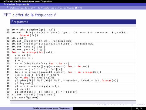
FFT : effet de la fréquence f
Programme
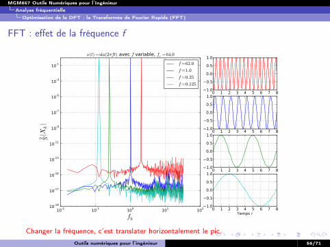
29 p0 = p l t . s u bp l o t ( gs [ : , : 2 ] )30 p0 . s e t _ t i t l e ( r ’ $x ( t ) = \ sin (2 \ pi f t ) $ avec $f$ variable , $f_e ={} $ ’ .
f o rmat ( f e ) )31 p0 . g r i d ( )32 p0 . s e t_x l a b e l ( r ’ $f_k$ ’ , f o n t s i z e =20)33 p0 . s e t_y l a b e l ( r ’$ \ frac {2}{ N }| X_k | $ ’ , f o n t s i z e =20)34 p0 . s e t_x s c a l e ( ’ log ’ )35 p0 . s e t_y s c a l e ( ’ log ’ )36 f o r z i n x r ange ( l e n ( v a l ) ) :37 v = v a l [ z ]38 #stddev = v39 f = v40 xn = [ s i n (2∗ p i ∗ f ∗ t ) f o r t i n tn ]41 v_amort = a r r a y ( [ exp(− t∗amort ) f o r t i n tn ] )42 c o l o r = [ ’r ’ , ’b ’ , ’g ’ , ’c ’ ] [ z ]43 b r u i t = a r r a y ( [ gaus s (0 , s tddev ) f o r i i n x r ange (N) ] )44 xxn = ( xn + b r u i t )∗v_amort45 Xk = abs ( f f t ( xxn ) ) ∗2./N46 p0 . p l o t ( f k [ 0 :N/2 ] , Xk [ 0 :N/2 ] , ’ - ’+co l o r , l a b e l = l a b . f o rmat ( v ) )47 p0 . l e g end ( )48 p1 = p l t . s u bp l o t ( gs [ z ,−1])49 p1 . g r i d ( )50 p1 . p l o t ( tn [ : i_t ] , xxn [ : i_t ] , ’ - ’+co l o r )51 p1 . s e t_x l a b e l ( ’ Temps $t$ ’ )52 p l t . s a v e f i g (nom)
Outils numériques pour l’ingénieur 55/71
MGM657 Outils Numériques pour l’IngénieurAnalyse fréquentielle
Optimisation de la DFT : la Transformée de Fourier Rapide (FFT)
FFT : effet de la fréquence f
10-2 10-1 100 101 102
fk
10-19
10-17
10-15
10-13
10-11
10-9
10-7
10-5
10-3
10-1
2 N|X
k|
x(t) =sin(2πft) avec f variable, fe =64.0
f=62.0
f=1.0
f=0.25
f=0.125
0 1 2 3 4 5 6 7 81.0
0.5
0.0
0.5
1.0
0 1 2 3 4 5 6 7 81.0
0.5
0.0
0.5
1.0
0 1 2 3 4 5 6 7 81.0
0.5
0.0
0.5
1.0
0 1 2 3 4 5 6 7 8Temps t
1.0
0.5
0.0
0.5
1.0
Changer la fréquence, c’est translater horizontalement le pic.
Outils numériques pour l’ingénieur 56/71
MGM657 Outils Numériques pour l’IngénieurAnalyse fréquentielle
Optimisation de la DFT : la Transformée de Fourier Rapide (FFT)
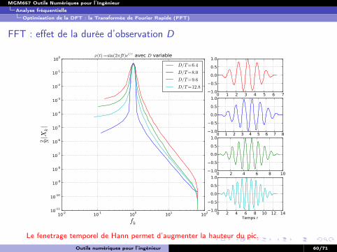
FFT : effet de la durée d’observation D
Programme
1 # l i s t i n g s /exemple_FFT_D . py2 f rom math impo r t pi , s i n , exp3 f rom s c i p y . f f t p a c k impo r t f f t4 f rom random impo r t gauss5 f rom numpy impo r t a r r ay , arange , f l o o r , hann ing6 f rom ma t p l o t l i b impo r t pyp l o t as p l t7 impo r t ma t p l o t l i b . g r i d s p e c as g r i d s p e c8 f rom s i g n a l _ s i n u s o i d a l impo r t ∗9 beaucoup = 1000
10 f e = 128 . # Frequence d ’ e c h a n t i l l o n a g e11 f = 1 . # Frequence du s i g n a l12 t_min = 0 . # Debut du c a l c u l du s i g n a l13 s tddev = 0 . # Eca r t type du b r u i t14 nom = ’ ../ figures / FFT_D . pdf ’15 amort = 0 .16 v a l = 8 ./ f ∗ a r r a y ( [ . 8 , 1 . , 1 . 2 , 1 . 6 ] )17 l a b = ’ $D / T ={0} $ ’181920 p l t . f i g u r e (0 , f i g s i z e =(12 ,8) )21 p l t . c l f ( )22 gs = g r i d s p e c . Gr idSpec (4 , 3) # G r i l l e de zone de t r a c e23 p0 = p l t . s u bp l o t ( gs [ : , : 2 ] )24 p0 . s e t _ t i t l e ( r ’ $x ( t ) = \ sin (2 \ pi f t ) $ avec $D$ variable ’ )25 p0 . g r i d ( )26 p0 . s e t_x l a b e l ( r ’ $f_k$ ’ , f o n t s i z e =20)27 p0 . s e t_y l a b e l ( r ’$ \ frac {2}{ N }| X_k | $ ’ , f o n t s i z e =20)28 p0 . s e t_x s c a l e ( ’ log ’ )
Outils numériques pour l’ingénieur 57/71
MGM657 Outils Numériques pour l’IngénieurAnalyse fréquentielle
Optimisation de la DFT : la Transformée de Fourier Rapide (FFT)
FFT : effet de la durée d’observation D
Programme
29 p0 . s e t_y s c a l e ( ’ log ’ )30 f o r z i n x r ange ( l e n ( v a l ) ) :31 v = v a l [ z ]32 D = v33 i_t=−134 N = i n t (D∗ f e )35 f k = arange (N) /D # D i s c r e t i s a t i o n des f r e q u e n c e s36 t_max = t_min+D # Fin du c a l c u l du s i g n a l37 tn = arange (N) / f l o a t (N)∗D+t_min38 xn = [ s i n (2∗ p i ∗ f ∗ t ) f o r t i n tn ]39 v_amort = a r r a y ( [ exp(− t∗amort ) f o r t i n tn ] )40 c o l o r = [ ’r ’ , ’b ’ , ’g ’ , ’c ’ ] [ z ]41 b r u i t = a r r a y ( [ gaus s (0 , s tddev ) f o r i i n x r ange (N) ] )42 xxn = ( xn + b r u i t )∗v_amort #∗hann ing (N)43 Xk = abs ( f f t ( xxn ) ) ∗2./N44 p0 . p l o t ( f k [ 0 :N/2 ] , Xk [ 0 :N/2 ] , ’ - ’+co l o r , l a b e l = l a b . f o rmat ( v∗ f ) )45 p1 = p l t . s u bp l o t ( gs [ z ,−1])46 p1 . g r i d ( )47 p1 . p l o t ( tn [ : i_t ] , xxn [ : i_t ] , ’ - ’+co l o r )48 p0 . l e g end ( )49 p1 . s e t_x l a b e l ( ’ Temps $t$ ’ )50 p l t . s a v e f i g (nom)
Outils numériques pour l’ingénieur 58/71
MGM657 Outils Numériques pour l’IngénieurAnalyse fréquentielle
Optimisation de la DFT : la Transformée de Fourier Rapide (FFT)
FFT : effet de la durée d’observation D
10-2 10-1 100 101 102
fk
10-18
10-16
10-14
10-12
10-10
10-8
10-6
10-4
10-2
100
2 N|X
k|
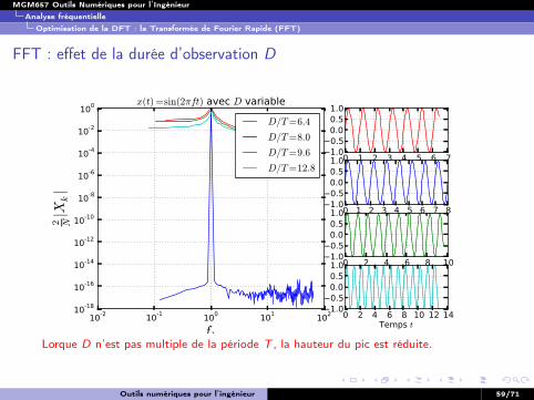
x(t) =sin(2πft) avec D variable
D/T=6.4
D/T=8.0
D/T=9.6
D/T=12.80 1 2 3 4 5 6 71.0
0.50.00.51.0
0 1 2 3 4 5 6 7 81.00.50.00.51.0
0 2 4 6 8 101.00.50.00.51.0
0 2 4 6 8 10 12 14Temps t
1.00.50.00.51.0
Lorque D n’est pas multiple de la période T , la hauteur du pic est réduite.
Outils numériques pour l’ingénieur 59/71
MGM657 Outils Numériques pour l’IngénieurAnalyse fréquentielle
Optimisation de la DFT : la Transformée de Fourier Rapide (FFT)
FFT : effet de la durée d’observation D
10-2 10-1 100 101 102
fk
10-11
10-10
10-9
10-8
10-7
10-6
10-5
10-4
10-3
10-2
10-1
100
2 N|X
k|
x(t) =sin(2πft)et/τ avec D variable
D/T=6.4
D/T=8.0
D/T=9.6
D/T=12.8
0 1 2 3 4 5 6 71.0
0.5
0.0
0.5
1.0
0 1 2 3 4 5 6 7 81.0
0.5
0.0
0.5
1.0
0 2 4 6 8 101.0
0.5
0.0
0.5
1.0
0 2 4 6 8 10 12 14Temps t
1.0
0.5
0.0
0.5
1.0
Le fenetrage temporel de Hann permet d’augmenter la hauteur du pic.
Outils numériques pour l’ingénieur 60/71
MGM657 Outils Numériques pour l’IngénieurAnalyse fréquentielle
Optimisation de la DFT : la Transformée de Fourier Rapide (FFT)
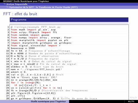
FFT : effet du bruitProgramme
1 # l i s t i n g s /exemple_FFT_bruit . py2 f rom math impo r t pi , s i n , exp3 f rom s c i p y . f f t p a c k impo r t f f t4 f rom random impo r t gauss5 f rom numpy impo r t a r r ay , arange , f l o o r6 f rom ma t p l o t l i b impo r t pyp l o t as p l t7 impo r t ma t p l o t l i b . g r i d s p e c as g r i d s p e c8 f rom s i g n a l _ s i n u s o i d a l impo r t ∗9 beaucoup = 1000
10 f e = 64 . # Frequence d ’ e c h a n t i l l o n a g e11 N = 4096 # Nombre de p o i n t s d ’ e c h a n t i l l o n a g e12 D = N/ f e # Duree d ’ o b s e r v a t i o n13 f = 8 ./D # Frequence du s i g n a l14 t_min = 0 . # Debut du c a l c u l du s i g n a l15 t_max = t_min+D # Fin du c a l c u l du s i g n a l16 s tddev = 0 . # Eca r t type du b r u i t17 nom = ’ ../ figures / FFT_bruit . pdf ’18 amort = 0 .19 v a l = [ 1 . , 1 . e−1 ,1. e−2 ,0 . ] # B ru i t20 l a b = ’ Ecart type bruit : {0} ’21 tn = arange (N) /(D∗ f e )∗D+t_min22 f o r i i n x r ange (N) :23 i f tn [ i ]<=1./ f : i_t = i24 xn = [ s i n (2∗ p i ∗ f ∗ t ) f o r t i n tn ]25 f k = arange (N) /D # D i s c r e t i s a t i o n des f r e q u e n c e s26 p l t . f i g u r e (0 , f i g s i z e =(12 ,8) )27 p l t . c l f ( )28 gs = g r i d s p e c . Gr idSpec (4 , 3) # G r i l l e de zone de t r a c e
Outils numériques pour l’ingénieur 61/71
MGM657 Outils Numériques pour l’IngénieurAnalyse fréquentielle
Optimisation de la DFT : la Transformée de Fourier Rapide (FFT)
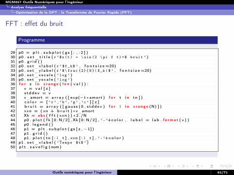
FFT : effet du bruit
Programme
29 p0 = p l t . s u bp l o t ( gs [ : , : 2 ] )30 p0 . s e t _ t i t l e ( r ’ $x ( t ) = \ sin (2 \ pi f t ) + $ bruit ’ )31 p0 . g r i d ( )32 p0 . s e t_x l a b e l ( r ’ $f_k$ ’ , f o n t s i z e =20)33 p0 . s e t_y l a b e l ( r ’$ \ frac {2}{ N }| X_k | $ ’ , f o n t s i z e =20)34 p0 . s e t_x s c a l e ( ’ log ’ )35 p0 . s e t_y s c a l e ( ’ log ’ )36 f o r z i n x r ange ( l e n ( v a l ) ) :37 v = v a l [ z ]38 s tddev = v39 v_amort = a r r a y ( [ exp(− t∗amort ) f o r t i n tn ] )40 c o l o r = [ ’r ’ , ’b ’ , ’g ’ , ’c ’ ] [ z ]41 b r u i t = a r r a y ( [ gaus s (0 , s tddev ) f o r i i n x r ange (N) ] )42 xxn = ( xn + b r u i t )∗v_amort43 Xk = abs ( f f t ( xxn ) ) ∗2./N44 p0 . p l o t ( f k [ 0 :N/2 ] , Xk [ 0 :N/2 ] , ’ - ’+co l o r , l a b e l = l a b . f o rmat ( v ) )45 p0 . l e g end ( )46 p1 = p l t . s u bp l o t ( gs [ z ,−1])47 p1 . g r i d ( )48 p1 . p l o t ( tn [ : i_t ] , xxn [ : i_t ] , ’ - ’+co l o r )49 p1 . s e t_x l a b e l ( ’ Temps $t$ ’ )50 p l t . s a v e f i g (nom)
Outils numériques pour l’ingénieur 62/71
MGM657 Outils Numériques pour l’IngénieurAnalyse fréquentielle
Optimisation de la DFT : la Transformée de Fourier Rapide (FFT)
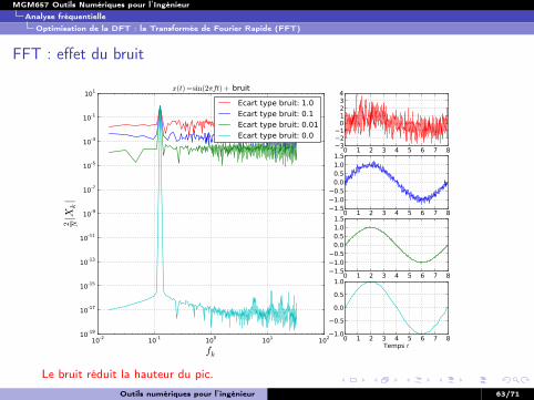
FFT : effet du bruit
10-2 10-1 100 101 102
fk
10-19
10-17
10-15
10-13
10-11
10-9
10-7
10-5
10-3
10-1
101
2 N|X
k|
x(t) =sin(2πft) + bruit
Ecart type bruit: 1.0Ecart type bruit: 0.1Ecart type bruit: 0.01Ecart type bruit: 0.0
0 1 2 3 4 5 6 7 832101234
0 1 2 3 4 5 6 7 81.51.00.50.00.51.01.5
0 1 2 3 4 5 6 7 81.51.00.50.00.51.01.5
0 1 2 3 4 5 6 7 8Temps t
1.0
0.5
0.0
0.5
1.0
Le bruit réduit la hauteur du pic.
Outils numériques pour l’ingénieur 63/71
MGM657 Outils Numériques pour l’IngénieurAnalyse fréquentielle
Optimisation de la DFT : la Transformée de Fourier Rapide (FFT)
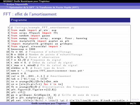
FFT : effet de l’amortissementProgramme
1 # l i s t i n g s /exemple_FFT_amortissement . py2 f rom math impo r t pi , s i n , exp3 f rom s c i p y . f f t p a c k impo r t f f t4 f rom random impo r t gauss5 f rom numpy impo r t a r r ay , arange , f l o o r , hann ing6 f rom ma t p l o t l i b impo r t pyp l o t as p l t7 impo r t ma t p l o t l i b . g r i d s p e c as g r i d s p e c8 f rom s i g n a l _ s i n u s o i d a l impo r t ∗9 beaucoup = 1000
10 f e = 64 . # Frequence d ’ e c h a n t i l l o n a g e11 N = 1024 # Nombre de p o i n t s d ’ e c h a n t i l l o n a g e12 D = N/ f e # Duree d ’ o b s e r v a t i o n13 f = 32 ./D # Frequence du s i g n a l14 t_min = 0 . # Debut du c a l c u l du s i g n a l15 t_max = t_min+D # Fin du c a l c u l du s i g n a l16 s tddev = 0 . # Eca r t type du b r u i t17 nom = ’ ../ figures / FFT_amortissement - hann . pdf ’18 amort = 0 .19 v a l = [ 0 . , . 0 0 1 , . 1 , 1 . ] # Amort i s sement20 l a b = r ’ $1 /\ tau = {0} $ ’21 tn = arange (N) /(D∗ f e )∗D+t_min22 xn = [ s i n (2∗ p i ∗ f ∗ t ) f o r t i n tn ]23 f k = arange (N) /D # D i s c r e t i s a t i o n des f r e q u e n c e s24 p l t . f i g u r e (0 , f i g s i z e =(12 ,8) )25 p l t . c l f ( )26 gs = g r i d s p e c . Gr idSpec (4 , 3) # G r i l l e de zone de t r a c e27 p0 = p l t . s u bp l o t ( gs [ : , : 2 ] )28 p0 . s e t _ t i t l e ( r ’ $x ( t ) = \ sin (2 \ pi f t ) e ^{ t /\ tau } $ avec $ \ tau$ variable +
Hann ’ ) Outils numériques pour l’ingénieur 64/71
MGM657 Outils Numériques pour l’IngénieurAnalyse fréquentielle
Optimisation de la DFT : la Transformée de Fourier Rapide (FFT)
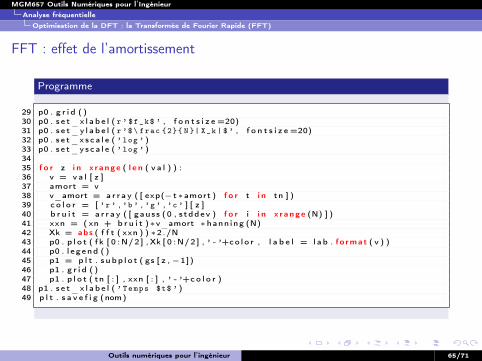
FFT : effet de l’amortissement
Programme
29 p0 . g r i d ( )30 p0 . s e t_x l a b e l ( r ’ $f_k$ ’ , f o n t s i z e =20)31 p0 . s e t_y l a b e l ( r ’$ \ frac {2}{ N }| X_k | $ ’ , f o n t s i z e =20)32 p0 . s e t_x s c a l e ( ’ log ’ )33 p0 . s e t_y s c a l e ( ’ log ’ )3435 f o r z i n x r ange ( l e n ( v a l ) ) :36 v = v a l [ z ]37 amort = v38 v_amort = a r r a y ( [ exp(− t∗amort ) f o r t i n tn ] )39 c o l o r = [ ’r ’ , ’b ’ , ’g ’ , ’c ’ ] [ z ]40 b r u i t = a r r a y ( [ gaus s (0 , s tddev ) f o r i i n x r ange (N) ] )41 xxn = ( xn + b r u i t )∗v_amort ∗hann ing (N)42 Xk = abs ( f f t ( xxn ) ) ∗2./N43 p0 . p l o t ( f k [ 0 :N/2 ] , Xk [ 0 :N/2 ] , ’ - ’+co l o r , l a b e l = l a b . f o rmat ( v ) )44 p0 . l e g end ( )45 p1 = p l t . s u bp l o t ( gs [ z ,−1])46 p1 . g r i d ( )47 p1 . p l o t ( tn [ : ] , xxn [ : ] , ’ - ’+co l o r )48 p1 . s e t_x l a b e l ( ’ Temps $t$ ’ )49 p l t . s a v e f i g (nom)
Outils numériques pour l’ingénieur 65/71
MGM657 Outils Numériques pour l’IngénieurAnalyse fréquentielle
Optimisation de la DFT : la Transformée de Fourier Rapide (FFT)
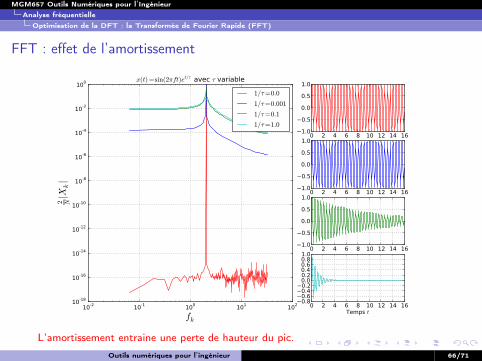
FFT : effet de l’amortissement
10-2 10-1 100 101 102
fk
10-18
10-16
10-14
10-12
10-10
10-8
10-6
10-4
10-2
100
2 N|X
k|
x(t) =sin(2πft)et/τ avec τ variable
1/τ=0.0
1/τ=0.001
1/τ=0.1
1/τ=1.0
0 2 4 6 8 10 12 14 161.0
0.5
0.0
0.5
1.0
0 2 4 6 8 10 12 14 161.0
0.5
0.0
0.5
1.0
0 2 4 6 8 10 12 14 161.0
0.5
0.0
0.5
1.0
0 2 4 6 8 10 12 14 16Temps t
0.80.60.40.20.00.20.40.60.81.0
L’amortissement entraine une perte de hauteur du pic.
Outils numériques pour l’ingénieur 66/71
MGM657 Outils Numériques pour l’IngénieurAnalyse fréquentielle
Optimisation de la DFT : la Transformée de Fourier Rapide (FFT)
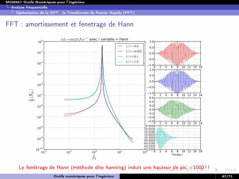
FFT : amortissement et fenetrage de Hann
10-2 10-1 100 101 102
fk
10-10
10-9
10-8
10-7
10-6
10-5
10-4
10-3
10-2
10-1
100
2 N|X
k|
x(t) =sin(2πft)et/τ avec τ variable + Hann
1/τ=0.0
1/τ=0.001
1/τ=0.1
1/τ=1.0
0 2 4 6 8 10 12 14 161.0
0.5
0.0
0.5
1.0
0 2 4 6 8 10 12 14 161.0
0.5
0.0
0.5
1.0
0 2 4 6 8 10 12 14 160.60.40.20.00.20.40.6
0 2 4 6 8 10 12 14 16Temps t
0.0200.0150.0100.0050.0000.0050.0100.0150.020
Le fenêtrage de Hann (méthode dite hanning) induit une hauteur de pic ×1000 ! !Outils numériques pour l’ingénieur 67/71
MGM657 Outils Numériques pour l’IngénieurAnalyse fréquentielle
Optimisation de la DFT : la Transformée de Fourier Rapide (FFT)
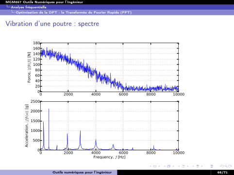
Vibration d’une poutre : spectre
0 2000 4000 6000 8000 10000020406080
100120140160180
Forc
e, |fft
(f)|
[N]
0 2000 4000 6000 8000 10000Frequency, f [Hz]
0
500
1000
1500
2000
2500
Acce
lera
tion,
|fft
(a)|
[g]
Outils numériques pour l’ingénieur 68/71

MGM657 Outils Numériques pour l’IngénieurAnalyse fréquentielle
Optimisation de la DFT : la Transformée de Fourier Rapide (FFT)
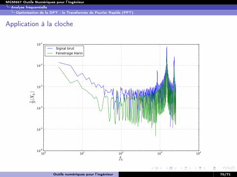
Application à la cloche
1 # l i s t i n g s /exemple_FFT_cloche . py2 f rom s c i p y . f f t p a c k impo r t f f t3 f rom numpy impo r t a r r ay , arange , hann ing4 f rom ma t p l o t l i b impo r t pyp l o t as p l t5 impo r t p i c k l e6 nom = ’ ../ figures / FFT_cloche - log . pdf ’7 f i c h i e r = open ( ’ cloche . pckl ’ , ’r ’ ) # Ouver tu re du f i c h i e r8 c l o c h e = p i c k l e . l o ad ( f i c h i e r ) # Chargement des donnees9 f i c h i e r . c l o s e ( ) # Fermeture du f i c h i e r
10 xn = c l o c h e [ ’x ’ ] [ : : 3 2 ] # Redimens ionnement des donnees11 f e = f l o a t ( c l o c h e [ ’ fe ’ ] ) # D e f i n i t i o n de l a f r e qu en c e d ’ e c h a n t i l l o n a g e12 tn = arange ( l e n ( xn ) ) / f l o a t ( f e )13 N = l e n ( tn )14 D = N/ f e15 p l t . f i g u r e (0 , f i g s i z e =(12 ,8) )16 p l t . c l f ( )17 f k = arange (N) /D # D i s c r e t i s a t i o n des f r e q u e n c e s18 Xk = abs ( f f t ( xn ) ) ∗2./N19 Xkh = abs ( f f t ( xn∗hann ing (N) ) ) ∗2./N20 p l t . p l o t ( f k [ 0 :N/2 ] , Xk [ 0 :N/2 ] , ’ - ’ , l a b e l=’ Signal brut ’ )21 p l t . p l o t ( f k [ 0 :N/2 ] , Xkh [ 0 :N/2 ] , ’ - ’ , l a b e l=’ Fenetrage Hann ’ )22 p l t . x l a b e l ( r ’ $f_k$ ’ , f o n t s i z e =20)23 p l t . y l a b e l ( r ’$ \ frac {2}{ N }| X_k | $ ’ , f o n t s i z e =20)24 p l t . x s c a l e ( ’ log ’ )25 p l t . y s c a l e ( ’ log ’ )26 p l t . g r i d ( True )27 p l t . l e g end ( l o c=’ upper left ’ )28 p l t . s a v e f i g (nom)
Outils numériques pour l’ingénieur 69/71
MGM657 Outils Numériques pour l’IngénieurAnalyse fréquentielle
Optimisation de la DFT : la Transformée de Fourier Rapide (FFT)
Application à la cloche
100 101 102 103 104
fk
10-6
10-5
10-4
10-3
10-2
10-1
2 N|X
k|
Signal brutFenetrage Hann
Outils numériques pour l’ingénieur 70/71
MGM657 Outils Numériques pour l’IngénieurAnalyse fréquentielle
Optimisation de la DFT : la Transformée de Fourier Rapide (FFT)
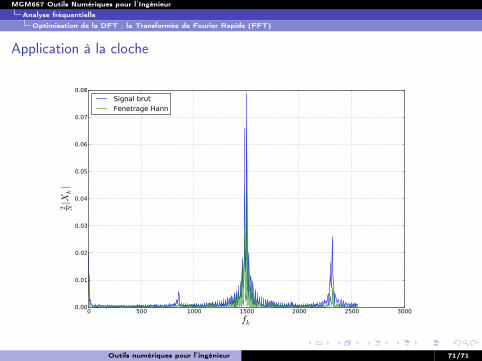
Application à la cloche
0 500 1000 1500 2000 2500 3000fk
0.00
0.01
0.02
0.03
0.04
0.05
0.06
0.07
0.08
2 N|X
k|
Signal brutFenetrage Hann
Outils numériques pour l’ingénieur 71/71