Embed Size (px)
Citation preview
MINITAB Manual ForDavid Moore and George McCabe�s
Introduction ToThe Practice ofStatistics
Michael EvansUniversity of Toronto

ii
Contents
Preface vii
I Minitab for Data Management 11 Manual Overview and Conventions . . . . . . . . . . . . . . . . . 32 Accessing and Exiting Minitab . . . . . . . . . . . . . . . . . . . . 43 Files Used by Minitab . . . . . . . . . . . . . . . . . . . . . . . . . 74 Getting Help . . . . . . . . . . . . . . . . . . . . . . . . . . . . . . 75 The Worksheet . . . . . . . . . . . . . . . . . . . . . . . . . . . . . 86 Minitab Commands . . . . . . . . . . . . . . . . . . . . . . . . . . 107 Entering Data into a Worksheet . . . . . . . . . . . . . . . . . . . 13
7.1 Importing Data . . . . . . . . . . . . . . . . . . . . . . . . 147.2 Patterned Data . . . . . . . . . . . . . . . . . . . . . . . . 187.3 Printing Data in the Session Window . . . . . . . . . . . . 197.4 Assigning Constants . . . . . . . . . . . . . . . . . . . . . . 207.5 Naming Variables and Constants . . . . . . . . . . . . . . . 217.6 Information about a Worksheet . . . . . . . . . . . . . . . 227.7 Editing a Worksheet . . . . . . . . . . . . . . . . . . . . . . 23
8 Saving, Retrieving, and Printing . . . . . . . . . . . . . . . . . . . 269 Recording and Printing Sessions . . . . . . . . . . . . . . . . . . . 2910 Mathematical Operations . . . . . . . . . . . . . . . . . . . . . . . 29
10.1 Arithmetical Operations . . . . . . . . . . . . . . . . . . . 2910.2 Mathematical Functions . . . . . . . . . . . . . . . . . . . 3110.3 Column and Row Statistics . . . . . . . . . . . . . . . . . . 3210.4 Comparisons and Logical Operations . . . . . . . . . . . . 33
11 Some More Minitab Commands . . . . . . . . . . . . . . . . . . . 3511.1 Coding . . . . . . . . . . . . . . . . . . . . . . . . . . . . . 3511.2 Concatenating Columns . . . . . . . . . . . . . . . . . . . 3611.3 Converting Data Types . . . . . . . . . . . . . . . . . . . . 3711.4 History . . . . . . . . . . . . . . . . . . . . . . . . . . . . . 3811.5 Computing Ranks . . . . . . . . . . . . . . . . . . . . . . . 3911.6 Sorting Data . . . . . . . . . . . . . . . . . . . . . . . . . . 4011.7 Stacking and Unstacking Columns . . . . . . . . . . . . . . 41
12 Exercises . . . . . . . . . . . . . . . . . . . . . . . . . . . . . . . . 43
iii
iv CONTENTS
II Minitab for Data Analysis 45
1 Looking at Data–Distributions 471.1 Tabulating and Summarizing Data . . . . . . . . . . . . . . . . . 48
1.1.1 Tallying Data . . . . . . . . . . . . . . . . . . . . . . . . . 491.1.2 Describing Data . . . . . . . . . . . . . . . . . . . . . . . 51
1.2 Plotting Data in a Graph Window . . . . . . . . . . . . . . . . . 531.2.1 Dotplots . . . . . . . . . . . . . . . . . . . . . . . . . . . . 531.2.2 Stem-and-Leaf Plots . . . . . . . . . . . . . . . . . . . . . 541.2.3 Histograms . . . . . . . . . . . . . . . . . . . . . . . . . . 551.2.4 Boxplots . . . . . . . . . . . . . . . . . . . . . . . . . . . . 571.2.5 Time Series Plots . . . . . . . . . . . . . . . . . . . . . . . 591.2.6 Bar Charts . . . . . . . . . . . . . . . . . . . . . . . . . . 601.2.7 Pie Charts . . . . . . . . . . . . . . . . . . . . . . . . . . 60
1.3 The Normal Distribution . . . . . . . . . . . . . . . . . . . . . . . 601.3.1 Calculating the Density . . . . . . . . . . . . . . . . . . . 611.3.2 Calculating the Distribution Function . . . . . . . . . . . 621.3.3 Calculating the Inverse Distribution Function . . . . . . . 621.3.4 Normal Probability Plots . . . . . . . . . . . . . . . . . . 63
1.4 Exercises . . . . . . . . . . . . . . . . . . . . . . . . . . . . . . . 64
2 Looking at Data–Relationships 672.1 Scatterplots . . . . . . . . . . . . . . . . . . . . . . . . . . . . . . 672.2 Correlations . . . . . . . . . . . . . . . . . . . . . . . . . . . . . . 702.3 Regression . . . . . . . . . . . . . . . . . . . . . . . . . . . . . . . 702.4 Transformations . . . . . . . . . . . . . . . . . . . . . . . . . . . 742.5 Exercises . . . . . . . . . . . . . . . . . . . . . . . . . . . . . . . 75
3 Producing Data 773.1 Generating a Random Sample . . . . . . . . . . . . . . . . . . . . 783.2 Sampling from Distributions . . . . . . . . . . . . . . . . . . . . . 803.3 Exercises . . . . . . . . . . . . . . . . . . . . . . . . . . . . . . . 82
4 Probability: The Study of Randomness 854.1 Basic Probability Calculations . . . . . . . . . . . . . . . . . . . . 854.2 More on Sampling from Distributions . . . . . . . . . . . . . . . 864.3 Simulation for Approximating Probabilities . . . . . . . . . . . . 894.4 Simulation for Approximating Means . . . . . . . . . . . . . . . . 904.5 Exercises . . . . . . . . . . . . . . . . . . . . . . . . . . . . . . . 91
5 Sampling Distributions 955.1 The Binomial Distribution . . . . . . . . . . . . . . . . . . . . . . 955.2 Simulating Sampling Distributions . . . . . . . . . . . . . . . . . 985.3 Exercises . . . . . . . . . . . . . . . . . . . . . . . . . . . . . . . 102
CONTENTS v
6 Introduction to Inference 1056.1 z-ConÞdence Intervals . . . . . . . . . . . . . . . . . . . . . . . . 1056.2 z-Tests . . . . . . . . . . . . . . . . . . . . . . . . . . . . . . . . . 1076.3 Simulations for ConÞdence Intervals . . . . . . . . . . . . . . . . 1096.4 Simulations for Power Calculations . . . . . . . . . . . . . . . . . 1106.5 The Chi-Square Distribution . . . . . . . . . . . . . . . . . . . . 1136.6 Exercises . . . . . . . . . . . . . . . . . . . . . . . . . . . . . . . 114
7 Inference for Distributions 1177.1 The Student Distribution . . . . . . . . . . . . . . . . . . . . . . 1177.2 t-ConÞdence Intervals . . . . . . . . . . . . . . . . . . . . . . . . 1187.3 t-Tests . . . . . . . . . . . . . . . . . . . . . . . . . . . . . . . . . 1197.4 The Sign Test . . . . . . . . . . . . . . . . . . . . . . . . . . . . . 1207.5 Comparing Two Samples . . . . . . . . . . . . . . . . . . . . . . 1227.6 The F -Distribution . . . . . . . . . . . . . . . . . . . . . . . . . . 1257.7 Exercises . . . . . . . . . . . . . . . . . . . . . . . . . . . . . . . 126
8 Inference for Proportions 1298.1 Inference for a Single Proportion . . . . . . . . . . . . . . . . . . 1298.2 Inference for Two Proportions . . . . . . . . . . . . . . . . . . . . 1318.3 Exercises . . . . . . . . . . . . . . . . . . . . . . . . . . . . . . . 133
9 Inference for Two-Way Tables 1359.1 Tabulating and Plotting . . . . . . . . . . . . . . . . . . . . . . . 1359.2 The Chi-square Test . . . . . . . . . . . . . . . . . . . . . . . . . 1389.3 Analyzing Tables of Counts . . . . . . . . . . . . . . . . . . . . . 1419.4 Exercises . . . . . . . . . . . . . . . . . . . . . . . . . . . . . . . 143
10 Inference for Regression 14510.1 Simple Regression Analysis . . . . . . . . . . . . . . . . . . . . . 14510.2 Exercises . . . . . . . . . . . . . . . . . . . . . . . . . . . . . . . 152
11 Multiple Regression 15511.1 Example . . . . . . . . . . . . . . . . . . . . . . . . . . . . . . . . 15511.2 Exercises . . . . . . . . . . . . . . . . . . . . . . . . . . . . . . . 160
12 One-Way Analysis of Variance 16312.1 A Categorical Variable and a Quantitative Variable . . . . . . . . 16312.2 One-Way Analysis of Variance . . . . . . . . . . . . . . . . . . . 16612.3 Exercises . . . . . . . . . . . . . . . . . . . . . . . . . . . . . . . 171
13 Two-Way Analysis of Variance 17313.1 The Two-Way ANOVA Command . . . . . . . . . . . . . . . . . 17313.2 Exercises . . . . . . . . . . . . . . . . . . . . . . . . . . . . . . . 177
vi CONTENTS
14 Nonparametric Tests 17914.1 The Wilcoxon Rank Sum Procedures . . . . . . . . . . . . . . . . 17914.2 The Wilcoxon Signed Rank Procedures . . . . . . . . . . . . . . . 18114.3 The Kruskal-Wallis Test . . . . . . . . . . . . . . . . . . . . . . . 18214.4 Exercises . . . . . . . . . . . . . . . . . . . . . . . . . . . . . . . 183
15 Logistic Regression 18515.1 The Logistic Regression Model . . . . . . . . . . . . . . . . . . . 18515.2 Example . . . . . . . . . . . . . . . . . . . . . . . . . . . . . . . . 18615.3 Exercises . . . . . . . . . . . . . . . . . . . . . . . . . . . . . . . 188
Appendices 191
A Projects 191
B Mathematical and Statistical Functions in Minitab 193B.1 Mathematical Functions . . . . . . . . . . . . . . . . . . . . . . . 193B.2 Column Statistics . . . . . . . . . . . . . . . . . . . . . . . . . . . 194B.3 Row Statistics . . . . . . . . . . . . . . . . . . . . . . . . . . . . . 195
C Macros and Execs 197C.1 Global Macros . . . . . . . . . . . . . . . . . . . . . . . . . . . . 197
C.1.1 Control Statements . . . . . . . . . . . . . . . . . . . . . . 198C.1.2 Startup Macro . . . . . . . . . . . . . . . . . . . . . . . . 202C.1.3 Interactive Macros . . . . . . . . . . . . . . . . . . . . . . 202
C.2 Local Macros . . . . . . . . . . . . . . . . . . . . . . . . . . . . . 203C.3 Execs . . . . . . . . . . . . . . . . . . . . . . . . . . . . . . . . . 203
C.3.1 Creating and Using an Exec . . . . . . . . . . . . . . . . . 203C.3.2 The CK Capability for Looping . . . . . . . . . . . . . . . 204C.3.3 Interactive Execs . . . . . . . . . . . . . . . . . . . . . . . 205C.3.4 Startup Execs . . . . . . . . . . . . . . . . . . . . . . . . . 206
D Matrix Algebra in Minitab 207D.1 Creating Matrices . . . . . . . . . . . . . . . . . . . . . . . . . . 208D.2 Commands for Matrix Operations . . . . . . . . . . . . . . . . . 210
E Advanced Statistical Methods in Minitab 213
F References 215
Index 216

Preface
This Minitab manual is to be used as an accompaniment to Introduction tothe Practice of Statistics, Fourth Edition, by David S. Moore and George P.McCabe, and to the CD-ROM that accompanies this text. We abbreviate thetextbook title as IPS.Minitab is a statistical software package that was designed especially for the
teaching of introductory statistics courses. It is our view that an easy-to-usestatistical software package is a vital and signiÞcant component of such a course.This permits the student to focus on statistical concepts and thinking ratherthan computations or the learning of a statistical package. The main aim of anyintroductory statistics course should always be the �why� of statistics ratherthan technical details that do little to stimulate the majority of students or, inour opinion, do little to reinforce the key concepts. IPS succeeds admirably incommunicating the important basic foundations of statistical thinking, and it ishoped that this manual serves as a useful adjunct to the text.It is natural to ask why Minitab is advocated for the course. In the author�s
experience, ease of learning and use are the salient features of the package, withobvious beneÞts to the student and to the instructor, who can relegate manydetails to the software. While more sophisticated packages are necessary forhigher-level professional work, it is our experience that attempting to teach oneof these in a course forces too much attention on technical aspects. The timestudents need to spend to learn Minitab is relatively small and that it is a greatvirtue. Further Minitab will serve as a perfectly adequate tool for many of thestatistical problems students will encounter in their undergraduate education.This manual is divided into two parts. Part I is an introduction that pro-
vides the necessary details to start using Minitab and in particular how to useworksheets. Not all the material in Part I needs to be absorbed on Þrst reading.We recommend reading I.1�I.10 before starting to use Minitab. The materialin I.11 is more for reference and for later reading. References are made to thesesections later in the manual and can provide the stimulus to read them. Overall,the introductory Part I also serves as a reference for most of the nonstatisticalcommands in Minitab.
vii
viii
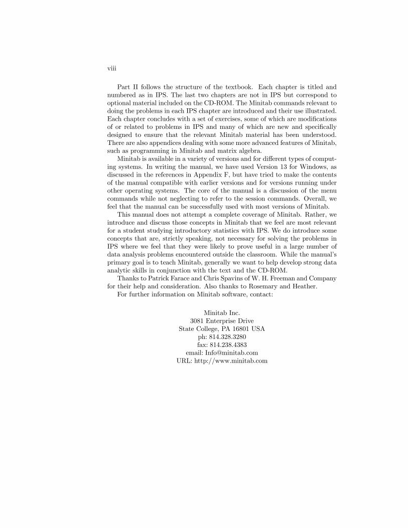
Part II follows the structure of the textbook. Each chapter is titled andnumbered as in IPS. The last two chapters are not in IPS but correspond tooptional material included on the CD-ROM. The Minitab commands relevant todoing the problems in each IPS chapter are introduced and their use illustrated.Each chapter concludes with a set of exercises, some of which are modiÞcationsof or related to problems in IPS and many of which are new and speciÞcallydesigned to ensure that the relevant Minitab material has been understood.There are also appendices dealing with some more advanced features of Minitab,such as programming in Minitab and matrix algebra.Minitab is available in a variety of versions and for different types of comput-
ing systems. In writing the manual, we have used Version 13 for Windows, asdiscussed in the references in Appendix F, but have tried to make the contentsof the manual compatible with earlier versions and for versions running underother operating systems. The core of the manual is a discussion of the menucommands while not neglecting to refer to the session commands. Overall, wefeel that the manual can be successfully used with most versions of Minitab.This manual does not attempt a complete coverage of Minitab. Rather, we
introduce and discuss those concepts in Minitab that we feel are most relevantfor a student studying introductory statistics with IPS. We do introduce someconcepts that are, strictly speaking, not necessary for solving the problems inIPS where we feel that they were likely to prove useful in a large number ofdata analysis problems encountered outside the classroom. While the manual�sprimary goal is to teach Minitab, generally we want to help develop strong dataanalytic skills in conjunction with the text and the CD-ROM.Thanks to Patrick Farace and Chris Spavins of W. H. Freeman and Company
for their help and consideration. Also thanks to Rosemary and Heather.For further information on Minitab software, contact:
Minitab Inc.3081 Enterprise Drive
State College, PA 16801 USAph: 814.328.3280fax: 814.238.4383
email: [email protected]: http://www.minitab.com

Part I
Minitab for DataManagement
1

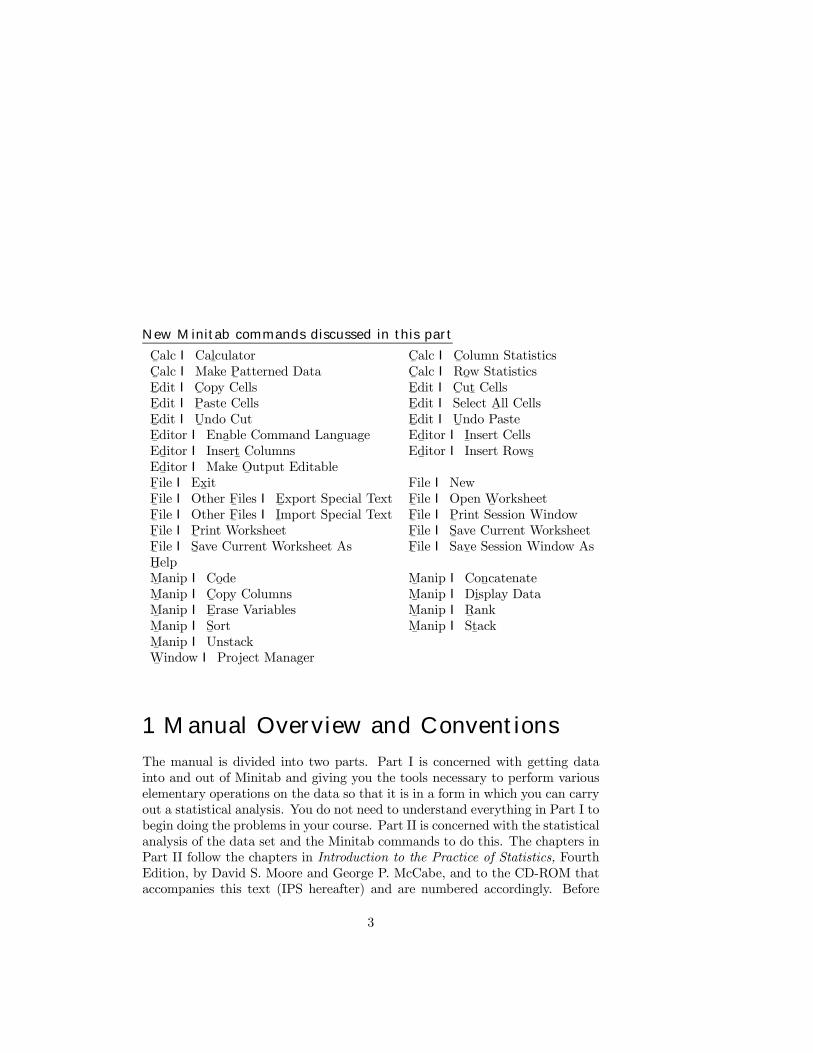
New Minitab commands discussed in this part
C¯alc I Cal
¯culator C
¯alc I C
¯olumn Statistics
C¯alc I Make P
¯atterned Data C
¯alc I Ro
¯w Statistics
E¯dit I C
¯opy Cells E
¯dit I C
¯ut¯Cells
E¯dit I P
¯aste Cells E
¯dit I Select A
¯ll Cells
E¯dit I U
¯ndo Cut E
¯dit I U
¯ndo Paste
E¯ditor I Ena
¯ble Command Language Ed
¯itor I I
¯nsert Cells
Ed¯itor I Insert
¯Columns Ed
¯itor I Insert Rows
¯Ed¯itor I Make O
¯utput Editable
F¯ile I Ex
¯it File I New
F¯ile I Other F
¯iles I E
¯xport Special Text F
¯ile I Open W
¯orksheet
F¯ile I Other F
¯iles I I
¯mport Special Text F
¯ile I P
¯rint Session Window
F¯ile I P
¯rint Worksheet F
¯ile I S
¯ave Current Worksheet
F¯ile I S
¯ave Current Worksheet As F
¯ile I Sav
¯e Session Window As
H¯elpM¯anip I Co
¯de M
¯anip I Con
¯catenate
M¯anip I C
¯opy Columns M
¯anip I Di
¯splay Data
M¯anip I E
¯rase Variables M
¯anip I R
¯ank
M¯anip I S
¯ort M
¯anip I St
¯ack
M¯anip I Unstack
W¯indow I Project Manager
1 Manual Overview and ConventionsThe manual is divided into two parts. Part I is concerned with getting datainto and out of Minitab and giving you the tools necessary to perform variouselementary operations on the data so that it is in a form in which you can carryout a statistical analysis. You do not need to understand everything in Part I tobegin doing the problems in your course. Part II is concerned with the statisticalanalysis of the data set and the Minitab commands to do this. The chapters inPart II follow the chapters in Introduction to the Practice of Statistics, FourthEdition, by David S. Moore and George P. McCabe, and to the CD-ROM thataccompanies this text (IPS hereafter) and are numbered accordingly. Before
3
4 Minitab for Data Management
you start on Chapter II.1, however, you should read I.1�I.10 and leave I.11 forlater reading.Minitab is a software package that runs on a variety of different types of
computers and comes in a number of versions. This manual does not try todescribe all the possible implementations or the full extent of the package. Welimit our discussion to those features common to the most recent versions ofMinitab and, in particular, Versions 12 and 13. Also, we present only thoseaspects of Minitab relevant to carrying out the statistical analyses discussed inIPS. Of course, this is a fairly wide range of analyses, but the full power ofMinitab is not necessary. Depending on the version of Minitab you are using,there may be many more useful features, and we encourage you to learn anduse them. Throughout the manual, we point out what some of the additionaluseful features of Minitab are and how you can go about learning how to usethem. Version 13 refers to the most current version of Minitab at the time ofwriting this manual.In this manual, special statistical or Minitab concepts will be highlighted in
italic font. You should be sure that you understand these concepts. We willprovide a brief explanation for any terms not deÞned in IPS. When a reference ismade to a Minitab session command or subcommand , its name will be in boldfont. Primarily, we will be discussing the menu commands that are available inMinitab. Menu commands are accessed by clicking the left button of the mouseon items in lists. We use a special notation for menu commands. For example,
A I B I C
is to be interpreted as left click the command A on the menu bar, then in the listthat drops down, left click the command B, and, Þnally, left click C. The menucommands will be denoted in ordinary font (the actual appearance may varyslightly depending on the version of Windows you use). Any commands thatwe type and the output obtained will be denoted in typewriter font, as willthe names of any Þles used by Minitab, variables, constants, and worksheets.At the end of each chapter, we provide a few exercises that can be used to
make sure you have understood the material. We recommend, however, thatwhenever possible you use Minitab to do the problems in IPS. While manyproblems can be done by hand, you will save a considerable amount of time andavoid errors by learning to use Minitab effectively. We also recommend thatyou try out the Minitab commands as you read about them, as this will ensurefull understanding.
2 Accessing and Exiting MinitabThe Þrst thing you should do is Þnd out how to access the Minitab package foryour course. This information will come from your instructor, system personnel,or from your software documentation if you have purchased Minitab to run onyour own computer.
Minitab for Data Management 5
In some cases, this may mean you type a command such as minitab ata computer system prompt and then hit the Enter or Return key on the key-board after you have logged on, i.e., provided a login name and password to thecomputer system being used in your course. Typically, you will see the prompt
MTB >
on your screen, and this indicates that you have started a Minitab session.In most cases, you will double click an icon, such as that shown in Display
I.1, that corresponds to the Minitab program.
Display I.1: Minitab icon.
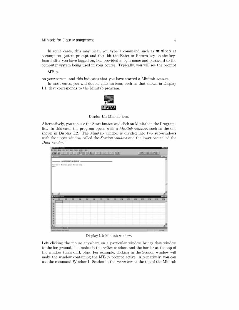
Alternatively, you can use the Start button and click on Minitab in the Programslist. In this case, the program opens with a Minitab window, such as the oneshown in Display I.2. The Minitab window is divided into two sub-windowswith the upper window called the Session window and the lower one called theData window.
Display I.2: Minitab window.
Left clicking the mouse anywhere on a particular window brings that windowto the foreground, i.e., makes it the active window, and the border at the top ofthe window turns dark blue. For example, clicking in the Session window willmake the window containing the MTB > prompt active. Alternatively, you canuse the command W
¯indow I Session in the menu bar at the top of the Minitab
6 Minitab for Data Management
window to make this window active. You may not see the MTB > prompt inyour Session window, and for this manual it is important that you do so. Youcan ensure that this prompt always appears in your Session window by usingE¯dit I Preferences
¯, doubleclick on Session Window in the Preferences list that
comes up, clicking on the E¯nable radio button under Command Language in
the Session Window Preferences, clicking on O¯K, and clicking on Sa
¯ve. Without
the MTB > prompt, you cannot type commands to be executed in the Sessionwindow.In the session window, Minitab commands are typed after the MTB > prompt
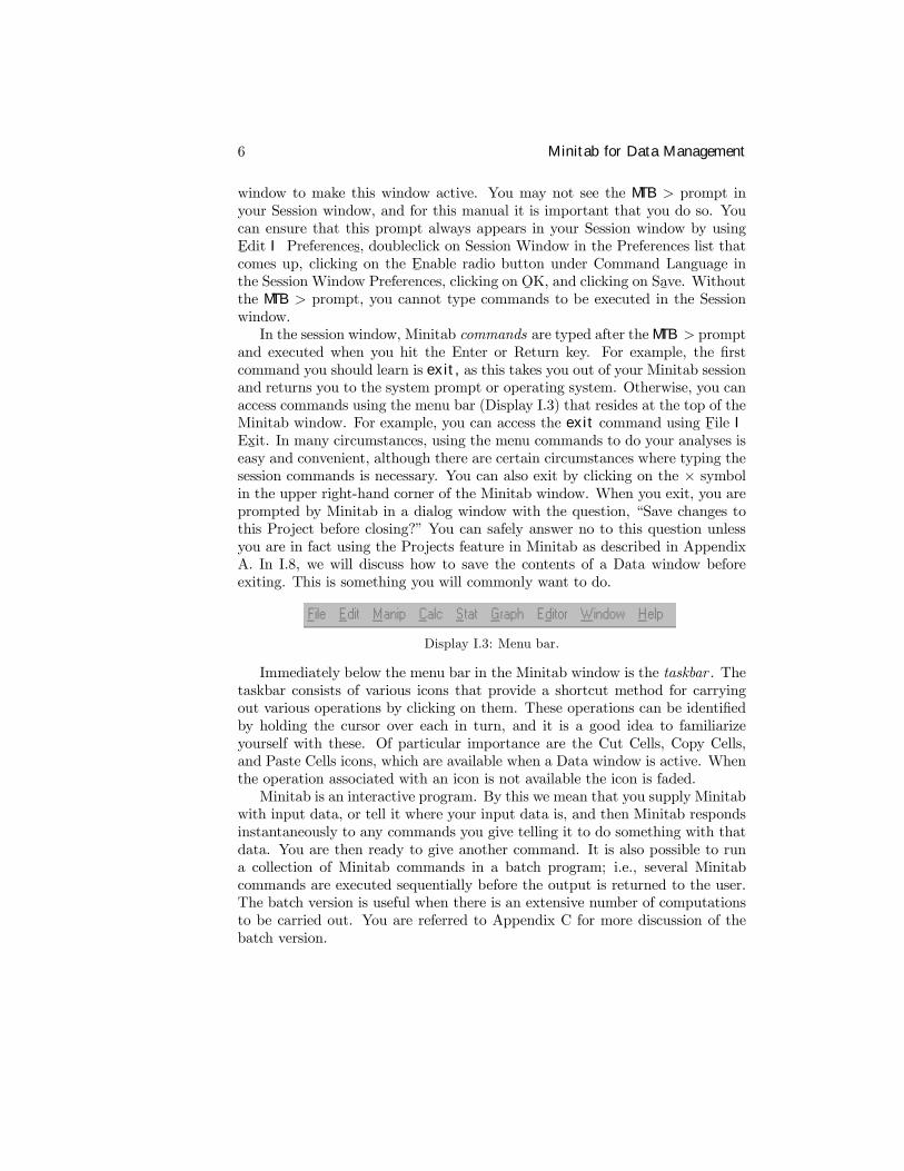
and executed when you hit the Enter or Return key. For example, the Þrstcommand you should learn is exit, as this takes you out of your Minitab sessionand returns you to the system prompt or operating system. Otherwise, you canaccess commands using the menu bar (Display I.3) that resides at the top of theMinitab window. For example, you can access the exit command using F
¯ile I
Ex¯it. In many circumstances, using the menu commands to do your analyses is
easy and convenient, although there are certain circumstances where typing thesession commands is necessary. You can also exit by clicking on the × symbolin the upper right-hand corner of the Minitab window. When you exit, you areprompted by Minitab in a dialog window with the question, �Save changes tothis Project before closing?� You can safely answer no to this question unlessyou are in fact using the Projects feature in Minitab as described in AppendixA. In I.8, we will discuss how to save the contents of a Data window beforeexiting. This is something you will commonly want to do.
Display I.3: Menu bar.
Immediately below the menu bar in the Minitab window is the taskbar. Thetaskbar consists of various icons that provide a shortcut method for carryingout various operations by clicking on them. These operations can be identiÞedby holding the cursor over each in turn, and it is a good idea to familiarizeyourself with these. Of particular importance are the Cut Cells, Copy Cells,and Paste Cells icons, which are available when a Data window is active. Whenthe operation associated with an icon is not available the icon is faded.Minitab is an interactive program. By this we mean that you supply Minitab
with input data, or tell it where your input data is, and then Minitab respondsinstantaneously to any commands you give telling it to do something with thatdata. You are then ready to give another command. It is also possible to runa collection of Minitab commands in a batch program; i.e., several Minitabcommands are executed sequentially before the output is returned to the user.The batch version is useful when there is an extensive number of computationsto be carried out. You are referred to Appendix C for more discussion of thebatch version.
Minitab for Data Management 7
3 Files Used by MinitabMinitab can accept input from a variety of Þles and write output to a variety ofÞles. Each Þle is distinguished by a Þle name and an extension that indicatesthe type of Þle it is. For example, marks.mtw is the name of a Þle that wouldbe referred to as �marks� (note the single quotes around the Þle name) withinMinitab. The extension .mtw indicates that this is a Minitab worksheet. Wedescribe what a worksheet is in I.5. This Þle is stored somewhere on the harddrive of a computer as a Þle called marks.mtw.There are other Þles that you will want to access from outside Minitab,
perhaps to print them out on a printer. Depending on the version of Minitabyou are using, to do this, you may have to exit Minitab and give the relevantsystem print command together with the full path name of the Þle you wish toprint. As various implementations of Minitab differ as to where these Þles arestored on the hard drive, you will have to determine this information from yourinstructor or documentation or systems person. For example, in the windowsenvironment the full path name of the Þle could be
c:\Program Files\MTBWIN\Data\marks.mtw
or something similar. This path name indicates that the Þle marks.mtw is storedon the C hard drive in the directory called Program Files\Mtbwin\Data. Wewill discuss several different types of Þles in this chapter.In many versions of Minitab, there are restrictions on Þle names. For ex-
ample, in earlier versions a Þle name can be at most eight characters in lengthusing any symbols except # and � and the Þrst character cannot be a blank.There is no length restriction on Þle names in Versions 12 or 13. It is generallybest to name your Þles so that the Þle name reßects its contents. For example,the Þle name marks may refer to a data set composed of student marks in anumber of courses.
4 Getting HelpAt times, you may want more information about a command or some otheraspect of Minitab than this manual provides, or you may wish to remind yourselfof some detail that you have partially forgotten. Minitab contains an onlinemanual that is very convenient. You can access this information directly byclicking on H
¯elp in the Menu bar and using the table of
¯Contents or doing a
S¯earch of the manual for a particular concept.From the MTB > prompt, you can use the help command for this purpose.
Typing help followed by the name of the command of interest and hitting Enterwill cause Minitab to produce relevant output. For example, asking for help onthe command help itself via the command
MTB >help help
8 Minitab for Data Management
will give you an overview of what help information can be accessed on yoursystem. The help command should be used to Þnd out about session commands.
5 The WorksheetThe basic structural component of Minitab is the worksheet . Basically, theworksheet can be thought of as a big rectangular array, or matrix, of cellsorganized into rows and columns as in the Data window of Display I.2. Each cellholds one piece of data. This piece of data could be a number, i.e. numeric data,or it could be a sequence of characters, such as a word or an arbitrary sequenceof letters and numbers, i.e., text data. Data often comes as numbers, such as1.7, 2.3, . . . but sometimes it comes in the form of a sequence of characters,such as black, brown, red, etc. Typically, sequences of characters are used asidentiÞers in classiÞcations for some variable of interest, e.g., color, gender. Apiece of text data can be up to 80 characters in length in Minitab. Version 13also allows for date data, which is data especially formatted to indicate a date,for example, 3/4/97. We will not discuss date data.If possible, try to avoid using text data with Minitab, i.e., make sure all
the values of a variable are numbers, as dealing with text data in Minitab ismore difficult. For example, denote colors by numbers rather than by names.Still there will be applications where data comes to you as text data, e.g., ina computer Þle, and it is too extensive to convert to numeric data. So we willdiscuss how to input text data into a Minitab worksheet, but we recommendthat in such cases you convert this to numeric data, using the methods of I.11.3,once it has been input. In Version 13 of Minitab it is somewhat easier to dealwith text data than earlier versions, and this proviso is not as necessary.Display I.4 provides an example of a worksheet. Notice that the columns are
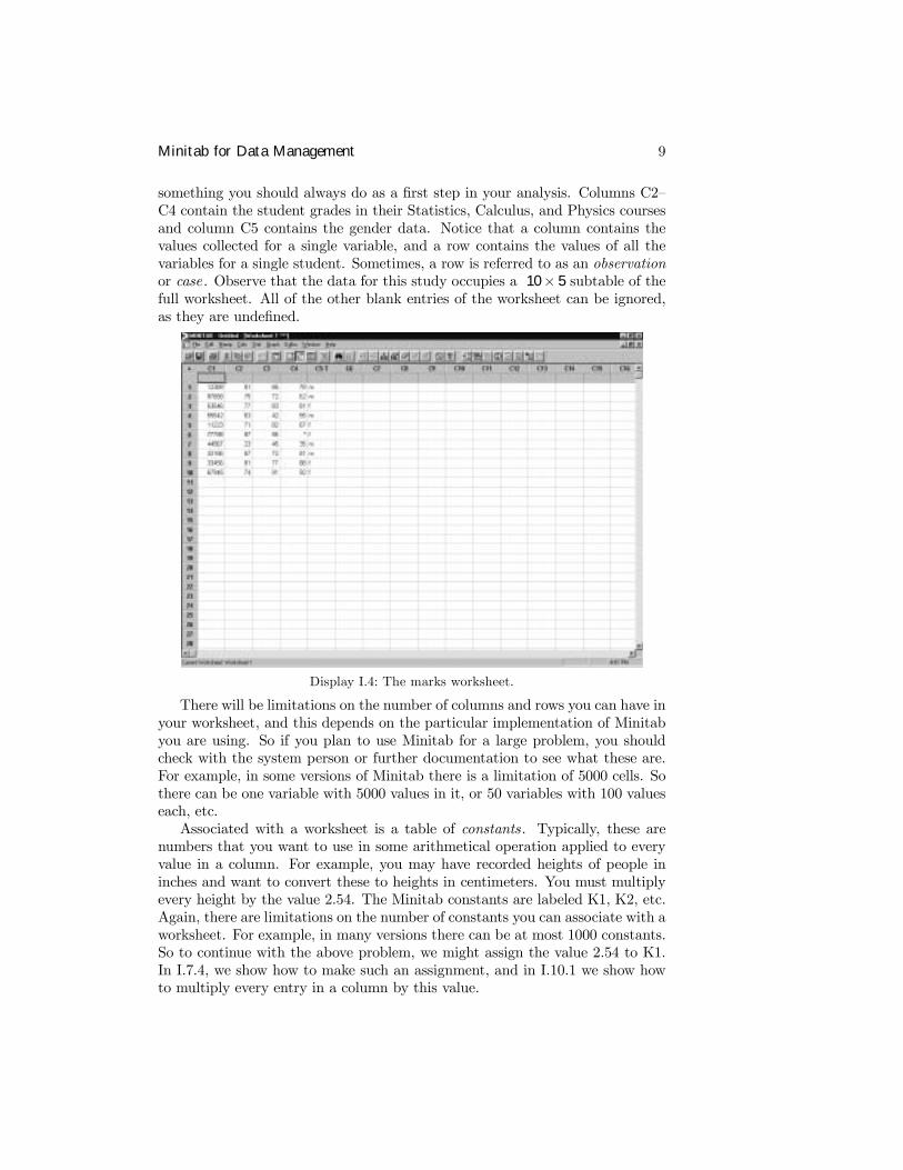
labeled C1, C2, etc. and the rows are labeled 1, 2, 3, etc. We will refer to theworksheet depicted in Display I.4 as the marks worksheet hereafter and will useit throughout Part I to illustrate various Minitab commands and operations.Data arises from the process of taking measurements of variables in some
real-world context. For example, in a population of students, suppose that weare conducting a study of academic performance in a Statistics course. Specif-ically, suppose that we want to examine the relationship between grades inStatistics, grades in a Calculus course, grades in a Physics course and gender.So we collect the following information for each student in the study: studentnumber, grade in Statistics, grade in Calculus, grade in Physics, and gender.Therefore, we have 5 variables � student number and the grades in the threesubjects are numeric variables, and gender is a text variable. Let us furthersuppose that there are 10 students in the study.Display I.4 gives a possible outcome from collecting the data in such a study.
Column C1 contains the student number (note that this is a categorical vari-able even though it is a number). The student number primarily serves as anidentiÞer so that we can check that the data has been entered correctly. This is
Minitab for Data Management 9
something you should always do as a Þrst step in your analysis. Columns C2�C4 contain the student grades in their Statistics, Calculus, and Physics coursesand column C5 contains the gender data. Notice that a column contains thevalues collected for a single variable, and a row contains the values of all thevariables for a single student. Sometimes, a row is referred to as an observationor case. Observe that the data for this study occupies a 10× 5 subtable of thefull worksheet. All of the other blank entries of the worksheet can be ignored,as they are undeÞned.
Display I.4: The marks worksheet.
There will be limitations on the number of columns and rows you can have inyour worksheet, and this depends on the particular implementation of Minitabyou are using. So if you plan to use Minitab for a large problem, you shouldcheck with the system person or further documentation to see what these are.For example, in some versions of Minitab there is a limitation of 5000 cells. Sothere can be one variable with 5000 values in it, or 50 variables with 100 valueseach, etc.Associated with a worksheet is a table of constants. Typically, these are
numbers that you want to use in some arithmetical operation applied to everyvalue in a column. For example, you may have recorded heights of people ininches and want to convert these to heights in centimeters. You must multiplyevery height by the value 2.54. The Minitab constants are labeled K1, K2, etc.Again, there are limitations on the number of constants you can associate with aworksheet. For example, in many versions there can be at most 1000 constants.So to continue with the above problem, we might assign the value 2.54 to K1.In I.7.4, we show how to make such an assignment, and in I.10.1 we show howto multiply every entry in a column by this value.
10 Minitab for Data Management
In Version 13 of Minitab, there is an additional structure beyond the work-sheet called the project . A project can have multiple worksheets associated withit. Also, a project can have associated with it various graphs and records of thecommands you have typed and the output obtained while working on the work-sheets. Projects, which are discussed in Appendix A, can be saved and retrievedfor later work. Projects .
6 Minitab CommandsWe will now begin to introduce various Minitab commands to get data into aworksheet, edit a worksheet, perform various operations on the elements of aworksheet, and save and access a saved worksheet. Before we do, however, it isuseful to know something about the basic structure of all Minitab commands.Associated with every command is of course its name, as in F
¯ile I Ex
¯it and
H¯elp. Most commands also take arguments, and these arguments are columnnames, constants, and sometimes Þle names.Commands can be accessed by making use of the F
¯ile, E
¯dit, M
¯anip, C
¯alc,
S¯tat, G
¯raph and E
¯ditor entries in the menu bar. Clicking any of these brings
up a list of commands that you can use to operate on your worksheet. The liststhat appear may depend on which window is active, e.g., either a Data windowor the Session window. Unless otherwise speciÞed, we will always assume thatthe Session window is active when discussing menu commands. If a commandname in a list is faded, then it is not available.Typically, using a command from the menu bar requires the use of a dialog
box or dialog window that opens when you click on a command in the list.These are used to provide the arguments and subcommands to the commandand specify where the output is to go. Dialog boxes have various boxes thatmust be Þlled in to correctly execute a command. Clicking in a box that needsto be Þlled in typically causes a variable list to appear in the left-most box, ofall items in the active worksheet that can be placed in that box. Double clickingon items in the variable list places them in the box, or, alternatively, you cantype them in directly. When you have Þlled in the dialog box and clicked O
¯K,
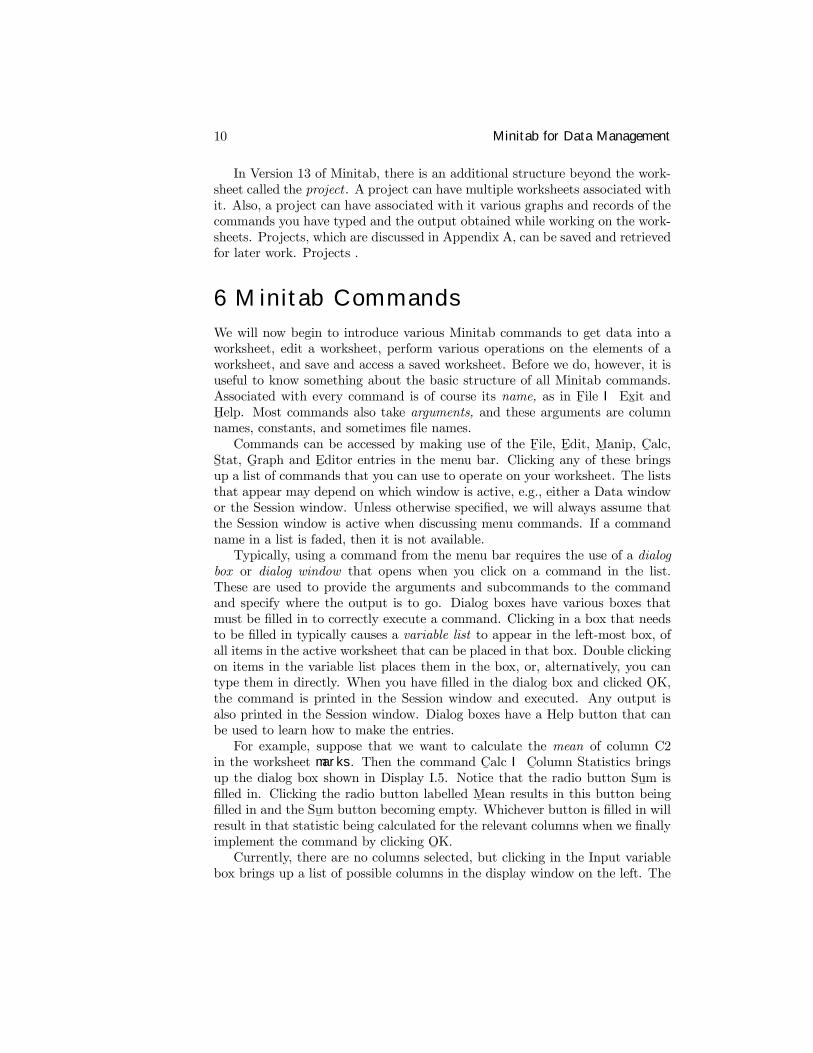
the command is printed in the Session window and executed. Any output isalso printed in the Session window. Dialog boxes have a Help button that canbe used to learn how to make the entries.For example, suppose that we want to calculate the mean of column C2
in the worksheet marks. Then the command C¯alc I C
¯olumn Statistics brings
up the dialog box shown in Display I.5. Notice that the radio button Su¯m is
Þlled in. Clicking the radio button labelled M¯ean results in this button being
Þlled in and the Su¯m button becoming empty. Whichever button is Þlled in will
result in that statistic being calculated for the relevant columns when we Þnallyimplement the command by clicking O
¯K.
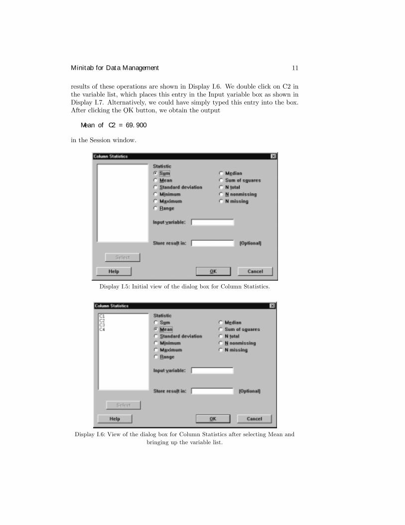
Currently, there are no columns selected, but clicking in the Input variablebox brings up a list of possible columns in the display window on the left. The
Minitab for Data Management 11
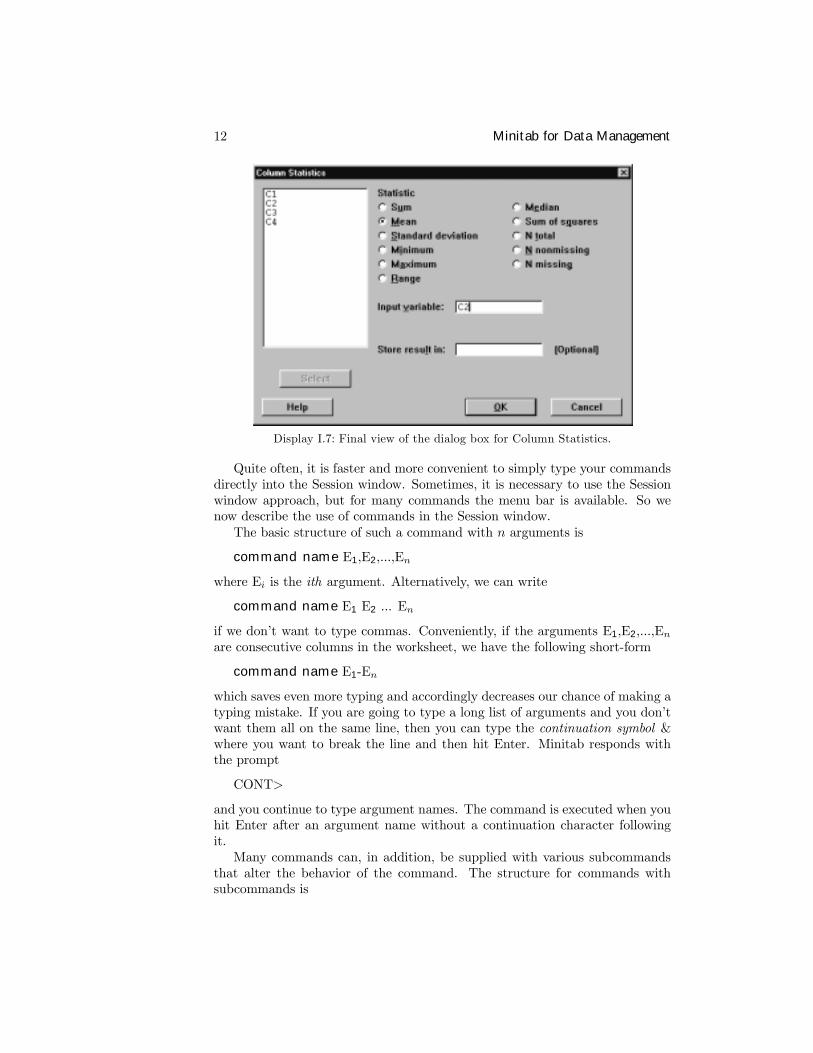
results of these operations are shown in Display I.6. We double click on C2 inthe variable list, which places this entry in the Input v
¯ariable box as shown in
Display I.7. Alternatively, we could have simply typed this entry into the box.After clicking the O
¯K button, we obtain the output
Mean of C2 = 69.900
in the Session window.
Display I.5: Initial view of the dialog box for Column Statistics.
Display I.6: View of the dialog box for Column Statistics after selecting Mean andbringing up the variable list.
12 Minitab for Data Management
Display I.7: Final view of the dialog box for Column Statistics.
Quite often, it is faster and more convenient to simply type your commandsdirectly into the Session window. Sometimes, it is necessary to use the Sessionwindow approach, but for many commands the menu bar is available. So wenow describe the use of commands in the Session window.The basic structure of such a command with n arguments is
command name E1,E2,...,En
where Ei is the ith argument. Alternatively, we can write
command name E1 E2 ... En
if we don�t want to type commas. Conveniently, if the arguments E1,E2,...,Enare consecutive columns in the worksheet, we have the following short-form
command name E1-En
which saves even more typing and accordingly decreases our chance of making atyping mistake. If you are going to type a long list of arguments and you don�twant them all on the same line, then you can type the continuation symbol &where you want to break the line and then hit Enter. Minitab responds withthe prompt
CONT>
and you continue to type argument names. The command is executed when youhit Enter after an argument name without a continuation character followingit.Many commands can, in addition, be supplied with various subcommands
that alter the behavior of the command. The structure for commands withsubcommands is
Minitab for Data Management 13
command name E1 ... En1 ;subcommand name En1+1 ... En2
;...
subcommand name Enk−1+1 ... Enk .
Notice that when there are subcommands each line ends with a semicolon untilthe last subcommand, which ends with a period. Also, subcommands may havearguments. When Minitab encounters a line ending in a semicolon it expects asubcommand on the next line and changes the prompt to
SUBC >
until it encounters a period, whereupon it executes the command. If whiletyping in one of your subcommands you suddenly decide that you would rathernot execute the subcommand � perhaps you realize something was wrong on aprevious line � then type abort after the SUBC > prompt and hit Enter. Asa further convenience, it is worth noting that you need to only type in the Þrstfour letters of any Minitab command or subcommand.For example, to calculate the mean of column C2 in the worksheet marks
we can use the mean command in the Session window, as in
MTB > mean c2
and we obtain the same output in the Session window as before.There are two additional ways in which you can input commands to Minitab.
Instead of typing the commands directly into the Session window, you can alsotype these directly into the Command Line Editor, which is available via E
¯dit
I Com¯mand Line Editor. Multiple commands can then be typed directly into a
box that pops up and executed when the S¯ubmit Commands button is clicked.
Output appears in the Session window. Also, many commands are available ona toolbar that lies just below the menu bar at the top of the Minitab window.There is a different toolbar depending upon which window is active. We give abrief discussion of some of the features available in the toolbar in later sections.
7 Entering Data into a WorksheetThere are various methods for entering data into a worksheet. The simplestapproach is to use the Data window to enter data directly into the worksheet byclicking your mouse in a cell and then typing the corresponding data entry andhitting Enter. Remember that you can make a Data window active by clickinganywhere in the window or by using W
¯indows in the menu bar. If you type any
character that is not a number, Minitab automatically identiÞes the columncontaining that cell as a text variable and indicates that by appending T tothe column name, e.g., C5-T in Display I.4. You do not need to append the Twhen referring to the column. Also, there is a data direction arrow in the upperleft corner of the data window that indicates the direction the cursor moves
14 Minitab for Data Management
after you hit Enter. Clicking on it alternates between row-wise and column-wise data entry. Certainly, this is an easy way to enter data when it is suitable.Remember, columns are variables and rows are observations! Also, you can havemultiple data windows open and move data between them. Use the commandF¯ile I N
¯ew to open a new worksheet.
7.1 Importing Data
If your data is in an external Þle (not an .mtw Þle), you will need to use F¯ile
I Other F¯iles I I
¯mport Special Text to get the data into your worksheet. For
example, suppose in the Þle marks.txt we have the following data recorded,just as it appears.
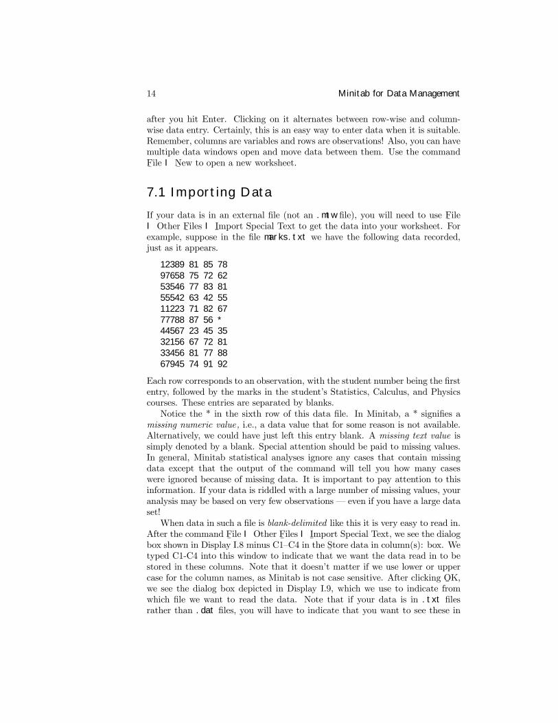
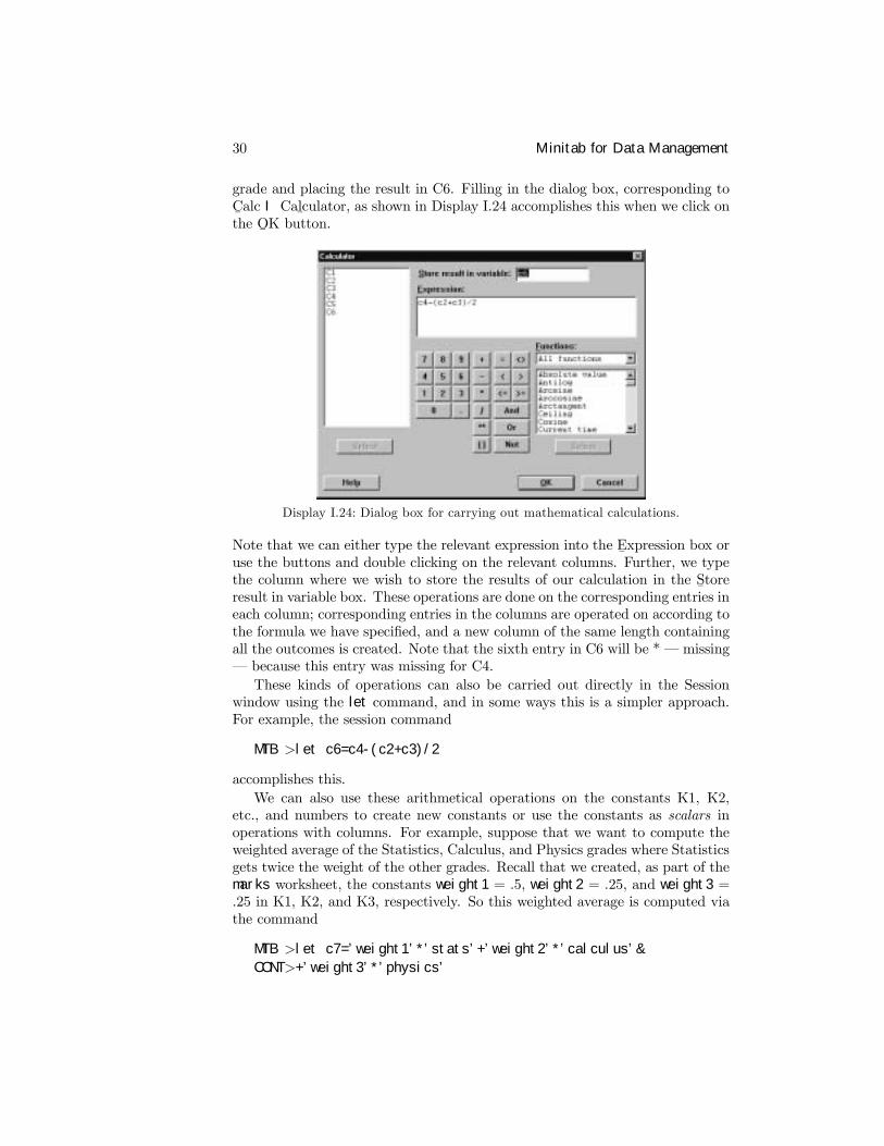
12389 81 85 7897658 75 72 6253546 77 83 8155542 63 42 5511223 71 82 6777788 87 56 *44567 23 45 3532156 67 72 8133456 81 77 8867945 74 91 92
Each row corresponds to an observation, with the student number being the Þrstentry, followed by the marks in the student�s Statistics, Calculus, and Physicscourses. These entries are separated by blanks.Notice the * in the sixth row of this data Þle. In Minitab, a * signiÞes a
missing numeric value, i.e., a data value that for some reason is not available.Alternatively, we could have just left this entry blank. A missing text value issimply denoted by a blank. Special attention should be paid to missing values.In general, Minitab statistical analyses ignore any cases that contain missingdata except that the output of the command will tell you how many caseswere ignored because of missing data. It is important to pay attention to thisinformation. If your data is riddled with a large number of missing values, youranalysis may be based on very few observations � even if you have a large dataset!When data in such a Þle is blank-delimited like this it is very easy to read in.
After the command F¯ile I Other F
¯iles I I
¯mport Special Text, we see the dialog
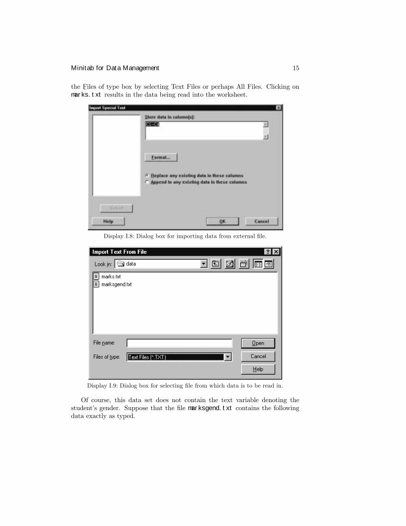
box shown in Display I.8 minus C1�C4 in the S¯tore data in column(s): box. We
typed C1-C4 into this window to indicate that we want the data read in to bestored in these columns. Note that it doesn�t matter if we use lower or uppercase for the column names, as Minitab is not case sensitive. After clicking O
¯K,
we see the dialog box depicted in Display I.9, which we use to indicate fromwhich Þle we want to read the data. Note that if your data is in .txt Þlesrather than .dat Þles, you will have to indicate that you want to see these in
Minitab for Data Management 15
the F¯iles of type box by selecting Text Files or perhaps All Files. Clicking on
marks.txt results in the data being read into the worksheet.
Display I.8: Dialog box for importing data from external Þle.
Display I.9: Dialog box for selecting Þle from which data is to be read in.
Of course, this data set does not contain the text variable denoting thestudent�s gender. Suppose that the Þle marksgend.txt contains the followingdata exactly as typed.
16 Minitab for Data Management
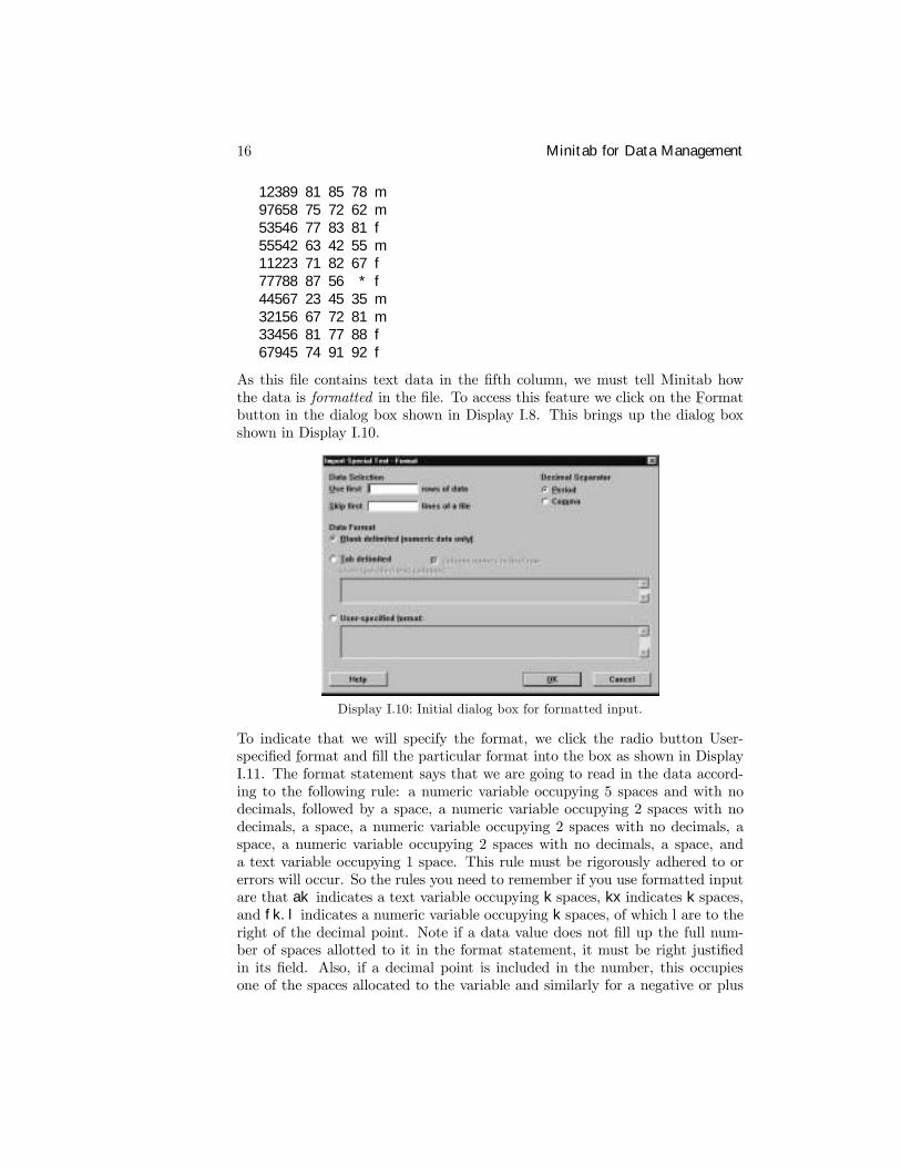
12389 81 85 78 m97658 75 72 62 m53546 77 83 81 f55542 63 42 55 m11223 71 82 67 f77788 87 56 * f44567 23 45 35 m32156 67 72 81 m33456 81 77 88 f67945 74 91 92 f
As this Þle contains text data in the Þfth column, we must tell Minitab howthe data is formatted in the Þle. To access this feature we click on the F
¯ormat
button in the dialog box shown in Display I.8. This brings up the dialog boxshown in Display I.10.
Display I.10: Initial dialog box for formatted input.
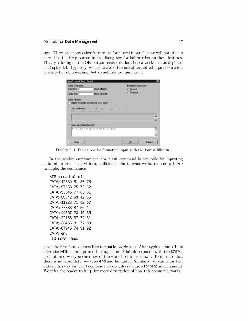
To indicate that we will specify the format, we click the radio button User-speciÞed f
¯ormat and Þll the particular format into the box as shown in Display
I.11. The format statement says that we are going to read in the data accord-ing to the following rule: a numeric variable occupying 5 spaces and with nodecimals, followed by a space, a numeric variable occupying 2 spaces with nodecimals, a space, a numeric variable occupying 2 spaces with no decimals, aspace, a numeric variable occupying 2 spaces with no decimals, a space, anda text variable occupying 1 space. This rule must be rigorously adhered to orerrors will occur. So the rules you need to remember if you use formatted inputare that ak indicates a text variable occupying k spaces, kx indicates k spaces,and fk.l indicates a numeric variable occupying k spaces, of which l are to theright of the decimal point. Note if a data value does not Þll up the full num-ber of spaces allotted to it in the format statement, it must be right justiÞedin its Þeld. Also, if a decimal point is included in the number, this occupiesone of the spaces allocated to the variable and similarly for a negative or plus
Minitab for Data Management 17
sign. There are many other features to formatted input that we will not discusshere. Use the Help button in the dialog box for information on these features.Finally, clicking on the O
¯K button reads this data into a worksheet as depicted
in Display I.4. Typically, we try to avoid the use of formatted input because itis somewhat cumbersome, but sometimes we must use it.
Display I.11: Dialog box for formatted input with the format Þlled in.
In the session environment, the read command is available for inputtingdata into a worksheet with capabilities similar to what we have described. Forexample, the commands
MTB >read c1-c4DATA>12389 81 85 78DATA>97658 75 72 62DATA>53546 77 83 81DATA>55542 63 42 55DATA>11223 71 82 67DATA>77788 87 56 *DATA>44567 23 45 35DATA>32156 67 72 81DATA>33456 81 77 88DATA>67945 74 91 92DATA>end10 rows read.
place the Þrst four columns into the marks worksheet. After typing read c1-c4after the MTB > prompt and hitting Enter, Minitab responds with the DATA>prompt, and we type each row of the worksheet in as shown. To indicate thatthere is no more data, we type end and hit Enter. Similarly, we can enter textdata in this way but can�t combine the two unless we use a format subcommand.We refer the reader to help for more description of how this command works.
18 Minitab for Data Management
7.2 Patterned Data
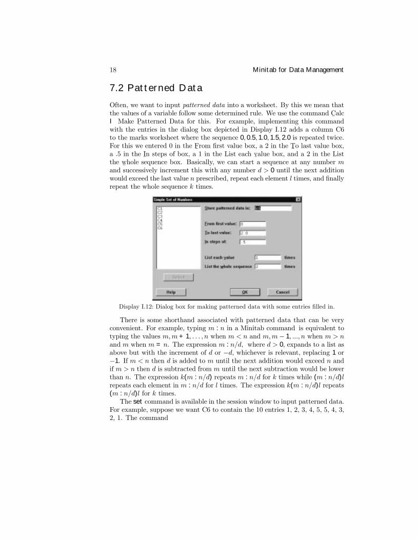
Often, we want to input patterned data into a worksheet. By this we mean thatthe values of a variable follow some determined rule. We use the command C
¯alc
I Make P¯atterned Data for this. For example, implementing this command
with the entries in the dialog box depicted in Display I.12 adds a column C6to the marks worksheet where the sequence 0, 0.5, 1.0, 1.5, 2.0 is repeated twice.For this we entered 0 in the F
¯rom Þrst value box, a 2 in the T
¯o last value box,
a .5 in the I¯n steps of box, a 1 in the List each v
¯alue box, and a 2 in the List
the w¯hole sequence box. Basically, we can start a sequence at any number m
and successively increment this with any number d > 0 until the next additionwould exceed the last value n prescribed, repeat each element l times, and Þnallyrepeat the whole sequence k times.
Display I.12: Dialog box for making patterned data with some entries Þlled in.
There is some shorthand associated with patterned data that can be veryconvenient. For example, typing m : n in a Minitab command is equivalent totyping the values m,m+ 1, . . . , n when m < n and m,m− 1, ..., n when m > nand m when m = n. The expression m : n/d, where d > 0, expands to a list asabove but with the increment of d or −d, whichever is relevant, replacing 1 or−1. If m < n then d is added to m until the next addition would exceed n andif m > n then d is subtracted from m until the next subtraction would be lowerthan n. The expression k(m : n/d) repeats m : n/d for k times while (m : n/d)lrepeats each element in m : n/d for l times. The expression k(m : n/d)l repeats(m : n/d)l for k times.The set command is available in the session window to input patterned data.
For example, suppose we want C6 to contain the 10 entries 1, 2, 3, 4, 5, 5, 4, 3,2, 1. The command
Minitab for Data Management 19
MTB >set c6DATA>1:5DATA>5:1DATA>end
does this. Also, we can add elements in parentheses. For example, the command
MTB >set c6DATA>(1:2/.5 4:3/.2)DATA>end
creates the column with entries 1.0, 1.5, 2.0, 4.0, 3.8, 3.6, 3.4, 3.2, 3.0. Themultiplicative factors k and l can also be used in such a context. Obviously,there is a great deal of scope for entering patterned data with set. The generalsyntax of the set command is
set E1
where E1 is a column.
7.3 Printing Data in the Session Window
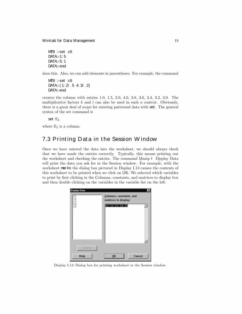
Once we have entered the data into the worksheet, we should always checkthat we have made the entries correctly. Typically, this means printing outthe worksheet and checking the entries. The command M
¯anip I Di
¯splay Data
will print the data you ask for in the Session window. For example, with theworksheet marks the dialog box pictured in Display I.13 causes the contents ofthis worksheet to be printed when we click on O
¯K. We selected which variables
to print by Þrst clicking in the C¯olumns, constants, and matrices to display box
and then double clicking on the variables in the variable list on the left.
Display I.13: Dialog box for printing worksheet in the Session window.
20 Minitab for Data Management
The print command is available in the Session window and is often conve-nient to use. The general syntax for the print command is
print E1 ... Em
where E1, ..., Em are columns and constants.
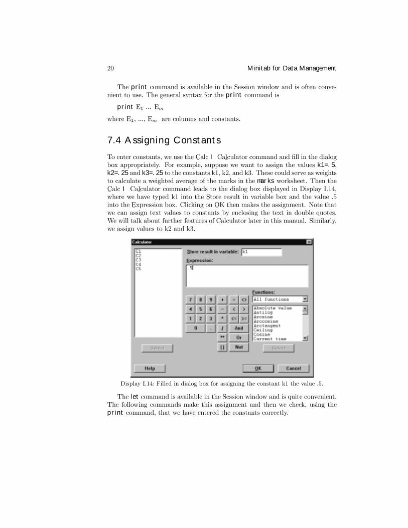
7.4 Assigning Constants
To enter constants, we use the C¯alc I Cal
¯culator command and Þll in the dialog
box appropriately. For example, suppose we want to assign the values k1=.5,k2=.25 and k3=.25 to the constants k1, k2, and k3. These could serve as weightsto calculate a weighted average of the marks in the marks worksheet. Then theC¯alc I Cal
¯culator command leads to the dialog box displayed in Display I.14,
where we have typed k1 into the S¯tore result in variable box and the value .5
into the E¯xpression box. Clicking on O
¯K then makes the assignment. Note that
we can assign text values to constants by enclosing the text in double quotes.We will talk about further features of Calculator later in this manual. Similarly,we assign values to k2 and k3.
Display I.14: Filled in dialog box for assigning the constant k1 the value .5.
The let command is available in the Session window and is quite convenient.The following commands make this assignment and then we check, using theprint command, that we have entered the constants correctly.
Minitab for Data Management 21
MTB >let k1=.5MTB >let k2=.25MTB >let k3=.25MTB >print k1-k3K1 0.500000K2 0.250000K3 0.250000
Also, we can assign constants text values. For example,
MTB >let k4=’’result’’
assigns K4 the value result. Note the use of double quotes.
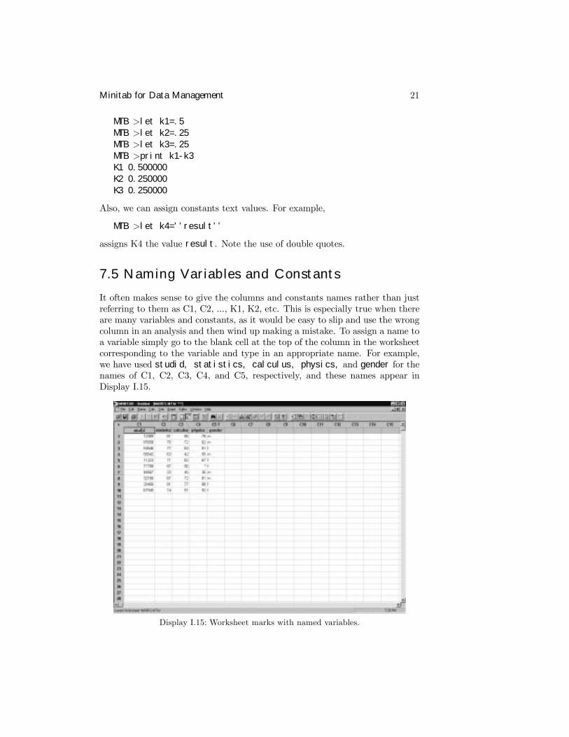
7.5 Naming Variables and Constants
It often makes sense to give the columns and constants names rather than justreferring to them as C1, C2, ..., K1, K2, etc. This is especially true when thereare many variables and constants, as it would be easy to slip and use the wrongcolumn in an analysis and then wind up making a mistake. To assign a name toa variable simply go to the blank cell at the top of the column in the worksheetcorresponding to the variable and type in an appropriate name. For example,we have used studid, statistics, calculus, physics, and gender for thenames of C1, C2, C3, C4, and C5, respectively, and these names appear inDisplay I.15.
Display I.15: Worksheet marks with named variables.
22 Minitab for Data Management
In the Session window, the name command is available for naming variablesand constants. For example, the commands
MTB >name c1 ’studid’ c2 ’stats’ c3 ’calculus’ &CONT>c4 ’physics’ c5 ’gender’ &CONT>k1 ’weight1’ k2 ’weight2’ k3 ’weight3’
give the names studid to C1, stats to C2, calculus to C3, physics to C4,gender to C5, weight1 to K1, weight2 to K2, and weight3 to K3. Notice thatwe have made use of the continuation character & for convenience in typing inthe full input to name. When using the variables as arguments just enclose thenames in single quotes. For example,
MTB >print ’studid’ ’calculus’
prints out the contents of these variables in the Session window.Variable and constant names can be at most 31 characters in length, cannot
include the characters # and � and cannot start with a leading blank or *. Recallthat Minitab is not case sensitive, so it does not matter if we use lower or uppercase letters when specifying the names.
7.6 Information about a Worksheet
We can get information on the data we have entered into the worksheet by usingthe info command in the Session window. For example, we get the followingresults based on what we have entered into the marks worksheet so far.
MTB >infoColumn Name Count Missing
A C1 studid 10 0C2 stats 10 0C3 calculus 10 0C4 physics 10 1
A C5 gender 10 0Constant Name ValueK1 weight1 0.500000K2 weight2 0.250000K3 weight3 0.250000
Notice that the info command tells us how many missing values there are andin what columns they occur and also the values of the constants.This information can also be accessed directly from the Project Manager
window via W¯indow I Project Manager.
Minitab for Data Management 23
7.7 Editing a Worksheet
It often happens that after data entry we notice that we have made some mis-takes or we obtain some additional information, such as more observations. Sofar, the only way we could change any entries in the worksheet or add somerows is to reenter the whole worksheet!Editing the worksheet is straightforward because we simply change any cells
by retyping their entries and hitting the Enter key. We can add rows andcolumns at the end of the worksheet by simply typing new data entries in therelevant cells. To insert a row before a particular row, simply click on any entryin that row and then the menu command Ed
¯itor I Insert Rows
¯. Fill in the
blank entries in the new row. To insert a column before a particular column,simply click on any entry in that column and then the menu command Ed
¯itor
I Insert¯Columns. Fill in the blank entries in the new column. To insert a
cell before a particular cell, simply click on any entry in that cell and the menucommand Ed
¯itor I I
¯nsert Cells. Fill in the blank entry in the new cell that
appears in place of the original with all other cells in that column � and onlythat column � pushed down.If you wish to clear a number of cells in a block, click in the cell at the
start of the block, and holding the mouse key down, drag the cursor throughthe block so that it is highlighted in black. Click on the Cut Cells icon on theMinitab taskbar, and all the entries will be deleted. Cells immediately below theblock move up to Þll in the vacated places. A convenient method for clearingall the data entries in a worksheet, with the relevant Data window active, isto use the command E
¯dit I Select A
¯ll Cells, which causes all the cells to be
highlighted, and click on the Cut Cells icon. Always save the contents of thecurrent worksheet before doing this unless you are absolutely sure you don�tneed the data again. We discuss how to save the contents of a worksheet inI.8.1.To copy a block of cells, click in the cell at the start of the block and, holding
the mouse key down, drag the cursor through the block so that it is highlightedin black, but, instead of hitting the backspace key, use the command E
¯dit I
C¯opy Cells or click on the Copy Cells icon on the Minitab taskbar. The blockof cells is now copied to your clipboard. If you not only want to copy a block ofcells to your clipboard but remove them from the worksheet, use the commandE¯dit I C
¯ut¯Cells or the Cut Cells icon on the Minitab taskbar instead. Note
that any cells below the removed block will move up to replace these entries.To paste the block of cells into the worksheet, click on the cell before which youwant the block to appear or that is at the start of the block of cells you wish toreplace and issue the command E
¯dit I P
¯aste Cells, or use the Paste Cells icon
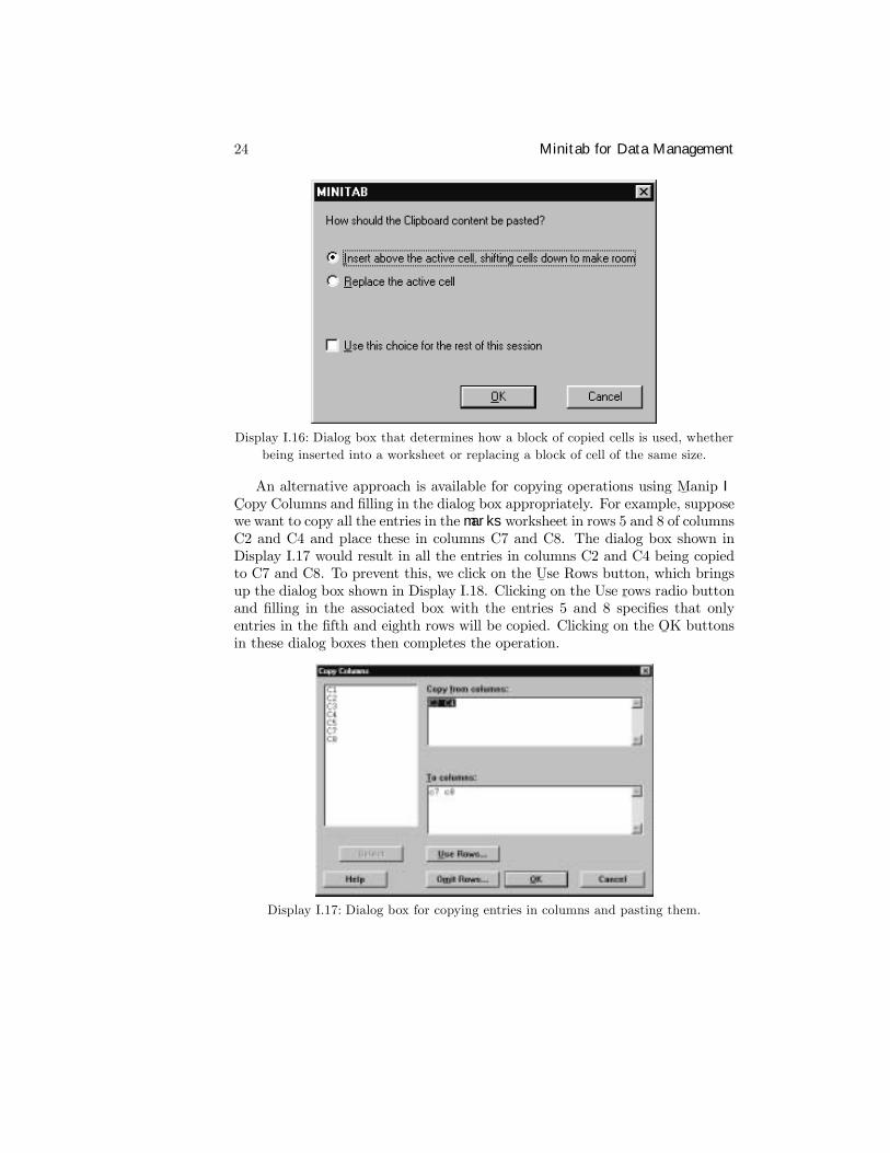
on the Minitab taskbar. A dialog box appears as in Display I.16, where you areprompted as to what you want to do with the copied block of cells. If you feelthat a cutting or pasting was in error, you can undo this operation by usingE¯dit I U
¯ndo Cut or E
¯dit I U
¯ndo Paste, respectively, or use the Undo icon on
the Minitab taskbar.
24 Minitab for Data Management
Display I.16: Dialog box that determines how a block of copied cells is used, whetherbeing inserted into a worksheet or replacing a block of cell of the same size.
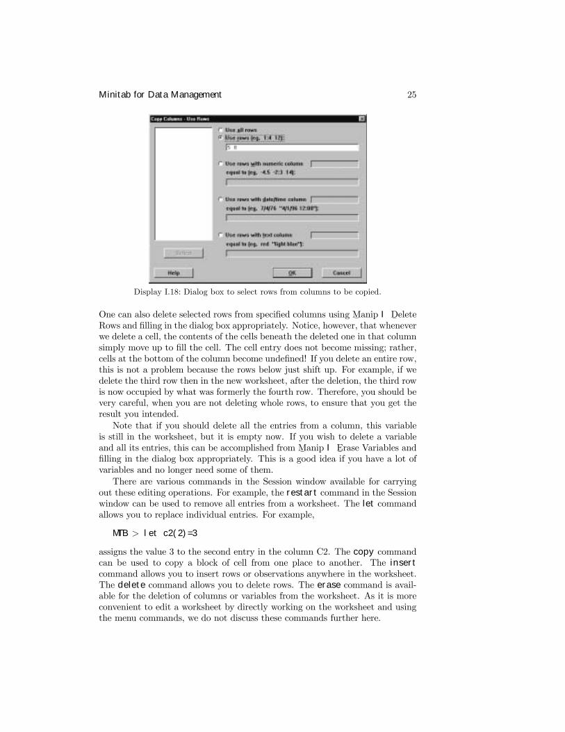
An alternative approach is available for copying operations using M¯anip I
C¯opy Columns and Þlling in the dialog box appropriately. For example, supposewe want to copy all the entries in the marks worksheet in rows 5 and 8 of columnsC2 and C4 and place these in columns C7 and C8. The dialog box shown inDisplay I.17 would result in all the entries in columns C2 and C4 being copiedto C7 and C8. To prevent this, we click on the U
¯se Rows button, which brings
up the dialog box shown in Display I.18. Clicking on the Use r¯ows radio button
and Þlling in the associated box with the entries 5 and 8 speciÞes that onlyentries in the Þfth and eighth rows will be copied. Clicking on the O
¯K buttons
in these dialog boxes then completes the operation.
Display I.17: Dialog box for copying entries in columns and pasting them.
Minitab for Data Management 25
Display I.18: Dialog box to select rows from columns to be copied.
One can also delete selected rows from speciÞed columns using M¯anip I D
¯elete
Rows and Þlling in the dialog box appropriately. Notice, however, that wheneverwe delete a cell, the contents of the cells beneath the deleted one in that columnsimply move up to Þll the cell. The cell entry does not become missing; rather,cells at the bottom of the column become undeÞned! If you delete an entire row,this is not a problem because the rows below just shift up. For example, if wedelete the third row then in the new worksheet, after the deletion, the third rowis now occupied by what was formerly the fourth row. Therefore, you should bevery careful, when you are not deleting whole rows, to ensure that you get theresult you intended.Note that if you should delete all the entries from a column, this variable
is still in the worksheet, but it is empty now. If you wish to delete a variableand all its entries, this can be accomplished from M
¯anip I E
¯rase Variables and
Þlling in the dialog box appropriately. This is a good idea if you have a lot ofvariables and no longer need some of them.There are various commands in the Session window available for carrying
out these editing operations. For example, the restart command in the Sessionwindow can be used to remove all entries from a worksheet. The let commandallows you to replace individual entries. For example,
MTB > let c2(2)=3
assigns the value 3 to the second entry in the column C2. The copy commandcan be used to copy a block of cell from one place to another. The insertcommand allows you to insert rows or observations anywhere in the worksheet.The delete command allows you to delete rows. The erase command is avail-able for the deletion of columns or variables from the worksheet. As it is moreconvenient to edit a worksheet by directly working on the worksheet and usingthe menu commands, we do not discuss these commands further here.
26 Minitab for Data Management
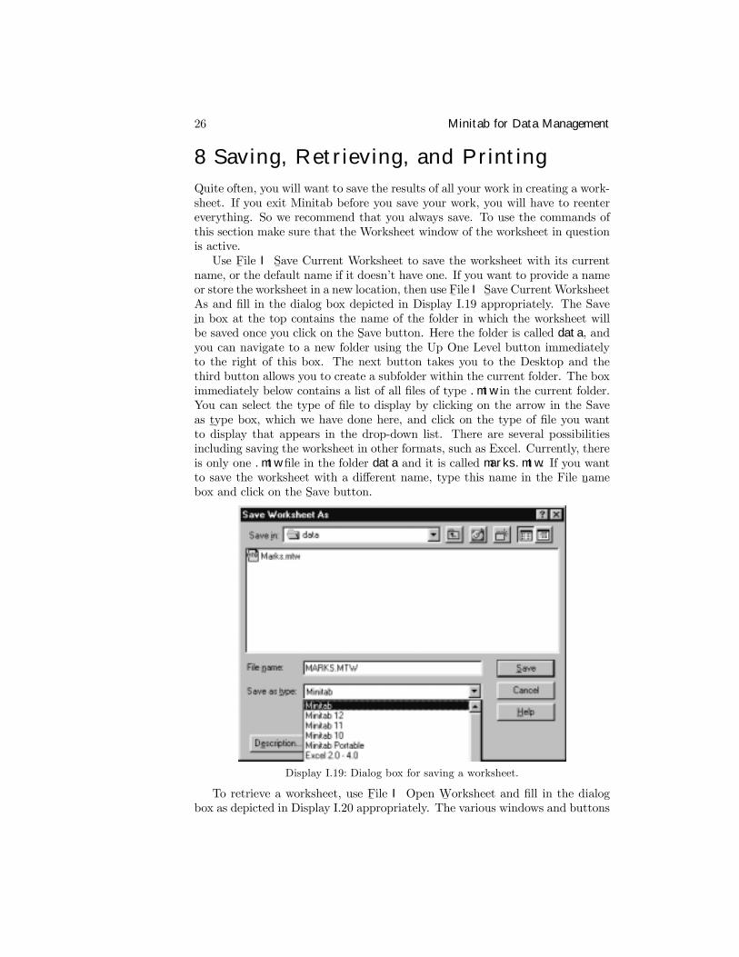
8 Saving, Retrieving, and PrintingQuite often, you will want to save the results of all your work in creating a work-sheet. If you exit Minitab before you save your work, you will have to reentereverything. So we recommend that you always save. To use the commands ofthis section make sure that the Worksheet window of the worksheet in questionis active.Use F
¯ile I S
¯ave Current Worksheet to save the worksheet with its current
name, or the default name if it doesn�t have one. If you want to provide a nameor store the worksheet in a new location, then use F
¯ileI S
¯ave CurrentWorksheet
As and Þll in the dialog box depicted in Display I.19 appropriately. The Savei¯n box at the top contains the name of the folder in which the worksheet willbe saved once you click on the S
¯ave button. Here the folder is called data, and
you can navigate to a new folder using the Up One Level button immediatelyto the right of this box. The next button takes you to the Desktop and thethird button allows you to create a subfolder within the current folder. The boximmediately below contains a list of all Þles of type .mtw in the current folder.You can select the type of Þle to display by clicking on the arrow in the Saveas t¯ype box, which we have done here, and click on the type of Þle you want
to display that appears in the drop-down list. There are several possibilitiesincluding saving the worksheet in other formats, such as Excel. Currently, thereis only one .mtw Þle in the folder data and it is called marks.mtw. If you wantto save the worksheet with a different name, type this name in the File n
¯ame
box and click on the S¯ave button.
Display I.19: Dialog box for saving a worksheet.
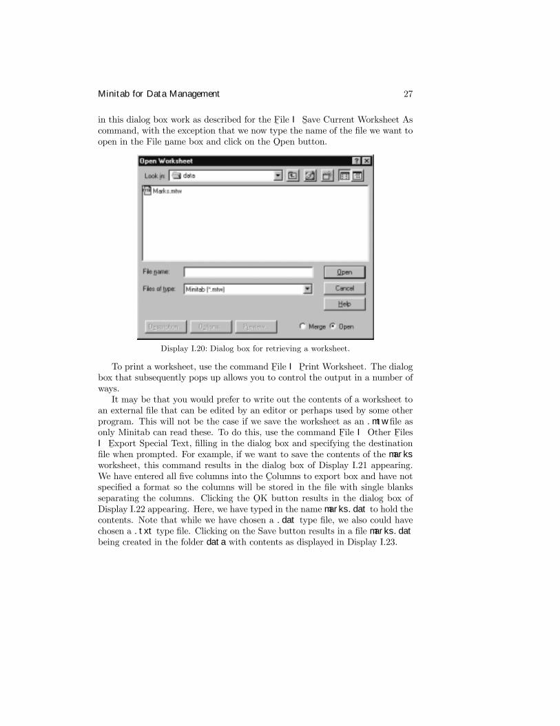
To retrieve a worksheet, use F¯ile I Open W
¯orksheet and Þll in the dialog
box as depicted in Display I.20 appropriately. The various windows and buttons
Minitab for Data Management 27
in this dialog box work as described for the F¯ile I S
¯ave Current Worksheet As
command, with the exception that we now type the name of the Þle we want toopen in the File n
¯ame box and click on the O
¯pen button.
Display I.20: Dialog box for retrieving a worksheet.
To print a worksheet, use the command F¯ile I P
¯rint Worksheet. The dialog
box that subsequently pops up allows you to control the output in a number ofways.It may be that you would prefer to write out the contents of a worksheet to
an external Þle that can be edited by an editor or perhaps used by some otherprogram. This will not be the case if we save the worksheet as an .mtw Þle asonly Minitab can read these. To do this, use the command F
¯ile I Other F
¯iles
I E¯xport Special Text, Þlling in the dialog box and specifying the destination
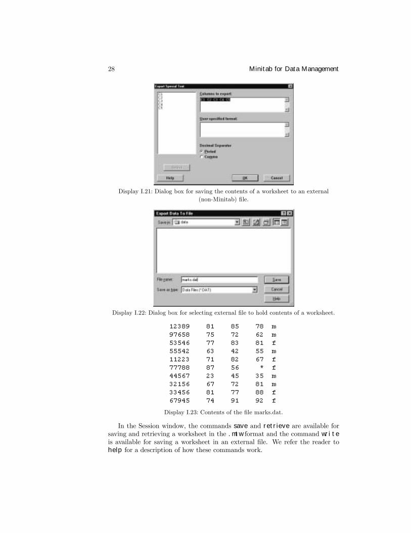
Þle when prompted. For example, if we want to save the contents of the marksworksheet, this command results in the dialog box of Display I.21 appearing.We have entered all Þve columns into the C
¯olumns to export box and have not
speciÞed a format so the columns will be stored in the Þle with single blanksseparating the columns. Clicking the O
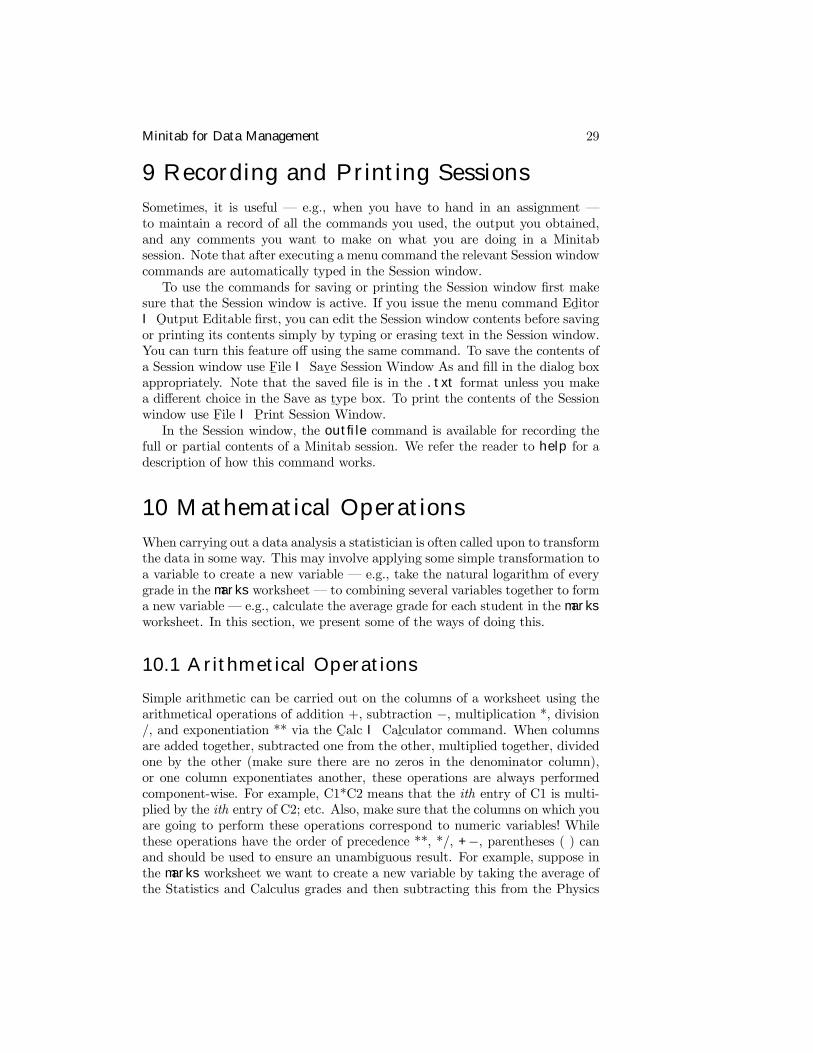
¯K button results in the dialog box of
Display I.22 appearing. Here, we have typed in the name marks.dat to hold thecontents. Note that while we have chosen a .dat type Þle, we also could havechosen a .txt type Þle. Clicking on the Save button results in a Þle marks.datbeing created in the folder data with contents as displayed in Display I.23.
28 Minitab for Data Management
Display I.21: Dialog box for saving the contents of a worksheet to an external(non-Minitab) Þle.
Display I.22: Dialog box for selecting external Þle to hold contents of a worksheet.
Display I.23: Contents of the Þle marks.dat.
In the Session window, the commands save and retrieve are available forsaving and retrieving a worksheet in the .mtw format and the command writeis available for saving a worksheet in an external Þle. We refer the reader tohelp for a description of how these commands work.
Minitab for Data Management 29
9 Recording and Printing SessionsSometimes, it is useful � e.g., when you have to hand in an assignment �to maintain a record of all the commands you used, the output you obtained,and any comments you want to make on what you are doing in a Minitabsession. Note that after executing a menu command the relevant Session windowcommands are automatically typed in the Session window.To use the commands for saving or printing the Session window Þrst make
sure that the Session window is active. If you issue the menu command Ed¯itor
I O¯utput Editable Þrst, you can edit the Session window contents before saving
or printing its contents simply by typing or erasing text in the Session window.You can turn this feature off using the same command. To save the contents ofa Session window use F
¯ile I Sav
¯e Session Window As and Þll in the dialog box
appropriately. Note that the saved Þle is in the .txt format unless you makea different choice in the Save as t
¯ype box. To print the contents of the Session
window use F¯ile I P
¯rint Session Window.
In the Session window, the outfile command is available for recording thefull or partial contents of a Minitab session. We refer the reader to help for adescription of how this command works.
10 Mathematical OperationsWhen carrying out a data analysis a statistician is often called upon to transformthe data in some way. This may involve applying some simple transformation toa variable to create a new variable � e.g., take the natural logarithm of everygrade in the marks worksheet � to combining several variables together to forma new variable � e.g., calculate the average grade for each student in the marksworksheet. In this section, we present some of the ways of doing this.
10.1 Arithmetical Operations
Simple arithmetic can be carried out on the columns of a worksheet using thearithmetical operations of addition +, subtraction −, multiplication *, division/, and exponentiation ** via the C
¯alc I Cal
¯culator command. When columns
are added together, subtracted one from the other, multiplied together, dividedone by the other (make sure there are no zeros in the denominator column),or one column exponentiates another, these operations are always performedcomponent-wise. For example, C1*C2 means that the ith entry of C1 is multi-plied by the ith entry of C2; etc. Also, make sure that the columns on which youare going to perform these operations correspond to numeric variables! Whilethese operations have the order of precedence **, */, +−, parentheses ( ) canand should be used to ensure an unambiguous result. For example, suppose inthe marks worksheet we want to create a new variable by taking the average ofthe Statistics and Calculus grades and then subtracting this from the Physics
30 Minitab for Data Management
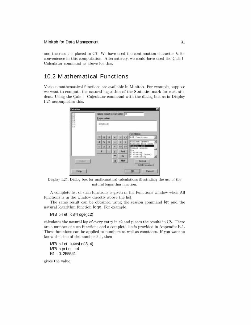
grade and placing the result in C6. Filling in the dialog box, corresponding toC¯alc I Cal
¯culator, as shown in Display I.24 accomplishes this when we click on
the O¯K button.
Display I.24: Dialog box for carrying out mathematical calculations.
Note that we can either type the relevant expression into the E¯xpression box or
use the buttons and double clicking on the relevant columns. Further, we typethe column where we wish to store the results of our calculation in the S
¯tore
result in variable box. These operations are done on the corresponding entries ineach column; corresponding entries in the columns are operated on according tothe formula we have speciÞed, and a new column of the same length containingall the outcomes is created. Note that the sixth entry in C6 will be * � missing� because this entry was missing for C4.These kinds of operations can also be carried out directly in the Session
window using the let command, and in some ways this is a simpler approach.For example, the session command
MTB >let c6=c4-(c2+c3)/2
accomplishes this.We can also use these arithmetical operations on the constants K1, K2,
etc., and numbers to create new constants or use the constants as scalars inoperations with columns. For example, suppose that we want to compute theweighted average of the Statistics, Calculus, and Physics grades where Statisticsgets twice the weight of the other grades. Recall that we created, as part of themarks worksheet, the constants weight1 = .5, weight2 = .25, and weight3 =.25 in K1, K2, and K3, respectively. So this weighted average is computed viathe command
MTB >let c7=’weight1’*’stats’+’weight2’*’calculus’&CONT>+’weight3’*’physics’
Minitab for Data Management 31
and the result is placed in C7. We have used the continuation character & forconvenience in this computation. Alternatively, we could have used the C
¯alc I
Cal¯culator command as above for this.
10.2 Mathematical Functions
Various mathematical functions are available in Minitab. For example, supposewe want to compute the natural logarithm of the Statistics mark for each stu-dent. Using the C
¯alc I Cal
¯culator command with the dialog box as in Display
I.25 accomplishes this.
Display I.25: Dialog box for mathematical calculations illustrating the use of thenatural logarithm function.
A complete list of such functions is given in the Functions window when Allfunctions is in the window directly above the list.The same result can be obtained using the session command let and the
natural logarithm function loge. For example,
MTB >let c8=loge(c2)
calculates the natural log of every entry in c2 and places the results in C8. Thereare a number of such functions and a complete list is provided in Appendix B.1.These functions can be applied to numbers as well as constants. If you want toknow the sine of the number 3.4, then
MTB >let k4=sin(3.4)MTB >print k4K4 -0.255541
gives the value.
32 Minitab for Data Management
10.3 Column and Row Statistics
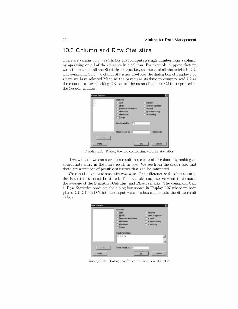
There are various column statistics that compute a single number from a columnby operating on all of the elements in a column. For example, suppose that wewant the mean of all the Statistics marks, i.e., the mean of all the entries in C2.The command C
¯alc I C
¯olumn Statistics produces the dialog box of Display I.26
where we have selected Mean as the particular statistic to compute and C2 asthe column to use. Clicking O
¯K causes the mean of column C2 to be printed in
the Session window.
Display I.26: Dialog box for computing column statistics.
If we want to, we can store this result in a constant or column by making anappropriate entry in the Store resu
¯lt in box. We see from the dialog box that
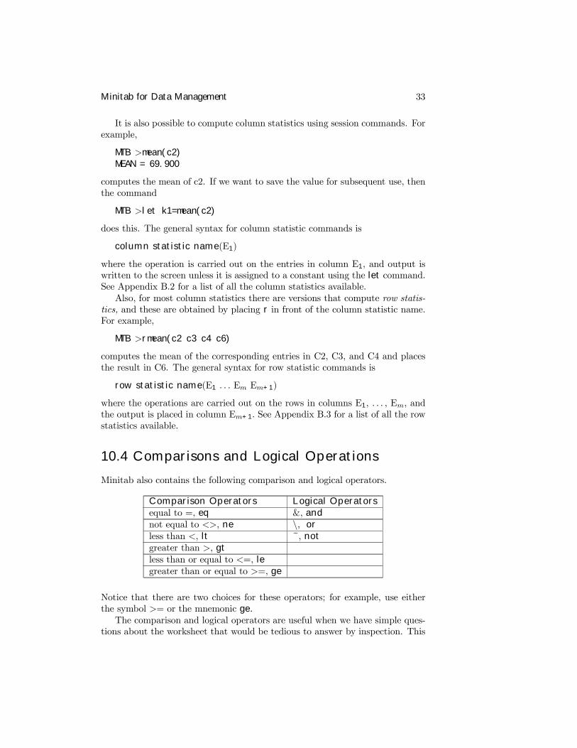
there are a number of possible statistics that can be computed.We can also compute statistics row-wise. One difference with column statis-
tics is that these must be stored. For example, suppose we want to computethe average of the Statistics, Calculus, and Physics marks. The command C
¯alc
I Ro¯w Statistics produces the dialog box shown in Display I.27 where we have
placed C2, C3, and C4 into the Input v¯ariables box and c6 into the Store resul
¯t
in box.
Display I.27: Dialog box for computing row statistics.
Minitab for Data Management 33
It is also possible to compute column statistics using session commands. Forexample,
MTB >mean(c2)MEAN = 69.900
computes the mean of c2. If we want to save the value for subsequent use, thenthe command
MTB >let k1=mean(c2)
does this. The general syntax for column statistic commands is
column statistic name(E1)
where the operation is carried out on the entries in column E1, and output iswritten to the screen unless it is assigned to a constant using the let command.See Appendix B.2 for a list of all the column statistics available.Also, for most column statistics there are versions that compute row statis-
tics, and these are obtained by placing r in front of the column statistic name.For example,
MTB >rmean(c2 c3 c4 c6)
computes the mean of the corresponding entries in C2, C3, and C4 and placesthe result in C6. The general syntax for row statistic commands is
row statistic name(E1 . . . Em Em+1)
where the operations are carried out on the rows in columns E1, . . . , Em, andthe output is placed in column Em+1. See Appendix B.3 for a list of all the rowstatistics available.
10.4 Comparisons and Logical Operations
Minitab also contains the following comparison and logical operators.
Comparison Operators Logical Operatorsequal to =, eq &, andnot equal to <>, ne \, orless than <, lt ~, notgreater than >, gtless than or equal to <=, legreater than or equal to >=, ge
Notice that there are two choices for these operators; for example, use eitherthe symbol >= or the mnemonic ge.The comparison and logical operators are useful when we have simple ques-
tions about the worksheet that would be tedious to answer by inspection. This
34 Minitab for Data Management
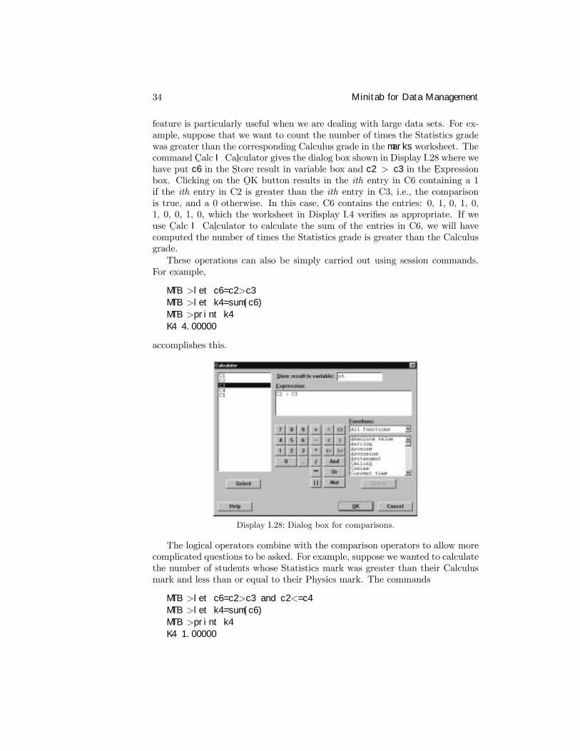
feature is particularly useful when we are dealing with large data sets. For ex-ample, suppose that we want to count the number of times the Statistics gradewas greater than the corresponding Calculus grade in the marks worksheet. Thecommand C
¯alc I Cal
¯culator gives the dialog box shown in Display I.28 where we
have put c6 in the S¯tore result in variable box and c2 > c3 in the E
¯xpression
box. Clicking on the O¯K button results in the ith entry in C6 containing a 1
if the ith entry in C2 is greater than the ith entry in C3, i.e., the comparisonis true, and a 0 otherwise. In this case, C6 contains the entries: 0, 1, 0, 1, 0,1, 0, 0, 1, 0, which the worksheet in Display I.4 veriÞes as appropriate. If weuse C
¯alc I Cal
¯culator to calculate the sum of the entries in C6, we will have
computed the number of times the Statistics grade is greater than the Calculusgrade.These operations can also be simply carried out using session commands.
For example,
MTB >let c6=c2>c3MTB >let k4=sum(c6)MTB >print k4K4 4.00000
accomplishes this.
Display I.28: Dialog box for comparisons.
The logical operators combine with the comparison operators to allow morecomplicated questions to be asked. For example, suppose we wanted to calculatethe number of students whose Statistics mark was greater than their Calculusmark and less than or equal to their Physics mark. The commands
MTB >let c6=c2>c3 and c2<=c4MTB >let k4=sum(c6)MTB >print k4K4 1.00000
Minitab for Data Management 35
accomplish this. In this case, both conditions c2>c3 and c2<=c4 have to betrue for a 1 to be recorded in C6. Note that the observation with the missingPhysics mark is excluded. Of course, we can also implement this using C
¯alc I
Cal¯culator and Þlling in the dialog box appropriately.Text variables can be used in comparisons where the ordering is alphabetical.
For example,
MTB >let c6=c5<’’m’’
puts a 1 in C6 whenever the corresponding entry in C5 is alphabetically smallerthan m.
11 Some More Minitab CommandsIn this section we discuss some commands that can be very helpful in certainapplications. We will make reference to these commands at appropriate placesthroughout the manual. It is probably best to wait to read these descriptionsuntil such a context arises.
11.1 Coding
The M¯anip I Co
¯de command is used to recode columns. By this we mean that
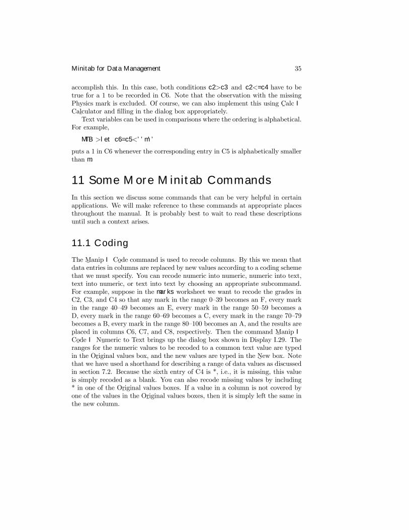
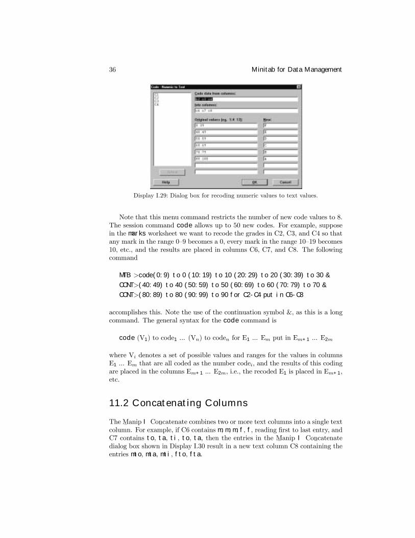
data entries in columns are replaced by new values according to a coding schemethat we must specify. You can recode numeric into numeric, numeric into text,text into numeric, or text into text by choosing an appropriate subcommand.For example, suppose in the marks worksheet we want to recode the grades inC2, C3, and C4 so that any mark in the range 0�39 becomes an F, every markin the range 40�49 becomes an E, every mark in the range 50�59 becomes aD, every mark in the range 60�69 becomes a C, every mark in the range 70�79becomes a B, every mark in the range 80�100 becomes an A, and the results areplaced in columns C6, C7, and C8, respectively. Then the command M
¯anip I
Co¯de I Nu
¯meric to Text brings up the dialog box shown in Display I.29. The
ranges for the numeric values to be recoded to a common text value are typedin the Or
¯iginal values box, and the new values are typed in the N
¯ew box. Note
that we have used a shorthand for describing a range of data values as discussedin section 7.2. Because the sixth entry of C4 is *, i.e., it is missing, this valueis simply recoded as a blank. You can also recode missing values by including* in one of the Or
¯iginal values boxes. If a value in a column is not covered by
one of the values in the Or¯iginal values boxes, then it is simply left the same in
the new column.
36 Minitab for Data Management
Display I.29: Dialog box for recoding numeric values to text values.
Note that this menu command restricts the number of new code values to 8.The session command code allows up to 50 new codes. For example, supposein the marks worksheet we want to recode the grades in C2, C3, and C4 so thatany mark in the range 0�9 becomes a 0, every mark in the range 10�19 becomes10, etc., and the results are placed in columns C6, C7, and C8. The followingcommand
MTB >code(0:9) to 0 (10:19) to 10 (20:29) to 20 (30:39) to 30 &
CONT>(40:49) to 40 (50:59) to 50 (60:69) to 60 (70:79) to 70 &
CONT>(80:89) to 80 (90:99) to 90 for C2-C4 put in C6-C8
accomplishes this. Note the use of the continuation symbol &, as this is a longcommand. The general syntax for the code command is
code (V1) to code1 ... (Vn) to coden for E1 ... Em put in Em+1 ... E2m
where Vi denotes a set of possible values and ranges for the values in columnsE1 ... Em that are all coded as the number codei, and the results of this codingare placed in the columns Em+1 ... E2m, i.e., the recoded E1 is placed in Em+1,etc.
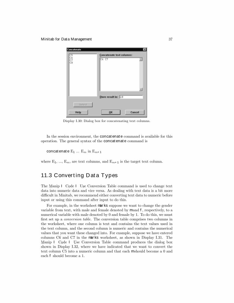
11.2 Concatenating Columns
The M¯anip I Con
¯catenate combines two or more text columns into a single text
column. For example, if C6 contains m, m, m, f, f, reading Þrst to last entry, andC7 contains to, ta, ti, to, ta, then the entries in the M
¯anip I Con
¯catenate
dialog box shown in Display I.30 result in a new text column C8 containing theentries mto, mta, mti, fto, fta.
Minitab for Data Management 37
Display I.30: Dialog box for concatenating text columns.
In the session environment, the concatenate command is available for thisoperation. The general syntax of the concatenate command is
concatenate E1 ... Em in Em+1
where E1, ..., Em, are text columns, and Em+1 is the target text column.
11.3 Converting Data Types
The M¯anip I Co
¯de I Us
¯e Conversion Table command is used to change text
data into numeric data and vice versa. As dealing with text data is a bit moredifficult in Minitab, we recommend either converting text data to numeric beforeinput or using this command after input to do this.
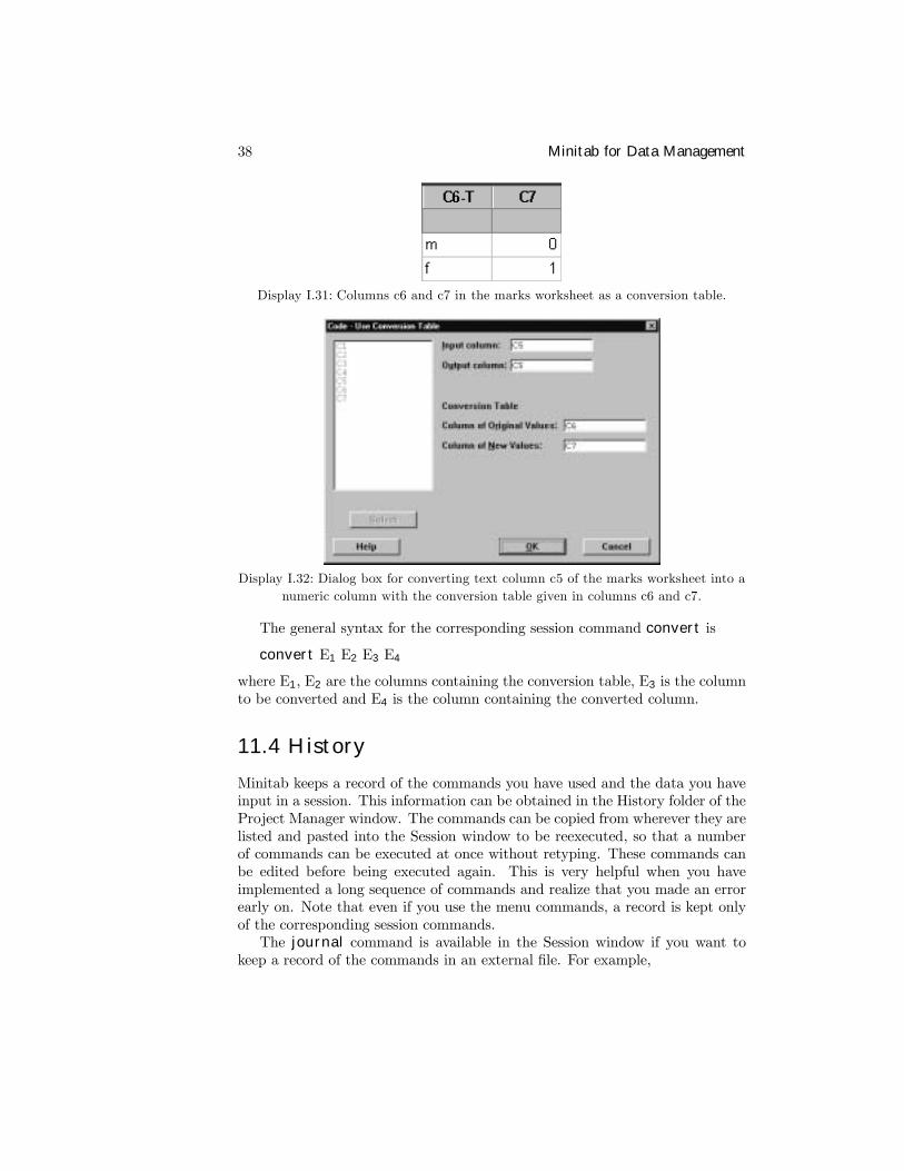
For example, in the worksheet marks suppose we want to change the gendervariable from text, with male and female denoted by m and f, respectively, to anumerical variable with male denoted by 0 and female by 1. To do this, we mustÞrst set up a conversion table. The conversion table comprises two columns inthe worksheet, where one column is text and contains the text values used inthe text column, and the second column is numeric and contains the numericalvalues that you want these changed into. For example, suppose we have enteredcolumns C6 and C7 in the marks worksheet, as shown in Display I.31. TheM¯anip I Co
¯de I U
¯se Conversion Table command produces the dialog box
shown in Display I.32, where we have indicated that we want to convert thetext column C5 into a numeric column and that each m should become a 0 andeach f should become a 1.
38 Minitab for Data Management
Display I.31: Columns c6 and c7 in the marks worksheet as a conversion table.
Display I.32: Dialog box for converting text column c5 of the marks worksheet into anumeric column with the conversion table given in columns c6 and c7.
The general syntax for the corresponding session command convert is
convert E1 E2 E3 E4
where E1, E2 are the columns containing the conversion table, E3 is the columnto be converted and E4 is the column containing the converted column.
11.4 History
Minitab keeps a record of the commands you have used and the data you haveinput in a session. This information can be obtained in the History folder of theProject Manager window. The commands can be copied from wherever they arelisted and pasted into the Session window to be reexecuted, so that a numberof commands can be executed at once without retyping. These commands canbe edited before being executed again. This is very helpful when you haveimplemented a long sequence of commands and realize that you made an errorearly on. Note that even if you use the menu commands, a record is kept onlyof the corresponding session commands.The journal command is available in the Session window if you want to
keep a record of the commands in an external Þle. For example,
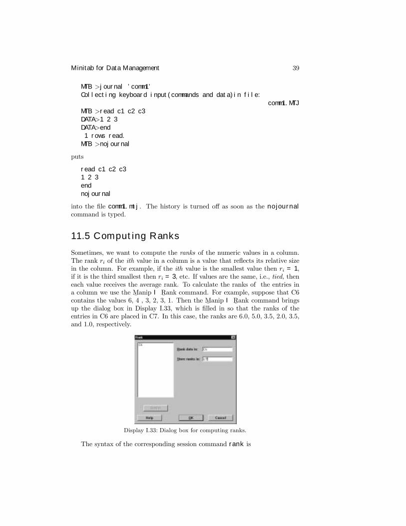
Minitab for Data Management 39
MTB >journal ’comm1’Collecting keyboard input(commands and data)in file:
comm1.MTJMTB >read c1 c2 c3DATA>1 2 3DATA>end1 rows read.
MTB >nojournal
puts
read c1 c2 c31 2 3endnojournal
into the Þle comm1.mtj. The history is turned off as soon as the nojournalcommand is typed.
11.5 Computing Ranks
Sometimes, we want to compute the ranks of the numeric values in a column.The rank ri of the ith value in a column is a value that reßects its relative sizein the column. For example, if the ith value is the smallest value then ri = 1,if it is the third smallest then ri = 3, etc. If values are the same, i.e., tied, theneach value receives the average rank. To calculate the ranks of the entries ina column we use the M
¯anip I R
¯ank command. For example, suppose that C6
contains the values 6, 4 , 3, 2, 3, 1. Then the M¯anip I R
¯ank command brings
up the dialog box in Display I.33, which is Þlled in so that the ranks of theentries in C6 are placed in C7. In this case, the ranks are 6.0, 5.0, 3.5, 2.0, 3.5,and 1.0, respectively.
Display I.33: Dialog box for computing ranks.
The syntax of the corresponding session command rank is
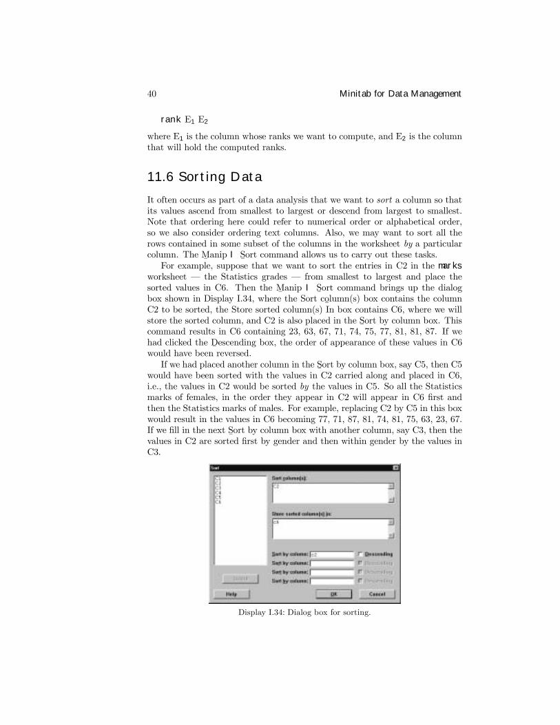
40 Minitab for Data Management
rank E1 E2
where E1 is the column whose ranks we want to compute, and E2 is the columnthat will hold the computed ranks.
11.6 Sorting Data
It often occurs as part of a data analysis that we want to sort a column so thatits values ascend from smallest to largest or descend from largest to smallest.Note that ordering here could refer to numerical order or alphabetical order,so we also consider ordering text columns. Also, we may want to sort all therows contained in some subset of the columns in the worksheet by a particularcolumn. The M
¯anip I S
¯ort command allows us to carry out these tasks.
For example, suppose that we want to sort the entries in C2 in the marksworksheet � the Statistics grades � from smallest to largest and place thesorted values in C6. Then the M
¯anip I S
¯ort command brings up the dialog
box shown in Display I.34, where the Sort co¯lumn(s) box contains the column
C2 to be sorted, the Store sorted column(s) In box contains C6, where we willstore the sorted column, and C2 is also placed in the S
¯ort by column box. This
command results in C6 containing 23, 63, 67, 71, 74, 75, 77, 81, 81, 87. If wehad clicked the D
¯escending box, the order of appearance of these values in C6
would have been reversed.If we had placed another column in the S
¯ort by column box, say C5, then C5
would have been sorted with the values in C2 carried along and placed in C6,i.e., the values in C2 would be sorted by the values in C5. So all the Statisticsmarks of females, in the order they appear in C2 will appear in C6 Þrst andthen the Statistics marks of males. For example, replacing C2 by C5 in this boxwould result in the values in C6 becoming 77, 71, 87, 81, 74, 81, 75, 63, 23, 67.If we Þll in the next S
¯ort by column box with another column, say C3, then the
values in C2 are sorted Þrst by gender and then within gender by the values inC3.
Display I.34: Dialog box for sorting.
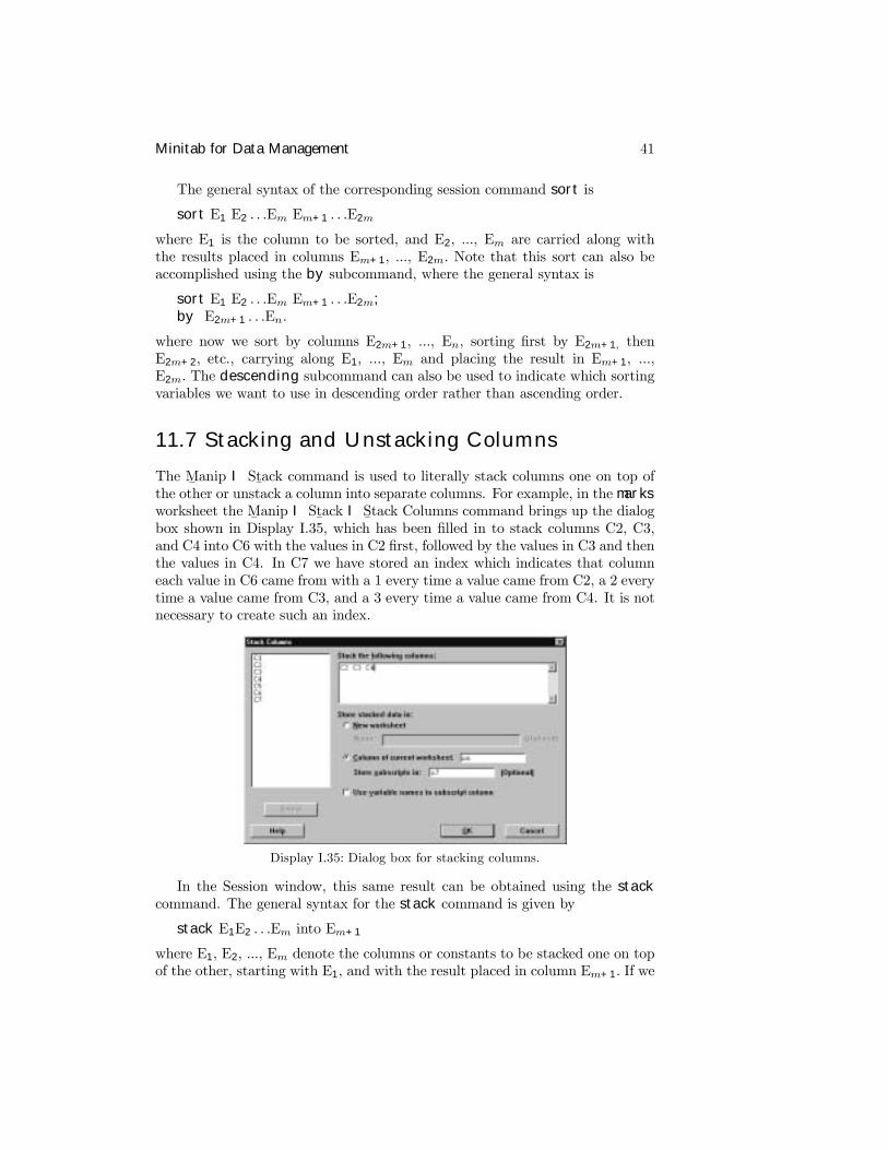
Minitab for Data Management 41
The general syntax of the corresponding session command sort is
sort E1 E2 . . .Em Em+1 . . .E2m
where E1 is the column to be sorted, and E2, ..., Em are carried along withthe results placed in columns Em+1, ..., E2m. Note that this sort can also beaccomplished using the by subcommand, where the general syntax is
sort E1 E2 . . .Em Em+1 . . .E2m;by E2m+1 . . .En.
where now we sort by columns E2m+1, ..., En, sorting Þrst by E2m+1, thenE2m+2, etc., carrying along E1, ..., Em and placing the result in Em+1, ...,E2m. The descending subcommand can also be used to indicate which sortingvariables we want to use in descending order rather than ascending order.
11.7 Stacking and Unstacking Columns
The M¯anip I St
¯ack command is used to literally stack columns one on top of
the other or unstack a column into separate columns. For example, in the marksworksheet the M
¯anip I St
¯ack I S
¯tack Columns command brings up the dialog
box shown in Display I.35, which has been Þlled in to stack columns C2, C3,and C4 into C6 with the values in C2 Þrst, followed by the values in C3 and thenthe values in C4. In C7 we have stored an index which indicates that columneach value in C6 came from with a 1 every time a value came from C2, a 2 everytime a value came from C3, and a 3 every time a value came from C4. It is notnecessary to create such an index.
Display I.35: Dialog box for stacking columns.
In the Session window, this same result can be obtained using the stackcommand. The general syntax for the stack command is given by
stack E1E2 . . .Em into Em+1
where E1, E2, ..., Em denote the columns or constants to be stacked one on topof the other, starting with E1, and with the result placed in column Em+1. If we
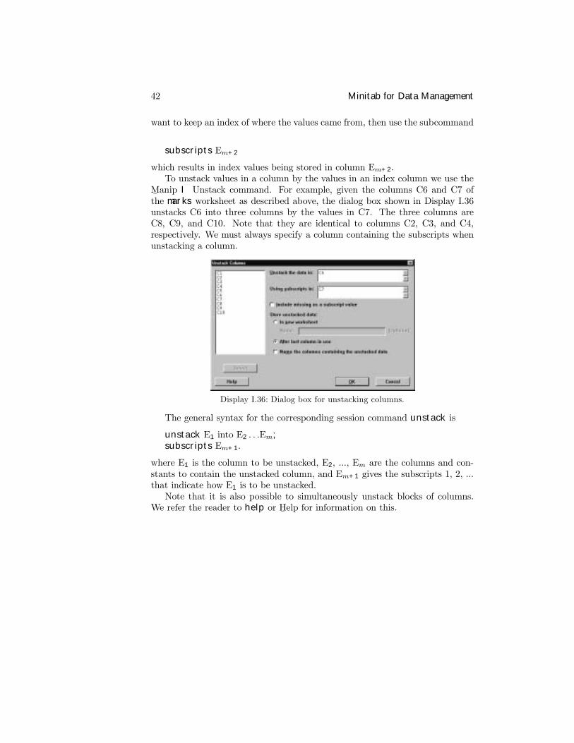
42 Minitab for Data Management
want to keep an index of where the values came from, then use the subcommand
subscripts Em+2
which results in index values being stored in column Em+2.To unstack values in a column by the values in an index column we use the
M¯anip I Unstack command. For example, given the columns C6 and C7 of
the marks worksheet as described above, the dialog box shown in Display I.36unstacks C6 into three columns by the values in C7. The three columns areC8, C9, and C10. Note that they are identical to columns C2, C3, and C4,respectively. We must always specify a column containing the subscripts whenunstacking a column.
Display I.36: Dialog box for unstacking columns.
The general syntax for the corresponding session command unstack is
unstack E1 into E2 . . .Em;subscripts Em+1.
where E1 is the column to be unstacked, E2, ..., Em are the columns and con-stants to contain the unstacked column, and Em+1 gives the subscripts 1, 2, ...that indicate how E1 is to be unstacked.Note that it is also possible to simultaneously unstack blocks of columns.
We refer the reader to help or H¯elp for information on this.
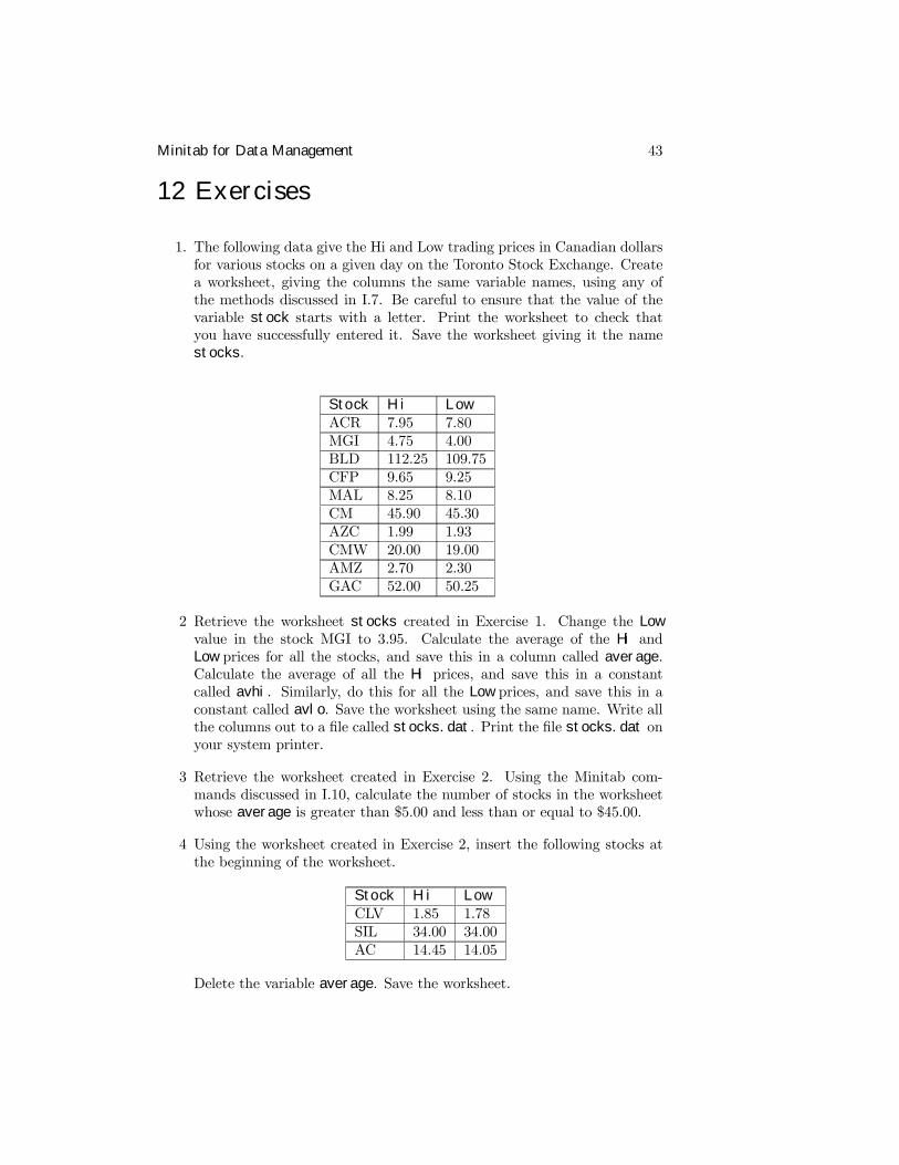
Minitab for Data Management 43
12 Exercises
1. The following data give the Hi and Low trading prices in Canadian dollarsfor various stocks on a given day on the Toronto Stock Exchange. Createa worksheet, giving the columns the same variable names, using any ofthe methods discussed in I.7. Be careful to ensure that the value of thevariable stock starts with a letter. Print the worksheet to check thatyou have successfully entered it. Save the worksheet giving it the namestocks.
Stock Hi LowACR 7.95 7.80MGI 4.75 4.00BLD 112.25 109.75CFP 9.65 9.25MAL 8.25 8.10CM 45.90 45.30AZC 1.99 1.93CMW 20.00 19.00AMZ 2.70 2.30GAC 52.00 50.25
2 Retrieve the worksheet stocks created in Exercise 1. Change the Lowvalue in the stock MGI to 3.95. Calculate the average of the Hi andLow prices for all the stocks, and save this in a column called average.Calculate the average of all the Hi prices, and save this in a constantcalled avhi. Similarly, do this for all the Low prices, and save this in aconstant called avlo. Save the worksheet using the same name. Write allthe columns out to a Þle called stocks.dat. Print the Þle stocks.dat onyour system printer.
3 Retrieve the worksheet created in Exercise 2. Using the Minitab com-mands discussed in I.10, calculate the number of stocks in the worksheetwhose average is greater than $5.00 and less than or equal to $45.00.
4 Using the worksheet created in Exercise 2, insert the following stocks atthe beginning of the worksheet.
Stock Hi LowCLV 1.85 1.78SIL 34.00 34.00AC 14.45 14.05
Delete the variable average. Save the worksheet.
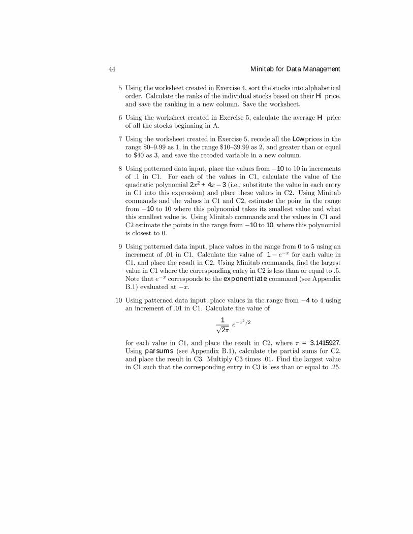
44 Minitab for Data Management
5 Using the worksheet created in Exercise 4, sort the stocks into alphabeticalorder. Calculate the ranks of the individual stocks based on their Hi price,and save the ranking in a new column. Save the worksheet.
6 Using the worksheet created in Exercise 5, calculate the average Hi priceof all the stocks beginning in A.
7 Using the worksheet created in Exercise 5, recode all the Low prices in therange $0�9.99 as 1, in the range $10�39.99 as 2, and greater than or equalto $40 as 3, and save the recoded variable in a new column.
8 Using patterned data input, place the values from −10 to 10 in incrementsof .1 in C1. For each of the values in C1, calculate the value of thequadratic polynomial 2x2 + 4x− 3 (i.e., substitute the value in each entryin C1 into this expression) and place these values in C2. Using Minitabcommands and the values in C1 and C2, estimate the point in the rangefrom −10 to 10 where this polynomial takes its smallest value and whatthis smallest value is. Using Minitab commands and the values in C1 andC2 estimate the points in the range from −10 to 10, where this polynomialis closest to 0.
9 Using patterned data input, place values in the range from 0 to 5 using anincrement of .01 in C1. Calculate the value of 1− e−x for each value inC1, and place the result in C2. Using Minitab commands, Þnd the largestvalue in C1 where the corresponding entry in C2 is less than or equal to .5.Note that e−x corresponds to the exponentiate command (see AppendixB.1) evaluated at −x.
10 Using patterned data input, place values in the range from −4 to 4 usingan increment of .01 in C1. Calculate the value of
1√2π
e−x2/2
for each value in C1, and place the result in C2, where π = 3.1415927.Using parsums (see Appendix B.1), calculate the partial sums for C2,and place the result in C3. Multiply C3 times .01. Find the largest valuein C1 such that the corresponding entry in C3 is less than or equal to .25.

Part II
Minitab for Data Analysis
45

Chapter 1
Looking atData–Distributions
New Minitab commands discussed in this chapterC¯alc I Probability D
¯istributions I N
¯ormal
F¯ile I Open G
¯raph
F¯ile I Sav
¯e Graph As
G¯raph I B
¯oxplot
G¯raph I C
¯hart
G¯raph I Do
¯tplot
G¯raph I H
¯istogram
G¯raph I Pi
¯e Chart
G¯raph I Probability
¯Plot
G¯raph I Stem-and-Leaf
¯G¯raph I T
¯ime Series Plot
M¯anip I Co
¯de
S¯tat I B
¯asic Statistics I D
¯isplay Descriptive Statistics
S¯tat I B
¯asic Statistics I S
¯tore Descriptive Statistics
S¯tat I T
¯ables I Ta
¯lly
This chapter of IPS is concerned with the various ways of presenting and sum-marizing a data set. By presenting data, we mean convenient and informativemethods of conveying the information contained in a data set. There are twobasic methods for presenting data, namely graphically and through tabulations.Still, it can be hard to summarize exactly what these presentations are sayingabout the data. So the chapter also introduces various summary statistics thatare commonly used to convey meaningful information in a concise way.All of these topics can involve much tedious, error prone calculation, if we
were to insist on doing them by hand. An important point is that you should
47
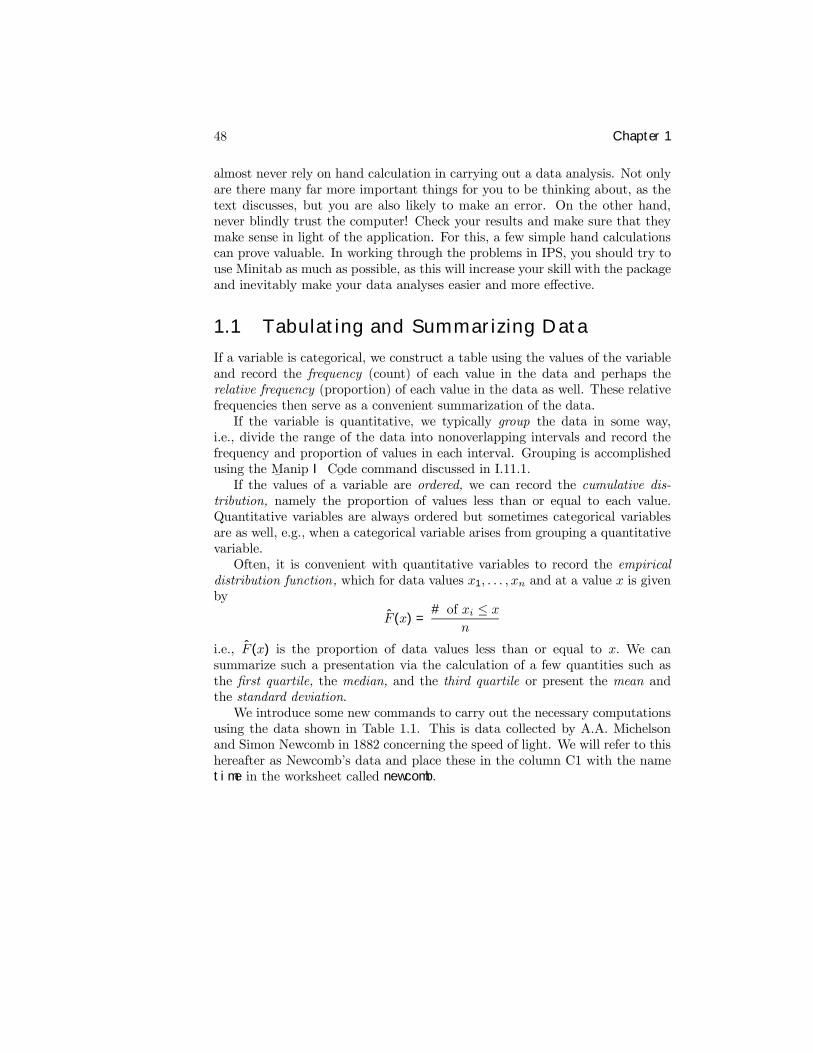
48 Chapter 1
almost never rely on hand calculation in carrying out a data analysis. Not onlyare there many far more important things for you to be thinking about, as thetext discusses, but you are also likely to make an error. On the other hand,never blindly trust the computer! Check your results and make sure that theymake sense in light of the application. For this, a few simple hand calculationscan prove valuable. In working through the problems in IPS, you should try touse Minitab as much as possible, as this will increase your skill with the packageand inevitably make your data analyses easier and more effective.
1.1 Tabulating and Summarizing Data
If a variable is categorical, we construct a table using the values of the variableand record the frequency (count) of each value in the data and perhaps therelative frequency (proportion) of each value in the data as well. These relativefrequencies then serve as a convenient summarization of the data.If the variable is quantitative, we typically group the data in some way,
i.e., divide the range of the data into nonoverlapping intervals and record thefrequency and proportion of values in each interval. Grouping is accomplishedusing the M
¯anip I Co
¯de command discussed in I.11.1.
If the values of a variable are ordered, we can record the cumulative dis-tribution, namely the proportion of values less than or equal to each value.Quantitative variables are always ordered but sometimes categorical variablesare as well, e.g., when a categorical variable arises from grouping a quantitativevariable.Often, it is convenient with quantitative variables to record the empirical
distribution function, which for data values x1, . . . , xn and at a value x is givenby
F (x) =# of xi ≤ x
n
i.e., F (x) is the proportion of data values less than or equal to x. We cansummarize such a presentation via the calculation of a few quantities such asthe Þrst quartile, the median, and the third quartile or present the mean andthe standard deviation.We introduce some new commands to carry out the necessary computations
using the data shown in Table 1.1. This is data collected by A.A. Michelsonand Simon Newcomb in 1882 concerning the speed of light. We will refer to thishereafter as Newcomb�s data and place these in the column C1 with the nametime in the worksheet called newcomb.
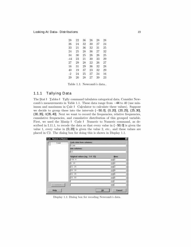
Looking At Data–Distributions 49
28 22 36 26 28 2826 24 32 30 27 2433 21 36 32 31 2524 25 28 36 27 3234 30 25 26 26 25-44 23 21 30 33 2927 29 28 22 26 2716 31 29 36 32 2840 19 37 23 32 29-2 24 25 27 24 1629 20 28 27 39 23
Table 1.1: Newcomb�s data..
1.1.1 Tallying Data
The S¯tat I T
¯ables I Ta
¯lly command tabulates categorical data. Consider New-
comb�s measurements in Table 1.1. These data range from −44 to 40 (use min-imum and maximum in C
¯alc I Cal
¯culator to calculate these values). Suppose
we decide to group these into the intervals (−50, 0], (0, 20], (20, 25], (25, 30],(30, 35], 0(35, 40]. Next we want to record the frequencies, relative frequencies,cumulative frequencies, and cumulative distribution of this grouped variable.First, we used the M
¯anip I Co
¯de I N
¯umeric to Numeric command, as de-
scribed in I.11.1, to recode the data so that every value in (−50, 0] is given thevalue 1, every value in (0, 20] is given the value 2, etc., and these values areplaced in C2. The dialog box for doing this is shown in Display 1.1.
Display 1.1: Dialog box for recoding Newcomb�s data.
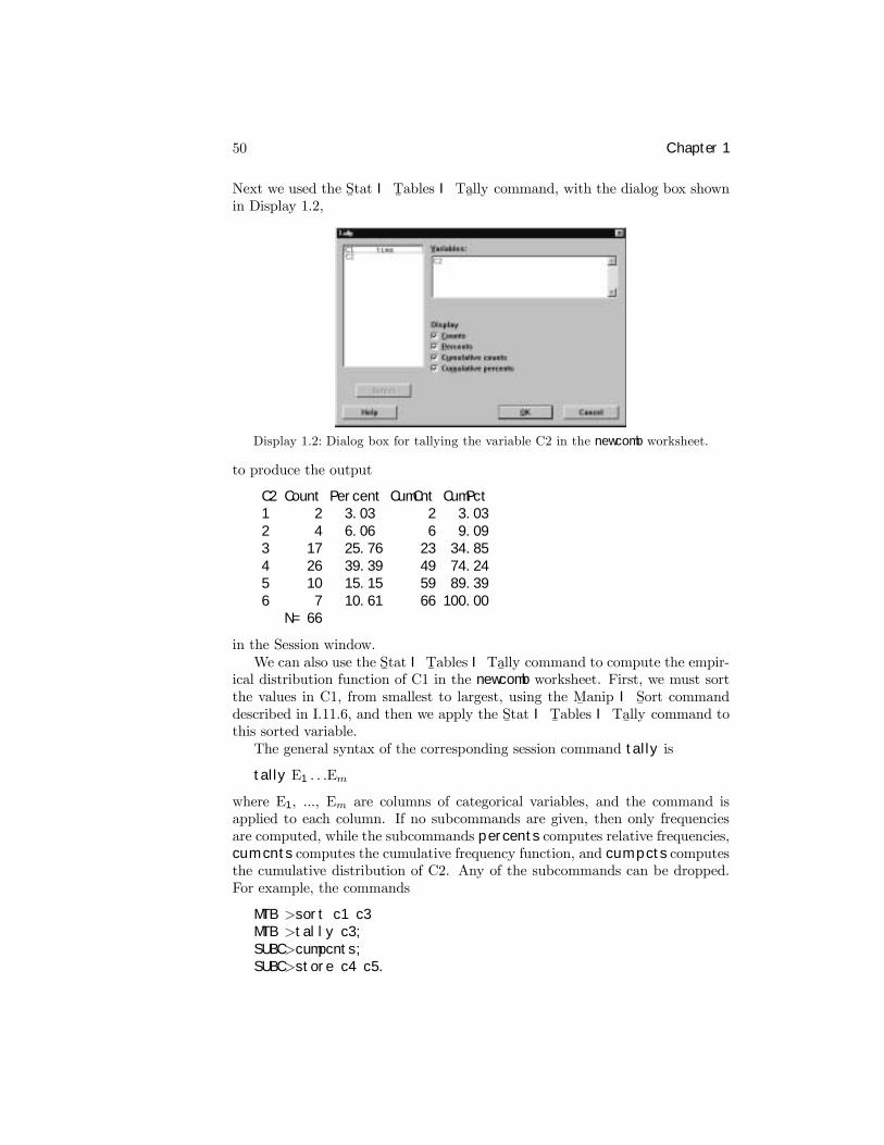
50 Chapter 1
Next we used the S¯tat I T
¯ables I Ta
¯lly command, with the dialog box shown
in Display 1.2,
Display 1.2: Dialog box for tallying the variable C2 in the newcomb worksheet.
to produce the output
C2 Count Percent CumCnt CumPct1 2 3.03 2 3.032 4 6.06 6 9.093 17 25.76 23 34.854 26 39.39 49 74.245 10 15.15 59 89.396 7 10.61 66 100.00
N= 66
in the Session window.We can also use the S
¯tat I T
¯ables I Ta
¯lly command to compute the empir-
ical distribution function of C1 in the newcomb worksheet. First, we must sortthe values in C1, from smallest to largest, using the M
¯anip I S
¯ort command
described in I.11.6, and then we apply the S¯tat I T
¯ables I Ta
¯lly command to
this sorted variable.The general syntax of the corresponding session command tally is
tally E1 . . .Em
where E1, ..., Em are columns of categorical variables, and the command isapplied to each column. If no subcommands are given, then only frequenciesare computed, while the subcommands percents computes relative frequencies,cumcnts computes the cumulative frequency function, and cumpcts computesthe cumulative distribution of C2. Any of the subcommands can be dropped.For example, the commands
MTB >sort c1 c3MTB >tally c3;SUBC>cumpcnts;SUBC>store c4 c5.
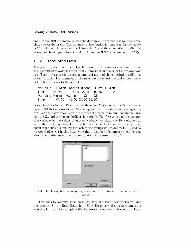
Looking At Data–Distributions 51
Þrst use the sort command to sort the data in C1 from smallest to largest andplace the results in C3. The cumulative distribution is computed for the valuesin C3 with the unique values in C3 stored in C4 and the cumulative distributionat each of the unique values stored in C5 via the store subcommand to tally.
1.1.2 Describing Data
The S¯tat I B
¯asic Statistics I D
¯isplay Descriptive Statistics command is used
with quantitative variables to present a numerical summary of the variable val-ues. These values are in a sense a summarization of the empirical distributionof the variable. For example, in the newcomb worksheet the dialog box shownin Display 1.3 leads to the output
Variable N Mean Median TrMean StDev SE Meantime 66 26.21 27.00 27.40 10.75 1.32Variable Minimum Maximum Q1 Q3time -44.00 40.00 24.00 31.00
in the Session window. This provides the count N, the mean, median, trimmedmean TrMean (removes lower 5% and upper 5% of the data and averages therest), standard deviation, standard error of the mean, minimum, maximum, Þrstquartile Q1, and third quartile Q3 of the variable C1. If we want such a summaryof a variable by the values of another variable, we check the B
¯y variable box
and indicate the by variable in the box to the right of this. For example, wemight want such a summary for each of the groups we created in II.1.1, and sowe would place C2 in this box. Note that a number of summary statistics canalso be computed using the Column Statistics discussed in I.10.3.
Display 1.3: Dialog box for computing basic descriptive statistics of a quantitativevariable.
If we wish to compute some basic statistics and store these values for lateruse, then the S
¯tat I B
¯asic Statistics I S
¯tore Descriptive Statistics command is
available for this. For example, with the newcomb worksheet this command leads
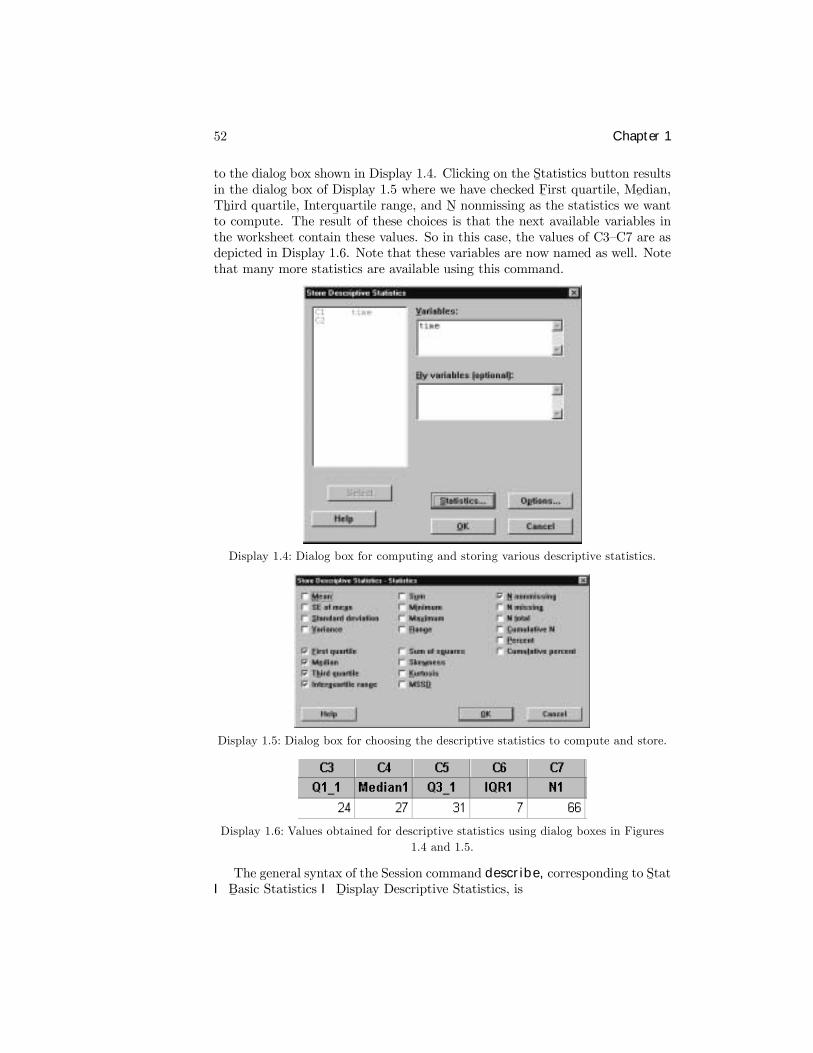
52 Chapter 1
to the dialog box shown in Display 1.4. Clicking on the S¯tatistics button results
in the dialog box of Display 1.5 where we have checked F¯irst quartile, Me
¯dian,
Th¯ird quartile, Interq
¯uartile range, and N
¯nonmissing as the statistics we want
to compute. The result of these choices is that the next available variables inthe worksheet contain these values. So in this case, the values of C3�C7 are asdepicted in Display 1.6. Note that these variables are now named as well. Notethat many more statistics are available using this command.
Display 1.4: Dialog box for computing and storing various descriptive statistics.
Display 1.5: Dialog box for choosing the descriptive statistics to compute and store.
Display 1.6: Values obtained for descriptive statistics using dialog boxes in Figures1.4 and 1.5.
The general syntax of the Session command describe, corresponding to S¯tat
I B¯asic Statistics I D
¯isplay Descriptive Statistics, is
Looking At Data–Distributions 53
describe E1 . . .Em
where E1, ..., Em are columns of quantitative variables and the command isapplied to each column. A by subcommand can also be used. The statscommand is available in the Session window if we want to store the values ofstatistics. We refer the reader to help for a description of this command.
1.2 Plotting Data in a Graph Window
One of the most informative ways of presenting data is via a plot. There aremany different types of plots within Minitab, and which one to use depends onthe type of variable you have and what you are trying to learn. In this sectionwe describe how to use the plotting features in Minitab. There are, however,many features of plotting that we will not describe. For example, there aremany graphical editing capabilities that allow you to add features, such as titlesor legends. Some of these features are accessed via G
¯raph I L
¯ayout. We refer
the reader to H¯elp for more details on these features.
Each plot in Minitab is made in a Graph window. You can make multipleplots and retain each Graph window until you want to delete it simply by clickingthe × symbol in the upper right-hand corner. You make any particular Graphwindow active by clicking in it or by using the W
¯indow command. A plot can
be saved in an external Þle in a variety of formats, such as Minitab graph .mgf,bitmap .bmp, JPEG .jpg, etc., using the F
¯ile I Sav
¯e Graph As command. If
a graph has been saved in the .mgf format, it can be reopened using the F¯ile I
Open G¯raph command.
1.2.1 Dotplots
The G¯raphIDo
¯tplot command is used with quantitative variables and produces
a plot of each data value as a dot along the x-axis so that you get a generalidea of the location of the data and how much scatter there is. Actually, thedata is grouped before plotting and multiple observations in a group are stackedover the x-axis. The interval between successive tick (+) marks on the x-axisis divided into 10 equal-length subintervals for the grouping. Typically, onealso looks for points that are far from the main scatter of points as these maybe identiÞed as outliers and, as such, deleted from the data set for subsequentanalysis. For example, for the newcomb worksheet dialog box in Display 1.7results in the plot of Display 1.8.The general syntax of the corresponding Session command dotplot is
dotplot E1 . . .Em
where E1, ..., Em are columns, and a dotplot is produced for each. There are anumber of subcommands available. The same subcommand ensures the scalesof the dotplots are the same for each column. The by subcommand allowsplotting of a variable by the values of another variable with all plots havingthe same scale. The increment subcommand allows for control of the distance
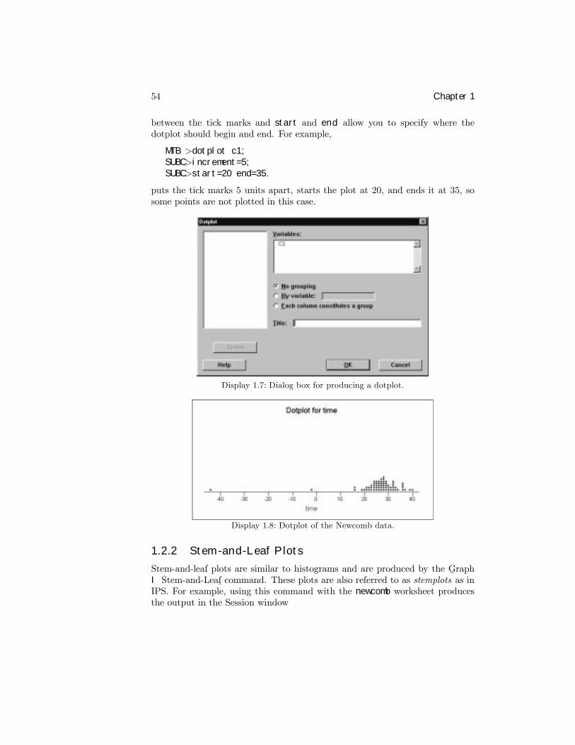
54 Chapter 1
between the tick marks and start and end allow you to specify where thedotplot should begin and end. For example,
MTB >dotplot c1;SUBC>increment=5;SUBC>start=20 end=35.
puts the tick marks 5 units apart, starts the plot at 20, and ends it at 35, sosome points are not plotted in this case.
Display 1.7: Dialog box for producing a dotplot.
Display 1.8: Dotplot of the Newcomb data.
1.2.2 Stem-and-Leaf Plots
Stem-and-leaf plots are similar to histograms and are produced by the G¯raph
I Stem-and-Leaf¯command. These plots are also referred to as stemplots as in
IPS. For example, using this command with the newcomb worksheet producesthe output in the Session window
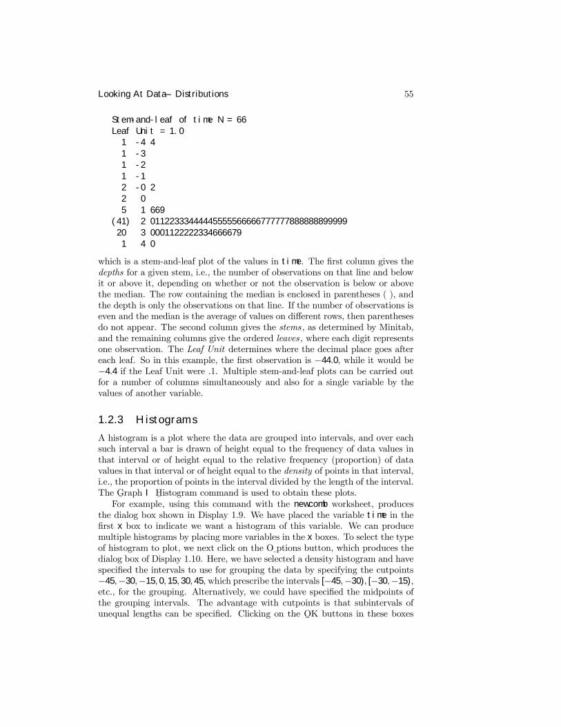
Looking At Data–Distributions 55
Stem-and-leaf of time N = 66Leaf Unit = 1.0
1 -4 41 -31 -21 -12 -0 22 05 1 669
(41) 2 0112233344444555556666677777788888889999920 3 00011222223346666791 4 0
which is a stem-and-leaf plot of the values in time. The Þrst column gives thedepths for a given stem, i.e., the number of observations on that line and belowit or above it, depending on whether or not the observation is below or abovethe median. The row containing the median is enclosed in parentheses ( ), andthe depth is only the observations on that line. If the number of observations iseven and the median is the average of values on different rows, then parenthesesdo not appear. The second column gives the stems, as determined by Minitab,and the remaining columns give the ordered leaves, where each digit representsone observation. The Leaf Unit determines where the decimal place goes aftereach leaf. So in this example, the Þrst observation is −44.0, while it would be−4.4 if the Leaf Unit were .1. Multiple stem-and-leaf plots can be carried outfor a number of columns simultaneously and also for a single variable by thevalues of another variable.
1.2.3 Histograms
A histogram is a plot where the data are grouped into intervals, and over eachsuch interval a bar is drawn of height equal to the frequency of data values inthat interval or of height equal to the relative frequency (proportion) of datavalues in that interval or of height equal to the density of points in that interval,i.e., the proportion of points in the interval divided by the length of the interval.The G
¯raph I H
¯istogram command is used to obtain these plots.
For example, using this command with the newcomb worksheet, producesthe dialog box shown in Display 1.9. We have placed the variable time in theÞrst x box to indicate we want a histogram of this variable. We can producemultiple histograms by placing more variables in the x boxes. To select the typeof histogram to plot, we next click on the O
¯ptions button, which produces the
dialog box of Display 1.10. Here, we have selected a density histogram and havespeciÞed the intervals to use for grouping the data by specifying the cutpoints−45,−30,−15, 0, 15, 30, 45, which prescribe the intervals [−45,−30), [−30,−15),etc., for the grouping. Alternatively, we could have speciÞed the midpoints ofthe grouping intervals. The advantage with cutpoints is that subintervals ofunequal lengths can be speciÞed. Clicking on the O
¯K buttons in these boxes
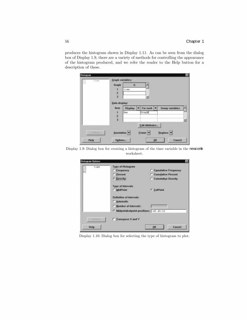
56 Chapter 1
produces the histogram shown in Display 1.11. As can be seen from the dialogbox of Display 1.9, there are a variety of methods for controlling the appearanceof the histogram produced, and we refer the reader to the Help button for adescription of these.
Display 1.9: Dialog box for creating a histogram of the time variable in the newcombworksheet.
Display 1.10: Dialog box for selecting the type of histogram to plot.
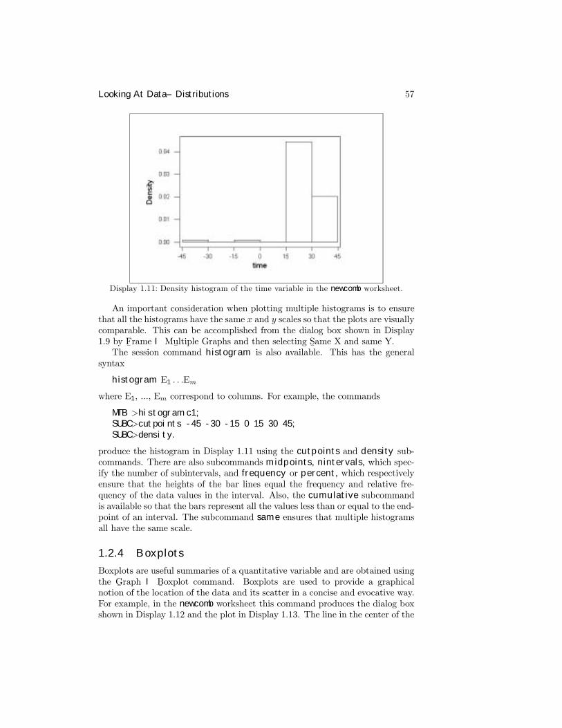
Looking At Data–Distributions 57
Display 1.11: Density histogram of the time variable in the newcomb worksheet.
An important consideration when plotting multiple histograms is to ensurethat all the histograms have the same x and y scales so that the plots are visuallycomparable. This can be accomplished from the dialog box shown in Display1.9 by F
¯rame I Mu
¯ltiple Graphs and then selecting S
¯ame X and same Y.
The session command histogram is also available. This has the generalsyntax
histogram E1 . . .Em
where E1, ..., Em correspond to columns. For example, the commands
MTB >histogram c1;SUBC>cutpoints -45 -30 -15 0 15 30 45;SUBC>density.
produce the histogram in Display 1.11 using the cutpoints and density sub-commands. There are also subcommands midpoints, nintervals, which spec-ify the number of subintervals, and frequency or percent, which respectivelyensure that the heights of the bar lines equal the frequency and relative fre-quency of the data values in the interval. Also, the cumulative subcommandis available so that the bars represent all the values less than or equal to the end-point of an interval. The subcommand same ensures that multiple histogramsall have the same scale.
1.2.4 Boxplots
Boxplots are useful summaries of a quantitative variable and are obtained usingthe G
¯raph I B
¯oxplot command. Boxplots are used to provide a graphical
notion of the location of the data and its scatter in a concise and evocative way.For example, in the newcomb worksheet this command produces the dialog boxshown in Display 1.12 and the plot in Display 1.13. The line in the center of the
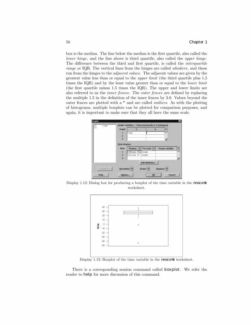
58 Chapter 1
box is the median. The line below the median is the Þrst quartile, also called thelower hinge, and the line above is third quartile, also called the upper hinge.The difference between the third and Þrst quartile, is called the interquartilerange or IQR. The vertical lines from the hinges are called whiskers, and theserun from the hinges to the adjacent values. The adjacent values are given by thegreatest value less than or equal to the upper limit (the third quartile plus 1.5times the IQR) and by the least value greater than or equal to the lower limit(the Þrst quartile minus 1.5 times the IQR). The upper and lower limits arealso referred to as the inner fences. The outer fences are deÞned by replacingthe multiple 1.5 in the deÞnition of the inner fences by 3.0. Values beyond theouter fences are plotted with a * and are called outliers. As with the plottingof histograms, multiple boxplots can be plotted for comparison purposes, andagain, it is important to make sure that they all have the same scale.
Display 1.12: Dialog box for producing a boxplot of the time variable in the newcombworksheet.
Display 1.13: Boxplot of the time variable in the newcomb worksheet.
There is a corresponding session command called boxplot. We refer thereader to help for more discussion of this command.
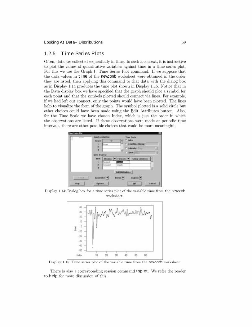
Looking At Data–Distributions 59
1.2.5 Time Series Plots
Often, data are collected sequentially in time. In such a context, it is instructiveto plot the values of quantitative variables against time in a time series plot.For this we use the G
¯raph I T
¯ime Series Plot command. If we suppose that
the data values in time of the newcomb worksheet were obtained in the orderthey are listed, then applying this command to that data with the dialog boxas in Display 1.14 produces the time plot shown in Display 1.15. Notice that inthe D
¯ata display box we have speciÞed that the graph should plot a symbol for
each point and that the symbols plotted should connect via lines. For example,if we had left out connect, only the points would have been plotted. The lineshelp to visualize the form of the graph. The symbol plotted is a solid circle butother choices could have been made using the E
¯dit Attributes button. Also,
for the Time Scale we have chosen Index, which is just the order in whichthe observations are listed. If these observations were made at periodic timeintervals, there are other possible choices that could be more meaningful.
Display 1.14: Dialog box for a time series plot of the variable time from the newcomb
worksheet.
Display 1.15: Time series plot of the variable time from the newcomb worksheet.
There is also a corresponding session command tsplot. We refer the readerto help for more discussion of this.
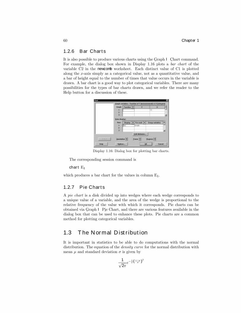
60 Chapter 1
1.2.6 Bar Charts
It is also possible to produce various charts using the G¯raph I C
¯hart command.
For example, the dialog box shown in Display 1.16 plots a bar chart of thevariable C2 in the newcomb worksheet. Each distinct value of C1 is plottedalong the x-axis simply as a categorical value, not as a quantitative value, anda bar of height equal to the number of times that value occurs in the variable isdrawn. A bar chart is a good way to plot categorical variables. There are manypossibilities for the types of bar charts drawn, and we refer the reader to theHelp button for a discussion of these.
Display 1.16: Dialog box for plotting bar charts.
The corresponding session command is
chart E1
which produces a bar chart for the values in column E1.
1.2.7 Pie Charts
A pie chart is a disk divided up into wedges where each wedge corresponds toa unique value of a variable, and the area of the wedge is proportional to therelative frequency of the value with which it corresponds. Pie charts can beobtained via G
¯raph I Pi
¯e Chart, and there are various features available in the
dialog box that can be used to enhance these plots. Pie charts are a commonmethod for plotting categorical variables.
1.3 The Normal Distribution
It is important in statistics to be able to do computations with the normaldistribution. The equation of the density curve for the normal distribution withmean µ and standard deviation σ is given by
1√2πe−
12 ( z−µσ )2
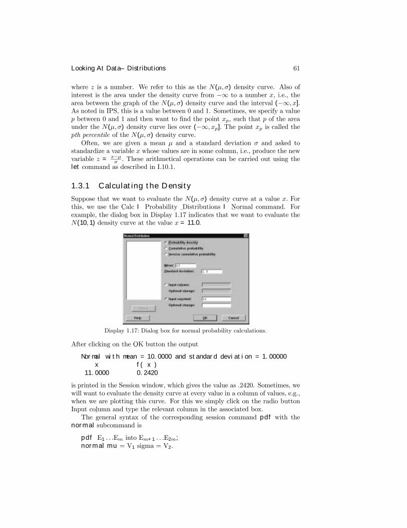
Looking At Data–Distributions 61
where z is a number. We refer to this as the N(µ, σ) density curve. Also ofinterest is the area under the density curve from −∞ to a number x, i.e., thearea between the graph of the N(µ, σ) density curve and the interval (−∞, x].As noted in IPS, this is a value between 0 and 1. Sometimes, we specify a valuep between 0 and 1 and then want to Þnd the point xp, such that p of the areaunder the N(µ, σ) density curve lies over (−∞, xp]. The point xp is called thepth percentile of the N(µ, σ) density curve.Often, we are given a mean µ and a standard deviation σ and asked to
standardize a variable x whose values are in some column, i.e., produce the newvariable z = x−µ
σ . These arithmetical operations can be carried out using thelet command as described in I.10.1.
1.3.1 Calculating the Density
Suppose that we want to evaluate the N(µ, σ) density curve at a value x. Forthis, we use the C
¯alc I Probability
¯Distributions I N
¯ormal command. For
example, the dialog box in Display 1.17 indicates that we want to evaluate theN(10, 1) density curve at the value x = 11.0.
Display 1.17: Dialog box for normal probability calculations.
After clicking on the O¯K button the output
Normal with mean = 10.0000 and standard deviation = 1.00000x f( x )
11.0000 0.2420
is printed in the Session window, which gives the value as .2420. Sometimes, wewill want to evaluate the density curve at every value in a column of values, e.g.,when we are plotting this curve. For this we simply click on the radio buttonInput col
¯umn and type the relevant column in the associated box.
The general syntax of the corresponding session command pdf with thenormal subcommand is
pdf E1 . . .Em into Em+1 . . .E2m;normal mu = V1 sigma = V2.
62 Chapter 1
where E1, ..., Em are columns or constants containing numbers and Em+1, ...,E2m are the columns or constants that store the values of the N(µ,σ) densitycurve at these numbers and V1 = µ and V2 = σ. If no storage is speciÞed, thenthe values are printed. For example, if we want to compute the N(−.5, 1.2) den-sity curve at every value between −3 and 3 in increments of .01, the commands
MTB >set c1DATA>-3:3/.01DATA>endMTB >pdf c1 c2;SUBC>normal mu=-.5 sigma=1.2.
put the values between −3 and 3 in increments of .01 in C1 using the setcommand. The pdf command with the normal subcommand calculates theN(−.5, 1.2) density curve at each of these values and puts the outcomes in thecorresponding entries of C2. If we plot C2 against C1, we will have a plot ofthe density curve of this distribution. For this, we use the scatterplot facilitiesin Minitab as discussed in II.3. Note that with the normal subcommand wemust also specify the mean and the standard deviation via mu and sigma.
1.3.2 Calculating the Distribution Function
Suppose that we want to evaluate the area under N(µ, σ) density curve over theinterval (−∞, x]. This is the value of the cumulative distribution function ofthe N(µ, σ) distribution at the value x. For this, we use the C
¯alc I Probability
D¯istributions I N
¯ormal as well, but in this case in the dialog box of Display
1.17 we select C¯umulative probability instead. Making this change in the dialog
box of Display 1.17, we get the output
x P( X <= x )11.0000 0.8413
in the Session window. Again, we can evaluate this function at a single pointor at every value in a variable.The general syntax of the corresponding Session command cdf command
with the normal subcommand is
cdf E1 . . .Em into Em+1 . . .E2m;normal mu = V1 sigma = V2.
where E1, ..., Em are columns or constants containing numbers and Em+1, ...,E2m are the columns or constants that store the values of the area under N(µ,σ)density curve over the interval from −∞ to these numbers and V1 = µ and V2
= σ. If no storage is speciÞed, the values are printed.
1.3.3 Calculating the Inverse Distribution Function
Suppose that we want to evaluate percentiles for the N(µ, σ) density curve.Again, we use the C
¯alc I Probability D
¯istributions I N
¯ormal command, but
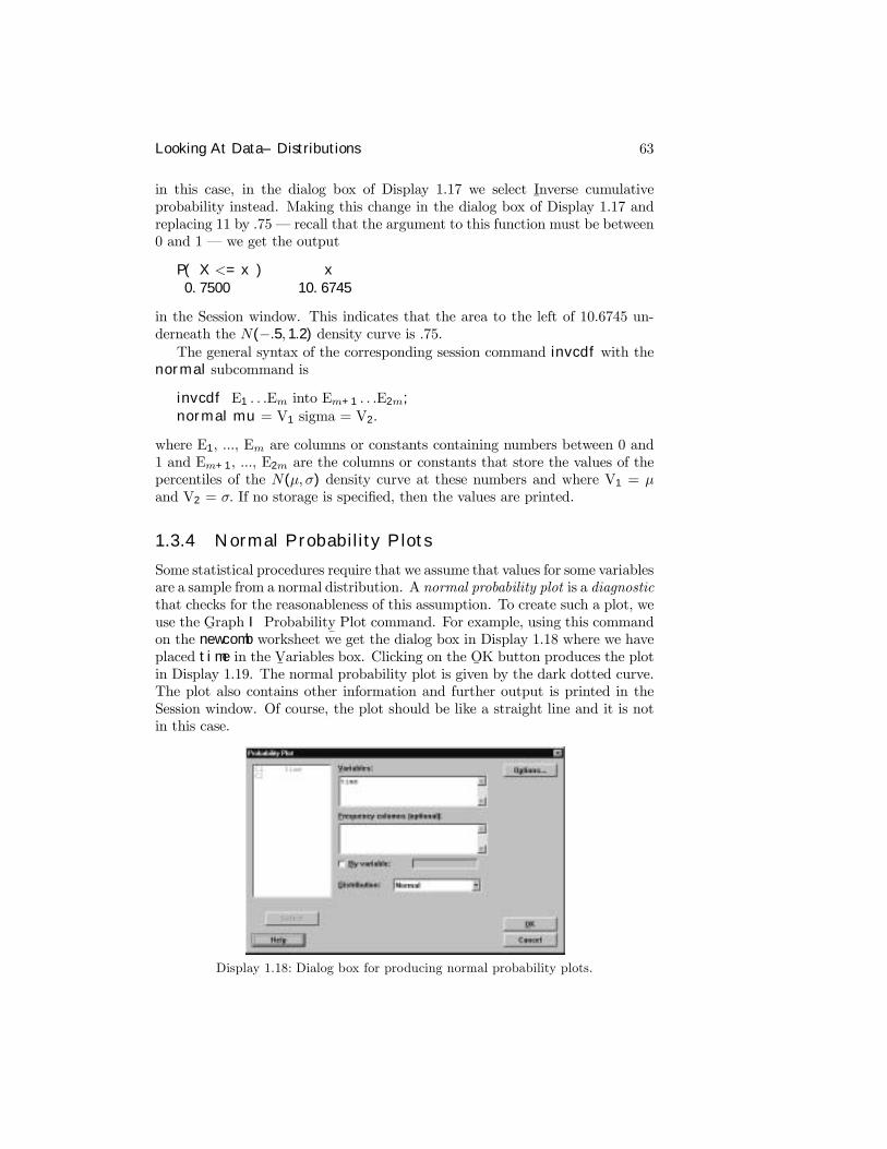
Looking At Data–Distributions 63
in this case, in the dialog box of Display 1.17 we select I¯nverse cumulative
probability instead. Making this change in the dialog box of Display 1.17 andreplacing 11 by .75 � recall that the argument to this function must be between0 and 1 � we get the output
P( X <= x ) x0.7500 10.6745
in the Session window. This indicates that the area to the left of 10.6745 un-derneath the N(−.5, 1.2) density curve is .75.The general syntax of the corresponding session command invcdf with the
normal subcommand is
invcdf E1 . . .Em into Em+1 . . .E2m;normal mu = V1 sigma = V2.
where E1, ..., Em are columns or constants containing numbers between 0 and1 and Em+1, ..., E2m are the columns or constants that store the values of thepercentiles of the N(µ, σ) density curve at these numbers and where V1 = µand V2 = σ. If no storage is speciÞed, then the values are printed.
1.3.4 Normal Probability Plots
Some statistical procedures require that we assume that values for some variablesare a sample from a normal distribution. A normal probability plot is a diagnosticthat checks for the reasonableness of this assumption. To create such a plot, weuse the G
¯raph I Probability
¯Plot command. For example, using this command
on the newcomb worksheet we get the dialog box in Display 1.18 where we haveplaced time in the V
¯ariables box. Clicking on the O
¯K button produces the plot
in Display 1.19. The normal probability plot is given by the dark dotted curve.The plot also contains other information and further output is printed in theSession window. Of course, the plot should be like a straight line and it is notin this case.
Display 1.18: Dialog box for producing normal probability plots.
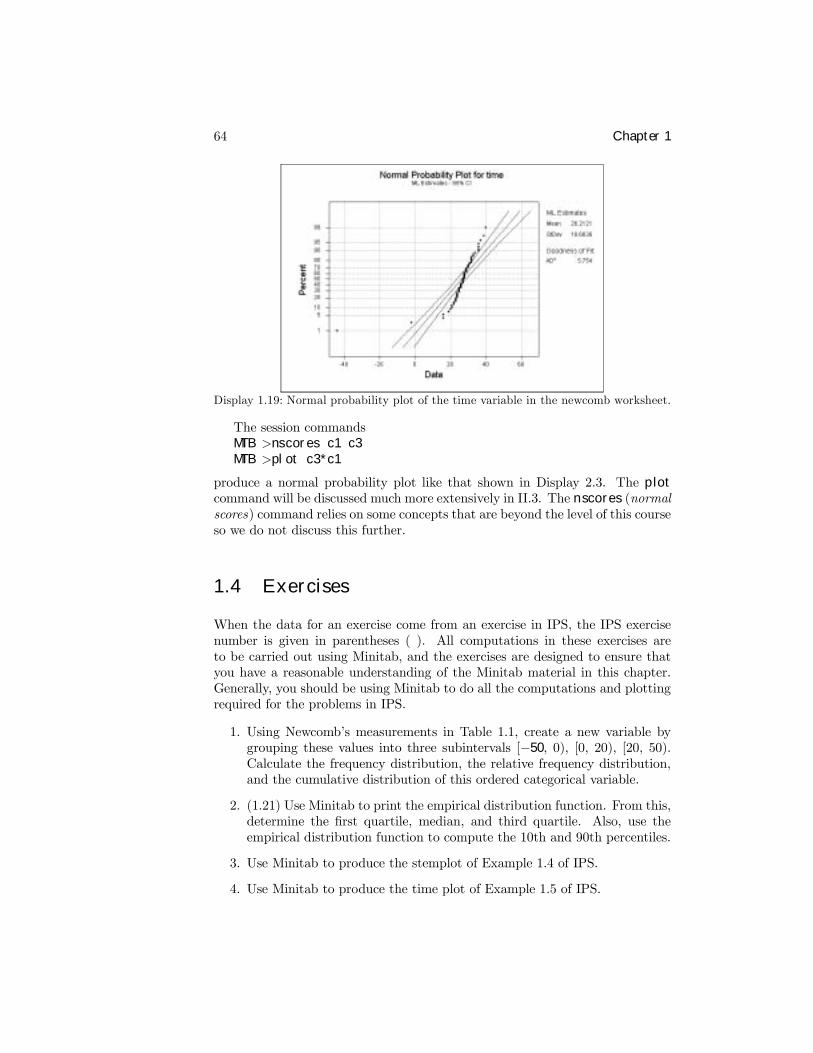
64 Chapter 1
Display 1.19: Normal probability plot of the time variable in the newcomb worksheet.
The session commandsMTB >nscores c1 c3MTB >plot c3*c1
produce a normal probability plot like that shown in Display 2.3. The plotcommand will be discussed much more extensively in II.3. The nscores (normalscores) command relies on some concepts that are beyond the level of this courseso we do not discuss this further.
1.4 Exercises
When the data for an exercise come from an exercise in IPS, the IPS exercisenumber is given in parentheses ( ). All computations in these exercises areto be carried out using Minitab, and the exercises are designed to ensure thatyou have a reasonable understanding of the Minitab material in this chapter.Generally, you should be using Minitab to do all the computations and plottingrequired for the problems in IPS.
1. Using Newcomb�s measurements in Table 1.1, create a new variable bygrouping these values into three subintervals [−50, 0), [0, 20), [20, 50).Calculate the frequency distribution, the relative frequency distribution,and the cumulative distribution of this ordered categorical variable.
2. (1.21) Use Minitab to print the empirical distribution function. From this,determine the Þrst quartile, median, and third quartile. Also, use theempirical distribution function to compute the 10th and 90th percentiles.
3. Use Minitab to produce the stemplot of Example 1.4 of IPS.
4. Use Minitab to produce the time plot of Example 1.5 of IPS.
Looking At Data–Distributions 65
5. (1.29) Use Minitab commands for the stemplot and the time plot. UseMinitab commands to compute a numerical summary of this data, andjustify your choices.
6. (1.30) Transform the data in this problem by subtracting 5 from each valueand multiplying by 10. Calculate the means and standard deviations,using any Minitab commands, of both the original and transformed data.Compute the ratio of the standard deviation of the transformed data tothe standard deviation of the original data. Comment on this value.
7. (1.30) Transform this data by multiplying each value by 3. Computethe ratio of the standard deviation to the mean (called the coefficient ofvariation) for the original data and for the transformed data. Justify theoutcome.
8. For the N(6, 1.1) density curve, compute the area between the interval(3, 5) and the density curve. What number has 53% of the area to the leftof it for this density curve?
9. Use Minitab commands to verify the 68-95-99.7 rule for theN(2, 3) densitycurve.
10. Calculate and store the values of the N(0, 1) density curve at each valuein [−3, 3] using an increment of .01. Put the values in the interval [−3, 3]in C1 and the values of the density curve in C2. Using the command plotC2*C1, plot the density curve. Comment on the shape of this curve.
11. Use Minitab commands to make the normal quantile plots presented inFigures 1.31 and 1.32 of IPS.

66 Chapter 1
Chapter 2
Looking atData–Relationships
New Minitab commands discussed in this chapterG¯raph I P
¯lot
S¯tat I B
¯asic Statistics I C
¯orrelation
S¯tat I R
¯egression I F
¯itted Line Plot
S¯tat I R
¯egression I R
¯egression
In this chapter, Minitab commands are described that permit the analysis ofrelationships among two variables. The methods are different depending onwhether or not both variables are quantitative, both variables are categorical,or one is quantitative and the other is categorical. This chapter considers rela-tionships between two quantitative variables with the remaining cases discussedin later chapters. Graphical methods are very useful in looking for relationshipsamong variables, and we examine various plots for this.
2.1 Scatterplots
A scatterplot of two quantitative variables is a useful technique when lookingfor a relationship between two variables. By a scatterplot we mean a plot ofone variable on the y-axis against the other variable on the x-axis. For exam-ple, consider Example 2.4 in IPS, where we are concerned with the relationshipbetween the length of the femur and the length of the humerus in an extinctspecies. Suppose that we have input the data so that length of the femurmeasurements are in C1, which has been named femur, and the length of thehumerus measurements are in C2, which has been named humerus, of the work-sheet archaeopteryx. The command G
¯raph I P
¯lot produces the dialog box of
Display 2.1, where we have placed femur into the Þrst box for the y variable
67
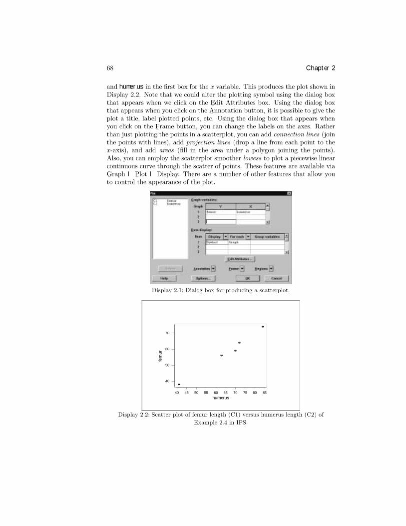
68 Chapter 2
and humerus in the Þrst box for the x variable. This produces the plot shown inDisplay 2.2. Note that we could alter the plotting symbol using the dialog boxthat appears when we click on the E
¯dit Attributes box. Using the dialog box
that appears when you click on the A¯nnotation button, it is possible to give the
plot a title, label plotted points, etc. Using the dialog box that appears whenyou click on the F
¯rame button, you can change the labels on the axes. Rather
than just plotting the points in a scatterplot, you can add connection lines (jointhe points with lines), add projection lines (drop a line from each point to thex-axis), and add areas (Þll in the area under a polygon joining the points).Also, you can employ the scatterplot smoother lowess to plot a piecewise linearcontinuous curve through the scatter of points. These features are available viaG¯raph I P
¯lot I Display. There are a number of other features that allow you
to control the appearance of the plot.
Display 2.1: Dialog box for producing a scatterplot.
85807570656055504540
70
60
50
40
humerus
fem
ur
Display 2.2: Scatter plot of femur length (C1) versus humerus length (C2) ofExample 2.4 in IPS.
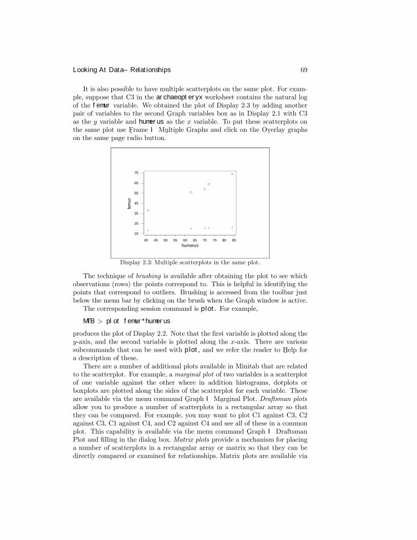
Looking At Data–Relationships 69
It is also possible to have multiple scatterplots on the same plot. For exam-ple, suppose that C3 in the archaeopteryx worksheet contains the natural logof the femur variable. We obtained the plot of Display 2.3 by adding anotherpair of variables to the second G
¯raph variables box as in Display 2.1 with C3
as the y variable and humerus as the x variable. To put these scatterplots onthe same plot use F
¯rame I Mu
¯ltiple Graphs and click on the Ov
¯erlay graphs
on the same page radio button.
85807570656055504540
75
65
55
45
35
25
15
humerus
fem
ur
Display 2.3: Multiple scatterplots in the same plot.
The technique of brushing is available after obtaining the plot to see whichobservations (rows) the points correspond to. This is helpful in identifying thepoints that correspond to outliers. Brushing is accessed from the toolbar justbelow the menu bar by clicking on the brush when the Graph window is active.The corresponding session command is plot. For example,
MTB > plot femur*humerus
produces the plot of Display 2.2. Note that the Þrst variable is plotted along they-axis, and the second variable is plotted along the x-axis. There are varioussubcommands that can be used with plot, and we refer the reader to H
¯elp for
a description of these.There are a number of additional plots available in Minitab that are related
to the scatterplot. For example, a marginal plot of two variables is a scatterplotof one variable against the other where in addition histograms, dotplots orboxplots are plotted along the sides of the scatterplot for each variable. Theseare available via the menu command G
¯raph I Ma
¯rginal Plot. Draftsman plots
allow you to produce a number of scatterplots in a rectangular array so thatthey can be compared. For example, you may want to plot C1 against C3, C2against C3, C1 against C4, and C2 against C4 and see all of these in a commonplot. This capability is available via the menu command G
¯raph I Draftsman
Plot and Þlling in the dialog box. Matrix plots provide a mechanism for placinga number of scatterplots in a rectangular array or matrix so that they can bedirectly compared or examined for relationships. Matrix plots are available via
70 Chapter 2
the command G¯raph I M
¯atrix Plot. Also three-dimensional scatterplots are
available via G¯raph I 3
¯D Plot and contour plots via G
¯raph I Con
¯tour Plot.
2.2 Correlations
While a scatterplot is a convenient graphical method for assessing whether ornot there is any relationship between two variables, we would also like to assessthis numerically. The correlation coefficient provides a numerical summariza-tion of the degree to which a linear relationship exists between two quantita-tive variables, and this can be calculated using the S
¯tat I B
¯asic Statistics I
C¯orrelation command. For example, applying this command to the femur and
humerus variables of the worksheet archaeopteryx, i.e., the data of Example2.4 in IPS and depicted in Display 2.2, we obtain the output
Pearson correlation of femur and humerus = 0.994P-Value = 0.001
in the Session window. For now, we ignore the number recorded as P-Value.The general syntax of the corresponding session command correlate is given
by
correlate E1 . . . Em
where E1, ..., Em are columns corresponding to numerical variables, and a cor-relation coefficient is computed between each pair. This gives m(m − 1)/2correlation coefficients. The subcommand nopvalues is available if you wantto suppress the printing of P -values.
2.3 RegressionRegression is another technique for assessing the strength of a linear relationshipexisting between two variables and it is closely related to correlation. For this,we use the S
¯tat I R
¯egression command.
As noted in IPS, the regression analysis of two quantitative variables involvescomputing the least-squares line y = a+ bx, where one variable is taken to bethe response variable y and the other is taken to be the explanatory variablex. Note that the least squares line is different depending upon which choice ismade. For example, for the data of Example 2.4 in IPS and plotted in Display2.2 letting femur be the response and humerus be the predictor or explanatoryvariable, the S
¯tat I R
¯egression I R
¯egression command leads to the dialog box
of Display 2.4, where we have made the appropriate entries in the Re¯sponse and
Predi¯ctors boxes. Clicking on the O
¯K button leads to the output of Display
2.5 being printed in the Session window. This gives the least-squares line asy = 3.70 + .826x, i.e., a = 3.70 and b = .826, which we also see under the Coefcolumn in the Þrst table. In addition, we obtain the value of the square of thecorrelation coefficient, also known as the coefficient of determination, as R-Sq= 98.8%. We will discuss the remaining output from this command in II.10.
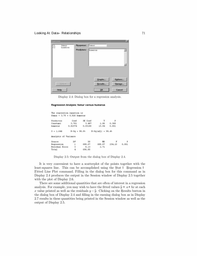
Looking At Data–Relationships 71
Display 2.4: Dialog box for a regression analysis.
Display 2.5: Output from the dialog box of Display 2.4.
It is very convenient to have a scatterplot of the points together with theleast-squares line. This can be accomplished using the S
¯tat I R
¯egression I
F¯itted Line Plot command. Filling in the dialog box for this command as inDisplay 2.4 produces the output in the Session window of Display 2.5 togetherwith the plot of Display 2.6.There are some additional quantities that are often of interest in a regression
analysis. For example, you may wish to have the Þtted values y = a+bx at eachx value printed as well as the residuals y− y. Clicking on the R
¯esults button in
the dialog box of Display 2.4 and Þlling in the ensuing dialog box as in Display2.7 results in these quantities being printed in the Session window as well as theoutput of Display 2.5.
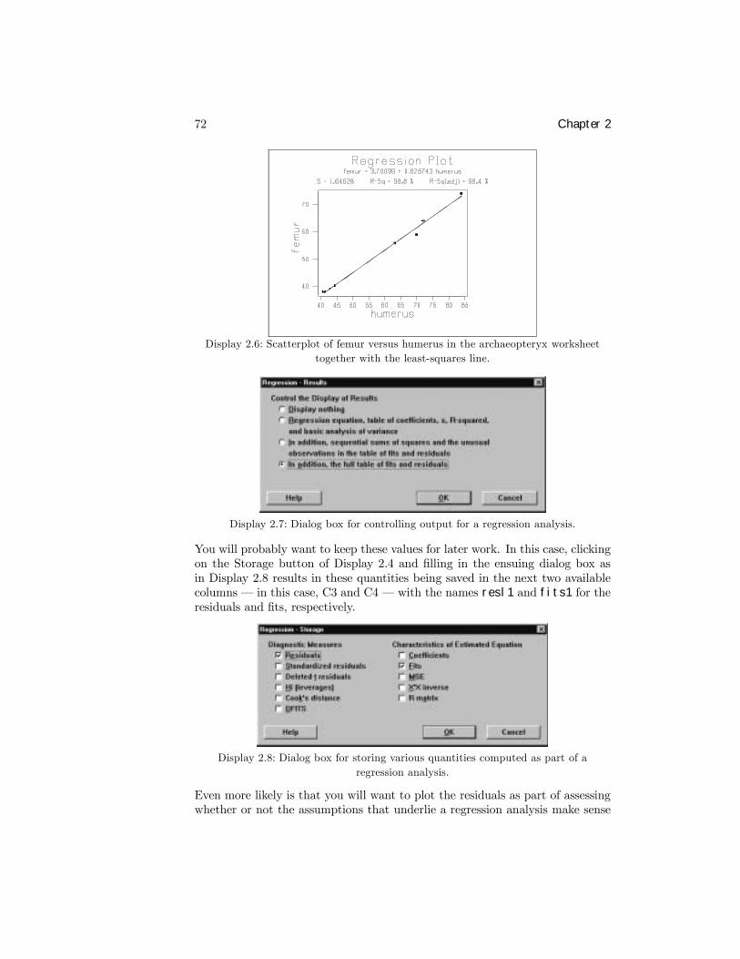
72 Chapter 2
Display 2.6: Scatterplot of femur versus humerus in the archaeopteryx worksheettogether with the least-squares line.
Display 2.7: Dialog box for controlling output for a regression analysis.
You will probably want to keep these values for later work. In this case, clickingon the Storage button of Display 2.4 and Þlling in the ensuing dialog box asin Display 2.8 results in these quantities being saved in the next two availablecolumns � in this case, C3 and C4 � with the names resl1 and fits1 for theresiduals and Þts, respectively.
Display 2.8: Dialog box for storing various quantities computed as part of aregression analysis.
Even more likely is that you will want to plot the residuals as part of assessingwhether or not the assumptions that underlie a regression analysis make sense
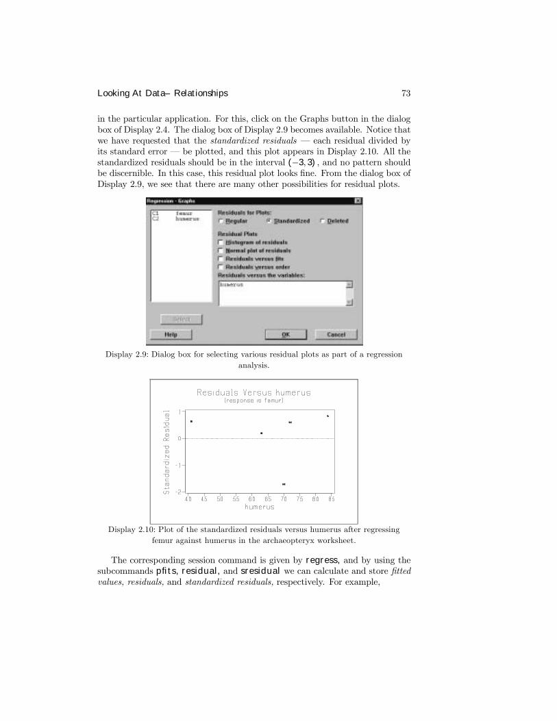
Looking At Data–Relationships 73
in the particular application. For this, click on the Graphs button in the dialogbox of Display 2.4. The dialog box of Display 2.9 becomes available. Notice thatwe have requested that the standardized residuals � each residual divided byits standard error � be plotted, and this plot appears in Display 2.10. All thestandardized residuals should be in the interval (−3, 3) , and no pattern shouldbe discernible. In this case, this residual plot looks Þne. From the dialog box ofDisplay 2.9, we see that there are many other possibilities for residual plots.
Display 2.9: Dialog box for selecting various residual plots as part of a regressionanalysis.
Display 2.10: Plot of the standardized residuals versus humerus after regressingfemur against humerus in the archaeopteryx worksheet.
The corresponding session command is given by regress, and by using thesubcommands pfits, residual, and sresidual we can calculate and store Þttedvalues, residuals, and standardized residuals, respectively. For example,
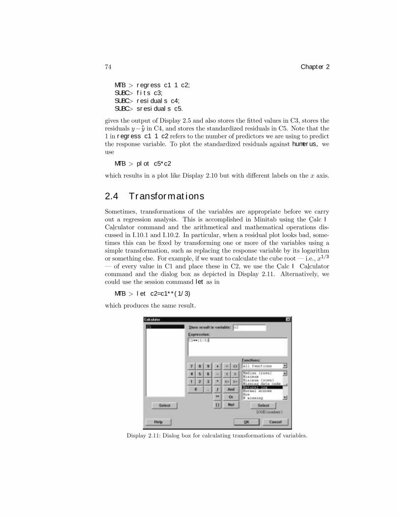
74 Chapter 2
MTB > regress c1 1 c2;SUBC> fits c3;SUBC> residuals c4;SUBC> sresiduals c5.
gives the output of Display 2.5 and also stores the Þtted values in C3, stores theresiduals y− y in C4, and stores the standardized residuals in C5. Note that the1 in regress c1 1 c2 refers to the number of predictors we are using to predictthe response variable. To plot the standardized residuals against humerus, weuse
MTB > plot c5*c2
which results in a plot like Display 2.10 but with different labels on the x axis.
2.4 Transformations
Sometimes, transformations of the variables are appropriate before we carryout a regression analysis. This is accomplished in Minitab using the C
¯alc I
Cal¯culator command and the arithmetical and mathematical operations dis-
cussed in I.10.1 and I.10.2. In particular, when a residual plot looks bad, some-times this can be Þxed by transforming one or more of the variables using asimple transformation, such as replacing the response variable by its logarithmor something else. For example, if we want to calculate the cube root � i.e., x1/3
� of every value in C1 and place these in C2, we use the C¯alc I Cal
¯culator
command and the dialog box as depicted in Display 2.11. Alternatively, wecould use the session command let as in
MTB > let c2=c1**(1/3)
which produces the same result.
Display 2.11: Dialog box for calculating transformations of variables.
Looking At Data–Relationships 75
2.5 Exercises
When the data for an exercise come from an exercise in IPS, the IPS exercisenumber is given in parentheses ( ). All computations in these exercises areto be carried out using Minitab, and the exercises are designed to ensure thatyou have a reasonable understanding of the Minitab material in this chapter.Generally, you should be using Minitab to do all the computations and plottingrequired for the problems in IPS.
1. (2.10) Calculate the least-squares line and make a scatterplot of Fuel usedagainst Speed together with the least-squares line. Plot the standard-ized residuals against Speed. What is the squared correlation coefficientbetween these variables?
2. (2.11) Make a scatterplot of Rate against Mass where the points for dif-ferent Sexes are labeled differently (use Minitab for the labeling, too) andwith the least-squares line on it. Hint: Make use of the stack commanddiscussed in I.11.7.
3. Place the values 1 through 100 with an increment of .1 in C1 and thesquare of these values in C2. Calculate the correlation coefficient betweenC1 and C2. Multiply each value in C1 by 10, add 5, and place the resultsin C3. Calculate the correlation coefficient between C2 and C3. Why arethese correlation coefficients the same?
4. Place the values 1 through 100 with an increment of .1 in C1 and thesquare of these values in C2. Calculate the least-squares line with C2 asresponse and C1 as explanatory variable. Plot the standardized residuals.If you see such a pattern of residuals what transformation, might you useto remedy the problem?
5. (2.54) For the data in this problem, numerically verify the algebraic re-lationship that exists between the correlation coefficient and the slope ofthe least-squares line.
6. For Example 2.17 in IPS, calculate the least-squares line and reproduceDisplay 2.21. Calculate the sum of the residuals and the sum of thesquared residuals and divide this by the number of data points minus 2.Is there anything you can say about what these quantities are equal to ingeneral?
7. (2.62) Use Minitab to do all the calculations in this problem.
8. Place the values 1 through 10 with an increment of .1 in C1, and placeexp (−1 + 2x) of these values in C2. Calculate the least-squares line usingC2 as the response variable, and plot the standardized residuals againstC1. What transformation would you use to remedy this residual plot?What is the least-squares line when you carry out this transformation?

76 Chapter 2
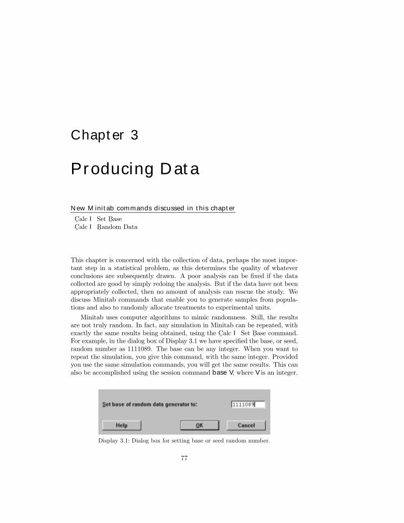
Chapter 3
Producing Data
New Minitab commands discussed in this chapter
C¯alc I Set B
¯ase
C¯alc I R
¯andom Data
This chapter is concerned with the collection of data, perhaps the most impor-tant step in a statistical problem, as this determines the quality of whateverconclusions are subsequently drawn. A poor analysis can be Þxed if the datacollected are good by simply redoing the analysis. But if the data have not beenappropriately collected, then no amount of analysis can rescue the study. Wediscuss Minitab commands that enable you to generate samples from popula-tions and also to randomly allocate treatments to experimental units.
Minitab uses computer algorithms to mimic randomness. Still, the resultsare not truly random. In fact, any simulation in Minitab can be repeated, withexactly the same results being obtained, using the C
¯alc I Set B
¯ase command.
For example, in the dialog box of Display 3.1 we have speciÞed the base, or seed,random number as 1111089. The base can be any integer. When you want torepeat the simulation, you give this command, with the same integer. Providedyou use the same simulation commands, you will get the same results. This canalso be accomplished using the session command base V, where V is an integer.
Display 3.1: Dialog box for setting base or seed random number.
77
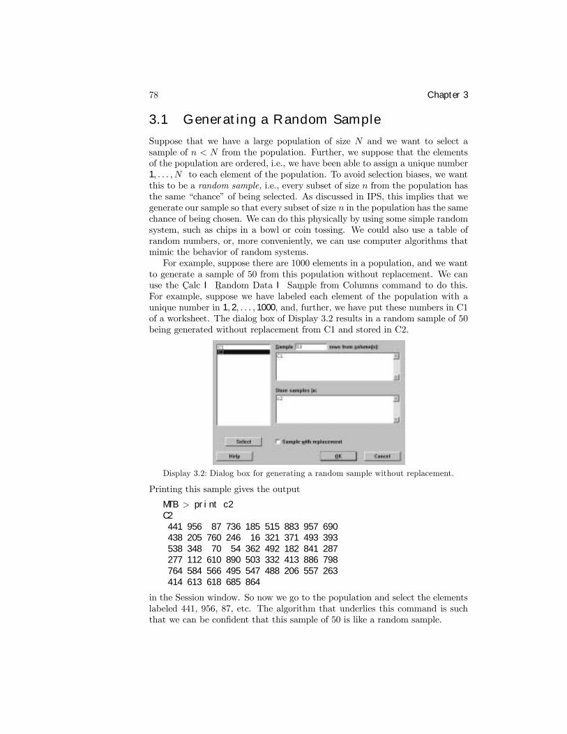
78 Chapter 3
3.1 Generating a Random Sample
Suppose that we have a large population of size N and we want to select asample of n < N from the population. Further, we suppose that the elementsof the population are ordered, i.e., we have been able to assign a unique number1, . . . , N to each element of the population. To avoid selection biases, we wantthis to be a random sample, i.e., every subset of size n from the population hasthe same �chance� of being selected. As discussed in IPS, this implies that wegenerate our sample so that every subset of size n in the population has the samechance of being chosen. We can do this physically by using some simple randomsystem, such as chips in a bowl or coin tossing. We could also use a table ofrandom numbers, or, more conveniently, we can use computer algorithms thatmimic the behavior of random systems.For example, suppose there are 1000 elements in a population, and we want
to generate a sample of 50 from this population without replacement. We canuse the C
¯alc I R
¯andom Data I Sam
¯ple from Columns command to do this.
For example, suppose we have labeled each element of the population with aunique number in 1, 2, . . . , 1000, and, further, we have put these numbers in C1of a worksheet. The dialog box of Display 3.2 results in a random sample of 50being generated without replacement from C1 and stored in C2.
Display 3.2: Dialog box for generating a random sample without replacement.
Printing this sample gives the output
MTB > print c2C2441 956 87 736 185 515 883 957 690438 205 760 246 16 321 371 493 393538 348 70 54 362 492 182 841 287277 112 610 890 503 332 413 886 798764 584 566 495 547 488 206 557 263414 613 618 685 864
in the Session window. So now we go to the population and select the elementslabeled 441, 956, 87, etc. The algorithm that underlies this command is suchthat we can be conÞdent that this sample of 50 is like a random sample.
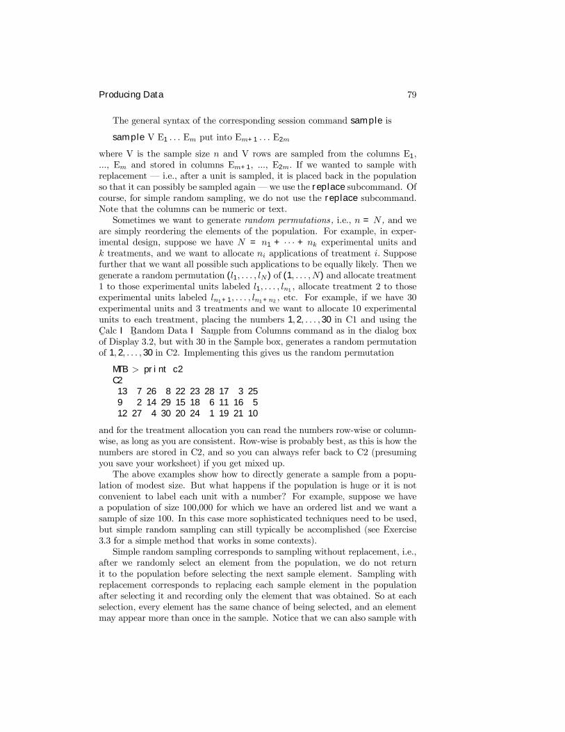
Producing Data 79
The general syntax of the corresponding session command sample is
sample V E1 . . . Em put into Em+1 . . . E2m
where V is the sample size n and V rows are sampled from the columns E1,..., Em and stored in columns Em+1, ..., E2m. If we wanted to sample withreplacement � i.e., after a unit is sampled, it is placed back in the populationso that it can possibly be sampled again � we use the replace subcommand. Ofcourse, for simple random sampling, we do not use the replace subcommand.Note that the columns can be numeric or text.Sometimes we want to generate random permutations, i.e., n = N , and we
are simply reordering the elements of the population. For example, in exper-imental design, suppose we have N = n1 + · · · + nk experimental units andk treatments, and we want to allocate ni applications of treatment i. Supposefurther that we want all possible such applications to be equally likely. Then wegenerate a random permutation (l1, . . . , lN) of (1, . . . , N) and allocate treatment1 to those experimental units labeled l1, . . . , ln1 , allocate treatment 2 to thoseexperimental units labeled ln1+1, . . . , ln1+n2 , etc. For example, if we have 30experimental units and 3 treatments and we want to allocate 10 experimentalunits to each treatment, placing the numbers 1, 2, . . . , 30 in C1 and using theC¯alc I R
¯andom Data I Sam
¯ple from Columns command as in the dialog box
of Display 3.2, but with 30 in the S¯ample box, generates a random permutation
of 1, 2, . . . , 30 in C2. Implementing this gives us the random permutation
MTB > print c2C213 7 26 8 22 23 28 17 3 259 2 14 29 15 18 6 11 16 512 27 4 30 20 24 1 19 21 10
and for the treatment allocation you can read the numbers row-wise or column-wise, as long as you are consistent. Row-wise is probably best, as this is how thenumbers are stored in C2, and so you can always refer back to C2 (presumingyou save your worksheet) if you get mixed up.The above examples show how to directly generate a sample from a popu-
lation of modest size. But what happens if the population is huge or it is notconvenient to label each unit with a number? For example, suppose we havea population of size 100,000 for which we have an ordered list and we want asample of size 100. In this case more sophisticated techniques need to be used,but simple random sampling can still typically be accomplished (see Exercise3.3 for a simple method that works in some contexts).Simple random sampling corresponds to sampling without replacement, i.e.,
after we randomly select an element from the population, we do not returnit to the population before selecting the next sample element. Sampling withreplacement corresponds to replacing each sample element in the populationafter selecting it and recording only the element that was obtained. So at eachselection, every element has the same chance of being selected, and an elementmay appear more than once in the sample. Notice that we can also sample with
80 Chapter 3
replacement if we check the Sample w¯ith replacement box in the dialog box of
Display 3.2.
3.2 Sampling from Distributions
Once we have generated a sample from a population, we measure various at-tributes of the sampled elements. For example, if we were sampling from a pop-ulation of humans, we might measure each sampled unit�s height. The height forthe sample unit is now a random variable that follows the height distribution inthe population from which we are sampling. For example, if 80% of the peoplein the population are between 4.5 feet and 6 feet, then under repeated samplingof an element from the population (with replacement) in the long run, 80% ofthe sampled units will have their heights in this range.Sometimes, we want to sample directly from this population distribution,
i.e., generate a number in such a way that under repeated sampling in the longrun the proportion of values falling in any range agrees with that prescribed bythe population distribution. Of course, we typically don�t know the populationdistribution, as this is what we want to Þnd out about in a statistical investiga-tion. Still, there are many instances where we want to pretend that we do knowit and simulate from this distribution, e.g., perhaps we want to consider theeffect of various choices of population distribution on the sampling distributionof some statistic of interest.There are computer algorithms that allow us to do this for a variety of
distributions. In Minitab, this is accomplished using the C¯alc I R
¯andom Data
command. For example, suppose that we want to simulate the tossing of a faircoin (a coin where head and tail are equally likely as outcomes). The C
¯alc I
R¯andom Data I Be
¯rnoulli command together with the dialog box of Display
3.3 generates a sample of 100 from the Bernoulli(.5) distribution and placesthese values in C1. A random variable has a Bernoulli(p) distribution if theprobability the variable equals 1 � success � is p and the probability thevariable equals 0 � failure � is 1 − p. So to generate a sample of n from theBernoulli(p) distribution, we put n in the G
¯enerate box and p in the P
¯robability
of success box. In such a case, we are simulating the tossing of a coin thatproduces a head on a single toss with probability p, i.e., the long-run proportionof heads that we observe in repeated tossing is p. Note that we can generate msamples of size n by putting m distinct columns in the S
¯tore in column(s) box.
Often, a normal distribution with some particular mean and standard devia-tion is considered a reasonable assumption for the distribution of a measurementin a population. For example, the C
¯alc I R
¯andom Data I N
¯ormal command
together with the dialog box of Display 3.4 generates a sample of 200 from theN (5.2, 1.3) distribution and places this sample in C1. To generate a sample ofn from the N (µ, σ) distribution, we put n in the G
¯enerate box, µ in the M
¯ean
box, and σ in the St¯andard deviation box.
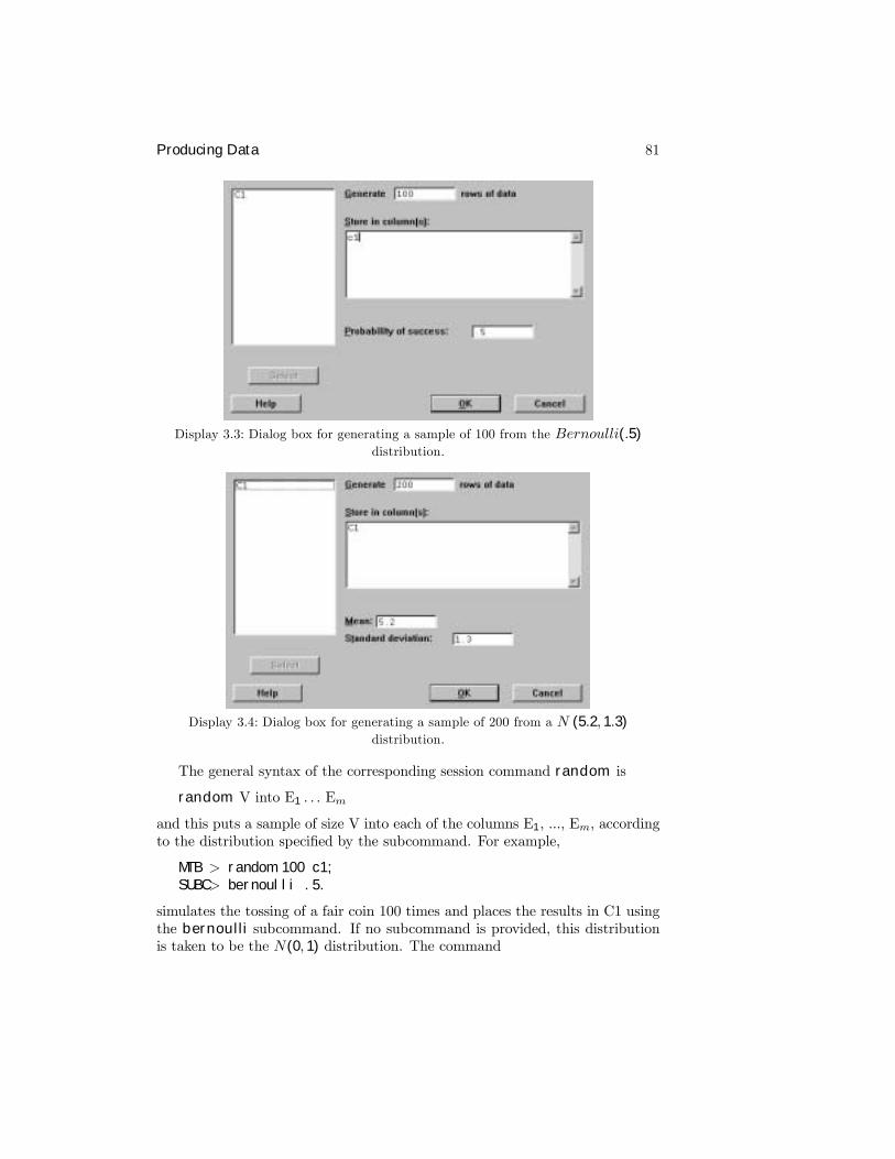
Producing Data 81
Display 3.3: Dialog box for generating a sample of 100 from the Bernoulli(.5)distribution.
Display 3.4: Dialog box for generating a sample of 200 from a N (5.2, 1.3)distribution.
The general syntax of the corresponding session command random is
random V into E1 . . . Em
and this puts a sample of size V into each of the columns E1, ..., Em, accordingto the distribution speciÞed by the subcommand. For example,
MTB > random 100 c1;SUBC> bernoulli .5.
simulates the tossing of a fair coin 100 times and places the results in C1 usingthe bernoulli subcommand. If no subcommand is provided, this distributionis taken to be the N(0, 1) distribution. The command
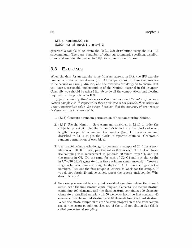
82 Chapter 3
MTB > random 200 c1;SUBC> normal mu=2.1 sigma=3.3.
generates a sample of 200 from the N(2.1, 3.3) distribution using the normalsubcommand. There are a number of other subcommands specifying distribu-tions, and we refer the reader to help for a description of these.
3.3 Exercises
When the data for an exercise come from an exercise in IPS, the IPS exercisenumber is given in parentheses ( ). All computations in these exercises areto be carried out using Minitab, and the exercises are designed to ensure thatyou have a reasonable understanding of the Minitab material in this chapter.Generally, you should be using Minitab to do all the computations and plottingrequired for the problems in IPS.If your version of Minitab places restrictions such that the value of the sim-
ulation sample size N requested in these problems is not feasible, then substitutea more appropriate value. Be aware, however, that the accuracy of your resultsis dependent on how large N is.
1. (3.13) Generate a random permutation of the names using Minitab.
2. (3.32) Use the M¯anip I S
¯ort command described in I.11.6 to order the
subjects by weight. Use the values 1�5 to indicate Þve blocks of equallength in a separate column, and then use the M
¯anip I Unstack command
described in I.11.7 to put the blocks in separate columns. Generate arandom permutation of each block.
3. Use the following methodology to generate a sample of 20 from a pop-ulation of 100,000. First, put the values 0�9 in each of C1�C5. Next,use sampling with replacement to generate 50 values from C1, and putthe results in C6. Do the same for each of C2�C5 and put the resultsin C7�C10 (don�t generate from these columns simultaneously). Create asingle column of numbers using the digits in C6�C10 as the digits in thenumbers. Pick out the Þrst unique 20 entries as labels for the sample. Ifyou do not obtain 20 unique values, repeat the process until you do. Whydoes this work?
4. Suppose you wanted to carry out stratiÞed sampling where there are 3strata, with the Þrst stratum containing 500 elements, the second stratumcontaining 400 elements, and the third stratum containing 100 elements.Generate a stratiÞed sample with 50 elements from the Þrst stratum, 40elements from the second stratum, and 10 elements from the third stratum.When the strata sample sizes are the same proportion of the total samplesize as the strata population sizes are of the total population size this iscalled proportional sampling.
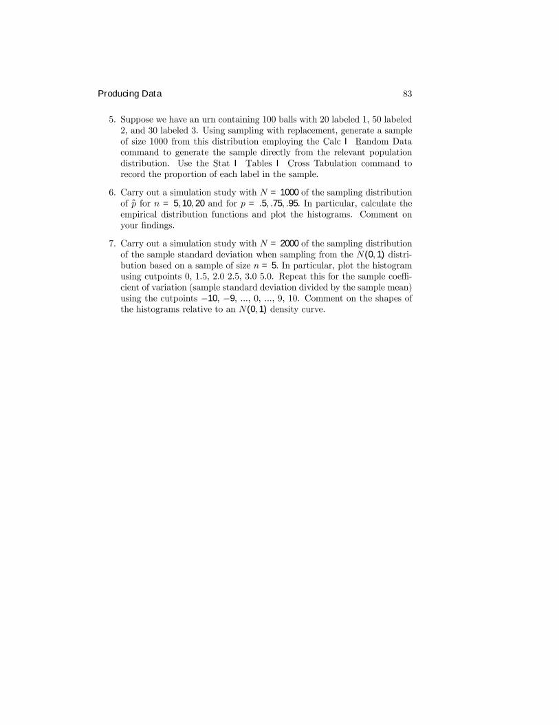
Producing Data 83
5. Suppose we have an urn containing 100 balls with 20 labeled 1, 50 labeled2, and 30 labeled 3. Using sampling with replacement, generate a sampleof size 1000 from this distribution employing the C
¯alc I R
¯andom Data
command to generate the sample directly from the relevant populationdistribution. Use the S
¯tat I T
¯ables I C
¯ross Tabulation command to
record the proportion of each label in the sample.
6. Carry out a simulation study with N = 1000 of the sampling distributionof p for n = 5, 10, 20 and for p = .5, .75, .95. In particular, calculate theempirical distribution functions and plot the histograms. Comment onyour Þndings.
7. Carry out a simulation study with N = 2000 of the sampling distributionof the sample standard deviation when sampling from the N(0, 1) distri-bution based on a sample of size n = 5. In particular, plot the histogramusing cutpoints 0, 1.5, 2.0 2.5, 3.0 5.0. Repeat this for the sample coeffi-cient of variation (sample standard deviation divided by the sample mean)using the cutpoints −10, −9, ..., 0, ..., 9, 10. Comment on the shapes ofthe histograms relative to an N(0, 1) density curve.

84 Chapter 3
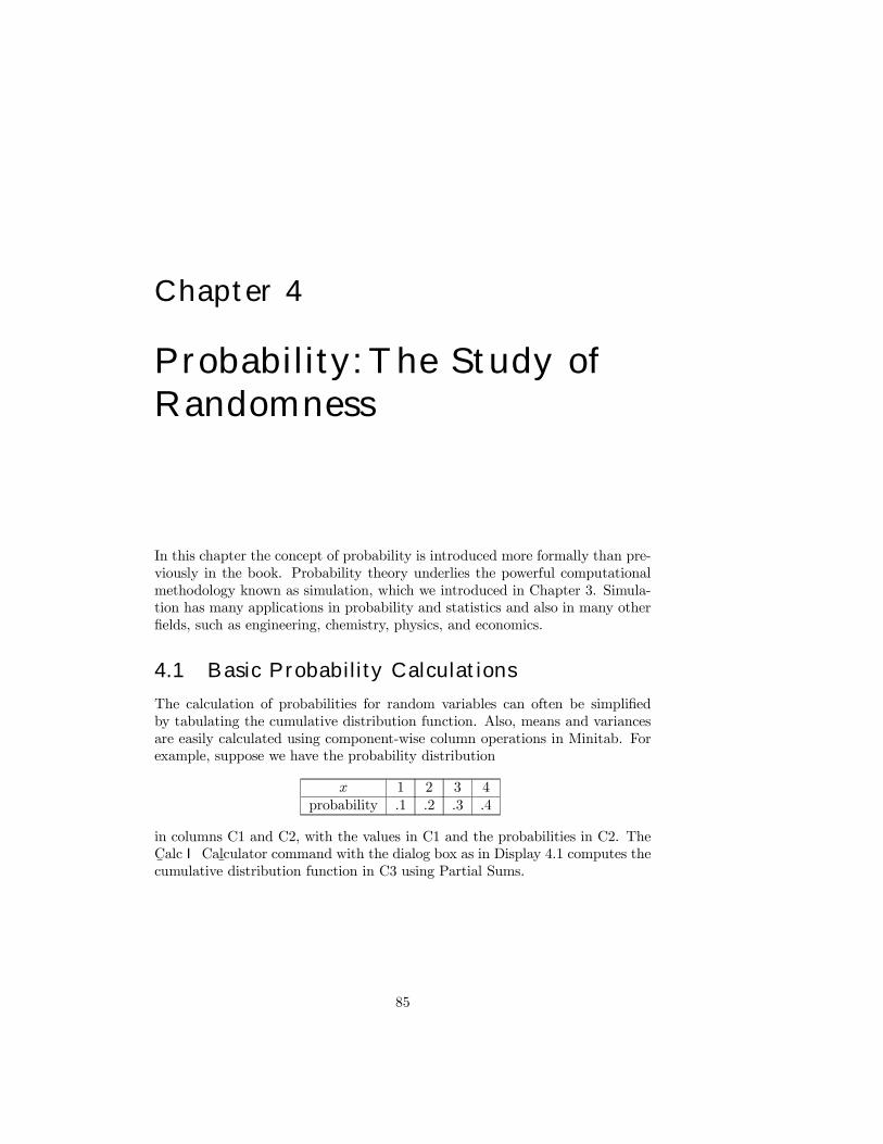
Chapter 4
Probability:The Study ofRandomness
In this chapter the concept of probability is introduced more formally than pre-viously in the book. Probability theory underlies the powerful computationalmethodology known as simulation, which we introduced in Chapter 3. Simula-tion has many applications in probability and statistics and also in many otherÞelds, such as engineering, chemistry, physics, and economics.
4.1 Basic Probability CalculationsThe calculation of probabilities for random variables can often be simpliÞedby tabulating the cumulative distribution function. Also, means and variancesare easily calculated using component-wise column operations in Minitab. Forexample, suppose we have the probability distribution
x 1 2 3 4probability .1 .2 .3 .4
in columns C1 and C2, with the values in C1 and the probabilities in C2. TheC¯alc I Cal
¯culator command with the dialog box as in Display 4.1 computes the
cumulative distribution function in C3 using Partial Sums.
85
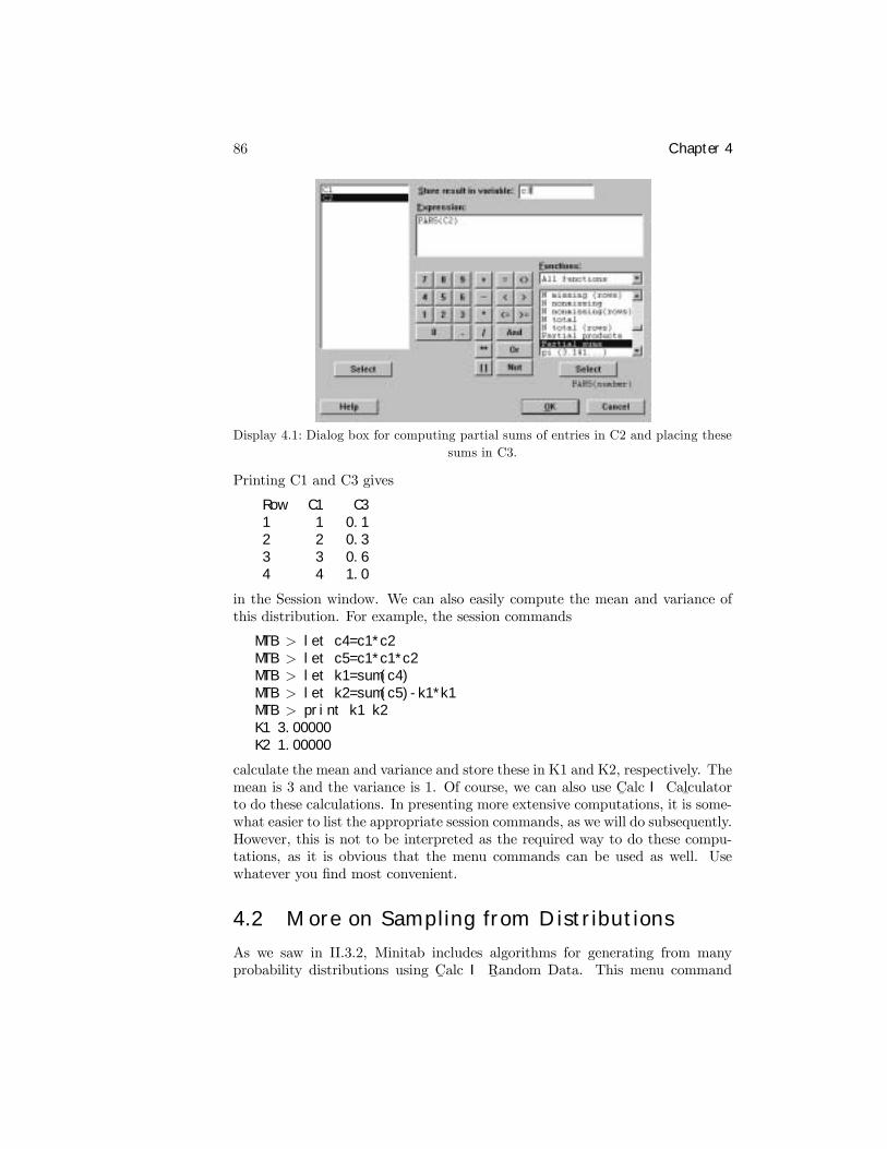
86 Chapter 4
Display 4.1: Dialog box for computing partial sums of entries in C2 and placing thesesums in C3.
Printing C1 and C3 gives
Row C1 C31 1 0.12 2 0.33 3 0.64 4 1.0
in the Session window. We can also easily compute the mean and variance ofthis distribution. For example, the session commands
MTB > let c4=c1*c2MTB > let c5=c1*c1*c2MTB > let k1=sum(c4)MTB > let k2=sum(c5)-k1*k1MTB > print k1 k2K1 3.00000K2 1.00000
calculate the mean and variance and store these in K1 and K2, respectively. Themean is 3 and the variance is 1. Of course, we can also use C
¯alc I Cal
¯culator
to do these calculations. In presenting more extensive computations, it is some-what easier to list the appropriate session commands, as we will do subsequently.However, this is not to be interpreted as the required way to do these compu-tations, as it is obvious that the menu commands can be used as well. Usewhatever you Þnd most convenient.
4.2 More on Sampling from Distributions
As we saw in II.3.2, Minitab includes algorithms for generating from manyprobability distributions using C
¯alc I R
¯andom Data. This menu command
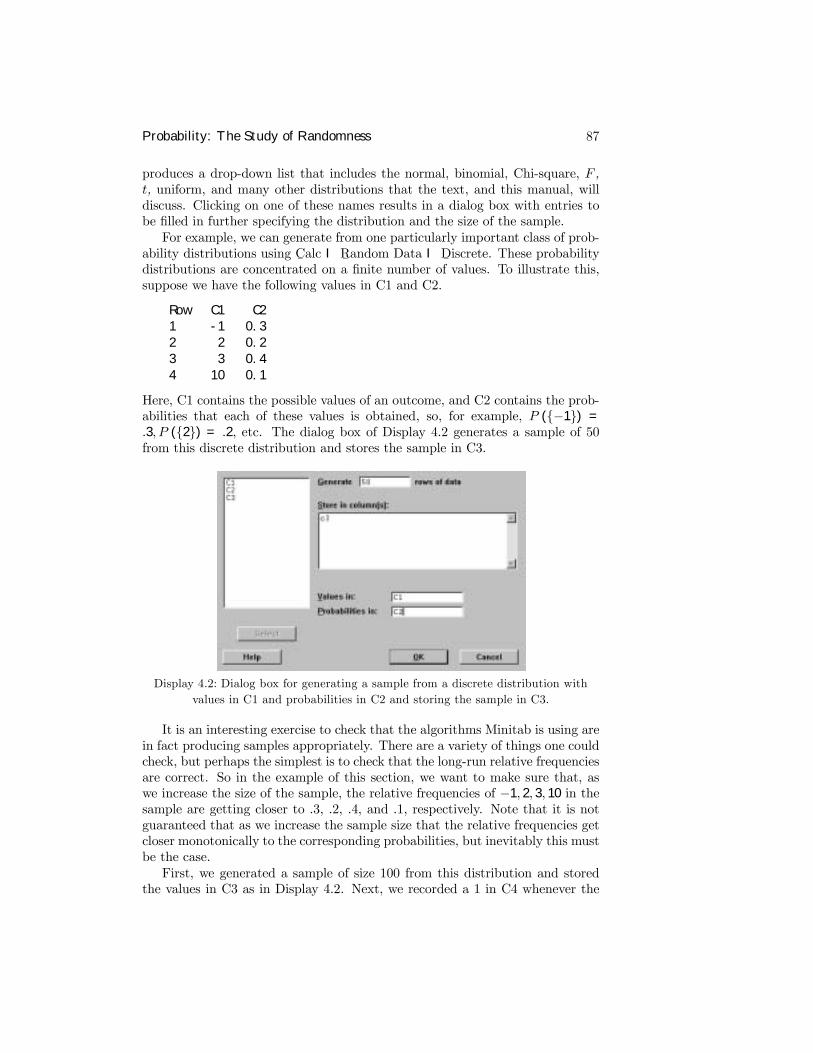
Probability: The Study of Randomness 87
produces a drop-down list that includes the normal, binomial, Chi-square, F ,t, uniform, and many other distributions that the text, and this manual, willdiscuss. Clicking on one of these names results in a dialog box with entries tobe Þlled in further specifying the distribution and the size of the sample.For example, we can generate from one particularly important class of prob-
ability distributions using C¯alc I R
¯andom Data I D
¯iscrete. These probability
distributions are concentrated on a Þnite number of values. To illustrate this,suppose we have the following values in C1 and C2.
Row C1 C21 -1 0.32 2 0.23 3 0.44 10 0.1
Here, C1 contains the possible values of an outcome, and C2 contains the prob-abilities that each of these values is obtained, so, for example, P ({−1}) =.3, P ({2}) = .2, etc. The dialog box of Display 4.2 generates a sample of 50from this discrete distribution and stores the sample in C3.
Display 4.2: Dialog box for generating a sample from a discrete distribution withvalues in C1 and probabilities in C2 and storing the sample in C3.
It is an interesting exercise to check that the algorithms Minitab is using arein fact producing samples appropriately. There are a variety of things one couldcheck, but perhaps the simplest is to check that the long-run relative frequenciesare correct. So in the example of this section, we want to make sure that, aswe increase the size of the sample, the relative frequencies of −1, 2, 3, 10 in thesample are getting closer to .3, .2, .4, and .1, respectively. Note that it is notguaranteed that as we increase the sample size that the relative frequencies getcloser monotonically to the corresponding probabilities, but inevitably this mustbe the case.First, we generated a sample of size 100 from this distribution and stored
the values in C3 as in Display 4.2. Next, we recorded a 1 in C4 whenever the
88 Chapter 4
corresponding entry in C3 was −1 and recorded a 0 in C4 otherwise. To do this,we used the C
¯alc I Cal
¯culator command with dialog box as shown in Display
4.3.
Display 4.3: Dialog box to record the incidence of a −1 in C3.
It is clear that the mean of C4 is the relative frequency of −1 in the sample.We calculated this mean using C
¯alc I C
¯olumn Statistics, as discussed in I.10.3,
which gave the output
Mean of C4 = 0.33000
in the Session window. Repeating this with a sample of size 1000, we obtained
Mean of C4 = 0.28100
which we can see is a bit closer to the true value of .3. Repeating this with asample of size 10, 000 from this distribution, we obtained
Mean of C4 = 0.29300
which is closer still. It would appear that the relative frequency of −1 is indeedconverging to .3.We can generate a randomly chosen point from the line interval (a, b) , where
a < b, using C¯alc I R
¯andom Data I U
¯niform. For example, the dialog box
of Display 4.4 generates a sample of 1500 from the uniform distribution on theinterval (3.0, 6.3) .With this distribution, the probability of any subinterval (c, d)of (a, b) is given by (d− c) / (b− a), i.e., the length of (c, d) over the length of(a, b). Of course, we can estimate this probability by just counting the numberof times the generated response falls in the interval (c, d) and dividing this bythe total sample size. For example, using the outcomes from the dialog boxof Display 4.3 and estimating the probability of the interval (4, 5), we get therelative frequency 0.30867, which is close to the true value of (5− 4) / (6.3− 3) =0.30303.
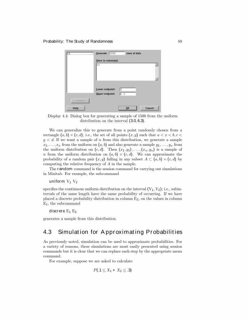
Probability: The Study of Randomness 89
Display 4.4: Dialog box for generating a sample of 1500 from the uniformdistribution on the interval (3.0, 6.3).
We can generalize this to generate from a point randomly chosen from arectangle (a, b)× (c, d), i.e., the set of all points (x, y) such that a < x < b, c <y < d. If we want a sample of n from this distribution, we generate a samplex1, . . . , xn from the uniform on (a, b) and also generate a sample y1, . . . , yn fromthe uniform distribution on (c, d). Then (x1, y1) , . . . , (xn, yn) is a sample ofn from the uniform distribution on (a, b) × (c, d). We can approximate theprobability of a random pair (x, y) falling in any subset A ⊂ (a, b) × (c, d) bycomputing the relative frequency of A in the sample.The random command is the session command for carrying out simulations
in Minitab. For example, the subcommand
uniform V1 V2
speciÞes the continuous uniform distribution on the interval (V1,V2); i.e., subin-tervals of the same length have the same probability of occurring. If we haveplaced a discrete probability distribution in column E2, on the values in columnE1, the subcommand
discrete E1 E2
generates a sample from this distribution.
4.3 Simulation for Approximating Probabilities
As previously noted, simulation can be used to approximate probabilities. Fora variety of reasons, these simulations are most easily presented using sessioncommands but it is clear that we can replace each step by the appropriate menucommand.For example, suppose we are asked to calculate
P (.1 ≤ X1 +X2 ≤ .3)
90 Chapter 4
when X1,X2 are both independent and follow the uniform distribution on theinterval (0, 1) . The session commands
MTB > random 1000 c1 c2;SUBC> uniform 0 1.MTB > let c3=c1+c2MTB > let c4 = .1<=c3 and c3<=.3MTB > let k1=sum(c4)/n(c4)MTB > print k1K1 0.0400000MTB > let k2=sqrt(k1*(1-k1)/n(c4))MTB > print k2K2 0.00619677MTB > let k3=k1-3*k2MTB > let k4=k1+3*k2MTB > print k3 k4K3 0.0214097K4 0.0585903
generate N = 1000 independent values of X1,X2 and place these values in C1and C2, respectively, then calculate the sum X1 +X2 and put these values inC3. Using the comparison operators discussed in I.10.4, a 1 is recorded in C4every time .1 ≤ X1 +X2 ≤ .3 is true and a 0 is recorded there otherwise. Wethen calculate the proportion of 1�s in the sample as K1, and this is our estimatep of the probability. We will see later that a good measure of the accuracy ofthis estimate is the standard error of the estimate, which in this case is givenby p
p (1− p) /Nand this is computed in K2. Actually, we can feel fairly conÞdent that the truevalue of the probability is in the interval
p± 3pp (1− p) /N
which in this case, equals the interval (0.0214097, 0.0585903). So we know thetrue value of the probability with reasonable accuracy. As the simulation sizeN increases, the Law of Large Numbers says that p converges to the true valueof the probability.
4.4 Simulation for Approximating Means
The means of distributions can also be approximated using simulations in Minitab.For example, suppose X1,X2 are both independent and follow the uniformdistribution on the interval (0, 1) and that we want to calculate the mean ofY = 1/ (1 +X1 +X2) . We can approximate this in a simulation. The sessioncommands
Probability: The Study of Randomness 91
MTB > random 1000 c1 c2;SUBC> uniform 0 1.MTB > let c3=1/(1+c1+c2)MTB > let k1=mean(c3)MTB > let k2=stdev(c3)/sqrt(n(c3))MTB > print k1 k2K1 0.521532K2 0.00375769MTB > let k3=k1-3*k2MTB > let k4=k1+3*k2MTB > print k3 k4K3 0.510259K4 0.532805
generate N = 1000 independent values of X1,X2 and place these values in C1,C2, then calculate Y = 1/ (1 +X1 +X2) and put these values in C3. The meanof C3 is stored in K1, and this is our estimate of the mean value of Y . As ameasure of how accurate this estimate is, we compute the standard error of theestimate, which is given by the standard deviation divided by the square rootof the simulation sample size N . Again, we can feel fairly conÞdent that theinterval given by the estimate plus or minus 3 times the standard error of theestimate contains the true value of the mean. In this case, this interval is givenby (0.510259, 0.532805), and so we know this mean with reasonable accuracy.As the simulation size N increases, the Law of Large Numbers says that theapproximation converges to the true value of the mean.
4.5 Exercises
When the data for an exercise come from an exercise in IPS, the IPS exercisenumber is given in parentheses ( ). All computations in these exercises areto be carried out using Minitab, and the exercises are designed to ensure thatyou have a reasonable understanding of the Minitab material in this chapter.Generally, you should be using Minitab to do all the computations and plottingrequired for the problems in IPS.If your version of Minitab places restrictions such that the value of the sim-
ulation sample size N requested in these problems is not feasible, then substitutea more appropriate value. Be aware, however, that the accuracy of your resultsis dependent on how large N is.
1. Suppose we have the probability distribution
x 1 2 3 4 5probability .15 .05 .33 .37 .10
on the values 1, 2, 3, 4, and 5. Calculate the mean and variance of thisdistribution. Suppose that three independent outcomes (X1,X2,X3) are
92 Chapter 4
generated from this distribution. Compute the probability that 1 < X1 ≤4, 2 ≤ X2 and 3 < X3 ≤ 5.
2. Suppose we have the probability distribution
x 1 2 3 4 5probability .15 .05 .33 .37 .10
on the values 1, 2, 3, 4, and 5. Using Minitab, verify that this is aprobability distribution. Make a bar chart (probability histogram) of thisdistribution. Generate a sample of size 1000 from this distribution andplot a relative frequency histogram for the sample.
3. (4.23) Indicate how you would simulate the game of roulette using Minitab.Based on a simulation of N = 1000, estimate the probability of gettingred and a multiple of 3.
4. A probability distribution is placed on the integers 1, 2, ..., 100, where theprobability of integer i is c/i2. Determine c so that this is a probabilitydistribution. What is the 90th percentile? Generate a sample of 20 fromthe distribution.
5. Suppose an outcome is random on the square (0, 1)× (0, 1). Using simula-tion, approximate the probability that the Þrst coordinate plus the secondcoordinate is less than .75 but greater than .25.
6. Generate a sample of 1000 from the uniform distribution on the unit diskD =
©(x, y) : x2 + y2 ≤ 1
ª.
7. The expression e−x for x > 0 is the density curve for what is called theExponential (1) distribution. Plot this density curve in the interval from0 to 10 using an increment of .1. The C
¯alc I R
¯andom Data I Ex
¯ponential
command can be used to generate from this distribution by specifying theMean as 1 in the ensuing dialog box. Generate a sample of 1000 from thisdistribution and estimate its mean. Approximate the probability that avalue generated from this distribution is in the interval (1,2). The generalExponential (λ) has a density curve given by λ−1e−x/λ for x > 0 andwhere λ > 0 is the mean. Repeat the simulation with mean λ = 3.Comment on the values of the estimated means.
8. Suppose you carry out a simulation to approximate the mean of a randomvariable X and you report the value 1.23 with a standard error of .025.If you are asked to approximate the mean of Y = 3 + 5X, do you haveto carry out another simulation? If not, what is your approximation, andwhat is the standard error of this approximation?
9. Suppose that a random variable X follows an N(3, 2.3) distribution. Sub-sequently, conditions change and no values smaller than −1 or bigger than9.5 can occur, i.e., the distribution is conditioned to the interval (−1, 9.5).
Probability: The Study of Randomness 93
Generate a sample of 1000 from the truncated distribution, and use thesample to approximate its mean.
10. Suppose that X is a random variable and follows an N(0, 1) distribution.SimulateN = 1000 values from the distribution of Y = X2, and plot thesevalues in a histogram with cutpoints 0, .5, 1, 1.5, ..., 15. Approximate themean of this distribution. Generate Y directly from its distribution, whichis known to be a Chisquare(1) distribution. In general, the Chisquare(k)distribution can be generated from via the command C
¯alcI R
¯andom Data
I C¯hi-Square, where k is speciÞed as the D
¯egrees of freedom in the dialog
box. Plot the Y values in a histogram using the same cutpoints. Commenton the two histograms. Note that you can plot the density curve of thesedistributions using C
¯alc I Probability D
¯istributions I C
¯hi-Square and
evaluating the probability density at a range of points as we discussed inII.2 for the normal distribution.
11. If X1 and X2 are independent random variables with X1 following aChisquare(k1) distribution and X2 following a Chisquare(k2) distribu-tion, then it is known that Y = X1 + X2 follows a Chisquare(k1 + k2)distribution. For k1 = 1, k2 = 1, verify this empirically by plotting his-tograms with cutpoints 0, .5, 1, 1.5, ..., 15, based on simulations of sizeN = 1000.
12. If X1 and X2 are independent random variables with X1 following anN(0, 1) distribution and X2 following a Chisquare(k) distribution, thenit is known that
Y =X1pX2/k
follows a Student(k) distribution. The Student(k) distribution can begenerated from using the command C
¯alc I R
¯andom Data I t
¯, where k
is the D¯egrees of freedom and must be speciÞed in the dialog box. For
k = 3, verify this result empirically by plotting histograms with cutpoints−10, −9, ..., 9, 10, based on simulations of size N = 1000.
13. If X1 and X2 are independent random variables with X1 following aChisquare(k1) distribution and X2 following a Chisquare(k2) distribu-tion, then it is known that
Y =X1/k1
X2/k2
follows an F (k1, k2) distribution. The F (k1, k2) distribution can be gen-erated from using the subcommand C
¯alc I R
¯andom Data I F
¯, where k1
is the N¯umerator degrees of freedom and k2 is the D¯
enominator degreesof freedom, both of which must be speciÞed in the dialog box. For k1 = 1,k2 = 1, verify this empirically by plotting histograms with cutpoints 0, .5,1, 1.5, ..., 15, based on simulations of size N = 1000.

94 Chapter 4
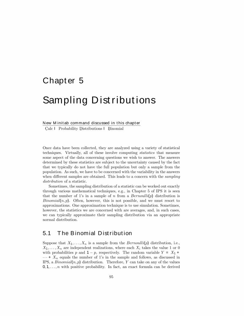
Chapter 5
Sampling Distributions
New Minitab command discussed in this chapterC¯alc I Probability D
¯istributions I B
¯inomial
Once data have been collected, they are analyzed using a variety of statisticaltechniques. Virtually, all of these involve computing statistics that measuresome aspect of the data concerning questions we wish to answer. The answersdetermined by these statistics are subject to the uncertainty caused by the factthat we typically do not have the full population but only a sample from thepopulation. As such, we have to be concerned with the variability in the answerswhen different samples are obtained. This leads to a concern with the samplingdistribution of a statistic.Sometimes, the sampling distribution of a statistic can be worked out exactly
through various mathematical techniques, e.g., in Chapter 5 of IPS it is seenthat the number of 1�s in a sample of n from a Bernoulli(p) distribution isBinomial(n, p). Often, however, this is not possible, and we must resort toapproximations. One approximation technique is to use simulation. Sometimes,however, the statistics we are concerned with are averages, and, in such cases,we can typically approximate their sampling distribution via an appropriatenormal distribution.
5.1 The Binomial Distribution
Suppose that X1, . . . ,Xn is a sample from the Bernoulli(p) distribution, i.e.,X1, . . . ,Xn are independent realizations, where each Xi takes the value 1 or 0with probabilities p and 1 − p, respectively. The random variable Y = X1 +· · · + Xn equals the number of 1�s in the sample and follows, as discussed inIPS, a Binomial(n, p) distribution. Therefore, Y can take on any of the values0, 1, . . . , n with positive probability. In fact, an exact formula can be derived
95
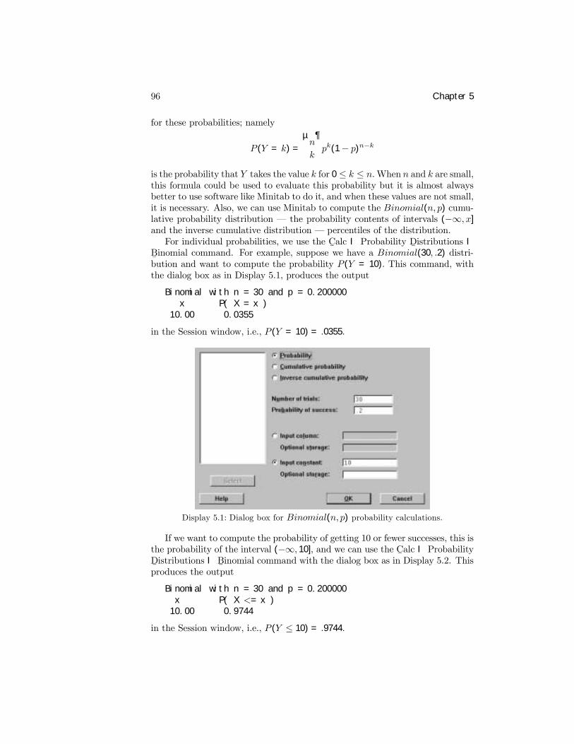
96 Chapter 5
for these probabilities; namely
P (Y = k) =
µn
k
¶pk(1− p)n−k
is the probability that Y takes the value k for 0 ≤ k ≤ n.When n and k are small,this formula could be used to evaluate this probability but it is almost alwaysbetter to use software like Minitab to do it, and when these values are not small,it is necessary. Also, we can use Minitab to compute the Binomial(n, p) cumu-lative probability distribution � the probability contents of intervals (−∞, x]and the inverse cumulative distribution � percentiles of the distribution.For individual probabilities, we use the C
¯alc I Probability D
¯istributions I
B¯inomial command. For example, suppose we have a Binomial(30, .2) distri-bution and want to compute the probability P (Y = 10). This command, withthe dialog box as in Display 5.1, produces the output
Binomial with n = 30 and p = 0.200000x P( X = x )
10.00 0.0355
in the Session window, i.e., P (Y = 10) = .0355.
Display 5.1: Dialog box for Binomial(n, p) probability calculations.
If we want to compute the probability of getting 10 or fewer successes, this isthe probability of the interval (−∞, 10], and we can use the C
¯alc I Probability
D¯istributions I B
¯inomial command with the dialog box as in Display 5.2. This
produces the output
Binomial with n = 30 and p = 0.200000x P( X <= x )
10.00 0.9744
in the Session window, i.e., P (Y ≤ 10) = .9744.
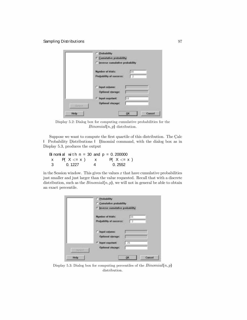
Sampling Distributions 97
Display 5.2: Dialog box for computing cumulative probabilities for theBinomial(n, p) distribution.
Suppose we want to compute the Þrst quartile of this distribution. The C¯alc
I Probability D¯istributions I B
¯inomial command, with the dialog box as in
Display 5.3, produces the output
Binomial with n = 30 and p = 0.200000x P( X <= x ) x P( X <= x )3 0.1227 4 0.2552
in the Session window. This gives the values x that have cumulative probabilitiesjust smaller and just larger than the value requested. Recall that with a discretedistribution, such as the Binomial(n, p), we will not in general be able to obtainan exact percentile.
Display 5.3: Dialog box for computing percentiles of the Binomial(n, p)distribution.
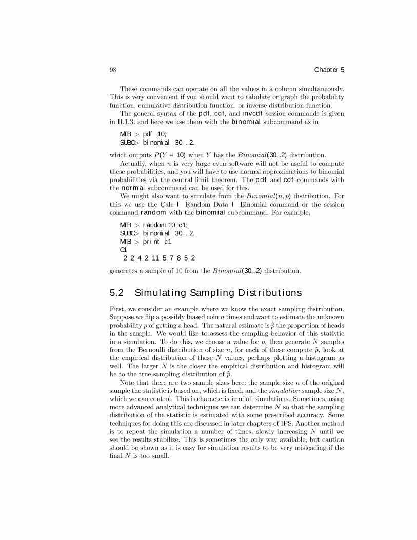
98 Chapter 5
These commands can operate on all the values in a column simultaneously.This is very convenient if you should want to tabulate or graph the probabilityfunction, cumulative distribution function, or inverse distribution function.The general syntax of the pdf, cdf, and invcdf session commands is given
in II.1.3, and here we use them with the binomial subcommand as in
MTB > pdf 10;SUBC> binomial 30 .2.
which outputs P (Y = 10) when Y has the Binomial(30, .2) distribution.Actually, when n is very large even software will not be useful to compute
these probabilities, and you will have to use normal approximations to binomialprobabilities via the central limit theorem. The pdf and cdf commands withthe normal subcommand can be used for this.We might also want to simulate from the Binomial(n, p) distribution. For
this we use the C¯alc I R
¯andom Data I B
¯inomial command or the session
command random with the binomial subcommand. For example,
MTB > random 10 c1;SUBC> binomial 30 .2.MTB > print c1C12 2 4 2 11 5 7 8 5 2
generates a sample of 10 from the Binomial(30, .2) distribution.
5.2 Simulating Sampling Distributions
First, we consider an example where we know the exact sampling distribution.Suppose we ßip a possibly biased coin n times and want to estimate the unknownprobability p of getting a head. The natural estimate is p the proportion of headsin the sample. We would like to assess the sampling behavior of this statisticin a simulation. To do this, we choose a value for p, then generate N samplesfrom the Bernoulli distribution of size n, for each of these compute p, look atthe empirical distribution of these N values, perhaps plotting a histogram aswell. The larger N is the closer the empirical distribution and histogram willbe to the true sampling distribution of p.Note that there are two sample sizes here: the sample size n of the original
sample the statistic is based on, which is Þxed, and the simulation sample sizeN ,which we can control. This is characteristic of all simulations. Sometimes, usingmore advanced analytical techniques we can determine N so that the samplingdistribution of the statistic is estimated with some prescribed accuracy. Sometechniques for doing this are discussed in later chapters of IPS. Another methodis to repeat the simulation a number of times, slowly increasing N until wesee the results stabilize. This is sometimes the only way available, but cautionshould be shown as it is easy for simulation results to be very misleading if theÞnal N is too small.
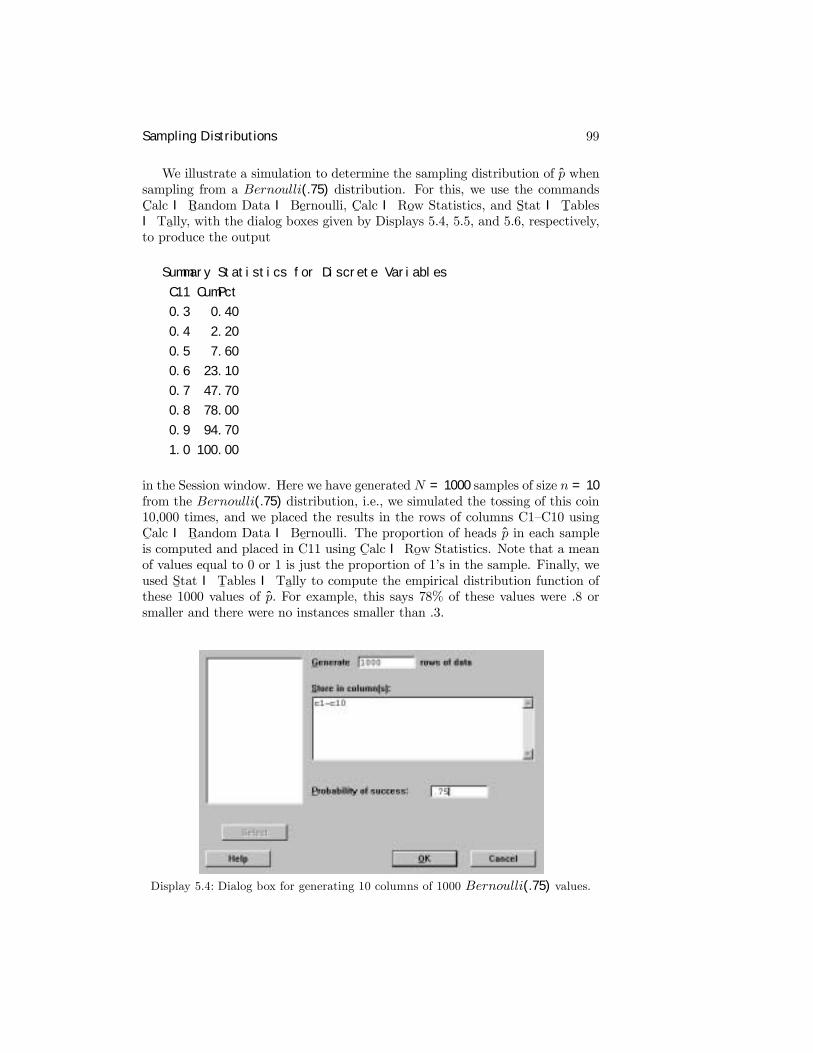
Sampling Distributions 99
We illustrate a simulation to determine the sampling distribution of p whensampling from a Bernoulli(.75) distribution. For this, we use the commandsC¯alc I R
¯andom Data I Be
¯rnoulli, C
¯alc I Ro
¯w Statistics, and S
¯tat I T
¯ables
I Ta¯lly, with the dialog boxes given by Displays 5.4, 5.5, and 5.6, respectively,
to produce the output
Summary Statistics for Discrete Variables
C11 CumPct
0.3 0.40
0.4 2.20
0.5 7.60
0.6 23.10
0.7 47.70
0.8 78.00
0.9 94.70
1.0 100.00
in the Session window. Here we have generated N = 1000 samples of size n = 10from the Bernoulli(.75) distribution, i.e., we simulated the tossing of this coin10,000 times, and we placed the results in the rows of columns C1�C10 usingC¯alc I R
¯andom Data I Be
¯rnoulli. The proportion of heads p in each sample
is computed and placed in C11 using C¯alc I Ro
¯w Statistics. Note that a mean
of values equal to 0 or 1 is just the proportion of 1�s in the sample. Finally, weused S
¯tat I T
¯ables I Ta
¯lly to compute the empirical distribution function of
these 1000 values of p. For example, this says 78% of these values were .8 orsmaller and there were no instances smaller than .3.
Display 5.4: Dialog box for generating 10 columns of 1000 Bernoulli(.75) values.
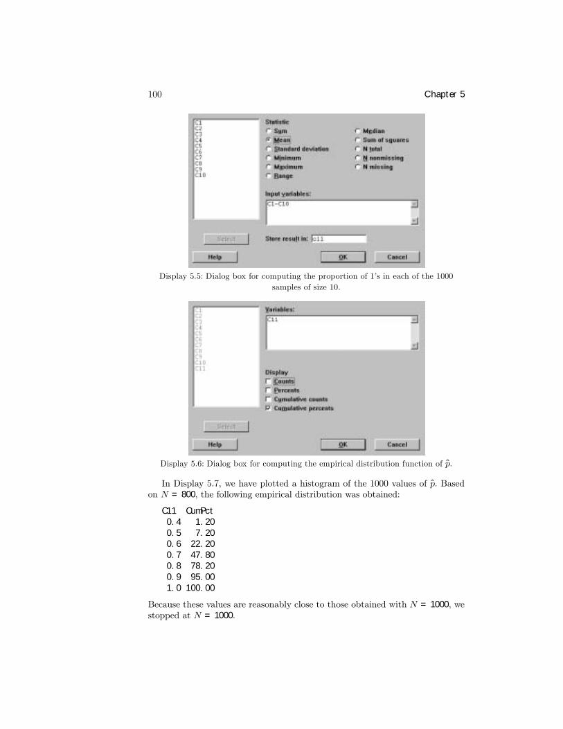
100 Chapter 5
Display 5.5: Dialog box for computing the proportion of 1�s in each of the 1000samples of size 10.
Display 5.6: Dialog box for computing the empirical distribution function of p.
In Display 5.7, we have plotted a histogram of the 1000 values of p. Basedon N = 800, the following empirical distribution was obtained:
C11 CumPct0.4 1.200.5 7.200.6 22.200.7 47.800.8 78.200.9 95.001.0 100.00
Because these values are reasonably close to those obtained with N = 1000, westopped at N = 1000.
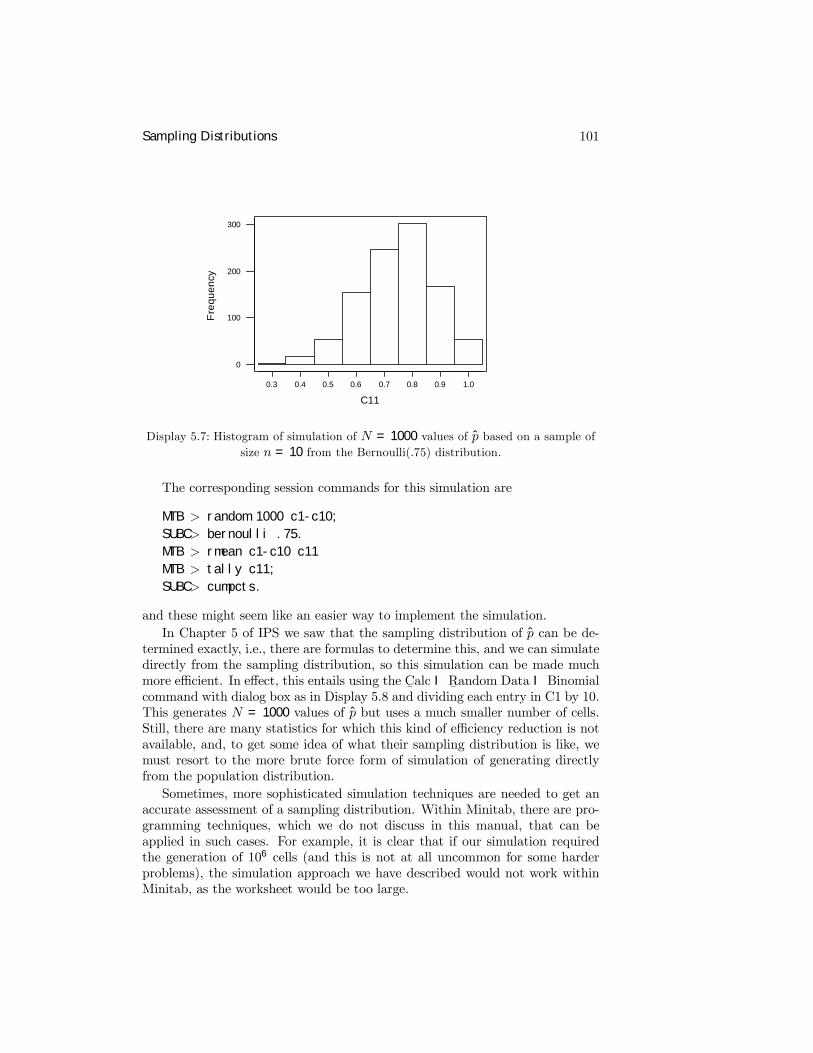
Sampling Distributions 101
1.00.90.80.70.60.50.40.3
300
200
100
0
C11
Fre
quen
cy
Display 5.7: Histogram of simulation of N = 1000 values of p based on a sample ofsize n = 10 from the Bernoulli(.75) distribution.
The corresponding session commands for this simulation are
MTB > random 1000 c1-c10;SUBC> bernoulli .75.MTB > rmean c1-c10 c11MTB > tally c11;SUBC> cumpcts.
and these might seem like an easier way to implement the simulation.In Chapter 5 of IPS we saw that the sampling distribution of p can be de-
termined exactly, i.e., there are formulas to determine this, and we can simulatedirectly from the sampling distribution, so this simulation can be made muchmore efficient. In effect, this entails using the C
¯alc I R
¯andom Data I Binomial
command with dialog box as in Display 5.8 and dividing each entry in C1 by 10.This generates N = 1000 values of p but uses a much smaller number of cells.Still, there are many statistics for which this kind of efficiency reduction is notavailable, and, to get some idea of what their sampling distribution is like, wemust resort to the more brute force form of simulation of generating directlyfrom the population distribution.Sometimes, more sophisticated simulation techniques are needed to get an
accurate assessment of a sampling distribution. Within Minitab, there are pro-gramming techniques, which we do not discuss in this manual, that can beapplied in such cases. For example, it is clear that if our simulation requiredthe generation of 106 cells (and this is not at all uncommon for some harderproblems), the simulation approach we have described would not work withinMinitab, as the worksheet would be too large.
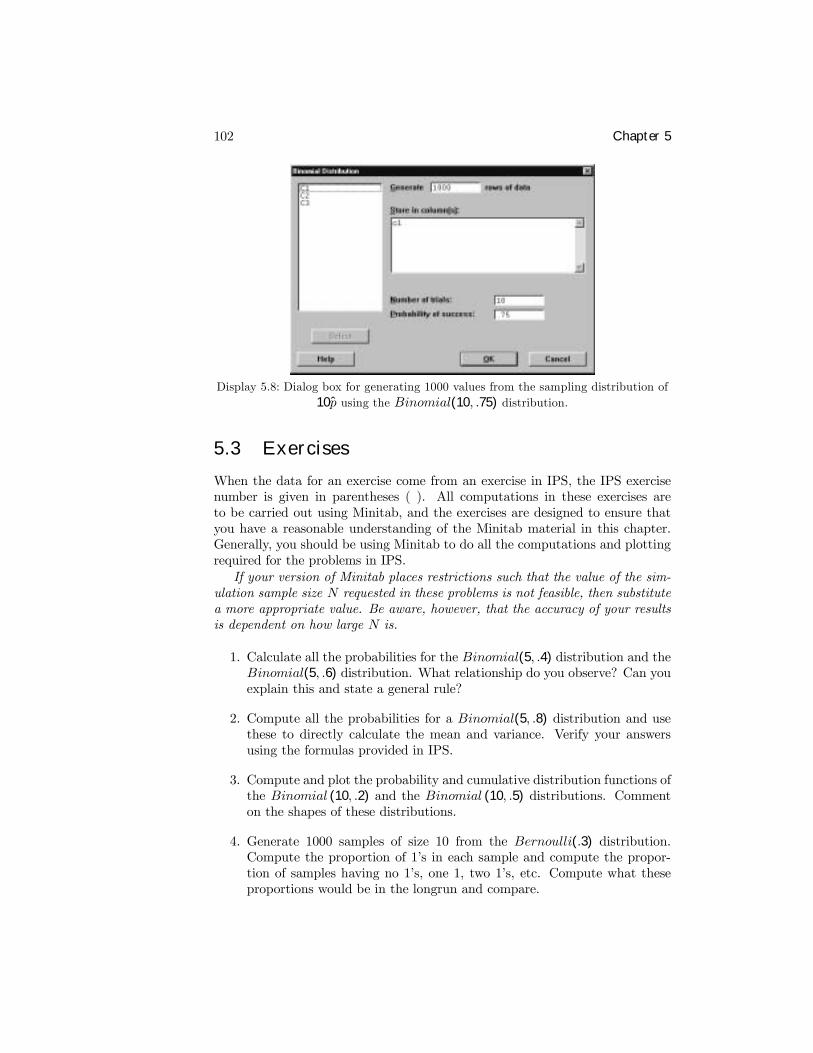
102 Chapter 5
Display 5.8: Dialog box for generating 1000 values from the sampling distribution of10p using the Binomial(10, .75) distribution.
5.3 Exercises
When the data for an exercise come from an exercise in IPS, the IPS exercisenumber is given in parentheses ( ). All computations in these exercises areto be carried out using Minitab, and the exercises are designed to ensure thatyou have a reasonable understanding of the Minitab material in this chapter.Generally, you should be using Minitab to do all the computations and plottingrequired for the problems in IPS.If your version of Minitab places restrictions such that the value of the sim-
ulation sample size N requested in these problems is not feasible, then substitutea more appropriate value. Be aware, however, that the accuracy of your resultsis dependent on how large N is.
1. Calculate all the probabilities for the Binomial(5, .4) distribution and theBinomial(5, .6) distribution. What relationship do you observe? Can youexplain this and state a general rule?
2. Compute all the probabilities for a Binomial(5, .8) distribution and usethese to directly calculate the mean and variance. Verify your answersusing the formulas provided in IPS.
3. Compute and plot the probability and cumulative distribution functions ofthe Binomial (10, .2) and the Binomial (10, .5) distributions. Commenton the shapes of these distributions.
4. Generate 1000 samples of size 10 from the Bernoulli(.3) distribution.Compute the proportion of 1�s in each sample and compute the propor-tion of samples having no 1�s, one 1, two 1�s, etc. Compute what theseproportions would be in the longrun and compare.
Sampling Distributions 103
5. Carry out a simulation study with N = 1000 of the sampling distributionof p for n = 5, 10, 20 and for p = .5, .75, .95. In particular, calculate theempirical distribution functions and plot the histograms. Comment onyour Þndings.
6. Suppose that X1,X2,X3, . . . are independent realizations from theBernoulli(p) distribution, i.e., each Xi takes the value 1 or 0 with prob-abilities p and 1 − p, respectively. If the random variable Y counts thenumber of tosses until we obtain the Þrst head in a sequence of inde-pendent tosses X1,X2,X3, . . . , then Y has a Geometric(p) distribution.Minitab does not have built-in algorithms for computing the probabil-ity function, distribution function, inverse distribution function, and forgenerating from this distribution. The probability function for this distri-bution is given by
P (Y = y) = (1− p)y−1 p
for y = 1, 2, . . . . Plot the probability function for the Geometric (.5) dis-tribution for the values y = 1, . . . , 10. Do the same for the Geometric (.1)distribution. What do you notice?
7. Using methods for summing geometric sums, the cumulative distributionfunction of the Geometric (p) distribution (see Exercise II.5.6) is givenby P (Y ≤ y) = 1 − (1− p)y. Plot the cumulative distribution functionfor the Geometric (.5) and Geometric (.1) distribution for the values y =1, . . . , 10. What do you notice?
8. To randomly generate from the Geometric(p) distribution (see ExerciseII.5.6), we can repeatedly generate from a Bernoulli(p) and count howmany times we did this until the Þrst 1 appeared. A simple way to do thisin Minitab is to generate N values from the Bernoulli(p) into a column.Count the number of entries until the Þrst 1, count the number of subse-quent entries until the next 1, etc. These counts are identically and inde-pendently distributed according to the Geometric(p) distribution. Thisis a very inefficient method when p is small and much better algorithmsexist. Generate a sample of 10 from the Geometric (.5) distribution.
9. Carry out a simulation study, with N = 2000, of the sampling distributionof the sample standard deviation when sampling from the N(0, 1) distri-bution, based on a sample of size n = 5. In particular, plot the histogramusing cutpoints 0, 1.5, 2.0 2.5, 3.0 5.0. Repeat this for the sample coeffi-cient of variation (sample standard deviation divided by the sample mean)using the cutpoints −10, −9, ..., 0, ..., 9, 10. Comment on the shapes ofthe histograms relative to a N(0, 1) density curve.
10. Generate N = 1000 samples of size n = 5 from the N(0, 1) distribution.Record a histogram for x using the cutpoints −3,−2.5,−2, ..., 2.5, 3.0.Generate a sample of size N = 1000 from the N(0, 1/
√5) distribution.
Plot the histogram using the same cutpoints and compare the histograms.What will happen to these histograms as we increase N?
104 Chapter 5
11. Generate N = 1000 values of X1,X2, where X1 follows a N(3, 2) distri-bution and X2 follows a N(−1, 3) distribution. Compute Y = X1 − 2X2
for each of these pairs and plot a histogram for Y using the cutpoints−20,−15, ..., 25, 30. Generate a sample of N = 1000 from the appropriatedistribution of Y and plot a histogram using the same cutpoints.
12. Plot the density curve for the Exponential(3) distribution (see ExerciseII.4.7) between 0 and 15 with an increment of .1. Generate N = 1000samples of size n = 2 from the Exponential(3) distribution and recordthe sample means. Standardize the sample of x using µ = 3 and σ = 3.Plot a histogram of the standardized values using the cutpoints −5, −4,..., 4, 5. Repeat this for n = 5, 10. Comment on the shapes of thesehistograms.
13. Plot the density of the uniform distribution on (0,1). Generate N = 1000samples of size n = 2 from this distribution. Standardize the sample of xusing µ = .5 and σ =
p1/12. Plot a histogram of the standardized values
using the cutpoints −5,−4, ..., 4, 5. Repeat this for n = 5, 10. Commenton the shapes of these histograms.
14. The Weibull(β) has density curve given by βxβ−1e−xβ
for x > 0, whereβ > 0 is a Þxed constant. Plot the Weibull(2) density in the range 0 to10 with an increment of .1 using the C
¯alc I Probability D
¯istributions I
W¯eibull, command. Generate a sample of N = 1000 from this distribu-
tion using the subcommand C¯alc I R
¯andom Data I W
¯eibull where β
is the Sh¯ape parameter and the Sc
¯ale parameter is 1. Plot a probability
histogram and compare with the density curve.
Chapter 6
Introduction to Inference
New Minitab commands discussed in this chapterS¯tat I B
¯asic Statistics I 1-Sample Z
¯P¯ower and Sample Size I 1-Sample Z
¯
In this chapter, the basic tools of statistical inference are discussed. Thereare a number of Minitab commands that aid in the computation of conÞdenceintervals and for carrying out tests of signiÞcance.
6.1 z-Confidence Intervals
The command S¯tat I B
¯asic Statistics I 1-Sample Z
¯computes conÞdence inter-
vals for the mean µ using a sample x1, . . . , xn from a distribution where we knowthe standard deviation σ. There are three situations when this is appropriate:
(1) We know that we are sampling from a normal distribution with unknownmean µ and known standard deviation σ, and thus
z =x− µσ/√n
is distributed N(0, 1).(2) We have a large sample from a distribution with unknown mean µ andknown standard deviation σ, and the central limit theorem approximation tothe distribution of x is appropriate, i.e., the distribution of
z =x− µσ/√n
is approximately distributed N(0, 1).
105
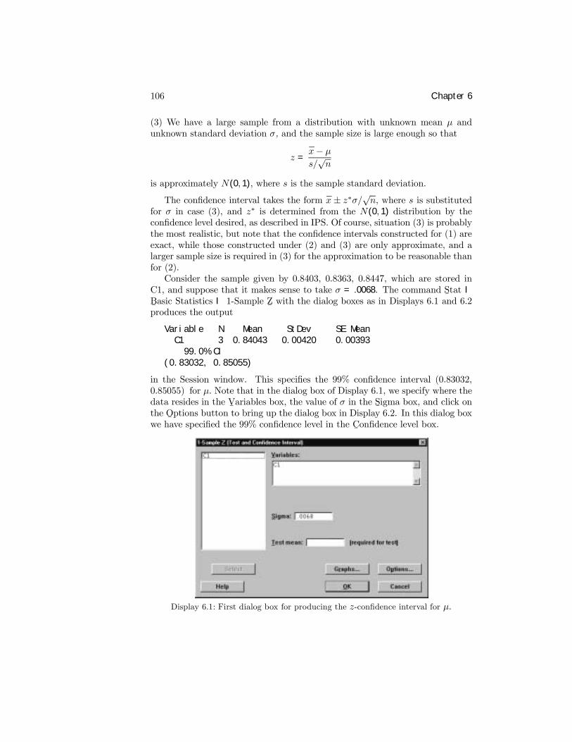
106 Chapter 6
(3) We have a large sample from a distribution with unknown mean µ andunknown standard deviation σ, and the sample size is large enough so that
z =x− µs/√n
is approximately N(0, 1), where s is the sample standard deviation.
The conÞdence interval takes the form x ± z∗σ/√n, where s is substitutedfor σ in case (3), and z∗ is determined from the N(0, 1) distribution by theconÞdence level desired, as described in IPS. Of course, situation (3) is probablythe most realistic, but note that the conÞdence intervals constructed for (1) areexact, while those constructed under (2) and (3) are only approximate, and alarger sample size is required in (3) for the approximation to be reasonable thanfor (2).Consider the sample given by 0.8403, 0.8363, 0.8447, which are stored in
C1, and suppose that it makes sense to take σ = .0068. The command S¯tat I
B¯asic Statistics I 1-Sample Z
¯with the dialog boxes as in Displays 6.1 and 6.2
produces the output
Variable N Mean StDev SE MeanC1 3 0.84043 0.00420 0.00393
99.0% CI(0.83032, 0.85055)
in the Session window. This speciÞes the 99% conÞdence interval (0.83032,0.85055) for µ. Note that in the dialog box of Display 6.1, we specify where thedata resides in the V
¯ariables box, the value of σ in the S
¯igma box, and click on
the O¯ptions button to bring up the dialog box in Display 6.2. In this dialog box
we have speciÞed the 99% conÞdence level in the C¯onÞdence level box.
Display 6.1: First dialog box for producing the z-conÞdence interval for µ.
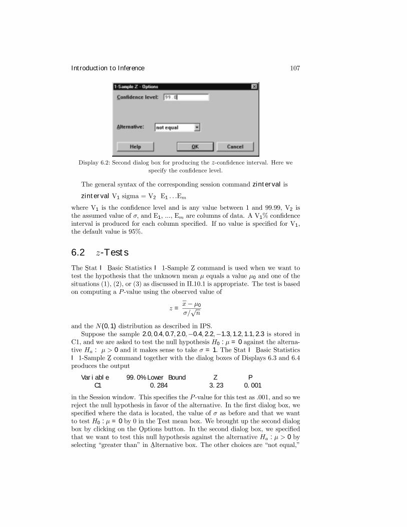
Introduction to Inference 107
Display 6.2: Second dialog box for producing the z-conÞdence interval. Here wespecify the conÞdence level.
The general syntax of the corresponding session command zinterval is
zinterval V1 sigma = V2 E1 . . .Em
where V1 is the conÞdence level and is any value between 1 and 99.99, V2 isthe assumed value of σ, and E1, ..., Em are columns of data. A V1% conÞdenceinterval is produced for each column speciÞed. If no value is speciÞed for V1,the default value is 95%.
6.2 z-TestsThe S
¯tat I B
¯asic Statistics I 1-Sample Z
¯command is used when we want to
test the hypothesis that the unknown mean µ equals a value µ0 and one of thesituations (1), (2), or (3) as discussed in II.10.1 is appropriate. The test is basedon computing a P -value using the observed value of
z =x− µ0
σ/√n
and the N(0, 1) distribution as described in IPS.Suppose the sample 2.0, 0.4, 0.7, 2.0,−0.4, 2.2,−1.3, 1.2, 1.1, 2.3 is stored in
C1, and we are asked to test the null hypothesis H0 : µ = 0 against the alterna-tive Ha : µ > 0 and it makes sense to take σ = 1. The S
¯tat I B
¯asic Statistics
I 1-Sample Z¯command together with the dialog boxes of Displays 6.3 and 6.4
produces the output
Variable 99.0% Lower Bound Z PC1 0.284 3.23 0.001
in the Session window. This speciÞes the P -value for this test as .001, and so wereject the null hypothesis in favor of the alternative. In the Þrst dialog box, wespeciÞed where the data is located, the value of σ as before and that we wantto test H0 : µ = 0 by 0 in the T
¯est mean box. We brought up the second dialog
box by clicking on the O¯ptions button. In the second dialog box, we speciÞed
that we want to test this null hypothesis against the alternative Ha : µ > 0 byselecting �greater than� in A
¯lternative box. The other choices are �not equal,�
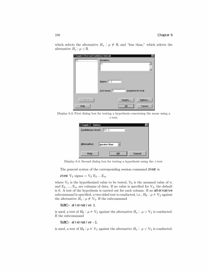
108 Chapter 6
which selects the alternative Ha : µ 6= 0, and �less than,� which selects thealternative Ha : µ < 0.
Display 6.3: First dialog box for testing a hypothesis concerning the mean using az-test.
Display 6.4: Second dialog box for testing a hypothesis using the z-test.
The general syntax of the corresponding session command ztest is
ztest V1 sigma = V2 E1 . . .Em
where V1 is the hypothesized value to be tested, V2 is the assumed value of σ,and E1, ..., Em are columns of data. If no value is speciÞed for V1, the defaultis 0. A test of the hypothesis is carried out for each column. If no alternativesubcommand is speciÞed, a two-sided test is conducted, i.e., H0 : µ =V1 againstthe alternative Ha : µ 6= V1. If the subcommand
SUBC> alternative 1.
is used, a test of H0 : µ = V1 against the alternative Ha : µ > V1 is conducted.If the subcommand
SUBC> alternative -1.
is used, a test of H0 : µ = V1 against the alternative Ha : µ < V1 is conducted.
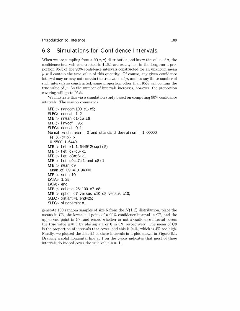
Introduction to Inference 109
6.3 Simulations for Confidence Intervals
When we are sampling from a N(µ, σ) distribution and know the value of σ, theconÞdence intervals constructed in II.6.1 are exact, i.e., in the long run a pro-portion 95% of the 95% conÞdence intervals constructed for an unknown meanµ will contain the true value of this quantity. Of course, any given conÞdenceinterval may or may not contain the true value of µ, and, in any Þnite number ofsuch intervals so constructed, some proportion other than 95% will contain thetrue value of µ. As the number of intervals increases, however, the proportioncovering will go to 95%.We illustrate this via a simulation study based on computing 90% conÞdence
intervals. The session commands
MTB > random 100 c1-c5;SUBC> normal 1 2.MTB > rmean c1-c5 c6MTB > invcdf .95;SUBC> normal 0 1.Normal with mean = 0 and standard deviation = 1.00000P( X <= x) x0.9500 1.6449
MTB > let k1=1.6449*2/sqrt(5)MTB > let c7=c6-k1MTB > let c8=c6+k1MTB > let c9=c7<1 and c8>1MTB > mean c9Mean of C9 = 0.94000
MTB > set c10DATA> 1:25DATA> endMTB > delete 26:100 c7 c8MTB > mplot c7 versus c10 c8 versus c10;SUBC> xstart=1 end=25;SUBC> xincrement=1.
generate 100 random samples of size 5 from the N(1, 2) distribution, place themeans in C6, the lower end-point of a 90% conÞdence interval in C7, and theupper end-point in C8, and record whether or not a conÞdence interval coversthe true value µ = 1 by placing a 1 or 0 in C9, respectively. The mean of C9is the proportion of intervals that cover, and this is 94%, which is 4% too high.Finally, we plotted the Þrst 25 of these intervals in a plot shown in Figure 6.1.Drawing a solid horizontal line at 1 on the y-axis indicates that most of theseintervals do indeed cover the true value µ = 1.
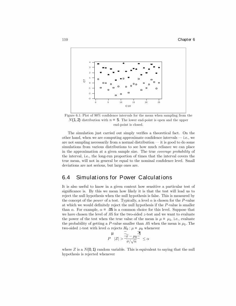
110 Chapter 6
2520151050
4
3
2
1
0
-1
-2
-3
C10
C7
Figure 6.1: Plot of 90% conÞdence intervals for the mean when sampling from theN(1, 2) distribution with n = 5. The lower end-point is open and the upper
end-point is closed.
The simulation just carried out simply veriÞes a theoretical fact. On theother hand, when we are computing approximate conÞdence intervals � i.e., weare not sampling necessarily from a normal distribution � it is good to do somesimulations from various distributions to see how much reliance we can placein the approximation at a given sample size. The true coverage probability ofthe interval, i.e., the long-run proportion of times that the interval covers thetrue mean, will not in general be equal to the nominal conÞdence level. Smalldeviations are not serious, but large ones are.
6.4 Simulations for Power Calculations
It is also useful to know in a given context how sensitive a particular test ofsigniÞcance is. By this we mean how likely it is that the test will lead us toreject the null hypothesis when the null hypothesis is false. This is measured bythe concept of the power of a test. Typically, a level α is chosen for the P -valueat which we would deÞnitely reject the null hypothesis if the P -value is smallerthan α. For example, α = .05 is a common choice for this level. Suppose thatwe have chosen the level of .05 for the two-sided z-test and we want to evaluatethe power of the test when the true value of the mean is µ = µ1, i.e., evaluatethe probability of getting a P -value smaller than .05 when the mean is µ1. Thetwo-sided z-test with level α rejects H0 : µ = µ0 whenever
P
µ|Z| >
¯x− µ0
σ/√n
¯¶≤ α
where Z is a N(0, 1) random variable. This is equivalent to saying that the nullhypothesis is rejected whenever
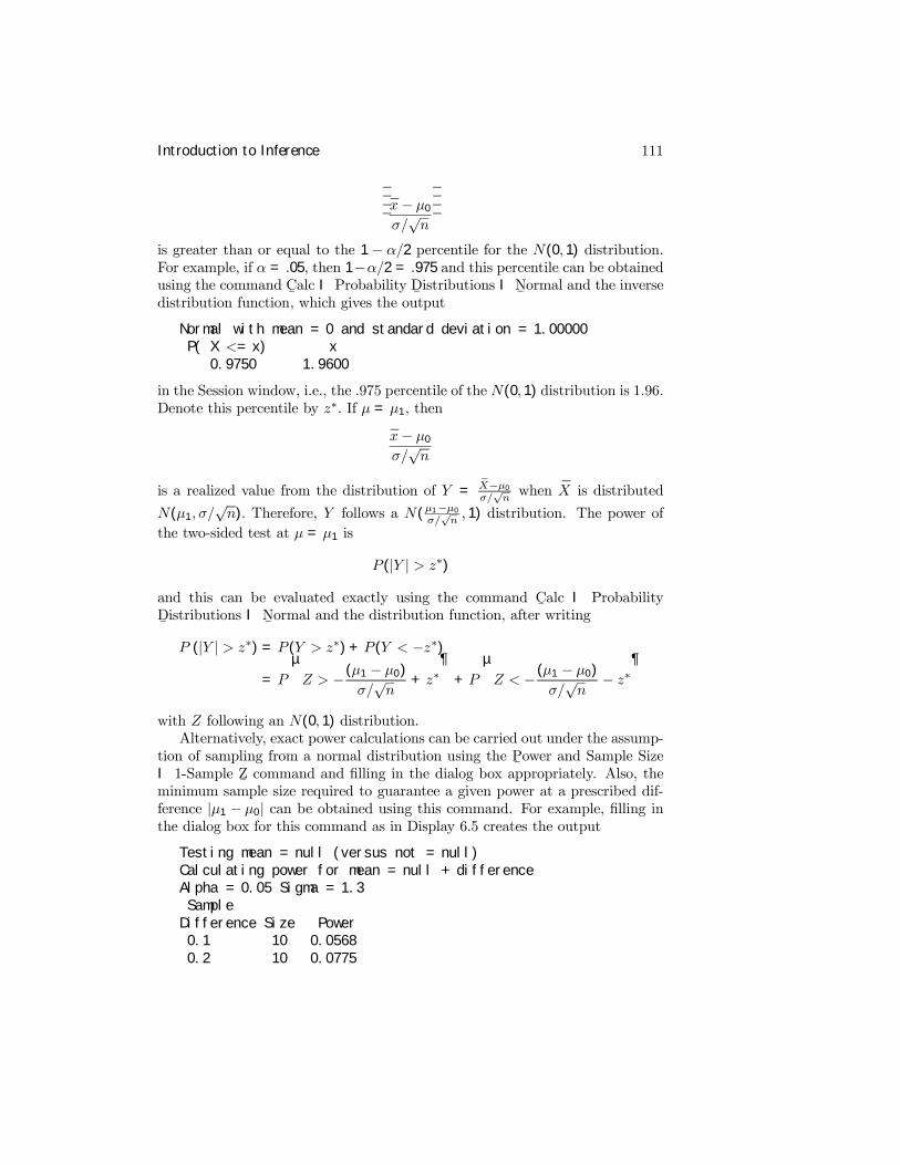
Introduction to Inference 111
¯x− µ0
σ/√n
¯is greater than or equal to the 1 − α/2 percentile for the N(0, 1) distribution.For example, if α = .05, then 1−α/2 = .975 and this percentile can be obtainedusing the command C
¯alc I Probability D
¯istributions I N
¯ormal and the inverse
distribution function, which gives the output
Normal with mean = 0 and standard deviation = 1.00000P( X <= x) x
0.9750 1.9600
in the Session window, i.e., the .975 percentile of the N(0, 1) distribution is 1.96.Denote this percentile by z∗. If µ = µ1, then
x− µ0
σ/√n
is a realized value from the distribution of Y = X−µ0
σ/√nwhen X is distributed
N(µ1, σ/√n). Therefore, Y follows a N(µ1−µ0
σ/√n, 1) distribution. The power of
the two-sided test at µ = µ1 is
P (|Y | > z∗)
and this can be evaluated exactly using the command C¯alc I Probability
D¯istributions I N
¯ormal and the distribution function, after writing
P (|Y | > z∗) = P (Y > z∗) + P (Y < −z∗)
= P
µZ > −(µ1 − µ0)
σ/√n
+ z∗
+ P
µZ < −(µ1 − µ0)
σ/√n
− z∗
with Z following an N(0, 1) distribution.Alternatively, exact power calculations can be carried out under the assump-
tion of sampling from a normal distribution using the P¯ower and Sample Size
I 1-Sample Z¯command and Þlling in the dialog box appropriately. Also, the
minimum sample size required to guarantee a given power at a prescribed dif-ference |µ1 − µ0| can be obtained using this command. For example, Þlling inthe dialog box for this command as in Display 6.5 creates the output
Testing mean = null (versus not = null)Calculating power for mean = null + differenceAlpha = 0.05 Sigma = 1.3Sample
Difference Size Power0.1 10 0.05680.2 10 0.0775
112 Chapter 6
in the Session window. This gives the power for testing H0 : µ = µ0 versusH0 : µ 6= µ0 at |µ1 − µ0| = .1 and |µ1 − µ0| = .2 when n = 10, σ = 1.3, andα = .05. These powers are given by .0568 and .0775, respectively. Clicking onthe Op
¯tions button allows you to choose other alternatives and specify other
values of α in the S¯igniÞcance level box.
Display 6.5: Dialog box for calculating powers and minimum sample sizes.
If we had instead Þlled in Pow¯er values at .1 and .2 in the dialog box of
Display 6.5, say as .8 and .9, and had left the S¯ample sizes box empty, we would
have obtained the output
Testing mean = null (versus not = null)Calculating power for mean = null + differenceAlpha = 0.05 Sigma = 1.3Sample Target ActualDifference Size Power Power
0.1 1327 0.8000 0.80020.1 1776 0.9000 0.90000.2 332 0.8000 0.80050.2 444 0.9000 0.9000
in the Session window. This prescribes the minimum sample sizes n = 1327and n = 1776 to obtain the powers .8 and .9, respectively, at the difference.1 and the sample sizes n = 332 and n = 444 to obtain the powers .8 and .9,respectively, at the difference .2.This derivation of the power of the two-sided test depended on the sample
coming from a normal distribution, as this leads to X having an exact normaldistribution. In general, however, X will be only approximately normal, and sothe normal calculation is not exact. To assess the effect of the nonnormality,however, we can often simulate sampling from a variety of distributions andestimate the probability P (|Y | > z∗). For example, suppose that we want to
Introduction to Inference 113
test H0 : µ = 0 in a two-sided z-test based on a sample of 10, where we estimateσ by the sample standard deviation and we want to evaluate the power at 1. Letus further suppose that we are actually sampling from a uniform distributionon the interval (−10, 12), which indeed has its mean at 1. The simulation givenby the session commands
MTB > random 1000 c1-c10;SUBC> uniform -10 12.MTB > rmean c1-c10 c11MTB > rstdev c1-c10 c12MTB > let c13=absolute(c11/(c12/sqrt(10)))MTB > let c14=c13>1.96MTB > let k1=mean(c14)MTB > let k2=sqrt(k1*(1-k1)/n(c14))MTB > print k1 k2K1 0.112000K2 0.00997276
estimates the power to be .112, and the standard error of this estimate, asgiven in K2, is approximately .01. The application determines whether or notthe assumption of a uniform distribution makes sense and whether or not thispower is indicative of a sensitive test or not.
6.5 The Chi-Square Distribution
If Z is distributed according to the N(0, 1) distribution, then Y = Z2 isdistributed according to the Chisquare(1) distribution. If X1 is distributedChisquare(k1) independent ofX2 distributed Chisquare(k2), then Y = X1+X2
is distributed according to the Chisquare(k1 + k2) distribution. There areMinitab commands that assist in carrying out computations for theChisquare(k)distribution. Note that k is any positive value and is referred to as the degreesof freedom.The values of the density curve for the Chisquare(k) distribution can be
obtained using the C¯alc I Probability D
¯istributions I C
¯hi-Square command,
with k as the D¯egrees of freedom in the dialog box, or the session command pdf
with the subcommand chisquare. For example, the command
MTB > pdf c1 c2;SUBC> chisquare 4.
calculates the value of the Chisquare(4) density curve at each value in C1 andstores these values in C2. This is useful for plotting the density curve. The C
¯alc
I Probability D¯istributions I C
¯hi-Square command, or the session commands
cdf and invcdf, can also be used to obtain values of the Chisquare(k) cumu-lative distribution function and inverse distribution function, respectively. Weuse the C
¯alc I R
¯andom Data I C
¯hi-Square command, or the session command
random, to obtain random samples from these distributions.
114 Chapter 6
We will see applications of the chi-square distribution later in the book butwe mention one here. In particular, if x1, . . . , xn is a sample from a N(µ,σ)
distribution, then (n− 1) s2/σ2 =Pni=1 (xi − x)2 /σ2 is known to follow a
Chisquare(n − 1) distribution, and this fact is used as a basis for inferenceabout σ (conÞdence intervals and tests of signiÞcance). Because of the nonro-bustness of these inferences to small deviations from normality, these inferencesare not recommended.
6.6 ExercisesWhen the data for an exercise come from an exercise in IPS, the IPS exercisenumber is given in parentheses ( ). All computations in these exercises areto be carried out using Minitab, and the exercises are designed to ensure thatyou have a reasonable understanding of the Minitab material in this chapter.Generally, you should be using Minitab to do all the computations and plottingrequired for the problems in IPS.If your version of Minitab places restrictions such that the value of the sim-
ulation sample size N requested in these problems is not feasible, then substitutea more appropriate value. Be aware, however, that the accuracy of your resultsis dependent on how large N is.
1. (6.6) Use the S¯tat I B
¯asic Statistics I 1- Sample Z
¯command to compute
90%, 95%, and 99% conÞdence intervals for µ.
2. (6.49) Use the S¯tat I B
¯asic Statistics I 1- Sample Z
¯command to test the
null hypothesis against the appropriate alternative. Evaluate the powerof the test with level α = .05 at µ = 225.
3. Simulate N = 1000 samples of size 5 from the N(1, 2) distribution, andcalculate the proportion of .90 z-conÞdence intervals for the mean thatcover the true value µ = 1.
4. Simulate N = 1000 samples of size 10 from the uniform distribution on(0,1), and calculate the proportion of .90 z-conÞdence intervals for themean that cover the true value µ = .5. Use σ = 1/
√12.
5. Simulate N = 1000 samples of size 10 from the Exponential(1) distribu-tion (see Exercise II.4.7), and calculate the proportion of .95 z-conÞdenceintervals for the mean that cover the true value µ = 1. Use σ = 1.
6. The density curve for the Student(1) distribution takes the form
1
π
1
1 + x2
for −∞ < x <∞. This special case is called the Cauchy distribution. Plotthis density curve in the range (−20, 20) using an increment of .1. SimulateN = 1000 samples of size 5 from the Student(1) distribution (see Exercise
Introduction to Inference 115
II.4.12), and calculate the proportion of .90 conÞdence intervals for themean, using the sample standard deviation for σ, that cover the valueµ = 0. It is possible to obtain very bad approximations in this examplebecause the central limit theorem does not apply to this distribution. Infact, it does not have a mean.
7. Suppose we are testingH0 : µ = 3 versusH0 : µ 6= 3 when we are samplingfrom a N (µ, σ) distribution with σ = 2.1 and the sample size is n = 20.If we use the critical value α = .01, determine the power of this test atµ = 4.
8. Suppose we are testing H0 : µ = 3 versus H0 : µ > 3 when we aresampling from a N (µ, σ) distribution with σ = 2.1. If we use the criticalvalue α = .01, determine the minimum sample size so that the power ofthis test at µ = 4 is .99.
9. The uniform distribution on the interval (a, b) has mean µ = (a+ b) /2
and standard deviation σ =
q(b− a)2 /12. Calculate the power at µ = 1
of the two-sided z-test at level α = .95 for testing H0 : µ = 0 when thesample size is n = 10, σ is the standard deviation of a uniform distributionon (−10, 12), and we are sampling from a normal distribution.
10. Suppose that we are testing H0 : µ = 0 in a two-sided test based ona sample of 3. Approximate the power of the z-test at level α = .1 atµ = 5 when we are sampling from the distribution of Y = 5 +W, whereW follows a Student(6) distribution (see Exercise II.4.12) and we usethe sample standard deviation to estimate σ. Note that the mean of thedistribution of Y is 5.

116 Chapter 6