Embed Size (px)
Citation preview
Modeling Point Clouds with Self-Attention and Gumbel Subset Sampling
Jiancheng Yang1,2 Qiang Zhang1,2 Bingbing Ni1∗
{jekyll4168, zhangqiang2016, nibingbing}@sjtu.edu.cn
Linguo Li1,2 Jinxian Liu1,2 Mengdie Zhou1,2 Qi Tian3
{LLG440982,liujinxian,dandanzmd}@sjtu.edu.cn, [email protected]
1Shanghai Jiao Tong University2MoE Key Lab of Artificial Intelligence, AI Institute, Shanghai Jiao Tong University
3Huawei Noahs Ark Lab
Abstract
Geometric deep learning is increasingly important
thanks to the popularity of 3D sensors. Inspired by
the recent advances in NLP domain, the self-attention
transformer is introduced to consume the point clouds.
We develop Point Attention Transformers (PATs), using a
parameter-efficient Group Shuffle Attention (GSA) to re-
place the costly Multi-Head Attention. We demonstrate its
ability to process size-varying inputs, and prove its permu-
tation equivariance. Besides, prior work uses heuristics de-
pendence on the input data (e.g., Furthest Point Sampling)
to hierarchically select subsets of input points. Thereby, we
for the first time propose an end-to-end learnable and task-
agnostic sampling operation, named Gumbel Subset Sam-
pling (GSS), to select a representative subset of input points.
Equipped with Gumbel-Softmax, it produces a ”soft” con-
tinuous subset in training phase, and a ”hard” discrete sub-
set in test phase. By selecting representative subsets in a
hierarchical fashion, the networks learn a stronger repre-
sentation of the input sets with lower computation cost. Ex-
periments on classification and segmentation benchmarks
show the effectiveness and efficiency of our methods. Fur-
thermore, we propose a novel application, to process event
camera stream as point clouds, and achieve a state-of-the-
art performance on DVS128 Gesture Dataset.
1. Introduction
We live in a 3D world. Geometric data have raised in-
creasing research concerns thanks to the popularity of 3D
sensors, e.g., LiDAR and RGB-D cameras. In particular,
we are interested in analyzing 3D point clouds with end-to-
end deep learning, which theoretically requires the neural
networks to consume 1) size-varying and 2) permutation-
∗Corresponding author.
Furthest Point Sampling
Group Shuffle Attention Gumbel Subset Sampling
Outlier
Atte
ntio
n W
eig
hts
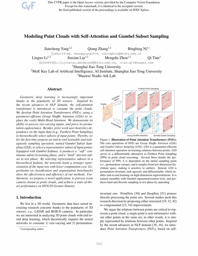
Figure 1. Illustration of Point Attention Transformers (PATs).
The core operations of PATs are Group Shuffle Attention (GSA)
and Gumbel Subset Sampling (GSS). GSA is a parameter-efficient
self-attention operation on learning relations between points. GSS
serves as a differentiable alternative to Furthest Point Sampling
(FPS) in point cloud reasoning. Several flaws hinder the per-
formance of FPS: it is dependent on the initial sampling point
(i.e., permutation-variant), and it samples from low-dimension Eu-
clidean space, making it sensitive to outliers. Instead, GSS is
permutation-invariant, task-agnostic and differentiable, which en-
ables end-to-end learning on high-dimension representations. It is
trained smoothly with Gumbel reparameterization trick, and pro-
duces hard and discrete sampling in test phase by annealing.
invariant sets. PointNets [30] and DeepSets [51] pioneer
directly processing the point sets. Several studies push this
research direction by proposing either structural [19, 32, 42]
or componential [23, 34] improvements.
We argue the relations between points are critical to rep-
resent a point cloud: a single point is non-informative with-
out other points in the same set; in other words, it is sim-
ply represented by relations between other points. Inspired
by the recent advances in NLP domain [39, 10], we intro-
duce Point Attention Transformers (PATs), based on self-
3323
attention to model the relations with powerful multi-head
design [39]. Combining with ideas of the light-weight but
high-performance model, we propose a parameter-efficient
Group Shuffle Attention (GSA) to replace the costly Multi-
Head Attention [39] with superior performance.
Besides, prior studies [32, 23] demonstrate the effec-
tiveness of hierarchical structures in point cloud reasoning.
By sampling central subsets of input points and grouping
them with graph-based operations at multiple levels, the hi-
erarchical structures mimic receptive fields in CNNs with
bottom-up representation learning. Despite great success,
we however figure out that the sampling operation is a bot-
tleneck of the hierarchical structures.
Few prior works study sampling from high-dimension
embeddings. The most popular sampling operation on 3D
point clouds is the Furthest Point Sampling (FPS). How-
ever, it is task-dependent, i.e., designed for low-dimension
Euclidean space exclusively, without sufficiently utilizing
the semantically high-level representations. Moreover, as
illustrated in Figure 1, FPS is permutation-variant, and sen-
sitive to outliers in point clouds.
To this end, we propose a task-agnostic and permutation-
invariant sampling operation, named Gumbel Subset Sam-
pling (GSS), to address the set sampling problem. Impor-
tantly, it is end-to-end trainable. To our knowledge, we are
the first study to propose a differentiable subset sampling
method. Equipped with Gumbel-Softmax [16, 26], our GSS
samples soft virtual points in training phase, and produces
hard selection in test phase via annealing. With GSS, our
PAT classification models are better-performed with lower
computation cost.
2. Preliminaries
2.1. Deep Learning on Point Clouds
CNNs (especially 3D CNNs [31, 54]) dominate early-
stage researches of deep learning on 3D vision, where the
point clouds are rendered into 2D multi-view images [37] or
3D voxels [31]. These methods require compute-intensively
pre-rendering the sparse points into voluminous representa-
tions with quantization artifacts [30]. To improve memory
efficiency and running speed, several researchers [41, 36]
introduce sparse CNNs on specific data structures.
On the other hand, deep learning directly on the
Euclidean-space point clouds raises research attention.
By design, these networks should be able to process 1)
size-varying and 2) permutation-invariant (or permutation-
equivariant) point sets (called Theoretical Conditions for
simplicity). PointNet [30] and DeepSet [51] pioneer this
direction, where a symmetric function (e.g., shared FC be-
fore max-pooling) is used for learning each point’s high-
level representation before aggregation; However, relations
between the points are not sufficiently captured in this way.
To this end, PointNet++ [32] introduces a hierarchical struc-
ture based on Euclidean-space nearest-neighbor graph, Kd-
Net [19] designs spatial KD-trees for efficient information
aggregation, and DGCNN [42] develops a graph neural net-
work (GNN) approach with dynamic graph construction.
Not all studies satisfy both Theoretical Conditions at the
same time; For instance, Kd-Net [19] resamples the input
points to evade the ”size-varying” condition, and PointCNN
[23] groups and processes the points via specific operators
without ”permutation-invariant” condition.
In a word, the follow-up researches on point clouds are
mainly 1) voxel-based CNNs [41, 9], 2) variants of geomet-
ric deep learning [6], i.e., graph neural networks on point
sets [46, 34, 23, 22], or 3) hybrid [55, 21, 36]. There is also
research on the adversarial security on point clouds [50]
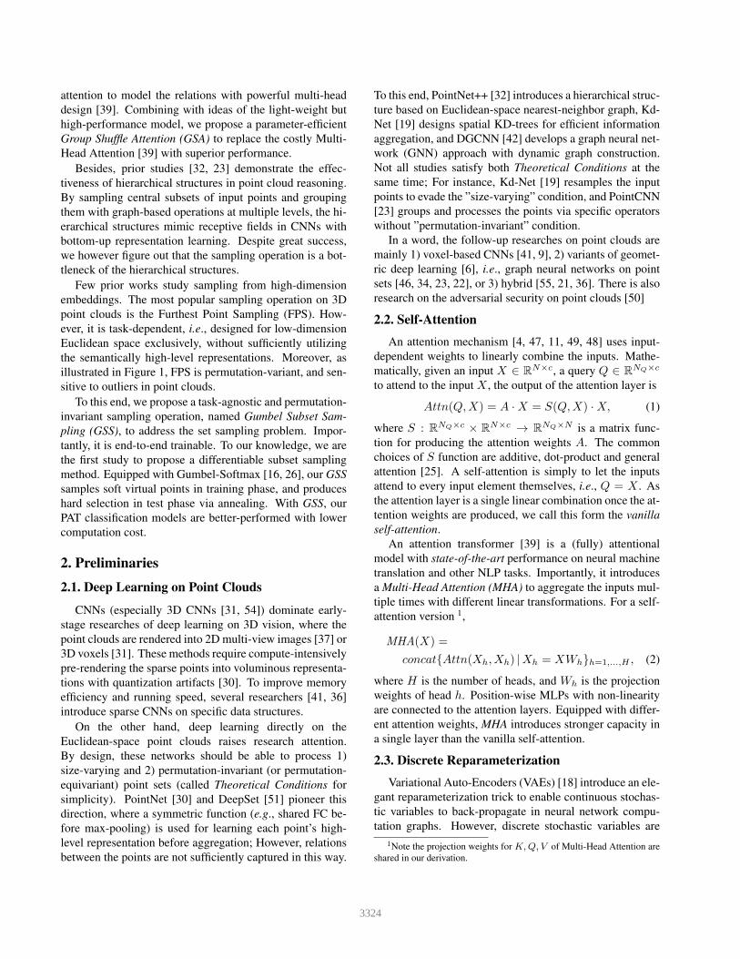
2.2. SelfAttention
An attention mechanism [4, 47, 11, 49, 48] uses input-
dependent weights to linearly combine the inputs. Mathe-
matically, given an input X ∈ RN×c, a query Q ∈ R
NQ×c
to attend to the input X , the output of the attention layer is
Attn(Q,X) = A ·X = S(Q,X) ·X, (1)
where S : RNQ×c × RN×c → R
NQ×N is a matrix func-
tion for producing the attention weights A. The common
choices of S function are additive, dot-product and general
attention [25]. A self-attention is simply to let the inputs
attend to every input element themselves, i.e., Q = X . As
the attention layer is a single linear combination once the at-
tention weights are produced, we call this form the vanilla
self-attention.
An attention transformer [39] is a (fully) attentional
model with state-of-the-art performance on neural machine
translation and other NLP tasks. Importantly, it introduces
a Multi-Head Attention (MHA) to aggregate the inputs mul-
tiple times with different linear transformations. For a self-
attention version 1,
MHA(X) =
concat{Attn(Xh, Xh) |Xh = XWh}h=1,...,H , (2)
where H is the number of heads, and Wh is the projection
weights of head h. Position-wise MLPs with non-linearity
are connected to the attention layers. Equipped with differ-
ent attention weights, MHA introduces stronger capacity in
a single layer than the vanilla self-attention.
2.3. Discrete Reparameterization
Variational Auto-Encoders (VAEs) [18] introduce an ele-
gant reparameterization trick to enable continuous stochas-
tic variables to back-propagate in neural network compu-
tation graphs. However, discrete stochastic variables are
1Note the projection weights for K,Q, V of Multi-Head Attention are
shared in our derivation.
3324
non-trivial to be reparameterized. To this regard, sev-
eral stochastic gradient estimation methods are proposed,
e.g., REINFORCE-based methods [38, 33] and Straight-
Through Estimators [5].
For a categorical distribution Cat(s1, ..., sM ), where M
denotes the number of categories, si (s.t.∑M
i=1(si) =1) means the probability score of category i, a Gumbel-
Softmax [16, 26] is designed as a discrete reparameteriza-
tion trick, to estimate smooth gradient with a continuous
relaxation for the categorical variable. Given i.i.d Gumbel
noise g = (g1, ..., gM ) drawn from Gumbel(0, 1) distribu-
tion, a soft categorical sample can be drawn (or computed)
by
y = softmax ((log(s) + g)/τ), s = (s1, ..., sM ). (3)
The Eq. 3 is referred as gumbel softmax operation on s.
Parameter τ > 0 is the annealing temperature, as τ →0+, y degenerates into the Gumbel-Max form,
y = one hot encoding(argmax((log(s) + g))), (4)
which is an unbiased sample from Cat(s1, ..., sM ).In this way, we are able to draw differentiable samples
(Eq. 3) from the distribution Cat(s1, ..., sM ) in training
phase. In practice, τ starts at a high value (e.g., 1.0), and an-
neals to a small value (e.g., 0.1). Optimization on the Gum-
bel Softmax distribution could be interpreted as solving a
certain entropy-regularized linear program on the probabil-
ity simplex [27]. In test phase, discrete samples can be
drawn with Gumbel-Max trick (Eq. 4).
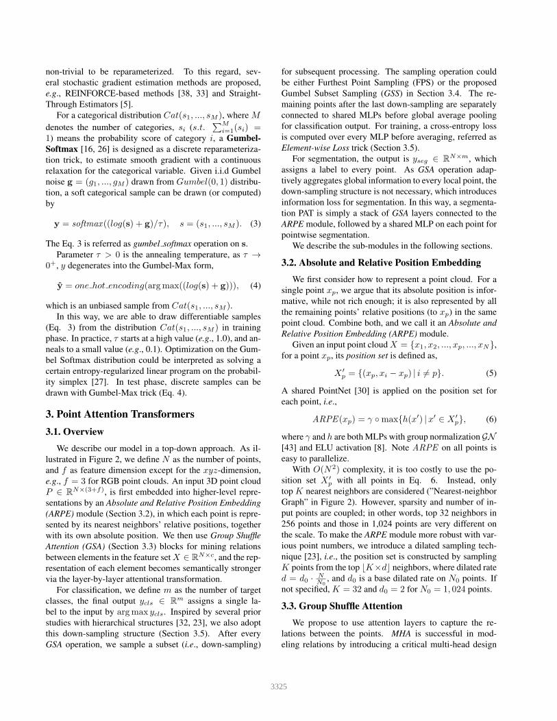
3. Point Attention Transformers
3.1. Overview
We describe our model in a top-down approach. As il-
lustrated in Figure 2, we define N as the number of points,
and f as feature dimension except for the xyz-dimension,
e.g., f = 3 for RGB point clouds. An input 3D point cloud
P ∈ RN×(3+f), is first embedded into higher-level repre-
sentations by an Absolute and Relative Position Embedding
(ARPE) module (Section 3.2), in which each point is repre-
sented by its nearest neighbors’ relative positions, together
with its own absolute position. We then use Group Shuffle
Attention (GSA) (Section 3.3) blocks for mining relations
between elements in the feature setX ∈ RN×c, and the rep-
resentation of each element becomes semantically stronger
via the layer-by-layer attentional transformation.
For classification, we define m as the number of target
classes, the final output ycls ∈ Rm assigns a single la-
bel to the input by argmax ycls. Inspired by several prior
studies with hierarchical structures [32, 23], we also adopt
this down-sampling structure (Section 3.5). After every
GSA operation, we sample a subset (i.e., down-sampling)
for subsequent processing. The sampling operation could
be either Furthest Point Sampling (FPS) or the proposed
Gumbel Subset Sampling (GSS) in Section 3.4. The re-
maining points after the last down-sampling are separately
connected to shared MLPs before global average pooling
for classification output. For training, a cross-entropy loss
is computed over every MLP before averaging, referred as
Element-wise Loss trick (Section 3.5).
For segmentation, the output is yseg ∈ RN×m, which
assigns a label to every point. As GSA operation adap-
tively aggregates global information to every local point, the
down-sampling structure is not necessary, which introduces
information loss for segmentation. In this way, a segmenta-
tion PAT is simply a stack of GSA layers connected to the
ARPE module, followed by a shared MLP on each point for
pointwise segmentation.
We describe the sub-modules in the following sections.
3.2. Absolute and Relative Position Embedding
We first consider how to represent a point cloud. For a
single point xp, we argue that its absolute position is infor-
mative, while not rich enough; it is also represented by all
the remaining points’ relative positions (to xp) in the same
point cloud. Combine both, and we call it an Absolute and
Relative Position Embedding (ARPE) module.
Given an input point cloudX = {x1, x2, ..., xp, ..., xN},
for a point xp, its position set is defined as,
X ′
p = {(xp, xi − xp) | i 6= p}. (5)
A shared PointNet [30] is applied on the position set for
each point, i.e.,
ARPE (xp) = γ ◦max{h(x′) |x′ ∈ X ′
p}, (6)
where γ and h are both MLPs with group normalization GN[43] and ELU activation [8]. Note ARPE on all points is
easy to parallelize.
With O(N2) complexity, it is too costly to use the po-
sition set X ′
p with all points in Eq. 6. Instead, only
top K nearest neighbors are considered (”Nearest-neighbor
Graph” in Figure 2). However, sparsity and number of in-
put points are coupled; in other words, top 32 neighbors in
256 points and those in 1,024 points are very different on
the scale. To make the ARPE module more robust with var-
ious point numbers, we introduce a dilated sampling tech-
nique [23], i.e., the position set is constructed by sampling
K points from the top ⌊K×d⌋ neighbors, where dilated rate
d = d0 · NN0
, and d0 is a base dilated rate on N0 points. If
not specified, K = 32 and d0 = 2 for N0 = 1, 024 points.
3.3. Group Shuffle Attention
We propose to use attention layers to capture the re-
lations between the points. MHA is successful in mod-
eling relations by introducing a critical multi-head design
3325
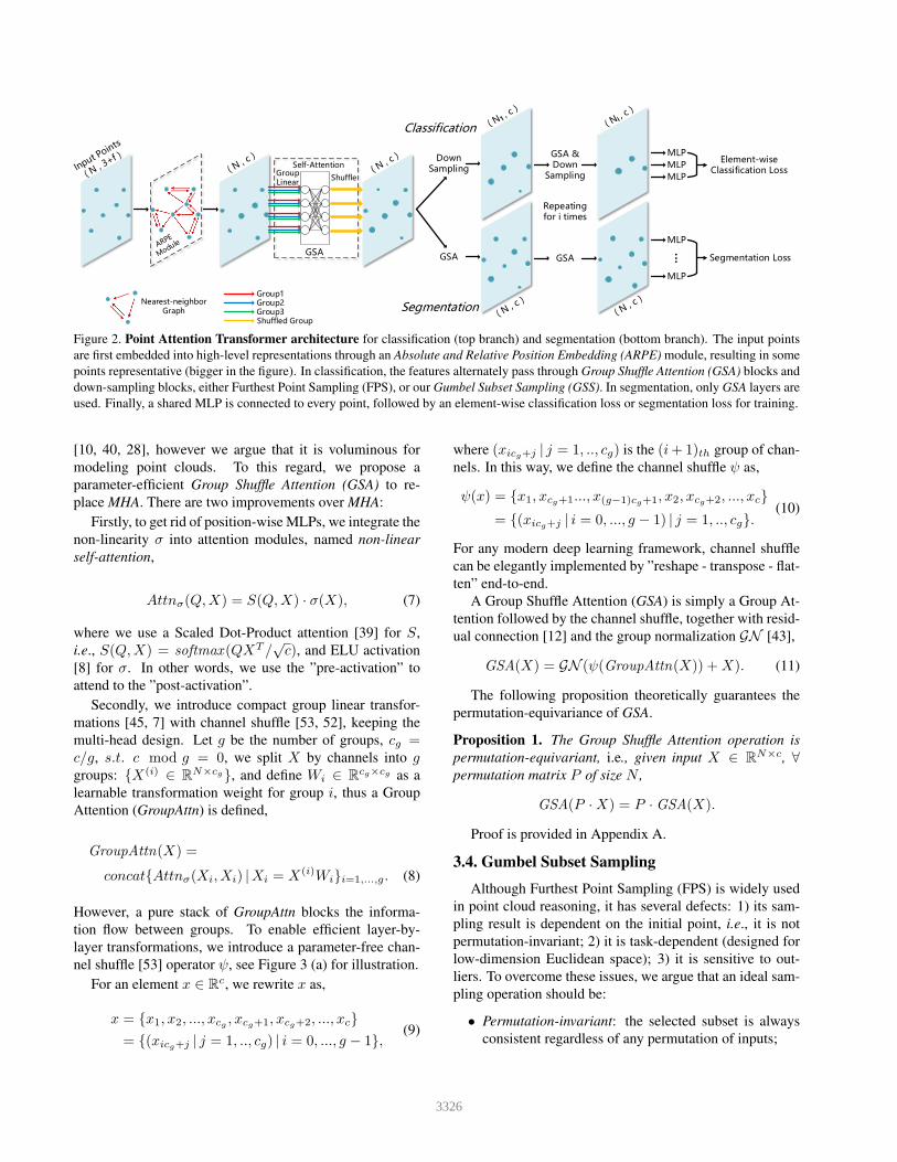
GroupLinear
Shuffle
GSA GSA
Down Sampling
Element-wise Classification Loss
Segmentation Loss
Segmentation
Classification
Self-Attention
GSA
GSA & Down
Sampling
Repeatingfor i times
Group1Group2Group3Shuffled Group
MLP
MLP
...
MLP
MLP
MLP
Nearest-neighbor Graph
Figure 2. Point Attention Transformer architecture for classification (top branch) and segmentation (bottom branch). The input points
are first embedded into high-level representations through an Absolute and Relative Position Embedding (ARPE) module, resulting in some
points representative (bigger in the figure). In classification, the features alternately pass through Group Shuffle Attention (GSA) blocks and
down-sampling blocks, either Furthest Point Sampling (FPS), or our Gumbel Subset Sampling (GSS). In segmentation, only GSA layers are
used. Finally, a shared MLP is connected to every point, followed by an element-wise classification loss or segmentation loss for training.
[10, 40, 28], however we argue that it is voluminous for
modeling point clouds. To this regard, we propose a
parameter-efficient Group Shuffle Attention (GSA) to re-
place MHA. There are two improvements over MHA:
Firstly, to get rid of position-wise MLPs, we integrate the
non-linearity σ into attention modules, named non-linear
self-attention,
Attnσ(Q,X) = S(Q,X) · σ(X), (7)
where we use a Scaled Dot-Product attention [39] for S,
i.e., S(Q,X) = softmax (QXT /√c), and ELU activation
[8] for σ. In other words, we use the ”pre-activation” to
attend to the ”post-activation”.
Secondly, we introduce compact group linear transfor-
mations [45, 7] with channel shuffle [53, 52], keeping the
multi-head design. Let g be the number of groups, cg =c/g, s.t. c mod g = 0, we split X by channels into ggroups: {X(i) ∈ R
N×cg}, and define Wi ∈ Rcg×cg as a
learnable transformation weight for group i, thus a Group
Attention (GroupAttn) is defined,
GroupAttn(X) =
concat{Attnσ(Xi, Xi) |Xi = X(i)Wi}i=1,...,g. (8)
However, a pure stack of GroupAttn blocks the informa-
tion flow between groups. To enable efficient layer-by-
layer transformations, we introduce a parameter-free chan-
nel shuffle [53] operator ψ, see Figure 3 (a) for illustration.
For an element x ∈ Rc, we rewrite x as,
x = {x1, x2, ..., xcg , xcg+1, xcg+2, ..., xc}= {(xicg+j | j = 1, .., cg) | i = 0, ..., g − 1}, (9)
where (xicg+j | j = 1, .., cg) is the (i+ 1)th group of chan-
nels. In this way, we define the channel shuffle ψ as,
ψ(x) = {x1, xcg+1..., x(g−1)cg+1, x2, xcg+2, ..., xc}= {(xicg+j | i = 0, ..., g − 1) | j = 1, .., cg}.
(10)
For any modern deep learning framework, channel shuffle
can be elegantly implemented by ”reshape - transpose - flat-
ten” end-to-end.
A Group Shuffle Attention (GSA) is simply a Group At-
tention followed by the channel shuffle, together with resid-
ual connection [12] and the group normalization GN [43],
GSA(X) = GN (ψ(GroupAttn(X)) +X). (11)
The following proposition theoretically guarantees the
permutation-equivariance of GSA.
Proposition 1. The Group Shuffle Attention operation is
permutation-equivariant, i.e., given input X ∈ RN×c, ∀
permutation matrix P of size N ,
GSA(P ·X) = P ·GSA(X).
Proof is provided in Appendix A.
3.4. Gumbel Subset Sampling
Although Furthest Point Sampling (FPS) is widely used
in point cloud reasoning, it has several defects: 1) its sam-
pling result is dependent on the initial point, i.e., it is not
permutation-invariant; 2) it is task-dependent (designed for
low-dimension Euclidean space); 3) it is sensitive to out-
liers. To overcome these issues, we argue that an ideal sam-
pling operation should be:
• Permutation-invariant: the selected subset is always
consistent regardless of any permutation of inputs;
3326
Dot-Product
In-GroupAttention
Group Norm
Group Linear
Channel Shuffle
Group1
Group2
Group3
Point 2
Non-linearity
+
Input
FC Layer
Transposed
Gumbel Noise
1/τ
Softmax
Dot-Product
( Ni , c )
( Ni+1 , Ni )
( Ni+1 , Ni )
( Ni+1 , c )
×
+
(a) Group Shuffle Attention (b) Gumbel Subset Sampling
Point 1 Point 3
Annealing
τ → 0+τ = 1
Figure 3. (a) Group Shuffle Attention. The core representation
learning block in PATs. An input of 3 points is demonstrated. The
feature of each point is divided into several groups (different colors
in the figure). Within each group, the input points are transformed
by a shared linear layer and a non-linear self-attention (Eq. 7). We
then apply channel shuffle on each point feature. Residual con-
nection and group normalization are used for better optimization
property. (b) Gumbel Subset Sampling is used for end-to-end
learning a representative subset of the input set. For Ni+1 rounds,
one point is selected from the Ni input points competitively. Dur-
ing each round, every input point produces one selection score (Eq.
13), with a max score to be selected. A Gumbel-Softmax (Eq. 3)
with high temperature is used for soft selection in training phase.
At inference, a Gumbel-Max (Eq. 4) is applied with annealing.
Best viewed in color.
• Sampling from a high-dimension embedding space:
the sampling operation should be designed task-
agnostic and less sensitive to outliers by learning rep-
resentative and robust embeddings;
• Differentiable: it enables the sampling operation to in-
tegrate into neural networks painlessly.
For these purposes, we develop a permutation-invariant,
task-agnostic and differentiable Gumbel Subset Sampling
(GSS). Given an input set Xi ∈ RNi×c, which could be
output of a neural network layer, the goal is to select a repre-
sentative subset Xi+1 ∈ RNi+1×c ⊆ Xi with differentiable
operations. Inspired by Attention-based MIL pooling [15],
where the pooling output y is an average value weighted by
normalized scores produced element-wisely, i.e.,
y = softmax (wXTi ) ·Xi, w ∈ R
c. (12)
Note w ∈ Rc is a learnable weight and could be replaced
with an MLP.
We reinterpret Attention-based MIL pooling (Eq. 12)
as competitively selecting one soft virtual point. Though
differentiable, the virtual point is however untraceable and
less interpretable, especially when selecting multiple points.
Instead, we use a hard and discrete selection with an end-
to-end trainable gumbel softmax (Eq. 3):
ygumbel = gumbel softmax (wXTi ) ·Xi, w ∈ R
c. (13)
in training phase, it provides smooth gradients using dis-
crete reparameterization trick. With annealing, it degener-
ates to a hard selection in test phase.
A Gumbel Subset Sampling (GSS) is simply a multiple-
point version of Eq. 13, which means a distribution of sub-
sets,
GSS (Xi) = gumbel softmax (WXTi )·Xi, W ∈ R
Ni+1×c.(14)
The following proposition theoretically guarantees the
permutation-invariance of GSS.
Proposition 2. The Gumbel Subset Sampling operation is
permutation-invariant, i.e., given input X ∈ RN×c, ∀ per-
mutation matrix P of size N ,
GSS (P ·X) = GSS (X).
Proof is provided in Appendix B.
3.5. Other Architecture Design
Down-sampling Structure In our classification models,
we down-sample input points at 3 levels (from 1,024 points
to 384 - 128 - 64 points). Although GSS is theoretically su-
perior to FPS, the Gumbel noises also serve as a (too) strong
regularization. Instead of using GSS in all down-sampling,
we find that replacing the first down-sampling with FPS per-
forms slightly better in our experiments.
Element-wise Loss We compute the classification loss as
segmentation [23]: a shared MLP is connected to each re-
maining point to output the same target class, where the
MLP is a stack of ”FC - GN - ELU - dropout [35]”. The
final loss is averaged by element-wise cross entropy. The
element-wise loss trick does not bring any performance
boost, while the training is significantly faster to converge.
At inference, the final classification score is averaged by the
element-wise outputs.
4. Applications
In this section, we first demonstrate the effectiveness and
efficiency of PATs on a benchmark of point cloud classifi-
cation, ModelNet40 dataset [44] of CAD models. We then
explore the model performance on real-world datasets. We
report the segmentation results on S3DIS dataset [2]. Fur-
thermore, we propose a novel application on recognizing
gestures with event camera on DVS128 Gesture Dataset [1].
To our knowledge, this is the first study to process event-
camera stream as spatio-temporal point clouds, with state-
of-the-art performance.
3327
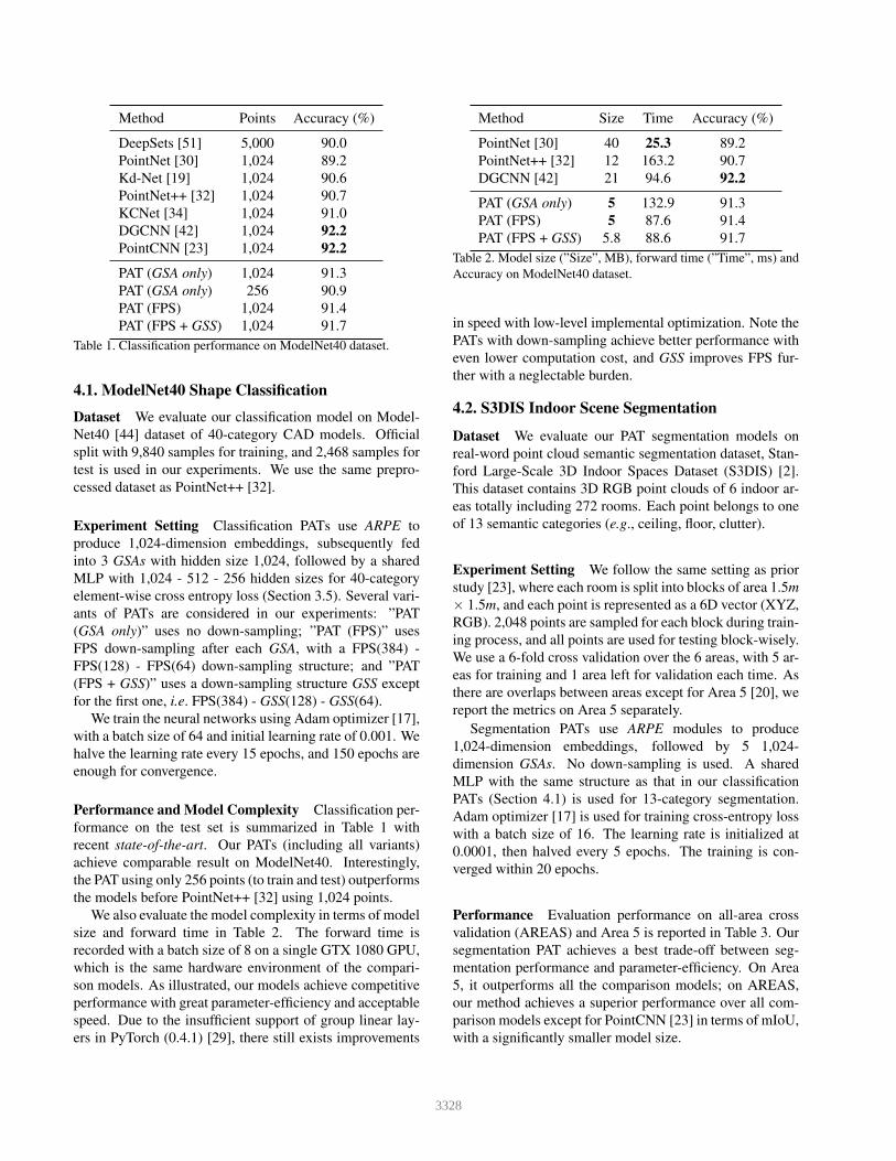
Method Points Accuracy (%)
DeepSets [51] 5,000 90.0
PointNet [30] 1,024 89.2
Kd-Net [19] 1,024 90.6
PointNet++ [32] 1,024 90.7
KCNet [34] 1,024 91.0
DGCNN [42] 1,024 92.2
PointCNN [23] 1,024 92.2
PAT (GSA only) 1,024 91.3
PAT (GSA only) 256 90.9
PAT (FPS) 1,024 91.4
PAT (FPS + GSS) 1,024 91.7
Table 1. Classification performance on ModelNet40 dataset.
4.1. ModelNet40 Shape Classification
Dataset We evaluate our classification model on Model-
Net40 [44] dataset of 40-category CAD models. Official
split with 9,840 samples for training, and 2,468 samples for
test is used in our experiments. We use the same prepro-
cessed dataset as PointNet++ [32].
Experiment Setting Classification PATs use ARPE to
produce 1,024-dimension embeddings, subsequently fed
into 3 GSAs with hidden size 1,024, followed by a shared
MLP with 1,024 - 512 - 256 hidden sizes for 40-category
element-wise cross entropy loss (Section 3.5). Several vari-
ants of PATs are considered in our experiments: ”PAT
(GSA only)” uses no down-sampling; ”PAT (FPS)” uses
FPS down-sampling after each GSA, with a FPS(384) -
FPS(128) - FPS(64) down-sampling structure; and ”PAT
(FPS + GSS)” uses a down-sampling structure GSS except
for the first one, i.e. FPS(384) - GSS(128) - GSS(64).
We train the neural networks using Adam optimizer [17],
with a batch size of 64 and initial learning rate of 0.001. We
halve the learning rate every 15 epochs, and 150 epochs are
enough for convergence.
Performance and Model Complexity Classification per-
formance on the test set is summarized in Table 1 with
recent state-of-the-art. Our PATs (including all variants)
achieve comparable result on ModelNet40. Interestingly,
the PAT using only 256 points (to train and test) outperforms
the models before PointNet++ [32] using 1,024 points.
We also evaluate the model complexity in terms of model
size and forward time in Table 2. The forward time is
recorded with a batch size of 8 on a single GTX 1080 GPU,
which is the same hardware environment of the compari-
son models. As illustrated, our models achieve competitive
performance with great parameter-efficiency and acceptable
speed. Due to the insufficient support of group linear lay-
ers in PyTorch (0.4.1) [29], there still exists improvements
Method Size Time Accuracy (%)
PointNet [30] 40 25.3 89.2
PointNet++ [32] 12 163.2 90.7
DGCNN [42] 21 94.6 92.2
PAT (GSA only) 5 132.9 91.3
PAT (FPS) 5 87.6 91.4
PAT (FPS + GSS) 5.8 88.6 91.7
Table 2. Model size (”Size”, MB), forward time (”Time”, ms) and
Accuracy on ModelNet40 dataset.
in speed with low-level implemental optimization. Note the
PATs with down-sampling achieve better performance with
even lower computation cost, and GSS improves FPS fur-
ther with a neglectable burden.
4.2. S3DIS Indoor Scene Segmentation
Dataset We evaluate our PAT segmentation models on
real-word point cloud semantic segmentation dataset, Stan-
ford Large-Scale 3D Indoor Spaces Dataset (S3DIS) [2].
This dataset contains 3D RGB point clouds of 6 indoor ar-
eas totally including 272 rooms. Each point belongs to one
of 13 semantic categories (e.g., ceiling, floor, clutter).
Experiment Setting We follow the same setting as prior
study [23], where each room is split into blocks of area 1.5m
× 1.5m, and each point is represented as a 6D vector (XYZ,
RGB). 2,048 points are sampled for each block during train-
ing process, and all points are used for testing block-wisely.
We use a 6-fold cross validation over the 6 areas, with 5 ar-
eas for training and 1 area left for validation each time. As
there are overlaps between areas except for Area 5 [20], we
report the metrics on Area 5 separately.
Segmentation PATs use ARPE modules to produce
1,024-dimension embeddings, followed by 5 1,024-
dimension GSAs. No down-sampling is used. A shared
MLP with the same structure as that in our classification
PATs (Section 4.1) is used for 13-category segmentation.
Adam optimizer [17] is used for training cross-entropy loss
with a batch size of 16. The learning rate is initialized at
0.0001, then halved every 5 epochs. The training is con-
verged within 20 epochs.
Performance Evaluation performance on all-area cross
validation (AREAS) and Area 5 is reported in Table 3. Our
segmentation PAT achieves a best trade-off between seg-
mentation performance and parameter-efficiency. On Area
5, it outperforms all the comparison models; on AREAS,
our method achieves a superior performance over all com-
parison models except for PointCNN [23] in terms of mIoU,
with a significantly smaller model size.
3328
Method mIoU mIoU on Area 5 Size (MB)
RSNet [13] 56.47 - -
SPGraph [20] 62.1 58.04 -
PointNet [30] 47.71 47.6 4.7
DGCNN [42] 56.1 - 6.9
PointCNN [23] 65.39 57.26 46.2
PAT 64.28 60.07 6.1
Table 3. 3D semantic segmentation results on S3DIS. Mean per-
class IoU (mIoU, %) is used as evaluation metric. Model sizes are
obtained using the official codes.
To further analyze the performance between PointCNN
and our method, we compare per-class IoU and mean per-
class accuracy (mAcc) on AREAS and Area 5. As depicted
in Table 4, on AREAS, our method outperforms PointCNN
in terms of mAcc; on Area 5, our method outperforms
PointCNN in terms of both mIoU and mAcc, plus superior
per-class IoUs on majority of classes.
4.3. Event Camera Stream as Point Clouds:DVS128 Gesture Recognization
Motivation and Dataset Point cloud approaches are pri-
marily designed for 3D spatial sensors, e.g., LiDAR and
Matterport 3D Cameras. However, there are numbers of
potential applications with point-based records. In this sec-
tion, we explore a novel application on event camera with
point cloud approaches.
Dynamic Vision Sensor (DVS) [24] is a biologically in-
spired event camera, which ”transmits data only when a
pixel detects a change” [1]. On the 128×128 sensor ma-
trix, it records whether there is a change (by a user-defined
threshold) on the corresponding position in microseconds.
In particular, we explore gesture recognition on DVS128
Gesture Dataset [1], with 11 classes of gestures (10 named
gestures, e.g., ”Arm Roll”, and 1 ”others”) collected from
122 users. Training data is collected from 94 users with 939
event streams, and test data is collected from 24 users with
249 event streams. The gesture action records is a sequence
of points, each of which is point change represented as a
4-dimension vector: abscissa x, ordinate y, timestamp t,and polarity (1 for appear and 0 for disappear). In this way,
we regard the event stream as spatio-temporal point clouds.
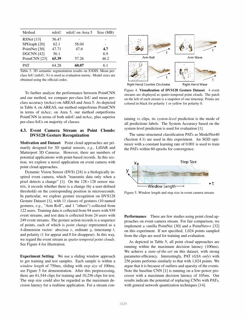
See Figure 4 for illustration.
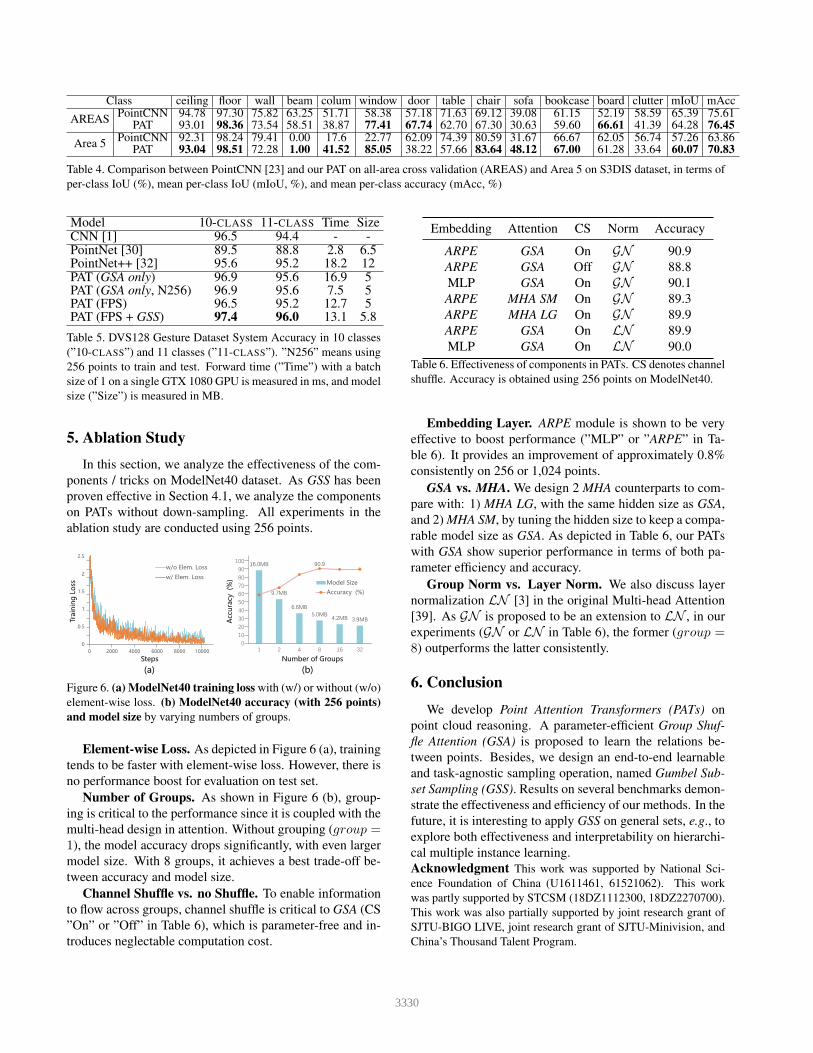
Experiment Setting We use a sliding window approach
to get training and test samples. Each sample is within a
window length of 750ms, sliding with step size of 100ms,
see Figure 5 for demonstration. After this preprocessing,
there are 61,544 clips for training and 10,256 clips for test.
The step size could also be regarded as the maximum de-
cision latency for a realtime application. For a stream con-
Figure 4. Visualization of DVS128 Gesture Dataset. 4 event
streams are displayed as spatio-temporal point clouds. The patch
on the left of each stream is a snapshot of one timestep. Points are
colored in black for polarity 1 or yellow for polarity 0.
taining m clips, its system-level prediction is the mode of
all predictions labels. The System Accuracy based on the
system-level prediction is used for evaluation [1].
The same-structured classification PATs as ModelNet40
(Section 4.1) are used in this experiment. An SGD opti-
mizer with a constant learning rate of 0.001 is used to train
the PATs within 60 epochs for convergence.
Figure 5. Window length and step size in event camera stream.
Performance There are few studies using point cloud ap-
proaches on event camera stream. For fair comparison, we
implement a vanilla PointNet [30] and a PointNet++ [32]
on this experiment. If not specified, 1,024 points sampled
from the clips are used for training and evaluation.
As depicted in Table 5, all point cloud approaches are
running within the maximum decision latency (100ms).
We achieve a state-of-the-art on this dataset, with strong
parameter-efficiency. Interestingly, PAT (GSA only) with
256 points performs similarly to that with 1,024 points. We
argue that it is because of outliers and sparsity of the events.
Note the baseline CNN [1] is running on a low-power pro-
cessor with a maximum decision latency of 105ms. Our
results indicate the potential of replacing CNNs with PATs,
with general network quantization techniques [14].
3329
Class ceiling floor wall beam colum window door table chair sofa bookcase board clutter mIoU mAcc
AREASPointCNN 94.78 97.30 75.82 63.25 51.71 58.38 57.18 71.63 69.12 39.08 61.15 52.19 58.59 65.39 75.61
PAT 93.01 98.36 73.54 58.51 38.87 77.41 67.74 62.70 67.30 30.63 59.60 66.61 41.39 64.28 76.45
Area 5PointCNN 92.31 98.24 79.41 0.00 17.6 22.77 62.09 74.39 80.59 31.67 66.67 62.05 56.74 57.26 63.86
PAT 93.04 98.51 72.28 1.00 41.52 85.05 38.22 57.66 83.64 48.12 67.00 61.28 33.64 60.07 70.83
Table 4. Comparison between PointCNN [23] and our PAT on all-area cross validation (AREAS) and Area 5 on S3DIS dataset, in terms of
per-class IoU (%), mean per-class IoU (mIoU, %), and mean per-class accuracy (mAcc, %)
Model 10-CLASS 11-CLASS Time SizeCNN [1] 96.5 94.4 - -PointNet [30] 89.5 88.8 2.8 6.5PointNet++ [32] 95.6 95.2 18.2 12PAT (GSA only) 96.9 95.6 16.9 5PAT (GSA only, N256) 96.9 95.6 7.5 5PAT (FPS) 96.5 95.2 12.7 5PAT (FPS + GSS) 97.4 96.0 13.1 5.8
Table 5. DVS128 Gesture Dataset System Accuracy in 10 classes
(”10-CLASS”) and 11 classes (”11-CLASS”). ”N256” means using
256 points to train and test. Forward time (”Time”) with a batch
size of 1 on a single GTX 1080 GPU is measured in ms, and model
size (”Size”) is measured in MB.
5. Ablation Study
In this section, we analyze the effectiveness of the com-
ponents / tricks on ModelNet40 dataset. As GSS has been
proven effective in Section 4.1, we analyze the components
on PATs without down-sampling. All experiments in the
ablation study are conducted using 256 points.
16.0MB
9.7MB
6.6MB
5.0MB4.2MB 3.9MB
90.9
0
10
20
30
40
50
60
70
80
90
100
1 2 4 8 16 32
Model Size
Accuracy (%)
Acc
ura
cy (%
)
Number of Groups
0
0.5
1
1.5
2
2.5
0 2000 4000 6000 8000 10000
w/o Elem. Loss
w/ Elem. Loss
Train
ing
Lo
ss
Steps
(a) (b)
Figure 6. (a) ModelNet40 training loss with (w/) or without (w/o)
element-wise loss. (b) ModelNet40 accuracy (with 256 points)
and model size by varying numbers of groups.
Element-wise Loss. As depicted in Figure 6 (a), training
tends to be faster with element-wise loss. However, there is
no performance boost for evaluation on test set.
Number of Groups. As shown in Figure 6 (b), group-
ing is critical to the performance since it is coupled with the
multi-head design in attention. Without grouping (group =1), the model accuracy drops significantly, with even larger
model size. With 8 groups, it achieves a best trade-off be-
tween accuracy and model size.
Channel Shuffle vs. no Shuffle. To enable information
to flow across groups, channel shuffle is critical to GSA (CS
”On” or ”Off” in Table 6), which is parameter-free and in-
troduces neglectable computation cost.
Embedding Attention CS Norm Accuracy
ARPE GSA On GN 90.9
ARPE GSA Off GN 88.8
MLP GSA On GN 90.1
ARPE MHA SM On GN 89.3
ARPE MHA LG On GN 89.9
ARPE GSA On LN 89.9
MLP GSA On LN 90.0
Table 6. Effectiveness of components in PATs. CS denotes channel
shuffle. Accuracy is obtained using 256 points on ModelNet40.
Embedding Layer. ARPE module is shown to be very
effective to boost performance (”MLP” or ”ARPE” in Ta-
ble 6). It provides an improvement of approximately 0.8%
consistently on 256 or 1,024 points.
GSA vs. MHA. We design 2 MHA counterparts to com-
pare with: 1) MHA LG, with the same hidden size as GSA,
and 2) MHA SM, by tuning the hidden size to keep a compa-
rable model size as GSA. As depicted in Table 6, our PATs
with GSA show superior performance in terms of both pa-
rameter efficiency and accuracy.
Group Norm vs. Layer Norm. We also discuss layer
normalization LN [3] in the original Multi-head Attention
[39]. As GN is proposed to be an extension to LN , in our
experiments (GN or LN in Table 6), the former (group =8) outperforms the latter consistently.
6. Conclusion
We develop Point Attention Transformers (PATs) on
point cloud reasoning. A parameter-efficient Group Shuf-
fle Attention (GSA) is proposed to learn the relations be-
tween points. Besides, we design an end-to-end learnable
and task-agnostic sampling operation, named Gumbel Sub-
set Sampling (GSS). Results on several benchmarks demon-
strate the effectiveness and efficiency of our methods. In the
future, it is interesting to apply GSS on general sets, e.g., to
explore both effectiveness and interpretability on hierarchi-
cal multiple instance learning.
Acknowledgment This work was supported by National Sci-
ence Foundation of China (U1611461, 61521062). This work
was partly supported by STCSM (18DZ1112300, 18DZ2270700).
This work was also partially supported by joint research grant of
SJTU-BIGO LIVE, joint research grant of SJTU-Minivision, and
China’s Thousand Talent Program.
3330
References
[1] Arnon Amir, Brian Taba, David J Berg, Timothy Melano,
Jeffrey L McKinstry, Carmelo Di Nolfo, Tapan K Nayak,
Alexander Andreopoulos, Guillaume Garreau, Marcela
Mendoza, et al. A low power, fully event-based gesture
recognition system. In CVPR, pages 7388–7397, 2017.
[2] Iro Armeni, Ozan Sener, Amir R Zamir, Helen Jiang, Ioannis
Brilakis, Martin Fischer, and Silvio Savarese. 3d semantic
parsing of large-scale indoor spaces. In CVPR, pages 1534–
1543, 2016.
[3] Jimmy Lei Ba, Jamie Ryan Kiros, and Geoffrey E Hin-
ton. Layer normalization. arXiv preprint arXiv:1607.06450,
2016.
[4] Dzmitry Bahdanau, Kyunghyun Cho, and Yoshua Bengio.
Neural machine translation by jointly learning to align and
translate. In ICLR, 2015.
[5] Yoshua Bengio, Nicholas Leonard, and Aaron Courville.
Estimating or propagating gradients through stochastic
neurons for conditional computation. arXiv preprint
arXiv:1308.3432, 2013.
[6] Michael M Bronstein, Joan Bruna, Yann LeCun, Arthur
Szlam, and Pierre Vandergheynst. Geometric deep learning:
going beyond euclidean data. IEEE Signal Processing Mag-
azine, 34(4):18–42, 2017.
[7] Francois Chollet. Xception: Deep learning with depthwise
separable convolutions. In CVPR, pages 1251–1258, 2017.
[8] Djork-Arne Clevert, Thomas Unterthiner, and Sepp Hochre-
iter. Fast and accurate deep network learning by exponential
linear units (elus). In ICLR, 2016.
[9] Taco S Cohen, Mario Geiger, Jonas Kohler, and Max
Welling. Spherical cnns. In ICLR, 2018.
[10] Jacob Devlin, Ming-Wei Chang, Kenton Lee, and Kristina
Toutanova. Bert: Pre-training of deep bidirectional
transformers for language understanding. arXiv preprint
arXiv:1810.04805, 2018.
[11] Jonas Gehring, Michael Auli, David Grangier, Denis Yarats,
and Yann Dauphin. Convolutional sequence to sequence
learning. In ICML, 2017.
[12] Kaiming He, Xiangyu Zhang, Shaoqing Ren, and Jian Sun.
Deep residual learning for image recognition. In CVPR,
pages 770–778, 2016.
[13] Qiangui Huang, Weiyue Wang, and Ulrich Neumann. Recur-
rent slice networks for 3d segmentation of point clouds. In
CVPR, pages 2626–2635, 2018.
[14] Itay Hubara, Matthieu Courbariaux, Daniel Soudry, Ran El-
Yaniv, and Yoshua Bengio. Binarized neural networks. In
NIPS, pages 4107–4115, 2016.
[15] Maximilian Ilse, Jakub M Tomczak, and Max Welling.
Attention-based deep multiple instance learning. In ICML,
2018.
[16] Eric Jang, Shixiang Gu, and Ben Poole. Categorical repa-
rameterization with gumbel-softmax. In ICLR, 2017.
[17] Diederik P Kingma and Jimmy Ba. Adam: A method for
stochastic optimization. In ICLR, 2015.
[18] Diederik P Kingma and Max Welling. Auto-encoding varia-
tional bayes. In ICLR, 2014.
[19] Roman Klokov and Victor Lempitsky. Escape from cells:
Deep kd-networks for the recognition of 3d point cloud mod-
els. In ICCV, pages 863–872, 2017.
[20] Loıc Landrieu and Martin Simonovsky. Large-scale point
cloud semantic segmentation with superpoint graphs. In
CVPR, pages 4558–4567, 2018.
[21] Truc Le and Ye Duan. Pointgrid: A deep network for 3d
shape understanding. In CVPR, pages 9204–9214, 2018.
[22] Jiaxin Li, Ben M Chen, and Gim Hee Lee. So-net: Self-
organizing network for point cloud analysis. In CVPR, pages
9397–9406, 2018.
[23] Yangyan Li, Rui Bu, Mingchao Sun, Wei Wu, Xinhan Di,
and Baoquan Chen. Pointcnn: Convolution on x-transformed
points. In NeurIPS, 2018.
[24] Patrick Lichtsteiner, Christoph Posch, and Tobi Delbruck.
A 128x128 120 db 15 mu s latency asynchronous temporal
contrast vision sensor. IEEE journal of solid-state circuits,
43(2):566–576, 2008.
[25] Minh-Thang Luong, Hieu Pham, and Christopher D Man-
ning. Effective approaches to attention-based neural machine
translation. In EMNLP, 2015.
[26] Chris J Maddison, Andriy Mnih, and Yee Whye Teh. The
concrete distribution: A continuous relaxation of discrete
random variables. In ICLR, 2017.
[27] Gonzalo Mena, David Belanger, Scott Linderman, and
Jasper Snoek. Learning latent permutations with gumbel-
sinkhorn networks. In ICLR, 2018.
[28] Niki Parmar, Ashish Vaswani, Jakob Uszkoreit, Łukasz
Kaiser, Noam Shazeer, and Alexander Ku. Image trans-
former. In ICML, 2018.
[29] Adam Paszke, Sam Gross, Soumith Chintala, Gregory
Chanan, Edward Yang, Zachary DeVito, Zeming Lin, Al-
ban Desmaison, Luca Antiga, and Adam Lerer. Automatic
differentiation in pytorch. In NIPS-W, 2017.
[30] Charles Ruizhongtai Qi, Hao Su, Kaichun Mo, and
Leonidas J. Guibas. Pointnet: Deep learning on point sets
for 3d classification and segmentation. In CVPR, pages 77–
85, 2017.
[31] Charles R Qi, Hao Su, Matthias Nießner, Angela Dai,
Mengyuan Yan, and Leonidas J Guibas. Volumetric and
multi-view cnns for object classification on 3d data. In
CVPR, pages 5648–5656, 2016.
[32] Charles Ruizhongtai Qi, Li Yi, Hao Su, and Leonidas J.
Guibas. Pointnet++: Deep hierarchical feature learning on
point sets in a metric space. In NIPS, pages 5105–5114,
2017.
[33] John Schulman, Nicolas Heess, Theophane Weber, and
Pieter Abbeel. Gradient estimation using stochastic compu-
tation graphs. In NIPS, pages 3528–3536, 2015.
[34] Yiru Shen, Chen Feng, Yaoqing Yang, and Dong Tian. Min-
ing point cloud local structures by kernel correlation and
graph pooling. In CVPR, volume 4, 2018.
[35] Nitish Srivastava, Geoffrey Hinton, Alex Krizhevsky, Ilya
Sutskever, and Ruslan Salakhutdinov. Dropout: a simple way
to prevent neural networks from overfitting. The Journal of
Machine Learning Research, 15(1):1929–1958, 2014.
3331
[36] Hang Su, Varun Jampani, Deqing Sun, Subhransu Maji,
Evangelos Kalogerakis, Ming-Hsuan Yang, and Jan Kautz.
Splatnet: Sparse lattice networks for point cloud processing.
In CVPR, pages 2530–2539, 2018.
[37] Hang Su, Subhransu Maji, Evangelos Kalogerakis, and Erik
Learned-Miller. Multi-view convolutional neural networks
for 3d shape recognition. In CVPR, pages 945–953, 2015.
[38] Richard S Sutton, David A McAllester, Satinder P Singh, and
Yishay Mansour. Policy gradient methods for reinforcement
learning with function approximation. In NIPS, pages 1057–
1063, 2000.
[39] Ashish Vaswani, Noam Shazeer, Niki Parmar, Jakob Uszko-
reit, Llion Jones, Aidan N Gomez, Łukasz Kaiser, and Illia
Polosukhin. Attention is all you need. In NIPS, pages 6000–
6010, 2017.
[40] Petar Velickovic, Guillem Cucurull, Arantxa Casanova,
Adriana Romero, Pietro Lio, and Yoshua Bengio. Graph at-
tention networks. In ICLR, 2018.
[41] Peng-Shuai Wang, Yang Liu, Yu-Xiao Guo, Chun-Yu Sun,
and Xin Tong. O-cnn: Octree-based convolutional neu-
ral networks for 3d shape analysis. ACM Transactions on
Graphics, 36(4):72, 2017.
[42] Yue Wang, Yongbin Sun, Ziwei Liu, Sanjay E Sarma,
Michael M Bronstein, and Justin M Solomon. Dynamic
graph cnn for learning on point clouds. arXiv preprint
arXiv:1801.07829, 2018.
[43] Yuxin Wu and Kaiming He. Group normalization. In ECCV,
2018.
[44] Zhirong Wu, Shuran Song, Aditya Khosla, Fisher Yu, Lin-
guang Zhang, Xiaoou Tang, and Jianxiong Xiao. 3d
shapenets: A deep representation for volumetric shapes. In
CVPR, pages 1912–1920, 2015.
[45] Saining Xie, Ross Girshick, Piotr Dollar, Zhuowen Tu, and
Kaiming He. Aggregated residual transformations for deep
neural networks. In CVPR, pages 5987–5995, 2017.
[46] Saining Xie, Sainan Liu, Zeyu Chen, and Zhuowen Tu. At-
tentional shapecontextnet for point cloud recognition. In
CVPR, pages 4606–4615, 2018.
[47] Kelvin Xu, Jimmy Ba, Ryan Kiros, Kyunghyun Cho, Aaron
Courville, Ruslan Salakhudinov, Rich Zemel, and Yoshua
Bengio. Show, attend and tell: Neural image caption gen-
eration with visual attention. In ICML, pages 2048–2057,
2015.
[48] Yichao Yan, Bingbing Ni, and Xiaokang Yang. Fine-grained
recognition via attribute-guided attentive feature aggrega-
tion. In ACM MM, pages 1032–1040, 2017.
[49] Yichao Yan, Bingbing Ni, and Xiaokang Yang. Predicting
human interaction via relative attention model. In IJCAI,
pages 3245–3251, 2017.
[50] Jiancheng Yang, Qiang Zhang, Rongyao Fang, Bingbing Ni,
Jinxian Liu, and Qi Tian. Adversarial attack and defense on
point sets. arXiv preprint arXiv:1902.10899, 2019.
[51] Manzil Zaheer, Satwik Kottur, Siamak Ravanbakhsh, Barn-
abas Poczos, Ruslan R Salakhutdinov, and Alexander J
Smola. Deep sets. In NIPS, pages 3391–3401, 2017.
[52] Ting Zhang, Guo-Jun Qi, Bin Xiao, and Jingdong Wang. In-
terleaved group convolutions. In CVPR, 2017.
[53] Xiangyu Zhang, Xinyu Zhou, Mengxiao Lin, and Jian Sun.
Shufflenet: An extremely efficient convolutional neural net-
work for mobile devices. In CVPR, pages 6848–6856, 2018.
[54] Wei Zhao, Jiancheng Yang, Yingli Sun, Cheng Li, Weilan
Wu, Liang Jin, Zhiming Yang, Bingbing Ni, Pan Gao, Peijun
Wang, et al. 3d deep learning from ct scans predicts tumor
invasiveness of subcentimeter pulmonary adenocarcinomas.
Cancer research, 78(24):6881–6889, 2018.
[55] Yin Zhou and Oncel Tuzel. Voxelnet: End-to-end learning
for point cloud based 3d object detection. In CVPR, 2017.
3332