Embed Size (px)
Citation preview
ANNÉE 2014
THÈSE / UNIVERSITÉ DE RENNES 1
sous le sceau de l’Université Européenne de Bretagne
pour le grade de
DOCTEUR DE L’UNIVERSITÉ DE RENNES 1 Mention : mécanique
Ecole doctorale SDLM
présentée par
Yannick Laridon Préparée à l’unité de recherche TERE
(Technologie des équipements agroalimentaires) Irstea
Modélisation et visualisation d’une
croissance de bulle dans un milieu viscoélastique
évolutif et hétérogène
Thèse soutenue à Rennes le 5 juin 2014 devant le jury composé de :
Valérie GUILLARD Maître de conférence, UMR iAte Montpellier rapporteur
Sofiane GUESSASMA Chargé de recherche, INRA Nantes rapporteur
Jean-Dominique DAUDIN Directeur de recherche, INRA Theix-Clermont examinateur
Alain LE BAIL Professeur, ONIRIS Nantes examinateur
Tiphaine LUCAS Directrice adjointe scientifique, Irstea Rennes directeur de thèse
Denis FLICK Professeur, UMR 1145, Paris co-directeur de thèse

La reconnaissance silencieuse ne sert à personne
— G. B. Stern
R E M E R C I E M E N T S
La première de mes pensées va à Tiphaine. Il est difficile de donner sur le papier lamesure ma gratitude à son égard, mais son implication sans faille à chaque étape,la force de travail qu’elle su (et pu) déployer, l’invariable méticulosité qui caractériseson travail, sans oublier sa sympathie ont été autant de facteurs clés pour l’aboutisse-ment de cette thèse. Un très grand merci à Denis pour sa patience, sa persévérence, lagrande richesse scientifique de ses apports et la constante justesse de ses réflexions. Jetiens à remercier très chaleureusement David pour son accompagnement, son soutiensans faille, sa disponibilité ininterrompue, son amitié, son grand sens physique et lapertinence ses contributions. Je ne désespère pas de danser ensemble une bourrée enbal un de ces jours !
Je remercie très sincèrement Valérie Guillard et Sofiane Guessasma qui ont acceptéla tâche de rapporteurs de ce mémoire, ainsi que Jean-Dominique Daudin et AlainLe Bail qui ont accepté de les rejoindre dans le jury.
Tous les travaux réalisés dans le cadre de cette thèse ont bénéficié de la contributionde beaucoup de personnes. Un grand merci à Christophe pour son aide à l’analyse nu-mérique des problèmes étudiés, et pour sa ténacité dans le débogage des programmesqui m’ont accompagné au quotidien. Merci aussi aux personnes de l’équipe IRMFoodet de l’unité TERE avec qui j’ai pu travailler. Je remercie en particulier Sylvain pour sagrande disponibilité et sa bonne humeur, Dominique et Michel pour l’ingéniosité dontils ont fait preuve et qui ont permis que la validation expérimentale se passe aussibien que possible, Stéphane pour sa pédagogie dans ma découverte de l’IRM, Aminapour son soutien technique et, last but not least, un très grand merci à Yvonne, Julieet Marie-Christine pour la très grande qualité de leur accompagnement. Merci aussià François de m’avoir accueilli, et d’avoir supporté mes velléités à l’encontre des logi-ciels propriétaites en général, et d’Office en particulier. Merci aussi à lui et à tous lespartenaires du projet U2M-ChOp pour leurs retours sur le travail accompli pendantcette thèse. En particulier, je remercie Camille pour avoir contribué à lever le voile debrume qui entourait la rhéologie à la sortie de mon master, et tout le monde à Agro-ParisTech Massy pour m’avoir accueilli et avoir réussi en un temps très bref à me fairerenouer avec un accessoire que je pensais avoir laissé au vestiaire il y a longtemps :la blouse. Merci aussi à Guy et Benoît pour leur recul très appréciable par rapport auproduit.
Toute ma reconnaissance et ma sympathie pour Maëlle et David H., qui ont contri-bué de façon non-négligeable à l’aboutissement de cette thèse.
iii
Il serait injuste de laisser penser que ces années se résument uniquement aux inter-actions professionnelles. Aussi, je tiens à remercier très chaleureusement tous les gensqui rendent plaisante la vie à l’Irstea de Rennes. Je pense aux différentes équipes deMosaïque, mais aussi à ceux que j’ai eu le plaisir de rencontrer et avec qui j’ai partagédes moments conviviaux pendant ces quelques années. Une pensée amicale à tous lesdoctorants du centre. Tout spécialement, je voudrais remercier Cécile, Clément, Del-phine et Faustine de s’être trouvés là au même moment. L’aventure n’aurait pas étéaussi agréable sans eux.
Naturellement, une pensée aux membres de ma famille qui se demandent bien com-ment on peut faire des trucs et des machins sur du fromage, mais qui n’ont jamais remisen question mon choix de me lancer dans cette entreprise et m’ont toujours soutenu.Enfin, un merci tout particulier à Riwalenn pour son soutien infaillible.
iv

À mon grand-père.

TA B L E D E S M AT I È R E S
Introduction 1
Chapitre 1 14
1 new assessment method of the viscoelastic parameters of ma-terials . application to semi-hard cheese . 15
1 introduction 17
2 materials and method 21
2.1 Modelling of the compression-relaxation test . . . . . . . . . . . . . . . . 21
2.1.1 Modelling hypotheses . . . . . . . . . . . . . . . . . . . . . . . . . 21
2.1.2 Governing laws . . . . . . . . . . . . . . . . . . . . . . . . . . . . . 22
2.2 Identification of the Maxwell model parameters . . . . . . . . . . . . . . 24
2.2.1 Instantaneous compression . . . . . . . . . . . . . . . . . . . . . . 25
2.2.2 Linear compression . . . . . . . . . . . . . . . . . . . . . . . . . . . 25
2.2.3 Non-linear compression . . . . . . . . . . . . . . . . . . . . . . . . 27
2.3 Implementation of the proposed method . . . . . . . . . . . . . . . . . . 27
2.4 Implementation of the reference method . . . . . . . . . . . . . . . . . . 29
2.5 3-D models . . . . . . . . . . . . . . . . . . . . . . . . . . . . . . . . . . . . 29
2.6 Simulated data sets . . . . . . . . . . . . . . . . . . . . . . . . . . . . . . . 30
2.6.1 Reference material . . . . . . . . . . . . . . . . . . . . . . . . . . . 30
2.6.2 Application of the methods to replicates of simulated solicitationtrials and estimation of their effectiveness . . . . . . . . . . . . . 32
2.7 Compression-relaxation tests of semi-hard cheese . . . . . . . . . . . . . 32
2.7.1 Experimental procedure . . . . . . . . . . . . . . . . . . . . . . . . 32
2.7.2 Sample preparation . . . . . . . . . . . . . . . . . . . . . . . . . . . 33
2.7.3 Measurement of force-position-time data: compression-relaxation experiment . . . . . . . . . . . . . . . . . . . . . . . . . 33
2.7.4 Validity of the modelling hypotheses and numerical applications 34
3 results and discussion 37
3.1 Optimisation of the conditions for identification of parameters of thelast Maxwell element with the proposed method . . . . . . . . . . . . . . 37
3.2 Estimation of the uncertainty associated with the proposed method . . 38
3.2.1 Effects of experimental noise . . . . . . . . . . . . . . . . . . . . . 38
3.2.2 Effects of cross-head speed of the upper plate of the rheometer . 41
3.2.3 Effects of non-parallelity between the upper and lower surfacesof the sample . . . . . . . . . . . . . . . . . . . . . . . . . . . . . . 43
vii
3.2.4 Estimation of the overall uncertainty in the determination of theMaxwell model parameters . . . . . . . . . . . . . . . . . . . . . . 46
3.3 Application to semi-hard cheese . . . . . . . . . . . . . . . . . . . . . . . 47
3.3.1 Effects of ripening on the viscoelastic parameters of the Maxwellmodel . . . . . . . . . . . . . . . . . . . . . . . . . . . . . . . . . . 47
3.3.2 Effects of location in the cheese block on the Maxwell model vis-coelastic parameters . . . . . . . . . . . . . . . . . . . . . . . . . . 52
4 conclusion 55
Chapitre 2 61
2 monitoring a single eye growth under known gas pressure :mri measurements and teachings about the mechanical be-haviour of a semi-hard cheese 61
1 introduction 63
2 material and methods 65
2.1 Cheese . . . . . . . . . . . . . . . . . . . . . . . . . . . . . . . . . . . . . . 65
2.2 Sample preparation . . . . . . . . . . . . . . . . . . . . . . . . . . . . . . . 65
2.3 Experimental procedure . . . . . . . . . . . . . . . . . . . . . . . . . . . . 67
2.4 Methods of measurement . . . . . . . . . . . . . . . . . . . . . . . . . . . 68
2.4.1 Water content . . . . . . . . . . . . . . . . . . . . . . . . . . . . . . 68
2.4.2 Gas pressure measurements within the bubble . . . . . . . . . . . 68
2.4.3 MRI measurements . . . . . . . . . . . . . . . . . . . . . . . . . . . 69
2.5 Image and data analysis . . . . . . . . . . . . . . . . . . . . . . . . . . . . 70
2.5.1 Bubble volume . . . . . . . . . . . . . . . . . . . . . . . . . . . . . 70
2.5.2 Radii . . . . . . . . . . . . . . . . . . . . . . . . . . . . . . . . . . . 71
2.5.3 Upper surface deflected shape . . . . . . . . . . . . . . . . . . . . 73
2.5.4 Bi-extensional strain rate and strain within the cheese cylinder . 74
3 results 77
3.1 Water content . . . . . . . . . . . . . . . . . . . . . . . . . . . . . . . . . . 77
3.2 Bubble volume . . . . . . . . . . . . . . . . . . . . . . . . . . . . . . . . . . 77
3.3 Bubble radius and upper deflected shape . . . . . . . . . . . . . . . . . . 79
4 discussion 81
4.1 Ability of MRI and associated image analysis to describe the geometryof bubble and cheese dynamically . . . . . . . . . . . . . . . . . . . . . . 81
4.2 Low pressure was found to be able to inflate the cheese bubble . . . . . 81
4.3 Quasi-absence of time-independant elasticity and small elastic strain incheese during bubble growth . . . . . . . . . . . . . . . . . . . . . . . . . 82
4.4 Linear response of the cheese and low bi-extensional strain rate . . . . . 83
5 conclusion 85
viii
Chapitre 3 87
3 modelling of the mechanical deformation of a single bub-ble in semi-hard cheese , with experimental verification and
sensitivity analysis 87
1 introduction 89
2 materials and methods 93
2.1 Experimental procedure . . . . . . . . . . . . . . . . . . . . . . . . . . . . 93
2.1.1 Sample preparation . . . . . . . . . . . . . . . . . . . . . . . . . . . 94
2.1.2 Measurements . . . . . . . . . . . . . . . . . . . . . . . . . . . . . . 94
2.1.3 Data analysis and uncertainties . . . . . . . . . . . . . . . . . . . . 95
2.2 Modelling . . . . . . . . . . . . . . . . . . . . . . . . . . . . . . . . . . . . 96
2.2.1 Model assumptions . . . . . . . . . . . . . . . . . . . . . . . . . . . 96
2.2.2 Governing equations . . . . . . . . . . . . . . . . . . . . . . . . . . 96
2.2.3 Boundary conditions . . . . . . . . . . . . . . . . . . . . . . . . . . 97
2.2.4 Evaluation of model parameters . . . . . . . . . . . . . . . . . . . 98
2.3 Numerical implementation . . . . . . . . . . . . . . . . . . . . . . . . . . 99
2.4 Sensitivity analysis . . . . . . . . . . . . . . . . . . . . . . . . . . . . . . . 100
2.4.1 Screening method . . . . . . . . . . . . . . . . . . . . . . . . . . . 101
2.4.2 Statistical method . . . . . . . . . . . . . . . . . . . . . . . . . . . . 101
3 results and discussion 103
3.1 Sensitivity analyses . . . . . . . . . . . . . . . . . . . . . . . . . . . . . . . 103
3.2 Experimental validation . . . . . . . . . . . . . . . . . . . . . . . . . . . . 104
4 conclusions 111
Chapitre 4 115
4 simulation of bubble growth in semi-hard cheese with mass
and momentum transport : comparison with experiment and
sensitivity analysis 115
1 introduction 117
2 experimental procedure and data analysis 121
3 model description 123
3.1 Geometry . . . . . . . . . . . . . . . . . . . . . . . . . . . . . . . . . . . . . 123
3.2 Hypotheses . . . . . . . . . . . . . . . . . . . . . . . . . . . . . . . . . . . 124
3.3 Mechanical behaviour . . . . . . . . . . . . . . . . . . . . . . . . . . . . . 124
3.4 Mass transport . . . . . . . . . . . . . . . . . . . . . . . . . . . . . . . . . . 124
3.5 Coupling of transport phenomena . . . . . . . . . . . . . . . . . . . . . . 125
3.6 Boundary conditions . . . . . . . . . . . . . . . . . . . . . . . . . . . . . . 126
3.7 Initial conditions . . . . . . . . . . . . . . . . . . . . . . . . . . . . . . . . 126
3.8 Numerical implementation and calculations . . . . . . . . . . . . . . . . 127
ix
4 estimation of values for input parameters 129
4.1 Carbon dioxide production rate . . . . . . . . . . . . . . . . . . . . . . . . 129
4.2 Carbon dioxide diffusivity . . . . . . . . . . . . . . . . . . . . . . . . . . . 130
4.3 Carbon dioxide concentration in cheese and saturation . . . . . . . . . . 131
4.3.1 Estimation of CO2 saturation . . . . . . . . . . . . . . . . . . . . . 131
4.3.2 Estimation of CO2 concentration directly on cheese material . . . 131
4.3.3 Comparison between experimental CO2 concentration and ex-pected concentration at saturation . . . . . . . . . . . . . . . . . . 132
4.4 Mechanical properties of cheese . . . . . . . . . . . . . . . . . . . . . . . 134
5 results and discussion 137
6 conclusions 143
Chapitre 5 145
5 first steps towards a better understanding of the growth of
multiple neighbouring bubbles in cheese 145
1 introduction 147
2 material and methods 149
2.1 Experimental set-up . . . . . . . . . . . . . . . . . . . . . . . . . . . . . . 149
2.2 Cheese sampling . . . . . . . . . . . . . . . . . . . . . . . . . . . . . . . . 151
2.3 Experimental procedure . . . . . . . . . . . . . . . . . . . . . . . . . . . . 152
2.4 Measurements . . . . . . . . . . . . . . . . . . . . . . . . . . . . . . . . . . 153
2.4.1 Pressure and temperature . . . . . . . . . . . . . . . . . . . . . . . 153
2.4.2 MRI sequences . . . . . . . . . . . . . . . . . . . . . . . . . . . . . 153
2.5 Image analysis for indirect assessment of bubble volume . . . . . . . . . 154
2.5.1 Determination of the volume of other cavities . . . . . . . . . . . 154
2.6 Model of bubble growth and carbon dioxide transport . . . . . . . . . . 155
3 preliminary experimental results 157
3.1 Experiment 1 . . . . . . . . . . . . . . . . . . . . . . . . . . . . . . . . . . . 158
3.2 Experiment 2 . . . . . . . . . . . . . . . . . . . . . . . . . . . . . . . . . . . 160
3.3 Experiment 3 . . . . . . . . . . . . . . . . . . . . . . . . . . . . . . . . . . . 163
3.4 General discussion of the experimental results . . . . . . . . . . . . . . . 165
4 simulation results 167
5 conclusions 173
Conclusions et perspectives 175
Annexes 181
a fabrication d’un fromage à pâte pressée non-cuite 183
a.1 Définition . . . . . . . . . . . . . . . . . . . . . . . . . . . . . . . . . . . . 183
a.2 Étapes de fabrication . . . . . . . . . . . . . . . . . . . . . . . . . . . . . . 184
x
a.2.1 Préparation du lait . . . . . . . . . . . . . . . . . . . . . . . . . . . 184
a.2.2 Fabrication du fromage . . . . . . . . . . . . . . . . . . . . . . . . 184
a.2.3 Affinage . . . . . . . . . . . . . . . . . . . . . . . . . . . . . . . . . 185
b principes d’imagerie par résonance magnétique (irm) 187
b.1 Résonance magnétique nucléaire (rmn) . . . . . . . . . . . . . . . . . . . 187
b.1.1 Spin, moment magnétique . . . . . . . . . . . . . . . . . . . . . . . 187
b.1.2 Principe de mesure rmn — T1 et T2 . . . . . . . . . . . . . . . . . 188
b.2 Imagerie . . . . . . . . . . . . . . . . . . . . . . . . . . . . . . . . . . . . . 189
b.2.1 Appareillage . . . . . . . . . . . . . . . . . . . . . . . . . . . . . . . 189
b.2.2 Séquences . . . . . . . . . . . . . . . . . . . . . . . . . . . . . . . . 191
b.2.3 Obtention des images — Pondération . . . . . . . . . . . . . . . . 192
b.3 Apports et contraintes . . . . . . . . . . . . . . . . . . . . . . . . . . . . . 192
Bibliographie 195
bibliographie 197
xi
TA B L E D E S F I G U R E S
Figure 1.1 Experimental relaxation curve and step responses calculatedwith 3, 4, and 5 Maxwell elements. . . . . . . . . . . . . . . . . . 31
Figure 1.2 Simulated force-time step responses generated from the refer-ence material (see Table 1.1) before the addition of noise, andits comparison with the best adjustment provided by the pro-posed and the reference methods performed on the force-timesimulated dataset for the reference material, with and withoutnoise added. . . . . . . . . . . . . . . . . . . . . . . . . . . . . . . 39
Figure 1.3 Effects of cross-head speed of the upper plate of the rheometeron the determination of Young’s modulus with the referenceand the proposed methods; errors calculated from Eq. 1.44 us-ing simulated sets of force-time data generated from the refer-ence material without noise (see Table 1.1). . . . . . . . . . . . . 42
Figure 1.4 Effects of cross-head speed of the upper plate of the rheometeron the relaxation parameters with the reference method (+) andthe proposed method (o); errors calculated from Eq. 1.44 usingsimulated sets of force-time data generated from the referencematerial without noise (see Table 1.1). Vertical line at 3 mm/sindicates the value retained for the experimental study. . . . . 42
Figure 1.5 Stress-strain curves computed with the reference material (seeTable 1.1) with the angle β (0°, 1° and 2°) formed by the uppersurface of the sample with the horizontal line; comparison witha typical experimental stress-strain curve from a compression-relaxation test performed on semi-hard cheese. . . . . . . . . . . 44
Figure 1.6 Effects of the angle β (0°, 1° and 2°) formed by the upper surfaceof the sample with the horizontal line,on the determination ofthe Young’s modulus by the proposed and reference methodsapplied to simulated sets of force-time data generated from thereference material without noise (see Table 1.2). The horizontalline indicates the Young’s modulus of the reference material. . 45
Figure 1.7 Step responses obtained with the proposed and reference meth-ods applied to the step response simulated for the referencematerial, with noise added. Effects of the angle β (0°, 1° and 2°)formed by the upper surface of the sample with the horizontalline. Solid red line indicates the step response obtained withthe reference material parameters. . . . . . . . . . . . . . . . . . 45
xii
Figure 1.8 Evolution of Young’s modulus at core of cheese block duringripening. The error bar is the overall uncertainty due to theproposed method. Vertical lines at d = 0 denote the change inroom temperature. The horizontal plain and dotted lines rep-resent the mean value calculated over all values and the overalluncertainty (see values in Table 1.4). . . . . . . . . . . . . . . . . 50
Figure 1.9 Evolution of relaxation times (a) and proportions (b) of coresamples of cheese material during ripening (vertical line atd = 0 refers to change from cold to warm storage rooms). Thehorizontal plain and dotted lines represent the mean value cal-culated over all values and the overall uncertainty (see valuesin Table 1.4). . . . . . . . . . . . . . . . . . . . . . . . . . . . . . . 51
Figure 1.10 Effects of x-position in the cheese block on (a) Young’s modulus,and (b) step responses. The error bar in (a) is the overall uncer-tainty due to the proposed method. The horizontal plain anddotted lines in (a) represent the mean value calculated over allvalues for 4≤x≤9cm and the overall uncertainty (experimen-tal variability and uncertainty produced by the identificationmethod). . . . . . . . . . . . . . . . . . . . . . . . . . . . . . . . . 53
Figure 1.11 Experimental set-up for cutting the samples. The boring cylinder was placed
inside the cylinder to avoid strain when lowering the blades. . . . . . . . . 59
Figure 1.12 Typical experimental force-time curve from a compression-relaxation test per-
formed on a semi-hard cheese sample. . . . . . . . . . . . . . . . . . . . 59
Figure 1.13 Location of samples in the cheese block. The XY plane is located at the middle
of the cheese block height. . . . . . . . . . . . . . . . . . . . . . . . . . 60
Figure 2.1 Experimental device for the bubble growth experiment. (a) Lo-cations of the cylinders of cheese sampled in the cheese blockand used for bubble growth experiment and for water contentanalysis. The 32 samples used for the analysis of the gradi-ent of water content can be seen using the left and right handside drawings (the lattices) (b) Cylinder of cheese in its sustain-ing apparatus. The height of the cylinder of cheese is in the(O, depth) direction of the larger cheese block and the width ofthe cylinder of cheese is in the (O, x) direction. . . . . . . . . . . 66
xiii
Figure 2.2 Typical MRI image and associated processed inages. (a)Raw MRI image containing the largest section of the bubble(largest horizontal lines constituted by the voxels in the bubble)amongst the 88 images of the 3D reference sequence (300) be-fore the creep. (b) Thresheld image of the image presented in(a). (c) A mask was applied in order to make the thread roddisappear in the image (b). (d) Masked and thresheld image atthe end of the creep. . . . . . . . . . . . . . . . . . . . . . . . . . 71
Figure 2.3 Dimensional calculations applied to a typical bubble in cheese,with their uncertainties. Calculations were applied onto the im-age presenting the largest dimensions for the bubble, and afterthresholding and labeling of the MRI image. The bubble pre-sented here was acquired with the 3D (500) sequence, at theend of the creep. The pixel indetermination on xi and yi arepresented. yb and yt are the lowest and highest positions of thelargest diameters in the image. . . . . . . . . . . . . . . . . . . . 73
Figure 2.4 Comparison between the MRI method and a comparator gaugeapplied to a reference upside surface of a cheese cylinderroughly cut with a knife. The vertical bar depicted the com-bined standard deviation on the comparator measurement (in-cluding three measurements at each of the 18 points) and thehorizontal bar, the standard uncertainty on the horizontal posi-tion of the comparator gauge. . . . . . . . . . . . . . . . . . . . . 75
Figure 2.5 Contours were obtained with the 3D (300) on the cylinder ofcheese. The initial contour at t0 was the contour obtained justbefore the creep and the contour at the End of the creep (at t1)was obtained just after the beginning of recovery. dRh an dRv
were variations in horizontal radius between t0 and t1. L wasthe distance between the right-hand side of the bubble and theright-hand side of the cylinder. . . . . . . . . . . . . . . . . . . . 76
Figure 2.6 (a) Volume and air pressure according to time; creep, P > 0 ,recovery, P = 0 , lowering in pressure, P < 0 . The natural pres-sure in semi-hard cheese (Grenier et al. 37) is indicated by thegrey area in (a). Bars are the expanded standard uncertaintieson the pressure (0.3 kPa) and on the volume (as a function ofthe volume see section 3.1). (b) Details of the volume and pres-sure according to time for the stages of creep, (c) the recoveryand (d) the lowering in pressure. . . . . . . . . . . . . . . . . . . 78
xiv
Figure 2.7 (a) Horizontal and vertical radii according to time (creep); (1)Instantaneous increase in horizontal radius, (2) 3.7 · 10−7 m/s,(3) linear increase in horizontal radius, 3.2 · 10−8 m/s deflectedshapes according to time (c) creep (d) recovery. The expandedstandard uncertainty (not shown) on the upper surface de-flected shape was evaluated at 0.20 mm (see Table 2.1 and sec-tion 3.1). . . . . . . . . . . . . . . . . . . . . . . . . . . . . . . . . 80
Figure 3.1 Sustaining apparatus (the values given for the heights of thecheese cylinder, the bubble and the radius of the bubble arespecific to Experiment 2). . . . . . . . . . . . . . . . . . . . . . . . 94
Figure 3.2 (a) geometry and boundary conditions of the domain and (b)the associated mesh retained after mesh sensitivity analysis (seesection 2.3 for more details).For each experiment, rc was set at27 mm. . . . . . . . . . . . . . . . . . . . . . . . . . . . . . . . . . 98
Figure 3.3 Sensitivity indices for the model parameters selected, at dif-ferent simulation times. (a) sensitivity indices on the bubblevolume, (b) sensitivity indices on the upside surface deflectedshape. The higher the indices, the greater the influence of theparameter on the model output. . . . . . . . . . . . . . . . . . . . 106
Figure 3.4 Selection of second order sensitivity indices for bubble volume,at t = 100 ks. . . . . . . . . . . . . . . . . . . . . . . . . . . . . . . 107
Figure 3.5 MRI cross-sections of the experimental set-up at the beginning(left) and end (right) of the experiment. . . . . . . . . . . . . . . 107
Figure 3.6 (a) Experimental deflected shape of the upside surface of cheeseover time, with no apparent initial strain (Experiment 2); (b) Ex-perimental deflected shape over time, with initial strain (Exper-iment 3). Uncertainties on the upside surface are not shown forclarity, but were estimated at ± 0.2 mm. Plain horizontal linedenotes the expected height of the samples. . . . . . . . . . . . . 108
Figure 3.7 Experimental and simulated bubble volumes and headspacepressures (a, c, e) displacement of the middle of the upsidesurface (b, d, f) for Experiments 1, 2, 3 respectively. Due tocombinatory effects, the propagation of uncertainties did notnecessarily yield output curves that were centered on the refer-ence ouput, especially for (b, d, f). . . . . . . . . . . . . . . . . . 109
Figure 4.1 Axisymmetrical geometry used for modelling (left), and do-main meshing (right) . . . . . . . . . . . . . . . . . . . . . . . . . 123
Figure 4.2 Carbon dioxide production under rind (top) and at core (bot-tom) at 293K. Two replications are shown for each graph, i.e.one bottle for each replication. . . . . . . . . . . . . . . . . . . . 135
xv
Figure 4.3 Experimental and simulated bubble volumes at the core of thecheese block. Effect of the variations of input parameters of themodel all other parameters being set at fixed value: (a) tsat, (b)rCO2 , (c) Dch
CO2. Average and standard deviation are calculated
over at least 7 bubbles located in the region of interest. Runsare separated by several months and involved a cheese blockcoming from a different batch. . . . . . . . . . . . . . . . . . . . 140
Figure 4.4 Experimental and simulated bubble volumes under the rind.Average and standard deviation are calculated over at least 7
bubbles located in the region of interest. Runs are separatedby several months and involved a cheese block coming from adifferent batch. . . . . . . . . . . . . . . . . . . . . . . . . . . . . . 142
Figure 5.1 Typical situations investigated experimentally . . . . . . . . . . 150
Figure 5.2 Cross-section of the experimental device . . . . . . . . . . . . . . 151
Figure 5.3 Thresholding and labeling of a MRI cross-section image, in thecase of extreme detachment of the cheese from the internal sur-faces of the sustaining apparatus. Red: headspace and sus-taining apparatus (not detected by MRI), blue: cheese, yellow:bubble; green: cavities. . . . . . . . . . . . . . . . . . . . . . . . . 154
Figure 5.4 Geometry and boundary conditions used for the simulations . 156
Figure 5.5 Time-course changes in bubble volume and headspace pressureduring Experiment 1, with a selection of MRI cross-section s attimes t = 0, 10 and 85 h . . . . . . . . . . . . . . . . . . . . . . . 158
Figure 5.6 Vertical profiles of CO2 partial pressure-equivalent deducedfrom the time-course changes in the bubble volume and thepressure in the headspace during Experiment 1. The verticalprofile is placed at the centre of the cylinder. . . . . . . . . . . . 158
Figure 5.7 Time-course changes in bubble volume and headspace pressureduring Experiment 2, with a selection of MRI cross-section s attimes t = 0, 20, 90, and 130 h . . . . . . . . . . . . . . . . . . . . 160
Figure 5.8 Vertical profiles of CO2 partial pressure-equivalent deducedfrom the time-course changes in the bubble volume and thepressure in the headspace during Experiment 2. The verticalprofile is placed at the centre of the cylinder. . . . . . . . . . . . 161
Figure 5.9 Bubble and cavities volumes for Experiment 2 . . . . . . . . . . 162
Figure 5.10 Time-course changes in bubble volume and headspace pressureduring Experiment 3, with a selection of MRI cross-sections attimes t = 0, 20, 60 and 120 h . . . . . . . . . . . . . . . . . . . . . 163
xvi
Figure 5.11 Vertical profiles of CO2 partial pressure-equivalent deducedfrom the time-course changes in the bubble volume and thepressure in the headspace during Experiment 3. The verticalprofile is placed at the centre of the cylinder. . . . . . . . . . . . 163
Figure 5.12 Bubble and cavities volume for experiment 3 . . . . . . . . . . . 164
Figure 5.13 Concentration in the domain and deformed shape at the end ofsimulation (t = 96h). . . . . . . . . . . . . . . . . . . . . . . . . . 167
Figure 5.14 Bubble and headspace volume (left) and pressure (right) for ref-erence parameters . . . . . . . . . . . . . . . . . . . . . . . . . . . 168
Figure 5.15 CO2 partial pressure equivalent, relative to atmospheric pres-sure, at several simulation steps. . . . . . . . . . . . . . . . . . . 169
Figure 5.16 Carbon dioxide concentration streamlines for reference set ofparameters. . . . . . . . . . . . . . . . . . . . . . . . . . . . . . . . 169
Figure B.1 a) Le moment magnétique est représenté sous la forme d’unvecteur en rotation sur lui-même. b) Mouvement de précessiondu proton autour de
−→B0 . . . . . . . . . . . . . . . . . . . . . . . . 187
Figure B.2 Vue en coupe d’un appareil IRM standard (illus. Campus Medica)189
Figure B.3 Gradients de codage. Le gradient de codage de fréquence (GCF)modifie les fréquences des protons (± fi) dans la direction sui-vant laquelle il est appliqué , le gradient de codage de phase(GCP) modifie la phase des protons (±pi), mais dans l’autredirection du plan. Les valeurs de fréquence et de phase per-mettent alors de réaliser un codage du plan. . . . . . . . . . . . 190
Figure B.4 Séquence d’écho de spin . . . . . . . . . . . . . . . . . . . . . . . 191
Figure B.5 Séquence d’écho de gradient . . . . . . . . . . . . . . . . . . . . 192
L I S T E D E S TA B L E A U X
Table 1.1 Mean values of parameters adjusted by both methods and de-viation of the mean values from the expected values on 1000
simulated sets of data (in the case of noise). tc = 0.22 s, b(tc) = 0.1. 40
Table 1.2 Calculated values of parameters adjusted by both methods anddeviation from expected values in the simulated data with vary-ing angle (without noise). tc = 0.22 s, b(tc) = 0.1. . . . . . . . . 40
xvii
Table 1.3 Overall uncertainty for the Maxwell parameters determined bythe proposed and reference methods; contributions of the differ-ent sources of uncertainty tested in the sensitivity study to theexperimental protocol of sample preparation and measurement. 47
Table 1.4 Average values of Maxwell parameters (as if there was no ef-fect of the ripening time) determined by the proposed methodon experimental data obtained from core samples of semi-hardcheese, overall uncertainties and contributions of the differentsources of uncertainty. The variability in the sampling loca-tion (different between duplicates at a given day of ripening,different between days of sampling also), the cheese making(two productions were used) and the rheometer used (one foreach duplicate) were of experimental nature (refer to the textfor more details). . . . . . . . . . . . . . . . . . . . . . . . . . . . 49
Table 2.1 Expanded standard uncertainties on volume, radii of the bubbleand the upper deflected shape of the cheese cylinder for thedifferent MRI sequences used in the study. . . . . . . . . . . . . 75
Table 3.1 Model parameters for the three experiments and estimation ofuncertainties. For each experiment, rc was set at 27 mm. . . . . 99
Table 3.2 Highest and lowest, and reference values for input parametersin the frame of the screening analysis, and selection of the mostsensitive parameters (in bold). . . . . . . . . . . . . . . . . . . . . 103
Table 4.1 Experimental configurations . . . . . . . . . . . . . . . . . . . . . 121
Table 4.2 Rate of CO2 production in cheese (mol·m-3·s-1); standard devia-tions were calculated on 5 and 7 experimental curves for Stage Iand Stage II (respectively), originating from two runs, and wereattributed to the intra- and inter-batch variability. . . . . . . . . 130
Table 4.3 Compilation of CO2 concentration values measured in semihard cheese or estimated from its composition, expressed inmoles of CO2 per m3 of cheese . . . . . . . . . . . . . . . . . . . 133
Table 4.4 Values of model parameters for the screening study and the as-sociated sensitivity indices of the bubble volume to each modelparameter. Ik was determined at day 15. . . . . . . . . . . . . . . 138
Table 5.1 Summary of the three experiments and of their most significantcharacteristics . . . . . . . . . . . . . . . . . . . . . . . . . . . . . 153
Table 5.2 Values used in the screening study for each entry parameter ofthe model and impact of these variations on the variation of thebubble volume after 72 h, multiple bubbles model . . . . . . . . 171
Table 5.3 Values of model parameters for the screening study and the as-sociated sensitivity indices of the bubble volume to each modelparameter. Ik was determined at day 15. . . . . . . . . . . . . . . 171
xviii

I N T R O D U C T I O N
1

C O N T E X T E G É N É R A L D U T R AVA I L D E T H È S E
Les produits agroalimentaires aérés sont présents sous de nombreuses formes, allantdes boissons gazeuses, en passant par les mousses laitières et crèmes glacées, les pro-duits céréaliers (pain, biscuits), ou certains fromages. La fraction gazeuse comprisedans ces produits est variable, pouvant atteindre des niveaux très élevés, environ 10%pour les fromages à pâte pressée (Huc et al. 44), 50% minimum pour la crème glacée,70 à 80% pour le pain. À l’état final dans le pain, les bulles atteignent un diamètre deplusieurs millimètres, alors que pour les fromages à pâte pressée elles atteignent undiamètre de plusieurs centimètres. L’aération, suivant son importance et sa distribu-tion en taille de bulles, donne accès à un panel de textures très riche et constitue un élé-ment non négligeable pour les démarches d’innovation produit. La présence d’ouver-tures est une caractéristique organoleptique (principalement visuelle) essentielle desfromages à pâte pressée, qu’elle soit cuite, comme pour l’emmental, ou non, commepour le maasdammer. Pour le consommateur c’est un critère déterminant d’achat etdonc pour le producteur, c’est un indicateur privilégié de la qualité du produit fini,comptant jusqu’à 60 % de la note finale.
Le fromage considéré dans ce travail de thèse appartient à la famille des fromages àpâte pressée non-cuite. Il n’existe pas à proprement parler de codex alimentaire dédié,ni de dénomination canonique pour ce type de fromage (on parle indifféremment deSwiss-type ou de fromage semi-dur), mais ils sont cependant très proches de fromagescomme l’emmental (codex stan 269-1967) ou le gouda (codex stan 266-1966). Lafermentation lactique et la fermentation propionique sont les deux acteurs majeursde l’affinage de ce type de fromages. Pour ce type de fromages, la croissance d’ou-vertures est en grande partie reliée au développement bactérien (fermentation propio-nique principalement, Huc et al. 45) au cœur du produit, et constitue en cela un bonrévélateur du déroulement de la maturation. Ainsi, trop peu d’ouvertures sont le révé-lateur d’un développement bactérien limité, qui influencera le produit fini en termesde goût et d’aspect. À l’inverse, trop d’ouvertures est le signe d’un développementbactérien anormal et engendre en outre des problèmes lors de la manutention desproduits : avec l’apparition d’ouvertures dites mécaniques par les technologues (oucracks), qui consistent en une agglomération de bulles de petite taille, des ruptures deblocs ou de meules peuvent se produire lors de la manutention.
Malgré l’importance de la croissance de bulles dans le fromage, du procédé de fa-brication jusqu’à la vente, il est paradoxal de constater que la connaissance des phé-nomènes impliqués lors de la croissance de bulles reste actuellement essentiellementempirique. La multiplicité des phénomènes, aussi bien de microbiologie, de biochimie,de rhéologie, de transport de matière ou de quantité de mouvement, ainsi que leur
3
possible couplage, expliquent sans doute le peu d’études aujourd’hui disponibles surle sujet. Cependant, il est important pour l’industriel d’augmenter les connaissancesscientifiques autour de la croissance de bulles afin d’améliorer la conduite du procédéde fabrication, et en particulier dans un contexte d’optimisation multicritères où lescritères de qualité organoleptique (ouvertures, arômes) peuvent rentrer en compéti-tion avec des critères de qualité nutritionnelle (apport en matière grasse, en minéraux,etc.), ou de maîtrise de critères énergétiques liés à l’affinage du produit (niveau detempérature, durée).
La modélisation de la croissance de bulles dans les produits agroalimentaires a faitl’objet d’un regain d’intérêt au cours des dix dernières années, avec comme produitcible les produits panifiés ou similaires. Ces études se situent à plusieurs stades duprocédé de fabrication, dans des démarches expérimentales, de modélisation ou d’unecombinaison de ces deux approches. Cependant, pour des raisons ayant trait aux dyna-miques considérées, à la taille et au nombre d’ouvertures dans ces produits, la visuali-sation et le suivi dans le temps de bulles individuelles est difficile, rendant quasimentimpossible la validation expérimentale à l’échelle d’une bulle des modèles utilisés.Pour les études décrivant la croissance individuelle des bulles et incluant une étapede validation, cette dernière s’est faite à une échelle macroscopique (volume total duproduit). Dans le cas du fromage, le changement de taille des bulles, allié à une dy-namique beaucoup plus lente et à la nature plus rigide de la matrice permettent d’en-visager cette étape de validation à l’échelle de la bulle plus aisément. Ce changementd’échelle permet d’instrumenter les bulles en pression ou en température plus simple-ment que précédemment (plusieurs ordres de grandeur de taille de bulle d’écart) ; lechangement d’échelle et de dynamique donne aussi accès à des techniques de tomo-graphie permettant un suivi non-invasif et non-destructif des ouvertures au cours dutemps. Ces techniques appliquées à la pâte à pain n’offrent pas la résolution suffisantepour suivre la croissance individuelle de bulles dans un pain de taille réelle ou avoisi-nante. La meilleure résolution dans le plan de l’image est 1 mm2 et combinée avec uneépaisseur de coupe très fine comme en RX, elle permet de suivre au mieux les bullesd’un diamètre équivalent voire supérieur (Whitworth and Alava 93). De meilleuresrésolutions dans le plan peuvent être obtenues sur synchrotron (Babin et al. 7), maisau prix d’une très forte réduction en taille de l’échantillon (de l’ordre du centimètrecube), plus difficilement représentative des conditions réelles du procédé ou au prixde nombreuses astuces expérimentales.
La plupart des phénomènes impliqués dans la croissance de bulle font l’objetd’études parcellaires, les connaissances étant acquises discipline par discipline. Dansun objectif de compréhension des mécanismes associés à la croissance d’ouvertures, lamodélisation est un outil précieux. Moyennant l’intégration et la validation de chacunede ces connaissances, elle fournit un moyen d’investigation de l’influence de certainsleviers difficilement réalisable expérimentalement. Dans cette optique, la modélisationpermet de balayer de façon systématique – et relativement rapide – des situations
4
qui prendraient beaucoup de temps et de ressources à réaliser via des essais pilotesconduits par un savoir-faire empirique. Encore peu présente dans le domaine agroa-limentaire, c’est une approche qui se développe, si ce n’est comme un outil prédictifquantitatif vu la multiplicité des phénomènes étudiés et leur possible couplage – quienglobent très souvent le transport de masse, d’énergie et de quantité de mouvement–, tout du moins comme un moyen de hiérarchisation des phénomènes dominants etd’accompagnement d’une amélioration ciblée du procédé de fabrication.
La présente thèse s’est inscrite au sein du projet de recherche U2M-ChOp (Un-derstanding, modelling and managing cheese openings) regroupant deux industriels dusecteur laitier (Standa Industries et les fromageries Bel) ainsi que trois acteurs dela recherche publique (équipe IRM-Food de l’Irstea de Rennes, umr 1145, AgroPa-risTech/Inra/Cnam et l’Ifip de Rennes). L’objectif de ce projet était de mettre encommun des expertises variées sur des problématiques liées à la croissance de bullesdans des fromages à pâte pressée non-cuite. Les domaines d’expertises concernent laconduite de procédés industriels (Bel), la microbiologie (Standa Industries), la rhéolo-gie (umr 1145), la modélisation (umr 1145, Irstea) ou les techniques d’imagerie (Ifip,Irstea). Deux travaux de thèse étaient inclus dans ce projet, ayant tous les deux pourbut la hiérarchisation des différents mécanismes impliqués lors de la croissance debulle, mais construites de façon complémentaire pour mieux couvrir cette probléma-tique. La première (thèse de Delphine Huc, 2013) était positionnée essentiellement àl’échelle du produit entier (47× 23,5× 9 cm) et a balayé expérimentalement l’influencede plusieurs paramètres technologiques sur la croissance des bulles et les produits deréactions fermentaires via une méthodologie de type plan d’expérience. Elle a aussicherché à comprendre le rôle d’éléments structuraux comme les grains de caillé ou lesgouttelettes de matière grasse, et développé à cet effet une approche multi-échelle dela phase continue du fromage. La seconde thèse, objet du présent mémoire, était po-sitionnée à l’échelle de la bulle ; en d’autre termes, contrairement à la première thèse,elle n’a pas cherché à prendre en compte l’hétérogénéité spatiale existante à l’intérieurd’un fromage, privilégiant le comportement typique d’une bulle isolée au cœur d’unemeule. Ce travail a mis l’accent sur la modélisation des phénomènes impliqués à cetteéchelle et sa validation expérimentale. Il a été encadré par David Grenier (Irstea) eta bénéficié de l’appui de Christophe Doursat (umr 1145), et co-dirigé par Denis Flick(umr 1145) et Tiphaine Lucas (Irstea).
5

C O N T E X T E B I B L I O G R A P H I Q U E
Cette section vise à apporter un regard d’ensemble sur les connaissances liées à lamodélisation de la croissance de bulles, pour donner un contexte scientifique généralà la thèse. Une étude bibliographique vient introduire chaque chapitre de la thèse pourcompléter ce point de vue global.
La croissance de bulles, peu importe le milieu dans lequel elle survient, est condi-tionnée par : la présence de nuclei ; un apport de gaz depuis le milieu vers la cavité(causé par migration, production, changement de conditions de pression ou de tem-pérature, etc.) ; et la résistance du milieu à cette croissance de bulle. Les nuclei sontcausés par des inhomogénéités de phase dans le milieu, ces inhomogénéités pouvantêtre subies ou voulues selon les cas. La nucléation sort du cadre de la présente thèse.Cependant le lecteur curieux pourra consulter les travaux d’Akkerman et al. [3] pourplus d’informations sur la nucléation dans le cas de fromages à pâte pressée non-cuite.
Premiers travaux sur la croissance de bulles
La mécanique des fluides est le domaine qui s’est intéressé le premier à l’analyse descavités. Cette analyse répond à une motivation issue du génie maritime pour lequelles phénomènes de cavitation sont importants. La cavitation est le phénomène de for-mation et d’évolution de bulles de gaz dans un écoulement de liquide. Ce sont lestravaux de Lord Rayleigh en 1917 qui amorcent la réflexion autour du comportementdes bulles. La contribution majeure en matière de cavitation est néanmoins celle deMilton S. Plesset, qui a élargi le modèle proposé par Rayleigh (76). Si l’on s’intéresseautant à ce phénomène, c’est que ces cavités sont hautement instables. Dans le cas dugénie maritime, la croissance de bulles a lieu au niveau des imperfections des coquesou des hélices, et présente deux conséquences majeures :
1. la nature de l’écoulement est modifiée à mesure que le nombre de bulles aug-mente (réduisant le rendement des engins) ;
2. l’affaissement ou l’éclatement des bulles a d’une part un effet dévastateur sur leséquipements et d’autre part libère des ondes acoustiques favorisant la détectiondes navires.
On va donc, dans ce cas, chercher à caractériser la croissance de bulles dans le but dela minimiser.
7
Extension de l’étude de la croissance bulle : le cas des polymères
À la différence de la cavitation, la présence de bulles dans certains procédés de fa-brication de polymères est un élément désiré. En effet, les propriétés antichocs decertains matériaux polymères dépendent des propriétés mécaniques de leur phase ga-zeuse comme la fraction volumique, la densité ou la structure du réseau formé par lamousse (Gibson and Ashby 31). La plupart du temps, la croissance de bulles dans lespolymères est provoquée par l’ajout d’un composant en sursaturation dans le milieu,causant ainsi sa migration vers les nuclei, voire dans certains cas l’établissement d’unrégime d’ébullition. La production de gaz dans le milieu peut aussi être provoquéepar réaction chimique. Dans le cas des polymères, les milieux considérés contiennentun très grand nombre de bulles relativement rapprochées, subissant des déformationsimportantes, allant jusqu’à la coalescence. La démarche de modélisation reprend lesbases établies pour l’étude de la cavitation, mais un formalisme a été adopté parun grand nombre d’études : le modèle de cellule d’Amon et Denson (5). Ce modèleconsiste à étudier un motif unitaire représentatif du comportement à l’échelle macro-scopique des bulles, et est constitué d’une bulle entourée d’une sphère concentriquede liquide. L’interaction entre la bulle et le domaine qui l’entoure est ensuite consi-dérée et selon les polymères étudiés et le niveau de complexité des études, différentsphénomènes sont envisagés. Le comportement mécanique du milieu est le plus sou-vent considéré comme visqueux (Amon and Denson 5, Venerus and Yala 90), mêmesi certaines études utilisent des lois de comportement viscoélastiques non-linéaires(Ramesh et al. 77, Feng and Bertelo 29). Plusieurs types de transports sont aussi consi-dérés, suivant les procédés de fabrication étudiés. La plupart des études considèrentl’interaction entre le transport de quantité de mouvement et le transport de matière,mais si le procédé étudié nécessite le chauffage du matériau, le transport d’énergiepeut aussi être envisagé (Lee et al. 62).
Application au domaine agroalimentaire
La modélisation de la croissance de bulles dans le domaine agroalimentaire doit beau-coup aux produits céréaliers, les extrudés et le pain en particulier. Dans le cas desproduits céréaliers, les nuclei sont majoritairement provoqués par l’aération de la pâtelors de l’étape de pétrissage, alors que pour les fromages à pâte pressée non-cuite, lesnuclei sont majoritairement provoqués par des imperfections au niveau des jonctionsde grains de caillé lors du pressage ou par l’inclusion de bulles d’airs dans le caillé(Clark 18, Akkerman et al. 3). Dans le pain, la fermentation (ou pousse) et la cuissonsont les deux étapes de fabrication les plus remarquables pour la croissance de bulles.C’est l’étape de fermentation qui se rapproche le plus des conditions dans lesquellesse produit la croissance de bulles dans les fromages à pâte pressée non-cuite. En effet,les mécanismes mis en œuvre sont les mêmes, à savoir une fermentation bactérienne
8
produisant un gaz qui diffuse sous forme dissoute dans la pâte en direction des nu-clei, et provoque après dé-solubilisation la croissance d’ouvertures. Dans le cas dupain, il s’agit d’une fermentation alcoolique, alors que dans le cas du fromage, c’estmajoritairement la fermentation propionique qui est en cause (Huc 46). Dans les deuxcas, la croissance de bulle est dépendante de l’activité fermentaire, qui conditionne engrande partie la production de gaz au cours du temps, mais aussi de la capacité dugaz à diffuser dans la pâte (la diffusion étant modélisée par la loi de Fick) et de la ré-sistance mécanique de la pâte (souvent modélisée par un modèle purement visqueux).Les travaux centrés sur la fermentation de la pâte à pain s’inspirent fortement destravaux sur les polymères, et à raison tant les dynamiques et les tailles de bulles sontproches. En revanche, la fermentation des fromages considérés dans ce travail de thèsese produit sur des temps beaucoup plus longs. La fabrication de pain est de l’ordre dequelques heures, alors que la maturation de fromages à pâte pressée non-cuite s’étalesur plusieurs semaines. De plus, le changement de dimension impose d’adapter les hy-pothèses de travail, comme par exemple le fait que la tension de surface, importantesur les bulles de petite taille rencontrées dans les polymères et les matrices céréalières,devienne négligeable dans le cas de la croissance de bulle dans le fromage. À l’inverse,la large taille des bulles rencontrées dans les fromages à pâte pressée permet d’envi-sager une instrumentation à l’échelle d’une bulle, pour apporter une validation plusapprofondie des mécanismes supposés et rassemblés dans un modèle de connaissance.Enfin, bien qu’étant tous deux des matériaux viscoélastiques, le comportement rhéo-logique de la matrice fromagère diffère de celui de la pâte à pain, et il faut signalerque la caractérisation rhéologique du fromage a été très bien traitée dans le domaineélastique mais que les caractérisations viscoélastiques sont rares. Il n’y a à ce jour et ànotre connaissance, aucune étude complète portant sur la modélisation de croissancede bulles au sein de fromages à pâte pressée non-cuite.
positionnement des travaux de thèse
Les principales originalités des travaux réalisés pendant cette thèse se situent à deuxniveaux. Le premier consiste en l’adaptation de la modélisation de croissance de bulleà un nouveau matériau : le fromage à pâte pressée non-cuite. Le modèle développése rapproche d’autres modèles de fermentation de pâte à pain, mais avec des dyna-miques et des échelles différentes. Le second niveau consiste en la mise en place deprotocoles expérimentaux de validation du modèle, et au soin apporté à la détermi-nation expérimentale des paramètres du modèle et leurs incertitudes. Rappelons quepour la croissance de bulle survenant dans les mousses polymériques ou les produitscéréaliers, il est difficile de réaliser une validation expérimentale à une échelle autreque globale (échelle du produit) et la phase gazeuse est souvent caractérisée unique-ment par sa contribution au volume total. D’un autre côté, les valeurs des paramètresd’entrée du modèle sont rarement acquises sur le matériau d’étude, mais repris dans
9

des études antérieures portant sur des matériaux ou conditions avoisinantes. Un effortparticulier du travail de thèse a porté sur l’acquisition de certains paramètres, jugésclé a priori, sur le matériau d’étude du travail de thèse. Le postulat de départ du pré-sent travail de thèse se base sur une prédominance du comportement mécanique dela matrice fromagère sur la croissance de bulle. Ce postulat, doublé par l’insuffisancede la littérature à ce sujet, a motivé une attention particulière à la caractérisation mé-canique du produit. Cette caractérisation a fait l’objet d’une validation expérimentaledans les conditions réelles de sollicitation du matériau fromage (extension bi-axiale àl’interface de la bulle), elle-même découplée des effets liés au transport de matière.
10
O R G A N I S AT I O N D U T R AVA I L D E R E C H E R C H E M E N É P E N D A N TL A T H È S E
La thèse a été structurée en trois étapes, chacune de ces étapes comprenant une partnon négligeable d’études expérimentales :
• la caractérisation mécanique du fromage étudié ;
• la modélisation de la croissance de bulle d’un point de vue mécanique unique-ment ;
• la modélisation de la croissance de bulle comprenant le couplage entre compor-tement mécanique et transport de matière.
1re étape. Caractérisation mécanique du fromage étudié
Elle consiste à acquérir des données rhéologiques sur le fromage étudié, à mettre aupoint une méthode de détermination des paramètres mécaniques du fromage à partirdes tests expérimentaux, et à estimer les incertitudes induites par la méthode sur les va-leurs identifiées des paramètres mécaniques. Plusieurs tests de compression-relaxationen conditions lubrifiées ont été réalisés par les partenaires de l’umr 1145 sur le site deMassy (Antony Hutin, Julien Mottet, Gabrielle Moulin et Camille Michon), ma contri-bution se situant au niveau de l’établissement et de l’amélioration, à plusieurs reprises,du protocole expérimental. La méthode de détermination des paramètres consiste enla reproduction numérique de ce test de compression relaxation, et à la minimisationdes écarts entre les données expérimentales et les prédictions du modèle numériquedéveloppé. Le modèle viscoélastique retenu est le modèle de Maxwell généralisé, unmodèle viscoélastique linéaire qui a l’avantage de la simplicité. La variation des pa-ramètres au cours de l’affinage et en fonction de la position dans le fromage a étéétudiée. Cette étape constitue le premier chapitre du présent mémoire.
2e étape. Modélisation de la croissance de bulle d’un point de vue mécanique uniquement
La seconde étape comprend aussi une approche expérimentale et de modélisationcombinée. Tout d’abord un protocole expérimental dédié a été mis au point pour re-produire une croissance de bulle en condition de sollicitations mécaniques connues.Ensuite, un modèle numérique de croissance de bulle se basant sur le modèle méca-nique mis en œuvre lors de la première étape et reproduisant au plus près le dispositifde validation expérimental a été implémenté. Le dispositif expérimental a consisté à
11
faire croître une bulle isolée dans un cylindre de fromage en maitrisant les conditionsde contraintes à l’intérieur de la bulle ainsi qu’aux autres limites du système fromage,et en mesurant les changements sur la bulle au cours du temps grâce l’imagerie parrésonance magnétique (IRM). La présentation du dispositif expérimental, mis au pointpar un de mes encadrants de proximité, David Grenier, et par Dominique Le Ray (as-sistant ingénieur de l’équipe IRM-Food de l’Irstea) fait l’objet du deuxième chapitredu présent mémoire. Ma contribution se situe au niveau de la discussion des effetsobservés expérimentalement et leur interprétation sur le comportement mécanique dufromage, ainsi que sur des questions d’incertitude de mesure. Le 3
e chapitre présentequelques redondances avec le chapitre suivant mais présente in extenso le dispositifexpérimental utilisé dans ces deux chapitres.
Le modèle numérique développé a ensuite été confronté aux données expérimen-tales dans le but de valider l’adéquation du modèle de Maxwell (et de son paramé-trage) en configuration de sollicitation réelle, lors d’une croissance de bulle. Il a aussiservi à la réalisation d’études de sensibilité donnant un regard critique sur l’influencedes paramètres du modèle mécanique sur la croissance d’une bulle. Les incertitudessur la détermination des paramètres d’entrée du modèle – issues du travail présentédans le 1
er chapitre – ont été propagées avec le modèle, permettant de présenter lesrésultats de simulation sous forme d’un « domaine de confiance ». Les résultats del’étude de sensibilité ont été obtenus avec l’aide d’un stagiaire de master 2 (DavidHoueix), que j’ai encadré. L’ensemble des résultats de modélisation de cette étape fontl’objet du troisième chapitre du présent mémoire.
3e étape. Modélisation de la croissance de bulle comprenant le couplage entre comportementmécanique et transport de matière
Le modèle développé dans la seconde étape a été repris pour y ajouter une descriptiondes transports et échanges de matière. La validation de ce modèle et de son paramé-trage s’est déroulée en deux temps. C’est néanmoins la deuxième configuration expé-rimentale qui a guidé le développement du modèle, ce qui peut expliquer certaines in-adéquations avec la première configuration de validation. On cherchera à montrer queces inadéquations sont somme toute minimes. Dans un premier temps, les résultatsde simulation ont été comparés au comportement moyen d’une bulle dans des blocsde fromage, en se basant sur les données expérimentales acquises sur fromages indus-triels dans le cadre de la thèse de D. Huc. Une étude de sensibilité a été conduite sur lemodèle numérique pour discuter de l’influence respective des différents phénomènesde transport envisagés sur la croissance de bulle. Cette étude a à son tour alimenté uneréflexion sur la plage de valeurs attendues ou acceptable pour les paramètres d’entréenon mesurés dans la présente étude, mais estimés à partir de la littérature. Cette partie(modèle et validation) fait l’objet du chapitre 4 du présent mémoire.
12
Dans un deuxième temps, nous avons cherché à étudier l’interaction entre deux cavi-tés gazeuses. Un nouveau dispositif expérimental, adapté de l’étape 2, a été développéà cet effet. À la différence de la deuxième étape du travail de thèse, le dispositif déve-loppé n’envisage pas le suivi de la pression à l’intérieur de la bulle, mais l’observationd’une bulle laissée libre, en maitrisant toujours les conditions aux limites en termesde transport de matière et de quantité de mouvement. Un cylindre de fromage conte-nant une seule bulle a été placé dans un dispositif hermétique, contenant un espacede tête qui agit comme une deuxième bulle à proximité. Le modèle numérique a étéadapté pour correspondre le plus possible à ces conditions expérimentales. Ce dispo-sitif expérimental a nécessité une longue phase de mise au point (nature des gaz descavités gazeuses, fuites, panne de capteurs, décollement des parois latérales, etc.), quej’ai entièrement gérée, contrairement aux autres étapes. Pour cette phase de mise aupoint, j’ai bénéficié de l’aide d’une stagiaire d’IUT (Maëlle Gueneugues). Les résultatsreportés dans ce mémoire sont préliminaires, car bien que le protocole soit désormaismaitrisé, les résultats font apparaître certains enseignements qui incitent à l’améliora-tion de ce protocole et à la réalisation d’acquisitions supplémentaires. La présentationde cette étape fait l’objet du cinquième chapitre du présent mémoire.
Chaque étape est rédigée sous forme d’une ou plusieurs publications dans un jour-nal scientifique à comité de lecture. La première publication (chapitre 1), a été soumiseau journal Rheologica Acta fin 2013. Les deux publications suivantes (chapitres 2 et 3)sont prêtes à être soumises en avril 2014, dans Journal of Materials Science pour la pre-mière et Journal of the Mechanics and Physics of Solids pour la deuxième. Le chapitre 4
sur le comportement moyen des bulles dans les blocs de fromage et son approchepar modélisation sera soumis à un journal du type Journal of Food Engineering. Lechapitre 5, s’intéressant à l’interaction entre deux cavités gazeuses d’un point de vueexpérimental, est présentée à titre d’ouverture possible des travaux réalisés. Davantagede travaux sont à envisager pour pouvoir transmettre les résultats et leurs enseigne-ments sous forme de publication. Il est néanmoins rédigé en anglais et en suivant lesrègles d’une publication à comité de lecture.
Chaque étape a fait l’objet d’une bibliographie spécifique, et relativement décou-plée des autres étapes, qui se trouve sous une forme condensée en introduction dechaque article. En raison de ce découpage sous forme de publications, toute la nomen-clature n’est pas forcément homogène à l’échelle du document. Les références biblio-graphiques sont en revanches toutes réunies en fin de manuscrit. Enfin, les principauxapports du travail de thèse sont rassemblés dans un dernier chapitre de conclusion.
13

Chapitre 1
N E W A S S E S S M E N T M E T H O D O F T H E V I S C O E L A S T I CPA R A M E T E R S O F M AT E R I A L S . A P P L I C AT I O N T O
S E M I - H A R D C H E E S E .
This paper sets out a method to extract Maxwell model parameters fromexperimental compression-relaxation tests, and investigates common exper-imental sources of bias when dealing with viscoelastic materials. Particularattention was given to viscoelastic materials that relax stress quickly. Theproposed method differs from the methods usually used in that it takesinto account the stress that can relax when a material is submitted to com-pression before proper relaxation. Among the experimental biases that canaffect the tests, this study investigated the impact of the geometry defectsof the samples, of the sensitivity of the rheometer used and of the com-pression speed on the characterisation of the material. The uncertaintiescaused by these biases were then propagated in the proposed method. Theproposed method was used to study the evolution of the viscoelastic prop-erties of semi-hard cheese during ripening. Variability between cheesesproved to be greater than the uncertainty of the proposed method, and notendency could be established, meaning that the viscoelastic parameterswere considered constant during ripening.Keywords : generalised Maxwell model; viscoelasticity; characterisation; ripening

1I N T R O D U C T I O N
The rate of deformation of foods is high during mastication and deformation is consid-erable, often to the extent of fracture (O’Callaghan and Guinee 70). Objective character-isation of food properties in this context is important for the food industry, beginningfor cheese with the studies of Harper and Baron [41], the various measurement tech-niques being summarised by Szczesniak in 1963. Interest in the constitutive modellingof the mechanical behaviour of food materials has been more limited. Despite the in-spirational work of Peleg that validated the use of the generalised Maxwell model forthe description of viscoelastic food products (Peleg 74), modelling studies in food sci-ence area are more rare than in the polymer science where the approach was first usedduring the 50’s (e.g. Tobolsky 88). As other food products, cheese exhibits viscoelasticbehaviour, as modelled successfully by Masi [65] for the first time for Italian cheeses.The results of studies from Goh et al. [34] and Del Nobile et al. [24] showed that cheese(particularly pressed cheese) exhibits a wide range of relaxation times: although partof the stress relaxes quickly (relaxation time of a few seconds at most), there is a slowerreturn to equilibrium due to longer relaxation times (about 1 ks). Cheese is thereforea material that needs both a short compression stage to limit the early relaxation anda long relaxation stage to exhibit the long-term behaviour of the material for adequatecharacterization of its mechanical parameters, as suggested by Buggisch et al. [13].
Linear viscoelasticity is only suitable for materials which exhibit both elastic andviscous behaviours. The range of applications for viscoelastic materials is wide sinceit can be used in geophysics and seismology science, polymer and biomedical scienceand structural engineering (Lakes 56). Although few actual loading situations matchthe small strain assumption, linear viscoelasticity is easily modelled, the generalisedMaxwell model being the most frequently used. A set of material properties can beadjusted after applying a given low level of strain impulse and observing the mate-rial stress response according to time in a compression-relaxation test. Many studieshave been performed on the subject with the analysis of compression or tension andrelaxation tests, dynamic studies and acoustic studies, and there are many ways toapproach linear viscoelasticity. However, the compression-relaxation test remains thesimplest way to determine the Maxwell model parameters.
Ideally the time needed to reach the maximum level of strain (the compression stage)has to be much shorter than the shortest relaxation time so that elastic and viscousproperties can be disentangled as far as possible. When little stress relaxation occursduring compression, it is possible to determine a set of Maxwell model parametersonly by fitting experimental data during the relaxation stage with a sum of exponential
17
18 introduction
decays (Del Nobile et al. 24, Masi 65). The elastic modulus can also be determinedfrom the linear regression of the experimental data from the compression stage only.However, the upper plate speeds which can be applied in compression-relaxation testsare limited by the available machines. As a large amount of stress may relax duringcompression of specific materials, determination of the shortest relaxation time and theelastic modulus could be biased and relaxation cannot be considered independentlyfrom compression and vice versa, and thus models taking into account the wholestrain-stress history are required.
Some earlier studies dedicated to food materials have already considered minimisa-tion of the difference between the stress calculated using linear or non-linear viscoelas-tic models in FEM (finite-element method) computation and the stress measured exper-imentally in a compression-relaxation or an indentation test. Kim et al. [52] computedthe stress generated in a compression-relaxation test as a whole using ANSYS withthe built-in non-linear fitting functionality (SUMT algorithm); they assessed the pa-rameter values of a two-element Maxwell model by minimizing the error between themodelled and the experimental stress data. This method made it possible to determineboth the elastic and the viscous properties appropriately. The method was validatedon agar/agar-gelatin gels and was applied to apple material (Kim et al. 52, 53).
In a large strain indentation test situation, Goh et al. [33] used a visco-hyperelasticmodel, and the mechanical properties were evaluated by non-linear fitting (imple-mented by the ABAQUS FEM software). Being a non-linear approach, the large strainbehaviour of materials was evaluable up to 15%. Nevertheless, as the model had agreater number of parameters to be adjusted than that in the Maxwell model, a prioriassumptions on the relaxation times were required and only the proportions of eachelement were adjusted by a minimization method.
The sensitivity of the fitting method to experimental conditions was not investigatedin these earlier studies, as they failed to evaluate the effectiveness and the limitations ofthe proposed method. The effects of the experimental noise on the numerical methodsmay induce error in the determination of parameters, especially for the short relaxationcomponent if the experimental data acquisition frequency is not high enough. Thespeed of the upper plate can also impact on the way the stress or strain is appliedto the material. Finally, a small degree of non-parallelity between the upper andlower surfaces of the material under compression-relaxation can shift the measuredstress to lower values than those normally measured when faces are perfectly parallel(Del Nobile et al. 24).
The aims of this study were to model a compression-relaxation test as a whole withthe Maxwell model and to propose a method of identification of the Maxwell modelparameters. The provided identification method was then used for semi-hard cheesecharacterisation. In this respect, the main contribution of this study is methodological.
introduction 19
Compared to previous studies, the method implementation was not software-dependent, and the uncertainties were calculated to provide an estimate of its effective-ness under a wide range of operating conditions. Special care was paid to retrievingthe stress relaxed during the compression stage, making the proposed method par-ticularly appropriate for materials such as some cheese showing both short and longrelaxation times. Instantaneous, linear and non-linear compression conditions versustime during the downward displacement of the upper plate were considered.
In the second stage, the impact of the experimental errors on the uncertainty ofMaxwell model parameters was investigated. Uncertainty encompasses systematicerror (bias) and variability, which can be approached by standard deviation. The un-certainty of the calculated parameters was also compared to those obtained with areference method. This reference method included linear and multiple exponentialregressions evoked earlier in the introduction and which are considered to be valid inthe case where the compression stage is much shorter than the shortest relaxation time.Particular attention was paid to the influence of the level of noise, to the compressionstage (the upper plate speed) and to the parallelity of the upper and lower sample sur-faces. Such experimental bias are known of the experimenter, but were rarely assessedthoroughly. One outcome of these first two stages of the study was estimation of theoverall uncertainty associated with each Maxwell model parameter.
In the third stage, the method was applied to a semi-hard cheese for determinationof the viscoelastic properties along a profile in a cheese block at given ripening timesand at the core of the cheese block during ripening; observed variations are discussedin relation to the uncertainties estimated previously.

2M AT E R I A L S A N D M E T H O D
2.1 modelling of the compression-relaxation test
The underlying hypotheses of compression-relaxation test modelling are first pre-sented in the following subsection and are only discussed in the light of the exper-imental conditions later on when presenting the experimental method. The mechani-cal approach and the momentum equation to be solved are then presented. The initialcompression stage of the compression-relaxation test is then examined theoreticallyaccording to the three possible configurations of downward motion of the upper plateof the rheometer. The method which was developed in this study to determine theMaxwell model parameters from the force-time and force-strain experimental dataduring both the compression and the relaxation stages is then presented, as well asthe classical reference method to which it was compared. As no ideal Maxwell mate-rial was available to check the ability of the proposed and the reference methods todetermine the Maxwell model parameters, a simulated set of data from fictive refer-ence Maxwell material was computed. Finally the experimental device and procedureused for the measurement of the material reaction force, upper plate displacement andtime are presented in the last subsection.
2.1.1 Modelling hypotheses
A typical experimental result is presented in Figure 1.12. The uniaxial compression-relaxation test for a vertical cylindrical sample of cheese was modelled. In view of thesymmetry of the sample, a 2-D axisymmetric domain was considered except when theupper and lower surfaces of the cylinder were not parallel (see the section 2.5).
A generalised Maxwell model was used to model the linear viscoelastic behaviourof the cheese. The cheese studied was also assumed to be a nearly-incompressiblematerial. Cheese was assumed to be homogeneous and isotropic.
Roller boundary conditions were hypothesised for the upper and lower surfaces ofthe cylinder and the lateral surface of the cylinder was free. No initial stress wasconsidered inside the cheese.
Inertia, convection terms, vorticity and gravity were ignored conservation of mo-mentum law, that was thus reduced to a quasi-static equilibrium.
21
22 materials and method
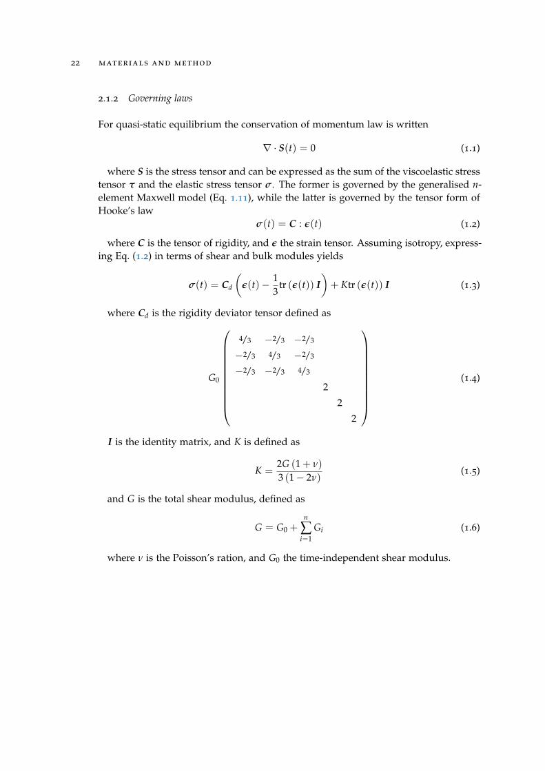
2.1.2 Governing laws
For quasi-static equilibrium the conservation of momentum law is written
∇ · S(t) = 0 (1.1)
where S is the stress tensor and can be expressed as the sum of the viscoelastic stresstensor τ and the elastic stress tensor σ. The former is governed by the generalised n-element Maxwell model (Eq. 1.11), while the latter is governed by the tensor form ofHooke’s law
σ(t) = C : ε(t) (1.2)
where C is the tensor of rigidity, and ε the strain tensor. Assuming isotropy, express-ing Eq. (1.2) in terms of shear and bulk modules yields
σ(t) = Cd
(ε(t)− 1
3tr (ε(t)) I
)+ Ktr (ε(t)) I (1.3)
where Cd is the rigidity deviator tensor defined as
G0
4/3 −2/3 −2/3
−2/3 4/3 −2/3
−2/3 −2/3 4/3
2
2
2
(1.4)
I is the identity matrix, and K is defined as
K =2G (1 + ν)
3 (1− 2ν)(1.5)
and G is the total shear modulus, defined as
G = G0 +n
∑i=1
Gi (1.6)
where ν is the Poisson’s ration, and G0 the time-independent shear modulus.
2.1 modelling of the compression-relaxation test 23
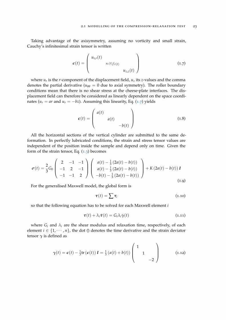
Taking advantage of the axisymmetry, assuming no vorticity and small strain,Cauchy’s infinitesimal strain tensor is written
ε(t) =
ur,r(t)ur(t)/r(t)
uz,z(t)
(1.7)
where ur is the r-component of the displacement field, uz its z-values and the commadenotes the partial derivative (uθθ = 0 due to axial symmetry). The roller boundaryconditions mean that there is no shear stress at the cheese-plate interfaces. The dis-placement field can therefore be considered as linearly dependent on the space coordi-nates (ur = ar and ur = −bz). Assuming this linearity, Eq. (1.7) yields
ε(t) =
a(t)
a(t)
−b(t)
(1.8)
All the horizontal sections of the vertical cylinder are submitted to the same de-formation. In perfectly lubricated conditions, the strain and stress tensor values areindependent of the position inside the sample and depend only on time. Given theform of the strain tensor, Eq. (1.3) becomes
σ(t) =23
G0
2 −1 −1
−1 2 −1
−1 −1 2
a(t)− 1
3 (2a(t)− b(t))
a(t)− 13 (2a(t)− b(t))
−b(t)− 13 (2a(t)− b(t))
+ K (2a(t)− b(t)) I
(1.9)For the generalised Maxwell model, the global form is
τ(t) = ∑ τi (1.10)
so that the following equation has to be solved for each Maxwell element i
τ(t) + λiτ(t) = Giλiγ(t) (1.11)
where Gi and λi are the shear modulus and relaxation time, respectively, of eachelement i ∈ {1, · · · , n}, the dot () denotes the time derivative and the strain deviatortensor γ is defined as
γ(t) = ε(t)− 13 tr (ε(t)) I = 1
3 (a(t) + b(t))
1
1
−2
(1.12)
24 materials and method
Given the form of the strain deviator tensor, τrr(t) = τθθ(t) = −1/2τzz(t). This alsoyields Srr(t) = Sθθ(t). In view of the previous hypothesis, the axisymmetric form ofEq. (1.1) reduces to
Srr,r(t) = 0
Sθθ,θ(t) = 0
Szz,z(t) = 0
(1.13)
Moreover, Eq. 1.13 combined with the absence of radial stress on the side of thecylinder (free lateral boundary condition) becomes Srr(t) = Sθθ(t) = 0. Thus thefollowing system is obtained:{
Srr(t) = 23 G0 (a(t) + b(t)) + K (2a(t)− b(t))− 1
2 τzz(t) = 0 (i)
Szz(t) = − 43 G0 (a(t) + b(t)) + K (2a(t)− b(t)) + τzz(t) (ii)
(1.14)
Subtracting Eq. 1.14ii from Eq. 1.14i gives the following expression of the stress:
Szz(t) = 32 τzz(t)− 2G0 (a(t) + b(t)) (1.15)
No time-independant elasticity was considered for the material studied (see Chap-ter 2), thus G0 = 0. The stress is then reduced to:
Szz(t) = 32
n
∑i=1
τizz(t) (1.16)
where τizz(t) can be calculated from Eq 1.11:
τizz(t) + λiτ
izz(t) = −2Giλi b(t) (1.17)
The global shear modulus G and the proportion of each element in terms of shearmodulus αi are written:
G = ∑ Gi (1.18)
αi =Gi
G(1.19)
2.2 identification of the maxwell model parameters
In the compression-relaxation test, the compression cannot be assumed to be instan-taneous. A small amount of stress is relaxed during the compression stage. Threerelationships between the upper plate displacement and time were considered in thetheoretical approach of the compression stage. The proposed fitting method takes intoaccount the loss of stress during the compression in the cases of linear and non-linearcompression.
2.2 identification of the maxwell model parameters 25
2.2.1 Instantaneous compression
When the compression is considered as instantaneous, the upper plate reaches its finalposition instantaneously and no stress relaxation occurs; the solution of Eq. 1.16 iswritten
Szz(t) = −3dc
H0G
n
∑i=1
αi exp(− t
λi
)(1.20)
where H0 is the initial height of the cylinder and dc the maximum displacement ofthe upper surface of the sample (i.e. its value at the end of the compression stage).
2.2.2 Linear compression
In the case where the downward displacement of the upper plate is linear with timefollowed by holding the upper plate position, the height of the sample according totime is defined as {
H(t) = H0 − ttc
dc , t ≤ tc
H(t) = H0 − dc , t > tc(1.21)
where tc is the time taken to achieve the maximum displacement. This leads to thefollowing expression of the z-component of strain
b(t) =
{ttc
dcH0
, t ≤ tcdcH0
= b(tc) , t > tc(1.22)
For t ≤ tc, the solution of Eq. 1.17 is written
τizz(t) = −2λGi
b(tc)
tc
(1− exp
(− t
λi
))(1.23)
This can be re-written in order to highlight the proportion of stress that did not relaxduring compression
τizz(t) = −2Gib(tc)pi(t) (1.24)
where pi is defined as
pi(t) =1− exp
(− t
λi
)tcλi
(1.25)
26 materials and method
If pi(tc) remains close to 1, no stress has been relaxed during compression. The morepi(tc) diminishes, the more stress has been relaxed. The combination of Eqns. 1.16 and1.24 gives the overall form of the stress during the compression stage
Szz(t) = −3Gb(tc)n
∑i=1
αi pi(t), t ≤ tc (1.26)
For t > tc, Eq. 1.17 has a null right-hand term, so that the solution is written
τizz(t) = −2Gi
b(tc)
tcλi
(1− exp
(− tc
λi
))(exp
(− t− tc
λi
))(1.27)
Combining Eqns. 1.27 and 1.16 yields the overall expression of the stress
Szz(t) = −3Gb(tc)n
∑i=1
αi pi(tc) exp(− t− tc
λi
), t > tc (1.28)
The first step in the determination of Maxwell model parameters was applied to therelaxation stage. The stress was divided by the state of stress at the beginning of therelaxation stage
S∗zz(t′) =
Szz(t′ + tc)
Szz(tc)=
n
∑i=1
αi pi(tc)
∑nj=1 αj pj(tc)
exp(− t′
λi
)=
n
∑i=1
ci exp(− t′
λi
)(1.29)
where ci are the proportions of the stress in Maxwell elements at the beginning ofthe relaxation stage, starting at t
′= t − tc = 0. However, relaxation already occurs
during the compression stage (Eq. 1.24), and therefore the ci are not directly equal tothe true proportions αi of the moduli. Instead, ci and αi are related according to thefollowing equation
ci =αi pi(tc)
∑nj=1 aj pj(tc)
(1.30)
which can be re-written as the following system
∀i ∈ {1, · · · , n} , αi(1− ci)pi(tc)−n
∑j=1j 6=i
cjαj pj(tc) (1.31)
where ci and pi(tc) can be estimated by regression from the stress measurementsduring the relaxation stage (Eq. 1.29).
2.3 implementation of the proposed method 27
2.2.3 Non-linear compression
In the case where the compression has no specific form, the general solution of Eq. 1.11
is written
τizz(t) = −2Gi
∫ t
0b(ξ) exp
(− t− ξ
λi
)dξ (1.32)
The proportion of stress pi(tc) that did not relax during compression is written
pi(tc) =1
b(tc)
∫ tc
0b(ξ) exp
(− tc − ξ
λi
)dξ (1.33)
Expression of the stress at the end of compression then becomes
Szz(tc) = −3Gb(tc)n
∑i=1
αi pi(tc) (1.34)
During the relaxation stage, Eqns. 1.29 to 1.31 apply as previously. This third non-linear case was used for the numerical computation.
2.3 implementation of the proposed method
First, the relaxation times λi and the proportions ci were calculated by a least squaresminimisation of the difference between computed and experimental force-time dataduring the relaxation stage. The computed force Fsim was calculated from the expres-sion of the simulated stress Szz as
Fsim(t) = Szz(t)A(t) = Szz(t)πR2(t) (1.35)
where the area A(t) is a function of the experimental cylinder radius R(t)
R(t) = R0 (1− νb(t)) (1.36)
where R0 is the initial radius, ν the Poisson’s ratio, and b(t) the strain in the z-direction defined as
b(t) = 1− H(t)H0
(1.37)
The force was normalised by the maximum value of the force to provide direct accessto the proportion values using Eq. 1.29.
To reduce the effect of the uncertainty induced by the experimental noise on forcedata when the force values were low (a little higher than the order of the rheometersensitivity), the proportion and the relaxation time of the last Maxwell element cn andλn were first evaluated by a linear regression of ln (F/ max(F)) against time, whereF can be either the experimental force values or the simulated values. Given that
28 materials and method
the regression was performed at the end of the relaxation stage, and given that therelaxation times were at about one order of magnitude from each other, all the Maxwellelements except the last had almost totally relaxed and the bias on the parameters ofthe last Maxwell element resulting from the linear regression applied to data at longrelaxation times was ignored. The conditions minimising this effect and the effects ofsignal to noise ratio will be discussed in the Results and Discussion section.
The coefficients resulting from linear regression were related to the Maxwell modelas follows
λn = − 1A
(1.38)
cn = exp(B) (1.39)
where A is the slope of the linear regression and B the intercept of the y-axis.The built-in fminsearch function of the Matlab software (The MathWorks, USA) was
then used to fit the Maxwell parameters ci and λi, ∀i 6= n. On initiating this fittingprocess step, the values of cn and λn were set to those obtained by the previous linearregression. The proportion of stress pi(tc) that did not relax during compression wascomputed using Eq. 1.33.
A linear piecewise approximation was used to calculate b(t) from experimental com-pression data.
Eq. 1.31 was used to assess the αi values using the ci and pi values. As the system hasan infinite number of solutions, one of the equations was replaced by the constraint
n
∑i=1
αi = 1 (1.40)
Finally, the elastic shear modulus G was determined at the end of the compressionstage, when the maximum amount of stress was reached, using Eq. 1.34:
G = − Szz(tc)
3b(tc)∑ni=1 αi pi(tc)
(1.41)
Young’s modulus E is written
E = 2G (1 + ν) (1.42)
which, in the case of incompressible materials, reduces to E = 3G.
2.4 implementation of the reference method 29
2.4 implementation of the reference method
It is usually admitted that the Young’s modulus can be determined by simple linearregression of stress-strain data, even on viscoelastic materials, so long as the test iscarried in the linear region. For such a method, called in the present paper “referencemethod”, Young’s modulus E is the slope of the linear regression on the compressionstress-strain experimental curve.
In practice, the linear regression was performed using Matlab software; only the last20 data points of the compression stage were used in order not to take into accountthe curve of the force-time observed at the beginning of the compression stage. Thiscurve will be presented and discussed further in the Results and Discussion section.
Relaxation is also usually studied in the case described by Eq 1.20 where the com-pression stage is considered instantaneous. For such a method, called in the presentpaper “reference method”, the modulus proportions are directly estimated from therelaxation stage, i.e. αi ≈ ci, whereas the proposed method applies a correction step inorder to reach as close as possible the true values of the proportions.
The basic difference between the reference method and the proposed method istherefore that the reference method does not take into account the proportion of stressthat relaxed during compression.
2.5 3-d models
In the experiment, despite all the care taken, the upper surface of the sample wasnot fully parallel to its lower surface. The 0-D analytical model first presented wasinappropriate to evaluate the effects of such non-parallelity on determination of theMaxwell model parameters. A 3-D version of the model was therefore implementedusing the FEM software COMSOL Multiphysics (COMSOL AB, Sweden). The geom-etry was half a cylinder with an adjustable angle between the upper and the lowersurfaces of the sample, denoted as the inclination (β). The geometry was meshed with4,790 tetrahedral elements. Computation time depended on the angle between the twosurfaces, but did not exceed one hour (Intel Core i5 at 3.1 GHz, 4GB RAM).
The lateral boundary of the domain was left free to move and roller conditions wereapplied on the upper and the lower surfaces. To take into account the angle of theupper surface of the sample, the following specific downward displacement functionwas applied to the upper boundary of the domain
d(t, r) = −max (0, H0 (1− b(t))− r tan(β)) (1.43)
where H0 (1− b(t)) is the same displacement as that used in the analytical modeland r the position along the radius.
30 materials and method
Angles were set at 0 (the reference configuration), and 2 degrees (which representeda difference in height of 420 μm between one border of the upper surface and theother).
2.6 simulated data sets
Maxwell model parameters were identified with the two types of method applied sep-arately on force-time data originating from a reference Maxwell material of known(true) values. As such a reference material does not exist, the force-time data of thismaterial was computed. The discrepancy between adjusted and true values was esti-mated and served as the evaluation of the effectiveness of each method. Effectivenessand uncertainties evaluated from this analysis (see Results and Discussion section) willtherefore be applicable in the case of cheese.
2.6.1 Reference material
In order to have a reference that was representative of the material under study, thevalues of the reference material (of known proportions αi and known relaxation timesλi) were set at the average values determined on cheese samples when applying theproposed method.
The number of Maxwell elements was set at 5 as it proved to reproduce satisfacto-rily the mechanical behaviour of cheese under compression-relaxation, and has alreadybeen used in the literature for a similar type of cheese (Goh et al. 32, 33, 34). Com-parison of the fitting of a typical experimental force-time with 3, 4, and 5 elements ispresented in Figure 1.1.
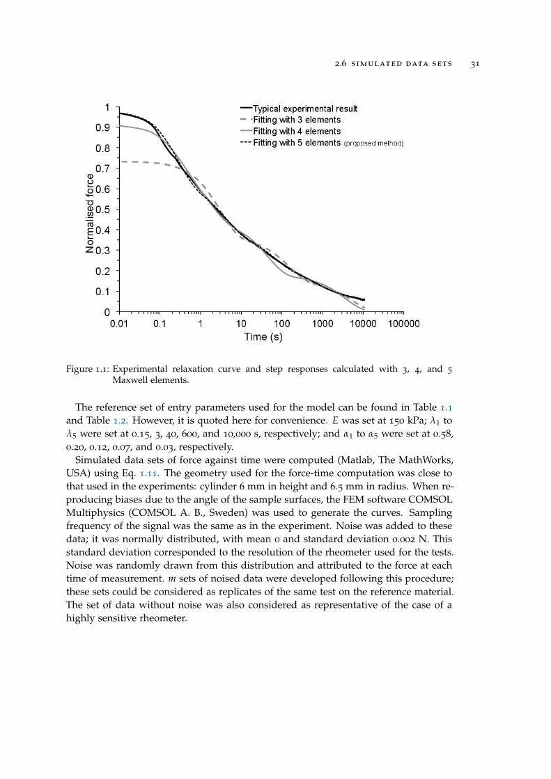
2.6 simulated data sets 31
Figure 1.1: Experimental relaxation curve and step responses calculated with 3, 4, and 5
Maxwell elements.
The reference set of entry parameters used for the model can be found in Table 1.1and Table 1.2. However, it is quoted here for convenience. E was set at 150 kPa; λ1 toλ5 were set at 0.15, 3, 40, 600, and 10,000 s, respectively; and α1 to α5 were set at 0.58,0.20, 0.12, 0.07, and 0.03, respectively.
Simulated data sets of force against time were computed (Matlab, The MathWorks,USA) using Eq. 1.11. The geometry used for the force-time computation was close tothat used in the experiments: cylinder 6 mm in height and 6.5 mm in radius. When re-producing biases due to the angle of the sample surfaces, the FEM software COMSOLMultiphysics (COMSOL A. B., Sweden) was used to generate the curves. Samplingfrequency of the signal was the same as in the experiment. Noise was added to thesedata; it was normally distributed, with mean 0 and standard deviation 0.002 N. Thisstandard deviation corresponded to the resolution of the rheometer used for the tests.Noise was randomly drawn from this distribution and attributed to the force at eachtime of measurement. m sets of noised data were developed following this procedure;these sets could be considered as replicates of the same test on the reference material.The set of data without noise was also considered as representative of the case of ahighly sensitive rheometer.
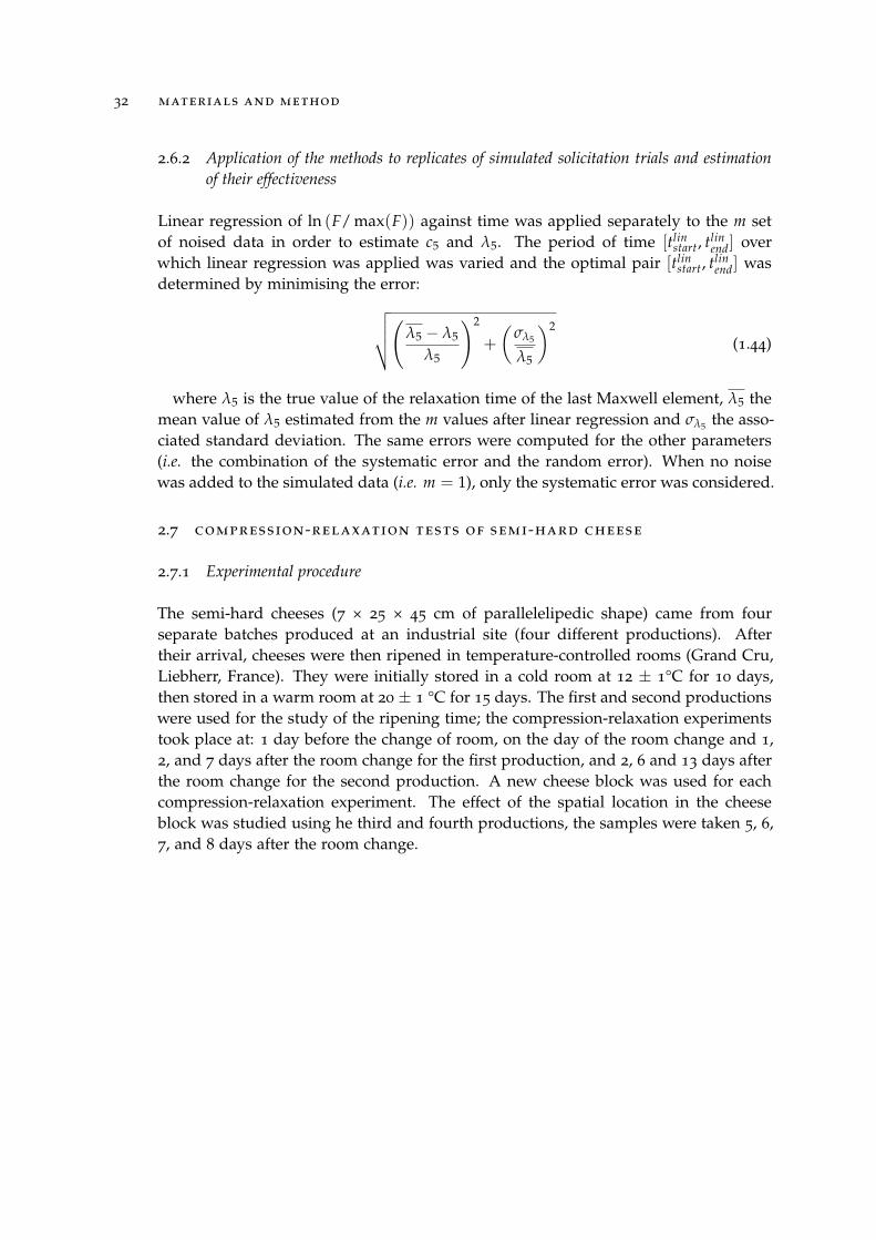
32 materials and method
2.6.2 Application of the methods to replicates of simulated solicitation trials and estimationof their effectiveness
Linear regression of ln (F/ max(F)) against time was applied separately to the m setof noised data in order to estimate c5 and λ5. The period of time [tlin
start, tlinend] over
which linear regression was applied was varied and the optimal pair [tlinstart, tlin
end] wasdetermined by minimising the error:√√√√(λ5 − λ5
λ5
)2
+
(σλ5
λ5
)2
(1.44)
where λ5 is the true value of the relaxation time of the last Maxwell element, λ5 themean value of λ5 estimated from the m values after linear regression and σλ5 the asso-ciated standard deviation. The same errors were computed for the other parameters(i.e. the combination of the systematic error and the random error). When no noisewas added to the simulated data (i.e. m = 1), only the systematic error was considered.
2.7 compression-relaxation tests of semi-hard cheese
2.7.1 Experimental procedure
The semi-hard cheeses (7 × 25 × 45 cm of parallelelipedic shape) came from fourseparate batches produced at an industrial site (four different productions). Aftertheir arrival, cheeses were then ripened in temperature-controlled rooms (Grand Cru,Liebherr, France). They were initially stored in a cold room at 12 ± 1°C for 10 days,then stored in a warm room at 20 ± 1 °C for 15 days. The first and second productionswere used for the study of the ripening time; the compression-relaxation experimentstook place at: 1 day before the change of room, on the day of the room change and 1,2, and 7 days after the room change for the first production, and 2, 6 and 13 days afterthe room change for the second production. A new cheese block was used for eachcompression-relaxation experiment. The effect of the spatial location in the cheeseblock was studied using he third and fourth productions, the samples were taken 5, 6,7, and 8 days after the room change.
2.7 compression-relaxation tests of semi-hard cheese 33
2.7.2 Sample preparation
At a given time of ripening, one cheese was taken from the cold or warm room, un-wrapped and two samples were cut from the cheese with a 14 mm diameter cork borer.For the study during ripening, one to two samples were taken from a parallelepipedof 22 × 16 × 1.5 cm3 at the core of the cheese block. For the study of the location inthe cheese block, samples were taken regularly across the width (or x-direction) at thecore of the cheese block (±1 cm in the y- and z-directions). Two samples were takenfrom each block: one at the core, the other at a given x-position. As four differentx-positions were considered, four cheese blocks, at close ripening times, were used.
The cork borer must be used very slowly in order to avoid unwanted permanentstrain. A dedicated apparatus operating with two parallel blades (Figure 1.11 in sec-tion 4) was then used to cut the upper and lower surfaces of the sample and to ensurethe best possible parallelity between the two surfaces.
The initial radius of the sample was measured with a Vernier caliper. Uncertainty onthe measurement of the radius was estimated at 0.1 mm due to the softness of the ma-terial, although special care was taken not to compress the cylinder when measuringit.
The samples were immediately submerged in a silicone oil bath (at 20 °C) to limitdehydration of the sample during the experiment and to ensure lubricated conditionsbetween the rheometer plates and the cheese sample.
All the experiments were performed at 20 °C. The cheese samples were placed on thelubricated, temperature-controlled Peltier plate and a waiting period of at least 45 minwas applied to reach thermal equilibrium in the sample. Thermal equilibrium couldalso be achieved in a crystallizer before placing it on the Peltier plate. Rheologicalanalysis was started just afterwards.
2.7.3 Measurement of force-position-time data: compression-relaxation experiment
The compression-relaxation experiments were performed with a rheometer MCR301
(Anton Paar, Austria). For study during ripening, two distinct rheometers MCR301
were used in order to study two duplicates from the same cheese block at each time ofmeasurement. Each rheometer was equipped with a Teflon Peltier lower plate (diam-eter 100 mm) and a quartz glass upper plate (diameter 43 mm). The upper plate wasplaced in contact with the sample, taking care that the resulting force was no greaterthan 0.02 N, the displacement of the upper plate at that moment being considered asthe initial height of the sample (with an accuracy of 0.1 mm corresponding to the irreg-ularity of the sample upper surface). The cross-head speed of the upper plate was setat 3 mm·s-1 and deformation was not pursued beyond 10% of the initial height. The
34 materials and method
deformation was maintained for 15 h, which represented about 5 times the longestrelaxation time of the material. The resulting force and upper plate displacement weremeasured at the following sampling times: 0.01 s from 0 to the end of the compressionstage, 0.06 s from the end of the compression stage to 500 s, 1 s from 500 s to 3,600 sand 60 s from 3,600 s to the end (54,000 s). The force resolution was 0.002 N.
2.7.4 Validity of the modelling hypotheses and numerical applications
A typical experimental set of force vs. time is presented in Figure 1.12. For the cheeseon which the model was applied (see the last subsection of the Results and Discussionsection), no relevant remaining stress was observed after a long period of relaxation(15 h), meaning that the hypothesis of the absence of time-independent elasticity wasconsidered valid.
As the displacement of the upper surface did not exceed 10% of the initial sampleheight, the theory of small strain could be considered.
Cheese could be considered as incompressible, as demonstrated for hard and semi-hard cheeses (Calzada and Peleg 14). The Poisson’s ratio ν was therefore set very nearto 0.5 but not equal to 0.5 (ν = 0.499) to avoid indetermination in the 3-D implementa-tion of the model.
As the plates were larger than the sample, the volume of cheese was constant un-derneath the upper plate throughout the experiment (Engmann et al. 26, Launay andMichon 59).
The lubricated condition at the cheese-plate interfaces allowed us to assume bound-ary roller conditions at the upper and lower surfaces of the cheese cylinder. The lateralsurface of the cylinder remained straight in the experiment.
The samples dimensions were height 6.9 ± 0.2 mm and radius 6.6 ± 0.3 mm (stan-dard deviation taking into account both the sensitivity of the measurement method,which was of 0.1 mm, and the reproducibility among 30 samples). These were alsosmall enough to avoid any gradient in composition (water, salts, etc.) within the sam-ple. The thickness of the curd grains was less than 1 mm on average in the final cheeseand in the direction of curd pressing. The dimensions of the curd grains in the per-pendicular direction (i.e. in the radial direction of the samples) were higher (6 mm onaverage, Huc et al. 44), which was of the same order of magnitude as the diameterof the sample. However, the curd grain has not proved to be the major mechanicalstructuring element so far, and the mechanical structure governing the compressionand relaxation behaviour of the cheese in a small strain approach is probably smaller(e.g. at a molecular level). The material was hence considered to be homogeneousthroughout the sample. The number and size of bubbles increased at prolonged ripen-ing times, yet the small dimensions of the sample ensured that the samples were freeof bubbles, with fixed geometry.

2.7 compression-relaxation tests of semi-hard cheese 35
The velocity and acceleration fields were justifiably ignored, due to the relativelyslow dynamics involved. Compared with the load applied to the cheese samples,gravity was also ignored.

3R E S U LT S A N D D I S C U S S I O N
In the first subsection, determination of the parameters of the last Maxwell element bythe proposed method was presented. A generalised criterion that could be applied inthe study of materials other than cheese was proposed for choosing the time intervalon which the regression of ln (F/ max(F)) against time should be performed.
In the second subsection, the sensitivity of the proposed and reference methods toexperimental bias (noise, compression time relative to the shortest relaxation, paral-lelity of sample surfaces) were presented, as well as the resulting overall uncertaintyresulting from these methods of identification. This is called the sensitivity study tothe experimental protocol of sample preparation and measurement.
In both subsections, the efficacy of the methods was evaluated against simulatedsets of force-time data generated for a reference material of known (true) mechanicalparameters. Values for these parameters were set close to those of the cheese studiedin the third subsection. These sets were synthesised with different operating condi-tions depending on the subsection, noise being part of these varying conditions. Eachcondition was varied separately from the other; hence the addition of noise was notcombined to the variation of another condition.
In the third subsection, the variations in the Maxwell model parameters of semi-hardcheese during ripening or with the location inside the cheese block and determinedwith the proposed method were discussed in the light of the overall uncertainty.
3.1 optimisation of the conditions for identification of parameters
of the last maxwell element with the proposed method
The linear behaviour of the logarithm of the force may be polluted by the relaxationof the other elements and by the decrease in the signal-to-noise ratio. These sourcesof pollution imply the choice of high values of tlin
start so that the contribution of the firstMaxwell elements is negligible and low values of tlin
end to reduce the effect of noise onthe results. The time interval [tlin
start, tlinend] was first optimised by adopting a numerical
approach.
37
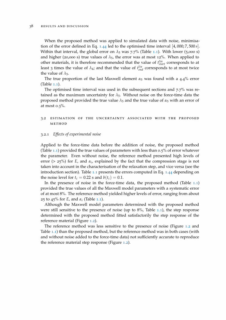
38 results and discussion
When the proposed method was applied to simulated data with noise, minimisa-tion of the error defined in Eq. 1.44 led to the optimised time interval [4, 000; 7, 500 s].Within that interval, the global error on λ5 was 7.7% (Table 1.1). With lower (5,000 s)and higher (20,000 s) true values of λ5, the error was at most 12%. When applied toother materials, it is therefore recommended that the value of tlin
start corresponds to atleast 3 times the value of λ4; and that the value of tlin
end corresponds to at most twicethe value of λ5.
The true proportion of the last Maxwell element α5 was found with a 4.4% error(Table 1.1).
The optimised time interval was used in the subsequent sections and 7.7% was re-tained as the maximum uncertainty for λ5. Without noise on the force-time data theproposed method provided the true value λ5 and the true value of α5 with an error ofat most 0.3%.
3.2 estimation of the uncertainty associated with the proposed
method
3.2.1 Effects of experimental noise
Applied to the force-time data before the addition of noise, the proposed method(Table 1.1) provided the true values of parameters with less than 0.5% of error whateverthe parameter. Even without noise, the reference method presented high levels oferror (> 25%) for E, and αi, explained by the fact that the compression stage is nottaken into account in the characterisation of the relaxation step, and vice versa (see theintroduction section). Table 1.1 presents the errors computed in Eq. 1.44 depending onthe noise level for tc = 0.22 s and b(tc) = 0.1.
In the presence of noise in the force-time data, the proposed method (Table 1.1)provided the true values of all the Maxwell model parameters with a systematic errorof at most 8%. The reference method yielded higher levels of error, ranging from about25 to 45% for E, and αi (Table 1.1).
Although the Maxwell model parameters determined with the proposed methodwere still sensitive to the presence of noise (up to 8%, Table 1.1), the step responsedetermined with the proposed method fitted satisfactorily the step response of thereference material (Figure 1.2).
The reference method was less sensitive to the presence of noise (Figure 1.2 andTable 1.1) than the proposed method, but the reference method was in both cases (withand without noise added to the force-time data) not sufficiently accurate to reproducethe reference material step response (Figure 1.2).
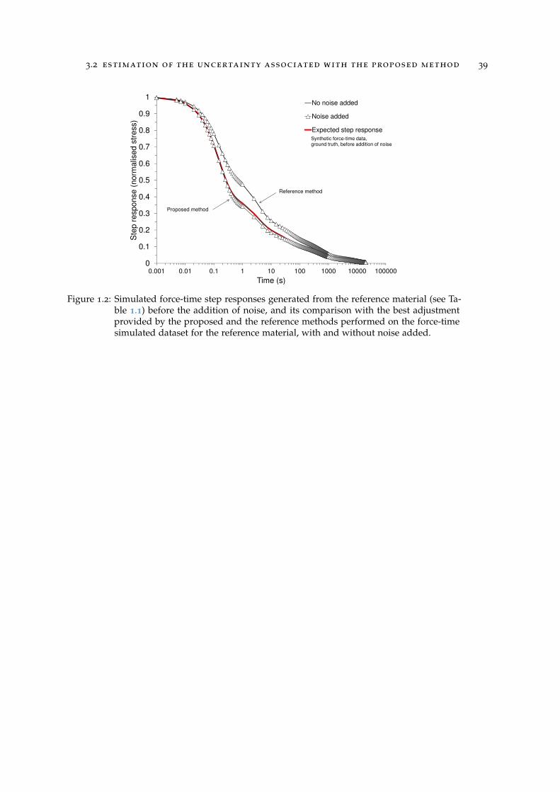
3.2 estimation of the uncertainty associated with the proposed method 39
Figure 1.2: Simulated force-time step responses generated from the reference material (see Ta-ble 1.1) before the addition of noise, and its comparison with the best adjustmentprovided by the proposed and the reference methods performed on the force-timesimulated dataset for the reference material, with and without noise added.
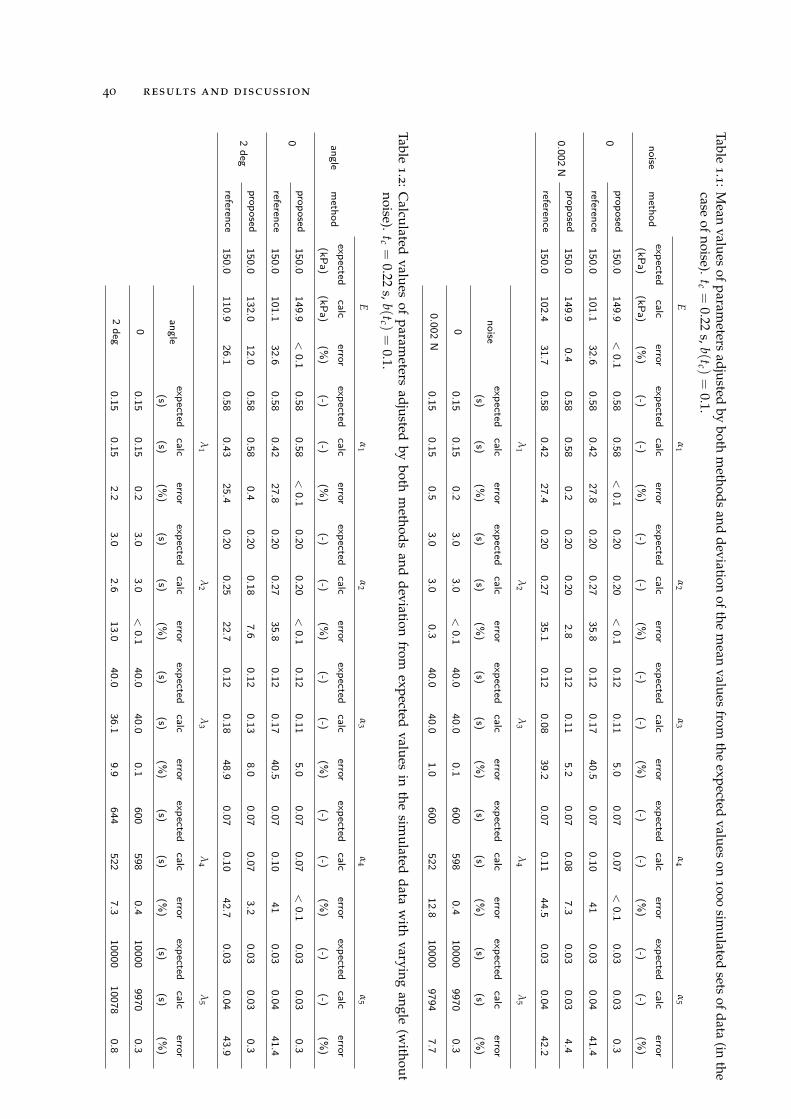
40 results and discussion
Table1.
1:Mean
valuesofparam
etersadjusted
byboth
methods
anddeviation
ofthem
eanvalues
fromthe
expectedvalues
on1
00
0sim
ulatedsets
ofdata(in
thecase
ofnoise).
tc=
0.22s,b(tc )
=0.1.
Eα
1α
2α
3α
4α
5
noisem
ethodexpected(kPa)
calc(kPa)
error(%
)expected
(-)calc(-)
error(%
)expected
(-)calc(-)
error(%
)expected
(-)calc(-)
error(%
)expected
(-)calc(-)
error(%
)expected
(-)calc(-)
error(%
)
0proposed
150.0149.9
<0.1
0.580.58
<0.1
0.200.20
<0.1
0.120.11
5.00.07
0.07<
0.10.03
0.030.3
reference150.0
101.132.6
0.580.42
27.80.20
0.2735.8
0.120.17
40.50.07
0.1041
0.030.04
41.4
0.002N
proposed150.0
149.90.4
0.580.58
0.20.20
0.202.8
0.120.11
5.20.07
0.087.3
0.030.03
4.4
reference150.0
102.431.7
0.580.42
27.40.20
0.2735.1
0.120.08
39.20.07
0.1144.5
0.030.04
42.2
λ1
λ2
λ3
λ4
λ5
noiseexpected
(s)calc(s)
error(%
)expected
(s)calc(s)
error(%
)expected
(s)calc(s)
error(%
)expected
(s)calc(s)
error(%
)expected
(s)calc(s)
error(%
)
00.15
0.150.2
3.03.0
<0.1
40.040.0
0.1600
5980.4
100009970
0.3
0.002N
0.150.15
0.53.0
3.00.3
40.040.0
1.0600
52212.8
100009794
7.7
Table1.
2:Calculated
valuesof
parameters
adjustedby
bothm
ethodsand
deviationfrom
expectedvalues
inthe
simulated
dataw
ithvarying
angle(w
ithoutnoise).
tc=
0.22s,b(tc )
=0.1.
Eα
1α
2α
3α
4α
5
anglem
ethodexpected(kPa)
calc(kPa)
error(%
)expected
(-)calc(-)
error(%
)expected
(-)calc(-)
error(%
)expected
(-)calc(-)
error(%
)expected
(-)calc(-)
error(%
)expected
(-)calc(-)
error(%
)
0proposed
150.0149.9
<0.1
0.580.58
<0.1
0.200.20
<0.1
0.120.11
5.00.07
0.07<
0.10.03
0.030.3
reference150.0
101.132.6
0.580.42
27.80.20
0.2735.8
0.120.17
40.50.07
0.1041
0.030.04
41.4
2deg
proposed150.0
132.012.0
0.580.58
0.40.20
0.187.6
0.120.13
8.00.07
0.073.2
0.030.03
0.3
reference150.0
110.926.1
0.580.43
25.40.20
0.2522.7
0.120.18
48.90.07
0.1042.7
0.030.04
43.9
λ1
λ2
λ3
λ4
λ5
angleexpected
(s)calc(s)
error(%
)expected
(s)calc(s)
error(%
)expected
(s)calc(s)
error(%
)expected
(s)calc(s)
error(%
)expected
(s)calc(s)
error(%
)
00.15
0.150.2
3.03.0
<0.1
40.040.0
0.1600
5980.4
100009970
0.3
2deg
0.150.15
2.23.0
2.613.0
40.036.1
9.9644
5227.3
1000010078
0.8
3.2 estimation of the uncertainty associated with the proposed method 41
3.2.2 Effects of cross-head speed of the upper plate of the rheometer
For this study, the same compression conditions applied, i.e. b(tc) = 0.1, but tc varieddepending on the compression speeds. As the different sources of uncertainty arecombined in the following sections, no noise was added to the simulated data.
In the range of cross-head speed values from 0.05 to 10 mm/s under consideration,the error in the Young’s modulus determination did not exceed 0.1% with the pro-posed method (Figure 1.3) whereas the error in the reference method reached 90%. Asexpected, the error decreased as the cross-head speed increased, because the amountof stress that relaxed during compression at high speeds was less than the amount ofstress that relaxed at low speed. The reference method was appropriate only when thecompression time did not exceed one tenth of the true value of λ1, the error was thenlower than 15% in the determination of Young’s modulus.
Determination of the relaxation times and proportions with the proposed methodwas only slightly affected by the cross-head speed of the upper plate of the rheometer(Figure 1.4), with an error of at most 2% even at speed values as low as 0.1 mm/s.The error was less than 0.5% at 3 mm/s, the value retained for the experimental study.In the range of compression times under consideration, the reference method reachederrors in the proportions ranging from 67 to 1,000%. The error was at most 42% at3 mm/s, the value retained for the experimental study. Due to the inertia of therheometer engine and to the small dimensions of the samples, it can take time to reachhigh speeds, so that in practice a speed threshold can be observed, and a constantspeed during the experiment could not be guaranteed for higher speed values.
When the compression time is greater than about one tenth of the smaller relax-ation time of the material (Figure 1.3), a method that takes into account both thecompression and the relaxation stages should be used; the usual linear regression onthe stress-strain data being inappropriate for determination of Young’s modulus.
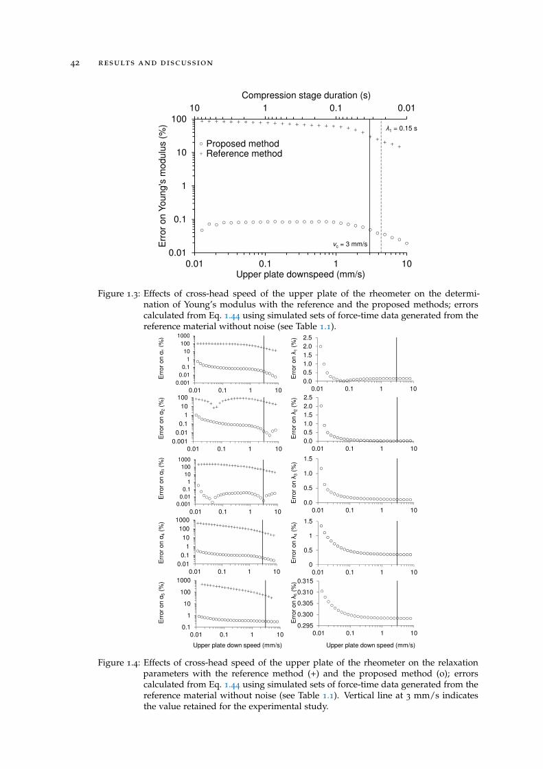
42 results and discussion
Figure 1.3: Effects of cross-head speed of the upper plate of the rheometer on the determi-nation of Young’s modulus with the reference and the proposed methods; errorscalculated from Eq. 1.44 using simulated sets of force-time data generated from thereference material without noise (see Table 1.1).
Figure 1.4: Effects of cross-head speed of the upper plate of the rheometer on the relaxationparameters with the reference method (+) and the proposed method (o); errorscalculated from Eq. 1.44 using simulated sets of force-time data generated from thereference material without noise (see Table 1.1). Vertical line at 3 mm/s indicatesthe value retained for the experimental study.
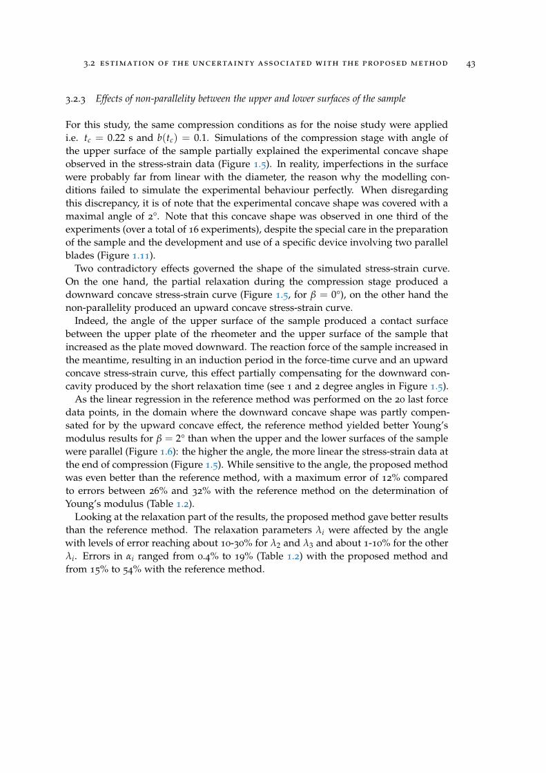
3.2 estimation of the uncertainty associated with the proposed method 43
3.2.3 Effects of non-parallelity between the upper and lower surfaces of the sample
For this study, the same compression conditions as for the noise study were appliedi.e. tc = 0.22 s and b(tc) = 0.1. Simulations of the compression stage with angle ofthe upper surface of the sample partially explained the experimental concave shapeobserved in the stress-strain data (Figure 1.5). In reality, imperfections in the surfacewere probably far from linear with the diameter, the reason why the modelling con-ditions failed to simulate the experimental behaviour perfectly. When disregardingthis discrepancy, it is of note that the experimental concave shape was covered with amaximal angle of 2°. Note that this concave shape was observed in one third of theexperiments (over a total of 16 experiments), despite the special care in the preparationof the sample and the development and use of a specific device involving two parallelblades (Figure 1.11).
Two contradictory effects governed the shape of the simulated stress-strain curve.On the one hand, the partial relaxation during the compression stage produced adownward concave stress-strain curve (Figure 1.5, for β = 0°), on the other hand thenon-parallelity produced an upward concave stress-strain curve.
Indeed, the angle of the upper surface of the sample produced a contact surfacebetween the upper plate of the rheometer and the upper surface of the sample thatincreased as the plate moved downward. The reaction force of the sample increased inthe meantime, resulting in an induction period in the force-time curve and an upwardconcave stress-strain curve, this effect partially compensating for the downward con-cavity produced by the short relaxation time (see 1 and 2 degree angles in Figure 1.5).
As the linear regression in the reference method was performed on the 20 last forcedata points, in the domain where the downward concave shape was partly compen-sated for by the upward concave effect, the reference method yielded better Young’smodulus results for β = 2° than when the upper and the lower surfaces of the samplewere parallel (Figure 1.6): the higher the angle, the more linear the stress-strain data atthe end of compression (Figure 1.5). While sensitive to the angle, the proposed methodwas even better than the reference method, with a maximum error of 12% comparedto errors between 26% and 32% with the reference method on the determination ofYoung’s modulus (Table 1.2).
Looking at the relaxation part of the results, the proposed method gave better resultsthan the reference method. The relaxation parameters λi were affected by the anglewith levels of error reaching about 10-30% for λ2 and λ3 and about 1-10% for the otherλi. Errors in αi ranged from 0.4% to 19% (Table 1.2) with the proposed method andfrom 15% to 54% with the reference method.
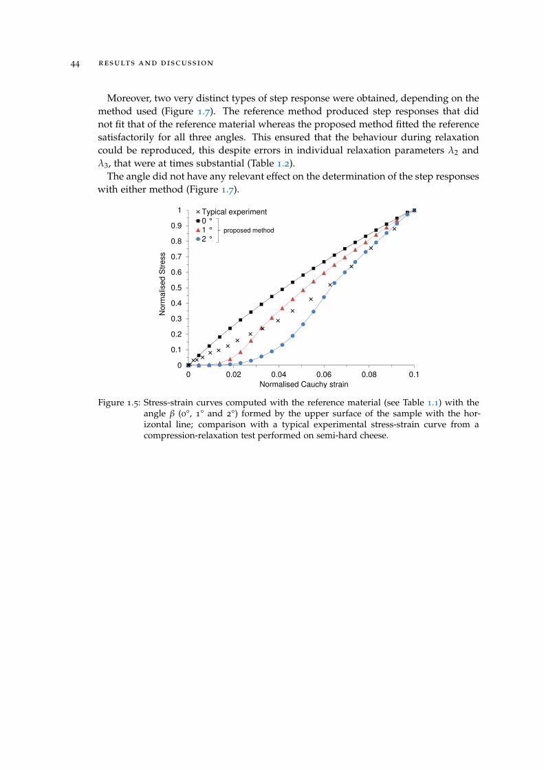
44 results and discussion
Moreover, two very distinct types of step response were obtained, depending on themethod used (Figure 1.7). The reference method produced step responses that didnot fit that of the reference material whereas the proposed method fitted the referencesatisfactorily for all three angles. This ensured that the behaviour during relaxationcould be reproduced, this despite errors in individual relaxation parameters λ2 andλ3, that were at times substantial (Table 1.2).
The angle did not have any relevant effect on the determination of the step responseswith either method (Figure 1.7).
Figure 1.5: Stress-strain curves computed with the reference material (see Table 1.1) with theangle β (0°, 1° and 2°) formed by the upper surface of the sample with the hor-izontal line; comparison with a typical experimental stress-strain curve from acompression-relaxation test performed on semi-hard cheese.
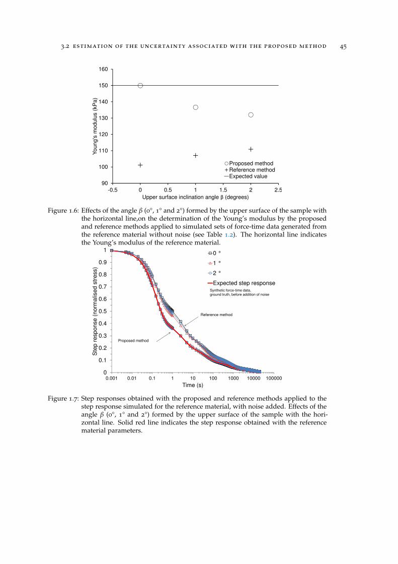
3.2 estimation of the uncertainty associated with the proposed method 45
Figure 1.6: Effects of the angle β (0°, 1° and 2°) formed by the upper surface of the sample withthe horizontal line,on the determination of the Young’s modulus by the proposedand reference methods applied to simulated sets of force-time data generated fromthe reference material without noise (see Table 1.2). The horizontal line indicatesthe Young’s modulus of the reference material.
Figure 1.7: Step responses obtained with the proposed and reference methods applied to thestep response simulated for the reference material, with noise added. Effects of theangle β (0°, 1° and 2°) formed by the upper surface of the sample with the hori-zontal line. Solid red line indicates the step response obtained with the referencematerial parameters.
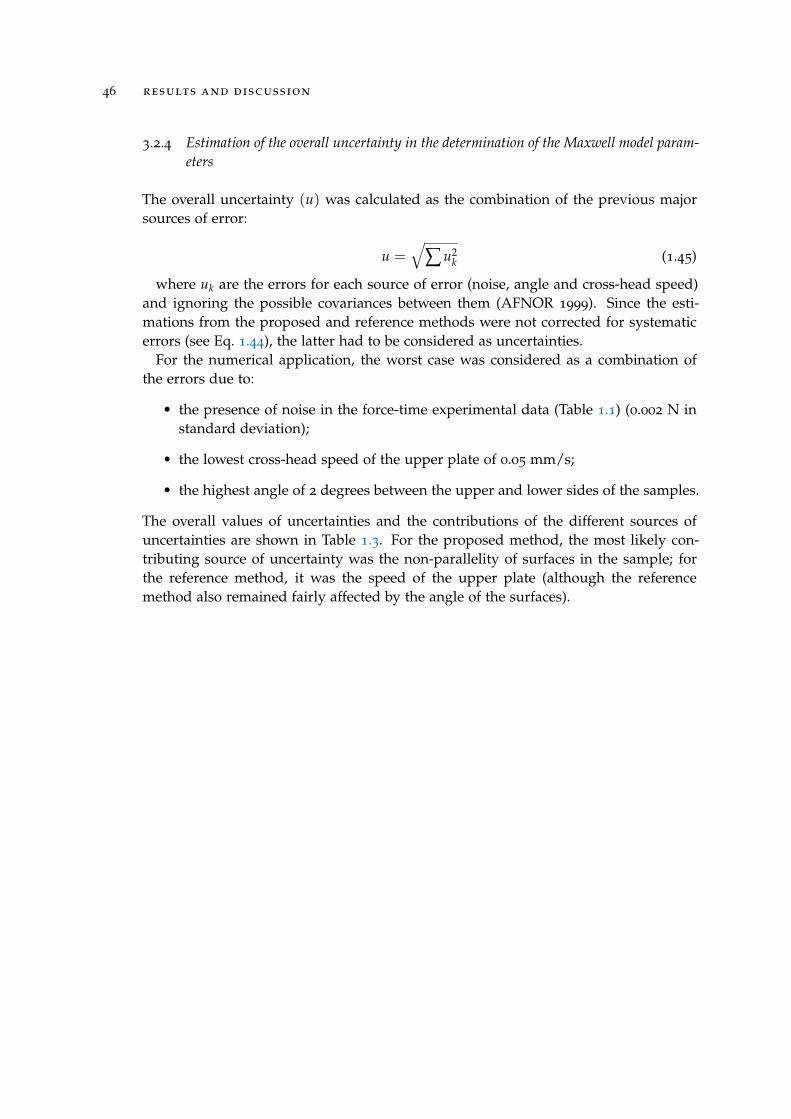
46 results and discussion
3.2.4 Estimation of the overall uncertainty in the determination of the Maxwell model param-eters
The overall uncertainty (u) was calculated as the combination of the previous majorsources of error:
u =√
∑ u2k (1.45)
where uk are the errors for each source of error (noise, angle and cross-head speed)and ignoring the possible covariances between them (AFNOR 1999). Since the esti-mations from the proposed and reference methods were not corrected for systematicerrors (see Eq. 1.44), the latter had to be considered as uncertainties.
For the numerical application, the worst case was considered as a combination ofthe errors due to:
• the presence of noise in the force-time experimental data (Table 1.1) (0.002 N instandard deviation);
• the lowest cross-head speed of the upper plate of 0.05 mm/s;
• the highest angle of 2 degrees between the upper and lower sides of the samples.
The overall values of uncertainties and the contributions of the different sources ofuncertainties are shown in Table 1.3. For the proposed method, the most likely con-tributing source of uncertainty was the non-parallelity of surfaces in the sample; forthe reference method, it was the speed of the upper plate (although the referencemethod also remained fairly affected by the angle of the surfaces).
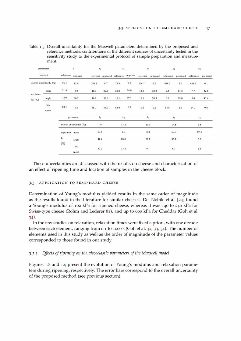
3.3 application to semi-hard cheese 47
Table 1.3: Overall uncertainty for the Maxwell parameters determined by the proposed andreference methods; contributions of the different sources of uncertainty tested in thesensitivity study to the experimental protocol of sample preparation and measure-ment.
parameter E α1 α2 α3 α4 α5
method reference proposed reference proposed reference proposed reference proposed reference proposed reference proposed
overall uncertainty (%) 96.4 12.0 105.3 0.7 79.4 8.2 224.7 9.5 444.0 8.0 468.8 6.1
explained
by (%)
noise 21.9 2.9 18.1 22.3 28.0 24.8 12.9 38.2 8.4 67.3 7.7 47.6
angle 18.0 96.7 16.8 32.8 18.1 66.4 16.1 59.3 8.1 29.8 8.0 43.4
low
speed60.1 0.4 65.1 44.9 53.9 8.8 71.0 2.5 83.5 2.9 84.3 9.0
parameter λ1 λ2 λ3 λ4 λ5
overall uncertainty (%) 3.0 13.2 10.0 14.8 7.8
explained
by
(%)
noise 10.6 1.8 8.3 59.8 87.6
angle 47.4 85.0 82.0 33.9 8.8
low
speed42.0 13.2 9.7 6.3 3.6
These uncertainties are discussed with the results on cheese and characterization ofan effect of ripening time and location of samples in the cheese block.
3.3 application to semi-hard cheese
Determination of Young’s modulus yielded results in the same order of magnitudeas the results found in the literature for similar cheeses. Del Nobile et al. [24] founda Young’s modulus of 102 kPa for ripened cheese, whereas it was 140 to 240 kPa forSwiss-type cheese (Rohm and Lederer 81), and up to 600 kPa for Cheddar (Goh et al.34).
In the few studies on relaxation, relaxation times were fixed a priori, with one decadebetween each element, ranging from 0.1 to 1000 s (Goh et al. 32, 33, 34). The number ofelements used in this study as well as the order of magnitude of the parameter valuescorresponded to those found in our study.
3.3.1 Effects of ripening on the viscoelastic parameters of the Maxwell model
Figures 1.8 and 1.9 present the evolution of Young’s modulus and relaxation parame-ters during ripening, respectively. The error bars correspond to the overall uncertaintyof the proposed method (see previous section).
48 results and discussion
Variability between the duplicates (easily noticeable for the Young’s modulus inFigure 1.8) might be explained by spatial variability in the rectangular slice (14 ×17 × 1.5 cm) extracted from the core of the cheese block and used for sampling. Itshould be remembered that the dimensions of the sampling area were imposed bythe presence of bubbles in the cheese from which the sample was taken. Variabilityin Young’s modulus between batches included this spatial variability, and obviouslyvariability in the milk composition and/or in the cheesemaking process.
In view of the variability between the samples (experimental variability), the pa-rameters did not evolve in a significant way during ripening (Table 1.4). Under theseconditions, no effect of ripening time could be detected; Young’s modulus was onaverage 162 ± 39 kPa (overall uncertainty due to the method, sample location andbatches).
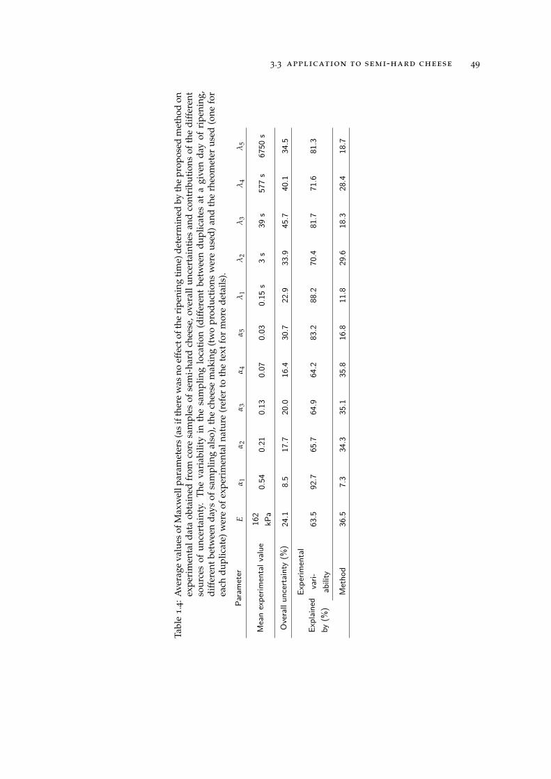
3.3 application to semi-hard cheese 49
Tabl
e1.4
:Ave
rage
valu
esof
Max
wel
lpar
amet
ers
(as
ifth
ere
was
noef
fect
ofth
eri
peni
ngti
me)
dete
rmin
edby
the
prop
osed
met
hod
onex
peri
men
tald
ata
obta
ined
from
core
sam
ples
ofse
mi-
hard
chee
se,o
vera
llun
cert
aint
ies
and
cont
ribu
tion
sof
the
diff
eren
tso
urce
sof
unce
rtai
nty.
The
vari
abili
tyin
the
sam
plin
glo
cati
on(d
iffer
ent
betw
een
dupl
icat
esat
agi
ven
day
ofri
peni
ng,
diff
eren
tbe
twee
nda
ysof
sam
plin
gal
so),
the
chee
sem
akin
g(t
wo
prod
ucti
ons
wer
eus
ed)
and
the
rheo
met
erus
ed(o
nefo
rea
chdu
plic
ate)
wer
eof
expe
rim
enta
lnat
ure
(ref
erto
the
text
for
mor
ede
tails
).
Parameter
Eα
1α
2α
3α
4α
5λ
1λ
2λ
3λ
4λ
5
Meanexperim
entalv
alue
162
kPa
0.54
0.21
0.13
0.07
0.03
0.15
s3s
39s
577s
6750
s
Overallun
certa
inty
(%)
24.1
8.5
17.7
20.0
16.4
30.7
22.9
33.9
45.7
40.1
34.5
Explained
by(%
)
Experim
ental
vari-
ability
63.5
92.7
65.7
64.9
64.2
83.2
88.2
70.4
81.7
71.6
81.3
Metho
d36.5
7.3
34.3
35.1
35.8
16.8
11.8
29.6
18.3
28.4
18.7
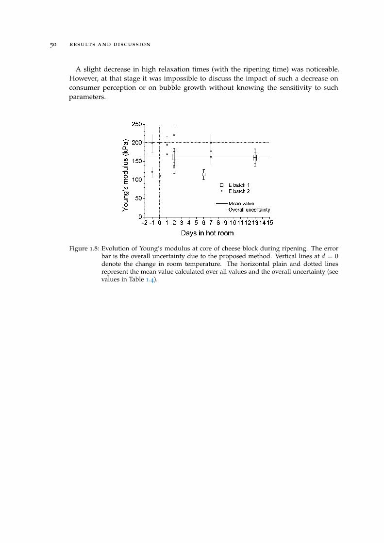
50 results and discussion
A slight decrease in high relaxation times (with the ripening time) was noticeable.However, at that stage it was impossible to discuss the impact of such a decrease onconsumer perception or on bubble growth without knowing the sensitivity to suchparameters.
Figure 1.8: Evolution of Young’s modulus at core of cheese block during ripening. The errorbar is the overall uncertainty due to the proposed method. Vertical lines at d = 0denote the change in room temperature. The horizontal plain and dotted linesrepresent the mean value calculated over all values and the overall uncertainty (seevalues in Table 1.4).
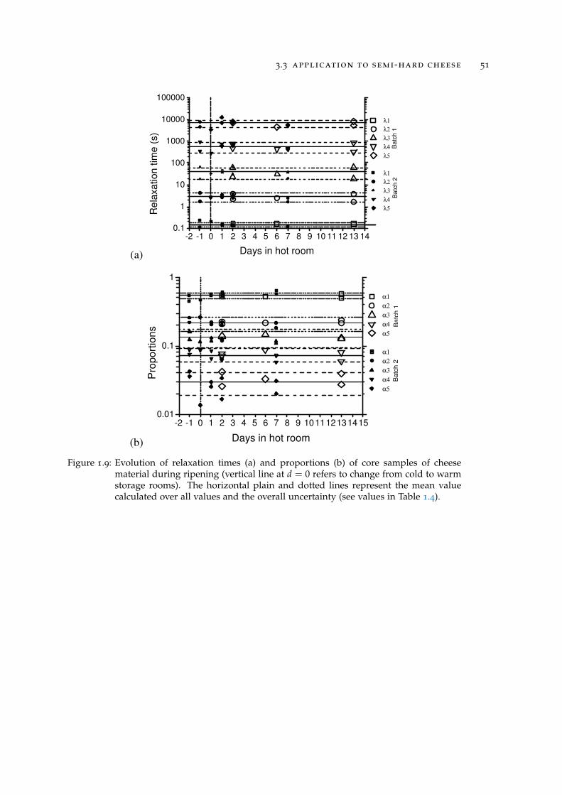
3.3 application to semi-hard cheese 51
Figure 1.9: Evolution of relaxation times (a) and proportions (b) of core samples of cheesematerial during ripening (vertical line at d = 0 refers to change from cold to warmstorage rooms). The horizontal plain and dotted lines represent the mean valuecalculated over all values and the overall uncertainty (see values in Table 1.4).
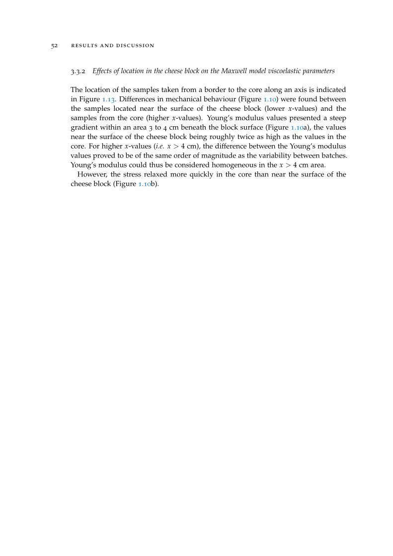
52 results and discussion
3.3.2 Effects of location in the cheese block on the Maxwell model viscoelastic parameters
The location of the samples taken from a border to the core along an axis is indicatedin Figure 1.13. Differences in mechanical behaviour (Figure 1.10) were found betweenthe samples located near the surface of the cheese block (lower x-values) and thesamples from the core (higher x-values). Young’s modulus values presented a steepgradient within an area 3 to 4 cm beneath the block surface (Figure 1.10a), the valuesnear the surface of the cheese block being roughly twice as high as the values in thecore. For higher x-values (i.e. x > 4 cm), the difference between the Young’s modulusvalues proved to be of the same order of magnitude as the variability between batches.Young’s modulus could thus be considered homogeneous in the x > 4 cm area.
However, the stress relaxed more quickly in the core than near the surface of thecheese block (Figure 1.10b).
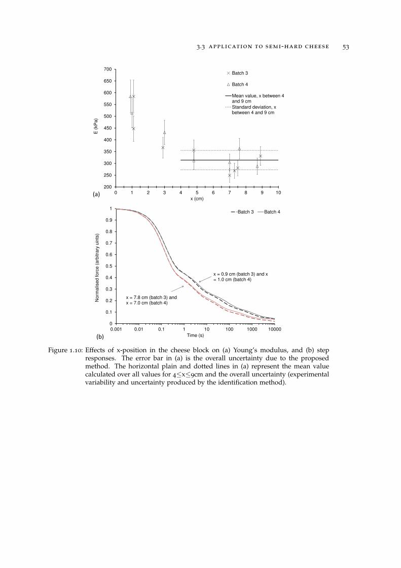
3.3 application to semi-hard cheese 53
Figure 1.10: Effects of x-position in the cheese block on (a) Young’s modulus, and (b) stepresponses. The error bar in (a) is the overall uncertainty due to the proposedmethod. The horizontal plain and dotted lines in (a) represent the mean valuecalculated over all values for 4≤x≤9cm and the overall uncertainty (experimentalvariability and uncertainty produced by the identification method).

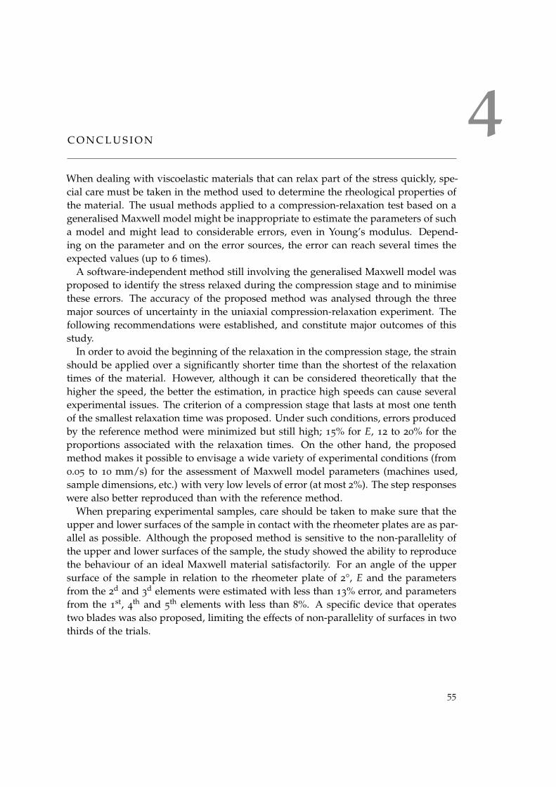
4C O N C L U S I O N
When dealing with viscoelastic materials that can relax part of the stress quickly, spe-cial care must be taken in the method used to determine the rheological properties ofthe material. The usual methods applied to a compression-relaxation test based on ageneralised Maxwell model might be inappropriate to estimate the parameters of sucha model and might lead to considerable errors, even in Young’s modulus. Depend-ing on the parameter and on the error sources, the error can reach several times theexpected values (up to 6 times).
A software-independent method still involving the generalised Maxwell model wasproposed to identify the stress relaxed during the compression stage and to minimisethese errors. The accuracy of the proposed method was analysed through the threemajor sources of uncertainty in the uniaxial compression-relaxation experiment. Thefollowing recommendations were established, and constitute major outcomes of thisstudy.
In order to avoid the beginning of the relaxation in the compression stage, the strainshould be applied over a significantly shorter time than the shortest of the relaxationtimes of the material. However, although it can be considered theoretically that thehigher the speed, the better the estimation, in practice high speeds can cause severalexperimental issues. The criterion of a compression stage that lasts at most one tenthof the smallest relaxation time was proposed. Under such conditions, errors producedby the reference method were minimized but still high; 15% for E, 12 to 20% for theproportions associated with the relaxation times. On the other hand, the proposedmethod makes it possible to envisage a wide variety of experimental conditions (from0.05 to 10 mm/s) for the assessment of Maxwell model parameters (machines used,sample dimensions, etc.) with very low levels of error (at most 2%). The step responseswere also better reproduced than with the reference method.
When preparing experimental samples, care should be taken to make sure that theupper and lower surfaces of the sample in contact with the rheometer plates are as par-allel as possible. Although the proposed method is sensitive to the non-parallelity ofthe upper and lower surfaces of the sample, the study showed the ability to reproducethe behaviour of an ideal Maxwell material satisfactorily. For an angle of the uppersurface of the sample in relation to the rheometer plate of 2°, E and the parametersfrom the 2
d and 3d elements were estimated with less than 13% error, and parameters
from the 1st, 4
th and 5th elements with less than 8%. A specific device that operates
two blades was also proposed, limiting the effects of non-parallelity of surfaces in twothirds of the trials.
55
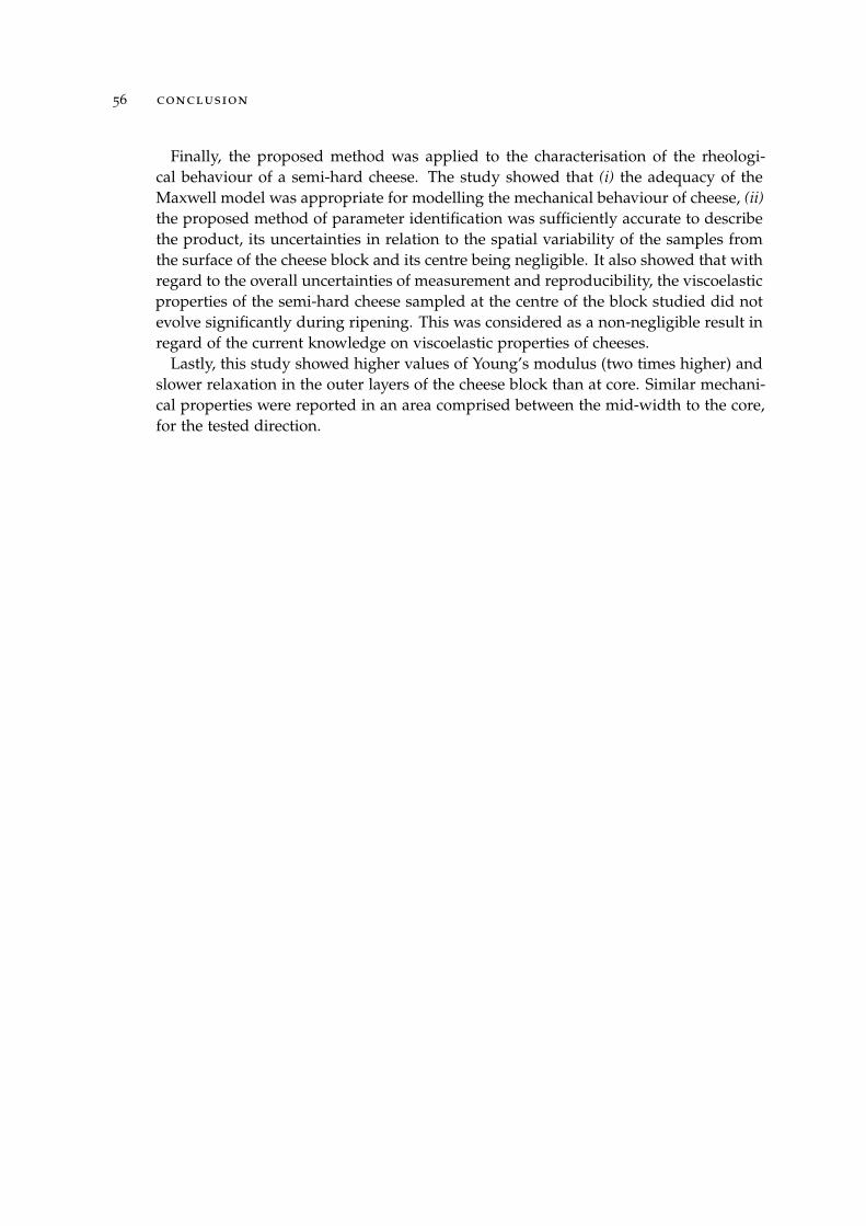
56 conclusion
Finally, the proposed method was applied to the characterisation of the rheologi-cal behaviour of a semi-hard cheese. The study showed that (i) the adequacy of theMaxwell model was appropriate for modelling the mechanical behaviour of cheese, (ii)the proposed method of parameter identification was sufficiently accurate to describethe product, its uncertainties in relation to the spatial variability of the samples fromthe surface of the cheese block and its centre being negligible. It also showed that withregard to the overall uncertainties of measurement and reproducibility, the viscoelasticproperties of the semi-hard cheese sampled at the centre of the block studied did notevolve significantly during ripening. This was considered as a non-negligible result inregard of the current knowledge on viscoelastic properties of cheeses.
Lastly, this study showed higher values of Young’s modulus (two times higher) andslower relaxation in the outer layers of the cheese block than at core. Similar mechani-cal properties were reported in an area comprised between the mid-width to the core,for the tested direction.

A C K N O W L E D G M E N T S
The authors wish to thank Anthony Hutin, Julien Mottet, Gabrielle Moulin and MichelLoubat for technical assistance. This study was carried out with financial supportfrom VALORIAL and the Regional Councils of Bretagne, Pays de Loire and Basse-Normandie. First author, Yannick Laridon, is the holder of a grant from INRA andIrstea.
57

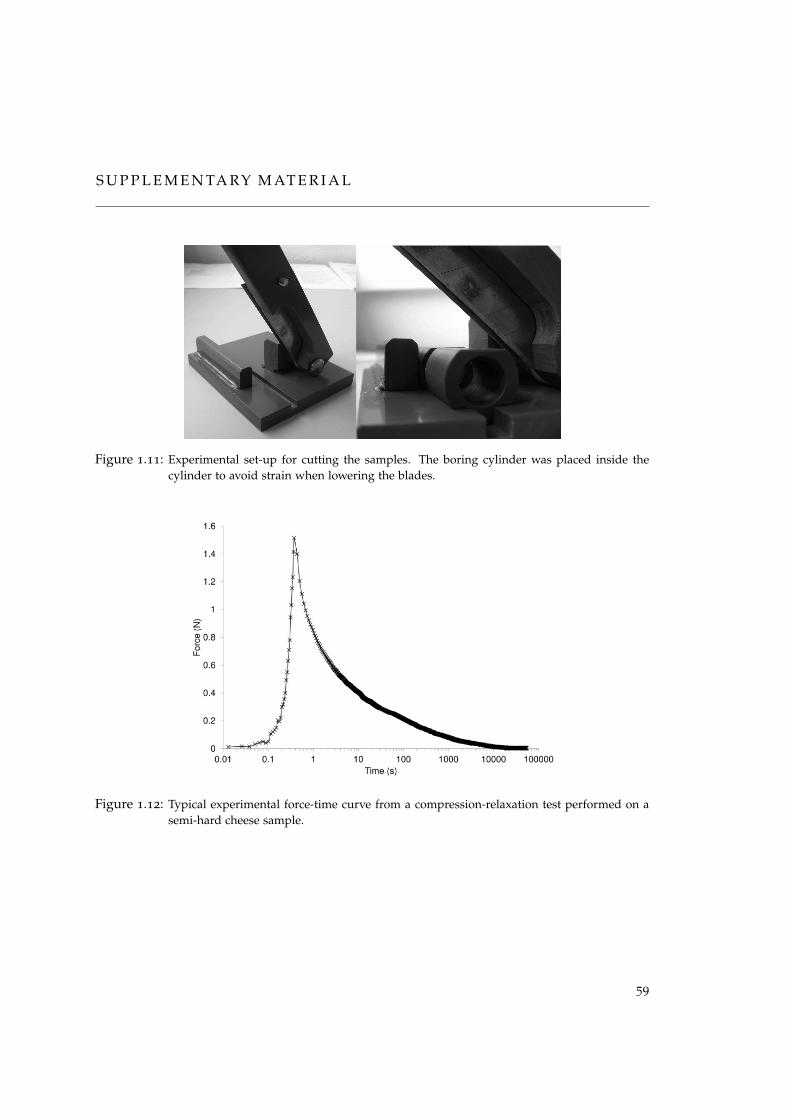
S U P P L E M E N TA RY M AT E R I A L
Figure 1.11: Experimental set-up for cutting the samples. The boring cylinder was placed inside thecylinder to avoid strain when lowering the blades.
Figure 1.12: Typical experimental force-time curve from a compression-relaxation test performed on asemi-hard cheese sample.
59
60 conclusion
Figure 1.13: Location of samples in the cheese block. The XY plane is located at the middle of the cheeseblock height.
Chapitre 2
M O N I T O R I N G A S I N G L E E Y E G R O W T H U N D E R K N O W NG A S P R E S S U R E : M R I M E A S U R E M E N T S A N D T E A C H I N G S
A B O U T T H E M E C H A N I C A L B E H AV I O U R O F A S E M I - H A R DC H E E S E
A dedicated setup was developed to measure both pressure and volumesimultaneously in a single eye within a cylinder of semi-hard cheese. Airpressure was applied within the cheese eye and the resulting eye inflationwas monitored using Magnetic Resonance Imaging (MRI). Image analysismethods were developed not only to measure the eye volume but also thehorizontal and vertical diameters of the eye and the upside deflected shapeof the cylinder of cheese. The uncertainty on each parameter was estimated.Two amounts of pressure were applied so to attempt to reproduce a creep-recovery experiment in situ. In a last stage, a lowering in pressure wasapplied in order to discuss a time-independent elasticity. The core of thesemi-hard cheese under processing was found to show no relevant time-independent elasticity on a 90 h experiment. Low amount of pressure (<3.5 kPa), together with slow pressure variations, was found to be able toinflate eyes in semi-hard cheese within the linear domain.Keywords: creep-recovery; viscoelasticity

1I N T R O D U C T I O N
Bubble growth results from the balance between the increase in gas amount within thebubble (Huc et al. 47) and the mechanical resistance the surrounding cheese opposesto this increase (Laridon et al. [58]). Understanding of cheese mechanics, and theway it reacts to the formation of a gas bubble, is of importance in mastering semi-hard cheese processing because it determines whether to focus on gas production,mechanical properties or a mix of them (Huc et al. 47).
A first step in understanding gas formation in cheese is to monitor the growth ofbubbles. The formation of a single bubble and its displacement in a fluid has beenstudied in either boiling water (Lee et al. 60) or in a molten silica (Mourtada-Bonnefoiand Mader 67, Minami et al. 66) using a high speed camera. The transparent natureof the fluids studied allowed such monitoring, while the high levels of displacementinvolved in these studies required quite high time frequencies. These conditions arefar from thoses involved in the growth of a single bubble in cheese for which bubblemotion is slow, and occurs in an opaque medium.
The advances in imaging techniques make it possible to measure bubble volume ordisplacements continuously in opaque media. The visualisation of a swarm of bubblesin cheese has recently been carried out using X-Ray tomography and MRI in order toevaluate the effect of cheese formulation and processing conditions (Guggisberg et al.38, Kraggerud et al. 55, Musse et al. 68, Schuetz et al. 83). Bubbles within Goudacheese of round shape (13.7 cm in diameter and 6.9 cm in height) have been observedwith an acquisition time of 28 s using X-ray tomography with a slice thickness of 1 mmand a Field of View of 180 mm (Lee et al. 61). Spatial resolution of 1 mm3 has beenused in parallelepipeds of cheese of 48 cm × 24 cm × 10 cm in dimensions so to assessaccurate bubble distributions with an acquisition time of 51 min by MRI (Musse et al.68). Other techniques such as ultra-sound make it also possible to assess defaults incheese (Conde et al. 20, Eskelinen et al. 27). However, this technique only reveal thepresence or defaults and cannot be used to appropriately monitor the growth of asingle bubble for the purpose of discussing mechanics in cheese.
Since the way a material reacts to a mechanical load (gas pressure) depends on themagnitude and the speed at which the load is applied, both volume and pressure mea-surements, performed simultaneously, are needed to understand the gas expansion.The bubble volume is required to monitor the strain and strain rate, and pressure toevaluate how much resistance is opposed to gas inflation.
63
64 introduction
In polymer science, Yano and Shimiya [94] monitored pressure and droplet volumesimultaneously in order to predict the critical radius of a bubble to shrink at a con-stant temperature. A droplet of paraffin oil was blown up inside a gelatine gel andpressure was measured using a mercury barometer. The volume was measured pho-tographically, since the medium was transparent. In cheese, known gas pressure wasapplied in an bubble of Emmental cheese with the use of a needle which basement wasglued to insure tightness between the needle and the cheese, but, bubble inflation wasonly non-continuously and destructively evaluated by slicing cheeses from differentbatches (Fluckiger et al. 30). No discussion about the relation between the gas pres-sure and the volume of the bubble was developed. Blowing up a bubble with pressuremeasurements using an alveograph is a widespread technique used in studying howa bubble would behave during bread making (Codina et al. 19). Apart from these fewstudies, the growth of an individual bubble under a known gas pressure has poorlybeen investigated so far and never with the use of imaging techniques in cheese.
In this study, a dedicated setup was developed to sustain a single round bubblewithin a small cheese cylinder taken from a cheese block under ripening. Specialattention was paid to insure a good contact between the cheese and the lateral faces ofthe sustaining apparatus. The upper surface of the cheese cylinder was let free to move.A level of gas pressure at the bubble-cheese interface was set by gas compression.Pressure and volume in the bubble were monitored continuously. The first objectivewas to present the methods used for measuring the bubble volume, the horizontaland the vertical bubble radii and the upper surface deflected shape. The expandedstandard uncertainties associated with these measurements were estimated. The aimwas also to discuss the viscoelastic response in a semi-hard cheese to a solicitationsimilar to that actually found in an bubble within a semi-hard cheese block duringripening. To do so, three mechanical solicitations were applied; a creep, a recoveryand a lowering in pressure.
2M AT E R I A L A N D M E T H O D S
2.1 cheese
A semi-hard cheese block (parallelepiped, length 47 cm, width 23.5 cm, height 9 cm)(Figure 2.1) was picked up from a production batch at the plant and was sent tothe laboratory in its foil. The cheese block was ripened for 9 days in a temperaturecontrolled cabinet (Grand Cru, Liebherr, France).
2.2 sample preparation
On day 9, a Magnetic Resonance Imager (MRI) (Avanto 1.5 T, Siemens, Germany) wasused to locate a single bubble surrounded by a volume of plain cheese inside the blockof cheese (Figure 2.1a). After being located, the bubble (1) (Figure 2.1b) was extractedfrom the block of cheese within a cylinder of cheese (54.4 ± 0.15 mm in diameter and32.3 ± 0.15 mm in height) with the help of a stainless tube (device not shown). Thecenter of the bubble (10.9 ± 0.5 mm in diameter) was set to be as close as possible tothe axis of symmetry of the removed cylinder of cheese.
The upper surface (3) of the cylinder of cheese was carefully sliced with a steel wireso to make it as plane as possible and also to adjust the distance of the bubble fromthe upper surface (3.85 ± 0.85 mm).
The cylinder of cheese was put inside a sustaining apparatus (4) made of plastic(Figure 2.1b). In order to avoid too much stress to appear within the cylinder of cheesewhen put inside the sustaining apparatus, several sizes of sustaining apparatus weremanufactured so to choose the one that best fitted the size of the cylinder of cheese.Without taking this precaution it was quite impossible to appropriately match the sizeof the cylinder of cheese with that of the sustaining apparatus. Before the beginningof the bubble growth experiment the cheese was let three hours, free of load, in thesustaining apparatus in order to let the possible remaining stress to relax.
The top part (5) of the sustaining apparatus prevented the lateral boundaries of thecylinder of cheese from moving upward. A cap (6) allowed the cheese upper surfacenot to dry during the experiment. Pressure equilibrium between the gas chamber(7) above the cheese and the atmospheric pressure was insured by a very small hole(8) in the cap. A needle (9), inserted into the bubble on one side and connected tothe injection device on the other side (Figure 2.1b), made it possible to increase air
65
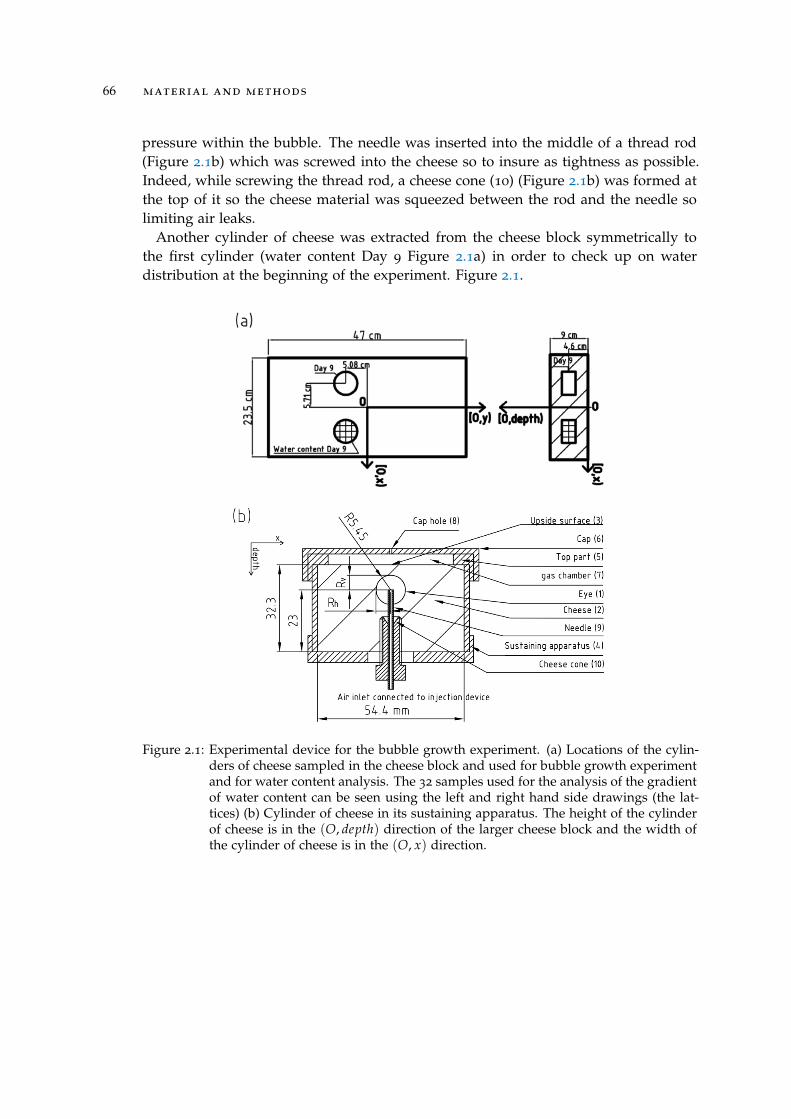
66 material and methods
pressure within the bubble. The needle was inserted into the middle of a thread rod(Figure 2.1b) which was screwed into the cheese so to insure as tightness as possible.Indeed, while screwing the thread rod, a cheese cone (10) (Figure 2.1b) was formed atthe top of it so the cheese material was squeezed between the rod and the needle solimiting air leaks.
Another cylinder of cheese was extracted from the cheese block symmetrically tothe first cylinder (water content Day 9 Figure 2.1a) in order to check up on waterdistribution at the beginning of the experiment. Figure 2.1.
Figure 2.1: Experimental device for the bubble growth experiment. (a) Locations of the cylin-ders of cheese sampled in the cheese block and used for bubble growth experimentand for water content analysis. The 32 samples used for the analysis of the gradientof water content can be seen using the left and right hand side drawings (the lat-tices) (b) Cylinder of cheese in its sustaining apparatus. The height of the cylinderof cheese is in the (O, depth) direction of the larger cheese block and the width ofthe cylinder of cheese is in the (O, x) direction.
2.3 experimental procedure 67
2.3 experimental procedure
The sustaining apparatus was placed into the knee antenna of the MRI scanner oncefor all. The experiment of bubble growth was carried out at the ripening temperature(20 ± 1°C) within and around the MRI scanner.
A 3D (300) MRI sequence (see section 2.4.3) was launched before gas pressure wasincreased in the bubble, in order to measure the upper deflected shape of the cheesecylinder as well as the initial volume and radii of the bubble which may have evolvedsince the extraction of the cylinder from the cheese block. Three main solicitationswere then applied; the creep, the recovery and the lowering in pressure (Figure 2.6):
The creep consisted of different pressure levels (the gray number in Figure 2.6b, c, d),with P > 0, P being the relative pressure of the gas in the bubble to the atmosphericpressure;
1. at 0 min, air was injected into the injection device producing a steep increasein pressure in the bubble from 0 up to 7.5 ± 0.3 kPa, and followed by a slightdecrease in pressure down to 6 ± 0.3 kPa, (from 0 to 40 min);
2. at 41 min, a steep drop in pressure from 6 ± 0.3 kPa to 3.5 ± 0.3 kPa;
3. from 41 min to 700 min, a constant load with slight and slow linear decrease inpressure from 3.5 ± 0.3 kPa to 2.8 ± 0.3 kPa;
4. at 701 min, a sudden drop in pressure from 2.8 ± 0.3 kPa to 2 ± 0.3 kPa followedby a constant pressure of 2 ± 0.3 kPa (from 701 min to 901 min);
5. the recovery, from 901 min to 4,350 min, consisted of a return to the atmosphericpressure (0 ± 0.3 kPa), P = 0;
6. the lowering in pressure, from 4,351 min to 5,300 min, consisted of a slight andsudden decrease in pressure (- 1.4 ± 0.3 kPa) followed by a slow increase inpressure up to the atmospheric pressure, P < 0.
A series of six 2D (240) and one 3D (500) sequences was repeatedly launched. At900 min and 5170 min, a 3D (300) MRI sequence was launched to assess the volume,radii and upper deflected shape with higher accuracy.
68 material and methods
2.4 methods of measurement
2.4.1 Water content
The water content at the beginning of the experiment was measured on the cylindercalled “water content Day 9” coming from the same cheese block as that used forthe bubble growth experiment (Figure 2.1a). The cylinders were cut horizontally intotwo slices, and then into 16 small blocks as presented in Figure 2.1a (the lattices in thecircle and rectangle representing the water content cylinder). The 32 small blocks wereweighed before and after being oven-dried at 104 ± 1°C for 24 h. The water content xw
was calculated.
2.4.2 Gas pressure measurements within the bubble
Gas pressure was measured inside an injection device with a calibrated absolute pres-sure transducer (XCEL-100-25A, Kulite, USA). The injection device was connected tothe air inlet of the needle. The acquisition frequency of the pressure measurement was1 Hz with an adequate resolution on an Ahlborn data logger (Almemo 2590, Ahlborn,Germany). Daily variations in atmospheric pressure inside the laboratory during theexperiment were of the same order as the applied gas pressure in the bubble. Theatmospheric pressure was recorded using an outside barometer (La Crosse Technol-ogy, WS3500, France). The gas pressure in the bubble, denoted earlier as P, relativeto the atmospheric pressure inside the laboratory was considered in the present study(Eq. 2.1).
P = Ptransducer − PA (2.1)
where Ptransducer was the pressure measured by the pressure transducer. The ex-panded standard uncertainty on gas pressure measurement was estimated followingthe directions made by the Joint Committee for Guides in Metrology [49]. Accordingto Eq. 2.1 and to standards, the combined standard uncertainty on pressure measure-ment, uc(P), was estimated at 0.15 kPa, Eq. 2.2.
uc(P) =√
u(Ptransducer)2 + u(PA)2 (2.2)
with null covariance between the two variables and with
u(Ptransducer) =√
u2s + u2
c + u2r (2.3)
where
• uSwas due to instabilities in the voltage supplied to the pressure transducer. Itwas estimated at 0.068 kPa;
2.4 methods of measurement 69
• ucwas the standard uncertainty on the pressure transducer measurement, esti-mated with the help of a calibration device developed at the lab. It was estimatedat 0.058 kPa;
• uTwas due to the sinusoidal temperature variation in the air surrounding theinjection device. This uncertainty was estimated at 0.12 kPa;
• uPA was the standard uncertainty on the measurement of the atmospheric pres-sure, estimated at 0.014 kPa.
These standard uncertainties were estimated based on the premise they behaved sym-metrically and uniformly (except for temperature for which an arcsine distribution wasconsidered). They were estimated from the full amplitude of uncertainty (a), Eq. 2.4.
ui(x) =ai
2√
3(2.4)
where i is a given source of uncertainty on the variable x. Variations in air temper-ature contributed to 80% of the combined standard uncertainty. Special care was sogiven not to have too much temperature fluctuations around the injection device byadjusting the thermostat setting. As the distribution laws of the uncertainties were con-sidered as well known, the resulting combined standard uncertainty, uc(P), was mul-tiplied by a factor of two so as to obtain the expanded uncertainty as recommendedby standards. The resulting expanded uncertainty on pressure measurement u(P) was0.3 kPa.
2.4.3 MRI measurements
Based on the work of Musse et al. 68, three specific Spin Echo sequences were set upto measure the volume, radii and the upper deflected shape of the cylinder of cheese,with either a good spatial resolution or a good time resolution.
3D (300)
Time of echo (TE) of 12 ms, Time of repetition (TR) of 400 ms, Echo Train Length (ETL)of 6, bandwidth = 296 Hz, 1 scan, voxel size = 0.3× 0.3 × 0.3 mm3, 88 slices (imagesto be processed), Signal Noise Ratio = 27, acquisition time 1 h 08 min.
3D (500)
Time of echo (TE) of 10 ms, Time of repetition (TR) of 400 ms, Echo Train Length (ETL)of 6, bandwidth = 296 Hz, 1 scan, voxel size = 0.5× 0.5 × 0.5 mm3, 52 slices (imagesto be processed), Signal Noise Ratio = 53, acquisition time 8 min 45 s.
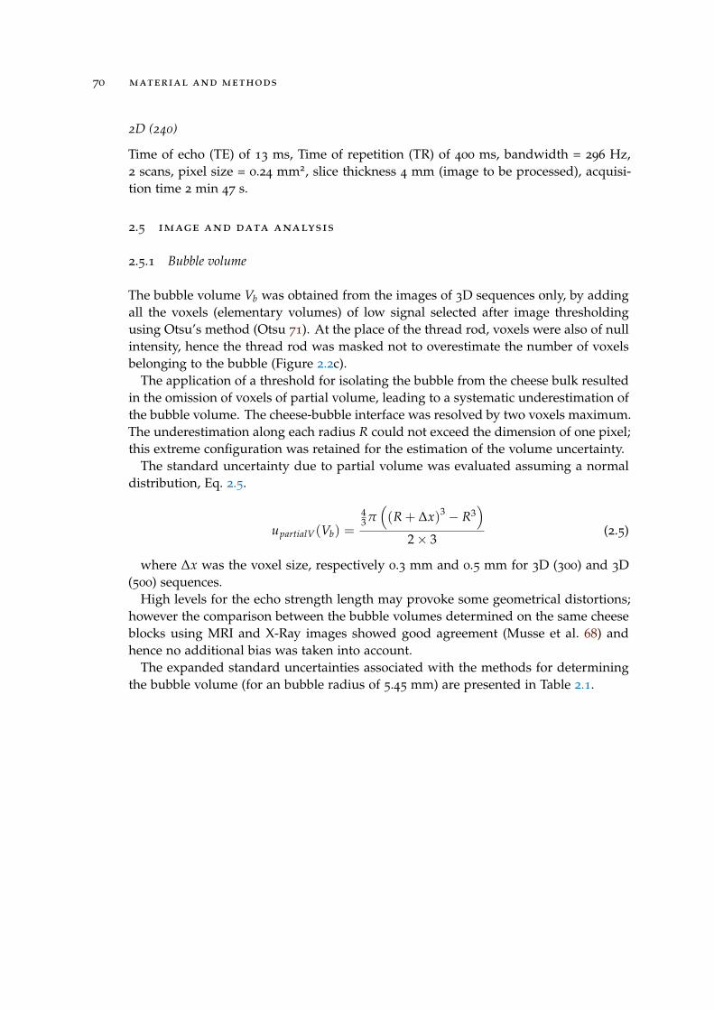
70 material and methods
2D (240)
Time of echo (TE) of 13 ms, Time of repetition (TR) of 400 ms, bandwidth = 296 Hz,2 scans, pixel size = 0.24 mm2, slice thickness 4 mm (image to be processed), acquisi-tion time 2 min 47 s.
2.5 image and data analysis
2.5.1 Bubble volume
The bubble volume Vb was obtained from the images of 3D sequences only, by addingall the voxels (elementary volumes) of low signal selected after image thresholdingusing Otsu’s method (Otsu 71). At the place of the thread rod, voxels were also of nullintensity, hence the thread rod was masked not to overestimate the number of voxelsbelonging to the bubble (Figure 2.2c).
The application of a threshold for isolating the bubble from the cheese bulk resultedin the omission of voxels of partial volume, leading to a systematic underestimation ofthe bubble volume. The cheese-bubble interface was resolved by two voxels maximum.The underestimation along each radius R could not exceed the dimension of one pixel;this extreme configuration was retained for the estimation of the volume uncertainty.
The standard uncertainty due to partial volume was evaluated assuming a normaldistribution, Eq. 2.5.
upartialV(Vb) =
43 π((R + ∆x)3 − R3
)2× 3
(2.5)
where ∆x was the voxel size, respectively 0.3 mm and 0.5 mm for 3D (300) and 3D(500) sequences.
High levels for the echo strength length may provoke some geometrical distortions;however the comparison between the bubble volumes determined on the same cheeseblocks using MRI and X-Ray images showed good agreement (Musse et al. 68) andhence no additional bias was taken into account.
The expanded standard uncertainties associated with the methods for determiningthe bubble volume (for an bubble radius of 5.45 mm) are presented in Table 2.1.
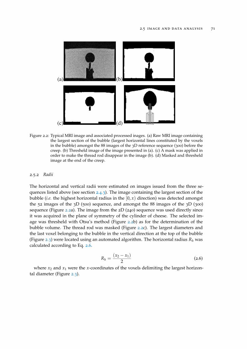
2.5 image and data analysis 71
(a) (b)
(c) (d)
Figure 2.2: Typical MRI image and associated processed inages. (a) Raw MRI image containingthe largest section of the bubble (largest horizontal lines constituted by the voxelsin the bubble) amongst the 88 images of the 3D reference sequence (300) before thecreep. (b) Thresheld image of the image presented in (a). (c) A mask was applied inorder to make the thread rod disappear in the image (b). (d) Masked and thresheldimage at the end of the creep.
2.5.2 Radii
The horizontal and vertical radii were estimated on images issued from the three se-quences listed above (see section 2.4.3). The image containing the largest section of thebubble (i.e. the highest horizontal radius in the [0, x) direction) was detected amongstthe 52 images of the 3D (500) sequence, and amongst the 88 images of the 3D (300)sequence (Figure 2.2a). The image from the 2D (240) sequence was used directly sinceit was acquired in the plane of symmetry of the cylinder of cheese. The selected im-age was thresheld with Otsu’s method (Figure 2.2b) as for the determination of thebubble volume. The thread rod was masked (Figure 2.2c). The largest diameters andthe last voxel belonging to the bubble in the vertical direction at the top of the bubble(Figure 2.3) were located using an automated algorithm. The horizontal radius Rh wascalculated according to Eq. 2.6.
Rh =(x2 − x1)
2(2.6)
where x2 and x1 were the x-coordinates of the voxels delimiting the largest horizon-tal diameter (Figure 2.3).
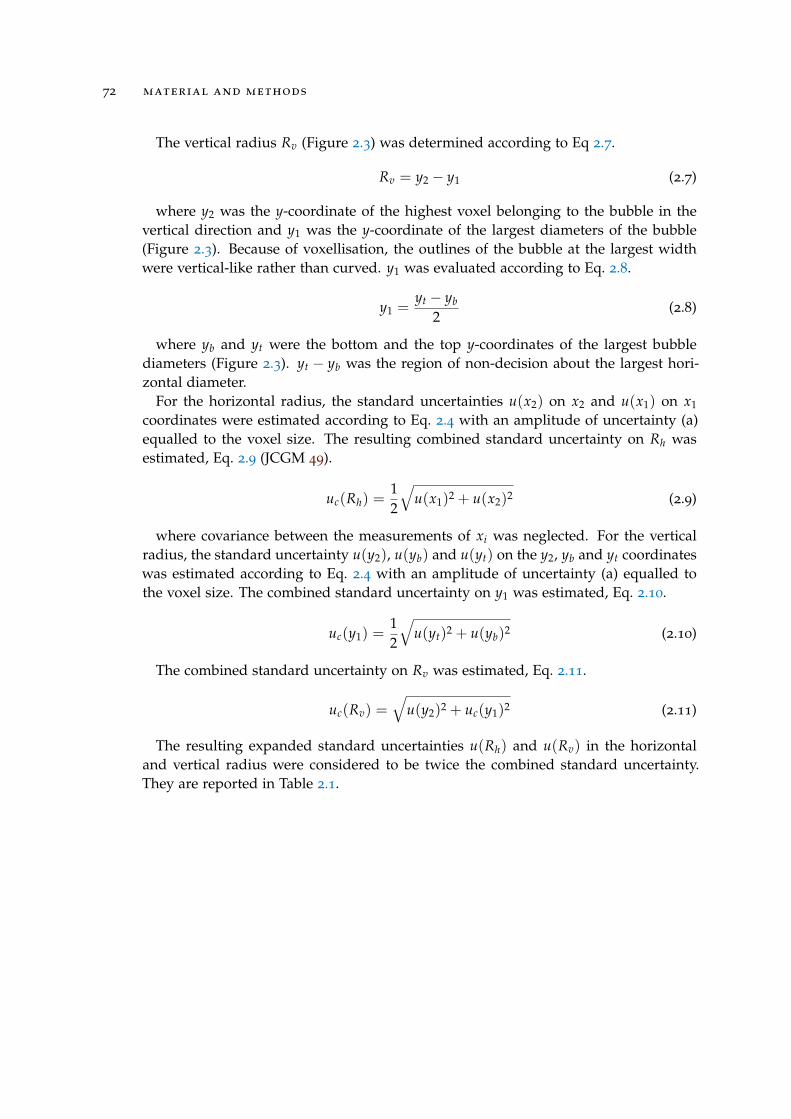
72 material and methods
The vertical radius Rv (Figure 2.3) was determined according to Eq 2.7.
Rv = y2 − y1 (2.7)
where y2 was the y-coordinate of the highest voxel belonging to the bubble in thevertical direction and y1 was the y-coordinate of the largest diameters of the bubble(Figure 2.3). Because of voxellisation, the outlines of the bubble at the largest widthwere vertical-like rather than curved. y1 was evaluated according to Eq. 2.8.
y1 =yt − yb
2(2.8)
where yb and yt were the bottom and the top y-coordinates of the largest bubblediameters (Figure 2.3). yt − yb was the region of non-decision about the largest hori-zontal diameter.
For the horizontal radius, the standard uncertainties u(x2) on x2 and u(x1) on x1
coordinates were estimated according to Eq. 2.4 with an amplitude of uncertainty (a)equalled to the voxel size. The resulting combined standard uncertainty on Rh wasestimated, Eq. 2.9 (JCGM 49).
uc(Rh) =12
√u(x1)2 + u(x2)2 (2.9)
where covariance between the measurements of xi was neglected. For the verticalradius, the standard uncertainty u(y2), u(yb) and u(yt) on the y2, yb and yt coordinateswas estimated according to Eq. 2.4 with an amplitude of uncertainty (a) equalled tothe voxel size. The combined standard uncertainty on y1 was estimated, Eq. 2.10.
uc(y1) =12
√u(yt)2 + u(yb)2 (2.10)
The combined standard uncertainty on Rv was estimated, Eq. 2.11.
uc(Rv) =√
u(y2)2 + uc(y1)2 (2.11)
The resulting expanded standard uncertainties u(Rh) and u(Rv) in the horizontaland vertical radius were considered to be twice the combined standard uncertainty.They are reported in Table 2.1.
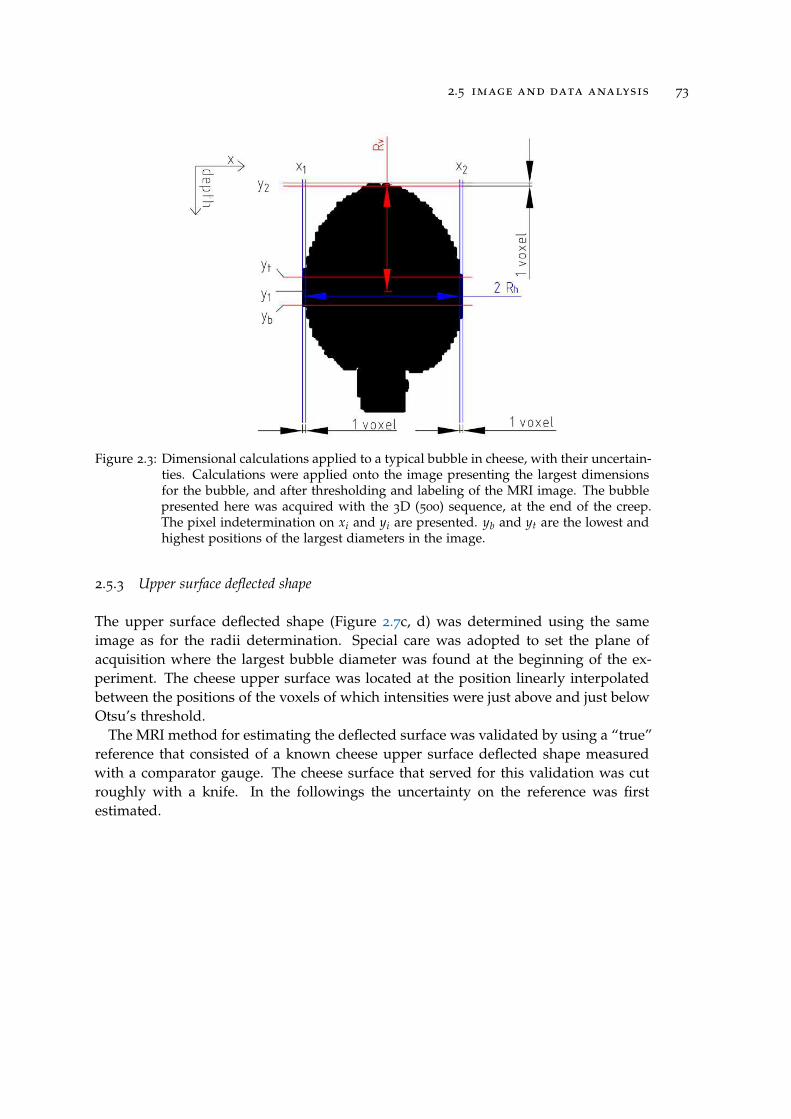
2.5 image and data analysis 73
Figure 2.3: Dimensional calculations applied to a typical bubble in cheese, with their uncertain-ties. Calculations were applied onto the image presenting the largest dimensionsfor the bubble, and after thresholding and labeling of the MRI image. The bubblepresented here was acquired with the 3D (500) sequence, at the end of the creep.The pixel indetermination on xi and yi are presented. yb and yt are the lowest andhighest positions of the largest diameters in the image.
2.5.3 Upper surface deflected shape
The upper surface deflected shape (Figure 2.7c, d) was determined using the sameimage as for the radii determination. Special care was adopted to set the plane ofacquisition where the largest bubble diameter was found at the beginning of the ex-periment. The cheese upper surface was located at the position linearly interpolatedbetween the positions of the voxels of which intensities were just above and just belowOtsu’s threshold.
The MRI method for estimating the deflected surface was validated by using a “true”reference that consisted of a known cheese upper surface deflected shape measuredwith a comparator gauge. The cheese surface that served for this validation was cutroughly with a knife. In the followings the uncertainty on the reference was firstestimated.
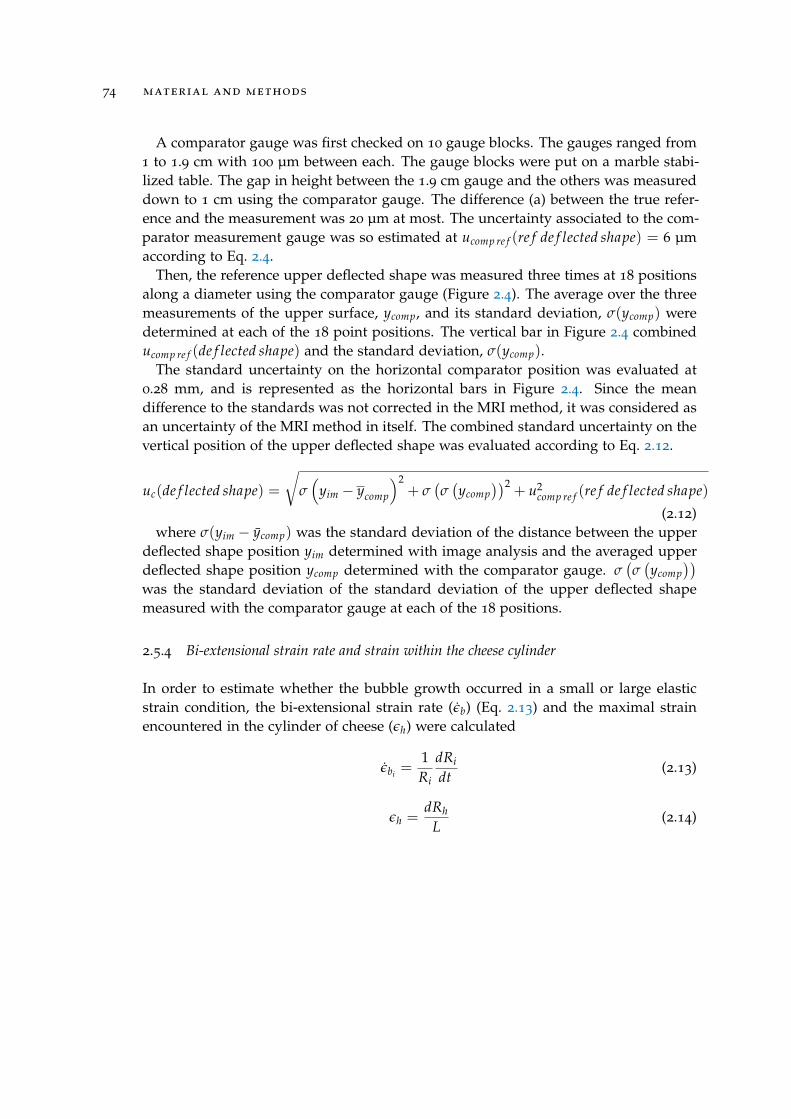
74 material and methods
A comparator gauge was first checked on 10 gauge blocks. The gauges ranged from1 to 1.9 cm with 100 µm between each. The gauge blocks were put on a marble stabi-lized table. The gap in height between the 1.9 cm gauge and the others was measureddown to 1 cm using the comparator gauge. The difference (a) between the true refer-ence and the measurement was 20 µm at most. The uncertainty associated to the com-parator measurement gauge was so estimated at ucomp re f (re f de f lected shape) = 6 µmaccording to Eq. 2.4.
Then, the reference upper deflected shape was measured three times at 18 positionsalong a diameter using the comparator gauge (Figure 2.4). The average over the threemeasurements of the upper surface, ycomp, and its standard deviation, σ(ycomp) weredetermined at each of the 18 point positions. The vertical bar in Figure 2.4 combineducomp re f (de f lected shape) and the standard deviation, σ(ycomp).
The standard uncertainty on the horizontal comparator position was evaluated at0.28 mm, and is represented as the horizontal bars in Figure 2.4. Since the meandifference to the standards was not corrected in the MRI method, it was considered asan uncertainty of the MRI method in itself. The combined standard uncertainty on thevertical position of the upper deflected shape was evaluated according to Eq. 2.12.
uc(de f lected shape) =
√σ(
yim − ycomp
)2+ σ
(σ(ycomp
))2+ u2
comp re f (re f de f lected shape)
(2.12)where σ(yim − ycomp) was the standard deviation of the distance between the upper
deflected shape position yim determined with image analysis and the averaged upperdeflected shape position ycomp determined with the comparator gauge. σ
(σ(ycomp
))was the standard deviation of the standard deviation of the upper deflected shapemeasured with the comparator gauge at each of the 18 positions.
2.5.4 Bi-extensional strain rate and strain within the cheese cylinder
In order to estimate whether the bubble growth occurred in a small or large elasticstrain condition, the bi-extensional strain rate (εb) (Eq. 2.13) and the maximal strainencountered in the cylinder of cheese (εh) were calculated
εbi =1Ri
dRi
dt(2.13)
εh =dRh
L(2.14)
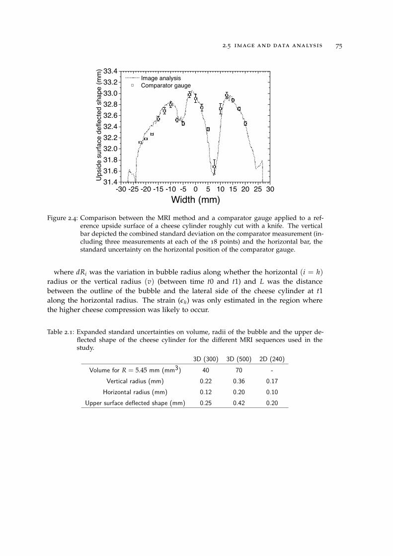
2.5 image and data analysis 75
-30 -25 -20 -15 -10 -5 0 5 10 15 20 25 3031.431.631.832.032.232.432.632.833.033.233.4
Image analysis Comparator gauge
Ups
ide
surfa
ce d
efle
cted
sha
pe (m
m)
Width (mm)
Figure 2.4: Comparison between the MRI method and a comparator gauge applied to a ref-erence upside surface of a cheese cylinder roughly cut with a knife. The verticalbar depicted the combined standard deviation on the comparator measurement (in-cluding three measurements at each of the 18 points) and the horizontal bar, thestandard uncertainty on the horizontal position of the comparator gauge.
where dRi was the variation in bubble radius along whether the horizontal (i = h)radius or the vertical radius (v) (between time t0 and t1) and L was the distancebetween the outline of the bubble and the lateral side of the cheese cylinder at t1along the horizontal radius. The strain (εh) was only estimated in the region wherethe higher cheese compression was likely to occur.
Table 2.1: Expanded standard uncertainties on volume, radii of the bubble and the upper de-flected shape of the cheese cylinder for the different MRI sequences used in thestudy.
3D (300) 3D (500) 2D (240)Volume for R = 5.45 mm (mm3) 40 70 -
Vertical radius (mm) 0.22 0.36 0.17Horizontal radius (mm) 0.12 0.20 0.10
Upper surface deflected shape (mm) 0.25 0.42 0.20
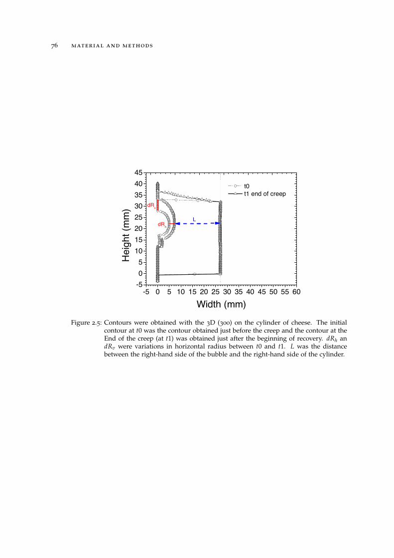
76 material and methods
-5 0 5 10 15 20 25 30 35 40 45 50 55 60-505
1015202530354045
dRv
t0 t1 end of creep
Hei
ght (
mm
)
Width (mm)
dRh
L
Figure 2.5: Contours were obtained with the 3D (300) on the cylinder of cheese. The initialcontour at t0 was the contour obtained just before the creep and the contour at theEnd of the creep (at t1) was obtained just after the beginning of recovery. dRh andRv were variations in horizontal radius between t0 and t1. L was the distancebetween the right-hand side of the bubble and the right-hand side of the cylinder.
3R E S U LT S
3.1 water content
The water content within the cylinder of cheese was 41.1 ± 0.43% in average withinthe 32 slices at the beginning of the experiment. No difference was found between thebottom and the top of the cylinder (along the [O; depth) axis) since averages were notdifferent; respectively 41.04 ± 0.47% and 41.16 ± 0.40%. The water content increasedfrom 40.54 ± 0.15% to 41.48 ± 0.23% from the left to the right of the cylinder of cheesealong the [0; x) axis (Figure 2.1b). The mechanical properties might have been a littleaffected (Laridon et al. 57) but were considered to be sufficiently homogenous not toaffect the bubble growth behavior in a relevant manner.
3.2 bubble volume
Figure 2.6 presents typical changes in volume and pressure inside the bubble isolatedin the cheese material. Sudden variations in volume increase were measured whensteep variations in pressure were applied as at 0 min (Figure 2.6b 1 increase in pres-sure), at 41 min (Figure 2.6b 2 drop in pressure), and at 700 min when the pressuresuddenly decreased due to gas leaks (Figure 2.6b 4 drop in pressure).
The volume of the bubble was 677 ± 40 mm3 initially. At the very beginning (1), thevolume increased almost instantaneously from 677 ± 40 mm3 to 900 ± 82 mm3 (theblack line in Figure 2.6b 1). Then, the volume linearly increased from 900 ± 82 mm3 to1290 ± 102 mm3 (the red line in Figure 2.6b 2) at a speed of the order of 8.7·10
-11 m3/swhile pressure was almost constant. When the pressure stabilized at about 2.7 timesas much as the natural pressure in cheese (Figure 2.6b 3) the volume increase, from1290 ± 102 mm3 to 2200 ± 145 mm3, was linear and of the order of 2.6·10
-11 m3/s (theblue line in Figure 2.6b 3). Such a linear response in the bubble volume increase toa constant load has observed repeatedly (from other runs) with a standard deviationof the slope of 1.1·10
-11 m3/s. When the atmospheric pressure (5) was applied, thevolume decreased exponentially (Figure 2.6c). At the end of the recovery, the volumestill slightly decreased but seemed to tend to a horizontal asymptote.
When the lowering in pressure was applied (6), the volume decreased first and thenincreased slightly when the pressure returned to the atmospheric (in Figure 2.6d). Thevolume tended to an asymptote and not to return to the volume the bubble had at thebeginning of the experiment.
77
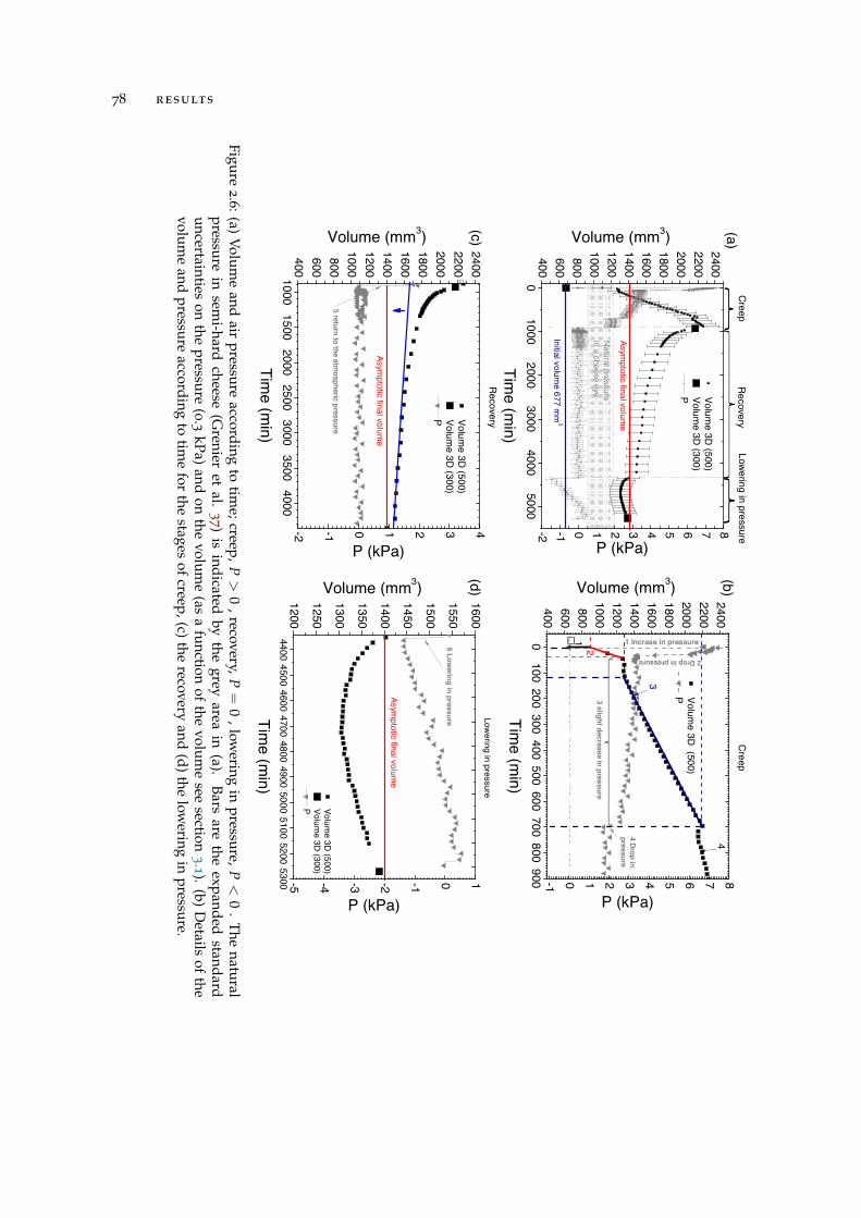
78 results
01000
20003000
40005000
400600800
10001200140016001800200022002400
Initial volume 677 m
m3
Volume 3D
(500) Volum
e 3D (300)
P
Volume (mm3)
Time (m
in)
Asymptotic final volum
e
(a)
-2 -1 0 1 2 3 4 5 6 7 8
P (kPa)
Natural pressure in a cheese eye
Creep
Recovery
Lowering in pressure
0100
200300
400500
600700
800900
400600800
10001200140016001800200022002400
(b)Volume (mm3)
Time (m
in)
Volume 3D
(500) P
-1 0 1 2 3 4 5 6 7 8 C
reep
1
3 slight decrease in pressure
3
4 Drop in pressure
P (kPa)
2 Drop in pressure
1 Incrase in pressure2
4
10001500
20002500
30003500
4000400600800
10001200140016001800200022002400
5 return to the atmospheric pressure
Volume (mm3)
Time (m
in)
Volume 3D
(500) Volum
e 3D (300)
P
Asymptotic final volum
e
-2 -1 0 1 2 3 4 R
ecovery
(c)
P (kPa)4400
45004600
47004800
49005000
51005200
53001200
1250
1300
1350
1400
1450
1500
1550
1600
6 Lowering in pressure
Volume 3D
(500) Volum
e 3D (300)
P
(d)Volume (mm3)Tim
e (min)
Asymptotic final volum
e
-5 -4 -3 -2 -1 0 1 Low
ering in pressure
P (kPa)
Figure2.
6:(a)Volum
eand
airpressure
accordingto
time;creep,P
>0
,recovery,P=
0,low
eringin
pressure,P<
0.
Thenatural
pressurein
semi-hard
cheese(G
renieret
al.3
7)is
indicatedby
thegrey
areain
(a).Bars
arethe
expandedstandard
uncertaintieson
thepressure
(0.
3kPa)
andon
thevolum
e(as
afunction
ofthe
volume
seesection
3.1).
(b)D
etailsof
thevolum
eand
pressureaccording
totim
efor
thestages
ofcreep,(c)
therecovery
and(d)
thelow
eringin
pressure.
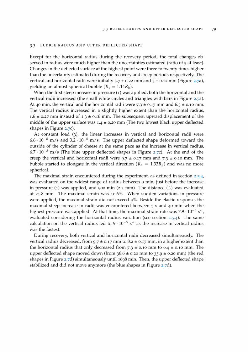
3.3 bubble radius and upper deflected shape 79
3.3 bubble radius and upper deflected shape
Except for the horizontal radius during the recovery period, the total changes ob-served in radius were much higher than the uncertainties estimated (ratio of 5 at least).Changes in the deflected surface at the highest point were three to twenty times higherthan the uncertainty estimated during the recovery and creep periods respectively. Thevertical and horizontal radii were initially 5.7 ± 0.22 mm and 5 ± 0.12 mm (Figure 2.7a),yielding an almost spherical bubble (Rv = 1.14Rh).
When the first steep increase in pressure (1) was applied, both the horizontal and thevertical radii increased (the small white circles and triangles with bars in Figure 2.7a).At 40 min, the vertical and the horizontal radii were 7.3 ± 0.17 mm and 6.3 ± 0.10 mm.The vertical radius increased in a slightly higher extent than the horizontal radius,1.6 ± 0.27 mm instead of 1.3 ± 0.16 mm. The subsequent upward displacement of themiddle of the upper surface was 1.4 ± 0.20 mm (The two lowest black upper deflectedshapes in Figure 2.7c).
At constant load (3), the linear increases in vertical and horizontal radii were6.6 · 10−8 m/s and 3.2 · 10−8 m/s. The upper deflected shape deformed toward theoutside of the cylinder of cheese at the same pace as the increase in vertical radius,6.7 · 10−8 m/s (The blue upper deflected shapes in Figure 2.7c). At the end of thecreep the vertical and horizontal radii were 9.7 ± 0.17 mm and 7.3 ± 0.10 mm. Thebubble started to elongate in the vertical direction (Rv = 1.33Rh) and was no morespherical.
The maximal strain encountered during the experiment, as defined in section 2.5.4,was evaluated on the widest range of radius between 0 min, just before the increasein pressure (1) was applied, and 900 min (2.3 mm). The distance (L) was evaluatedat 21.8 mm. The maximal strain was 10.6%. When sudden variations in pressurewere applied, the maximal strain did not exceed 3%. Beside the elastic response, themaximal steep increase in radii was encountered between 5 s and 40 min when thehighest pressure was applied. At that time, the maximal strain rate was 7.9 · 10−5 s-1,evaluated considering the horizontal radius variation (see section 2.5.4). The samecalculation on the vertical radius led to 9 · 10−5 s-1 as the increase in vertical radiuswas the fastest.
During recovery, both vertical and horizontal radii decreased simultaneously. Thevertical radius decreased, from 9.7 ± 0.17 mm to 8.2 ± 0.17 mm, in a higher extent thanthe horizontal radius that only decreased from 7.3 ± 0.10 mm to 6.4 ± 0.10 mm. Theupper deflected shape moved down (from 36.6 ± 0.20 mm to 35.9 ± 0.20 mm) (the redshapes in Figure 2.7d) simultaneously until 1698 min. Then, the upper deflected shapestabilized and did not move anymore (the blue shapes in Figure 2.7d).
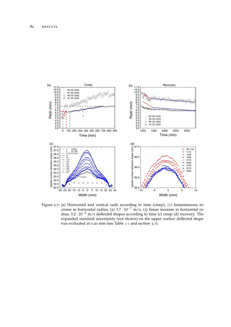
80 results
0 100 200 300 400 500 600 700 800 9003.03.54.04.55.05.56.06.57.07.58.08.59.09.5
10.010.511.0(a)
Rh 2D (240) Rv 2D (240) Rh 3D (300) Rv 3D (300)
Creep
Rad
ii (m
m)
Time (min)
2 3 1
1000 1500 2000 2500 30003.03.54.04.55.05.56.06.57.07.58.08.59.09.5
10.010.511.0(b) Recovery
Rv 2D (240) Rh 2D (240) Rh 3D (300) Rv 3D (300)
Rad
ii (m
m)
Time (min)
-30 -25 -20 -15 -10 -5 0 5 10 15 20 25 3032.032.533.033.534.034.535.035.536.036.537.037.5
(c)
Ups
ide
surfa
ce d
efle
cted
sha
pe (m
m)
Width (mm)
0 Calliper 0 3D (300) 3 min 2D (240) 21 44 173 297 421 504 629 753 877
1.4 mm
-10 -5 0 5 1035.0
35.5
36.0
36.5
37.0(d)
Ups
ide
surfa
ce d
efle
cted
sha
pe (m
m)
Width (mm)
991 min 1115 1239 1698 2779 2959 3139 3319 3499
Figure 2.7: (a) Horizontal and vertical radii according to time (creep); (1) Instantaneous in-crease in horizontal radius, (2) 3.7 · 10−7 m/s, (3) linear increase in horizontal ra-dius, 3.2 · 10−8 m/s deflected shapes according to time (c) creep (d) recovery. Theexpanded standard uncertainty (not shown) on the upper surface deflected shapewas evaluated at 0.20 mm (see Table 2.1 and section 3.1).
4D I S C U S S I O N
4.1 ability of mri and associated image analysis to describe the ge-ometry of bubble and cheese dynamically
For an bubble radius of 5.45 mm, the method developed in this study made it possibleto measure the volume with an accuracy of 6% and 10% with voxel sizes of 0.33 mm3
(acquisition time of 1 h 08 min) and 0.53 mm3 (acquisition time of 8 min 45 s). Thisrelative uncertainty decreased with the increase in bubble volume. Experiments wherethe initial volume of the bubble was too small (namely diameters between 4 and 6 mm)and levels of pressure were too low (because of early leakage) were not considered forthe present analysis since variations in volume were not enough large compared to theuncertainties reported above.
Likewise, the increase in accuracy with the decrease of the voxel size from 0.53 mm3
to 0.33 mm3 was low regarding the increase in the time of acquisition from 8 min 45 sto 1 h 08 min. Except when steep variations in pressure (within a few seconds) wereapplied, the acquisition time of 8 min 45 s was satisfactory to follow the variationsin volume (of the order of 8.7 · 10−11 m3/s) and images did not present any blurring.Note that assessing bubble volume within a few seconds would have dramatically de-teriorated the spatial resolution. This point will be further discussed in the Discussionsection.
The development of the method for determining the upper deflected shape was astep forward compared to the use of a comparator gauge. It allowed us not to removethe setup from the MRI table to measure it with the comparator gauge on a separatetable, by the way decreasing the risk in gas leaks.
4.2 low pressure was found to be able to inflate the cheese bubble
At the very beginning of the experiment (1), the applied pressure (7.5 kPa) was higherthan that actually measured in cheese (1.3 kPa, Grenier et al. 37) and that found to beable to inflate an bubble in Emmental cheese (5 kPa, Fluckiger et al. 30).
81
82 discussion
After 41 min, the pressure was between half and twice as much as that found inreal cheese. These results showed that level of pressure of the order of 3.5 kPa wasable to inflate an bubble in semi-hard cheese. Measurements of bubble volume carriedout within real cheese blocks (Grenier et al. 37) were influenced by the outer ring,possibly including spatial variability in mechanical properties and the effect of the foilsurrounding the cheese. In this study, only the proximate surrounding cheese wascontrolling the bubble growth.
Such a level of pressure remains very low and of the order of the atmospheric pres-sure variations; in the meantime the bubble inflated a lot (up to 3.2 times as much asthe initial volume). Both low pressure and high volume increase were pieces of evi-dence that bubble growth was poorly controlled by mechanics in that experiment andthat semi-hard cheese mostly flowed around the bubble. Low pressure seems typicalso far of bubble growth in food materials; internal pressure during the fermentationof bread dough (closed bubbles) was 6 times as low as that found in cheese during thefirst days of hot room (Grenier et al. 35).
4.3 quasi-absence of time-independant elasticity and small elastic
strain in cheese during bubble growth
During the recovery, the volume and both horizontal and vertical radii decreased si-multaneously, chiefly due to the stress relaxation and in a less extent to the gravity. Ona duration of 3,450 min (57.5 h), i.e. 21 times as much as the highest time of relaxationof the cheese (of the order of 10,000 s,Laridon et al. 57), the volume still slightly de-creased. This slight decrease in volume did not make possible to evidence the absenceof time-independent elasticity by itself. However, the slight increase in volume foundafter the lowering in pressure was applied, evidenced that no time-independent elas-ticity was driving the mechanical behavior of the cheese in the area where the cylinderof cheese was taken from, i.e. not too close to the surface whereby lower water contentcould have possibly modified this behaviour. Such a result was in agreement with thelow level of stress encountered in a semi-hard cheese after a 15 hours’ compression-relaxation experiment (Laridon et al. 57). However results from Laridon et al. [57]has been obtained on a duration 3.7 times as high as that used in an experiment ofcompression-relaxation. During an experiment of compression relaxation such as thatperformed in Laridon et al. [57], the small sample involved is very likely to dry on along duration even when embedded in an oil film and drying can eventually interferewith the measurement. In this bubble growth experiment the water content did notevolve (section 3.1) and the conclusion of time-independent elasticity was even morereliable.
The extent of strain and extensional strain rate can also be analyzed more thoroughlyto evaluate if small elastic strain can be considered for describing the bubble growthin semi-hard cheese.
4.4 linear response of the cheese and low bi-extensional strain rate 83
The growth rate of the bubble, 8.7 · 10−11 m3/s, was of the same order of magnitudethan that found in real cheese; 7.7 · 10−11 m3/s evaluated during ripening, between10 and 13 days of hot room (Huc et al. 47). In the meantime, the cheese betweenthe bubble and the sustaining apparatus was squeezed at a maximum linear strainof 10.6%. It can be concluded that when the volume increase was of the same orderthan that really measured in cheese blocks, the strain imposed to the cheese materialwas within the limit usually admitted for being linear in a purely elastic material.Note that it happened over a period equal to 5.4 times as much as the longest time ofrelaxation of the cheese (Laridon et al. 57). The bubble growth involved small elasticstrains as soon as the deformations applied to the cheese were not too brief and toolarge. Consequently, the bubble growth in cheese is very unlikely to be described bynonlinear models and generalized Maxwell’s model for instance can be applied fordescribing the bubble growth in cheese.
4.4 linear response of the cheese and low bi-extensional strain rate
The maximal bi-extensional strain rate, 9 · 10−5 s-1, was about 40 times as much asthat encountered during cheese ripening when estimated from the evolution of bubblediameters between day 8 and 12 of hot room ripening (1.9 · 10−6 s-1, Grenier et al.37). The conclusion of the experiment can be hence extended to the bubble growthin real cheese. Note that the lowest strain rate usually applied to cheese samples inrheological testing are 20 to 100 times as much as this maximal bi-extensional strainrate (Goh et al. 32, Masi and Addeo 64, Culioli and Sherman 21) and 5 times as muchas the bi-extensional strain rate encountered in bubble growth during bread doughproofing (Babin et al. 7). The small strain rate involved in the experiment was also apiece of evidence that linear models are very likely to fit the bubble growth in cheese.
The linear increases in volume against an almost constant load (3 in Figure 2.6b,Figure 2.7a and c), as well as the progressive evolution of the upper deflected shape,were the evidence of a mainly viscous behavior. Viscosity was of the order of the ratioof the relative gas pressure to bi-extensional strain rate i.e. 3,500 Pa
9·10−5s−1 = 3.9 · 107 Pa·s.

5C O N C L U S I O N
Gas pressure and gas volume inside a cheese bubble were continuously and simulta-neously measured for the first time. A specific maintaining apparatus was developedin order to produce non-destructive, dynamic but accurate information about the size(volume and radii) of a gas bubble in cheese and about the shape of the upper sur-face of a cylindrical cheese sample. Calculation of the expanded standard uncertaintymade it possible to give confidence in the variations that were reported and discussed.
Low amount of pressure (< 3.5 kPa) was proved to be able to inflate an bubble incheese and evidenced that low resistance was opposed to gas inflation in cheese. Thequasi-absence of time-independent elasticity was evidenced close to the core of thecheese block. Note that near the surface of the cheese block, the higher salt contentand the lower water content could have modified this behavior and this result can onlybe considered close to the core of a semi-hard cheese. On a time scale close to that ofthe actual bubble growth in cheese, the bubble growth was driven by the viscous partof the viscoelasticity in a low elastic strain and low bi-extensional strain rate situation.Linear viscoelasticity is hence applicable to describe bubble growth in the semi-hardcheese under study.
The setup developed in this study and the MRI opens a way to connect informa-tion about geometry to known mechanical loads and further analysis of formulationchanges on the mechanical behaviour of cheese.
85

Chapitre 3
M O D E L L I N G O F T H E M E C H A N I C A L D E F O R M AT I O N O F AS I N G L E B U B B L E I N S E M I - H A R D C H E E S E , W I T H
E X P E R I M E N TA L V E R I F I C AT I O N A N D S E N S I T I V I T YA N A LY S I S
The aim of the study presented here was to investigate the momentumtransport occurring during bubble growth in a viscoelastic material. Themechanical behaviour was modelled with a 5-element Maxwell model, im-plemented with the finite elements method, and a sensitivity analysis ofthe model parameters was undertaken. Air was injected into the bubbleand growth was monitored with pressure sensors and by MRI image anal-ysis. The experiment was repeated three times. Each time mechanicalparameters were characterised on the same material as that used for thevalidation of the model. Simulations were conducted in conditions as closeas possible to those of the experiment, and yielded good agreement withthe experimental results.Keywords: generalised Maxwell model; viscoelasticity ; ripening; momentumtransport; relaxation times; elasticity ; bubble growth ; eye

1I N T R O D U C T I O N
Bubble growth is a phenomenon occurring in various fields of application; it is causedby different dynamics and different mechanical behaviours of the material surround-ing the bubble. The majority of scientific studies have considered rapid phenomenasuch as cavitation in liquids (Plesset 76), foaming of polymers (Ramesh et al. 77) andgrowth of bubbles in magma (Navon et al. 69). These studies have generated a vari-ety of results in terms of bubble size (from the micrometre to the centimetre) and interms of overall porosity of materials (up to 75% for polymer foams). The polymerindustry has benefited from numerous studies on this subject and this has led to otherdevelopments, in particular in the food science area.
Amon and Denson [5] proposed a 1-D bubble growth model made of a single bubblesurrounded by a small spherical amount of liquid polymer, constituting a cell unitthat was considered to be representative of average bubble growth. Their approachhad the advantage of being relatively simple, and included the modelling of masstransport from the polymer to the bubble (Patel 72, Elshereef et al. 25), but did notcover any interaction between bubbles and the possible coalescence of neighbouringbubbles. The notion of cell-based model was then extended to compressible materials(Arefmanesh et al. 6), viscoelastic materials (Ramesh et al. 77), and generalised to 3-D (Bruchon and Coupez 12). These studies duplicated the cell unit to take multiplebubble growth into account. Some of these models were reviewed by Lee and Ramesh[63]. Feng and Bertelo [29] showed that the influence of the viscoelastic material onbubble growth depends on the duration of the loading: for process times shorter thanthe characteristic relaxation time, viscoelasticity enhances bubble growth, whereas forprocess times longer than or of the same order of magnitude as the characteristicrelaxation time, viscoelasticity slows the bubble growth down. Venerus et al. [89]studied several non-linear viscoelastic models (Oldroyd-B, upper convected Maxwelland Phan-Thien-Tanner models) and showed that the nonlinearity of the models wasof little importance for bubble growth, since the deformation rate was significant atthe beginning of the process but very rapidly decreased afterwards.
There are few modelling approaches for the bubble growth in food products, andthey are almost exclusively confined to sparkling drinks or cereal products (Campbelland Mougeot 15). There are two main approaches for the study of bubble growthin food products. The first considers bubble growth mainly from a mass transportpoint of view, where bubble growth is controlled only by the transport of dissolvedgas from the material into the bubble (Handleman and Lyons 40, Huang and Kokini43, Shah et al. 85), the mechanical reaction of the bubble being controlled only by sur-
89
90 introduction
face tension. The mathematical model developed to describe a single bubble growthin bread dough (Shah et al. 85) was later extended to multiple bubbles in a contin-uum approach (Chiotellis and Campbell 16, 17). The second approach consideredcoupled modelling within a continuous domain, where bubble growth is controlledby the interaction between several phenomena such as momentum and mass trans-port. Additional coverage of heat transport phenomena is often needed to cover thebaking process. de Cindio and Correra [23] and Hailemariam et al. [39] consideredthe case of a viscoelastic material (bread dough) modelled by linear or nonlinear vis-coelastic models. Bikard et al. [9] and Bikard et al. [8] investigated a similar approachfor coupling mass and momentum transport, where the material (bread dough) wasmodelled with a purely viscous law. The choice of a particular mechanical behaviourmodel was rather a postulate and was not discussed in these previous studies.
While more realistic, multiphysics approaches (coupling between momentum trans-port and mass and heat transport) require a large number of model parameters. Thesecan be difficult to assess experimentally, and are often extracted from other studies inthe literature, and are not appropriate for the specific experimental validation condi-tions used by the modellers. Input parameters can also be determined by comparisonbetween simulated and experimental data, with either trial and error or numericaloptimisation. Moreover, the scale of observation is rarely consistent with that of thedescription of phenomena in previous models, rendering the validation of low value.In the case of bubble growth in food, experimental validation, when included in thestudy, often takes place at a macroscopic level, i.e. total volume and total mass loss(Fan et al. 28, Feng and Bertelo 29). Validation on the bubble scale is rare (Kontopoulouand Vlachopoulos 54, Yano and Shimiya 94). Moreover, with the growing numbers ofmechanisms and parameters, critical analysis of the influence of each mechanism orparameter on the model becomes more difficult, and analysis of the couplings is notstraightforward. Generally, the experimental and simulated results are compared froman overall point of view (Ramesh et al. 77). The acquisition of experimental data, whenappropriate, in conditions involving a single transport phenomenon, separately fromthe others, should improve the quality of the fitting and adjustment of the few, specificentry parameters, thus contributing to a higher quality validation/invalidation proce-dure for the complete model. Together with observation at the bubble scale, this is theglobal approach applied in this study. Observation on the bubble scale has been madepossible by the recent advances in imaging techniques, e.g. Aguilera and Lillford [2].
Compared to the phenomenon investigated in the present study, previous studiesperformed on polymers have presented two main drawbacks: the bubbles were smallwith diameters lower than 10
-5 m, whereas bubbles in cheese are in the order of 10-3
m (Huc et al. 44); and the processes were relatively fast, several minutes for polymerfoaming compared to several days for cheese ripening. Their conclusions cannot easilybe extrapolated to the present study.
introduction 91
On the other hand, because of the large size of bubbles in cheese under ripening,the isolation and instrumentation (pressure measurement) of a single bubble are pos-sible experimentally (Grenier et al. 37), and provide consistency between the scalesof observation and theory. Slow dynamics allow the use of tomographic techniquesfor monitoring the volume of the bubble despite the opacity of the material. Finally,by controlling the boundary and load conditions, the mechanical behaviour can bestudied separately from mass production and transport.
The aims of the present study were:
• To extend the study of bubble growth in viscoelastic material to semi-hardcheeses. There are no studies in the literature to our knowledge that deal withthe modelling of bubble growth in semi-hard cheeses. Prior focus has been lim-ited to nucleation and early bubble growth with major contribution of surfacetension ; it did not include any experimental verification (Akkerman et al. 3).
• To test the suitability of the generalised Maxwell mechanical model by imple-menting a finite element model to reproduce the mechanical deformation of asingle bubble as observed experimentally; three repetitions were used to meetthis aim.
• To characterise the effects of different model parameters on mechanical deforma-tion and to provide a critical analysis of these effects by performing sensitivitystudies.

2M AT E R I A L S A N D M E T H O D S
2.1 experimental procedure
The aim of the experiment was to isolate a single bubble from a semi-hard cheese blockin a dedicated maintaining apparatus (Figure 3.1) and to inflate the bubble by addinga given amount of gas, thus increasing the pressure inside the bubble. The wholeexperiment was monitored with MRI (Magnetic Resonance Imaging) and a pressuresensor.
Three experiments were conducted on three separate bubbles isolated in a cheesecylinder, differing in their load history. In Experiment 1, pressure was maintainedrelatively constant (slow decrease from 5.5 kPa to 3.7 kPa) for 8 h (Figure 3.7a). ForExperiment 2, a 6 kPa pressure peak was applied, followed by holding at a lowerpressure value of 3 kPa for 2 h (Figure 3.7c). Finally, slight pressure (1 kPa) wasmaintained for the remaining time of the experiment (Figure 3.7c). For Experiment 3,successive holdings of pressure were applied, with decreasing pressure levels at eachstep (Figure 3.7e). Special care was taken that the pressure applied to the bubble wasof the same order as that found in real cheeses, from 0.5 ± 0.3 to 3.8 ± 0.3 kPa over thefirst few days and 0.5 ± 0.3 to 1.5 ± 0.3 kPa thereafter (Grenier et al. 37).
The various loads applied to the bubble interface were intended to mimic plausi-ble situations: the long-term low-pressure was characteristic of bubble growth, whilesudden high-pressure changes were representative of handling of cheese blocks or ofsudden temperature changes that occur during ripening and that cause the pressureto change accordingly, following the ideal gas law.
Experiments 1 to 3 also differed by the mechanical properties of the cheese material(variability between batches) and the size and position of the bubble inside the cheesecylinder (Table 3.1).
93
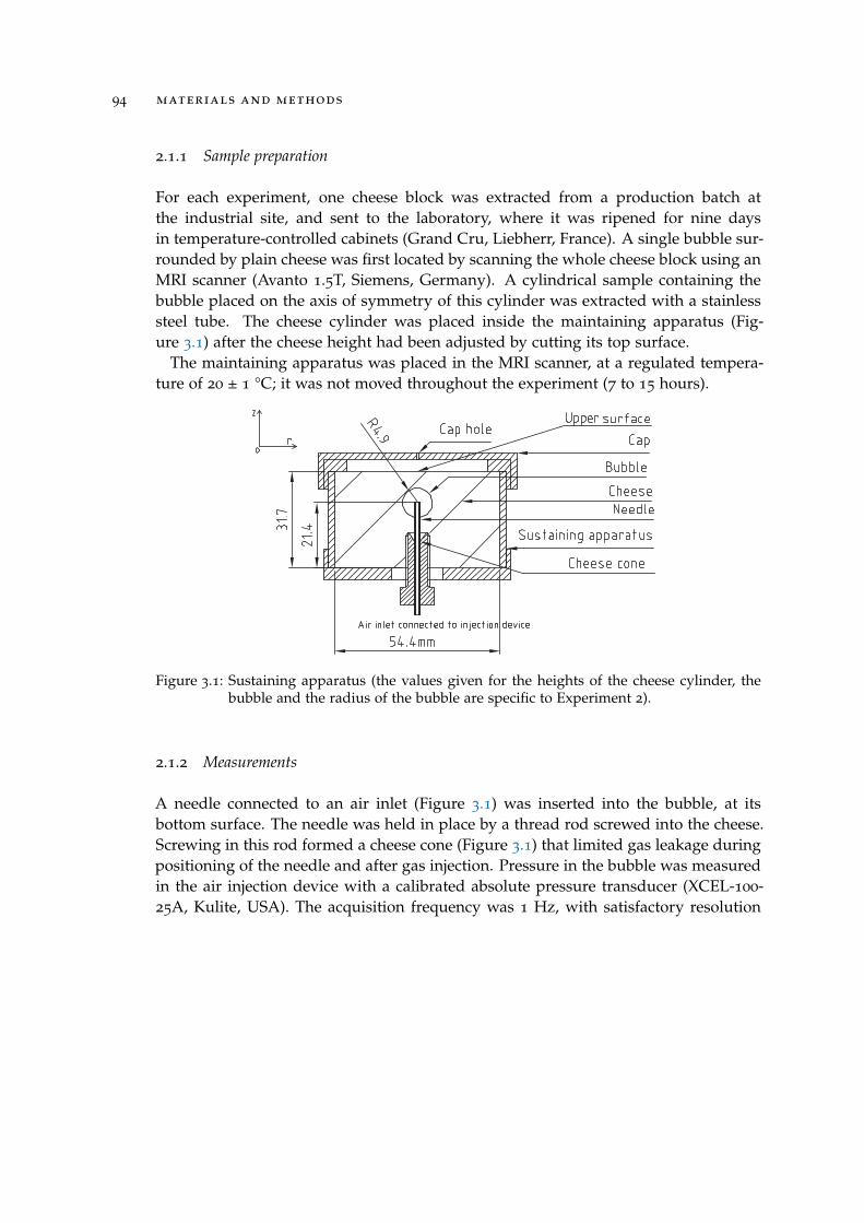
94 materials and methods
2.1.1 Sample preparation
For each experiment, one cheese block was extracted from a production batch atthe industrial site, and sent to the laboratory, where it was ripened for nine daysin temperature-controlled cabinets (Grand Cru, Liebherr, France). A single bubble sur-rounded by plain cheese was first located by scanning the whole cheese block using anMRI scanner (Avanto 1.5T, Siemens, Germany). A cylindrical sample containing thebubble placed on the axis of symmetry of this cylinder was extracted with a stainlesssteel tube. The cheese cylinder was placed inside the maintaining apparatus (Fig-ure 3.1) after the cheese height had been adjusted by cutting its top surface.
The maintaining apparatus was placed in the MRI scanner, at a regulated tempera-ture of 20 ± 1 °C; it was not moved throughout the experiment (7 to 15 hours).
Figure 3.1: Sustaining apparatus (the values given for the heights of the cheese cylinder, thebubble and the radius of the bubble are specific to Experiment 2).
2.1.2 Measurements
A needle connected to an air inlet (Figure 3.1) was inserted into the bubble, at itsbottom surface. The needle was held in place by a thread rod screwed into the cheese.Screwing in this rod formed a cheese cone (Figure 3.1) that limited gas leakage duringpositioning of the needle and after gas injection. Pressure in the bubble was measuredin the air injection device with a calibrated absolute pressure transducer (XCEL-100-25A, Kulite, USA). The acquisition frequency was 1 Hz, with satisfactory resolution
2.1 experimental procedure 95
on an Ahlborn data logger (Almemo 2590, Ahlborn, Germany). The atmosphericpressure outside the device was measured and pressure relative to the atmospherewas obtained by subtracting the atmospheric pressure from the absolute pressure. Inthis study, pressure is given relative to the atmospheric pressure. For more details seeGrenier et al. [36].
MRI sequences were launched before gas injection to characterise the initial geom-etry of the domain (bubble dimension and upper deflected shape). Gas was injectedjust after the first MRI acquisition.
A 3-D Spin-Echo sequence was used for this study, with two different sets of pa-rameters. The following set of parameter values was used to monitor bubble volumeand upper deflected shape over time: echo time = 10 ms, repetition time = 400 ms,bandwidth = 295 Hz, pixel size = 0.5×0.5 mm2, slice thickness 0.5 mm, 1 scan, Sig-nal to Noise Ratio = 53. The acquisition time was 8 min 45 s, and the whole cheesecylinder (52 slices) was acquired. Spatial resolution in the plane was increased forthe first acquisition (pixel size = 0.3×0.3 mm2, slice thickness 0.7 mm), with a reducedSignal to Noise Ratio (27) and increased number of slices (88), echo time (12 ms) andacquisition time (1 h 08 min). MRI cross-sections are shown in Figure 3.5 for the threeexperiments, at the beginning and at the end.
2.1.3 Data analysis and uncertainties
Bubble volume was obtained from MRI image analysis by adding together all thebubble voxels after thresholding according to the Otsu method (Otsu 71). With such amethod, some voxels of partial volume (partially filled with gas and cheese) were notconsidered, leading to a systematic underestimation of the volume. The uncertaintyon determination of the bubble volume was a function of the measured volume, anddid not exceed 10% of the measured volume (Grenier et al. 36).
The upper deflected shape was evaluated by image analysis from a single MRI imagethat contained the axis of symmetry of the cylinder. The Otsu method was used todefine the greylevel threshold that made it possible to distinguish between cheese andgas in the MRI images. Smooth interpolation of the greylevel presented by the pixelsnear the upper surface of the cheese as a function of the z-coordinate was used tolocate the upper surface of the cheese cylinder. This MRI method for measuring thedeflected shape was validated by comparison with measurements with a comparatorperformed on the same cheese surface; the deflected shape of the upper surface wasdetermined by MRI with an uncertainty of 0.2 mm (Grenier et al. 36)
The uncertainty associated with the pressure measurement was estimated to be0.3 kPa (Grenier et al. 36).
96 materials and methods
2.2 modelling
Modelling of the rheological behaviour of semi-hard cheese has been reported in aprevious paper (Laridon et al. 57). The modelling briefly outlined in sections 2.2.1and 2.2.2 was adapted to match a specific geometry (section 2.2.3). Moreover, whereasin the previous study the geometry allowed reduction of the problem to a temporaldimension, the presence of the bubble interface necessitated the use of more complexmodelling, and increased the number of model parameters.
2.2.1 Model assumptions
The semi-hard cheese studied was considered incompressible (Calzada and Peleg 14),and the domain was considered to be homogeneous. Bubble growth in cheeses is arelatively slow phenomenon, the bubble interface moving at about 10−7 m/s (Musseet al. 68), and therefore no inertial terms were considered.
2.2.2 Governing equations
Quasistatic equilibrium was expressed by the conservation of momentum:
∇ · S = ρg (3.1)
where S is the stress tensor, ρ the material density, and g the gravity. S was dividedinto a purely elastic part σ, and a viscoelastic part τ. The former was expressed usingthe tensor form of Hooke’s law and the latter using a 5-element generalised Maxwellmodel, thus providing:
σ = C : ε (3.2)
where C is the usual fourth-order tensor of rigidity and ε the strain tensor. Thiselastic part of the stress was split into spherical and deviatoric parts to separate shearand bulk moduli (Voigt notation is used for convenience):
σ = G0
4/3 −2/3 −2/3
−2/3 4/3 −2/3
−2/3 −2/3 4/3
2
2
2
ε + Ktr(ε)I (3.3)
2.2 modelling 97
where G0 is the shear modulus, K the bulk modulus and I the identity tensor. Theviscoelastic part of the stress is the sum of the stress in each Maxwell element:
τ =N
∑i=1
τi (3.4)
For each Maxwell element the following equation has to be solved:
τi + λi∂τi
∂t= λiGi
∂γ
∂t(3.5)
where λi and Gi are the relaxation time and the shear modulus of the Maxwellelement i, respectively, and γ is the deviatoric part of the strain tensor.
The generalised Maxwell model usually presents a purely elastic element, that hasbeen expressed here in the deviatoric part of the elastic stress tensor (Eq. 3.3). However,the previous studies did not show any long-term elastic behaviour (Laridon et al. 57,Grenier et al. 36), and therefore G0 was set at 0. Thus, Eq. 3.1 becomes: ∇·
(Ktr(ε)I + ∑N
i=1 τi
)= ρg
τi + λi∂τi∂t = λiGi
∂γ∂t
(3.6)
The shear moduli were expressed in terms of proportions αi of the overall shearmodulus G:
αi =Gi
G = ∑Ni=1 Gi
(3.7)
2.2.3 Boundary conditions
The plain cheese geometry consisted of a cylinder, which is represented by the domainbetween boundaries 2, 3 and 4 in Figure 3.2a. A 2-D axisymmetric representation wasused to take advantage of the symmetry of the geometry (Figure 3.2a - 1). The bubblewas located on the axis of symmetry and was represented by the bubble interface 5
in Figure 3.2a. The boundary conditions (Figure 3.2a) were set to match as closely aspossible the experimental conditions (see section 2.1). The pressure measured duringthe experiment was used as the applied pressure p(t) at the bubble interface.
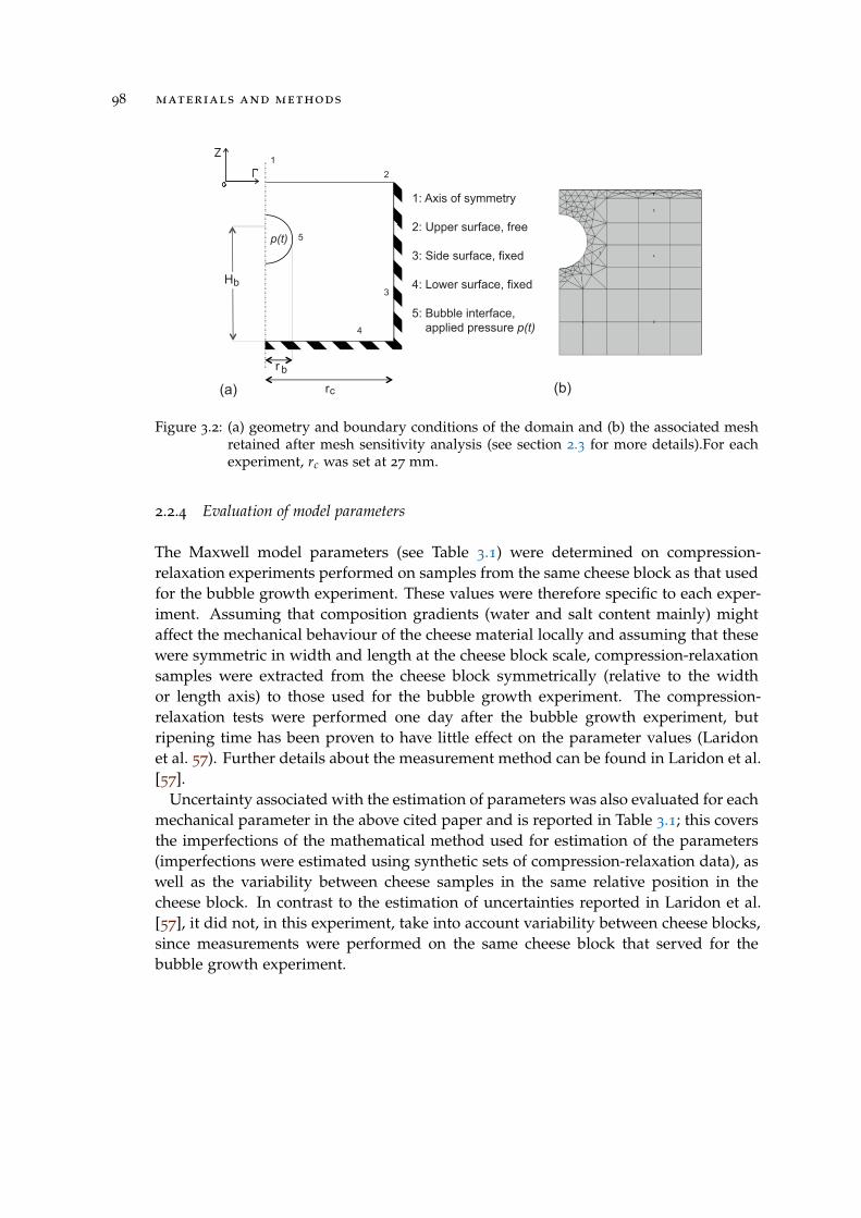
98 materials and methods
12
3
4
5p(t)
1: Axis of symmetry
2: Upper surface, free
3: Side surface, fixed
4: Lower surface, fixed
5: Bubble interface, applied pressure p(t)
(a) (b)
b
b
c
H
r
r
Figure 3.2: (a) geometry and boundary conditions of the domain and (b) the associated meshretained after mesh sensitivity analysis (see section 2.3 for more details).For eachexperiment, rc was set at 27 mm.
2.2.4 Evaluation of model parameters
The Maxwell model parameters (see Table 3.1) were determined on compression-relaxation experiments performed on samples from the same cheese block as that usedfor the bubble growth experiment. These values were therefore specific to each exper-iment. Assuming that composition gradients (water and salt content mainly) mightaffect the mechanical behaviour of the cheese material locally and assuming that thesewere symmetric in width and length at the cheese block scale, compression-relaxationsamples were extracted from the cheese block symmetrically (relative to the widthor length axis) to those used for the bubble growth experiment. The compression-relaxation tests were performed one day after the bubble growth experiment, butripening time has been proven to have little effect on the parameter values (Laridonet al. 57). Further details about the measurement method can be found in Laridon et al.[57].
Uncertainty associated with the estimation of parameters was also evaluated for eachmechanical parameter in the above cited paper and is reported in Table 3.1; this coversthe imperfections of the mathematical method used for estimation of the parameters(imperfections were estimated using synthetic sets of compression-relaxation data), aswell as the variability between cheese samples in the same relative position in thecheese block. In contrast to the estimation of uncertainties reported in Laridon et al.[57], it did not, in this experiment, take into account variability between cheese blocks,since measurements were performed on the same cheese block that served for thebubble growth experiment.
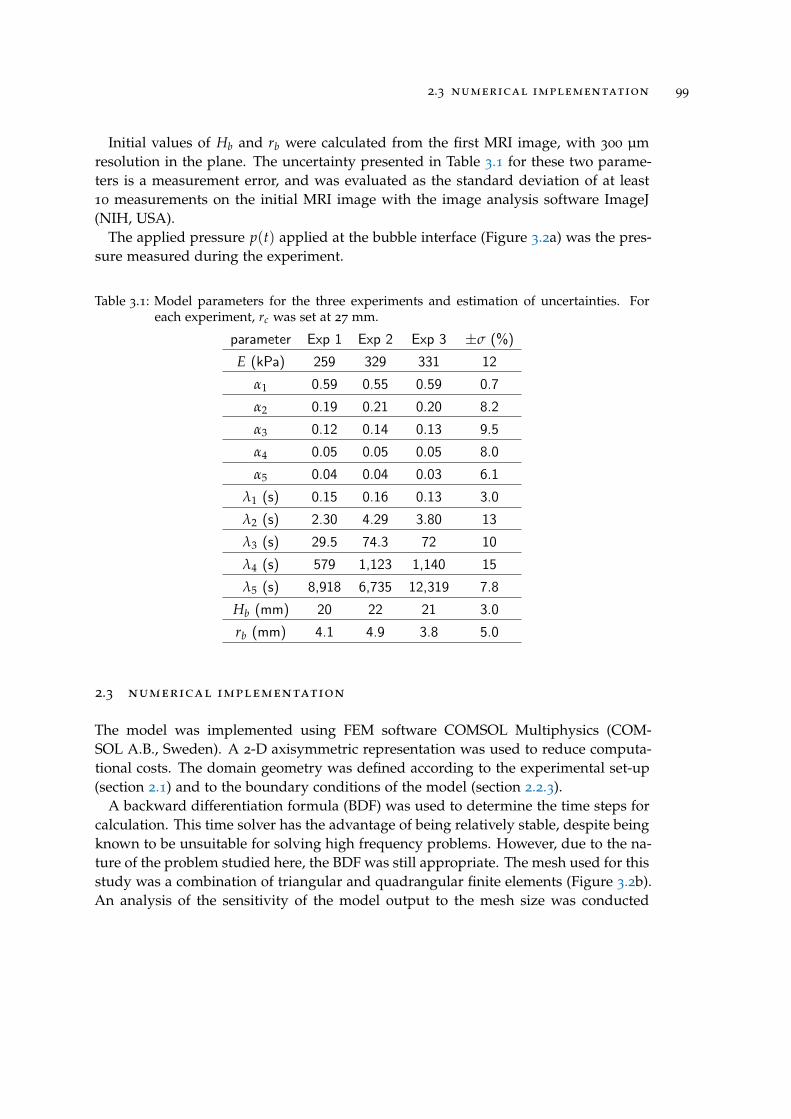
2.3 numerical implementation 99
Initial values of Hb and rb were calculated from the first MRI image, with 300 µmresolution in the plane. The uncertainty presented in Table 3.1 for these two parame-ters is a measurement error, and was evaluated as the standard deviation of at least10 measurements on the initial MRI image with the image analysis software ImageJ(NIH, USA).
The applied pressure p(t) applied at the bubble interface (Figure 3.2a) was the pres-sure measured during the experiment.
Table 3.1: Model parameters for the three experiments and estimation of uncertainties. Foreach experiment, rc was set at 27 mm.
parameter Exp 1 Exp 2 Exp 3 ±σ (%)E (kPa) 259 329 331 12
α1 0.59 0.55 0.59 0.7α2 0.19 0.21 0.20 8.2α3 0.12 0.14 0.13 9.5α4 0.05 0.05 0.05 8.0α5 0.04 0.04 0.03 6.1
λ1 (s) 0.15 0.16 0.13 3.0λ2 (s) 2.30 4.29 3.80 13λ3 (s) 29.5 74.3 72 10λ4 (s) 579 1,123 1,140 15λ5 (s) 8,918 6,735 12,319 7.8
Hb (mm) 20 22 21 3.0rb (mm) 4.1 4.9 3.8 5.0
2.3 numerical implementation
The model was implemented using FEM software COMSOL Multiphysics (COM-SOL A.B., Sweden). A 2-D axisymmetric representation was used to reduce computa-tional costs. The domain geometry was defined according to the experimental set-up(section 2.1) and to the boundary conditions of the model (section 2.2.3).
A backward differentiation formula (BDF) was used to determine the time steps forcalculation. This time solver has the advantage of being relatively stable, despite beingknown to be unsuitable for solving high frequency problems. However, due to the na-ture of the problem studied here, the BDF was still appropriate. The mesh used for thisstudy was a combination of triangular and quadrangular finite elements (Figure 3.2b).An analysis of the sensitivity of the model output to the mesh size was conducted
100 materials and methods
to determine the most suitable mesh size. Several mesh sizes were considered andcompared to a finer reference mesh of more than 2,500 elements. Finally, 139 finiteelements with cubic shape functions were used, comprising about 15,000 degrees offreedom, depending on the size and position of the bubble in the domain. This en-sured that the displacement field calculated was within 2% of the values obtained withthe finer reference mesh and yielded a computational time that was 75 times shorter.
The average runtime of a calculation was about two minutes on a 4-core Intel pro-cessor at 3.1 GHz, with 16 GB RAM.
2.4 sensitivity analysis
The aims of the sensitivity analyses performed in this study were:
• To determine the input parameters that were most influential on the model out-put;
• To quantify the impact of the variability of these parameters on the model outputand this was also used as a way to propagate the error on the model parametersin the solution of the problem.
Sensitivity analysis based on statistical methods requires a high number of calculationsas the number of parameters studied increases. In our case, the input parametersincluded the Maxwell model parameters, the geometric parameters (such as bubbleposition Hb) and the pressure applied to the bubble surface. A first screening methodwas therefore used to rule out the parameters that had the least influence on the modeloutput values (section 2.4.1).
The two model output values that were studied were the bubble volume and thedisplacement of the center of the deflected shape of the upper surface of the domain(section 2.2.3).
The two types of sensitivity analysis were performed using the above COMSOLMultiphysics model in a script written in Matlab (The MathWorks, USA). This madeit possible to script the calculations with a greater level of control over the modelparameters.
2.4 sensitivity analysis 101
2.4.1 Screening method
Three values were used for each input parameter: the reference value, a lower andan upper value (Table 3.2). The variation range studied for each parameter (Table 3.2)was defined to reproduce variations that could be observed physically and that werecaused by variability of the product studied, or errors in the assessment of the param-eters, either of experimental nature or originating from calculation and fitting steps.The pressure applied on the bubble consisted of a 3 kPa hold (this is a plausible pres-sure level observed in cheese) for 10 h followed by null pressure for 17 h. Parameterswere ranked according to:
Ik = 100
∣∣∣∣∣ f(Xmaxk )− f
(Xre f
k
)f(
Xre fk
)∣∣∣∣∣+∣∣∣∣∣ f(Xmin
k )− f(
Xre fk
)f(
Xre fk
)∣∣∣∣∣∣∣∣∣Xmax
k −Xre fk
Xre fk
∣∣∣∣+ ∣∣∣∣Xmink −Xre f
k
Xre fk
∣∣∣∣ (3.8)
where f is the model output being considered (bubble volume or deflected shape ofthe upper surface), and Xre f
k , Xmink , and Xmax
k the reference, minimum, and maximumvalues of parameter k, respectively. The higher the Ik, the higher the sensitivity. f wascalculated at a simulated time of 100 ks (27 h) in order to consider only the long-termbehaviour. The ranks were considered as a first order approximation of the influenceof variation in the parameters on output values.
2.4.2 Statistical method
The method was split into two parts: the use of response surface methodology toapproximate the solution to the problem, and estimation of the sensitivity indices asdefined by Sobol [86].
The output of the model f was approximated by a quadratic response surface y:
f (X) ≈ y(X) = c +n
∑i=1
aiXi +n−1
∑i=1
n
∑j=i+1
bijXiXj +n
∑i=1
biiX2i (3.9)
where X is the vector containing the model parameters, n the number of parameters,and c, ai, and bij the coefficients that need to be fitted. To determine these coefficients,simulated data were generated using COMSOL Multiphysics, following a 3n factorialdesign, and the coefficients were fitted by multilinear regression using the regstatsMatlab function. The RMSE between the response surface y and the COMSOL modelwas 5%.
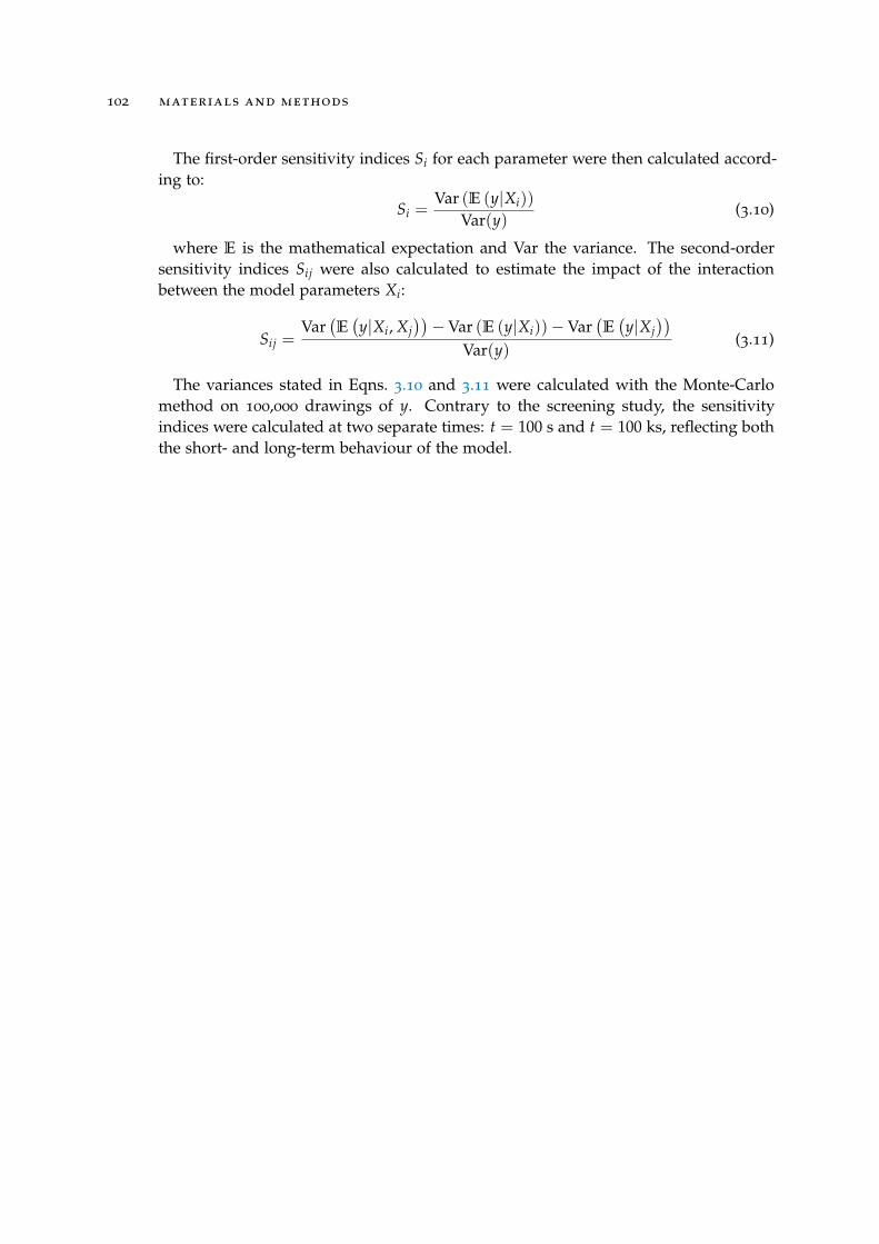
102 materials and methods
The first-order sensitivity indices Si for each parameter were then calculated accord-ing to:
Si =Var (E (y|Xi))
Var(y)(3.10)
where E is the mathematical expectation and Var the variance. The second-ordersensitivity indices Sij were also calculated to estimate the impact of the interactionbetween the model parameters Xi:
Sij =Var
(E(y|Xi, Xj
))−Var (E (y|Xi))−Var
(E(y|Xj
))Var(y)
(3.11)
The variances stated in Eqns. 3.10 and 3.11 were calculated with the Monte-Carlomethod on 100,000 drawings of y. Contrary to the screening study, the sensitivityindices were calculated at two separate times: t = 100 s and t = 100 ks, reflecting boththe short- and long-term behaviour of the model.
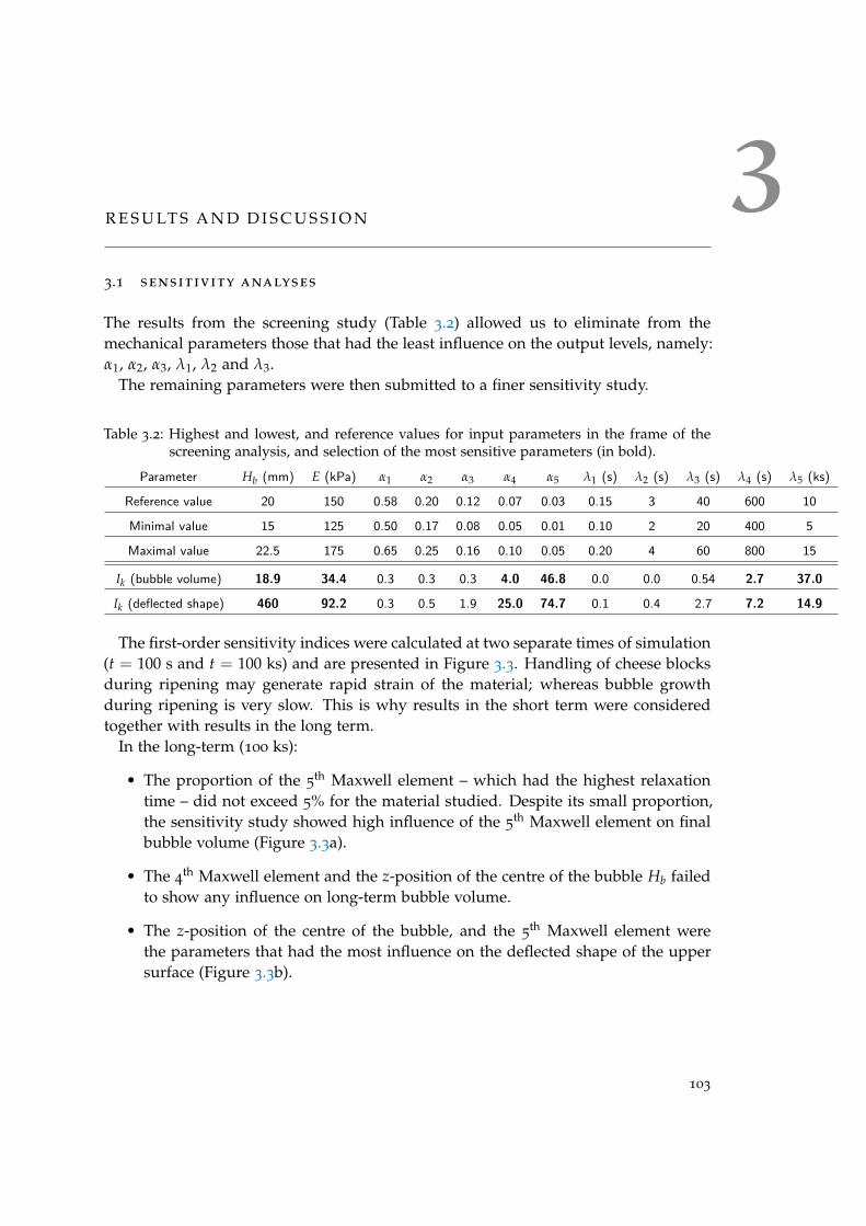
3R E S U LT S A N D D I S C U S S I O N
3.1 sensitivity analyses
The results from the screening study (Table 3.2) allowed us to eliminate from themechanical parameters those that had the least influence on the output levels, namely:α1, α2, α3, λ1, λ2 and λ3.
The remaining parameters were then submitted to a finer sensitivity study.
Table 3.2: Highest and lowest, and reference values for input parameters in the frame of thescreening analysis, and selection of the most sensitive parameters (in bold).
Parameter Hb (mm) E (kPa) α1 α2 α3 α4 α5 λ1 (s) λ2 (s) λ3 (s) λ4 (s) λ5 (ks)
Reference value 20 150 0.58 0.20 0.12 0.07 0.03 0.15 3 40 600 10
Minimal value 15 125 0.50 0.17 0.08 0.05 0.01 0.10 2 20 400 5
Maximal value 22.5 175 0.65 0.25 0.16 0.10 0.05 0.20 4 60 800 15
Ik (bubble volume) 18.9 34.4 0.3 0.3 0.3 4.0 46.8 0.0 0.0 0.54 2.7 37.0
Ik (deflected shape) 460 92.2 0.3 0.5 1.9 25.0 74.7 0.1 0.4 2.7 7.2 14.9
The first-order sensitivity indices were calculated at two separate times of simulation(t = 100 s and t = 100 ks) and are presented in Figure 3.3. Handling of cheese blocksduring ripening may generate rapid strain of the material; whereas bubble growthduring ripening is very slow. This is why results in the short term were consideredtogether with results in the long term.
In the long-term (100 ks):
• The proportion of the 5th Maxwell element – which had the highest relaxation
time – did not exceed 5% for the material studied. Despite its small proportion,the sensitivity study showed high influence of the 5
th Maxwell element on finalbubble volume (Figure 3.3a).
• The 4th Maxwell element and the z-position of the centre of the bubble Hb failed
to show any influence on long-term bubble volume.
• The z-position of the centre of the bubble, and the 5th Maxwell element were
the parameters that had the most influence on the deflected shape of the uppersurface (Figure 3.3b).
103
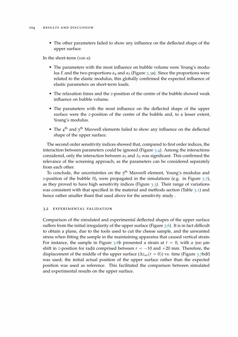
104 results and discussion
• The other parameters failed to show any influence on the deflected shape of theupper surface.
In the short-term (100 s):
• The parameters with the most influence on bubble volume were Young’s modu-lus E and the two proportions α4 and α5 (Figure 3.3a). Since the proportions wererelated to the elastic modulus, this globally confirmed the expected influence ofelastic parameters on short-term loads.
• The relaxation times and the z-position of the centre of the bubble showed weakinfluence on bubble volume.
• The parameters with the most influence on the deflected shape of the uppersurface were the z-position of the centre of the bubble and, to a lesser extent,Young’s modulus.
• The 4th and 5
th Maxwell elements failed to show any influence on the deflectedshape of the upper surface.
The second order sensitivity indices showed that, compared to first order indices, theinteraction between parameters could be ignored (Figure 3.4). Among the interactionsconsidered, only the interaction between α5 and λ5 was significant. This confirmed therelevance of the screening approach, as the parameters can be considered separatelyfrom each other.
To conclude, the uncertainties on the 5th Maxwell element, Young’s modulus and
z-position of the bubble Hb were propagated in the simulations (e.g. in Figure 3.7),as they proved to have high sensitivity indices (Figure 3.3). Their range of variationswas consistent with that specified in the material and methods section (Table 3.1) andhence rather smaller thant that used above for the sensitivity study .
3.2 experimental validation
Comparison of the simulated and experimental deflected shapes of the upper surfacesuffers from the initial irregularity of the upper surface (Figure 3.6). It is in fact difficultto obtain a plane, due to the tools used to cut the cheese sample, and the unwantedstress when fitting the sample in the maintaining apparatus that caused vertical strain.For instance, the sample in Figure 3.6b presented a strain at t = 0, with a 500 µmshift in z-position for radii comprised between r = −10 and +20 mm. Therefore, thedisplacement of the middle of the upper surface (∆zus(r = 0)) vs. time (Figure 3.7bdf)was used; the initial actual position of the upper surface rather than the expectedposition was used as reference. This facilitated the comparison between simulatedand experimental results on the upper surface.
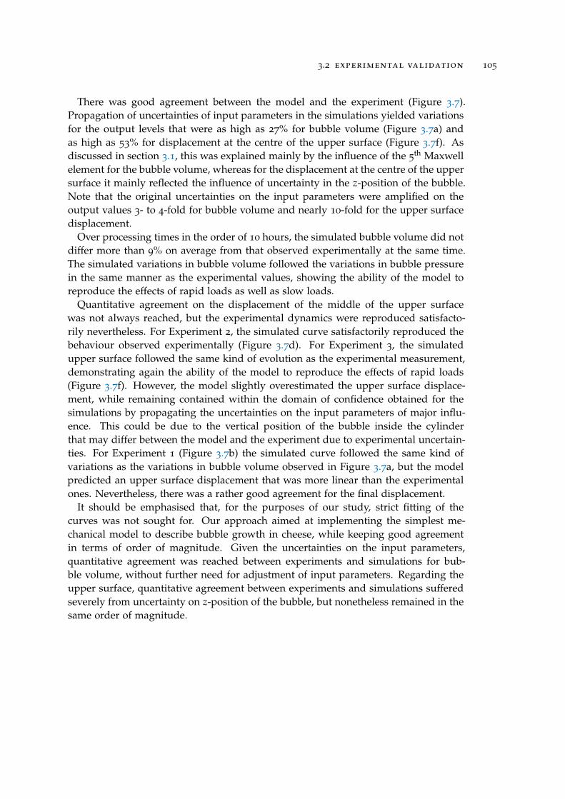
3.2 experimental validation 105
There was good agreement between the model and the experiment (Figure 3.7).Propagation of uncertainties of input parameters in the simulations yielded variationsfor the output levels that were as high as 27% for bubble volume (Figure 3.7a) andas high as 53% for displacement at the centre of the upper surface (Figure 3.7f). Asdiscussed in section 3.1, this was explained mainly by the influence of the 5
th Maxwellelement for the bubble volume, whereas for the displacement at the centre of the uppersurface it mainly reflected the influence of uncertainty in the z-position of the bubble.Note that the original uncertainties on the input parameters were amplified on theoutput values 3- to 4-fold for bubble volume and nearly 10-fold for the upper surfacedisplacement.
Over processing times in the order of 10 hours, the simulated bubble volume did notdiffer more than 9% on average from that observed experimentally at the same time.The simulated variations in bubble volume followed the variations in bubble pressurein the same manner as the experimental values, showing the ability of the model toreproduce the effects of rapid loads as well as slow loads.
Quantitative agreement on the displacement of the middle of the upper surfacewas not always reached, but the experimental dynamics were reproduced satisfacto-rily nevertheless. For Experiment 2, the simulated curve satisfactorily reproduced thebehaviour observed experimentally (Figure 3.7d). For Experiment 3, the simulatedupper surface followed the same kind of evolution as the experimental measurement,demonstrating again the ability of the model to reproduce the effects of rapid loads(Figure 3.7f). However, the model slightly overestimated the upper surface displace-ment, while remaining contained within the domain of confidence obtained for thesimulations by propagating the uncertainties on the input parameters of major influ-ence. This could be due to the vertical position of the bubble inside the cylinderthat may differ between the model and the experiment due to experimental uncertain-ties. For Experiment 1 (Figure 3.7b) the simulated curve followed the same kind ofvariations as the variations in bubble volume observed in Figure 3.7a, but the modelpredicted an upper surface displacement that was more linear than the experimentalones. Nevertheless, there was a rather good agreement for the final displacement.
It should be emphasised that, for the purposes of our study, strict fitting of thecurves was not sought for. Our approach aimed at implementing the simplest me-chanical model to describe bubble growth in cheese, while keeping good agreementin terms of order of magnitude. Given the uncertainties on the input parameters,quantitative agreement was reached between experiments and simulations for bub-ble volume, without further need for adjustment of input parameters. Regarding theupper surface, quantitative agreement between experiments and simulations sufferedseverely from uncertainty on z-position of the bubble, but nonetheless remained in thesame order of magnitude.
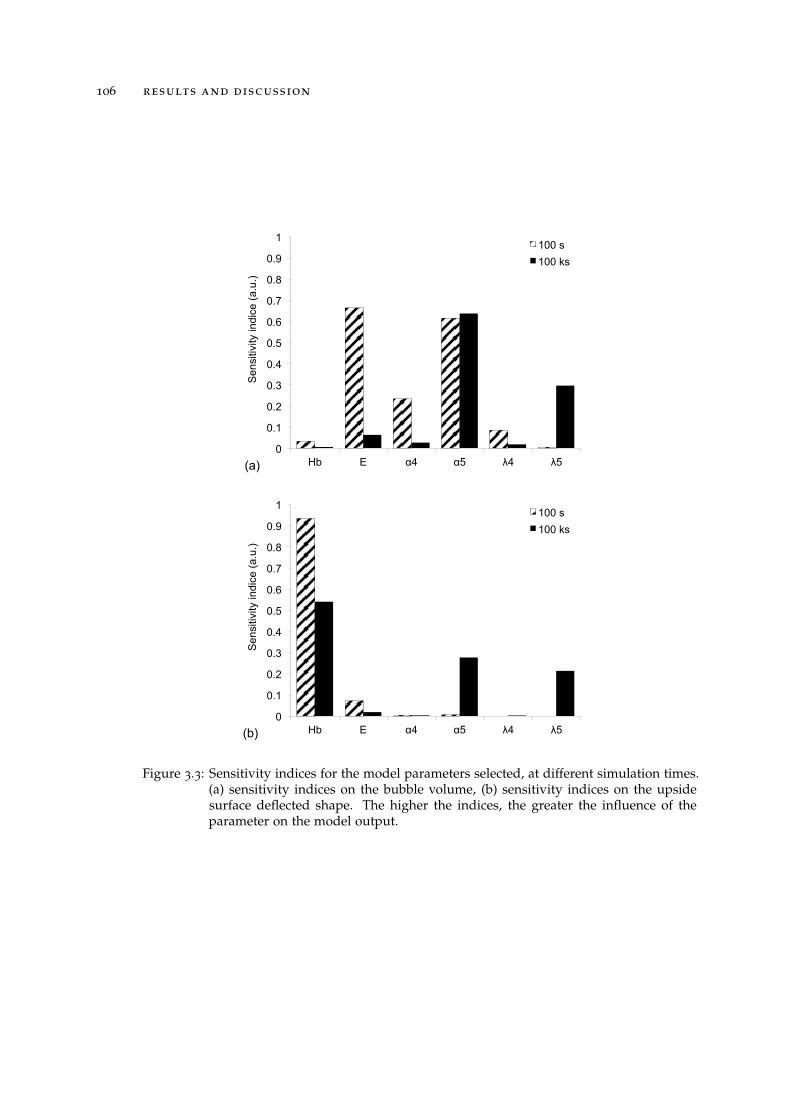
106 results and discussion
0
0.1
0.2
0.3
0.4
0.5
0.6
0.7
0.8
0.9
1
Hb E α4 α5 λ4 λ5
Sen
sitiv
ity in
dice
(a.u
.) 100 s 100 ks
(a)
0
0.1
0.2
0.3
0.4
0.5
0.6
0.7
0.8
0.9
1
Hb E α4 α5 λ4 λ5
Sen
sitiv
ity in
dice
(a.u
.)
100 s 100 ks
(b)
Figure 3.3: Sensitivity indices for the model parameters selected, at different simulation times.(a) sensitivity indices on the bubble volume, (b) sensitivity indices on the upsidesurface deflected shape. The higher the indices, the greater the influence of theparameter on the model output.
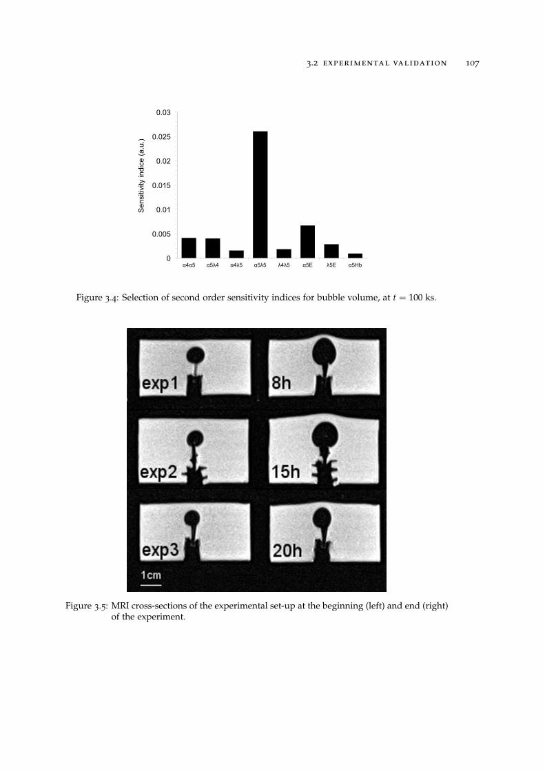
3.2 experimental validation 107
0
0.005
0.01
0.015
0.02
0.025
0.03
α4α5 α5λ4 α4λ5 α5λ5 λ4λ5 α5E λ5E α5Hb
Sen
sitiv
ity in
dice
(a.u
.)
Figure 3.4: Selection of second order sensitivity indices for bubble volume, at t = 100 ks.
Figure 3.5: MRI cross-sections of the experimental set-up at the beginning (left) and end (right)of the experiment.
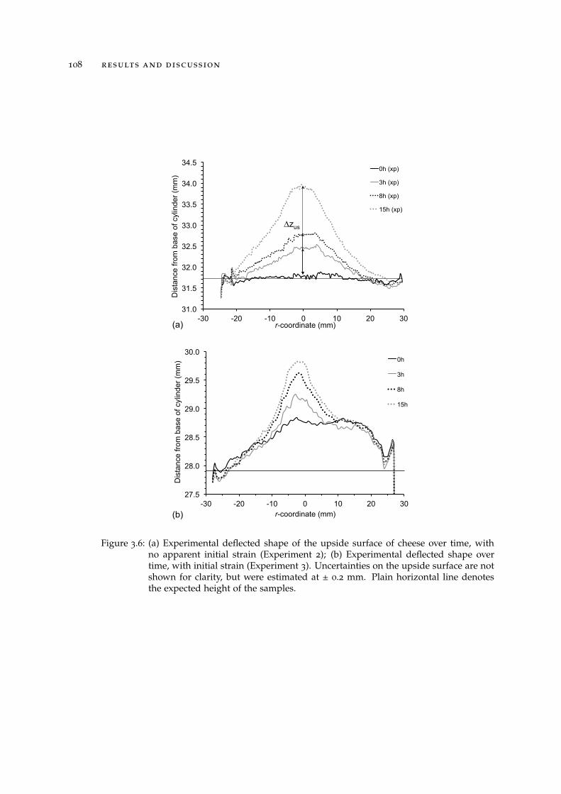
108 results and discussion
31.0
31.5
32.0
32.5
33.0
33.5
34.0
34.5
-30 -20 -10 0 10 20 30 r-coordinate (mm)
0h (xp)
3h (xp)
8h (xp)
15h (xp)
(a)
Dis
tanc
e fro
m b
ase
of c
ylin
der (
mm
)
zus
27.5
28.0
28.5
29.0
29.5
30.0
-30 -20 -10 0 10 20 30
Dis
tanc
e fro
m b
ase
of c
ylin
der (
mm
)
r-coordinate (mm)
0h
3h
8h
15h
(b)
Figure 3.6: (a) Experimental deflected shape of the upside surface of cheese over time, withno apparent initial strain (Experiment 2); (b) Experimental deflected shape overtime, with initial strain (Experiment 3). Uncertainties on the upside surface are notshown for clarity, but were estimated at ± 0.2 mm. Plain horizontal line denotesthe expected height of the samples.
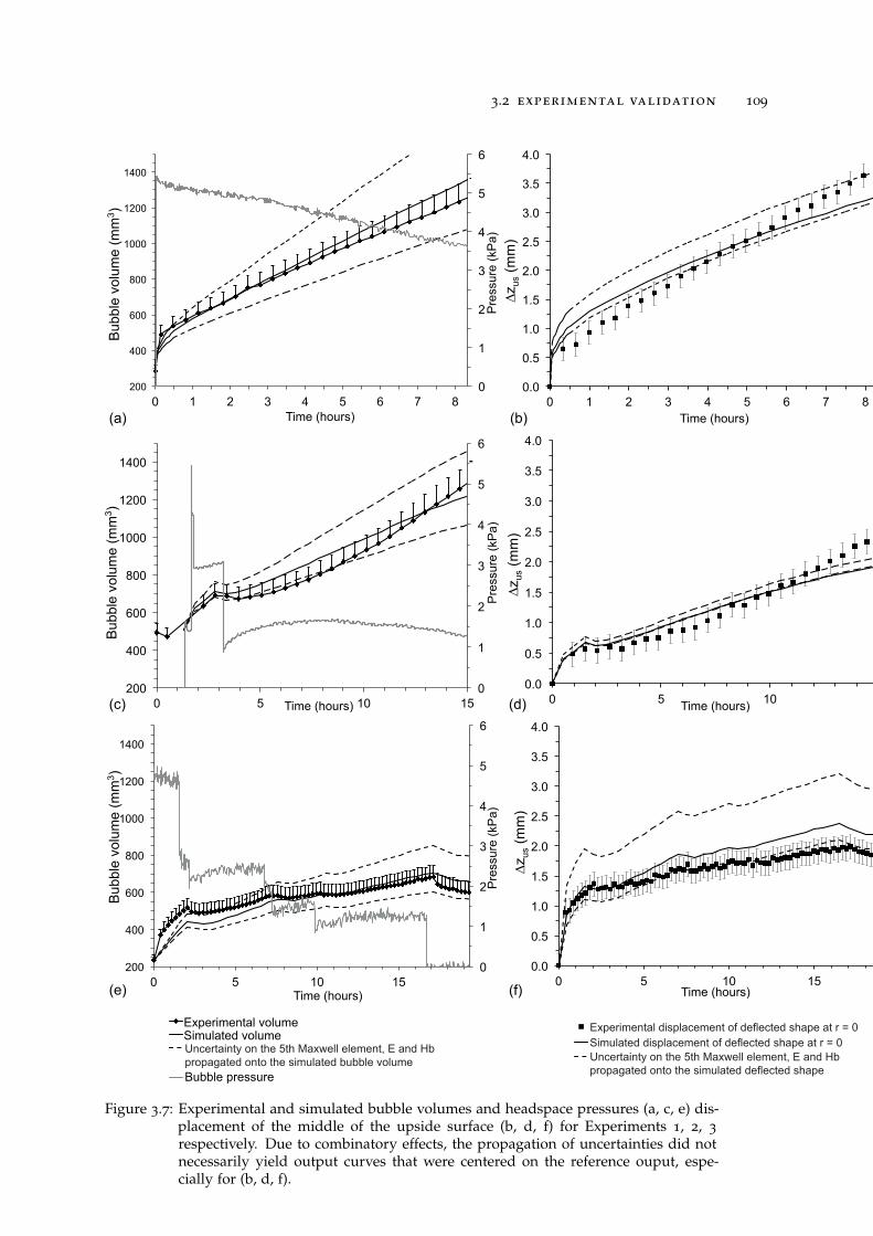
3.2 experimental validation 109
0
1
2
3
4
5
6
200
400
600
800
1000
1200
1400
0 1 2 3 4 5 6 7 8
Pre
ssur
e (k
Pa)
Bub
ble
volu
me
(mm
3 )
Time (hours) (a)
0.0
0.5
1.0
1.5
2.0
2.5
3.0
3.5
4.0
0 1 2 3 4 5 6 7 8 Time (hours) (b)
0
1
2
3
4
5
6
200
400
600
800
1000
1200
1400
0 5 10 15
Pre
ssur
e (k
Pa)
Time (hours) (c) 0.0
0.5
1.0
1.5
2.0
2.5
3.0
3.5
4.0
0 5 10 15 Time (hours) (d)
0
1
2
3
4
5
6
200
400
600
800
1000
1200
1400
0 5 10 15
Pre
ssur
e (k
Pa)
(e)
0.0
0.5
1.0
1.5
2.0
2.5
3.0
3.5
4.0
0 5 10 15 Time (hours) (f)
Simulated volume
Bubble pressure
Bub
ble
volu
me
(mm
3 )
Bub
ble
volu
me
(mm
3 )
z us (
mm
) z u
s (m
m)
z us (
mm
)
Time (hours)
Uncertainty on the 5th Maxwell element, E and Hbpropagated onto the simulated bubble volume Uncertainty on the 5th Maxwell element, E and Hb
propagated onto the simulated deflected shape
Simulated displacement of deflected shape at r = 0Experimental displacement of deflected shape at r = 0
Figure 3.7: Experimental and simulated bubble volumes and headspace pressures (a, c, e) dis-placement of the middle of the upside surface (b, d, f) for Experiments 1, 2, 3
respectively. Due to combinatory effects, the propagation of uncertainties did notnecessarily yield output curves that were centered on the reference ouput, espe-cially for (b, d, f).

4C O N C L U S I O N S
A model for mechanical deformation of a single bubble in semi-hard cheese materialwas proposed. The model was implemented to respect the experimental configura-tion as far as possible. Two types of output were considered: bubble volume anddisplacement of the upper surface of the cheese cylinder surrounding the bubble.
A sensitivity study was performed to evaluate the influence of the model inputparameters on the model output parameters. It showed that the parameters of theMaxwell element that had the longest relaxation time (α5 and λ5) were responsiblefor the long-term behaviour of the bubble. This was in agreement with the results ofFeng and Bertelo [29] on polymer foams, that used an Oldroyd-B model. This alsoconfirmed that special care should be taken when characterising the behaviour of thistype of cheese to ensure that the parameters of the Maxwell element that have thelongest relaxation time are determined with sufficient accuracy to limit the propaga-tion of uncertainties in the simulated data. Enhancing accuracy could be achieved byconsidering relaxation experiments of at least 3 to 5 times the order of magnitude ofthe longest relaxation time. However, such an experiment would require sensitivity inthe force measurement, as well as a specific device to guarantee the integrity of thecheese sample for such long durations. The use of a creep-recovery test might com-plement and increase understanding of the actual meaning of this longest relaxationtime.
Rapid and long-lasting loads were imposed on the bubble in order to mimic plausi-ble situations within cheeses: rapid loads mirrored the sudden change on handling inthe ripening room temperature while long lasting loads mirrored the natural bubblegrowth due to microbial activity. Given the uncertainties in the experimental data,the simple model proposed in this study was proved to reproduce the experimentalsituations satisfactorily, in particular for bubble volume. Validation of this model al-lows further development of the model to include mass transport phenomena that areresponsible for bubble growth in semi-hard cheeses. This stage will include at leastfour additional input parameters (carbon dioxide diffusivity, Henry’s constant, carbondioxide production rate and initial carbon dioxide concentration in cheeses). Someof these will be characterised in the conditions of the experiment and others takenfrom the literature. This more complete model will be validated against new sets ofdata involving free inflation of the bubble. In accordance with the results from thepresent study, discrepancies between these future experiments and model larger than10% will be assigned to the physics of mass transport and the associated values ofinput parameters.
111

A C K N O W L E D G M E N T S
Compression-relaxation tests on cheese were performed at the JRU Genial, Paris, di-rected by Camille Michon. The authors wish to thank her for this contribution to thework, as well as Gabrielle Moulin for technical assistance.
This study was carried out with financial support from VALORIAL and the RegionalCouncils of Bretagne, Pays de Loire and Basse-Normandie. The first author, YannickLaridon, is the holder of a grant from INRA ansd Irstea.
113

Chapitre 4
S I M U L AT I O N O F B U B B L E G R O W T H I N S E M I - H A R DC H E E S E W I T H M A S S A N D M O M E N T U M T R A N S P O RT:C O M PA R I S O N W I T H E X P E R I M E N T A N D S E N S I T I V I T Y
A N A LY S I S
The growth of a single bubble within a semi-hard cheese cylinder was in-vestigated both experimentally and by numerical simulation. Two trans-port phenomena were modelled: mass and momentum transport, and sim-ulation results were compared to the average bubble growth in industrialcheeses that were acquired with help of MRI imaging. The proposed modelproved to be able to describe the bubble growth in a qualitative manner. Asensitivity study was conducted to determine the most influent input pa-rameters on the bubble growth. The mechanical parameters did not provedto have a significant influence over bubble growth compared to the masstransport properties (carbon dioxide production and carbon dioxide diffu-sivity), that proved to be the most important parameters.Keywords: multiphysics modelling, mass transport; sensitivity analysis

1I N T R O D U C T I O N
Whilst bubbles are found in numerous food products (Campbell and Mougeot 15), themodelling of bubble growth for foodstuff is almost exclusively limited to the study ofsparkling beverages or cereal products. The studies of the first are heavily inspired bycavitation studies in liquids, while for the latter, the studies are inspired by the workson polymer foaming. The dynamics involved for the growth of bubbles in cheeseduring ripening encourages considering the present study as a continuation of workson dough proofing.
Bubble growth in polymeric foams is caused by diffusion of gas following a suddensupersaturation of a given gas in a liquid, and can be controlled by several aspectsof the foaming process: polymeric reactions, geometric and temperature conditions,blowing agent used, etc. (Amon and Denson 5). Nucleation can be caused eitherby a boiling regime (homogeneous nucleation), by the presence of nucleating agents(heterogeneous nucleation), or by a combination of both (Jones et al. 50). However,the present study did not consider nucleation but focused on the subsequent bubblegrowth, with an already significant size in diameter (higher than 4 mm).
Modelling of bubble growth in polymers covers coupling between mass and mo-mentum transport, and often considers multiple bubbles by generalising the 1-D cellmodel proposed by Amon and Denson (5). If heating is involved in the process understudy, energy transport can be included (Alavi et al. 4, Lee et al. 62). Few modellingstudies on aerated cereal products went to the extent of characterising the growth incereal products at the bubble scale (de Cindio and Correra 23, Fan et al. 28, Haile-mariam et al. 39, Shah et al. 85), this selection encompassing both modelling studieson proving and baking. The dough is often thought of as a purely viscous material,but some studies considered viscoelastic models. De Cindio and Correra (23) consid-ered the dough with a linear viscoelastic model very similar to that used in the presentstudy. They proved that, contrary to the viscous models, the use of viscoelastic consti-tutive equations allowed to reproduce cases that had asymptotic bubble volumes dueto the time-independent elastic properties of their viscoelastic modelling. Some otherstudies considered non-linear viscoelastic models, such as the Lodge model used byHailemariam et al. [39], that give a better description of the material behaviour, butnecessitate a more time consuming evaluation of the input parameters (for the Lodgemodel it enforces the knowledge of memory function for the material). They foundthat viscoelasticity of the dough tends to prevent bubbles from collapsing.
117
118 introduction
Mass transfer was proved to be the main contributing factor to bubble growth duringproving (Hailemariam et al. 39, de Cindio and Correra 23). Mass transport in the liquidphase can be modelled by Fick’s law and applied to the phases where carbon dioxide issoluble (liquid water and liquid fat in the case of cheese, Jakobsen et al. 48). Exchangesat the bubble-material interface are often described using the Henry’s law. Shah et al.[85] discussed the influence of the carbon dioxide saturation on the bubble growth, andshowed that for subsaturation regime, bubbles were to have an asymptotic size, thatwas influenced mainly by the initial bubble size and carbon dioxide concentration. Forsupersaturation regime, they showed that above a critical size, bubble growth wouldhappen indefinitely. No asymptotic bubble size could be observed in the same type ofcheese like that studied in this paper (Huc et al. 44) evidencing that supersaturationalso happens in the semi-hard cheese under study.
Despite the similarity of the driving phenomena between bread dough proving andcheese ripening, some differences have to be underlined. The growth kinetics are sub-stantially higher for cereal products: the bread making process takes several hours,whereas it takes several weeks of ripening for semi-hard cheese. This discrepancyin the kinetics may be explained by differences in the microbiological phenomena in-volved. Carbon dioxide production in semi-hard cheese is caused by propionic fermen-tation, whereas it is caused by alcoholic fermentation for bread dough, and the optimalconditions of carbon dioxide production, in terms of temperature or pH for instance,highly differ between the two processes. The bubble growth kinetics is also influencedby the mechanical behaviour of the material surrounding the bubbles. Although bothmaterials (dough and cheese) are viscoelastic materials with similar relaxation timespectrum (Keentok et al. 51), viscoelasticity of cheese is one to two orders of magni-tude higher than that of cereal doughs (Launay and Michon 59). At last, bread doughis also a highly porous product: about 70-80% in porosity, compared to about 10% forsemi-hard cheeses; it involves bubbles that are smaller (a couple of millimetres at theend of proving, compared to a couple of centimetres at the end of cheese ripening),and for which surface tension may not be negligible.
Experimental validation of the models focused on dough, when implemented, oftentook place at a macroscopic level, by using overall morphologic descriptors (Fan et al.28, Chiotellis and Campbell 16). Both characteristic size of bubble and their rate ofgrowth in cheese are compatible with tomographic monitoring, hence offering thepossibility to validate the modelling at a single bubble level.
For appropriate validation, the model of transport has also to be fed with values ofseveral input parameters, specific for semi-hard cheeses, such as carbon dioxide diffu-sivity, solubility and production rate. Characterisation of these parameters for cheeseis sparsely covered in the literature, despite a great interest from the cheese-makingcommunity. There is, as far as we know, no paper dedicated to the estimation of car-bon dioxide diffusivity in semi-hard cheese. Numerous studies, however, were doneon modified atmosphere packaging, and covered the exchange of carbon dioxide at
introduction 119
the product interface. The interest of these studies is to provide data on interfacialtransfers for a wide variety of products, for instance the work on Swiss-type cheese byBlanc et al. [10]. If such studies give a hint of the carbon dioxide production withincheese, they fail to disentangle the respective influence of diffusion and productionwithin the product by focusing on the interface only. Rodriguez-Aguilera et al. [80]and Vivier et al. [91] successfully estimated carbon dioxide production rate, but theirstudy was applied to soft cheeses, for which the fermentation mechanism differedfrom that of semi-hard cheeses. In semi-hard cheeses, the carbon dioxide productionoriginates from propionic fermentation, but also from proteolysis (to a lesser extent,only 20%, Actilait 1). Propionic fermentation is a well-described phenomenon, andthe influence of various process-related factors has already been covered, such as saltcontent (Boyaval et al. 11, Huc et al. 45), type of bacterial strain (White et al. 92) ortemperature (Richoux et al. 79). These factors can induce huge variations in the micro-bial activity, and may therefore, among other parameters, influence the carbon dioxideproduction within the cheese (Huc et al. 45). At last, some studies have estimated thecarbon dioxide solubility in cheese, but on the whole cheese block, and only at the endof the ripening (Seuvre and Mathlouthi 84, Jakobsen et al. 48).
The purpose of the present paper was to model the coupled momentum and masstransport in the case of a single bubble growth in semi-hard cheese. Indeed, the me-chanics involved in the bubble growth were already validated on a separate experi-ment involving known pressure forces (Laridon et al. 58) , allowing the focus of thepresent study on mass transport and its coupling with momentum transport. Thestudy aimed at sorting out model parameters that are the most influential on bubblegrowth. This was based on a compilation of literature data for input parameters butalso on the measurement of carbon dioxide production rate in our specific case. Thebubble growth monitored by MRI (Magnetic Resonance Imaging) and X-Ray Imagingon industrial cheese blocks during ripening (hot room) served as the reference for thisdiscussion.

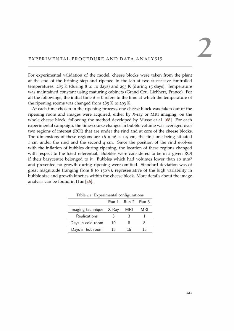
2E X P E R I M E N TA L P R O C E D U R E A N D D ATA A N A LY S I S
For experimental validation of the model, cheese blocks were taken from the plantat the end of the brining step and ripened in the lab at two successive controlledtemperatures: 285 K (during 8 to 10 days) and 293 K (during 15 days). Temperaturewas maintained constant using maturing cabinets (Grand Cru, Liebherr, France). Forall the followings, the initial time d = 0 refers to the time at which the temperature ofthe ripening rooms was changed from 285 K to 293 K.
At each time chosen in the ripening process, one cheese block was taken out of theripening room and images were acquired, either by X-ray or MRI imaging, on thewhole cheese block, following the method developed by Musse et al. [68]. For eachexperimental campaign, the time-course changes in bubble volume was averaged overtwo regions of interest (ROI) that are under the rind and at core of the cheese blocks.The dimensions of these regions are 16 × 16 × 1.5 cm, the first one being situated1 cm under the rind and the second 4 cm. Since the position of the rind evolveswith the inflation of bubbles during ripening, the location of these regions changedwith respect to the fixed referential. Bubbles were considered to be in a given ROIif their barycentre belonged to it. Bubbles which had volumes lower than 10 mm3
and presented no growth during ripening were omitted. Standard deviation was ofgreat magnitude (ranging from 8 to 150%), representative of the high variability inbubble size and growth kinetics within the cheese block. More details about the imageanalysis can be found in Huc [46].
Table 4.1: Experimental configurations
Run 1 Run 2 Run 3
Imaging technique X-Ray MRI MRIReplications 3 3 1
Days in cold room 10 8 8Days in hot room 15 15 15
121

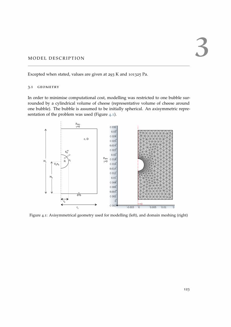
3M O D E L D E S C R I P T I O N
Excepted when stated, values are given at 293 K and 101325 Pa.
3.1 geometry
In order to minimise computational cost, modelling was restricted to one bubble sur-rounded by a cylindrical volume of cheese (representative volume of cheese aroundone bubble). The bubble is assumed to be initially spherical. An axisymmetric repre-sentation of the problem was used (Figure 4.1).
γ=0
γ=0
Figure 4.1: Axisymmetrical geometry used for modelling (left), and domain meshing (right)
123
124 model description
3.2 hypotheses
Cheese was considered nearly-incompressible, with a Poisson ratio ν at 0.49. Its com-position (other than CO2), mechanical and diffusive properties were considered homo-geneous at the scale considered. Carbon dioxide was also considered to be producedhomogeneously. Although carbon dioxide is soluble in the fat fraction of the cheese,diffusion of carbon dioxide in fat was considered to be negligible compared to thatin the water phase, so that only carbon dioxide in the aqueous phase was considered.Within the bubble, pressure was considered uniform and gases other than carbon diox-ide were neglected. Temperature was considered uniform and constant.
3.3 mechanical behaviour
The behaviour of the cheese was modelled with a 5-element generalised Maxwellmodel described earlier in a dedicated paper (Laridon et al. 57). The mechanicalequilibrium was expressed through the conservation of momentum:
∇ · σ = ρg (4.1)
Stress was calculated as the sum of elastic and viscoelastic parts and the viscoelasticpart was described by the Maxwell model. (Laridon et al. 57).
3.4 mass transport
Mass diffusion was described according to Fick’s law; mass conservation writes asfollows:
∂c∂t− Dch
CO2∆c = rCO2 (4.2)
where c is the number of moles of carbon dioxide in the water phase of cheese bycubic meter of cheese, later denoted as the apparent carbon dioxide concentration inthe domain, Dch
CO2the apparent diffusivity of carbon dioxide in cheese (section 4.2) and
rCO2 the carbon dioxide production rate within the cheese domain (section 4.1). Carbondioxide is also dissolved in the fat phase, but it was assumed, as a first approach, thatthis amount of carbon dioxide did not vary during bubble growth (no exchange withthe aqueous and gaseous phases, no diffusion nor production in the fat phase).
The equilibrium at the gas-cheese interface was expressed according to Henry’s law:
ci = kchH pi (4.3)
where ci is the apparent carbon dioxide concentration at the interface, pi the pressureexerted by the gas on the interface and kch
H the Henry’s constant for carbon dioxide incheese (section 4.3.1).
3.5 coupling of transport phenomena 125
The atmospheric pressure patm is used as the reference pressure in the mechanicalaspects.
3.5 coupling of transport phenomena
The carbon dioxide flux at the gas-cheese interface ji can be written as:
ji = −DchCO2
(∇c)i · n (4.4)
where n is the normal vector of the interface. This flux was numerically computedas:
ji = γ(
ci − kchH pi
)(4.5)
where γ is the transfer coefficient at the interface. To ensure that the effect of diffu-sion in the cheese was limiting, the Biot number for mass transport was set at a highvalue (10
5):
Bim =γL
DchCO2
(4.6)
This implied that γ was set at a high value and assured conditions very near toequilibrium (γ → ∞ leads to Eq. 4.3). Characteristic length L was set at 20 mm, asit was the typical length between the gas-cheese interface and the boundaries of thedomain (Figure 4.1).
The evolution with time of the quantity of CO2 in the gaseous phase, dnbdt , was de-
duced from the CO2 flux:dnb
dt=∫
Γi
jidSi (4.7)
where Γi is the gas-cheese interface boundary and Si its surface. Using Eqns. 4.5 and4.7, and the ideal gas law, the following ODE was solved at the gas-cheese interface:
dnb
dt= γ
∫Γi
cidSi − γkchH RT
Si
Vbnb (4.8)
where Vb is the volume of the gaseous phase (bubble). The quantity of CO2 deter-mined with Eq. 4.8 was used to calculate the pressure of the gas at the interface withthe cheese domain, following the ideal gas law:
pi =nbRT
Vb(4.9)
The pressure calculated by Eq. 4.9 was used as mechanical boundary condition atthe gas-cheese interface (Eq. 4.11), and therefore constitutes the coupling between massand momentum transports.
126 model description
3.6 boundary conditions
Mechanical boundary conditions
In order to prevent unrealistic displacement of the domain, a roller boundary conditionwas applied at the lower surface:
u · n = 0 (4.10)
where u is the displacement field. Pressure calculated through Eq. 4.9 was appliedat the bubble-cheese interface:
σi · n = − (pi − patm) (4.11)
where σi is the stress applied to the gas-cheese interface.All other boundaries were let free of stress.
Mass transport boundary conditions
There was no flux of CO2 at the boundaries of the cheese cylinder, except at the inter-face with the bubble, where the flux calculated by Eq. 4.5 was used.
Under these conditions, the growth of a bubble is considered with no mechanicalconstraint other than that exerted by the cheese material itself (restricted at the bound-aries of the cheese cylinder which contents a representative volume of cheese aroundone bubble). Mechanical interactions between adjacent bubbles were not reproduced.All the CO2 produced in the cylinder diffuses toward the bubble; competition for CO2
between adjacent bubbles, or large-scale diffusion between regions of low and highCO2 content at the cheese block scale were not taken into account by the model.
3.7 initial conditions
It is considered that at a time denoted by tsat the cheese is saturated in CO2. All thesimulations began at this saturation time, with t defined as t = d − tsat. The initialbubble radius rb in the simulation was set at the average experimental value observedat that time.
Mechanical initial conditions
Equilibrium at the atmospheric pressure was considered, so that:
pi (t = 0) = patm (4.12)
3.8 numerical implementation and calculations 127
Mass transport initial conditions
Following the initial saturation hypothesis, initial carbon dioxide concentration withinthe domain was defined as:
c (t = 0) = kchH patm (4.13)
The initial CO2 quantity in the bubble was calculated with the help of ideal gas law:
nb (t = 0) =patmVb (tsat)
RT(4.14)
3.8 numerical implementation and calculations
The model was implemented in COMSOL Multiphysics (COMSOL AB, Sweden) usinga 2-D axisymmetric geometry.
The domain was meshed using triangular elements and was refined near the bubbleinterface (Figure 4.1). Simulations were conducted from the time at which saturationin CO2 is reached to the end of hot room ripening (15 days).
Bubble volume was estimated at each time step using the following integral on thegas interface:
Vb = −∫
Γi
πr2n · erdl (4.15)
where er is the unitary base vector, in r-direction.

4E S T I M AT I O N O F VA L U E S F O R I N P U T PA R A M E T E R S
4.1 carbon dioxide production rate
Carbon dioxide production rates, rCO2 , were measured on the same type of cheese asthat used in the experiment, both at core and under rind (same locations as mentionedin section 2 for the analysis of bubble volume). Cheese blocks used for these mea-surements were from different batches than those studied according to the protocoldefined in section 2 (data for validation of the model); different batches were used tocharacterise the inter-batch variability.
About 20 cheese disks (2 mm thick at most) were deposited in a sealed bottle ontosmall grids of large mesh and separated from the other disks by a sustaining stand.The full device is detailed in Huc et al. [45]. The total mass of cheese disks in a bottle,mch (about 25 g), was measured before each experiment.
The bottles were initially filled with N2 at atmospheric pressure, and placed in atemperature-controlled ambiance at 293 K. Nitrogen recreated the nonaerobic condi-tions of bacterial growth during cheese ripening and also avoid the growth of moulds.
The pressure of the gas within the bottle, p(t), was monitored over duration rele-vant of the ripening process (hot room). The time-course changes in pressure wereattributed to the production of carbon dioxide only. Measurements were assumed tobe diffusion-independent, because of the very low thickness of the cheese disks.
The gaseous volume, Vgas, surrounding the cheese disks was estimated by subtract-ing the volume occupied by the cheese disks and the sustaining stand to the overallbottle volume. The bottle volume was determined by filling the bottle with water andcalculating the volume by weighing the water. The number of moles of CO2 producedat a given time per volume of cheese was deduced from the pressure, using the idealgas law:
produced CO2 =ρch
mch(p(t)− patm)Vgas
RT(4.16)
The amount of CO2 produced during the experiment relative to the cheese volumeis presented in Figure 4.2.
At the very beginning of the experiment (until one day at most), a slight decreasein pressure could be observed and was attributed to the entrance of nitrogen into thecheese.
129
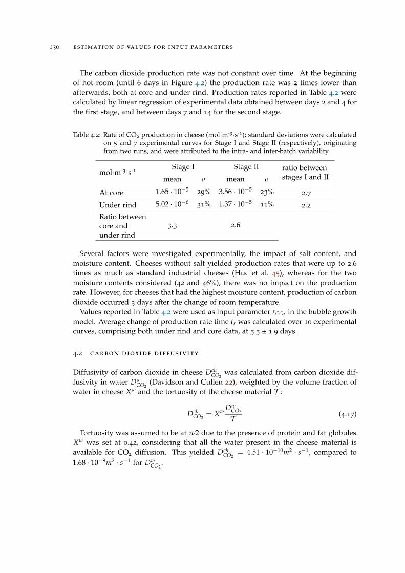
130 estimation of values for input parameters
The carbon dioxide production rate was not constant over time. At the beginningof hot room (until 6 days in Figure 4.2) the production rate was 2 times lower thanafterwards, both at core and under rind. Production rates reported in Table 4.2 werecalculated by linear regression of experimental data obtained between days 2 and 4 forthe first stage, and between days 7 and 14 for the second stage.
Table 4.2: Rate of CO2 production in cheese (mol·m-3·s-1); standard deviations were calculatedon 5 and 7 experimental curves for Stage I and Stage II (respectively), originatingfrom two runs, and were attributed to the intra- and inter-batch variability.
mol·m-3·s-1 Stage I Stage II ratio betweenstages I and IImean σ mean σ
At core 1.65 · 10−529% 3.56 · 10−5
23% 2.7
Under rind 5.02 · 10−631% 1.37 · 10−5
11% 2.2
Ratio betweencore andunder rind
3.3 2.6
Several factors were investigated experimentally, the impact of salt content, andmoisture content. Cheeses without salt yielded production rates that were up to 2.6times as much as standard industrial cheeses (Huc et al. 45), whereas for the twomoisture contents considered (42 and 46%), there was no impact on the productionrate. However, for cheeses that had the highest moisture content, production of carbondioxide occurred 3 days after the change of room temperature.
Values reported in Table 4.2 were used as input parameter rCO2 in the bubble growthmodel. Average change of production rate time tr was calculated over 10 experimentalcurves, comprising both under rind and core data, at 5.5 ± 1.9 days.
4.2 carbon dioxide diffusivity
Diffusivity of carbon dioxide in cheese DchCO2
was calculated from carbon dioxide dif-fusivity in water Dw
CO2(Davidson and Cullen 22), weighted by the volume fraction of
water in cheese Xw and the tortuosity of the cheese material T :
DchCO2
= Xw DwCO2
T (4.17)
Tortuosity was assumed to be at π⁄2 due to the presence of protein and fat globules.Xw was set at 0.42, considering that all the water present in the cheese material isavailable for CO2 diffusion. This yielded Dch
CO2= 4.51 · 10−10m2 · s−1, compared to
1.68 · 10−9m2 · s−1 for DwCO2
.
4.3 carbon dioxide concentration in cheese and saturation 131
4.3 carbon dioxide concentration in cheese and saturation
Here are considered values in cheese material and in pure water.
4.3.1 Estimation of CO2 saturation
CO2 concentration at saturation can be estimated from the Henry’s constant valuereported in the literature. Temperature dependency of kw
H is given by:
kwH = kw
H (Tstd) exp(−∆H
R
(1T− 1
Tstd
))(4.18)
where Tstd = 298 K, T is the temperature of the hot room in the ripening process (293
K), kwH (Tstd) =2.92·10
-4 mol·m-3·Pa-1 (Sander 82), and ∆H the standard enthalpy set at1.995·10
-4 J·mol-1 (Sander 82), R is the ideal gas constant (8.314 J·mol-1·K-1). Henry’sconstant equivalent for the cheese considered can be determined from the Henry’sconstant for CO2 in pure water, using Eq. 4.19:
kchH = Xwkw
H (4.19)
where Xw is the volumetric fraction of water in cheese (0.42).Total pressure within the bubbles is of the same order of magnitude than the at-
mospheric pressure, with a slight overpressure (about 2%, Grenier et al. 37), and thebubbles contain mainly carbon dioxide. CO2 concentration at saturation in pure watersw under the same conditions is given by:
sw = patmkwH (4.20)
where kwH is Henry’s constant value. This yielded a value of 29.6 moles of CO2 per
m3 of pure water at 293K. CO2 concentration expected at saturation in the water phasein cheese sch was found to be equal to 12.45 moles of CO2 per m3 of cheese.
4.3.2 Estimation of CO2 concentration directly on cheese material
In Danish semi-hard cheese after equilibration with carbon dioxide
Carbon dioxide concentration was estimated by a titration method (Jakobsen et al. 48).Cheese samples extracted from semi-hard cheeses ready to be sold (hence for whichripening was advanced and stopped by low temperature) and equilibrated with differ-ent levels of partial pressure of carbon dioxide. After equilibration, these samples wereput in perchloric acid solution in a Buchner connected to another Buchner containingBa(OH)2. This stage lasted about 20h, and then the dissolved CO2 in the precipitatewas estimated with HCl titration. Concentration xCO2 was expressed as a volume of
132 estimation of values for input parameters
carbon dioxide per mass of cheese. For semi-hard cheeses at 293 K and with a partialpressure of carbon dioxide equals to the atmospheric pressure, they found values of0.5 10-3 m3·kg-1, that were consistent with previous results on Swiss-type cheeses byPauchard et al. [73]. In order to be expressed in mol·m-3, the following conversion wasperformed:
sw+ f atCO2
= xCO2 (t∞)ρCO2 ρch
MCO2
(4.21)
where ρch =1030 kg·m-3, MCO2 =4.4·10-2 kg·mol-1, ρCO2 =1.842 kg·m-3 (Perry 75).
This yielded a concentration value at saturation of schCO2
= 22 mol·of CO2 per m3 ofcheese. Note that this amount of carbon dioxide is located both in the water and fatphases.
In semi-hard cheese used in this study
Carbon dioxide concentration was measured by a titration method similar to that usedby Jakobsen et al. [48] on the same type of cheese as that used in the experiment, bothat core and under rind (same locations indicated in section 2) at the very beginning ofthe hot room. Concentration x′CO2
was expressed in moles of carbon dioxide per kg ofcheese, the values were therefore converted in mol·m-3 with the cheese density:
cw+ f atCO2
(d = 0) = x′CO2(d = 0)ρch (4.22)
where ρch is also set at 1030 kg·m-3. This yielded the following concentration val-ues, 16.1 ± 1.4 and 20.6 ± 1.5 moles·of CO2 per m3 of cheese under the rind and atcore respectively. The standard deviation corresponded to the intra-batch variability.Reproducibility (inter-batch variability) was not characterized.
4.3.3 Comparison between experimental CO2 concentration and expected concentration atsaturation
On the one hand, carbon dioxide in cheese is dissolved both in water and fat phases.Measured carbon dioxide concentration in cheeses can be compared with the theo-retical value by estimating the amount of carbon dioxide dissolved in the fat phase.Considering that, at the temperature under study, carbon dioxide concentration in thefat phase is approximately equal to that in the water phase as assumed at saturationby Jakobsen et al. 48:
cw+ f atCO2
=(
Xw + X f at)
cwCO2
(4.23)
where cwCO2
is the theoretical carbon dioxide concentration in the water phase.On the other hand, for the simulations, the apparent carbon dioxide concentration c
was used, that is the amount of carbon dioxide dissolved only in the water phase percubic meter of cheese. Therefore:
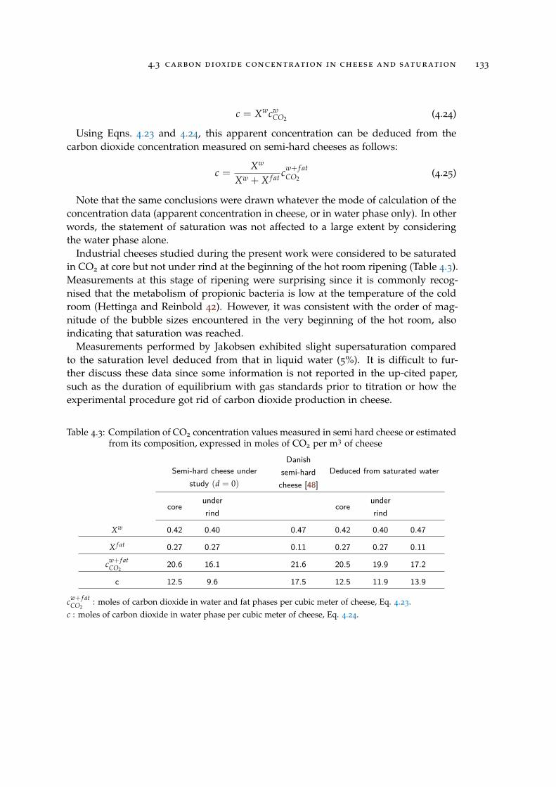
4.3 carbon dioxide concentration in cheese and saturation 133
c = XwcwCO2
(4.24)
Using Eqns. 4.23 and 4.24, this apparent concentration can be deduced from thecarbon dioxide concentration measured on semi-hard cheeses as follows:
c =Xw
Xw + X f at cw+ f atCO2
(4.25)
Note that the same conclusions were drawn whatever the mode of calculation of theconcentration data (apparent concentration in cheese, or in water phase only). In otherwords, the statement of saturation was not affected to a large extent by consideringthe water phase alone.
Industrial cheeses studied during the present work were considered to be saturatedin CO2 at core but not under rind at the beginning of the hot room ripening (Table 4.3).Measurements at this stage of ripening were surprising since it is commonly recog-nised that the metabolism of propionic bacteria is low at the temperature of the coldroom (Hettinga and Reinbold 42). However, it was consistent with the order of mag-nitude of the bubble sizes encountered in the very beginning of the hot room, alsoindicating that saturation was reached.
Measurements performed by Jakobsen exhibited slight supersaturation comparedto the saturation level deduced from that in liquid water (5%). It is difficult to fur-ther discuss these data since some information is not reported in the up-cited paper,such as the duration of equilibrium with gas standards prior to titration or how theexperimental procedure got rid of carbon dioxide production in cheese.
Table 4.3: Compilation of CO2 concentration values measured in semi hard cheese or estimatedfrom its composition, expressed in moles of CO2 per m3 of cheese
Semi-hard cheese understudy (d = 0)
Danishsemi-hardcheese [48]
Deduced from saturated water
coreunderrind
coreunderrind
Xw 0.42 0.40 0.47 0.42 0.40 0.47
X f at 0.27 0.27 0.11 0.27 0.27 0.11
cw+ f atCO2
20.6 16.1 21.6 20.5 19.9 17.2
c 12.5 9.6 17.5 12.5 11.9 13.9
cw+ f atCO2
: moles of carbon dioxide in water and fat phases per cubic meter of cheese, Eq. 4.23.c : moles of carbon dioxide in water phase per cubic meter of cheese, Eq. 4.24.

134 estimation of values for input parameters
4.4 mechanical properties of cheese
Values of the parameters of the Maxwell model were fixed according to the averagevalue that was determined on the same type of semi-cheese than the one under study.See section 2.4 of Laridon et al. [58].

4.4 mechanical properties of cheese 135
-2
0
2
4
6
8
10
0 2 4 6 8 10 12 14
Pro
duce
d C
O2 (
mol
.m-3
)
Time (days)
Stage I Stage II
-5
0
5
10
15
20
25
30
0 2 4 6 8 10 12 14
Pro
duce
d C
O2 (
mol
.m-3
)
Time (days)
Stage I Stage II
Figure 4.2: Carbon dioxide production under rind (top) and at core (bottom) at 293K. Tworeplications are shown for each graph, i.e. one bottle for each replication.

5R E S U LT S A N D D I S C U S S I O N
A sensitivity study was performed in order to characterise the relative influence of themodel inputs on the outputs i.e. the bubble growth. The objective was, if necessary,and despite the care paid to the estimation of input parameters, to adjust the valueof one input parameter most influential and for which the estimate was not enoughaccurate. Table 4.4 summarises the upper, lower and reference values used for eachinput parameter. Each parameter was varied separately, all other parameters beingkept at their reference values.
Reference values of the input parameters reported in Table 4.4 were relevant of thecore of the cheese block. For the mechanical aspects, only the relaxation properties ofthe last Maxwell element were considered, as they proved to be the most influentialparameters on bubble growth (Laridon et al. 58); their variations corresponded to theinter-batch variability. Diffusivity was swept with a +50% and -75% variation to coverextreme variations in diffusivity within the cheese, and to take into account that allthe water contained within the cheese may not be available for the carbon dioxide todiffuse. Production rate was swept according to the inter-batch variability estimatedin section 4.1, taking into account the highest standard deviation obtained betweenstages I and II. Since the inter-batch variability of tsat was unknown, large variations intsat were tested in the sensitivity study, with two extremes values: the first consideredthe case when saturation is reached at the middle of the hot room ripening, the secondconsidered the case when saturation is reached near the end of the ripening.
In order to rank the most influential parameters on bubble growth, sensitivity in-dices Ik were calculated for each input parameter Xk as:
Ik = 100
∣∣∣∣∣Vb(Xmaxk )−Vb
(Xre f
k
)Vb
(Xre f
k
)∣∣∣∣∣+∣∣∣∣∣Vb(Xmin
k )−Vb
(Xre f
k
)Vb
(Xre f
k
)∣∣∣∣∣∣∣∣∣Xmax
k −Xre fk
Xre fk
∣∣∣∣+ ∣∣∣∣Xmink −Xre f
k
Xre fk
∣∣∣∣ (4.26)
The sensitivity indices were assessed at the end of the simulations (15 days). Theseresults are represented in Table 4.4. Some are also compared to the experimental dataat the corresponding location (Figure 4.3).
137
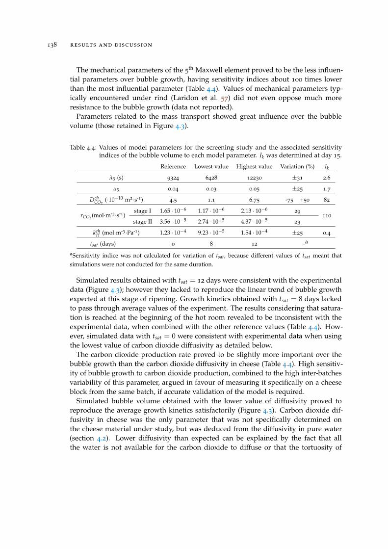
138 results and discussion
The mechanical parameters of the 5th Maxwell element proved to be the less influen-
tial parameters over bubble growth, having sensitivity indices about 100 times lowerthan the most influential parameter (Table 4.4). Values of mechanical parameters typ-ically encountered under rind (Laridon et al. 57) did not even oppose much moreresistance to the bubble growth (data not reported).
Parameters related to the mass transport showed great influence over the bubblevolume (those retained in Figure 4.3).
Table 4.4: Values of model parameters for the screening study and the associated sensitivityindices of the bubble volume to each model parameter. Ik was determined at day 15.
Reference Lowest value Highest value Variation (%) Ik
λ5 (s) 9324 6428 12230 ±31 2.6
α5 0.04 0.03 0.05 ±25 1.7
DchCO2
(·10−10 m2·s-1) 4.5 1.1 6.75 -75 +50 82
rCO2 (mol·m-3·s-1)stage I 1.65 · 10−6 1.17 · 10−6 2.13 · 10−6
29
110
stage II 3.56 · 10−5 2.74 · 10−5 4.37 · 10−523
kchH (mol·m-3·Pa-1) 1.23 · 10−4 9.23 · 10−5 1.54 · 10−4 ±25 0.4
tsat (days) 0 8 12 -a
aSensitivity indice was not calculated for variation of tsat, because different values of tsat meant thatsimulations were not conducted for the same duration.
Simulated results obtained with tsat = 12 days were consistent with the experimentaldata (Figure 4.3); however they lacked to reproduce the linear trend of bubble growthexpected at this stage of ripening. Growth kinetics obtained with tsat = 8 days lackedto pass through average values of the experiment. The results considering that satura-tion is reached at the beginning of the hot room revealed to be inconsistent with theexperimental data, when combined with the other reference values (Table 4.4). How-ever, simulated data with tsat = 0 were consistent with experimental data when usingthe lowest value of carbon dioxide diffusivity as detailed below.
The carbon dioxide production rate proved to be slightly more important over thebubble growth than the carbon dioxide diffusivity in cheese (Table 4.4). High sensitiv-ity of bubble growth to carbon dioxide production, combined to the high inter-batchesvariability of this parameter, argued in favour of measuring it specifically on a cheeseblock from the same batch, if accurate validation of the model is required.
Simulated bubble volume obtained with the lower value of diffusivity proved toreproduce the average growth kinetics satisfactorily (Figure 4.3). Carbon dioxide dif-fusivity in cheese was the only parameter that was not specifically determined onthe cheese material under study, but was deduced from the diffusivity in pure water(section 4.2). Lower diffusivity than expected can be explained by the fact that allthe water is not available for the carbon dioxide to diffuse or that the tortuosity of
results and discussion 139
the material has been underestimated. Indeed, tortuosity was set at π/2 under thehypothesis that fat and protein were spherical, but because of the cheese structurecomplexity, the tortuosity value may be higher. This also encourages further effort forexperimental characterisation of carbon dioxide diffusivity in cheese. Let us remindform the introduction section that there is ni such data in the literature.
It is interesting to note that the acceleration of the bubble growth expected beyondthe saturation can be postponed by several days because of the low levels of diffusivity,hence calling in question the previously published conclusions about the saturationtime (Huc et al. [44]).
At last, the Henry’s constant did not present much influence on the bubble growth(Table 4.4), meaning that the first approximation of the carbon dioxide concentrationat saturation used in Eq. 4.20 was sufficient.
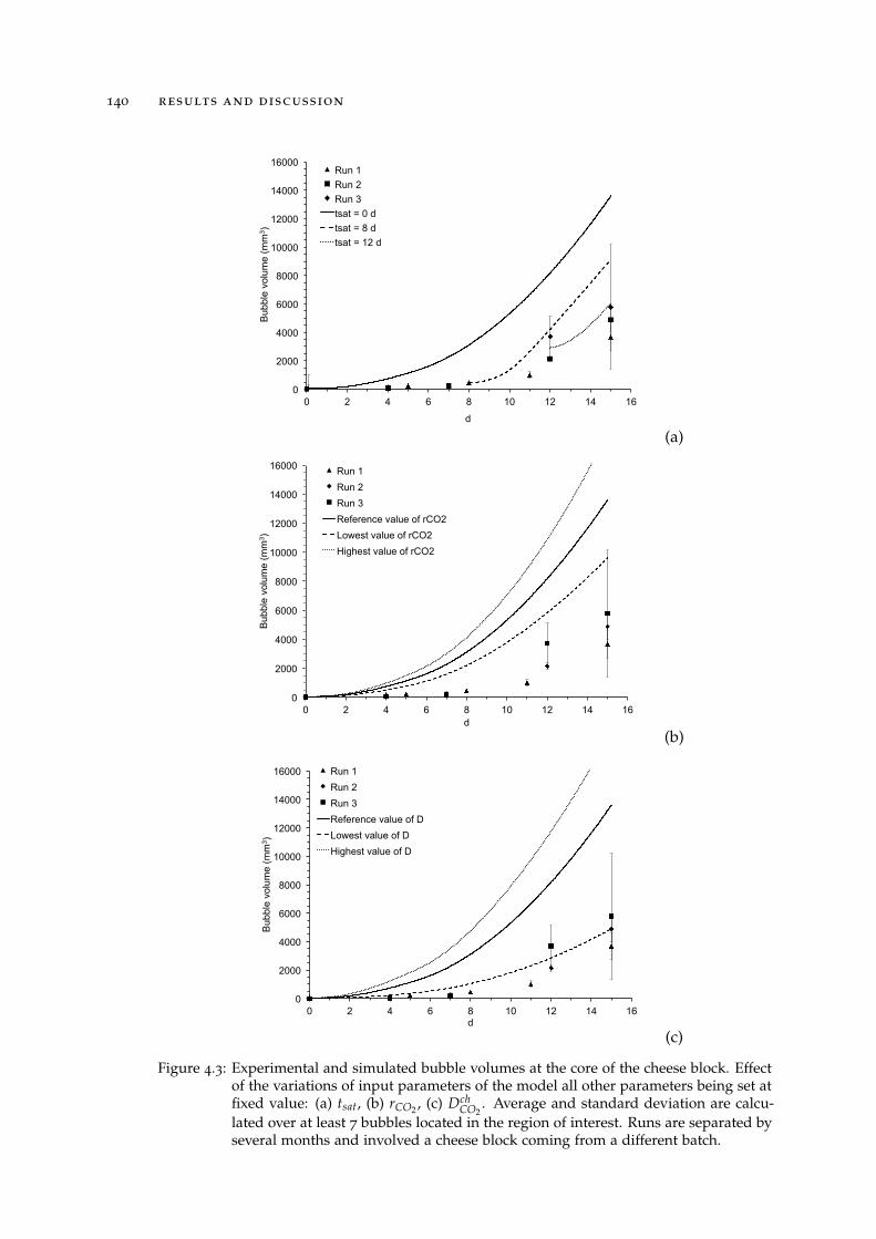
140 results and discussion
0
2000
4000
6000
8000
10000
12000
14000
16000
0 2 4 6 8 10 12 14 16
Bub
ble
volu
me
(mm
3 )
d
Run 1 Run 2 Run 3 tsat = 0 d tsat = 8 d tsat = 12 d
(a)
0
2000
4000
6000
8000
10000
12000
14000
16000
0 2 4 6 8 10 12 14 16
Bub
ble
volu
me
(mm
3 )
d
Run 1 Run 2 Run 3 Reference value of rCO2 Lowest value of rCO2 Highest value of rCO2
(b)
0
2000
4000
6000
8000
10000
12000
14000
16000
0 2 4 6 8 10 12 14 16
Bub
ble
volu
me
(mm
3 )
d
Run 1 Run 2 Run 3 Reference value of D Lowest value of D Highest value of D
(c)
Figure 4.3: Experimental and simulated bubble volumes at the core of the cheese block. Effectof the variations of input parameters of the model all other parameters being set atfixed value: (a) tsat, (b) rCO2 , (c) Dch
CO2. Average and standard deviation are calcu-
lated over at least 7 bubbles located in the region of interest. Runs are separated byseveral months and involved a cheese block coming from a different batch.
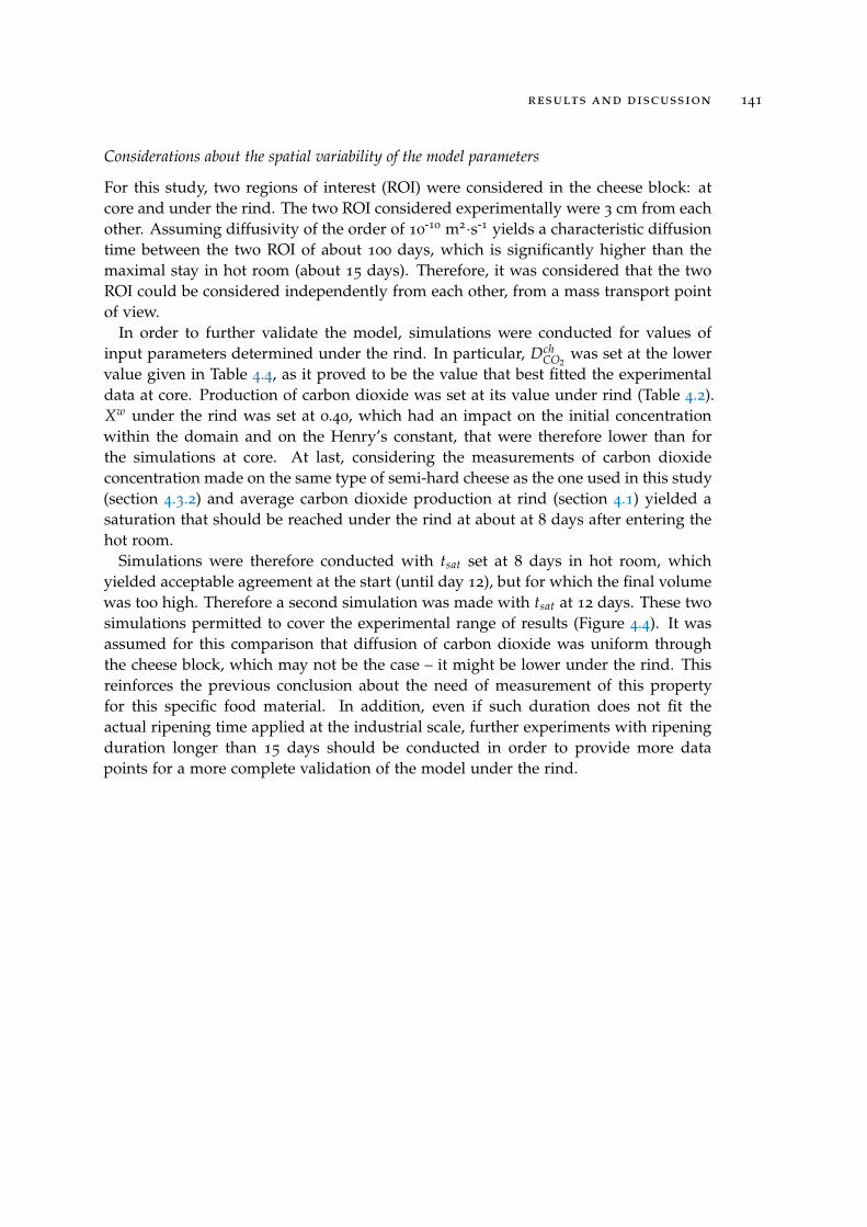
results and discussion 141
Considerations about the spatial variability of the model parameters
For this study, two regions of interest (ROI) were considered in the cheese block: atcore and under the rind. The two ROI considered experimentally were 3 cm from eachother. Assuming diffusivity of the order of 10
-10 m2·s-1 yields a characteristic diffusiontime between the two ROI of about 100 days, which is significantly higher than themaximal stay in hot room (about 15 days). Therefore, it was considered that the twoROI could be considered independently from each other, from a mass transport pointof view.
In order to further validate the model, simulations were conducted for values ofinput parameters determined under the rind. In particular, Dch
CO2was set at the lower
value given in Table 4.4, as it proved to be the value that best fitted the experimentaldata at core. Production of carbon dioxide was set at its value under rind (Table 4.2).Xw under the rind was set at 0.40, which had an impact on the initial concentrationwithin the domain and on the Henry’s constant, that were therefore lower than forthe simulations at core. At last, considering the measurements of carbon dioxideconcentration made on the same type of semi-hard cheese as the one used in this study(section 4.3.2) and average carbon dioxide production at rind (section 4.1) yielded asaturation that should be reached under the rind at about at 8 days after entering thehot room.
Simulations were therefore conducted with tsat set at 8 days in hot room, whichyielded acceptable agreement at the start (until day 12), but for which the final volumewas too high. Therefore a second simulation was made with tsat at 12 days. These twosimulations permitted to cover the experimental range of results (Figure 4.4). It wasassumed for this comparison that diffusion of carbon dioxide was uniform throughthe cheese block, which may not be the case – it might be lower under the rind. Thisreinforces the previous conclusion about the need of measurement of this propertyfor this specific food material. In addition, even if such duration does not fit theactual ripening time applied at the industrial scale, further experiments with ripeningduration longer than 15 days should be conducted in order to provide more datapoints for a more complete validation of the model under the rind.
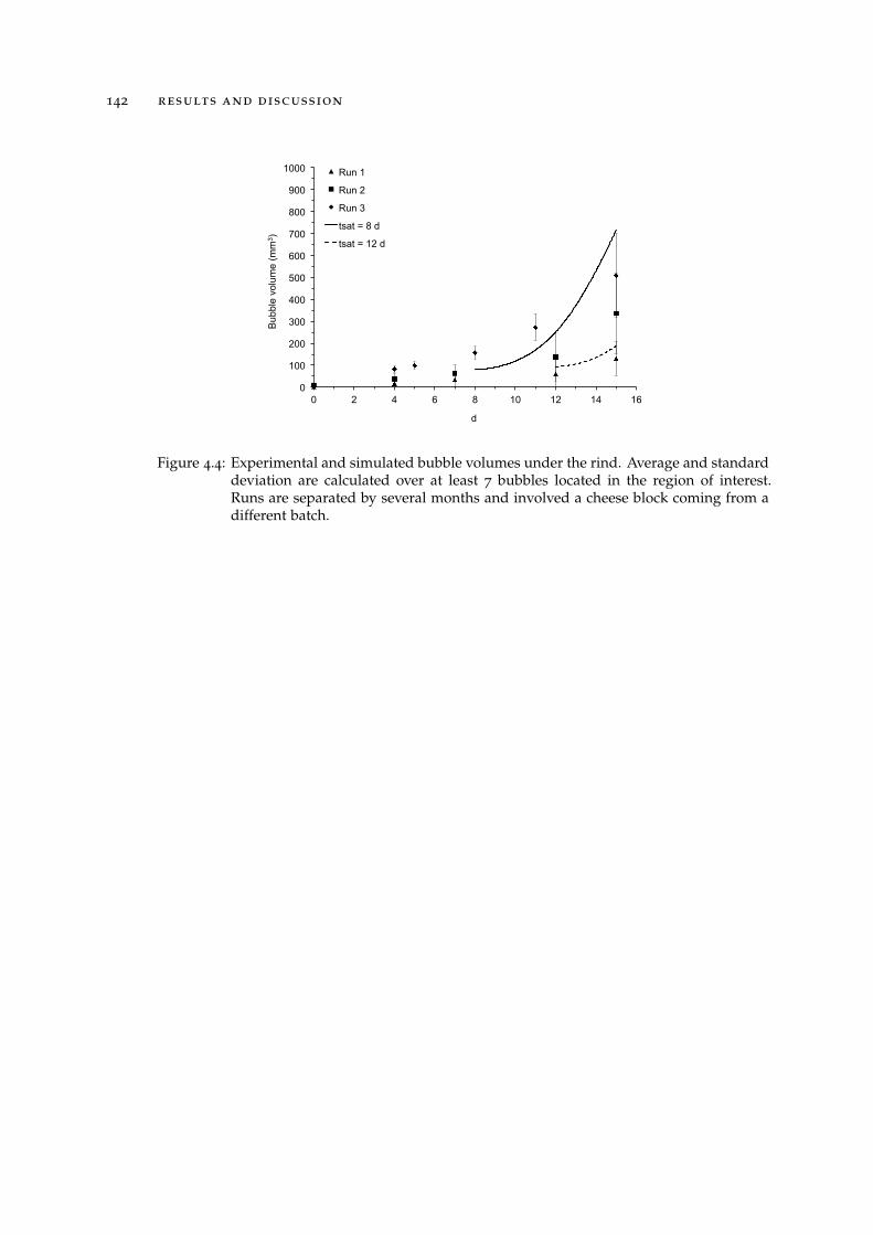
142 results and discussion
0
100
200
300
400
500
600
700
800
900
1000
0 2 4 6 8 10 12 14 16
Bub
ble
volu
me
(mm
3 )
d
Run 1
Run 2
Run 3
tsat = 8 d
tsat = 12 d
Figure 4.4: Experimental and simulated bubble volumes under the rind. Average and standarddeviation are calculated over at least 7 bubbles located in the region of interest.Runs are separated by several months and involved a cheese block coming from adifferent batch.
6C O N C L U S I O N S
The growth of bubbles in cheese was investigated both experimentally and by sim-ulation. Bubble volumes in chees blocks during ripening were assed experimentallywith the help of X-Ray imaging and MRI with a dedicated image processing method.Special care was taken on the determination of the model parameters. Mass transportparameters were assessed both from literature data and from dedicated experimentswhile mechanical parameters were already investigated in a previous study. Growthwas considered to occur only when saturation in carbon dioxide was reached underthe conditions of the experiment (atmospheric pressure, 293K). A sensitivity study wasconducted on the bubble growth model in order to rank the parameters that were themost influential.
Experimental results were compared to simulations, and the model proved to repro-duce the bubble growth in cheese in a qualitative manner. The only parameter that wasnot determined experimentally was adjusted to fit the experimental sets of data withgood agreement. Lower diffusivity of carbon dioxide than expected was explained byeither an underestimation of tortuosity (initially assumed for spherically-shaped andregularly arranged obstacles) or an overestimation of the space available for diffusion(it was assumed for the first-hand estimation of diffusivity that the whole fraction ofwater was available for carbon dioxide diffusion).
Experimental bubble growth proved to be highly variable between batches, espe-cially under the rind. Likewise, among the most influential parameters, all involvedin the mass balance, production of carbon dioxide also showed to be quite variable be-tween batches, with a standard deviation of about 30%. The latter being most probablythe cause of the former. This conclusion argued in favor of high number of repetitions(for instance more than three runs retained for the monitoring of bubble growth) inorder to attain a more complete validation of the model.
The sensitivity analysis also showed the predominance of diffusivity on the bubblegrowth, with an identical level compared to production rate. This conclusion, togetherwith the adjustment of this parameter in the model for the fitting of experimental data,highlighted the need of the measurement of this property in cheese, still lacking in theliterature. At last, the mechanical behaviour of cheese proved not to have any effecton bubble growth compared to the mass transport properties.
143

Chapitre 5
F I R S T S T E P S T O WA R D S A B E T T E R U N D E R S TA N D I N G O FT H E G R O W T H O F M U LT I P L E N E I G H B O U R I N G B U B B L E S
I N C H E E S E

1I N T R O D U C T I O N
The previous chapter on the growth of a single bubble highlighted the most influentfactors driving the bubble growth, while validating the ability of this simplistic modelto reproduce the average bubble growth within semi-hard cheese blocks. However,it should be emphasised that in cheese blocks, bubbles can rarely be considered tobe isolated from each other, and rather present an average of six neighbouring, veryclose bubbles. In order to move forwards a better understanding of these multipleinteractions, a dedicated experiment similar to that used in Chapter 3 and involvingtwo adjacent gaseous cavities was conducted, and was reproduced numerically. Thispart of the PhD work has necessitated a great amount of implementation, and still re-quires further work; the results presented below, especially the experimental ones, arepreliminary and some tracks of improvement are proposed at the end of the presentchapter. For this reason, and although some promising results are already available,the content of this chapter should be considered as pespectives of Chapter 4.
147

2M AT E R I A L A N D M E T H O D S
2.1 experimental set-up
The experiment consisted in placing a cheese sample containing a single bubble in anhermetically sealed maintaining apparatus comprising a non-negligible headspace.
The cheese sample consisted of a cylinder comprising a single bubble, and wasplaced in a maintaining apparatus (Figure 5.2) that ensured constant height of thelateral face of the cylinder throughout the experiment. The headspace height is 23 mmfor 30 mm diameter, yielding a volume of 16 258 mm3, that is two orders of magnitudehigher than the typical bubble volume (typical bubble radius ranging from 3 to 5 mm).The headspace was considered as a second gaseous cavity that had a specific volume(surface of the interface divided by the volume of the cavity) lower than the isolatedbubble within the sample. The height of the headspace was adjustable at wish, butkept constant in the present study.
The vicinity of the two gaseous cavities aimed at reproducing the real conditions ofbubble growth in cheese, either near the crust, where the headspace of the apparatusreproduces the headspace between the cheese and the surrounding foil (Configura-tion 1 in Figure 5.1) ; either at core between neighboring bubbles, where the headspaceof the apparatus acts as a cylindrically shaped bubble with a different specific volumethan the actual bubble (Configuration 2 in Figure 5.1).
149
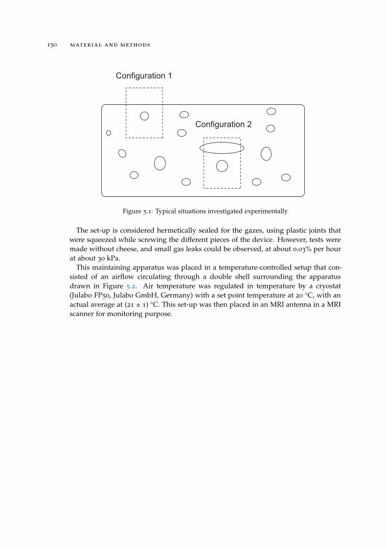
150 material and methods
Configuration 1
Configuration 2
Figure 5.1: Typical situations investigated experimentally
The set-up is considered hermetically sealed for the gazes, using plastic joints thatwere squeezed while screwing the different pieces of the device. However, tests weremade without cheese, and small gas leaks could be observed, at about 0.03% per hourat about 30 kPa.
This maintaining apparatus was placed in a temperature-controlled setup that con-sisted of an airflow circulating through a double shell surrounding the apparatusdrawn in Figure 5.2. Air temperature was regulated in temperature by a cryostat(Julabo FP50, Julabo GmbH, Germany) with a set point temperature at 20 °C, with anactual average at (21 ± 1) °C. This set-up was then placed in an MRI antenna in a MRIscanner for monitoring purpose.
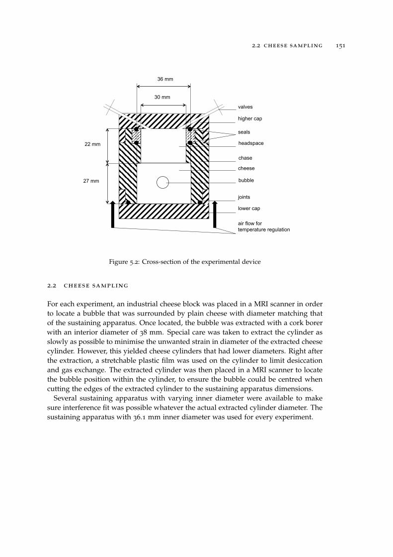
2.2 cheese sampling 151
valves
higher cap
headspace
chase
cheese
bubble
lower cap
joints
seals
27 mm
22 mm
36 mm
30 mm
air flow for temperature regulation
Figure 5.2: Cross-section of the experimental device
2.2 cheese sampling
For each experiment, an industrial cheese block was placed in a MRI scanner in orderto locate a bubble that was surrounded by plain cheese with diameter matching thatof the sustaining apparatus. Once located, the bubble was extracted with a cork borerwith an interior diameter of 38 mm. Special care was taken to extract the cylinder asslowly as possible to minimise the unwanted strain in diameter of the extracted cheesecylinder. However, this yielded cheese cylinders that had lower diameters. Right afterthe extraction, a stretchable plastic film was used on the cylinder to limit desiccationand gas exchange. The extracted cylinder was then placed in a MRI scanner to locatethe bubble position within the cylinder, to ensure the bubble could be centred whencutting the edges of the extracted cylinder to the sustaining apparatus dimensions.
Several sustaining apparatus with varying inner diameter were available to makesure interference fit was possible whatever the actual extracted cylinder diameter. Thesustaining apparatus with 36.1 mm inner diameter was used for every experiment.
152 material and methods
Moisture content was measured on a test sample and on a sample that had beenused for an experiment, and it proved that there was a loss of about 1 percentagepoint between the test sample and the one that was used for the experiment after 6
days. This allowed us to neglect any changes in cheese composition and to neglect thewater exchange between cheese and the cavities, as well as their possible impact onthe mechanics of cheese
2.3 experimental procedure
The experimental conditions are synthesised in Table 5.1 for the three experimentsconsidered. Before headspace gas was flushed with CO2, a first MRI sequence waslaunched to measure the exact initial volume and morphology of the bubble as wellas its exact initial location within the sample. Hence, there was a non-negligible timebetween the sampling of the cheese cylinder and the first headspace flushing, duringwhich some carbon dioxide could flow out of the sample. This time is indicated in Ta-ble 5.1, and is further discussed in section 2. It was hypothesised that at the beginningof the experiment, concentration of gases other than CO2 was negligible in the bubble,the reason why this gaseous cavity was not flushed. The pressure in the headspace andthe volume of the bubble in cheese were monitored continuously. Multiple flushingof the headspace with CO2 could be carried out during the experiment (see Table 5.1,and refer to the results section). Conversely to the experiment presented in Chapter 3,the pressure in the bubble was not monitored since leakage of gas were not perfectlycontrolled, biasing the mass balance which is a key point of this study.
2.4 measurements 153
Table 5.1: Summary of the three experiments and of their most significant characteristics
Experiment 1 2 3
Start date 16/05/13 20/06/13 15/10/13
End date 20/05/13 25/06/13 20/10/13
Extent of ripening in hot roombefore sampling (days)
6 6 5
Duration of the experiment (h) 100 130 120
Time between sampling andlaunching of the 1st MRI sequence
(h)
1.5 1.0 2.0
Initial gas compositionHeadspace CO2
Bubble assumingly 100% CO2
Flushing of headspace duringexperiment
no yes yes
Bubble initial radius (mm) 5.8 4.0 4.7
Hc − Hb (mm) 9.3 10.7 8.0
Cylinder initial height (mm) 19.7 28.2 26.4
Cylinder initial diameter (mm) 36.1 36.1 36.1
Use of glue onto the externalsurfaces of the sample
no bottom bottom and lateral
2.4 measurements
2.4.1 Pressure and temperature
Pressure sensors (XCEL-100-25A, Kulite, USA) were connected to the headspace withthe help of the valves indicated in Figure 5.2. The pressure sensors were connected toa data logger (Agilent 34970A, Agilent Technologies, USA) and saved with an acqui-sition frequency of 2·10
-2 Hz. The headspace was also monitored in temperature withthe help of optic fibres connected to a data logger (FISO UMI 8, Fiso Technologies,Canada) with the same acquisition frequency.
2.4.2 MRI sequences
A 3-D Spin-Echo sequence with the following parameters was used to monitor thetime-course changes in volume of the bubble:
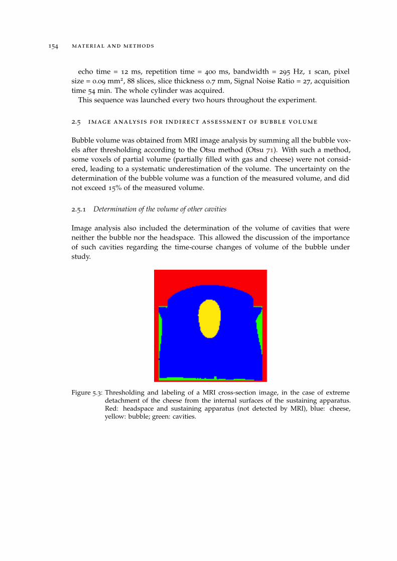
154 material and methods
echo time = 12 ms, repetition time = 400 ms, bandwidth = 295 Hz, 1 scan, pixelsize = 0.09 mm2, 88 slices, slice thickness 0.7 mm, Signal Noise Ratio = 27, acquisitiontime 54 min. The whole cylinder was acquired.
This sequence was launched every two hours throughout the experiment.
2.5 image analysis for indirect assessment of bubble volume
Bubble volume was obtained from MRI image analysis by summing all the bubble vox-els after thresholding according to the Otsu method (Otsu 71). With such a method,some voxels of partial volume (partially filled with gas and cheese) were not consid-ered, leading to a systematic underestimation of the volume. The uncertainty on thedetermination of the bubble volume was a function of the measured volume, and didnot exceed 15% of the measured volume.
2.5.1 Determination of the volume of other cavities
Image analysis also included the determination of the volume of cavities that wereneither the bubble nor the headspace. This allowed the discussion of the importanceof such cavities regarding the time-course changes of volume of the bubble understudy.
Figure 5.3: Thresholding and labeling of a MRI cross-section image, in the case of extremedetachment of the cheese from the internal surfaces of the sustaining apparatus.Red: headspace and sustaining apparatus (not detected by MRI), blue: cheese,yellow: bubble; green: cavities.
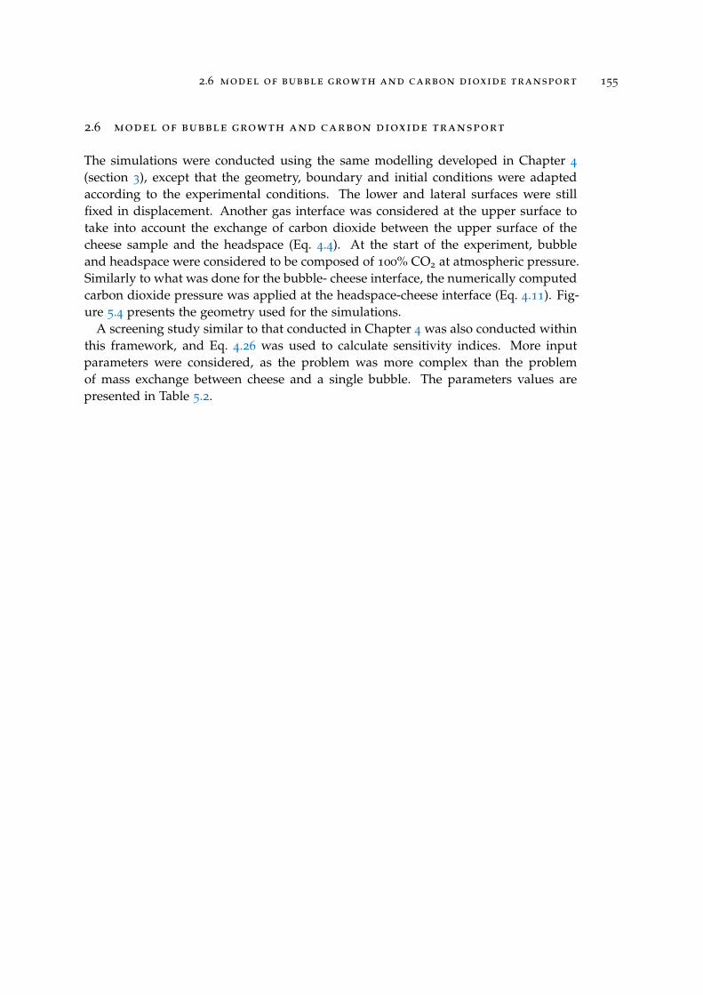
2.6 model of bubble growth and carbon dioxide transport 155
2.6 model of bubble growth and carbon dioxide transport
The simulations were conducted using the same modelling developed in Chapter 4
(section 3), except that the geometry, boundary and initial conditions were adaptedaccording to the experimental conditions. The lower and lateral surfaces were stillfixed in displacement. Another gas interface was considered at the upper surface totake into account the exchange of carbon dioxide between the upper surface of thecheese sample and the headspace (Eq. 4.4). At the start of the experiment, bubbleand headspace were considered to be composed of 100% CO2 at atmospheric pressure.Similarly to what was done for the bubble- cheese interface, the numerically computedcarbon dioxide pressure was applied at the headspace-cheese interface (Eq. 4.11). Fig-ure 5.4 presents the geometry used for the simulations.
A screening study similar to that conducted in Chapter 4 was also conducted withinthis framework, and Eq. 4.26 was used to calculate sensitivity indices. More inputparameters were considered, as the problem was more complex than the problemof mass exchange between cheese and a single bubble. The parameters values arepresented in Table 5.2.
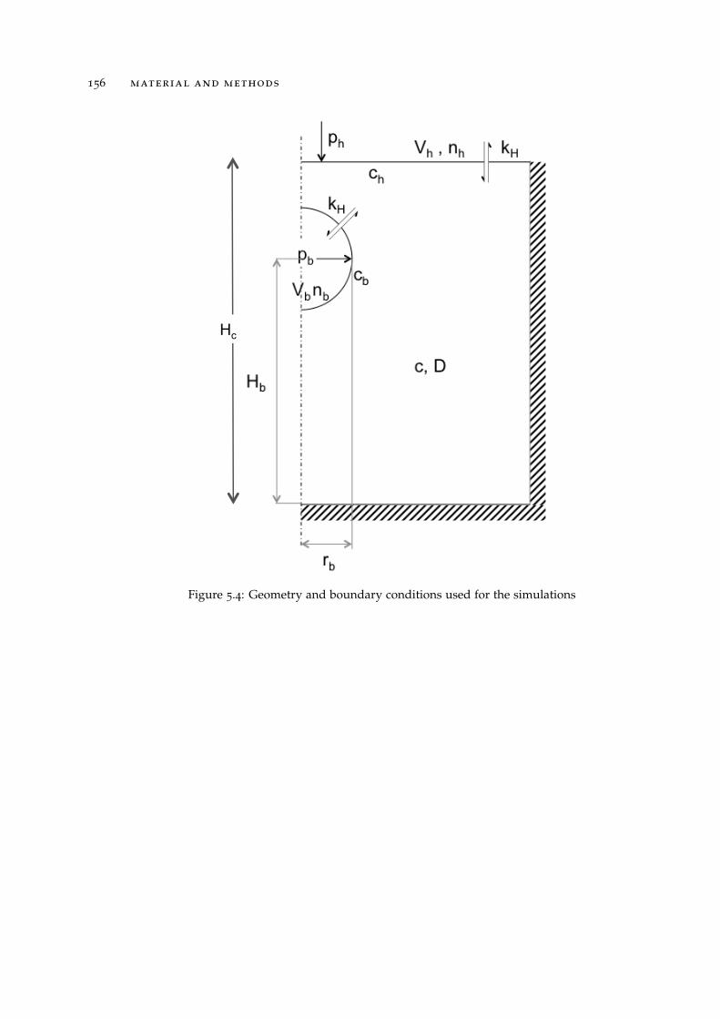
156 material and methods
Figure 5.4: Geometry and boundary conditions used for the simulations
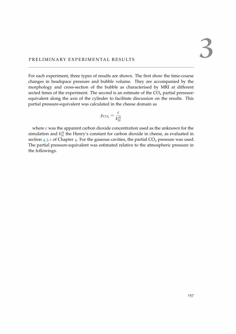
3P R E L I M I N A RY E X P E R I M E N TA L R E S U LT S
For each experiment, three types of results are shown. The first show the time-coursechanges in headspace pressure and bubble volume. They are accompanied by themorphology and cross-section of the bubble as characterised by MRI at differentsected times of the experiment. The second is an estimate of the CO2 partial pressure-equivalent along the axis of the cylinder to facilitate discussion on the results. Thispartial pressure-equivalent was calculated in the cheese domain as
pCO2 =c
kchH
where c was the apparent carbon dioxide concentration used as the unknown for thesimulation and kch
H the Henry’s constant for carbon dioxide in cheese, as evaluated insection 4.3.1 of Chapter 4. For the gaseous cavities, the partial CO2 pressure was used.The partial pressure-equivalent was estimated relative to the atmospheric pressure inthe followings.
157
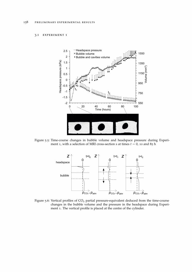
158 preliminary experimental results
3.1 experiment 1
550
750
950
1150
1350
1550
-2
-1.5
-1
-0.5
0
0.5
1
1.5
2
2.5
0 20 40 60 80 100
Volu
me
(mm
3 )
Hea
dspa
ce p
ress
ure
(kP
a)
Time (hours)
Headspace pressure Bubble volume Bubble and cavities volume
t1 t2
Figure 5.5: Time-course changes in bubble volume and headspace pressure during Experi-ment 1, with a selection of MRI cross-section s at times t = 0, 10 and 85 h
headspace
z
bubble
z zt=t0 t=t1 t=t2
pCO2 patm-
0 0 0
pCO2 patm- pCO2 patm-
Figure 5.6: Vertical profiles of CO2 partial pressure-equivalent deduced from the time-coursechanges in the bubble volume and the pressure in the headspace during Experi-ment 1. The vertical profile is placed at the centre of the cylinder.
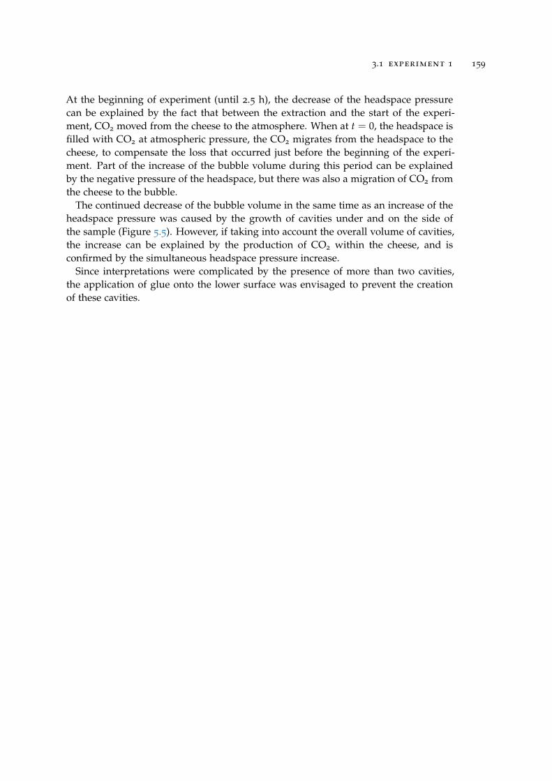
3.1 experiment 1 159
At the beginning of experiment (until 2.5 h), the decrease of the headspace pressurecan be explained by the fact that between the extraction and the start of the experi-ment, CO2 moved from the cheese to the atmosphere. When at t = 0, the headspace isfilled with CO2 at atmospheric pressure, the CO2 migrates from the headspace to thecheese, to compensate the loss that occurred just before the beginning of the experi-ment. Part of the increase of the bubble volume during this period can be explainedby the negative pressure of the headspace, but there was also a migration of CO2 fromthe cheese to the bubble.
The continued decrease of the bubble volume in the same time as an increase of theheadspace pressure was caused by the growth of cavities under and on the side ofthe sample (Figure 5.5). However, if taking into account the overall volume of cavities,the increase can be explained by the production of CO2 within the cheese, and isconfirmed by the simultaneous headspace pressure increase.
Since interpretations were complicated by the presence of more than two cavities,the application of glue onto the lower surface was envisaged to prevent the creationof these cavities.
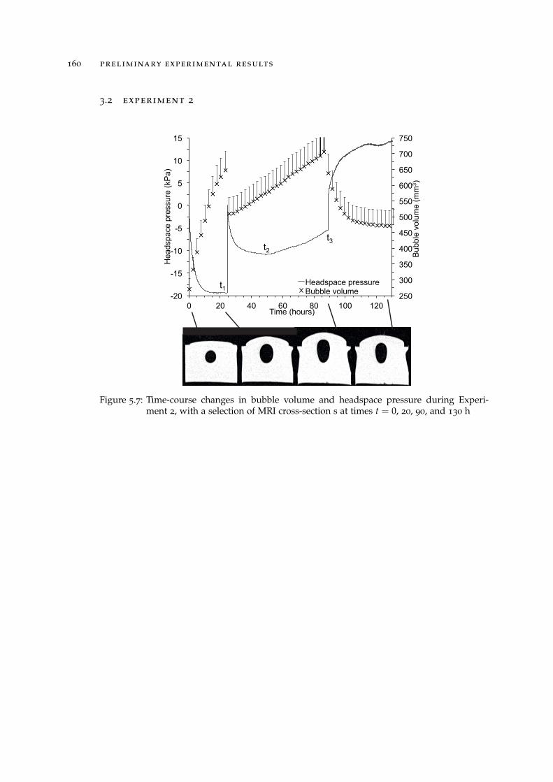
160 preliminary experimental results
3.2 experiment 2
250
300
350
400
450
500
550
600
650
700
750
-20
-15
-10
-5
0
5
10
15
0 20 40 60 80 100 120
Bub
ble
volu
me
(mm
3 )
Hea
dspa
ce p
ress
ure
(kP
a)
Time (hours)
Headspace pressure Bubble volume
t1
t2
t3
Figure 5.7: Time-course changes in bubble volume and headspace pressure during Experi-ment 2, with a selection of MRI cross-section s at times t = 0, 20, 90, and 130 h
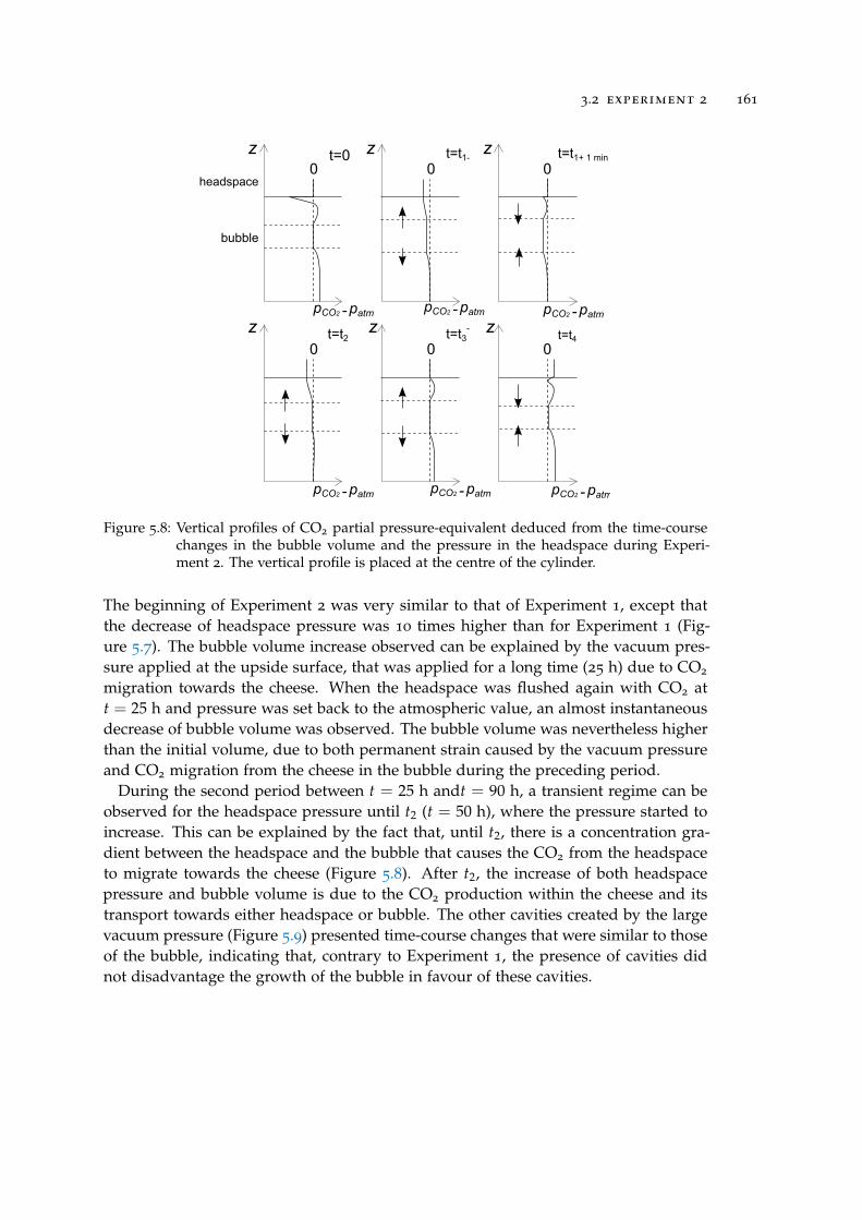
3.2 experiment 2 161
headspace
z
bubble
z z
z z z
t=0 t=t1- t=t1+ 1 min
t=t2 t=t3- t=t4
pCO2 patm- pCO2 patm- pCO2 patm-
pCO2 patm-pCO2 patm-pCO2 patm-
0 0 0
0 0 0
Figure 5.8: Vertical profiles of CO2 partial pressure-equivalent deduced from the time-coursechanges in the bubble volume and the pressure in the headspace during Experi-ment 2. The vertical profile is placed at the centre of the cylinder.
The beginning of Experiment 2 was very similar to that of Experiment 1, except thatthe decrease of headspace pressure was 10 times higher than for Experiment 1 (Fig-ure 5.7). The bubble volume increase observed can be explained by the vacuum pres-sure applied at the upside surface, that was applied for a long time (25 h) due to CO2
migration towards the cheese. When the headspace was flushed again with CO2 att = 25 h and pressure was set back to the atmospheric value, an almost instantaneousdecrease of bubble volume was observed. The bubble volume was nevertheless higherthan the initial volume, due to both permanent strain caused by the vacuum pressureand CO2 migration from the cheese in the bubble during the preceding period.
During the second period between t = 25 h andt = 90 h, a transient regime can beobserved for the headspace pressure until t2 (t = 50 h), where the pressure started toincrease. This can be explained by the fact that, until t2, there is a concentration gra-dient between the headspace and the bubble that causes the CO2 from the headspaceto migrate towards the cheese (Figure 5.8). After t2, the increase of both headspacepressure and bubble volume is due to the CO2 production within the cheese and itstransport towards either headspace or bubble. The other cavities created by the largevacuum pressure (Figure 5.9) presented time-course changes that were similar to thoseof the bubble, indicating that, contrary to Experiment 1, the presence of cavities didnot disadvantage the growth of the bubble in favour of these cavities.
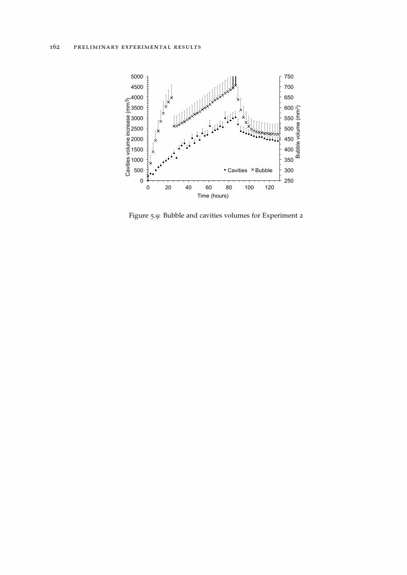
162 preliminary experimental results
250
300
350
400
450
500
550
600
650
700
750
0
500
1000
1500
2000
2500
3000
3500
4000
4500
5000
0 20 40 60 80 100 120
Bub
ble
volu
me
(mm
3 )
Cav
ities
vol
ume
incr
ease
(mm
)
3
Time (hours)
Cavities Bubble
Figure 5.9: Bubble and cavities volumes for Experiment 2
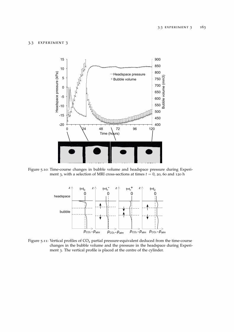
3.3 experiment 3 163
3.3 experiment 3
400
450
500
550
600
650
700
750
800
850
900
-20
-15
-10
-5
0
5
10
15
0 24 48 72 96 120
Bub
ble
volu
me
(mm
3)
Hea
dspa
ce p
ress
ure
(kP
a)
Time (hours)
Headspace pressure Bubble volume
Figure 5.10: Time-course changes in bubble volume and headspace pressure during Experi-ment 3, with a selection of MRI cross-sections at times t = 0, 20, 60 and 120 h
headspace
bubble
z z zz t=t0 t=t1- t=t1+ t=t20 0 0 0
pCO2 patm- pCO2 patm- pCO2 patm- pCO2 patm-
Figure 5.11: Vertical profiles of CO2 partial pressure-equivalent deduced from the time-coursechanges in the bubble volume and the pressure in the headspace during Experi-ment 3. The vertical profile is placed at the centre of the cylinder.
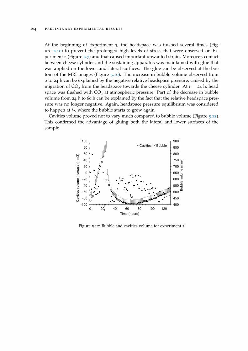
164 preliminary experimental results
At the beginning of Experiment 3, the headspace was flushed several times (Fig-ure 5.10) to prevent the prolonged high levels of stress that were observed on Ex-periment 2 (Figure 5.7) and that caused important unwanted strain. Moreover, contactbetween cheese cylinder and the sustaining apparatus was maintained with glue thatwas applied on the lower and lateral surfaces. The glue can be observed at the bot-tom of the MRI images (Figure 5.10). The increase in bubble volume observed from0 to 24 h can be explained by the negative relative headspace pressure, caused by themigration of CO2 from the headspace towards the cheese cylinder. At t = 24 h, headspace was flushed with CO2 at atmospheric pressure. Part of the decrease in bubblevolume from 24 h to 60 h can be explained by the fact that the relative headspace pres-sure was no longer negative. Again, headspace pressure equilibrium was consideredto happen at t2, where the bubble starts to grow again.
Cavities volume proved not to vary much compared to bubble volume (Figure 5.12).This confirmed the advantage of gluing both the lateral and lower surfaces of thesample.
400
450
500
550
600
650
700
750
800
850
900
-100
-80
-60
-40
-20
0
20
40
60
80
100
0 20 40 60 80 100 120
Bub
ble
volu
me
(mm
3 )
Cav
ities
vol
ume
incr
ease
(mm
3)
Time (hours)
Cavities Bubble
t1
t2
Figure 5.12: Bubble and cavities volume for experiment 3
3.4 general discussion of the experimental results 165
3.4 general discussion of the experimental results
Firstly, it should be emphasised that dealing with foodstuff brings a lot of product-related constraints, among them the evolving nature of the product was the most hin-dering and required particular attention, for instance in maintaining the temperaturestable and close to that of the actual ripening or the nonaerobic conditions to preventunwanted microbiological activity. Besides, the dimensions of the set-up made theinstrumentation difficult, necessitating to deal with significant measurement uncer-tainties (see Chapter 2).
After a long period of implementation (six runs additional to the three presentedabove), the feasibility of mastering such type of experiment was demonstrated. Quitesimilar trends observed during Experiments 2 and 3 provided evidence of possiblereproducibility, a point which was highly questioned during the stage of implementa-tion of the experimental procedure. The most notable similarities were the fact that thesample absorbed a great amount of carbon dioxide, causing negative relative pressurein the headspace as high as 30 kPa (to be compared to the average bubble pressurewithin cheese that is ten times lower), and the fact that bubble growth was monitoredonly after headspace pressure equilibrium was reached. This behaviour would tend tosuggest that carbon dioxide saturation was not reached everywhere in the cheese cylin-der at the beginning of the experiment. However, this is in contradiction with the sizeof the bubble contained within the samples, that indicated bubble growth occurring insaturation regime. This contradictory effect is still not fully explained. Transfer fromthe cut surfaces of the cheese cylinder during the waiting time is the most plausibleexplanation; nevertheless the amount of carbon dioxide estimated from the loweringin pressure in the headspace was two-fold that estimated from the diffusion of carbondioxide (using analytical solution).
The headspace pressure equilibrium time was observed late in the experiment, indi-cating that the experiment should have been much prolonged. Indeed, bubble growthconcomitant to an increase in pressure in the headspace was only noticeable at the endof the experiment (2 and 3), and not enough data was available for model validation.The developped experimental procedure is not totally questioned, but requires someadaptation, as detailed below.
The first way will be to minimize the time elapsed between the sampling of thecheese cylinder and the launching of the experiment (t = 0). Note here that in theprevious experimental procedure, most of the time elapsed between the sampling ofthe cheese cylinder and the initial flush of the headspace was due to the acquisitionof a first, highly resolved image of the cheese cylinder and its bubble. This could bemuch reduced.
166 preliminary experimental results
If despite of these precautions, the lowering in pressure is still observed in theheadspace over a long time, the headspace will be flushed with carbon dioxide, asregularly as necessary to prevent unwanted stress due to a negative relative pressurein headspace. However, contrary to the previous experimental procedure, only theheadspace pressure would need monitoring.
Optimal monitoring conditions will be considered to be reached when the headspacepressure starts increasing again. MRI monitoring should only begin at that moment.
The rest of the experiment could be conducted following the procedure alreadyestablished, over the same duration as initially envisaged, i.e. comprised between 5
and 7 days.At last, the apparition of unwanted cavities between the lower and lateral surfaces
and the maintaining apparatus, could be avoided or limited in a large extent by theuse of glue on these lower and lateral surfaces.
At the moment, the numerical model developed is unable to produce results consis-tent with the observed experiments. This discrepancy between simulated and experi-mental behaviours can be explained by the fact that the headspace equilibrium stagewas not convered by the model, that hypothesed saturation regime.
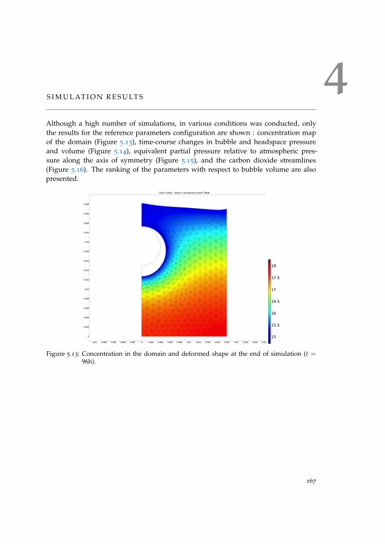
4S I M U L AT I O N R E S U LT S
Although a high number of simulations, in various conditions was conducted, onlythe results for the reference parameters configuration are shown : concentration mapof the domain (Figure 5.13), time-course changes in bubble and headspace pressureand volume (Figure 5.14), equivalent partial pressure relative to atmospheric pres-sure along the axis of symmetry (Figure 5.15), and the carbon dioxide streamlines(Figure 5.16). The ranking of the parameters with respect to bubble volume are alsopresented.
Figure 5.13: Concentration in the domain and deformed shape at the end of simulation (t =96h).
167
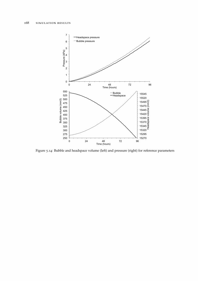
168 simulation results
0
1
2
3
4
5
6
7
0 24 48 72 96
Pre
ssur
e (k
Pa)
Time (hours)
Headspace pressure Bubble pressure
15270 15295 15320 15345 15370 15395 15420 15445 15470 15495 15520 15545
250 275 300 325 350 375 400 425 450 475 500 525 550
0 24 48 72 96
Hea
dspa
ce v
olum
e (m
m3)
Bub
ble
volu
me
(mm
3)
Time (hours)
Bubble Headspace
Figure 5.14: Bubble and headspace volume (left) and pressure (right) for reference parameters
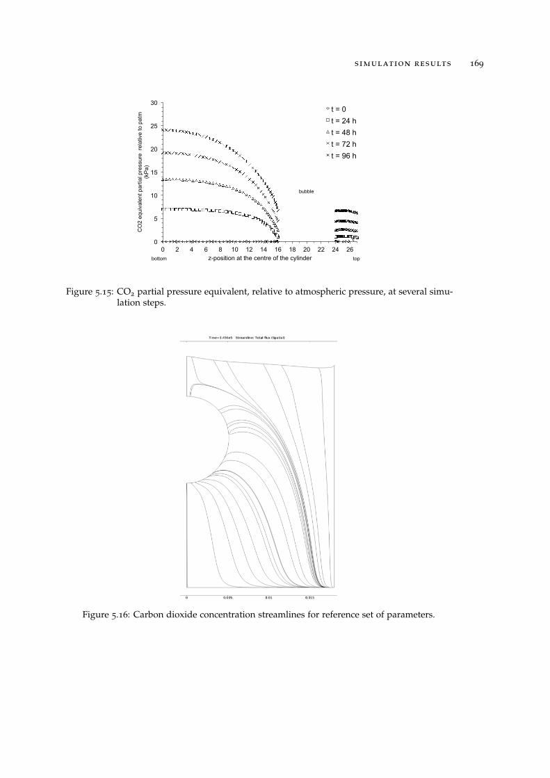
simulation results 169
0
5
10
15
20
25
30
0 2 4 6 8 10 12 14 16 18 20 22 24 26
CO
2 eq
uiva
lent
par
tial p
ress
ure
rela
tive
to p
atm
(k
Pa)
z-position at the centre of the cylinder
t = 0 t = 24 h t = 48 h t = 72 h t = 96 h
bottom top
bubble
Figure 5.15: CO2 partial pressure equivalent, relative to atmospheric pressure, at several simu-lation steps.
Figure 5.16: Carbon dioxide concentration streamlines for reference set of parameters.
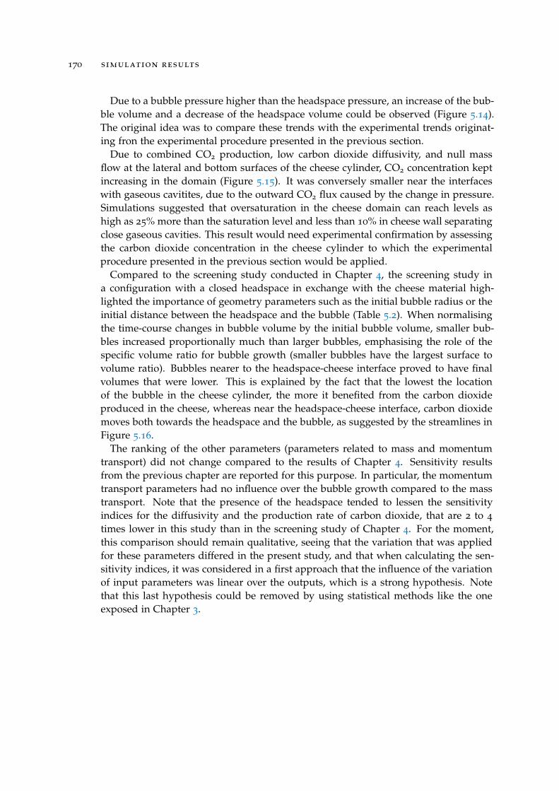
170 simulation results
Due to a bubble pressure higher than the headspace pressure, an increase of the bub-ble volume and a decrease of the headspace volume could be observed (Figure 5.14).The original idea was to compare these trends with the experimental trends originat-ing fron the experimental procedure presented in the previous section.
Due to combined CO2 production, low carbon dioxide diffusivity, and null massflow at the lateral and bottom surfaces of the cheese cylinder, CO2 concentration keptincreasing in the domain (Figure 5.15). It was conversely smaller near the interfaceswith gaseous cavitites, due to the outward CO2 flux caused by the change in pressure.Simulations suggested that oversaturation in the cheese domain can reach levels ashigh as 25% more than the saturation level and less than 10% in cheese wall separatingclose gaseous cavities. This result would need experimental confirmation by assessingthe carbon dioxide concentration in the cheese cylinder to which the experimentalprocedure presented in the previous section would be applied.
Compared to the screening study conducted in Chapter 4, the screening study ina configuration with a closed headspace in exchange with the cheese material high-lighted the importance of geometry parameters such as the initial bubble radius or theinitial distance between the headspace and the bubble (Table 5.2). When normalisingthe time-course changes in bubble volume by the initial bubble volume, smaller bub-bles increased proportionally much than larger bubbles, emphasising the role of thespecific volume ratio for bubble growth (smaller bubbles have the largest surface tovolume ratio). Bubbles nearer to the headspace-cheese interface proved to have finalvolumes that were lower. This is explained by the fact that the lowest the locationof the bubble in the cheese cylinder, the more it benefited from the carbon dioxideproduced in the cheese, whereas near the headspace-cheese interface, carbon dioxidemoves both towards the headspace and the bubble, as suggested by the streamlines inFigure 5.16.
The ranking of the other parameters (parameters related to mass and momentumtransport) did not change compared to the results of Chapter 4. Sensitivity resultsfrom the previous chapter are reported for this purpose. In particular, the momentumtransport parameters had no influence over the bubble growth compared to the masstransport. Note that the presence of the headspace tended to lessen the sensitivityindices for the diffusivity and the production rate of carbon dioxide, that are 2 to 4
times lower in this study than in the screening study of Chapter 4. For the moment,this comparison should remain qualitative, seeing that the variation that was appliedfor these parameters differed in the present study, and that when calculating the sen-sitivity indices, it was considered in a first approach that the influence of the variationof input parameters was linear over the outputs, which is a strong hypothesis. Notethat this last hypothesis could be removed by using statistical methods like the oneexposed in Chapter 3.
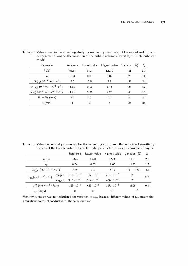
simulation results 171
Table 5.2: Values used in the screening study for each entry parameter of the model and impactof these variations on the variation of the bubble volume after 72 h, multiple bubblesmodel
Parameter Reference Lowest value Highest value Variation (%) Ik
λ5(s) 9324 6428 12230 31 1.3
α5 0.04 0.03 0.05 25 3.0
DchCO2
(·10−10 m2·s-2) 5.0 2.5 7.9 54 24
rCO2(·10−5mol·m-3·s-1) 1.15 0.58 1.44 37 50
kchH (·10−4mol·m-3·Pa-1) 1.41 1.06 2.28 43 8.9
Hc − Hb (mm) 8.0 10 6.0 25 24
rb(mm) 4 3 5 25 85
Table 5.3: Values of model parameters for the screening study and the associated sensitivityindices of the bubble volume to each model parameter. Ik was determined at day 15.
Reference Lowest value Highest value Variation (%) Ik
λ5 (s) 9324 6428 12230 ±31 2.6
α5 0.04 0.03 0.05 ±25 1.7
DchCO2
(·10−10 m2·s-1) 4.5 1.1 6.75 -75 +50 82
rCO2(mol·m-3·s-1)stage I 1.65 · 10−6 1.17 · 10−6 2.13 · 10−6 29
110stage II 3.56 · 10−5 2.74 · 10−5 4.37 · 10−5 23
kchH (mol·m-3·Pa-1) 1.23 · 10−4 9.23 · 10−5 1.54 · 10−4 ±25 0.4
tsat (days) 0 8 12 -a
aSensitivity indice was not calculated for variation of tsat, because different values of tsat meant thatsimulations were not conducted for the same duration.

5C O N C L U S I O N S
In order to validate the model and its set of values for entry parameters, future inves-tigation will focus on repeated experiments accordingly to the improved experimentalprocedure detailed in section 3.4.
Experiments conducted so far allowed to demonstrate the feasibility of experimentalvalidation at the bubble scale with a dedicated experiment, with control over initialand boundary conditions for mass and momentum transport.
The sensitivity study that was conducted underlined the importance of geometricalparameters in the case of multiple neighbouring bubbles growth. In particular, dis-tance between the two cavities and the cavities sizes proved to be as important as thediffusive parameters related to the mass balance, previously identified as the drivingparameters in Chapter 4.
173


C O N C L U S I O N S E T P E R S P E C T I V E S
175

conclusions 177
Au terme des trois axes de travail développés au cours de cette thèse, plusieursenseignements ont pu être tirés à la fois sur la croissance de bulles dans les fromagesà pâte pressée non-cuite mais aussi sur les propriétés mécaniques et de transport dumatériau étudié.
Tout d’abord, la caractérisation mécanique du produit a permis de découvrir que,contrairement à ce qui est plus ou moins accepté par les technologues et ce qui étaitenvisagé au début du projet, les propriétés rhéologiques du fromage étudié ne varientpas au cours de l’affinage, ou que tout du moins la grande variabilité entre batches etla précision à la fois de la mesure et de la méthode de détermination de paramètresrendent impossible l’estimation d’une telle évolution. La seule variation observée se-rait liée à un effet de la température, au cours du passage entre la cave froide et la cavechaude, qui peut diminuer la rigidité du produit à mesure que la température aug-mente. L’étape de caractérisation mécanique du produit a permis de dégager certainsbiais expérimentaux, qui bien qu’ils soient connus, sont souvent négligés, et de propo-ser des suggestions d’améliorations. En particulier, deux biais sont importants, car ilsdépassent le cadre de tests de compression-relaxation. En premier lieu, une partie descontraintes relaxe pendant la compression du produit. Cela signifie que, même pourla caractérisation élastique de produits de ce type, une attention particulière doit êtreportée sur les conditions de sollicitations de celui-ci. En second lieu, citons l’aspectdes échantillons, pour lesquels la découpe s’est révélée avoir une forte influence sur ladétermination de paramètres. En effet, les échantillons affichant une taille de quelquesmillimètres, les méthodes de découpe et la nature du matériau font qu’il est difficiled’assurer le parallélisme des faces de l’échantillon. Ce défaut de parallélisme peut cau-ser par la suite des biais de mesure importants selon la méthode de déterminationutilisée. Il a été montré dans ce travail de thèse que ce biais peut atteindre 25% avecles méthodes usuelles de régression linéaire.
La méthode de détermination des paramètres viscoélastiques proposée dans le cadrede cette thèse n’est pas limitée au fromage, mais pourrait s’envisager sur d’autres ma-tériaux possédant un large spectre de temps de relaxation, s’étalant de la millisecondeà plusieurs heures. De plus, la méthode proposée s’est avérée moins sensible aux biaisexpérimentaux étudiés que les méthodes usuelles de détermination de paramètres.
La validation expérimentale du modèle de Maxwell a été menée en conditions desollicitations mécaniques uniquement. Cela a consisté à imposer une pression à l’inté-rieur d’une bulle dans un dispositif expérimental de suivi, sur des durées de l’ordrede quelques heures, permettant de raisonnablement négliger les effets de la diffusionde matière au sein du matériau. Cette validation a permis d’affirmer la pertinence dece modèle, qui, bien que restant simple, propose un accord tant qualitatif que quanti-tatif pour la reproduction du comportement mécanique des fromages à pâte presséeautour d’une bulle. Cette validation met aussi en avant la bonne adéquation du testrhéologique choisi vis-à-vis des sollicitations à long-terme que subit le fromage lorsde la croissance de bulles. En outre, en conditions de sollicitations proches des condi-
178 conclusions
tions réelles, il a pu être démontré que les biais de détermination des paramètres àlong-terme rencontrés lors de la première étape (bruit sur les données expérimentales,évolution du produit sur la durée de l’expérimentation) ne sont pas un frein à la carac-térisation du produit, au regard des différentes incertitudes caractérisées. Si le modèlede Maxwell généralisé n’est pas exempt de défauts, étant limité pour les sollicitationsbrèves au domaine élastique, il faut souligner le fait que des modèles plus complexesimpliquent une caractérisation du matériau qui ne l’est pas moins. En outre, cettecaractérisation peut s’avérer délicate sur des produits agroalimentaires, qui peuventêtre évolutifs dans le temps : séchage du produit, influence de la composition del’atmosphère l’environnant sur ses transformations internes et présentent une grandevariabilité d’un échantillon à l’autre. Au regard de ces incertitudes, et dans l’état demaîtrise des procédés expérimentaux de détermination de paramètres, il est tout à faitprobable qu’un éventuel gain apporté par un modèle rhéologique plus complexe soitentravé par une variabilité (intra produit, intra-batch voire inter-batch) qui peut êtretrès importante.
Le bon accord obtenu entre simulation et expérience découle de deux aspects prin-cipaux :
− la grande viscosité du produit sur les échelles de temps considérées, qui permetde ne pas outrepasser la limite élastique lors des sollicitations ;
− le soin apporté à la détermination de paramètres du modèle sur le matériauétudié.
Cette première étape de validation du modèle en conditions de sollicitations mé-caniques uniquement a aussi permis de dégager les paramètres mécaniques les plusinfluents sans subir l’influence du transport de matière, à savoir les paramètres à long-terme que sont le module de cisaillement et le temps de relaxation de la dernièrebranche du modèle de Maxwell, de l’ordre 5% du module de cisaillement total et 3
heures pour le temps de relaxation.L’inclusion du transport de matière dans le modèle de croissance de bulle a permis
de montrer la faible influence des paramètres mécaniques sur la croissance de bulle.Ce résultat s’articule de manière cohérente avec le fait que la croissance des bullesdans les blocs de fromage est très significative en cave chaude, alors que les propriétésrhéologiques varient peu dans le même temps. Le modèle développé permet de re-produire un comportement moyen de bulle dans un fromage à pâte pressée non-cuite,et souligne l’importance à cet égard des paramètres liés au transport de matière, enparticulier le taux de production de dioxyde de carbone et le coefficient de diffusiondu dioxyde de carbone dans le fromage. Le premier a fait l’objet de mesures sur lefromage étudié et l’incertitude inter-batch associée a pu être caractérisée, alors quec’est sur le second que les efforts d’ajustement se sont portés. Les résultats du chapitre
conclusions 179
4 montrent qu’une estimation à partir des valeurs de diffusion du dioxyde de carbonedans l’eau, pondérées par la teneur en eau et par la tortuosité du matériau donne aumieux un ordre de grandeur, mais ne suffit pas à assurer l’accord des simulations avecles observations expérimentales. Ce constat engage à une détermination expérimentalede ce paramètre pour se rapprocher le plus possible des conditions réelles.
La prédominance du transport de matière met aussi en avant le fait que ce sont avecles leviers pilotant le transport de matière que le technologue pourra opérer des modi-fications sur le produit. À cet égard, le levier le plus visible reste l’activité fermentairequi, pour les souches bactériennes envisagées, est une caractéristique de l’affinage encave chaude. Seulement, cette activité fermentaire n’a pas une influence uniquementsur la teneur en dioxyde de carbone (qui peut être vue comme un coproduit de la fer-mentation et non comme son objet principal), mais aussi sur d’autres caractéristiquesorganoleptiques, tel l’aspect aromatique, qui ont, pour l’instant, été négligées.
En outre, la modélisation effectuée n’a envisagé que partiellement le cas de plu-sieurs bulles interagissant entre elles. Les résultats préliminaires portant sur l’interac-tion entre deux cavités gazeuses montrent bien que cela perturbe la hiérarchisationdes phénomènes de transport établie dans le cas d’une bulle isolée et introduit denouveaux paramètres qui peuvent piloter la croissance de bulles, essentiellement géo-métriques cette fois-ci. Ainsi, la taille des cavités gazeuses et la distance les séparantjouent-elles un rôle aussi important que le taux de production de dioxyde de carboneou de diffusion de celui-ci.
Un autre aspect, qui révèle son importance dans la conduite du procédé de fabri-cation, est la prise en compte des variations de température. En effet, le projet U2M-ChOp s’est focalisé sur des processus monothermes, à savoir l’affinage en cave chaude.Cependant, la variabilité dans le maintien de la température lors du procédé d’affinagesuggère que tous les fromages ne sont pas affinés à la même température, et que celapourrait expliquer la variabilité observée entre échantillons : tous les phénomènesimpliqués dans la croissance de bulles sont sensibles à la température (propriétés mé-caniques, activité fermentaire, diffusion). De plus, l’exploration de l’aspect thermiqueapparaît intéressant dans une optique de réduction des coûts énergétiques de produc-tion.


A N N E X E S
181

AFA B R I C AT I O N D ’ U N F R O M A G E À PÂT E P R E S S É E N O N - C U I T E
a.1 définition
Le codex stan 283-1978 définit le fromage comme suit.
Le fromage est le produit affiné ou non affiné, de consistance molle ou semi-dure,dure ou extra-dure qui peut être enrobé et dans lequel le rapport protéines de lactosé-rum/caséine ne dépasse pas celui du lait, et qui est obtenu :
a. par coagulation complète ou partielle des protéines du lait, du lait écrémé, dulait partiellement écrémé, de la crème, de la crème de lactosérum ou du babeurre,seuls ou en combinaison, grâce à l’action de la présure ou d’autres agents coa-gulants appropriés et par égouttage partiel du lactosérum résultant de cette coa-gulation, tout en respectant le principe selon lequel la fabrication du fromageentraîne la concentration des protéines du lait (notamment de la caséine), la te-neur en protéines du fromage étant par conséquent nettement plus élevée que lateneur en protéines du mélange des matières premières ci-dessus qui a servi à lafabrication du fromage et/ou
b. par l’emploi de techniques de fabrication entraînant la coagulation des protéinesdu lait ou des produits provenant du lait, de façon à obtenir un produit fini ayantdes caractéristiques physiques, chimiques et organoleptiques similaires à cellesdu produit défini à l’alinéa (A).
Comme indiqué en introduction du présent mémoire, il n’existe pas de codex généralpour les fromages à pâte pressée, mais des standards spécifiques à certaines variétés(emmental, gouda, cheddar, etc.), qui définissent les conditions d’appellations des ditsfromages en fonction de propriétés du lait utilisé pour la fabrication, des conditionsde fabrication et de la composition du produit fini.
Il existe deux types de fromages à pâte pressée : ceux pour lesquels la pâte est cuite(comme l’emmental ou le comté) et ceux pour lesquels la pâte n’est pas cuite (commele maasdam ou le laguiole).
183
184 fabrication d’un fromage à pâte pressée non-cuite
a.2 étapes de fabrication
a.2.1 Préparation du lait
Avant la fabrication proprement dite du fromage, le lait utilisé est préparé. Il subitplusieurs traitements.
1. Standardisation en matière grasse : permet d’ajuster le rapport gras sur sec duproduit fini.
2. Pasteurisation : étape d’assainissement du lait.
3. Ensemencement : ajout de ferments lactiques et propioniques.
a.2.2 Fabrication du fromage
Une fois le lait préparé, on peut passer à la fabrication proprement dite du fromage.
1. Emprésurage : on ajoute de la présure, qui a pour effet de former un gel, le caillé.
2. Tranchage : opération de découpage du caillé en grains, qui vont favoriserl’égouttage du caillé (c.-à-d. l’expulsion du sérum).
3. Égouttage : cette opération comporte plusieurs étapes toutes visant à favoriserl’expulsion du sérum des grains de caillé, et à préparer la suite. On va ainsi :
a) brasser le mélange sérum-caillé afin que les grains de caillé soient mobileset que leurs surfaces d’échange restent libres ;
b) réduire la concentration en lactose du sérum (délactosage).
4. Moulage : cette première étape de mise en forme du fromage dans des moulesvise à séparer le sérum des grains de caillé et donne sa forme au fromage.
5. Pressage : cette étape consiste à appliquer une pression sur les grains de cailléprésents dans le moule afin de donner sa forme définitive au fromage et decompléter l’égouttage.
6. Saumurage : le fromage est plongé dans un bain de saumure (solution saturéeen sel), qui permet de compléter l’égouttage, d’amorcer le développement or-ganoleptique du produit et de travailler la surface (durcissement de la croûte,assainissement de la surface).

A.2 étapes de fabrication 185
a.2.3 Affinage
Une fois le fromage fabriqué intervient l’étape d’affinage. Elle est essentielle car c’estl’étape qui voit le développement des qualités organoleptiques du produit. La pâte su-bit différentes transformations (par exemple par protéolyse ou lipolyse) qui assurentsa maturation. De plus, dans le cas des fromages étudiés dans le cadre de cette thèse,l’affinage est aussi le siège du développement d’ouvertures (ou bulles ou yeux). Sui-vant les recettes de fromages, l’affinage peut avoir lieu à différentes températures aucours du temps, et se dérouler sur des périodes de temps très variables (de quelquessemaines à plusieurs années suivant le type de fromage).

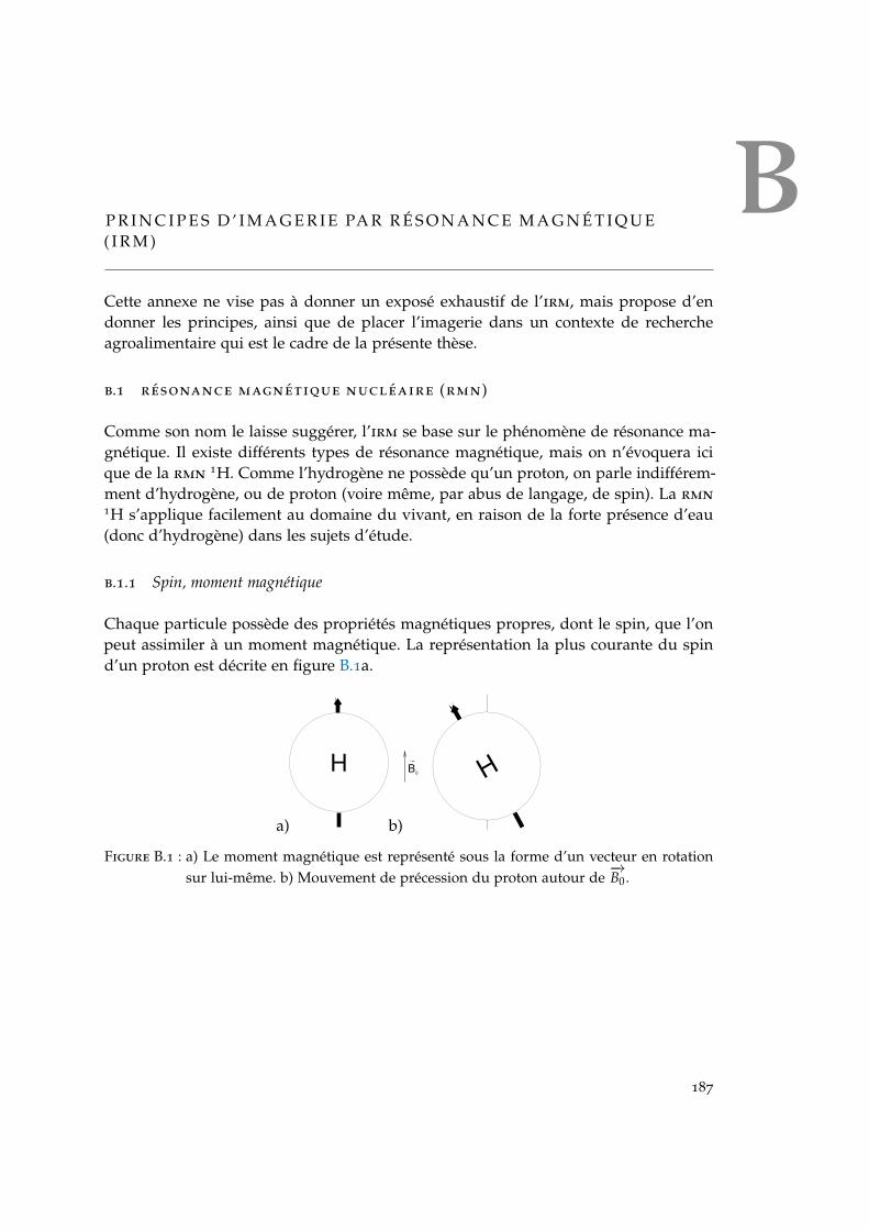
BP R I N C I P E S D ’ I M A G E R I E PA R R É S O N A N C E M A G N É T I Q U E( I R M )
Cette annexe ne vise pas à donner un exposé exhaustif de l’irm, mais propose d’endonner les principes, ainsi que de placer l’imagerie dans un contexte de rechercheagroalimentaire qui est le cadre de la présente thèse.
b.1 résonance magnétique nucléaire (rmn)
Comme son nom le laisse suggérer, l’irm se base sur le phénomène de résonance ma-gnétique. Il existe différents types de résonance magnétique, mais on n’évoquera icique de la rmn
1H. Comme l’hydrogène ne possède qu’un proton, on parle indifférem-ment d’hydrogène, ou de proton (voire même, par abus de langage, de spin). La rmn
1H s’applique facilement au domaine du vivant, en raison de la forte présence d’eau(donc d’hydrogène) dans les sujets d’étude.
b.1.1 Spin, moment magnétique
Chaque particule possède des propriétés magnétiques propres, dont le spin, que l’onpeut assimiler à un moment magnétique. La représentation la plus courante du spind’un proton est décrite en figure B.1a.
a)
H
b)
0 HB
Figure B.1 : a) Le moment magnétique est représenté sous la forme d’un vecteur en rotationsur lui-même. b) Mouvement de précession du proton autour de
−→B0 .
187
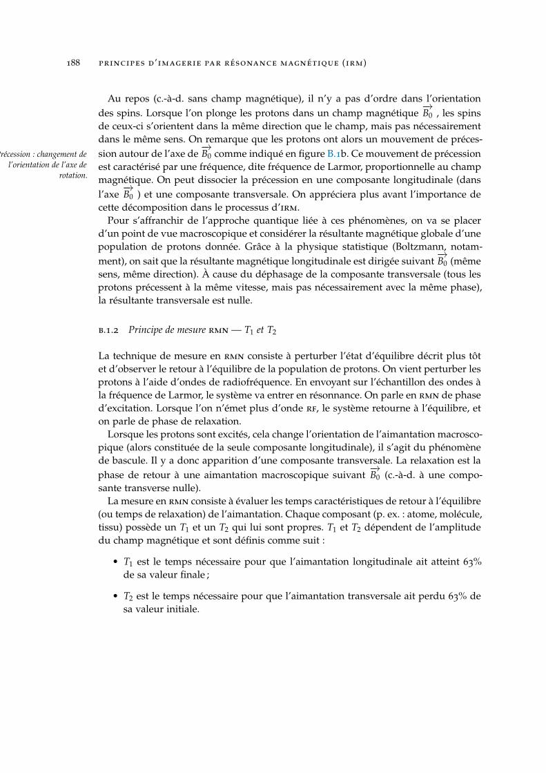
188 principes d’imagerie par résonance magnétique (irm)
Au repos (c.-à-d. sans champ magnétique), il n’y a pas d’ordre dans l’orientationdes spins. Lorsque l’on plonge les protons dans un champ magnétique
−→B0 , les spins
de ceux-ci s’orientent dans la même direction que le champ, mais pas nécessairementdans le même sens. On remarque que les protons ont alors un mouvement de préces-sion autour de l’axe de
−→B0 comme indiqué en figure B.1b. Ce mouvement de précessionPrécession : changement de
l’orientation de l’axe derotation.
est caractérisé par une fréquence, dite fréquence de Larmor, proportionnelle au champmagnétique. On peut dissocier la précession en une composante longitudinale (dansl’axe
−→B0 ) et une composante transversale. On appréciera plus avant l’importance de
cette décomposition dans le processus d’irm.Pour s’affranchir de l’approche quantique liée à ces phénomènes, on va se placer
d’un point de vue macroscopique et considérer la résultante magnétique globale d’unepopulation de protons donnée. Grâce à la physique statistique (Boltzmann, notam-ment), on sait que la résultante magnétique longitudinale est dirigée suivant
−→B0 (même
sens, même direction). À cause du déphasage de la composante transversale (tous lesprotons précessent à la même vitesse, mais pas nécessairement avec la même phase),la résultante transversale est nulle.
b.1.2 Principe de mesure rmn — T1 et T2
La technique de mesure en rmn consiste à perturber l’état d’équilibre décrit plus tôtet d’observer le retour à l’équilibre de la population de protons. On vient perturber lesprotons à l’aide d’ondes de radiofréquence. En envoyant sur l’échantillon des ondes àla fréquence de Larmor, le système va entrer en résonnance. On parle en rmn de phased’excitation. Lorsque l’on n’émet plus d’onde rf, le système retourne à l’équilibre, eton parle de phase de relaxation.
Lorsque les protons sont excités, cela change l’orientation de l’aimantation macrosco-pique (alors constituée de la seule composante longitudinale), il s’agit du phénomènede bascule. Il y a donc apparition d’une composante transversale. La relaxation est laphase de retour à une aimantation macroscopique suivant
−→B0 (c.-à-d. à une compo-
sante transverse nulle).La mesure en rmn consiste à évaluer les temps caractéristiques de retour à l’équilibre
(ou temps de relaxation) de l’aimantation. Chaque composant (p. ex. : atome, molécule,tissu) possède un T1 et un T2 qui lui sont propres. T1 et T2 dépendent de l’amplitudedu champ magnétique et sont définis comme suit :
• T1 est le temps nécessaire pour que l’aimantation longitudinale ait atteint 63%de sa valeur finale ;
• T2 est le temps nécessaire pour que l’aimantation transversale ait perdu 63% desa valeur initiale.
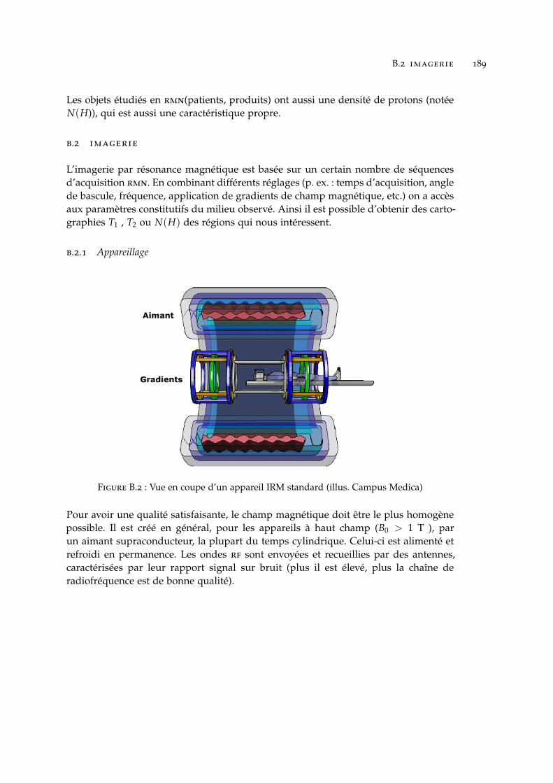
B.2 imagerie 189
Les objets étudiés en rmn(patients, produits) ont aussi une densité de protons (notéeN(H)), qui est aussi une caractéristique propre.
b.2 imagerie
L’imagerie par résonance magnétique est basée sur un certain nombre de séquencesd’acquisition rmn. En combinant différents réglages (p. ex. : temps d’acquisition, anglede bascule, fréquence, application de gradients de champ magnétique, etc.) on a accèsaux paramètres constitutifs du milieu observé. Ainsi il est possible d’obtenir des carto-graphies T1 , T2 ou N(H) des régions qui nous intéressent.
b.2.1 Appareillage
Figure B.2 : Vue en coupe d’un appareil IRM standard (illus. Campus Medica)
Pour avoir une qualité satisfaisante, le champ magnétique doit être le plus homogènepossible. Il est créé en général, pour les appareils à haut champ (B0 > 1 T ), parun aimant supraconducteur, la plupart du temps cylindrique. Celui-ci est alimenté etrefroidi en permanence. Les ondes rf sont envoyées et recueillies par des antennes,caractérisées par leur rapport signal sur bruit (plus il est élevé, plus la chaîne deradiofréquence est de bonne qualité).
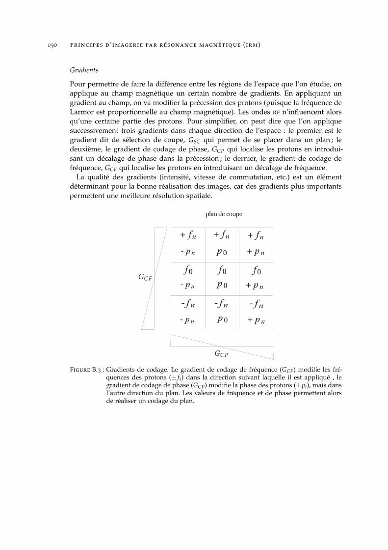
190 principes d’imagerie par résonance magnétique (irm)
Gradients
Pour permettre de faire la différence entre les régions de l’espace que l’on étudie, onapplique au champ magnétique un certain nombre de gradients. En appliquant ungradient au champ, on va modifier la précession des protons (puisque la fréquence deLarmor est proportionnelle au champ magnétique). Les ondes rf n’influencent alorsqu’une certaine partie des protons. Pour simplifier, on peut dire que l’on appliquesuccessivement trois gradients dans chaque direction de l’espace : le premier est legradient dit de sélection de coupe, GSC qui permet de se placer dans un plan ; ledeuxième, le gradient de codage de phase, GCP qui localise les protons en introdui-sant un décalage de phase dans la précession ; le dernier, le gradient de codage defréquence, GCF qui localise les protons en introduisant un décalage de fréquence.
La qualité des gradients (intensité, vitesse de commutation, etc.) est un élémentdéterminant pour la bonne réalisation des images, car des gradients plus importantspermettent une meilleure résolution spatiale.
plan de coupe
+ fn + fn + fn
- fn - fn - fn
f0 f0 f0GCF
GCP
+ pn
+ pn
+ pn
p0
p0
p0
- pn
- pn
- pn
Figure B.3 : Gradients de codage. Le gradient de codage de fréquence (GCF) modifie les fré-quences des protons (± fi) dans la direction suivant laquelle il est appliqué , legradient de codage de phase (GCP) modifie la phase des protons (±pi), mais dansl’autre direction du plan. Les valeurs de fréquence et de phase permettent alorsde réaliser un codage du plan.

B.2 imagerie 191
b.2.2 Séquences
Il y a principalement deux types de séquences irm : la séquence à écho de spin et celleà écho de gradient. Ces séquences ont deux paramètres :
• le temps que l’on met à observer un écho du signal de départ ou temps d’échote ;
• le temps entre deux impulsions à 90º ou temps de répétition tr.
Écho de spin (figure B.4)
Elle consiste à :
1. basculer l’aimantation à l’aide d’une impulsion rf à 90º ;
2. inverser le déphasage à l’aide d’une impulsion rf à 180º ;
3. recueillir le signal au temps te, quand les protons sont à nouveau en phase.
Figure B.4 : Séquence d’écho de spin
Écho de gradient (figure B.5)
Pour la séquence à echo de gradient, on n’applique pas d’impulsion à 180º, en revancheon inverse le gradient de codage de phase. Cela permet d’avoir des te et tr plus courts,en contrepartie d’une plus grande dépendance au déphasage.
Pour simplifier, l’imagerie consiste donc à combiner application de gradients etd’ondes rf de façon adaptée au phénomène à étudier. D’autres types de séquences,et d’autres paramètres existent et permettent d’améliorer l’acquisition d’images danscertaines situations, mais elles sont toutes basées sur ces deux séquences de base.
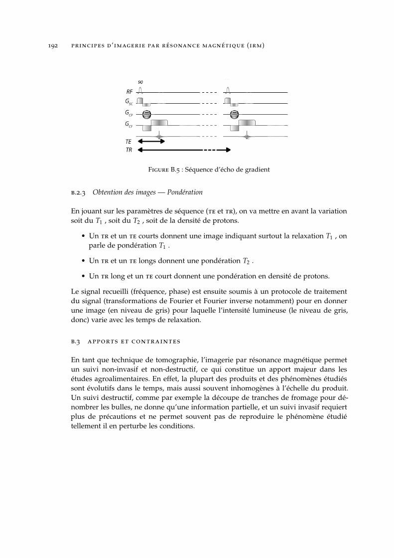
192 principes d’imagerie par résonance magnétique (irm)
Figure B.5 : Séquence d’écho de gradient
b.2.3 Obtention des images — Pondération
En jouant sur les paramètres de séquence (te et tr), on va mettre en avant la variationsoit du T1 , soit du T2 , soit de la densité de protons.
• Un tr et un te courts donnent une image indiquant surtout la relaxation T1 , onparle de pondération T1 .
• Un tr et un te longs donnent une pondération T2 .
• Un tr long et un te court donnent une pondération en densité de protons.
Le signal recueilli (fréquence, phase) est ensuite soumis à un protocole de traitementdu signal (transformations de Fourier et Fourier inverse notamment) pour en donnerune image (en niveau de gris) pour laquelle l’intensité lumineuse (le niveau de gris,donc) varie avec les temps de relaxation.
b.3 apports et contraintes
En tant que technique de tomographie, l’imagerie par résonance magnétique permetun suivi non-invasif et non-destructif, ce qui constitue un apport majeur dans lesétudes agroalimentaires. En effet, la plupart des produits et des phénomènes étudiéssont évolutifs dans le temps, mais aussi souvent inhomogènes à l’échelle du produit.Un suivi destructif, comme par exemple la découpe de tranches de fromage pour dé-nombrer les bulles, ne donne qu’une information partielle, et un suivi invasif requiertplus de précautions et ne permet souvent pas de reproduire le phénomène étudiétellement il en perturbe les conditions.
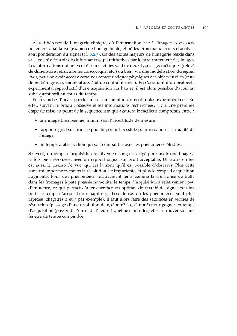
B.3 apports et contraintes 193
À la différence de l’imagerie clinique, où l’information liée à l’imagerie est essen-tiellement qualitative (examen de l’image finale) et où les principaux leviers d’analysesont pondération du signal (cf. B.2.3), un des atouts majeurs de l’imagerie réside danssa capacité à fournir des informations quantititatives par le post-traitement des images.Les informations qui peuvent être recueillies sont de deux types : géométriques (relevéde dimensions, structure macroscopique, etc.) ou bien, via une modélisation du signalrmn, peut-on avoir accès à certaines caractéristiques physiques des objets étudiés (tauxde matière grasse, température, état de contrainte, etc.). En s’assurant d’un protocoleexpérimental reproductif d’une acquisition sur l’autre, il est alors possible d’avoir unsuivi quantitatif au cours du temps.
En revanche, l’irm apporte un certain nombre de contraintes expérimentales. Eneffet, suivant le produit observé et les informations recherchées, il y a une premièreétape de mise au point de la séquence irm qui assurera le meilleur compromis entre :
• une image bien résolue, minimisant l’incertitude de mesure ;
• rapport signal sur bruit le plus important possible pour maximiser la qualité del’image ;
• un temps d’observation qui soit compatible avec les phénomènes étudiés.
Souvent, un temps d’acquisition relativement long est exigé pour avoir une image àla fois bien résolue et avec un rapport signal sur bruit acceptable. Un autre critèreest aussi le champ de vue, qui est la zone qu’il est possible d’observer. Plus cettezone est importante, moins la résolution est importante, et plus le temps d’acquisitionaugmente. Pour des phénomènes relativement lents comme la croissance de bulledans les fromages à pâte pressée non-cuite, le temps d’acquisition a relativement peud’influence, ce qui permet d’aller chercher un optimal de qualité de signal peu im-porte le temps d’acquisition (chapitre 5). Pour le cas où les phénomènes sont plusrapides (chapitres 2 et 3 par exemple), il faut alors faire des sacrifices en termes derésolution (passage d’une résolution de 0,33 mm3 à 0,53 mm3) pour gagner en tempsd’acquisition (passer de l’ordre de l’heure à quelques minutes) et se retrouver sur unefenêtre de temps compatible.


B I B L I O G R A P H I E
195

B I B L I O G R A P H I E
[1] ITFF-ITG / Actilait. Production de gaz carbonique et formation de l’ouverturedans l’emmental et le comté. etude itg ss 1984/05/c. Technical study, 1984. (Citedon page 119.)
[2] José M Aguilera and Peter J Lillford. Microstructural and imaging analyses as re-lated to food engineering. Food Engineering, pages 23–38, 2000. (Cited on page 90.)
[3] J.C. Akkerman, P. Walstra, and van H.J.M. Dijk. Holes in dutch type cheese. 1.conditions allowing eye formation. Netherlands milk and dairy journal, 1989. (Citedon pages 7, 8 et 91.)
[4] S. H. Alavi, S. S. H. Rizvi, and P. Harriott. Process dynamics of starch-basedmicrocellular foams produced by supercritical fluid extrusion. ii : Numerical si-mulation and experimental evaluation. Food Research International, 36(4) :321–330,2003. 0963-9969 doi : DOI : 10.1016/S0963-9969(02)00223-5. (Cited on page 117.)
[5] Moris Amon and Costel D. Denson. A study of the dynamics of foam growth :Analysis of the growth of closely spaced spherical bubbles. Polym. Eng. Sci., 24
(13) :1026–1034, 1984. 10.1002/pen.760241306. (Cited on pages 8, 89 et 117.)
[6] A. Arefmanesh, S. G. Advani, and E. E. Michaelides. A numerical study of bubblegrowth during low pressure structural foam molding process. Polymer Engineering& Science, 30(20) :1330–1337, 1990. 10.1002/pen.760302011. (Cited on page 89.)
[7] P. Babin, G. Della Valle, H. Chiron, P. Cloetens, J. Hoszowska, P. Pernot, A. L.Réguerre, L. Salvo, and R. Dendievel. Fast x-ray tomography analysis of bubblegrowth and foam setting during breadmaking. Journal of Cereal Science, 43(3) :393–397, 2006. (Cited on pages 4 et 83.)
[8] J. Bikard, T. Coupez, G. Della Valle, and B. Vergnes. Simulation of bread makingprocess using a direct 3d numerical method at microscale : analysis of baking step.International Journal of Material Forming, 5(1) :11–24, 2012. (Cited on page 90.)
[9] Jérôme Bikard, Thierry Coupez, Guy Della Valle, and Bruno Vergnes. Simulationof bread making process using a direct 3d numerical method at microscale : Ana-lysis of foaming phase during proofing. Journal of Food Engineering, 85(2) :259–267,2008. (Cited on page 90.)
[10] B. Blanc, J. O. Bosset, B. Martin, and J. Jimeno. Gas exchanges at the surface ofgruyere cheese during ripening. Schweizerische Milchwirtschaftliche Forschung, 12
(2) :30–34, 1983. Times Cited : 0. (Cited on page 119.)
197
198 bibliographie
[11] P. Boyaval, C. Deborde, C. Corre, C. Blanco, and E. Begue. Stress and osmopro-tection in propionibacteria. Lait, 79(1) :59–69, 1999. 186KM Times Cited :10 CitedReferences Count :29. (Cited on page 119.)
[12] J. Bruchon and T. Coupez. A numerical strategy for the direct 3d simulation of theexpansion of bubbles into a molten polymer during a foaming process. Internatio-nal Journal for Numerical Methods in Fluids, 57(8) :977–1003, 2008. 10.1002/fld.1660.(Cited on page 89.)
[13] H. Buggisch, P. Mazilu, and H. Weber. Parameter-identification for viscoelasticmaterials. Rheologica Acta, 27(4) :363–368, 1988. Q3046 Times Cited :0 Cited Refe-rences Count :6. (Cited on page 17.)
[14] J. F. Calzada and M. Peleg. Mechanical interpretation of compressive stress-strainrelationships of solid foods. Journal of Food Science, 43(4) :1087–1092, 1978. (Citedon pages 34 et 96.)
[15] Grant M. Campbell and Estelle Mougeot. Creation and characterisation of aeratedfood products. Trends in Food Science & Technology, 10(9) :283–296, 1999. 0924-2244
doi : DOI : 10.1016/S0924-2244(00)00008-X. (Cited on pages 89 et 117.)
[16] E. Chiotellis and G. M. Campbell. Proving of bread dough i - modelling theevolution of the bubble size distribution. Food and Bioproducts Processing, 81(C3) :194–206, 2003. 742DB Times Cited :19 Cited References Count :43. (Cited onpages 90 et 118.)
[17] E Chiotellis and GM Campbell. Proving of bread dough ii : measurement ofgas production and retention. Food and bioproducts processing, 81(3) :207–216, 2003.(Cited on page 90.)
[18] William Mansfield Clark. On the formation of "eyes" in emmental cheese. Journalof Dairy Science, 1(2) :91–113, 1917. (Cited on page 8.)
[19] G. G. Codina, S. Mironeasa, C. Mironeasa, C. N. Popa, and R. Tamba-Berehoiu.Wheat flour dough alveograph characteristics predicted by mixolab regressionmodels. Journal of the Science of Food and Agriculture, 92(3) :638–644, 2012. (Citedon page 64.)
[20] T. Conde, A. Mulet, G. Clemente, and J. Benedito. Detection of internal cracks inmanchego cheese using the acoustic impulse-response technique and ultrasounds.Journal of Dairy Science, 91(3) :918–927, 2008. (Cited on page 63.)
[21] J. Culioli and P. Sherman. Evaluation of gouda cheese firmness by compressiontests. Journal of Texture Studies, 7(3) :353–372, 1976. Times Cited : 74. (Cited onpage 83.)
bibliographie 199
[22] J.F. Davidson and M. A. Cullen. The determination of diffusion coefficients forsparingly soluble gases in liquids. Transactions of the Institution of Chemical Engi-neers, 35 :51–60, 1957. (Cited on page 130.)
[23] B. de Cindio and S. Correra. Mathematical modelling of leavened cerealgoods. Journal of Food Engineering, 24(3) :379–403, 1995. 0260-8774 doi : DOI :10.1016/0260-8774(95)90052-D. (Cited on pages 90, 117 et 118.)
[24] M. A. Del Nobile, S. Chillo, A. Mentana, and A. Baiano. Use of the generalizedmaxwell model for describing the stress relaxation behavior of solid-like foods.Journal of Food Engineering, 78(3) :978–983, 2007. ISI Document Delivery No. :092CB Times Cited : 15 Cited Reference Count : 21 Del Nobile, M. A. Chillo, S.Mentana, A. Baiano, A. ELSEVIER SCI LTD OXFORD. (Cited on pages 17, 18
et 47.)
[25] R. Elshereef, J. Vlachopoulos, and A. Elkamel. Comparison and analysis of bubblegrowth and foam formation models. Engineering Computations, 27(3-4) :387–408,2010. (Cited on page 89.)
[26] J. Engmann, C. Servais, and A. S. Burbidge. Squeeze flow theory and applicationsto rheometry : A review. Journal of Non-Newtonian Fluid Mechanics, 132(1-3) :1–27,2005. Times Cited : 38. (Cited on page 34.)
[27] J. J. Eskelinen, A. P. Alavuotunki, E. Haeggstrom, and T. Alatossava. Preliminarystudy of ultrasonic structural quality control of swiss-type cheese. Journal of DairyScience, 90(9) :4071–4077, 2007. (Cited on page 63.)
[28] J. T. Fan, J. R. Mitchell, and J. M. V. Blanshard. A model for the oven rise ofdough during baking. Journal of Food Engineering, 41(2) :69–77, 1999. 223EX TimesCited :44 Cited References Count :37. (Cited on pages 90, 117 et 118.)
[29] James J. Feng and Christopher A. Bertelo. Prediction of bubble growth and sizedistribution in polymer foaming based on a new heterogeneous nucleation model.Journal of Rheology, 48(2) :439–462, 2004. (Cited on pages 8, 89, 90 et 111.)
[30] E. Fluckiger, P. Eberhard, and F. Walser. Experiments on eye formation in emmen-tal cheese. Schweizerische Milchzeitung, 104(84) :623–624, 1978. Cited ReferenceCount : 5 ref. Versuche zur Lochbildung im Emmentalerkase. (Cited on pages 64
et 81.)
[31] Lorna J Gibson and Michael F Ashby. Cellular solids : structure and properties. Cam-bridge university press, 1999. (Cited on page 8.)
[32] S. M. Goh, M. N. Charalambides, and J. G. Williams. Large strain time dependentbehavior of cheese. Journal of Rheology, 47(3) :16, 2003. (Cited on pages 30, 47
et 83.)
200 bibliographie
[33] S. M. Goh, M. N. Charalambides, and J. G. Williams. Characterisation of non-linear viscoelastic foods by the indentation technique. Rheologica Acta, 44(1) :47–54, 2004. ISI Document Delivery No. : 887KJ Times Cited : 4 Cited ReferenceCount : 19 SPRINGER NEW YORK. (Cited on pages 18, 30 et 47.)
[34] S. M. Goh, M. N. Charalambides, and J. G. Williams. Characterization of the nonli-near viscoelastic constitutive properties of mild cheddar cheese from indentationtests. Journal of Texture Studies, 36(5-6) :459–477, 2005. ISI Document Delivery No. :987LJ Times Cited : 3 Cited Reference Count : 30 BLACKWELL PUBLISHING OX-FORD. (Cited on pages 17, 30 et 47.)
[35] D. Grenier, T. Lucas, and D. Le Ray. Measurement of local pressure during pro-ving of bread dough sticks : Contribution of surface tension and dough viscosityto gas pressure in bubbles. Journal of Cereal Science, 52(3) :373–377, 2010. (Citedon page 82.)
[36] David Grenier, Yannick Laridon, Dominique Le Ray, Sylvain Challois, and Ti-phaine Lucas. Experimental growth of a single eye in a semi-hard cheese undera known gas pressure : an mri device and its associated methods. Food ResearchInternational, to be submitted. (Cited on pages 95 et 97.)
[37] David Grenier, Tiphaine Lucas, and Dominique Le Ray. Gas pressure measure-ments in eyes of semi-hard cheese : Influence of the cheese outskirts on the growthof the bubbles at the core of the cheese. International Dairy Journal, to be submitted.(Cited on pages xiv, 78, 81, 82, 83, 91, 93 et 131.)
[38] D. Guggisberg, M. T. Frohlich-Wyder, S. Irmler, M. Greco, D. Wechsler, andP. Schuetz. Eye formation in semi-hard cheese : X-ray computed tomographyas a non-invasive tool for assessing the influence of adjunct lactic acid bacteria.Dairy Science and Technology, 93(2) :135–149, 2013. (Cited on page 63.)
[39] L. Hailemariam, M. Okos, and O. Campanella. A mathematical model for theisothermal growth of bubbles in wheat dough. Journal of Food Engineering, 82(4) :466–477, 2007. ISI Document Delivery No. : 177RG Times Cited : 5 Cited ReferenceCount : 48. (Cited on pages 90, 117 et 118.)
[40] Conn J F Handleman, A R and J W Lyons. Bubble mechanics in thick foams andtheir effects on cake quality. Ceral Chemistry, 38 :294–305, 1961. (Cited on page 89.)
[41] R. Harper and M. Baron. Cheese grading. mechanical properties compared withquality assessed subjectively. Journal of Dairy Research, 16(03) :363–367, 1949. (Ci-ted on page 17.)
[42] D. H. Hettinga and G. W. Reinbold. The propionic acid bacteria - a review. ii.metabolism. Journal of Milk and Food Technology, 35 :358–372, 1972. (Cited onpage 133.)
bibliographie 201
[43] H Huang and J.L. Kokini. Prediction of dough volume development which considers thebiaxial extensional growth of cells, pages 113–120. Eagan Press, St Paul, MN, USA,1999. (Cited on page 89.)
[44] D. Huc, F. Mariette, S. Challois, J. Barreau, and G. Moulin. Multi-scale investiga-tion of eyes in semi-hard cheese. Innovative Food Science and Emerging Technologies,2013. (Cited on pages 3, 34, 90, 118 et 139.)
[45] D. Huc, C. Michon, N. Roland, S. Challois, and F. Mariette. Influence of saltcontent on eye growth in semi-hard cheeses using mri and co2 production mea-surements. International Dairy Journal, 2014. (Cited on pages 3, 119, 129 et 130.)
[46] Delphine Huc. Hiérarchisation des facteurs contribuant à la croissance des bulles dansdes fromages à pâte pressée non cuite par une approche multi-échelles. PhD thesis, Uni-versité de Rennes 1, 2013. (Cited on pages 5, 9 et 121.)
[47] Delphine Huc, Sylvain Challois, Matthieu Monziols, Camille Michon, and Fran-çois Mariette. Spatially-resolved characterization of eye-growing kinetics in semi-hard cheeses. Journal of Dairy Science, 2014. (Cited on pages 63 et 83.)
[48] M. Jakobsen, P. N. Jensen, and J. Risbo. Assessment of carbon dioxide solubilitycoefficients for semihard cheeses : the effect of temperature and fat content. Eu-ropean Food Research and Technology, 229(2) :287–294, 2009. Times Cited : 0. (Citedon pages 118, 119, 131, 132 et 133.)
[49] JCGM. Guide to the expression of uncertainty in measurement. BIPM, 2008. (Cited onpages 68 et 72.)
[50] S. F. Jones, G. M. Evans, and K. P. Galvin. Bubble nucleation from gas cavities— a review. Advances in Colloid and Interface Science, 80(1) :27–50, 1999. (Cited onpage 117.)
[51] Matti Keentok, Marcus P. Newberry, Peter Gras, Frank Bekes, and Roger I. Tanner.The rheology of bread dough made from four commercial flours. Rheologica Acta,41(1-2) :173–179, 2002. (Cited on page 118.)
[52] Gyeong-Won Kim, Gab-Soo Do, Yeonghwan Bae, and Yasuyuki Sagara. Deter-mination of the viscoelastic properties of agar/agar-gelatin gels based on finiteelement method optimization. Food Science and Technology Research, 14(6) :525–525,2008. (Cited on page 18.)
[53] Gyeong-Won Kim, Man-Soo Kim, Yasuyuki Sagara, Yeong-Hwan Bae, In-Bok Lee,Gab-Soo Do, Sung-Hyoun Lee, and Suk-Won Kang. Determination of the viscoe-lastic properties of apple flesh under quasi-static compression based on finiteelement method optimization. Food Science and Technology Research, 14(3) :221–231,2008. (Cited on page 18.)
202 bibliographie
[54] M. Kontopoulou and J. Vlachopoulos. Bubble dissolution in molten polymers andits role in rotational molding. Polymer Engineering and Science, 39(7) :1189–1198,1999. Kontopoulou, M Vlachopoulos, J. (Cited on page 90.)
[55] H. Kraggerud, J. P. Wold, M. Hoy, and R. K. Abrahamsen. X-ray images for thecontrol of eye formation in cheese. International Journal of Dairy Technology, 62
(2) :147–153, 2009. ISI Document Delivery No. : 448NA Times Cited : 1 CitedReference Count : 16 Kraggerud, H. Wold, J. P. Hoy, M. Abrahamsen, R. K. Wiley-blackwell publishing, inc Malden. (Cited on page 63.)
[56] R.S. Lakes. Viscoelastic Materials. Cambridge University Press, 2009. (Cited onpage 17.)
[57] Y. Laridon, C. Doursat, D. Grenier, C. Michon, D. Flick, and T. Lucas. New methodfor the assessment of the viscoelastic parameters of materials. application to semi-hard type cheese. Rheologica Acta, Submitted. (Cited on pages 77, 82, 83, 96, 97,98, 124 et 138.)
[58] Y. Laridon, D. Grenier, D. Houeix, C. Doursat, T. Lucas, and D. Flick. Modellingof the growth of a single bubble in semi-hard cheese ; with experimental verifica-tion and sensitivity analysis. Journal of the Mechanics and Physics of Solids, to besubmitted. (Cited on pages 63, 119, 134 et 137.)
[59] B. Launay and C. Michon. Biaxial extension of wheat flour doughs : Lubricatedsqueezing flow and stress relaxation properties. Journal of Texture Studies, 39(5) :496–529, 2008. ISI Document Delivery No. : 351GJ Times Cited : 1 Cited ReferenceCount : 78 Launay, B. Michon, C. BLACKWELL PUBLISHING OXFORD. (Citedon pages 34 et 118.)
[60] Han Choon Lee, Byung Do Oh, Sung Won Bae, and Moo Hwan Kim. Singlebubble growth in saturated pool boiling on a constant wall temperature surface.International Journal of Multiphase Flow, 29(12) :1857–1874, 2003. (Cited on page 63.)
[61] Kija Lee, Kaho Uegaki, Chihiro Nishii, Tadashi Nakamura, Auska Kubota, TsunaoHirai, and Kazutaka Yamada. Computed tomographic evaluation of gas holeformation and structural quality in gouda-type cheese. International Journal ofDairy Technology, 65(2) :232–236, 2012. Times Cited : 0. (Cited on page 63.)
[62] Shau-Tarng Lee, N. S. Ramesh, and Gregory A. Campbell. Study of thermoplas-tic foam sheet formation. Polymer Engineering & Science, 36(19) :2477–2482, 1996.10.1002/pen.10645. (Cited on pages 8 et 117.)
[63] ShauTarng Lee and N. S. Ramesh. Polymeric Foams : Mechanisms and Materials.CRC Press, Boca Raton, London, New York, Washington DC, 2004. (Cited onpage 89.)
bibliographie 203
[64] P. Masi and F. Addeo. An examination of some mechanical properties of a groupof italian cheeses and their relation to structure and conditions of manufacture.Journal of Food Engineering, 5(3) :217–229, 1986. (Cited on page 83.)
[65] Paolo Masi. Characterization of history-dependent stress-relaxation behaviour ofcheeses. Journal of Texture Studies, 19(4) :373–388, 1988. (Cited on pages 17 et 18.)
[66] Toshiro Minami, Susumu Maeda, Mitsuo Higasa, and Kazuhiko Kashima. In-situobservation of bubble formation at silicon melt–silica glass interface. Journal ofCrystal Growth, 318(1) :196–199, 2011. (Cited on page 63.)
[67] C. C. Mourtada-Bonnefoi and H. M. Mader. Experimental observations of theeffect of crystals and pre-existing bubbles on the dynamics and fragmentation ofvesiculating flows. Journal of Volcanology and Geothermal Research, 129(1–3) :83–97,2004. (Cited on page 63.)
[68] M. Musse, S. Challois, D. Huc, S. Quellec, and F. Mariette. Mri method for in-vestigation of eye growth in swiss-type cheese. Journal of Food Engineering, 2014.(Cited on pages 63, 69, 70, 96 et 121.)
[69] Oded Navon, Anatoly Chekhmir, and Vladimir Lyakhovsky. Bubble growth inhighly viscous melts : theory, experiments, and autoexplosivity of dome lavas.Earth and Planetary Science Letters, 160(3–4) :763–776, 1998. (Cited on page 89.)
[70] D. J. O’Callaghan and T. P. Guinee. Rheology and Texture of Cheese, volume Volume1, pages 511–540. Academic Press, 2004. (Cited on page 17.)
[71] N. Otsu. Threshold selection method from gray-level histograms. Ieee Transactionson Systems Man and Cybernetics, 9(1) :62–66, 1979. ISI Document Delivery No. :GE960 Times Cited : 4354 Cited Reference Count : 5 Otsu, n Ieee-inst electricalelectronics engineers inc New york. (Cited on pages 70, 95 et 154.)
[72] R. D. Patel. Bubble-growth in a viscous newtonian liquid. Chemical EngineeringScience, 35(11) :2352–2356, 1980. (Cited on page 89.)
[73] J. P. Pauchard, E. Flückiger, J. O. Bosset, and B. Blanc. Co2 solubility, concentra-tion and distribution in relation to eye formation in emmental cheese. Schweize-rische Milchwirtschaftliche Forschung, 9(4) :69–73, 1980. Times Cited : 0. (Cited onpage 132.)
[74] M. Peleg. Considerations of a general rheological model for the mechanical be-havior of viscoelastic solid food materials. Journal of Texture Studies, 7(2) :243–255,1976. (Cited on page 17.)
[75] R. H. Perry. Perry’s Chemical Engineers’ Handbook. McGraw-Hill Professional, 8thedition edition, 2007. (Cited on page 132.)
204 bibliographie
[76] M. S. Plesset. The dynamics of cavitation bubbles. Journal of Applied Mechanics,16 :277–82, 1949. (Cited on pages 7 et 89.)
[77] N. S. Ramesh, H. Rasmussen Don, and A. Campbell Gregory. Numerical andexperimental studies of bubble growth during the microcellular foaming process.Polymer Engineering & Science, 31(23) :1657–1664, 1991. 10.1002/pen.760312305.(Cited on pages 8, 89 et 90.)
[78] Rayleigh. On the pressure developed in a liquid during the collapse of a sphericalcavity. Philosophical Magazine Series 6, 34(200) :94–98, 1917. 1941-5982. (Cited onpage 7.)
[79] N. B. Richoux, D. Deibel, R. J. Thompson, and C. C. Parrish. Seasonal and deve-lopmental variation in the fatty acid composition of mysis mixta (mysidacea) andacanthostepheia malmgreni (amphipoda) from the hyperbenthos of a cold-oceanenvironment (conception bay, newfoundland). Journal of Plankton Research, 27(8) :719–733, 2005. 974LM Times Cited :14 Cited References Count :34. (Cited onpage 119.)
[80] Rocio Rodriguez-Aguilera, Jorge C. Oliveira, Julio C. Montanez, and Pramod V.Mahajan. Gas exchange dynamics in modified atmosphere packaging of softcheese. Journal of Food Engineering, 95(3) :438–445, 2009. (Cited on page 119.)
[81] Harald Rohm and Harald Lederer. Uniaxial compression of swiss-type cheese atdifferent strain rates. International Dairy Journal, 2(6) :331–343, 1992. (Cited onpage 47.)
[82] R. Sander. Compilation of henry’s law constants for inorganic and organic speciesof potential importance in environmental chemistry, 1999. (Cited on page 131.)
[83] P. Schuetz, D. Guggisberg, I. Jerjen, M. T. Frohlich-Wyder, J. Hofmann, D. Wechs-ler, A. Flisch, W. Bisig, U. Sennhauser, and H. P. Bachmann. Quantitative compari-son of the eye formation in cheese using radiography and computed tomographydata. International Dairy Journal, 31(2) :150–155, 2013. (Cited on page 63.)
[84] A. M. Seuvre and M. Mathlouthi. Contribution to the study of gas-release duringthe maturation of a french emmental cheese. Lebensmittel-Wissenschaft & Technolo-gie, 15(5) :258–262, 1982. Pn270 Times Cited :1 Cited References Count :36. (Citedon page 119.)
[85] P. Shah, M. Campbell, G, .L. McKee, S, and C. D. Rielly. Proving of bread dough :modelling the growth of individual bubbles, volume 76. Institution of Chemical Engi-neers, 1998. (Cited on pages 89, 90, 117 et 118.)
bibliographie 205
[86] IM Sobol. Global sensitivity indices for nonlinear mathematical models and theirmonte carlo estimates. Mathematics and Computers in Simulation, 55(1–3) :271–280,2001. (Cited on page 101.)
[87] Alina Surmacka Szczesniak. Objective measurements of food texture. Journal ofFood Science, 28(4) :410–420, 1963. (Cited on page 17.)
[88] Arthur V. Tobolsky. Elastoviscous properties of polyisobutylene. vi. relation bet-ween stress relaxation modulus and dynamic modulus. Journal of the AmericanChemical Society, 74(15) :3786–3788, 1952. doi : 10.1021/ja01135a021. (Cited onpage 17.)
[89] D. C. Venerus, N. Yala, and B. Bernstein. Analysis of diffusion-induced bubblegrowth in viscoelastic liquids. Journal of Non-Newtonian Fluid Mechanics, 75(1) :55–75, 1998. 0377-0257 doi : DOI : 10.1016/S0377-0257(97)00076-1. (Cited on page 89.)
[90] David C Venerus and Nadia Yala. Transport analysis of diffusion-induced bubblegrowth and collapse in viscous liquids. AIChE Journal, 43(11) :2948–2959, 1997.10.1002/aic.690431108. (Cited on page 8.)
[91] D. Vivier, D. Compan, G. Moulin, and P. Galzy. Study of carbon dioxide releasefrom feta cheese. Food Research International, 29(2) :169–174, 1996. Uy713 TimesCited :3 Cited References Count :13. (Cited on page 119.)
[92] S. R. White, J. R. Broadbent, C. J. Oberg, and D. J. McMahon. Effect of lactobacillushelveticus and propionibacterium freudenrichii ssp shermanii combinations onpropensity for split defect in swiss cheese. Journal of Dairy Science, 86(3) :719–727,2003. 656HD Times Cited :8 Cited References Count :33. (Cited on page 119.)
[93] MB Whitworth and JM Alava. Non-destructive imaging of bread and cake struc-ture during baking. In Using Cereal Science and Technology for the Benefit of Consu-mers : Proceedings of the 12th International ICC Cereal and Bread Congress 24-26 May,2004, volume 109, page 456. CRC Press, 2004. (Cited on page 4.)
[94] T. Yano and Y. Shimiya. Expansion of a spherical hole in elastic food materialswith surface-tension. Agricultural and Biological Chemistry, 52(12) :3113–3117, 1988.(Cited on pages 64 et 90.)


Modélisation et visualisation d’une croissance de bulle dans un milieu viscoélastique évolutif et hétérogène
Résumé L'objectif de cette thèse était de caractériser, de modéliser et de hiérarchiser les mécanismes acteurs de la croissance de bulles dans un fromage à pâte pressée non-cuite à l'échelle de la bulle. Pour cela, trois étapes majeures ont été envisagées. Une première étape de mise au point d’une méthode de détermination des paramètres du modèle mécanique (modèle de Maxwell généralisé) par ajustement de courbes expérimentales de compression-relaxation a été effectuée. Une deuxième étape de validation a consisté en la réalisation d'un dispositif expérimental permettant de soumettre une bulle isolée dans un cylindre de fromage à diverses sollicitations mécaniques, à suivre l'évolution du dispositif en temps réel et de façon non invasive par IRM, et à confronter ces résultats à des simulations reproduisant les conditions d'acquisition. Une dernière étape a consisté à rajouter la prise en compte du transport de matière (CO2) au sein du fromage dans la modélisation. Les résultats de simulation ont dans un premier temps été confrontés au comportement moyen des bulles au sein d'un bloc de fromage, et dans un deuxième temps un dispositif expérimental de validation similaire à celui de l'étape précédente a été développé. La caractérisation mécanique du fromage a montré que les propriétés rhéologiques n'évoluent pas au cours de l'affinage, mais qu'elles sont soumises à un fort gradient spatial. Le modèle de Maxwell a été validé expérimentalement dans des conditions de sollicitations mécaniques uniquement et une étude de sensibilité a permis de montrer la forte influence des temps de relaxation les plus longs (plusieurs heures) et de la position de la bulle sur la croissance. L'étude du couplage entre transport de quantité de mouvement et transport de matière dans un contexte de croissance d'une seule bulle a permis de montrer la grande influence des paramètres de transport de matière sur la croissance de bulle, en particulier pour le coefficient de diffusion et le taux de production de CO2. Dans un contexte où deux cavités gazeuses sont mobilisées, les paramètres géométriques (position, dimensions, forme des cavités) se sont montrés aussi importants que les paramètres de transport de matière. Abstract The objective of this PhD thesis was to characterise, model and rank the mechanisms involved in the growth of bubbles in semi-hard cheeses, at the bubble scale. Three steps were considered. First, a mechanical characterisation of the material enabled to define a rheological model to describe the behaviour of the material (generalised Maxwell model), and to set-up a method to determine the model parameters by fitting of compression-relaxation data. Secondly, the Maxwell model consisted in setting up an experimental validation procedure allowing studying different loads on a single bubble surrounded by a cheese cylinder. Experiments were monitored in real-time in a non-invasive manner by MRI imaging and were compared to simulations reproducing the experimental conditions. Finally, mass transport (CO2) was also taken into account in the model. Simulation results were first compared to the average bubble growth in cheese blocks, and then a dedicated experimental set-up similar to that used previously was used. Mechanical characterisation of semi-hard cheese showed the rheological properties did not evolve during ripening, but presented a steep spatial gradient. Despite its simplicity, the Maxwell model showed good agreement with the experimental results. A sensitivity study demonstrated that the highest relaxation time (about several hours) and the bubble position were the most influent parameters over bubble growth, when only the mechanical model was involved. Coupling between mass and momentum transport in a single bubble case demonstrated the great influence of the mass transport parameters on bubble growth, especially diffusivity and CO2 production rate. In the case where two gaseous cavities are involved, geometric parameters (cavities positions, dimensions and shape) proved to be as important as the mass transport parameters on the bubble growth.