Embed Size (px)
Citation preview
NNALESSCIENIFIQUES
SUPÉRIEUE
dL ÉCOLEORMALE
ISSN 0012-9593
ASENAH
SOCIÉTÉ MATHÉMATIQUE DE FRANCE
quatrième série - tome 41 fascicule 3 mai-juin 2008
Laura G. DeMARCO & Curtis T. McMULLEN
Trees and the dynamics of polynomials
Ann. Scient. Éc. Norm. Sup.4 e série, t. 41, 2008, p. 337 à 383
TREES AND THE DYNAMICS OF POLYNOMIALS∗
ʙʏ Lʀ G. DMARCO ɴ Cʀɪ T. MMULLEN
Aʙʀ. – In this paper we study branched coverings of metrized, simplicial trees F : T → T
which arise from polynomial maps f : C → C with disconnected Julia sets. We show that the collec-tion of all such trees, up to scale, forms a contractible space PTD compactifying the moduli space ofpolynomials of degree D; that F records the asymptotic behavior of the multipliers of f ; and that anymeromorphic family of polynomials over ∆∗ can be completed by a unique tree at its central fiber. Inthe cubic case we give a combinatorial enumeration of the trees that arise, and show that PT3 is itselfa tree.
R. – Dans ce travail, nous étudions des revêtements ramifiés d’arbres métriques simpliciauxF : T → T qui sont obtenus à partir d’applications polynomiales f : C → C possédant un ensemblede Julia non connexe. Nous montrons que la collection de tous ces arbres, à un facteur d’échelle près,forme un espace contractilePTD qui compactifie l’espace des modules des polynômes de degré D. Nousmontrons aussi que F enregistre le comportement asymptotique des multiplicateurs de f et que toutefamille méromorphe de polynômes définis sur ∆∗ peut être complétée par un unique arbre comme safibre centrale. Dans le cas cubique, nous donnons une énumération combinatoire des arbres ainsi ob-tenus et montrons que PT3 est lui-même un arbre.
1. Introduction
The basin of infinity of a polynomial map f : C → C carries a natural foliation and a flatmetric with singularities, determined by the escape rate of orbits. As f diverges in the modulispace of polynomials, this Riemann surface collapses along its foliation to yield a metrizedsimplicial tree (T, d), with limiting dynamics F : T → T .
In this paper we characterize the trees that arise as limits, and show they provide a naturalboundary PTD compactifying the moduli space of polynomials of degree D. We show that
∗Research of both authors supported in part by the NSF..
ANNALES SCIENTIFIQUES DE L’ÉCOLE NORMALE SUPÉRIEURE0012-9593/03/© 2008 Société Mathématique de France. Tous droits réservés
338 L. G. DMARCO AND C. T. MMULLEN
(T, d, F ) records the limiting behavior of the multipliers of f at its periodic points, and thatany degenerating analytic family of polynomials ft(z) : t ∈ ∆∗ can be completed by aunique tree at its central fiber. Finally we show that in the cubic case, the boundary of modulispace PT3 is itself a tree; and for any D, PTD is contractible.
The metrized trees (T, d, F ) provide a counterpart, in the setting of iterated rational maps,to the R-trees that arise as limits of hyperbolic manifolds.
The quotient tree. – Let f : C → C be a polynomial of degree D ≥ 2. The points z ∈ Cwith bounded orbits under f form the compact filled Julia set
K(f) = z : supn
|fn(z)| < ∞;
its complement, Ω(f) = C \K(f), is the basin of infinity. The escape rate G : C → [0,∞) isdefined by
G(z) = limn→∞
D−nlog+|fn(z)|;
it is the Green function for K(f) with a logarithmic pole at infinity. The escape rate satisfiesG(f(z)) = DG(z), and thus it gives a semiconjugacy from f to the simple dynamical systemt → Dt on [0,∞).
Now suppose that the Julia set J(f) = ∂K(f) is disconnected; equivalently, suppose thatat least one critical point of f lies in the basin Ω(f). Then some fibers of G are also discon-nected, although for each t > 0 the fiber G−1(t) has only finitely many components.
To record the combinatorial information of the dynamics of f on Ω(f), we form the quo-
tient tree T by identifying points of C that lie in the same connected component of a level setof G. The resulting space carries an induced dynamical system
F : T → T .
The escape rate G descends to give the height function H on T , yielding a commutative dia-gram
C
π
G
TH [0,∞)
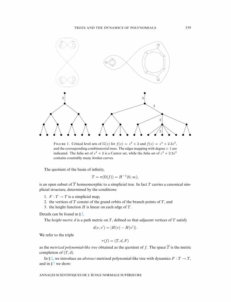
respecting the dynamics. See Figure 1 for an illustration of the trees in two examples. Notethat only a finite subtree of T has been drawn in each case.
The Julia set of F : T → T is defined by
J(F ) = π(J(f)) = H−1(0).
It is a Cantor set with one point for each connected component of J(f). With respect to themeasure of maximal entropy µf , the quotient map π : J(f) → J(F ) is almost injective, in thesense that µf -almost every component of J(f) is a single point (Theorem 3.2). In particular,there is no loss of information when passing to the quotient dynamical system:
Tʜʀ 1.1. – Let f be a polynomial of degree D ≥ 2 with disconnected Julia set. The
measure-theoretic entropy of (f, J(f), µf ) and its quotient (F, J(F ), π∗(µf )) are the same —
they are both log D.
4 e SÉRIE – TOME 41 – 2008 – No 3
TREES AND THE DYNAMICS OF POLYNOMIALS 339
2
2
2
3
2
Fɪɢʀ 1. Critical level sets of G(z) for f(z) = z2 + 2 and f(z) = z3 + 2.3z2,and the corresponding combinatorial trees. The edges mapping with degree > 1 areindicated. The Julia set of z2 + 2 is a Cantor set, while the Julia set of z3 + 2.3z2
contains countably many Jordan curves.
The quotient of the basin of infinity,
T = π(Ω(f)) = H−1(0,∞),
is an open subset of T homeomorphic to a simplicial tree. In fact T carries a canonical sim-plicial structure, determined by the conditions:
1. F : T → T is a simplicial map,2. the vertices of T consist of the grand orbits of the branch points of T , and3. the height function H is linear on each edge of T .
Details can be found in § 2.The height metric d is a path metric on T , defined so that adjacent vertices of T satisfy
d(v, v) = |H(v)−H(v)|.
We refer to the tripleτ(f) = (T, d, F )
as the metrized polynomial-like tree obtained as the quotient of f . The space T is the metriccompletion of (T, d).
In § 2, we introduce an abstract metrized polynomial-like tree with dynamics F : T → T ,and in § 7 we show:
ANNALES SCIENTIFIQUES DE L’ÉCOLE NORMALE SUPÉRIEURE

340 L. G. DMARCO AND C. T. MMULLEN
Tʜʀ 1.2. – Every metrized polynomial-like tree (T, d, F ) arises as the quotient τ(f)of a polynomial f .
Special cases of Theorem 1.2 were proved by Emerson; Theorems 9.4 and 10.1 of [7] showthat any tree with just one escaping critical point (though possibly of high multiplicity) andwith divergent sums of moduli can be realized by a polynomial.
Spaces of trees and polynomials. – Let TD denote the space of isometry classes of metrizedpolynomial-like trees (T, d, F ) of degree D. The space TD carries a natural geometric topol-ogy, defined by convergence of finite subtrees. There is a continuous action of R+ on TD byrescaling the metric d, yielding as quotient the projective space
PTD = TD/R+.
In § 5 we show:
Tʜʀ 1.3. – The space PTD is compact and contractible.
Now let MPolyD denote the moduli space of polynomials of degree D, the space of poly-nomials modulo conjugation by the affine automorphisms of C. The conjugacy class of apolynomial f will be denoted [f ]. The space MPolyD is a complex orbifold, finitely coveredby CD−1. The maximal escape rate
M(f) = maxG(c) : f (c) = 0
depends only on the conjugacy class of f ; Branner and Hubbard observed in [3] that M de-scends to a continuous and proper map M : MPolyD → [0,∞).
The connectedness locus CD ⊂ MPolyD is the subset of polynomials with connected Juliaset; it coincides with the locus M(f) = 0 and is therefore a compact subset of MPolyD. Wedenote its complement by
MPoly∗D = MPolyD \CD.
The metrized polynomial-like tree τ(f) = (T, d, F ) depends only on the conjugacy class off , so τ induces a map
τ : MPoly∗D → TD.
Note that the compactness of the connectedness locus CD implies that every divergent se-quence in MPolyD will eventually be contained in the domain of τ .
There is a natural action of R+ on MPoly∗D obtained by ‘stretching’ the complex structureon the basin of infinity. In § 6 and § 8 we show:
Tʜʀ 1.4. – The map τ : MPoly∗D → TD is continuous, proper, surjective, and equiv-
ariant with respect to the action of R+ by stretching of polynomials and by metric rescaling of
trees.
Tʜʀ 1.5. – The moduli space of polynomials admits a natural compactification
MPolyD = MPolyD ∪PTD such that
– MPolyD is dense in MPolyD, and
– the iteration map [f ] → [fn] extends continuously to MPolyD → MPolyDn .
4 e SÉRIE – TOME 41 – 2008 – No 3
TREES AND THE DYNAMICS OF POLYNOMIALS 341
Periodic points. – Fix a polynomial f with disconnected Julia set, and let τ(f) = (T, d, F )be its metrized polynomial-like tree. The modulus metric δ is another useful path metric onT , defined on adjacent vertices by
δ(v, v) = 2π mod(A)
where A = π−1(e) ⊂ Ω(f) is the annulus lying over the open edge e joining v to v. (Heremod(A) = h/c when A is conformally a right cylinder of height h and circumference c.) Letp ∈ J(F ) be a fixed point of Fn. The translation length of Fn at p is defined by
L(p, Fn) = limv→p
δ(v, Fn(v)),
where the limit is taken over vertices v ∈ T along the unique path from ∞ to p. In § 4 weestablish:
Tʜʀ 1.6. – Let z ∈ C be a fixed point of fn, and let p = π(z) ∈ J(F ). Then the
log-multiplier of z and translation length at p satisfy
L(p, Fn) ≤ log+|(fn)(z)| ≤ L(p, Fn) + C(n, D),
where C(n, D) is a constant depending only on n and D.
The argument also shows the periodic points p ∈ J(F ) with L(p, Fn) > 0 are in bijec-tive correspondence with the periodic points z ∈ J(f) that form singleton components ofthe Julia set (see Proposition 4.2). In particular, we have the following curious consequence(which also follows from [30]):
Cʀʟʟʀʏ 1.7. – All singleton periodic points in J(f) are repelling.
A metrized tree (T, d, F ) is normalized if the distance from the highest branched pointv0 ∈ T to the Julia set J(F ) is 1. In § 8, we introduce a notion of pointed convergence ofpolynomials and trees, and we use Theorem 1.6 to prove:
Tʜʀ 1.8. – Suppose [fk] is a sequence in MPolyD which converges to the normalized
tree (T, d, F ) in the boundary PTD. Let zk ∈ C be a sequence of fixed-points of (fk)nconverg-
ing to p ∈ T . Then the translation length of Fnat p is given by
L(p, Fn) = limk→∞
log+|(fn
k )(zk)|
M(fk)·
Recall that M is the maximal escape rate, and so M(fk) tends to infinity as k →∞.
Metrizing the basin of infinity. – The holomorphic 1-form ω = 2∂G provides a dynamicallydetermined conformal metric |ω| on the basin of infinity Ω(f), with singularities at the escap-ing critical points and their inverse images. In this metric f is locally expanding by a factorof D, and a neighborhood of infinity is isometric to a cylinder S1 × [0,∞) of radius one.
Let c(f) denote (one of) the fastest escaping critical point(s) of f , so that M(f) =G(c(f)). Let X(f) denote the metric completion of (Ω(f), |ω|), rescaled so the distancefrom c(f) to the boundary X(f) \ Ω(f) is 1. In § 9 we show:
ANNALES SCIENTIFIQUES DE L’ÉCOLE NORMALE SUPÉRIEURE
342 L. G. DMARCO AND C. T. MMULLEN
Tʜʀ 1.9. – If [fk] converges to the normalized tree (T, d, F ) in MPolyD, then
(X(fn), c(fn)) → (T , v0)
in the Gromov-Hausdorff topology on pointed metric spaces, where v0 is the highest branch point
of the tree T , and fn : X(fn) → X(fn) converges to F : T → T .
Algebraic limits. – Theorems 1.8 and 1.9 show the space of trees PTD = ∂ MPolyD is largeenough to record the growth of multipliers at periodic points and the limiting geometry ofthe basin of infinity. The next result shows it is small enough that any holomorphic map ofthe punctured disk
∆∗→ MPolyD
which is meromorphic at t = 0 extends to a continuous map ∆ → MPolyD (see § 10).
Tʜʀ 1.10. – Let ft(z) = zD + a2(t)zD−2 + · · ·+ aD(t) be a holomorphic family of
polynomials over ∆∗, whose coefficients have poles of finite order at t = 0. Then either:
– ft(z) extends holomorphically to t = 0, or
– the conjugacy classes of ft in MPolyD converge to a unique normalized tree (T, d, F ) ∈PTD as t → 0.
In the latter case the edges of T have rational length, and hence the translation lengths of its
periodic points are also rational.
The rationality of translation lengths is related to valuations: it reflects the fact that themultiplier λ(t) of a periodic point of ft is given by a Puiseux series
λ(t) = tp/q + [higher order terms]
at t = 0; compare [15].
Cubic polynomials. – We conclude by examining the topology of PTD for D = 3. Given apartition 1 ≤
pi ≤ D − 1, let
TD(p1, . . . , pN ) ⊂ TD
denote the locus where the escaping critical points fall into N grand orbits, each containingpi points (counted with multiplicity). Each connected component of PTD(p1, . . . , pN ) is anopen simplex of dimension N − 1 (see Proposition 2.17), and each component of
pi=e
PTD(p1, . . . , pN )
is a simplicial complex of dimension e− 1. In § 11 we show:
Tʜʀ 1.11. – The boundary PT3 of the moduli space of cubic polynomials is the union
of an infinite simplicial tree PT3(2) ∪ PT3(1, 1) and its set of ends PT3(1).
We also give an algorithm for constructing PT3 via a combinatorial encoding of its verticesPT3(2).
4 e SÉRIE – TOME 41 – 2008 – No 3
TREES AND THE DYNAMICS OF POLYNOMIALS 343
Notes and references. – Branner and Hubbard initiated the study of the tree-like combina-torics of Julia sets, and its ramifications for the moduli space of polynomials, especially cu-bics, using the language of tableaux [3], [4]; see also [23].
Trees for polynomials of the type we consider here were studied independently by Emer-son [7]; see also [8]. Other connections between trees and complex dynamics appear in [37]and [32].
Trees also arise naturally from limits of group actions on hyperbolic spaces (see e.g. [25],[26], [24], [27], [29]). For hyperbolic surface groups, the space of limiting R-trees coincideswith Thurston’s boundary to Teichmüller space, and the translation lengths on the R-treerecord the limiting behavior of the lengths of closed geodesics. These results motivated theformulation of Theorems 1.8 and 8.3. The theory of R-trees can be developed for limits ofproper holomorphic maps the unit disk as well [22]. For a survey of connections betweenrational maps and Kleinian groups, see [20].
We would like to thank the referee for useful comments.
2. Abstract trees with dynamics
In this section we discuss polynomial-like maps F on simplicial trees. We show F has anaturally defined set of critical points, a canonical invariant measure µF on its Julia set J(F ),and a finite-dimensional space of compatible metrics.
In § 7 we will show that every polynomial-like tree actually comes from a polynomial.
Trees. – A simplicial tree T is a nonempty, connected, locally finite, 1-dimensional simplicialcomplex without cycles. The set of vertices of T will be denoted by V (T ), and the set of(unoriented, closed) edges by E(T ). The edges adjacent to a given vertex v ∈ V (T ) form afinite set Ev(T ), whose cardinality val(v) is the valence of v.
The space of ends of T , denoted ∂T , is the compact, totally disconnected space obtainedas the inverse limit of the set of connected components of T −K as K ranges over all finitesubtrees. The union T ∪ ∂T , with its natural topology, is compact.
Branched covers. – We say a map F : T1 → T2 between simplicial trees is a branched covering
if:
1. F is proper, open and continuous; and2. F is simplicial (every edge maps linearly to another edge).
These conditions imply that F extends continuously to the boundary of T , yielding an open,surjective map
F : ∂T1 → ∂T2.
ANNALES SCIENTIFIQUES DE L’ÉCOLE NORMALE SUPÉRIEURE
344 L. G. DMARCO AND C. T. MMULLEN
Local and global degree. – A local degree function for a branched covering F is a map
deg : E(T1) ∪ V (T1) → 1, 2, 3 . . .
satisfying, for every v ∈ V (T1), the inequality
(2.1) 2 deg(v)− 2 ≥
e∈Ev(T1)
(deg(e)− 1),
as well as the equality
(2.2) deg(v) =
e∈Ev(T1):F (e)=F (e)
deg(e)
for every e ∈ Ev(T1). These conditions imply that (F,deg) is locally modeled on a deg(v)branched covering map between spheres. The tree maps arising from polynomials alwayshave this property (§ 3).
In terms of the local degree, the global degree deg(F ) is defined by:
(2.3) deg(F ) =
F (e1)=e2
deg(e1) =
F (v1)=v2
deg(v1)
for any edge e2 or vertex v2 in T2. It is easy to verify that this expression is independent ofthe choice of e2 or v2, using (2.2) and connectedness of T2.
Polynomial-like tree maps. – Now let F : T → T be the dynamical system given by abranched covering map of a simplicial tree to itself. Two points of T are in the same grand
orbit if Fn(x) = Fm(y) for some n, m > 0.We say F is polynomial-like if:
I. There is a unique isolated end ∞ ∈ ∂T ;II. There exists a local degree function compatible with F ;
III. The tree T has no endpoints (vertices of valence one); andIV. The grand orbit of any vertex includes a vertex of valence 3 or more.
We will later see that the local degree function is unique (Theorem 2.9).Here are some basic properties of a polynomial-like F : T → T that follow quickly from
the definitions.
1. We have val(v) ≥ val(F (v)) ≥ 2 for all v ∈ V (T ).2. If val(v) = 2, then its adjacent edges satisfy
(2.4) deg(e1) = deg(e2) = deg(v).
3. If val(v) ≥ 3, then F is a local homeomorphism at v if and only if deg(v) = 1.4. The Julia set
J(F ) = ∂T − ∞
is homeomorphic to a Cantor set. Note that J(F ) is compact, totally disconnected andperfect, and J(F ) is nonempty because T has no endpoints.
5. Every point of J(F ) is a limit of vertices of valence three or more.6. The extended map F : T → T is finite-to-one. This follows from (2.3).7. The point ∞ ∈ ∂T is totally invariant; that is, F−1∞ = ∞. This follows from
the fact that ∞ is the unique isolated point in ∂T and F |∂T is finite, continuous andsurjective.
4 e SÉRIE – TOME 41 – 2008 – No 3
TREES AND THE DYNAMICS OF POLYNOMIALS 345
Combinatorial height. – Since the end ∞ ∈ ∂T is isolated, every vertex close enough to ∞has valence two. The base v0 ∈ T is the unique vertex of valence 3 or more that is closest to∞ ∈ ∂T . This vertex splits T into a pair of subtrees
T = (J(F ), v0] ∪ [v0,∞)
meeting only at v0. The subtree [v0,∞) is an infinite path converging to ∞ ∈ ∂T ; the re-mainder (J(F ), v0] accumulates on the Julia set.
The combinatorial height function
h : V (T ) → Z
is defined by |h(v)| = the minimal number of edges needed to connect v to v0; its sign is de-termined by the condition that h(v) ≥ 0 on [v0,∞) while h(v) ≤ 0 on (J(F ), v0]. (Equiva-lently,−h(v) is a horofunction measuring the number of edges between v and∞, normalizedso h(v0) = 0.)
L 2.1. – There is an integer N(F ) > 0 such that the combinatorial height satisfies
(2.5) h(F (v)) = h(v) + N(F ).
Proof. – Since every internal vertex of (v0,∞) has degree two, F |(v0,∞) is a homeomor-phism. Since F (∞) = ∞, we must have F (v0,∞) ⊂ (v0,∞). (The image cannot containv0 since val(v0) ≥ 3.) Consequently (2.5) holds for all v with h(v) ≥ 1, with N(F ) ≥ 0. Infact we have N(F ) > 0; otherwise any vertex close enough to ∞ would be totally invariant(since∞ is), contradicting our assumption that its grand orbit contains a vertex of valence 3or more.
To see (2.5) holds globally, just note that h(F (v)) can have no local maximum, by open-ness of F .
Cʀʟʟʀʏ 2.2. – We have Fn(x) → ∞ for every x ∈ T , and the quotient space T/F is a simplicial circle with N(F ) vertices.
(To form the quotient, we identify every grand orbit to a single point.)
Local degree. – Every vertex v ∈ V (T ) has a unique upper edge, leading towards ∞; andone or more lower edges, leading to vertices of lower height.
L 2.3. – The upper edge e of any vertex v satisfies deg(e) = deg(v); and deg(v) =deg(F ) when h(v) ≥ 0.
Proof. – By (2.5), only the upper edge e at v can map to the upper edge at F (v), and thusdeg(e) = deg(v). For the second statement, suppose h(v) ≥ 0 and F (v) = F (v); thenh(v) = h(v), so v = v. Applying equation (2.3) with e2 = F (e), we obtain deg(F ) =deg(v).
Cʀʟʟʀʏ 2.4. – The degree function is increasing along any sequence of consecutive
vertices converging to ∞.
ANNALES SCIENTIFIQUES DE L’ÉCOLE NORMALE SUPÉRIEURE
346 L. G. DMARCO AND C. T. MMULLEN
Critical points. – We define the critical multiplicity of a vertex v ∈ V (T ) by
m(v) = 2 deg(v)− 2−
e∈Ev(T )
(deg(e)− 1),
which is non-negative by (2.1). Similarly, if vi is a sequence of consecutive vertices convergingto a point p ∈ J(F ), then deg(vi) is decreasing and we define
m(p) = lim deg(vi)− 1 ≥ 0.
If x ∈ V (T ) ∪ J(F ) and m(x) > 0, we say x is a critical point of multiplicity m(x).
L 2.5. – The base v0 ∈ T is a critical point.
Proof. – The base v0 has degree deg(F ) and lower edges e1, . . . , ek with k > 1 andF (e1) = · · · = F (ek). The critical multiplicity is therefore m(v0) = k − 1 > 0.
L 2.6. – The total number of critical points of F , counted with multiplicity, is
deg(F ) − 1. The degree of an edge is one more than the number of critical points below it,
counted with multiplicities.
Proof. – Using Lemma 2.3, the critical multiplicity can be computed as
m(v) = deg(v)− 1−
El(v)
(deg(e)− 1),
where El(v) is the collection of lower edges of v. Furthermore, if eu is the upper edge of v,then
deg(eu) = deg(v) = m(v) + 1 +
El(v)
(deg(e)− 1).
For each lower edge, we can replace deg(e) with a similar expression involving the criticalmultiplicity of the vertex below it and degrees of its lower edges. Continuing inductively, weconclude that the degree of eu is exactly one more than the number of critical points belowit. In particular, since deg(v) = deg(F ) for all vertices above the base v0, the total numberof critical points is deg(F )− 1.
Cʀʟʟʀʏ 2.7. – The edges with deg(e) > 1 form the convex hull of the critical points
union ∞.
Cʀʟʟʀʏ 2.8. – We have N(F ) ≤ deg(F )− 1.
Proof. – Every vertex of valence two is in the forward orbit of a vertex of valence threeor more, and hence in the forward orbit of a critical point.
4 e SÉRIE – TOME 41 – 2008 – No 3
TREES AND THE DYNAMICS OF POLYNOMIALS 347
Uniqueness of the local degree. – Let J(F, v) denote the subset of the Julia set lying below agiven vertex v ∈ V (T ). That is, J(F, v) is the collection of all ends p ∈ J(F ) such that theunique path joining ∞ and p passes through v. Because F takes the lower edges of a vertexsurjectively to the lower edges of the image vertex, we have
F (J(F, v)) = J(F, F (v)).
We can now show:
Tʜʀ 2.9. – If F : T → T is polynomial-like, then its local degree function is unique.
The degree deg(v) of a vertex v is the topological degree of F |J(F, v), counting critical points
with multiplicity.
Proof. – Fix a vertex v and an end q below F (v). Set w0 = F (v), and let wi denote theconsecutive sequence of vertices tending to q with combinatorial height h(wi) = h(w0)− i.Let e be the upper edge of w1 (so it is a lower edge of F (v)). By (2.2), we have
deg(v) =
e∈Ev(T ):F (e)=e
deg(e).
From Lemma 2.3, deg(e) = deg(v) where e is the upper edge to vertex v, and conse-quently,
deg(v) =
v below v, F (v)=w1
deg(v).
Proceeding inductively on the combinatorial height, we have
deg(v) =
v below v, F (v)=wi
deg(v)
for every i ≥ 1. Passing to the limit, we see that deg(v) records the number of preimagesof the end q, counted with multiplicities. Finally, this implies uniqueness of the degree func-tion because there are only finitely many critical points. The degree of v is the number ofpreimages in J(F, v) of a generic point in J(F, F (v)).
Vertex counts. – Because of the preceding result, (2.3) gives an unambiguous definition ofthe global degree of a polynomial-like F . Next we show T has controlled exponentiallygrowth below its base. Let Vk(T ) = v ∈ V (T ) : h(v) = −kN(F ).
L 2.10. – Let D = deg(F ). For any k ≥ 0, we have:
Dk≥ |Vk(T )| ≥ 2 + D + D2 + · · ·+ Dk−1
≥Dk
D − 1·
Proof. – The upper bound follows from the fact that |V0(T )| = 1 and |Vk+1(T )| ≤D|Vk(T )|, since F (Vk+1(T )) = Vk(T ). Since there are at most (D− 2) critical points belowthe base of the tree, and deg(v) = 1 unless there is a critical point at or below v, we alsohave:
|Vk+1(T )| ≥ D|Vk(T )|− (D − 2),
which gives the lower bound.
ANNALES SCIENTIFIQUES DE L’ÉCOLE NORMALE SUPÉRIEURE
348 L. G. DMARCO AND C. T. MMULLEN
Invariant measure. – The mass function µ : V (T ) → Q is characterized by the conditions
(2.6) µ(F (v)) =deg(F )
deg(v)· µ(v)
for all v ∈ V (T ), and µ(v) = 1 when h(v) ≥ 0. These properties determine µ(v) uniquely,since the forward orbit of every vertex converges to ∞.
Recall that J(F, v) denotes the subset of the Julia set lying below a given vertex v ∈ V (T ).Note that F |J(F, v) is injective if deg(v) = 1.
By induction on the combinatorial height, one can readily verify that if v1, . . . , vs are thevertices immediately below v, then
µ(v) = µ(v1) + µ(v2) + · · ·µ(vs).
Consequently, there is a unique Borel probability measure µF on J(T ) satisfying
µF (J(F, v)) = µ(v)
for all v ∈ V (T ).
L 2.11. – The probability measure µF is invariant under F .
Proof. – By (2.3), if F−1(v) = v1, . . . , vs, then deg(F ) =s
1 deg(vi) and thus
µ(v) =s
1
deg(vi)/ deg(F ) =s
1
µ(vi).
Consequently we have
µF (F−1(J(F, v)) =s
1
µF (J(F, vi)) =s
1
µ(vi) = µ(v) = µF (J(F, v)).
Since open sets of the form J(F, v) generate the Borel algebra of J(F ), µF is invariant.
The exponential growth of T gives an a priori diffusion to the mass of µF .
L 2.12. – For any vertex v ∈ Vk(T ), we have:
µF (J(F, v)) ≤
ÅD − 1
D
ãk
.
Proof. – The vertex v maps in k iterates to v0, which satisfies µ(v0) = 1. Along the waythe degree is bounded by (D − 1), and thus µ(v) ≤ ((D − 1)/D)k by (2.6).
Cʀʟʟʀʏ 2.13. – The measure µF has no atoms.
Cʀʟʟʀʏ 2.14. – For any Borel set where F |A is injective, we have:
(2.7) µF (F (A)) = deg(F ) · µF (A).
Proof. – By (2.6) this Corollary holds when A = J(F, v) and deg(v) = 1; and since thereare only finitely many critical points in J(F ), deg(v) = 1 for some vertex above almost anypoint in J(F ).
4 e SÉRIE – TOME 41 – 2008 – No 3
TREES AND THE DYNAMICS OF POLYNOMIALS 349
Univalent maps. – The degree function for the map Fn : T → T is given by
deg(v, Fn) = deg(v) · deg(F (v)) · · ·deg(Fn−1(v)).
We say Fn is univalent at v if deg(v, Fn) = 1. The next result shows ‘almost every’ vertexcan be mapped univalently up to a definite height.
L 2.15. – For almost every x ∈ J(F ) there exists a k ≥ 0 such that for each i ≥ 0,
the map F iis univalent at the vertex v ∈ Vk+i(T ) lying above x.
Proof. – Let Ci denote the union of J(F, v) for all vertices v ∈ Vi(T ) lying above criticalpoints of F . Since there are most (D − 2) critical points below the base of T , Lemma 2.12gives
µF (Ci) ≤ (D − 2)((D − 1)/D)i.
It is easily verified that the lemma holds for all x in
Jk = J(F )−∞
i=1
F−i(Ck+i).
Since F is measure preserving and
µF (Ci) < ∞, we have µF (Jk) → 1 as k → ∞, andthus the lemma holds for almost every x ∈ J(F ).
Entropy and ergodicity. – We can now show:
Tʜʀ 2.16. – The invariant measure µF for F |J(F ) is ergodic, and its entropy is
log deg(F ).
Proof. – Let A ⊂ J(F ) be an F -invariant Borel set of positive measure. Then the den-sity of A in J(F, v) tends to 1 as v approaches almost any point of A. Pick a point of densityx ∈ A where Lemma 2.15 also holds. Then there exists a vertex v ∈ Vk(T ) such that arbi-trarily small neighborhoods of x map univalently onto J(F, v). By (2.7) the density of Ais preserved under univalent maps, and hence there A has density 1 in some J(F, v). ButF k(J(F, v)) = J(F ), and thus A has full measure.
Similarly, Lemma 2.15 implies that for almost every x ∈ J(F ), the vertices vn ∈ Vn(T )lying above x satisfy, for n ≥ 0,
− log µ(vn) = n log deg(F ) + O(1).
The entropy of F is thus log deg(F ) by the Shannon-McMillan-Breiman theorem [28].
See [5], [10], [18] and [12] for analogous results for polynomials and rational maps.
ANNALES SCIENTIFIQUES DE L’ÉCOLE NORMALE SUPÉRIEURE
350 L. G. DMARCO AND C. T. MMULLEN
Height metric. – A path metric d(x, y) on a simplicial tree T is a metric satisfying
d(x, y) + d(y, z) = d(x, z)
whenever y lies on the unique arc connecting x to z (cf. [11, § 1.7]). We will also require that apath metric is linear on edges (with respect to the simplicial structure). Then d is determinedby the lengths d(e) = d(x, y) it assigns to edges e = [x, y] ∈ E(T ).
A height metric d for (T, F ) is a path metric satisfying
d(F (e)) = deg(F ) · d(e).
A height metric is uniquely determined by the lengths it assigns to the edges
ei = [vi−1, vi], i = 1, 2, . . . , N(F )
joining the consecutive vertices v0, . . . , vN(F ) = FN(F )(v0), since this list includes exactlyone edge from each grand orbit in E(T ). The lengths of these edges can be arbitrary, andtherefore:
Pʀɪɪɴ 2.17. – The set of height metrics d compatible with (T, F ) is parameterized
by RN(F )+ .
Since any path leading to the Julia set has length bounded by O(
D−n), the space
T = T ∪ J(F )
is homeomorphic to the metric completion of (T, d). Moreover, the height function H : T →
[0,∞), defined by
H(x) = d(x, J(F )),
satisfies H(F (x)) = deg(F ) ·H(x).
Modulus metric. – A height metric determines a unique modulus metric δ, characterized theconditions
δ(F (e)) = deg(e) · δ(e)
for all e ∈ E(T ), and by δ(e) = d(e) for edges e in [v0,∞). Note that if e is the upper edgeat v, we have δ(e)µ(v) = d(e).
L 2.18. – Almost every x ∈ J(F ) lies at infinite distance from v0 in the modulus
metric.
Proof. – By Lemma 2.15, for almost every x there are a k ≥ 0 and a sequence of con-secutive vertices vi → x, each of which can be mapped univalently up to a vertex in Vk(T ).Since Vk(T ) is finite, the correspond upper edges ei have δ(ei) bounded below, and thus
δ(ei) = ∞.
4 e SÉRIE – TOME 41 – 2008 – No 3
TREES AND THE DYNAMICS OF POLYNOMIALS 351
Summary. – For later applications we will focus on the metric space (T, d) and its dynamicsF . Since the vertices of T are the grand orbits of its branch points, the simplicial structureand its further consequences are already implicit in this data.
Tʜʀ 2.19. – The metric space (T, d) and the continuous map F : T → T uniquely
determine:
1. the simplicial structure of T ,
2. the degree function on its vertices and edges,
3. the set of critical points with multiplicities,
4. the height function H : T → R,
5. the modulus metric δ and
6. the invariant measure µF on J(F ).
We refer to the triple (T, d, F ) as a metrized polynomial-like tree.
3. Trees from polynomials
In this section we discuss the relationship between a polynomial f(z) and the quotientdynamical system τ(f) = (T, d, F ).
Foliations, metrics and measures. – Let f : C → C be a polynomial of degree D ≥ 2, withescape rate
G(z) = lim D−nlog+|fn(z)|
as in the Introduction.
The level sets of G determine a foliation F of the basin of infinity Ω(f), with transverseinvariant measure |dG|. The holomorphic 1-form
ω = 2∂G ∼ dz/z
determines a flat metric |ω| making the leaves of F into closed geodesics. The distribution
µf = (2π)−1∆G
gives the harmonic measure on the Julia set J(f), as well as the probability measure of max-imal entropy, log D [18].
The length of a closed leaf L ofF determines the measure of the Julia set inside the disk Uit bounds; namely, we have:
(3.1) 2πµf (U) =
U∆G =
L|ω|
by Stokes’ theorem. The foliation and metric have isolated singularities along the grand or-bits of the critical points in Ω(f).
ANNALES SCIENTIFIQUES DE L’ÉCOLE NORMALE SUPÉRIEURE
352 L. G. DMARCO AND C. T. MMULLEN
The quotient tree. – As in the introduction, let T be the space obtained by collapsing eachleaf of F to a single point, and let
π : Ω(f) → T
be the quotient map. We make T into a metric space by defining
d(π(a), π(b)) = inf
b
a|ω|,
where the infimum is over all paths joining a to b. Since f preserves the level sets of G, itdescends to give a map F : T → T .
Tʜʀ 3.1. – If Ω(f) contains a critical point, then (T, d, F ) is a metrized polynomial-
like tree.
Proof. – Since the map G : Ω(f) → (0,∞) is proper, with a discrete set of critical points,the quotient T is a tree. Its branch points come from the critical points of G, which coincidewith the backwards orbits of critical point of f in Ω(f). The maximum principle implies Thas no endpoints.
Since f |Ω(f) is open and proper, so is F |T . The projections of the grand orbits of the crit-ical points determine a discrete set of vertices V (T ), giving T a compatible simplicial struc-ture. The level set of G near z = ∞ is connected, so z = ∞ gives an isolated end of T . Onthe other hand, the Julia set J(f) is contained in the closure of the grand orbit of any criticalpoint in Ω(f), so the remaining ends of T are not isolated.
Finally we show F has a compatible degree function. Since G is a submersion overT − V (T ), the preimage of the midpoint of an edge e is a smooth loop L(e) ⊂ Ω(f). Givena vertex v, let S(v) ⊂ Ω(f) denote the compact region bounded by the loops L(e) for edgesadjacent to v. Note that f : S(v) → S(F (v)) is a branched covering map, with branchpoints only in the interior. Defining
deg(e) = deg(f |L(e)), deg(v) = deg(f |S(v)),
we see the degree axioms (2.2) and (2.1) follow from the Riemann-Hurwitz formula and thefact that deg(f |S(v)) = deg(f |∂S(v)).
Dictionary. – Recall from § 2 that (T, d, F ) determines a set of critical points, a height func-tion, a modulus metric and an invariant measure. These objects correspond to f as follows.
1. The critical vertices of T are the images of the critical points of f . Every vertex lies inthe grand orbit of a critical point.
2. The height function H : T → (0,∞) satisfies H(π(x)) = G(x) as in the introduction.3. The preimage of the interior of e ∈ E(T ) is an open annulus A(e) foliated by smooth
level sets of G. In the |ω|-metric, this annulus has height d(e) and satisfies
(3.2) 2π mod(A) = δ(e).
4. The degree of an edge e is the same as the degree of f : A(e) → A(F (e)).5. If e is the upper edge of v, then the circumference of A(e) is given by (2π)µF (v).
4 e SÉRIE – TOME 41 – 2008 – No 3
TREES AND THE DYNAMICS OF POLYNOMIALS 353
6. The quotient map π extends continuously to a map π : C → T sending K(f) to J(F )by collapsing its components to distinct, single points. By the preceding observationand (3.1), this map satisfies
(3.3) π∗(µf ) = µF .
7. The measures µf and µF have the same entropy, namely log D.8. The critical points in J(F ) are the images of the critical points in K(f).
Functoriality. – We remark that the tree construction is functorial: a conformal conjugacyfrom f(z) to g(z) determines an isometry between the quotient trees τ(f) and τ(g), respect-ing the dynamics. Similarly, if τ(f) = (T, d, F ) then τ(fn) = (Tn, dn, Fn) is naturally iso-metric to (T, d, Fn).
Singletons. – We say x ∈ J(f) is a singleton if x is a connected component of J(f).
Tʜʀ 3.2. – If J(f) is disconnected, then µf -almost every point x ∈ J(f) is a single-
ton.
Proof. – Let x ∈ J(f) and y = π(x) ∈ J(F ). By Theorem 2.18 and (3.3), y is almostsurely at infinite distance from v0 in the modulus metric. This means there is a sequenceof consecutive edges ei leading to y with
δ(ei) = ∞. Thus by (3.2), the disjoint annuli
A(ei) ⊂ Ω(f) nested around x satisfy
mod(Ai) = ∞, and therefore x is a singleton.
Cʀʟʟʀʏ 3.3. – The map π : (J(f), µf ) → (J(F ), µF ) becomes a bijection after
excluding sets of measure zero.
This gives another proof that π preserves measure-theoretic entropy.
Remark. – Qiu and Yin and, independently, Kozlovski and van Strien have recently shownthat for any polynomial f(z), all but countably many components of J(f) are singletons [33],[16]. For a rational map, however, the Julia set can be homeomorphic to the product of aCantor set with a circle, as for f(z) = z2 +/z3 with small [19]. Another proof of Theorem3.2, using [33], appears in [8].
4. Multipliers and translation lengths
Let (T, d, F ) be the quotient tree of a polynomial f(z). In this section we introduce thetranslation lengths L(p, Fn), and establish:
Tʜʀ 4.1. – Let z ∈ C be a fixed point of fn, and let p = π(z) ∈ J(F ). Then the
log-multiplier of z and translation length at p satisfy
L(p, Fn) ≤ log+|(fn)(z)| ≤ L(p, Fn) + C(n, D),
where C(n, D) is a constant depending only on n and D.
This result is a restatement of Theorem 1.6.We remark that the inequality log+
|(fn)(z)| ≥ L(p, Fn) follows easily from subadditiv-ity of the modulus, using the fact that a path in T corresponds to a sequence of nested annuliin C. For the reverse inequality, we must show these annuli are glued together efficiently.
ANNALES SCIENTIFIQUES DE L’ÉCOLE NORMALE SUPÉRIEURE
354 L. G. DMARCO AND C. T. MMULLEN
Definitions. – Let f(z) be a polynomial with disconnected Julia set. The log-multiplier of aperiodic point z of period n is the quantity log+
|(fn)(z)|.Let (T, d, F ) be the quotient tree of f . Let p ∈ J(F ) be a fixed point of Fn and vi be a
sequence of consecutive vertices converging to p. Using the modulus metric (see (3.2)), wedefine the translation length of Fn at p by:
L(p, Fn) = limi→∞
δ(vi, Fn(vi)).
If the forward orbit of p contains a critical point of F , then L(p, Fn) = 0. Otherwise, Fn isunivalent at vi for all i sufficiently large, and hence it eventually acts by an isometric trans-lation on the infinite path leading to p. In this case we say p is a repelling periodic point. Wehave L(p, Fn) > 0 since every point in T converges to infinity under iteration.
Pʀɪɪɴ 4.2. – The repelling periodic points in J(F ) correspond bijectively to the sin-
gleton repelling periodic points in J(f).
Proof. – If p = π(z) is a repelling periodic point then the path from v0 to π(z) has infinitelength in the modulus metric, so z is a singleton. Any edge e sufficiently close to p, along thepath from p to ∞, gives a nested pair of annuli encircling p and mapping by degree one:
A(e)fn
→ A(Fn(e));
thus |(fn)(z)| > 1 by the Schwarz lemma.Conversely, if z ∈ J(f) is a periodic singleton then it cannot be a critical point of fn, so
p = π(z) is repelling.
Polynomial-like maps. – A proper holomorphic map f : U1 → U0 between regions in theplane is polynomial-like if U1 is a compact subset of U0 and U0−U1 is an annulus. To beginthe proof of Theorem 4.1, we show:
Tʜʀ 4.3. – Let f : U1 → U0 be a polynomial-like map of degree d ≥ 2, whose critical
values lie in U1. Let U2 = f−1(U1), and suppose
1/m < mod(U0 − U1) < mod(U0 − U2) < m.
Then the fixed points of f satisfy
|f (p)| ≤ C(d,m).
Proof. – By the Riemann mapping theorem we can assume U0 is the unit disk ∆ andp = 0. We can then write
f = B h
where h : U1 → U0 is degree one, B : U0 → U0 is degree d, and B(0) = h(0) = p. LetV = B−1(U1), so U2 = h−1(V ). Then we have
mod(U1 − U2) = mod(U0 − V ) = (1/d) mod(U0 − U1) ≥ 1/(dm),
since h : (U1 − U2) → (U0 − V ) is an isomorphism, and B : (U0 − V ) → (U0 − U1) is acovering map of degree d.
Since 0 ∈ U2 and mod(U0−U2) = mod(∆−U2) ≤ m, there is a point q ∈ U2 with |q| >r(m, d) > 0. Since the annulus U1−U2 has modulus≥ 1/(dm) and encloses p, q = 0, q,
4 e SÉRIE – TOME 41 – 2008 – No 3
TREES AND THE DYNAMICS OF POLYNOMIALS 355
the region U1 contains a ball of radius r(d,m) = C(m)r(m, d) > 0 about p = 0. Finally,since h maps U1 into ∆, the Schwarz lemma implies
|f (0)| = |h(0)| · |B(0)| ≤ |h(0)| ≤ 1/r(m, d),
as required.
Counterexample. – We emphasize that the preceding result is false if we only require 1/m <mod(U0 − U1) < m.
To see this, let B : ∆ → ∆ be a fixed degree two Blaschke product with B(0) = 0 and withits unique critical value at z = −1/6. Let Mr(z) = (z+r)/(1+rz), and let Ar(z) = (z−r)/3,where 0 < r < 1. Then Ar(Mr(∆)) = Ur is the disk of radius 1/3 centered at −r/3, so itcontains the critical value of B. Moreover,
hr = (Ar Mr)−1 : Ur → ∆
is a degree one map, with hr(0) = 0 and hr(0) = 3/(1− r2). Thus
fr = B hr : Ur → ∆
is a polynomial-like map of degree 2, with critical values in Ur and with mod(∆ − Ur)bounded above and below. On the other hand fr(0) = 0, and the multiplier
|f r(0)| = 3|B(0)|/(1− r2)
tends to infinity as r → 1.
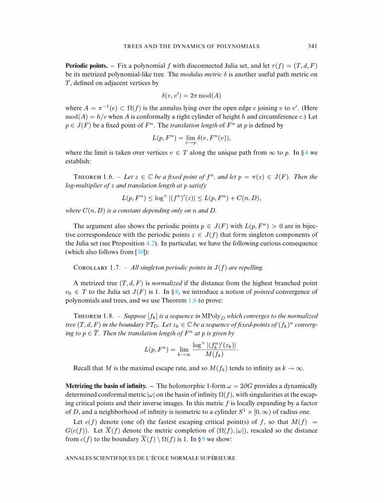
Consecutive annuli. – Next we give an estimate for the modulus of an annulus A ⊂ C formedfrom consecutive annuli A1, . . . , An of the kind that arise from the tree construction.
1A
0c
3c2c
1c
3A
2A
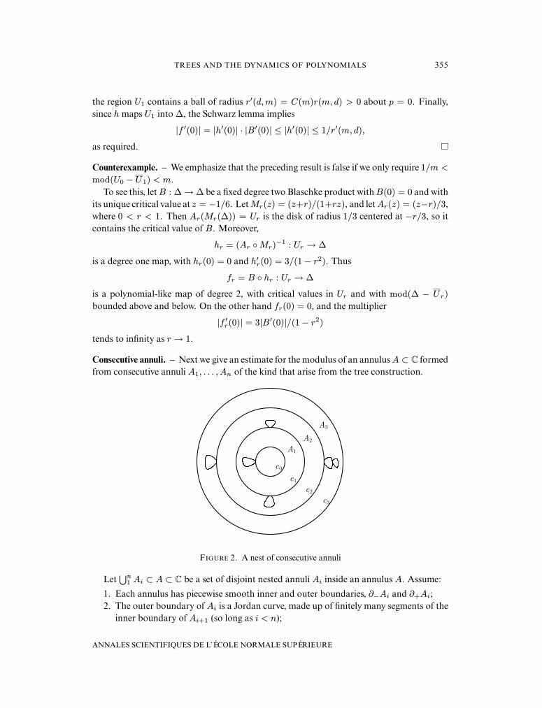
Fɪɢʀ 2. A nest of consecutive annuli
Letn
1 Ai ⊂ A ⊂ C be a set of disjoint nested annuli Ai inside an annulus A. Assume:
1. Each annulus has piecewise smooth inner and outer boundaries, ∂−Ai and ∂+Ai;2. The outer boundary of Ai is a Jordan curve, made up of finitely many segments of the
inner boundary of Ai+1 (so long as i < n);
ANNALES SCIENTIFIQUES DE L’ÉCOLE NORMALE SUPÉRIEURE
356 L. G. DMARCO AND C. T. MMULLEN
3. There is a continuous conformal metric ρ = ρ(z)|dz| onn
1 Ai, making each annulusAi into a flat right cylinder of height hi and circumference ci;
4. The boundary of A is a pair of Jordan curves, with ∂−A ⊂ ∂−A1 and ∂+A = ∂+An.
These conditions imply mod(Ai) = hi/ci. Letting c0 denote the ρ-length of ∂−A, we have
c0 ≤ c1 ≤ · · · ≤ cn.
Tʜʀ 4.4. – The modulus of A satisfies:
(4.1)n
1
mod(Ai) ≤ mod(A) ≤ 3n(cn/c0)2 +
n
1
mod(Ai).
Proof. – The first inequality is standard; for the second, we will use the method ofextremal length (cf. [17]).
Let us say an annulus Ai is short if hi < 2c0 + ci; otherwise it is tall. Define a conformalmetric σ on A by setting σ = (1/c0)ρ on all the short annuli, and on cylindrical collars ofρ-height c0 at the two ends of the tall annuli. Between the collars of each tall annulus Ai, letσ = (1/ci)ρ. Extend σ to the rest of A by setting it equal to zero.
Let Γ denote the set of all rectifiable loops in A separating its boundary components. Itis now straightforward to verify that
Lσ(γ) =
γσ ≥ 1
for all γ ∈ Γ.
To see this, first suppose γ meets the region between the collars of a tall annulus Ai. If γis contained in Ai then it must separate the boundary components of Ai, so Lρ(γ) ≥ ci, andthus Lσ(γ) ≥ 1 (since 1/c0 > 1/ci). Otherwise γ must cross one of the collars of Ai; buteach collar has σ-height one, so again Lσ(γ) ≥ 1.
Now suppose γ ∩
Ai is covered by short annuli and the collars of tall annuli. On thisregion σ = (1/c0)ρ. Consider the foliation F of
Ai by geodesics in the flat ρ-metric, which
start at ∂−A and proceed perpendicular to the boundary in the outward direction. Any γ ∈ Γmust cross all the leaves of F . By construction the leaves are parallel, with constant separa-tion, within the short annuli and collars of tall annuli. Thus the projection of γ ∩ F (alongleaves of F) to ∂−A is σ-distance decreasing, and thus
Lσ(γ) ≥ Lσ(∂−A) = (1/c0)c0 = 1
in this case as well.
Since the modulus of A is the reciprocal of the extremal length of Γ, we have:
mod(A) = 1/λ(Γ) ≤
Å
Aσ2
ãÇinfΓ
γσ
å2
≤
areaσ(Ai).
Each short annulus has height hi ≤ 2c0 + ci ≤ 3cn, so it contributes area hici/c20 ≤
3(cn/c0)2. Each tall annulus contributes area at most hi/ci + 2c0ci/c20 ≤ mod(Ai) +
3(cn/c0)2; summing over i, we obtain (4.1).
4 e SÉRIE – TOME 41 – 2008 – No 3
TREES AND THE DYNAMICS OF POLYNOMIALS 357
Torus shape. – Let f : ∂−A → ∂+A be a piecewise smooth homeomorphism preservingorientation, and expanding the metric ρ linearly by a factor of cn/c0. Let
T = A/f
be the complex torus obtained by gluing together corresponding points, and let B ⊂ T bean annulus of maximum modulus homotopic to A.
A straightforward modification of the proof above yields:
Tʜʀ 4.5. – We have
mod(Ai) ≤ mod(B). In addition, we have
mod(B) ≤ 3n(cn/c0)2 +
mod(Ai)
provided mod(A1) ≥ 3.
The condition on mod(A1) implies that A1 is a tall annulus, and hence it cannot be crossedby loops with Lσ(γ) ≤ 1.
Bounds on multipliers. – We can now complete the proof of Theorem 4.1. It suffices to treatthe case where z is a fixed point of f .
L 4.6. – We have L(p, F ) ≤ log+|f (z)|.
Proof. – The statement is clear if L(p, F ) = 0. Otherwise both p and z are repelling fixedpoints (by Proposition 4.2), and the degree of F is one near p. Let ei, i ∈ Z, be the uniquepath of consecutive edges in T connecting p to ∞; it satisfies
F (ei) = ei+n,
where n = N(F ) ≤ D − 1. Note that deg(ei) is monotone increasing, and equal to 1 for alli sufficiently small. After shifting indices we can assume deg(en) = 1; then deg(ei) = 1 forall i ≤ n, and we have
L(p, F ) =n
1
δ(ei).
Let Ai = A(ei) be the open annulus in Ω(f) lying over the edge ei, and let A be the annulusbounded by ∂+An and ∂+A0. Note that f identifies the inner and outer boundaries of Abijectively, yielding a quotient torus
T = A/f.
Since f(w) = λw in suitable local coordinates near z, with λ = f (z), we have
T ∼= C/(2πiZ⊕ log(λ)Z).
Let B ⊂ T be the annulus homotopic to A that is covered by
w : 0 < Re(w) < log |λ| ⊂ C.
Since ∂B is geodesic, its modulus
mod(B) =log |λ|
2π
is the maximum possible for any annulus for its homotopy class.
ANNALES SCIENTIFIQUES DE L’ÉCOLE NORMALE SUPÉRIEURE
358 L. G. DMARCO AND C. T. MMULLEN
Applying Theorem 4.5, we obtain
L(p, f) =n
1
δ(ei) = 2πn
1
mod(Ai) ≤ 2π mod(B) = log |f (z)|
as desired.
Let O(1) denote a bound depending only on D = deg(f).
L 4.7. – If L(p, F ) ≥ 6πD, then log |f (z)| ≤ L(p, F ) + O(1).
Proof. – We continue the argument from the preceding proof. Note that δ(ei) is periodic,with period n, for i ≤ n. Shifting indices, we can assume δ(e1) ≥ δ(ei) for 1 < i ≤ n(and deg(en) = 1 as before). Then the assumption L(p, F ) =
δ(ei) ≥ 6πD implies
2π mod(A1) = δ(e1) ≥ 6π, and thus mod(A1) ≥ 3 (using the fact that n ≤ D). Thuswe can apply the upper bound of Theorem 4.5 to obtain
log |f (z)| = 2π mod(B) ≤ L(p, F ) + 6πn(cn/c0)2.
Now recall that f identifies the boundaries of A and expands metric ρ = |ω| by a factor of D.Thus (cn/c0) = D, and therefore the defect 6πn(cn/c0)2 is less than 6πD3, which dependsonly on D.
L 4.8. – If L(p, F ) < 6πD, then log+|f (z)| = O(1).
Proof. – Let Li =i+n−1
i δ(ei). Then Li is monotone increasing, deg(ei)Li ≤ Li+n ≤
DLi, and Li < 6πD for i 0. This implies we can find an index j with deg(ej) ≥ 2 and1 ≤ Lj ≤ 6πD2 = O(1). Now the monotone increasing sequence
deg(ej),deg(ej+n),deg(ej+2n), . . .
can assume at most D different values, so we can find a k with j ≤ k ≤ j + Dn such that
2 ≤ deg(ek) = deg(ek+n) ≤ D.
Since Lj+Dn ≤ DDLj , we have 1 ≤ Lk ≤ O(1).Now shift indices so that k = 0; then 1 ≤ L0 ≤ O(1). Let d = deg(ek). Let A0, . . . , A2n
be the annuli lying over e0, . . . , e2n. Let U2 ⊂ U1 ⊂ U0 be the disks in C obtained by fillingin the bounded complementary components of A0, An and A2n respectively. Then
f : U1 → U0
is a polynomial-like map of degree d, and the fixed point z of f lies in U1. By construction,this polynomial-like map satisfies U2 = f−1(U1). Since deg(e0) = deg(en) = d, the criticalpoints of f lie in U2, and hence its critical values lie in U1.
To control mod(U0 − U1) and mod(U0 − U2), we use the flat metric ρ = |ω|. Note thatc2n/c0 ≤ D2, since f2 maps ∂+A0 onto ∂+A2n and locally expands the ρ-metric by a factorof D2. By the lower bound in Theorem 4.4, we have
2π mod(U0 − U1) ≥ 2π2n
n+1
mod(Ai) = Ln ≥ L0 ≥ 1,
4 e SÉRIE – TOME 41 – 2008 – No 3
TREES AND THE DYNAMICS OF POLYNOMIALS 359
while the upper bound (together with n = N(F ) ≤ D − 1) yields:
2π mod(U0 − U2) ≤ 6πn(c2n/c0)2 + 2π
2n
1
mod(Ai) ≤ 6πD5 + L0 + DL0 = O(1).
Since the moduli of U0 −U1 and U0 −U2 are bounded above and below just in terms of D,we have log+
|f (z)| = O(1) by Theorem 4.3.
Proof of Theorem 4.1. – Combine the results of Lemmas 4.6, 4.7, and 4.8.
5. The moduli space of trees
In this section we introduce the geometric topology on the moduli space TD of metrizedpolynomial-like trees of degree D. Passing to the quotient projective space, we then showPTD is compact and contractible (Theorem 1.3).
We also discuss the space TD,1 of pointed trees and prove:
Pʀɪɪɴ 5.1. – If (Tn, dn, Fn, pn) → (T, d, F, p) in TD,1 and Fn(pn) = pn, then
F (p) = p and the translation lengths satisfy
L(pn, Fn) → L(p, F ).
The moduli space of trees. – Let TD be the set of all equivalence classes of degree D metrizedpolynomial-like trees (T, d, F ). Trees (T1, d1, F1) and (T2, d2, F2) are equivalent if there ex-ists an isometry i : T1 → T2 such that i F1 = F2 i.
There is a natural action of R+ on TD which simply rescales the metric d; the quotientprojective space will be denoted PTD. A tree is normalized if d(v0, J(F )) = 1, where v0 is thebase of the tree. The normalized trees form a cross-section to the projection TD → PTD.
Strong convergence. – Let vi ∈ V (T ), denote the unique vertex at combinatorial heighth(vi) = i ≥ 0, and let T (k) ⊂ T denote the finite subtree spanned by the vertices with com-binatorial height −kN(F ) ≤ h(v) ≤ kN(F ). Recall that N(F ) is the number of disjointgrand orbits of vertices, as introduced in Lemma 2.1.
We say a sequence (Tn, dn, Fn) in TD converges strongly if:
1. The distances dn(v0, vi) converge for i = 1, 2, . . . ,D;2. We have lim dn(v0, vD) > 0; and3. For any k > 0 and n > n(k), there is a simplicial isomorphism Tn(k) ∼= Tn+1(k)
respecting the dynamics.
The last condition implies N(Fn) is eventually constant.
L 5.2. – Any sequence of normalized trees in TD has a strongly convergent subse-
quence.
Proof. – In a sequence of normalized trees, dn(v0, vi) ≤ Di and dn(v0, vD) ≥ 1, so thefirst two properties of strong convergence hold along a subsequence. The number of verticesin Tn(k) is bounded in terms of D and k, so the third property holds along a further subse-quence.
ANNALES SCIENTIFIQUES DE L’ÉCOLE NORMALE SUPÉRIEURE
360 L. G. DMARCO AND C. T. MMULLEN
Limits. – Suppose (Tn, dn, Fn) converges strongly. Then there is a unique pointed simplicialcomplex (T , v0) with dynamics F : T → T such that Tn(k) ∼= T (k) for all n > n(k), andthe simplicial isomorphism respects the dynamics. It is possible, however, that certain edgelengths of Tn tend to 0 in the limit; this happens when the grand orbits of critical points col-lide. Our assumptions therefore yield only a pseudo-metric d on T as a limit of the metricsdn. Let (T, d, F ) be the metrized dynamical system obtained by collapsing the edges of lengthzero to points.
L 5.3. – Suppose (Tn, dn, Fn) converges strongly. The limiting triple (T, d, F ) is a
metrized polynomial-like tree.
Proof. – Let the vertices V (T ) be the grand orbits of its branch points. Sincelim dn(v0, vD) > 0, V (T ) is nonempty, and it is easy to see that T has the structure ofa locally finite simplicial tree, and F : T → T is a branched cover. We must show T has acompatible degree function.
To define this, pass to a subsequence such that for each k the degree function of Tn re-stricted to Tn(k) stabilizes as n → ∞. This defines a degree function deg : E(T ) → N onthe simplicial limit T compatible with F .
Note that T may have vertices of valence two whose grand orbits under F contain nobranch points. These vertices arise when the critical point that used to label them no longerescapes. Since they have valence two, the value of deg is the same on both their adjacentedges. We can thus modify the simplicial structure on T by removing all such vertices, andmaintain a compatible degree function by taking its common value on all edges that arecoalesced.
With this modified simplicial structure on T , the natural collapsing map T → T is sim-plicial. We define deg : E(T ) → N by deg(e) = deg(e) for the unique edge e lying over e,and for v ∈ V (T ) define deg(v) = deg(e) where e is the upper edge of v. It is then straight-forward to check that the resulting degree function is compatible with F : T → T .
The geometric topology. – The geometric topology on TD is the unique metrizable topologysatisfying
(Tn, dn, Fn) → (T, d, F )
whenever (Tn, dn, Fn) is strongly convergent and (T, d, F ) is defined as above. In § 9, we showthat the geometric topology coincides with the Gromov-Hausdorff topology on pointed dy-
namical metric spaces; in particular, we describe there a basis of open sets for the topology.
Lemma 5.2 immediately implies:
Tʜʀ 5.4. – The space PTD is compact in the quotient geometric topology.
4 e SÉRIE – TOME 41 – 2008 – No 3
TREES AND THE DYNAMICS OF POLYNOMIALS 361
Iteration. – For each (T, d, F ) ∈ TD, its n-th iterate (T, d, Fn) is a metrized polynomial-liketree of degree Dn. Define
in : TD → TDn
by (T, d, F ) → (T, d, Fn). It is useful to observe:
L 5.5. – The iterate maps in are continuous in the geometric topology.
Proof. – It suffices to consider sequences (Tm, dm, Fm) converging strongly to (T, d, F ) inTD. For each k > 0, any simplicial isomorphism s : Tm(k) → T (k) such that sFm = F swill also satisfy sFn
m = (F )n s. Therefore, the sequence (Tm, dm, Fnm) converges strongly
to (T, d, Fn).
Next we establish:
Tʜʀ 5.6. – The space PTD is contractible.
The proof is based on a natural construction which accelerates the rate of escape of criticalpoints in a tree. A version of the following result appears as Theorem 7.5 in [7].
Tʜʀ 5.7. – Let (T, d, F ) be a metrized polynomial-like tree, and let S ⊂ T be a
forward-invariant subtree. Then F |S can be extended to a unique metrized polynomial-like tree
(T , d, F ) with the same degree function on S, and whose critical points all lie in S.
We emphasize that the subtree S can have endpoints, and that these endpoints need notcoincide with vertices of T . The degree of a terminal edge of S is defined to be the degree ofthe edge of T which contains it.
Proof. – The characterization of critical points in Lemma 2.6 requires that all edges inT \ S have degree 1. The tree T and the map F : T → T will be defined inductivelyon (descending) height, uniquely determined by the conditions that each added edge has de-gree 1 and that (2.1) and (2.2) are satisfied at all vertices of T .
Let p be a point of maximal height in T \ S; set T = S, F |T = F |S, and d|T = d|S.Then p is a highest point in T such that either (a) F (p) lies in the interior of an edge of T ,or (b) F (p) is a vertex and the local degree condition (2.2) for F |T is not satisfied at p.
In case (a), the point p belonged to the interior of an edge e of T . We make p into a vertexof degree deg(e). Extend (T , d, F ) below p down to height H(p)/d to be a local homeo-morphism, defining d so that d(e) = d(F (e))/d on each new edge e. Assigning new edgesdegree 1, the conditions (2.1) and (2.2) will both be satisfied at p. Note that the degree con-ditions are always satisfied at vertices where F is a local homeomorphism and all adjacentedges have degree 1.
In case (b), define (T , d, F ) in a neighborhood of p by adding enough new edges ofdegree 1 below p so that the local degree condition (2.2) is satisfied with degree deg(p).Again, we can define (T , d, F ) on the added edges and vertices of T below p down toheight H(p)/d so that F is a local homeomorphism and d(e) = d(F (e))/d on all newedges e. Condition (2.1) will be automatically satisfied at p because it is satisfied at p for(T, F ) and the right-hand side can only decrease with the replaced edges of degree 1.
There are only finitely many endpoints or vertices x ∈ T with height H(p)/d < H(x) ≤H(p) where (a) or (b) is satisfied, and we repeat the above construction for each of these
ANNALES SCIENTIFIQUES DE L’ÉCOLE NORMALE SUPÉRIEURE
362 L. G. DMARCO AND C. T. MMULLEN
points. We then may proceed by induction on height of vertices where the local degree isnot well-defined, until we have completed the construction of (T , d, F ).
Escaping trees. – A metrized polynomial-like tree (T, d, F ) is escaping if there are no criticalpoints in J(F ).
Cʀʟʟʀʏ 5.8. – Escaping trees are dense in the spaces TD and PTD.
Proof. – Let (T, d, F ) be a metrized polynomial-like tree with height function H : T →
[0,∞). For each > 0, let S ⊂ T be the subtree of all points with height ≥ . By Theo-rem 5.7, we can extend F |S uniquely so that all critical points are contained in S to obtain(T, d, F). Letting → 0, we have
(T, d, F) → (T, d, F )
in the geometric topology.
Proof of Theorem 5.6. – Identify PTD with the subset of normalized trees in TD. For eachnormalized tree (T, d, F ) with height function H : T → [0,∞) and each t ∈ [0, 1], considerthe forward-invariant subtree
St = x ∈ T : H(x) ≥ t.
By Theorem 5.7, there is a unique metrized polynomial-like tree (Tt, dt, Ft) extending F |St
and the local degree function on St so that all critical points belong to St.
Define
R : PTD × [0, 1] → PTD
by ((T, d, F ), t) → (Tt, dt, Ft). Then R( · , 0) is the identity, and R( · , 1) is the constantmap sending all trees to the unique normalized tree (T1, d1, F1) with all critical points at thebase v0. Note that R((T1, d1, F1), t) = (T1, d1, F1) for all t. It remains to show that R iscontinuous.
Fix (T, d, F ), t ∈ [0, 1], a sequence (Tn, dn, Fn) of normalized trees converging stronglyto (T, d, F ), and a sequence tn → t. Because the number of critical points (and thus theirgrand orbits) is finite, we may pass to a subsequence so that the subtrees Stn ⊂ Tn are sim-plicially isomorphic (respecting dynamics) for all n 0. The isomorphisms can be extendedto Tn,tn
∼= Tn+1,tn+1 using the construction of Fn,tn as a local homeomorphism below Stn .Therefore, the image sequence R((Tn, Fn), tn) converges strongly. The limit clearly coincideswith T above height t. Because the degree functions converge, it must have all edges of de-gree 1 below height t. By the uniqueness in Theorem 5.7, the limit must be (Tt, dt, Ft).
Proof of Theorem 1.3. – Combine Theorems 5.4 and 5.6.
4 e SÉRIE – TOME 41 – 2008 – No 3
TREES AND THE DYNAMICS OF POLYNOMIALS 363
Pointed trees. – A pointed tree is a quadruple (T, d, F, p) where (T, d, F ) ∈ TD and p ∈ T .Let TD,1 denote the set of isometry classes pointed trees of degree D.
Let p(k) ∈ T (k) denote the image of p ∈ T under the nearest-point retraction T → T (k).We say a sequence (Tn, dn, Fn, pn) in TD,1 converges strongly if
1. (Tn, dn, Fn) converges strongly;2. dn(v0, pn) converges to a finite limit as n →∞; and3. for all k > 0 and all n > n(k), there exists a simplicial isomorphism of pointed spaces
(Tn(k), pn(k)) ∼= (Tn+1(k), pn+1(k)) respecting the dynamics.
In this case the pointed isomorphisms on finite trees determine a natural pointed limit(T, d, F, p), and we define the geometric topology on TD,1 by requiring that (Tn, dn, Fn, pn) →(T, d, F, p) for every strongly convergent sequence. (Similar definitions can be given for Td,m,m > 1.)
Continuity of translation lengths. – This space of pointed trees is useful for tracking periodicpoints and critical points. For example, it is straightforward to verify:
Pʀɪɪɴ 5.9. – The set of normalized pointed trees (T, d, F, p) such that p is a critical
point of F is compact in TD,1.
We can now establish continuity of translation lengths.
Proof of Proposition 5.1. – It is enough to treat the case where
(Tn, dn, Fn, pn) → (T, d, F, p)
strongly; then clearly F (p) = p. If p is not a critical point of F , then there is a k > 0 suchthat T has no critical points below p(k). By Proposition 5.9, Fn has no critical points belowpn(k) for n 0, and thus
L(Fn, pn) = δn(pn(k), Fn(pn(k))).
By geometric convergence, the metric dn|Tn(k) converges to d|T (k), and similarly for the de-gree function; thus the corresponding modulus metrics also satisfy δn → δ on finite subtrees,and hence
δn(pn(k), Fn(pn(k))) → δ(p(k), F (p(k))) = L(F, p).
On the other hand, if p is a critical point then L(F, p) = 0 and hence δ(p(k), F (p(k))) → 0as k → ∞. By geometric convergence, pn(k) is also moved a small amount by Fn whenn 0, and thus L(pn, Fn) → 0.
6. Continuity of the quotient tree
In this section we study the map from the moduli space of polynomials to the moduli spaceof trees, and establish:
Tʜʀ 6.1. – The map τ : MPoly∗D → TD is continuous, proper, and equivariant with
respect to the action of R+ by stretching of polynomials and by metric rescaling of trees.
This gives Theorem 1.4 apart from surjectivity, which will be established in § 7.
ANNALES SCIENTIFIQUES DE L’ÉCOLE NORMALE SUPÉRIEURE
364 L. G. DMARCO AND C. T. MMULLEN
The moduli space of polynomials. – Let MPolyD = PolyD / Aut(C) be the moduli space ofpolynomials of degree D ≥ 2. Every polynomial is conjugate to one which is monic andcentered, i.e. of the form
f(z) = zD + aD−2zD−2 + · · · a1z + a0
with coefficients ai ∈ C, and thus MPolyD is a complex orbifold finitely covered by CD−1.The escape-rate function of a polynomial satisfies GAfA−1(Az) = Gf (z) for any A ∈
Aut(C). Consequently, the maximal escape rate
M(f) = maxGf (c) : f (c) = 0
is well-defined on MPolyD. The open subspace MPoly∗D where J(f) is disconnected coin-cides with the locus M(f) > 0.
By Branner and Hubbard [3, Prop 1.2, Cor 1.3, Prop 3.6] we have:
Pʀɪɪɴ 6.2. – The escape-rate function Gf (z) is continuous in both f ∈ PolyD and
z ∈ C.
Pʀɪɪɴ 6.3. – The maximal escape rate M : MPoly∗D → (0,∞) is proper and con-
tinuous.
Stretching. – The stretching deformation associates to any polynomial f(z) of degree D > 1a 1-parameter family of topologically conjugate polynomials ft(z), t ∈ R+. To define thisfamily, note that the Beltrami differential defined by
µ =ω
ωon the basin of infinity, where ω = 2∂Gf , and µ = 0 elsewhere, is invariant under f . Con-sequently, if we let φt : C → C be a smooth family of quasiconformal maps solving theBeltrami equation
dφt/dz
dφt/dz=
t− 1
t + 1µ,
t ∈ R+, thenft = φt f φ−1
t
is a smooth family of polynomials with f1 = f . The maps φt(z) behave like (r, θ) → (rt, θ)near infinity, and thus the corresponding Green’s functions satisfy
Gft(φt(z)) = tGf (z)
(compare [3, § 8]). Together with Proposition 6.3, this implies:
Pʀɪɪɴ 6.4. – For any polynomial f with disconnected Julia set, the stretched poly-
nomials ft determine a smooth and proper map (0,∞) → MPoly∗D.
In addition:
Pʀɪɪɴ 6.5. – The quotient tree for the stretched polynomial ft is obtained from the
quotient tree (T, d, F ) for f by replacing the height metric d(x, y) with td(x, y).
Note that there is also a twisting deformation, using iµ, which does not change the quo-tient tree for f .
4 e SÉRIE – TOME 41 – 2008 – No 3
TREES AND THE DYNAMICS OF POLYNOMIALS 365
Proof of Theorem 6.1. – Equivariance of τ : MPoly∗D → TD with respect to stretching isProposition 6.5.
To prove continuity, suppose [fn] → [f ] in MPoly∗D. Lift to a convergent sequence fn → fin PolyD. Since M(fn) → M(f) > 0 we can pass to a subsequence so the correspondingtrees (Tn, dn, Fn) converge strongly to (T, d, F ) ∈ TD. It suffices to show that (T, d, F ) isisometric to the tree for f .
By the definition of strong convergence, we have a limiting simplicial tree map F :T →T
with a pseudo-metric d, and simplicial isomorphisms T (k) ∼= Tn(k) for all n > n(k), re-specting the dynamics (see § 5 where the geometric topology is introduced). Fix k > 0, andrecall that the Green’s function Gn for fn factors through Tn. Moreover the subtree Tn(k)corresponds to the compact region
Ωk(fn) = z ∈ C : D−kM(fn) ≤ G(z) ≤ DkM(fn).
Thus the vertices of T (k) label components of the critical level sets of Gn in this range forall n sufficiently large. By Proposition 6.2, Gn converges uniformly on compact sets to theGreen’s function G for f . Thus Ωk(fn) converges to Ωk(f), and we obtain a correspondinglabeling of the critical level sets of G by T (k) (though multiple vertices can label the samecomponent of a level set). The distance d(v1, v2) between consecutive vertices in T encodinglevel sets L1 and L2 is given simply by |G(L1) − G(L2)|. It follows that (T, d, F ) is exactlythe quotient tree for f , and thus τ is continuous.
Finally Proposition 6.3 implies that τ is proper, since M(f) = d(v0, J(F )) is boundedabove and below on any compact subset of TD.
Remark: planar embeddings. – Topologically, the level sets of the Green’s function of f(z)are graphs embedded in C. These planar graphs are not always uniquely determined by thetree of f , and thus the map τ : MPoly∗D → TD can have disconnected fibers. In the simplestexamples, different graphs correspond to different choices for a primitive n-th root of unity,suggesting a connection with Galois theory and dessins d’enfants; cf. [31]
7. Polynomials from trees
In this section we prove:
Tʜʀ 7.1. – Any metrized polynomial-like tree (T, d, F ) ∈ TD can be realized by a
polynomial f .
Together with Theorem 6.1, this completes the proofs of Theorems 1.2 and 1.4 of the in-troduction. The first part of the proof of Theorem 7.1 is a local realization (for every vertexof the tree T ), related to the Hurwitz problem of constructing coverings of surfaces with spec-ified branching behavior; see e.g. [6], [39] and the references therein.
ANNALES SCIENTIFIQUES DE L’ÉCOLE NORMALE SUPÉRIEURE
366 L. G. DMARCO AND C. T. MMULLEN
Permutations. – A partition P of D ≥ 1 is an unordered sequence of positive integers(a1, . . . , am) such that D = a1 + · · ·+ am. A partition P of D determines a conjugacy classSD(P ) in the symmetric group SD, consisting of all permutations which are products of mdisjoint cycles with lengths (a1, a2, . . . , am).
Let c(P ) = D − m =
(ai − 1). In our application to branched coverings, c(P ) willcount the number of critical points coming from the blocks of P . The following propositionalso follows from [6, Thm. 5.2].
Pʀɪɪɴ 7.2. – Let P1, . . . , Pn be partitions of D such thatn
1 c(Pi) = D−1. Then
there exist permutations σ1, . . . ,σn in the corresponding conjugacy classes of SD, such that
σ1 · · ·σn = (123 . . . D).
Proof. – First note that if P = (a1, . . . , am) and c(P ) < D/2, then m > D/2 and thusai = 1 for some i.
We proceed by induction on D, the case D = 1 being trivial. Assume the result for D =D − 1. Let us order the partitions Pi and their entries (a1, . . . , am) so that c(P1) ≥ c(Pi)and a1 ≥ ai for all i. Then c(P1) > 0 so a1 > 1, and c(Pi) < D/2 for i > 1, so each of thesepartitions has at least one block of size 1.
Let P 1 = (a1−1, a2, . . . am), and define P i , i > 1 by discarding a block of size 1 from Pi.Then P 1, . . . , P
n are partitions of d satisfying
c(P i ) = D−1 = D−2. By induction there
are permutations σi ∈ SD−1 corresponding to P i whose product is the cycle (123 . . . D).We can assume that 1 belongs to the cycle of length (a1− 1) for σ1. Then σ1 = (1D)σ1 ∈
SD has a cycle of length a1 and overall cycle structure given by P1. Taking σi = σi for i > 1(under the natural inclusion SD−1 → SD), we find σi has an additional cycle of length 1 andhence it lies in the conjugacy class SD(Pi). Finally we have
σ1 · · ·σn = (1D)σ1 · · ·σn = (1D)(123 . . . (D − 1)) = (123 . . . D).
Branched coverings. – Suppose f : X → Y is a degree D branched covering of Riemannsurfaces. Given y ∈ Y , the branching partition of f over y is the partition of D given in termsof the local degree of f at each of the preimages f−1(y) = (x1, . . . , xm) by
P (f, y) = (deg(f, x1), . . . ,deg(f, xm)).
The quantity c(P (f, y)) = D−m is the number of critical points in the fiber f−1(y), countedwith multiplicities.
Suppose now that f : C → C is a polynomial of degree D, with critical valuesp1, . . . , pn. Choose a basepoint b which is not a critical value of f . Then the fundamentalgroup π1(C \ p1, . . . , pn, b) acts by permutations on the fiber f−1(b). If σi denotes thepermutation induced by a loop around pi, then up to relabeling, the product σ1σ2 · · ·σn isequal to the permutation (123 · · ·D) which is the permutation induced by a loop around∞.
Let (T, d, F ) be a polynomial-like tree, and let v be a vertex of T . A polynomial f : C → Cof degree deg(v) has the branching behavior of (T, F, v) over p1, . . . , pn ∈ C if there is anordering of the lower edges e1, . . . , en of T at F (v) such that
P (f, pi) = (deg(e) : e ∈ Ev, F (e) = ei)
4 e SÉRIE – TOME 41 – 2008 – No 3
TREES AND THE DYNAMICS OF POLYNOMIALS 367
for i = 1, . . . , n. If the critical multiplicity
m(v) = 2 deg(v)− 2−
e∈Ev
(deg(e)− 1)
is non-zero, then f will have critical values outside the set p1, . . . , pn.
Pʀɪɪɴ 7.3. – Let (T, d, F ) be a metrized polynomial-like tree, v a vertex of T , and
n the number of lower edges at F (v). For any set of distinct points p1, . . . , pn, q in C, there
exists a polynomial of degree deg(v) with the branching behavior of (T, F, v) over p1, . . . , pn
and all critical values contained in p1, . . . , pn, q.
Proof. – Let e1, . . . , en be the lower edges of T at F (v). For each ei, its set of preimagesin Ev determines the partition Pi of deg(v) given by (deg(e) : F (e) = ei). Let Q be thepartition (m(v) + 1, 1, . . . , 1) of deg(v). Then c(Q) +
c(Pi) = deg(v)− 1.
By Proposition 7.2, there exist permutations σ1, . . . ,σn, σq in the corresponding conju-gacy classes of the symmetric group Sdeg(v) with product σ1 · · ·σnσq = (12 . . . deg(v)). Therepresentation
π1(C \ p1, . . . , pn, q) → Sdeg(v)
which associates to each generating loop the permutation σi or σq determines a holomorphicbranched covering f : C → C, with branching partitions P (f, pi) = Pi, P (f, q) = Q andP (f,∞) = (deg(v)). In particular, f is totally ramified over ∞. Choosing coordinates onthe domain so that f(∞) = ∞, we find that f is a polynomial with the required branchingbehavior.
Proof of Theorem 7.1. – We will first prove the realization theorem in the escaping case,where (T, d, F ) has no critical points in its Julia set J(F ). The general case will fol-low by density of escaping trees and a compactness argument, using the continuity ofτ : MPoly∗D → TD (Theorem 6.1).
Let (T, d, F ) be an escaping tree of degree D. For each vertex v of T , we will use Propo-sition 7.3 to construct a local polynomial realization
fv : Cv → CF (v),
together with a foliation Fv of Cv. The foliation will have the following structure: its leavesare the level sets of a subharmonic function Gv : Cv → [−∞,∞) with ∆Gv =
ciδζi for a
finite collection of points ζi in bijective correspondence with the lower edges of v, the level setLv = Gv = 0 is connected, and the connected components of Gv < 0 are topologicaldisks each containing a unique ζi. We require the compatibility condition
(7.1) Gv(z) = GF (v)(fv(z))/ deg(v),
so that fv pulls back the foliation FF (v) to the foliation Fv, taking the central leaf LF (v) tothe central leaf Lv. We then glue the local realizations along leaves of the foliations to obtaina polynomial f such that τ(f) = (T, d, F ).
ANNALES SCIENTIFIQUES DE L’ÉCOLE NORMALE SUPÉRIEURE
368 L. G. DMARCO AND C. T. MMULLEN
The local models. – Fix a vertex v with critical multiplicity m(v), and assume that F (v) is avertex of valence 2; this is always the case if the combinatorial height of v is ≥ 0. Mark thepoint p1 = 0 in CF (v). Let GF (v)(z) = log |z|; the associated foliation of CF (v) is by circles|z| = c with the unit circle as central leaf. For m(v) = 0, let q be a point on the unit circle.Let fv : Cv → CF (v) be any polynomial guaranteed by Proposition 7.3 with the branchingbehavior of (T, F, v) over p1 and critical values p1, q. Define Gv on Cv by the compatibilitycondition (7.1). The foliation by circles |z| = c in CF (v) pulls back to a (singular) foliation ofCv: the preimages of the circle |z| = c with c = 0, 1 are topological circles, and the central leafis a connected degree deg(v) branched cover of the unit circle, branched over one point withmultiplicity m(v). The preimages of the marked point p1 are indexed by the edges below v.For the case m(v) = 0, we can take fv(z) = zdeg(v).
We complete the definitions of the local realizations by induction. Assume that fv : Cv →
CF (v) has been defined and the foliation with distinguished central leaf has been specifiedon the domain. There is also a marked set of points in Cv corresponding to the lower edgesadjacent to v. For each vertex v such that F (v) = v, we use Proposition 7.3 to define thepolynomial fv with the branching behavior of (T, F, v) over the marked points in Cv withbranch point of multiplicity m(v) over an arbitrary point q on the central leaf.
Cutting and pasting. – For each vertex v, we define a Riemann surface with boundary Sv ⊂
Cv according to the data of (T, d, F ). For vertices connected by an edge, we will glue theassociated surfaces so that the local maps match up.
Let v0 be the base of T . Consider the consecutive vertices v0, v1, . . . , vn = F (v0), vn+1 =F (v1), bounding edges e0, e1, . . . , en of lengths l0, . . . , ln, where ln = Dl0, in the heightmetric d. For each i = 1, . . . , n, let
Svi = e−li−1 ≤ |z| ≤ eli ⊂ Cvi
with central leaf |z| = 1. For each i, we identify the outer boundary of Svi with the innerboundary of Svi+1 via an isometry with respect to the metric |dz/z| to form a cylinder; thetwist parameters are free. Because the leaves |z| = c are extremal curves of these annuli,the central leaves of Svi and Svi+1 bound an annulus of modulus exactly (li/4π)+(li/4π) =li/2π. For the vertex v0, let Sv0 = f−1
v0(Svn) ⊂ Cv0 , and glue the outer boundary of Sv0 to
the inner boundary of Sv1 . By construction, the modulus of the annulus bounded by the cen-tral leaves of Sv0 and Sv1 is therefore ln/(4πD)+l0/4π = l0/2π. The holomorphic functionsfvi and fvi+1 extend across the common boundary of Svi and Svi+1 for all i = 0, . . . , n.
We are now set up for an inductive construction. Suppose that v and w are two verticesconnected by an edge, and suppose we have defined Sv, Sw, and the gluing between them.Let v and w be adjacent vertices such that F (v) = v and F (w) = w. Set Sv = f−1
v (Sv)and Sw = f−1
w (Sw). Let e be the edge connecting v and w. There are exactly deg(e) waysto glue Sv and Sw so that the maps fv and fw extend across the common boundary; makeany of these choices.
It remains to consider the edges of combinatorial height > N(F ). Suppose v and w arevertices connected by an edge e of degree D, and let V and W be their images under F . LetSV = fv(Sv) ⊂ CV and SW = fw(Sw) ⊂ CW . In this setting, there is a unique gluing of
4 e SÉRIE – TOME 41 – 2008 – No 3
TREES AND THE DYNAMICS OF POLYNOMIALS 369
SV and SW so that the maps fv and fw extend continuously across the common boundaryof Sv and Sw.
The result of the inductive construction. – We have produced a holomorphic map f : S → Son a planar Riemann surface S equipped with a foliation such that F : T → T is the quotientof f : S → S by this foliation. Furthermore, to every edge e in T is associated an annulusAe ⊂ S with modulus satisfying mod(Ae) = mod(f(Ae))/ deg(e). If e is an edge containedin the path [v0,∞), then d(e) = 2π mod(Ae).
The map f extends to a polynomial. – Since S is planar, there exists a holomorphic embed-ding S → C sending the unique isolated end of S to infinity [38, § 9-1]. Because (T, d, F ) isan escaping metrized polynomial-like tree, there is a height > 0 so that all edges of height< have degree 1. These edges give chains of disjoint annuli of definite modulus nestingaround the remaining ends of S. Therefore K = C \ S is a Cantor set of absolute area zero,and hence f : S → S extends to a polynomial endomorphism of C (see e.g. [21, § 2.8] and[36, § 8D].)
The approximation step. – An arbitrary metrized polynomial-like tree (T, d, F ) in TD can beapproximated in the geometric topology by a sequence (Tn, dn, Fn) of escaping trees (Corol-lary 5.8). Realize each escaping tree by a polynomial fn. The maximal escape rates M(fn) =dn(v0, J(Fk)) converge to d(v0, J(F )); by Proposition 6.3 these polynomials lie in a compactsubset of MPoly∗D. Pass to a convergent subsequence [fn] → [f ]. By Theorem 6.1 the treemap τ : MPoly∗D → TD is continuous, so (T, d, F ) is the metrized polynomial-like tree asso-ciated to f . This completes the proof of Theorem 7.1.
Proof of Theorem 1.4. – Continuity, equivariance, and properness follow from Theorem6.1. Surjectivity is Theorem 7.1.
8. Compactification
In this section, we show the projective space of trees PTD forms a natural boundary forthe moduli space of polynomials, and that the translation lengths in trees record the limitingmultipliers at periodic points (Theorems 1.5 and 1.8 of the introduction). As a corollary,we show that the log-multiplier spectra converge to the length spectrum of the limiting tree(Theorem 8.3).
Compactifying moduli space. – Recall that τ : MPoly∗D → TD assigns to each polynomialwith disconnected Julia set its associated metrized tree map (T, d, F ). Projectivizing, we ob-tain a continuous and surjective map to PTD where the height metric d is only determinedup to scale. The map τ makes MPolyD ∪PTD into a compact topological space: every un-bounded sequence [fn] in MPolyD has a subsequence for which τ(fn) converges in PTD. Thefollowing lemma implies that all points in PTD arise as limits of polynomials.
L 8.1. – The projectivization of τ to PTD satisfies
τ(MPoly∗D \K) = τ(MPoly∗D) = PTD
for every compact K ⊂ MPolyD.
ANNALES SCIENTIFIQUES DE L’ÉCOLE NORMALE SUPÉRIEURE
370 L. G. DMARCO AND C. T. MMULLEN
Proof. – The first equality is immediate from Propositions 6.4 and 6.5, and the second isthe surjectivity of τ (Theorem 7.1).
Proof of Theorem 1.5. – Theorems 6.1 and 5.4 imply that PTD defines a boundary toMPolyD via the continuous map τ , making
MPolyD = MPolyD ∪PTD
into a compact topological space; Lemma 8.1 shows that MPolyD is dense in MPolyD.To see that iteration [f ] → [fn] extends continuously to this boundary, first note that it-
eration in : TD → TDn , defined by (T, d, F ) → (T, d, Fn), is continuous in the geometrictopology (Lemma 5.5), and in(τ(f)) = τ(fn). Suppose [fk] is a sequence in MPoly∗D con-verging to the normalized tree (T, d, F ) ∈ ∂ MPolyD. Then [fk] is unbounded in MPolyD,so M(fk) → ∞ by Proposition 6.3, and the normalized trees (Tk, dk, Fk) associated to fk
converge to (T, d, F ). Consequently,
M(fnk ) = M(fk) →∞
for each n, so [fnk ] is unbounded in MPolyDn , and
(Tk, dk, Fnk ) → (T, d, Fn)
in TDn . Thus, we have [fnk ] → (T, d, Fn) in MPolyDn .
Limits of multipliers. – We now turn to the proof of Theorem 1.8.To formulate this theorem more precisely, it is useful to introduce the bundle MPolyD,1 →
MPolyD of pairs [f, p], where f(z) is a polynomial of degree D and p is a point in C. For anyaffine transformation A(z) = az + b, we regard [f, p] and [AfA−1, A(p)] as representing thesame point in MPolyD,1. There is a natural continuous map
MPoly∗D,1 → TD,1
sending [f, p] to the tree (T, d, F ) = τ(f) with the marked point π(p) ∈ T . This projectionmakes PTD,1 into a natural boundary for MPolyD,1, compatible with the compactificationof MPolyD by PTD.
Tʜʀ 8.2. – Let [fk, zk] ∈ MPolyD,1 be a sequence of polynomials with distinguished
periodic points, satisfying fnk (zk) = zk. Suppose [fk, zk] converges to the normalized pointed
tree (T, d, F, p) ∈ PTD,1. Then Fn(p) = p, and we have:
(8.1) L(p, Fn) = limk→∞
log+|(fn
k )(zk)|
M(fk).
Proof. – Let (Tk, dk, Fk) denote the normalized tree maps obtained by rescaling τ(fk) sothat dk(v0, J(Fk)) = 1. By Proposition 5.1, the point p is fixed by Fn and
L(π(zk), Fnk ) → L(p, Fn)
as k →∞. Theorem 4.1 implies that
log+|(fn
k )(zk)| = M(fk)L(π(zk), Fnk ) + O(1).
By Proposition 6.3, M(fk) →∞ as k →∞, and equation (8.1) follows.
4 e SÉRIE – TOME 41 – 2008 – No 3
TREES AND THE DYNAMICS OF POLYNOMIALS 371
Spectra. – Let f : C → C be a polynomial of degree D ≥ 2, and let Ln(f) be the unorderedcollection of log-multipliers log+
|(fn)(p)| for periodic points p of period n (counted withmultiplicity). Note that the cardinality of the set Ln(f) is exactly Dn. The log-multiplier
spectrum of f is the list
L(f) = L1(f),L2(f),L3(f), . . ..
For a metrized polynomial-like tree (T, d, F ) of degree D, and for each period n ≥ 1, letLn(T, d, F ) be the unordered collection of translation lengths L(p, Fn) of all periodic pointsp ∈ J(F ) of period n (with respect to the modulus metric δ). We count critical periodicends with multiplicity (= deg(p, Fn)), so thatLn(T, d, F ) contains exactly Dn elements. Thelength spectrum of (T, d, F ) is the list
L(T, d, F ) = L1(T, d, F ),L2(T, d, F ),L3(T, d, F ), . . ..
Tʜʀ 8.3. – For any sequence fk in PolyD such that
[fk] → (T, d, F ) ∈ ∂MPolyD,
the log-multiplier spectrum L(fk) converges (up to scale) to the length spectrum L(T, d, F ).
Proof. – Let zk be a sequence of fixed points of fnk for some iterate n, and let
(Tk, dk, Fk) = τ(fk). Pass to a subsequence so that the normalized pointed trees(Tk, dk, Fk, π(zk)) converge in TD,1 to (T, d, F, p). By Proposition 5.1, this point p ∈ Tis fixed by Fn; Theorem 1.8 implies that the log-multipliers of zk converge (up to scale) tothe translation length of p.
On the other hand, suppose p ∈ J(F ) is fixed by Fn for some n. By passing to a stronglyconvergent subsequence, we can always find a sequence pk ∈ J(Fk) fixed by Fn
k which con-verges to p. For every fixed point pk of Fn
k , there exists at least one point zk fixed by fnk such
that π(zk) = pk.
9. Trees as limits of Riemann surfaces
In this section we recall the Gromov-Hausdorff topology on metric spaces, and observethat it coincides with the geometric topology on the space of trees. We prove:
Tʜʀ 9.1. – Let [fn] ∈ MPoly∗D be a sequence of polynomials converging to the nor-
malized tree (T, d, F ) in ∂ MPolyD = PTD. Then the pointed dynamical metric spaces
(Ω(fn), c(fn), |ωn|/M(fn), fn)
converge in the Gromov-Hausdorff topology to (T, v0, d, F ).
An analogous theorem for Kleinian groups appears in [29].
ANNALES SCIENTIFIQUES DE L’ÉCOLE NORMALE SUPÉRIEURE
372 L. G. DMARCO AND C. T. MMULLEN
Pointed metric spaces. – Suppose (X, dX) and (Y, dY ) are metric spaces with basepointsx0 ∈ X and y0 ∈ Y . An -identification between (X,x0, dX) and (Y, y0, dY ) is a relationR ⊂ X × Y such that
1. (x0, y0) ∈ R
2. if (x, y) and (x, y) are in R, then
|dX(x, x)− dY (y, y)| ≤ ,
3. for every p ∈ X, there exists a pair (x, y) ∈ R such that dX(p, x) ≤ , and4. for every q ∈ Y , there exists a pair (x, y) ∈ R such that dY (q, y) ≤ .
Almost-conjugacy. – A quadruple (X,x0, dX , F ), where (X, dX) is a metric space, x0 ∈ X,and F : X → X, will be called a pointed dynamical metric space. An -identification between(X,x0, dX , F ) and (Y, y0, dY , G) is a relation R ⊂ X × Y which satisfies conditions (1–4)above and also
5. for each (x, y) ∈ R, there exists (x, y) ∈ R such that dX(x, F (x)) ≤ anddY (y, G(y)) ≤ .
Gromov-Hausdorff topology. – Fix a pointed dynamical metric space (X,x, dX , F ). ForR > 0, let
XR = x ∈ X : dX(x0, x) ≤ R,
and defineR = dX(x0, F (x0)).
A basis of open sets for the Gromov-Hausdorff topology can be described as follows. Foreach R > R and > 0, the open set U(R, ) consists of all pointed dynamical metric spaces(Y, y0, dY , G) for which there is an -identification between (XR∩F−1(XR), x0, dX , F ) and(Y R ∩G−1(Y R), y0, dY , G).
Each element of the space of trees TD defines a pointed dynamical metric space(T, v0, d, F ) where v0 ∈ T is the base and d is the height metric. The Gromov-Hausdorff
topology on TD identifies (T1, v0, d1, F1) and (T2, v0, d2, F2) if and only if there exists anisometry i : (T1, v0) → (T2, v0) such that F2 i = i F1.
L 9.2. – The geometric topology on TD coincides with the Gromov-Hausdorff topol-
ogy.
Proof. – Suppose (Tn, dn, Fn) converges strongly to (T, d, F ). Then for each k > 0, > 0and all n > n(k, ), the simplicial isomorphisms between Tn(k) and Tn+1(k) can be cho-sen as -identifications. Thus the sequence (Tn, v0, dn, Fn) converges to (T, v0, d, F ) in theGromov-Hausdorff topology.
Now suppose that (Tn, dn, Fn) does not converge to (T, d, F ) in the geometric topology,but the distances dn(v0, Fn(v0)) remain bounded away from 0 and ∞. Then there exists astrongly convergent subsequence which converges to (S, dS , G) = (T, d, F ), and thereforethe subsequence converges to (S, v0, dS , G) in the Gromov-Hausdorff topology. The pointeddynamical metric spaces (T, v0, d, F ) and (S, v0, dS , G) are distinct, and therefore the se-quence (Tn, v0, dn, Fn) does not converge to (T, v0, d, F ) in the Gromov-Hausdorff topol-ogy.
4 e SÉRIE – TOME 41 – 2008 – No 3
TREES AND THE DYNAMICS OF POLYNOMIALS 373
The modulus metric. – The Gromov-Hausdorff topology on the space of metrized polyno-mial-like trees (T, v0, δ, F ) with the modulus metric in place of the height metric does not
coincide with the geometric topology. For example, consider a degree 3 polynomial f withone critical point escaping and one in a fixed component of K(f). Suppose that under aslight perturbation (in MPoly3) the second critical point also escapes. Then for the perturbedmap, all ends of the tree are at infinite distance from the base, but for T the distance to thefixed end is finite. On the other hand, we know the trees with the height metric vary contin-uously with f in the geometric topology by Theorem 6.1.
Pointed trees. – The geometric topology on the space of pointed trees TD,1 defined in § 5 isequivalent to the Gromov-Hausdorff topology on TD,1 where the metric space is the com-pletion T and the basepoint is the marked point p ∈ T .
Convergence of the basins of infinity. – Let f be a polynomial of degree D ≥ 2 with maximalescape rate M(f) > 0. Let c(f) denote any choice of critical point with G(c(f)) = M(f). Asin the introduction, there is a flat conformal metric (with singularities) |ω| on Ω(f) definedby ω = 2∂G. With normalized metric |ω|/M(f), the total length of any level set G−1(t)with t > 0 is equal to 2π/M(f). Therefore, the quotient π : Ω(f) → T defines a 2π/M(f)-identification between (Ω(f), c(f), |ω|/M(f), f) and (T, v0, d, F ).
Proof of Theorem 9.1. – Let (Tn, dn, Fn) be the normalized polynomial-like tree associ-ated to fn. The maximal escape rate M(f) is a proper function of f ∈ MPolyD by Propo-sition 6.3. Therefore, any Gromov-Hausdorff limit of the pointed dynamical metric spaces(Ω(fn), c(fn), |ωn|/M(fn), fn) will coincide with the Gromov-Hausdorff limit of the trees(Tn, v0, dn, Fn). But the sequence (Tn, dn, Fn) converges to (T, d, F ) in the geometric topol-ogy, so in fact
(Ω(fn), c(fn), |ωn|/M(fn), fn) → (T, v0, d, F )
in the Gromov-Hausdorff topology as n →∞.
10. Families of polynomials over the punctured disk
Let O be the local ring consisting of germs of analytic functions a(t) =∞
0 antn definednear t = 0 in C, and let K be its field of fractions. The elements of K are given by Laurentseries a(t) =
∞−m antn, with finite tails and positive radius of convergence.
Let f ∈ K[z] be a monic centered polynomial of degree D ≥ 2. Then f determines ameromorphic family of polynomials
ft(z) = zD + a2(t)zD−2 + · · ·+ aD(t)
defined near t = 0. Conversely, any such family gives an element of K[z]. (We also note thatany f ∈ K[z] of degree D ≥ 2 is conjugate to a monic centered polynomial, so there is noloss of generality with this normalization.)
In this section we establish Theorem 1.10 by showing:
ANNALES SCIENTIFIQUES DE L’ÉCOLE NORMALE SUPÉRIEURE
374 L. G. DMARCO AND C. T. MMULLEN
Tʜʀ 10.1. – Either ft(z) extends holomorphically to t = 0, or there is a unique nor-
malized tree such that
limt→0
[ft] = (T, d, F ) ∈ PTD.
In the latter case the edges of T have rational length, and hence the translation lengths of all of
its periodic points are also rational.
For more on the dynamics of rational maps over local rings and fields, see e.g. [2], [15],[34], [35], [9] and [1, Ch. 8].
Coefficient bounds. – For a polynomial f of degree D, let
Gn(z) =1
Dnlog+
|fn(z)|,
so that its escape-rate function is given by G(z) = lim Gn(z). Recall that M(f) =maxG(c) : f (c) = 0 denotes the maximal escape rate of f .
L 10.2. – The coefficients and maximal escape rate of any monic and centered poly-
nomial f(z) = zD + a2zD−2 + · · ·+ aD−1z + a0 are related by:
maxi
|ai| = O(eDM(f)).
Proof. – Let h be the conformal map that conjugates z → zD to f(z) near infinity withderivative 1 at∞. Then h is univalent on the disk |z| > R = eM(f), and the Green’s functionis given by G(z) = log |h−1(z)|. Moreover, h(z) = z + b1/z + b2/z2 + · · · since f is monicand centered. By the Koebe estimates, all critical points of f lie inside the disk |z| < 4R. Inparticular, the coefficients of f (z) are bounded by O(RD−1). This gives the desired bound(cf. [3]).
L 10.3. – For any monic and centered polynomial f(z) = zD + a2zD−2 + · · · +aD−1z + aD of degree D ≥ 2, we have
|G(z)−Gn(z)| ≤1
Dnlog
Ä1 +
|ai|
ä
for all z ∈ C.
Proof. – By definition,
Gn+1(z)−Gn(z) =1
Dn+1(log+
|f(fn(z))|−D log+|fn(z)|).
For z such that |fn(z)| ≤ 1, we obtain
|Gn+1(z)−Gn(z)| ≤1
Dn+1log
Ä1 +
|ai|
ä.
For z such that |fn(z)| > 1, we have
|Gn+1(z)−Gn(z)| ≤1
Dn+1
log|f(fn(z)|
|fn(z)|D
≤1
Dn+1log
Ä1 +
|ai|
ä.
In either case, we obtain by summing over n that
|G(z)−Gn(z)| ≤1
Dnlog
1 +
i
|ai|
.
4 e SÉRIE – TOME 41 – 2008 – No 3
TREES AND THE DYNAMICS OF POLYNOMIALS 375
Meromorphic families. – Now suppose that ft(z) is a meromorphic family of monic and cen-tered polynomials, whose coefficients are holomorphic on the punctured disk
∆∗ = t : 0 < |t| < 1.
Suppose that the critical points of ft(z) can be holomorphically parameterized by functionscj(t), j = 1, 2, . . . ,D− 1. We also suppose that the conjugacy classes [ft] are unbounded inMPolyD as t → 0. Thus there exists an N ≥ 1 such that maxi |ai(t)| ≥ C|t|N > 0. We writeGt for the escape-rate function of ft.
Pʀɪɪɴ 10.4. – There exist rational numbers ej ∈ Z[1/D] such that
Gt(cj(t)) = ej log1
|t|+ o
Ålog
1
|t|
ã
as |t|→ 0, and ej > 0 for some j.
Proof. – Fix j and consider the meromorphic function
fnt (cj(t)) ∼ Cnt−pn
as t → 0. If pn → ∞ then for all n sufficiently large, we have pn+1 = Dpn and Cn+1 = CDn
(this holds, for example, provided pn > maxiord0ai(t)). Then the limit
ej := limn→∞
pn/Dn
exists and is non-zero in the ring Z[1/D]. If the degrees pn remain bounded, we set ej = 0.For any large n we have
Gnt (cj(t)) =
1
Dnlog+
|fnt (cj(t))| = D−npn log
1
|t|+ o
Ålog
1
|t|
ã
as t → 0. On the other hand maxi |ai(t)| = O(|t|−N ) for some N , so by Lemma 10.3
Gt(cj(t)) = Gnt (cj(t)) + O
ÅND−n log
1
|t|
ã
which gives the desired asymptotics.To prove at least one ej > 0, use the fact that max |ai(t)| grows like |t|−N 0 to conclude
by Lemma 10.2 that
maxj
Gt(cj(t)) ≥ C log1
|t|> 0.
There are only finitely many critical points, so for some j we must have ej > 0.
Proof of Theorem 10.1. – Let ft(z) be a meromorphic family of monic centered polyno-mials defined near t = 0. If the conjugacy classes [ft] remain bounded in MPolyD as t → 0,then ft extends to a holomorphic family at t = 0 (equivalently, f ∈ O[z]).
Now assume that [ft] is unbounded in MPolyD. Write f t(z) = dft/dz as a product ofirreducible polynomials gi(z) in the ring K[z], where K is the field of Laurent series. Thenthe discriminant of gi with respect to z is a meromorphic function di = di(t) ∈ K whichis not identically zero. Since the zeros of di(t) are isolated, after a base change of the formt → st, 0 < s 1, we can assume di(t) = 0 for all t ∈ ∆∗. This implies the numberof roots of f t(z) = 0 is a constant, independent of t. These roots are cyclically permutatedunder monodromy around t = 0, so after a further base change of the form t → tn they
ANNALES SCIENTIFIQUES DE L’ÉCOLE NORMALE SUPÉRIEURE
376 L. G. DMARCO AND C. T. MMULLEN
can be labelled by holomorphic functions c1(t), . . . , cD−1(t). We are then in the setting ofProposition 10.4.
Let (Tt, dt, Ft) be the normalized tree associated to ft. Then the heights of all criticalpoints converge as t → 0: the limiting heights are given by the values ej/(maxi ei) of Propo-sition 10.4. For each k > 0, the number of subtrees (T (k), d, F |T (k)) with critical heightsej/(maxi ei) : j = 1, . . . ,D−1 is finite, and therefore the family (Tt, dt, Ft) must convergeby the continuity of the tree map.
Proposition 10.4 also implies that the heights ej/(maxi ei) are rational, so all edge lengthsin the normalized limiting tree are rational.
11. Cubic polynomials
In this section we discuss the topology and combinatorics of PTD in the case D = 3. Inparticular we prove:
Tʜʀ 11.1. – The space PT3 is the completion of an infinite simplicial tree PT3(2) ∪PT3(1, 1) by its space of ends PT3(1).
We also describe an algorithm to construct a concrete model for PT3.
Strata. – As mentioned in the introduction, the space of cubic trees decomposes into strata
PT3 = PT3(2) PT3(1, 1) PT3(1).
In the top-dimensional stratum PT3(1, 1) there are two escaping critical points with disjointforward orbits; in PT3(2) there are two escaping critical points whose forward orbits collide;and in PT3(1) there is only one escaping critical point.
In each stratum, the simplicial structure of the tree is locally constant; only the metricvaries. Thus the components of PT (1) and PT (2) are points, and those of PT (1, 1) are openintervals.
Levels. – We define the level of a cubic tree by
(T, d, F ) =log H(v0)/H(c0)
log 3,
where v0 ∈ T is the fastest escaping critical point (as usual), c0 ∈ T is the remaining criticalpoint, and H : T → [0,∞) is the height function.
The level gives a continuous map : PT3 → [0,∞] such that
1. = ∞ iff c0 ∈ J(F ) iff (T, d, F ) ∈ PT3(1);2. is an integer iff (T, d, F ) ∈ PT3(2), in which case F (c0) = v0; and3. maps each component of PT3(1, 1) homeomorphically to an open interval of the form
(n, n + 1) where n ≥ 0 is an integer.
Recall that T (k) ⊂ T denotes the finite subtree spanned by the vertices with combina-torial height −kN(F ) ≤ h(v) ≤ kN(F ). If T is normalized so H(v0) = 1, then T (k) =H−1([3−k, 3k]). By Theorem 5.7, any tree in PT3 at level ≤ k is determined by its level andby its combinatorial dynamics on the finite subtree T (k). Since there are only finitely manypossibilities for the combinatorial dynamics, we have:
4 e SÉRIE – TOME 41 – 2008 – No 3
TREES AND THE DYNAMICS OF POLYNOMIALS 377
Pʀɪɪɴ 11.2. – The strata PT3(1, 1) and PT3(2) have only finitely many components
below any given level .
Proof of Theorem 11.1. – We begin by showing that P = PT3(2)∪PT3(1, 1) is a simplicialtree.
The preceding proposition shows that P is a simplicial 1-complex, and that : P → [0,∞)is a proper map taking integral values exactly on the 0-cells of P . As remarked earlier, thereis a unique point where = 0.
By Theorem 5.7, any tree at level > 0 is a limit of trees with levels n < . Moreover,if (Tn, dn, Fn) → (T, d, F ) ∈ PT3(2) are normalized trees converging from below, then bythe definition of convergence, there is eventually an isometric embedding of the part Un ofTn at height ≥ 3−n into T , respecting the dynamics. By Theorem 5.7 again, this meansthe combinatorial dynamics of Fn|Tn is eventually determined by (T, F ). Consequently all(Tn, dn, Fn) lie in a single component of PT3(1, 1) for n sufficiently large.
This shows every 0-cell of P is the limit from below of a unique 1-cell, and thus P is aninfinite simplicial tree.
By density of escaping trees (Corollary 5.8), P = PT3. Given a normalized tree (T, d, F ) inPT3(1), the dynamics on the subtree of height≥ 3− determines the unique vertex in PT3(2)lying above it at level , and hence the stratum PT3(1) corresponds canonically to the set ofends of P .
Encoding trees. – Next we define a finite sequence of integers encoding each vertex of PT3.
Let (T, d, F ) be a tree at level in PT3(2), with critical points v0 and c0. As usualwe let v1, v2, . . . denote the unique vertices with combinatorial height h(vi) = i; sinceN(F ) = 1, we have vi = F i(v0). The spine of T is the unique sequence of consecutivevertices (s0, s1, . . . , s) with s0 = v0 and s = c0.
Let S ⊂ T be the union of the forward orbits of the vertices si in the spine. Define g :S → 0, 1, 2, . . . by setting g(v) equal to the least i such that v is in the forward orbit of si.For example, g(si) = i and g(vi) = 0.
Let N ⊂ S be the set of vertices at combinatorial distance ≤ 1 from the unique path(s, s−1, . . . , s1, s0 = v0, v1, v2, . . . ) joining c0 to infinity. Let FN : N → N be the firstreturn map; in other words, FN (v) = F j(v) for the least j > 0 such that F j(v) ∈ N . Thenfor 1 ≤ i ≤ we define:
– the lifetime k(i) of si to be the number of vertices in N with g(v) = i; and– the terminus t(i) of si to be the value of g(F j
N (si)) for the least j > 0 such thatg(F j
N (si)) = i.
The code for the tree (T, d, F ) is the finite sequence (k(i), t(i)), i = 1, . . . , .
For a tree with only one escaping critical point, the code is the infinite sequence definedusing the unique path (s0, s1, s2, . . . ) joining v0 to c0 ∈ J(F ).
Tʜʀ 11.3. – Any tree (T, d, F ) ∈ PT3(2)∪PT3(1) is uniquely determined by its code.
ANNALES SCIENTIFIQUES DE L’ÉCOLE NORMALE SUPÉRIEURE
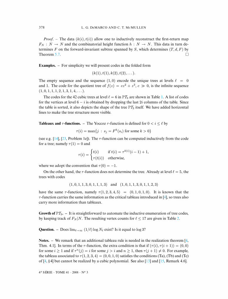
378 L. G. DMARCO AND C. T. MMULLEN
Proof. – The data (k(i), t(i)) allow one to inductively reconstruct the first-return mapFN : N → N and the combinatorial height function h : N → N . This data in turn de-termines F on the forward-invariant subtree spanned by S, which determines (T, d, F ) byTheorem 5.7.
Examples. – For simplicity we will present codes in the folded form
(k(1), t(1), k(2), t(2), . . . ).
The empty sequence and the sequence (1, 0) encode the unique trees at levels = 0and 1. The code for the quotient tree of f(z) = cz2 + z3, c 0, is the infinite sequence(1, 0, 1, 1, 1, 2, 1, 3, 1, 4, . . . ).
The codes for the 42 cubic trees at level = 6 in PT3 are shown in Table 1. A list of codesfor the vertices at level 6 − i is obtained by dropping the last 2i columns of the table. Sincethe table is sorted, it also depicts the shape of the tree PT3 itself. We have added horizontallines to make the tree structure more visible.
Tableaux and τ -functions. – The Yoccoz τ -function is defined for 0 < i ≤ by
τ(i) = maxj : sj = F k(si) for some k > 0
(see e.g. [14], [23, Problem 1e]). The τ -function can be computed inductively from the codefor a tree; namely τ(1) = 0 and
τ(i) =
t(i) if t(i) = τk(i)(i− 1) + 1,
τ(t(i)) otherwise,
where we adopt the convention that τ(0) = −1.
On the other hand, the τ -function does not determine the tree. Already at level = 5, thetrees with codes
(1, 0, 1, 1, 3, 0, 1, 1, 1, 3) and (1, 0, 1, 1, 3, 0, 1, 1, 2, 3)
have the same τ -function, namely τ(1, 2, 3, 4, 5) = (0, 1, 0, 1, 0). It is known that theτ -function carries the same information as the critical tableau introduced in [4], so trees alsocarry more information than tableaux.
Growth of PT3. – It is straightforward to automate the inductive enumeration of tree codes,by keeping track of FN |N . The resulting vertex counts for ≤ 17 are given in Table 2.
Question. – Does lim→∞ (1/) log N exist? Is it equal to log 3?
Notes. – We remark that an additional tableau rule is needed in the realization theorem [4,Thm. 4.1]. In terms of the τ -function, the extra condition is that if (τ(i), τ(i + 1)) = (0, 0)for some i ≥ 1 and if τn(j) = i for some j > i and n ≥ 1, then τ(j + 1) = 0. For example,the tableau associated to τ(1, 2, 3, 4) = (0, 0, 1, 0) satisfies the conditions (Ta), (Tb) and (Tc)of [4, § 4] but cannot be realized by a cubic polynomial. See also [13] and [15, Remark 4.6].
4 e SÉRIE – TOME 41 – 2008 – No 3
TREES AND THE DYNAMICS OF POLYNOMIALS 379
ANNALES SCIENTIFIQUES DE L’ÉCOLE NORMALE SUPÉRIEURE
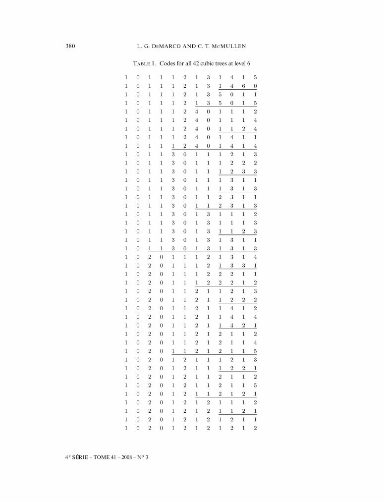
380 L. G. DMARCO AND C. T. MMULLEN
Tʙʟ 1. Codes for all 42 cubic trees at level 6
1 0 1 1 1 2 1 3 1 4 1 5
1 0 1 1 1 2 1 3 1 4 6 0
1 0 1 1 1 2 1 3 5 0 1 1
1 0 1 1 1 2 1 3 5 0 1 5
1 0 1 1 1 2 4 0 1 1 1 2
1 0 1 1 1 2 4 0 1 1 1 4
1 0 1 1 1 2 4 0 1 1 2 4
1 0 1 1 1 2 4 0 1 4 1 1
1 0 1 1 1 2 4 0 1 4 1 4
1 0 1 1 3 0 1 1 1 2 1 3
1 0 1 1 3 0 1 1 1 2 2 2
1 0 1 1 3 0 1 1 1 2 3 3
1 0 1 1 3 0 1 1 1 3 1 1
1 0 1 1 3 0 1 1 1 3 1 3
1 0 1 1 3 0 1 1 2 3 1 1
1 0 1 1 3 0 1 1 2 3 1 3
1 0 1 1 3 0 1 3 1 1 1 2
1 0 1 1 3 0 1 3 1 1 1 3
1 0 1 1 3 0 1 3 1 1 2 3
1 0 1 1 3 0 1 3 1 3 1 1
1 0 1 1 3 0 1 3 1 3 1 3
1 0 2 0 1 1 1 2 1 3 1 4
1 0 2 0 1 1 1 2 1 3 3 1
1 0 2 0 1 1 1 2 2 2 1 1
1 0 2 0 1 1 1 2 2 2 1 2
1 0 2 0 1 1 2 1 1 2 1 3
1 0 2 0 1 1 2 1 1 2 2 2
1 0 2 0 1 1 2 1 1 4 1 2
1 0 2 0 1 1 2 1 1 4 1 4
1 0 2 0 1 1 2 1 1 4 2 1
1 0 2 0 1 1 2 1 2 1 1 2
1 0 2 0 1 1 2 1 2 1 1 4
1 0 2 0 1 1 2 1 2 1 1 5
1 0 2 0 1 2 1 1 1 2 1 3
1 0 2 0 1 2 1 1 1 2 2 1
1 0 2 0 1 2 1 1 2 1 1 2
1 0 2 0 1 2 1 1 2 1 1 5
1 0 2 0 1 2 1 1 2 1 2 1
1 0 2 0 1 2 1 2 1 1 1 2
1 0 2 0 1 2 1 2 1 1 2 1
1 0 2 0 1 2 1 2 1 2 1 1
1 0 2 0 1 2 1 2 1 2 1 2
4 e SÉRIE – TOME 41 – 2008 – No 3
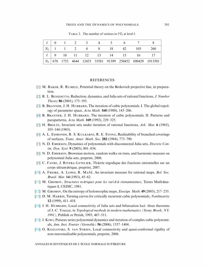
TREES AND THE DYNAMICS OF POLYNOMIALS 381
Tʙʟ 2. The number of vertices in PT3 at level .
0 1 2 3 4 5 6 7 8
N 1 1 2 4 8 18 42 103 260
9 10 11 12 13 14 15 16 17
N 670 1753 4644 12433 33581 91399 250452 690429 1913501
REFERENCES
[1] M. Bʀ, R. Rʟʏ, Potential theory on the Berkovich projective line, in prepara-tion.
[2] R. L. Bɴ, Reduction, dynamics, and Julia sets of rational functions, J. Number
Theory 86 (2001), 175–195.[3] B. Bʀɴɴʀ, J. H. Hʙʙʀ, The iteration of cubic polynomials. I. The global topol-
ogy of parameter space, Acta Math. 160 (1988), 143–206.[4] B. Bʀɴɴʀ, J. H. Hʙʙʀ, The iteration of cubic polynomials. II. Patterns and
parapatterns, Acta Math. 169 (1992), 229–325.[5] H. Bʀʟɪɴ, Invariant sets under iteration of rational functions, Ark. Mat. 6 (1965),
103–144 (1965).[6] A. L. Eɴ, R. S. Kʟʀɴɪ, R. E. Sɴɢ, Realizability of branched coverings
of surfaces, Trans. Amer. Math. Soc. 282 (1984), 773–790.[7] N. D. Eʀɴ, Dynamics of polynomials with disconnected Julia sets, Discrete Con-
tin. Dyn. Syst. 9 (2003), 801–834.[8] N. D. Eʀɴ, Brownian motion, random walks on trees, and harmonic measure on
polynomial Julia sets, preprint, 2006.[9] C. Fʀ, J. Rɪʀ-Lʟɪʀ, Théorie ergodique des fractions rationnelles sur un
corps ultramétrique, preprint, 2007.[10] A. Fʀɪʀ, A. L, R. M, An invariant measure for rational maps, Bol. Soc.
Brasil. Mat. 14 (1983), 45–62.[11] M. Gʀ, Structures métriques pour les variétés riemanniennes, Textes Mathéma-
tiques 1, CEDIC, 1981.[12] M. Gʀ, On the entropy of holomorphic maps, Enseign. Math. 49 (2003), 217–235.[13] D. M. Hʀʀɪ, Turning curves for critically recurrent cubic polynomials, Nonlinearity
12 (1999), 411–418.[14] J. H. Hʙʙʀ, Local connectivity of Julia sets and bifurcation loci: three theorems
of J.-C. Yoccoz, in Topological methods in modern mathematics (Stony Brook, NY,
1991), Publish or Perish, 1993, 467–511.[15] J. Kɪɪ, Puiseux series polynomial dynamics and iteration of complex cubic polynomi-
als, Ann. Inst. Fourier (Grenoble) 56 (2006), 1337–1404.[16] O. Kʟɪ, S. ɴ Sʀɪɴ, Local connectivity and quasi-conformal rigidity of
non-renormalizable polynomials, preprint, 2006.
ANNALES SCIENTIFIQUES DE L’ÉCOLE NORMALE SUPÉRIEURE
382 L. G. DMARCO AND C. T. MMULLEN
[17] O. Lʜ, K. I. Vɪʀɴɴ, Quasiconformal mappings in the plane, second ed.,Springer, 1973.
[18] M. J. Lʏʙɪʜ, Entropy properties of rational endomorphisms of the Riemann sphere,Ergodic Theory Dynam. Systems 3 (1983), 351–385.
[19] C. T. MMʟʟɴ, Automorphisms of rational maps, in Holomorphic functions and
moduli, Vol. I (Berkeley, CA, 1986), Math. Sci. Res. Inst. Publ. 10, Springer, 1988,31–60.
[20] C. T. MMʟʟɴ, The classification of conformal dynamical systems, in Current de-
velopments in mathematics, 1995 (Cambridge, MA), 323–360, Int. Press, Cambridge,MA, 1994.
[21] C. T. MMʟʟɴ, Complex dynamics and renormalization, Annals of MathematicsStudies 135, Princeton University Press, 1994.
[22] C. T. MMʟʟɴ, Ribbon R-trees and holomorphic dynamics on the unit disk,preprint, 2007.
[23] J. Mɪʟɴʀ, Local connectivity of Julia sets: expository lectures, in The Mandelbrot set,
theme and variations, London Math. Soc. Lecture Note Ser. 274, Cambridge Univ.Press, 2000, 67–116.
[24] J. W. Mʀɢɴ, Trees and hyperbolic geometry, in Proceedings of the International
Congress of Mathematicians, Vol. 1, 2 (Berkeley, Calif., 1986), Amer. Math. Soc.,1987, 590–597.
[25] J. W. Mʀɢɴ, P. B. Sʜʟɴ, Valuations, trees, and degenerations of hyperbolic struc-tures. I, Ann. of Math. 120 (1984), 401–476.
[26] J. W. Mʀɢɴ, P. B. Sʜʟɴ, An introduction to compactifying spaces of hyper-bolic structures by actions on trees, in Geometry and topology (College Park, Md.,
1983/84), Lecture Notes in Math. 1167, Springer, 1985, 228–240.[27] J.-P. Oʟ, Le théorème d’hyperbolisation pour les variétés fibrées de dimension 3,
Astérisque 235 (1996).[28] W. Pʀʀʏ, Entropy and generators in ergodic theory, W. A. Benjamin, Inc., New York-
Amsterdam, 1969.[29] F. Pʟɪɴ, Topologie de Gromov équivariante, structures hyperboliques et arbres réels,
Invent. Math. 94 (1988), 53–80.[30] R. Pʀ-Mʀ, Fixed points and circle maps, Acta Math. 179 (1997), 243–294.[31] K. M. Pɪʟɢʀɪ, Dessins d’enfants and Hubbard trees, Ann. Sci. École Norm. Sup. 33
(2000), 671–693.[32] F. Pʀʏʏɪ, J. Sʀʏ, Convergence and pre-images of limit points for coding
trees for iterations of holomorphic maps, Math. Ann. 290 (1991), 425–440.[33] W. Qɪ, Y. Yɪɴ, Proof of the Branner-Hubbard conjecture on Cantor Julia sets,
preprint, 2006.[34] J. Rɪʀ-Lʟɪʀ, Dynamique des fonctions rationnelles sur des corps locaux, in
Geometric methods in dynamics. II, Astérisque 287, 2003, 147–230.[35] J. Rɪʀ-Lʟɪʀ, Points périodiques des fonctions rationnelles dans l’espace hyper-
bolique p-adique, Comment. Math. Helv. 80 (2005), 593–629.
4 e SÉRIE – TOME 41 – 2008 – No 3
TREES AND THE DYNAMICS OF POLYNOMIALS 383
[36] L. Sʀɪ, M. Nɪ, Classification theory of Riemann surfaces, Die Grund. Math.Wiss., Band 164, Springer, 1970.
[37] M. Sʜɪʜɪʀ, Trees associated with the configuration of Herman rings, Ergodic The-
ory Dynam. Systems 9 (1989), 543–560.[38] G. Sʀɪɴɢʀ, Riemann surfaces, Chelsea Publishing Co., 1981.[39] R. Vɪʟ, Genus 0 and 1 Hurwitz numbers: recursions, formulas, and graph-theoretic
interpretations, Trans. Amer. Math. Soc. 353 (2001), 4025–4038.
(Manuscrit reçu le 1er septembre 2006;accepté, après révision, le 14 janvier 2008.)
Laura G. DMʀMathematics Department
University of Illinois at Chicago851 S Morgan (M/C 249)
Chicago, IL 60607-7045, U.S.A.E-mail: [email protected]
Curtis T. MMʟʟɴMathematics Department
Harvard University1 Oxford St
Cambridge, MA 02138, U.S.A.E-mail: [email protected]
ANNALES SCIENTIFIQUES DE L’ÉCOLE NORMALE SUPÉRIEURE