No-regret control for nonlinear distributed systems with incomplete data

J. Math. Pures Appl. 81 (2002) 1161–1189

No-regret control for nonlinear distributed systemswith incomplete data

O. Nakoulima, A. Omrane∗, J. Velin

Laboratoire de Mathématiques et Informatique, Université des Antilles et de la Guyane, Campus Fouillole,97159 Pointe-à-Pitre, Guadeloupe (FWI)

Accepted 16 August 2002

Dédié à la mémoire de J.-L. Lions

Abstract

We study the control of distributed systems with incomplete data extending the work in[Nakoulima, et al., C. R. Acad. Sci. Paris Sér. I 330 (2000) 801–806] to the nonlinear case.

In a first part, we discuss the regularity of the state solution to the problem in the general case, andwe give an application.

The second part deals with the optimal control problem. We prove the convergence of the low-regret control introduced in [Nakoulima, et al., C. R. Acad. Sci. Paris Sér. I 330 (2000) 801–806] tothe no-regret control for which we obtain a singular optimality system. We also continue studyingthe application of the first part. 2002 Éditions scientifiques et médicales Elsevier SAS. All rights reserved.

MSC:49K40; 35B37; 35K55; 90C30; 93A15; 93D09

Keywords:Pareto control; No-regret control; Adapted low-regret control; Systems with incomplete data; Costfunction; Quadratic perturbation; Nonlinear distributed systems

Introduction

Optimal control problems governed by nonlinear partial differential equations are a fieldof active research. Most of the work is done to derive necessary or sufficient optimalityconditions of first or second order. But the question of existence and characterization of

* Corresponding author.E-mail addresses:[email protected] (O. Nakoulima), [email protected] (A. Omrane),

[email protected] (J. Velin).

0021-7824/02/$ – see front matter 2002 Éditions scientifiques et médicales Elsevier SAS. All rights reserved.PII: S0021-7824(02)01268-0

1162 O. Nakoulima et al. / J. Math. Pures Appl. 81 (2002) 1161–1189

optimal controls has not been considered in detail, since the regularity of the state solutionis not straight forward. The assumptions on the control problem are mostly chosen insuch a way that a more or less known standard method can be applied to derive theexistence of solutions. We apply here the no-regret method used by the authors in [11],to nonlinear distributed systems with incomplete data in general. The no-regret control is amethod applied to control the systems where there arecontrolsandunknown perturbations(uncertainties): we search for the controls, if they exist, which make things better thanwhen there is no control on the system, for any given perturbation parameter.

The no-regretconcept is introduced by Savage [13]. Lions [8] used this concept inoptimal control, motivated by a number of applications in economics, and ecology as well.

The Pareto concept (see [2], for example) which is equivalent to this one, is alsoused by Lions in [7]. As far as we know, he was the first to use these two concepts tocontrol distributed systems with incomplete data in different areas in applied mathematics(see [7–10,4]): In [8], for example, he extends the work of Allwright [1] to the infinitedimension case. In [4] with Gabay [3], a decision criteria is added to the uncertaintiesclosed subspace, and they improve the results obtained so far by extending the notion oflow-regret to many agents in economics.

In [11] (see also [12]), Nakoulima et al. give a precise optimality system (which is asingular optimality system). In [12], they characterize the no-regret (Pareto) control forproblems of incomplete data, in both the stationary and evolution cases. A number ofapplications is given too.

In the literature mentioned above, the linear case is considered only. In this article, wegeneralize the study to the control of nonlinear systems with incomplete data. We use theadaptedlow-regret control (details in part II) because the low-regret control is not uniquein general. Following the lines of the work in [11], the no-regret control is shown to be thelimit of the low-regret control when the perturbation parameter tends to zero.

The paper is organised in two parts as follows: The Part I contains the regularity resultson the nonlinear state equation (Section 1), and we also give an application in Section 2.The Part II deals with the optimal control. We define the no-regret control for the nonlinearcase and we give the general theory for the control problem in Section 3. We then pass tothe limit in the adapted low-regret control problem, and characterize the no-regret controlby giving a singular optimality system. In Section 4 we continue analysing the applicationof the first part by the development of the optimal control problem.

Part I. Regularity results

1. Preliminaries and general theory

Let V be a real Hilbert space of dualV ′, A ∈ L(V;V ′) an elliptic differential operatormodelling a distributed system,U the Hilbert space of controls andB ∈ L(U;V ′). LetF be the Hilbert space of uncertainties, andG be a closed vector subspace ofF , andβ ∈L(F ;V ′).

For s ∈ V ′ a source term (independent ofv andg), the state equation related to thecontrolv ∈ U and to the uncertaintyg ∈G is given by:

O. Nakoulima et al. / J. Math. Pures Appl. 81 (2002) 1161–1189 1163

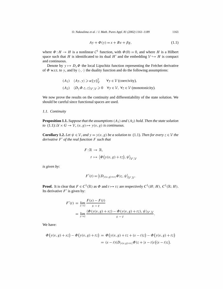
Ay +Φ(y)= s +Bv + βg, (1.1)

whereΦ :H → H is a nonlinearC1 function, withΦ(0) = 0, and whereH is a Hilbertspace such thatH is identificated to its dualH ′ and the embeddingV → H is compactand continuous.

Denote byy → DyΦ the local Lipschitz function representing the Fréchet derivativeof Φ w.r.t. toy, and by〈·, ·〉 the duality function and do the following assumptions:

(A1) 〈Ay,y〉 α‖y‖2V ∀y ∈ V (coercivity),

(A2) 〈DyΦ.z, z〉V ′,V 0 ∀y ∈ V, ∀z ∈ V (monotonicity).

We now prove the results on the continuity and differentiability of the state solution. Weshould be careful since functional spaces are used.

1.1. Continuity

Proposition 1.1. Suppose that the assumptions(A1) and(A2) hold. Then the state solutionto (1.1):U ×G→ V , (v, g) → y(v, g) is continuous.

Corollary 1.2. Letψ ∈ V , andy = y(v, g) be a solution to(1.1). Then for everyz ∈ V thederivativeF ′ of the real functionF such that

F :R → R,

t → ⟨Φ

(y(v, g)+ tz),ψ ⟩

V ′,V

is given by:

F ′(t)= ⟨(Dy(v,g)+tzΦ)z,ψ

⟩V ′,V .

Proof. It is clear thatF ∈ C1(R) asΦ andt → tz are respectivelyC1(H ;H), C1(R;H).Its derivativeF ′ is given by:

F ′(t) = lims→t

F (s)−F(t)s − t

= lims→t

〈Φ(y(v, g)+ sz)−Φ(y(v, g)+ tz),ψ〉V ′,Vs − t .

We have:

Φ(y(v, g)+ sz) −Φ(

y(v, g)+ tz) = Φ(y(v, g)+ tz+ (s − t)z) −Φ(

y(v, g)+ tz)= (s − t)(Dy(v,g)+tzΦ)z+ |s − t|ε((s − t)z).


Whenε→ 0 we obtain:

F ′(t)= ⟨(Dy(v,g)+tzΦ)z,ψ

⟩V ′,V .

Proof of Proposition 1.1. Let y ∈ V a solution to (1.1), and denote byy = y(v, g,w,h) the state function:

y = y(v+w,g + h)− y(v, g). (1.2)

Noting that

⟨Φ

(y(v +w,g + h)),ψ ⟩

V ′,V − ⟨Φ

(y(v, g)

),ψ

⟩V ′,V = F(1)− F(0)

thanks to the mean value theorem, there existsθ ∈ ]0,1[ such that for everyψ ∈ V , wehave:

⟨Φ

(y(v +w,g + h)) −Φ(

y(v, g)),ψ

⟩V ′,V = ⟨

(Dy(v,g)+θyΦ)y,ψ⟩ ∀ψ ∈ V . (1.3)

Consequently, we can write:

Φ(y(v +w,g + h)) −Φ(

y(v, g)) = (Dy(v,g)+θyΦ)y. (1.4)

Now, asy verifies:

Az+Φ(y(v +w,g + h)) −Φ(

y(v, g)) = Bw+ βh,

thanks to (1.4). It turns thaty is a solution to the problem:

Ay + (Dy(v,g)+θyΦ)y = Bw+ βh. (1.5)

After puttingψ = y in (1.3) and multiplying (1.5) byy, it results, thanks to (A1) that

α‖y‖2V 〈Ay, y〉 −⟨

(Dy(v,g)+θyΦ).y, y⟩ + (‖B‖‖w‖ + ‖β‖‖h‖)‖y‖V .

Using (A2) and lettingc= max(‖B‖,‖β‖), we obtain:

‖y‖V c

α

(‖w‖ + ‖h‖). (1.6)

It follows that‖y‖V → 0 when(‖w‖,‖h‖)→ (0,0).


1.1.1. DifferentiabilityProposition 1.3. Under the assumptions(A1) and(A2) we have:

y(v +w,g + h)− y(v, g)= L(v,g)(w,h)+∥∥(w,h)∥∥U×F ε(w,h), (1.7)

whereL(v,g)(·, ·) :U ×G→ V is a linear and continuous application, defined by:

L(v,g)(w,h)= ∂y∂v(v, g)(w)+ ∂y

∂g(v, g)(h).

Moreover, denoting byAy(v,g) =A+Dy(v,g) for v ∈ U andg ∈G, the partial derivatives

∂y

∂v(v, g)(w) and

∂y

∂g(v, g)(h)

are respectively defined by:

Ay(v,g)(∂y

∂v(v, g)(w)

)= Bw,

and

Ay(v,g)(∂y

∂g(v, g)(h)

)= βh.

Proof. Let z be defined as in (1.2). From (1.4) we have:

Φ(y(v +w,g + h)) −Φ(

y(v, g)) = Φ

(y(v, g)+ z) −Φ(

y(v, g))

= (Dy(v,g)Φ)z(w,h)+ ‖z‖Vε(z).

Consequently, by subtraction the statez writes:

Ay(v,g)z= −‖z‖Vε(z)+Bw+ βh.

And multiplying by 1/‖(w,h)‖U×F , we deduce that

Ay(v,g)z

‖(w,h)‖U×F= − ‖z‖V

‖(w,h)‖U×Fε(z)+ Bw+ βh

‖(w,h)‖U×F. (1.8)

Let L(v,g)(w,h) be such that

Ay(v,g)L(v,g)(w,h)= Bw+ βh. (1.9)


It is clear thatL(v,g)(w,h) is linear with respect tow andh. Now, we multiply (1.9) by1/‖(w,h)‖U×F and we substract with (1.8). We obtain:

Ay(v,g)(z−L(v,g)(w,h)‖(w,h)‖U×F

)= − ‖z‖V

‖(w,h)‖U×Fε(z). (1.10)

So, interpreting

− ‖z‖V‖(w,h)‖U×F

ε(z)

as a data, we can associate the unique solutionθ(w,h) ∈ V to the problem:

Ay(v,g)θ = − ‖z‖V‖(w,h)‖U×F

ε(z).

Hence,θ(w,h) tends to zero inV as‖(w,h)‖U×F → 0, since from (1.6),

z

‖(w,h)‖U×F

is bounded.Now, asθ is unique, we have:

θ(w,h)= z−L(v,g)(w,h)‖(w,h)‖U×F

and we conclude that

y(v +w,g + h)= y(v, g)+L(v,g)(w,h)+∥∥(w,h)∥∥U×F θ(w,h).

Consequently,L(v,g)(w,h) being the unique solution of a well-posed linear problem,we can define the derivative ofy with respect tov (respectivelyg) in the directionw(respectivelyh) in setting

∂y

∂v(v, g)(w)= L(v,g)(w,0) and

∂y

∂g(v, g)(h)= L(v,g)(0, h).

2. Application

In this section, we discuss the regularity of the solutions to the problem with incompletedata:


infv∈U

(∥∥y(v, g)− zd∥∥2L2(Ω)

+ ‖v‖2U

) ∀g ∈G,subject to

Ay(v,g)+ f (y(v, g)

) = v inΩ,

∂y

∂ν(v, g)= g on∂Ω,

(2.1)

and whereA is given by:

A= − ∂

∂xi

(aij (x)

∂

∂xj

)+ a0. (2.2)

The coefficientsaij (·) (i, j = 1, . . . , n) are measurable functions satisfying to thecoercivity and symmetry properties:

(1)∑ni,j=1 aij ξiξj α|ξ |2, ∀ξ = (ξi)i=1,...,n ∈ R

n with α 0;(2) aij = aji, i, j = 1, . . . , n;(3) a0 is a measurable positive function.

We denote byY the Hilbert spaceY := y ∈ V; Ay ∈ L2(Ω),whereV is a real Hilbertspace such thatV =H 1(Ω), V ′ is the corresponding topological dual;Y is equipped withthe Hilbert norm:

‖y‖2Y = ‖y‖2

V + ‖Ay‖2L2(Ω)

. (2.3)

Theorem 2.1. Suppose thatf ∈ C1(R) and the applicationy → f (y) is L2(Ω). ThenU ×G→ Y , (v, g) → y(v, g) is continuous w.r.t.(v, g).

Proof. Step1. Leth ∈ G⊂ L2(∂Ω) andw ∈ L2(Ω), we denote byy(v +w,g + h) theassociated state to the datav+w,g+h, and as in the previous section,y defined by (1.2).Then we have:

Ay + f (

y(v +w,g + h)) − f (y(v, g)

) =w in Ω,

∂y

∂ν= h on∂Ω.

(2.4)

Now, sincef ∈ C1(R), we apply the mean value theorem to

[y(v, g)(x), y(v+w,g + h)(x)]

(x being fixed inRn). There existsθ ∈ ]0,1[ such that

f(y(v+w,g + h)) − f (

y(v, g)) = yf ′(y(v, g)+ θy).


Then (2.4) becomes Ay + yf ′(y(v, g)+ θy) =w in Ω,

∂y

∂ν= h on∂Ω.

(2.5)

Multiplying (2.5) by y, we get:

〈Ay, y〉 +∫Ω

y2f ′(y(v, g)+ θy)dx =∫Ω

wy dx.

Thus, by the Green formula, we have:

n∑i,j=1

∫Ω

aij∂y

∂xi

∂y

∂xjdx +

∫Ω

a0y2 dx +∫Ω

y2f ′(y(v, g)+ θy)dx

=∫Ω

wy dx +∫∂Ω

y∂φ

∂νdσ.

From the coercivity property (A1) and the positivity off ′, it results:

α′‖y‖2V ‖h‖L2(∂Ω)‖y‖L2(∂Ω) + ‖w‖L2(Ω)‖y‖L2(Ω)

(‖h‖L2(∂Ω)‖ + ‖w‖L2(Ω)

)‖y‖V ,and so,

‖y‖V ‖h‖L2(∂Ω) + ‖w‖2. (2.6)

Step2. The second part of the proof is devoted to show that‖Ay‖2 tends to 0 when(‖h‖L2(∂Ω),‖w‖2)→ (0,0).

In fact, let beφ in L2(Ω),multiply (2.5) byφ, we obtain, for allφ ∈L2(Ω),∫Ω

Ayφ dx +∫Ω

yf ′(y + θy)φ dx =∫Ω

wφ dx

and ∣∣∣∣∫Ω

Ayφ dx

∣∣∣∣ ‖φ‖2∥∥yf ′(y + θy)∥∥2 + ‖w‖2

,

we divide by‖φ‖2 = 0, then

| ∫Ω Ayφ dx|‖φ‖2

∥∥yf ′(y + θy)∥∥2 + ‖w‖2.


Consequently,

‖Ay‖ ∥∥yf ′(y + θy)∥∥2 + ‖w‖2. (2.7)

The first term in the right-hand side of (2.7) tends to 0, then thanks to (2.6) we conclude(in view of (2.3)) that‖y‖Y tends to 0 when(‖h‖L2(∂Ω),‖w‖2)→ (0,0). Lemma 2.2. We have the following limit:

∥∥yf ′(y + θy)∥∥2 → 0 as(‖h‖L2(∂Ω),‖w‖2

) → (0,0).

Proof. Indeed, using (2.6) (after extracting a subsequence denoted againy), we have inorder:

(1) y tends to 0 a.e. inΩ as(‖h‖L2(∂Ω),‖w‖2),(2) ∃k ∈ L2(Ω) a positive function such that∀h ∈L2(∂Ω),

∣∣y(x)∣∣ k(x) a.e. inΩ.

Consequently, we deduce successively:

(1) y(v, g)(x)+ θy(x) tends toy(v, g) a.e. inΩ ,(2) there exists a positive function inL2(Ω) denotedk such that a.e.x ∈Ω , ∀h ∈L2(∂Ω),

∥∥y(v, g)(x)+ θy(x)∥∥ k(x),

(3) f ′(y(v, g)(x) + θy(x)) tends to f ′(y(v, g))(x) since f ′ is continuous. Then,y(x)f ′(y(v, g)(x)+ θy(x)) tends to 0 a.e. inΩ ,

(4) we have:

∣∣f (y(v, g)(x)+ θy(x))∣∣ sup

z(x)∈[−k(x),+k(x)]

∣∣f (z(x)

)∣∣ = ∣∣f (z(x)

)∣∣,wherez is in [−k(x),+k(x)] a.e. inΩ .This result is obvious because we have on one side

∣∣y(x)f ′(y(v, g)(x)+ θy(x))∣∣ ∣∣f (y(v, g)(x)+ θy(x))∣∣ + ∣∣f (

y(v, g)(x))∣∣,

and on another side,y(v, g)(x) + θy(x) is in the compact[−k(x),+k(x)] andf iscontinuous, so

∣∣f (y(v, g)(x)+ θy(x))∣∣ sup

z(x)∈[−k(x),+k(x)]

∣∣f (z(x)

)∣∣ = ∣∣f (z(x)

)∣∣,


wherez is in [−k(x),+k(x)] a.e. inΩ . Consequently,z ∈ L2(Ω), and for allx a.e.in Ω : ∣∣y(x)f ′(y(v, g)(x)+ θy(x))∣∣

∣∣f (z(x)

)∣∣ + ∣∣f (y(v, g)

)∣∣.It is clear that the function|f (z)| + |f (y(v, g)| is inL2(Ω).

Now, applying the mean convergence Lebesgue’s theorem we conclude that∥∥yf ′(y(v, g)+ θy)∥∥ → 0 as(‖h‖L2(∂Ω),‖w‖2

) → (0,0). Lemma 2.3. The solutions(0, h) to the problem:

As + sf ′(y(v, g)) = 0 inΩ,

∂s

∂ν= h on∂Ω,

(2.8)

is such that

lim‖h‖L2(∂Ω)→0

∥∥s(0, h)∥∥Y = 0.

Proof. We multiply (2.8) bys(0, h) and we integrate overΩ. From the GREEN’s formula,we obtain:

n∑i,j=1

∫Ω

aij∂s(0, h)

∂xi

∂s(0, h)

∂xjdx +

∫Ω

a0s(0, h)

2 dx +∫Ω

s(0, h)

2f ′(y(v, g)+ θy)dx

=∫∂Ω

s(0, h)∂s(0, h)

∂νdσ =

∫∂Ω

hs(0, h)dσ.

We achieve the proof using similar and adapted arguments as in the above sectionconcluding that‖s(0, h)‖Y tends to zero as‖h‖L2(∂Ω) → 0. Moreover, it is clear thatL2(∂Ω)→ Y , h → s(0, h) is a linear and continuous function.

Now, we present another regularity result. In fact, we have:

Theorem 2.4. Assume thatf ∈ C1(R). Then

y(v, g + h)− y(v, g)= s(0, h)+ ‖h‖L2(∂Ω)ε(h).

Proof. We setzh = y(v, g+ h)− y(v, g), wherezh is the solution to the problem:Azh + sf ′(y(v, g)+ θzh) = 0 inΩ,

∂zh

∂ν= h on∂Ω.

(2.9)


Denote byΨ (h) andv(h) the terms:

Ψ (h)= zh − s(0, h)‖h‖L2(∂Ω)

and

v(h)= s(0, h)

‖h‖L2(∂Ω)

[f ′(y(v, g)+ θzh) − f ′(y(v, g))].

We have:

AΨ(h)+Ψ (h)f ′(y(v, g)+ θzh) = v(h) inΩ,

∂Ψ (h)

∂ν= 0 on∂Ω,

(2.10)

after substraction of (2.8) from (2.9). It is easy to notice that‖Ψ (h)‖Y → 0 when‖h‖L2(∂Ω) → 0. In fact, conforming to the previous section, it is sufficient to show that‖v(h)‖2 → 0 when‖h‖L2(∂Ω) → 0.

To establish this result, we notice that

s(0, h)

‖h‖L2(∂Ω)

= s(

0,h

‖h‖L2(∂Ω)

),

and that ∥∥∥∥s(

0,h

‖h‖L2(∂Ω)

)∥∥∥∥Y

is bounded independently ofh because the linear applicationT :h → s(0, h) is continuousfromG to Y . Now, from (2.3), the supremum:

suph∈N

∥∥s(h)∥∥V with N = h ∈ L2(∂Ω); ‖h‖L2(∂Ω) = 1

exists independently ofh. Moreover, sinceV → L2(Ω) is continuous and compact, wecan extract a subsequence denoted again

s

(0,

h

‖h‖L2(∂Ω)

),

which converges strongly inL2(Ω).Then, we conclude as in the proof of Lemma 2.2 which insures that‖v(h)‖2 tends to 0

when‖h‖L2(∂Ω) → 0.


Now, using the continuity result, we have‖Ψ (h)‖Y → 0, ‖h‖L2(∂Ω) → 0. This meansthat:

lim‖h‖L2(∂Ω)→0

y(v, g + h)− y(v, g)− s(0, h)‖h‖L2(∂Ω)

= 0.

From another side, we have

y(v, g + h)= y(v, g)+ s(0, h)+ ‖h‖L2(∂Ω)ε(h). Now, let us give the:

Definition 2.5. We call partial derivative ofy with respect tog at the point(v, g) in thedirectionh, the solutions(0, h) of the problem (2.8) defined by:

∂y

∂g(v, g) :F → Y,

h → s(0, h).

And we define by the partial derivative ofy with respect tov at the point(v, g) in thedirectionw, the application denoted∂y/∂v (v, g), and given by:

∂y

∂v(v, g) :L2(Ω) → Y,

w → s(w,0),

wheres(w,0) is such that:As(w,0)+ s(w,0)f ′(y(v, g)) =w inΩ,

∂s(w,0)

∂ν= 0 on∂Ω.

Lemma 2.6. Letw be a direction inU . The application∂y/∂g is continuous at the point(v,0) in the directionw.

Proof. Note that

∂y

∂g(v+ tw,0) and

∂y

∂g(v,0)

are such thatA∂y

∂g(v + tw,0)(g)+ ∂y

∂g(v + tw,0)(g)f ′(y(v, g)) = 0 inΩ,

∂

∂ν

(∂y

∂g(v + tw,0)(g)

)= g on∂Ω,


and

A∂y

∂g(v,0)(g)+ ∂y

∂g(v,0)(g)f ′(y(v, g)) = 0 inΩ,

∂

∂ν

(∂y

∂g(v,0)(g)

)= g on∂Ω.

And also that

∂y

∂g(v + tw,0)f ′(y(v + tw,g)) − ∂y

∂g(v,0)f ′(y(v, g))

=[∂y

∂g(v + tw,0)− ∂y

∂g(v,0)

]f ′(y(v+ tw,g))

+ [f ′(y(v + tw,g)) − f ′(y(v, g))]∂y

∂g(v,0)(g),

so that we have for

Zg(t)= ∂y

∂g(v + tw,0)− ∂y

∂g(v,0),

AZg(t)+Zg(t)f ′(y(v + tw,g)) = −∂y

∂g(v,0)(g)

[f ′(y(v+ tw,g)) − f ′(y(v, g))],

∂Zg(t)

∂ν= 0.

We also notice from above that

∥∥∥∥∂y∂g (v,0)(g)[f ′(y(v + tw,g)) − f ′(y(v, g))]∥∥∥∥L2(Ω)

→ 0 whent → 0.

We conclude following the lines of the proof of the continuity ofv → y(v, g). We get atthe end,

∥∥Zg(t)∥∥Y −→t↓0

0.

This gives:

∂y

∂g(v + tw,0)−→

t↓0

∂y

∂g(v,0).


Part II. The optimal control

Let G be a non-empty closed subspace of the Hilbert space of uncertaintiesF , andβ ∈L(F,V ′).

Forf ∈ V ′, the state equation related to the controlv ∈ U and to the uncertaintyg ∈Gis given (1.1). Supposing thatA is an isomorphism fromV to V ′, Eq. (1.1) is well-posedin V . Denote byy = y(v, g) the unique solution to (1.1). For everyg ∈G we have then apossible state for which we rely a cost function given by:

J (v, g)= ‖Cy − zd‖2H +N‖v‖2

U , (2.11)

whereC ∈L(V;H), H is a Hilbert space,zd ∈H fixed,N > 0, and‖ · ‖X being the normon the real Hilbert spaceX. We are concerned by the optimal control of the problem (1.1),(2.11).

Definition 2.7. The no-regret control related to a controlu0 is the uniqueu ∈ U solution tothe problem:

infv∈U

supg∈G

(J (v, g)− J (u0, g)

).

We note that foru0 = 0, we find the definition of the no-regret control of Lions [8].

3. No-regret optimal control and the associated optimality system

For the sake of simplicity, we consider the caseu0 = 0. We are then interested in theno-regret control.

For this nonlinear case, we consider the cost function defined as below:Using the regularity ofy(·, ·) (Part I), we substitute in (2.11)y(v, g) by:

y(v,0)+ ∂y∂g(v,0)(g).

This defines anewcost-function notedJ1:

J1(v, g)= J (v,0)+ 2

⟨∂y

∂g(v,0)(g), C∗(Cy(v,0)− zd)⟩

H,H.

Hence, we are interested by solving the following problem:

infv∈U

supg∈G

(J1(v, g)− J1(0, g)

). (3.1)

The solution of (3.1)—if it exists—is calledno-regretcontrol for nonlinear problems.Now we have the following lemma:


Lemma 3.1. For any(v, g) ∈ U ×G, the following equality holds:

J1(v, g)− J1(0, g)= J (v,0)− J (0, g)+ 2⟨β∗(ξ(v)− ξ(0)), g⟩, (3.2)

whereξ is defined by:

A∗(ξ(v)) = C∗(Cy(v,0)− zd), (3.3)

A∗ being the adjoint ofA.

Proof. With simple calculations, we obtain:

J1(v, g)− J1(0, g) = J (v,0)− J (0, g)+ 2

[⟨∂y

∂g(v,0)(g),C∗(Cy(v,0)− zd)⟩

−⟨∂y

∂g(0,0)(g),C∗(Cy(0,0)− zd)⟩].

For everyv in U, denote byξ(v) the solution of the dual problem (3.3).Consequently, using Proposition 1.3, we can write:⟨

∂y

∂g(v,0)(g),C∗(Cy(v,0)− zd)⟩ −

⟨∂y

∂g(0,0)(g),C∗(Cy(0,0)− zd)⟩

=⟨A∂y∂g(v,0)(g), ξ(v)

⟩−

⟨A∂y∂g(0,0)(g), ξ(0)

⟩= ⟨βg, ξ(v)

⟩ − ⟨βg, ξ(0)

⟩ = ⟨g,β∗(ξ(v)− ξ(0))⟩.

Remark 1. The idea consisting in replacingy(v, g) by

y(v,0)+ ∂y∂g(v,0)(g)

joins the one of Lions [5], which is to substitute the cost function by

J (v,0)+ ∂y∂g(v,0)(g).

Indeed, some calculations show that

∂J

∂g(v,0)(g)= 2

⟨∂y

∂g(v,0)(g),C∗(Cy(v,0)− zd)⟩,

and hence, we also obtain:

J1(v, g)− J1(0, g)= J (v,0)− J (0,0)+[∂J

∂g(v,0)− ∂J

∂g(0,0)

](g). (3.4)


We now define the applicationS acting onU by:

S(v)= 2β∗(ξ(v)− ξ(0)). (3.5)

From Proposition 1.3, it is clear thatS(v) is linear and continuous onG. Henceforth, (3.1)turns to:

infv∈U

supg∈G

(J (v,0)− J (0,0)+ ⟨

S(v), g⟩G′,G

). (3.6)

To continue, we follow the lines of [11,12].In (3.6), the term supg∈G〈S(v), g〉G′ ,G is equal 0, or not upper bounded. Then as for the

linear case, we have to consider the set:

M = v ∈ U; ⟨

2β∗(ξ(v)− ξ(0)), g⟩G′,G = 0, ∀g ∈G

.

In this context, (3.6) admits at least a solution inM. In fact, we have the following result:

Theorem 3.2. Assumey → DyΦ is local Lipschitz, andA andΦ satisfy the assump-tions(A1) and(A2). The problem defined by(3.6)admits at least a solution inM.

Proof. The setM is strongly closed inU . Indeed, the application

v → ⟨2β∗(ξ(v)− ξ(0)), g⟩

G′,G

is continuous fromU to R. To prove this, consider a sequencevn included inM, andconverging strongly to an elementv ∈ U . Thanks to (3.3), we can write:

A∗(ξ(vn)− ξ(v)) + Dy(vn,g)Φ∗ξ(vn)− Dy(v,g)Φ∗ξ(v)= C∗C(y(vn,0)− y(v,0)

).

Hence, Proposition 1.1 allows us to deduce thaty(vn,0)n tends toy(v,0) in V . Now,multiplying the above equality byξ(vn) − ξ(v) and using the local Lipschitz properties,(A1) and (A2), there is a positive constantc such that∥∥ξ(vn)− ξ(v)∥∥V c

(Lv

∥∥ξ(v)∥∥V + ‖C∗C‖)∥∥y(vn,0)− y(v,0)∥∥V , (3.7)

whereLv is a local-Lipschitz constant depending onv only.Consequently, (3.7) insures thatξ is continuous onV . Finally,v ∈ M. This proves that

v → ⟨2β∗(ξ(v)− ξ(0)), g⟩

G′,G

is continuous onU .Moreover, it is obvious to remark that onU, v → J (v,0)− J (0,0) is continuous, 0-

coercive(by definition ofJ (v,0)), and bounded below by−J (0,0).Then, using a minimizing sequence, it is clear that there existsv ∈ M satisfying (3.6).

From Definition 2.7, we deduce thatv is a no-regret control.


3.1. The low-regret control

Let v be a no-regret optimal control. We derive now the optimal control system forv.As in the linear case, the difficulty is to characterize the setM.

We proceed as for the linear case (see [11,12]) by relaxing the function

J (v,0)− J (0,0)+ ⟨S(v), g

⟩G′,G.

Let beγ > 0 a fixed number, then the relaxed problem has the following formulation:

infv∈U

supg∈G

(J (v,0)− J (0,0)+ ⟨

S(v), g⟩G′,G − γ ‖g‖2

G

). (3.8)

So, by the Fenchel–Moreau formula, and identifyingG to its dualG′, we obtain:

infv∈U

(J (v,0)− J (0,0)+ 1

4γ

∥∥S(v)∥∥2G

). (3.9)

Hence we obtain a standard control problem.As for the linear case, (3.9) also admits a solution noteduγ . That is thelow-regret

control.

Remark 2. At the opposite of the linear case, the application

v → J (v,0)− J (0,0)+ 1

4γ

∥∥S(v)∥∥2G

is not convex and then we do not have necessarily the uniqueness foruγ . Moreover, we arenot sure thatuγ converges in the setM. However, we can adapt

v → J (v,0)− J (0,0)+ 1

4γ

∥∥S(v)∥∥2G

to a given no-regret optimal control like in the work of Lions [6] for the penalisationmethod.

3.2. The adapted low-regret control

Let u be a no-regret optimal control, and define the function:

v → J (v,0)− J (0,0)+ 1

2‖v − u‖2

U + 1

4γ

∥∥S(v)∥∥2G.

We consider the following problem:

infv∈U

J γa (v), (3.10)


where

J γa (v)= J (v,0)− J (0,0)+ 1

2‖v − u‖2

U + 1

4γ

∥∥S(v)∥∥2G. (3.11)

Then, we have the:

Proposition 3.3. The problem(3.10), (3.11)has at least a solutionuγ in U .

Proof. Using the same arguments as for the proof of Theorem 3.2, the proof of Proposi-tion 3.3 follows. Definition 3.4. We define by the adapted low-regret control, the optimal controluγ , solu-tion to (3.10), (3.11).

Theorem 3.5. The adapted low-regret controluγ is characterized by the unique solutiony(uγ ,0), ζγ , ργ ,pγ of the optimality system:

(S.O.S)γ

Ay(uγ ,0)+Φ(y(uγ ,0)

) = s +Buγ , (1γ )

A∗ζγ = Cy(uγ ,0)− zd , (2γ )

Aργ = 1

γββ∗(ζγ − ζ0), (3γ )

A∗pγ = C∗(Cy(uγ ,0)− zd) +C∗Cργ , (4γ )B∗pγ +Nuγ = u− uγ . (5γ )

Proof. The solutionuγ satisfies the Euler conditions. That is, in each directionw ∈ U :

limt→0

J γa (uγ + tw)−J γ (uγ )t

0.

Simple calculations give:

J γa (uγ + tw)−J γa (uγ )t

= t[∥∥∥∥Cy(uγ + tw,0)−Cy(uγ ,0)

t

∥∥∥∥2

H+ (N + 1)‖w‖2

+ 1

4γ

∥∥∥∥S(uγ + tw)− S(uγ )t

∥∥∥∥2]

+ 2

⟨y(uγ + tw,0)− y(uγ ,0)

t,C∗(Cy(uγ ,0)− zd)⟩ + 2〈Nuγ + uγ − u,w〉

+ 1

2γ

⟨S(uγ + tw)− S(uγ )

t, S(uγ )

⟩.


The first term in the right-hand side tends to zero witht , since there existK1,γ andK2,γindependent oft such that∥∥∥∥Cy(uγ + tw,0)− y(uγ ,0)

t

∥∥∥∥H

K1,γ , (3.12)

∥∥∥∥S(uγ + tw)− S(uγ )t

∥∥∥∥H

K2,γ . (3.13)

In fact, (1.7) allows us to write:

y(uγ + tw,0)− y(uγ ,0)= t ∂y∂v(uγ ,0)(w)+ |t|∥∥(w,0)∥∥U×F ε(tw,0).

Then, consequently, we get:∥∥∥∥Cy(uγ + tw,0)− y(uγ ,0)t

∥∥∥∥H

‖C‖L(V ,H)∥∥∥∥y(uγ + tw,0)− y(uγ ,0)

t

∥∥∥∥V

‖C‖L(V ,H)∥∥∥∥∂y∂v (uγ ,0)(w)

∥∥∥∥V.

Now, from(2γ ) we have:

A∗ ζ(uγ + tw)− ζ(uγ )t

+ (Dy(uγ+tw,0)Φ)ζ(uγ + tw)− (Dy(uγ ,0)Φ)ζ(uγ )t

= C∗Cy(uγ + tw,0)− y(uγ ,0)

t

and more precisely,

(Dy(uγ+tw,0)Φ)ζ(uγ + tw)− (Dy(uγ ,0)Φ)ζ(uγ )t

= (Dy(uγ+tw,0)Φ)(ζ(uγ + tw)− ζ(uγ )

t

)+

[(Dy(uγ+tw,0) −Dy(uγ ,0)

t

)Φ

]ζ(uγ ).

It results that

A∗ ζ(uγ + tw)− ζ(uγ )t

+ (Dy(uγ+tw,0)Φ)(ζ(uγ + tw)− ζ(uγ )

t

)

= −[(Dy(uγ+tw,0) −Dy(uγ ,0)

t

)Φ

](ζ(uγ )

) +C∗Cy(uγ + tw,0)− y(uγ ,0)

t.

Multiplying by

ζγ,t = ζ(uγ + tw)− ζ(uγ )t


and integrating by parts overΩ we obtain:

〈Aζγ,t , ζγ,t〉 + ⟨(Dy(uγ+tw,0)Φ)ζγ,t , ζγ,t

⟩=

⟨−

[(Dy(uγ+tw,0) −Dy(uγ ,0)

t

)Φ

](ζ(uγ )

), ζγ,t

⟩

+⟨C∗C

y(uγ + tw,0)− y(uγ ,0)t

, ζγ,t

⟩.

Using the assumptions(A1) and(A2) we have:

α‖ζγ,t‖2V

∥∥∥∥Dy(uγ+tw,0)Φ −Dy(uγ ,0)Φt

∥∥∥∥L(H)

∥∥ζ(uγ )∥∥V‖ζγ,t‖V

+ ‖C∗‖∥∥∥∥C y(uγ + tw,0)− y(uγ ,0)

t

∥∥∥∥V‖ζγ,t‖V .

Now, sincey →DyΦ is local Lipschitz, there exists a positive constantCγ such that

∥∥∥∥Dy(uγ+tw,0)Φ −Dy(uγ ,0)Φt

∥∥∥∥L(H)

Cγ∥∥∥∥y(uγ + tw,0)− y(uγ ,0)

t

∥∥∥∥V,

so that

α‖ζγ,t‖V Lγ

∥∥∥∥y(uγ + tw,0)− y(uγ ,0)t

∥∥∥∥V

∥∥ζ(uγ )∥∥V+ ‖C∗‖

∥∥∥∥C y(uγ + tw,0)− y(uγ ,0)t

∥∥∥∥V.

And we easily deduce the desired estimations (3.12) and (3.13).Now, denote byργ the solution to the problem:

Aργ = 1

γββ∗(ξ(uγ )− ξ(0)).

Then, thanks to the transposition process we obtain:

⟨S(uγ + tw)− S(uγ ,0)

t,

1

γS(uγ )

⟩

=⟨ξ(uγ + tw)− ξ(uγ ,0)

t,

1

γββ∗(ξ(uγ )− ξ(0))⟩

=⟨A∗ξ(uγ + tw)−A∗ξ(uγ ,0)

t, ργ

⟩V ′,V


=⟨y(uγ + tw,0)− y(uγ ,0)

t,C∗Cργ

⟩V ,V.

Moreover, from the Proposition 1.3, we have:

limt→0

y(uγ + tw,0)− y(uγ ,0)t

= ∂y∂v(uγ ,0)(w).

Then

limt→0

J γa (uγ + tw)−J γa (uγ )t

=⟨∂y

∂v(uγ ,0)(w),C∗(Cy(uγ ,0)− zd) +C∗Cργ

⟩+ 〈Nuγ + uγ − u,w〉.

Finally, the adjoint statepγ is the solution to the problem:

A∗pγ = C∗(Cy(uγ ,0)− zd) +C∗Cργ ,

and we have:⟨∂y

∂v(uγ ,0)(w),C

∗(Cy(uγ ,0)− zd) +C∗Cργ⟩=

⟨A∂y∂v(uγ ,0)(w),pγ

⟩= 〈B∗pγ ,w〉

so that,

limt→0

J γ (uγ + tw)−J γ (uγ )t

= 〈B∗pγ +Nuγ + uγ − u,w〉 0, ∀w ∈ U .

Hence,〈B∗pγ +Nuγ + uγ − u,w〉 = 0, and the low-regret controluγ is characterizedby the following relation:

B∗pγ +Nuγ = u− uγ . 3.3. The singular optimality system(S.O.S.)

Before we derive the optimality system for the no-regret control, let us give someremarks and results.

As in [7] let R be an operator defined as follows:We solve first

Aρ = βg, g ∈G, ρ ∈ V,

then

A∗σ = C∗Cρ, σ ∈ V,


and we set:Rg = B∗σ . We suppose that:

‖Rg‖G c‖g‖G, c > 0, for anyg ∈G, (3.14)

whereG is the completion ofG in F , containing the elementsRg.

Remark 3. The spaceG is in fact the completion ofG for a subspace(H,‖ · ‖‖·‖) of Fwhich can be bigger thanG. This will be precised in the applications below.

Remark 4. The hypothesis (3.14) is theoretically very useful, but is not necessary inpractice. We only need to make sure that the adjoint statepγ of Theorem 3.5 is boundedin a suitable Hilbert space, which is the case in the applications given below.

Proposition 3.6. Suppose that the hypothesis(3.14)holds. Then, there existsC > 0 (whichmay not be the same at each time) such that

(i) ‖uγ ‖U C,(ii) ‖yγ ‖V C,(iii) ‖ργ ‖V C,(iv) ‖pγ ‖V C,(v) ‖ζγ ‖V C.

Proof. (i) uγ solves the optimal problem infv∈U J γa (v), and we particularly have:

J γa (uγ ) J γa (0). (3.15)

That is, from the definition ofJ :

1

2‖uγ − u‖2

U + ∥∥Cy(uγ ,0)− zd∥∥2H +N‖uγ ‖2

U J (0,0).

Estimation (i) results.(ii) We multiply (1γ ) by y(uγ ,0) to get:⟨Ay(uγ ,0), y(uγ ,0)

⟩ + ⟨Φ

(y(uγ ,0)

), y(uγ ,0)

⟩ = ⟨s, y(uγ ,0)

⟩ + ⟨Buγ , y(uγ ,0)

⟩.

Now, asΦ(0)= 0. Then we can write:⟨Φ

(y(uγ ,0)

), y(uγ ,0)

⟩ = ⟨Φ

(y(uγ ,0)

) −Φ(0), y(uγ ,0)− 0⟩.

Using the mean value theorem, there existsθ ∈ ]0,1[ such that⟨Φ

(y(uγ ,0)

) −Φ(0), y(uγ ,0)− 0⟩ = ⟨

(Dθy(uγ ,0)Φ)y(uγ ,0), y(uγ ,0)⟩.

From (A2), we have:⟨Ay(uγ ,0), y(uγ ,0)

⟩

∣∣⟨s, y(uγ ,0)⟩∣∣ + ∣∣⟨Buγ , y(uγ ,0)⟩∣∣.


By (A1) there exists a positive constantα such that

α∥∥y(uγ )∥∥2

V ‖s‖V ′∥∥y(uγ )∥∥V + ‖Buγ ‖V ′

∥∥y(uγ )∥∥V .From the previous remarks and after some simplifications, there is a constantC > 0 suchthat ∥∥y(uγ )∥∥V C2. (3.16)

(iii) We proceed as in [11]. We solve in order, the following two equations:

Aw = βg, g ∈ F, w ∈ V,

A∗σ = C∗(Cy(uγ ,0)− zd) +C∗Cw.

We denote bywγ andσγ the corresponding solutions.Now, we put

g = gγ = 1

γββ∗(ξ(uγ )− ξ(0)).

Then, since the solutions of(3γ ) and(4γ ) are unique, we obtainwγ = ργ andσγ = pγ ;(i) is established. Consequently, Eq.(5γ ) implies that there exitsC > 0 such that‖B∗pγ ‖U C. Hence, from (3.14) we also have‖Rgγ ‖ C, and then we concludethat there existsC > 0 such that‖gγ ‖V ′ C. Scalarizing(3γ ) by ργ , we obtain afterusing (A1) and (A2) ‖ργ ‖V C.

Analogously, the same arguments permit to show that‖pγ ‖V C and‖ζγ ‖V ′ C. 3.4. The no-regret control

In this subsection, we treat the passage to the limit onγ . We first have the proposition:

Proposition 3.7. The adapted low-regret optimal controluγ weakly converges inU tothe no-regret controlu. Moreover, the associated statey(uγ ,0) weakly converges inVto y(u,0), solution of the following problem:

Ay(u,0)+Φ(y(u,0)

) = s +Bu. (3.17)

Proof. From Proposition 3.6(ii), we can extract a subsequence(y(uγ )) converging weaklyto the elementy(u,0) ∈ V (y is continuous). Now, sinceΦ ∈ C1(H ;H), Φ(y(uγ ,0))weakly converges toΦ(y(u,0)).

The proof is complete if we show that the adapted low-regret controluγ converges tothe no-regret controlu.

We first notice that:

J γa (uγ )J γa (u).


And sinceu ∈ M it results:

J (uγ ,0)− J (0,0)+ 1

2‖uγ − u‖2

U J γa (uγ ) J γa (u)

J (u,0)− J (0,0) (3.18)

(indeed〈S(u), g〉 = 0 for all g, implies that the supremum‖S(u)‖ = 0).From another side, from Proposition 3.6(i),uγ has a weak limitu ∈ U .Now, passing to the limit in (3.18), and sinceJ is s.c.i. onU , we obtain:

J (u,0)− J (0,0)+ 1

2‖u− u‖2

U J (u,0)− J (0,0). (3.19)

Moreover, observe thatu ∈ M. So, with (3.15), we observe that

∥∥S(uγ )∥∥G √γ(√

2‖u‖U + J (0,0)).Then, from the definition of‖S(uγ )‖G, it results that:

0 ∣∣⟨S(uγ ), g⟩∣∣ C√

γ → 0 ∀g ∈G,

sincev → S(v) is continuous strongly onU . Then

∣∣⟨S(uγ ), g⟩∣∣ = 0 ∀g ∈G, (3.20)

and thereforeu ∈M.Now, we come back to (3.19). Sinceu solves (3.1), we can write:

J (u,0)− J (0,0) J (u,0)− J (0,0) J (u,0)− J (0,0)+ 1

2‖u− u‖2

U

J (u,0)− J (0,0).

We deduceJ (u,0)− J (0,0)= J (u,0)− J (0,0) and consequently

J (u,0)− J (0,0)+ 1

2‖u− u‖2

U = J (u,0)− J (0,0).

Finally, we get‖u − u‖U = 0, and thenu = u. This achieves the proof of Proposi-tion 3.7.

We now can prove the following theorem:


Theorem 3.8. Under the hypothesis of Proposition3.6, the no-regret controlu ischaracterized by the singular optimality system:

(S.O.S)

Ay(u,0)+Φ(y(u,0)

) = s +Bu,A∗ζ = C∗(Cy(u,0)− zd),Aρ = λ,A∗p = C∗(Cy(u,0)− zd) +C∗Cρ,B∗p+Nu= 0.

Proof. The result of Proposition 3.6 allows us to extract a subsequence denoted againuγ , (y(uγ ,0), ζγ , ργ andpγ , respectively). The subsequence weakly convergesto a limit denotedu, (y(u,0)= y, ζ, ρ, p, respectively).

In the goal to obtain the system(S.O.S), let us observe first that

(Dy(uγ ,0)Φ)zγ (DyΦ)z, weakly inV ′, (3.21)

for y(uγ ,0)γ andzγ γ converging weakly toy andz respectively. Indeed, letφ ∈ V,we can write:

∣∣⟨(Dy(uγ ,0)Φ)zγ − (DyΦ)z,φ⟩∣∣

∣∣⟨(Dy(uγ ,0)Φ −DyΦ)zγ ,φ

⟩V ′,V

∣∣ + ∣∣⟨DyΦ(zγ − z),φ⟩V ′,V

∣∣

∣∣((Dy(uγ ,0)Φ −DyΦ)zγ ,φ)H,H

∣∣ + ∣∣(DyΦ(zγ − z),φ)H,H

∣∣. (3.22)

The compactness of the embeddingV →H implies that the sequencey(uγ ,0)γ stronglyconverges toy. And, sinceΦ ∈ C1(H ;H), we conclude that the sequence’s operatorsDy(uγ ,0)Φγ strongly converge toDyΦ in L(H ;H). Consequently,

∣∣((Dy(uγ ,0)Φ −DyΦ)(zγ ),φ)H ;H

∣∣ ‖Dy(uγ ,0)Φ −DyΦ‖L(H ;H)‖zγ ‖H ‖φ‖H K‖Dy(uγ ,0)Φ −DyΦ‖L(H ;H)‖φ‖H .

HereK is a positive constant such that‖zγ ‖H K.We deduce from above that the first term in the right-hand side of (3.22) tends to zero

whenγ → 0. The second term also tends to zero because of theC1(H ;H) regularity ofΦand the compactness of the applicationV →H .

Note that(DyΦ)(zγ − z)γ strongly converges to zero whenγ → 0. So, (3.21) isobvious, and by passing to the limit onγ in (S.O.S)γ the system(S.O.S) yields.

4. Application

In this section, we follow the study of the no-regret control problem to the Exam-ple (2.1), (2.2).

We adapt to this specifical case, the results obtained in Section 3 (Part II).


In order, Theorem 3.5 becomes:

Theorem 4.1. The adapted low-regret controluγ for the problem(2.1), (2.2)is character-ized by the unique solutiony(uγ ,0), ζγ , ργ ,pγ of the optimality system:

(1γ )

Ay(uγ ,0)+ f

(y(uγ ,0)

) = uγ in Ω,

∂y

∂ν(uγ ,0)= 0 on∂Ω,

(2γ )

A∗ζγ = 0 inΩ,∂ζγ

∂ν(uγ )= y(uγ ,0)− zd on∂Ω,

(3γ )

A∗ργ = 0 inΩ,∂ργ

∂ν(uγ )= 1

γ(ζγ − ζ0) on∂Ω,

(4γ )

A∗pγ = 0 inΩ,

∂pγ

∂ν= −(

y(uγ ,0)− zd + ργ)

on∂Ω,

(5γ ) pγ +Nuγ = u− uγ .

Proof. From the boundless of the cost function, (3.3) becomes:

(2γ )

A∗ζγ = 0 inΩ,∂ζγ

∂ν(v)= yγ − zd on∂Ω.

(4.1)

Similarly to (3.5), we getS(uγ ) = 2(ξ(uγ ) − ξ(0)). Consequently, denoting byργ theunique solution of the problem:

(3γ )

A∗ργ = 0 inΩ,∂ργ

∂ν(v)= 1

γ(ζγ − ζ0) on∂Ω,

we have:

⟨S(uγ + tw)− S(uγ ,0)

t,

1

γS(uγ )

⟩=

⟨ξ(uγ + tw)− ξ(uγ ,0)

t,

1

γ

(ξ(uγ )− ξ(0)

)⟩

=⟨y(uγ + tw)− y(uγ ,0)

t, ργ

⟩.

Applying the Euler–Lagrange method, we obtain:


limt→0

J γ (uγ + tw)−J γ (uγ )t

=⟨∂y

∂v(uγ ,0)(w), y(uγ ,0)− zd + ργ

⟩+ 〈Nuγ ,w〉 + 〈uγ − u,w〉. (4.2)

Then we define bypγ the unique solution to the problem:

(4γ )

A∗pγ = 0 inΩ,∂pγ

∂ν= −(

y(uγ ,0)− zd + ργ)

on∂Ω.

We have ⟨∂y

∂v(uγ ,0)(w), y(uγ ,0)− zd + ργ

⟩= 〈w,pγ 〉.

Passing to the limit ont → 0 in (4.2) the optimality condition ensures

(5γ ) 〈pγ +Nuγ + uγ − u,w〉 = 0, ∀w ∈ U . (4.3)

4.1. Passage to the limit

Theorem 4.2. Assume thatf ∈ C1(Ω) and is such thattf (t) 0 for everyt ∈ R. Then theadapted low-regret controluγ converges weakly inL2(Ω) to the no-regret controlu.

Moreover, the associated statey(uγ ,0) tends weakly toy = y(u,0), asγ → 0, and wehave:

(1)

Ay(u,0)+ f (

y(u,0)) = u inΩ,

∂y

∂ν(u,0)= 0 on∂Ω.

To prove the theorem, we need the following lemma:

Lemma 4.3. Assumef ∈ C1(R). Then, the applicationV → L2(Ω), y → f (y) is weaklycontinuous.

Proof. Let yγ be a sequence converging weakly toy ∈ V . Let x be a fixed vector inRn.Thanks to the mean value theorem, we can write:

f(yγ (x)

) − f (y(x)

) = (yγ (x)− y(x)

)f ′(y(x)+ θ(yγ (x)− y(x))).

Let φ ∈L2(Ω), we have:∫Ω

[f

(yγ (x)

) − f (y(x)

)]φ dx =

∫Ω

(yγ (x)− y(x)

)f ′(yγ (x))φ dx.


Let us show that the sequence(yγ − y)f ′γ tends to 0 whenγ → 0:Sinceyγ weakly converges toy in V, the compactness of the embeddingH 1(Ω) →

L2(Ω) implies that a subsequence denoted againyγ strongly converges toy ∈ L2(Ω).Then, we proceed like in the proof of Lemma 2.2. The assertion of Lemma 4.3 iscomplete. Proof of Theorem 4.2. As for the proof of Propositions 3.6 and 3.7, it is easy to verifythat there existsC > 0 such that

‖uγ ‖L2(Ω) C.

Then there is a subsequence that we still noteuγ γ which weakly converges tou. Thesequencey(uγ ,0)γ converges (up to a subsequence) toy(u,0) in Y by Theorem 2.1.Hence, by Lemma 4.3,f (y(uγ ,0)) weakly converges tof (y(u,0)) in L2(Ω).

Passing to the weak limit in(1γ ), we obtain:

Ay + f (y)= u in Ω. (4.4)

Moreover, multiplying (4.4) byϕ ∈ C∞(Ω) such that∂ϕ/∂ν = 0, and integrating, we getthanks to the Green’s formula:

−〈y,A∗ϕ〉 +∫Ω

uϕ dx −∫Ω

f (y)ϕ dx =∫Γ

∂y

∂νϕ.

So, asy is the weak limit of the sequencey(uγ ,0)γ (denotedyγ γ ) we can write:

limγ→0

[−〈yγ ,A∗ϕ〉 +

∫Ω

uϕ dx −∫Ω

f (yγ )ϕ dx

]=

∫Γ

∂y

∂νϕ dσ.

Using again the Green formula, we have:

limγ→0

[∫Γ

∂yγ

∂νϕ dσ − 〈Ayγ ,ϕ〉 −

∫Ω

f (yγ )ϕ dx +∫Ω

uϕ dx

]=

∫Γ

∂y

∂νϕ dσ.

And thanks to (1γ ), we finally obtain:

∫Γ

∂y

∂νϕ dσ = 0,

hence∂y/∂ν = 0 on∂Γ.Passing to the limit onγ in (1γ ), we then have(1).


Corollary 4.4. The no-regret controlu for the problem(2.1), (2.2)is characterized by theunique solutiony(u,0), ζ, ρ,p of the optimality system:

(1)

Ay

(u,0

) + f (y(u,0)

) = u inΩ,

∂y

∂ν(u,0)= 0 on∂Ω,

(2)

A∗ζ = 0 inΩ,∂ζ

∂ν(u)= y(u,0)− zd on∂Ω,

(3)

A∗ρ = 0 inΩ,∂ρ

∂ν(u)= 1

γ(ζ − ζ0) on∂Ω,

(4)

A∗p = 0 inΩ,∂p

∂ν= −(

y(u,0)− zd + ρ) on∂Ω,

(5) p+Nu= 0.

Proof. The optimality conditions(2), (3), (4) and then(5) can be easily checked fromthe above: We follow the lines of the proof in Theorem 3.8 (without any supplementaryhypothesis in this case).

References

[1] J.C. Allwright, Deterministic optimal control, J. Optim. Theory Appl. 32 (3) (1980) 327–344.[2] J.P. Aubin, L’analyse non-linéaire et ses motivations économiques, Masson, Paris, 1984.[3] D. Gabay, Communication personnelle. Almeria (juillet 1992).[4] D. Gabay, J.L. Lions, Décisions stratégiques à moindres regrets, C. R. Acad. Sci. Paris Sér. I 319 (1994)

1249–1256.[5] J.L. Lions, Contrôle optimal des systèmes gouvernés par des équations aux dérivées partielles, Dunod, Paris,

1969.[6] J.L. Lions, Contrôle optimal pour les systèmes distribués singuliers, Gauthiers–Villars, Paris, 1983.[7] J.L. Lions, Contrôle de Pareto de systèmes distribués. Le cas stationnaire, C. R. Acad. Sci. Paris Sér. I 302 (6)

(1986) 223–227.[8] J.L. Lions, Contrôle à moindres regrets des systèmes distribués, C. R. Acad. Sci. Paris Sér. I 315 (1992)

1253–1257.[9] J.L. Lions, No-regret and low-regret control. Environment, economics and their mathematical models, 1994.

[10] J.L. Lions, Duality arguments for multi agents least regret control. Institut de France, 1999.[11] O. Nakoulima, A. Omrane, J. Velin, Perturbations à moindres regrets dans les systèmes distribués à données

manquantes, C. R. Acad. Sci. Paris Sér. I 330 (2000) 801–806.[12] O. Nakoulima, A. Omrane, J. Velin, Pareto control and no-regret control for distributed systems with

incomplete data, to appear.[13] L.J. Savage, The Foundations of Statistics, 2nd Edition, Dover, 1972.

Documents

No-regret control for nonlinear distributed systems with incomplete data