M :

Institut National Polytechnique de Toulouse (INP Toulouse)

Systèmes (EDSYS)

Prise en compte de la flexibilité des ressources humaines dans la planificationet l'ordonnancement des activités industrielles

vendredi 5 avril 2013El-Awady ATALLA EL-AWADY ATTIA

Systèmes Industriels

M. Eric BONJOURM. Emmanuel CAILLAUD

M. Jean-Marc LE LANNM. Philippe DUQUENNE

Laboratoire de Génie Chimique, UMR 5503

M. Alexandre DOLGUIM. Bernard GRABOT

ABSTRACT The growing need of responsiveness for manufacturing companies facing the market volatility raises a strong

demand for flexibility in their organization. This flexibility can be used to enhance the robustness of a baseline

schedule for a given programme of activities. Since the company personnel are increasingly seen as the core of

the organizational structures, they provide the decision-makers with a source of renewable and viable flexibility.

First, this work was implemented to model the problem of multi-period workforce allocation on industrial

activities with two degrees of flexibility: the annualizing of the working time, which offers opportunities of

changing the schedules, individually as well as collectively. The second degree of flexibility is the versatility of

operators, which induces a dynamic view of their skills and the need to predict changes in individual

performances as a result of successive assignments. The dynamic nature of workforce’s experience was

modelled in function of learning-by-doing and of oblivion phenomenon during the work interruption periods.

We firmly set ourselves in a context where the expected durations of activities are no longer deterministic, but

result from the number and levels of experience of the workers assigned to perform them.

After that, the research was oriented to answer the question “What kind of problem is raises the project we are

facing to schedule?”: therefore the different dimensions of the project are inventoried and analysed to be

measured. For each of these dimensions, the related sensitive assessment methods have been proposed. Relying

on the produced correlated measures, the research proposes to aggregate them through a factor analysis in order

to produce the main principal components of an instance. Consequently, the complexity or the easiness of

solving or realising a given scheduling problem can be evaluated. In that view, we developed a platform software

to solve the problem and construct the project baseline schedule with the associated resources allocation. This

platform relies on a genetic algorithm. The model has been validated, moreover, its parameters has been tuned to

give the best performance, relying on an experimental design procedure. The robustness of its performance was

also investigated, by a comprehensive solving of four hundred instances of projects, ranked according to the

number of their tasks.

Due to the dynamic aspect of the workforce’s experience, this research work investigates a set of different

parameters affecting the development of their versatility. The results recommend that the firms seeking for

flexibility should accept an amount of extra cost to develop the operators’ multi functionality. In order to control

these over-costs, the number of operators who attend a skill development program should be optimised, as well

as the similarity of the new developed skills relative to the principal ones, or the number of the additional skills

an operator may be trained to, or finally the way the operators’ working hours should be distributed along the

period of skill acquisition: this is the field of investigations of the present work which will, in the end, open the

door for considering human factors and workforce’s flexibility in generating a work baseline program.

KEYWORDS: Project planning and scheduling, human resources allocation, flexibility, Multi-skills,

annualised working hours, experience evolution, principal component analysis, genetic algorithms.

RÉSUMÉ Le besoin croissant de réactivité dans les différents secteurs industriels face à la volatilité des marchés soulève

une forte demande de la flexibilité dans leur organisation. Cette flexibilité peut être utilisée pour améliorer la

robustesse du planning de référence d’un programme d’activités donné. Les ressources humaines de l’entreprise

étant de plus en plus considérées comme le cœur des structures organisationnelles, elles représentent une source

de flexibilité renouvelable et viable. Tout d’abord, ce travail a été mis en œuvre pour modéliser le problème

d’affectation multi-périodes des effectifs sur les activités industrielles en considérant deux dimensions de la

flexibilité: L’annualisation du temps de travail, qui concerne les politiques de modulation d’horaires, individuels

ou collectifs, et la polyvalence des opérateurs, qui induit une vision dynamique de leurs compétences et la

nécessité de prévoir les évolutions des performances individuelles en fonction des affectations successives. La

nature dynamique de l’efficacité des effectifs a été modélisée en fonction de l’apprentissage par la pratique et de

la perte de compétence pendant les périodes d’interruption du travail. En conséquence, nous sommes résolument

placés dans un contexte où la durée prévue des activités n’est plus déterministe, mais résulte du nombre des

acteurs choisis pour les exécuter, en plus des niveaux de leur expérience.

Ensuite, la recherche a été orientée pour répondre à la question : « quelle genre, ou quelle taille, de problème

pose le projet que nous devons planifier? ». Par conséquent, les différentes dimensions du problème posé sont

classées et analysés pour être évaluées et mesurées. Pour chaque dimension, la méthode d’évaluation la plus

pertinente a été proposée : le travail a ensuite consisté à réduire les paramètres résultants en composantes

principales en procédant à une analyse factorielle. En résultat, la complexité (ou la simplicité) de la recherche de

solution (c’est-à-dire de l’élaboration d’un planning satisfaisant pour un problème donné) peut être évaluée. Pour

ce faire, nous avons développé une plate-forme logicielle destinée à résoudre le problème et construire le

planning de référence du projet avec l’affectation des ressources associées, plate-forme basée sur les algorithmes

génétiques. Le modèle a été validé, et ses paramètres ont été affinés via des plans d’expériences pour garantir la

meilleure performance. De plus, la robustesse de ces performances a été étudiée sur la résolution complète d’un

échantillon de quatre cents projets, classés selon le nombre de leurs tâches.

En raison de l’aspect dynamique de l’efficacité des opérateurs, le présent travail examine un ensemble de

facteurs qui influencent le développement de leur polyvalence. Les résultats concluent logiquement qu’une

entreprise en quête de flexibilité doit accepter des coûts supplémentaires pour développer la polyvalence de ses

opérateurs. Afin de maîtriser ces surcoûts, le nombre des opérateurs qui suivent un programme de

développement des compétences doit être optimisé, ainsi que, pour chacun d’eux, le degré de ressemblance entre

les nouvelles compétences développées et les compétences initiales, ou le nombre de ces compétences

complémentaires (toujours pour chacun d’eux), ainsi enfin que la façon dont les heures de travail des opérateurs

doivent être réparties sur la période d’acquisition des compétences. Enfin, ce travail ouvre la porte pour la prise

en compte future des facteurs humains et de la flexibilité des effectifs pendant l’élaboration d'un planning de

référence.

MOTS CLÉS : Planification du projet, affectation des ressources humaines, la flexibilité, polyvalence, annualisation du temps de travail, évolution d’expérience, analyse en composantes principales, algorithmes génétiques.

REMERCIEMENTS Ce travail a été préparé sous la direction de Monsieur Philippe DUQUENNE, Maître de conférences au département PSI et le responsable du département "Génie Industriel de l’ENSIACET", et Monsieur Jean-Marc Le LANN, Professeur d’Université et directeur de l’ENSIACET /INP-Toulouse. Je ne sais comment exprimer ma gratitude à M. DUQUENNE et M. Le LANN. Avant tout, je tiens à les remercier de m’avoir accueilli, de m'avoir fait confiance, de m’avoir soutenu et notamment de leur disponibilité tout au long de la période d'étude.

Je remercie mes rapporteurs de thèse, d’abord pour avoir accepté la charge d’être rapporteurs et pour l’intérêt qu’ils ont porté à mon travail : Monsieur Emmanuel CAILLAUD, Professeur des Universités, Directeur du Centre de Metz des Arts et Métiers, ParisTech, et Monsieur Éric BONJOUR, Professeur des Universités, École nationale Supérieure en Génie des Systèmes Industriels, Université de Nancy/INPL.

Je remercie également les membres du Jury: Monsieur Alexandre DOLGUI, Professeur de classe exceptionnelle, Directeur délégué du Laboratoire LIMOS, UMR 6158 CNRS et de l'Institut Henri Fayol de Saint-Étienne, et Éditeur en chef de la revue « International Journal of Production Research (Taylor & Francis) », et Monsieur Bernard GRABOT, Professeur des Universités, École Nationale d'Ingénieurs de Tarbes qui m’ont fait l’honneur de discuter de mes travaux et qui m’ont permis d’entrevoir des perspectives très intéressantes.

Je tiens également à exprimer ma gratitude à tous les personnels de l'ENSIACET, du LGC, et de l’école doctorale systèmes industriels, et plus particulièrement à Mme Caroline Bérard, Mme Beatrice Biscans, Mme Danièle Bouscary, Mme Hélène Dufrénois, Mme Chantal Laplaine, Mme Christine Taurines et Mme Hélène Thirion pour leur soutien administratif.

Je souhaite également exprimer tous mes sincères remerciements à l’ensemble des membres de département PSI et plus particulièrement à : Jesùs M. B. Ferrer, Guillaume Busset, Laszlo Hegely, Ferenc Dénes, Anthony Ramaroson, Jean-Stéphane Ulmer et Eduardo R. Reyes pour leur temps et pour leurs discussions très intéressantes. Je tiens à souligner l’aide substantielle que Guillaume et Jean-Stéphane m’ont apportée par rapport l’amélioration de ma langue française. J’exprime également mes remerciements à mes amis Sofia De-Leon, Raul P. Gallardo, Sayed Gillani, et Marie Roland pour leur soutien infini pendant le jour de soutenance de thèse.

Considérant que cette thèse a été financée par le gouvernement égyptien qui m'a permis de rester complètement et uniquement concentré sur ma recherche, je tiens à remercier mon cher pays, l’Egypte. En outre, je remercie tous les membres du Bureau culturel de l'ambassade d'Egypte à Paris qui ont contribué le bon déroulement de ma thèse. Aussi, mes remerciements sont adressés à toutes les équipes administratives et scientifiques de la faculté d'Ingénierie à Shoubra, Université de Benha, où je travaille. Un remerciement très particulier est adressé à mes professeurs M. Moustafa Z. Zahran, M. Attia H. Gomma, et M. Mamdouh Soliman pour leurs conseils et leur soutien pendant mes études de master qui ont influencé ma façon de penser rationnelle. Également, je tiens à saluer tous mes amis Hassan Ait-Haddou, Ahmed Akl, Mohamed Gad, Hany Gamal, Ossama Hamouda, Mahmoud Mostafa, Yasser Nassar, Khalid Salih, Hassan Tantawy et Ussama Zaghlol pour leur soutien au cours de mon séjour à Toulouse.

Je termine en remerciant ma famille: ma mère, ma femme Mme M. Emam, mes frères, mes fils, pour leur soutien émotionnel, pour leur encouragement continu, ce qui m'a aidé à rester sur la bonne voie et à surmonter des situations difficiles.

Encore Merci.

Table of contents

1 INDUSTRIAL PROJECT MANAGEMENT AND FLEXIBILITY ........................................... 1

1.1 INDUSTRIAL PROJECT MANAGEMENT ............................................................................... 2

1.1.1 Project hierarchical planning ................................................................................. 3 1.1.2 Project scheduling with resource loading and levelling .................................... 6

1.2 UNCERTAINTIES IN PROJECT MANAGEMENT .................................................................... 7

1.3 FLEXIBILITY VERSUS UNCERTAINTY ................................................................................. 7

1.3.1 Flexibility theoretical concept ................................................................................ 8 1.3.2 Flexibility dimensions in manufacturing ............................................................... 9 1.3.3 Human resources flexibility ................................................................................. 10

1.4 HUMAN FACTOR IN PLANNING AND SCHEDULING .......................................................... 11

1.5 CONCLUSION .................................................................................................................. 12

2 STATE OF THE ART REVIEW ON INDUSTRIAL PROJECT PLANNING AND

SCHEDULING WITH WORKFORCE ALLOCATION ................................................................. 13

2.1 Project planning and scheduling ................................................................................. 14

2.1.1 Rough Cut Capacity Planning “RCCP” problem .................................................... 14 2.1.2 Resource Constraint Project Scheduling Problem ................................................... 15

2.2 Uncertainty and project scheduling ............................................................................ 20

2.2.1 Reactive scheduling ................................................................................................. 20 2.2.2 Proactive-reactive scheduling .................................................................................. 21 2.2.3 Schedule robustness ................................................................................................. 22 2.2.4 Flexible schedules.................................................................................................... 23

2.3 Considering manpower in scheduling ........................................................................ 24

2.3.1 Workforce allocation problem ................................................................................. 24 2.3.2 Workforce flexibility ............................................................................................... 26 2.3.3 Modelling of workforce productivity ...................................................................... 29 2.3.4 Dynamic vision of workforce performance ............................................................. 31

2.4 Conclusion: ................................................................................................................... 37

x

3 CHARACTERIZATION AND MODELLING OF THE MULTI-PERIOD WORKFORCE

ALLOCATION PROBLEM ............................................................................................................... 39

3.1 Project Characterisation .............................................................................................. 40

3.1.1 Tasks characterisation .............................................................................................. 40 3.1.2 Scheduling dependencies between tasks ................................................................. 41 3.1.3 Project due date and contractual duration ................................................................ 41

3.2 Workforce Characterisation ....................................................................................... 42

3.2.1 Working time flexibility .......................................................................................... 42 3.2.2 Multi-functional flexibility ...................................................................................... 42

3.3 Project scheduling with workforce allocation optimization problem ..................... 47

3.3.1 Problem representation ............................................................................................ 47 3.3.2 Modelling of problem objectives ............................................................................. 47 3.3.3 Modelling of problem constraints............................................................................ 50

3.4 Model analysis .............................................................................................................. 53

3.4.1 Variables dependency investigation ........................................................................ 54 3.4.2 Variables expected values ....................................................................................... 54 3.4.3 Variable domain investigations ............................................................................... 54 3.4.4 Dynamic investigation ............................................................................................. 57 3.4.5 Continuity investigation .......................................................................................... 57 3.4.6 Linearity investigation ............................................................................................. 57

3.5 Model complexity ......................................................................................................... 58

3.6 Conclusion ..................................................................................................................... 58

4 PROJECT CHARACTERISTICS AND COMPLEXITY ASSESSMENT RELYING ON

PRINCIPAL COMPONENT ANALYSIS ........................................................................................ 59

4.1 Introduction .................................................................................................................. 60

4.2 Activities-related parameters ...................................................................................... 61

4.2.1 Network based parameters ....................................................................................... 61 4.2.2 Parameters related to time ....................................................................................... 70 4.2.3 Parameters based on temporal - Network: ............................................................... 71 4.2.4 Parameters based on the work content .................................................................... 72 4.2.5 Parameters based on temporal-Network-Work content ........................................... 73

4.3 Parameters related to resources .................................................................................. 76

4.3.1 Resources availability .............................................................................................. 76 4.3.2 Overall average productivity ................................................................................... 76

xi

4.4 Activities- resources interaction .................................................................................. 77

4.5 Composition of project main dimensions ................................................................... 79

4.6 Conclusion ..................................................................................................................... 86

5 SOLUTION TECHNIQUES AND PROBLEM SOLVING USING GENETIC

ALGORITHMS................................................................................................................................... 87

5.1 Introductions ................................................................................................................. 88

5.2 Exact methods ............................................................................................................... 88

5.2.1 Calculation-based methods ...................................................................................... 88 5.2.2 Numeration-based methods ..................................................................................... 89

5.3 Approximated methods ................................................................................................ 91

5.3.1 Heuristic algorithms ................................................................................................ 91 5.3.2 Metaheuristics algorithms........................................................................................ 92 5.3.3 Hybrid algorithms .................................................................................................... 97

5.4 The proposed approach ............................................................................................... 97

5.4.1 The proposed genetic algorithm .............................................................................. 98 5.4.2 Scheduling algorithm ............................................................................................. 103 5.4.3 Approach validation .............................................................................................. 105 5.4.4 Tuning the algorithm’s parameters ........................................................................ 107

5.5 Conclusion ................................................................................................................... 116

6 PERFORMANCE INVESTIGATION AND RESULT ANALYSIS...................................... 117

6.1 Defining the managerial strategy .............................................................................. 118

6.1.1 The economic strategy: .......................................................................................... 118 6.1.2 Experience development strategy .......................................................................... 119 6.1.3 Compromise between savings and experience development strategies ................ 121

6.2 Results analysis and discussions................................................................................ 121

6.2.1 Data set #I .............................................................................................................. 121 6.2.2 Data set #II ............................................................................................................. 126 6.2.3 Data set #III ........................................................................................................... 130 6.2.4 Data set #IV ........................................................................................................... 133

6.3 robustness of the approach ........................................................................................ 138

6.4 Conclusion ................................................................................................................... 139

xii

7 FACTORS AFFECTING THE DEVELOPMENT OF WORKFORCE VERSATILITY .... 141

7.1 Factors to be investigated .......................................................................................... 142

7.1.1 Parameters associated to human resources ............................................................ 142 7.1.2 Skills associated parameters .................................................................................. 144 7.1.3 Firms’ policies about the use of flexibility ............................................................ 145

7.2 Illustrative example .................................................................................................... 146

7.3 Experimental design ................................................................................................... 149

7.4 Results and discussion ................................................................................................ 149

7.4.1 Number of flexible workers ................................................................................... 149 7.4.2 Average occupational rate ..................................................................................... 152 7.4.3 Flexibility degree of workers ................................................................................. 154 7.4.4 The minimum level of workers’ productivity ........................................................ 156 7.4.5 Learning and forgetting rates ................................................................................. 157 7.4.6 The similarity degree between skills ..................................................................... 158

7.5 Conclusions ................................................................................................................. 160

8 GENERAL CONCLUSION AND PERSPECTIVES .............................................................. 161

8.1 Overall conclusion ...................................................................................................... 162

8.2 Future perspectives .................................................................................................... 163

BIBLIOGRAPHY ............................................................................................................................. 167

INSTANCE GENERATION AND THE REQUIRED DATA ...................................................... 183

ON PROJECT COMPLEXITY ........................................................................................................ 189

STATISTICAL ANALYSIS ............................................................................................................. 199

RESULTS OF SIMULATIONS ...................................................................................................... 211

LIST OF FIGURES

Figure 1.1 Appropriate project life cycle (Heagney, 2011) ..................................................................................... 3 Figure 1.2 Anthony’s hierarchical classification of the project planning decisions ................................................ 4 Figure 1.3 A Hierarchical framework for planning and control (Hans et al., 2007) ............................................... 4 Figure 2.1 classification of activities durations ..................................................................................................... 16 Figure 3.1 the tasks dependency relations (Eppinger et al., 1991) ........................................................................ 41 Figure 3.2 the project delivery date and its related costs ...................................................................................... 42 Figure 3.3 The interaction between skills’ domains of actors who can participate ............................................... 43 Figure 3.4 The effect of learning and forgetting on the working efficiency of operators ..................................... 46 Figure 3.5 The distribution of average daily interest rate “Euro LIBOR”, (homefinance, n.d.) ........................... 49 Figure 4.1 Classification of project scheduling complexity parameters................................................................ 60 Figure 4.2 Interaction of activities characteristics ................................................................................................. 61 Figure 4.3 an aggregated plot of the standardised parameters of (C, CNC, NT, RT, Cl) ...................................... 66 Figure 4.4 plot of the standardised values of the network length, width and aspect ratio ..................................... 68 Figure 4.5 the distribution of SASyM for a set of 400 projects ............................................................................ 69 Figure 4.6 the plot of the networks bottleneck measure TDmax ............................................................................. 70 Figure 4.7 the plot of the average load factors: ARLF, ARPF, and PCE. ............................................................. 75 Figure 4.8 the plot of the average maximum load: AMLF, ARB, and RBL. ........................................................ 75 Figure 4.9 the project different quantifiers ............................................................................................................ 80 Figure 4.10 Scree plot of the different Eigenvalues for the PCA of all quantifiers ............................................... 81 Figure 4.11 the contributions of different quantifiers on the axis of F1, and F2 ................................................... 81 Figure 4.12 the hierarchical cluster analysis of the standardised measures .......................................................... 82 Figure 5.1 The genetic algorithm .......................................................................................................................... 98 Figure 5.2 chromosome representation priority lists ............................................................................................. 99 Figure 5.3 representation of the parameterized uniform crossover ..................................................................... 102 Figure 5.4 The next generation reproduction scheme ......................................................................................... 103 Figure 5.5 Workforce allocation algorithm ......................................................................................................... 105 Figure 5.6 treating the algorithm during the validation ....................................................................................... 106 Figure 5.7 machine running time versus IP_size and β ....................................................................................... 112 Figure 5.8 running time versus probability of regeneration and Pc ..................................................................... 112 Figure 5.9 running time versus Pm and stopping criterion................................................................................... 112 Figure 5.10 objective function versus IP_size and (β) ........................................................................................ 113 Figure 5.11 objective function versus probability of regeneration and Pc. .......................................................... 113 Figure 5.12 objective function versus Pm and stopping criterion ........................................................................ 113 Figure 5.13 total work versus IP_size and (β) ..................................................................................................... 113 Figure 5.14 total work versus probability of regeneration and Pc ....................................................................... 114 Figure 5.15 total work versus Pm and stopping criterion ..................................................................................... 114

xiv

Figure 5.16 overtime versus IP_size and (β) ....................................................................................................... 114 Figure 5.17 overtime versus probability of regeneration and Pc ......................................................................... 114 Figure 5.18 overtime versus Pm and stopping criterion ....................................................................................... 114 Figure 5.19 workforce occupation versus IP_size and (β) .................................................................................. 115 Figure 5.20 workforce occupation versus probability of regeneration and Pc ..................................................... 115 Figure 5.21 workforce occupation versus Pm and stopping criterion .................................................................. 115 Figure 6.1 Evolution of the fitness function and objectives functions during exploration .................................. 118 Figure 6.2 Best cost strategy: The evolution of actors’ skills during the project horizon ................................... 119 Figure 6.3 Skills development strategy: The evolution of actors’ skills during the project horizon .................. 120 Figure 6.4 the Distribution of PSI, NFI, PWI, PLLI, TDI, and NBI for the data set #I ...................................... 122 Figure 6.5 the distribution of the fitness function: F for projects of the data set#1 ............................................. 122 Figure 6.6 distribution of the different objectives for the data set #1 ................................................................. 124 Figure 6.7 percentage of the excess of labour cost to the optima costs ............................................................... 124 Figure 6.8 the different number of generations versus computational time for data set #I. ................................ 126 Figure 6.9 Distribution of the indices PSI, NFI, PWI, PLLI, TDI, and NBI for the data set #II ......................... 127 Figure 6.10 distribution of the fitness function: F for data set #II ....................................................................... 127 Figure 6.11 the linear relation between f1 and project indices for data set #II ................................................... 128 Figure 6.12 the percentage of the excess of labour cost to the optima costs against PSI and PWI ..................... 129 Figure 6.13 the different number of generations verses computational time for data set #II. ............................. 130 Figure 6.14 Distribution of the proposed indices PSI, NFI, PWI, PLLI, TDI, and NBI for data set #III ............ 131 Figure 6.15 distribution of the fitness function: F for data set #III. .................................................................... 131 Figure 6.16 the linear relation between f1 and project indices for the data set #III. ........................................... 132 Figure 6.17 distribution of the excess of labour cost to the optima costs ............................................................ 132 Figure 6.18 different number of generations verses computational time for data set #II. ................................... 133 Figure 6.19 distribution of indices PSI, NFI, PWI, PLLI, TDI, and NBI for the data set #IV ............................ 134 Figure 6.20 Distribution of the indices PSI, NFI, PWI, PLLI, TDI, and NBI after modification. ...................... 135 Figure 6.21 distribution of the fitness function: F for projects in data set #VI ................................................... 135 Figure 6.22 the linear relation of f1 and f2 with the project indices for the data set #IV. ................................... 136 Figure 6.23 the excess of labour cost to the optima costs against project parameters ......................................... 137 Figure 6.24 the different number of generations and computational time for data set #IV. ................................ 138 Figure 7.1 Evolution of actors’ skills after modification of actors’ efficiencies ................................................. 147 Figure 7.2 Cost of skills betterment .................................................................................................................... 148 Figure 7.3 The distribution of different workers efficiencies on five levels. ...................................................... 150 Figure 7.4 distribution of %AWEE for different efficiency levels and different levels of SD. .......................... 151 Figure 7.5 Percentage of labour over-cost for different levels of workforce’s efficiencies. ............................... 151 Figure 7.6 effect of actors’ occupational rates on %AWEE................................................................................ 153 Figure 7.7 The effect of workforce occupational rates on %AWEE for the same project. ................................. 154 Figure 7.8 interval plot of the percentage of different flexibly levels within the data set ................................... 154 Figure 7.9 interval plot of %AWEE for different levels of workers flexibility at different “SD” levels ............ 155 Figure 7.10 The effect of θk

min on the “%AWEE”. ............................................................................................. 156

xv

Figure 7.11 interval plot of the different learning and forgetting levels results .................................................. 157 Figure 7.12 The effect of SD on the actors’ skills attrition. ................................................................................ 159

LIST OF TABLES

Table 1.1 Different forms of flexibility (Goudswaard and De Nanteuil, 2000) ...................................................... 11

Table 2.1 Three resource allocation processes with their specific goals (Hendriks et al., 1999) .......................... 24 Table 2.2 A subset of the previously proposed learning curves models ............................................................... 33 Table 2.3 Classification of related works. ............................................................................................................. 37 Table 3.1 Model unknown variables and their characteristics. ............................................................................. 54 Table 3.2 model given variables and their characteristics ..................................................................................... 56 Table 3.3 Model objectives and their linearity characteristics .............................................................................. 57 Table 3.4 Model constraints and their linearity characteristics ............................................................................. 58 Table 4.1 project float related parameters ............................................................................................................. 71 Table 4.2 Factor loading after Varimax rotation ................................................................................................... 84 Table 4.3 Squared cosines of the variables after Varimax rotation ....................................................................... 85 Table 4.4 Component score coefficients after Varimax rotation........................................................................... 85 Table 5.1 GA’s parameters used during validation ............................................................................................. 106 Table 5.2 the extreme limits of the genetic algorithms factors ........................................................................... 109 Table 5.3 the results of the selected parameters combinations vectors ............................................................... 110 Table 5.4 Pearson's correlation coefficient test for the machine running time .................................................... 111 Table 5.5 Pearson's correlation coefficient test for the aggregated objective function ....................................... 111 Table 5.6 Pearson's correlation coefficient test for the separated objective functions ........................................ 111 Table 5.7 Pearson's correlation coefficient test for the separated objective functions ........................................ 112 Table 5.8 The values of tuned parameters that will be used in simulations ........................................................ 115 Table 6.1 Exploration results related to labour costs fL and the skills development f5. ...................................... 121 Table 6.2 linear regression of the computational time ........................................................................................ 126 Table 6.3 the confidence interval for the estimated mean values for the results ................................................. 138 Table 6.4 the significant predictors of each performance criterion ..................................................................... 139 Table 7.1 Initial efficiencies of actors after modification ................................................................................... 147 Table 7.2 Exploration results related to labour costs fL and skills development f5 after modification ................ 147 Table 7.3 ANOVA results of different levels of workforce follows PMSD on %AWEE................................... 152 Table 7.4 ANOVA results of the effect of different levels of workforce availability on %AWEE .................... 153 Table 7.5 Correlation analysis results between “%AWEE” and workforce flexibly levels ................................ 154 Table 7.6 ANOVA results of the workforce flexibility levels on %AWEE ........................................................ 155 Table 7.7 ANOVA results of the effect of different levels of “SD” on the “%AWEE” ..................................... 156 Table 7.8 ANOVA Results for the effect of “project, learning, and forgetting” on the %AWEE ...................... 158 Table 7.9 ANOVA results of the effect of different levels of “SD” on the “%AWEE” ..................................... 159 Table 7.10 ANOVA results of the four levels of “SD” on the %AWEE ............................................................ 159 Table 7.11 Two-way ANOVA of SD-levels and project characteristics effect on %AWEE .............................. 160

LIST OF NOMENCLATURES

Abbreviations: %AWEE : Percentage of average evolution of workforce efficiencies ACO : Ant colony optimisation, AD : Adjacency matrix of a graph. AH : Annualised hours, ALBP : Assembly line balancing problem ANOVA : Analysis of variance AoA : Activity on arc AoN : Activity on node B&B : Branch and bound, CNC : Coefficient of network complexity CSP : Constraint satisfaction problem, DCSP : Dynamic constraint satisfaction problem, DRC : Dual resource constrained, DTCTP : Discrete Time/Cost trade-off problem GAs : Genetic algorithms, GPC : Generalized precedence constraint, HC : Hard constraints, ISM : Interpretive structural modelling KMO : Kaiser-Meyer-Olkin measure of sampling adequacy LC : Learning curve, LFCM : Learning-forgetting curve model, LFL : learn-forget-learn model LIBOR : London Interbank Offered Rate. LP : linear programming, MA : Memetic algorithms, MILP : Mixed integer linear programming, MIP : Mixed integer programming, MSPSP : Multi-skilled project scheduling problem, NBI : Network bottleneck index, NFI : Network flexibility index, NP-Hard : Non-deterministic polynomial-time hard PCA : Principal component analysis PERT : Program Evaluation and Review Technique. PGS : Parallel generation scheme, PID : Power integration diffusion model, PLLI : Project load location index, PMSD : Program of multi-skilled development PSI : Project scales index, PSO : Particle swarm optimisation, PWI : Project weight index, R&D : Research and development, RCCP : Rough Cut Capacity Planning problem, RCPSP : Resource constrained project scheduling problem RCPSVP : Resource constrained project scheduling variable intensity problem, RLP : restricted linear programming, RMP : Restricted master problem, SA : Simulated annealing, SC : Soft constraints, SGS : Serial generation scheme, TDI : Task durations index, TS : Tabu search, VRIF : Variable regression to invariant forgetting model, WBS : Work break-down structure,

xviii

Indices: a : indicates a given worker. g : indicates generation. i, c : indicates tasks. j : indicates temporal periods or days. k : indicates skills or a specified resource type. n : indicates work repetition. s : indicates working week. t : indicates temporal intervals.

Variables and parameters: A : Set of the actors, also used as the cardinality of this set (integer): A = {1,2, ..., a, ..., A}. AMLF : Average maximum load factor for resources, in number of resources, real number. AR : Graph aspect ratio, (real positive number), dimensionless. ARB : Normalized average resources bottleneck factor, real number [0, 1]. ARLFl : Average resource loading factor of project l, in number of resources, real number. ARP : Average resources requisite per period, in number of resources, (real number). ARPF : Normalized average resources requisite per period, real number, real number [0, 1]. ARW : Average of available real workforce, integer number. ASyM : Asymmetry measure of the network, dimensionless, (real number). ATFF : Average tasks possessing positive free floats, dimensionless, real number [0, 1]. ATMD : Average of tasks’ mean duration, in days, real positive number. ATSD : Average standard variation of tasks’ duration, dimensionless, real positive number. ATTF : Average tasks possessing positive total float, dimensionless, real number [0, 1]. b : Learning curve slope, dimension less, real number. C : Network complexity index relying on the non-redundant edges, real number. C_time : Computational time, in seconds, integer number. C4

max,C5max ,C6

max : Constants used to normalise respectively the value of f4, f5, and f6 . Cl : Network complexity measure considering its length, dimensionless, real number [0, 1]. Cmax : Constant used to convert the problem from minimisation to maximization one,

dimensionless, real positive number. CNC : Coefficient of network complexity, real positive number. CP : Project critical path length, in days, integer number. CPmin : Critical path considering that all tasks have their minimum durations (Di

min) in days. CS0 : Standard number of working hours per week, integer number. CV : Coefficient of variance of resources profiles, dimensionless, real number. Detii : Tree-generating determinant at nod i. DFF : Network density based free-float, dimensionless, real number [0, 1]. dFi : Finish date of task i, integer number. Di : Standard duration for the task i I, in days, integer number. di : Make-span for the task i I, in days, integer number. di,k : Actual execution time for a job “ i,k”, from task i that required skill k, in days, integer. Di

max / Dimin : Maximum/ Minimum duration for the task i I, in days, integer.

DIP : Work interruption period, in hours, real positive number. DMax12S : Maximum value of average weekly hours for a period of twelve consecutive weeks, in

hours, integer number. DMaxJ : Maximum duration of daily work, in hours, integer number. DMaxMod : Normal weekly work set by the collective agreement, in hours, integer number. DMaxS : Maximum duration of weekly work, in hours, integer number. DSA : Maximum annual work for one individual, in hours, integer number. dSi : Start date of task i I, integer number.

nE : The number of non- redundant arcs in the network, integer number. nEmax / nEmin : Upper / lower bound of non- redundant arcs for a network of size Nn, integer number.

EEk : Equivalent workforce available to master skill k, real positive number. ER : Group of actual workforce indicts also its cardinality (integer). ESS -ESF- EFS -EFF : Set of temporal relations between pairs of tasks; S means the start event of task and F

means the finish one. F : The cost objective to be minimised, real number.

xix

f : Forgetting curve slope during interruption period, dimension less, real number. f1 : Direct labour standard costs, in currency units, real positive number. f2 : Direct labour overtime costs, in currency units, real positive number. f3 : Fictive costs related to the loss of future working capacity, in currency units, real number. f3

max : Maximum estimated value of f3, in currency units, real positive number. f4 : Project delivery date associated costs, in currency units, real positive number. f5 : Experience development associated costs, in currency units, real positive number. f6 : Constraints satisfaction related costs, in currency units, real positive number. fab(ε) : Absolute fitness of a given chromosome “ε”, dimensionless, real number. FF : Sum of activities free floats, in days, (real positive number). FF : Average free float per activity, in days, real positive number.

min,ciFF / max

,ciFF : Minimum/ maximum delay between the finish-finish events of two tasks i and c, in days. ffi : Free float of activity i I, in days, (real positive number). fL : Direct labour costs (fL = f1 + f2), in currency units, real positive number. fL

max / fLmin : Maximum / Minimum estimated value of fL, in currency units, real positive number.

min,ciFS / max

,ciFS : Minimum/ maximum delay between finish-start events of two tasks i and c, in days. GN : Number of generation, integer number. HAS : Maximum annual overtime for an actor, in hours, integer number. HSa,s : Overtime hours for the actor a during the week s, in hours, real number. HSPa : Overtime for the actor a previously worked during the current year, in hours, real number. I : Set of tasks in the work package (or project), also its cardinality: I = {1,2, ..., i, ..., I}. IP_size : Initial population size, integer number. K : Set of the required skills, also its cardinality: K = {1,2, ..., k, ..., K}. L : Contractual duration of the work package (or project), in days, integer number. LV : Actual duration of the work package (or project), in days, integer: LV = {1,2, ..., j, ..., LV}. MaxWC/ MinWC : Maximum / Minimum percentage of work content required from resource type k K,

dimensionless, (real number [0, 1]). MLFk : Maximum Load Factor for resources k, in resource amount, real number. MW : Network width, the maximum number of tasks within the same rank, integer. Na : Number of arcs in the network graph, integer number. NAk : Set of the actors mastering skill k, also used to present its cardinality, integer. Nbi : A pre-specified number of individuals, used to calculate the convergence of GAs fitness. neq : Equivalent number of work repetitions for a given worker “a” in a given skill “k” at a

given date, real positive number. NJS : Number of days worked per week, identical for all workers, integer. nka : Set of the skills mastered by the actor a,– it also means its cardinal (integer) nki : Set of the skills needed to perform the task i, also used as its cardinality (integer). NKli : Number of resources required by task i in project l, integer number. NL : The network length, NL= TI-1, integer number. Nn : Number of nodes in the network graph, integer number. NS : The network serialism degree, (real number [0, 1]), dimensionless. NT : Number of maximum distinct trees in a graph, integer number. NW : Set of the working weeks during which the project is carried out, also represents its

cardinality, NW = |{SSW,..., s,..., SFW}|. OC : Average occupation of the workforce, dimensionless, real number. OCW : Overall available capacity of the workforce, in number of workers, real number. OF : Average obstruction factor of resources, dimensionless, real number [0, 1]. Ok : Obstruction factor of resource type k K, dimensionless, real number [0, 1]. OS : Network order strength, dimensionless, real number [0, 1]. P_value : The estimated probability of rejecting a null hypothesis that is true, real number [0, 1]. Pc : Probability of crossover, dimensionless, real number [0, 1]. PCDF : Project contractual duration factor, dimensionless, real number [0, 1]. PCF : Average profile central factor for the project, dimensionless, real number [0, 1]. PCFk : Profile central factor for resource k K, dimensionless, real number [0, 1]. PHC : Penalties associated to violation of hard constraint, in currency units, real number. PLD : Project load density, dimensionless, real number [0, 1]. PLi : Progressive level (the rank) of task i, integer number. Pm : Probability of mutation, dimensionless, real number [0, 1].

xx

PN : Set of projects, also indicate its cardinality, integer number, PN = {1,2, ..., l, ..., PN}. PRi : Set of immediate predecessors of tasks i, also used as its cardinality (integer number). Ps : Probability of survival, dimensionless, real number [0, 1]. PSC : Penalties associated to violation of soft constraint, in currency units, real number. P-Size : Normalised number of tasks indicates project size, real number [0, 1]. Qk : Average available capacity per-period of resource k K, in working hours, real number. R : Person product-moment correlation coefficient of two variables, real number [-1, 1].

maxkR : Peak demand required from resource type k K, in resources units, real number. minkR : Minimum demand required from resource type k K, in resources units, real number.

kRA : Vector of daily availability from resource k along CP, in number of workers.

ra,k : Learning rate of worker a in competence k, dimensionless, real number [0, 1]. RAk,t : Availability of resource k, at the period t, in resources amount, integer number. RC : Resources-Constrainedness, dimensionless, real number [0, 1]. RF : Resources factor, dimensionless, real number [0, 1].

kRR : Vector of daily needs from resource k along CP, in working hours (integer).

RRk,t : Requisites from resource k, at period/day t, in resource units, integer number. RRk

max : The maximum peak in the destitution of the demand profile from resource type k K, along the critical path of the project(s), in number of resources, real number.

RS : Resource-Strength, dimensionless, real number. RSI : Resources scarcity index, dimensionless, real number [0, 1]. RT : The restrictiveness estimator, dimensionless, real number [0, 1]. SASyM : Normalised asymmetry measure of the network, dimensionless, (real number [0, 1]). SDk1↔k2 : Similarity degree between a pair of skills k1 and k2, dimensionless, real number [0, 1].

min,ciSF / max

,ciSF : Minimum/ maximum delay between the start-finish events of two tasks i and c, in days. SFW : The finish week of work-package (or project), week number, integer.

min,ciSS / max

,ciSS : Minimum/ maximum delay between the start-start events of two tasks i and c, in days. SSW : The start week of work-package (or project), week number, integer. SUi : Set of immediate successors of tasks i, also used as its cardinality (integer number). T : Signifies the set of schedule time periods, in days, integer number. t : Time period at which a maximum peak RRk

max has been observed in specified profile. Ta : Duration of uninterrupted exercise of a given competence, during which the efficiency was

developed, in days, real positive number. Tb : The interruption period after which, if this skill is no longer practiced at all, the actor

efficiency has decreased back to its initial value inika,, in days, real number.

TDi : Task degree of activity i I, in number of tasks, integer. TDmax : Maximum task degree in the network, in number of tasks, integer. TF : Sum of activities total floats, in days, real positive number. TF : Average total float per activity, in days, real positive number. TFF : Number of tasks possessing positive (non-zero) free float, integer. tfi : Total floats of activity i I, in days, real positive number. TI : The number of ranks in the given network, integer number.

kTR : Average requisite per activity from resource k, real positive number. TRC : Average resource constrainedness along CP, dimensionless, real number [0, 1]. TTF : Number of tasks possessing positive (non-zero) total float, integer. u : Multiplicative factor applied to the standard hourly cost Ua to compensate the overtime

working hours, dimensionless, real positive number. Ua : Standard hourly cost of the actor a, in currency units, real positive number. UFa : Virtual value associated to temporal flexibility of actor a, in monetary units, real number. Uk : Virtual value associated to the development of actors’ efficiency in competence k, in

currency units, real positive number. UL : Daily lateness penalty, in monetary units, real number. W : Total work-content required to create the project, in working hours, integer number. WI : Width indicator of the network or rank, dimensionless (real number [0, 1]). Wk : Percentage of work content required from k K, dimensionless, real number [0, 1]. WL(l) : Number of activities at a given rank, integer number.

xxi

α_level : Pre-specified significant level of type I-error in the hypothesis test, real number [0, 1]. : Grace period in project delivery without delay penalties, in days, integer number. i : Pre-specified weight associated to each objective within the set {f1, f2, f3, f4, f5, f6},

dimensionless, real number [0, 1]. a,i,k : The difference in real working time of job “Ωi,k

” from the nominal value, due to the

assignment of actor a , in hours, real positive number. )1(

a,i,kΔ : The extra cost found from the nominal value at the first time actor a working for skill k, in

hours, real positive number. f

a,kΔ : The extra costs that will be produced if actor a assigned to work with skill k after an interruption period.

)1(fa,kΔ : The extra cost that can be found at the first repetition relying on the forgetting curve.

○ : Number of observations of the maximum peak RRkmax in the profile of resource k, integer.

: Workforce overall productivity level, dimensionless, real number [0, 1]. θa,k / θa,k( SP

eqn ) : Effectiveness of the actor a in the competence k, at the start date of the project, dimensionless, real number [0, 1].

θa,k(neq) : Effectiveness of the actor a in the competence k, at an equivalent number of work repetitions “neq”, dimensionless, real number [0, 1].

θa,k( FPeqn ) : Effectiveness of the actor a in the competence k, at the finish date of the project,

dimensionless, real number [0, 1]. dIPkaf , : Actor’s efficiency level in mastering skill k after a given interruption period “dIP”,

dimensionless, real number [0, 1]. ini

ka, : Initial efficiency level of actor a on competence k, dimensionless, real number [0, 1].

θkmin : Minimum level of efficiency required to practice the competence k, real number [0, 1].

a,k : Number of work repetitions for worker a in practicing skill k corresponding to the interruption period, assuming that interruption had not been occurred, real number.

μdi : Mean duration of the activity i I, in days, real positive number. νdi : Variance of the activity duration i I, dimensionless, real positive number. : Minimum temporal ratio between the work-interruption time “Tb” and the practicing work

“Ta” that will achieve total forgetting, dimensionless, real number. : Set of the tasks under progress at a given date – it also means its cardinality. a,i,k,j : The allocation decision of the actor a for his skill k on the activity i and at the time instance

j: a,i,k,j = 1 if this actor is assigned under these conditions, and a,i,k,j = 0 otherwise. τj : Factor associated to daily storage costs (can be considered as a daily discount ratio),

dimensionless, real number. : Boolean variable expressing the violation state of a given constraint: =1 for constraint

violation and =0 for the constraint satisfaction. φi,j : Represents an element of the network reachability matrix, φi,j =1 if node j is reached from

node i, and φi,j=0 otherwise. Ωi,k : The required workload from resource type k to perform task i I, number of hours, integer. ωa,i,k(n) : The evolution function of the working time for actor a in the skill k in function of the work

repetitions, in hours, real number. ωa,i,k,j : Working time for the actor a on the workload i,k, during the day j, in hours, real number. ωpa : Work already performed by an actor a on the current year on previous projects, in hours,

real number. ωsa,s : Working time for the actor a on the week s in hours, real number.

xxii

GENERAL INTRODUCTION

Achieving a given programme of industrial activities requires two main procedures before starting: the

estimation of different works, then the generation of the road-map of work. First, the projects office “PO” starts

to analyse the different aspects of the project; then constructs the project break-down structure that divides the

work into a set of work-packages. Each work-package can be divided to a group of tasks, by its turn each task

may require a set of skills to be realised. For each task, the PO starts estimating the workload required from each

skill, and the available manpower to provide these skills. After the definition of these ingredients the PO should

generate the work-plan that defines the temporal window for the realisation of each job, with the associated man-

power, inventory of required machines, equipments, materials, etc. This road-map is known as the project

“baseline schedule”.

But this baseline schedule is generally modified during the project realisation phase, due to the high levels of

uncertainty in the estimation of the project ingredients, uncertainty of resources availability in time, uncertainty

of environmental changes, even uncertainty of the demand according to market changes. Preventing changes in

the baseline schedule or even reducing them is greatly appreciated, because all engagements between the

different stakeholders of the project rely on this schedule. And based on this plan, commitments are made to

subcontractors to deliver materials, support activities, and due dates are set for the delivery of project results.

This importance cultivates the need of developing firms’ responsiveness in order to face market volatility

without modifying this baseline schedule. The ability of organisation to respond and react towards unexpected

changes is always viewed as synonyms of flexibility. Since the company personnel are increasingly seen as the

core of the organizational structures, strong and forward-looking human resources flexibility is crucial for

performance in many industries. The human resources flexibility can be viewed mainly on two axes:

The quantitative axis: represents the human resources flexibility resulting from contractual flexibility

and working time modulation. Contractual flexibility includes for example seasonal hiring or job

contracts...etc. The working time flexibility represents here the annualising and modulation of

individual work amount that relies on policies of changing schedules, individual as well as collective.

These changes should respect a set of working milestones.

The qualitative axis: represents the human resources flexibility produced from the firms’ internal

manpower by developing their multi-functional flexibility. This versatility of each worker provides the

firms with a dynamic working capacity using stable number of workers.

Many recent academic works were conducted dealing with these flexibility dimensions in different applications.

The development of workers versatility (the qualitative flexibility) has a greet attention. This development can

be assured by adopting job-rotation policy when performing resources allocations. In such case, it is important to

take into consideration the dynamic nature of experience acquisition. This dynamic nature can be viewed relying

on the learning-by-doing at the work-centre, and avoid as most as possible the undesirable effect of knowledge

losses due to forgetting effect.

General introduction

xxiv

Responding to this growing need to generate a robust baseline schedule while developing the employee’s

qualitative flexibility, the objective of this research is to model, to solve and investigate the problem of

workforce allocation on industrial activities. This model considers two dimensions of human resources

flexibility, moreover to the dynamic nature of their experience. The first flexibility results from the annualising

of working time and its modulation. The second flexibility is the versatility of each operator.

Organisation of the manuscript

The consideration of human factor in the problem of workforce allocation, simultaneously with industrial

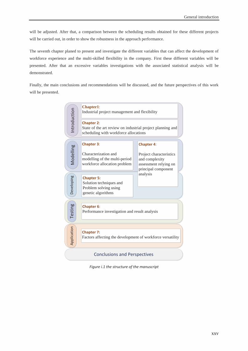
activities schedule, will be the main subject of this thesis. It is organised and constructed in seven chapters,

shown by the schematic figure (i.1) at the end of this section.

The first chapter presents a brief context of the industrial project management. The different hierarchical levels

of manufacturing planning will be discussed. The uncertainty in project planning and scheduling will be

presented. Then, the flexibility concept and its different dimensions will be considered. In the end, the human

factors in planning and scheduling will be briefly introduced.

The second chapter presents a review of literature related to the project planning and scheduling problem. The

different classical and non classical problems will be discussed. The many strategies that were developed to deal

with the uncertainty in scheduling will be discussed. In addition, the numerous considerations of the role of

human resource in this domain will be presented.

The third chapter aims to model the problem of staff allocation with the two degrees of flexibility: the working

time modulation, and multi-skills of operators. With induces a dynamic view of their skills and the need to

predict changes in individual performance as a result of successive assignments. The mathematical model of this

problem will be presented altogether with the analysis of its variables and constraints.

The fourth chapter seeks to define an instance of the current problem and measure its complexity. First the

project and the required resources will be divided into a set of dimensions. These dimensions contain the project

network, tasks durations, required workload, required skilled, the available resources. The different parameters

related to each dimension will be presented and quantified. For each dimension a sensitive quantifier will be

investigated and selected. After that, a principal component analysis and a cluster analysis will be performed to

define linearly the minimum quantifiers needed to measure the problem complexity.

The fifth chapter aims at presenting simultaneously two main parts. The first one is a brief discussion of

resolution techniques for optimisation problems. The second part is the detailed presentation of the proposed

approach that relays on genetic algorithms and the schedules serial generation scheme. Moreover, it presents the

proposed approach validation and the tuning of its parameters.

The sixth one presents a detailed investigation of the proposed approach through the examination of a vast

number of projects with different characteristics. First the respective weights associated to different objectives

General introduction

xxv

will be adjusted. After that, a comparison between the scheduling results obtained for these different projects

will be carried out, in order to show the robustness in the approach performance.

The seventh chapter planed to present and investigate the different variables that can affect the development of

workforce experience and the multi-skilled flexibility in the company. First these different variables will be

presented. After that an excessive variables investigations with the associated statistical analysis will be

demonstrated.

Finally, the main conclusions and recommendations will be discussed, and the future perspectives of this work

will be presented.

Chapter1:Industrial project management and flexibility

Chapter 2: State of the art review on industrial project planning andscheduling with workforce allocations

Chapter 3:

Characterization andmodelling of the multi-periodworkforce allocation problem

Chapter 4:

Project characteristicsand complexityassessment relying onprincipal componentanalysis

Chapter 5:Solution techniques andProblem solving usinggenetic algorithms

Chapter 6: Performance investigation and result analysis

Chapter 7: Factors affecting the development of workforce versatility

Intr

oduc

tion

Mod

ellin

gDe

velo

ping

Test

ing

Appl

icat

ion

Conclusions and Perspectives

Figure i.1 the structure of the manuscript

1 INDUSTRIAL PROJECT MANAGEMENT AND

FLEXIBILITY

This chapter presents a brief introduction to the management of industrial

projects, and aims to raise awareness about issues of responsiveness. First,

the different hierarchical levels of manufacturing planning will be

discussed. The sources of uncertainty in project planning and scheduling

will be presented; the flexibility concept and its different dimensions will

be pointed out. Furthermore, a brief discussion of human factors in

planning and scheduling will be introduced.

CH

APT

ER

1

Industrial project management and flexibility

2

A project can be defined as a set of coordinated activities with a clearly defined objective that can be achieved

through synergetic, coordinated efforts within a given time, and with a predetermined amount of human and

financial resources (Tonchia, 2008). The project can be intended to create products or services. Kumar and

Suresh (2007) distinguished between the manufacturing operations and services ones by some criteria: the

tangible or intangible nature of outputs (products in manufacturing), the nature of work, the customer contact (is

little in manufacturing), and the measurement of output. Managing a project is the “application of knowledge,

skills, tools, and techniques to project activities to achieve project requirements”, (Heagney, 2011). Lewis,

(2000) defined project management as the “facilitation of the planning, scheduling, and controlling of all

activities that must be done to meet project objectives”. Generally, project management deals with activities,

tools (work analysis, scheduling algorithms or software; risk analysis ...), people and systems under a set of

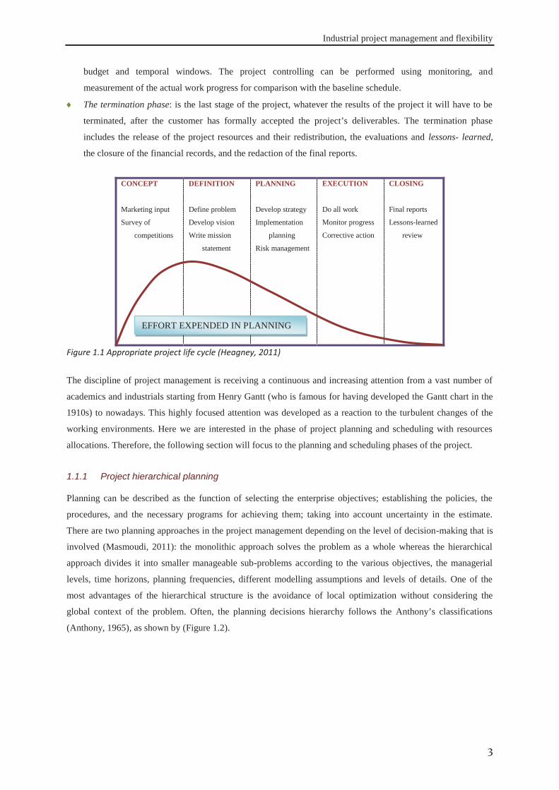
performance, budget and time constraints during the project phases. As shown by (Figure 1.1), project life

contains five phases: initiating or concept, definition, planning and scheduling, executing controlling and co-

ordinating, and closing. Demeulemeester and Herroelen, (2002) discussed each phase of the project as:

The concept phase: is the point at which the customer (funds provider) identifies the needs that must be met

for a product or service in order to solve a given problem. The needs identification can result in customer

request for a proposal from organisations (contractors). The contractors’ proposals usually contain the

description of the problem’s solution, with the associated costs and schedules. At this stage there is a rather

fuzzy definition of the solution, therefore feasibility studies should be conducted.

The definition phase: presents a clear approach of what is going to be developed as a proposal to solve the

problem. It contains three main parts: - Project objectives; it refers to the end state that the project

management is trying to achieve. - Project scope; it identifies the project outcomes, and what is the

expectation of the costumer by project completeness. - Project strategy; it describes clearly the organisation

approach to reach the project scope and optimising the project objectives. Additionally, the different

economic, environmental, technological, legal, geographic, or social factors that may affect the project

should be identified and investigated. At the end of this phase, we can answer the fundamental project

questions of: what we are going to do? How we are going to do it?

The planning and scheduling phase: contains a set of steps of identifying the project work content and

different activities, estimates the temporal and resources requirements considering uncertainty, itemizes the

required competences and skills, and specifies the dependencies relations between activities and the

scheduling constraints. In order to manage the project efficiently, it should be broken down to manageable

portions (Work-breakdown-structure: WBS). This WBS translates the results of the systems engineering

analysis and requirements into a structure of the products and services which comprise the entire work effort

(Wiley et al., 1998). The scheduling: represents the project base plan which specifies to each activity a start

and completion date, the amount and type of each resource. The development of a well-thought-out plan is

essential to a successful achievement of the project.

The executing and control phase: represents the implementation of the baseline plan; by performing the

required work and controlling the advancements in order to meet the project scope within the estimated

1.1 INDUSTRIAL PROJECT MANAGEMENT

Industrial project management and flexibility

3

budget and temporal windows. The project controlling can be performed using monitoring, and

measurement of the actual work progress for comparison with the baseline schedule.

The termination phase: is the last stage of the project, whatever the results of the project it will have to be

terminated, after the customer has formally accepted the project’s deliverables. The termination phase

includes the release of the project resources and their redistribution, the evaluations and lessons- learned,

the closure of the financial records, and the redaction of the final reports.

CONCEPT

Marketing input

Survey of

competitions

DEFINITION

Define problem

Develop vision

Write mission

statement

PLANNING

Develop strategy

Implementation

planning

Risk management

EXECUTION

Do all work

Monitor progress

Corrective action

CLOSING

Final reports

Lessons-learned

review

Figure 1.1 Appropriate project life cycle (Heagney, 2011)

The discipline of project management is receiving a continuous and increasing attention from a vast number of

academics and industrials starting from Henry Gantt (who is famous for having developed the Gantt chart in the

1910s) to nowadays. This highly focused attention was developed as a reaction to the turbulent changes of the

working environments. Here we are interested in the phase of project planning and scheduling with resources

allocations. Therefore, the following section will focus to the planning and scheduling phases of the project.

Planning can be described as the function of selecting the enterprise objectives; establishing the policies, the

procedures, and the necessary programs for achieving them; taking into account uncertainty in the estimate.

There are two planning approaches in the project management depending on the level of decision-making that is

involved (Masmoudi, 2011): the monolithic approach solves the problem as a whole whereas the hierarchical

approach divides it into smaller manageable sub-problems according to the various objectives, the managerial

levels, time horizons, planning frequencies, different modelling assumptions and levels of details. One of the

most advantages of the hierarchical structure is the avoidance of local optimization without considering the

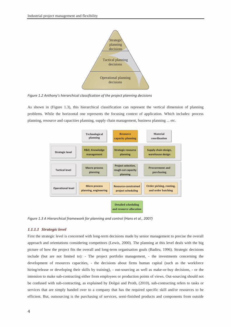
global context of the problem. Often, the planning decisions hierarchy follows the Anthony’s classifications

(Anthony, 1965), as shown by (Figure 1.2).

1.1.1 Project hierarchical planning

EFFORT EXPENDED IN PLANNING

Industrial project management and flexibility

4

Strategicplanningdecisions

Tactical planningdecisions

Operational planningdecisions

Figure 1.2 Anthony’s hierarchical classification of the project planning decisions

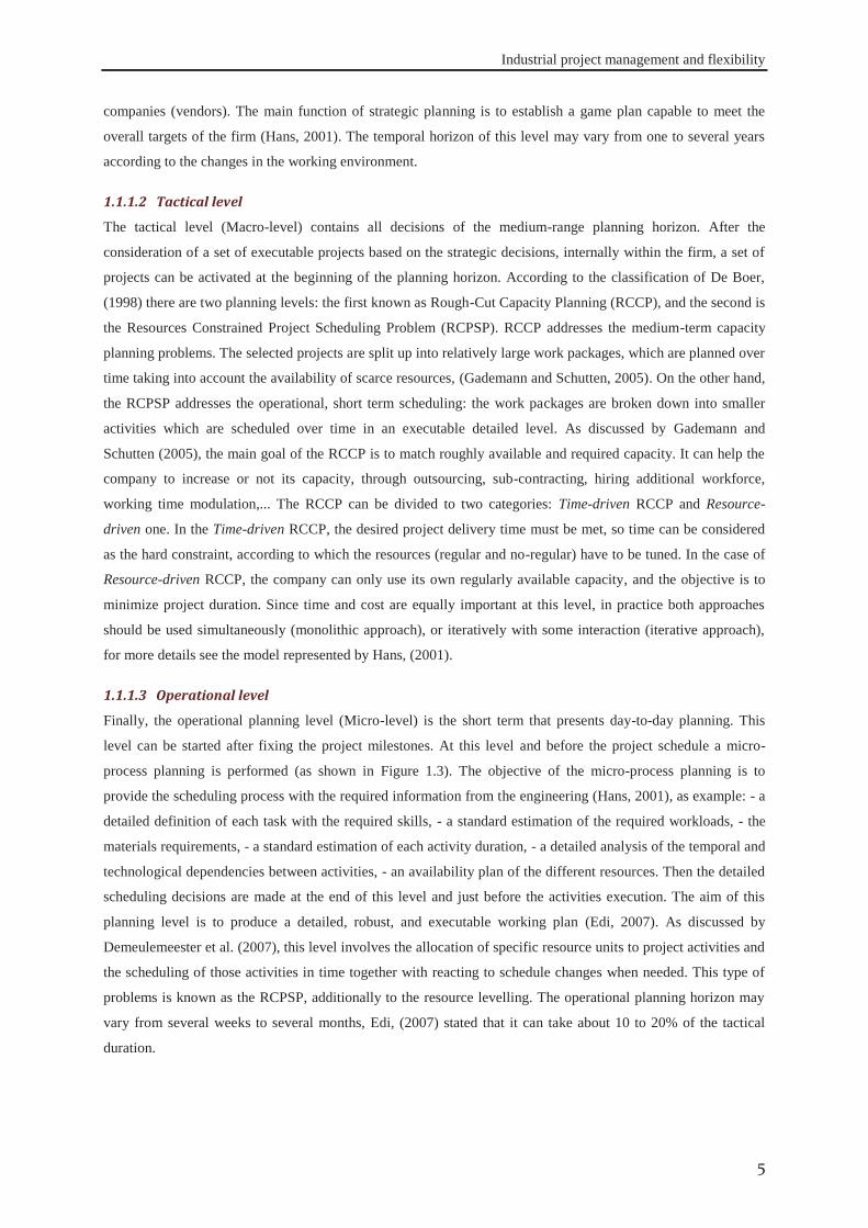
As shown in (Figure 1.3), this hierarchical classification can represent the vertical dimension of planning

problems. While the horizontal one represents the focusing context of application. Which includes: process

planning, resource and capacities planning, supply chain management, business planning ... etc.

R&D, Knowledge management

Strategic resource planning

Supply chain design, warehouse design

Macro process planning

Project selection, rough-cut capacity

planning

Procurement andpurchasing

Micro process planning, engineering

Resource-constrained project scheduling

Order picking, routing,and order batching

Detailed schedulingand resource allocation

Strategic level

Tactical level

Operational level

Technologicalplanning

Resourcecapacity planning

Materialcoordination

Figure 1.3 A Hierarchical framework for planning and control (Hans et al., 2007)

1.1.1.1 Strategic level

First the strategic level is concerned with long-term decisions made by senior management to precise the overall

approach and orientations considering competitors (Lewis, 2000). The planning at this level deals with the big

picture of how the project fits the overall and long-term organisation goals (Badiru, 1996). Strategic decisions

include (but are not limited to): - The project portfolio management, - the investments concerning the

development of resources capacities, - the decisions about firms human capital (such as the workforce

hiring/release or developing their skills by training), - out-sourcing as well as make-or-buy decisions, - or the

intension to make sub-contracting either from employees or production points of views. Out-sourcing should not

be confused with sub-contracting, as explained by Dolgui and Proth, (2010), sub-contracting refers to tasks or

services that are simply handed over to a company that has the required specific skill and/or resources to be

efficient. But, outsourcing is the purchasing of services, semi-finished products and components from outside

Industrial project management and flexibility

5

companies (vendors). The main function of strategic planning is to establish a game plan capable to meet the

overall targets of the firm (Hans, 2001). The temporal horizon of this level may vary from one to several years

according to the changes in the working environment.

1.1.1.2 Tactical level

The tactical level (Macro-level) contains all decisions of the medium-range planning horizon. After the

consideration of a set of executable projects based on the strategic decisions, internally within the firm, a set of

projects can be activated at the beginning of the planning horizon. According to the classification of De Boer,

(1998) there are two planning levels: the first known as Rough-Cut Capacity Planning (RCCP), and the second is

the Resources Constrained Project Scheduling Problem (RCPSP). RCCP addresses the medium-term capacity

planning problems. The selected projects are split up into relatively large work packages, which are planned over

time taking into account the availability of scarce resources, (Gademann and Schutten, 2005). On the other hand,

the RCPSP addresses the operational, short term scheduling: the work packages are broken down into smaller

activities which are scheduled over time in an executable detailed level. As discussed by Gademann and

Schutten (2005), the main goal of the RCCP is to match roughly available and required capacity. It can help the

company to increase or not its capacity, through outsourcing, sub-contracting, hiring additional workforce,

working time modulation,... The RCCP can be divided to two categories: Time-driven RCCP and Resource-

driven one. In the Time-driven RCCP, the desired project delivery time must be met, so time can be considered

as the hard constraint, according to which the resources (regular and no-regular) have to be tuned. In the case of

Resource-driven RCCP, the company can only use its own regularly available capacity, and the objective is to

minimize project duration. Since time and cost are equally important at this level, in practice both approaches

should be used simultaneously (monolithic approach), or iteratively with some interaction (iterative approach),

for more details see the model represented by Hans, (2001).

1.1.1.3 Operational level

Finally, the operational planning level (Micro-level) is the short term that presents day-to-day planning. This

level can be started after fixing the project milestones. At this level and before the project schedule a micro-

process planning is performed (as shown in Figure 1.3). The objective of the micro-process planning is to

provide the scheduling process with the required information from the engineering (Hans, 2001), as example: - a

detailed definition of each task with the required skills, - a standard estimation of the required workloads, - the

materials requirements, - a standard estimation of each activity duration, - a detailed analysis of the temporal and

technological dependencies between activities, - an availability plan of the different resources. Then the detailed

scheduling decisions are made at the end of this level and just before the activities execution. The aim of this

planning level is to produce a detailed, robust, and executable working plan (Edi, 2007). As discussed by

Demeulemeester et al. (2007), this level involves the allocation of specific resource units to project activities and

the scheduling of those activities in time together with reacting to schedule changes when needed. This type of

problems is known as the RCPSP, additionally to the resource levelling. The operational planning horizon may

vary from several weeks to several months, Edi, (2007) stated that it can take about 10 to 20% of the tactical

duration.

Industrial project management and flexibility

6

1.1.1.4 Interaction between planning levels

The three hierarchical planning levels cannot be isolated from each others, and information is promulgated from

the higher levels to the lower one(s). Feedback is essential from lower to higher levels, in order to enhance the

process, and appreciate the return of experience. Hans et al. (2007) discussed the interaction (changing

information) between the three levels of the hierarchical planning with respect to two variables: the variability

and the dependency. For project organisations with high dependency, the “matrix-organisation structure” is

generally adopted. On the other hand, low dependency cases can be represented by the dedicated or pure “project

organisations”. Hans et al. (2007) proposed another interaction way: since the resources are dedicated to the

project, they proposed to allocate them during the tactical level; therefore, the information transferred to the

operational level contains due dates, milestones, capacity levels, and resources allocation decisions. This type of

organisation is preferable for complex projects, (Hobday, 2000). Generally, the tactical and operational levels are

very interdependent levels (Kovács et al., 2005).

The scheduling was defined by Leung and Anderson (2004) as “the allocation of scarce resources to activities

with the objective of optimising one or more of the performance measures”. Resources and activities can be

taken in many forms, or specification, e.g. resources can be workers and/or machines in manufacturing plants,

utilities, runway at airport, I/O devices in computer system, etc. Activities can be any action which monopolizes

or consumes resources during a specified period of time. In manufacturing context, the schedules often describe

the sequencing and assignment of products (activities) to machines (resources) (Hans, 2001), or workforce to

specified jobs, during specified temporal milestones. This is known also as resources loading. The temporal

milestones of the schedule contain: the release date, the processing time, the due/completion date of each

activity, moreover to the program deadline. This operational plan is known as “Baseline schedule” also called a

predictive schedule or pre-schedule. As discussed by Herroelen and Leus (2005), the baseline schedules serve as

a basis for communication and coordination with external entities in the company’s inbound and outbound

supply chain. The scheduling problem is often NP-hard complex, (Neumann and Zhan, 1995; Shue and Zamani,

1999; and Brucker and Knust, 2011 P.34).

Resource levelling refers to the process of reducing the period-to-period fluctuations (load smoothing) in

resource’s loading. The resource levelling was discussed by Badiru (1996) in the way of resource profiling

during the project horizon, i.e. developing a graphical representation to convey information about the resource

availability, utilization, responsibilities loading and assignment. The variations of the graph can be used to

conclude information about depletion rate of the project budget. Also, the resources idleness and critical resource

diagrams are effective tools used to manage a program of activities. This graphical representation may be done

for all types of resources involved in the project. The advantages of stable loading plans include the

improvement of workers’ learning opportunity at work–station. The pattern of resource usage versus time might

be more important than the peak demand of the schedule, (Demeulemeester and Herroelen, 2002). In such cases,

the RCPSP can be shifted to a resource levelling problem, where the objective is to complete the activities

program before its deadline with a resource loading profile that would be as even as possible over the entire

project horizon – for more details, see e.g. Younis and Saad (1996); or Leu et al. (2000).

1.1.2 Project scheduling with resource loading and levelling

Industrial project management and flexibility

7

The project risks management is mainly relying on the analysis of uncertainties in the different dimensions of a

project, and putting the suitable strategy(ies) to control the estimated outcomes, if any. As explained by Ward

and Chapman (2003), managing the project uncertainty is managing the project risk. Regarding the sources of

uncertainty, Atkinson et al. (2006) argue that uncertainly can be produced in a given project relying on three

attributes: uncertainty in estimates, uncertainty associated with project stakeholders, and uncertainty associated

with different phases in project life cycle. According to Herroelen and Leus (2004), the uncertainty is also

associated with the size of the project parameters (such as time, cost, and quality) and the process (what is to be

done, how, when, by whom and at what cost). The main reasons for uncertainties in estimates are: - the lack of

specification of what is exactly required, lack of the required knowledge, - complexity associated to inter-

dependencies between activities. –Insufficient analysis of the different activities, - possible occurrence of

particular events or conditions which might affect the activity, or even the estimator’s bias, (Ward and Chapman,

2003; Atkinson et al., 2006). The uncertainty associated with the project stakeholders often concerns large

projects, where the project deliverance can be shared by some parties. In such situations, uncertainty can be

produced from: the objectives and motivations of each party, the alignment of the parties’ objectives and that of

the owner, the abilities and availabilities of each party, or the fundamental relationships between the various

project parties involved. This type of uncertainty reduces as the parties are embedded in the same organisation.

In such situations, the dependency of project on internal coordination is more important than that on the external

one. Concerning the uncertainty associated with different phases in project life cycle, we propose the work of

Atkinson et al. (2006) for more details.

Organizations face significant uncertainty from continuous and dynamic changes: -Customers are demanding a

greater variety of high quality, low cost goods and services. –The difficult competition between companies

requires rapid responses to the customers’ desires, with low costs and best quality. Organizations continuously

develop new methods and perspectives to meet these needs in a timely and cost effectiveness fashion. Thus

creating flexible organizations is one response to dealing with such challenges (Koste and Malhotra, 1999; Zaeh

and Mueller, 2007). And organizations need to be internally and/or externally flexible to face uncertainties, (Hitt

et al., 1998). The use of flexibility to accommodate uncertainty of the environment has received a significant

recognition. As example, Groote (1994) defined the flexibility as “a hedge against the diversity of the

environment”, while flexibility is considered as a property of technologies and diversity is a property of

environments. The more flexible technology is the one which benefits from the diversity of environments with

more desirable changes in its performance than its others competitors under the same conditions. The word

“diversity” was used to represent the variability, variety, or complexity of the customers’ requirements types and

quantities. The word “technology” was used too as a general representation of the firm aspects. Others as Beach

et al. (2000) argue strongly that each specific type of uncertainty requires a given form of flexibility to

accommodate its effects (reactive response), and each type of uncertainty in its turn requires a different and a

particular type of flexibility to accommodate it (proactive response). But Treville et al. (2007) suggested that the

1.2 UNCERTAINTIES IN PROJECT MANAGEMENT

1.3 FLEXIBILITY VERSUS UNCERTAINTY

Industrial project management and flexibility

8

firm flexibility can be evaluated by the manner in which the firm reacts to environmental uncertainty by

responding efficiently, responding in reactive and ad hoc way. Or limiting the uncertainty instead of responding

may depend on the firm’s scanning level of environmental changes and whatever this environment is analyzable

or not. And the active firm is that one which views its environment as an analyzable one and established its own

strategic flexibility. But the passive firms that view their environment as un-analyzable, are more likely firms to

respond in ad hoc way. The firms must work to reduce environmental uncertainty by becoming

proactive/offensive rather than reactive/defensive ones.

For several decades the concept of flexibility received a lot of attention from researches, in many fields like

design, manufacturing systems, management, planning and scheduling, information technology, etc, but still

there isn’t any exact definition for its general concept and its measurements (Bordoloi et al., 1999). And there is

only a diversity of its concepts that depend only on some specified subject. Why does the general concept of

flexibility seem so difficult to be introduced? The answer to this question has been introduced in many works. A

lot of authors link the difficulties of the general concept of flexibility to its multidimensional aspects and

varieties of contexts in which flexibility has been employed, or to the variety of entities where it has been

applied (Sethi and Sethi, 1990; Mitchell, 1995; Shewchuk and Moodie, 1998; Koornhof, 2001; Démery-Lebrun,

2005). According to Golden and Powell (2000), the flexibility definitions ‘‘are often coloured by particular

managerial situations or problems’. The most frequent definitions of flexibility always relate to other terms such

as adaptability, rapidity, responsiveness, resilience, efficiency, and sometimes to complexity and reliability

(Bordoloi et al., 1999), and other terms like ability or capacity to react, to respond, to adjust, or to cope with the

environmental changes. We represent here some definitions of flexibility:

Adaptability: flexibility was defined as the ability of the manufacturing system to adapt to the customers demand

for each production horizon. Recently Zaeh and Mueller (2007) defined it as “the company’s ability to adapt its

manufacturing capacity to changes in customer demand with little or no effort”. Sethi and Sethi (1990) also

defined the flexibility of a system as its adaptability to a wide range of possible environments that it may

encounter: a flexible system must be capable of changing in order to deal with a changing environment. Golden

and Powell (2000) supported the definition that the flexibility is ‘‘the capacity to adapt’’, and they explained

why they used the word “capacity” rather than the word “capability”: they mentioned that the capacity is ‘‘the

power of containing, receiving, experiencing or producing’’, and it represents well the multidimensional aspects

of flexibility, whereas the capability is ‘‘the power to do something’’. With a similar approach, Valverde et al.

(2000) argued that organizations need to have the ability to adapt to fluctuations in demand and to changes in

their environment in order to be successful or even in order to survive.

Rapidity and responsiveness: many authors defined the flexibility in terms of rapidity and responsiveness in

dealing with the environmental conditions. Sanchez (1995) defined the firm flexibility as “a firm’s abilities to

respond to various demands from dynamic competitive environments”. In the field of human resources

management, Wright and Snell (1998) defined it as “a firm’s ability to quickly reconfigure resources and

activities in response to environmental demands”. But Mitchell (1995) describes the flexibility relying on two

sides: the first side is the change: “the flexibility itself involves the characteristic of rapid and significant

1.3.1 Flexibility theoretical concept

Industrial project management and flexibility

9

change”, and the other side of flexibility is the reaction: “the characteristic of being unable – or intellectually

unwilling – to change in any degree or with any speed”. Youndt et al. (1996) also defined flexibility in general

terms as it refers to firm’s agility, adaptability, and responsiveness. More precisely Koornhof (2001) defined it

as: ‘‘flexibility is the ability and capacity to reposition resources and functions of the organization in a manner

consistent with the evolving strategy of management as they respond, proactively or reactively, to change in the

environment’’. He argues strongly within this definition that flexibility is both an organisational and individual

variable, and it contains the operation, financial, strategic, marketing, manufacturing and behavioural flexibility

aspects. And it recognises the dynamic relationship that can exist between the organisation and its environment.

Resilience: it refers to the ability of organizations to recover from the environmental disturbance by returning to

its previous state or gain some fitness in its performance. The ability of an organization to re-compete and share

the market landscape after meeting an environmental disturbance is an example of organization’s resilience

flexibility. For more details, we propose the work of Hu et al. (2008) and De Haan et al. (2011).

Within companies there are many dimensions and levels of flexibility that must be defined and classified; such

as: internal, external, quantitative, qualitative, static, dynamic, offensive, and defensive. And each type contains

subcategories of flexibility elements. With all these types and multi-forms, the company’s overall flexibility is

the mixture results of these forms’ with given levels and tolerances for each form (Démery-Lebrun, 2005). Thus,

it is helpful to classify the firm’s flexibility levels and sub-dimensions. Authors such as (Golden and Powell,

2000; Koste and Malhotra, 1999; Shewchuk and Moodie, 1998) have tried to distinguish between these sub-

dimensions, and they have introduced four flexibility dimensions: intension, focus, range, and temporal. The

intension represents the strategy of firms to accommodate to working changes, whether, the organisation is being

proactive or reactive (offensive or defensive, active or passive). In the proactive policy, the organizations attempt

to control the environment changes by accommodating unknown uncertainty in the way that they can gain

competitive advantage. But in the reactive policy the organizations treated the changes after they have occurred.

The “focus” dimension symbolizes that the flexibility is gained internally within the organisation, or by

managing external relationships with trading partners. The “range” represents the number and varieties of the

alternatives. Associated to these alternatives with the range dimension, one can find the uniformity and the

mobility. Uniformity represents the similarity of performance outcomes within the range which can include

quality, costs, time, etc. Where, mobility represents the easiness or penalties associated to switching between

alternatives.

Finally, the temporal dimension classifies flexibility based on time scale to: long, medium or short terms that can

be represented as the three subcategories of strategic, tactical, and operational flexibilities. The strategic

flexibility represents the actions that presently taken out by companies with a future expected returns, such as

investments in machines, labour training or education (Golden and Powell, 2000). The tactical flexibility can be

represented as the action flexibility, where the outside intervention is required before the system response to the

change, (Shewchuk and Moodie, 1998). The operational level of flexibility concerns the short term flexibility,

the ability to replan in alternative ways, due to events that suddenly happened, (Golden and Powell, 2000;

Treville et al., 2007). This level can be formed from numerous manufacturing components; Koste and Malhotra

1.3.2 Flexibility dimensions in manufacturing

Industrial project management and flexibility

10

(1999) distinguish between several types of operational flexibility in manufacturing systems and they give a brief

description and definition of each type:

- Labour flexibility: ‘‘the number and heterogeneity (variety) of tasks/operations a worker can execute without

incurring high transition penalties or large changes in performance outcomes’’. - Product flexibility: includes

new product flexibility and product modification flexibility. New product flexibility: the range of new products

which are introduced into production. Where the Product modification flexibility: it addresses the ability of

making modification on the current product according to the customer requests without incurring high transition

penalties. - Operation flexibility: the number of products which have alternate sequencing plans. -Machine

flexibility: is the range of operations a machine can execute. -Volume flexibility: represents the ability of the

enterprise to respond quickly and efficiently to the turbulent demand. -Mix flexibility: represents the number of

products that the enterprise produces and also the varieties between products models. -Material handling

flexibility: the number of existing paths between processing centres and the heterogeneity of material which can

be transported along those paths. -Routing flexibility: represents the ability to use alternate processing work-

centres to execute operations, its significant impact can be appreciated in case of machine breakdowns or

overlaps. And - Expansion flexibility: is the range of expansions which can be accommodated without producing

high transition penalties or large changes in performance.

Human resources can be considered as one of the most flexible resources in the manufacturing processes in their

nature. They have the ability to migrate from work stations to others, when/where needed. As classified by

Goudswaard and De Nanteuil (2000) shown in (Table 1.1), workforce flexibility can be achieved relying on two

main sources: the external and internal sources of flexibility. External flexibility refers to the adjustment of the

workers number from the external market for a short term contracts, to balance between the required workforce

and that actually available. This can be achieved by employing workers on temporary work or fixed-term

contracts or through relaxed hiring and firing regulations. Solutions of this kind seem to provide the companies

with a raped and costless strategic flexibility when facing the problem of turbulent changes in customer

demands. But, the resulting high staff turnover has a serious effect on the development of core competences,

health and safety, recruitment costs and time. According to Hitt et al. (1998), this strategy produces a static

flexibility rather than a dynamic one, reduces the development or the evolution of the core competences, and in

addition the firm loose workers’ loyalty, motivation: most of the time, they are less productive compared to the

permanent workers.

The internal flexibility relies on two sub-dimensions: the multi-skills flexibility and the temporal one. Multi-

skills flexibility is the ability of employees to transfer to and carry out different activities and tasks required by

firms changing workload, production methods and/or technology. This kind of flexibility requires heavy training

programs to provide the firm with a multi-skilled workforce that would be ready to face and respond rapidly to

environment changes (Valverde et al., 2000). This kind of flexibility is known as “functional flexibility” and

represents the qualitative side of workforce flexibility. It can have a significant impact on the firms’ capacity,

quality and performance. With functional flexibility, workers are able to work with a high performance level for

their own competences, and they have an acceptable efficiency or performance for other competences from the

1.3.3 Human resources flexibility

Industrial project management and flexibility

11

quality and cost points of views. On the other side, functional flexibility requires training as a long term

investment, and development policies planed by the organizations to develop their core competences and gain an

important flexibility lever.

The quantitative part of the workforce flexibility can be developed relying on the working time specifications.

This kind of flexibility is known as “temporal flexibility”, as shown by (Table 1.1), and relies mainly on the

distribution of employees’ working hours over the week: that can be defined by answering two questions: when

does the worker go to work? (At morning, afternoon, evening, or at night), and how many are his daily working

hours? The different answers to these two questions shape the temporal flexibility. Here we are interested to the

new working time modulation with annualized working hours (see section 3.2.1).

Table 1.1 Different forms of flexibility (Goudswaard and De Nanteuil, 2000) Forms of flexibility Quantitative flexibility Qualitative flexibility External flexibility Employment status:

- Permanent contracts - Fixed-term contracts - Temporary agency contracts - Seasonal work - Work on demand/call Numerical flexibility and/or contract flexibility

Production system: - Subcontracting - Outsourcing - Self employed Productive and/or geographical flexibility

Internal flexibility Working time: - Reduction of working hours - Overtime/part-time work - Night and shift work - Weekend work - Compressed working week - Varying working hours - Irregular/unpredictable working

time Temporal flexibility

Work organisation: - Job enrichment/job rotation - Teamwork/autonomous work - Multitasking, multi-skilling - Project groups - Responsibility of workers over:

planning, budget, innovation, technology

Functional flexibility

The human resource is one of the most crucial sectors in an organisation. The individuals might be responsible

for the majority of activities sequencing and resource allocation decisions from the initial demand until the

delivery to the customer. An individual might be responsible for setting up machines, initiating parameters of

scheduler algorithms, coding machines, or creating the activity manually using the required equipments.

According to McKay and Wiers (2006), human resources can be characterised by a set of dimensions such as

flexibility, adaptability, learning, communications, negotiation, and intuition in case of missing information. As

previously discussed, the flexibility and adaptability represent the capability of human individuals to desirably

react against a specified change for a specified period of time under a set of goals and constraints (stated, not-

stated, or incomplete). Humans are also capable to learn and store knowledge, and retrieve the suitable amount

from it for a specified situation. This process of learning-storage-retrieval of knowledge is known as the memory

dynamics either on the macro or micro levels of knowledge acquisition, (Wickelgren, 1981). The storage phase

induces two phenomena: the consolidation and forgetting. Assuming that memory can be constructed in traces,

strengthening these traces represents the consolidation; and weaken them represents forgetting. The strength of

these memory traces can be increased by work repetitions: it is well known that “practice makes perfection”.

1.4 HUMAN FACTOR IN PLANNING AND SCHEDULING

Industrial project management and flexibility

12

Therefore, one of the important factors that can be found in the product pricing is the learning curve effect. Thus,

the production cost per item of a given product reduces as the number of items grows, this reduction in

production cost resulting from the labour knowledge accumulation, or experience development. Moreover,

humans are able to communicate and transfer knowledge and negotiate with the different parties of the project.,

Human resource also have intuition, i.e. the ability of humans to fill-in the blanks of missing information

required to perform a specified job, which requires a great amount of ‘tacit knowledge’ (McKay and Wiers,

2006). All of these aspects enable human resources to deal with the uncertainties of the working environment.

On the other side, there are differences between individuals with respect to all human aspects, behaviour,

learning rate, forgetting rate, ability to communicate, to negotiates, fatigue, stress...etc. For example, individuals

exhibiting different behaviours towards a given situation, this behaviour can be represented in terms of

individual motivations, adaptability, as opposed to the routine behaviour. Beltrán-Martín et al. (2008)

distinguished between the rigid behaviour and the flexible one; when a worker who applied a certain script in

repetitive work situations selects the same script for the novel situation, his behaviour is considered as rigid. But

when they look for new procedures or actions to deal with new works, their behaviour can be considered as

flexible. These human factors can affect the project schedule outcomes; therefore, we argue that it is important to

consider them in humans-to-tasks allocation problems.

In this chapter an overall introduction of project management and flexibility were discussed. First, the different

phases of a project life cycle were introduced. After that the different hierarchical levels of project planning are

presented: the strategic, the tactical and the operational levels. The uncertainty in the context of project

management had been discussed. And due to the important of using flexibility as a hedge against uncertainty, the

theoretical concept of flexibility has been discussed in terms of adaptability, ability to respond, and resilience.

Afterwards, the different dimensions of flexibility in manufacturing context have been presented. The different

types of human flexibilities had been highlighted, more over to the human factors that can be considered in the

current context, such as the learning and forgetting.

As discussed in this chapter, developing flexibility is an important aspect to help firms to remain competitive in

the new turbulent working environment. As it was discussed, the human resource is the main sector offering

such important characteristic. Therefore, we are motivated to model the project planning and scheduling

problem, with integrating both aspects of the workforce flexibility.

1.5 CONCLUSION

2 STATE OF THE ART REVIEW ON INDUSTRIAL

PROJECT PLANNING AND SCHEDULING WITH

WORKFORCE ALLOCATION

This chapter aims to review the literature related to the project planning

and scheduling problem. The different classical and non classical

problems will be discussed. One can find various strategies that were

developed as a response to the uncertainty at work, such as the reactive,

proactive-reactive, robustness, and flexible schedules. Moreover, the

different considerations of human resource in planning and scheduling

will be also discussed.

CH

APT

ER

2

State of the art review on industrial project planning and scheduling with workforce allocation

14

As discussed earlier in chapter 1, the hierarchical classification of project management is based on three levels:

strategic, tactical and operational levels. In this section we review the recent works that are oriented towards the

tactical and operational levels of planning and scheduling. We present in some details some tools used in project

planning and scheduling, starting from the rough cut capacity planning, resource scheduling, handling

uncertainty and generating a robust schedule.

The RCCP is a process of balancing the required aggregated work to the available regular and/or irregular

capacity. More precisely it can be described as stated by Daniel et al. (1997), relying on the “APICS Dictionary”

(Dougherty and Wallace, 1992): “The process of converting the production plan and/or the master production

schedule (MPS) into capacity needs for key resources: work force, machinery, warehouse space, suppliers’

capabilities, and in some cases, money. Bills of resources are often used to accomplish this. Comparison of

capacity required of items in the MPS to available capacity is usually done for each key resource. RCCP assists

the master scheduler in establishing a feasible MPS”. Knowing that, the MPS is what a company uses to

determine how many products/work-content will be processed for (a) given period(s) of time. Hans (2001)

identified three goals of the RCCP problem:

Determine the capacity utilization of new and accepted orders,

Perform a due date analysis on new or accepted orders, and/or to quote realistic due dates,

Minimize the usage of non-regular capacity (overtime and/or outsourcing).

To satisfy the first aim of pre-specified the capacity; Daniel et al. (1997) proposed a model to calculate the

capacity planning in remanufacturing environment based on the RCCP. After that a comparison between the

available capacity and the requirement can be done for each work centre or for a specified resource. They

computed a rough capacity from the temporal availability factor, the productivity rate of the work centre, and the

rate of utilisation to the work centre. Zhang et al. (2001) presented a macro-level scheduling problem in

manufacturing cells. The product’s processing at each cell is treated as an aggregated operation. They adopted

the elasticity nature of the operation’s processing time at each cell according to the allocated resources. Hans

(2001) formulated a RCCP problem for a job shop as a mixed integer linear programming, in which every

aggregated order contains a set of specified jobs, with specified precedence constraints, to be loaded on a set of

resources. Two types of resource capacities are considered: machine group fixed capacity (independent

machines: they don’t share tools) and operators’ capacity. He adopted the assumption that operators are fully

cross-trained and can thus operate any machine in any machine group. For operators, they distinguished between

regular and non-regular capacities (i.e., working overtime and hiring staff). Kis (2005) studied a similar model to

that of Hans (2001), in which the resource consumption of each activity may vary over time proportionally to its

varying intensity. In other words, the activity performance-speed or intensity is determined by a continuous, non-

decreasing function of the amount of resource allocated to it at any moment. The novelty of the proposed mixed

integer linear programming “MILP” lays in the modelling of the precedence constraints, in function of binary

variables that represent the activity allocation to the temporal buckets, and the overlap conditions for two

2.1 PROJECT PLANNING AND SCHEDULING

2.1.1 Rough Cut Capacity Planning “RCCP” problem

State of the art review on industrial project planning and scheduling with workforce allocation

15

activities. The regular and un-regular capacities restrictions were adopted too. The objective is to minimize the

weighted sum of external capacity requirement, where the weights represent the activities completion dates.

Gademann and Schutten (2005) studied the problem of RCCP within a capacity-driven multi-project

organisation. The problem contains a set of jobs to be planned on resources that were aggregated from different

projects. The aim is to allocate these jobs on a temporal horizon divided in to buckets (weeks in this case) while

complying with the resources availability. The main variables denote the fractions of job that are performed by

given resources during a specified week. These fractions can differ from week to week, respecting a maximum

value. For each job there is a specified temporal interval that should contain the job release and due dates with

respecting the precedence constraints, if any. The objective is to reduce the total cost of using non-regular

resources. Recently, Bassan, (2010), and Masmoudi and Haït (2012) proposed fuzzy approach to deal with the

uncertainty associated to the RCCP. Bassan (2010) proposed a rough-cut capacity requirements planning under

fuzzy environment that includes fuzzy setup times per lot, fuzzy run time per part, and fuzzy lot of each part.

Masmoudi and Haït (2012) modelled the problem of helicopter maintenance planning, the model integrates

uncertainties into tactical and operational multi-project planning.

The scheduling problem is the object of great consideration from researchers and industrials, starting from Henry

Laurence Gantt (1861-1919) who developed his famous chart during the World War I, in order to evaluate the

production schedules. The huge varieties of problems encouraged stakeholders to invent a set of classification

schemes. A first classification scheme was presented by Graham et al. (1979), related to production machine

schedule, that holds three fields: Alpha Beta Gamma. The first field Alpha represents the machine of single

kind, or various types of parallel machines, flow shops, general shops, open shops, multi-processor task system.

The second field Beta is reserved for the activities and resources characteristics, such as possibility of task pre-

emption, precedence constraints, due dates, task processing times, batching, or additional resources. The third

term Gamma represents the performance measure or objective function as example, project makespan, minimise

the lateness/tardiness, unit penalty. Relying on the three fields’ classification, Herroelen et al. (1997) presented a

classification scheme of the operational project schedule problem. The resources field contains a set of Alpha{1,

2, 3} representing respectively the number of resources, the specific resource type, and the resource availability.

The second field Beta specifies the activity characteristics of a project scheduling problem, where Beta {1, 2, 3, 4,

5, 6, 7, 8} are, respectively, {possibility of activity pre-emption, precedence constraints, activities ready times,

activities duration characteristics, project or/activities deadlines, activities-resource requirements, activities

execution modes, activities financial implications}. The third filed “Gamma” is the optimised performance that

can contain {project makespan, the average flow time over all subprojects or activities, project due date

performance, resources levelling, financial performance, stochastic cases, multiple objectives, multi-criteria

optimisation} – the list is not exhaustive. For more details about this classification see, e.g. Herroelen et al.

(1997); Brucker et al. (1999); Demeulemeester and Herroelen (2002); or Kocsis (2011).

The resources-constrained project scheduling problem “RCPSP” is a very general operational level of activities

scheduling problem which may be used to handle a varieties of different applications in practice. For example,

manufacturing processes (Dorn et al., 1995; Artigues et al., 2008), maintenance (Yang et al., 2003; Masmoudi,

2.1.2 Resource Constraint Project Scheduling Problem

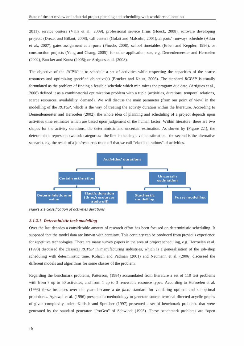
State of the art review on industrial project planning and scheduling with workforce allocation

16

2011), service centers (Valls et al., 2009), professional service firms (Hoeck, 2008), software developing

projects (Drezet and Billaut, 2008), call centers (Gulati and Malcolm, 2001), airports’ runways schedule (Atkin

et al., 2007), gates assignment at airports (Pinedo, 2008), school timetables (Erben and Keppler, 1996), or

construction projects (Yang and Chang, 2005), for other application, see, e.g. Demeulemeester and Herroelen

(2002), Brucker and Knust (2006); or Artigues et al. (2008).

The objective of the RCPSP is to schedule a set of activities while respecting the capacities of the scarce

resources and optimizing specified objective(s) (Brucker and Knust, 2006). The standard RCPSP is usually

formulated as the problem of finding a feasible schedule which minimizes the program due date. (Artigues et al.,

2008) defined it as a combinatorial optimization problem with a tuple (activities, durations, temporal relations,

scarce resources, availability, demand). We will discuss the main parameter (from our point of view) in the

modelling of the RCPSP, which is the way of treating the activity duration within the literature. According to

Demeulemeester and Herroelen (2002), the whole idea of planning and scheduling of a project depends upon

activities time estimates which are based upon judgement of the human factor. Within literature, there are two

shapes for the activity durations: the deterministic and uncertain estimation. As shown by (Figure 2.1), the

deterministic represents two sub categories: -the first is the single value estimation, -the second is the alternative

scenario, e.g. the result of a job/resources trade off that we call “elastic durations” of activities.

Figure 2.1 classification of activities durations

2.1.2.1 Deterministic task modelling

Over the last decades a considerable amount of research effort has been focused on deterministic scheduling. It

supposed that the model data are known with certainty. This certainty can be produced from previous experience

for repetitive technologies. There are many survey papers in the area of project scheduling, e.g. Herroelen et al.

(1998) discussed the classical RCPSP in manufacturing industries, which is a generalisation of the job-shop

scheduling with deterministic time. Kolisch and Padman (2001) and Neumann et al. (2006) discussed the

different models and algorithms for some classes of the problem.

Regarding the benchmark problems, Patterson, (1984) accumulated from literature a set of 110 test problems

with from 7 up to 50 activities, and from 1 up to 3 renewable resource types. According to Herroelen et al.

(1998) these instances over the years became a de facto standard for validating optimal and suboptimal

procedures. Agrawal et al. (1996) presented a methodology to generate source-terminal directed acyclic graphs

of given complexity index. Kolisch and Sprecher (1997) presented a set of benchmark problems that were

generated by the standard generator “ProGen” of Schwindt (1995). These benchmark problems are “open

State of the art review on industrial project planning and scheduling with workforce allocation

17

access” and available at (PSPLib, 1996). Demeulemeester et al. (2003) developed a project generator for the

activities-on- nodes networks. More recently, Browning and Yassine (2009) developed instance generator for the

multi-projects scheduling with resource constrained, where project interdependencies might exist beyond

common resources.

Regarding the mathematical modelling, Demassey (2008) presented the different mathematical formulations of

the RCPSP based on two main classes of decision variables: sequence-based formulation, and time-indexed

formulation. In the sequence-based formulation, the scheduling is performed in two steps: first, determination of

the sequence of activities that satisfies the precedence constraints, and then fixing the processing times of the

activities according to the resources constraints. The sequence-based formulation contains the minimum

forbidden sets and the resources flow concept (Artigues et al., 2003). The time-based formulation relies on a

time discretization describing the resources consumption and activities durations over time. This type contains

the resource-conflict modelling and the feasible configurations of Mingozzi et al. (1998). Xu et al. (2008)

formulate the traditional deterministic RCPSP as a sequential decision problem and solved it using combination

of rollout algorithm with priority rule heuristics and justification. Carlier et al. (2009) adopted the double

constrained problem with both renewable and non-renewable resources.

2.1.2.2 Elastic task modelling

This consideration of activity’s duration is always related to the resources characteristics, either quantitative (e.g.

number of workers) or qualitative (e.g. the workers’ productivity rates). We called it elastic, as a simulation to

the metal spring elasticity: the spring length is inversely related to the applied force. By the same principle the

activity duration is inversely related to the allocated resources capacity. Within literature one can find some

similar consideration; (Talbot, 1982; Sprecher et al., 1997; Vidal et al., 1999; De Reyck and Herroelen, 1999).

Demeulemeester et al. (2000) proposed a discrete model of the activity duration known as “Discrete Time-

Resource Trade-off”, in order to obtain more realistic model. Where, the duration of an activity is assumed to be

a discrete, non-increasing function of the amount of a single renewable resource allocated to it. The proposed

problem is strongly NP-Hard. The problem is known also as multi-mode RCPSP, (Mori and Tseng, 1997; Lova

et al., 2006). Zhang et al. (2006) adopted the problem of multi-mode consideration with renewable and non-

renewable resources and solved it using particle swarm optimization. Zhang et al. (2001) considered the time-

resources trade-off in the aggregated level of the macro-activity planning, in which the processing time required

to complete a given operation depends on the allocated resources. But in order to simplify the problem, they

considered only discrete values of the operations processing time. Daniels and Mazzola (1994) and Daniels et al.

(2004) proposed the elastic processing time of jobs as non-increasing function on the number of allocated

workers.

For the non-renewable resources, the problem is known as time-cost trade-off problem, where it is assumed that

the direct activity cost is a linear non-increasing function. As explained by Vanhoucke (2005) the objective was

to determine the activity durations and to schedule the activities in order to minimize the sum of the direct costs

of activities and the time-dependent indirect project costs, within a specified project deadline. The activity

crushing is the reduction of its duration resulting from the allocation of additional resources. Knowing that, the

State of the art review on industrial project planning and scheduling with workforce allocation

18

activity costs are a function of the activity durations, which are bounded within the interval of: the minimum

duration that represents the most crushed one, and the maximum corresponding to the normal duration.

Tareghian and Taheri (2006) took into consideration the quality along with the time and cost tradeoffs. They

argued that the project crushing affects the quality of the jobs performed, as well as it inflates the required costs.

Discrete elastic processing time is adopted by Turkcan et al. (2009) in the manufacturing applications where the

processing times can be controlled by using additional resources, or by changing machining conditions, such as

cutting speed and feed rate. They assumed that the manufacturing cost is a convex function on the processing

times. More recently Węglarz et al. (2011) presented a survey study to this class of problems with the different

solution approaches.

The elastic task modelling can be considered generally as time-resource trade-off and resource-resource (time-

cost) trade-off problems. As explained by Demeulemeester and Herroelen (2002), the different alternatives of the

quantitative allocation of workforce to a given activity can be considered as “time-resource trade-off”. And the

different alternatives of allocating workers with different productivities (qualitative allocation) to a given activity

can be considered as “time-cost trade-off”. This concept of task modelling was adopted by Attia et al. (2012c);

the proposed problem is extended and explained in details in chapter 3.

2.1.2.3 Probabilistic/ Possibilistic task modelling

The activity duration is always associated to uncertainty, due to the unpredictability and rapidly changes of the

working environment, e.g. unexpected external events such as weather changes, or internal events such as

manpower availability, some activities may take more or less time than estimated, material may arrive behind

schedule, human performance variability, etc. Within literature, in order to increase the robustness of the

generated baseline schedules, there are two ways to deal with activity durational uncertainty: the first uses

probabilistic models, and the second fuzzy models. The schedule robustness means the insensitivity of planned

activities dates to schedule disruptions. In this section we discuss some approaches proposed to deal with the

uncertain scheduling problem.

2.1.2.3.1 Probabilistic activity durational modelling

First, during the “Polaris” Navy project, General Electric raised a scheduling method known as “PERT: Program

Evaluation and Review Technique”, in which tasks durations were represented by three values (optimistic,

realistic and pessimistic durations) instead of one only (Malcolm et al., 1959). The expected activity duration

was then calculated from these three values relying on beta distribution. Afterwards, a growing number of works

have been proposed dealing with different classes of project scheduling problems, considering probabilistic

distributions of activity durations. The probabilistic modelling is rational when the descriptions of the uncertain

parameters are available from the historical data (Kilic, 2007).

Rubinovitch (1972) considered the variable representation of the amount of time needed to perform a given job.

He proposed a model of activity duration composed of two parts, a fixed deterministic one, which would be a

normal execution time, and the second part which is a random delay to deal with uncertainty. The delay part was

assumed to be an independent random variable with a known distribution function. Another variable was

coupled to the normal execution time to represent the time-cost trade-off, in order to ensure that the job

State of the art review on industrial project planning and scheduling with workforce allocation

19

execution time could be shortened, within given limits, and with an increased cost. Golenko-Ginzburg and Gonik

(1998) considered activities random durations for the R&D activities. The activity duration depending on the

resource amounts assigned to it: duration of activity = required workload / the speed of operating activity. The

speed of operating a given activity is assumed to be linearly dependent on the resource capacities. To simulate a

random distribution of the realisation speed, they introduced a multiplier factor that holds the distribution

function over a pre-specified interval.

Ke and Liu (2005) considered project scheduling problem with stochastic activity durations, with the objective

of minimizing the total cost under some completion time limits; Creemers et al. (2008) adopted the project

scheduling with net-present-value objective and exponential activity durations; Sobel et al. (2009) modelled the

scheduling problem to maximise the project net present value with stochastic activity duration by presenting

activities as pairs of random variables: each pair holds respectively the cash flow and activity duration; Zhu et al.

(2007) studied the problem of how to set the due dates of the project activities under their uncertain durations

during the early stages of the project. Each activity was presented by a set of discrete future scenarios; each

scenario occurs with a given probability. Then a two-stage decision model was developed: in the first step, the

activities due dates are computed from the probabilistic information; from these due dates, a detailed schedule is

derived in the second stage that represents the operational level. The objective is to minimize the penalty costs

associated to a deviation of due dates from the original plan. In order to overcome the difficulties associated to

calculating the activities floats in a stochastic environment, Yakhchali, (2011) proposed an approach to

determine the exact cumulative distribution functions of earliest and latest starting and finishing and floats of

activities, based on confidence interval. The concept of confidence interval was used to obtain networks with

imprecise durations, represented by intervals. After computing the intervals of project quantities at each

confidence level, cumulative distribution functions of the different quantities are reconstructed from their

interval. They investigated the results of the different discrete and continuous distribution function with the

results of Monte Carlo simulation.

2.1.2.3.2 Possibilistic activity durational modelling

The Possibilistic models are often coupled with Fuzzy Logic approaches or Fuzzy Sets. As illustrated by

Fortemps (2000), and Liberatore, (2008), fuzzy sets are an approach for measuring imprecision or vagueness in

expert estimation. It may be preferred to probability theory in capturing activity duration uncertainty in situations

where past data are either unavailable or not relevant from a statistical point of view. Or, the definition of the

activity itself is somewhat unclear, or the notion of the activity’s completion is vague. Fuzzy modelling is a

suitable tool for the situations where it can be effectively described in a linguistic manner rather than with

mathematical terms (Majozi and Zhu (Frank), 2005).

Kilic (2007) coped with the problem of flow-shop scheduling with fuzzy processing times and flexible due dates.

According to him, considering fuzzy processing times is more suitable to describe and characterize real-world

problems closely. And concerning due dates, he argued that fuzzy values are particularly suitable in human-

incorporated systems, since on every occasion of human interference, there may be some deviation from

deterministic values, inducing difficulties in applying the reference schedule. Liberatore (2008) presented a

methodology for fuzzy critical path analysis in project networks, in order to determine both the fuzzy critical

State of the art review on industrial project planning and scheduling with workforce allocation

20

path lengths and activities’ fuzzy criticality. The uncertainty in activity duration was represented by three

possible time estimates (triangular membership function) in a way that is similar to that of the original PERT

approach. Chen and Tsai (2011) proposed an approach for the time-cost trade-off analysis of a project network

relying on the fuzzy theories. The membership function of the project fuzzy minimum total crush cost was

constructed relying on alpha-cuts (standard method in fuzzy for performing arithmetic operations), so that it

completely conserves all the fuzziness of parameters, and the corresponding optimal activity time for each

activity under different possibility levels. Using alpha-cuts principle, the fuzzy number can be represented by

different levels of confidence intervals. The triangular fuzzy numbers are assumed for all parameters.

In the activities scheduling environment there are two main approaches dealing with uncertainty of the project

execution phase: the reactive scheduling and proactive-reactive scheduling. Herroelen and Leus (2005) reviewed

project scheduling under uncertainty. They also include fuzzy scheduling and sensitivity analysis among the

techniques that are used to cope with uncertainty. Sensitivity analysis is a post-schedule analysis that tries to

answer several “what-if” questions, or to check the schedule robustness. Within literature one can find many

expressions such as: reactive scheduling, predictive-reactive scheduling, proactive-reactive scheduling,

robust/insensitive scheduling, realised schedule, and flexible scheduling. In this section we will distinguish

between these types and the different approaches developed to cope with the uncertain working environment.

According to Herroelen and Leus (2005); Hans et al. (2007) and Van de Vonder et al. (2007b), the reactive

approaches aim at generating the best possible reaction to a disturbance that cannot be absorbed by the baseline

schedule without changing it. The reaction is usually done by re-planning approaches, which re-optimise or

repair the complete plan after the occurrence of an unexpected event. These unexpected events include for

example arrival of new orders, cancelling of some orders, shortage of raw material, power shortage, workforce

unavailability, machine break-down, accidents at work, over/under estimation of the work-content, etc. The

reactive schedule does not cope with uncertainty during the creation of the baseline schedule. Repairing or

regenerating a new baseline schedule to take into account the unexpected events is known as: predictive-reactive

scheduling. Many research works were conducted dealing with this type of scheduling: Raheja and Subramaniam

(2002) reviewed the reactive and repairing approaches of the job-shop schedule problem. Wang, (2005) provided

a flexible framework to detect and repair schedule conflicts in the product development project scheduling

problem. The developed model can handle a set of changing events that can occur within the project execution

phase such as: - Shifting of an activity, - Modification in activity duration, - Change in certain resource

capacities, - Adding or removing of a temporal constraint. Van de Vonder et al. (2007a) proposed a procedure

relying on priority rules and scheduling generation scheme that can be used during project execution to repair the

initial project schedule when needed.

Guéret and Jussien (2008) discussed a predictive-reactive approach for a situation where no stochastic model of

possible disruptions can be provided. They addressed two main questions in this kind of schedules: - When is a

2.2 UNCERTAINTY AND PROJECT SCHEDULING

2.2.1 Reactive scheduling

State of the art review on industrial project planning and scheduling with workforce allocation

21

new schedule needed? -How should a new schedule be computed? In order to deal with the difficulties

associated with these questions, they proposed a dynamic constraint satisfaction problem (DCSP) to the project

scheduling. The DCSP is a sequence of static constraint satisfaction problems “CSP”, each new CSP resulting

from some change in the definition of the previous one. The changes can affect any of the CSP components

including variables and/or constraints. To solve the proposed model, they proposed to use explanation-based

constraint programming approaches. The approach is mainly relying on two steps: first the tree-based search

embedded within a constraint solver, and the second is the active use of explanations. An initial schedule is

generated using the tree search for the initial problem; afterwards the modifications are incrementally taken into

account according to the kind of change:

Adding new information: the schedule feasibility will be checked, and if a contradiction is introduced by the

new information, a re-optimization step is performed. That starts from the initial solution using the

explanations provided by the solver to determine the set of decisions induced by the contradiction. Then, it

dynamically starts to remove from this set one or more decisions in order to compute a new solution;

Removing information: re-optimization is asked after incrementally removal of all the constraints related to

this information;

Modifying information: a removal (of the old information) followed by an addition (of the new information)

is performed.

Turkcan et al. (2009) adopted the machine scheduling problem with controllable processing times in the

unrelated parallel-machines environment. The objective is to minimize the manufacturing costs including the

processing time, and total weighted earliness and tardiness. They proposed a predictive-reactive construction

approach, which aims to include the disruption and find a new schedule that is close to the predictive schedule in

terms of both stability and efficiency. Measuring the efficiency of the predictive-reactive schedule was

performed by the same way than that used for the predictive scheduling, i.e. manufacturing costs and earliness

and tardiness. For the measurement of the stability, they used the absolute difference between the completion

times of the parts in the predictive and the predictive-reactive schedules. Other reactive approaches such as:

right-shift rescheduling approach (Raheja and Subramaniam, 2002), or knowledge-based approaches (Noronha

and Sarma, 1991; Novas and Henning, 2010); for other rules see the work of Deblaere et al. (2011).

In the proactive schedule, the statistical knowledge of uncertainty is used by the scheduling generation

algorithms to constructs the baseline schedule or a family of schedules. So, it tries to alleviate the consequences

of uncertainty prior to the start of the project execution by considering a set of alternatives (Hans et al., 2007).

As previously discussed, the levels and varieties of uncertainties have to be estimated and analyzed in the project

planning phase. Therefore, the consideration of uncertainty information is used to make the predictive schedule

more robust, to cope with the disruptions that may happen during the project execution. It can be concluded that

the proactive schedule is a baseline schedule that is built before the project execution phase, and that takes into

account some predicted uncertainties. During the execution phase and in case of schedule disruptions that cannot

be absorbed by the baseline schedule, one needs to bring modifications to the planned schedule in order to cope

with the new events. The repaired plan that handles the changes is known as proactive-reactive schedule.

Demeulemeester et al. (2008) defined the proactive-reactive scheduling as: a procedure that tries to cope with

2.2.2 Proactive-reactive scheduling

State of the art review on industrial project planning and scheduling with workforce allocation

22

working disruptions that may occur during project execution through the combination of the proactive baselines

generated with a reactive procedure. These reactive procedures are taken to cope with some changes that were

not absorbed by the initial schedule. Vonder et al. (2006) argued too that the proactive technique will always

require a reactive component to deal with schedule disruptions that cannot be absorbed by the old schedule.

Concerning the proactive approaches, Van de Vonder et al. (2008) developed a number of heuristic for

generating a proactive baseline schedule. The robustness of the proposed model was assured by adopting

stochastic durations with time buffers between activities. The baseline schedule was generated relying on a two-

stage approach: the first stage solves the RCPSP using average activities durations, then at the second stage,

safety time buffers were added to assure the robustness of the schedule. The temporal buffers are inserted to act

as cushions to prevent the propagation of any disruption throughout the schedule. The buffer size in front of an

activity is estimated based on two factors: first, the temporal variability of all the predecessors of the considered

activity (in function of their standard deviation); the second is the baseline cost deviation that reflects how costly

it is to disrupt the starting time of a given activity in relation to its predecessors and successors in the schedule.

Lambrechts et al. (2008) adopted the concept of uncertainty in resource availabilities that are subject to

unforeseen breakdowns. They developed eight proactive approaches relying on three main strategies: -the

addition of time buffers in front of the activity’s schedule, -generating schedules based on resources buffering, -

schedule first, the activity with highest cumulative instability weight. The resource buffer size was computed

from the probabilistic distribution of the resources availability.

The realised schedule is the schedule that can be known after finishing the project: at this level, the complete and

certain information about the activities durations, their start dates will be known certainty, even for the resources

used to perform these activities. The actual robustness of a planned schedule can be defined as a function of the

deviation between this realised schedule and the predictive one, (Van de Vonder et al., 2007a). According to

Lambrechts et al. (2008), it is necessary to protect the baseline schedule against the adverse effects of possible

disruptions, in order to avoid the schedule repair consequences especially in some cases including subcontracted

activities or jobs executed by resources that are not exclusively reserved for the current project. In such

situations, the changes in activities start dates could lead to infeasibilities or penalties to the stakeholders, or at

least causes system nervousness (Goren and Sabuncuoglu, 2008). The robustness of a baseline schedule is

defined from the number of interventions of the reactive components during the execution phase, and the

robustness of the predictive baseline schedule will be all the lower as this number is important (Demeulemeester

et al., 2008).

Developing metric measures to estimate the schedule robustness is essential for building robust scheduling

algorithms (Hazır et al., 2010). At planning level all the quantitative metrics of sensitivity analysis and

robustness are surrogate measures. Ali et al. (2004) developed metrics to measure the robustness degree of the

resources allocation in parallel and distributed computing. This robustness measure follows a four step process: -

determination of the system performance parameters, -identification of the “perturbations” of the environment

parameters that could affect the system performance, - “mathematical” mapping of the impact of the perturbation

parameters on the system performance features, -then determination of the smallest collective variation in the

2.2.3 Schedule robustness

State of the art review on industrial project planning and scheduling with workforce allocation

23

perturbation parameters that will violate the performance features acceptable variation (this represents robustness

degree). Hazır et al. (2010) proposed slack-based measures to assess schedule robustness; some measures can be

computed as: -Average total slack, - the sum of weighted total slacks, -The slack utility function, -the coefficient

of variation of activities slacks, -Potential criticality of the activity, -the project buffer size, which is a temporal

tolerance between the project contractual delivery date and the project planned completion date, proposed by

Vidal et al. (1999) and adopted by Edi, (2007) and Attia et al. (2012c). The project buffer is used as an

aggregated safety factor, instead of allowing a safety factor to each activity. They provided empirical evidence

that the project buffer size is the more appropriate robustness measure regardless of the project network

complexity. Goren and Sabuncuoglu (2008) proposed two surrogate measures related to the schedule robustness

and stability in the application of single machine with random breakdown events: the robustness measure is

relying on the expected real performance, and the stability measure is relying on the expected deviation of the

real schedule from the baseline schedule.

Schedule flexibility is the freedom allowed at the execution phase for building the final realised schedule (Billaut

et al., 2010). According to Herroelen and Leus (2005) or Aloulou and Portmann (2005), integrating proactive

schedules with some built-in flexibility minimises the need of complex search procedures for the reactive

algorithm, and increases the robustness of the system. Billaut et al. (2010) also illustrated that building a robust

schedule is all the easier as the schedule is more flexible. Introducing flexibility in scheduling can be done

following two directions: activities-based flexibility, and resources-based flexibility.

In activities-based flexibility, one can develop the flexibility via activities temporal events, such as the activities

start dates, or the sequence of their execution. Activities-based flexible schedules can be generated according to

the partial order scheduling proposed by Policella et al. (2004) or Aloulou and Portmann (2005), or performed

with the ordered group assignment representation (Artigues et al., 2005). Aloulou and Portmann (2005)

presented a proactive-reactive approach for the single machine scheduling. First, they aimed to develop the

schedule flexibility by building a set of schedules restricted to follow a partial order of jobs. Then, this flexibility

can be used on-line (during the execution phase) as a hedge against some changes in the workshop environment.

It can also be used by the decision-maker to take into account some preferences or some non-modelled

constraints. They proposed two types of scheduling flexibility: the job sequencing flexibility –and the temporal

flexibility. The job sequence flexibility was measured as the number of feasible partial ordered schedule

scenarios; the temporal flexibility was measured as the ratio between the time window in which the jobs can be

executed and the total processing time of the jobs. During the execution they proposed the reactive approach that

has to perform the following: - fix the remaining schedules decisions, - react to the perturbation that can occur, -

detect the unfeasibility of in-process schedule with respect to the stakeholders’ objectives, and if necessary,

switch to another feasible one.

Resources-based flexibility refers to the easiness of dynamic reallocation of one or more resource(s) during the

execution phase, without disturbing the activities predictive schedule. Dauzère-Pérès et al. (1998) adopted the

general workshop problem with integrating: -The multi-resource (an operation may be created by more than one

machine), -The resource flexibility (a resource may be selected from a given set to create a specified operation

2.2.4 Flexible schedules

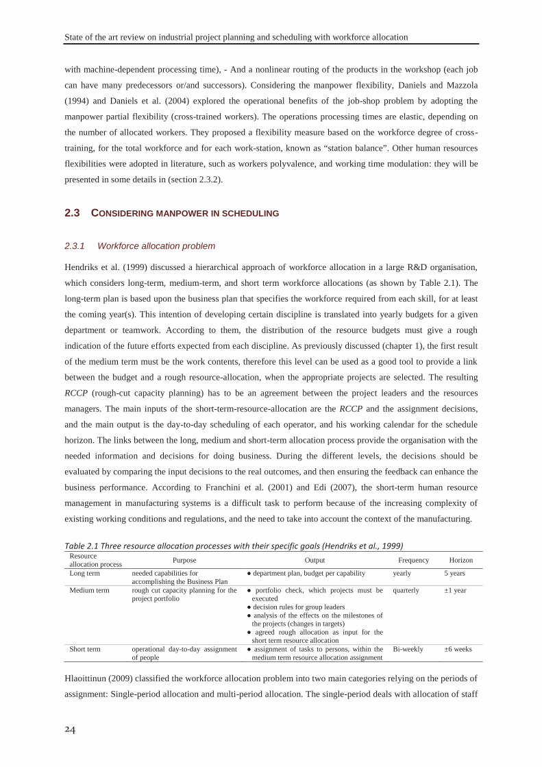
State of the art review on industrial project planning and scheduling with workforce allocation

24

with machine-dependent processing time), - And a nonlinear routing of the products in the workshop (each job

can have many predecessors or/and successors). Considering the manpower flexibility, Daniels and Mazzola

(1994) and Daniels et al. (2004) explored the operational benefits of the job-shop problem by adopting the

manpower partial flexibility (cross-trained workers). The operations processing times are elastic, depending on

the number of allocated workers. They proposed a flexibility measure based on the workforce degree of cross-

training, for the total workforce and for each work-station, known as “station balance”. Other human resources

flexibilities were adopted in literature, such as workers polyvalence, and working time modulation: they will be

presented in some details in (section 2.3.2).

Hendriks et al. (1999) discussed a hierarchical approach of workforce allocation in a large R&D organisation,

which considers long-term, medium-term, and short term workforce allocations (as shown by Table 2.1). The

long-term plan is based upon the business plan that specifies the workforce required from each skill, for at least

the coming year(s). This intention of developing certain discipline is translated into yearly budgets for a given

department or teamwork. According to them, the distribution of the resource budgets must give a rough

indication of the future efforts expected from each discipline. As previously discussed (chapter 1), the first result

of the medium term must be the work contents, therefore this level can be used as a good tool to provide a link

between the budget and a rough resource-allocation, when the appropriate projects are selected. The resulting

RCCP (rough-cut capacity planning) has to be an agreement between the project leaders and the resources

managers. The main inputs of the short-term-resource-allocation are the RCCP and the assignment decisions,

and the main output is the day-to-day scheduling of each operator, and his working calendar for the schedule

horizon. The links between the long, medium and short-term allocation process provide the organisation with the

needed information and decisions for doing business. During the different levels, the decisions should be

evaluated by comparing the input decisions to the real outcomes, and then ensuring the feedback can enhance the

business performance. According to Franchini et al. (2001) and Edi (2007), the short-term human resource

management in manufacturing systems is a difficult task to perform because of the increasing complexity of

existing working conditions and regulations, and the need to take into account the context of the manufacturing.

Table 2.1 Three resource allocation processes with their specific goals (Hendriks et al., 1999) Resource allocation process Purpose Output Frequency Horizon

Long term needed capabilities for accomplishing the Business Plan

● department plan, budget per capability yearly 5 years

Medium term rough cut capacity planning for the project portfolio

● portfolio check, which projects must be executed

● decision rules for group leaders ● analysis of the effects on the milestones of

the projects (changes in targets) ● agreed rough allocation as input for the

short term resource allocation

quarterly ±1 year

Short term operational day-to-day assignment of people

● assignment of tasks to persons, within the medium term resource allocation assignment

Bi-weekly ±6 weeks

Hlaoittinun (2009) classified the workforce allocation problem into two main categories relying on the periods of

assignment: Single-period allocation and multi-period allocation. The single-period deals with allocation of staff

2.3 CONSIDERING MANPOWER IN SCHEDULING

2.3.1 Workforce allocation problem

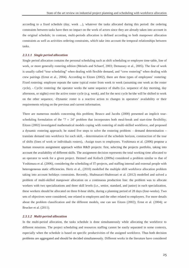
State of the art review on industrial project planning and scheduling with workforce allocation

25

according to a fixed schedule (day, week ...), whatever the tasks allocated during this period: the ordering

constraints between tasks have then no impact on the work of actors since they are already taken into account in

the original schedule; in contrast, multi-periods allocation is defined according to both manpower allocation

constraints as well as activities ordering constraints, which take into account the temporal relationships between

tasks.

2.3.1.1 Single period allocation

Single period allocation contains the personal scheduling such as shift scheduling or employee time-table, line of

work, or more generally rostering edition (Meisels and Schaerf, 2003; Demassey et al., 2005). The line of work

is usually called “tour scheduling” when dealing with flexible demand, and “crew rostering” when dealing with

crew pairings (Ernst et al., 2004). According to Eitzen (2002), there are three types of employees’ rostering:

Fixed rostering: employee repeats the same typical roster from week to week (assuming one week as the roster

cycle), - Cyclic rostering: the operator works the same sequence of shafts (i.e. sequence of day morning, day

afternoon, or nights) over the active roster cycle (e.g. week), and for the next cycle he/she will be shifted to work

on the other sequence, -Dynamic roster is a reactive action to changes in operators’ availability or their

requirements relying on the previous and current information.

There are numerous models concerning this problem; Brusco and Jacobs (2000) presented an implicit tour-

scheduling formulation of the "7 24" problem that incorporates both meal-break and start-time flexibility;

Eitzen (2002) investigated mathematical models coping with rostering of multi-skilled workforce, and proposed

a dynamic rostering approach; he stated five steps to solve the rostering problem: - demand determination –

translate demand into workforce for each skill, - determination of the schedule horizon, construction of the tour

of shifts (lines of work or individuals rosters), -Assign tours to employees. Yoshimura et al. (2006) propose a

human resources assignment approach within R&D projects: first, selecting the projects portfolio, taking into

account the availability of different skills. The assignment decision represents the total working time allocated to

an operator to work for a given project. Heimerl and Kolisch (2009a) considered a problem similar to that of

Yoshimura et al. (2006), considering the scheduling of IT-projects, and staffing internal and external people with

heterogeneous static efficiencies. Hertz et al., (2010) modelled the multiple shift workforce allocation problem

taking into account holidays constraints. Recently, Shahnazari-Shahrezaei et al. (2012) modelled and solved a

problem of multi-skilled manpower allocation on a continuous production line: the problem was to allocate

workers with two specializations and three skill levels (i.e., senior, standard, and junior) in each specialization,

these workers should be allocated on three 8-hour shifts, during a planning period of 28 days (four-weeks). Two

sets of objectives were considered, one related to employers and the other related to employees. For more details

about the problem classification and the different models, one can see Eitzen (2002); Ernst et al. (2004); or

Brucker et al. (2011).

2.3.1.2 Multi-period allocation

In the multi-period allocation, the tasks schedule is done simultaneously while allocating the workforce to

different missions. The project scheduling and resources staffing cannot be easily separated in some contexts,

especially when the schedule is based on specific productivities of the assigned workforce. Thus both decision

problems are aggregated and should be decided simultaneously. Different works in the literature have considered

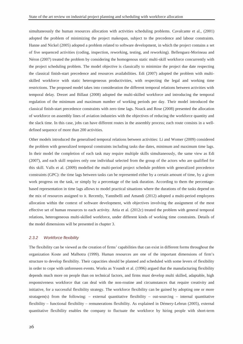
State of the art review on industrial project planning and scheduling with workforce allocation

26

simultaneously the human resources allocation with activities scheduling problems. Cavalcante et al., (2001)

adopted the problem of minimizing the project makespan, subject to the precedence and labour constraints.

Hanne and Nickel (2005) adopted a problem related to software development, in which the project contains a set

of five sequenced activities (coding, inspection, reworking, testing, and reworking). Bellenguez-Morineau and

Néron (2007) treated the problem by considering the homogenous static multi-skill workforce concurrently with

the project scheduling problem. The model objective is classically to minimize the project due date respecting

the classical finish-start precedence and resources availabilities. Edi (2007) adopted the problem with multi-

skilled workforce with static heterogeneous productivities, with respecting the legal and working time

restrictions. The proposed model takes into consideration the different temporal relations between activities with

temporal delay. Drezet and Billaut (2008) adopted the multi-skilled workforce and introducing the temporal

regulation of the minimum and maximum number of working periods per day. Their model introduced the

classical finish-start precedence constraints with zero time lags. Noack and Rose (2008) presented the allocation

of workforce on assembly lines of aviation industries with the objectives of reducing the workforce quantity and

the slack time. In this case, jobs can have different routes in the assembly process; each route consists in a well-

defined sequence of more than 200 activities.

Other models introduced the generalised temporal relations between activities: Li and Womer (2009) considered

the problem with generalized temporal constraints including tasks due dates, minimum and maximum time lags.

In their model the completion of each task may require multiple skills simultaneously, the same view as Edi

(2007), and each skill requires only one individual selected from the group of the actors who are qualified for

this skill. Valls et al. (2009) modelled the multi-period project schedule problem with generalized precedence

constraints (GPC): the time lags between tasks can be represented either by a certain amount of time, by a given

work progress on the task, or simply by a percentage of the task duration. According to them the percentage-

based representation in time lags allows to model practical situations where the durations of the tasks depend on

the mix of resources assigned to it. Recently, Yannibelli and Amandi (2012) adopted a multi-period employees

allocation within the context of software development, with objectives involving the assignment of the most

effective set of human resources to each activity. Attia et al. (2012c) treated the problem with general temporal

relations, heterogeneous multi-skilled workforce, under different kinds of working time constraints. Details of

the model dimensions will be presented in chapter 3.

The flexibility can be viewed as the creation of firms’ capabilities that can exist in different forms throughout the

organization Koste and Malhotra (1999). Human resources are one of the important dimensions of firm’s

structure to develop flexibility. Their capacities should be planned and scheduled with some levers of flexibility

in order to cope with unforeseen events. Works as Youndt et al. (1996) argued that the manufacturing flexibility

depends much more on people than on technical factors, and firms must develop multi skilled, adaptable, high

responsiveness workforce that can deal with the non-routine and circumstances that require creativity and

initiative, for a successful flexibility strategy. The workforce flexibility can be gained by adopting one or more

stratagem(s) from the following: – external quantitative flexibility – out-sourcing – internal quantitative

flexibility – functional flexibility – remunerations flexibility. As explained in Démery-Lebrun (2005), external

quantitative flexibility enables the company to fluctuate the workforce by hiring people with short-term

2.3.2 Workforce flexibility

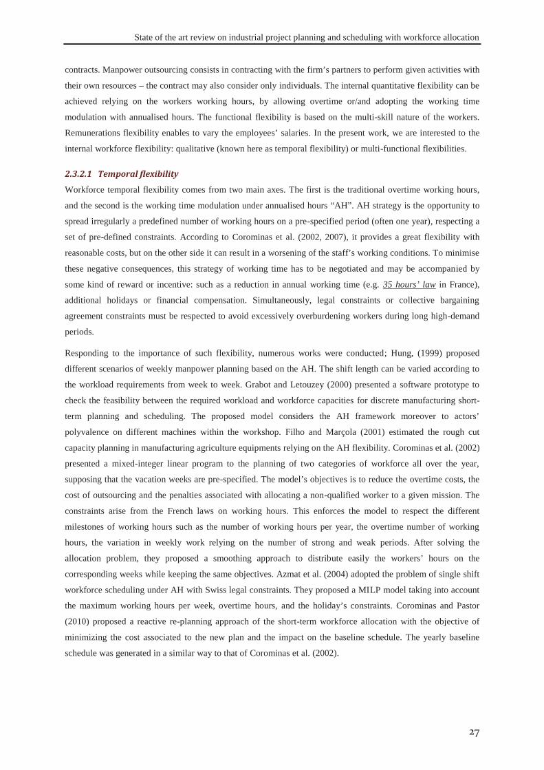
State of the art review on industrial project planning and scheduling with workforce allocation

27

contracts. Manpower outsourcing consists in contracting with the firm’s partners to perform given activities with

their own resources – the contract may also consider only individuals. The internal quantitative flexibility can be

achieved relying on the workers working hours, by allowing overtime or/and adopting the working time

modulation with annualised hours. The functional flexibility is based on the multi-skill nature of the workers.

Remunerations flexibility enables to vary the employees’ salaries. In the present work, we are interested to the

internal workforce flexibility: qualitative (known here as temporal flexibility) or multi-functional flexibilities.

2.3.2.1 Temporal flexibility

Workforce temporal flexibility comes from two main axes. The first is the traditional overtime working hours,

and the second is the working time modulation under annualised hours “AH”. AH strategy is the opportunity to

spread irregularly a predefined number of working hours on a pre-specified period (often one year), respecting a

set of pre-defined constraints. According to Corominas et al. (2002, 2007), it provides a great flexibility with

reasonable costs, but on the other side it can result in a worsening of the staff’s working conditions. To minimise

these negative consequences, this strategy of working time has to be negotiated and may be accompanied by

some kind of reward or incentive: such as a reduction in annual working time (e.g. 35 hours’ law in France),

additional holidays or financial compensation. Simultaneously, legal constraints or collective bargaining

agreement constraints must be respected to avoid excessively overburdening workers during long high-demand

periods.

Responding to the importance of such flexibility, numerous works were conducted; Hung, (1999) proposed

different scenarios of weekly manpower planning based on the AH. The shift length can be varied according to

the workload requirements from week to week. Grabot and Letouzey (2000) presented a software prototype to

check the feasibility between the required workload and workforce capacities for discrete manufacturing short-

term planning and scheduling. The proposed model considers the AH framework moreover to actors’

polyvalence on different machines within the workshop. Filho and Marçola (2001) estimated the rough cut

capacity planning in manufacturing agriculture equipments relying on the AH flexibility. Corominas et al. (2002)

presented a mixed-integer linear program to the planning of two categories of workforce all over the year,

supposing that the vacation weeks are pre-specified. The model’s objectives is to reduce the overtime costs, the

cost of outsourcing and the penalties associated with allocating a non-qualified worker to a given mission. The

constraints arise from the French laws on working hours. This enforces the model to respect the different

milestones of working hours such as the number of working hours per year, the overtime number of working

hours, the variation in weekly work relying on the number of strong and weak periods. After solving the

allocation problem, they proposed a smoothing approach to distribute easily the workers’ hours on the

corresponding weeks while keeping the same objectives. Azmat et al. (2004) adopted the problem of single shift

workforce scheduling under AH with Swiss legal constraints. They proposed a MILP model taking into account

the maximum working hours per week, overtime hours, and the holiday’s constraints. Corominas and Pastor

(2010) proposed a reactive re-planning approach of the short-term workforce allocation with the objective of

minimizing the cost associated to the new plan and the impact on the baseline schedule. The yearly baseline

schedule was generated in a similar way to that of Corominas et al. (2002).

State of the art review on industrial project planning and scheduling with workforce allocation

28

2.3.2.2 Multi-functional flexibility and job-rotation

Workforce multi-functional flexibility is the ability of a given worker to develop a set of competences required

to perform different tasks, associated with multiple activities resulting from changing load-contents, production

methods or technology. This flexibility is naturally embedded in the workforce, where they have the ability to

migrate from a workstation to others, when and where needed. However it requires heavy training programs to

produce and develop a multi-skilled workforce. Koste and Malhotra (1999) defined it as “the number and variety

of tasks/operations a worker can execute without incurring high transition penalties or large changes in

performance outcomes”.

This flexibility dimension has had a great attention in literature in many applications, starting by Nelson (1970)

who investigated the cross-training configurations in job-shop with dual resources. Brusco and Johns (1998)

examined different cross-training configurations in planning the maintenance operations in a large paper-mill

factory, aiming to minimise the staffing costs associated to the heterogeneous productivity levels. Bokhorst and

Gaalman (2009) explored the effect of cross-training workers on dual machines that have different mean

processing times. In project scheduling problem, Bellenguez-Morineau and Néron (2007) and Al-Anzi et al.

(2010) extended the traditional RCPSP with the objective of minimizing the project makespan by integrating the

homogenous workforce multi-skilled flexibility. In software development Hanne and Nickel (2005); Li and

Womer (2009); and Yannibelli and Amandi (2012), introduced the multi-skilled personnel into RCPSP to

minimize the total staffing costs. Hanne and Nickel (2005) integrated quality objectives expressed by the number

of defects depending on the developers’ skill levels. Yannibelli and Amandi (2012) adopted the objective of

assigning the most effective resources for achieving a given job. In call-centres, Avramidis et al. (2010)

examined a day schedule problem with multi-skilled employees; the model specifies the stochastic data for the

call arrivals and the duration of each call. In health care and hospitality sectors, Caron et al. (1999) proposed the

problem of nurse schedule under seniority and job priority constraints. Recently Shahnazari-Shahrezaei et al.

(2012) modelled the multi-shift workforce problem in manufacturing of polyethylene pipes and connections for

drip irrigation.

On the other side, Hoyt and Matuszek (2001) empirically showed that there is no direct relationship between

employees’ skill diversity and financial performance in high technological industries. And companies should be

aware of over-skilled workforce when considering plans to expand employee skill sets as part of a strategy for

improving their responsiveness. The same conclusion was adopted by Attia et al. (2012a), over-skilled workforce

can be misleading and have negative consequences on the financial aspects, especially during the experience

acquisition periods (this will be discussed in chapter 7). However, the multi-skill capabilities may be associated

with systemic changes that result in improved financial performance.

2.3.2.3 External labour flexibility

As mentioned earlier, the external flexibility refers to the adjustment of the required workforce from external

sources. According to Goudswaard and De Nanteuil (2000); Valverde et al. (2000) or Démery-Lebrun (2005),

this can be achieved by employing workers on temporary work or fixed-term contracts or through relaxed hiring

and firing regulations, where employers can hire and fire permanent employees according to the firms’ needs.

The main reason of this flexibility is the cost reduction strategy by means of transferring risks and costs to other

employment situations. This type seems to provide the companies with a raped and costless strategic flexibility

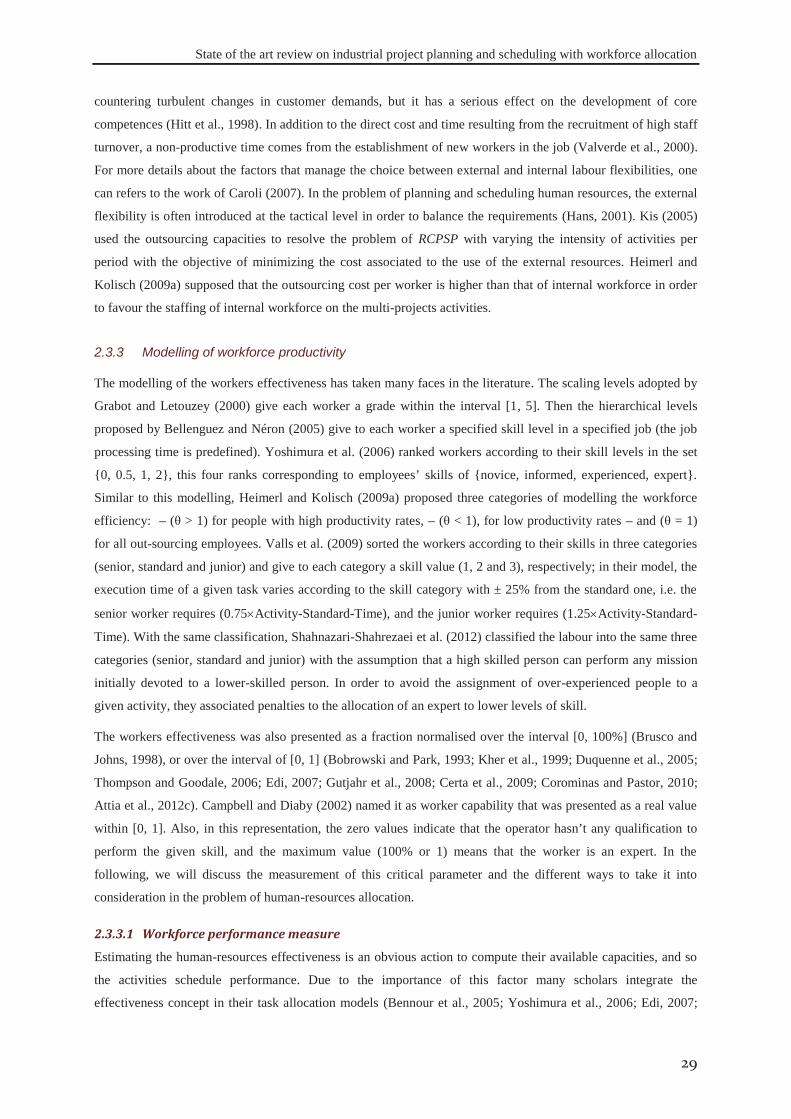
State of the art review on industrial project planning and scheduling with workforce allocation

29

countering turbulent changes in customer demands, but it has a serious effect on the development of core

competences (Hitt et al., 1998). In addition to the direct cost and time resulting from the recruitment of high staff

turnover, a non-productive time comes from the establishment of new workers in the job (Valverde et al., 2000).

For more details about the factors that manage the choice between external and internal labour flexibilities, one

can refers to the work of Caroli (2007). In the problem of planning and scheduling human resources, the external

flexibility is often introduced at the tactical level in order to balance the requirements (Hans, 2001). Kis (2005)

used the outsourcing capacities to resolve the problem of RCPSP with varying the intensity of activities per

period with the objective of minimizing the cost associated to the use of the external resources. Heimerl and

Kolisch (2009a) supposed that the outsourcing cost per worker is higher than that of internal workforce in order

to favour the staffing of internal workforce on the multi-projects activities.

The modelling of the workers effectiveness has taken many faces in the literature. The scaling levels adopted by

Grabot and Letouzey (2000) give each worker a grade within the interval [1, 5]. Then the hierarchical levels

proposed by Bellenguez and Néron (2005) give to each worker a specified skill level in a specified job (the job

processing time is predefined). Yoshimura et al. (2006) ranked workers according to their skill levels in the set

{0, 0.5, 1, 2}, this four ranks corresponding to employees’ skills of {novice, informed, experienced, expert}.

Similar to this modelling, Heimerl and Kolisch (2009a) proposed three categories of modelling the workforce

efficiency: – (θ > 1) for people with high productivity rates, – (θ < 1), for low productivity rates – and (θ = 1)

for all out-sourcing employees. Valls et al. (2009) sorted the workers according to their skills in three categories

(senior, standard and junior) and give to each category a skill value (1, 2 and 3), respectively; in their model, the

execution time of a given task varies according to the skill category with ± 25% from the standard one, i.e. the

senior worker requires (0.75 Activity-Standard-Time), and the junior worker requires (1.25 Activity-Standard-

Time). With the same classification, Shahnazari-Shahrezaei et al. (2012) classified the labour into the same three

categories (senior, standard and junior) with the assumption that a high skilled person can perform any mission

initially devoted to a lower-skilled person. In order to avoid the assignment of over-experienced people to a

given activity, they associated penalties to the allocation of an expert to lower levels of skill.

The workers effectiveness was also presented as a fraction normalised over the interval [0, 100%] (Brusco and

Johns, 1998), or over the interval of [0, 1] (Bobrowski and Park, 1993; Kher et al., 1999; Duquenne et al., 2005;

Thompson and Goodale, 2006; Edi, 2007; Gutjahr et al., 2008; Certa et al., 2009; Corominas and Pastor, 2010;

Attia et al., 2012c). Campbell and Diaby (2002) named it as worker capability that was presented as a real value

within [0, 1]. Also, in this representation, the zero values indicate that the operator hasn’t any qualification to

perform the given skill, and the maximum value (100% or 1) means that the worker is an expert. In the

following, we will discuss the measurement of this critical parameter and the different ways to take it into

consideration in the problem of human-resources allocation.

2.3.3.1 Workforce performance measure

Estimating the human-resources effectiveness is an obvious action to compute their available capacities, and so

the activities schedule performance. Due to the importance of this factor many scholars integrate the

effectiveness concept in their task allocation models (Bennour et al., 2005; Yoshimura et al., 2006; Edi, 2007;

2.3.3 Modelling of workforce productivity

State of the art review on industrial project planning and scheduling with workforce allocation

30

Valls et al., 2009; Corominas and Pastor, 2010; Attia et al., 2012c). Relying on the three-axis (temporal,

financial and quality) performance, Bennour et al. (2005) described a methodology adopted by their industrial

partners to estimate the activity performance: it is based on three main parameters: -The estimated nominal

performance -The modulation coefficient associated to each skill, - And the skill important weight. The essential

parameter in the activity performance model is the quantification of the resources performance that was assumed

to be available. This availability assumption was adopted by many authors (Yoshimura et al., 2006; Valls et al.,

2009; Corominas and Pastor, 2010; Edi, 2007; and Attia et al., 2012c) supposed that this effectiveness can be

calculated relying on the ratio between the worker actual productivity rate and a nominal one. In job-shops, Kher

et al. (1999) supposed to estimate it relying on the learning-forgetting effects. Majozi and Zhu (Frank), (2005)

presented an application of fuzzy sets theory within the context of integrated batch processes planning and

scheduling. In their model, the operators are fuzzy evaluated to (not competent, reasonably competent, and

highly competent) based on the linguistic terms that can be used to produce a fuzzy decision table, relying on

their age, experience, expertise, health, and availability. Hanne and Nickel (2005), Yannibelli and Amandi,

(2011), Yannibelli and Amandi (2012) aligned with Doerr and Arreola-Risa (2000), proposed to estimate the

productivity of an employee relying on activities and persons attributes: - the nature of the activity and work

contents, domain of knowledge, complexity etc. – the employee characterisation is based on the available

information such as curriculum vitae, expert evaluations, information about his/her participation on previous

projects, etc. – the other employees assigned to the same activity, - the required skill. Then these parameters can

be used to attribute the employee an effectiveness value within the interval [0, 1].

2.3.3.2 Homogenous workforce performance

In the problem of multi-skilled workforce allocation to different activities, there are two ways of considering

employees’ performance: homogeneous or heterogeneous productivity. One should differentiate between the

worker-based homogeneous productivity and the skill-based homogeneous productivity. In the first, each worker

can master a set of different skills with equal productivity rates, whatever the skills. In the second case (skill-

based), all workers can behave the same performance rates in practicing a given skill. In this vision, Cai and Li

(2000) proposed two types of resources: the first is unary-skill and the second is multi-skill with homogeneous

productivity (more expensive). Fraser (2009) adopted this homogeneous nature in his investigation of the impact

of labour flexibility on team processes and team effectiveness in cellular manufacturing. Bellenguez-Morineau

and Néron (2007) modelled the multi-skilled project scheduling problem “MSPSP”, in which each actor can

master a set of skills with equal performance rates, and all workers perform the same rates in any skill. Others

like Daniels et al. (2004) considered the homogeneous productivity in flow-shop activities scheduling. They

adopted the concept of cross-trained workers for different workstations, with the ability of performing a given

task or not: in their model, all actors having this skill are able to perform a given task with equal amount of time.

Corominas et al. (2006) assumed homogeneous working efficiencies for all of the completely multi-functional

workers in service centres. Drezet and Billaut (2008) and Li and Womer (2009) considered this multi-skilled

workforce characteristic in the software industries. Avramidis et al. (2010) presented it in call centres. Recently,

Kazemipoor et al. (2013) applied this vision in project portfolio scheduling with multi-skilled workforce.

State of the art review on industrial project planning and scheduling with workforce allocation

31

2.3.3.3 Mixed workforce performance

The case where the two workforce productivities, the “worker-based” and the “skill-based”, one is homogeneous

and the other is heterogeneous, is called “mixed workforce performance”: Grabot and Letouzey (2000) proposed

a mixed model of homogeneous/heterogeneous workforce performance. They scaled the workers skills in five

levels, and each activity requires a pre-specified skill level, therefore, the allocation process relies on the activity

satisfaction by assigning the workers with the required skill levels. The allocated workers may have the same

required skill level; therefore this case is considered as a mixed model. Considering the heterogeneous

performance-based workers, Eitzen et al. (2004) proposed an employee rostering model that considers a multi-

skilled nature of workforce, taking into account that each worker has a core competence and one or more

additional one(s). In order to avoid the loss of these supplementary skills, they supposed that during each

fortnight, every worker should be allocated for his/her additional skill during at least one shift. Bellenguez and

Néron (2005) modelled the problem of MSPSP, considering that each worker can master a set of different skills,

with a maximum operational skill level associated to each one of them. On the other side; the performances of all

workers in practicing a given skill are equal (workers’ homogeneous performance), so we considered it as a

worker’s heterogeneous performance. In qualitative models of workforce productivity (such as: senior, standard,

and junior), all workers of the same category can be considered as a homogeneous, therefore this modelling view

can be considered as a mixed one (Yoshimura et al., 2006; Valls et al., 2009; Shahnazari-Shahrezaei et al.,

2012).

2.3.3.4 Heterogeneous workforce performance

We call multi-skilled workforce as completely heterogeneous in the case where neither worker-based

productivity, nor skill-based productivity, are homogeneous. According to the best of our knowledge, the first

work in this heterogeneous workforce characteristic is the work of Nelson (1970) in a dual resource constrained

“DRC” job-shop with two work centres. He examined the effect of limited employee productivity policies

(referred as “labour efficiency”), along with policies concerning the degree of centralized control and queue

discipline. The results suggested a strong interaction between the degree of centralized control and labour

efficiency. Then Bobrowski and Park (1993) considered this heterogeneous vision in investigating the staffing

rules on job-shop problems. Campbell and Diaby (2002) introduced this performance diversity in staffing a

cross-trained workforce on multiple departments. Cowling et al. (2006) introduced the productivity function of

staff allocation on the problem of multi-site activities scheduling. Heimerl and Kolisch (2009a) and Kolisch and

Heimerl (2012) adopted this heterogeneous vision in staffing and scheduling multi-skilled workforce on IT-

multiple projects activities. In order to preserve the company’s core competences, they constrained a given

minimum percentage of the work to be performed by the internal workforce. Hanne and Nickel (2005), Al-Anzi

et al. (2010) adopted it in staffing employees and scheduling the different activities of software production.

Recently, we can find the work of Yannibelli and Amandi (2011), Attia et al. (2012c) or Yannibelli and Amandi

(2012) that adopted the heterogeneous workforce productivities.

The dynamic vision of the workers performance is the continuous changes in their productivities as a function of

experience accumulation: “learning-by-doing”, or loss of capacities in reasons of forgetting. Considering this

dynamics vision of experience, the assignment of workers to different activities has received relatively little

2.3.4 Dynamic vision of workforce performance

State of the art review on industrial project planning and scheduling with workforce allocation

32

attention in the literature. This is partially due to the difficulty in collecting detailed performance data at the

individual level (Nembhard, 2001). Microscopically within the industrial context, there are two levels of

learning; the first is the managerial or organizational learning and the second is the individual learning. In this

section, we will discuss the different modelling of these phenomena (learning, forgetting), and review a subset of

works which considered them.

2.3.4.1 Experience development

The amount of time or effort required to complete a given task will decrease every time the task is repeated, i.e.

the actors can perform their tasks more efficiently and more rapidly if they go on working on the same activity as

long as possible. According to DeJong (1957), this skill development phenomenon includes not only the under-

skilled workmen but also the skilled and experienced operators. This phenomenon has been followed in product

cost estimation, since the period between the two world wars. It has many labels in literature, such as the

learning curve, progression function, product acceleration curve, improvement curve, performance curve,

experience curve, efficiency curve, even learning-by-doing and cost-quality relationships, (Badiru, 1996). It was

first described by Wright (1936) who reported it as one of the factors that affects the cost of airplanes; in his

research work, the labour cost of an aircraft is declined significantly with the accumulated experience gained

from the repetition of the manufacturing process. This cost showed a constant reduction percentage with each

doubling of the cumulative production. He then plotted his empirical relationship “unit cost versus serial

number” on a log-log scale as a straight line, and named it the “eighty percent curve”, since he found that a value

of “eighty percent” represents the exponent of the learning curve based on the relation (learning curve exponent

= log (0.8)/log (2)). Since this finding, the phenomenon is admitted but there is a hard debate between scholars

about its most representative mathematical model.

2.3.4.1.1 Modelling of learning phenomenon

Within the literature we can find many formulations of the learning curve “LC”, starting from the power model

of Wright (1936). According to the review paper of Yelle (1979), the reason for searching other models than the

log-linear of Wright (1936) is that the log-linear model does not always provide the best fit in all simulations.

But on the other side, it is the most used model in reasons of its simplicity and generality of applications.

Nembhard and Uzumeri (2000a) classified the LC’s according to two attributes relying on the originated bases:

aggregated models or individual models, where Badiru, (1992) classified them according to univariate or

multivariate models. Relying on the work of Badiru, (1992, 1996), Nembhard and Uzumeri (2000a) and

Osothsilp (2002) we present a set of these models on Table 2.2.

The variable b is computed in function of the learning rate; the lowercase is the value of learning curve slope,

and the uppercase is the learning effect. According to Badiru (1992) the set of models listed in (Table 2.2) are

univariate models (there is only one independent variable). And to accommodate numerous factors that can

influence how fast, how far, and how well a worker learns within a specified horizon, multivariate models were

proposed: for more details, we propose the works of Badiru (1992), Badiru (1996) or Shafiei-Monfared and

Jenab (2010).

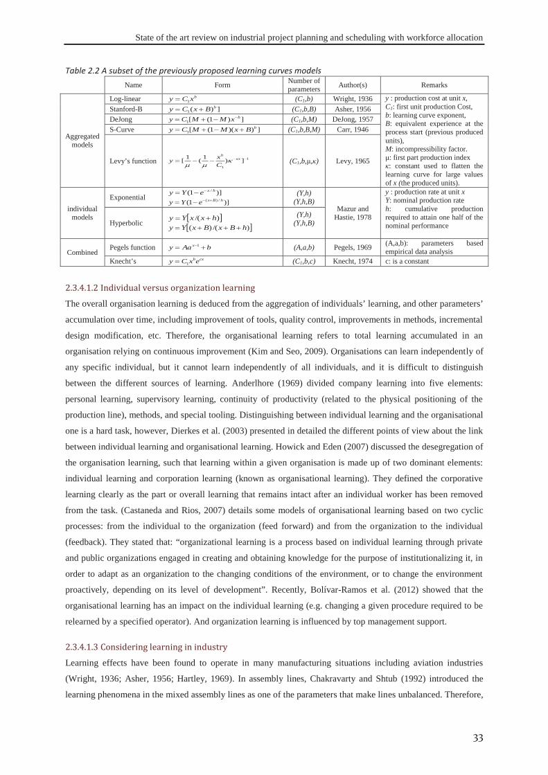
State of the art review on industrial project planning and scheduling with workforce allocation

33

Table 2.2 A subset of the previously proposed learning curves models Name Form Number of

parameters Author(s) Remarks

Aggregated models

Log-linear bxCy 1 (C1,b) Wright, 1936 y : production cost at unit x,

C1: first unit production Cost, b: learning curve exponent, B: equivalent experience at the process start (previous produced units), M: incompressibility factor. μ: first part production index κ: constant used to flatten the learning curve for large values of x (the produced units).

Stanford-B ])(1bBxCy (C1,b,B) Asher, 1956

DeJong ])1([1bxMMCy (C1,b,M) DeJong, 1957

S-Curve ]))(1([1bBxMMCy (C1,b,B,M) Carr, 1946

Levy’s function 1

1

])1(1[ xb

Cxy

(C1,b,μ,κ) Levy, 1965

individual models

Exponential )]1( / hxeYy

)]1( /)( hBxeYy (Y,h)

(Y,h,B) Mazur and

Hastie, 1978

y : production rate at unit x Y: nominal production rate h: cumulative production required to attain one half of the nominal performance

Hyperbolic )/( hxxYy

)/()( hBxBxYy (Y,h)

(Y,h,B)

Combined Pegels function bAay x 1 (A,a,b) Pegels, 1969 (A,a,b): parameters based

empirical data analysis Knecht’s cxbexCy 1

(C1,b,c) Knecht, 1974 c: is a constant

2.3.4.1.2 Individual versus organization learning

The overall organisation learning is deduced from the aggregation of individuals’ learning, and other parameters’

accumulation over time, including improvement of tools, quality control, improvements in methods, incremental

design modification, etc. Therefore, the organisational learning refers to total learning accumulated in an

organisation relying on continuous improvement (Kim and Seo, 2009). Organisations can learn independently of

any specific individual, but it cannot learn independently of all individuals, and it is difficult to distinguish

between the different sources of learning. Anderlhore (1969) divided company learning into five elements:

personal learning, supervisory learning, continuity of productivity (related to the physical positioning of the

production line), methods, and special tooling. Distinguishing between individual learning and the organisational

one is a hard task, however, Dierkes et al. (2003) presented in detailed the different points of view about the link

between individual learning and organisational learning. Howick and Eden (2007) discussed the desegregation of

the organisation learning, such that learning within a given organisation is made up of two dominant elements:

individual learning and corporation learning (known as organisational learning). They defined the corporative

learning clearly as the part or overall learning that remains intact after an individual worker has been removed

from the task. (Castaneda and Rios, 2007) details some models of organisational learning based on two cyclic

processes: from the individual to the organization (feed forward) and from the organization to the individual

(feedback). They stated that: “organizational learning is a process based on individual learning through private

and public organizations engaged in creating and obtaining knowledge for the purpose of institutionalizing it, in

order to adapt as an organization to the changing conditions of the environment, or to change the environment

proactively, depending on its level of development”. Recently, Bolívar-Ramos et al. (2012) showed that the

organisational learning has an impact on the individual learning (e.g. changing a given procedure required to be

relearned by a specified operator). And organization learning is influenced by top management support.

2.3.4.1.3 Considering learning in industry

Learning effects have been found to operate in many manufacturing situations including aviation industries

(Wright, 1936; Asher, 1956; Hartley, 1969). In assembly lines, Chakravarty and Shtub (1992) introduced the

learning phenomena in the mixed assembly lines as one of the parameters that make lines unbalanced. Therefore,

State of the art review on industrial project planning and scheduling with workforce allocation

34

they developed a methodology for redesigning the line. The objective is to minimize inventory costs, setup costs,

and labour costs subject to dynamic capacity constraints dictated by the learning effect while satisfying demand

without back orders. In software development, Hanakawa et al. (1998) proposed to use the developer’s learning

curve to compute developer’s productivity and the quantity of gain to the developer’s knowledge after executing

an activity. Their model contains three attributes: activity, knowledge and productivity attribute. The different

levels of knowledge required by the sub-jobs of an activity attribute were defined relying on the normal

distribution for the knowledge type. The developer productivity was modelled in function of the required level of

knowledge by the activity and the actual level of the developer. The knowledge attribute represents the gain of

knowledge of an individual after performing a given activity it was modelled based on individual efficiency of

gain knowledge (learning) and the maximum amount to be learned. In resources planning, Liao (1979)

incorporated learning effect in resource planning for product-mix problem and production scheduling.

Khoshnevis and Wolfe (1986) also introduced the learning effect in the aggregated workforce planning.

Nembhard (2001) proposes a heuristic approach for worker assignment based on individual learning rates. In

project scheduling and personal staffing, Wu and Sun (2005) considered the learning effect in allocating staff to

multi-project activities in the research and development (R&D) departments. The objective function is to minimize

the outsourcing costs that will be applied whenever any task cannot be completed before its due date. The cumulative

average efficiency was used to estimate the particular efficiency of a given employee. Also In R&D

organisations, Certa et al. (2009) presented the heterogeneous workforce allocation problem with incorporation

of leaning effect, and workforce social relations. In concurrent engineering on software industry, Huang and

Chen (2006) proposed to estimate the project completion time relying on a set of parameters including learning

effect.

2.3.4.2 Experience degradation

Reciprocally to the development of the actors’ experience, thanks to learning-by-doing effect, we can find the

erosion of this experience due to the lack of practice of a specified discipline. This phenomenon is known as

‘forgetting effect’ (Elmaghraby, 1990), and it has many names including: experience degradation, experience

deterioration, experience depreciation or experience erosion. The amount of experience deterioration depends on

the amount of experience gained prior to the interruption, the rate of forgetting, and the length of the interruption

period (Bailey, 1989; Globerson et al., 1989; Jaber and Bonney, 1996). Within the industrial environment, the

lack of practice induced by work interruptions, which can be produced from machines breakdown, product

modifications, changing tools, discontinuous production of a given product, transforming workers between

skills, introducing new machines, new technologies, production breaks, and vacations. According to Jaber

(2006), scientists and practitioners have not developed yet a full understanding of the behaviour and factors

affecting the forgetting process. And on the organisation level, knowledge can depreciate because of worker

turnover and changes in products or processes that make previous knowledge obsolete. By the following, we will

review a set of different attempts to model the forgetting and the industrial applications.

2.3.4.2.1 Modelling of forgetting phenomenon

In order to model the forgetting and computing the experience deterioration, within literature, one can find three

types of the modelling of forgetting effect on individuals’ performance, as classified by Jaber and Sikström

(2004). The first is the use of mathematical modelling without using empirical data such as that of the learn-

State of the art review on industrial project planning and scheduling with workforce allocation

35

forget-learn model of Carlson and Rowe (1976), the variable regression to invariant forgetting (VRIF) of

Elmaghraby (1990), the learning-forgetting curve model (LFCM) of Jaber and Bonney (1996). The second uses

empirical data from real-life setting as a basis of model regression for the individuals’ performance decline

formula, known as the “Recency Model” of Nembhard and Uzumeri (2000b) that was used by Sayin and

Karabati (2007). The third type of modelling is the one using empirical data obtained from laboratory

experiments as a basis of stochastic regression and analysis of variances: Bailey (1989) considered mechanical

assembly/disassembly highly procedural tasks with different complexities; Globerson et al. (1989) considered

computer data entry, the tasks was to complete a specific form for a company’s employees, each form related to

a specific employee; Hewitt et al. (1992) examined assembly of pegboards (as a low cognitive task), and design

a spread sheet (as a moderately high cognitive task). According to Jaber and Sikström (2004) there are two

limitations of these laboratory experiments-based models of the forgetting curve: the first is the use of short-

duration breaks, rather than long interruptions, to simulate periods without practice. The second is the

application of these models to experimental settings that often differ from the industrial ones. Other models such

as the “power integration diffusion (PID)” of Sikström and Jaber (2002) that relies on strengthen of memory

traces during learning and diffusion of these traces during forgetting. And recently, Kim and Seo (2009)

proposed a learning curve model that measures acquisition and depreciation of knowledge in a single framework

but governed by two different rules: the knowledge acquisition relying on learning-by-doing, and knowledge

transfer between production lines.

For the comparison between the different models, Jaber and Bonney (1997) conducted a comparative study

between three models of LFL, VRIF and LFCM, noting that the three models are based on the Wright (1936)

formula. Jaber and Sikström (2004) conducted a numerical comparison of three potential learning-forgetting

models: learn-forget curve model “LFCM” (Jaber and Bonney, 1996), “Recency” model (Nembhard and

Uzumeri, 2000b), and “PID” (Sikström and Jaber, 2002). Results indicate that for a moderate learning scenario

(where the learning rate classifies a task as being more cognitive than motor skills), the three models, on the

average, produced very close predictions for all values of production breaks and initial processing times. So in

such learning scenarios the differentiation between the three models by empirical data is quite difficult. But if the

task becomes more cognitive than motor skills, the learning becomes faster, and the predictions of LFCM and

“Recency model” are below those of PID. Reciprocally, as the task becomes more motor skill than cognitive

(slow learning rate) the prediction of the LFCM and “Recency model” are above those of PID. They indicated

that the prediction by LFCM is closer to PID than “Recency model”. They concluded with: the two models of

LFCM and PID suggest that the learning becomes slower as the forgetting becomes faster, in opposite to that of

“Recency model”, which suggests that, the fast (slow) learners forget faster (slower).

2.3.4.2.2 Considering forgetting in industry

The learning-forgetting phenomena have been considered in industrial applications for decades. Consequently,

this section will briefly introduce the most relevant research works and refers the reader to more comprehensive

reviews, e.g. the work of Jaber (2006). First, starting from the model of learn-forget-learn of Carlson and Rowe

(1976), Kher et al. (1999) performed a numerical analysis on workers learning and forgetting effects in DRC

systems. They applied the study to complex tasks where the learning and relearning phenomena have managerial

interests, and a direct impact to the firm performance. Therefore, they used the initial processing time as 400% of

State of the art review on industrial project planning and scheduling with workforce allocation

36

the standard one, learning rate of 85% and forgetting rates varies between 85% and 95%. Kher (2000) extended

this work, by considering flexibility acquisition in stochastic DRC job-shop environment, and measuring the

impact of learning, relearning, and worker attrition on inventory and customer service measures. Yue et al.

(2007) too investigated the cross-training policies in DRC parallel job-shop using the same model (LFL), where

new part types are regularly introduced and where learning and forgetting play a role. They investigated three

factors: the level of multi-functionality, the pattern of skill overlaps, and the distribution of skills. Results

showed that limited level of multi-functionality workers gives the best results in most cases. High levels of

multi-functional negatively affect performance. The significant effect of the pattern of skills overlaps depends on

the lengths of the new part life cycles. Equal distribution of two skills is preferable due to equal worker

assignment opportunities.

In assembly lines under learning and forgetting consideration, Mccreery and Krajewski (1999) investigated the

amount of cross training given to each employee, and the deployment policy on the performance under product

varieties and tasks’ different complexities. In environment in which workers are learning to process jobs on

different machines, Jaber et al. (2003) reviewed and examined factors that influence worker forgetting in

industrial settings, and analyzed the degree to which existing mathematical models comply with observed human

forgetting behaviour. They used LFCM and VRVF forgetting models to show the effects of cross-training and

deployment policies in reducing the forgetting effect. In lot sizing problems, Elmaghraby (1990) integrated

VRIF model, where Jaber and Bonney (1996) and Jaber et al. (2009) used the LFCM to determine the economic

manufacturing quantities for finite and infinite planning horizons. Others, such as Bailey and McIntyre (2003)

developed a parameters prediction model relying on a project management simulator, in order to provide early

estimates of post-interruption production times.

In the assignment of workers to tasks based on learning-forgetting behaviour, Osothsilp (2002) introduced

workers learning and forgetting based on the assignment on tasks of varying complexity, aiming to enhance the

workstation performance. Sayin and Karabati (2007) proposed a framework of two stages to solve the workforce

assignment problem with incorporating learning and forgetting effects. The first-stage maximizes the total

departmental utility subject to typical assignment constraints (assign the most efficient worker to each

department). The optimal values of department utilities were then fed to the second stage model that seeks to

maximize total skill improvement while respecting a given deviation to the first model optimal results. Gutjahr et

al. (2008) introduced the problem of portfolio selection and projects scheduling with resources allocation, taking

into account the strategic development of their competences. They presented the actors’ efficiencies for working

in a given skill as a function of the allocation scores. In other words, the working of the actor for a given skill

increases his score for this one and also increases his efficiency, but shifting the actor away from this skill

reduces his score, and hence his efficiency. Then the actor efficiency was normalized over the [0, 1] interval

using the “logistic function: y(x) = (1/(1+ex)”. In products design, Hlaoittinun et al. (2010) modelled and solved

staff allocation to different tasks relying on the task-compatibility indicators. By integrating the learning-

forgetting, their models aims to optimise the supplementary salary cost due to the extended task duration when

using under-competent employees and the financial penalties when the goals of competency development have

not been reached. Attia et al. (2011) adopted the LFCM in the project scheduling and flexible resources

allocations (chapter 3).

State of the art review on industrial project planning and scheduling with workforce allocation

37

The uncertainty in working environment increases the importance of developing firms’ flexibility. This flexibility can be used as a hedge against uncertainty. Therefore, it is appreciated to integrate human resources flexibility in generating a robust activities baseline schedule. And relying on the fact that a high quality product depends mainly on high-skilled workers, we are oriented to consider also the development of human resources experience. This work will refer simultaneously to four dimensions according to the literature classification presented in (Table 2.3). The first is the workforce allocation period that can be single or multi period. The second is the modelling vision of the working efficiency of the multi-skilled workforce, can be divided to static or dynamic. The third is the consideration of the employees working time that can be classical or flexible. And the fourth is the characteristics of the activities durations that can be rigid or elastic. Relying on the literature review, considering theses dimensions altogether represents an original work.

Table 2.3 Classification of related works. Period Skill modelling Working time Task duration

Single Multi Static Dynamic modelling

Classical Flexible Rigid Elastic Learning Forgetting The present thesis

Attia et al., 2012c G -- --

Azmat et al., 2004 -- -- -- -- --

Cai and Li, 2000 -- -- -- --

Cavalcante et al., 2001 A

Certa et al., 2009

Corominas and Pastor, 2010

Corominas et al., 2007 -- --

Corominas et al., 2006

Cowling et al., 2006

Daniels et al., 2004

Drezet and Billaut, 2008 T D

Edi, 2007

Eitzen et al., 2004 * -- --

Gutjahr et al., 2008 T **

Hanne and Nickel, 2005 T

Heimerl and Kolisch, 2009a M OE

Hertz et al., 2010 -- -- -- SH -- --

Hlaoittinun, 2009 T -Pre **

Kazemipoor et al., 2013 P -- -- -- --

Li and Womer, 2009 G ** --

Morineau and Néron, 2007 T *

Nembhard, 2001 -- --

Noack and Rose, 2008

Perron, 2010 Sayin and Karabati, 2007 -- -- -- --

Shahnazari-Shahrezaei et al., 2012 -- --

Valls et al., 2009 G -- --

Vidal et al., 1999 T * C

Wu and Sun, 2005 **

Yannibelli and Amandi, 2011-12 T *: Resources with binary availabilities: 0 or 1. **: Maximum capacity of work per each scheduling period without considering overtime. A: Given labour availability per period and variable labour profiles to each job. C: Concerns the cycle time of a workstation centre. D: the flexibility of working with maximum and minimum working periods per day, without overtime. G: multi period project scheduling with generalized temporal relations. M: multi-project scheduling without precedence constraints (each project has pre-specified interval of early and late start).

OE: with overtime flexibility and external labour resourcing. P: Project portfolio scheduling. SH: flexibility of working time without overtime. T: multi period project scheduling with traditional finish-start constraints. T –Pre: with the consideration of: “the project breakdown and its tasks schedule over the project periods are data entry”.

2.4 CONCLUSION:

State of the art review on industrial project planning and scheduling with workforce allocation

38

3 CHARACTERIZATION AND MODELLING OF THE

MULTI-PERIOD WORKFORCE ALLOCATION PROBLEM

In this chapter, we look at the line-up of multi-period project, considering

the problem of staff allocation with two degrees of flexibility: the first

results from the annualizing of working time, and relies on policies of

changing schedules, individually as well as collectively. The second degree

of flexibility is the versatility of the operators, which induces a dynamic

view of their skills and the need to predict changes in individual

performance as a result of successive assignments. We are firmly in a

context where the expected durations of activities is no longer

deterministic, but results from the performance of the operators selected

for their execution. We present a mathematical model of this problem and

the analysis of its variables and constrains.

CH

APT

ER

3

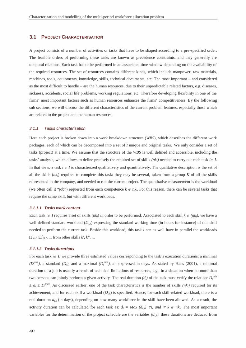
Characterization and modelling of the multi-period workforce allocation problem

40

A project consists of a number of activities or tasks that have to be shaped according to a pre-specified order.

The feasible orders of performing these tasks are known as precedence constraints, and they generally are

temporal relations. Each task has to be performed in an associated time window depending on the availability of

the required resources. The set of resources contains different kinds, which include manpower, raw materials,

machines, tools, equipments, knowledge, skills, technical documents, etc. The most important – and considered

as the most difficult to handle – are the human resources, due to their unpredictable related factors, e.g. diseases,

sickness, accidents, social life problems, working regulations, etc. Therefore developing flexibility in one of the

firms’ most important factors such as human resources enhances the firms’ competitiveness. By the following

sub sections, we will discuss the different characteristics of the current problem features, especially those which

are related to the project and the human resources.

Here each project is broken down into a work breakdown structure (WBS), which describes the different work

packages, each of which can be decomposed into a set of I unique and original tasks. We only consider a set of

tasks (project) at a time. We assume that the structure of the WBS is well defined and accessible, including the

tasks’ analysis, which allows to define precisely the required set of skills (nki) needed to carry out each task i I.

In that view, a task i I is characterized qualitatively and quantitatively. The qualitative description is the set of

all the skills (nki) required to complete this task: they may be several, taken from a group K of all the skills

represented in the company, and needed to run the current project. The quantitative measurement is the workload

(we often call it “job”) requested from each competence k nki. For this reason, there can be several tasks that

require the same skill, but with different workloads.

3.1.1.1 Tasks work content

Each task i I requires a set of skills (nki) in order to be performed. Associated to each skill k (nki), we have a

well defined standard workload (Ωi,k) expressing the standard working time (in hours for instance) of this skill

needed to perform the current task. Beside this workload, this task i can as well have in parallel the workloads ׳i,k'', ׳׳

i,k'', ... from other skills k', k'', ...

3.1.1.2 Tasks durations

For each task i I, we provide three estimated values corresponding to the task’s execution durations: a minimal

(Dimin), a standard (Di), and a maximal (Di

max), all expressed in days. As stated by Hans (2001), a minimal

duration of a job is usually a result of technical limitations of resources, e.g., in a situation when no more than

two persons can jointly perform a given activity. The real duration (di) of the task must verify the relation: Dimin

di Dimax. As discussed earlier, one of the task characteristics is the number of skills (nki) required for its

achievement, and for each skill a workload (Ωi,k) is specified. Hence, for each skill-related workload, there is a

real duration di,k (in days), depending on how many workforce in the skill have been allowed. As a result, the

activity duration can be calculated for each task as: di = Max (di,k) i, and k nki. The most important

variables for the determination of the project schedule are the variables (di,k): these durations are deduced from

3.1 PROJECT CHARACTERISATION

3.1.1 Tasks characterisation

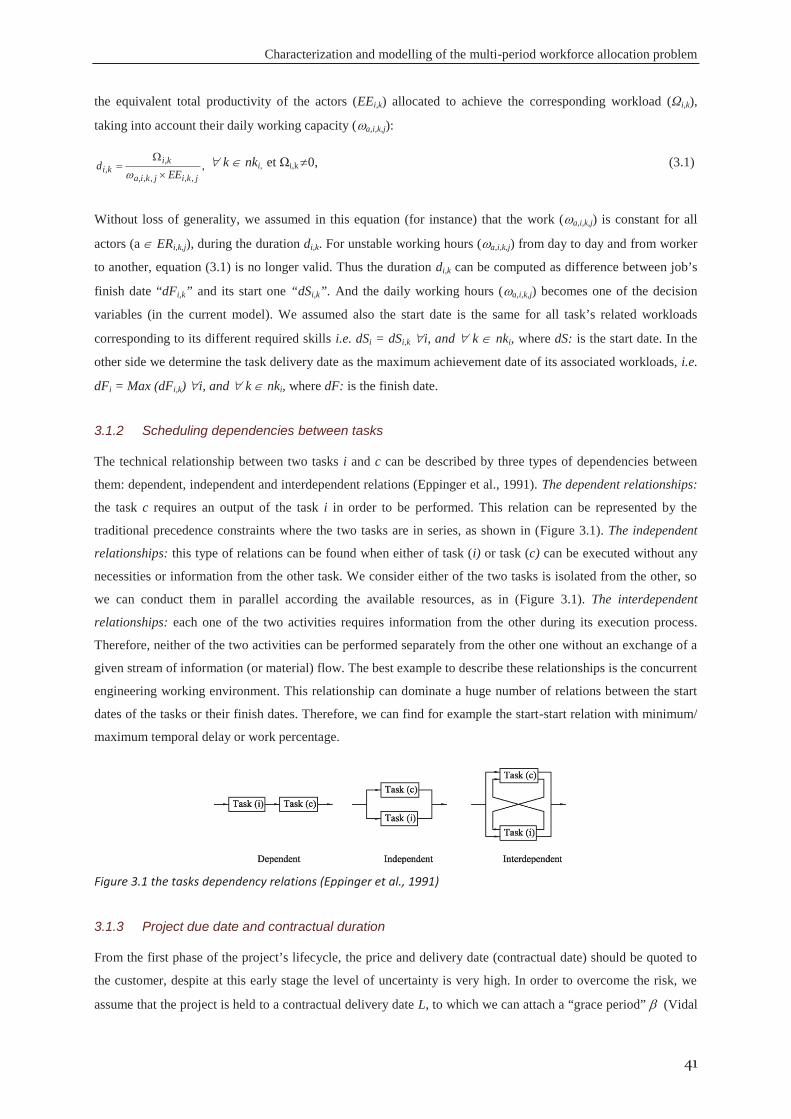
Characterization and modelling of the multi-period workforce allocation problem

41

the equivalent total productivity of the actors (EEi,k) allocated to achieve the corresponding workload (Ωi,k),

taking into account their daily working capacity ( a,i,k,j):

,,,,,,

,,

jkijkia

kiki EE

d k nki, et Ωi,k 0, (3.1)

Without loss of generality, we assumed in this equation (for instance) that the work ( a,i,k,j) is constant for all

actors (a ERi,k,j), during the duration di,k. For unstable working hours ( a,i,k,j) from day to day and from worker

to another, equation (3.1) is no longer valid. Thus the duration di,k can be computed as difference between job’s

finish date “dFi,k” and its start one “dSi,k”. And the daily working hours ( a,i,k,j) becomes one of the decision

variables (in the current model). We assumed also the start date is the same for all task’s related workloads

corresponding to its different required skills i.e. dSi = dSi,k i, and k nki, where dS: is the start date. In the

other side we determine the task delivery date as the maximum achievement date of its associated workloads, i.e.

dFi = Max (dFi,k) i, and k nki, where dF: is the finish date.

The technical relationship between two tasks i and c can be described by three types of dependencies between

them: dependent, independent and interdependent relations (Eppinger et al., 1991). The dependent relationships:

the task c requires an output of the task i in order to be performed. This relation can be represented by the

traditional precedence constraints where the two tasks are in series, as shown in (Figure 3.1). The independent

relationships: this type of relations can be found when either of task (i) or task (c) can be executed without any

necessities or information from the other task. We consider either of the two tasks is isolated from the other, so

we can conduct them in parallel according the available resources, as in (Figure 3.1). The interdependent

relationships: each one of the two activities requires information from the other during its execution process.

Therefore, neither of the two activities can be performed separately from the other one without an exchange of a

given stream of information (or material) flow. The best example to describe these relationships is the concurrent

engineering working environment. This relationship can dominate a huge number of relations between the start

dates of the tasks or their finish dates. Therefore, we can find for example the start-start relation with minimum/

maximum temporal delay or work percentage.

Figure 3.1 the tasks dependency relations (Eppinger et al., 1991)

From the first phase of the project’s lifecycle, the price and delivery date (contractual date) should be quoted to

the customer, despite at this early stage the level of uncertainty is very high. In order to overcome the risk, we

assume that the project is held to a contractual delivery date L, to which we can attach a “grace period” (Vidal

3.1.2 Scheduling dependencies between tasks

3.1.3 Project due date and contractual duration

Characterization and modelling of the multi-period workforce allocation problem

42

et al., 1999; Edi, 2007). This grace period can be considered as project temporal buffer, which is used as an

aggregated safety factor instead of using a safety factor to each activity, that known as “activities buffer (see

section 2.2.2). As shown by (Figure 3.2), if the results are delivered to the client with a delay greater than

some lateness penalty will be taken into account; reciprocally, we avoid to achieve the project earlier than (L-β)

with the intention of avoiding storage costs. Accordingly, it is necessary that the real project delivery date (LV) is

located within the interval:

L – ≤ LV ≤ L + (3.2)

This project real delivery date (LV) will be the result of the project schedule, after determining the tasks’

durations from the actors’ different allocations on the different project missions.

Figure 3.2 the project delivery date and its related costs

The workforce can be characterised relying on three dimensions: the working time modulation flexibility, the

workforce versatility and their dynamic competences. We present each dimension in the following sub-sections.

This dimension represents the new working time flexibilities such as annualised hours working strategy with

working hours’ modulation. In which each actor has a fixed amount of working hours per year that can be

irregularly spread during weeks. Each individual can have his own timetable, which can vary on daily or weekly

bases. This variation should obey some pre-specified milestones, as the minimum/maximum number of working

hours per day, a maximum number of working hours per week, and a maximum number of average working

hours per a number of weeks, called the reference period (implicitly 12 weeks, according to the French working

law), see section (3.3.3.4).

Recently the importance of multi-functional work-teams was increased responding to the variable customer

demands and unforeseen working environment. In this characterisation each operator can master a set of skills

with a specified productivity level to each one. In order to characterise this flexibility dimension, we need to

precise some parameters: - the first is the way to measure and model the operators’ productivities, - the second is

3.2 WORKFORCE CHARACTERISATION

3.2.1 Working time flexibility

3.2.2 Multi-functional flexibility

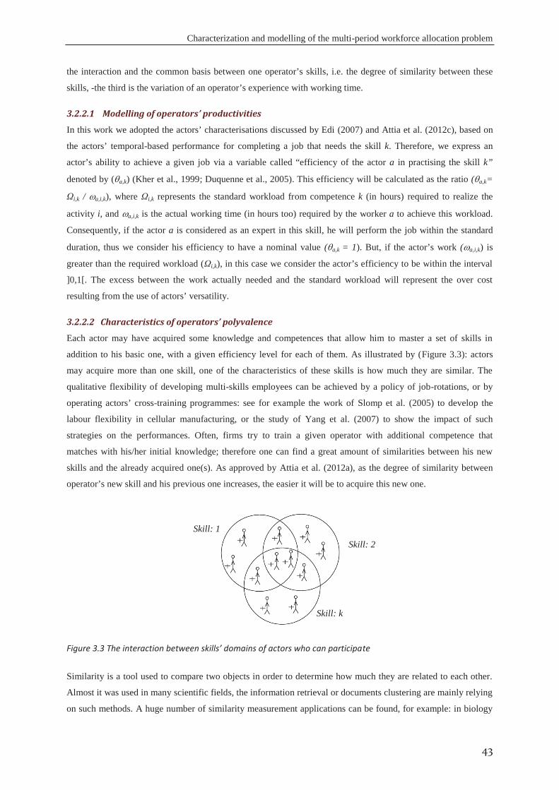
Characterization and modelling of the multi-period workforce allocation problem

43

the interaction and the common basis between one operator’s skills, i.e. the degree of similarity between these

skills, -the third is the variation of an operator’s experience with working time.

3.2.2.1 Modelling of operators’ productivities

In this work we adopted the actors’ characterisations discussed by Edi (2007) and Attia et al. (2012c), based on

the actors’ temporal-based performance for completing a job that needs the skill k. Therefore, we express an

actor’s ability to achieve a given job via a variable called “efficiency of the actor a in practising the skill k”

denoted by ( a,k) (Kher et al., 1999; Duquenne et al., 2005). This efficiency will be calculated as the ratio ( a,k=

Ωi,k / a,i,k), where Ωi,k represents the standard workload from competence k (in hours) required to realize the

activity i, and a,i,k is the actual working time (in hours too) required by the worker a to achieve this workload.

Consequently, if the actor a is considered as an expert in this skill, he will perform the job within the standard

duration, thus we consider his efficiency to have a nominal value ( a,k = 1). But, if the actor’s work ( a,i,k) is

greater than the required workload (Ωi,k), in this case we consider the actor’s efficiency to be within the interval

]0,1[. The excess between the work actually needed and the standard workload will represent the over cost

resulting from the use of actors’ versatility.

3.2.2.2 Characteristics of operators’ polyvalence

Each actor may have acquired some knowledge and competences that allow him to master a set of skills in

addition to his basic one, with a given efficiency level for each of them. As illustrated by (Figure 3.3): actors

may acquire more than one skill, one of the characteristics of these skills is how much they are similar. The

qualitative flexibility of developing multi-skills employees can be achieved by a policy of job-rotations, or by

operating actors’ cross-training programmes: see for example the work of Slomp et al. (2005) to develop the

labour flexibility in cellular manufacturing, or the study of Yang et al. (2007) to show the impact of such

strategies on the performances. Often, firms try to train a given operator with additional competence that

matches with his/her initial knowledge; therefore one can find a great amount of similarities between his new

skills and the already acquired one(s). As approved by Attia et al. (2012a), as the degree of similarity between

operator’s new skill and his previous one increases, the easier it will be to acquire this new one.

Figure 3.3 The interaction between skills’ domains of actors who can participate

Similarity is a tool used to compare two objects in order to determine how much they are related to each other.

Almost it was used in many scientific fields, the information retrieval or documents clustering are mainly relying

on such methods. A huge number of similarity measurement applications can be found, for example: in biology

Skill: 1

Skill: 2

Skill: k

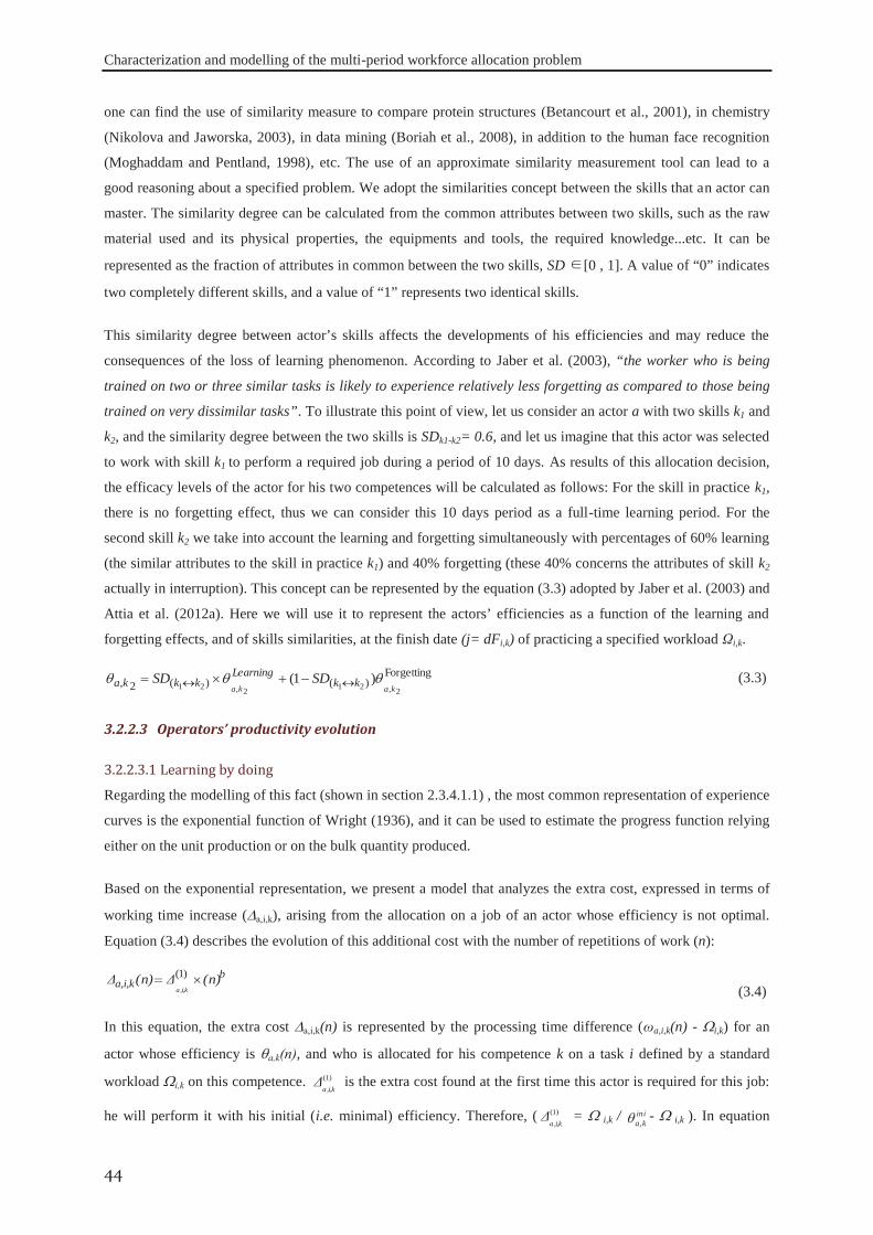
Characterization and modelling of the multi-period workforce allocation problem

44

one can find the use of similarity measure to compare protein structures (Betancourt et al., 2001), in chemistry

(Nikolova and Jaworska, 2003), in data mining (Boriah et al., 2008), in addition to the human face recognition

(Moghaddam and Pentland, 1998), etc. The use of an approximate similarity measurement tool can lead to a

good reasoning about a specified problem. We adopt the similarities concept between the skills that an actor can

master. The similarity degree can be calculated from the common attributes between two skills, such as the raw

material used and its physical properties, the equipments and tools, the required knowledge...etc. It can be

represented as the fraction of attributes in common between the two skills, SD [0 , 1]. A value of “0” indicates

two completely different skills, and a value of “1” represents two identical skills.

This similarity degree between actor’s skills affects the developments of his efficiencies and may reduce the

consequences of the loss of learning phenomenon. According to Jaber et al. (2003), “the worker who is being

trained on two or three similar tasks is likely to experience relatively less forgetting as compared to those being

trained on very dissimilar tasks”. To illustrate this point of view, let us consider an actor a with two skills k1 and

k2, and the similarity degree between the two skills is SDk1-k2= 0.6, and let us imagine that this actor was selected

to work with skill k1 to perform a required job during a period of 10 days. As results of this allocation decision,

the efficacy levels of the actor for his two competences will be calculated as follows: For the skill in practice k1,

there is no forgetting effect, thus we can consider this 10 days period as a full-time learning period. For the

second skill k2 we take into account the learning and forgetting simultaneously with percentages of 60% learning

(the similar attributes to the skill in practice k1) and 40% forgetting (these 40% concerns the attributes of skill k2

actually in interruption). This concept can be represented by the equation (3.3) adopted by Jaber et al. (2003) and

Attia et al. (2012a). Here we will use it to represent the actors’ efficiencies as a function of the learning and

forgetting effects, and of skills similarities, at the finish date (j= dFi,k) of practicing a specified workload Ωi,k.

Forgetting)()(2,

2,212,21)1(

kaka kkLearning

kkka SDSD (3.3)

3.2.2.3 Operators’ productivity evolution

3.2.2.3.1 Learning by doing

Regarding the modelling of this fact (shown in section 2.3.4.1.1) , the most common representation of experience

curves is the exponential function of Wright (1936), and it can be used to estimate the progress function relying

either on the unit production or on the bulk quantity produced.

Based on the exponential representation, we present a model that analyzes the extra cost, expressed in terms of

working time increase ( a,i,k), arising from the allocation on a job of an actor whose efficiency is not optimal.

Equation (3.4) describes the evolution of this additional cost with the number of repetitions of work (n):

ba,i,k (n)Δ(n)Δ

a,i,k

)1(

(3.4)

In this equation, the extra cost a,i,k(n) is represented by the processing time difference (ωa,i,k(n) - i,k) for an

actor whose efficiency is a,k(n), and who is allocated for his competence k on a task i defined by a standard

workload i,k on this competence. )1(

a,i,kΔ is the extra cost found at the first time this actor is required for this job:

he will perform it with his initial (i.e. minimal) efficiency. Therefore, ( )1(

a,i,kΔ = i,k / ini

ka,- i,k ). In equation

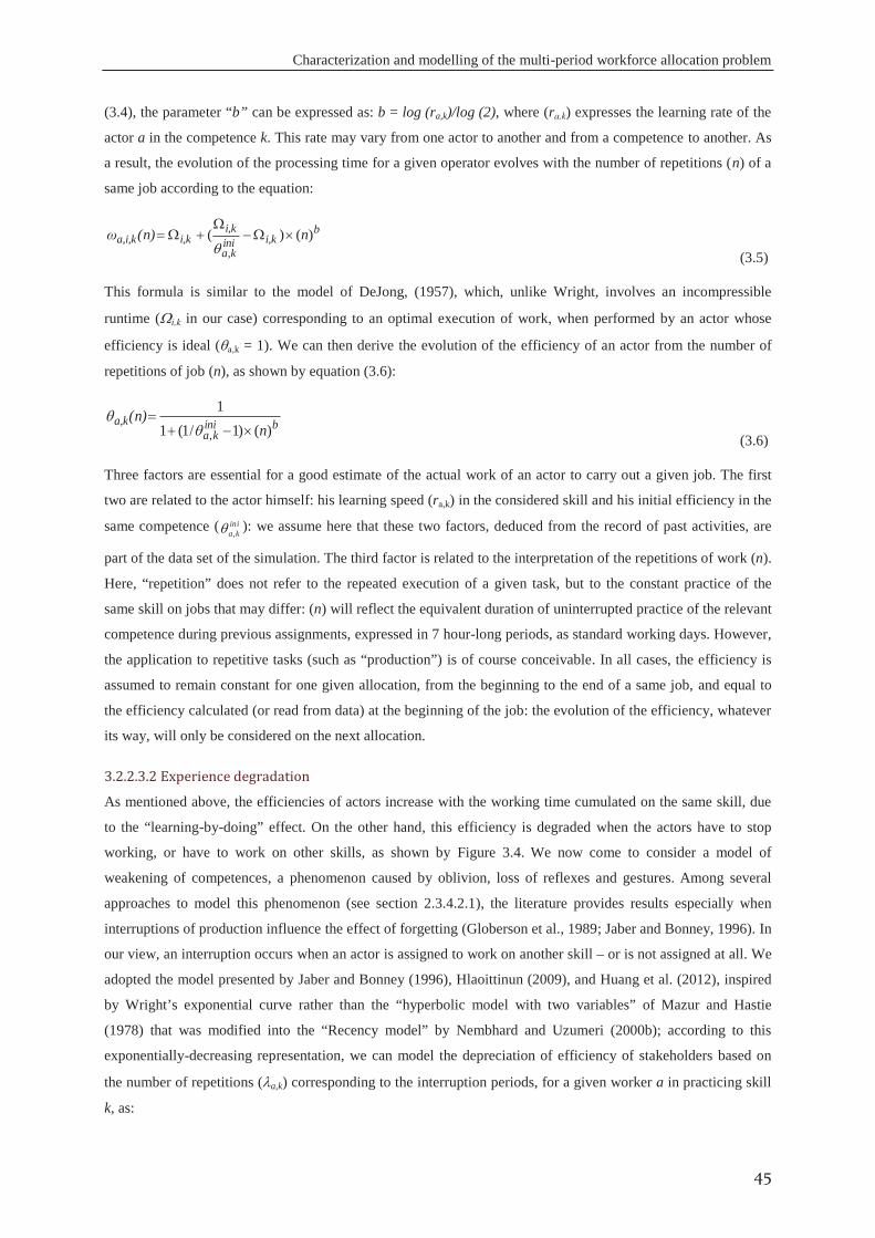
Characterization and modelling of the multi-period workforce allocation problem

45

(3.4), the parameter “b” can be expressed as: b = log (ra,k)/log (2), where (ra,k) expresses the learning rate of the

actor a in the competence k. This rate may vary from one actor to another and from a competence to another. As

a result, the evolution of the processing time for a given operator evolves with the number of repetitions (n) of a

same job according to the equation:

bi,kini

ka

i,ki,ka,i,k n(n)ω )()(

, (3.5)

This formula is similar to the model of DeJong, (1957), which, unlike Wright, involves an incompressible

runtime ( i,k in our case) corresponding to an optimal execution of work, when performed by an actor whose

efficiency is ideal ( a,k = 1). We can then derive the evolution of the efficiency of an actor from the number of

repetitions of job (n), as shown by equation (3.6):

binika

a,kn

(n))()1/1(1

1

, (3.6)

Three factors are essential for a good estimate of the actual work of an actor to carry out a given job. The first

two are related to the actor himself: his learning speed (ra,k) in the considered skill and his initial efficiency in the

same competence ( inika,): we assume here that these two factors, deduced from the record of past activities, are

part of the data set of the simulation. The third factor is related to the interpretation of the repetitions of work (n).

Here, “repetition” does not refer to the repeated execution of a given task, but to the constant practice of the

same skill on jobs that may differ: (n) will reflect the equivalent duration of uninterrupted practice of the relevant

competence during previous assignments, expressed in 7 hour-long periods, as standard working days. However,

the application to repetitive tasks (such as “production”) is of course conceivable. In all cases, the efficiency is

assumed to remain constant for one given allocation, from the beginning to the end of a same job, and equal to

the efficiency calculated (or read from data) at the beginning of the job: the evolution of the efficiency, whatever

its way, will only be considered on the next allocation.

3.2.2.3.2 Experience degradation

As mentioned above, the efficiencies of actors increase with the working time cumulated on the same skill, due

to the “learning-by-doing” effect. On the other hand, this efficiency is degraded when the actors have to stop

working, or have to work on other skills, as shown by Figure 3.4. We now come to consider a model of

weakening of competences, a phenomenon caused by oblivion, loss of reflexes and gestures. Among several

approaches to model this phenomenon (see section 2.3.4.2.1), the literature provides results especially when

interruptions of production influence the effect of forgetting (Globerson et al., 1989; Jaber and Bonney, 1996). In

our view, an interruption occurs when an actor is assigned to work on another skill – or is not assigned at all. We

adopted the model presented by Jaber and Bonney (1996), Hlaoittinun (2009), and Huang et al. (2012), inspired

by Wright’s exponential curve rather than the “hyperbolic model with two variables” of Mazur and Hastie

(1978) that was modified into the “Recency model” by Nembhard and Uzumeri (2000b); according to this

exponentially-decreasing representation, we can model the depreciation of efficiency of stakeholders based on

the number of repetitions ( a,k) corresponding to the interruption periods, for a given worker a in practicing skill

k, as:

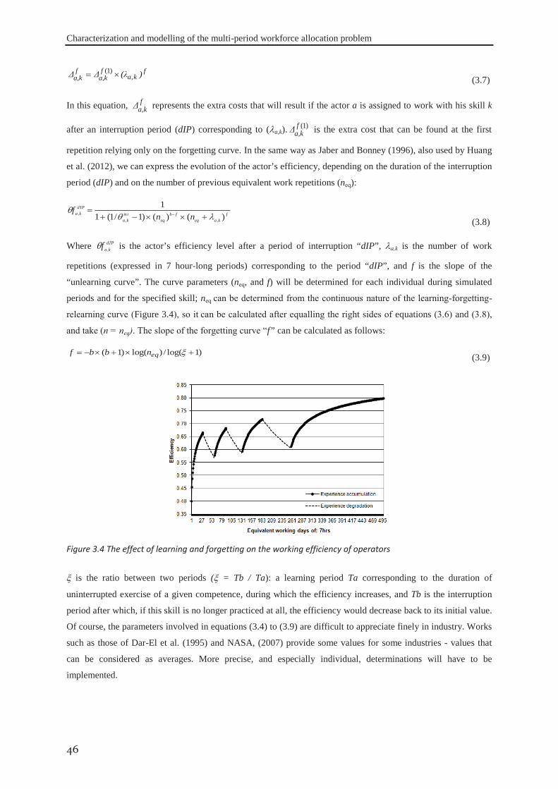
Characterization and modelling of the multi-period workforce allocation problem

46

fka

fa,k

fa,k )(λΔΔ ,

)1( (3.7)

In this equation, fa,kΔ represents the extra costs that will result if the actor a is assigned to work with his skill k

after an interruption period (dIP) corresponding to ( a,k). )1(fa,kΔ is the extra cost that can be found at the first

repetition relying only on the forgetting curve. In the same way as Jaber and Bonney (1996), also used by Huang

et al. (2012), we can express the evolution of the actor’s efficiency, depending on the duration of the interruption

period (dIP) and on the number of previous equivalent work repetitions (neq):

fkaeq

fbeq

inika

dIPka nn

f)()()1/1(1

1

,,,

(3.8)

Where dIPkaf , is the actor’s efficiency level after a period of interruption “dIP”, a,k is the number of work

repetitions (expressed in 7 hour-long periods) corresponding to the period “dIP”, and f is the slope of the

“unlearning curve”. The curve parameters (neq, and f) will be determined for each individual during simulated

periods and for the specified skill; neq can be determined from the continuous nature of the learning-forgetting-

relearning curve (Figure 3.4), so it can be calculated after equalling the right sides of equations (3.6) and (3.8),

and take (n = neq). The slope of the forgetting curve “f” can be calculated as follows:

)1log(/)log()1( eqnbbf (3.9)

Figure 3.4 The effect of learning and forgetting on the working efficiency of operators

is the ratio between two periods ( = Tb / Ta): a learning period Ta corresponding to the duration of

uninterrupted exercise of a given competence, during which the efficiency increases, and Tb is the interruption

period after which, if this skill is no longer practiced at all, the efficiency would decrease back to its initial value.

Of course, the parameters involved in equations (3.4) to (3.9) are difficult to appreciate finely in industry. Works

such as those of Dar-El et al. (1995) and NASA, (2007) provide some values for some industries - values that

can be considered as averages. More precise, and especially individual, determinations will have to be

implemented.

Characterization and modelling of the multi-period workforce allocation problem

47

The present project scheduling and workforce allocation problem can be presented as follows: A project consists

in a set I of unique and original tasks with predefined temporal relations. Each task i I requires a given set of

skills for its execution, taken within a group K of all the skills, present in the company. Each of these

competence-specific jobs that build up the task will require a specified workload. On another side, we consider

set A of human resources; each individual or actor “a” from these resources is able to perform one or more

competence(s) “nka” from the set K, with a dynamic time-dependent performance. i.e., we consider the actors as

multi-skilled. For each actor “a”, we have a value, known as his efficiency θa,k(n) that indicates his performance

for practicing a given competence “k”. This efficiency is a real number θa,k(n) [0,1] varying with time

according to the previous allocations represented by the work repetitions “n”. Moreover, the efficiency is each

actor’s one, and is measured for each skill k that he practices: it is therefore natural to find, for one given actor

with two skills k and k', that a,k ≠ a,k'. In order to make our model more similar to industrial reality, we

introduced for each skill k a lower limit of efficiency θkmin below which an assignment will not be considered

acceptable, for economic or quality reasons: θa,k(n) [θkmin,1]. If the actor has an efficiency θa,k(n) = 1, then this

actor can be considered as expert with nominal competence in the skill “k”. So when this actor is allocated for

this skill on a given job, he will perform his work in the standard job’s duration, whereas other actors, whose

efficiencies are lower than unity for this skill, will require a longer working time. While the activity is being

processed, competence k of a task i requires a workload Ωi,k. For this execution process, if the actor is considered

as an expert (i.e. θa,k(n) = 1) then the actual execution time ωi,k equals the standard one, thus ωi,k = Ωi,k . But, in

the other case when an actor is assigned, for whom θa,k(n) < 1, then the actual work will be ωi,k = Ωi,k / θa,k(n) >

Ωi,k, resulting in an increase of both execution time and labour cost. As we have seen, the efficiency of an

operator determines the effective working time needed to achieve a standard defined workload: the actual

execution time (di,k) required in the competence k for the task i is not predetermined, but results from the

previous allocations of the actors chosen. In addition to the multi-skill, we consider that the company is managed

according to a working time modulation strategy: i.e. the timetables of its employees may be changed according

to the required workloads to be executed.

Thus, we aim simultaneously at optimizing a set of objectives while respecting a vast number of constraints: this

leads to a huge optimization and project scheduling problem. The mathematical model (objectives and

constraints) is presented by the following.

First the objective function, we wish to minimize the sum of four terms of costs (f1,..., f4), in addition to the

maximization of a virtual profit function (f5):

Minimize: F= f1 + f2 + f3 + f4 - f5 (3.10)

3.3 PROJECT SCHEDULING WITH WORKFORCE ALLOCATION OPTIMIZATION PROBLEM

3.3.1 Problem representation

3.3.2 Modelling of problem objectives

Characterization and modelling of the multi-period workforce allocation problem

48

3.3.2.1 Direct labour standard costs

The first objective (f1) represents the actual cost of work executed during “normal opening” hours, with a

standard hourly cost “Ua”. Knowing that, SSW and respectively SFW are respectively the start week and the finish

week of the project, ωsa,s is the work scheduled for the worker a during the week s in hours.

A

a

S

Sssaa

FW

SW

sUf1

,1

(3.10-a)

3.3.2.2 Direct labour over costs

The second objective is the excess cost due to overtime (f2), which is added to the cost of normal hours (f1) in

order to determine the labour direct cost. It is determined by applying a multiplier “u” to standard hourly cost.

According to the French law this multiplier can be estimated at 25% of the standard working hourly rates. The

actor’s weekly overtime (HSa,s: overtime of actor a during week s) can be rewarded by either money or time off,

or combination of both. Without loss of generality, here we considered only the money-compensated way. The

implementation of other rewarding method can be directly implemented by subtracting the temporal

compensation hours from the yearly remaining number of working hours for the worker considered. The

overtime is calculated according to the company-level agreement.

A

a

S

Sssaa

FW

SW

HSuUf1

,2

(3.10-b)

3.3.2.3 Cost associated to loss of temporal flexibility

The third objective (f3) is a virtual cost associated to the loss of temporal flexibility (the future working capacity)

of the actors at the end of the simulation horizon. In this equation, the cost derives from the weekly occupancy

rates of the actors, compared to the standard duration of work per week “CS0”; this term f3 is intended to

distinguish and favour solutions involving the minimum effort for a given load – i.e. it is intended to preserve the

future flexibility of the company (Attia et al., 2012c). Considering that UFa is the virtual value associated with

the residual flexibility of the actor a, in monetary units (real number), and NW is the cardinality of the set of

project working weeks.

FWSWA

a

S

Ss S

saa S, ..., Swhere: NW

CNWs

UFfFW

SW

, 11 0

,3

(3.10-c)

3.3.2.4 Project due date earliest/tardiness associated costs

As discussed in section (3.1.3), a penalty is associated to the completion of a work outside of its tolerance range

(Vidal et al., 1999), resulting either from storage costs (or financial immobilization) or from payment of

penalties for late; the objective (f4) can be calculated from the difference between the actual duration “LV” of the

project and its contract term “L”, compared to a tolerance window [L - , L + ], where is the a negotiable

temporal tolerance, or grace period.

LLVLLLVLLV

LLVULf

f

LVLjL

if,

0

11 )(

4

(3.10-d)

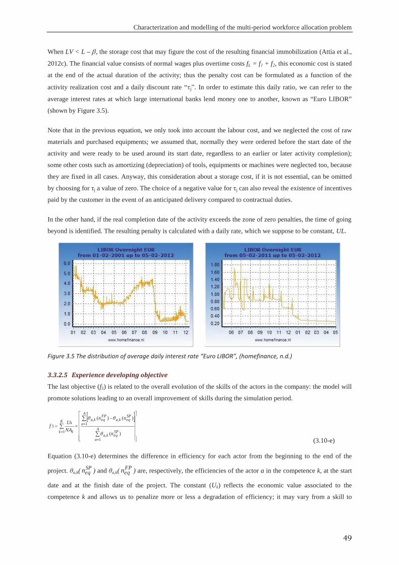
Characterization and modelling of the multi-period workforce allocation problem

49

When LV < L – , the storage cost that may figure the cost of the resulting financial immobilization (Attia et al.,

2012c). The financial value consists of normal wages plus overtime costs fL = f1 + f2, this economic cost is stated

at the end of the actual duration of the activity; thus the penalty cost can be formulated as a function of the

activity realization cost and a daily discount rate “ j”. In order to estimate this daily ratio, we can refer to the

average interest rates at which large international banks lend money one to another, known as “Euro LIBOR”

(shown by Figure 3.5).

Note that in the previous equation, we only took into account the labour cost, and we neglected the cost of raw

materials and purchased equipments; we assumed that, normally they were ordered before the start date of the

activity and were ready to be used around its start date, regardless to an earlier or later activity completion);

some other costs such as amortizing (depreciation) of tools, equipments or machines were neglected too, because

they are fixed in all cases. Anyway, this consideration about a storage cost, if it is not essential, can be omitted

by choosing for τj a value of zero. The choice of a negative value for τj can also reveal the existence of incentives

paid by the customer in the event of an anticipated delivery compared to contractual duties.

In the other hand, if the real completion date of the activity exceeds the zone of zero penalties, the time of going

beyond is identified. The resulting penalty is calculated with a daily rate, which we suppose to be constant, UL.

Figure 3.5 The distribution of average daily interest rate “Euro LIBOR”, (homefinance, n.d.)

3.3.2.5 Experience developing objective

The last objective (f5) is related to the overall evolution of the skills of the actors in the company: the model will

promote solutions leading to an overall improvement of skills during the simulation period.

K

k A

a

SPeqka

A

a

SPeqka

FPeqka

k

k

n

nn

NAUf

1

1,

1,,

5

)(

)()(

(3.10-e)

Equation (3.10-e) determines the difference in efficiency for each actor from the beginning to the end of the

project. θa,k( SPeqn ) and θa,k( FP

eqn ) are, respectively, the efficiencies of the actor a in the competence k, at the start

date and at the finish date of the project. The constant (Uk) reflects the economic value associated to the

competence k and allows us to penalize more or less a degradation of efficiency; it may vary from a skill to

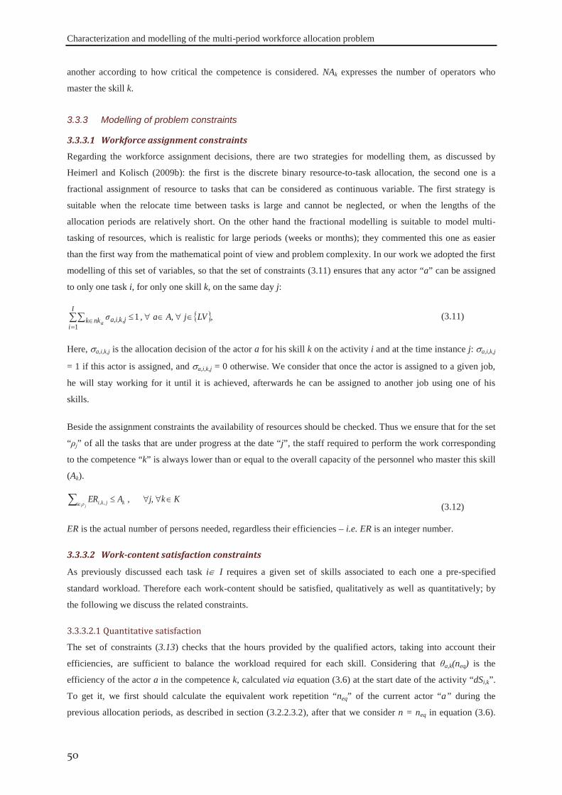
Characterization and modelling of the multi-period workforce allocation problem

50

another according to how critical the competence is considered. NAk expresses the number of operators who

master the skill k.

3.3.3.1 Workforce assignment constraints

Regarding the workforce assignment decisions, there are two strategies for modelling them, as discussed by

Heimerl and Kolisch (2009b): the first is the discrete binary resource-to-task allocation, the second one is a

fractional assignment of resource to tasks that can be considered as continuous variable. The first strategy is

suitable when the relocate time between tasks is large and cannot be neglected, or when the lengths of the

allocation periods are relatively short. On the other hand the fractional modelling is suitable to model multi-

tasking of resources, which is realistic for large periods (weeks or months); they commented this one as easier

than the first way from the mathematical point of view and problem complexity. In our work we adopted the first

modelling of this set of variables, so that the set of constraints (3.11) ensures that any actor “a” can be assigned

to only one task i, for only one skill k, on the same day j:

,11

VL jA, a, σI

inkk a,i,k,ja

(3.11)

Here, a,i,k,j is the allocation decision of the actor a for his skill k on the activity i and at the time instance j: a,i,k,j

= 1 if this actor is assigned, and a,i,k,j = 0 otherwise. We consider that once the actor is assigned to a given job,

he will stay working for it until it is achieved, afterwards he can be assigned to another job using one of his

skills.

Beside the assignment constraints the availability of resources should be checked. Thus we ensure that for the set

“ρj” of all the tasks that are under progress at the date “j”, the staff required to perform the work corresponding

to the competence “k” is always lower than or equal to the overall capacity of the personnel who master this skill

(Ak).

Kkj, AER ki jkij

,,, (3.12)

ER is the actual number of persons needed, regardless their efficiencies – i.e. ER is an integer number.

3.3.3.2 Work-content satisfaction constraints

As previously discussed each task i I requires a given set of skills associated to each one a pre-specified

standard workload. Therefore each work-content should be satisfied, qualitatively as well as quantitatively; by

the following we discuss the related constraints.

3.3.3.2.1 Quantitative satisfaction

The set of constraints (3.13) checks that the hours provided by the qualified actors, taking into account their

efficiencies, are sufficient to balance the workload required for each skill. Considering that θa,k(neq) is the

efficiency of the actor a in the competence k, calculated via equation (3.6) at the start date of the activity “dSi,k”.

To get it, we first should calculate the equivalent work repetition “neq” of the current actor “a” during the

previous allocation periods, as described in section (3.2.2.3.2), after that we consider n = neq in equation (3.6).

3.3.3 Modelling of problem constraints

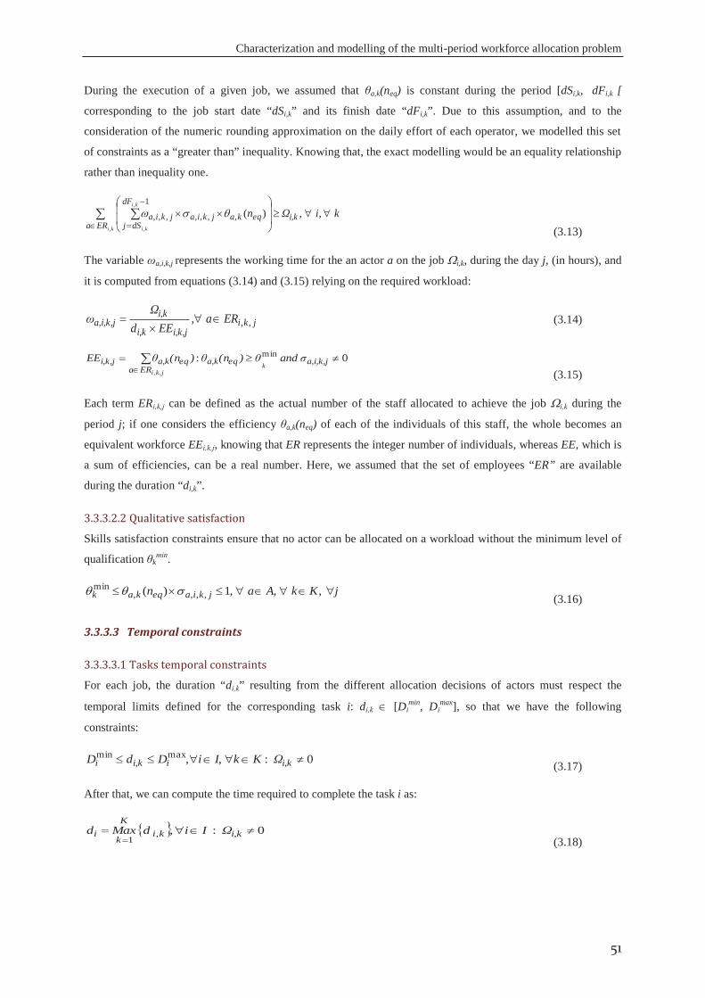
Characterization and modelling of the multi-period workforce allocation problem

51

During the execution of a given job, we assumed that θa,k(neq) is constant during the period [dSi,k, dFi,k [

corresponding to the job start date “dSi,k” and its finish date “dFi,k”. Due to this assumption, and to the

consideration of the numeric rounding approximation on the daily effort of each operator, we modelled this set

of constraints as a “greater than” inequality. Knowing that, the exact modelling would be an equality relationship

rather than inequality one.

k i, , Ωn i,kERa

dF

dSjeqkajkiajkia

ki

ki

ki,

,

,

1

,,,,,,, )(

(3.13)

The variable ωa,i,k,j represents the working time for the an actor a on the job i,k, during the day j, (in hours), and

it is computed from equations (3.14) and (3.15) relying on the required workload:

jkii,k,ji,k

i,ka,i,k,j ER a,

EEdΩ

ω ,, (3.14)

0 : mina,i,k,jeqa,k

ERaeqa,ki,k,j and σθ)(nθ)(nθEE

ki,k,j (3.15)

Each term ERi,k,j can be defined as the actual number of the staff allocated to achieve the job i,k during the

period j; if one considers the efficiency θa,k(neq) of each of the individuals of this staff, the whole becomes an

equivalent workforce EEi,k,j, knowing that ER represents the integer number of individuals, whereas EE, which is

a sum of efficiencies, can be a real number. Here, we assumed that the set of employees “ER” are available

during the duration “di,k”.

3.3.3.2.2 Qualitative satisfaction

Skills satisfaction constraints ensure that no actor can be allocated on a workload without the minimum level of

qualification θkmin.

j K kA, a, n jkiaeqkak ,1)( ,,,,min

(3.16)

3.3.3.3 Temporal constraints

3.3.3.3.1 Tasks temporal constraints

For each job, the duration “di,k” resulting from the different allocation decisions of actors must respect the

temporal limits defined for the corresponding task i: di,k [Dimin, Di

max], so that we have the following

constraints:

0: maxmini,kii,ki ΩKkI, i,DdD (3.17)

After that, we can compute the time required to complete the task i as:

0: , ,1

i,kkiK

ki ΩI idMaxd

(3.18)

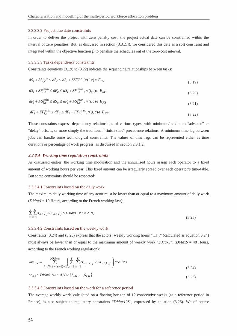
Characterization and modelling of the multi-period workforce allocation problem

52

3.3.3.3.2 Project due date constraints

In order to deliver the project with zero penalty cost, the project actual date can be constrained within the

interval of zero penalties. But, as discussed in section (3.3.2.4), we considered this date as a soft constraint and

integrated within the objective function f4 to penalise the schedules out of the zero-cost interval.

3.3.3.3.3 Tasks dependency constraints

Constraints equations (3.19) to (3.22) indicate the sequencing relationships between tasks:

SSciiccii EciSSdSdSSSdS ),( , max,

min, (3.19)

SFciiccii EciSFdSdFSFdS ),( , max,

min, (3.20)

FSciiccii EciFSdFdSFSdF ),( , max,

min, (3.21)

FFciiccii EciFFdFdFFFdF ),( , max,

min, (3.22)

These constraints express dependency relationships of various types, with minimum/maximum “advance” or

“delay” offsets, or more simply the traditional “finish-start” precedence relations. A minimum time lag between

jobs can handle some technological constraints. The values of time lags can be represented either as time

durations or percentage of work progress, as discussed in section 2.3.1.2.

3.3.3.4 Working time regulation constraints

As discussed earlier, the working time modulation and the annualised hours assign each operator to a fixed

amount of working hours per year. This fixed amount can be irregularly spread over each operator’s time-table.

But some constraints should be respected:

3.3.3.4.1 Constraints based on the daily work

The maximum daily working time of any actor must be lower than or equal to a maximum amount of daily work

(DMaxJ = 10 Hours, according to the French working law):

jDMaxJI

i

K

kjkiajkia A,a ,

1 1,,,,,,

(3.23)

3.3.3.4.2 Constraints based on the weekly work

Constraints (3.24) and (3.25) express that the actors’ weekly working hours “ωsa,s” (calculated as equation 3.24)

must always be lower than or equal to the maximum amount of weekly work “DMaxS”: (DMaxS = 48 Hours,

according to the French working regulation):

s ,,1)1( 1 1

,,,,,,, assNJS

sNJSj

I

i

K

kjkiajkiasa

(3.24)

FWSWsa S, ..., SAaDMaxSs s ,,, (3.25)

3.3.3.4.3 Constraints based on the work for a reference period

The average weekly work, calculated on a floating horizon of 12 consecutive weeks (as a reference period in

France), is also subject to regulatory constraints “DMax12S”, expressed by equation (3.26). We of course

Characterization and modelling of the multi-period workforce allocation problem

53

assumed that the data about operators’ working time on activities performed before our simulation window have

been properly recorded and are available at any time. These data should be included in the data file concerning

the company (Attia et al., 2012c).

FWSW p

s

spa,p S, ..., SA, and a, SDMaxωs s12

121

111 (3.26)

3.3.3.4.4 Constraints based on the annual work

The set of constraints equation (3.27) guarantees that for each actor, the total number of working hours for the

current activity is always below his yearly quota “DSA”. Here “ωpa” represents the working hours of the actor a

on other previous activities during the considered year, and “DSA” is the maximum number of annual working

hours of each actor.

AapDSAs aS

Sssa

FW

SW

,, (3.27)

3.3.3.4.5 Constraints based on overtime

Finally, we have to compute for each operator the weekly overtime “HS” as equation (3.28). Every actor has for

each week “s” a number of overtime hours (HSa,s). Knowing that, DMaxMod represents the maximum weekly

standard work (i.e. “non-overtime”), according to internal modulation and agreements adopted by the company.

These overtime hours must verify that HSa,s [0, DMaxS - DMaxMod]. Here we assume that the actual amount

of overtime hours already performed by any operator on previous activities “HSPa” are available. Equation

(3.29) checks that overtime on our project always respect an annual limit “HSA” for each actor:

FWSWsa,sa,

sa, S ,..,Ss A,a , otherwise0

DMaxModωsifDMaxModωsHS

(3.28)

Aa,HSPHSAHS aS

Ssa,s

FW

SW (3.29)

A mathematical model is an abstraction which uses the mathematical language to describe a natural phenomenon

or objects’ behaviour. The basic ingredient to construct any mathematical model is the set of the variables and

the interactions between them to formulate the goals and restrictions. After the declaration phase of variables,

they can be classified according to many properties such as: – The dependency: dependent or independent on

each others. – The expected value of the variable: deterministic or probabilistic. – The nature of their domain

that can contain real, binary, or integer numbers. –The variation with the temporal axis; it can be static, or

change dynamically. Moreover, they can be classified according to the discrete or continuous nature along the

temporal axis. On the other side the way that these variables interact with each others represents the linearity of

the model: linear or nonlinear model. So by the following we present the analytical description of the proposed

model.

3.4 MODEL ANALYSIS

Characterization and modelling of the multi-period workforce allocation problem

54

For any problem analysis, one needs to define first the problem unknown variables, variables’ domains with a

finite set of possible values. These values can be assigned to the corresponding variable, considering some

relations with other dependent or independent variables. As shown in (Table 3.1) we listed a set of unknown

variables of the problem. The problem decision variables can be represented by the independent variables: ( a,i,k,j,

dSi , ωa,i,k,j), respectively the workers assignment decisions, the activities start dates, and the amount of working

hours per day for each worker. Referring to equation (3.1) the jobs durations di,k can be selected as decision

variables rather than the workers daily amount of work: this selection can be suitable for solving the static model

of this problem with constraints programming for example, with constant ωa,i,k,j during di,k . But here, and due to

the dynamic nature of some data we consider, we are motivated to solve it with meta-heuristic (see chapter 5).

Therefore, we adopted the selection of “ωa,i,k,j” as a decision variable in order to reduce the representation length

of the problem. All the other unknown variables dependent on these selected decision variables, with linear or

nonlinear dependency relations, as shown by (Table 3.1).

For each known or unknown variable there is an expected value. This value can be either deterministic or

probabilistic. The deterministic variables are the set of all variables that have given expected values, knowing the

input states of their independent variables. In contrast, the probabilistic variables represent the set of the

variables whose expected values depend on the chance or probabilities. All the unknown and known variables of

(Table 3.1 and Table 3.2) can be considered as deterministic variables except the problem decision variables, and

the workers parameters as their speed of learning (ra,k) and the maximum interruption period after which, the

efficiency of a given worker has decreased back to its initial value (Tb). For the later variables (ra,k), and (Tb), we

assumed a deterministic case. Therefore, this model can be classified as a deterministic rather than stochastic

one.

In order to solve the optimisation problems, the domain of each variable should be defined. The variable domain

represents the set of values that it can take. The domain of each unknown variables in the current model is listed

in the domain column in (Table 3.1); in addition in (Table 3.2) the expected values of the known variables

(assumed to be given) are listed. The natures of the domains of variables normally overcome the method used to

solve the problem, furthermore it can increase the complexity of solving it. As example the problems with

continuous variables can be considered as easier to be optimally solved especially for linear relations. But it

can’t be solved with some exact methods as for example branch and X (bound, infer,...).

Table 3.1 Model unknown variables and their characteristics.

3.4.1 Variables dependency investigation

3.4.2 Variables expected values

3.4.3 Variable domain investigations

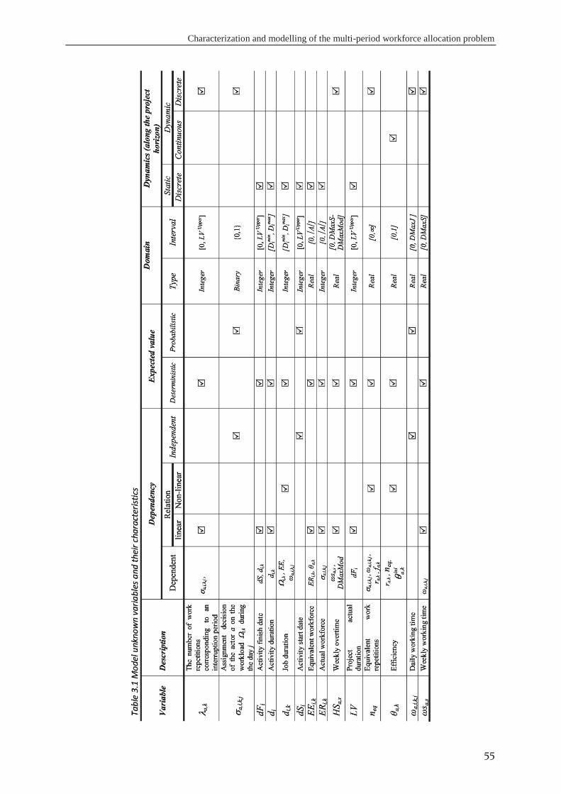
Characterization and modelling of the multi-period workforce allocation problem

55

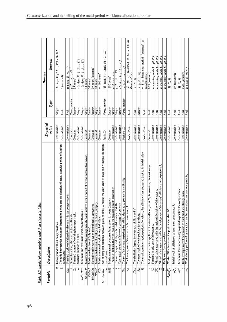
Characterization and modelling of the multi-period workforce allocation problem

56

Table 3.2 model given variables and their characteristics

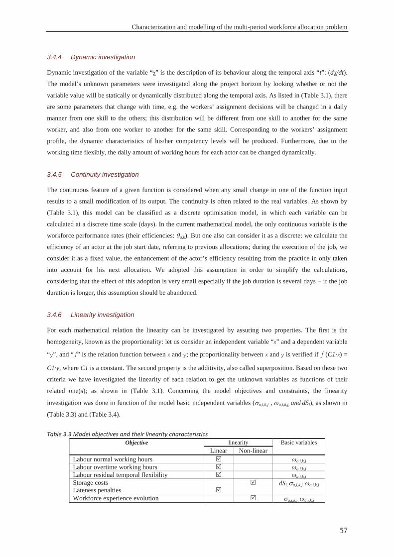
Characterization and modelling of the multi-period workforce allocation problem

57

Dynamic investigation of the variable “χ” is the description of its behaviour along the temporal axis “t”: (dχ/dt).

The model’s unknown parameters were investigated along the project horizon by looking whether or not the

variable value will be statically or dynamically distributed along the temporal axis. As listed in (Table 3.1), there

are some parameters that change with time, e.g. the workers’ assignment decisions will be changed in a daily

manner from one skill to the others; this distribution will be different from one skill to another for the same

worker, and also from one worker to another for the same skill. Corresponding to the workers’ assignment

profile, the dynamic characteristics of his/her competency levels will be produced. Furthermore, due to the

working time flexibly, the daily amount of working hours for each actor can be changed dynamically.

The continuous feature of a given function is considered when any small change in one of the function input

results to a small modification of its output. The continuity is often related to the real variables. As shown by

(Table 3.1), this model can be classified as a discrete optimisation model, in which each variable can be

calculated at a discrete time scale (days). In the current mathematical model, the only continuous variable is the

workforce performance rates (their efficiencies: θa,k). But one also can consider it as a discrete: we calculate the

efficiency of an actor at the job start date, referring to previous allocations; during the execution of the job, we

consider it as a fixed value, the enhancement of the actor’s efficiency resulting from the practice in only taken

into account for his next allocation. We adopted this assumption in order to simplify the calculations,

considering that the effect of this adoption is very small especially if the job duration is several days – if the job

duration is longer, this assumption should be abandoned.

For each mathematical relation the linearity can be investigated by assuring two properties. The first is the

homogeneity, known as the proportionality: let us consider an independent variable “x” and a dependent variable

“y”, and “f” is the relation function between x and y; the proportionality between x and y is verified if f (C1·x) =

C1·y, where C1 is a constant. The second property is the additivity, also called superposition. Based on these two

criteria we have investigated the linearity of each relation to get the unknown variables as functions of their

related one(s); as shown in (Table 3.1). Concerning the model objectives and constraints, the linearity

investigation was done in function of the model basic independent variables ( a,i,k,j , ωa,i,k,j, and dSi), as shown in

(Table 3.3) and (Table 3.4).

Table 3.3 Model objectives and their linearity characteristics Objective linearity Basic variables

Linear Non-linear Labour normal working hours ωa,i,k,j Labour overtime working hours ωa,i,k,j Labour residual temporal flexibility ωa,i,k,j Storage costs Lateness penalties

dSi, a,i,k,j, ωa,i,k,j

Workforce experience evolution a,i,k,j, ωa,i,k,j

3.4.4 Dynamic investigation

3.4.5 Continuity investigation

3.4.6 Linearity investigation

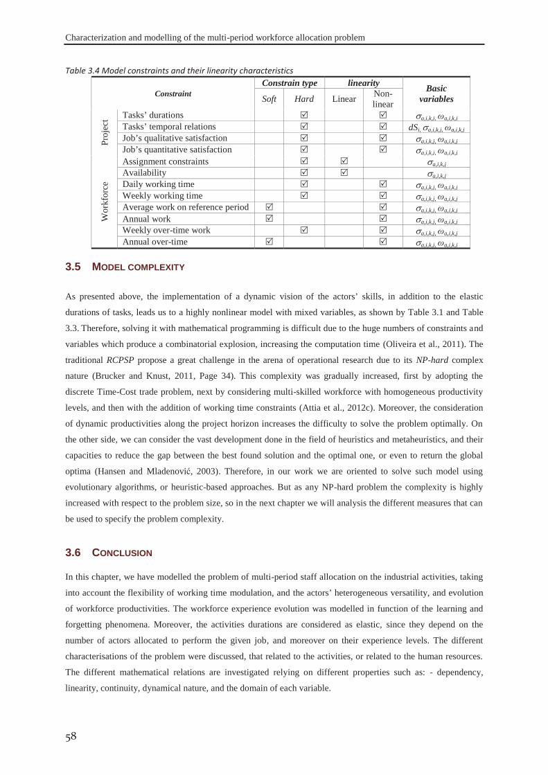
Characterization and modelling of the multi-period workforce allocation problem

58

Table 3.4 Model constraints and their linearity characteristics

Constraint Constrain type linearity Basic

variables Soft Hard Linear Non-linear

Proj

ect Tasks’ durations a,i,k,j, ωa,i,k,j

Tasks’ temporal relations dSi, a,i,k,j, ωa,i,k,j Job’s qualitative satisfaction a,i,k,j, ωa,i,k,j Job’s quantitative satisfaction a,i,k,j, ωa,i,k,j

Wor

kfor

ce

Assignment constraints a,i,k,j Availability a,i,k,j Daily working time a,i,k,j, ωa,i,k,j Weekly working time a,i,k,j, ωa,i,k,j Average work on reference period a,i,k,j, ωa,i,k,j Annual work a,i,k,j, ωa,i,k,j Weekly over-time work a,i,k,j, ωa,i,k,j Annual over-time a,i,k,j, ωa,i,k,j

As presented above, the implementation of a dynamic vision of the actors’ skills, in addition to the elastic

durations of tasks, leads us to a highly nonlinear model with mixed variables, as shown by Table 3.1 and Table

3.3. Therefore, solving it with mathematical programming is difficult due to the huge numbers of constraints and

variables which produce a combinatorial explosion, increasing the computation time (Oliveira et al., 2011). The

traditional RCPSP propose a great challenge in the arena of operational research due to its NP-hard complex

nature (Brucker and Knust, 2011, Page 34). This complexity was gradually increased, first by adopting the

discrete Time-Cost trade problem, next by considering multi-skilled workforce with homogeneous productivity

levels, and then with the addition of working time constraints (Attia et al., 2012c). Moreover, the consideration

of dynamic productivities along the project horizon increases the difficulty to solve the problem optimally. On

the other side, we can consider the vast development done in the field of heuristics and metaheuristics, and their

capacities to reduce the gap between the best found solution and the optimal one, or even to return the global

optima (Hansen and Mladenović, 2003). Therefore, in our work we are oriented to solve such model using

evolutionary algorithms, or heuristic-based approaches. But as any NP-hard problem the complexity is highly

increased with respect to the problem size, so in the next chapter we will analysis the different measures that can

be used to specify the problem complexity.

In this chapter, we have modelled the problem of multi-period staff allocation on the industrial activities, taking

into account the flexibility of working time modulation, and the actors’ heterogeneous versatility, and evolution

of workforce productivities. The workforce experience evolution was modelled in function of the learning and

forgetting phenomena. Moreover, the activities durations are considered as elastic, since they depend on the

number of actors allocated to perform the given job, and moreover on their experience levels. The different

characterisations of the problem were discussed, that related to the activities, or related to the human resources.

The different mathematical relations are investigated relying on different properties such as: - dependency,

linearity, continuity, dynamical nature, and the domain of each variable.

3.5 MODEL COMPLEXITY

3.6 CONCLUSION

4 PROJECT CHARACTERISTICS AND COMPLEXITY

ASSESSMENT RELYING ON PRINCIPAL COMPONENT

ANALYSIS

This chapter seeks to characterize different projects in terms of complexity, and

to sort them through the use of the smallest number of measures as possible.

Therefore, the different parameters related to each of the dimensions according

to which the complexity of a given project could be linked will be presented and

quantified. For each dimension, a sensitive quantifier will be selected. After that

and in order to reduce the number of the project correlated dimensions, a

principal component analysis and cluster analysis will be performed. By the end

of this chapter, the resulting smallest number of measures will be presented,

that explain most of the variance amongst the different instances.

CH

APT

ER

4

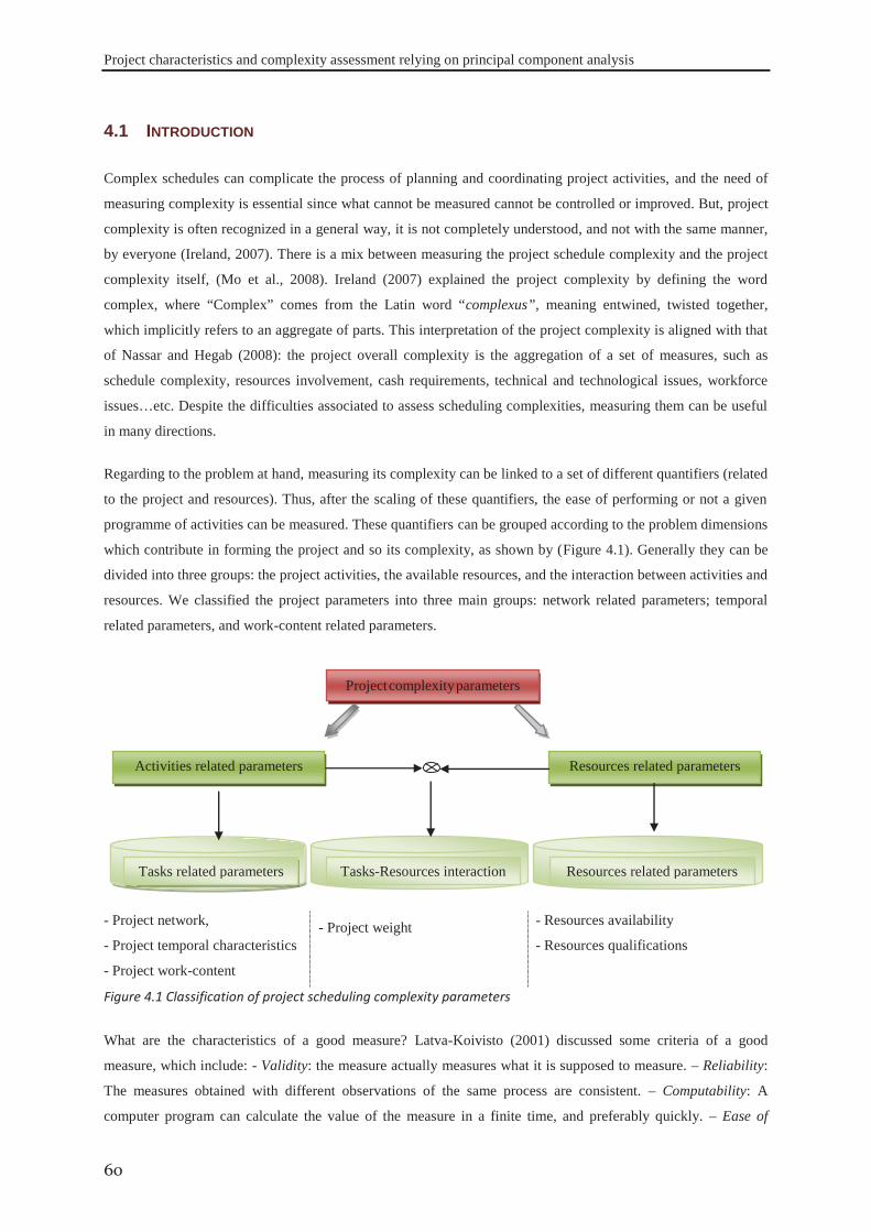
Project characteristics and complexity assessment relying on principal component analysis

60

Complex schedules can complicate the process of planning and coordinating project activities, and the need of

measuring complexity is essential since what cannot be measured cannot be controlled or improved. But, project

complexity is often recognized in a general way, it is not completely understood, and not with the same manner,

by everyone (Ireland, 2007). There is a mix between measuring the project schedule complexity and the project

complexity itself, (Mo et al., 2008). Ireland (2007) explained the project complexity by defining the word

complex, where “Complex” comes from the Latin word “complexus”, meaning entwined, twisted together,

which implicitly refers to an aggregate of parts. This interpretation of the project complexity is aligned with that

of Nassar and Hegab (2008): the project overall complexity is the aggregation of a set of measures, such as

schedule complexity, resources involvement, cash requirements, technical and technological issues, workforce

issues…etc. Despite the difficulties associated to assess scheduling complexities, measuring them can be useful

in many directions.

Regarding to the problem at hand, measuring its complexity can be linked to a set of different quantifiers (related

to the project and resources). Thus, after the scaling of these quantifiers, the ease of performing or not a given

programme of activities can be measured. These quantifiers can be grouped according to the problem dimensions

which contribute in forming the project and so its complexity, as shown by (Figure 4.1). Generally they can be

divided into three groups: the project activities, the available resources, and the interaction between activities and

resources. We classified the project parameters into three main groups: network related parameters; temporal

related parameters, and work-content related parameters.

- Project network,

- Project temporal characteristics

- Project work-content

- Project weight - Resources availability

- Resources qualifications

Figure 4.1 Classification of project scheduling complexity parameters

What are the characteristics of a good measure? Latva-Koivisto (2001) discussed some criteria of a good

measure, which include: - Validity: the measure actually measures what it is supposed to measure. – Reliability:

The measures obtained with different observations of the same process are consistent. – Computability: A

computer program can calculate the value of the measure in a finite time, and preferably quickly. – Ease of

4.1 INTRODUCTION

Tasks-Resources interaction Tasks related parameters Resources related parameters

Activities related parameters Resources related parameters

Project complexity parameters

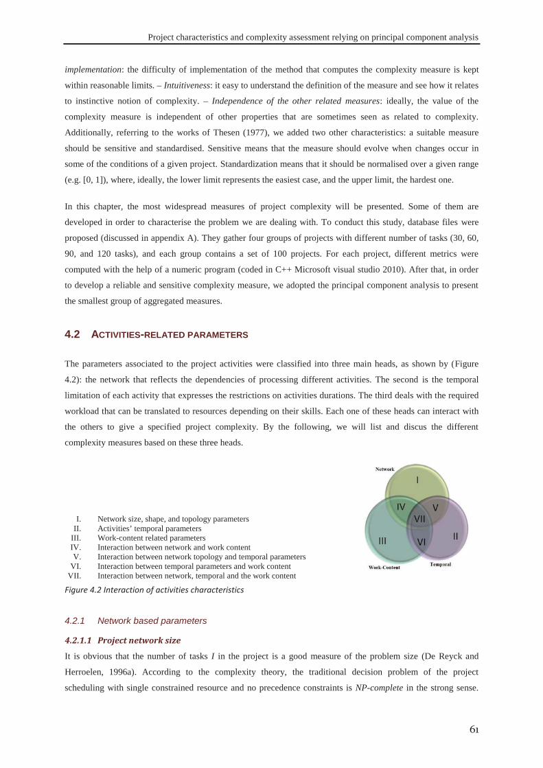
Project characteristics and complexity assessment relying on principal component analysis

61

implementation: the difficulty of implementation of the method that computes the complexity measure is kept

within reasonable limits. – Intuitiveness: it easy to understand the definition of the measure and see how it relates

to instinctive notion of complexity. – Independence of the other related measures: ideally, the value of the

complexity measure is independent of other properties that are sometimes seen as related to complexity.

Additionally, referring to the works of Thesen (1977), we added two other characteristics: a suitable measure

should be sensitive and standardised. Sensitive means that the measure should evolve when changes occur in

some of the conditions of a given project. Standardization means that it should be normalised over a given range

(e.g. [0, 1]), where, ideally, the lower limit represents the easiest case, and the upper limit, the hardest one.

In this chapter, the most widespread measures of project complexity will be presented. Some of them are

developed in order to characterise the problem we are dealing with. To conduct this study, database files were

proposed (discussed in appendix A). They gather four groups of projects with different number of tasks (30, 60,

90, and 120 tasks), and each group contains a set of 100 projects. For each project, different metrics were

computed with the help of a numeric program (coded in C++ Microsoft visual studio 2010). After that, in order

to develop a reliable and sensitive complexity measure, we adopted the principal component analysis to present

the smallest group of aggregated measures.

The parameters associated to the project activities were classified into three main heads, as shown by (Figure

4.2): the network that reflects the dependencies of processing different activities. The second is the temporal

limitation of each activity that expresses the restrictions on activities durations. The third deals with the required

workload that can be translated to resources depending on their skills. Each one of these heads can interact with

the others to give a specified project complexity. By the following, we will list and discus the different

complexity measures based on these three heads.

I. Network size, shape, and topology parameters II. Activities’ temporal parameters

III. Work-content related parameters IV. Interaction between network and work content V. Interaction between network topology and temporal parameters

VI. Interaction between temporal parameters and work content VII. Interaction between network, temporal and the work content

Figure 4.2 Interaction of activities characteristics

4.2.1.1 Project network size

It is obvious that the number of tasks I in the project is a good measure of the problem size (De Reyck and

Herroelen, 1996a). According to the complexity theory, the traditional decision problem of the project

scheduling with single constrained resource and no precedence constraints is NP-complete in the strong sense.

4.2 ACTIVITIES-RELATED PARAMETERS

4.2.1 Network based parameters

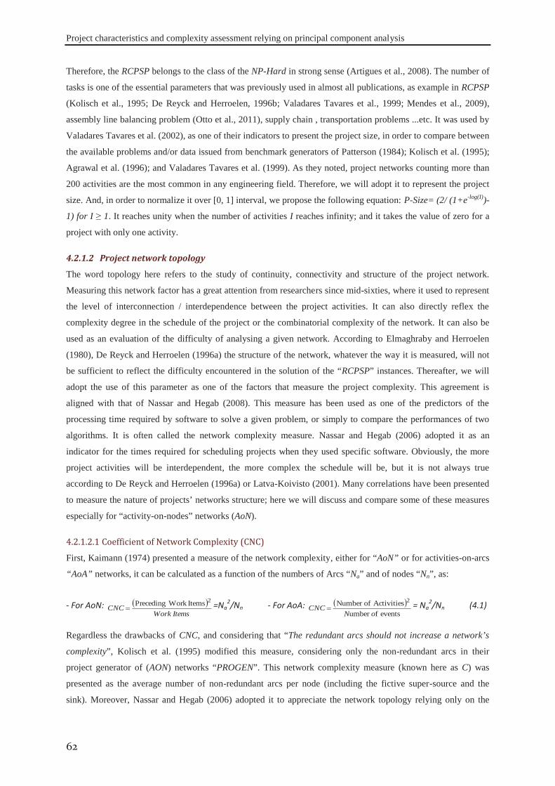
Project characteristics and complexity assessment relying on principal component analysis

62

Therefore, the RCPSP belongs to the class of the NP-Hard in strong sense (Artigues et al., 2008). The number of

tasks is one of the essential parameters that was previously used in almost all publications, as example in RCPSP

(Kolisch et al., 1995; De Reyck and Herroelen, 1996b; Valadares Tavares et al., 1999; Mendes et al., 2009),

assembly line balancing problem (Otto et al., 2011), supply chain , transportation problems ...etc. It was used by

Valadares Tavares et al. (2002), as one of their indicators to present the project size, in order to compare between

the available problems and/or data issued from benchmark generators of Patterson (1984); Kolisch et al. (1995);

Agrawal et al. (1996); and Valadares Tavares et al. (1999). As they noted, project networks counting more than

200 activities are the most common in any engineering field. Therefore, we will adopt it to represent the project

size. And, in order to normalize it over [0, 1] interval, we propose the following equation: P-Size= (2/ (1+e-log(I))-

1) for I ≥ 1. It reaches unity when the number of activities I reaches infinity; and it takes the value of zero for a

project with only one activity.

4.2.1.2 Project network topology

The word topology here refers to the study of continuity, connectivity and structure of the project network.

Measuring this network factor has a great attention from researchers since mid-sixties, where it used to represent

the level of interconnection / interdependence between the project activities. It can also directly reflex the

complexity degree in the schedule of the project or the combinatorial complexity of the network. It can also be

used as an evaluation of the difficulty of analysing a given network. According to Elmaghraby and Herroelen

(1980), De Reyck and Herroelen (1996a) the structure of the network, whatever the way it is measured, will not

be sufficient to reflect the difficulty encountered in the solution of the “RCPSP” instances. Thereafter, we will

adopt the use of this parameter as one of the factors that measure the project complexity. This agreement is

aligned with that of Nassar and Hegab (2008). This measure has been used as one of the predictors of the

processing time required by software to solve a given problem, or simply to compare the performances of two

algorithms. It is often called the network complexity measure. Nassar and Hegab (2006) adopted it as an

indicator for the times required for scheduling projects when they used specific software. Obviously, the more

project activities will be interdependent, the more complex the schedule will be, but it is not always true

according to De Reyck and Herroelen (1996a) or Latva-Koivisto (2001). Many correlations have been presented

to measure the nature of projects’ networks structure; here we will discuss and compare some of these measures

especially for “activity-on-nodes” networks (AoN).

4.2.1.2.1 Coefficient of Network Complexity (CNC)

First, Kaimann (1974) presented a measure of the network complexity, either for “AoN” or for activities-on-arcs

“AoA” networks, it can be calculated as a function of the numbers of Arcs “Na” and of nodes “Nn”, as:

- For AoN: ItemsWork

CNC

Items Work Preceding 2 =Na2/Nn - For AoA:

events fumber Activities ofNumber 2

oNCNC = Na

2/Nn (4.1)

Regardless the drawbacks of CNC, and considering that “The redundant arcs should not increase a network’s

complexity”, Kolisch et al. (1995) modified this measure, considering only the non-redundant arcs in their

project generator of (AON) networks “PROGEN”. This network complexity measure (known here as C) was

presented as the average number of non-redundant arcs per node (including the fictive super-source and the

sink). Moreover, Nassar and Hegab (2006) adopted it to appreciate the network topology relying only on the

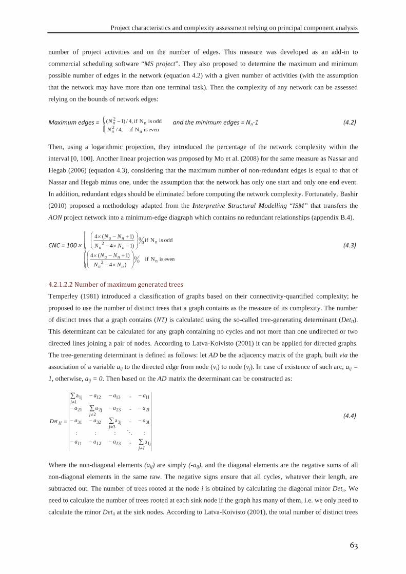
Project characteristics and complexity assessment relying on principal component analysis

63

number of project activities and on the number of edges. This measure was developed as an add-in to

commercial scheduling software “MS project”. They also proposed to determine the maximum and minimum

possible number of edges in the network (equation 4.2) with a given number of activities (with the assumption

that the network may have more than one terminal task). Then the complexity of any network can be assessed

relying on the bounds of network edges:

Maximum edges = even is N if ,4/

odd is N if ,4/)1( n

2n

2

n

nNN and the minimum edges = Nn-1 (4.2)

Then, using a logarithmic projection, they introduced the percentage of the network complexity within the

interval [0, 100]. Another linear projection was proposed by Mo et al. (2008) for the same measure as Nassar and

Hegab (2006) (equation 4.3), considering that the maximum number of non-redundant edges is equal to that of

Nassar and Hegab minus one, under the assumption that the network has only one start and only one end event.

In addition, redundant edges should be eliminated before computing the network complexity. Fortunately, Bashir

(2010) proposed a methodology adapted from the Interpretive Structural Modelling “ISM” that transfers the

AON project network into a minimum-edge diagraph which contains no redundant relationships (appendix B.4).

CNC = 100 ×

even is N if )4

)1(4

odd is N if )14)1(4

n00

2

n00

2

nn

na

nn

na

NNNN

NNNN

(4.3)

4.2.1.2.2 Number of maximum generated trees

Temperley (1981) introduced a classification of graphs based on their connectivity-quantified complexity; he

proposed to use the number of distinct trees that a graph contains as the measure of its complexity. The number

of distinct trees that a graph contains (NT) is calculated using the so-called tree-generating determinant (DetII).

This determinant can be calculated for any graph containing no cycles and not more than one undirected or two

directed lines joining a pair of nodes. According to Latva-Koivisto (2001) it can be applied for directed graphs.

The tree-generating determinant is defined as follows: let AD be the adjacency matrix of the graph, built via the

association of a variable aij to the directed edge from node (vi) to node (vj). In case of existence of such arc, aij =

1, otherwise, aij = 0. Then based on the AD matrix the determinant can be constructed as:

IjIII

j

j

j

II

aaa

aaa

aaa

aaa

Det

Ij321

3I3

3j3231

2I232

2j21

1I13121

1j

a..::::

..a

..a

..a

(4.4)

Where the non-diagonal elements (aij) are simply (-aij), and the diagonal elements are the negative sums of all

non-diagonal elements in the same raw. The negative signs ensure that all cycles, whatever their length, are

subtracted out. The number of trees rooted at the node i is obtained by calculating the diagonal minor Detii. We

need to calculate the number of trees rooted at each sink node if the graph has many of them, i.e. we only need to

calculate the minor Detii at the sink nodes. According to Latva-Koivisto (2001), the total number of distinct trees

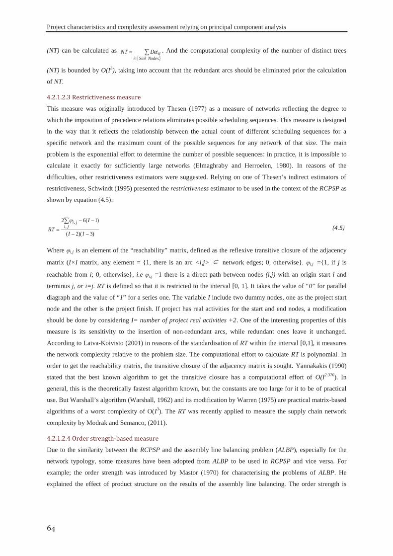
Project characteristics and complexity assessment relying on principal component analysis

64

(NT) can be calculated as NodesSinki

iiDetNT

. And the computational complexity of the number of distinct trees

(NT) is bounded by O(I3), taking into account that the redundant arcs should be eliminated prior the calculation

of NT.

4.2.1.2.3 Restrictiveness measure

This measure was originally introduced by Thesen (1977) as a measure of networks reflecting the degree to

which the imposition of precedence relations eliminates possible scheduling sequences. This measure is designed

in the way that it reflects the relationship between the actual count of different scheduling sequences for a

specific network and the maximum count of the possible sequences for any network of that size. The main

problem is the exponential effort to determine the number of possible sequences: in practice, it is impossible to

calculate it exactly for sufficiently large networks (Elmaghraby and Herroelen, 1980). In reasons of the

difficulties, other restrictiveness estimators were suggested. Relying on one of Thesen’s indirect estimators of

restrictiveness, Schwindt (1995) presented the restrictiveness estimator to be used in the context of the RCPSP as

shown by equation (4.5):

)3)(2(

)1(62,

,

II

IRT ji

ji (4.5)

Where φi,j is an element of the “reachability” matrix, defined as the reflexive transitive closure of the adjacency

matrix (I×I matrix, any element = {1, there is an arc <i,j> network edges; 0, otherwise}. φi,j ={1, if j is

reachable from i; 0, otherwise}, i.e φi,j =1 there is a direct path between nodes (i,j) with an origin start i and

terminus j, or i=j. RT is defined so that it is restricted to the interval [0, 1]. It takes the value of “0” for parallel

diagraph and the value of “1” for a series one. The variable I include two dummy nodes, one as the project start

node and the other is the project finish. If project has real activities for the start and end nodes, a modification

should be done by considering I= number of project real activities +2. One of the interesting properties of this

measure is its sensitivity to the insertion of non-redundant arcs, while redundant ones leave it unchanged.

According to Latva-Koivisto (2001) in reasons of the standardisation of RT within the interval [0,1], it measures

the network complexity relative to the problem size. The computational effort to calculate RT is polynomial. In

order to get the reachability matrix, the transitive closure of the adjacency matrix is sought. Yannakakis (1990)

stated that the best known algorithm to get the transitive closure has a computational effort of O(I2.376). In

general, this is the theoretically fastest algorithm known, but the constants are too large for it to be of practical

use. But Warshall’s algorithm (Warshall, 1962) and its modification by Warren (1975) are practical matrix-based

algorithms of a worst complexity of O(I3). The RT was recently applied to measure the supply chain network

complexity by Modrak and Semanco, (2011).

4.2.1.2.4 Order strength-based measure

Due to the similarity between the RCPSP and the assembly line balancing problem (ALBP), especially for the

network typology, some measures have been adopted from ALBP to be used in RCPSP and vice versa. For

example; the order strength was introduced by Mastor (1970) for characterising the problems of ALBP. He

explained the effect of product structure on the results of the assembly line balancing. The order strength is

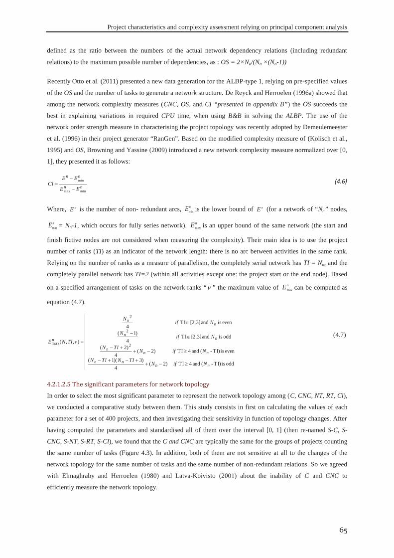
Project characteristics and complexity assessment relying on principal component analysis

65

defined as the ratio between the numbers of the actual network dependency relations (including redundant

relations) to the maximum possible number of dependencies, as : OS = 2×Na/(Nn ×(Nn-1))

Recently Otto et al. (2011) presented a new data generation for the ALBP-type 1, relying on pre-specified values

of the OS and the number of tasks to generate a network structure. De Reyck and Herroelen (1996a) showed that

among the network complexity measures (CNC, OS, and CI “presented in appendix B”) the OS succeeds the

best in explaining variations in required CPU time, when using B&B in solving the ALBP. The use of the

network order strength measure in characterising the project topology was recently adopted by Demeulemeester

et al. (1996) in their project generator “RanGen”. Based on the modified complexity measure of (Kolisch et al.,

1995) and OS, Browning and Yassine (2009) introduced a new network complexity measure normalized over [0,

1], they presented it as follows:

nn

nn

EE

EECl

minmax

min (4.6)

Where, nE is the number of non- redundant arcs, nEmin is the lower bound of nE (for a network of “Nn” nodes,

nEmin = Nn-1, which occurs for fully series network). nEmax is an upper bound of the same network (the start and

finish fictive nodes are not considered when measuring the complexity). Their main idea is to use the project

number of ranks (TI) as an indicator of the network length: there is no arc between activities in the same rank.

Relying on the number of ranks as a measure of parallelism, the completely serial network has TI = Nn, and the

completely parallel network has TI=2 (within all activities except one: the project start or the end node). Based

on a specified arrangement of tasks on the network ranks “ ” the maximum value of nEmax can be computed as

equation (4.7).

odd is TI)-( and 4TI )2(4

)3)(1(

even is TI)-( and 4TI )2(4

)2(

odd is and [2,3]TI 4

)1(

even is and [2,3]TI 4

),,(2

2

2

max

nnnn

nnn

nn

nn

n

NifNTINTIN

NifNTIN

NifN

NifN

TINE (4.7)

4.2.1.2.5 The significant parameters for network topology

In order to select the most significant parameter to represent the network topology among (C, CNC, NT, RT, Cl),

we conducted a comparative study between them. This study consists in first on calculating the values of each

parameter for a set of 400 projects, and then investigating their sensitivity in function of topology changes. After

having computed the parameters and standardised all of them over the interval [0, 1] (then re-named S-C, S-

CNC, S-NT, S-RT, S-Cl), we found that the C and CNC are typically the same for the groups of projects counting

the same number of tasks (Figure 4.3). In addition, both of them are not sensitive at all to the changes of the

network topology for the same number of tasks and the same number of non-redundant relations. So we agreed

with Elmaghraby and Herroelen (1980) and Latva-Koivisto (2001) about the inability of C and CNC to

efficiently measure the network topology.

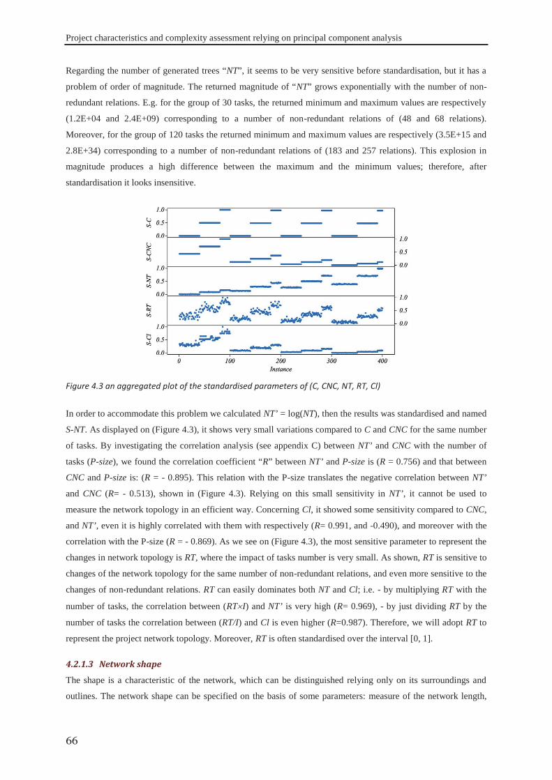
Project characteristics and complexity assessment relying on principal component analysis

66

Regarding the number of generated trees “NT”, it seems to be very sensitive before standardisation, but it has a

problem of order of magnitude. The returned magnitude of “NT” grows exponentially with the number of non-

redundant relations. E.g. for the group of 30 tasks, the returned minimum and maximum values are respectively

(1.2E+04 and 2.4E+09) corresponding to a number of non-redundant relations of (48 and 68 relations).

Moreover, for the group of 120 tasks the returned minimum and maximum values are respectively (3.5E+15 and

2.8E+34) corresponding to a number of non-redundant relations of (183 and 257 relations). This explosion in

magnitude produces a high difference between the maximum and the minimum values; therefore, after

standardisation it looks insensitive.

Figure 4.3 an aggregated plot of the standardised parameters of (C, CNC, NT, RT, Cl)

In order to accommodate this problem we calculated NT’ = log(NT), then the results was standardised and named

S-NT. As displayed on (Figure 4.3), it shows very small variations compared to C and CNC for the same number

of tasks. By investigating the correlation analysis (see appendix C) between NT’ and CNC with the number of

tasks (P-size), we found the correlation coefficient “R” between NT’ and P-size is (R = 0.756) and that between

CNC and P-size is: (R = - 0.895). This relation with the P-size translates the negative correlation between NT’

and CNC (R= - 0.513), shown in (Figure 4.3). Relying on this small sensitivity in NT’, it cannot be used to

measure the network topology in an efficient way. Concerning Cl, it showed some sensitivity compared to CNC,

and NT’, even it is highly correlated with them with respectively (R= 0.991, and -0.490), and moreover with the

correlation with the P-size (R = - 0.869). As we see on (Figure 4.3), the most sensitive parameter to represent the

changes in network topology is RT, where the impact of tasks number is very small. As shown, RT is sensitive to

changes of the network topology for the same number of non-redundant relations, and even more sensitive to the

changes of non-redundant relations. RT can easily dominates both NT and Cl; i.e. - by multiplying RT with the

number of tasks, the correlation between (RT I) and NT’ is very high (R= 0.969), - by just dividing RT by the

number of tasks the correlation between (RT/I) and Cl is even higher (R=0.987). Therefore, we will adopt RT to

represent the project network topology. Moreover, RT is often standardised over the interval [0, 1].

4.2.1.3 Network shape

The shape is a characteristic of the network, which can be distinguished relying only on its surroundings and

outlines. The network shape can be specified on the basis of some parameters: measure of the network length,

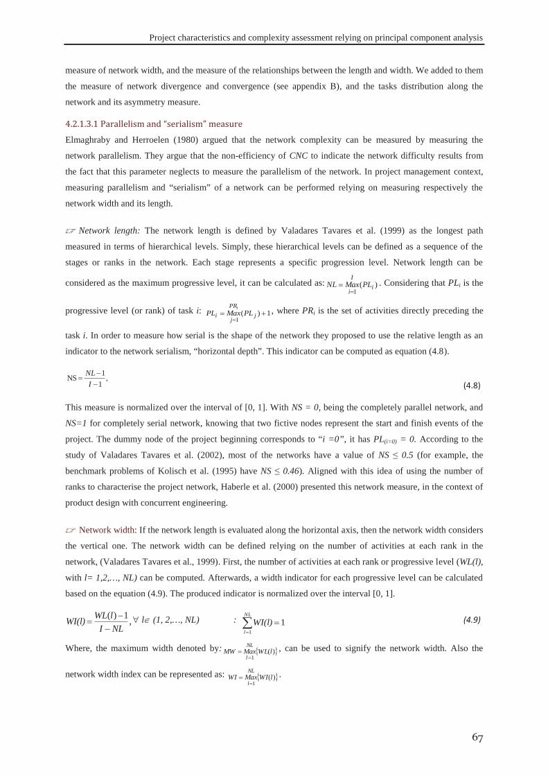
Project characteristics and complexity assessment relying on principal component analysis

67

measure of network width, and the measure of the relationships between the length and width. We added to them

the measure of network divergence and convergence (see appendix B), and the tasks distribution along the

network and its asymmetry measure.

4.2.1.3.1 Parallelism and “serialism” measure

Elmaghraby and Herroelen (1980) argued that the network complexity can be measured by measuring the

network parallelism. They argue that the non-efficiency of CNC to indicate the network difficulty results from

the fact that this parameter neglects to measure the parallelism of the network. In project management context,

measuring parallelism and “serialism” of a network can be performed relying on measuring respectively the

network width and its length.

Network length: The network length is defined by Valadares Tavares et al. (1999) as the longest path

measured in terms of hierarchical levels. Simply, these hierarchical levels can be defined as a sequence of the

stages or ranks in the network. Each stage represents a specific progression level. Network length can be

considered as the maximum progressive level, it can be calculated as: )(1

iI

iPLMaxNL . Considering that PLi is the

progressive level (or rank) of task i: 1)(1

jPR

ji PLMaxPL

i , where PRi is the set of activities directly preceding the

task i. In order to measure how serial is the shape of the network they proposed to use the relative length as an

indicator to the network serialism, “horizontal depth”. This indicator can be computed as equation (4.8).

,11NS

INL

(4.8)

This measure is normalized over the interval of [0, 1]. With NS = 0, being the completely parallel network, and

NS=1 for completely serial network, knowing that two fictive nodes represent the start and finish events of the

project. The dummy node of the project beginning corresponds to “i =0”, it has PL(i=0) = 0. According to the

study of Valadares Tavares et al. (2002), most of the networks have a value of NS ≤ 0.5 (for example, the

benchmark problems of Kolisch et al. (1995) have NS ≤ 0.46). Aligned with this idea of using the number of

ranks to characterise the project network, Haberle et al. (2000) presented this network measure, in the context of

product design with concurrent engineering.

Network width: If the network length is evaluated along the horizontal axis, then the network width considers

the vertical one. The network width can be defined relying on the number of activities at each rank in the

network, (Valadares Tavares et al., 1999). First, the number of activities at each rank or progressive level (WL(l),

with l= 1,2,…, NL) can be computed. Afterwards, a width indicator for each progressive level can be calculated

based on the equation (4.9). The produced indicator is normalized over the interval [0, 1].

,1)(NLIlWLWI(l) l (1, 2,…, NL) : 1

1

NL

lWI(l) (4.9)

Where, the maximum width denoted by: )(1

lWLMaxMWNL

l, can be used to signify the network width. Also the

network width index can be represented as: )(1

lWIMaxWINL

l.

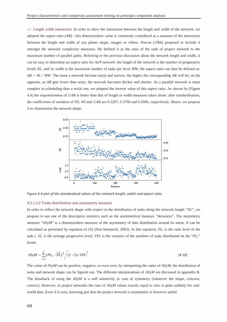
Project characteristics and complexity assessment relying on principal component analysis

68

Length width interaction: In order to show the interaction between the length and width of the network, we

adopted the aspect ratio (AR) : this dimensionless value is commonly considered as a measure of the interaction

between the length and width of any planer shape, images or videos. Pascoe (1966) proposed to include it

amongst the network complexity measures. He defined it as the ratio of the rank of project network to the

maximum number of parallel paths. Referring to the previous discussion about the network length and width, it

can be easy to determine an aspect ratio for AoN network: the length of the network is the number of progressive

levels NL, and its width is the maximum number of tasks per level MW; the aspect ratio can thus be defined as:

AR = NL / MW. The more a network become serial and narrow, the higher the corresponding AR will be; on the

opposite, as AR gets lower than unity, the network becomes thicker and shorter. As a parallel network is more

complex in scheduling than a serial one, we adopted the inverse value of this aspect ratio. As shown by (Figure

4.4) the responsiveness of 1/AR is better than that of length or width measures taken alone: after standardisation,

the coefficients of variation of NS, WI and 1/AR are 0.3287, 0.2760 and 0.5906, respectively. Hence, we propose

it to characterize the network shape.

Figure 4.4 plot of the standardised values of the network length, width and aspect ratio

4.2.1.3.2 Tasks distribution and asymmetry measure

In order to reflect the network shape with respect to the distribution of tasks along the network length “NL”, we

propose to use one of the descriptive statistics such as the asymmetrical measure “skewness”. The asymmetry

measure “ASyM” is a dimensionless measure of the asymmetry of data distribution around its mean. It can be

calculated as presented by equation (4.10) (Nist-Sematech, 2003). In this equation, PLi is the rank level of the

task i, PL is the average progressive level, VPL is the variance of the numbers of tasks distributed on the “PLi”

levels.

23

)1()( 3

1VPLIPLPLASyM

I

ii (4.10)

The value of ASyM can be positive, negative, or even zero; by interpreting the value of ASyM, the distribution of

tasks and network shape can be figured out. The different interpretations of ASyM are discussed in appendix B.

The drawback of using the ASyM is a null sensitivity in case of symmetry (whatever the shape, concave,

convex). However, in project networks the case of ASyM values exactly equal to zero is quite unlikely for real-

world data. Even if it exist, knowing just that the project network is asymmetric is however useful.

Project characteristics and complexity assessment relying on principal component analysis

69

In order to standardise this measure, we propose to use the logistic function, and to name the result the

“standardised asymmetry measure”, SASyM =1/(1+e ASyM). Examining this standardised form, one can find that

as the tasks concentrate at the beginning of the network, the SASyM approaches zero, (as shown in Figure B.3 in

appendix B). For exactly symmetrical networks SASyM = 0.5.On the other side, the value of SASyM approaches

unity when tasks are concentrated at the end of the project. In this case, we will consider that the project

schedule is more complex, since the risk of discovering the project unfeasibility can be higher. As shown by

(Figure 4.5), the behaviour of the “SASyM” is remarkable for the set of 400 projects, responding to variations of

the tasks distribution along the network length. As we see, almost all the projects have a value lower than 0.5.

Therefore, one can infer that the majority of these projects have tasks concentrated at the first half.

Figure 4.5 the distribution of SASyM for a set of 400 projects

4.2.1.4 Network bottleneck measure

A bottleneck is a phenomenon where the resulting performance of an entire dynamic system can be limited by a

single or limited number of components or resources. Usually, any facility, function, department or resource

which is not able to meet the demand placed upon it at a specified time, becomes a bottleneck. For instance, in

production lines, it can be defined as the most charged workstation, so that any lateness occurring at this

workstation will slow down or even stop the whole production line. For supply chain networks, performance

indicator can be revealed by the network bottleneck(s), especially at the interfaces between its members

(Stadtler, 2005). In scheduling, the bottlenecks can result from the dependent and interdependent relations

between activities. Each bottleneck may bring two associated risks: blocking and starving. Blocking occurs

upstream the bottleneck, and the starving occurs downstream it. The degree of considering a given task as a

bottleneck in a network is determined in function of its immediate predecessors (PRi) and successors (SUi). The

network bottlenecks can be formulated by considering PRi of a given task as its blocking activities and SUi as its

starving ones. In literature, Johnson (1967) proposed a measure called activity density, relying on PRi and SUi of

each activity. The concept of “task degree” in the context of assembly lines networks was proposed also relying

on PRi and SUi (Otto et al., 2011). The task degree of a task is the sum of the numbers of its direct predecessors

and of its direct successors TDi = {PRi + SUi}. By constructing the tasks’ degrees vector:{TD1,TD2,…, TDI}, the

maximum value TDmax can be considered as one of the network measures. As shown in (Figure 4.6), this

measure cannot be used independently, but it should be usefully aggregated with other measures in order to

reflect the network complexity.

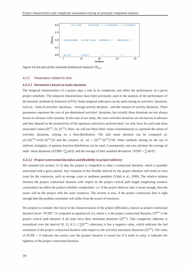
Project characteristics and complexity assessment relying on principal component analysis

70

Figure 4.6 the plot of the networks bottleneck measure TDmax

4.2.2.1 Parameters based on tasks duration

The temporal characteristics of a project play a role in its complexity and affect the performance of a given

project scheduler. The temporal characteristics have been previously used in the analysis of the performance of

the heuristic methods by Patterson (1976). Some temporal indicators can be used relying on activities’ durations,

such as: - Sum of activities’ durations, - Average activity duration, - and the variance in activity durations. These

parameters represent the case of pre-determined activities’ durations, but actually these durations are not always

known in advance with certainty. In the case of our study, the exact activities durations are not known in advance

and they depend on the productivity of the operators selected to perform them: we only have for each task three

associated values (Dimin, Di, Di

max). Here, we will use these three values simultaneously to represent the nature of

activities durations, relying on a beta-distribution. The task mean duration can be computed as:

μdi=(Dimin+4×Di+Di

max)/6 and the variance as: νdi = (Dimax-Di

min)2/36. Other methods relying on the use of

uniform, triangular, or gamma function distribution can be used. Consequently, one can calculate the average of

tasks’ mean durations (ATMD =∑μdi/I), and the average of their standard deviations “ATSD = ∑νdi/I)”.

4.2.2.2 Project contractual duration and flexibility in project delivery

We assumed (in section 3.1.3) that the project is compelled to obey a contractual duration, which is possibly

associated with a grace period. Any violation of this flexible interval by the project duration will result in extra

costs for the contractor, such as storage costs or tardiness penalties (Vidal et al., 1999). The relative relation

between the project contractual duration with respect to the project critical path length (neglecting resource

constraints) can affect the project schedule complexities. i.e. if the project delivery date is loose enough, then the

easier will be the project with the same resources. The reverse is true, if the project contractual date is tight

enough then the problem resolution will suffer from the scarce of resources.

We propose to consider this factor in the characterisation of the project difficulties, known as project contractual

duration factor “PCDF”. It computed as equation (4.11), where L is the project contractual duration, CPmin is the

project critical path duration if all tasks have their minimum durations (Dimin). This complexity indicator is

normalized over the interval [0, 1], if L ≤ ∑Dimax; otherwise, it has a negative value, which indicates the bad

estimation of the project contractual duration with respect to the activities maximum durations (Dimax). The value

of PCDF = 0 indicates the easiest case the (project duration is loose) but if it tends to unity, it indicates the

tightness of the project contractual duration.

4.2.2 Parameters related to time

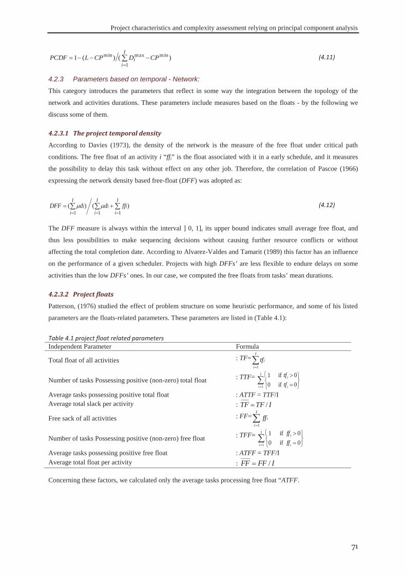
Project characteristics and complexity assessment relying on principal component analysis

71

)()(1 min

1

maxmin CPDCPLPCDFI

ii (4.11)

This category introduces the parameters that reflect in some way the integration between the topology of the

network and activities durations. These parameters include measures based on the floats - by the following we

discuss some of them.

4.2.3.1 The project temporal density

According to Davies (1973), the density of the network is the measure of the free float under critical path

conditions. The free float of an activity i “ffi” is the float associated with it in a early schedule, and it measures

the possibility to delay this task without effect on any other job. Therefore, the correlation of Pascoe (1966)

expressing the network density based free-float (DFF) was adopted as:

)()(1 11

I

i

I

iii

I

ii ffddDFF (4.12)

The DFF measure is always within the interval ] 0, 1], its upper bound indicates small average free float, and

thus less possibilities to make sequencing decisions without causing further resource conflicts or without

affecting the total completion date. According to Alvarez-Valdes and Tamarit (1989) this factor has an influence

on the performance of a given scheduler. Projects with high DFFs’ are less flexible to endure delays on some

activities than the low DFFs’ ones. In our case, we computed the free floats from tasks’ mean durations.

4.2.3.2 Project floats

Patterson, (1976) studied the effect of problem structure on some heuristic performance, and some of his listed

parameters are the floats-related parameters. These parameters are listed in (Table 4.1):

Table 4.1 project float related parameters Independent Parameter Formula

Total float of all activities : TF=I

iitf

1

Number of tasks Possessing positive (non-zero) total float : TTF= I

1i 0 if 0 if

01

i

i

tftf

Average tasks possessing positive total float : ATTF = TTF/I Average total slack per activity : ITFTF /

Free sack of all activities : FF=I

iiff

1

Number of tasks Possessing positive (non-zero) free float : TFF= I

1i

i

0 if 0 if

01

iffff

Average tasks possessing positive free float : ATFF = TFF/I Average total float per activity : IFFFF /

Concerning these factors, we calculated only the average tasks processing free float “ATFF.

4.2.3 Parameters based on temporal - Network:

Project characteristics and complexity assessment relying on principal component analysis

72

4.2.4.1 Resources requirements by activities

The resource requirements can be represented by the density of the jobs-skills requisition matrix (if the activity i

requires the skill k, the matrix element takes the value of “1”, and “0” otherwise). This density can be measured

with the Resources Factor (RF):

I

i

K

k

i,k

KIRF

1 1

0 IfOtherwise

1 0

1 (4.13)

The RF was developed by Pascoe (1966) to reflect the jobs-resources requirement relation, it reflects the average

portion requested of resources per each job, relying on equation (4.13); if RF = 1, it means that each activity

requires all the resources for its execution. If RF = 0, it indicates that there is no resources constrained problem

where no activity requires any of the resources. The RF is normalised over the interval [0, 1], and was used by

Patterson (1976) under the name of average percent of demands. It was also modified by Kolisch et al., (1995) to

reflect the density of the three-dimensions matrix of job-resources requirements for multi-mode project

scheduling. (Kolisch et al., 1995) indicated that a growth of RF increases the computational effort to solve the

problem; Yet, Alvarez-Valdes and Tamarit (1989) observed that the computational effort of heuristic algorithms

are influenced by the RF, and that problems with RF = 0.5 are more likely to show bottleneck activities

expanding the difficulty to be schedule than other problems with RF = 1. We expect that the temporal

performance effort of our problem will validate that of Kolisch et al. (1995).

4.2.4.2 Activities work content

This parameter can be used to highlight the critical resources in the firm, i.e. the most charged ones. As the work

content increases, scheduling the project gets harder for a given set of resources. The work-content per skill “Wk”

can be calculated as:

K kWWI

ikik ,, , and I

i

K

kkiW

1 1,

(4.14)

Where W is the total project work content. We adopted the minimum and maximum resource work contents

among all resources, respectively “MinWC” and “MaxWC”. Moreover, the “total work content W” will be used

as a gross measure of the total resources requirements of the project. This gross measure can be represented as a

required effort per person as a way of sizing the project.

4.2.4.3 Technical complexity of the Work-content

In the proposed problem, the technical complexity can be considered as one of the parameters that affect the

productivities of workforce and their experience accumulation. As previously discussed (in section 3.2.2.3) the

workforce productivities are functions of learning and forgetting rates. These rates are highly correlated to the

technical complexity of the required work and task complexity (Osothsilp, 2002). Therefore, the number of

technologies involved (e.g. mechanical, electrical, hydraulic, aeronautic, digital…), as well as their nature, affect

the overall project complexity. The technical complexity can be simply represented as a novelty degree for the

considered skill or resource (machines, equipment, tools, the required raw material….), i.e. it simply reflects the

4.2.4 Parameters based on the work content

Project characteristics and complexity assessment relying on principal component analysis

73

similarity degree between the new work and what has been performed prior by the same workforce. This novelty

degree can be measured relying on the ratio between the new required resource and the total resources. The value

of “0” means well-mastered work, and a value of “1” indicates a novel one. We propose to integrate only the

similarity degree between skills, as discussed in (3.2.2.2), this similarity degree can affect the productivity of

workforce secondary skills. It can be computed as the average value of all the pairs of skills, known as “SD”.

By constructing the profile of each resource along the critical path, a set of variables can be computed, such as:

the maximum, minimum, average and variance of demand, or the centre of the workload profile area. In order to

characterise a given profile, we should distinguish between two types of variables: the location factors,

representing the variable location relative to the critical path (e.g. the location of the maximum demand of a

given resource profile), and the magnitude of variables or the description of the workload distribution. Therefore,

we propose to measure each kind of parameters separately. First, the resource requirement vector can be

computed by: - Construct the project early schedule, and get the project duration corresponding to the length of

critical path “CP” (in time periods or days). - For each resource type, construct the resource-workload profile

based on project schedule, such that, it can be represented as a vector of resource requirement at each time

interval t CP, CPktkkkk RRRRRRRRRR ,,2,1, ,...,,, , k K. This vector will be calculated for each resource,

for each project (if there are many). Thereafter, the different quantifications can be modelled, as follows.

4.2.5.1 Characterisation of resource work-content

Average load: One of the integration between the network, temporal and work-content parameters is the

Average Resource Loading Factor (ARLF), proposed by Kurtulus and Davis (1982). This ARLF identifies

whether the peak of total resource requirements is located in the first or the second half of the project’s original

critical path. First, Davis (1975) presented a measure called “Product Moment” PM. It was used to indicate the

predominant location of resource requirement along the project temporal periods. Relying on the same principle

of the Product Moment, and with the modification of dividing the project duration into two segments, the ARLF

measure of Kurtulus and Davis (1982) was presented for multi-project scheduling. Recently Browning and

Yassine, (2009) presented a measure of resources constrained multi-projects scheduling problem, by adopting

the (ARLF) indicator. They normalised ARLF over the projects’ maximum CP rather than over each individual

project’s CP length. This modification was carried out in order “to identify whether the bulk of a problem’s total

resource requirements fall in the front or back half of its critical path duration”. In order to present clearly the

average resource load factor magnitude, we propose to use the average resources requirement per period:

ARP= CPKRRK

k

CP

tkt

1 1

. And in order to use it as complexity indicator, we propose to normalise it over the

interval [0, 1] using the logistic function of its log scale, as: ARPF=2/(1+e -log(ARPF) -1.

Maximum load: In a multi-project scheduling, Kurtulus and Narula (1985) developed a project summery

relying on the maximum consumption of a given resource, called the Maximum Load Factor (MLF). They

present the localisation of the peak in a resource’s profile as one of the project measures. In order to eliminate

the contribution of the number of tasks in the problem, they proposed to divide the MLF by the total number of

tasks. As previously mentioned, we propose to separate the values of factors from their locations. Therefore; we

4.2.5 Parameters based on temporal-Network-Work content

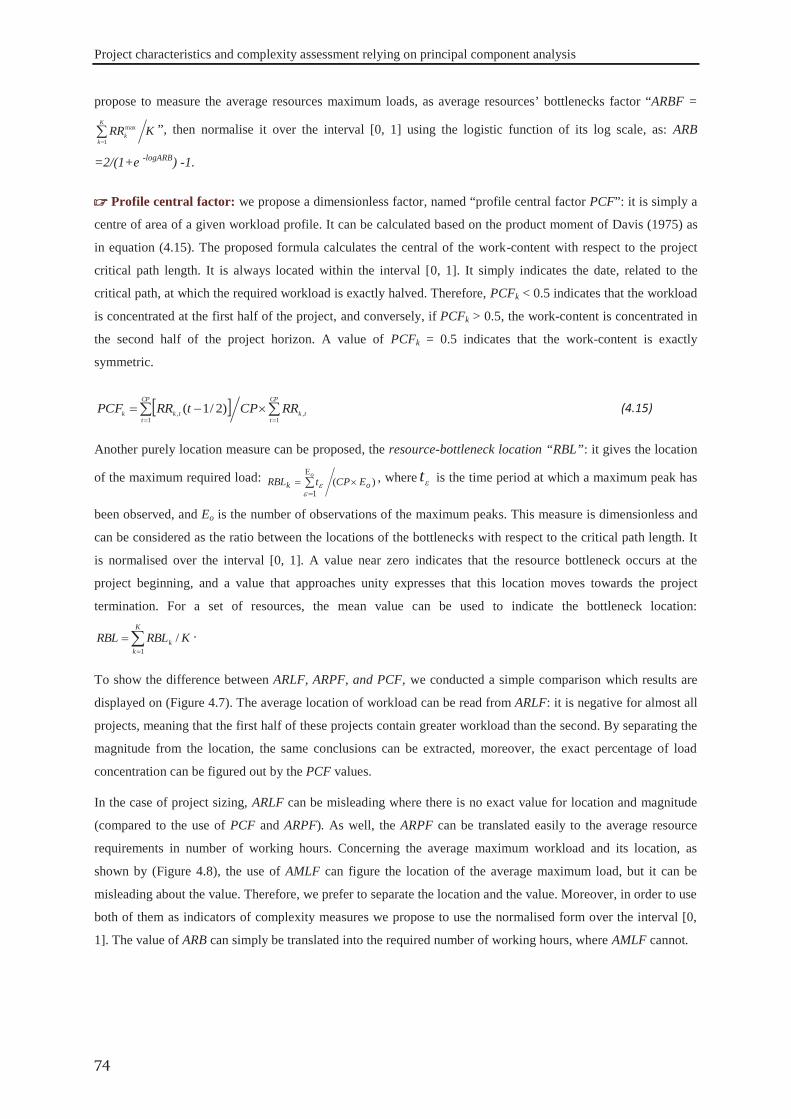
Project characteristics and complexity assessment relying on principal component analysis

74

propose to measure the average resources maximum loads, as average resources’ bottlenecks factor “ARBF =

KRRK

kk

1

max ”, then normalise it over the interval [0, 1] using the logistic function of its log scale, as: ARB

=2/(1+e -logARB) -1.

Profile central factor: we propose a dimensionless factor, named “profile central factor PCF”: it is simply a

centre of area of a given workload profile. It can be calculated based on the product moment of Davis (1975) as

in equation (4.15). The proposed formula calculates the central of the work-content with respect to the project

critical path length. It is always located within the interval [0, 1]. It simply indicates the date, related to the

critical path, at which the required workload is exactly halved. Therefore, PCFk < 0.5 indicates that the workload

is concentrated at the first half of the project, and conversely, if PCFk > 0.5, the work-content is concentrated in

the second half of the project horizon. A value of PCFk = 0.5 indicates that the work-content is exactly

symmetric.

CP

ttk

CP

ttkk RRCPtRRPCF

1,

1, )2/1( (4.15)

Another purely location measure can be proposed, the resource-bottleneck location “RBL”: it gives the location

of the maximum required load: )(1

ok ECPtRBLo , where εt is the time period at which a maximum peak has

been observed, and Eo is the number of observations of the maximum peaks. This measure is dimensionless and

can be considered as the ratio between the locations of the bottlenecks with respect to the critical path length. It

is normalised over the interval [0, 1]. A value near zero indicates that the resource bottleneck occurs at the

project beginning, and a value that approaches unity expresses that this location moves towards the project

termination. For a set of resources, the mean value can be used to indicate the bottleneck location:

KRBLRBLK

kk /

1

.

To show the difference between ARLF, ARPF, and PCF, we conducted a simple comparison which results are

displayed on (Figure 4.7). The average location of workload can be read from ARLF: it is negative for almost all

projects, meaning that the first half of these projects contain greater workload than the second. By separating the

magnitude from the location, the same conclusions can be extracted, moreover, the exact percentage of load

concentration can be figured out by the PCF values.

In the case of project sizing, ARLF can be misleading where there is no exact value for location and magnitude

(compared to the use of PCF and ARPF). As well, the ARPF can be translated easily to the average resource

requirements in number of working hours. Concerning the average maximum workload and its location, as

shown by (Figure 4.8), the use of AMLF can figure the location of the average maximum load, but it can be

misleading about the value. Therefore, we prefer to separate the location and the value. Moreover, in order to use

both of them as indicators of complexity measures we propose to use the normalised form over the interval [0,

1]. The value of ARB can simply be translated into the required number of working hours, where AMLF cannot.

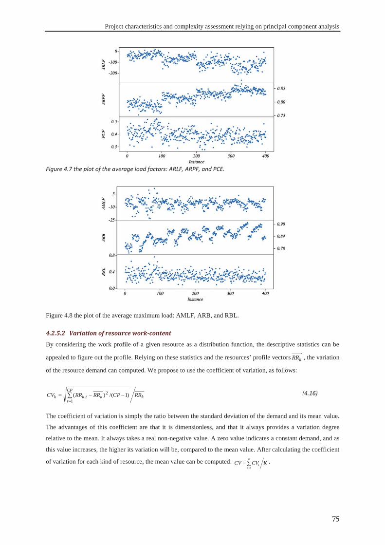
Project characteristics and complexity assessment relying on principal component analysis

75

Figure 4.7 the plot of the average load factors: ARLF, ARPF, and PCE.

Figure 4.8 the plot of the average maximum load: AMLF, ARB, and RBL.

4.2.5.2 Variation of resource work-content

By considering the work profile of a given resource as a distribution function, the descriptive statistics can be

appealed to figure out the profile. Relying on these statistics and the resources’ profile vectors kRR , the variation

of the resource demand can computed. We propose to use the coefficient of variation, as follows:

kCP

tktkk RRCPRRRRCV )1/()(

1

2,

(4.16)

The coefficient of variation is simply the ratio between the standard deviation of the demand and its mean value.

The advantages of this coefficient are that it is dimensionless, and that it always provides a variation degree

relative to the mean. It always takes a real non-negative value. A zero value indicates a constant demand, and as

this value increases, the higher its variation will be, compared to the mean value. After calculating the coefficient

of variation for each kind of resource, the mean value can be computed: KCVCVK

kk

1

.

Project characteristics and complexity assessment relying on principal component analysis

76

The availability is always measured relative to the requirements, i.e. it reflects the relation between demands and

accessibility of a given resource. The computational effort to solve a given problem is logically a function of

resources number and availability; some authors such as Elmaghraby and Herroelen (1980) argued that there is a

bell-shaped relationship between the computational effort and the resource availability. As they explained this

hypothesise, if resource are only available in extremely small amounts, there will be relatively little freedom in

scheduling activities: as a result, the activities may have to be placed in series and the resulting project duration

will be equal to the sum of tasks’ durations. At the other side, if the resources are amply available the activities

can be scheduled in parallel and the resulting project duration will be equal to that of the critical path, the

complexity will be reduced. This conjecture is then confirmed by De Reyck and Herroelen (1996a) by using the

Resources-Constrainedness (RC) introduced by Patterson (1976).

Within literature some measures can be found concerning the resources constrainedness in project scheduling.

For example, Davies (1973) developed a resources limitations measure that stated the proportion of the expected

maximum demand for resources. The expected maximum demand is the product of average activity demand and

the number of real parallel activities, i.e. which could be theoretically under progress at the same time. By the

following, we detail some of them. But in order to measure only the availability of a resource type k, the

availability per period for each resource can be constructed as a vector of real resources (workers)

CPkkkkk RARARARARA ,3,2,1, ,...,,, . Afterwards, the average availability related to the project critical path

can be estimated as CPRARACP

ttkk

1,

. In case of constant resources per period “|Ak|”, the average availability

can be computed as CPtRAARA tkkk ,, then the average real workforce can be computed as

KAARWK

kk

1.

Due to the heterogeneous productivities of a versatile workforce in our model, we propose to use the operators’

overall average productivity. As the productivity of each operator in practicing a specified skill is already

normalised over the interval [0, 1], the overall mean productivity “ ” will also be normalized, and can be

computed as follows:

K

kk

K

k

A

ak A

K,aθ1 (4.17)

Where Ak is the cardinality of the set of operators who can master the skill k. The value of“ ” approaches

unity: when firm’s staff are all experts in practicing all of their skills. In order to predict the labour capacity, we

propose to integrate “ ”with the real number of resources. This available capacity can be expressed either as a

number of working hours, or as an equivalent workforce. The overall available capacity of the workforce

4.3 PARAMETERS RELATED TO RESOURCES

4.3.1 Resources availability

4.3.2 Overall average productivity

Project characteristics and complexity assessment relying on principal component analysis

77

“OCW” (in equivalent number of persons) can be defined as OCW = ×A. The effective number of operators

for each skill can be computed as A

ake

kA1

,aθ , thus the average effective workforce per skill can be computed

as: AEW= KAK

k

ek /

1

.

By investigating the correlation between the average real workforce per skill “ARW”, the average effective

workforce per skill “AEW”, and overall available capacity “OCW”, we found a correlation coefficient between

OCW and ARW of (R=0.993), and (R=0.994) between OCW and AEW. Therefore, we propose to use only the

OCW and to represent the workforce availability.

The assessment of the interaction between project activities and resources can be represented as an obstruction or

scarcity factor. This scarcity can be defined as the condition at which at any given time t the demand for one or

more resource(s) exceeds the supply. As explained by Pascoe (1966), the resource scarcity is the main problem

of resources allocation problems. An increase in network complexity or resource requirement is likely to

increase the obstruction to realizing a given project. Accordingly, measuring scarcity of resource is very

important, thus by the following we discus some of these measures.

Resource scarcity index (RSI)

In order to quantify the relation between resources requirements and their availabilities a Resource-Strength (RS)

was proposed by Cooper (1976). It can be defined as the ratio between the available amounts of the resource k to

the average requirements from this resource per job. Kolisch et al. (1995) stated three drawbacks of this measure:

RS is not standardized within the interval [0, 1]; small values of “RS” do not guarantee a feasible solution; the

scarcity of resources is calculated in a “myopic” fashion. In order to overcome these three drawbacks, they

modified it for multi-mode RCPSPs’ as:

minmax

min

kk

kkk RR

RRARS (4.18)

For renewable resources, ]][[ ,,11

minkmi

Mi

m

I

ik RRMinMaxR is the minimum demand and “ max

kR ” is the peak demand for

resources of kind k in precedence-preserving early start schedule; RAk is the total available capacity for this

resource, and “Mi” is the number of modes of activity “i”. Relying on this expression, if we have only one mode,

we can rewrite and calculate minkR as: ][ ,

1

minki

I

ik RRMaxR , max

kR being unchanged. Now, RS is always within the

interval [0, 1]. As noted by De Reyck and Herroelen (1996a) this new RS incorporates information about the

network structure.

We can adapt this measure to the current problem, relying on the fact that the project should be executed with the

minimum resources if all tasks are expanded to their maximum durations while it cannot when durations are

minimum. Therefore the minimum requirements can be calculated as ][ max,

1

miniki

I

ik DMaxR . In order to determine

4.4 ACTIVITIES- RESOURCES INTERACTION

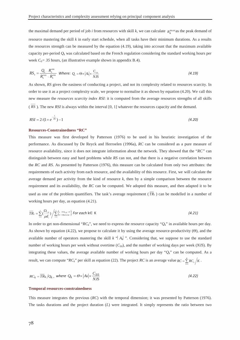
Project characteristics and complexity assessment relying on principal component analysis

78

the maximal demand per period of job i from resources with skill k, we can calculate maxkR as the peak demand of

resource mastering the skill k in early start schedule, when all tasks have their minimum durations. As a results

the resources strength can be measured by the equation (4.19), taking into account that the maximum available

capacity per-period Qk was calculated based on the French regulation considering the standard working hours per

week C0= 35 hours, (an illustrative example shown in appendix B.4).

minmax

min

kk

kkk RR

RQRS Where: NJS

AQ Skk

0C (4.19)

As shown, RS gives the easiness of conducting a project, and not its complexity related to resources scarcity. In

order to use it as a project complexity scale, we propose to normalise it as shown by equation (4.20). We call this

new measure the resources scarcity index RSI: it is computed from the average resources strengths of all skills

( RS ). The new RSI is always within the interval [0, 1] whatever the resources capacity and the demand.

1)1/(21

RSeRSI (4.20)

Resources-Constrainedness “RC”

This measure was first developed by Patterson (1976) to be used in his heuristic investigation of the

performance. As discussed by De Reyck and Herroelen (1996a), RC can be considered as a pure measure of

resource availability, since it does not integrate information about the network. They showed that the “RC” can

distinguish between easy and hard problems while RS can not, and that there is a negative correlation between

the RC and RS. As presented by Patterson (1976), this measure can be calculated from only two attributes: the

requirements of each activity from each resource, and the availability of this resource. First, we will calculate the

average demand per activity from the kind of resource k, then by a simple comparison between the resource

requirement and its availability, the RC can be computed. We adopted this measure, and then adapted it to be

used as one of the problem quantifiers. The task’s average requirement ( kTR ) can be modelled in a number of

working hours per day, as equation (4.21).

I

i

I

i i

kik

dTR

1

0 ki, IfOtherwise

1 0

1

, )( For each k K (4.21)

In order to get non-dimensional “RCk”, we need to express the resource capacity “Qk” in available hours per day.

As shown by equation (4.22), we propose to calculate it by using the average resource-productivity (Θ), and the

available number of operators mastering the skill k “ Ak ”. Considering that, we suppose to use the standard

number of working hours per week without overtime (CS0), and the number of working days per week (NJS). By

integrating these values, the average available number of working hours per day “Qk” can be computed. As a

result, we can compute “RCk” per skill as equation (22). The project RC is an average value KRCRCK

kk

1

.

,kkk QTRRC where NJSCAΘQ Skk

0 (4.22)

Temporal resources-constrainedness

This measure integrates the previous (RC) with the temporal dimension; it was presented by Patterson (1976).

The tasks durations and the project duration (L) were integrated. It simply represents the ratio between two

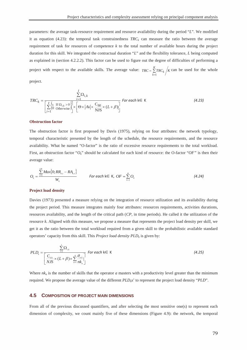
Project characteristics and complexity assessment relying on principal component analysis

79

parameters: the average task-resource requirement and resource availability during the period “L”. We modified

it as equation (4.23): the temporal task constrainedness TRCk can measure the ratio between the average

requirement of task for resources of competence k to the total number of available hours during the project

duration for this skill. We integrated the contractual duration “L” and the flexibility tolerance, L being computed

as explained in (section 4.2.2.2). This factor can be used to figure out the degree of difficulties of performing a

project with respect to the available skills. The average value: KTRCTRCK

kk

1can be used for the whole

project.

)(NJSCS0

1

0 IfOtherwise

1 0

1,

ki, LATRC

kI

i

I

iki

k For each k K (4.23)

Obstruction factor

The obstruction factor is first proposed by Davis (1975), relying on four attributes: the network typology,

temporal characteristic presented by the length of the schedule, the resource requirements, and the resource

availability. What he named “O-factor” is the ratio of excessive resource requirements to the total workload.

First, an obstruction factor “Ok” should be calculated for each kind of resource: the O-factor “OF” is then their

average value:

k

CP

ttktk

k W

RARRMaxO 1

,,;0 For each k K,

K

kkOOF

1 (4.24)

Project load density

Davies (1973) presented a measure relying on the integration of resource utilization and its availability during

the project period. This measure integrates mainly four attributes: resources requirements, activities durations,

resources availability, and the length of the critical path (CP, in time periods). He called it the utilization of the

resource k. Aligned with this measure, we propose a measure that represents the project load density per skill, we

get it as the ratio between the total workload required from a given skill to the probabilistic available standard

operators’ capacity from this skill. This Project load density PLDk is given by:

A

a a

kaS

I

iki

k

nkL

NJS

PLD

1

,0

1,

)(C For each k K (4.25)

Where nka is the number of skills that the operator a masters with a productivity level greater than the minimum

required. We propose the average value of the different PLDks’ to represent the project load density “PLD”.

From all of the previous discussed quantifiers, and after selecting the most sensitive one(s) to represent each

dimension of complexity, we count mainly five of these dimensions (Figure 4.9): the network, the temporal

4.5 COMPOSITION OF PROJECT MAIN DIMENSIONS

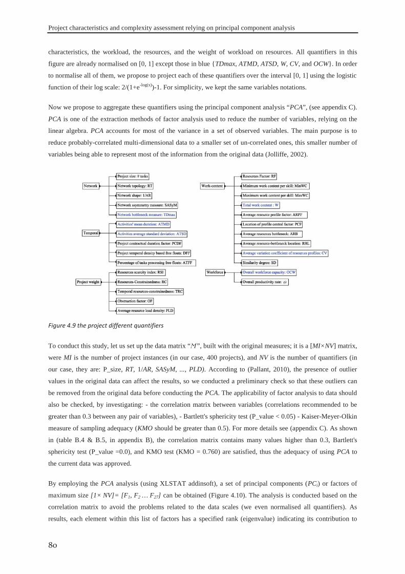
Project characteristics and complexity assessment relying on principal component analysis

80

characteristics, the workload, the resources, and the weight of workload on resources. All quantifiers in this

figure are already normalised on [0, 1] except those in blue {TDmax, ATMD, ATSD, W, CV, and OCW}. In order

to normalise all of them, we propose to project each of these quantifiers over the interval [0, 1] using the logistic

function of their log scale: 2/(1+e-log(x))-1. For simplicity, we kept the same variables notations.

Now we propose to aggregate these quantifiers using the principal component analysis “PCA”, (see appendix C).

PCA is one of the extraction methods of factor analysis used to reduce the number of variables, relying on the

linear algebra. PCA accounts for most of the variance in a set of observed variables. The main purpose is to

reduce probably-correlated multi-dimensional data to a smaller set of un-correlated ones, this smaller number of

variables being able to represent most of the information from the original data (Jolliffe, 2002).

Figure 4.9 the project different quantifiers

To conduct this study, let us set up the data matrix “Ϻ”, built with the original measures; it is a [MI×NV] matrix,

were MI is the number of project instances (in our case, 400 projects), and NV is the number of quantifiers (in

our case, they are: P_size, RT, 1/AR, SASyM, ..., PLD). According to (Pallant, 2010), the presence of outlier

values in the original data can affect the results, so we conducted a preliminary check so that these outliers can

be removed from the original data before conducting the PCA. The applicability of factor analysis to data should

also be checked, by investigating: - the correlation matrix between variables (correlations recommended to be

greater than 0.3 between any pair of variables), - Bartlett's sphericity test (P_value < 0.05) - Kaiser-Meyer-Olkin

measure of sampling adequacy (KMO should be greater than 0.5). For more details see (appendix C). As shown

in (table B.4 & B.5, in appendix B), the correlation matrix contains many values higher than 0.3, Bartlett's

sphericity test (P_value =0.0), and KMO test (KMO = 0.760) are satisfied, thus the adequacy of using PCA to

the current data was approved.

By employing the PCA analysis (using XLSTAT addinsoft), a set of principal components (PCi) or factors of

maximum size [1× NV]= [F1, F2 … F27] can be obtained (Figure 4.10). The analysis is conducted based on the

correlation matrix to avoid the problems related to the data scales (we even normalised all quantifiers). As

results, each element within this list of factors has a specified rank (eigenvalue) indicating its contribution to

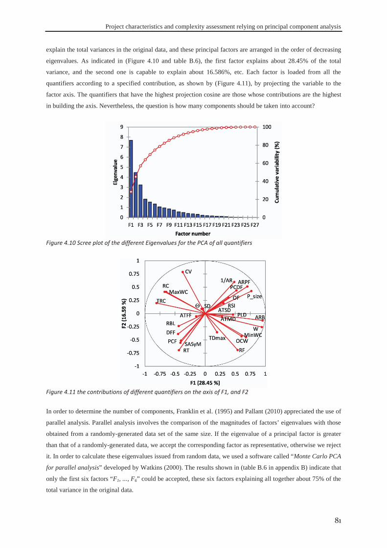
Project characteristics and complexity assessment relying on principal component analysis

81

explain the total variances in the original data, and these principal factors are arranged in the order of decreasing

eigenvalues. As indicated in (Figure 4.10 and table B.6), the first factor explains about 28.45% of the total

variance, and the second one is capable to explain about 16.586%, etc. Each factor is loaded from all the

quantifiers according to a specified contribution, as shown by (Figure 4.11), by projecting the variable to the

factor axis. The quantifiers that have the highest projection cosine are those whose contributions are the highest

in building the axis. Nevertheless, the question is how many components should be taken into account?

Figure 4.10 Scree plot of the different Eigenvalues for the PCA of all quantifiers

Figure 4.11 the contributions of different quantifiers on the axis of F1, and F2

In order to determine the number of components, Franklin et al. (1995) and Pallant (2010) appreciated the use of

parallel analysis. Parallel analysis involves the comparison of the magnitudes of factors’ eigenvalues with those

obtained from a randomly-generated data set of the same size. If the eigenvalue of a principal factor is greater

than that of a randomly-generated data, we accept the corresponding factor as representative, otherwise we reject

it. In order to calculate these eigenvalues issued from random data, we used a software called “Monte Carlo PCA

for parallel analysis” developed by Watkins (2000). The results shown in (table B.6 in appendix B) indicate that

only the first six factors “F1, ..., F6” could be accepted, these six factors explaining all together about 75% of the

total variance in the original data.

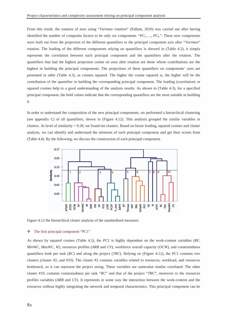
Project characteristics and complexity assessment relying on principal component analysis

82

From this result, the rotation of axes using “Varimax rotation” (Pallant, 2010) was carried out after having

identified the number of composite factors to be only six components “PC1, ..., PC6”. These new components

were built out from the projection of the different quantifiers to the principal component axis after “Varimax”

rotation. The loading of the different components relying on quantifiers is showed in (Table 4.2), it simply

represents the correlation between each principal component and the quantifiers after the rotation. The

quantifiers that had the highest projection cosine on axes after rotation are those whose contributions are the

highest in building the principal components. The projections of these quantifiers on components’ axes are

presented in table (Table 4.3), as cosines squared. The higher the cosine squared is, the higher will be the

contribution of the quantifier in building the corresponding principal component. The loading (correlation) or

squared cosines help to a good understanding of the analysis results. As shown in (Table 4.3), for a specified

principal component, the bold values indicate that the corresponding quantifiers are the most suitable in building

it.

In order to understand the composition of the new principal components, we performed a hierarchical clustering

(see appendix C) of all quantifiers, shown in (Figure 4.12). This analysis grouped the similar variables in

clusters. At level of similarity = 0.30, we found ten clusters. Based on factor loading, squared cosines and cluster

analysis, we can identify and understand the elements of each principal component and get their scores from

(Table 4.4). By the following, we discuss the construction of each principal component.

Figure 4.12 the hierarchical cluster analysis of the standardised measures

The first principal component “PC1”

As shown by squared cosines (Table 4.3), the PC1 is highly dependent on the work-content variables (RF,

MinWC, MaxWC, W), resources profiles (ARB and CV), workforce overall capacity (OCW), and constraindness

quantifiers both per task (RC) and along the project (TRC). Relying on (Figure 4.12), the PC1 contains two

clusters (cluster #2, and #10). The cluster #2 contains variables related to resources, workload, and resources

bottleneck, so it can represent the project sizing. These variables are somewhat similar correlated. The other

cluster #10, contains constraindness per task “RC” and that of the project “TRC”, moreover to the resources

profiles variables (ARB and CV). It represents in some way the interaction between the work-content and the

resources without highly integrating the network and temporal characteristics. This principal component can be

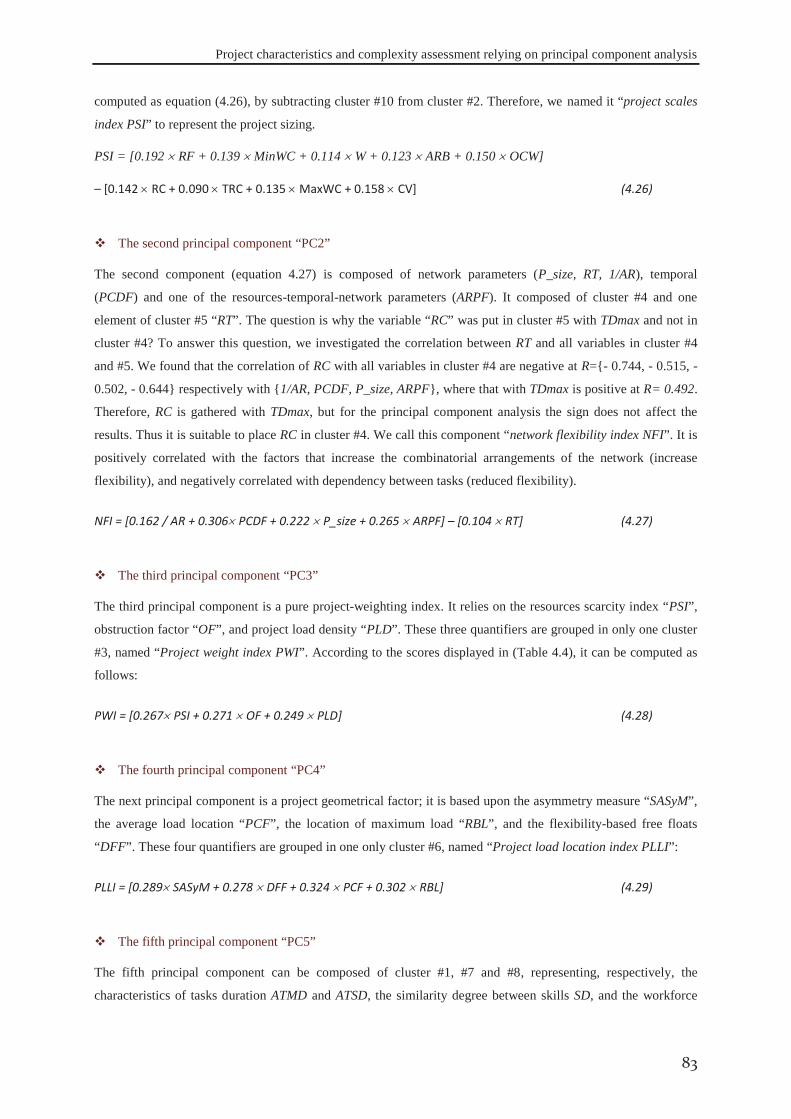
Project characteristics and complexity assessment relying on principal component analysis

83

computed as equation (4.26), by subtracting cluster #10 from cluster #2. Therefore, we named it “project scales

index PSI” to represent the project sizing.

PSI = [0.192 RF + 0.139 MinWC + 0.114 W + 0.123 ARB + 0.150 OCW]

– [0.142 RC + 0.090 TRC + 0.135 MaxWC + 0.158 CV] (4.26)

The second principal component “PC2”

The second component (equation 4.27) is composed of network parameters (P_size, RT, 1/AR), temporal

(PCDF) and one of the resources-temporal-network parameters (ARPF). It composed of cluster #4 and one

element of cluster #5 “RT”. The question is why the variable “RC” was put in cluster #5 with TDmax and not in

cluster #4? To answer this question, we investigated the correlation between RT and all variables in cluster #4

and #5. We found that the correlation of RC with all variables in cluster #4 are negative at R={- 0.744, - 0.515, -

0.502, - 0.644} respectively with {1/AR, PCDF, P_size, ARPF}, where that with TDmax is positive at R= 0.492.

Therefore, RC is gathered with TDmax, but for the principal component analysis the sign does not affect the

results. Thus it is suitable to place RC in cluster #4. We call this component “network flexibility index NFI”. It is

positively correlated with the factors that increase the combinatorial arrangements of the network (increase

flexibility), and negatively correlated with dependency between tasks (reduced flexibility).

NFI = [0.162 / AR + 0.306 PCDF + 0.222 P_size + 0.265 ARPF] – [0.104 RT] (4.27)

The third principal component “PC3”

The third principal component is a pure project-weighting index. It relies on the resources scarcity index “PSI”,

obstruction factor “OF”, and project load density “PLD”. These three quantifiers are grouped in only one cluster

#3, named “Project weight index PWI”. According to the scores displayed in (Table 4.4), it can be computed as

follows:

PWI = [0.267 PSI + 0.271 OF + 0.249 PLD] (4.28)

The fourth principal component “PC4”

The next principal component is a project geometrical factor; it is based upon the asymmetry measure “SASyM”,

the average load location “PCF”, the location of maximum load “RBL”, and the flexibility-based free floats

“DFF”. These four quantifiers are grouped in one only cluster #6, named “Project load location index PLLI”:

PLLI = [0.289 SASyM + 0.278 DFF + 0.324 PCF + 0.302 RBL] (4.29)

The fifth principal component “PC5”

The fifth principal component can be composed of cluster #1, #7 and #8, representing, respectively, the

characteristics of tasks duration ATMD and ATSD, the similarity degree between skills SD, and the workforce

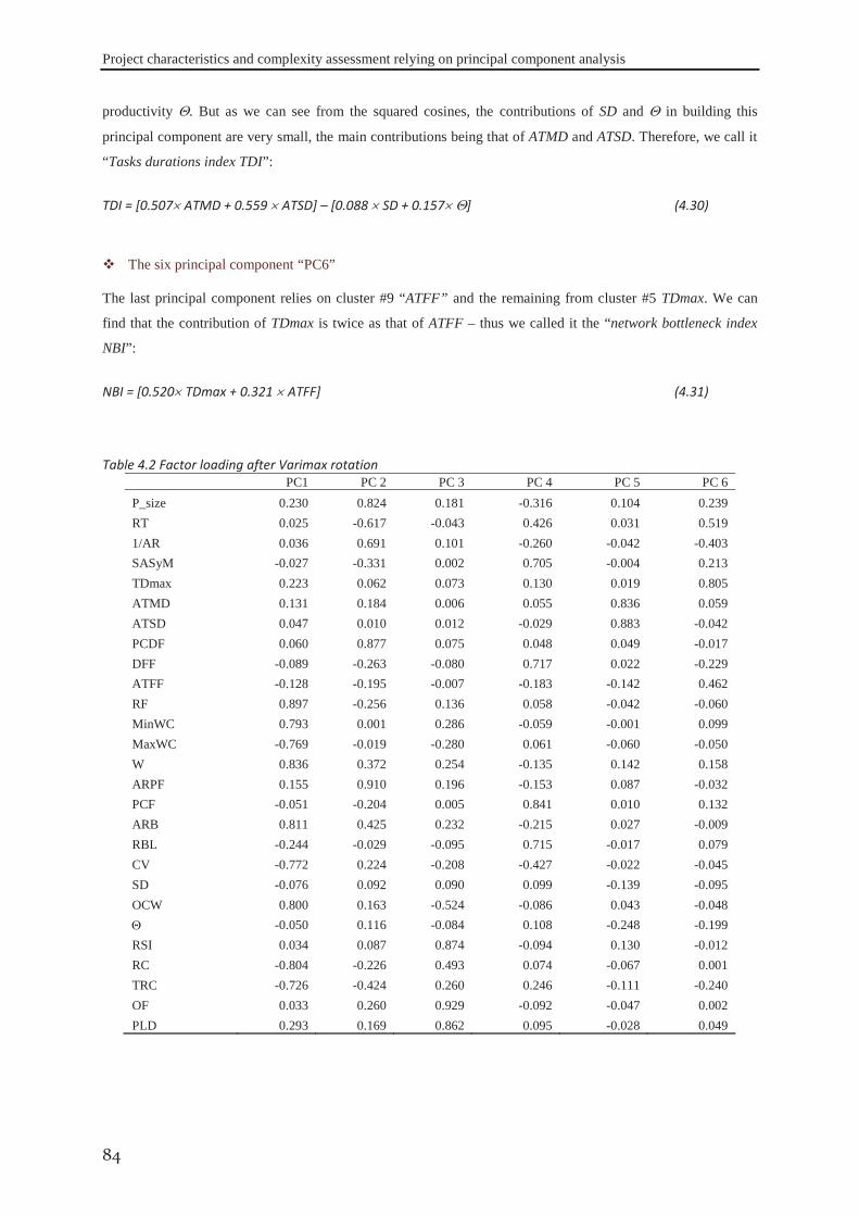
Project characteristics and complexity assessment relying on principal component analysis

84

productivity . But as we can see from the squared cosines, the contributions of SD and in building this

principal component are very small, the main contributions being that of ATMD and ATSD. Therefore, we call it

“Tasks durations index TDI”:

TDI = [0.507 ATMD + 0.559 ATSD] – [0.088 SD + 0.157 ] (4.30)

The six principal component “PC6”

The last principal component relies on cluster #9 “ATFF” and the remaining from cluster #5 TDmax. We can

find that the contribution of TDmax is twice as that of ATFF – thus we called it the “network bottleneck index

NBI”:

NBI = [0.520 TDmax + 0.321 ATFF] (4.31)

Table 4.2 Factor loading after Varimax rotation PC1 PC 2 PC 3 PC 4 PC 5 PC 6

P_size 0.230 0.824 0.181 -0.316 0.104 0.239 RT 0.025 -0.617 -0.043 0.426 0.031 0.519 1/AR 0.036 0.691 0.101 -0.260 -0.042 -0.403 SASyM -0.027 -0.331 0.002 0.705 -0.004 0.213 TDmax 0.223 0.062 0.073 0.130 0.019 0.805 ATMD 0.131 0.184 0.006 0.055 0.836 0.059 ATSD 0.047 0.010 0.012 -0.029 0.883 -0.042 PCDF 0.060 0.877 0.075 0.048 0.049 -0.017 DFF -0.089 -0.263 -0.080 0.717 0.022 -0.229 ATFF -0.128 -0.195 -0.007 -0.183 -0.142 0.462 RF 0.897 -0.256 0.136 0.058 -0.042 -0.060 MinWC 0.793 0.001 0.286 -0.059 -0.001 0.099 MaxWC -0.769 -0.019 -0.280 0.061 -0.060 -0.050 W 0.836 0.372 0.254 -0.135 0.142 0.158 ARPF 0.155 0.910 0.196 -0.153 0.087 -0.032 PCF -0.051 -0.204 0.005 0.841 0.010 0.132 ARB 0.811 0.425 0.232 -0.215 0.027 -0.009 RBL -0.244 -0.029 -0.095 0.715 -0.017 0.079 CV -0.772 0.224 -0.208 -0.427 -0.022 -0.045 SD -0.076 0.092 0.090 0.099 -0.139 -0.095 OCW 0.800 0.163 -0.524 -0.086 0.043 -0.048

-0.050 0.116 -0.084 0.108 -0.248 -0.199 RSI 0.034 0.087 0.874 -0.094 0.130 -0.012 RC -0.804 -0.226 0.493 0.074 -0.067 0.001 TRC -0.726 -0.424 0.260 0.246 -0.111 -0.240 OF 0.033 0.260 0.929 -0.092 -0.047 0.002 PLD 0.293 0.169 0.862 0.095 -0.028 0.049

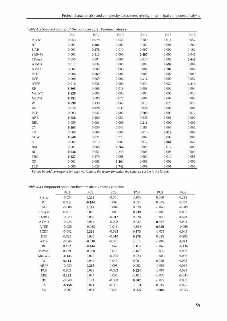
Project characteristics and complexity assessment relying on principal component analysis

85

Table 4.3 Squared cosines of the variables after Varimax rotation PC1 PC 2 PC 3 PC 4 PC 5 PC 6

P_size 0.053 0.679 0.033 0.100 0.011 0.057 RT 0.001 0.381 0.002 0.182 0.001 0.269 1/AR 0.001 0.478 0.010 0.067 0.002 0.162 SASyM 0.001 0.110 0.000 0.497 0.000 0.045 TDmax 0.050 0.004 0.005 0.017 0.000 0.648 ATMD 0.017 0.034 0.000 0.003 0.699 0.004 ATSD 0.002 0.000 0.000 0.001 0.780 0.002 PCDF 0.004 0.769 0.006 0.002 0.002 0.000 DFF 0.008 0.069 0.006 0.514 0.000 0.052 ATFF 0.016 0.038 0.000 0.034 0.020 0.213 RF 0.805 0.066 0.018 0.003 0.002 0.004 MinWC 0.630 0.000 0.082 0.004 0.000 0.010 MaxWC 0.592 0.000 0.078 0.004 0.004 0.003 W 0.698 0.138 0.065 0.018 0.020 0.025 ARPF 0.024 0.828 0.038 0.024 0.008 0.001 PCF 0.003 0.042 0.000 0.708 0.000 0.017 ARB 0.658 0.180 0.054 0.046 0.001 0.000 RBL 0.059 0.001 0.009 0.511 0.000 0.006 CV 0.595 0.050 0.043 0.183 0.000 0.002 SD 0.006 0.009 0.008 0.010 0.019 0.009 OCW 0.640 0.027 0.275 0.007 0.002 0.002

0.002 0.013 0.007 0.012 0.061 0.040 RSI 0.001 0.008 0.764 0.009 0.017 0.000 RC 0.646 0.051 0.243 0.005 0.005 0.000 TRC 0.527 0.179 0.068 0.060 0.012 0.058 OF 0.001 0.068 0.864 0.008 0.002 0.000 PLD 0.086 0.029 0.742 0.009 0.001 0.002 Values in bold correspond for each variable to the factor for which the squared cosine is the largest

Table 4.4 Component score coefficients after Varimax rotation PC1 PC2 PC3 PC4 PC5 PC6

P_size -0.034 0.222 -0.001 -0.008 0.000 0.212 RT 0.006 -0.104 0.002 0.051 0.025 0.279

1/AR -0.006 0.162 0.004 0.029 -0.049 -0.209 SASyM 0.007 0.025 0.005 0.239 -0.008 0.085 TDmax -0.023 0.087 -0.012 0.028 -0.040 0.520 ATMD -0.025 0.014 -0.008 0.032 0.507 0.004 ATSD -0.026 -0.068 0.011 -0.033 0.559 -0.069 PCDF -0.042 0.306 -0.033 0.175 -0.031 0.045 DFF 0.025 0.025 -0.010 0.278 0.025 -0.202

ATFF -0.044 -0.048 -0.001 -0.135 -0.087 0.321 RF 0.192 -0.144 0.047 -0.007 -0.045 -0.134

MinWC 0.139 -0.068 0.076 -0.026 -0.035 0.000 MaxWC -0.135 0.068 -0.075 0.023 -0.006 0.032

W 0.114 0.044 0.043 0.001 0.028 0.063 ARPF -0.030 0.265 0.005 0.092 -0.006 0.034 PCF 0.002 0.088 -0.002 0.324 -0.007 0.034 ARB 0.123 0.047 0.038 -0.013 -0.037 -0.034 RBL -0.040 0.144 -0.038 0.302 -0.022 0.037 CV -0.158 0.061 -0.061 -0.151 0.015 0.075 SD -0.007 0.051 0.023 0.066 -0.088 -0.053

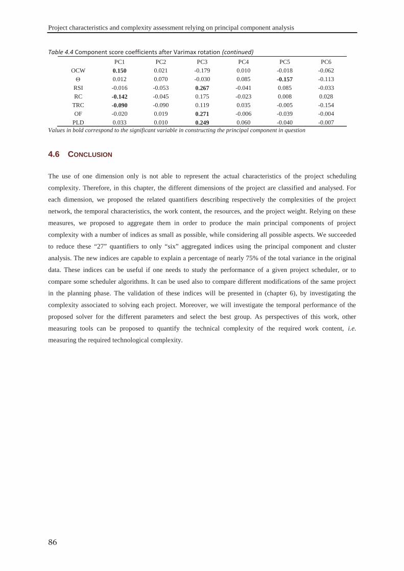
Project characteristics and complexity assessment relying on principal component analysis

86

Table 4.4 Component score coefficients after Varimax rotation (continued) PC1 PC2 PC3 PC4 PC5 PC6

OCW 0.150 0.021 -0.179 0.010 -0.018 -0.062 0.012 0.070 -0.030 0.085 -0.157 -0.113

RSI -0.016 -0.053 0.267 -0.041 0.085 -0.033 RC -0.142 -0.045 0.175 -0.023 0.008 0.028

TRC -0.090 -0.090 0.119 0.035 -0.005 -0.154 OF -0.020 0.019 0.271 -0.006 -0.039 -0.004

PLD 0.033 0.010 0.249 0.060 -0.040 -0.007 Values in bold correspond to the significant variable in constructing the principal component in question

The use of one dimension only is not able to represent the actual characteristics of the project scheduling

complexity. Therefore, in this chapter, the different dimensions of the project are classified and analysed. For

each dimension, we proposed the related quantifiers describing respectively the complexities of the project

network, the temporal characteristics, the work content, the resources, and the project weight. Relying on these

measures, we proposed to aggregate them in order to produce the main principal components of project

complexity with a number of indices as small as possible, while considering all possible aspects. We succeeded

to reduce these “27” quantifiers to only “six” aggregated indices using the principal component and cluster

analysis. The new indices are capable to explain a percentage of nearly 75% of the total variance in the original

data. These indices can be useful if one needs to study the performance of a given project scheduler, or to

compare some scheduler algorithms. It can be used also to compare different modifications of the same project

in the planning phase. The validation of these indices will be presented in (chapter 6), by investigating the

complexity associated to solving each project. Moreover, we will investigate the temporal performance of the

proposed solver for the different parameters and select the best group. As perspectives of this work, other

measuring tools can be proposed to quantify the technical complexity of the required work content, i.e.

measuring the required technological complexity.

4.6 CONCLUSION

5 SOLUTION TECHNIQUES AND PROBLEM SOLVING

USING GENETIC ALGORITHMS

This chapter aims at presenting simultaneously two main parts. The first is

a brief discussion of resolution techniques for highly-combinatorial

optimisation problems. The second part is the detailed presentation of the

approach we propose, based on genetic algorithms.

CH

APT

ER

5

Solution techniques and Problem solving using genetic algorithms

88

After the characterisation of the planning and scheduling problem with or without human factors, the proposed

models often lead to highly-combinatorial problems. These can be solved exactly or approximately, depending

on the performance criteria granted for the solution. As discussed by Russell and Norvig (2002) these

performance criteria contain: –completeness: the guarantee that the algorithm will find a solution if there is one,

–optimality: the capability of the solving method to return the optimal solution with respect to pre-defined

objectives, –time complexity: the computing time required to come to a solution, – space complexity: the

machine memory required to conduct the solution search procedures. These four criteria can be used to measure

the efficiency and applicability of any proposed method to solve a given problem. By the following we will

discuss briefly some exact and approximate methods adopted in literature. For more extensive details of these

methods, one can refer to the academic books such as Demeulemeester and Herroelen (2002); Artigues et al.

(2008); Brucker and Knust (2011).

The exact methods are proposed to provide the most accurate results with guarantee of optimality. Almost all the

problems of project scheduling with resources constraints are NP-Hard problems (section 3.5); relying on the

works of Cavalcante et al. (2001), solving exactly such problems is valid only for medium-size instances, from

the computing time point of view. However, in many applications the exact solutions are essential; therefore, the

research efforts continue in order to develop exact methods that can return optimal solutions with acceptable

CPU time. These methods can be classified into two main categories: the first is the calculation-based methods,

where the second is the enumeration of spanning trees-based approaches. In this section we will discuss some

approaches recently developed in this matter.

According to Demassey (2008), the earliest studies of project scheduling with resources constraints were

oriented towards exact methods. She reviewed the different forms of mathematical programming of the problem.

Demeulemeester and Herroelen (2002) discussed too the different linear programming formulations of the

RCPSP; Cavalcante et al. (2001) discussed several integer programming models for the minimum make-span

project scheduling problem, with precedence and labour constraints. The difficulties of solving such models

optimally were proved. Moreover, they discussed the linear programming based on ordering heuristics. Recently,

Sayin and Karabati (2007) proposed a mixed integer programming model to solve the problem of staff

scheduling taking into account learning/forgetting effect. They modelled the problem as a set of two linear

programming serial optimization models, and solved them by the “CPLEX” solver after encoding them with

OPL script language. Turkcan et al. (2009) proposed a two-stage algorithm in order to solve the unrelated

parallel-machine scheduling problem with continuously controllable processing times. In the first stage, a time-

indexed integer programming model was used to assign parts to machines and to determine the sequence of parts

on each machine. In the second stage, a non-linear programming model was used to determine the optimal start

5.1 INTRODUCTIONS

5.2 EXACT METHODS

5.2.1 Calculation-based methods

Solution techniques and Problem solving using genetic algorithms

89

times and processing times for a given sequence of parts on each machine. This non-linear model was converted

to a minimum-cost network flow model by piece-wise linearization of the convex cost objective function. The

models were coded in C language and solved optimally using CPLEX. Heimerl and Kolisch (2009a) proposed a

mixed-integer linear program for simultaneous scheduling and staffing of multiple projects with a multi-skilled

human workforce, with heterogeneous and static efficiencies solved by CPLEX.

Numeration (or branching) techniques can be considered as heuristics that guarantee to return the optimal

solution, if it can be allowed to construct the complete search tree. In industrial problems, construction of the

complete search tree by all the enumerations is almost impossible, in raisons of the required time, and machine

memory. Therefore, many methods are proposed to reduce the number of enumerations by truncating the search

tree according to a set of specified rules, to limit the search to only the promising solutions. Truncating or

pruning is a technique aiming at a reduction of the search by cutting branches that proved to lead to unfeasible or

non-optimal solution.

5.2.2.1 Branch and X family

In discrete combinatorial optimisation problems, methods from Branch and X family can be applied to solve

linear/nonlinear models and provide the optimal solutions. Branch and X is a set of algorithms including: Branch

and Bound, Branch and Cut, Branch and Price, Branch and Infer. The first member of this family is the branch

and bound “B&B”, in which the systematic search is governed by three main acts: -the first is the branching or

splitting scheme. It represents the search space corresponding to the current node is partitioned into subsets such

that the union of these subsets is the set of solutions of the node (Néron, 2008). - The second is the bounding; it

is the process of computing the upper and lower bound of the objective function at each node. Depending on

these values, some sub-nodes can be discarded from further considerations; - The third tool is the search

strategy: which sub-node should be selected first. There are many search strategies such as “depth-first-search”,

“depth-limited-search”, “width first search”, “breadth-first-search”, “iterative deepening-search”, “bidirectional

search” for more details about these types, see Russell and Norvig (2002). The B&B algorithms were

intensively used to solve the RCPSPs’ with their different characteristics; the study of Demeulemeester and

Herroelen (2002) shows many of these researches and the determination of the different lower bounds. Néron

(2008) too, discussed the various branching schemes in RCPSP problems. In the multi-mode RCPSP, Sprecher et

al. (1997) developed an extended B&B algorithm that relies on the concept of delay alternatives proposed by

Demeulemeester and Herroelen (1992) for single mode RCPSP. Vanhoucke (2005) solved the time-cost trade-

off problem with time-switch constraints using B&B algorithms. Daniels et al. (2004) developed B&B algorithm

to optimally solve the problem of production scheduling with multi-skilled individual assignment. In multi

skilled project scheduling with resources allocations, Bellenguez-Morineau and Néron (2007) solved the

problem by a B&B, moreover they presented a lower bound.

Branch and Cut algorithms used to solve MILP problems relying on the relaxation. These algorithms consisting

of a combination of a cutting plane method with a B&B algorithm. As discussed by Hans (2001) and Mitchell

(2002), these methods work by solving a sequence of linear programming “LP” relaxations of the integer

programming problem, known as the restricted linear programming “RLP” relaxation. This RLP is then solved

5.2.2 Numeration-based methods

Solution techniques and Problem solving using genetic algorithms

90

until optimality. Cutting plane methods improve the relaxation of the problem to approximate more closely the

integer programming problem “ILP”. In that way, if the optimal solution for the RLP is not reachable for the

ILP, a sub-problem called the “separation problem” is solved to try to identify the violated inequalities. If one or

more violated inequalities are found, some are added to the LP relaxation to cut-off the infeasible solution. Then

the “LP” is solved optimally. Branching occurs when no violated inequalities are found to cut-off an infeasible

solution. The procedure is continued until no violated inequalities exist anymore: at this point the optimal

solution to the RLP is also the optimal solution to the original problem. Aykin (1998) presented a branch and cut

algorithm for optimal shift scheduling. Kis (2005) proposed branch and cut to solve MILP models of project

scheduling with variable intensity of resource requirement.

Branch and Price method is simply a generalisation between B&B and LP relaxation. The main difference from

branch and cut is that: it applies column generations during B&B search tree to tight the LP relaxation. First, the

original problem is reformed by one of the decomposition algorithms, to give a LP relaxation “known as master

problem”. Align with the branch and cut, a “LP” relaxation is optimally solved by considering the restricted LP

relaxation (called restricted master problem: RMP), where many columns (variables) are lift out. For optimality

verification a pricing algorithm is used at each node. If the solution of RMP is not optimal, the pricing algorithm

identifies at least one column (variable) with negative reduced cost. This column is added to the RMP and the

procedures continued until there are no more columns with negative reduced cost. The optimal solution of the

RMP is also the optimal one for original problem. In scheduling, Jacquet-Lagrèze and Lebbar, (1999) adopted it

to solve the scheduling with maintenance constraints. Hans, (2001) used it to solve the resources loading

problem and the rough-cut capacity planning problem. Recently, Coughlan et al., (2010) proposed branch and

price algorithm to solve the multi-mode project scheduling with resources constraints, and availability per period

constraints.

Branch and Infer algorithms refer to the implementation of constraints programming “CP” techniques. In CP the

problem is modelled as a “constraint satisfaction problem CSP”. In this kind of problem, one needs to define the

variables, and their domains with a finite set of possible values. These values can be assigned to the

corresponding variables without any contradiction in the problem constraints. The CSP links the problem

variables together with some relations or instructions. Based on this principle, the scheduling problem can be

formulated with two groups of variables: the temporal variables and the resources allocation variables. The

temporal variables gather all the variables related to the time, e.g. the tasks’ start dates dSi {dSimin,…, dSi

max},

and tasks’ durations [Dimin,…, Di

max] (if it is known in advance). During the solution search procedures,

constraints propagation methods are used, in order to infer the contradiction or the infeasibility of continuing the

search process (at the current node), or to indicate a solution (occurs at the bottom levels of the search tree).

Bockmayr and Kasper (1998) introduced a framework that proposed to integrate the ILP and finite domain CP.

The framework is called “branch and infer”, it unifies the branch and cut approach with CP. Modelling problems

as CSP and solving them using CP has attracted the attention of the operational research community, so

numerous applications can be found on the arena. Meisels and Schaerf (2003) proposed to solve employee

timetable problem using CP, after coded it in ECLiPSe. For the same problem, Demassey et al. (2005) proposed a

hybrid constraints-linear programming approach based on column generation. in which sub-problems are

modelled as CSP and solved using CP. De la Fuente and Lozano (2008) proposed a CP paradigm to provide one

Solution techniques and Problem solving using genetic algorithms

91

year-wide calendars for multi-shift employees schedule. Li and Womer (2009) present an application in software

production technology. They solved the proposed MILP by using benders decomposition algorithm and CP. For

more details about CP in scheduling and different propagation algorithms, we propose the academic book of

Baptiste et al. (2001) or Laborie and Nuijten (2010).

5.2.2.2 Dynamic programming

In mathematical optimisation, the dynamic programming “DP” is a complete enumeration scheme that attempts

to minimise the amount of computations to solve a problem, by convert it into a sequence of interrelated sub

problems arranged in stages. It is based on the concept that the decision in one stage cannot be taken separately

due to problem constraints. It determines the optimal solution to each sub-problem and its contribution to the

objective function. Also, it avoids re-computation by storing the solutions of sub-problems. DP characterised by

three types of equations: -Initial conditions, -Recurrence relations, and –Contribution function. Zhang et al.

(2001) proposed to solve a macro-level scheduling problem using Lagrangian relaxation, in which the resource

capacity constraints were relaxed by the Lagrange multiplier for the use of resources at each time unit. The

“relaxed problem” then decomposed into smaller sub-problems. The solutions of these sub-problems were

obtained by the DP. Stanimirovic et al. (2009) proposed a heuristic algorithm to solve the RCPSP based on the

DP of knapsack problem.

Real industrial optimisation problems are often NP-Hard, even when they are deterministic. Therefore, no

algorithm reveals to be efficient to solve them optimally, especially for large size problems (Sevaux et al., 2010).

In the scheduling problems under resources constraints, Kolisch and Hartmann (1998) stated that the heuristic

solution procedures are indispensable when solving large problem instances – as they usually appear to be in

practical cases. Heuristics and metaheuristics have become reference tools, guaranteeing a compromise between

the solution quality and the computing time. Demeulemeester and Herroelen (2002) classified the heuristic

methods into two main categories: the constructive heuristics (referred here as heuristics) and the improvement

heuristics. Constructive heuristics start from an empty schedule and add one task after the other until it

constructs a feasible schedule. On the other hand, the improvement heuristics start from an initial schedule

(feasible as well as unfeasible), and repetitively try to improve it. Gademann and Schutten (2005) classified these

algorithms into three categories by dividing the improvements into two types: – the first category starts by

infeasible schedule – and the second starts with feasible schedule. In order to avoid cycling around local optima,

many algorithms were developed as local search-oriented, and population search algorithms. By the following

we discuss briefly some of these methods.

The constructive algorithms can be classified as “Greedy algorithms”, in which the problem solution is obtained

by a very intuitive idea that depends mainly on the problem nature. As stated before the constructed algorithms

start from scratch to construct the schedule by adding activities in a successive way according to a predefined

list. The definition of this list depends on the intuitive idea to design the algorithm. In scheduling under

resources constraints, the list predefinition relies on a set of rules that known as priority rules. As discussed in

5.3 APPROXIMATED METHODS

5.3.1 Heuristic algorithms

Solution techniques and Problem solving using genetic algorithms

92

Demeulemeester and Herroelen (2002), there are five types of priority rules:- activity-based priority rules –

network-based priority rules – critical path-based priority rules – resources-based priority rules – composite

priority rules. Kolisch and Hartmann (1998) explained two schedule generation schemes to be adopted when

using priority rules: the first is the parallel generation scheme “PGS” – the second is the serial generation scheme

“SGS”. The PGS iterates over time by searching at each decision step as many unscheduled activities as possible

considering the temporal and resource constraints. For each iteration in the SGS, the next unscheduled activity in

the priority list is selected and assigned at the first possible start date that satisfies the constraints. Van de Vonder

et al. (2007a) added three other generation schemes for generating the robust schedule: The stochastic SGS,

robust PGS, and robust SGS. The greedy heuristics based on priority rules were extremely adopted in many

applications: Nembhard (2001) examined the problem of worker-to-task assignment based on the worker’s

learning rates. The proposed heuristic assigns fast learners to short duration tasks and slow learners to longer

duration tasks in a greedy manner. Edi (2007) proposed a greedy heuristic to solve the project scheduling with

flexible workforce annual hours. Gutjahr et al. (2008) adopted a greedy algorithm to assign workforce to the

different activities of project portfolio according to a set of priority lists. Browning and Yassine (2010)

conducted a comprehensive analysis of 20 priority rules to solve resource-constrained multi-project scheduling

problem. Recently, Attia et al. (2012b) used the priority rules for encoding the chromosomes of a genetic

algorithm model developed to solve the problem of project scheduling with dynamic productivities (section 5.4).

Metaheuristics algorithms have become a kind of general problem solvers, and are applied to numerous

applications for solving the most difficult optimisation problems. Metaheuristics represent the improvement type

of heuristics, in which the solution can be improved iteratively over time starting from the initial solution(s).

Each meta-heuristic algorithm can belong to one or more of the following classification: population-based

algorithms, nature-inspired algorithms, evolutionary algorithms, swarm-based algorithms, memory-based

algorithms, stochastic algorithms, and local search algorithms. By the following, we will highlight only two

classes: the population-based and the local search methods.

5.3.2.1 Population-based methods

Population-based metaheuristics represent the set of algorithms that handle a number of individuals at each trial,

where each individual represents a solution to the problem. Here we present some of these types that were used

for scheduling and resources allocation: genetic algorithms “GA”; ant colony optimization “ACO”; particle

swarm optimisation “PSO”. There are numerous kinds of metaheuristics algorithms, but many of them share

some characteristics (such as: natural inspiration, stochastic nature, evolution strategy, etc). For example,

Abboud (1998) proposed a metaheuristics method for the problem of manpower allocation. The developed

heuristics known as mutate and spread metaheuristics (MSM), a sibling of GA. It differs from GA only in the

selection and matting operation. For more algorithms, we propose the metaheuristics books of Glover and

Kochenberger (2003) and Doerner et al. (2007).

5.3.2.1.1 Genetic algorithms

Genetic algorithms are an artificial intelligence probabilistic search method emulating the nature evolution: a

population of problem solutions evolves over time under the influence of specified genetic operators. These

5.3.2 Metaheuristics algorithms

Solution techniques and Problem solving using genetic algorithms

93

operators were adopted from the biological processes known as crossover, mutation, and survival of the fittest

individual(s). First, the solutions of the problem, whatever feasible or not, should be coded in a vector called

chromosome. Each chromosome is composed of a finite number of genes describing this solution, via either a

direct or indirect representation; the gene can take any kind of value: alphabetic string, binary, integer, real

number, etc. This process is known as the chromosome encoding. On the other side, if the chromosome carries

an indirect representation of a solution, a decoding process should convert the genes to the problem solution.

After defining the problem representation (encoding process), the initial population should be generated by either

constructed heuristics or randomly. Then iteratively, the solution state space can be explored by performing the

following procedures: evaluation of the current population, select individuals (named “parents”) for matting,

mate individuals to produce offsprings, mutate offspring, build the next population, evaluate the individuals and

check the stopping criteria.

For manufacturing problems, GAs’ were successfully applied to numerous problems with especially difficult

levels. Mori and Tseng (1997) used GAs’ to solve the non-pre-emptive multi-mode project scheduling problem

(time-resource trade-off). The chromosomes were encoded directly with all of the required data: the activity

mode, the schedule order, and start/finish dates. Aloulou and Portmann (2005) developed multi-criteria GAs’ to

find a compromise between the schedule flexibility and its aptitude to generate a proactive baseline schedule for

a job shop problem. Wang (2005) modelled the problem of repairing the schedule of product development

process as a dynamic constraints satisfaction problem. The proposed GAs’ were planned to solve the problem

based on activity priority rules for the chromosomes encoding. Relying on the priority rules held by the

chromosomes, a generation scheme was used to build the schedule.

Wu and Sun (2005) presented a mixed non-linear integer program for a multi-project scheduling problem taking

into account actors’ competences evolutions, with objective to reduce the outsourcing costs resulting from hiring

external staff. They solved the proposed model using GAs’, with a direct encoding chromosome for the actors’

assignment decisions. Their model handled two other variables, the outsourcing actors’ number and the task

completion percentage: after fixing the allocation decisions, the model would be transformed to a linear one,

which was solved by using “ILOG CPLEX 7.5”. Cowling et al. (2006) used the open source genetic algorithms

NSGA-II in order to solve the multi-objectives multi-site scheduling. Yoshimura et al. (2006) solved the problem

of project portfolio selection with allocation of multi-skilled workforce using GAs’. Van Peteghem and

Vanhoucke (2008) proposed a bi-population GAs’ to solve multi-mode RCPSP: One population for the right-

justified schedule and the other for left-justified schedule. The chromosomes were encoded relying on two

vectors: the topological ordered random key and the modes list. After that a schedule generation scheme was

developed relying on SGS to build the schedule. Gutjahr et al. (2008) adopted GAs’ to solve the problem of

project portfolio selection with optimisation of the economic objective versus the strategic workforce

competency. Yannibelli and Amandi (2011) solved the multi-skilled workforce allocation with knowledge-based

genetic algorithms. This knowledge arises from historical information about the participation of the employees in

previously executed projects. Recently in scheduling IT project with multi-skilled workforce staffing, Kolisch

and Heimerl (2012) proposed a two stages metaheuristics approach: the first stage used GAs’ for solving the MIP

model of the problem, afterwards a Tabu search algorithm was called to enhance the best obtained solution from

GAs’.

Solution techniques and Problem solving using genetic algorithms

94

5.3.2.1.2 Ant colony optimization

Ant colony optimisation “ACO” is one of the swarm intelligence and population-based metaheuristics that

combines stochastic search and learning mechanisms. Learning through the cooperation of large number of

homogeneous agents (artificial Ants) in the environment when they foraging. The information is stored

throughout the interaction with the environment by producing pheromones. This mechanism is called stigmergy.

For more details about the algorithms, we propose the work of Glover and Kochenberger (2003).The ACO has

been applied to scheduling with resources constraints problem. Merkle et al. (2002) developed an ACO approach

for RCPSP, while, Luo et al. (2003) developed an approach to solve the RCPSP with generalised precedence

constraints. Kilic (2007) used ACO approach to generate a flow shop schedule for the cases where the processing

times are uncertain and due dates are flexible in some range. Processing times and flexible due dates are handled

respectively as fuzzy processing time and due dates. Gutjahr et al. (2008) adopted the ACO to solve the project

portfolio selection. Problem solutions are encoded as walks in a so-called construction graph, assigning to each

arc a visibility value depending on the pheromone strength.

5.3.2.1.3 Particle swarm algorithms

Particle swarm optimisation “PSO” uses a population of particles to explore the best solutions in a multi-

dimensions search space. PSO is inspired by the social behaviour of foraging flocks of birds: here, particles in a

swarm fly through the environment, following the particle flow but biasing their movements towards the good

areas. Similar to the meta-heuristic methods, PSO starts with initial solutions and develop them over time. As

discussed by Doerner et al. (2007), each particle represents a candidate solution of the problem, and has an

associated position, velocity, and memory vectors. The memory stores the particle’s best position encountered so

far (known as personal best). Also, the best position found so far by the whole swarm (known as global best) is

memorised during the exploration. The PSO was adopted in scheduling and resources allocation; Zhang et al.

(2006) proposed PSO for multi-mode RCPSP considering renewable and non- renewable resources. The

particles was represented as a priority list vector for the activities and modes, a SGS was adopted to construct the

feasible solution. Chen (2011) presented a “justified” particle swarm optimisation to the traditional RCPSP. The

justification technique adjusts the start time of each activity of a given schedule to shorten the project makespan.

Kazemi and Tavakkoli-Moghaddam (2011) proposed a PSO for solving multi-objective multi-mode RCPSP. The

proposed algorithm uses GAs’ operators for updating the particles’ positions. Shahnazari-Shahrezaei et al. (2012)

used the same concept in the developed PSO algorithm to solve the problem of single-period multi-skilled

manpower scheduling, considering the employees’ preferences. They generated a number of particles, for each

particle they assign randomly feasible solutions relying on greedy algorithms-based procedures. Local heuristics

were used to improve the particles’ solution.

5.3.2.1.4 Other algorithms

There are some other population-based algorithms that were adopted in scheduling under resources constraints,

as example, the Scatter algorithm, GRASP algorithms (Greedy Randomised Adaptive Search Procedures), bees

algorithms...etc. The scatter algorithms rely on combining decision rules and constraints (Glover and

Kochenberger, 2003). According to Brownlee (2011), the strategy involves an iterative process, where a

population of diverse (stored information about the global optima) and high-quality candidate (elite set)

solutions. These solutions are partitioned into subsets and linearly recombined to create weighted centroids of

sample-based neighbourhoods. The GRASP is a multi-start metaheuristics, and each iteration contains two

Solution techniques and Problem solving using genetic algorithms

95

phases: construction and local search (improvement phase). The best overall solution is kept as the result.

Alvarez-Valdes et al. (2008) proposed a GRASP algorithm to solve project scheduling with partially renewable

resources. The bees’ algorithm is a one of population and swarm based metaheuristics that is inspired by the way

that the honey bees forage for food. The principal, the flowers batches that have a lot of nectar will be visited

more than those that have less nectar. The bees communicate with each other by a dance known as “waggle

dance”. Akbari et al. (2011) proposed a “bees’ algorithm” for the scheduling problem with resource constraints.

5.3.2.2 Local search-based methods

Local search methods are iterative algorithms, which explore the solution space by using a single solution, and

moves step by step from this current solution to its neighbour according to a set of pre-defined rules. The search

loops are continued until it reaches a stopping criterion. The local search methods have two basic elements: the

search space and the neighbourhood structure. The neighbourhood structure is the set of solutions obtained by

applying a single local transformation to a current solution. According to Russell and Norvig (2002), local search

methods have two main advantages: they use very little memory, usually constant and they can often find

reasonable solution in large or continuous spaces for which systematic algorithms are unsuitable. On the other

side, using such algorithms bring two drawbacks: the size of the neighbourhood of the current solution (the

search of the best neighbour can be another problem), and the incapability to avoid local optima (Widmer et al.,

2010). By the following we review the most utilisable algorithms.

5.3.2.2.1 Simulated annealing method

Simulated annealing “SA” is a global optimisation algorithm that belongs to the stochastic search metaheuristics.

SA is inspired by a metallurgy process called annealing: a heat treatment process used to increase the toughness

of steel elements by increasing their microstructure grains size. It usually starts with an initial solution and

improves the solution repeatedly by moving around the neighbourhood of the current solution until no further

improvement can be found. According to Wang (2005), SA approach attempts to avoid entrapment in a local

optimum by accepting a move that deteriorates the objective value with a certain probability. While exploring

solution space, the new obtained neighbour solution will be accepted if e′ < e for minimisation problems, where

e: is the energy (objectives value) of the current solution; e′: is the energy of the candidate solution. On the other

hand it can be accepted or rejected, based on the probabilistic function: (exp(e-e′)/T) | e′ > e, where T is the

current temperature. The temperature can be controlled by a cooling scheme that specifies how it should be

progressively reduced. According to Bouleimen and Lecocq (2003), the total number of iterations depend on the

initial temperature and the reduction factor within]0, 1[, the process is called cooling chains. The SA was applied

to scheduling with resources constraints. As example, for single-period manpower schedule problem, Brusco and

Jacobs (1993) proposed SA to solve flexible labour schedule problem (discontinuous tour schedule) with the

objective of minimizing the number of full-time employees. Recently, Hlaoittinun (2009) proposed a SA

algorithm for manpower allocation to activities of a product development, considering their dynamic experience.

Józefowska et al. (2001) and Bouleimen and Lecocq (2003) proposed to solve the RCPSP and its multi-mode

extension by SA algorithms with the objective of minimum makespan. They used activity list representation

where a precedence-feasible solution is represented by an ordered list of activities, and then a SGS was used to

construct solution. Mika et al. (2005) adopted it in solving multi-mode project scheduling problem with

discounted cash flows and four payment models with the aim to maximise the net present value. The problem

Solution techniques and Problem solving using genetic algorithms

96

was encoded relying on the list of feasible activities and modes assignment as that was used by Józefowska et al.

(2001), and then a SGS was adopted to decode the solution. The neighbour probabilistic generated relying on the

three bases: the rearranging of the activities list, of the mode list, and the combination of both.

5.3.2.2.2 Tabu search method

Tabu search “TS” is a control strategy for local search algorithms relying on machine memory. In order to avoid

cycling, a tabu list imposes restriction to guide the search process. The tabu list imposes a short term memory of

the specific changes of recently performed moves within the search space, in order to prevent the same moves as

that listed. A tabu list is managed using a method known as tabu navigation method (as example FIFO method)

(Mika et al., 2005). According to Brownlee (2011) TS was designed to manage the hill climbing algorithm, it can

be adopted to manage any neighbourhood method. TS algorithms were used in solving the scheduling with

resources constraints. Thomas and Salhi (1998) proposed it for the traditional RCPSP, the tabu list was put

relying on the project network complexity. De Reyck and Herroelen (1999) adopted it for the multi-mode

RCPSP with generalised precedence relations and divided the problem into two successive phases: mode

assignment phase and RCPSP phase. Deblaere et al. (2011) also adopted it for the reactive schedule to repair the

baseline schedule of a multi-mode RCPSP. Atkin et al. (2007) proposed a hybrid algorithm “Aid to Runway

Scheduling” at London Heathrow Airport to find the best order for take-off for the aircraft under considerations

relying on TS. Van de Vonder et al. (2008) proposed it to solve project scheduling with stochastic activities

duration and temporal buffers between activities. Drezet and Billaut (2008) proposed a model for multi-period

project scheduling with workforce allocation. In their model the release date and completion date of the activity

are “time–dependent activities”. They solved the presented model with the integration of the priority rules and

TS, by using priority rules to generate the initial solution and TS as a local search technique to enhance the

solution. Recently, Kolisch and Heimerl (2012) used TS as a local search to enhance the best solution obtained

by Gas’ for project scheduling with manpower allocation. Shahnazari-Shahrezaei et al. (2012) solved single-

period multi-skilled manpower scheduling considering the employees’ preferences using TS.

5.3.2.2.3 Other algorithms

There are many other local search techniques, as example, the “Hill climbing algorithms” that try to

continuously improve the solution initially generated by a specified construction algorithm. It is continuously

moves on the direction of increasing value- that is uphill. The search loop terminates when it reaches the peak,

such that no neighbour has a higher value than that reached. Russell and Norvig (2002) stated that the hill

clamping algorithm sometimes called greedy local search where it grabs a good neighbourhood state without

thinking ahead about where to go next. The hill clamping is not a single local search technique but rather a

family of techniques based on the idea of performing only moves that improve or leave unchanged value of the

cost function (Meisels and Schaerf, 2003). As reviewed by Demeulemeester and Herroelen (2002) there is

another family of local search algorithms called “descent approaches” that can be divided into steepest descents,

fastest descents, and iterated descents. The steepest descent, called “best fit approach”, evaluates all solutions in

the neighbourhood of the current solution, selects the one with the best objective and continues the search with

this new one. Fastest descent, “first fit approach”, evaluates all solutions in the neighbourhood of the current one

in a random order, and stops as soon as a better solution is found, then the procedure is repeated with the new

position. In the iterated descent both steepest and fastest descent approaches can be extended with a random

restart procedure that randomly regenerates initial solution upon which the algorithm is restarted.

Solution techniques and Problem solving using genetic algorithms

97

In metaheuristics, hybrid algorithm is an approach that combines two different algorithms. The hybrid

algorithms that combine evolutionary population-based metaheuristics with local search metaheuristics are

known as “Memetic algorithms: MA”. MAs are inspired by the interplay of genetic evolution and memetic

evolution, the term “meme” being used to refer to a piece of discrete cultural information (Brownlee, 2011).

Chen and Shahandashti (2009) proposed a hybrid algorithm relying on GAs’ and SA in order to solve multi-

project scheduling problems with resources constraints. They used the SA probabilistic function to manage the

replacement of the new produced offspring by crossover and mutation. In order to solve project scheduling with

allocating of multi-skilled operators, Valls et al. (2009) proposed a hybrid approach relying on GAs and some

local search approaches. The approach starts with a GA population, then for each individual a SGS scheduler

than a local search used to enhance the schedule before computing the individual fitness. For a similar problem,

Yannibelli and Amandi (2012) proposed a Memetic algorithm that combines GA and local search algorithms.

From the previous survey, it can be concluded that both exact methods and heuristics are proposed to solve the

scheduling problem with resources constraints. The exact methods are capable to solve small and medium sized

problems in acceptable running time, the approximate methods are preferred to return high quality solution in

acceptable running time for large problems. As presented previously (in section 3.2.2.3), the implementation of a

dynamic vision of the actors’ skills, in addition to the elastic durations of the tasks, leads us to a highly nonlinear

model with mixed integer variables. Therefore, solving it with mathematical programming will be difficult due

to the huge numbers of constraints and variables, producing a combinatorial explosion. On the other side and

relying on the previous section, a vast development was done in the subject of heuristics and metaheuristics. We

therefore directed towards metaheuristics. Genetic algorithms are one of the most used among the population-

based search methods, and have proven to be effective in providing solutions more than adequate in a timely

manner for many industrial applications, or to solve extremely difficult problems (Munawar et al., 2011; Yun

and Moon, 2011). This choice of genetic algorithms is also based on the experience of previous researchers in

the same team, and their conclusions in terms of performance and computation time. Experience had then shown

that as soon as the problem size reaches a still very modest extent as an industrial example, the computing time

made prohibitive the use of an exact method, while genetic algorithms provided the optimal solution – or

approached it with an excellent approximation. In view of this demonstration, we did not in that time focus

carefully on the relative performances of the different heuristics available, and genetic algorithms were chosen

for their robustness and ease of implementation. By the following, the approach adopted to bring a solution will

be discussed: first, the GAs’ will be presented, and then, the scheduling procedure based on the chromosomes

will be discussed. Also Figure 5.1 shows the main elements of the approach based GAs.

5.3.3 Hybrid algorithms

5.4 THE PROPOSED APPROACH

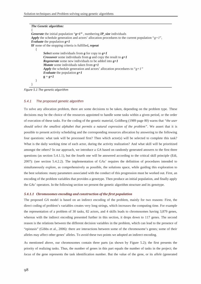
Solution techniques and Problem solving using genetic algorithms

98

The Genetic algorithm: { Generate the initial population “g=1” , numbering IP_size individuals Apply the schedule generation and actors’ allocation procedures to the current population “g=1”, Evaluate the population g=1 IF none of the stopping criteria is fulfilled, repeat { Select some individuals from g for copy to g+1 Crossover some individuals from g and copy the result to g+1 Regenerate some new individuals to be added into g+1 Mutate some individuals taken from g+1 Apply the schedule generation and actors’ allocation procedures to “g+1” Evaluate the population g+1 g = g+1 } }

Figure 5.1 The genetic algorithm

To solve any allocation problem, there are some decisions to be taken, depending on the problem type. These

decisions may be the choice of the resources appointed to handle some tasks within a given period, or the order

of execution of these tasks. For the coding of the genetic material, Goldberg (1989 page 80) warns that “the user

should select the smallest alphabet that permits a natural expression of the problem”. We assert that it is

possible to present activity scheduling and the corresponding resources allocation by answering to the following

four questions: what task will be processed first? Then which actor(s) will be selected to complete this task?

What is the daily working time of each actor, during the activity realization? And what skill will be prioritized

amongst the others? In our approach, we introduce a GA based on randomly generated answers to the first three

questions (as section 5.4.1.1), but the fourth one will be answered according to the critical skill principle (Edi,

2007): (see section 5.4.2.2). The implementation of GAs’ requires the definition of procedures intended to

simultaneously explore, as comprehensively as possible, the solutions space, while guiding this exploration to

the best solutions: many parameters associated with the conduct of this progression must be worked out. First, an

encoding of the problem variables that provides a genotype. Then produce an initial population, and finally apply

the GAs’ operators. In the following section we present the genetic algorithm structure and its genotype.

5.4.1.1 Chromosomes encoding and construction of the first population

The proposed GA model is based on an indirect encoding of the problem, mainly for two reasons: First, the

direct coding of problem’s variables creates very long strings, which increases the computing time. For example

the representation of a problem of 30 tasks, 82 actors, and 4 skills leads to chromosomes having 3,879 genes,

whereas with the indirect encoding presented further in this section, it drops down to 117 genes. The second

reason is the relations between the different decision variables in the problem, which can lead to the presence of

“epistasis” (Gibbs et al., 2006): there are interactions between some of the chromosome’s genes; some of their

alleles may affect other genes’ alleles. To avoid these two points we adopted an indirect encoding.

As mentioned above, our chromosomes contain three parts (as shown by Figure 5.2); the first presents the

priority of realizing tasks. Thus, the number of genes in this part equals the number of tasks in the project; the

locus of the gene represents the task identification number. But the value of the gene, or its allele (generated

5.4.1 The proposed genetic algorithm

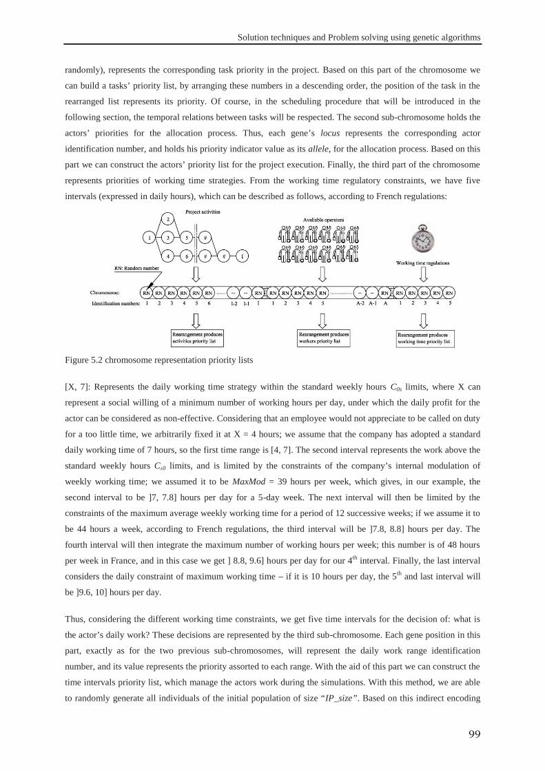
Solution techniques and Problem solving using genetic algorithms

99

randomly), represents the corresponding task priority in the project. Based on this part of the chromosome we

can build a tasks’ priority list, by arranging these numbers in a descending order, the position of the task in the

rearranged list represents its priority. Of course, in the scheduling procedure that will be introduced in the

following section, the temporal relations between tasks will be respected. The second sub-chromosome holds the

actors’ priorities for the allocation process. Thus, each gene’s locus represents the corresponding actor

identification number, and holds his priority indicator value as its allele, for the allocation process. Based on this

part we can construct the actors’ priority list for the project execution. Finally, the third part of the chromosome

represents priorities of working time strategies. From the working time regulatory constraints, we have five

intervals (expressed in daily hours), which can be described as follows, according to French regulations:

Figure 5.2 chromosome representation priority lists

[X, 7]: Represents the daily working time strategy within the standard weekly hours C0s limits, where X can

represent a social willing of a minimum number of working hours per day, under which the daily profit for the

actor can be considered as non-effective. Considering that an employee would not appreciate to be called on duty

for a too little time, we arbitrarily fixed it at X = 4 hours; we assume that the company has adopted a standard

daily working time of 7 hours, so the first time range is [4, 7]. The second interval represents the work above the

standard weekly hours Cs0 limits, and is limited by the constraints of the company’s internal modulation of

weekly working time; we assumed it to be MaxMod = 39 hours per week, which gives, in our example, the

second interval to be ]7, 7.8] hours per day for a 5-day week. The next interval will then be limited by the

constraints of the maximum average weekly working time for a period of 12 successive weeks; if we assume it to

be 44 hours a week, according to French regulations, the third interval will be ]7.8, 8.8] hours per day. The

fourth interval will then integrate the maximum number of working hours per week; this number is of 48 hours

per week in France, and in this case we get ] 8.8, 9.6] hours per day for our 4th interval. Finally, the last interval

considers the daily constraint of maximum working time – if it is 10 hours per day, the 5th and last interval will

be ]9.6, 10] hours per day.

Thus, considering the different working time constraints, we get five time intervals for the decision of: what is

the actor’s daily work? These decisions are represented by the third sub-chromosome. Each gene position in this

part, exactly as for the two previous sub-chromosomes, will represent the daily work range identification

number, and its value represents the priority assorted to each range. With the aid of this part we can construct the

time intervals priority list, which manage the actors work during the simulations. With this method, we are able

to randomly generate all individuals of the initial population of size “IP_size”. Based on this indirect encoding

Solution techniques and Problem solving using genetic algorithms

100

of the problem, we can gain some benefits towards the feasibility of the chromosome after the reproduction

processes, and avoid some correction procedures to the individuals, such as fixing the distortions that could

result from crossovers or mutations.

5.4.1.2 Fitness calculation

For each individual, the scheduling algorithm (described in section 5.4.2) will take place, for decoding the

chromosome, and constructing the project schedule. After that, the corresponding objectives, expressed by five

cost functions (fi), can be calculated as described in (section 3.3.2, equations 3.10); the next step consists in

determining the fitness of each of the chromosomes. In this view, we first have to normalize the cost functions

(fi); the normalization is intended to standardise the order of magnitude of the objectives, in order to project the

value of each objective over a given interval: [0, 1]× Cmax, where Cmax is a pre-specified constant.

First, the labour cost (that represents the sum of standard hours cost f1 plus the extra-hours cost f2) is treated as a

single objective. It can be expressed by fL = f1 + f2; this labour cost will be minimal (fLmin) if all the missions in

the project can be performed by fully-qualified persons ( = 1) during standard hours; on the opposite, the

maximum labour cost (fLmax) will be encountered if unfortunately all the jobs have to be undertaken by beginners

( = min) during their extra hours. The labour cost fL can then be normalized to the new function fL'= (fL – fL

min) /

(fLmax – fL

min).

In a similar way, the occupation of any operator may be bounded: by zero if he is not allocated at all during the

project, and by [DMaxS/ CS0] if he is required as much as possible. So the virtual cost (f3) associated to the loss

of flexibility can be normalized too, as f3'= (f3) / (f3

max). The objectives functions (f4, f5, f6) were rescaled by

simply dividing each of them by its maximum value (C4max, C5

max, and C6max respectively).

In the case where one or more constraint(s) would be violated, we should distinguish between the feasible and

unfeasible schedules by the use of penalties to weight and highlight these unsatisfied constraints. These penalties

are expressed in monetary units so that they can be added to the other (fi)s’ – we named this the penalty function

(f6) as the sum of all the penalties related to the working time constraints violations, if any; it was calculated

according to equation (5.1). In this equation, PHC and PSC are, respectively, the penalties related to sets of the

hard (HC) and soft (SC) constraints, and is a Boolean variable expressing the violation state of a given

constraint: =1 for constraint violation and =0 for the constraint satisfaction.

SCSC

HC

hhHC PPf

116 (5.1)

After normalisation, it can be added with an associated weight to the fitness function as (f’6), accordingly and

after the normalization of different terms (f 'i), we get the fitness function as:

Populationffffffitness LL ,)( '66

'55

'44

'33

' (5.2)

Where, the i are the objectives’ weights, the sum of all the weights being equal to unity, so that the fitness

function is normalized too. We treated f1 and f2 as a single objective “fL” with “ L= 1= 2”. Using this

normalization method enables us first to favour the feasible solutions with zero-penalties, and then to monitor the

compromise between execution costs and skills development.

Solution techniques and Problem solving using genetic algorithms

101

The evaluation phase consists in calculating the force of each individual within the population (i.e. its adaptation

to environmental constraints in the spirit of the comparison with a natural evolutionary process). Despite the

genetic algorithms are usually implemented to maximize an objective function (Goldberg, 1989), our problem

consists in minimizing an economic cost. Therefore, it is necessary to map the objective function so that its

minimum value will correspond to the strongest individuals. Based on Goldberg’s work, it is possible to

associate a constant Cmax as large as possible to the fitness function of each individual (ε) in order to get a new

function fab(ε) = Cmax– f(ε). We refer to it as the “individual absolute force fab”. This method makes it possible to

overcome the problems related to the sign of the function, if any. The value of Cmax can be estimated relying on

maximum extreme values of the different terms: the project realisation cost, the maximum cost value of the

constraints that may be violated, and the penalty costs that may arise from the date of completion of the project.

Based on this absolute force, we can perform the different selection procedures that build the next generation.

5.4.1.3 Selection

The selection procedure is the determination of the opportunity given to some individuals from the current

generation to play a role in the process of production of the next generation. The selection process is very

sensitive to the values of the individuals’ fitness, especially the worst, average, and the best values in the

population. These three values determine the selection tendency, and control the force of individuals that can be

selected for the reproduction procedure. According to Goldberg (1989), if the average value is very close to the

fittest one, then the search becomes as a random walk, because the average-fitting individuals have the same

probability of being selected as the best individuals. The same problem is stated by Davis (1996): when the three

values are very close, then the effect of the natural selection becomes negligible. But if the average value is

much closer to the best fit compared to the worst one, then we encounter a strong selection pressure that favours

the best chromosomes against the worst ones. For the creation of the next generation described in the following

section, we will present how we can overcome this problem. The selection was done based on two selection

methodologies. The first one is the elitist selection, with a pre-specified elitist size equal to a probability of

survival population size (Ps IP_size). This selection type forces GA to retain a number of the best individuals

at each generation. These fittest individuals will be copied directly to the selected list of candidates for survival

and/or passing through the mating pool. This selection approach can enhance the GA performance and ensure no

loss among the best solutions found. The second methodology is the stochastic sampling with replacement, or

the “roulette wheel selection”, where the probability of one individual to be chosen is proportional to its fitness

fab(ind). For each individual a slice of the wheel is assigned; the size of each slice is proportional to the

individual’s fitness. Then the wheel is spun “IP_size” times, and at each turn a specified individual is selected.

The selected individuals will be directly inserted in the mating pool for performing the crossover.

5.4.1.4 Crossover

In order to perform the crossover (shown in Figure 5.3), we construct the mating pool containing two sets of

parents: The first one is the group of “survivors” (the best individuals) selected by elitist selection as described

above, of size Ps IP_size. The second one has the same size (IP_size) as the previous population, but its

individuals are selected from this population via a roulette-wheel selection, a process for which random is

weighted by the individual’s fitness: the number of the population is the same, but some individuals, according

to their fitness, may be replicated many times, whereas others may have disappeared. Afterwards we apply the

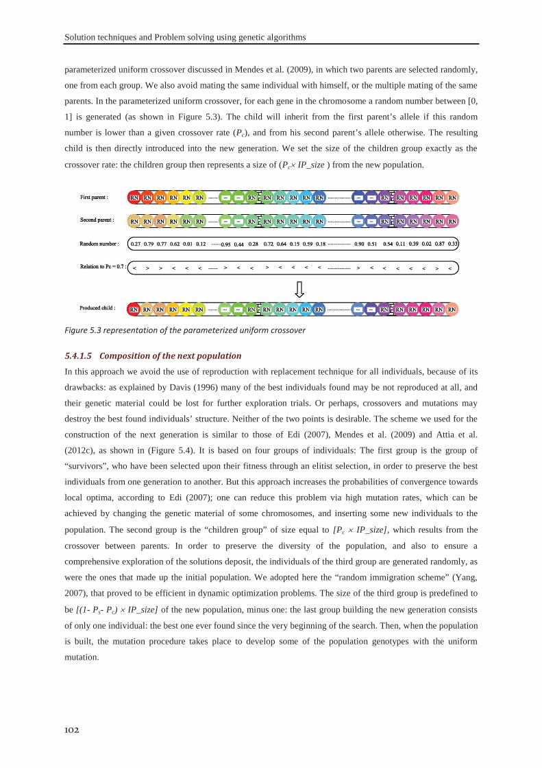
Solution techniques and Problem solving using genetic algorithms

102

parameterized uniform crossover discussed in Mendes et al. (2009), in which two parents are selected randomly,

one from each group. We also avoid mating the same individual with himself, or the multiple mating of the same

parents. In the parameterized uniform crossover, for each gene in the chromosome a random number between [0,

1] is generated (as shown in Figure 5.3). The child will inherit from the first parent’s allele if this random

number is lower than a given crossover rate (Pc), and from his second parent’s allele otherwise. The resulting

child is then directly introduced into the new generation. We set the size of the children group exactly as the

crossover rate: the children group then represents a size of (Pc IP_size ) from the new population.

Figure 5.3 representation of the parameterized uniform crossover

5.4.1.5 Composition of the next population

In this approach we avoid the use of reproduction with replacement technique for all individuals, because of its

drawbacks: as explained by Davis (1996) many of the best individuals found may be not reproduced at all, and

their genetic material could be lost for further exploration trials. Or perhaps, crossovers and mutations may

destroy the best found individuals’ structure. Neither of the two points is desirable. The scheme we used for the

construction of the next generation is similar to those of Edi (2007), Mendes et al. (2009) and Attia et al.

(2012c), as shown in (Figure 5.4). It is based on four groups of individuals: The first group is the group of

“survivors”, who have been selected upon their fitness through an elitist selection, in order to preserve the best

individuals from one generation to another. But this approach increases the probabilities of convergence towards

local optima, according to Edi (2007); one can reduce this problem via high mutation rates, which can be

achieved by changing the genetic material of some chromosomes, and inserting some new individuals to the

population. The second group is the “children group” of size equal to [Pc IP_size], which results from the

crossover between parents. In order to preserve the diversity of the population, and also to ensure a

comprehensive exploration of the solutions deposit, the individuals of the third group are generated randomly, as

were the ones that made up the initial population. We adopted here the “random immigration scheme” (Yang,

2007), that proved to be efficient in dynamic optimization problems. The size of the third group is predefined to

be [(1- Ps- Pc) IP_size] of the new population, minus one: the last group building the new generation consists

of only one individual: the best one ever found since the very beginning of the search. Then, when the population

is built, the mutation procedure takes place to develop some of the population genotypes with the uniform

mutation.

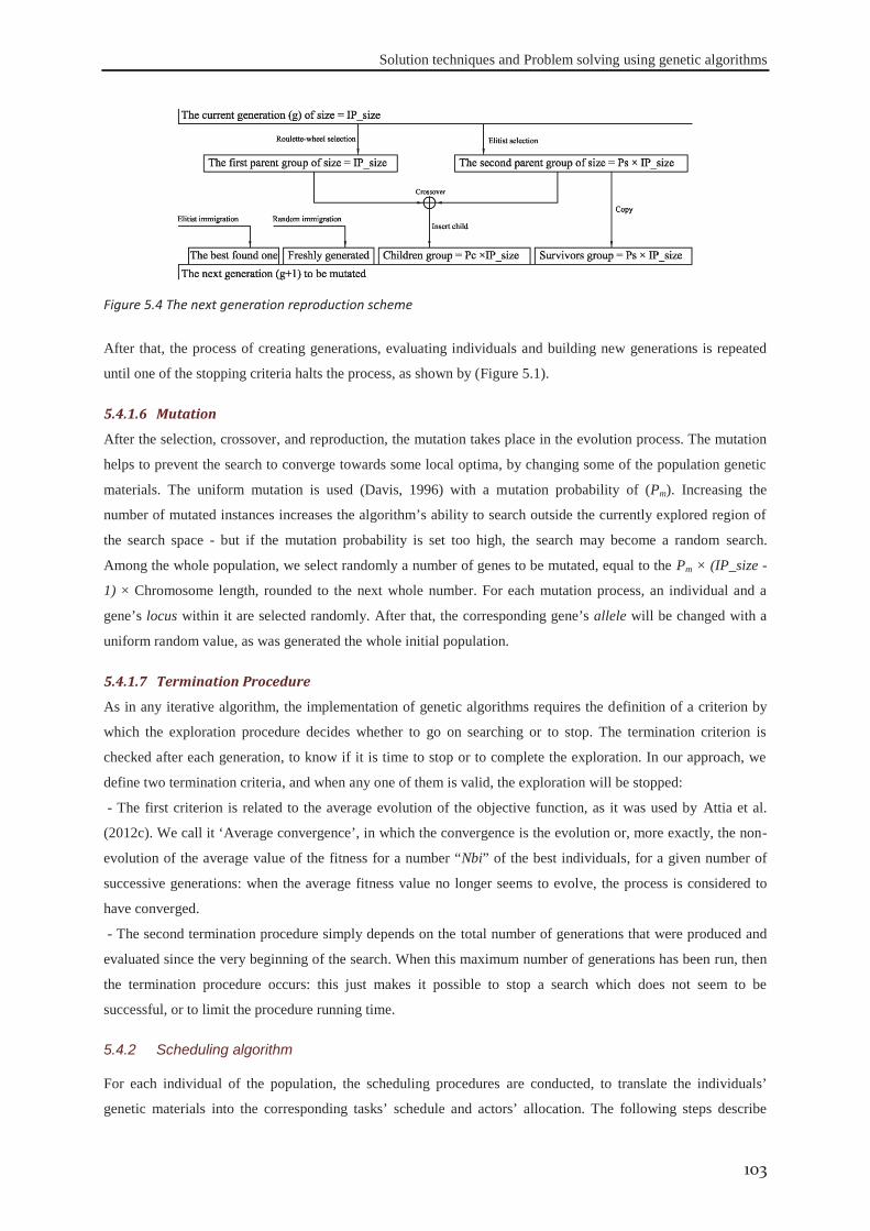
Solution techniques and Problem solving using genetic algorithms

103

Figure 5.4 The next generation reproduction scheme

After that, the process of creating generations, evaluating individuals and building new generations is repeated

until one of the stopping criteria halts the process, as shown by (Figure 5.1).

5.4.1.6 Mutation

After the selection, crossover, and reproduction, the mutation takes place in the evolution process. The mutation

helps to prevent the search to converge towards some local optima, by changing some of the population genetic

materials. The uniform mutation is used (Davis, 1996) with a mutation probability of (Pm). Increasing the

number of mutated instances increases the algorithm’s ability to search outside the currently explored region of

the search space - but if the mutation probability is set too high, the search may become a random search.

Among the whole population, we select randomly a number of genes to be mutated, equal to the Pm × (IP_size -

1) × Chromosome length, rounded to the next whole number. For each mutation process, an individual and a

gene’s locus within it are selected randomly. After that, the corresponding gene’s allele will be changed with a

uniform random value, as was generated the whole initial population.

5.4.1.7 Termination Procedure

As in any iterative algorithm, the implementation of genetic algorithms requires the definition of a criterion by

which the exploration procedure decides whether to go on searching or to stop. The termination criterion is

checked after each generation, to know if it is time to stop or to complete the exploration. In our approach, we

define two termination criteria, and when any one of them is valid, the exploration will be stopped:

- The first criterion is related to the average evolution of the objective function, as it was used by Attia et al.

(2012c). We call it ‘Average convergence’, in which the convergence is the evolution or, more exactly, the non-

evolution of the average value of the fitness for a number “Nbi” of the best individuals, for a given number of

successive generations: when the average fitness value no longer seems to evolve, the process is considered to

have converged.

- The second termination procedure simply depends on the total number of generations that were produced and

evaluated since the very beginning of the search. When this maximum number of generations has been run, then

the termination procedure occurs: this just makes it possible to stop a search which does not seem to be

successful, or to limit the procedure running time.

For each individual of the population, the scheduling procedures are conducted, to translate the individuals’

genetic materials into the corresponding tasks’ schedule and actors’ allocation. The following steps describe

5.4.2 Scheduling algorithm

Solution techniques and Problem solving using genetic algorithms

104

these decoding procedures, starting from the first day of the project execution and based on the serial scheduling

generation scheme. This builds up a feasible schedule by sequentially adding the tasks one by one until a

complete schedule is obtained. The scheduling algorithm has mainly two sub-procedures: search for sets of

feasible tasks, and workforce allocation. At each time instance (or day), the feasible sets (fs) are generated,

which represent the group of tasks that may be scheduled together according to the temporal relations between

tasks, resources availability, or even the workforce regulations. First of all, a set of three lists are generated based

on the priorities carried by the chromosome: a list of the tasks, a list of the actors, and the list of the working

time policies. Then the following procedures for decoding the chromosomes will be applied for each

chromosome in order to construct the project plan it carries.

5.4.2.1 Tasks feasible sets

First, at each time interval we consider the set of the activities that can be performed in parallel without

constraints violation. After a search of all the tasks that can be considered as feasible (considering only the

temporal constraints), they are grouped into a set of “the candidates list”. With the aid of tasks priorities, which

are hold by the corresponding chromosomes, we can select the most prioritized task. After that, other procedures

of checking feasibility based on the extremes values of the resources availabilities, and regulation constraints

should be conducted. We then assign to the selected activity the maximum permissible duration, and for each

available actor, we assign the maximum permissible number of working hours per day (10 hours according to the

French law). According to these conditions if ever a reason of unfeasibility was proven (because the need for

resources exceeds their availabilities for example), the task with the next maximum priority in the list is selected.

We follow this procedure until we can find the suitable task, then we call the resources allocation procedures (as

explained in section 5.4.2.2). If a feasible task was found that respects all the hard constraints, the candidate list

will be updated. All tasks within the candidates list will be checked, until we can find a feasible set of tasks,

considering precedence relations, resources’ availabilities and working time regulations, all together. Thus, first

we look for a feasible set fs, so that:

- For any pair of tasks (i, c) in the feasible set (fs), there is no restriction for performing them

simultaneously at the current time instance, considering the precedence constraints.

- The workload requirements by the tasks within the set (fs) must be satisfied, qualitatively as well as

quantitatively.

- The total resources requirement by the feasible set must be lower than or equal to the resources

availabilities.

- Each actor always works without any violation of the working time regulations.

5.4.2.2 Resources allocation

The skills’ criticality list is used to prioritize the different skills within the same task. This list is established,

considering skills scarcity, and a given skill will be all the more prioritized as it is critical, i.e. scarce. We are

now ready to conduct actors’ allocation. By the end of actors’ allocation algorithm, we should be able to assign a

value to each variable (ωa,i,k,j, EEi,k , di,k), according to the relation ωa,i,k,j = Ωi,k/(di,k× EEi,k ). Therefore, we can

compute all the possibilities of every task’s workload durations di,k and the resulting actors’ daily number of

working hours (ωa,i,k,j). Regarding the actors’ working time strategies hold by the chromosome, we can start a

search for the actors’ values of daily working hours (ωa,i,k,j) which would satisfy the task execution window and

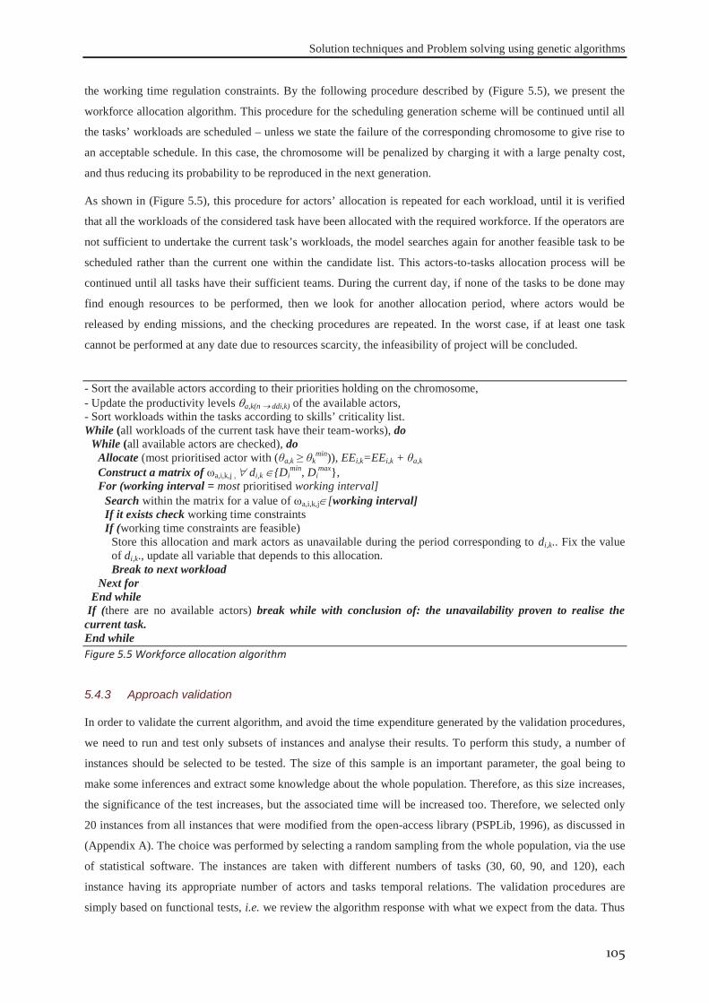
Solution techniques and Problem solving using genetic algorithms

105

the working time regulation constraints. By the following procedure described by (Figure 5.5), we present the

workforce allocation algorithm. This procedure for the scheduling generation scheme will be continued until all

the tasks’ workloads are scheduled – unless we state the failure of the corresponding chromosome to give rise to

an acceptable schedule. In this case, the chromosome will be penalized by charging it with a large penalty cost,

and thus reducing its probability to be reproduced in the next generation.

As shown in (Figure 5.5), this procedure for actors’ allocation is repeated for each workload, until it is verified

that all the workloads of the considered task have been allocated with the required workforce. If the operators are

not sufficient to undertake the current task’s workloads, the model searches again for another feasible task to be

scheduled rather than the current one within the candidate list. This actors-to-tasks allocation process will be

continued until all tasks have their sufficient teams. During the current day, if none of the tasks to be done may

find enough resources to be performed, then we look for another allocation period, where actors would be

released by ending missions, and the checking procedures are repeated. In the worst case, if at least one task

cannot be performed at any date due to resources scarcity, the infeasibility of project will be concluded.

- Sort the available actors according to their priorities holding on the chromosome, - Update the productivity levels a,k(n ddi,k) of the available actors, - Sort workloads within the tasks according to skills’ criticality list. While (all workloads of the current task have their team-works), do

While (all available actors are checked), do Allocate (most prioritised actor with (θa,k ≥ θk

min)), EEi,k=EEi,k + θa,k Construct a matrix of ωa,i,k,j , di,k {Di

min, Dimax},

For (working interval = most prioritised working interval] Search within the matrix for a value of ωa,i,k,j [working interval] If it exists check working time constraints If (working time constraints are feasible)

Store this allocation and mark actors as unavailable during the period corresponding to di,k.. Fix the value of di,k., update all variable that depends to this allocation. Break to next workload

Next for End while

If (there are no available actors) break while with conclusion of: the unavailability proven to realise the current task. End while Figure 5.5 Workforce allocation algorithm

In order to validate the current algorithm, and avoid the time expenditure generated by the validation procedures,

we need to run and test only subsets of instances and analyse their results. To perform this study, a number of

instances should be selected to be tested. The size of this sample is an important parameter, the goal being to

make some inferences and extract some knowledge about the whole population. Therefore, as this size increases,

the significance of the test increases, but the associated time will be increased too. Therefore, we selected only

20 instances from all instances that were modified from the open-access library (PSPLib, 1996), as discussed in

(Appendix A). The choice was performed by selecting a random sampling from the whole population, via the use

of statistical software. The instances are taken with different numbers of tasks (30, 60, 90, and 120), each

instance having its appropriate number of actors and tasks temporal relations. The validation procedures are

simply based on functional tests, i.e. we review the algorithm response with what we expect from the data. Thus

5.4.3 Approach validation

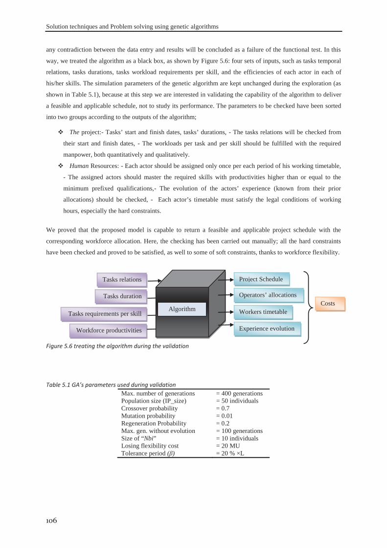
Solution techniques and Problem solving using genetic algorithms

106

any contradiction between the data entry and results will be concluded as a failure of the functional test. In this

way, we treated the algorithm as a black box, as shown by Figure 5.6: four sets of inputs, such as tasks temporal

relations, tasks durations, tasks workload requirements per skill, and the efficiencies of each actor in each of

his/her skills. The simulation parameters of the genetic algorithm are kept unchanged during the exploration (as

shown in Table 5.1), because at this step we are interested in validating the capability of the algorithm to deliver

a feasible and applicable schedule, not to study its performance. The parameters to be checked have been sorted

into two groups according to the outputs of the algorithm;

The project:- Tasks’ start and finish dates, tasks’ durations, - The tasks relations will be checked from

their start and finish dates, - The workloads per task and per skill should be fulfilled with the required

manpower, both quantitatively and qualitatively.

Human Resources: - Each actor should be assigned only once per each period of his working timetable,

- The assigned actors should master the required skills with productivities higher than or equal to the

minimum prefixed qualifications,- The evolution of the actors’ experience (known from their prior

allocations) should be checked, - Each actor’s timetable must satisfy the legal conditions of working

hours, especially the hard constraints.

We proved that the proposed model is capable to return a feasible and applicable project schedule with the

corresponding workforce allocation. Here, the checking has been carried out manually; all the hard constraints

have been checked and proved to be satisfied, as well to some of soft constraints, thanks to workforce flexibility.

Figure 5.6 treating the algorithm during the validation

Table 5.1 GA’s parameters used during validation Max. number of generations = 400 generations Population size (IP_size) = 50 individuals Crossover probability = 0.7 Mutation probability = 0.01 Regeneration Probability = 0.2 Max. gen. without evolution = 100 generations Size of “Nbi” = 10 individuals Losing flexibility cost = 20 MU Tolerance period (β) = 20 % ×L

Project Schedule

Operators’ allocations

Workers timetable Algorithm

Tasks relations

Tasks requirements per skill

Workforce productivities

Tasks duration Costs

Experience evolution

Solution techniques and Problem solving using genetic algorithms

107

The behaviour of any evolutionary algorithm (EA) could be modified by changing the value of one or more of its

parameters. The way of setting the EA’s parameters is crucial for a good performance and robustness aspects.

Regarding to the lack of knowledge about the fitness search-space that will be explored, one of the somewhat

tough processes of any EA consists in figuring out the values of its parameters, because of the huge number of

iterations required to set some parameters with respect to a particular problem. This procedure is generally a high

time-consumer, and CPU-time expensive. In the spirit, one should answer the question: How to fix the

appropriate value to each parameter, in order to explore efficiently the problem solutions landscapes?

According to Eiben et al. (2007) there are two forms of parameter settings: the parameter tuning, and the

parameter control. The parameter tuning consists in assigning a suitable value to each parameter before running

the algorithm, then fixing these values after the algorithm running procedures. In parameters control, the

algorithm starts with some values at the initialization phase, and then these values will be changed during the

running procedures. Generally speaking, in parameters tuning, one can design an experimental study to test the

different values and select the ones which gives the best results. Recently, Eiben and Smit (2011) considered the

parameters tuning from two aspects: - configuring an evolutionary algorithm by choosing parameters values that

optimize its performance. - Analyzing an evolutionary algorithm by studying how its performance depends on

the values of its parameters. By the following we will discuss the algorithm quality and the experimental design

proposed to tune the proposed approach.

5.4.4.1 The algorithm quality

In order to test the quality of a given algorithm, one needs to test its performance and robustness. The algorithm

performance measures usually result from the quality of the solution, and the fastness to return this solution

back. The solution quality can be measured as a function of the individual fitness. Eiben and Jelasity (2002)

discussed some performance measuring tools based on the calculating time and fitness values: - if the maximum

running time is defined then one can measure the algorithm performance as the best fitness at termination. - If

the minimum fitness value is defined, one can measure the algorithm performance as the running time to reach

this limit. If both are defined, the performance measure is the binary “yes/no” answer to a successful search. If

the optimal value is not known in advance, one can use the “Mean Best Fitness: MBF” at termination. The MBF

should be calculated under a pre-specified running period. Finally, one can use the progress function in terms of

the best/average/worst fitness of successive populations, and plot them against the time axis. This plot provides

much more information about the algorithm performance than the other methods. In our model we used the

“MBF” at termination. In our case, the termination condition depends on the model stopping criteria (as

previously discussed in section 5.4.1.7), so we considered the maximum number of generations without

convergence as one of the parameters that will be tuned. On the other side, the main objective of measuring the

robustness of a given algorithm is to check its performance stability under the presence of uncertainty conditions

within the data input. And it is strongly related to the algorithm performance variance in function of three

dimensions: – Robustness to a change in the parameter vectors, – Robustness to changes in the random seed that

was used to render the stochastic nature, – Robustness to changes in the problem instances. By the following we

introduce an experiment to tune the approach parameters, where its robustness will be analysed in next chapter.

5.4.4 Tuning the algorithm’s parameters

Solution techniques and Problem solving using genetic algorithms

108

5.4.4.2 Experimental design

The purpose of any experiment is the collection of data that will be analysed in order to infer one or many

conclusion(s). The ways to collect the data are observations, surveys, computer simulations, and experiments.

Here, in order to test the performance of our algorithm to solve the problem presented previously, we need to

know the values of the performance measuring indicators, which can be determined by tests. As discussed above,

testing all the parameters combinations by enumerating them is almost impossible. Therefore, we needed to

design an experimental study to test a selected sample from all parameters which will perfectly reflect the nature

of independent variables. In general, any experimental study has three phases: the sampling phase, the testing

phase, and the results analysis. Thus, in order to manage all the aspects of any experiment, it seems

indispensable to conduct a “Design Of Experiment: DOE”. According to Dean and Voss (1998), there are three

basic techniques in DOE: replication, blocking, and randomization. The replication and blocking help to increase

the precision in the experiment; but the randomization is used to decrease personal bias. By the following we

will discuss the different features of experiment.

5.4.4.2.1 Problem definition

Any scientific study conducted to solve a problem rests on three bases: objectives definition, methods to reach

these objectives, and the evaluation of these methods in reaching the objectives. Our main objectives are to tune

the parameters of the algorithm in order to have the best performance. To reach these objectives one should

investigate all the possible interaction between parameters combinations. But investigating comprehensively all

the parameters by factorial design is almost impossible due to the related time. The factorial design produces a

combinatory explosion making the experimental effort excessive. Especially, we have a set of factors with many

levels. The effort in this case is exponential and can be calculated as “test effort = levelsfactors numbers”, in order to

avoid the fully factorial experimental, we propose to use fractional factorial (see section 5.4.4.2.2).

First of all, we need to precise the parameters that have to be set. Generally, genetic algorithms contain two main

categories of parameters, the qualitative parameters and the quantitative. The qualitative group represents the

chromosome encoding, crossover type (one point, multi-point or uniform crossover), mutation type (bit-flip,

uniform or Gaussian mutation), and selection (elitist, tournament, uniform random…etc). The quantitative or the

numerical category represents all the parameters that can have specified numerical values. The most obvious

parameter to be defined of this category is the population size that will be fixed during the search procedures.

Afterwards, we need to define the reproduction parameters monitoring the variation degree between parent and

offspring generations. In the present genetic algorithm, the reproduction of a given population (as discussed in

section 5.4.1.5) depends on four static parameters: crossover percentage, survival percentage, regenerated

percentage, mutation probability. Two other factors are the termination criteria. After the identification of the

algorithm parameters, one needs to define the domain of each variable, so as to define the factors levels. In other

words one needs to answers the following three questions:

Q1: What are the lowest and highest measurable value of each factor?

Q2: What is the number of steps between factor extremes limits?

Q3: What are the increments between each two consecutive steps?

To answer the first question, we adopted the attitude of being guided by the previous practical and experimental

researches. Relying on previously published works, we can have the perspective to figure out the factors discrete

Solution techniques and Problem solving using genetic algorithms

109

values and their extremes points. As shown in (Table 5.2), we present the domain related to each factor; in

addition to GAs’ parameters we also present another factor related to the project delivery date, “the tolerance β”.

To answers the second and third questions, we need to solve another optimization problem that will provide the

best value for each factor, the value that maximizes the performance of our algorithm. As previously discussed,

the implementation of such optimization problem forms another challenge problem in the artificial intelligence,

see for example Eiben and Smit (2011). But in the other side there are some methods that will give us a good

exploration of the surface response; these methods will be presented and discussed in the following section.

5.4.4.2.2 Initialization phase

As mentioned previously, the experimental effort increased exponentially in function of factors and the number

of their levels in the complete factorial. One of the cheapest methods adopted to avoid this problem is the

fractionally replicated factorial design. Then, and relying on the “no free lunch theorem” of (Wolpert and

Macready, 1997), one can use these parameters values in solving other instances. There are some methods which

used to generate the response surface such as: - Taguchi method that has been developed in the industrial

manufacturing by Genichi Taguchi (Taguchi, 1995), - Latin-square orthogonal matrix, - Central composite, it has

five levels for each factor, 1, α, 0., - Doehlert design, - Box–Behnken designs. We adopted the box- Behnken

method to generate the parameters combination vectors. According to Ferreira et al. (2007), one of the most

important aspects of it is the requirement of fewer treatment combinations in comparison with the others. It is a

second-order design method based on incomplete three-levels for each factor. These three levels are the

minimum, centre, and maximum values, (see appendix C.9). One of its drawbacks is the "missing of corners",

so, the factors extremes limits should be increased. Using parameters’ extreme values shown in (Table 5.2), the

parameters combination was generated with software devoted to statistics (minitab).

Table 5.2 the extreme limits of the genetic algorithms factors The factors Extreme limits that will be used

Population size [20 to 200] individuals Crossover probability [0.50 to 0.90] Mutation probability [0.01 to 0.2]

Regeneration percentage [0.0 to 0.2] Maximum number of generations without divergence [50 to 200] generations

Flexibility of project delivery (as percentage from the contractual duration) [0.0% to 60%]

5.4.4.2.3 Testing phase

After the generation of the parameters with the Box-Behnken method we have a set of 54 vectors to be tested, as

shown in (Table 5.3). We selected randomly a project instance of 30 tasks to be used during this investigation. In

order to avoid the stochastic nature of GAs’, we decided to run each simulation at least 10 times, and to take the

average of their results. The averages of these results are illustrated within (Table 5.3). In this step, we

abandoned the objective of developing the resources skills due to the contradiction between this objective and

the other problem objectives. Based on the “free lunch theorem” the produced parameters will be used for all the

next investigation for the rest of this work.

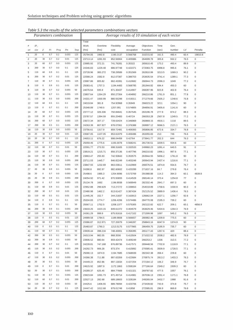
Solution techniques and Problem solving using genetic algorithms

110

Table 5.3 the results of the selected parameters combinations vectors Parameters combination Average results of 10 simulation of each vector

#

set

IP_

size β Pc Preg Pm Stop

Total

Work

(hrs)

Overtime

(hrs)

Flexibility

cost

Average

occupation

Objectives

Function

Time

(sec)

Gen.

number LV Penalty

1 20 0 0.7 0.2 0.055 125 25794.05 1992.8 1190.2137 0.566768 310215.92 161.5 490.4 60.4 19810.8

2 20 30 0.7 0.2 0.01 125 23713.14 1091.93 852.56904 0.405986 264699.78 305.8 932.2 76.5 0

3 20 60 0.7 0.0 0.055 125 23985.92 372.21 741.76281 0.35322 265610.45 173.2 493.4 89.9 0

4 200 30 0.7 0.0 0.1 125 24346.83 1229.48 886.97748 0.422371 272083.75 6998.8 995.6 76.1 0

5 110 60 0.9 0.1 0.1 125 23728.96 383.272 738.29589 0.351569 262810.99 3213.5 1069.3 90.2 0

6 200 30 0.7 0.2 0.01 125 22588.24 1582.8 812.07387 0.386703 253635.54 3741.4 1289.1 77.3 0

7 110 30 0.7 0.1 0.055 125 23987.86 805.82 862.43391 0.410682 266944.73 2096.3 1049 77.2 0

8 110 0 0.9 0.1 0.01 125 25083.41 1757.3 1194.4483 0.568785 281944.82 694.4 450.3 60 0

9 110 30 0.7 0.2 0.055 50 24076.64 935.9 871.30437 0.414907 268287.96 823.8 402.8 76.4 0

10 110 30 0.7 0.1 0.055 125 23807.64 1264.29 850.27304 0.404892 266210.86 1761.9 851.1 77.8 0

11 110 30 0.5 0.0 0.055 200 24331.47 1000.99 880.55299 0.419311 271279.66 2505.2 1248.6 75.8 0

12 110 60 0.5 0.1 0.1 125 24019.84 381.8 754.92868 0.35949 266023.22 3211 1054.1 90 0

13 110 0 0.7 0.1 0.1 200 25348.89 1749.5 1207.091 0.574805 284856.91 3405.6 1141.6 60 0

14 20 60 0.7 0.2 0.055 125 23777.12 326.336 750.84641 0.357545 263196.78 277.9 874.2 88.3 0

15 110 30 0.7 0.1 0.055 125 23787.57 1394.59 855.20483 0.40724 266353.28 2507.8 1249.5 77.2 0

16 200 60 0.7 0.0 0.055 125 23572.34 307.17 728.63424 0.346969 260869.15 4916.1 1118 89.5 0

17 200 30 0.5 0.1 0.055 200 24263.39 807.927 878.07061 0.376388 269997.12 9066.5 2121.1 76.5 0

18 110 30 0.9 0.0 0.055 50 23756.61 1317.9 859.72481 0.409393 265806.85 672.6 334.7 76.8 0

19 20 30 0.7 0.0 0.01 125 23587.05 1107.05 853.61979 0.406486 263355.83 213 746 76.6 0

20 20 30 0.7 0.0 0.1 125 24653.11 676.22 898.04459 0.42764 273941.77 202.3 644 76.3 0

21 200 0 0.7 0.2 0.055 125 25059.46 1775.6 1193.3078 0.568241 281730.51 3209.5 934.6 60 0

22 110 60 0.7 0.1 0.01 50 22591.77 273.53 698.31605 0.332533 249960.23 1091.4 640.5 91 0

23 110 30 0.7 0.1 0.055 125 23819.21 1215.71 856.37136 0.407796 266210.82 1996.1 997.6 77.1 0

24 110 60 0.7 0.1 0.1 200 23863.47 255.93 742.50843 0.353575 263944.55 5656.2 1761.8 90 0

25 110 30 0.9 0.0 0.055 200 23711.03 1445.7 846.82249 0.403248 265643.94 2437.4 1216.6 77.1 0

26 110 30 0.7 0.1 0.055 125 23847.55 1232.69 863.03611 0.410969 266576.51 1874.8 934.6 76.7 0

27 20 30 0.9 0.1 0.055 50 24390.8 892.97 882.60602 0.420289 271637.16 84.7 279.8 76.4 0

28 20 0 0.7 0.0 0.055 125 25498.6 1985.3 1204.9096 0.573769 291988.88 114.2 394.3 60.1 4839.8

29 20 30 0.9 0.1 0.055 200 24054.92 971.42 870.50655 0.414528 268146.14 373.4 1254.8 77 0

30 200 0 0.7 0.0 0.055 125 25134.78 1692 1196.8938 0.569949 282332.46 2841.7 697.3 60 0

31 110 60 0.9 0.1 0.01 125 22952.88 299.629 713.27272 0.339653 254018.89 1758.6 1030.9 90.3 0

32 200 30 0.7 0.0 0.01 125 22480.98 1462.2 813.61427 0.387434 252125.52 3989.9 1436.4 76.5 0

33 110 60 0.5 0.1 0.01 125 11445.26 152.7 344.21837 0.163913 126662.04 2227.1 1256.7 92.6 0

34 110 0 0.9 0.1 0.1 125 25334.83 1774.7 1206.4206 0.574486 284770.08 2195.3 739.2 60 0

35 110 0 0.7 0.1 0.1 50 25567.11 1752.5 1208.1377 0.575305 292122.82 622.7 209.1 60.1 4856.9

36 200 30 0.9 0.1 0.055 200 23633.25 1023.15 849.61372 0.404579 263629.46 5434.6 1264.3 76.9 0

37 110 30 0.5 0.2 0.055 50 24361.29 999.9 875.91616 0.417102 271599.98 1097 545.2 76.5 0

38 110 0 0.5 0.1 0.01 125 24989.58 1784.5 1189.9808 0.566657 280982.46 1209.8 775.5 60 0

39 200 60 0.7 0.2 0.055 125 23386.87 312.971 727.20079 0.346287 258843.16 6047.9 1374.9 90 0

40 110 0 0.5 0.1 0.1 125 25483.87 1790.3 1213.5175 0.577865 286459.75 2195.9 735.7 60 0

41 110 60 0.7 0.1 0.1 50 23939.44 398.216 748.43001 0.356395 265177.43 1267.6 420 88.4 0

42 200 30 0.5 0.1 0.055 50 24313.94 982.05 868.3556 0.413504 271022.52 2038.2 482.6 76.9 0

43 200 30 0.9 0.1 0.055 50 23906.52 880.64 859.42474 0.409249 266253.2 1336 313.5 77.2 0

44 200 30 0.7 0.2 0.1 125 24228.81 747.168 876.89736 0.417571 269448.56 7702.8 1118.9 77.1 0

45 110 30 0.5 0.2 0.055 200 24292.73 906.28 873.374 0.415892 270585.41 3509.9 1728.5 77.1 0

46 110 0 0.7 0.1 0.01 50 25090.13 1874.9 1194.7685 0.568939 282342.38 358.4 229.8 60 0

47 110 30 0.5 0.2 0.055 200 24366.38 711.88 887.63359 0.422684 270875.74 2813.2 1403.3 76.3 0

48 20 30 0.5 0.1 0.055 50 24449.22 852.86 897.13034 0.427204 272184.12 106.2 346.9 75.7 0

49 110 0 0.7 0.1 0.01 200 24615.92 1897.9 1172.1863 0.558184 277166.64 2349.2 1509.3 60 0

50 20 30 0.7 0.1 0.055 200 24289.37 625.45 884.77669 0.421321 269787.82 477.5 1557 76.1 0

51 110 30 0.7 0.1 0.055 125 23923.84 1091.73 871.45714 0.414981 267036.13 2351.4 1171.1 76.8 0

52 110 60 0.7 0.1 0.01 200 22527.13 282.68 689.18603 0.328184 249265.04 3432.7 1988 91.6 0

53 110 30 0.7 0.0 0.055 50 24425.6 1406.55 889.78094 0.423706 273439.82 743.9 374.8 75.7 0

54 20 30 0.7 0.2 0.1 125 24447.42 1012.68 879.01748 0.41858 272585.81 296.9 869.8 76.8 0

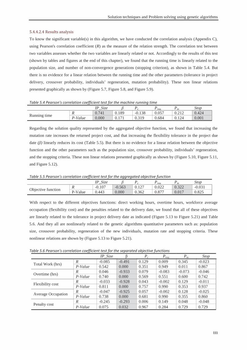
Solution techniques and Problem solving using genetic algorithms

111

5.4.4.2.4 Results analysis

To know the significant variable(s) in this algorithm, we have conducted the correlation analysis (Appendix C),

using Pearson's correlation coefficient (R) as the measure of the relation strength. The correlation test between

two variables assesses whether the two variables are linearly related or not. Accordingly to the results of this test

(shown by tables and figures at the end of this chapter), we found that the running time is linearly related to the

population size, and number of non-convergence generations (stopping criterion), as shown in Table 5.4. But

there is no evidence for a linear relation between the running time and the other parameters (tolerance in project

delivery, crossover probability, individuals’ regeneration, mutation probability). These non linear relations

presented graphically as shown by (Figure 5.7, Figure 5.8, and Figure 5.9).

Table 5.4 Pearson's correlation coefficient test for the machine running time IP_Size β Pc Preg. Pm Stop

Running time R 0.741 0.189 -0.138 0.057 0.212 0.424 P-Value 0.000 0.171 0.319 0.684 0.124 0.001

Regarding the solution quality represented by the aggregated objective function, we found that increasing the

mutation rate increases the returned project cost, and that increasing the flexibility tolerance in the project due

date (β) linearly reduces its cost (Table 5.5). But there is no evidence for a linear relation between the objective

function and the other parameters such as the population size, crossover probability, individuals’ regeneration,

and the stopping criteria. These non linear relations presented graphically as shown by (Figure 5.10, Figure 5.11,

and Figure 5.12).

Table 5.5 Pearson's correlation coefficient test for the aggregated objective function IP_Size β Pc Preg. Pm Stop

Objective function R -0.107 -0.563 0.127 0.022 0.322 -0.031 P-Value 0.443 0.000 0.362 0.877 0.017 0.825

With respect to the different objectives functions: direct working hours, overtime hours, workforce average

occupation (flexibility cost) and the penalties related to the delivery date, we found that all of these objectives

are linearly related to the tolerance in project delivery date as indicated (Figure 5.13 to Figure 5.21) and Table

5.6. And they all are nonlinearly related to the genetic algorithms quantitative parameters such as: population

size, crossover probability, regeneration of the new individuals, mutation rate and stopping criteria. These

nonlinear relations are shown by (Figure 5.13 to Figure 5.21).

Table 5.6 Pearson's correlation coefficient test for the separated objective functions IP_Size β Pc Preg. Pm Stop

Total Work (hrs) R -0.085 -0.491 0.129 0.009 0.345 -0.023 P-Value 0.542 0.000 0.351 0.949 0.011 0.867

Overtime (hrs) R 0.046 -0.933 0.079 -0.083 -0.073 -0.046 P-Value 0.740 0.000 0.569 0.551 0.600 0.742

Flexibility cost R -0.033 -0.928 0.043 -0.002 0.129 -0.011 P-Value 0.811 0.000 0.757 0.990 0.353 0.937

Average Occupation R -0.047 -0.925 0.057 -0.002 0.128 -0.025 P-Value 0.738 0.000 0.681 0.990 0.355 0.860

Penalty cost R -0.245 -0.293 0.006 0.149 0.048 -0.048 P-Value 0.075 0.032 0.967 0.284 0.729 0.729

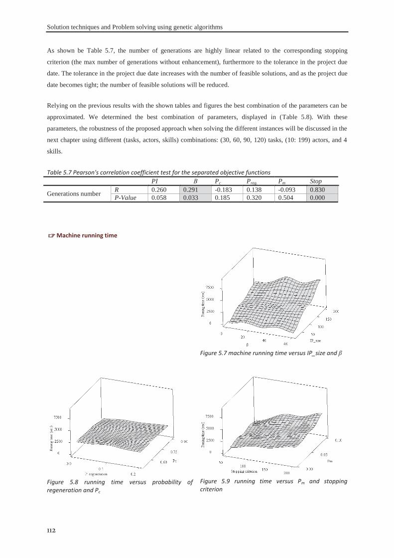
Solution techniques and Problem solving using genetic algorithms

112

As shown be Table 5.7, the number of generations are highly linear related to the corresponding stopping

criterion (the max number of generations without enhancement), furthermore to the tolerance in the project due

date. The tolerance in the project due date increases with the number of feasible solutions, and as the project due

date becomes tight; the number of feasible solutions will be reduced.

Relying on the previous results with the shown tables and figures the best combination of the parameters can be

approximated. We determined the best combination of parameters, displayed in (Table 5.8). With these

parameters, the robustness of the proposed approach when solving the different instances will be discussed in the

next chapter using different (tasks, actors, skills) combinations: (30, 60, 90, 120) tasks, (10: 199) actors, and 4

skills.

Table 5.7 Pearson's correlation coefficient test for the separated objective functions PI Β Pc Preg. Pm Stop

Generations number R 0.260 0.291 -0.183 0.138 -0.093 0.830 P-Value 0.058 0.033 0.185 0.320 0.504 0.000

Machine running time

Figure 5.7 machine running time versus IP_size and β

Figure 5.8 running time versus probability of regeneration and Pc

Figure 5.9 running time versus Pm and stopping criterion

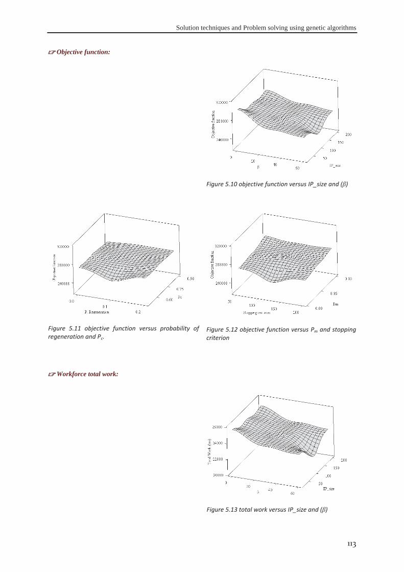
Solution techniques and Problem solving using genetic algorithms

113

Objective function:

Figure 5.10 objective function versus IP_size and (β)

Figure 5.11 objective function versus probability of regeneration and Pc.

Figure 5.12 objective function versus Pm and stopping criterion

Workforce total work:

Figure 5.13 total work versus IP_size and (β)

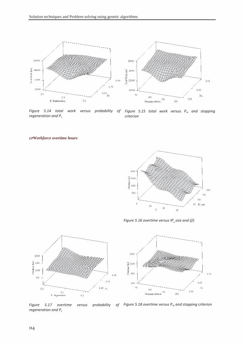
Solution techniques and Problem solving using genetic algorithms

114

Figure 5.14 total work versus probability of regeneration and Pc

Figure 5.15 total work versus Pm and stopping criterion

Workforce overtime hours

Figure 5.16 overtime versus IP_size and (β)

Figure 5.17 overtime versus probability of regeneration and Pc

Figure 5.18 overtime versus Pm and stopping criterion

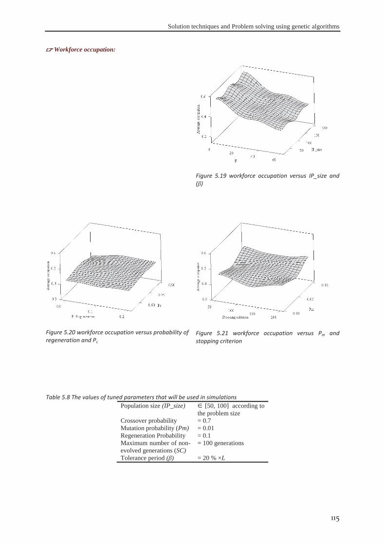
Solution techniques and Problem solving using genetic algorithms

115

Workforce occupation:

Figure 5.19 workforce occupation versus IP_size and (β)

Figure 5.20 workforce occupation versus probability of regeneration and Pc

Figure 5.21 workforce occupation versus Pm and stopping criterion

Table 5.8 The values of tuned parameters that will be used in simulations Population size (IP_size) [50, 100] according to

the problem size Crossover probability = 0.7 Mutation probability (Pm) = 0.01 Regeneration Probability = 0.1 Maximum number of non-evolved generations (SC)

= 100 generations

Tolerance period (β) = 20 % ×L

Solution techniques and Problem solving using genetic algorithms

116

A genetic algorithm-based approach to solve the problem of project schedule with workforce allocations was

developed and described. Our approach relies mainly on the answers to three questions defining the process

priorities: what task will be processed next? Then which actor(s) will be allocated to realise this task? What is

the working time strategy that the actors will respect, during the activity realization? A serial schedule generation

scheme is adopted to construct the project schedule and then allocated the workforce according to the randomly-

generated priority lists. The model has been validated, moreover, its parameters has been tuned to give the best

performance. The model robustness to return a feasible solution despite changes in the genetic algorithms

parameters was proven and investigated. By the next chapters this approach will be used to solve numerous

project instances with variable characteristics as a step to prove its robustness towards changing the problem

characteristics. Then it will be used as a vehicle to investigate the factors that affect the multi-skilled resources.

5.5 CONCLUSION

6 PERFORMANCE INVESTIGATION AND RESULT

ANALYSIS

In this chapter a detailed analysis of our approach will be conducted. The

analysis used a vast number of projects with different characteristics. First

the firms’ managerial policies will be defined, which is translated by

different objectives and their weights. After that, the scheduling results

obtained with 4 groups of problems (Appendix A) will be analysed and

discussed. Each of these groups gathers one hundred projects with

different characteristics. By the end of the chapter, a brief comparison

between the results of these four groups will be carried out in order to

show the robustness of the approach.

CH

APT

ER

6

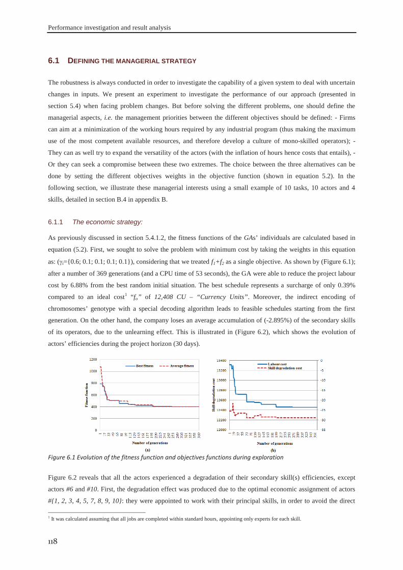
Performance investigation and result analysis

118

The robustness is always conducted in order to investigate the capability of a given system to deal with uncertain

changes in inputs. We present an experiment to investigate the performance of our approach (presented in

section 5.4) when facing problem changes. But before solving the different problems, one should define the

managerial aspects, i.e. the management priorities between the different objectives should be defined: - Firms

can aim at a minimization of the working hours required by any industrial program (thus making the maximum

use of the most competent available resources, and therefore develop a culture of mono-skilled operators); -

They can as well try to expand the versatility of the actors (with the inflation of hours hence costs that entails), -

Or they can seek a compromise between these two extremes. The choice between the three alternatives can be

done by setting the different objectives weights in the objective function (shown in equation 5.2). In the

following section, we illustrate these managerial interests using a small example of 10 tasks, 10 actors and 4

skills, detailed in section B.4 in appendix B.

As previously discussed in section 5.4.1.2, the fitness functions of the GAs’ individuals are calculated based in

equation (5.2). First, we sought to solve the problem with minimum cost by taking the weights in this equation

as: ( i={0.6; 0.1; 0.1; 0.1; 0.1}), considering that we treated f1+f2 as a single objective. As shown by (Figure 6.1);

after a number of 369 generations (and a CPU time of 53 seconds), the GA were able to reduce the project labour

cost by 6.88% from the best random initial situation. The best schedule represents a surcharge of only 0.39%

compared to an ideal cost1 “fo” of 12,408 CU – “Currency Units”. Moreover, the indirect encoding of

chromosomes’ genotype with a special decoding algorithm leads to feasible schedules starting from the first

generation. On the other hand, the company loses an average accumulation of (-2.895%) of the secondary skills

of its operators, due to the unlearning effect. This is illustrated in (Figure 6.2), which shows the evolution of

actors’ efficiencies during the project horizon (30 days).

Figure 6.1 Evolution of the fitness function and objectives functions during exploration

Figure 6.2 reveals that all the actors experienced a degradation of their secondary skill(s) efficiencies, except

actors #6 and #10. First, the degradation effect was produced due to the optimal economic assignment of actors

#{1, 2, 3, 4, 5, 7, 8, 9, 10}: they were appointed to work with their principal skills, in order to avoid the direct

1 It was calculated assuming that all jobs are completed within standard hours, appointing only experts for each skill.

6.1 DEFINING THE MANAGERIAL STRATEGY

6.1.1 The economic strategy:

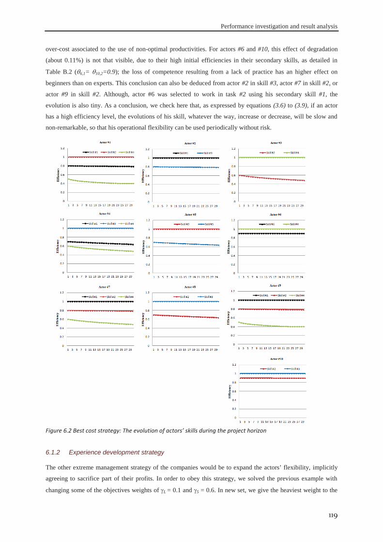
Performance investigation and result analysis

119

over-cost associated to the use of non-optimal productivities. For actors #6 and #10, this effect of degradation

(about 0.11%) is not that visible, due to their high initial efficiencies in their secondary skills, as detailed in

Table B.2 ( 6,1= 10,2=0.9); the loss of competence resulting from a lack of practice has an higher effect on

beginners than on experts. This conclusion can also be deduced from actor #2 in skill #3, actor #7 in skill #2, or

actor #9 in skill #2. Although, actor #6 was selected to work in task #2 using his secondary skill #1, the

evolution is also tiny. As a conclusion, we check here that, as expressed by equations (3.6) to (3.9), if an actor

has a high efficiency level, the evolutions of his skill, whatever the way, increase or decrease, will be slow and

non-remarkable, so that his operational flexibility can be used periodically without risk.

Figure 6.2 Best cost strategy: The evolution of actors’ skills during the project horizon

The other extreme management strategy of the companies would be to expand the actors’ flexibility, implicitly

agreeing to sacrifice part of their profits. In order to obey this strategy, we solved the previous example with

changing some of the objectives weights of L = 0.1 and 5 = 0.6. In new set, we give the heaviest weight to the

6.1.2 Experience development strategy

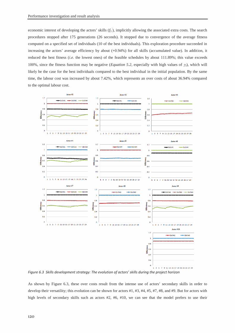
Performance investigation and result analysis

120

economic interest of developing the actors’ skills (f5`), implicitly allowing the associated extra costs. The search

procedures stopped after 175 generations (26 seconds). It stopped due to convergence of the average fitness

computed on a specified set of individuals (10 of the best individuals). This exploration procedure succeeded in

increasing the actors’ average efficiency by about (+0.94%) for all skills (accumulated value). In addition, it

reduced the best fitness (i.e. the lowest ones) of the feasible schedules by about 111.89%; this value exceeds

100%, since the fitness function may be negative (Equation 5.2, especially with high values of 5), which will

likely be the case for the best individuals compared to the best individual in the initial population. By the same

time, the labour cost was increased by about 7.42%, which represents an over costs of about 36.94% compared

to the optimal labour cost.

Figure 6.3 Skills development strategy: The evolution of actors’ skills during the project horizon

As shown by Figure 6.3, these over costs result from the intense use of actors’ secondary skills in order to

develop their versatility; this evolution can be shown for actors #1, #3, #4, #5, #7, #8, and #9. But for actors with

high levels of secondary skills such as actors #2, #6, #10, we can see that the model prefers to use their

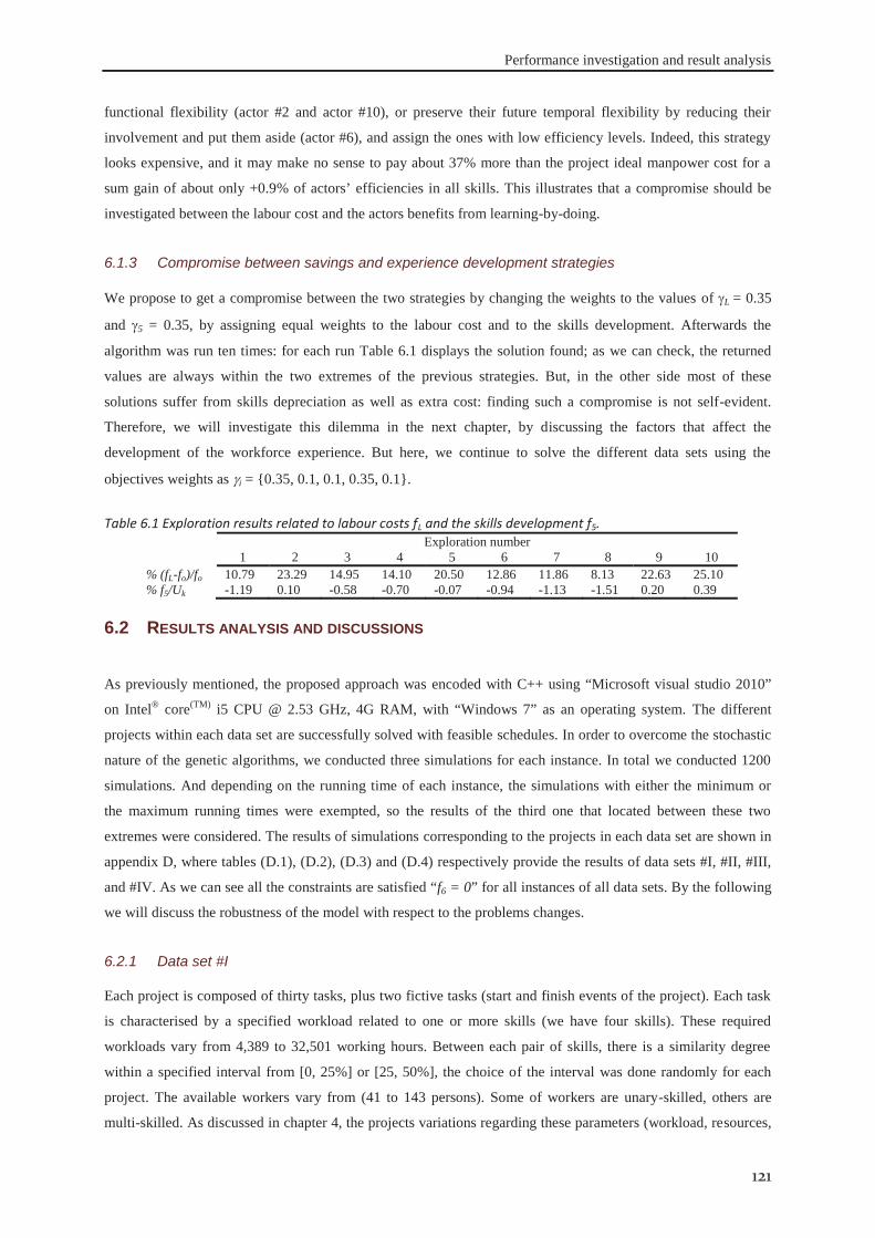
Performance investigation and result analysis

121

functional flexibility (actor #2 and actor #10), or preserve their future temporal flexibility by reducing their

involvement and put them aside (actor #6), and assign the ones with low efficiency levels. Indeed, this strategy

looks expensive, and it may make no sense to pay about 37% more than the project ideal manpower cost for a

sum gain of about only +0.9% of actors’ efficiencies in all skills. This illustrates that a compromise should be

investigated between the labour cost and the actors benefits from learning-by-doing.

We propose to get a compromise between the two strategies by changing the weights to the values of L = 0.35

and 5 = 0.35, by assigning equal weights to the labour cost and to the skills development. Afterwards the

algorithm was run ten times: for each run Table 6.1 displays the solution found; as we can check, the returned

values are always within the two extremes of the previous strategies. But, in the other side most of these

solutions suffer from skills depreciation as well as extra cost: finding such a compromise is not self-evident.

Therefore, we will investigate this dilemma in the next chapter, by discussing the factors that affect the

development of the workforce experience. But here, we continue to solve the different data sets using the

objectives weights as i = {0.35, 0.1, 0.1, 0.35, 0.1}.

Table 6.1 Exploration results related to labour costs fL and the skills development f5.

Exploration number 1 2 3 4 5 6 7 8 9 10

% (fL-fo)/fo 10.79 23.29 14.95 14.10 20.50 12.86 11.86 8.13 22.63 25.10 % f5/Uk -1.19 0.10 -0.58 -0.70 -0.07 -0.94 -1.13 -1.51 0.20 0.39

As previously mentioned, the proposed approach was encoded with C++ using “Microsoft visual studio 2010”

on Intel® core(TM) i5 CPU @ 2.53 GHz, 4G RAM, with “Windows 7” as an operating system. The different

projects within each data set are successfully solved with feasible schedules. In order to overcome the stochastic

nature of the genetic algorithms, we conducted three simulations for each instance. In total we conducted 1200

simulations. And depending on the running time of each instance, the simulations with either the minimum or

the maximum running times were exempted, so the results of the third one that located between these two

extremes were considered. The results of simulations corresponding to the projects in each data set are shown in

appendix D, where tables (D.1), (D.2), (D.3) and (D.4) respectively provide the results of data sets #I, #II, #III,

and #IV. As we can see all the constraints are satisfied “f6 = 0” for all instances of all data sets. By the following

we will discuss the robustness of the model with respect to the problems changes.

Each project is composed of thirty tasks, plus two fictive tasks (start and finish events of the project). Each task

is characterised by a specified workload related to one or more skills (we have four skills). These required

workloads vary from 4,389 to 32,501 working hours. Between each pair of skills, there is a similarity degree

within a specified interval from [0, 25%] or [25, 50%], the choice of the interval was done randomly for each

project. The available workers vary from (41 to 143 persons). Some of workers are unary-skilled, others are

multi-skilled. As discussed in chapter 4, the projects variations regarding these parameters (workload, resources,

6.1.3 Compromise between savings and experience development strategies

6.2 RESULTS ANALYSIS AND DISCUSSIONS

6.2.1 Data set #I

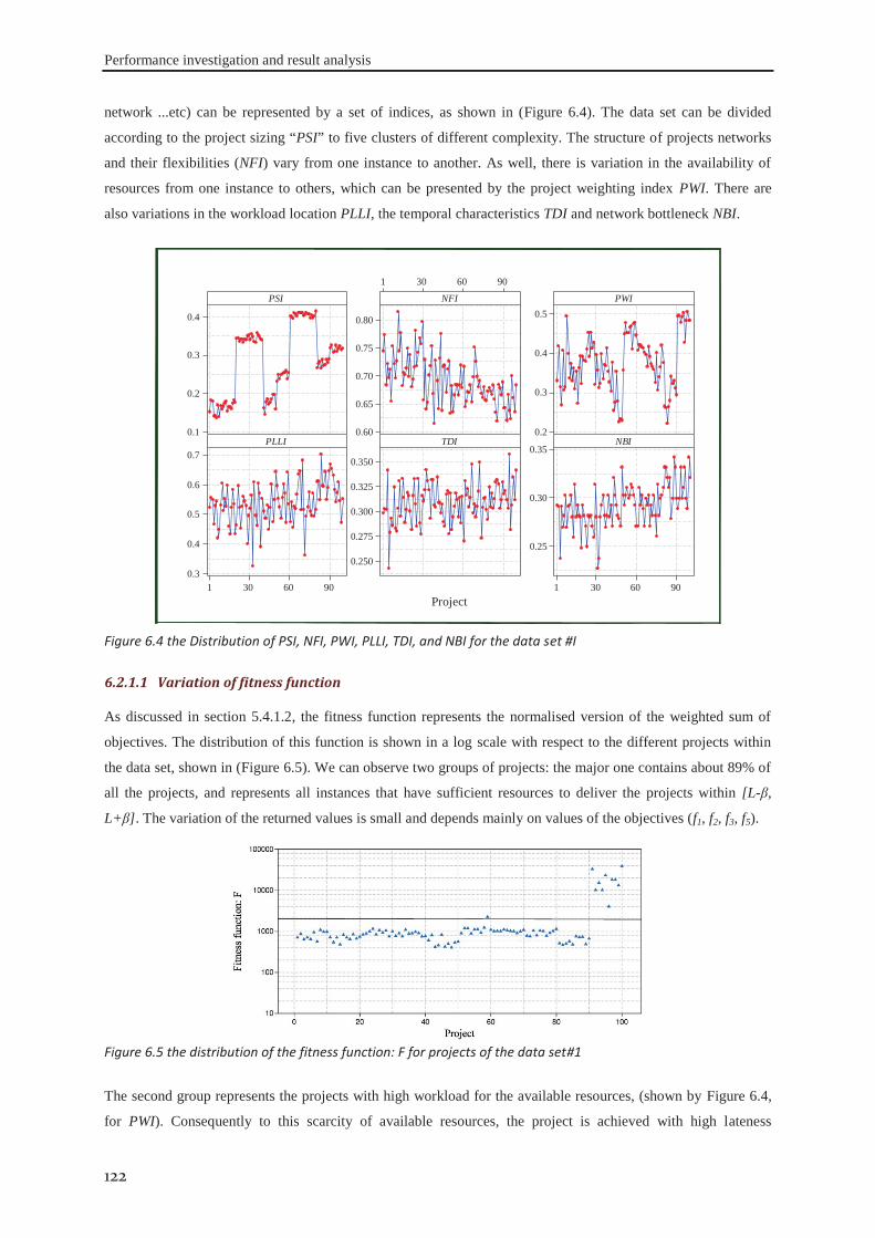
Performance investigation and result analysis

122

network ...etc) can be represented by a set of indices, as shown in (Figure 6.4). The data set can be divided

according to the project sizing “PSI” to five clusters of different complexity. The structure of projects networks

and their flexibilities (NFI) vary from one instance to another. As well, there is variation in the availability of

resources from one instance to others, which can be presented by the project weighting index PWI. There are

also variations in the workload location PLLI, the temporal characteristics TDI and network bottleneck NBI.

0.4

0.3

0.2

0.1

9060301

0.80

0.75

0.70

0.65

0.60

0.5

0.4

0.3

0.2

9060301

0.7

0.6

0.5

0.4

0.3

0.350

0.325

0.300

0.275

0.250

9060301

0.35

0.30

0.25

PSI

Project

NFI PWI

PLLI TDI NBI

Figure 6.4 the Distribution of PSI, NFI, PWI, PLLI, TDI, and NBI for the data set #I

6.2.1.1 Variation of fitness function

As discussed in section 5.4.1.2, the fitness function represents the normalised version of the weighted sum of

objectives. The distribution of this function is shown in a log scale with respect to the different projects within

the data set, shown in (Figure 6.5). We can observe two groups of projects: the major one contains about 89% of

all the projects, and represents all instances that have sufficient resources to deliver the projects within [L-β,

L+β]. The variation of the returned values is small and depends mainly on values of the objectives (f1, f2, f3, f5).

Figure 6.5 the distribution of the fitness function: F for projects of the data set#1

The second group represents the projects with high workload for the available resources, (shown by Figure 6.4,

for PWI). Consequently to this scarcity of available resources, the project is achieved with high lateness

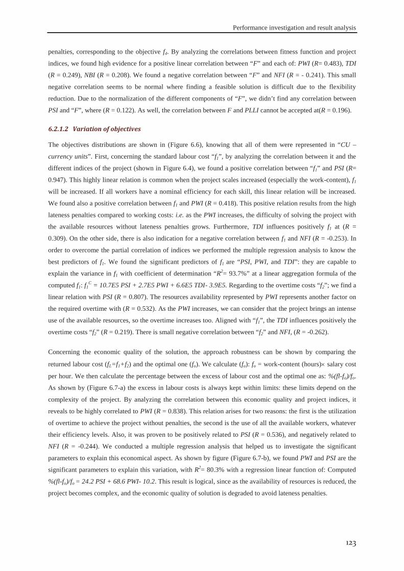
Performance investigation and result analysis

123

penalties, corresponding to the objective f4. By analyzing the correlations between fitness function and project

indices, we found high evidence for a positive linear correlation between “F” and each of: PWI (R= 0.483), TDI

(R = 0.249), NBI (R = 0.208). We found a negative correlation between “F” and NFI (R = - 0.241). This small

negative correlation seems to be normal where finding a feasible solution is difficult due to the flexibility

reduction. Due to the normalization of the different components of “F”, we didn’t find any correlation between

PSI and “F”, where (R = 0.122). As well, the correlation between F and PLLI cannot be accepted at(R = 0.196).

6.2.1.2 Variation of objectives

The objectives distributions are shown in (Figure 6.6), knowing that all of them were represented in “CU –

currency units”. First, concerning the standard labour cost “f1”, by analyzing the correlation between it and the

different indices of the project (shown in Figure 6.4), we found a positive correlation between “f1” and PSI (R=

0.947). This highly linear relation is common when the project scales increased (especially the work-content), f1

will be increased. If all workers have a nominal efficiency for each skill, this linear relation will be increased.

We found also a positive correlation between f1 and PWI (R = 0.418). This positive relation results from the high

lateness penalties compared to working costs: i.e. as the PWI increases, the difficulty of solving the project with

the available resources without lateness penalties grows. Furthermore, TDI influences positively f1 at (R =

0.309). On the other side, there is also indication for a negative correlation between f1 and NFI (R = -0.253). In

order to overcome the partial correlation of indices we performed the multiple regression analysis to know the

best predictors of f1. We found the significant predictors of f1 are “PSI, PWI, and TDI”: they are capable to

explain the variance in f1 with coefficient of determination “R2= 93.7%” at a linear aggregation formula of the

computed f1: f1C = 10.7E5 PSI + 2.7E5 PWI + 6.6E5 TDI- 3.9E5. Regarding to the overtime costs “f2”; we find a

linear relation with PSI (R = 0.807). The resources availability represented by PWI represents another factor on

the required overtime with (R = 0.532). As the PWI increases, we can consider that the project brings an intense

use of the available resources, so the overtime increases too. Aligned with “f1”, the TDI influences positively the

overtime costs “f2” (R = 0.219). There is small negative correlation between “f2” and NFI, (R = -0.262).

Concerning the economic quality of the solution, the approach robustness can be shown by comparing the

returned labour cost (fL=f1+f2) and the optimal one (fo). We calculate (fo): fo = work-content (hours) salary cost

per hour. We then calculate the percentage between the excess of labour cost and the optimal one as: %(fl-fo)/fo.

As shown by (Figure 6.7-a) the excess in labour costs is always kept within limits: these limits depend on the

complexity of the project. By analyzing the correlation between this economic quality and project indices, it

reveals to be highly correlated to PWI (R = 0.838). This relation arises for two reasons: the first is the utilization

of overtime to achieve the project without penalties, the second is the use of all the available workers, whatever

their efficiency levels. Also, it was proven to be positively related to PSI (R = 0.536), and negatively related to

NFI (R = -0.244). We conducted a multiple regression analysis that helped us to investigate the significant

parameters to explain this economical aspect. As shown by figure (Figure 6.7-b), we found PWI and PSI are the

significant parameters to explain this variation, with R2= 80.3% with a regression linear function of: Computed

%(fl-fo)/fo = 24.2 PSI + 68.6 PWI- 10.2. This result is logical, since as the availability of resources is reduced, the

project becomes complex, and the economic quality of solution is degraded to avoid lateness penalties.

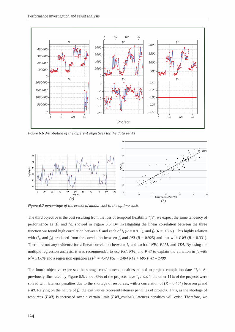
Performance investigation and result analysis

124

400000

300000

200000

100000

0

9060301

8000

6000

4000

2000

0

2000

1500

1000

500

9060301

2000000

1500000

1000000

500000

0

0

-5

-10

-15

-209060301

0.50

0.25

0.00

-0.25

-0.50

f1

Project

f2 f3

f4 f5 f6

Figure 6.6 distribution of the different objectives for the data set #1

(a)

(b) Figure 6.7 percentage of the excess of labour cost to the optima costs

The third objective is the cost resulting from the loss of temporal flexibility “f3”; we expect the same tendency of

performance as (f1, and f2), showed in Figure 6.6. By investigating the linear correlation between the three

function we found high correlation between f3 and each of f1 (R = 0.911), and f2 (R = 0.807). This highly relation

with (f1, and f2) produced from the correlation between f3 and PSI (R = 0.925) and that with PWI (R = 0.331).

There are not any evidence for a linear correlation between f3 and each of NFI, PLLI, and TDI. By using the

multiple regression analysis, it was recommended to use PSI, NFI, and PWI to explain the variation in f3 with

R2= 91.6% and a regression equation as f3C = 4573 PSI + 2484 NFI + 685 PWI – 2408.

The fourth objective expresses the storage cost/lateness penalties related to project completion date “f4”. As

previously illustrated by Figure 6.5, about 89% of the projects have “f4=0.0”, the other 11% of the projects were

solved with lateness penalties due to the shortage of resources, with a correlation of (R = 0.454) between f4 and

PWI. Relying on the nature of f4, the exit values represent lateness penalties of projects. Thus, as the shortage of

resources (PWI) is increased over a certain limit (PWI_critical), lateness penalties will exist. Therefore, we

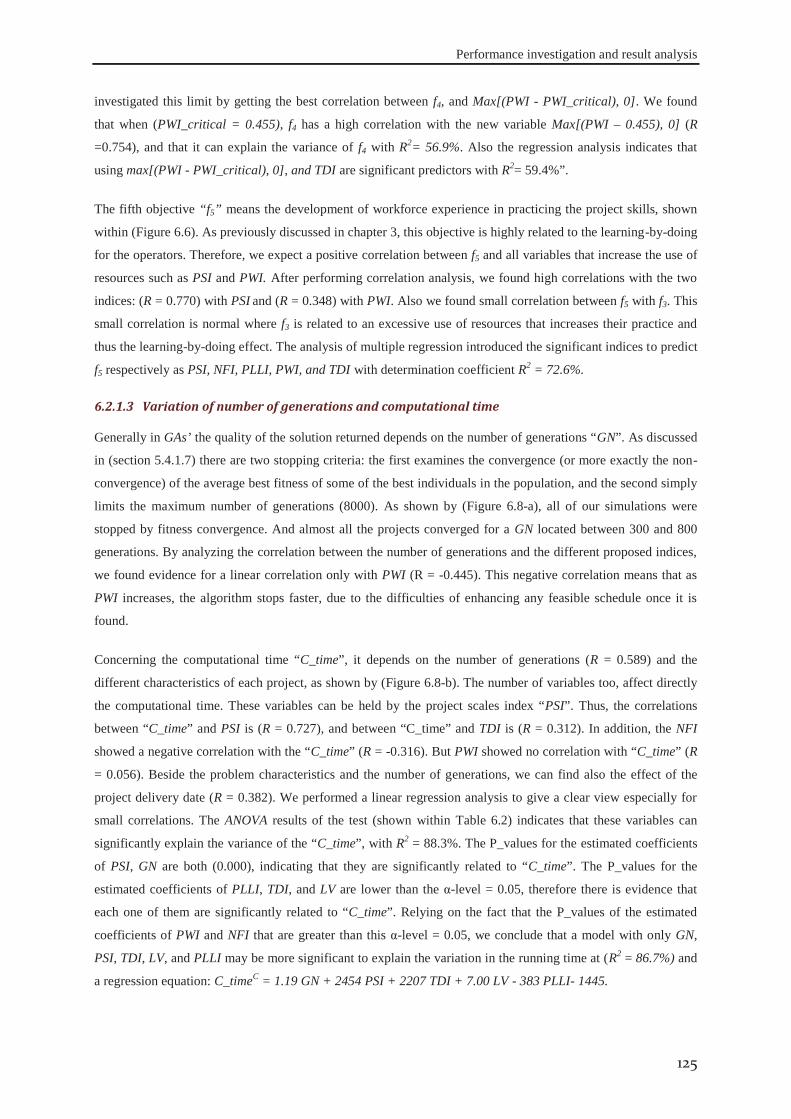
Performance investigation and result analysis

125

investigated this limit by getting the best correlation between f4, and Max[(PWI - PWI_critical), 0]. We found

that when (PWI_critical = 0.455), f4 has a high correlation with the new variable Max[(PWI – 0.455), 0] (R

=0.754), and that it can explain the variance of f4 with R2= 56.9%. Also the regression analysis indicates that

using max[(PWI - PWI_critical), 0], and TDI are significant predictors with R2= 59.4%”.

The fifth objective “f5” means the development of workforce experience in practicing the project skills, shown

within (Figure 6.6). As previously discussed in chapter 3, this objective is highly related to the learning-by-doing

for the operators. Therefore, we expect a positive correlation between f5 and all variables that increase the use of

resources such as PSI and PWI. After performing correlation analysis, we found high correlations with the two

indices: (R = 0.770) with PSI and (R = 0.348) with PWI. Also we found small correlation between f5 with f3. This

small correlation is normal where f3 is related to an excessive use of resources that increases their practice and

thus the learning-by-doing effect. The analysis of multiple regression introduced the significant indices to predict

f5 respectively as PSI, NFI, PLLI, PWI, and TDI with determination coefficient R2 = 72.6%.

6.2.1.3 Variation of number of generations and computational time

Generally in GAs’ the quality of the solution returned depends on the number of generations “GN”. As discussed

in (section 5.4.1.7) there are two stopping criteria: the first examines the convergence (or more exactly the non-

convergence) of the average best fitness of some of the best individuals in the population, and the second simply

limits the maximum number of generations (8000). As shown by (Figure 6.8-a), all of our simulations were

stopped by fitness convergence. And almost all the projects converged for a GN located between 300 and 800

generations. By analyzing the correlation between the number of generations and the different proposed indices,

we found evidence for a linear correlation only with PWI (R = -0.445). This negative correlation means that as

PWI increases, the algorithm stops faster, due to the difficulties of enhancing any feasible schedule once it is

found.

Concerning the computational time “C_time”, it depends on the number of generations (R = 0.589) and the

different characteristics of each project, as shown by (Figure 6.8-b). The number of variables too, affect directly

the computational time. These variables can be held by the project scales index “PSI”. Thus, the correlations

between “C_time” and PSI is (R = 0.727), and between “C_time” and TDI is (R = 0.312). In addition, the NFI

showed a negative correlation with the “C_time” (R = -0.316). But PWI showed no correlation with “C_time” (R

= 0.056). Beside the problem characteristics and the number of generations, we can find also the effect of the

project delivery date (R = 0.382). We performed a linear regression analysis to give a clear view especially for

small correlations. The ANOVA results of the test (shown within Table 6.2) indicates that these variables can

significantly explain the variance of the “C_time”, with R2 = 88.3%. The P_values for the estimated coefficients

of PSI, GN are both (0.000), indicating that they are significantly related to “C_time”. The P_values for the

estimated coefficients of PLLI, TDI, and LV are lower than the α-level = 0.05, therefore there is evidence that

each one of them are significantly related to “C_time”. Relying on the fact that the P_values of the estimated

coefficients of PWI and NFI that are greater than this α-level = 0.05, we conclude that a model with only GN,

PSI, TDI, LV, and PLLI may be more significant to explain the variation in the running time at (R2 = 86.7%) and

a regression equation: C_timeC = 1.19 GN + 2454 PSI + 2207 TDI + 7.00 LV - 383 PLLI- 1445.

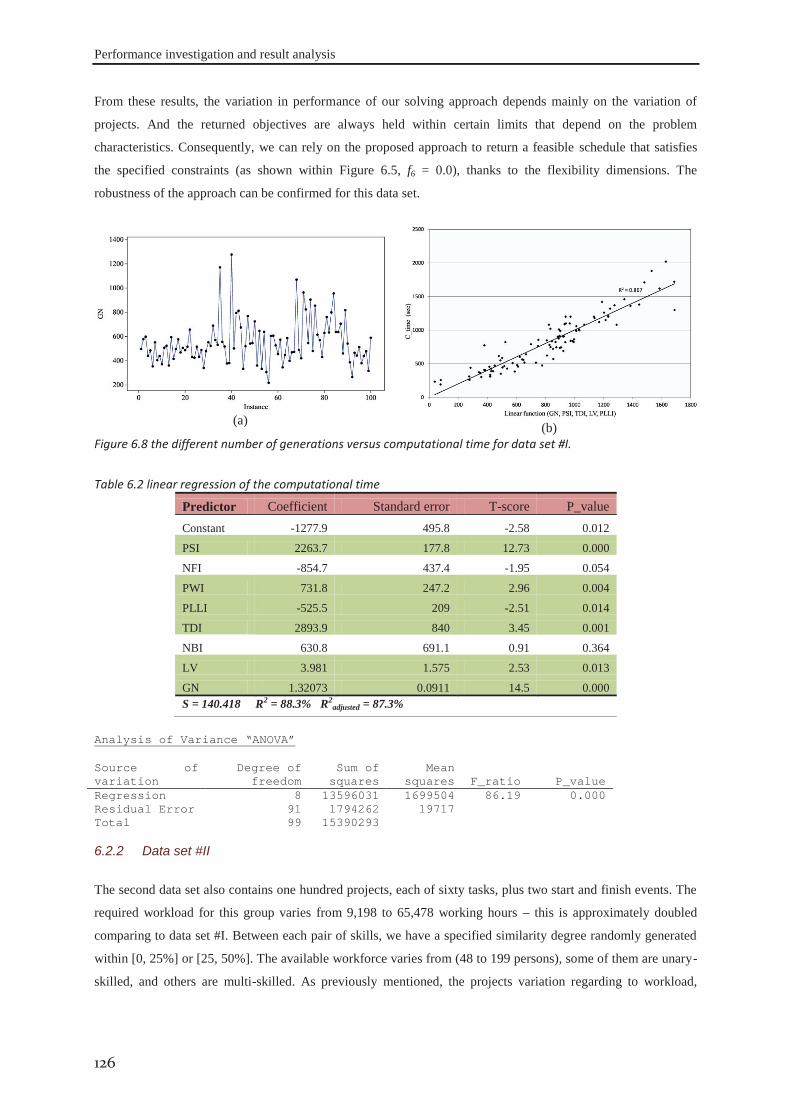
Performance investigation and result analysis

126

From these results, the variation in performance of our solving approach depends mainly on the variation of

projects. And the returned objectives are always held within certain limits that depend on the problem

characteristics. Consequently, we can rely on the proposed approach to return a feasible schedule that satisfies

the specified constraints (as shown within Figure 6.5, f6 = 0.0), thanks to the flexibility dimensions. The

robustness of the approach can be confirmed for this data set.

(a)

(b) Figure 6.8 the different number of generations versus computational time for data set #I.

Table 6.2 linear regression of the computational time

Predictor Coefficient Standard error T-score P_value Constant -1277.9 495.8 -2.58 0.012

PSI 2263.7 177.8 12.73 0.000

NFI -854.7 437.4 -1.95 0.054

PWI 731.8 247.2 2.96 0.004

PLLI -525.5 209 -2.51 0.014

TDI 2893.9 840 3.45 0.001

NBI 630.8 691.1 0.91 0.364

LV 3.981 1.575 2.53 0.013

GN 1.32073 0.0911 14.5 0.000 S = 140.418 R2 = 88.3% R2

adjusted = 87.3%

Analysis of Variance “ANOVA”

Source of variation

Degree of freedom

Sum of squares

Mean squares F_ratio P_value

Regression 8 13596031 1699504 86.19 0.000 Residual Error 91 1794262 19717 Total 99 15390293

The second data set also contains one hundred projects, each of sixty tasks, plus two start and finish events. The

required workload for this group varies from 9,198 to 65,478 working hours – this is approximately doubled

comparing to data set #I. Between each pair of skills, we have a specified similarity degree randomly generated

within [0, 25%] or [25, 50%]. The available workforce varies from (48 to 199 persons), some of them are unary-

skilled, and others are multi-skilled. As previously mentioned, the projects variation regarding to workload,

6.2.2 Data set #II

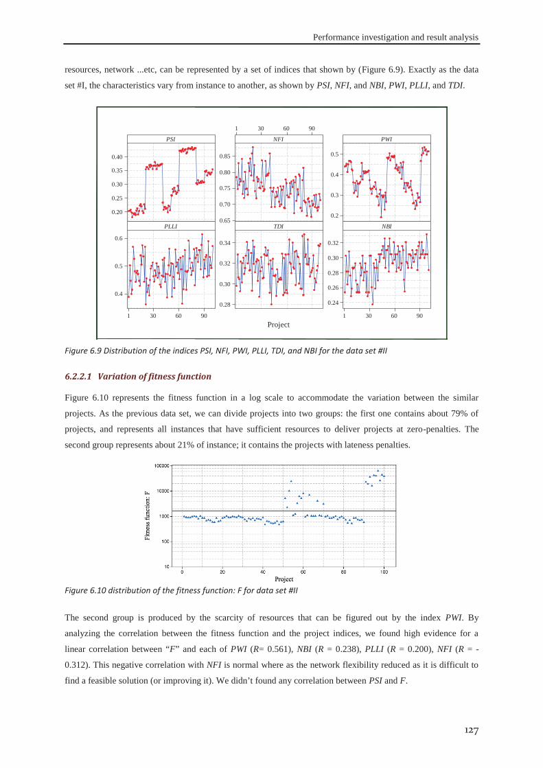
Performance investigation and result analysis

127

resources, network ...etc, can be represented by a set of indices that shown by (Figure 6.9). Exactly as the data

set #I, the characteristics vary from instance to another, as shown by PSI, NFI, and NBI, PWI, PLLI, and TDI.

0.40

0.35

0.30

0.25

0.20

9060301

0.85

0.80

0.75

0.70

0.65

0.5

0.4

0.3

0.2

9060301

0.6

0.5

0.4

0.34

0.32

0.30

0.28

9060301

0.32

0.30

0.28

0.26

0.24

PSI

Project

NFI PWI

PLLI TDI NBI

Figure 6.9 Distribution of the indices PSI, NFI, PWI, PLLI, TDI, and NBI for the data set #II

6.2.2.1 Variation of fitness function

Figure 6.10 represents the fitness function in a log scale to accommodate the variation between the similar

projects. As the previous data set, we can divide projects into two groups: the first one contains about 79% of

projects, and represents all instances that have sufficient resources to deliver projects at zero-penalties. The

second group represents about 21% of instance; it contains the projects with lateness penalties.

Figure 6.10 distribution of the fitness function: F for data set #II

The second group is produced by the scarcity of resources that can be figured out by the index PWI. By

analyzing the correlation between the fitness function and the project indices, we found high evidence for a

linear correlation between “F” and each of PWI (R= 0.561), NBI (R = 0.238), PLLI (R = 0.200), NFI (R = -

0.312). This negative correlation with NFI is normal where as the network flexibility reduced as it is difficult to

find a feasible solution (or improving it). We didn’t found any correlation between PSI and F.

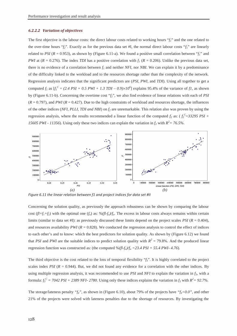
Performance investigation and result analysis

128

6.2.2.2 Variation of objectives

The first objective is the labour costs: the direct labour costs related to working hours “f1” and the one related to

the over-time hours “f2”. Exactly as for the previous data set #I, the normal direct labour costs “f1” are linearly

related to PSI (R = 0.953), as shown by (Figure 6.11-a). We found a positive small correlation between “f1” and

PWI at (R = 0.276). The index TDI has a positive correlation with f1 (R = 0.206). Unlike the previous data set,

there is no evidence of a correlation between f1 and neither NFI, nor NBI. We can explain it by a predominance

of the difficulty linked to the workload and to the resources shortage rather than the complexity of the network.

Regression analysis indicates that the significant predictors are (PSI, PWI, and TDI). Using all together to get a

computed f1 as [f1C = (2.4 PSI + 0.5 PWI + 1.3 TDI – 0.9) 106] explains 95.4% of the variance of f1, as shown

by (Figure 6.11-b). Concerning the overtime cost “f2”, we also find evidence of linear relations with each of PSI

(R = 0.797), and PWI (R = 0.427). Due to the high constraints of workload and resources shortage, the influences

of the other indices (NFI, PLLI, TDI and NBI) on f2 are unremarkable. This relation also was proven by using the

regression analysis, where the results recommended a linear function of the computed f2 as: ( f2C=33295 PSI +

15605 PWI - 11356). Using only these two indices can explain the variation in f2 with R2= 76.5%.

(a)

(b)

Figure 6.11 the linear relation between f1 and project indices for data set #II

Concerning the solution quality, as previously the approach robustness can be shown by comparing the labour

cost (fl=f1+f2) with the optimal one (fo) as: %(fl-fo)/fo. The excess in labour costs always remains within certain

limits (similar to data set #I): as previously discussed these limits depend on the project scales PSI (R = 0.404),

and resources availability PWI (R = 0.828). We conducted the regression analysis to control the effect of indices

to each other’s and to know: which the best predictors for solution quality. As shown by (Figure 6.12) we found

that PSI and PWI are the suitable indices to predict solution quality with R2 = 79.8%. And the produced linear

regression function was constructed as: (the computed %(fl-fo)/fo =23.4 PSI + 55.4 PWI- 4.76).

The third objective is the cost related to the loss of temporal flexibility “f3”. It is highly correlated to the project

scales index PSI (R = 0.944). But, we did not found any evidence for a correlation with the other indices. By

using multiple regression analysis, it was recommended to use PSI and NFI to explain the variation in f3, with a

formula: f3C = 7042 PSI + 2389 NFI- 2780. Using only these indices explains the variation in f3 with R2= 92.7%.

The storage/lateness penalty “f4”, as shown in (Figure 6.10), about 79% of the projects have “f4=0.0”, and other

21% of the projects were solved with lateness penalties due to the shortage of resources. By investigating the

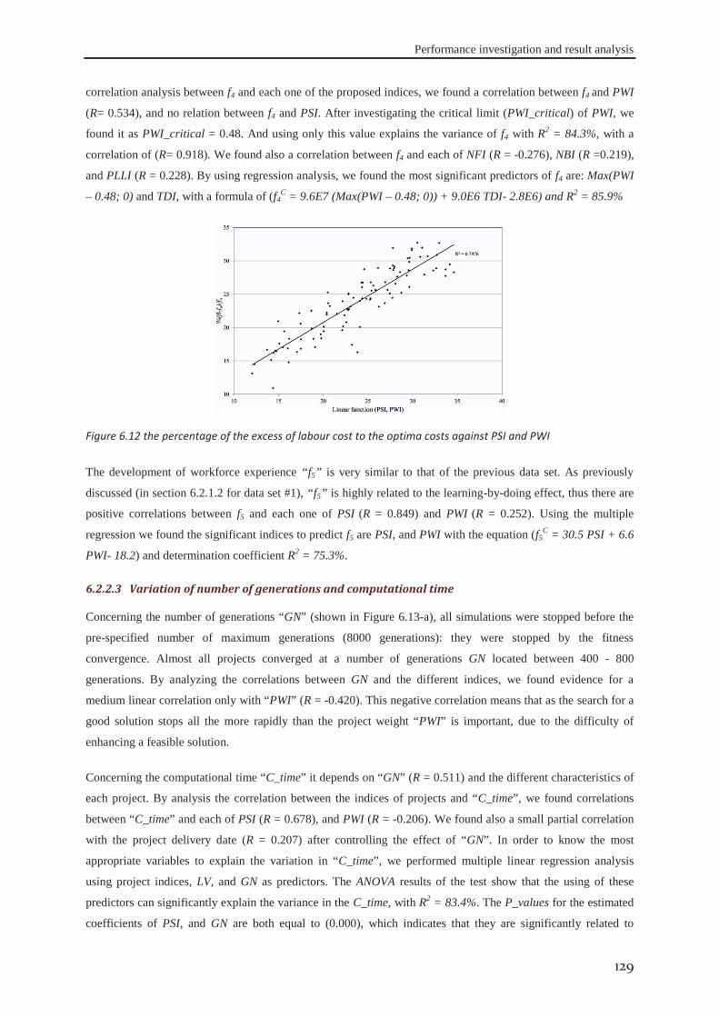
Performance investigation and result analysis

129

correlation analysis between f4 and each one of the proposed indices, we found a correlation between f4 and PWI

(R= 0.534), and no relation between f4 and PSI. After investigating the critical limit (PWI_critical) of PWI, we

found it as PWI_critical = 0.48. And using only this value explains the variance of f4 with R2 = 84.3%, with a

correlation of (R= 0.918). We found also a correlation between f4 and each of NFI (R = -0.276), NBI (R =0.219),

and PLLI (R = 0.228). By using regression analysis, we found the most significant predictors of f4 are: Max(PWI

– 0.48; 0) and TDI, with a formula of (f4C = 9.6E7 (Max(PWI – 0.48; 0)) + 9.0E6 TDI- 2.8E6) and R2 = 85.9%

Figure 6.12 the percentage of the excess of labour cost to the optima costs against PSI and PWI

The development of workforce experience “f5” is very similar to that of the previous data set. As previously

discussed (in section 6.2.1.2 for data set #1), “f5” is highly related to the learning-by-doing effect, thus there are

positive correlations between f5 and each one of PSI (R = 0.849) and PWI (R = 0.252). Using the multiple

regression we found the significant indices to predict f5 are PSI, and PWI with the equation (f5C = 30.5 PSI + 6.6

PWI- 18.2) and determination coefficient R2 = 75.3%.

6.2.2.3 Variation of number of generations and computational time

Concerning the number of generations “GN” (shown in Figure 6.13-a), all simulations were stopped before the

pre-specified number of maximum generations (8000 generations): they were stopped by the fitness

convergence. Almost all projects converged at a number of generations GN located between 400 - 800

generations. By analyzing the correlations between GN and the different indices, we found evidence for a

medium linear correlation only with “PWI” (R = -0.420). This negative correlation means that as the search for a

good solution stops all the more rapidly than the project weight “PWI” is important, due to the difficulty of

enhancing a feasible solution.

Concerning the computational time “C_time” it depends on “GN” (R = 0.511) and the different characteristics of

each project. By analysis the correlation between the indices of projects and “C_time”, we found correlations

between “C_time” and each of PSI (R = 0.678), and PWI (R = -0.206). We found also a small partial correlation

with the project delivery date (R = 0.207) after controlling the effect of “GN”. In order to know the most

appropriate variables to explain the variation in “C_time”, we performed multiple linear regression analysis

using project indices, LV, and GN as predictors. The ANOVA results of the test show that the using of these

predictors can significantly explain the variance in the C_time, with R2 = 83.4%. The P_values for the estimated

coefficients of PSI, and GN are both equal to (0.000), which indicates that they are significantly related to

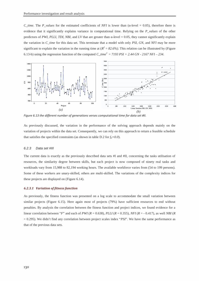
Performance investigation and result analysis

130

C_time. The P_values for the estimated coefficients of NFI is lower than (α-level = 0.05), therefore there is

evidence that it significantly explains variance in computational time. Relying on the P_values of the other

predictors of PWI, PLLI, TDI, NBI, and LV that are greater than α-level = 0.05, they cannot significantly explain

the variation in C_time for this data set. This terminate that a model with only PSI, GN, and NFI may be more

significant to explain the variation in the running time at (R2 = 82.6%). This relation can be illustrated by (Figure

6.13-b) using the regression function of the computed C_timeC = 7193 PSI + 2.44 GN - 2167 NFI – 234.

(a)

(b) Figure 6.13 the different number of generations verses computational time for data set #II.

As previously discussed, the variation in the performance of the solving approach depends mainly on the

variation of projects within the data set. Consequently, we can rely on this approach to return a feasible schedule

that satisfies the specified constraints (as shown in table D.2 for f6=0.0).

The current data is exactly as the previously described data sets #I and #II, concerning the tasks utilisation of

resources, the similarity degree between skills, but each project is now composed of ninety real tasks and

workloads vary from 15,988 to 82,194 working hours. The available workforce varies from (54 to 199 persons).

Some of these workers are unary-skilled, others are multi-skilled. The variations of the complexity indices for

these projects are displayed on (Figure 6.14).

6.2.3.1 Variation of fitness function

As previously, the fitness function was presented on a log scale to accommodate the small variation between

similar projects (Figure 6.15). Here again most of projects (79%) have sufficient resources to end without

penalties. By analysis the correlation between the fitness function and project indices, we found evidence for a

linear correlation between “F” and each of PWI (R = 0.638), PLLI (R = 0.355), NFI (R = - 0.417), as well NBI (R

= 0.295). We didn’t find any correlation between project scales index “PSI”. We have the same performance as

that of the previous data sets.

6.2.3 Data set #III

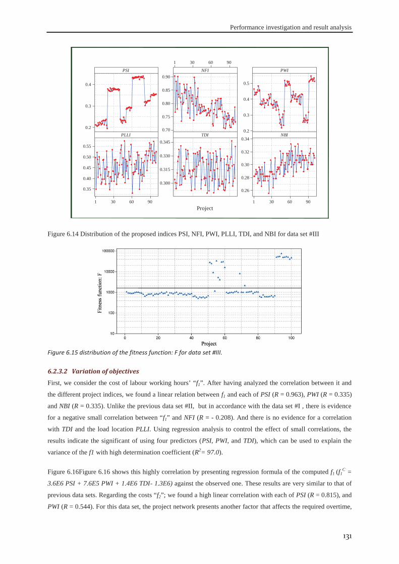
Performance investigation and result analysis

131

0.4

0.3

0.2

9060301

0.90

0.85

0.80

0.75

0.70

0.5

0.4

0.3

0.2

9060301

0.55

0.50

0.45

0.40

0.35

0.345

0.330

0.315

0.300

9060301

0.34

0.32

0.30

0.28

0.26

PSI

Project

NFI PWI

PLLI TDI NBI

Figure 6.14 Distribution of the proposed indices PSI, NFI, PWI, PLLI, TDI, and NBI for data set #III

Figure 6.15 distribution of the fitness function: F for data set #III.

6.2.3.2 Variation of objectives

First, we consider the cost of labour working hours’ “f1”. After having analyzed the correlation between it and

the different project indices, we found a linear relation between f1 and each of PSI (R = 0.963), PWI (R = 0.335)

and NBI (R = 0.335). Unlike the previous data set #II, but in accordance with the data set #I , there is evidence

for a negative small correlation between “f1” and NFI (R = - 0.208). And there is no evidence for a correlation

with TDI and the load location PLLI. Using regression analysis to control the effect of small correlations, the

results indicate the significant of using four predictors (PSI, PWI, and TDI), which can be used to explain the

variance of the f1 with high determination coefficient (R2= 97.0).

Figure 6.16Figure 6.16 shows this highly correlation by presenting regression formula of the computed f1 (f1C =

3.6E6 PSI + 7.6E5 PWI + 1.4E6 TDI- 1.3E6) against the observed one. These results are very similar to that of

previous data sets. Regarding the costs “f2”; we found a high linear correlation with each of PSI (R = 0.815), and

PWI (R = 0.544). For this data set, the project network presents another factor that affects the required overtime,

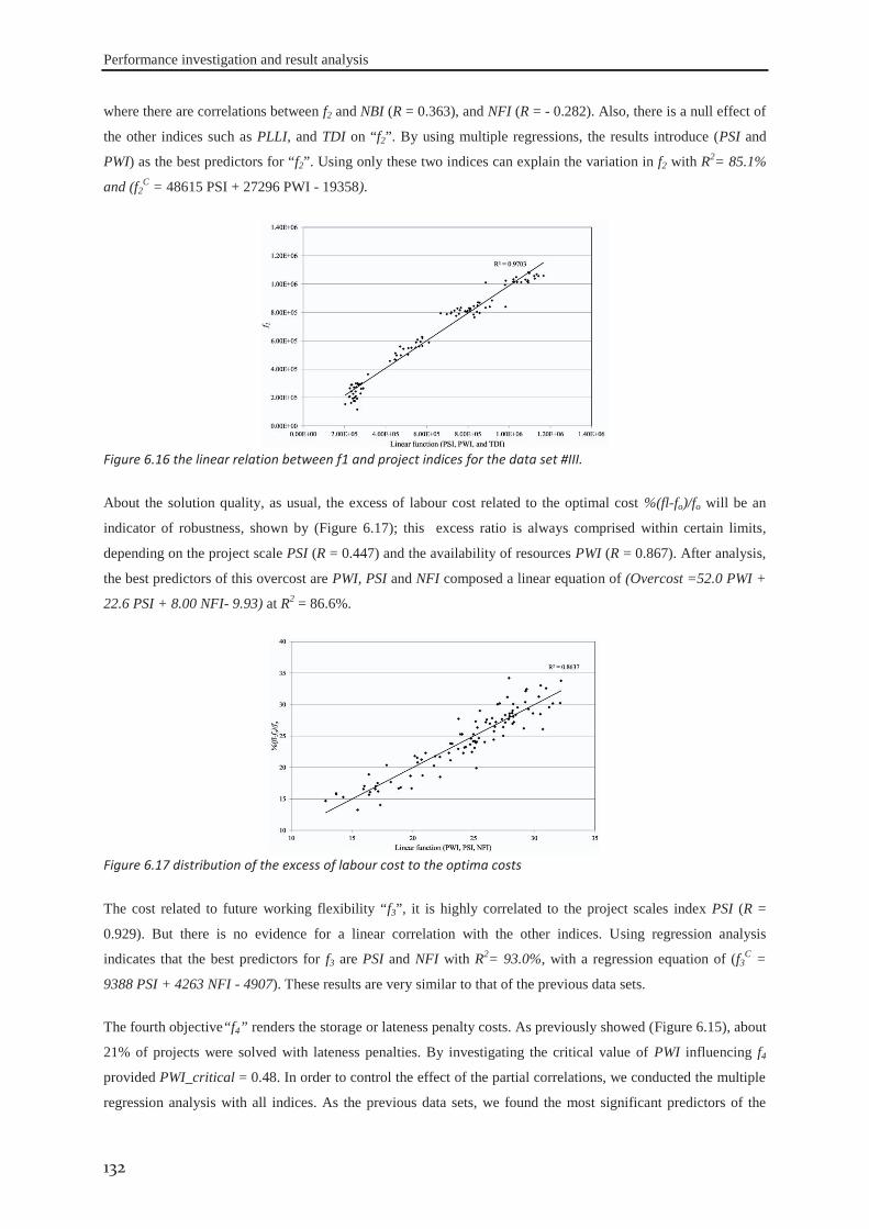
Performance investigation and result analysis

132

where there are correlations between f2 and NBI (R = 0.363), and NFI (R = - 0.282). Also, there is a null effect of

the other indices such as PLLI, and TDI on “f2”. By using multiple regressions, the results introduce (PSI and

PWI) as the best predictors for “f2”. Using only these two indices can explain the variation in f2 with R2= 85.1%

and (f2C = 48615 PSI + 27296 PWI - 19358).

Figure 6.16 the linear relation between f1 and project indices for the data set #III.

About the solution quality, as usual, the excess of labour cost related to the optimal cost %(fl-fo)/fo will be an

indicator of robustness, shown by (Figure 6.17); this excess ratio is always comprised within certain limits,

depending on the project scale PSI (R = 0.447) and the availability of resources PWI (R = 0.867). After analysis,

the best predictors of this overcost are PWI, PSI and NFI composed a linear equation of (Overcost =52.0 PWI +

22.6 PSI + 8.00 NFI- 9.93) at R2 = 86.6%.

Figure 6.17 distribution of the excess of labour cost to the optima costs

The cost related to future working flexibility “f3”, it is highly correlated to the project scales index PSI (R =

0.929). But there is no evidence for a linear correlation with the other indices. Using regression analysis

indicates that the best predictors for f3 are PSI and NFI with R2= 93.0%, with a regression equation of (f3C =

9388 PSI + 4263 NFI - 4907). These results are very similar to that of the previous data sets.

The fourth objective“f4” renders the storage or lateness penalty costs. As previously showed (Figure 6.15), about

21% of projects were solved with lateness penalties. By investigating the critical value of PWI influencing f4

provided PWI_critical = 0.48. In order to control the effect of the partial correlations, we conducted the multiple

regression analysis with all indices. As the previous data sets, we found the most significant predictors of the

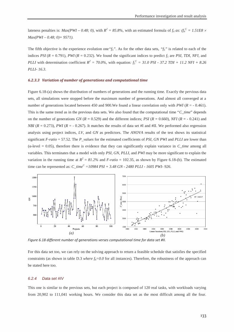
Performance investigation and result analysis

133

lateness penalties is: Max(PWI – 0.48; 0), with R2 = 85.8%, with an estimated formula of f4 as: (f4C = 1.51E8

Max(PWI – 0.48; 0)+ 9571).

The fifth objective is the experience evolution one“f5”. As for the other data sets, “f5” is related to each of the

indices PSI (R = 0.791), PWI (R = 0.232). We found the significant indices to predict f5 are PSI, TDI, NFI, and

PLLI with determination coefficient R2 = 70.0%, with equation: f5C = 31.0 PSI - 37.2 TDI + 11.2 NFI + 8.26

PLLI- 16.3.

6.2.3.3 Variation of number of generations and computational time

Figure 6.18-(a) shows the distribution of numbers of generations and the running time. Exactly the pervious data

sets, all simulations were stopped before the maximum number of generations. And almost all converged at a

number of generations located between 450 and 900.We found a linear correlation only with PWI (R = - 0.461).

This is the same trend as in the previous data sets. We also found that the computational time “C_time” depends

on the number of generations GN (R = 0.529) and the different indices; PSI (R = 0.660), NFI (R = - 0.241) and

NBI (R = 0.273), PWI (R = - 0.267). It matches the results of data set #I and #II. We performed also regression

analysis using project indices, LV, and GN as predictors. The ANOVA results of the test shows its statistical

significant F-ratio = 57.52. The P_values for the estimated coefficients of PSI, GN PWI and PLLI are lower than

(α-level = 0.05), therefore there is evidence that they can significantly explain variance in C_time among all

variables. This terminates that a model with only PSI, GN, PLLI, and PWI may be more significant to explain the

variation in the running time at R2 = 81.2% and F-ratio = 102.35, as shown by Figure 6.18-(b). The estimated

time can be represented as: C_timeC =10984 PSI + 3.48 GN - 2480 PLLI - 1605 PWI- 926.

(a)

(b) Figure 6.18 different number of generations verses computational time for data set #II.

For this data set too, we can rely on the solving approach to return a feasible schedule that satisfies the specified

constraints (as shown in table D.3 where f6=0.0 for all instances). Therefore, the robustness of the approach can

be stated here too.

This one is similar to the previous sets, but each project is composed of 120 real tasks, with workloads varying

from 20,902 to 111,041 working hours. We consider this data set as the most difficult among all the four.

6.2.4 Data set #IV

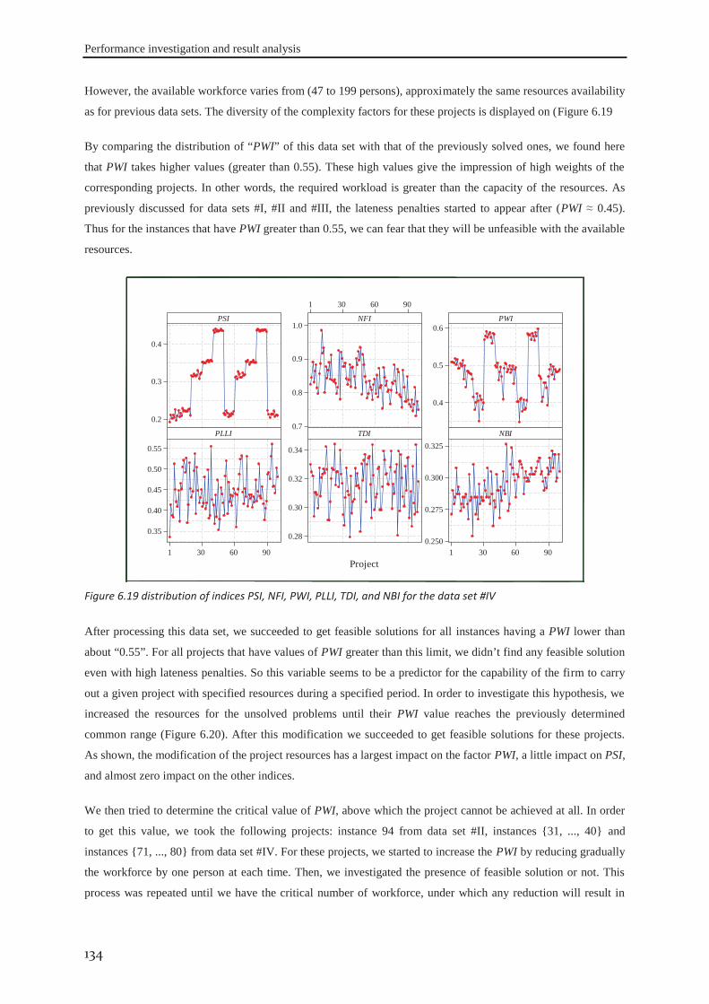
Performance investigation and result analysis

134

However, the available workforce varies from (47 to 199 persons), approximately the same resources availability

as for previous data sets. The diversity of the complexity factors for these projects is displayed on (Figure 6.19

By comparing the distribution of “PWI” of this data set with that of the previously solved ones, we found here

that PWI takes higher values (greater than 0.55). These high values give the impression of high weights of the

corresponding projects. In other words, the required workload is greater than the capacity of the resources. As

previously discussed for data sets #I, #II and #III, the lateness penalties started to appear after (PWI ≈ 0.45).

Thus for the instances that have PWI greater than 0.55, we can fear that they will be unfeasible with the available

resources.

0.4

0.3

0.2

9060301

1.0

0.9

0.8

0.7

0.6

0.5

0.4

9060301

0.55

0.50

0.45

0.40

0.35

0.34

0.32

0.30

0.28

9060301

0.325

0.300

0.275

0.250

PSI

Project

NFI PWI

PLLI TDI NBI

Figure 6.19 distribution of indices PSI, NFI, PWI, PLLI, TDI, and NBI for the data set #IV

After processing this data set, we succeeded to get feasible solutions for all instances having a PWI lower than

about “0.55”. For all projects that have values of PWI greater than this limit, we didn’t find any feasible solution

even with high lateness penalties. So this variable seems to be a predictor for the capability of the firm to carry

out a given project with specified resources during a specified period. In order to investigate this hypothesis, we

increased the resources for the unsolved problems until their PWI value reaches the previously determined

common range (Figure 6.20). After this modification we succeeded to get feasible solutions for these projects.

As shown, the modification of the project resources has a largest impact on the factor PWI, a little impact on PSI,

and almost zero impact on the other indices.

We then tried to determine the critical value of PWI, above which the project cannot be achieved at all. In order

to get this value, we took the following projects: instance 94 from data set #II, instances {31, ..., 40} and

instances {71, ..., 80} from data set #IV. For these projects, we started to increase the PWI by reducing gradually

the workforce by one person at each time. Then, we investigated the presence of feasible solution or not. This

process was repeated until we have the critical number of workforce, under which any reduction will result in

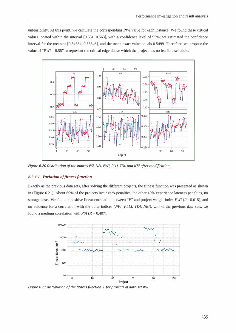
Performance investigation and result analysis

135

unfeasibility. At this point, we calculate the corresponding PWI value for each instance. We found these critical

values located within the interval [0.531, 0.563], with a confidence level of 95%; we estimated the confidence

interval for the mean as [0.54634, 0.55346], and the mean exact value equals 0.5499. Therefore, we propose the

value of “PWI = 0.55” to represent the critical edge above which the project has no feasible schedule.

0.4

0.3

0.2

9060301

1.0

0.9

0.8

0.7

0.55

0.50

0.45

0.40

0.35

9060301

0.55

0.50

0.45

0.40

0.35

0.34

0.32

0.30

0.28

9060301

0.325

0.300

0.275

0.250

PSI

Project

NFI PWI

PLLI TDI NBI

Figure 6.20 Distribution of the indices PSI, NFI, PWI, PLLI, TDI, and NBI after modification.

6.2.4.1 Variation of fitness function

Exactly as the previous data sets, after solving the different projects, the fitness function was presented as shown

in (Figure 6.21). About 60% of the projects incur zero-penalties, the other 40% experience lateness penalties, no

storage costs. We found a positive linear correlation between “F” and project weight index PWI (R= 0.615), and

no evidence for a correlation with the other indices (NFI, PLLI, TDI, NBI). Unlike the previous data sets, we

found a medium correlation with PSI (R = 0.407).

Figure 6.21 distribution of the fitness function: F for projects in data set #VI

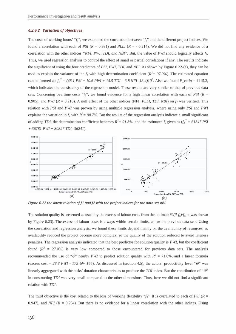
Performance investigation and result analysis

136

6.2.4.2 Variation of objectives

The costs of working hours’ “f1”, we examined the correlation between “f1” and the different project indices. We

found a correlation with each of PSI (R = 0.981) and PLLI (R = - 0.214). We did not find any evidence of a

correlation with the other indices “NFI, PWI, TDI, and NBI”. But, the value of PWI should logically affects f1.

Thus, we used regression analysis to control the effect of small or partial correlations if any. The results indicate

the significant of using the four predictors of PSI, PWI, TDI, and NFI. As shown by Figure 6.22-(a), they can be

used to explain the variance of the f1 with high determination coefficient (R2= 97.9%). The estimated equation

can be formed as: f1C = (48.1 PSI + 10.6 PWI + 14.5 TDI – 3.8 NFI- 13.4)105. Also we found F_ratio = 1115.2,

which indicates the consistency of the regression model. These results are very similar to that of previous data

sets. Concerning overtime costs “f2”; we found evidence for a high linear correlation with each of PSI (R =

0.905), and PWI (R = 0.216). A null effect of the other indices (NFI, PLLI, TDI, NBI) on f2 was verified. This

relation with PSI and PWI was proven by using multiple regression analysis, where using only PSI and PWI

explains the variation in f2 with R2= 90.7%. But the results of the regression analysis indicate a small significant

of adding TDI, the determination coefficient becomes R2= 91.3%, and the estimated f2 given as (f2C = 61347 PSI

+ 36781 PWI + 30827 TDI- 36241).

(a)

(b) Figure 6.22 the linear relation of f1 and f2 with the project indices for the data set #IV.

The solution quality is presented as usual by the excess of labour costs from the optimal: %(fl-fo)/fo, it was shown

by Figure 6.23). The excess of labour costs is always within certain limits, as for the pervious data sets. Using

the correlation and regression analysis, we found these limits depend mainly on the availability of resources, as

availability reduced the project become more complex, so the quality of the solution reduced to avoid lateness

penalties. The regression analysis indicated that the best predictor for solution quality is PWI, but the coefficient

found (R2 = 27.0%) is very low compared to those encountered for previous data sets. The analysis

recommended the use of “ ” nearby PWI to predict solution quality with R2 = 71.6%, and a linear formula

(excess cost = 28.8 PWI - 172 + 144). As discussed in (section 4.5), the actors’ productivity level “ ” was

linearly aggregated with the tasks’ duration characteristics to produce the TDI index. But the contribution of “ ”

in constructing TDI was very small compared to the other dimensions. Thus, here we did not find a significant

relation with TDI.

The third objective is the cost related to the loss of working flexibility “f3”. It is correlated to each of PSI (R =

0.947), and NFI (R = 0.264). But there is no evidence for a linear correlation with the other indices. Using

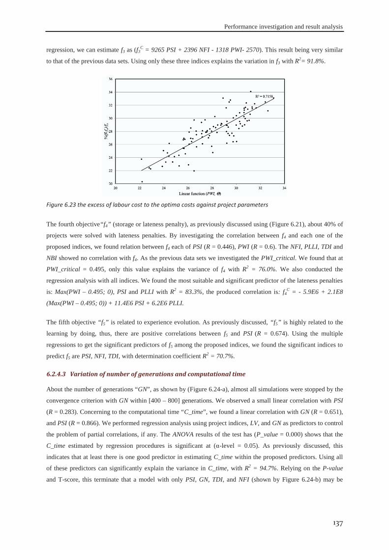
Performance investigation and result analysis

137

regression, we can estimate f3 as (f3C = 9265 PSI + 2396 NFI - 1318 PWI- 2570). This result being very similar

to that of the previous data sets. Using only these three indices explains the variation in f3 with R2= 91.8%.

Figure 6.23 the excess of labour cost to the optima costs against project parameters

The fourth objective“f4” (storage or lateness penalty), as previously discussed using (Figure 6.21), about 40% of

projects were solved with lateness penalties. By investigating the correlation between f4 and each one of the

proposed indices, we found relation between f4 each of PSI (R = 0.446), PWI (R = 0.6). The NFI, PLLI, TDI and

NBI showed no correlation with f4. As the previous data sets we investigated the PWI_critical. We found that at

PWI_critical = 0.495, only this value explains the variance of f4 with R2 = 76.0%. We also conducted the

regression analysis with all indices. We found the most suitable and significant predictor of the lateness penalties

is: Max(PWI – 0.495; 0), PSI and PLLI with R2 = 83.3%, the produced correlation is: f4C = - 5.9E6 + 2.1E8

(Max(PWI – 0.495; 0)) + 11.4E6 PSI + 6.2E6 PLLI.

The fifth objective “f5” is related to experience evolution. As previously discussed, “f5” is highly related to the

learning by doing, thus, there are positive correlations between f5 and PSI (R = 0.674). Using the multiple

regressions to get the significant predictors of f5 among the proposed indices, we found the significant indices to

predict f5 are PSI, NFI, TDI, with determination coefficient R2 = 70.7%.

6.2.4.3 Variation of number of generations and computational time

About the number of generations “GN”, as shown by (Figure 6.24-a), almost all simulations were stopped by the

convergence criterion with GN within [400 – 800] generations. We observed a small linear correlation with PSI

(R = 0.283). Concerning to the computational time “C_time”, we found a linear correlation with GN (R = 0.651),

and PSI (R = 0.866). We performed regression analysis using project indices, LV, and GN as predictors to control

the problem of partial correlations, if any. The ANOVA results of the test has (P_value = 0.000) shows that the

C_time estimated by regression procedures is significant at (α-level = 0.05). As previously discussed, this

indicates that at least there is one good predictor in estimating C_time within the proposed predictors. Using all

of these predictors can significantly explain the variance in C_time, with R2 = 94.7%. Relying on the P-value

and T-score, this terminate that a model with only PSI, GN, TDI, and NFI (shown by Figure 6.24-b) may be

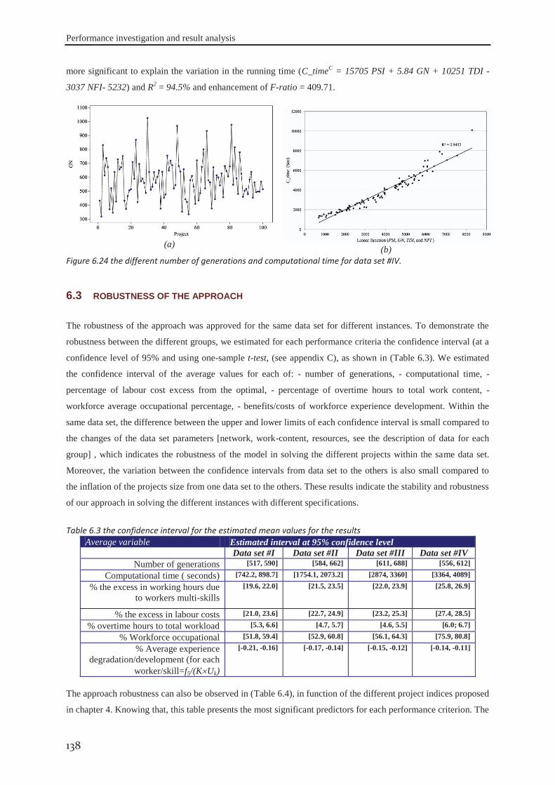
Performance investigation and result analysis

138

more significant to explain the variation in the running time (C_timeC = 15705 PSI + 5.84 GN + 10251 TDI -

3037 NFI- 5232) and R2 = 94.5% and enhancement of F-ratio = 409.71.

(a)

(b) Figure 6.24 the different number of generations and computational time for data set #IV.

The robustness of the approach was approved for the same data set for different instances. To demonstrate the

robustness between the different groups, we estimated for each performance criteria the confidence interval (at a

confidence level of 95% and using one-sample t-test, (see appendix C), as shown in (Table 6.3). We estimated

the confidence interval of the average values for each of: - number of generations, - computational time, -

percentage of labour cost excess from the optimal, - percentage of overtime hours to total work content, -

workforce average occupational percentage, - benefits/costs of workforce experience development. Within the

same data set, the difference between the upper and lower limits of each confidence interval is small compared to

the changes of the data set parameters [network, work-content, resources, see the description of data for each

group] , which indicates the robustness of the model in solving the different projects within the same data set.

Moreover, the variation between the confidence intervals from data set to the others is also small compared to

the inflation of the projects size from one data set to the others. These results indicate the stability and robustness

of our approach in solving the different instances with different specifications.

Table 6.3 the confidence interval for the estimated mean values for the results Average variable Estimated interval at 95% confidence level Data set #I Data set #II Data set #III Data set #IV

Number of generations [517, 590] [584, 662] [611, 688] [556, 612]

Computational time ( seconds) [742.2, 898.7] [1754.1, 2073.2] [2874, 3360] [3364, 4089]

% the excess in working hours due to workers multi-skills

[19.6, 22.0]

[21.5, 23.5]

[22.0, 23.9] [25.8, 26.9]

% the excess in labour costs [21.0, 23.6] [22.7, 24.9] [23.2, 25.3] [27.4, 28.5]

% overtime hours to total workload [5.3, 6.6] [4.7, 5.7] [4.6, 5.5] [6.0; 6.7]

% Workforce occupational [51.8, 59.4] [52.9, 60.8] [56.1, 64.3] [75.9, 80.8]

% Average experience degradation/development (for each

worker/skill=f5/(K Uk)

[-0.21, -0.16] [-0.17, -0.14] [-0.15, -0.12] [-0.14, -0.11]

The approach robustness can also be observed in (Table 6.4), in function of the different project indices proposed

in chapter 4. Knowing that, this table presents the most significant predictors for each performance criterion. The

6.3 ROBUSTNESS OF THE APPROACH

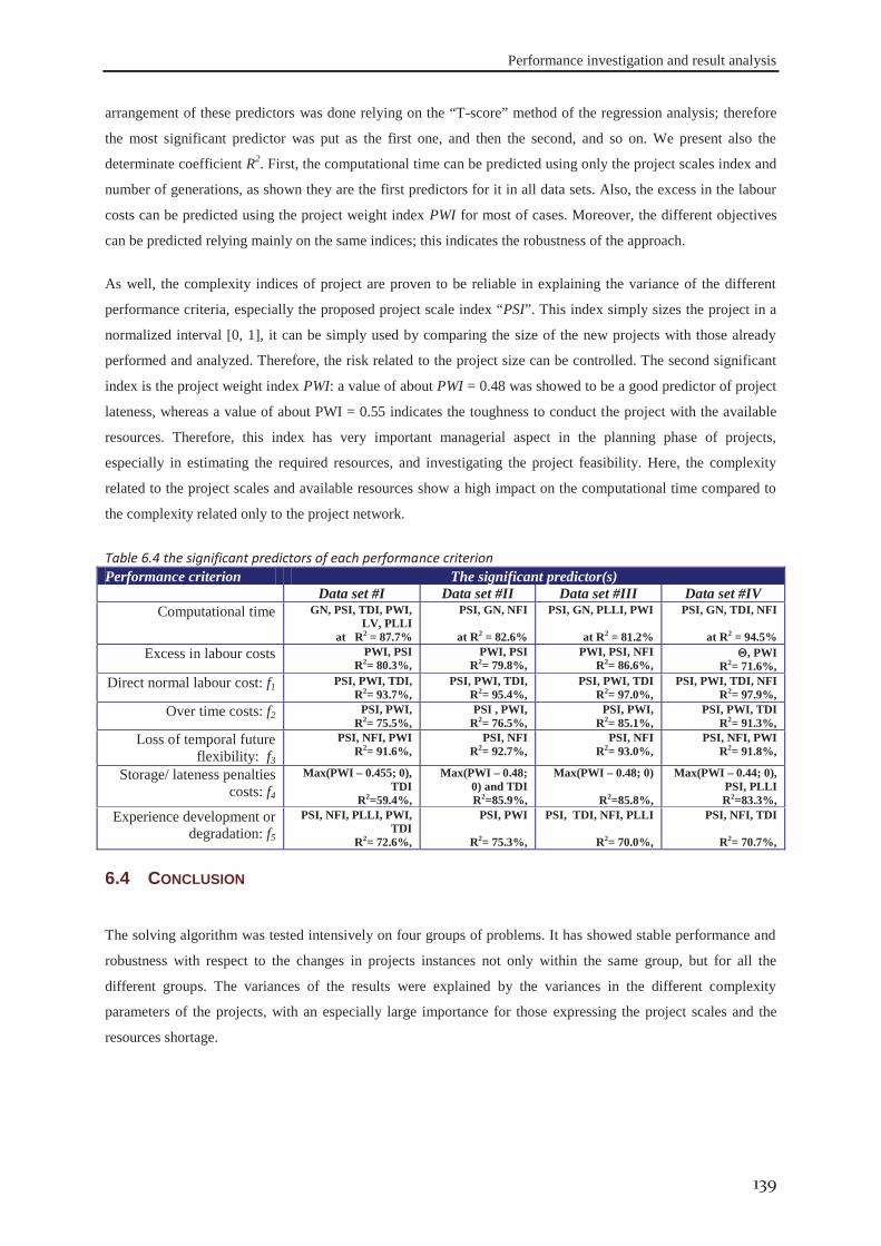
Performance investigation and result analysis

139

arrangement of these predictors was done relying on the “T-score” method of the regression analysis; therefore

the most significant predictor was put as the first one, and then the second, and so on. We present also the

determinate coefficient R2. First, the computational time can be predicted using only the project scales index and

number of generations, as shown they are the first predictors for it in all data sets. Also, the excess in the labour

costs can be predicted using the project weight index PWI for most of cases. Moreover, the different objectives

can be predicted relying mainly on the same indices; this indicates the robustness of the approach.

As well, the complexity indices of project are proven to be reliable in explaining the variance of the different

performance criteria, especially the proposed project scale index “PSI”. This index simply sizes the project in a

normalized interval [0, 1], it can be simply used by comparing the size of the new projects with those already

performed and analyzed. Therefore, the risk related to the project size can be controlled. The second significant

index is the project weight index PWI: a value of about PWI = 0.48 was showed to be a good predictor of project

lateness, whereas a value of about PWI = 0.55 indicates the toughness to conduct the project with the available

resources. Therefore, this index has very important managerial aspect in the planning phase of projects,

especially in estimating the required resources, and investigating the project feasibility. Here, the complexity

related to the project scales and available resources show a high impact on the computational time compared to

the complexity related only to the project network.

Table 6.4 the significant predictors of each performance criterion Performance criterion The significant predictor(s) Data set #I Data set #II Data set #III Data set #IV

Computational time GN, PSI, TDI, PWI, LV, PLLI

at R2 = 87.7%

PSI, GN, NFI

at R2 = 82.6%

PSI, GN, PLLI, PWI

at R2 = 81.2%

PSI, GN, TDI, NFI

at R2 = 94.5% Excess in labour costs PWI, PSI

R2= 80.3%, PWI, PSI

R2= 79.8%, PWI, PSI, NFI

R2= 86.6%, , PWI

R2= 71.6%, Direct normal labour cost: f1 PSI, PWI, TDI,

R2= 93.7%, PSI, PWI, TDI,

R2= 95.4%, PSI, PWI, TDI

R2= 97.0%, PSI, PWI, TDI, NFI

R2= 97.9%, Over time costs: f2 PSI, PWI,

R2= 75.5%, PSI , PWI,

R2= 76.5%, PSI, PWI,

R2= 85.1%, PSI, PWI, TDI

R2= 91.3%, Loss of temporal future

flexibility: f3 PSI, NFI, PWI

R2= 91.6%, PSI, NFI

R2= 92.7%, PSI, NFI

R2= 93.0%, PSI, NFI, PWI

R2= 91.8%,

Storage/ lateness penalties costs: f4

Max(PWI – 0.455; 0), TDI

R2=59.4%,

Max(PWI – 0.48; 0) and TDI R2=85.9%,

Max(PWI – 0.48; 0)

R2=85.8%,

Max(PWI – 0.44; 0), PSI, PLLI R2=83.3%,

Experience development or degradation: f5

PSI, NFI, PLLI, PWI, TDI

R2= 72.6%,

PSI, PWI

R2= 75.3%,

PSI, TDI, NFI, PLLI

R2= 70.0%,

PSI, NFI, TDI

R2= 70.7%,

The solving algorithm was tested intensively on four groups of problems. It has showed stable performance and

robustness with respect to the changes in projects instances not only within the same group, but for all the

different groups. The variances of the results were explained by the variances in the different complexity

parameters of the projects, with an especially large importance for those expressing the project scales and the

resources shortage.

6.4 CONCLUSION

Performance investigation and result analysis

140

7 FACTORS AFFECTING THE DEVELOPMENT OF

WORKFORCE VERSATILITY

This chapter aims to present and investigate the different variables that

affect the development of workforce’s experience and their multi-skill

flexibility. First, these different variables will be presented. Then, using an

illustration example, the factors that affect the costs of developing such

flexibility will be discussed. Afterwards, a comprehensive investigation of

these variables will be conducted. At the end of the chapter, the

conclusions and some recommendations will be discussed.

CH

APT

ER

7

Factors affecting the development of workforce versatility

142

In order to develop the actors’ versatility with acceptable additional costs, one needs to investigate the effect of

some factors. This investigation can be intended to reduce the cost resulting from the learning-forgetting-

relearning cycles. In this section we discuss three groups of parameters, related to the human resources

themselves, to the characteristics of the firm’s core competences, and to the firms’ managerial policy,

respectively.

7.1.1.1 Number of flexible workers

It is the number of employees involved within the program of multi-skills development “PMSD”: the overhead

cost of developing their secondary skills will be all the higher as this number is important. It can be represented

by the number of actors whose productivity levels are within the experience acquisition interval, θa,k [θkmin, 0.8

(roughly estimated)]. As indicated in the work of Attia et al. (2011), firms should accept an augmentation of

overhead costs just to preserve the productivity levels of their operators, even though serious reduction of the

firm’s profits may result. Part of this cost may be misplaced, if it happens that the workforce’s productivity

levels decrease during the project execution, due to the learning/learning-loss/relearning cycles. These cycles

result from the periodic utilisation of the actors’ polyvalence, which may interrupt the practice of a secondary

skill during its acquisition period. If a large number of actors are following the skills development program, one

should find a compromise between reducing the overhead costs and avoiding the interruptions in the practice of

the secondary skills. In the study presented by Sayin and Karabati, (2007) relying on the “Recency” model of

Nembhard and Uzumeri (2000a), the impact of the number of actors involved in the skills development program

did not showed any significant impact. We argue here that it can have a noteworthy effect.

7.1.1.2 The occupational rates of the workforce

This factor can be presented as the total number of actors (versatile or not) available to provide the workloads

required for a given project. We assert that this factor has a great influence on the skills attrition rate (experience

depreciation). When the number of available actors increases, we can expect that the average workforce’s

occupational rate will reduce, that a high level of workforce’s future temporal flexibility will be preserved, and

hence, that the workers’ practice will decrease. Consequently to the reduction of workers’ practice of the skills

under development, the skills degradation can be shaped. Sayin and Karabati (2007) investigated this factor in

the allocation of workforce in different departments. Under the name of tightness of human resources, they

investigated the shortage of workforce in the development of workforce experience. Their results showed that

this factor is the most noteworthy in affecting the total skills development, with statistical significance. Other

variables that can be much correlated to the workforce occupation is the Resources loading: it refers to the

requirements profile of a resource. Sayin and Karabati (2007) studied two profile variables: the first is the

temporal pattern that can be repeated at every time period. The second factor is the variation in demand from a

period to another; it was represented by the standard deviation of demand. The results indicate the positively

significant effects of both of them on the development of skills.

7.1 FACTORS TO BE INVESTIGATED

7.1.1 Parameters associated to human resources

Factors affecting the development of workforce versatility

143

7.1.1.3 Actor’s number of skills

It is the number of skills that an actor can master, either with optimal or sub-optimal performance. This number

is sometimes used to represent the workforce flexibility degree (Kher et al., 1999). As the average number of

actors’ skills increases, the probability of practice interruption increases, and hence the skills attrition may occur,

especially in cases of low similarities levels between these skills. Kher et al. (1999) stated that managers should

decide the number of different tasks for which a worker should be trained, how to train the workers, and how to

assign the workers in order to increase the learning and reduce the loss of learning. The investigation carried out

by Sayin and Karabati (2007) showed that the number of departments (that can be considered as skills) is not

significant at all in their analysis model. Contrary to their results, we expect this variable to be significant in the

current investigation. As well, this flexibility degree of workforce was investigated using the LFL (learning-

forgetting-learning) curve of Carlson and Rowe (1976) by Yue et al. (2007) in dual resources constraint. Their

results showed the significant effect of the number of skills per worker in a job-shop system performance,

whereas more specialised workers are especially important to gain optimal performance in dynamic

environments (short products’ production campaigns). For most of the investigated cases, a number of two skills

per worker showed a great influence on performance for all of the working conditions.

7.1.1.4 Minimum productivity level

This is the minimum accepted efficiency level for any actor to practice a given skill k, noted θkmin. An actor

whose efficiency is above this level can be assigned to perform any workload with this skill. This limit was set to

0.5 for the previous simulations discussed in chapters “5”and “6”. That is to say, the time required from a

beginner to perform a specified task is twice the standard time required from a fully-efficient operator. In this

chapter, we will investigate the effect of this factor in the skills attrition, to show whenever one can use the

actor’s versatility. We expect that, as this limit increases, the risk of workers losing their experience due to work

interruption will decrease.

7.1.1.5 Rate of learning/ forgetting

As shown in chapter “3”, the workforce’s efficiency evolution is function of the actors’ learning rates and

forgetting speeds. Theses parameters can vary from an actor to another, and from one skill to another, which can

be related to the skill complexity as discussed by Osothsilp (2002) and also in section (2.3.4). The reduction of

forgetting rate has a beneficial impact on the worker efficiency (Kher et al., 1999). It was also proven in

experimental studies by Bailey (1989) and Globerson et al. (1989) that the efficiency attrition is function of the

duration of learning prior interruption, and of the duration of the interruption period (that increases the forgetting

rates). According to Jaber et al. (2003), the level of forgetting depends upon the rate of learning, and Nembhard

and Uzumeri (2000a) found, relying on empirical data, that the actor who learns faster is likely to forget rapidly.

Here also, we will investigate this effect in presence of the working time flexibility. In addition, Sayin and

Karabati (2007) proved the direct effect of learning speed on skills development, especially under the normal

availability of workforce.

7.1.1.6 Teamwork structure

The composition of the teamwork affects the knowledge transfer and thus the efficiency of individuals’ learning

process. Hung-Chun Huang et al. (2010) considered the teamwork structure as a micro social system, hence

different teamwork structures conduct different members’ performances, so the teamwork structure can be used

Factors affecting the development of workforce versatility

144

as a way to manage indirectly the knowledge transfer. More about this factor can be found in Eurofound (2007).

Sayin and Karabati (2007) represented the team structure by introducing a variable called homogeneity of the

workforce: it is simply represented by the coefficient of variance in the workforce steady state productivity level

in a specified department (or skill). They found that the more homogeneous the teamwork is, the more flexibility

is gained in allocating workers: this variable has a statistical significant influence on skill development.

7.1.1.7 Social relations

The social relations between the team members and their consequences on the transfer of knowledge can affect

the multi-functional developments. This factor was investigated by Alexopoulos (2008), he found that the

effective transfer of knowledge hinges upon the extent to which individuals share common attitudes for

communication and entrusting each other, both professionally and personally. In particular, personal trust was

found to be a key to the transfer of tacit knowledge, thereby underlining the importance of positive affect as a

criterion for the formation of productive knowledge exchange relations.

7.1.1.8 Actors’ attitudes

Actors’ attitudes gather the motivation, willingness, innovation ability, stress at work, degree of knowledge, etc.

As investigated by Dam (2003), an enquiry based on a questionnaire addressed to 165 employees showed that

experts are generally motivated about developing multi-skill flexibility, and that experts’ willingness to take part

in development programmes is highly related to their motivations. Concerning the versatility development, he

concluded that the individual factors have more influence on flexibility development than organizational ones.

7.1.2.1 Similarity degree

The similarity degree figures the resemblance between an actor’s main skill and the secondary skill under

development. This parameter can be calculated from the attributes that are common between the two considered

skills (different knowledge fields, tools, machines, raw material, etc). According to the attributes in common,

one can estimate the degree of similarity between the two skills. Thus, it is simply the fraction of the elements in

common between the two skills SD [0, 1].

7.1.2.2 Skill type

Each competency is a mix of two main categories (cognitive or motor skills): according to these ingredients, the

kinetic of learning or forgetting a given skill is determined. According to Globerson et al. (1998) the individuals

are more likely to forget the cognitive skills than the motor skills. Concerning the learning speed, Dar-El et al.

(1995) proposed to estimate the actors’ learning parameters from these two ingredients. The skill type is also

investigated practically by Nembhard and Uzumeri (2000a) based on their “Recency model”, the nature of a

presently performed task influencing the amount of forgetting (Jaber et al., 2003). The effect of task complexity

in presence of product diversity was investigated by Mccreery and Krajewski (1999): the results showed a

significant impact of the task complexity degree on the cross-training flexibility and on the firms’ performance.

As the task complexity increases, it is useful to restrict the deployment of the workers. And an intensive use of

cross-training flexibility can be useful to face numerous product varieties, especially for low-complexity tasks.

7.1.2 Skills associated parameters

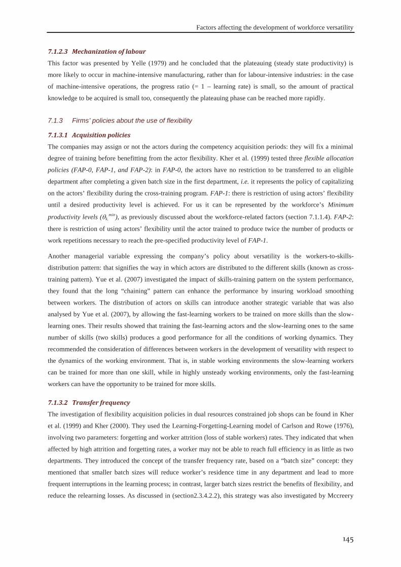
Factors affecting the development of workforce versatility

145

7.1.2.3 Mechanization of labour

This factor was presented by Yelle (1979) and he concluded that the plateauing (steady state productivity) is

more likely to occur in machine-intensive manufacturing, rather than for labour-intensive industries: in the case

of machine-intensive operations, the progress ratio (= 1 – learning rate) is small, so the amount of practical

knowledge to be acquired is small too, consequently the plateauing phase can be reached more rapidly.

7.1.3.1 Acquisition policies

The companies may assign or not the actors during the competency acquisition periods: they will fix a minimal

degree of training before benefitting from the actor flexibility. Kher et al. (1999) tested three flexible allocation

policies (FAP-0, FAP-1, and FAP-2): in FAP-0, the actors have no restriction to be transferred to an eligible

department after completing a given batch size in the first department, i.e. it represents the policy of capitalizing

on the actors’ flexibility during the cross-training program. FAP-1: there is restriction of using actors’ flexibility

until a desired productivity level is achieved. For us it can be represented by the workforce’s Minimum

productivity levels ( k,min), as previously discussed about the workforce-related factors (section 7.1.1.4). FAP-2:

there is restriction of using actors’ flexibility until the actor trained to produce twice the number of products or

work repetitions necessary to reach the pre-specified productivity level of FAP-1.

Another managerial variable expressing the company’s policy about versatility is the workers-to-skills-

distribution pattern: that signifies the way in which actors are distributed to the different skills (known as cross-

training pattern). Yue et al. (2007) investigated the impact of skills-training pattern on the system performance,

they found that the long “chaining” pattern can enhance the performance by insuring workload smoothing

between workers. The distribution of actors on skills can introduce another strategic variable that was also

analysed by Yue et al. (2007), by allowing the fast-learning workers to be trained on more skills than the slow-

learning ones. Their results showed that training the fast-learning actors and the slow-learning ones to the same

number of skills (two skills) produces a good performance for all the conditions of working dynamics. They

recommended the consideration of differences between workers in the development of versatility with respect to

the dynamics of the working environment. That is, in stable working environments the slow-learning workers

can be trained for more than one skill, while in highly unsteady working environments, only the fast-learning

workers can have the opportunity to be trained for more skills.

7.1.3.2 Transfer frequency

The investigation of flexibility acquisition policies in dual resources constrained job shops can be found in Kher

et al. (1999) and Kher (2000). They used the Learning-Forgetting-Learning model of Carlson and Rowe (1976),

involving two parameters: forgetting and worker attrition (loss of stable workers) rates. They indicated that when

affected by high attrition and forgetting rates, a worker may not be able to reach full efficiency in as little as two

departments. They introduced the concept of the transfer frequency rate, based on a “batch size” concept: they

mentioned that smaller batch sizes will reduce worker’s residence time in any department and lead to more

frequent interruptions in the learning process; in contrast, larger batch sizes restrict the benefits of flexibility, and

reduce the relearning losses. As discussed in (section2.3.4.2.2), this strategy was also investigated by Mccreery

7.1.3 Firms’ policies about the use of flexibility

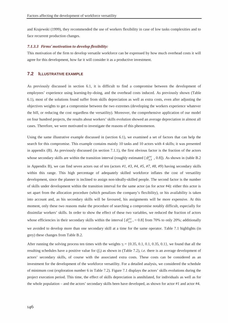
Factors affecting the development of workforce versatility

146

and Krajewski (1999), they recommended the use of workers flexibility in case of low tasks complexities and to

face recurrent production changes.

7.1.3.3 Firms’ motivation to develop flexibility:

This motivation of the firm to develop versatile workforce can be expressed by how much overhead costs it will

agree for this development, how far it will consider it as a productive investment.

As previously discussed in section 6.1, it is difficult to find a compromise between the development of

employees’ experience using learning-by–doing, and the overhead costs induced. As previously shown (Table

6.1), most of the solutions found suffer from skills depreciation as well as extra costs, even after adjusting the

objectives weights to get a compromise between the two extremes (developing the workers experience whatever

the bill, or reducing the cost regardless the versatility). Moreover, the comprehensive application of our model

on four hundred projects, the results about workers’ skills evolution showed an average depreciation in almost all

cases. Therefore, we were motivated to investigate the reasons of this phenomenon.

Using the same illustrative example discussed in (section 6.1), we examined a set of factors that can help the

search for this compromise. This example contains mainly 10 tasks and 10 actors with 4 skills; it was presented

in appendix (B). As previously discussed (in section 7.1.1), the first obvious factor is the fraction of the actors

whose secondary skills are within the transition interval (roughly estimated [ inika, , 0.8]). As shown in (table B.2

in Appendix B), we can find seven actors out of ten (actors #1, #3, #4, #5, #7, #8, #9) having secondary skills

within this range. This high percentage of adequately skilled workforce inflates the cost of versatility

development, since the planner is inclined to assign non-ideally-skilled people. The second factor is the number

of skills under development within the transition interval for the same actor (as for actor #4): either this actor is

set apart from the allocation procedure (which penalizes the company’s flexibility), or his availability is taken

into account and, as his secondary skills will be favoured, his assignments will be more expensive. At this

moment, only these two reasons make the procedure of searching a compromise notably difficult, especially for

dissimilar workers’ skills. In order to show the effect of these two variables, we reduced the fraction of actors

whose efficiencies in their secondary skills within the interval [ inika, , ≈ 0.8] from 70% to only 20%; additionally

we avoided to develop more than one secondary skill at a time for the same operator. Table 7.1 highlights (in

grey) these changes from Table B.2.

After running the solving process ten times with the weights γi = {0.35, 0.1, 0.1, 0.35, 0.1}, we found that all the

resulting schedules have a positive value for (f5) as shown in (Table 7.2), i.e. there is an average development of

actors’ secondary skills, of course with the associated extra costs. These costs can be considered as an

investment for the development of the workforce versatility. For a detailed analysis, we considered the schedule

of minimum cost (exploration number 6 in Table 7.2). Figure 7.1 displays the actors’ skills evolutions during the

project execution period. This time, the effect of skills depreciation is annihilated, for individuals as well as for

the whole population – and the actors’ secondary skills been have developed, as shown for actor #1 and actor #4.

7.2 ILLUSTRATIVE EXAMPLE

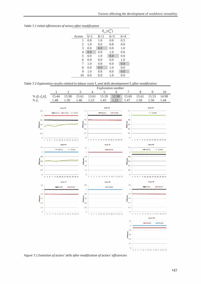
Factors affecting the development of workforce versatility

147

Table 7.1 Initial efficiencies of actors after modification

Actors )(,

SPeqka n

k=1 K=2 k=3 k=4 1 0.8 1.0 0.0 0.5 2 1.0 0.0 0.8 0.0 3 0.0 0.0 0.0 1.0 4 0.0 0.0 1.0 0.6 5 0.0 1.0 0.0 0.0 6 0.9 0.0 0.0 1.0 7 1.0 0.8 0.0 0.0 8 0.0 0.0 1.0 0.0 9 1.0 0.8 0.0 0.0

10 0.0 0.9 1.0 0.0

Table 7.2 Exploration results related to labour costs fL and skills development f5 after modification

Exploration number 1 2 3 4 5 6 7 8 9 10

% (fL-fo)/fo 15.44 15.98 15.61 13.61 15.39 12.98 15.69 15.61 15.53 14.98 % f5 1.48 1.50 1.46 1.23 1.43 1.22 1.47 1.50 1.50 1.44

Figure 7.1 Evolution of actors’ skills after modification of actors’ efficiencies

Factors affecting the development of workforce versatility

148

In order to evaluate the impact of the previously discussed factors on the associated over-costs, and to find the

best compromise between the two objectives, Figure 7.2 displays a graphical comparison between the results

from (Table 6.1) and (Table 7.2). As we see, companies must accept extra costs just to preserve the productivity

level of their actors (i.e. %f5 = 0.0). But these extra costs are all the more important as the number of actors

enrolled in the development program increases. In other words, with 70% of actors following the program of

multi-skilled development (PMSD), this over-cost can be estimated at 21% over the optimal labour cost, whereas

with only 20% of actors involved, it should drop down to 2.36%. According to this model, the number of the

actors engaged in a development program should be optimised.

Figure 7.2 Cost of skills betterment

Figure 7.2 indicates a linear growth of labour costs versus skills evolution, whatever the percentage of weakly-

qualified actors that can be assigned on activities. The y-values of these lines, all positive here, may result from

the difficulty for the project to meet the customer’s deadline with the optimally-skilled workforce, thus causing

the deliberate choice of the company to allocate non-ideally qualified workforce. What is more significant is that

the two sets of data lead to the same slopes for the curves expressing the impact of skills average change on

labour cost. In order to investigate the main reason that produces this constant slop, we performed an ANOVA

analysis between the two results of the two cases. We found there is no significant difference in the percentage

of over-costs of the two cases: with the results obtained (F-ratio = 0.49 and P-value = 0.492 > α_level = 0.05),

we concluded that there is no difference between the over-costs before and after modification (secondary skills

reduction). By the same way, we investigated the variance in the percentage of workforce’s experience

development (%f5): here, results indicate a significant difference of this development before and after

modifications (with F-ratio = 85.65 and P-value = 0.000 < α_level = 0.05). In the two cases, we optimised the

cost with respect to skills evolution by adjusting the weights of the fitness function (equals in the two cases). So

the slopes of the two curves are constant, which represents the compromise between the two criteria. As

previously mentioned, the changes between the two cases consist in deleting the misleading secondary skills of

the workforce, skills that were already avoided in the results of the first case by the optimisation approach.

Moreover, before modification, the depreciation of these avoided secondary skills was integrated in the results of

the workforce experience. The contribution of the secondary skills appears only on the constant of the regression

model. Thus, the difference between the two cases can be found between constants of the regression models.

That is to say, these misleading secondary skills shifted the results to the negative side (experience degradation

side). Now, the question is: why are the results before modification largely distributed around the regression line,

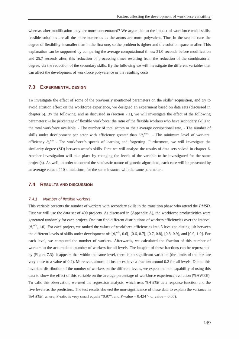
Factors affecting the development of workforce versatility

149

whereas after modification they are more concentrated? We argue this to the impact of workforce multi-skills:

feasible solutions are all the more numerous as the actors are more polyvalent. Thus in the second case the

degree of flexibility is smaller than in the first one, so the problem is tighter and the solution space smaller. This

explanation can be supported by comparing the average computational times: 31.0 seconds before modification

and 25.7 seconds after, this reduction of processing times resulting from the reduction of the combinatorial

degree, via the reduction of the secondary skills. By the following we will investigate the different variables that

can affect the development of workforce polyvalence or the resulting costs.

To investigate the effect of some of the previously mentioned parameters on the skills’ acquisition, and try to

avoid attrition effect on the workforce experience, we designed an experiment based on data sets (discussed in

chapter 6). By the following, and as discussed in (section 7.1), we will investigate the effect of the following

parameters: -The percentage of flexible workforce: the ratio of the flexible workers who have secondary skills to

the total workforce available. - The number of total actors or their average occupational rate, - The number of

skills under development per actor with efficiency greater than “θkmin”. - The minimum level of workers’

efficiency θkmin - The workforce’s speeds of learning and forgetting. Furthermore, we will investigate the

similarity degree (SD) between actor’s skills. First we will analyse the results of data sets solved in chapter 6.

Another investigation will take place by changing the levels of the variable to be investigated for the same

project(s). As well, in order to control the stochastic nature of genetic algorithms, each case will be presented by

an average value of 10 simulations, for the same instance with the same parameters.

This variable presents the number of workers with secondary skills in the transition phase who attend the PMSD.

First we will use the data set of 400 projects. As discussed in (Appendix A), the workforce productivities were

generated randomly for each project. One can find different distributions of workers efficiencies over the interval

[θkmin, 1.0]. For each project, we ranked the values of workforce efficiencies into 5 levels to distinguish between

the different levels of skills under development of: [θkmin, 0.6[, [0.6, 0.7[, [0.7, 0.8[, [0.8, 0.9[, and [0.9, 1.0]. For

each level, we computed the number of workers. Afterwards, we calculated the fraction of this number of

workers to the accumulated number of workers for all levels. The boxplot of these fractions can be represented

by (Figure 7.3): it appears that within the same level, there is no significant variation (the limits of the box are

very close to a value of 0.2). Moreover, almost all instances have a fraction around 0.2 for all levels. Due to this

invariant distribution of the number of workers on the different levels, we expect the non capability of using this

data to show the effect of this variable on the average percentage of workforce experience evolution (%AWEE).

To valid this observation, we used the regression analysis, which uses %AWEE as a response function and the

five levels as the predictors. The test results showed the non-significance of these data to explain the variance in

%AWEE, where, F-ratio is very small equals “0.97”, and P-value = 0.424 > α_value = 0.05).

7.3 EXPERIMENTAL DESIGN

7.4 RESULTS AND DISCUSSION

7.4.1 Number of flexible workers

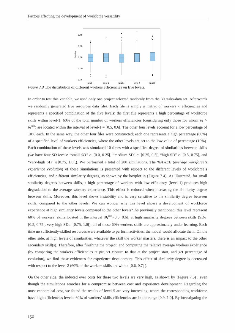
Factors affecting the development of workforce versatility

150

Figure 7.3 The distribution of different workers efficiencies on five levels.

In order to test this variable, we used only one project selected randomly from the 30 tasks-data set. Afterwards

we randomly generated five resources data files. Each file is simply a matrix of workers efficiencies and

represents a specified combination of the five levels: the first file represents a high percentage of workforce

skills within level-1; 60% of the total number of workers efficiencies (considering only those for whom k >

θkmin) are located within the interval of level-1 = [0.5, 0.6[. The other four levels account for a low percentage of

10% each. In the same way, the other four files were constructed; each one represents a high percentage (60%)

of a specified level of workers efficiencies, where the other levels are set to the low value of percentage (10%).

Each combination of these levels was simulated 10 times with a specified degree of similarities between skills

(we have four SD-levels: “small SD” [0.0, 0.25[, “medium SD” [0.25, 0.5[, “high SD” [0.5, 0.75[, and

“very-high SD” [0.75, 1.0[,). We performed a total of 200 simulations. The %AWEE (average workforce’s

experience evolution) of these simulations is presented with respect to the different levels of workforce’s

efficiencies, and different similarity degrees, as shown by the boxplot in (Figure 7.4). As illustrated, for small

similarity degrees between skills, a high percentage of workers with low efficiency (level-1) produces high

degradation to the average workers experience. This effect is reduced when increasing the similarity degree

between skills. Moreover, this level shows instability and is very sensitive to the similarity degree between

skills, compared to the other levels. We can wonder why this level shows a development of workforce

experience at high similarity levels compared to the other levels? As previously mentioned, this level represent

60% of workers’ skills located in the interval [θkmin=0.5, 0.6[; at high similarity degrees between skills (SD

[0.5, 0.75[, very-high SD [0.75, 1.0[), all of these 60% workers skills are approximately under learning. Each

time no sufficiently-skilled resources were available to perform activities, the model would allocate them. On the

other side, at high levels of similarities, whatever the skill the worker masters, there is an impact to the other

secondary skill(s). Therefore, after finishing the project, and computing the relative average workers experience

(by comparing the workers efficiencies at project closure to that at the project start, and get percentage of

evolution), we find these evidences for experience development. This effect of similarity degree is decreased

with respect to the level-2 (60% of the workers skills are within [0.6, 0.7[ ).

On the other side, the induced over costs for these two levels are very high, as shown by (Figure 7.5) , even

though the simulations searches for a compromise between cost and experience development. Regarding the

most economical cost, we found the results of level-5 are very interesting, where the corresponding workforce

have high efficiencies levels: 60% of workers’ skills efficiencies are in the range [0.9, 1.0]. By investigating the

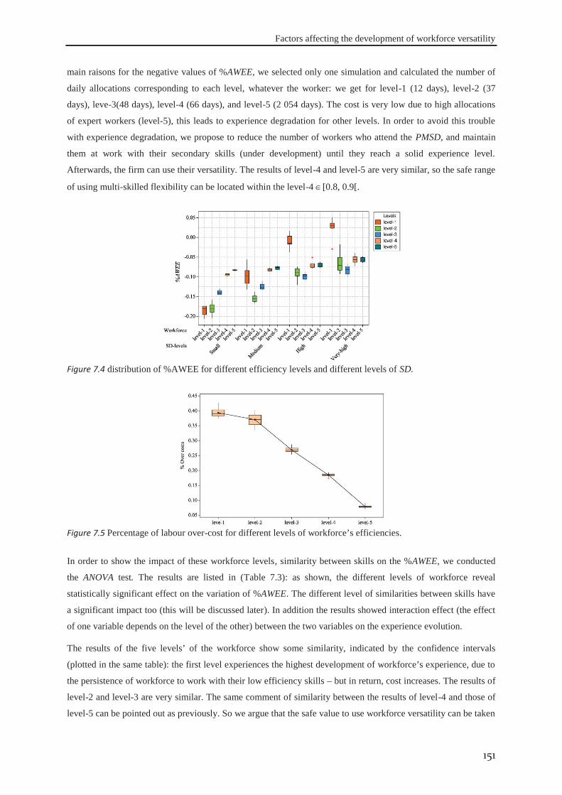
Factors affecting the development of workforce versatility

151

main raisons for the negative values of %AWEE, we selected only one simulation and calculated the number of

daily allocations corresponding to each level, whatever the worker: we get for level-1 (12 days), level-2 (37

days), leve-3(48 days), level-4 (66 days), and level-5 (2 054 days). The cost is very low due to high allocations

of expert workers (level-5), this leads to experience degradation for other levels. In order to avoid this trouble

with experience degradation, we propose to reduce the number of workers who attend the PMSD, and maintain

them at work with their secondary skills (under development) until they reach a solid experience level.

Afterwards, the firm can use their versatility. The results of level-4 and level-5 are very similar, so the safe range

of using multi-skilled flexibility can be located within the level-4 [0.8, 0.9[.

Figure 7.4 distribution of %AWEE for different efficiency levels and different levels of SD.

Figure 7.5 Percentage of labour over-cost for different levels of workforce’s efficiencies.

In order to show the impact of these workforce levels, similarity between skills on the %AWEE, we conducted

the ANOVA test. The results are listed in (Table 7.3): as shown, the different levels of workforce reveal

statistically significant effect on the variation of %AWEE. The different level of similarities between skills have

a significant impact too (this will be discussed later). In addition the results showed interaction effect (the effect

of one variable depends on the level of the other) between the two variables on the experience evolution.

The results of the five levels’ of the workforce show some similarity, indicated by the confidence intervals

(plotted in the same table): the first level experiences the highest development of workforce’s experience, due to

the persistence of workforce to work with their low efficiency skills – but in return, cost increases. The results of

level-2 and level-3 are very similar. The same comment of similarity between the results of level-4 and those of

level-5 can be pointed out as previously. So we argue that the safe value to use workforce versatility can be taken

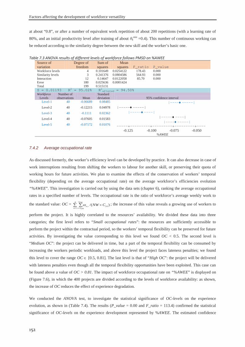
Factors affecting the development of workforce versatility

152

at about “0.8”, or after a number of equivalent work repetition of about 200 repetitions (with a learning rate of

80%, and an initial productivity level after training of about θkmin =0.4). This number of continuous working can

be reduced according to the similarity degree between the new skill and the worker’s basic one.

Table 7.3 ANOVA results of different levels of workforce follows PMSD on %AWEE Source of variation

Degree of freedom

Sum of squares

Mean squares F_ratio P_value

Workforce levels 4 0.101649 0.0254122 178.43 0.000 Similarity levels 3 0.241376 0.0804586 564.93 0.000 Interaction 12 0.14647 0.0122058 85.70 0.000 Error 180 0.025636 0.0001424 Total 199 0.515131 S = 0.01193 R2 = 95.02% R2adjusted = 94.50% Workforce

Levels Number of

observations Mean Standard deviation 95% confidence interval

Level-1 40 -0.06689 0.08485 |---- -----| |----- -----| |----- ----| |----- ----| |---- -----| -----+---------+---------+---------+---- -0.125 -0.100 -0.075 -0.050

%AWEE

Level-2 40 -0.12215 0.04978

Level-3 40 -0.1111 0.02362

Level-4 40 -0.07605 0.01583

Level-5 40 -0.07172 0.01076

As discussed formerly, the worker’s efficiency level can be developed by practice. It can also decrease in case of

work interruptions resulting from shifting the workers to labour for another skill, or preserving their quota of

working hours for future activities. We plan to examine the effects of the conservation of workers’ temporal

flexibility (depending on the average occupational rate) on the average workforce’s efficiencies evolution

“%AWEE”. This investigation is carried out by using the data sets (chapter 6), ranking the average occupational

rates in a specified number of levels. The occupational rate is the ratio of workforce’s average weekly work to

the standard value: OC = A

aS

FWS

SWSssa CNW

10, )/( ; the increase of this value reveals a growing use of workers to

perform the project. It is highly correlated to the resources’ availability. We divided these data into three

categories; the first level refers to “Small occupational rates”: the resources are sufficiently accessible to

perform the project within the contractual period, so the workers’ temporal flexibility can be preserved for future

activities. By investigating the value corresponding to this level we found OC < 0.5. The second level is

“Medium OC”: the project can be delivered in time, but a part of the temporal flexibility can be consumed by

increasing the workers periodic workloads, and above this level the project faces lateness penalties; we found

this level to cover the range OC [0.5, 0.81]. The last level is that of “High OC”: the project will be delivered

with lateness penalties even though all the temporal flexibility opportunities have been exploited. This case can

be found above a value of OC > 0.81. The impact of workforce occupational rate on “%AWEE” is displayed on

(Figure 7.6), in which the 400 projects are divided according to the levels of workforce availability: as shown,

the increase of OC reduces the effect of experience degradation.

We conducted the ANOVA test, to investigate the statistical significance of OC-levels on the experience

evolution, as shown in (Table 7.4). The results (P_value = 0.00 and F_ratio = 113.4) confirmed the statistical

significance of OC-levels on the experience development represented by %AWEE. The estimated confidence

7.4.2 Average occupational rate

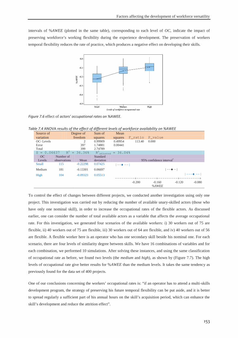
Factors affecting the development of workforce versatility

153

intervals of %AWEE (plotted in the same table), corresponding to each level of OC, indicate the impact of

preserving workforce’s working flexibility during the experience development. The preservation of workers

temporal flexibility reduces the rate of practice, which produces a negative effect on developing their skills.

Figure 7.6 effect of actors’ occupational rates on %AWEE.

Table 7.4 ANOVA results of the effect of different levels of workforce availability on %AWEE Source of variation

Degree of freedom

Sum of squares

Mean squares F_ratio P_value

OC- Levels 2 0.99909 0.49954 113.40 0.000 Error 397 1.74881 0.00441 Total 399 2.74789 S = 0.06637 R2 = 36.36% R2adjusted = 36.04%

OC Levels

Number of observations Mean

Standard deviation 95% confidence interval*

Small 115 -0.22298 0.07425 |-- --| |-- -| |--- --| ---------+---------+---------+---------+ -0.200 -0.160 -0.120 -0.080

%AWEE

Medium 181 -0.13301 0.06697

High 104 -0.09323 0.05513

To control the effect of changes between different projects, we conducted another investigation using only one

project. This investigation was carried out by reducing the number of available unary-skilled actors (those who

have only one nominal skill), in order to increase the occupational rates of the flexible actors. As discussed

earlier, one can consider the number of total available actors as a variable that affects the average occupational

rate. For this investigation, we generated four scenarios of the available workers: i) 30 workers out of 75 are

flexible, ii) 40 workers out of 75 are flexible, iii) 30 workers out of 64 are flexible, and iv) 40 workers out of 56

are flexible. A flexible worker here is an operator who has one secondary skill beside his nominal one. For each

scenario, there are four levels of similarity degree between skills. We have 16 combinations of variables and for

each combination, we performed 10 simulations. After solving these instances, and using the same classification

of occupational rate as before, we found two levels (the medium and high), as shown by (Figure 7.7). The high

levels of occupational rate give better results for %AWEE than the medium levels. It takes the same tendency as

previously found for the data set of 400 projects.

One of our conclusions concerning the workers’ occupational rates is: “if an operator has to attend a multi-skills

development program, the strategy of preserving his future temporal flexibility can be put aside, and it is better

to spread regularly a sufficient part of his annual hours on the skill’s acquisition period, which can enhance the

skill’s development and reduce the attrition effect”.

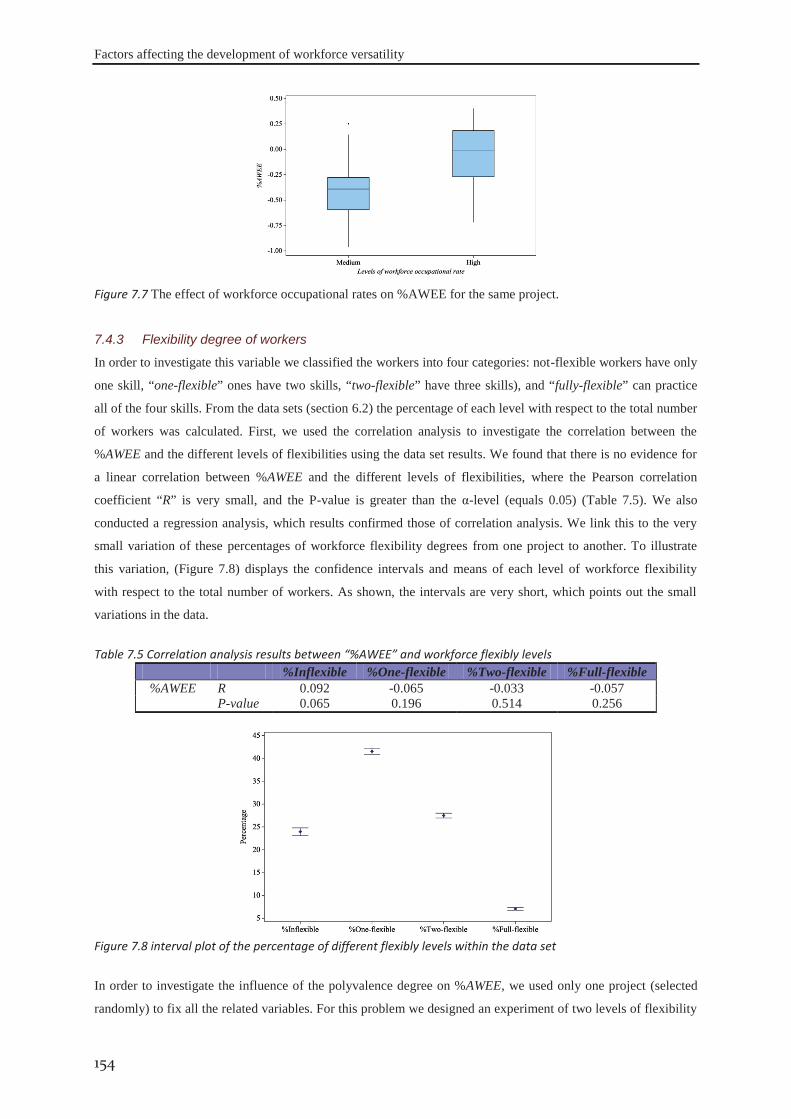
Factors affecting the development of workforce versatility

154

Figure 7.7 The effect of workforce occupational rates on %AWEE for the same project.

In order to investigate this variable we classified the workers into four categories: not-flexible workers have only

one skill, “one-flexible” ones have two skills, “two-flexible” have three skills), and “fully-flexible” can practice

all of the four skills. From the data sets (section 6.2) the percentage of each level with respect to the total number

of workers was calculated. First, we used the correlation analysis to investigate the correlation between the

%AWEE and the different levels of flexibilities using the data set results. We found that there is no evidence for

a linear correlation between %AWEE and the different levels of flexibilities, where the Pearson correlation

coefficient “R” is very small, and the P-value is greater than the α-level (equals 0.05) (Table 7.5). We also

conducted a regression analysis, which results confirmed those of correlation analysis. We link this to the very

small variation of these percentages of workforce flexibility degrees from one project to another. To illustrate

this variation, (Figure 7.8) displays the confidence intervals and means of each level of workforce flexibility

with respect to the total number of workers. As shown, the intervals are very short, which points out the small

variations in the data.

Table 7.5 Correlation analysis results between “%AWEE” and workforce flexibly levels %Inflexible %One-flexible %Two-flexible %Full-flexible

%AWEE R 0.092 -0.065 -0.033 -0.057 P-value 0.065 0.196 0.514 0.256

Figure 7.8 interval plot of the percentage of different flexibly levels within the data set

In order to investigate the influence of the polyvalence degree on %AWEE, we used only one project (selected

randomly) to fix all the related variables. For this problem we designed an experiment of two levels of flexibility

7.4.3 Flexibility degree of workers

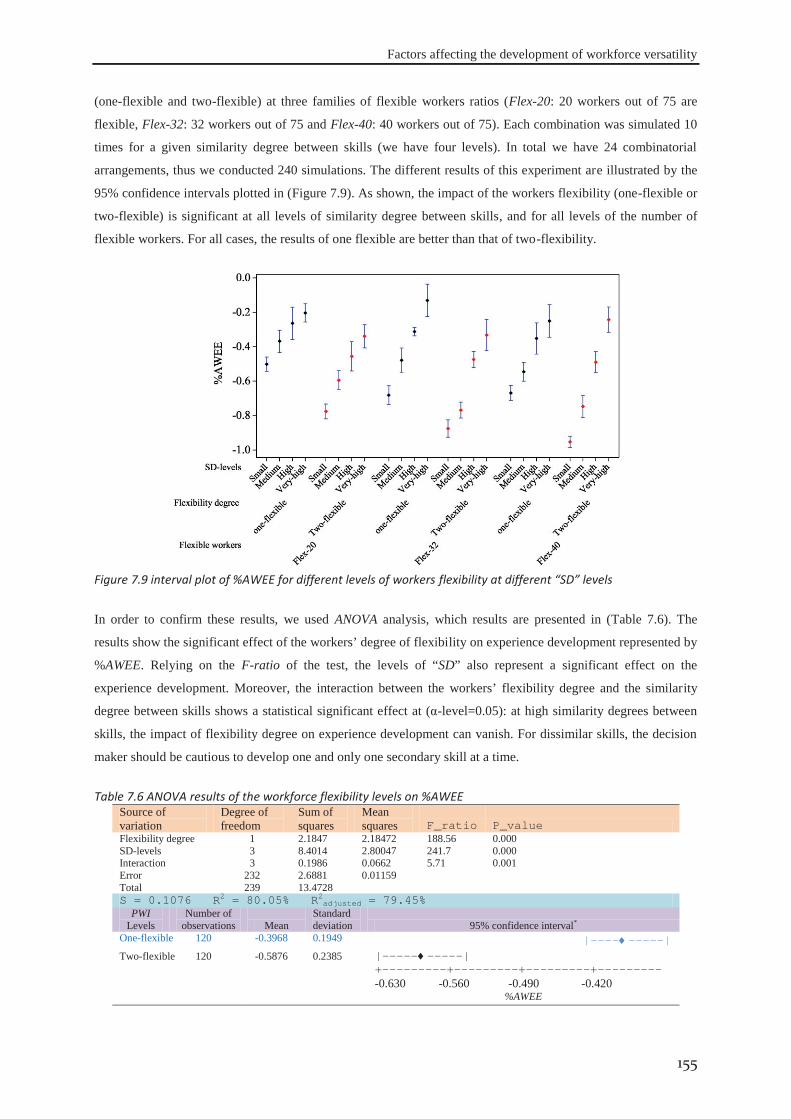
Factors affecting the development of workforce versatility

155

(one-flexible and two-flexible) at three families of flexible workers ratios (Flex-20: 20 workers out of 75 are

flexible, Flex-32: 32 workers out of 75 and Flex-40: 40 workers out of 75). Each combination was simulated 10

times for a given similarity degree between skills (we have four levels). In total we have 24 combinatorial

arrangements, thus we conducted 240 simulations. The different results of this experiment are illustrated by the

95% confidence intervals plotted in (Figure 7.9). As shown, the impact of the workers flexibility (one-flexible or

two-flexible) is significant at all levels of similarity degree between skills, and for all levels of the number of

flexible workers. For all cases, the results of one flexible are better than that of two-flexibility.

Figure 7.9 interval plot of %AWEE for different levels of workers flexibility at different “SD” levels

In order to confirm these results, we used ANOVA analysis, which results are presented in (Table 7.6). The

results show the significant effect of the workers’ degree of flexibility on experience development represented by

%AWEE. Relying on the F-ratio of the test, the levels of “SD” also represent a significant effect on the

experience development. Moreover, the interaction between the workers’ flexibility degree and the similarity

degree between skills shows a statistical significant effect at (α-level=0.05): at high similarity degrees between

skills, the impact of flexibility degree on experience development can vanish. For dissimilar skills, the decision

maker should be cautious to develop one and only one secondary skill at a time.

Table 7.6 ANOVA results of the workforce flexibility levels on %AWEE Source of variation

Degree of freedom

Sum of squares

Mean squares F_ratio P_value

Flexibility degree 1 2.1847 2.18472 188.56 0.000 SD-levels 3 8.4014 2.80047 241.7 0.000 Interaction 3 0.1986 0.0662 5.71 0.001 Error 232 2.6881 0.01159 Total 239 13.4728 S = 0.1076 R2 = 80.05% R2adjusted = 79.45%

PWI Levels

Number of observations Mean

Standard deviation 95% confidence interval*

One-flexible 120 -0.3968 0.1949 |---- -----| |----- -----| +---------+---------+---------+--------- -0.630 -0.560 -0.490 -0.420

%AWEE

Two-flexible 120 -0.5876 0.2385

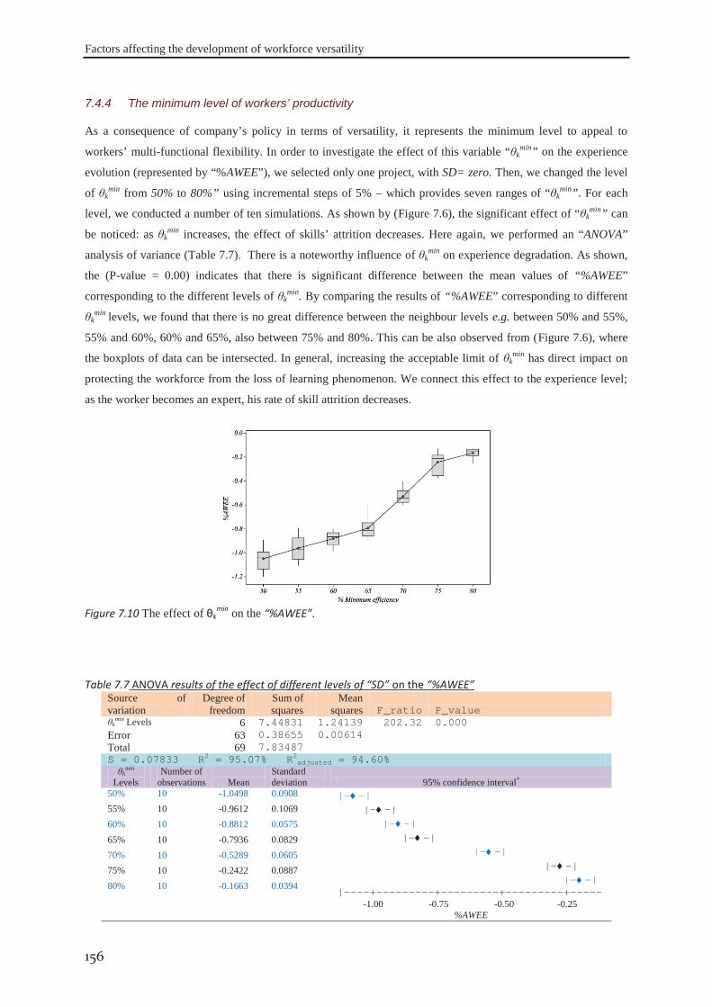
Factors affecting the development of workforce versatility

156

As a consequence of company’s policy in terms of versatility, it represents the minimum level to appeal to

workers’ multi-functional flexibility. In order to investigate the effect of this variable “θkmin” on the experience

evolution (represented by “%AWEE”), we selected only one project, with SD= zero. Then, we changed the level

of θkmin from 50% to 80%” using incremental steps of 5% – which provides seven ranges of “θk

min”. For each

level, we conducted a number of ten simulations. As shown by (Figure 7.6), the significant effect of “θkmin” can

be noticed: as θkmin increases, the effect of skills’ attrition decreases. Here again, we performed an “ANOVA”

analysis of variance (Table 7.7). There is a noteworthy influence of θkmin on experience degradation. As shown,

the (P-value = 0.00) indicates that there is significant difference between the mean values of “%AWEE”

corresponding to the different levels of θkmin. By comparing the results of “%AWEE” corresponding to different

θkmin levels, we found that there is no great difference between the neighbour levels e.g. between 50% and 55%,

55% and 60%, 60% and 65%, also between 75% and 80%. This can be also observed from (Figure 7.6), where

the boxplots of data can be intersected. In general, increasing the acceptable limit of θkmin has direct impact on

protecting the workforce from the loss of learning phenomenon. We connect this effect to the experience level;

as the worker becomes an expert, his rate of skill attrition decreases.

Figure 7.10 The effect of θk

min on the “%AWEE”.

Table 7.7 ANOVA results of the effect of different levels of “SD” on the “%AWEE” Source of variation

Degree of freedom

Sum of squares

Mean squares F_ratio P_value

θkmin Levels 6 7.44831 1.24139 202.32 0.000

Error 63 0.38655 0.00614 Total 69 7.83487 S = 0.07833 R2 = 95.07% R2adjusted = 94.60% θk

min Levels

Number of observations Mean

Standard deviation 95% confidence interval*

50% 10 -1.0498 0.0908 |- -| |- -| |- -| |- -| |- -| |- -| |- -| |----+---------+---------+---------+----- -1.00 -0.75 -0.50 -0.25

%AWEE

55% 10 -0.9612 0.1069 60% 10 -0.8812 0.0575 65% 10 -0.7936 0.0829 70% 10 -0.5289 0.0605 75% 10 -0.2422 0.0887 80% 10 -0.1663 0.0394

7.4.4 The minimum level of workers’ productivity

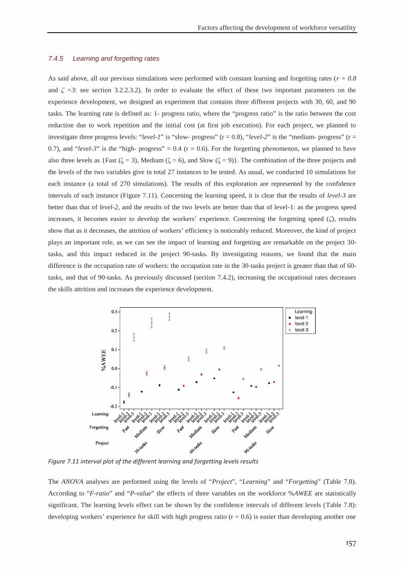
Factors affecting the development of workforce versatility

157

As said above, all our previous simulations were performed with constant learning and forgetting rates (r = 0.8

and ζ =3: see section 3.2.2.3.2). In order to evaluate the effect of these two important parameters on the

experience development, we designed an experiment that contains three different projects with 30, 60, and 90

tasks. The learning rate is defined as: 1- progress ratio, where the “progress ratio” is the ratio between the cost

reduction due to work repetition and the initial cost (at first job execution). For each project, we planned to

investigate three progress levels: “level-1” is “slow- progress” (r = 0.8), “level-2” is the “medium- progress” (r =

0.7), and “level-3” is the “high- progress” = 0.4 (r = 0.6). For the forgetting phenomenon, we planned to have

also three levels as {Fast (ζ = 3), Medium (ζ = 6), and Slow (ζ = 9)}. The combination of the three projects and

the levels of the two variables give in total 27 instances to be tested. As usual, we conducted 10 simulations for

each instance (a total of 270 simulations). The results of this exploration are represented by the confidence

intervals of each instance (Figure 7.11). Concerning the learning speed, it is clear that the results of level-3 are

better than that of level-2, and the results of the two levels are better than that of level-1: as the progress speed

increases, it becomes easier to develop the workers’ experience. Concerning the forgetting speed (ζ), results

show that as it decreases, the attrition of workers’ efficiency is noticeably reduced. Moreover, the kind of project

plays an important role, as we can see the impact of learning and forgetting are remarkable on the project 30-

tasks, and this impact reduced in the project 90-tasks. By investigating reasons, we found that the main

difference is the occupation rate of workers: the occupation rate in the 30-tasks project is greater than that of 60-

tasks, and that of 90-tasks. As previously discussed (section 7.4.2), increasing the occupational rates decreases

the skills attrition and increases the experience development.

Figure 7.11 interval plot of the different learning and forgetting levels results

The ANOVA analyses are performed using the levels of “Project”, “Learning” and “Forgetting” (Table 7.8).

According to “F-ratio” and “P-value” the effects of three variables on the workforce %AWEE are statistically

significant. The learning levels effect can be shown by the confidence intervals of different levels (Table 7.8):

developing workers’ experience for skill with high progress ratio (r = 0.6) is easier than developing another one

7.4.5 Learning and forgetting rates

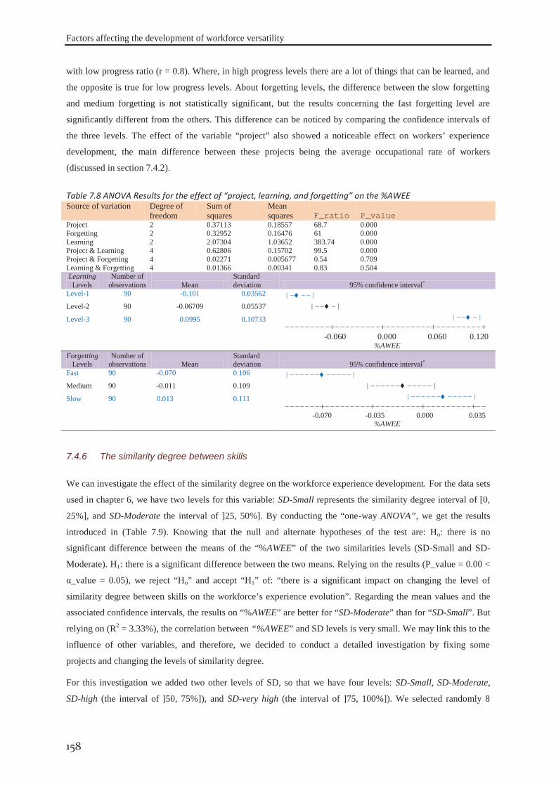
Factors affecting the development of workforce versatility

158

with low progress ratio (r = 0.8). Where, in high progress levels there are a lot of things that can be learned, and

the opposite is true for low progress levels. About forgetting levels, the difference between the slow forgetting

and medium forgetting is not statistically significant, but the results concerning the fast forgetting level are

significantly different from the others. This difference can be noticed by comparing the confidence intervals of

the three levels. The effect of the variable “project” also showed a noticeable effect on workers’ experience

development, the main difference between these projects being the average occupational rate of workers

(discussed in section 7.4.2).

Table 7.8 ANOVA Results for the effect of “project, learning, and forgetting” on the %AWEE Source of variation Degree of

freedom Sum of squares

Mean squares F_ratio P_value

Project 2 0.37113 0.18557 68.7 0.000 Forgetting 2 0.32952 0.16476 61 0.000 Learning 2 2.07304 1.03652 383.74 0.000 Project & Learning 4 0.62806 0.15702 99.5 0.000 Project & Forgetting 4 0.02271 0.005677 0.54 0.709 Learning & Forgetting 4 0.01366 0.00341 0.83 0.504 Learning Levels

Number of observations Mean

Standard deviation 95% confidence interval*

Level-1 90 -0.101 0.03562 |- --| |-- -| |-- -| ---------+---------+---------+---------+ -0.060 0.000 0.060 0.120

%AWEE

Level-2 90 -0.06709 0.05537

Level-3 90 0.0995 0.10733

Forgetting Levels

Number of observations Mean

Standard deviation 95% confidence interval*

Fast 90 -0.070 0.106 |------ -----| |------ -----| |------ -----| -------+---------+---------+---------+-- -0.070 -0.035 0.000 0.035

%AWEE

Medium 90 -0.011 0.109

Slow 90 0.013 0.111

We can investigate the effect of the similarity degree on the workforce experience development. For the data sets

used in chapter 6, we have two levels for this variable: SD-Small represents the similarity degree interval of [0,

25%], and SD-Moderate the interval of ]25, 50%]. By conducting the “one-way ANOVA”, we get the results

introduced in (Table 7.9). Knowing that the null and alternate hypotheses of the test are: Ho: there is no

significant difference between the means of the “%AWEE” of the two similarities levels (SD-Small and SD-

Moderate). H1: there is a significant difference between the two means. Relying on the results (P_value = 0.00 <

α_value = 0.05), we reject “Ho” and accept “H1” of: “there is a significant impact on changing the level of

similarity degree between skills on the workforce’s experience evolution”. Regarding the mean values and the

associated confidence intervals, the results on “%AWEE” are better for “SD-Moderate” than for “SD-Small”. But

relying on (R2 = 3.33%), the correlation between “%AWEE” and SD levels is very small. We may link this to the

influence of other variables, and therefore, we decided to conduct a detailed investigation by fixing some

projects and changing the levels of similarity degree.

For this investigation we added two other levels of SD, so that we have four levels: SD-Small, SD-Moderate,

SD-high (the interval of ]50, 75%]), and SD-very high (the interval of ]75, 100%]). We selected randomly 8

7.4.6 The similarity degree between skills

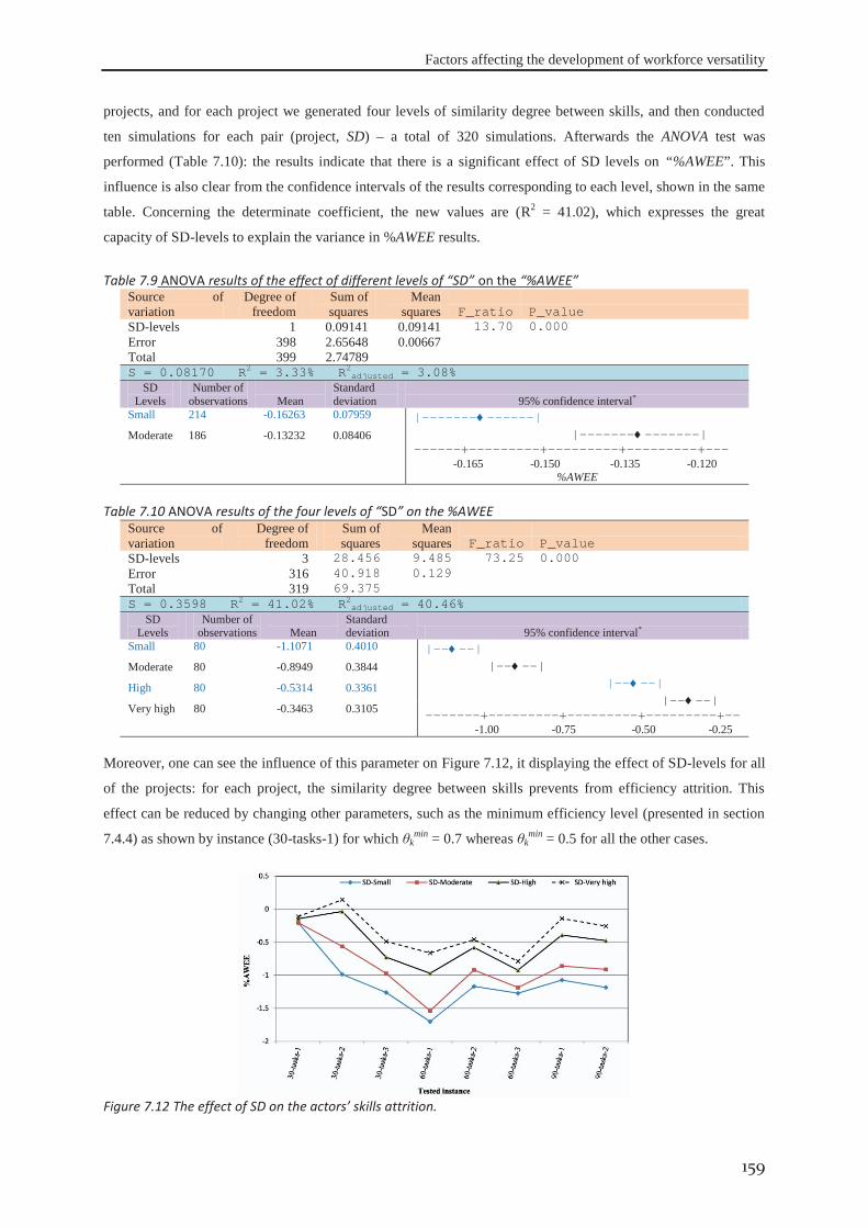
Factors affecting the development of workforce versatility

159

projects, and for each project we generated four levels of similarity degree between skills, and then conducted

ten simulations for each pair (project, SD) – a total of 320 simulations. Afterwards the ANOVA test was

performed (Table 7.10): the results indicate that there is a significant effect of SD levels on “%AWEE”. This

influence is also clear from the confidence intervals of the results corresponding to each level, shown in the same

table. Concerning the determinate coefficient, the new values are (R2 = 41.02), which expresses the great

capacity of SD-levels to explain the variance in %AWEE results.

Table 7.9 ANOVA results of the effect of different levels of “SD” on the “%AWEE” Source of variation

Degree of freedom

Sum of squares

Mean squares F_ratio P_value

SD-levels 1 0.09141 0.09141 13.70 0.000 Error 398 2.65648 0.00667 Total 399 2.74789 S = 0.08170 R2 = 3.33% R2adjusted = 3.08%

SD Levels

Number of observations Mean

Standard deviation 95% confidence interval*

Small 214 -0.16263 0.07959 |------- ------| |------- -------| ------+---------+---------+---------+--- -0.165 -0.150 -0.135 -0.120

%AWEE

Moderate 186 -0.13232 0.08406

Table 7.10 ANOVA results of the four levels of “SD” on the %AWEE Source of variation

Degree of freedom

Sum of squares

Mean squares F_ratio P_value

SD-levels 3 28.456 9.485 73.25 0.000 Error 316 40.918 0.129 Total 319 69.375 S = 0.3598 R2 = 41.02% R2adjusted = 40.46%

SD Levels

Number of observations Mean

Standard deviation 95% confidence interval*

Small 80 -1.1071 0.4010 |-- --| |-- --| |-- --| |-- --| -------+---------+---------+---------+-- -1.00 -0.75 -0.50 -0.25

Moderate 80 -0.8949 0.3844

High 80 -0.5314 0.3361

Very high 80 -0.3463 0.3105

Moreover, one can see the influence of this parameter on Figure 7.12, it displaying the effect of SD-levels for all

of the projects: for each project, the similarity degree between skills prevents from efficiency attrition. This

effect can be reduced by changing other parameters, such as the minimum efficiency level (presented in section

7.4.4) as shown by instance (30-tasks-1) for which θkmin = 0.7 whereas θk

min = 0.5 for all the other cases.

Figure 7.12 The effect of SD on the actors’ skills attrition.

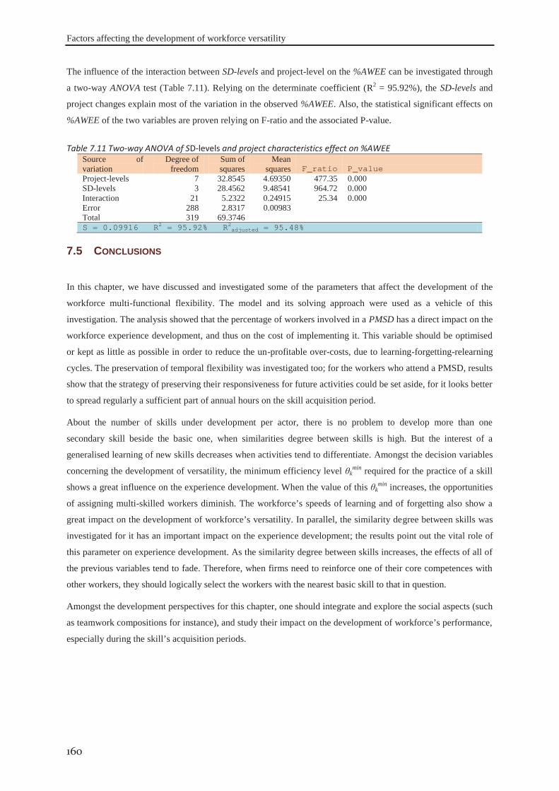
Factors affecting the development of workforce versatility

160

The influence of the interaction between SD-levels and project-level on the %AWEE can be investigated through

a two-way ANOVA test (Table 7.11). Relying on the determinate coefficient (R2 = 95.92%), the SD-levels and

project changes explain most of the variation in the observed %AWEE. Also, the statistical significant effects on

%AWEE of the two variables are proven relying on F-ratio and the associated P-value.

Table 7.11 Two-way ANOVA of SD-levels and project characteristics effect on %AWEE Source of variation

Degree of freedom

Sum of squares

Mean squares F_ratio P_value

Project-levels 7 32.8545 4.69350 477.35 0.000 SD-levels 3 28.4562 9.48541 964.72 0.000 Interaction 21 5.2322 0.24915 25.34 0.000 Error 288 2.8317 0.00983 Total 319 69.3746 S = 0.09916 R2 = 95.92% R2adjusted = 95.48%

In this chapter, we have discussed and investigated some of the parameters that affect the development of the

workforce multi-functional flexibility. The model and its solving approach were used as a vehicle of this

investigation. The analysis showed that the percentage of workers involved in a PMSD has a direct impact on the

workforce experience development, and thus on the cost of implementing it. This variable should be optimised

or kept as little as possible in order to reduce the un-profitable over-costs, due to learning-forgetting-relearning

cycles. The preservation of temporal flexibility was investigated too; for the workers who attend a PMSD, results

show that the strategy of preserving their responsiveness for future activities could be set aside, for it looks better

to spread regularly a sufficient part of annual hours on the skill acquisition period.

About the number of skills under development per actor, there is no problem to develop more than one

secondary skill beside the basic one, when similarities degree between skills is high. But the interest of a

generalised learning of new skills decreases when activities tend to differentiate. Amongst the decision variables

concerning the development of versatility, the minimum efficiency level θkmin required for the practice of a skill

shows a great influence on the experience development. When the value of this θkmin increases, the opportunities

of assigning multi-skilled workers diminish. The workforce’s speeds of learning and of forgetting also show a

great impact on the development of workforce’s versatility. In parallel, the similarity degree between skills was

investigated for it has an important impact on the experience development; the results point out the vital role of

this parameter on experience development. As the similarity degree between skills increases, the effects of all of

the previous variables tend to fade. Therefore, when firms need to reinforce one of their core competences with

other workers, they should logically select the workers with the nearest basic skill to that in question.

Amongst the development perspectives for this chapter, one should integrate and explore the social aspects (such

as teamwork compositions for instance), and study their impact on the development of workforce’s performance,

especially during the skill’s acquisition periods.

7.5 CONCLUSIONS

8 GENERAL CONCLUSION AND PERSPECTIVES

EPIL

OG

UE

8

General conclusion and perspectives

162

Responding to the growing need of generating a robust baseline schedule, first, this research was implemented to

model the problem of multi-period workforce allocation on industrial activities. This model considers the

heterogeneous productivities of operators, the qualitative workforce flexibility that known as multi-function

flexibility, the working time flexibility, and the dynamic nature of experience. The dynamic nature of workforce

experience was modelled in function of learning-by-doing and forgetting during the work interruption periods.

Moreover, the activities durations are considered as elastic, so that the jobs’ durations depend on the number of

workers allocated to perform them in addition to the levels of their experience.

Second, this research was oriented to answer the question “What is an instance of the current problem?”,

therefore the different dimensions of the problem are classified and analysed. For each dimension, the related

sensitive assessment method had been proposed. These dimensions include the project network, the project

temporal characteristics, the project work content, the available resources, and work-content to resources

weighting quantifiers. Relying on these measures, this research proposed to aggregate them using factor analysis

in order to produce the main principal components of an instance. Relying on these main components, an

instance of the problem can be defined; moreover the difference between instances can be evaluated.

Consequently, the complexity or easiness of solving or realising a given problem instance can be evaluated.

Third, this research developed platform software to solve the proposed problem and construct the project

baseline schedule with the associated resources allocation. The proposed platform relies on a genetic algorithm-

based approach. This genetic algorithm relies mainly on answering three questions based on the priority

encoding: what task will be processed first? Then which actor(s) will be allocated to realise this task? What is the

working time strategy that the actors will respect, during the activity realization? After that a serial schedule

generation scheme was adopted to gradually construct the project schedule and allocated the workforce

according the random generated priority lists. The model has been validated, likewise, its parameters has been

tuned to give the best performance.

Fourth, the research investigated the robustness of the proposed approach by excessively solving four hundred

problems. Which contains four groups according to number of tasks (30 tasks, 60 tasks, 90 tasks, and 120 tasks);

each group contains a number of one hundred projects with different characteristics. The proposed approach was

showed a stable performance and robustness with respect to the changes in projects instances within the same

group, moreover within the different groups. The variances of the different results were explained by the

variances between project instances. Knowing that these different project instances were represented by the

smallest principal components obtained from factor analysis and cluster analysis of the problem variables.

Fifth, this research was used the developed model and the proposed problem solving approach as a vehicle of

investigation of the different parameters that can affect the development of workforce multi-function flexibility.

The parameters that had been investigated are the percentage of employees who are integrated in the program of

multi-skilled development, the preservation of temporal flexibility, the workers’ flexibility degree (the number of

8.1 OVERALL CONCLUSION

General conclusion and perspectives

163

skills under development per each worker), the minimum level of workers’ productivity θkmin, the workforce

speed of learning and forgetting, and the similarity degree between skills.

Based on the research analysis, some conclusions about the model and its resolution method can be drawn.

Regarding the behaviour of the model, some reasons for satisfactory raise from results that show to be consistent

regarding the way we modelled facts. Beside the fact that these results always provide feasible schedules (with

or without lateness penalties), without any hard constraint violation, they also express a logical relationship

between the use of versatility and the cost inflation; the actors who have low levels of efficiency are more likely

to lose their skills than their highly-efficient colleagues during equivalent interruption periods – and reciprocally,

they can learn faster; tuning the objectives weight set of parameters {γi} has always resulted in the expected

behaviour. These points witness a good transcription of the published observations on which the model is based:

they help the user to feel more comfortable towards the model’s reliability, concerning details of encoding

procedures that are more awkward to test than are the feasibility of the schedules provided.

Some managerial lessons can also be learnt from this research: – The firms seeking for reactivity should accept

an amount of extra cost to develop their operators’ multifunctional flexibility. Therefore the number of operators

who will follow a skill development program should be optimised in order to find a good compromise between

the over costs induced and the overall average skills developments. – In order to enhance the acquisition of

secondary skills, the operators in question should be regularly practicing their new skills, and avoid to preserve

before all their future temporal flexibility. –Moreover, firms should allocate these operators to work with their

new skills until they have reached a sufficient degree of mastering that can protect them from the loss of learning

produced during the use of multifunctional flexibility. – The same recommendation may be formulated for

economic reasons: the effort of growing up a new skill is costly and must be continued until this skill is

consolidated. –The surplus of developing the actors’ secondary skills can be misleading or become out of control

especially for non-similar skills. – Developing an operator with more than one secondary skill beside his basic

one is very difficult and costly, especially for completely different skills. The company should select the workers

with high speed of learning and slow forgetting to develop their multi-functional flexibility. Finally, the

similarity degree between skills showed the vital role of workforce experience development. Therefore, firms

should select workers with the nearest basic skill to the skill in question for the development.

This work can be extended relying on many axes, including – but not limited to: mathematical modelling,

industrial project management, computer-aided decision making, and problem solving techniques. By the

following we will discuss the possible extension of each axis.

The axis of mathematical modelling: We considered only one project at time, transforming the problem to a

multi-project planning and scheduling can be appreciated, to approach this model to the real industrial situations.

Moreover, one can integrate labour mobility constraints between project activities, which can signify

transportations cost. In other words, considering the cost of actors’ transportation means: if an actor a is

allocated to work in project “p1” at a working day t, and if it is planned to allow him to work in project “p2” for

8.2 FUTURE PERSPECTIVES

General conclusion and perspectives

164

the same working day t, a transportation cost/time should be considered. These costs represent the displacements

from location of project p1 to location of project p2, or they can figure the difficulty for the actor to switch his

state of mind from the p1 context to the p2. These costs can be estimated relying on two dimensions: the

transportation time, and transportations fees. Moreover, the distance between actor’s home and the project

location can be considered. Also, the relation between tasks can be modelled using dependency structure matrix,

which allows us to consider all the dependency relation between activities. Especially when the information

exchange streams between activities is required.

Regarding the worker’s productivity assessment, we considered only the temporal performance as a basis of

measurement of the worker productivity rates. There is often a trade-off between temporal performance and

production quality aspects. Therefore, adding the dimension of work quality to the current model increases the

workability and applicability of the model. The assessment of the worker production quality can be reviewed

with the product required specifications. Consequently, one can estimate the worker’s working quality level, and

define the minimum required level for each skill.

Concerning the uncertainty of estimating the project and resources characteristics, the problem at hand can be

expanded into two branches: the stochastic estimation of parameters, or the possibilistic one. The stochastic

or/and fuzzy modelling can be adopted for many variables in the current model; the project related parameters or

the resources ones. The stochastic models apply if there are historical data at hand; if it is not the case, the

estimation of these parameters is often done by an expert, therefore, it is quite logical to model them relying on

fuzzy numbers instead of crisp numbers. That is, the estimator gives for each variable a possibilistic values,

associated to each value a possibilistic index (weight) within the interval [0, 1]. The relation between the weights

and the possibilistic values known as the membership function. These variables contains (but not limited to) the

workload required from each skill, the duration of each workload.

The employees social aspects will express the workers’ own satisfaction or the social relation between a group of

workers. First, the worker’s own satisfaction can be modelled by integrating his preferences in selecting tasks,

skills, working days, and /or vacations. These preferences of human resources can be modelled with linguistic

terms and the use of fuzzy logic. Recently, there has been considerable effort in applying fuzzy sets theory in

social sciences with more emphasis on performance evaluation. Moreover, the relation between the individuals

of the same team can be enhanced by considering and comparing the linguistic working preferences between

workers. Adopting these social criteria enhances the communication between members of the team, and as a

result, the rate of knowledge transfer between them can be enhanced.

Regarding the assessment of learning and forgetting parameters such as (r, ζ) for a given worker with respect to a

specified skill, one can evaluate them based on the social factors, job technical nature, working environmental,

stress at work, incentive systems etc. As mentioned previously, each factor can be modelled with fuzzy numbers

and then aggregated using fuzzy logic. Consequently, the learning and forgetting parameters of each individual

can be evaluated relying on the fuzzy estimation of an expert and considering as many as possible of the

individual, technical, environmental and economic aspects.

General conclusion and perspectives

165

The axis of project management: The current work was oriented to generate a robust baseline schedule with

human resources allocation relying on the human resources flexibility. But in real situations and during the

activities’ realisation phases some changes often occur, in reasons of the dynamic working enviroment: e.g. new

incoming orders, cancelling of some orders, shortage of raw material, power shortage, machine break-down,

workers’ absence, accidents at work, etc. One of our future works consists in modelling and solving the problem

of constructing a predictive-reactive schedule, considering a set of efficiency and stability objectives. The

efficiency objectives can be the schedule costs of the number of working hours and overtime hours, project

delivery date. And the stability objectives can be the deviation of the new schedule from the old one. These

deviations can be calculated from the activities start and finish dates, or from the changes in actors’ allocations.

This deviation can be considered as a reaction cost to the new event.

We proposed to measure the project complexity relying on principal component analysis by using the static

dimensions of project activities and resources. One of the possible extensions of this work would be to

development a generic approach to accommodate also the project technical complexity measure. This technical

complexity can be measured by comparing the project required knowledge to the available resources knowledge

(explicit and tacit), which seems to be specific to the applied context and difficult to be evaluated. Therefore, this

extension can be performed by studying the different tools of project technical analysis and the different

techniques of capitalising the workforce’s knowledge. This generic approach should lead to a software platform

that would handle both the project technical characteristics and the human resources knowledge, and possibly

refer to data mining algorithms to compare the knowledge requirements and the available one to conclude on the

project technical complexity.

Axis of computer-aided decision-making: In the current work we modelled the problem as a multi-objective one,

using a weighted sum as unique criterion. As a logical extension of this work, we propose to model the problem

as a multiple-criteria decision-making system. These criteria can be defined relying on: the economic objectives,

workforce experience evolution and the social aspects if they are integrated as previously discussed. After that

and based on Pareto front, the decision maker can select the suitable project schedule according to the situations.

Axis of problem solving techniques: In this work, our problem was solved using one of the metaheuristics, the

genetic algorithms. As a future expansion of this axis, the problem can also be solved with many other methods

such as particle swarm optimisation, ant colony optimisation, or by one of the local search methods such as

simulated annealing, tabu search or even the hybridisation of two algorithms such as the memetic algorithms.

Concerning exact methods, our model is nonlinear, so in order to solve it exactly and with acceptable computing

times, one should first make it linear and then apply one of the decomposition techniques, such as Bender’s

decomposition or Dantzig wolf decomposition, in order to solve it optimally. The hybridisation between exact

methods and metaheuristics can be adopted too to accommodate the problem of nonlinearity.

General conclusion and perspectives

166

Bibliography

Bibliography

168

Abboud, M.S., 1998. Fuzzy manpower allocation using the mutate and spread metaheuristics. In: Second International Conference on Knowledge-Based Intelligent Electronic Systems, KES '98. 1, 87–93.

Agrawal, M.K., Elmaghraby, S.E., Herroelen, W.S., 1996. DAGEN: A generator of test sets for project activity nets. European journal of operational research, 90, 376–382.

Akbari, R., Zeighami, V., Ziarati, K., 2011. Artificial Bee colony for resource constrained project scheduling problem. International Journal of Industrial Engineering Computations, 1, 45–60.

Al-Anzi, F.S., Allahverdi, A., Al-Zamel, K., 2010. Weighted multi-skill resources project scheduling. Journal of Software Engineering and Applications, 3, 1125–1130.

Alexopoulos, A., 2008. Social relations, human resource management, and knowledge transfer in work organisations: toward an integrated approach. PhD thesis, Dublin City University, Irlande.

Ali, S., Maciejewski, A.A., Siegel, H.J., Kim, J.-K., 2004. Measuring the robustness of a resource allocation. IEEE Transactions on parallel and distributed systems, 15, 630 – 641.

Aloulou, M.A., Portmann, M.-C., 2005. An Efficient proactive-reactive scheduling approach to hedge against shop floor disturbances. in: Kendall, G., Burke, E.K., Petrovic, S., Gendreau, M. (Eds.), Multidisciplinary Scheduling: Theory and Applications. Springer US, pp. 223–246.

Alvarez-Valdes, R., Crespo, E., Tamarit, J.M., Villa, F., 2008. GRASP and path relinking for project scheduling under partially renewable resources. European Journal of Operational Research, 189, 1153–1170.

Alvarez-Valdes, R., Tamarit, J.M., 1989. Heuristic algorithms for resource-constrained project scheduling: A review and an empirical analysis, in: Advances in Project Scheduling, Elsevier, Amsterdam. Slowinski, R. and Weglarz, Amsterdam.

Anderlhore, G., 1969. What Production Breaks Cost. Industrial Engineering, 34–36.

Anthony, R.N., 1965. Planning and control systems: a framework for analysis. Division of Research, Graduate School of Business Administration, Harvard University.

Artigues, C., Billaut, J.-C., Esswein, C., 2005. Maximization of solution flexibility for robust shop scheduling. European Journal of Operational Research, 165, 314–328.

Artigues, C., Demassey, S., Neron, E., 2008. Resource-Constrained Project Scheduling: Models, Algorithms, Extensions and Applications. ISTE Publishing Company.

Artigues, C., Michelon, P., Reusser, S., 2003. Insertion techniques for static and dynamic resource-constrained project scheduling. European Journal of Operational Research, 149, 249–267.

Asher, H., 1956. Cost-quantity relationships in the airframe industry (No. R291), Rand Corp. Santa Monica, CA.

Atkin, J.A.D., Burke, E.K., Greenwood, J.S., Reeson, D., 2007. Hybrid metaheuristics to aid runway scheduling at London Heathrow airport. Transportation Science, 41, 90–106.

Atkinson, R., Crawford, L., Ward, S., 2006. Fundamental uncertainties in projects and the scope of project management. International Journal of Project Management, 24, 687–698.

Attia, E.-A., Dumbrava, V., Duquenne, P., 2012a. Factors affecting the development of workforce versatility, in: Theodor, B. (Ed.), Information Control Problems in Manufacturing. 14th IFAC Symposium on Information Control Problems in Manufacturing, Elsevier, Bucharest, Romania - May 23-25, pp. 1221–1226.

Attia, E.-A., Duquenne, P., Le-Lann, J.-M., 2011. Prise en compte des évolutions de compétences pour les ressources humaines. In, CIGI-2011, 12-14 octobre 2011, Saint-Sauveur, Québec, Canada.

Attia, E.-A., Duquenne, P., Le-Lann, J.-M., 2012b. Decision-based genetic algorithms for solving multi-period project scheduling with dynamically experienced workforce. In: 9th International Conference on Modeling, Optimization & SIMulation, MOSIM-2012, 6-8 June. Bordeaux, France.

Attia, E.-A., Edi, H.K., Duquenne, P., 2012c. Flexible resources allocation techniques: characteristics and modelling. Int. J. Operational Research, 14, 221–254.

Avramidis, A.N., Chan, W., Gendreau, M., L’ecuyer, P., Pisacane, O., 2010. Optimizing daily agent scheduling in a multiskill call center. European journal of operational research, 200, 822–832.

Aykin, T., 1998. A composite branch and cut algorithm for optimal shift scheduling with multiple breaks and break windows. The Journal of the Operational Research Society, 49, 603–615.

Azmat, C.S., Hürlimann, T., Widmer, M., 2004. Mixed integer programming to schedule a single-shift workforce under annualized hours. Annals of Operations Research, 128, 199–215.

Bibliography

169

Badiru, A., 1992. Computational survey of univariate and multivariate learning curve models. IEEE Transactions on Engineering Management, 39, 176–188.

Badiru, A.B., 1996. Project management in manufacturing and high technology operations. John Wiley & Sons.

Bailey, C.D., 1989. Forgetting and the learning curve: a laboratory study. Management Science, 35, 340–352.

Bailey, C.D., McIntyre, E.V., 2003. Using parameter prediction models to forecast post-interruption learning. IIE – Transactions, 35, 1077.

Baptiste, P., Pape, C.L., Nuijten, W., 2001. Constraint-based scheduling: applying constraint programming to scheduling problems. Springer.

Bashir, H.A., 2010. Removal of redundant relationships in an AON project network for evaluating schedule complexity. Journal of Construction Engineering and Management, 136(7), 787-793.

Bassan, G.S., 2010. Capacity planning under Fuzzy environment using possibilistic approach. Master thesis, University of Manitoba, Canada.

Beach, R., Muhlemann, A.P., Price, D.H.R., Paterson, A., Sharp, J.A., 2000. A review of manufacturing flexibility. European Journal of Operational Research, 122(1), 41–57.

Bein, W.W., Kamburowski, J., F, M., Stallmann, M., 1992. Optimal reduction of two-terminal directed acyclic graphs. SIAM Journal on Computing, 21(6), 1112–1129.

Bellenguez, O., Néron, E., 2005. Lower bounds for the multi-skill project scheduling problem with hierarchical levels of skills, in: E. Burke and M. Trick (Eds.): PATAT 2004, LNCS. Springer, pp. 229–243.

Bellenguez-Morineau, O., Néron, E., 2007. A Branch-and-Bound method for solving multi-skill project scheduling problem. RAIRO Operations Research, 41(2), 155-170.

Beltrán-Martín, I., Roca-Puig, V., Escrig-Tena, A., Bou-Llusar, J.C., 2008. Human resource flexibility as a mediating variable between high performance work systems and performance. Journal of Management, 34(5), 1009–1044.

Bennour, M., Crestani, D., Crespo, O., Prunet, F., 2005. Computer-aided decision for human task allocation with mono- and multi-performance evaluation. International journal of production research, 43(21), 4559–4588.

Betancourt, M.R., Skolnick, J., Donald, T., Plant, D., 2001. Universal similarity measure for comparing protein structures. Biopolymers, 59(5), 305–309.

Billaut, J.-C., Moukrim, A., Sanlaville, E., 2010. Introduction to flexibility and robustness in scheduling, in: Billaut, J.-C., Moukrim, A., Sanlaville, E. (Eds.), Flexibility and Robustness in Scheduling. ISTE, Wiley Online Library, pp.15–33.

Bobrowski, P.M., Park, P.S., 1993. An evaluation of labor assignment rules when workers are not perfectly interchangeable. Journal of Operations Management, 11(3), 257–268.

Bockmayr, A., Kasper, T., 1998. Branch and Infer: A unifying framework for integer and finite domain constraint programming. INFORMS Journal on Computing, 10(3), 287–300.

Bokhorst, J.A.C., Gaalman, G.J.C., 2009. Cross-training workers in dual resource constrained systems with heterogeneous processing times. International Journal of Production Research, 47(22), 6333–6356.

Bolívar-Ramos, M.T., García-Morales, V.J., García-Sánchez, E., 2012. Technological distinctive competencies and organizational learning: Effects on organizational innovation to improve firm performance. Journal of Engineering and Technology Management, 29(3), 331–357.

Bordoloi, S.K., Cooper, W.W., Matsuo, H., 1999. Flexibility, adaptability, and efficiency in manufacturing systems. Production and Operations Management, 8(2), 133–150.

Boriah, S., Chandola, V., Kumar, V., 2008. Similarity measures for categorical data: a comparative evaluation. In. SIAM International Conference on Data Mining - SDM , April 24-26, Atlanta, Georgia, pp. 243-254

Bouleimen, K., Lecocq, H., 2003. A new efficient simulated annealing algorithm for the resource-constrained project scheduling problem and its multiple mode version. European Journal of Operational Research, 149(2), 268–281.

Browning, T.R., Yassine, A.A., 2009. A random generator of resource-constrained multi-project network problems. Journal of Scheduling, 13(2), 143–161.

Browning, T.R., Yassine, A.A., 2010. Resource-constrained multi-project scheduling: Priority rule performance revisited. International Journal of Production Economics, 126(2), 212–228.

Bibliography

170

Brownlee, J., 2011. Clever Algorithms: Nature-Inspired Programming Recipes. ISBN: 978-1-4467-8506-5.

Brucker, P., Drexl, A., Mohring, R., Neumann, K., Pesch, E., 1999. Resource-constrained project scheduling: Notation, classification, models, and methods. European Journal of Operational Research, 112(1), 3–41.

Brucker, P., Knust, S., 2006. Scheduling models, in: complex scheduling, GOR-Publications. Springer Berlin Heidelberg, pp. 1–22.

Brucker, P., Knust, S., 2011. Complex Scheduling. 2nd ed. Springer Verlag.

Brucker, P., Qu, R., Burke, E., 2011. Personnel scheduling: Models and complexity. European Journal of Operational Research, 210(3), 467–473.

Brusco, M.J., Jacobs, L.W., 1993. A simulated annealing approach to the solution of flexible labour scheduling problems. The Journal of the Operational Research Society, 44, 1191–1200.

Brusco, M.J., Jacobs, L.W., 2000. Optimal models for meal-break and start-time flexibility in continuous tour scheduling. Management Science, 46(12), 1630–1641.

Brusco, M.J., Johns, T.R., 1998. Staffing a multi skilled workforce with varying levels of productivity: an analysis of cross training policies. Decision Sciences, 29(2), 499–515.

Burstyn, I., 2004. Principal component analysis is a powerful instrument in occupational hygiene inquiries. Annals of Occupational Hygiene, 48(8), 655–661.

Cai, X., Li, K.., 2000. A genetic algorithm for scheduling staff of mixed skills under multi-criteria. European Journal of Operational Research, 125(2), 359–369.

Campbell, G.M., Diaby, M., 2002. Development and evaluation of an assignment heuristic for allocating cross-trained workers. European Journal of Operational Research, 138(1), 9–20.

Carlier, J., Moukrim, A., Xu, H., 2009. The project scheduling problem with production and consumption of resources: A list-scheduling based algorithm. Discrete Applied Mathematics, 157(17), 3631–3642.

Carlson, J.G., Rowe, R.G., 1976. How much does forgetting cost? Industrial Engineering, 8, 40–47.

Caroli, E., 2007. Internal versus external labour flexibility : the role of knowledge codification. National Institute Economic Review, 201(1), 107-118.

Caron, G., Hansen, P., Jaumard, B., 1999. The assignment problem with seniority and job priority constraints. Operations Research, 47(3), 449–453.

Carr, G.W., 1946. Peacetime cost estimation requires new learning curves. Aviation, 45, 76–77.

Castaneda, D.I., Rios, M.F., 2007. From individual learning to organizational learning. The Electronic Journal of Knowledge Management, 5(4), 363–372.

Cavalcante, C.C.B., Carvalho de Souza, C., Savelsbergh, M.W.P., Wang, Y., Wolsey, L.A., 2001. Scheduling projects with labor constraints. Discrete Applied Mathematics, 112(1), 27–52.

Certa, A., Enea, M., Galante, G., Manuela La Fata, C., 2009. Multi-objective human resources allocation in R&D projects planning. International Journal of Production Research, 47(13), 3503–3523.

Chakravarty, A.K., Shtub, A., 1992. The effect of learning on the operation of mixed-model assembly lines. Production and Operations Management, 1(2), 198–211.

Chen, P.-H., Shahandashti, S.M., 2009. Hybrid of genetic algorithm and simulated annealing for multiple project scheduling with multiple resource constraints. Automation in Construction 18, 434–443.

Chen, R.-M., 2011. Particle swarm optimization with justification and designed mechanisms for resource-constrained project scheduling problem. Expert Systems with Applications, 38(6), 7102–7111.

Chen, S.-P., Tsai, M.-J., 2011. Time–cost trade-off analysis of project networks in fuzzy environments. European Journal of Operational Research, 212(2), 386–397.

Cooper, D.F., 1976. Heuristics for scheduling resource-constrained projects: An experimental investigation. Management Science, 22(11), 1186–1194.

Corominas, A., Lusa, A., Pastor, R., 2002. Using MILP to plan annualised working hours. Journal of the Operational Research Society, 53, 1101–1108.

Corominas, A., Lusa, A., Pastor, R., 2007. Using a MILP model to establish a framework for an annualised hours agreement. European Journal of Operational Research, 177(3), 1495–1506.

Bibliography

171

Corominas, A., Ojeda, J., Pastor, R., 2006. Multi-Objective allocation of multi-function workers with lower bounded capacity. The Journal of the Operational Research Society, 56(6), 738–743.

Corominas, A., Pastor, R., 2010. Replanning working time under annualised working hours. International Journal of Production Research, 48(5), 1493–1515.

Coughlan, E., Lübbecke, M., Schulz, J., 2010. A Branch-and-Price algorithm for multi-mode resource leveling, In: Festa, P. (Ed.), Experimental Algorithms, Lecture Notes in Computer Science. Springer Berlin / Heidelberg, pp. 226–238.

Cowling, P., Colledge, N., Dahal, K., Remde, S., 2006. The trade off between diversity and quality for multi-objective workforce scheduling. In. Evolutionary computation in combinatorial optimization, Springer, pp.13–24.

Creemers, S., Leus, R., De Reyck, B., Lambrecht, M., 2008. Project scheduling for maximum NPV with variable activity durations and uncertain activity outcomes, In: IEEE International Conference on Industrial Engineering and Engineering Management, IEEM 2008. pp.183 –187.

Dam, K. van, 2003. Understanding experts’ attitudes towards functional flexibility. International Journal of Human Resources Development and Management, 3(2), 138–153.

Daniel, V., Guide, R., Spencer, M.S., 1997. Rough-cut capacity planning for remanufacturing firms. Production Planning & Control, 8(13), 237–244.

Daniels, R.L., Mazzola, J.B., 1994. Flow shop scheduling with resource flexibility. Operations Research, 42(3), 504–522.

Daniels, R.L., Mazzola, J.B., Shi, D., 2004. Flow shop scheduling with partial resource flexibility. Management Science, 50(5), 658–669.

Dar-El, E.M., Ayas, K., Gilad, I., 1995. Predicting performance times for long cycle time tasks. IIE-Transactions, 27(3), 272.

Dauzère-Pérès, S., Roux, W., Lasserre, J.B., 1998. Multi-resource shop scheduling with resource flexibility. European Journal of Operational Research, 107(2), 289–305.

Davies, E.M., 1973. An experimental investigation of resource allocation in multi activity projects. Operational Research Quarterly, 24, 587–591.

Davis, E.W., 1975. Project network summary measures constrained- resource scheduling. AIIE Transactions, 7(2), 132–142.

Davis, L., 1996. Handbook of genetic algorithms. International Thomson Computer Press.

De Boer, R., 1998. Resource-constrained multi-project management - A hierarchical decision support system. Febodruk, Enschede.

De Haan, J., Kwakkel, J.H., Walker, W.E., Spirco, J., Thissen, W.A.H., 2011. Framing flexibility: Theorising and data mining to develop a useful definition of flexibility and related concepts. Futures, 43(9), 923–933.

De la Fuente, D., Lozano, J., 2008. Management of working shifts using the constraint programming paradigm, In: IEEE International Conference on Industrial Engineering and Engineering Management, 2008. IEEM 2008. pp. 1991 –1995.

De Reyck, B., Herroelen, W., 1996a. On the use of the complexity index as a measure of complexity in activity networks. European Journal of Operational Research, 91(2), 347–366.

De Reyck, B., Herroelen, W., 1996b. Assembly line balancing by resource-constrained project scheduling techniques - A critical appraisal. Poznan Polytechnic University: Poznan, Poland, pp. 79 – 83.

De Reyck, B., Herroelen, W., 1999. The multi-mode resource-constrained project scheduling problem with generalized precedence relations. European Journal of Operational Research, 119(2), 538–556.

Dean, A.M., Voss, D., 1998. Design and Analysis of Experiments. Springer, Berlin.

Deblaere, F., Demeulemeester, E., Herroelen, W., 2011. Reactive scheduling in the multi-mode RCPSP. Computers & Operations Research, 38(1), 63–74.

DeJong, J.R., 1957. The effects of increasing skill on cycle time and its consequences for time standards. Ergonomics, 1, 51–61.

Dekking, F.M., Kraaikamp, C., Lopuhaa, H.P., Meester, L.E., 2005. A Modern Introduction to Probability and Statistics. Springer-Verlag London.

Bibliography

172

Demassey, S., 2008. Mathematical programming formulations and lower bounds for the RCPSP. In: Christian Artigues, S.D., Néron, E. (Eds.), Resource-Constrained Project Scheduling – Models, Algorithms, Extensions and Applications. ISTE/Wiley, pp. 49–62.

Demassey, S., Pesant, G., Rousseau, L.-M., 2005. Constraint programming based column generation for employee timetabling, in: Barták, R., Milano, M. (Eds.), Integration of AI and OR Techniques in Constraint Programming for Combinatorial Optimization Problems, Lecture Notes in Computer Science. Springer Berlin / Heidelberg, pp. 830–833.

Démery-Lebrun, M., 2005. Regard sur la flexibilité des ressources humaines : une approche exploratoire systémique de la flexibilité, appliquée aux entreprises aérospatiales. Paris -15-16 septembre, France.

Demeulemeester, E., De reyck Bert, Herroelen, W., 2000. The discrete time/resource trade-off problem in project networks: a branch-and-bound approach. IIE Transactions, 32(11), 1059–1069.

Demeulemeester, E., Deblaere, F., Herbots, J., Lambrechts, O., Vonder, S.V. de, 2007. A Multi-level Approach to project management under uncertainty. Review of Business and Economics, 52(3), 391–409.

Demeulemeester, E., Herroelen, W., 1992. A Branch-and-Bound procedure for the multiple resource-constrained project scheduling problem. Management Science, 38(12), 1803–1818.

Demeulemeester, E., Herroelen, W., Leus, R., 2008. Proactive-reactive Project Scheduling, In: Artigues, C., Demassey, S., Néron, E. (Eds.), Resource-Constrained Project Scheduling. ISTE, pp. 203–211.

Demeulemeester, E., Vanhoucke, M., Herroelen, W., 2003. RanGen: A random network generator for activity-on-the-node networks (Open Access publications from Katholieke Universiteit Leuven). Katholieke Universiteit Leuven.

Demeulemeester, E.L., Herroelen, W., 2002. Project scheduling: a research handbook. Springer.

Demeulemeester, E.L., Herroelen, W.S., Elmaghraby, S.E., 1996. Optimal procedures for the discrete time/cost trade-off problem in project networks. European Journal of Operational Research, 88(1), 50–68.

Dierkes, M., Antal, A.B., Child, J., Nonaka, I., 2003. Handbook of organizational learning and knowledge. Oxford University Press.

Doerner, K.F., Gendreau, M., Greistorfer, P., Gutjahr, W., Hartl, R.F., Reimann, M. (Eds.), 2007. Metaheuristics: Progress in Complex Systems Optimization, 1st ed. Springer.

Doerr, K.H., Arreola-Risa, A., 2000. A worker-based approach for modeling variability in task completion times. IIE Transactions, 32(7), 625–636.

Dolgui, A., Proth, J.-M., 2010. Supply chain engineering: Useful methods and techniques, 1st ed. Springer London Ltd.

Dorn, J., Kerr, R., Thalhammer, G., 1995. Reactive scheduling: improving the robustness of schedules and restricting the effects of shop floor disturbances by fuzzy reasoning. International Journal of Human-Computer Studies, 42, 687–704.

Dougherty, J.R., Wallace, T.F., 1992. APICS Dictionary, 7th ed. Amer Production & Inventory.

Drezet, L.-E., Billaut, J.-C., 2008. A project scheduling problem with labour constraints and time-dependent activities requirements. International Journal of Production Economics, 112(1), 217–225.

Duquenne, P., EDI, H.K., Le-Lann, J.-M., 2005. Characterization and modelling of flexible resources allocation on industrial activities. Presented at :7th World Congress of Chemical Engineering, Glasgow, Scotland.

Edi, H.K., 2007. Affectation flexible des ressources dans la planification des activités industrielles: prise en compte de la modulation d’horaires et de la polyvalence. PhD thesis, Paul Sabatier University, Toulouse, France.

Eiben, A.E., Jelasity, M., 2002. A critical note on experimental research methodology in EC. In: Proceedings of 2002 congress on evolutionary computation, CEC’2002, 1, 582–587.

Eiben, A.E., Michalewicz, Z., Schoenauer, M., Smith, J.E., 2007. Parameter control in evolutionary algorithms, In: Lobo, F.G., Lima, C.F., Michalewicz, Z. (Eds.), Parameter Setting in Evolutionary Algorithms. Springer Berlin Heidelberg, Berlin, Heidelberg, pp. 19–46.

Eiben, A.E., Smit, S.K., 2011. Evolutionary algorithms parameters and methods to tune them, in: Autonomous Search. Springer London, Limited.

Eitzen, G., 2002. Integer programming methods for solving multi-skilled workforce optimization problems. PhD thesis, School of Mathematics, University of South Australia.

Bibliography

173

Eitzen, G., Panton, D., Mills, G., 2004. Multi-skilled workforce optimisation. Annals of Operations Research, 127(1), 359–372.

Elmaghraby, S.E., 1990. Economic manufacturing quantities under conditions of learning and forgetting (EMQ/LaF). Production Planning & Control, 1(4), 196.

Elmaghraby, S.E., Herroelen, W.S., 1980. On the measurement of complexity in activity networks. European Journal of Operational Research, 5(4), 223–234.

Eppinger, S., Whitney, D., Smith, R., Gebala, D., 1991. Organizing the tasks in complex design projects, in: Sriram, D., Logcher, R., Fukuda, S. (Eds.), Computer-Aided Cooperative Product Development, Lecture Notes in Computer Science. Springer Berlin / Heidelberg, pp. 229–252.

Erben, W., Keppler, J., 1996. A genetic algorithm solving a weekly course-timetabling problem, in: Burke, E., Ross, P. (Eds.), Practice and theory of automated timetabling, Lecture notes in computer science. Springer Berlin / Heidelberg, pp. 198–211.

Ernst, A.., Jiang, H., Krishnamoorthy, M., Sier, D., 2004. Staff scheduling and rostering: A review of applications, methods and models. European Journal of Operational Research, 153(1), 3–27.

Eurofound, europa, 2007. Teamwork and high performance work organisation. European Foundation for the Improvement of Living and Working Conditions. [Online document] available at: < http://www.eurofound.europa.eu/ewco/reports/TN0507TR01/TN0507TR01.pdf > (Accessed October, 2011).

Ferreira, S.L.C., Bruns, R.E., Ferreira, H.S., Matos, G.D., David, J.M., Brandão, G.C., Da Silva, E.G.P., Portugal, L.A., Dos Reis, P.S., Souza, A.S., Dos Santos, W.N.L., 2007. Box-Behnken design: An alternative for the optimization of analytical methods. Analytica Chimica Acta, 597(2), 179–186.

Filho, E.V.G., Marçola, J.A., 2001. Annualized hours as a capacity planning tool in make-to-order or assemble-to-order environment: An agricultural implements company case. Production Planning & Control, 12 (4), 388–398.

Fortemps, P., 2000. Introducing flexibility in scheduling: the preference approach. In: R. Slowinski, M. Hapke (Eds.). Advances in Scheduling and Sequencing under Fuzziness. Springer Verlag. ed.

Franchini, L., Caillaud, E., Nguyen, P., Lacoste, G., 2001. Workload control of human resources to improve production management. International Journal of Production Research, 39(7), 1385–1403.

Franklin, S.B., Gibson, D.J., Robertson, P.A., Pohlmann, J.T., Fralish, J.S., 1995. Parallel analysis: a method for determining significant principal components. Journal of Vegetation Science, 6(1), 99–106.

Fraser, K., 2009. Labour flexibility: Impact of functional and localised strategies on team-based product manufacturing. International journal of cocreation in design and the arts, 5(3), 143–158.

Gademann, N., Schutten, M., 2005. Linear-programming-based heuristics for project capacity planning. IIE Transactions, 37(2), 153–165.

Gibbs, M.S., Maier, H.R., Dandy, G.C., Nixon, J.B., 2006. Minimum number of generations required for convergence of genetic algorithms, In: IEEE Congress on Evolutionary Computation, CEC 2006. CEC 2006, 565–572.

Globerson, S., Levin, N., Shtub, A., 1989. The impact of breaks on forgetting when performing a repetitive task. IIE – Transactions, 21(4), 376.

Globerson, S., Nahumi, A., Ellis, S., 1998. Rate of forgetting for motor and cognitive tasks. International Journal of Cognitive Ergonomics, 2(3), 181–191.

Glover, F., Kochenberger, G.A., 2003. Handbook of metaheuristics. Springer.

Goldberg, D.E., 1989. Genetic algorithms in search, optimization and machine learning, 1st ed. Addison-Wesley Longman Publishing Co., Inc.

Golden, W., Powell, P., 2000. Towards a definition of flexibility: in search of the Holy Grail? Omega, 28(4), 373–384.

Golenko-Ginzburg, D., Gonik, A., 1998. A heuristic for network project scheduling with random activity durations depending on the resource allocation. International J. of production economics, 55(2), 149–162.

Goren, S., Sabuncuoglu, I., 2008. Robustness and stability measures for scheduling: single-machine environment. IIE Transactions, 40(1), 66–83.

Bibliography

174

Goudswaard, A., De Nanteuil, M., 2000. Flexibility and working conditions: a qualitative and comparative study in seven EU Member States. (Article No. TJ-31-00-247-EN-C), European Foundation for the Improvement of Living and Working Conditions. Luxembourg.

Grabot, B., Letouzey, A., 2000. Short-term manpower management in manufacturing systems: new requirements and DSS prototyping. Computers in Industry, 43(1), 11–29.

Graham, R.L., Lawler, E.L., Lenstra, J.K., Kan, A.H.G.R., 1979. Optimization and approximation in deterministic sequencing and scheduling: a survey. Annals of Discrete Mathematics, ((2), 287–326.

Groote, X. de, 1994. The flexibility of production processes: a general framework. Management Science, 40(7), 933–945.

Guéret, C., Jussien, N., 2008. Reactive approaches, in: Artigues, C., Demassey, S., Néron, E. (Eds.), Resource-Constrained Project Scheduling. ISTE, pp. 191–201.

Gulati, S., Malcolm, S.A., 2001. Call center scheduling technology evaluation using simulation. In: Simulation Conference, 2001. Proceedings of the Winter, 2, 1438 –1442.

Gutjahr, W.J., Katzensteiner, S., Reiter, P., Stummer, C., Denk, M., 2008. Competence-driven project portfolio selection, scheduling and staff assignment. Central European J. of Operations Research,16(3), 281–306.

Haberle, K.R., Burke, R.J., Graves, R.J., 2000. A note on measuring parallelism in concurrent engineering. International Journal of Production Research, 38(8), 1947–1952.

Hanakawa, N., Morisaki, S., Matsumoto, K., 1998. A learning curve based simulation model for software development. In: Proceedings of the 1998 International Conference on Software Engineering, pp.350 –359.

Hanne, T., Nickel, S., 2005. A multi objective evolutionary algorithm for scheduling and inspection planning in software development projects. European Journal of Operational Research, 167(3), 663–678.

Hans, E.W., 2001. Resource Loading by Branch-and-Price Techniques. Twente University Press.

Hans, E.W., Herroelen, W., Leus, R., Wullink, G., 2007. A hierarchical approach to multi-project planning under uncertainty. Omega, 35(5), 563–577.

Hansen, P., Mladenović, N., 2003. Variable neighborhood search. In: Handbook of Metaheuristics, International Series in Operations Research & Management Science. Springer.

Hartley, K., 1969. Estimating military aircraft production outlays: the British experience. The Economic Journal, 79, 861–881.

Hazır, Ö., Haouari, M., Erel, E., 2010. Robust scheduling and robustness measures for the discrete time/cost trade-off problem. European Journal of Operational Research, 207(2), 633–643.

Heagney, J., 2011. Fundamentals of project management, Fourth Edition. Ed. AMACOM.

Heimerl, C., Kolisch, R., 2009a. Scheduling and staffing multiple projects with a multi-skilled workforce. OR Spectrum, 32(2), 343–368.

Heimerl, C., Kolisch, R., 2009b. Work assignment to and qualification of multi-skilled human resources under knowledge depreciation and company skill level targets. International Journal of Production Research, 48(13), 3759–3781.

Hendriks, M., Voeten, B., Kroep, L., 1999. Human resource allocation in a multi-project R&D environment: resource capacity allocation and project portfolio planning in practice. International Journal of Project Management, 17 (3), 181–188.

Herroelen, W., De Reyck, B., Demeulemeester, E., 1998. Resource-constrained project scheduling: A survey of recent developments. Computers & Operations Research, 25, 279–302.

Herroelen, W., Demeulemeester, E., De Reyck, B., 1997. A classification scheme for project scheduling problems. (DTEW Research Report No. 09727), K.U.Leuven - Departement toegepaste economische wetenschappen. German

Herroelen, W., Leus, R., 2004. Robust and reactive project scheduling: a review and classification of procedures. International Journal of Production Research, 42(8), 1599–1620.

Herroelen, W., Leus, R., 2005. Project scheduling under uncertainty: Survey and research potentials. European Journal of Operational Research, 165(2), 289–306.

Hertz, A., Lahrichi, N., Widmer, M., 2010. A flexible MILP model for multiple-shift workforce planning under annualized hours. European Journal of Operational Research, 200(3), 860–873.

Bibliography

175

Hewitt, D., Sprague, K., Yearout, R., Lisnerski, D., Sparks, C., 1992. The effects of unequal relearning rates on estimating forgetting parameters associated with performance curves. International Journal of Industrial Ergonomics, 10(3), 217–224.

Hitt, M.A., Keats, B.W., DeMarie, S.M., 1998. Navigating in the new competitive landscape: building strategic flexibility and competitive advantage in the 21st century. The Academy of Management Executive, 12(4), 22–42.

Hlaoittinun, O., 2009. Contribution à la constitution d’équipes de conception couplant la structuration du projet et le pilotage des compétences. PhD thesis, Université de Franche comté, Besançon, France.

Hlaoittinun, O., Bonjour, E., Dulmet, M., 2010. Managing the competencies of team members in design projects through multi-period task assignment. Collaborative Networks for a Sustainable World, 338–345.

Hobday, M., 2000. The project-based organisation: an ideal form for managing complex products and systems? Research Policy, 29(7), 871–893.

Hoeck, M., 2008. Decision rules for the project selection and scheduling problem of professional service firms. International Journal of Services and Operations Management, 4(4), 427–440.

homefinance, n.d. Euro LIBOR interest rates [Online document]. HomeFinance.nl. URL < http://www.homefinance.nl/english/international-interest-rates/libor/libor-interest-rates-eur.asp> (accessed 5 Mars 2012).

Horn, J.L., 1965. A rationale and test for the number of factors in factor analysis. Psychometrika, 30, 179–185.

Howick, S., Eden, C., 2007. Learning in disrupted projects: on the nature of corporate and personal learning. International Journal of Production Research, 45(12), 2775–2797.

Hoyt, J., Matuszek, T., 2001. Testing the contribution of multi-skilled employees to the financial performance of high-tech organizations. The Journal of High Technology Management Research, 12(2), 167–181.

Hu, Y., Li, J., Holloway, L.E., 2008. Towards modeling of resilience dynamics in manufacturing enterprises: Literature review and problem formulation. In: IEEE International Conference on Automation Science and Engineering, 2008. CASE 2008. CASE 2008, 279 –284.

Huang, E., Chen, S.-J. (Gary), 2006. Estimation of project completion time and factors analysis for concurrent engineering project management: A simulation approach. Concurrent Engineering, 14(4), 329–341.

Huang, Y., Chu, F., Chu, C., Wang, Y., 2012. Determining the number of new employees with learning, forgetting and variable wage with a Newsvendor model in pull systems. Journal of Intelligent Manufacturing, 23(1), 73–89.

Hung, R., 1999. Scheduling a workforce under annualized hours. International Journal of Production Research. 37(11), 2419–2427.

Hung-Chun Huang, Hsin-Yu Shih, Sheng-Cheng Hsu, 2010. Team structure to accelerate knowledge diffusion: A case study in computer software developer. In: IEEE International Conference on Management of Innovation and Technology, (ICMIT), 928–933.

Ireland, L., 2007. PrezSez: Project complexity: A brief exposure to difficult situations, by lew Ireland [Online Document]. asapm “the American Society for the Advancement of Project Management”. URL <http://www.asapm.org/asapmag/resources/2007-Oct.htm> (Accessed 11 December 2012)

Jaber, M.Y., 2006. Learning and forgetting models and their applications. In: Handbook of Industrial and Systems Engineering. CRC Press (Taylor & Francis Group), pp. 30_1–30_27.

Jaber, M.Y., Bonney, M.C. address, 1996. Production breaks and the learning curve: the forgetting phenomenon. Applied Mathematical Modelling, 20(2), 162–169.

Jaber, M.Y., Bonney, M., 1997. A comparative study of learning curves with forgetting. Applied Mathematical Modelling, 21(8), 523–531.

Jaber, M.Y., Bonney, M., Moualek, I., 2009. Lot sizing with learning, forgetting and entropy cost. International Journal of Production Economics, 118(1), 19–25.

Jaber, M.Y., Kher, H.V., Davis, D.J., 2003. Countering forgetting through training and deployment. International Journal of Production Economics; 85(1), 33–46.

Jaber, M.Y., Sikström, S., 2004. A numerical comparison of three potential learning and forgetting models. International Journal of Production Economics, 92(3), 281–294.

Bibliography

176

Jacquet-Lagrèze, E., Lebbar, M., 1999. A column generation model for a scheduling problem with maintenance constraints. Electronic Notes in Discrete Mathematics, 1, 1–12.

Jolliffe, I.T., 2002. Principal Component Analysis. Springer.

Józefowska, J., Mika, M., Różycki, R., Waligóra, G., Węglarz, J., 2001. Simulated annealing for multi-mode resource-constrained project scheduling. Annals of Operations Research, 102(1), 137–155.

Kaimann, R.A., 1974. Coefficient of network complexity. Management Science, 21(2), 172–177.

Kazemi, F., Tavakkoli-Moghaddam, R., 2011. Solving a multi-objective multi-mode resource-constrained project scheduling problem with particle swarm optimization. Int. J. of Academic Research, 3, 103–110.

Kazemipoor, H., Tavakkoli-Moghaddam, R., Shahnazari-Shahrezaei, P., Azaron, A., 2013. A differential evolution algorithm to solve multi-skilled project portfolio scheduling problems. The International Journal of Advanced Manufacturing Technology,64, 1099–1111.

Ke, H., Liu, B., 2005. Project scheduling problem with stochastic activity duration times. Applied mathematics and computation, 168(1), 342–353.

Kher, H.V., 2000. Examination of flexibility acquisition policies in dual resource constrained job shops with simultaneous worker learning and forgetting effects. The Journal of the Operational Research Society, 51, 592–601.

Kher, H.V., Malhotra, M.K., Philipoom, P.R., Fry, T.D., 1999. Modeling simultaneous worker learning and forgetting in dual resource constrained systems. European J. of Operational Research, 115(1), 158–172.

Khoshnevis, B., Wolfe, P.M., 1986. A short-cycle product aggregate planning model incorporating improvement curve productivity. Engineering Costs and Production Economics, 10(1), 217–233.

Kilic, S., 2007. Scheduling a Fuzzy Flowshop Problem with flexible due dates using ant colony optimization. In: Giacobini, M. (Ed.), Applications of Evolutionary Computing, Lecture Notes in Computer Science. Springer Berlin / Heidelberg, pp.742–751.

Kim, I., Seo, H.L., 2009. Depreciation and transfer of knowledge: an empirical exploration of a shipbuilding process. International Journal of Production Research, 47(7), 1857–1876.

Kis, T., 2005. A branch-and-cut algorithm for scheduling of projects with variable-intensity activities. Mathematical Programming, 103(3), 515–539.

Knecht, G.R., 1974. Costing, technological growth and generalized learning curves. Operational Research Quarterly, 25, 487–491.

Kocsis, T., 2011. Study on application possibilities of case-based reasoning on the domain of scheduling problems. PhD thesis, Toulouse University, France.

Kolisch, R., Hartmann, S., 1998. Heuristic algorithms for solving the resource-constrained project scheduling problem: classification and computational analysis. In: Weglarz, J. (Ed.), Project Scheduling: Recent Models, Algorithms and Applications. Springer, pp. 147–178.

Kolisch, R., Heimerl, C., 2012. An efficient metaheuristic for integrated scheduling and staffing IT projects based on a generalized minimum cost flow network. Naval Research Logistics (NRL) 59, 111–127.

Kolisch, R., Padman, R., 2001. An integrated survey of deterministic project scheduling. Omega, 29, 249–272.

Kolisch, R., Sprecher, A., 1997. PSPLIB - A project scheduling problem library: OR Software - ORSEP Operations Research Software Exchange Program. European J. of Operational Research, 96(1), 205–216.

Kolisch, R., Sprecher, A., Drexl, A., 1995. Characterization and generation of a general class of resource-constrained project scheduling problems. Management Science, 41(10), 1693–1703.

Koornhof, C., 2001. Developing a framework for flexibility within organisations. South Africa Journal of Business Management, 32(4), 21-30.

Koste, L.L., Malhotra, M.K., 1999. A theoretical framework for analyzing the dimensions of manufacturing flexibility. Journal of Operations Management, 18(1), 75–93.

Kovács, A., Egri, P., Kis, T., Váncza, J., 2005. Proterv-II: An integrated production planning and scheduling system. In: van Beek, P. (Ed.), Principles and practice of constraint programming - CP 2005, Lecture Notes in Computer Science. Springer Berlin / Heidelberg, pp. 880–880.

Bibliography

177

Kumar, A., Suresh, N., 2007. Production and operations management (with skill development, caselets and cases), 2nd ed. New Age International (P) Ltd. Available at: universitas pendidikan indonesia Library website <http://tn.upi.edu/?x=Ebooks>, [e-book] New Delhi.

Kurtulus, I., Davis, E.W., 1982. Multi-Project Scheduling: Categorization of Heuristic Rules Performance. Management Science, 28(2), 161–172.

Kurtulus, I.S., Narula, S.C., 1985. Multi-project scheduling: Analysis of project performance. IIE Transactions, 17, 58–66.

Laborie, P., Nuijten, W., 2010. Constraint programming formulations and propagation algorithms. In: Artigues, C., Demassey, S., Néron, E. (Eds.), Resource-Constrained Project Scheduling. ISTE, pp. 63–72.

Lambrechts, O., Demeulemeester, E., Herroelen, W., 2008. Proactive and reactive strategies for resource-constrained project scheduling with uncertain resource availabilities. Journal of Scheduling, 11(2), 121–136.

Latva-Koivisto, A.M., 2001. Finding a complexity measure for business process models. Research Rep.prepared for Helsinki University of Technology, Systems Analysis Laboratory, Espoo,Filand.

Leu, S.-S., Yang, C.-H., Huang, J.-C., 2000. Resource leveling in construction by genetic algorithm-based optimization and its decision support system application. Automation in Construction, 10(1), 27–41.

Leung, J.Y.-T., Anderson, J.H., 2004. Handbook of scheduling: algorithms, models, and performance analysis, 1st ed. Chapman and Hall/CRC.

Levy, F.K., 1965. Adaptation in the production process. Management Science, 11(6), B136–B154.

Lewis, J.P., 2000. Project planning, scheduling & control, 3rd Edition, McGraw-Hill.

Li, H., Womer, K., 2009. Scheduling projects with multi-skilled personnel by a hybrid MILP/CP benders decomposition algorithm. Journal of Scheduling 12(3), 281–298.

Liao, W.M., 1979. Effects of learning on resource allocation decisions. Decision Sciences, 10(1), 116–125.

Liberatore, M.J., 2008. Critical path analysis with fuzzy activity times. IEEE Transactions on Engineering Management, 55(2), 329 –337.

Lova, A., Tormos, P., Sanchís, F.B., 2006. Multi-mode resource constrained project scheduling: scheduling schemes, priority rules and mode selection rules. Inteligencia artificial: Revista Iberoamericana de Inteligencia Artificial, 10(30), 69–86.

Luo, S., Wang, C., Wang, J., 2003. Ant colony optimization for resource-constrained project scheduling with generalized precedence relations. In: 15th IEEE International Conference on Tools with Artificial Intelligence. pp. 284 – 289.

Majozi, T., Zhu (Frank), X.X., 2005. A combined fuzzy set theory and MILP approach in integration of planning and scheduling of batch plants—Personnel evaluation and allocation. Computers & Chemical Engineering, 29, 2029–2047.

Malcolm, D.G., Roseboom, J.H., Clark, C.E., Fazar, W., 1959. Application of a technique for research and development program evaluation. Operations Research, 7(5), 646–669.

Marques de Sa Joaquim P., 2007. Applied statistics using SPSS, STATISTICA, MATLAB and R. Springer Berlin / Heidelberg.

Masmoudi, M., 2011. Tactical and operational project planning under uncertainties: application to helicopter maintenance. PhD thesis, Toulouse University, France.

Masmoudi, M., Haït, A., 2012. Fuzzy uncertainty modelling for project planning: application to helicopter maintenance. International Journal of Production Research, 50(13), 3594--3611.

Mastor, A.A., 1970. An experimental investigation and comparative evaluation of production line balancing techniques. Management Science, 16(11), 728–746.

Mazur, J.E., Hastie, R., 1978. Learning as accumulation: A reexamination of the learning curve. Psychological Bulletin, 85, 1256–1274.

Mccreery, J.K., Krajewski, L.J., 1999. Improving performance using workforce flexibility in an assembly environment with learning and forgetting effects. Int. J. of Production Research, 37(9), 2031–2058.

McKay, K.N., Wiers, V.C.S., 2006. The human factor in planning and scheduling. In: Herrmann, J.W., Hillier, F.S., Price, C.C. (Eds.), Handbook of production scheduling, international series in operations research & management science. Springer USA, pp. 23–57.

Bibliography

178

Meisels, A., Schaerf, A., 2003. Modelling and solving employee timetabling problems. Annals of Mathematics and Artificial Intelligence, 39(1), 41–59.

Mendes, J.J.M., Gonçalves, J.F., Resende, M.G.C., 2009. A random key based genetic algorithm for the resource constrained project scheduling problem. Computers & Operations Research, 36(1), 92–109.

Merkle, D., Middendorf, M., Schmeck, H., 2002. Ant colony optimization for resource-constrained project scheduling. IEEE Transactions on Evolutionary Computation, 6(4), 333 – 346.

Mika, M., Waligóra, G., Węglarz, J., 2005. Simulated annealing and tabu search for multi-mode resource-constrained project scheduling with positive discounted cash flows and different payment models. European Journal of Operational Research, 164(3), 639–668.

Mingozzi, A., Maniezzo, V., Ricciardelli, S., Bianco, L., 1998. An exact algorithm for the resource-constrained project scheduling problem based on a new mathematical formulation. Management Science, 44, 714–729.

Mitchell, C., 1995. Flexibility: nature, sources, and effects. The ANNALS of the American Academy of Political and Social Science, 542, 213–218.

Mitchell, J.E., 2002. Branch-and-Cut algorithms for combinatorial optimization problems. In: Panos M. Pardalos and Mauricio G. C. Resende, Handbook of Applied Optimization, pp.65–77.

Mo, J., Yin, Y., Gao, M., 2008. Discussion of “Developing a complexity measure for project schedules” by Khaled M. Nassar and Mohamed Y. Hegab. Journal of Construction Engineering and Management 134, 228–230.

Modrak, V., Semanco, P., 2011. A comparative study of complexity metrics for supply chains. In:3rd IEEE International Symposium on Logistics and Industrial Informatics (LINDI), , pp. 235–239.

Moghaddam, B., Pentland, A., 1998. Probabilistic matching for face recognition. IN: IEEE Southwest Symposium on Image Analysis and Interpretation, pp. 186–191.

Mori, M., Tseng, C.C., 1997. A genetic algorithm for multi-mode resource constrained project scheduling problem. European Journal of Operational Research, 100(1), 134–141.

Munawar, A., Wahib, M., Munetomo, M., Akama, K., 2011. Solving extremely difficult MINLP problems using adaptive resolution micro-GA with Tabu Search. In: Learning and Intelligent Optimization, Lecture Notes in Computer Science. pp. 203–217.

NASA, 2007. Cost Estimating Web Site: Learning Curve Calculator [www Document]. Available at: <http://cost.jsc.nasa.gov/learn.html>, (Accessed 18 April 2010).

Nassar, K.M., Hegab, M.Y., 2006. Developing a complexity measure for project schedules. Journal of Construction Engineering and Management, 132, 554–561.

Nassar, K.M., Hegab, M.Y., 2008. Closure of “Developing a complexity measure for project schedules” by Khaled M. Nassar and Mohamed Y. Hegab. Journal of Construction Engineering and Management, 134, 230–232.

Nelson, R.T., 1970. A Simulation of labor efficiency and centralized assignment in a production model. Management Science, 17(2), B97–B106.

Nembhard, D.A., 2001. Heuristic approach for assigning workers to tasks based on individual learning rates. International Journal of Production Research, 39(9), 1955–1968.

Nembhard, D.A., Uzumeri, M.V., 2000a. An individual-based description of learning within an organization. IEEE Transactions on Engineering Management, 47(3), 370–378.

Nembhard, D.A., Uzumeri, M.V., 2000b. Experiential learning and forgetting for manual and cognitive tasks. International Journal of Industrial Ergonomics, 25(4), 315–326.

Néron, E., 2008. Branching schemes for branch-and-bound. In: Artigues, C., Demassey, S., Néron, E. (Eds.), Resource-Constrained Project Scheduling. ISTE, pp. 73–85.

Neumann, K., Schwindt, C., Zimmermann, J., 2006. Resource-constrained project scheduling with time Windows. in: Józefowska, J., Weglarz, J., Hillier, F.S., Price, C.C. (Eds.), Perspectives in modern project scheduling, International Series in Operations Research & Management Science. Springer US, pp. 375–407.

Neumann, K., Zhan, J., 1995. Heuristics for the minimum project-duration problem with minimal and maximal time lags under fixed resource constraints. Journal of Intelligent Manufacturing, 6(2), 145–154.

Nikolova, N., Jaworska, J., 2003. Approaches to measure chemical similarity – a review. QSAR & Combinatorial Science, 22, 1006–1026.

Bibliography

179

Nist/Sematech, 2003. e-handbook of Statistical Methods [Online Document]. Available at: <http://www.itl.nist.gov/div898/handbook/index.htm> (Accessed 10 September 2012).

Noack, D., Rose, O., 2008. A simulation based optimization algorithm for slack reduction and workforce scheduling. In: Proceedings of the 40th Conference on Winter Simulation, WSC ’08. Winter Simulation Conference, pp. 1989–1994.

Noronha, S.J., Sarma, V.V.S., 1991. Knowledge-based approaches for scheduling problems: a survey. In: IEEE Transactions on Knowledge and Data Engineering, 3, 160 –171.

Novas, J.M., Henning, G.P., 2010. Reactive scheduling framework based on domain knowledge and constraint programming. Computers & Chemical Engineering, 34(12), 2129–2148.

Oliveira, F., Hamacher, S., Almeida, M.R., 2011. Process industry scheduling optimization using genetic algorithm and mathematical programming. Journal of Intelligent Manufacturing, 22(5), 801–813.

Osothsilp, N., 2002. Worker-task assignment based in individual learning, forgetting, and task complexity. PhD thesis, University of Wisconsin-Madison, USA.

Otto, A., Otto, C., Scholl, A., 2011. SALBPGen - A systematic data generator for (simple) assembly line balancing (Jena Research Papers in Business and Economics - Working and Discussion Papers No. 05/2011). Friedrich-Schiller-University Jena, School of Economics and Business Administration.

Pallant, J., 2010. SPSS Survival Manual: A step by step guide to data analysis using SPSS. McGraw-Hill International.

Pascoe, T.L., 1966. Allocation of resources C.P.M. Revue Francaise de Recherche Operationelle, 38, 31–38.

Patterson, J.H., 1976. Project scheduling: The effects of problem structure on heuristic performance. Naval Research Logistics Quarterly, 23, 95–123.

Patterson, J.H., 1984. A Comparison of exact approaches for solving the multiple constrained resource, project scheduling problem. Management Science, 30(7), 854–867.

Pegels, C.C., 1969. On Startup or learning curves: An expanded view. AIIE Transactions, 1, 216–222.

Pinedo, M.L., 2008. Scheduling: theory, algorithms, and systems, 3rd Ed. Springer.

Policella, N., Oddi, A., Smith, S., Cesta, A., 2004. Generating robust partial order schedules. In: Wallace, M. (Ed.), Principles and practice of constraint programming – CP 2004, Lecture Notes in Computer Science. Springer Berlin / Heidelberg, pp.496–511.

PSPLib, 1996. PSPLIB: library for project scheduling problems [www Document]. Available at: <http://129.187.106.231/psplib/> (accessed 16 Mai 2011).

Raheja, A.S., Subramaniam, V., 2002. Reactive recovery of job shop schedules – A review. The International Journal of Advanced Manufacturing Technology, 19, 756–763.

Rubinovitch, M., 1972. A probabilistic model for optimal project scheduling. Operations Research, 20, 309-317.

Russell, S., Norvig, P., 2002. Artificial Intelligence: A Modern Approach, 2nd Ed. Prentice Hall.

Sanchez, R., 1995. Strategic flexibility in product competition. Strategic Management Journal, 16, 135–159.

Sayin, S., Karabati, S., 2007. Assigning cross-trained workers to departments: A two-stage optimization model to maximize utility and skill improvement. European Journal of Operational Research, 176(3), 1643–1658.

Scholl, A., 1999. Balancing and sequencing of assembly lines. Physica-Verlag.

Schwindt, C., 1995. ProGen/max: A new problem generator for different resource-constrained project scheduling problems with minimal and maximal time lags (Technical report WIOR-449, Institut für Wirtschaftstheorie Und Operations Research, UNIVERSITÄT KARLSRUHE).

Sethi, A.K., Sethi, S.P., 1990. Flexibility in manufacturing: A survey. Int. J. Flex. Manuf. Syst., 2, 289–328.

Sevaux, M., Sörensen, K., Le Quéré, Y., 2010. Metaheuristics for robust planning and scheduling. In: Billaut, J.-C., Moukrim, A., Sanlaville, E. (Eds.), Flexibility and robustness in scheduling. ISTE, pp.123–141.

Shafiei-Monfared, S., Jenab, K., 2010. Complexity analysis of an operation in demand-based manufacturing. International Journal of Production Research, 49(17), 5303–5315.

Shahnazari-Shahrezaei, P., Tavakkoli-Moghaddam, R., Kazemipoor, H., 2012. Solving a new fuzzy multi-objective model for a multi-skilled manpower scheduling problem by particle swarm optimization and elite tabu search. The International Journal of Advanced Manufacturing Technology. 1–24

Bibliography

180

Shewchuk, J.P., Moodie, C.L., 1998. Definition and classification of manufacturing flexibility types and measures. International Journal of Flexible Manufacturing Systems, 10(4), 325–349.

Shue, L.-Y., Zamani, R., 1999. An intelligent search method for project scheduling problems. Journal of Intelligent Manufacturing, 10(3), 279–288.

Sikström, S., Jaber, M.Y., 2002. The power integration diffusion model for production breaks. Journal of Experimental Psychology: Applied, 8(2), 118–126.

Slomp, J., Bokhorst, J.A.C., Molleman, E., 2005. Cross-training in a cellular manufacturing environment. Computers & Industrial Engineering, 48(3), 609–624.

Sobel, M.J., Szmerekovsky, J.G., Tilson, V., 2009. Scheduling projects with stochastic activity duration to maximize expected net present value. European Journal of Operational Research, 198(3), 697–705.

Sprecher, A., Hartmann, S., Drexl, A., 1997. An exact algorithm for project scheduling with multiple modes. OR Spectrum, 19, 195–203.

Stadtler, H., 2005. Supply Chain Management — An Overview. In: Stadtler, H., Kilger, C. (Eds.), Supply Chain Management and Advanced Planning. Springer-Verlag, Berlin/Heidelberg, pp.9–35.

Stanimirovic, I., Petkovic, M., Stanimirovic, P., Ciric, M., 2009. Heuristic algorithm for single resource constrained project scheduling problem based on the dynamic programming. The Yugoslav Journal of Operations Research, 19(2). 281–298

Taguchi, G., 1995. Quality engineering (Taguchi methods) for the development of electronic circuit technology. IEEE Transactions on Reliability, 44(2), 225 –229.

Talbot, F.B., 1982. Resource-constrained project scheduling with time-resource tradeoffs: The nonpreemptive case. Management Science, 28(10), 1197–1210.

Tan, P.-N., Steinbach, M., Kumar, V., 2006. Introduction to data mining. Addison-Wesley, USA.

Tareghian, H.R., Taheri, S.H., 2006. On the discrete time, cost and quality trade-off problem. Applied Mathematics and Computation, 181(2), 1305–1312.

Temperley, H.N.V., 1981. Graph theory and applications. Ellis Horwood Limited.

Thesen, A., 1977. Measures of the restrictiveness of project networks. Networks, 7(3), 193–208.

Thomas, P.R., Salhi, S., 1998. A Tabu Search Approach for the resource constrained project scheduling problem. Journal of Heuristics, 4(2), 123–139.

Thompson, G.M., Goodale, J.C., 2006. Variable employee productivity in workforce scheduling. European Journal of Operational Research, 170(2), 376–390.

Tonchia, S., 2008. Industrial project management: planning, design, and construction, 1st Ed. Springer.

Treville, S. de, Bendahan, S., Vanderhaeghe, A., 2007. Manufacturing flexibility and performance: bridging the gap between theory and practice. Int. J. Flexible Manufacturing Systems, 19(4), 334–357.

Turkcan, A., Akturk, M.S., Storer, R.H., 2009. Predictive/reactive scheduling with controllable processing times and earliness-tardiness penalties. IIE Transactions, 41(12), 1080–1095.

Valadares Tavares, L., Antunes Ferreira, J., Silva Coelho, J., 1999. The risk of delay of a project in terms of the morphology of its network. European Journal of Operational Research, 119(2), 510–537.

Valadares Tavares, L., Antunes Ferreira, J., Silva Coelho, J., 2002. A comparative morphologic analysis of benchmark sets of project networks. International Journal of Project Management, 20(6), 475–485.

Valls, V., Perez, A., Quintanilla, S., 2009. Skilled workforce scheduling in service centres. European Journal of Operational Research, 193(3), 791–804.

Valverde, M., Tregaskis, O., Brewster, C., 2000. Labor flexibility and firm performance. International Advances in Economic Research, 6(4), 649–661.

Van de Vonder, S., Ballestín, F., Demeulemeester, E., Herroelen, W., 2007a. Heuristic procedures for reactive project scheduling. Computers & Industrial Engineering, 52(1), 11–28.

Van de Vonder, S., Demeulemeester, E., Herroelen, W., 2007b. A classification of predictive-reactive project scheduling procedures. Journal of Scheduling, 10(3), 195–207.

Van de Vonder, S., Demeulemeester, E., Herroelen, W., 2008. Proactive heuristic procedures for robust project scheduling: An experimental analysis. European Journal of Operational Research, 189(3), 723–733.

Bibliography

181

Van Peteghem, V., Vanhoucke, M., 2008. A genetic algorithm for the multi-mode resource-constrained project scheduling problem (Working Papers of Faculty of Economics and Business Administration, Ghent University, Belgium). Ghent University, Faculty of Economics and Business Administration.

Vanhoucke, M., 2005. New computational results for the discrete time/cost trade-off problem with time-switch constraints. European Journal of Operational Research, 165(2), 359–374.

Vidal, E., Duquenne, A., Pingaud, H., 1999. Optimisation des plans de charge pour un flow-shop dans le cadre d’une production en Juste A Temps: 2- Formulation mathématique. In : 3ème Congrès Franco-Quebequois de Génie Industriel, Montréal, Québec, Canada, pp.1175–1184.

Vonder, S., Demeulemeester, E., Leus, R., Herroelen, W., 2006. Proactive-reactive project scheduling trade-offs and procedures. In: Józefowska, J., Weglarz, J., Hillier, F.S., Price, C.C. (Eds.), Perspectives in Modern Project Scheduling. Springer US, pp. 25–51.

Wang, J., 2005. Constraint-based schedule repair for product development projects with time-limited constraints. International Journal of Production Economics, 95(3), 399–414.

Ward, S., Chapman, C., 2003. Transforming project risk management into project uncertainty management. International Journal of Project Management, 21(2), 97–105.

Warren,Jr., H.S., 1975. A modification of Warshall’s algorithm for the transitive closure of binary relations. Communication of the ACM, 18(4), 218–220.

Warshall, T., 1962. A Theorem on Boolean Matrices. Journal of the ACM, 9(1), 11–12.

Watkins, M.W., 2000. Monte Carlo PCA for parallel analysis [computer software]. State College, PA: Ed & Psych Associates.

Węglarz, J., Józefowska, J., Mika, M., Waligóra, G., 2011. Project scheduling with finite or infinite number of activity processing modes – A survey. European Journal of Operational Research, 208(3), 177–205.

Wickelgren, W.A., 1981. Human learning and memory. Annual review of psychology, 32(1), 21–52.

Widmer, M., Hertz, A., Costa, D., 2010. Metaheuristics and Scheduling. In: Lopez, P., Roubellat, F. (Eds.), Production Scheduling. ISTE, pp. 33–68.

Wiley, V.D., Deckro, R.F., Jackson Jr., J.A., 1998. Optimization analysis for design and planning of multi-project programs. European Journal of Operational Research, 107(2), 492–506.

Wolpert, D.H., Macready, W.G., 1997. No free lunch theorems for optimization. IEEE Transactions on Evolutionary Computation, 1(1), 67–82.

Wright, P.M., Snell, S.A., 1998. Toward a unifying framework for exploring fit and flexibility in strategic human resource management. The Academy of Management Review, 23, 756–772.

Wright, T., 1936. Factors affecting the cost of airplanes. Journal of Aeronautical Sciences, 3, 122–128.

Wu, M.-C., Sun, S.-H., 2005. A project scheduling and staff assignment model considering learning effect. The International Journal of Advanced Manufacturing Technology, 28(11), 1190–1195.

Xu, N., McKee, S.A., Nozick, L.K., Ufomata, R., 2008. Augmenting priority rule heuristics with justification and rollout to solve the resource-constrained project scheduling problem. Computers & Operations Research , 35(10), 3284–3297.

Yakhchali, S.H., 2011. A Simple approach to project scheduling in networks with stochastic durations. In: Proceedings of the World Congress on Engineering. WCE 2011, July 6 - 8, 2011, London, U.K.

Yang, I.-T., Chang, C.-Y., 2005. Stochastic resource-constrained scheduling for repetitive construction projects with uncertain supply of resources and funding. International Journal of Project Management, 23, 546–553.

Yang, K.-K., Webster, S., Ruben, R.A., 2007. An evaluation of worker cross training and flexible workdays in job shops. IIE – Transactions, 39(7), 735.

Yang, S., 2007. Genetic Algorithms with elitism-based immigrants for changing optimization problems. In: Giacobini, M. (Ed.), Applications of evolutionary computing. Springer Berlin Heidelberg, Berlin, Heidelberg, pp.627–636.

Yang, T.-H., Yan, S., Chen, H.-H., 2003. An airline maintenance manpower planning model with flexible strategies. Journal of Air Transport Management, 9(4), 233–239.

Yannakakis, M., 1990. Graph-theoretic methods in database theory. In: Proceedings of the ninth ACM SIGACT-SIGMOD-SIGART symposium on Principles of database systems, New York, USA, pp. 230–242.

Bibliography

182

Yannibelli, V., Amandi, A., 2011. A knowledge-based evolutionary assistant to software development project scheduling. Expert Systems with Applications, 38(7), 8403–8413.

Yannibelli, V., Amandi, A., 2012. A Memetic approach to project scheduling that maximizes the effectiveness of the human resources assigned to project activities. In: Corchado, E., Snášel, V., Abraham, A., Wozniak, M., Graña, M., Cho, S.-B. (Eds.), Hybrid Artificial Intelligent Systems, Lecture Notes in Computer Science. Springer Berlin / Heidelberg, pp.159–173.

Yelle, L.E., 1979. The learning curve: historical review and comprehensive survey. Decision Sciences, 10(2), 302–328.

Yoshimura, M., Fujimi, Y., Izui, K., Nishiwaki, S., 2006. Decision-making support system for human resource allocation in product development projects. International Journal of Production Research, 44(5), 831–848.

Youndt, M.A., Snell, S.A., Dean, J.W., Lepak, D.P., 1996. Human resource management, manufacturing strategy, and firm performance. The Academy of Management Journal, 39, 836–866.

Younis, M.A., Saad, B., 1996. Optimal resource leveling of multi-resource projects. Computers & Industrial Engineering, 31(1), 1–4.

Yue, H., Slomp, J., Molleman, E., Van Der Zee, D.J., 2007. Worker flexibility in a parallel dual resource constrained job shop. International Journal of Production Research, 46(2), 451–467.

Yun, Y., Moon, C., 2011. Genetic algorithm approach for precedence-constrained sequencing problems. Journal of Intelligent Manufacturing, 22(3), 379–388.

Zaeh, M.F., Mueller, N., 2007. A modeling approach for evaluating capacity flexibilities in uncertain markets. International Journal of Flexible Manufacturing Systems,19(3), 151–172.

Zhang, H., Tam, C.M., Li, H., 2006. Multimode project scheduling based on particle swarm optimization. Computer-Aided Civil and Infrastructure Engineering, 21(2), 93–103.

Zhang, Y., Luh, P.B., Narimatsu, K., Moriya, T., Shimada, T., Fang, L., 2001. A macro-level scheduling method using Lagrangian relaxation. IEEE Transactions on Robotics and Automation, 17(1), 70 –79.

Zhu, G., Bard, J., Yu, G., 2007. A two-stage stochastic programming approach for project planning with uncertain activity durations. Journal of Scheduling, 10(3), 167–180.

INSTANCE GENERATION AND THE REQUIRED DATA

APP

END

IX

A

Instance generation and the required data

184

As previously discussed, we deal with project scheduling and human resources allocations problem. The

proposed model considers the heterogeneous efficiencies of a multi-skilled workforce, either with the static or

the dynamic nature. Due to the originality of the problem, within literature one could not find any standard

benchmark problems. In order to investigate the managerial features of the proposed model, we need to generate

some instances of different characteristics. These instances should be neither too general nor too specific;

therefore we selected a set of traditional RCPSP benchmark problems. Then we carried out some modifications

to these problems, in order to match the requirements. The modifications that have been brought are related to

the required resources, in order to generate their levels of efficiencies. The problems seem specific considering

the project structure, but in the same time they seem general since the efficiencies of actors are randomly

generated. This generality of the actors productivity levels can in some manner reflect real actors’ situations (the

heterogeneous nature), where the productivity to perform a given task may vary from one actor to another – or

even for the same actor, from skill to another.

We adopted the benchmark problems of the traditional RCPSP that generated by the standard project generator

ProGen (Kolisch et al., 1996). It can be found in PSPIB library site (PSPLib, 1996). Within this library, we can

find different data sets, J30 (480 instances each with 30 tasks), J60 (480 instances each with 60 tasks), J90 (480

instances each with 90 tasks), and J120 (480 instances each with 120 tasks). From each case we taken a sample

of 100 instances (for example for 30 tasks problem we taken instances of: J301.1,..., J302.10; J3010.1,...,

J3011.10; J3020.1,..., J3021.10; J3030.1,..., J3031.10; and J3040.1,..., J3041.10). As we can see, each data set

contains five groups of 20 projects; the different parameters of these 20 projects are in some way within a

specified range. In total we selected a sample of 400 instances (containing projects of 30, 60, 90, 120 tasks). We

then modified the selected instances according to project activities and the required resources; which presented

by the following.

A.1 Project related data

A.1.1 Precedence relations In order to produce a specific instances and ovoid cycling in the temporal relations between tasks, we left the

precedence relations as they are within the original files. Thus, the precedence relations between tasks are

feasible for all of the adopted instances.

A.1.2 The tasks durations As previously discussed, for task duration we assumed that each task i is defined by three durations (in number

of working days): standard Di, minimum Dimin and maximum Di

max. For the standard durations Di, we kept the

tasks’ deterministic durations that were precisely defined in the original files. For the two others durations, we

operated the Microsoft Excel random numbers in order to generate integer values for Dimin and Di

max, so that 1 ≤

Dimin ≤ Di, and Di ≤ Di

max ≤ 2×Di. The results of this step are stored within project data file shown in (Table A.1).

A.1.3 The required workload from each resource As previously discussed, each task requires a specified number of workloads Ωi,k (in hours) from each skill k

K. Therefore, we computed the required workload of each task from the data of the original file as: Ωi,k =

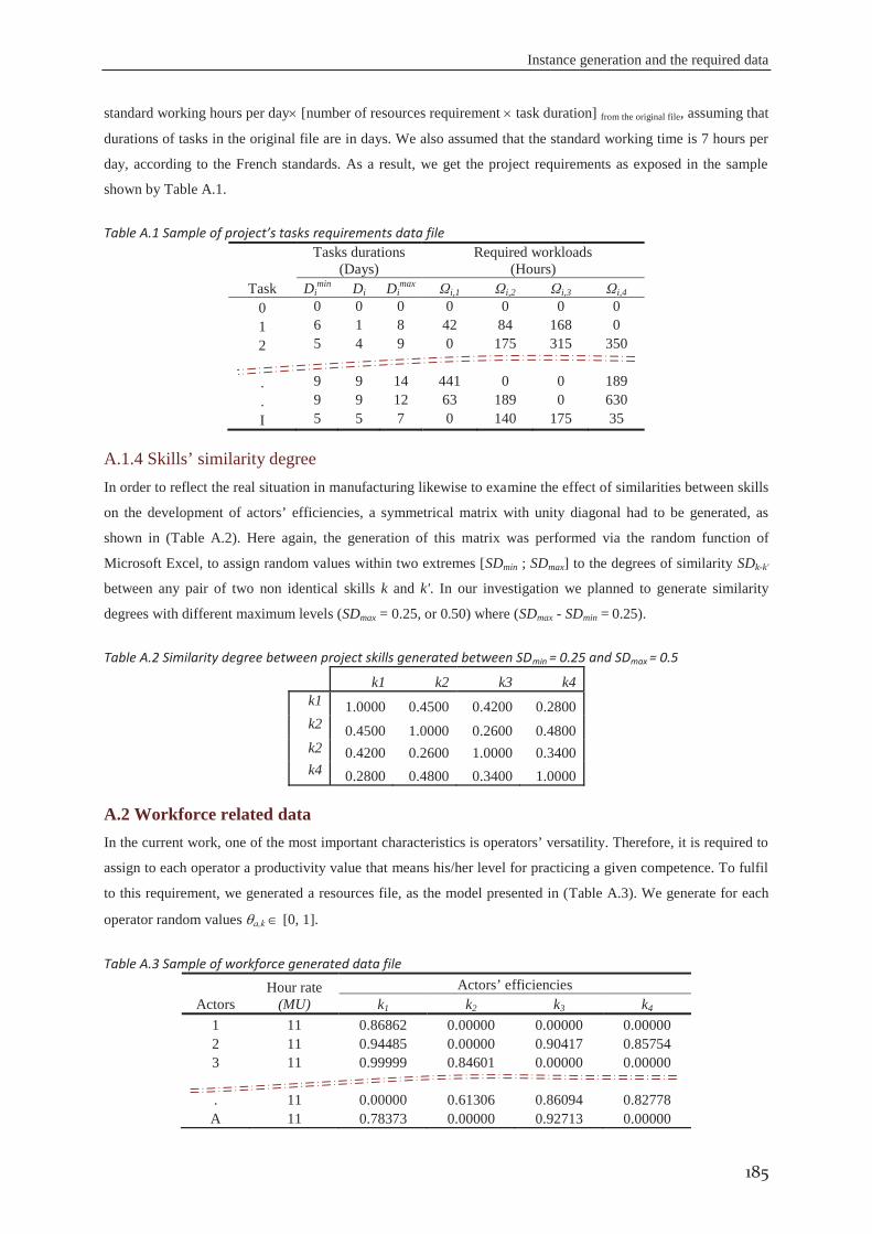
Instance generation and the required data

185

standard working hours per day [number of resources requirement task duration] from the original file, assuming that

durations of tasks in the original file are in days. We also assumed that the standard working time is 7 hours per

day, according to the French standards. As a result, we get the project requirements as exposed in the sample

shown by Table A.1.

Table A.1 Sample of project’s tasks requirements data file

Task

Tasks durations (Days)

Required workloads (Hours)

Dimin Di Di

max Ωi,1 Ωi,2 Ωi,3 Ωi,4 0 0 0 0 0 0 0 0 1 6 1 8 42 84 168 0 2 5 4 9 0 175 315 350

. 9 9 14 441 0 0 189 . 9 9 12 63 189 0 630 I 5 5 7 0 140 175 35

A.1.4 Skills’ similarity degree In order to reflect the real situation in manufacturing likewise to examine the effect of similarities between skills

on the development of actors’ efficiencies, a symmetrical matrix with unity diagonal had to be generated, as

shown in (Table A.2). Here again, the generation of this matrix was performed via the random function of

Microsoft Excel, to assign random values within two extremes [SDmin ; SDmax] to the degrees of similarity SDk-k'

between any pair of two non identical skills k and k'. In our investigation we planned to generate similarity

degrees with different maximum levels (SDmax = 0.25, or 0.50) where (SDmax - SDmin = 0.25).

Table A.2 Similarity degree between project skills generated between SDmin = 0.25 and SDmax = 0.5 k1 k2 k3 k4

k1 1.0000 0.4500 0.4200 0.2800 k2 0.4500 1.0000 0.2600 0.4800 k2 0.4200 0.2600 1.0000 0.3400 k4 0.2800 0.4800 0.3400 1.0000

A.2 Workforce related data In the current work, one of the most important characteristics is operators’ versatility. Therefore, it is required to

assign to each operator a productivity value that means his/her level for practicing a given competence. To fulfil

to this requirement, we generated a resources file, as the model presented in (Table A.3). We generate for each

operator random values a,k [0, 1].

Table A.3 Sample of workforce generated data file

Actors Hour rate

(MU) Actors’ efficiencies

k1 k2 k3 k4 1 11 0.86862 0.00000 0.00000 0.00000 2 11 0.94485 0.00000 0.90417 0.85754 3 11 0.99999 0.84601 0.00000 0.00000

. 11 0.00000 0.61306 0.86094 0.82778 A 11 0.78373 0.00000 0.92713 0.00000

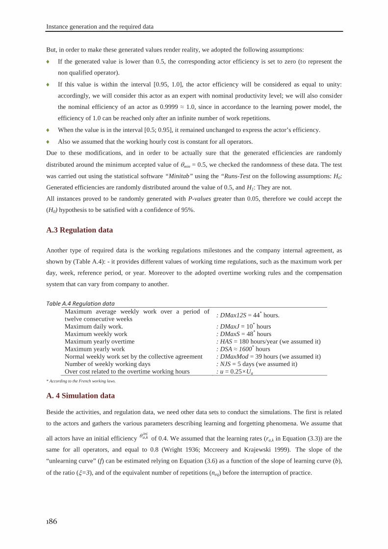
Instance generation and the required data

186

But, in order to make these generated values render reality, we adopted the following assumptions:

If the generated value is lower than 0.5, the corresponding actor efficiency is set to zero (to represent the

non qualified operator).

If this value is within the interval [0.95, 1.0], the actor efficiency will be considered as equal to unity:

accordingly, we will consider this actor as an expert with nominal productivity level; we will also consider

the nominal efficiency of an actor as 0.9999 ≈ 1.0, since in accordance to the learning power model, the

efficiency of 1.0 can be reached only after an infinite number of work repetitions.

When the value is in the interval [0.5; 0.95], it remained unchanged to express the actor’s efficiency.

Also we assumed that the working hourly cost is constant for all operators.

Due to these modifications, and in order to be actually sure that the generated efficiencies are randomly

distributed around the minimum accepted value of min = 0.5, we checked the randomness of these data. The test

was carried out using the statistical software “Minitab” using the “Runs-Test on the following assumptions: H0:

Generated efficiencies are randomly distributed around the value of 0.5, and H1: They are not.

All instances proved to be randomly generated with P-values greater than 0.05, therefore we could accept the

(H0) hypothesis to be satisfied with a confidence of 95%.

A.3 Regulation data

Another type of required data is the working regulations milestones and the company internal agreement, as

shown by (Table A.4): - it provides different values of working time regulations, such as the maximum work per

day, week, reference period, or year. Moreover to the adopted overtime working rules and the compensation

system that can vary from company to another.

Table A.4 Regulation data Maximum average weekly work over a period of twelve consecutive weeks : DMax12S = 44* hours.

Maximum daily work. : DMaxJ = 10* hours Maximum weekly work : DMaxS = 48* hours Maximum yearly overtime : HAS = 180 hours/year (we assumed it) Maximum yearly work : DSA ≈ 1600* hours Normal weekly work set by the collective agreement : DMaxMod = 39 hours (we assumed it) Number of weekly working days : NJS = 5 days (we assumed it) Over cost related to the overtime working hours : u = 0.25×Ua

* According to the French working laws.

A. 4 Simulation data

Beside the activities, and regulation data, we need other data sets to conduct the simulations. The first is related

to the actors and gathers the various parameters describing learning and forgetting phenomena. We assume that

all actors have an initial efficiency ini

ka, of 0.4. We assumed that the learning rates (ra,k in Equation (3.3)) are the

same for all operators, and equal to 0.8 (Wright 1936; Mccreery and Krajewski 1999). The slope of the

“unlearning curve” (f) can be estimated relying on Equation (3.6) as a function of the slope of learning curve (b),

of the ratio ( =3), and of the equivalent number of repetitions (neq) before the interruption of practice.

Instance generation and the required data

187

The last set of data provides the parameters of the genetic algorithm, such as population size, probabilities of

crossover and mutation, the composition of the new generations, and the stopping criteria of the search

algorithm, as shown in the (Table A.5). They were fixed after an exploration intended both to validate the model

and to set these parameters to reliable values (as discussed in chapter 5).

Table A.5 Exploration data Population size = 100 individuals Crossing probability = 0.7 Mutation probability = 0.01 Fraction of immigrated individuals in the new generation = 0.2 Max. n° of generations = 8000 generations N° of iterations without convergence = 100 generations N° of the best individuals on which convergence is computed = 10 individuals

Instance generation and the required data

188

ON PROJECT COMPLEXITY

APP

END

IX

B

On project complexity

190

B.1 Other network complexity measures

Complexity index: CI: Bein et al. (1992) introduced a way to measure the topological structure of a graph

based on the reduction sequence of the two terminal acyclic graphs. This complexity measuring is relying on the

minimum number of node reductions. The graph reduction mainly done based on three types: parallel, series and

node reductions in order to reach a single edge graph. Parallel reductions: a parallel reduction of nodes v, w

replaces two or more edges e1,…, ek joining v to w by a single edge g=(v, w). Series reductions: if there is an

edge e= (u, v) is a unique edge to v, and f = (v, w) is the unique edge out of v, then e and f are replaced by g=(u,

w). After all parallel and series reductions, one can have a new graph [G], if the obtained graph [G] = the initial

G, then G is said to be irreducible. In the irreducible graph, the node v is eligible for a node reduction when it has

in-degree=1 or out-degree = 1. In case of in-degree=1: let e=(u, v) be the edge into the node v, let f1=(v, w1),

…, fk=(v, wk) be the edges out of v. replace {e,f1,…,fk} by {g1, …, gk}, where gi=(u, wi). The case of out-degree =

1 is symmetric, where e=(v, w) , fi=(ui, v) and gi=(ui, w). After the graph reduction one can define the reduction

complexity of graph “G” as: the minimum number of node reductions sufficient to reduce “G” to a single edge,

in other words, one can calculate complexity index as: CI = C(number of reduction sequences), which there

exists a reduction sequences v1,…, vc such that [… [[[G]◦ v1] ◦ v2]… ◦ vc] is a single edge. The complexity of this

reduction algorithm is O(I2.5), where I is the number of tasks.

Network divergence and convergence: Scholl (1999)(Section 2.2.1.5 page 34) presented measures of the

network degree of divergence and convergence. These measures can be defined and presented be considering the

network as a digraph G(V,E), where V is the set of graph nodes with cardinality |V| and E is the set of its edges.

|E| is the cardinality of the network set of edges E= {<i , c>| i V, c SUi }. Where, SUi is set of successors of

i, a non-cyclical directed graph G(V,E) with a single source v0 is transformed to an out-tree by arbitrarily

eliminating δi-1 of the entering arcs for each node i V – {v0 }. Therefore, the positive degree of divergence for

G can be defined as:

0

/)1(1)(vVi

i EGDIV (B.1)

An analogous degree of convergence is the CNV(G) is achieved by considering the reverse precedence graph.

According to Otto et al. (2011) the mathematical formulation can be reformulating to take the shape as presented

in equations (B.2) and (B.3), where NWP1 is the number of tasks without predecessors, and NWS1 is the number

of tasks without successors.

Degree of divergence: ED

VNWPEDIV 11 , such that

1 1

1

11

if NWPif NWP

ENWPE

ED , (B.2)

Degree of convergence: EC

VNWSECNV 11 , such that

1 1

1

11

if NWSif NWS

ENWSE

EC , (B.3)

As discussed by Scholl (1999) in the case of DIV(G)=1, G is an out-tree, i.e. it is strictly diverging. If DIV(G) is

smaller than but near to 1, the graph is almost diverging or almost-tree. The precedence graph can be

transformed into a single-source graph by adding a fictitious source node with operation time “0” and arcs to the

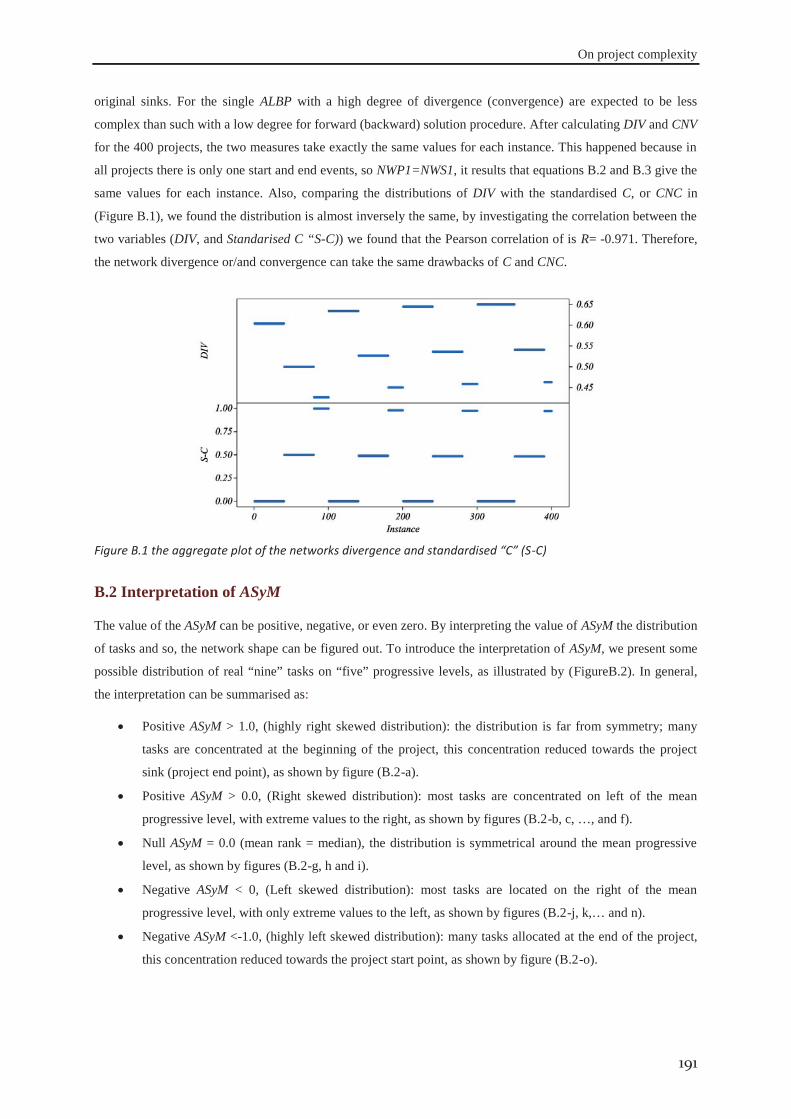
On project complexity

191

original sinks. For the single ALBP with a high degree of divergence (convergence) are expected to be less

complex than such with a low degree for forward (backward) solution procedure. After calculating DIV and CNV

for the 400 projects, the two measures take exactly the same values for each instance. This happened because in

all projects there is only one start and end events, so NWP1=NWS1, it results that equations B.2 and B.3 give the

same values for each instance. Also, comparing the distributions of DIV with the standardised C, or CNC in

(Figure B.1), we found the distribution is almost inversely the same, by investigating the correlation between the

two variables (DIV, and Standarised C “S-C)) we found that the Pearson correlation of is R= -0.971. Therefore,

the network divergence or/and convergence can take the same drawbacks of C and CNC.

Figure B.1 the aggregate plot of the networks divergence and standardised “C” (S-C)

B.2 Interpretation of ASyM

The value of the ASyM can be positive, negative, or even zero. By interpreting the value of ASyM the distribution

of tasks and so, the network shape can be figured out. To introduce the interpretation of ASyM, we present some

possible distribution of real “nine” tasks on “five” progressive levels, as illustrated by (FigureB.2). In general,

the interpretation can be summarised as:

Positive ASyM > 1.0, (highly right skewed distribution): the distribution is far from symmetry; many

tasks are concentrated at the beginning of the project, this concentration reduced towards the project

sink (project end point), as shown by figure (B.2-a).

Positive ASyM > 0.0, (Right skewed distribution): most tasks are concentrated on left of the mean

progressive level, with extreme values to the right, as shown by figures (B.2-b, c, …, and f).

Null ASyM = 0.0 (mean rank = median), the distribution is symmetrical around the mean progressive

level, as shown by figures (B.2-g, h and i).

Negative ASyM < 0, (Left skewed distribution): most tasks are located on the right of the mean

progressive level, with only extreme values to the left, as shown by figures (B.2-j, k,… and n).

Negative ASyM <-1.0, (highly left skewed distribution): many tasks allocated at the end of the project,

this concentration reduced towards the project start point, as shown by figure (B.2-o).

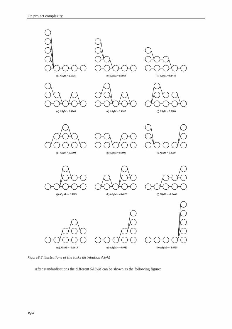
On project complexity

192

FigureB.2 Illustrations of the tasks distribution ASyM

After standardisations the different SASyM can be shown as the following figure:

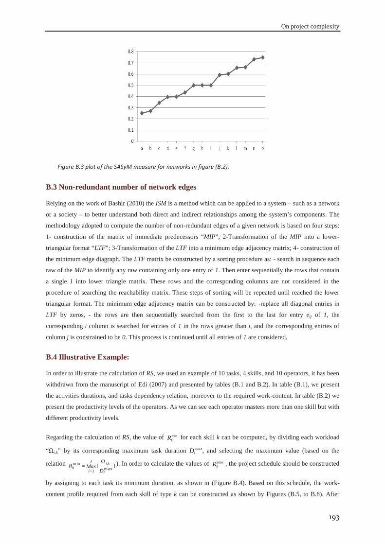
On project complexity

193

Figure B.3 plot of the SASyM measure for networks in figure (B.2).

B.3 Non-redundant number of network edges

Relying on the work of Bashir (2010) the ISM is a method which can be applied to a system – such as a network

or a society – to better understand both direct and indirect relationships among the system’s components. The

methodology adopted to compute the number of non-redundant edges of a given network is based on four steps:

1- construction of the matrix of immediate predecessors “MIP”; 2-Transformation of the MIP into a lower-

triangular format “LTF”; 3-Transformation of the LTF into a minimum edge adjacency matrix; 4- construction of

the minimum edge diagraph. The LTF matrix be constructed by a sorting procedure as: - search in sequence each

raw of the MIP to identify any raw containing only one entry of 1. Then enter sequentially the rows that contain

a single 1 into lower triangle matrix. These rows and the corresponding columns are not considered in the

procedure of searching the reachability matrix. These steps of sorting will be repeated until reached the lower

triangular format. The minimum edge adjacency matrix can be constructed by: -replace all diagonal entries in

LTF by zeros, - the rows are then sequentially searched from the first to the last for entry eij of 1, the

corresponding i column is searched for entries of 1 in the rows greater than i, and the corresponding entries of

column j is constrained to be 0. This process is continued until all entries of 1 are considered.

B.4 Illustrative Example:

In order to illustrate the calculation of RS, we used an example of 10 tasks, 4 skills, and 10 operators, it has been

withdrawn from the manuscript of Edi (2007) and presented by tables (B.1 and B.2). In table (B.1), we present

the activities durations, and tasks dependency relation, moreover to the required work-content. In table (B.2) we

present the productivity levels of the operators. As we can see each operator masters more than one skill but with

different productivity levels.

Regarding the calculation of RS, the value of minkR for each skill k can be computed, by dividing each workload

“Ωi,k” by its corresponding maximum task duration Dimax, and selecting the maximum value (based on the

relation ][max1

min ,

i

I

ik

DMaxR ki ). In order to calculate the values of max

kR , the project schedule should be constructed

by assigning to each task its minimum duration, as shown in (Figure B.4). Based on this schedule, the work-

content profile required from each skill of type k can be constructed as shown by Figures (B.5, to B.8). After

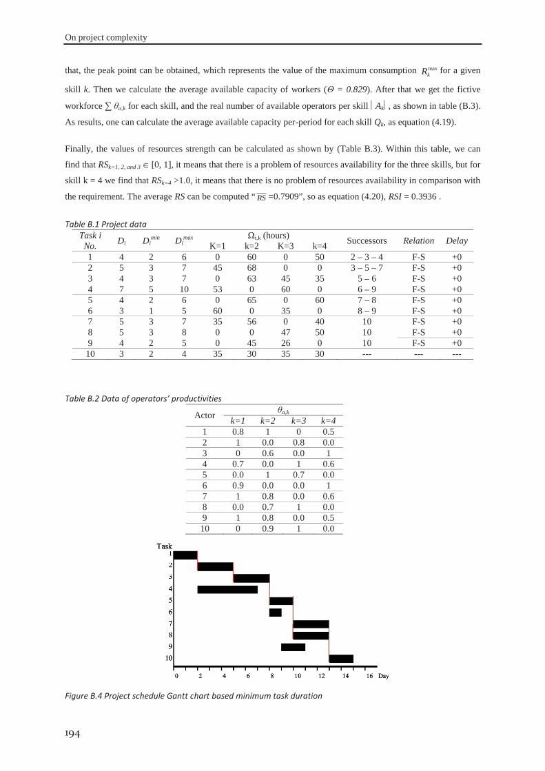
On project complexity

194

that, the peak point can be obtained, which represents the value of the maximum consumption maxkR for a given

skill k. Then we calculate the average available capacity of workers (Θ = 0.829). After that we get the fictive

workforce ∑ θa,k for each skill, and the real number of available operators per skill Ak , as shown in table (B.3).

As results, one can calculate the average available capacity per-period for each skill Qk, as equation (4.19).

Finally, the values of resources strength can be calculated as shown by (Table B.3). Within this table, we can

find that RSk=1, 2, and 3 [0, 1], it means that there is a problem of resources availability for the three skills, but for

skill k = 4 we find that RSk=4 >1.0, it means that there is no problem of resources availability in comparison with

the requirement. The average RS can be computed “ RS =0.7909”, so as equation (4.20), RSI = 0.3936 .

Table B.1 Project data Task i No. Di Di

min Dimax Ωi,k (hours) Successors Relation Delay K=1 k=2 K=3 k=4

1 4 2 6 0 60 0 50 2 – 3 – 4 F-S +0 2 5 3 7 45 68 0 0 3 – 5 – 7 F-S +0 3 4 3 7 0 63 45 35 5 – 6 F-S +0 4 7 5 10 53 0 60 0 6 – 9 F-S +0 5 4 2 6 0 65 0 60 7 – 8 F-S +0 6 3 1 5 60 0 35 0 8 – 9 F-S +0 7 5 3 7 35 56 0 40 10 F-S +0 8 5 3 8 0 0 47 50 10 F-S +0 9 4 2 5 0 45 26 0 10 F-S +0 10 3 2 4 35 30 35 30 --- --- ---

Table B.2 Data of operators’ productivities

Actor θa,k k=1 k=2 k=3 k=4

1 0.8 1 0 0.5 2 1 0.0 0.8 0.0 3 0 0.6 0.0 1 4 0.7 0.0 1 0.6 5 0.0 1 0.7 0.0 6 0.9 0.0 0.0 1 7 1 0.8 0.0 0.6 8 0.0 0.7 1 0.0 9 1 0.8 0.0 0.5 10 0 0.9 1 0.0

Figure B.4 Project schedule Gantt chart based minimum task duration

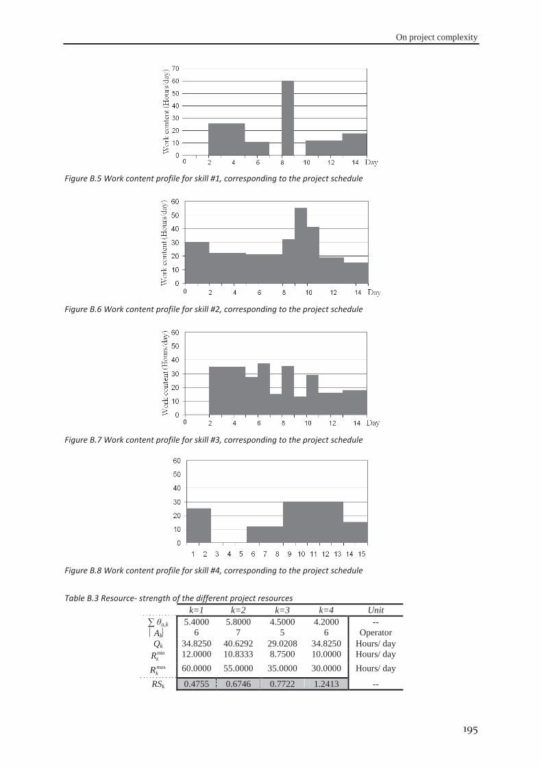
On project complexity

195

Figure B.5 Work content profile for skill #1, corresponding to the project schedule

Figure B.6 Work content profile for skill #2, corresponding to the project schedule

Figure B.7 Work content profile for skill #3, corresponding to the project schedule

Figure B.8 Work content profile for skill #4, corresponding to the project schedule

Table B.3 Resource- strength of the different project resources k=1 k=2 k=3 k=4 Unit

∑ θa,k 5.4000 5.8000 4.5000 4.2000 -- Ak 6 7 5 6 Operator Qk 34.8250 40.6292 29.0208 34.8250 Hours/ day

minkR 12.0000 10.8333 8.7500 10.0000 Hours/ day maxkR 60.0000 55.0000 35.0000 30.0000 Hours/ day

RSk 0.4755 0.6746 0.7722 1.2413 --

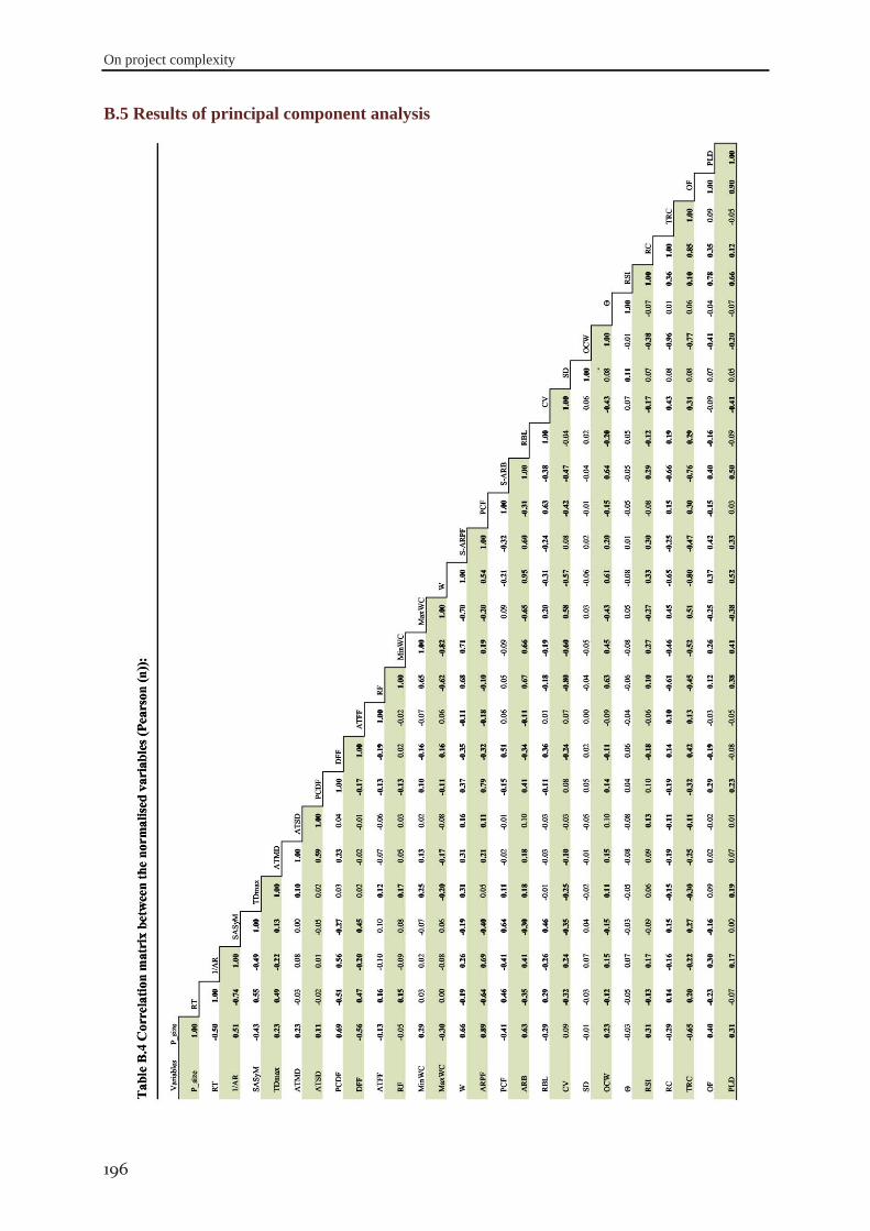
On project complexity

196

B.5 Results of principal component analysis

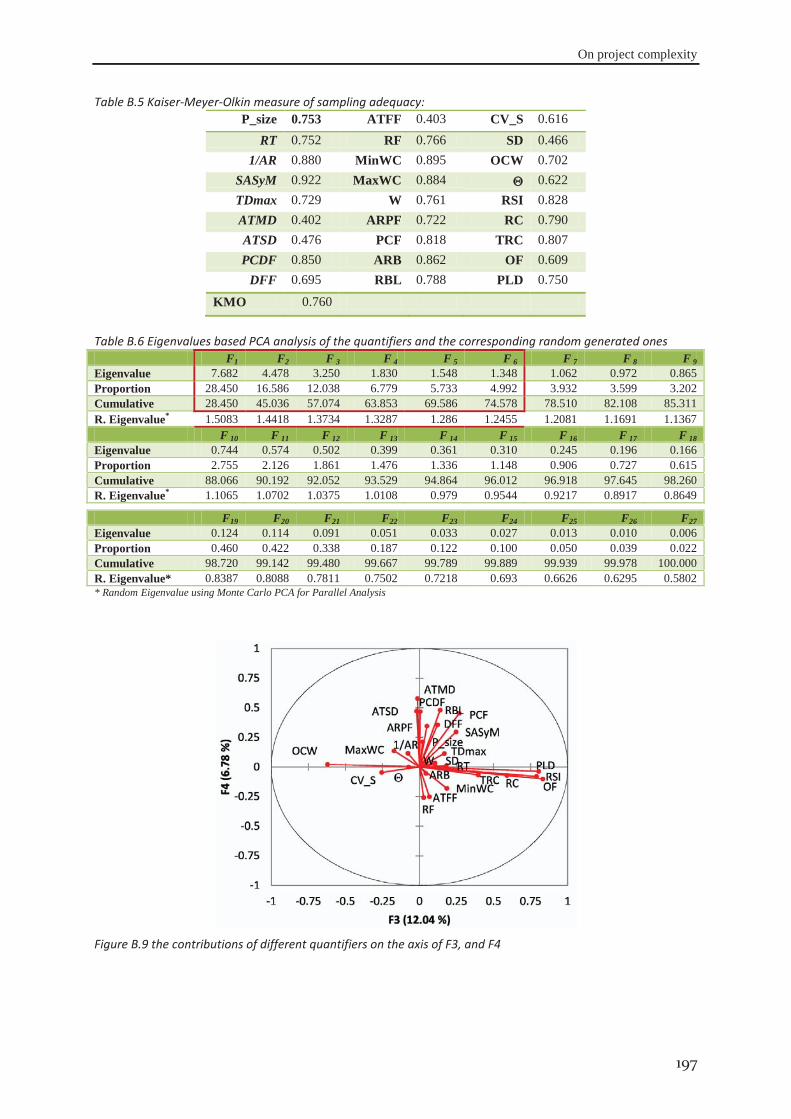
On project complexity

197

Table B.5 Kaiser-Meyer-Olkin measure of sampling adequacy: P_size 0.753 ATFF 0.403 CV_S 0.616

RT 0.752 RF 0.766 SD 0.466 1/AR 0.880 MinWC 0.895 OCW 0.702

SASyM 0.922 MaxWC 0.884 0.622 TDmax 0.729 W 0.761 RSI 0.828 ATMD 0.402 ARPF 0.722 RC 0.790 ATSD 0.476 PCF 0.818 TRC 0.807 PCDF 0.850 ARB 0.862 OF 0.609

DFF 0.695 RBL 0.788 PLD 0.750

KMO 0.760

Table B.6 Eigenvalues based PCA analysis of the quantifiers and the corresponding random generated ones F1 F2 F 3 F 4 F 5 F 6 F 7 F 8 F 9 Eigenvalue 7.682 4.478 3.250 1.830 1.548 1.348 1.062 0.972 0.865 Proportion 28.450 16.586 12.038 6.779 5.733 4.992 3.932 3.599 3.202 Cumulative 28.450 45.036 57.074 63.853 69.586 74.578 78.510 82.108 85.311 R. Eigenvalue* 1.5083 1.4418 1.3734 1.3287 1.286 1.2455 1.2081 1.1691 1.1367 F 10 F 11 F 12 F 13 F 14 F 15 F 16 F 17 F 18 Eigenvalue 0.744 0.574 0.502 0.399 0.361 0.310 0.245 0.196 0.166 Proportion 2.755 2.126 1.861 1.476 1.336 1.148 0.906 0.727 0.615 Cumulative 88.066 90.192 92.052 93.529 94.864 96.012 96.918 97.645 98.260 R. Eigenvalue* 1.1065 1.0702 1.0375 1.0108 0.979 0.9544 0.9217 0.8917 0.8649

F19 F20 F21 F22 F23 F24 F25 F26 F27 Eigenvalue 0.124 0.114 0.091 0.051 0.033 0.027 0.013 0.010 0.006 Proportion 0.460 0.422 0.338 0.187 0.122 0.100 0.050 0.039 0.022 Cumulative 98.720 99.142 99.480 99.667 99.789 99.889 99.939 99.978 100.000 R. Eigenvalue* 0.8387 0.8088 0.7811 0.7502 0.7218 0.693 0.6626 0.6295 0.5802 * Random Eigenvalue using Monte Carlo PCA for Parallel Analysis

Figure B.9 the contributions of different quantifiers on the axis of F3, and F4

On project complexity

198

STATISTICAL ANALYSIS

APP

END

IX

C

Statistical analysis

200

C.1 principal component analysis

Principal component analysis is one of the factor analysis techniques. It used mainly to reduce the dimensionality

of data containing a large number of inter-correlated variables into only the smallest manageable factors, while

retain as most as possible the variation of the original data. This smallest number of factors is called principal

components. Each principal component is a linear combination of a subset of the original variables that have

some similar characteristics. It constructed as follows: PC1 = )(1 ini ib , where bi is the score of variable νi in

constructing the principal component PCi . As the score of the variable approaches to zero the impact of the

associated variable can be neglecting in constructing the PCi in question. All principal components are ranked

according to their ability in explaining the variance in the original data set. That is to say, the first component has

the most significant impact in explaining the original data variance. The second component is computed under

the constraints of being orthogonal to the first one, and explaining as most as possible the largest amount of the

remaining variance. Likewise, this continued until the last principal component (the nth component) is computed,

it has the smallest impact in explaining the variance of the original data. Relying on the linear algebraic,

principal components are computed using either the correlation matrix or the covariance matrix. That used to

produce what is known eigenvalues and orthogonal eigenvectors. This eigenvalue used to indicate the proportion

of the total variance explained from the original data by the corresponding principal component. So the ranking

of the different components is done relying on these eigenvalues. As it well known, the covariance between two

variables is not standardised so the scale of each variable affects the results of the test. Therefore in order to use

the covariance matrix, the data should be standardised before performing the test. Standardisation is performed

by the following formula: ν̓i,o = (xi,o - i ) / Sνi , o {observations of νi }, where: νi̓,o is the standardised

version of the observation “o” of variable νi, xi,o the real observation “o” of the variable νi , i the average value

of the different observations of νi , and Sνi is the standard deviation of νi. The use of the correlation matrix

controls the problem associated with scale of variables, where the correlation is always standardised. For more

details about the theoretical bases, we recommended the book of Jolliffe (2002). But here we focused more on

the practical application to conduct the factor analysis using principal component as an extraction method.

Therefore, we present by the following the different conditions to investigate the sample adequacy to conduct

this analysis. We discuss also the different methodologies to select the smallest number of components, the

rotation of axis, projection of variable on component axis “square cosines”, the loading of variables, and finally

the scores of each variable.

C.1.1 Adequacy of data to the test According to Pallant (2010), there are two issues should be considered to investigate the adequacy of the data to

the factor analysis: the sample size and the inter-dependency strength between the variables. First the sample

size: they discussed that as most as the sample size increased as it is reliable to conduct such factor analysis. And

a sample of at least 300 cases can be considered as comfortable to conduct the test. There is a ratio to determine

the minimum number of cases depending on the variables number; this ratio is 10 cases for each variable.

Finally, they advised to make more literature investigation about the effect of small sample size especially if we

have a sample size less than 150 cases. The second issue is the strength of the inter-association between the

different variables. This strength can be checked using one of the following three methods:

Statistical analysis

201

- Correlation analysis, the test is conducted simply by constructing correlation matrix of all variables. After that

investigating the number of correlations greater than “0.3”, as this number is high as the adequacy of the test will

be good. If few correlations above this level are found, then factor analysis may not be appropriate. Knowing

that, each element of the correlation matrix can be computed as the Person correlation coefficient (see section

C.6) between the corresponding two variables (raw, column).

- Bartlett's sphericity test, It is a hypothesis test (see section C.3) that used to test the null hypothesis H0: There is

no correlation significantly different from 0 between the variables. And the alternate hypothesis H1: At least one

of the correlations between the variables is significantly different from 0. If the observed significance level is

very small (the test P-value < α-value), we can reject the null hypothesis without any significant error. It is

concluded that the strength of the relationship is strong at least for a pair of variables. Therefore, conducting the

factor analysis seems to be adequacy for the data.

- Kaiser-Meyer-Olkin measure of sampling adequacy: KMO, is a popular diagnostic measure in factor analysis.

It provides a factor between 0 and 1, according to Pallant (2010), a value of “KMO” between 0.6 and 1 indicates

the adequacy of using factor analysis for the data in question. And value of “KMO” of less than 0.5 is probably

not appropriate to use factor analysis on data.

C.1.2 Components to be retained The principal component analysis is conducted in order to have the smallest number of factors that best describe

the variance of the data. Therefore, we have to get a compromise between the minimum components and the

largest variance explication. To get this compromise and relying on Pallant (2010), there is three methods: -

Kaiser’s criterion –Scree test and -Parallel analysis.

Kaiser’s criterion; is the criterion that most frequently utilised by practicing social scientists. The criterion is

very simple, where we retain only the factors with eigenvalue equals or greater than a value of “1.0”. And all the

factors with egienvalues less than “1.0” can be neglected.

Scree test; the scree plot is a graph within it we plot the different eigenvalues ranked from the largest to the

smallest. Then by investigating this plot one can decide the factors that may be significantly explain the data

total variance. Within this plot, we search to find a point at which the shape of the curve becomes approximately

horizontal. Relying on this plot, we can retain only the factors above the elbow, where they have almost the

major cumulated value in explaining the data total variance.

Parallel analysis; according to Pallant (2010), this technique is also utilised by social scientists and first

presented by Horn (1965). This analysis started by generating randomly a data matrix of size exactly equals that

of the original data matrix. For this random generated matrix, its eigenvalues are computed by the same way as

that of the original data matrix. Then by comparing these eigenvalues (driven from the random data) with

eigenvalues driven from the real data, we can decide the minimum number of principal components. That is, if a

real eigenvalue is greater than a random eigenvalue we accept the corresponding factor, otherwise we reject it. In

order to calculate these “eignvalues” based random data, we used a software called “Monte Carlo PCA for

parallel analysis” developed by Watkins (2000).

Statistical analysis

202

C.1.3 Axis rotation After determining the number of minimum factors, the great task is to interpret them; one of the ways that

enhance this interpretation is the rotation of axis. This rotation does not change the underlying solution - rather,

it presents the pattern of loadings in a manner that is easier to interpret. There are two main types of rotations

that can be used: the first is the orthogonal (uncorrelated), the new axes are also orthogonal to each other. The

second is the oblique (correlated), the new axes are not required to be orthogonal to each other. Associated to

each rotation type there are some techniques to perform it: Varimax, Quartimax, Equamax are associated to the

orthogonal type, and direct Oblimin and Promax are oblique methods. according to Pallant (2010) the most

commonly used orthogonal approach is the Varimax rotation, which maximizes the sum of the variances of the

squared loadings. Thus, the number of variables that have high impact on each factor can be distinguished by

inspecting the squared correlation with the factor. The goal is to associate each variable to at most one factor.

C.1.4 Results interpretation Due to the rotation of coordinates, the angles between each variable vector and the axes of the principal factors

were changed. The projection of each variable on the factors axes can be used as a good indicator to the

association between this variable and factors. Therefore “XLSTAT” presents a table of squared cosines (to

reflect the different projection of variables on each factor), which used to avoid interpretation errors due to

projection effects. For each variable there is a high squared cosine associated with only one factor. Observing

this value indicates that this variable may be highly contributed in constructing this factor rather than any of the

others. Also the variable contribution in building a given factor can be computed based on the squared cosines.

The linear correlation (Pearson correlation coefficient, see section C.6) between variables and principal

components can be used in the interpretation of results, to know the association of variables to different

components. The linear correlation matrix between variables and components is exactly equals the factors

loading for the normalised principal component analysis. After define the variables that highly associated to each

factor, for each one there is a multiplier coefficient “score” that used in constructing the formula of the

corresponding component. For more details about the computations of these scores we propose the work of

Burstyn (2004).

C.2 Cluster analysis Cluster analysis is one of the data mining techniques that divided data to meaningful groups that share specified

characteristics. Clustering is a common technique in biology, information retrieval (search engines), climate,

psychology and medicine, business and marketing, etc. Clustering is used to understanding the nature of the data

in question. According to Tan et al. (2006), the goal is that the objects within a group be similar (or related) to

one another and different from the objects in the other group. There are many types of clustering: hierarchical

(nested) versus partitional (un-nested), exclusive versus overlapping versus fuzzy, complete versus partial. Here,

we are interested to the most common one, the hierarchical clustering. In hierarchical clustering the sub

clustering is permitted, thus it can be nested looks like a tree. The main idea is to build a binary nested tree of the

data that successively merged the similar groups. It relies on a measure of similarity between the data; this

similarity can be a correlation between groups. The common technique used is known as agglomerative

hierarchical clustering. It starts by placing each data point by its own singleton group, and repetitively merges

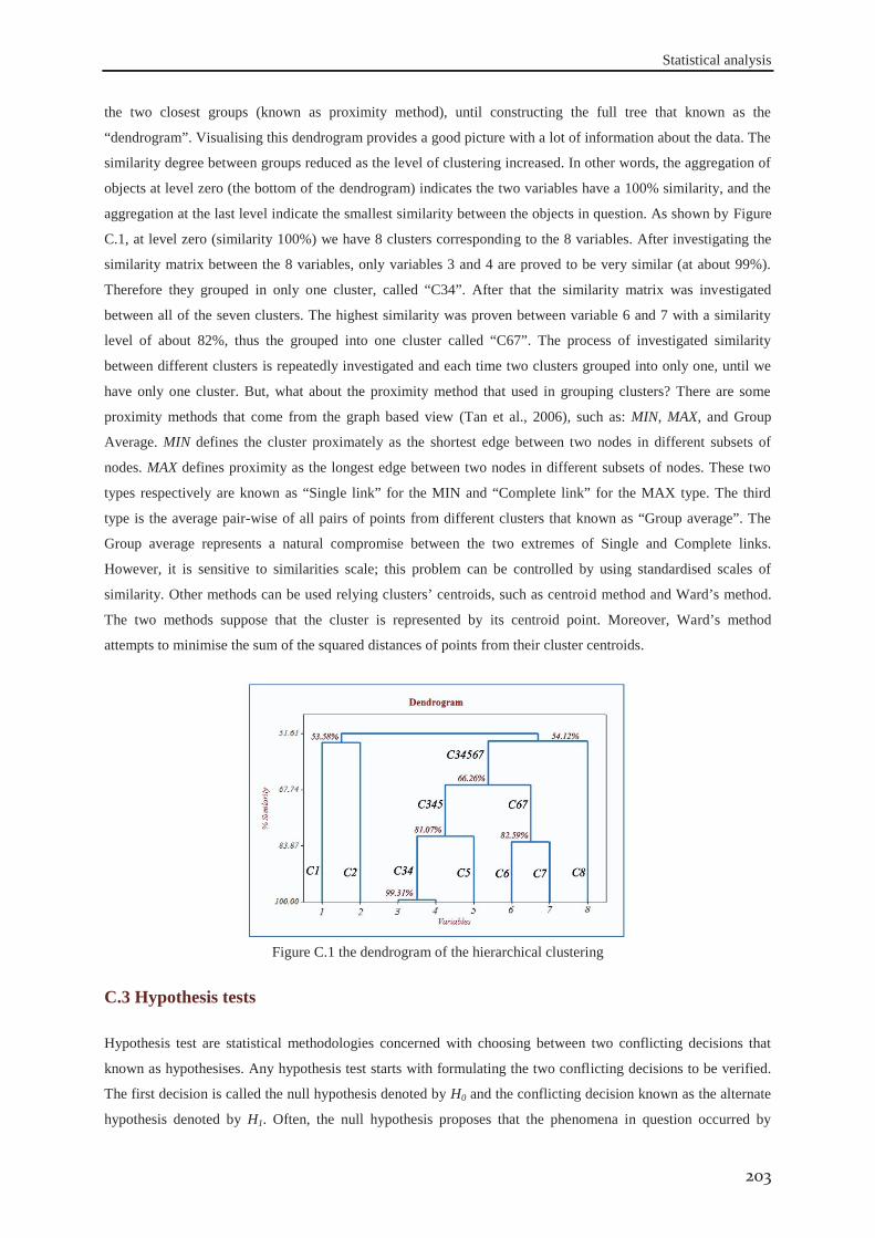
Statistical analysis

203

the two closest groups (known as proximity method), until constructing the full tree that known as the

“dendrogram”. Visualising this dendrogram provides a good picture with a lot of information about the data. The

similarity degree between groups reduced as the level of clustering increased. In other words, the aggregation of

objects at level zero (the bottom of the dendrogram) indicates the two variables have a 100% similarity, and the

aggregation at the last level indicate the smallest similarity between the objects in question. As shown by Figure

C.1, at level zero (similarity 100%) we have 8 clusters corresponding to the 8 variables. After investigating the

similarity matrix between the 8 variables, only variables 3 and 4 are proved to be very similar (at about 99%).

Therefore they grouped in only one cluster, called “C34”. After that the similarity matrix was investigated

between all of the seven clusters. The highest similarity was proven between variable 6 and 7 with a similarity

level of about 82%, thus the grouped into one cluster called “C67”. The process of investigated similarity

between different clusters is repeatedly investigated and each time two clusters grouped into only one, until we

have only one cluster. But, what about the proximity method that used in grouping clusters? There are some

proximity methods that come from the graph based view (Tan et al., 2006), such as: MIN, MAX, and Group

Average. MIN defines the cluster proximately as the shortest edge between two nodes in different subsets of

nodes. MAX defines proximity as the longest edge between two nodes in different subsets of nodes. These two

types respectively are known as “Single link” for the MIN and “Complete link” for the MAX type. The third

type is the average pair-wise of all pairs of points from different clusters that known as “Group average”. The

Group average represents a natural compromise between the two extremes of Single and Complete links.

However, it is sensitive to similarities scale; this problem can be controlled by using standardised scales of

similarity. Other methods can be used relying clusters’ centroids, such as centroid method and Ward’s method.

The two methods suppose that the cluster is represented by its centroid point. Moreover, Ward’s method

attempts to minimise the sum of the squared distances of points from their cluster centroids.

Figure C.1 the dendrogram of the hierarchical clustering

C.3 Hypothesis tests

Hypothesis test are statistical methodologies concerned with choosing between two conflicting decisions that

known as hypothesises. Any hypothesis test starts with formulating the two conflicting decisions to be verified.

The first decision is called the null hypothesis denoted by H0 and the conflicting decision known as the alternate

hypothesis denoted by H1. Often, the null hypothesis proposes that the phenomena in question occurred by

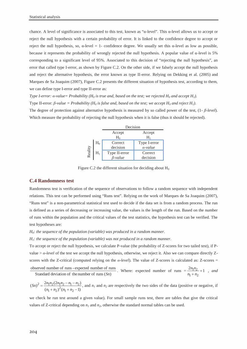
Statistical analysis

204

chance. A level of significance is associated to this test, known as “α-level”. This α-level allows us to accept or

reject the null hypothesis with a certain probability of error. It is linked to the confidence degree to accept or

reject the null hypothesis, so, α-level = 1- confidence degree. We usually set this α-level as low as possible,

because it represents the probability of wrongly rejected the null hypothesis. A popular value of α-level is 5%

corresponding to a significant level of 95%. Associated to this decision of “rejecting the null hypothesis”, an

error that called type I-error, as shown by Figure C.2. On the other side, if we falsely accept the null hypothesis

and reject the alternative hypothesis, the error known as type II-error. Relying on Dekking et al. (2005) and

Marques de Sa Joaquim (2007), Figure C.2 presents the different situation of hypothesis test, according to them,

we can define type I-error and type II-error as:

Type I-error: α-value= Probability (H0 is true and, based on the test; we rejected H0 and accept H1).

Type II-error: β-value = Probability (H0 is false and, based on the test; we accept H0 and reject H1).

The degree of protection against alternative hypothesis is measured by so called power of the test, (1- β-level).

Which measure the probability of rejecting the null hypothesis when it is false (thus it should be rejected).

Decision Accept Accept

Rea

lity

H0 H1 H0 Correct

decision Type I-error α-value

H1 Type II-error β-value

Correct decision

Figure C.2 the different situation for deciding about H0

C.4 Randomness test Randomness test is verification of the sequence of observations to follow a random sequence with independent

relations. This test can be performed using “Runs test”. Relying on the work of Marques de Sa Joaquim (2007),

“Runs test” is a non-parametrical statistical test used to decide if the data set is from a random process. The run

is defined as a series of decreasing or increasing value, the values is the length of the run. Based on the number

of runs within the population and the critical values of the test statistics, the hypothesis test can be verified. The

test hypotheses are:

H0: the sequence of the population (variable) was produced in a random manner.

H1: the sequence of the population (variable) was not produced in a random manner.

To accept or reject the null hypothesis, we calculate P-value (the probability of Z-scores for two tailed test), if P-

value > α-level of the test we accept the null hypothesis, otherwise, we reject it. Also we can compare directly Z-

scores with the Z-critical (computed relying on the α-level). The value of Z-scores is calculated as: Z-scores =

)( runs ofnumber theofdeviation Standardruns ofnumber expected - runs ofnumber observed

Sn. Where: expected number of runs = 12

21

21nnnn , and

)1()()2(2)(

212

21

2121212

nnnnnnnnnnSn , and n1 and n2 are respectively the two sides of the data (positive or negative, if

we check he run test around a given value). For small sample runs test, there are tables that give the critical

values of Z-critical depending on n1 and n2, otherwise the standard normal tables can be used.

Statistical analysis

205

C.5 1-sample t-test 1-sample t-test is a statistical methodology that used to estimate the confidence interval of the population mean

for unknown population standard deviation relying on a sample drawn from it. Moreover, it can be used to

perform a hypothesis test for a proposed population mean. The estimation of the confidence interval of the

population mean is necessary where the estimate of only one mean value can vary from sample to another. And

in order to good estimate this unique value, one should have a very large sample size that can be costly. Instead

of that, we relying on the confidence interval of the population mean. In order to estimate this confidence

interval, the confidence degree should be defined (the most common confidence degree = 95 %). Based on

Nist/Sematech (2003), the limits of the interval can be computed as follows: ± t(1- (α-level/2), n-1) n/ ,

where: is the sample mean, t(1- (α-level/2), n-1) is the t-distribution score corresponding to (1-α-value/2) and

degree of freedom equals (n -1), α-value = 1- confidence degree, n is the sample size, and σ is the sample

standard deviation.

C.6 Correlation analysis Correlation analysis is used to describe the strength and direction of a linear relationship between pair of

variables. There are many indicators used to describe this relationship, one of them is the “Pearson product

moment correlation coefficient” simply known as Pearson correlation coefficient “R”. Relying on the work of

Dekking et al. (2005), the correlation coefficient “R” can be defined as: Let X and Y be two random variables the

correlation coefficient R(X,Y) is defined to be 0 if Variance (X) = 0 , or/and Variance (Y) = 0, otherwise

)Variance(Y)Variance(XY)(X,Covariance),( YXR . R can take any value within the interval [-1, 1]. The negative side of the

interval used for the negative correlation, where the positive side used for a positive one. According to Pallant

(2010), a small relationship can be found for R = ±0.1 : ± 0.29, and a medium R = ±0.3 : ±0.49, and large

relationships R = ±0.5 : ±1. In order to know how much the two variables share the same amount of variance, we

can get the coefficient of determination “R2”. It can be simply calculated as: “R2 = 100 (R)2”.

In order to investigate the existence of a correlation between two variables, a hypothesis test can be conducted.

That is, between a pair of variables, we can accept or reject the hypothesis for a linear correlation between them

according to the calculated Pearson correlation coefficient “R”, as follow:

H0: there is no linear correlation between the two variables.

H1: there is a linear correlation between the two variables.

At a specified confidence degree, we get type I-error or that known as α-level = (1- confidence degree). This

value signifies the limit at which we can make the decision about any of the hypothesis “H0” and “H1”. That is, if

the estimated probability that known as P-value is greater than the α-level we accept the null hypothesis and

reject the alternative hypothesis. On the other side, if P-value is smaller than α-level we reject the null hypothesis

and accept the alternative i.e. there is evidence for a linear correlation between the two variables.

C.7 Partial correlation Partial correlation is used when we need to explore the relationships between two variables, while controlling the

effect of other variable(s). According to Pallant (2010), controlling the effect of a variable means that partially

Statistical analysis

206

removing the inference of this variable (that might be contaminating or influencing the relationship) on the

desired pair of variables. The partial correlation between two variables (X, Y) after controlling the effect of a set

of n variables {ν1, ν2, ... νn} can be done simply as follows:

- Make the regression of X in {ν1, ν2, ... νn}, and save the residuals in Res-X.

- Make the regression of Y in {ν1, ν2, ... νn}, and save the residuals in Res-Y.

- Compute the Pearson correlation coefficient between Rex-X and Res-Y.

The resultant Pearson correlation coefficient is the partial correlation strength between X and Y after controlling

the effect of {ν1, ν2, ... νn}. Exactly as the correlation analysis, we can perform the hypothesis test to investigate

the significant of the partial correlation between the two variables.

C.8 Regression analysis: It used to investigate how well a set of variables are able to predict an outcome of dependent variable. Or it can

be used to tell us how much the proposed predictors explain the variance of that response. Moreover, it gives the

relative contribution for each predictor that enables us to know which predictor is significantly explaining the

variance of the response. To conduct a good multiple regression analysis Pallant (2010) gives a small formula for

the observation size: sample size > 50 + 8 number of independent variables used in the regression. Also, the

Multi-collinearity and singularity should be checked. Multi-collinearity produced due to high correlation

between the independent variables (R > 0.9). In order to ovoid multi-collinearity, the correlation matrix between

any pairs of the predictors should be less than “0.7”. In case of high correlation between variables, they can be

composed with a specified score for each to give only one predictor. Moreover, the variance inflation factors can

be used to check the multi-collinearity. Singularity produced when one independent variable is a combination of

some others independent variable. Also, the test residuals should be investigated. Residuals represent the

differences between the real and the predicted dependent variable (response). They should be investigated

against normality, linearity, homoscedasticity and independence of residuals.

C.8.1 Investigating the most significant predictors: After conducting the multiple linear regressions using any method such as least squares, we have an estimated

function performed from a composition of a set of predictors. Associated to each predictor we have a specified

multiplier, known as “Coefficient” (as shown by table C.1). Therefore, the estimated response can be represented

from table C.1 as Yc = Coefficient of constant + ∑ Coefficient#i Predictor#i. For each predictor we can calculate

the standard error, as example for simple regression: standard error = 22n1i ii )(/))2/()Yc-(Y( ii xxn ,

where Y is the response and x is the predictor, and n is the number of observations. In order to know the

significant impact of a specified predictor on the regression model, one can conduct the hypothesis test for the

regression slop using the student t-test with the following hypothesis:

H0: the coefficient of the specified predictor is equal to zero (the statistical significant p_value ≥ α_level).

H1: the coefficient of the specified predictor is different from zero (the statistical significant p_value < α_level).

The t-test scores “T-score” then calculated relying on the coefficient and the standard error as: T-score =

coefficient/standard error. The largest the T-score is the highest the impact of the predictor in explaining the

variance of the response. Therefore, one can rearrange or select the most important predictors based on their T-

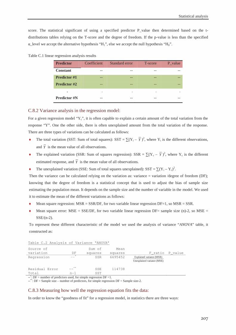
Statistical analysis

207

score. The statistical significant of using a specified predictor P_value then determined based on the t-

distributions tables relying on the T-score and the degree of freedom. If the p-value is less than the specified

α_level we accept the alternative hypothesis “H1”, else we accept the null hypothesis “H0”.

Table C.1 linear regression analysis results

Predictor Coefficient Standard error T-score P_value

Constant -- -- -- --

Predictor #1 -- -- -- --

Predictor #2 -- -- -- --

. . . . .

Predictor #N -- -- -- --

C.8.2 Variance analysis in the regression model: For a given regression model “Yc”, it is often capable to explain a certain amount of the total variation from the

response “Y”. One the other side, there is often unexplained amount from the total variation of the response.

There are three types of variations can be calculated as follows:

The total variation (SST: Sum of total squares): SST = ∑(Yi – Y )2, where Yi is the different observations,

and Y is the mean value of all observations.

The explained variation (SSR: Sum of squares regression): SSR = ∑(Yc – Y )2, where Yc is the different

estimated response, and Y is the mean value of all observations.

The unexplained variation (SSE: Sum of total squares unexplained): SST = ∑(Yi – Yc)2.

Then the variance can be calculated relying on the variation as: variance = variation /degree of freedom (DF);

knowing that the degree of freedom is a statistical concept that is used to adjust the bias of sample size

estimating the population mean. It depends on the sample size and the number of variable in the model. We used

it to estimate the mean of the different variations as follows:

Mean square regression: MSR = SSR/DF, for two variable linear regression DF=1, so MSR = SSR.

Mean square error: MSE = SSE/DF, for two variable linear regression DF= sample size (n)-2, so MSE =

SSE/(n-2).

To represent these different characteristic of the model we used the analysis of variance “ANOVA” table, it

constructed as:

Table C.2 Analysis of Variance “ANOVA”

Source of variation DF

Sum of squares

Mean squares F_ratio P_value

Regression --* SSR 6695452 (MSE) variancedUnexplaine

(MSR) varianceExplained

Residual Error --** SSE 114738 Total n-1 SST --*: DF = number of predictors used, for simple regression DF =1. --**: DF = Sample size – number of predictors, for simple regression DF = Sample size-2.

C.8.3 Measuring how well the regression equation fits the data: In order to know the “goodness of fit” for a regression model, in statistics there are three ways:

Statistical analysis

208

Coefficient of determination R2. It measures the strength of the association between the dependent and

independent variable(s), R2 [0, 100]%. R2 = 0.0, there is no linear relation between the response and the

model predictors. R2 = 100%, there is a perfect linear relation between the response and the model

predictors. Therefore, if R2 is close to 100%, it means that the regression relation fits the data at a level of

R2. It can be computed as R2 =100 SSR/SST, so R2 = 80% means that 80% of the variation in the response

observations has been explained by the predicted function. There is another form to calculate R2 based on

the SSE, as: R2 =100 (SST-SSE)/SST. We can also compute the adjusted R2 based on the variance instead

of the variation: R2adjusted = 100 (MST-MSE)/MST, where MST = SST/Degrees of freedom. Using adjusted

R2adjusted is useful especially for small size observations, where for small sample size R2 seems to be an

optimistic over estimation of the real value.

Standard error of the estimate (S): it measures the accuracy of the regression equation. It represents the

variability of observations around the regression line. Such that, for each value of the independent variable

there is an array of possible response, which is normally distributed around the response line. The mean of

this distribution (located on the regression line) is one of the regression points corresponding to these

independent variables. The interpretation of S is similar to the interpretation of the standard deviation of the

normal distribution curve: Yc = S (contains approximately 68% of the total observations of Yi); Yc = 2S

(contains approximately 95% of the total observations of Yi); Yc =3S (contains approximately 99% of the

total observations of Yi). This standard deviation is calculated as the root square of “MSE”: S = MSE .

F_ratio for the significant of the regression equation: by using the f-distribution and assuming that the

variance of both observed and estimated responses are equals. One can used the F-ratio or the associated P-

value to decide the significant of the regression model to explain the variance in the response. The

hypothesis test: H0: the linear regression function is not significant in explaining the response so all

predictors have a coefficient equals zero. And H1: the linear regression function has at least one significant

predictor to explain the variance in the response with a confidence level = 1-P_value. Therefore, for a

specified confidence level (= 1- α_level), and based on the estimated P-value, we can accept or reject the

significant of the regression function. If P-value < α_level, we reject H0 and accept H1. The selection of the

significant level “α_level”is a management decision. That is, the management decide the level of risk

associated with an estimate function, which it will be accept. The common value is α_level = 0.05,

corresponding to a confidence level of 95%. The large value of the F-ratio gives evidence towards the

alternate hypothesis H1. The corresponding probability P_value can be calculated based on F-ratio and the

degrees of freedom (table C.2) by using the f-distribution tables.

C.9 Box-Behnken design: As described by Dean and Voss (1998) the box-behnken design is a one of a second-order response models,

simply it can be graphically represented as in Figure C.3-(a). As we can see there are 13 different treatments

conditions for three factors with only one central point. To calculate this number of treatments, first we should

know that the Box-Behnken designed based on only three levels to each factor, these three levels are the

minimum, centre, and maximum values. The matrix representation of these iterations can be represented as

shown in Figure C.3-(b), taking into account that (+1) represents the maximum extreme point of the factor, (–1)

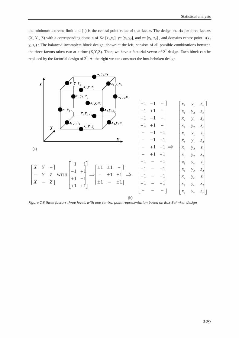
Statistical analysis

209

the minimum extreme limit and (–) is the central point value of that factor. The design matrix for three factors

(X, Y , Z) with a corresponding domain of X [x1,x2], y [y1,y2], and z [z1, z2] , and domains centre point is(xc

yc zc) : The balanced incomplete block design, shown at the left, consists of all possible combinations between

the three factors taken two at a time (X,Y,Z). Then, we have a factorial vector of 22 design. Each block can be

replaced by the factorial design of 22. At the right we can construct the box-behnken design.

(a)

1111111111111111

11111111

ccc

c

c

c

c

c

c

c

c

c

c

c

c

zyxzyxzyxzyxzyxzyxzyxzyxzyxzyxzyxzyxzyx

22

12

21

11

22

12

21

11

22

12

21

11

ZXZY

YX WITH

11111111

1111

11

(b) Figure C.3 three factors three levels with one central point representation based on Box-Behnken design

Statistical analysis

210

RESULTS OF SIMULATIONS

APP

END

IX

D

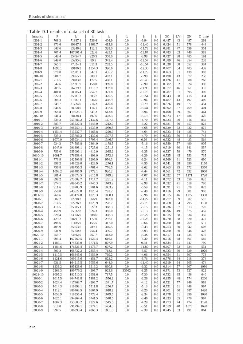
Results of simulations

212

Table D.1 results of data set of 30 tasks Instance F f1 f2 f3 f4 f5 f6 OC LV GN C_time j301-1 708.3 71387.1 536.6 408.9 0.0 -9.94 0.0 0.487 43 497 261 j301-2 870.6 89867.9 1869.7 415.6 0.0 -11.40 0.0 0.424 51 578 444 j301-3 643.6 63246.6 112.1 328.0 0.0 -11.78 0.0 0.381 47 599 351 j301-4 707.4 107001.4 622.6 425.1 0.0 -13.87 0.0 0.483 63 440 389 j301-5 648.4 55454.7 226.5 358.6 0.0 -8.98 0.0 0.427 38 485 191 j301-6 949.0 65995.6 89.9 342.4 0.0 -12.57 0.0 0.389 46 354 233 j301-7 565.1 77024.1 611.3 283.5 0.0 -16.54 0.0 0.338 68 552 384 j301-8 1090.1 99106.3 1354.3 390.6 0.0 -12.30 0.0 0.407 64 405 439 j301-9 978.0 92501.1 342.1 435.2 0.0 -11.79 0.0 0.463 51 439 303

j301-10 981.7 69965.7 309.1 402.1 0.0 -8.99 0.0 0.490 43 372 258 j302-1 716.5 69483.8 172.5 400.1 0.0 -10.48 0.0 0.426 41 508 260 j302-2 542.6 82691.9 158.0 389.8 0.0 -9.90 0.0 0.382 52 524 390 j302-3 709.5 76779.2 1313.7 392.0 0.0 -11.95 0.0 0.377 46 361 310 j302-4 481.8 68385.4 254.7 321.8 0.0 -12.78 0.0 0.287 51 595 309 j302-5 822.3 85881.3 303.7 370.5 0.0 -15.54 0.0 0.343 58 415 334 j302-6 708.3 71387.1 536.6 408.9 0.0 -9.94 0.0 0.487 43 497 409 j302-7 649.7 81724.0 716.2 420.8 0.0 -9.79 0.0 0.376 49 577 454 j302-8 846.6 78058.0 114.1 337.4 0.0 -10.44 0.0 0.392 57 469 404 j302-9 668.8 119528.1 841.2 513.8 0.0 -8.96 0.0 0.408 59 507 464

j302-10 741.4 78128.4 497.6 403.3 0.0 -10.78 0.0 0.373 47 488 426 j3010-1 839.3 253786.2 2137.6 1307.3 0.0 -4.70 0.0 0.623 50 516 835 j3010-2 883.7 285222.4 5245.0 1212.0 0.0 -3.22 0.0 0.681 60 657 822 j3010-3 1003.3 308250.1 1939.0 1060.8 0.0 -4.68 0.0 0.639 72 432 875 j3010-4 1154.4 313237.7 5465.8 1229.9 0.0 -4.64 0.0 0.723 64 425 744 j3010-5 839.3 253786.2 2137.6 1307.3 0.0 -4.70 0.0 0.623 50 516 748 j3010-6 1070.9 265034.1 5793.4 1346.7 0.0 0.20 0.0 0.732 48 433 564 j3010-7 934.3 274586.8 2364.9 1178.5 0.0 -5.16 0.0 0.589 57 490 905 j3010-8 1047.0 291898.1 2725.6 1251.8 0.0 -4.15 0.0 0.719 60 341 557 j3010-9 753.0 255096.1 4412.0 1085.2 0.0 -6.35 0.0 0.527 59 479 570

j3010-10 1001.7 276658.4 4198.0 1572.6 0.0 -3.29 0.0 0.735 45 553 735 j3011-1 773.9 242509.8 3206.9 956.3 0.0 -6.24 0.0 0.569 61 523 690 j3011-2 899.2 348029.0 4128.9 1276.1 0.0 -4.50 0.0 0.541 68 690 1150 j3011-3 756.8 288756.3 4761.4 776.5 0.0 -8.62 0.0 0.363 95 572 1360 j3011-4 1098.2 268485.9 2772.1 920.2 0.0 -4.44 0.0 0.561 72 532 1060 j3011-5 881.4 238073.5 2615.8 1019.3 0.0 -7.07 0.0 0.622 57 1171 1720 j3011-6 899.2 273002.7 1717.7 1281.2 0.0 -4.11 0.0 0.572 53 556 820 j3011-7 974.1 289546.2 4745.3 1643.9 0.0 -2.98 0.0 0.632 41 518 780 j3011-8 911.6 310783.9 3781.6 1063.2 0.0 -6.59 0.0 0.591 71 378 823 j3011-9 750.8 245527.8 1828.4 791.2 0.0 -7.48 0.0 0.416 79 381 908

j3011-10 768.6 203174.8 1028.3 1050.1 0.0 -3.96 0.0 0.515 46 1277 1300 j3020-1 607.2 92998.3 566.9 343.0 0.0 -14.27 0.0 0.277 69 502 510 j3020-2 814.5 92226.2 1025.9 278.7 0.0 -17.70 0.0 0.268 84 795 1100 j3020-3 416.5 85605.1 522.3 368.3 0.0 -8.15 0.0 0.236 57 813 720 j3020-4 458.9 75032.8 924.3 385.0 0.0 -9.13 0.0 0.296 49 675 457 j3020-5 828.4 83966.9 888.6 308.3 0.0 -18.22 0.0 0.315 68 334 359 j3020-6 423.2 68791.3 172.0 297.1 0.0 -12.28 0.0 0.270 58 520 472 j3020-7 498.6 61185.9 155.5 317.0 0.0 -9.66 0.0 0.260 48 769 517 j3020-8 405.9 85653.6 289.1 369.5 0.0 -9.43 0.0 0.253 60 542 603 j3020-9 531.9 75960.8 756.4 390.7 0.0 -8.93 0.0 0.260 50 546 428

j3020-10 559.7 73392.0 967.7 418.0 0.0 -10.00 0.0 0.317 44 725 616 j3021-1 905.4 167960.5 1929.4 616.1 0.0 -8.30 0.0 0.716 68 361 586 j3021-2 1187.1 174835.0 3771.5 807.9 0.0 0.78 0.0 0.824 51 647 790 j3021-3 1184.6 176821.4 1478.7 607.2 0.0 -11.80 0.0 0.607 72 334 551 j3021-4 890.3 168732.2 2853.4 718.1 0.0 -8.57 0.0 0.733 60 639 1020 j3021-5 1110.5 166345.6 3456.9 769.2 0.0 -4.06 0.0 0.754 51 307 773 j3021-6 1121.6 209913.6 4151.7 822.2 0.0 -3.76 0.0 0.776 64 218 374 j3021-7 931.5 164213.5 3055.6 644.0 0.0 -11.40 0.0 0.619 64 605 474 j3021-8 1233.2 195128.6 3219.2 830.8 0.0 -6.32 0.0 0.814 57 607 1080 j3021-9 2268.3 199779.2 4208.7 923.6 33962 -1.25 0.0 0.871 53 527 822

j3021-10 1095.2 182510.3 2951.6 717.5 0.0 -7.30 0.0 0.732 65 456 640 j3030-1 1015.5 304741.8 5181.2 1556.2 0.0 -2.26 0.0 0.855 48 574 1200 j3030-2 1024.4 417463.7 4209.7 1341.7 0.0 -4.12 0.0 0.721 77 346 988 j3030-3 1014.3 319993.1 5511.8 1256.7 0.0 -5.13 0.0 0.731 61 448 997 j3030-4 1112.1 380463.5 6667.9 1618.2 0.0 -3.20 0.0 0.801 60 587 1420 j3030-5 1058.9 418555.4 5773.4 1649.5 0.0 -2.34 0.0 0.778 61 399 1090 j3030-6 1025.1 394264.4 6741.5 1548.5 0.0 -3.46 0.0 0.833 65 470 997 j3030-7 1007.3 453608.2 7327.6 1545.6 0.0 -4.29 0.0 0.773 74 474 1120 j3030-8 910.8 291794.1 5974.1 1484.8 0.0 -3.51 0.0 0.619 48 1070 1620 j3030-9 997.5 386393.4 4865.3 1801.8 0.0 -2.39 0.0 0.745 53 491 864

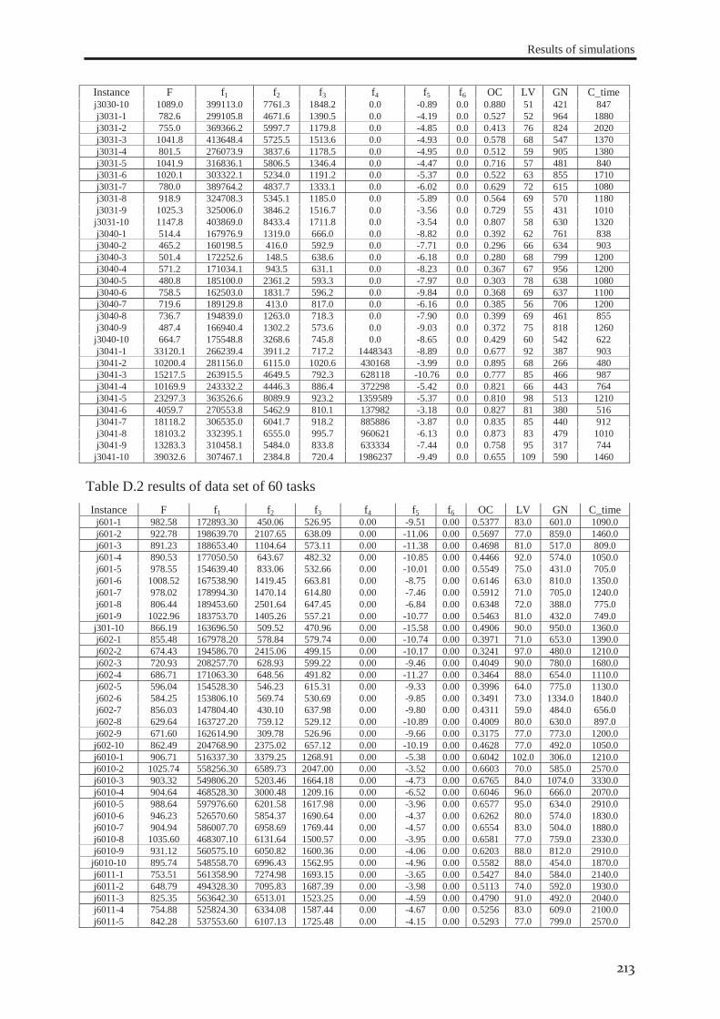
Results of simulations

213

Instance F f1 f2 f3 f4 f5 f6 OC LV GN C_time j3030-10 1089.0 399113.0 7761.3 1848.2 0.0 -0.89 0.0 0.880 51 421 847 j3031-1 782.6 299105.8 4671.6 1390.5 0.0 -4.19 0.0 0.527 52 964 1880 j3031-2 755.0 369366.2 5997.7 1179.8 0.0 -4.85 0.0 0.413 76 824 2020 j3031-3 1041.8 413648.4 5725.5 1513.6 0.0 -4.93 0.0 0.578 68 547 1370 j3031-4 801.5 276073.9 3837.6 1178.5 0.0 -4.95 0.0 0.512 59 905 1380 j3031-5 1041.9 316836.1 5806.5 1346.4 0.0 -4.47 0.0 0.716 57 481 840 j3031-6 1020.1 303322.1 5234.0 1191.2 0.0 -5.37 0.0 0.522 63 855 1710 j3031-7 780.0 389764.2 4837.7 1333.1 0.0 -6.02 0.0 0.629 72 615 1080 j3031-8 918.9 324708.3 5345.1 1185.0 0.0 -5.89 0.0 0.564 69 570 1180 j3031-9 1025.3 325006.0 3846.2 1516.7 0.0 -3.56 0.0 0.729 55 431 1010

j3031-10 1147.8 403869.0 8433.4 1711.8 0.0 -3.54 0.0 0.807 58 630 1320 j3040-1 514.4 167976.9 1319.0 666.0 0.0 -8.82 0.0 0.392 62 761 838 j3040-2 465.2 160198.5 416.0 592.9 0.0 -7.71 0.0 0.296 66 634 903 j3040-3 501.4 172252.6 148.5 638.6 0.0 -6.18 0.0 0.280 68 799 1200 j3040-4 571.2 171034.1 943.5 631.1 0.0 -8.23 0.0 0.367 67 956 1200 j3040-5 480.8 185100.0 2361.2 593.3 0.0 -7.97 0.0 0.303 78 638 1080 j3040-6 758.5 162503.0 1831.7 596.2 0.0 -9.84 0.0 0.368 69 637 1100 j3040-7 719.6 189129.8 413.0 817.0 0.0 -6.16 0.0 0.385 56 706 1200 j3040-8 736.7 194839.0 1263.0 718.3 0.0 -7.90 0.0 0.399 69 461 855 j3040-9 487.4 166940.4 1302.2 573.6 0.0 -9.03 0.0 0.372 75 818 1260

j3040-10 664.7 175548.8 3268.6 745.8 0.0 -8.65 0.0 0.429 60 542 622 j3041-1 33120.1 266239.4 3911.2 717.2 1448343 -8.89 0.0 0.677 92 387 903 j3041-2 10200.4 281156.0 6115.0 1020.6 430168 -3.99 0.0 0.895 68 266 480 j3041-3 15217.5 263915.5 4649.5 792.3 628118 -10.76 0.0 0.777 85 466 987 j3041-4 10169.9 243332.2 4446.3 886.4 372298 -5.42 0.0 0.821 66 443 764 j3041-5 23297.3 363526.6 8089.9 923.2 1359589 -5.37 0.0 0.810 98 513 1210 j3041-6 4059.7 270553.8 5462.9 810.1 137982 -3.18 0.0 0.827 81 380 516 j3041-7 18118.2 306535.0 6041.7 918.2 885886 -3.87 0.0 0.835 85 440 912 j3041-8 18103.2 332395.1 6555.0 995.7 960621 -6.13 0.0 0.873 83 479 1010 j3041-9 13283.3 310458.1 5484.0 833.8 633334 -7.44 0.0 0.758 95 317 744

j3041-10 39032.6 307467.1 2384.8 720.4 1986237 -9.49 0.0 0.655 109 590 1460

Table D.2 results of data set of 60 tasks Instance F f1 f2 f3 f4 f5 f6 OC LV GN C_time

j601-1 982.58 172893.30 450.06 526.95 0.00 -9.51 0.00 0.5377 83.0 601.0 1090.0 j601-2 922.78 198639.70 2107.65 638.09 0.00 -11.06 0.00 0.5697 77.0 859.0 1460.0 j601-3 891.23 188653.40 1104.64 573.11 0.00 -11.38 0.00 0.4698 81.0 517.0 809.0 j601-4 890.53 177050.50 643.67 482.32 0.00 -10.85 0.00 0.4466 92.0 574.0 1050.0 j601-5 978.55 154639.40 833.06 532.66 0.00 -10.01 0.00 0.5549 75.0 431.0 705.0 j601-6 1008.52 167538.90 1419.45 663.81 0.00 -8.75 0.00 0.6146 63.0 810.0 1350.0 j601-7 978.02 178994.30 1470.14 614.80 0.00 -7.46 0.00 0.5912 71.0 705.0 1240.0 j601-8 806.44 189453.60 2501.64 647.45 0.00 -6.84 0.00 0.6348 72.0 388.0 775.0 j601-9 1022.96 183753.70 1405.26 557.21 0.00 -10.77 0.00 0.5463 81.0 432.0 749.0

j301-10 866.19 163696.50 509.52 470.96 0.00 -15.58 0.00 0.4906 90.0 950.0 1360.0 j602-1 855.48 167978.20 578.84 579.74 0.00 -10.74 0.00 0.3971 71.0 653.0 1390.0 j602-2 674.43 194586.70 2415.06 499.15 0.00 -10.17 0.00 0.3241 97.0 480.0 1210.0 j602-3 720.93 208257.70 628.93 599.22 0.00 -9.46 0.00 0.4049 90.0 780.0 1680.0 j602-4 686.71 171063.30 648.56 491.82 0.00 -11.27 0.00 0.3464 88.0 654.0 1110.0 j602-5 596.04 154528.30 546.23 615.31 0.00 -9.33 0.00 0.3996 64.0 775.0 1130.0 j602-6 584.25 153806.10 569.74 530.69 0.00 -9.85 0.00 0.3491 73.0 1334.0 1840.0 j602-7 856.03 147804.40 430.10 637.98 0.00 -9.80 0.00 0.4311 59.0 484.0 656.0 j602-8 629.64 163727.20 759.12 529.12 0.00 -10.89 0.00 0.4009 80.0 630.0 897.0 j602-9 671.60 162614.90 309.78 526.96 0.00 -9.66 0.00 0.3175 77.0 773.0 1200.0

j602-10 862.49 204768.90 2375.02 657.12 0.00 -10.19 0.00 0.4628 77.0 492.0 1050.0 j6010-1 906.71 516337.30 3379.25 1268.91 0.00 -5.38 0.00 0.6042 102.0 306.0 1210.0 j6010-2 1025.74 558256.30 6589.73 2047.00 0.00 -3.52 0.00 0.6603 70.0 585.0 2570.0 j6010-3 903.32 549806.20 5203.46 1664.18 0.00 -4.73 0.00 0.6765 84.0 1074.0 3330.0 j6010-4 904.64 468528.30 3000.48 1209.16 0.00 -6.52 0.00 0.6046 96.0 666.0 2070.0 j6010-5 988.64 597976.60 6201.58 1617.98 0.00 -3.96 0.00 0.6577 95.0 634.0 2910.0 j6010-6 946.23 526570.60 5854.37 1690.64 0.00 -4.37 0.00 0.6262 80.0 574.0 1830.0 j6010-7 904.94 586007.70 6958.69 1769.44 0.00 -4.57 0.00 0.6554 83.0 504.0 1880.0 j6010-8 1035.60 468307.10 6131.64 1500.57 0.00 -3.95 0.00 0.6581 77.0 759.0 2330.0 j6010-9 931.12 560575.10 6050.82 1600.36 0.00 -4.06 0.00 0.6203 88.0 812.0 2910.0

j6010-10 895.74 548558.70 6996.43 1562.95 0.00 -4.96 0.00 0.5582 88.0 454.0 1870.0 j6011-1 753.51 561358.90 7274.98 1693.15 0.00 -3.65 0.00 0.5427 84.0 584.0 2140.0 j6011-2 648.79 494328.30 7095.83 1687.39 0.00 -3.98 0.00 0.5113 74.0 592.0 1930.0 j6011-3 825.35 563642.30 6513.01 1523.25 0.00 -4.59 0.00 0.4790 91.0 492.0 2040.0 j6011-4 754.88 525824.30 6334.08 1587.44 0.00 -4.67 0.00 0.5256 83.0 609.0 2100.0 j6011-5 842.28 537553.60 6107.13 1725.48 0.00 -4.15 0.00 0.5293 77.0 799.0 2570.0

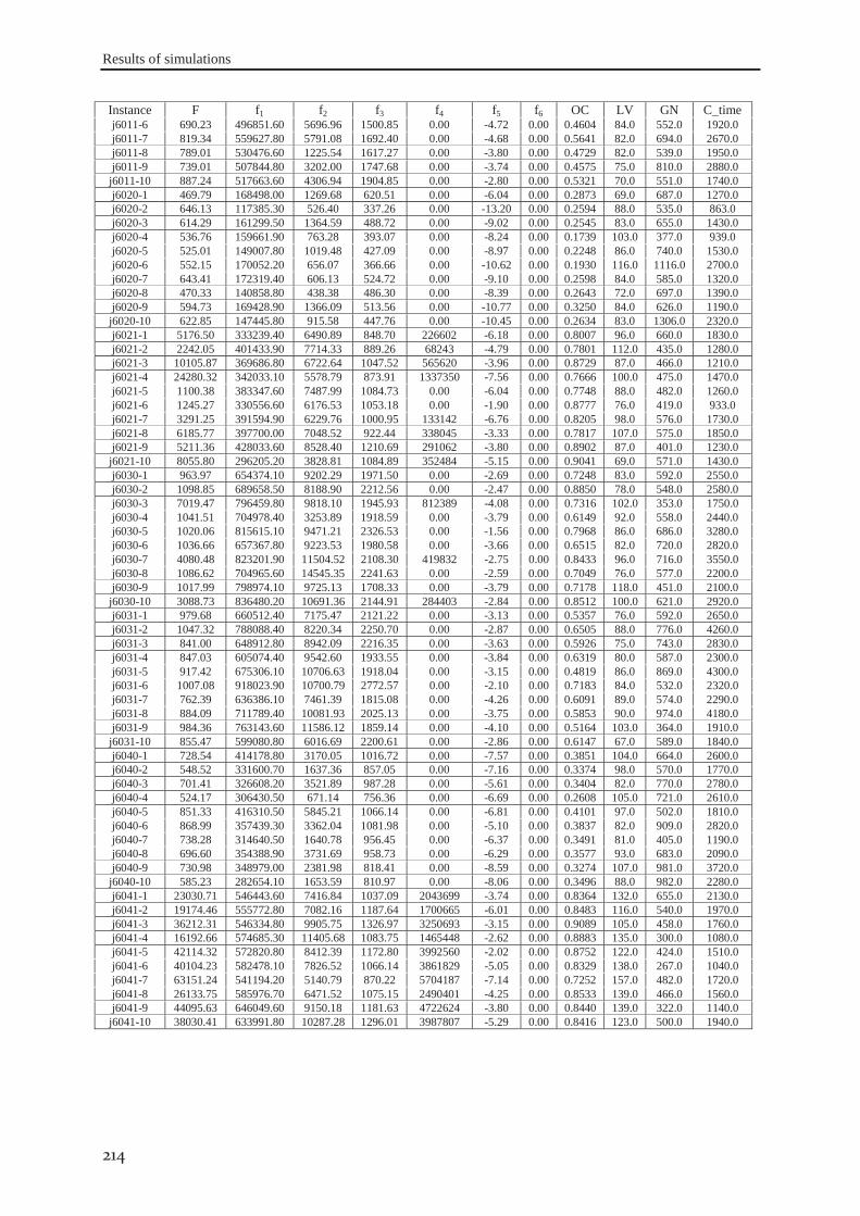
Results of simulations

214

Instance F f1 f2 f3 f4 f5 f6 OC LV GN C_time j6011-6 690.23 496851.60 5696.96 1500.85 0.00 -4.72 0.00 0.4604 84.0 552.0 1920.0 j6011-7 819.34 559627.80 5791.08 1692.40 0.00 -4.68 0.00 0.5641 82.0 694.0 2670.0 j6011-8 789.01 530476.60 1225.54 1617.27 0.00 -3.80 0.00 0.4729 82.0 539.0 1950.0 j6011-9 739.01 507844.80 3202.00 1747.68 0.00 -3.74 0.00 0.4575 75.0 810.0 2880.0

j6011-10 887.24 517663.60 4306.94 1904.85 0.00 -2.80 0.00 0.5321 70.0 551.0 1740.0 j6020-1 469.79 168498.00 1269.68 620.51 0.00 -6.04 0.00 0.2873 69.0 687.0 1270.0 j6020-2 646.13 117385.30 526.40 337.26 0.00 -13.20 0.00 0.2594 88.0 535.0 863.0 j6020-3 614.29 161299.50 1364.59 488.72 0.00 -9.02 0.00 0.2545 83.0 655.0 1430.0 j6020-4 536.76 159661.90 763.28 393.07 0.00 -8.24 0.00 0.1739 103.0 377.0 939.0 j6020-5 525.01 149007.80 1019.48 427.09 0.00 -8.97 0.00 0.2248 86.0 740.0 1530.0 j6020-6 552.15 170052.20 656.07 366.66 0.00 -10.62 0.00 0.1930 116.0 1116.0 2700.0 j6020-7 643.41 172319.40 606.13 524.72 0.00 -9.10 0.00 0.2598 84.0 585.0 1320.0 j6020-8 470.33 140858.80 438.38 486.30 0.00 -8.39 0.00 0.2643 72.0 697.0 1390.0 j6020-9 594.73 169428.90 1366.09 513.56 0.00 -10.77 0.00 0.3250 84.0 626.0 1190.0

j6020-10 622.85 147445.80 915.58 447.76 0.00 -10.45 0.00 0.2634 83.0 1306.0 2320.0 j6021-1 5176.50 333239.40 6490.89 848.70 226602 -6.18 0.00 0.8007 96.0 660.0 1830.0 j6021-2 2242.05 401433.90 7714.33 889.26 68243 -4.79 0.00 0.7801 112.0 435.0 1280.0 j6021-3 10105.87 369686.80 6722.64 1047.52 565620 -3.96 0.00 0.8729 87.0 466.0 1210.0 j6021-4 24280.32 342033.10 5578.79 873.91 1337350 -7.56 0.00 0.7666 100.0 475.0 1470.0 j6021-5 1100.38 383347.60 7487.99 1084.73 0.00 -6.04 0.00 0.7748 88.0 482.0 1260.0 j6021-6 1245.27 330556.60 6176.53 1053.18 0.00 -1.90 0.00 0.8777 76.0 419.0 933.0 j6021-7 3291.25 391594.90 6229.76 1000.95 133142 -6.76 0.00 0.8205 98.0 576.0 1730.0 j6021-8 6185.77 397700.00 7048.52 922.44 338045 -3.33 0.00 0.7817 107.0 575.0 1850.0 j6021-9 5211.36 428033.60 8528.40 1210.69 291062 -3.80 0.00 0.8902 87.0 401.0 1230.0

j6021-10 8055.80 296205.20 3828.81 1084.89 352484 -5.15 0.00 0.9041 69.0 571.0 1430.0 j6030-1 963.97 654374.10 9202.29 1971.50 0.00 -2.69 0.00 0.7248 83.0 592.0 2550.0 j6030-2 1098.85 689658.50 8188.90 2212.56 0.00 -2.47 0.00 0.8850 78.0 548.0 2580.0 j6030-3 7019.47 796459.80 9818.10 1945.93 812389 -4.08 0.00 0.7316 102.0 353.0 1750.0 j6030-4 1041.51 704978.40 3253.89 1918.59 0.00 -3.79 0.00 0.6149 92.0 558.0 2440.0 j6030-5 1020.06 815615.10 9471.21 2326.53 0.00 -1.56 0.00 0.7968 86.0 686.0 3280.0 j6030-6 1036.66 657367.80 9223.53 1980.58 0.00 -3.66 0.00 0.6515 82.0 720.0 2820.0 j6030-7 4080.48 823201.90 11504.52 2108.30 419832 -2.75 0.00 0.8433 96.0 716.0 3550.0 j6030-8 1086.62 704965.60 14545.35 2241.63 0.00 -2.59 0.00 0.7049 76.0 577.0 2200.0 j6030-9 1017.99 798974.10 9725.13 1708.33 0.00 -3.79 0.00 0.7178 118.0 451.0 2100.0

j6030-10 3088.73 836480.20 10691.36 2144.91 284403 -2.84 0.00 0.8512 100.0 621.0 2920.0 j6031-1 979.68 660512.40 7175.47 2121.22 0.00 -3.13 0.00 0.5357 76.0 592.0 2650.0 j6031-2 1047.32 788088.40 8220.34 2250.70 0.00 -2.87 0.00 0.6505 88.0 776.0 4260.0 j6031-3 841.00 648912.80 8942.09 2216.35 0.00 -3.63 0.00 0.5926 75.0 743.0 2830.0 j6031-4 847.03 605074.40 9542.60 1933.55 0.00 -3.84 0.00 0.6319 80.0 587.0 2300.0 j6031-5 917.42 675306.10 10706.63 1918.04 0.00 -3.15 0.00 0.4819 86.0 869.0 4300.0 j6031-6 1007.08 918023.90 10700.79 2772.57 0.00 -2.10 0.00 0.7183 84.0 532.0 2320.0 j6031-7 762.39 636386.10 7461.39 1815.08 0.00 -4.26 0.00 0.6091 89.0 574.0 2290.0 j6031-8 884.09 711789.40 10081.93 2025.13 0.00 -3.75 0.00 0.5853 90.0 974.0 4180.0 j6031-9 984.36 763143.60 11586.12 1859.14 0.00 -4.10 0.00 0.5164 103.0 364.0 1910.0

j6031-10 855.47 599080.80 6016.69 2200.61 0.00 -2.86 0.00 0.6147 67.0 589.0 1840.0 j6040-1 728.54 414178.80 3170.05 1016.72 0.00 -7.57 0.00 0.3851 104.0 664.0 2600.0 j6040-2 548.52 331600.70 1637.36 857.05 0.00 -7.16 0.00 0.3374 98.0 570.0 1770.0 j6040-3 701.41 326608.20 3521.89 987.28 0.00 -5.61 0.00 0.3404 82.0 770.0 2780.0 j6040-4 524.17 306430.50 671.14 756.36 0.00 -6.69 0.00 0.2608 105.0 721.0 2610.0 j6040-5 851.33 416310.50 5845.21 1066.14 0.00 -6.81 0.00 0.4101 97.0 502.0 1810.0 j6040-6 868.99 357439.30 3362.04 1081.98 0.00 -5.10 0.00 0.3837 82.0 909.0 2820.0 j6040-7 738.28 314640.50 1640.78 956.45 0.00 -6.37 0.00 0.3491 81.0 405.0 1190.0 j6040-8 696.60 354388.90 3731.69 958.73 0.00 -6.29 0.00 0.3577 93.0 683.0 2090.0 j6040-9 730.98 348979.00 2381.98 818.41 0.00 -8.59 0.00 0.3274 107.0 981.0 3720.0

j6040-10 585.23 282654.10 1653.59 810.97 0.00 -8.06 0.00 0.3496 88.0 982.0 2280.0 j6041-1 23030.71 546443.60 7416.84 1037.09 2043699 -3.74 0.00 0.8364 132.0 655.0 2130.0 j6041-2 19174.46 555772.80 7082.16 1187.64 1700665 -6.01 0.00 0.8483 116.0 540.0 1970.0 j6041-3 36212.31 546334.80 9905.75 1326.97 3250693 -3.15 0.00 0.9089 105.0 458.0 1760.0 j6041-4 16192.66 574685.30 11405.68 1083.75 1465448 -2.62 0.00 0.8883 135.0 300.0 1080.0 j6041-5 42114.32 572820.80 8412.39 1172.80 3992560 -2.02 0.00 0.8752 122.0 424.0 1510.0 j6041-6 40104.23 582478.10 7826.52 1066.14 3861829 -5.05 0.00 0.8329 138.0 267.0 1040.0 j6041-7 63151.24 541194.20 5140.79 870.22 5704187 -7.14 0.00 0.7252 157.0 482.0 1720.0 j6041-8 26133.75 585976.70 6471.52 1075.15 2490401 -4.25 0.00 0.8533 139.0 466.0 1560.0 j6041-9 44095.63 646049.60 9150.18 1181.63 4722624 -3.80 0.00 0.8440 139.0 322.0 1140.0

j6041-10 38030.41 633991.80 10287.28 1296.01 3987807 -5.29 0.00 0.8416 123.0 500.0 1940.0

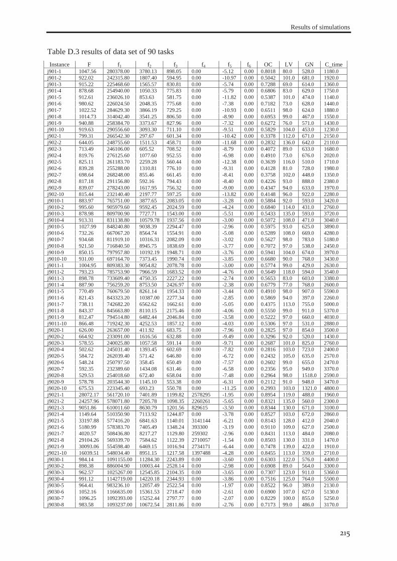
Results of simulations

215

Table D.3 results of data set of 90 tasks Instance F f1 f2 f3 f4 f5 f6 OC LV GN C_time

j901-1 1047.56 280378.00 3780.13 898.05 0.00 -5.12 0.00 0.8018 80.0 528.0 1180.0 j901-2 922.02 242315.80 1807.40 594.95 0.00 -10.97 0.00 0.5042 101.0 681.0 1920.0 j901-3 915.22 225468.60 1565.57 830.81 0.00 -5.74 0.00 0.7288 69.0 614.0 1360.0 j901-4 878.68 254940.00 1050.33 775.83 0.00 -5.79 0.00 0.6806 83.0 629.0 1750.0 j901-5 912.61 236026.10 853.63 581.75 0.00 -11.82 0.00 0.5387 101.0 474.0 1140.0 j901-6 980.62 226024.50 2048.35 775.68 0.00 -7.38 0.00 0.7182 73.0 628.0 1440.0 j901-7 1022.52 284629.30 3866.19 729.25 0.00 -10.93 0.00 0.6511 98.0 624.0 1880.0 j901-8 1014.73 314042.40 3541.25 806.50 0.00 -8.90 0.00 0.6953 99.0 467.0 1550.0 j901-9 940.88 258384.70 3373.67 827.96 0.00 -7.32 0.00 0.6272 76.0 571.0 1430.0 j901-10 919.63 290556.60 3093.30 711.10 0.00 -9.51 0.00 0.5829 104.0 453.0 1230.0 j902-1 799.31 266542.30 297.67 601.34 0.00 -10.42 0.00 0.3378 112.0 671.0 2150.0 j902-2 644.05 248755.60 1511.53 458.71 0.00 -11.68 0.00 0.2832 136.0 642.0 2110.0 j902-3 713.49 246106.00 605.52 708.52 0.00 -8.79 0.00 0.4072 89.0 633.0 1680.0 j902-4 819.76 276125.60 1077.60 952.55 0.00 -6.98 0.00 0.4910 73.0 676.0 2020.0 j902-5 825.11 261183.70 2259.28 560.44 0.00 -12.38 0.00 0.3639 116.0 510.0 1710.0 j902-6 839.28 255288.00 1310.81 776.10 0.00 -9.31 0.00 0.4128 81.0 728.0 1980.0 j902-7 698.64 268248.00 855.46 661.45 0.00 -8.41 0.00 0.3758 102.0 448.0 1350.0 j902-8 817.18 291156.80 592.16 794.43 0.00 -8.40 0.00 0.4226 93.0 888.0 2380.0 j902-9 839.07 278243.00 1617.95 756.32 0.00 -9.00 0.00 0.4347 94.0 633.0 1970.0 j902-10 815.44 232140.40 2197.77 597.25 0.00 -13.82 0.00 0.4148 96.0 922.0 2280.0 j9010-1 883.97 765751.00 3877.65 2083.05 0.00 -3.28 0.00 0.5884 92.0 593.0 3420.0 j9010-2 995.60 905979.60 9592.45 2024.59 0.00 -4.24 0.00 0.6840 114.0 431.0 2760.0 j9010-3 878.98 809700.90 7727.71 1543.00 0.00 -5.51 0.00 0.5433 135.0 593.0 3720.0 j9010-4 913.31 831138.80 10579.78 1937.56 0.00 -3.00 0.00 0.5072 108.0 471.0 3040.0 j9010-5 1027.99 848240.80 9038.39 2294.47 0.00 -2.96 0.00 0.5975 93.0 625.0 3890.0 j9010-6 732.26 667067.20 8564.74 1554.91 0.00 -5.08 0.00 0.5289 108.0 669.0 4280.0 j9010-7 934.68 811919.10 10316.31 2082.09 0.00 -3.02 0.00 0.5627 98.0 783.0 5180.0 j9010-8 921.50 716840.50 8945.75 1838.69 0.00 -3.77 0.00 0.7072 97.0 538.0 2450.0 j9010-9 850.15 797957.80 10192.19 1948.71 0.00 -3.76 0.00 0.5941 104.0 674.0 3970.0 j9010-10 931.00 697164.70 7373.45 1990.74 0.00 -3.85 0.00 0.6680 90.0 768.0 3430.0 j9011-1 1004.95 809383.30 9054.82 2078.78 0.00 -3.00 0.00 0.5774 99.0 429.0 2630.0 j9011-2 793.23 785753.90 7966.59 1683.52 0.00 -4.76 0.00 0.5649 118.0 594.0 3540.0 j9011-3 898.78 733609.40 4750.35 2227.22 0.00 -2.74 0.00 0.5653 83.0 603.0 3380.0 j9011-4 887.90 756259.20 8753.50 2426.97 0.00 -2.38 0.00 0.6779 77.0 768.0 2600.0 j9011-5 770.49 760679.50 8261.14 1954.33 0.00 -3.44 0.00 0.4910 98.0 907.0 5590.0 j9011-6 821.43 843323.20 10387.00 2277.34 0.00 -2.85 0.00 0.5869 94.0 397.0 2260.0 j9011-7 738.11 742682.20 6562.62 1662.61 0.00 -5.05 0.00 0.4375 113.0 755.0 5000.0 j9011-8 843.37 845663.80 8110.15 2175.46 0.00 -4.06 0.00 0.5550 99.0 911.0 5370.0 j9011-9 812.47 794514.80 6482.44 2046.84 0.00 -3.58 0.00 0.5222 97.0 660.0 4030.0 j9011-10 866.48 719242.30 4252.53 1857.12 0.00 -4.03 0.00 0.5306 97.0 531.0 2880.0 j9020-1 626.00 263657.00 411.92 683.75 0.00 -7.96 0.00 0.2825 97.0 854.0 3500.0 j9020-2 664.92 233091.00 1616.56 632.88 0.00 -9.49 0.00 0.3296 92.0 520.0 1430.0 j9020-3 578.55 240025.80 1057.58 591.14 0.00 -9.71 0.00 0.2687 101.0 825.0 2760.0 j9020-4 502.62 245031.40 1393.45 602.69 0.00 -7.82 0.00 0.2816 103.0 723.0 2400.0 j9020-5 584.72 262039.40 571.42 646.80 0.00 -6.72 0.00 0.2432 105.0 635.0 2570.0 j9020-6 548.24 250797.50 358.45 650.49 0.00 -7.57 0.00 0.2602 99.0 655.0 2470.0 j9020-7 592.35 232389.60 1434.08 631.46 0.00 -6.58 0.00 0.2356 95.0 949.0 3370.0 j9020-8 529.53 254018.60 672.40 658.04 0.00 -7.48 0.00 0.2964 98.0 1518.0 2590.0 j9020-9 578.78 203544.30 1145.10 553.38 0.00 -6.31 0.00 0.2112 91.0 948.0 3470.0 j9020-10 675.53 223345.40 693.23 550.78 0.00 -11.25 0.00 0.2993 103.0 1321.0 4800.0 j9021-1 28072.17 561720.10 7401.89 1199.82 2578295 -1.95 0.00 0.8954 119.0 488.0 1960.0 j9021-2 24257.96 578071.80 7205.78 1098.35 2260261 -5.65 0.00 0.8321 135.0 560.0 2300.0 j9021-3 9051.86 610011.60 8630.79 1201.56 829615 -3.50 0.00 0.8344 130.0 671.0 3100.0 j9021-4 1149.64 510350.90 7113.92 1244.87 0.00 -3.78 0.00 0.8527 103.0 672.0 2860.0 j9021-5 33197.88 577416.20 6841.63 1140.01 3141144 -6.21 0.00 0.8143 128.0 412.0 2040.0 j9021-6 5180.99 578383.70 7405.49 1348.24 393300 -3.19 0.00 0.9110 109.0 627.0 2500.0 j9021-7 4020.57 508436.80 8217.27 1129.80 259302 -2.96 0.00 0.8431 113.0 484.0 2080.0 j9021-8 29104.26 569339.70 7584.62 1122.39 2710057 -1.54 0.00 0.8503 130.0 331.0 1470.0 j9021-9 30093.06 554598.40 6469.15 1016.94 2734171 -6.44 0.00 0.7478 139.0 422.0 1910.0 j9021-10 16039.51 548034.40 8951.15 1217.58 1397488 -4.28 0.00 0.8455 113.0 359.0 2710.0 j9030-1 984.14 1091155.00 11284.30 2243.89 0.00 -3.60 0.00 0.6303 122.0 576.0 4400.0 j9030-2 898.38 886004.90 10003.44 2528.14 0.00 -2.98 0.00 0.6908 89.0 564.0 3300.0 j9030-3 962.57 1025267.00 12545.85 2104.35 0.00 -3.65 0.00 0.7307 123.0 911.0 5360.0 j9030-4 991.12 1142719.00 14220.18 2344.93 0.00 -3.86 0.00 0.7516 125.0 764.0 5500.0 j9030-5 964.41 983236.10 12057.49 2522.54 0.00 -1.97 0.00 0.8522 96.0 389.0 2130.0 j9030-6 1052.16 1166635.00 15361.53 2718.47 0.00 -2.61 0.00 0.6900 107.0 627.0 5130.0 j9030-7 1096.25 1092393.00 15252.44 2797.77 0.00 -2.07 0.00 0.8229 100.0 855.0 5250.0 j9030-8 983.58 1093237.00 10672.54 2811.86 0.00 -2.76 0.00 0.7173 99.0 486.0 3170.0

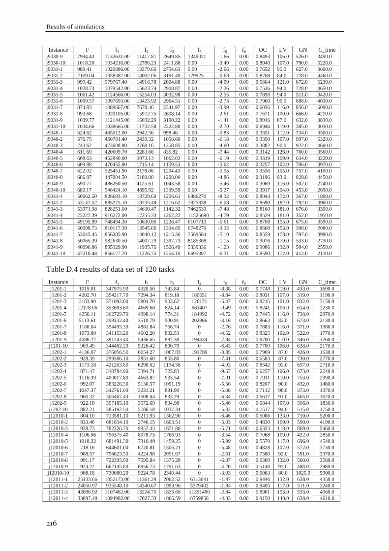
Results of simulations

216

Instance F f1 f2 f3 f4 f5 f6 OC LV GN C_time j9030-9 7994.43 1133631.00 11417.81 2649.85 1349021 -1.66 0.00 0.8493 106.0 526.0 3490.0 j9030-10 1018.20 1034216.00 12786.23 2411.88 0.00 -3.40 0.00 0.8040 107.0 790.0 5220.0 j9031-1 989.41 1020886.00 13379.66 2754.63 0.00 -2.66 0.00 0.7652 95.0 627.0 3600.0 j9031-2 2109.04 1058387.00 14002.06 3191.40 179925 -0.68 0.00 0.8768 84.0 778.0 4460.0 j9031-3 999.42 979767.40 14916.78 2004.88 0.00 -4.09 0.00 0.5664 121.0 672.0 5230.0 j9031-4 1028.73 1079542.00 15623.74 2908.87 0.00 -2.26 0.00 0.7536 94.0 728.0 4650.0 j9031-5 1061.42 1124566.00 15254.03 3032.98 0.00 -2.55 0.00 0.7898 94.0 511.0 3420.0 j9031-6 1099.57 1097693.00 13423.92 2964.51 0.00 -2.73 0.00 0.7969 95.0 888.0 4030.0 j9031-7 874.83 1089667.00 7678.46 2341.97 0.00 -3.99 0.00 0.6036 116.0 856.0 6090.0 j9031-8 993.68 1020105.00 15972.75 2608.14 0.00 -2.61 0.00 0.7671 100.0 666.0 4210.0 j9031-9 1039.77 1121445.00 16032.29 3190.22 0.00 -1.41 0.00 0.8016 87.0 632.0 3830.0 j9031-10 1034.66 1038665.00 11732.58 2222.80 0.00 -2.70 0.00 0.6946 119.0 385.0 3030.0 j9040-1 624.62 445012.00 2942.56 998.46 0.00 -5.83 0.00 0.3351 112.0 734.0 3500.0 j9040-2 576.75 450781.40 2439.32 1058.66 0.00 -6.18 0.00 0.3350 107.0 997.0 5320.0 j9040-3 743.62 473608.80 2768.16 1358.85 0.00 -4.60 0.00 0.3882 90.0 922.0 4600.0 j9040-4 611.60 420609.70 2283.66 835.82 0.00 -7.44 0.00 0.3142 126.0 760.0 3560.0 j9040-5 608.63 452840.00 3073.13 1062.02 0.00 -6.19 0.00 0.3319 109.0 634.0 3220.0 j9040-6 609.88 470455.80 1715.14 1159.53 0.00 -5.62 0.00 0.3257 102.0 706.0 3970.0 j9040-7 622.02 525451.90 2178.06 1294.43 0.00 -5.05 0.00 0.3556 105.0 757.0 4100.0 j9040-8 686.87 447004.50 5180.00 1208.00 0.00 -4.86 0.00 0.3196 93.0 829.0 4450.0 j9040-9 590.77 486260.50 4125.61 1043.58 0.00 -5.46 0.00 0.3069 116.0 502.0 2740.0 j9040-10 682.17 546424.10 4895.92 1339.59 0.00 -5.27 0.00 0.3917 104.0 453.0 2690.0 j9041-1 50062.50 826683.10 13729.60 1206.61 6886270 -8.32 0.00 0.8044 172.0 367.0 1890.0 j9041-2 53147.52 885275.10 18735.49 1216.62 7825838 -6.08 0.00 0.8690 182.0 792.0 3960.0 j9041-3 53971.98 828251.00 14630.47 1142.32 7462539 -7.48 0.00 0.8160 181.0 676.0 3390.0 j9041-4 75227.39 916272.00 17255.33 1262.22 11526690 -4.79 0.00 0.8529 181.0 352.0 1950.0 j9041-5 49195.99 748494.30 10630.86 1236.47 6107713 -5.61 0.00 0.8708 155.0 675.0 3590.0 j9041-6 50098.73 810117.30 13545.06 1334.85 6748279 -3.32 0.00 0.8668 153.0 398.0 2080.0 j9041-7 53045.45 856285.90 14040.12 1215.36 7569564 -5.10 0.00 0.8559 178.0 797.0 3990.0 j9041-8 50065.39 982630.50 14007.29 1397.73 8185308 -1.15 0.00 0.9076 179.0 533.0 2730.0 j9041-9 40096.86 805329.90 11935.76 1526.49 5339336 -1.23 0.00 0.9086 132.0 504.0 2550.0 j9041-10 47210.48 856177.70 11226.75 1254.10 6695307 -6.31 0.00 0.8590 172.0 412.0 2130.0

Table D.4 results of data set of 120 tasks Instance F f1 f2 f3 f4 f5 f6 OC LV GN C_time j1201-1 1019.01 347975.90 4320.50 743.84 0 -8.38 0.00 0.7748 119.0 433.0 1600.0 j1201-2 4202.70 354217.70 7294.34 819.18 180651 -8.84 0.00 0.8031 107.0 319.0 1190.0 j1201-3 3183.90 371092.00 5804.70 903.62 126171 -5.47 0.00 0.8215 101.0 832.0 3150.0 j1201-4 12178.06 353693.60 4669.60 824.14 661407 -0.49 0.00 0.8241 106.0 614.0 2230.0 j1201-5 4256.11 362729.70 4998.14 774.31 184992 -4.72 0.00 0.7445 116.0 738.0 2970.0 j1201-6 5113.61 298332.40 3510.79 900.91 202866 -3.16 0.00 0.8663 82.0 673.0 2130.0 j1201-7 1180.64 354495.30 4881.84 756.74 0 -2.76 0.00 0.7883 116.0 371.0 1380.0 j1201-8 1073.89 341153.20 4602.20 832.53 0 -4.52 0.00 0.8325 102.0 522.0 1770.0 j1201-9 4086.27 381243.40 5436.65 887.38 194434 -7.84 0.00 0.8700 110.0 346.0 1260.0

j1201-10 909.49 344462.20 5326.42 800.79 0 -6.43 0.00 0.7700 106.0 638.0 2170.0 j1202-1 4136.07 376056.50 6054.27 1067.83 191789 -3.85 0.00 0.7969 87.0 426.0 1530.0 j1202-2 928.39 299386.10 2851.60 855.80 0 -7.41 0.00 0.6583 87.0 730.0 2770.0 j1202-3 1173.18 421263.80 6298.62 1134.56 0 -4.03 0.00 0.8342 92.0 657.0 2710.0 j1202-4 871.47 310784.90 3394.71 725.83 0 -9.67 0.00 0.6257 106.0 673.0 2240.0 j1202-5 1116.39 400017.80 4663.87 933.54 0 -7.01 0.00 0.7911 110.0 753.0 2990.0 j1202-6 992.07 383226.30 5130.57 1091.19 0 -5.56 0.00 0.8267 90.0 432.0 1480.0 j1202-7 1047.37 342761.00 3231.21 881.90 0 -5.48 0.00 0.7112 98.0 373.0 1370.0 j1202-8 960.32 306467.40 1508.64 833.79 0 -6.34 0.00 0.6617 91.0 465.0 1620.0 j1202-9 922.18 357185.10 3572.69 834.98 0 -5.46 0.00 0.6844 107.0 506.0 1830.0

j1202-10 882.21 385192.50 5786.18 1037.34 0 -5.32 0.00 0.7517 94.0 515.0 1750.0 j12010-1 804.10 713581.10 5211.93 1362.90 0 -6.46 0.00 0.5086 133.0 710.0 5200.0 j12010-2 833.48 681834.10 2746.15 1603.51 0 -5.03 0.00 0.4830 109.0 590.0 4190.0 j12010-3 938.73 782326.70 9957.43 1671.80 0 -5.71 0.00 0.6333 118.0 869.0 5460.0 j12010-4 1106.06 756375.40 8078.75 1766.93 0 -3.54 0.00 0.7068 109.0 422.0 2850.0 j12010-5 1018.22 681491.30 7316.49 1459.25 0 -5.99 0.00 0.5570 117.0 696.0 4540.0 j12010-6 718.16 644601.00 6720.81 1506.21 0 -5.48 0.00 0.4828 107.0 572.0 3730.0 j12010-7 988.57 754623.50 4224.98 2051.67 0 -2.61 0.00 0.7380 92.0 591.0 3370.0 j12010-8 991.17 722395.90 7595.84 1375.28 0 -6.87 0.00 0.6309 132.0 560.0 3580.0 j12010-9 924.22 662145.80 6856.73 1791.63 0 -4.20 0.00 0.5148 93.0 488.0 2980.0

j12010-10 908.18 730080.20 9224.78 2340.44 0 -3.03 0.00 0.6063 80.0 1025.0 5900.0 j12011-1 25133.66 1052173.00 11361.29 2002.52 6313041 -1.47 0.00 0.9446 132.0 638.0 4350.0 j12011-2 24050.97 935548.10 14340.67 1993.96 5379402 -1.84 0.00 0.9405 117.0 511.0 3240.0 j12011-3 42086.92 1107462.00 13224.75 1833.66 11351480 -2.84 0.00 0.8901 153.0 533.0 4060.0 j12011-4 33097.40 1094982.00 17027.33 1866.59 8759856 -4.33 0.00 0.9150 148.0 638.0 4610.0

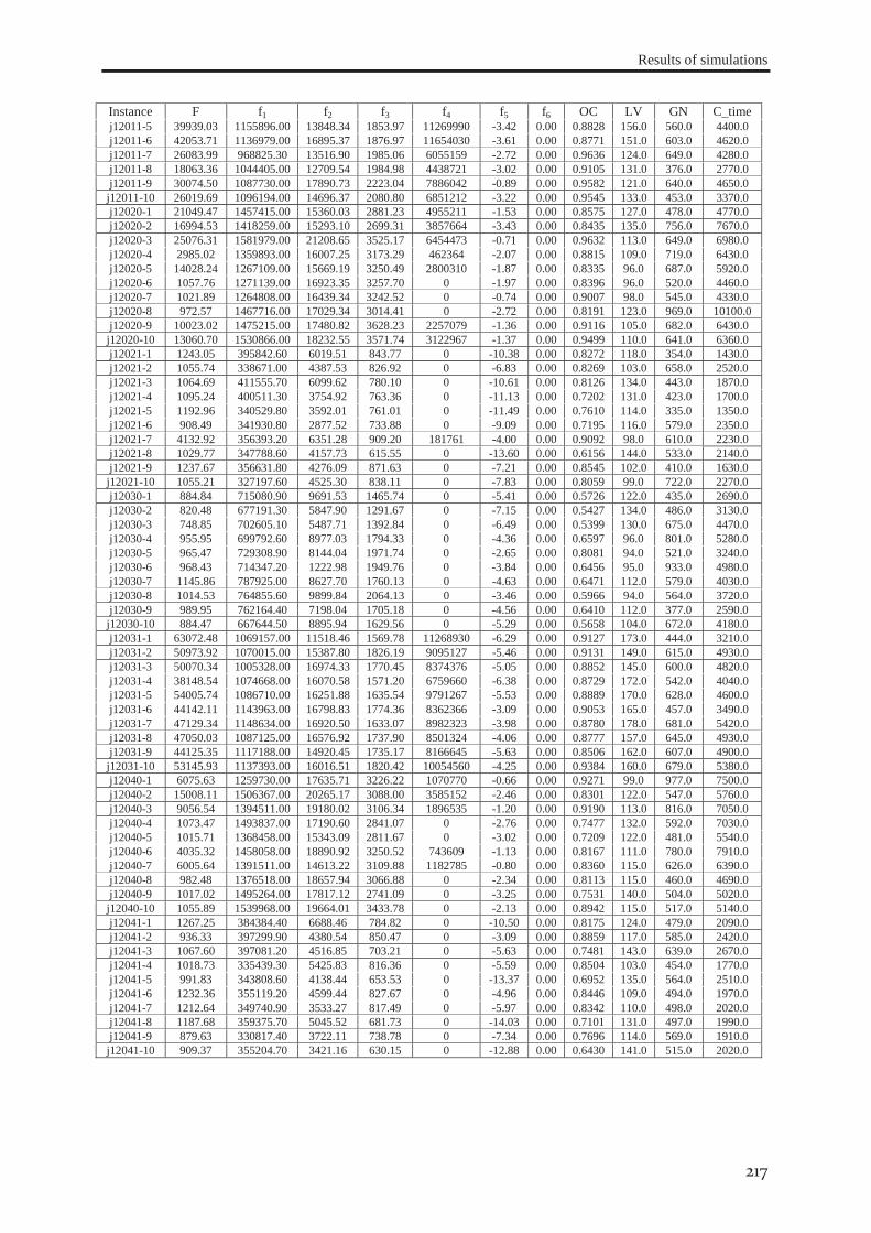
Results of simulations

217

Instance F f1 f2 f3 f4 f5 f6 OC LV GN C_time j12011-5 39939.03 1155896.00 13848.34 1853.97 11269990 -3.42 0.00 0.8828 156.0 560.0 4400.0 j12011-6 42053.71 1136979.00 16895.37 1876.97 11654030 -3.61 0.00 0.8771 151.0 603.0 4620.0 j12011-7 26083.99 968825.30 13516.90 1985.06 6055159 -2.72 0.00 0.9636 124.0 649.0 4280.0 j12011-8 18063.36 1044405.00 12709.54 1984.98 4438721 -3.02 0.00 0.9105 131.0 376.0 2770.0 j12011-9 30074.50 1087730.00 17890.73 2223.04 7886042 -0.89 0.00 0.9582 121.0 640.0 4650.0

j12011-10 26019.69 1096194.00 14696.37 2080.80 6851212 -3.22 0.00 0.9545 133.0 453.0 3370.0 j12020-1 21049.47 1457415.00 15360.03 2881.23 4955211 -1.53 0.00 0.8575 127.0 478.0 4770.0 j12020-2 16994.53 1418259.00 15293.10 2699.31 3857664 -3.43 0.00 0.8435 135.0 756.0 7670.0 j12020-3 25076.31 1581979.00 21208.65 3525.17 6454473 -0.71 0.00 0.9632 113.0 649.0 6980.0 j12020-4 2985.02 1359893.00 16007.25 3173.29 462364 -2.07 0.00 0.8815 109.0 719.0 6430.0 j12020-5 14028.24 1267109.00 15669.19 3250.49 2800310 -1.87 0.00 0.8335 96.0 687.0 5920.0 j12020-6 1057.76 1271139.00 16923.35 3257.70 0 -1.97 0.00 0.8396 96.0 520.0 4460.0 j12020-7 1021.89 1264808.00 16439.34 3242.52 0 -0.74 0.00 0.9007 98.0 545.0 4330.0 j12020-8 972.57 1467716.00 17029.34 3014.41 0 -2.72 0.00 0.8191 123.0 969.0 10100.0 j12020-9 10023.02 1475215.00 17480.82 3628.23 2257079 -1.36 0.00 0.9116 105.0 682.0 6430.0

j12020-10 13060.70 1530866.00 18232.55 3571.74 3122967 -1.37 0.00 0.9499 110.0 641.0 6360.0 j12021-1 1243.05 395842.60 6019.51 843.77 0 -10.38 0.00 0.8272 118.0 354.0 1430.0 j12021-2 1055.74 338671.00 4387.53 826.92 0 -6.83 0.00 0.8269 103.0 658.0 2520.0 j12021-3 1064.69 411555.70 6099.62 780.10 0 -10.61 0.00 0.8126 134.0 443.0 1870.0 j12021-4 1095.24 400511.30 3754.92 763.36 0 -11.13 0.00 0.7202 131.0 423.0 1700.0 j12021-5 1192.96 340529.80 3592.01 761.01 0 -11.49 0.00 0.7610 114.0 335.0 1350.0 j12021-6 908.49 341930.80 2877.52 733.88 0 -9.09 0.00 0.7195 116.0 579.0 2350.0 j12021-7 4132.92 356393.20 6351.28 909.20 181761 -4.00 0.00 0.9092 98.0 610.0 2230.0 j12021-8 1029.77 347788.60 4157.73 615.55 0 -13.60 0.00 0.6156 144.0 533.0 2140.0 j12021-9 1237.67 356631.80 4276.09 871.63 0 -7.21 0.00 0.8545 102.0 410.0 1630.0

j12021-10 1055.21 327197.60 4525.30 838.11 0 -7.83 0.00 0.8059 99.0 722.0 2270.0 j12030-1 884.84 715080.90 9691.53 1465.74 0 -5.41 0.00 0.5726 122.0 435.0 2690.0 j12030-2 820.48 677191.30 5847.90 1291.67 0 -7.15 0.00 0.5427 134.0 486.0 3130.0 j12030-3 748.85 702605.10 5487.71 1392.84 0 -6.49 0.00 0.5399 130.0 675.0 4470.0 j12030-4 955.95 699792.60 8977.03 1794.33 0 -4.36 0.00 0.6597 96.0 801.0 5280.0 j12030-5 965.47 729308.90 8144.04 1971.74 0 -2.65 0.00 0.8081 94.0 521.0 3240.0 j12030-6 968.43 714347.20 1222.98 1949.76 0 -3.84 0.00 0.6456 95.0 933.0 4980.0 j12030-7 1145.86 787925.00 8627.70 1760.13 0 -4.63 0.00 0.6471 112.0 579.0 4030.0 j12030-8 1014.53 764855.60 9899.84 2064.13 0 -3.46 0.00 0.5966 94.0 564.0 3720.0 j12030-9 989.95 762164.40 7198.04 1705.18 0 -4.56 0.00 0.6410 112.0 377.0 2590.0

j12030-10 884.47 667644.50 8895.94 1629.56 0 -5.29 0.00 0.5658 104.0 672.0 4180.0 j12031-1 63072.48 1069157.00 11518.46 1569.78 11268930 -6.29 0.00 0.9127 173.0 444.0 3210.0 j12031-2 50973.92 1070015.00 15387.80 1826.19 9095127 -5.46 0.00 0.9131 149.0 615.0 4930.0 j12031-3 50070.34 1005328.00 16974.33 1770.45 8374376 -5.05 0.00 0.8852 145.0 600.0 4820.0 j12031-4 38148.54 1074668.00 16070.58 1571.20 6759660 -6.38 0.00 0.8729 172.0 542.0 4040.0 j12031-5 54005.74 1086710.00 16251.88 1635.54 9791267 -5.53 0.00 0.8889 170.0 628.0 4600.0 j12031-6 44142.11 1143963.00 16798.83 1774.36 8362366 -3.09 0.00 0.9053 165.0 457.0 3490.0 j12031-7 47129.34 1148634.00 16920.50 1633.07 8982323 -3.98 0.00 0.8780 178.0 681.0 5420.0 j12031-8 47050.03 1087125.00 16576.92 1737.90 8501324 -4.06 0.00 0.8777 157.0 645.0 4930.0 j12031-9 44125.35 1117188.00 14920.45 1735.17 8166645 -5.63 0.00 0.8506 162.0 607.0 4900.0

j12031-10 53145.93 1137393.00 16016.51 1820.42 10054560 -4.25 0.00 0.9384 160.0 679.0 5380.0 j12040-1 6075.63 1259730.00 17635.71 3226.22 1070770 -0.66 0.00 0.9271 99.0 977.0 7500.0 j12040-2 15008.11 1506367.00 20265.17 3088.00 3585152 -2.46 0.00 0.8301 122.0 547.0 5760.0 j12040-3 9056.54 1394511.00 19180.02 3106.34 1896535 -1.20 0.00 0.9190 113.0 816.0 7050.0 j12040-4 1073.47 1493837.00 17190.60 2841.07 0 -2.76 0.00 0.7477 132.0 592.0 7030.0 j12040-5 1015.71 1368458.00 15343.09 2811.67 0 -3.02 0.00 0.7209 122.0 481.0 5540.0 j12040-6 4035.32 1458058.00 18890.92 3250.52 743609 -1.13 0.00 0.8167 111.0 780.0 7910.0 j12040-7 6005.64 1391511.00 14613.22 3109.88 1182785 -0.80 0.00 0.8360 115.0 626.0 6390.0 j12040-8 982.48 1376518.00 18657.94 3066.88 0 -2.34 0.00 0.8113 115.0 460.0 4690.0 j12040-9 1017.02 1495264.00 17817.12 2741.09 0 -3.25 0.00 0.7531 140.0 504.0 5020.0

j12040-10 1055.89 1539968.00 19664.01 3433.78 0 -2.13 0.00 0.8942 115.0 517.0 5140.0 j12041-1 1267.25 384384.40 6688.46 784.82 0 -10.50 0.00 0.8175 124.0 479.0 2090.0 j12041-2 936.33 397299.90 4380.54 850.47 0 -3.09 0.00 0.8859 117.0 585.0 2420.0 j12041-3 1067.60 397081.20 4516.85 703.21 0 -5.63 0.00 0.7481 143.0 639.0 2670.0 j12041-4 1018.73 335439.30 5425.83 816.36 0 -5.59 0.00 0.8504 103.0 454.0 1770.0 j12041-5 991.83 343808.60 4138.44 653.53 0 -13.37 0.00 0.6952 135.0 564.0 2510.0 j12041-6 1232.36 355119.20 4599.44 827.67 0 -4.96 0.00 0.8446 109.0 494.0 1970.0 j12041-7 1212.64 349740.90 3533.27 817.49 0 -5.97 0.00 0.8342 110.0 498.0 2020.0 j12041-8 1187.68 359375.70 5045.52 681.73 0 -14.03 0.00 0.7101 131.0 497.0 1990.0 j12041-9 879.63 330817.40 3722.11 738.78 0 -7.34 0.00 0.7696 114.0 569.0 1910.0

j12041-10 909.37 355204.70 3421.16 630.15 0 -12.88 0.00 0.6430 141.0 515.0 2020.0