Embed Size (px)
Citation preview
Linear Algebra and its Applications 359 (2003) 197–218www.elsevier.com/locate/laa
Perturbation bounds for coupled matrix Riccatiequations
Mihail Konstantinov a,∗, Vera Angelova b, Petko Petkov c,Dawei Gu d, Vassilios Tsachouridis d
aUniversity of Architecture and Civil Engineering, 1 Hr. Smirnenski Blvd., 1046 Sofia, BulgariabInstitute of Information Technologies, Akad. G. Bonchev Str., Bl. 2, 1113 Sofia, Bulgaria
cDepartment of Automatics, Technical University of Sofia, 1756 Sofia, BulgariadDepartment of Engineering, University of Leicester, Leicester LE1 7RH, England, UK
Received 20 August 2001; accepted 6 May 2002
Submitted by V. Mehrmann
Abstract
Local and non-local perturbation bounds for real continuous-time coupled algebraic matrixRiccati equations are derived using the technique of Lyapunov majorants and fixed point prin-ciples. Asymptotic expansions of non-linear non-local bounds are also presented. Equationsof this type arise in the H2/H∞ analysis and design of linear control systems.© 2002 Elsevier Science Inc. All rights reserved.
AMS classification: 15A24; 93B36; 94C73
Keywords: Perturbation analysis; Coupled algebraic matrix Riccati equations; Condition numbersH2/H∞ control
1. Introduction and notation
The real Continuous-time Coupled Algebraic matrix Riccati Equations (CCARE),considered below, are related to the H2 and H∞ analysis and design of linear multi-variable system, see [1,2,5,12]. The numerical solution of these equations is usually
∗ Corresponding author.E-mail addresses: [email protected] (M. Konstantinov), [email protected] (V. Angelova), php@
tu-sofia.acad.bg (P. Petkov), [email protected] (D. Gu), [email protected] (V. Tsachouridis).
0024-3795/02/$ - see front matter � 2002 Elsevier Science Inc. All rights reserved.PII: S0024 -3795(02)00416-0
198 M. Konstantinov et al. / Linear Algebra and its Applications 359 (2003) 197–218
contaminated with rounding and parameters errors. This may lead to significant lossof accuracy and, in particular, to divergence of the numerical procedure, carried outin floating point computing environment. The error in the computed solution dependson the sensitivity of the solution of CCARE to perturbations in their matrix coef-ficients. Hence obtaining perturbation bounds for CCARE is important from boththeoretical and computational point of view.
In this paper we present a complete perturbation analysis of CCARE of the formFi(X1, X2, Pi) = 0, i = 1, 2, where Fi are matrix quadratic functions in the un-known matrices Xi , and Pi are collections of matrix coefficients (see (1) for moredetails). Suppose that Pi are subject to perturbations Pi → Pi + δPi which lead toperturbations Xi → Xi + δXi in the solution matrices. Then the perturbation anal-ysis problem is to estimate the norms of the perturbations δXi as functions of thenorms of the perturbations δPi in the coefficient matrices. In practice, the perturba-tions δPi may be due to parameter uncertainties as well as to rounding errors whensolving the equations in finite precision arithmetics.
As a result of the perturbation analysis, using the technique of Lyapunov majo-rants [3,7] and fixed point principles [11], local first order homogeneous as wellas non-local non-linear perturbation bounds are derived. The non-local bounds arerigorous and they are valid in a certain finite domain in the space of perturbations inthe coefficient matrices. The local bounds are asymptotic, valid for δP → 0. Theselocal bounds are first order homogeneous non-linear functions and are better than thebounds, based on individual condition numbers.
An experimental analysis is made to compare the performance of the proposedperturbation bounds. It is shown that for some particular example the non-localbounds are slightly more pessimistic than the local ones.
Throughout the paper we use the following notation: Rm×n—the space of m × n
real matrices; Rm = Rm×1; R+ = [0,∞); AT ∈ Rn×m—the transpose of the matrixA ∈ Rm×n; —the component-wise order relation on Rm×n; vec(A) ∈ Rmn—thecolumn-wise vector representation of the matrix A ∈ Rm×n; Mat(L) ∈ Rpq×mn—the matrix representation of the linear matrix operator L : Rm×n → Rp×q , i.e.,
vec(L(X)) = Mat(L)vec(X)
for all X ∈ Rm×n; In—the unit n × n matrix; �n2 —the n2 × n2 vec-permutationmatrix such that vec(AT) = �n2 vec(A) for all A ∈ Rn×n; A ⊗ B = [apqB]—theKronecker product of the matrices A = [apq ] and B; ‖ · ‖2—the Euclidean normin Rm or the spectral (or 2-) norm in Rm×n; ‖ · ‖F—the Frobenius (or F-) norm inRm×n; ‖ · ‖—a replacement of either ‖ · ‖2 or ‖ · ‖F; rad(A)—the spectral radius ofthe square matrix A; det(A)—the determinant of the square matrix A.
If P = (E1, . . . , Er) is a matrix r-tuple, we denote by
|||P ||| = [‖E1‖, . . . , ‖Er‖]T ∈ Rr+its generalized norm. We also set R = Rn×n and S = {A ∈ R : A = AT} ⊂ R. Theset of non-negative definite matrices from S is denoted as S+.
M. Konstantinov et al. / Linear Algebra and its Applications 359 (2003) 197–218 199
The space of linear operators L1 → L2, where L1, L2 are linear spaces, isdenoted by Lin(L1,L2), while Lin is an abbreviation for Lin(R,R).
We usually identify the Cartesian product Rm×n × Rm×n, endowed with the struc-ture of a linear space, with any of the spaces Rm×2n, R2m×n and R2mn. In particular,the ordered pair (A,B) ∈ Rm×n × Rm×n and the matrix [A,B] ∈ Rm×2n are consid-ered as identical objects. Finally, we use the same notation P for an ordered matrixr-tuple (E1, . . . , Er) (considered as an element of a linear space) as well as for thecollection {E1, . . . , Er} (a collection is a set with possibly repeated elements). ThusZ ∈ P means that Z is some of the matrices Ek of P, or that Z varies over the set P.
The notation ‘:=’ stands for ‘equal by definition’.
2. Problem statement
Consider the system of CCARE
F1(X1, X2, P1) := (A1 + B1X2)TX1 + X1(A1 + B1X2)
+C1 − X1D1X1 = 0,
F2(X1, X2, P2) := (A2 + X1B2)X2 + X2(A2 + X1B2)T
+C2 − X2D2X2 = 0,
(1)
where Xi ∈ R are the unknown matrices, Ai, Bi ∈ R, Ci,Di ∈ S, i = 1, 2, aregiven matrix coefficients and Pi := (Ai, Bi, Ci,Di) ∈ R4.
We set
P :=(P1, P2) = (A1, B1, C1,D1, A2, B2, C2,D2)
=:(E1, E2, E3, E4, E5, E6, E7, E8) ∈ R8.
The generalized norm of the matrix 8-tuple P is the vector
|||P ||| := [‖E1‖F, . . . , ‖E8‖F]T ∈ R8+. (2)
Although the matrices Ci , Di are symmetric, system (1) may have solutions(X1, X2) in which some of the matrices Xi is not symmetric. In this work we areinterested only in symmetric solutions of system (1), i.e., (X1, X2) ∈ S2. The non-symmetric case is treated similarly.
An important feature of the solutions of (1) is whether they stabilize the corre-sponding closed-loop system matrices (we recall that a matrix A ∈ R is stable if itseigenvalues have negative real parts).
Definition 2.1. The solution pair (X1, X2) ∈ S2 is called stabilizing if the matricesG1 := A1 + B1X2 − D1X1 and G2 := A2 + X1B2 − X2D2 are stable.
Note that Fi as defined by (1) are functions from R × R × R4 = R6 to R. It willbe convenient to write the system of CCARE as one matrix equation. For this purposewe denote X := (X1, X2), F := (F1, F2). Then the system (1) may be written as
200 M. Konstantinov et al. / Linear Algebra and its Applications 359 (2003) 197–218
F(X, P ) = 0. (3)
Here F is considered as a mappingR10 → R2, or equivalently, as a mapping Rn×2n ×R8 → Rn×2n, see the end of Section 1.
The problem of existence of (stabilizing) solutions (X1, X2) ∈ S2+ of system (1)is a difficult one and is not considered here.
In what follows we assume the following.
Assumption 2.1. The system (1) has a solution X = (X1, X2) ∈ S2 such that thepartial Fréchet derivative FX(X, P )(·) of F in X at the point (X, P ) is invertible.
The partial Fréchet derivative of F in X at (X, P ) is a linear operator R2 → R2,calculated as follows. Let Y = (Y1, Y2) ∈ R2 be arbitrary. We have
FX(X, P )(Y ) = (F1,X(X, P1)(Y ),F2,X(X, P2)(Y ))
and
Fi,X(X, Pi)(Y ) = Fi,X1(X, Pi)(Y1) + Fi,X2(X, Pi)(Y2).
A direct calculation gives
F1,X1(X, P1)(Z)=GT1Z + ZG1, F1,X2(X, P1)(Z) = X1B1Z + ZTBT
1 X1,
F2,X1(X, P2)(Z)=X2BT2 Z
T + ZB2X2, F2,X2(X, P2)(Z) = G2Z + ZGT2 .
Further on we use the following abbreviations for the partial Fréchet derivativesof F and Fi
L(·) := FX(X, P )(·) ∈ Lin(R2,R2),
Li (·) := Fi,X(X, Pi)(·) ∈ Lin(R2,R),
Lij (·) := Fi,Xj(X, Pi)(·) ∈ Lin(R,R).
Thus
FX(X, P )(Y ) = (L1(Y ),L2(Y )) = (L11(Y1) + L12(Y2),L21(Y1) + L22(Y2)).
Note that Lii (·) are Lyapunov operators [6]. At the same time Lij (·), i /= j , areassociated Lyapunov operators when Xi ∈ S.
Applying the vec operation to the pair FX(X, P )(Y ) and using the identity (A ⊗B)�n2 = �n2(B ⊗ A) (see [4]) we find that the matrix representation of the linearoperator L(·) is
L := Mat(L(·)) =[L11 L12L21 L22
]∈ R2n2×2n2
, (4)
whereL11 := In ⊗ GT
1 + GT1 ⊗ In, L12 := (In2 + �n2)(In ⊗ (X1B1)),
L21 := (In2 + �n2)((B2X2)
T ⊗ In), L22 := In ⊗ G2 + G2 ⊗ In.
(5)
Here Lij ∈ Rn2×n2is the matrix representation of the operator Lij (·).
M. Konstantinov et al. / Linear Algebra and its Applications 359 (2003) 197–218 201
It follows from Assumption 2.1 and the implicit function theorem [11] that thesolution X is isolated, i.e., there exists ε > 0 such that Eq. (3) has no other solutionX̃ with ‖X̃ − X‖ < ε.
Hereinafter, with certain abuse of notation, we consider Pi as an ordered pair (andhence as an element of the linear space R4) as well as a collection, i.e., as a set.
The perturbation problem for CCARE (1) is stated as follows. Let the matricesfrom Pi be perturbed as Ai �→ Ai + δAi , Bi �→ Bi + δBi , Ci �→ Ci + δCi , Di �→Di + δDi . We assume that the perturbations δCi and δDi are symmetric. This as-sumption is necessary to ensure that the perturbed equation, considered below, alsohas a solution in S2. Symmetric perturbations in Ci and Di arise naturally in manyapplications, where these matrices are factorized as Ci = �i�T
i , etc.Denote by Pi + δPi the perturbed collection Pi , in which each matrix Z ∈ Pi is
replaced by Z + δZ and let δP = (δP1, δP2). Then the perturbed version of Eq. (3)is
F(X + δX, P + δP ) = 0. (6)
The invertibility of the operator FX and the symmetry of the matrices Ci + δCi ,Di + δDi implies that Eq. (6) has a unique isolated solution Y = X + δX ∈ S2 inthe neighbourhood of X if the perturbation δP is sufficiently small. Moreover, in thiscase the elements of δX are analytic functions of the elements of δP , see [9].
Let
δ :=[δ1δ2
]∈ R8+,
where δi := [δAi, δBi
, δCi, δDi
]T ∈ R4+, be the vector of absolute Frobenius normperturbations δZ := ‖δZ‖F in the data matrices Z ∈ P .
The perturbation problem for CCARE (1) is to find bounds
δXi� fi(δ), δ ∈ � ⊂ R8+, i = 1, 2, (7)
for the perturbations δXi:= ‖δXi‖F. Here � is a certain set and fi are continuous
functions, non-decreasing in each of their arguments and satisfying fi(0) = 0. Theinclusion δ ∈ � guarantees that the perturbed CCARE (6) has a unique solution Y =X + δX in a neighbourhood of the unperturbed solution X such that the elements ofδX1, δX2 are analytic functions of the elements of the matrices δZ, Z ∈ P , providedδ is in the interior of �.
First order local bounds
δXi� esti (δ) + O(‖δ‖2), δ → 0, i = 1, 2, (8)
are first derived with esti (δ) = O(‖δ‖), δ → 0, which are then incorporated in thenon-local bounds (7). Here the functions esti : R8+ → R+ are non-linear first orderhomogeneous, i.e., esti (λδ) = λesti (δ) for every λ � 0.
202 M. Konstantinov et al. / Linear Algebra and its Applications 359 (2003) 197–218
3. Local perturbation analysis
In this section we present a local perturbation analysis for CCARE (1) whichconsists in determining the functions esti in (8).
3.1. Condition numbers
Consider first the conditioning of the CCARE (1).Having in mind that Fi(X, Pi) = 0, the perturbed equations may be written as
Fi(X + δXi, Pi + δPi) =2∑
j=1
Lij (δXj ) +∑Z∈Pi
Fi,Z(δZ) + Hi(δX, δPi) = 0,
where Fi,Z(·) := Fi,Z(X, Pi)(.) ∈ Lin, Z ∈ Pi , i = 1, 2, are the Fréchet derivativesof Fi(X, Pi) in the matrix argument Z, evaluated at the point (X, Pi). The matrixexpression Hi(δX, δPi) = O(‖[δX, δPi]‖2) contains second and higher order termsin δX, δPi . In fact, for Y = (Y1, Y2) ∈ S2, we have
H1(Y, δP1)=(δB1Y2 − δD1Y1)TX1 + X1(δB1Y2 − δD1Y1)
+ Y1δB1X2 + X2δBT1 Y1 − Y1(D1 + δD1)Y1 + Y1δA1
+ δAT1Y1 + Y1(B1 + δB1)Y2 + Y2(B1 + δB1)
TY1 (9)
and
H2(Y, δP2)=X2 (Y1δB2 − Y2δD2)T + (Y1δB2 − Y2δD2)X2 + X1δB2Y2
+ Y2δBT2 X1 − Y2(D2 + δD2)Y2 + δA2Y2 + Y2δA
T2
+ Y2(B2 + δB2)TY1 + Y1(B2 + δB2)Y2. (10)
We stress that the first four terms in the right-hand sides of (9) and (10) have astructure (an outer non-perturbed multiplier X1 or X2) which will be exploited laterin the derivation of tighter non-local bounds. Indeed, suppose that we want to boundfrom above the 2-norms of the vector Avec(BZC), where A, B and C are given ma-trices and the only information about the matrix Z is that ‖Z‖F = ‖vec(Z)‖2 � δZ .Then we have the ‘rough’ bound
‖A vec(BZC)‖2 �‖A‖2‖vec(BZC)‖2 = ‖A‖2‖BZC‖F
�‖A‖2‖B‖2‖C‖2‖Z‖F = ‖A‖2‖B‖2‖C‖2δZ. (11)
But we have also the bound
‖A vec(BZC)‖2 = ‖A(CT ⊗ B)vec(Z)‖2 � ‖A(CT ⊗ B)‖2δZ. (12)
Since ‖A(CT ⊗ B)‖2 � ‖A‖2‖B‖2‖C‖2 and the strict inequality is possible, we seethat the bound (12) is tighter than (11).
M. Konstantinov et al. / Linear Algebra and its Applications 359 (2003) 197–218 203
We recall that the matrix representation of Lij (·) is denoted by Lij . We also have,for (X1, X2) ∈ S2,
F1,A1(Z) = X1Z + ZTX1, F1,B1(Z) = X1ZX2 + X2ZTX1,
F1,C1(Z) = Z, F1,D1(Z) = −X1ZX1,
F2,A2(Z) = ZX2 + X2ZT, F2,B2(Z) = X1ZX2 + X2Z
TX1,
F2,C2(Z) = Z, F2,D2(Z) = −X2ZX2.
(13)
The inverse M(·) := L(·)−1 ∈ Lin(R2,R2) of the operator L = FX(X, P )(·)maybe represented as L−1(·) = (M1(·),M2(·)), where, for Z := (Z1, Z2) ∈ R2,
Mi (Z) = Mi1(Z1) + Mi2(Z2),Mij (·) ∈ Lin, i = 1, 2.
Hence δX = −M(W1(δX, δP1),W2(δX, δP2)), where
Wi(Y, δPi) :=∑Z∈Pi
Fi,Z(δZ) + Hi(Y, δPi).
In this way
δXi = −2∑
j=1
Mij (Wj (δX, δPj )), i = 1, 2,
which gives
δXi = −2∑
j=1
∑Z∈Pj
Mij ◦ Fj,Z(δZ) −2∑
j=1
Mij (Hj (δX, δPj )), i = 1, 2.
(14)
Therefore
δXi�
2∑j=1
∑Z∈Pj
Kij,ZδZ + O(‖δ‖2), δ → 0, (15)
where the quantity Kij,Z := ‖Mij ◦ Fj,Z‖Lin is the absolute condition number of thesolution component Xi with respect to the matrix coefficient Z ∈ Pj . Here ‖.‖Lin isthe induced norm in the space Lin of linear operators R → R.
The calculation of the condition numbers Kij,Z is straightforward when theFrobenius norm is used in R. Indeed, let U ∈ Lin. Then
‖U‖Lin := max{‖U(Z)‖F : ‖Z‖F = 1} = ‖Mat(U)‖2.
Let Li,Z ∈ Rn2×n2be the matrix of the operator Fi,Z ∈ Lin. A direct calculation
in view of (13) yields
L1,A1 = (�n2 + In2)(In ⊗ X1), L2,A2 = (�n2 + In2)(X2 ⊗ In),
L1,B1 = (�n2 + In2)(X2 ⊗ X1), L2,B2 = (�n2 + In2)(X2 ⊗ X1),
L1,C1 = In2 , L2,C2 = In2 , L1,D1 = −X1 ⊗ X1, L2,D2 = −X2 ⊗ X2.
(16)
204 M. Konstantinov et al. / Linear Algebra and its Applications 359 (2003) 197–218
Denote the matrix representation of the operator
M(·) = F−1X (X, P )(·) ∈ Lin(R2,R2)
as
M := Mat(M) = L−1 :=[M11 M12M21 M22
], Mij ∈ Rn2×n2
. (17)
Then we have the following result.
Theorem 3.1. In the Frobenius norm the absolute condition number of the solu-tion component Xi relative to the matrix coefficient Z ∈ Pj is Kij,Z = ‖MijLj,Z‖2,
i, j = 1, 2, where the matrices Mij and Lj,Z are defined by (16) and (17) in view of(4), (5).
Proof. The proof follows from (15) and the exprerssions for the matrix representa-tions Li,Z of the linear matrix operators Li,Z and for the blocks Mij of the matrixM = L−1 of M. �
3.2. First order homogeneous bounds
Rewrite Eq. (14) in vectorized form as
vec(δXi) =2∑
j=1
∑Z∈Pj
Ni,Zvec(δZ) −2∑
j=1
Mijvec(Hj (δX, δPj )),
i = 1, 2, (18)
where Ni,Z := −MijLj,Z ∈ Rn2×n2, Z ∈ Pj .
The condition number based perturbation bounds are an immediate consequenceof (18),
δXi= ‖δXi‖F = ‖vec(δXi)‖2 � est(1)i (δ) + O(‖δ‖2), δ → 0, (19)
where
est(1)i (δ) :=2∑
j=1
∑Z∈Pj
‖Ni,Z‖2δZ =2∑
j=1
∑Z∈Pj
Kij,ZδZ.
The bounds est(1)i (·) are linear functions in the perturbation vector δ ∈ R8.Relations (18) also give another perturbation bound
δXi� est(2)i (δ) + O(‖δ‖2), δ → 0, (20)
where est(2)i (δ) := ‖Ni‖2‖δ‖2 and
Ni := [Ni,1, Ni,2] ∈ Rn2×8n2,
Ni,j := [Ni,Aj, Ni,Bj
, Ni,Cj, Ni,Dj
] ∈ Rn2×4n2, i = 1, 2.
(21)
M. Konstantinov et al. / Linear Algebra and its Applications 359 (2003) 197–218 205
The bounds est(1)i (δ) and est(2)i (δ) are alternative, i.e., which one is better dependson the particular value of δ.
There is a third bound, which is always less or equal to est(1)1 (δ), see also [8].Indeed, we have δ2
Xi= vecT(δXi)vec(δXi) = ηTNT
i Niη + O(‖δ‖2), δ → 0, where
η := [vecT(δA1), vecT(δB1), . . . , vecT(δD2)
]T ∈ R8n2. (22)
We shall represent the matrixNTi Ni ∈ R8n2×8n2
+ as a 8 × 8 block matrix with n2 × n2
blocks as follows. Let the n2 × n2 blocks of Ni be denoted as N̂i,k , k = 1, . . . , 8, i.e.,
Ni = [N̂i,1, N̂i,2, . . . , N̂i,8
], N̂i,k ∈ Rn2×n2
,
where
N̂i,1 := Ni,A1 , N̂i,2 := Ni,B1 , . . . , N̂i,8 := Ni,D2 .
Then ηTNTi Niη � δTN̂iδ, where N̂i = [ni,pq ] ∈ R8×8+ is a matrix with elements
ni,pq :=∥∥∥N̂T
i,pN̂i,q
∥∥∥2, p, q = 1, . . . , 8
(note that the non-negative matrices N̂i may be indefinite). Therefore we find a thirdtype perturbation bounds
δXi� est(3)i (δ) + O(‖δ‖2), δ → 0, (23)
where est(3)i (δ) :=√δT N̂iδ.
The overall estimates are summarized in the next theorem.
Theorem 3.2. It is fulfilled that
δXi� esti (δ) + O(‖δ‖2), δ → 0, i = 1, 2,
where
esti (δ) := min{
est(2)i (δ), est(3)i (δ)}, i = 1, 2,
and est(2)i (δ), est(3)i (δ) are determined by (20) and (23), respectively.
Proof. We have three local first order bounds, defined by (19) and (23). The bounds(19) and (20) are alternative, and the bounds (20) and (23) are also alternative. At thesame time we have∥∥∥N̂T
i,pN̂i,q
∥∥∥2
�∥∥N̂i,p
∥∥2
∥∥N̂i,q
∥∥2 ,
which yields est(3)i (δ) � est(1)i (δ) and completes the proof. �
We stress that the local bounds, given in Theorem 3.2, may be very accurate forcertain collections of data and data perturbations. This will be the case when, for
206 M. Konstantinov et al. / Linear Algebra and its Applications 359 (2003) 197–218
example, the vector η in (22) is (approximately) proportional to the right singularvector of the matrix Ni from (21), corresponding to its maximum singular value‖Ni‖2.
The local bounds considered in this section are continuous, first order homoge-neous, non-linear functions in δ. Also, for δ /= 0 these functions are real analytic.
All the three bounds est(k)i are in fact majorants for the solution of a complicatedoptimization problem, defining the conditioning of the problem as follows. Set ξi :=vec(δXi) and δ := [δ1, . . . , δ8]T := [δA1 , . . . , δD2 ]T ∈ R8+. Then we have
ξi =8∑
k=1
N̂i,kηk + O(‖δ‖2), δ → 0
and δXi= ‖ξi‖2 � Ki(δ) + O(‖δ‖2), δ → 0. Here
Ki(δ) := max
{∥∥∥∥∥8∑
k=1
N̂i,kηk
∥∥∥∥∥2
: ‖ηk‖ � δk, k = 1, . . . , 8
}is the exact upper bound for the first order term in the perturbation bound for thesolution component Xi (note that Ki(δ) is well defined, since the minimization in η
is carried out over a compact set).The calculation of Ki(δ) is a difficult task. Instead, one can use a bound above
such as esti (δ) � Ki(δ).Let γ ∈ R8+ be a given vector. Then we may define the relative conditioning of
the problem as follows.
Definition 3.1. Let Xi /= 0. The quantity κi(γ ) := Ki(γ )/‖Xi‖F is the relative con-dition number of Xi with respect to γ . If |||P ||| is the generalized norm (2) of P, thenκi(|||P |||) is the relative norm-wise condition number of Xi .
Note that if all elements γk of γ are zero except one, equal to ‖El‖F in the lthposition, then the quantity κi(γ ) is the individual relative condition number of Xi
with respect to perturbations in the matrix coefficient El .
4. Non-local perturbation analysis
4.1. Introductory remarks
Local bounds of the type considered in Section 3 are valid only asymptotically,for δ → 0. But in practice they are usually used simply neglecting terms of orderO(‖δ‖2), e.g., δXi
� esti (δ). Unfortunately, such chopped bounds may not be correcteither because they underestimate the true perturbed quantity or because the solutionof the perturbed problem does not exist. The reason is that it is usually impossibleto say, having a small but a finite perturbation δ, whether the neglected terms are
M. Konstantinov et al. / Linear Algebra and its Applications 359 (2003) 197–218 207
indeed negligible. Moreover, for some critical values of the perturbations in the co-efficient matrices the solution may not exist (or may go to infinity when these criticalvalues are approached). Nevertheless, even in such cases the local estimates will stillproduce a ‘bound’ for a very large or even for a non-existing solution which surelyis not desirable.
The disadvantages of the local estimates may be overcome using the techniquesof non-linear perturbation analysis. As a result, we get a domain � ⊂ R8+ and twonon-linear continuous functions f1, f2 : � → R+, satisfying f1(0)=f2(0) = 0, andsuch that δXi
� fi(δ), δ ∈ �, i = 1, 2. The inclusion δ ∈ � guarantees that the per-turbed equation has an unique solution in a neighbourhood of the unperturbed solu-tion. Furthermore, the last estimate is rigorous, i.e., the inequality holds true for allperturbations with δ ∈ �.
A disadvantage of the non-local bounds is that they may not exist or may bepessimistic for some collections of perturbations.
4.2. The perturbed equation
The perturbed equation F(X + δX, P + δP ) = 0 may be rewritten as an operatorequation for the perturbation δX
δX = �(δX, δP ), � = (�1,�2), (24)
where �(Y, δP ) := −M(FP (X, P )(δP ) + H(Y, δP )). Here
H(Y, δP ) := (H1(Y, δP1),H2(Y, δP2))
contains second and third order terms in Y and δP , see (9), (10).Eq. (24) comprises two equations, namely
δXi = �i (δX, δPi), i = 1, 2, (25)
where the right-hand side of (25) is defined by relations (14). Setting
ξi := vec(δXi) ∈ Rn2, i = 1, 2, ξ :=
[ξ1ξ2
]∈ R2n2
,
we obtain the vector operator equation
ξ = π(ξ, η), (26)
in R2n2, which is reduced to two coupled vector equations ξi = πi(ξ, η), i = 1, 2, in
Rn2.
Next we present a brief description of the method of Lyapunov majorants [3,7]for the analysis of operator equations of type (26). We recall that our purpose is tofind bounds for δXi
= ‖ξi‖2.
Define generalized norms in R2n2and R8n2
by
|||ξ ||| :=[‖ξ1‖2‖ξ2‖2
]∈ R2+
208 M. Konstantinov et al. / Linear Algebra and its Applications 359 (2003) 197–218
and |||η||| := [‖η1‖2, . . . , ‖η8‖2]T ∈ R8+. For all ρ ∈ R2+ let
Bρ :={ξ ∈ R2n2 : |||ξ ||| ρ
}be the ball centered at the origin and of generalized radius ρ.
Suppose that we can find a continuous function
h =[h1h2
]: R2+ × R8+ → R2+
such that the following assumption takes place.
Assumption 4.11. The components hi are non-decreasing in all of their scalar arguments, for all
δ ∈ R8+ the function h(·, δ) : R2+ → R2+ is differentiable, and
h(0, 0) = 0, rad(hρ(0, 0)) < 1.
2. For all ρ ∈ R2+; ξ, ξ̃ ∈ Bρ and η ∈ Bδ the inequalities |||π(ξ, η)||| h(ρ, δ) and|||π(ξ, η) − π(̃ξ, η)||| hρ(ρ, δ)|||ξ − ξ̃ ||| hold.
Here hρ(ρ, δ) is the Jacobi matrix of the function ρ �→ h(ρ, δ) for a fixed valueof δ. In our case the matrix hρ(ρ, δ) is non-negative and according to the Perron–Frobenius theorem [10] its spectral radius is equal to its maximum (non-negative)eigenvalue.
Definition 4.1. The function h, satisfying Assumption 4.1, is called a Lyapunovmajorant for the operator equation (26).
If h is a Lyapunov majorant, then there exists a domain � ⊂ R8+ such that for δ ∈� the vector majorant equationρ = h(ρ, δ)has a solutionρ = f (δ) = (f1(δ), f2(δ)).
Heref : � → R2+ is a continuous function, the componentsfi of f are non-decreasingin each of their scalar arguments (i.e., δ δ̃ implies f (δ) f (̃δ)), and f (0) = 0.
For δ ∈ � the operator π(·, η) : Rn2 → Rn2maps the closed convex set Bf (δ)
into itself. Hence, according to the Schauder fixed point principle [11], there ex-ists a solution ξ ∈ Bf (δ) of the operator equation (26). Now the desired non-localperturbation bounds for the solution are
δXi= ‖ξi‖2 � fi(δ), δ ∈ �.
We have πi(ξ, η) = Niηi + ψi(ξ, η), where
ψi(ξ, η) := −vec
2∑j=1
Mijvec(Hj
(vec−1(ξ), vec−1(ηj )
)) .
We next apply the theory of Lyapunov majorants and fixed point principles ofBanach and Schauder [3,7] to show that the operator π(·, η) : R2n2 → R2n2
is a con-
M. Konstantinov et al. / Linear Algebra and its Applications 359 (2003) 197–218 209
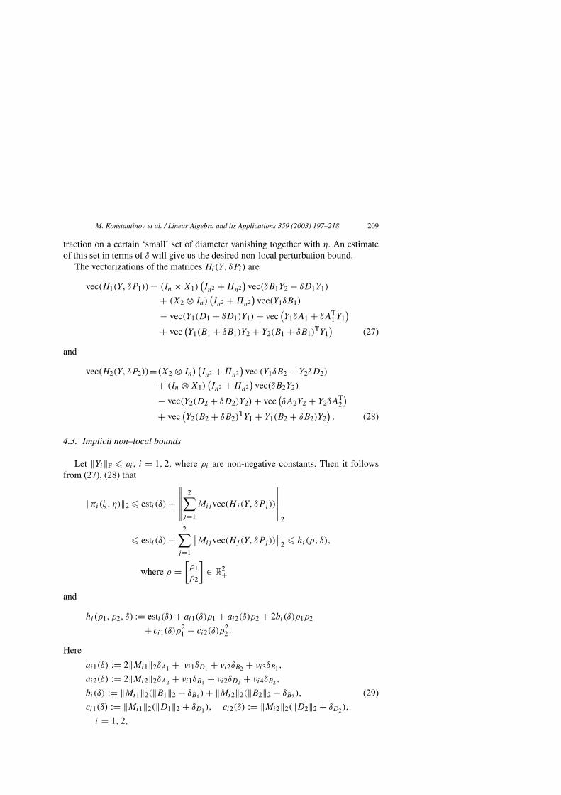
traction on a certain ‘small’ set of diameter vanishing together with η. An estimateof this set in terms of δ will give us the desired non-local perturbation bound.
The vectorizations of the matrices Hi(Y, δPi) are
vec(H1(Y, δP1))= (In × X1)(In2 + �n2
)vec(δB1Y2 − δD1Y1)
+ (X2 ⊗ In)(In2 + �n2
)vec(Y1δB1)
− vec(Y1(D1 + δD1)Y1) + vec(Y1δA1 + δAT
1Y1)
+ vec(Y1(B1 + δB1)Y2 + Y2(B1 + δB1)
TY1)
(27)
and
vec(H2(Y, δP2))=(X2 ⊗ In)(In2 + �n2
)vec (Y1δB2 − Y2δD2)
+ (In ⊗ X1)(In2 + �n2
)vec(δB2Y2)
− vec(Y2(D2 + δD2)Y2) + vec(δA2Y2 + Y2δA
T2
)+ vec
(Y2(B2 + δB2)
TY1 + Y1(B2 + δB2)Y2). (28)
4.3. Implicit non–local bounds
Let ‖Yi‖F � ρi , i = 1, 2, where ρi are non-negative constants. Then it followsfrom (27), (28) that
‖πi(ξ, η)‖2 � esti (δ) +∥∥∥∥∥∥
2∑j=1
Mijvec(Hj (Y, δPj ))
∥∥∥∥∥∥2
� esti (δ) +2∑
j=1
∥∥Mijvec(Hj (Y, δPj ))∥∥
2 � hi(ρ, δ),
where ρ =[ρ1ρ2
]∈ R2+
and
hi(ρ1, ρ2, δ) := esti (δ) + ai1(δ)ρ1 + ai2(δ)ρ2 + 2bi(δ)ρ1ρ2
+ ci1(δ)ρ21 + ci2(δ)ρ
22 .
Here
ai1(δ) := 2‖Mi1‖2δA1 + νi1δD1 + νi2δB2 + νi3δB1 ,
ai2(δ) := 2‖Mi2‖2δA2 + νi1δB1 + νi2δD2 + νi4δB2 ,
bi(δ) := ‖Mi1‖2(‖B1‖2 + δB1) + ‖Mi2‖2(‖B2‖2 + δB2),
ci1(δ) := ‖Mi1‖2(‖D1‖2 + δD1), ci2(δ) := ‖Mi2‖2(‖D2‖2 + δD2),
i = 1, 2,
(29)
210 M. Konstantinov et al. / Linear Algebra and its Applications 359 (2003) 197–218
and
νi1 := ∥∥Mi1(In ⊗ X1)(In2 + �n2
)∥∥2 ,
νi2 := ∥∥Mi2(X2 ⊗ In)(In2 + �n2
)∥∥2 ,
νi3 := ∥∥Mi1(X2 ⊗ In)(In2 + �n2
)∥∥2 ,
νi4 := ∥∥Mi2(In ⊗ X1)(In2 + �n2
)∥∥2 .
(30)
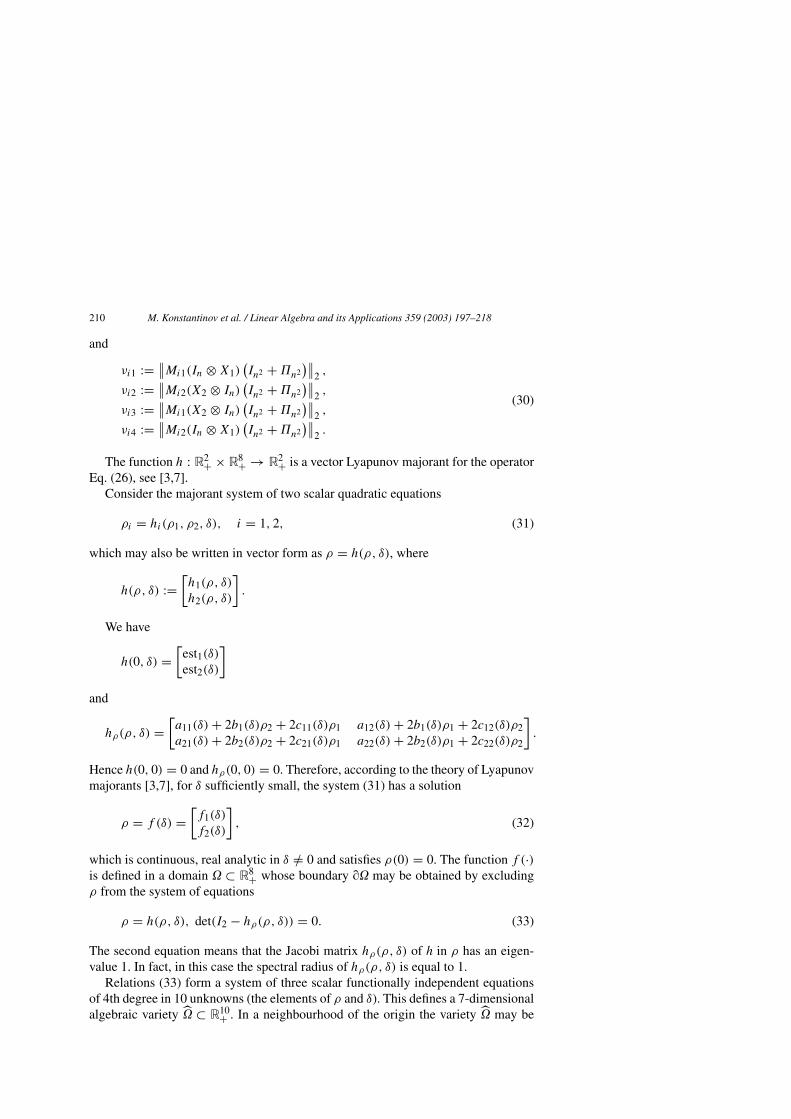
The function h : R2+ × R8+ → R2+ is a vector Lyapunov majorant for the operatorEq. (26), see [3,7].
Consider the majorant system of two scalar quadratic equations
ρi = hi(ρ1, ρ2, δ), i = 1, 2, (31)
which may also be written in vector form as ρ = h(ρ, δ), where
h(ρ, δ) :=[h1(ρ, δ)
h2(ρ, δ)
].
We have
h(0, δ) =[
est1(δ)est2(δ)
]and
hρ(ρ, δ) =[a11(δ) + 2b1(δ)ρ2 + 2c11(δ)ρ1 a12(δ) + 2b1(δ)ρ1 + 2c12(δ)ρ2a21(δ) + 2b2(δ)ρ2 + 2c21(δ)ρ1 a22(δ) + 2b2(δ)ρ1 + 2c22(δ)ρ2
].
Hence h(0, 0) = 0 and hρ(0, 0) = 0. Therefore, according to the theory of Lyapunovmajorants [3,7], for δ sufficiently small, the system (31) has a solution
ρ = f (δ) =[f1(δ)
f2(δ)
], (32)
which is continuous, real analytic in δ /= 0 and satisfies ρ(0) = 0. The function f (·)is defined in a domain � ⊂ R8+ whose boundary �� may be obtained by excludingρ from the system of equations
ρ = h(ρ, δ), det(I2 − hρ(ρ, δ)) = 0. (33)
The second equation means that the Jacobi matrix hρ(ρ, δ) of h in ρ has an eigen-value 1. In fact, in this case the spectral radius of hρ(ρ, δ) is equal to 1.
Relations (33) form a system of three scalar functionally independent equationsof 4th degree in 10 unknowns (the elements of ρ and δ). This defines a 7-dimensionalalgebraic variety �̂ ⊂ R10+ . In a neighbourhood of the origin the variety �̂ may be
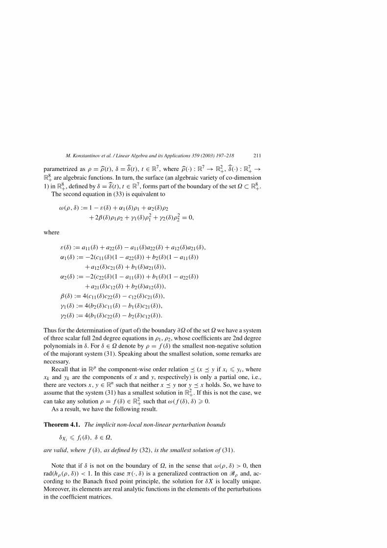
M. Konstantinov et al. / Linear Algebra and its Applications 359 (2003) 197–218 211
parametrized as ρ = ρ̂(t), δ = δ̂(t), t ∈ R7, where ρ̂(·) : R7 → R2+, δ̂(·) : R7+ →R8+ are algebraic functions. In turn, the surface (an algebraic variety of co-dimension1) in R8+, defined by δ = δ̂(t), t ∈ R7, forms part of the boundary of the set � ⊂ R8+.
The second equation in (33) is equivalent to
ω(ρ, δ) := 1 − ε(δ) + α1(δ)ρ1 + α2(δ)ρ2
+ 2β(δ)ρ1ρ2 + γ1(δ)ρ21 + γ2(δ)ρ
22 = 0,
where
ε(δ) := a11(δ) + a22(δ) − a11(δ)a22(δ) + a12(δ)a21(δ),
α1(δ) := −2(c11(δ)(1 − a22(δ)) + b2(δ)(1 − a11(δ))
+ a12(δ)c21(δ) + b1(δ)a21(δ)),
α2(δ) := −2(c22(δ)(1 − a11(δ)) + b1(δ)(1 − a22(δ))
+ a21(δ)c12(δ) + b2(δ)a12(δ)),
β(δ) := 4(c11(δ)c22(δ) − c12(δ)c21(δ)),
γ1(δ) := 4(b2(δ)c11(δ) − b1(δ)c21(δ)),
γ2(δ) := 4(b1(δ)c22(δ) − b2(δ)c12(δ)).
Thus for the determination of (part of) the boundary ∂� of the set � we have a systemof three scalar full 2nd degree equations in ρ1, ρ2, whose coefficients are 2nd degreepolynomials in δ. For δ ∈ � denote by ρ = f (δ) the smallest non-negative solutionof the majorant system (31). Speaking about the smallest solution, some remarks arenecessary.
Recall that in Rp the component-wise order relation (x y if xi � yi , wherexk and yk are the components of x and y, respectively) is only a partial one, i.e.,there are vectors x, y ∈ Rn such that neither x y nor y x holds. So, we have toassume that the system (31) has a smallest solution in R2+. If this is not the case, wecan take any solution ρ = f (δ) ∈ R2+ such that ω(f (δ), δ) � 0.
As a result, we have the following result.
Theorem 4.1. The implicit non-local non-linear perturbation bounds
δXi� fi(δ), δ ∈ �,
are valid, where f (δ), as defined by (32), is the smallest solution of (31).
Note that if δ is not on the boundary of �, in the sense that ω(ρ, δ) > 0, thenrad(hρ(ρ, δ)) < 1. In this case π(·, δ) is a generalized contraction on Bρ and, ac-cording to the Banach fixed point principle, the solution for δX is locally unique.Moreover, its elements are real analytic functions in the elements of the perturbationsin the coefficient matrices.
212 M. Konstantinov et al. / Linear Algebra and its Applications 359 (2003) 197–218
4.4. Asymptotic bounds
For δ sufficiently small the perturbation bound ρ = f (δ) which is the solution ofthe majorant equation ρ = h(ρ, δ), is analytic in δ and, for every integer m � 1, wehave the asymptotic expansions
fi(δ) =m∑k=1
fi,k(δ) + O(‖δ‖m+1), δ → 0, i = 1, 2,
where fi,k(δ) = O(‖δ‖k), δ → 0. The expressions fi,k(δ) may be derived as fol-lows. Introduce a ficticious ‘small’ parameter ε and replace δ by εδ. Then fi,k(εδ) =εkfi,k(δ). Substituting these expressions in the majorant system and equating thecoefficients of the corresponding powers of ε we obtain recurrence relations for de-termining fi,k(δ). Finally, the parameter ε is set to 1. In particular for m = 2 we havethe following result.
Theorem 4.2. The asymptotic estimates
δXi� esti (δ) + fi,2(δ) + O(‖δ‖3), δ → 0, i = 1, 2,
are valid, where
fi,2(δ)= ai1(δ)est1(δ) + ai2(δ)est2(δ) + 2b0i est1(δ)est2(δ) + c0
i1est21(δ)
+ c0i2est22(δ)
and
b0i := ‖Mi1‖2‖B1‖2 + ‖Mi2‖2‖B2‖2, c
0ij := ‖Mij‖2‖Dj‖2.
Proof. The proof is a straightforward calculation and is hence omitted. �
4.5. Explicit non-local bounds
In practice it is not necessary to explicitly determine the domain � and the func-tions fi . It suffices, for a given δ, to solve numerically the majorant system (31) andthen to check the condition ω(ρ̃, δ) � 0, where ρ̃ is the computed solution. Then, ifit exists, one has to choose the smallest non-negative solution of the system (31).
This ‘numerical’ approach to the non-local perturbation analysis may still beavoided, obtaining explicit perturbation bounds at the price of certain wortheningof the corresponding estimates. The idea is to find a new Lyapunov majorant g, suchthat h(ρ, δ) g(ρ, δ) and for which the equation
ρ = g(ρ, δ) (34)
has an explicit form solution. This can be done in many ways. Three of them aredescribed below.
M. Konstantinov et al. / Linear Algebra and its Applications 359 (2003) 197–218 213
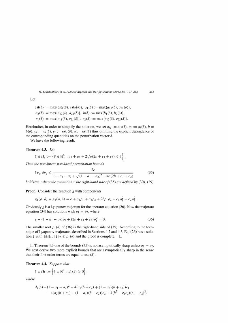
Let
est(δ) := max{est1(δ), est2(δ)}, a1(δ) := max{a11(δ), a21(δ)},a2(δ) := max{a12(δ), a22(δ)}, b(δ) := max{b1(δ), b2(δ)},c1(δ) := max{c11(δ), c21(δ)}, c2(δ) := max{c12(δ), c22(δ)}.
Hereinafter, in order to simplify the notation, we set aij := aij (δ), ai := ai(δ), b =b(δ), ci := ci(δ), ei := esti (δ), e := est(δ) thus omitting the explicit dependence ofthe corresponding quantities on the perturbation vector δ.
We have the following result.
Theorem 4.3. Let
δ ∈ �g :={δ ∈ R8+ : a1 + a2 + 2
√e(2b + c1 + c2) � 1
}.
Then the non-linear non-local perturbation bounds
δX1 , δX2 � 2e
1 − a1 − a2 + √(1 − a1 − a2)2 − 4e(2b + c1 + c2)
(35)
hold true,where the quantities in the right-hand side of (35) are defined by (30), (29).
Proof. Consider the function g with components
g1(ρ, δ) = g2(ρ, δ) = e + a1ρ1 + a2ρ2 + 2bρ1ρ2 + c1ρ21 + c2ρ
22 .
Obviously g is a Lyapunov majorant for the operator equation (26). Now the majorantequation (34) has solutions with ρ1 = ρ2, where
e − (1 − a1 − a2)ρ1 + (2b + c1 + c2)ρ21 = 0. (36)
The smaller root ρ1(δ) of (36) is the right-hand side of (35). According to the tech-nique of Lyapunov majorants, described in Sections 4.2 and 4.3, Eq. (26) has a solu-tion ξ with ‖ξi‖2, ‖ξ‖2 � ρ1(δ) and the proof is complete. �
In Theorem 4.3 one of the bounds (35) is not asymptotically sharp unless e1 = e2.We next derive two more explicit bounds that are asymptotically sharp in the sensethat their first order terms are equal to esti (δ).
Theorem 4.4. Suppose that
δ ∈ �k :={δ ∈ R8+ : dk(δ) � 0
},
where
dk(δ)=(1 − a1 − a2)2 − 4(a1(b + c2) + (1 − a2)(b + c1))e1
− 4(a2(b + c1) + (1 − a1)(b + c2))e2 + 4(b2 − c1c2)(e1 − e2)2.
214 M. Konstantinov et al. / Linear Algebra and its Applications 359 (2003) 197–218
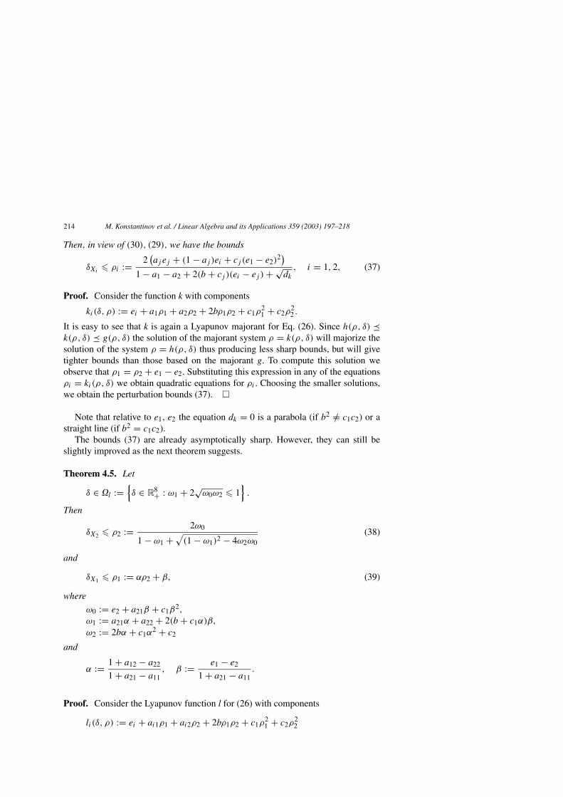
Then, in view of (30), (29), we have the bounds
δXi� ρi := 2
(aj ej + (1 − aj )ei + cj (e1 − e2)
2)
1 − a1 − a2 + 2(b + cj )(ei − ej ) + √dk, i = 1, 2, (37)
Proof. Consider the function k with components
ki(δ, ρ) := ei + a1ρ1 + a2ρ2 + 2bρ1ρ2 + c1ρ21 + c2ρ
22 .
It is easy to see that k is again a Lyapunov majorant for Eq. (26). Since h(ρ, δ) k(ρ, δ) g(ρ, δ) the solution of the majorant system ρ = k(ρ, δ) will majorize thesolution of the system ρ = h(ρ, δ) thus producing less sharp bounds, but will givetighter bounds than those based on the majorant g. To compute this solution weobserve that ρ1 = ρ2 + e1 − e2. Substituting this expression in any of the equationsρi = ki(ρ, δ) we obtain quadratic equations for ρi . Choosing the smaller solutions,we obtain the perturbation bounds (37). �
Note that relative to e1, e2 the equation dk = 0 is a parabola (if b2 /= c1c2) or astraight line (if b2 = c1c2).
The bounds (37) are already asymptotically sharp. However, they can still beslightly improved as the next theorem suggests.
Theorem 4.5. Let
δ ∈ �l :={δ ∈ R8+ : ω1 + 2
√ω0ω2 � 1
}.
Then
δX2 � ρ2 := 2ω0
1 − ω1 + √(1 − ω1)2 − 4ω2ω0
(38)
and
δX1 � ρ1 := αρ2 + β, (39)
where
ω0 := e2 + a21β + c1β2,
ω1 := a21α + a22 + 2(b + c1α)β,
ω2 := 2bα + c1α2 + c2
and
α := 1 + a12 − a22
1 + a21 − a11, β := e1 − e2
1 + a21 − a11.
Proof. Consider the Lyapunov function l for (26) with components
li (δ, ρ) := ei + ai1ρ1 + ai2ρ2 + 2bρ1ρ2 + c1ρ21 + c2ρ
22
M. Konstantinov et al. / Linear Algebra and its Applications 359 (2003) 197–218 215
together with the majorant equations ρi = li (ρ, δ), i = 1, 2. Substracting both sidesof these equations we get
ρ1 − ρ2 = e1 − e2 + a11ρ1 + a12ρ2 − a21ρ1 − a22ρ2.
Supposing that aii < 1 we have
ρ1 = ρ2α + β := ρ21 + a12 − a22
1 + a21 − a11+ e1 − e2
1 + a21 − a11. (40)
Substituting this expression in any of the equations ρi = li (ρ, δ) we get the quadraticequation
ω2ρ22 − (1 − ω1)ρ2 + ω0 = 0
for ρ2. The smaller root of this equation is the desired bound for δX2 and this is theright-hand side of (38). The other bound (39) now follows from (40). �
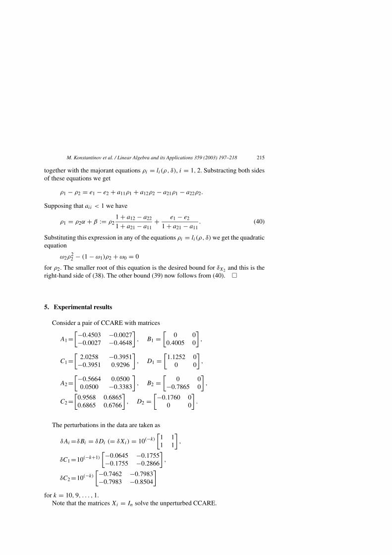
5. Experimental results
Consider a pair of CCARE with matrices
A1 =[−0.4503 −0.0027−0.0027 −0.4648
], B1 =
[0 0
0.4005 0
],
C1 =[
2.0258 −0.3951−0.3951 0.9296
], D1 =
[1.1252 0
0 0
],
A2 =[−0.5664 0.0500
0.0500 −0.3383
], B2 =
[0 0
−0.7865 0
],
C2 =[
0.9568 0.68650.6865 0.6766
], D2 =
[−0.1760 00 0
].
The perturbations in the data are taken as
δAi =δBi = δDi (= δXi) = 10(−k)
[1 11 1
],
δC1 =10(−k+1)[−0.0645 −0.1755−0.1755 −0.2866
],
δC2 =10(−k)
[−0.7462 −0.7983−0.7983 −0.8504
]for k = 10, 9, . . . , 1.
Note that the matrices Xi = In solve the unperturbed CCARE.
216 M. Konstantinov et al. / Linear Algebra and its Applications 359 (2003) 197–218
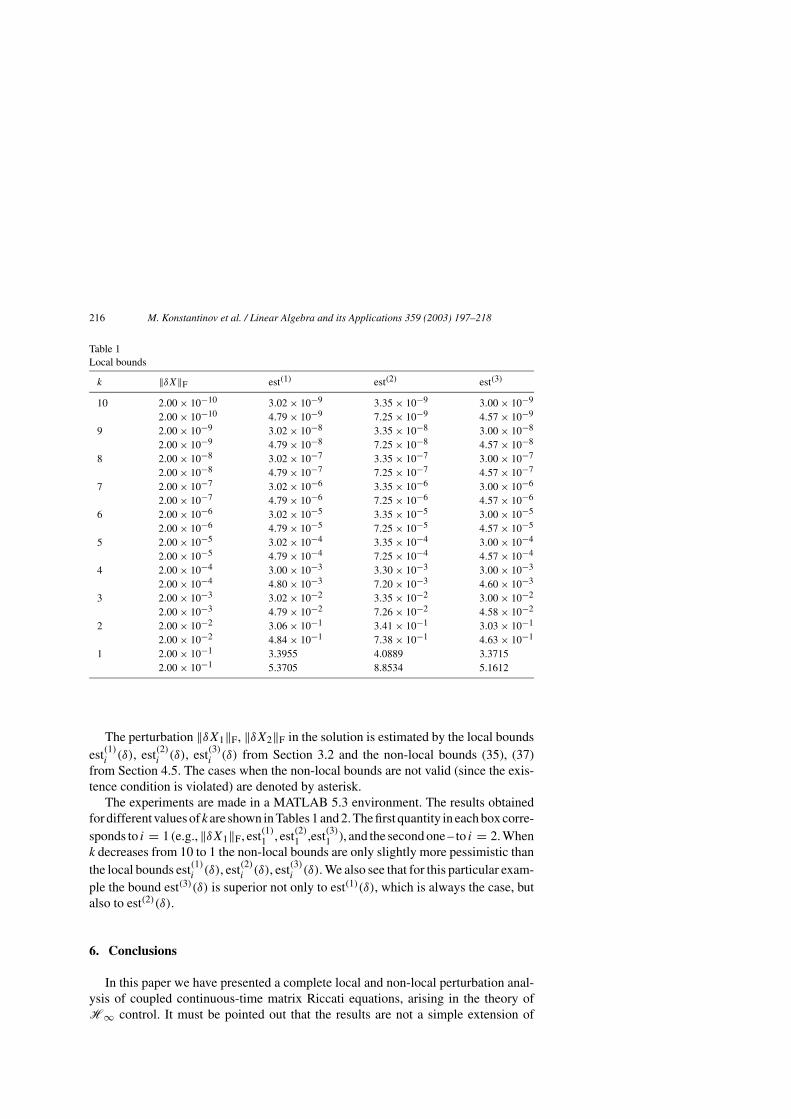
Table 1Local bounds
k ‖δX‖F est(1) est(2) est(3)
10 2.00 × 10⁻¹⁰ 3.02 × 10⁻⁹ 3.35 × 10⁻⁹ 3.00 × 10⁻⁹
2.00 × 10⁻¹⁰ 4.79 × 10⁻⁹ 7.25 × 10⁻⁹ 4.57 × 10⁻⁹
9 2.00 × 10⁻⁹ 3.02 × 10⁻⁸ 3.35 × 10⁻⁸ 3.00 × 10⁻⁸
2.00 × 10⁻⁹ 4.79 × 10⁻⁸ 7.25 × 10⁻⁸ 4.57 × 10⁻⁸
8 2.00 × 10⁻⁸ 3.02 × 10⁻⁷ 3.35 × 10⁻⁷ 3.00 × 10⁻⁷
2.00 × 10⁻⁸ 4.79 × 10⁻⁷ 7.25 × 10⁻⁷ 4.57 × 10⁻⁷
7 2.00 × 10⁻⁷ 3.02 × 10⁻⁶ 3.35 × 10⁻⁶ 3.00 × 10⁻⁶
2.00 × 10⁻⁷ 4.79 × 10⁻⁶ 7.25 × 10⁻⁶ 4.57 × 10⁻⁶
6 2.00 × 10⁻⁶ 3.02 × 10⁻⁵ 3.35 × 10⁻⁵ 3.00 × 10⁻⁵
2.00 × 10⁻⁶ 4.79 × 10⁻⁵ 7.25 × 10⁻⁵ 4.57 × 10⁻⁵
5 2.00 × 10⁻⁵ 3.02 × 10⁻⁴ 3.35 × 10⁻⁴ 3.00 × 10⁻⁴
2.00 × 10⁻⁵ 4.79 × 10⁻⁴ 7.25 × 10⁻⁴ 4.57 × 10⁻⁴
4 2.00 × 10⁻⁴ 3.00 × 10⁻³ 3.30 × 10⁻³ 3.00 × 10⁻³
2.00 × 10⁻⁴ 4.80 × 10⁻³ 7.20 × 10⁻³ 4.60 × 10⁻³
3 2.00 × 10⁻³ 3.02 × 10⁻² 3.35 × 10⁻² 3.00 × 10⁻²
2.00 × 10⁻³ 4.79 × 10⁻² 7.26 × 10⁻² 4.58 × 10⁻²
2 2.00 × 10⁻² 3.06 × 10⁻¹ 3.41 × 10⁻¹ 3.03 × 10⁻¹
2.00 × 10⁻² 4.84 × 10⁻¹ 7.38 × 10⁻¹ 4.63 × 10⁻¹
1 2.00 × 10⁻¹ 3.3955 4.0889 3.37152.00 × 10−1 5.3705 8.8534 5.1612
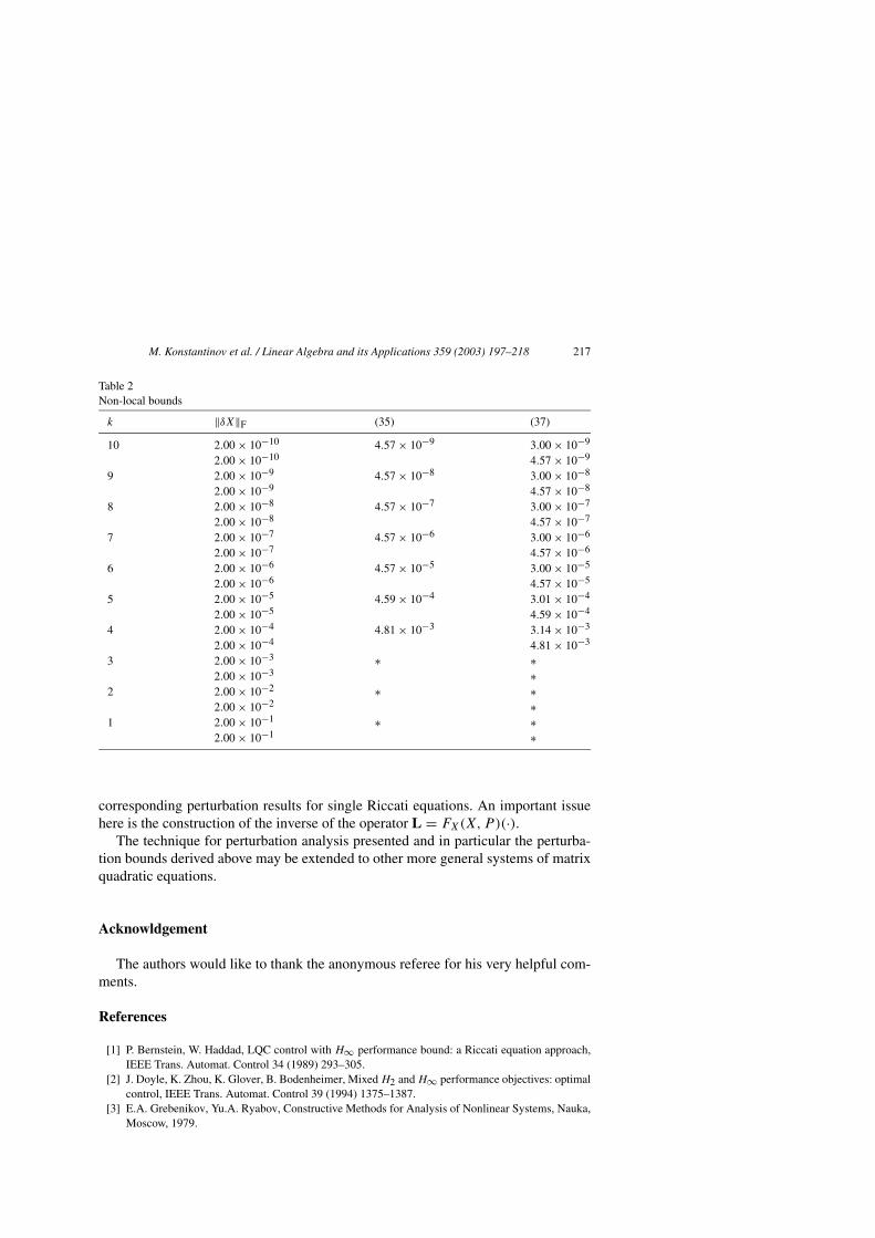
The perturbation ‖δX1‖F, ‖δX2‖F in the solution is estimated by the local boundsest(1)i (δ), est(2)i (δ), est(3)i (δ) from Section 3.2 and the non-local bounds (35), (37)from Section 4.5. The cases when the non-local bounds are not valid (since the exis-tence condition is violated) are denoted by asterisk.
The experiments are made in a MATLAB 5.3 environment. The results obtainedfor different values of k are shown in Tables 1 and 2. The first quantity in each box corre-sponds to i = 1 (e.g.,‖δX1‖F, est(1)1 , est(2)1 ,est(3)1 ), and the second one – to i = 2. Whenk decreases from 10 to 1 the non-local bounds are only slightly more pessimistic thanthe local bounds est(1)i (δ), est(2)i (δ), est(3)i (δ). We also see that for this particular exam-ple the bound est(3)(δ) is superior not only to est(1)(δ), which is always the case, butalso to est(2)(δ).
6. Conclusions
In this paper we have presented a complete local and non-local perturbation anal-ysis of coupled continuous-time matrix Riccati equations, arising in the theory ofH∞ control. It must be pointed out that the results are not a simple extension of
M. Konstantinov et al. / Linear Algebra and its Applications 359 (2003) 197–218 217
Table 2Non-local bounds
k ‖δX‖F (35) (37)
10 2.00 × 10⁻¹⁰ 4.57 × 10⁻⁹ 3.00 × 10⁻⁹
2.00 × 10⁻¹⁰ 4.57 × 10⁻⁹
9 2.00 × 10⁻⁹ 4.57 × 10⁻⁸ 3.00 × 10⁻⁸
2.00 × 10⁻⁹ 4.57 × 10⁻⁸
8 2.00 × 10⁻⁸ 4.57 × 10⁻⁷ 3.00 × 10⁻⁷
2.00 × 10⁻⁸ 4.57 × 10⁻⁷
7 2.00 × 10⁻⁷ 4.57 × 10⁻⁶ 3.00 × 10⁻⁶
2.00 × 10⁻⁷ 4.57 × 10⁻⁶
6 2.00 × 10⁻⁶ 4.57 × 10⁻⁵ 3.00 × 10⁻⁵
2.00 × 10⁻⁶ 4.57 × 10⁻⁵
5 2.00 × 10⁻⁵ 4.59 × 10⁻⁴ 3.01 × 10⁻⁴
2.00 × 10⁻⁵ 4.59 × 10⁻⁴
4 2.00 × 10⁻⁴ 4.81 × 10⁻³ 3.14 × 10⁻³
2.00 × 10⁻⁴ 4.81 × 10⁻³
3 2.00 × 10⁻³ ∗ ∗2.00 × 10−3 ∗
2 2.00 × 10⁻² ∗ ∗2.00 × 10−2 ∗
1 2.00 × 10⁻¹ ∗ ∗2.00 × 10⁻¹ ∗
corresponding perturbation results for single Riccati equations. An important issuehere is the construction of the inverse of the operator L = FX(X, P )(·).
The technique for perturbation analysis presented and in particular the perturba-tion bounds derived above may be extended to other more general systems of matrixquadratic equations.
Acknowldgement
The authors would like to thank the anonymous referee for his very helpful com-ments.
References
[1] P. Bernstein, W. Haddad, LQC control with H∞ performance bound: a Riccati equation approach,IEEE Trans. Automat. Control 34 (1989) 293–305.
[2] J. Doyle, K. Zhou, K. Glover, B. Bodenheimer, Mixed H2 and H∞ performance objectives: optimalcontrol, IEEE Trans. Automat. Control 39 (1994) 1375–1387.
[3] E.A. Grebenikov, Yu.A. Ryabov, Constructive Methods for Analysis of Nonlinear Systems, Nauka,Moscow, 1979.
218 M. Konstantinov et al. / Linear Algebra and its Applications 359 (2003) 197–218
[4] R.A. Horn, C.R. Johnson, Topics in Matrix Analysis (in Russian), Cambridge University Press,Cambridge, UK, 1991.
[5] V. Kapila, W. Haddad, A multivariable extension of the Tsypkin criterion using a Lyapunov-functionapproach, IEEE Trans. Automat. Control 41 (1996) 149–159.
[6] M. Konstantinov, V. Mehrmann, P. Petkov, On properties of general Sylvester and Lyapunov oper-ators, Linear Algebra Appl. 312 (2000) 35–71.
[7] M. Konstantinov, P. Petkov, D.W. Gu, I. Postlethwaite, Perturbation analysis in finite dimensionalspaces, Technical Report 96–18, Department of Engineering, Leicester University, Leicester, UK,June 1996.
[8] M. Konstantinov, M. Stanislavova, P. Petkov, Perturbation bounds and characterisation of the solu-tion of the associated algebraic Riccati equation, Linear Algebra Appl. 285 (1998) 7–31.
[9] P. Lancaster, L. Rodman, The Algebraic Riccati Equation, Oxford University Press, Oxford, 1995.[10] P. Lancaster, M. Tismenetsky, The Theory of Matrices, second ed., Academic Press, Orlando, FL,
1985.[11] J. Ortega, W. Rheinboldt, Iterative Solution of Nonlinear Equations in Several Variables, Academic
Press, New York, 1970.[12] E. Tyan, P. Bernstein, Anti-windup compensator synthesis for systems with saturation actuators, Int.
J. Robust. Nonlinear Control 5 (1995) 321–337.


![Simple bounds for convergence of empirical and occupation ... · with notable importance in statistics. For many examples, we refer to the book of Van der Vaart and Wellner [32] and](https://img.pdfslide.fr/doc/110x75/5e819644000a552a9656d0fa/simple-bounds-for-convergence-of-empirical-and-occupation-with-notable-importance.jpg)