Physique des Particules Avancées 2

Interactions Fortes

et Interactions Faibles

Leçon 1 – Introduction au Modèle Standard (http://dpnc.unige.ch/~bravar/PPA2/L1)

enseignant

Alessandro Bravar Alessandro.Bravar@unige.ch

tél.: 96210 bureau: EP 206

assistant

Alexander Korzenev Korzenev@mail.cern.ch

tél.: 93456 bureau: EP 221

19 février 2018

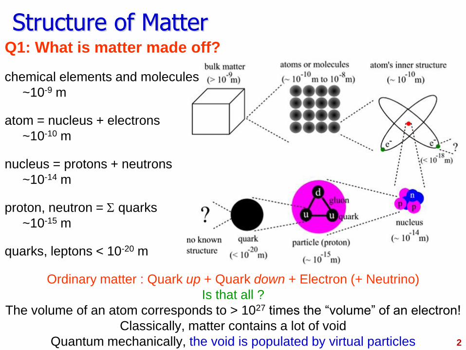
Structure of Matter Q1: What is matter made off?

chemical elements and molecules

~10-9 m

atom = nucleus + electrons

~10-10 m

nucleus = protons + neutrons

~10-14 m

proton, neutron = S quarks

~10-15 m

quarks, leptons < 10-20 m

Ordinary matter : Quark up + Quark down + Electron (+ Neutrino)

Is that all ?

The volume of an atom corresponds to > 1027 times the “volume” of an electron!

Classically, matter contains a lot of void

Quantum mechanically, the void is populated by virtual particles

2

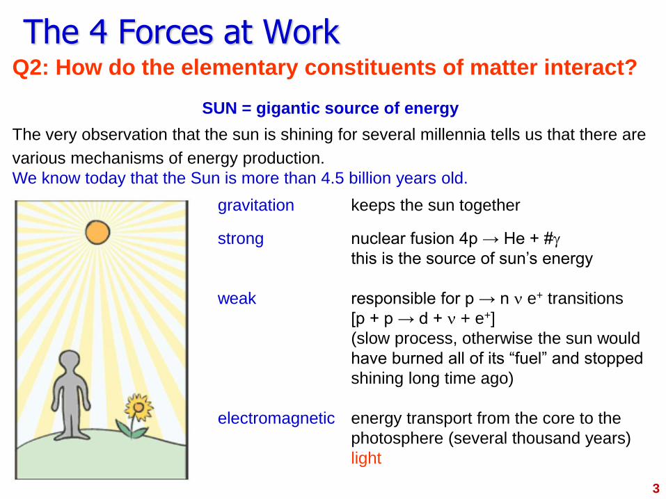
The 4 Forces at Work Q2: How do the elementary constituents of matter interact?

SUN = gigantic source of energy

The very observation that the sun is shining for several millennia tells us that there are

various mechanisms of energy production.

We know today that the Sun is more than 4.5 billion years old.

gravitation keeps the sun together

strong nuclear fusion 4p → He + #g

this is the source of sun’s energy

weak responsible for p → n n e+ transitions

[p + p → d + n + e+]

(slow process, otherwise the sun would

have burned all of its “fuel” and stopped

shining long time ago)

electromagnetic energy transport from the core to the

photosphere (several thousand years)

light

3

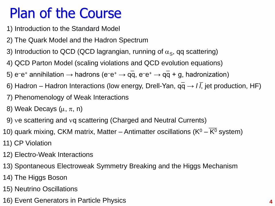
Plan of the Course 1) Introduction to the Standard Model

2) The Quark Model and the Hadron Spectrum

3) Introduction to QCD (QCD lagrangian, running of aS, qq scattering)

4) QCD Parton Model (scaling violations and QCD evolution equations)

5) e–e+ annihilation → hadrons (e–e+ → qq, e–e+ → qq + g, hadronization)

6) Hadron – Hadron Interactions (low energy, Drell-Yan, qq → l l, jet production, HF)

7) Phenomenology of Weak Interactions

8) Weak Decays (m, p, n)

9) ne scattering and nq scattering (Charged and Neutral Currents)

10) quark mixing, CKM matrix, Matter – Antimatter oscillations (K0 – K0 system)

11) CP Violation

12) Electro-Weak Interactions

13) Spontaneous Electroweak Symmetry Breaking and the Higgs Mechanism

14) The Higgs Boson

15) Neutrino Oscillations

16) Event Generators in Particle Physics 4

References F. Halzen and A. D. Martin (our main references)

Quarks & Leptons

M. Thomson (our main references)

Modern Particle Physics

G.Kane

Modern Elementary Particle Physics (2nd Ed.)

D. Griffiths

Introduction to Elementary Particles (2nd Rev. Ed.)

A. Bettini

Introduction to Elementary Particle Physics (2nd Rev. Ed.)

Recent developments and results

review articles in Annual Reviews of Nuclear and Particle Physics Science

reviews and articles posted on the archive http://arXiv.org

And on Quantum Field Theory

C. Quigg

Gauge Theories of the Strong, Weak, and Electromagnetic Interactions (2nd Ed.)

I.J.R. Aitchison and A.J.G. Hey

Gauge Theories in Particle Physics (4th Ed.)

Lecture notes: http://dpnc.unige.ch/~bravar/PPA2 5

Evaluation

Oral exam in June or September (must have passed PPA1)

Active participation in exercise sessions

homeworks!

Halzen & Martin and Thomson textbooks are our main reference for the course

(they are almost equivalent, Thomson is more recent)

For topics not covered in Halzen & Martin or Thomson,

we shall provide the reference material.

Evaluation of the course (you) via a questioner at the end of the semester.

During the semester one or two additional question times, if you ask for

(you ask questions, we try to answer them).

6

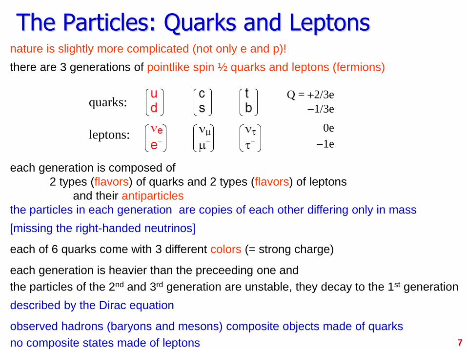
nature is slightly more complicated (not only e and p)!

there are 3 generations of pointlike spin ½ quarks and leptons (fermions)

each generation is composed of

2 types (flavors) of quarks and 2 types (flavors) of leptons

and their antiparticles

the particles in each generation are copies of each other differing only in mass

[missing the right-handed neutrinos]

each of 6 quarks come with 3 different colors (= strong charge)

each generation is heavier than the preceeding one and

the particles of the 2nd and 3rd generation are unstable, they decay to the 1st generation

described by the Dirac equation

observed hadrons (baryons and mesons) composite objects made of quarks

no composite states made of leptons

The Particles: Quarks and Leptons

Q = 2/3e

1/3e

0e

1e

quarks:

leptons:

7

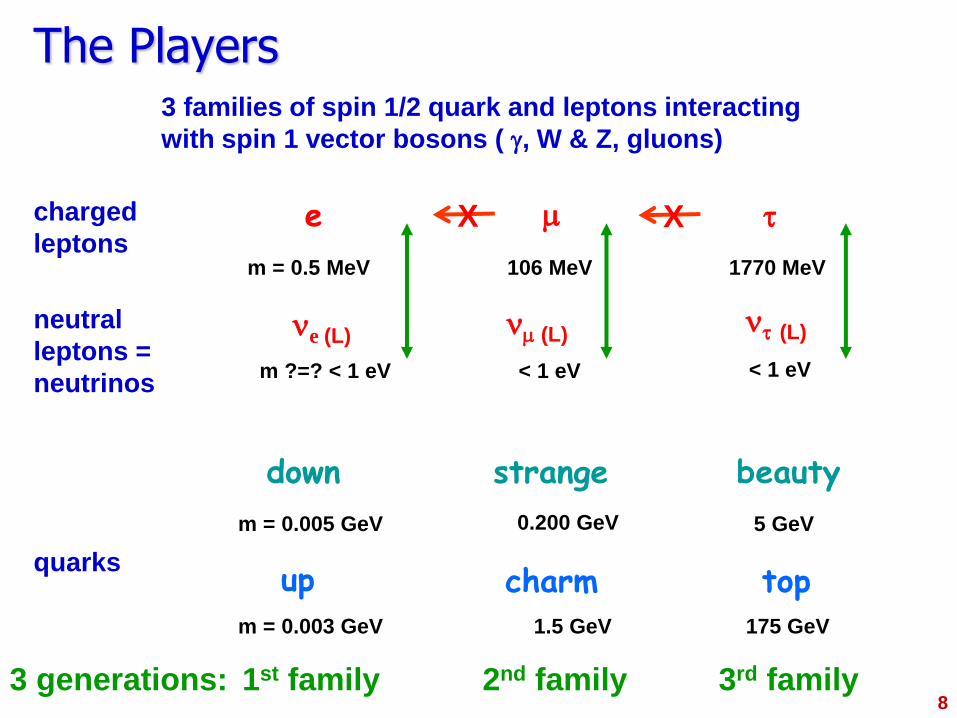
The Players

e

ne (L)

down

up

1st family

m = 0.5 MeV

m ?=? < 1 eV

m = 0.005 GeV

m = 0.003 GeV

< 1 eV

m

nm (L)

strange

charm

2nd family

106 MeV

0.200 GeV

1.5 GeV

t

nt (L)

beauty

top

3rd family

1770 MeV

< 1 eV

5 GeV

175 GeV

charged

leptons

neutral

leptons =

neutrinos

quarks

3 families of spin 1/2 quark and leptons interacting

with spin 1 vector bosons ( g, W & Z, gluons)

3 generations:

X X

8

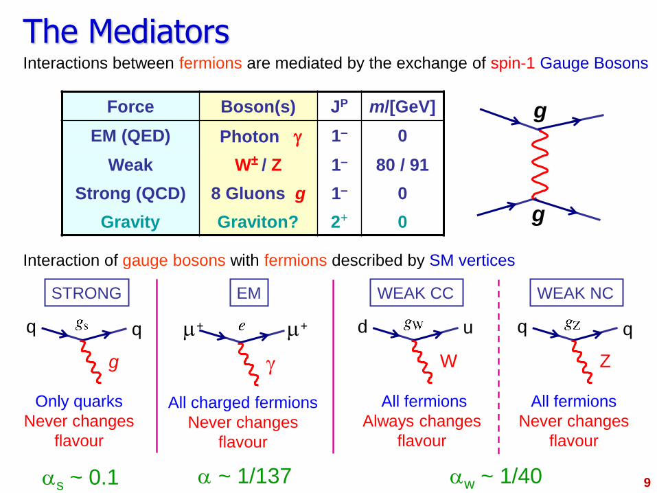
The Mediators

9

Interactions between fermions are mediated by the exchange of spin-1 Gauge Bosons

Interaction of gauge bosons with fermions described by SM vertices

Force Boson(s) JP m/[GeV]

EM (QED) Photon g 1– 0

Weak W± / Z 1– 80 / 91

Strong (QCD) 8 Gluons g 1– 0

Gravity Graviton? 2+ 0

g

g

STRONG EM WEAK CC WEAK NC

Only quarks

Never changes

flavour

All charged fermions

Never changes

flavour

All fermions

Always changes

flavour

All fermions

Never changes

flavour

q q

g

d

W

u q q

Z

m+

g

m+

as ~ 0.1 a ~ 1/137 aw ~ 1/40

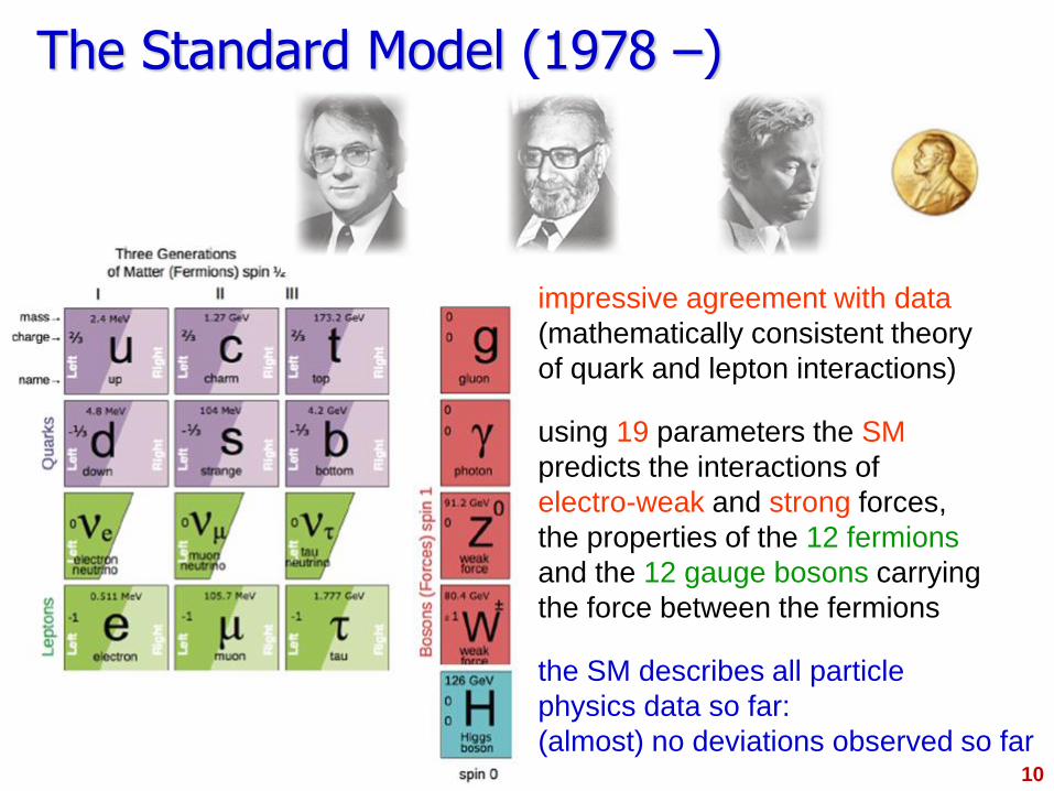
The Standard Model (1978 –)

impressive agreement with data

(mathematically consistent theory

of quark and lepton interactions)

using 19 parameters the SM

predicts the interactions of

electro-weak and strong forces,

the properties of the 12 fermions

and the 12 gauge bosons carrying

the force between the fermions

the SM describes all particle

physics data so far:

(almost) no deviations observed so far 10

Particle Physics Goals 1. Identify the basic (structureless) constituents of matter

2. Understand the nature of forces acting between them

“three” distinct type of particles:

quarks and leptons – spin ½ fermions

gauge bosons – spin 1 bosons, mediate interactions between quarks and leptons

Higgs boson – spin 0 boson, origin of mass

four interactions in Nature:

strong

electromagnetic

weak

gravitational

Symmetries play a central role in particle physics: our knowledge of forces stems from

our understanding of the underlying symmetries and the way in which they are broken.

One aim of particle physics is to discover the fundamental symmetries.

Link experimental (measurable) observables with calculable quantities:

scattering

spectroscopy

decays 11

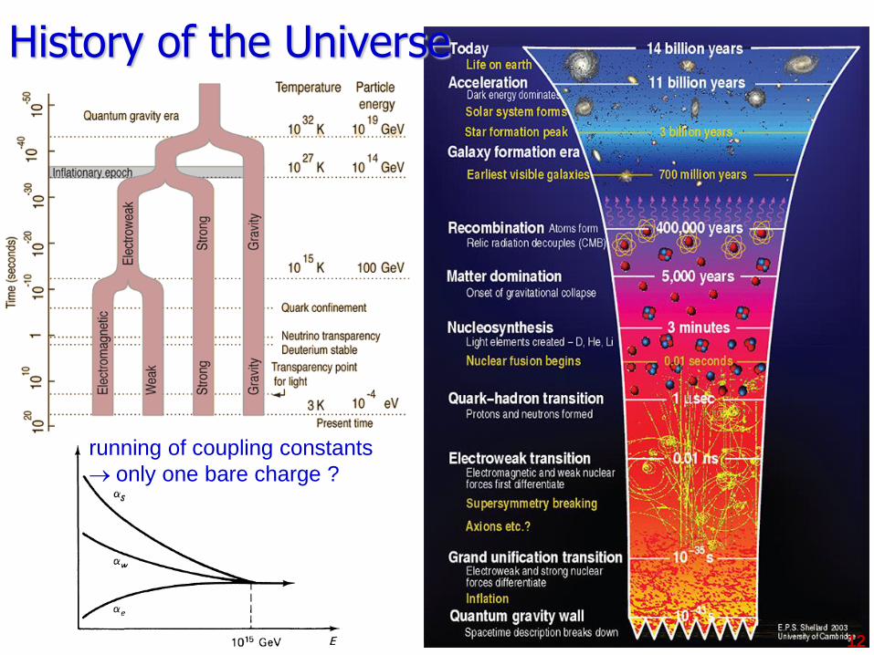
History of the Universe

12

running of coupling constants

only one bare charge ?

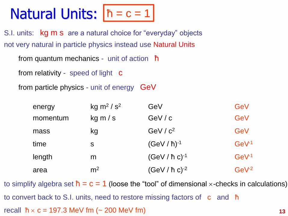
Natural Units:

13

S.I. units: kg m s are a natural choice for “everyday” objects

not very natural in particle physics instead use Natural Units

from quantum mechanics - unit of action ћ

from relativity - speed of light c

from particle physics - unit of energy GeV

energy kg m2 / s2 GeV GeV

momentum kg m / s GeV / c GeV

mass kg GeV / c2 GeV

time s (GeV / ћ)-1 GeV-1

length m (GeV / ћ c)-1 GeV-1

area m2 (GeV / ћ c)-2 GeV-2

to simplify algebra set ћ = c = 1 (loose the “tool” of dimensional -checks in calculations)

to convert back to S.I. units, need to restore missing factors of c and ћ

recall ћ c = 197.3 MeV fm (~ 200 MeV fm)

ћ = c = 1

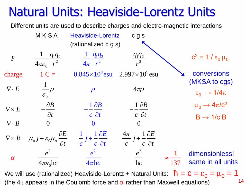
Natural Units: Heaviside-Lorentz Units Different units are used to describe charges and electro-magnetic interactions

M K S A Heaviside-Lorentz c g s

(rationalized c g s)

1 2 1 2

2 2

0

9

0

0

2

2

22

9

0

1

2

1

4

0.84

1

4

2.997 10charge 1 C =

1

13

esu

14

1

0 0

4 1

4

5 10 esu

1

0

1 1

4 7

o o

q q q qF

r r

E

B BE

t

q q

r

c t

B

E EB j

B

c t

Ej

c c t

e

jt c c

c

t

e e

c c

p

p

pm m

pa

p

p

hhh

14

We will use (rationalized) Heaviside-Lorentz + Natural Units: ћ = c = 0 = m0 = 1 (the 4p appears in the Coulomb force and a rather than Maxwell equations)

c2 = 1 / 0 m0

conversions

(MKSA to cgs)

0 → 1/4p

m0 → 4p/c2

B → 1/c B

dimensionless!

same in all units

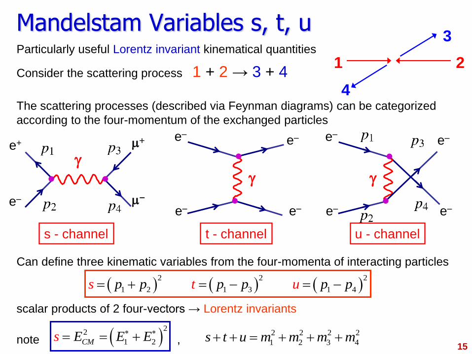
Mandelstam Variables s, t, u

15

Particularly useful Lorentz invariant kinematical quantities

Consider the scattering process 1 + 2 → 3 + 4

The scattering processes (described via Feynman diagrams) can be categorized

according to the four-momentum of the exchanged particles

Can define three kinematic variables from the four-momenta of interacting particles

scalar products of 2 four-vectors → Lorentz invariants

note ,

1 2

4

3

e– e–

e– e–

g

e– m–

e+ m

g

e– e–

e– e–

g

s - channel t - channel u - channel

2 2 2

1 2 1 3 1 4p p ps t up p p

2

2

1 2CME Es E 2 2 2 2

1 2 3 4s t u m m m m

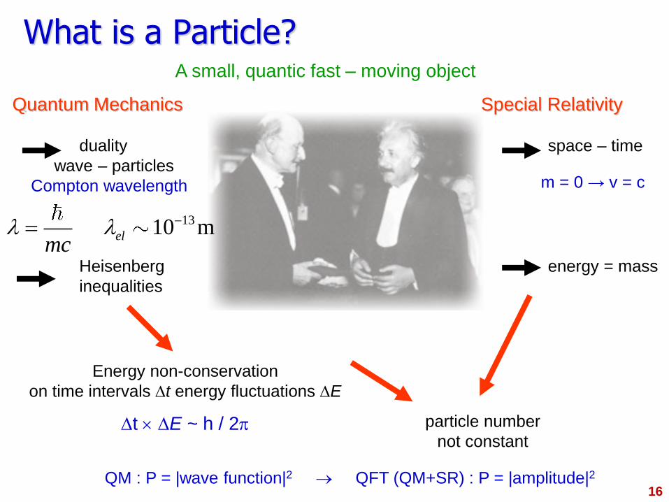
Quantum Mechanics Special Relativity

duality space – time

wave – particles

Compton wavelength

Heisenberg energy = mass

inequalities

What is a Particle? A small, quantic fast – moving object

Energy non-conservation

on time intervals Dt energy fluctuations DE

Dt DE ~ h / 2p particle number

not constant

QM : P = |wave function|2 QFT (QM+SR) : P = |amplitude|2

16

m = 0 → v = c

13 10 melmc

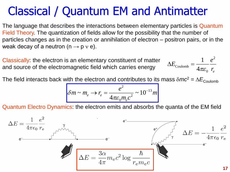
Classical / Quantum EM and Antimatter The language that describes the interactions between elementary particles is Quantum

Field Theory. The quantization of fields allow for the possibility that the number of

particles changes as in the creation or annihilation of electron – positron pairs, or in the

weak decay of a neutron (n → p n e).

Classically: the electron is an elementary constituent of matter

and source of the electromagnetic field which carries energy

The field interacts back with the electron and contributes to its mass dmc2 = DECoulomb

Quantum Electro Dynamics: the electron emits and absorbs the quanta of the EM field

17

213

2

0

~ ~ 104

e e

e

em m r m

m cd

p

2

Coulomb

0

1

4 e

eE

rpD

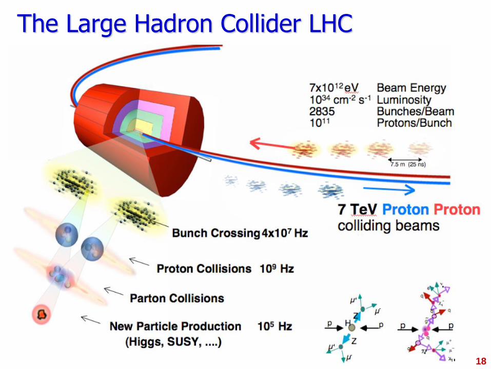
The Large Hadron Collider LHC

18

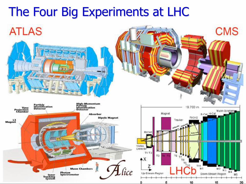
The Four Big Experiments at LHC

19

Relativistic Quantum Field Theory

20

General framework to study fundamental interactions, which leads to a unified treatment

of all interactions.

Relativistic QFT combines quantum theory

relativity

the concept of field

The quantization of any classical field introduces the quanta of the field which are

particles with well defined properties. The interactions between these particles are

mediated by other fields whose quanta are yet other particles:

e.g. the interaction between an electron and a positron is mediated by the

electromagnetic field (action at a distance) or due to an exchange of photons (local).

The electron and the positron themselves can be thought of as the quanta of an electron-

positron field. That allows the number of particles to change, like the creation or

annihilation of an electron-positron pairs.

These processes occur through the interaction of fields.

the solution of the equations of the quantized interacting fields is extremely difficult

if the interaction is sufficiently weak one can employ perturbation theory,

like in electrodynamics.

Major difficulty when calculating beyond leading order, is the (almost unavoidable)

appearance of UV divergences (e.g. in loop diagrams) renormalization

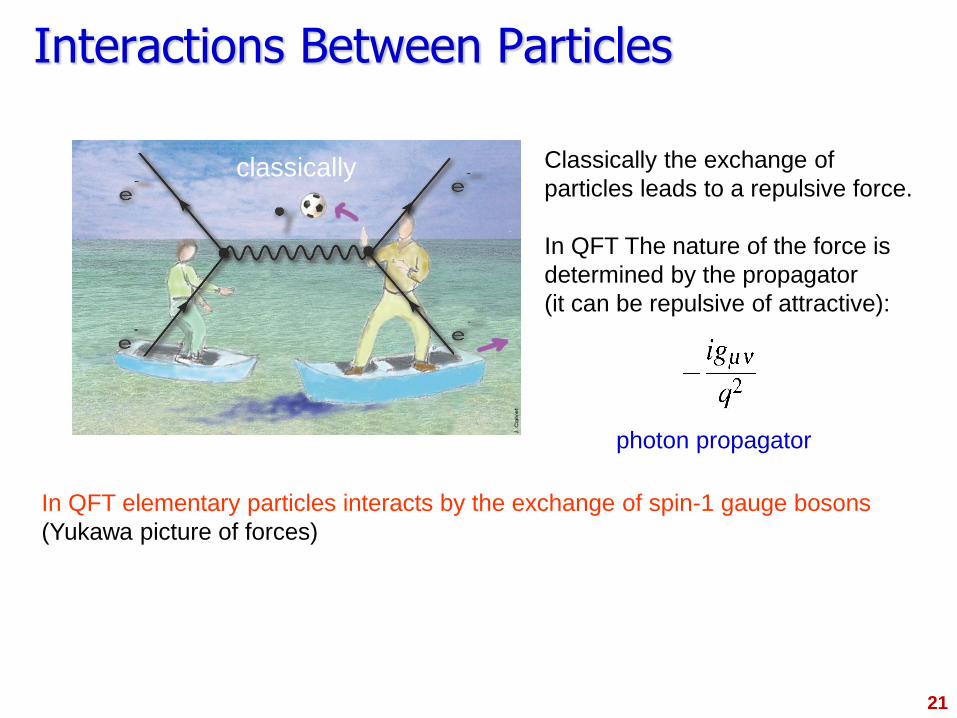
Interactions Between Particles

In QFT elementary particles interacts by the exchange of spin-1 gauge bosons

(Yukawa picture of forces)

21

photon propagator

classically Classically the exchange of

particles leads to a repulsive force.

In QFT The nature of the force is

determined by the propagator

(it can be repulsive of attractive):

Feynman Calculus Relativistic quantum Field theory is a highly formal and sophisticated discipline. Technical

complexities are particular evident in the case of gauge theories (QED is an exception).

Short circuit the formalism and reach the calculational stage more quickly by

emphasizing the important physics aspects.

In this course we will follow a heuristic approach (as in H&M), based on solutions of

relativistic wave equations for free particles and treat the interaction as a perturbation,

but in agreement with rigorous QFT calculations.

Antiparticles are introduced following the Stückelberg – Feynman prescription:

negative energy particle solutions going backward in time describe positive-energy

antiparticles going forward in time (exp –i(–E)(–t) = exp i E t !).

Feynman diagrams NB They are much more than simple drawings!

They tell us how to calculate the interaction (physics)!

The most important modern perturbation-theoretic technique employs Feynman calculus

and rules, and Feynman diagrams, which use is quite simple and intuitive in deriving

important particle physics results.

In Quantum Electro-Dynamics a complete agreement exists between theory and

experiment to an incredibly high degree of accuracy.

QED is the prototype theory for all other interactions (strong and weak). 22

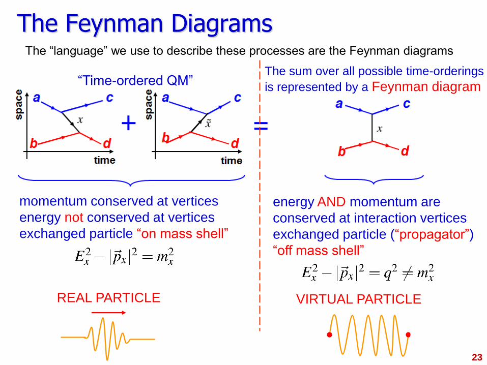
The Feynman Diagrams The “language” we use to describe these processes are the Feynman diagrams

momentum conserved at vertices

energy not conserved at vertices

exchanged particle “on mass shell”

energy AND momentum are

conserved at interaction vertices

exchanged particle (“propagator”)

“off mass shell”

REAL PARTICLE

“Time-ordered QM” The sum over all possible time-orderings

is represented by a Feynman diagram

23

VIRTUAL PARTICLE

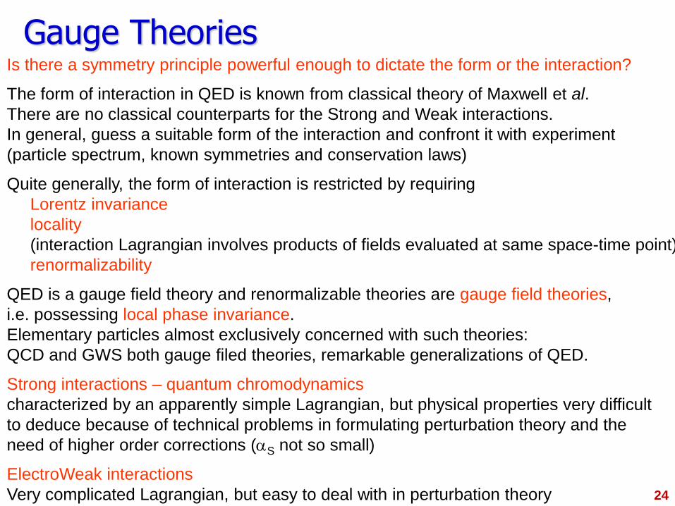
Gauge Theories

24

Is there a symmetry principle powerful enough to dictate the form or the interaction?

The form of interaction in QED is known from classical theory of Maxwell et al.

There are no classical counterparts for the Strong and Weak interactions.

In general, guess a suitable form of the interaction and confront it with experiment

(particle spectrum, known symmetries and conservation laws)

Quite generally, the form of interaction is restricted by requiring

Lorentz invariance

locality

(interaction Lagrangian involves products of fields evaluated at same space-time point)

renormalizability

QED is a gauge field theory and renormalizable theories are gauge field theories,

i.e. possessing local phase invariance.

Elementary particles almost exclusively concerned with such theories:

QCD and GWS both gauge filed theories, remarkable generalizations of QED.

Strong interactions – quantum chromodynamics

characterized by an apparently simple Lagrangian, but physical properties very difficult

to deduce because of technical problems in formulating perturbation theory and the

need of higher order corrections (aS not so small)

ElectroWeak interactions

Very complicated Lagrangian, but easy to deal with in perturbation theory

QED: Dirac + EM Fields

25

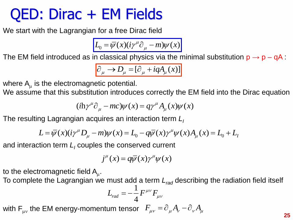
We start with the Lagrangian for a free Dirac field

The EM field introduced as in classical physics via the minimal substitution p → p – qA :

where Am is the electromagnetic potential.

We assume that this substitution introduces correctly the EM field into the Dirac equation

The resulting Lagrangian acquires an interaction term LI

and interaction term LI couples the conserved current

to the electromagnetic field Am.

To complete the Lagrangian we must add a term Lrad describing the radiation field itself

with Fmn the EM energy-momentum tensor

0 ( )( ) ( )L x i m xm

m g

[ ( )]D iqA xm m m m

0 0( )( ) ( ) ( ) ( ) ( ) IL x i D m x L q x x A x L Lm m

m m g g

( ) ( ) ( ) ( )i mc x q A x xm m

m mg g h

( ) ( ) ( )j x q x xm m g

1

4radL F Fmn

mn

F A Amn m n n m

26

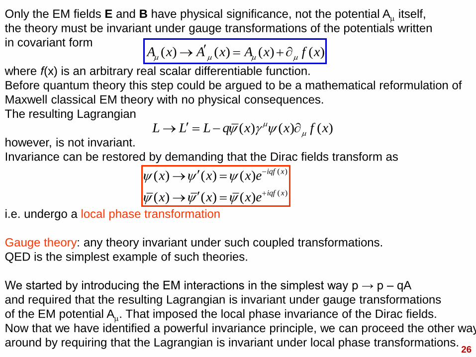
Only the EM fields E and B have physical significance, not the potential Am itself,

the theory must be invariant under gauge transformations of the potentials written

in covariant form

where f(x) is an arbitrary real scalar differentiable function.

Before quantum theory this step could be argued to be a mathematical reformulation of

Maxwell classical EM theory with no physical consequences.

The resulting Lagrangian

however, is not invariant.

Invariance can be restored by demanding that the Dirac fields transform as

i.e. undergo a local phase transformation

Gauge theory: any theory invariant under such coupled transformations.

QED is the simplest example of such theories.

We started by introducing the EM interactions in the simplest way p → p – qA

and required that the resulting Lagrangian is invariant under gauge transformations

of the EM potential Am. That imposed the local phase invariance of the Dirac fields.

Now that we have identified a powerful invariance principle, we can proceed the other way

around by requiring that the Lagrangian is invariant under local phase transformations.

( ) ( ) ( )L L L q x x f xm

m g

( )

( )

( ) ( ) ( )

( ) ( ) ( )

iqf x

iqf x

x x x e

x x x e

( ) ( ) ( ) ( )A x A x A x f xm m m m

Gauge Fields

27

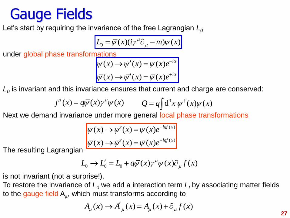
Let’s start by requiring the invariance of the free Lagrangian L0

under global phase transformations

L0 is invariant and this invariance ensures that current and charge are conserved:

Next we demand invariance under more general local phase transformations

The resulting Lagrangian

is not invariant (not a surprise!).

To restore the invariance of L0 we add a interaction term LI by associating matter fields

to the gauge field Am, which must transforms according to

0 ( )( ) ( )L x i m xm

m g

( ) ( ) ( )

( ) ( ) ( )

i

i

x x x e

x x x e

a

a

( ) ( ) ( )j x q x xm m g 3 †d ( ) ( )Q q x x x

( )

( )

( ) ( ) ( )

( ) ( ) ( )

iqf x

iqf x

x x x e

x x x e

0 0 0 ( ) ( ) ( )L L L q x x f xm

m g

( ) ( ) ( ) ( )A x A x A x f xm m m m

28

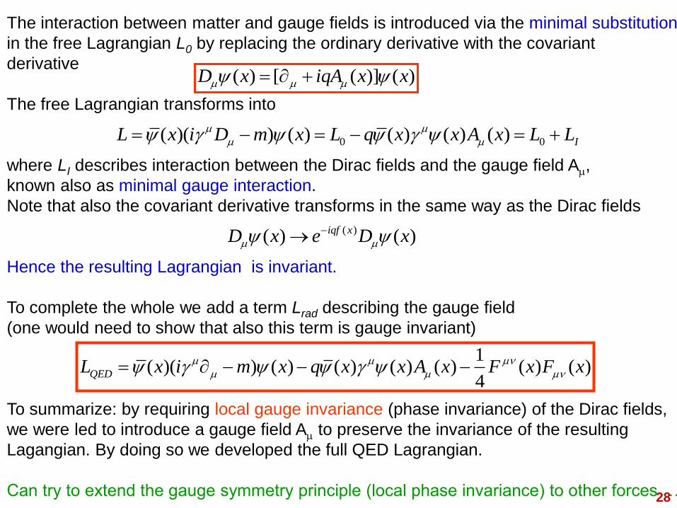
The interaction between matter and gauge fields is introduced via the minimal substitution

in the free Lagrangian L0 by replacing the ordinary derivative with the covariant

derivative

The free Lagrangian transforms into

where LI describes interaction between the Dirac fields and the gauge field Am,

known also as minimal gauge interaction.

Note that also the covariant derivative transforms in the same way as the Dirac fields

Hence the resulting Lagrangian is invariant.

To complete the whole we add a term Lrad describing the gauge field

(one would need to show that also this term is gauge invariant)

To summarize: by requiring local gauge invariance (phase invariance) of the Dirac fields,

we were led to introduce a gauge field Am to preserve the invariance of the resulting

Lagangian. By doing so we developed the full QED Lagrangian.

Can try to extend the gauge symmetry principle (local phase invariance) to other forces …

( ) [ ( )] ( )D x iqA x xm m m

0 0( )( ) ( ) ( ) ( ) ( ) IL x i D m x L q x x A x L Lm m

m m g g

( )( ) ( )iqf xD x e D xm m

1( )( ) ( ) ( ) ( ) ( ) ( ) ( )

4QEDL x i m x q x x A x F x F xm m mn

m m mn g g

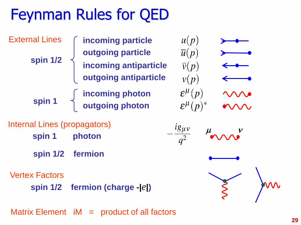
Feynman Rules for QED

29

m n spin 1 photon

spin 1/2 fermion

spin 1/2 fermion (charge -|e|)

Matrix Element iM = product of all factors

External Lines

Internal Lines (propagators)

Vertex Factors

outgoing particle

outgoing antiparticle

incoming antiparticle

incoming particle

spin 1/2

spin 1 outgoing photon

incoming photon

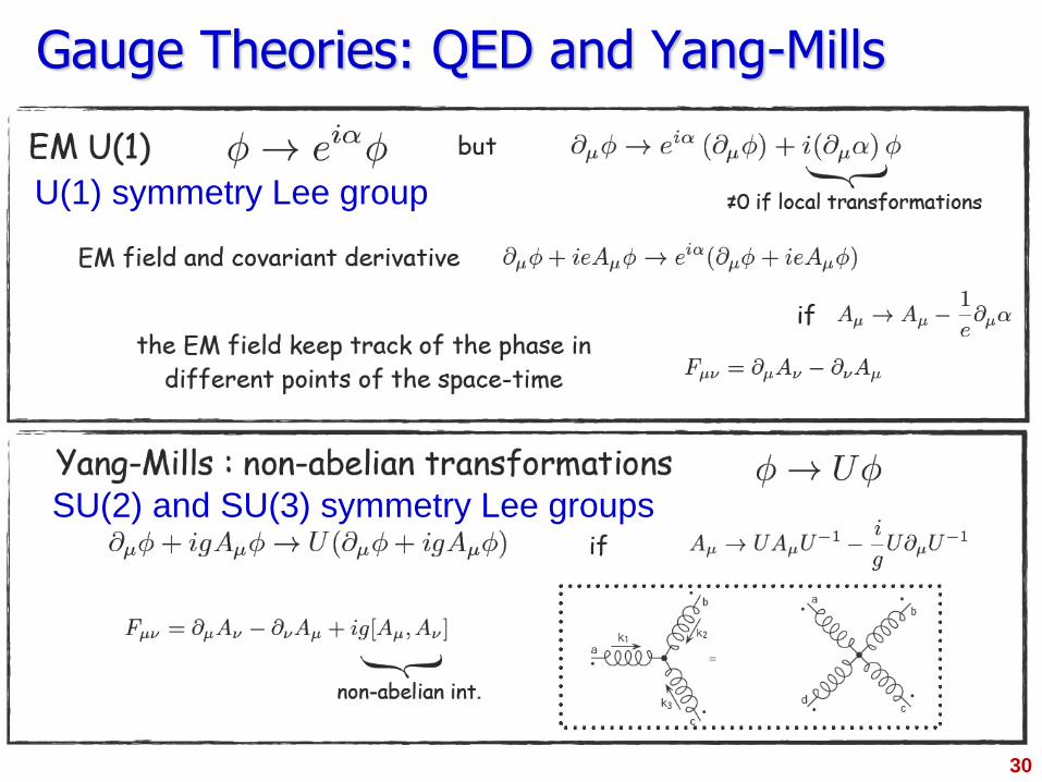
Gauge Theories: QED and Yang-Mills

SU(2) and SU(3) symmetry Lee groups

U(1) symmetry Lee group

30

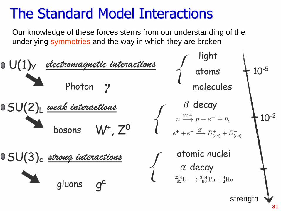
The Standard Model Interactions Our knowledge of these forces stems from our understanding of the

underlying symmetries and the way in which they are broken

strength 31

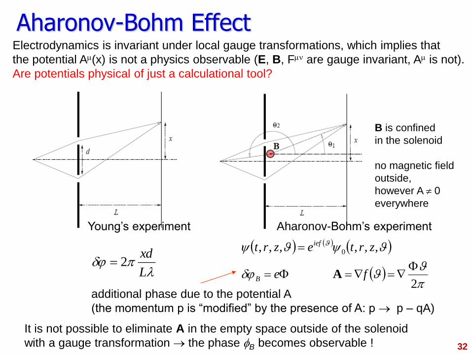
Aharonov-Bohm Effect Electrodynamics is invariant under local gauge transformations, which implies that

the potential Am(x) is not a physics observable (E, B, Fmn are gauge invariant, Am is not).

Are potentials physical of just a calculational tool?

It is not possible to eliminate A in the empty space outside of the solenoid

with a gauge transformation the phase fB becomes observable !

Young’s experiment Aharonov-Bohm’s experiment

p

d

2

,,,,,, 0

fe

zrtezrt

B

ief

A

additional phase due to the potential A

(the momentum p is “modified” by the presence of A: p p – qA)

B is confined

in the solenoid

no magnetic field

outside,

however A 0

everywhere

32

pd

L

xd2

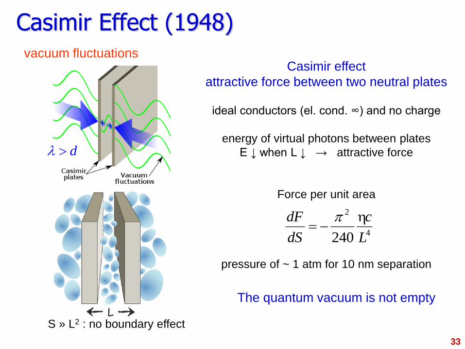
Casimir Effect (1948)

S » L2 : no boundary effect

The quantum vacuum is not empty

Casimir effect

attractive force between two neutral plates

ideal conductors (el. cond. ∞) and no charge

energy of virtual photons between plates

E ↓ when L ↓ → attractive force

Force per unit area

pressure of ~ 1 atm for 10 nm separation

4

2

240 L

c

dS

dF p

d

33

vacuum fluctuations

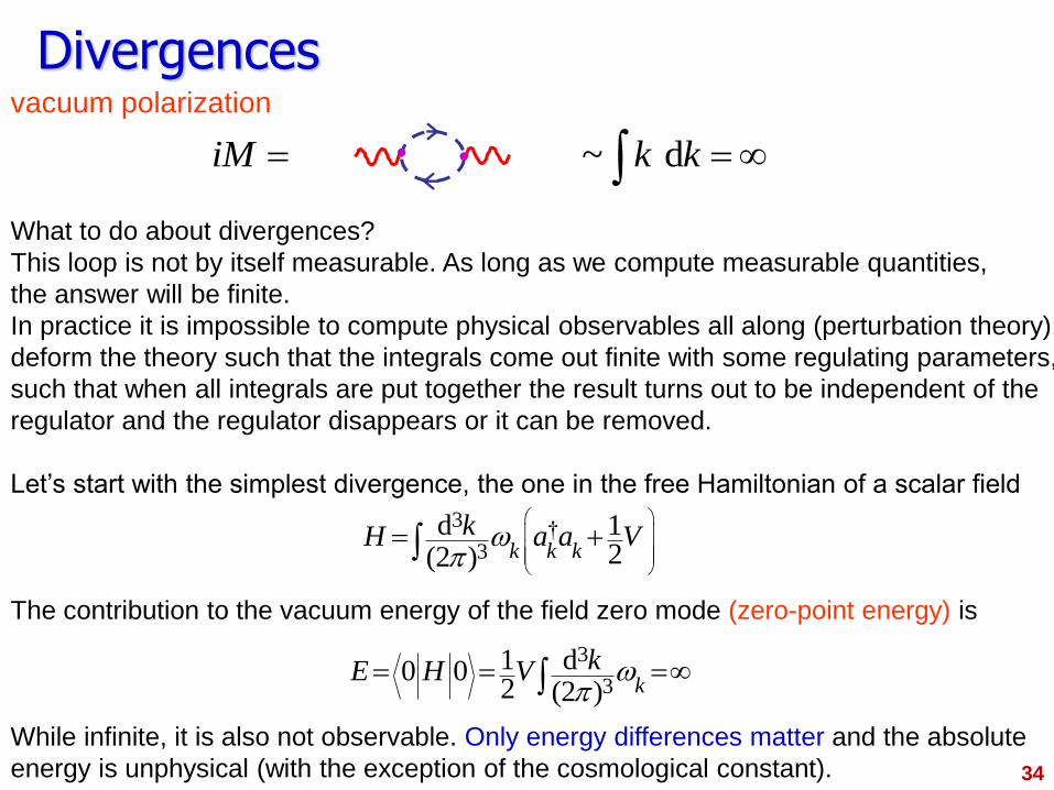
Divergences

34

vacuum polarization

What to do about divergences?

This loop is not by itself measurable. As long as we compute measurable quantities,

the answer will be finite.

In practice it is impossible to compute physical observables all along (perturbation theory):

deform the theory such that the integrals come out finite with some regulating parameters,

such that when all integrals are put together the result turns out to be independent of the

regulator and the regulator disappears or it can be removed.

Let’s start with the simplest divergence, the one in the free Hamiltonian of a scalar field

The contribution to the vacuum energy of the field zero mode (zero-point energy) is

While infinite, it is also not observable. Only energy differences matter and the absolute

energy is unphysical (with the exception of the cosmological constant).

~ diM k k

3 †3

d 12(2 ) k k k

kH a a Vp

3

31 d0 02 (2 ) k

kE H V p

35

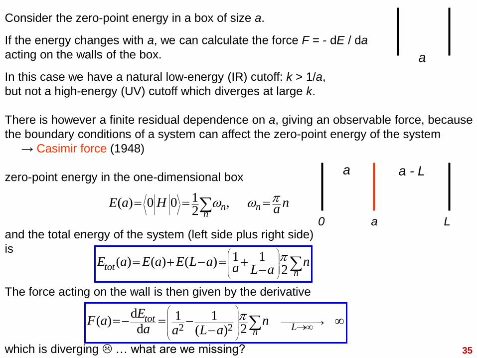
Consider the zero-point energy in a box of size a.

If the energy changes with a, we can calculate the force F = - dE / da

acting on the walls of the box.

In this case we have a natural low-energy (IR) cutoff: k > 1/a,

but not a high-energy (UV) cutoff which diverges at large k.

There is however a finite residual dependence on a, giving an observable force, because

the boundary conditions of a system can affect the zero-point energy of the system

→ Casimir force (1948)

zero-point energy in the one-dimensional box

and the total energy of the system (left side plus right side)

is

The force acting on the wall is then given by the derivative

which is diverging … what are we missing?

1 1( ) ( ) ( )2tot

nE a E a E L a n

a L ap

2 2

d 1 1( ) 2d ( )

totL

n

EF a n

a a L ap

a

a a - L

0 a L

1( ) 0 0 , 2 n n

nE a H n

ap

36

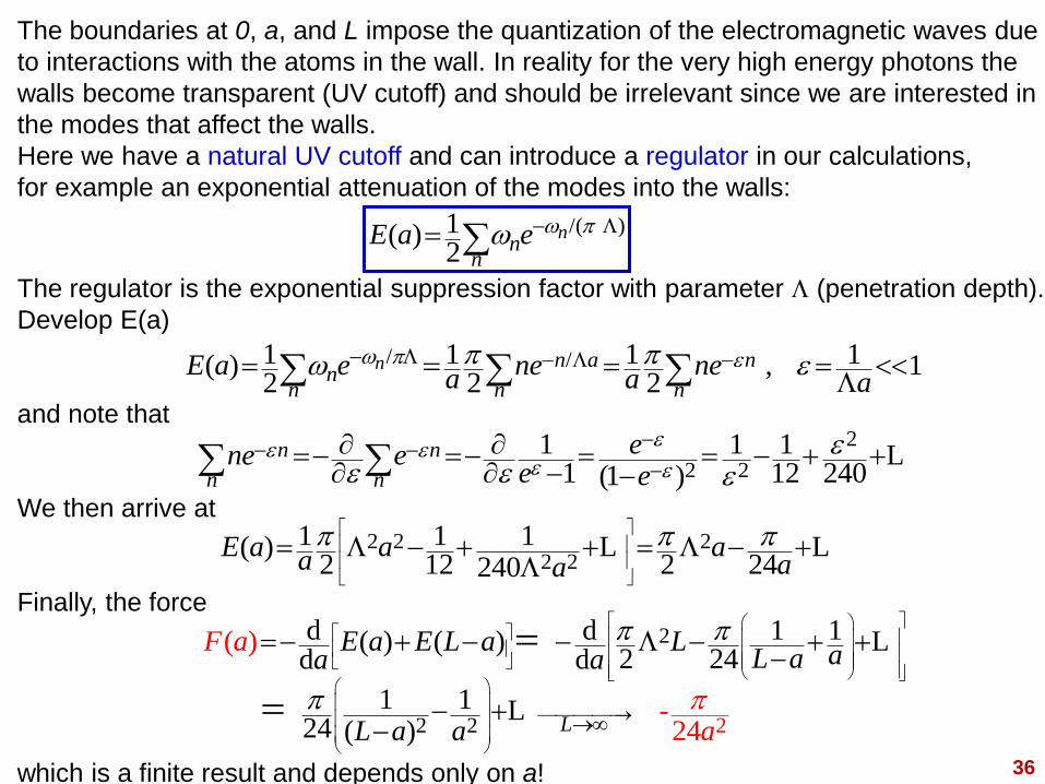
The boundaries at 0, a, and L impose the quantization of the electromagnetic waves due

to interactions with the atoms in the wall. In reality for the very high energy photons the

walls become transparent (UV cutoff) and should be irrelevant since we are interested in

the modes that affect the walls.

Here we have a natural UV cutoff and can introduce a regulator in our calculations,

for example an exponential attenuation of the modes into the walls:

The regulator is the exponential suppression factor with parameter L (penetration depth).

Develop E(a)

and note that

We then arrive at

Finally, the force

which is a finite result and depends only on a!

/( )1( )2

nn

nE a e p L

/ /1 1 1 1( ) , 12 2 2

n n a nn

n n nE a e ne ne

a a a p p p L L

L

2

2 21 1 1

1 12 240(1 )n n

n n

ene ee e

L

2 2 22 2

1 1 1( )2 12 2 24240

E a a aa aa

p p p

L L L

L L

2 2

2

2

d d 1 1( ) ( ) 2 24

( )

-24

d d

1 1 24 ( )

L

E a E L a LaL aa a

L a a

F a

a

p p

p p

L

L

L

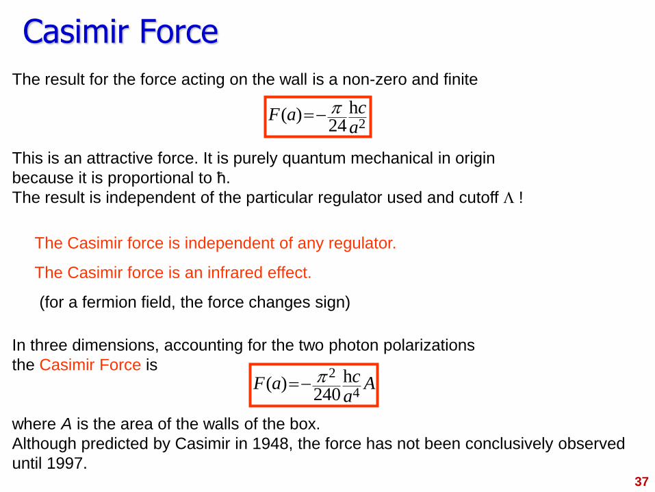
Casimir Force

37

The result for the force acting on the wall is a non-zero and finite

This is an attractive force. It is purely quantum mechanical in origin

because it is proportional to ћ.

The result is independent of the particular regulator used and cutoff L !

The Casimir force is independent of any regulator.

The Casimir force is an infrared effect.

(for a fermion field, the force changes sign)

In three dimensions, accounting for the two photon polarizations

the Casimir Force is

where A is the area of the walls of the box.

Although predicted by Casimir in 1948, the force has not been conclusively observed

until 1997.

2( )

24cF a

ap h

2

4( )

240cF a A

ap h

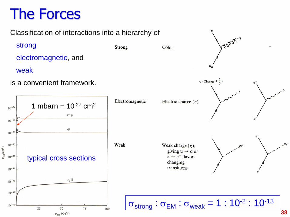
The Forces

sstrong : sEM : sweak = 1 : 10-2 : 10-13

typical cross sections

1 mbarn = 10-27 cm2

Classification of interactions into a hierarchy of

strong

electromagnetic, and

weak

is a convenient framework.

38

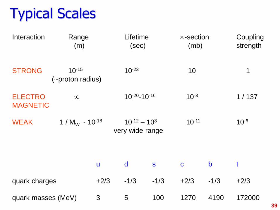
Typical Scales

Interaction Range Lifetime -section Coupling

(m) (sec) (mb) strength

STRONG 10-15 10-23 10 1

(~proton radius)

ELECTRO 10-20-10-16 10-3 1 / 137

MAGNETIC

WEAK 1 / MW ~ 10-18 10-12 – 103 10-11 10-6

very wide range

u d s c b t

quark charges +2/3 -1/3 -1/3 +2/3 -1/3 +2/3

quark masses (MeV) 3 5 100 1270 4190 172000 39

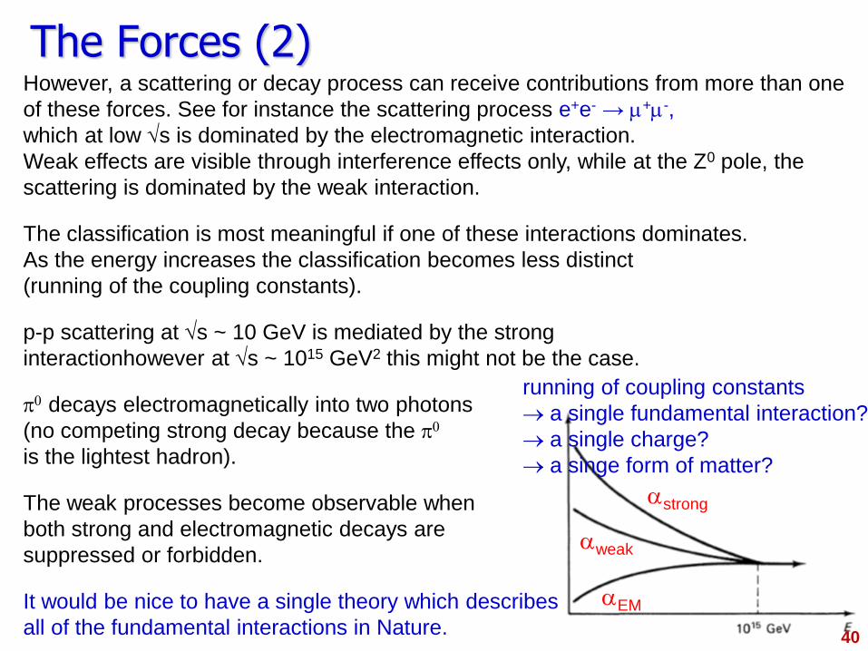
The Forces (2) However, a scattering or decay process can receive contributions from more than one

of these forces. See for instance the scattering process e+e- → m+m-,

which at low s is dominated by the electromagnetic interaction.

Weak effects are visible through interference effects only, while at the Z0 pole, the

scattering is dominated by the weak interaction.

The classification is most meaningful if one of these interactions dominates.

As the energy increases the classification becomes less distinct

(running of the coupling constants).

p-p scattering at s ~ 10 GeV is mediated by the strong

interactionhowever at s ~ 1015 GeV2 this might not be the case.

p0 decays electromagnetically into two photons

(no competing strong decay because the p0

is the lightest hadron).

The weak processes become observable when

both strong and electromagnetic decays are

suppressed or forbidden.

It would be nice to have a single theory which describes

all of the fundamental interactions in Nature.

running of coupling constants

a single fundamental interaction?

a single charge?

a singe form of matter?

40

aEM

aweak

astrong

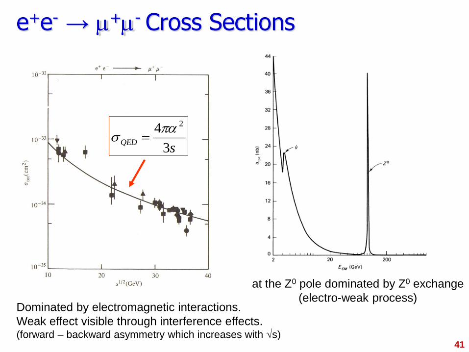
e+e- → m+m- Cross Sections

Dominated by electromagnetic interactions.

Weak effect visible through interference effects. (forward – backward asymmetry which increases with s)

at the Z0 pole dominated by Z0 exchange

(electro-weak process)

sQED

3

4 2pas

41

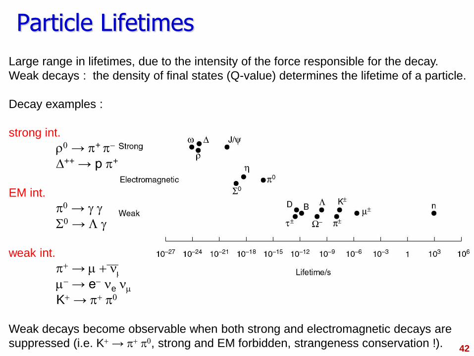
Particle Lifetimes

Large range in lifetimes, due to the intensity of the force responsible for the decay.

Weak decays : the density of final states (Q-value) determines the lifetime of a particle.

Decay examples :

strong int.

0 → p+ p

D++ → p p+

EM int.

p0 → g g

S0 → L g

weak int.

p → m nm

m → e ne nm

K → p p0

Weak decays become observable when both strong and electromagnetic decays are

suppressed (i.e. K → p p0, strong and EM forbidden, strangeness conservation !). 42

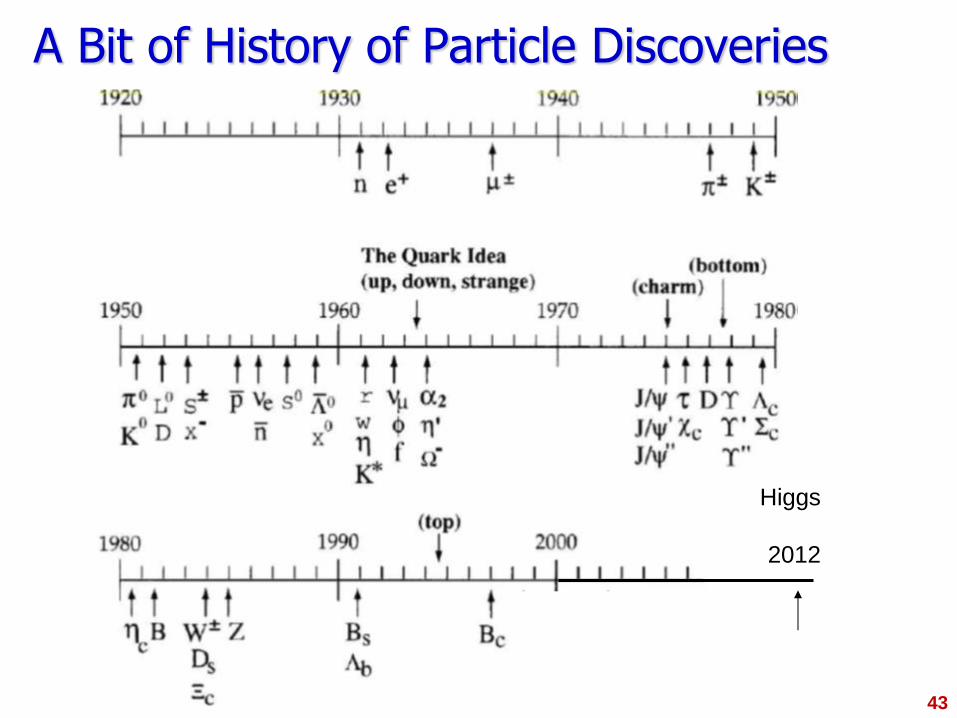
A Bit of History of Particle Discoveries

Higgs

43

2012

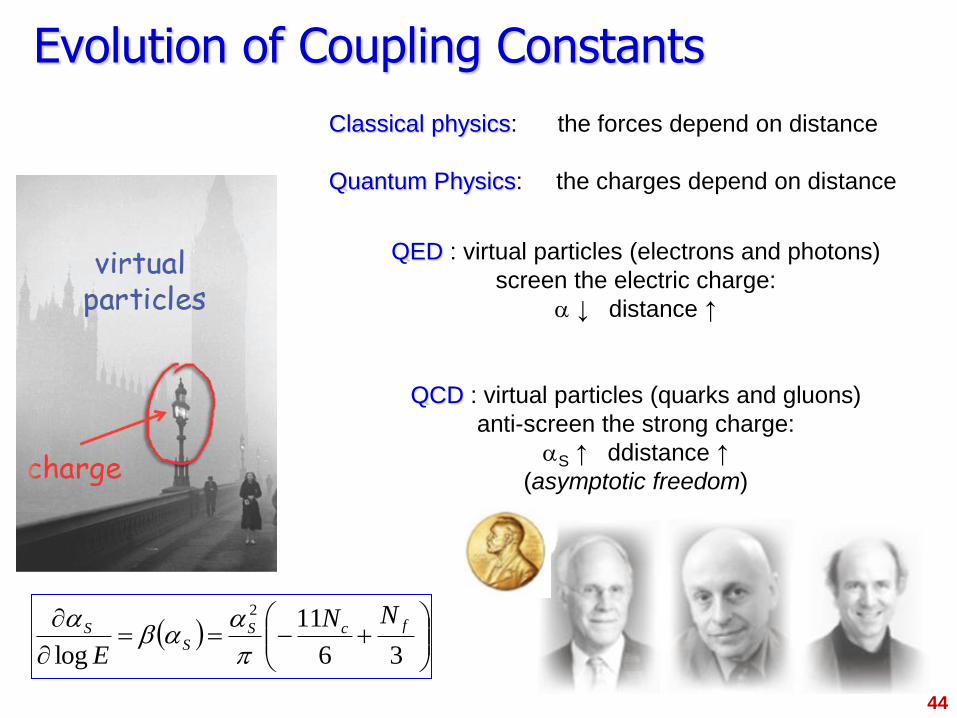
Evolution of Coupling Constants

Classical physics: the forces depend on distance

Quantum Physics: the charges depend on distance

QED : virtual particles (electrons and photons)

screen the electric charge:

a ↓ distance ↑

QCD : virtual particles (quarks and gluons)

anti-screen the strong charge:

aS ↑ ddistance ↑

(asymptotic freedom)

36

11

log

2fcS

SS

NN

E p

aa

a

44

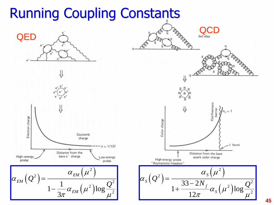
Running Coupling Constants

QED QCD

45

2

2

22

2

11 log

3

EM

EM

EM

QQ

a ma

a mp m

2

2

22

2

33 21 log

12

S

Sf

S

QN Q

a ma

a mp m

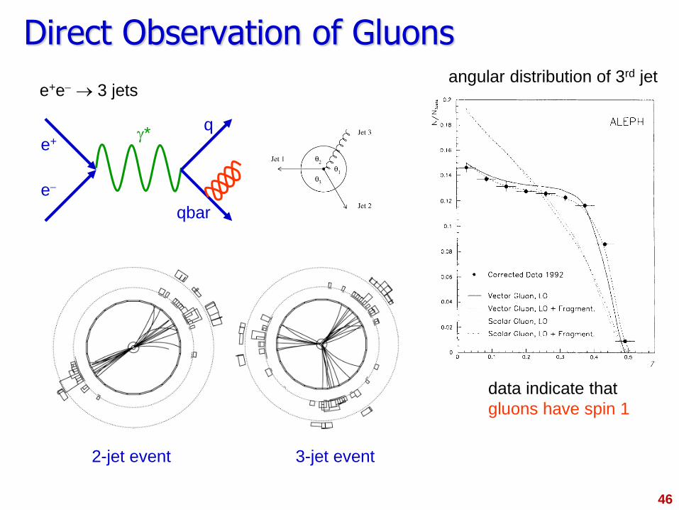
Direct Observation of Gluons

e+e 3 jets

e+

e

g* q

qbar

angular distribution of 3rd jet

data indicate that

gluons have spin 1

2-jet event 3-jet event

46

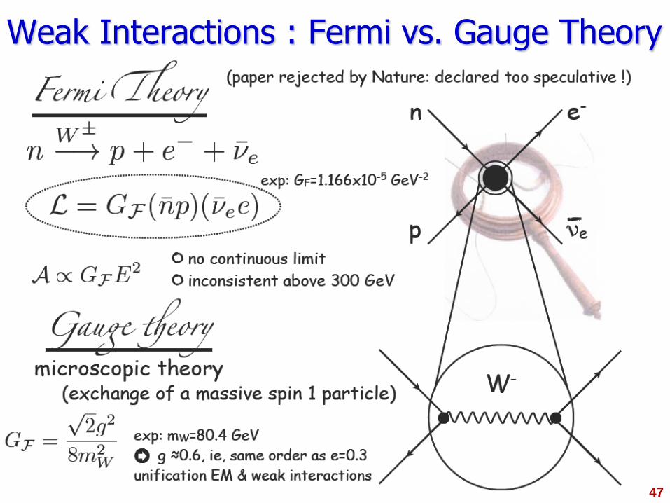
Weak Interactions : Fermi vs. Gauge Theory

47

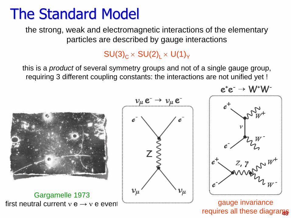
The Standard Model the strong, weak and electromagnetic interactions of the elementary

particles are described by gauge interactions

SU(3)C SU(2)L U(1)Y

this is a product of several symmetry groups and not of a single gauge group,

requiring 3 different coupling constants: the interactions are not unified yet !

Gargamelle 1973

first neutral current n e → n e event gauge invariance

requires all these diagrams 48

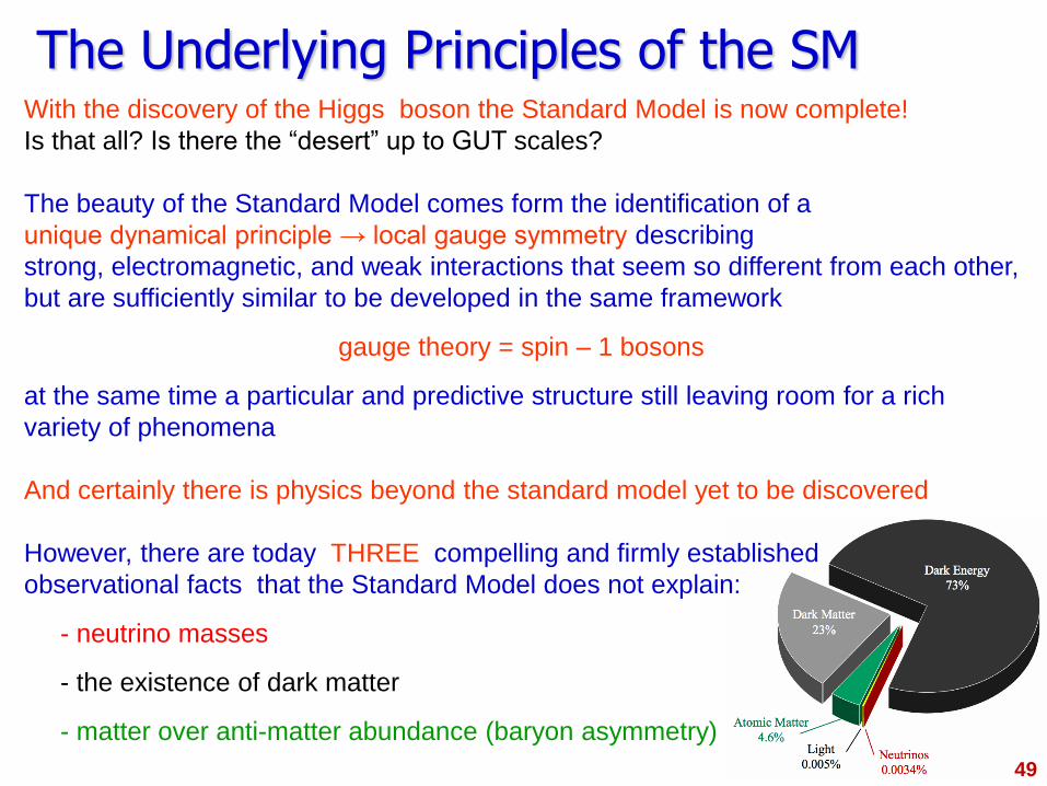
The Underlying Principles of the SM With the discovery of the Higgs boson the Standard Model is now complete!

Is that all? Is there the “desert” up to GUT scales?

The beauty of the Standard Model comes form the identification of a

unique dynamical principle → local gauge symmetry describing

strong, electromagnetic, and weak interactions that seem so different from each other,

but are sufficiently similar to be developed in the same framework

gauge theory = spin – 1 bosons

at the same time a particular and predictive structure still leaving room for a rich

variety of phenomena

And certainly there is physics beyond the standard model yet to be discovered

However, there are today THREE compelling and firmly established

observational facts that the Standard Model does not explain:

- neutrino masses

- the existence of dark matter

- matter over anti-matter abundance (baryon asymmetry)

49

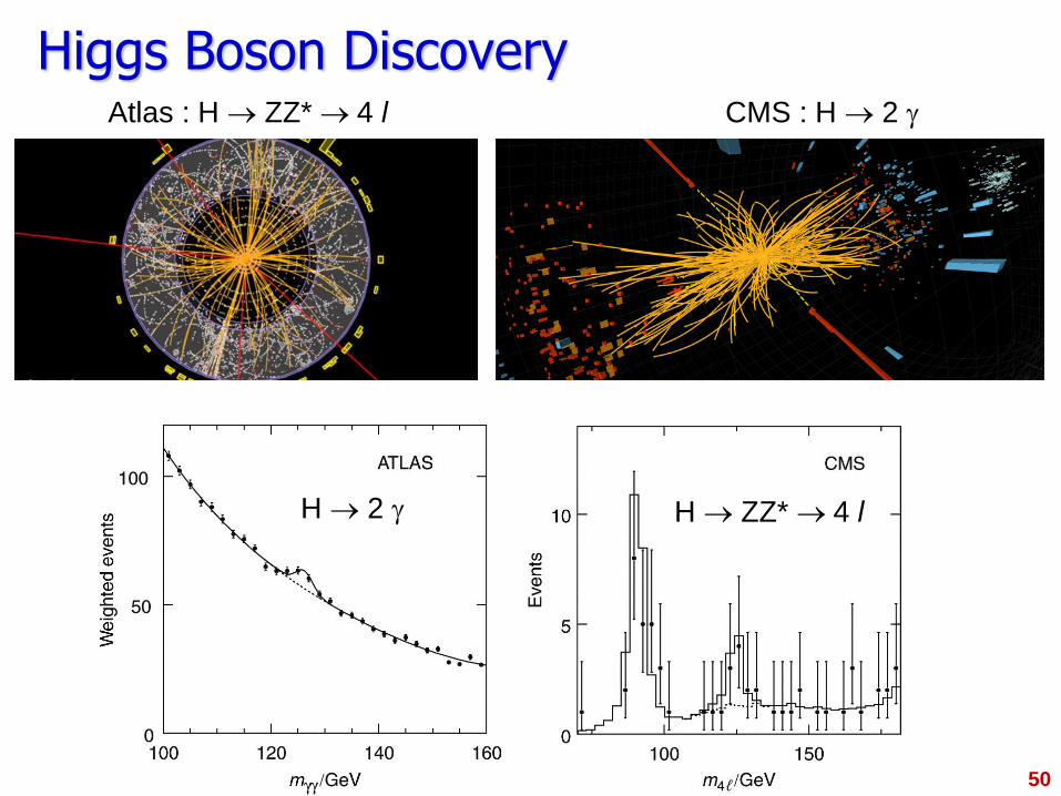
Higgs Boson Discovery

H 2 g H ZZ* 4 l

Atlas : H ZZ* 4 l CMS : H 2 g

50

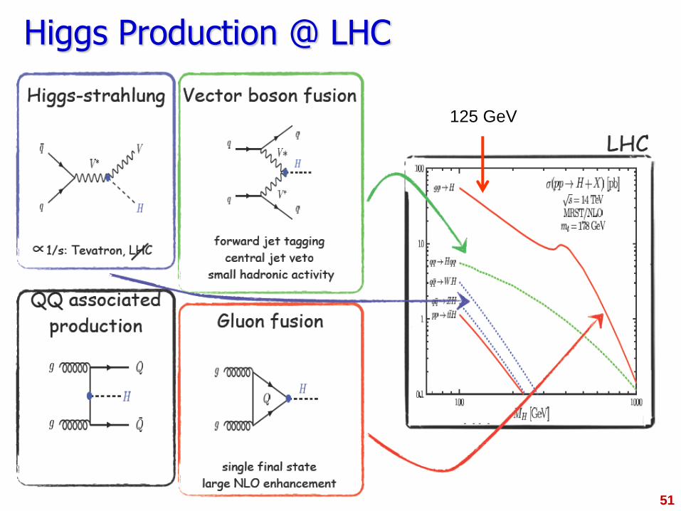
Higgs Production @ LHC

51

125 GeV

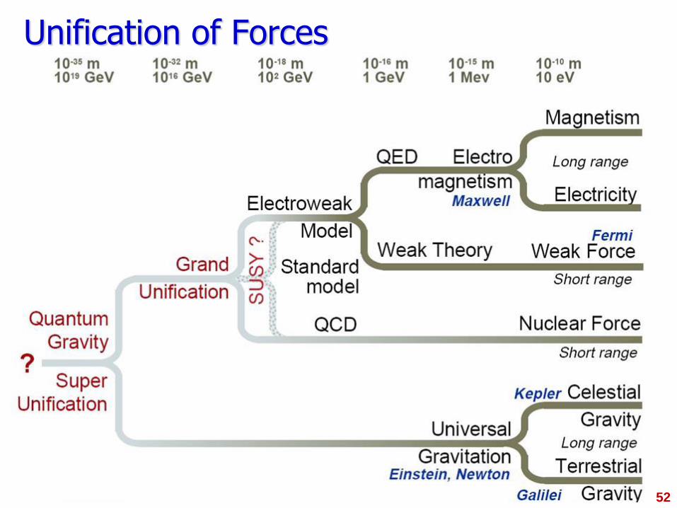
Unification of Forces

52

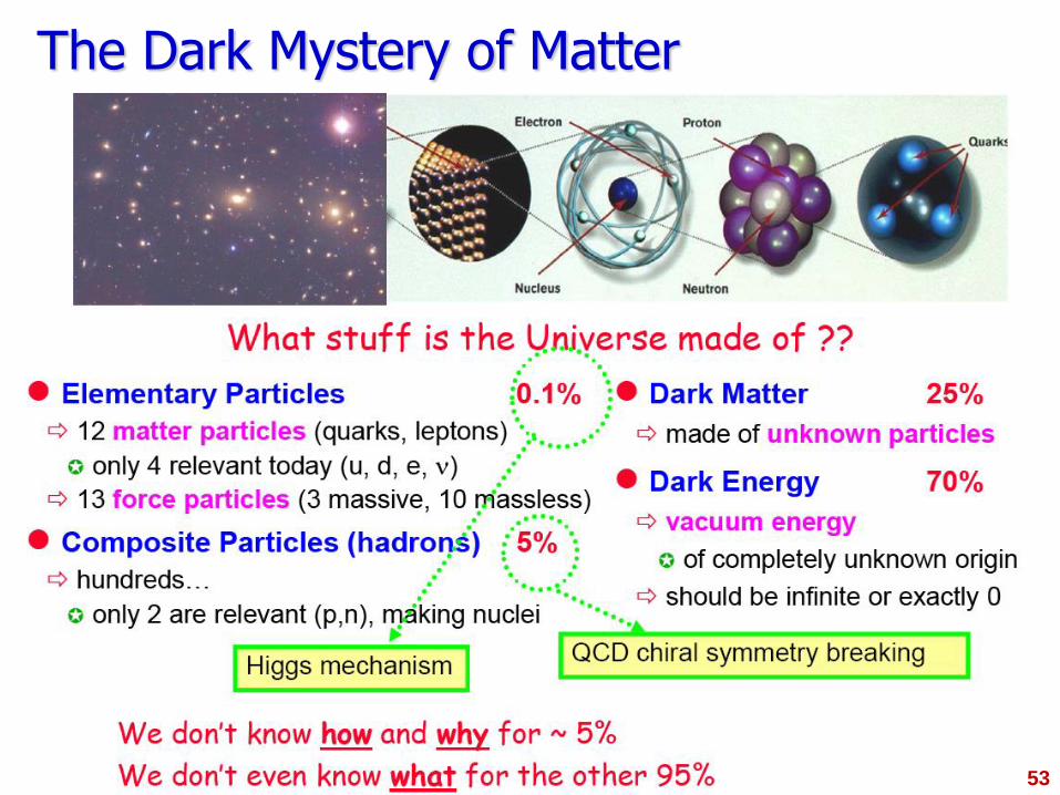
The Dark Mystery of Matter

53

54