Première loi de la thermodynamique: détermination du coefficient

CPH316: Méthodes de la chimie physique

1

Première loi de la thermodynamique: détermination du coefficient Joule-Thomson pour différents gaz

Rédigé par Pierre-Alexandre Turgeon

Introduction

L'énergie d'un gaz parfait est indépendante du volume et de la pression, elle ne

dépend que de la température. En conséquence, la température d'un gaz idéal soumis à

une expansion adiabatique demeure inchangée dans le processus. En revanche, en 1854

James Prescott Joule et William Thomson (aussi connu sous le nom de Lord Kelvin) ont

démontré que la température d'un gaz réel changeait dans une expansion adiabatique. Ce

phénomène connu sous le nom d'effet Joule-Thomson est aujourd'hui largement utilisé

dans la liquéfaction des gaz. Pour comprendre cet effet, il faut tenir compte du

comportement non-idéal des gaz en introduisant des paramètres comme les interactions

intermoléculaires et le volume des particules. Cette non-idéalité se traduit par un

coefficient Joule-Thomson propre à chaque gaz.

Vous aurez à mesurer le coefficient Joule-Thomson de 3 gaz différents, soit

l'hélium, le dioxyde de carbone et l'azote. Cette expérience vise à vous familiariser avec

différentes techniques expérimentales telles que la manipulation de gaz comprimés,

l'acquisition de données par ordinateur ainsi que l'utilisation de thermocouples et de

capteurs de pression. Le montage expérimental que vous utiliserez devra être assemblé

par votre équipe avant de pouvoir effectuer les mesures. L'ensemble de la théorie reliée à

l'expérience de détermination du coefficient Joule-Thomson se trouve dans les documents

complémentaires cités à la fin de ce protocole, principalement dans l'ouvrage de Garland,

Nibler et Shoemaker. Pour cette raison, elle ne sera pas exposée plus en détail dans le

présent document.

Appareillage

Pour réaliser vos mesures, vous aurez à votre disposition un capteur de pression

électronique, des thermocouples, une carte d'acquisition ainsi qu'un amplificateur de

voltage. Ces appareils sont peut-être nouveaux pour vous, c'est pourquoi ils seront

brièvement décrits dans le protocole.

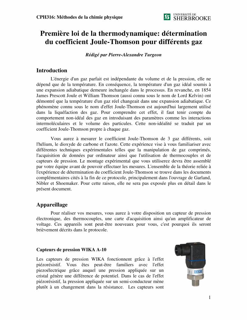
Capteurs de pression WIKA A-10

Les capteurs de pression WIKA fonctionnent grâce à l'effet

piézorésistif. Vous êtes peut-être familiers avec l'effet

piezoélectrique grâce auquel une pression appliquée sur un

cristal génère une différence de potentiel. Dans le cas de l'effet

piézorésistif, la pression appliquée sur un semi-conducteur mène

plutôt à un changement dans la résistance. Les capteurs sont


2

conçus pour donner un signal de sortie allant de 0 à 10V en fonction de la pression

appliquée. Ceux qui seront mis à votre disposition auront une plage de réponse linéaire

allant de 0 à 160 PSIG (PSIG: PSI par rapport à la pression atmosphérique). Par exemple,

un signal lu de 0 V correspondra à la pression atmosphérique alors qu'un signal lu de

3.48 V correspondra à 58.5 PSIG. Pour vos analyses, vous devrez convertir le voltage en

pression à l'aide des informations précédentes. L'unité SI de pression est le bar, alors vous

aurez à effectuer une conversion. Veuillez prendre note que le capteur de pression peut

avoir un décalage (offset), ce qui aura pour conséquence que le voltage ne sera pas

exactement de 0V à pression ambiante. Vous devrez en tenir compte dans le traitement de

vos données.

Pour fonctionner, les capteurs de pression ont besoin d’une source d’alimentation

24VDC. Vous devrez donc connecter le petit transformateur dans une des fiches

d'alimentation située sur votre espace de travail.

Thermocouple type T (Cuivre/Constantan)

Résumé de façon simple, un thermocouple est la jonction physique entre deux métaux ou

deux alliages différents. Cette jonction génère un potentiel (appelé potentiel de jonction)

dont la valeur dépend de la température. En mesurant ce potentiel par rapport à une

référence, la température de la jonction peut être déterminée avec une assez bonne

précision. Le thermocouple est l'un des outils de mesure de température le plus utilisé

puisqu'il est peu coûteux, durable et qu'il est généralement assez sensible. Dans

l'expérience de détermination du coefficient Joule-Thomson, deux thermocouples seront

mis en série, de sorte que la différence de potentiel mesurée entre les deux jonctions sera

directement proportionnelle à la différence de température des deux jonctions. Le fait de

faire une mesure "différentielle" à deux thermocouples nous permet d'éviter l'utilisation

d'une référence externe. Les thermocouples de type T (cuivre/constantan) ont une réponse

d'environ 39 µV/K. Une charte détaillée du voltage en fonction de la température est

incluse à la fin de ce document. Comme le signal est relativement faible, il faudra

l'amplifier à l'aide d'un circuit électrique qui est détaillé ci-dessous

Circuit d'amplification thermocouple

Comme mentionné précédemment, le signal généré par le thermocouple est très faible :

39 µV/K, soit 4x10-5

V/K. Pour amener ce signal à un niveau acceptable, il vous faudra

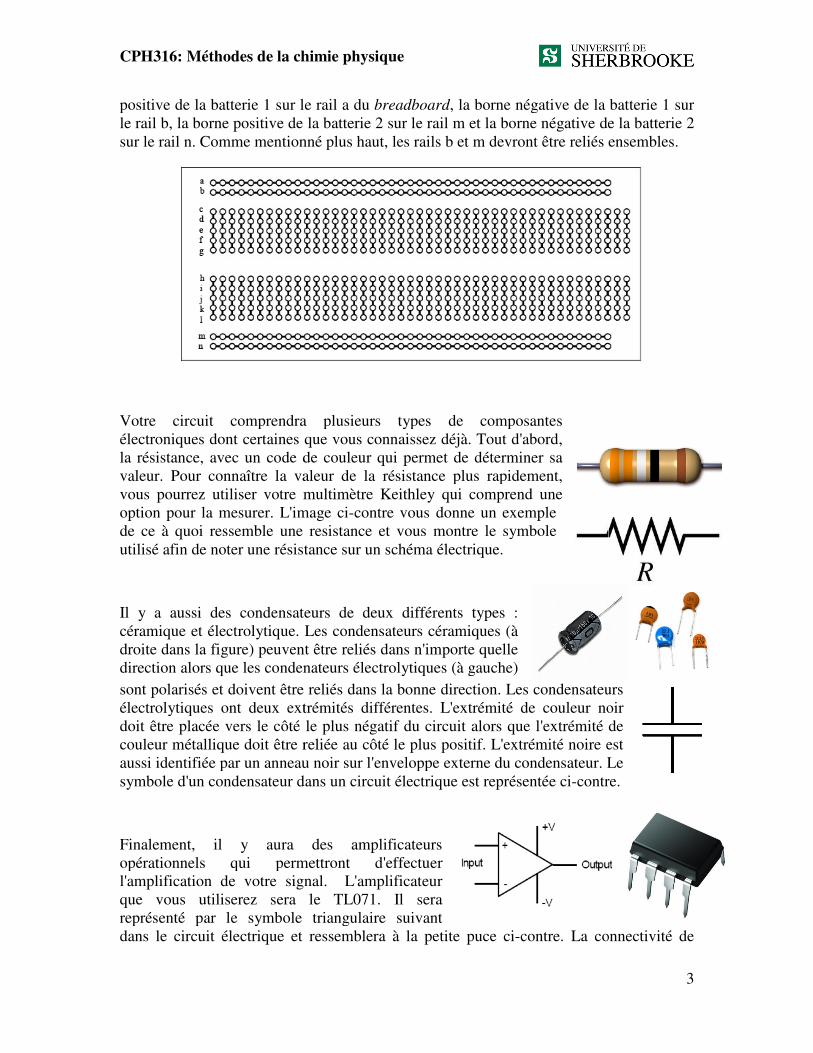
construire un circuit d'amplification. Le circuit sera construit sur un breadboard, une

petite plaque qui permet de connecter les composantes sans les souder. La figure à la

page suivante représente les connections à l'intérieur du breadboard. Le rail a servira à

l'alimentation positive alors que le rail n servira à l'alimenation négative. Les rails b et m

seront reliés à la terre (ground) et vous devrez vous-même les relier ensembles. Les

composantes seront disposées sur les rails intermédiaires de c à l.

L'alimentation du circuit sera fournie à l'aide de deux batteries de 9V que vous devrez

connecter en série. Une fois votre circuit complété, vous devrez connecter la borne


positive de la batterie 1 sur le rail

le rail b, la borne positive de la batterie 2 sur le rail

sur le rail n. Comme mentionné plus haut, les rails

Votre circuit comprendra plusieurs types de composantes

électroniques dont certaines que vous connaissez déjà. Tout d'abord,

la résistance, avec un code de couleur qui permet de déterminer sa

valeur. Pour connaître la valeur de la résistance plus rapidement,

vous pourrez utiliser votre multimètre Keithley qui comprend une

option pour la mesurer. L'image ci

de ce à quoi ressemble une resistance et vous montre le symbole

utilisé afin de noter une résistance sur un schéma électrique.

Il y a aussi des condensateurs de deux différents types :

céramique et électrolytique. Les condensateurs céramiques (à

droite dans la figure) peuvent être reliés dans n'importe quelle

direction alors que les condenateurs électrolytiques (à gauche)

sont polarisés et doivent être reliés dans la bonne direction. Les condensateurs

électrolytiques ont deux extrémités différentes. L'extrémité de coul

doit être placée vers le côté le plus négatif du circuit alors que l'extrémité de

couleur métallique doit être reliée au côté le plus positif. L'extrémité noire est

aussi identifiée par un anneau noir sur l'enveloppe externe du condensateur. Le

symbole d'un condensateur dans un circuit électrique est représentée ci

Finalement, il y aura des amplificateurs

opérationnels qui permettront d'effectuer

l'amplification de votre signal. L'amplificateur

que vous utiliserez sera le TL071

représenté par le symbole triangulaire suivant

dans le circuit électrique et ressemblera à la petite puce ci

chimie physique

positive de la batterie 1 sur le rail a du breadboard, la borne négative de la batterie 1 sur

, la borne positive de la batterie 2 sur le rail m et la borne négative de la ba

. Comme mentionné plus haut, les rails b et m devront être reliés ensembles.

Votre circuit comprendra plusieurs types de composantes

électroniques dont certaines que vous connaissez déjà. Tout d'abord,

code de couleur qui permet de déterminer sa

valeur. Pour connaître la valeur de la résistance plus rapidement,

vous pourrez utiliser votre multimètre Keithley qui comprend une

option pour la mesurer. L'image ci-contre vous donne un exemple

semble une resistance et vous montre le symbole

utilisé afin de noter une résistance sur un schéma électrique.

Il y a aussi des condensateurs de deux différents types :

céramique et électrolytique. Les condensateurs céramiques (à

peuvent être reliés dans n'importe quelle

direction alors que les condenateurs électrolytiques (à gauche)


électrolytiques ont deux extrémités différentes. L'extrémité de couleur noir




mbole d'un condensateur dans un circuit électrique est représentée ci-contre.

Finalement, il y aura des amplificateurs

opérationnels qui permettront d'effectuer

l'amplification de votre signal. L'amplificateur

vous utiliserez sera le TL071. Il sera

représenté par le symbole triangulaire suivant

dans le circuit électrique et ressemblera à la petite puce ci-contre. La connectivité de

3

, la borne négative de la batterie 1 sur

et la borne négative de la batterie 2

devront être reliés ensembles.


eur noir




contre.

contre. La connectivité de


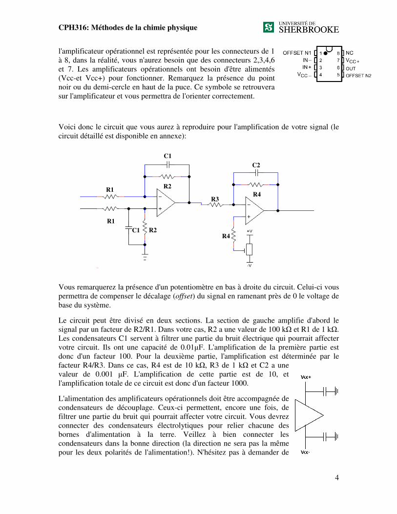
l'amplificateur opérationnel est représentée pour les connecteurs de 1

à 8, dans la réalité, vous n'aurez besoin que d

et 7. Les amplificateurs opérationnels ont besoin d'être alimentés

(Vcc-et Vcc+) pour fonctionner. Remarquez la présence du point

noir ou du demi-cercle en haut de la puce. Ce symbole

sur l'amplificateur et vous permet

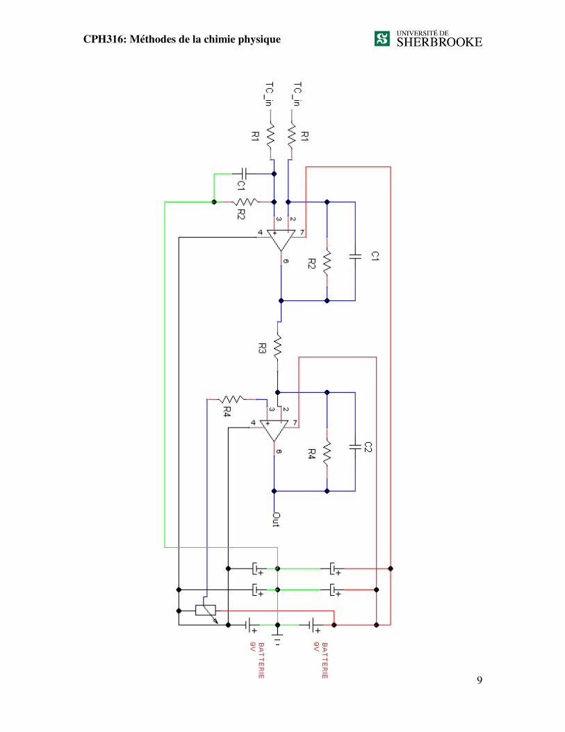
Voici donc le circuit que vous aurez à reproduire pour l'amplification de votre signal

circuit détaillé est disponible en annexe)

Vous remarquerez la présence d'un potentiomètre en bas à droite du

permettra de compenser le décalage (

base du système.

Le circuit peut être divisé en deux sections. La section de gauche

signal par un facteur de R2/R1. Dans v

Les condensateurs C1 servent

votre circuit. Ils ont une capacité de 0.01

donc d'un facteur 100. Pour la deuxième partie, l'amplification

facteur R4/R3. Dans ce cas, R4

valeur de 0.001 µF. L'amplification

l'amplification totale de ce circuit

L'alimentation des amplificateurs opérationnels

condensateurs de découplage. Ceux

filtrer une partie du bruit qui pourrait affecter votre circuit. Vous devrez

connecter des condensateurs élec

bornes d'alimentation à la terre. Veillez à bien connecter les

condensateurs dans la bonne direction (la direction ne sera pas la même

pour les deux polarités de l'alimentation!). N'hésitez pas à demander de

R1

R1 C1

chimie physique

l'amplificateur opérationnel est représentée pour les connecteurs de 1

à 8, dans la réalité, vous n'aurez besoin que des connecteurs 2,3,4,6

et 7. Les amplificateurs opérationnels ont besoin d'être alimentés

et Vcc+) pour fonctionner. Remarquez la présence du point

cercle en haut de la puce. Ce symbole se retrouvera

sur l'amplificateur et vous permettra de l'orienter correctement.

Voici donc le circuit que vous aurez à reproduire pour l'amplification de votre signal

est disponible en annexe):

Vous remarquerez la présence d'un potentiomètre en bas à droite du circuit. Celui

permettra de compenser le décalage (offset) du signal en ramenant près de 0 le voltage de

Le circuit peut être divisé en deux sections. La section de gauche amplifie

signal par un facteur de R2/R1. Dans votre cas, R2 a une valeur de 100 kΩ et R1 de 1

servent à filtrer une partie du bruit électrique qui pourrait affecter

une capacité de 0.01µF. L'amplification de la première partie

our la deuxième partie, l'amplification est déterminée par le

facteur R4/R3. Dans ce cas, R4 est de 10 kΩ, R3 de 1 kΩ et C2 a une

F. L'amplification de cette partie est de 10, et

totale de ce circuit est donc d'un facteur 1000.

L'alimentation des amplificateurs opérationnels doit être accompagnée de

condensateurs de découplage. Ceux-ci permettent, encore une fois, de

filtrer une partie du bruit qui pourrait affecter votre circuit. Vous devrez

connecter des condensateurs électrolytiques pour relier chacune des

bornes d'alimentation à la terre. Veillez à bien connecter les

condensateurs dans la bonne direction (la direction ne sera pas la même

pour les deux polarités de l'alimentation!). N'hésitez pas à demander de

R2

R2

R3 R4

R4

C1

C2

4

Voici donc le circuit que vous aurez à reproduire pour l'amplification de votre signal (le

circuit. Celui-ci vous

) du signal en ramenant près de 0 le voltage de

amplifie d'abord le

Ω et R1 de 1 kΩ.

pourrait affecter

ère partie est

déterminée par le


5

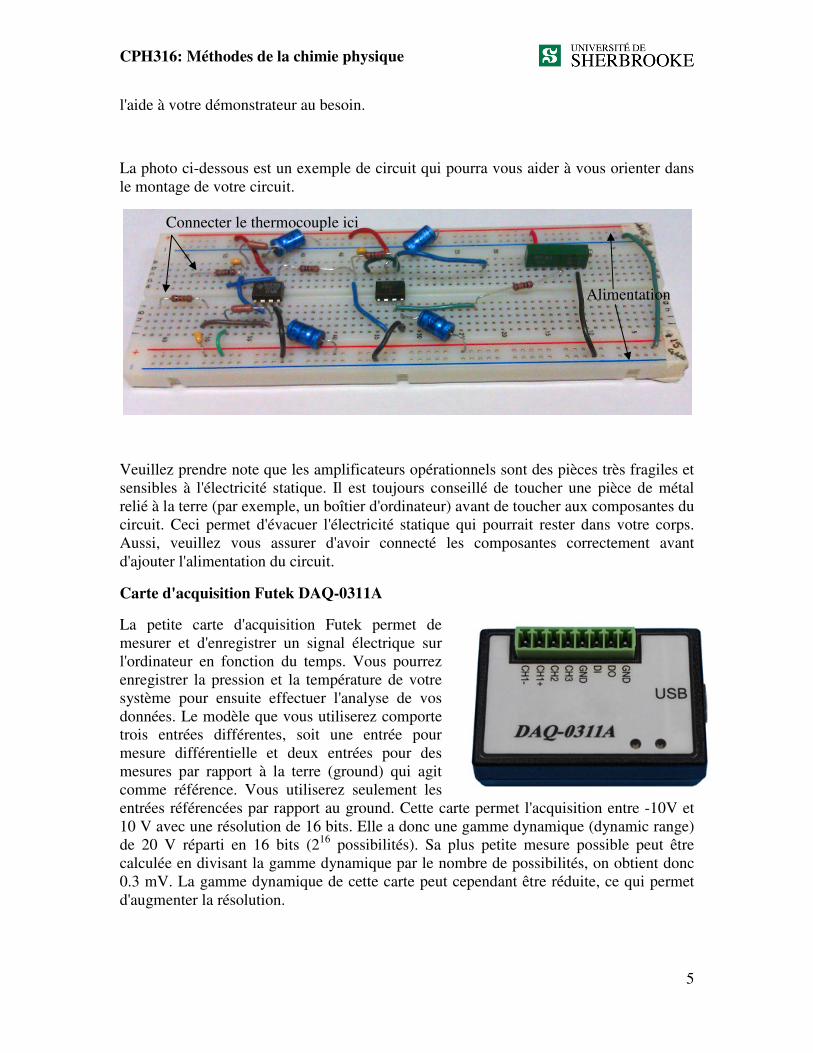
l'aide à votre démonstrateur au besoin.

La photo ci-dessous est un exemple de circuit qui pourra vous aider à vous orienter dans

le montage de votre circuit.

Veuillez prendre note que les amplificateurs opérationnels sont des pièces très fragiles et

sensibles à l'électricité statique. Il est toujours conseillé de toucher une pièce de métal

relié à la terre (par exemple, un boîtier d'ordinateur) avant de toucher aux composantes du

circuit. Ceci permet d'évacuer l'électricité statique qui pourrait rester dans votre corps.

Aussi, veuillez vous assurer d'avoir connecté les composantes correctement avant

d'ajouter l'alimentation du circuit.

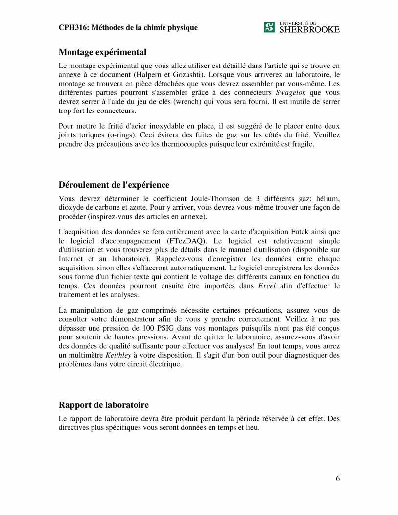
Carte d'acquisition Futek DAQ-0311A

La petite carte d'acquisition Futek permet de

mesurer et d'enregistrer un signal électrique sur

l'ordinateur en fonction du temps. Vous pourrez

enregistrer la pression et la température de votre

système pour ensuite effectuer l'analyse de vos

données. Le modèle que vous utiliserez comporte

trois entrées différentes, soit une entrée pour

mesure différentielle et deux entrées pour des

mesures par rapport à la terre (ground) qui agit

comme référence. Vous utiliserez seulement les

entrées référencées par rapport au ground. Cette carte permet l'acquisition entre -10V et

10 V avec une résolution de 16 bits. Elle a donc une gamme dynamique (dynamic range)

de 20 V réparti en 16 bits (216

possibilités). Sa plus petite mesure possible peut être

calculée en divisant la gamme dynamique par le nombre de possibilités, on obtient donc

0.3 mV. La gamme dynamique de cette carte peut cependant être réduite, ce qui permet

d'augmenter la résolution.

Connecter le thermocouple ici

Alimentation


6

Montage expérimental

Le montage expérimental que vous allez utiliser est détaillé dans l'article qui se trouve en

annexe à ce document (Halpern et Gozashti). Lorsque vous arriverez au laboratoire, le

montage se trouvera en pièce détachées que vous devrez assembler par vous-même. Les

différentes parties pourront s'assembler grâce à des connecteurs Swagelok que vous

devrez serrer à l'aide du jeu de clés (wrench) qui vous sera fourni. Il est inutile de serrer

trop fort les connecteurs.

Pour mettre le fritté d'acier inoxydable en place, il est suggéré de le placer entre deux

joints toriques (o-rings). Ceci évitera des fuites de gaz sur les côtés du frité. Veuillez

prendre des précautions avec les thermocouples puisque leur extrémité est fragile.

Déroulement de l'expérience

Vous devrez déterminer le coefficient Joule-Thomson de 3 différents gaz: hélium,

dioxyde de carbone et azote. Pour y arriver, vous devrez vous-même trouver une façon de

procéder (inspirez-vous des articles en annexe).

L'acquisition des données se fera entièrement avec la carte d'acquisition Futek ainsi que

le logiciel d'accompagnement (FTezDAQ). Le logiciel est relativement simple

d'utilisation et vous trouverez plus de détails dans le manuel d'utilisation (disponible sur

Internet et au laboratoire). Rappelez-vous d'enregistrer les données entre chaque

acquisition, sinon elles s'effaceront automatiquement. Le logiciel enregistrera les données

sous forme d'un fichier texte qui contient le voltage des différents canaux en fonction du

temps. Ces données pourront ensuite être importées dans Excel afin d'effectuer le

traitement et les analyses.

La manipulation de gaz comprimés nécessite certaines précautions, assurez vous de

consulter votre démonstrateur afin de vous y prendre correctement. Veillez à ne pas

dépasser une pression de 100 PSIG dans vos montages puisqu'ils n'ont pas été conçus

pour soutenir de hautes pressions. Avant de quitter le laboratoire, assurez-vous d'avoir

des données de qualité suffisante pour effectuer vos analyses! En tout temps, vous aurez

un multimètre Keithley à votre disposition. Il s'agit d'un bon outil pour diagnostiquer des

problèmes dans votre circuit électrique.

Rapport de laboratoire

Le rapport de laboratoire devra être produit pendant la période réservée à cet effet. Des

directives plus spécifiques vous seront données en temps et lieu.


7

Liste de documents complémentaires

Experiments in Physical Chemistry, 8th

Edition, by Carl W. Garland, Joseph W.

Nibler, and David P. Shoemaker, McGraw-Hill, NEW YORK, 2009.

(EXPÉRIENCE 2)

An improved apparatus for the measurement of the Joule-Thomson coefficient of

gases, A.M Halpern and S. Gozashti, Journal of Chemical Education,

1986 63 (11), 1001.

Physical Chemistry, 6th

Edition, by Ira N. Levine, McGraw-Hill, NEW YORK,

2009.

Manuel d'utilisation pour carte d'acquisition FUTEK DAQ-0311A


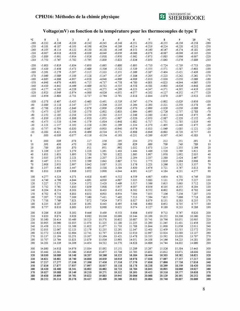
Voltage(mV) en fonction de la température pour les thermocouples de type T

chimie physique

) en fonction de la température pour les thermocouples de type T

8

) en fonction de la température pour les thermocouples de type T


9

Rev. Confirming Pages

98 Chapter IV Gases

SAFETY ISSUES

The ballast bulb must be taped to prevent flying glass fragments in the unlikely event of breakage. Safety glasses should be worn for all laboratory work. Gas cylinders must be chained securely to the wall or laboratory bench (see pp. 644–646 and Appendix C). Liq-uid nitrogen must be handled properly (see Appendix C).

APPARATUS

Pressure manometer (such as a Honeywell stain-gauge device) and digital voltme-ter for readout; properly taped and mounted ballast bulb; heavy-wall pressure tubing; Dewar flask; large ring stirrer; notched cover plate for Dewar with hole for mounting gas thermometer bulb; electrical heating mantle; steam generator with rubber connecting tubing; steam jacket; two ring stands; ring clamp; two clamp holders; one large and one medium clamp.

Cylinder of helium or dry nitrogen; pure ice (1 kg); ice grinder; liquid nitrogen (1 L); boiling chips; stopcock grease; vacuum pump or water aspirator.

REFERENCES

1. R. J. Silbey, R. A. Alberty, and M. G. Bawendi, Physical Chemistry, 4th ed., pp. 7–8, 97, Wiley, New York (2005).

2. J. A. Beattie and coworkers, Proc. Am. Acad. Arts Sci. 74, 327 (1941); 77, 255 (1949).

GENERAL READING

J. R. Leigh, Temperature Measurement and Control, INSPEC, Edison, NJ (1988).

R. P. Benedict, Fundamentals of Temperature, Pressure, and Flow Measurements, 3d ed., Wiley-Interscience, New York (1984).

J. F. Schooley, Thermometry, CRC Reprint, Franklin, Elkins Park, PA (1986).

EXPERIMENT 2 Joule–Thomson Effect The Joule–Thomson effect is a measure of the deviation of the behavior of a real gas from what is defined to be ideal-gas behavior. In this experiment a simple technique for measur-ing this effect will be applied to a few common gases.

THEORY

An ideal gas may be defined as one for which the following two conditions apply at all temperatures for a fixed quantity of the gas: (1) Boyle’s law is obeyed; i.e.,

••

••

••

••

••

pV f T ( )pV f T ( )

gar28420_ch04_091-118.indd 98gar28420_ch04_091-118.indd 98 1/14/08 5:22:03 PM1/14/08 5:22:03 PM


and (2) the internal energy E is independent of volume. Accordingly, E is independent of pressure as well, and in the absence of other pertinent variables (such as applied fields), E of an ideal gas is therefore a function of the temperature alone:

It is apparent that the enthalpy H of an ideal gas is also a function of temperature alone:

Accordingly, we can write for a definite quantity of an ideal gas at all temperatures

a b a b a b a b

E

V

E

p

H

V

H

pT T T T

0

(1)

The absence of any dependence of the internal energy of a gas on volume was sug-gested by the early experiments of Gay-Lussac and Joule. They found that, when a quantity of gas in a container initially at a given temperature was allowed to expand into another previously evacuated container without work or heat flow to or from the surroundings ( E 0), the final temperature (after the two containers came into equilibrium with each other) was the same as the initial temperature. However, that kind of experiment (known as the Joule experiment ) is of limited sensitivity, because the heat capacity of the containers is large in comparison with that of the gases studied. Subsequently, Joule and Thomson 1 showed, in a different kind of experiment, that real gases do undergo small temperature changes upon free expansion. This experiment utilized continuous gas flow through a porous plug under adiabatic conditions. Because of the continuous flow, the solid parts of the apparatus come into thermal equilibrium with the flowing gas, and their heat capacities impose a much less serious limitation than in the case of the Joule experiment.

Let it be imagined that gas is flowing slowly from left to right through the porous plug in Fig. 1 . To the left of the plug, the temperature and pressure of the gas are T 1 and p 1 ; and to the right of the plug, they are T 2 and p 2 . The volume of a definite quantity of gas (say 1 mol) is V 1 on the left and V 2 on the right, and the internal energy is E 1 and E 2 , respectively. When 1 mol of gas flows through the plug, the work done on the system by the surroundings is

Since the process is adiabatic, the change in internal energy is

Combining these two equations we obtain

or

(2)

Thus this process takes place at constant enthalpy.

E g T ( )E g T ( )

H E pV h T ( )H E pV h T ( )

w p V p V 1 1 2 2w p V p V 1 1 2 2

E E E q w w2 1 E E E q w w2 1

E p V E p V1 1 1 2 2 2 E p V E p V1 1 1 2 2 2

H H1 2H H1 2

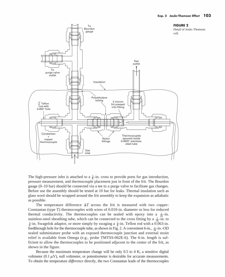
FIGURE 1Schematic diagram of the Joule–Thomson experiment. The stippled area represents a porous plug.

Exp. 2 Joule–Thomson Effect 99



100 Chapter IV Gases

For a process involving arbitrary infinitesimal changes in pressure and temperature, the change in enthalpy is

dH

H

pdp

H

TdT

T p

a b a b

(3)

In the present experiment dH is zero and dT and dp cannot be arbitrary but are related by

m a b

T

p

H p

H TH

T

p

( )

( ) (4)

The quantity m defined by this equation is known as the Joule–Thomson coefficient. It rep-resents the limiting value of the experimental ratio of temperature difference to pressure difference as the pressure difference approaches zero:

m

limp

H

T

p→0a b

(5)

Experimentally, T is found to be very nearly linear with p over a considerable range; this is in accord with expectations based on the theory given below.

The denominator on the right side of Eq. (4) is the heat capacity at constant pressure C p. The numerator is zero for an ideal gas [see Eq. (1)]. Accordingly, for an ideal gas the Joule–Thomson coefficient is zero, and there should be no temperature difference across the porous plug. For a real gas, the Joule–Thomson coefficient is a measure of the quantity ( H / p ) T [which can be related thermodynamically to the quantity involved in the Joule experiment, ( E / V ) T ]. Using the general thermodynamic relation 2

a b a b

H

pT

V

TV

T p (6)

it can be shown that, for an ideal gas satisfying the criteria already given,

(7)

where T is the absolute thermodynamic temperature. The coefficient ( H / p ) T is therefore a measure of the deviation from the behavior predicted by Eq. (7). On combining Eqs. (4) and (6), we obtain

m

T V T V

Cp

p

( )

(8)

In order to predict the magnitude and behavior of the Joule–Thomson coefficient for a real gas, we can use the van der Waals equation of state, 2 which is

a bpa

VV b RT

2( ) (9)

where V

is the molar volume. We can rearrange this equation (neglecting the very small second-order term ab VN 2 and substituting p / RT for 1NV

in a first-order term) to obtain

Thus,

pV T constpV T const

pV RTap

RTbp pV RT

ap

RTbp

a b

V

T

R

p

a

RTp

2a b

V

T

R

p

a

RTp

2



Combination of these two equations yields

a b

VT

V b

T

a

RTp

2

2 (10)

which on substitution into Eq. (8) gives the expression

m

( )( )

2a RT b

Cp van der Waals

(11)

This expression does not contain p or V explicitly, and the molar heat capacity Cp

may be considered essentially independent of these variables. The temperature dependence of Cp

is small, and accordingly that of m is also small enough to be neglected over the T obtain-able with a p of about 1–5 bar (namely about 4 K or less for the gases considered here). Accordingly, we may expect that m will be approximately independent of p over a wide range, as stated previously.

For most gases under ordinary conditions, 2 a / RT b (the attractive forces pre-dominate over the repulsive forces in determining the nonideal behavior) and the Joule–Thomson coefficient is therefore positive (gas cools on expansion). At a sufficiently high temperature, the inequality is reversed, and the gas warms on expansion. The temperature at which the Joule–Thomson coefficient changes sign is called the inversion temperature T I. For a van der Waals gas,

T

a

RbI

2

(12)

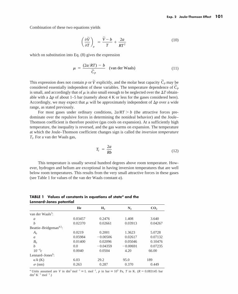
This temperature is usually several hundred degrees above room temperature. How-ever, hydrogen and helium are exceptional in having inversion temperatures that are well below room temperatures. This results from the very small attractive forces in these gases (see Table 1 for values of the van der Waals constant a ).

TABLE 1 Values of constants in equations of statea and the Lennard–Jones potential

He H2 N2 CO2

van der Waals3: a 0.03457 0.2476 1.408 3.640 b 0.02370 0.02661 0.03913 0.04267Beattie–Bridgeman4,5: A0 0.0219 0.2001 1.3623 5.0728 a 0.05984 0.00506 0.02617 0.07132 B0 0.01400 0.02096 0.05046 0.10476 b 0.0 0.04359 0.00691 0.07235 104c 0.0040 0.0504 4.20 66.00Lennard–Jones6: /k (K) 6.03 29.2 95.0 189 s (nm) 0.263 0.287 0.370 0.449

a Units assumed are V in dm3 mol1 L mol1, p in bar 105 Pa, T in K. (R 0.083145 bar dm3 K1 mol1.)


gar28420_ch04_091-118.indd 101gar28420_ch04_091-118.indd 101 11/13/08 1:29:32 AM11/13/08 1:29:32 AM



Other semiempirical equations of state can be used to predict Joule–Thomson coef-ficients. Perhaps the best of these is the Beattie–Bridgeman equation, 4,5 which can be writ-ten (for 1 mol) as

p

RT

VV B

A

V

( )( )

12 2

(13)

where A A a V B B b V 0 01 1( ), ( ),N N and c V TN 3. In this equation of state, there are five constants which are characteristic of the particular gas: A 0 , B 0 , a, b, and c. In terms of these constants and the pressure and temperature, the Joule–Thomson coefficient is given 4 by

m 1 2 4 2 3 5

00

30 0

20

CB

A

RT

c

T

B b

RT

A a

RT

B c

Rp ( ) TT

p4

(14)

This equation predicts a small dependence on pressure not shown by Eq. (11), which is based on the van der Waals equation.

The most general of the equations of state is the virial equation, which is also the most fundamental since it has a direct theoretical connection to the intermolecular poten-tial function. The virial equation of state expresses the deviation from ideality as a series expansion in density and, in terms of molar volume, can be written

(15)

The virial coefficients B2 and B3 depend only on temperature and are determined by two- and three-body interactions between molecules, respectively. For pressures below about 10 bar, the B3 term is very small and can be neglected. Solving Eq. (15) for V and ( ) V T p

/ in a manner similar to that for the van der Waals case above gives

m

T B T B

C

p

p

( )2 2

(16)

From statistical mechanics, 6 B 2 ( T ) is given by

B T N e r drU r kT

2 00

21 2( ) [ ]( )

p

(17)

and ( B 2 / T ) p can be obtained by differentiation. U ( r ) is the potential energy as a function of the separation of the molecules, taken to be spherical, and is important because it can be used to predict many of the transport and collisional properties of a molecule. One com-mon choice for U ( r ) is the so-called Lennard–Jones 6-12 potential, which has the form

U r

r r( ) 4

12 6

es sa b a b

(18)

where e is the well depth corresponding to the minimum in the potential and is the sepa-ration corresponding to U ( r ) 0; see Fig. 47-1. Values for these parameters are included in Table 1 for the gases of interest in this experiment.

EXPERIMENTAL

The experimental apparatus shown in Fig. 2 is patterned after a design given in Ref. 7 . The “porous plug” is a 38 -in.-OD stainless steel frit of 2 m m pore size and 116 -in. thick-ness pressed into a 38 -in. Swagelok tee made of nylon for reduced thermal conductivity.

pVRT

B T

V

B T

V

1 2 3

2

( ) ( ). . .

pVRT

B T

V

B T

V

1 2 3

2

( ) ( ). . .

••



The high-pressure inlet is attached to a 38 -in. cross to provide ports for gas introduction, pressure measurement, and thermocouple placement just in front of the frit. The Bourdon gauge (0–10 bar) should be connected via a tee to a purge valve to facilitate gas changes. Before use the assembly should be tested at 10 bar for leaks. Thermal insulation such as glass wool should be wrapped around the frit assembly to keep the expansion as adiabatic as possible.

The temperature difference T across the frit is measured with two copper-Constantan (type T) thermocouples with wires of 0.010-in. diameter or less for reduced thermal conductivity. The thermocouples can be sealed with epoxy into a 1

16 -in. stainless-steel sheathing tube, which can be connected to the cross fitting by a 1

16 -in. to 38 -in. Swagelok adaptor, or more simply by swaging a 38 -in. Teflon rod with a 0.063-in. feedthrough hole for the thermocouple tube, as shown in Fig. 2 . A convenient 6-in., 1

16 -in.-OD sealed subminiature probe with an exposed thermocouple junction and external strain relief is available from Omega (e.g., probe TMTSS-062E-6). The 6-in. length is suf-ficient to allow the thermocouples to be positioned adjacent to the center of the frit, as shown in the figure.

Because the maximum temperature change will be only 0.5 to 4 K, a sensitive digital voltmeter (0.1 m V ), null voltmeter, or potentiometer is desirable for accurate measurements. To obtain the temperature difference directly, the two Constantan leads of the thermocouples

ToBourdon

gauge

Topurge valve

outlet

Insulation

Gasoutlet

Polyethylenetubing 2 micron

frit pressedinto fitting

Nylonfittings

Gasinlet

Constantan+

copperthermocouple

" Teflonrod with

0.063" hole

38

Thermocouplesepoxied inside

0.0625" stainless-steel tube

FIGURE 2Detail of Joule–Thomson cell.





should be clamped together and the copper leads should be attached to the measuring device. † For best absolute accuracy, the two thermocouples should be calibrated (e.g., using a standard thermometer) to determine their temperature coefficients (Seebeck coefficient) . However, for a copper–Constantan thermocouple, varies only slightly with temperature, from 39 to 43 m V K 1 from 0 to 50 C. At 25 C, is 40.6 m V K 1 and the variation is small from one thermocou-ple to another. For small temperature differences, a linear relation V TC T ( dT / dP ) p is a good approximation for the thermocouple potential difference between the two junctions. ‡ Thus, to the accuracy needed for this experiment, the slope of a plot of V TC versus p can be combined with an assumed value of 40.6 m V K 1 to yield ( dT / dp ) and hence m .

Procedure. Set up the apparatus shown in Fig. 2 . The gas supply should be a cylin-der or supply line equipped with a pressure regulator and a control valve. The supply pres-sure should be constant during the measurements. Because a signifi cant temperature change occurs as gases go from high to low pressure through the pressure regulator itself, the gas should be passed through about 50 ft of 14 -in. coiled copper tubing contained in a water bath at 25 1 C. A 14 -in.-to- 38 -in. adaptor can be used for a short, insulated polyethylene tubing connection to the expansion apparatus. Before initiating gas fl ow, record the bath temperature and determine any offset voltage between the two thermocouples.

Start the measurements with CO 2 with the pressure regulator set to minimum pressure. Open the control valve and purge the copper line and pressure gauge of air or any other gases with the purge valve open. Then close the purge valve and slowly increase the pres-sure to 4 bar. After this pressure is reached, record the thermocouple reading every 30 s, until the values become constant (typically a few minutes). Lower the regulator pressure by about 0.5 bar and again take readings every 30 s until a constant value is obtained. Continue this procedure down to a final pressure of 0.5 bar. Note that this is the excess pressure over the discharge pressure into the room (assumed to be at 1 bar).

Change the gas supply to N 2 and again purge the copper coil and pressure gauge with the purge valve open. Close this valve and bring the pressure slowly to 10 bar, a higher value than for CO 2 since the cooling is less. After the temperature has stabilized, repeat the sequence of measurements as for CO 2 but at 1-bar intervals. Finally, repeat the N 2 proce-dure using He gas. In this case, the temperature change will be much smaller and positive: i.e., the gas heats on expansion because it is above the so-called Joule–Thomson inversion point, the temperature at which the coefficient m is zero. After completion of the experi-ment, make sure that all cylinder valves are closed.

CALCULATIONS

For each gas studied, do a linear regression to fit V TC (or T ) versus p so as to obtain the slope along with its standard error. On a single graph, show for each of the three gases the best-fit straight line along with the experimental data points. From the slopes, evaluate the Joule–Thomson coefficient m in units of K bar 1 . Compare your results with literature values given in Ref. 7 . Calculate m for these gases at 25 C from the van der

••

†As an alternative to a thermocouple, one can use two sensitive thermistor probes and an appropriate resistance bridge circuit (see Chapters XVI and XVII). A calibration to convert the bridge measurement to T is required in this case.

‡In practice, one often finds that VTC T VTC, where VTC is a small offset voltage (1–3 mV) observed when both the reference and the measuring junction are at the same temperature. This “nonthermodynamic” result can occur if the thermocouple wire has regions of compositional variation or strain (e.g., from kinking) that are subject to a temperature gradient. VTC can be ignored in this experiment, since it affects only the intercept of the plot of VTC versus p and not the slope.



Waals and Beattie–Bridgeman constants given in Table 1 . Cp

values for He, N 2 , and CO 2 at 25 C are 20.79, 29.12, and 37.11 J K 1 mol 1 , respectively.

Plot the Lennard–Jones potentials for each of the gases studied. Obtain m from Eqs. (16)–(18) by numerical integration and compare the values from this two-parameter potential with those from the van der Waals and Beattie–Bridgeman equations of state. [ Optional: A simple square-well potential model can also be used to crudely represent the interaction of two molecules. In place of Eq. (18), use the square-well potential and param-eters of Ref. 6 to calculate m. Contrast with the results from the Lennard–Jones potential and comment on the sensitivity of the calculations to the form of the potential.]

DISCUSSION

The Joule–Thomson coefficient gives a measure of how much potential energy is con-verted into kinetic energy or vice versa as molecules in a dense gas change their average separation during an adiabatic expansion. As mentioned earlier, the magnitude and sign of m are determined by the balance of attractive and repulsive interactions and, for most gases at room temperature, cooling occurs as molecules work against a net attractive force as they move apart. The exceptions are the weakly interacting species He and H 2 , where m is negative at 300 K and precooling below the inversion temperature is first necessary before cooling can occur on expansion. Calculate the inversion temperature for the gases of Table 1 using Eqs. (11), (14), and (16), neglecting the last, small pressure-dependent term in (14), and compare your values with experimental ones you find in the literature. Equations (14) and (16) can be most easily solved for T I by iteration, using for example the Solve For function of spreadsheet programs, as discussed in Chapter III.

Joule–Thomson cooling is the basis for the Linde method of gas liquefaction, in which a gas is compressed, allowed to cool by heat exchange, and is then expanded to cool suf-ficiently that the gas liquefies. This effect is also important in the operation of refrigerators and heat pumps. Using cylinders of high-pressure gas, cooling can be achieved without power input in a device without moving parts, and hence the Joule–Thomson process has been used in cooling of small infrared and optical detectors on space probes. Discuss some of the design factors that might be important in achieving maximum cooling efficiency in the latter kind of a device.

For the more difficult Joule experiment, we can write

h

y

a bT

V

E V

E T

T p T p

CE

T

V

V( )

( )

( )

(19)

This quantity is called the Joule coefficient. It is the limit of ( T / V ) E, corrected for the heat capacity of the containers as V approaches zero. With the van der Waals equation of state, we obtain h y a V CN 2 . The corrected temperature change when the two contain-

ers are of equal volume is found by integration to be T a VCN2y, where V is the

initial molar volume and Cy is the molar constant-volume heat capacity. It is instructive to calculate this T for a gas such as CO 2 . In addition, the student may consider the relative heat capacities of 10 L of the gas at a pressure of 1 bar and that of the quantity of copper required to construct two spheres of this volume with walls (say) 1 mm thick and then cal-culate the T expected to be observed with such an experimental arrangement.

SAFETY ISSUES

Gas cylinders must be chained securely to the wall or laboratory bench (see pp. 644–646 and Appendix C).

••

••


gar28420_ch04_091-118.indd 105gar28420_ch04_091-118.indd 105 11/13/08 1:16:22 AM11/13/08 1:16:22 AM



APPARATUS

Insulated Joule–Thomson cell similar to that of Fig. 2 (suitable stainless steel frits can be obtained from chromatographic parts suppliers, e.g., Upchurch Scientific part C-414); metal or nylon tees, crosses, and reducers (available from Swagelok and other manufacturers); 38 -in. Teflon rod; type T insulated copper–Constantan thermocouples with 0.010-in.-diameter wires; voltmeter with 0.1- mV resolution (e.g., Keithley 196), null voltmeter (e.g., Hewlett Packard 419A or Keithley 155), or sensitive potentiometer (e.g., Keithley K-3). Cylinders of CO 2 , N 2 , and He with regulators and control valves; 50 ft of 14 -in. copper coil, 38 -in. and 14 -in. polyethylene tubing; 0- to 10-bar Bourdon gauge; 25 C water bath.

REFERENCES

1. J. P. Joule and W. Thomson (Lord Kelvin), Phil. Trans. 143, 357 (1853); 144, 321 (1854). [Reprinted in Harper’s Scientific Memoirs I, The Free Expansion of Gases, Harper, New York (1898).]

2. R. J. Silbey, R. A. Alberty, and M. G. Bawendi, Physical Chemistry, 4th ed., p. 127, Wiley, New York (2005).

3. Landolt-Börnstein Physikalisch-chimische Tabellen, 5th ed., p. 254, Springer, Berlin (1923). [Reprinted by Edwards, Ann Arbor, MI (1943).] [This is the source of van der Waals constants cited in the CRC Handbook of Chemistry and Physics. ]

4. J. A. Beattie and W. H. Stockmayer, “The Thermodynamics and Statistical Mechanics of Real Gases,” in H. S. Taylor and S. Glasstone (eds.), A Treatise on Physical Chemistry, Vol. II, pp. 187ff., esp. pp. 206, 234, Van Nostrand, Princeton, NJ (1951).

5. J. A. Beattie and O. C. Bridgeman, J. Am. Chem. Soc. 49, 1665 (1927); Proc. Am. Acad. Arts Sci. 63, 229 (1928).

6. J. O. Hirschfelder, C. F. Curtiss, and R. B. Bird, Molecular Theory of Gases and Liquids, chap. 3 and table I-A, Wiley, New York (1964).

7. A. M. Halpern and S. Gozashti, J. Chem. Educ. 63, 1001 (1986).

EXPERIMENT 3 Heat-Capacity Ratios for Gases The ratio C p / C y of the heat capacity of a gas at constant pressure to that at constant vol-ume will be determined by either the method of adiabatic expansion or the sound velocity method. Several gases will be studied, and the results will be interpreted in terms of the contribution made to the specific heat by various molecular degrees of freedom.

THEORY

In considering the theoretical calculation of the heat capacities of gases, we shall be concerned only with perfect gases. Since C C Rp

y for an ideal gas (where Cp

and Cy

are the molar quantities C p / n and C v / n ), our discussion can be restricted to C v.

••

••

••


An Improved Apparatus for the Measurement of the- ~oule-~homson Coefficient of Gases Arthur M. Halpern and Saeed Gozashti Northeastern University. Boston. MA 021 15

One of the common annlications of real eases nresented in ~~~ ~~~~~~~

undergraduate treatme& of thermodynakics is the Joule- Thomson (JT) effect. This tonic not onlv ex~licitlv shows " . how a nonzero J T coefficient arises from an equation of state for a real gas, but i t also appeals to the student's physical experience with the cooling associated with most expanding gases. In addition, the ability to calculate the J T coefficient (PJT) from an equation of state illustrates the computational nature of thermodynamics as well as the relative utilitv of equations of state.

Experimental measurements of PJT nicely fit into the laboratory portion of physical chemistry. Accordingly, this experiment is described in Shoemaker et al. ( I ) . The procedure described there, however, is awkward and probably lacks the sensitivity needed to observe and quantitatively to measure the effect for He. A somewhat different approach was described by Hecht and Zimmerman (2), but this procedure, while an improvement, is also unwieldy and may not work satisfactorily with He. One of the drawbacks with these apparatus is the need to construct specialized and cumber- some equipment.

In this paper, we describe an apparatus that can be constructed from commercially available components and that has the sensitivity to measure FJT for He with reasonable accurwy. l'he strategy is to usegas fitting sand a porous plug made trom sti~inless steel. This material was chosen because of its h e r thermal ronducrivitv (relative to brass). Lnlike the glass used in the J T cells pre&usly described, dur stainless steel apparatus can withstand higher pressures, and, in the case of He, this contributes to the ability to measure pJT with reasonable accuracy. The two commonly used gases Np and Cop are easily studied with this apparatus. In addition, SFG is used; i t is a good choice for this experiment because it is presumably nontoxic, nonreactive, andrelatively inexpen- sive. Moreover, there is considerable interest in this material as a dielectric and possible refrigerant and as a model for multiple infrared photon absorption. The students can thus made aware of this information.

A diagram of this apparatus is shown in Figure 1. The heart of the high-pressure Dart of the J T cell is a 3/R-in. union cross (swagel;k SS-600-4j adapted on three sides to S/s-in. (SS-200-R-6). The gas inlet is coupled via a %-in. Teflon tube and the pressure is read via a 0-100 psi gauge also connected by '18-in. Teflon tubing (used to reduce heat trans-

Figure 1. Cutaway diagram of the apparatus. The stainless steel fiuings and Other components are described in the text.

fer tolfrom the J T cell). A copperlconstantan thermocouple, sealed with an epoxy adhesive passes through a 'I8-in. tube and is positioned in the center of the interior of the cross. This thermocouple is constructed from narrow gauge leads (0.010 in.) also to reduce heat transfer (Omega Engineering Inc). The expansion plug (2 pm) used was a 3/s-in. stainless steel HPLC bed support (43-38BS, Rainin Inst. Co.). The frit is contained in a 3/8-in. union (SS-600-6); the latter is connected to the cross via a 3/8-in. close-couple. The low- pressure thermocouple is fed through a #17 stainless steel syringe needle (the s h a r ~ end removed) as a euide and held rigid hy a 3s-\G-in. reducing union (ss-600-6:l) with Teflon ferrules. The gas nutlet is provided by several holes drilled through a short length ( 2 in.) of ,*-in. tul~ing placed betwen thr frit-containing union and the reducing union. 1Lo damp out flurtuatiuns in the temperature difference read hv the therrnocouplrs, the low-pressure thermocouple was fastened to a small brass cup attached to the end of the guide using a minute amount of epoxy adhesive, heavily impregnated with brass filinri to im~rove th~ . thermal conductivitv. The cun

~ ~~~

was prepared by simply filing down the lock-end of th'e syringe. To provide additional insulation, a short length of Tygon tubing is inserted into the high-pressure side of the frit. Holes are provided for the thermocounle and nressure gauge. ina ally,-to krrp the entire apparatus as adinhatic as pussihle, it was wrapped in several la\ws of class wool.

The two therm&ouples were found to be very well matched so that when connected in series to indicate the temperature difference between them, an immeasurably small potential was observed when they were isothermally equilibrated. As an indication of the thermal balance between the thermocouples, the voltage of the equilibrated, static apparatus was usually found to be less than 1 pv. Best results were obtained under this condition which could be brought about by a very slow trickle of gas (He or Nz) through the apparatus. The potential developed by the thermocouples was directly read by a Hewlett-Packard model 419A null voltmeter. Alternatively, another readout device having an appruprtatrly high input resistance can be used. A cnlibratioti of :!I p\'/Y: \confirmed hy the freezing point of benzene) was used in these experiments.

The measurements for He were carried out between pressures of 90 and 30 psi. Stable voltages were established after about 15-30 s. Readings were taken in increments of 10 psi. For the other gases where the J T effect is larger, the highest pressure used could be reduced. 'l'he entireexperiment involving the measurement uf the four gases can he carried out in less than 3 h.

The J T coefficients were determined by a linear regression of the data, (see Fig. 2) assuming alow-nressure value of

~ ~~ ~ - 1 ntm. The highest prtswre used is low enough to justify the asnnmption of P-inde~endvnt JT coefficients. These w e r ~ compared with ~ J T a; calculated from three equations of state: van der Waals (vdW), Redlich-Kwong (RK) (3 ,4 ) and Beattie-Bridgeman (BB) ( 5 6 ) . The results are shown in the table. The first two involve two parameters which can he obtained from critical data while the latter incorporates five empirical parameters.

Volume 63 Number 11 November 1986 1001

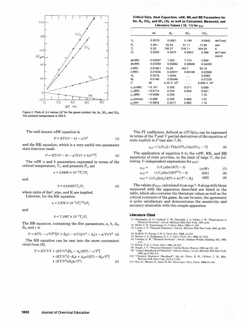
Critical Data, Heat Capacnies, vdW, RK,and BB Parameters for He, N,, CO,, and SF8 (9) , as well as Calculated, Measured, and

Literature Values ( lo, 11) for fin

a(vdW) "4 :iT 0.03397 0.02369 0.07651 15.38 0.03862 1.350

b (RK) 0.01636 0.02677 Ao 0.0216 1.3445

40 & 0.0140 0.05046 C 40 4.20 X 10'

p d v d W ) -0,101 0.250

0 P ~ R K ) -0.0774 0.224

HE w d B B ) -0.0596 0.229

-20 p d m e a s ) -0.066 0.230 0 20 40 60 80 p d l i t ) -0.0624 0.2217

AP. PSI

F w r e 2 Plots of AVversus APfar the gases s t d w he. N,. SF,, and C02 The ammen1 1emperstLre is 298 K

The well-known vdW equation is The J T coefficient, defined as (aTlap)x can be expressed in terms of the T and Vpartial derivatives of the equation of

P = RTI(V- b) - a l p state explicit in P (see also 7,8), and the RK equation, which is a very useful two parameter state function reads p~~ = ( ~ I c ~ ) [ - T ~ J P / ~ ~ ~ I ( J P I ~ ~ ~ - V) (6)

P = RTI(V - b ) - ~ V ( V + b)~l"I The application of equation 6 to the vdW, RK, and BB

(2) equations of state ~rovides. in the limit of laree V. the fol- - . The vdW o and b parameters expressed in terms of the lowing V-independent expressions for wT:

critical temperature, T,, and pressure PC, are p = (l/Cp)IZa/(RT) - bl (udW) (7) a = 2.8408 x 10-3T:/P, PJT = ( 1 / ~ ~ ) 1 5 a / ( 2 ~ 7 0 ~ ~ ) - bl (RK) (8)

and PJ'JT = (11Cp)12Ad(RTj + 4 c l P - BB,J (BB) (9)

where units of dm3, atm, and K are implied. Likewise, for the RK equation

a = 2.879 X IO-~(T~")/P,

and

The BB equation, containing the five parameters, a, b, Ao, Bo, and c is

The BB equation can he cast into the more convenient virial form (6) ,

Thevalues of ~ J T , calculated from eqs 7-9 along with those measured with the apparatus described are listed in the table, which also contains the literature values as well as the critical constants of the gases. As can be seen, the agreement is quite satisfactory and demonstrates the sensitivity and accuracy attainable with this simple apparatus.

Literature Cited (11 Shoemaker, D. P.; Gsrknd, C. W.: Steinfeld, J. I.; Nibler, J . W. -~xperimenk in

Phyrieal Chemistry)', 4th od.; McCraw-Hill: New York, 1961; p 6 5 (21 Hecht. C. E.: Zimmermsn. G. J. Chem. Edue. 1954.31.530. (8, Levine.1. N."Physical Chemir~y", 2nd ed.: McCrsw~Hill: New York, 1981:pp 2W-

9°K -. ... I 4 Redlich, 0.; Kwong, J. N.S. ChamReu. 1949.44.283. (5 ) Beattie.J.A.: Brideeman.0. C. J.Amer. Chem.Sor. 1928.50.8133. 161 Catellan, G. W. "Physicsl Chemistry", 3rd ed.: Addison-Wesley: Reading. MA, 1983: ." p w . (7) Ryho1t.T. R. J.Chom.Educ. 1981.58.621. (61 Nwde. J. T . "Phyaieal Chemistry"; Liltle. Brown: Boaton, 1985: pp 105-110. (91 "Lange'sHsndhmkofChemiatcy': 13Lhed.; Dean. J. A.ed.:MeGraw-Hill: New York,

1985; pp9-180, 9-4. 1101 "Chemical Engineers' Hsndboolt': 5th ed.; Perry, R. H.; Chilfon. C. H., Eda.:

McCraw-Hill: New York. ,978: p3102. 1111 Bier, K.; Mauier, G.:Sand,H. Rer. Runsewes.Phya. Chcm. 1980,81,480.

1002 Journal of Chemical Education

Documents

Première loi de la thermodynamique: détermination du coefficient