Embed Size (px)
Citation preview

Probabilistic estimation of fatigue loads
on monopile-based offshore wind turbines
- Application to sensitivity assessment & clusteringoptimization for support structure cost reduction -
Master of Science Thesis
Author: Lisa Ziegler
Supervisors: Prof. Dr. A.V. Metrikine TU Delft - ChairmanDr. E. Lourens TU DelftProf. Dr. M. Muskulus NTNUS. Schafhirt NTNUDr. S.N. Voormeeren Siemens Wind PowerR. Haghi Siemens Wind PowerE. Smid Siemens Wind Power
May 12, 2015


Abstract
Offshore wind energy faces three important trends: (1) wind farms grow in size, (2)monopiles are installed in deeper water, and (3) cost reduction remains the most im-portant challenge. With wind farm size, the importance of variations in environmentalsite conditions across the wind farm increases. These site variations, e.g. water depthand soil conditions, can lead to significant differences of loads on support structures.For monopiles in deeper water, design is dominated by wave-induced fatigue loads.Since full fatigue load calculations are computationally demanding, they can typicallynot be performed for each turbine within large wind farms. Therefore, turbines must begrouped into clusters in early project phases, making time-efficient approaches essen-tial. Optimization of design clustering is necessary to reduce design conservatism andthe cost of offshore wind energy.Hence, the goal of this thesis is to investigate load site variations and clustering. There-fore, a probabilistic fatigue load estimation method is developed and verified with aero-elastic simulations in the time domain. Subsequently, the developed method is appliedfor an exemplary wind farm of 150 turbines in 30-40m water depth to perform
– sensitivity studies of loads to changes in MSL, soil stiffness, and wave parameters,
– probabilistic assessments of data, statistical and model uncertainties, and
– deterministic and probabilistic design clustering.
The estimation method is based on frequency domain analysis to calculate wave-induced fatigue loads, a scaling approach for wind loads, combination of wind-waveloads with quadratic superposition, and Monte-Carlo simulations to assess uncertain-ties. Verification confirms an accuracy of 95% for lifetime equivalent fatigue loadscompared to time domain simulations. The computational speed is in the order of100 times faster than typical time domain tools. Sensitivity studies show a significantinfluence of water depth and wave period on EFLs. The influence of soil on EFLs isminor for high soil stiffness but can increase significant for soils with low stiffness.Normal distributed input parameters in a probabilistic assessment yield a positivelyskewed probability distribution of EFLs. Design clustering is optimized based on site-specific fatigue loads using brute-force and discrete optimization algorithms. Resultsfor the exemplary wind farm show a design load reduction of up to 13% comparedto standardized design. Probabilistic clustering proved to be only relevant at clusterborders leading to a difference in allocation for 12 out of 150 turbines.Project results show that it is essential to account for load differences in large windfarms due to varying site conditions. This study improves clustering and provides a basisfor design optimization and uncertainty analysis in large wind farms. Further work isneeded to extend tool verification and formulate design clustering for cost optimization.
i

ii

Acknowledgements
Many people have contributed to the success of this project with their experiences,ideas and recommendations. In particular, I want to thank:
Prof. Michael Muskulus for the guidance on this project from NTNU. Thanksfor making it possible for me to attend the DeepWind’2015 R&D conference and tosubmit two scientific papers. I can honestly say that your support had a big impact onthe success of this thesis - and on my decision to stay with research in the coming years.Thanks also to Sebastian Schafhirt from NTNU for your great help with computationsand reporting. It’s a pleasure to come back to Trondheim and the offshore wind groupsoon.
Prof. Andrei Metrikine and Eliz-Mari Lourens who supervised my thesis fromTU Delft’s end. Thanks for your advice and always pushing the “physical meaning” infocus. And who knows, we may have some interesting discussions about StructuralHealth Monitoring in the future.
My supervisors from Siemens Wind Power for their support. Thanks to SvenVoormeeren who initiated this project. I appreciate our discussions, feedback and thebig chunk of time you invested in my thesis. I want to thank Rad Haghi who not onlysupervised my work, but also set up many BHawC simulations so that I could verify myestimation tool. Thanks a lot also to Erik Smid for sharing your extensive experiencesin load analysis with me and answering all my questions. Thank you, all three, forreading and correcting my report - that cannot be taken for granted! Finally, thanks toall my Siemens and study colleagues for always helping when needed. The offshorewind community is small - I am looking forward to meet you guys again in the future.
My parents who are just awesome. Danke, dass ihr immer da seid, egal wieviele Kilometer zwischen uns liegen.
iii

iv

Contents
Abstract i
Acknowledgements ii
List of Figures vii
List of Tables viii
Nomenclature xi
1 Importance of load estimates in the offshore wind industry 1
2 Loads on offshore wind turbines 52.1 Loads and load cases . . . . . . . . . . . . . . . . . . . . . . . . . . . . . 52.2 Parameters effecting the load level . . . . . . . . . . . . . . . . . . . . . 72.3 State-of-the-art of load calculation process . . . . . . . . . . . . . . . . . 9
2.3.1 Design positions . . . . . . . . . . . . . . . . . . . . . . . . . . . 92.3.2 Design split versus integrated methods . . . . . . . . . . . . . . . 92.3.3 Deterministic versus probabilistic design . . . . . . . . . . . . . . 102.3.4 Time versus frequency domain calculations . . . . . . . . . . . . 11
2.4 Load modeling . . . . . . . . . . . . . . . . . . . . . . . . . . . . . . . . 122.4.1 Wave load modeling . . . . . . . . . . . . . . . . . . . . . . . . . 122.4.2 Wind load modeling . . . . . . . . . . . . . . . . . . . . . . . . . 13
2.5 Uncertainty in fatigue loads . . . . . . . . . . . . . . . . . . . . . . . . . 15
3 Probabilistic fatigue load estimation method 173.1 Model objective and tool structure . . . . . . . . . . . . . . . . . . . . . 173.2 Assumptions for proposed method . . . . . . . . . . . . . . . . . . . . . 193.3 Frequency domain method for wave fatigue loads . . . . . . . . . . . . . 21
3.3.1 Generalized wave loads . . . . . . . . . . . . . . . . . . . . . . . 213.3.2 Structural response . . . . . . . . . . . . . . . . . . . . . . . . . . 253.3.3 Fatigue load estimates with Dirlik’s method . . . . . . . . . . . . 27
3.4 Scaling method for wind loads . . . . . . . . . . . . . . . . . . . . . . . 313.4.1 Turbulence intensity scaling . . . . . . . . . . . . . . . . . . . . . 313.4.2 Natural frequency correction . . . . . . . . . . . . . . . . . . . . 32
3.5 Combining wind and wave loads . . . . . . . . . . . . . . . . . . . . . . 333.6 Probabilistic load assessment . . . . . . . . . . . . . . . . . . . . . . . . 34
3.6.1 Input distributions . . . . . . . . . . . . . . . . . . . . . . . . . . 353.6.2 Bootstrapping . . . . . . . . . . . . . . . . . . . . . . . . . . . . . 36
v

4 Verification of developed fatigue estimation method 394.1 Reference case . . . . . . . . . . . . . . . . . . . . . . . . . . . . . . . . 394.2 Time domain simulations using aero-elastic code BHawC . . . . . . . . . 404.3 Comparison of wave-only fatigue loads . . . . . . . . . . . . . . . . . . . 42
4.3.1 Qualitative analysis using power spectra . . . . . . . . . . . . . . 434.3.2 Quantitative analysis of equivalent fatigue loads . . . . . . . . . . 45
4.4 Comparison of wind-only fatigue loads . . . . . . . . . . . . . . . . . . . 474.5 Comparison of wind-wave combined loads . . . . . . . . . . . . . . . . . 484.6 Discussion of verification study . . . . . . . . . . . . . . . . . . . . . . . 50
5 Fatigue load modeling results 535.1 Wave load analysis . . . . . . . . . . . . . . . . . . . . . . . . . . . . . . 53
5.1.1 Simulation cases . . . . . . . . . . . . . . . . . . . . . . . . . . . 535.1.2 Comparison of three sea states . . . . . . . . . . . . . . . . . . . 535.1.3 Effect of wind-wave directionality . . . . . . . . . . . . . . . . . . 54
5.2 Statistical uncertainty in wave loads . . . . . . . . . . . . . . . . . . . . 565.3 Sensitivity of wave fatigue loads (Paper A) . . . . . . . . . . . . . . . . . 585.4 Optimization of design clustering (Paper B) . . . . . . . . . . . . . . . . 58
6 Discussion of fatigue estimation and its applications 596.1 Evaluation of estimation method and applications . . . . . . . . . . . . . 596.2 Limitations . . . . . . . . . . . . . . . . . . . . . . . . . . . . . . . . . . 606.3 Industry application . . . . . . . . . . . . . . . . . . . . . . . . . . . . . 626.4 Scientific value . . . . . . . . . . . . . . . . . . . . . . . . . . . . . . . . 63
7 Conclusions and recommendations 65
Bibliography 69
A Properties of developed method 75
B Scientific papers 77
C Local search optimization 103

List of Figures
2.1 Dominant wave forces on cylindrical offshore structures. . . . . . . . . . 132.2 Local forces on an airfoil. . . . . . . . . . . . . . . . . . . . . . . . . . . 14
3.1 Flowchart of fatigue load estimation method. . . . . . . . . . . . . . . . 183.2 Flowchart of generalized wave load calculation. . . . . . . . . . . . . . . 223.3 McCamy-Fuchs diffraction correction for inertia coefficient CM . . . . . . 243.4 JONSWAP wave spectrum and equivalent wave load spectrum. . . . . . 253.5 Transfer function and force response spectrum. . . . . . . . . . . . . . . 263.6 Flowchart for obtaining EFL estimates with Dirlik’s method. . . . . . . . 283.7 Probability density function of load ranges. . . . . . . . . . . . . . . . . 303.8 Turbulence intensities. . . . . . . . . . . . . . . . . . . . . . . . . . . . . 313.9 Natural frequency correction for wind-only loads. . . . . . . . . . . . . . 333.10 Input distribution. . . . . . . . . . . . . . . . . . . . . . . . . . . . . . . 36
4.1 Structural dimensions of foundation structure. . . . . . . . . . . . . . . . 404.2 Time series of sea surface elevation and bending moment. . . . . . . . . 424.3 PSD of sea surface simulation and JONSWAP wave spectrum. . . . . . . 434.4 Comparison of PSDs of response moment and force at mudline. . . . . . 444.5 Comparison of PSDs of response moments and forces at interface. . . . . 454.6 Comparison of rainflow-counting and Dirlik’s PDF. . . . . . . . . . . . . 454.7 Comparison of rainflow-counting and Dirlik’s PDF. . . . . . . . . . . . . 464.8 Turbulence intensity and Weibull distribution. . . . . . . . . . . . . . . . 474.9 Verification of wind-only fatigue loads. . . . . . . . . . . . . . . . . . . . 484.10 Verification of combined EFL mudline. . . . . . . . . . . . . . . . . . . . 494.11 Verification of combined EFL interface. . . . . . . . . . . . . . . . . . . . 49
5.1 PSDs of response moment for three different sea states. . . . . . . . . . . 545.2 PSD of bending moments for wind-wave (mis-)alignment. . . . . . . . . 555.3 Scatter diagram and histogram of probabilities. . . . . . . . . . . . . . . 575.4 Standard deviation in scatter diagram and histogram of EFLs. . . . . . . 57
C.1 Flowchart of local search. . . . . . . . . . . . . . . . . . . . . . . . . . . 104
vii

viii

List of Tables
2.1 Permanent and variable loads. . . . . . . . . . . . . . . . . . . . . . . . . 52.2 Load influencing parameters. . . . . . . . . . . . . . . . . . . . . . . . . 8
3.1 Maximum fatigue load differences due to site variations. . . . . . . . . . 173.2 MC computation time. . . . . . . . . . . . . . . . . . . . . . . . . . . . . 353.3 Standard deviation of input parameters. . . . . . . . . . . . . . . . . . . 35
4.1 BHawC simulation parameters. . . . . . . . . . . . . . . . . . . . . . . . 414.2 Choices for Welch’s method. . . . . . . . . . . . . . . . . . . . . . . . . . 424.3 Sea states in verification study. . . . . . . . . . . . . . . . . . . . . . . . 424.4 Normalized EFLs of time and frequency domain methods. . . . . . . . . 464.5 Turbulence scaling errors. . . . . . . . . . . . . . . . . . . . . . . . . . . 484.6 Errors of load estimation tool. . . . . . . . . . . . . . . . . . . . . . . . . 50
5.1 Normalized EFLs for three sea states. . . . . . . . . . . . . . . . . . . . . 545.2 Normalized EFLs of for wind-wave alignment. . . . . . . . . . . . . . . . 565.3 Statistical properties of EFLs due to scatter diagram variability. . . . . . . 58
ix

x
Nomenclature
Latin symbols
b wind amplitude m/s
c airfoil chord length m
C structural damping Ns/m
CD drag coefficient −CL lift coefficient −CM inertia coefficient −d water depth m
dt time step s
D damage −D diameter m
Di Dirlik’s constant −e average Monte-Carlo error −E expected value −EFL equivalent fatigue load N , Nm
f frequency Hz
fdrag drag force N/m
finertia inertia force N/m
fp wave peak frequency Hz
F areo- or hydrodynamic force N
FD drag force N
FL lift force N
g gravitational acceleration m/s2
H transfer function m/N,m/Nm
HS significant wave height m
k wave number rad/m
K structural stiffness N/m
L length scale m
L load range N,Nm
m Woehler slope −mn nth spectral moment [unit]2/sn
xi
M structural mass kg
n number of seeds or load ranges −N number of cycles −N number of Monte-Carlo simulations −p probability density function −Q Dirlik’s constants −R Dirlik’s constants −S power spectrum [unit]2/Hz
STD standard deviation unit
t time s
TC mean time between peaks s
TI turbulence intensity −Tlife lifetime s
TP wave spectrum peak period s
Tsime simulation time s
TZ zero-crossing period s
u water particle velocity m/s
u water particle acceleration m/s2
Urel relative wind speed at blade section m/s
VW wind speed m/s
Z normalized load range −
Greek symbols
γ peak enhancement factor −γ irregularity factor −ε random phase rad
ζ damping ratio −λ wave length m
φ inflow angle degree
φ mode shape −ρ water density kg/m3
ρa air density kg/m3
ω angular frequency rad/s
Abbreviations
ALS Accidental Limit State
BEM Blade Element Momentum
BHawC Bonus Energy Horizontal axis wind turbine Code
DLC Design Load Case

DNV Det Norske Veritas
EFL Equivalent Fatigue Loads
FDM Frequency Domain Method
IEC International Electrotechnical Commission
(I)FFT (Inverse) Fast Fourier Transform
FLS Fatigue Limit State
JONSWAP JOint North Sea WAve Project
MSL Mean Sea Level
MCS Monte-Carlo Simulation
PDF Probability Density Function
PSD Power Spectral Density
RNA Rotor Nacelle Assembly
SLS Serviceability Limit State
ULS Ultimate Limit State
OWT Offshore Wind Turbine

xiv
Chapter 1
Importance of load estimates in theoffshore wind industry
Offshore wind energy is a growing industry vital for successful transition from fossilfuels to renewable energy. Compared to onshore technology, offshore turbines benefitfrom higher mean wind speeds, more steady wind conditions and greater availability ofpotential sites. Nevertheless, costs of offshore wind energy are still too high due to moreexpensive support structures, grid connections and offshore installations [1]. In orderto make offshore wind energy economically viable, the wind industry has committed to40% cost reduction in 2020 with respect to the 2012 cost level [2].Part of this cost reduction is realized from support structures, where a recentstudy shows a potential of approximately one sixth of the total cost reduction [2].Predominating support structures are monopiles as they cover 75% of the offshore windmarket in 2013 [3]. According to the European Wind Energy Association [3], the trendof increasing size of offhore wind farms is expected to continue in the next years. Largeoffshore wind farms are predominantly located in deeper water (25-40m), for whichmonopile designs are typically governed by fatigue loads with significant contributionsfrom wave excitation [4].Large offshore wind farms cover areas of several square kilometer, in which considerablevariations in environmental site conditions, for instance water depth, soil properties,and turbulence can exist. These variations lead to divergent design loads on supportstructures across the wind farm. Full load calculations are computationally demandingand can typically not be performed for each turbine [5]. In industry projects, offshorewind turbines (OWTs) are therefore often grouped into design clusters, where loads areonly evaluated for a limited number of design positions. Allocating of OWT to designclusters must be performed in an early project phase, making time-efficient approachesessential. Hence fatigue load estimates are of highest relevance for a systematic conceptof design optimization of offshore support structures and thus for the reduction ofoffshore wind energy costs.
Review of literature
Several approaches exist in literature to decrease computational costs of load analysison OWT [6–17]. Approaches either use integrated analysis or suggest wind-waveseparate assessment. In separate assessments, wave fatigue loads are mainly estimatedwith frequency domain analysis [6–9, 12, 13], which has also been applied to wind
1

2 1. IMPORTANCE OF LOAD ESTIMATES IN THE OFFSHORE WIND INDUSTRY
loads [7, 9, 13–15]. Other authors suggest simplified rotor load models or parametricmodels for fatigue damage estimation [10,15]. For integrated methods, proposal existsfor reducing the number of environmental conditions, load cases, number of seeds orsimulations length [6,11,17].Since fatigue load calculation processes contain significant uncertainties, a numberof researchers performed probabilistic fatigue assessment. A brief overview ofexisting publications is given by Yeter [18] and Veldkamp [19]. Sensitivity studiesinvestigated the influence of site parameters and foundation configuration on thenatural frequency, and emphasized the need for further work regarding sensitivity offatigue damage [20,21].Nowadays, industry practices base clustering decisions on variations of mean sea level(MSL) or eigenfrequency of the support structures [22]. Recently, Seidel suggestedan improved approach of clustering using a site parameter that takes structural andhydrodynamic properties into account [22]. This site parameter is, however, onlysuitable for wave-load dominated designs. Thus, further work is needed to formulateturbine clustering as an optimization problem incorporating all important site-specificinformation.
Research objectives and methodology
Based on the problem statement and review of existing publications, there is theneed for research to obtain a better understanding of how fatigue loads behave inlarge offshore wind farms due to varying and uncertain site conditions. Thus, a linkbetween fatigue estimation methods and probabilistic assessments is necessary that canbe applied for sensitivity study of loads and optimization of turbine clustering in largeoffshore wind farms.Given this research motivation, the main research question of the thesis is:
How can probabilistic fatigue load estimation improve turbine clusteringin large offshore wind farms to reduce costs of offshore wind energy?
From this question the following three research objectives were derived:
1. Insight into load sensitivity to varying site conditions,
2. Analysis of effects of uncertainties in data, statistics and models, and
3. Optimization of turbine clustering.
In order to approach the research objectives, a probabilistic fatigue estimation methodwas developed in the computing environment MATLAB R©. A verification study isperformed with aero-elastic simulations for a 4MW OWT in approximately 35m waterdepth. The developed method is applied in local and global sensitivity studies to assesseffects of site variations of the parameters MSL, soil stiffness, wave height, and waveperiod on fatigue loads. Furthermore, a probabilistic assessment is carried out withMonte-Carlo simulations (MCS) to analyze impacts of uncertainties on fatigue loads.Finally, the previous results are used to optimize turbine clustering based on site-specificfatigue load estimates.

3
Outline of report
The thesis consists of two research papers and a summary report. The main researchwork is presented in the papers. The summary report adds theoretical background andwork that has not been published. The remaining report is structured as follows:
Chapter 2 In Chapter 2 relevant theoretical fundamentals of loadanalysis on OWT support structures are described. Thefocus is on types of loads, state-of-the-art of load modeling,and uncertainties in fatigue load calculation. Furthermore,parameters affecting the load level are outlined according topresent scientific and industrial knowledge.
Chapter 3 Chapter 3 describes the implementation of the developedmethod for probabilistic fatigue load estimation on monopilesusing frequency domain calculations for wave loads, scalingmethods for wind loads and MCS. Next to the programstructure, the objective of the model, assumptions, andlimitations are discussed.
Chapter 4 In the fourth chapter the developed fatigue estimationmethod is verified with time domain aero-elastic simulations.Verification is performed for wave-only, wind-only and wind-wave combined loads. Finally, results and limitations of theverification study are discussed.
Chapter 5 Wave-induced fatigue loads for three simulation cases arepresented in Chapter 5. Special emphasis is placedon the effect of aerodynamic damping and wind-wavemisalignment. Statistical uncertainty in wave loads isanalyzed using resampling methods. Finally, an overviewof the content of the appended papers about wave loadsensitivity and design clustering is given.
Chapter 6 Chapter 6 assesses the probabilistic fatigue estimationmethod and its applications for sensitivity assessment andclustering optimization. Limitations are discussed followedby an evaluation of scientific value and potential applicationsof method and results in industry.
Chapter 7 The last chapter summarizes the performed study and results.The report closes with recommendations for future research.
Appendix Paper A deals with the sensitivity of wave fatigue loads undervarying side conditions. Design clustering using deterministicand probabilistic fatigue estimates is topic of paper B.

4 1. IMPORTANCE OF LOAD ESTIMATES IN THE OFFSHORE WIND INDUSTRY
Papers and authorship
The main work of the papers regarding programming, analysis and post-processing wascarried out by the author of this thesis. Forming of the research idea, approaches, resultdiscussion and minor parts of programming (time domain simulations, finite elementmodel, discrete optimization solver) was a collaboration of the thesis supervisors fromNTNU, Prof. Michael Muskulus and Sebastian Schafhirt, and the industry supervisor,Sven Voormeeren and his colleagues. In the following, the integration of the papers inthe thesis scope is outlined.
Paper 1: Lisa Ziegler, Sven Voormeeren, Sebastian Schafhirt and Michael Muskulus.“Sensitivity of Wave Fatigue Loads on Offshore Wind Turbines under varying SiteConditions”, accepted for publication in Energy Procedia (Elsevier).This paper presents the sensitivity analysis of wave-induced fatigue loads to varyingsite conditions using frequency domain analysis. An probabilistic assessment isperformed with MCS. This paper addresses the first two research objectives and laysthe groundwork for optimization of turbine clustering.
Paper 2: Lisa Ziegler, Sven Voormeeren, Sebastian Schafhirt and Michael Muskulus.“Design clustering of offshore wind turbines using probabilistic fatigue load estimation”,submitted to Renewable Energy (Elsevier).Design clustering of OWTs in large wind farms is the subject of this paper usingdeterministic and probabilistic fatigue load estimates. Therefore, the paper presents anapplication of the in this thesis developed fatigue estimation method and answers thecentral research question about turbine clustering.
Chapter 2
Loads on offshore wind turbines
The relevant theoretical fundamentals of load analysis on offshore wind turbinesupport structures are described in this chapter. The focus is hereby on typesof loads, state-of-the-art of load modeling and uncertainties in fatigue loadcalculations. Furthermore, parameters affecting the load level are outlinedaccording to present scientific and industrial knowledge. For theoreticalbackground on offshore wind turbines, aerodynamics and hydrodynamic loads,reference is made to relevant literature [23–25].
2.1 Loads and load cases
OWT are subjected to various load sources. The design of OWTs has to withstand allloads during anticipated lifetime of the structure while being cost-effective. Therefore,knowledge of expected loads during lifetime is crucial for a successful design. Loadscan be categorized either through load origin or according to the affected limit state. Inorder to ensure a reliable design, a large number of load cases need to be analyzed [26].Several engineering standards from classification societies as well as internationalstandards exist for the design of OWTs. Mainly the standards “Design requirementsfor offshore wind turbines” by International Electrotechnical Commission (IEC 61400-3) [26] and “Design of offshore wind turbine support structures” by Det Norske Veritas(DNV-OS-J101) [27] are considered for this study.
Functional and environmental loads
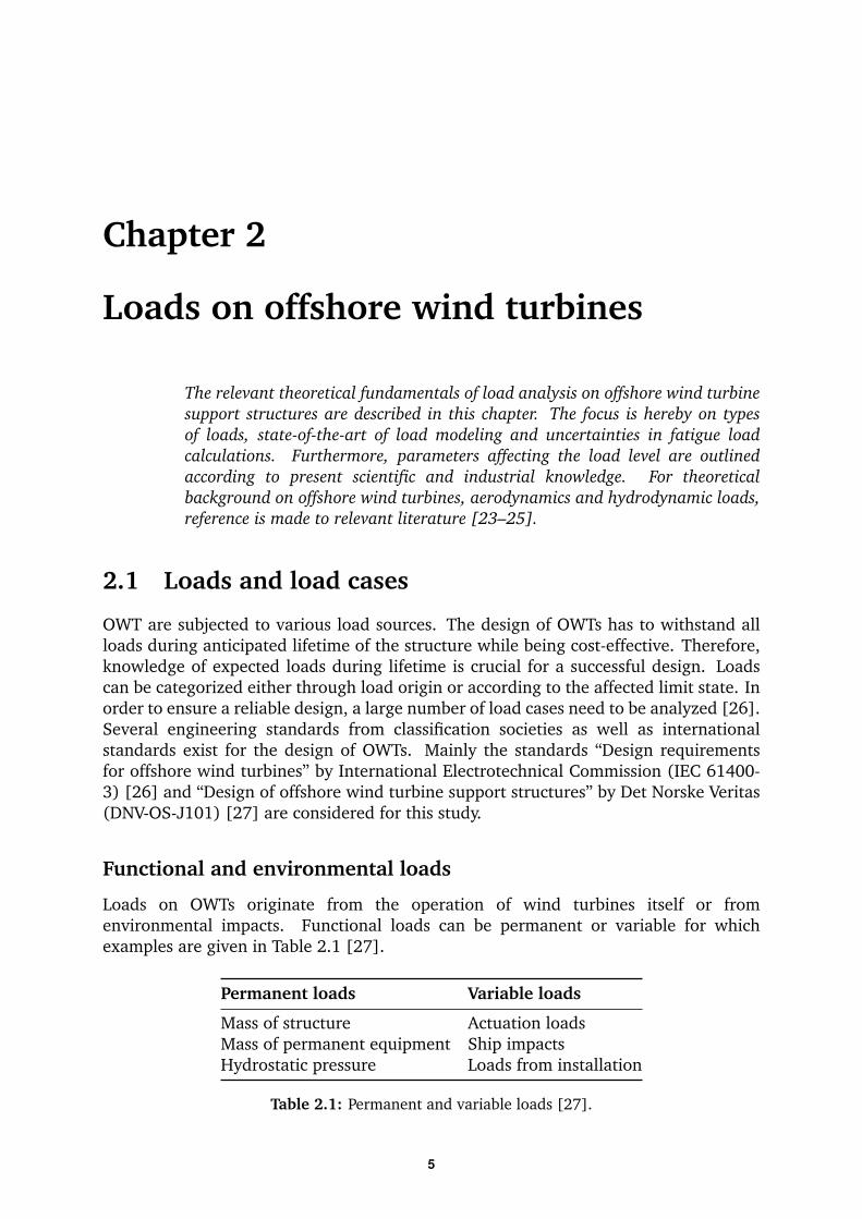
Loads on OWTs originate from the operation of wind turbines itself or fromenvironmental impacts. Functional loads can be permanent or variable for whichexamples are given in Table 2.1 [27].
Permanent loads Variable loads
Mass of structure Actuation loadsMass of permanent equipment Ship impactsHydrostatic pressure Loads from installation
Table 2.1: Permanent and variable loads [27].
5

6 2. LOADS ON OFFSHORE WIND TURBINES
Permanent loads stay constant during lifetime of the structure, while variable loadsdepend on operation, and therefore change in time. Environmental loads acting onthe structure are site-specific and vary in size and point of application during lifetime.Examples of environmental influences causing loads on OWTs are
– wind,
– wave and current,
– tides,
– ice (floating and on blades),
– marine growth, and
– earthquakes if applicable.
Depending on the impact characteristic these influences either affect the maximum loadcarrying capacity, being ultimate loads, or the fatigue resistance of the materials, beingfatigue loads, as described in the following section.
Ultimate and fatigue loads
In the design standards for OWTs several limit states are defined, which state the marginof the structure of still being able to satisfy design requirements [26,27]. These are thecriteria
– Ultimate Limit State (ULS),
– Fatigue Limit State (FLS),
– Accidental Limit State (ALS), and
– Serviceability Limit State (SLS).
In this thesis, ULS and FLS are further examined, since these are typically design driving.ULS describes the capacity to withstand maximum extreme loads, while cumulativedamage due to cyclic loading is covered in FLS [27].Examples of typical extreme loads in the design practice are combinations of 1-year,5-year, and 50-year maximum wind or wave extremes. Fatigue loads are cyclic loadswith lower amplitude than extreme loads occurring continuously during the entirelifetime of the structure, for example wind and wave loads in wind turbine operation.For monopile support structures in deeper water locations, fatigue loads are typicallydesign driving [28]. Furthermore, in these locations the contribution of wave loadsplays a major role in fatigue analysis [12]. A recent study of a monopile supportstructure for a 6MW wind turbine in 40m water depth shows that the combined wind-wave fatigue loads are clearly dominated by wave contributions [4]. Accordingly, theinfluence of wind loads on total fatigue loads is minor. Additionally, wind loads can bepredicted with good accuracy and are less sensitive to site variations. Therefore, thisstudy focuses on detailed estimation of wave-induced fatigue loads, while wind loadsare approximated with a simple scaling method.
Load cases
In order to represent the most important load contributing events occurring duringlife of the OWT, various design situations with several load cases are considered in itsdesign. IEC 61400-3 defines eight design situations, namely

2.2. PARAMETERS EFFECTING THE LOAD LEVEL 7
– power production,
– power production plus occurrence of fault,
– start up,
– normal/ extreme shut down,
– emergency shut down,
– parked (standstill or idling),
– parked and fault conditions, and
– transport, assembly, maintenance, repair [26].
Load cases are set up as further specification of these design situations, for examplestating appropriate normal or extreme condition for wind, waves, directionality,currents, water levels, and other factors. Each load case then either contributes tofatigue or ultimate load analysis for which a specific safety factor is defined [26].All load cases with a reasonable probability of occurrence should be consideredwhich leads to a total number of more than thirty cases to analyze according to IEC61400-3 [26]. For each of the cases multiple time domain simulations with three totwelve seeds and simulation length of typically ten minutes need to be set up. Nextto the general load cases defined in the standard, specific situations might need to beanalyzed additionally. Altogether, for one position within a wind farm the total numberof performed load simulations are typically in the range of 2000 to 10000 for oneiteration [29]. Due to this enormous effort, it is often not possible to perform timedomain load analyses for every turbine position within the wind farm.
This condensed outline of the various loads and load cases illustrates the complexityof load analysis. In order to decrease the design effort by implementing validsimplifications, a better understanding of the influence of various parameters on theload level is needed. Parameters effecting the load level are examined in the followingsection.
2.2 Parameters effecting the load level
Parameters influencing the load level of OWTs can be categorized into internal systemconditions and external influences. Internal parameters are structural or turbineproperties, for instance mass or mode shapes, while external parameters are relatedto environmental influences, for example water depth or soil conditions. All parametersare evaluated according their
– importance for load level, and
– availability and uncertainty at project start.
The criteria availability and uncertainty are important since the fatigue estimationmethod is mainly for use in early project phases. In these phases, not all siteconditions are given for every turbine location and interpolation between available site

8 2. LOADS ON OFFSHORE WIND TURBINES
measurements introduces uncertainties.For the following parameter study, reference is made to design standards,relevant articles and reports as well as project experience within Siemens WindPower [4, 6, 12, 26, 27, 30, 31]. Table 2.2 gives an overview of categorization of loadinfluencing parameters.
Category ParameterImportance[- to ++]
Availability[- to +]
StructuralParameter
Eigenfrequency ++ 0Mode shape ++ 0Mass + +Damping ratio ++ 0
EnvironmentalParameter
Water depth ++ +Wind ++ +Wave climate ++ 0Current 0 0Directionality + 0Ice 0 0Soil ++ 0Earthquake 0 0Scour and erosion - +Marine growth - +
TurbineParameter
Rated power 0 +Actuation loads 0 +Yaw misalignment 0 +Operation mode + +Wakes 0 -
Table 2.2: Categorization of load influencing parameters.
The analysis identified the parameters from which a high importance for the load levelis expected as the following:
– water depth,
– soil,
– wind and wave climate,
– directionality,
– eigenfrequency, and
– damping ratio.
Results for sensitivities of fatigue loads to changes and uncertainties in these parametersare presented in section 5.2 and the scientific papers in Appendix B.

2.3. STATE-OF-THE-ART OF LOAD CALCULATION PROCESS 9
2.3 State-of-the-art of load calculation process
The load influencing parameters vary between different offshore sites which leads todivergent loads on support structures. Consequently, support structures are customengineered for every offshore wind farm. This custom engineering includes thefollowing iterative steps:
1. load evaluation based on site-specific conditions and
2. subsequent structural design of tower and foundation using site-specific loads.
One loop in this iterative process typically takes four to six weeks [32].
2.3.1 Design positions
Larger offshore wind farms nowadays consist of sixty or more turbines which cover awide area of several square kilometers. This large area leads to considerable variationsof environmental site conditions within the farm. Ideally, support structures for eachindividual wind turbine should be custom engineered. However, this is not feasible inpractice since time for the development phase of the project is limited.In practice, loads are evaluated for a limited number of design positions within the windfarm. A design position is chosen in order to perform the engineering only once. Theresulting load levels and structural design need to hold for all assigned positions withinthe wind farm. Consequently, the design position must be the position where highestloads occur [32]. This position can be either physical or virtual. A virtual design positioncombines worst-case properties of several physical positions. After the design positionsare selected, the remaining turbines are allocated to clusters.Nowadays, clustering and selection of design position in the wind turbine industryis often performed based on previous project experiences using criteria such asapproximate first eigenfrequency and water depth. These parameters indeed have animportant influence on the load level as shown in section 2.2. However, latest studieshave shown that the interpolation accuracy is not sufficient for design purposes [12].Recently, an alternative approach was published which states a “site parameter” thatcan be used to interpolate loads between different turbine positions [12]. Optimizationof design positions and clustering will decrease design conservatism and thereforecontribute to the cost reduction of offshore wind energy.
2.3.2 Design split versus integrated methods
In industry practice, a design split usually exists between wind turbine manufacturersand foundation designers. This split evolved from the history of wind energy, wherewind turbine manufacturer benefited from their experiences from onshore wind energy,while foundation designers build on expertise from the offshore oil and gas industry [6].Wind loads are typically calculated by a wind turbine manufacturer which is alsoresponsible for the design of wind turbine towers. Foundation designers take careof wave loads and the foundation design. However, the support structure acts asone system with foundation and tower influencing the response behavior. Therefore,extensive communication is needed at the interface leading to slow design progressand conservative design since different models and safety factors are applied [33].

10 2. LOADS ON OFFSHORE WIND TURBINES
Several researchers conclude that an integrated design method can lead to an optimizeddesign while reducing engineering efforts [4,6,33–36]. Accordingly, this study uses anintegrated model incorporating foundation and tower in a single system.
2.3.3 Deterministic versus probabilistic design
The design of OWT support structures contains high numbers of stochastic variables thatinfluence loads and material strength. These stochastic variables lead to uncertainty indesign procedures. Design approaches treat this uncertainty either deterministic, whereall uncertain variables are represented with one characteristic value, or probabilistic,where structural reliability is defined through an accepted probability of failure intime [27].The design standards for OWTs recommend deterministic design based on the partialsafety factor method [26, 27]. In this method, load and resistance factors are appliedin calculations in order to achieve a target safety value. The target safety valuefor OWT foundations as unmanned structures should match a probability of failureof 10-4 according to [27]. The only standard considering probability-based designis DNV-OS-J101, which recommends it for calibration of load and material factorsin deterministic analysis, specific design problems, and novel designs with limitedexperience available [27].In daily engineering practice, deterministic approaches are convenient due to limitedtime and resources. Research results from probabilistic analysis can be used to improvedeterministic approaches and to assess the chances that results differ significant fromdeterministically calculated ones. The main gain from probabilistic approaches isimproved knowledge of structural reliability. This is important for
– reduction of design conservatism through exact matching of target safetyvalues [19],
– better financing conditions from security of economic planning [37,38],
– planning of operation and maintenance [18], and
– decision on remaining structural reliability at the end of OWTs design lifetime.
A brief overview of previous work on probabilistic design of OWTs is given byVeldkamp [19] and Yeter et al. [18]. Veldkamp focused on probabilistic analysis offatigue design considering also randomness of wave loads for OWTs [19]. In hiswork, he calibrates partial safety factors from annual failure probabilities derivedwith First Order Reliability Methods and MCS. Later, uncertainty modeling, reliabilityassessment and use of test results through Maximum Likelihood Methods and Bayesianstatistics is described by Sorensen and Toft [39]. A current research project by ForWindon probabilistic safety assessment of OWTs tries to answer the overall question ofprobability of failures in current OWT design [40]. Recently, Yeter et al. [18] publisheda fatigue reliability assessment of a tripod OWT support structure using a stochasticspectral approach for wind and wave loading [18].The briefly summarized publications above assess the frame of reliability-based designfor OWTs. Additionally, several studies examine the importance of specific uncertaintiesin load calculations [17, 41–44]. As an example, Zwick and Muskulus [17] state
2.3. STATE-OF-THE-ART OF LOAD CALCULATION PROCESS 11
a maximum error of 35% for substructure fatigue loading caused by input loadingvariability due to a single 10min simulation.The main novelty of this work is to apply probabilistic load estimates for sensitivityassessment of fatigue loads to varying site conditions, which provides a basis for designclustering in large offshore wind farms. Beyond the scope of this thesis, further work isneeded to combine the here obtained probabilistic loads with uncertainties in structuralresistance.
2.3.4 Time versus frequency domain calculations
In current engineering practice, fatigue loads on OWTs are mainly assessed by extensivetime domain simulations of various load cases described in section 2.1. Time domainsimulations are used since they enable non-linear analysis with coupled simulations ofwind, wave and control system [45]. The results of time domain analysis are treated asmost accurate and are therefore commonly used for certification purpose. Results withhigh accuracy are important especially for checking Rotor Nacelle Assemblies (RNA)against type certification loads. However, for support structure design less sophisticatedmodels might be sufficient, which will be further investigated in this study. Especiallyfor preliminary design and clustering optimization, time domain simulations are notsuitable due to high computational costs.Frequency domain methods, as an alternative, have the potential to heavily decreasecomputational costs. Since frequency domain analysis is linearized and treats windand waves as decoupled, the method is considered less accurate than time domainapproaches. Nevertheless, frequency domain methods have been preferably appliedhistorically in the offshore oil and gas industry, when computationally resources werelimited, and are also recommended in offshore guidelines [46]. Frequency domainmethods also have been transferred to OWTs by several researchers [6,7,12].Kuehn [6] suggested a simplified method for fatigue analysis by superimposing timedomain simulations of aerodynamic loads with frequency domain results of wave loadson the support structure. Later, van der Tempel [7] applied frequency domain analysisto complete support structure design, where a comparison to time domain resultsshowed reasonable accuracy. Both researchers treat wind and wave loads separately,but emphasize the importance of accounting for aerodynamic damping due to its largeeffect on support structure dynamics. Seidel [12] recently published a highly simplifiedapproach to calculate wave-induced fatigue loads on monopiles only considering thefirst mode of structural response, while not accounting for aerodynamic damping.Furthermore, Seidel [4] suggests methods to use this approach for lumping of scatterdiagrams and fatigue load interpolation.The above mentioned studies developed, applied and verified frequency domainmethods and stated the potential of it to be used for design optimization due to itscalculation speed. The model developed in this study combines elements of the existingworks describes above and uses these in sensitivity and uncertainty studies.
12 2. LOADS ON OFFSHORE WIND TURBINES
2.4 Load modeling
For a detailed description of hydrodynamic and aerodynamic load modeling on OWTs,reference is made to standard literature [23–25, 47–49]. In the following a briefsummary of the for this study relevant concepts is given.
2.4.1 Wave load modeling
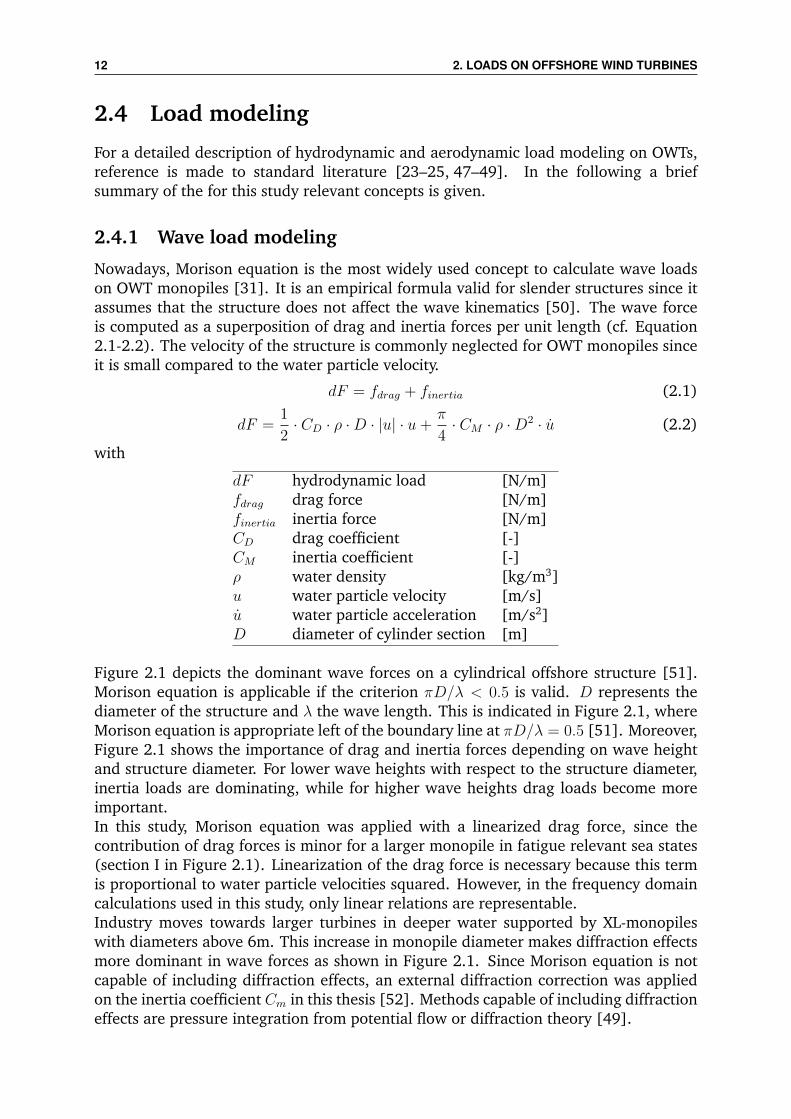
Nowadays, Morison equation is the most widely used concept to calculate wave loadson OWT monopiles [31]. It is an empirical formula valid for slender structures since itassumes that the structure does not affect the wave kinematics [50]. The wave forceis computed as a superposition of drag and inertia forces per unit length (cf. Equation2.1-2.2). The velocity of the structure is commonly neglected for OWT monopiles sinceit is small compared to the water particle velocity.
dF = fdrag + finertia (2.1)
dF =1
2· CD · ρ ·D · |u| · u+
π
4· CM · ρ ·D2 · u (2.2)
with
dF hydrodynamic load [N/m]fdrag drag force [N/m]finertia inertia force [N/m]CD drag coefficient [-]CM inertia coefficient [-]ρ water density [kg/m3]u water particle velocity [m/s]u water particle acceleration [m/s2]D diameter of cylinder section [m]
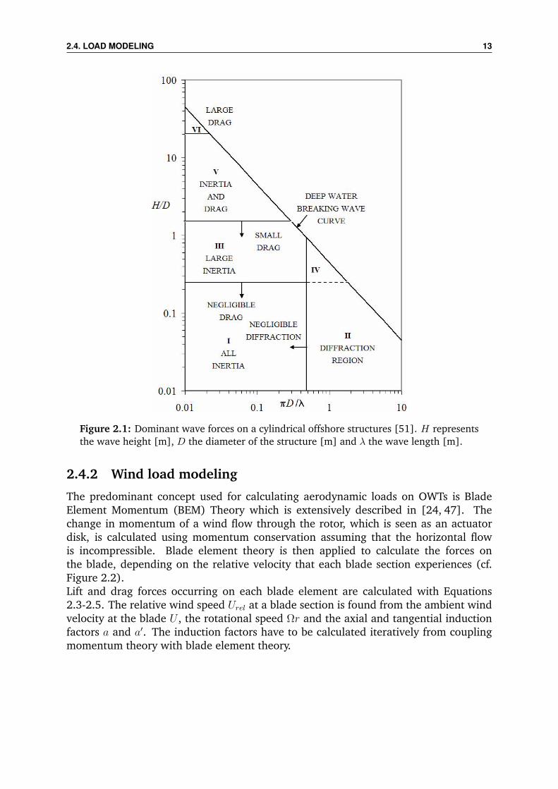
Figure 2.1 depicts the dominant wave forces on a cylindrical offshore structure [51].Morison equation is applicable if the criterion πD/λ < 0.5 is valid. D represents thediameter of the structure and λ the wave length. This is indicated in Figure 2.1, whereMorison equation is appropriate left of the boundary line at πD/λ = 0.5 [51]. Moreover,Figure 2.1 shows the importance of drag and inertia forces depending on wave heightand structure diameter. For lower wave heights with respect to the structure diameter,inertia loads are dominating, while for higher wave heights drag loads become moreimportant.In this study, Morison equation was applied with a linearized drag force, since thecontribution of drag forces is minor for a larger monopile in fatigue relevant sea states(section I in Figure 2.1). Linearization of the drag force is necessary because this termis proportional to water particle velocities squared. However, in the frequency domaincalculations used in this study, only linear relations are representable.Industry moves towards larger turbines in deeper water supported by XL-monopileswith diameters above 6m. This increase in monopile diameter makes diffraction effectsmore dominant in wave forces as shown in Figure 2.1. Since Morison equation is notcapable of including diffraction effects, an external diffraction correction was appliedon the inertia coefficient Cm in this thesis [52]. Methods capable of including diffractioneffects are pressure integration from potential flow or diffraction theory [49].
2.4. LOAD MODELING 13
Figure 2.1: Dominant wave forces on a cylindrical offshore structures [51]. H representsthe wave height [m], D the diameter of the structure [m] and λ the wave length [m].
2.4.2 Wind load modeling
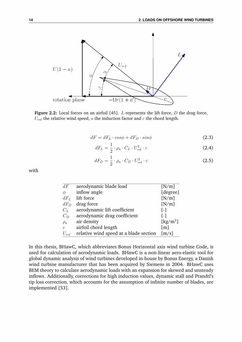
The predominant concept used for calculating aerodynamic loads on OWTs is BladeElement Momentum (BEM) Theory which is extensively described in [24, 47]. Thechange in momentum of a wind flow through the rotor, which is seen as an actuatordisk, is calculated using momentum conservation assuming that the horizontal flowis incompressible. Blade element theory is then applied to calculate the forces onthe blade, depending on the relative velocity that each blade section experiences (cf.Figure 2.2).Lift and drag forces occurring on each blade element are calculated with Equations2.3-2.5. The relative wind speed Urel at a blade section is found from the ambient windvelocity at the blade U , the rotational speed Ωr and the axial and tangential inductionfactors a and a′. The induction factors have to be calculated iteratively from couplingmomentum theory with blade element theory.
14 2. LOADS ON OFFSHORE WIND TURBINES
Figure 2.2: Local forces on an airfoil [45]. L represents the lift force, D the drag force,Urel the relative wind speed, a the induction factor and c the chord length.
dF = dFL · cosφ+ dFD · sinφ (2.3)
dFL =1
2· ρa · CL · U2
rel · c (2.4)
dFD =1
2· ρa · CD · U2
rel · c (2.5)
with
dF aerodynamic blade load [N/m]φ inflow angle [degree]dFL lift force [N/m]dFD drag force [N/m]CL aerodynamic lift coefficient [-]CD aerodynamic drag coefficient [-]ρa air density [kg/m3]c airfoil chord length [m]Urel relative wind speed at a blade section [m/s]
In this thesis, BHawC, which abbreviates Bonus Horizontal axis wind turbine Code, isused for calculation of aerodynamic loads. BHawC is a non-linear aero-elastic tool forglobal dynamic analysis of wind turbines developed in-house by Bonus Energy, a Danishwind turbine manufacturer that has been acquired by Siemens in 2004. BHawC usesBEM theory to calculate aerodynamic loads with an expansion for skewed and unsteadyinflows. Additionally, corrections for high induction values, dynamic stall and Prandtl’stip loss correction, which accounts for the assumption of infinite number of blades, areimplemented [53].

2.5. UNCERTAINTY IN FATIGUE LOADS 15
2.5 Uncertainty in fatigue loads
Uncertainties in fatigue loads can be categorized into aleatory and epistemicuncertainty. Aleatory uncertainty is inherent due to the random nature of processes,for example randomness of sea states. Epistemic uncertainty is knowledge based andcan be reduced if more information is gathered [54]. Sources of epistemic uncertaintiesare [39,55]:
1. Data uncertainty due to measurement imperfection, for example soil or MSL data.
2. Statistical uncertainty due to estimation of parameters from a limited number ofobservations, for example wave characteristics in scatter diagrams.
3. Model uncertainty due to simplification of physical phenomena in modelformulations, for example use of linear wave theory, wake modeling or inputprobability distributions.
According to Sorensen and Toft [39], the most important uncertainties are naturalfluctuations and model uncertainties. It is important to notice that the level ofuncertainties change during different phases of the offshore wind project. In an earlyproject stage, e.g. preliminary design, not all input data exists for every turbine locationwithin the wind farm. Therefore, uncertainties increase due to interpolation of existingdata. In the subsequent detailed design phase, more data is typically available reducinginput uncertainty. Additionally, in an initial design phase, simplified load models areapplied due to time constraints leading to higher model uncertainty.

16
Chapter 3
Probabilistic fatigue load estimationmethod
This chapter describes the developed method for probabilistic fatigue loadestimation on monopiles using frequency domain calculations for waveloads and a scaling method for wind loads. Probabilistic assessment isperformed with Monte-Carlo simulations. The tool is realized in the computingenvironment MATLAB R©. Next to the structure of the tool, objectives of themodel, assumptions, and limitations are discussed.
3.1 Model objective and tool structure
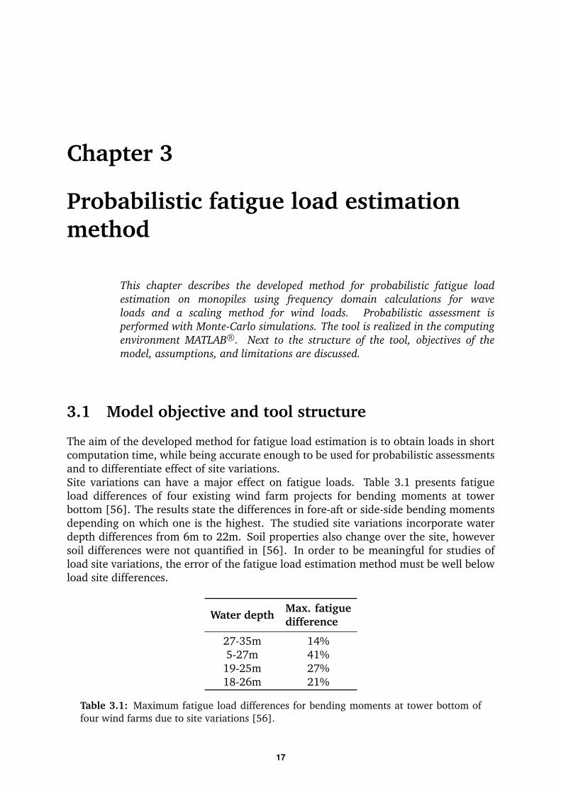
The aim of the developed method for fatigue load estimation is to obtain loads in shortcomputation time, while being accurate enough to be used for probabilistic assessmentsand to differentiate effect of site variations.Site variations can have a major effect on fatigue loads. Table 3.1 presents fatigueload differences of four existing wind farm projects for bending moments at towerbottom [56]. The results state the differences in fore-aft or side-side bending momentsdepending on which one is the highest. The studied site variations incorporate waterdepth differences from 6m to 22m. Soil properties also change over the site, howeversoil differences were not quantified in [56]. In order to be meaningful for studies ofload site variations, the error of the fatigue load estimation method must be well belowload site differences.
Water depthMax. fatiguedifference
27-35m 14%5-27m 41%19-25m 27%18-26m 21%
Table 3.1: Maximum fatigue load differences for bending moments at tower bottom offour wind farms due to site variations [56].
17
18 3. PROBABILISTIC FATIGUE LOAD ESTIMATION METHOD
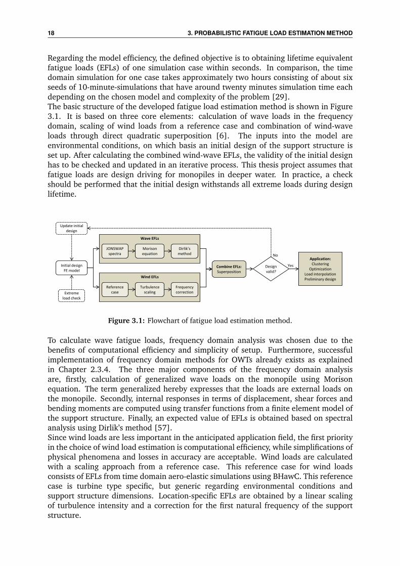
Regarding the model efficiency, the defined objective is to obtaining lifetime equivalentfatigue loads (EFLs) of one simulation case within seconds. In comparison, the timedomain simulation for one case takes approximately two hours consisting of about sixseeds of 10-minute-simulations that have around twenty minutes simulation time eachdepending on the chosen model and complexity of the problem [29].The basic structure of the developed fatigue load estimation method is shown in Figure3.1. It is based on three core elements: calculation of wave loads in the frequencydomain, scaling of wind loads from a reference case and combination of wind-waveloads through direct quadratic superposition [6]. The inputs into the model areenvironmental conditions, on which basis an initial design of the support structure isset up. After calculating the combined wind-wave EFLs, the validity of the initial designhas to be checked and updated in an iterative process. This thesis project assumes thatfatigue loads are design driving for monopiles in deeper water. In practice, a checkshould be performed that the initial design withstands all extreme loads during designlifetime.
Initial design FE model
Wind EFLs
Combine EFLs: Superposition
Extreme load check
Reference case
Turbulence scaling
Frequency correction
Wave EFLs
JONSWAP spectra
Morison equation
Dirlik’s method
Design valid?
Update initial design
Application: Clustering
Optimization Load interpolation Preliminary design
No
Yes
Figure 3.1: Flowchart of fatigue load estimation method.
To calculate wave fatigue loads, frequency domain analysis was chosen due to thebenefits of computational efficiency and simplicity of setup. Furthermore, successfulimplementation of frequency domain methods for OWTs already exists as explainedin Chapter 2.3.4. The three major components of the frequency domain analysisare, firstly, calculation of generalized wave loads on the monopile using Morisonequation. The term generalized hereby expresses that the loads are external loads onthe monopile. Secondly, internal responses in terms of displacement, shear forces andbending moments are computed using transfer functions from a finite element model ofthe support structure. Finally, an expected value of EFLs is obtained based on spectralanalysis using Dirlik’s method [57].Since wind loads are less important in the anticipated application field, the first priorityin the choice of wind load estimation is computational efficiency, while simplifications ofphysical phenomena and losses in accuracy are acceptable. Wind loads are calculatedwith a scaling approach from a reference case. This reference case for wind loadsconsists of EFLs from time domain aero-elastic simulations using BHawC. This referencecase is turbine type specific, but generic regarding environmental conditions andsupport structure dimensions. Location-specific EFLs are obtained by a linear scalingof turbulence intensity and a correction for the first natural frequency of the supportstructure.
3.2. ASSUMPTIONS FOR PROPOSED METHOD 19
Finally, wind and wave EFLs are combined using direct quadratic superposition [6].The output of the method is EFLs for a specified number of cycles. This information canfurther be used to compute the lifetime damage of the structure. Each component ofthe tool is described in detail in the following sections.
3.2 Assumptions for proposed method
In order to create a fast computational model for fatigue load estimation, severalassumptions have been implemented to simplify full load calculations. Thesesimplifications might have an influence on the accuracy of the obtained EFLs. The effectof some of the assumptions is analysed further in the verification study (cf. Chapter 4).
Assumptions for environmental data:
• Wind-wave scatter diagrams are lumped into 20 simulation cases consisting ofmean wind speeds VW , significant wave heights HS, and wave peak periods TP .The lumping is performed in a damage equivalent way using a method suggestedby Kuehn [6]. For each simulation case wind-wave directionality is simplifiedinto fully aligned or fully misaligned. For this purpose, wind and wave roses arelumped in bins of 30degree. Fully aligned wind and waves occur in the same bin.All other combination of wind and wave directions are treated as fully misaligned.
• Soil is modeled with distributed linear springs according to the Winkler model[58,59].
• Further effects like currents and sea ice are neglected since the effects on the loadlevel are expected to be minor (cf. Chapter 2.2). In general, it has to be notedthat sea ice can have a major impact on loads, but is assumed to not occur for theconsidered sites e.g. North Sea. It is assumed that scour protection is installed, sothat erosion and scour effects are not considered.
Reduction of scatter diagrams and the chosen soil model are conform with latestindustry practices. These simplifications are not expected to cause any differencescompared to simulation results of time domain models. Expected to be morecritical is the assumption regarding directionality, for which results are presented inChapter 5.1.3.
Assumptions for structural model:
The structural model in the wind load calculation has the setup used in BHawCwith a full representation of the RNA. For a detailed description about the structuralformulation in BHawC reference is made to [53].The following assumptions concern the structural model used in the frequency domainanalysis for wave loads.
• The foundation and tower are described with a linear finite element model ofTimoshenko beam elements. It is based on a realistic reference design, whereouter diameter, wall thickness and elastic properties change over height of thesupport structure.

20 3. PROBABILISTIC FATIGUE LOAD ESTIMATION METHOD
• The first ten modes of the structure are taken into account according to teneigenfrequencies.
• The RNA is modeled as an equivalent concentrated mass on top of the tower.
• Damping consists of a contribution from combined structural, hydrodynamic andsoil damping (critical damping ratio ca. 1%) and a contribution from aerodynamicdamping (critical damping ratio ca. 1.5 - 8%). The latter is a function of windspeed, rotor speed, and mode shape and is superimposed to structural damping.It is determined turbine specific with modal analysis from a non-linear aero-elasticmodel. Aerodynamic damping for the first mode (fore-aft) is increased for alignedwind and waves, while it is decreased for higher structure modes as well as forwind-wave misalignment.
• The term interface refers to the node at tower bottom.
Through the finite element model an accurate description of the modal properties ofthe support structure is achieved. The first ten eigenfrequencies cover the frequencyrange of wave excitation broadly. Simplifying the RNA as concentrated mass will effectthe response of the support structure, for instance influences of blade eigenfrequenciescannot be depicted.
Assumptions for calculation method:
• Only fatigue relevant design load cases of the design situations power productionand idling are taken into account, since these are the predominantly occuringevents and therefore are expected to contribute most to fatigue damage.
• The wind estimation approach only accounts for turbulence intensity and firstnatural frequency. Differences in air density, wind shear, structural geometry ormode shapes are neglected, since the effects on the load level are expected toeither be minor or represented through the natural frequency correction.
• Applying a turbulence and natural frequency scaling on a wind-only reference caseassumes that both effects are independent. The natural frequency correction hasnot been checked for different turbulence intensities. However, the dependencyof both effects is expected to be minor and neglected in the following analysis.
• Turbulence scaling assumes that wind loads can be approximated by takingturbulence intensity as a linear factor out of the calculation.
• The absolute formulation of Morisons equation is used, since structural velocityis low compared to wave velocity. The drag term is linearized with a methoddeveloped by Borgman [60].
• Constant stretching is used to stretch the wave kinematics from MSL to wavecrest [61]. Diffraction is accounted for by use of the empirical MacCamy-Fuchsdiffraction correction [52].
3.3. FREQUENCY DOMAIN METHOD FOR WAVE FATIGUE LOADS 21
• Instead of using distributed transfer functions of the finite element model alongthe monopile wave-action zone, only transfer functions for equivalent wave loadsat MSL are generated. This is done in order to minimize the computational effortfor creating transfer functions.
• Dirlik’s approximation is used as spectral method to obtain expected number ofcycles and load ranges from load power spectra [57].
• Direct quadratic superposition of wind and wave response assumes that (i) thebehaviour of the structure is linear and (ii) the zero-crossing period of windand wave responses are identical [6]. Linear behaviour is commonly validfor the environmental conditions contributing most to fatigue damage. Zero-crossing periods are not equal in general, however detailed verification studiesby Kuehn [6] proofed good performance of the method.
The largest effect on the accuracy of the results is expected to be caused by theapplication of Dirlik’s method. Previous studies using Dirlik’s method for OWTshave shown that result accuracies are fluctuating with the problem statement [7, 14].Ragan & Manuel showed that Dirlik’s method performed well for estimation ofequivalent fatigue tower bending moments on onshore wind turbines, while only poorresults are obtained for blade edge bending moments [14]. Neglecting the velocity ofthe structure in Morison equation is a common industry practice for monopile designfor OWTs. Furthermore, the effect of linearizing the drag term in Morison equation isexpected to be negligible, since wave loads are inertia dominated for this problem (cf.Chapter 2.4.1). Simplifying the use of transfer functions on only a single interactionpoint is expected to introduce result inaccuracies, since the structural response is alsoinfluenced by the mode shape of the structure at the point of force application. Directquadratic superposition of separately calculated wind and wave loads is commonlyreferred to as conservative, since it neglects the interference term, which is assumedto be negative [62]. The influence of the interference term is expected lower when theproblem is majorly dominated by one load component. For the considered applicationfor monopiles in deeper water, wave loads are exceeding wind loads majorly forenvironmental conditions around rated wind speed, while for lower and higher windspeeds the contributions converge more.
3.3 Frequency domain method for wave fatigue loads
The concept behind each component of the developed method is explained in thefollowing section in detail. Explicit values of chosen coefficients, discretization andother input parameters are given in Appendix A.
3.3.1 Generalized wave loads
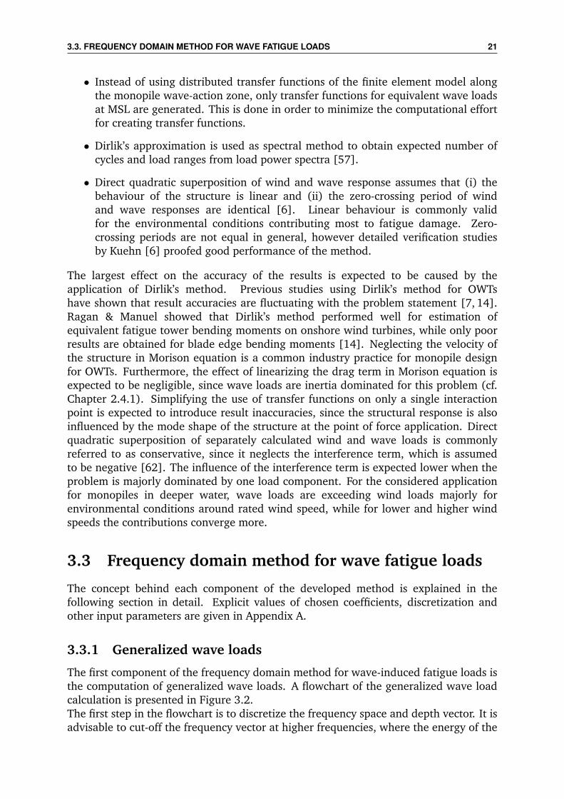
The first component of the frequency domain method for wave-induced fatigue loads isthe computation of generalized wave loads. A flowchart of the generalized wave loadcalculation is presented in Figure 3.2.The first step in the flowchart is to discretize the frequency space and depth vector. It isadvisable to cut-off the frequency vector at higher frequencies, where the energy of the
22 3. PROBABILISTIC FATIGUE LOAD ESTIMATION METHOD
wave spectrum is minimal and therefore the contribution to the sea surface elevationis negligible. In this study, the cut-off frequency is 1Hz. Accordingly, in the structuralmodel all modes that can possibly be excited by the wave loading need to be included.For discretization of the depth vector maximum size elements of 0.5m are used whilea finer definition around MSL might be beneficial due to rapid change of the wavekinematics in this area. The explicit values chosen for the discretization in this modelare stated in Appendix A.
Figure 3.2: Flowchart of generalized wave load calculation.
Afterwards, a JONSWAP wave spectrum is created based on environmental inputconditions of HS and TP which are obtained from lumped scatter diagrams (cf.Equation 3.1-3.4) [63].
SJW (f) = C(γ) · 0.3125 ·H2S · f 5
p · f−5 · exp
[−5
4
(fpf
)4]· γexp(α) (3.1)
σ =
0.07 for f ≤ fp
0.09 for f > fp(3.2)
C(γ) = 1− 0.287 · lnγ (3.3)
α = − (f − fp)2
2 · σ2 · f 2p
(3.4)
3.3. FREQUENCY DOMAIN METHOD FOR WAVE FATIGUE LOADS 23
with
SJW JONSWAP wave spectrum [m2s]γ peak enhancement factor [-]HS significant wave height [m]fp wave peak frequency [Hz]f frequency [Hz]C(γ) normalizing factor [-]
Next to setting up the wave spectrum, the dispersion relation, as stated in Equation 3.5,needs to be solved in order to obtain the wave numbers k.
ω2 = g · k · tanh(kd) (3.5)
with
ω angular frequency [rad/s]g gravitational acceleration [m/s2]k wave number [rad/m]d water depth [m]
Afterwards, Morison equation is applied to generate wave loads on the monopile.Input herefore is the monopile diameter in the water column. In order to treatMorison equation in the frequency domain, the drag term has to be linearized sinceit is proportional to the water particle velocity squared (cf. Chapter 2.4.1). Thelinearization method suggested by Borgmann [60] is implemented which approximatesthe drag term by the first term of the Fourier series expansion (cf. Equation 3.6-3.11).
SV V (f, z) =
[(2 · π · f)2 · cosh2(k · z)
sinh2(k · d)
]· SJW (f) (3.6)
SAA(f, z) =
[(2 · π · f)4 · cosh2(k · z)
sinh2(k · d)
]· SJW (f) (3.7)
Sf (f, z) =8 · c2mor · σ2
π· SV V (f) + k2mor · SAA(f) (3.8)
cmor =1
2· CD · ρ ·D (3.9)
kmor = CM · ρ ·π
4·D2 (3.10)
σ2 =
∫ ∞0
SJW (f) df (3.11)
24 3. PROBABILISTIC FATIGUE LOAD ESTIMATION METHOD
with
SV V velocity spectrum [m2/s]SAA acceleration spectrum [m2/s3]ρ water density [kg/m3]f frequency vector [Hz]z depth vector [m]k wave number [rad/m]d water depth [m]SJW JONSWAP wave spectrum [m2s]CM inertia coefficient [-]CD drag coefficient [-]D monopile diameter [m]σ2 variance [m]
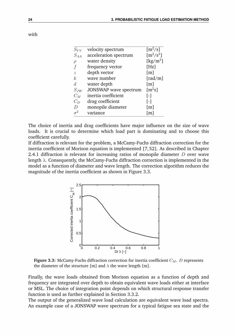
The choice of inertia and drag coefficients have major influence on the size of waveloads. It is crucial to determine which load part is dominating and to choose thiscoefficient carefully.If diffraction is relevant for the problem, a McCamy-Fuchs diffraction correction for theinertia coefficient of Morison equation is implemented [7,52]. As described in Chapter2.4.1 diffraction is relevant for increasing ratios of monopile diameter D over wavelength λ. Consequently, the McCamy-Fuchs diffraction correction is implemented in themodel as a function of diameter and wave length. The correction algorithm reduces themagnitude of the inertia coefficient as shown in Figure 3.3.
0 0.2 0.4 0.6 0.8 10
0.5
1
1.5
2
2.5
D/ λ [−]
Cor
rect
ed in
ertia
coe
ffici
ent C
M [−
]
Figure 3.3: McCamy-Fuchs diffraction correction for inertia coefficient CM . D representsthe diameter of the structure [m] and λ the wave length [m].
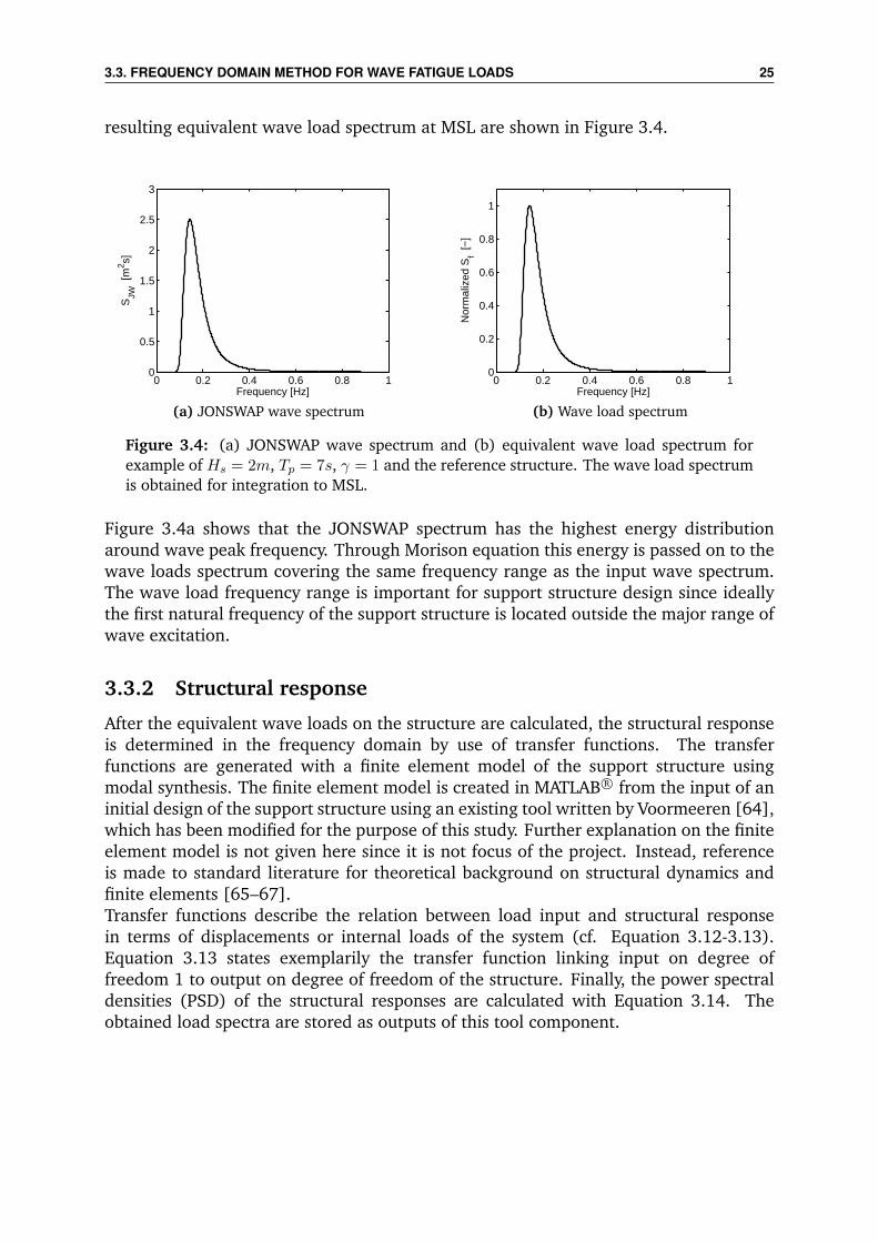
Finally, the wave loads obtained from Morison equation as a function of depth andfrequency are integrated over depth to obtain equivalent wave loads either at interfaceor MSL. The choice of integration point depends on which structural response transferfunction is used as further explained in Section 3.3.2.The output of the generalized wave load calculation are equivalent wave load spectra.An example case of a JONSWAP wave spectrum for a typical fatigue sea state and the
3.3. FREQUENCY DOMAIN METHOD FOR WAVE FATIGUE LOADS 25
resulting equivalent wave load spectrum at MSL are shown in Figure 3.4.
0 0.2 0.4 0.6 0.8 10
0.5
1
1.5
2
2.5
3
Frequency [Hz]
SJW
[m
2 s]
(a) JONSWAP wave spectrum
0 0.2 0.4 0.6 0.8 10
0.2
0.4
0.6
0.8
1
Frequency [Hz]
Nor
mal
ized
Sf [
−]
(b) Wave load spectrum
Figure 3.4: (a) JONSWAP wave spectrum and (b) equivalent wave load spectrum forexample of Hs = 2m, Tp = 7s, γ = 1 and the reference structure. The wave load spectrumis obtained for integration to MSL.
Figure 3.4a shows that the JONSWAP spectrum has the highest energy distributionaround wave peak frequency. Through Morison equation this energy is passed on to thewave loads spectrum covering the same frequency range as the input wave spectrum.The wave load frequency range is important for support structure design since ideallythe first natural frequency of the support structure is located outside the major range ofwave excitation.
3.3.2 Structural response
After the equivalent wave loads on the structure are calculated, the structural responseis determined in the frequency domain by use of transfer functions. The transferfunctions are generated with a finite element model of the support structure usingmodal synthesis. The finite element model is created in MATLAB R© from the input of aninitial design of the support structure using an existing tool written by Voormeeren [64],which has been modified for the purpose of this study. Further explanation on the finiteelement model is not given here since it is not focus of the project. Instead, referenceis made to standard literature for theoretical background on structural dynamics andfinite elements [65–67].Transfer functions describe the relation between load input and structural responsein terms of displacements or internal loads of the system (cf. Equation 3.12-3.13).Equation 3.13 states exemplarily the transfer function linking input on degree offreedom 1 to output on degree of freedom of the structure. Finally, the power spectraldensities (PSD) of the structural responses are calculated with Equation 3.14. Theobtained load spectra are stored as outputs of this tool component.
26 3. PROBABILISTIC FATIGUE LOAD ESTIMATION METHOD
H(ω) =Output
Input=Displacement
Force(3.12)
H11(ω) =n∑j=1
φj,1 · φTj,1(ω2
j − ω2) + 2 · i · ζj · ωj · ω(3.13)
SR(f) = |H(f)|2 · Sf (f) (3.14)
with
H transfer function [m/N]ω angular frequency [rad/s]f frequency [Hz]ωj jth natural frequency [rad/s]φ mode shape [-]ζ damping ratio [-]SR structural response PSD [m2/Hz], [N2/Hz], [(Nm)2/Hz]Sf wave load PSD [N2/Hz], [(Nm)2/Hz]
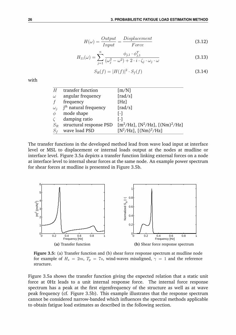
The transfer functions in the developed method lead from wave load input at interfacelevel or MSL to displacement or internal loads output at the nodes at mudline orinterface level. Figure 3.5a depicts a transfer function linking external forces on a nodeat interface level to internal shear forces at the same node. An example power spectrumfor shear forces at mudline is presented in Figure 3.5b.
0 0.2 0.4 0.6 0.8 10
1
2
3
4
5
6
Frequency [Hz]
|H|2 [(
m/N
)2 ]
(a) Transfer function
0 0.2 0.4 0.6 0.8 10
0.2
0.4
0.6
0.8
1
Frequency [Hz]
Nor
mal
ized
SR
[−]
(b) Shear force response spectrum
Figure 3.5: (a) Transfer function and (b) shear force response spectrum at mudline nodefor example of Hs = 2m, Tp = 7s, wind-waves misaligned, γ = 1 and the referencestructure.
Figure 3.5a shows the transfer function giving the expected relation that a static unitforce at 0Hz leads to a unit internal response force. The internal force responsespectrum has a peak at the first eigenfrequency of the structure as well as at wavepeak frequency (cf. Figure 3.5b). This example illustrates that the response spectrumcannot be considered narrow-banded which influences the spectral methods applicableto obtain fatigue load estimates as described in the following section.

3.3. FREQUENCY DOMAIN METHOD FOR WAVE FATIGUE LOADS 27
3.3.3 Fatigue load estimates with Dirlik’s method
Fatigue loads are cyclic loads on the support structure as explained in Chapter 2.1. Inthis tool component, fatigue load estimates are deduced from the internal load powerspectra given out in the previous step.The common method to consider fatigue loads during the design of OWTs is to comparelong-term stress distributions with a material response model, for example S-N curves.S-N curves are created based on laboratory tests of materials and state the number ofcycles N a material can withstand for a specific stress range S before failure [68]. In thedesign standard DNV-OS-J101 [27] suitable S-N curves are given for support structuredesign. The cumulative fatigue damage is then calculated based on S-N-curves usingPalmgren-Miners rule as stated in Equation 3.15 [69]. The cumulative damage Dfatigue
needs to be smaller than one for the entire lifetime so that the structure does not faildue to fatigue.
Dfatigue =∑i
niNi
(3.15)
with
Dfatigue cumulative fatigue damage [-]n number of cycles from stress history [-]N number of cycles from S-N curve [-]
In this study, the concept of EFLs is used since it allows a quantitative comparison ofstructural response loads due to different environmental input. EFLs are defined as theconstant-amplitude load range that causes the same amount of fatigue damage as allvariable-amplitude load ranges L from the load time history for a specified number ofload cycles Nk (cf. Equation 3.16) [19].
EFL =∑i
(ni · LmiNk
) 1m
(3.16)
with
EFL equivalent fatigue load [N], [Nm]L load range [N], [Nm]n number of cycles [-]Nk specified number of cycles [-]m Woehler slope [-]
In order to calculate EFLs, information about the number of cycles and loadranges occuring during the entire lifetime of the structure is needed. For timedomain simulations, this information is typically obtained by performing cycle-counting algorithms, e.g. rainflow-counting, on the computed load history. Forfurther explanation on rainflow-counting reference is made to the developers Endo &Matsuishi [70].In the frequency domain, equivalent results to rainflow-counting on time historiesneed to be obtained from the load power spectrum. For narrow-band spectra, load
28 3. PROBABILISTIC FATIGUE LOAD ESTIMATION METHOD
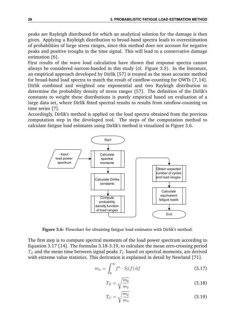
peaks are Rayleigh distributed for which an analytical solution for the damage is thengiven. Applying a Rayleigh distribution to broad-band spectra leads to overestimationof probabilities of large stress ranges, since this method does not account for negativepeaks and positive troughs in the time signal. This will lead to a conservative damageestimation [6].First results of the wave load calculation have shown that response spectra cannotalways be considered narrow-banded in this study (cf. Figure 3.5). In the literature,an empirical approach developed by Dirlik [57] is treated as the most accurate methodfor broad-band load spectra to match the result of rainflow-counting for OWTs [7, 14].Dirlik combined and weighted one exponential and two Rayleigh distribution todetermine the probability density of stress ranges [57]. The definition of the Dirlik’sconstants to weight these distributions is purely empirical based on evaluation of alarge data set, where Dirlik fitted spectral results to results from rainflow-counting ontime series [7].Accordingly, Dirlik’s method is applied on the load spectra obtained from the previouscomputation step in the developed tool. The steps of the computation method tocalculate fatigue load estimates using Dirlik’s method is visualized in Figure 3.6.
Figure 3.6: Flowchart for obtaining fatigue load estimates with Dirlik’s method.
The first step is to compute spectral moments of the load power spectrum according toEquation 3.17 [14]. The formulas 3.18-3.19, to calculate the mean zero-crossing periodTZ and the mean time between signal peaks TC based on spectral moments, are derivedwith extreme value statistics. This derivation is explained in detail by Newland [71].
mn =
∫ ∞0
fn · Sl(f) df (3.17)
TZ =
√m0
m2
(3.18)
TC =
√m2
m4
(3.19)

3.3. FREQUENCY DOMAIN METHOD FOR WAVE FATIGUE LOADS 29
with
mn nth spectral moment [(unit)2/sn]Sl load power spectral density [N2/Hz],[(Nm)2/Hz]f frequency [Hz]TZ zero-crossing period [s]TC mean time between peaks [s]
The irregularity factor γ, defined as the ratio of time between peaks TC to zero-crossingsTZ , is a measure of the bandwidth of a signal (cf. Equation 3.20). For γ being one, TCequals TZ which means that here is only one dominant frequency in the signal, andthus the spectrum is narrow-banded. If γ equals zero, then the signal contains an equalamount of energy at all frequencies [48]. A broad-band signal is defined by 0≤ γ < 1which is reflected in the time signal with a higher number of peaks than zero-crossingsin a defined time interval.
γ =TCTZ
=m2√m0 ·m4
(3.20)
with
γ irregularity factor [-]mn nth spectral moment [(unit)2/sn]TZ zero-crossing period [s]TC mean time between peaks [s]
Based on the previous parameters, Dirlik’s constants are calculated with Equation 3.21-3.26.
xm =m1
m0
·√m2
m4
(3.21)
D1 =2 · (xm − γ2)
1 + γ2(3.22)
R =γ − xm −D2
1
1− γ −D1 +D21
(3.23)
D2 =1− γ −D1 +D2
1
1−R(3.24)
D3 = 1−D1 −D2 (3.25)
Q =1.25 · (γ −D3 −D2 ·R)
D1
(3.26)
with
mn nth spectral moment [(unit)2/sn]γ irregularity factor [-]xm Dirlik’s parameter [-]Di, R, Q Dirlik’s constants [-]
Subsequently, the probability density function (PDF) of the load ranges is defined byDirlik [57] with Equation 3.27-3.28. The expected value of the constant amplitude load
30 3. PROBABILISTIC FATIGUE LOAD ESTIMATION METHOD
range E[L] for n number of cycles is obtained by integrating load ranges weighted withthe PDF as shown in Equation 3.29. The expected number of cycles E[n] is given bydividing the lifetime of the structure T with the mean time between peaks TC .
p(L) =1
2 · √m0
·[D1
Q· e
−ZQ +
D2 · ZR2
· e−Z2
2·R2 +D3 · Z · e−Z2
2
](3.27)
Z =L
2 · √m0
(3.28)
E[L] =
[∫ ∞0
Lm · p(L) dL
]1/m(3.29)
E[n] =T
TC= T ·
√m4
m2
(3.30)
with
p(L) load range PDF [-]Di, R, Q Dirlik’s constants [-]mn nth spectral moment [(unit)2/sn]Z normalized load range [-]L load ranges [N],[Nm]E[L] expected value of load range [N],[Nm]m Woehler slope [-]E[n] expected value of cycles [-]T lifetime of structure [s]TC mean time between peaks [s]
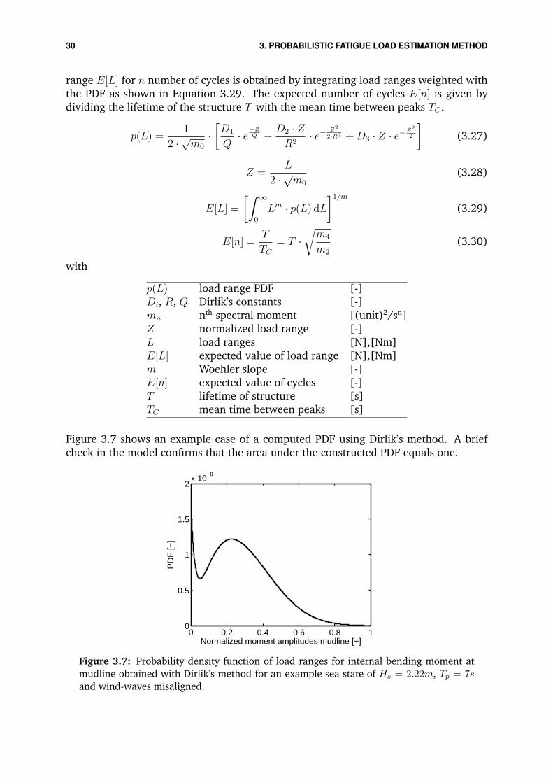
Figure 3.7 shows an example case of a computed PDF using Dirlik’s method. A briefcheck in the model confirms that the area under the constructed PDF equals one.
0 0.2 0.4 0.6 0.8 10
0.5
1
1.5
2x 10
−8
Normalized moment amplitudes mudline [−]
PD
F [−
]
Figure 3.7: Probability density function of load ranges for internal bending moment atmudline obtained with Dirlik’s method for an example sea state of Hs = 2.22m, Tp = 7sand wind-waves misaligned.
3.4. SCALING METHOD FOR WIND LOADS 31
3.4 Scaling method for wind loads
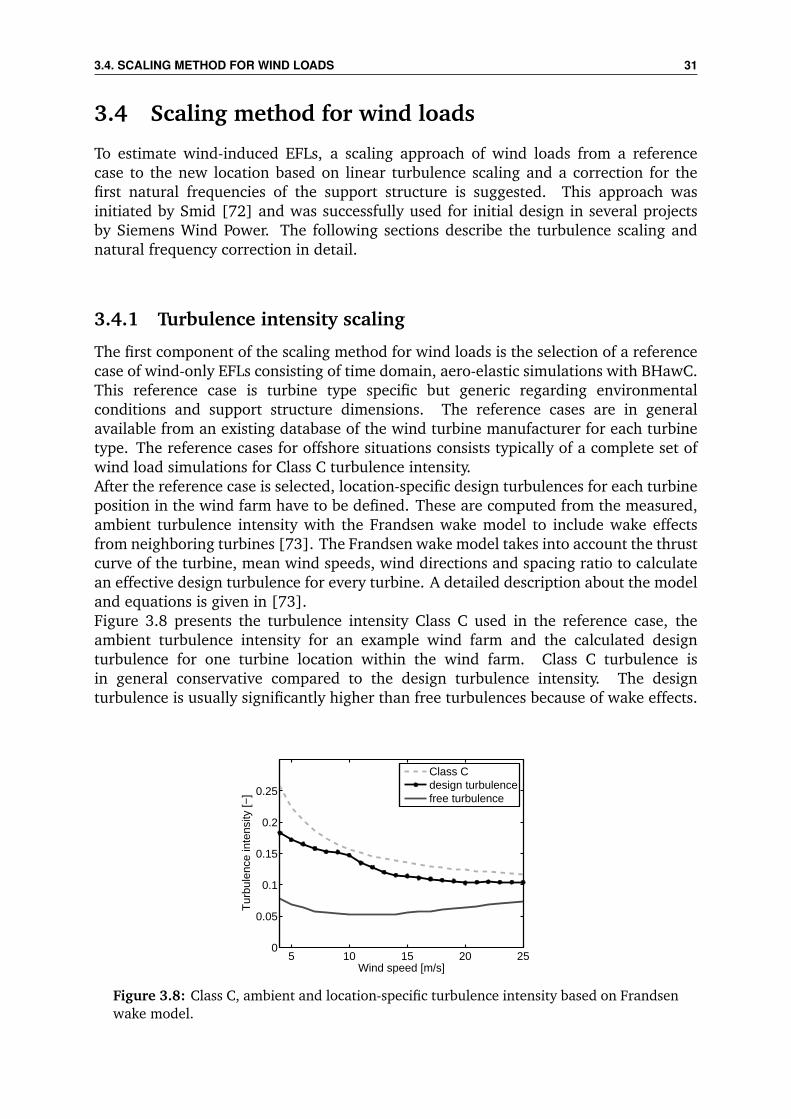
To estimate wind-induced EFLs, a scaling approach of wind loads from a referencecase to the new location based on linear turbulence scaling and a correction for thefirst natural frequencies of the support structure is suggested. This approach wasinitiated by Smid [72] and was successfully used for initial design in several projectsby Siemens Wind Power. The following sections describe the turbulence scaling andnatural frequency correction in detail.
3.4.1 Turbulence intensity scaling
The first component of the scaling method for wind loads is the selection of a referencecase of wind-only EFLs consisting of time domain, aero-elastic simulations with BHawC.This reference case is turbine type specific but generic regarding environmentalconditions and support structure dimensions. The reference cases are in generalavailable from an existing database of the wind turbine manufacturer for each turbinetype. The reference cases for offshore situations consists typically of a complete set ofwind load simulations for Class C turbulence intensity.After the reference case is selected, location-specific design turbulences for each turbineposition in the wind farm have to be defined. These are computed from the measured,ambient turbulence intensity with the Frandsen wake model to include wake effectsfrom neighboring turbines [73]. The Frandsen wake model takes into account the thrustcurve of the turbine, mean wind speeds, wind directions and spacing ratio to calculatean effective design turbulence for every turbine. A detailed description about the modeland equations is given in [73].Figure 3.8 presents the turbulence intensity Class C used in the reference case, theambient turbulence intensity for an example wind farm and the calculated designturbulence for one turbine location within the wind farm. Class C turbulence isin general conservative compared to the design turbulence intensity. The designturbulence is usually significantly higher than free turbulences because of wake effects.
5 10 15 20 250
0.05
0.1
0.15
0.2
0.25
Wind speed [m/s]
Tur
bule
nce
inte
nsity
[−]
Class Cdesign turbulencefree turbulence
Figure 3.8: Class C, ambient and location-specific turbulence intensity based on Frandsenwake model.

32 3. PROBABILISTIC FATIGUE LOAD ESTIMATION METHOD
Location-specific wind loads are then approximated applying linear scaling of theturbulence intensity as shown in Equation 3.31. It should be noted that this scalingmethod is an approximation assuming that the effect of turbulence intensity can betaken as linear factor out of the fatigue load calculation.Physically, the turbulence intensity goes squared in the Kaimal spectrum which is anoften used turbulence model for design load calculation (cf. Equation 3.32) [74]. Later,the square root of the Kaimal spectrum is taken for calculating local wind velocityfluctuations (cf. Equation 3.33-3.34). This makes wind-only EFLs approximately lineardependent on turbulence intensity. However, wind-only loads are also influencedby other effects, for example the controller behavior, which is not captured by theturbulence intensity scaling.
EFLls(VW ) ≈ EFLref (VW ) · TIls(VW )
TIref (VW )(3.31)
SK(f) =4 · TI2 · L · VW(1 + 6 · f ·L
VW)53
(3.32)
V (t) = VW +m∑p=1
bp · cos(ωp · t+ εp) (3.33)
b(f) =√
2 · Sk(f) ·∆f (3.34)
with
EFLls location-specific wind EFL [Nm]EFLref reference case wind EFL [Nm]TIls location-specific turbulence intensity [-]TIref reference case turbulence intensity [-]SK Kaimal spectrum [(m/s)2s]L integral length scale [m]VW mean wind speed [m/s]V wind speed [m/s]f frequency [Hz]m number of wind components [-]b wind amplitudes [m/s]t time [s]ω angular frequency [rad/s]ε random phase [rad]
3.4.2 Natural frequency correction
After the wind-only EFLs are calculated for location-specific turbulences, EFLs arecorrected for the location-specific first natural frequency of the support structure. Thelocation-specific first natural frequency is obtained from the finite element model of thesupport structure during the wave-load computation (cf. Section 3.3.2).The natural frequency correction was derived by analyzing results of aero-elastic time
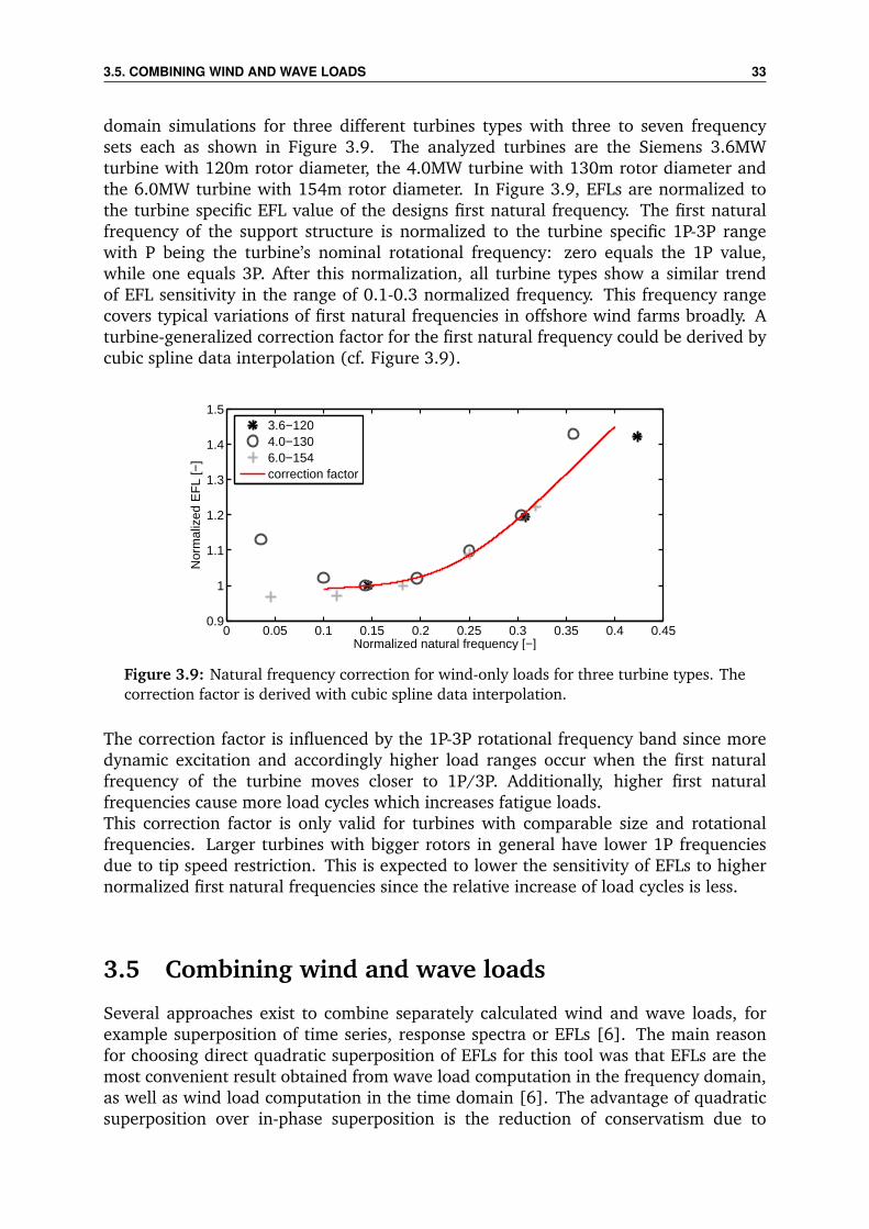
3.5. COMBINING WIND AND WAVE LOADS 33
domain simulations for three different turbines types with three to seven frequencysets each as shown in Figure 3.9. The analyzed turbines are the Siemens 3.6MWturbine with 120m rotor diameter, the 4.0MW turbine with 130m rotor diameter andthe 6.0MW turbine with 154m rotor diameter. In Figure 3.9, EFLs are normalized tothe turbine specific EFL value of the designs first natural frequency. The first naturalfrequency of the support structure is normalized to the turbine specific 1P-3P rangewith P being the turbine’s nominal rotational frequency: zero equals the 1P value,while one equals 3P. After this normalization, all turbine types show a similar trendof EFL sensitivity in the range of 0.1-0.3 normalized frequency. This frequency rangecovers typical variations of first natural frequencies in offshore wind farms broadly. Aturbine-generalized correction factor for the first natural frequency could be derived bycubic spline data interpolation (cf. Figure 3.9).
0 0.05 0.1 0.15 0.2 0.25 0.3 0.35 0.4 0.450.9
1
1.1
1.2
1.3
1.4
1.5
Normalized natural frequency [−]
Nor
mal
ized
EF
L [−
]
3.6−1204.0−1306.0−154correction factor
Figure 3.9: Natural frequency correction for wind-only loads for three turbine types. Thecorrection factor is derived with cubic spline data interpolation.
The correction factor is influenced by the 1P-3P rotational frequency band since moredynamic excitation and accordingly higher load ranges occur when the first naturalfrequency of the turbine moves closer to 1P/3P. Additionally, higher first naturalfrequencies cause more load cycles which increases fatigue loads.This correction factor is only valid for turbines with comparable size and rotationalfrequencies. Larger turbines with bigger rotors in general have lower 1P frequenciesdue to tip speed restriction. This is expected to lower the sensitivity of EFLs to highernormalized first natural frequencies since the relative increase of load cycles is less.
3.5 Combining wind and wave loads
Several approaches exist to combine separately calculated wind and wave loads, forexample superposition of time series, response spectra or EFLs [6]. The main reasonfor choosing direct quadratic superposition of EFLs for this tool was that EFLs are themost convenient result obtained from wave load computation in the frequency domain,as well as wind load computation in the time domain [6]. The advantage of quadraticsuperposition over in-phase superposition is the reduction of conservatism due to

34 3. PROBABILISTIC FATIGUE LOAD ESTIMATION METHOD
accounting for the random phase between wind and wave loads [6].Wind and wave EFLs are combined using direct quadratic superposition according toEquation 3.35 [6].
EFLtot ≈√EFL2
wind + EFL2wave (3.35)
with
EFLtot wind-wave combined EFL [Nm]EFLwind wind-induced EFL [Nm]EFLwave wave-induced EFL [Nm]
It must be emphasized that this approach is only an approximation with no theoreticalproof since it also neglects the interference term between wind and wave loads. Thevalidity of this approximation is confirmed for the problem setting of this thesis in theverification study (cf. Chapter 4).
3.6 Probabilistic load assessment
The computational efficiency of the proposed fatigue load estimation method allowsprobabilistic assessment through MCS. MCS repeat random sampling to discover thesolution space of a problem numerically [71].In the probabilistic load assessment, all uncertain input parameters are representedwith a probability distribution. In each MCS, random samples from all independentparameter distributions are drawn simultaneously. EFLs are then calculated basedon these data samples. The MCS are repeated a large number of times leading to anumerical set of EFLs. For this set of EFLs statistical properties like mean, standarddeviation, skewness and kurtosis are calculated. These statistical properties characterizewhat probability distribution EFLs have due to the specified input uncertainty. In detail,kurtosis describes how peaked the probability distribution is, while skewness indicatesthe symmetry.The accuracy of MC estimates depend on the number of simulations. The average MCerrors of mean and standard deviation scale roughly with Equation 3.36-3.37 [75].
emean ≈1√N
(3.36)
eSTD ≈STD√N
(3.37)
with
e average MC error [-]N number of MCS [-]STD output standard deviation [-]
The advantage of MCS is simplicity of use making it a powerful tool when analyticalsolutions are complex. On the other hand, many simulations are needed for a good MC
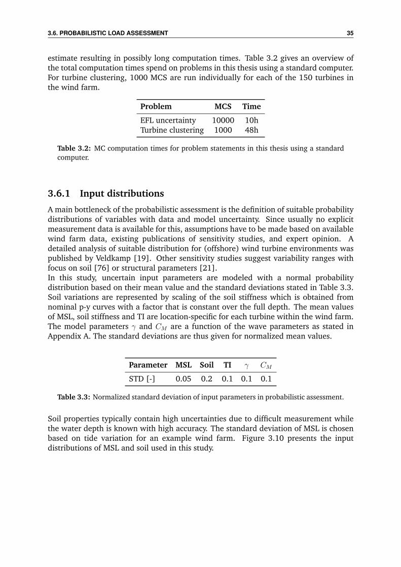
3.6. PROBABILISTIC LOAD ASSESSMENT 35
estimate resulting in possibly long computation times. Table 3.2 gives an overview ofthe total computation times spend on problems in this thesis using a standard computer.For turbine clustering, 1000 MCS are run individually for each of the 150 turbines inthe wind farm.
Problem MCS Time
EFL uncertainty 10000 10hTurbine clustering 1000 48h
Table 3.2: MC computation times for problem statements in this thesis using a standardcomputer.
3.6.1 Input distributions
A main bottleneck of the probabilistic assessment is the definition of suitable probabilitydistributions of variables with data and model uncertainty. Since usually no explicitmeasurement data is available for this, assumptions have to be made based on availablewind farm data, existing publications of sensitivity studies, and expert opinion. Adetailed analysis of suitable distribution for (offshore) wind turbine environments waspublished by Veldkamp [19]. Other sensitivity studies suggest variability ranges withfocus on soil [76] or structural parameters [21].In this study, uncertain input parameters are modeled with a normal probabilitydistribution based on their mean value and the standard deviations stated in Table 3.3.Soil variations are represented by scaling of the soil stiffness which is obtained fromnominal p-y curves with a factor that is constant over the full depth. The mean valuesof MSL, soil stiffness and TI are location-specific for each turbine within the wind farm.The model parameters γ and CM are a function of the wave parameters as stated inAppendix A. The standard deviations are thus given for normalized mean values.
Parameter MSL Soil TI γ CM
STD [-] 0.05 0.2 0.1 0.1 0.1
Table 3.3: Normalized standard deviation of input parameters in probabilistic assessment.
Soil properties typically contain high uncertainties due to difficult measurement whilethe water depth is known with high accuracy. The standard deviation of MSL is chosenbased on tide variation for an example wind farm. Figure 3.10 presents the inputdistributions of MSL and soil used in this study.
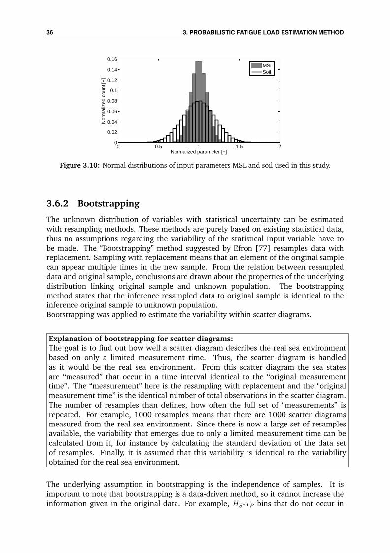
36 3. PROBABILISTIC FATIGUE LOAD ESTIMATION METHOD
0 0.5 1 1.5 20
0.02
0.04
0.06
0.08
0.1
0.12
0.14
0.16
Normalized parameter [−]
Nor
mal
ized
cou
nt [−
]
MSLSoil
Figure 3.10: Normal distributions of input parameters MSL and soil used in this study.
3.6.2 Bootstrapping
The unknown distribution of variables with statistical uncertainty can be estimatedwith resampling methods. These methods are purely based on existing statistical data,thus no assumptions regarding the variability of the statistical input variable have tobe made. The “Bootstrapping” method suggested by Efron [77] resamples data withreplacement. Sampling with replacement means that an element of the original samplecan appear multiple times in the new sample. From the relation between resampleddata and original sample, conclusions are drawn about the properties of the underlyingdistribution linking original sample and unknown population. The bootstrappingmethod states that the inference resampled data to original sample is identical to theinference original sample to unknown population.Bootstrapping was applied to estimate the variability within scatter diagrams.
Explanation of bootstrapping for scatter diagrams:The goal is to find out how well a scatter diagram describes the real sea environmentbased on only a limited measurement time. Thus, the scatter diagram is handledas it would be the real sea environment. From this scatter diagram the sea statesare “measured” that occur in a time interval identical to the “original measurementtime”. The “measurement” here is the resampling with replacement and the “originalmeasurement time” is the identical number of total observations in the scatter diagram.The number of resamples than defines, how often the full set of “measurements” isrepeated. For example, 1000 resamples means that there are 1000 scatter diagramsmeasured from the real sea environment. Since there is now a large set of resamplesavailable, the variability that emerges due to only a limited measurement time can becalculated from it, for instance by calculating the standard deviation of the data setof resamples. Finally, it is assumed that this variability is identical to the variabilityobtained for the real sea environment.
The underlying assumption in bootstrapping is the independence of samples. It isimportant to note that bootstrapping is a data-driven method, so it cannot increase theinformation given in the original data. For example, HS-TP bins that do not occur in

3.6. PROBABILISTIC LOAD ASSESSMENT 37
the original scatter diagram can never occur in one of the resampled scatter diagrams.Bootstrapping is implemented for scatter diagrams with the following procedure:
1. Calculate the cumulative sum of occurrence for all HS-TP bins in the originalscatter diagram.
2. Generate N uniformly distributed random numbers between 0 and 1, with Nbeing the number of observations within the original scatter diagram.
3. Select the HS-TP bin that just exceeds the drawn random number and assign thecount 1 to this bin.
4. Obtain the resampled scatter diagram by normalizing the occurrence of each HS-TP bin with the total number of observations. This gives each new scatter diagrama total probability of 100%.
This procedure is repeated a sufficient large number of times, which defines the numberof resamples. In this thesis 10000 resamples are used.

38
Chapter 4
Verification of developed fatigueestimation method
In this chapter, the developed fatigue estimation method is verified with aero-elastic simulations in the time domain. Verification is performed for wave-only,wind-only and wind-wave combined loads. After description of the referencecase, setup and post-processing of time domain simulations is outlined. Finally,verification results are presented followed by a discussion of the verificationstudy and detected limitations.
4.1 Reference case
The purpose of the verification study is to confirm that the developed fatigue estimationmethod is appropriate for study of site variations and probabilistic assessments asdefined in Chapter 3.1. Additionally, the verification study provides insight ondifferences in results between time and frequency domain calculations.In order to compare time and frequency domain methods as close as possible, a simpleset up of a reference case is used with a 4MW OWT in a water depth of approximately35m. The reference case consists of various simulations with
– an identical structural model in terms of structural dimensions, damping andmodal properties,
– several fatigue relevant sea states with various VW , HS, and TP values, and
– simplified wind and wave directionalities for each sea state, namely fully alignedand fully misaligned.
The structural dimensions of the monopile are presented in Figure 4.1. The axes arenormalized due to confidentiality. The diameter of the pile is decreased before MSL inorder to lower wave loads. At interface level the monopile is connected to the tower viaa transition piece.
39
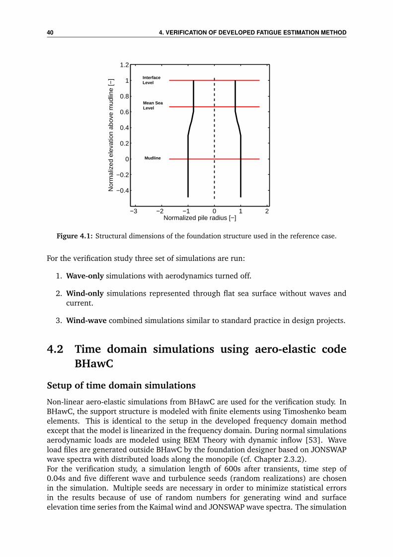
40 4. VERIFICATION OF DEVELOPED FATIGUE ESTIMATION METHOD
−3 −2 −1 0 1 2
−0.4
−0.2
0
0.2
0.4
0.6
0.8
1
1.2
Normalized pile radius [−]
Nor
mal
ized
ele
vatio
n ab
ove
mud
line
[−] Interface
Level
Mean SeaLevel
Mudline
Figure 4.1: Structural dimensions of the foundation structure used in the reference case.
For the verification study three set of simulations are run:
1. Wave-only simulations with aerodynamics turned off.
2. Wind-only simulations represented through flat sea surface without waves andcurrent.
3. Wind-wave combined simulations similar to standard practice in design projects.
4.2 Time domain simulations using aero-elastic codeBHawC
Setup of time domain simulations
Non-linear aero-elastic simulations from BHawC are used for the verification study. InBHawC, the support structure is modeled with finite elements using Timoshenko beamelements. This is identical to the setup in the developed frequency domain methodexcept that the model is linearized in the frequency domain. During normal simulationsaerodynamic loads are modeled using BEM Theory with dynamic inflow [53]. Waveload files are generated outside BHawC by the foundation designer based on JONSWAPwave spectra with distributed loads along the monopile (cf. Chapter 2.3.2).For the verification study, a simulation length of 600s after transients, time step of0.04s and five different wave and turbulence seeds (random realizations) are chosenin the simulation. Multiple seeds are necessary in order to minimize statistical errorsin the results because of use of random numbers for generating wind and surfaceelevation time series from the Kaimal wind and JONSWAP wave spectra. The simulation
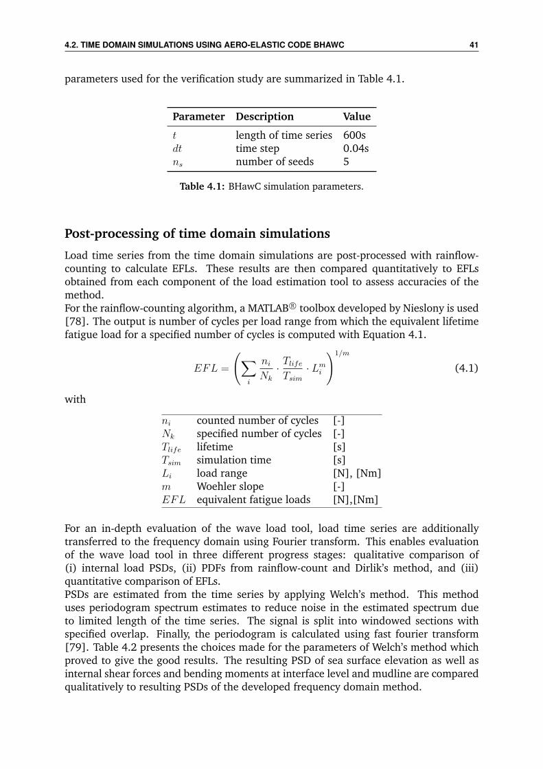
4.2. TIME DOMAIN SIMULATIONS USING AERO-ELASTIC CODE BHAWC 41
parameters used for the verification study are summarized in Table 4.1.
Parameter Description Value
t length of time series 600sdt time step 0.04sns number of seeds 5
Table 4.1: BHawC simulation parameters.
Post-processing of time domain simulations
Load time series from the time domain simulations are post-processed with rainflow-counting to calculate EFLs. These results are then compared quantitatively to EFLsobtained from each component of the load estimation tool to assess accuracies of themethod.For the rainflow-counting algorithm, a MATLAB R© toolbox developed by Nieslony is used[78]. The output is number of cycles per load range from which the equivalent lifetimefatigue load for a specified number of cycles is computed with Equation 4.1.
EFL =
(∑i
niNk
· TlifeTsim
· Lmi
)1/m
(4.1)
with
ni counted number of cycles [-]Nk specified number of cycles [-]Tlife lifetime [s]Tsim simulation time [s]Li load range [N], [Nm]m Woehler slope [-]EFL equivalent fatigue loads [N],[Nm]
For an in-depth evaluation of the wave load tool, load time series are additionallytransferred to the frequency domain using Fourier transform. This enables evaluationof the wave load tool in three different progress stages: qualitative comparison of(i) internal load PSDs, (ii) PDFs from rainflow-count and Dirlik’s method, and (iii)quantitative comparison of EFLs.PSDs are estimated from the time series by applying Welch’s method. This methoduses periodogram spectrum estimates to reduce noise in the estimated spectrum dueto limited length of the time series. The signal is split into windowed sections withspecified overlap. Finally, the periodogram is calculated using fast fourier transform[79]. Table 4.2 presents the choices made for the parameters of Welch’s method whichproved to give the good results. The resulting PSD of sea surface elevation as well asinternal shear forces and bending moments at interface level and mudline are comparedqualitatively to resulting PSDs of the developed frequency domain method.
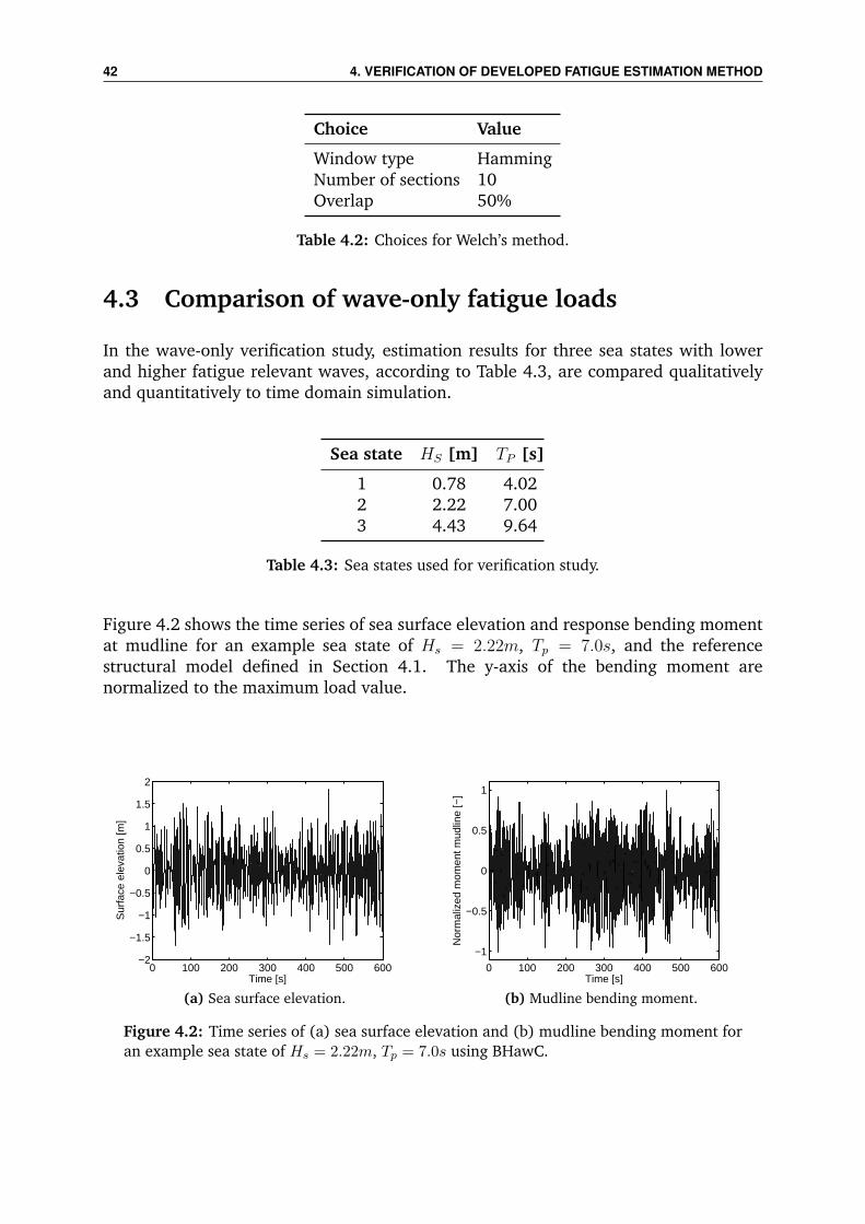
42 4. VERIFICATION OF DEVELOPED FATIGUE ESTIMATION METHOD
Choice Value
Window type HammingNumber of sections 10Overlap 50%
Table 4.2: Choices for Welch’s method.
4.3 Comparison of wave-only fatigue loads
In the wave-only verification study, estimation results for three sea states with lowerand higher fatigue relevant waves, according to Table 4.3, are compared qualitativelyand quantitatively to time domain simulation.
Sea state HS [m] TP [s]
1 0.78 4.022 2.22 7.003 4.43 9.64
Table 4.3: Sea states used for verification study.
Figure 4.2 shows the time series of sea surface elevation and response bending momentat mudline for an example sea state of Hs = 2.22m, Tp = 7.0s, and the referencestructural model defined in Section 4.1. The y-axis of the bending moment arenormalized to the maximum load value.
0 100 200 300 400 500 600−2
−1.5
−1
−0.5
0
0.5
1
1.5
2
Time [s]
Sur
face
ele
vatio
n [m
]
(a) Sea surface elevation.
0 100 200 300 400 500 600
−1
−0.5
0
0.5
1
Time [s]
Nor
mal
ized
mom
ent m
udlin
e [−
]
(b) Mudline bending moment.
Figure 4.2: Time series of (a) sea surface elevation and (b) mudline bending moment foran example sea state of Hs = 2.22m, Tp = 7.0s using BHawC.
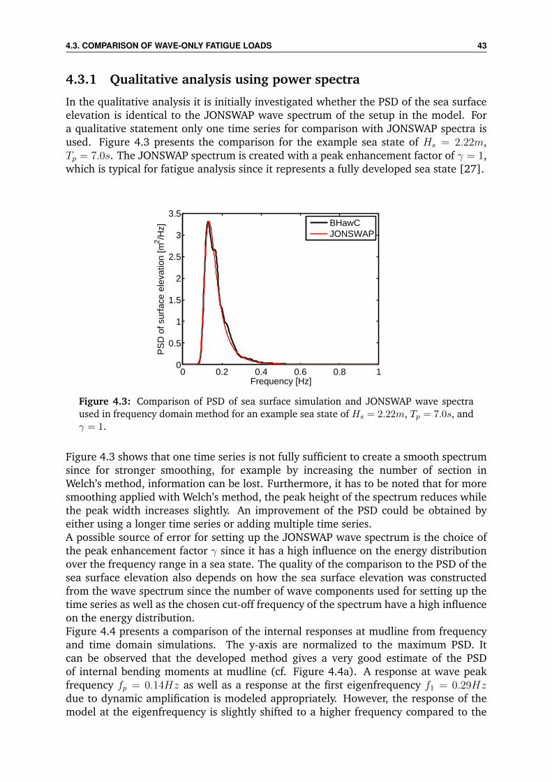
4.3. COMPARISON OF WAVE-ONLY FATIGUE LOADS 43
4.3.1 Qualitative analysis using power spectra
In the qualitative analysis it is initially investigated whether the PSD of the sea surfaceelevation is identical to the JONSWAP wave spectrum of the setup in the model. Fora qualitative statement only one time series for comparison with JONSWAP spectra isused. Figure 4.3 presents the comparison for the example sea state of Hs = 2.22m,Tp = 7.0s. The JONSWAP spectrum is created with a peak enhancement factor of γ = 1,which is typical for fatigue analysis since it represents a fully developed sea state [27].
0 0.2 0.4 0.6 0.8 10
0.5
1
1.5
2
2.5
3
3.5
Frequency [Hz]
PS
D o
f sur
face
ele
vatio
n [m
2 /Hz]
BHawCJONSWAP
Figure 4.3: Comparison of PSD of sea surface simulation and JONSWAP wave spectraused in frequency domain method for an example sea state of Hs = 2.22m, Tp = 7.0s, andγ = 1.
Figure 4.3 shows that one time series is not fully sufficient to create a smooth spectrumsince for stronger smoothing, for example by increasing the number of section inWelch’s method, information can be lost. Furthermore, it has to be noted that for moresmoothing applied with Welch’s method, the peak height of the spectrum reduces whilethe peak width increases slightly. An improvement of the PSD could be obtained byeither using a longer time series or adding multiple time series.A possible source of error for setting up the JONSWAP wave spectrum is the choice ofthe peak enhancement factor γ since it has a high influence on the energy distributionover the frequency range in a sea state. The quality of the comparison to the PSD of thesea surface elevation also depends on how the sea surface elevation was constructedfrom the wave spectrum since the number of wave components used for setting up thetime series as well as the chosen cut-off frequency of the spectrum have a high influenceon the energy distribution.Figure 4.4 presents a comparison of the internal responses at mudline from frequencyand time domain simulations. The y-axis are normalized to the maximum PSD. Itcan be observed that the developed method gives a very good estimate of the PSDof internal bending moments at mudline (cf. Figure 4.4a). A response at wave peakfrequency fp = 0.14Hz as well as a response at the first eigenfrequency f1 = 0.29Hzdue to dynamic amplification is modeled appropriately. However, the response of themodel at the eigenfrequency is slightly shifted to a higher frequency compared to the
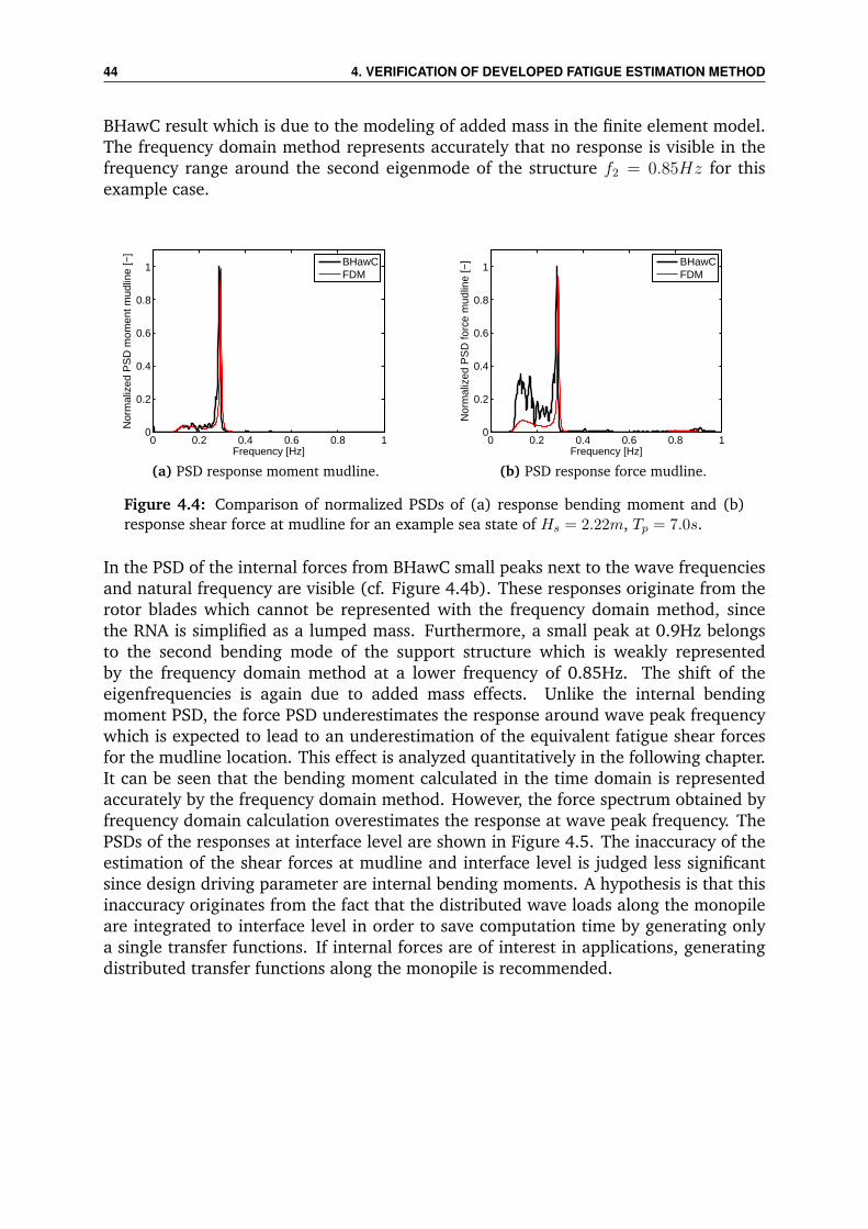
44 4. VERIFICATION OF DEVELOPED FATIGUE ESTIMATION METHOD
BHawC result which is due to the modeling of added mass in the finite element model.The frequency domain method represents accurately that no response is visible in thefrequency range around the second eigenmode of the structure f2 = 0.85Hz for thisexample case.
0 0.2 0.4 0.6 0.8 10
0.2
0.4
0.6
0.8
1
Frequency [Hz]
Nor
mal
ized
PS
D m
omen
t mud
line
[−]
BHawCFDM
(a) PSD response moment mudline.
0 0.2 0.4 0.6 0.8 10
0.2
0.4
0.6
0.8
1
Frequency [Hz]N
orm
aliz
ed P
SD
forc
e m
udlin
e [−
]
BHawCFDM
(b) PSD response force mudline.
Figure 4.4: Comparison of normalized PSDs of (a) response bending moment and (b)response shear force at mudline for an example sea state of Hs = 2.22m, Tp = 7.0s.
In the PSD of the internal forces from BHawC small peaks next to the wave frequenciesand natural frequency are visible (cf. Figure 4.4b). These responses originate from therotor blades which cannot be represented with the frequency domain method, sincethe RNA is simplified as a lumped mass. Furthermore, a small peak at 0.9Hz belongsto the second bending mode of the support structure which is weakly representedby the frequency domain method at a lower frequency of 0.85Hz. The shift of theeigenfrequencies is again due to added mass effects. Unlike the internal bendingmoment PSD, the force PSD underestimates the response around wave peak frequencywhich is expected to lead to an underestimation of the equivalent fatigue shear forcesfor the mudline location. This effect is analyzed quantitatively in the following chapter.It can be seen that the bending moment calculated in the time domain is representedaccurately by the frequency domain method. However, the force spectrum obtained byfrequency domain calculation overestimates the response at wave peak frequency. ThePSDs of the responses at interface level are shown in Figure 4.5. The inaccuracy of theestimation of the shear forces at mudline and interface level is judged less significantsince design driving parameter are internal bending moments. A hypothesis is that thisinaccuracy originates from the fact that the distributed wave loads along the monopileare integrated to interface level in order to save computation time by generating onlya single transfer functions. If internal forces are of interest in applications, generatingdistributed transfer functions along the monopile is recommended.
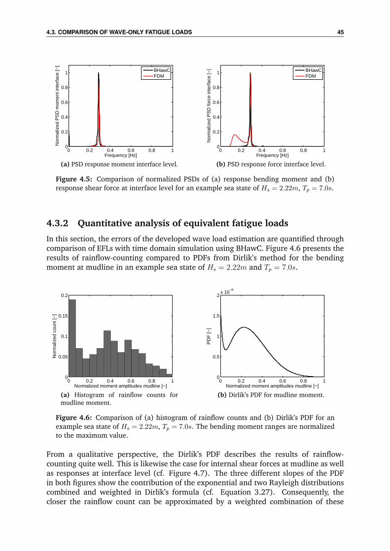
4.3. COMPARISON OF WAVE-ONLY FATIGUE LOADS 45
0 0.2 0.4 0.6 0.8 10
0.2
0.4
0.6
0.8
1
Frequency [Hz]
Nor
mal
ized
PS
D m
omen
t int
erfa
ce [−
]
BHawCFDM
(a) PSD response moment interface level.
0 0.2 0.4 0.6 0.8 10
0.2
0.4
0.6
0.8
1
Frequency [Hz]
Nor
mal
ized
PS
D fo
rce
inte
rfac
e [−
]
BHawCFDM
(b) PSD response force interface level.
Figure 4.5: Comparison of normalized PSDs of (a) response bending moment and (b)response shear force at interface level for an example sea state of Hs = 2.22m, Tp = 7.0s.
4.3.2 Quantitative analysis of equivalent fatigue loads
In this section, the errors of the developed wave load estimation are quantified throughcomparison of EFLs with time domain simulation using BHawC. Figure 4.6 presents theresults of rainflow-counting compared to PDFs from Dirlik’s method for the bendingmoment at mudline in an example sea state of Hs = 2.22m and Tp = 7.0s.
0 0.2 0.4 0.6 0.8 10
0.05
0.1
0.15
0.2
Normalized moment amplitudes mudline [−]
Nor
mal
ized
cou
nt [−
]
(a) Histogram of rainflow counts formudline moment.
0 0.2 0.4 0.6 0.8 10
0.5
1
1.5
2x 10
−8
Normalized moment amplitudes mudline [−]
PD
F [−
]
(b) Dirlik’s PDF for mudline moment.
Figure 4.6: Comparison of (a) histogram of rainflow counts and (b) Dirlik’s PDF for anexample sea state of Hs = 2.22m, Tp = 7.0s. The bending moment ranges are normalizedto the maximum value.
From a qualitative perspective, the Dirlik’s PDF describes the results of rainflow-counting quite well. This is likewise the case for internal shear forces at mudline as wellas responses at interface level (cf. Figure 4.7). The three different slopes of the PDFin both figures show the contribution of the exponential and two Rayleigh distributionscombined and weighted in Dirlik’s formula (cf. Equation 3.27). Consequently, thecloser the rainflow count can be approximated by a weighted combination of these
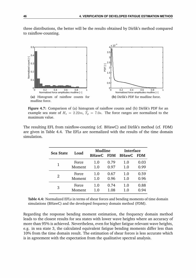
46 4. VERIFICATION OF DEVELOPED FATIGUE ESTIMATION METHOD
three distributions, the better will be the results obtained by Dirlik’s method comparedto rainflow-counting.
0 0.2 0.4 0.6 0.8 10
0.1
0.2
0.3
0.4
0.5
Normalized force amplitudes mudline [−]
Nor
mal
ized
cou
nt [−
]
(a) Histogram of rainflow counts formudline force.
0 0.2 0.4 0.6 0.8 10
0.5
1
1.5
2
2.5
3
3.5
4x 10
−6
Normalized force amplitudes mudline [−]
PD
F [−
]
(b) Dirlik’s PDF for mudline force.
Figure 4.7: Comparison of (a) histogram of rainflow counts and (b) Dirlik’s PDF for anexample sea state of Hs = 2.22m, Tp = 7.0s. The force ranges are normalized to themaximum value.
The resulting EFL from rainflow-counting (cf. BHawC) and Dirlik’s method (cf. FDM)are given in Table 4.4. The EFLs are normalized with the results of the time domainsimulation.
Sea State LoadMudline Interface
BHawC FDM BHawC FDM
1Force 1.0 0.79 1.0 0.03
Moment 1.0 0.97 1.0 0.99
2Force 1.0 0.67 1.0 0.59
Moment 1.0 0.96 1.0 0.96
3Force 1.0 0.74 1.0 0.88
Moment 1.0 1.08 1.0 0.94
Table 4.4: Normalized EFLs in terms of shear forces and bending moments of time domainsimulations (BHawC) and the developed frequency domain method (FDM).
Regarding the response bending moment estimation, the frequency domain methodleads to the closest results for sea states with lower wave heights where an accuracy ofmore than 95% is achieved. Nevertheless, even for higher fatigue relevant wave heights,e.g. in sea state 3, the calculated equivalent fatigue bending moments differ less than10% from the time domain result. The estimation of shear forces is less accurate whichis in agreement with the expectation from the qualitative spectral analysis.
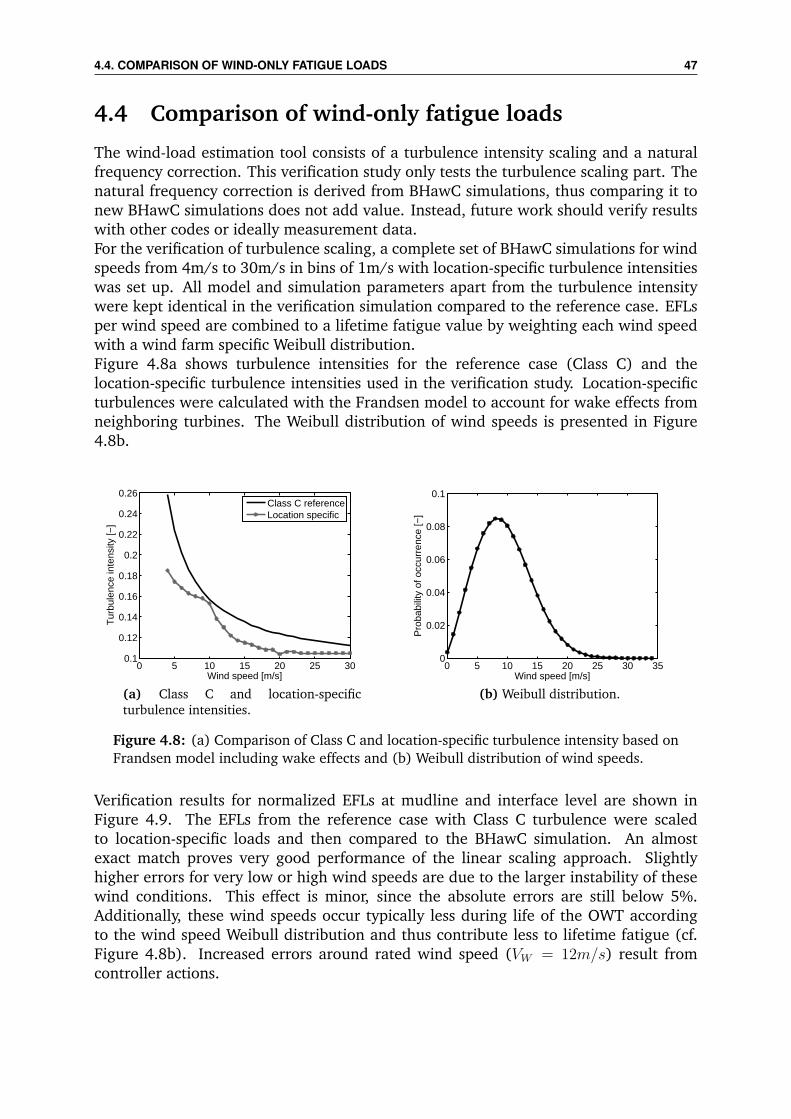
4.4. COMPARISON OF WIND-ONLY FATIGUE LOADS 47
4.4 Comparison of wind-only fatigue loads
The wind-load estimation tool consists of a turbulence intensity scaling and a naturalfrequency correction. This verification study only tests the turbulence scaling part. Thenatural frequency correction is derived from BHawC simulations, thus comparing it tonew BHawC simulations does not add value. Instead, future work should verify resultswith other codes or ideally measurement data.For the verification of turbulence scaling, a complete set of BHawC simulations for windspeeds from 4m/s to 30m/s in bins of 1m/s with location-specific turbulence intensitieswas set up. All model and simulation parameters apart from the turbulence intensitywere kept identical in the verification simulation compared to the reference case. EFLsper wind speed are combined to a lifetime fatigue value by weighting each wind speedwith a wind farm specific Weibull distribution.Figure 4.8a shows turbulence intensities for the reference case (Class C) and thelocation-specific turbulence intensities used in the verification study. Location-specificturbulences were calculated with the Frandsen model to account for wake effects fromneighboring turbines. The Weibull distribution of wind speeds is presented in Figure4.8b.
0 5 10 15 20 25 300.1
0.12
0.14
0.16
0.18
0.2
0.22
0.24
0.26
Wind speed [m/s]
Tur
bule
nce
inte
nsity
[−]
Class C referenceLocation specific
(a) Class C and location-specificturbulence intensities.
0 5 10 15 20 25 30 350
0.02
0.04
0.06
0.08
0.1
Wind speed [m/s]
Pro
babi
lity
of o
ccur
renc
e [−
]
(b) Weibull distribution.
Figure 4.8: (a) Comparison of Class C and location-specific turbulence intensity based onFrandsen model including wake effects and (b) Weibull distribution of wind speeds.
Verification results for normalized EFLs at mudline and interface level are shown inFigure 4.9. The EFLs from the reference case with Class C turbulence were scaledto location-specific loads and then compared to the BHawC simulation. An almostexact match proves very good performance of the linear scaling approach. Slightlyhigher errors for very low or high wind speeds are due to the larger instability of thesewind conditions. This effect is minor, since the absolute errors are still below 5%.Additionally, these wind speeds occur typically less during life of the OWT accordingto the wind speed Weibull distribution and thus contribute less to lifetime fatigue (cf.Figure 4.8b). Increased errors around rated wind speed (VW = 12m/s) result fromcontroller actions.
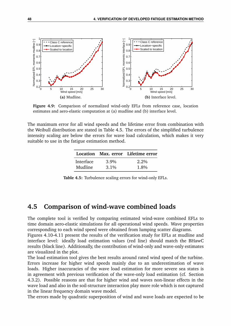
48 4. VERIFICATION OF DEVELOPED FATIGUE ESTIMATION METHOD
0 5 10 15 20 25 300.2
0.3
0.4
0.5
0.6
0.7
0.8
0.9
1
Wind speed [m/s]
Nor
mal
ized
EF
L m
omen
ts m
udlin
e [−
]
Class C referenceLocation−specificScaled to location
(a) Mudline.
0 5 10 15 20 25 300.2
0.3
0.4
0.5
0.6
0.7
0.8
0.9
1
Wind speed [m/s]
Nor
mal
ized
EF
L m
omen
ts in
terf
ace
[−]
Class C referenceLocation−specificScaled to location
(b) Interface level.
Figure 4.9: Comparison of normalized wind-only EFLs from reference case, locationestimates and aero-elastic computation at (a) mudline and (b) interface level.
The maximum error for all wind speeds and the lifetime error from combination withthe Weibull distribution are stated in Table 4.5. The errors of the simplified turbulenceintensity scaling are below the errors for wave load calculation, which makes it verysuitable to use in the fatigue estimation method.
Location Max. error Lifetime error
Interface 3.9% 2.2%Mudline 3.1% 1.8%
Table 4.5: Turbulence scaling errors for wind-only EFLs.
4.5 Comparison of wind-wave combined loads
The complete tool is verified by comparing estimated wind-wave combined EFLs totime domain aero-elastic simulations for all operational wind speeds. Wave propertiescorresponding to each wind speed were obtained from lumping scatter diagrams.Figures 4.10-4.11 present the results of the verification study for EFLs at mudline andinterface level: ideally load estimation values (red line) should match the BHawCresults (black line). Additionally, the contribution of wind-only and wave-only estimatesare visualized in the plot.The load estimation tool gives the best results around rated wind speed of the turbine.Errors increase for higher wind speeds mainly due to an underestimation of waveloads. Higher inaccuracies of the wave load estimation for more severe sea states isin agreement with previous verification of the wave-only load estimation (cf. Section4.3.2). Possible reasons are that for higher wind and waves non-linear effects in thewave load and also in the soil-structure interaction play more role which is not capturedin the linear frequency domain wave model.The errors made by quadratic superposition of wind and wave loads are expected to be
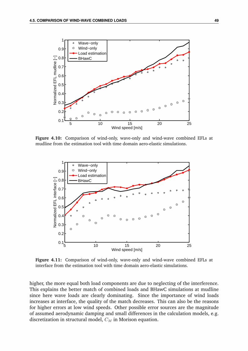
4.5. COMPARISON OF WIND-WAVE COMBINED LOADS 49
5 10 15 20 250.1
0.2
0.3
0.4
0.5
0.6
0.7
0.8
0.9
1
Wind speed [m/s]
Nor
mal
ized
EF
L m
udlin
e [−
]
Wave−onlyWind−onlyLoad estimationBHawC
Figure 4.10: Comparison of wind-only, wave-only and wind-wave combined EFLs atmudline from the estimation tool with time domain aero-elastic simulations.
5 10 15 20 250.1
0.2
0.3
0.4
0.5
0.6
0.7
0.8
0.9
1
Wind speed [m/s]
Nor
mal
ized
EF
L in
terf
ace
[−]
Wave−onlyWind−onlyLoad estimationBHawC
Figure 4.11: Comparison of wind-only, wave-only and wind-wave combined EFLs atinterface from the estimation tool with time domain aero-elastic simulations.
higher, the more equal both load components are due to neglecting of the interference.This explains the better match of combined loads and BHawC simulations at mudlinesince here wave loads are clearly dominating. Since the importance of wind loadsincreases at interface, the quality of the match decreases. This can also be the reasonsfor higher errors at low wind speeds. Other possible error sources are the magnitudeof assumed aerodynamic damping and small differences in the calculation models, e.g.discretization in structural model, CM in Morison equation.

50 4. VERIFICATION OF DEVELOPED FATIGUE ESTIMATION METHOD
Table 4.6 states the maximum error of all wind speeds and the lifetime error fromcombination with the Weibull distribution (cf. Figure 4.8b). Maximum errors areunconservative due to underestimation of EFLs at high wind speeds. For weightedlifetime EFLs a total load estimation accuracy of 94% for interface and 95% for mudlinebending moments (conservative error, EFLs are overestimated) is achieved.
Location Max. error Lifetime error
Interface 15.3% 6.0%Mudline 13.6% 4.9%
Table 4.6: Errors of load estimation tool for wind-wave combined EFLs.
4.6 Discussion of verification study
From all three parts of the verification study (wave-only, wind-only, wind-wavecombined), it appears that the fatigue load estimation method delivers results closeto time domain simulations for internal bending moments at mudline and seabed. Asa result, it is concluded that the developed method is appropriate to be used for sitesensitivity assessments and uncertainty studies.
Limitations detected from verification study:
A major limitation of the developed method is that no consistent statement aboutconservatism is possible as required by industry. The total fatigue estimation methodhas a maximum conservative lifetime error of 6% (EFLs are overestimated). However,the tool underpredicts loads especially for low and high wind speeds. Thus, forapplication of the tool in industry projects contingency should be added.Errors in the combined loads are introduced from wave-only loads, wind-only loads andload combination. Errors in the wave-only EFLs are larger for higher waves. Scalingof wind-only EFLs leads in general to unconservative results for turbulence factors <1.This is less critical since wind loads are of minor importance compared wave loads fordeeper water sites and the scaling error is quite small. Combining wind and wave loadsis expected to lead to higher errors when both load components are of comparable size.Further limitations are the insufficient estimation of shear forces by the wave tool.Force estimation can be improved if distributed wave loads along the monopileare transferred to internal loads directly instead of integration to equivalent forces.Nevertheless, the inaccuracy of the force estimation is judged less severe since designdriving are internal bending moments. For this reason, the verification work of wind-only and wind-wave combined loads as well as the following sensitivity and uncertaintystudies only consider bending moments (cf. Chapter 5 and appended papers).

4.6. DISCUSSION OF VERIFICATION STUDY 51
Adequacy of verification study:
The verification study enables statements about the accuracy of the load estimationmethod compared to time domain simulations for a full set of load cases. A limitationhereby is that time domain simulations themselves contain potential errors anduncertainties. The aero-elastic simulation software used, BHawC, is so far only validatedwith measurements for onshore, but not for offshore conditions.The verification study can be improved by eliminating remaining minor differences incalculation models, especially regarding choices of CM and γ. Additionally, it is limitedto one specific site, turbine and support structure. The following list indicates whichimportant aspects have not been covered by the verification study:
– site conditions e.g. MSL or soil conditions,
– structural parameters e.g. eigenfrequency, geometry, mode shapes, elasticproperties,
– turbine types,
– simplification of wind-wave directionality,
– lumping of sea states,
– wind-only: natural frequency correction and independence of turbulence andfrequency scaling,
– accuracy of time domain simulation software, and
– accuracy of applied aerodynamic damping.

52
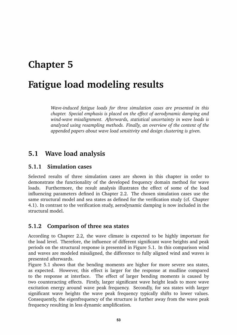
Chapter 5
Fatigue load modeling results
Wave-induced fatigue loads for three simulation cases are presented in thischapter. Special emphasis is placed on the effect of aerodynamic damping andwind-wave misalignment. Afterwards, statistical uncertainty in wave loads isanalyzed using resampling methods. Finally, an overview of the content of theappended papers about wave load sensitivity and design clustering is given.
5.1 Wave load analysis
5.1.1 Simulation cases
Selected results of three simulation cases are shown in this chapter in order todemonstrate the functionality of the developed frequency domain method for waveloads. Furthermore, the result analysis illustrates the effect of some of the loadinfluencing parameters defined in Chapter 2.2. The chosen simulation cases use thesame structural model and sea states as defined for the verification study (cf. Chapter4.1). In contrast to the verification study, aerodynamic damping is now included in thestructural model.
5.1.2 Comparison of three sea states
According to Chapter 2.2, the wave climate is expected to be highly important forthe load level. Therefore, the influence of different significant wave heights and peakperiods on the structural response is presented in Figure 5.1. In this comparison windand waves are modeled misaligned, the difference to fully aligned wind and waves ispresented afterwards.Figure 5.1 shows that the bending moments are higher for more severe sea states,as expected. However, this effect is larger for the response at mudline comparedto the response at interface. The effect of larger bending moments is caused bytwo counteracting effects. Firstly, larger significant wave height leads to more waveexcitation energy around wave peak frequency. Secondly, for sea states with largersignificant wave heights the wave peak frequency typically shifts to lower values.Consequently, the eigenfrequency of the structure is further away from the wave peakfrequency resulting in less dynamic amplification.
53
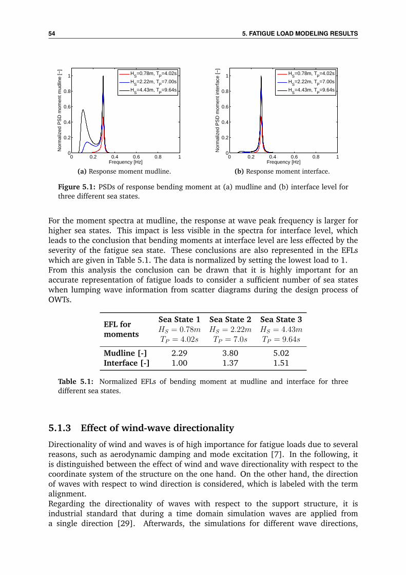
54 5. FATIGUE LOAD MODELING RESULTS
0 0.2 0.4 0.6 0.8 10
0.2
0.4
0.6
0.8
1
Frequency [Hz]
Nor
mal
ized
PS
D m
omen
t mud
line
[−]
HS=0.78m, T
P=4.02s
HS=2.22m, T
P=7.00s
HS=4.43m, T
P=9.64s
(a) Response moment mudline.
0 0.2 0.4 0.6 0.8 10
0.2
0.4
0.6
0.8
1
Frequency [Hz]
Nor
mal
ized
PS
D m
omen
t int
erfa
ce [−
]
HS=0.78m, T
P=4.02s
HS=2.22m, T
P=7.00s
HS=4.43m, T
P=9.64s
(b) Response moment interface.
Figure 5.1: PSDs of response bending moment at (a) mudline and (b) interface level forthree different sea states.
For the moment spectra at mudline, the response at wave peak frequency is larger forhigher sea states. This impact is less visible in the spectra for interface level, whichleads to the conclusion that bending moments at interface level are less effected by theseverity of the fatigue sea state. These conclusions are also represented in the EFLswhich are given in Table 5.1. The data is normalized by setting the lowest load to 1.From this analysis the conclusion can be drawn that it is highly important for anaccurate representation of fatigue loads to consider a sufficient number of sea stateswhen lumping wave information from scatter diagrams during the design process ofOWTs.
EFL formoments
Sea State 1HS = 0.78mTP = 4.02s
Sea State 2HS = 2.22mTP = 7.0s
Sea State 3HS = 4.43mTP = 9.64s
Mudline [-] 2.29 3.80 5.02Interface [-] 1.00 1.37 1.51
Table 5.1: Normalized EFLs of bending moment at mudline and interface for threedifferent sea states.
5.1.3 Effect of wind-wave directionality
Directionality of wind and waves is of high importance for fatigue loads due to severalreasons, such as aerodynamic damping and mode excitation [7]. In the following, itis distinguished between the effect of wind and wave directionality with respect to thecoordinate system of the structure on the one hand. On the other hand, the directionof waves with respect to wind direction is considered, which is labeled with the termalignment.Regarding the directionality of waves with respect to the support structure, it isindustrial standard that during a time domain simulation waves are applied froma single direction [29]. Afterwards, the simulations for different wave directions,
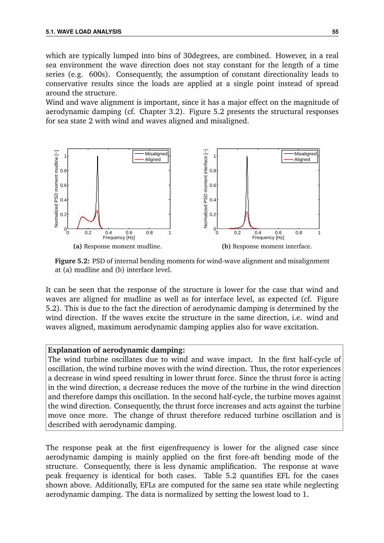
5.1. WAVE LOAD ANALYSIS 55
which are typically lumped into bins of 30degrees, are combined. However, in a realsea environment the wave direction does not stay constant for the length of a timeseries (e.g. 600s). Consequently, the assumption of constant directionality leads toconservative results since the loads are applied at a single point instead of spreadaround the structure.Wind and wave alignment is important, since it has a major effect on the magnitude ofaerodynamic damping (cf. Chapter 3.2). Figure 5.2 presents the structural responsesfor sea state 2 with wind and waves aligned and misaligned.
0 0.2 0.4 0.6 0.8 10
0.2
0.4
0.6
0.8
1
Frequency [Hz]
Nor
mal
ized
PS
D m
omen
t mud
line
[−]
MisalignedAligned
(a) Response moment mudline.
0 0.2 0.4 0.6 0.8 10
0.2
0.4
0.6
0.8
1
Frequency [Hz]
Nor
mal
ized
PS
D m
omen
t int
erfa
ce [−
]
MisalignedAligned
(b) Response moment interface.
Figure 5.2: PSD of internal bending moments for wind-wave alignment and misalignmentat (a) mudline and (b) interface level.
It can be seen that the response of the structure is lower for the case that wind andwaves are aligned for mudline as well as for interface level, as expected (cf. Figure5.2). This is due to the fact the direction of aerodynamic damping is determined by thewind direction. If the waves excite the structure in the same direction, i.e. wind andwaves aligned, maximum aerodynamic damping applies also for wave excitation.
Explanation of aerodynamic damping:The wind turbine oscillates due to wind and wave impact. In the first half-cycle ofoscillation, the wind turbine moves with the wind direction. Thus, the rotor experiencesa decrease in wind speed resulting in lower thrust force. Since the thrust force is actingin the wind direction, a decrease reduces the move of the turbine in the wind directionand therefore damps this oscillation. In the second half-cycle, the turbine moves againstthe wind direction. Consequently, the thrust force increases and acts against the turbinemove once more. The change of thrust therefore reduced turbine oscillation and isdescribed with aerodynamic damping.
The response peak at the first eigenfrequency is lower for the aligned case sinceaerodynamic damping is mainly applied on the first fore-aft bending mode of thestructure. Consequently, there is less dynamic amplification. The response at wavepeak frequency is identical for both cases. Table 5.2 quantifies EFL for the casesshown above. Additionally, EFLs are computed for the same sea state while neglectingaerodynamic damping. The data is normalized by setting the lowest load to 1.
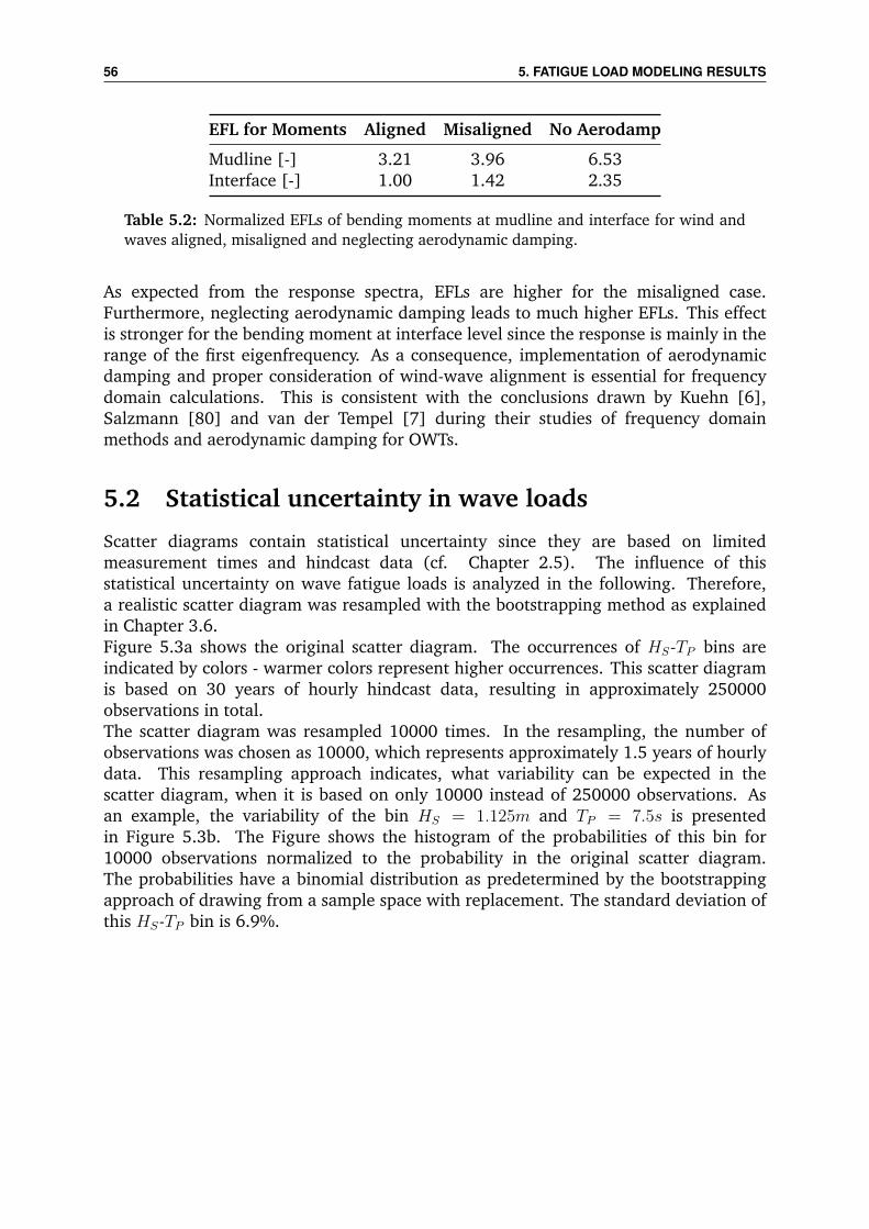
56 5. FATIGUE LOAD MODELING RESULTS
EFL for Moments Aligned Misaligned No Aerodamp
Mudline [-] 3.21 3.96 6.53Interface [-] 1.00 1.42 2.35
Table 5.2: Normalized EFLs of bending moments at mudline and interface for wind andwaves aligned, misaligned and neglecting aerodynamic damping.
As expected from the response spectra, EFLs are higher for the misaligned case.Furthermore, neglecting aerodynamic damping leads to much higher EFLs. This effectis stronger for the bending moment at interface level since the response is mainly in therange of the first eigenfrequency. As a consequence, implementation of aerodynamicdamping and proper consideration of wind-wave alignment is essential for frequencydomain calculations. This is consistent with the conclusions drawn by Kuehn [6],Salzmann [80] and van der Tempel [7] during their studies of frequency domainmethods and aerodynamic damping for OWTs.
5.2 Statistical uncertainty in wave loads
Scatter diagrams contain statistical uncertainty since they are based on limitedmeasurement times and hindcast data (cf. Chapter 2.5). The influence of thisstatistical uncertainty on wave fatigue loads is analyzed in the following. Therefore,a realistic scatter diagram was resampled with the bootstrapping method as explainedin Chapter 3.6.Figure 5.3a shows the original scatter diagram. The occurrences of HS-TP bins areindicated by colors - warmer colors represent higher occurrences. This scatter diagramis based on 30 years of hourly hindcast data, resulting in approximately 250000observations in total.The scatter diagram was resampled 10000 times. In the resampling, the number ofobservations was chosen as 10000, which represents approximately 1.5 years of hourlydata. This resampling approach indicates, what variability can be expected in thescatter diagram, when it is based on only 10000 instead of 250000 observations. Asan example, the variability of the bin HS = 1.125m and TP = 7.5s is presentedin Figure 5.3b. The Figure shows the histogram of the probabilities of this bin for10000 observations normalized to the probability in the original scatter diagram.The probabilities have a binomial distribution as predetermined by the bootstrappingapproach of drawing from a sample space with replacement. The standard deviation ofthis HS-TP bin is 6.9%.
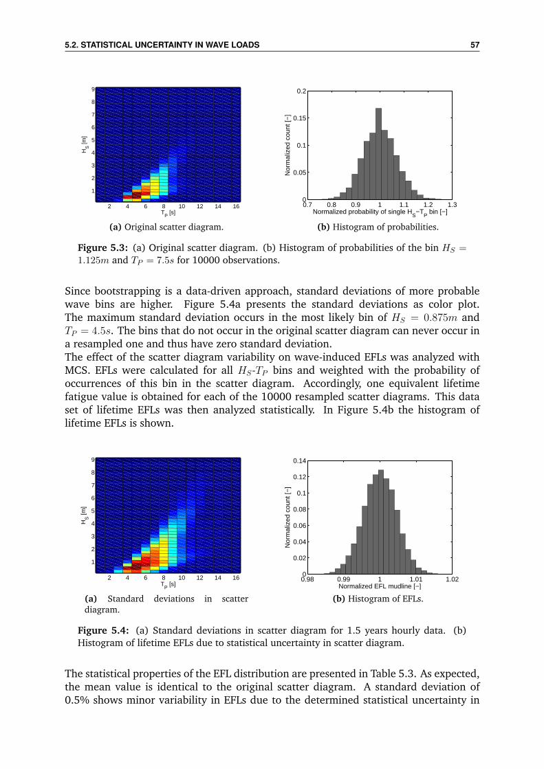
5.2. STATISTICAL UNCERTAINTY IN WAVE LOADS 57
2 4 6 8 10 12 14 16
1
2
3
4
5
6
7
8
9
TP [s]
HS [m
]
(a) Original scatter diagram.
0.7 0.8 0.9 1 1.1 1.2 1.30
0.05
0.1
0.15
0.2
Normalized probability of single HS−T
P bin [−]
Nor
mal
ized
cou
nt [−
]
(b) Histogram of probabilities.
Figure 5.3: (a) Original scatter diagram. (b) Histogram of probabilities of the bin HS =1.125m and TP = 7.5s for 10000 observations.
Since bootstrapping is a data-driven approach, standard deviations of more probablewave bins are higher. Figure 5.4a presents the standard deviations as color plot.The maximum standard deviation occurs in the most likely bin of HS = 0.875m andTP = 4.5s. The bins that do not occur in the original scatter diagram can never occur ina resampled one and thus have zero standard deviation.The effect of the scatter diagram variability on wave-induced EFLs was analyzed withMCS. EFLs were calculated for all HS-TP bins and weighted with the probability ofoccurrences of this bin in the scatter diagram. Accordingly, one equivalent lifetimefatigue value is obtained for each of the 10000 resampled scatter diagrams. This dataset of lifetime EFLs was then analyzed statistically. In Figure 5.4b the histogram oflifetime EFLs is shown.
2 4 6 8 10 12 14 16
1
2
3
4
5
6
7
8
9
TP [s]
HS [m
]
(a) Standard deviations in scatterdiagram.
0.98 0.99 1 1.01 1.020
0.02
0.04
0.06
0.08
0.1
0.12
0.14
Normalized EFL mudline [−]
Nor
mal
ized
cou
nt [−
]
(b) Histogram of EFLs.
Figure 5.4: (a) Standard deviations in scatter diagram for 1.5 years hourly data. (b)Histogram of lifetime EFLs due to statistical uncertainty in scatter diagram.
The statistical properties of the EFL distribution are presented in Table 5.3. As expected,the mean value is identical to the original scatter diagram. A standard deviation of0.5% shows minor variability in EFLs due to the determined statistical uncertainty in

58 5. FATIGUE LOAD MODELING RESULTS
scatter diagrams. A sensitivity study of wave fatigue loads to wave parameters hasshown that the wave period TP has a significant influence on loads (cf. appended paperB). Nevertheless, significant variabilities within the scatter diagram lead to only a minorvariability in wave loads. The reason is the high number of bins in the scatter diagram(629 bins in total), which makes the difference of wave parameters to neighboringbins small (∆HS = 0.25m, ∆TP = 1s). Thus, the effect of higher occurrences of singleHS-TP bins is compensated by neighboring bins with respect to the lifetime EFLs.
Mean STD Skewness Kurtosis
1.0 0.005 -0.033 2.982
Table 5.3: Statistical properties of EFLs due to scatter diagram variability.
5.3 Sensitivity of wave fatigue loads (Paper A)
The paper describes a sensitivity study of wave fatigue loads to changes in governingparameters such as water depth, soil stiffness, wave height, and wave period. Aprobabilistic assessment is performed with MCS.Results show a significant influence of water depth and wave period on EFLs. Normaldistributed input parameters in a probabilistic assessment yield a positively skewedprobability distribution of EFLs.This paper demonstrates that the developed probabilistic frequency domain method forwave fatigue loads is suitable for systematic studies on the influence of a variety ofparameters on EFLs. Hence the paper is of highest relevance for a systematic concept ofdesign optimization of offshore support structures and thus for the reduction of offshorewind energy costs.
5.4 Optimization of design clustering (Paper B)
The aim of this paper is to apply the probabilistic fatigue estimation method fordesign clustering in large offshore wind farms. Design clustering was formulated asan optimization problem by calculating site-specific EFLs for every turbine location inthe wind farm. Brute-force and discrete optimization algorithm are used to solve theoptimization problem. Additionally, the paper illustrates, how uncertainties in loadcalculation can alter allocation of turbines to clusters.A study of an example wind farm of 150 turbines in 30-40m water depth shows amaximum EFL difference of 25% within the wind farm. Clustering gave a reductionof up to 13% of total design loads compared to standardized design, with the highestimprovements through the first 6 clusters.This paper suggests a novel approach to design clustering that improves nowadaysindustry practices. It demonstrates how design clustering can contribute to offshorewind energy cost reduction and is thus of highest relevance.Further explanation on the discrete optimization algorithm is given in Appendix C.
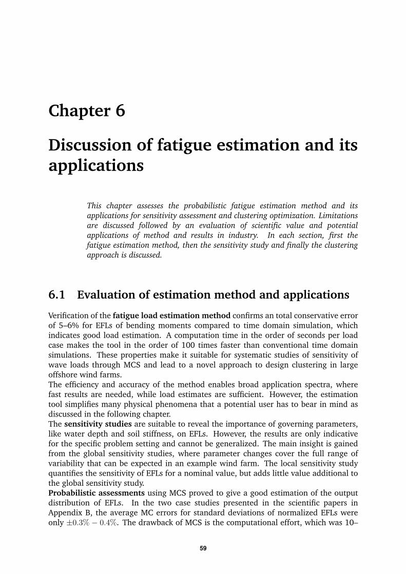
Chapter 6
Discussion of fatigue estimation and itsapplications
This chapter assesses the probabilistic fatigue estimation method and itsapplications for sensitivity assessment and clustering optimization. Limitationsare discussed followed by an evaluation of scientific value and potentialapplications of method and results in industry. In each section, first thefatigue estimation method, then the sensitivity study and finally the clusteringapproach is discussed.
6.1 Evaluation of estimation method and applications
Verification of the fatigue load estimation method confirms an total conservative errorof 5–6% for EFLs of bending moments compared to time domain simulation, whichindicates good load estimation. A computation time in the order of seconds per loadcase makes the tool in the order of 100 times faster than conventional time domainsimulations. These properties make it suitable for systematic studies of sensitivity ofwave loads through MCS and lead to a novel approach to design clustering in largeoffshore wind farms.The efficiency and accuracy of the method enables broad application spectra, wherefast results are needed, while load estimates are sufficient. However, the estimationtool simplifies many physical phenomena that a potential user has to bear in mind asdiscussed in the following chapter.The sensitivity studies are suitable to reveal the importance of governing parameters,like water depth and soil stiffness, on EFLs. However, the results are only indicativefor the specific problem setting and cannot be generalized. The main insight is gainedfrom the global sensitivity studies, where parameter changes cover the full range ofvariability that can be expected in an example wind farm. The local sensitivity studyquantifies the sensitivity of EFLs for a nominal value, but adds little value additional tothe global sensitivity study.Probabilistic assessments using MCS proved to give a good estimation of the outputdistribution of EFLs. In the two case studies presented in the scientific papers inAppendix B, the average MC errors for standard deviations of normalized EFLs wereonly ±0.3% − 0.4%. The drawback of MCS is the computational effort, which was 10–
59

60 6. DISCUSSION OF FATIGUE ESTIMATION AND ITS APPLICATIONS
48h computation time for the presented case studies.For design clustering, the needs of industry are fast and robust tools, while nowadayslarger wind farms typically have only 2–3 clusters. Brute-force optimization guaranteesglobal optima at the expense of solution time, making it the best choice for upto 5 clusters for wind farms with 100–150 turbines. For more clusters, the localsearch algorithm showed very good performance for solution quality and computationalefficiency in the order of seconds.In the probabilistic clustering example shown in Appendix B, only few turbines changecluster since the distribution of STDs follows that of EFLs relatively closely. Thus STDsare only of importance near cluster-borders. It can be concluded that deterministicclustering has good stability for uniform sites.
6.2 Limitations
In order to be computational efficient and simple to use, the fatigue load estimationtool simplifies many physical contexts. Assumptions have been discussed inChapter 3.2. Here, the focus is on critical simplifications concerning industry applicationand trends in offshore wind. The main aspects are stated in the following:
• The frequency domain model cannot depict non-linearity of waves and soil p-y-curves. This might be a reason that the combined tool underestimates loadsfor high wind speeds. Being conservative however, is indispensable in industryprojects, thus contingency should be added in project applications.
• Diffraction is implemented simplified through the McCamy-Fuchs diffractioncorrection. Industry is moving to bigger turbines supported by XL-monopiles, thuswave diffraction becomes more important. This might reduce the accuracy of theestimation tool, since Morison equation and linear wave theory are less applicable.
• Wind-wave directionality is simplified into fully aligned and fully misaligned.Additionally, wind and waves are applied from a constant direction with respect tothe support structure coordinate system during one simulation. This will lead toconservative results as it is standard in today’s offshore wind industry. Due to itsefficiency, the fatigue estimation tool offers an ideal starting point to investigatethis conservatism in further studies.
• Equivalent loads at MSL and single transfer functions are used instead ofdistribution along the structure leading to a poor quality estimate of shear forcesat mudline and interface level. This is unacceptable in industry projects and thetool should be adjusted to generate distributed transfer functions along the wave-action zone.
• Interaction between wind and wave loads is only accounted for with aerodynamicdamping. All other effects are not modeled. This is of minor relevance whenone load component is dominating. However, it might become a bottleneck forestimation accuracy for sites with equal magnitude of wind and wave loads.
• Clearly, this study provides an estimation tool for loads on OWT monopiles, whichcannot be applied to other support structures one-to-one. Alternative support

6.2. LIMITATIONS 61
structures for deeper water sites, especially jackets and floating structures, comeinto focus of research and industry. Nevertheless, there are still many projectsnowadays with monopiles of the size considered in this study.
The limitations of the verification study were presented in detail in Chapter 4.6.Most important is here that the verification was conducted with BHawC which isonly validated for onshore wind problems. In general, aero-hydro-servo-elastic toolsdo not reflect real loads exactly like measurement campaigns and code comparisonsshowed [81, 82]. For example, in a recent publication measured first tower bendingfrequencies are compared with design frequencies for 400 OWTs [82]. Results show thatdesigns underpredict the natural frequencies in general, with a maximum difference of20%. However, in the current design of the West of Duddon Sands Offshore Wind Farma match of ±2% for the first natural frequency has been achieved using an automateddesign process and a tuned, site-specific pilesoil response formulation [82].Since the wave load file for this verification study are provided externally, minordifferences in parameter choices cannot be ruled out. A discussion with M. Seidel,who recently studied frequency domain methods for wave loads on monopiles aswell [12], led to the conclusion that the true accuracy of the frequency domain methodis expected to be even higher when eliminating remaining differences of models andcalculation parameters in the verification study (personal communication, February 27,2015).Regarding applications in future projects, it is critical that the verification study islimited to only one specific site and geometry. Thus, there is no verification of theaccuracy of the method for different structural and environmental settings.
The key limitation of the sensitivity study and probabilistic assessment is that resultsstrongly depend on chosen input distributions and thus cannot be be generalized. Forexample, soil stiffness had in paper A only minor influence on EFLs due to high soilstiffness. For the study presented in paper B however, the influence of soil increasedsignificantly for turbine locations with lower soil stiffness. Further limitations are:
• Input distributions were chosen based on publications and expert opinion, butthey are not verified with data. The calculated distributions of EFLs have to beexamined with reference to input choices and thus cannot be treated as validated.
• Only selected sources of uncertainties are considered which does not nearly coverall uncertainties in the load calculation. Some of the not covered uncertaintiesmight have even higher influence on loads. This can be for example modeluncertainties regarding directionality or diffraction correction.
• All parameters are assumed to be independent in the analyses which isquestionable, e.g. for HS and TP .
• The validity of initial design across all parameter variations was only checked forthe first natural frequency constraint and not for stresses and structural resistance.
• The study examines only load uncertainty and does not investigate uncertaintyin structural resistances. Uncertainty in structural resistance can even be moresignificant for structural reliability than load uncertainty and needs to be addedfor use in reliability-based design.

62 6. DISCUSSION OF FATIGUE ESTIMATION AND ITS APPLICATIONS
The sensitivity studies and probabilistic assessments focus mainly on wave loads.The implemented wind load scaling method is comparatively unappealing for use insensitivity study with MCS since (i) factor influence can be derived directly from thescaling approach and (ii) wind loads contribute less in combined fatigue loads for thechosen example wind farm so that uncertainty influence is barely visible in total EFLs.Accordingly, the results of the sensitivity studies presented in this thesis are mainlyuseful for deeper water sites, where wave loads are dominating.
A detailed description of the limitation for design clustering is given in paper Bin Appendix B. The primary limitation for application in practice is the formulation ofthe optimization problem regarding “design loads” and not costs. Furthermore, possibleconstraints like maximum variation of MSL or load interpolation within clusters are notconsidered.
6.3 Industry application
The suggested fatigue load estimation approach has an efficiency that makes it veryappealing for industry application. The essential question is: Is the method accurateenough for use in practice?This question cannot be answered in this thesis, since it depends on application purposesand intentions of the user. The summary of limitations critical for application, as statedpreviously, should enable users to take their decisions fact-based. Assuming that theaccuracy is sufficient for purpose, possible applications are:
1. clustering of turbines and design position optimization,
2. sensitivity and uncertainty analysis of load calculations,
3. interpolation of wave fatigue loads between design positions,
4. wind farm layout optimization, and
5. use in actual design process instead of time domain methods e.g. in preliminarydesign phase.
The first and second item were demonstrated in this thesis. Interpolation of fatigueloads between design position can either be based on the results of the sensitivity study,or on fatigue load estimates directly. Regarding item 4, wind farm layout is typicallyoptimized for power output through wake modeling and cable costs [83]. Having thisfast load estimation tool, support structure loads and costs can add a new dimensionto layout optimization. The use of the method for preliminary design is of highestinterest for industry. Additionally, the tool can help for proper lumping of sea states inpreliminary design due to its efficiency. For detailed design and certification however,more elaborate tools are recommended.
Results from the sensitivity study can be applied to determine which parametersshould be known with good accuracy already in an initial project phase. For thisexample case, MSL was confirmed to be one of the most influential site input parameter.Soil stiffness became an important parameter for poor quality soils. It was emphasized

6.4. SCIENTIFIC VALUE 63
before that the results of the sensitivity study cannot be generalized, however in everysituation the first eigenfrequency of the structure showed high influence. If no detailedstudies for a project exist, the first eigenfrequency is recommended as initial indicatorfor sensitivity.
The main message from the probabilistic assessment for industry is that uncertaintiesin input parameters can lead to a shifted mean value of EFLs compared to deterministicanalysis. The distribution of EFLs depend highly on the range of input uncertainties,thus applying a general safety factor is not target-aiming for design optimization.A possible application of the probabilistic assessment approach is to perform theanalysis for the highest loaded position of the wind farm, which is assumed to give aconservative variability for all other locations. This result combined with uncertainty instructural resistance can serve as suggestion for optimized safety factors for the specificwind farm and thus reduce design conservatism.
The design clustering tool is designed for immediate application in industry. It shouldbe used in early project phases to improve decision-making on the optimal numberof clusters and cluster configuration of a wind farm. Probabilistic clustering showedlittle effect on allocation of turbines to clusters and therefore is not recommendedfor daily engineering practice. It can be useful, however, for application with specificclustering problems, where only limited experience is available (e.g. large variations insite-specific uncertainties).
6.4 Scientific value
Frequency domain methods for wave load calculations have been applied to OWTs byseveral researchers before (cf. Chaper 2.3.4). Also the wind load scaling approachand the combination of wind and wave loads is based on existing knowledge andpublications (cf. Chapter 3).The main novelty of this work is the implementation of these tools for use inprobabilistic assessments with MCS, sensitivity studies, and for design clustering inlarge offshore wind farms. Additionally, the definition and solution of design clusteringof OWTs as a mathematical problem in discrete optimization is a novel approach.
Generalization of work:For the offshore wind community, it is of particular interest to know how the resultsof this study can be generalized. The suggested fatigue estimation tool is madefor monopile-based OWT and cannot be used directly for other support structures.However, the applied methodology and the idea, how to approach the problem of sitevariations, is very suitable for generalization to other foundation types. Publishedwork exists that evaluates frequency domain analysis for other support structures, forexample on semi-submersibles [45].Once the estimation tool is extended, the sensitivity and probabilistic assessmentscan be performed with an identical methodology using MCS. The clustering approachis applicable directly for other support structure types. With load estimates availablefor all turbine locations, the suggested formulation of the optimization problem andsolution algorithms can be applied generalized.

64

Chapter 7
Conclusions and recommendations
As cost reduction remains the most important challenge of offshore wind energy,conservatism of support structure designs has to be reduced. An important approachis the integration of variations of environmental site condition in the design process oflarge offshore wind farms, since they proved to have significant influence on supportstructure loading. In early design phases, OWTs are typically grouped into clusters, inwhich the support structure design is only performed once. A better understanding ofload site variations and uncertainty in load calculations is needed to improve designclustering, and thus reduce design conservatism. As a result, the central researchquestion of this thesis is (cf. Chapter 1):
How can probabilistic fatigue load estimation improve turbine clusteringin large offshore wind farms to reduce costs of offshore wind energy?
In this thesis, a developed probabilistic fatigue load estimation method has proven tobe suitable for site-specific EFL estimation. The method consists of four core elements:
1. frequency domain analysis to calculate wave loads,
2. turbulence and natural frequency scaling for wind loads,
3. combination of wind and wave loads with quadratic superposition, and
4. MCS to assess uncertainties.
A verified accuracy of 95% for lifetime EFLs of bending moments at mudline comparedto time domain simulations with only seconds of computation time for one simulationcase makes the estimation tool ideal for application in clustering optimization, loadinterpolation, uncertainty studies and preliminary design.With the estimation tool, design clustering can now be formulated as an discreteoptimization problem by calculating site-specific (probabilistic) EFLs for every turbinelocation in wind farms. A realistic case study with 150 OWTs in 30-40m water depthdemonstrated the value of clustering optimization as it gave a reduction of up to13% of total design loads compared to standardized design. Thus, a valuable designclustering approach was developed for use in offshore wind industry. It can, therefore,be concluded that the central research question of this master thesis has been answered.In the following, conclusions for the corresponding three research objectives are drawn.
65

66 7. CONCLUSIONS AND RECOMMENDATIONS
Results of the sensitivity study show a significant influence of water depth and waveperiod on EFLs. The influence of soil stiffness on EFLs is minor for soils with highstiffness, but can increase significant for soils with low stiffness.The computational efficiency of the fatigue estimation method allowed to assessuncertainties with MCS. Normal distributed input parameters in a probabilisticassessment yield a positively skewed probability distribution of EFLs. The variabilityof loads over a wind farm was shown to be quite similar with a maximum absolutedifference of 4.5% for standard deviations. Turbines with higher EFLs featured highervariability. This is consistent with higher order sensitivity trends for larger MSL andlower soil stiffness.For the exemplary wind farm, it was demonstrated that brute-force and discreteoptimization algorithms are well suited to solve the formulated clustering optimizationproblem. Probabilistic clustering, which accounts for load variability by increasing themean load level with 3*STD, proved to be only relevant at cluster borders leading to adifference in allocation for 12 out of 150 turbines.
To conclude, this project shows that it is essential to account for load differences inlarge offshore wind farms due to varying site conditions. Probabilistic load variabilitywas shown to be highly dependent on input uncertainties. This questions the usefulnessof generic safety factors in deterministic load calculations for design optimization.Design clustering proved to be an important approach for optimization of supportstructures and thus for cost reduction of offshore wind energy. As a key result, thesuggested clustering approach is highly recommended for application in industry.
Recommendations:
For academics and industry, this work contributes to better understanding of loadsensitivity to varying and uncertain site conditions, leading to enhanced turbineclustering. Further work is needed to improve the suggested fatigue estimation methodand its verification and to extend sensitivity studies and design clustering. Therefore,five major recommendations are defined for future development:
1. Improvement of estimation methodIn order to increase estimation accuracy, the method should be extended to usedistributed transfer functions in wave load calculations. Additionally, a detailedstudy of applicable aerodynamic damping values is recommended. The influenceof support structure appurtenances on loads, for instance boat landing, should beinvestigated and accounted for in the estimation process. Since the estimationmethod proved to be valuable for a broad range of applications, further studies todevelop load estimation tools for alternative support structures, e.g. jackets andfloating foundations, are recommended.
2. Extension of verification studyFurther work is needed to extend the verification study to different structural,environmental and turbines settings. More precisely, focus of the studies should beto confirm the accuracy of the estimation method for (i) different eigenfrequenciesof the support structure to validate results of sensitivity studies presented inthe appended papers, (ii) shallow water depth where wind-loads have moreinfluence, and (iii) larger turbines with bigger monopiles due to diffraction

67
effects. Additionally, the tool should be validated with other codes or ideally withexperimental data in the future.
3. Including uncertainty of structural resistanceThe probabilistic assessment only accounts for load uncertainty, howeveruncertainty in structural resistance is also highly important for structuralreliability. Thus an extension of the probabilistic approach to include uncertaintyin resistance is recommended. Clustering can then be based on structuralreliability instead of (probabilistic) design loads only.
4. Clustering for cost optimizationClustering optimization minimizes design loads which are assumed to beindicative for mass and costs of the support structure. Since this relation isnot linear, further research is required to formulate the optimization problemregarding support structure costs. Finally, a study revealing the economic value ofclustering optimization for cost of wind energy based on data from existing windfarm projects is desirable.
5. Generalization of workFor generalization of the load estimation tool to alternative support structures,the methodology suggested in this thesis can provide a good developmentbasis. Previous studies have shown that frequency domain analysis is suitableto calculate wave loads on various foundation types (cf. Chapter 6.4). Newstudies are needed to confirm the functionality of the wind load scaling approachfor other support structures. It is expected to perform well for jackets due tosmall wave-induced support structure movements, however not be suitable forfloating platforms. Finally, the relevance of site conditions and clustering fordesign optimization should be evaluated for alternative support structures.

68

Bibliography
[1] M. Bilgili, A. Yasar, and E. Simsek, “Offshore wind power development in europeand its comparison with onshore counterpart,” Renewable and Sustainable EnergyReviews, vol. 15, no. 2, pp. 905–915, 2011.
[2] DNV GL Group, “Offshore wind: A manifesto for cost reduction,” 2014. Retrievedfrom www.dnvgl.com on 12/12/2014.
[3] G. Corbetta, I. Pineda, J. Moccia, and J. Guillet, “The european offshore windindustry - key trends and statistics 2013,” tech. rep., European Wind EnergyAssociation, 2014.
[4] M. Seidel, “Integrated design approach for the material optimisation of steelmonopiles,” Presentation at 4th Annual Future Offshore Foundations Forum,Hamburg, Germany, 2014.
[5] F. Vorpahl, H. Schwarze, T. Fischer, M. Seidel, and J. Jonkman, “Offshorewind turbine environment, loads, simulation, and design,” Wiley InterdisciplinaryReviews: Energy and Environment, vol. 2, no. 5, pp. 548–570, 2013.
[6] M. J. Kuhn, Dynamics and design optimisation of offshore wind energy conversionsystems. PhD thesis, TU Delft, The Netherlands, 2001.
[7] J. van der Tempel, Design of support structures for offshore wind turbines. PhDthesis, TU Delft, The Netherlands, 2006.
[8] L. Ziegler, S. Voormeeren, S. Schafhirt, and M. Muskulus, “Sensitivity of wavefatigue loads on offshore wind turbines under varying site conditions,” EnergyProcedia, in press.
[9] L. Arany, S. Bhattacharya, J. Macdonald, and S. J. Hogan, “Simplified criticalmudline bending moment spectra of offshore wind turbine support structures,”Wind Energy, 2014. (doi:10.1002/we.1812).
[10] M. Muskulus, “Simplified rotor load models and fatigue damage estimates foroffshore wind turbines,” Philosophical Transactions of the Royal Society of LondonA: Mathematical, Physical and Engineering Sciences, vol. 373, no. 2035, 2015.
[11] D. Zwick and M. Muskulus, “Simplified fatigue load assessment in offshore windturbine structural analysis,” Wind Energy, 2015. (doi: 10.1002/we.1831).
[12] M. Seidel, “Wave induced fatigue loads,” Stahlbau, vol. 83, no. 8, pp. 535–541,2014.
69

70 BIBLIOGRAPHY
[13] B. Yeter, Y. Garbatov, and C. G. Soares, “Spectral fatigue assessment of an offshorewind turbine structure under wave and wind loading,” Developments in MaritimeTransportation and Exploitation of Sea Resources, vol. 1, pp. 425–433, 2013.
[14] P. Ragan and L. Manuel, “Comparing estimates of wind turbine fatigue loads usingtime-domain and spectral methods,” Wind engineering, vol. 31, no. 2, pp. 83–99,2007.
[15] M. Mrsnik, J. Slavic, and M. Boltezar, “Frequency-domain methods for a vibration-fatigue-life estimation–application to real data,” International journal of fatigue,vol. 47, pp. 8–17, 2013.
[16] L. Manuel, P. S. Veers, and S. R. Winterstein, “Parametric models for estimatingwind turbine fatigue loads for design,” Journal of solar energy engineering,vol. 123, no. 4, pp. 346–355, 2001.
[17] D. Zwick and M. Muskulus, “The simulation error caused by input loadingvariability in offshore wind turbine structural analysis,” Wind Energy, 2014. (doi:10.1002/we.1767).
[18] B. Yeter, Y. Garbatov, and C. Guedes Soares, “Fatigue reliability assessment of anoffshore supporting structure,” The Maritime Technology and Engineering, vol. 1,pp. 671–680, 2015.
[19] H. F. Veldkamp, Chances in wind energy: a probalistic approach to wind turbinefatigue design. PhD thesis, TU Delft, The Netherlands, 2006.
[20] M. Zaaijer, “Foundation modelling to assess dynamic behaviour of offshore windturbines,” Applied Ocean Research, vol. 28, no. 1, pp. 45–57, 2006.
[21] W. De Vries, N. K. Vemula, P. Passon, T. Fischer, D. Kaufer, D. Matha, et al.,“Final report WP 4.2: Support structure concepts for deep water sites,” tech. rep.,Upwind, 2011.
[22] M. Seidel, “Wave induced fatigue loads on monopiles - new approaches forlumping of scatter tables and site specific interpolation of fatigue loads,”Conference Proceedings IWEC, Hannover, Germany, 2014.
[23] J. Twidell and G. Gaudiosi, Offshore wind power. Multi-Science PublishingCompany, 2009.
[24] M. O. Hansen, Aerodynamics of wind turbines. Earthscan, 2nd ed., 2000.
[25] O. Faltinsen, Sea loads on ships and offshore structures. Cambridge University Press,1990.
[26] International Electrotechnical Commission, “IEC 61400-3: Design requirementsfor offshore wind turbines,” 2009.
[27] Det Norske Veritas, “DNV-OS-J101: Design of offshore wind turbine structures,”2014.

BIBLIOGRAPHY 71
[28] F. Savenije and J. Peeringa, “Integral wind turbine design and analysis in thefrequency domain,” Conference Proceedings EWEA Offshore, Stockholm, Sweden,2009.
[29] R. Haghi, “Loads and load cases,” Lecture Notes OE5655-Offshore Wind SupportStructures, TU Delft, The Netherlands, 2014.
[30] T. Camp, M. Morris, R. Van Rooij, J. Van Der Tempel, M. Zaaijer, A. Henderson,et al., “Design methods for offshore wind turbines at exposed sites,” tech. rep.,OWTES Project, 2003.
[31] A. Henderson, M. Zaaijer, and T. Camp, “Hydrodynamic loading on offshore windturbines,” Conference Proceedings ISOPE, Toulon, France.
[32] E. Smid, “Offshore load calculations - load calculation process for sales projects,”Presentation at Siemens Wind Power, Den Haag, The Netherlands, 2014.
[33] R. Haghi, T. Ashuri, P. L. van der Valk, and D. P. Molenaar, “Integratedmultidisciplinary constrained optimization of offshore support structures,”vol. 555, no. 1, 2014.
[34] T. Fischer, W. de Vries, P. Rainey, B. Schmidt, K. Argyriadis, and M. Kuehn,“Offshore support structure optimization by means of integrated design andcontrols,” Wind Energy, vol. 15, no. 1, pp. 99–117, 2012.
[35] D. Kaufer, N. Cosack, C. Boker, M. Seidel, and M. Kuhn, “Integrated analysis of thedynamics of offshore wind turbines with arbitrary support structures,” ConferenceProceedings EWEC, Marseille, France, 2009.
[36] T. Ashuri, Beyond classical upscaling: integrated aeroservoelastic design andoptimization of large offshore wind turbines. PhD thesis, TU Delft, The Netherlands,2012.
[37] P. S. Veers, “All wind farm uncertainty is not the same: the economics of commonversus independent causes,” Conference Proceedings AWEA Windpower’95,Washington, USA, 1995.
[38] P. S. Veers, “Fatigue reliability of wind turbine fleets: The effect of uncertainty onprojected costs,” Journal of solar energy engineering, vol. 118, no. 4, pp. 222–227,1996.
[39] J. D. Sørensen and H. S. Toft, “Probabilistic design of wind turbines,” Energies,vol. 3, no. 2, pp. 241–257, 2010.
[40] M. Hansen, L. Lohaus, T. Schlurmann, M. Achmus, P. Schaumann, R. Rolfes, et al.,“Probabilistic safety assessment of offshore wind turbines: Annual report 2010,”tech. rep., PSA, 2013.
[41] W. Dong, T. Moan, and Z. Gao, “Long-term fatigue analysis of multi-planartubular joints for jacket-type offshore wind turbine in time domain,” EngineeringStructures, vol. 33, no. 6, pp. 2002–2014, 2011.

72 BIBLIOGRAPHY
[42] W. Dong, T. Moan, and Z. Gao, “Fatigue reliability analysis of the jacket supportstructure for offshore wind turbine considering the effect of corrosion andinspection,” Reliability Engineering & System Safety, vol. 106, pp. 11–27, 2012.
[43] B. Ernst, H. Schmitt, and J. R. Seume, “Effect of geometric uncertainties on theaerodynamic characteristic of offshore wind turbine blades,” Journal of Physics:Conference Series, vol. 555, no. 1, 2014.
[44] J. D. Sorensen and N. J. Tarp-Johansen, “Reliability-based optimization andoptimal reliability level of offshore wind turbines,” International Journal ofOffshore and Polar Engineering, vol. 15, no. 2, pp. 141–146, 2005.
[45] M. I. Kvittem, Modelling and response analysis for fatigue design of a semi-submersible wind turbine. PhD thesis, NTNU, Norway, 2014.
[46] Det Norske Veritas, “DNVRP-C103: Column-stabilised units,” 2010.
[47] T. Burton, D. Sharpe, N. Jenkins, and E. Bossanyi, Wind energy handbook. JohnWiley & Sons, 2001.
[48] N. D. Barltrop and A. J. Adams, Dynamics of fixed marine structures. Butterworth-Heinemann, 3rd ed., 1991.
[49] S. K. Chakrabarti, Hydrodynamics of offshore structures. WIT press, 1987.
[50] J. Morison, J. Johnson, S. Schaaf, et al., “The force exerted by surface waves onpiles,” Journal of Petroleum Technology, vol. 2, no. 5, pp. 149–154, 1950.
[51] Det Norske Veritas, “DNV-RP-C205: Environmental conditions and environmentalloads,” 2007.
[52] R. C. MacCamy and R. A. Fuchs, “Wave forces on piles: a diffraction theory,” tech.rep., Beach Erosion Board, 1954.
[53] P. F. Skjoldan, Aeroelastic modal dynamics of wind turbines including anisotropiceffects. PhD thesis, DTU, Denmark, 2011.
[54] S. Hirdaris, W. Bai, D. Dessi, A. Ergin, X. Gu, O. Hermundstad, et al., “Loads foruse in the design of ships and offshore structures,” Ocean Engineering, vol. 78,pp. 131–174, 2014.
[55] C. G. Soares, “Effect of spectral shape uncertainty in the short term wave-inducedship responses,” Applied Ocean Research, vol. 12, no. 2, pp. 54–69, 1990.
[56] E. Smid, “Load differences within offshore wind farms,” tech. rep., Siemens WindPower, 2014.
[57] T. Dirlik, Application of computers in fatigue analysis. PhD thesis, University ofWarwick, England, 1985.
[58] American Petroleum Institute, “RP 2A-WSD: Recommended practice for planning,designing and constructing fixed offshore platforms-working stress design,” 2005.
BIBLIOGRAPHY 73
[59] P. Passon and M. Kuhn, “State-of-the-art and development needs of simulationcodes for offshore wind turbines,” Conference Proceedings IEA Expert Meeting,Copenhagen, Denmark, 2005.
[60] L. E. Borgman, “The spectral density for ocean wave forces,” ConferenceProceedings Speciality Conference, Santa Barbara, USA, 1965.
[61] J. Wheeler et al., “Method for calculating forces produced by irregular waves,”Journal of Petroleum Technology, vol. 22, no. 3, pp. 359–367, 1970.
[62] S. Manenti and F. Petrini, “Dynamic analysis of an offshore wind turbine: Wind-waves nonlinear interaction,” Conference Proceedings Earth and Space, Honolulu,USA, pp. 2014–2026, 2010.
[63] K. Hasselmann, T. Barnett, E. Bouws, H. Carlson, D. Cartwright, K. Enke, et al.,“Measurements of wind-wave growth and swell decay during the joint north seawave project (JONSWAP),” tech. rep., Deutsches Hydrographisches Institut, 1973.
[64] S. Voormeeren, “Finite element model of offshore wind support structure,”Internal Tool of Siemens Wind Power, Den Haag, The Netherlands, 2014.
[65] R. R. Craig and A. J. Kurdila, Fundamentals of structural dynamics. John Wiley &Sons, 2006.
[66] T. J. Hughes, The finite element method: linear static and dynamic finite elementanalysis. Courier Dover Publications, 2012.
[67] A. Naess and T. Moan, Stochastic dynamics of marine structures. CambridgeUniversity Press, 2012.
[68] A. Carpinteri, Handbook of fatigue crack: Propagation in metallic structures.Elsevier, 1994.
[69] J. E. Shigley, Shigley’s mechanical engineering design. McGraw-Hill, 2008.
[70] M. Matsuishi and T. Endo, “Fatigue of metals subjected to varying stress,” JapanSociety of Mechanical Engineers, Fukuoka, Japan, pp. 37–40, 1968.
[71] D. E. Newland, An introduction to random vibrations, spectral & wavelet analysis.Courier Corporation, 2012.
[72] E. Smid, “Influence of turbulence on fatigue loads,” 2013. Internal Report ID: EW EN OEN DES TLS 4 2-50-0000-942401, Siemens Wind Power. Den Haag, TheNetherlands.
[73] S. Frandsen, R. Barthelmie, S. Pryor, O. Rathmann, S. Larsen, J. Højstrup, et al.,“Analytical modelling of wind speed deficit in large offshore wind farms,” Windenergy, vol. 9, no. 1-2, pp. 39–53, 2006.
[74] International Electrotechnical Commission, “IEC 61400-1: Design requirements,”2006.

74 BIBLIOGRAPHY
[75] R. Kleiss and A. Lazopoulos, “Error in monte carlo, quasi-error in quasi-montecarlo,” Computer Physics Communications, vol. 175, no. 2, pp. 93–115, 2006.
[76] W. Carswell, S. R. Arwade, D. J. DeGroot, and M. A. Lackner, “Soil–structurereliability of offshore wind turbine monopile foundations,” Wind Energy, vol. 18,no. 3, pp. 483–498, 2015.
[77] B. Efron, The jackknife, the bootstrap and other resampling plans, vol. 38. Societyfor Industrial and Applied Mathematics, 1982.
[78] A. Nieslony, “Rainflow counting algorithm,” 2003. MATLAB Central File Exchange.Retrieved from www.mathworks.com on 18/09/2014.
[79] P. D. Welch, “The use of fast fourier transform for the estimation of power spectra:a method based on time averaging over short, modified periodograms,” IEEETransactions on audio and electroacoustics, vol. 15, no. 2, pp. 70–73, 1967.
[80] D. Salzmann and J. Van der Tempel, “Aerodynamic damping in the designof support structures for offshore wind turbines,” Conference ProceedingsCopenhagen Offshore Wind, 2005.
[81] J. Jonkman and W. Musial, “Offshore code comparison collaboration (OC3) forIEA task 23 offshore wind technology and deployment,” tech. rep., NationalRenewable Energy Laboratory, 2010.
[82] D. Kallehave, B. W. Byrne, C. L. Thilsted, and K. K. Mikkelsen, “Optimizationof monopiles for offshore wind turbines,” Philosophical Transactions of the RoyalSociety of London A: Mathematical, Physical and Engineering Sciences, vol. 373,no. 2035, 2015.
[83] C. N. Elkinton, J. F. Manwell, and J. G. McGowan, “Optimizing the layout ofoffshore wind energy systems,” Marine Technology Society Journal, vol. 42, no. 2,pp. 19–27, 2008.
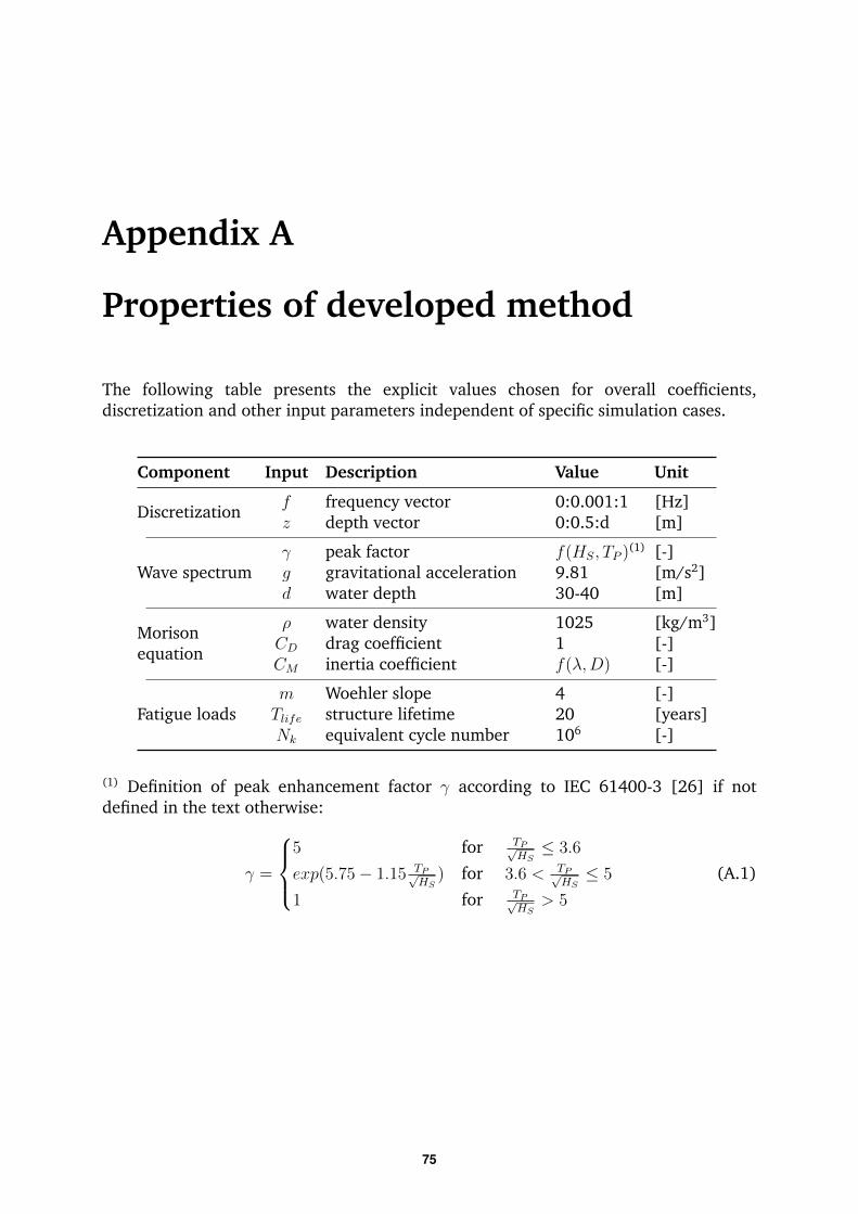
Appendix A
Properties of developed method
The following table presents the explicit values chosen for overall coefficients,discretization and other input parameters independent of specific simulation cases.
Component Input Description Value Unit
Discretizationf frequency vector 0:0.001:1 [Hz]z depth vector 0:0.5:d [m]
Wave spectrumγ peak factor f(HS, TP )(1) [-]g gravitational acceleration 9.81 [m/s2]d water depth 30-40 [m]
Morisonequation
ρ water density 1025 [kg/m3]CD drag coefficient 1 [-]CM inertia coefficient f(λ,D) [-]
Fatigue loadsm Woehler slope 4 [-]Tlife structure lifetime 20 [years]Nk equivalent cycle number 106 [-]
(1) Definition of peak enhancement factor γ according to IEC 61400-3 [26] if notdefined in the text otherwise:
γ =
5 for TP√
HS≤ 3.6
exp(5.75− 1.15 TP√HS
) for 3.6 < TP√HS≤ 5
1 for TP√HS
> 5
(A.1)
75

76

Appendix B
Scientific papers
77

78 B. SCIENTIFIC PAPERS

79
Paper A
Sensitivity of Wave Fatigue Loads on Offshore Wind Turbines undervarying Site Conditions
L. Ziegler, S. Voormeeren, S. Schafhirt and M. Muskulus
05/01/2015: Submission for EERA DeepWind’201508/04/2015: Accepted with with minor editorial changes for publication in
Elsevier Energy Procedia20/04/2015: Submission of revised paper

Available online at www.sciencedirect.com
Energy Procedia 00 (2015) 000–000
www.elsevier.com/locate/procedia
1876-6102 © 2015 The Authors. Published by Elsevier Ltd.
Selection and peer-review under responsibility of SINTEF Energi AS.
12th Deep Sea Offshore Wind R&D Conference, EERA DeepWind'2015
Sensitivity of Wave Fatigue Loads on Offshore Wind Turbines
under varying Site Conditions
Lisa Ziegler1,2
*, Sven Voormeeren2, Sebastian Schafhirt
1, Michael Muskulus
1
1 Department of Civil and Transport Engineering, NTNU, Høgskoleringen 7A, 7491 Trondheim, Norway 2 Siemens Wind Power, Offshore Center of Competence, Prinses Beatrixlaan 800, 2595BN The Hague, Netherlands
Abstract
Considerable variations in environmental site conditions can exist within large offshore wind farms leading to divergent fatigue
loads on support structures. An efficient frequency-domain method to calculate wave-induced fatigue loads on offshore wind
turbine monopile foundations was developed. A verification study with time-domain simulations for a 4MW offshore wind
turbine showed result accuracies of more than 90% for equivalent bending moments at mudline and interface level. This
accuracy and computation times in the order of seconds make the frequency-domain method ideal for preliminary design and
support structure optimization. The model is applied in sensitivity analysis of fatigue loads using Monte-Carlo simulations.
Local and global sensitivity studies and a probabilistic assessment give insight into the importance of site parameters like water
depth, soil stiffness, wave height, and wave period on fatigue loads. Results show a significant influence of water depth and
wave period. This provides a basis for design optimization, load interpolation and uncertainty analysis in large wind farms.
© 2015 The Authors. Published by Elsevier Ltd.
Selection and peer-review under responsibility of SINTEF Energi AS.
Offshore wind turbines; wave fatigue load; sensitivity analysis; frequency-domain; site variation
1. Introduction
Fatigue loads on offshore wind turbine (OWT) support structures vary in large wind farms due to changing
environmental site conditions. Full load calculations, which are commonly done in the time-domain, are
computationally demanding and cannot be performed for each turbine within the wind farm [1]. In practice, loads
* Corresponding author
E-mail address: [email protected]
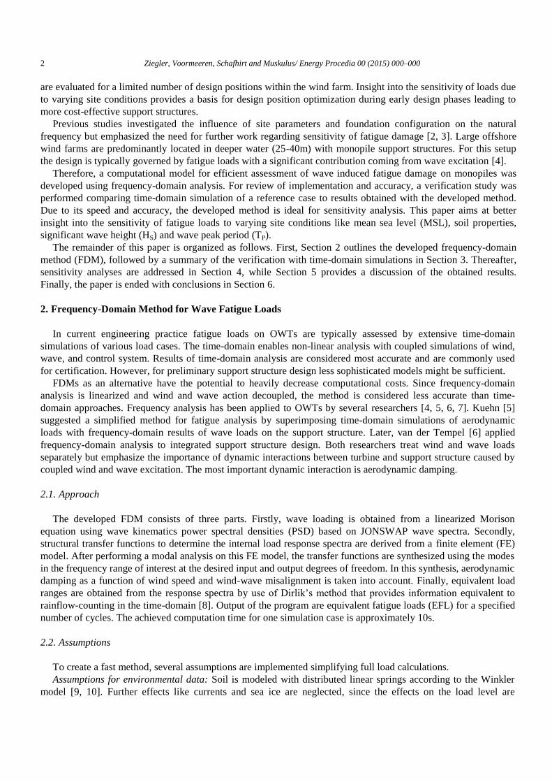
2 Ziegler, Voormeeren, Schafhirt and Muskulus/ Energy Procedia 00 (2015) 000–000
are evaluated for a limited number of design positions within the wind farm. Insight into the sensitivity of loads due
to varying site conditions provides a basis for design position optimization during early design phases leading to
more cost-effective support structures.
Previous studies investigated the influence of site parameters and foundation configuration on the natural
frequency but emphasized the need for further work regarding sensitivity of fatigue damage [2, 3]. Large offshore
wind farms are predominantly located in deeper water (25-40m) with monopile support structures. For this setup
the design is typically governed by fatigue loads with a significant contribution coming from wave excitation [4].
Therefore, a computational model for efficient assessment of wave induced fatigue damage on monopiles was
developed using frequency-domain analysis. For review of implementation and accuracy, a verification study was
performed comparing time-domain simulation of a reference case to results obtained with the developed method.
Due to its speed and accuracy, the developed method is ideal for sensitivity analysis. This paper aims at better
insight into the sensitivity of fatigue loads to varying site conditions like mean sea level (MSL), soil properties,
significant wave height (HS) and wave peak period (TP).
The remainder of this paper is organized as follows. First, Section 2 outlines the developed frequency-domain
method (FDM), followed by a summary of the verification with time-domain simulations in Section 3. Thereafter,
sensitivity analyses are addressed in Section 4, while Section 5 provides a discussion of the obtained results.
Finally, the paper is ended with conclusions in Section 6.
2. Frequency-Domain Method for Wave Fatigue Loads
In current engineering practice fatigue loads on OWTs are typically assessed by extensive time-domain
simulations of various load cases. The time-domain enables non-linear analysis with coupled simulations of wind,
wave, and control system. Results of time-domain analysis are considered most accurate and are commonly used
for certification. However, for preliminary support structure design less sophisticated models might be sufficient.
FDMs as an alternative have the potential to heavily decrease computational costs. Since frequency-domain
analysis is linearized and wind and wave action decoupled, the method is considered less accurate than time-
domain approaches. Frequency analysis has been applied to OWTs by several researchers [4, 5, 6, 7]. Kuehn [5]
suggested a simplified method for fatigue analysis by superimposing time-domain simulations of aerodynamic
loads with frequency-domain results of wave loads on the support structure. Later, van der Tempel [6] applied
frequency-domain analysis to integrated support structure design. Both researchers treat wind and wave loads
separately but emphasize the importance of dynamic interactions between turbine and support structure caused by
coupled wind and wave excitation. The most important dynamic interaction is aerodynamic damping.
2.1. Approach
The developed FDM consists of three parts. Firstly, wave loading is obtained from a linearized Morison
equation using wave kinematics power spectral densities (PSD) based on JONSWAP wave spectra. Secondly,
structural transfer functions to determine the internal load response spectra are derived from a finite element (FE)
model. After performing a modal analysis on this FE model, the transfer functions are synthesized using the modes
in the frequency range of interest at the desired input and output degrees of freedom. In this synthesis, aerodynamic
damping as a function of wind speed and wind-wave misalignment is taken into account. Finally, equivalent load
ranges are obtained from the response spectra by use of Dirlik’s method that provides information equivalent to
rainflow-counting in the time-domain [8]. Output of the program are equivalent fatigue loads (EFL) for a specified
number of cycles. The achieved computation time for one simulation case is approximately 10s.
2.2. Assumptions
To create a fast method, several assumptions are implemented simplifying full load calculations.
Assumptions for environmental data: Soil is modeled with distributed linear springs according to the Winkler
model [9, 10]. Further effects like currents and sea ice are neglected, since the effects on the load level are

Ziegler, Voormeeren, Schafhirt and Muskulus/ Energy Procedia 00 (2015) 000–000 3
expected to be minor. Sea ice can have a major impact on loads but is assumed to not occur for the considered sites
e.g. North Sea. It is assumed that scour protection is installed so that erosion and scour effects are not considered.
Assumptions for structural model: Foundation and tower are described with a linear FE model of Timoshenko
beam elements. It is based on a realistic reference design, where outer diameter, wall thickness and elastic
properties change over height of the support structure. The first ten modes of the structure are taken into account
according to ten eigenfrequencies. The rotor-nacelle-assembly (RNA) is modeled as an equivalent concentrated
mass on top of the tower. Damping consists of a contribution from combined structural, hydrodynamic and soil
damping (damping ratio ca. 1%) and a contribution from aerodynamic damping (damping ratio ca. 1.5 - 8%). The
latter is a function of wind speed, rotor speed, and mode shape and is superimposed to structural damping. It is
determined turbine-specific with modal analysis from a non-linear aero-elastic model. Aerodynamic damping for
the first mode (fore-aft) is increased for aligned wind and waves, while it is decreased for higher structure modes
as well as for wind-wave misalignment. The term interface refers to the node at tower bottom.
Assumptions for calculation method: The absolute formulation of Morison’s equation is used, since structural
velocity is low compared to wave velocity. The drag term is linearized with a method developed by Borgman [11].
Constant stretching is used to stretch wave kinematics from mean sea level to wave crest [12]. Diffraction is
accounted for by use of the empirical MacCamy-Fuchs diffraction correction [13]. Instead of using distributed
transfer functions of the FE model along the monopile wave-action zone, only transfer functions for equivalent
wave loads at mean sea level are generated in order to minimize the computational effort.
3. Verification
The frequency-domain approach is verified with time-domain simulations for a reference case using a non-
linear aero-elastic tool, Bonus Energy Horizontal axis wind turbine Code (BHawC), for global dynamic analysis of
wind turbines. The reference case consists of a 4MW OWT in several fatigue relevant sea states. The turbine is
located in a water depth of approximately 35m. For each sea state wind and wave directionalities are simplified
into fully aligned or misaligned. Fully aligned describes identical wind and wave directions while fully misaligned
waves arrive with 90° offset to wind. Structural models for the support structures are identical in terms of structural
dimensions, damping, and modal properties. Simulations are run wave-only, i.e., with aerodynamics turned off.
The parameters for the time-domain simulation are summarized in Table 1a. Each simulation has a length of 600s
with 0.04s time step. The use of 5 random realizations (seeds) minimizes statistical errors in the simulation.
Table 1a. Simulation parameters verification study.
Parameter Value
Length of time series 600s
Time step 0.04s
Number of seeds 5
Table 1b. Parameter Welch’s method.
Parameter Value
Window type Hamming
Number of sections 10
Overlap 50%
Simulation results are compared qualitatively in terms of response moment PSDs and quantitatively with EFLs.
PSDs are generated from the load time series by applying Welch’s method for which the choices are specified in
Table 1b. The time series were multiplied with a Hamming window and divided into 10 sections with 50%
overlap. Welch’s method uses periodogram spectrum estimates to reduce noise in the estimated spectrum due to
limited length of the time series. Rainflow-counting is applied to the load time series to obtain the number of
cycles Ni per load range Li from which the equivalent lifetime fatigue load EFL for a specified number of cycles Nk
is computed with Equation 1 [14]. The material parameter m=4 is chosen for welded steel. Tsim is the simulation
time and n equals the number of load ranges. Results of the verification study are presented in section 5.
1/
1
mn
life mii
i k sim
TNEFL L
N T
(1)
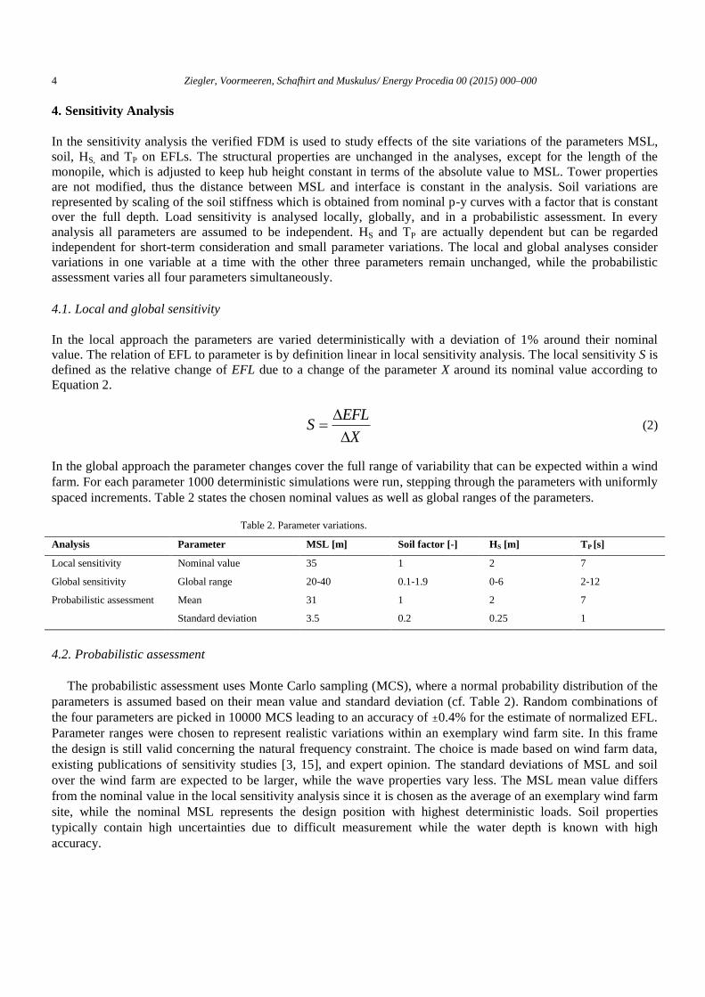
4 Ziegler, Voormeeren, Schafhirt and Muskulus/ Energy Procedia 00 (2015) 000–000
4. Sensitivity Analysis
In the sensitivity analysis the verified FDM is used to study effects of the site variations of the parameters MSL,
soil, HS, and TP on EFLs. The structural properties are unchanged in the analyses, except for the length of the
monopile, which is adjusted to keep hub height constant in terms of the absolute value to MSL. Tower properties
are not modified, thus the distance between MSL and interface is constant in the analysis. Soil variations are
represented by scaling of the soil stiffness which is obtained from nominal p-y curves with a factor that is constant
over the full depth. Load sensitivity is analysed locally, globally, and in a probabilistic assessment. In every
analysis all parameters are assumed to be independent. HS and TP are actually dependent but can be regarded
independent for short-term consideration and small parameter variations. The local and global analyses consider
variations in one variable at a time with the other three parameters remain unchanged, while the probabilistic
assessment varies all four parameters simultaneously.
4.1. Local and global sensitivity
In the local approach the parameters are varied deterministically with a deviation of 1% around their nominal
value. The relation of EFL to parameter is by definition linear in local sensitivity analysis. The local sensitivity S is
defined as the relative change of EFL due to a change of the parameter X around its nominal value according to
Equation 2.
X
EFLS
(2)
In the global approach the parameter changes cover the full range of variability that can be expected within a wind
farm. For each parameter 1000 deterministic simulations were run, stepping through the parameters with uniformly
spaced increments. Table 2 states the chosen nominal values as well as global ranges of the parameters.
Table 2. Parameter variations.
Analysis Parameter MSL [m] Soil factor [-] HS [m] TP [s]
Local sensitivity Nominal value 35 1 2 7
Global sensitivity Global range 20-40 0.1-1.9 0-6 2-12
Probabilistic assessment Mean 31 1 2 7
Standard deviation 3.5 0.2 0.25 1
4.2. Probabilistic assessment
The probabilistic assessment uses Monte Carlo sampling (MCS), where a normal probability distribution of the
parameters is assumed based on their mean value and standard deviation (cf. Table 2). Random combinations of
the four parameters are picked in 10000 MCS leading to an accuracy of ±0.4% for the estimate of normalized EFL.
Parameter ranges were chosen to represent realistic variations within an exemplary wind farm site. In this frame
the design is still valid concerning the natural frequency constraint. The choice is made based on wind farm data,
existing publications of sensitivity studies [3, 15], and expert opinion. The standard deviations of MSL and soil
over the wind farm are expected to be larger, while the wave properties vary less. The MSL mean value differs
from the nominal value in the local sensitivity analysis since it is chosen as the average of an exemplary wind farm
site, while the nominal MSL represents the design position with highest deterministic loads. Soil properties
typically contain high uncertainties due to difficult measurement while the water depth is known with high
accuracy.
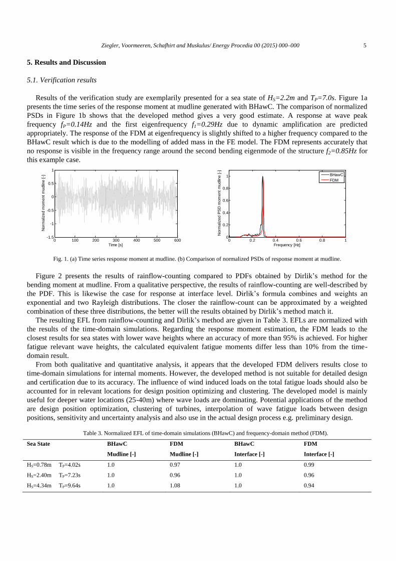
Ziegler, Voormeeren, Schafhirt and Muskulus/ Energy Procedia 00 (2015) 000–000 5
5. Results and Discussion
5.1. Verification results
Results of the verification study are exemplarily presented for a sea state of HS=2.2m and TP=7.0s. Figure 1a
presents the time series of the response moment at mudline generated with BHawC. The comparison of normalized
PSDs in Figure 1b shows that the developed method gives a very good estimate. A response at wave peak
frequency fP=0.14Hz and the first eigenfrequency f1=0.29Hz due to dynamic amplification are predicted
appropriately. The response of the FDM at eigenfrequency is slightly shifted to a higher frequency compared to the
BHawC result which is due to the modelling of added mass in the FE model. The FDM represents accurately that
no response is visible in the frequency range around the second bending eigenmode of the structure f2=0.85Hz for
this example case.
Fig. 1. (a) Time series response moment at mudline. (b) Comparison of normalized PSDs of response moment at mudline.
Figure 2 presents the results of rainflow-counting compared to PDFs obtained by Dirlik’s method for the
bending moment at mudline. From a qualitative perspective, the results of rainflow-counting are well-described by
the PDF. This is likewise the case for response at interface level. Dirlik’s formula combines and weights an
exponential and two Rayleigh distributions. The closer the rainflow-count can be approximated by a weighted
combination of these three distributions, the better will the results obtained by Dirlik’s method match it.
The resulting EFL from rainflow-counting and Dirlik’s method are given in Table 3. EFLs are normalized with
the results of the time-domain simulations. Regarding the response moment estimation, the FDM leads to the
closest results for sea states with lower wave heights where an accuracy of more than 95% is achieved. For higher
fatigue relevant wave heights, the calculated equivalent fatigue moments differ less than 10% from the time-
domain result.
From both qualitative and quantitative analysis, it appears that the developed FDM delivers results close to
time-domain simulations for internal moments. However, the developed method is not suitable for detailed design
and certification due to its accuracy. The influence of wind induced loads on the total fatigue loads should also be
accounted for in relevant locations for design position optimizing and clustering. The developed model is mainly
useful for deeper water locations (25-40m) where wave loads are dominating. Potential applications of the method
are design position optimization, clustering of turbines, interpolation of wave fatigue loads between design
positions, sensitivity and uncertainty analysis and also use in the actual design process e.g. preliminary design.
Table 3. Normalized EFL of time-domain simulations (BHawC) and frequency-domain method (FDM).
Sea State BHawC
Mudline [-]
FDM
Mudline [-]
BHawC
Interface [-]
FDM
Interface [-]
HS=0.78m TP=4.02s 1.0 0.97 1.0 0.99
HS=2.40m TP=7.23s 1.0 0.96 1.0 0.96
HS=4.34m TP=9.64s 1.0 1.08 1.0 0.94
0 100 200 300 400 500 600-1.5
-1
-0.5
0
0.5
1
Time [s]
Norm
aliz
ed m
om
ent
mudlin
e [
-]
0 0.2 0.4 0.6 0.8 10
0.2
0.4
0.6
0.8
1
Frequency [Hz]
Norm
aliz
ed P
SD
mom
ent
mudlin
e [
-]
BHawC
FDM
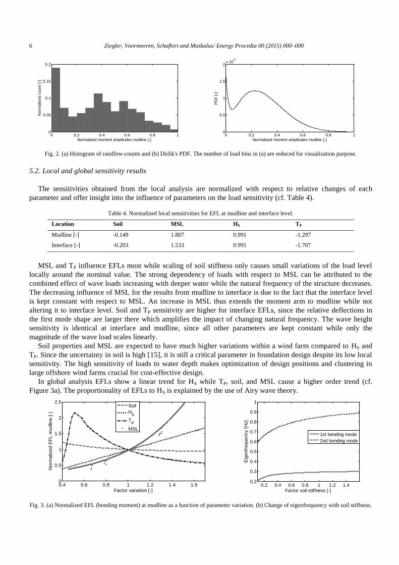
6 Ziegler, Voormeeren, Schafhirt and Muskulus/ Energy Procedia 00 (2015) 000–000
Fig. 2. (a) Histogram of rainflow-counts and (b) Dirlik's PDF. The number of load bins in (a) are reduced for visualization purpose.
5.2. Local and global sensitivity results
The sensitivities obtained from the local analysis are normalized with respect to relative changes of each
parameter and offer insight into the influence of parameters on the load sensitivity (cf. Table 4).
Table 4. Normalized local sensitivities for EFL at mudline and interface level.
Location Soil MSL HS TP
Mudline [-] -0.149 1.807 0.991 -1.297
Interface [-] -0.203 1.533 0.991 -1.707
MSL and TP influence EFLs most while scaling of soil stiffness only causes small variations of the load level
locally around the nominal value. The strong dependency of loads with respect to MSL can be attributed to the
combined effect of wave loads increasing with deeper water while the natural frequency of the structure decreases.
The decreasing influence of MSL for the results from mudline to interface is due to the fact that the interface level
is kept constant with respect to MSL. An increase in MSL thus extends the moment arm to mudline while not
altering it to interface level. Soil and TP sensitivity are higher for interface EFLs, since the relative deflections in
the first mode shape are larger there which amplifies the impact of changing natural frequency. The wave height
sensitivity is identical at interface and mudline, since all other parameters are kept constant while only the
magnitude of the wave load scales linearly.
Soil properties and MSL are expected to have much higher variations within a wind farm compared to HS and
TP. Since the uncertainty in soil is high [15], it is still a critical parameter in foundation design despite its low local
sensitivity. The high sensitivity of loads to water depth makes optimization of design positions and clustering in
large offshore wind farms crucial for cost-effective design.
In global analysis EFLs show a linear trend for HS while TP, soil, and MSL cause a higher order trend (cf.
Figure 3a). The proportionality of EFLs to HS is explained by the use of Airy wave theory.
Fig. 3. (a) Normalized EFL (bending moment) at mudline as a function of parameter variation. (b) Change of eigenfrequency with soil stiffness.
0 0.2 0.4 0.6 0.8 10
0.05
0.1
0.15
0.2
Normalized moment amplitudes mudline [-]
Norm
aliz
ed c
ount
[-]
0 0.2 0.4 0.6 0.8 10
0.5
1
1.5
2x 10
-8
Normalized moment amplitudes mudline [-]
PD
F [
-]
0.4 0.6 0.8 1 1.2 1.4 1.60
0.5
1
1.5
2
2.5
Factor variation [-]
Norm
aliz
ed E
FL m
udlin
e [
-]
Soil
HS
TP
MSL
0.2 0.4 0.6 0.8 1 1.2 1.40.2
0.3
0.4
0.5
0.6
0.7
0.8
0.9
1
Factor soil stiffness [-]
Eig
enfr
equency [
Hz]
1st bending mode
2nd bending mode
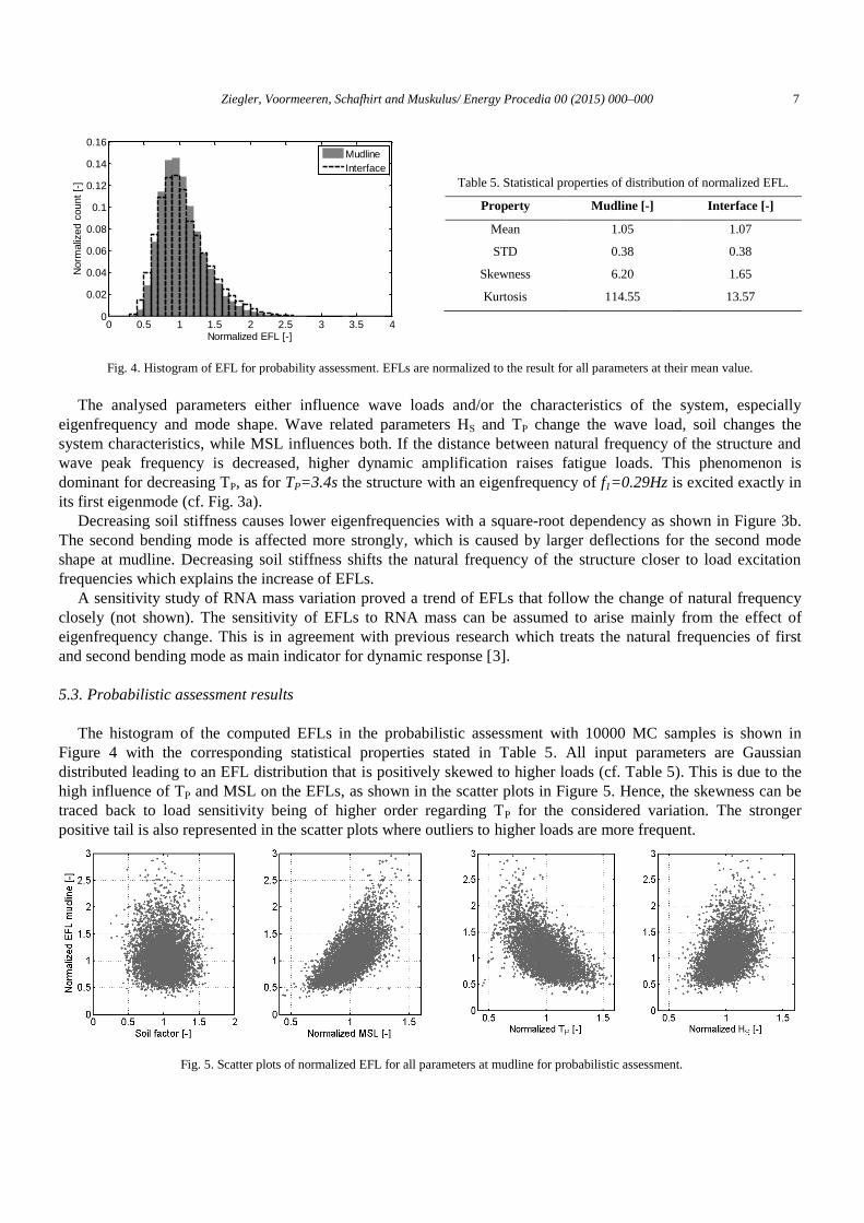
Ziegler, Voormeeren, Schafhirt and Muskulus/ Energy Procedia 00 (2015) 000–000 7
Table 5. Statistical properties of distribution of normalized EFL.
Property Mudline [-] Interface [-]
Mean 1.05 1.07
STD 0.38 0.38
Skewness 6.20 1.65
Kurtosis 114.55 13.57
Fig. 4. Histogram of EFL for probability assessment. EFLs are normalized to the result for all parameters at their mean value.
The analysed parameters either influence wave loads and/or the characteristics of the system, especially
eigenfrequency and mode shape. Wave related parameters HS and TP change the wave load, soil changes the
system characteristics, while MSL influences both. If the distance between natural frequency of the structure and
wave peak frequency is decreased, higher dynamic amplification raises fatigue loads. This phenomenon is
dominant for decreasing TP, as for TP=3.4s the structure with an eigenfrequency of f1=0.29Hz is excited exactly in
its first eigenmode (cf. Fig. 3a).
Decreasing soil stiffness causes lower eigenfrequencies with a square-root dependency as shown in Figure 3b.
The second bending mode is affected more strongly, which is caused by larger deflections for the second mode
shape at mudline. Decreasing soil stiffness shifts the natural frequency of the structure closer to load excitation
frequencies which explains the increase of EFLs.
A sensitivity study of RNA mass variation proved a trend of EFLs that follow the change of natural frequency
closely (not shown). The sensitivity of EFLs to RNA mass can be assumed to arise mainly from the effect of
eigenfrequency change. This is in agreement with previous research which treats the natural frequencies of first
and second bending mode as main indicator for dynamic response [3].
5.3. Probabilistic assessment results
The histogram of the computed EFLs in the probabilistic assessment with 10000 MC samples is shown in
Figure 4 with the corresponding statistical properties stated in Table 5. All input parameters are Gaussian
distributed leading to an EFL distribution that is positively skewed to higher loads (cf. Table 5). This is due to the
high influence of TP and MSL on the EFLs, as shown in the scatter plots in Figure 5. Hence, the skewness can be
traced back to load sensitivity being of higher order regarding TP for the considered variation. The stronger
positive tail is also represented in the scatter plots where outliers to higher loads are more frequent.
Fig. 5. Scatter plots of normalized EFL for all parameters at mudline for probabilistic assessment.
0 0.5 1 1.5 2 2.5 3 3.5 40
0.02
0.04
0.06
0.08
0.1
0.12
0.14
0.16
Normalized EFL [-]
Norm
aliz
ed c
ount
[-]
Mudline
Interface
8 Ziegler, Voormeeren, Schafhirt and Muskulus/ Energy Procedia 00 (2015) 000–000
The scatter plots show the same trends as observed for the global sensitivity study. For this reference case soil
has no significant influence on the mean EFL. This is consistent with the expectation based on the local sensitivity
analysis. Sensitivity results are strongly influenced by the chosen parameter ranges of the reference case.
Therefore, care must be taken for generalization of the results regarding assumptions and conditions in other cases.
6. Conclusion and Outlook
Increased insight into sensitivity of fatigue loads is needed in order to optimize support structures in large
offshore wind farms, where considerable variations in environmental site conditions might occur. This paper uses
frequency-domain load calculations to analyze the sensitivity of wave-induced fatigue loads to varying site
conditions for OWT monopile foundations in deeper water locations. A FDM was created which calculates EFLs
based on JONSWAP wave spectra, Morison equation, transfer functions from a FE model of the support structure,
and Dirlik’s method. This approach results in a computation time of approximately 10s for one simulation case.
Verification of the FDM using time-domain simulations from an aero-elastic code indicates an accuracy of more
than 90% for fatigue bending moments at mudline and interface level. Additionally, a qualitative analysis of power
spectral densities showed good agreement regarding responses at TP and first eigenfrequency of the structure. The
FDM is used in sensitivity analysis with MC sampling. Local and global analysis reveal high fatigue load
sensitivity to changes in MSL and TP. Normal distributed parameters in a probabilistic assessment yield a
positively skewed probability distribution of EFLs.
Due to its accuracy and efficiency, the FDM is ideal for applications where fast simulations are needed, e.g. in
design position optimization, clustering of turbines, interpolation of wave fatigue loads and in preliminary design.
Further study is required to extend the developed method to include wind loads. Due to the identified importance
of wave peak frequency and MSL on the results, further work should reveal the effect of uncertainty in wave loads
on fatigue loads.
References
[1] Vorpahl, F., Schwarze, H., Fischer, T., Seidel, M., & Jonkman, J. (2013). Offshore wind turbine environment, loads, simulation, and
design. Wiley Interdisciplinary Reviews: Energy and Environment, 2(5), 548-570. [2] Zaaijer, M. B. (2006). Foundation modelling to assess dynamic behaviour of offshore wind turbines. Applied Ocean Research, 28(1), 45-57.
[3] de Vries, W., et al. (2011). Final report WP 4.2: Support Structure Concepts for Deep Water Sites: Deliverable D4.2.8 (WP4: offshore
foundations and support structures). Upwind. [4] Seidel, M. (2014). Wave induced fatigue loads - Insights from frequency domain calculations. Stahlbau, 83, 535–541.
[5] Kuehn, M. J (2001). Dynamics and design optimisation of offshore wind energy conversion systems. PhD diss. TU Delft, The Netherlands.
[6] Van der Tempel, J. (2006). Design of support structures for offshore wind turbines. PhD diss. TU Delft, The Netherlands.
[7] Ragan, P., & Manuel, L. (2007). Comparing estimates of wind turbine fatigue loads using time-domain and spectral methods. Wind
engineering, 31(2), 83-99.
[8] Dirlik, T. (1985). Application of computers in fatigue analysis. PhD thesis, University of Warwick, England.
[9] American Petroleum Institute (API). Recommended Practice for Planning, Designing, and Constructing Fixed Offshore Platforms—
Working Stress Design (2A-WSD). American Petroleum Institute, Washington, D. C., 2005.
[10] Passon, P., & Kühn, M. (2005). State-of-the-art and development needs of simulation codes for offshore wind turbines. In Copenhagen
Offshore Wind 2005 Conference and Expedition Proceedings (pp. 26-28).
[11] Borgman, L. E. (1965). The spectral density for ocean wave forces. ASCE .Santa Barbara speciality conference. [12] Wheeler, J. D. (1970). Method for calculating forces produced by irregular waves. Journal of Petroleum Technology, 22(03), 359-367.
[13] MacCamy, R. C., & Fuchs, R. A. (1954). Wave forces on piles: a diffraction theory. Tech. rep., DTIC Document (No. TM-69)
[14] Matsuishi, M., & Endo, T. (1968). Fatigue of metals subjected to varying stress. Japan Society of Mechanical Engineers, Fukuoka, Japan,
37-40.
[15] Carswell, W., Arwade, S. R., DeGroot, D. J. and Lackner, M. A. (2014). Soil–structure reliability of offshore wind turbine monopile
foundations. Wind Energy.

88 B. SCIENTIFIC PAPERS

89
Paper B
Design clustering of offshore wind turbines using probabilisticfatigue load estimation
L. Ziegler, S. Voormeeren, S. Schafhirt and M. Muskulus
12/05/2015: Submission to Renewable Energy
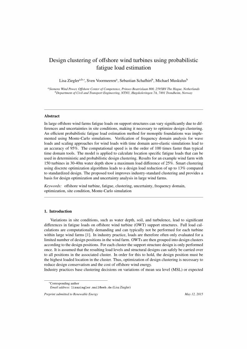
Design clustering of offshore wind turbines using probabilisticfatigue load estimation
Lisa Zieglera,b,∗, Sven Voormeerena, Sebastian Schafhirtb, Michael Muskulusb
aSiemens Wind Power, Offshore Center of Competence, Prinses Beatrixlaan 800, 2595BN The Hague, NetherlandsbDepartment of Civil and Transport Engineering, NTNU, Høgskoleringen 7A, 7491 Trondheim, Norway
Abstract
In large offshore wind farms fatigue loads on support structures can vary significantly due to dif-ferences and uncertainties in site conditions, making it necessary to optimize design clustering.An efficient probabilistic fatigue load estimation method for monopile foundations was imple-mented using Monte-Carlo simulations. Verification of frequency domain analysis for waveloads and scaling approaches for wind loads with time domain aero-elastic simulations lead toan accuracy of 95%. The computational speed is in the order of 100 times faster than typicaltime domain tools. The model is applied to calculate location specific fatigue loads that can beused in deterministic and probabilistic design clustering. Results for an example wind farm with150 turbines in 30-40m water depth show a maximum load difference of 25%. Smart clusteringusing discrete optimization algorithms leads to a design load reduction of up to 13% comparedto standardized design. The proposed tool improves industry-standard clustering and provides abasis for design optimization and uncertainty analysis in large wind farms.
Keywords: offshore wind turbine, fatigue, clustering, uncertainty, frequency domain,optimization, site condition, Monte-Carlo simulation
1. Introduction
Variations in site conditions, such as water depth, soil, and turbulence, lead to significantdifferences in fatigue loads on offshore wind turbine (OWT) support structures. Full load cal-culations are computationally demanding and can typically not be performed for each turbinewithin large wind farms [1]. In industry practice, loads are therefore often only evaluated for alimited number of design positions in the wind farm. OWTs are then grouped into design clustersaccording to the design positions. For each cluster the support structure design is only performedonce. It is assumed that the resulting load levels and structural designs can safely be carried overto all positions in the associated cluster. In order for this to hold, the design position must bethe highest loaded location in the cluster. Thus, optimization of design clustering is necessary toreduce design conservatism and the cost of offshore wind energy.Industry practices base clustering decisions on variations of mean sea level (MSL) or expected
∗Corresponding authorEmail address: [email protected] (Lisa Ziegler)
Preprint submitted to Renewable Energy May 12, 2015

first eigenfrequency of the support structures [2]. Recently, Seidel [2] suggested an improved ap-proach of clustering using a site parameter that takes into account structural and hydrodynamicproperties. This site parameter is however only suitable for wave load dominated designs. Thus,further work is needed to formulate turbine clustering as an optimization problem incorporatingall important site specific information.Since grouping of OWTs into design clusters must be performed in an early project phase, time-efficient approaches are essential. In this paper, a design clustering method for OWTs was de-veloped using probabilistic fatigue load estimation. The fatigue load estimation method usesfrequency domain analysis to calculate wave loads and a scaling approach for wind loads onmonopile-based OWTs. Uncertainties in input data and model assumptions are analyzed throughMonte-Carlo simulations (MCS). The deterministic estimation tool was verified with fully inte-grated, aero-elastic time domain simulations. Due to computational efficiency, fatigue loads canbe calculated site specific for every turbine location within the wind farm. This makes turbineclustering a discrete optimization problem.This paper provides a novel approach of optimization of turbine clustering. Additionally, prob-abilistic assessments give insight on how uncertainties in load calculation can alter allocation ofturbines to clusters. This paper is organized as follows. Section 2 outlines the developed fatigueload estimation method, its model assumptions and verification. A summary of the probabilis-tic load assessment is presented in Section 3. Section 4 focuses on clustering optimization bydiscussing problem formulations and solution approaches using brute-force and discrete opti-mization algorithms. Section 5 demonstrates the established clustering optimization method foran exemplary wind farm of 150 monopile-based OWTs in a water depth range of 30-40m.
2. Method for Fatigue Load Estimation
Since a high number of load cases have to be performed for detailed design and certificationof OWTs, computational effort for standard time domain fatigue load analysis is significant [3, 4].Such simulations, although they are considered most accurate, are ill-suited for clustering opti-mization and probabilistic assessments. For these applications, load estimates are sufficient, asfast simulations are a necessity.Several approaches exist in literature to decrease computational costs of OWT load analysis [6-16], either using integrated analysis or wind-wave separate assessment. In separate assessments,wave fatigue loads are mainly estimated from frequency domain analysis [6, 5, 7, 8, 9, 2, 13],which has also been applied to wind loads [7, 9, 13, 14, 16]. Other authors suggest simplifiedrotor load models or parametric models for fatigue damage estimation [10, 15]. For integratedmethods, proposals exist for reducing the number of environmental conditions, number of simu-lation seeds or length [6, 11]. For example, Zwick and Muskulus [11] suggest simplified fatigueload assessment based on statistical regression models to reduce the number of load cases fordamage estimation.
2.1. Approach
The developed estimation method calculates location specific equivalent fatigue loads (EFLs).The method is based on three core elements (cf. Figure 1): (1) calculation of wave-induced EFLsin the frequency domain using Dirlik’s method, (2) scaling of wind-induced EFLs from a refer-ence case, and (3) combination of wind-wave EFLs with direct quadratic superposition [6].Wave loads are calculated based on JONSWAP wave spectra and Morison equation. To deter-
2
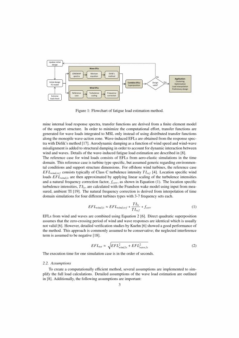
Initial design FE model
Wind EFLs
Combine EFLs: Superposition
Extreme load check
Reference case
Turbulence scaling
Frequency correction
Wave EFLs
JONSWAP spectra
Morison equation
Dirlik’s method
Design valid?
Update initial design
Application: Clustering
Optimization Load interpolation Preliminary design
No
Yes
Figure 1: Flowchart of fatigue load estimation method.
mine internal load response spectra, transfer functions are derived from a finite element modelof the support structure. In order to minimize the computational effort, transfer functions aregenerated for wave loads integrated to MSL only instead of using distributed transfer functionsalong the monopile wave-action zone. Wave-induced EFLs are obtained from the response spec-tra with Dirlik’s method [17]. Aerodynamic damping as a function of wind speed and wind-wavemisalignment is added to structural damping in order to account for dynamic interaction betweenwind and waves. Details of the wave-induced fatigue load estimation are described in [8].The reference case for wind loads consists of EFLs from aero-elastic simulations in the timedomain. This reference case is turbine type specific, but assumed generic regarding environmen-tal conditions and support structure dimensions. For offshore wind turbines, the reference caseEFLwind,re f consists typically of Class C turbulence intensity T Ire f [4]. Location specific windloads EFLwind,ls are then approximated by applying linear scaling of the turbulence intensitiesand a natural frequency correction factor, fcorr, as shown in Equation (1). The location specificturbulence intensities, T Ils, are calculated with the Frandsen wake model using input from mea-sured, ambient TI [19]. The natural frequency correction is derived from interpolation of timedomain simulations for four different turbines types with 3-7 frequency sets each.
EFLwind,ls ≈ EFLwind,re f ∗ T Ils
T Ire f∗ fcorr (1)
EFLs from wind and waves are combined using Equation 2 [6]. Direct quadratic superpositionassumes that the zero-crossing period of wind and wave responses are identical which is usuallynot valid [6]. However, detailed verification studies by Kuehn [6] showed a good performance ofthe method. This approach is commonly assumed to be conservative; the neglected interferenceterm is assumed to be negative [18].
EFLtot ≈√
EFL2wind,ls + EFL2
wave,ls (2)
The execution time for one simulation case is in the order of seconds.
2.2. Assumptions
To create a computationally efficient method, several assumptions are implemented to sim-plify the full load calculations. Detailed assumptions of the wave load estimation are outlinedin [8]. Additionally, the following assumptions are important:
3

Assumptions for environmental data: Wind-wave scatter diagrams are lumped into 20 simulationcases consisting of mean wind speeds (VW ), significant wave heights (HS ), and wave peak peri-ods (TP). The lumping is performed in a damage equivalent way using a method suggested byKuehn [6]. For each simulation case wind-wave directionality is simplified into fully aligned orfully misaligned. For this purpose, wind and wave roses are lumped in bins of 30degree. Fullyaligned wind and waves occur in the same bin, where the aerodynamic damping is maximum.All other combination of wind and wave directions are treated as fully misaligned with reducedaerodynamic damping.Assumptions for calculation method: The estimation approach for wind-induced EFLs only ad-justs for TI and natural frequency. Differences in air density, wind shear, structural geometry ormode shapes are neglected since the effects on the load level are expected to either be minor orrepresented through the natural frequency correction.
2.3. Verification
The fatigue load estimation method is verified empirically against time domain simulationsusing the non-linear aero-elastic tool Bonus Horizontal axis wind turbine Code (BHawC), whichallows for a global dynamic analysis of wind turbines. The verification was done for wave-onlyload cases (as described in [8]), as well as wind-only loads, and wind-wave combined loads fora 4MW OWT in 35m water depth. Results of this verification study are presented in Section 5.
3. Probabilistic Load Assessment
Fatigue load calculation processes contain significant uncertainties commonly addressed withsafety factors in the design standards [4, 5]. Insight on the effect of uncertainties on EFLs im-proves the understanding of the actual structural reliability. A brief overview of existing work onprobabilistic fatigue assessment of wind turbines is given by Yeter [20] and Veldkamp [21].The novelty of this work is the use of frequency domain analysis with MCS to assess uncertain-ties in fatigue loads for application in probabilistic design clustering of OWTs. For every turbinelocation 1000 MCS were run with simultaneous, random variation of input parameters. As aresult, the output distribution of EFLs can be estimated with a root-mean-square error of 0.3%.Epistemic uncertainties in fatigue load calculations occur in the form of data, statistical andmodel uncertainty [22]. Previous work showed significant influence of data uncertainties inMSL and TP on fatigue loads [8]. For the clustering problem, the probabilistic assessment isextended to include uncertainty in TI and model uncertainty. Model uncertainty is analyzed re-garding the development of sea states, represented with the peak enhancement factor γ in theJONSWAP wave spectrum, and regarding diffraction, represented with the inertia coefficient CM
in the McCamy-Fuchs diffraction correction for Morison equation. All parameters in the proba-bilistic assessment are independent, normal distributed with mean value and standard deviation(STD) stated in Table 1.Data uncertainty was given a constant STD over the wind farm. In practice, uncertainties candiffer for some locations due to incomplete measurement data, for example soil measurementsmay not be available for every turbine position in early project phases.Parameter ranges were chosen to represent realistic uncertainties for design clustering in large
wind farms. The choice is made based on wind farm data, existing publications of sensitivitystudies [21, 23, 24], and expert opinion. For example, the variation of MSL is chosen as tidalvariation. Soil properties typically contain high uncertainties due to difficult measurement and
4
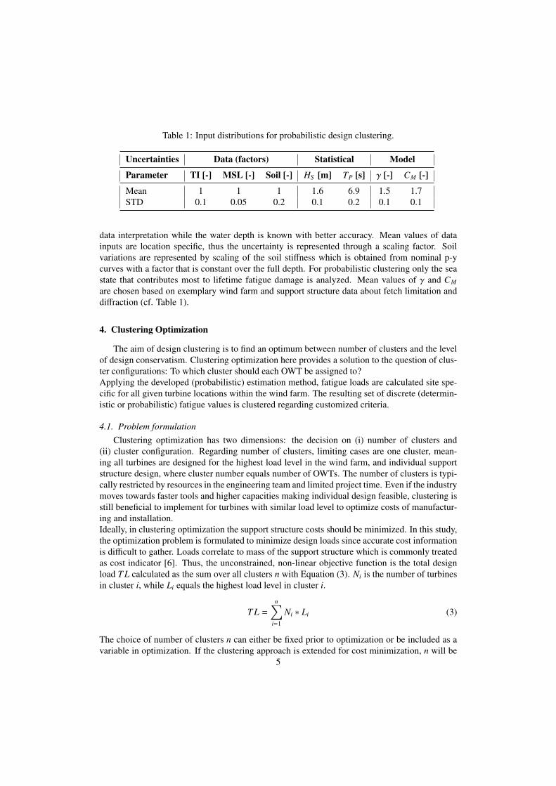
Table 1: Input distributions for probabilistic design clustering.
Uncertainties Data (factors) Statistical Model
Parameter TI [-] MSL [-] Soil [-] HS [m] TP [s] γ [-] CM [-]
Mean 1 1 1 1.6 6.9 1.5 1.7STD 0.1 0.05 0.2 0.1 0.2 0.1 0.1
data interpretation while the water depth is known with better accuracy. Mean values of datainputs are location specific, thus the uncertainty is represented through a scaling factor. Soilvariations are represented by scaling of the soil stiffness which is obtained from nominal p-ycurves with a factor that is constant over the full depth. For probabilistic clustering only the seastate that contributes most to lifetime fatigue damage is analyzed. Mean values of γ and CM
are chosen based on exemplary wind farm and support structure data about fetch limitation anddiffraction (cf. Table 1).
4. Clustering Optimization
The aim of design clustering is to find an optimum between number of clusters and the levelof design conservatism. Clustering optimization here provides a solution to the question of clus-ter configurations: To which cluster should each OWT be assigned to?Applying the developed (probabilistic) estimation method, fatigue loads are calculated site spe-cific for all given turbine locations within the wind farm. The resulting set of discrete (determin-istic or probabilistic) fatigue values is clustered regarding customized criteria.
4.1. Problem formulationClustering optimization has two dimensions: the decision on (i) number of clusters and
(ii) cluster configuration. Regarding number of clusters, limiting cases are one cluster, mean-ing all turbines are designed for the highest load level in the wind farm, and individual supportstructure design, where cluster number equals number of OWTs. The number of clusters is typi-cally restricted by resources in the engineering team and limited project time. Even if the industrymoves towards faster tools and higher capacities making individual design feasible, clustering isstill beneficial to implement for turbines with similar load level to optimize costs of manufactur-ing and installation.Ideally, in clustering optimization the support structure costs should be minimized. In this study,the optimization problem is formulated to minimize design loads since accurate cost informationis difficult to gather. Loads correlate to mass of the support structure which is commonly treatedas cost indicator [6]. Thus, the unconstrained, non-linear objective function is the total designload T L calculated as the sum over all clusters n with Equation (3). Ni is the number of turbinesin cluster i, while Li equals the highest load level in cluster i.
T L =
n∑
i=1
Ni ∗ Li (3)
The choice of number of clusters n can either be fixed prior to optimization or be included as avariable in optimization. If the clustering approach is extended for cost minimization, n will be
5

an optimization result.Including uncertainties in fatigue load calculations results in a set of fatigue load distributionsfor all turbines. Probabilistic clustering is performed by increasing the mean load value withk ∗ S T D. Choice of k represents how much of the load variability is accounted for, for examplek = 3 accounts for 99.7% of the sample population for a normal distribution. The higher k ischosen, the smaller is the chance of misgrouping turbines into clusters with too low load level.
4.2. Assumptions for clustering optimization
The formulation of the optimization problem reveals underlying assumptions for clustering:
• All turbines are designed for the highest load in the cluster, no design interpolation is donewithin clusters.
• Fatigue is design driving, extreme loads do not influence clustering. This is typicallyvalid for monopiles in deeper water, where the design is often dominated by wave inducedfatigue loads. A check should be performed for every project to confirm fatigue as a designdriver.
• Location specific loads are calculated with the same initial design for all positions. Thus,the validity of the design for all positions has to be confirmed which can be done throughthe frequency constraint. Alternatively, the initial design can be updated in an iterativeprocedure of clustering and renewed load calculation.
4.3. Solution approaches
The pattern of the optimization problem is explained for an example of 150 turbines equallydivided into five clusters with cluster 1 (T1 − T30) containing the highest loaded turbines andcluster 5 the lowest loaded turbines (T120 − T150). Thus, 30 turbines are in each cluster (N = 30).Moving one turbine T60 from cluster n2 to cluster n3 causes:
1. (N − 1) turbines in cluster n2,2. (N + 1) turbines in cluster n3 and3. Increase of maximum load in cluster n3 to L60.
The formulated problem is addressable with algorithms of combinatorial optimization [25]. Thediscrete solution approaches brute-force and local search were compared in terms of efficiencyand robustness. In brute-force the number of recombination are reduced by using pre-knowledgeof the solution that (i) clusters are filled with turbines sorted in load descending order makingoptimization only a cluster-border decision and (ii) when adding a cluster, the number of turbinesin every cluster is less or equal to the maximum number of turbines in the previous n clusters.Problems with 150 OWTs and up to 6 clusters can be solved with brute-force giving the globalminimum in a computation time of less than 1 hour.An approximate algorithm using local search starts from an initial cluster guess, selects a randomcluster-border, and optimizes it in terms of decreasing the objective function, while keeping allremaining positions constant. The optimization of the single cluster-border is performed byselecting the position with the minimum cost of all possible border positions. This procedure isrepeated in every iteration step. With a chance of 5%, the previously optimized cluster-borderis replaced by a random border to ensure that the algorithm does not become trapped in a localminimum with poor quality. In the tested example for 150 OWTs, 100 iterations were sufficient
6
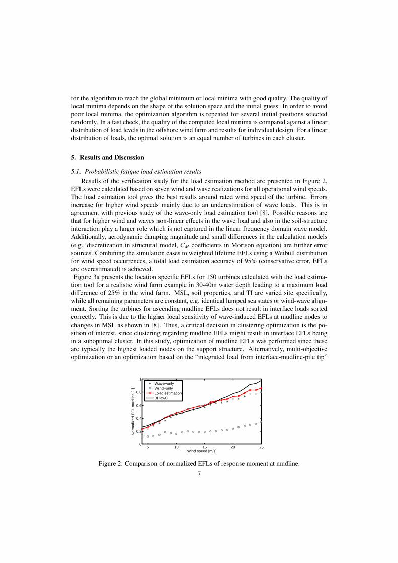
for the algorithm to reach the global minimum or local minima with good quality. The quality oflocal minima depends on the shape of the solution space and the initial guess. In order to avoidpoor local minima, the optimization algorithm is repeated for several initial positions selectedrandomly. In a fast check, the quality of the computed local minima is compared against a lineardistribution of load levels in the offshore wind farm and results for individual design. For a lineardistribution of loads, the optimal solution is an equal number of turbines in each cluster.
5. Results and Discussion
5.1. Probabilistic fatigue load estimation resultsResults of the verification study for the load estimation method are presented in Figure 2.
EFLs were calculated based on seven wind and wave realizations for all operational wind speeds.The load estimation tool gives the best results around rated wind speed of the turbine. Errorsincrease for higher wind speeds mainly due to an underestimation of wave loads. This is inagreement with previous study of the wave-only load estimation tool [8]. Possible reasons arethat for higher wind and waves non-linear effects in the wave load and also in the soil-structureinteraction play a larger role which is not captured in the linear frequency domain wave model.Additionally, aerodynamic damping magnitude and small differences in the calculation models(e.g. discretization in structural model, CM coefficients in Morison equation) are further errorsources. Combining the simulation cases to weighted lifetime EFLs using a Weibull distributionfor wind speed occurrences, a total load estimation accuracy of 95% (conservative error, EFLsare overestimated) is achieved.Figure 3a presents the location specific EFLs for 150 turbines calculated with the load estima-
tion tool for a realistic wind farm example in 30-40m water depth leading to a maximum loaddifference of 25% in the wind farm. MSL, soil properties, and TI are varied site specifically,while all remaining parameters are constant, e.g. identical lumped sea states or wind-wave align-ment. Sorting the turbines for ascending mudline EFLs does not result in interface loads sortedcorrectly. This is due to the higher local sensitivity of wave-induced EFLs at mudline nodes tochanges in MSL as shown in [8]. Thus, a critical decision in clustering optimization is the po-sition of interest, since clustering regarding mudline EFLs might result in interface EFLs beingin a suboptimal cluster. In this study, optimization of mudline EFLs was performed since theseare typically the highest loaded nodes on the support structure. Alternatively, multi-objectiveoptimization or an optimization based on the “integrated load from interface-mudline-pile tip”
5 10 15 20 250
0.2
0.4
0.6
0.8
1
Wind speed [m/s]
Nor
mal
ized
EF
L m
udlin
e [−
]
Wave−onlyWind−onlyLoad estimationBHawC
Figure 2: Comparison of normalized EFLs of response moment at mudline.
7
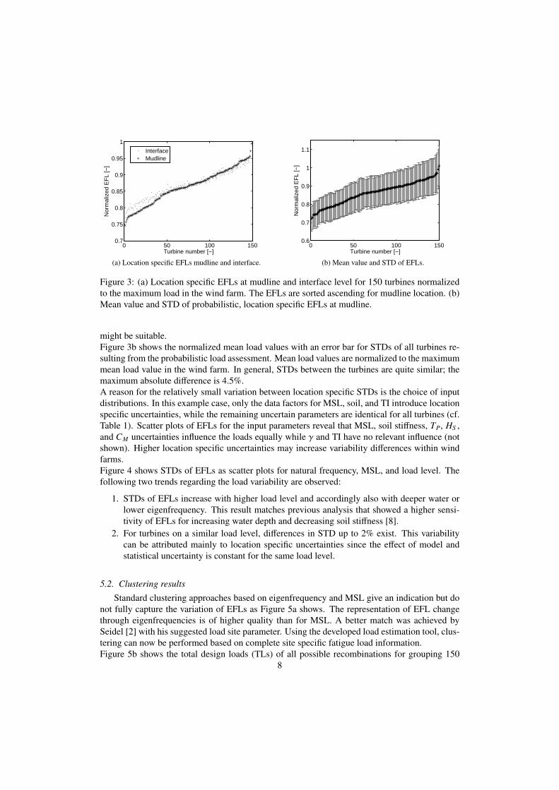
0 50 100 1500.7
0.75
0.8
0.85
0.9
0.95
1
Turbine number [−]
Nor
mal
ized
EF
L [−
]
InterfaceMudline
(a) Location specific EFLs mudline and interface.
0 50 100 1500.6
0.7
0.8
0.9
1
1.1
Turbine number [−]
Nor
mal
ized
EF
L [−
]
(b) Mean value and STD of EFLs.
Figure 3: (a) Location specific EFLs at mudline and interface level for 150 turbines normalizedto the maximum load in the wind farm. The EFLs are sorted ascending for mudline location. (b)Mean value and STD of probabilistic, location specific EFLs at mudline.
might be suitable.Figure 3b shows the normalized mean load values with an error bar for STDs of all turbines re-sulting from the probabilistic load assessment. Mean load values are normalized to the maximummean load value in the wind farm. In general, STDs between the turbines are quite similar; themaximum absolute difference is 4.5%.A reason for the relatively small variation between location specific STDs is the choice of inputdistributions. In this example case, only the data factors for MSL, soil, and TI introduce locationspecific uncertainties, while the remaining uncertain parameters are identical for all turbines (cf.Table 1). Scatter plots of EFLs for the input parameters reveal that MSL, soil stiffness, TP, HS ,and CM uncertainties influence the loads equally while γ and TI have no relevant influence (notshown). Higher location specific uncertainties may increase variability differences within windfarms.Figure 4 shows STDs of EFLs as scatter plots for natural frequency, MSL, and load level. Thefollowing two trends regarding the load variability are observed:
1. STDs of EFLs increase with higher load level and accordingly also with deeper water orlower eigenfrequency. This result matches previous analysis that showed a higher sensi-tivity of EFLs for increasing water depth and decreasing soil stiffness [8].
2. For turbines on a similar load level, differences in STD up to 2% exist. This variabilitycan be attributed mainly to location specific uncertainties since the effect of model andstatistical uncertainty is constant for the same load level.
5.2. Clustering results
Standard clustering approaches based on eigenfrequency and MSL give an indication but donot fully capture the variation of EFLs as Figure 5a shows. The representation of EFL changethrough eigenfrequencies is of higher quality than for MSL. A better match was achieved bySeidel [2] with his suggested load site parameter. Using the developed load estimation tool, clus-tering can now be performed based on complete site specific fatigue load information.Figure 5b shows the total design loads (TLs) of all possible recombinations for grouping 150
8
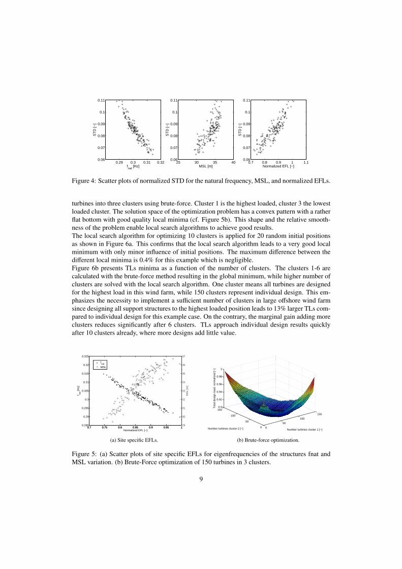
0.29 0.3 0.31 0.320.06
0.07
0.08
0.09
0.1
0.11
fnat
[Hz]
ST
D [−
]
25 30 35 400.06
0.07
0.08
0.09
0.1
0.11
MSL [m]S
TD
[−]
0.7 0.8 0.9 1 1.10.06
0.07
0.08
0.09
0.1
0.11
Normalized EFL [−]
ST
D [−
]
Figure 4: Scatter plots of normalized STD for the natural frequency, MSL, and normalized EFLs.
turbines into three clusters using brute-force. Cluster 1 is the highest loaded, cluster 3 the lowestloaded cluster. The solution space of the optimization problem has a convex pattern with a ratherflat bottom with good quality local minima (cf. Figure 5b). This shape and the relative smooth-ness of the problem enable local search algorithms to achieve good results.The local search algorithm for optimizing 10 clusters is applied for 20 random initial positionsas shown in Figure 6a. This confirms that the local search algorithm leads to a very good localminimum with only minor influence of initial positions. The maximum difference between thedifferent local minima is 0.4% for this example which is negligible.Figure 6b presents TLs minima as a function of the number of clusters. The clusters 1-6 arecalculated with the brute-force method resulting in the global minimum, while higher number ofclusters are solved with the local search algorithm. One cluster means all turbines are designedfor the highest load in this wind farm, while 150 clusters represent individual design. This em-phasizes the necessity to implement a sufficient number of clusters in large offshore wind farmsince designing all support structures to the highest loaded position leads to 13% larger TLs com-pared to individual design for this example case. On the contrary, the marginal gain adding moreclusters reduces significantly after 6 clusters. TLs approach individual design results quicklyafter 10 clusters already, where more designs add little value.
0.7 0.75 0.8 0.85 0.9 0.95 10.285
0.29
0.295
0.3
0.305
0.31
0.315
0.32
0.325
f nat [H
z]
Normalized EFL [−]
0.7 0.75 0.8 0.85 0.9 0.95 129
30
31
32
33
34
35
36
37
MS
L [m
]
fnat
MSL
(a) Site specific EFLs.
0
50
100
150
0
50
100
1500.9
0.92
0.94
0.96
0.98
1
Number turbines cluster 1 [−]Number turbines cluster 2 [−]
Tot
al d
esig
n lo
ad, n
orm
aliz
ed [−
]
(b) Brute-force optimization.
Figure 5: (a) Scatter plots of site specific EFLs for eigenfrequencies of the structures fnat andMSL variation. (b) Brute-Force optimization of 150 turbines in 3 clusters.
9
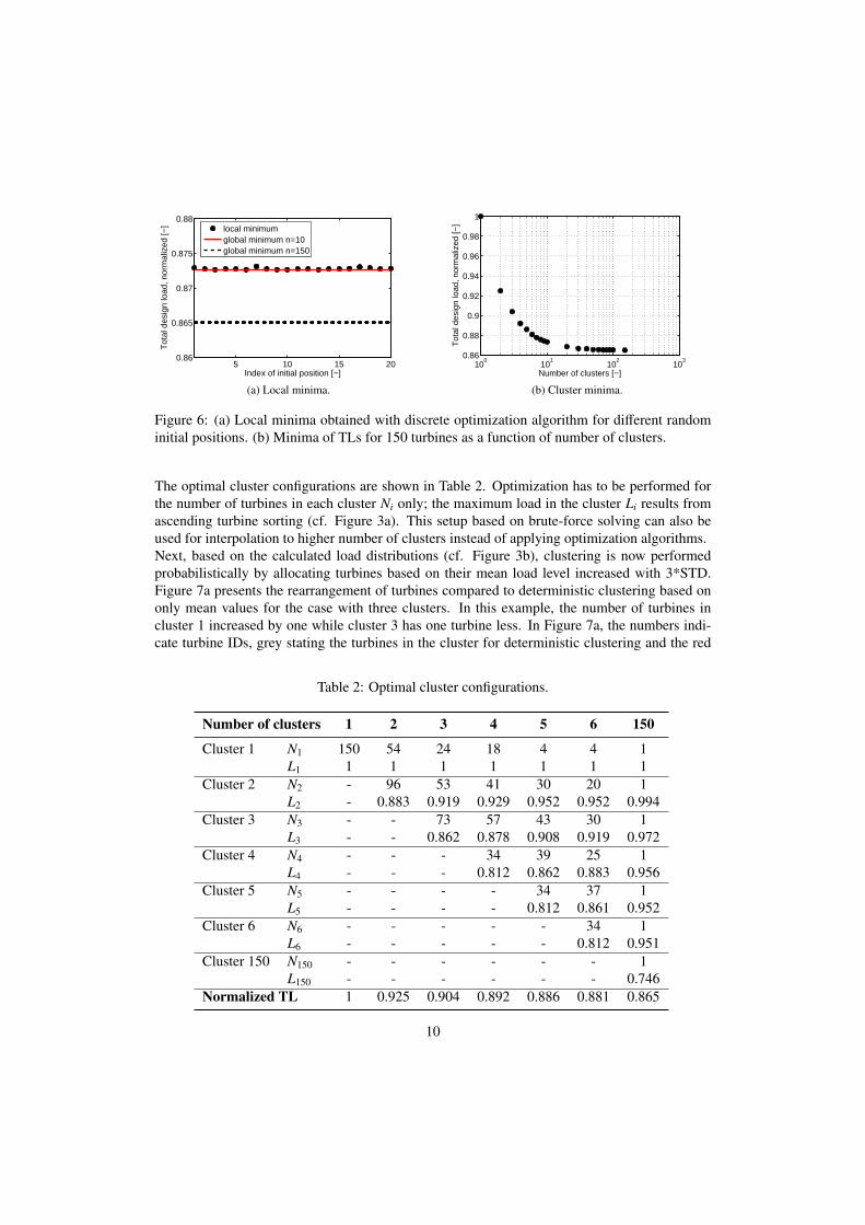
5 10 15 200.86
0.865
0.87
0.875
0.88
Index of initial position [−]
Tot
al d
esig
n lo
ad, n
orm
aliz
ed [−
]
local minimumglobal minimum n=10global minimum n=150
(a) Local minima.
100
101
102
103
0.86
0.88
0.9
0.92
0.94
0.96
0.98
1
Number of clusters [−]
Tot
al d
esig
n lo
ad, n
orm
aliz
ed [−
]
(b) Cluster minima.
Figure 6: (a) Local minima obtained with discrete optimization algorithm for different randominitial positions. (b) Minima of TLs for 150 turbines as a function of number of clusters.
The optimal cluster configurations are shown in Table 2. Optimization has to be performed forthe number of turbines in each cluster Ni only; the maximum load in the cluster Li results fromascending turbine sorting (cf. Figure 3a). This setup based on brute-force solving can also beused for interpolation to higher number of clusters instead of applying optimization algorithms.Next, based on the calculated load distributions (cf. Figure 3b), clustering is now performedprobabilistically by allocating turbines based on their mean load level increased with 3*STD.Figure 7a presents the rearrangement of turbines compared to deterministic clustering based ononly mean values for the case with three clusters. In this example, the number of turbines incluster 1 increased by one while cluster 3 has one turbine less. In Figure 7a, the numbers indi-cate turbine IDs, grey stating the turbines in the cluster for deterministic clustering and the red
Table 2: Optimal cluster configurations.
Number of clusters 1 2 3 4 5 6 150
Cluster 1 N1 150 54 24 18 4 4 1L1 1 1 1 1 1 1 1
Cluster 2 N2 - 96 53 41 30 20 1L2 - 0.883 0.919 0.929 0.952 0.952 0.994
Cluster 3 N3 - - 73 57 43 30 1L3 - - 0.862 0.878 0.908 0.919 0.972
Cluster 4 N4 - - - 34 39 25 1L4 - - - 0.812 0.862 0.883 0.956
Cluster 5 N5 - - - - 34 37 1L5 - - - - 0.812 0.861 0.952
Cluster 6 N6 - - - - - 34 1L6 - - - - - 0.812 0.951
Cluster 150 N150 - - - - - - 1L150 - - - - - - 0.746
Normalized TL 1 0.925 0.904 0.892 0.886 0.881 0.865
10
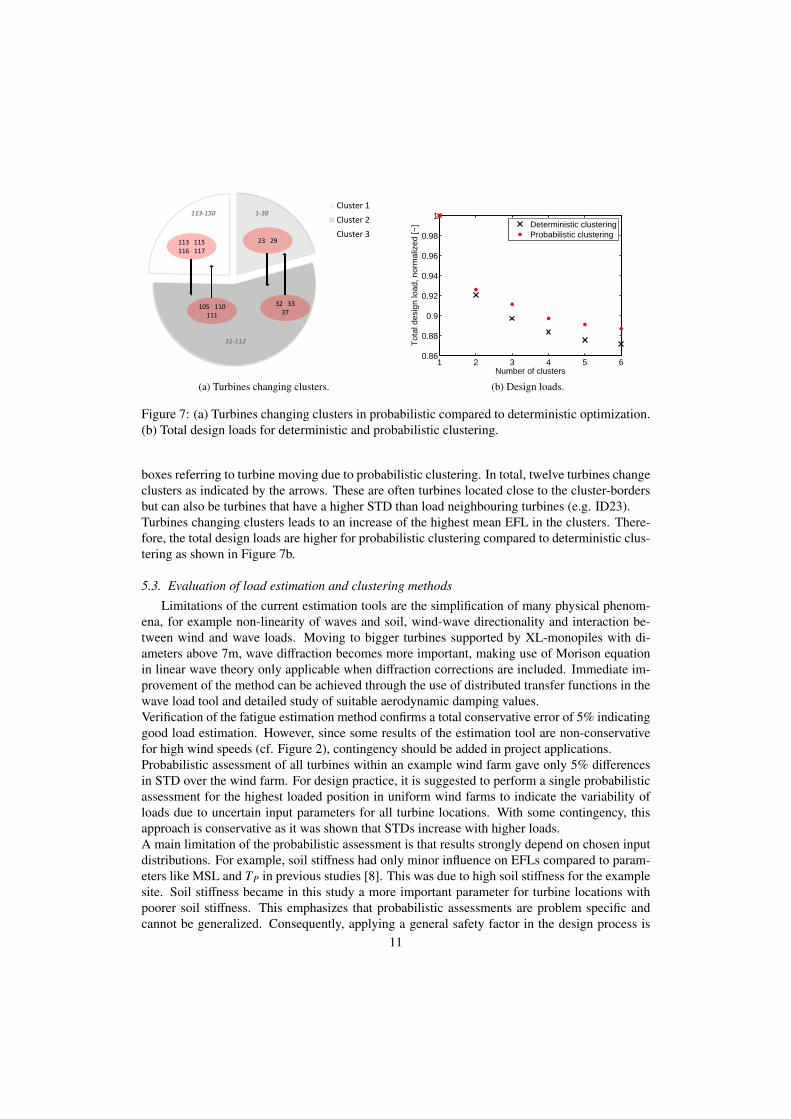
Cluster 1
Cluster 2
Cluster 3 113 115 116 117
32 33 37
105 110 111
23 29
113-150
31-112
1-30
(a) Turbines changing clusters.
1 2 3 4 5 60.86
0.88
0.9
0.92
0.94
0.96
0.98
1
Number of clusters
Tot
al d
esig
n lo
ad, n
orm
aliz
ed [−
]
Deterministic clusteringProbabilistic clustering
(b) Design loads.
Figure 7: (a) Turbines changing clusters in probabilistic compared to deterministic optimization.(b) Total design loads for deterministic and probabilistic clustering.
boxes referring to turbine moving due to probabilistic clustering. In total, twelve turbines changeclusters as indicated by the arrows. These are often turbines located close to the cluster-bordersbut can also be turbines that have a higher STD than load neighbouring turbines (e.g. ID23).Turbines changing clusters leads to an increase of the highest mean EFL in the clusters. There-fore, the total design loads are higher for probabilistic clustering compared to deterministic clus-tering as shown in Figure 7b.
5.3. Evaluation of load estimation and clustering methods
Limitations of the current estimation tools are the simplification of many physical phenom-ena, for example non-linearity of waves and soil, wind-wave directionality and interaction be-tween wind and wave loads. Moving to bigger turbines supported by XL-monopiles with di-ameters above 7m, wave diffraction becomes more important, making use of Morison equationin linear wave theory only applicable when diffraction corrections are included. Immediate im-provement of the method can be achieved through the use of distributed transfer functions in thewave load tool and detailed study of suitable aerodynamic damping values.Verification of the fatigue estimation method confirms a total conservative error of 5% indicatinggood load estimation. However, since some results of the estimation tool are non-conservativefor high wind speeds (cf. Figure 2), contingency should be added in project applications.Probabilistic assessment of all turbines within an example wind farm gave only 5% differencesin STD over the wind farm. For design practice, it is suggested to perform a single probabilisticassessment for the highest loaded position in uniform wind farms to indicate the variability ofloads due to uncertain input parameters for all turbine locations. With some contingency, thisapproach is conservative as it was shown that STDs increase with higher loads.A main limitation of the probabilistic assessment is that results strongly depend on chosen inputdistributions. For example, soil stiffness had only minor influence on EFLs compared to param-eters like MSL and TP in previous studies [8]. This was due to high soil stiffness for the examplesite. Soil stiffness became in this study a more important parameter for turbine locations withpoorer soil stiffness. This emphasizes that probabilistic assessments are problem specific andcannot be generalized. Consequently, applying a general safety factor in the design process is
11
not expedient for design optimization. Probabilistic load assessment can, combined with uncer-tainty in structural resistance, form a good decision-making basis for optimizing safety factors.For design clustering, the needs of industry are fast and robust tools, while nowadays larger windfarms typically have only 2-3 clusters. Brute-force optimization guarantees global optima atthe expense of solution time making it the best choice for up to 5 clusters for wind farms with100-150 turbines. For more clusters, the local search algorithm is recommended which showedvery good performance for solution quality and computational efficiency. For practice, a possibleconstraint in the optimization routine can be a limit on MSL difference within clusters so thatmonopile lengths can be kept constant for all cluster positions.In the probabilistic clustering example, only few turbines change cluster since the distribution ofSTDs follows that of EFLs relatively closely. Thus STDs are only of importance near cluster-borders. It can be concluded that deterministic clustering has good stability for uniform sites.
6. Conclusion and Recommendations
6.1. ConclusionFatigue load differences of 25% for 150 OWTs in 30-40m water depth showed the impor-
tance of site condition variations, making design clustering necessary. A developed probabilisticfatigue load estimation method proved to be suitable for site specific EFL estimation. A veri-fied accuracy of 95% with only seconds of computation time for one simulation case makes theestimation tool ideal for application in clustering optimization, load interpolation, uncertaintystudies and preliminary design. Based on EFL estimates, optimization of design clustering gavea reduction of up to 13% of total design loads compared to standardized design. This makesclustering an important approach in support structure cost reduction.By investigation of the marginal gain of adding additional clusters (cf. Figure 6b), the clusteringtool can improve decision-making on the optimal number of clusters of a wind farm in earlyproject phases and is strongly recommended for use in industry. An alternative application of thecombined load estimation and clustering tool is wind farm layout design. The layout is typicallyoptimized for power output through wake modeling and cable costs. Having this fast load esti-mation tool, support structure loads and costs can add a new dimension to layout optimization.
6.2. RecommendationsTwo main recommendations for the load estimation tool are: firstly, the verification study
should be extended to different structural and environmental settings. More precisely, studiesshould confirm the accuracy of the estimation method for different support structure eigenfre-quencies and in shallow water depths where wind loads have more influence. Ideally, the toolshould be validated on experimental data in the future. Secondly, resistance uncertainty shouldbe included in the probabilistic approach making it applicable for reliability-based design. Clus-tering can then be based on structural reliability instead of (probabilistic) design loads only.For clustering optimization the following recommendations are made:
• Extend the clustering algorithms for costs optimization.
• Test the local search algorithm for load distributions that feature significant local minima.
• Include load interpolation by formulating the objective function for minimum load dif-ference within clusters. Multi-objective optimization should be implemented to considerEFLs at multiple support structure levels.
12
REFERENCES
[1] Vorpahl, F., Schwarze, H., Fischer, T., Seidel, M. and Jonkman, J. (2013). Offshore wind turbine environment,loads, simulation, and design. Wiley Interdisciplinary Reviews: Energy and Environment, 2(5), 548-570.
[2] Seidel, M. (2014). Wave induced fatigue loads on monopiles - New approaches for lumping of scatter tables andsite specific interpolation of fatigue loads. Conference Proceedings IWEC 2014, Hannover, Germany.
[3] Fischer, T., De Vries, W. E. and Schmidt, B. (2010). Upwind design basis (WP4: offshore foundations and supportstructures). Upwind.
[4] International Electrotechnical Commission (2009). IEC 61400-3: Design requirements for offshore wind turbines.[5] Det Norske Veritas (2010). DNV-OS-J101: Design of offshore wind turbine structures.[6] Kuehn, M. J. (2001). Dynamics and design optimisation of offshore wind energy conversion systems. PhD thesis,
TU Delft, The Netherlands.[7] Van der Tempel, J. (2006). Design of support structures for offshore wind turbines. PhD thesis, TU Delft, The
Netherlands.[8] Ziegler, L., Voormeeren, S., Schafhirt, S. and Muskulus, M. (in press). Sensitivity of wave fatigue loads on offshore
wind turbines under varying site conditions. Energy Procedia.[9] Arany L., Bhattacharya S., Macdonald J. and Hogan S. J. (2014). Simplified critical mudline bending moment
spectra of offshore wind turbine support structures, Wind Energy. doi: 10.1002/we.1812.[10] Muskulus, M. (2015). Simplified rotor load models and fatigue damage estimates for offshore wind turbines.
Philosophical Transactions of the Royal Society of London A: Mathematical, Physical and Engineering Sciences,373(2035). doi: 10.1098/rsta.2014.0347.
[11] Zwick, D. and Muskulus, M. (2015). Simplified fatigue load assessment in offshore wind turbine structural analysis.Wind Energy. doi: 10.1002/we.1831.
[12] Seidel, M. (2014). Wave induced fatigue loads - Insights from frequency domain calculations. Stahlbau, 83, 535-541.
[13] Yeter, B., Garbatov, Y. and Soares, C. G. (2013). Spectral fatigue assessment of an offshore wind turbine structureunder wave and wind loading. Developments in Maritime Transportation and Exploitation of Sea Resources, 425-433. doi: 10.1201/b15813-52.
[14] Ragan, P. and Manuel, L. (2007). Comparing estimates of wind turbine fatigue loads using time-domain and spectralmethods. Wind engineering, 31(2), 83-99.
[15] Manuel, L., Veers, P. S. and Winterstein, S. R. (2001). Parametric models for estimating wind turbine fatigue loadsfor design. Journal of solar energy engineering, 123(4), 346-355.
[16] Mrsnik, M., Slavic, J. and Boltezar, M. (2013). Frequency-domain methods for a vibration-fatigue-life estimation-Application to real data. International journal of fatigue, 47, 8-17.
[17] Dirlik, T. (1985). Application of computers in fatigue analysis. PhD thesis, University of Warwick, England.[18] Manenti, S. and Petrini, F. (2010). Dynamic analysis of an offshore wind turbine: wind-waves nonlinear interaction.
Earth and Space, 2014-2026.[19] Frandsen, S., Barthelmie, R., Pryor, S., Rathmann, O., Larsen, S., Hjstrup, J. et al. (2006). Analytical modelling of
wind speed deficit in large offshore wind farms. Wind Energy, 9, 39-53. doi: 10.1002/we.189[20] Yeter, B., Garbatov, Y. and Guedes Soares, C. (2015). Fatigue reliability assessment of an offshore supporting
structure. The Maritime Technology and Engineering. Taylor & Francis Group, 671-680.[21] Veldkamp, H. F. (2006). Chances in Wind energy: a Probabilistic Approach to Wind Turbine Fatigue Design. PhD
thesis, TU Delft, The Netherlands.[22] Soares, C. G. (1990). Effect of spectral shape uncertainty in the short term wave-induced ship responses. Applied
Ocean Research, 12(2), 54-69.[23] De Vries, W. E., Vemula, N. K., Passon, P., Fischer, T., Kaufer, D., Matha, D. et al. (2011). Final report WP 4.2:
Support Structure Concepts for Deep Water Sites, tech. rep., Upwind.[24] Carswell, W., Arwade, S. R., DeGroot, D. J. and Lackner, M. A. (2014). Soil–structure reliability of offshore wind
turbine monopile foundations. Wind Energy, 18, 483-498. doi: 10.1002/we.1710.[25] Wolsey, L. A. and Nemhauser, G. L. (2014). Integer and combinatorial optimization. John Wiley & Sons.
13

Appendix C
Local search optimization
This appendix extends the explanation of the local search algorithm for solving theclustering optimization problem that is introduced in the paper “Design clustering ofoffshore wind turbines using probabilistic fatigue load estimation” in Appendix B. Thelocal search algorithm is implemented in the software environment R for statisticalcomputing.Figure C.1 presents the flowchart of the local search algorithm. The algorithm startswith the choice of number of clusters n. Secondly, a random initial guess about thenumber of turbines Ti in each cluster i is made. According to the initial guess, turbinesare sorted to clusters in load descending order. Afterwards, a random cluster-borderbi with i = 1...(n − 1)is selected. The total design loads TL are calculated for allpossible positions of the selected cluster-border, while keeping the remaining bordersconstant. For the selected border, (Ti+T(i+1)−1) possible positions exist between the twoneighboring, constant cluster-borders. Finally, the cluster-border is put on the positionwith the smallest TL value. The steps from selection of a cluster-boarder to putting iton the local optimum position form one iteration loop. After the local optimum cluster-border position is chosen, this border position is replaced by a random position with achance of 5% before the start of the next iteration. This avoids that the optimizationalgorithm is trapped in a local minimum with poor quality. The local search algorithmstops after a defined number of iterations.For the example case in paper B with 150 turbines, 100 iterations were sufficient for thealgorithm to reach the global minimum of the solution space or local minima with goodquality. Alternatively, a stopping criteria could be defined, when the solution convergesto a local minimum.An alternative solution approach to the clustering problem based on site-specific EFLs isthe application of standard continuous optimization solvers for nonlinear functions, forexample “fminsearch” in MATLAB R©. For this case, the discrete distribution of fatigueloads has to be approximated by a continuous function through interpolation. Theobtained solution must then be rounded to the nearest discrete value. This approachis comparable efficient, in terms of computation time, as the local search algorithm.However, for the example case of 150 turbines, it leads to a local optimum that is lessgood compared to results obtained with the discrete local search algorithm due to thecontinuous approximation and rounding.
103

104 C. LOCAL SEARCH OPTIMIZATION
Figure C.1: Flowchart of local search algorithm for clustering optimization.