Embed Size (px)
Citation preview
1Corrigés des exercices
Corrigé de l’exercice 12.
# version itérativedef palindrome(chaine):
i, n = 0, len(chaine) - 1while i < n and chaine[i] == chaine[n]:
i += 1n -= 1
return n <= i
print(palindrome('ressasser'), palindrome('ressassir'), palindrome('serres'))
True False True
# version récursivedef palindrome(chaine):
if len(chaine) <= 1:return True
if chaine[0] != chaine[-1]:return False
else:return palindrome(chaine[1:-1])
print(palindrome('ressasser'), palindrome('ressassir'), palindrome('serres'))
True False True
# variantedef palindrome(chaine):
return chaine == chaine[::-1]
print(palindrome('ressasser'), palindrome('ressassir'), palindrome('serres'))
True False True
2 Programmation en Python pour les mathématiques
Corrigé de l’exercice 13.
def champernowne(n):x = '0.'k = 0while len(x) <= n+2:
k += 1x += str(k)
return x[0:n+2]
print(champernowne(75))
# variante avec joindef champernowne(n):
return '0.' + ''.join(str(i) for i in range(1, n))[:n]
0.123456789101112131415161718192021222324252627282930313233343536373839404142
Corrigé de l’exercice 15.
def cosinus(x, epsilon):p = 0somme = 1terme = 1reste = abs(x)while reste > epsilon:
p += 2terme *= - x**2 / (p * (p - 1))somme += termereste *= abs(x)**2 / (p * (p + 1))
return somme
# Pour la vérification, on peut utiliser le module math :import math
print(cosinus(1, 1e-5))print(cosinus(1, 1e-14))print(math.cos(1))
print(cosinus(math.pi/4, 1e-5))print(cosinus(math.pi/4, 1e-14))print(math.sqrt(2)/2)
0.54030257936507930.54030230586813980.54030230586813980.70710680568329420.70710678118654750.7071067811865476
Corrigés des exercices 3
Corrigé de l’exercice 16.
def pythagoriciens(n):return [(x, y, z) for x in range(1, n) for y in range(x, n)
for z in range(y, n) if x**2 + y**2 == z**2]
print(pythagoriciens(101))print("Au total, on trouve {} triplets.".format(len(pythagoriciens(101))))
[(3, 4, 5), (5, 12, 13), (6, 8, 10), (7, 24, 25), (8, 15, 17), (9, 12, 15),(9, 40, 41), (10, 24, 26), (11, 60, 61), (12, 16, 20), (12, 35, 37),(13, 84, 85), (14, 48, 50), (15, 20, 25), (15, 36, 39), (16, 30, 34),(16, 63, 65), (18, 24, 30), (18, 80, 82), (20, 21, 29), (20, 48, 52),(21, 28, 35), (21, 72, 75), (24, 32, 40), (24, 45, 51), (24, 70, 74),(25, 60, 65), (27, 36, 45), (28, 45, 53), (28, 96, 100), (30, 40, 50),(30, 72, 78), (32, 60, 68), (33, 44, 55), (33, 56, 65), (35, 84, 91),(36, 48, 60), (36, 77, 85), (39, 52, 65), (39, 80, 89), (40, 42, 58),(40, 75, 85), (42, 56, 70), (45, 60, 75), (48, 55, 73), (48, 64, 80),(51, 68, 85), (54, 72, 90), (57, 76, 95), (60, 63, 87), (60, 80, 100),(65, 72, 97)]Au total, on trouve 52 triplets.
Corrigé de l’exercice 17.
for n in range(2, 20):print(' + '.join('{:2}^2'.format(i) for i in range(1, n))
+ ' = {}'.format(sum(i**2 for i in range(1, n))))
1^2 = 11^2 + 2^2 = 51^2 + 2^2 + 3^2 = 141^2 + 2^2 + 3^2 + 4^2 = 301^2 + 2^2 + 3^2 + 4^2 + 5^2 = 551^2 + 2^2 + 3^2 + 4^2 + 5^2 + 6^2 = 911^2 + 2^2 + 3^2 + 4^2 + 5^2 + 6^2 + 7^2 = 1401^2 + 2^2 + 3^2 + 4^2 + 5^2 + 6^2 + 7^2 + 8^2 = 2041^2 + 2^2 + 3^2 + 4^2 + 5^2 + 6^2 + 7^2 + 8^2 + 9^2 = 2851^2 + 2^2 + 3^2 + 4^2 + 5^2 + 6^2 + 7^2 + 8^2 + 9^2 + 10^2 = 3851^2 + 2^2 + 3^2 + 4^2 + 5^2 + 6^2 + 7^2 + 8^2 + 9^2 + 10^2 + 11^2 = 506[...]
Corrigé de l’exercice 18.
def parfait(n):return sum([d for d in range(1, n) if n % d == 0]) == n
def liste_parfaits(n):return [i for i in range(2, n) if parfait(i)]
4 Programmation en Python pour les mathématiques
print(liste_parfaits(10000))
def somme(n):diviseurs = [d for d in range(1, n) if n % d == 0]if sum(diviseurs) == n:
print('{} = '.format(n) + ' + '.join(str(d) for d in diviseurs))
for i in liste_parfaits(10000):somme(i)
[6, 28, 496, 8128]
6 = 1 + 2 + 328 = 1 + 2 + 4 + 7 + 14496 = 1 + 2 + 4 + 8 + 16 + 31 + 62 + 124 + 2488128 = 1 + 2 + 4 + 8 + 16 + 32 + 64 + 127 + 254 + 508 + 1016 + 2032 + 4064
Corrigé de l’exercice 19.
def crible(prems):if prems == []:
return []return [prems[0]] + crible([p for p in prems[1:] if p % prems[0] != 0])
print(crible(range(2, 1000)))
[2, 3, 5, 7, 11, 13, 17, 19, 23, 29, 31, 37, 41, 43, 47, 53, 59, 61, 67, 71, 73,79, 83, 89, 97, 101, 103, 107, 109, 113, 127, 131, 137, 139, 149, 151, 157,163, 167, 173, 179, 181, 191, 193, 197, 199, 211, 223, 227, 229, 233, 239,241, 251, 257, 263, 269, 271, 277, 281, 283, 293, 307, 311, 313, 317, 331,337, 347, 349, 353, 359, 367, 373, 379, 383, 389, 397, 401, 409, 419, 421,431, 433, 439, 443, 449, 457, 461, 463, 467, 479, 487, 491, 499, 503, 509,521, 523, 541, 547, 557, 563, 569, 571, 577, 587, 593, 599, 601, 607, 613,617, 619, 631, 641, 643, 647, 653, 659, 661, 673, 677, 683, 691, 701, 709,719, 727, 733, 739, 743, 751, 757, 761, 769, 773, 787, 797, 809, 811, 821,823, 827, 829, 839, 853, 857, 859, 863, 877, 881, 883, 887, 907, 911, 919,929, 937, 941, 947, 953, 967, 971, 977, 983, 991, 997]
2Corrigés des exercices
Corrigé de l’exercice 27.
import osimport sys
def parcours(repertoire):arborescence = os.walk(repertoire)
for dossier in arborescence:for fichier in dossier[2]:
if fichier.endswith('.py'):print(os.path.join(dossier[0], fichier))#variante : print(os.path.abspath(fichier))
if __name__ == "__main__":try:
parcours(sys.argv[1])except IndexError:
parcours(os.getcwd())
Corrigé de l’exercice 28.
from math import *import syssys.path.append('../../modules')from PostScript import *
def rectangle(base, k):[A, B] = basenorme = hypot(B[0] - A[0], B[1] - A[1])orthog = [A[1]-B[1], B[0]-A[0]]D = [a + k*u for (a, u) in zip(A, orthog)]C = [b + k*u for (b, u) in zip(B, orthog)]return [A, B, C, D]
6 Programmation en Python pour les mathématiques
def triangle(base, theta):[A, B] = baseC = [b - a for (a, b) in zip(A, B)]R = [(1+cos(2*theta))/2, sin(2*theta)/2]C = [R[0]*C[0] - R[1]*C[1],
R[1]*C[0] + R[0]*C[1]]C = [a + c for (a, c) in zip(A, C)]return [A, B, C]
def pythagore(base, k, theta, niveau, N=None):if N == None:
N = niveauq = niveau/Ncouleur = (q, 4*q*(1-q), (1-q)) # arbre multicolorerc = rectangle(base, k)graphique.ajouteCourbe(rc, couleur, fill=True)tr = triangle(rc[:-3:-1], theta)if niveau > 1:
pythagore([tr[0], tr[2]], k, theta, niveau - 1, N)pythagore([tr[2], tr[1]], k, theta, niveau - 1, N)
if __name__ == "__main__":N = 14base = [[0, 0], [2, 0]]nomFichier = "pythagore"boite = [-8, -1, 6, 9]zoom, marge, ratioY, trait = 30, 1.02, 1, 0.1graphique = Plot(nomFichier, boite, zoom, marge, ratioY)graphique.preambule()graphique.cadre()pythagore(base, 0.9, pi/6, N)graphique.fin()graphique.exportePDF()graphique.affichePS()
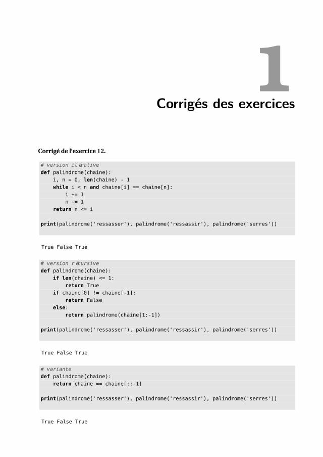
Corrigé de l’exercice 29.
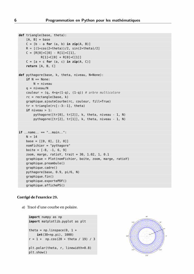
a) Tracé d’une courbe en polaire.
import numpy as npimport matplotlib.pyplot as plt
theta = np.linspace(0, 1 +int(38*np.pi), 1000)
r = 1 + np.cos(20 * theta / 19) / 3
plt.polar(theta, r, linewidth=0.8)plt.show()
0°
45°
90°
135°
180°
225°
270°
315°
0.20.4
0.60.8
1.01.2
1.4
Corrigés des exercices 7
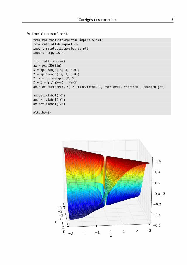
b) Tracé d’une surface 3D.
from mpl_toolkits.mplot3d import Axes3Dfrom matplotlib import cmimport matplotlib.pyplot as pltimport numpy as np
fig = plt.figure()ax = Axes3D(fig)X = np.arange(-3, 3, 0.07)Y = np.arange(-3, 3, 0.07)X, Y = np.meshgrid(X, Y)Z = X * Y / (X**2 + Y**2)ax.plot_surface(X, Y, Z, linewidth=0.1, rstride=1, cstride=1, cmap=cm.jet)
ax.set_xlabel('X')ax.set_ylabel('Y')ax.set_zlabel('Z')
plt.show()
X
3210123
Y3 2 1 0 1 2 3
Z
0.6
0.4
0.2
0.0
0.2
0.4
0.6
3Corrigés des exercices
Corrigé de l’exercice 40.
Maintenant, on effectue 7 multiplications matricielles (n3 multiplications élémentaires) mais18 additions (n2 additions élémentaires).Les multiplications matricielles étant plus coûteuses, théoriquement on gagne en efficacitépour les grandes matrices. On obtient en effet une complexité en Θ(nlog2 n) au lieu de Θ(n3).Si la taille des matrices n’est pas une racine de 2, on complète avec des zéros.On crée donc une fonction qui calcule la puissance de 2 directement supérieure :
def next_pow_2(x):return 2**(ceil(log(x)/log(2)))
Puis une fonction qui découpe une matrice en quatre blocs carrés après avoir complété avecdes zéros :matrice.py
def coupe_en_4(self):[r,c] = self.Dt = max(next_pow_2(r),next_pow_2(c))m = Mat([t,t], lambda i,j: self[i,j] if (i < r and j < c) else 0)s = t//2A = Mat([s, s], lambda i,j: m[i ,j ])B = Mat([s, s], lambda i,j: m[i ,j + s])C = Mat([s, s], lambda i,j: m[i + s,j ])D = Mat([s, s], lambda i,j: m[i + s,j + s])return(A,B,C,D)
Enfin, on applique les calculs de STRASSEN récursivement jusqu’à une limite de 32 (qui cor-respond théoriquement à la limite d’efficacité de l’algo par rapport au nombre d’additions quideviennent trop gourmandes) et on découpe la matrice obtenue selon la taille attendue :matrice.py
def strassen(self,other):ld = self.D + other.Dt = max(map(next_pow_2,ld))if t <= 32:
return self*othera,b,c,d = self.coupe_en_4()e,f,g,h = other.coupe_en_4()[li,co] = a.D
Corrigés des exercices 9
p1 = a.strassen(f - h)p2 = (a + b).strassen(h)p3 = (c + d).strassen(e)p4 = d.strassen(g - e)p5 = (a + d).strassen(e + h)p6 = (b - d).strassen(g + h)p7 = (c - a).strassen(e + f)w = p4 + p5 + p6 - p2x = p1 + p2y = p3 + p4z = p1 + p5 - p3 + p7def fs(i,j):
if i < li:if j < li:
return w.F(i,j)else:
return x.F(i,j - li)elif j < li:
return y.F(i - li,j)else:
return z.F(i - li,j - li)return Mat(self.D, fs)
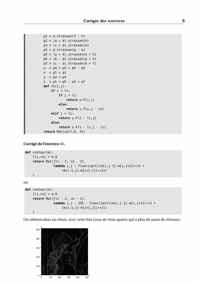
Corrigé de l’exercice 41.
def contour(m):[li,co] = m.Dreturn Mat([li - 2, co - 2],
lambda i,j : floor(sqrt((m[i,j-1]-m[i,j+1])**2 +(m[i-1,j]-m[i+1,j])**2))
)
ou
def contour(m):[li,co] = m.Dreturn Mat([li - 2, co - 2],
lambda i,j : 255 - floor(sqrt((m[i,j-1]-m[i,j+1])**2 +(m[i-1,j]-m[i+1,j])**2))
)
On obtient alors au choix, avec cette fois Lena de trois-quarts qui a plus de sauts de niveaux :
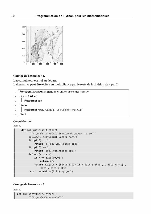
10 Programmation en Python pour les mathématiques
Corrigé de l’exercice 44.
L’accumulateur est nul au départ.L’alternative peut être évitée en multipliant y par le reste de la division de x par 2
1 Fonction MULRUSSE( x:entier ,y: entier, acc:entier ):entier
2 Si x == 0 Alors3 Retourner acc
4 Sinon5 Retourner MULRUSSE(x // 2, y*2, acc + y*(x % 2))
6 FinSi
Ce qui donne :
Bits.py
def mul_russe(self,other):"""Algo de la multiplication du paysan russe"""op1,op2 = self.norm(),other.norm()if op1[0] == 1:
return -((-op1).mul_russe(op2))if op2[0] == 1:
return -(op1.mul_russe(-op2))def aux(acc,x,y):
if x == Bits([0,0]):return acc
return aux(acc + (Bits([0,0]) if x.pair() else y), Bits(x[:-1]),Bits(y.bits + [0]))
return aux(Bits([0,0]),op1,op2)
Corrigé de l’exercice 45.
Bits.py
def mul_karat(self, other):"""Algo de Karatsouba"""
Corrigés des exercices 11
op1,op2 = self.norm(),other.norm()if op1.signe() == 1:
return -((-op1).mul_karat(op2))if op2.signe() == 1:
return -(op1.mul_karat(-op2))long = max(len(op1), len(op2))op1 = Bits([0 for i in range(len(op1), long)] + op1.bits)op2 = Bits([0 for i in range(len(op2), long)] + op2.bits)
if long <= 2:return Bits([0, op1[1] & op2[1]])
m0 = (long + 1) >> 1m1 = long >> 1
x0 = Bits([0] + op1[ : m0]).norm()x1 = Bits([0] + op1[m0 : ]).norm()y0 = Bits([0] + op2[ : m0]).norm()y1 = Bits([0] + op2[m0 : ]).norm()
p0 = x0.mul_karat(y0)p1 = (x0 - x1).mul_divis(y0 - y1)p2 = x1.mul_divis(y1)
z0 = Bits(p0.bits + [0 for i in range(0, m1 << 1)])z1 = Bits((p0 + p2 - p1).bits + [0 for i in range(0, m1)])z2 = p2
return z0 + z1 + z2
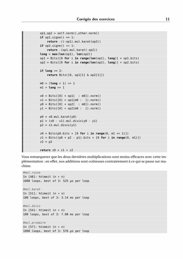
Vous remarquerez que les deux dernières multiplications sont moins efficaces avec cette im-plémentation : en effet, nos additions sont coûteuses contrairement à ce qui se passe sur ma-chine.
#mul_russeIn [48]: %timeit (n * n)1000 loops, best of 3: 525 µs per loop
#mul_karatIn [51]: %timeit (n * n)100 loops, best of 3: 3.14 ms per loop
#mul_divisIn [54]: %timeit (n * n)100 loops, best of 3: 7.08 ms per loop
#mul_primaireIn [57]: %timeit (n * n)1000 loops, best of 3: 576 µs per loop
12 Programmation en Python pour les mathématiques
Corrigé de l’exercice 46.
On se rappelle que les 5 heures 48’55” sont causes de la création des années bissextiles : lesannées dont les millésimes sont des multiples de 4 ont 366 jours sauf les fins de siècles qui nesont pas des multiples de 400 mais cela reste approximatif.En étudiant les fractions continues, Grégoire XIII aurait pu être plus précis. Pour cela, étudionsla suite des différences des réduites successives.
In [1]: F = rationnel(5,24) + rationnel(48,24*60) + rationnel(55,24*60*60)In [2]: Q = fci(F)In [3]: [reduite(k + 1, Q) - reduite(k, Q) for k in range(7)]Out[3]: [1 / 4, -1 / 116, 1 / 957, -1 / 7491, 1 / 59020, -1 / 194220, 1 / 1310238]
Ainsi qu’une année est égale en jours à :
365+ 1
4− 1
116+ 1
957− 1
7 491+ 1
59 020− 1
194 220+ 1
1 310 238+·· ·
On obtient ainsi que tous les 4 ans il faut rajouter un jour, en enlever 1 tous les 116 ans, enrajouter 1 tous les 957 ans, etc.
Corrigé de l’exercice 47.
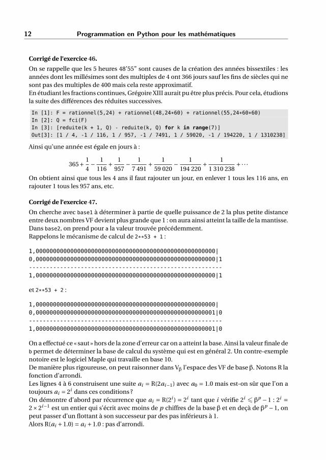
On cherche avec base1 à déterminer à partie de quelle puissance de 2 la plus petite distanceentre deux nombres VF devient plus grande que 1 : on aura ainsi atteint la taille de la mantisse.Dans base2, on prend pour a la valeur trouvée précédemment.Rappelons le mécanisme de calcul de 2**53 + 1 :
1,0000000000000000000000000000000000000000000000000000|0,0000000000000000000000000000000000000000000000000000|1--------------------------------------------------------1,0000000000000000000000000000000000000000000000000000|1
et 2**53 + 2 :
1,0000000000000000000000000000000000000000000000000000|0,0000000000000000000000000000000000000000000000000001|0--------------------------------------------------------1,0000000000000000000000000000000000000000000000000001|0
On a effectué ce « saut » hors de la zone d’erreur car on a atteint la base. Ainsi la valeur finale deb permet de déterminer la base de calcul du système qui est en général 2. Un contre-exemplenotoire est le logiciel Maple qui travaille en base 10.De manière plus rigoureuse, on peut raisonner dans Vβ l’espace des VF de base β. Notons R lafonction d’arrondi.Les lignes 4 à 6 construisent une suite ai = R(2ai−1) avec a0 = 1.0 mais est-on sûr que l’on atoujours ai = 2i dans ces conditions ?On démontre d’abord par récurrence que ai = R(2i ) = 2i tant que i vérifie 2i 6 βp −1 : 2i =2×2i−1 est un entier qui s’écrit avec moins de p chiffres de la base β et en deçà de βp −1, onpeut passer d’un flottant à son successeur par des pas inférieurs à 1.Alors R(ai +1.0) = ai +1.0 : pas d’arrondi.
Corrigés des exercices 13
Puis R(R(ai + 1.0)− ai ) = R(ai + 1.0− ai ) = 1.0 : la condition de la première boucle est doncvérifiée tant que 2i < βp . Que se passe-t-il après ?Dès que βp −1 est atteint, les choses changent.Considérons la première itération is telle que 2is > βp .On a
ais = R(2×ais−1) = R(2×2is−1) < R(2×βp )6R(β×βp ) = βp+1
car d’une part ais−1 = 2is−1, d’autre part ais−1 6 βp −1 < βp et enfin 26 β.Ainsi
βp 6 ais < βp+1
L’exposant de la forme normale de ais est donc p et le successeur d’un VF v vérifie (en notantn = p −1 la longueur de la pseudo-mantisse) :
succ(v) = v +βE(v)−n = v +βE(v)−p+1
Ici succ(ais ) = ais +βE(ais −p+1) = ais +βp−p+1 = ais +β.On en déduit que ais +1.0 est entre ais et son successeur ais +β.Donc, selon l’arrondi, R(ais +1.0) vaut ais ou ais +β et finalement R(R(ais +1.0)− ais ) vaut 0ou β mais en aucun cas 1.0 : on sort donc de la boucle.
On en déduit que boucle1 1 vaut ais donc que βp 6 boucle1 1 < βp+1
Notons a = boucle1 1. Son successeur est a +β.On démontre alors la seconde boucle.Cette démonstration est plutôt technique et difficile en première lecture. Cependant elle estpleine d’enseignements :
– elle nous montre bien que nous changeons de monde : un test du style if (a + 1.0)-
a /= 1.0 paraîtrait bien hors de propos si nous raisonnions avec des réels ;
– nous avons vu que l’on pouvait raisonner rigoureusement sur les VF ;
– nous pouvons malgré tout retenir la trame intuitive de la démonstration : tant que notrenombre entier est représentable avec p chiffres, on reste exact. Les problèmes arriventlorsqu’on n’a plus assez de place pour stocker tous les chiffres : il y a de la perte d’infor-mation...
– Ce genre de raisonnement se retrouve très souvent pour travailler sur les erreurs com-mises : il faudra donc en retenir la substantifique moelle...
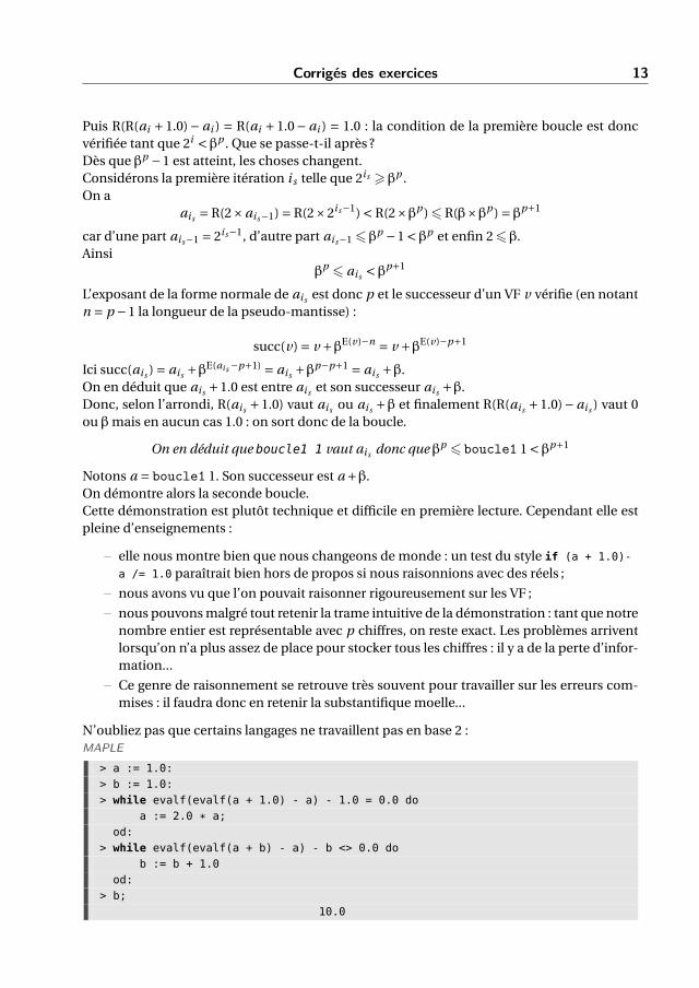
N’oubliez pas que certains langages ne travaillent pas en base 2 :MAPLE
> a := 1.0:> b := 1.0:> while evalf(evalf(a + 1.0) - a) - 1.0 = 0.0 do
a := 2.0 * a;od:
> while evalf(evalf(a + b) - a) - b <> 0.0 dob := b + 1.0
od:> b;
10.0
14 Programmation en Python pour les mathématiques
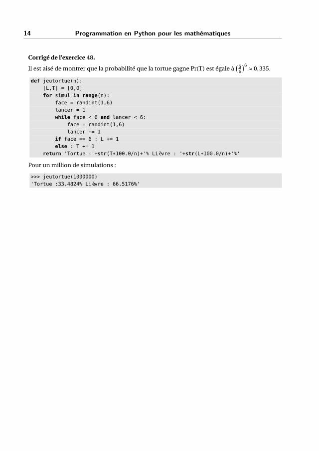
Corrigé de l’exercice 48.
Il est aisé de montrer que la probabilité que la tortue gagne Pr(T) est égale à( 5
6
)6 ≈ 0,335.
def jeutortue(n):[L,T] = [0,0]for simul in range(n):
face = randint(1,6)lancer = 1while face < 6 and lancer < 6:
face = randint(1,6)lancer += 1
if face == 6 : L += 1else : T += 1
return 'Tortue :'+str(T*100.0/n)+'% Lièvre : '+str(L*100.0/n)+'%'
Pour un million de simulations :
>>> jeutortue(1000000)'Tortue :33.4824% Lièvre : 66.5176%'
4Corrigés des exercices
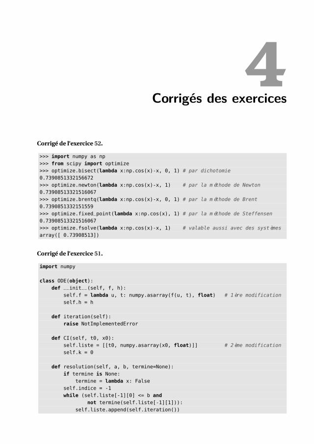
Corrigé de l’exercice 52.
>>> import numpy as np>>> from scipy import optimize>>> optimize.bisect(lambda x:np.cos(x)-x, 0, 1) # par dichotomie0.7390851332156672>>> optimize.newton(lambda x:np.cos(x)-x, 1) # par la méthode de Newton0.73908513321516067>>> optimize.brentq(lambda x:np.cos(x)-x, 0, 1) # par la méthode de Brent0.7390851332151559>>> optimize.fixed_point(lambda x:np.cos(x), 1) # par la méthode de Steffensen0.73908513321516067>>> optimize.fsolve(lambda x:np.cos(x)-x, 1) # valable aussi avec des systèmesarray([ 0.73908513])
Corrigé de l’exercice 51.
import numpy
class ODE(object):def __init__(self, f, h):
self.f = lambda u, t: numpy.asarray(f(u, t), float) # 1ère modificationself.h = h
def iteration(self):raise NotImplementedError
def CI(self, t0, x0):self.liste = [[t0, numpy.asarray(x0, float)]] # 2ème modificationself.k = 0
def resolution(self, a, b, termine=None):if termine is None:
termine = lambda x: Falseself.indice = -1while (self.liste[-1][0] <= b and
not termine(self.liste[-1][1])):self.liste.append(self.iteration())
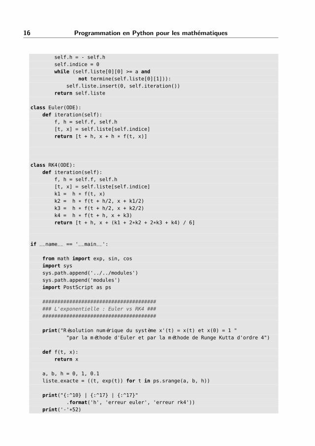
16 Programmation en Python pour les mathématiques
self.h = - self.hself.indice = 0while (self.liste[0][0] >= a and
not termine(self.liste[0][1])):self.liste.insert(0, self.iteration())
return self.liste
class Euler(ODE):def iteration(self):
f, h = self.f, self.h[t, x] = self.liste[self.indice]return [t + h, x + h * f(t, x)]
class RK4(ODE):def iteration(self):
f, h = self.f, self.h[t, x] = self.liste[self.indice]k1 = h * f(t, x)k2 = h * f(t + h/2, x + k1/2)k3 = h * f(t + h/2, x + k2/2)k4 = h * f(t + h, x + k3)return [t + h, x + (k1 + 2*k2 + 2*k3 + k4) / 6]
if __name__ == '__main__':
from math import exp, sin, cosimport syssys.path.append('../../modules')sys.path.append('modules')import PostScript as ps
######################################### L'exponentielle : Euler vs RK4 #########################################
print("Résolution numérique du système x'(t) = x(t) et x(0) = 1 ""par la méthode d'Euler et par la méthode de Runge Kutta d'ordre 4")
def f(t, x):return x
a, b, h = 0, 1, 0.1liste_exacte = ((t, exp(t)) for t in ps.srange(a, b, h))
print("{:^10} | {:^17} | {:^17}".format('h', 'erreur euler', 'erreur rk4'))
print('-'*52)
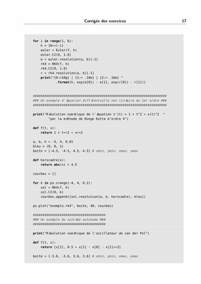
Corrigés des exercices 17
for i in range(1, 6):h = 10**(-i)euler = Euler(f, h)euler.CI(0, 1.0)e = euler.resolution(a, b)[-1]rk4 = RK4(f, h)rk4.CI(0, 1.0)r = rk4.resolution(a, b)[-1]print("{0:>10g} | {1:> .10e} | {2:> .10e} "
.format(h, exp(e[0]) - e[1], exp(r[0]) - r[1]))
######################################################################### Un exemple d'équation différentielle non linéaire du 1er ordre #########################################################################
print("Résolution numérique de l'équation x'(t) = 1 + t^2 * x(t)^2 ""par la méthode de Runge Kutta d'ordre 4")
def f(t, x):return 1 + t**2 * x**2
a, b, h = -4, 4, 0.01bleu = (0, 0, 1)boite = [-4.5, -4.5, 4.5, 4.5] # xmin, ymin, xmax, ymax
def horscadre(x):return abs(x) > 4.5
courbes = []
for k in ps.srange(-4, 4, 0.2):sol = RK4(f, h)sol.CI(0, k)courbes.append([sol.resolution(a, b, horscadre), bleu])
ps.plot("exemple_rk4", boite, 40, courbes)
######################################### Un exemple de système autonome #########################################
print("Résolution numérique de l'oscillateur de van der Pol")
def f(t, x):return [x[1], 0.5 * x[1] - x[0] - x[1]**3]
boite = [-3.6, -3.6, 3.6, 3.6] # xmin, ymin, xmax, ymax
18 Programmation en Python pour les mathématiques
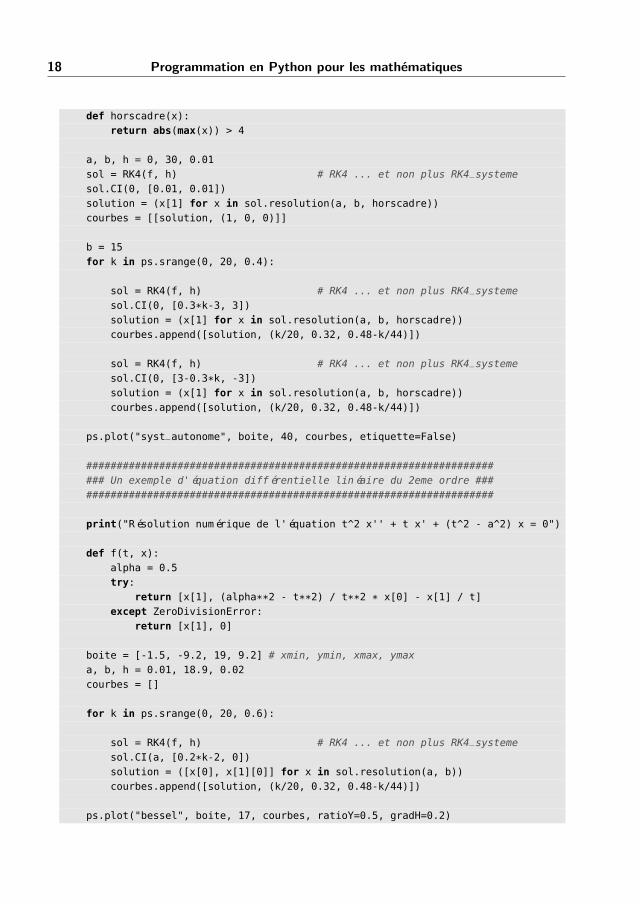
def horscadre(x):return abs(max(x)) > 4
a, b, h = 0, 30, 0.01sol = RK4(f, h) # RK4 ... et non plus RK4_systemesol.CI(0, [0.01, 0.01])solution = (x[1] for x in sol.resolution(a, b, horscadre))courbes = [[solution, (1, 0, 0)]]
b = 15for k in ps.srange(0, 20, 0.4):
sol = RK4(f, h) # RK4 ... et non plus RK4_systemesol.CI(0, [0.3*k-3, 3])solution = (x[1] for x in sol.resolution(a, b, horscadre))courbes.append([solution, (k/20, 0.32, 0.48-k/44)])
sol = RK4(f, h) # RK4 ... et non plus RK4_systemesol.CI(0, [3-0.3*k, -3])solution = (x[1] for x in sol.resolution(a, b, horscadre))courbes.append([solution, (k/20, 0.32, 0.48-k/44)])
ps.plot("syst_autonome", boite, 40, courbes, etiquette=False)
###################################################################### Un exemple d'équation différentielle linéaire du 2eme ordre ######################################################################
print("Résolution numérique de l'équation t^2 x'' + t x' + (t^2 - a^2) x = 0")
def f(t, x):alpha = 0.5try:
return [x[1], (alpha**2 - t**2) / t**2 * x[0] - x[1] / t]except ZeroDivisionError:
return [x[1], 0]
boite = [-1.5, -9.2, 19, 9.2] # xmin, ymin, xmax, ymaxa, b, h = 0.01, 18.9, 0.02courbes = []
for k in ps.srange(0, 20, 0.6):
sol = RK4(f, h) # RK4 ... et non plus RK4_systemesol.CI(a, [0.2*k-2, 0])solution = ([x[0], x[1][0]] for x in sol.resolution(a, b))courbes.append([solution, (k/20, 0.32, 0.48-k/44)])
ps.plot("bessel", boite, 17, courbes, ratioY=0.5, gradH=0.2)
Corrigés des exercices 19
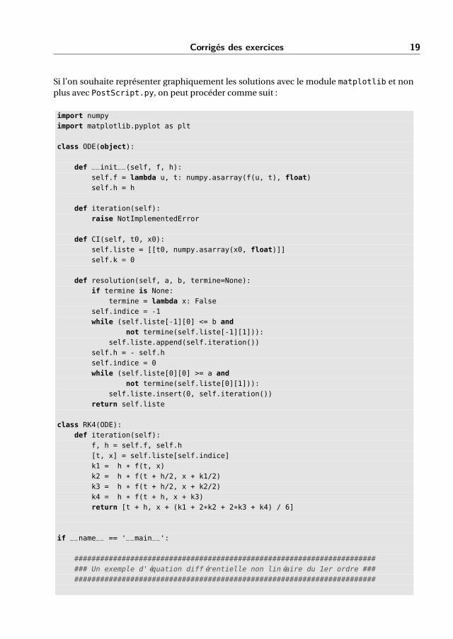
Si l’on souhaite représenter graphiquement les solutions avec le module matplotlib et nonplus avec PostScript.py, on peut procéder comme suit :
import numpyimport matplotlib.pyplot as plt
class ODE(object):
def __init__(self, f, h):self.f = lambda u, t: numpy.asarray(f(u, t), float)self.h = h
def iteration(self):raise NotImplementedError
def CI(self, t0, x0):self.liste = [[t0, numpy.asarray(x0, float)]]self.k = 0
def resolution(self, a, b, termine=None):if termine is None:
termine = lambda x: Falseself.indice = -1while (self.liste[-1][0] <= b and
not termine(self.liste[-1][1])):self.liste.append(self.iteration())
self.h = - self.hself.indice = 0while (self.liste[0][0] >= a and
not termine(self.liste[0][1])):self.liste.insert(0, self.iteration())
return self.liste
class RK4(ODE):def iteration(self):
f, h = self.f, self.h[t, x] = self.liste[self.indice]k1 = h * f(t, x)k2 = h * f(t + h/2, x + k1/2)k3 = h * f(t + h/2, x + k2/2)k4 = h * f(t + h, x + k3)return [t + h, x + (k1 + 2*k2 + 2*k3 + k4) / 6]
if __name__ == '__main__':
######################################################################### Un exemple d'équation différentielle non linéaire du 1er ordre #########################################################################
20 Programmation en Python pour les mathématiques
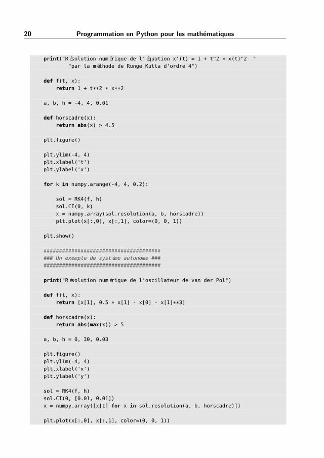
print("Résolution numérique de l'équation x'(t) = 1 + t^2 * x(t)^2 ""par la méthode de Runge Kutta d'ordre 4")
def f(t, x):return 1 + t**2 * x**2
a, b, h = -4, 4, 0.01
def horscadre(x):return abs(x) > 4.5
plt.figure()
plt.ylim(-4, 4)plt.xlabel('t')plt.ylabel('x')
for k in numpy.arange(-4, 4, 0.2):
sol = RK4(f, h)sol.CI(0, k)x = numpy.array(sol.resolution(a, b, horscadre))plt.plot(x[:,0], x[:,1], color=(0, 0, 1))
plt.show()
######################################### Un exemple de système autonome #########################################
print("Résolution numérique de l'oscillateur de van der Pol")
def f(t, x):return [x[1], 0.5 * x[1] - x[0] - x[1]**3]
def horscadre(x):return abs(max(x)) > 5
a, b, h = 0, 30, 0.03
plt.figure()plt.ylim(-4, 4)plt.xlabel('x')plt.ylabel('y')
sol = RK4(f, h)sol.CI(0, [0.01, 0.01])x = numpy.array([x[1] for x in sol.resolution(a, b, horscadre)])
plt.plot(x[:,0], x[:,1], color=(0, 0, 1))
Corrigés des exercices 21
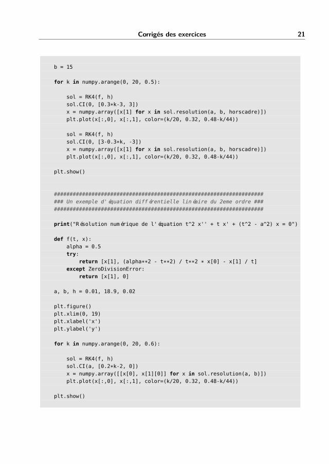
b = 15
for k in numpy.arange(0, 20, 0.5):
sol = RK4(f, h)sol.CI(0, [0.3*k-3, 3])x = numpy.array([x[1] for x in sol.resolution(a, b, horscadre)])plt.plot(x[:,0], x[:,1], color=(k/20, 0.32, 0.48-k/44))
sol = RK4(f, h)sol.CI(0, [3-0.3*k, -3])x = numpy.array([x[1] for x in sol.resolution(a, b, horscadre)])plt.plot(x[:,0], x[:,1], color=(k/20, 0.32, 0.48-k/44))
plt.show()
###################################################################### Un exemple d'équation différentielle linéaire du 2eme ordre ######################################################################
print("Résolution numérique de l'équation t^2 x'' + t x' + (t^2 - a^2) x = 0")
def f(t, x):alpha = 0.5try:
return [x[1], (alpha**2 - t**2) / t**2 * x[0] - x[1] / t]except ZeroDivisionError:
return [x[1], 0]
a, b, h = 0.01, 18.9, 0.02
plt.figure()plt.xlim(0, 19)plt.xlabel('x')plt.ylabel('y')
for k in numpy.arange(0, 20, 0.6):
sol = RK4(f, h)sol.CI(a, [0.2*k-2, 0])x = numpy.array([[x[0], x[1][0]] for x in sol.resolution(a, b)])plt.plot(x[:,0], x[:,1], color=(k/20, 0.32, 0.48-k/44))
plt.show()
22 Programmation en Python pour les mathématiques
3 2 1 0 1 2 3t
4
3
2
1
0
1
2
3
4
x
4 3 2 1 0 1 2 3 4x
4
3
2
1
0
1
2
3
4
y
0 5 10 15x
10
5
0
5
10
y
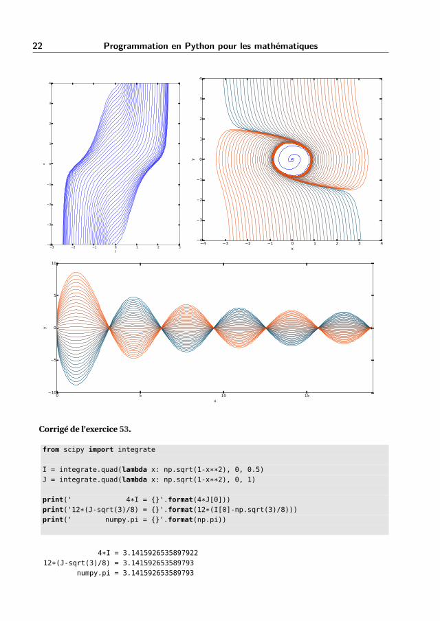
Corrigé de l’exercice 53.
from scipy import integrate
I = integrate.quad(lambda x: np.sqrt(1-x**2), 0, 0.5)J = integrate.quad(lambda x: np.sqrt(1-x**2), 0, 1)
print(' 4*I = {}'.format(4*J[0]))print('12*(J-sqrt(3)/8) = {}'.format(12*(I[0]-np.sqrt(3)/8)))print(' numpy.pi = {}'.format(np.pi))
4*I = 3.141592653589792212*(J-sqrt(3)/8) = 3.141592653589793
numpy.pi = 3.141592653589793
Corrigés des exercices 23
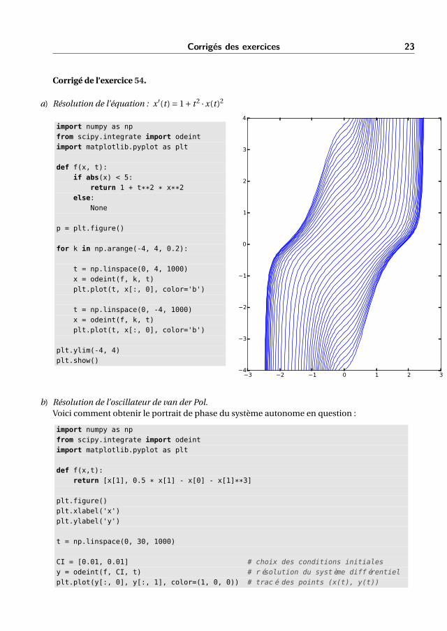
Corrigé de l’exercice 54.
a) Résolution de l’équation : x ′(t ) = 1+ t 2 · x(t )2
import numpy as npfrom scipy.integrate import odeintimport matplotlib.pyplot as plt
def f(x, t):if abs(x) < 5:
return 1 + t**2 * x**2else:
None
p = plt.figure()
for k in np.arange(-4, 4, 0.2):
t = np.linspace(0, 4, 1000)x = odeint(f, k, t)plt.plot(t, x[:, 0], color='b')
t = np.linspace(0, -4, 1000)x = odeint(f, k, t)plt.plot(t, x[:, 0], color='b')
plt.ylim(-4, 4)plt.show()
3 2 1 0 1 2 34
3
2
1
0
1
2
3
4
b) Résolution de l’oscillateur de van der Pol.Voici comment obtenir le portrait de phase du système autonome en question :
import numpy as npfrom scipy.integrate import odeintimport matplotlib.pyplot as plt
def f(x,t):return [x[1], 0.5 * x[1] - x[0] - x[1]**3]
plt.figure()plt.xlabel('x')plt.ylabel('y')
t = np.linspace(0, 30, 1000)
CI = [0.01, 0.01] # choix des conditions initialesy = odeint(f, CI, t) # résolution du système différentielplt.plot(y[:, 0], y[:, 1], color=(1, 0, 0)) # tracé des points (x(t), y(t))
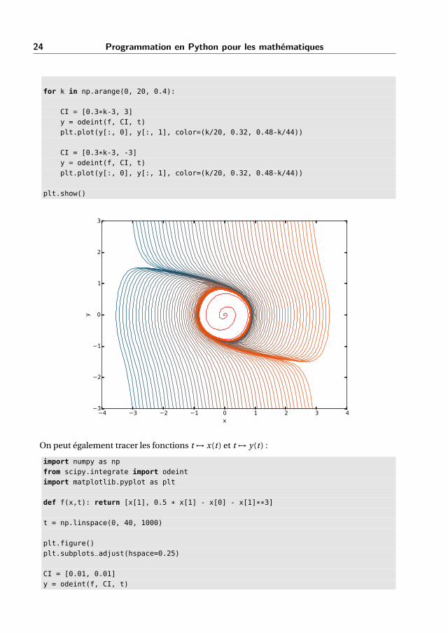
24 Programmation en Python pour les mathématiques
for k in np.arange(0, 20, 0.4):
CI = [0.3*k-3, 3]y = odeint(f, CI, t)plt.plot(y[:, 0], y[:, 1], color=(k/20, 0.32, 0.48-k/44))
CI = [0.3*k-3, -3]y = odeint(f, CI, t)plt.plot(y[:, 0], y[:, 1], color=(k/20, 0.32, 0.48-k/44))
plt.show()
4 3 2 1 0 1 2 3 4x
3
2
1
0
1
2
3
y
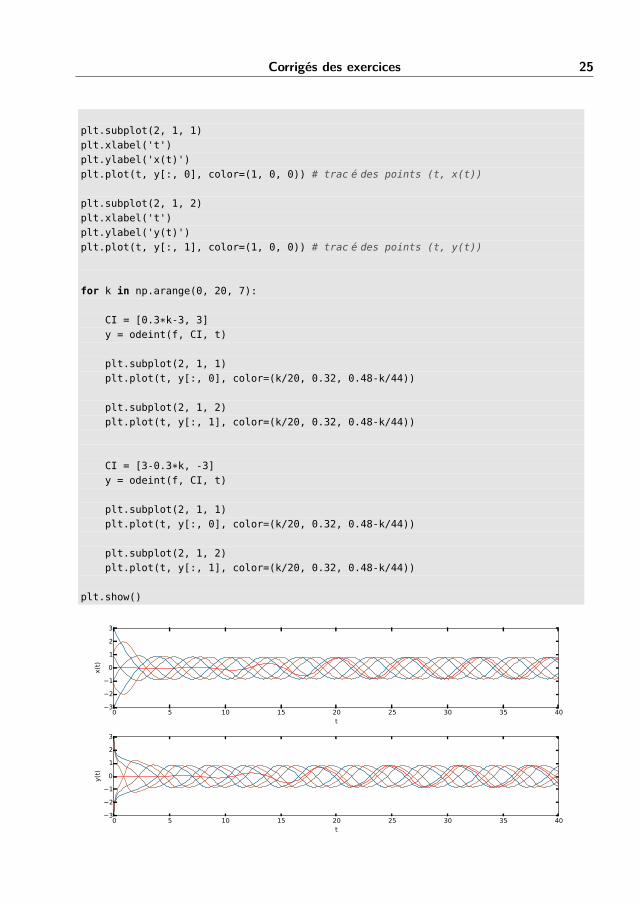
On peut également tracer les fonctions t 7→ x(t ) et t 7→ y(t ) :
import numpy as npfrom scipy.integrate import odeintimport matplotlib.pyplot as plt
def f(x,t): return [x[1], 0.5 * x[1] - x[0] - x[1]**3]
t = np.linspace(0, 40, 1000)
plt.figure()plt.subplots_adjust(hspace=0.25)
CI = [0.01, 0.01]y = odeint(f, CI, t)
Corrigés des exercices 25
plt.subplot(2, 1, 1)plt.xlabel('t')plt.ylabel('x(t)')plt.plot(t, y[:, 0], color=(1, 0, 0)) # tracé des points (t, x(t))
plt.subplot(2, 1, 2)plt.xlabel('t')plt.ylabel('y(t)')plt.plot(t, y[:, 1], color=(1, 0, 0)) # tracé des points (t, y(t))
for k in np.arange(0, 20, 7):
CI = [0.3*k-3, 3]y = odeint(f, CI, t)
plt.subplot(2, 1, 1)plt.plot(t, y[:, 0], color=(k/20, 0.32, 0.48-k/44))
plt.subplot(2, 1, 2)plt.plot(t, y[:, 1], color=(k/20, 0.32, 0.48-k/44))
CI = [3-0.3*k, -3]y = odeint(f, CI, t)
plt.subplot(2, 1, 1)plt.plot(t, y[:, 0], color=(k/20, 0.32, 0.48-k/44))
plt.subplot(2, 1, 2)plt.plot(t, y[:, 1], color=(k/20, 0.32, 0.48-k/44))
plt.show()
0 5 10 15 20 25 30 35 40t
3
2
1
0
1
2
3
x(t)
0 5 10 15 20 25 30 35 40t
3
2
1
0
1
2
3
y(t)
26 Programmation en Python pour les mathématiques
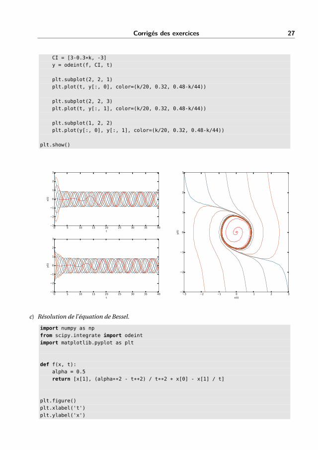
Les trois graphiques précédents peuvent être construits simultanément et placés dans ununique objet plt.figure().
import numpy as npfrom scipy.integrate import odeintimport matplotlib.pyplot as plt
def f(x,t):return [x[1], 0.5 * x[1] - x[0] - x[1]**3]
t = np.linspace(0, 40, 1000)
plt.figure()plt.subplots_adjust(hspace=0.25,wspace=0.3)
CI = [0.01, 0.01]y = odeint(f, CI, t)
plt.subplot(2, 2, 1)plt.xlabel('t')plt.ylabel('x(t)')plt.plot(t, y[:, 0], color=(1, 0, 0))
plt.subplot(2, 2, 3)plt.xlabel('t')plt.ylabel('y(t)')plt.plot(t, y[:, 1], color=(1, 0, 0))
plt.subplot(1, 2, 2)plt.xlabel('x(t)')plt.ylabel('y(t)')plt.plot(y[:, 0], y[:, 1], color=(1, 0, 0))
for k in np.arange(0, 20, 4):
CI = [0.3*k-3, 3]y = odeint(f, CI, t)
plt.subplot(2, 2, 1)plt.plot(t, y[:, 0], color=(k/20, 0.32, 0.48-k/44))
plt.subplot(2, 2, 3)plt.plot(t, y[:, 1], color=(k/20, 0.32, 0.48-k/44))
plt.subplot(1, 2, 2)plt.plot(y[:, 0], y[:, 1], color=(k/20, 0.32, 0.48-k/44))
Corrigés des exercices 27
CI = [3-0.3*k, -3]y = odeint(f, CI, t)
plt.subplot(2, 2, 1)plt.plot(t, y[:, 0], color=(k/20, 0.32, 0.48-k/44))
plt.subplot(2, 2, 3)plt.plot(t, y[:, 1], color=(k/20, 0.32, 0.48-k/44))
plt.subplot(1, 2, 2)plt.plot(y[:, 0], y[:, 1], color=(k/20, 0.32, 0.48-k/44))
plt.show()
0 5 10 15 20 25 30 35 40t
3
2
1
0
1
2
3
x(t)
0 5 10 15 20 25 30 35 40t
3
2
1
0
1
2
3
y(t)
3 2 1 0 1 2 3x(t)
3
2
1
0
1
2
3y(
t)
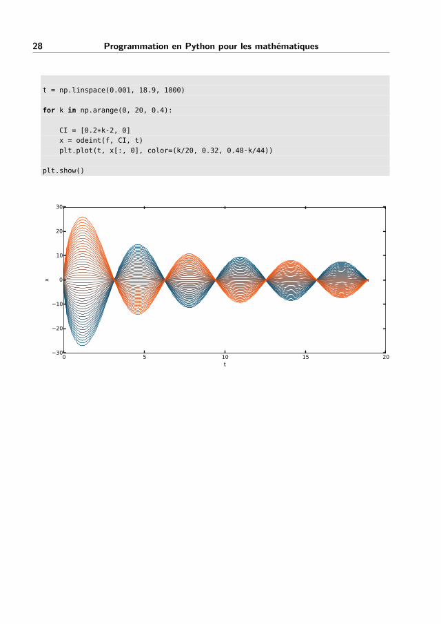
c) Résolution de l’équation de Bessel.
import numpy as npfrom scipy.integrate import odeintimport matplotlib.pyplot as plt
def f(x, t):alpha = 0.5return [x[1], (alpha**2 - t**2) / t**2 * x[0] - x[1] / t]
plt.figure()plt.xlabel('t')plt.ylabel('x')
28 Programmation en Python pour les mathématiques
t = np.linspace(0.001, 18.9, 1000)
for k in np.arange(0, 20, 0.4):
CI = [0.2*k-2, 0]x = odeint(f, CI, t)plt.plot(t, x[:, 0], color=(k/20, 0.32, 0.48-k/44))
plt.show()
0 5 10 15 20t
30
20
10
0
10
20
30
x
5Corrigés des exercices
Corrigé de l’exercice 60.
table.py
def table(multiplicande, multiplicateur):if multiplicateur > 0:
table(multiplicande, multiplicateur - 1)
print("{0:4d} * {1:4d} = {2}".format(\multiplicande, multiplicateur, multiplicande * multiplicateur))
table(7, 10)
L’ordre décroissant s’obtient simplement en inversant le test if et le corps de la boucle, réduitdans cet exemple à l’instruction print() :tabledec.py
def table_decroissante(multiplicande, multiplicateur):print("{0:4d} * {1:4d} = {2}".format(\
multiplicande, multiplicateur, multiplicande * multiplicateur))
if multiplicateur > 0:table_decroissante(multiplicande, multiplicateur - 1)
table_decroissante(7, 10)
On observera dans le chapitre suivant l’intérêt d’une telle souplesse pour les parcours d’arbrebinaire.arrange1.py
def arrangement(k, n):if n >= k:
return n * arrangement(k, n - 1)else:
return 1
print(arrangement(7, 10))
On donne également une version récursive terminale :arrange2.py
def __arrangement(acc, k, n):
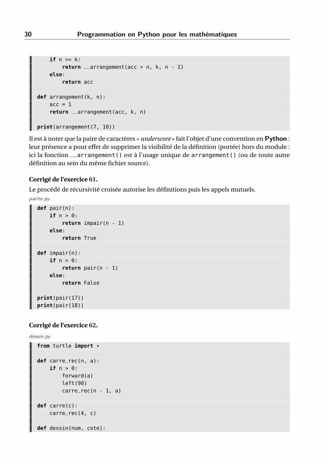
30 Programmation en Python pour les mathématiques
if n >= k:return __arrangement(acc * n, k, n - 1)
else:return acc
def arrangement(k, n):acc = 1return __arrangement(acc, k, n)
print(arrangement(7, 10))
Il est à noter que la paire de caractères « underscore » fait l’objet d’une convention en Python :leur présence a pour effet de supprimer la visibilité de la définition (portée) hors du module :ici la fonction __arrangement() est à l’usage unique de arrangement() (ou de toute autredéfinition au sein du même fichier source).
Corrigé de l’exercice 61.
Le procédé de récursivité croisée autorise les définitions puis les appels mutuels.parite.py
def pair(n):if n > 0:
return impair(n - 1)else:
return True
def impair(n):if n > 0:
return pair(n - 1)else:
return False
print(pair(17))print(pair(18))
Corrigé de l’exercice 62.
dessin.py
from turtle import *
def carre_rec(n, a):if n > 0:
forward(a)left(90)carre_rec(n - 1, a)
def carre(c):carre_rec(4, c)
def dessin(num, cote):
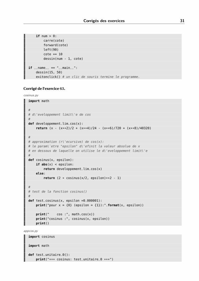
Corrigés des exercices 31
if num > 0:carre(cote)forward(cote)left(90)cote += 10dessin(num - 1, cote)
if __name__ == "__main__":dessin(15, 50)exitonclick() # un clic de souris termine le programme.
Corrigé de l’exercice 63.
cosinus.py
import math
## d\'eveloppement limit\'e de cos#def developpement_lim_cos(x):
return (x - (x**2)/2 + (x**4)/24 - (x**6)/720 + (x**8)/40320)
## approximation (r\'ecursive) de cos(x):# le param\`etre "epsilon" d\'efinit la valeur absolue de x# en dessous de laquelle on utilise le d\'eveloppement limit\'e#def cosinus(x, epsilon):
if abs(x) < epsilon:return developpement_lim_cos(x)
else:return (2 * cosinus(x/2, epsilon)**2 - 1)
## test de la fonction cosinus()#def test_cosinus(x, epsilon =0.000001):
print("pour x = {0} (epsilon = {1}):".format(x, epsilon))
print(" cos :", math.cos(x))print("cosinus :", cosinus(x, epsilon))print()
appcos.py
import cosinus
import math
def test_unitaire_0():print("*** cosinus: test_unitaire_0 ***")
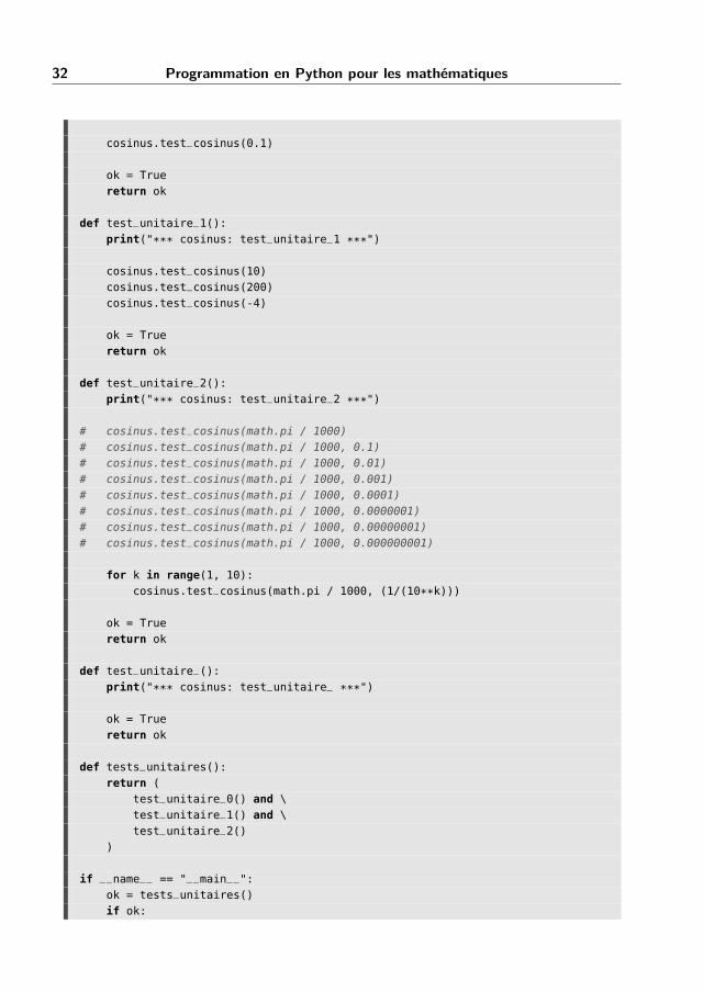
32 Programmation en Python pour les mathématiques
cosinus.test_cosinus(0.1)
ok = Truereturn ok
def test_unitaire_1():print("*** cosinus: test_unitaire_1 ***")
cosinus.test_cosinus(10)cosinus.test_cosinus(200)cosinus.test_cosinus(-4)
ok = Truereturn ok
def test_unitaire_2():print("*** cosinus: test_unitaire_2 ***")
# cosinus.test_cosinus(math.pi / 1000)# cosinus.test_cosinus(math.pi / 1000, 0.1)# cosinus.test_cosinus(math.pi / 1000, 0.01)# cosinus.test_cosinus(math.pi / 1000, 0.001)# cosinus.test_cosinus(math.pi / 1000, 0.0001)# cosinus.test_cosinus(math.pi / 1000, 0.0000001)# cosinus.test_cosinus(math.pi / 1000, 0.00000001)# cosinus.test_cosinus(math.pi / 1000, 0.000000001)
for k in range(1, 10):cosinus.test_cosinus(math.pi / 1000, (1/(10**k)))
ok = Truereturn ok
def test_unitaire_():print("*** cosinus: test_unitaire_ ***")
ok = Truereturn ok
def tests_unitaires():return (
test_unitaire_0() and \test_unitaire_1() and \test_unitaire_2()
)
if __name__ == "__main__":ok = tests_unitaires()if ok:
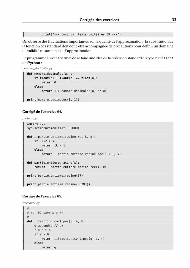
Corrigés des exercices 33
print("*** cosinus: tests unitaires OK ***")
On observe des fluctuations importantes sur la qualité de l’approximation : la substitution dela fonction cos standard doit donc être accompagnée de précautions pour définir un domainede validité raisonnable de l’approximation.
Le programme suivant permet de se faire une idée de la précision standard du type natif floatde Python :
nombre_decimales.py
def nombre_decimales(a, b):if float(a) + float(b) == float(a):
return 0else:
return 1 + nombre_decimales(a, b/10)
print(nombre_decimales(1, 1))
Corrigé de l’exercice 64.
partent.py
import syssys.setrecursionlimit(100000)
def __partie_entiere_racine_rec(k, x):if k**2 > x:
return (k - 1)else:
return __partie_entiere_racine_rec(k + 1, x)
def partie_entiere_racine(x):return __partie_entiere_racine_rec(1, x)
print(partie_entiere_racine(17))
print(partie_entiere_racine(36703))
Corrigé de l’exercice 65.
fraccont1.py
## (a, b) dans N x N*#def __fraction_cont_pos(q, a, b):
q.append(a // b)r = a % bif r > 0:
return __fraction_cont_pos(q, b, r)else:
return q
34 Programmation en Python pour les mathématiques
## (a, b) dans Z x N*#def __fraction_cont_b_pos(a, b):
q = []if a < 0:
q.append(-((-a + b) // b))else:
q.append(a // b)return q + __fraction_cont_pos([], a - b * q[0], b)[1:]
## (a, b) dans Z x Z*#def fraction_cont(a, b):
if b < 0:return __fraction_cont_b_pos(-a, -b)
else:return __fraction_cont_b_pos(a, b)
x = fraction_cont(111, 40)print(x)
x = fraction_cont(-111, 40)print(x)
Corrigé de l’exercice 66.
La solution proposée sépare le code du programme en deux fichiers : un module avec lesfonctions à réaliser, puis un programme principal qui utilise les fonctions du module.outils.py
def est_vide(l):return len(l) == 0
def tete(l):if est_vide(l):
return Noneelse:
return l[0]
def suite(l):if est_vide(l):
return []else:
return l[1:]
def longueur(l):if est_vide(l):
return 0
Corrigés des exercices 35
else:return 1 + longueur(suite(l))
def debut_rec(n, l, acc):if n == 0:
return accelse:
x = tete(l)if x is not None:
acc.append(x)debut_rec(n - 1, suite(l), acc)
def debut(n, l):acc = []debut_rec(n, l, acc)return acc
def coupe(n, l):if n == 0:
return lelse:
return coupe(n - 1, suite(l))
Le programme principal suivant utilise le module précédent :
primliste.py
import random
from outils import *
def recherche(x, liste):if len(liste) == 0:
return False
if tete(liste) == x:return True
return recherche(x, suite(liste))
if __name__ == "__main__":hasard = [random.randrange(50) for t in range(20)]
print(longueur(hasard)) # donne 20print(hasard)
print(recherche(tete(hasard), hasard)) # donne Trueprint(recherche(200, hasard)) # donne False
print(tete(hasard))print(suite(hasard))
36 Programmation en Python pour les mathématiques
print(debut(2, hasard))print(coupe(2, hasard))
hasard = [random.randrange(50) for t in range(10)]print(hasard)
n = longueur(hasard)for i in range(n):
print(debut(1, hasard))hasard = coupe(1, hasard)
6Corrigés des exercices
Corrigé de l’exercice 70.
maliste.py
class maliste(object):
def __init__(self, l =[], indice_ext =0):self.__elements = lself.__indice_ext = indice_ext
def __str__(self):return str(self.__elements)
def extraire(self):if len(self.__elements) == 0:
return None
x = self.__elements[self.__indice_ext]del self.__elements[self.__indice_ext]
return x
def inscrire(self, x):return self.__elements.append(x)
def lire(self):return self.__elements[self.__indice_ext]
def est_vide(self):return (len(self.__elements) == 0)
mafile.py
import maliste
class mafile(maliste.maliste):
def __init__(self, l =[]):super().__init__(l, 0)
38 Programmation en Python pour les mathématiques
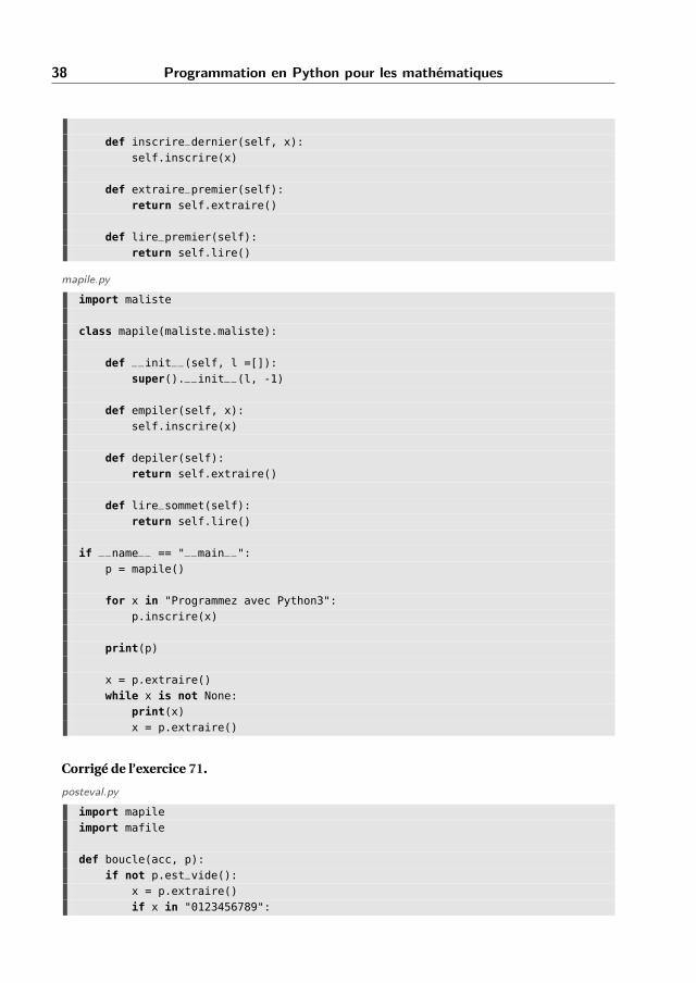
def inscrire_dernier(self, x):self.inscrire(x)
def extraire_premier(self):return self.extraire()
def lire_premier(self):return self.lire()
mapile.py
import maliste
class mapile(maliste.maliste):
def __init__(self, l =[]):super().__init__(l, -1)
def empiler(self, x):self.inscrire(x)
def depiler(self):return self.extraire()
def lire_sommet(self):return self.lire()
if __name__ == "__main__":p = mapile()
for x in "Programmez avec Python3":p.inscrire(x)
print(p)
x = p.extraire()while x is not None:
print(x)x = p.extraire()
Corrigé de l’exercice 71.
posteval.py
import mapileimport mafile
def boucle(acc, p):if not p.est_vide():
x = p.extraire()if x in "0123456789":
Corrigés des exercices 39
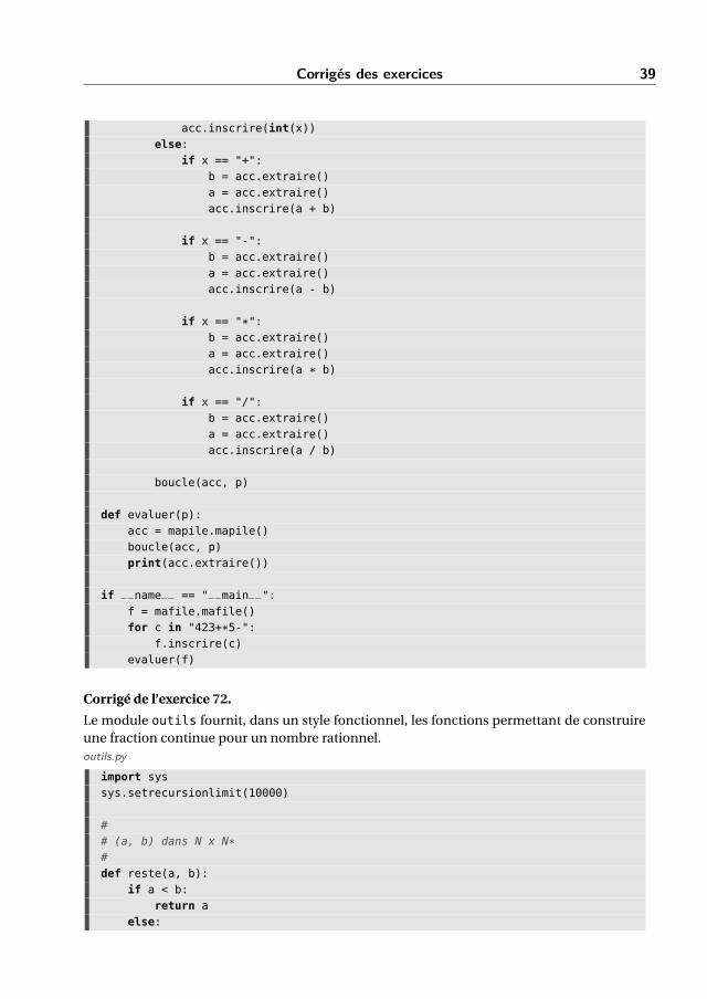
acc.inscrire(int(x))else:
if x == "+":b = acc.extraire()a = acc.extraire()acc.inscrire(a + b)
if x == "-":b = acc.extraire()a = acc.extraire()acc.inscrire(a - b)
if x == "*":b = acc.extraire()a = acc.extraire()acc.inscrire(a * b)
if x == "/":b = acc.extraire()a = acc.extraire()acc.inscrire(a / b)
boucle(acc, p)
def evaluer(p):acc = mapile.mapile()boucle(acc, p)print(acc.extraire())
if __name__ == "__main__":f = mafile.mafile()for c in "423+*5-":
f.inscrire(c)evaluer(f)
Corrigé de l’exercice 72.
Le module outils fournit, dans un style fonctionnel, les fonctions permettant de construireune fraction continue pour un nombre rationnel.outils.py
import syssys.setrecursionlimit(10000)
## (a, b) dans N x N*#def reste(a, b):
if a < b:return a
else:
40 Programmation en Python pour les mathématiques
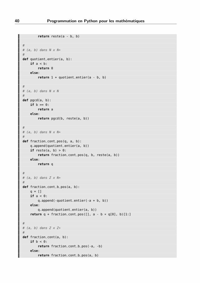
return reste(a - b, b)
## (a, b) dans N x N*#def quotient_entier(a, b):
if a < b:return 0
else:return 1 + quotient_entier(a - b, b)
## (a, b) dans N x N#def pgcd(a, b):
if b == 0:return a
else:return pgcd(b, reste(a, b))
## (a, b) dans N x N*#def fraction_cont_pos(q, a, b):
q.append(quotient_entier(a, b))if reste(a, b) > 0:
return fraction_cont_pos(q, b, reste(a, b))else:
return q
## (a, b) dans Z x N*#def fraction_cont_b_pos(a, b):
q = []if a < 0:
q.append(-quotient_entier(-a + b, b))else:
q.append(quotient_entier(a, b))return q + fraction_cont_pos([], a - b * q[0], b)[1:]
## (a, b) dans Z x Z*#def fraction_cont(a, b):
if b < 0:return fraction_cont_b_pos(-a, -b)
else:return fraction_cont_b_pos(a, b)
Corrigés des exercices 41
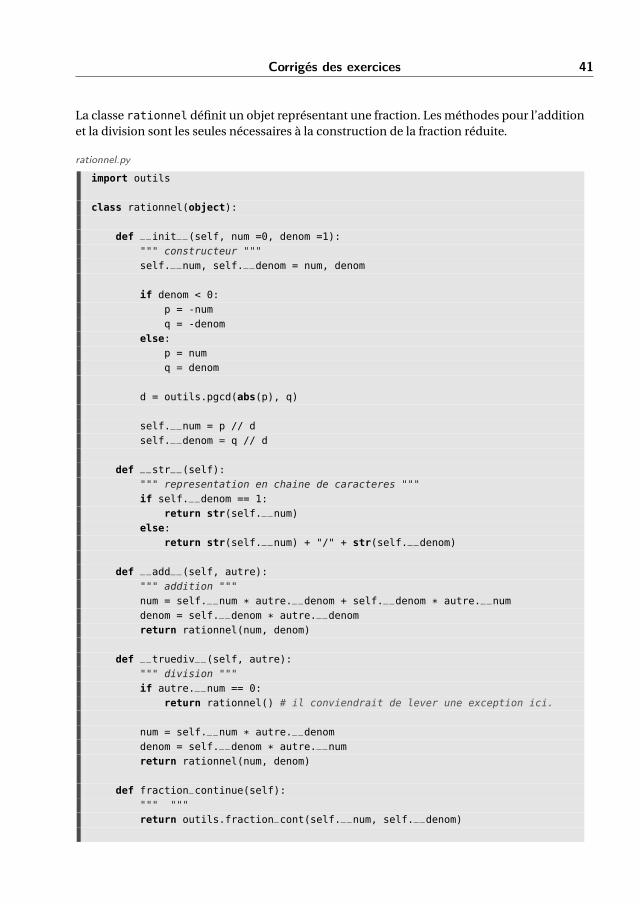
La classe rationnel définit un objet représentant une fraction. Les méthodes pour l’additionet la division sont les seules nécessaires à la construction de la fraction réduite.
rationnel.py
import outils
class rationnel(object):
def __init__(self, num =0, denom =1):""" constructeur """self.__num, self.__denom = num, denom
if denom < 0:p = -numq = -denom
else:p = numq = denom
d = outils.pgcd(abs(p), q)
self.__num = p // dself.__denom = q // d
def __str__(self):""" representation en chaine de caracteres """if self.__denom == 1:
return str(self.__num)else:
return str(self.__num) + "/" + str(self.__denom)
def __add__(self, autre):""" addition """num = self.__num * autre.__denom + self.__denom * autre.__numdenom = self.__denom * autre.__denomreturn rationnel(num, denom)
def __truediv__(self, autre):""" division """if autre.__num == 0:
return rationnel() # il conviendrait de lever une exception ici.
num = self.__num * autre.__denomdenom = self.__denom * autre.__numreturn rationnel(num, denom)
def fraction_continue(self):""" """return outils.fraction_cont(self.__num, self.__denom)
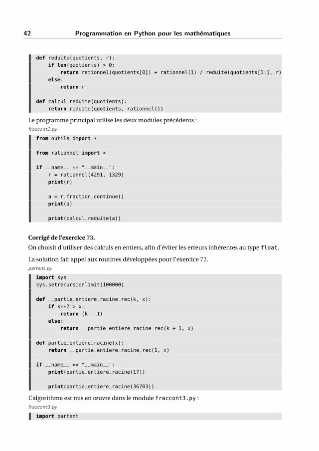
42 Programmation en Python pour les mathématiques
def reduite(quotients, r):if len(quotients) > 0:
return rationnel(quotients[0]) + rationnel(1) / reduite(quotients[1:], r)else:
return r
def calcul_reduite(quotients):return reduite(quotients, rationnel())
Le programme principal utilise les deux modules précédents :fraccont2.py
from outils import *
from rationnel import *
if __name__ == "__main__":r = rationnel(4291, 1329)print(r)
a = r.fraction_continue()print(a)
print(calcul_reduite(a))
Corrigé de l’exercice 73.
On choisit d’utiliser des calculs en entiers, afin d’éviter les erreurs inhérentes au type float.
La solution fait appel aux routines développées pour l’exercice 72.partent.py
import syssys.setrecursionlimit(100000)
def __partie_entiere_racine_rec(k, x):if k**2 > x:
return (k - 1)else:
return __partie_entiere_racine_rec(k + 1, x)
def partie_entiere_racine(x):return __partie_entiere_racine_rec(1, x)
if __name__ == "__main__":print(partie_entiere_racine(17))
print(partie_entiere_racine(36703))
L’algorithme est mis en œuvre dans le module fraccont3.py :fraccont3.py
import partent
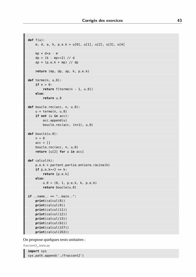
Corrigés des exercices 43
def f(u):m, d, a, k, p_e_k = u[0], u[1], u[2], u[3], u[4]
mp = d*a - mdp = (k - mp**2) // dap = (p_e_k + mp) // dp
return (mp, dp, ap, k, p_e_k)
def terme(n, u_0):if n > 0:
return f(terme(n - 1, u_0))else:
return u_0
def boucle_rec(acc, n, u_0):u = terme(n, u_0)if not (u in acc):
acc.append(u)boucle_rec(acc, (n+1), u_0)
def boucle(u_0):n = 0acc = []boucle_rec(acc, n, u_0)return [u[2] for u in acc]
def calcul(k):p_e_k = partent.partie_entiere_racine(k)if p_e_k**2 == k:
return [p_e_k]else:
u_0 = (0, 1, p_e_k, k, p_e_k)return boucle(u_0)
if __name__ == "__main__":print(calcul(8))print(calcul(9))print(calcul(11))print(calcul(12))print(calcul(13))print(calcul(61))print(calcul(227))print(calcul(263))
On propose quelques tests unitaires :
fraccont3_tests.py
import syssys.path.append('./fraccont2')
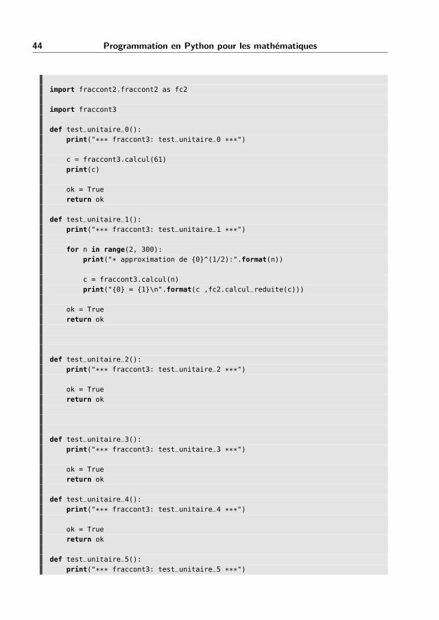
44 Programmation en Python pour les mathématiques
import fraccont2.fraccont2 as fc2
import fraccont3
def test_unitaire_0():print("*** fraccont3: test_unitaire_0 ***")
c = fraccont3.calcul(61)print(c)
ok = Truereturn ok
def test_unitaire_1():print("*** fraccont3: test_unitaire_1 ***")
for n in range(2, 300):print("* approximation de {0}^(1/2):".format(n))
c = fraccont3.calcul(n)print("{0} = {1}\n".format(c ,fc2.calcul_reduite(c)))
ok = Truereturn ok
def test_unitaire_2():print("*** fraccont3: test_unitaire_2 ***")
ok = Truereturn ok
def test_unitaire_3():print("*** fraccont3: test_unitaire_3 ***")
ok = Truereturn ok
def test_unitaire_4():print("*** fraccont3: test_unitaire_4 ***")
ok = Truereturn ok
def test_unitaire_5():print("*** fraccont3: test_unitaire_5 ***")
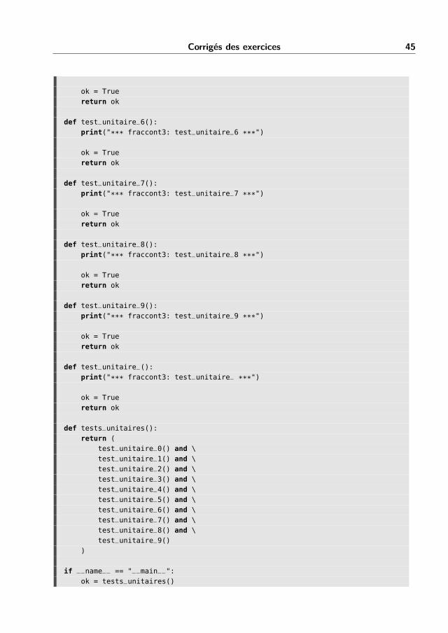
Corrigés des exercices 45
ok = Truereturn ok
def test_unitaire_6():print("*** fraccont3: test_unitaire_6 ***")
ok = Truereturn ok
def test_unitaire_7():print("*** fraccont3: test_unitaire_7 ***")
ok = Truereturn ok
def test_unitaire_8():print("*** fraccont3: test_unitaire_8 ***")
ok = Truereturn ok
def test_unitaire_9():print("*** fraccont3: test_unitaire_9 ***")
ok = Truereturn ok
def test_unitaire_():print("*** fraccont3: test_unitaire_ ***")
ok = Truereturn ok
def tests_unitaires():return (
test_unitaire_0() and \test_unitaire_1() and \test_unitaire_2() and \test_unitaire_3() and \test_unitaire_4() and \test_unitaire_5() and \test_unitaire_6() and \test_unitaire_7() and \test_unitaire_8() and \test_unitaire_9()
)
if __name__ == "__main__":ok = tests_unitaires()
46 Programmation en Python pour les mathématiques
if ok:print("*** fraccont3: tests unitaires OK ***")
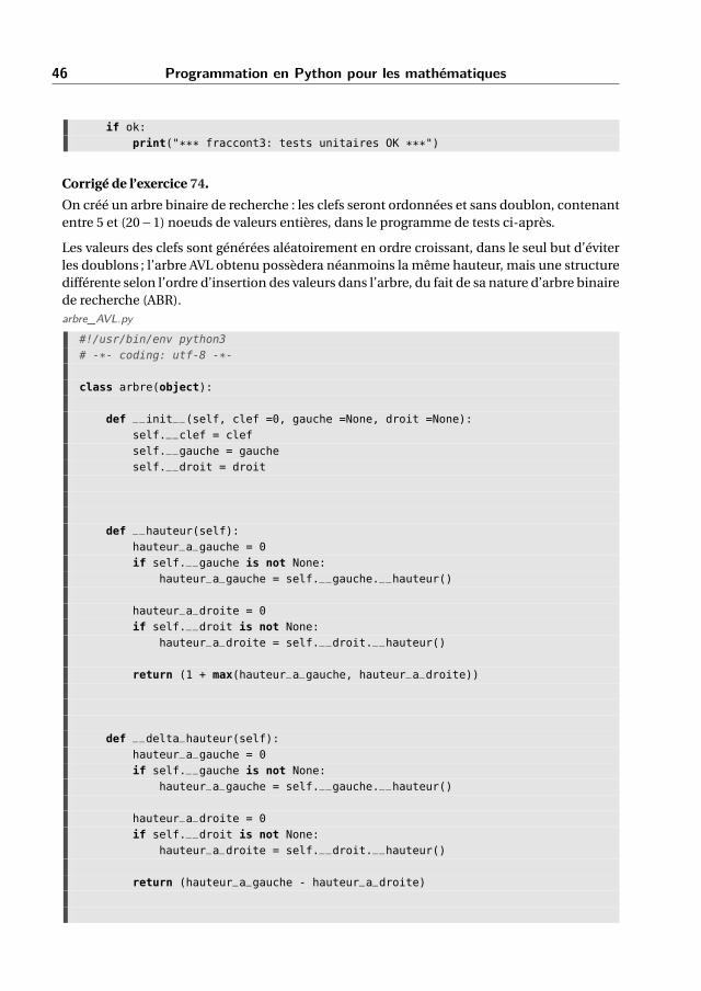
Corrigé de l’exercice 74.
On créé un arbre binaire de recherche : les clefs seront ordonnées et sans doublon, contenantentre 5 et (20−1) noeuds de valeurs entières, dans le programme de tests ci-après.
Les valeurs des clefs sont générées aléatoirement en ordre croissant, dans le seul but d’éviterles doublons ; l’arbre AVL obtenu possèdera néanmoins la même hauteur, mais une structuredifférente selon l’ordre d’insertion des valeurs dans l’arbre, du fait de sa nature d’arbre binairede recherche (ABR).arbre_AVL.py
#!/usr/bin/env python3# -*- coding: utf-8 -*-
class arbre(object):
def __init__(self, clef =0, gauche =None, droit =None):self.__clef = clefself.__gauche = gaucheself.__droit = droit
def __hauteur(self):hauteur_a_gauche = 0if self.__gauche is not None:
hauteur_a_gauche = self.__gauche.__hauteur()
hauteur_a_droite = 0if self.__droit is not None:
hauteur_a_droite = self.__droit.__hauteur()
return (1 + max(hauteur_a_gauche, hauteur_a_droite))
def __delta_hauteur(self):hauteur_a_gauche = 0if self.__gauche is not None:
hauteur_a_gauche = self.__gauche.__hauteur()
hauteur_a_droite = 0if self.__droit is not None:
hauteur_a_droite = self.__droit.__hauteur()
return (hauteur_a_gauche - hauteur_a_droite)
Corrigés des exercices 47
def __rotation_a_gauche(self):self.__clef, self.__droit.__clef = self.__droit.__clef, self.__clef
t = self.__gauche
self.__gauche = self.__droitself.__droit = self.__droit.__droit
self.__gauche.__droit = self.__gauche.__gaucheself.__gauche.__gauche = t
def __rotation_a_droite(self):self.__clef, self.__gauche.__clef = self.__gauche.__clef, self.__clef
t = self.__droit
self.__droit = self.__gaucheself.__gauche = self.__gauche.__gauche
self.__droit.__gauche = self.__droit.__droitself.__droit.__droit = t
def __equilibrer(self):d = self.__delta_hauteur()if d > 1:
if self.__gauche.__delta_hauteur() < 1:self.__gauche.__rotation_a_gauche()
self.__rotation_a_droite()
if d < -1:if self.__droit.__delta_hauteur() > -1:
self.__droit.__rotation_a_droite()self.__rotation_a_gauche()
def inserer(self, clef):if clef < self.__clef:
if self.__gauche is None:self.__gauche = arbre(clef)
else:self.__gauche.inserer(clef)
else:if self.__droit is None:
self.__droit = arbre(clef)
48 Programmation en Python pour les mathématiques
else:self.__droit.inserer(clef)
self.__equilibrer()
def afficher(self, decalage =0):if self.__droit is not None:
self.__droit.afficher(decalage + 2)
print(" " * decalage + ("{:3d}".format(self.__clef)))
if self.__gauche is not None:self.__gauche.afficher(decalage + 2)
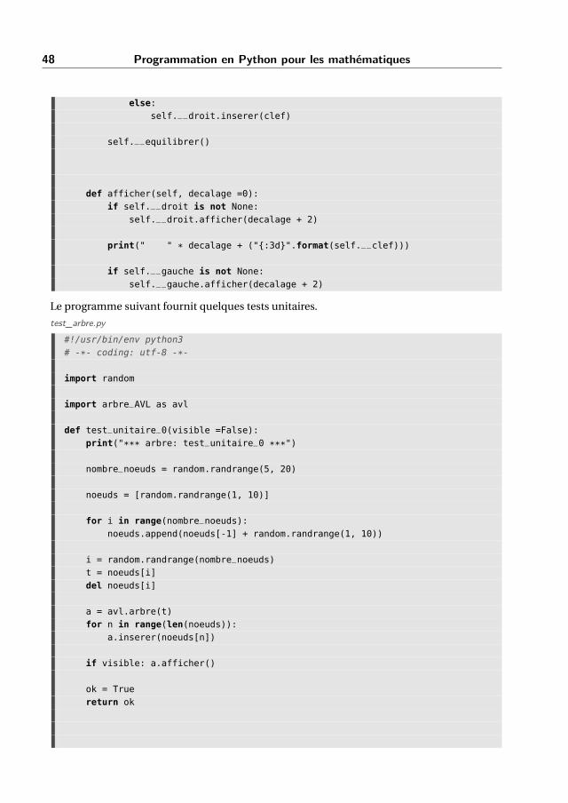
Le programme suivant fournit quelques tests unitaires.
test_arbre.py
#!/usr/bin/env python3# -*- coding: utf-8 -*-
import random
import arbre_AVL as avl
def test_unitaire_0(visible =False):print("*** arbre: test_unitaire_0 ***")
nombre_noeuds = random.randrange(5, 20)
noeuds = [random.randrange(1, 10)]
for i in range(nombre_noeuds):noeuds.append(noeuds[-1] + random.randrange(1, 10))
i = random.randrange(nombre_noeuds)t = noeuds[i]del noeuds[i]
a = avl.arbre(t)for n in range(len(noeuds)):
a.inserer(noeuds[n])
if visible: a.afficher()
ok = Truereturn ok

Corrigés des exercices 49
def test_unitaire_1(visible =False):print("*** arbre: test_unitaire_1 ***")
nombre_noeuds = random.randrange(5, 20)
noeuds = [random.randrange(1, 10)]
for i in range(nombre_noeuds):noeuds.append(noeuds[-1] + random.randrange(1, 10))
if visible: print(noeuds)
## on prend une copie (profonde) de a#copie = list(noeuds)
i = random.randrange(nombre_noeuds)t = noeuds[i]del noeuds[i]
a = avl.arbre(t)for n in range(len(noeuds)):
a.inserer(noeuds[n])
if visible: a.afficher()
if visible: print("-----")
## on prend la copie de a et on y met un peu d'entropie.#if visible: print(copie)
k = random.randrange(1, 10)for i in range(1, k):
t = copie[0]copie.append(t)del copie[0]
if visible: print(copie)
i = random.randrange(nombre_noeuds)t = copie[i]del copie[i]
b = avl.arbre(t)for n in range(len(copie)):
b.inserer(copie[n])
50 Programmation en Python pour les mathématiques
if visible: b.afficher()
ok = Truereturn ok
def test_unitaire_2(visible =False):print("*** arbre: test_unitaire_2 ***")
ok = Truereturn ok
def test_unitaire_(visible =False):print("*** arbre: test_unitaire_ ***")
ok = Truereturn ok
def tests_unitaires():return (
test_unitaire_0(True) and \test_unitaire_1(True) and \test_unitaire_2()
)
if __name__ == "__main__":ok = tests_unitaires()if ok:
print("*** arbre: tests unitaires OK ***")