N° d’ordre

THESE DE DOCTORAT

Présentée à l’Université Djillali Liabes de Sidi- Bel-Abbes

Faculté de Génie Electrique

Département de Télécommunications

Laboratoire Télécommunications et de Traitement Numérique du Signal

Pour l’obtention du Diplôme de Doctorat LMD

Filière : Télécommunications

Spécialité : Télécommunications

M. Mouad ADDAD

Codes de zone à corrélation nulle : Conception, analyse

et applications

Soutenu le 31 / 10 / 2018

Devant le jury composé de :

M. NAOUM Rafah Pr Président UDL-SBA

M. DJEBBARI Ali Pr Directeur de thèse UDL-SBA

M. ELAHMAR Sid Ahmed Pr Examinateur UDL-SBA

M. BOUZIANI Merahi Pr Examinateur UDL-SBA

M. DJEBBAR Ahmed Bouzidi Pr Examinateur UDL-SBA

M. BENAISSA Mohamed MCA Examinateur CU-Ain Temouchent

Année Universitaire: 2018-2019

i

Acknowledgement

This thesis is the result of my research at the Laboratory of Telecommunications and

Digital Signal Processing, Djillali Liabes University of Sidi Bel Abbes. I would like to

thank all my Lab colleagues for creating a nice and friendly working environment.

First and foremost, I offer sincere gratitude to my advisor Prof. Ali Djebbari who has

guided me through my Ph.D. pursuit with his knowledge. It has been an exceptional

experience to work with Prof. Djebbari in the past years. The dissertation would have

been next to impossible without his supervision and research support.

Furthermore, I am grateful for the collaboration with Prof. Iyad Dayoub of Valenciennes

University, France. I heartily appreciate his contribution to my research journey.

I acknowledge my committee members Professors Naoum Rafah, Elahmar Sid Ahmed,

Bouziani Merahi, and Djebbar Ahmed Bouzidi from the University of Djillali Liabes and

associate prof. Benaissa Mohamed from the University Center of Ain Temouchent. I am

truly thankful for the time and efforts that they spent on reviewing and commenting my

research proposal.

Last but not the least, I am greatly indebted to my parents and people closest to me. They

have provided me with immense understanding and support all these years. I have enjoyed

every moment we spent together with care and love. This dissertation is dedicated to

them.

ii

iii

Abstract

In order to make efficient use of the available resources, the users of communication

systems, which are more and more numerous, have to cohabit. The problem posed by this

cohabitation then consists in examining how to organize the access of a large number of

users to a resource. Code Division Multiple Access (CDMA) is one of the techniques that

allows access to a communication network, but suffers from interference between users

(MUI: Multiuser Interference). The latter depends heavily on the spreading sequences

that must be constructed in order to minimize cross-correlation function (CCF) between

sequences and to minimize the correlation between each sequence and its shifted version

(ACF: Auto-Correlation Function). The aim of the thesis is to study the spreading

sequences and in particular the so-called Zero Correlation Zone (ZCZ) sequences. We

have four contributions. The first concerns the construction of two sequence families for

the optical CDMA system: a ZCZ family and a Zero Cross-Correlation (ZCC) family of

sequences. The second is to establish a new Bit Error Rate (BER) expression for the quasi-

synchronous, uplink DS-CDMA system, based on the CCF properties of the spreading

sequences. We have shown that to eliminate MUI interference, sequences must have zero

even and odd CCF functions. This new expression has not only made it possible to

evaluate the performance of said system for the case of ternary sequences, but to show

that the elimination of MUIs in the case of ZCZ sequences is only possible if the even

and odd CCF functions are both zero; contrary to what is generally accepted: to have only

zero even CCF. The third is dedicated to the generalization of the BER of the quasi-

synchronous MC-CDMA system, uplink, to include ternary sequences, which made it

possible to evaluate the performances of suitable sequences. Also, a comparative study

was developed in terms of Crest Factor (CF) concerning the binary sequences; ZCZ

sequences have been shown to have low CF compared to conventional sequences (Walsh-

Hadamard and Orthogonal Gold). At last, the fourth is to show that the optical ZCZ

sequences for the quasi-synchronous, uplink SAC-OCDMA system eliminate the MUIs,

if the maximum delay between users is within the ZCZ zone, but their performance

remains low compared to the ZCC codes with the same parameters (number of sequences

and weight).

iv

Résumé

Afin d'obtenir une utilisation efficace des ressources disponibles, les utilisateurs des

systèmes de communications, de plus en plus nombreux, sont amenés à cohabiter. Le

problème posé par cette cohabitation, consiste alors à examiner comment organiser l'accès

d'un nombre important d'utilisateurs à une ressource. L'accès multiple par répartition de

code (CDMA : Code Division Multiple Access) est une des techniques qui permet l’accès

à un réseau de communication, mais soufre des interférences entre utilisateurs (MUI :

Multiuser Interference). Ces dernières dépendent fortement des séquences d’étalement

qui doivent être construites de façon à minimiser la corrélation croisée (CCF : Cross-

Correlation Function) entre les séquences et à minimiser la corrélation entre chaque

séquence et sa version décalée (ACF : Auto-Correlation Function). Cette thèse a pour

objectifs d’étudier, donc, les séquences d’étalement et notamment les séquences dites de

zone à corrélation nulle (ZCZ : Zero Correlation Zone). Nous avons présenté quatre

contributions. La première concerne la construction de deux familles de séquences pour

le système CDMA optiques : une famille ZCZ et une famille de séquences à corrélation

croisée nulle (ZCC : Zero Cross-Correlation). Quant à la deuxième, il s’agit d’établir une

nouvelle expression du taux d’erreurs binaires (BER : Bit error rate) pour le système DS-

CDMA quasi synchrone, en liaison montante, en fonction des propriétés de CCF des

séquences d’étalement. Nous avons montré que pour éliminer les interférences MUI, les

séquences doivent posséder des fonctions de CCF paires et impaires nulle. Cette nouvelle

expression a permis non seulement l’évaluation des performances dudit système pour le

cas des séquences dites ternaires, mais de montrer que l’élimination des MUI dans le cas

des séquences ZCZ n’est possible que si les fonctions CCF paires et impaires sont

conjointement nulles ; contrairement à ce qui généralement répandu : le fait d’avoir

seulement la CCF paire nulle. La troisième est dédiée à la généralisation du BER du

système MC-CDMA quasi synchrone, liaison montante, dans le cas des séquences

ternaires, ce qui a permis non seulement d’évaluer les performances de ces dernières mais

d’en choisir les familles de séquences les plus adaptés. Aussi, nous élaborons une étude

comparative en termes de facteur de crête (Crest Factor : CF) concernant les séquences

binaires ; il a été montré que les séquences ZCZ ont un faible CF comparativement aux

séquences conventionnelles (Walsh-Hadamard et Gold orthogonal). Enfin, la dernière

consiste à montrer que les séquences ZCZ optiques pour le système SAC-OCDMA quasi

synchrone, en voie montante, éliminent les MUI, si le retard maximal entre utilisateur est

à l’intérieur de la zone ZCZ, mais leur performance reste faible comparativement au codes

ZCC de même paramètres (nombre de séquences et poids).

v

خصمل

تتكون المشكلة في فحص يجب على مستخدمي أنظمة االتصاالت التعايش. المتاحة،من أجل االستخدام الفعال للموارد

المتعدد بتقسيم الشفرة النفاذكيفية تنظيم وصول هؤالء المستخدمين إلى مورد. يوفر

(CDMA: Code Division Multiple Access الوصول إلى شبكة )،ولكنه يخضع لتداخل بين اتصاالت

التي يجب بناؤها لتقليل وظيفة رموزال(. هذه تعتمد بشدة على MUI: Multiuser Interferenceالمستخدمين )

( ووظيفة االرتباط التلقائيCCF: Cross-Correlation Functionاالرتباط المتبادل )

(ACF: Auto-Correlation Function الهدف من األطروحة هو دراسة .)منطقة الصفر رموزوتحديدًا رموزال

(ZCZ: Zero Cross-Correlation قدمنا .) لنظام الرموز من عائلتينأربع مساهمات. تتعلق األولى ببناء

CDMA البصري: عائلةZCZ رموزوعائلة (ZCC: Zero Cross-Correlation) والثاني هو إنشاء تعبير .

CCFsاستناداً إلى (،QS: quasi synchroneشبه المتزامن ) DS-CDMA( لنظام BERجديد لخطأ البتات )

. منعدمة فرديةو ةيزوج CCFsعلى الرموزيجب أن تحتوي ،MUI. لقد أظهرنا أنه للتخلص من تداخل لرموزل

الرموزفي حالة MUIsولكن إلظهار أن القضاء على ،ةيالثالث الرموزسمح هذا التعبير الجديد ليس فقط بتقييم أداء

ZCZ ممكن فقط إذا كانCCFs على عكس ما هو منتشر بشكل عام: منعدمة؛ وفردية ةيزوجCCFs فقط ةيزوج.

فقط بتقييم أدائها سيلوالذي يسمح لنا الثالثية، الرموز QS-MC-CDMAأما الثالث فهو مخصص لتعميم نظام

فيما يتعلق (CF: Crest Factor)تم تطوير دراسة مقارنة من حيث أيضا،مالءمة. رموز ةولكن الختيار مجموع

Walsh-Hadamard andالتقليدية ) رموزلمقارنة با CFمنخفضة في ZCZ رموزلوقد ثبت أن الثنائية؛ رموزبال

Orthogonal Gold رموزال(. والرابع هو إظهار أن ZCZ البصرية لنظامQS-SAC-OCDMA تقضي على ،

MUI ر بين المستخدمين هو داخل المنطقة ، إذا كان الحد األقصى للتأخZCZ ًولكن أدائها ال يزال منخفضا ،

والوزن(. رموزالمع نفس المعلمات )عدد ZCCبالمقارنة مع رموز

vi

vii

Contents

Acknowledgement ............................................................................................................ i

Abstract .......................................................................................................................... iii

Content .......................................................................................................................... vii

List of Figures ................................................................................................................ xi

List of Tables ................................................................................................................ xiii

Acronyms ........................................................................................................................ xv

Introduction ..................................................................................................................... 1

Chapter 1: Sequence Design ........................................................................................... 5

1.1 Introduction ................................................................................................................... 5

1.2 Sequence Operations ..................................................................................................... 5

1.3 Correlation Functions .................................................................................................... 6

1.4 Perfect Sequences .......................................................................................................... 8

1.5 Walsh-Hadamard Sequences ......................................................................................... 9

1.6 Pseudo-Noise Sequences ............................................................................................... 9

M-sequences ........................................................................................................ 10

Gold Sequences ................................................................................................... 12

Orthogonal Gold Sequences ................................................................................ 13

1.7 Complementary Sequences ......................................................................................... 13

Complementary Pairs .......................................................................................... 13

Orthogonal Golay Complementary Sequences ................................................... 14

Mutually Orthogonal Complementary Sets ......................................................... 14

1.8 Zero Correlation Zone Sequences ............................................................................... 15

Binary ZCZ Sequences ........................................................................................ 16

Ternary ZCZ Sequences ...................................................................................... 18

Optical ZCZ Sequences ....................................................................................... 19

1.9 Zero Cross Correlation Sequences .............................................................................. 20

Contents

viii

New ZCC sequences [23] .................................................................................... 21

Abd et al [22]....................................................................................................... 21

1.10 Conclusion ................................................................................................................... 22

Chapter 2: An overview of Spread Spectrum and CDMA ........................................ 23

2.1 Introduction ................................................................................................................. 23

2.2 Spread Spectrum Modulation ...................................................................................... 23

2.3 Multiple access and multiplexing ................................................................................ 24

2.4 Noise and Interference ................................................................................................ 27

2.5 Delay Spread ............................................................................................................... 29

2.6 Power control .............................................................................................................. 30

Uplink and downlink ........................................................................................... 30

Power Control ..................................................................................................... 30

2.7 Multicarrier Modulation .............................................................................................. 30

2.8 Applications ................................................................................................................ 31

Ad-hoc Networks ................................................................................................ 31

Underwater Communications .............................................................................. 32

Satellite communication ...................................................................................... 32

2.9 Conclusion ................................................................................................................... 33

Chapter 3: On ZCZ Sequences and their Application to DS-CDMA ....................... 35

3.1 Introduction ................................................................................................................. 35

3.2 DS-CDMA System Model .......................................................................................... 35

Transmitter .......................................................................................................... 35

Channel ............................................................................................................... 36

Derivation of a New BER in terms of ECF and OCF ......................................... 37

3.3 Numerical Results ....................................................................................................... 40

Interference vs. Chip delay .................................................................................. 41

BER vs. SNR for different types of sequences.................................................... 42

BER vs. Chip delay of a ZCZ set with zero even and odd CCFs ........................ 45

3.4 Conclusion ................................................................................................................... 46

Chapter 4: On ZCZ Sequences and their Application to MC-CDMA ..................... 47

4.1 Introduction ................................................................................................................. 47

4.2 CF Analysis ................................................................................................................. 47

Contents

ix

4.3 BER Analysis .............................................................................................................. 50

MC-CDMA System Model ................................................................................. 50

Derivation of a new BER for ternary sequences in MC-CDMA system ............. 52

4.4 Numerical Results ....................................................................................................... 56

BER vs. Chip delay ............................................................................................. 56

BER vs. SNR for different types of sequences.................................................... 57

4.5 Conclusion ................................................................................................................... 58

Chapter 5: On Optical ZCZ Sequences and their Application to OCDMA ............ 59

5.1 Introduction ................................................................................................................. 59

5.2 OCDMA VLC System ................................................................................................ 62

Transmitter .......................................................................................................... 62

Receiver ............................................................................................................... 63

5.3 Numerical Results and Analysis ................................................................................. 66

MUI vs. Time Delay ............................................................................................ 66

MUI vs. Sequence Length ................................................................................... 67

MUI vs. Number of Active Users ....................................................................... 68

Comparison between ZCC and OZCZ Sequences .............................................. 68

5.4 Conclusion ................................................................................................................... 70

Conclusions and Future Work ..................................................................................... 71

Annexes ........................................................................................................................... 73

Annex A .......................................................................................................................... 75

Annex B .......................................................................................................................... 85

Annex C .......................................................................................................................... 97

Annex D ........................................................................................................................ 103

References..................................................................................................................... 105

x

xi

List of Figures

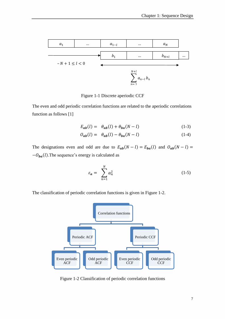
Figure 1-1 Discrete aperiodic CCF ................................................................................... 7

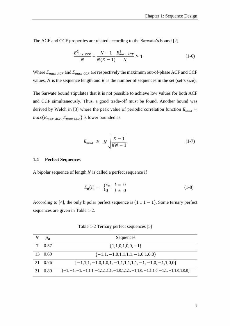
Figure 1-2 Classification of periodic correlation functions .............................................. 7

Figure 1-3 Generic 𝐿𝐹𝑆𝑅 generator [6] .......................................................................... 10

Figure 1-4 Gold sequence generator ............................................................................... 12

Figure 2-1 Direct-sequence transmitter .......................................................................... 23

Figure 2-2 PSD of original and spread signals [30] ....................................................... 24

Figure 2-3 Various CDMA technologies [31] ................................................................ 24

Figure 2-4 a) Spreading in DS-CDMA; b) Dispreading in DS-CDMA [32] ................. 26

Figure 2-5 Dispreading at unauthorized receiver [32].................................................... 26

Figure 2-6 MUI in cellular systems ................................................................................ 27

Figure 2-7 Wireless channel with multipath propagation [34]. ...................................... 28

Figure 2-8 Generic Rake receiver [35] ........................................................................... 28

Figure 2-9 Multiple access in cellular networks [32] ..................................................... 30

Figure 2-10 MC-CDMA Transmitted signal [37] .......................................................... 31

Figure 2-11 CDMA-based Satellite system .................................................................... 32

Figure 3-1 Generic DS-CDMA system [40] .................................................................. 36

Figure 3-2 Performance of various sequences in terms of CCCF .................................. 42

Figure 3-3 BER comparison between various spreading sequences .............................. 43

Figure 3-4 BER vs. chip delay ....................................................................................... 44

Figure 3-5 BER vs. chip delay of a ZCZ set with zero even and odd CCFs .................. 45

Figure 4-1 Average CF of sequences for various lengths .............................................. 50

Figure 4-2 MC-CDMA transmitter for the 𝑘𝑡ℎ user ...................................................... 51

Figure 4-3 MC-CDMA receiver for the 𝑖𝑡ℎ user ............................................................ 53

Figure 4-4 Performance of various sequences in terms of CCCF .................................. 56

Figure 4-5 BER versus 𝑆𝑁𝑅 of various spreading sequences ........................................ 57

Figure 5-1 VLC spectrum [51] ....................................................................................... 59

Figure 5-2 a) Direct LOS link; b) non-direct-LOS link [50] .......................................... 60

List of Figures

xii

Figure 5-3 Broadband wireless network scenario [50] ................................................... 60

Figure 5-4 a) cell per user; b) cell per room; c) cellular topology [50] .......................... 61

Figure 5-5 SAC-OCDMA transmitter for VLC system ................................................. 62

Figure 5-6 SAC-OCDMA receiver for VLC system ...................................................... 63

Figure 5-7 𝑀𝑈𝐼 vs. time delay ....................................................................................... 67

Figure 5-8 𝑀𝑈𝐼 vs. sequence length. ............................................................................. 67

Figure 5-9 𝑀𝑈𝐼 vs. number of active users .................................................................... 68

Figure 5-10 BER comparison between ZCC and ZCZ sequences ................................. 69

Figure A-1 Three-stages LFSR generator ...................................................................... 75

Figure B-1 Continuous-time partial CCFs. .................................................................... 88

Figure D-1 Even periodic CCF. .................................................................................... 103

xiii

List of Tables

Table 1-1 Sequence operations ......................................................................................... 5

Table 1-2 Ternary perfect sequences [5] .......................................................................... 8

Table 1-3 Feedback taps for m-sequence [7].................................................................. 11

Table 1-4 Preferred pairs of m-sequences ...................................................................... 11

Table 1-5 Comparison between Gold sequence m-sequences [7] .................................. 12

Table 1-6 Complementary sets [10] ............................................................................... 13

Table 2-1 Rake receiver improvement [36] .................................................................... 29

Table 2-2 Delay spread of different environments [31] ................................................. 29

Table 3-1 SNR values for different BER levels ............................................................. 44

Table 4-1 Parameters of Fan’s construction ................................................................... 48

Table 4-2 Parameters of Maeda’s construction .............................................................. 49

Table 4-3 Parameters of Cha’s construction .................................................................. 49

Table 4-4 Family size of sequences with lengths 𝑁 = 8, 16, 32, 64, and 128............... 49

Table 4-5 𝐵𝐸𝑅 and 𝐶𝐹 Performance comparison in QS-MC-CDMA ........................... 58

Table 5-1- OCDMA System’s parameters ..................................................................... 69

Table A-1 A 3-stage 𝐿𝐹𝑆𝑅 generator’s output. .............................................................. 76

xiv

xv

Acronyms

ACF Auto Correlation Function

AP Access Point

AWGN Additive White Gaussian Noise

BER Bit Error Rate

BPSK Binary Phase Shift Keying

BS Base Station

CC Complementary Codes

CCF Cross Correlation Function

CDMA Code Division Multiple Access

CF Crest Factor

DS Direct Sequence

DSSS Direct Sequence Spread Spectrum

FDMA Frequency Division Multiple Access

FH Frequency Hopping

ICI Inter Channel Interference

ISI Inter-Symbol Interference

LED Light Emitting Diode

LOS Line of Sight

LTE Long Term Evolution

MAI Multiple Access Interference

MC Multicarrier

MPI Multipath Interference

MUI Multiuser Interference

MT Multi-Tone

NOMA Non-Orthogonal Multiple Access

Acronyms

xvi

OFDM Orthogonal Frequency Division Multiplexing

OWC Optical Wireless Communication

PAPR Peak-to-Average Power Ratio

PCF Periodic Correlation Function

PN Pseudo-Noise

QS Quasi-Synchronous

SAC Spectral Amplitude Coding

SINR Signal to Interference Plus Noise Ratio

SNR Signal to Noise Ratio

SS Spread Spectrum

TDMA Time Division Multiple Access

TH Time Hopping

UWB Ultra wide Band

WDMA Wavelength Division Multiple Access

VLC Visible Light Communication

V2V Vehicle-To-Vehicle

WH Walsh-Hadamard

ZCC Zero Cross-Correlation

ZCZ Zero Correlation Zone

1

Introduction

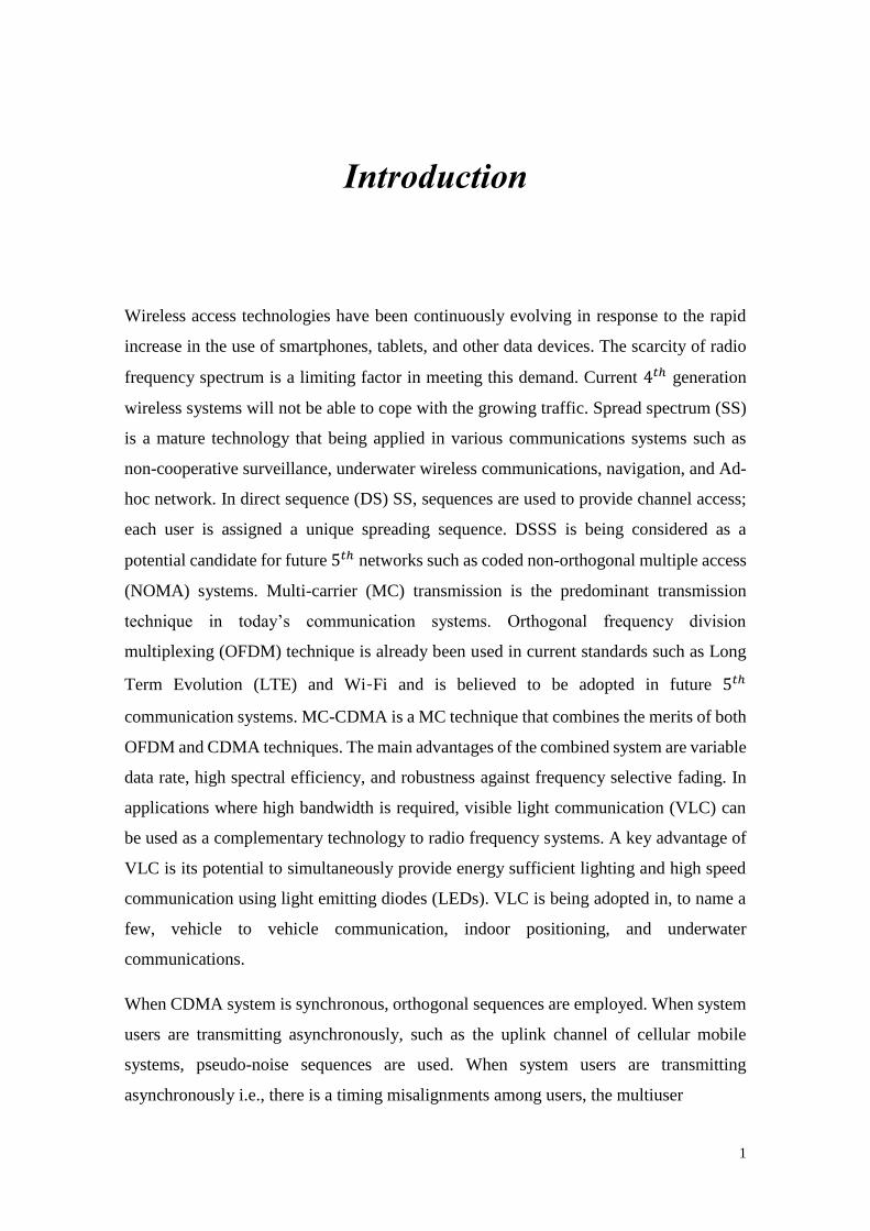
Wireless access technologies have been continuously evolving in response to the rapid

increase in the use of smartphones, tablets, and other data devices. The scarcity of radio

frequency spectrum is a limiting factor in meeting this demand. Current 4𝑡ℎ generation

wireless systems will not be able to cope with the growing traffic. Spread spectrum (SS)

is a mature technology that being applied in various communications systems such as

non-cooperative surveillance, underwater wireless communications, navigation, and Ad-

hoc network. In direct sequence (DS) SS, sequences are used to provide channel access;

each user is assigned a unique spreading sequence. DSSS is being considered as a

potential candidate for future 5𝑡ℎ networks such as coded non-orthogonal multiple access

(NOMA) systems. Multi-carrier (MC) transmission is the predominant transmission

technique in today’s communication systems. Orthogonal frequency division

multiplexing (OFDM) technique is already been used in current standards such as Long

Term Evolution (LTE) and Wi-Fi and is believed to be adopted in future 5𝑡ℎ

communication systems. MC-CDMA is a MC technique that combines the merits of both

OFDM and CDMA techniques. The main advantages of the combined system are variable

data rate, high spectral efficiency, and robustness against frequency selective fading. In

applications where high bandwidth is required, visible light communication (VLC) can

be used as a complementary technology to radio frequency systems. A key advantage of

VLC is its potential to simultaneously provide energy sufficient lighting and high speed

communication using light emitting diodes (LEDs). VLC is being adopted in, to name a

few, vehicle to vehicle communication, indoor positioning, and underwater

communications.

When CDMA system is synchronous, orthogonal sequences are employed. When system

users are transmitting asynchronously, such as the uplink channel of cellular mobile

systems, pseudo-noise sequences are used. When system users are transmitting

asynchronously i.e., there is a timing misalignments among users, the multiuser

Introduction

2

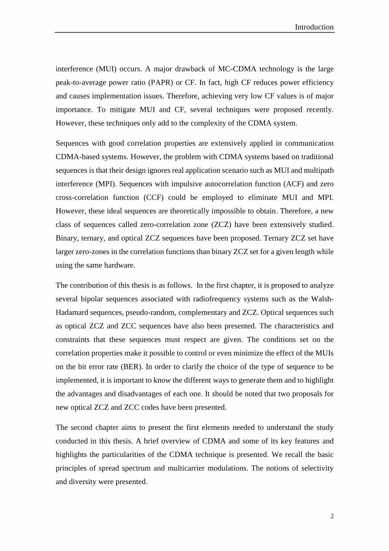
interference (MUI) occurs. A major drawback of MC-CDMA technology is the large

peak-to-average power ratio (PAPR) or CF. In fact, high CF reduces power efficiency

and causes implementation issues. Therefore, achieving very low CF values is of major

importance. To mitigate MUI and CF, several techniques were proposed recently.

However, these techniques only add to the complexity of the CDMA system.

Sequences with good correlation properties are extensively applied in communication

CDMA-based systems. However, the problem with CDMA systems based on traditional

sequences is that their design ignores real application scenario such as MUI and multipath

interference (MPI). Sequences with impulsive autocorrelation function (ACF) and zero

cross-correlation function (CCF) could be employed to eliminate MUI and MPI.

However, these ideal sequences are theoretically impossible to obtain. Therefore, a new

class of sequences called zero-correlation zone (ZCZ) have been extensively studied.

Binary, ternary, and optical ZCZ sequences have been proposed. Ternary ZCZ set have

larger zero-zones in the correlation functions than binary ZCZ set for a given length while

using the same hardware.

The contribution of this thesis is as follows. In the first chapter, it is proposed to analyze

several bipolar sequences associated with radiofrequency systems such as the Walsh-

Hadamard sequences, pseudo-random, complementary and ZCZ. Optical sequences such

as optical ZCZ and ZCC sequences have also been presented. The characteristics and

constraints that these sequences must respect are given. The conditions set on the

correlation properties make it possible to control or even minimize the effect of the MUIs

on the bit error rate (BER). In order to clarify the choice of the type of sequence to be

implemented, it is important to know the different ways to generate them and to highlight

the advantages and disadvantages of each one. It should be noted that two proposals for

new optical ZCZ and ZCC codes have been presented.

The second chapter aims to present the first elements needed to understand the study

conducted in this thesis. A brief overview of CDMA and some of its key features and

highlights the particularities of the CDMA technique is presented. We recall the basic

principles of spread spectrum and multicarrier modulations. The notions of selectivity

and diversity were presented.

Introduction

3

In the third chapter, we will analyze the performances of sequences in a quasi-

synchronous DS-CDMA system (DS: Direct-Sequence). Here, we directly multiply the

message to be transmitted by a sequence. The spectral spread of the coded signal comes

from the fact that the frequency of sequences is much greater than the frequency of data.

We will develop a theoretical model describing their statistics. We will determine the

signal-to-noise plus interference ratio (SINR: Signal to Interference plus Noise Ratio) in

the uplink. The latter makes it possible to define new correlation criteria, in particular the

even and odd correlation functions, which will make it possible to choose the right set of

sequences to be used in the system. It should be noted that the ZCZ sequences have

transmission performance that is much greater than Gold sequences when the delay

between users is within their zero-correlation zone. We also note that some ZCZ

sequences maintain better performance beyond their zero-correlation zone.

In the fourth chapter, we will analyze the performances of sequences in a quasi-

synchronous MC-CDMA system (MC: Multi Carrier). The MC-CDMA technique is

based on the concatenation of spread spectrum and multicarrier modulation. Unlike the

previous technique (DS-CDMA), MC-CDMA modulation spreads the data of each user

in the frequency domain. The major advantage of this technique is that it allows multiple

access with a transmitted signal having all the characteristics and advantages of

multicarrier modulation. In addition, the frequency diversity of the channel is fully

exploited. However, the MC-CDMA technique did not inherit only the advantages of

multicarrier modulation and CDMA technique. Indeed, the MC-CDMA signal, by its

multi-carrier nature, has a large amplitude fluctuation that can lead to performance

degradation due to the power amplification function, amplification which is by nature

non-linear. In addition, after transmission on a channel, the MC-CDMA receiver must

fight against MUI. First, we compare the influence of ZCZ sequences with conventional

sequences on Crest Factor (CF) variation. In addition to their low CF values, ZCZ

sequences also have stable CF, which is a major advantage in MC-CDMA systems. The

second contribution of this chapter focuses on the optimization of the uplink using

spreading sequences. The BER of the quasi-synchronous MC CDMA system, uplink, is

generalized to include the case of ternary sequences. According to the BER criterion, the

best results are obtained when the ZCZ sequences are used. These latter sequences

Introduction

4

eliminate interference and provide BER performance similar to the AWGN channel. We

conclude that ZCZ sequences have low CF and interference-free communication.

In the fifth chapter, the transmission of CDMA signals on an optical channel is

approached and the performance of the optical system using different optical sequences

is studied. The objective is to find optical sequences allowing a significant increase of

performance. It is shown that the optical ZCZ sequences used in the case of the uplink

quasi synchronous SAC-OCDMA system, eliminate the MUI, if the maximum delay

between user is at inside the zero-correlation zone, but their performance remains low

compared to ZCC codes with the same parameters (number of sequences and weight).

Finally, a general conclusion summarizes the main contributions of this thesis and some

perspectives to this work are then presented.

5

Chapter 1: Sequence Design

1.1 Introduction

Sequences (codes) with good correlation properties are extensively applied in

communication systems. There are various kinds of sequences, binary and non-binary

sequences, unipolar and bipolar sequences, periodic and aperiodic sequences,

complementary pairs and complementary sets etc. The focus of this chapter is on the

properties of digital sequences that will be used in the succeeding chapters. This chapter

also includes new constructions of optical zero correlation zone (ZCZ) and zero cross-

correlation (ZCC) sequences.

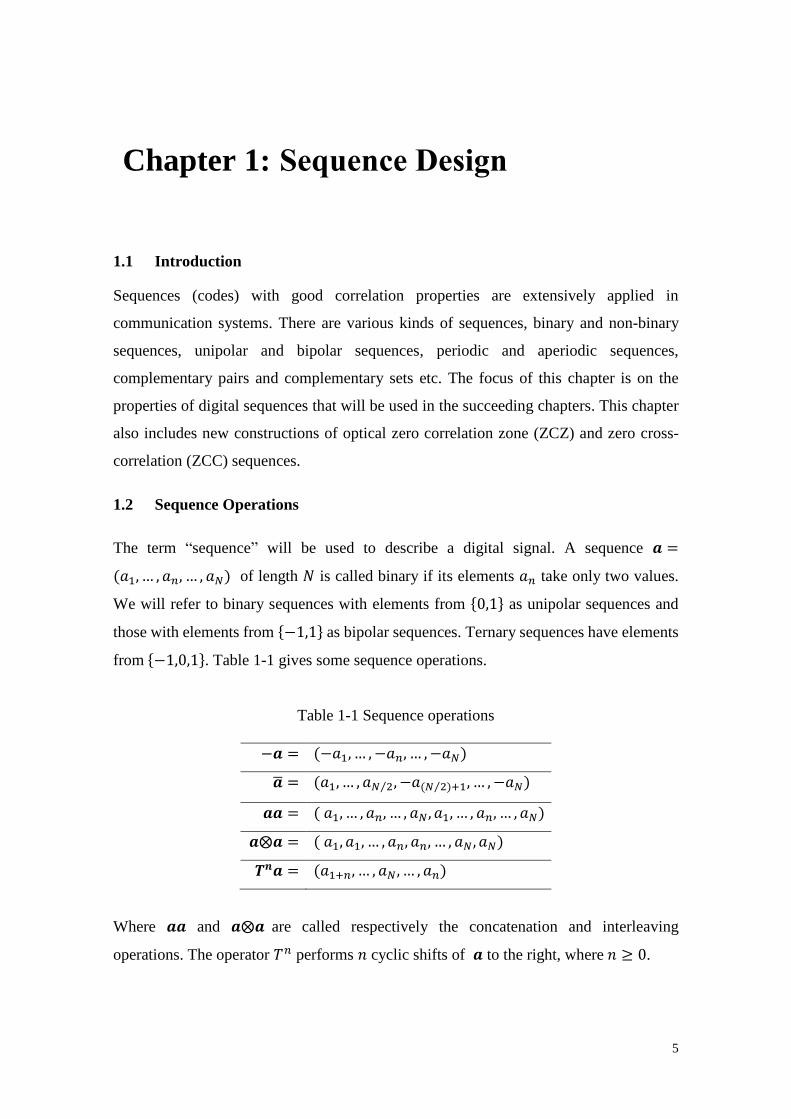
1.2 Sequence Operations

The term “sequence” will be used to describe a digital signal. A sequence 𝒂 =

(𝑎1, … , 𝑎𝑛, … , 𝑎𝑁) of length 𝑁 is called binary if its elements 𝑎𝑛 take only two values.

We will refer to binary sequences with elements from {0,1} as unipolar sequences and

those with elements from {−1,1} as bipolar sequences. Ternary sequences have elements

from {−1,0,1}. Table 1-1 gives some sequence operations.

Table 1-1 Sequence operations

−𝒂 = (−𝑎1, … , −𝑎𝑛, … , −𝑎𝑁)

�̅� = (𝑎1, … , 𝑎𝑁 2⁄ , −𝑎(𝑁 2)⁄ +1, … , −𝑎𝑁)

𝒂𝒂 = ( 𝑎1, … , 𝑎𝑛, … , 𝑎𝑁 , 𝑎1, … , 𝑎𝑛, … , 𝑎𝑁)

𝒂⨂𝒂 = ( 𝑎1, 𝑎1, … , 𝑎𝑛, 𝑎𝑛, … , 𝑎𝑁 , 𝑎𝑁)

𝑻𝒏𝒂 = (𝑎1+𝑛, … , 𝑎𝑁 , … , 𝑎𝑛)

Where 𝒂𝒂 and 𝒂⨂𝒂 are called respectively the concatenation and interleaving

operations. The operator 𝑇𝑛 performs 𝑛 cyclic shifts of 𝒂 to the right, where 𝑛 ≥ 0.

Chapter 1: Sequence Design

6

If 𝒂 is a unipolar sequence, the corresponding bipolar sequence 𝒃 is obtained using the

following formula

𝑏𝑛 = (−1)𝑎𝑛 (1-1)

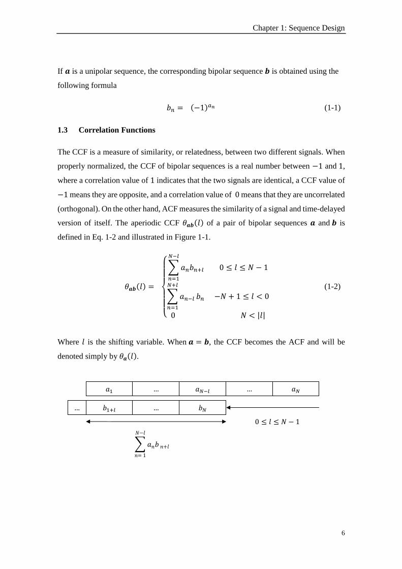
1.3 Correlation Functions

The CCF is a measure of similarity, or relatedness, between two different signals. When

properly normalized, the CCF of bipolar sequences is a real number between −1 and 1,

where a correlation value of 1 indicates that the two signals are identical, a CCF value of

−1 means they are opposite, and a correlation value of 0 means that they are uncorrelated

(orthogonal). On the other hand, ACF measures the similarity of a signal and time-delayed

version of itself. The aperiodic CCF 𝜃𝒂𝒃(𝑙) of a pair of bipolar sequences 𝒂 and 𝒃 is

defined in Eq. 1-2 and illustrated in Figure 1-1.

𝜃𝒂𝒃(𝑙) =

{

∑𝑎𝑛𝑏𝑛+𝑙

𝑁−𝑙

𝑛=1

0 ≤ 𝑙 ≤ 𝑁 − 1

∑𝑎𝑛−𝑙

𝑁+𝑙

𝑛=1

𝑏𝑛 −𝑁 + 1 ≤ 𝑙 < 0

0 𝑁 < |𝑙|

(1-2)

Where 𝑙 is the shifting variable. When 𝒂 = 𝒃, the CCF becomes the ACF and will be

denoted simply by 𝜃𝒂(𝑙).

𝑏𝑁 …

𝑎𝑁−𝑙 … 𝑎1 … 𝑎𝑁

𝑏1+𝑙

0 ≤ 𝑙 ≤ 𝑁 − 1

∑ 𝑎𝑛𝑏 𝑛+𝑙

𝑁−𝑙

𝑛= 1

…

Chapter 1: Sequence Design

7

Figure 1-1 Discrete aperiodic CCF

The even and odd periodic correlation functions are related to the aperiodic correlations

function as follows [1]

𝐸𝒂𝒃(𝑙) = 𝜃𝒂𝒃(𝑙) + 𝜃𝒃𝒂(𝑁 − 𝑙) (1-3)

𝑂𝒂𝒃(𝑙) = 𝜃𝒂𝒃(𝑙) − 𝜃𝒃𝒂(𝑁 − 𝑙) (1-4)

The designations even and odd are due to 𝐸𝒂𝒃(𝑁 − 𝑙) = 𝐸𝒃𝒂(𝑙) and 𝑂𝒂𝒃(𝑁 − 𝑙) =

−𝑂𝒃𝒂(𝑙).The sequence’s energy is calculated as

휀𝒂 = ∑𝑎𝑛2

𝑁

𝑛=1

(1-5)

The classification of periodic correlation functions is given in Figure 1-2.

Figure 1-2 Classification of periodic correlation functions

Correlation functions

Periodic ACF

Even periodic ACF

Odd periodic ACF

Periodic CCF

Even periodic CCF

Odd periodic CCF

𝑎1−𝑙 … 𝑎1 … 𝑎𝑁

… 𝑏𝑁+𝑙 … 𝑏1

–𝑁 + 1 ≤ 𝑙 < 0

∑ 𝑎𝑛−𝑙

𝑁+𝑙

𝑛= 1

𝑏𝑛

Chapter 1: Sequence Design

8

The ACF and CCF properties are related according to the Sarwate’s bound [2]

𝐸𝑚𝑎𝑥 𝐶𝐶𝐹2

𝑁+

𝑁 − 1

𝑁(𝐾 − 1)

𝐸𝑚𝑎𝑥 𝐴𝐶𝐹2

𝑁≥ 1 (1-6)

Where 𝐸𝑚𝑎𝑥 𝐴𝐶𝐹 and 𝐸𝑚𝑎𝑥 𝐶𝐶𝐹 are respectively the maximum out-of-phase ACF and CCF

values, 𝑁 is the sequence length and 𝐾 is the number of sequences in the set (set’s size).

The Sarwate bound stipulates that it is not possible to achieve low values for both ACF

and CCF simultaneously. Thus, a good trade-off must be found. Another bound was

derived by Welch in [3] where the peak value of periodic correlation function 𝐸𝑚𝑎𝑥 =

𝑚𝑎𝑥{𝐸𝑚𝑎𝑥 𝐴𝐶𝐹, 𝐸𝑚𝑎𝑥 𝐶𝐶𝐹} is lower bounded as

𝐸𝑚𝑎𝑥 ≥ 𝑁 √𝐾 − 1

𝐾𝑁 − 1 (1-7)

1.4 Perfect Sequences

A bipolar sequence of length 𝑁 is called a perfect sequence if

𝐸𝒂(𝑙) = {휀𝒂 𝑙 = 0

0 𝑙 ≠ 0 (1-8)

According to [4], the only bipolar perfect sequence is {1 1 1 − 1}. Some ternary perfect

sequences are given in Table 1-2.

Table 1-2 Ternary perfect sequences [5]

𝑁 𝜇𝒂 Sequences

7 0.57 {1,1,0,1,0,0,−1}

13 0.69 {−1,1, −1,0,1,1,1,1,−1,0,1,0,0}

21 0.76 {−1,1,1, −1,0,1,0,1, −1,1,1,1,1,1,−1, −1,0, −1,1,0,0}

31 0.80 {−1,−1, −1,−1,1,1, −1,1,1,1,1, −1,0,1,1,1, −1,1,0, −1,1,1,0, −1,1, −1,1,0,1,0,0}

Chapter 1: Sequence Design

9

Where 𝜇𝒂 is the energy per element ratio (𝐸𝐸𝑅) defined as

𝜇𝒂 = 휀𝒂𝑁≤ 1 (1-9)

The equality 𝜇𝒂 = 1 is achieved when the sequence is bipolar.

1.5 Walsh-Hadamard Sequences

Walsh-Hadamard (𝑊𝐻) sequences are created out of Hadamard matrix 𝑯𝑵 =

[𝒉𝟏 , … , 𝒉𝒏… ,𝒉𝑵]𝑻 of order 𝑁. Any pair of bipolar WH sequences 𝒉𝒊 and 𝒉𝒋 is

orthogonal that is

𝐸𝒉𝒊𝒉𝒋(0) = {𝑁 𝑖 = 𝑗0 𝑖 ≠ 𝑗

(1-10)

Higher order Hadamard matrices are generated recursively using

𝑯𝟐𝑵 = [𝑯𝑵 𝑯𝑵

𝑯𝑵 −𝑯𝑵] (1-11)

Example 1 of Annex A shows the construction of Hadamard matrices. The ACF of WH

sequences do not have good characteristics; it can have more than one peak. The CCF can

also have peaks in the out-of-phase shifts (𝑙 ≠ 0). Therefore, WH sequences do not have

the best correlation properties.

1.6 Pseudo-Noise Sequences

A pseudo-noise (𝑃𝑁) sequence is a deterministic periodic sequence with properties

associated with randomness. For example, when an ideal coin is tossed, the result is

obviously either head 1 or tail 0. The sequence obtained by repeatedly tossing an ideal

coin has the following properties [4]

1. Balance property: the number of 1𝑠 is approximately equal to the number of 0s.

Chapter 1: Sequence Design

10

2. Run property: a run is defined as a consecutive occurrence of 1𝑠 or 0𝑠. Short runs

are more probable than long runs.

3. Correlation property: 𝑃𝑁 sequence and its cyclically shifted version have very

low correlation values. The 𝐴𝐶𝐹 general form of any 𝑃𝑁 sequence 𝒂 is

𝐸𝒂(𝑙) = {𝑁 𝑙 = 0𝑘 𝑙 ≠ 0

(1-12)

Where 𝑘 is preferably zero. These ideal properties can only be approximated in practice

since the smallest possible values of 𝑘 are ±1 [4].

M-sequences

One type of 𝑃𝑁 sequences is the so called maximum length sequence (m-sequence). It

has a length of 𝑁 = 2𝑚 − 1 and can be generated by 𝑚-stage linear feedback shift

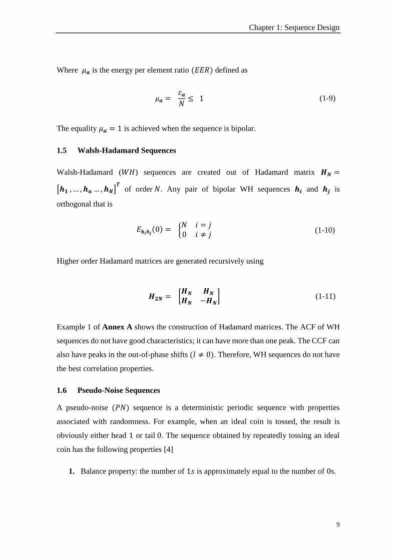
registers (𝐿𝐹𝑆𝑅) [4]. The generic form of 𝐿𝐹𝑆𝑅 is depicted in Figure 1-3.

Figure 1-3 Generic 𝐿𝐹𝑆𝑅 generator [6]

Where (𝑎𝑛−1, 𝑎𝑛−2 , … , 𝑎𝑛−𝑚) are the contents (memory elements) of the LFSR and

(𝑐1, 𝑐2, … , 𝑐𝑚) are the feedback connection coefficients.

The addition of elements is performed modulo-2 defined by 0 ⊕ 0 = 1⊕ 1 = 0

and 0 ⊕ 1 = 1⊕ 0 = 1. Table 1-3 lists the feedback connections for m-sequence and

the number of available sequences for a given length, where the rest of 𝑚-sequences can

be derived by means of sampling [4].

𝑐1 𝑐2 𝑐𝑚−1

𝑎𝑛−1 𝑎𝑛−2 𝑎𝑛−(𝑚−1) 𝑎𝑛−𝑚

𝑐𝑚

.......

.......

𝑎𝑛

Chapter 1: Sequence Design

11

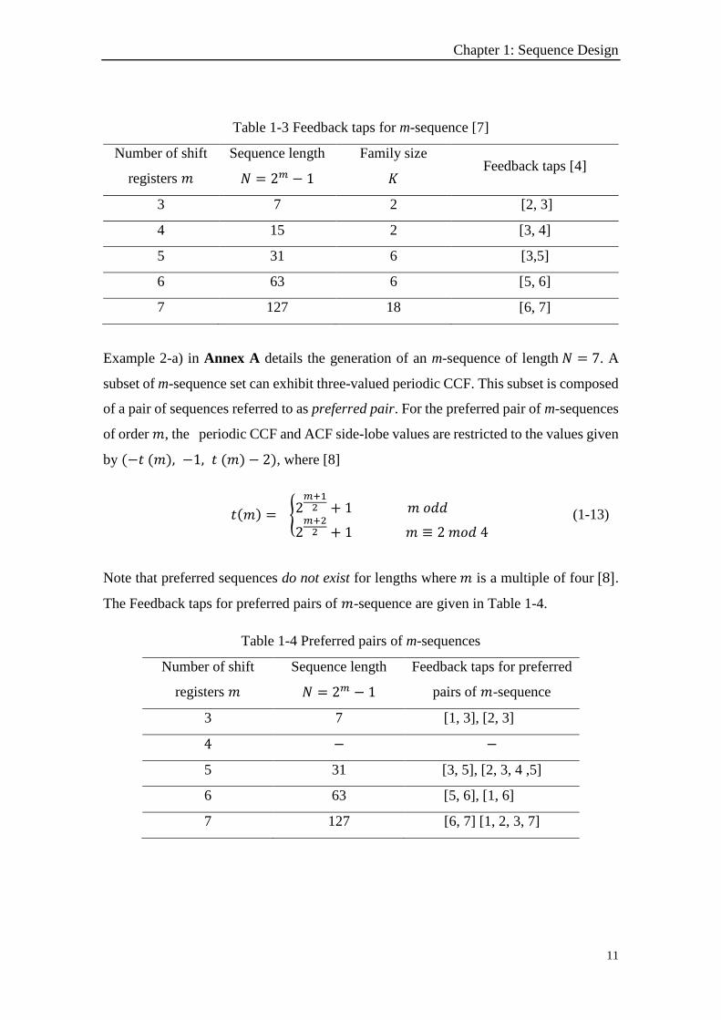
Table 1-3 Feedback taps for m-sequence [7]

Number of shift

registers 𝑚

Sequence length

𝑁 = 2𝑚 − 1

Family size

𝐾 Feedback taps [4]

3 7 2 [2, 3]

4 15 2 [3, 4]

5 31 6 [3,5]

6 63 6 [5, 6]

7 127 18 [6, 7]

Example 2-a) in Annex A details the generation of an m-sequence of length 𝑁 = 7. A

subset of m-sequence set can exhibit three-valued periodic CCF. This subset is composed

of a pair of sequences referred to as preferred pair. For the preferred pair of m-sequences

of order 𝑚, the periodic CCF and ACF side-lobe values are restricted to the values given

by (−𝑡 (𝑚), −1, 𝑡 (𝑚) − 2), where [8]

𝑡(𝑚) = {2𝑚+12 + 1 𝑚 𝑜𝑑𝑑

2𝑚+22 + 1 𝑚 ≡ 2 𝑚𝑜𝑑 4

(1-13)

Note that preferred sequences do not exist for lengths where 𝑚 is a multiple of four [8].

The Feedback taps for preferred pairs of 𝑚-sequence are given in Table 1-4.

Table 1-4 Preferred pairs of m-sequences

Number of shift

registers 𝑚

Sequence length

𝑁 = 2𝑚 − 1

Feedback taps for preferred

pairs of 𝑚-sequence

3 7 [1, 3], [2, 3]

4 − −

5 31 [3, 5], [2, 3, 4 ,5]

6 63 [5, 6], [1, 6]

7 127 [6, 7] [1, 2, 3, 7]

Chapter 1: Sequence Design

12

Gold Sequences

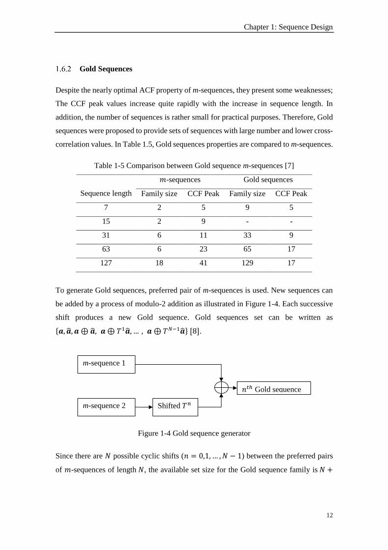
Despite the nearly optimal ACF property of m-sequences, they present some weaknesses;

The CCF peak values increase quite rapidly with the increase in sequence length. In

addition, the number of sequences is rather small for practical purposes. Therefore, Gold

sequences were proposed to provide sets of sequences with large number and lower cross-

correlation values. In Table 1.5, Gold sequences properties are compared to m-sequences.

Table 1-5 Comparison between Gold sequence m-sequences [7]

Sequence length

𝑚-sequences Gold sequences

Family size CCF Peak Family size CCF Peak

7 2 5 9 5

15 2 9 - -

31 6 11 33 9

63 6 23 65 17

127 18 41 129 17

To generate Gold sequences, preferred pair of m-sequences is used. New sequences can

be added by a process of modulo-2 addition as illustrated in Figure 1-4. Each successive

shift produces a new Gold sequence. Gold sequences set can be written as

{𝒂, �̂�, 𝒂 ⊕ �̂�, 𝒂⊕ 𝑇1�̂�, … , 𝒂 ⊕ 𝑇𝑁−1�̂�} [8].

Figure 1-4 Gold sequence generator

Since there are 𝑁 possible cyclic shifts (𝑛 = 0,1, … ,𝑁 − 1) between the preferred pairs

of 𝑚-sequences of length 𝑁, the available set size for the Gold sequence family is 𝑁 +

m-sequence 1

m-sequence 2 Shifted 𝑇𝑛

𝑛𝑡ℎ Gold sequence

Chapter 1: Sequence Design

13

2 = 2𝑚 + 1. Example 2-b) in Annex A details the generation of 𝐾 = 9 Gold sequences

each with length 𝑁 = 7.

Orthogonal Gold Sequences

Experiments results show that CCF values of the Gold sequences are “ − 1” for many

sequence shifts [4]. This suggests that it may be possible to turn the “ − 1” CCF values

to “0” by attaching an additional “0” to the original unipolar Gold sequences. In fact, 𝐾 =

2𝑚 orthogonal sequences (except �̂�) can be obtained by this simple zero-padding [9].

These sequences referred to as orthogonal Gold sequences (OG) show reasonable cross-

correlation and off-peak autocorrelation values. Example 2-c) in Annex A details the

generation of 𝐾 = 8 orthogonal Gold sequences each with length 𝑁 = 8.

1.7 Complementary Sequences

Complementary Pairs

Complementary pairs (𝐶𝑃𝑠) were first introduced by Golay [10]. A set of 𝐶𝑃𝑠 is defined

as a pair of equally long which have the property that the number of pairs of like elements

with any given separation in one sequence is equal to the number of pairs of unlike

elements with the same separation in the other sequence [10]. The latter property can also

be expressed in aperiodic ACF terms; A pair of two bipolar sequences (𝒂, 𝒃) is a 𝐶𝑃 if

the sum of their aperiodic ACFs is [10]

𝜃𝒂(𝑙) + 𝜃𝒃(𝑙) = {2𝑁, 𝑙 = 00, 𝑙 ≠ 0

(1-14)

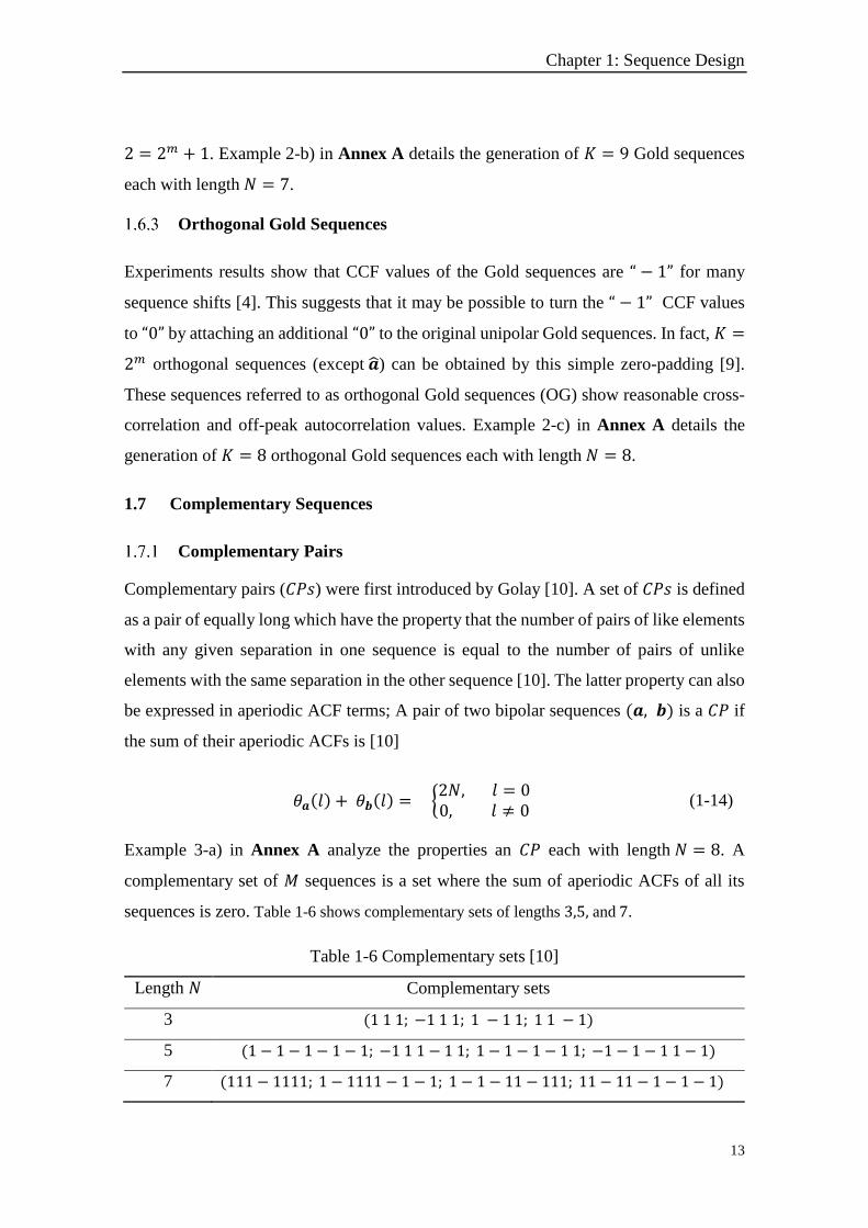
Example 3-a) in Annex A analyze the properties an 𝐶𝑃 each with length 𝑁 = 8. A

complementary set of 𝑀 sequences is a set where the sum of aperiodic ACFs of all its

sequences is zero. Table 1-6 shows complementary sets of lengths 3,5, and 7.

Table 1-6 Complementary sets [10]

Length 𝑁 Complementary sets

3 (1 1 1; −1 1 1; 1 − 1 1; 1 1 − 1)

5 (1 − 1 − 1 − 1 − 1; −1 1 1 − 1 1; 1 − 1 − 1 − 1 1; −1 − 1 − 1 1 − 1)

7 (111 − 1111; 1 − 1111 − 1 − 1; 1 − 1 − 11 − 111; 11 − 11 − 1 − 1 − 1)

Chapter 1: Sequence Design

14

To extend the length of a CP we use the following property [10].

Property: let (𝒂, 𝒃) be an 𝐶𝑃 each of length 𝐿, an extended pair of two concatenated

sequences such as (𝒂𝒃, (−𝒂)𝒃) is also a 𝐶𝑃. Applying the latter operation 𝑚 times

results in a pair of sequences each of length 𝑁 = 2𝑚𝐿.

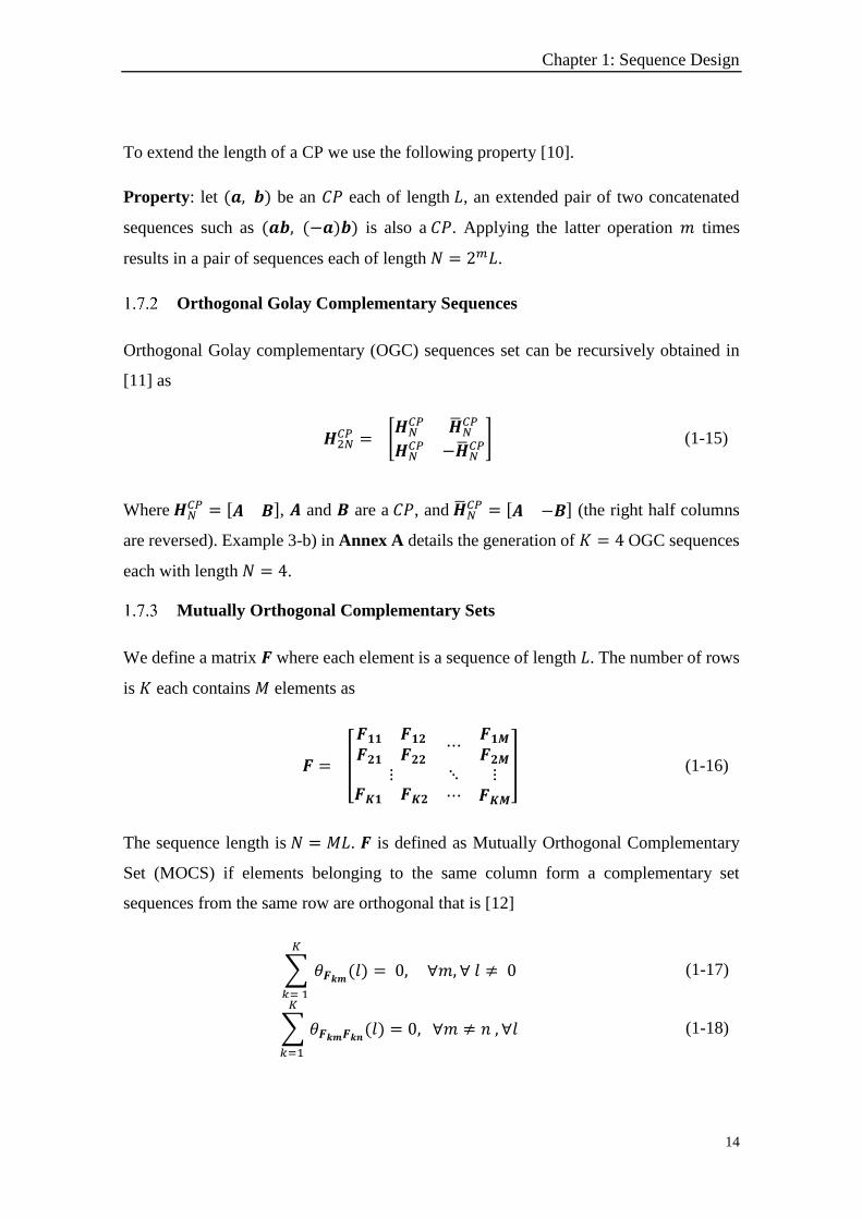
Orthogonal Golay Complementary Sequences

Orthogonal Golay complementary (OGC) sequences set can be recursively obtained in

[11] as

𝑯2𝑁𝐶𝑃 = [

𝑯𝑁𝐶𝑃 �̅�𝑁

𝐶𝑃

𝑯𝑁𝐶𝑃 −�̅�𝑁

𝐶𝑃] (1-15)

Where 𝑯𝑁𝐶𝑃 = [𝑨 𝑩], 𝑨 and 𝑩 are a 𝐶𝑃, and �̅�𝑁

𝐶𝑃 = [𝑨 −𝑩] (the right half columns

are reversed). Example 3-b) in Annex A details the generation of 𝐾 = 4 OGC sequences

each with length 𝑁 = 4.

Mutually Orthogonal Complementary Sets

We define a matrix 𝑭 where each element is a sequence of length 𝐿. The number of rows

is 𝐾 each contains 𝑀 elements as

𝑭 = [

𝑭𝟏𝟏 𝑭𝟏𝟐𝑭𝟐𝟏 𝑭𝟐𝟐

⋯𝑭𝟏𝑴𝑭𝟐𝑴

⋮ ⋱ ⋮𝑭𝑲𝟏 𝑭𝑲𝟐 ⋯ 𝑭𝑲𝑴

] (1-16)

The sequence length is 𝑁 = 𝑀𝐿. 𝑭 is defined as Mutually Orthogonal Complementary

Set (MOCS) if elements belonging to the same column form a complementary set

sequences from the same row are orthogonal that is [12]

∑ 𝜃𝑭𝒌𝒎(𝑙)

𝐾

𝑘= 1

= 0, ∀𝑚, ∀ 𝑙 ≠ 0 (1-17)

∑𝜃𝑭𝒌𝒎𝑭𝒌𝒏(𝑙)

𝐾

𝑘=1

= 0, ∀𝑚 ≠ 𝑛 , ∀𝑙 (1-18)

Chapter 1: Sequence Design

15

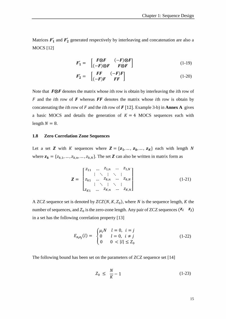
Matrices 𝑭𝟏′ and 𝑭𝟐

′ generated respectively by interleaving and concatenation are also a

MOCS [12]

𝑭𝟏′ = [

𝑭⨂𝑭 (−𝑭)⨂𝑭(−𝑭)⨂𝑭 𝑭⨂𝑭

] (1-19)

𝑭𝟐′ = [

𝑭𝑭 (−𝑭)𝑭(−𝑭)𝑭 𝑭𝑭

] (1-20)

Note that 𝑭⨂𝑭 denotes the matrix whose 𝑖th row is obtain by interleaving the 𝑖th row of

𝐹 and the 𝑖th row of 𝑭 whereas 𝑭𝑭 denotes the matrix whose 𝑖th row is obtain by

concatenating the 𝑖th row of 𝐹 and the 𝑖th row of 𝑭 [12]. Example 3-b) in Annex A gives

a basic MOCS and details the generation of 𝐾 = 4 MOCS sequences each with

length 𝑁 = 8.

1.8 Zero Correlation Zone Sequences

Let a set 𝒁 with 𝐾 sequences where 𝒁 = {𝒛𝟏, … , 𝒛𝒌, … , 𝒛𝑲} each with length 𝑁

where 𝒛𝒌 = {𝑧𝑘,1, … , 𝑧𝑘,𝑛, … , 𝑧𝑘,𝑁}. The set 𝒁 can also be written in matrix form as

𝒁 =

[ 𝑧11 … 𝑧1,𝑛 … 𝑧1,𝑁

⋮ ⋱ ⋮ ⋱ ⋮𝑧𝑘1 … 𝑧𝑘,𝑛 … 𝑧𝑘,𝑁

⋮ ⋱ ⋮ ⋱ ⋮𝑧𝐾1 … 𝑧𝐾,𝑛 … 𝑧𝐾,𝑁]

(1-21)

A ZCZ sequence set is denoted by 𝑍𝐶𝑍(𝑁,𝐾, 𝑍0), where 𝑁 is the sequence length, 𝐾 the

number of sequences, and 𝑍0 is the zero-zone length. Any pair of ZCZ sequences (𝒛𝒊 𝒛𝒋)

in a set has the following correlation property [13]

𝐸𝒛𝒊𝒛𝒋(𝑙) = {

𝜇𝑖𝑁 𝑙 = 0, 𝑖 = 𝑗

0 𝑙 = 0, 𝑖 ≠ 𝑗

0 0 < |𝑙| ≤ 𝑍0

(1-22)

The following bound has been set on the parameters of ZCZ sequence set [14]

𝑍0 ≤ 𝑁

𝐾− 1 (1-23)

Chapter 1: Sequence Design

16

From equation above, note that there is a tradeoff between the 𝑍0 width and the family

size 𝐾. For a fixed length 𝑁, increasing 𝐾 size must be achieved at the cost of reduced 𝑍0

and vice versa. A ZCZ sequences set that satisfies the theoretical limit is called an optimal

ZCZ set. For bipolar sequence set, ZCZ bound becomes even tighter [15]

𝑍0 ≤ 𝑁

2𝐾

(1-24)

Binary ZCZ Sequences

1.8.1.1 Fan et al [13]

Let a MOCS matrix 𝑭(𝑛) with 𝐾 rows each of length 𝑁. Using the concatenation operation

in Eq. 1-20, we can obtain a matrix 𝑭(𝑛+1) with 2𝐾 rows each of length 2𝑁. If the basic

starter 𝑭(0) is a Hadamard matrix of order 2 (𝐾 = 𝑁 = 2), the rows of MOCS 𝑭(𝑛)

extended 𝑛 times form ZCZ sequences of 𝑍𝐶𝑍(22𝑛+1, 2𝑛+1, 2𝑛−1 ) , where 𝑛 ≥ 1. CPs

of length 𝐿 = 2𝑚 each can also be used to generate 𝑍𝐶𝑍(22𝑛+𝑚+1, 2𝑛+1, 2𝑛+𝑚−1 ) using

the concatenation operation. Example 4-a) in Annex A details the generation of Fan et

al binary ZCZ sequences set of size 𝐾 = 4, sequence length 𝑁 = 8, and zero-zone 𝑍0 =

1.

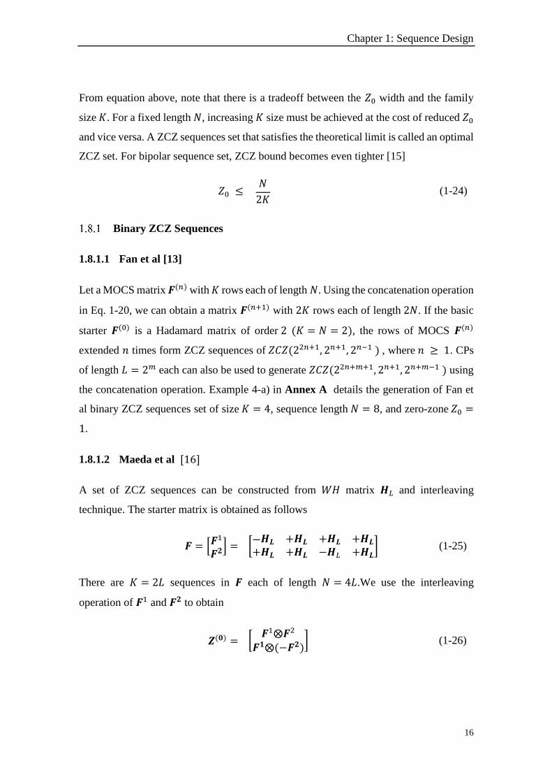
1.8.1.2 Maeda et al [16]

A set of ZCZ sequences can be constructed from 𝑊𝐻 matrix 𝑯𝐿 and interleaving

technique. The starter matrix is obtained as follows

𝑭 = [𝑭1

𝑭𝟐] = [

−𝑯𝑳 +𝑯𝑳 +𝑯𝑳 +𝑯𝑳

+𝑯𝑳 +𝑯𝑳 −𝑯𝐿 +𝑯𝑳] (1-25)

There are 𝐾 = 2𝐿 sequences in 𝑭 each of length 𝑁 = 4𝐿.We use the interleaving

operation of 𝑭1 and 𝑭𝟐 to obtain

𝒁(𝟎) = [𝑭1⨂𝑭2

𝑭𝟏⨂(−𝑭𝟐)] (1-26)

Chapter 1: Sequence Design

17

The set 𝒁(𝟎) is a ZCZ sequences set with 𝑍𝐶𝑍(8𝐿, 2𝐿, 1). In general, an extended set

𝒁(𝒎) with 𝑍𝐶𝑍(2𝑚+3𝐿, 2𝐿, 2𝑚+1 − 1) can be recursively constructed by interleaving

ZCZ sequence set 𝒁(𝒎−𝟏) as

𝒁(𝒎) = [𝒁(𝒎−𝟏)⨂𝒁(𝒎−𝟏)

𝒁(𝒎−𝟏)⨂(−𝒁(𝒎−𝟏))] (1-27)

Example 4-b) in Annex A details the generation of Maeda et al ZCZ sequences set of

size 𝐾 = 4, sequence length 𝑁 = 16, and zero-zone 𝑍0 = 1.

1.8.1.3 Cha et al [17]

A set of ZCZ sequences can be constructed from binary perfect sequence 𝒑(𝟎) of length 4.

First, the perfect sequence is extended as

𝒑(𝒏) = [𝒑(𝒏−𝟏) �̅�(𝒏−𝟏)] (1-28)

Where 𝑛 ≥ 1 and �̅� means that the right half columns of 𝒑 are reversed. The length of

𝒑(𝒏) is 𝑁 = 4×2𝑛. Another sequence 𝒈(𝒏) can be generated as

𝑔𝑖(𝑛)

= (−1)𝑖𝑝𝑖(𝑛)

(1-29)

Where 𝑝𝑖(𝑛)

is an element of 𝒑(𝒏) and 𝑖 = 1, … ,𝑁.

The pair (𝒑(𝒏), 𝒈(𝒏)) is called binary preferred pair. The number of sequences in the set

can be further increased as

𝒁 = {𝒑(𝒏), 𝒈(𝒏), 𝑻∆𝒑(𝒏), 𝑻∆𝒈(𝒏), … , 𝑻𝑠∆𝒑(𝒏), 𝑻𝑠∆𝒈(𝒏)} (1-30)

Where ∆> 0 is a shift increment and 𝑠 > 0 is the maximum shift related as follows

(𝑠 + 1)∆≤ 𝑁

4+ 1 (1-31)

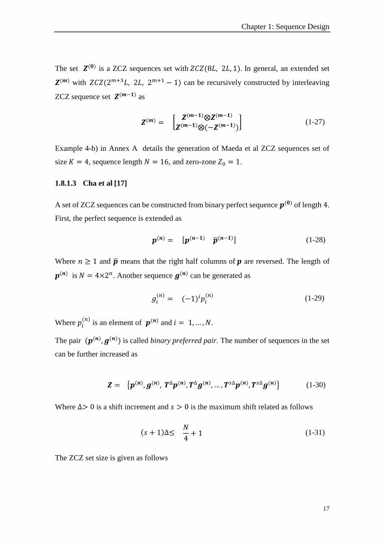
The ZCZ set size is given as follows

Chapter 1: Sequence Design

18

𝐾 = 2(𝑠 + 1) (1-32)

And 𝑍0 length is given as

𝑍𝑐𝑧 = |2∆ − 1| (1-33)

Where 𝑍𝑐𝑧 = 2𝑍0 + 1. Example 4-c) in Annex A details the generation of Cha et al ZCZ

sequences set of size 𝐾 = 4, sequence length 𝑁 = 16, and zero-zone 𝑍0 = 1.

Ternary ZCZ Sequences

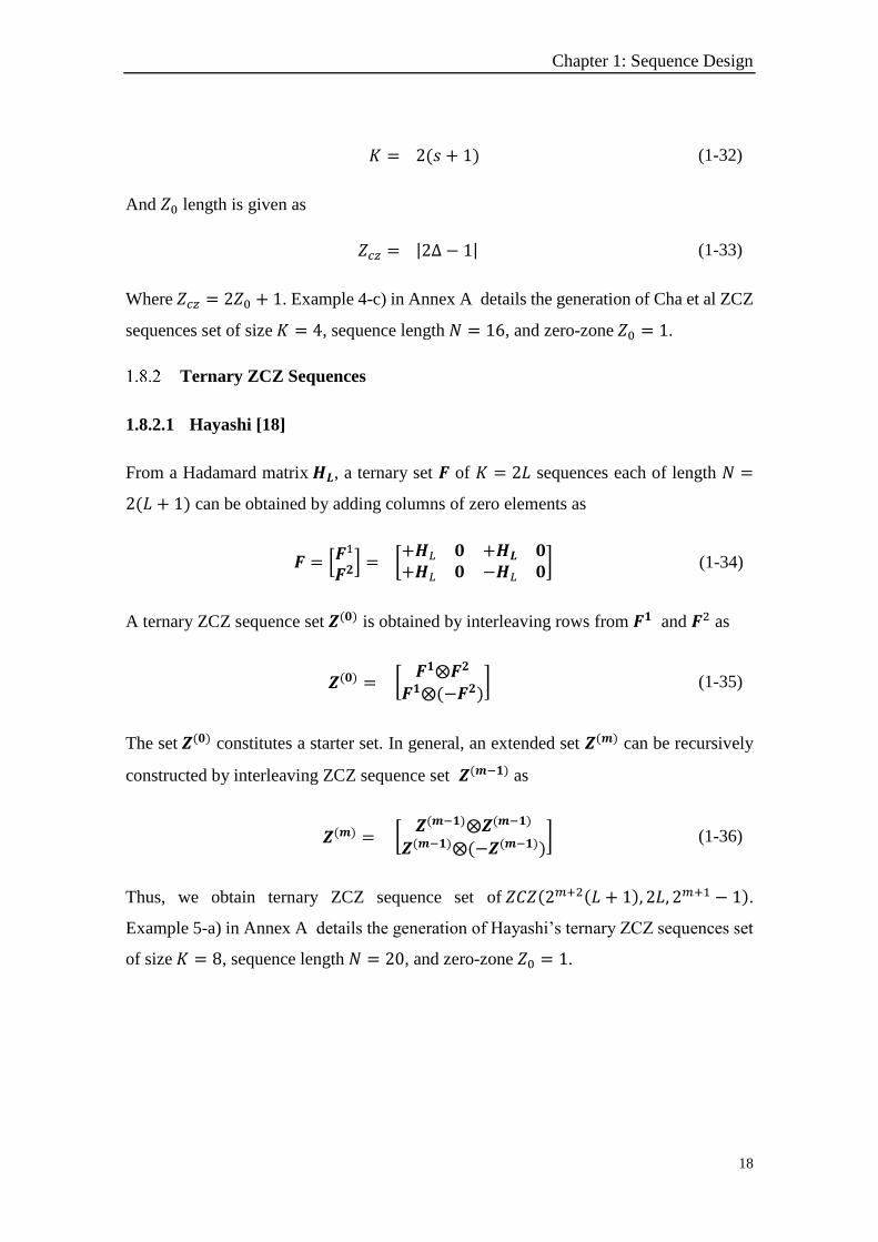
1.8.2.1 Hayashi [18]

From a Hadamard matrix 𝑯𝑳, a ternary set 𝑭 of 𝐾 = 2𝐿 sequences each of length 𝑁 =

2(𝐿 + 1) can be obtained by adding columns of zero elements as

𝑭 = [𝑭1

𝑭𝟐] = [

+𝑯𝐿 𝟎 +𝑯𝑳 𝟎+𝑯𝐿 𝟎 −𝑯𝐿 𝟎

] (1-34)

A ternary ZCZ sequence set 𝒁(𝟎) is obtained by interleaving rows from 𝑭𝟏 and 𝑭2 as

𝒁(𝟎) = [𝑭𝟏⨂𝑭𝟐

𝑭𝟏⨂(−𝑭𝟐)] (1-35)

The set 𝒁(𝟎) constitutes a starter set. In general, an extended set 𝒁(𝒎) can be recursively

constructed by interleaving ZCZ sequence set 𝒁(𝒎−𝟏) as

𝒁(𝒎) = [𝒁(𝒎−𝟏)⨂𝒁(𝒎−𝟏)

𝒁(𝒎−𝟏)⨂(−𝒁(𝒎−𝟏))] (1-36)

Thus, we obtain ternary ZCZ sequence set of 𝑍𝐶𝑍(2𝑚+2(𝐿 + 1), 2𝐿, 2𝑚+1 − 1).

Example 5-a) in Annex A details the generation of Hayashi’s ternary ZCZ sequences set

of size 𝐾 = 8, sequence length 𝑁 = 20, and zero-zone 𝑍0 = 1.

Chapter 1: Sequence Design

19

1.8.2.2 Takatsukasa et al [5]

This construction is based on a ternary perfect sequence 𝒕 = (𝑡1, … , 𝑡𝑛, … , 𝑡𝑁1) and binary

orthogonal set 𝑯𝑁2 = [𝒉𝟏 , … , 𝒉𝒊… , 𝒉𝑵𝟐]𝑇. If the greatest common

divisor gcd(𝑁1, 𝑁2 ) = 1, a ternary ZCZ sequence set 𝒁 with 𝑍𝐶𝑍(𝑁1𝑁2 , 𝑁2, 𝑁1 − 1) can

be constructed as follows

𝑧𝑖,𝑘 = 𝑡𝑘 𝑚𝑜𝑑 𝑁1ℎ𝑖,𝑘 𝑚𝑜𝑑𝑁2 (1-37)

Where 𝑘 = 1,… ,𝑁1𝑁2 , for ZCZ sequence element 𝑧𝑖,𝑘.

The ZCZ sequence obtained from Eq. 1-37 is

𝒛𝒊 = {𝑧𝑖,1 , … , 𝑧𝑖,𝑘… , 𝑧𝑖,𝑁1𝑁2 } (1-38)

Example 5-b) in Annex A details the generation of Takatsukasa et al ternary ZCZ

sequences set of size 𝐾 = 4, sequence length 𝑁 = 28, and zero-zone 𝑍0 = 6.

Optical ZCZ Sequences

Let a set 𝑪 with 𝐾 sequences each of length 𝑁 where each element 𝑐𝑘,𝑛 ∈ {0,1} as

𝑪 = [

𝒄𝟏⋮𝒄𝒌⋮𝒄𝑲

] =

[ 𝑐1,1 … 𝑐1,𝑛 … 𝑐1,𝑁

⋮ ⋱ ⋮ ⋱ ⋮𝑐𝑘,1 … 𝑐𝑘,𝑛 … 𝑐𝑘,𝑁

⋮ ⋱ ⋮ ⋱ ⋮𝑐𝐾,1 … 𝑐𝐾,𝑛 … 𝑐𝐾,𝑁]

(1-39)

The set 𝑪 is called optical ZCZ set if the correlation functions satisfy [19]

𝐸𝒄𝒊𝒄𝒌(𝑙) = ∑ 𝑐𝑖,𝑛𝑐𝑘,(𝑛+𝑙)𝑚𝑜𝑑𝑁

𝑁

𝑛=1

= {𝑤 𝑖 = 𝑘, 𝑙 = 00 𝑖 ≠ 𝑘, 𝑙 = 00 0 < |𝑙| ≤ 𝑍0

(1-40)

Where 𝑤 is the sequence Hamming weight (number of ones in in the sequence).

A system referred to as optical ZCZ-CDMA was proposed in [20]. Only few constructions

of OZCZ sequences were proposed for this system. In this section, a new construction

Chapter 1: Sequence Design

20

method of OZCZ sequences family is proposed. Compared to other OZCZ sequences, the

new set is easy to generate, has a large Hamming weight and a flexible zero-zone.

1.8.3.1 Proposed constructions

First, we define a bipolar matrix denoted by 𝑭 of 𝑀 rows each row of length 𝑁 written as

𝑭 =

[ 𝒇𝟏

⋮𝒇𝒎

⋮𝒇𝑴]

=

[ 𝑓11 … 𝑓𝑛

1 … 𝑓𝑁1

⋮ ⋱ ⋮ ⋱ ⋮𝑓1𝑚 … 𝑓𝑛

𝑚 … 𝑓𝑁𝑚

⋮ ⋱ ⋮ ⋱ ⋮𝑓1𝑀 … 𝑓𝑛

𝑀 … 𝑓𝑁𝑀 ]

(1-41)

Where 𝑓𝑛𝑚 ∈ {1,−1} is the element of 𝑭. Next, balanced sequences that satisfy

∑ 𝑓𝑛𝑚 =𝑁−1

𝑛=1 0 are selected and denoted by 𝒇𝒌 where 𝑘 = 1,2, … , 𝐾 ≤ 𝑀. A unipolar

sequence set 𝑮𝒅 can be obtained using the following operation on 𝑭

𝑔𝑛𝑘,𝑑 =

(−1)𝑑𝑓𝑛𝑘 + 1

2 (1-42)

Where 𝑔𝑛𝑘,𝑑 ∈ {0, 1} is the element of 𝑮𝒅 and 𝑑 ∈ {1,0}.

The optical sequence set is a collection of pairs of bipolar and unipolar sequences

{(𝒇𝟏 𝒈𝟏,𝒅) … (𝒇𝒌 𝒈𝒌,𝒅) … (𝒇𝑲 𝒈𝑲,𝒅)} (1-43)

Theorem [21]: A set of sequences obtained by applying Eq. 1-42 on any bipolar ZCZ

sequences set that satisfies the balance condition is an OZCZ set; that is all the bipolar

ZCZ sequences can be used to constructed OZCZ sequences for ZCZ-CDMA system if

they satisfy the balance condition.

Example 5-b) in Annex A details the generation of two new constructions of OZCZ

sequences set of size 𝐾 = 2, sequence length 𝑁 = 8, and zero-zone 𝑍0 = 1.

1.9 Zero Cross Correlation Sequences

The sequence set 𝑪 of the previous section is called zero cross correlation (ZCC) set if

the correlation functions satisfy [22]

Chapter 1: Sequence Design

21

𝐸𝒄𝒊𝒄𝒌(0) = {𝑤 𝑖 = 𝑘0 𝑖 ≠ 𝑘

(1-44)

The code length for ZCC codes is 𝑁 = 𝐾𝑤.

New ZCC sequences [23]

In this section, a simple and flexible construction method of ZCC sequences is presented.

The construction procedure is as follows. For 𝑤 = 2, a starter ZCC set of size 𝐾 = 2 and

sequence length 𝑁 = 4 is given as follows

𝒁𝑪𝑪 = [1 1 0 00 0 1 1

] (1-45)

To increase the number of codes to 𝐾′ = 𝐾 + 1, the following mapping technique is used

𝒁𝑪𝑪 = [𝑨 𝑩𝑪 𝑫

] (1-46)

Where 𝑨 is the original ZCC set of [𝐾, 𝑁], 𝑩 consists of [𝐾, 𝑤] zeros, 𝑪 consists of

[1, 𝑁] zeros, and 𝑫 of a [1, 𝑤] ones.

For example, we can obtain a ZCC set of size 𝐾 = 3, sequence length 𝑁 = 6, and

weight 𝑤 = 2 by using the mapping technique of Eq. 1-46 on ZCC starter of Eq. 1-45 as

𝒁𝑪𝑪𝒘=𝟐𝑲=𝟑 = [

1 1 0 00 0 1 1

0 00 0

0 0 0 0 1 1] (1-47)

In general, the ZCC sequence length is 𝑁 = 𝐾𝑤.

Abd et al [22]

The construction procedure of Abd et al ZCZ set is as follows. For a given number of

users 𝐾, a starter identity matrix is generated

𝑰𝑲 =

[ 1 … 0 … 0⋮ ⋱ ⋮ ⋱ ⋮0 … 1 … 0⋮ ⋱ ⋮ ⋱ ⋮0 … 0 … 1]

𝐾

(1-48)

Chapter 1: Sequence Design

22

Obviously, the set 𝑰𝑲 is a ZCC set with sequence length 𝑁 = 𝐾 and a Hamming

weight 𝑤 = 1. To increase the sequence weight to 𝑤 = 2, a mapping technique is used

as follows

𝒁𝑪𝑪 = [𝑰𝑲 �⃗�𝑲] (1-49)

Where �⃗�𝑲 is the reverse of 𝑰𝑲 given bellow

�⃗�𝑲 =

[ 0 … 0 … 1⋮ ⋱ ⋮ ⋱ ⋮0 … 1 … 0⋮ ⋱ ⋮ ⋱ ⋮1 … 0 … 0]

𝐾

(1-50)

ZCC sets with bigger Hamming weight can be obtained by alternating between 𝑰𝑲 and �⃗�𝑲.

1.10 Conclusion

This chapter has presented some basic concepts which will be used in succeeding

chapters. The most important concept is the correlation function. Theoretical correlation

limits were presented. It was shown that it is generally not possible to achieve good ACF

and CCF simultaneously. Thus, a good compromise must be found. In addition, various

construction of sequences with specific correlation properties were discussed: perfect

sequences, WH sequences, PN sequences, complementary sets, ZCZ, and ZCC

sequences. Extensive design examples presented in Annex A allow constructions to be

explained in a straightforward manner. In the next chapter, an overview of spread

spectrum modulation and CDMA technique is given.

23

Chapter 2: An overview of Spread

Spectrum and CDMA

2.1 Introduction

The spectrum available for radio communication is a limited resource which calls for

optimal allotment to various services. In a multiuser system, efficient assignment of the

transmitting bandwidth to each user becomes necessary. Spread spectrum (SS) is a mature

technology that being applied in various communications systems such as non-

cooperative surveillance [24], underwater wireless communications [25], navigation [26],

and Ad-hoc network [27]. Direct sequence (DS) SS is being considered as a potential

candidate for future 5G networks [28] such as coded non-orthogonal multiple access

(NOMA) systems [29].

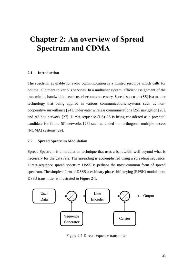
2.2 Spread Spectrum Modulation

Spread Spectrum is a modulation technique that uses a bandwidth well beyond what is

necessary for the data rate. The spreading is accomplished using a spreading sequence.

Direct-sequence spread spectrum DSSS is perhaps the most common form of spread

spectrum. The simplest form of DSSS uses binary phase shift keying (BPSK) modulation.

DSSS transmitter is illustrated in Figure 2-1.

Figure 2-1 Direct-sequence transmitter

Carrier

User

Data

Sequence

Generator

Line

Encoder Output

Chapter 2: An Overview of Spread Spectrum and CDMA

24

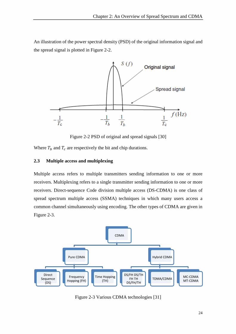
An illustration of the power spectral density (PSD) of the original information signal and

the spread signal is plotted in Figure 2-2.

Figure 2-2 PSD of original and spread signals [30]

Where 𝑇𝑏 and 𝑇𝑐 are respectively the bit and chip durations.

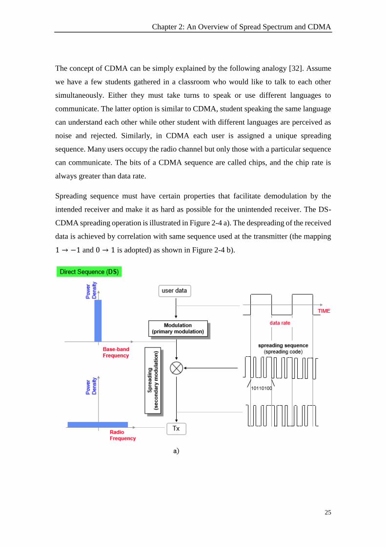
2.3 Multiple access and multiplexing

Multiple access refers to multiple transmitters sending information to one or more

receivers. Multiplexing refers to a single transmitter sending information to one or more

receivers. Direct-sequence Code division multiple access (DS-CDMA) is one class of

spread spectrum multiple access (SSMA) techniques in which many users access a

common channel simultaneously using encoding. The other types of CDMA are given in

Figure 2-3.

Figure 2-3 Various CDMA technologies [31]

CDMA

Pure CDMA

Direct Sequence

(DS)

Frequency Hopping (FH)

Time Hopping (TH)

Hybrid CDMA

DS/FH DS/TH FH TH

DS/FH/THTDMA/CDMA

MC-CDMA MT-CDMA

Chapter 2: An Overview of Spread Spectrum and CDMA

25

The concept of CDMA can be simply explained by the following analogy [32]. Assume

we have a few students gathered in a classroom who would like to talk to each other

simultaneously. Either they must take turns to speak or use different languages to

communicate. The latter option is similar to CDMA, student speaking the same language

can understand each other while other student with different languages are perceived as

noise and rejected. Similarly, in CDMA each user is assigned a unique spreading

sequence. Many users occupy the radio channel but only those with a particular sequence

can communicate. The bits of a CDMA sequence are called chips, and the chip rate is

always greater than data rate.

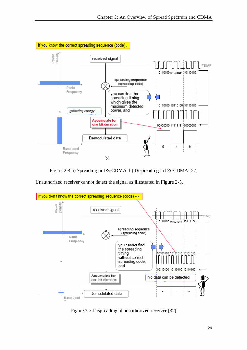
Spreading sequence must have certain properties that facilitate demodulation by the

intended receiver and make it as hard as possible for the unintended receiver. The DS-

CDMA spreading operation is illustrated in Figure 2-4 a). The despreading of the received

data is achieved by correlation with same sequence used at the transmitter (the mapping

1 → −1 and 0 → 1 is adopted) as shown in Figure 2-4 b).

Chapter 2: An Overview of Spread Spectrum and CDMA

26

Figure 2-4 a) Spreading in DS-CDMA; b) Dispreading in DS-CDMA [32]

Unauthorized receiver cannot detect the signal as illustrated in Figure 2-5.

Figure 2-5 Dispreading at unauthorized receiver [32]

Chapter 2: An Overview of Spread Spectrum and CDMA

27

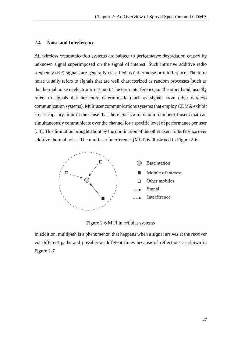
2.4 Noise and Interference

All wireless communication systems are subject to performance degradation caused by

unknown signal superimposed on the signal of interest. Such intrusive additive radio

frequency (RF) signals are generally classified as either noise or interference. The term

noise usually refers to signals that are well characterized as random processes (such as

the thermal noise in electronic circuits). The term interference, on the other hand, usually

refers to signals that are more deterministic (such as signals from other wireless

communication systems). Multiuser communications systems that employ CDMA exhibit

a user capacity limit in the sense that there exists a maximum number of users that can

simultaneously communicate over the channel for a specific level of performance per user

[33]. This limitation brought about by the domination of the other users’ interference over

additive thermal noise. The multiuser interference (MUI) is illustrated in Figure 2-6.

Figure 2-6 MUI in cellular systems

In addition, multipath is a phenomenon that happens when a signal arrives at the receiver

via different paths and possibly at different times because of reflections as shown in

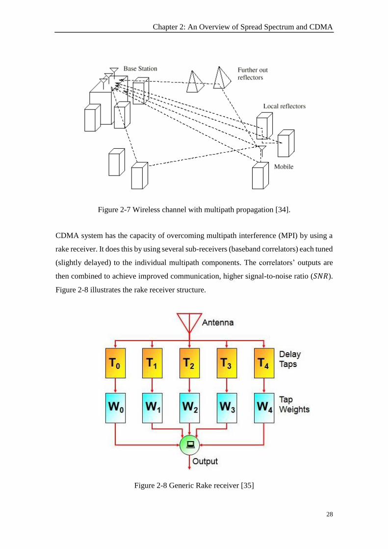
Figure 2-7.

Chapter 2: An Overview of Spread Spectrum and CDMA

28

Figure 2-7 Wireless channel with multipath propagation [34].

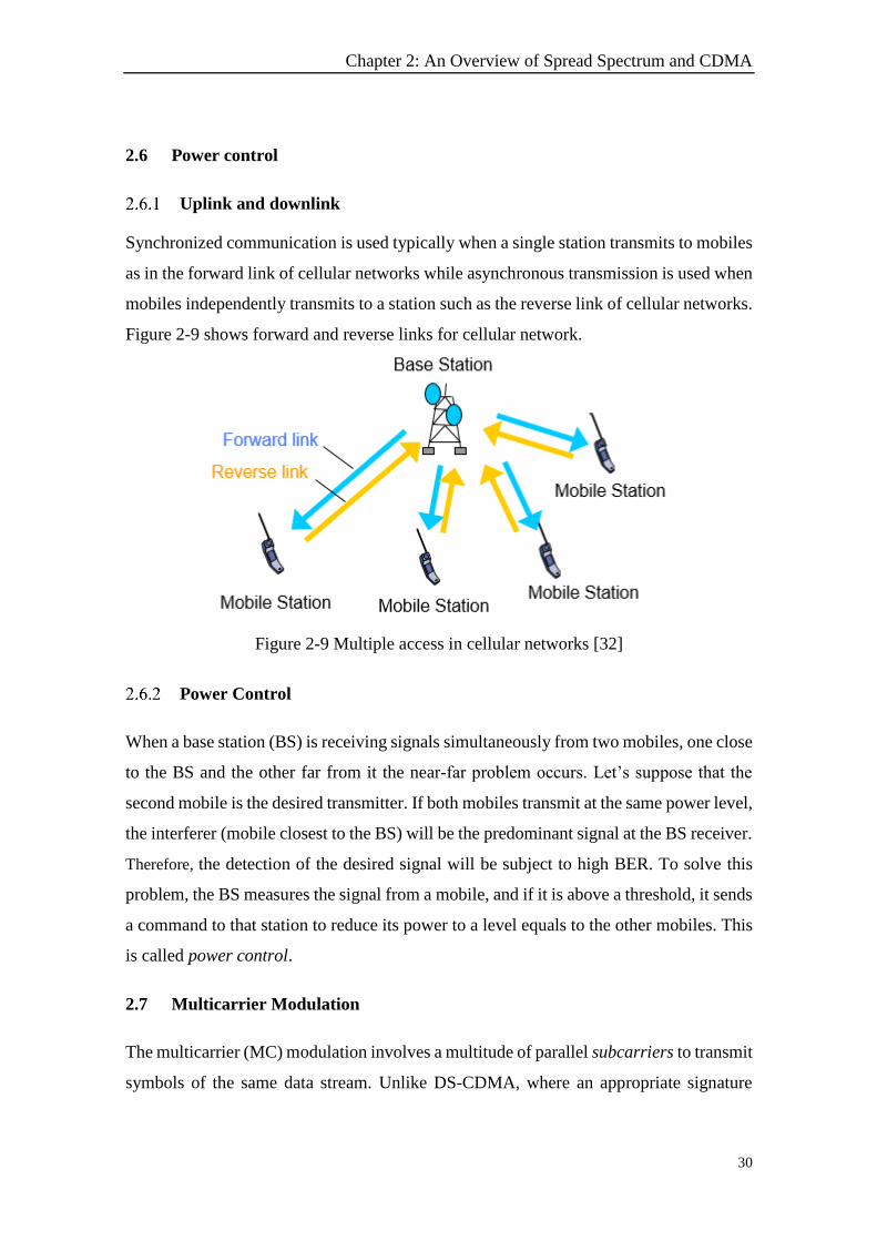
CDMA system has the capacity of overcoming multipath interference (MPI) by using a

rake receiver. It does this by using several sub-receivers (baseband correlators) each tuned

(slightly delayed) to the individual multipath components. The correlators’ outputs are

then combined to achieve improved communication, higher signal-to-noise ratio (𝑆𝑁𝑅).

Figure 2-8 illustrates the rake receiver structure.

Figure 2-8 Generic Rake receiver [35]

Chapter 2: An Overview of Spread Spectrum and CDMA

29

There are two primary ways to combine the rake finger outputs. The first method called

equal gain combining (EGC) weighs each output equally. The second method called

maximum ratio combining (MRC) uses data to estimate weights coefficients that

maximize SNR [31]. As for the improvement in performance, Table 2-1 gives the effect

of rake receiver for 𝐵𝐸𝑅 = 10−3.

Table 2-1 Rake receiver improvement [36]

System Modulation Rake (branches) 𝑆𝑁𝑅 (𝑑𝐵)

W-CDMA BPSK

1 24

2 14

3 10

Where W-CDMA means wideband CDMA.

2.5 Delay Spread

Knowledge of the propagation characteristics of the medium is essential to the

understanding and design of any communication system. A channel can be characterized

as being either frequency-selective or frequency nonselective (fading affects all

frequencies equally). Such characterization is based on the channel parameters, namely

the delay spread 𝑇𝑑 which is the time interval between the arrival of the first and last

significant multipath signals seen by the receiver. Delay spread for different environments

is given in Table 2-2.

Table 2-2 Delay spread of different environments [31]

Environment Max path length (𝑚) Delay spread 𝑇𝑑

Indoor 12 − 60 40 − 200 𝑛𝑠𝑒𝑐

Outdoor 300 − 6000 1 − 20 𝜇𝑠𝑒𝑐

A flat fading channel has a coherence bandwidth greater than the transmitted signal

bandwidth where the coherence bandwidth 𝑊𝑐 of a multipath channel is defined as

𝑊𝑐 =1

2𝜋𝑇𝑑 (2-1)

Chapter 2: An Overview of Spread Spectrum and CDMA

30

2.6 Power control

Uplink and downlink

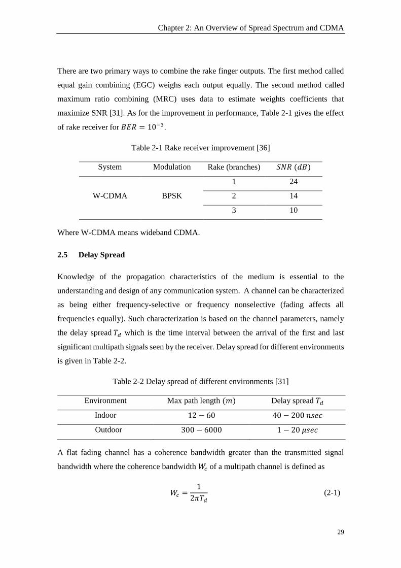
Synchronized communication is used typically when a single station transmits to mobiles

as in the forward link of cellular networks while asynchronous transmission is used when

mobiles independently transmits to a station such as the reverse link of cellular networks.

Figure 2-9 shows forward and reverse links for cellular network.

Figure 2-9 Multiple access in cellular networks [32]

Power Control

When a base station (BS) is receiving signals simultaneously from two mobiles, one close

to the BS and the other far from it the near-far problem occurs. Let’s suppose that the

second mobile is the desired transmitter. If both mobiles transmit at the same power level,

the interferer (mobile closest to the BS) will be the predominant signal at the BS receiver.

Therefore, the detection of the desired signal will be subject to high BER. To solve this

problem, the BS measures the signal from a mobile, and if it is above a threshold, it sends

a command to that station to reduce its power to a level equals to the other mobiles. This

is called power control.

2.7 Multicarrier Modulation

The multicarrier (MC) modulation involves a multitude of parallel subcarriers to transmit

symbols of the same data stream. Unlike DS-CDMA, where an appropriate signature

Chapter 2: An Overview of Spread Spectrum and CDMA

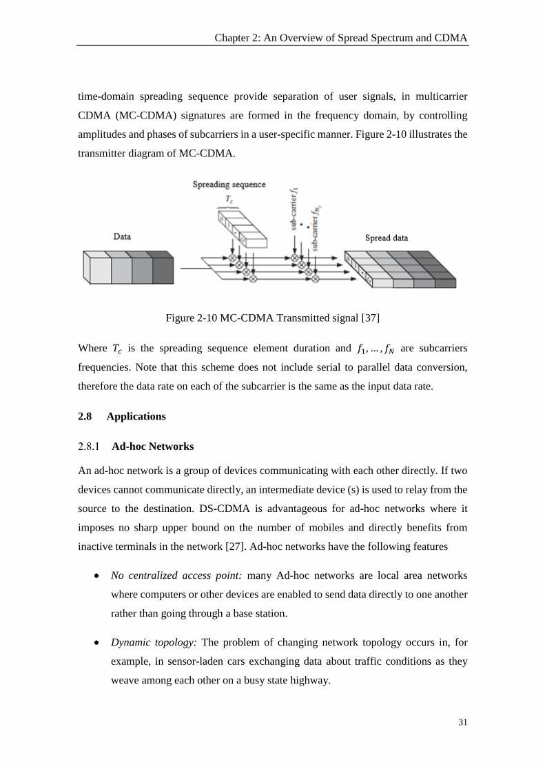
31

time-domain spreading sequence provide separation of user signals, in multicarrier

CDMA (MC-CDMA) signatures are formed in the frequency domain, by controlling

amplitudes and phases of subcarriers in a user-specific manner. Figure 2-10 illustrates the

transmitter diagram of MC-CDMA.

Figure 2-10 MC-CDMA Transmitted signal [37]

Where 𝑇𝑐 is the spreading sequence element duration and 𝑓1, … , 𝑓𝑁 are subcarriers

frequencies. Note that this scheme does not include serial to parallel data conversion,

therefore the data rate on each of the subcarrier is the same as the input data rate.

2.8 Applications

Ad-hoc Networks

An ad-hoc network is a group of devices communicating with each other directly. If two

devices cannot communicate directly, an intermediate device (s) is used to relay from the

source to the destination. DS-CDMA is advantageous for ad-hoc networks where it

imposes no sharp upper bound on the number of mobiles and directly benefits from

inactive terminals in the network [27]. Ad-hoc networks have the following features

No centralized access point: many Ad-hoc networks are local area networks

where computers or other devices are enabled to send data directly to one another

rather than going through a base station.

Dynamic topology: The problem of changing network topology occurs in, for

example, in sensor-laden cars exchanging data about traffic conditions as they

weave among each other on a busy state highway.

Chapter 2: An Overview of Spread Spectrum and CDMA

32

Limited power and capacity (memory and processing): The need to maximize the

efficiency of data exchange — in order to minimize energy consumption — makes

designing communications protocols for ad-hoc networks a challenging task.

Underwater Communications

Underwater acoustic communication (UAC) is the wireless communication in which

acoustic waves carry digital signal through an underwater channel. UAC has been

receiving intention due to its application in [38]

Marine research: collection of scientific data recorded at ocean-bottom stations

to monitor pollution and climate environmental systems

Marine commercial operations: remote control in off-shore oil and gas industry,

unmanned underwater vehicles, speech transmission between divers, and

mapping of the ocean floor for detection of objects and discovery of new

resources.

Defense: submarines and autonomous underwater vehicles (AUVs).

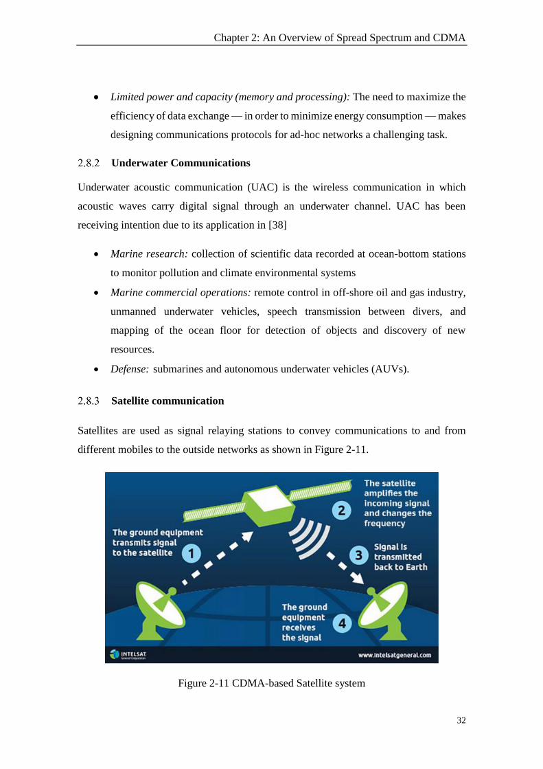
Satellite communication

Satellites are used as signal relaying stations to convey communications to and from

different mobiles to the outside networks as shown in Figure 2-11.

Figure 2-11 CDMA-based Satellite system

Chapter 2: An Overview of Spread Spectrum and CDMA

33

Because their applications are not limited by the geographical locations, satellite-based

communications play an important role in disaster relief and military operations. CDMA

is used in satellite-based global navigation systems (GNSS) such as [39] the navigation

satellite timing and Ranging System (NAVSTAR) which is a constellation of 27 satellites

deployed around the earth and managed by the United States Air Force (USAF).

2.9 Conclusion

In this chapter, we gave an overview on spread spectrum modulation and CDMA

technique. The propagation characteristics of an RF channel was also addressed. Various

operations such as rake receiver, power control, and multicarrier modulation were

discussed. Lastly, some important applications of CDMA were mentioned. In the next

chapter, we will investigate spreading sequences and their application to DS-CDMA

system.

34

35

Chapter 3: On ZCZ Sequences and their

Application to DS-CDMA

3.1 Introduction

In the previous chapter, we reviewed the basic concepts of multiple access spread

spectrum and CDMA systems. The analysis in this chapter identifies parameters of the

spreading sequence that influence CDMA system performance. Firstly, we will develop

analytical approaches to derive the 𝐵𝐸𝑅 for quasi-synchronous and asynchronous DS-

CDMA over multipath channels. Secondly, both binary and ternary spreading sequences

will be evaluated. Lastly, it is point out that interference-free communication can be

obtained only if both zero even and odd CCFs of binary ZCZ sequences are verified.

3.2 DS-CDMA System Model

Our goal in this section is to describe a communication link with several active

transmitters and a single receiver. One of the transmitted signals is intended for the

receiver and the rest produce undesired MUI. The basic model of DS-CDMA system in

frequency non-selective fading channel of 𝐾 users is illustrated in Figure 3-1.

Transmitter

For each user 𝑘, bipolar binary data 𝑑𝑘(𝑡) of duration 𝑇𝑏 is multiplied by a spreading

sequence 𝑐𝑘(𝑡) of duration 𝑇𝑐 and length 𝑁 = 𝑇𝑏 𝑇𝑐⁄ .

𝑑𝑘(𝑡) = ∑𝑑𝑘,𝑚𝑊(𝑡 − 𝑚𝑇𝑏)

𝑚

(3-1)

𝑐𝑘(𝑡) = ∑𝑐𝑘,𝑛𝑊(𝑡 − 𝑛𝑇𝑐)

𝑛

(3-2)

Where 𝑊(𝑡) is the rectangular pulse waveform.

Chapter 3: On ZCZ Sequences and their Application to DS-CDMA

36

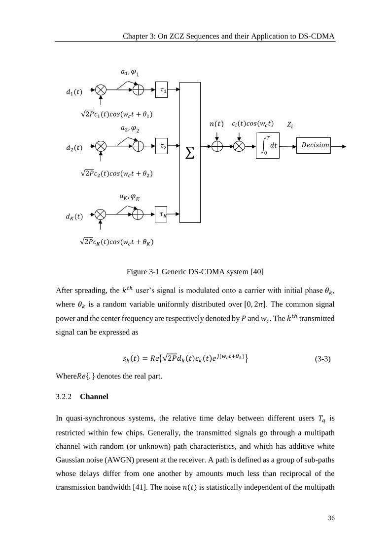
Figure 3-1 Generic DS-CDMA system [40]

After spreading, the 𝑘𝑡ℎ user’s signal is modulated onto a carrier with initial phase 𝜃𝑘,

where 𝜃𝑘 is a random variable uniformly distributed over [0, 2𝜋]. The common signal

power and the center frequency are respectively denoted by 𝑃 and 𝑤𝑐. The 𝑘𝑡ℎ transmitted

signal can be expressed as

𝑠𝑘(𝑡) = 𝑅𝑒{√2𝑃𝑑𝑘(𝑡)𝑐𝑘(𝑡)𝑒𝑗(𝑤𝑐𝑡+𝜃𝑘)} (3-3)

Where𝑅𝑒{. } denotes the real part.

Channel

In quasi-synchronous systems, the relative time delay between different users 𝑇𝑞 is

restricted within few chips. Generally, the transmitted signals go through a multipath

channel with random (or unknown) path characteristics, and which has additive white

Gaussian noise (AWGN) present at the receiver. A path is defined as a group of sub-paths

whose delays differ from one another by amounts much less than reciprocal of the

transmission bandwidth [41]. The noise 𝑛(𝑡) is statistically independent of the multipath

න 𝑑𝑡𝑇

0

𝐷𝑒𝑐𝑖𝑠𝑖𝑜𝑛

𝑍𝑖 𝑐𝑖(𝑡)𝑐𝑜𝑠(𝑤𝑐𝑡) 𝑛(𝑡)

∑

√2𝑃𝑐1(𝑡)𝑐𝑜𝑠(𝑤𝑐𝑡 + 𝜃1)

𝑑1(𝑡) 𝜏1

𝑎1,𝜑1

√2𝑃𝑐2(𝑡)𝑐𝑜𝑠(𝑤𝑐𝑡 + 𝜃2)

𝑑2(𝑡) 𝜏2

𝑎2,𝜑2

√2𝑃𝑐𝐾(𝑡)𝑐𝑜𝑠(𝑤𝑐𝑡 + 𝜃𝐾)

𝑑𝐾(𝑡) 𝜏𝐾

𝑎𝐾 ,𝜑𝐾

Chapter 3: On ZCZ Sequences and their Application to DS-CDMA

37

medium, stationary, Gaussian, with two-sided flat power-density spectrum 𝑁0 2⁄ (at least

over the transmission bandwidth). This noise model might correspond to thermal noise in

the receiver. The channel output signal is a sum of 𝐿 delayed, phase-shifted, and

attenuated replicas of the transmitted signal [42]

𝑦(𝑡) = ∑∑ 𝑅𝑒{𝑔𝑘,𝑚𝑠𝑘(𝑡 − 𝜏𝑘,𝑚)}

𝐿−1

𝑚=0

𝐾

𝑘=1

(3-4)

Where 𝜏𝑘,𝑚 is the 𝑚𝑡ℎ random delay of the 𝑘𝑡ℎ user uniformly distributed over [0, 𝑇𝑞]

and 𝑔𝑘,𝑚 is complex gain coefficient that combines the 𝑚𝑡ℎ scatter path attenuation and

phase-shifted components of the 𝑘𝑡ℎ user [43]

𝑔𝑘,0 = 1 + 𝑎𝑘,0𝑒𝑗𝜑𝑘,0

and 𝑔𝑘,𝑚 = 𝑎𝑘,𝑚𝑒𝑗𝜑𝑘,𝑚 for 1 ≤ 𝑚 ≤ 𝐿 − 1

(3-5)

Where 𝑎𝑘,𝑚 is the attenuation, and 𝜑𝑘,𝑚 is the phase-shift of 𝑘𝑡ℎ user signal coming from

the 𝑚𝑡ℎ path.

If all the interferers happen to be close to the receiver, the MUI can be very large

compared to the MPI [44]. In addition, for closely spaced geographical points, two signal

replicas from the same transmitter with similar delays are more likely than those with

large delays [44]. Therefore, we will consider only the 0𝑡ℎ path component (𝑚 = 0) and

its sub-paths. The overall amplitude of the signal 𝑔𝑘,0 could be characterized by a Rician

distribution [42]. The signal at the channel output is modeled as follows

𝑦(𝑡) = ∑𝑅𝑒{𝑔𝑘,0𝑠𝑘(𝑡 − 𝜏𝑘,0)}

𝐾

𝑘=1

(3-6)

In the remaining analysis, we will drop the subscript 0.

Derivation of a New BER in terms of ECF and OCF

The received signal can be expressed as [42]

Chapter 3: On ZCZ Sequences and their Application to DS-CDMA

38

𝑟(𝑡) = ∑𝑅𝑒{(1 + 𝑎𝑘𝑒𝑗𝜑𝑘)𝑠𝑘(𝑡 − 𝜏𝑘) + 𝑛(𝑡)}

𝐾

𝑘= 1

= 𝑦(𝑡) + 𝑛(𝑡) (3-7)

Where 𝑦(𝑡) is the sum of signals from all transmitters.

As was stated earlier, for closely spaced geographical points, the MPI is small compared

to MUI. Therefore, the DS-CDMA system under consideration will simply employ a

conventional matched filter (correlator). The 𝑖𝑡ℎ correlator’s output is

𝑍𝑖 = න 𝑟(𝑡)𝑐𝑖(𝑡) 𝑐𝑜𝑠(𝑤𝑐𝑡)𝑇𝑏

0

𝑑𝑡 = 𝐷𝑖 + 𝐼𝑖 + 𝑁𝑖 (3-8)

Where 𝐷𝑖 is the desired signal given as (see Annex B.1)

𝐷𝑖 = √𝑃 2⁄ 𝜇𝑖𝑇𝑏[1 + 𝑎𝑖 𝑐𝑜𝑠(𝜑𝑖)] (3-9)

And the interference term is (see Annex B.1)

𝐼𝑖 = √𝑃

2∑[𝑑𝑘,−1𝑅𝑐𝑘𝑐𝑖(𝜏𝑘) + 𝑑𝑘,0�̂�𝑐𝑘𝑐𝑖(𝜏𝑘)][𝑐𝑜𝑠(𝜗𝑘) + 𝑎𝑘 𝑐𝑜𝑠(𝜗𝑘 +𝜑𝑘)]

𝐾

𝑘=1𝑘≠𝑖

(3-10)

Where the data bits 𝑑𝑘,−1 and 𝑑𝑘,0 are respectively the previous and current symbols of

the 𝑘𝑡ℎ user and 𝜗𝑘 = 𝜃𝑘 − 𝑤𝑐𝜏𝑘. 𝑅𝑐𝑘𝑐𝑖(𝜏𝑘) and �̂�𝑐𝑘𝑐𝑖(𝜏𝑘) are called the continuous-time

partial CCFs expressed in terms of even and odd correlation function as follows (see

Annex B.2)

�̂�𝑐𝑘𝑐𝑖(𝑙𝑇𝑐) = 𝑇𝑐 (𝐸𝑐𝑘𝑐𝑖(𝑙) + 𝑂𝑐𝑘𝑐𝑖(𝑙)) 2⁄ (3-11)

𝑅𝑐𝑘𝑐𝑖(𝑙𝑇𝑐) = 𝑇𝑐 (𝐸𝑐𝑘𝑐𝑖(𝑙) − 𝑂𝑐𝑘𝑐𝑖(𝑙)) 2⁄ (3-12)

The noise component is

𝑁𝑖 = න 𝑛(𝑡)𝑐𝑖(𝑡) cos(𝑤𝑐𝑡)𝑇𝑏

0

𝑑𝑡 (3-13)

The 𝑆𝐼𝑁𝑅 of user 𝑖 is defined as [43]

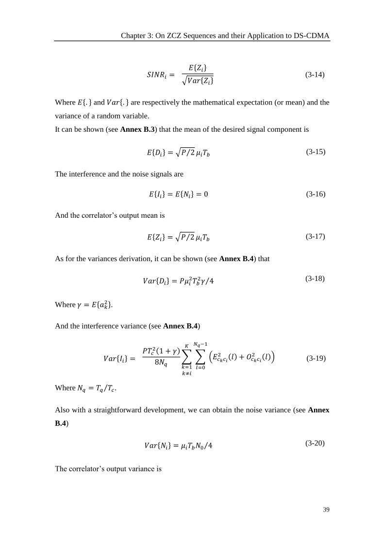
Chapter 3: On ZCZ Sequences and their Application to DS-CDMA

39

𝑆𝐼𝑁𝑅𝑖 = 𝐸{𝑍𝑖}

√𝑉𝑎𝑟{𝑍𝑖} (3-14)

Where 𝐸{. } and 𝑉𝑎𝑟{. } are respectively the mathematical expectation (or mean) and the

variance of a random variable.

It can be shown (see Annex B.3) that the mean of the desired signal component is

𝐸{𝐷𝑖} = √𝑃 2⁄ 𝜇𝑖𝑇𝑏 (3-15)

The interference and the noise signals are

𝐸{𝐼𝑖} = 𝐸{𝑁𝑖} = 0 (3-16)

And the correlator’s output mean is

𝐸{𝑍𝑖} = √𝑃 2⁄ 𝜇𝑖𝑇𝑏 (3-17)

As for the variances derivation, it can be shown (see Annex B.4) that

𝑉𝑎𝑟{𝐷𝑖} = 𝑃𝜇𝑖2𝑇𝑏

2𝛾 4⁄ (3-18)

Where 𝛾 = 𝐸{𝑎𝑘2}.

And the interference variance (see Annex B.4)

𝑉𝑎𝑟{𝐼𝑖} = 𝑃𝑇𝑐

2(1 + 𝛾)

8𝑁𝑞∑ ∑ (𝐸𝑐𝑘𝑐𝑖

2 (𝑙) + 𝑂𝑐𝑘𝑐𝑖2 (𝑙))

𝑁𝑞−1

𝑙=0

𝐾

𝑘=1𝑘≠𝑖

(3-19)

Where 𝑁𝑞 = 𝑇𝑞 𝑇𝑐⁄ .

Also with a straightforward development, we can obtain the noise variance (see Annex

B.4)

𝑉𝑎𝑟{𝑁𝑖} = 𝜇𝑖𝑇𝑏𝑁0 4⁄ (3-20)

The correlator’s output variance is

Chapter 3: On ZCZ Sequences and their Application to DS-CDMA

40

𝑉𝑎𝑟{𝑍𝑖} = 𝑃𝜇𝑖

2𝑇𝑏2𝛾

4+𝑃𝑇𝑏

2(1 + 𝛾)

8𝑁𝑞𝑁2

∑ ∑ (𝐸𝑐𝑘𝑐𝑖2 (𝑙) + 𝑂𝑐𝑘𝑐𝑖

2 (𝑙))

𝑁𝑞−1

𝑙=0

𝐾

𝑘=1𝑘≠𝑖

+𝜇𝑖𝑇𝑏𝑁04

(3-21)

Where 𝑇𝑐2 = 𝑇𝑏

2 𝑁2⁄ .

In [45], the authors state that when a transmitter and receiver use a DS-BPSK waveform

to communicate, all the interference in the channel can be approximated as AWGN which

justify the use of the Gaussian approximation to obtain the following 𝐵𝐸𝑅 = 𝑄(𝑆𝐼𝑁𝑅𝑖).

After simplification, we obtain [46]

𝐵𝐸𝑅𝑖 = 𝑄

(

1

√𝛾2 +

(1 + 𝛾)

4𝑁𝑞𝑁2𝜇𝑖2∑ ∑ (𝐸𝑐𝑘𝑐𝑖

2 (𝑙) + 𝑂𝑐𝑘𝑐𝑖2 (𝑙))

𝑁𝑞−1

𝑙=0𝐾𝑘=1𝑘≠𝑖

+𝑁02𝐸𝑏𝜇𝑖

)

(3-22)

Where 𝑄(. ) is the complementary error function and 𝐸𝑏 = 𝑇𝑏𝑃 is the data bit energy.

Note that the above equation can easily be generalized to asynchronous case by letting

𝑁𝑞 = 𝑁 as follows

𝐵𝐸𝑅𝑖 = 𝑄

(

1

√𝛾2 +

(1 + 𝛾)

4𝑁3𝜇𝑖2 ∑ ∑ (𝐸𝑐𝑘𝑐𝑖

2 (𝑙) + 𝑂𝑐𝑘𝑐𝑖2 (𝑙))𝑁−1

𝑙=0𝐾𝑘=1𝑘≠𝑖

+𝑁02𝐸𝑏𝜇𝑖

)

(3-23)

A more appropriate performance measure is the averaged BER overall users

𝐵𝐸𝑅 =1

𝐾∑𝐵𝐸𝑅𝑖

𝐾

𝑖=1

(3-24)

3.3 Numerical Results

The BER obtained in the previous section provides important criteria for the design of

suitable spreading sequences for both quasi-synchronous and asynchronous DS-CDMA

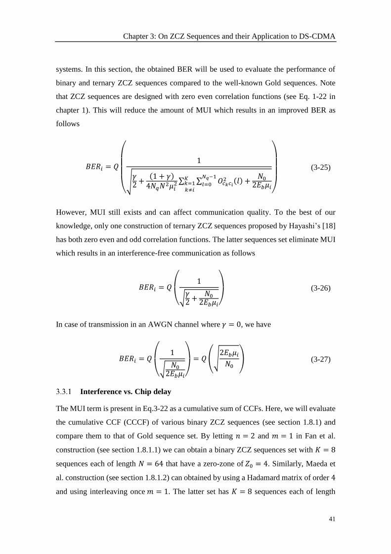
Chapter 3: On ZCZ Sequences and their Application to DS-CDMA

41

systems. In this section, the obtained BER will be used to evaluate the performance of

binary and ternary ZCZ sequences compared to the well-known Gold sequences. Note

that ZCZ sequences are designed with zero even correlation functions (see Eq. 1-22 in

chapter 1). This will reduce the amount of MUI which results in an improved BER as

follows

𝐵𝐸𝑅𝑖 = 𝑄

(

1

√𝛾2 +

(1 + 𝛾)

4𝑁𝑞𝑁2𝜇𝑖2∑ ∑ 𝑂𝑐𝑘𝑐𝑖

2 (𝑙)𝑁𝑞−1

𝑙=0𝐾𝑘=1𝑘≠𝑖

+𝑁0

2𝐸𝑏𝜇𝑖)

(3-25)

However, MUI still exists and can affect communication quality. To the best of our

knowledge, only one construction of ternary ZCZ sequences proposed by Hayashi’s [18]

has both zero even and odd correlation functions. The latter sequences set eliminate MUI

which results in an interference-free communication as follows

𝐵𝐸𝑅𝑖 = 𝑄

(

1

√𝛾2 +

𝑁02𝐸𝑏𝜇𝑖)

(3-26)

In case of transmission in an AWGN channel where 𝛾 = 0, we have

𝐵𝐸𝑅𝑖 = 𝑄

(

1

√𝑁02𝐸𝑏𝜇𝑖)

= 𝑄(√2𝐸𝑏𝜇𝑖𝑁0

) (3-27)

Interference vs. Chip delay

The MUI term is present in Eq.3-22 as a cumulative sum of CCFs. Here, we will evaluate

the cumulative CCF (CCCF) of various binary ZCZ sequences (see section 1.8.1) and

compare them to that of Gold sequence set. By letting 𝑛 = 2 and 𝑚 = 1 in Fan et al.

construction (see section 1.8.1.1) we can obtain a binary ZCZ sequences set with 𝐾 = 8

sequences each of length 𝑁 = 64 that have a zero-zone of 𝑍0 = 4. Similarly, Maeda et

al. construction (see section 1.8.1.2) can obtained by using a Hadamard matrix of order 4

and using interleaving once 𝑚 = 1. The latter set has 𝐾 = 8 sequences each of length

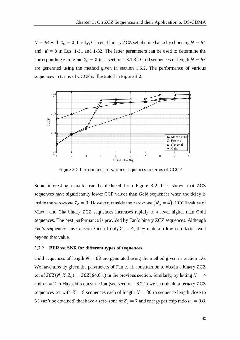
Chapter 3: On ZCZ Sequences and their Application to DS-CDMA

42

𝑁 = 64 with 𝑍0 = 3. Lastly, Cha et al binary ZCZ set obtained also by choosing 𝑁 = 64

and 𝐾 = 8 in Eqs. 1-31 and 1-32. The latter parameters can be used to determine the

corresponding zero-zone 𝑍0 = 3 (see section 1.8.1.3). Gold sequences of length 𝑁 = 63

are generated using the method given in section 1.6.2. The performance of various

sequences in terms of CCCF is illustrated in Figure 3-2.

Figure 3-2 Performance of various sequences in terms of CCCF

Some interesting remarks can be deduced from Figure 3-2. It is shown that ZCZ

sequences have significantly lower CCF values than Gold sequences when the delay is

inside the zero-zone 𝑍0 = 3. However, outside the zero-zone (𝑁𝑞 = 4), CCCF values of

Maeda and Cha binary ZCZ sequences increases rapidly to a level higher than Gold

sequences. The best performance is provided by Fan’s binary ZCZ sequences. Although

Fan’s sequences have a zero-zone of only 𝑍0 = 4, they maintain low correlation well

beyond that value.

BER vs. SNR for different types of sequences

Gold sequences of length 𝑁 = 63 are generated using the method given in section 1.6.

We have already given the parameters of Fan et al. construction to obtain a binary ZCZ

set of 𝑍𝐶𝑍(𝑁,𝐾, 𝑍0) = 𝑍𝐶𝑍(64,8,4) in the previous section. Similarly, by letting 𝑁 = 4

and 𝑚 = 2 in Hayashi’s construction (see section 1.8.2.1) we can obtain a ternary ZCZ

sequences set with 𝐾 = 8 sequences each of length 𝑁 = 80 (a sequence length close to

64 can’t be obtained) that have a zero-zone of 𝑍0 = 7 and energy per chip ratio 𝜇𝑖 = 0.8.

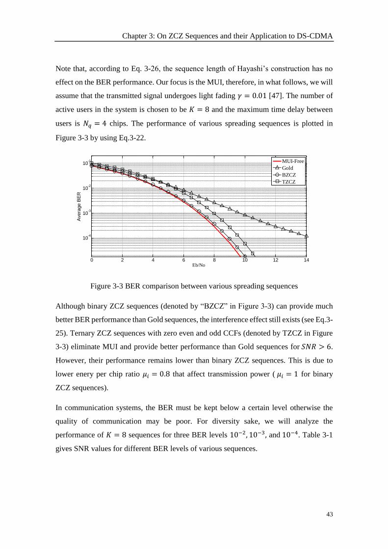
Chapter 3: On ZCZ Sequences and their Application to DS-CDMA

43

Note that, according to Eq. 3-26, the sequence length of Hayashi’s construction has no

effect on the BER performance. Our focus is the MUI, therefore, in what follows, we will

assume that the transmitted signal undergoes light fading 𝛾 = 0.01 [47]. The number of

active users in the system is chosen to be 𝐾 = 8 and the maximum time delay between

users is 𝑁𝑞 = 4 chips. The performance of various spreading sequences is plotted in

Figure 3-3 by using Eq.3-22.

Figure 3-3 BER comparison between various spreading sequences

Although binary ZCZ sequences (denoted by “BZCZ” in Figure 3-3) can provide much

better BER performance than Gold sequences, the interference effect still exists (see Eq.3-

25). Ternary ZCZ sequences with zero even and odd CCFs (denoted by TZCZ in Figure

3-3) eliminate MUI and provide better performance than Gold sequences for 𝑆𝑁𝑅 > 6.

However, their performance remains lower than binary ZCZ sequences. This is due to

lower enery per chip ratio 𝜇𝑖 = 0.8 that affect transmission power ( 𝜇𝑖 = 1 for binary

ZCZ sequences).

In communication systems, the BER must be kept below a certain level otherwise the

quality of communication may be poor. For diversity sake, we will analyze the

performance of 𝐾 = 8 sequences for three BER levels 10−2, 10−3, and 10−4. Table 3-1

gives SNR values for different BER levels of various sequences.

0 2 4 6 8 10 12 14

10-4

10-3

10-2

10-1

Eb/No

Avera

ge B

ER

MUI-Free

Gold

BZCZ

TZCZ

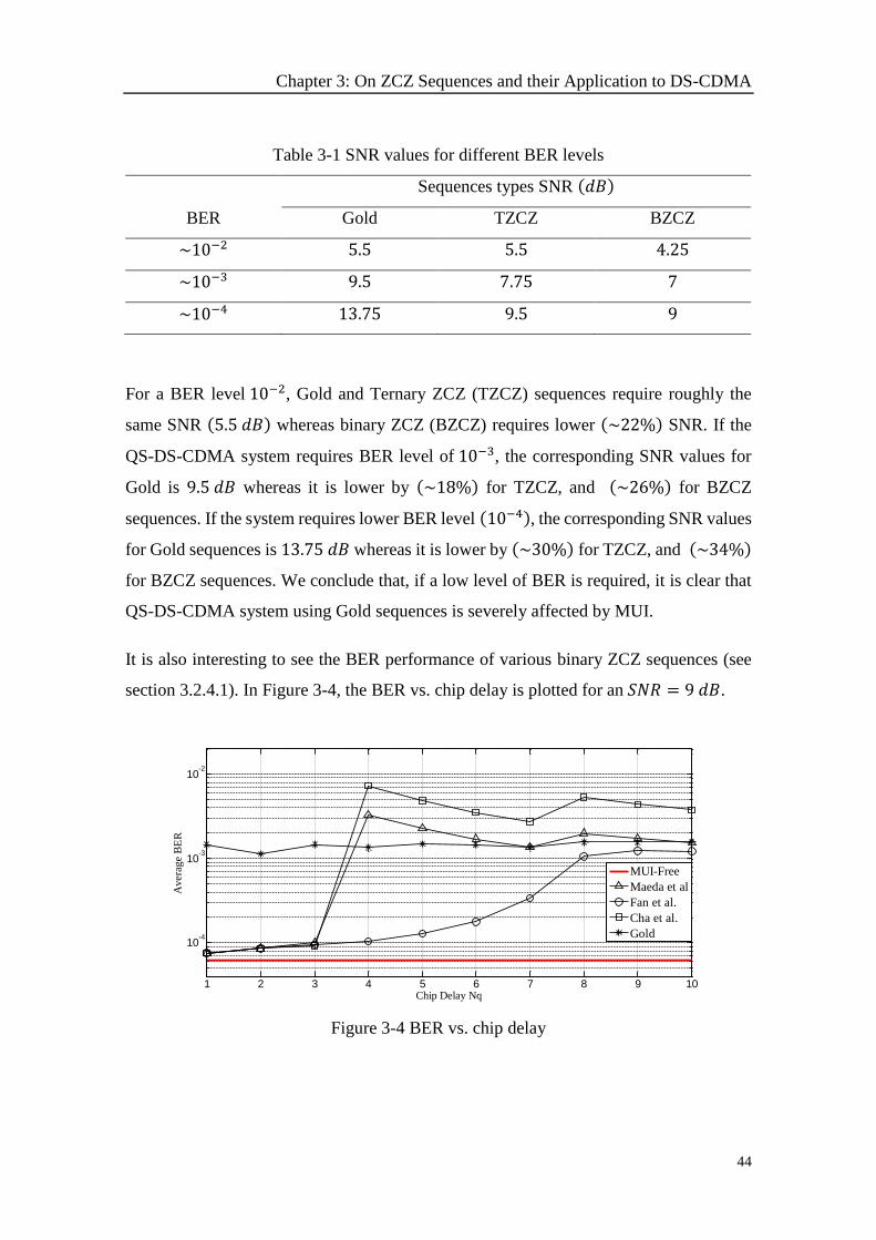
Chapter 3: On ZCZ Sequences and their Application to DS-CDMA

44

Table 3-1 SNR values for different BER levels

BER

Sequences types SNR (𝑑𝐵)

Gold TZCZ BZCZ

~10−2 5.5 5.5 4.25

~10−3 9.5 7.75 7

~10−4 13.75 9.5 9

For a BER level 10−2, Gold and Ternary ZCZ (TZCZ) sequences require roughly the

same SNR (5.5 𝑑𝐵) whereas binary ZCZ (BZCZ) requires lower (~22%) SNR. If the

QS-DS-CDMA system requires BER level of 10−3, the corresponding SNR values for

Gold is 9.5 𝑑𝐵 whereas it is lower by (~18%) for TZCZ, and (~26%) for BZCZ

sequences. If the system requires lower BER level (10−4), the corresponding SNR values

for Gold sequences is 13.75 𝑑𝐵 whereas it is lower by (~30%) for TZCZ, and (~34%)

for BZCZ sequences. We conclude that, if a low level of BER is required, it is clear that

QS-DS-CDMA system using Gold sequences is severely affected by MUI.

It is also interesting to see the BER performance of various binary ZCZ sequences (see

section 3.2.4.1). In Figure 3-4, the BER vs. chip delay is plotted for an 𝑆𝑁𝑅 = 9 𝑑𝐵.

Figure 3-4 BER vs. chip delay

1 2 3 4 5 6 7 8 9 10

10-4

10-3

10-2

Chip Delay Nq

Aver

age

BE

R

MUI-Free

Maeda et al

Fan et al.

Cha et al.

Gold

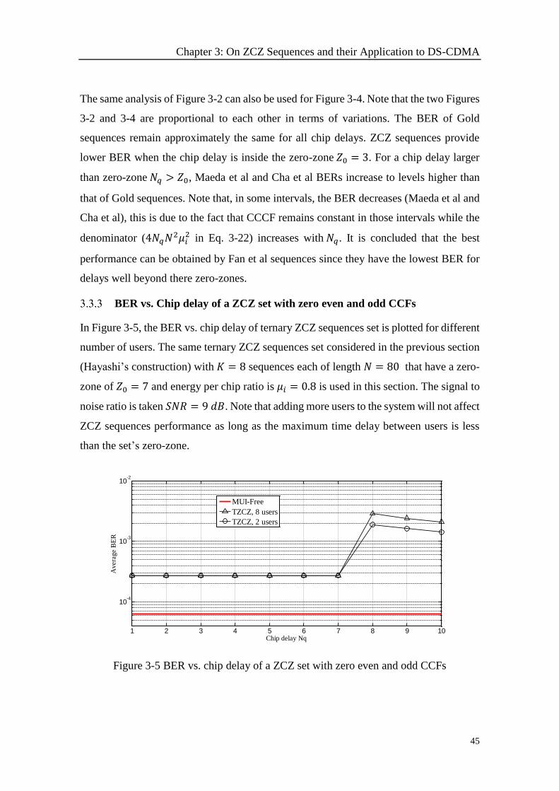
Chapter 3: On ZCZ Sequences and their Application to DS-CDMA

45

The same analysis of Figure 3-2 can also be used for Figure 3-4. Note that the two Figures

3-2 and 3-4 are proportional to each other in terms of variations. The BER of Gold

sequences remain approximately the same for all chip delays. ZCZ sequences provide

lower BER when the chip delay is inside the zero-zone 𝑍0 = 3. For a chip delay larger

than zero-zone 𝑁𝑞 > 𝑍0, Maeda et al and Cha et al BERs increase to levels higher than

that of Gold sequences. Note that, in some intervals, the BER decreases (Maeda et al and

Cha et al), this is due to the fact that CCCF remains constant in those intervals while the

denominator (4𝑁𝑞𝑁2𝜇𝑖

2 in Eq. 3-22) increases with 𝑁𝑞. It is concluded that the best

performance can be obtained by Fan et al sequences since they have the lowest BER for

delays well beyond there zero-zones.

BER vs. Chip delay of a ZCZ set with zero even and odd CCFs

In Figure 3-5, the BER vs. chip delay of ternary ZCZ sequences set is plotted for different

number of users. The same ternary ZCZ sequences set considered in the previous section

(Hayashi’s construction) with 𝐾 = 8 sequences each of length 𝑁 = 80 that have a zero-

zone of 𝑍0 = 7 and energy per chip ratio is 𝜇𝑖 = 0.8 is used in this section. The signal to

noise ratio is taken 𝑆𝑁𝑅 = 9 𝑑𝐵. Note that adding more users to the system will not affect

ZCZ sequences performance as long as the maximum time delay between users is less

than the set’s zero-zone.

Figure 3-5 BER vs. chip delay of a ZCZ set with zero even and odd CCFs

1 2 3 4 5 6 7 8 9 10

10-4

10-3

10-2

Chip delay Nq

Aver

age

BE

R

MUI-Free

TZCZ, 8 users

TZCZ, 2 users

Chapter 3: On ZCZ Sequences and their Application to DS-CDMA

46

We conclude that MUI-free QS-DS-CDMA can be obtained by using binary ZCZ

sequences with zero even and odd CCFs.

3.4 Conclusion

A new expression of BER for quasi-synchronous and asynchronous DS-CDMA system

in Rician fading channel was derived. The new BER allows the evaluation of both binary

and ternary sequences. The obtained results show that ZCZ sequences do effectively

reduce MUI. However, to ensure interference-free reliable communication, binary ZCZ

sequences with both zero even and odd PCFs must be designed.

47

Chapter 4: On ZCZ Sequences and their

Application to MC-CDMA

4.1 Introduction

Multi-carrier (MC) transmission is the predominant transmission technique in today’s

communication systems. The MC-CDMA transmission scheme combines orthogonal

frequency division multiplexing (OFDM) and CDMA. The main advantages of the

combined system are variable data rate, high spectral efficiency, and robustness against

frequency selective fading [9]. However, high crest factor (CF) is one of the major

drawbacks of MC transmission [11]. Thus, CF reduction is one of the most important

research areas in MC-CDMA systems. In addition, asynchronous MC-CDMA suffers

from the effect of MUI caused by all active users in the system. The degradation of

system’s BER caused by MUI must also be taken into consideration [48]. Spreading

sequences in MC-CDMA have an effective role in CF and MUI reduction [9], [48].

Hence, spreading sequences should be selected to simultaneously ensure low CF and low

BER values. Therefore, the effect of correlation properties of sequences on CF is

investigated. Furthermore, a new BER as a function of 𝑆𝑁𝑅 is derived. In this chapter,

conventional sequences and ZCZ sequences are analyzed in terms of CF and BER. First,

we evaluate the CF values of various sequences and then evaluate their performance in

quasi-synchronous and asynchronous MC-CDMA systems.

4.2 CF Analysis

In this study, we consider crest factor (CF) as a measure of signal envelope compactness.

Its relation to peak-to-average power ratio (PAPR) is given as follows [48]

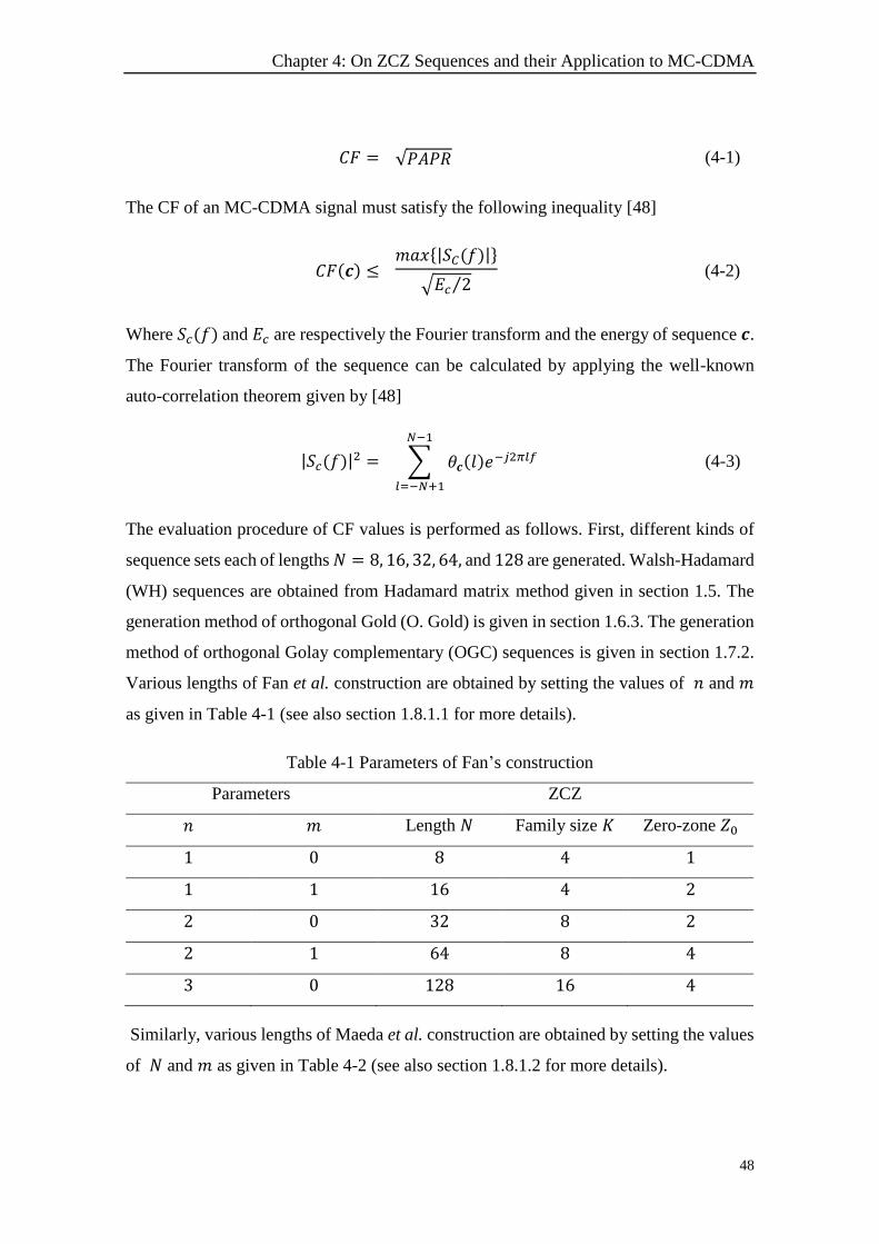
Chapter 4: On ZCZ Sequences and their Application to MC-CDMA

48

𝐶𝐹 = √𝑃𝐴𝑃𝑅 (4-1)

The CF of an MC-CDMA signal must satisfy the following inequality [48]

𝐶𝐹(𝒄) ≤ 𝑚𝑎𝑥{|𝑆𝐶(𝑓)|}

√𝐸𝑐 2⁄ (4-2)

Where 𝑆𝑐(𝑓) and 𝐸𝑐 are respectively the Fourier transform and the energy of sequence 𝒄.

The Fourier transform of the sequence can be calculated by applying the well-known

auto-correlation theorem given by [48]

|𝑆𝑐(𝑓)|2 = ∑ 𝜃𝒄(𝑙)𝑒

−𝑗2𝜋𝑙𝑓

𝑁−1

𝑙=−𝑁+1

(4-3)

The evaluation procedure of CF values is performed as follows. First, different kinds of

sequence sets each of lengths 𝑁 = 8, 16, 32, 64, and 128 are generated. Walsh-Hadamard

(WH) sequences are obtained from Hadamard matrix method given in section 1.5. The

generation method of orthogonal Gold (O. Gold) is given in section 1.6.3. The generation

method of orthogonal Golay complementary (OGC) sequences is given in section 1.7.2.

Various lengths of Fan et al. construction are obtained by setting the values of 𝑛 and 𝑚

as given in Table 4-1 (see also section 1.8.1.1 for more details).

Table 4-1 Parameters of Fan’s construction

Parameters ZCZ

𝑛 𝑚 Length 𝑁 Family size 𝐾 Zero-zone 𝑍0

1 0 8 4 1

1 1 16 4 2

2 0 32 8 2

2 1 64 8 4

3 0 128 16 4

Similarly, various lengths of Maeda et al. construction are obtained by setting the values

of 𝑁 and 𝑚 as given in Table 4-2 (see also section 1.8.1.2 for more details).

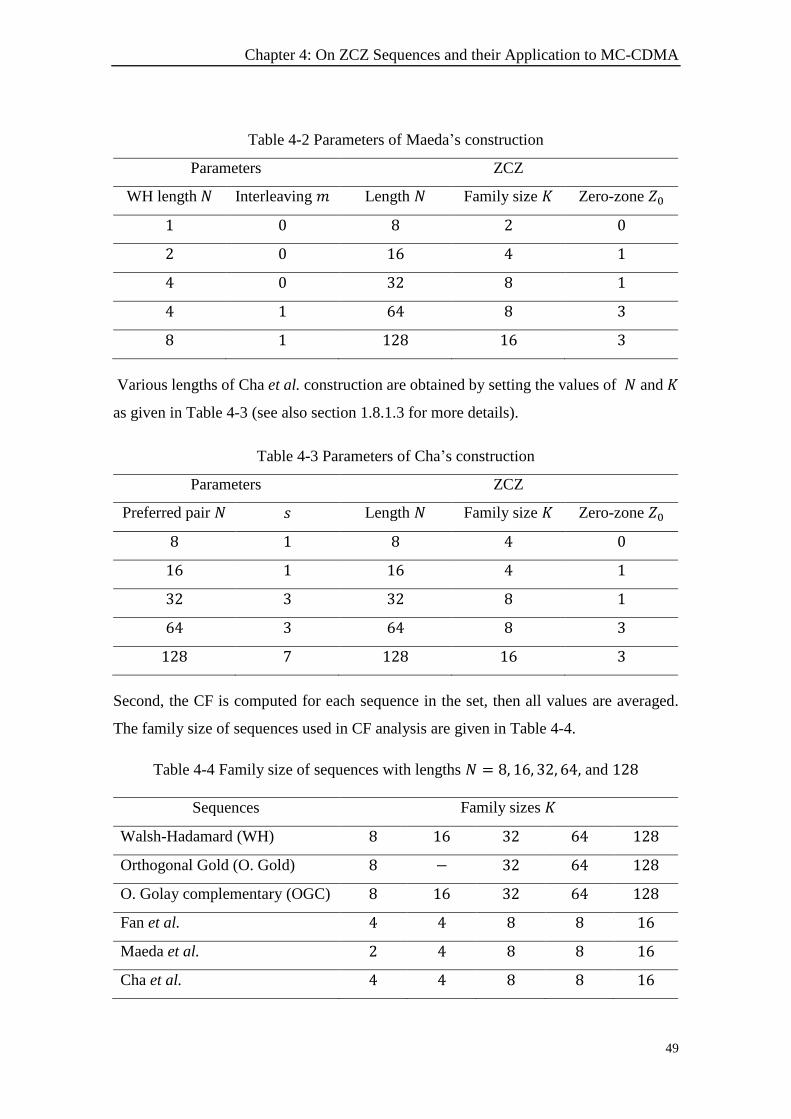
Chapter 4: On ZCZ Sequences and their Application to MC-CDMA

49

Table 4-2 Parameters of Maeda’s construction

Parameters ZCZ

WH length 𝑁 Interleaving 𝑚 Length 𝑁 Family size 𝐾 Zero-zone 𝑍0

1 0 8 2 0

2 0 16 4 1

4 0 32 8 1

4 1 64 8 3

8 1 128 16 3

Various lengths of Cha et al. construction are obtained by setting the values of 𝑁 and 𝐾

as given in Table 4-3 (see also section 1.8.1.3 for more details).

Table 4-3 Parameters of Cha’s construction

Parameters ZCZ

Preferred pair 𝑁 𝑠 Length 𝑁 Family size 𝐾 Zero-zone 𝑍0

8 1 8 4 0

16 1 16 4 1

32 3 32 8 1

64 3 64 8 3

128 7 128 16 3

Second, the CF is computed for each sequence in the set, then all values are averaged.

The family size of sequences used in CF analysis are given in Table 4-4.

Table 4-4 Family size of sequences with lengths 𝑁 = 8, 16, 32, 64, and 128

Sequences Family sizes 𝐾

Walsh-Hadamard (WH) 8 16 32 64 128

Orthogonal Gold (O. Gold) 8 − 32 64 128

O. Golay complementary (OGC) 8 16 32 64 128

Fan et al. 4 4 8 8 16

Maeda et al. 2 4 8 8 16

Cha et al. 4 4 8 8 16

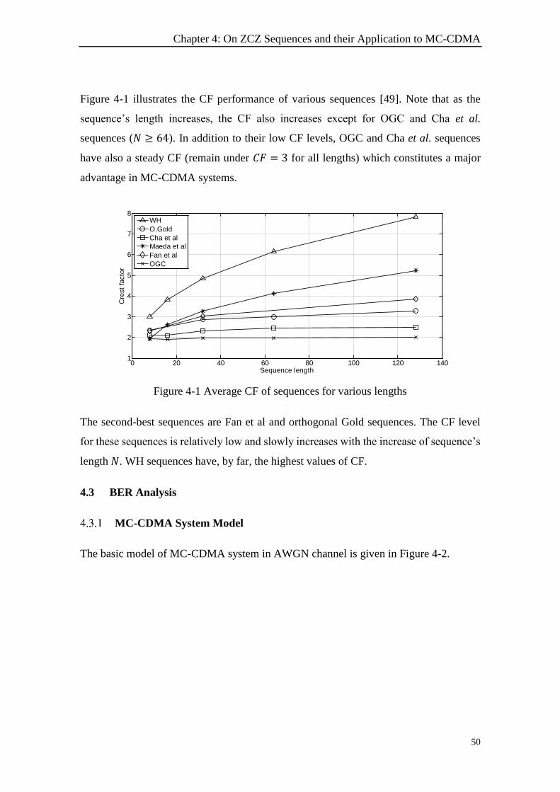
Chapter 4: On ZCZ Sequences and their Application to MC-CDMA

50

Figure 4-1 illustrates the CF performance of various sequences [49]. Note that as the

sequence’s length increases, the CF also increases except for OGC and Cha et al.

sequences (𝑁 ≥ 64). In addition to their low CF levels, OGC and Cha et al. sequences

have also a steady CF (remain under 𝐶𝐹 = 3 for all lengths) which constitutes a major

advantage in MC-CDMA systems.

Figure 4-1 Average CF of sequences for various lengths

The second-best sequences are Fan et al and orthogonal Gold sequences. The CF level

for these sequences is relatively low and slowly increases with the increase of sequence’s

length 𝑁. WH sequences have, by far, the highest values of CF.

4.3 BER Analysis

MC-CDMA System Model

The basic model of MC-CDMA system in AWGN channel is given in Figure 4-2.

0 20 40 60 80 100 120 1401

2

3

4

5

6

7

8

Sequence length

Cre

st

facto

r

WH

O.Gold

Cha et al

Maeda et al

Fan et al

OGC

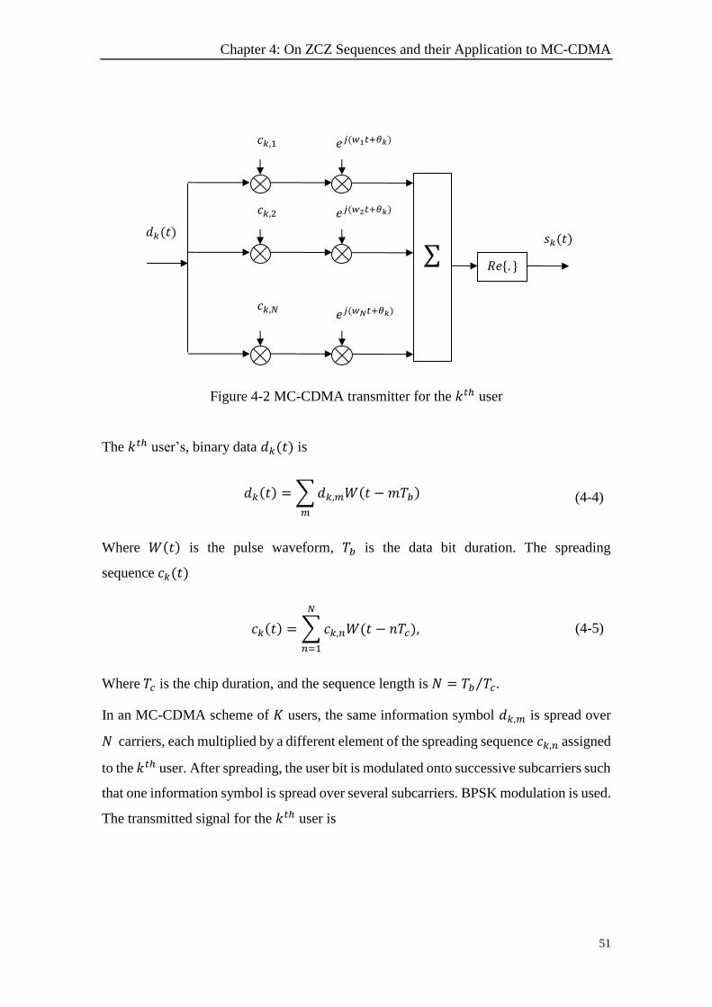
Chapter 4: On ZCZ Sequences and their Application to MC-CDMA

51

Figure 4-2 MC-CDMA transmitter for the 𝑘𝑡ℎ user

The 𝑘𝑡ℎ user’s, binary data 𝑑𝑘(𝑡) is

𝑑𝑘(𝑡) =∑𝑑𝑘,𝑚𝑊(𝑡 − 𝑚𝑇𝑏)

𝑚

(4-4)

Where 𝑊(𝑡) is the pulse waveform, 𝑇𝑏 is the data bit duration. The spreading

sequence 𝑐𝑘(𝑡)

𝑐𝑘(𝑡) = ∑𝑐𝑘,𝑛𝑊(𝑡 − 𝑛𝑇𝑐)

𝑁

𝑛=1

, (4-5)

Where 𝑇𝑐 is the chip duration, and the sequence length is 𝑁 = 𝑇𝑏 𝑇𝑐⁄ .

In an MC-CDMA scheme of 𝐾 users, the same information symbol 𝑑𝑘,𝑚 is spread over

𝑁 carriers, each multiplied by a different element of the spreading sequence 𝑐𝑘,𝑛 assigned

to the 𝑘𝑡ℎ user. After spreading, the user bit is modulated onto successive subcarriers such

that one information symbol is spread over several subcarriers. BPSK modulation is used.

The transmitted signal for the 𝑘𝑡ℎ user is

∑ 𝑅𝑒{. }

𝑑𝑘(𝑡) 𝑠𝑘(𝑡)

𝑐𝑘,2 𝑒𝑗(𝑤2𝑡+𝜃𝑘)

𝑐𝑘,1 𝑒𝑗(𝑤1𝑡+𝜃𝑘)

𝑐𝑘,𝑁 𝑒𝑗(𝑤𝑁𝑡+𝜃𝑘)

Chapter 4: On ZCZ Sequences and their Application to MC-CDMA

52

𝑠𝑘(𝑡) = √2𝑃

𝑁∑𝑅𝑒{𝑑𝑘(𝑡)𝑐𝑘,𝑛𝑒

𝑗(𝑤𝑛𝑡+𝜃𝑘)}

𝑁

𝑛=1

(4-6)

Where 𝑅𝑒{. } denotes the real part, 𝑃 is the power of data bits assumed to be equal for all

users, 𝑤𝑛 = 2𝜋𝑛 𝑇𝑏⁄ is the 𝑛𝑡ℎ subcarrier angular frequency, and the random phase 𝜃𝑘 is

uniformly distributed over [0, 2𝜋].

A QS-MC-CDMA system in AWGN channel is considered. In quasi-synchronous

systems, the relative time delay between different users 𝑇𝑞 is restricted within few chips.

We restrict our analysis to line of sight (LOS) conditions where the multipath replicas

have insignificant power compared to LOS signal [36]. We consider a correlation receiver

synchronized to the desired user 𝑖 (𝜏𝑖 = 0). The random time delays are quantized to

integer multiple of the sequence element (chip) duration 𝑇𝑐 where 𝑇𝑐 = 𝑇𝑏 𝑁⁄ . The time

delays and phase angles are measured relative to 𝜏𝑖 and 𝜃𝑖 (i.e., setting 𝜏𝑖 = 0, 𝜃𝑖 = 0).

The signal at the 𝑖𝑡ℎ receiver can be written as

𝑟(𝑡) = 𝑠𝑖(𝑡) +∑𝑠𝑘(𝑡 − 𝜏𝑘)

𝐾

𝑘=1𝑘≠𝑖

+ 𝑛(𝑡) (4-7)

Where 𝜏𝑘 is the random time delay of user 𝑘 assumed uniformly distributed over [0, 𝑇𝑞],

and 𝑛(𝑡) is a zero-mean bandpass white noise with equivalent low pass signal that has a

power spectral density 𝑁0.

Derivation of a new BER for ternary sequences in MC-CDMA system

The MC-CDMA receiver for the 𝑖𝑡ℎ user is shown in Figure 4-3.

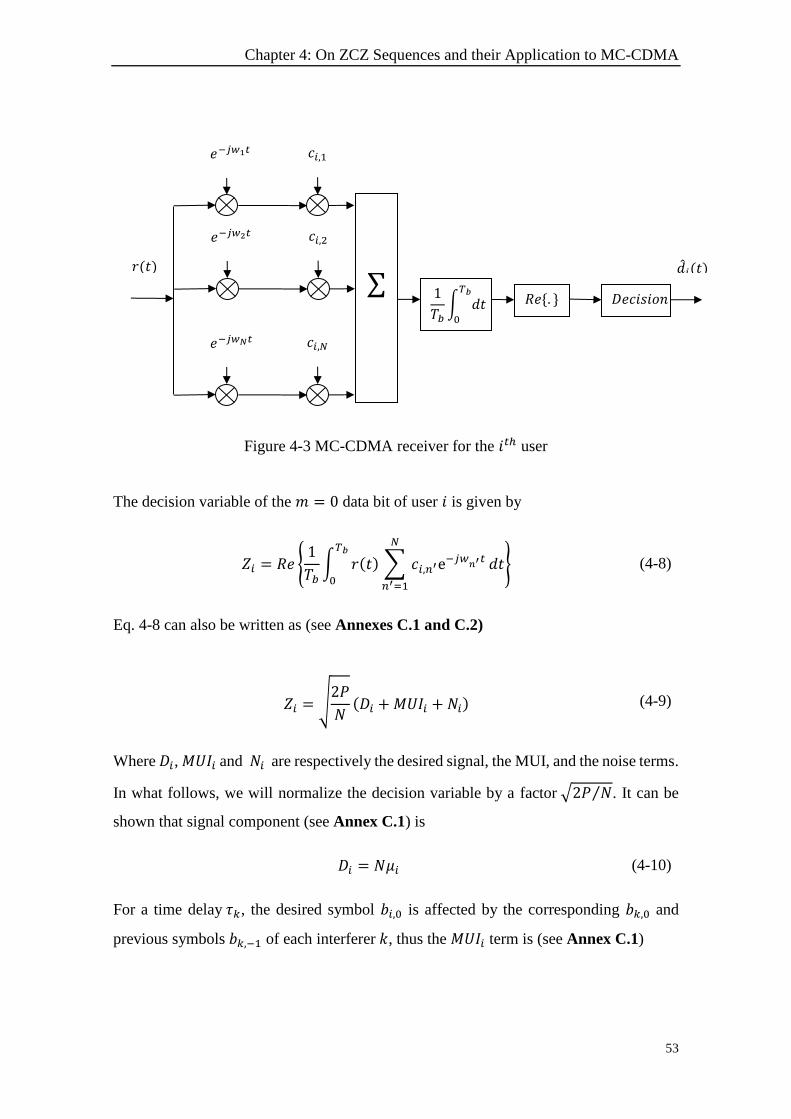
Chapter 4: On ZCZ Sequences and their Application to MC-CDMA

53

Figure 4-3 MC-CDMA receiver for the 𝑖𝑡ℎ user

The decision variable of the 𝑚 = 0 data bit of user 𝑖 is given by

𝑍𝑖 = 𝑅𝑒 {1

𝑇𝑏න 𝑟(𝑡) ∑ 𝑐𝑖,𝑛′e

−𝑗𝑤𝑛′𝑡

𝑁

𝑛′=1

𝑇𝑏

0

𝑑𝑡} (4-8)

Eq. 4-8 can also be written as (see Annexes C.1 and C.2)

𝑍𝑖 = √2𝑃

𝑁(𝐷𝑖 +𝑀𝑈𝐼𝑖 + 𝑁𝑖) (4-9)

Where 𝐷𝑖, 𝑀𝑈𝐼𝑖 and 𝑁𝑖 are respectively the desired signal, the MUI, and the noise terms.

In what follows, we will normalize the decision variable by a factor √2𝑃 𝑁⁄ . It can be

shown that signal component (see Annex C.1) is

𝐷𝑖 = 𝑁𝜇𝑖 (4-10)

For a time delay 𝜏𝑘, the desired symbol 𝑏𝑖,0 is affected by the corresponding 𝑏𝑘,0 and

previous symbols 𝑏𝑘,−1 of each interferer 𝑘, thus the 𝑀𝑈𝐼𝑖 term is (see Annex C.1)

∑ 1

𝑇𝑏න 𝑑𝑡𝑇𝑏

0

𝑑መ𝑖(𝑡)

𝑅𝑒{. }

𝑟(𝑡)

𝐷𝑒𝑐𝑖𝑠𝑖𝑜𝑛

𝑒−𝑗𝑤𝑁𝑡 𝑐𝑖,𝑁

𝑒−𝑗𝑤2𝑡 𝑐𝑖,2

𝑒−𝑗𝑤1𝑡 𝑐𝑖,1

Chapter 4: On ZCZ Sequences and their Application to MC-CDMA

54

𝑀𝑈𝐼𝑖 =1

𝑇𝑏∑∑ ∑ 𝑐𝑘,𝑛𝑐𝑖,𝑛′

𝑁

𝑛′=1

𝑁

𝑛=1

𝐾

𝑘=1𝑘≠𝑖

න 𝑑𝑘(𝑡 − 𝜏𝑘)𝑐𝑜𝑠[(𝑤𝑛 − 𝑤𝑛′)𝑡 + 𝜗𝑘,𝑛]𝑇𝑏

0

𝑑𝑡 (4-11)

Where 𝜗𝑘,𝑛 = 𝜃𝑘 − 𝑤𝑛𝜏𝑘

In the case where 𝑛′ = 𝑛, interference from the same subcarriers of user 𝑘 is called inter-

symbol interference (ISI) equals to (see Annex C.1)

𝐼𝑆𝐼𝑖 =1

𝑇𝑏∑∑[𝜏𝑘𝑑𝑘,−1 + (𝑇𝑏 − 𝜏𝑘)𝑑𝑘,0]𝑐𝑘,𝑛𝑐𝑖,𝑛′𝑐𝑜𝑠(𝜗𝑘,𝑛)

𝑁

𝑛=1

𝐾

𝑘=1𝑘≠𝑖

(4-12)

If 𝑛′ ≠ 𝑛, interference from other subcarriers of user 𝑘 is called inter-channel interference

(ICI) equal to (see Annex C.1)

𝐼𝐶𝐼𝑖 =1

𝑇𝑏∑∑ ∑ 𝑐𝑘,𝑛𝑐𝑖,𝑛′

𝑁

𝑛′=1𝑛′≠𝑛

𝑁

𝑛=1

𝐾

𝑘=1𝑘≠𝑖

න 𝑑𝑘(𝑡 − 𝜏𝑘)𝑐𝑜𝑠[(𝑤𝑛 − 𝑤𝑛′)𝑡 + 𝜗𝑘,𝑛]𝑇𝑏

0

𝑑𝑡 (4-13)

The noise term is (see Annex C.2)

𝑁𝑖 =1

𝑇𝑏√𝑁

2𝑃න 𝑛(𝑡) ∑ 𝑐𝑖,𝑛′𝑐𝑜𝑠(𝑤𝑛′𝑡)

𝑁

𝑛′=1

𝑇𝑏

0

𝑑𝑡 (4-14)

It is deduced from [50] that the signal-to-noise ratio (𝑆𝑁𝑅𝑖) for MC-CDMA is defined as

√𝑆𝑁𝑅𝑖 =𝐷𝑖 +𝑀𝑈𝐼𝑖

√2𝑉𝑎𝑟{𝑁𝑖} (4-15)

Where the variance of the noise 𝑉𝑎𝑟{𝑁𝑖} is (see Annex C.2)

𝑉𝑎𝑟{𝑁𝑖} = 𝑁0𝑁2𝜇𝑖 4𝐸𝑏⁄ (4-16)

The 𝑆𝑁𝑅𝑖 becomes

Chapter 4: On ZCZ Sequences and their Application to MC-CDMA

55

√𝑆𝑁𝑅𝑖 = 𝜇𝑖𝑁 +𝑀𝑈𝐼𝑖

𝑁√𝑁0𝜇𝑖 2𝐸𝑏⁄

= √2𝐸𝑏𝑁0𝜇𝑖

[𝜇𝑖 +𝑀𝑈𝐼𝑖𝑁

] (4-17)

Since we considered AWGN channel, the decision variable can be regarded as a Gaussian

random variable [50]. The 𝐵𝐸𝑅𝑖 of user 𝑖, conditioned on {𝜏𝑘}, {𝜃𝑘}, {𝑏𝑘,−1}, and {𝑏𝑘,0},

is

𝐵𝐸𝑅𝑖 =1

2𝑒𝑟𝑓𝑐(√𝑆𝑁𝑅𝑖) =

1

2𝑒𝑟𝑓𝑐 (√

2𝐸𝑏𝑁0𝜇𝑖

[𝜇𝑖 +𝑀𝑈𝐼𝑖𝑁

]) (4-18)

In the case of binary spreading sequences (𝜇𝑖 = 1), 𝐵𝐸𝑅𝑖 becomes

𝐵𝐸𝑅𝑖 =1

2𝑒𝑟𝑓𝑐 (√

2𝐸𝑏𝑁0

[1 +𝑀𝑈𝐼𝑖𝑁

]) (4-19)

An expression similar to Eq. 4-19 was obtained in [50] as

𝐵𝐸𝑅𝑖 =1

2𝑒𝑟𝑓𝑐 (√

𝐸𝑏𝑁0[1 +

𝑀𝑈𝐼𝑖𝑁

]) (4-20)

Note that a factor of 2 is missing, this is due to an error in calculation of noise term in

[50]. The correct noise variance analysis is given in Annex C.2. To obtain the

unconditional BER for user 𝑖, we average 𝐵𝐸𝑅𝑖 over all variables via Monte Carlo

integration. A more appropriate performance measure is the averaged BER over all users

[50]

𝐵𝐸𝑅 =1

𝐾∑𝐵𝐸𝑅𝑖

𝐾

𝑖=1

(4-21)

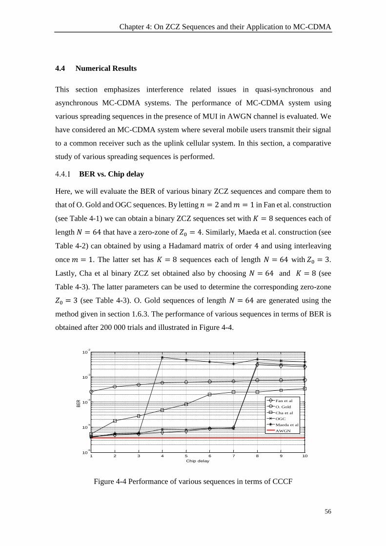
Chapter 4: On ZCZ Sequences and their Application to MC-CDMA

56

4.4 Numerical Results

This section emphasizes interference related issues in quasi-synchronous and

asynchronous MC-CDMA systems. The performance of MC-CDMA system using

various spreading sequences in the presence of MUI in AWGN channel is evaluated. We

have considered an MC-CDMA system where several mobile users transmit their signal

to a common receiver such as the uplink cellular system. In this section, a comparative

study of various spreading sequences is performed.

BER vs. Chip delay

Here, we will evaluate the BER of various binary ZCZ sequences and compare them to

that of O. Gold and OGC sequences. By letting 𝑛 = 2 and 𝑚 = 1 in Fan et al. construction

(see Table 4-1) we can obtain a binary ZCZ sequences set with 𝐾 = 8 sequences each of

length 𝑁 = 64 that have a zero-zone of 𝑍0 = 4. Similarly, Maeda et al. construction (see

Table 4-2) can obtained by using a Hadamard matrix of order 4 and using interleaving

once 𝑚 = 1. The latter set has 𝐾 = 8 sequences each of length 𝑁 = 64 with 𝑍0 = 3.

Lastly, Cha et al binary ZCZ set obtained also by choosing 𝑁 = 64 and 𝐾 = 8 (see

Table 4-3). The latter parameters can be used to determine the corresponding zero-zone

𝑍0 = 3 (see Table 4-3). O. Gold sequences of length 𝑁 = 64 are generated using the

method given in section 1.6.3. The performance of various sequences in terms of BER is

obtained after 200 000 trials and illustrated in Figure 4-4.

Figure 4-4 Performance of various sequences in terms of CCCF

1 2 3 4 5 6 7 8 9 1010

-6

10-5

10-4

10-3

10-2

Chip delay

BE

R

Fan et al

O. Gold

Cha et al

OGC

Maeda et al

AWGN

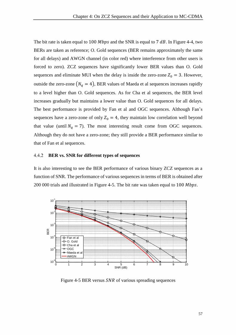
Chapter 4: On ZCZ Sequences and their Application to MC-CDMA

57

The bit rate is taken equal to 100 𝑀𝑏𝑝𝑠 and the SNR is equal to 7 𝑑𝐵. In Figure 4-4, two

BERs are taken as reference; O. Gold sequences (BER remains approximately the same

for all delays) and AWGN channel (in color red) where interference from other users is

forced to zero). ZCZ sequences have significantly lower BER values than O. Gold

sequences and eliminate MUI when the delay is inside the zero-zone 𝑍0 = 3. However,

outside the zero-zone (𝑁𝑞 = 4), BER values of Maeda et al sequences increases rapidly

to a level higher than O. Gold sequences. As for Cha et al sequences, the BER level

increases gradually but maintains a lower value than O. Gold sequences for all delays.

The best performance is provided by Fan et al and OGC sequences. Although Fan’s

sequences have a zero-zone of only 𝑍0 = 4, they maintain low correlation well beyond

that value (until 𝑁𝑞 = 7). The most interesting result come from OGC sequences.

Although they do not have a zero-zone; they still provide a BER performance similar to

that of Fan et al sequences.

BER vs. SNR for different types of sequences

It is also interesting to see the BER performance of various binary ZCZ sequences as a

function of SNR. The performance of various sequences in terms of BER is obtained after

200 000 trials and illustrated in Figure 4-5. The bit rate was taken equal to 100 𝑀𝑏𝑝𝑠.

Figure 4-5 BER versus 𝑆𝑁𝑅 of various spreading sequences

0 1 2 3 4 5 6 7 8 9 1010

-6

10-5

10-4

10-3

10-2

10-1

SNR (dB)

BE

R

Fan et al

O. Gold

Cha et al

OGC

Maeda et al

AWGN

Chapter 4: On ZCZ Sequences and their Application to MC-CDMA

58

In order to analyze ZCZ sequences inside and outside their zero-zones, the maximum

delay was chosen equal to 𝑁𝑞 = 4. The latter delay is inside the zero-zone for Fan et al

sequences (𝑍0 = 4) and outside the zero-zone for Maeda et al and Cha et al sequences

which have the same zero-zone 𝑍0 = 3. Outside the zero-zone 𝑍0 = 3; two different

behaviors are noted. Maeda et al sequences exhibit the worst BER performance while

Cha et al sequences maintain good performance (much better than O. Gold sequences).

According to the BER criterion, the best results are obtained when Fan et al sequences

are used for spreading (see Figure 4-5). The latter sequences eliminate interference and

provide a BER performance similar to AWGN channel. OGC sequences performance is

almost identical to Fan et al performance for 𝑆𝑁𝑅 ≤ 5 𝑑𝐵.

From the numerical results (CF and BER), it can be observed that ZCZ sequences have

both low CF and interference-free communication (see Table 4-5). Therefore, we

conclude that ZCZ sequences are the suitable candidate for QS-MC-CDMA systems.

Table 4-5 𝐵𝐸𝑅 and 𝐶𝐹 Performance comparison in QS-MC-CDMA

Criteria

Sequences CF BER (𝑁𝑞 ≤ 𝑍0)

ZCZ (Fan et al) Low Low

ZCZ ( Maeda et al) Highest Low

ZCZ ( Cha et al) Low Low

Orthogonal Gold Low Highest

OGC Lowest Low

4.5 Conclusion

In this chapter, the CF performances of various sequences, i.e. ZCZ, orthogonal Gold,

and OGC sequences were analyzed and compared. In addition, the BER performance of

QS-MC-CDMA in AWGN channel was also evaluated. With the use of efficient

spreading sequence, the system can operate at low CF and low BER. Based on the

obtained results for different sequences, it is observed that the QS-MC-CDMA system

with ZCZ sequences shows good performance in terms of both CF and BER and are

suitable candidate for QS-MC-CDMA.

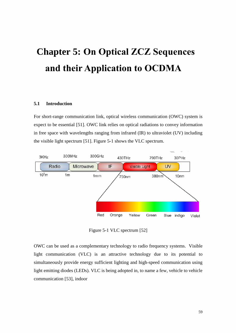
59

Chapter 5: On Optical ZCZ Sequences

and their Application to OCDMA

5.1 Introduction

For short-range communication link, optical wireless communication (OWC) system is

expect to be essential [51]. OWC link relies on optical radiations to convey information

in free space with wavelengths ranging from infrared (IR) to ultraviolet (UV) including

the visible light spectrum [51]. Figure 5-1 shows the VLC spectrum.

Figure 5-1 VLC spectrum [52]

OWC can be used as a complementary technology to radio frequency systems. Visible

light communication (VLC) is an attractive technology due to its potential to

simultaneously provide energy sufficient lighting and high-speed communication using

light emitting diodes (LEDs). VLC is being adopted in, to name a few, vehicle to vehicle

communication [53], indoor

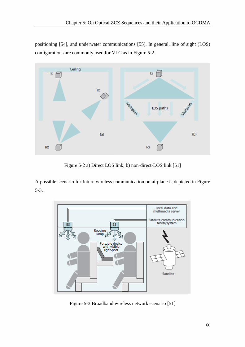
Chapter 5: On Optical ZCZ Sequences and their Application to OCDMA

60

positioning [54], and underwater communications [55]. In general, line of sight (LOS)

configurations are commonly used for VLC as in Figure 5-2

Figure 5-2 a) Direct LOS link; b) non-direct-LOS link [51]

A possible scenario for future wireless communication on airplane is depicted in Figure

5-3.

Figure 5-3 Broadband wireless network scenario [51]

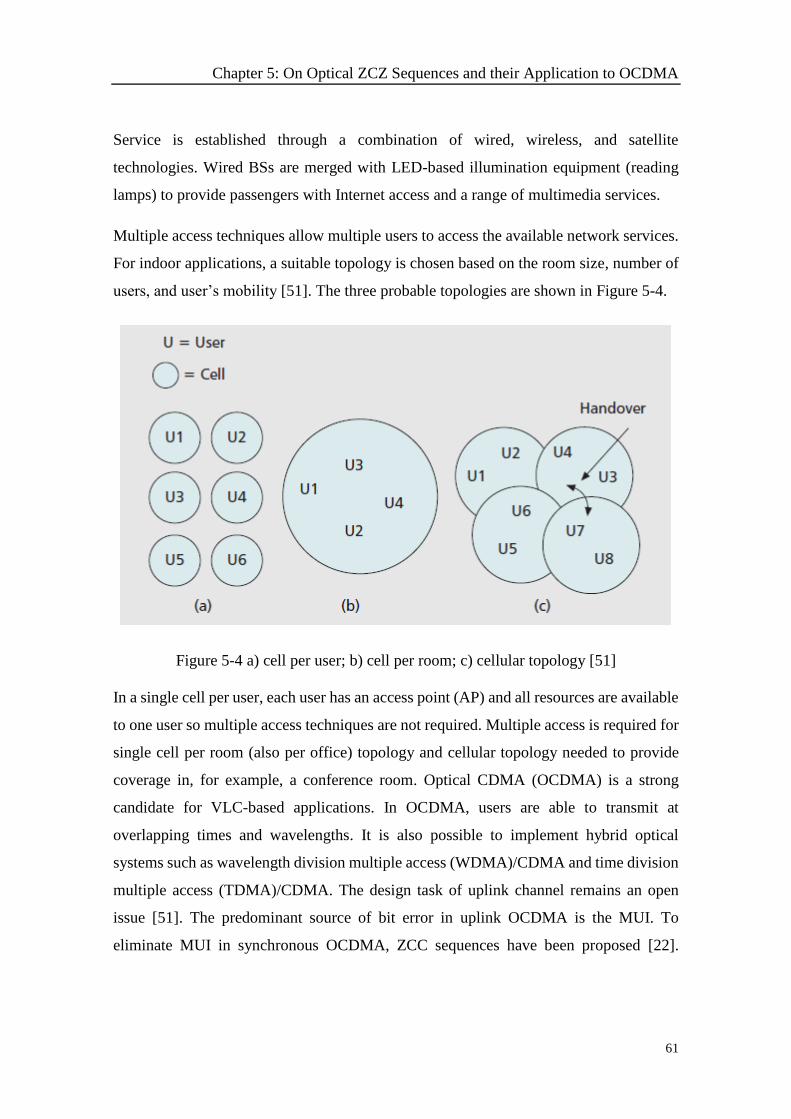
Chapter 5: On Optical ZCZ Sequences and their Application to OCDMA

61

Service is established through a combination of wired, wireless, and satellite

technologies. Wired BSs are merged with LED-based illumination equipment (reading

lamps) to provide passengers with Internet access and a range of multimedia services.

Multiple access techniques allow multiple users to access the available network services.

For indoor applications, a suitable topology is chosen based on the room size, number of

users, and user’s mobility [51]. The three probable topologies are shown in Figure 5-4.

Figure 5-4 a) cell per user; b) cell per room; c) cellular topology [51]

In a single cell per user, each user has an access point (AP) and all resources are available

to one user so multiple access techniques are not required. Multiple access is required for

single cell per room (also per office) topology and cellular topology needed to provide

coverage in, for example, a conference room. Optical CDMA (OCDMA) is a strong

candidate for VLC-based applications. In OCDMA, users are able to transmit at

overlapping times and wavelengths. It is also possible to implement hybrid optical

systems such as wavelength division multiple access (WDMA)/CDMA and time division

multiple access (TDMA)/CDMA. The design task of uplink channel remains an open

issue [51]. The predominant source of bit error in uplink OCDMA is the MUI. To

eliminate MUI in synchronous OCDMA, ZCC sequences have been proposed [22].

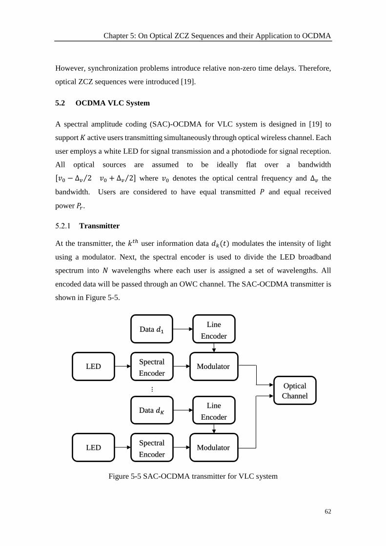
Chapter 5: On Optical ZCZ Sequences and their Application to OCDMA

62

However, synchronization problems introduce relative non-zero time delays. Therefore,

optical ZCZ sequences were introduced [19].

5.2 OCDMA VLC System

A spectral amplitude coding (SAC)-OCDMA for VLC system is designed in [19] to

support 𝐾 active users transmitting simultaneously through optical wireless channel. Each

user employs a white LED for signal transmission and a photodiode for signal reception.

All optical sources are assumed to be ideally flat over a bandwidth

[𝑣0 − ∆𝑣 2⁄ 𝑣0 + ∆𝑣 2⁄ ] where 𝑣0 denotes the optical central frequency and ∆𝑣 the

bandwidth. Users are considered to have equal transmitted 𝑃 and equal received

power 𝑃𝑟.

Transmitter

At the transmitter, the 𝑘𝑡ℎ user information data 𝑑𝑘(𝑡) modulates the intensity of light

using a modulator. Next, the spectral encoder is used to divide the LED broadband

spectrum into 𝑁 wavelengths where each user is assigned a set of wavelengths. All

encoded data will be passed through an OWC channel. The SAC-OCDMA transmitter is

shown in Figure 5-5.

Figure 5-5 SAC-OCDMA transmitter for VLC system

Spectral

Encoder LED Modulator

Data 𝑑1

⋮

Line

Encoder

Spectral

Encoder LED Modulator

Data 𝑑𝐾 Line

Encoder

Optical

Channel

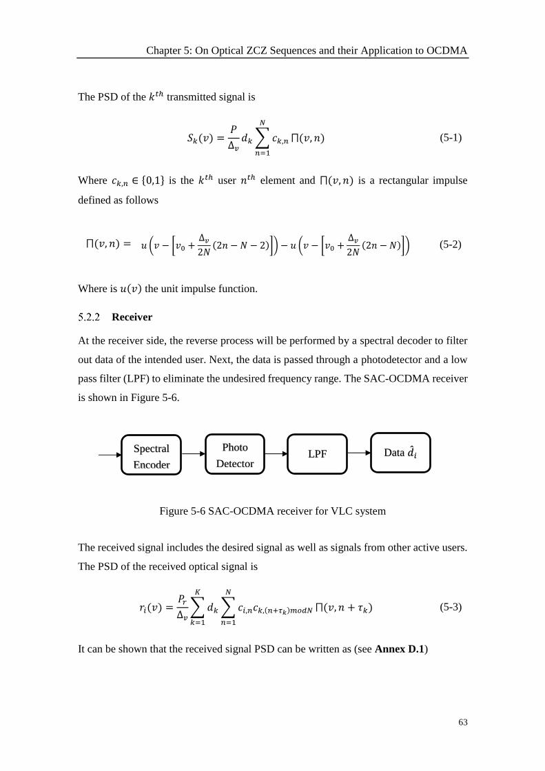
Chapter 5: On Optical ZCZ Sequences and their Application to OCDMA

63

The PSD of the 𝑘𝑡ℎ transmitted signal is

𝑆𝑘(𝑣) =𝑃

∆𝑣𝑑𝑘∑𝑐𝑘,𝑛

𝑁

𝑛=1

⨅(𝑣, 𝑛) (5-1)

Where 𝑐𝑘,𝑛 ∈ {0,1} is the 𝑘𝑡ℎ user 𝑛𝑡ℎ element and ⨅(𝑣, 𝑛) is a rectangular impulse

defined as follows

⨅(𝑣, 𝑛) = 𝑢 (𝑣 − [𝑣0 +∆𝑣2𝑁

(2𝑛 − 𝑁 − 2)]) − 𝑢 (𝑣 − [𝑣0 +∆𝑣2𝑁

(2𝑛 − 𝑁)]) (5-2)

Where is 𝑢(𝑣) the unit impulse function.

Receiver

At the receiver side, the reverse process will be performed by a spectral decoder to filter

out data of the intended user. Next, the data is passed through a photodetector and a low

pass filter (LPF) to eliminate the undesired frequency range. The SAC-OCDMA receiver

is shown in Figure 5-6.

Figure 5-6 SAC-OCDMA receiver for VLC system

The received signal includes the desired signal as well as signals from other active users.

The PSD of the received optical signal is

𝑟𝑖(𝑣) =𝑃𝑟∆𝑣∑𝑑𝑘∑𝑐𝑖,𝑛𝑐𝑘,(𝑛+𝜏𝑘)𝑚𝑜𝑑𝑁

𝑁

𝑛=1

⨅(𝑣, 𝑛 + 𝜏𝑘)

𝐾

𝑘=1

(5-3)

It can be shown that the received signal PSD can be written as (see Annex D.1)

Spectral

Encoder

Photo

Detector LPF Data 𝑑መ𝑖

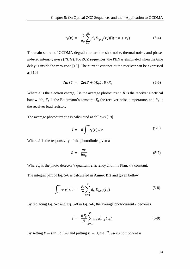
Chapter 5: On Optical ZCZ Sequences and their Application to OCDMA

64

𝑟𝑖(𝑣) = 𝑃𝑟∆𝑣∑𝑑𝑘𝐸𝑐𝑖𝑐𝑘(𝜏𝑘)⨅(𝑣, 𝑛 + 𝜏𝑘)

𝐾

𝑘=1

(5-4)

The main source of OCDMA degradation are the shot noise, thermal noise, and phase-

induced intensity noise (𝑃𝐼𝐼𝑁). For ZCZ sequences, the PIIN is eliminated when the time

delay is inside the zero-zone [19]. The current variance at the receiver can be expressed

as [19]

𝑉𝑎𝑟(𝑖) = 2𝑒𝐼𝐵 + 4𝐾𝑏𝑇𝑛𝐵 𝑅𝐿⁄ (5-5)

Where 𝑒 is the electron charge, 𝐼 is the average photocurrent, 𝐵 is the receiver electrical

bandwidth, 𝐾𝑏 is the Boltzmann’s constant, 𝑇𝑛 the receiver noise temperature, and 𝑅𝐿 is

the receiver load resistor.

The average photocurrent 𝐼 is calculated as follows [19]

𝐼 = 𝑅න 𝑟𝑖(𝑣)∞

0

𝑑𝑣 (5-6)

Where 𝑅 is the responsivity of the photodiode given as

𝑅 = 𝜂𝑒

ℎ𝑣0 (5-7)

Where 𝜂 is the photo detector’s quantum efficiency and ℎ is Planck’s constant.

The integral part of Eq. 5-6 is calculated in Annex D.2 and given bellow

න 𝑟𝑖(𝑣)∞

0

𝑑𝑣 = 𝑃𝑟𝑁∑𝑑𝑘

𝐾

𝑘=1

𝐸𝑐𝑖𝑐𝑘(𝜏𝑘) (5-8)

By replacing Eq. 5-7 and Eq. 5-8 in Eq. 5-6, the average photocurrent 𝐼 becomes

𝐼 = 𝑅𝑃𝑟𝑁∑𝑑𝑘

𝐾

𝑘=1

𝐸𝑐𝑖𝑐𝑘(𝜏𝑘) (5-9)

By setting 𝑘 = 𝑖 in Eq. 5-9 and putting 𝜏𝑖 = 0, the 𝑖𝑡ℎ user’s component is

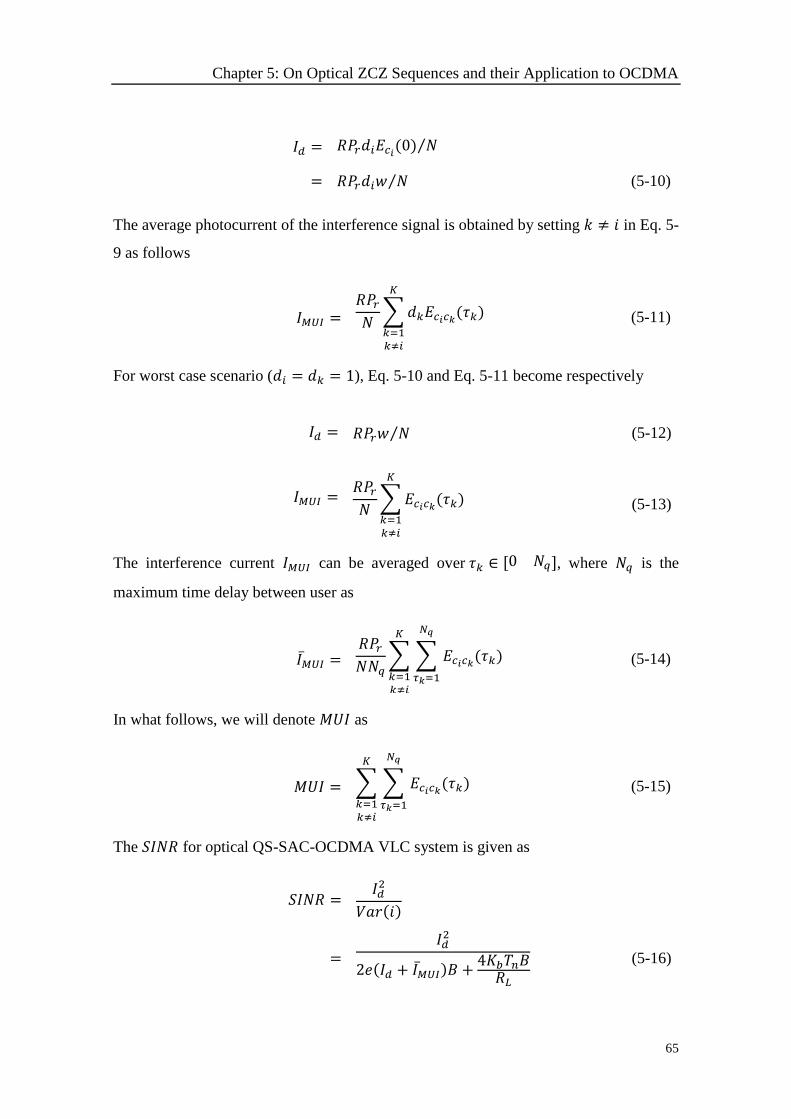
Chapter 5: On Optical ZCZ Sequences and their Application to OCDMA

65

𝐼𝑑 = 𝑅𝑃𝑟𝑑𝑖𝐸𝑐𝑖(0) 𝑁⁄

= 𝑅𝑃𝑟𝑑𝑖𝑤 𝑁⁄ (5-10)

The average photocurrent of the interference signal is obtained by setting 𝑘 ≠ 𝑖 in Eq. 5-

9 as follows

𝐼𝑀𝑈𝐼 = 𝑅𝑃𝑟𝑁∑𝑑𝑘𝐸𝑐𝑖𝑐𝑘(𝜏𝑘)

𝐾

𝑘=1𝑘≠𝑖

(5-11)

For worst case scenario (𝑑𝑖 = 𝑑𝑘 = 1), Eq. 5-10 and Eq. 5-11 become respectively

𝐼𝑑 = 𝑅𝑃𝑟𝑤 𝑁⁄ (5-12)

𝐼𝑀𝑈𝐼 = 𝑅𝑃𝑟𝑁∑𝐸𝑐𝑖𝑐𝑘(𝜏𝑘)

𝐾

𝑘=1𝑘≠𝑖

(5-13)

The interference current 𝐼𝑀𝑈𝐼 can be averaged over 𝜏𝑘 ∈ [0 𝑁𝑞], where 𝑁𝑞 is the

maximum time delay between user as

𝐼�̅�𝑈𝐼 = 𝑅𝑃𝑟𝑁𝑁𝑞

∑ ∑ 𝐸𝑐𝑖𝑐𝑘(𝜏𝑘)

𝑁𝑞

𝜏𝑘=1

𝐾

𝑘=1𝑘≠𝑖

(5-14)

In what follows, we will denote 𝑀𝑈𝐼 as

𝑀𝑈𝐼 = ∑ ∑ 𝐸𝑐𝑖𝑐𝑘(𝜏𝑘)

𝑁𝑞

𝜏𝑘=1

𝐾

𝑘=1𝑘≠𝑖

(5-15)

The 𝑆𝐼𝑁𝑅 for optical QS-SAC-OCDMA VLC system is given as

𝑆𝐼𝑁𝑅 = 𝐼𝑑2

𝑉𝑎𝑟(𝑖)

=

𝐼𝑑2

2𝑒(𝐼𝑑 + 𝐼�̅�𝑈𝐼)𝐵 +4𝐾𝑏𝑇𝑛𝐵𝑅𝐿

(5-16)

Chapter 5: On Optical ZCZ Sequences and their Application to OCDMA

66

If OZCZ sequences are used for spreading where 𝐸𝑐𝑖𝑐𝑘(𝜏𝑘) = 0 for 𝑁𝑞 ≤ 𝑍0, the

𝑀𝑈𝐼 becomes zero 𝐼�̅�𝑈𝐼 = 0 and the 𝑆𝐼𝑁𝑅 of Eq. 5-16 becomes

𝑆𝐼𝑁𝑅 =

𝐼𝑑2

2𝑒𝐼𝑑𝐵 +4𝐾𝑏𝑇𝑛𝐵𝑅𝐿

(5-17)

If the system is synchronous 𝜏𝑘 = 0 and ZCC sequences are used for spreading, the 𝑆𝐼𝑁𝑅

is the same form as Eq. 5-17. Note that Eq. 5-16 cannot be used to evaluate ZCC

sequences. This is because in asynchronous transmission, ZCC sequences lose their zero

in-phase CCF property and the 𝑃𝐼𝐼𝑁 occurs and must be added to Eq. 5-16. The term

MUI of Eq. 5-15 remains valid and can be used to compare ZCC sequences as it is done

in the following section.

5.3 Numerical Results and Analysis

The correlation properties of sequences are crucial to system’s capacity to eliminate MUI

and provide reliable communication. In this section, we first investigate MUI reduction

of the proposed ZCC sequences based on the following parameters: time delay, sequence

length, and the number of sequences. Second, the ZCC sequences are compared to ZCZ

sequences.

MUI vs. Time Delay

To evaluate the effect of correlation properties on the sequence’s performance, we

compared ZCC sequences proposed by Addad et al [23] to two ZCC sequences proposed

in [22] by Abd et al and [56] by Garadi et al. (see section 1.9) and plotted the results in

Figure 5-7. All ZCC sequences sets have the same parameters: family size 𝐾 = 10,

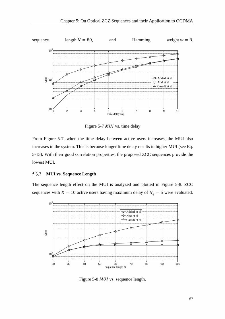
Chapter 5: On Optical ZCZ Sequences and their Application to OCDMA

67

sequence length 𝑁 = 80, and Hamming weight 𝑤 = 8.

Figure 5-7 𝑀𝑈𝐼 vs. time delay

From Figure 5-7, when the time delay between active users increases, the MUI also

increases in the system. This is because longer time delay results in higher MUI (see Eq.

5-15). With their good correlation properties, the proposed ZCC sequences provide the

lowest MUI.

MUI vs. Sequence Length

The sequence length effect on the MUI is analyzed and plotted in Figure 5-8. ZCC

sequences with 𝐾 = 10 active users having maximum delay of 𝑁𝑞 = 5 were evaluated.

Figure 5-8 𝑀𝑈𝐼 vs. sequence length.

1 2 3 4 5 6 7 8 9 1010

1

102

103

Time delay Nq

MU

I

Addad et al

Abd et al

Garadi et al

20 30 40 50 60 70 80 90 100

102

103

Sequence length N

MU

I

Addad et al

Abd et al

Garadi et al

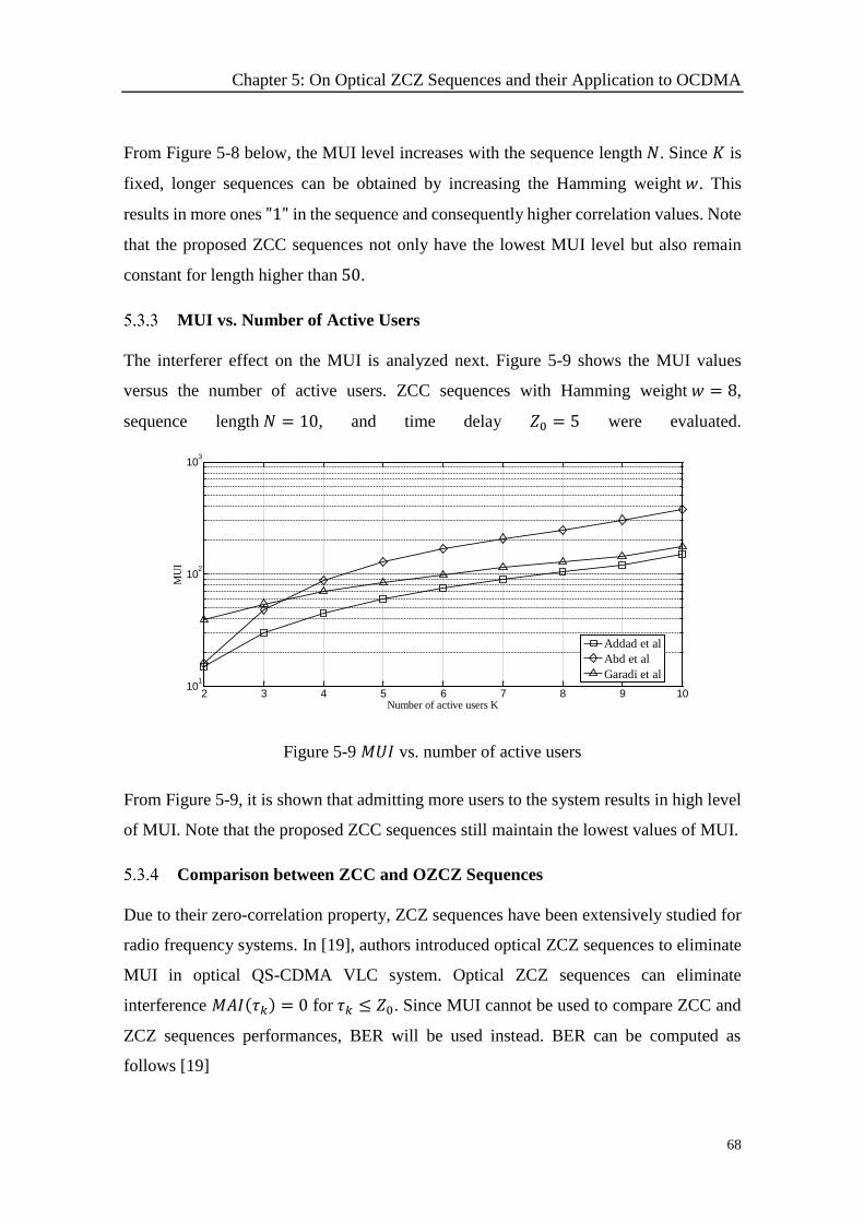
Chapter 5: On Optical ZCZ Sequences and their Application to OCDMA

68

From Figure 5-8 below, the MUI level increases with the sequence length 𝑁. Since 𝐾 is

fixed, longer sequences can be obtained by increasing the Hamming weight 𝑤. This

results in more ones "1" in the sequence and consequently higher correlation values. Note

that the proposed ZCC sequences not only have the lowest MUI level but also remain

constant for length higher than 50.

MUI vs. Number of Active Users

The interferer effect on the MUI is analyzed next. Figure 5-9 shows the MUI values

versus the number of active users. ZCC sequences with Hamming weight 𝑤 = 8,

sequence length 𝑁 = 10, and time delay 𝑍0 = 5 were evaluated.

Figure 5-9 𝑀𝑈𝐼 vs. number of active users

From Figure 5-9, it is shown that admitting more users to the system results in high level

of MUI. Note that the proposed ZCC sequences still maintain the lowest values of MUI.

Comparison between ZCC and OZCZ Sequences

Due to their zero-correlation property, ZCZ sequences have been extensively studied for

radio frequency systems. In [19], authors introduced optical ZCZ sequences to eliminate

MUI in optical QS-CDMA VLC system. Optical ZCZ sequences can eliminate

interference 𝑀𝐴𝐼(𝜏𝑘) = 0 for 𝜏𝑘 ≤ 𝑍0. Since MUI cannot be used to compare ZCC and

ZCZ sequences performances, BER will be used instead. BER can be computed as

follows [19]

2 3 4 5 6 7 8 9 1010

1

102

103

Number of active users K

MU

I

Addad et al

Abd et al

Garadi et al

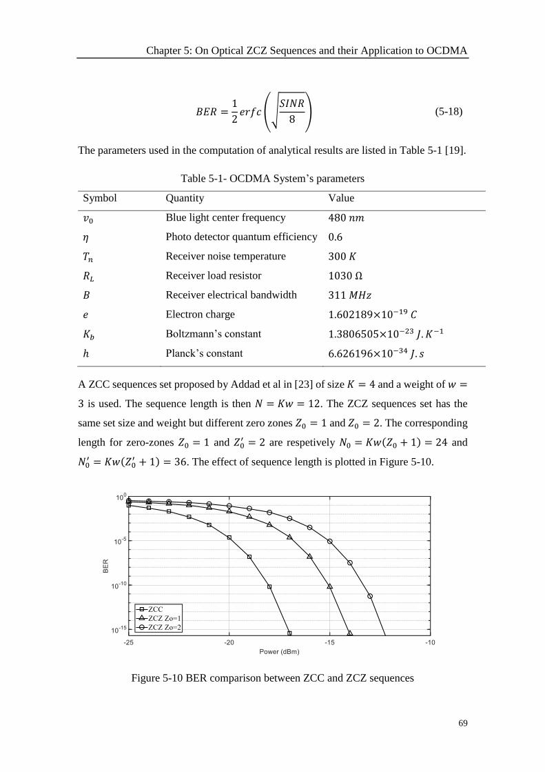
Chapter 5: On Optical ZCZ Sequences and their Application to OCDMA

69

𝐵𝐸𝑅 =1

2𝑒𝑟𝑓𝑐 (√

𝑆𝐼𝑁𝑅

8) (5-18)

The parameters used in the computation of analytical results are listed in Table 5-1 [19].

Table 5-1- OCDMA System’s parameters

Symbol Quantity Value

𝑣0 Blue light center frequency 480 𝑛𝑚

𝜂 Photo detector quantum efficiency 0.6

𝑇𝑛 Receiver noise temperature 300 𝐾

𝑅𝐿 Receiver load resistor 1030 Ω

𝐵 Receiver electrical bandwidth 311 𝑀𝐻𝑧

𝑒 Electron charge 1.602189×10−19 𝐶

𝐾𝑏 Boltzmann’s constant 1.3806505×10−23 𝐽. 𝐾−1

ℎ Planck’s constant 6.626196×10−34 𝐽. 𝑠

A ZCC sequences set proposed by Addad et al in [23] of size 𝐾 = 4 and a weight of 𝑤 =

3 is used. The sequence length is then 𝑁 = 𝐾𝑤 = 12. The ZCZ sequences set has the

same set size and weight but different zero zones 𝑍0 = 1 and 𝑍0 = 2. The corresponding

length for zero-zones 𝑍0 = 1 and 𝑍0′ = 2 are respetively 𝑁0 = 𝐾𝑤(𝑍0 + 1) = 24 and

𝑁0′ = 𝐾𝑤(𝑍0

′ + 1) = 36. The effect of sequence length is plotted in Figure 5-10.

Figure 5-10 BER comparison between ZCC and ZCZ sequences

Chapter 5: On Optical ZCZ Sequences and their Application to OCDMA

70

We can readily see from Figure 5-10 that ZCC sequences outperform ZCZ sequences by

a large extent. Although ZCZ sequences eliminate the MUI, their sequence length is

proportional to the zero zone 𝑍0. Large time delay require longue ZCZ sequences which

results in poor BER performance. Note that using 𝑆𝐼𝑁𝑅 Eq. 5-16 to compare ZCC

sequences to ZCZ sequences is not accurate. This is because ZCC sequences lose their

zero correlation property in asynchronous transmission. Therefore, the 𝑃𝐼𝐼𝑁 must be

computed and added to 𝑆𝐼𝑁𝑅 of Eq. 5-16. This will require a system with balanced

receiver developped in [57].

5.4 Conclusion

In this chapter, we evaluate the performance of optical QS-SAC-OCDMA for VLC

system. First, MUI caused by quasi-synchronous transmission of ZCC sequences was

investigated with respect correlation properties, sequence length, and number of

sequences in the set. It was shown that a new ZCC sequence (see section 1.9.1) with

flexible construction and good correlation properties provide the best results. It was

shown also that OZCZ sequences eliminated the MUI but their length is not practical

which results in poor BER performance. Therefore, we conclude that the optical ZCZ

sequences are not suitable for QS-SAC-OCDMA for VLC system.

71

Conclusions and Future Work

This chapter concludes the thesis. A summary of the main findings and suggestions for

future research is presented. This thesis has largely focused on the construction and

application of ZCZ sequences to CDMA systems. two new constructions of optical ZCZ

and ZCC sequences were proposed in Chapter 1. Introductory Chapter 2 is excluded from

the discussion because it does not contain any new research material. In Chapter 3, a new

BER for uplink QS-DS-CDMA system in nonselective Rician fading AWGN channel

was derived. The new BER allows the evaluation of both binary and ternary sequences.

First, MUI interference level as a function of chip delay of various binary ZCZ sequences

was analysed and compared to that of Gold sequences. Second, their BER performance

is investigated. The obtained results show that ZCZ sequences do effectively reduce MUI

interference and provide much better BER performance, when the maximum time delay

between users is inside their zero-zone. A class of ternary ZCZ sequences that eliminate

interference was presented and studied. It was concluded that the best BER performance

in QS-DS-CDMA could be obtained if binary ZCZ sequences with both zero even and

odd periodic CCFs were designed and used. As for application, ZCZ sequences can be

used to limit power consumption and prolong battery life while maintaining the

robustness in CDMA-based mobile wireless communications systems such as Ad-Hoc

networks.

Chapter 4 dealt with application of ZCZ sequences to QS-MC-CDMA system. The CF

performances of various sequences, i.e. ZCZ, WH, orthogonal Gold, and OGC sequences

were analyzed and compared. In addition, a new BER for ternary sequences in uplink QS-

MC-CDMA system with an AWGN channel was derived. Based on the obtained results,

a system using ZCZ sequences shows good performance in terms of both CF and BER.

In Chapter 5, attention was devoted to the application of optical ZCZ and ZCC sequences

in the uplink of QS-SAC-OCDMA system. It was shown that optical ZCZ sequences

eliminate the MUI interference. However, the BER turned out to be sensitive to the

72

sequence length which results in poor BER performance of optical ZCZ sequences

compared to ZCC sequences. In addition, the MUI caused by the quasi-synchronous

transmission was investigated with respect to ZCC correlation properties, sequence

length, and number of sequences in the set. It was shown that the ZCC sequences

proposed by the authors in Chapter 1 have the best performance.

From this work, some points deserve to be developed in the future. First, one can

investigate the behavior of ZCZ sequences in presence of MPI interference for both QS-

DS-CDMA and QS-MC-CDMA systems. Another possibility for contributing to the

existing literature would be to investigate the performance of ZCZ sequences in QS-MC-

DS-CDMA. Related to the subject of optical ZCZ sequences proposed in chapter 1, the

existing model for OCDMA needs to be further developed and accurate BER could be

obtained. Finally, more research must be put into the development of practical systems

using ZCZ sequences and compare their performances to theoretical models studied in

this thesis.

73

Annexes

74

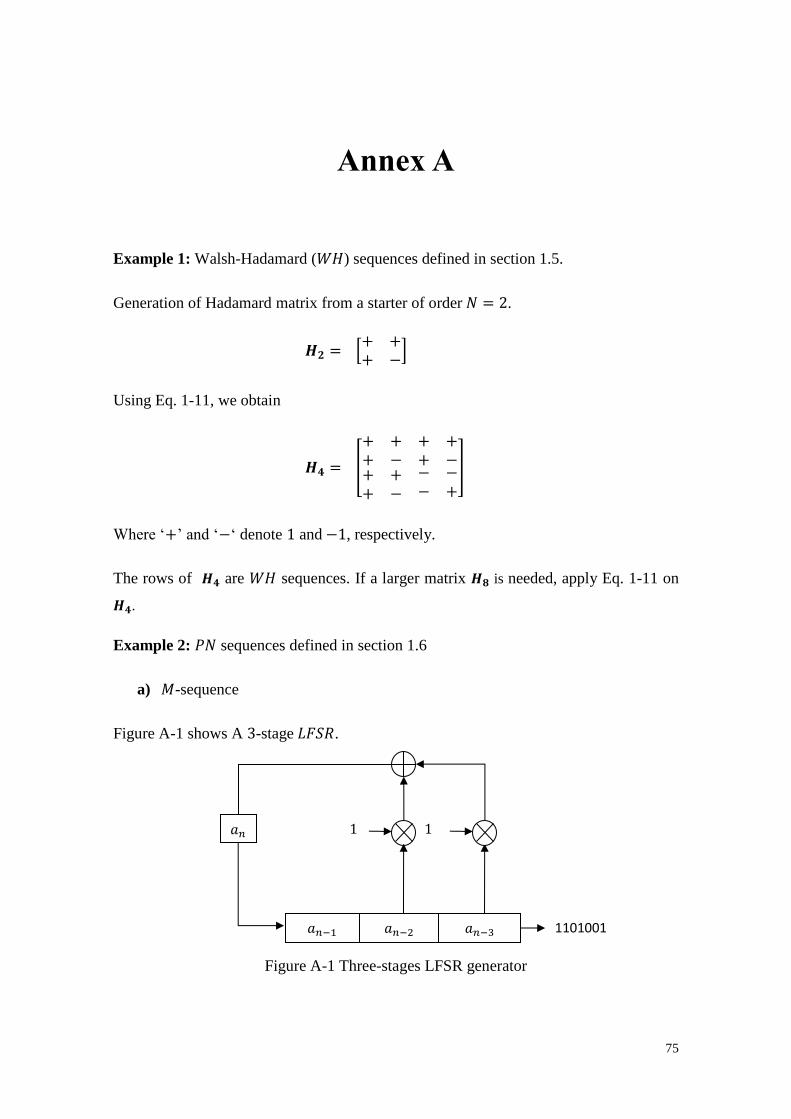
75

Annex A

Example 1: Walsh-Hadamard (𝑊𝐻) sequences defined in section 1.5.

Generation of Hadamard matrix from a starter of order 𝑁 = 2.

𝑯𝟐 = [+ ++ −

]

Using Eq. 1-11, we obtain

𝑯𝟒 = [

+ ++ −

+ ++ −

+ ++ −

− −− +

]

Where ‘+’ and ‘−‘ denote 1 and −1, respectively.

The rows of 𝑯𝟒 are 𝑊𝐻 sequences. If a larger matrix 𝑯𝟖 is needed, apply Eq. 1-11 on

𝑯𝟒.

Example 2: 𝑃𝑁 sequences defined in section 1.6

a) 𝑀-sequence

Figure A-1 shows A 3-stage 𝐿𝐹𝑆𝑅.

Figure A-1 Three-stages LFSR generator

1

𝑎𝑛−1 𝑎𝑛−2 𝑎𝑛−3

1 𝑎𝑛

1101001

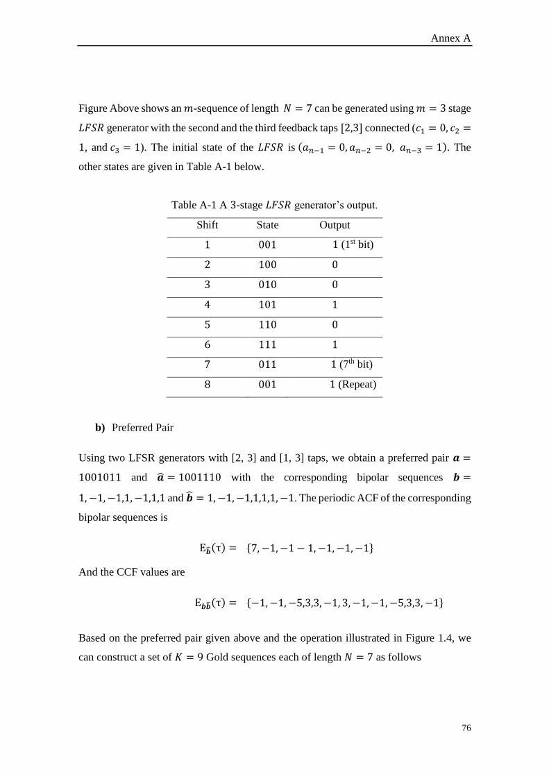
Annex A

76

Figure Above shows an 𝑚-sequence of length 𝑁 = 7 can be generated using 𝑚 = 3 stage

𝐿𝐹𝑆𝑅 generator with the second and the third feedback taps [2,3] connected (𝑐1 = 0, 𝑐2 =

1, and 𝑐3 = 1). The initial state of the 𝐿𝐹𝑆𝑅 is (𝑎𝑛−1 = 0, 𝑎𝑛−2 = 0, 𝑎𝑛−3 = 1). The

other states are given in Table A-1 below.

Table A-1 A 3-stage 𝐿𝐹𝑆𝑅 generator’s output.

Shift State Output

1 001 1 (1st bit)

2 100 0

3 010 0

4 101 1

5 110 0

6 111 1

7 011 1 (7th bit)

8 001 1 (Repeat)

b) Preferred Pair

Using two LFSR generators with [2, 3] and [1, 3] taps, we obtain a preferred pair 𝒂 =

1001011 and �̂� = 1001110 with the corresponding bipolar sequences 𝒃 =

1, −1,−1,1, −1,1,1 and �̂� = 1, −1,−1,1,1,1, −1. The periodic ACF of the corresponding

bipolar sequences is

E�̂�(τ) = {7, −1, −1 − 1,−1, −1,−1}

And the CCF values are

E𝒃�̂�(τ) = {−1,−1,−5,3,3, −1, 3, −1,−1, −5,3,3, −1}

Based on the preferred pair given above and the operation illustrated in Figure 1.4, we

can construct a set of 𝐾 = 9 Gold sequences each of length 𝑁 = 7 as follows

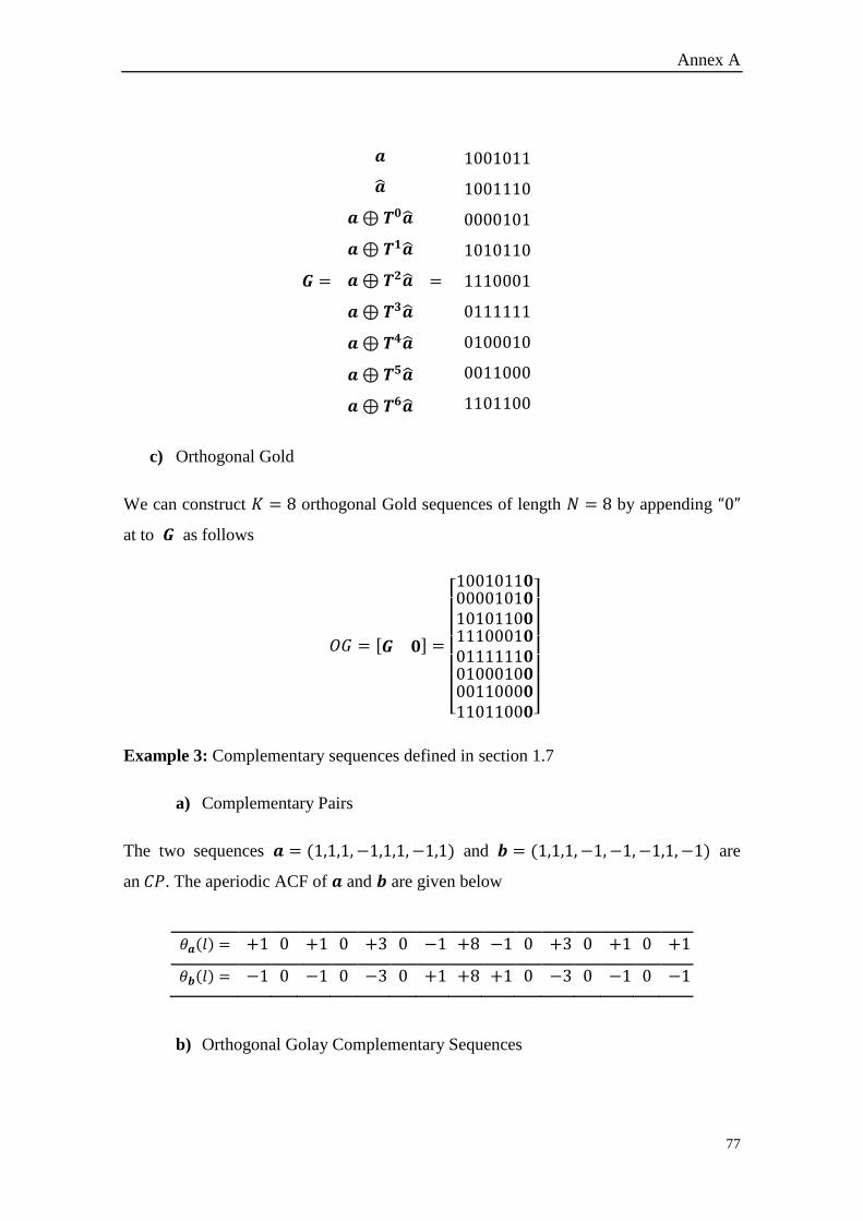
Annex A

77

𝑮 =

𝒂

�̂�

𝒂⊕ 𝑻𝟎�̂�

𝒂⊕ 𝑻𝟏�̂�

𝒂⊕ 𝑻𝟐�̂�

𝒂⊕ 𝑻𝟑�̂�

𝒂⊕ 𝑻𝟒�̂�

𝒂⊕ 𝑻𝟓�̂�

𝒂⊕ 𝑻𝟔�̂�

=

1001011

1001110

0000101

1010110

1110001

0111111

0100010

0011000

1101100

c) Orthogonal Gold

We can construct 𝐾 = 8 orthogonal Gold sequences of length 𝑁 = 8 by appending “0”

at to 𝑮 as follows

𝑂𝐺 = [𝑮 𝟎] =

[ 1001011𝟎0000101𝟎1010110𝟎1110001𝟎0111111𝟎0100010𝟎0011000𝟎1101100𝟎]

Example 3: Complementary sequences defined in section 1.7

a) Complementary Pairs

The two sequences 𝒂 = (1,1,1, −1,1,1, −1,1) and 𝒃 = (1,1,1, −1,−1,−1,1, −1) are

an 𝐶𝑃. The aperiodic ACF of 𝒂 and 𝒃 are given below

𝜃𝒂(𝑙) = +1 0 +1 0 +3 0 −1 +8 −1 0 +3 0 +1 0 +1

𝜃𝒃(𝑙) = −1 0 −1 0 −3 0 +1 +8 +1 0 −3 0 −1 0 −1

b) Orthogonal Golay Complementary Sequences

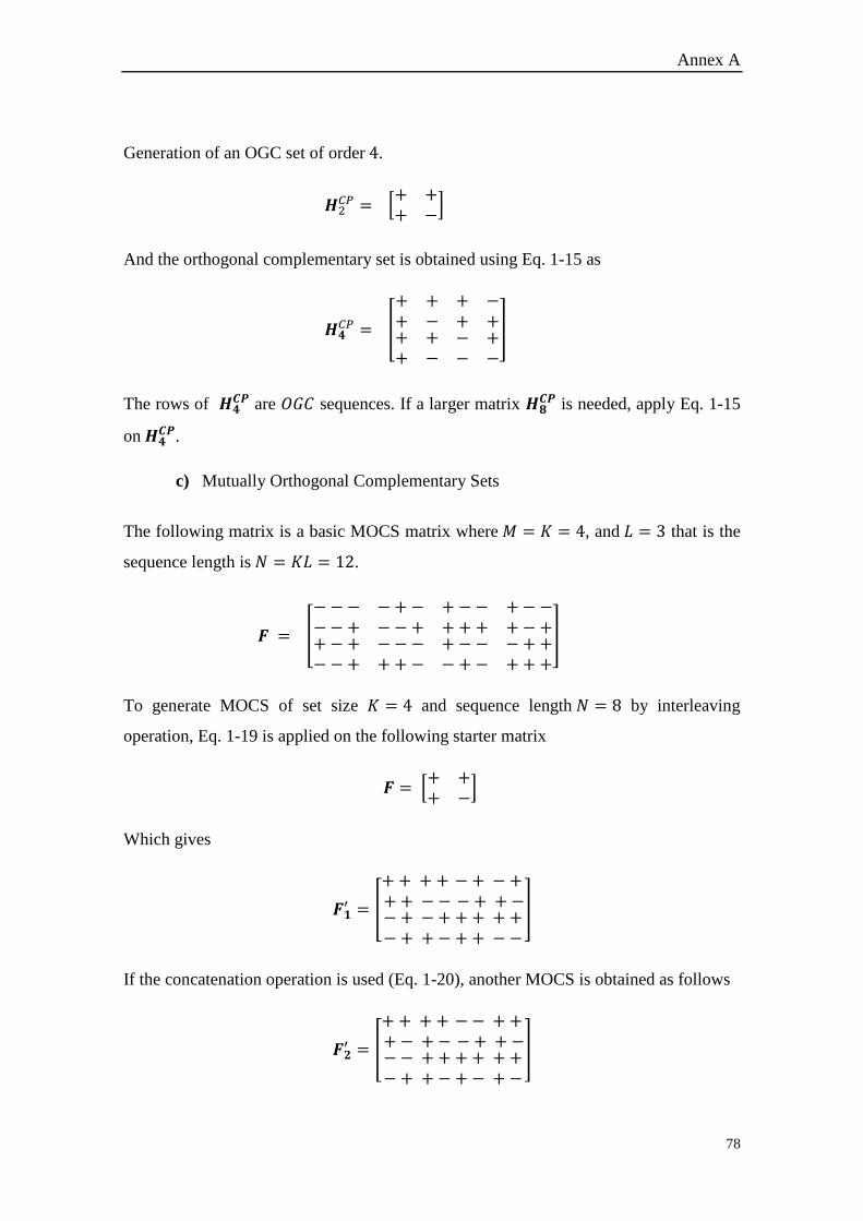
Annex A

78

Generation of an OGC set of order 4.

𝑯2𝐶𝑃 = [

+ ++ −

]

And the orthogonal complementary set is obtained using Eq. 1-15 as

𝑯𝟒𝐶𝑃 = [

+ ++ −

+ −+ +

+ ++ −

− +− −

]

The rows of 𝑯𝟒𝑪𝑷 are 𝑂𝐺𝐶 sequences. If a larger matrix 𝑯𝟖

𝑪𝑷 is needed, apply Eq. 1-15

on 𝑯𝟒𝑪𝑷.

c) Mutually Orthogonal Complementary Sets

The following matrix is a basic MOCS matrix where 𝑀 = 𝐾 = 4, and 𝐿 = 3 that is the

sequence length is 𝑁 = 𝐾𝐿 = 12.

𝑭 = [

− − − − + −−−+ −−+

+− − +−−++ + +−+

+−+ −−−−−+ ++−

+− − −++−+ − +++

]

To generate MOCS of set size 𝐾 = 4 and sequence length 𝑁 = 8 by interleaving

operation, Eq. 1-19 is applied on the following starter matrix

𝑭 = [+ ++ −

]

Which gives

𝑭𝟏′ = [

+ + + + + + − −

− + − + − + + −

− + − + − + + −

+ + + ++ + − −

]

If the concatenation operation is used (Eq. 1-20), another MOCS is obtained as follows

𝑭𝟐′ = [

+ + + + + − + −

− − + + − + + −

− − + + − + + −

+ + + ++ − + −

]

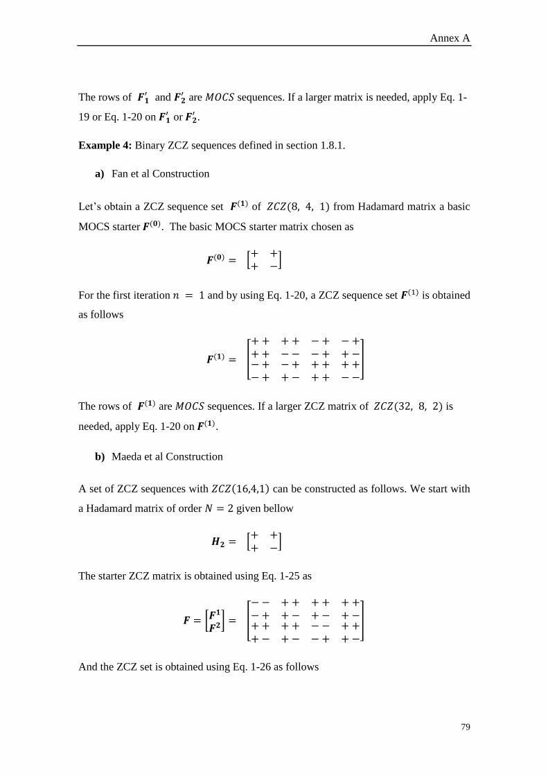
Annex A

79

The rows of 𝑭𝟏′ and 𝑭𝟐

′ are 𝑀𝑂𝐶𝑆 sequences. If a larger matrix is needed, apply Eq. 1-

19 or Eq. 1-20 on 𝑭𝟏′ or 𝑭𝟐

′ .

Example 4: Binary ZCZ sequences defined in section 1.8.1.

a) Fan et al Construction

Let’s obtain a ZCZ sequence set 𝑭(𝟏) of 𝑍𝐶𝑍(8, 4, 1) from Hadamard matrix a basic

MOCS starter 𝑭(𝟎). The basic MOCS starter matrix chosen as

𝑭(𝟎) = [+ ++ −

]

For the first iteration 𝑛 = 1 and by using Eq. 1-20, a ZCZ sequence set 𝑭(1) is obtained

as follows

𝑭(𝟏) = [

+ + + ++ + −−

−+ −+−+ +−

−+ −+−+ +−

++ ++++ −−

]

The rows of 𝑭(𝟏) are 𝑀𝑂𝐶𝑆 sequences. If a larger ZCZ matrix of 𝑍𝐶𝑍(32, 8, 2) is

needed, apply Eq. 1-20 on 𝑭(𝟏).

b) Maeda et al Construction

A set of ZCZ sequences with 𝑍𝐶𝑍(16,4,1) can be constructed as follows. We start with

a Hadamard matrix of order 𝑁 = 2 given bellow

𝑯𝟐 = [+ ++ −

]

The starter ZCZ matrix is obtained using Eq. 1-25 as

𝑭 = [𝑭𝟏

𝑭𝟐] = [

− − + + + + ++−+ +− +− +−++ ++ −− +++− +− −+ +−

]

And the ZCZ set is obtained using Eq. 1-26 as follows

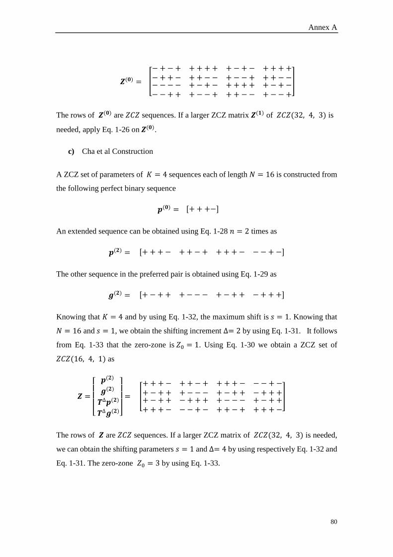
Annex A

80

𝒁(𝟎) = [

− + − + + +++ +−+− ++++−++− ++−− +−−+ ++−−−−−− +−+− ++++ +−+−−−++ +−−+ ++−− +−−+

]

The rows of 𝒁(𝟎) are 𝑍𝐶𝑍 sequences. If a larger ZCZ matrix 𝒁(𝟏) of 𝑍𝐶𝑍(32, 4, 3) is

needed, apply Eq. 1-26 on 𝒁(𝟎).

c) Cha et al Construction

A ZCZ set of parameters of 𝐾 = 4 sequences each of length 𝑁 = 16 is constructed from

the following perfect binary sequence

𝒑(𝟎) = [+ + +−]

An extended sequence can be obtained using Eq. 1-28 𝑛 = 2 times as

𝒑(𝟐) = [+ + + − ++−+ + ++− −−+−]

The other sequence in the preferred pair is obtained using Eq. 1-29 as

𝒈(𝟐) = [+ − + + +−−− + −++ −+++]

Knowing that 𝐾 = 4 and by using Eq. 1-32, the maximum shift is 𝑠 = 1. Knowing that

𝑁 = 16 and 𝑠 = 1, we obtain the shifting increment ∆= 2 by using Eq. 1-31. It follows

from Eq. 1-33 that the zero-zone is 𝑍0 = 1. Using Eq. 1-30 we obtain a ZCZ set of

𝑍𝐶𝑍(16, 4, 1) as

𝒁 =

[ 𝒑(𝟐)

𝒈(𝟐)

𝑻∆𝒑(𝟐)

𝑻∆𝒈(𝟐)]

= [

+ + + − + +−+ +++− −−+−+−++ +−−− +−++ −++++−++ −+++ +−−− +−+++++− −−+− ++−+ +++−

]

The rows of 𝒁 are 𝑍𝐶𝑍 sequences. If a larger ZCZ matrix of 𝑍𝐶𝑍(32, 4, 3) is needed,

we can obtain the shifting parameters 𝑠 = 1 and ∆= 4 by using respectively Eq. 1-32 and

Eq. 1-31. The zero-zone 𝑍0 = 3 by using Eq. 1-33.

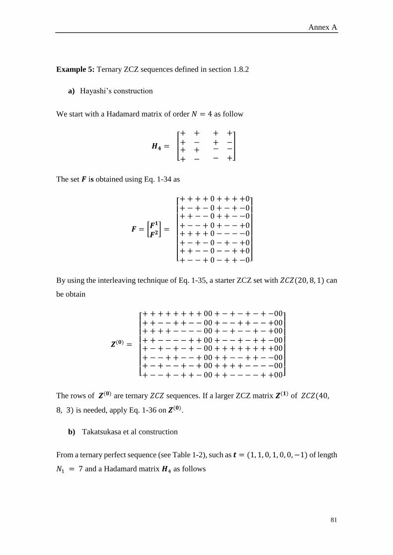
Annex A

81

Example 5: Ternary ZCZ sequences defined in section 1.8.2

a) Hayashi’s construction

We start with a Hadamard matrix of order 𝑁 = 4 as follow

𝑯𝟒 = [

+ ++ −

+ ++ −

+ ++ −

− − − +

]

The set 𝑭 is obtained using Eq. 1-34 as

𝑭 = [𝑭𝟏

𝑭𝟐] =

[ + + + + 0 + + + +0+ − + − 0 + − + −0+ + − − 0 + + − −0+ − − + 0 + − − +0+ + + + 0 − − − −0+ − + − 0 − + − +0+ + − − 0 − − + +0+ − − + 0 − + + −0]

By using the interleaving technique of Eq. 1-35, a starter ZCZ set with 𝑍𝐶𝑍(20, 8, 1) can

be obtain

𝒁(𝟎) =

[ + + + + + +++ 00 + − + − +−+−00+ + − − ++−− 00 + − − + +−−+00+ + + + −−−− 00 + − + − −+−+00+ + − − −−++ 00 + − − + −++−00+ − + − +−+− 00 + + + + ++++00+ − − + +−−+ 00 + + − − ++−−00+ − + − −+−+ 00 + + + + −−−−00+ − − + −++− 00 + + − − −−++00]

The rows of 𝒁(𝟎) are ternary 𝑍𝐶𝑍 sequences. If a larger ZCZ matrix 𝒁(𝟏) of 𝑍𝐶𝑍(40,

8, 3) is needed, apply Eq. 1-36 on 𝒁(𝟎).

b) Takatsukasa et al construction

From a ternary perfect sequence (see Table 1-2), such as 𝒕 = (1, 1, 0, 1, 0, 0, −1) of length

𝑁1 = 7 and a Hadamard matrix 𝑯4 as follows

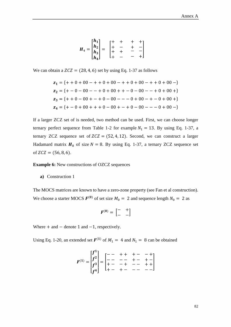
Annex A

82

𝑯4 = [

𝒉𝟏𝒉𝟐𝒉𝟑𝒉𝟒

] = [

+ ++ −

+ ++ −

+ ++ −

− − − +

]

We can obtain a 𝑍𝐶𝑍 = (28, 4, 6) set by using Eq. 1-37 as follows

𝒛𝟏 = {+ + 0 + 00 − + + 0 + 00 − + + 0 + 00 − + + 0 + 00 −}

𝒛𝟐 = {+ − 0 − 00 − − + 0 + 00 + + − 0 − 00 − − + 0 + 00 +}

𝒛𝟑 = {+ + 0 − 00 + − + 0 − 00 − − − 0 + 00 − + − 0 + 00 +}

𝒛𝟒 = {+ − 0 + 00 + + + 0 − 00 + − + 0 − 00 − − − 0 + 00 −}

If a larger ZCZ set of is needed, two method can be used. First, we can choose longer

ternary perfect sequence from Table 1-2 for example 𝑁1 = 13. By using Eq. 1-37, a

ternary ZCZ sequence set of 𝑍𝐶𝑍 = (52, 4, 12). Second, we can construct a larger

Hadamard matrix 𝑯8 of size 𝑁 = 8. By using Eq. 1-37, a ternary ZCZ sequence set

of 𝑍𝐶𝑍 = (56, 8, 6).

Example 6: New constructions of OZCZ sequences

a) Construction 1

The MOCS matrices are known to have a zero-zone property (see Fan et al construction).

We choose a starter MOCS 𝑭(𝟎) of set size 𝑀0 = 2 and sequence length 𝑁0 = 2 as

𝑭(𝟎) = [− +− −

]

Where + and − denote 1 and −1, respectively.

Using Eq. 1-20, an extended set 𝑭(𝟏) of 𝑀1 = 4 and 𝑁1 = 8 can be obtained

𝑭(𝟏) =

[ 𝒇𝟏

𝒇𝟐

𝒇𝟑

𝒇𝟒]

= [

− − + +− − −−

+− −++− +−

+− −++− +−

−− ++−− −−

]

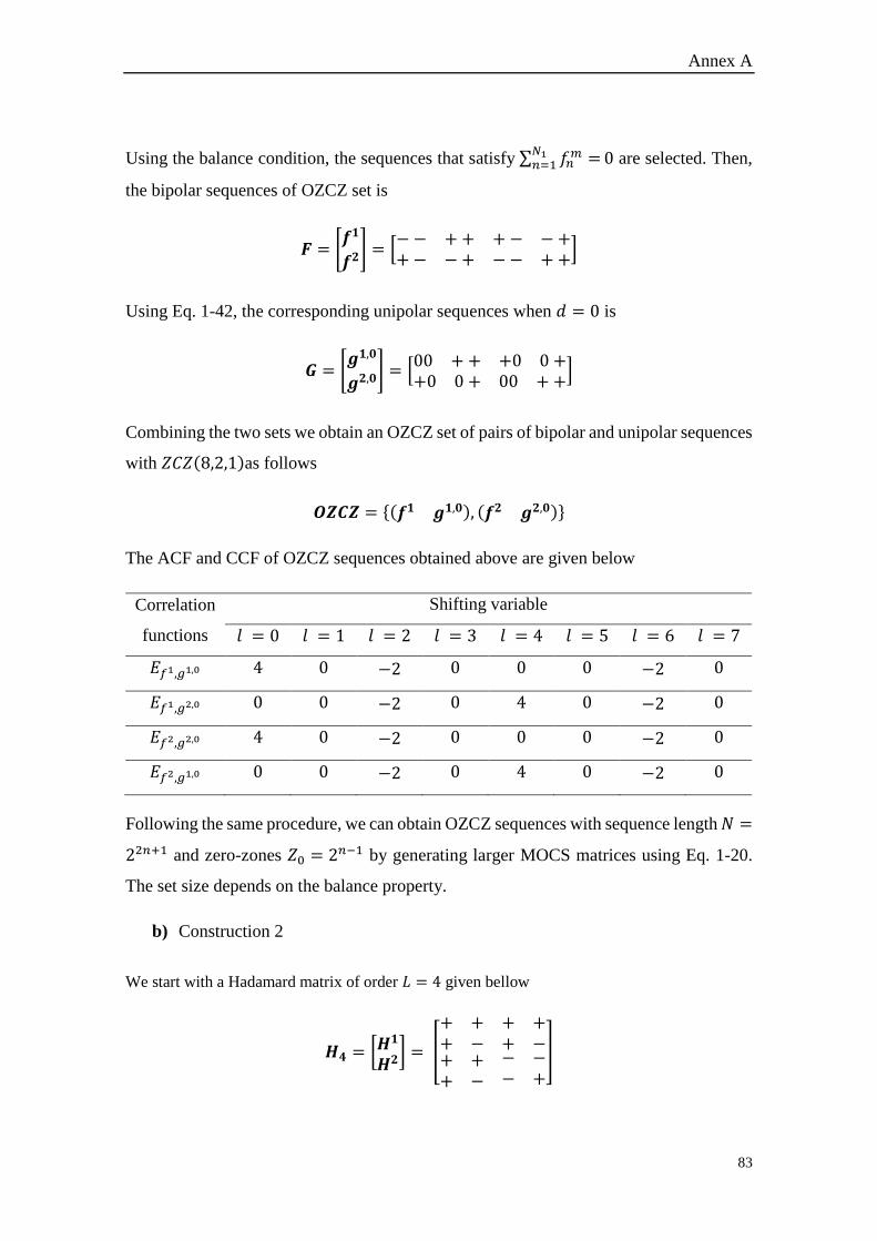
Annex A

83

Using the balance condition, the sequences that satisfy ∑ 𝑓𝑛𝑚 =

𝑁1𝑛=1 0 are selected. Then,

the bipolar sequences of OZCZ set is

𝑭 = [𝒇𝟏

𝒇𝟐] = [

− − + + + − −++− −+ −− ++

]

Using Eq. 1-42, the corresponding unipolar sequences when 𝑑 = 0 is

𝑮 = [𝒈𝟏,𝟎

𝒈𝟐,𝟎] = [

00 + + +0 0 ++0 0 + 00 + +

]

Combining the two sets we obtain an OZCZ set of pairs of bipolar and unipolar sequences

with 𝑍𝐶𝑍(8,2,1)as follows

𝑶𝒁𝑪𝒁 = {(𝒇𝟏 𝒈𝟏,𝟎), (𝒇𝟐 𝒈𝟐,𝟎)}

The ACF and CCF of OZCZ sequences obtained above are given below

Correlation

functions

Shifting variable

𝑙 = 0 𝑙 = 1 𝑙 = 2 𝑙 = 3 𝑙 = 4 𝑙 = 5 𝑙 = 6 𝑙 = 7

𝐸𝑓1,𝑔1,0 4 0 −2 0 0 0 −2 0

𝐸𝑓1,𝑔2,0 0 0 −2 0 4 0 −2 0

𝐸𝑓2,𝑔2,0 4 0 −2 0 0 0 −2 0

𝐸𝑓2,𝑔1,0 0 0 −2 0 4 0 −2 0

Following the same procedure, we can obtain OZCZ sequences with sequence length 𝑁 =

22𝑛+1 and zero-zones 𝑍0 = 2𝑛−1 by generating larger MOCS matrices using Eq. 1-20.

The set size depends on the balance property.

b) Construction 2

We start with a Hadamard matrix of order 𝐿 = 4 given bellow

𝑯𝟒 = [𝑯𝟏

𝑯𝟐] = [

+ ++ −

+ ++ −

+ ++ −

− −− +

]

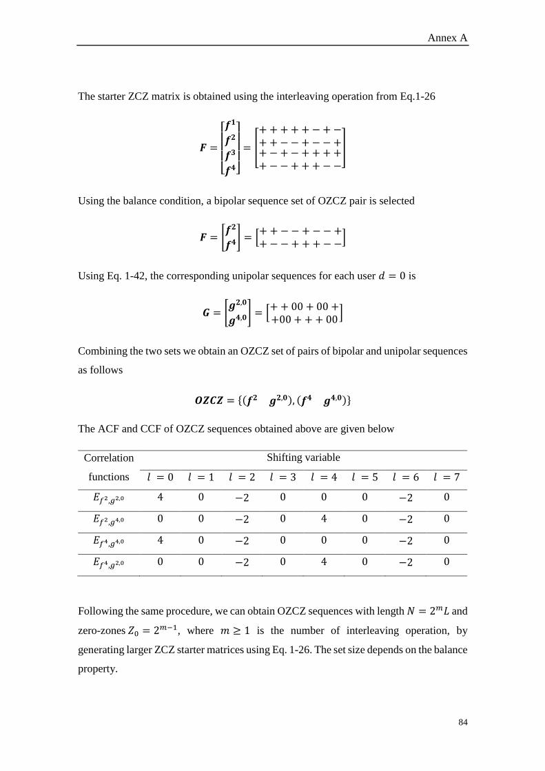
Annex A

84

The starter ZCZ matrix is obtained using the interleaving operation from Eq.1-26

𝑭 =

[ 𝒇𝟏

𝒇𝟐

𝒇𝟑

𝒇𝟒]

= [

+ + ++ + −+−++−− +−−++−+− +++++−−+ ++−−

]

Using the balance condition, a bipolar sequence set of OZCZ pair is selected

𝑭 = [𝒇𝟐

𝒇𝟒] = [

+ + − − + −−++−−+ ++−−

]

Using Eq. 1-42, the corresponding unipolar sequences for each user 𝑑 = 0 is

𝑮 = [𝒈𝟐,𝟎

𝒈𝟒,𝟎] = [

+ + 00 + 00 ++00 + + + 00

]

Combining the two sets we obtain an OZCZ set of pairs of bipolar and unipolar sequences

as follows

𝑶𝒁𝑪𝒁 = {(𝒇𝟐 𝒈𝟐,𝟎), (𝒇𝟒 𝒈𝟒,𝟎)}

The ACF and CCF of OZCZ sequences obtained above are given below

Correlation

functions

Shifting variable

𝑙 = 0 𝑙 = 1 𝑙 = 2 𝑙 = 3 𝑙 = 4 𝑙 = 5 𝑙 = 6 𝑙 = 7

𝐸𝑓2,𝑔2,0 4 0 −2 0 0 0 −2 0

𝐸𝑓2,𝑔4,0 0 0 −2 0 4 0 −2 0

𝐸𝑓4,𝑔4,0 4 0 −2 0 0 0 −2 0

𝐸𝑓4,𝑔2,0 0 0 −2 0 4 0 −2 0

Following the same procedure, we can obtain OZCZ sequences with length 𝑁 = 2𝑚𝐿 and

zero-zones 𝑍0 = 2𝑚−1, where 𝑚 ≥ 1 is the number of interleaving operation, by

generating larger ZCZ starter matrices using Eq. 1-26. The set size depends on the balance

property.

85

Annex B

Annex B.1: Received signal component

From section 3.2.1 of Chapter 3, we have

𝑠𝑘(𝑡) = √2𝑃𝑅𝑒{𝑑𝑘(𝑡)𝑐𝑘(𝑡)𝑒𝑗(𝑤𝑐𝑡+𝜃𝑘)} (B-1)

And from section 3.2.3, we have

𝑟(𝑡) = ∑𝑅𝑒{(1 + 𝑎𝑘𝑒𝑗𝜑𝑘)𝑠𝑘(𝑡 − 𝜏𝑘) + 𝑛(𝑡)}

𝐾

𝑘= 1

= 𝑦(𝑡) + 𝑛(𝑡) (B-2)

We can extract

𝑦(𝑡) = ∑𝑅𝑒{(1 + 𝑎𝑘𝑒𝑗𝜑𝑘)𝑠𝑘(𝑡 − 𝜏𝑘)}

𝐾

𝑘=1

(B-3)

By replacing Eq. B-1 in Eq. B-3, we obtain

𝑦(𝑡) = √2𝑃∑𝑅𝑒{𝑑𝑘(𝑡 − 𝜏𝑘)𝑐𝑘(𝑡 − 𝜏𝑘)[𝑒𝑗(𝑤𝑐𝑡+𝜗𝑘) + 𝑎𝑘𝑒

𝑗(𝑤𝑐𝑡+𝜗𝑘+𝜑𝑘)]}

𝐾

𝑘=1

(B-4)

Where 𝜗𝑘 = 𝜃𝑘 − 𝑤𝑐𝜏𝑘.

The exponential form of the 𝑖𝑡ℎ signal’s component at the receiver output is

𝑦𝑖 = න 𝑦(𝑡)𝑐𝑖(𝑡)𝑐𝑜𝑠(𝑤𝑐𝑡)𝑇𝑏

0

𝑑𝑡

= 1

2න (𝑦(𝑡)𝑐𝑖(𝑡)𝑒

𝑗𝑤𝑐𝑡) + (𝑦(𝑡)𝑐𝑖(𝑡)𝑒−𝑗𝑤𝑐𝑡)

𝑇𝑏

0

𝑑𝑡 (B-5)

The left term of the right side of Eq. B-5 is

Annex B

86

𝐿 = √𝑃

2න ∑𝑅𝑒{𝑑𝑘(𝑡 − 𝜏𝑘)𝑐𝑖(𝑡)𝑐𝑘(𝑡 − 𝜏𝑘)[𝑒

𝑗(2𝑤𝑐𝑡+𝜗𝑘)

𝐾

𝑘=1

𝑇𝑏

0

+ 𝑎𝑘𝑒𝑗(2𝑤𝑐𝑡+𝜗𝑘+𝜑𝑘)]} 𝑑𝑡

(B-6)

And the right term is

𝑅 = √𝑃

2න ∑𝑅𝑒{𝑑𝑘(𝑡 − 𝜏𝑘)𝑐𝑖(𝑡)𝑐𝑘(𝑡 − 𝜏𝑘)[𝑒

𝑗𝜗𝑘 + 𝑎𝑘𝑒𝑗(𝜗𝑘+𝜑𝑘)]}

𝐾

𝑘=1

𝑇𝑏

0

𝑑𝑡 (B-7)

If we assume 𝑓𝑐 ≫ 𝑇𝑏−1, we can then ignore term 𝐿. Then 𝑦𝑖 becomes

𝑦𝑖 = √𝑃

2∑𝑅𝑒 {න 𝑑𝑘(𝑡 − 𝜏𝑘)𝑐𝑖(𝑡)𝑐𝑘(𝑡 − 𝜏𝑘)[𝑒

𝑗𝜗𝑘 + 𝑎𝑘𝑒𝑗(𝜗𝑘+𝜑𝑘)]

𝑇𝑏

0

𝑑𝑡}

𝐾

𝑘=1

(B-8)

Since 𝑑𝑘(𝑡) is of the following form

𝑑𝑘(𝑡 − 𝜏𝑘) = {𝑑𝑘,−1 0 ≤ 𝑡 ≤ 𝜏𝑘𝑑𝑘,0 𝜏𝑘 ≤ 𝑡 ≤𝑇𝑏

(B-9)

Where the data bits 𝑑𝑘,−1 and 𝑑𝑘,0 are respectively the previous and current symbols of

the 𝑘𝑡ℎ user.

It can be used to simplify the following term in 𝑦𝑖 as

න 𝑑𝑘(𝑡 − 𝜏𝑘)𝑐𝑖(𝑡)𝑐𝑘(𝑡 − 𝜏𝑘)𝑑𝑡𝑇𝑏

0

= 𝑑𝑘,−1𝑅𝑐𝑘𝑐𝑖(𝜏𝑘) + 𝑑𝑘,0�̂�𝑐𝑘𝑐𝑖(𝜏𝑘) (B-10)

Where 𝑅𝑐𝑘𝑐𝑖(𝜏𝑘) and �̂�𝑐𝑘𝑐𝑖(𝜏𝑘) are called the continuous-time partial CCFs defined in

[43] as

𝑅𝑐𝑘𝑐𝑖(𝜏𝑘) = න 𝑐𝑘(𝑡 − 𝜏𝑘)𝑐𝑖(𝑡)𝜏𝑘

0

𝑑𝑡 (B-11)

�̂�𝑐𝑘𝑐𝑖(𝜏𝑘) = න 𝑐𝑘(𝑡 − 𝜏𝑘)𝑐𝑖(𝑡)𝑇𝑏

𝜏𝑘

𝑑𝑡 (B-12)

And Eq. B-8 becomes

Annex B

87

𝑦𝑖 = √𝑃

2∑𝑅𝑒{[𝑑𝑘,−1𝑅𝑐𝑘𝑐𝑖(𝜏𝑘) + 𝑑𝑘,0�̂�𝑐𝑘𝑐𝑖(𝜏𝑘)][𝑒

𝑗𝜗𝑘 + 𝑎𝑘𝑒𝑗(𝜗𝑘+𝜑𝑘)]}

𝐾

𝑘=1

(B-13)

a) Desired signal

The 𝑖𝑡ℎ receiver (setting 𝑘 = 𝑖 in Eq. B-13) can acquire time and phase synchronization

from the 𝑖𝑡ℎ non-faded transmitted signal. Therefore, time delays and phase angles are

measured relative to 𝜏𝑖 and 𝜃𝑖 (we take 𝜏𝑖 = 𝜃𝑖 = 𝜗𝑖 = 0). Putting 𝜏𝑖 = 0 in Eq. B-11,

we obtain 𝑅𝑐𝑖(0) = 0.The 𝑖𝑡ℎ user’s component is

𝐷𝑖 = √𝑃 2⁄ 𝑑𝑖,0�̂�𝑐𝑖(0)(1 + 𝑎𝑖 𝑐𝑜𝑠(𝜑𝑖)) (B-14)

We can express �̂�𝑐𝑖(0) as

�̂�𝑐𝑖(0) = න 𝑐𝑖2(𝑡)

𝑇𝑏

0

𝑑𝑡 = ∑න 𝑐𝑖2(𝑡)

𝑛𝑇𝑐

(𝑛−1)𝑇𝑐

𝑑𝑡 = ∑𝑐𝑖,𝑛2 𝑇𝑐

𝑁

𝑛=1

𝑁

𝑛=1

= 𝜇𝑖𝑇𝑏 (B-15)

Where 𝑐𝑖,𝑛 is the spreading sequence element ∈ {−1,0,1} and 𝜇𝑖 = (∑ 𝑐𝑖,𝑛2𝑁

𝑛=1 ) 𝑁⁄ is the

energy per chip ratio defined in Chapter 1, Eq. 1-9.

We consider only the case of 𝑑𝑖,0 = 1 [43], the 𝑖𝑡ℎ user’s component is

𝐷𝑖= √𝑃 2⁄ 𝜇𝑖𝑇𝑏(1 + 𝑎𝑖 cos(𝜑𝑖)) (B-16)

b) Interference

Setting 𝑘 ≠ 𝑖 in Eq. B-13 yields the MUI term as follows

𝐼𝑖 = √𝑃

2∑[𝑑𝑘,−1𝑅𝑐𝑘𝑐𝑖(𝜏𝑘) + 𝑑𝑘,0�̂�𝑐𝑘𝑐𝑖(𝜏𝑘)][cos(𝜗𝑘) + 𝑎𝑘 cos(𝜗𝑘 + 𝜑𝑘)]

𝐾

𝑘=1𝑘≠𝑖

(B-17)

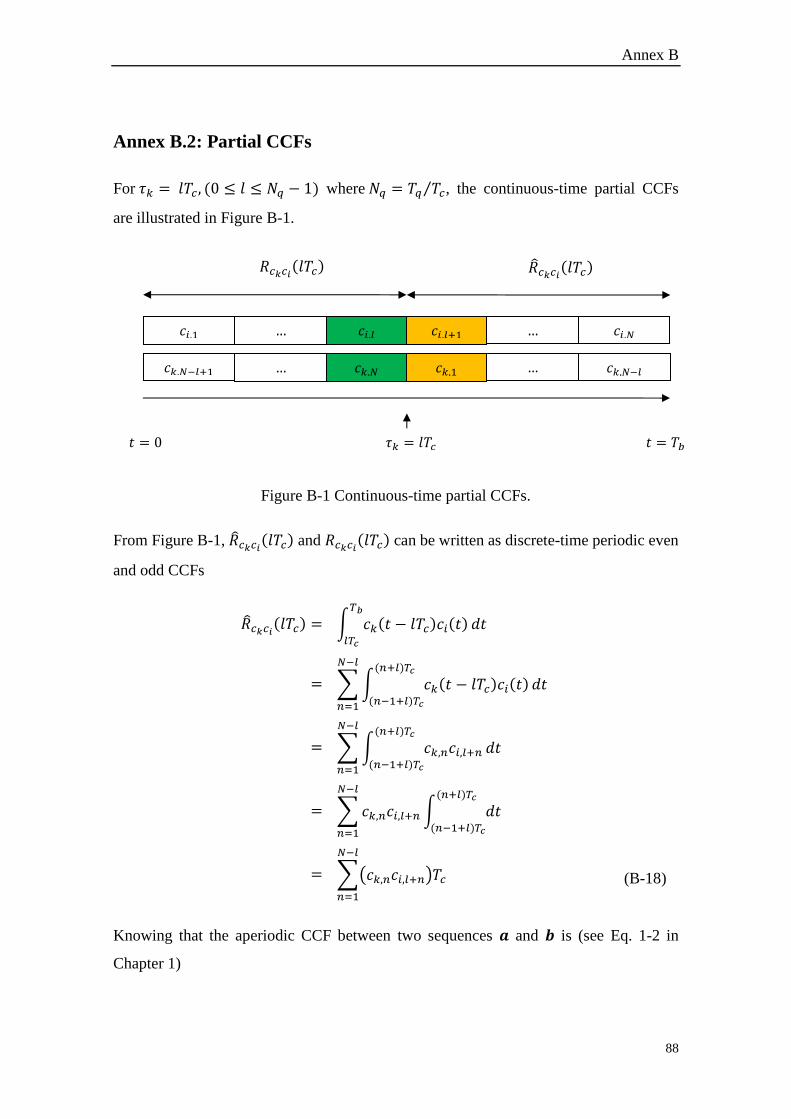
Annex B

88

Annex B.2: Partial CCFs

For 𝜏𝑘 = 𝑙𝑇𝑐, (0 ≤ 𝑙 ≤ 𝑁𝑞 − 1) where 𝑁𝑞 = 𝑇𝑞 𝑇𝑐⁄ , the continuous-time partial CCFs

are illustrated in Figure B-1.

Figure B-1 Continuous-time partial CCFs.

From Figure B-1, �̂�𝑐𝑘𝑐𝑖(𝑙𝑇𝑐) and 𝑅𝑐𝑘𝑐𝑖(𝑙𝑇𝑐) can be written as discrete-time periodic even

and odd CCFs

�̂�𝑐𝑘𝑐𝑖(𝑙𝑇𝑐) = න 𝑐𝑘(𝑡 − 𝑙𝑇𝑐)𝑐𝑖(𝑡)𝑇𝑏

𝑙𝑇𝑐

𝑑𝑡

= ∑න 𝑐𝑘(𝑡 − 𝑙𝑇𝑐)𝑐𝑖(𝑡)(𝑛+𝑙)𝑇𝑐

(𝑛−1+𝑙)𝑇𝑐

𝑑𝑡

𝑁−𝑙

𝑛=1

= ∑න 𝑐𝑘,𝑛𝑐𝑖,𝑙+𝑛

(𝑛+𝑙)𝑇𝑐

(𝑛−1+𝑙)𝑇𝑐

𝑑𝑡

𝑁−𝑙

𝑛=1

= ∑𝑐𝑘,𝑛𝑐𝑖,𝑙+𝑛න 𝑑𝑡(𝑛+𝑙)𝑇𝑐

(𝑛−1+𝑙)𝑇𝑐

𝑁−𝑙

𝑛=1

= ∑(𝑐𝑘,𝑛𝑐𝑖,𝑙+𝑛)𝑇𝑐

𝑁−𝑙

𝑛=1

(B-18)

Knowing that the aperiodic CCF between two sequences 𝒂 and 𝒃 is (see Eq. 1-2 in

Chapter 1)

𝑡 = 0 𝑡 = 𝑇𝑏 𝜏𝑘 = 𝑙𝑇𝑐

𝑐𝑘,𝑁 𝑐𝑘,1 … 𝑐𝑘,𝑁−𝑙+1 … 𝑐𝑘,𝑁−𝑙

𝑐𝑖,𝑙 𝑐𝑖,𝑙+1 … 𝑐𝑖,1 … 𝑐𝑖,𝑁

𝑅𝑐𝑘𝑐𝑖(𝑙𝑇𝑐) �̂�𝑐𝑘𝑐𝑖(𝑙𝑇𝑐)

Annex B

89

𝜃𝒂𝒃(𝑙) = ∑𝑎𝑛𝑏𝑛+𝑙

𝑁−𝑙

𝑛=1

0 ≤ 𝑙 ≤ 𝑁 − 1 (B-19)

We can write

�̂�𝑐𝑘𝑐𝑖(𝑙𝑇𝑐) = 𝑇𝑐𝜃𝑐𝑘𝑐𝑖(𝑙) (B-20)

Similarly, we can obtain as

𝑅𝑐𝑘𝑐𝑖(𝑙𝑇𝑐) = න 𝑐𝑘(𝑡 − 𝑙𝑇𝑐)𝑐𝑖(𝑡)𝑙𝑇𝑐

0

𝑑𝑡

= ∑න 𝑐𝑘,(𝑁−𝑙)+𝑛𝑐𝑖,𝑛

𝑛𝑇𝑐

(𝑛−1)𝑇𝑐

𝑑𝑡

𝑙

𝑛=1

= ∑(𝑐𝑘,(𝑁−𝑙)+𝑛𝑐𝑖,𝑛)𝑇𝑐

𝑙

𝑛=1

(B-21)

Replacing 𝑙 by 𝑁 − 𝑙 in Eq. B-19, we obtain

𝜃𝒂𝒃(𝑁 − 𝑙) = ∑𝑎𝑛𝑏𝑛+(𝑁−𝑙)

𝑙

𝑛=1

0 ≤ 𝑙 ≤ 𝑁 − 1 (B-22)

Which gives

𝑅𝑐𝑘𝑐𝑖(𝑙𝑇𝑐) = 𝑇𝑐𝜃𝑐𝑖𝑐𝑘(𝑁 − 𝑙) (B-23)

By using Eq. 1-3 and Eq. 1-4 from Chapter 1

�̂�𝑐𝑘𝑐𝑖(𝑙𝑇𝑐) = 𝑇𝑐 (𝐸𝑐𝑘𝑐𝑖(𝑙) + 𝑂𝑐𝑘𝑐𝑖(𝑙)) 2⁄ (B-24)

𝑅𝑐𝑘𝑐𝑖(𝑙𝑇𝑐) = 𝑇𝑐 (𝐸𝑐𝑘𝑐𝑖(𝑙) − 𝑂𝑐𝑘𝑐𝑖(𝑙)) 2⁄ (B-25)

Annex B

90

Annex B.3: Mean calculations

The following mean and variance properties will be need for the calculation of 𝐸{𝑍𝑖}.

Linearity: let 𝑋 and 𝑌 be two random variables and 𝑐 a constant, we have

𝐸{𝑋 + 𝑌 } = 𝐸{𝑋} + 𝐸{𝑌} (B-26)

𝐸{𝑐𝑋} = 𝑐𝐸{𝑋} (B-27)

If 𝑋 and 𝑌 are independent, we have

𝐸{𝑋𝑌 } = 𝐸{𝑋}𝐸{𝑌} (B-28)

𝐸{𝑓1(𝑋)𝑓2(𝑌) } = 𝐸{𝑓1(𝑋)}𝐸{𝑓2(𝑌)} (B-29)

Let 𝑋 be a uniformly distributed random variable then we have

𝐸{cos(𝑋)} = 𝐸{sin(𝑋)} = 𝐸{cos(𝑋) sin(𝑋)} = 0 (B-30)

𝐸{cos2(𝑋)} = 𝐸{sin2(𝑋)} = 1 2⁄ (B-31)

The mean of the correlator’s output is

𝐸{𝑍𝑖} = 𝐸{𝐷𝑖 + 𝐼𝑖 + 𝑁𝑖} (B-32)

Using the linearity properties of the mean

𝐸{𝑍𝑖} = 𝐸{𝐷𝑖} + 𝐸{𝐼𝑖} + 𝐸{𝑁𝑖} (B-33)

1) Desired signal mean

The mean of the desired signal component (from Eq. B-16)

𝐸{𝐷𝑖} = 𝐸 {√𝑃 2⁄ 𝜇𝑖𝑇𝑏(1 + 𝑎𝑖 𝑐𝑜𝑠(𝜑𝑖))} (B-34)

We assume that the random variables 𝑑𝑘,, 𝜃𝑘 , 𝜑𝑘, 𝜏𝑘 , and 𝑎𝑘 are mutually independent. By

using Eq. B-26 to Eq. B-28 we obtain

Annex B

91

𝐸{𝐷𝑖} = √𝑃 2⁄ 𝜇𝑖𝑇𝑏(1 + 𝐸{𝑎𝑖}𝐸{𝑐𝑜𝑠(𝜑𝑖)}) (B-35)

Using Eq. B-30, the remaining term is

𝐸{𝐷𝑖} = √𝑃 2⁄ 𝜇𝑖𝑇𝑏 (B-36)

2) Interference mean

The mean of the interference signal component from Eq. B-17 is

𝐸{𝐼𝑖} = 𝐸

{

√𝑃

2∑[𝑑𝑘,−1𝑅𝑐𝑘𝑐𝑖(𝜏𝑘) + 𝑑𝑘,0�̂�𝑐𝑘𝑐𝑖(𝜏𝑘)][𝑐𝑜𝑠(𝜗𝑘)

𝐾

𝑘=1𝑘≠𝑖

+ 𝑎𝑘 𝑐𝑜𝑠(𝜗𝑘 +𝜑𝑘)]

}

(B-37)

It can be readily shown using Eq. B-30 that

𝐸{𝑐𝑜𝑠(𝜗𝑘)} = 𝐸{𝑐𝑜𝑠(𝜗𝑘 +𝜑𝑘)} = 0 (B-38)

Therefore,

𝐸{𝐼𝑖} = 0 (B-39)

3) Noise mean

The noise has zero mean 𝐸{𝑛(𝑡)} = 0, therefore

𝐸{𝑁𝑖} = න 𝐸{𝑛(𝑡)}𝑐𝑖(𝑡) 𝑐𝑜𝑠(𝑤𝑐𝑡) 𝑑𝑡𝑇

0

= 0 (B-40)

Finally, the correlator’s out mean is

𝐸{𝑍𝑖} = √𝑃 2⁄ 𝜇𝑖𝑇𝑏 (B-41)

Annex B

92

Annex B.4: Variance calculation

The following mean and variance properties will be need for the calculation of 𝑉𝑎𝑟{𝑍𝑖}.

The variance of a random variable 𝑋 is defined as follows

𝑉𝑎𝑟[𝑋] = 𝐸{𝑋2} − (𝐸{𝑋})2 (B-42)

If 𝑋 and 𝑌 are independent, we have

𝑉𝑎𝑟{𝑋 + 𝑌} = 𝑉𝑎𝑟{𝑋} + 𝑉𝑎𝑟{𝑌} (B-43)

The correlator’s output variance is

𝑉𝑎𝑟{𝑍𝑖} = 𝑉𝑎𝑟{𝐷𝑖 + 𝐼𝑖 + 𝑁𝑖} (B-44)

We assume that the random variables 𝑑𝑘,, 𝜃𝑘 , 𝜏𝑘 , and 𝑎𝑘 have mutually independent

components that is 𝜃𝑖 and 𝜃𝑘 are independent if 𝑖 ≠ 𝑘. And the noise is statistically

independent of the multipath medium. Then, we can write

𝑉𝑎𝑟{𝑍𝑖} = 𝑉𝑎𝑟{𝐷𝑖} + 𝑉𝑎𝑟{𝐼𝑖} + 𝑉𝑎𝑟{𝑁𝑖} (B-45)

1) Desired signal variance

The desired signal variance is

𝑉𝑎𝑟{𝐷𝑖} = 𝐸 {(√𝑃 2⁄ 𝜇𝑖𝑇𝑏(1 + 𝑎𝑖 𝑐𝑜𝑠(𝜑𝑖)))2

} − (√𝑃 2⁄ 𝜇𝑖𝑇𝑏)2

= 𝑃𝜇𝑖

2𝑇𝑏2

2(1 + 𝐸{𝑎𝑖

2𝑐𝑜𝑠2(𝜑𝑖)} + 2𝐸{𝑎𝑖 𝑐𝑜𝑠(𝜑𝑖)}) −𝑃𝜇𝑖

2𝑇𝑏2

2 (B-46)

By using Eq. B-30 and B-31, we obtain

Annex B

93

𝑉𝑎𝑟{𝐷𝑖} =

𝑃𝜇𝑖2𝑇𝑏

2

2(1 +

𝐸{𝑎𝑖2}

2) −

𝑃𝜇𝑖2𝑇𝑏

2

2

= 𝑃𝜇𝑖2𝑇𝑏

2𝛾 4⁄ (B-47)

Where 𝛾 = 𝐸{𝑎𝑘2}, ∀𝑘.

2) Interference variance

Since 𝐸{𝐼𝑖} = 0, the interference variance is computed as follows

𝑉𝑎𝑟{𝐼𝑖} = 𝐸

{

(√

𝑃

2∑[𝑑𝑘,−1𝑅𝑐𝑘𝑐𝑖(𝜏𝑘) + 𝑑𝑘,0�̂�𝑐𝑘𝑐𝑖(𝜏𝑘)][𝑐𝑜𝑠(𝜗𝑘)

𝐾

𝑘=1𝑘≠𝑖

+ 𝑎𝑘 𝑐𝑜𝑠(𝜗𝑘 +𝜑𝑘)])

2

}

= 𝐸

{

𝑃

2∑∑[𝑑𝑘,−1𝑅𝑐𝑘𝑐𝑖(𝜏𝑘) + 𝑑𝑘,0�̂�𝑐𝑘𝑐𝑖(𝜏𝑘)][𝑑𝑠,−1𝑅𝑐𝑠𝑐𝑖(𝜏𝑠)

𝐾

𝑠=1𝑠≠𝑖

𝐾

𝑘=1𝑘≠𝑖

+ 𝑑𝑠,0�̂�𝑐𝑠𝑐𝑖(𝜏𝑠)][𝑐𝑜𝑠(𝜗𝑘)

+ 𝑎𝑘 𝑐𝑜𝑠(𝜗𝑘 +𝜑𝑘)][𝑐𝑜𝑠(𝜗𝑠) + 𝑎𝑠 𝑐𝑜𝑠(𝜗𝑠 + 𝜑𝑠)]

}

(B-48)

The random variable 𝑑𝑘 has mutually independent elements that is

𝐸{𝑑𝑘,𝑛𝑑𝑠,𝑚} = {1 𝑘 = 𝑠, 𝑛 = 𝑚0 𝑜𝑡ℎ𝑒𝑟𝑤𝑖𝑠𝑒

(B-49)

We obtain

𝑉𝑎𝑟{𝐼𝑖} =𝑃

2∑𝐸 {([𝑑𝑘,−1𝑅𝑐𝑘𝑐𝑖(𝜏𝑘) + 𝑑𝑘,0�̂�𝑐𝑘𝑐𝑖(𝜏𝑘)][𝑐𝑜𝑠(𝜗𝑘)

𝐾

𝑘=1𝑘≠𝑖

+ 𝑎𝑘 𝑐𝑜𝑠(𝜗𝑘 + 𝜑𝑘)])2}

(B-50)

Annex B

94

The following relations can be readily obtained from the means properties

𝐸{𝑐𝑜𝑠2(𝜗𝑘)} = 𝐸{𝑐𝑜𝑠2(𝜗𝑘 + 𝜑𝑘)} = 1 2⁄ (B-51)

Using Eq. B-51 and B-50, we can write

𝑉𝑎𝑟{𝐼𝑖} = 𝑃(1 + 𝛾)

4∑𝐸{𝑅𝑐𝑘𝑐𝑖

2 (𝜏𝑘) + �̂�𝑐𝑘𝑐𝑖2 (𝜏𝑘)}

𝐾

𝑘=1𝑘≠𝑖

(B-52)

Where

𝐸{𝑅𝑐𝑘𝑐𝑖2 (𝜏𝑘) + �̂�𝑐𝑘𝑐𝑖

2 (𝜏𝑘)} = 1

𝑇𝑞න 𝑅𝑐𝑘𝑐𝑖

2 (𝑙𝑇𝑐) + �̂�𝑐𝑘𝑐𝑖2 (𝑙𝑇𝑐)𝑑𝜏𝑘

𝑇𝑞

0

(B-53)

Therefore

𝑉𝑎𝑟{𝐼𝑖} = 𝑃(1 + 𝛾)

4𝑇𝑞∑න 𝑅𝑐𝑘𝑐𝑖

2 (𝑙𝑇𝑐) + �̂�𝑐𝑘𝑐𝑖2 (𝑙𝑇𝑐)𝑑𝜏𝑘

𝑇𝑞

0

𝐾

𝑘=1𝑘≠𝑖

(B4-54)

The integral part can be written as

න 𝑅𝑘,𝑖2 (𝑙𝑇𝑐) + �̂�𝑘,𝑖

2 (𝑙𝑇𝑐)𝑑𝜏𝑘

𝑇𝑞

0

= ∑ න 𝑅𝑐𝑘𝑐𝑖2 (𝑙𝑇𝑐) + �̂�𝑐𝑘𝑐𝑖

2 (𝑙𝑇𝑐)𝑑𝜏𝑘

(𝑙+1)𝑇𝑐

𝑙𝑇𝑐

𝑁𝑞−1

𝑙=0

(B-55)

Using Eq. 3-11 and Eq. 3-12 from chapter 3, we obtain

න 𝑅𝑘,𝑖2 (𝑙𝑇𝑐) + �̂�𝑘,𝑖

2 (𝑙𝑇𝑐)𝑑𝜏𝑘

𝑇𝑞

0

= 𝑇𝑐2

2න 𝐸𝑘,𝑖

2 (𝑙) + 𝑂𝑘,𝑖2 (𝑙)𝑑𝜏𝑘

𝑇𝑞

0

= 𝑇𝑐2

2∑ න 𝐸𝑘,𝑖

2 (𝑙) + 𝑂𝑘,𝑖2 (𝑙)𝑑𝜏𝑘

(𝑙+1)𝑇𝑐

𝑙𝑇𝑐

𝑁𝑞−1

𝑙=0

= 𝑇𝑐3

2∑ (𝐸𝑘,𝑖

2 (𝑙) + 𝑂𝑘,𝑖2 (𝑙))

𝑁𝑞−1

𝑙=0

(B-56)

Where 𝑁𝑞 = 𝑇𝑞 𝑇𝑐⁄ .

Annex B

95

The interference term (Eq. B-54) can be written as

𝑉𝑎𝑟{𝐼𝑖} = 𝑃𝑇𝑐

3(1 + 𝛾)

8𝑇𝑞∑ ∑ (𝐸𝑘,𝑖

2 (𝑙) + 𝑂𝑘,𝑖2 (𝑙))

𝑁𝑞−1

𝑙=0

𝐾

𝑘=1𝑘≠𝑖

= 𝑃𝑇𝑐

2(1 + 𝛾)

8𝑁𝑞∑ ∑ (𝐸𝑘,𝑖

2 (𝑙) + 𝑂𝑘,𝑖2 (𝑙))

𝑁𝑞−1

𝑙=0

𝐾

𝑘=1𝑘≠𝑖

(B-57)

3) Noise variance

The noise variance is calculated as follows

𝑉𝑎𝑟{𝑁𝑖} = 𝐸 {(න 𝑛(𝑡)𝑐𝑖(𝑡) 𝑐𝑜𝑠(𝑤𝑐𝑡) 𝑑𝑡𝑇𝑏

0

)

2

}

= 𝐸 {න 𝑛(𝑡)𝑐𝑖(𝑡) cos(𝑤𝑐𝑡) 𝑑𝑡

𝑇𝑏

0

න 𝑛(𝛼)𝑐𝑖(𝛼) cos(𝑤𝑐𝛼) 𝑑𝛼𝑇𝑏

0

}

= 𝐸 {න න 𝑛(𝑡)𝑛(𝛼)𝑐𝑖(𝑡) 𝑐𝑖(𝛼)cos(𝑤𝑐𝑡) cos(𝑤𝑐𝛼)𝑑𝑡𝑑𝛼𝑇𝑏

0

𝑇𝑏

0

}

= න න 𝐸{𝑛(𝑡)𝑛(𝛼)} 𝑐𝑖(𝑡)𝑐𝑖(𝛼)cos(𝑤𝑐𝑡) cos(𝑤𝑐𝛼)𝑑𝑡𝑑𝛼𝑇𝑏

0

𝑇𝑏

0

(B-58)

If the noise is wide-sense stationary random process, then

𝑉𝑎𝑟{𝑁𝑖} = න න 𝜃𝑛(𝛼 − 𝑡) 𝑐𝑖(𝑡)𝑐𝑖(𝛼)cos(𝑤𝑐𝑡) cos(𝑤𝑐𝛼)𝑑𝑡𝑑𝛼𝑇𝑏

0

𝑇𝑏

0

(B-59)

Knowing that the white noise has power spectral density (PSD) of 𝑆𝑛(𝑓) = 𝑁0 2⁄ and

using the inverse Fourier transform of the noise’s PSD, we obtain the noise ACF function

𝜃𝑛(𝛼 − 𝑡) = න 𝑆𝑛(𝑓)𝑒𝑗2𝜋𝑓(𝛼−𝑡)𝑑𝑓

+∞

−∞

=𝑁02𝛿(𝛼 − 𝑡) (B-60)

We obtain

𝑉𝑎𝑟{𝑁𝑖} = න න𝑁02𝛿(𝛼 − 𝑡)𝑐𝑖(𝑡)𝑐𝑖(𝛼)cos(𝑤𝑐𝑡) cos(𝑤𝑐𝛼) 𝑑𝑡𝑑𝛼

𝑇𝑏

0

𝑇𝑏

0

(B-61)

Annex B

96

Where 𝛿(𝑡) is Dirac delta function defined as follows

න 𝜙(𝑡)𝛿(𝑡 − 𝑡0)𝑑𝑡+∞

−∞

= 𝜙(𝑡0) (B-62)

Where 𝜙(𝑡) is a regular function continuous at 𝑡 = 𝑡0.

It follows that

න 𝑐𝑖(𝛼) cos(𝑤𝑐𝛼)𝛿(𝛼 − 𝑡) 𝑑𝛼𝑇𝑏

0

= 𝑐𝑖(𝑡) cos(𝑤𝑐𝑡) (B-63)

And the noise variance becomes

𝑉𝑎𝑟{𝑁𝑖} = 𝑁02න 𝑐𝑖

2(𝑡)(cos(𝑤𝑐𝑡))2

𝑇𝑏

0

𝑑𝑡

= 𝑁02∑𝑐𝑖,𝑛

2 න (cos(𝑤𝑐𝑡))2

𝑛𝑇𝑐

(𝑛−1)𝑇𝑐

𝑑𝑡

𝑁

𝑛=1

= 𝑁02∑𝑐𝑖,𝑛

2

𝑁

𝑛=1

𝑇𝑐2

= 𝜇𝑖𝑇𝑏𝑁04

(B-64)

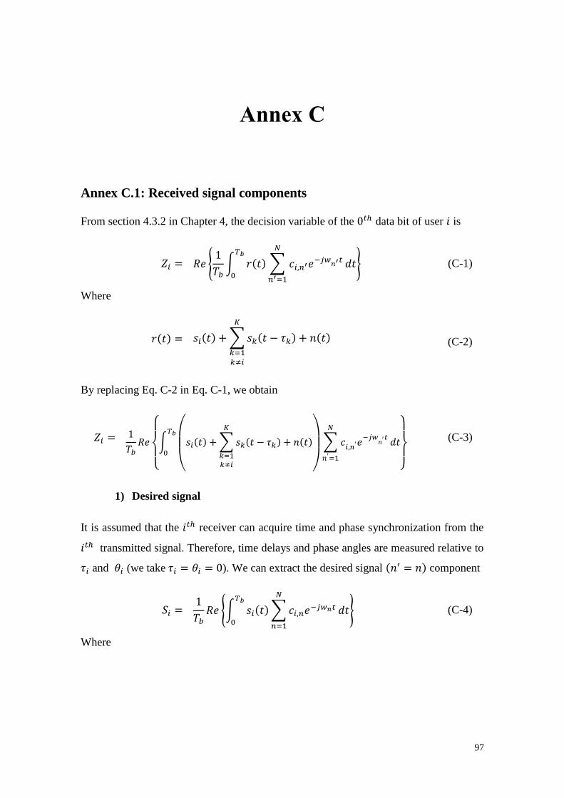
97

Annex C

Annex C.1: Received signal components

From section 4.3.2 in Chapter 4, the decision variable of the 0𝑡ℎ data bit of user 𝑖 is

𝑍𝑖 = 𝑅𝑒 {1

𝑇𝑏න 𝑟(𝑡) ∑ 𝑐𝑖,𝑛′𝑒

−𝑗𝑤𝑛′𝑡

𝑁

𝑛′=1

𝑇𝑏

0

𝑑𝑡} (C-1)

Where

𝑟(𝑡) = 𝑠𝑖(𝑡) +∑𝑠𝑘(𝑡 − 𝜏𝑘)

𝐾

𝑘=1𝑘≠𝑖

+ 𝑛(𝑡) (C-2)

By replacing Eq. C-2 in Eq. C-1, we obtain

𝑍𝑖 = 1

𝑇𝑏𝑅𝑒

{

න

(

𝑠𝑖(𝑡) +∑ 𝑠𝑘(𝑡 − 𝜏𝑘)

𝐾

𝑘=1𝑘≠𝑖

+ 𝑛(𝑡)

)

∑ 𝑐

𝑖,𝑛′𝑒−𝑗𝑤

𝑛′𝑡

𝑁

𝑛′=1

𝑇𝑏

0

𝑑𝑡

}

(C-3)

1) Desired signal

It is assumed that the 𝑖𝑡ℎ receiver can acquire time and phase synchronization from the

𝑖𝑡ℎ transmitted signal. Therefore, time delays and phase angles are measured relative to

𝜏𝑖 and 𝜃𝑖 (we take 𝜏𝑖 = 𝜃𝑖 = 0). We can extract the desired signal (𝑛′ = 𝑛) component

𝑆𝑖 = 1

𝑇𝑏𝑅𝑒 {න 𝑠𝑖(𝑡)∑ 𝑐𝑖,𝑛𝑒

−𝑗𝑤𝑛𝑡

𝑁

𝑛=1

𝑇𝑏

0

𝑑𝑡} (C-4)

Where

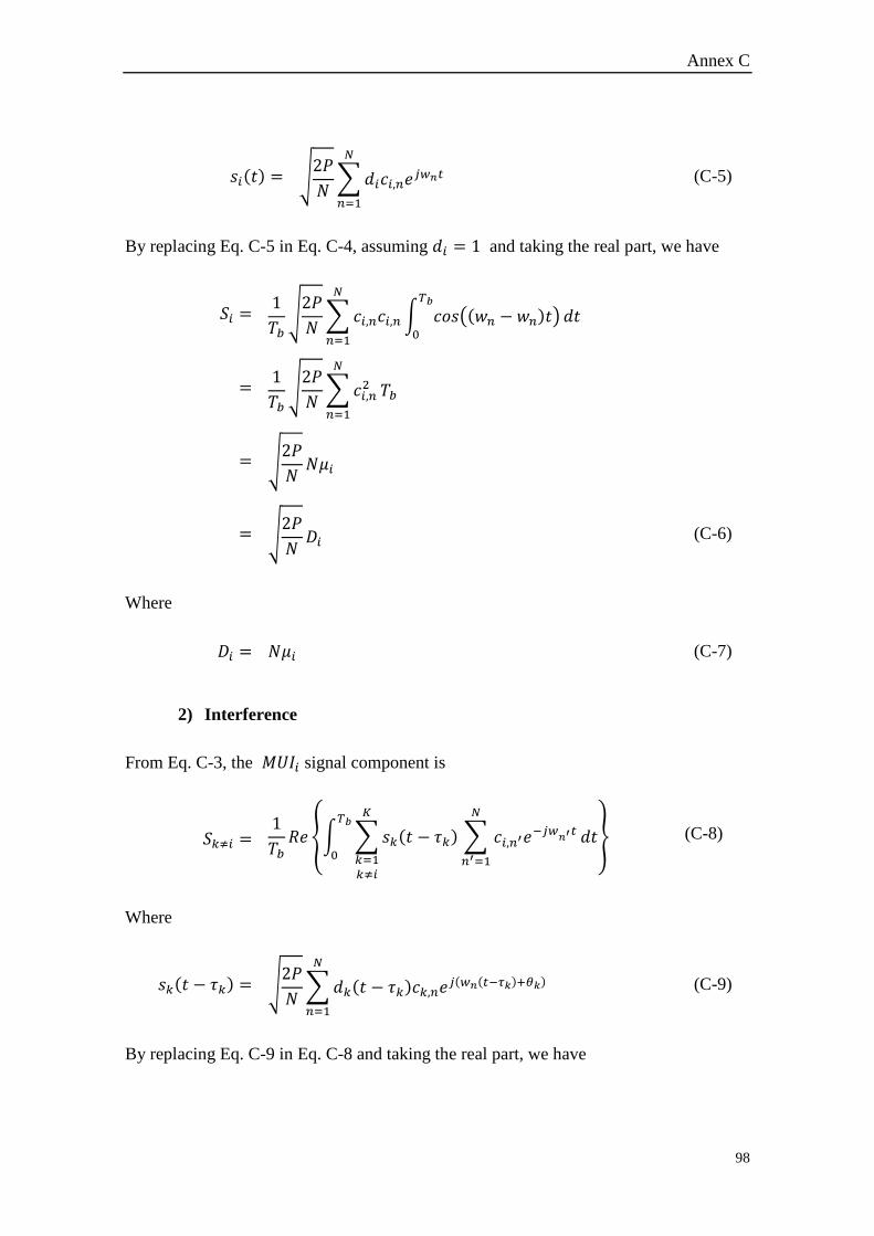
Annex C

98

𝑠𝑖(𝑡) = √2𝑃

𝑁∑𝑑𝑖𝑐𝑖,𝑛𝑒

𝑗𝑤𝑛𝑡

𝑁

𝑛=1

(C-5)

By replacing Eq. C-5 in Eq. C-4, assuming 𝑑𝑖 = 1 and taking the real part, we have

𝑆𝑖 = 1

𝑇𝑏√2𝑃

𝑁∑𝑐𝑖,𝑛𝑐𝑖,𝑛න 𝑐𝑜𝑠((𝑤𝑛 − 𝑤𝑛)𝑡)

𝑇𝑏

0

𝑑𝑡

𝑁

𝑛=1

= 1

𝑇𝑏√2𝑃

𝑁∑𝑐𝑖,𝑛

2

𝑁

𝑛=1

𝑇𝑏

= √2𝑃

𝑁𝑁𝜇𝑖

= √2𝑃

𝑁𝐷𝑖 (C-6)

Where

𝐷𝑖 = 𝑁𝜇𝑖 (C-7)

2) Interference

From Eq. C-3, the 𝑀𝑈𝐼𝑖 signal component is

𝑆𝑘≠𝑖 = 1

𝑇𝑏𝑅𝑒 {න ∑𝑠𝑘(𝑡 − 𝜏𝑘)

𝐾

𝑘=1𝑘≠𝑖

∑ 𝑐𝑖,𝑛′𝑒−𝑗𝑤

𝑛′𝑡

𝑁

𝑛′=1

𝑇𝑏

0

𝑑𝑡} (C-8)

Where

𝑠𝑘(𝑡 − 𝜏𝑘) = √2𝑃

𝑁∑𝑑𝑘(𝑡 − 𝜏𝑘)𝑐𝑘,𝑛𝑒

𝑗(𝑤𝑛(𝑡−𝜏𝑘)+𝜃𝑘)

𝑁

𝑛=1

(C-9)

By replacing Eq. C-9 in Eq. C-8 and taking the real part, we have

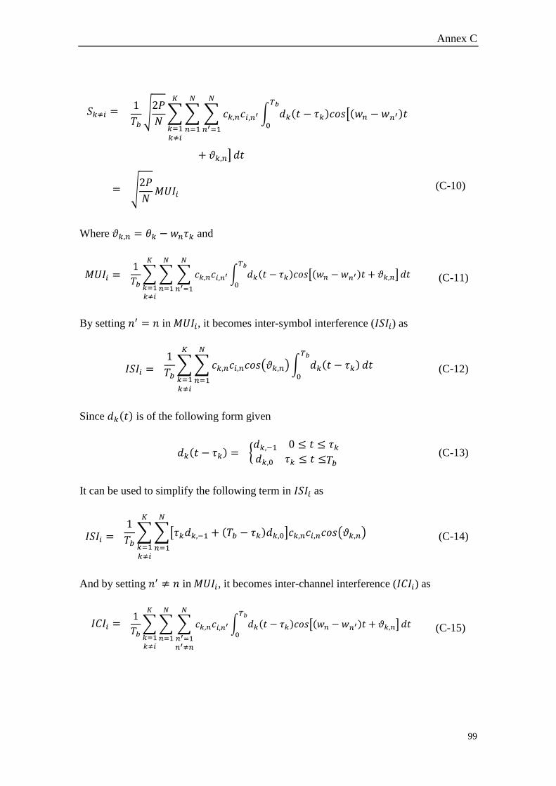
Annex C

99

𝑆𝑘≠𝑖 =

1

𝑇𝑏√2𝑃

𝑁∑∑ ∑ 𝑐𝑘,𝑛𝑐𝑖,𝑛′

𝑁

𝑛′=1

𝑁

𝑛=1

𝐾

𝑘=1𝑘≠𝑖

න 𝑑𝑘(𝑡 − 𝜏𝑘)𝑐𝑜𝑠[(𝑤𝑛 − 𝑤𝑛′)𝑡𝑇𝑏

0

+ 𝜗𝑘,𝑛] 𝑑𝑡

= √2𝑃

𝑁𝑀𝑈𝐼𝑖

(C-10)

Where 𝜗𝑘,𝑛 = 𝜃𝑘 − 𝑤𝑛𝜏𝑘 and

𝑀𝑈𝐼𝑖 = 1

𝑇𝑏∑∑ ∑ 𝑐𝑘,𝑛𝑐𝑖,𝑛′

𝑁

𝑛′=1

𝑁

𝑛=1

𝐾

𝑘=1𝑘≠𝑖

න 𝑑𝑘(𝑡 − 𝜏𝑘)𝑐𝑜𝑠[(𝑤𝑛 −𝑤𝑛′)𝑡 + 𝜗𝑘,𝑛]𝑇𝑏

0

𝑑𝑡 (C-11)

By setting 𝑛′ = 𝑛 in 𝑀𝑈𝐼𝑖, it becomes inter-symbol interference (𝐼𝑆𝐼𝑖) as

𝐼𝑆𝐼𝑖 = 1

𝑇𝑏∑∑𝑐𝑘,𝑛𝑐𝑖,𝑛𝑐𝑜𝑠(𝜗𝑘,𝑛)න 𝑑𝑘(𝑡 − 𝜏𝑘)

𝑇𝑏

0

𝑁

𝑛=1

𝐾

𝑘=1𝑘≠𝑖

𝑑𝑡 (C-12)

Since 𝑑𝑘(𝑡) is of the following form given

𝑑𝑘(𝑡 − 𝜏𝑘) = {𝑑𝑘,−1 0 ≤ 𝑡 ≤ 𝜏𝑘𝑑𝑘,0 𝜏𝑘 ≤ 𝑡 ≤𝑇𝑏

(C-13)

It can be used to simplify the following term in 𝐼𝑆𝐼𝑖 as

𝐼𝑆𝐼𝑖 = 1

𝑇𝑏∑∑[𝜏𝑘𝑑𝑘,−1 + (𝑇𝑏 − 𝜏𝑘)𝑑𝑘,0]𝑐𝑘,𝑛𝑐𝑖,𝑛𝑐𝑜𝑠(𝜗𝑘,𝑛)

𝑁

𝑛=1

𝐾

𝑘=1𝑘≠𝑖

(C-14)

And by setting 𝑛′ ≠ 𝑛 in 𝑀𝑈𝐼𝑖, it becomes inter-channel interference (𝐼𝐶𝐼𝑖) as

𝐼𝐶𝐼𝑖 = 1

𝑇𝑏∑∑ ∑ 𝑐𝑘,𝑛𝑐𝑖,𝑛′

𝑁

𝑛′=1𝑛′≠𝑛

𝑁

𝑛=1

𝐾

𝑘=1𝑘≠𝑖

න 𝑑𝑘(𝑡 − 𝜏𝑘)𝑐𝑜𝑠[(𝑤𝑛 −𝑤𝑛′)𝑡 + 𝜗𝑘,𝑛]𝑇𝑏

0

𝑑𝑡 (C-15)

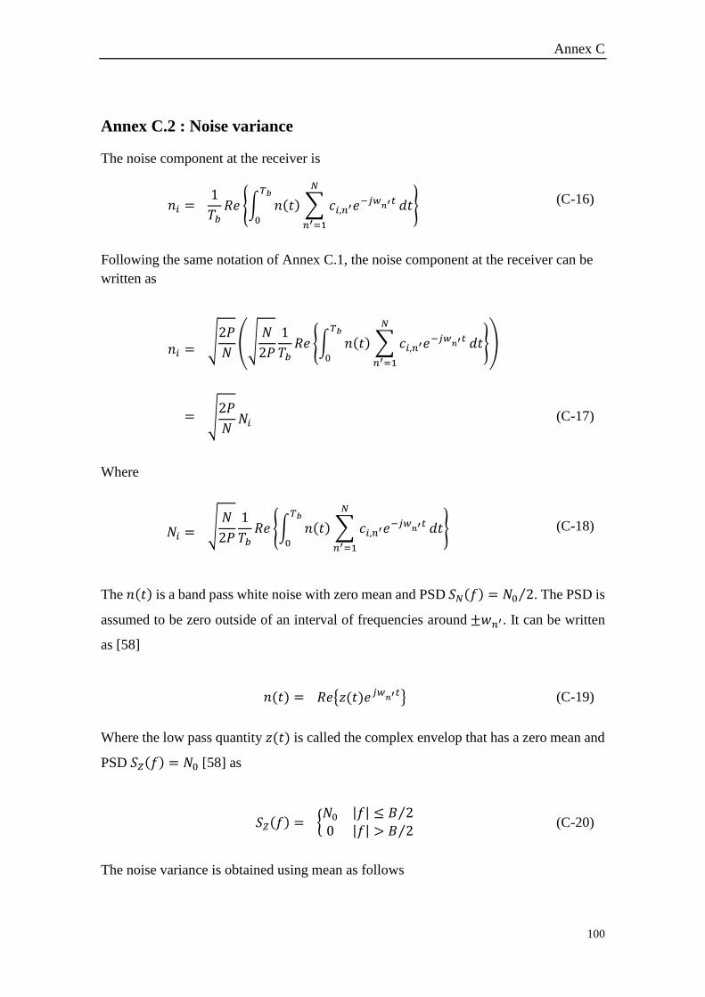
Annex C

100

Annex C.2 : Noise variance

The noise component at the receiver is

𝑛𝑖 = 1

𝑇𝑏𝑅𝑒 {න 𝑛(𝑡) ∑ 𝑐𝑖,𝑛′𝑒

−𝑗𝑤𝑛′𝑡

𝑁

𝑛′=1

𝑇𝑏

0

𝑑𝑡} (C-16)

Following the same notation of Annex C.1, the noise component at the receiver can be

written as

𝑛𝑖 = √2𝑃

𝑁(√

𝑁

2𝑃

1

𝑇𝑏𝑅𝑒 {න 𝑛(𝑡) ∑ 𝑐𝑖,𝑛′𝑒

−𝑗𝑤𝑛′𝑡

𝑁

𝑛′=1

𝑇𝑏

0

𝑑𝑡})

= √2𝑃

𝑁𝑁𝑖 (C-17)

Where

𝑁𝑖 = √𝑁

2𝑃

1

𝑇𝑏𝑅𝑒 {න 𝑛(𝑡) ∑ 𝑐𝑖,𝑛′𝑒

−𝑗𝑤𝑛′𝑡

𝑁

𝑛′=1

𝑇𝑏

0

𝑑𝑡} (C-18)

The 𝑛(𝑡) is a band pass white noise with zero mean and PSD 𝑆𝑁(𝑓) = 𝑁0 2⁄ . The PSD is

assumed to be zero outside of an interval of frequencies around ±𝑤𝑛′. It can be written

as [58]

𝑛(𝑡) = 𝑅𝑒{𝑧(𝑡)𝑒𝑗𝑤𝑛′𝑡} (C-19)

Where the low pass quantity 𝑧(𝑡) is called the complex envelop that has a zero mean and

PSD 𝑆𝑍(𝑓) = 𝑁0 [58] as

𝑆𝑍(𝑓) = {𝑁0 |𝑓| ≤ 𝐵 2⁄

0 |𝑓| > 𝐵 2⁄ (C-20)

The noise variance is obtained using mean as follows

Annex C

101

𝑉𝑎𝑟{𝑁𝑖} = 𝐸{𝑁𝑖2}

=

𝑁

2𝑃

1

𝑇𝑏2 ∑ 𝑐𝑖,𝑛′

2 න න 𝐸{𝑛(𝑡)𝑛(𝛼)}𝑇𝑏

0

𝑐𝑜𝑠𝑤𝑛′𝑡 𝑐𝑜𝑠𝑤𝑛′𝛼 𝑑𝑡𝑑𝛼𝑇𝑏

0

𝑁

𝑛′=1

(C-21)

Knowing that 𝐸𝑏 = 𝑃𝑇𝑏 and 𝑛(𝑡) is assumed to be wide sense stationary (WSS) process

with an ACF 𝐸{𝑛(𝑡)𝑛(𝛼)} = 𝜃𝑁(𝛼 − 𝑡).

𝑉𝑎𝑟{𝑁𝑖} = 𝑁

2𝑇𝑏𝐸𝑏∑ 𝑐𝑖,𝑛′

2 න න 𝜃𝑁(𝛼 − 𝑡)𝑇𝑏

0

𝑐𝑜𝑠𝑤𝑛′𝑡 𝑐𝑜𝑠𝑤𝑛′𝛼 𝑑𝑡𝑑𝛼𝑇𝑏

0

𝑁

𝑛′=1

(C-22)

The relation between the AFC of 𝑧(𝑡) and 𝑛(𝑡) is (see [58] chapter 4 pp.159-162)

𝜃𝑁(𝛼 − 𝑡) = 𝑅𝑒{𝜃𝑍(𝛼 − 𝑡)e𝑗𝑤

𝑛′(𝛼−𝑡)}

(C-23)

Note that the ACF of the bandpass stochastic process 𝑛(𝑡) is uniquely determined from

the ACF of its equivalent low-pass process 𝑧(𝑡) and the carrier frequency [58]. The

limiting form (𝐵 → ∞) of the ACF of the equivalent low-pass process 𝑧(𝑡) is (see [58]

chapter 4 pp.159-162)

𝜃𝑍(𝛼 − 𝑡) = 𝑁0𝛿(𝛼 − 𝑡) (C-24)

Then the ACF of 𝑛(𝑡) is

𝜃𝑁(𝛼 − 𝑡) = 𝑁0𝛿(𝛼 − 𝑡)cos 𝑤𝑛′(𝛼 − 𝑡) (C-25)

Then the noise variance of Eq. C.22 becomes

Annex C

102

𝑉𝑎𝑟{𝑁𝑖} =

𝑁𝑁02𝑇𝑏𝐸𝑏

∑ 𝑐𝑖,𝑛′2 න න 𝛿(𝛼

𝑇𝑏

0

𝑇𝑏

0

𝑁

𝑛′=1

− 𝑡) cos𝑤𝑛′(𝛼 − 𝑡) 𝑐𝑜𝑠𝑤𝑛′𝑡 𝑐𝑜𝑠𝑤𝑛′𝛼 𝑑𝑡𝑑𝛼

(C-26)

Using the following Dirac’s delta function property

න cos𝑤𝑛′(𝛼 − 𝑡) 𝑐𝑜𝑠𝑤𝑛′𝛼 𝛿(𝛼 − 𝑡)𝑑𝛼𝑇𝑏

0

= cos𝑤𝑛′(𝑡 − 𝑡) 𝑐𝑜𝑠𝑤𝑛′𝑡

= 𝑐𝑜𝑠𝑤𝑛′𝑡 (C-27)

Eq. C-26 becomes

𝑉𝑎𝑟{𝑁𝑖} =

𝑁𝑁02𝑇𝑏𝐸𝑏

∑ 𝑐𝑖,𝑛′2 න 𝑐𝑜𝑠2𝑤𝑛′𝑡 𝑑𝑡

𝑇𝑏

0

𝑁

𝑛′=1

= 𝑁𝑁04𝐸𝑏

∑𝑐𝑖,𝑛′2

𝑁

𝑛=1

(C-28)

Knowing that 𝜇𝑖 = ∑ 𝑐𝑖,𝑛′2𝑁

𝑛′=1 𝑁⁄ , the above equation can also be written as

𝑉𝑎𝑟{𝑁𝑖} = 𝑁2𝑁0𝜇𝑖4𝐸𝑏

(C-29)

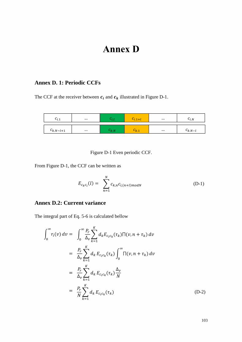
103

Annex D

Annex D. 1: Periodic CCFs

The CCF at the receiver between 𝒄𝒊 and 𝒄𝒌 illustrated in Figure D-1.

Figure D-1 Even periodic CCF.

From Figure D-1, the CCF can be written as

𝐸𝑐𝑘𝑐𝑖(𝑙) = ∑𝑐𝑘,𝑛𝑐𝑖,(𝑛+𝑙)𝑚𝑜𝑑𝑁

𝑁

𝑛=1

(D-1)

Annex D.2: Current variance

The integral part of Eq. 5-6 is calculated bellow

න 𝑟𝑖(𝑣)∞

0

𝑑𝑣 = න𝑃𝑟∆𝑣∑𝑑𝑘𝐸𝑐𝑖𝑐𝑘(𝜏𝑘)⨅(𝑣, 𝑛 + 𝜏𝑘)

𝐾

𝑘=1

∞

0

𝑑𝑣

= 𝑃𝑟∆𝑣∑𝑑𝑘

𝐾

𝑘=1

𝐸𝑐𝑖𝑐𝑘(𝜏𝑘)න ⨅(𝑣, 𝑛 + 𝜏𝑘)∞

0

𝑑𝑣

= 𝑃𝑟∆𝑣∑𝑑𝑘

𝐾

𝑘=1

𝐸𝑐𝑖𝑐𝑘(𝜏𝑘)∆𝑣𝑁

=

𝑃𝑟𝑁∑𝑑𝑘

𝐾

𝑘=1

𝐸𝑐𝑖𝑐𝑘(𝜏𝑘) (D-2)

𝑐𝑘,𝑁 𝑐𝑘,1 … 𝑐𝑘,𝑁−𝑙+1 … 𝑐𝑘,𝑁−𝑙

𝑐𝑖,𝑙 𝑐𝑖,1+𝑙 … 𝑐𝑖,1 … 𝑐𝑖,𝑁

Reference

104

Reference

105

References

[1] M. B. Pursley and D. V. Sarwate, "James L. Massey's Contributions in the Early

Years of Spread-Spectrum Communication Theory Research," IEEE

Communication Surveys & Tutorials, vol. 17, no. 03, pp. 1500-1510, 2015.

[2] D. V. Sarwate , "Bounds on Crosscorrelation and Autocorrelation of Sequences,"

IEEE Transactions on Information Theory, Vols. IT-25, no. 06, pp. 720-724, 1979.

[3] L. R. Welch, "Lower Bounds on the Maximum Cross Correlation of Signals," IEEE

Transactions on Information Theory, vol. 20, no. 03, pp. 397-399, 1974.

[4] P. Fan and M. Darnell, "Sequence Design for Communications Applications,"

Research Studies Press, 1996.

[5] K. Takatsukasa, S. Matsufuji, Y. Watanabi, N. Kuroyanagi and N. Suehiro,

"Ternary ZCZ Sequence Sets for Cellular CDMA Systems," IEICE Transactions

on Fundamentals of Electronics, Communications and Computer Sciences, Vols.

E85-A, no. 09, pp. 2135-2140, 2003.

[6] E. H. Dinan and B. Jabbari, "Spreading codes for direct sequence CDMA and

wideband CDMA cellular networks," IEEE Communications Magazine, vol. 36, no.

09, pp. 48-54, 1998.

[7] I. A. Glover, Digital Communications, 3 ed., Harlaw, England: Pearson Education

Limited, 2010.

[8] R. Gold, "Optimal binary sequences for spread spectrum multiplexing," IEEE

Transactions on Information Theory, vol. 13, no. 04, pp. 619 - 621, 1967.

[9] K. Fazel and S. Kaiser, Multi-Carrier Spread-Spectrum, Germany: Springer-

Science Business Media B.V., 2004.

[10] M. Golay, "Complementary Series," IRE Transactions on Information Theory, pp.

82-87, 1961.

[11] H. Ochiai and H. Imai, "OFDM-CDMA with Peak Power Reduction Based on the

Spreading Sequences," IEEE International Conference on Communication, pp.

1299-1303, 1998.

Reference

106

[12] C. Tseng and C. Liu, "Complementary sets of sequences," IEEE Transactions on

Information Theory, Vols. IT-18, pp. 644-652, 1972.

[13] P. Fan, N. Suehiro, N. Kuroyanagi and X. M. Deng, "Class of binary sequences with

zero correlation zone," Electronics Letters, vol. 32, no. 10, pp. 777-779, 1999.

[14] X. H. Tang, P. Z. Fan and S. Matsufuji, "Lower bounds on correlation of spreading

sequence set with low or zero correlation zone," Electronics Letters, vol. 36, no. 06,

pp. 551 - 552, 2000.

[15] H. Torii, M. Nakamura and N. Suehiro, "A new class of zero-correlation zone

sequences," IEEE Transactions on Information Theory, vol. 50, no. 03, pp. 559 -

565, 2004.

[16] T. Maeda, S. Kanemoto and T. Hayashi, "A Novel Class of Binary Zero-Correlation

Zone Sequence Sets," IEEE Region 10 Conference, pp. 708-711, 2010.

[17] J. Cha, S. Kameda, M. Yokoyama, H. Nakase, K. Masu and K. Tsubouchi, "New

binary sequences with zero-correlation duration for approximately synchronised

CDMA," Electronics Letters, vol. 36, pp. 991-993, 2000.

[18] T. Hayashi, "A Class of Ternary Sequence Sets having a Zero-Correlation Zone for

Even and Odd Correlation Functions," in IEEE International Symposium on

Information Theory, Yokohama, Japan, 2003.

[19] L. Feng, J. Wang, R. Q. Hu et L. Liu, «New design of optical zero correlation zone

codes in quasi-synchronous VLC CDMA systems,» EURASIP Journal on Wireless

Communications and Networking, vol. 120, 2015.

[20] T. Matsumoto, H. Torii et S. Matsufuji, «Theoretical analysis of BER performance

of optical ZCZ-CDMA system,» International Journal of Computers and

Communications , vol. 01, pp. 18-25, 2013.

[21] A. Abudoukeremu, S. Matsufuji and T. Matsumoto, "On optical ZCZ codes with a

good aperiodic autocorrelation property," in 15th International Conference on

Advanced Communications Technology (ICACT), PyeongChang, South Korea,

2013.

Reference

107

[22] T. H. Abd, S. A. Aljunid, H. A. Fadhil, R. A. Ahmad and N. M. Saad, "Development

of a new code family based on SAC-OCDMA system with large cardinality for

OCDMA network," Optical Fiber Technology, vol. 17, no. 04, pp. 273-280, 2011.

[23] M. Addad et A. Djebbari, «New code family for QS-CDMA visible light

communication systems,» Journal of Telecommunications and Information

Technology, vol. 03, pp. 5-8, 2018.

[24] J. H. Liang, X. Wang, F. H. Wang and Z. T. Huang, "Blind spreading sequence

estimation algorithm for long-code DS-CDMA signals in asynchronous multi-user

systems," IET Signal Processing, vol. 11, no. 06, pp. 704 - 710, 2017.

[25] F. Qu, X. Qin, L. Yang and T. C. Yang , "Spread-Spectrum Method Using Multiple

Sequences for Underwater Acoustic Communications," IEEE Journal of Oceanic

Engineering, vol. PP, no. 99, pp. 1-12, 2017.

[26] J. Khalife, K. Shamaei and Z. M. Kassas, "Navigation with Cellular CDMA

Signals-Part I: Signal Modeling and Software-Defined Receiver Design," IEEE

Transactions on Signal Processing, vol. PP, no. 99, pp. 1-13, 2018.

[27] F. T. Dagefu, G. Verma , P. Spasojevic and B. M. Sadler, "An Experimental study

of quasi-synchronous multiuser communications in cluttered scenarios at low

VHF," in International Conference on Military Communications and Information

Systems (ICMCIS), Oulu, Finland, 2017.

[28] A. Masmoudi , F. Bellili , S. Affes and A. Ghrayeb , "Maximum Likelihood Time

Delay Estimation From Single- and Multi-Carrier DSSS Multipath MIMO

Transmissions for Future 5G Networks," IEEE Transactions on Wireless

Communications, vol. 16, no. 08, pp. 4851 - 4865, 2017.

[29] Q. Sun, S. Wang, S. Han and I. L. Chih, "Unified framework towards flexible

multiple access schemes for 5G," ZTE Communications, vol. 14, no. 04, p. 26–34,

2016.

[30] R. M. Buehrer, Code Division Multiple Access (CDMA), Virginia, USA: Morgan

& Claypool, 2006.

[31] H. H. Chen, The Next Generation CDMA Technologies, West Sussex, England:

John Wiley and Sons Ltd, 2007.

Reference

108

[32] Tutorials Point, "Code Division Multiple Access," obtained from

www.tutorialspoint.com consulted in September 2018.

[33] D. Divsalar and M. K. Simon, "CDMA With Interference Cancellation for

Multiprobe Missions," TDA Progress Report 42-120, NASA, USA, 1995.

[34] J. P. Linnartz, Ed., Wireless communication, Vols. Wireless channels-Multipath

fading,

"http://www.wirelesscommunication.nl/reference/chaptr03/fading/delayspr.htm"

consulted in August 2018.

[35] TELETOPIX Telecom Techniques Guide, "What is Rake Receiver and its Purpose

in CDMA," http://www.teletopix.org/cdma/what-is-rake-receiver-and-its-purpose-

in-cdma/ consulted in August 2018.

[36] D. Boudreau, G. Caire, G. E. Corazza, R. De Gaudenzi, G. Gallinaro, M. Luglio, R.

Lyons, J. Romero-Garcia, A. Vernucci and H. Widmer, "Wide-band CDMA for the

UMTS/IMT-2000 satellite component," IEEE Transactions on Vehicular

Technology, vol. 51, no. 02, pp. 306 - 331, 2002.

[37] K. Fazel and S. Kaiser, Multi-Carrier and Spread Spectrum Systems, 2nd ed., West

Sussex, UK: John Wiley & Sons, 2008.

[38] M. Chitre, S. Shahabudeen, L. Freitag and M. Stojanovic, "Underwater Acoustic

Communications & Networking," in OCEANS 2008, Quebec City, QC, Canada,

2008.

[39] CCSDS, "Navigation Data-Definition and Conventions," Repport : Consultative

Committee for Space Data Systems , Oxfordshire, UK, 2001.

[40] C. Vladeanu, "Optimum chaotic quantized sequences for asynchronous DS-CDMA

system," in 13th European Signal Processing Conference, Antalya, Turkey, 2005.

[41] G. L. Turin, Communication Through Random-Multipath Channels, Cambridge,

Massachusets: PhD Thesis, Department of Electrical Engineering, Massachusets

Institute of Technology (MIT), 1952.

[42] E. Geraniotis and M. Pursley, "Performance of Coherent Direct-Sequence Spread-

Spectrum Communications over Specular Multipath Fading Channels," IEEE

Transactions on Communications, vol. 33, no. 06, pp. 502 - 508, 1985.

Reference

109

[43] M. Pursley, "Performance Evaluation for Phase-Coded Spread-Spectrum Multiple-

Access Communication- Part I: System Analysis," IEEE Transactions on

Communications, vol. 25, no. 08, pp. 795-799, 1977.

[44] J. S. Lehnert and M. B. Pursley, "Multipath Diversity Reception of Spread-

Spectrum Multiple-Access Communications," IEEE Transactions on

Communications , Vols. COM-35, no. 11, pp. 1189-1198, 1987.

[45] M. K. Simon, J. K. Omura, R. A. Scholtz and B. K. Levitt, Spread Spectrum

Communications Handbook, McGraw-Hill Companies, Inc, 2002.

[46] M. Addad, A. Djebbari and I. Dayoub, "Performance of ZCZ Codes in QS-DS-

CDMA Communication Systems," International Journal of Communication

Systems, p. recommended for publication with minor revision, 2018.

[47] E. Geraniotis, "Direct-Sequence Spread-Spectrum Multiple-Access

Communications Over Nonselective and Frequency-Selective Rician Fading

Channels," IEEE Transactions on Communications, vol. 34, no. 08, pp. 756 - 764,

1986.

[48] B. M. Popovic, "Spreading sequences for multicarrier CDMA systems," IEEE

Transactions on Communications, vol. 47, no. 06, pp. 918 - 926, 1999.

[49] M. Addad and A. Djebbari , "Suitable Spreading Sequences for Asynchronous MC-

CDMA Systems," Journal of Telecommunications and Information Technology,

vol. 03, pp. 9-13, 2018.

[50] Q. Shi and M. Latva-aho, "Spreading sequences for asynchronous MC-CDMA

revisited: accurate bit error rate analysis," IEEE Transactions on Communications,

vol. 51, no. 01, pp. 8 - 11, 2003.

[51] H. Elgala , R. Mesleh and H. Haas, "Indoor Optical Wireless Communication:

Potential and State-of-the-Art," IEEE Communications Magazine , vol. 49, no. 09,

pp. 56-62, 2011.

[52] L. U. Khan, "Visible light communication: Applications, architecture,

standardization and research challenges," Digital Communications and Networks,

vol. 03, no. 02, pp. 78-88, 2017.

Reference

110

[53] V. T. B. Tram and M. Yoo, "Vehicle-to-Vehicle Distance Estimation Using a Low-

Resolution Camera Based on Visible Light Communications," IEEE Access, vol.

06, pp. 4521 - 4527, 2018.

[54] A. Naz, H. M. Asif, T. Umer and B. S. Kim, "PDOA Based Indoor Positioning

Using Visible Light Communication," IEEE Access, vol. 06, pp. 7557 - 7564, 2018.

[55] F. Miramirkhani and M. Uysal, "Visible Light Communication Channel Modeling

for Underwater Environments With Blocking and Shadowing," IEEE Access, vol.

06, pp. 1082 - 1090, 2017.

[56] A. Garadi and A. Djebbari, "New technique for construction of a zero cross

correlation code," Optik - International Journal for Light and Electron Optics, vol.

123, no. 15, pp. 1382-1384, 2012.

[57] E. Smith, R. Blaikie and D. Taylor, "Performance enhancement of spectral-

amplitude-coding optical CDMA using pulse-position modulation," IEEE

Transactions on Communications , vol. 46, no. 09, pp. 1176 - 1185, 1998.

[58] J. G. Proakis, Digital Communications, New York: McGraw-Hill, 1995.